Modeling of Dune Morphology

Diplomarbeit

vorgelegt von

Veit Schwammle

aus Korntal

Hauptberichter: Prof. Dr. H. J. HerrmannMitberichter: Dr. F. Assaad

Institut fur Computeranwendungen 1 der Universitat Stuttgart

2002

Contents

Introduction 5

1 Basics 91.1 Atmospheric boundary layer . . . . . . . . . . . . . . . . . . . . . . . . 91.2 Aeolian sand transport . . . . . . . . . . . . . . . . . . . . . . . . . . . 10

1.2.1 Sand grain size and transport modes . . . . . . . . . . . . . . . . 111.2.2 Forces and entrainment threshold . . . . . . . . . . . . . . . . . 131.2.3 Saltation . . . . . . . . . . . . . . . . . . . . . . . . . . . . . . 15

1.3 Dune geomorphology . . . . . . . . . . . . . . . . . . . . . . . . . . . . 181.3.1 Hierarchies . . . . . . . . . . . . . . . . . . . . . . . . . . . . . 181.3.2 Classification and building conditions of simple dunes . . . . . . 191.3.3 A more detailed description of dune forms generated by unimodal

wind source . . . . . . . . . . . . . . . . . . . . . . . . . . . . . 231.3.4 Dune fields . . . . . . . . . . . . . . . . . . . . . . . . . . . . . 25

2 Air shear stress over heaps and dunes 272.1 Turbulence models . . . . . . . . . . . . . . . . . . . . . . . . . . . . . 272.2 The separation bubble and its justification . . . . . . . . . . . . . . . . . 282.3 An analytical model for the air shear stress . . . . . . . . . . . . . . . . . 30

3 A continuum saltation model 333.1 The model . . . . . . . . . . . . . . . . . . . . . . . . . . . . . . . . . . 33

3.1.1 The grain born shear stress . . . . . . . . . . . . . . . . . . . . . 343.1.2 Erosion and deposition rates . . . . . . . . . . . . . . . . . . . . 353.1.3 Forces . . . . . . . . . . . . . . . . . . . . . . . . . . . . . . . . 36

3.2 The closed model and the saturated sand flux . . . . . . . . . . . . . . . 363.3 Dynamics of the saltation layer and simplifications for dune modeling . . 38

4 The numerical model for sand dunes 414.1 The complete model . . . . . . . . . . . . . . . . . . . . . . . . . . . . 414.2 The air shear stressτ at the ground . . . . . . . . . . . . . . . . . . . . . 424.3 The sand fluxq . . . . . . . . . . . . . . . . . . . . . . . . . . . . . . . 42

3

4 Contents

4.4 Avalanches . . . . . . . . . . . . . . . . . . . . . . . . . . . . . . . . . 444.5 The time evolution of the surface . . . . . . . . . . . . . . . . . . . . . . 454.6 The initial surface and boundary conditions . . . . . . . . . . . . . . . . 454.7 Conclusion . . . . . . . . . . . . . . . . . . . . . . . . . . . . . . . . . 46

5 Transverse Dunes 475.1 Introduction . . . . . . . . . . . . . . . . . . . . . . . . . . . . . . . . . 475.2 The model of 3-dimensional dunes and translational invariance . . . . . . 495.3 The model of 2-dimensional dunes with constant sand influx . . . . . . . 55

5.3.1 Time evolution . . . . . . . . . . . . . . . . . . . . . . . . . . . 555.3.2 Dune velocity . . . . . . . . . . . . . . . . . . . . . . . . . . . . 61

5.4 The model of 2-dimensional dunes with periodic boundary . . . . . . . . 645.4.1 Time evolution . . . . . . . . . . . . . . . . . . . . . . . . . . . 645.4.2 Do transversal dunes behave like solitons? . . . . . . . . . . . . . 64

5.5 Conclusions . . . . . . . . . . . . . . . . . . . . . . . . . . . . . . . . . 69

6 Barchan dunes 716.1 Introduction . . . . . . . . . . . . . . . . . . . . . . . . . . . . . . . . . 716.2 The role of roughness length and dune size . . . . . . . . . . . . . . . . . 726.3 Scaling laws . . . . . . . . . . . . . . . . . . . . . . . . . . . . . . . . . 776.4 The effect of diffusion . . . . . . . . . . . . . . . . . . . . . . . . . . . 846.5 Barchanoids, between barchan and transverse dunes . . . . . . . . . . . . 846.6 Conclusions . . . . . . . . . . . . . . . . . . . . . . . . . . . . . . . . . 87

7 Conclusion 89

Bibliography 95

Introduction

Dune formations can be found in deserts and on coasts all over the world. Every continentcontains large areas of sand except the Antarctica. The Sahara is the world’s largest desertwith about 7 million square kilometers covering almost one half of the entire Africancontinent. When wind has the strength to move sand grains different kinds of dune formsappear. Even in the Antarctica (Figure 1) special dunes were found composed of snow.Dunes can also be seen in the ocean. This sort of dune formation is quite similar to the

Figure 1: Satellite view of a snow dune field in the Antarctica. (Photo: Ken Jezek, NASA- Goddard Space Flight Center Scientific Visualization Studio)

5

6 Contents

Figure 2: The Mars Viking and Global Surveyor missions revealed the existence ofbarchan dunes on Mars near the north pole. (Photos: Mars Global Surveyor, 1998/1999)

corresponding one on land although the interaction between fluid (air, water) and sandgrains is rather different. Recently barchan dunes have been found even on Mars near thenorth pole (Figure 2). Mars is surrounded by a less dense atmosphere than Earth.

A plain surface that has slack sediment grains from low to high disposal with grain sizeswhich can be moved by the acting flow matter is unstable. Observations proofed that alarge variety of dune forms exists (Finkel 1959; Coursin 1964; Hastenrath 1967; Lettauand Lettau 1969; Sarnthein and Walger 1974; Howard and Morton 1978; Jakel 1980; Has-tenrath 1987; Slattery 1990; Kocurek, Townsley, Yeh, Havholm, and Sweet 1992; Wiggs,Livingstone, and Warren 1996; Hesp and Hastings 1998; Walker 1998; Jimenez, Maia,Serra, and Morais 1999; Sauermann, Rognon, Poliakov, and Herrmann 2000; Sauermann,Andrade, and Herrmann 2001). However, this Diploma thesis will only regard dunes con-sisting of sand and formed by wind.

Contents 7

In comparison to other geological dynamic processes the topography of dune fieldschanges rapidly. Generally dunes move about some meters a year carrying large amountsof sand. The local population has to protect itself from this almost irresistibly advancinghazard. Nevertheless there are a lot of attempts to get along with this problem. Onemethod for example is to spend a lot of money on bulldozers in order to carry the sandaway from roads, pipelines and houses. In some areas it was helpful to plant vegetationon dunes to retain them from moving further on. Also the construction of fences hasbeen applied. The search for the best method, for example to put up fences at sensitiveplaces of a dune, is difficult to assure over large time periods. An experiment needs yearsto get useful results. Therefore people made many attempts to understand the processesbehind dune formation. Dune scales are too high to make experiments for example inwind tunnels. This is the reason why experiments cannot be made under well predefinedconditions to get more knowledge of dynamics and morphology.

When ground is filled up with sand grains and exposed to atmospheric movements, thesurface normally changes. Winds move sand grains over various distances. Differentconditions, for example changing wind directions, wind strength and grain size lead tothe generation of the variety of dune morphologies. On the micro scale exists a complexphysics describing the interaction between air, sand and sand bed. Wind tunnel experi-ments help to get more knowledge about wind field and sediment transport (Rasmussenand Mikkelsen 1991; White and Mounla 1991; Nalpanis, Hunt, and Barrett 1993; Wiggs,Livingstone, and Warren 1996; Nishimura and Hunt 2000). Phenomenological relationsfor the sand flux in saltation were published (Bagnold 1936; Bagnold 1941; Owen 1964;Lettau and Lettau 1978; Sørensen 1991; Sauermann, Kroy, and Herrmann 2001a). Nu-merical simulations of the dynamics of the saltation layer helped to understand more aboutsand transport (Anderson and Haff 1988; Anderson 1991; McEwan and Willetts 1991).Finally, numerical simulations of dune formation in two and three dimensions, which willbe the topic in this thesis, gave interesting results (Wippermann and Gross 1986; Zemanand Jensen 1988; Fisher and Galdies 1988; Stam 1997; Nishimori, Yamasaki, and Ander-sen 1999; van Boxel, Arens, and van Dijk 1999; van Dijk, Arens, and van Boxel 1999;Herrmann and Sauermann 2000; Kroy, Sauermann, and Herrmann 2001). Recently alsoan analytical work was published (Andreotti and Claudin 2002).

In this thesis the theory of the mechanisms involved in dune formation will be discussed.The wind field over the dune, the aeolian sand transport will be described and algorithmsto calculate them will be introduced. From these a dune model will be derived. The resultsof the dune model for barchan and transverse dunes will be presented.

8 Contents

Overview

In Chapter 1 the general physics involved in dune formation is described. Insight into thephysics of the atmospheric boundary layer (turbulent logarithmic profile), the differentmodes of aeolian sediment transport and their phenomenological sand flux relations isgiven in the first two sections. A section of dune geomorphology introduces dune typeswith respect to their external parameters and dune fields. Further insight into dunes gen-erated by an unimodal wind source concludes the chapter. Chapter 2 starts giving a shortsurvey over turbulence models. The separation of the air flow over a dune with a sharpbrink justifies the concept of a separation bubble. With this concept a smooth surface isused to calculate the shear stress with an analytical formula based on a linear perturbationtheory. With this approach the shear stress over dunes can be calculated more efficiently.In Chapter 3 a continuum model of saltation transport is introduced. Expressions for thegrain born shear stress, the source term comprising the erosion and deposition of sandfrom the ground and the forces acting on the grains are derived. This finally leads to aclosed model which describes the saltation transport of grains including time transientsand states out of equilibrium. The results of the model for saturated sand flux are de-picted. Finally the calculated dynamics of the model justifies some simplifications of themodel which decouple the equations to get a faster algorithm. In Chapter 4 the entire dunemodel is described. Shortly the different parts of the model are resumed. The shear stressover the dunes is calculated according to Chapter 2 and the sand flux follows the saltationmodel in Chapter 3. Additionally the model contains calculations of the avalanches andtime evolution of the dune surface. Different external parameters of the model can yieldto various solutions due to different boundary conditions and initial surfaces. In Chapter 5simulations of 3-dimensional transverse dunes lead to the assumption that the system triesto reach translational invariance. The modeling of 2-dimensional dune fields with openboundary reveals potential laws for the time evolution and dune velocity. Simulations of2-dimensional dune fields with periodic boundary show the same properties. The wan-dering of a small dune over a bigger one is discussed. In Chapter 6 the results of barchandune simulations with respect to different parameters of the shear stress calculation arecompared to measurements. The scaling laws of modeled barchan dunes are comparedwith the data of other models and measurements. The effect of an additional diffusionterm is examined. Finally the simulations of barchanoid dunes are presented.

Chapter 1

Basics

In this chapter the physics which drives the dynamics of desert dunes will be discussed.An introduction to the main quantities and features will be given. First the flow of air inthe atmospheric boundary layer will be explained. The aim is to get an expression for theshear stress of the air acting on the sand. In the second section different sand transportsby air movement are explained giving a more precise description of saltation. The thirdsection introduces dune types which are found in deserts. After that a further insight willbe given into dunes formed by an unidirectional wind force. The last section tries to givea small survey over the dynamics in dune fields.

1.1 Atmospheric boundary layer

To maintain the steady movement of dunes there has to be a source which carries theenergy to move sand over the surface. The shear stress of the air flow in the atmosphericboundary layer can force sediments to be entrained. At first it is important to know if theflow over dunes is situated in a laminar or a turbulent regime. The ReynoldsRe numbergives a good estimate. It consists of the ratio between inertial and viscous force:

Re =ρv2/L

µv/L2=Lv

ν, (1.1)

whereρ denotes the density of the fluid,L a characteristic length,v a characteristic windvelocity,µ the viscosity of the fluid andν = µ/ρ the kinematic viscosity. If the inertialforce dominates the viscous force the regime gets turbulent and the Reynolds numberbecomes greater than 1. The scaling of the objects which will be discussed is normallythat of the height of a dune. The calculation leads to a high Reynolds number of about6000 (Houghton 1986). Hence, even small wind speeds create turbulent flows. Turbulentflow means randomly directed and distributed fluctuations and eddies. The shear stresses

9

10 1.2 Aeolian sand transport

A) B)

Figure 1.1: a) Small grains are immersed in the laminar sub-layer which creates an aero-dynamically smooth surface. b) Grains larger than the laminar sub-layer are isolatedobjects and create an aerodynamically rough surface.

of turbulent flow are much higher than of laminar flow. According to the mixing lengththeory (Prandtl 1935) turbulent shear stress can be expressed by

τT = ηdv

dz= ρl2

(

dv

dz

)2

, (1.2)

whereη is turbulent viscosity andl the mixing length. At fully turbulent flows the dy-namic viscosityµ gets much smaller than the turbulent viscosityη. Thus the formerviscosity can be neglected. Under the assumption that the mixing length increases lin-early with the distance from the surface (l = κz, κ ≈ 0.4 is the von Karman universalconstant for turbulent flow) integration fromz0 to z of Equation 1.2 yields the widely usedlogarithmic profile of the atmospheric boundary layer:

v(z) =u∗κ

lnz

z0

. (1.3)

z0 has the meaning of a roughness length. This is either the thickness of the laminarsub-layer for aerodynamically smooth surfaces or the size of surface perturbations foraerodynamically rough surfaces (Figure 1.1).u∗ =

√

τ/ρ is called shear stress velocity.Although it has the dimension of a velocity the shear velocityu∗ anyhow is used as ameasure for the shear stress.

1.2 Aeolian sand transport

Different kinds of sand transport modes by wind are explained in this section. Sand getseroded and deposited. Particularly the saltation transport most interesting for the dune

Basics 11

formation will be described. On the microscopic scale forces act on the sand grains. Thecorresponding phenomenological relations for the macroscopic scale which hold for thesaturated saltation will be defined.

1.2.1 Sand grain size and transport modes

The main properties of sand are grain diameterd, shape and the material of which thegrains consist.

Diameter Classification ranges from large sand grain diameter (d = 2 mm) to smalldiameter (d ≈ 0.063 mm) (Friedman and Sanders 1978). They are called coarseand fine sand respectively.

Shape Since nature almost always produces very complex things sand grains are com-posed of a big variety of shapes. According to Pye and Tsoar (1990) it is classifiedinto “well rounded”, “angular”, “platy”, “elongated”, or “compact”.

Material Mostly sand grains consist of quartz (SiO2) which has a density ofρquartz =2650 kg m−3.

After Pye and Tsoar (1990) sand grains of dune fields have a sharply peaked distributionwith an average diameter of about 0.2 to 0.25 mm.

The form of sand transport depends on different parameters. Main parameters are shearvelocity and the weight of the sand grains. Weight can be expressed by the diameterassuming the same density. A good measure to distinguish between transport mechanismsis given according to the degree of detachment of the grains from the ground.

Bagnold (1941) proposed three distinct types of sand transport induced by wind:

creep The sand grains roll and slide along the surface. During this movement they stayin contact with the surface

saltation The sand grains jump short distances. The range is some centimeters. Theentrainment, i.e. lifting of the grains originates in the shear stress of the air flow orin the impact of other sand grains descending again to the surface. Impacting sandgrains transported by saltation sometimes cannot reach sufficient velocity to enterinto a new ballistic jump. So they are moving much shorter distances. This processis called reptation.

suspensionThe turbulent irregular movement of the atmospheric layer is strong enoughto keep the sand grains aloft. They are transported over long distances.

12 1.2 Aeolian sand transport

0.01

0.02

0.05

0.1

0.2

0.5

0.01 0.02 0.05 0.1 0.2 0.5

s

u

s

p

e

n

s

i

o

n

m

o

d

i

f

i

e

d

s

u

s

p

e

n

s

i

o

n

s

a

l

t

a

t

i

o

n

typ

ica

l w

in

d sp

ee

ds

an

d d

un

e sa

nd

PSfrag replacements

grain diameter [mm]

shea

rve

loci

ty[m

/s]

wfu∗

= 0.1wfu∗

= 1

Figure 1.2: The mechanism of transport depends on the shear velocity of the air andthe grain diameter. For typical dune sand (0.2 mm< d < 0.3 mm) and wind velocities(0.2 m s−1 < u∗ < 0.6 m s−1) on Earth, aeolian sand transport occurs by saltation (areainside the rectangle).

The latter three transport mechanisms are summarized by calling them bed-load. A goodmeasure for the vertical component of the turbulent shear stress is given by the shearvelocity (Lumley and Panofsky 1964; Bagnold 1973; Pasquill 1974). The ratio betweensettling velocitywf and shear velocity helps to distinguish suspension and bed-load. Thedemarkation linewf/u∗ = 1 is used to decide between the two processes. Thuswf/u∗ �1 andwf/u∗ � 1 define suspension and bed-load respectively (Pye and Tsoar 1990).For small grains within the range of 0.001–0.05 mm the settling velocity is expressed by(Green and Lane 1964),

wf =ρquartzg

18µd2 = K d2, (1.4)

whereK = 8.1 106 m−1s−1. Shear velocities in the range of 0.18 to 0.6 m s−1 are suffi-ciently strong to keep the trajectories of the sand grains of this diameter range within thedefinition of suspension. Hence, sand grains of dunes with a typical diameter of 0.25 mmmainly move by bed-load and thereby saltation (Figure 1.2). That is the reason why inour models only saltation transport is considered.

Basics 13

PSfrag replacements

Fg

Fl

Fd

φ

p

Figure 1.3: The grain starts to role when the drag and lift force exceed the gravitationalforce. This can be expressed by a momentum balance with respect to the pivot pointp.

1.2.2 Forces and entrainment threshold

The forces of the air flow acting on a single sand grain are estimated here. They can bedivided into the two directions parallel and perpendicular to the surface. In Figure 1.3also flow lines and the velocity profile are depicted. The parallel force calleddrag forceFd points in the direction of the air flow. A turbulent atmospheric layer yields a forcewhich scales quadratic with velocity, the so called Newton’s turbulent drag,

Fd = βρu2∗πd2

4, (1.5)

whereβ is a phenomenological parameter that includes some characteristics of the bedsuch as its packing. The other force of the air flow originates from the pressure difference∆p between bottom and top of the sand grain. The strong velocity gradient of wind speedleads to this pressure difference. The resulting force is calledlift force Fl:

Fl = ∆pπd2

4= CLρU

2πd2

2, (1.6)

whereCL = 0.0624 (Chepil 1958).U denotes the air velocity at a height of 0.35d withrespect to the zero level atz0. Chepil (1958) showed furthermore that the ratioc = 0.85between the forces of drag and lift is constant within the designated range of Reynoldsnumbers,

Fl = c Fd. (1.7)

14 1.2 Aeolian sand transport

As the force opposed toFl gravity has to be introduced. The sand grain is approximatedto be a sphere, so that

Fg = ρ′gπd3

6. (1.8)

The purpose of this section is to get an equation for the threshold of entrainment, i.e. theminimum shear stress of wind at which it will be able to lift a sand grain from the surface.Therefore the momentum balance of rotating the upper sand grain around its touchingpointp (Figure 1.3) can be expressed as

Fdd

2cosφ = (Fg − Fl)

d

2sinφ. (1.9)

φ is the angle between vertical direction and the line pointing from the sand grain centerto p. By inserting (1.5), (1.7), and (1.8) this finally leads to the so calledfluid thresholdor aerodynamic entrainment thresholdτta

τtaρ′gd

=2

3 β

(

sinφ

cosφ+ c sinφ

)

. (1.10)

So the parameters of the threshold, the grain diameterd and the immersed densityρ′, aredirectly proportional to the shear stress. The angleφ can be interpreted as a parameter ofthe packing of the grains.β is determined by shape and sorting.Shields (1936) named the right hand side of Equation (1.10) a dimensionless coefficientΘ (Shields parameter). It ranges from 0.01 to 0.014 for high Reynolds numbers. Hence,when using the expression for the shear velocity equationu∗ =

√

τ/ρair, then Equa-tion (1.10) defines the fluid threshold shear velocityu∗ta,

u∗ta =

√

Θρ′gd

ρair. (1.11)

The derivation of this paragraph holds only for sand grains which have a diameter that islarge enough to neglect cohesive and repulsive forces between the grains. This is validfor a diameter larger than 0.2 mm. Inserting typical values into Equation (1.11),u∗ta isreaching a shear velocity ofu∗ta = 0.25 ms−1.Nevertheless this value is valid only for entrainment of sand grains into air. When thereare already grains entrained, i.e the air flow is transporting sand, then an impacting sandgrain gives large momentum transfer to a resting grain on the bed. Thus the thresholdvalue gets lower. It is calledimpact thresholdu∗t (Bagnold 1937). Still the expression ofEquation (1.11) keeps valid but with the modification of an effective Shields parameterΘ = 0.0064. In the turbulent wind regimes over dune surfaces fluctuations can determineshear velocities which exceed the entrainment threshold. That is why sand transport canbe maintained for shear velocities betweenu∗ta andu∗t. Consequently impact thresholdgets the important value for aeolian transport.Of course these calculations of a single threshold are getting difficult for poorly sorted

Basics 15

sediments. Moisture and cementing neither have been included. On the other side thethreshold is changing at inclined surfaces. Gravity directs into another direction. Thiseffect should be included in the momentum balance (1.9). Pye and Tsoar (1990) made amore detailed discussion of these effects.

1.2.3 Saltation

When there are enough grains impacting onto the sand beddirect aerodynamic entrain-mentgets negligible. The process of the collision of sand grains entraining other grains iscalledsplash process. Theoretical and experimental investigation has been made recently(Nalpanis, Hunt, and Barrett 1993; Rioual, Valance, and Bideau 2000). As grains attainmomentum by the drag force of the air flow this flow is decelerated. This process is calledfeedback process. After some time and with sufficient sand supply saltation reaches anequilibrium transport rate called saturation.

Direct aerodynamic entrainment

As it was explained in the previous section sand grains are entrained directly from the sandbed for a shear stress higher than the fluid threshold shear stressτta. The linear model ofAnderson (1991) proposes the number of entrained grains proportional to excess shearstress,

Na = ζ(τ − τta), (1.12)

whereNa is the number of entrained grains per time andζ a proportionality constantof about 105 grains N−1 s−1. The direct entrainment gets important to begin the chainreaction leading to saltation like for example at places where the sand bed begins, i.e.where downwind no sand supply is available.

The saltation trajectory

Entrained grains in the air stream are exposed to the following forces. Aerodynamicforces lift and drag a sand grain. The gravitational forceFg obviously lets the trajectoryend on the surface again. The drag forceFd accelerates in the horizontal direction,

Fd =1

2ρairCd

πd2

4(v(z)− u) |v(z)− u| , (1.13)

whered is the grain diameter,v(z) the velocity of the air,u the velocity of the grain, andCd the drag coefficient that depends on the local Reynolds numberRe = |v−u|d/ν. Thelift force has remarkable effects only a few grain diameters away from ground (Andersonand Hallet 1986). Thus it is convenient to include the effects of the lift force in the initial

16 1.2 Aeolian sand transport

velocity of the grain. During its movement within the trajectory the lift force is neglected.Turbulent fluctuations in time and space are not taken in account. Hence, the trajectorycan be calculated by the second law of Newton,

dx

dt= u;

du

dt=

1

m(Fg + Fd) , (1.14)

where the gravitational force isFg = mg with m is the mass of the grain andg is thegravitational acceleration. As initial conditions the initial position and velocityu0 areintroduced. Thus flight time and maximal height of the grain trajectory are given by

T =2uz0g

; h =u2z0

2g, (1.15)

whereuz0 denotes the vertical component of the initial velocity. From a more detailedestimate it results that this simple calculation has an error of about 10–20% (Anderson andHallet 1986; Sørensen 1991). Finally there are presented some values of measurements ina wind tunnel: for a shear velocity ofu∗ = 0.5 m s−1 Nalpanis, Hunt, and Barrett (1993)obtained a flight timeT ≈ 0.08 s, hop heighth ≈ 3.8 cm and hop lengthl ≈ 45 cm.

The splash process

The reaction of the sand bed to the impact of a sand grain is of rather complex nature.The splash process comprises the interaction between the sand grain and the grains in thevicinity of the impact. Thus many grains can be involved in this process. Numerical andexperimental studies have been made by Anderson (1991, Rioual, Valance, and Bideau(2000). Mainly the splash process is described in a stochastic way. It is divided into thefollowing three different resulting situations: First the incoming sand grain distributesits momentum to the sand bed so that no other grain gains sufficient energy to leave theground. Secondly, the grain rebounces loosing some of its energy. Thirdly, the incominggrain distributes its energy so that one or more grains can leave the bed. The splash pro-cess is described by the splash functionS(ui, φi, θi;ue, φe, θe). It defines the probabilityto dislodge a grain with a certain angleφe, θe and velocityue due to an impacting grainwith an angleφi, θi and velocityui. Regarding the anglesθ to be the angles determininghorizontal directions they vary only due to lateral diffusion. That means that they resultto zero in average. For the saltation transport here described it is found an impact anglewith respect to the sand bed from 10o to 15o.

The feedback process

There are two possibilities to calculate the momentum transfer from the air to the grains.The first is to add a body forcef to the right side of the Naiver Stokes equation.f means

Basics 17

an average momentum transfer from the air to the grains,

ρair∂tv + ρair(v∇)v = −∇p+∇τ + f (1.16)

Here,ρair denotes the density,v the velocity,p the pressure, andτ the shear stress of theair. This was used by Anderson (1991).

The other approach (Owen 1964) divides the overall air shear stress into a grain bornand an air born part. The air born shear stress is used to determine the velocity profile.Sauermann, Kroy, and Herrmann (2001b) used this approach for their model of saltationtransport. The dune model described in Chapter 4 also contains these relations.

Due to the rising momentum transfer from the air to the grains for a larger amount ofgrains in air the air born shear stress drops. That means that the system reaches a steadystate. Thus the number of grains in air is limited.

Sand transport rate

Different approaches to describe saltation in a macroscopic way have been made. Theyare not directly connected with the microscopic processes explained before. Macroscopicvariable is the sand fluxq which means the sand flux per unit width and time. This sandflux depends on the shear velocityu∗, the thresholdu∗t, the grain diameterd and others.In the following relations history and transients out of non-equilibrium conditions are notconsidered. Hence, they describe the equilibrium state where the sand flux is saturated.

Measurements in wind tunnels showed that for shear velocitiesu∗ � u∗t the sand fluxscales with the cube of the shear velocity (q ∝ u3

∗) (Butterfield 1993; Rasmussen andMikkelsen 1991). Near the shear threshold the situation seems to be much more compli-cated. Still there are differences between empirical and theoretical flux predictions. Thefirst relation proposing the cubic proportionality is (Bagnold 1941),

qB = CBρair

g

√

d

Du3∗, (1.17)

whered is the grain diameter andD = 250µm a reference grain diameter. To include thefact that under a certain threshold the shear stress is not strong enough to keep saltationtransport many other phenomenological sand flux relations have been made. The mostlyused expression was mentioned by Lettau and Lettau (1978),

qL = CLρair

gu2∗(u∗ − u∗t) (1.18)

whereCL is a fit parameter.

Other attempts to average the microscopic processes contained more information aboutaeolian sand transport (Owen 1964; Ungar and Haff 1987; Sørensen 1985; Werner 1990).

18 1.3 Dune geomorphology

Sørensen (1991) calculated the following relation, whereCS is an analytically determinedparameter,

qS = CSρair

gu∗(u∗ − u∗t)(u∗ + 7.6 ∗ u∗t + 2.05 m s−1). (1.19)

Although experimental data is reproduced quite well with this functional structure theparameterCS is four times to small.

One additionally is interested in the way how the system behaves in non-equilibriumstates which still have not reached the saturation state. Numerical simulations on thegrain scale by Anderson and Haff (1988, Anderson (1991, McEwan and Willetts (1991)showed that the system needs about two seconds to reach the equilibrium state for a flatsurface. This matches quite well with experimental data by wind tunnel measurements(Butterfield 1993). A macroscopic continuum saltation model was proposed recently thatincludes saturation transients (Sauermann, Kroy, and Herrmann (2001b) and Chapter 3).

1.3 Dune geomorphology

In this section the aeolian geomorphology of sand sediments is explained. First the dif-ferent hierarchies of surface patterns are introduced. Different length scales yield varioustypes of sand formation. Secondly the dune types appearing for different parameters arediscussed. A more detailed overview of sand dunes with an unidirectional wind sourceare given. Finally the dynamics of whole dune fields is shortly discussed.

1.3.1 Hierarchies

According to Wilson (1972, Cooke, Warren, and Goudie (1993) dune fields show hier-archical structures. Wilson (1972) divided them into three groups of classification withrespect to their length scale. They are called ripples, dunes and draas with a typical wavelength of10−2 – 10−1, 101 – 102 and102 – 103 meters, respectively.

Ripples grow on the most bare sand surfaces which means that they also grow on dunes.The wavelength of ripples is not related to the saltation length. Instead it is related tothe mean reptation length (Anderson 1987). For an explanation of saltation and reptationsee the Section 1.2.3 of this chapter. Dunes and draas are governed by the saturationlength which determines a minimum dune size (Pascal, Douady, and Andreotti 2002).Wilson (1972) supposed that all three hierarchical structures co-exist in quasi-equilibriumbut none of them can grow into another. The other explanation of the superimpositionof these structure proposes that dunes and draas co-exist due to different wind regimes(Figure 1.4). In this thesis dunes and draas are considered equally.

Basics 19

Figure 1.4: Dune type diagram with regard to sand availability and wind direction vari-ability (after Livingstone and Warren (1996))

A further discussion is given in Chapter 5. The formation of sand ripples is not investi-gated here because of the much smaller length scale and the different dynamics.

1.3.2 Classification and building conditions of simple dunes

The main parameters to differentiate between the types of dunes is the sand availabilityand the change of wind direction. Dunes additionally are classified in free dunes and

20 1.3 Dune geomorphology

Figure 1.5: Schematic views of typical dunes: ( (a)–(e) after Ritter (1995) (f) after NASA(1986) )

anchored dunes. Anchored dunes cannot move because vegetation grows on them or thetopography stops them from moving. Free dunes can move freely and their shape canchange depending on actual wind speed and wind direction.

Although the model used in this thesis can be extended to get more knowledge aboutanchored dunes the discussion will be mainly on free dunes. One type of an anchoreddune, the so called parabolic dune, is shown in Figure 1.5. The arrow denotes the winddirection. The arms of this type are fixed by the growth of plants.

Free dunes are classified in three groups depending on the alignment of their crest to thenet sand transport. Most dunes consist of awindward sideand aslip face. At the wind-

Basics 21

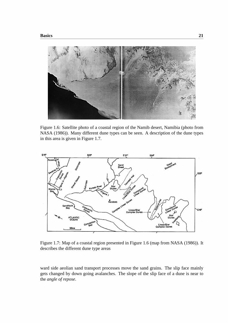
Figure 1.6: Satellite photo of a coastal region of the Namib desert, Namibia (photo fromNASA (1986)). Many different dune types can be seen. A description of the dune typesin this area is given in Figure 1.7.

Figure 1.7: Map of a coastal region presented in Figure 1.6 (map from NASA (1986)). Itdescribes the different dune type areas

ward side aeolian sand transport processes move the sand grains. The slip face mainlygets changed by down going avalanches. The slope of the slip face of a dune is near totheangle of repose.

22 1.3 Dune geomorphology

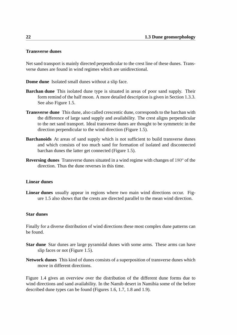
Transverse dunes

Net sand transport is mainly directed perpendicular to the crest line of these dunes. Trans-verse dunes are found in wind regimes which are unidirectional.

Dome dune Isolated small dunes without a slip face.

Barchan dune This isolated dune type is situated in areas of poor sand supply. Theirform remind of the half moon. A more detailed description is given in Section 1.3.3.See also Figure 1.5.

Transverse dune This dune, also called crescentic dune, corresponds to the barchan withthe difference of large sand supply and availability. The crest aligns perpendicularto the net sand transport. Ideal transverse dunes are thought to be symmetric in thedirection perpendicular to the wind direction (Figure 1.5).

Barchanoids At areas of sand supply which is not sufficient to build transverse dunesand which consists of too much sand for formation of isolated and disconnectedbarchan dunes the latter get connected (Figure 1.5).

Reversing dunesTransverse dunes situated in a wind regime with changes of180o of thedirection. Thus the dune reverses in this time.

Linear dunes

Linear dunes usually appear in regions where two main wind directions occur. Fig-ure 1.5 also shows that the crests are directed parallel to the mean wind direction.

Star dunes

Finally for a diverse distribution of wind directions these most complex dune patterns canbe found.

Star dune Star dunes are large pyramidal dunes with some arms. These arms can haveslip faces or not (Figure 1.5).

Network dunes This kind of dunes consists of a superposition of transverse dunes whichmove in different directions.

Figure 1.4 gives an overview over the distribution of the different dune forms due towind directions and sand availability. In the Namib desert in Namibia some of the beforedescribed dune types can be found (Figures 1.6, 1.7, 1.8 and 1.9).

Basics 23

Figure 1.8: Satellite photo of crescentic transverse dunes at the coast line of the Namibdesert, Namibia (photo from NASA (1986)).

Figure 1.9: Satellite photo of a star dune in the Namib desert, Namibia (photo from NASA(1986)).

1.3.3 A more detailed description of dune forms generated by uni-modal wind source

The main dune forms generated by an unimodal wind source are the Barchan dune andthe transverse dune. The model which is discussed in this thesis so far is restricted to

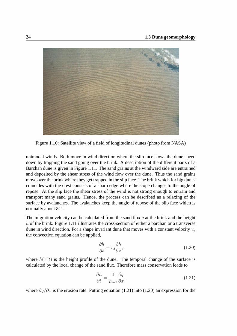
24 1.3 Dune geomorphology

Figure 1.10: Satellite view of a field of longitudinal dunes (photo from NASA)

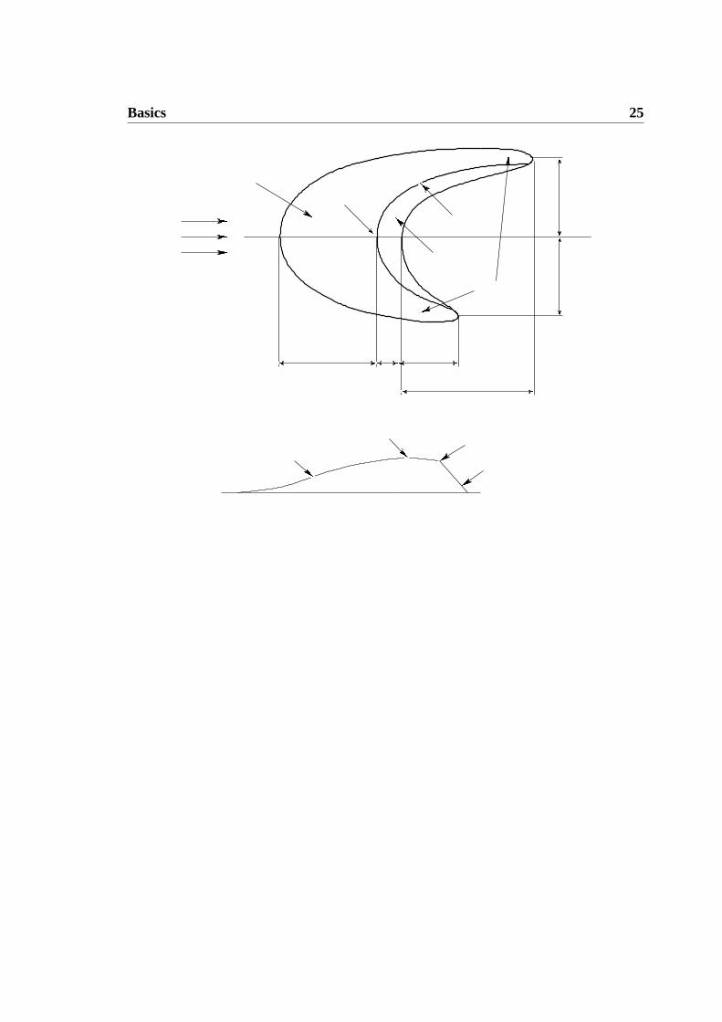
unimodal winds. Both move in wind direction where the slip face slows the dune speeddown by trapping the sand going over the brink. A description of the different parts of aBarchan dune is given in Figure 1.11. The sand grains at the windward side are entrainedand deposited by the shear stress of the wind flow over the dune. Thus the sand grainsmove over the brink where they get trapped in the slip face. The brink which for big dunescoincides with the crest consists of a sharp edge where the slope changes to the angle ofrepose. At the slip face the shear stress of the wind is not strong enough to entrain andtransport many sand grains. Hence, the process can be described as a relaxing of thesurface by avalanches. The avalanches keep the angle of repose of the slip face which isnormally about34o.

The migration velocity can be calculated from the sand fluxq at the brink and the heighth of the brink. Figure 1.11 illustrates the cross-section of either a barchan or a transversedune in wind direction. For a shape invariant dune that moves with a constant velocityvdthe convection equation can be applied,

∂h

∂t= vd

∂h

∂x, (1.20)

whereh(x, t) is the height profile of the dune. The temporal change of the surface iscalculated by the local change of the sand flux. Therefore mass conservation leads to

∂h

∂t=

1

ρsand

∂q

∂x, (1.21)

where∂q/∂x is the erosion rate. Putting equation (1.21) into (1.20) an expression for the

Basics 25

PSfrag replacements

L0 La

Lb

Ls

Wa

WbH

windward side

windward side

wind direction

brink

brink

slip face

slip face

crest

horns

Figure 1.11: Sketch of a barchan dune.

dependency of the dune velocity with respect to the dune height is obtained,

vd(h) =1

ρsand

dq

dh. (1.22)

This equation also is quite useful to examine if the dune reached a steady state or not. Fora height profile which holds no shape invariance following equation is not valid,

dq

dh= constant. (1.23)

1.3.4 Dune fields

Mostly deserts present wide areas of ground filled up with large amounts of mobile sandgrains. From the huge Sahara desert to smaller areas like Jericoacoara near to Fortalezain the north of Brazil sometimes various dune types are found in the same area. In sectionbefore the Namib sand sea shows a large field with different dune types due to the slightlyvarying conditions. Even single dunes depend strongly on their surrounding topography.

26 1.3 Dune geomorphology

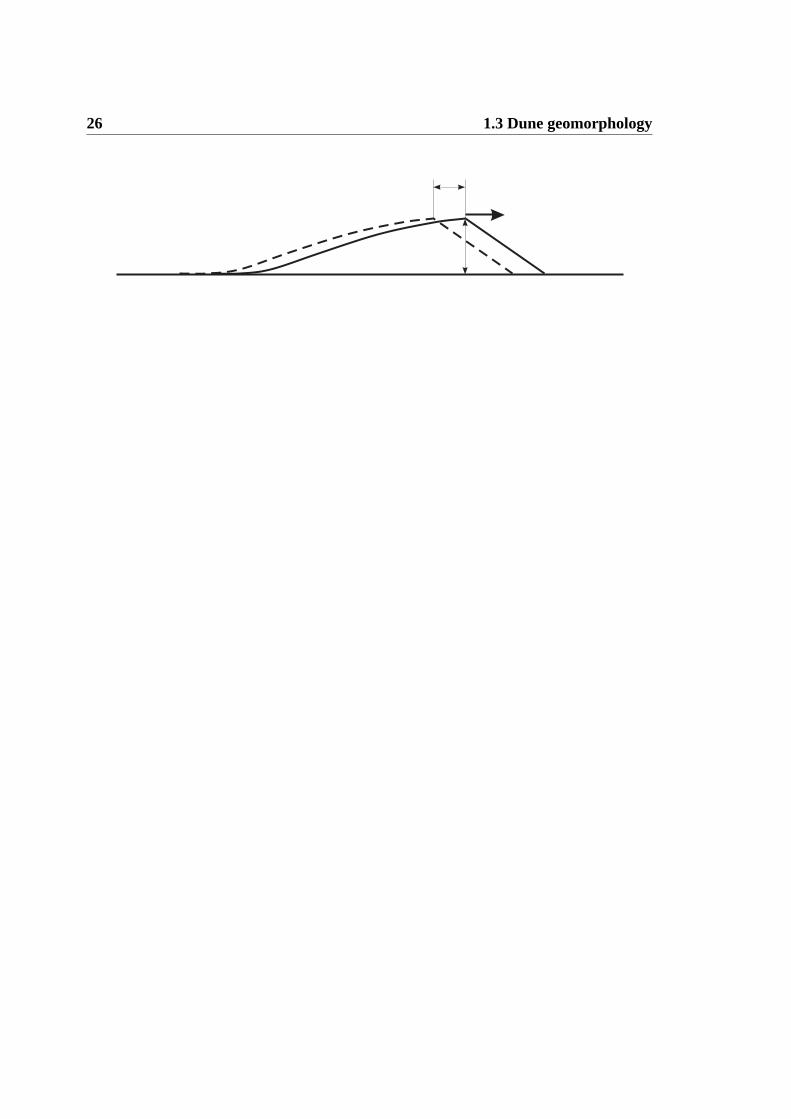
PSfrag replacements

h

dx = vddt

q

Figure 1.12: Sketch of the displacement of a dune. The deposition of the volume of sandh dx = q dt/ρsandcauses the dune to advance bydx = vddt.

That is for example the sand supply, mountains, the sea and so on. It is important toconsider the entire particular region. The dynamics of a single dune gets influenced byother dunes surrounding them. The steady state presumes for example a long sustainedconstant influx of sand which is not given in dune fields where the topography is changingrapidly. For example barchan dunes feel other barchans even over large distance by havingasymmetries of their shape ((Cooke, Warren, and Goudie 1993)).

Chapter 2

Air shear stress over heaps and dunes

In this chapter an algorithm to calculate the shear stress over a two- or three-dimensionalhill or dune will be introduced. A short overview of turbulence models will give aninsight in the different calculations of wind velocities and shear stresses. In the nextsection roughly an analytical perturbation theory which supplies a fast algorithm in orderto calculate the shear stress over smooth hills will be described. The final section willexplain the concept of a separation bubble.

2.1 Turbulence models

Turbulent flows consist of irregularly fluctuating velocity fields. Spatial and temporalfluctuations mix quantities such as the energy and momentum carried by them. The dis-tribution of these fluctuations extends over many scales of time and space so that thesimulations of them get computionally too expensive. To obtain reasonable results forpractical applications the Navier-Stokes equations have to be averaged to get rid of thesmall scale dynamics. There is time-averaging, ensemble-averaging and the usage ofother modifications of the Navier-Stokes equation to solve the air flow computionally lessexpensively. But the averaging of something unknown like the small scale fluctuationsleads to additional new unknown terms. The relation of these terms to averaged variablesis calledturbulence model. Turbulence models are based on two common methods whichare namedReynolds averagingandfiltering.

The interest in this thesis is restricted to Reynolds averaging. Therefore the variables ofthe Navier-Stokes equations are decomposed into a mean and a fluctuating part. Thatmeans for the components of the velocity

ui = ui + u′i, (2.1)

27

28 2.2 The separation bubble and its justification

and for the other scalar quantitiesφ = φ+ φ′, (2.2)

where ui, φ andu′i, φ′ are the mean and fluctuating parts, respectively.φ denotes for

example pressureρ or energy. After substituting Equation (2.1) and (2.2) into the Navier-Stokes equations and taking a time or ensemble average it is obtained

∂ρ

∂t+

∂

∂xi(ρu) = 0 (2.3)

ρDuiDt

= − ∂p

∂xi+

∂

∂xi

[

µ

(

∂ui∂xj

+∂uj∂xi− 2

3δij∂ul∂xl

)]

+∂

∂xi

(

−ρu′iu′j)

, (2.4)

where the bars on the mean velocity are omitted. Equations 2.3 and 2.4 are calledReynolds–averagedNavier-Stokes equations. Their only difference to the outgoingNavier-Stokes equations are the additional terms of theReynolds stresses∂

∂xi

(

−ρu′iu′j)

which have to be modeled in order to close (2.4). A relation of these to the mean velocitygradients comprises the Boussinesq hypothesis (Hinze 1975),

−ρu′iu′j = µt

(

∂ui∂xj

+∂uj∂xi

)

− 2

3

(

ρk + µt∂ui∂xi

)

δij (2.5)

wherek is the kinetic energy andµt the turbulent viscosity. The Boussinesq hypothesiscontains the small inconsistency thatµt is assumed to be isotropic and scalar which is notstrictly true. k andµt can be calculated for example with the semi-empiricalk-ε modelof Launder and Spalding (1972). There the turbulent kinetic energyk and the turbulencedissipation rateε are calculated by two differential equations. The turbulent viscosityfinally is obtained by

µt = ρCµk2

ε(2.6)

whereCµ = 0.09 is a constant, determined by experiments with air and water.

2.2 The separation bubble and its justification

It was shown in Sauermann (2001) that there appears a large eddy in the lee side afterthe sharp brink of a dune. A separation of the quasi-laminar flow which is also foundat the windward side and the turbulent eddy holds over a long distance after the brink(Figure 2.1). The separation streamline reaches from the point of flow separation (thebrink) to the point of re-attachment at a distance of approximately six times the height ofthe brink. The surface formed by the separation streamlines is called separation bubbles(x). According to Zeman and Jensen (1988) the air shear stressτ(x, y) on the windwardside of the dune can be calculated using the envelope that comprises the dune and the

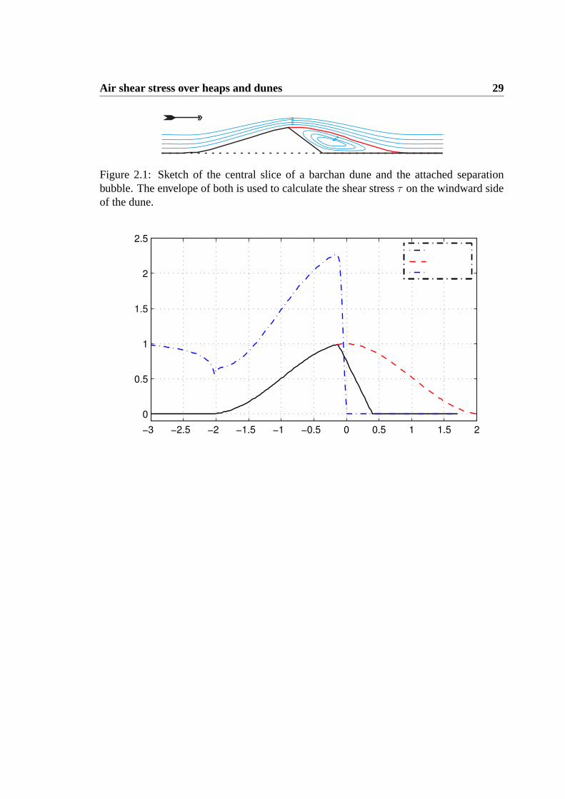
Air shear stress over heaps and dunes 29

Figure 2.1: Sketch of the central slice of a barchan dune and the attached separationbubble. The envelope of both is used to calculate the shear stressτ on the windward sideof the dune.

−3 −2.5 −2 −1.5 −1 −0.5 0 0.5 1 1.5 2

0

0.5

1

1.5

2

2.5

PSfrag replacements

x/L

h/H

andτ/τ

0

h(x)s(x)τ(x)

Figure 2.2: The envelopeh(x) of the windward profile of a duneh(x) and the separatingstreamlines(x) form together a smooth object which is used to calculate the air shearstressτ(x) on the windward side. In the region of re–circulation the air shear stressτ isset to zero.

separation bubble. Measurements of the shear stress over a barchan dune matched quitewell with this proposal.

This facilitates pretty well the search for a computionally sparse algorithm. A disconti-nuity like the sharp brink of a dune would make the calculation of the shear stress quitecomplex. Hence, the shear stress over the dune is not computed over the height profileh(x) of the dune but of the envelope surface,

h(x, y) = max(h(x, y), s(x, y)) . (2.7)

The other argument to use the concept of the separation bubble comes from the obser-vations made by Sauermann (2001) in Morocco and Brazil. Measurements performed on

30 2.3 An analytical model for the air shear stress

barchan dunes showed that between the horns of a barchan only a negligible amount ofsediment transport occurs. That means that the shear stressτ(x, y) in the separation bub-ble can be set to zero. Figure 2.2 depicts the shear stress approximation in the separationbubble.

Hence, the envelope surfaceh(x, y) is used for the calculation of the air shear stress overa dune. The functional form for a separation bubble is obtained by the minimal heuristicansatz of a polynomial of third order. Therefore the dune surface is cut into slides in thewind direction where every slide has its own separation streamlines(x). The conditionof smoothness determines already three parameters of the polynomial as the height ofthe brinks(0) = h0, the windward slope at the brink has to coincide with the separationstreamline’s first points′(0) = h′0 and the height and slope are zero at the reattachmentpoints(Lr) = 0, s′(Lr) = 0 (assuming that the separation streamline ends on the ground),i.e.

s(x) = a3x3 + a2x

2 + h′0x+ h0, (2.8)

a3 = (2h0 + h′0Lr)L−3r ,

a2 = − (3h0 + 2h′0Lr)L−2r .

The downwind distanceLr is determined by phenomenological observations. Accordingto (Sauermann 2001) a good estimate is given by setting the maximum slope of the sep-aration streamline equal toC = 0.25 (14◦). A second-order approximation yields finallythe equation for the length of the separation streamline,

Lr =3h0

2C

(

1 +1

4

h′0C

+1

8

(

h′0C

)2)

. (2.9)

For simulations of dune fields and of dunes which localize on a filled sand bed the separa-tion streamlines do not connect smoothly to the height profile but intersect the surface at adistance smaller thanLr after the brink. The heighth1 and the slopeh′1 at the intersectionpoint atx = x1 = x0 + L now substitute the parameterss(Lr) = 0 ands′(Lr) = 0,respectively. Hence, the new separation streamline is calculated according to

sn(x) = a3x3 + a2x

2 + h′0x+ h0, (2.10)

a2 = (3h1 − h′1x1 − 2h′0x1 − 3h0)L−2,

a3 = (h′1L− 2h1 + h′0L+ 2h0)L−3.

The two separation streamlines are depicted in Figure 2.2.

2.3 An analytical model for the air shear stress

Using the concept of the separation bubble the shear stress of the wind over a dune canbe calculated with an algorithm which is valid for smooth surfaces. Due to the fact that in

Air shear stress over heaps and dunes 31

Figure 2.3: When the separation streamlines(x) crosses the surface ath(x) 6= 0 theintersection is used to calculate the new separation streamlinesn(x).

the model of this thesis the time evolution of dune forms is considered the overall shearstress has to be calculated for every iteration. This computional quite expensive featureneeds a fast algorithm.

A smooth hill or the envelope of a dune can be considered as a perturbation of the surfacethat causes a perturbation of the air flow onto the plain. As a basis is used the logarithmicprofile of the atmospheric boundary layer over plain ground (Chapter 1). An analyticalcalculation of the shear stress perturbation onto a two dimensional hill has been performedby Jackson and Hunt (1975). Later, the work has been extended to three dimensional hillsand further refined (Sykes 1980; Zeman and Jensen 1988; Carruthers and Hunt 1990;Weng, Hunt, Carruthers, Warren, Wiggs, Livingstone, and Castro 1991). These modelsare approximations for smooth hills with the criteria thatH/L� 1 and0 < ln−1(l/z0)�1 whereH andL are the height and the half length at half heights, respectively.z0 andldenote the roughness length and the height of the so calledshear stress layerof the innerregion. According to the work of Hunt, Leibovich, and Richards (1988) the atmosphericboundary layer is divided in four regions which are combined into two, i.e. an inner andan outer region (cf. Figure 2.4). The different physical processes determine differentsolutions for each layer. These solutions are matched together afterwards.

In order to determine the shear stress which is responsible for the sand transport it has to

32 2.3 An analytical model for the air shear stress

Figure 2.4: Sketch of the different regions and layers of the flow used in the calculation ofHLR: Upper layer (U), Middle layer (M), shear stress layer (SS), and Inner surface layer(IS).

be calculated close to the surface. Thus the most suitable layer for this purpose should bethe shear stress layer. Weng, Hunt, Carruthers, Warren, Wiggs, Livingstone, and Castro(1991) obtained the following shear stress perturbation in wind direction for a smoothhill:

τx(kx, ky) =h(kx, ky)k

2x

|k|2

U2(l)

(

1 +2 lnL|kx|+ 4γ + 1 + i sign(kx)π

ln l/z0

)

, (2.11)

and for the shear stress perturbation in lateral direction:

τy(kx, ky) =h(kx, ky)kxky

|k|2

U2(l), (2.12)

where|k| =√

k2x + k2

y andγ = 0.577216 (Euler’s constant). Equations (4.1) and (4.2)are taken in Fourier space with the wave numberskx andky. U(l) is the normalizedvelocity of the undisturbed logarithmic profile at the heightl (Sauermann 2001),

U(l) =ln l/z0

ln Lz0

ln−1/2 L/z0

= ln−1

[

L

z0

ln−1/2 L

z0

]

ln

[

2κ2 L

z0

ln−1

(

2κ2 L

z0

ln−1 L

z0

)]

(2.13)whereκ = 0.4 denotes the von Karman constant. The shear stress of a central slice of a y-symmetric dune can be divided into two terms where the first determines mainly the windspeed-up over a hill and the second leads to an asymmetry which shifts the maximumof the shear stress perturbation upwind with respect to the hill (Sauermann, Kroy, andHerrmann 2001b).

Chapter 3

A continuum saltation model

In this chapter a short survey over the phenomenological model for saltation transportfrom Sauermann, Kroy, and Herrmann (2001b) will be given. The only difference will bethe addition of a diffusion term to the density equation. First the derivation of the modelwill be resumed. The grain born shear stress, the erosion and deposition rates will bederived. The forces acting on the sand grains and the erosion rate will lead to a closedmodel for saltation transport. Secondly the saturated sand flux will be calculated andcompared with other models. The temporal dynamics of the saltation layer will give moreknowledge about the sand flux on the windward side of a dune. Finally simplifications ofthe model will be made in order to obtain a faster algorithm.

3.1 The model

As it was used to model the formation and propagation of sand ripples as well asavalanches the bed-load is considered as a thin fluid-like granular layer on top of an im-mobile sand bed. In the further derivation all equations are integrated over the verticalcoordinate, i.e. all vectors point at horizontal direction.

The model consists of an equation of mass conservation and momentum conservation inpresence of erosion and external forces. The saltation layer exchanges its sand grains withthe sand bed through the termΓ which expresses erosion and deposition of sand,

∂ρ(x, y, t)

∂t+∇ρ(x, y, t)u(x, y, t) + Cdiff∆ρ(x, y, t) = Γ(x, y, t). (3.1)

Hereρ(x, y, t) andu(x, y, t) denote the density and velocity of the sand grains in the salta-tion layer, respectively. The erosion rateΓ(x, y, t) counts the number of grains per timeand area that get mobilized.∆ is the Laplace-operator andCdiff the diffusion constant.

33

34 3.1 The model

The diffusion term is included although no diffusion constant has been estimated or mea-sured so far. Section 6.4 describes the effect of diffusion whereas in the other simulationsdiffusion is switched off (Cdiff = 0).

For the momentum conservation the diffusion term is neglected,

∂u(x, y, t)

∂t+(u(x, y, t)∇) u(x, y, t) =

1

ρ(x, y, t)(fdrag(x, y, t) + f bed(x, y, t) + f g(x, y)) .

(3.2)fdrag is the drag force, accelerating the grains,f bed the friction force, deccelerating thegrains by the complex interaction with the sand bed, andf g the gravity force, involvingthe influences of inclined surfaces.

3.1.1 The grain born shear stress

The air transfers momentum to the saltating grains. A part of the shear stress is transportedto the surface. Hence, the overall shear stress can be divided in a grain born shear stressτg and an air born shear stressτa,

|τ | = τa(z) + τg(z) = constant, (3.3)

where at the top of the saltation layer the air born shear stress has to be equal to the overallshear stressτa(zm) = τ . The shear stresses are assumed to point at the same direction sothat the absolute values can be used for the derivation.

For further calculations the grain born shear stress on the groundτg0 (at a height of theroughness lengthz0) is estimated. The horizontal velocityu of a grain that is acceleratedin the saltation layer has increased when it impacts on the ground,

τg0 = Φ[udown(z0)− uup(z0)] = Φ∆ug0 =q

l∆ug0, (3.4)

whereΦ denotes the flux of grains impacting onto the surface,q = uρ the horizontal sandflux and l the mean trajectory length of a saltating grain. An estimation of the averageflight length as a simple ballistic trajectory gives,

l = u2uz0g, (3.5)

whereuz0 is the vertical component of the initial velocity of the grain andg the accelera-tion by gravity.

Inserting Equation (3.5) in Equation (3.4) and usingq = ρu it is obtained,

τg0 = ρg

2

∆ug0uz0

. (3.6)

A continuum saltation model 35

As a simplest estimation of the vertical ejection velocityuz0 it is set proportional to thehorizontal velocity difference∆ug0 neglecting any angle dependence,

uz0 = α∆ug0. (3.7)

α can be seen as a model parameter, representing an effective restitution coefficient forthe grain-bed interaction, which can be calculated out of the splash function (cf. Sec-tion 1.2.3). In this model the parameter is determined by comparing the model withexperimental results. With Equation (3.7), Equation (3.6) reduces to the simple result

τg0 = ρg

2α(3.8)

for the grain born shear stress on the ground.

3.1.2 Erosion and deposition rates

Assuming a simple effective splash function a simple relation for the erosion rate is ob-tained. Furthermore the average numbern of grains dislodged by an impacting grain isexpanded into a Taylor series at the shear stress thresholdτt where still no saltation fluxcan occur. These two steps lead to the following equation (for details cf. Sauermann,Kroy, and Herrmann (2001b)),

Γ =τg0

∆ug0(n− 1) = γ

τg0∆ug0

(

|τ | − τg0τt

− 1

)

. (3.9)

The model parameterγ characterizes the strength of the erosion and determines howfast the system reaches the equilibrium. The complex dependency ofγ on the time of asaltation trajectory and the grain-bed interaction is taken in account only by comparison ofthe model with measurements or microscopic computer simulations. Finally it is assumedthat the difference between impact and eject velocity of the grains is proportional to themean grain velocityu,

Γ = γτg0u

(

|τ | − τg0τt

− 1

)

, (3.10)

The proportionality constant is incorporated inγ.

Equation (3.10) models the erosion rate of a saltation transport that was initiated before.It is only valid if there are already grains in the saltation layer which impact onto thesurface. From Anderson (1991) was derived a similar relation for the direct entrainmentof grains from ground. The aerodynamic entrainment rate is proportional to the differencebetween the air born shear stressτa and the thresholdτta,

Γa = Φa

(

τa0

τta− 1

)

= Φa

(

|τ | − τg0τta

− 1

)

, (3.11)

whereΦa ≈ 5.7 10−4 kg m−2 s−1 is a model parameter defining the strength of the erosionrate for aerodynamic entrainment.

36 3.2 The closed model and the saturated sand flux

3.1.3 Forces

In this section the different forces acting on a grain in the saltation layer are specified. Thefriction force can be obtained directly from the derivation of the grain born shear stresson the ground in Section 3.1.1,

f bed = −τg0τ

τ. (3.12)

The drag force acting on a volume element of the saltation layer is presented by Newton’sdrag force (Section 1.2.3),

fdrag = ρ3

4Cd

ρair

ρquartz

1

d(veff − u)|veff − u|. (3.13)

whered denotes the grain diameter,Cd the drag coefficient andveff an effective windvelocity which is taken at a reference heightz1 within the saltation layer.z1 which holdsz0 < z1 � zm (zm denotes the mean saltation height and is obtained by measurements)has to be included as another model parameter which is determined by comparison of thesolution for saturated sand flux to measurements. The absolute effective wind velocityveff can be expressed by,

veff =u∗κ

√

1− τg0τ

(

2A1 − 2 + lnz1

z0

)

τ

τ. (3.14)

with

A1 =

√

1 +z1

zm

τg0τ − τg0

. (3.15)

For vanishing grain born shear stress the effective wind velocity reduces to the velocity ofthe undisturbed atmospheric boundary layer at the heightz1. Nevertheless, in the entiredune model (Chapter 4) a simpler expression for the effective wind velocity is applied tomake the calculation of the wind velocityu of the grains independent of the grain densityρ (also cf. the following sections).

In these equations it is assumed that the bed force and the drag force always point at thedirection of the shear stress. The only force which contains lateral forces is the gravitationforce,

f g = −ρg∇h, (3.16)

whereg is the gravitational constant andh(x, y, t) the height profile.

3.2 The closed model and the saturated sand flux

In the preceding section the erosion rateΓ, the grain born shear stressτg0 and the forceswere derived and can now be combined in order to obtain a complete closed model for

A continuum saltation model 37

the calculation of the density and velocity of the grains in the saltation layer. There arethe two model parametersα andz1 determining the equilibrium state and the parameterγ controlling the relaxation to the equilibrium. Inserting Equations (3.10) and (3.8) inEquation (3.1) yields,

∂ρ

∂t+∇(ρu) + Cdiff∆ρ =

1

Tsρ

(

1− ρ

ρs

)

. (3.17)

where the equation has been rewritten in a more compact form with,

ρs =2α

g(|τ | − τt) , (3.18)

Ts =2α|u|g

τtγ(|τ | − τt)

. (3.19)

ρs denotes the saturated density andTs the characteristic time that define the steady stateand the transients of the sand densityρ, respectively. An important quantity is the sat-uration lengthls = Tsu denoting the length of the transient state to reach a saturationtransport.ls plays a crucial role breaking the shape invariance of dune shapes (cf. Chap-ter 6). Direct entrainment can be included easily by addition of Equation (3.11) on theright side of (3.17).

Furthermore, inserting the Equations (3.12) and (3.13) in Equation (3.2) lead to a modelfor the sand velocityu in the saltation layer,

∂u

∂t+ (u∇)u =

3

4Cd

ρair

ρquartz

1

d(veff − u)|veff − u| − g

2α

τ

|τ |− ρg∇h, (3.20)

with veff defined in (3.14).

In order to calculate the saturated sand flux the diffusion and gravitation are neglected inthe model , the sand flux is set stationary (∂/∂t = 0), the sand bed is set homogeneous(∇ = 0) and the shear stress constant in time and space. Thus all lateral fluxes are 0 sothat it is sufficient to model the sand flux in one dimension. For a shear stress minor tothe shear stress threshold the solution is trivial. No saltation transport is possible. Theanalytical solution for the steady state densityρs with a shear stressτ > τt above thethreshold is,

ρs(u∗) =2αρair

g(u2∗ − u2

∗t). (3.21)

Likewise we obtain from Equations (3.20) the steady state velocityus,

us(u∗) =2u∗κ

√

z1

zm+

(

1− z1

zm

)

u2∗tu2∗− 2u∗t

κ+ ust, (3.22)

38 3.3 Dynamics of the saltation layer and simplifications for dune modeling

0

0.02

0.04

0.06

0.08

0.1

0.12

0.14

0 0.5 1 1.5 2 2.5 3 3.5 4 4.5 5

PSfrag replacements

qin

kgm−

1s−

1

t in s

u∗ = 0.3

u∗ = 0.4

u∗ = 0.5

u∗ = 0.6

u∗ = 0.7

Figure 3.1: Numerical simulations of the time evolution of the full model given by Equa-tion (3.17) and (3.20) with a constant shear velocityu∗.

where

ust ≡ us(u∗t) =u∗tκ

lnz1

z0

−

√

2 g d ρquartz

3αCd ρair. (3.23)

The productqs = ρsus yields the steady sand flux which is asymptotically proportionalto u3

∗ for large wind speeds according to the predictions given by Bagnold (1941), Lettauand Lettau (1978) and Sørensen (1991). The comparison of the saturated sand flux withexperimental data determined the two phenomenological parametersα = 0.35 andz1 =0.005 m.

3.3 Dynamics of the saltation layer and simplificationsfor dune modeling

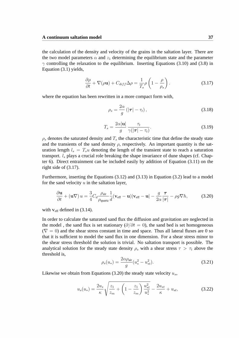
Figure 3.1 shows the time evolution of the one-dimensional model without diffusion andgravitation for different shear velocities with the parameterγ ≈ 0.4 determined out ofmeasurements. The figure reveals that the system reaches the stationary state after 2–3 seconds. Another conclusion is that the length scale to reach the saturation is aboutone meter supposing a typical grain velocity (Sauermann, Kroy, and Herrmann 2001b),probably playing an important role in dune dynamics.

A continuum saltation model 39

The system of the coupled partial differential equations (3.17) and (3.20) implies rathercomplex calculations to obtain good results. Now some approximations are made in orderto simplify the model. Therefore the one-dimensional model without diffusion term norgravity force are used to justify the simplifications.

First, according to the calculations which have shown a temporal transient to the stationarysolution of about two seconds, being magnitudes smaller than the temporal changes ofdune shapes, the time dependent term can be neglected (∂/∂t = 0).

Secondly, the convective term can be neglected even for drastic decreases of the grainvelocity (Sauermann, Kroy, and Herrmann 2001b). Calculations with the entire modelof Chapter 4 showed that a negligence of the convective term does not cause significantdifferences of the simulation results.

Thirdly, the effective wind velocityveff(ρ) is substituted by the effective wind velocity ofa saturated saltation layerveff(ρs). A negligible error is created for shear stresses near thethresholdτt. In the model the simulations are restricted to shear velocitiesu∗ ≤ 0.5ms−1. An effective wind velocity which is not dependent on the grain density decouples theequation for the grain velocity from the grain density calculation.

With these approximations the saltation model is restricted to stationary solutions includ-ing spatial saturation transients. According to all before described approximations thesaltation transport on sand dunes is modeled by,

div (ρu) + Cdiff ∆ρ =1

Tsρ

(

1− ρ

ρs

)

{

Θ(h) ρ < ρs

1 ρ ≥ ρs, (3.24)

with

ρs =2α

g(|τ | − τt) Ts =

2α|u|g

τtγ(|τ | − τt)

. (3.25)

and3

4Cd

ρair

ρquartzd−1 (veff − u)|veff − u| − g

2α

u

|u|− g∇h = 0, (3.26)

where,

veff =2u∗κ|u∗|

(√

z1

zmu2∗ +

(

1− z1

zm

)

u2∗t +

(

lnz1

z0

− 2

)

u∗tκ

)

, (3.27)

andu∗ =

√

τ/ρair (3.28)

The constants and model parameters have been taken from (Sauermann, Kroy, and Herr-mann 2001b) and are summarized here:g = 9.81 m s−2,κ = 0.4, ρair = 1.225 kg m−3,ρquartz = 2650 kg m−3, zm = 0.04 m, z0 = 2.5 10−5 m, D = d = 250µm, Cd = 3 andu∗t = 0.28 m s−1, γ = 0.4,α = 0.35 andz1 = 0.005 m.

40 3.3 Dynamics of the saltation layer and simplifications for dune modeling

Chapter 4

The numerical model for sand dunes

In this chapter the entire model for sand dunes will be described. It can be seen as anextension of the work of Sauermann (2001). The aim is to model various dune types withthe same program. Different parts compose the structure of the model to simulate shearstress, sand flux, avalanches and time evolution of dunes.

4.1 The complete model

To model a sand dune with all its sand grains (about1015) today’s computers are far tooslow. The problem of the wide range of lengthscales (from grain to dune field) and timescales (from the time to reach the steady state of the saltation flux to evolution times ofdune fields) leads to the restriction to a strongly simplified model. The physical processesacting on dune dynamics are highly complicated. Thus the sand grains are described asa continuum and the shear stress over a dune is calculated with a simplified algorithm.The essential ingredients of all involved physical processes have to be included in orderto obtain still reasonable results out of simulations.

As predecessor of the model described here the work of Sauermann (2001) revealed inter-esting new insights into dune dynamics and dune formation. The model now is extendedto a 2-dimensional shear stress calculation (longitudinal and lateral direction), a full sandbed and different boundary conditions. Nevertheless the wind is restriced to be constantand unidirectional in time. However, an extension to a wind field nearer to reality wouldnot cost much effort.

In the following sections the different parts of the dune model are described. They areadjusted to physical laws or in a phenomenological way to observations by measurements.Thus their parameters are regarded to be fixed and the dune model can be used as ablack box which yields different solutions depending on the initial surface, the boundary

41

42 4.2 The air shear stressτ at the ground

conditions, the shear velocity and the size of the simulated dune field. One aim is toobtain a final surface consisting of a steady state. The other aim is the observation of acontinuously developing surface to extract characteristic laws.

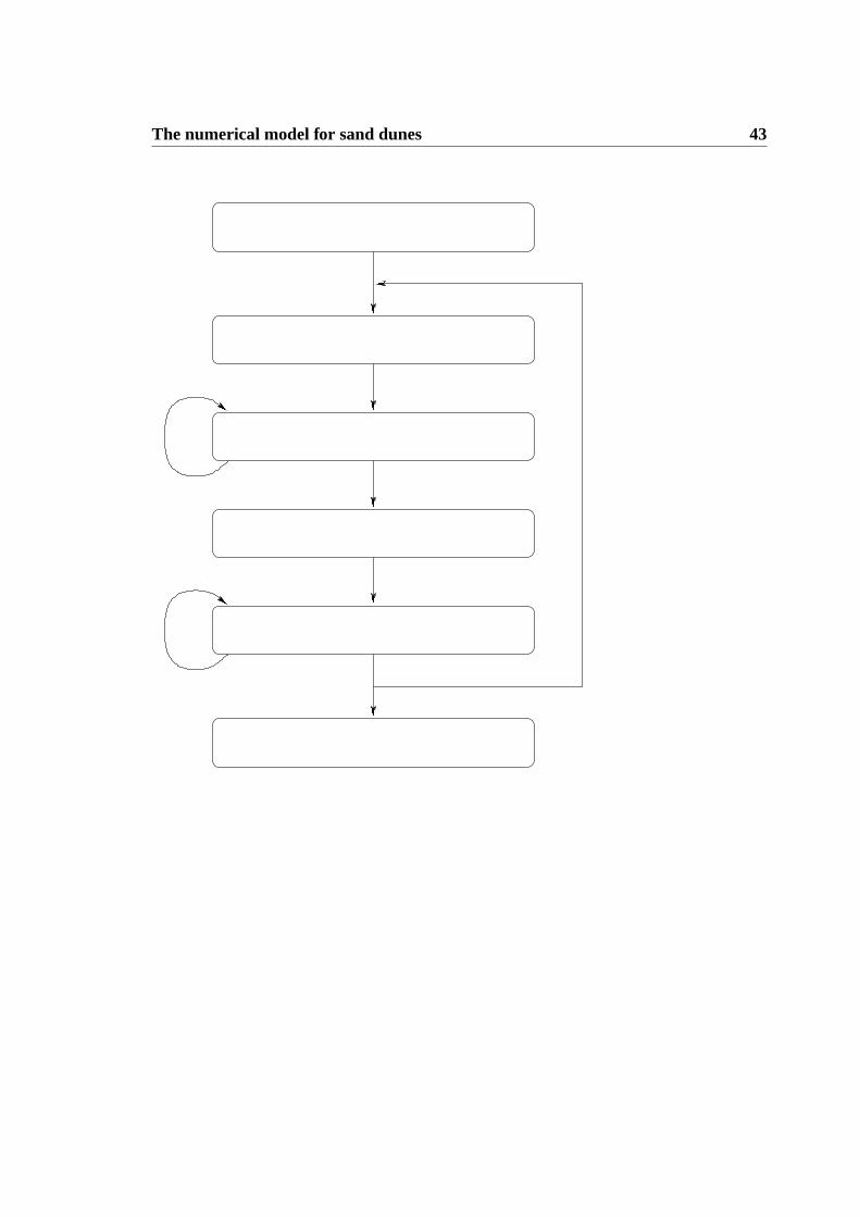
Figure 4.1 shows the principal structure of the model. The shear stress, the sand flux, theavalanches and the time integration are calculated in this order for the whole surface atevery iteration.

4.2 The air shear stressτ at the ground

The shear stress perturbation over a single dune or over a dune field is calculated withthe algorithm depicted in Chapter 2. Theτx-component points at wind direction and theτy-component denotes the lateral direction,

τx(kx, ky) =h(kx, ky)k

2x

|k|2

U2(l)

(

1 +2 lnL|kx|+ 4γ + 1 + i sign(kx)π

ln l/z0

)

, (4.1)

and

τy(kx, ky) =h(kx, ky)kxky

|k|2

U2(l), (4.2)

These are calculated in Fourier space and have to be multiplied with the logarithmic ve-locity profile in real space. The surface is assumed to be rigid and the effect of sedimenttransport is incorporated in the roughness lengthz0. The roughness lengthz0 and thelength of the hill at half heightsL are determined in Chapter 6 by comparing the resultsof the simulations to dune measurements. For the slices in wind direction of the dunesprofile the separation streamlines are calculated according to the equations discussed inChapter 2. The separation bubble guarantees a smooth surface and the shear stress in thearea of the separation bubble is set equal to zero. There are problems due to the numericalfluctuations of the slope of the brink where the separation bubble begins and due to thecalculation of a separation streamline for each slice. The surface built up of height profileand separation bubble showed small heaps and oscillations. To get rid of this numericalerror the surface is Fourier-filtered cutting small frequencies.

4.3 The sand fluxq

The sand density and the grain velocity are calculated according to Equation (3.24) and(3.26) derived in Chapter 3 from the before obtained shear stress and the surface gradi-ent. These are combined to the sand flux over a surface elementq(x, y) = u(x, y)ρ(x, y).The time to reach the steady state of sand flux over a new surface is some magnitudes of

The numerical model for sand dunes 43

PSfrag replacements

h(x, y, t = 0) initial surface

τ(x, y, h) wind shear

q(x, y, τ ) sand flux

ρsand∂th = −∇q dune surface

h(x, y,∇h) avalanches

h(x, y, t = N∆T ) final surface

stationary solu-tions (∂t = 0)

integrate forwardin time by∆T

assumed to be in-stantaneous

Figure 4.1: Sketch of the full dune model. An initial surfaceh is used to start the timeevolution. First, the air shear stressτ onto the given surfaceh is calculated using ananalytical model. Secondly, the sand fluxq is determined using the air shear stressτ . Theintegration of the surface forward in time is calculated from mass conservation. Finally,sand is eroded and transported downhill if the local angle∇h exceeds the angle of repose.This redistribution of mass (avalanches) is performed until the surface slope has relaxedbelow the critical angle. The time integration is performedN times until the final shapeinvariantly moving solution is obtained. The backward looped arrows indicate that aniterative numerical calculation is involved in this step.

44 4.4 Avalanches

time scales smaller than the time scale of the surface evolution. Hence, the steady stateis assumed to be reached instantaneously. The length scale of the model is too large toinclude sand ripples. Nevertheless the kinetics and the characteristic length scale of salta-tion influence the calculation by breaking the scale invariance of dunes and determiningthe minimal size of a barchan dunes. A calculation of the saltation transport by the wellknown flux relations (Bagnold 1941; Lettau and Lettau 1978; Sørensen 1991) would re-strict the model to saturated sand flux which is not the case for example at the foot of thewindward side of a barchan dune due to little sand supply or at the end of the separationbubble in the interdune region between transverse dunes due to the vanishing shear stressin the separation bubble.

4.4 Avalanches

Surfaces with slopes which exceed the maximal stable angle of a sand surface, the calledangle of reposeΘ ≈ 34o, undergo avalanches which slip down in the direction of thesteepest descent. The unstable surface relaxes to a somewhat smaller angle. For the studyof dune formation two global properties are of interest. These are the sand transportdownhill due to gravity and the maintenance of the angle of repose. To determine thenew surface after the relaxation by avalanches the model proposed by Bouchaud, Cates,Ravi Prakash, and Edwards (1994) is used. There the total mass of sand is divided intotwo layers, a thin moving surface layer and a static layer which contains most of thesand. For each layer the conservation of mass is valid with a source term consisting ofthe sand coming from the other layer, respectively. The source term can be expressedas an exchange rate describing the sand being moblized and transferred from the staticinto the mobile layer. Assuming a constant density of the layers the heights of the layerscorrespond to the amount of sand transported or resting, respectively. Hence there remainsa system of two coupled equations,

∂h

∂t= −CaR (|∇h| − tan Θ) (4.3)

∂R

∂t+∇ (Rua) = CaR (|∇h| − tan Θ) , (4.4)

whereh denotes the height of the sand bed,R the height of the moving layer,Ca is amodel parameter and the velocity of the sand grains in the moving layer is obtained by,

ua = −ua∇h

tan Θ. (4.5)

Like in the calculation of the sand flux the steady state of the avalanche model is assumedto be reached instantaneously. In the dune model a certain amount of sand is transportedover the brink on the slip face and in every iteration the sand grains are relaxed over theslip face by the avalanche model determining with the steady state.

The numerical model for sand dunes 45

4.5 The time evolution of the surface

The calculation of the sand flux over a not stationary dune surface leads to changes byerosion and deposition of sand grains. The change of the surface profile can be expressedby conservation of mass,

∂tρ+∇Φ = 0 , (4.6)

whereρ is the sand density andΦ the sand flux per time unit and area. Bothρ andΦ arenow integrated over the vertical coordinate assuming that the dune has a constant densityof ρsand,

h =1

ρsand

∫

ρdz, q =

∫

Φdz. (4.7)

Thus Equation (4.6) can be rewritten,

∂h

∂t=

1

ρsand

∂q

∂x. (4.8)

Finally, it is noted that Equation (4.8) is the only remaining time dependent equation andthus defines the characteristic time scale of the model which is normally 3–5 hours forevery iteration.

4.6 The initial surface and boundary conditions

There are the following different possibilities of initial surfaces:

Gaussian hills on plain solid ground without sediments. They are of arbitrary number,height and width.

Plain sand bed of arbitrary sand height over the solid ground which can be disturbed bysmall Gaussian hills additionally.

Arbitrary surface over plain solid ground without sediments created before.

An initial surface has to be smooth (at least with separation bubble) and hold angles notlarger than the angle of repose.

The integrated vertical components of the variables of the dune model restrict the bound-ary conditions to the horizontal directions. The boundary conditions influence the surfaceheighth with its separation bubble, the sand fluxq and the heightR of the moving layerof the avalanche model. The boundary in lateral directiony with respect to the directionx of the incoming wind is open or periodic and no further modifications are needed. Adescription of the boundary inx-direction has to be more detailed:

46 4.7 Conclusion

Open boundary An additional parameter controls the sand influxqin into the simulateddune field. It is set constant over the lateral direction atx = 0.

Periodic boundary The separation bubble enters at the beginning of the dune field if itleaves the end. The sand influx is set equal to the outflux. The calculation of thestationary state of the avalanche model has to include periodic boundary effects aswell.

Quasi periodic boundary Instead of settingqin(y) = qout(y) the outflux is integrated inorder to get the entire mass leaving the dune field within one iteration. To conservethe mass of the dune field a spatially constant sand influx is used according to

qin =1

Ly

∫ Ly

0

qout(y)dy, (4.9)

whereLy is the width of the dune field.

4.7 Conclusion

The most important features of dune field dynamics were included into the model byextension to a variety of initial surfaces and boundary conditions. The steps of every iter-ation was described. The last section explained the possible initial surfaces and boundaryconditions. The inclusion of the lateral shear stress component, a filled sand bed and peri-odic boundary conditions make it possible to simulate many different dune fields. Never-theless the dune model can be easily extended to varying wind velocities and directions,an uneven solid ground etc.

The crucial point is the increasing computional time which is needed for spatially and tem-porally more extended simulations. The model already reaches the limit of computionalpossibilities.

Chapter 5

Transverse Dunes

Transverse dunes are found rather often in deserts and along coasts. First some generalaspects will be introduced. A model of 3-dimensional dunes explains why lateral invari-ance plays a role in transverse dune formation. The time evolution and the velocity of thedune in a model of 2-dimensional dunes with constant sand influx are presented. In thefollowing the time evolution of a model of 2-dimensional dunes with periodic boundarygives some more insight into dune field dynamics. A final discussion of the statement thatdunes would behave like solitons will close this chapter.

5.1 Introduction

About 40% of all terrestrial sand seas are covered by transverse dunes. Mostly theyare located in sand seas where sand availability is high. Thus in larger sand seas thereoccur mainly ensembles of many transverse dunes which are subject to an interaction withrespect to their dynamics. The crest to crest spacing ranges from a few meters to over 3km (Breed and Grow 1979). They are common in the Northern Hemisphere, particularlyin China, and on coasts. On the Mars transverse dunes dominate the sand seas. Thefield of transverse dunes in Saudi Arabia on Figure 5.1 shows a very regular spacing.Normally transverse dunes have more irregular patterns and even smaller hierarchies ofsmaller dunes can be found on them. Directionally concentrated and strong winds seemto be the main environment where this type of dune can be found. Cooke, Warren, andGoudie (1993) proposed that in highly mobile environments cross winds distort the duneshape.

All calculations presented in the following sections are made with the conditions of acompletely filled sand bed and unidirectional wind. For a description of the model refer

47

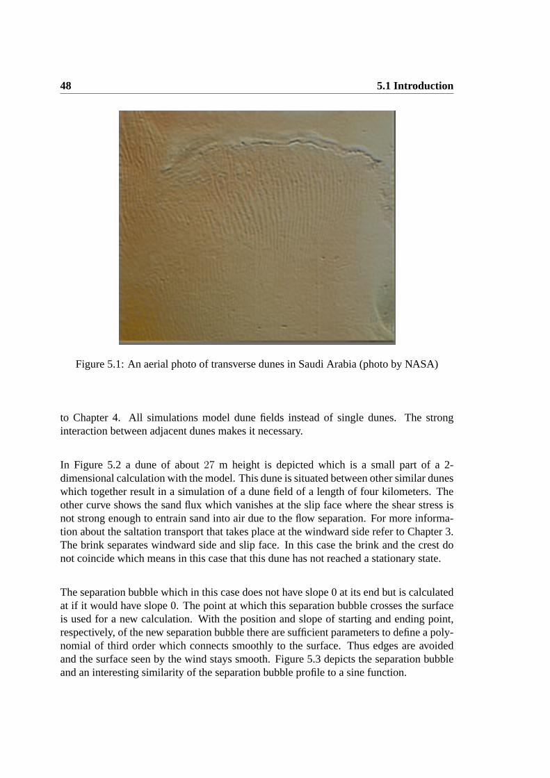
48 5.1 Introduction

Figure 5.1: An aerial photo of transverse dunes in Saudi Arabia (photo by NASA)

to Chapter 4. All simulations model dune fields instead of single dunes. The stronginteraction between adjacent dunes makes it necessary.

In Figure 5.2 a dune of about27 m height is depicted which is a small part of a 2-dimensional calculation with the model. This dune is situated between other similar duneswhich together result in a simulation of a dune field of a length of four kilometers. Theother curve shows the sand flux which vanishes at the slip face where the shear stress isnot strong enough to entrain sand into air due to the flow separation. For more informa-tion about the saltation transport that takes place at the windward side refer to Chapter 3.The brink separates windward side and slip face. In this case the brink and the crest donot coincide which means in this case that this dune has not reached a stationary state.

The separation bubble which in this case does not have slope 0 at its end but is calculatedat if it would have slope 0. The point at which this separation bubble crosses the surfaceis used for a new calculation. With the position and slope of starting and ending point,respectively, of the new separation bubble there are sufficient parameters to define a poly-nomial of third order which connects smoothly to the surface. Thus edges are avoidedand the surface seen by the wind stays smooth. Figure 5.3 depicts the separation bubbleand an interesting similarity of the separation bubble profile to a sine function.

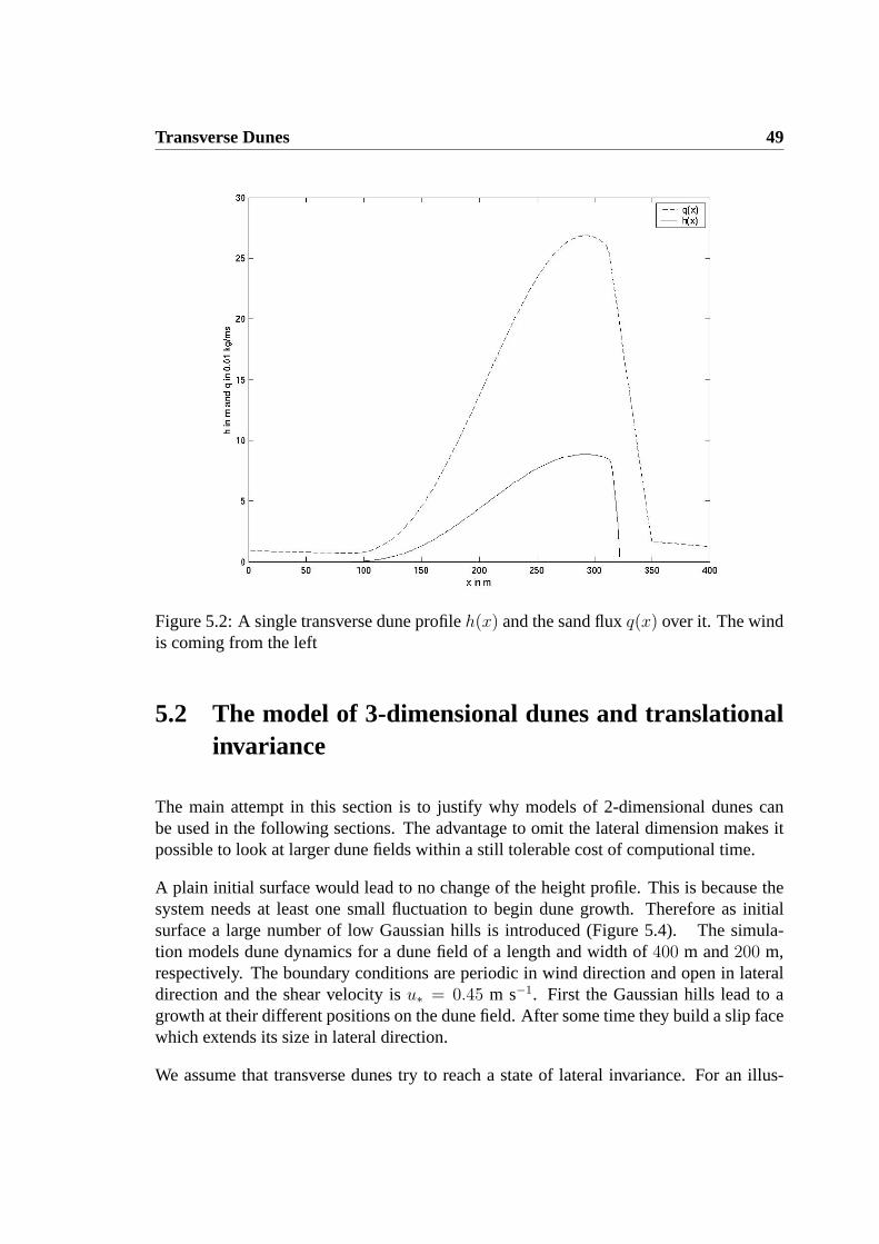
Transverse Dunes 49

Figure 5.2: A single transverse dune profileh(x) and the sand fluxq(x) over it. The windis coming from the left

5.2 The model of 3-dimensional dunes and translationalinvariance

The main attempt in this section is to justify why models of 2-dimensional dunes canbe used in the following sections. The advantage to omit the lateral dimension makes itpossible to look at larger dune fields within a still tolerable cost of computional time.

A plain initial surface would lead to no change of the height profile. This is because thesystem needs at least one small fluctuation to begin dune growth. Therefore as initialsurface a large number of low Gaussian hills is introduced (Figure 5.4). The simula-tion models dune dynamics for a dune field of a length and width of400 m and200 m,respectively. The boundary conditions are periodic in wind direction and open in lateraldirection and the shear velocity isu∗ = 0.45 m s−1. First the Gaussian hills lead to agrowth at their different positions on the dune field. After some time they build a slip facewhich extends its size in lateral direction.

We assume that transverse dunes try to reach a state of lateral invariance. For an illus-

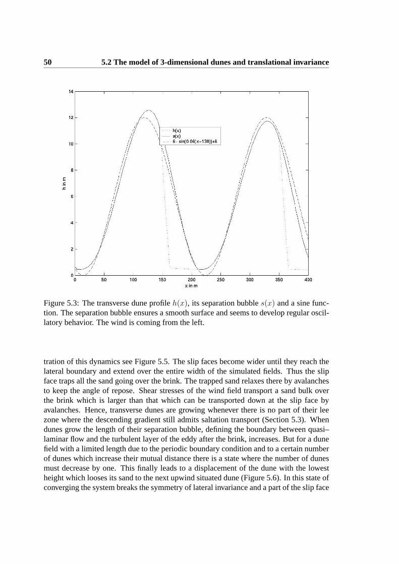
50 5.2 The model of 3-dimensional dunes and translational invariance

Figure 5.3: The transverse dune profileh(x), its separation bubbles(x) and a sine func-tion. The separation bubble ensures a smooth surface and seems to develop regular oscil-latory behavior. The wind is coming from the left.

tration of this dynamics see Figure 5.5. The slip faces become wider until they reach thelateral boundary and extend over the entire width of the simulated fields. Thus the slipface traps all the sand going over the brink. The trapped sand relaxes there by avalanchesto keep the angle of repose. Shear stresses of the wind field transport a sand bulk overthe brink which is larger than that which can be transported down at the slip face byavalanches. Hence, transverse dunes are growing whenever there is no part of their leezone where the descending gradient still admits saltation transport (Section 5.3). Whendunes grow the length of their separation bubble, defining the boundary between quasi–laminar flow and the turbulent layer of the eddy after the brink, increases. But for a dunefield with a limited length due to the periodic boundary condition and to a certain numberof dunes which increase their mutual distance there is a state where the number of dunesmust decrease by one. This finally leads to a displacement of the dune with the lowestheight which looses its sand to the next upwind situated dune (Figure 5.6). In this state ofconverging the system breaks the symmetry of lateral invariance and a part of the slip face

Transverse Dunes 51

Figure 5.4: Initial surface of a filled sand bed. The fluctuations are made by Gaussianhills. The shear velocity isu∗ = 0.45 m s−1, the boundary conditions are periodic in winddirection and open in lateral direction. One unit corresponds to the length of2 m.

disappears. There sand is transported to the following dune by saltation. When the dunehas vanished once again the system approaches lateral invariance. Hence, the effect ofconverging dunes perturbs the steady growth of transverse dunes in a field with a periodicboundary.

To get more information if a system of transverse dunes tends to gain lateral invariance asimulation of a dune field with periodic boundary in both horizontal directions is made.The field extends over400 m in length and width. As initial surface also small Gaussianhills are used. Figure 5.7 shows the height profile after 5,000 iterations which correspondsto a time of1.19 years. The results of this simulation yield to the same conclusions asthe simulation with open lateral boundary. Also each converging of two dunes leads toa breaking of the symmetry. Figure 5.8 and 5.9 show how the system approaches lateralinvariance. The final state of the calculation is reached when only one dune is left. Asimulation with periodic boundary in both directions shows no state where the system hasa lateral structure or lateral oscillations.

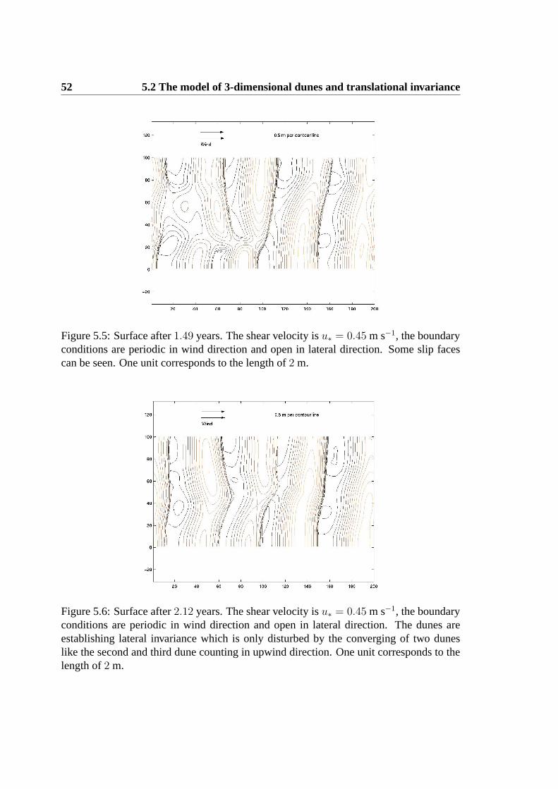
52 5.2 The model of 3-dimensional dunes and translational invariance

Figure 5.5: Surface after1.49 years. The shear velocity isu∗ = 0.45 m s−1, the boundaryconditions are periodic in wind direction and open in lateral direction. Some slip facescan be seen. One unit corresponds to the length of2 m.

Figure 5.6: Surface after2.12 years. The shear velocity isu∗ = 0.45 m s−1, the boundaryconditions are periodic in wind direction and open in lateral direction. The dunes areestablishing lateral invariance which is only disturbed by the converging of two duneslike the second and third dune counting in upwind direction. One unit corresponds to thelength of2 m.

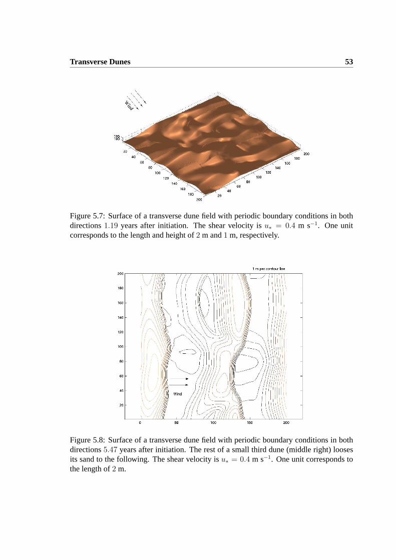
Transverse Dunes 53

Figure 5.7: Surface of a transverse dune field with periodic boundary conditions in bothdirections1.19 years after initiation. The shear velocity isu∗ = 0.4 m s−1. One unitcorresponds to the length and height of2 m and1 m, respectively.

Figure 5.8: Surface of a transverse dune field with periodic boundary conditions in bothdirections5.47 years after initiation. The rest of a small third dune (middle right) loosesits sand to the following. The shear velocity isu∗ = 0.4 m s−1. One unit corresponds tothe length of2 m.

54 5.2 The model of 3-dimensional dunes and translational invariance

Figure 5.9: Surface of a transverse dune field with periodic boundary conditions in bothdirections9.5 years after initiation. The system reached a state near to lateral invariance.The shear velocity isu∗ = 0.4 m s−1. One unit corresponds to the length of2 m.

Transverse Dunes 55

The conclusion from these calculations for 3-dimensional dunes can be that an open sys-tem of transverse sand dunes reaches lateral invariance supposing that there blows idealunidirectional wind. In the precedent simulations the periodic boundary constrained thesystem to break the invariance. A calculation with open boundary conditions in both hor-izontal directions which is closer to real dune fields would give more certainty about thisassumption but is rather complicated due to the fact that the dunes move out of the simu-lated area. More evidence is given in the following section. Assuming lateral invariancesimulations of fields of 2-dimensional dunes are much more effective. They consumemuch less computional time and give the opportunity to simulate larger dune fields. Inthe following two sections the models of 2-dimensional dunes are separated into a modelwith constant sand influx and periodic boundary, respectively. Both models lead to newinteresting conclusions.

5.3 The model of 2-dimensional dunes with constant sandinflux

The free parameters for this simulation are the sand influxqin and the shear velocityu∗.As initial surface suffices a plain ground filled with sand because the sand influx differs atleast a little bit from the saturation flux on the dune field. Thus dune formation is initiatedat the beginning of the dune field, i.e. where wind comes in.

5.3.1 Time evolution

The height profile of a dune field with a length of 4 km is presented at different times. Thesand influx is setqin = 0.017 kg m1s−1 and shear velocityu∗ = 0.5 m s−1. A sand influxqin which is not equal to the sand flux of saltation transport over a plain surface lowersor raises the starting points of the dune field constantly. This initiates a small oscillatorystructure which begins to move in wind direction (Figure 5.10). The initiating dunes atthe dune field inlet have increasing size in length and height with respect to the time. Itis assumed that the increasing difference between the starting points and the first crestleads to the creation of bigger dunes. With an increasing size the dunes have a lowervelocityvdune (Section 5.3.2). Hence, dune spacing, the distance between adjacent crests,increases with respect to time and no dune collides or converges with another. This factinvolves a new criterion that real dune fields can maintain a structure of lateral invariancewithout the effect of the breaking of symmetry as it was found in Section 5.2. Dune fieldswhere the sand influx stays rather constant in time can have a more regular structure thandune fields where the sand influx varies strongly with respect to time.

56 5.3 The model of 2-dimensional dunes with constant sand influx

Figure 5.10: Surface of an 2-dimensional simulation with constant sand influx after0.23years on the left figure and1.14 years on the right. The shear velocity isu∗ = 0.5 m s−1

and sand influxqin = 0.017 kg m−1s−1. On the left figure it is seen that initiation of duneformation began atx = 0. Dune height decreases with the distance to the dune field inlet.

Figure 5.11: Surface of an 2-dimensional simulation with constant sand influx after4.56years on the left figure and45.58 years on the right. The shear velocity isu∗ = 0.5 m s−1

and sand influxqin = 0.017 kg m−1s−1. On the left the first dune does not have a slipface. A final stationary surface is not reached. The evolution time of first dune of the rightfigure begins to build a slip face.

The slip face of the first dune is missing or is short due to the small time of evolution (Fig-ure 5.11). An observation of this absence for example at a coast where the sea provides acertain amount of sand supply was not found in literature. The simulation depicted hereand any other simulation of dune fields with lengths of 1 km to 4 km do not show that thesystem reaches a stationary state. According to Cooke, Warren, and Goudie (1993) dunefields with higher ages and less changes of climate comprise larger transverse dunes. Thesmaller slope at the brink found in this modeling agrees also with qualitative observa-tions. In the model a dune height of100 m is reached in roughly50 years. Estimates have

Transverse Dunes 57

found some10, 000 years to develop a100 m high dune. Probably this large differencecan be explained by the slower wind velocity, changes of wind direction for longer peri-ods, changes in sand supply and climate acting on real dunes. The so called memory (thetime to build a dune beginning with a plain sand bed) is related to the ratio of height ofthe dune and annual rate of sand movementH/Qann (Cooke, Warren, and Goudie 1993).The memory can vary by about four orders of time.

The results of the numerical calculations with different sand influxesqin at the same shearvelocities lead to the conclusion that there is a direct dependency between influx andheight growth of the first dune (Figure 5.12). The nearer the sand influx gets to the satu-ration flux of saltation transport the slower increases the height of the first dune. Hence,dune fields where the sand influx varies strongly in time around the saturation flux ofsaltation initiate first dunes with different heights fluctuating upwards and downwards.So there can be smaller dunes moving faster into the bigger and the symmetry breakingexplained in the Section 5.2 will occur. In the following some relations found for the time

Figure 5.12: The height of the first dune increases differently in time for different sandinflux qin. The shear velocity isu∗ = 0.5 ms−1. The saturation flux of a plain is about0.03 kg m−1s−1.

evolution of transverse dunes are presented. Figure 5.13 shows that the height versus timeincreases with a power law,

h(t) ∝√a · t, (5.1)

58 5.3 The model of 2-dimensional dunes with constant sand influx

Figure 5.13: Evolution of the height of the dunes counted beginning where the windcomes in. The shear velocity isu∗ = 0.4 m s−1 in the upper figure andu∗ = 0.5 m s−1 inthe lower figure. The height increases with the square root of time.

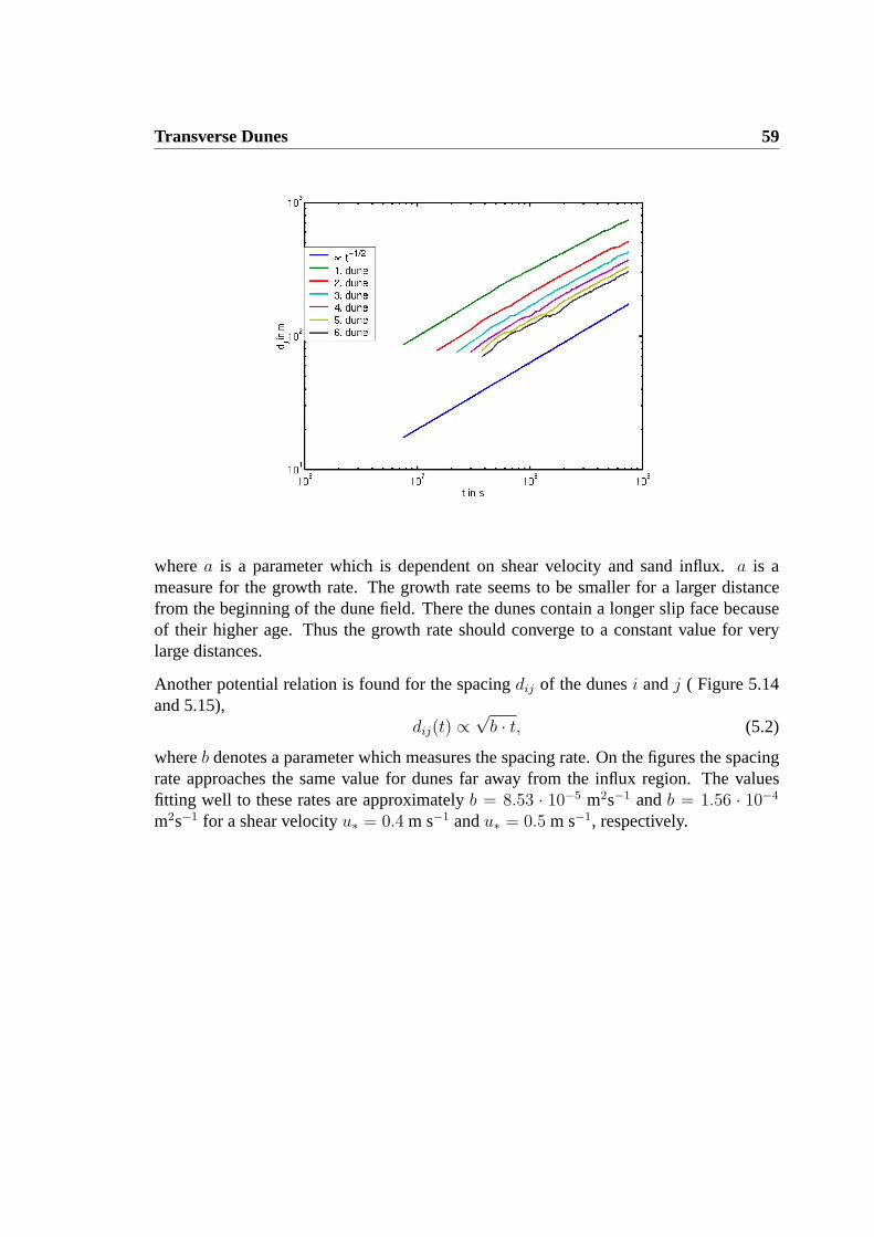
Transverse Dunes 59

wherea is a parameter which is dependent on shear velocity and sand influx.a is ameasure for the growth rate. The growth rate seems to be smaller for a larger distancefrom the beginning of the dune field. There the dunes contain a longer slip face becauseof their higher age. Thus the growth rate should converge to a constant value for verylarge distances.

Another potential relation is found for the spacingdij of the dunesi andj ( Figure 5.14and 5.15),

dij(t) ∝√b · t, (5.2)

whereb denotes a parameter which measures the spacing rate. On the figures the spacingrate approaches the same value for dunes far away from the influx region. The valuesfitting well to these rates are approximatelyb = 8.53 · 10−5 m2s−1 andb = 1.56 · 10−4

m2s−1 for a shear velocityu∗ = 0.4 m s−1 andu∗ = 0.5 m s−1, respectively.

60 5.3 The model of 2-dimensional dunes with constant sand influx

Figure 5.14: Evolution of the spacing between the dunes counted beginning where thewind comes in. The shear velocity isu∗ = 0.4 m s−1 in the upper figure andu∗ = 0.5 ms−1 in the lower figure . The spacing increases with the square root of time.

Figure 5.15: Comparing the evolution of the spacing for different shear velocities. Thespacing increases with the square root of time.

Transverse Dunes 61

5.3.2 Dune velocity

In the next chapter about barchan dunes also an examination on the dependency of thedune velocity of barchan dunes with respect to their height is made. The validity ofBagnold’s law ,

vdune =Φdune

h, (5.3)

whereΦdune is the bulk flux of sand blown over the brink has been shown by observationson real dunes. According to Sauermann (2001) a better fit is given by using instead ofthe heighth the characteristic length of a heap, i.e. the length of the envelope comprisingthe height profile and the separation bubble. Although Bagnold’s law already fits quitewell and still data from observations on real transverse dunes is absent, the Equation (5.3)is extended to a still simple relation. The length of the envelope can be expressed by afunction of the height. The function is developed into a Taylor series and higher ordersthan the linear order are neglected. This finally yields,

vdune =Φdune

h+ C, (5.4)

whereC denotes a constant. Figure 5.16 shows that the simulation data follows ratherwell the Equation 5.3. The fluctuations of the dune velocity can be explained with theinfluence of the system length. On Figure 5.17 the dune velocities with respect to theheight and their fits tp formula (5.4) are compared for the shear velocitiesu∗ = 0.4m s−1 andu∗ = 0.5 m s−1. The observed bulk fluxes areΦdune = 454.5 m2s−1 andΦdune = 833.3 m2s−1 with the corresponding constantsC = 0.45 m andC = 1.08m, respectively. These results are smaller than the bulk fluxes of isolated 2-dimensionaldunes calculated by Sauermann (2001) on plain ground without sand. Thus the velocitiesalso are smaller than those observed for isolated transverse dunes on plain ground withoutsand. Lancaster (1985) found less speed-up of the wind velocity over continuous sanddunes than over isolated transverse dunes. This agrees with the results in this model.

62 5.3 The model of 2-dimensional dunes with constant sand influx

Figure 5.16: Velocity of the dunes versus height. Counting begins on the left where thewind comes in. The shear velocity isu∗ = 0.4 m s−1 in the upper figure andu∗ = 0.5 ms−1 in the lower figure.

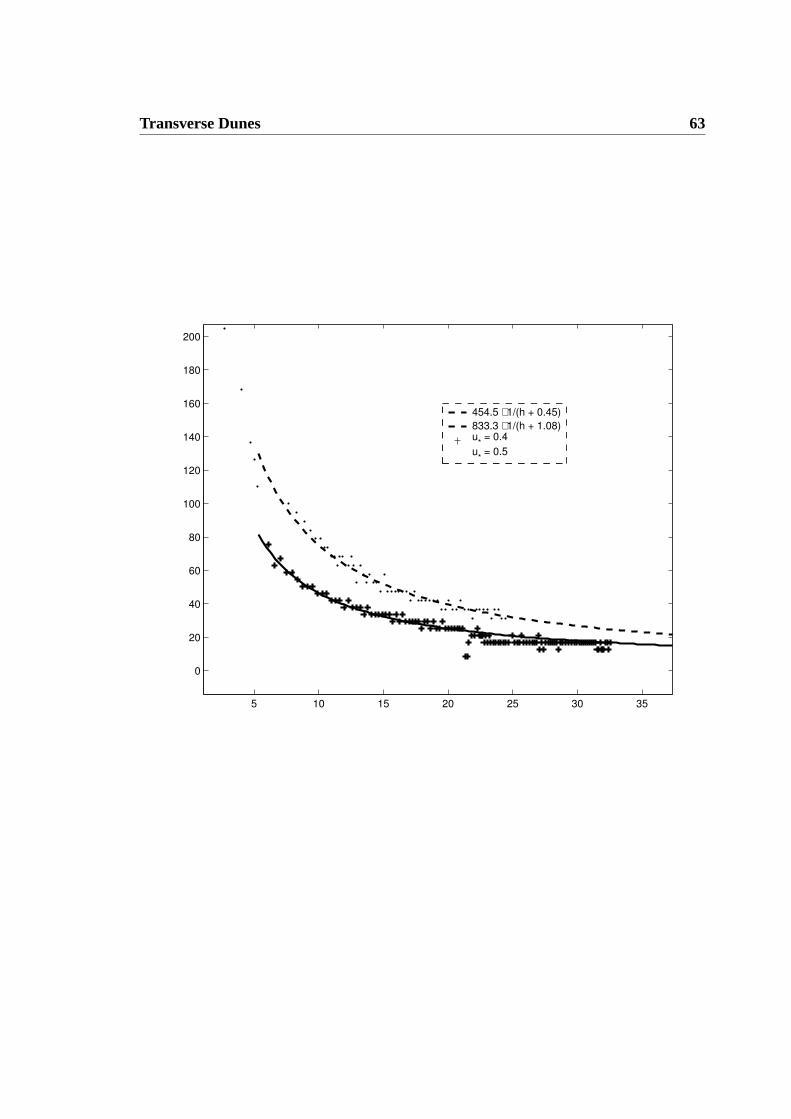
Transverse Dunes 63

5 10 15 20 25 30 35

0

20

40

60

80

100

120

140

160

180

200

h [m]

v dune

[m/y

ear]

454.5 ⋅ 1/(h + 0.45)833.3 ⋅ 1/(h + 1.08)u

* = 0.4

u* = 0.5

Figure 5.17: Comparation of dune velocityvdune versus heighth for the shear stressesu∗ = 0.4 m s−1 andu∗ = 0.5 m s−1. The velocity decreases proportional to the reciprocalheight.

64 5.4 The model of 2-dimensional dunes with periodic boundary

5.4 The model of 2-dimensional dunes with periodicboundary

The simulations in this section have a periodic boundary in wind direction. So the param-eter of sand influx that was used additionally before is no more available. Sand influx isset equal to the outflux. The avalanches flow down even if the slip face is divided throughthe boundary. Also the separation bubble enters in the boundary inlet. The calculationsare made with dune fields of a length of two kilometers. The ground is completely filledup with sand. The initial surface are small Gaussian hills which disturb the plain surface.

5.4.1 Time evolution

There is found a situation similar to the simulations of 3-dimensional transverse dunefields. In the beginning many dunes of different size grow in the system which beginto converge and approach same heights. As in the 3-dimensional case the dunes keepgrowing so that the number of dunes has to decrease. A more detailed description ofthe process of merging dunes is given in the following section. The periodic boundaryforces a decrease of the number of dunes and this process makes time dependent behaviorrather complex. Thus the potential growths described in Section 5.3.1 are disturbed anddecelerated for each merging of two dunes. Figures 5.18, 5.19 and 5.20 show the heightprofile of a dune field of a length of two kilometers at three time steps. Figure 5.18 depictsa surface with dunes of different dunes which seem to interact strongly with each other.The apparently stable state of the system on Figure 5.19 is disturbed in Figure 5.20. Thenumber of dunes decreases quite regularly versus time. This process is very slow and thedunes grow much slower than in the model with open boundary.

5.4.2 Do transversal dunes behave like solitons?

Besler (1997) proposed that barchan dunes behave like solitons. Solitons are self-stabilizing wave packs which do not change their shape during their propagation evennot after collision with other waves. They are found in non-linear systems like for ex-ample in hydrodynamics. Observations of barchan dunes showed that small dunes canmigrate over bigger ones without being absorbed completely. A closer examination ofthe merging of two or more dunes from calculations of a 2-dimensional dune field withperiodic boundary led to some interesting observations. In this case the dune field can-not break its lateral scale invariance to reach a faster colliding of two adjacent dunes.Thus the supposition would be that a smaller dune due to its higher velocity collides withthe next bigger one in wind direction without passing over it. That is not the case. Asan example see the Figures 5.21, 5.22 and 5.23. A small dune climbs up the windward

Transverse Dunes 65

Figure 5.18: Surface of a dune field with a length of two kilometers. The shear velocityis u∗ = 0.45 m s−1 after31.7 years, the boundary conditions are periodic. The structureis quite irregular.

side of the following bigger dune. As it reaches the same height as the following one itseems to hand over the state of being the smaller dune. The dune that was bigger beforebreaks its slip face and wanders towards the next bigger dune downwards. So also for2-dimensional modeling the slip face disappears in this transition state. This process canbe observed several times. Only the fact that the volume of the smaller dune decreasesafter every pass-over lets conclude that there will be a final dune which is absorbing thesmall one. Hence, these dunes do not behave exactly like solitons because of their lossof volume. Also the suggestion of Wilson (1972) that dunes of different hierarchies (forexample dunes and mega dunes) would not grow into the bigger hierarchy is not valid inthis case. Nevertheless the fact that small dunes can migrate over other leads to the con-clusion that different hierarchies of dune sizes can exist in a field of transverse dunes. Theloss of volume demonstrates the interaction between different hierarchies of dune sizes.

Finally Figures 5.24, 5.25 and 5.26 show a part of the same simulation where a very smalldune finally converges into the bigger one and the number of dunes decreases by one.

66 5.4 The model of 2-dimensional dunes with periodic boundary

Figure 5.19: Surface of a dune field with a length of two kilometers. The shear velocityis u∗ = 0.45m s−1 after95.1 years, the boundary conditions are periodic. There are threedunes left with similar heights.

Figure 5.20: Surface of a dune field with a length of two kilometers. The shear velocityis u∗ = 0.45 m s−1 after190.2 years, the boundary conditions are periodic. The numberof dunes will decrease by one after coalescence of two dunes.

Transverse Dunes 67

Figure 5.21: Wandering of a small dune over a big one. Part of a simulation of a transversedune field with a length of 2km. The shear velocity isu∗ = 0.5m s−1 and boundaryconditions are periodic. The first step is that a small dune begins to climb over a biggerone.

Figure 5.22: Wandering of a small dune over a big one. Part of a simulation of a transversedune field with a length of 2km. The shear velocity isu∗ = 0.5m s−1 and boundaryconditions are periodic. The second step is that the small dune reaches the top of thebigger one and hands over to the before bigger one.

Figure 5.23: Wandering of a small dune over a big one. Part of a simulation of a transversedune field with a length of 2km. The shear velocity isu∗ = 0.5m s−1 and boundaryconditions are periodic. The last step is that the faster moving small dune passed thebigger dune.

68 5.4 The model of 2-dimensional dunes with periodic boundary

Figure 5.24: Coalescence of small dune in a big one. Part of a simulation of a transversedune field with a length of 2km. The shear velocity isu∗ = 0.5ms−1 and boundaryconditions are periodic. Here a very small dune reaches the windward side of a big one

Figure 5.25: Coalescence of small dune in a big one. Part of a simulation of a transversedune field with a length of 2km. The shear velocity isu∗ = 0.5ms−1 and boundaryconditions are periodic. Here a very small dune begins to climb over the next one

Figure 5.26: Coalescence of small dune in a big one. Part of a simulation of a transversedune field with a length of 2km. The shear velocity isu∗ = 0.5ms−1 and boundaryconditions are periodic. Here the very small dune converges into the next dune

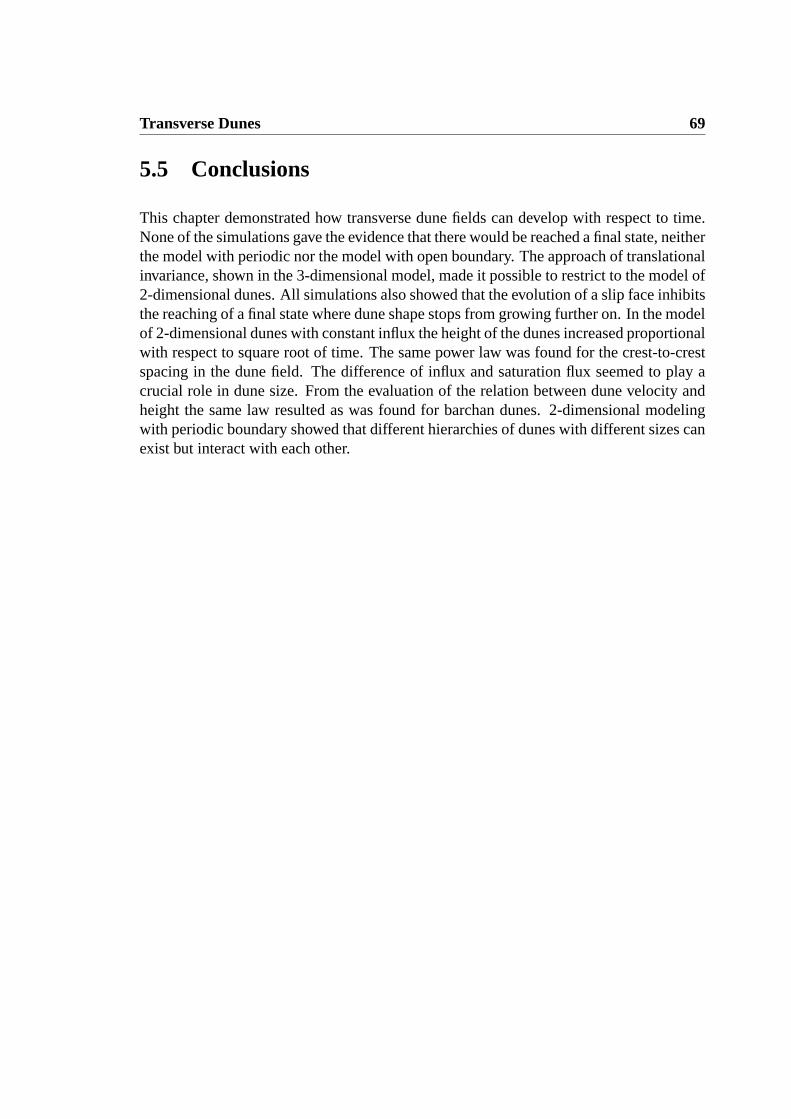
Transverse Dunes 69

5.5 Conclusions

This chapter demonstrated how transverse dune fields can develop with respect to time.None of the simulations gave the evidence that there would be reached a final state, neitherthe model with periodic nor the model with open boundary. The approach of translationalinvariance, shown in the 3-dimensional model, made it possible to restrict to the model of2-dimensional dunes. All simulations also showed that the evolution of a slip face inhibitsthe reaching of a final state where dune shape stops from growing further on. In the modelof 2-dimensional dunes with constant influx the height of the dunes increased proportionalwith respect to square root of time. The same power law was found for the crest-to-crestspacing in the dune field. The difference of influx and saturation flux seemed to play acrucial role in dune size. From the evaluation of the relation between dune velocity andheight the same law resulted as was found for barchan dunes. 2-dimensional modelingwith periodic boundary showed that different hierarchies of dunes with different sizes canexist but interact with each other.

70 5.5 Conclusions

Chapter 6

Barchan dunes

In this chapter a small introduction will explain some aspects concerning barchan dunes.The results of the model for different values of the roughness length and the fixed dunelength implemented in the shear stress calculation will be fitted to experimental data. Inthe following section scaling relations calculated with the model will be presented andcompared to measurements. The difference between the model results and real duneshapes for small barchan dunes will lead to an inclusion of diffusion in the saltation trans-port calculation. The last section will be about barchanoids.

6.1 Introduction

The wordbarchancomes from the turkic language and means “active dune”. It waspreserved to name this type of dune. Less than 1% of all dune sand on Earth is containedin barchan dunes. Barchan dunes are dunes which exist mainly in areas where not verymuch sand is available and wind stays unidirectional.

The size of barchans varies from heights of some meters (Figure 6.1) to over 50 m (Fig-ure 6.2). Barchan dunes are not shape invariant. There is a minimal height of 1-2 meterswhere the sand heap looses its sand and no stable shape is reached. Dune shapes seemto be controlled by the saturation length of the saltation transport on the windward side(Sauermann, Kroy, and Herrmann (2001b) and Chapter 3). This denotes the length of thesurface to reach the saturated sand flux over a sand sheet. The saturation length, not to bemistaken for the saltation length (mean length of the grain trajectory in air), has a complexdependency on the air shear stress. Low sand densities in the saltation layer over a groundwithout sand bed or in the separation bubble lead to a saltation transient at the place wherethe surface begins to be filled up with sand or where the shear stress exceeding the shearstress threshold begins to entrain grains into air, respectively.

71

72 6.2 The role of roughness length and dune size

Small stable barchan dunes have a short slip face and the crest does not coincide with thebrink. Whereas the sand is trapped completely in the slip face the lack of a slip face at thehorns lets the sand grains leave the dune from them. Thus a barchan dune grows if sandinflux is larger than outflux and vice versa. In the simulations the influx is set to be equalto the outflux. The total outflux is calculated and an averaged influx of the same volumeis blown into the modeled area. This boundary is called quasi–periodic here. Mostly aGaussian hill is taken as initial surface. The initial situation of dune generation still isnot known very well. Hence, in the simulations only the final results are analyzed, that iswhen the system reached the final steady state. A steady state means that the dune shapedoes not undergo temporal changes.

6.2 The role of roughness length and dune size

Two crucial parameters affect the calculation of the shear stress perturbation (Chapter 2).The roughness lengthz0 describes the roughness of the surface (cf. Chapter 1) here givenby the height of the saltation layer.L is the length between the half heights of a hill forwhich the shear stress perturbation is calculated. In the case of dunes where shear stressperturbation is calculated over the envelope of the dune composed by the dune profile andthe separation bubble, the value ofL should be close to the length between the half heightsof the envelope. The aim in this section is to get applicable values of these parameterswhich do not have to be changed for every new calculation. The implementation of thelengthL as the real length between half heights of the dune calculated by the model forevery iteration could cause recursive effects and complicate the understanding of duneformation.

The parameters are included only by the ratioz0/L in Equation (4.1) and (4.2) of theshear stress perturbation except for the logarithmic term2 ln (L|kx|). The results of adune model started with the same initial surface and a shear velocity ofu∗ = 0.5 ms−1

is used to estimate the optimal configuration. The results of calculations with the sameratioz0/L are depicted in Figure 6.3 and 6.4. For the results of different ratios at constantL = 10 see Figure 6.5. An increase ofL at constantz0/L leads to an increase of theshear stress perturbation at large wave lengths in the wind direction. By this the surfaceis flattened and the length of the dune increases. Thus the logarithmic term2 ln (L|kx|)cannot be neglected as it was done by Sauermann (2001). A higher ratioz0/L at constantL decreases the termln (l/z0) which then causes a more asymmetric shear stress distri-bution over the dune and thus a higher slope of the brink. In Table 6.1 the heighth,the widthw and the lengthl of the final shapes are shown with respect to the differentparametersz0 andL. In order to obtain the best fitting parameters the linear regressionsin Equation (6.1) of width height and length height relationship of dune measurements in

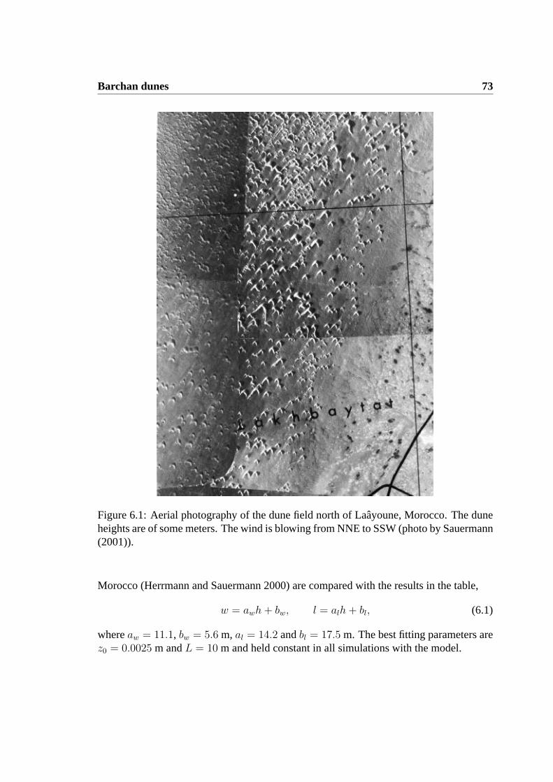
Barchan dunes 73

Figure 6.1: Aerial photography of the dune field north of Laayoune, Morocco. The duneheights are of some meters. The wind is blowing from NNE to SSW (photo by Sauermann(2001)).

Morocco (Herrmann and Sauermann 2000) are compared with the results in the table,

w = awh+ bw, l = alh+ bl, (6.1)

whereaw = 11.1, bw = 5.6 m, al = 14.2 andbl = 17.5 m. The best fitting parameters arez0 = 0.0025 m andL = 10 m and held constant in all simulations with the model.

74 6.2 The role of roughness length and dune size

Figure 6.2: Aerial photography of the dune field of Jericoacoara near Fortaleza, Brazil.Some dunes that are over 50 meters high can be found in this dune field. Photo by Sauer-mann (2001).

Figure 6.3: Calculation of dunes with the same initial surface and the ratioz0/L = 2.5 ∗10−5. On the left sidez0 = 0.00025 m andL = 10 m whereas on the right sidez0 =0.0025 m andL = 100 m.

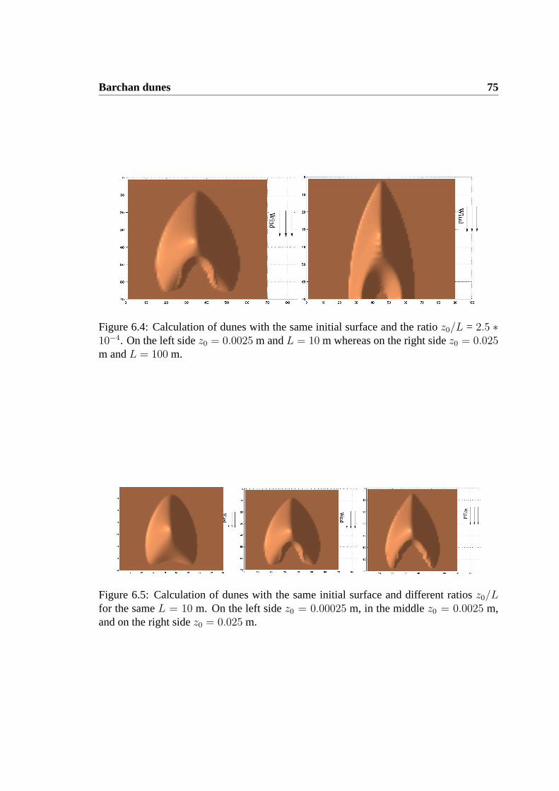
Barchan dunes 75

Figure 6.4: Calculation of dunes with the same initial surface and the ratioz0/L = 2.5 ∗10−4. On the left sidez0 = 0.0025 m andL = 10 m whereas on the right sidez0 = 0.025m andL = 100 m.

Figure 6.5: Calculation of dunes with the same initial surface and different ratiosz0/Lfor the sameL = 10 m. On the left sidez0 = 0.00025 m, in the middlez0 = 0.0025 m,and on the right sidez0 = 0.025 m.

76 6.2 The role of roughness length and dune size

Table 6.1: Heighth, widthw and lengthl of the final state with respect toz0 andL. Belowthe results are compared with the values ofl andw which are obtained by insertingh inEquation (6.1).

z0 = 2.5 · 10−2 mh w l

w = awh+ bw l = alh+ bl

L = 10 m 4.72 m 60.3 m 92 m57.99 m 84.5 m

L = 25 m 4.0 m 57.5 m 100 m50.0 m 74.3 m

L = 100 3.6 m 57.5 m > 100 m

z0 = 2.5 · 10−3 mh w l

L = 10 m 4.75 m 60.2 m 85 m58.33 m 84.95 m

L = 25 m 3.5 m 63.0 m > 100 m44.45 m 67.2 m

L = 100 m 3.2 m 63.4 m > 100 m

z0 = 2.5 · 10−4 mh w l

L = 10 m 3.95 m 63.5 m 85 m49.45 m 73.59 m

L = 25 m 3.0 m 71.0 m > 100 m38.9 m 60.1 m

L = 100 m 1.0 m > 135 m > 100 m

Barchan dunes 77

6.3 Scaling laws

In this section the morphologic relationships between heighth, width w, length l andvelocity vd of barchan dunes resulting of the simulations are presented. The shapes arecompared for different dune sizes. Therefore calculations of dunes which have differentsizes were performed for the shear velocitiesu∗ = 0.4 ms−1, u∗ = 0.45 ms−1 andu∗ =0.5 ms−1. The single isolated barchan dunes are modeled with a quasi-periodic boundaryuntil the final steady shape is reached.

Height, width and length relationships: Linear relationships between height, widthand length were observed by Finkel (1959), Hesp and Hastings (1998) for barchans insouthern Peru and by Herrmann and Sauermann (2000) in Morocco (also cf. Equa-tion (6.1)). Figures 6.6 and 6.7 depict the height width and the height length relationshipsfor different shear velocities, respectively. They are compared to the data of Herrmannand Sauermann (2000). The data of the barchans of Morocco fits best to the simulationsresults for a shear velocityu∗ = 0.5 ms−1. Hence, the determination of the parametersz0

andL for one dune of one size leads to reasonable results also for other sizes.

A linear relationship is obtained for bigger dunes. The linearity is valid only for lengthscales larger than the saturation length (l � ls). The functional dependence of the sat-uration length on the shear velocity predicts well the flatter shapes for decreasing shearvelocities. Sauermann, Kroy, and Herrmann (2001b) found an increase ofls at the shearvelocity threshold for saltation transport.

Dune velocity: In Chapter 5 the evaluation of the velocity of 2-dimensional transversedunes in a dune field showed that the dune velocity decreases inversely proportional tothe height plus a constanth + C. According to Sauermann (2001) the dune velocitydecreases inversely proportional to the length of the envelope of the surface formed bythe height profile and the separation bubble. The separation bubble of the barchans in thedune model described here fills almost exactly the region between the horns so that theoverall lengthl of the dune can be used in order to evaluate the simulation results. ThusBagnold’s law has to be modified,

vd =Φdune

l(6.2)

whereΦdune is determined for different shear velocities. The relation between dune ve-locity and height revealed the same deviations from the Bagnold’s law for small duneslike in the case of the height length relationship. Figure 6.8 depicts the dune velocityvd versus dune lengthl. The surprising result is that the dune velocity does not differfrom Equation 6.2 even for small dune sizes and so the saturation length seems to have noinfluence on the dune velocity.

78 6.3 Scaling laws

20

30

40

50

60

70

80

90

100

1 2 3 4 5 6 7 8 9

w[m

]

h [m]

PS

fragreplacem

ents

u∗ = 0.4ms−1

u∗ = 0.45ms−1

u∗ = 0.5ms−1

Morocco

Figure 6.6: Height width relation of dunes in Morocco (crosses) and the results of numer-ical calculations for different shear velocities.

40

50

60

70

80

90

100

110

120

130

140

1 2 3 4 5 6 7 8 9

l [m

]

h [m]

Morocco

PS

fragreplacem

ents

u∗ = 0.4ms−1

u∗ = 0.45ms−1

u∗ = 0.5ms−1

Figure 6.7: Height length relation of dunes in Morocco (crosses) and the results of nu-merical calculations for different shear velocities.

The shape: Barchans are not shape invariant due to the important role of the saturationlength of the saltation transport. Nevertheless the shapes of barchans with different sizes

Barchan dunes 79

Figure 6.8: The velocityvd of barchans fits very well to their reciprocal length. Note: Thevelocity is calculated for 365 days of wind per year and is thus smaller in real conditions.

are compared in order to obtain more information about the deviation from shape invari-ance. Herrmann and Sauermann (2000) fitted the normalized cross profile of the measureddunes with a parabola (Figure 6.10) and Sauermann (2001) found a good agreement ofthe normalized cross profile of his numerical calculations without lateral shear stress to aparabola. Therefore the axes are rescaled and dimensionless variables are introduced,

x =1

lx y =

1

wy z =

1

hz. (6.3)

Figure 6.9 shows the normalized cross profiles fitted with a parabola. The upper part ofthe profile fits quite well whereas the lower part is far away from a parabola. The situationis similar to Figure 6.10. So is there a better fit with another function? Figures 6.11 and6.12 indicate that asin2–function fits quite well, even for the longitudinal profile. Thusthe inclusion of lateral shear stress in the model leads to a change from a parabolic to asin2–profile. In Figure 6.12 the slope at brink decreases for bigger dunes. Finally theshapes of a45 and a5 meter high dune are compared in Figure 6.13. The slip face ofbigger dunes cuts a larger piece from the dune nucleus.

Figure 6.13 shows a sharp edge of the beginning of the windward side not observed in theresults of the dune model of Sauermann (2001). The inclusion of the lateral component inthe shear stress calculation leads to this characteristics. This edge has not been observedfor small dunes, for example in Morocco. But the big dunes in Figure 6.2 show a very

80 6.3 Scaling laws

Figure 6.9: The calculated cross profiles of the dunes are normalized. A parabolic func-tion does not fit very well like in the calculations with only one component of the shearstress.

similar shape. That is also the reason why this computionally very expensive calculationof a 45 meter high dune has been carried out. Exact measurements of the shape of abig barchan would reveal more information and probably validate the model results. Itis assumed that the absence of the edge for small dunes can be explained by diffusioneffects of the saltation transport. Diffusion which in the simulations depicted so far hasnot been regarded works on small scales and for larger scales the influence of diffusion onthe dune shape should disappear. In the next section the results of the model are comparedfor different diffusion constants.

Barchan dunes 81

−1.5 −1 −0.5 0 0.5 1 1.50

0.1

0.2

0.3

0.4

0.5

0.6

0.7

0.8

0.9

1

PSfrag replacements

normalized widthy

norm

aliz

edhe

ightz

Figure 6.10: Cross profile of the dunes measured in Morocco. They are fitted with aparabola (Figure from Herrmann and Sauermann (2000)).

Figure 6.11: The cross profiles of the dunes are normalized. A fit withsin2(x) fits quitewell.

82 6.3 Scaling laws

Figure 6.12: The longitudinal profiles of the dunes are normalized. A fit withsin2(x) fitsquite well at the windward side. The different shapes demonstrate the shape invariance ofbarchan dunes.

Figure 6.13: On the left side the surface of a45 m high barchan dune is depicted. Thedune on the right side has a height of5 m. There is no shape invariance.

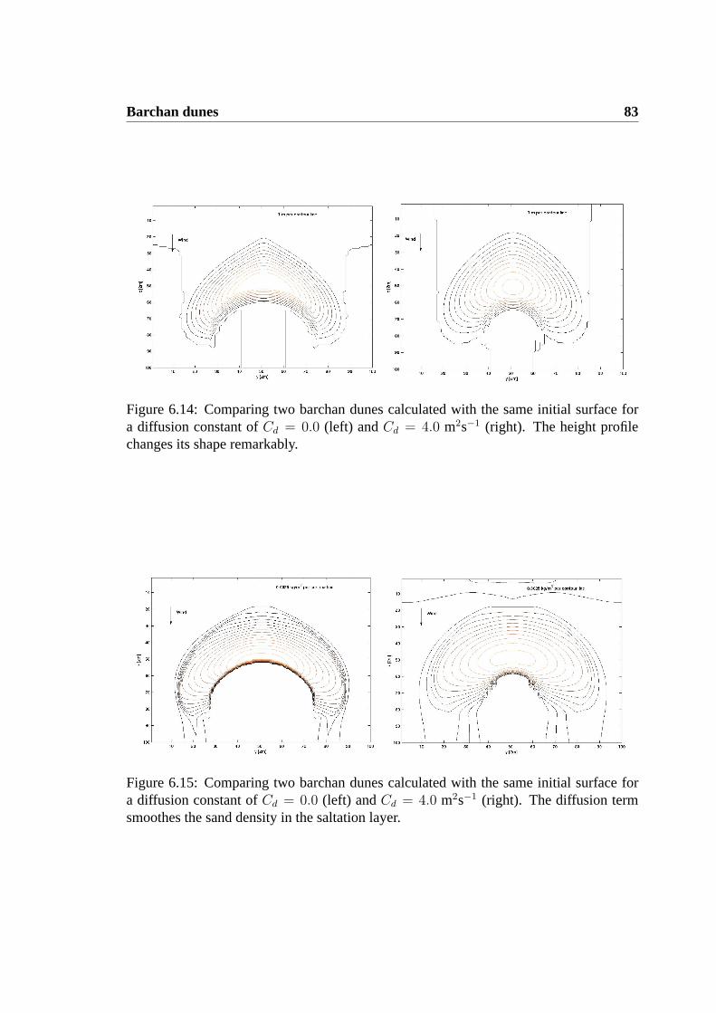
Barchan dunes 83

Figure 6.14: Comparing two barchan dunes calculated with the same initial surface fora diffusion constant ofCd = 0.0 (left) andCd = 4.0 m2s−1 (right). The height profilechanges its shape remarkably.

Figure 6.15: Comparing two barchan dunes calculated with the same initial surface fora diffusion constant ofCd = 0.0 (left) andCd = 4.0 m2s−1 (right). The diffusion termsmoothes the sand density in the saltation layer.

84 6.4 The effect of diffusion

6.4 The effect of diffusion

The dune model including the lateral component of the shear stress revealed a charac-teristic shape with a quite sharp edge of the windward side which is not found for smallbarchan dunes for example in Morocco. To understand more of this inconsistency somecalculations of the same barchan dune of about 12 meters height are made with differentdiffusion constantsCd. It can be assumed that for larger dunes and therefore larger lengthscales the effect of diffusion transport gets negligible and the final state calculated by thedune model without diffusion matches real dune shapes.

The results in this section can be discussed only qualitatively due to the fact that thediffusion constant is still unknown. The diffusion term was added to the equation of thesand density in the saltation layer (Chapter 3). Figures 6.14 and 6.15 show the contourlines of the height profile and the sand density in the saltation layer respectively. Veryhigh diffusion constants like that one determining the results of these figures show thatthe sharp edge of the shape of the windward side is smoothed. The sand density in thesaltation layer is flattened out as can be expected from diffusion processes. After the brinkthe sand density drops to zero due to the vanishing shear stress. The contour lines changetheir shape remarkably at the beginning of the windward side. Hence, these results canlead to the assumption that diffusion processes play a crucial role for small dunes wherethe characteristic edge has not been observed. An estimation of the diffusion constant andexact measurements of the height profiles of small and large barchans could give moreinsight into the influence of diffusion on the morphology of barchan dunes in the future.Further simulations with the dune model in order to compare the effect of diffusion forbarchan dunes of different sizes have to be executed.

Figures 6.16 and 6.17 depict a longitudinal and transversal cut of the barchan dune fordifferent diffusion constants. The height and the slope at the brink decrease for a higherdiffusion. The length of the barchans increases for a larger diffusion constant whereas thewidth stays constant. Thus the knowledge ofCd would help in order to determine bettervalues forz0 andL (Section 6.2) by fitting them to simulation results from a model withdiffusion. The other possibility to obtain these values would be to perform the simulationfor higher barchans. But the enormous computional costs and the missing measurementsof big barchans (there do not exist many big barchans) make the realization still not rea-sonable.

6.5 Barchanoids, between barchan and transverse dunes

Where an area does not contain sufficient sand to form transverse dunes and where toomuch sand is available to keep the barchans isolated the barchan dunes are connected and

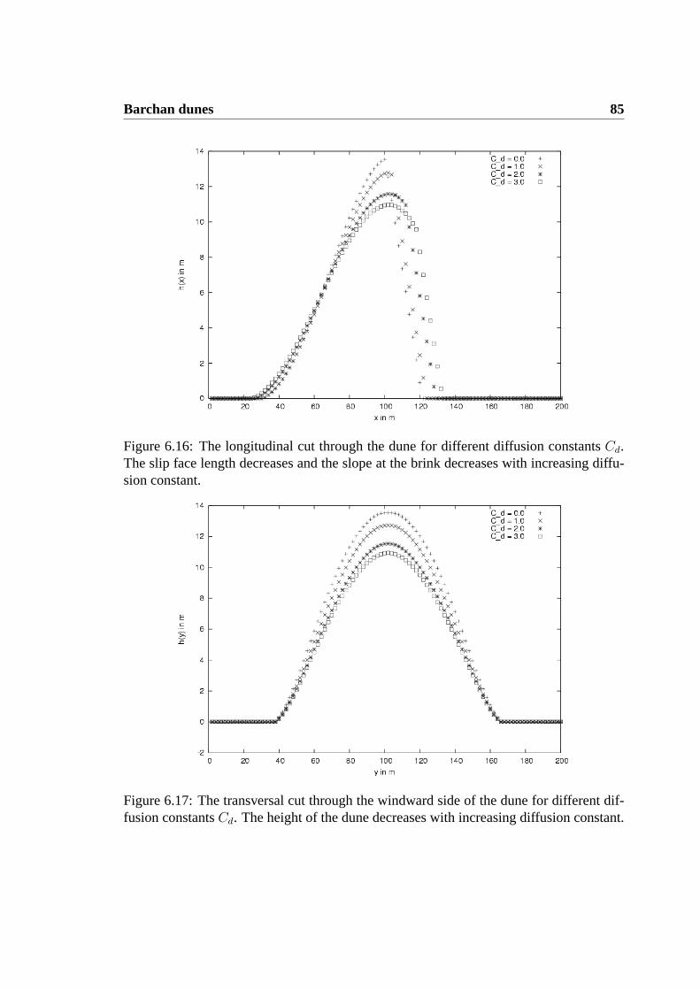
Barchan dunes 85

Figure 6.16: The longitudinal cut through the dune for different diffusion constantsCd.The slip face length decreases and the slope at the brink decreases with increasing diffu-sion constant.

Figure 6.17: The transversal cut through the windward side of the dune for different dif-fusion constantsCd. The height of the dune decreases with increasing diffusion constant.

86 6.5 Barchanoids, between barchan and transverse dunes

Figure 6.18: A simulation with quasi-periodic boundary conditions. There is too muchsand to build single barchans. The barchans are connected in the longitudinal and lateraldirection.

interesting hybrid forms appear, the so called barchanoids. The barchan dunes can beconnected longitudinally and transversally.

Here only the qualitative results are of interest in order to show the further abilities of thedune model. The simulation with the dune model is performed with a perturbed initialsurface of an averaged sand height of three meters. The boundary conditions are quasiperiodic in wind direction and open in the lateral direction. The volume of sand in thesimulation is held constant. Figures 6.18 and 6.19 show two states of the simulation. Inthe first figure the barchans are connected longitudinally and transversally. The barchansare growing so that the sand accumulates in one row of bigger dunes which are connectedlaterally. Similar barchanoids can be found for example in the dune field of LencoisMaranhenses in Brazil where the dunes are separated by lagoons filled with rainwater(Figure 6.20). In this dune field the barchan dunes are connected in the wind and thelateral direction.

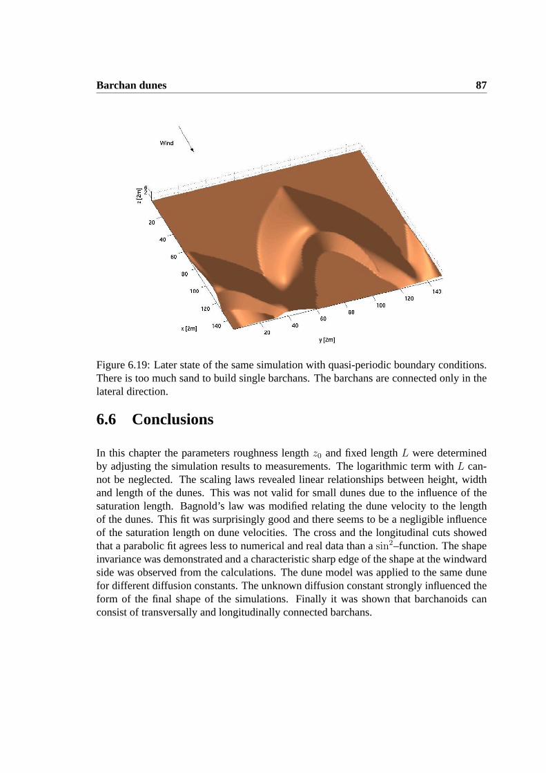
Barchan dunes 87

Figure 6.19: Later state of the same simulation with quasi-periodic boundary conditions.There is too much sand to build single barchans. The barchans are connected only in thelateral direction.

6.6 Conclusions

In this chapter the parameters roughness lengthz0 and fixed lengthL were determinedby adjusting the simulation results to measurements. The logarithmic term withL can-not be neglected. The scaling laws revealed linear relationships between height, widthand length of the dunes. This was not valid for small dunes due to the influence of thesaturation length. Bagnold’s law was modified relating the dune velocity to the lengthof the dunes. This fit was surprisingly good and there seems to be a negligible influenceof the saturation length on dune velocities. The cross and the longitudinal cuts showedthat a parabolic fit agrees less to numerical and real data than asin2–function. The shapeinvariance was demonstrated and a characteristic sharp edge of the shape at the windwardside was observed from the calculations. The dune model was applied to the same dunefor different diffusion constants. The unknown diffusion constant strongly influenced theform of the final shape of the simulations. Finally it was shown that barchanoids canconsist of transversally and longitudinally connected barchans.

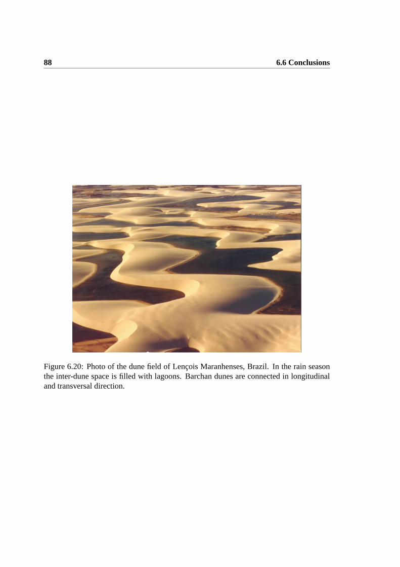
88 6.6 Conclusions

Figure 6.20: Photo of the dune field of Lencois Maranhenses, Brazil. In the rain seasonthe inter-dune space is filled with lagoons. Barchan dunes are connected in longitudinaland transversal direction.

Chapter 7

Conclusion

In this thesis the dune model of Sauermann (2001) has been extended and it has beenmade applicable to other dune types. In the theoretical part new terms have been added tocomplete the equations of the calculation of the dynamics acting on a dune. The relationsof the model are based on analytical and phenomenological theory. The simulations havebeen performed in order to model barchan and transverse dunes as well as dune fields.Interesting relations have been found for the time evolution and the scaling of the sanddunes. Surprising details of the dune shape have led to further assumptions.

Theory

The dune model contains three different physical processes: the global shear stress per-turbation over the dune surface, a continuum model to calculate the sand flux over a sanddune and a model for the avalanches that maintains the sand transport due to gravity on theslip face. The characteristic time scales of these processes differ over more than seven or-ders of magnitude. Thus the physical processes have been regarded to be in the stationarystate.

The air flow in the atmospheric boundary layer onto a sand dune is fully turbulent. Afterthe brink the flow is separated and a large eddy is situated determining the shear stress tobe less than the saltation threshold in this area. The calculation of the shear stress ontoa dune by averaged Navier-Stokes equations has been too time consuming. The analyt-ical solutions of the air shear stress over a gentle hill (Weng, Hunt, Carruthers, Warren,Wiggs, Livingstone, and Castro 1991) have been applied to obtain a fast algorithm in or-der to predict the time evolution of sand dunes . These algorithms cannot deal with flowseparation, but Zeman and Jensen (1988) and Sauermann (2001) introduced the conceptof the separation bubble which assures a smooth surface and thus the fast algorithm can

89

90

be applied. The determination of the separation bubble has been extended to the case of aarbitrary sand bed in order to attach it to the area between transverse dunes.

A phenomenological continuum saltation model which determines the sand flux of salta-tion transport onto a dune was derived by Kroy, Sauermann, and Herrmann (2001). Mi-croscopical models, which regard the sand grains not as a continuum, would have beencomputationally too time expensive. The advantage of this model consists in the inclusionof the saturation transients which play a crucial role in dune dynamics. The phenomeno-logical relations by Bagnold (1936), Owen (1964), Lettau and Lettau (1978) and Sørensen(1991) do not regard transients. The characteristic length scale called “saturation length”with its complex dependence on shear stress determines the shape difference betweensmall and large dunes. There are two equations for the density and the velocity of thesand in the saltation layer. They have been extended by the addition of a diffusion term tothe sand density equation.

In every iteration of the whole dune model the air shear stress, the saltation sand flux andthe avalanches have been calculated in order to determine the time evolution of the dunesurface. The 3-dimensional extension of the model of Bouchaud, Cates, Ravi Prakash,and Edwards (1994) has been applied to model the avalanches. Various types of initialsurfaces have been implemented. The parameters shear velocity, sand influx and sandheight have led to simulations with various final states or transients according to differentboundary conditions.

Results

The simulations have been carried out for transverse and barchan dunes formed by uni-directional wind sources. The time evolution of 3-dimensional transverse dune fieldshave been calculated. Ideal transverse dunes seem to be translationally invariant. Due tothe steady increase in the height of the dunes and the spacing between them, the periodicboundary conditions in these simulations have broken the invariance in order to acceleratethe process that two dunes converge. No final state representing a dune field moving with-out changing its shape has been found. The simulation of a 2-dimensional dune field withconstant sand influx has confirmed that dunes do not stop growing with respect to time.A surprising similarity of the dune field shape to sine functions has been observed. Theinflux controls the growth and leads to the creation of permanently higher initial dunes.Thus no converging could be observed in these simulations. Scaling laws for the growthof the height versus time, the spacing versus time and the dune velocity versus heighthave been found. The dune velocity scales with the reciprocal length as in the case ofbarchan dunes. Nevertheless, the dune velocity is smaller than the one of barchan dunesdue to the steadily changing shape of transverse dunes. Similar results have been revealedfor the modeling of a 2-dimensional dune field with periodic boundary conditions andfor a 3-dimensional dune field. The number of dunes in the field decreases with time. A

Conclusion 91

complex behavior has been observed for the converging process which is different to the3-dimensional case due to enforced translational invariance. Small dunes pass over biggerones, but the behavior has been found out to be different from that of solitons as proposedby Besler (1997).

In order to obtain reasonable results on barchan dune simulations the two parametersroughness lengthz0 and length of the duneL have been adjusted to the field measurementsof Sauermann, Rognon, Poliakov, and Herrmann (2000) in Morocco. These parametersplay an important role to determine an accurate dune shape. The scaling laws of barchandunes have been calculated from the simulation results. Linear height width as well asheight length relationships have been presented. They agree quite well with the resultsof the numerical simulations of Sauermann (2001) and measurements. The evaluationof the relationship between dune velocity and length has revealed that Bagnold’s lawfits much better if the height is substituted by the length. The new law is valid evenfor small dunes. Normalized cuts in the longitudinal and lateral direction have shown thatbarchan dunes are not shape invariant and that the cross section fits quite well with asin2–function in both directions. Comparing the resulting final shape of the barchans to theresults of Sauermann (2001) who calculated the dunes with a shear stress restricted to thecomponent in wind direction, a characteristic edge at the beginning of the windward sidehas been observed. The lack of this edge for small dunes can be explained by the diffusionof the sand in the saltation layer. Calculations with different diffusion constants haveagreed on the assumption that the edge would disappear as soon as diffusion is switchedon. Finally the shape of barchanoids has been calculated and compared qualitatively withreal barchanoids.

Outlook

Dune morphology has been studied intensively for a long time yielding many interest-ing results. Nevertheless, many unsolved questions still appear and many scientists suchas geologists, physicists, mathematicians, etc. work on the problems applying differenttechniques. The large sand amounts carried by dunes do not stop in front of buildings,pipelines or roads. Thus the knowledge about the dynamics of dunes and dune fields stillis of strong interest in order to obtain the possibility to control nature. The aim will be toprotect mankind from sand dunes trying to keep the costs as low as possible. Thereforeexperiments and measurements on real dunes as well as numerical simulations have beencarried out.

Many geologists examined dune fields and obtained characteristic relationships for differ-ent dune types existing in deserts, on beaches, etc. Nevertheless measurements are quitecomplicated due to the irregular behavior of nature and reasonable results demand timeand money consuming efforts. Numerical models like the dune model in this thesis haveled to quite interesting results and further questions which will have to be answered in the

92

future.

Further detailed measurements of the shape of all kinds of dunes will have to be made inorder to compare them to the predictions of numerical and analytical models and of coursealso to help to improve the models. The comparison of the shape of barchan dunes andfields of transverse dunes for different length scales is important due to their observedscale invariance. The sharp edge of the windward side of barchan dunes found in thisthesis still will have to be verified by measurements. Many measurements of the windspeed-up on the windward side of barchans and transverse dunes completed the under-standing of the shear stress perturbations. The measurements have been concentrated onthe whole shear stress but the lateral shear stress still is not known very well. Sand rippleswhich can be found almost everywhere on dunes provide an effective method to deter-mine the wind direction at different points of a dune. Furthermore, they do not react tosmall temporal fluctuations of wind direction and strength. The wind field over the leeside of dunes with a sharp brink is not understood very well. The flow separation in thisthesis is modeled by a simple heuristic separation bubble. More knowledge about the 3-dimensional form of the separation bubble could help to model it with more detail, takinginto account its strong influence on the dune shape.

In this thesis a phenomenological continuum model for the saltation transport has beenpresented. The complex interaction between the sand grains in the saltation layer and thesurface expressed by the splash function will have to be determined by further numericaland analytical investigations on grain scale as well as by wind channel experiments. Abetter understanding of the lateral flux which is driven by gravity, diffusion and lateralshear stress mechanisms could lead to obtain the value of the macroscopic diffusion con-stant. The implementation of diffusion already done in this dune model would also yieldquantitative results.

The results of the dune model of this thesis have given answers and raised many newquestions. The model can be extended by many ways in order to obtain other dune types,to simulate dune fields or to put up obstacles. The rotation of the height profile makes itpossible to regard the evolution of longitudinal, star dunes and reverse dunes. The groundwithout a sand bed can be modified in order to trap the sand grains as soon as they impacton it. Hence, dunes situated in regions where vegetation grows between the dunes canbe modeled. Another attempt is the implementation of vegetation on a dune. A betterunderstanding of the factors, leading to vegetation on some parts of a dune and not onothers, can be implemented and anchored dunes like the parabolic dune could be modeled.Simulations of barchan dune fields make it possible to learn more about the interactionbetween them. A restriction to the main features of a dune field with interaction can beused as the basis of a new computationally less expensive model which will be able toconsider even very large dune fields. The interesting case of a small barchan wanderingover a bigger one can be analyzed.

The computational costs of the dune model depicted here limits the user to small length

Conclusion 93

Figure 7.1: Photography of Nouakchott and its surrounding dunes (photo by Nasa).

and time scales concerning the size and evolution of an entire dune field. Even single veryhigh dunes have consumed very much computer power. An optimization of the programis an important aim for further modeling. The calculation of the shear stress over thedune profile with another, faster algorithm implying the same or more numerical stabilityand accuracy as well as a method in order to avoid the calculation of the entire saltationtransport for every time step are of great interest.

Finally, the most useful purpose of numerical dune models is to determine cheap and notvery time expensive methods in order to stop, direct or deform real dunes. For exampleNouakchott, the capital of Mauritania, is surrounded by enormous dune fields and hasto protected itself from them (Figure 7.1). The idea is to put up fences, walls, or otherconstructions on the sensitive points of a dune using the wind to transport the sand in apreferable direction. The question is: “in what way we have to put the obstacles in orderto maximize or minimize the erosion?”. The answer could be obtained by the implemen-tation of obstacles into the dune model. The influence of the obstacle on shear stress andsaltation transport will have to be modeled. Hopefully, mankind will be able to controldune movement, destruction and creation or even stop and repress desertification one day.

94

Bibliography

Anderson, R. S. (1987). A theoretical model for aeolian impact ripples.Sedimentol-ogy 34, 943–956.

Anderson, R. S. (1991). Wind modification and bed response during saltation of sandin air. Acta Mechanica (Suppl.) 1, 21–51.

Anderson, R. S. and P. K. Haff (1988). Simulation of eolian saltation.Science 241,820.

Anderson, R. S. and B. Hallet (1986). Sediment transport by wind: toward a generalmodel.Geol. Soc. Am. Bull. 97, 523–535.

Andreotti, B. and P. Claudin (2002). Selection of dune shapes and velocities; part 2:atwo-dimensional modelling. to appear in European Physical Journal B.

Bagnold, R. A. (1936). The movement of desert sand.Proc. R. Soc. London, Ser. A 157,594–620.

Bagnold, R. A. (1937). The size–grading of sand by wind.Proc. R. Soc. Lon-don 163(Ser. A), 250–264.

Bagnold, R. A. (1941).The physics of blown sand and desert dunes.London: Methuen.

Bagnold, R. A. (1973). The nature of saltation and bed–load transport in water.Proc.R. Soc. London 332(Ser. A), 473–504.

Besler, H. (1997). Eine Wanderdune als Soliton?Physikalische Blaetter. 10, 983.

Bouchaud, J. P., M. E. Cates, J. Ravi Prakash, and S. F. Edwards (1994). Hysteresisand metastability in a continuum sandpile model.J. Phys. France I 4, 1383.

Breed, C. S. and T. Grow (1979). Morphology and distribution of dunes in sand seasobserved by remote sensing.U.S. Geological Survey Professional Paper 1052, 266.

Butterfield, G. R. (1993). Sand transport response to fluctuating wind velocity. In N. J.Clifford, J. R. French, and J. Hardisty (Eds.),Turbulence: Perspectives on Flowand Sediment Transport, Chapter 13, pp. 305–335. John Wiley & Sons Ltd.

Carruthers, D. J. and J. C. R. Hunt (1990).Atmospheric Processes over Complex Ter-rain, Volume 23, Chapter Fluid Mechanics of Airflow over Hills: Turbulence,Fluxes, and Waves in the Boundary Layer. Am. Meteorological. Soc.

95

96

Chepil, W. S. (1958). The use of evenly spaced hemispheres to evaluate aerodynamicforces on a soil surface.Trans. Am. Geophys. Union 39(397–403).

Cooke, R., A. Warren, and A. Goudie (1993).Desert Geomorphology. London: UCLPress.

Coursin, A. (1964). Observations et experiences faites en avril et mai 1956 sur lesbarkhans du Souehel el Abiodh (region est de Port-Etienne).Bulletin de l’ I. F. A.N. 22A, no. 3, 989–1022.

Finkel, H. J. (1959). The barchans of southern Peru.Journal of Geology 67, 614–647.

Fisher, P. F. and P. Galdies (1988). A computer model for barchan-dune movement.Computer and Geosciences 14-2, 229–253.

Friedman, G. M. and J. E. Sanders (1978).Principles of sedimentology. New York:Wiley.

Green, H. L. and W. R. Lane (1964).Particle clouds: dust, smokes, and mists. Number2nd edn. London: Spon.

Hastenrath, S. (1967). The barchans of the Arequipa region, southern Peru.Zeitschriftfur Geomorphologie 11, 300–331.

Hastenrath, S. (1987). The barchan dunes of southern Peru revisited.Zeitschrift furGeomorphologie 31-2, 167–178.

Herrmann, H. J. and G. Sauermann (2000). The shape of dunes.Physica A 283, 24–30.

Hesp, P. A. and K. Hastings (1998). Width, height and slope relationships and aerody-namic maintenance of barchans.Geomorphology 22, 193–204.

Hinze, J. O. (1975).Turbulence. New York: McGraw-Hill Publishing Co.

Houghton, J. T. (1986).The physics of atmospheres, Volume 2nd edn. Cambridge:Cambridge Univ. Press.

Howard, A. D. and J. B. Morton (1978). Sand transport model of barchan dune equi-librium. Sedimentology 25, 307–338.

Hunt, J. C. R., S. Leibovich, and K. J. Richards (1988). Turbulent wind flow oversmooth hills.Q. J. R. Meteorol. Soc. 114, 1435–1470.

Jackson, P. S. and J. C. R. Hunt (1975). Turbulent wind flow over a low hill.Q. J. R.Meteorol. Soc. 101, 929.

Jakel, D. (1980). Die Bildung von Barchanen in Faya-Largeau/Rep. du Tchad.Zeitschrift fur Geomorphologie N.F. 24, 141–159.

Jimenez, J. A., L. P. Maia, J. Serra, and J. Morais (1999). Aeolian dune migration alongthe ceara coast, north–eastern brazil.Sedimentology 46, 689–701.

Bibliography 97

Kocurek, G., M. Townsley, E. Yeh, K. Havholm, and M. L. Sweet (1992). Duneand dune-field development on Pardre Island, Texas, with implocations for inter-dune deposition and water-table-controlled accumulation.Journal of SedimentaryPetrology 62-4, 622–635.

Kroy, K., G. Sauermann, and H. J. Herrmann (2001). A minimal model for sand dunes.cond-mat/0101380.

Lancaster, N. (1985). Variations in wind velocity and sand transport on the windwardflanks of desert sand dunes.Sedimentology 32, 581–593.

Launder, B. E. and D. B. Spalding (1972).Lectures in Mathematical Models of Turbu-lence. London, England: Academic Press.

Lettau, K. and H. Lettau (1969). Bulk transport of sand by the barchans of the Pampade La Joya in southern Peru.Zeitschrift fur Geomorphologie N.F. 13-2, 182–195.

Lettau, K. and H. Lettau (1978). Experimental and micrometeorological field studiesof dune migration. In H. H. Lettau and K. Lettau (Eds.),Exploring the world’sdriest climate. Center for Climatic Research, Univ. Wisconsin: Madison.

Lumley, J. L. and H. A. Panofsky (1964).The structure of atmospheric turbulence.New York: Wiley.

McEwan, I. K. and B. B. Willetts (1991). Numerical model of the saltation cloud.ActaMechanica (Suppl.) 1, 53–66.

Nalpanis, P., J. C. R. Hunt, and C. F. Barrett (1993). Saltating particles over flat beds.J. Fluid Mech. 251, 661–685.

Nishimori, H., M. Yamasaki, and K. H. Andersen (1999). A simple model for thevarious pattern dynamics of dunes.preprint 1.

Nishimura, K. and J. C. R. Hunt (2000). Saltation and incipient suspension above a flatparticle bed below a turbulent boundary layer.J. Fluid Mech. 417, 77–102.

Owen, P. R. (1964). Saltation of uniformed sand grains in air.J. Fluid. Mech. 20, 225–242.

Pascal, P., S. Douady, and B. Andreotti (2002). Relevant lengthscale of barchan dunes.preprint.

Pasquill, F. (1974).Atmospheric diffusion. Chichester: Ellis Horwood.

Prandtl, L. (1935). The mechanics of viscous fluids. In W. F. Durand (Ed.),Aerody-namic theory, Volume Vol. III, pp. 34–208. Berlin: Springer.

Pye, K. and H. Tsoar (1990).Aeolian sand and sand dunes. London: Unwin Hyman.

Rasmussen, K. R. and H. E. Mikkelsen (1991). Wind tunnel observations of aeoliantransport rates.Acta Mechanica Suppl 1, 135–144.

Rioual, F., A. Valance, and D. Bideau (2000). Experimental study of the collisionprocess of a grain on a two–dimensional granular bed.Phys. Rev. E 62, 2450–2459.

98

Sarnthein, M. and E. Walger (1974). Deraolische Sandstrom aus der W-Sahara zurAtlantikkuste.Geologische Rundschau 63, 1065–1087.

Sauermann, G. (2001).Modeling of Wind Blown Sand and Desert Dunes. Ph. D. thesis,University of Stuttgart.

Sauermann, G., J. S. Andrade, and H. J. Herrmann (2001). Evolution of a sand surfaceexposed to aeolian processes. In preparation.

Sauermann, G., K. Kroy, and H. J. Herrmann (2001a). A continuum saltation modelfor sand dunes. cond-mat/0101377.

Sauermann, G., K. Kroy, and H. J. Herrmann (2001b). A continuum saltation modelfor sand dunes. cond-mat/0101377.

Sauermann, G., P. Rognon, A. Poliakov, and H. J. Herrmann (2000). The shape of thebarchan dunes of southern Morocco.Geomorphology 36, 47–62.

Shields, A. (1936). Applications of similarity principles and turbulence research tobed–load movement. Technical Report Publ. No. 167, California Inst. Technol. Hy-drodynamics Lab. Translation of: Mitteilungen der preussischen Versuchsanstaltfur Wasserbau und Schiffsbau. W. P. Ott and J. C. van Wehelen (translators).

Slattery, M. C. (1990). Barchan migration on the Kuiseb river delta, Namibia.SouthAfrican Geographical Journal 72, 5–10.

Sørensen, M. (1985). Estimation of some eolian saltation transport parameters fromtransport rate profiles. In O. E. B.-N. et al. (Ed.),Proc. Int. Wkshp. Physics ofBlown Sand., Volume 1, Denmark, pp. 141–190. University of Aarhus.

Sørensen, M. (1991). An analytic model of wind-blown sand transport.Acta Mechan-ica (Suppl.) 1, 67–81.

Stam, J. M. T. (1997). On the modelling of two-dimensional aeolian dunes.Sedimen-tology 44, 127–141.

Sykes, R. I. (1980). An asymptotic theory of incompressible turbulent boundary layerflow over a small hump.J. Fluid Mech. 101, 647–670.

Ungar, J. E. and P. K. Haff (1987). Steady state saltation in air.Sedimentology 34,289–299.

van Boxel, J. H., S. M. Arens, and P. M. van Dijk (1999). Aeolian processes acrosstransverse dunes i: Modelling the air flow.Earth Surf. Process. Landforms 24,255–270.

van Dijk, P. M., S. M. Arens, and J. H. van Boxel (1999). Aeolian processes acrosstransverse dunes ii: Modelling the sediment transport and profile development.Earth Surf. Process. Landforms 24, 319–333.

Walker, I. J. (1998). Secondary airflow and sediment transport in the lee of a reversingdune.Earth Surface Processes and Landforms 24, 437–448.

Bibliography 99

Weng, W. S., J. C. R. Hunt, D. J. Carruthers, A. Warren, G. F. S. Wiggs, I. Livingstone,and I. Castro (1991). Air flow and sand transport over sand–dunes.Acta Mechanica(Suppl.) 2, 1–22.

Werner, B. T. (1990). A steady-state model of wind blown sand transport.J. Geol. 98,1–17.

White, B. R. and H. Mounla (1991). An experimental study of Froud number effect onwind-tunnel saltation.Acta Mechanica Suppl 1, 145–157.

Wiggs, G. F. S., I. Livingstone, and A. Warren (1996). The role of streamline curva-ture in sand dune dynamics: evidence from field and wind tunnel measurements.Geomorphology 17, 29–46.

Wilson, I. (1972). Aeolian bedforms–their development an origins.Sedimentology 19,173–210.

Wippermann, F. K. and G. Gross (1986). The wind-induced shaping and migrationof an isolated dune: A numerical experiment.Boundary Layer Meteorology 36,319–334.

Zeman, O. and N. O. Jensen (1988). Progress report on modeling permanent form sanddunes.Risø National Laboratory M-2738.

100