Embed Size (px)
Citation preview
Modellierung der jahreszeitlichen
Entwicklung einer Zooplankton-
Population in der Nordsee
Dissertation
zur Erlangung des Doktorgrades der Naturwissenschaften im
Department Geowissenschaften der Universität Hamburg
vorgelegt von
Christoph Stegert
aus Neumünster
Hamburg 2008

Modellierung der jahreszeitlichen Entwicklungeiner Zooplankton-Population in der Nordsee
Als Dissertation angenommen vom Department für Geowissenschaftender Universität Hamburg
Auf Grund der Gutachten von Prof. Dr. Jens Meincke undDr. Andreas Moll
Hamburg, den 11. Juni 2008
Prof. Dr. Jürgen OßenbrüggeLeiter des Departments für Geowissenschaften
Die Satellitenaufnahme im Titelbild und in der Übersicht entstammen
der NASA Image-Datenbank Visible Earth (visibleearth.nasa.gov).
Die Veröffentlichung ist unter Nennung der Quelle erlaubt.
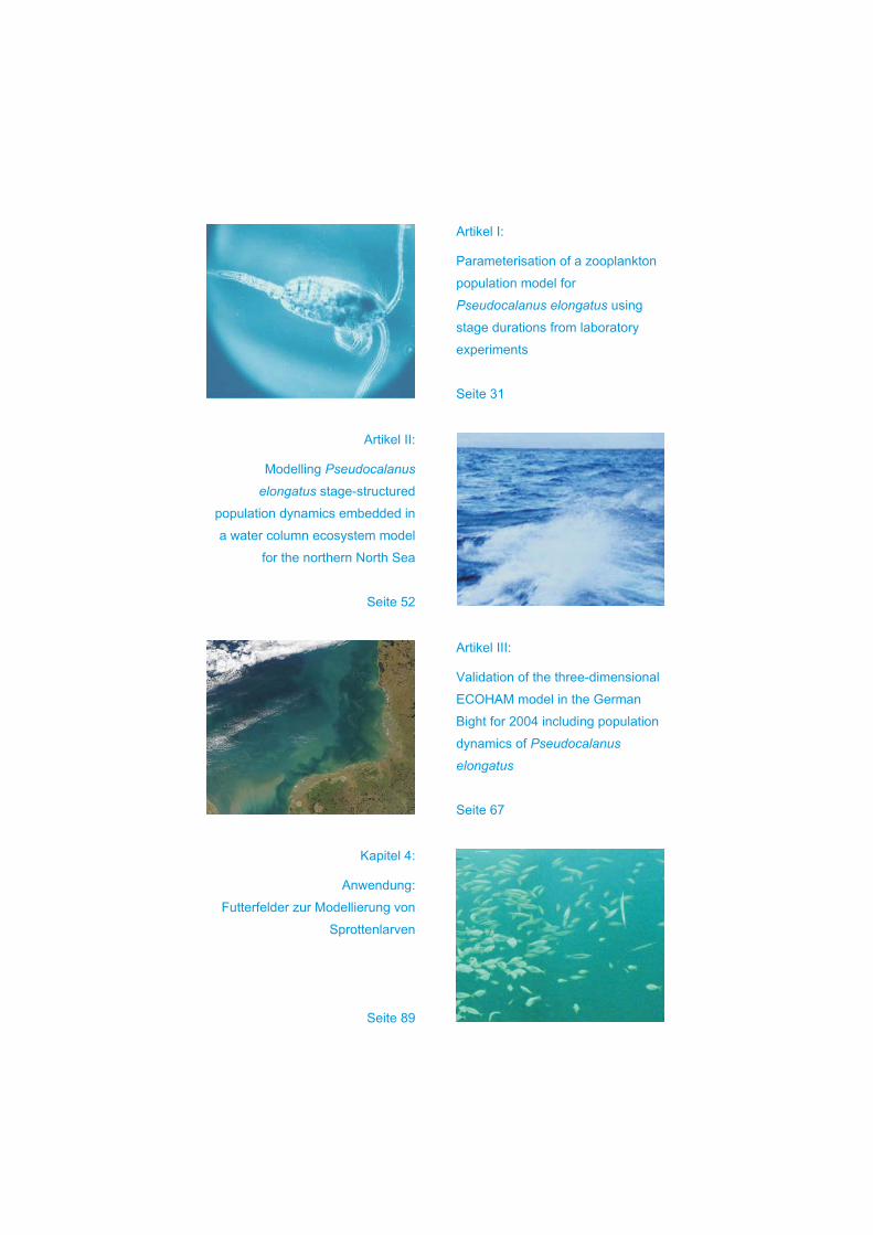
Artikel I:
Parameterisation of a zooplankton
population model for
using
stage durations from laboratory
experiments
Seite 31
Pseudocalanus elongatus
Artikel III:
Validation of the three-dimensional
ECOHAM model in the German
Bight for 2004 including population
dynamics of
Seite 67
Pseudocalanus
elongatus
Artikel II:
Modelling
stage-structured
population dynamics embedded in
a water column ecosystem model
for the northern North Sea
Seite 52
Pseudocalanus
elongatus
Kapitel 4:
Anwendung:
Futterfelder zur Modellierung von
Sprottenlarven
Seite 89
Inhaltsverzeichnis
1 Einfuhrung 9
1.1 Das Ökosystem der Nordsee . . . . . . . . . . . . . . . . . . . . . . . . . . . . 11
1.2 Zooplankton in der Nordsee . . . . . . . . . . . . . . . . . . . . . . . . . . . . 13
1.3 Modellierung der Populationsdynamik von Copepoden . . . . . . . . . . . . . 15
1.4 Übersicht über Ökosystemmodelle mit Zooplankton . . . . . . . . . . . . . . . 18
2 Beschreibung des ECOHAM-Modellsystems 21
2.1 Die Antriebsdaten . . . . . . . . . . . . . . . . . . . . . . . . . . . . . . . . . 22
2.2 Das hydrodynamische Modell . . . . . . . . . . . . . . . . . . . . . . . . . . . 22
2.3 Das biogeochemische Modell . . . . . . . . . . . . . . . . . . . . . . . . . . . . 24
2.4 Genutzte Modellvarianten und Erweiterung für Zooplankton . . . . . . . . . . 25
3 Parametrisierung, Validation und Auswertung des Modells 29
3.1 Artikel I: Entwicklung des Zooplankton-Populationsmodells . . . . . . . . . . 31
3.1.1 Publikation I: Stegert et al. (2007) . . . . . . . . . . . . . . . . . . . . 32
3.1.2 Fazit zu Artikel I . . . . . . . . . . . . . . . . . . . . . . . . . . . . . . 51
3.2 Artikel II: Test der Populationsdynamik im Jahresgang . . . . . . . . . . . . . 52
3.2.1 Publikation II: Moll und Stegert (2007) . . . . . . . . . . . . . . . . . 53
3.2.2 Fazit zu Artikel II . . . . . . . . . . . . . . . . . . . . . . . . . . . . . 66
3.3 Artikel III: Anwendung in der Deutschen Bucht . . . . . . . . . . . . . . . . . 67
3.3.1 Publikation III: Stegert et al. (eingereicht) . . . . . . . . . . . . . . . . 68
3.3.2 Fazit zu Artikel III . . . . . . . . . . . . . . . . . . . . . . . . . . . . . 87
3
4 Anwendung: Futterfelder zur Modellierung von Sprottenlarven 89
4.1 Beschreibung des Fischlarvenmodells für Sprotten . . . . . . . . . . . . . . . . 89
4.2 Erstellung von Beutefeldern aus dem ECOHAM-Modell . . . . . . . . . . . . 90
4.3 Studien zur Larvenentwicklung von Sprotten . . . . . . . . . . . . . . . . . . . 93
4.3.1 Das Wachstum zu verschiedenen Jahreszeiten . . . . . . . . . . . . . . 94
4.3.2 Regionale Unterschiede . . . . . . . . . . . . . . . . . . . . . . . . . . . 97
4.4 Vergleich verschiedener Futterfelder für das Wachstum . . . . . . . . . . . . . 97
5 Diskussion und Schlußfolgerungen 105
6 Danksagung 113
7 Beitrag zu den Publikationen 115
Literaturverzeichnis 117
4
Zusammenfassung
In der Dissertation wird die Entwicklung des Zooplanktons im hydrodynamischen und biolo-gischen Umfeld der Nordsee mittels mathematischer Modelle untersucht. Dazu wird der Le-benszyklus einer Zooplanktonart mit seinen Entwicklungs- und Stoffwechselprozessen durchAbundanz- und Stoffflußgleichungen für die Stadienentwicklung beschrieben. Diese Gleichun-gen wurden im Ökosystemmodell ECOHAM integriert, um im Kontext von Zirkulation,Nährstoff- und Phytoplanktonverteilung die Zooplanktondynamik in den regionalen Unter-schieden und der jahreszeitlichen Entwicklung zu untersuchen. Die Ergebnisse werden u. a.für die Modellierung des Rekrutierungserfolges von Fischlarven im GLOBEC-Germany Pro-jekt, in das die Arbeit eingegliedert ist, verwendet. Die Dissertation basiert im Kern auf dreiVeröffentlichungen.
Um das Verhalten einer typischen Copepodenart in der Nordsee zu untersuchen, wurdedie Entwicklungsphysiologie von Pseudocalanus elongatus, einer Schlüsselart im GLOBEC-Projekt, für die Nordsee parametrisiert. Darin wurden Zustandsvariablen für Abundanz undBiomasse für mehrere Stadiengruppen auf der Basis eines bestehenden Populationsmodellsformuliert. Mit Hilfe der Literatur wurde eine artenspezifische Parametrisierung für den Le-benszyklus in Nahrungsaufnahme, Metabolismus, Entwicklung (durch Wachstum und Häu-tung) sowie Reproduktion erarbeitet (Stegert et al., 2007, Artikel I). Das Populationsmodellwurde als neues Modul in das dreidimensionale ECOHAM-Modellsystem integriert. Dannwurde das Verhalten der Population zunächst an einer Station in der nördlichen Nordsee ge-testet und die zeitliche Entwicklung im Nährstoff-Plankton-Kreislauf untersucht (Moll undStegert , 2007, Artikel II)). Die Einbindung der Populationsdynamik in Konkurrenz zum rest-lichen Zooplankton ermöglicht dann die Analyse des quantitativen Anteils von P. elongatusin der artenreichen Nordsee. Die Validation erfolgte anhand von Meßdaten für das Jahr 2004.Mit diesem Modellsystem wurden Untersuchungen zum Verständnis der Zooplanktondyna-mik durchgeführt (Stegert et al., eingereicht, Artikel III). Dazu gehören die räumlich-zeitlicheVerteilung der Population und ihre Ursachen. So steuert die Futtermenge die Größe der Po-pulation während die Temperatur ihre Entwicklungsgeschwindigkeit beeinflußt.
In einem anschließenden Kapitel wird die Anwendung des Zooplankton-Populationsmodellsgezeigt, indem Futterfelder zur Modellierung von Sprottenlarven ausgewertet werden (Ka-pitel 4). Dabei zeigt sich der Einfluß der zeitlich-räumlich variablen Zooplanktonfelder auf
5

das Larvenwachstum, und es wird abschließend die Methodik diskutiert. Im letzten Kapitelwerden übergeordnete Fragestellungen behandelt, welche die einzelnen Publikationen undKapitel miteinander verbinden (Kapitel 5).
6
Summary
In this thesis the development of zooplankton within the hydrodynamical and biologicalenvironment of the North Sea is investigated using mathematical models. Thereto the lifecycle of a zooplankton population is described by abundance and cycles of matter withindevelopment and physiological processes. Equations with species-specific parameter valuesare implemented into the ecosystem model ECOHAM to simulate the annual cycle andregional differences influenced by circulation, nutrient and phytoplankton distribution. Theresults are also used for modelling the recruitment success of larval fish within the GermanGLOBEC project, to which the thesis work is a contribution. The thesis is based on threepublications.
To investigate the population dynamics of a copepod species typical for the North Seathe life cycle of the GLOBEC target species Pseudocalanus elongatus was parameterised.State variables were formulated for abundance and biomass of five stage groups based onan existing population model. Using literature data species-specific parameter values for thelife cycle processes of ingestion, metabolic terms and development (in growth and moulting)and reproduction were determined (Stegert et al., 2007, paper I). The population model wasimplemented into the three-dimensional ECOHAM model. The life cycle was tested at anorthern North Sea station to investigate the temporal development within the ecosystemmodel (Moll und Stegert , 2007, paper II). The integration of population dynamics competingto the rest zooplankton allows the analysis of the proportion of P. elongatus in the diverseNorth Sea ecosystem. The validation of the state variables against field data for 2004 wasperformed and the zooplankton dynamics were investigated (Stegert et al., eingereicht, paperIII). This investigation included the temporal and spatial distribution of the population,which shows, that the food concentration mostly affects the population abundance while thetemperature has a strong influence on the developmental rates.
In a subsequent chapter the modelled zooplankton population data were used as preyfields for modelling larval sprat (chapter 4). The preparation of these prey fields and theinfluence of the spatio-temporal variability of the zooplankton was investigated and themethods discussed. Finally, general questions linking the several papers and chapters werediscussed (chapter 5)
7

8
1 Einfuhrung
Wenn Kinder einen Moment Zeit nehmen, um Copepoden zu betrachten,
so wurden sie die Dinosaurier vergessen!
(Mark D. Ohman
Scripps Institute of Oceanography, San Diego)
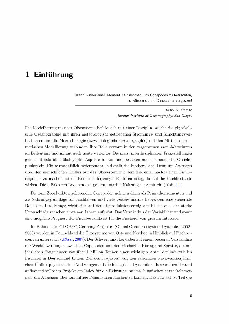
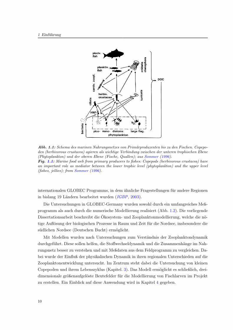
Die Modellierung mariner Ökosysteme befaßt sich mit einer Disziplin, welche die physikali-sche Ozeanographie mit ihren meteorologisch getriebenen Strömungs- und Schichtungsver-hältnissen und die Meeresbiologie (bzw. biologische Ozeanographie) mit den Mitteln der nu-merischen Modellierung verbindet. Ihre Rolle gewann in den vergangenen zwei Jahrzehntenan Bedeutung und nimmt auch heute weiter zu. Die meist interdisziplinären Fragestellungengehen oftmals über ökologische Aspekte hinaus und beziehen auch ökonomische Gesicht-punkte ein. Ein wirtschaftlich bedeutendes Feld stellt die Fischerei dar. Denn um Aussagenüber den menschlichen Einfluß auf das Ökosystem mit dem Ziel einer nachhaltigen Fische-reipolitik zu machen, ist die Kenntnis derjenigen Faktoren nötig, die auf die Fischbeständewirken. Diese Faktoren beziehen das gesamte marine Nahrungsnetz mit ein (Abb. 1.1).
Die zum Zooplankton gehörenden Copepoden nehmen darin als Primärkonsumenten undals Nahrungsgrundlage für Fischlarven und viele weitere marine Lebewesen eine steuerndeRolle ein. Ihre Menge wirkt sich auf den Reproduktionserfolg der Fische aus, der starkeUnterschiede zwischen einzelnen Jahren aufweist. Das Verständnis der Variabilität und somiteine mögliche Prognose der Fischbestände ist für die Fischerei von großem Interesse.
Im Rahmen des GLOBEC-Germany Projektes (Global Ocean Ecosystem Dynamics, 2002–2008) wurden in Deutschland die Ökosysteme von Ost- und Nordsee in Hinblick auf Fischres-sourcen untersucht (Alheit , 2007). Der Schwerpunkt lag dabei auf einem besseren Verständnisder Wechselwirkungen zwischen Copepoden und den Fischarten Hering und Sprotte, die mitjährlichen Fangmengen von über 1 Million Tonnen einen wichtigen Anteil der industriellenFischerei in Deutschland bilden. Ziel des Projektes war, den saisonalen wie zwischenjährli-chen Einfluß physikalischer Änderungen auf die biologische Dynamik zu beschreiben. Daraufaufbauend sollte im Projekt ein Index für die Rekrutierung von Jungfischen entwickelt wer-den, um Aussagen über zukünftige Fangmengen machen zu können. Das Projekt ist Teil des
9
1 Einfuhrung
Abb. 1.1: Schema des marinen Nahrungsnetzes von Primarproduzenten bis zu den Fischen. Copepo-den (herbivorous crustacea) agieren als wichtige Verbindung zwischen der unteren trophischen Ebene(Phytoplankton) und der oberen Ebene (Fische, Quallen); aus Sommer (1996).Fig. 1.1: Marine food web from primary producers to fishes: Copepods (herbivorous crustacea) havean important role as mediator between the lower trophic level (phytoplankton) and the upper level(fishes, jellies); from Sommer (1996).
internationalen GLOBEC Programms, in dem ähnliche Fragestellungen für andere Regionenin bislang 19 Ländern bearbeitet wurden (IGBP , 2003).
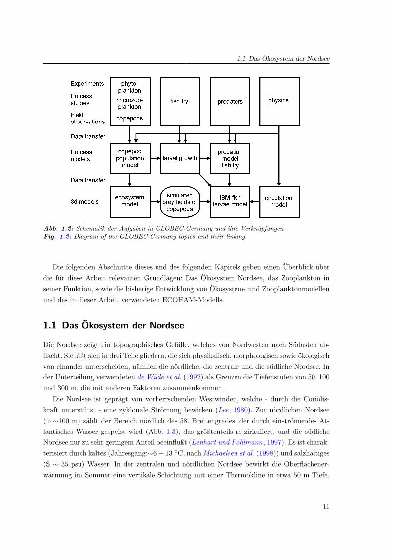
Die Untersuchungen in GLOBEC-Germany wurden sowohl durch ein umfangreiches Meß-programm als auch durch die numerische Modellierung realisiert (Abb. 1.2). Die vorliegendeDissertationsarbeit beschreibt die Ökosystem- und Zooplanktonmodellierung, welche die nö-tige Auflösung der biologischen Prozesse in Raum und Zeit für die Nordsee, insbesondere diesüdlichen Nordsee (Deutschen Bucht) ermöglicht.
Mit Modellen wurden nach Untersuchungen zum Verständnis der Zooplanktondynamikdurchgeführt. Diese sollen helfen, die Stoffwechseldynamik und die Zusammenhänge im Nah-rungsnetz besser zu verstehen und mit Meßdaten aus dem Feldprogramm zu vergleichen. Da-bei wurde der Einfluß der physikalischen Dynamik in ihren regionalen Unterschieden auf dieZooplanktonentwicklung untersucht. Im Zentrum steht dabei die Untersuchung von kleinenCopepoden und ihrem Lebenszyklus (Kapitel. 3). Das Modell ermöglicht es schließlich, drei-dimensionale größenaufgelöste Beutefelder für die Modellierung von Fischlarven im Projektzu erstellen. Ein Einblick auf diese Anwendung wird in Kapitel 4 gegeben.
10
1.1 Das Okosystem der Nordsee
Abb. 1.2: Schematik der Aufgaben in GLOBEC-Germany und ihre VerknupfungenFig. 1.2: Diagram of the GLOBEC-Germany topics and their linking.
Die folgenden Abschnitte dieses und des folgenden Kapitels geben einen Überblick überdie für diese Arbeit relevanten Grundlagen: Das Ökosystem Nordsee, das Zooplankton inseiner Funktion, sowie die bisherige Entwicklung von Ökosystem- und Zooplanktonmodellenund des in dieser Arbeit verwendeten ECOHAM-Modells.
1.1 Das Okosystem der Nordsee
Die Nordsee zeigt ein topographisches Gefälle, welches von Nordwesten nach Südosten ab-flacht. Sie läßt sich in drei Teile gliedern, die sich physikalisch, morphologisch sowie ökologischvon einander unterscheiden, nämlich die nördliche, die zentrale und die südliche Nordsee. Inder Unterteilung verwendeten de Wilde et al. (1992) als Grenzen die Tiefenstufen von 50, 100und 300 m, die mit anderen Faktoren zusammenkommen.
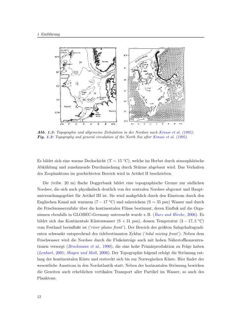
Die Nordsee ist geprägt von vorherrschenden Westwinden, welche - durch die Coriolis-kraft unterstützt - eine zyklonale Strömung bewirken (Lee, 1980). Zur nördlichen Nordsee(>∼100 m) zählt der Bereich nördlich des 58. Breitengrades, der durch einströmendes At-lantisches Wasser gespeist wird (Abb. 1.3), das größtenteils re-zirkuliert, und die südlicheNordsee nur zu sehr geringem Anteil beeinflußt (Lenhart und Pohlmann, 1997). Es ist charak-terisiert durch kaltes (Jahresgang:∼6− 13 ◦C, nach Michaelsen et al. (1998)) und salzhaltiges(S ∼ 35 psu) Wasser. In der zentralen und nördlichen Nordsee bewirkt die Oberflächener-wärmung im Sommer eine vertikale Schichtung mit einer Thermokline in etwa 50 m Tiefe.
11
1 Einfuhrung
Abb. 1.3: Topographie und allgemeine Zirkulation in der Nordsee nach Krause et al. (1995).Fig. 1.3: Topography and general circulation of the North Sea after Krause et al. (1995).
Es bildet sich eine warme Deckschicht (T ∼ 15 ◦C), welche im Herbst durch atmosphärischeAbkühlung und zunehmende Durchmischung durch Stürme abgebaut wird. Das Verhaltendes Zooplanktons im geschichteten Bereich wird in Artikel II beschrieben.
Die (teilw. 20 m) flache Doggerbank bildet eine topographische Grenze zur südlichenNordsee, die sich auch physikalisch deutlich von der zentralen Nordsee abgrenzt und Haupt-untersuchungsgebiet für Artikel III ist. Sie wird maßgeblich durch den Einstrom durch denEnglischen Kanal mit warmem (7− 17 ◦C) und salzreichem (S ∼ 35 psu) Wasser und durchdie Frischwasserzufuhr über die kontinentalen Flüsse bestimmt, deren Einfluß auf die Orga-nismen ebenfalls in GLOBEC-Germany untersucht wurde z. B. (Barz und Hirche, 2006). Esbildet sich das Kontinentale Küstenwasser (S « 31 psu), dessen Temperatur (3− 17, 5 ◦C)vom Festland beeinflußt ist (‘river plume front ’). Der Bereich des größten Salzgehaltsgradi-enten schwankt entsprechend des tidebestimmten Zyklus (‘tidal mixing front ’). Neben demFrischwasser wird die Nordsee durch die Flußeinträge auch mit hohen Nährstoffkonzentra-tionen versorgt (Brockmann et al., 1990), die eine hohe Primärproduktion zu Folge haben(Lenhart , 2001; Skogen und Moll , 2000). Der Topographie folgend erfolgt die Strömung ent-lang der kontinentalen Küste und erstreckt sich bis zur Norwegischen Küste. Hier findet derwesentliche Ausstrom in den Nordatlantik statt. Neben der horizontalen Strömung bewirkendie Gezeiten auch erheblichen vertikalen Transport aller Partikel im Wasser, so auch desPlanktons.
12
1.2 Zooplankton in der Nordsee
1.2 Zooplankton in der Nordsee
Der Begriff des Planktons wurde durch Hensen (1887) eingeführt und bezeichnet Pflan-zen (Phytoplankton) und Tiere (Zooplankton), die sich nicht oder nur bedingt eigenständigfortbewegen können und somit von den hydrodynamischen Gegebenheiten stark abhängigsind. Zum Zooplankton gehören eine Vielfalt verschiedener Organismen: Quallen, Muscheln,Schnecken, Würmer, Krebse und Fischlarven (Ichthyoplankton). Darunter bilden Copepo-den (Arthropoda, Crustacea) in der Nordsee - wie in vielen anderen Ökosystemen - denüberwiegenden Teil der Biomasse.
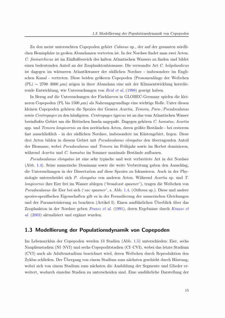
Auf Grund ihrer eingangs beschriebenen Rolle im marinen Nahrungsnetz wurden das Auf-treten und die Physiologie der Copepoden seit Beginn des letzten Jahrhunderts erforscht. ImLaufe der letzten 50 Jahre wurden die Feldmessungen in der Nordsee stark vorangetriebenund eine Reihe umfangreicher Datensätze erstellt. Darunter sind zum einen Langzeitmeßrei-hen an unterschiedlichen Positionen: Helgoland Reede (Greve et al., 2004), die Stationen L4im Englischen Kanal (Southward , 2005) sowie Stonehaven vor der Schottischen Küste. Unterden flächendeckenden Datensätzen bilden die CPR-Messungen1 den bedeutendsten Daten-satz. Im CPR-Atlas (CPRS , 2004) sind Monatsmittelwerte zu 240 Phyto- und Zooplankton-arten auf einem normierten Gitter graphisch dargestellt (acht davon in Abb. 1.4). AndereProgramme, wie das Fladengrund Experiment 19762 (Krause und Trahms, 1983) oder dasZISCH-Projekt3 1986–87 (Krause und Martens, 1990), geben die Zooplanktonverteilung füreinen kürzeren Zeitraum wieder.
Untersuchungen der zeitlich-räumlichen Verteilung sowie der Physiologie zeigen die An-passung verschiedener Arten an die genannten unterschiedlichen Bedingungen in der Nord-see. Diese Vielfalt der ökologischen Zonen der Nordsee spiegelt sich in der Artenvielfalt derCopepoden wider (Abb. 1.4): Nehmen in der (zentralen) Ostsee lediglich vier Copepodenar-ten den wesentlichen Teil der Zooplanktonabundanz ein (Dippner et al., 2000), so zeigt derCPR-Atlas in der Nordsee große Abundanzen für acht Arten.
1Continuous Plankton RecorderSSurveys (Reid et al., 2003) bezeichnet ein Programm der Sir Alister HardyFoundation of Ocean Science (SAHFOS), bei dem Planktonproben mit den CPR-Geraten wahrend derFahrt genommen und ausgewertet werden. So ist die Messung auf Handelsschiffen moglich, die regelmaßigin der Nordsee und im Nordatlantik verkehren. Damit ergaben sich im Zeitraum 1958-1999 fur 240 Speziesbereits 155669 Daten (Beaugrand , 2004), die uber das Internet abrufbar sind.
2Das Fladengrund-Experiment, 1976 (FLEX) wurde in Kooperation mehrerer europaischer Institute, dar-unter das Institut fur Meereskunde und das Zoologische Institut der Universitat Hamburg, durchgefuhrt.Wahrend der Fruhjahrsblute (Marz bis Juni) wurden physikalische und biologische Prozesse in der nord-lichen Nordsee untersucht, wobei an der Position 58◦ N 0,5◦ O dauerhaft Messungen stattfanden. DiesePosition (FLEX-Station) war auch Ort spaterer Forschung und wurde in dieser Arbeit fur das Wasser-saulenmodell (Artikel II) genutzt.
3“Zirkulation und Schadstoffe in der Nordsee”beinhaltete neben umfangreichen chemischen Untersuchungenauch Messungen von Zooplankton, welche in zwei Phasen - Mai-Juni 1986 und Januar-Marz 1987 -flachendeckend sowie tiefenaufgelost fur die ganze Nordsee durchgefuhrt wurden. Samtliche Daten wurdenim ZISCH-Atlas zusammengetragen und veroffentlicht (Moll und Radach, 1990).
13

1 Einfuhrung
(a) C. finmarchicus GUNNERUS, 1765
(b) C. helgolandicus CLAUS, 1863
(c) Acartia sp. (A. clausi GIESBRECHT, 1892)
(d) Temora longicornis MÜLLER, 1792
(e) Pseudocalanus elongatus BOECK, 1864
(f) Oithona spp. (O. similis CLAUS, 1863)
(g) Centropages hamatus LILLJEBORG, 1853
(h) Centropages typicus KRØYER, 1849
Abb. 1: Acht typische Copepoden der Nordsee mit ihrer Verteilung im
Nordatlantischen Ozean nach CPRS (2004). Quellen der Abbildungen: Calanus
finmarchicus, Acartia sp., Temora, P. elongatus und C. hamatus: Klein Breteler
(1982); C. helgolandicus: S. A. Poulet1, Oithona und C. typicus: A. Calbet2
1 Abteilung Marine Invertebraten und Zooplankton der Biologischen Station Roscoff (www.sb-roscoff.fr) 2 Aus der Photogallerie des ASLO: www.aslo.org/photopost/showgallery.php?cat=500&ppuser=306
Abb. 1.4: Acht typische Copepoden der Nordsee mit ihrer Verteilung im Nordatlantischen Ozeannach CPRS (2004). Quellen der Abbildungen: Calanus finmarchicus, Acartia sp., Temora, P.elongatus und C. hamatus: Klein Breteler (1982); C. helgolandicus: S. A. Pouleta; Oithona und C.typicus: A. Calbetb.Fig. 1.4: Eight copepod species tyical for the North Sea and their distribution in the North AtlanticOcean after CPRS (2004). Figure sources are: Calanus finmarchicus, Acartia sp., Temora, P.elongatus und C. hamatus: Klein Breteler (1982); C. helgolandicus: S. A. Pouleta; Oithona und C.typicus: A. Calbetb.
a Abteilung Marine Invertebraten und Zooplankton der Biologischen Station Roscoff (www.sb-roscoff.fr)b Aus der Photogallerie des ASLO: www.aslo.org/photopost/showgallery.php?cat=500&ppuser=306
14
1.3 Modellierung der Populationsdynamik von Copepoden
Zu den meist untersuchten Copepoden gehört Calanus sp., der auf der gesamten nördli-chen Hemisphäre in großen Abundanzen vertreten ist. In der Nordsee findet man zwei Arten.C. finmarchicus ist im Einflußbereich des kalten Atlantischen Wassers zu finden und bildeteinen bedeutenden Anteil an der Zooplanktonbiomasse. Die verwandte Art C. helgolandicusist dagegen im wärmeren Atlantikwasser der südlichen Nordsee - insbesondere im Engli-schen Kanal - vertreten. Diese beiden größeren Copepoden (Prosomenlänge der Weibchen(PL) ∼ 2700–3000 µm) zeigen in ihrer Abundanz eine mit der Klimaentwicklung korrelie-rende Entwicklung, wie Untersuchungen von Reid et al. (1998) gezeigt haben.
In Bezug auf die Untersuchungen der Fischlarven in GLOBEC-Germany spielen die klei-neren Copepoden (PL bis 1500 µm) als Nahrungsgrundlage eine wichtige Rolle. Unter diesenkleinen Copepoden gehören die Spezies der Genera Acartia, Temora, Para-/Pseudocalanussowie Centropages zu den häufigsten. Centropages typicus ist an das vom Atlantischen Wasserbeeinflußte Gebiet um die Britischen Inseln angepaßt. Dagegen gehören C. hamatus, Acartiaspp. und Temora longicornis zu den neritischen Arten, deren größte Bestände - bei ersteremfast ausschließlich - in der südlichen Nordsee, insbesondere im Küstengebiet, liegen. Diesedrei Arten bilden in diesem Gebiet mit Pseudocalanus elongatus den überragenden Anteilder Biomasse, wobei Pseudocalanus und Temora im Frühjahr sowie im Herbst dominieren,während Acartia und C. hamatus im Sommer maximale Bestände aufbauen.
Pseudocalanus elongatus ist eine sehr typische und weit verbreitete Art in der Nordsee(Abb. 1.4). Seine numerische Dominanz sowie die weite Verbreitung gaben den Ausschlag,die Untersuchungen in der Dissertation auf diese Spezies zu fokussieren. Auch in der Phy-siologie unterscheidet sich P. elongatus von anderen Arten. Während Acartia sp. und T.longicornis ihre Eier frei im Wasser ablegen (‘broadcast spawner ’), tragen die Weibchen vonPseudocalanus die Eier bei sich (‘sac spawner ’, s. Abb. 1.4, (Oithona sp.). Diese und anderespezies-spezifischen Eigenschaften gilt es in der Formulierung der numerischen Gleichungenund der Parametrisierung zu beachten (Artikel I). Einen ausführlichen Überblick über dasZooplankton in der Nordsee geben Fransz et al. (1991), deren Ergebnisse durch Krause etal. (2003) aktualisiert und ergänzt wurden.
1.3 Modellierung der Populationsdynamik von Copepoden
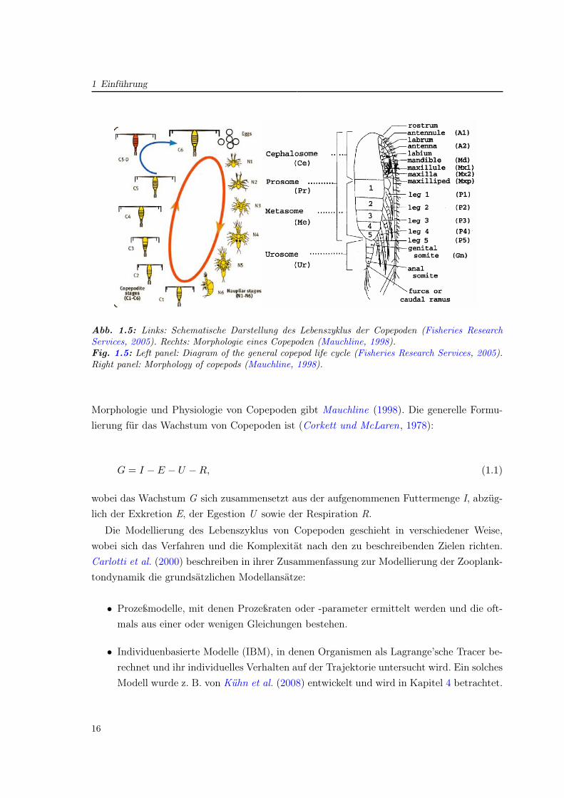
Im Lebenszyklus der Copepoden werden 13 Stadien (Abb. 1.5) unterschieden: Eier, sechsNauplienstadien (NI–NVI) und sechs Copepoditstadien (CI–CVI), wobei das letzte Stadium(CVI) auch als Adultenstadium bezeichnet wird, deren Weibchen durch Reproduktion denZyklus schließen. Der Übergang von einem Stadium zum nächsten geschieht durch Häutung,wobei sich von einem Stadium zum nächsten die Ausbildung der Segmente und Glieder er-weitert, wodurch einzelne Stadien zu unterscheiden sind. Eine ausführliche Darstellung der
15
1 EinfuhrungDissertation Christoph Stegert Fassung vom 22.05.2008
Seite 22/106
Abb. 5: Links: Schematische Darstellung des Lebenszyklus der Copepoden (FRS, 2005). Rechts: Morphologie eines Copepoden (Mauchline, 1998).
Die Modellierung des Lebenszyklus von Copepoden geschieht in verschiedener
Weise, wobei sich das Verfahren und die Komplexität nach den zu
beschreibenden Zielen richten. Carlotti et al. (2000) beschreiben in ihrer
Zusammenfassung zur Modellierung der Zooplanktondynamik die
grundsätzlichen Modellansätze:
- Prozeßmodelle, mit denen Prozeßraten oder -parameter ermittelt werden
und die oftmals aus einer oder wenigen Gleichungen bestehen.
- Individuenbasierte Modelle (IBM), in denen Organismen als
Lagrange'sche Tracer berechnet und ihr individuelles Verhalten auf der
Trajektorie untersucht wird. Ein solches Modell wurde z. B. von Kühn et
al. (2008) entwickelt und wird in Kapitel 4 betrachtet.
Abb. 1.5: Links: Schematische Darstellung des Lebenszyklus der Copepoden (Fisheries ResearchServices, 2005). Rechts: Morphologie eines Copepoden (Mauchline, 1998).Fig. 1.5: Left panel: Diagram of the general copepod life cycle (Fisheries Research Services, 2005).Right panel: Morphology of copepods (Mauchline, 1998).
Morphologie und Physiologie von Copepoden gibt Mauchline (1998). Die generelle Formu-lierung für das Wachstum von Copepoden ist (Corkett und McLaren, 1978):
G = I − E − U −R, (1.1)
wobei das Wachstum G sich zusammensetzt aus der aufgenommenen Futtermenge I, abzüg-lich der Exkretion E, der Egestion U sowie der Respiration R.
Die Modellierung des Lebenszyklus von Copepoden geschieht in verschiedener Weise,wobei sich das Verfahren und die Komplexität nach den zu beschreibenden Zielen richten.Carlotti et al. (2000) beschreiben in ihrer Zusammenfassung zur Modellierung der Zooplank-tondynamik die grundsätzlichen Modellansätze:
• Prozeßmodelle, mit denen Prozeßraten oder -parameter ermittelt werden und die oft-mals aus einer oder wenigen Gleichungen bestehen.
• Individuenbasierte Modelle (IBM), in denen Organismen als Lagrange’sche Tracer be-rechnet und ihr individuelles Verhalten auf der Trajektorie untersucht wird. Ein solchesModell wurde z. B. von Kühn et al. (2008) entwickelt und wird in Kapitel 4 betrachtet.
16
1.3 Modellierung der Populationsdynamik von Copepoden
• Populationsmodelle, in denen die Dynamik und (zahlenmäßige) Ausbreitung und Sta-dienverteilung einer oder mehrerer Populationen unter biologisch-physikalischen Be-dingungen simuliert wird. Diese Modellform wird in Artikel I verwendet und wird imfolgenden intensiv betrachtet.
• Ökosystemmodelle mit integrierter Zooplanktonpopulation, um Häufigkeit und Ver-breitung im räumlichen Ökosystem zu simulieren, wie es in der nördlichen Nordsee(Artikel II) und der Deutschen Bucht (Artikel III) angewandt wurde.
Nur die Erweiterung des Ökosystemmodells um Zustandsvariablen einzelner Copepoden-stadien und ihre physiologischen Prozesse ermöglicht detaillierte Untersuchungen der Ent-wicklung und des Verhaltens unter den variablen Bedingungen, die durch Repräsentation desZooplanktons in einer einzigen Zustandsvariablen nicht möglich ist. Hierauf wird insbeson-dere in Artikel II eingegangen.
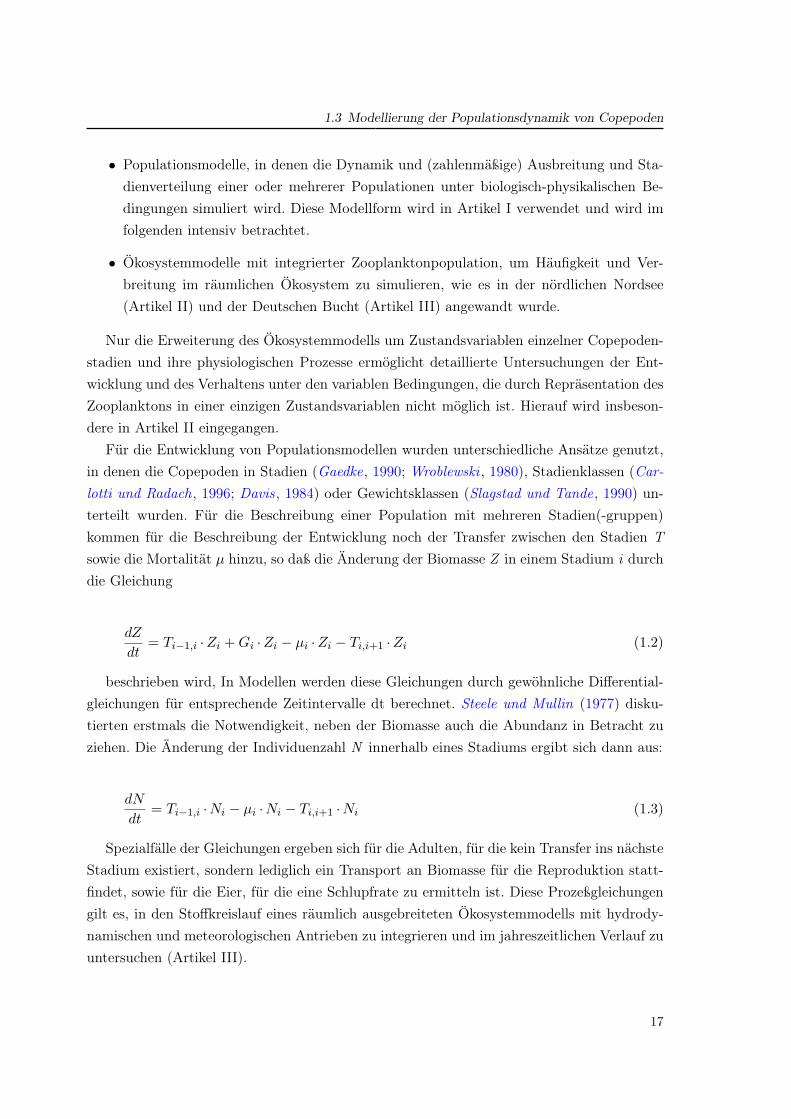
Für die Entwicklung von Populationsmodellen wurden unterschiedliche Ansätze genutzt,in denen die Copepoden in Stadien (Gaedke, 1990; Wroblewski , 1980), Stadienklassen (Car-lotti und Radach, 1996; Davis, 1984) oder Gewichtsklassen (Slagstad und Tande, 1990) un-terteilt wurden. Für die Beschreibung einer Population mit mehreren Stadien(-gruppen)kommen für die Beschreibung der Entwicklung noch der Transfer zwischen den Stadien Tsowie die Mortalität µ hinzu, so daß die Änderung der Biomasse Z in einem Stadium i durchdie Gleichung
dZ
dt= Ti−1,i ·Zi + Gi ·Zi − µi ·Zi − Ti,i+1 ·Zi (1.2)
beschrieben wird, In Modellen werden diese Gleichungen durch gewöhnliche Differential-gleichungen für entsprechende Zeitintervalle dt berechnet. Steele und Mullin (1977) disku-tierten erstmals die Notwendigkeit, neben der Biomasse auch die Abundanz in Betracht zuziehen. Die Änderung der Individuenzahl N innerhalb eines Stadiums ergibt sich dann aus:
dN
dt= Ti−1,i ·Ni − µi ·Ni − Ti,i+1 ·Ni (1.3)
Spezialfälle der Gleichungen ergeben sich für die Adulten, für die kein Transfer ins nächsteStadium existiert, sondern lediglich ein Transport an Biomasse für die Reproduktion statt-findet, sowie für die Eier, für die eine Schlupfrate zu ermitteln ist. Diese Prozeßgleichungengilt es, in den Stoffkreislauf eines räumlich ausgebreiteten Ökosystemmodells mit hydrody-namischen und meteorologischen Antrieben zu integrieren und im jahreszeitlichen Verlauf zuuntersuchen (Artikel III).
17
1 Einfuhrung
1.4 Ubersicht uber Okosystemmodelle mit Zooplankton
Anfang der fünfziger Jahre begannen erste Ansätze, wesentliche Komponenten im Stoff-kreislauf des Ökosystems durch mathematische Gleichungen zu beschreiben (de Wilde etal., 1992). Steele (1974) formulierte erstmals ein komplexes System, das physikalische (Hy-drodynamik, Thermodynamik und Licht), chemische (Nährstoffaufnahme, -vermischung und-regeneration) sowie biologische (Phyto- und Zooplanktondynamik incl. eines Kohortenmo-dells für Calanus bzw. Pseudocalanus) Prozesse miteinander verbindet.
Ein erstes Stadienaufgelöstes Modell wurde von Wroblewski (1980) für Acartia clausi aufdem Schelf vor Oregon (Nordpazifik) entwickelt, in dem mehrere Stadien zu Stadiengruppenzusammenfaßt wurden. Diese Vereinfachung wurde von Davis (1984) kritisiert4, da diese zuverkürzten Generationszeiten führten. Für seine Untersuchungen verschiedener Copepodenim Gebiet der Georges Bank (Nordwestatlantik) fügte er zusätzliche Altersklassen innerhalbder 13 Stadien ein. Dieses Prinzip wurde von Carlotti und Sciandra (1989) für die Mittel-meerspezies Euterpina acutifrons übernommen, die erstmals eine ausführliche Beschreibungder metabolischen Prozesse integrierten. Dieses Populationsmodell wurde in einer späterenArbeit mit einem für die Nordsee entwickelten Wassersäulenmodell (Radach und Moll , 1993)gekoppelt, um den Lebenszyklus von Calanus finmarchicus zu simulieren (Carlotti und Rad-ach, 1996).
Mitte der Neunziger Jahre wurden die ersten dreidimensionalen Ökosystemmodelle für dieNordsee entwickelt. Dazu gehörte neben NORWECOM (Skogen et al., 1995), GHER (Delhezund Martin, 1994) und ERSEM (Baretta et al., 1995) auch ECOHAM (Moll , 1995). Dieseund andere regionale Modelle widmeten sich zunächst dem Nährstoff-Phytoplankton-Systemund beinhalteten - mit Ausnahme von ERSEM und GHER - keine explizite Zustandsvariablefür Zooplankton (Moll und Radach, 2003).
In den folgenden Jahren wurden mehrere Populationsmodelle für C. finmarchicus inder Nordsee mit unterschiedlichen Ansätzen entwickelt: Heath et al. (1997) wendeten einLangrange’sches Wassersäulenmodell in einem dreidimensionalen Eulerschen hydrodynami-schen Feld an, um den sommerlichen Einstrom in die Nordsee durch den Fair Isle Kanal zuuntersuchen, während Bryant et al. (1997) eine vereinfachte physiologische Beschreibung derPopulation in einem Eulermodell von 1◦ × 1◦Boxen anwandten. Gurney et al. (2001) stell-ten eine zeitlich diskrete Beschreibung des Wachstums für ein zweidimensionales Modell derOberflächenschicht vor, das von Speirs et al. (2005) genutzt wurde, um die Überwinterung(Diapause) von C. finmarchicus zu untersuchen. Ähnliche Entwicklungen wurden für Cope-poden in anderen Ökosystemen durchgeführt, z. B. von Lynch et al. (1998) für die GeorgesBank oder Plaganyi et al. (1999) im südlichen Benguela-Auftriebsgebiet. In diesen Modellen
4Der in Artikel II zitierte Artikel Davies und Payne (1984) ist in diesem Zusammenhang nicht korrekt.
18
1.4 Ubersicht uber Okosystemmodelle mit Zooplankton
lag der modellierten Population ein Strömungs- und Temperaturfeld aus einem hydrody-namischen Modell sowie mit Ausnahme bei Heath et al. (1997) ein externer Datensatz anPhytoplankton als Futterantrieb vor. Ein gekoppeltes zweidimensionales (x,z) Ökosystem-und Individuen basiertes Populationsmodell, in dem Zooplankton und Phytoplankton inter-agieren, wurde von Batchelder et al. (2002)) veröffentlicht.
Für die Ostsee entwickelten Fennel und Neumann (2003) erstmals ein gekoppeltes drei-dimensionales Ökosystemmodell mit integrierter Populationsdynamik für Pseudocalanus. Indiesem Modell wurden, ähnlich zu Wroblewski (1980), Stadien zusammengefaßt, die jeweilszwischen zwei kritischen Gewichten definiert sind. Für jede der fünf Zustandsvariablen wer-den die Biomasse wie auch die Abundanz berechnet. Das sich daraus ergebende mittlereStadiengewicht steuert die Raten der in den Gleichungen 2 und 3 genannten Prozesse fürdas jeweilige Stadium. Eine ausführliche Beschreibung der Struktur und der Formulierun-gen des Populationsmodells sowie die Anwendung als 0d-Modell werden in Fennel (2001)gegeben.
Diese Arbeit bildete die Grundlage für die in der vorliegenden Dissertationsarbeit be-schriebene Populationsmodellierung von Copepoden (s. Artikel I).
19

1 Einfuhrung
20
2 Beschreibung des
ECOHAM-Modellsystems
Ein Modell sollte so einfach wie moglich sein,
aber nicht einfacher!
(nach dem Einstein’schen Prinzip)
Die Zooplanktonmodellierung in GLOBEC-Germany wurde mit dem am Institut für Meeres-kunde entwickelten ECOHAM (Ecological North Sea Model, Hamburg) durchgeführt. DasModell wird zur Untersuchung verschiedener Fragestellungen genutzt und entsprechend umunterschiedliche Module erweitert. Dabei liegt der Schwerpunkt auf geochemischen Prozessenund den unteren trophischen Stufen.
Die erste Version des Modells (ECOHAM1) war darauf ausgelegt, die Primärproduktionin der Nordsee zu simulieren (Moll , 1998), um Ursachen für Eutrophierung und die Folgenfür das Algenaufkommen in bestimmten Küstengebieten zu untersuchen. Um die Flüsse vonKohlenstoff und Stickstoff zu simulieren, wurden die Stoffkreisläufe hierfür nach Kühn undRadach (1997) für Stickstoff und Pätsch et al. (2002) für Kohlenstoff in ECOHAM2 erwei-tert. In dieser Variante fand auch eine Kopplung mit dem benthischen Modell CANDI statt(Luff und Moll , 2004). Ab ECOHAM3 wurde das Nordsee-Modellgebiet auf den gesamtennordwesteuropäischen Schelf erweitert, um Untersuchungen zum Austausch mit dem Nord-atlantik zu ermöglichen. Die aktuelle Version ECOHAM4 zeichnet sich durch Einteilung inje zwei Phyto- und Zooplanktongruppen aus, die in dieser Arbeit jedoch noch keine Anwen-dung findet. Diese Version dient derzeit zur Simulation von Nährstoff-Reduktionsszenarienim Rahmen einer Vergleichsstudie des OSPAR-Ausschusses für Eutrophierung, an dem meh-rere Modelle beteiligt sind. Die Studie beinhaltet auch eine Validation, die von Beginn anein wichtiger Bestandteil der Arbeit mit ECOHAM darstellte (Moll , 2000; Skogen und Moll ,2000). So geht den Untersuchungen in der nördlichen Nordsee (Artikel II) eine Validationder Ökosystemvariablen voraus, und sie ist wesentlicher Teil der Arbeit zur Deutschen Bucht(Artikel III). Einen Überblick über die Validation von Ökosystemmodellen geben Radach undMoll (2006).
21
2 Beschreibung des ECOHAM-Modellsystems5
Overview Model Run
Meteorological Forcing Data:NCEP Reanalysis data:Tair, clouds, evap, humidity, pressure, radiation, wind(6h)
Other Forcing Data:
- Silt concentration:SCOTSEASSPM(monthly data)
- Atm. deposition:EMEPNO3, NH4(annual data)
- River loads:ERSEMNO3, NH4, DIC, other(daily data)
Boundary Data:
- Water transport:HAMSOMNorth Atlantic,Baltic Sea(monthly)
- Nutrient cycle:WOA, 2001NO3(monthly)
- Carbon cycle:CANOBADIC, alkalinity(seasonal)
Simulation:2 years of spin-up (2003)20032004 (‘GLOBEC year’)
ECOHAMincl. HAMSOM for hydrodynamics*
Internal Data:
initial data: for prognostic variablestimesteps: 60 min. model parameter: for process
formulations*offline calculation (Pohlmann, 2006)
o o o o Model structure
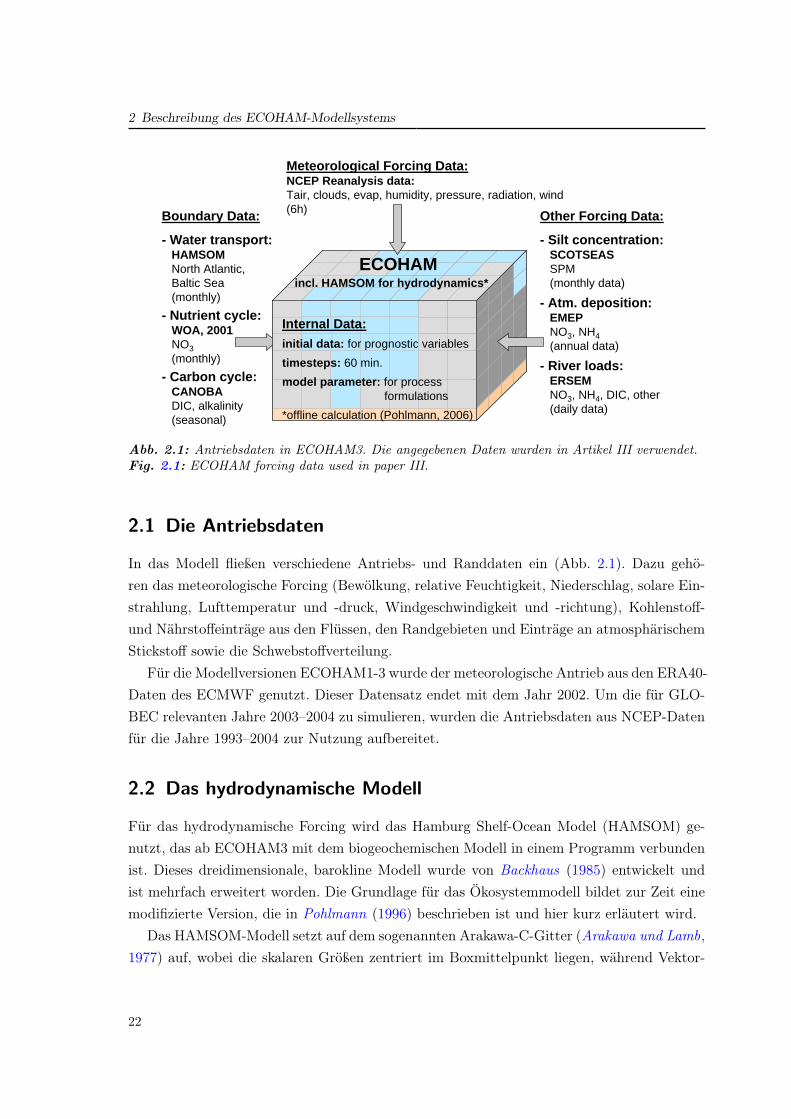
Abb. 2.1: Antriebsdaten in ECOHAM3. Die angegebenen Daten wurden in Artikel III verwendet.Fig. 2.1: ECOHAM forcing data used in paper III.
2.1 Die Antriebsdaten
In das Modell fließen verschiedene Antriebs- und Randdaten ein (Abb. 2.1). Dazu gehö-ren das meteorologische Forcing (Bewölkung, relative Feuchtigkeit, Niederschlag, solare Ein-strahlung, Lufttemperatur und -druck, Windgeschwindigkeit und -richtung), Kohlenstoff-und Nährstoffeinträge aus den Flüssen, den Randgebieten und Einträge an atmosphärischemStickstoff sowie die Schwebstoffverteilung.
Für die Modellversionen ECOHAM1-3 wurde der meteorologische Antrieb aus den ERA40-Daten des ECMWF genutzt. Dieser Datensatz endet mit dem Jahr 2002. Um die für GLO-BEC relevanten Jahre 2003–2004 zu simulieren, wurden die Antriebsdaten aus NCEP-Datenfür die Jahre 1993–2004 zur Nutzung aufbereitet.
2.2 Das hydrodynamische Modell
Für das hydrodynamische Forcing wird das Hamburg Shelf-Ocean Model (HAMSOM) ge-nutzt, das ab ECOHAM3 mit dem biogeochemischen Modell in einem Programm verbundenist. Dieses dreidimensionale, barokline Modell wurde von Backhaus (1985) entwickelt undist mehrfach erweitert worden. Die Grundlage für das Ökosystemmodell bildet zur Zeit einemodifizierte Version, die in Pohlmann (1996) beschrieben ist und hier kurz erläutert wird.
Das HAMSOM-Modell setzt auf dem sogenannten Arakawa-C-Gitter (Arakawa und Lamb,1977) auf, wobei die skalaren Größen zentriert im Boxmittelpunkt liegen, während Vektor-
22
2.2 Das hydrodynamische Modell
Dichtegradienten Gezeiten
Strömungen
Wind
+ Luftdruck
Topographie
advektive
Wärmeflußdichte
lokale
Wärmeflußdichte
Wärmeflußdichte
durch die
Meeresoberfläche
vertikaler
Austausch-
koeffizient
Oberflächen-
temperatur
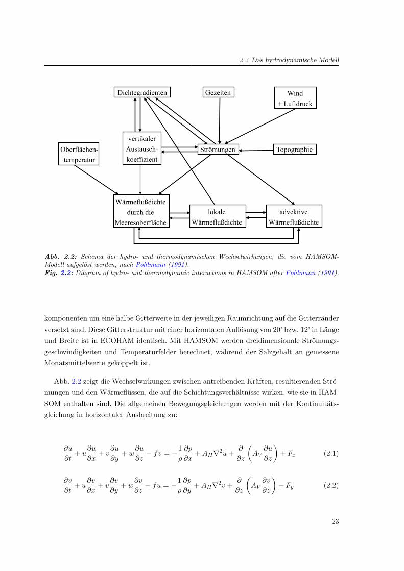
Abb. 2.2: Schema der hydro- und thermodynamischen Wechselwirkungen, die vom HAMSOM-Modell aufgelost werden, nach Pohlmann (1991).Fig. 2.2: Diagram of hydro- and thermodynamic interactions in HAMSOM after Pohlmann (1991).
komponenten um eine halbe Gitterweite in der jeweiligen Raumrichtung auf die Gitterränderversetzt sind. Diese Gitterstruktur mit einer horizontalen Auflösung von 20’ bzw. 12’ in Längeund Breite ist in ECOHAM identisch. Mit HAMSOM werden dreidimensionale Strömungs-geschwindigkeiten und Temperaturfelder berechnet, während der Salzgehalt an gemesseneMonatsmittelwerte gekoppelt ist.
Abb. 2.2 zeigt die Wechselwirkungen zwischen antreibenden Kräften, resultierenden Strö-mungen und den Wärmeflüssen, die auf die Schichtungsverhältnisse wirken, wie sie in HAM-SOM enthalten sind. Die allgemeinen Bewegungsgleichungen werden mit der Kontinuitäts-gleichung in horizontaler Ausbreitung zu:
∂u
∂t+ u
∂u
∂x+ v
∂u
∂y+ w
∂u
∂z− fv = −1
ρ
∂p
∂x+ AH∇2u +
∂
∂z
(AV
∂u
∂z
)+ Fx (2.1)
∂v
∂t+ u
∂v
∂x+ v
∂v
∂y+ w
∂v
∂z+ fu = −1
ρ
∂p
∂y+ AH∇2v +
∂
∂z
(AV
∂v
∂z
)+ Fy (2.2)
23
2 Beschreibung des ECOHAM-Modellsystems
und in der vertikalen Ausbreitung zur hydrostatischen Gleichung:
∂p
∂z= −ρg, mit Dichte : ρ = ρ(S,T,p) (2.3)
Des weiteren werden die Transportgleichungen für Temperatur und Salzgehalt berechnet:
∂T
∂t+ u
∂T
∂x+ v
∂T
∂y+ w
∂T
∂z= KH∇2T +
∂
∂z
(KV
∂T
∂z
)+ ST (2.4)
∂S
∂t+ u
∂S
∂x+ v
∂S
∂y+ w
∂S
∂z= KH∇2S +
∂
∂z
(KV
∂S
∂z
)+ SS , (2.5)
welche den diffusiven Austausch (mit Koeffizienten KH und KV ) antreiben. Für einendetaillierten Einblick in die Herleitung sowie ausführliche Erklärung der Einbindung sei hierauf Pohlmann (1991) und Huang (1995) verwiesen.
Die in dieser Arbeit genutzten Modellrechnungen wurden offline eingebunden, d.h. diedreidimensionalen Geschwindigkeiten, die Wirbelkoeffizienten sowie Temperatur- und Salz-gehaltswerte werden erst mit dem hydrodynamischen Modell berechnet und anschließend alsgezeitengemittelte Datensätze in das biogeochemische Modell als täglichen Antrieb eingele-sen.
2.3 Das biogeochemische Modell
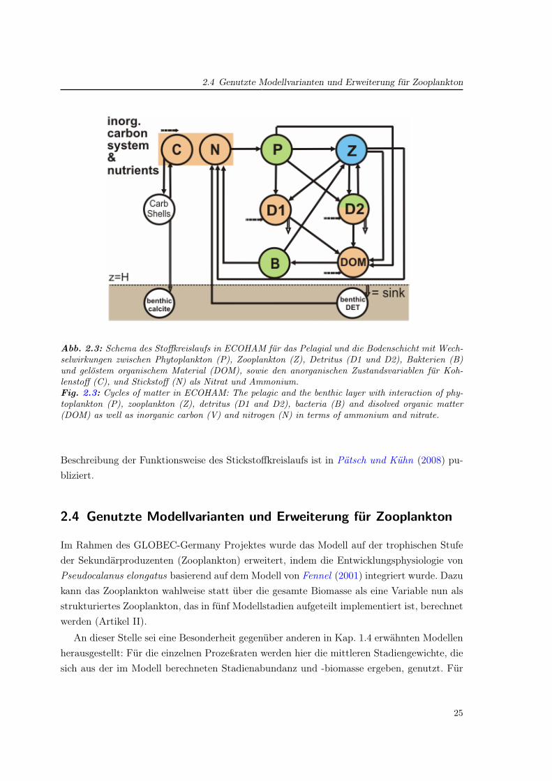
Der Stoffkreislauf wird durch die interne Dynamik des pelagischen und des benthischen Sy-stems mit seinen biologischen und chemischen Prozessen beschrieben. Das wird durch die inECOHAM realisierten Zustandsvariablen und Prozesse verdeutlicht. In Abb. 2.3 ist die all-gemeine Schematik des Stoffkreislaufs im ECOHAM mit seinen Zustandsvariablen in Bezugauf das Zooplankton abgebildet. Im Modell werden der Kohlenstoff- (C) sowie der Stick-stoffkreislauf (N) berechnet, wobei letzterer in den Zustandsvariablen Phytoplankton (P),Zooplankton (Z), Bakterien (B) und gelöste organische Stoffe (DOM) diagnostisch aus denC-Variablen ermittelt wird. In der Photosynthese baut das Phytoplankton aus Kohlendioxid(CO2) und anorganischen Nährstoffen (organische) Biomasse auf. Das Zooplankton nimmtPhytoplankton, kleine Partikel (Detritus, D2) und Bakterien auf (grün), und gibt über Mor-talität und Egestion (in Detritus), Exkretion (in DOM) sowie Respiration (in DIC bzw.Ammonium) Stoffe frei (braun). Die Remineralisierung in den anorganischen Teil geschiehtschließlich im Pelagial durch Bakterien sowie im Benthal, in dem abgesunkener Detrituszersetzt wird und anorganische Nährstoffe ins Pelagial entlassen werden. Eine ausführliche
24
2.4 Genutzte Modellvarianten und Erweiterung fur ZooplanktonDissertation Christoph Stegert Fassung vom 22.05.2008
Seite 37/106
Abb. 8: Schema des Stoffkreislaufs in ECOHAM für das Pelagial und die
Bodenschicht mit Wechselwirkungen zwischen Phytoplankton (P), Zooplankton
(Z), Detritus (D1 und D2), Bakterien (B) und gelöstem organischem Material
(DOM), sowie den anorganischen Zustandsvariablen für Kohlenstoff (C), und
Stickstoff (N) als Nitrat und Ammonium.
durch Bakterien sowie im Benthal, in dem abgesunkener Detritus zersetzt wird
und anorganische Nährstoffe ins Pelagial entläßt. Eine ausführliche
Beschreibung der Funktionsweise des Stickstoffkreislaufs ist in Pätsch und
Kühn (2008) publiziert.
Abb. 2.3: Schema des Stoffkreislaufs in ECOHAM fur das Pelagial und die Bodenschicht mit Wech-selwirkungen zwischen Phytoplankton (P), Zooplankton (Z), Detritus (D1 und D2), Bakterien (B)und gelostem organischem Material (DOM), sowie den anorganischen Zustandsvariablen fur Koh-lenstoff (C), und Stickstoff (N) als Nitrat und Ammonium.Fig. 2.3: Cycles of matter in ECOHAM: The pelagic and the benthic layer with interaction of phy-toplankton (P), zooplankton (Z), detritus (D1 and D2), bacteria (B) and disolved organic matter(DOM) as well as inorganic carbon (V) and nitrogen (N) in terms of ammonium and nitrate.
Beschreibung der Funktionsweise des Stickstoffkreislaufs ist in Pätsch und Kühn (2008) pu-bliziert.
2.4 Genutzte Modellvarianten und Erweiterung fur Zooplankton
Im Rahmen des GLOBEC-Germany Projektes wurde das Modell auf der trophischen Stufeder Sekundärproduzenten (Zooplankton) erweitert, indem die Entwicklungsphysiologie vonPseudocalanus elongatus basierend auf dem Modell von Fennel (2001) integriert wurde. Dazukann das Zooplankton wahlweise statt über die gesamte Biomasse als eine Variable nun alsstrukturiertes Zooplankton, das in fünf Modellstadien aufgeteilt implementiert ist, berechnetwerden (Artikel II).
An dieser Stelle sei eine Besonderheit gegenüber anderen in Kap. 1.4 erwähnten Modellenherausgestellt: Für die einzelnen Prozeßraten werden hier die mittleren Stadiengewichte, diesich aus der im Modell berechneten Stadienabundanz und -biomasse ergeben, genutzt. Für
25
2 Beschreibung des ECOHAM-ModellsystemsDissertation Christoph Stegert Fassung vom 22.05.2008
Seite 39/106
Abb. 9: Stadiendefinition im Modell durch kritische Gewichte X, sowie
Parametrisierung von Transfer ab Ri-1 und Ingestion.
In der Folgeversion ECOHAM3 wurde die Population in Futterkonkurrenz zur
restlichen Zooplanktonbiomasse gesetzt, sowie Neuerungen bezüglich der
Parametrisierung integriert (Kreus, 2006; Moll et al., submitted 2007). Des
weiteren wurden verschiedenartige Ergänzungen und Erweiterungen am
ECOHAM, die nicht in direkter Beziehung zum Zooplankton stehen, jedoch die
Beschreibung des Ökosystems Nordsee umfangreicher und auch präziser
ermöglichen, integriert. Somit basieren die einzelnen Arbeiten in den
Publikationen auf unterschiedlichen Modellvarianten, die in Tabelle 1
zusammengefaßt sind.
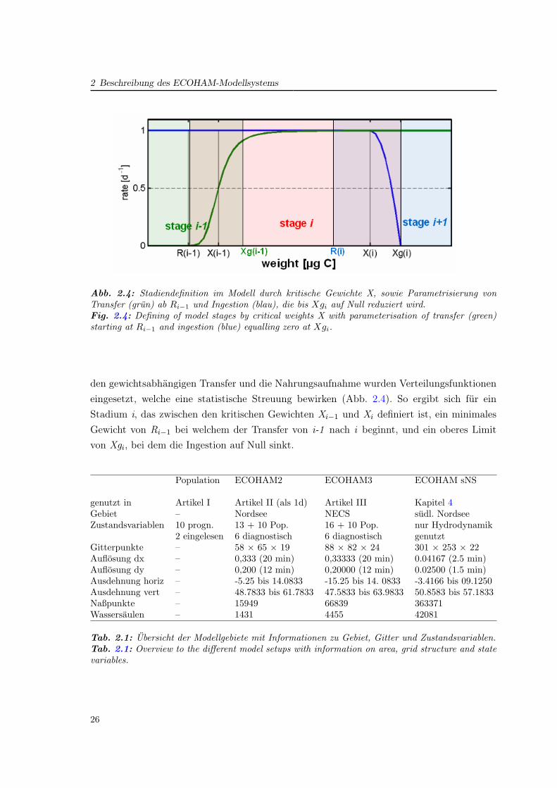
Abb. 2.4: Stadiendefinition im Modell durch kritische Gewichte X, sowie Parametrisierung vonTransfer (grun) ab Ri−1 und Ingestion (blau), die bis Xgi auf Null reduziert wird.Fig. 2.4: Defining of model stages by critical weights X with parameterisation of transfer (green)starting at Ri−1 and ingestion (blue) equalling zero at Xgi.
den gewichtsabhängigen Transfer und die Nahrungsaufnahme wurden Verteilungsfunktioneneingesetzt, welche eine statistische Streuung bewirken (Abb. 2.4). So ergibt sich für einStadium i, das zwischen den kritischen Gewichten Xi−1 und Xi definiert ist, ein minimalesGewicht von Ri−1 bei welchem der Transfer von i-1 nach i beginnt, und ein oberes Limitvon Xgi, bei dem die Ingestion auf Null sinkt.
Population ECOHAM2 ECOHAM3 ECOHAM sNS
genutzt in Artikel I Artikel II (als 1d) Artikel III Kapitel 4Gebiet – Nordsee NECS sudl. NordseeZustandsvariablen 10 progn. 13 + 10 Pop. 16 + 10 Pop. nur Hydrodynamik
2 eingelesen 6 diagnostisch 6 diagnostisch genutztGitterpunkte – 58 × 65 × 19 88 × 82 × 24 301 × 253 × 22Auflosung dx – 0,333 (20 min) 0,33333 (20 min) 0.04167 (2.5 min)Auflosung dy – 0,200 (12 min) 0,20000 (12 min) 0.02500 (1.5 min)Ausdehnung horiz – -5.25 bis 14.0833 -15.25 bis 14. 0833 -3.4166 bis 09.1250Ausdehnung vert – 48.7833 bis 61.7833 47.5833 bis 63.9833 50.8583 bis 57.1833Naßpunkte – 15949 66839 363371Wassersaulen – 1431 4455 42081
Tab. 2.1: Ubersicht der Modellgebiete mit Informationen zu Gebiet, Gitter und Zustandsvariablen.Tab. 2.1: Overview to the different model setups with information on area, grid structure and statevariables.
26
2.4 Genutzte Modellvarianten und Erweiterung fur Zooplankton
Dissertation Christoph Stegert Fassung vom 22.05.2008
Seite 41/106
Abb. 10: Modellgebiete verschiedener Modellvarianten. Oben:
Modelltopographie von ECOHAM2 (links) aus Artikel II und ECOHAM3
(rechts) aus Artikel III. Unten: Modelltopographie des Transportmodells aus
Kapitel 4.
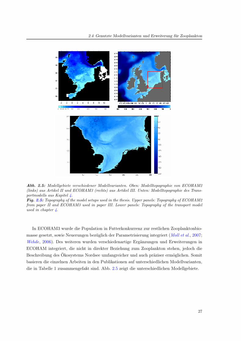
Abb. 2.5: Modellgebiete verschiedener Modellvarianten. Oben: Modelltopographie von ECOHAM2(links) aus Artikel II und ECOHAM3 (rechts) aus Artikel III. Unten: Modelltopographie des Trans-portmodells aus Kapitel 4.Fig. 2.5: Topography of the model setups used in the thesis. Upper panels: Topography of ECOHAM2from paper II and ECOHAM3 used in paper III. Lower panels: Topography of the transport modelused in chapter 4.
In ECOHAM3 wurde die Population in Futterkonkurrenz zur restlichen Zooplanktonbio-masse gesetzt, sowie Neuerungen bezüglich der Parametrisierung integriert (Moll et al., 2007;Wehde, 2006). Des weiteren wurden verschiedenartige Ergänzungen und Erweiterungen inECOHAM integriert, die nicht in direkter Beziehung zum Zooplankton stehen, jedoch dieBeschreibung des Ökosystems Nordsee umfangreicher und auch präziser ermöglichen. Somitbasieren die einzelnen Arbeiten in den Publikationen auf unterschiedlichen Modellvarianten,die in Tabelle 1 zusammengefaßt sind. Abb. 2.5 zeigt die unterschiedlichen Modellgebiete.
27

2 Beschreibung des ECOHAM-Modellsystems
28
3 Parametrisierung, Validation und
Auswertung des Modells
Wissenschaft wird aus Fakten gemacht,
so wie ein Haus aus Steinen gebaut wird.
Eine Sammlung von Fakten aber ist nicht mehr Wissenschaft
als daß ein Haufen von Steinen ein Haus ergibt.
(Henri Poincare)
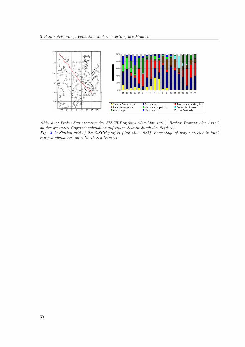
In drei Publikationen wird die Parametrisierung eines Populationsmodells für Pseudocalanuselongatus in der Nordsee, die Integration in ein Ökosystemmodell sowie dessen Auswertungbeschrieben. Es handelt sich dabei um eine Schlüsselart in GLOBEC, dessen Genus auch inanderen regionalen Programmen untersucht wurde (Keister und Peterson, 2003; McGillicud-dy und Bucklin, 2002). Ein Hauptkriterium für die Wahl dieser Art liegt in seiner Bedeutungals Beute für Fischlarven (Kapitel 4). Gegenüber anderen kleinen Copepoden ermöglichtseine numerische Dominanz (Fransz et al., 1991) und insbesondere seine weite Verbreitungauch Untersuchungen in ökologisch unterschiedlichen Bereichen der Nordsee (Abb. 3.1).
29
3 Parametrisierung, Validation und Auswertung des Modells
Dissertation Christoph Stegert Fassung vom 22.05.2008
Seite 43/106
3 Parametrisierung, Validation und Auswertung des
Modells
In drei Publikationen wird die Parametrisierung eines Populationsmodells für
Pseudocalanus elongatus in der Nordsee, die Integration in ein
Ökosystemmodell sowie dessen Auswertung beschrieben. Es handelt sich dabei
um eine Schlüsselart in GLOBEC, dessen Genus auch in anderen regionalen
Programmen untersucht wurde (McGillicuddy and Bucklin, 2002; Keister and
Peterson, 2003). Ein Hauptkriterium für die Wahl dieser Art liegt in seiner
Bedeutung als Beute für Fischlarven. Gegenüber anderen kleinen Copepoden
ermöglicht seine numerische Dominanz (Fransz et al., 1991) und insbesondere
seine weite Verbreitung auch Untersuchungen in ökologisch unterschiedlichen
Bereichen der Nordsee (Abb. 11).
0%
20%
40%
60%
80%
100%
7980818283848523456791011121314
Abb. 11: Stationsgitter des ZISCH-Projektes (Jan-Mar 1987). Prozentualer
Anteil an der gesamten Copepodenabundanz auf einem Schnitt durch die
Abb. 3.1: Links: Stationsgitter des ZISCH-Projektes (Jan-Mar 1987). Rechts: Prozentualer Anteilan der gesamten Copepodenabundanz auf einem Schnitt durch die Nordsee.Fig. 3.1: Station grid of the ZISCH project (Jan-Mar 1987). Percentage of major species in totalcopepod abundance on a North Sea transect
30
3.1 Artikel I: Entwicklung des Zooplankton-Populationsmodells
3.1 Artikel I: Entwicklung des Zooplankton-Populationsmodells
Ein null-dimensionales Populationsmodell basierend auf dem Copepodenmodell von (Fennel ,2001) wurde für die Beschreibung der Populationsdynamik von Pseudocalanus elongatus pa-rametrisiert. Die biologischen Funktionen wurden so gewählt, daß eine realistische Charakte-risierung des Wachstums und der Entwicklung unter für die Nordsee typischen Temperatur-und Futterbedingungen ermöglicht wurde. Parameterwerte für Gewichte, Schlüpfen und As-similation wurden der Literatur entnommen, wobei robuste Literaturwerte aus verschiedenenVeröffentlichungen zusammengeführt wurden, teils abgeleitet aus Werten für ähnliche Spezi-es. Der Einfluß der Temperatur auf Futteraufnahme und Atmung sowie die Halbsättigungs-konstante der Futteraufnahme wurden indirekt durch Anpassung der Entwicklungszeiten angemessene Stadiendauern aus Laborstudien bestimmt. Ein Datensatz von Klein Breteler etal. wurde genutzt, die Messungen bei Temperaturen von 5, 10, 15 und 20 ◦C jeweils fürFutterkonzentrationen von < 70, ∼100 und > 200 µg C l−1 durchführten. Simulationen fürjedes der Szenarien zeigte die Wirkung der Anpassung. Die Sensitivität der Modellparame-ter wurde hinsichtlich der resultierenden Abweichung in der Generationszeit getestet. DieAnalyse zeigte die Sensitivität der Entwicklung auf einzelne metabolische Prozesse, währenddie Bedeutung der Temperatur durch die Vielzahl der temperaturabhängigen Prozesse deut-lich wird. Mit dem Modell können Entwicklungsmuster wiedergegeben werden, während diephysiologische Komplexität von P. elongatus verdeutlicht wird.
31
3 Parametrisierung, Validation und Auswertung des Modells
3.1.1 Publikation I: Stegert et al. (2007)
Titel:
Parameterisation of a zooplankton population model for
Pseudocalanus elongatus using stage durations from laboratory experiments
Autoren:
Christoph Stegert, Markus Kreus, François Carlotti und Andreas Moll
Veröffentlicht in:
Ecological Modelling 206 (2007), Seiten 213-230
32
3.1 Artikel I: Entwicklung des Zooplankton-Populationsmodells
e c o l o g i c a l m o d e l l i n g 2 0 6 ( 2 0 0 7 ) 213–230
avai lab le at www.sc iencedi rec t .com
journa l homepage: www.e lsev ier .com/ locate /eco lmodel
Parameterisation of a zooplankton population model forPseudocalanus elongatus using stage durations fromlaboratory experiments
Christoph Stegerta,∗, Markus Kreusa, Francois Carlotti b, Andreas Molla,∗
a Institut fur Meereskunde (IfM), Universitat Hamburg (ZMK-ZMAW), Bundesstr. 53, 20146 Hamburg, Germanyb Universite de la Mediterranee, Centre d’Oceanologie de Marseille (COM), Rue de la Batterie des Lions,13007 Marseille, France
a r t i c l e i n f o
Article history:
Received 16 June 2006
Received in revised form
12 April 2007
Accepted 18 April 2007
Published on line 14 June 2007
Keywords:
Stage-structured population model
Copepod
Pseudocalanus
Parameterisation
Generation times
a b s t r a c t
A zero-dimensional population model based on a copepod model by Fennel (2001) was
parameterised according to the population dynamics of Pseudocalanus elongatus. Biologi-
cal functions were chosen particularly and formulated to get realistic characteristics of
growth and development under conditions of temperature and food reported for the North
Sea. Parameter values for weight, hatching and assimilation were taken from the litera-
ture, employing robust values from various published studies and parameters derived from
similar species. The influence of temperature on feeding and basal respiration and the
half-saturation of ingestion were obtained indirectly by successive fitting of developmental
times to stage durations observed from laboratory culture studies. A data set from Klein
Breteler et al. (1995) was used, which includes estimates at temperatures of 5, 10, 15 and
20 ◦C each at food concentrations of <70, ∼100 and >200 �g C l−1. Simulations at each sce-
nario showed the effectiveness of adjustments. The sensitivity of model parameter values
was tested in terms of variances in generation times. The analysis exhibited the sensitiv-
ity of development to specific metabolic processes, while the importance of temperature is
reflected in its recurrence within several processes. The model is able to represent consis-
tent development patterns, while reflecting the physiological complexity of a population of
P. elongatus.
© 2007 Elsevier B.V. All rights reserved.
1. Introduction
Fennel (2001) formulated a stage resolved zooplankton pop-ulation model adapted to Pseudocalanus sp. in the Baltic Sea,which calculates biomass and abundance for five model stagegroups. Necessary process parameterisation was derived fromthe literature and the Baltic Monitoring Programme to studythe physical impact on zooplankton dynamics and the inter-
∗ Corresponding authors.E-mail addresses: [email protected] (C. Stegert), [email protected] (A. Moll).
action with fish larvae in the frame of the German GLOBECProgramme (Fennel and Neumann, 2003).
Within this project we aimed to study the North Seazooplankton development, where copepods also form themajor part of the marine mesozooplankton throughout theyear. For both regional seas the three copepod groups Acartiaspp., Temora longicornis and Pseudo-/Paracalanus dominate thebiomass, but for the North Sea a number of additional cope-
0304-3800/$ – see front matter © 2007 Elsevier B.V. All rights reserved.doi:10.1016/j.ecolmodel.2007.04.012
33
3 Parametrisierung, Validation und Auswertung des Modells
214 e c o l o g i c a l m o d e l l i n g 2 0 6 ( 2 0 0 7 ) 213–230
Tabl
e1
–S
tage
du
rati
ons
(in
day
s)fr
omPs
eudo
cala
nu
sel
onga
tus
labo
rato
rycu
ltu
reex
per
imen
ts(K
lein
Bre
tele
ret
al.,
1995
)an
dre
-arr
ange
men
tfo
rco
mp
aris
onto
pop
ula
tion
mod
elre
sult
s
T(◦
C)
Food
sup
ply
1/16
1/4
1
Exp
t1
Exp
t2
Exp
t3
Mea
%Ex
pt
Sum
%Su
mEx
pt
1Ex
pt
2Ex
pt
3M
ea%
Exp
tSu
m%
Sum
Exp
1Ex
pt
2Ex
pt
3M
ea%
Exp
tSu
m%
Sum
5E
[7.2
]–
[7.2
]–
[7.2
]–
1[1
.8]
–[1
.8]
–[1
.8]
–
2[2
.7]
–11
.7–
[2.7
]–
11.7
–[2
.7]
–11
.7–
39.
413
.210
.711
.117
6.8
6.6
6.5
6.6
28.
46.
46.
87.
217
46.
44.
35.
25.
320
6.8
5.4
5.0
5.8
174.
46.
74.
25.
131
57.
55.
82.
75.
346
5.7
5.7
3.9
5.1
203.
2*3.
46.
14.
244
63.
13.
04.
23.
419
25.1
81.
81.
82.
92.
230
19.7
73.
2*2.
91.
32.
547
19.0
3
76.
27.
16.
86.
77
7.8
6.0
5.4
6.4
205.
35.
76.
65.
913
83.
94.
74.
54.
410
3.9
4.9
7.6
5.5
356.
34.
14.
45.
028
95.
25.
75.
15.
36
16.4
74.
64.
25.
84.
917
16.8
115.
04.
0*3.
94.
316
15.2
9
1013
.16.
34.
27.
859
7.8
8.1
3.4
6.4
414.
74.
0*4.
04.
211
1111
.18.
410
.510
.014
17.8
315.
37.
25.
56.
017
12.4
266.
712
.98.
39.
339
13.5
22
Gen
erat
ion
77.4
70.0
65.4
71.0
961
.961
.657
.560
.44
58.9
61.7
57.2
59.3
4
10E
[3.7
]–
[3.7
]–
[3.7
]–
1[1
.0]
–[1
.0]
–[1
.0]
–
2[1
.4]
–6.
1–
[1.4
]–
6.1
–[1
.4]
–6.
1–
34.
85.
45.
16
4.7
4.5
4.0
4.4
83.
84.
13.
63.
87
44.
33.
83.
73.
98
2.0
2.1
1.9
2.0
52.
71.
62.
2*2.
225
52.
82.
81.
42.
335
2.5
1.6
2.1
2.1
222.
42.
02.
2*2.
29
61.
31.
61.
11.
319
12.6
82.
31.
91.
21.
831
10.3
112.
82.
60.
92.
150
10.3
14
71.
8*4.
05.
43.
749
1.8
3.6
3.4
2.9
341.
52.
23.
52.
442
81.
8*3.
4*2.
42.
532
4.5
2.4
2.6
3.2
371.
62.
02.
52.
022
94.
13.
4*2.
33.
328
9.5
173.
22.
52.
72.
813
8.9
63.
22.
62.
12.
621
7.0
13
107.
53.
4*2.
75.
157
4.2
2.9
2.6
3.2
263.
12.
93.
03
1110
.37.
54.
97.
636
12.7
434.
06.
14.
74.
922
8.1
104.
84.
34.
56
7.5
5
Gen
erat
ion
44.6
41.1
35.3
40.3
1235
.033
.731
.233
.36
31.8
30.2
30.4
30.8
3
15E
[2.1
]–
[2.1
]–
[2.1
]–
1[0
.5]
–[0
.5]
–[0
.5]
–
2[0
.8]
–3.
4–
[0.8
]–
3.4
–[0
.8]
–3.
4–
3[4
.0]
–1.
91.
90
1.6
1.9*
1.7
9
42.
3*2.
30
2.1
2.3
2.2
51.
91.
9*1.
90
52.
3*2.
30
1.7
1.7
2.2
1.9
161.
4*1.
21.
31.
38
61.
61.
61.
60
9.9
31.
21.
41.
5*1.
311
7.3
61.
4*1.
71.
11.
421
6.3
2
73.
93.
43.
77
2.7
1.8
1.5*
2.0
311.
4*1.
92.
01.
818
83.
21.
42.
339
2.2
1.7
2.1
2.0
131.
4*1.
31.
51.
47
93.
54.
54.
013
10.5
191.
31.
31.
61.
412
5.4
132.
41.
51.
41.
831
5.0
5
101.
96.
64.
255
3.5
2.4
1.6
2.5
382.
21.
51.
81.
820
116.
52.
44.
446
8.6
42.
12.
65.
13.
349
5.8
152.
72.
63.
02.
78
4.5
9
Gen
erat
ion
32.6
31.6
32.1
222
.020
.522
.921
.86
20.0
18.5
19.1
19.2
4
34
3.1 Artikel I: Entwicklung des Zooplankton-Populationsmodells
e c o l o g i c a l m o d e l l i n g 2 0 6 ( 2 0 0 7 ) 213–230 215
20E
[2.9
]–
[2.9
]–
[2.9
]–
1[0
.7]
–[0
.7]
–[0
.7]
–
2[1
.1]
–4.
7–
[1.1
]–
4.7
–[1
.1]
–4.
7–
3[3
.4]
–[2
.2]
–2.
62.
42.
54
43.
82.
92.
22.
927
1.8
1.5
1.7
92.
51.
92.
214
53.
33.
3(0
)1.
12.
31.
735
1.4
2.2
1.2*
1.6
33
61.
71.
7(0
)11
.3(0
)1.
60.
41.
060
6.6
31.
11.
41.
2*1.
212
7.5
5
72.
52.
5(0
)3.
12.
9*3.
03
2.7
2.3
1.7
2.2
23
8[2
.7]
–1.
0*2.
9*2.
048
1.6
1.3
2.4
1.8
32
9[2
.7]
–7.
9–
1.0*
0.7
0.8
185.
812
1.6
2.0
2.5
2.0
226.
09
10[2
.7]
–1.
51.
5(0
)2.
92.
82.
12.
617
11[3
.8]
–6.
5–
3.4
3.4
(0)
4.9
(0)
2.4
2.6
3.9
3.0
285.
67
Gen
erat
ion
30.4
(0)
21.3
22.2
21.8
223
.423
.624
.323
.72
Stag
ed
ura
tion
ssu
mm
edu
pto
cum
ula
ted
sum
for
each
ofth
efi
vem
odel
stag
egr
oup
s(‘s
um
’)an
dca
lcu
late
dst
and
ard
dev
iati
onba
sed
onth
eth
ree
exp
erim
ents
inco
mp
aris
onto
the
mea
nst
age
du
rati
onfo
rsi
ngl
est
ages
(‘%Ex
pt’
)
and
stag
egr
oup
s(‘%
sum
’).[B
rack
ets]
ind
icat
em
ean
valu
esd
eriv
edfr
omd
ura
tion
sof
oth
erst
ages
atth
esa
me
con
dit
ion
.(*)
Star
sin
dic
ate
am
issi
ng
dev
elop
men
tti
me
ofa
sin
gle
stag
ees
tim
ated
.
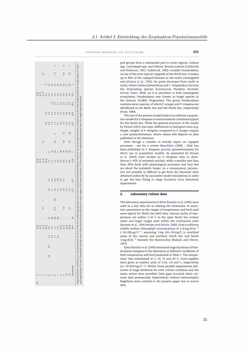
pod groups form a substantial part in some regions: Calanusspp., Centropages spp. and Oithona. Several authors (Colebrookand Robinson, 1961; Colebrook, 1982) consider Pseudocalanusas one of the most typical copepods of the North Sea: it makesup to 46% of the copepod biomass in the entire investigatedarea (Fransz et al., 1991). Its quota decreases from south tonorth, where Calanus finmarchicus and C. helgolandicus becomethe dominating species (Continuous Plankton RecorderSurvey Team, 2004). As it is abundant in both investigatedecosystems, Pseudocalanus was chosen as target species inthe German GLOBEC Programme. The genus Pseudocalanuscontains seven species, of which P. acuspes and P. elongatus aredistributed in the Baltic Sea and the North Sea, respectively(Frost, 1989).
The aim of the present model study is to calibrate a popula-tion model for P. elongatus at environmental conditions typicalfor the North Sea. While the general structure of the modelby Fennel (2001) was kept, differences in biological traits (e.g.length, weight) of P. elongatus compared to P. acuspes requirea new parameterisation, where values will depend on datapublished in the literature.
Even though a number of articles report on copepodprocesses – see for a review Mauchline (1998) – little hasbeen published on P. elongatus process parameterisation fordirect use in population models. As presented by Krauseet al. (2003) most studies on P. elongatus refer to abun-dances (∼65% of reviewed articles), while a smaller part (lessthan 30%) deals with physiological processes and very feware about the metabolic losses. As a consequence, parame-ters not possible or difficult to get from the literature wereobtained indirectly by successive model simulations in orderto get the best fitting to stage durations from laboratoryexperiments.
2. Laboratory culture data
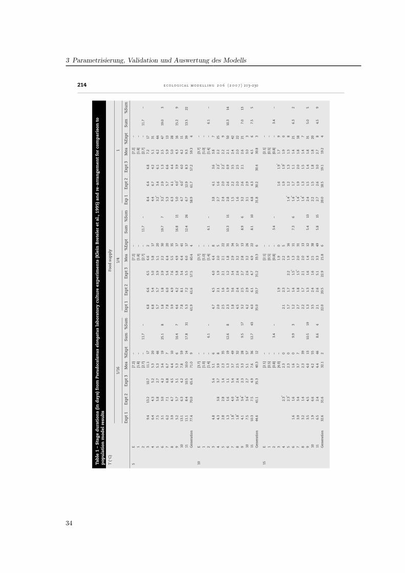
The laboratory experiments of Klein Breteler et al. (1995) wereused as a key data set in refining the estimation of uncer-tain parameters as the ranges of temperature and food usedwere typical for North Sea field data: Annual cycles of tem-perature are within 5–16 ◦C in the open North Sea surfacewater and larger ranges exist within the continental coast(Janssen et al., 1999; Becker and Schulz, 2000). Food conditionsexhibit surface chlorophyll concentrations of 1–4 mg chl m−3
(∼50–200 �g C l−1, assuming 1 mg chl = 50 mg C) in stratifiedareas of the central and northern North Sea and below1 mg chl m−3 beneath the thermocline (Radach and Patsch,1997).
Klein Breteler et al. (1995) measured stage durations of Pseu-docalanus elongatus in the laboratory at different conditions ofboth temperature and food presented in Table 1. The temper-ature was maintained at 5, 10, 15 and 20 ◦C. Food supplieswere given in relative units of 1/16, 1/4 and 1, respectively(i.e. 59–655 mg C l−1). Within three parallel experiments esti-mates of stage durations for each culture condition and themean values were provided. Data gaps occurred when cul-tures died prematurely. Experiments without heterotrophicflagellates were omitted in the present paper due to scarcedata.
35
3 Parametrisierung, Validation und Auswertung des Modells
216 e c o l o g i c a l m o d e l l i n g 2 0 6 ( 2 0 0 7 ) 213–230
Median development times of copepod life stages weredetermined as the time when 50% of the population reachedthe next stage. The generation time (D) was calculated afterKlein Breteler et al. (1995) as the sum of duration of all stages,i.e. the time from egg laying to the time when 50% of the pop-ulation had reached adulthood (stage CVI). The experimentsshowed a threefold change in generation times over the tem-perature range while the effect of food supply was reflectedby a factor of about 1.5 from saturation to a minimum of food(Table 1). Additional observations by Thompson (1982) sup-ported these findings.
3. Model concept and processparameterisation
3.1. Equation system
The original model by Fennel (2001) aimed at a consistent for-mulation of a stage resolved zooplankton model for copepodsusing universal and species-specific aspects. The model con-sists of 10 state variables with biomass (Z) and abundance (N)for each of five model stages, grouping stages to: eggs, nau-plii (NI–NVI), two copepodite stages (CI–CIII and CIV–CV) andadults (CVI). The basic approach for each model stage consistsof the following equations:
ddt
Zi = Ti−1,i · Zi−1 + gi · Zi − (�i + li) · Zi − Ti,i+1 · Zi
ddt
Ni = Ti−1,i · Ni−1 − �i · Ni − Ti,i,+1 · Ni
with rates of transfer Ti,i+1 from stage i to the next, grazing gi,mortality �i and losses li.
Stage-specific processes control the metabolism of a ‘meanindividual’ using the mean individual mass for each stage i,defined as stage biomass divided by the number of individ-uals (Zi/Ni). Thus, simulated abundances and biomasses areconnected as functions of time.
Fennel (2001) formulated stage-resolved equations for eachstate variable by employing the concept of critical masses ofCarlotti and Sciandra (1989), which defines a specific stage bya mass m within the values Xi−1 < m ≤ Xi. Thus, these criti-cal masses Xi had to be defined for each stage. Although it isknown that body weight and carbon content vary seasonallyand geographically (Krause et al., 2003), we tabulated stage-dependent dry weights from available literature and found arange of 2–5 times the minimal stage weights. Among oth-ers, three references (Klein Breteler et al., 1982; Hay et al.,1988, 1991) contain estimates of dry weights for all stages.We derived mean and extreme values from these literaturedata (Appendix A) which were used for the weight dependingfunctions of ingestion and transfer.
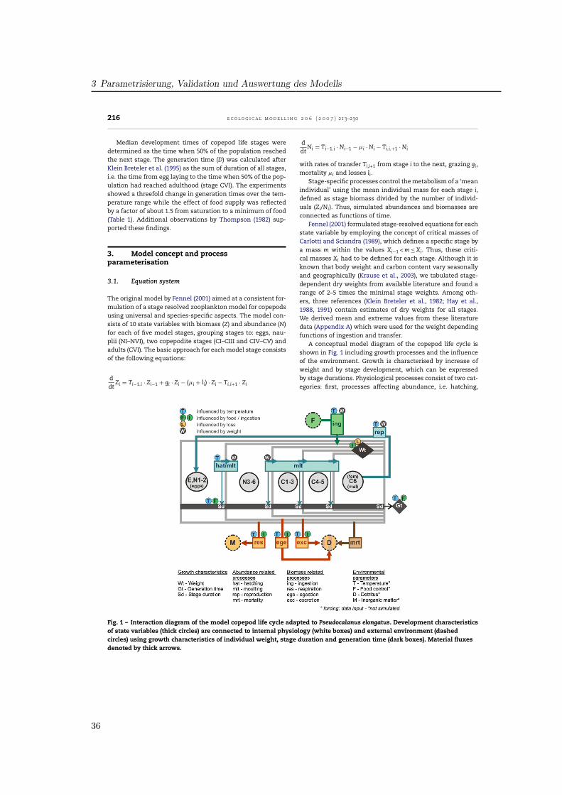
A conceptual model diagram of the copepod life cycle isshown in Fig. 1 including growth processes and the influenceof the environment. Growth is characterised by increase ofweight and by stage development, which can be expressedby stage durations. Physiological processes consist of two cat-egories: first, processes affecting abundance, i.e. hatching,
Fig. 1 – Interaction diagram of the model copepod life cycle adapted to Pseudocalanus elongatus. Development characteristicsof state variables (thick circles) are connected to internal physiology (white boxes) and external environment (dashedcircles) using growth characteristics of individual weight, stage duration and generation time (dark boxes). Material fluxesdenoted by thick arrows.
36
3.1 Artikel I: Entwicklung des Zooplankton-Populationsmodells
e c o l o g i c a l m o d e l l i n g 2 0 6 ( 2 0 0 7 ) 213–230 217
moulting and reproduction, which are controlled by weight,and mortality. Second, processes affecting only biomass.These determine stage-specific weights through gain (inges-tion) and loss (respiration, excretion and egestion) of matter.Ingestion itself is influenced by weight and depends on theenvironmental food supply and forms the population’s sourceof biomass. Temperature, directly or indirectly, influences sev-eral developmental processes. The overview in Fig. 1 illustratesthe steps of model process parameterisation. In the follow-ing subsections new parameterisations were compared to theoriginal version to show their differences. For a better com-parison the process formulas, parameter tables and resultingdiagrams were presented together in one figure.
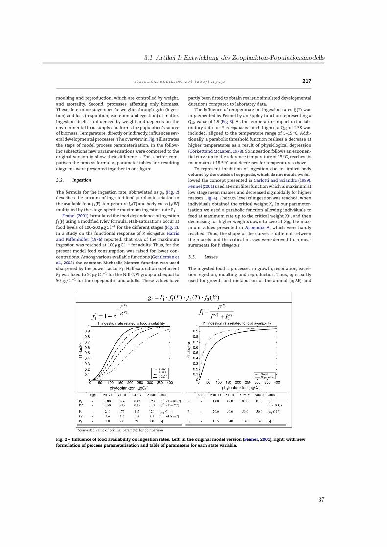
3.2. Ingestion
The formula for the ingestion rate, abbreviated as gi, (Fig. 2)describes the amount of ingested food per day in relation tothe available food f1(F), temperature f2(T) and body mass f3(W)multiplied by the stage-specific maximum ingestion rate P1.
Fennel (2001) formulated the food dependence of ingestionf1(F) using a modified Ivlev formula. Half-saturations occur atfood levels of 100–200 �g C l−1 for the different stages (Fig. 2).In a study on the functional response of P. elongatus Harrisand Paffenhofer (1976) reported, that 80% of the maximumingestion was reached at 100 �g C l−1 for adults. Thus, for thepresent model food consumption was raised for lower con-centrations. Among various available functions (Gentleman etal., 2003) the common Michaelis-Menten function was usedsharpened by the power factor P3. Half-saturation coefficientP2 was fixed to 20 �g C l−1 for the NIII-NVI group and equal to50 �g C l−1 for the copepodites and adults. These values have
partly been fitted to obtain realistic simulated developmentaldurations compared to laboratory data.
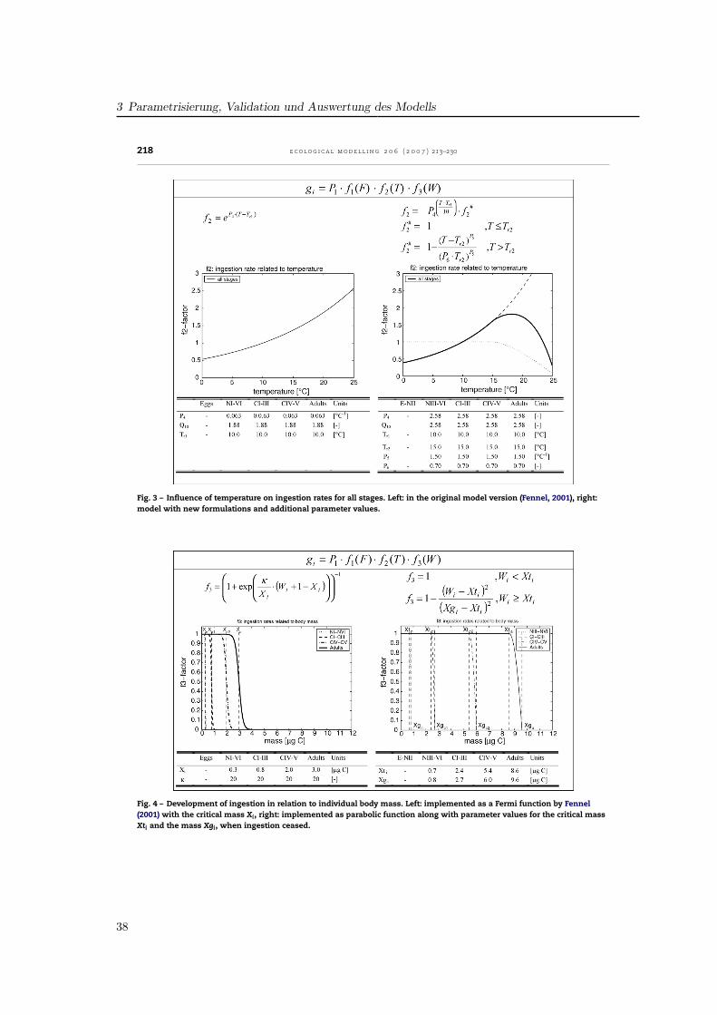
The influence of temperature on ingestion rates f2(T) wasimplemented by Fennel by an Eppley function representing aQ10-value of 1.9 (Fig. 3). As the temperature impact in the lab-oratory data for P. elongatus is much higher, a Q10 of 2.58 wasincluded, aligned to the temperature range of 5–15 ◦C. Addi-tionally, a parabolic threshold function realises a decrease athigher temperatures as a result of physiological depression(Corkett and McLaren, 1978). So, ingestion follows an exponen-tial curve up to the reference temperature of 15 ◦C, reaches itsmaximum at 18.5 ◦C and decreases for temperatures above.
To represent inhibition of ingestion due to limited bodyvolume by the cuticle of copepods, which do not moult, we fol-lowed the concept presented in Carlotti and Sciandra (1989).Fennel (2001) used a Fermi filter function which is maximum atlow stage mean masses and decreased sigmoidally for highermasses (Fig. 4). The 50% level of ingestion was reached, whenindividuals obtained the critical weight Xi. In our parameter-isation we used a parabolic function allowing individuals tofeed at maximum rate up to the critical weight Xti, and thendecreasing for higher weights down to zero at Xgi, the max-imum values presented in Appendix A, which were hardlyreached. Thus, the shape of the curves is different betweenthe models and the critical masses were derived from mea-surements for P. elongatus.
3.3. Losses
The ingested food is processed in growth, respiration, excre-tion, egestion, moulting and reproduction. Thus, gi is partlyused for growth and metabolism of the animal (gi·AE) and
Fig. 2 – Influence of food availability on ingestion rates. Left: in the original model version (Fennel, 2001), right: with newformulation of process parameterisation and table of parameters for each state variable.
37
3 Parametrisierung, Validation und Auswertung des Modells
218 e c o l o g i c a l m o d e l l i n g 2 0 6 ( 2 0 0 7 ) 213–230
Fig. 3 – Influence of temperature on ingestion rates for all stages. Left: in the original model version (Fennel, 2001), right:model with new formulations and additional parameter values.
Fig. 4 – Development of ingestion in relation to individual body mass. Left: implemented as a Fermi function by Fennel(2001) with the critical mass Xi, right: implemented as parabolic function along with parameter values for the critical massXti and the mass Xgi, when ingestion ceased.
38
3.1 Artikel I: Entwicklung des Zooplankton-Populationsmodells
e c o l o g i c a l m o d e l l i n g 2 0 6 ( 2 0 0 7 ) 213–230 219
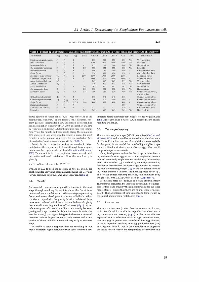
Table 2 – Species-specific parameter values for Pseudocalanus elongatus in the present model and their grade of sensitivity
Parameter Sig. Fct. Fig. E-NII NIII–VI CI–III CIV–V CVI Test Sensitivity
Maximum ingestion rate P1 f1 2 – 1.00 0.60 0.50 0.30 Yes Very sensitiveHalf saturation P2 f1 2 – 20.00 50.00 50.00 50.00 Yes SensiblePower coefficient P3 f1 2 – 1.15 1.40 1.40 1.40 Yes Not sensitiveQ10-parameter ingestion P4 f2 3 3.60 2.58 2.58 2.58 2.58 Yes SensiblePower coefficient P5 f2 3 – 1.50 1.50 1.50 1.50 – Curve fitted to dataSlope factor P6 f2 3 – 0.70 0.70 0.70 0.70 – Curve fitted to dataReference temperature Tr1 f2, li 3 10.00 10.00 10.00 10.00 10.00 – Reference valueReference temperature Tr2 f2 3 – 15.00 15.00 15.00 15.00 – Reference valueAssimilation efficiency AE li – – 0.65 0.65 0.65 0.55 Yes Very sensitiveActive Metabolism RA li – – 0.40 0.33 0.33 0.28 Yes Very sensitiveBasal Metabolism RB li – 0.07 0.05 0.02 0.02 0.02 Yes Not sensitiveQ10-parameter loss Q li – 3.60 2.58 2.58 2.58 2.58 Yes Not sensitiveReference mass Rti f4 5, 7 0.14 0.50 1.80 4.30 7.50 Yes Considered as robust,
not sensitiveCritical moulting mass Xti f3 4 – 0.70 2.40 5.40 8.60 – Considered as robustCritical ingestion mass Xgi f3, f4 4, 5, 7 – 0.80 2.70 6.00 9.60 – Considered as robustSlope factor P7 f4, Tnf 5, 6, 7 6.00 4.00 4.00 4.00 4.00 – Considered as robustMaximum biomass P8 R 7 – – – – 0.80 – Considered as robustReproductive females P9 R 7 – – – – 0.30 – Curve fitted to dataMortality �i – – 0.03 0.03 0.03 0.03 0.03 Yes Not sensitive
partly egested as faecal pellets (gi·(1 − AE)), where AE is theassimilation efficiency. For the losses Fennel assumed con-stant quotas of ingested food: 35% as egestion (correspondingto an assimilation efficiency of 65%), 10% as excretion and 10%by respiration, and about 15% for the moulting process, in total70%. Thus, for nauplii and copepodite stages the remaining30% of ingested food were used for growth whereas for adultfemales a higher amount is invested for egg production (see‘Reproduction’) and less goes to growth (see Table 2).
Beside the direct impact of feeding on loss due to activemetabolism, there are evidently losses through basal respira-tion when the copepods do not feed (Carlotti and Sciandra,1989). To realise this fact, the respiration losses were dividedinto active and basal metabolism. Thus, the total loss, li, isgiven by:
li = (1 − AE) · gi + (RA · gi + RB · Q (T−Tr1)/10)
with AE of 0.65 to keep the egestion at 0.35. RA and RB arecoefficients for active and basal metabolism and the Q10 value(Q) was assumed to be the same as for ingestion (Table 2).
3.4. Transfer
An essential consequence of growth is transfer to the nextstage through moulting. Fennel introduced the Fermi func-tion to realise a smooth transfer to the next stage representingfaster and slower development of some individuals. Whentransfer is coupled with the grazing function both Fermi func-tions were combined, which leads to a double threshold givingjust a small ‘moulting window’ of low rates (Fig. 5). As noreference gives information on direct relationship betweengrazing and stage transfer this is left out in our formula. TheFermi function f6 is of sigmoidal type which starts at zero andbecomes positive for positive mean body masses and a pro-portion of these individuals moulted very early to the nextstage.
To enable a certain response time for moulting, in ourmodel a different sigmoidal function was used. Transfer is now
inhibited before the subsequent stage reference weight Rti (seeTable 2) is reached and a rate of 50% is assigned at the criticalmoulting weight Xti.
3.5. The non-feeding group
The first two naupliar stages (NI/NII) do not feed (Corkett andMcLaren, 1978) and should be separated from the older nau-plii. To avoid the introduction of an additional state variablefor this group, in our model the non-feeding naupliar stageswere combined with the state variable for eggs. The naupliicomprise stages NIII–NVI only.
Thus, development within the first stage includes hatch-ing and transfer from eggs to NII. Due to respiration losses areduced mean body weight was assumed during this develop-ment. The transfer (Tnf) is defined by the weight-dependingfunction as described for the other stages but with an increas-ing rate at decreasing weight (Fig. 6). For the reference valueRtnf, when transfer is initiated, the mean egg mass of 0.14 �g Cand for the critical moulting mass Xtnf the minimum bodyweight of NII with 0.10 �g C were used (see Appendix A).
Respiration rates are difficult to obtain experimentally.Therefore we calculated the loss term depending on tempera-ture for this stage group by the same formula as for the othermodel stages—except that there are no ingestion terms (i.e.gnf = 0). Thus, development time is related to temperature bythe impact of embryonic metabolism (Fig. 6).
3.6. Reproduction
The reproduction rate (R) describes the amount of biomass,which female adults provide for reproduction when reach-ing the maturation mass Rta (Fig. 7). In the model this wasexpressed as a transfer from adults to eggs. Fennel assumed,that 30% (P8) of growth was transferred into egg biomass,i.e. 6% of ingestion, resulting in an egg production rate (EPR)of <1 egg fem−1 day−1. Due to the dependence on ingestionthe EPR is related to food and temperature. For Pseudocalanus
39
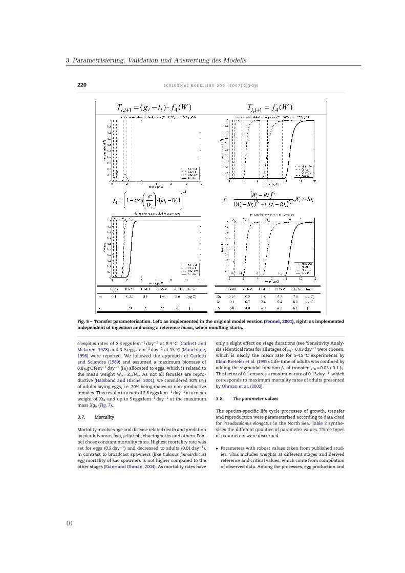
3 Parametrisierung, Validation und Auswertung des Modells
220 e c o l o g i c a l m o d e l l i n g 2 0 6 ( 2 0 0 7 ) 213–230
Fig. 5 – Transfer parameterisation. Left: as implemented in the original model version (Fennel, 2001), right: as implementedindependent of ingestion and using a reference mass, when moulting starts.
elongatus rates of 2.3 eggs fem−1 day−1 at 8.4 ◦C (Corkett andMcLaren, 1978) and 3–5 eggs fem−1 day−1 at 15 ◦C (Mauchline,1998) were reported. We followed the approach of Carlottiand Sciandra (1989) and assumed a maximum biomass of0.8 �g C fem−1 day−1 (P8) allocated to eggs, which is related tothe mean weight Wa = Za/Na. As not all females are repro-ductive (Halsband and Hirche, 2001), we considered 30% (P9)of adults laying eggs, i.e. 70% being males or non-productivefemales. This results in a rate of 2.8 eggs fem−1 day−1 at a meanweight of Xta and up to 5 eggs fem−1 day−1 at the maximummass Xga (Fig. 7).
3.7. Mortality
Mortality involves age and disease related death and predationby planktivorous fish, jelly fish, chaetognaths and others. Fen-nel chose constant mortality rates. Highest mortality rate wasset for eggs (0.2 day−1) and decreased to adults (0.01 day−1).In contrast to broadcast spawners (like Calanus finmarchicus)egg mortality of sac spawners is not higher compared to theother stages (Eiane and Ohman, 2004). As mortality rates have
only a slight effect on stage durations (see ‘Sensitivity Analy-sis’) identical rates for all stages of �i = 0.03 day−1 were chosen,which is nearly the mean rate for 5–15 ◦C experiments byKlein Breteler et al. (1995). Life-time of adults was confined byadding the sigmoidal function f4 of transfer: �a = 0.03 + 0.1·f4.The factor of 0.1 ensures a maximum rate of 0.13 day−1, whichcorresponds to maximum mortality rates of adults presentedby Ohman et al. (2002).
3.8. The parameter values
The species-specific life cycle processes of growth, transferand reproduction were parameterised according to data citedfor Pseudocalanus elongatus in the North Sea. Table 2 synthe-sizes the different qualities of parameter values. Three typesof parameters were discerned:
• Parameters with robust values taken from published stud-ies. This includes weights at different stages and derivedreference and critical values, which come from compilationof observed data. Among the processes, egg production and
40
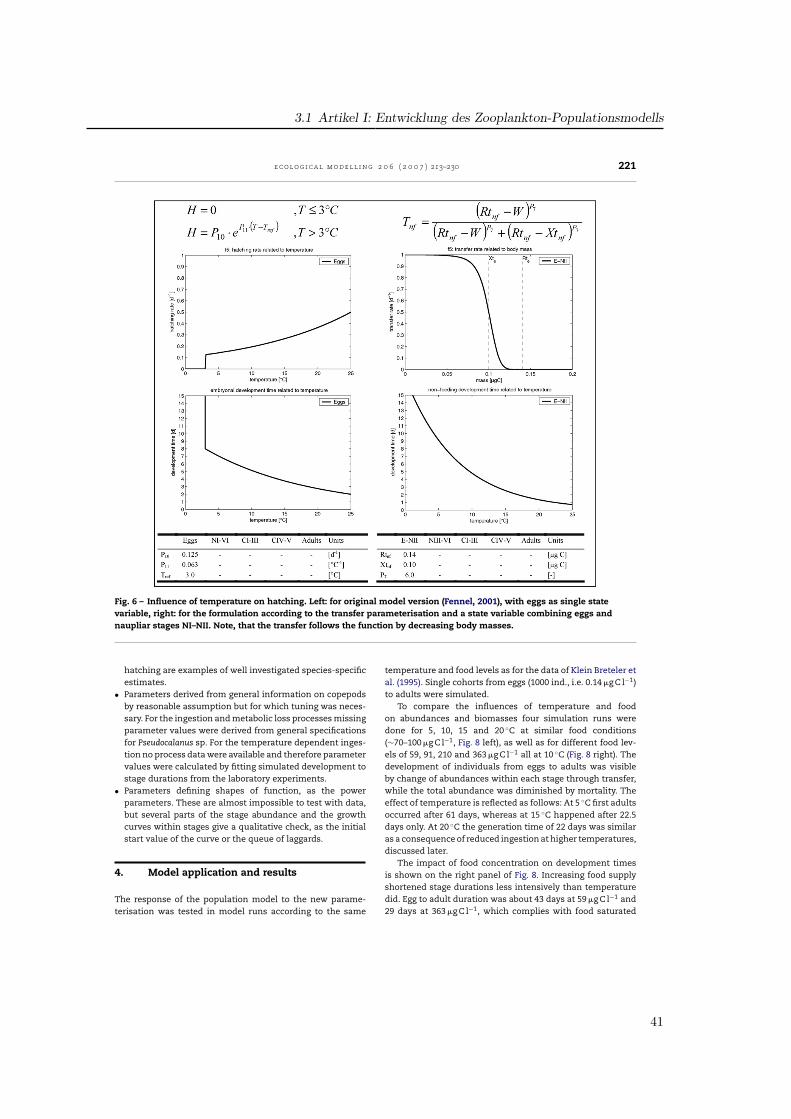
3.1 Artikel I: Entwicklung des Zooplankton-Populationsmodells
e c o l o g i c a l m o d e l l i n g 2 0 6 ( 2 0 0 7 ) 213–230 221
Fig. 6 – Influence of temperature on hatching. Left: for original model version (Fennel, 2001), with eggs as single statevariable, right: for the formulation according to the transfer parameterisation and a state variable combining eggs andnaupliar stages NI–NII. Note, that the transfer follows the function by decreasing body masses.
hatching are examples of well investigated species-specificestimates.
• Parameters derived from general information on copepodsby reasonable assumption but for which tuning was neces-sary. For the ingestion and metabolic loss processes missingparameter values were derived from general specificationsfor Pseudocalanus sp. For the temperature dependent inges-tion no process data were available and therefore parametervalues were calculated by fitting simulated development tostage durations from the laboratory experiments.
• Parameters defining shapes of function, as the powerparameters. These are almost impossible to test with data,but several parts of the stage abundance and the growthcurves within stages give a qualitative check, as the initialstart value of the curve or the queue of laggards.
4. Model application and results
The response of the population model to the new parame-terisation was tested in model runs according to the same
temperature and food levels as for the data of Klein Breteler etal. (1995). Single cohorts from eggs (1000 ind., i.e. 0.14 �g C l−1)to adults were simulated.
To compare the influences of temperature and foodon abundances and biomasses four simulation runs weredone for 5, 10, 15 and 20 ◦C at similar food conditions(∼70–100 �g C l−1, Fig. 8 left), as well as for different food lev-els of 59, 91, 210 and 363 �g C l−1 all at 10 ◦C (Fig. 8 right). Thedevelopment of individuals from eggs to adults was visibleby change of abundances within each stage through transfer,while the total abundance was diminished by mortality. Theeffect of temperature is reflected as follows: At 5 ◦C first adultsoccurred after 61 days, whereas at 15 ◦C happened after 22.5days only. At 20 ◦C the generation time of 22 days was similaras a consequence of reduced ingestion at higher temperatures,discussed later.
The impact of food concentration on development timesis shown on the right panel of Fig. 8. Increasing food supplyshortened stage durations less intensively than temperaturedid. Egg to adult duration was about 43 days at 59 �g C l−1 and29 days at 363 �g C l−1, which complies with food saturated
41
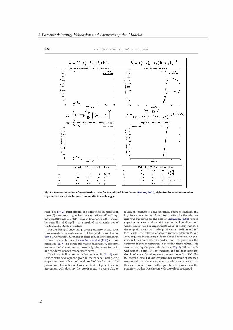
3 Parametrisierung, Validation und Auswertung des Modells
222 e c o l o g i c a l m o d e l l i n g 2 0 6 ( 2 0 0 7 ) 213–230
Fig. 7 – Parameterisation of reproduction. Left: for the original formulation (Fennel, 2001), right: for the new formulationrepresented as a transfer rate from adults to viable eggs.
rates (see Fig. 2). Furthermore, the differences in generationtimes (D) were less at higher food concentrations (�D = ∼2 daysbetween 210 and 363 �g C l−1) than at lower ones (�D = ∼7 daysbetween 59 and 91 �g C l−1) as a result of parameterisation ofthe Michaelis-Menten function.
For the fitting of uncertain process parameters simulationruns were done for each scenario of temperature and food ofTable 1. Cumulated durations of stage-groups were comparedto the experimental data of Klein Breteler et al. (1995) and pre-sented in Fig. 9. The parameter values calibrated by this dataset were the half-saturation constant P2, the power factor P3
and the dome-shaped temperature curve.The lower half-saturation value for nauplii (Fig. 2) con-
formed with development given in the data set. Comparingstage durations at low and medium food level at 15 ◦C theproportion of naupliar and copepodite development was inagreement with data. By the power factor we were able to
reduce differences in stage durations between medium andhigh food concentration. This fitted function for the relation-ship was supported by the data of Thompson (1982), whoseexperiments were all done at the same food condition andwhich, except for her experiments at 20 ◦C nearly matchedthe stage durations our model produced at medium and fullfood levels. The relation of stage durations between 15 and20 ◦C required introducing a dome-shaped function. As gen-eration times were nearly equal at both temperatures theoptimum ingestion appeared to be within these values. Thiswas realised by the parabolic function (Fig. 3). While the fitwas best at 10 and 15 ◦C for medium and full food supplies,simulated stage durations were underestimated at 5 ◦C. TheQ10 seemed invalid at low temperatures. However, at low foodconcentration again the function nearly fitted the data. Asthis scenario is relevant with regard to field simulations, theparameterisation was chosen with the values presented.
42
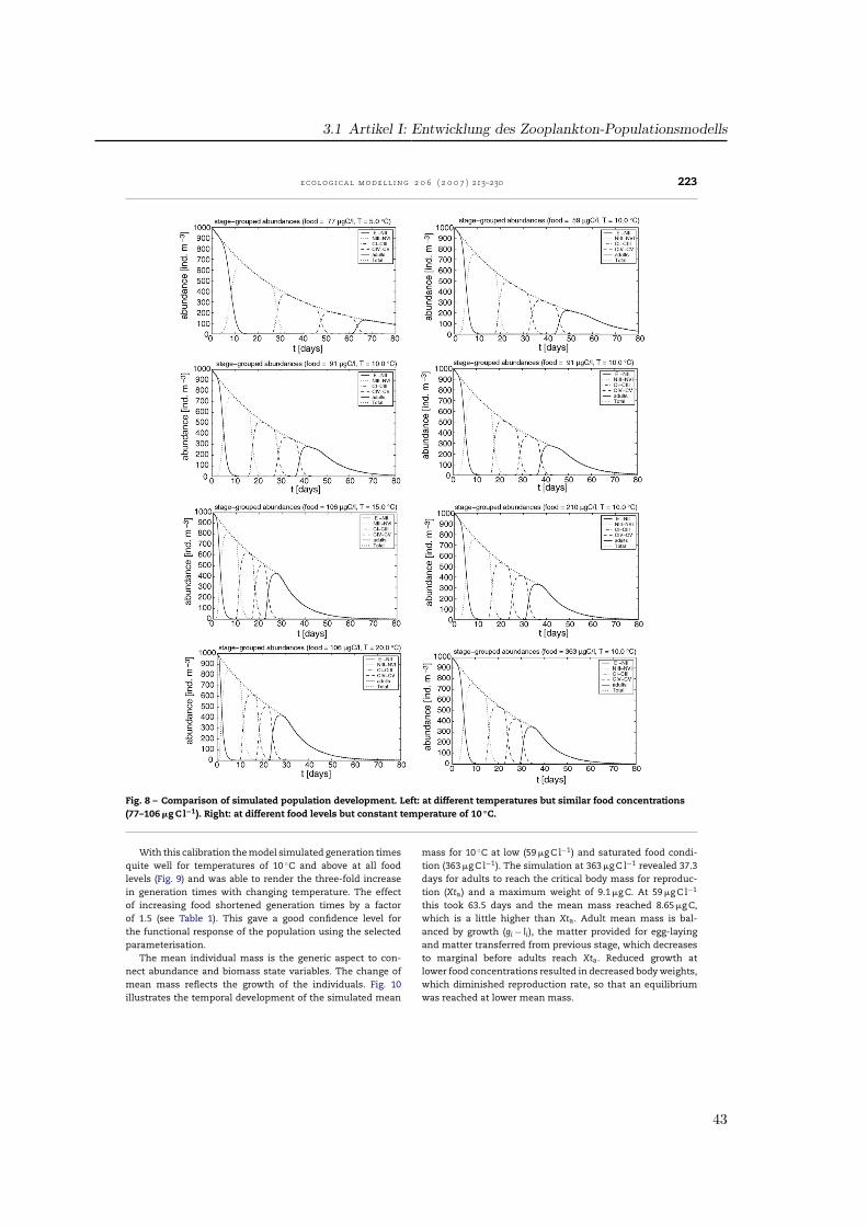
3.1 Artikel I: Entwicklung des Zooplankton-Populationsmodells
e c o l o g i c a l m o d e l l i n g 2 0 6 ( 2 0 0 7 ) 213–230 223
Fig. 8 – Comparison of simulated population development. Left: at different temperatures but similar food concentrations(77–106 �g C l−1). Right: at different food levels but constant temperature of 10 ◦C.
With this calibration the model simulated generation timesquite well for temperatures of 10 ◦C and above at all foodlevels (Fig. 9) and was able to render the three-fold increasein generation times with changing temperature. The effectof increasing food shortened generation times by a factorof 1.5 (see Table 1). This gave a good confidence level forthe functional response of the population using the selectedparameterisation.
The mean individual mass is the generic aspect to con-nect abundance and biomass state variables. The change ofmean mass reflects the growth of the individuals. Fig. 10illustrates the temporal development of the simulated mean
mass for 10 ◦C at low (59 �g C l−1) and saturated food condi-tion (363 �g C l−1). The simulation at 363 �g C l−1 revealed 37.3days for adults to reach the critical body mass for reproduc-tion (Xta) and a maximum weight of 9.1 �g C. At 59 �g C l−1
this took 63.5 days and the mean mass reached 8.65 �g C,which is a little higher than Xta. Adult mean mass is bal-anced by growth (gi − li), the matter provided for egg-layingand matter transferred from previous stage, which decreasesto marginal before adults reach Xta. Reduced growth atlower food concentrations resulted in decreased body weights,which diminished reproduction rate, so that an equilibriumwas reached at lower mean mass.
43
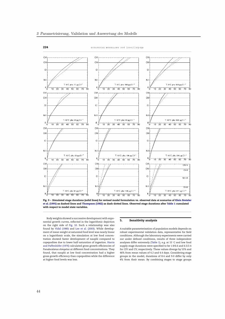
3 Parametrisierung, Validation und Auswertung des Modells
224 e c o l o g i c a l m o d e l l i n g 2 0 6 ( 2 0 0 7 ) 213–230
Fig. 9 – Simulated stage durations (solid lines) for revised model formulation vs. observed data at scenarios of Klein Breteleret al. (1995) as dashed lines and Thompson (1982) as dash-dotted lines. Observed stage durations after Table 1 cumulatedwith respect to model state variables.
Body weights showed a successive development with expo-nential growth curves, reflected in the logarithmic depictionon the right side of Fig. 10. Such a relationship was alsofound by Vidal (1980) and Lee et al. (2003). While develop-ment of mean weight at saturated food level was nearly linearon a logarithmic scale, the simulation at low food concen-tration showed faster development of nauplii compared tocopepodites due to lower half-saturation of ingestion. Harrisand Paffenhofer (1976) calculated gross growth efficiencies ofPseudocalanus elongatus at different food concentrations. Theyfound, that nauplii at low food concentration had a highergross growth efficiency than copepodites while the differenceat higher food levels was less.
5. Sensitivity analysis
A suitable parameterisation of population models depends onrobust experimental validation data, representative for fieldconditions. Although the laboratory experiments were carriedout under defined conditions, results of three independentanalyses differ extremely (Table 1), e.g. at 15 ◦C and low foodsupply stage durations were specified to be 1.9/6.6 and 6.5/2.4for CIV and CV, respectively. These values diverge by 55% and46% from mean values of 4.2 and 4.4 days. Considering stagegroups in the model, durations of 8.4 and 9.0 differ by only4% from their mean. By combining stages to stage groups
44
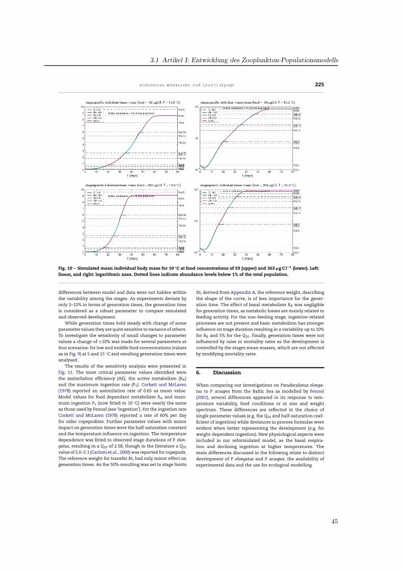
3.1 Artikel I: Entwicklung des Zooplankton-Populationsmodells
e c o l o g i c a l m o d e l l i n g 2 0 6 ( 2 0 0 7 ) 213–230 225
Fig. 10 – Simulated mean individual body mass for 10 ◦C at food concentrations of 59 (upper) and 363 �g C l−1 (lower). Left:linear, and right: logarithmic axes. Dotted lines indicate abundance levels below 1% of the total population.
differences between model and data were not hidden withinthe variability among the stages. As experiments deviate byonly 2–12% in terms of generation times, the generation timeis considered as a robust parameter to compare simulatedand observed development.
While generation times hold steady with change of someparameter values they are quite sensitive to variance of others.To investigate the sensitivity of small changes to parametervalues a change of ±10% was made for several parameters atfour scenarios: for low and middle food concentrations (valuesas in Fig. 9) at 5 and 15 ◦C and resulting generation times wereanalysed.
The results of the sensitivity analysis were presented inFig. 11. The most critical parameter values identified werethe assimilation efficiency (AE), the active metabolism (RA)and the maximum ingestion rate (P1). Corkett and McLaren(1978) reported an assimilation rate of 0.65 as mean value.Model values for food dependant metabolism RA and maxi-mum ingestion P1 (now fitted to 10 ◦C) were nearly the sameas those used by Fennel (see ‘Ingestion’). For the ingestion rateCorkett and McLaren (1978) reported a rate of 60% per dayfor older copepodites. Further parameter values with minorimpact on generation times were the half-saturation constantand the temperature influence on ingestion. The temperaturedependence was fitted to observed stage durations of P. elon-gatus, resulting in a Q10 of 2.58, though in the literature a Q10
value of 2.0–2.1 (Carlotti et al., 2000) was reported for copepods.The reference weight for transfer Rti had only minor effect ongeneration times. As the 50%-moulting was set to stage limits
Xti derived from Appendix A, the reference weight, describingthe shape of the curve, is of less importance for the gener-ation time. The effect of basal metabolism RB was negligiblefor generation times, as metabolic losses are mainly related tofeeding activity. For the non-feeding stage, ingestion-relatedprocesses are not present and basic metabolism has strongerinfluence on stage duration resulting in a variability up to 10%for RB and 5% for the Q10. Finally, generation times were notinfluenced by raise in mortality rates as the development iscontrolled by the stages mean masses, which are not affectedby modifying mortality rates.
6. Discussion
When comparing our investigations on Pseudocalanus elonga-tus to P. acuspes from the Baltic Sea as modelled by Fennel(2001), several differences appeared in its response to tem-perature variability, food conditions or in size and weightspectrum. These differences are reflected in the choice ofsingle parameter values (e.g. the Q10 and half-saturation coef-ficient of ingestion) while deviances in process formulae wereevident when better representing the development (e.g. forweight-dependent ingestion). New physiological aspects wereincluded in our reformulated model, as the basal respira-tion and declining ingestion at higher temperatures. Themain differences discussed in the following relate to distinctdevelopment of P. elongatus and P. acuspes, the availability ofexperimental data and the use for ecological modelling.
45
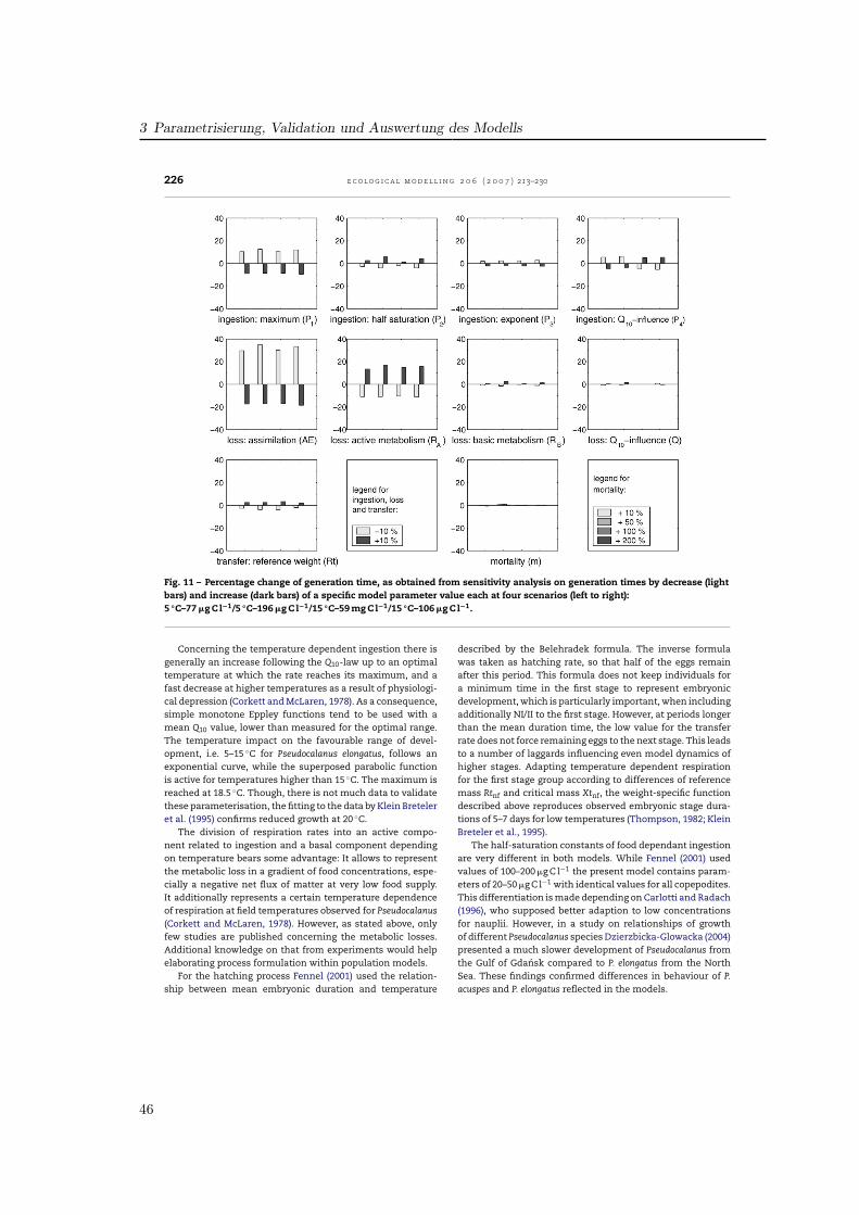
3 Parametrisierung, Validation und Auswertung des Modells
226 e c o l o g i c a l m o d e l l i n g 2 0 6 ( 2 0 0 7 ) 213–230
Fig. 11 – Percentage change of generation time, as obtained from sensitivity analysis on generation times by decrease (lightbars) and increase (dark bars) of a specific model parameter value each at four scenarios (left to right):5 ◦C–77 �g C l−1/5 ◦C–196 �g C l−1/15 ◦C–59 mg C l−1/15 ◦C–106 �g C l−1.
Concerning the temperature dependent ingestion there isgenerally an increase following the Q10-law up to an optimaltemperature at which the rate reaches its maximum, and afast decrease at higher temperatures as a result of physiologi-cal depression (Corkett and McLaren, 1978). As a consequence,simple monotone Eppley functions tend to be used with amean Q10 value, lower than measured for the optimal range.The temperature impact on the favourable range of devel-opment, i.e. 5–15 ◦C for Pseudocalanus elongatus, follows anexponential curve, while the superposed parabolic functionis active for temperatures higher than 15 ◦C. The maximum isreached at 18.5 ◦C. Though, there is not much data to validatethese parameterisation, the fitting to the data by Klein Breteleret al. (1995) confirms reduced growth at 20 ◦C.
The division of respiration rates into an active compo-nent related to ingestion and a basal component dependingon temperature bears some advantage: It allows to representthe metabolic loss in a gradient of food concentrations, espe-cially a negative net flux of matter at very low food supply.It additionally represents a certain temperature dependenceof respiration at field temperatures observed for Pseudocalanus(Corkett and McLaren, 1978). However, as stated above, onlyfew studies are published concerning the metabolic losses.Additional knowledge on that from experiments would helpelaborating process formulation within population models.
For the hatching process Fennel (2001) used the relation-ship between mean embryonic duration and temperature
described by the Belehradek formula. The inverse formulawas taken as hatching rate, so that half of the eggs remainafter this period. This formula does not keep individuals fora minimum time in the first stage to represent embryonicdevelopment, which is particularly important, when includingadditionally NI/II to the first stage. However, at periods longerthan the mean duration time, the low value for the transferrate does not force remaining eggs to the next stage. This leadsto a number of laggards influencing even model dynamics ofhigher stages. Adapting temperature dependent respirationfor the first stage group according to differences of referencemass Rtnf and critical mass Xtnf, the weight-specific functiondescribed above reproduces observed embryonic stage dura-tions of 5–7 days for low temperatures (Thompson, 1982; KleinBreteler et al., 1995).
The half-saturation constants of food dependant ingestionare very different in both models. While Fennel (2001) usedvalues of 100–200 �g C l−1 the present model contains param-eters of 20–50 �g C l−1 with identical values for all copepodites.This differentiation is made depending on Carlotti and Radach(1996), who supposed better adaption to low concentrationsfor nauplii. However, in a study on relationships of growthof different Pseudocalanus species Dzierzbicka-Glowacka (2004)presented a much slower development of Pseudocalanus fromthe Gulf of Gdansk compared to P. elongatus from the NorthSea. These findings confirmed differences in behaviour of P.acuspes and P. elongatus reflected in the models.
46
3.1 Artikel I: Entwicklung des Zooplankton-Populationsmodells
e c o l o g i c a l m o d e l l i n g 2 0 6 ( 2 0 0 7 ) 213–230 227
The dome-shaped temperature dependence and the basalmetabolism construct higher complexity of physiologicalbehaviour and allow realistic development at conditions withcertain interest for implementation into ecosystem models: athigh temperatures, found in coastal regions in summer, devel-opment is extenuated to prevent disproportionate increaseof the population. At low food concentrations, present fora large period within the annual cycle, growth is not onlyrelated to food through dependence on ingestion, but lossterms are included and thereby growth is influenced by tem-perature. The set of five model stages to represent the full lifecycle (Fig. 1), and using improved process descriptions adaptedto environmental conditions in the North Sea, allows goodrepresentation of the population dynamics of Pseudocalanuselongatus in our model.
7. Conclusion
This paper presents a comprehensive description on param-eterisation of a zero-dimensional population model forPseudocalanus elongatus to represent realistic development.The universal model formulations for a typical copepod lifecycle were adopted from Fennel (2001). Following the con-cept of critical moulting masses these masses were derivedfor all state variables from cited North Sea observations. Thespecies-specific life cycle processes of growth, transfer andreproduction were parameterised according to data cited forthe North Sea, when available. Other formulations, e.g. thehalf-saturation constant and ingestion at higher tempera-ture, were calibrated using laboratory experiments from KleinBreteler et al. (1995), which determined generation times atdifferent temperatures and food conditions. The generationtime is found to be a useful indicator for estimating the qualityof the simulation.
While egg production and hatching were examples forwell investigated species-specific processes, measurementsfor metabolic losses to assign parameter values were sparse.
As the model is quite sensitive to these metabolic processesas well as to the maximum ingestion new measurements ofthese processes would be worthwhile to check their param-eter values. For the present model these were derived fromgeneral specifications for Pseudocalanus sp. However, species ofthe same genus display differences in development and phys-iological behaviour. This was depicted, when comparing theparameterisation of the present model to the model by Fennel(2001), which was related to Pseudocalanus from the Baltic Sea.Differences in weight and physiology between the two species,suggested by the synthesis of laboratory culture data and thesimulations, may explain their distinct life cycle development,factors which have consequences for their role in the foodweb dynamics. Experimental evidence should be sought todemonstrate such differences between these species.
The next step in our modelling work is to verify total abun-dance and biomass levels under real environmental forcingconditions. Since food concentration is included as constantforcing value, its response to varying grazing pressure of thepopulation is not represented here. This has to be done byrunning the population model within an ecosystem model tostudy the impact of seasonal variations of food and tempera-ture in the North Sea.
Acknowledgements
We particularly thank Prof. Wolfgang Fennel for passing onand introducing the code of his population model, allow-ing work and changes to it. We acknowledge the help of Dr.Michael Krause for deriving the body weight table and Dr.W.C.M. Klein Breteler for statements on the data. This workwas done within the GLOBEC Germany project funded bythe BMBF (03F0320E). We thank the DAAD for financial sup-port in travelling within the French-German PROCOPE project(D/0205749). We finally appreciate the extensive textual andlinguistic annotations of Rev. #1, which helped improving thetext.
47
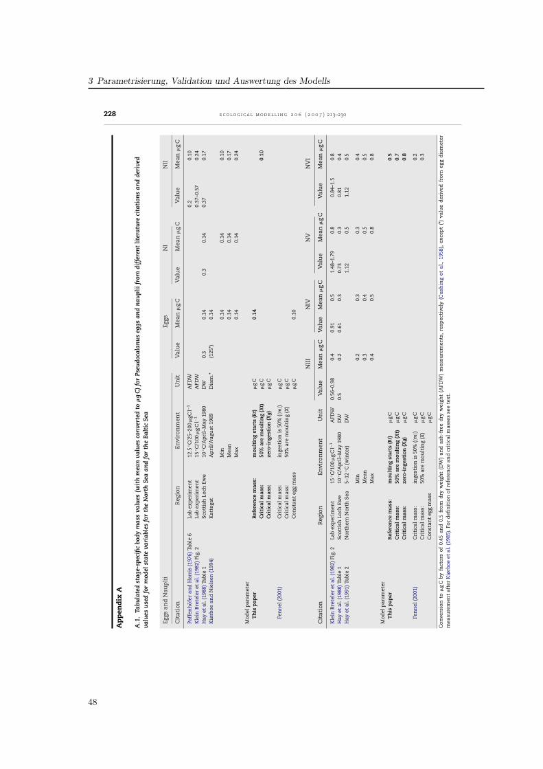
3 Parametrisierung, Validation und Auswertung des Modells
228 e c o l o g i c a l m o d e l l i n g 2 0 6 ( 2 0 0 7 ) 213–230A
pp
end
ixA
A.1
.Ta
bula
ted
stag
e-sp
ecifi
cbo
dym
ass
valu
es(w
ith
mea
nva
lues
conv
erte
dto
�g
C)
for
Pseu
doca
lan
us
eggs
and
nau
plii
from
diff
eren
tlit
erat
ure
cita
tion
san
dde
rive
dva
lues
use
dfo
rm
odel
stat
eva
riab
les
for
the
Nor
thSe
aan
dfo
rth
eBa
ltic
Sea
Eggs
and
Nau
pli
iEg
gsN
IN
II
Cit
atio
nR
egio
nEn
viro
nm
ent
Un
itV
alu
eM
ean
�g
CV
alu
eM
ean
�g
CV
alu
eM
ean
�g
C
Paff
enh
ofer
and
Har
ris
(197
6)Ta
ble
6La
bex
per
imen
t12
.5◦ C
/25–
200
�gC
l−1
AFD
W0.
20.
10K
lein
Bre
tele
ret
al.(
1982
)Fig
.2La
bex
per
imen
t15
◦ C/1
00�
gC
l−1
AFD
W0.
37–0
.57
0.24
Hay
etal
.(19
88)T
able
1Sc
otti
shLo
chEw
e10
◦ C/A
pri
l–M
ay19
80D
W0.
30.
140.
30.
140.
370.
17K
iørb
oean
dN
iels
en(1
994)
Kat
tega
tA
pri
l/A
ugu
st19
89D
iam
.*(1
25*)
0.14
Min
0.14
0.14
0.10
Mea
n0.
140.
140.
17M
ax0.
140.
140.
24
Mod
elp
aram
eter
Th
isp
aper
Ref
eren
cem
ass:
mou
ltin
gst
arts
(Rt)
�g
C0.
14C
riti
cal
mas
s:50
%ar
em
oult
ing
(Xt)
�g
C0.
10C
riti
cal
mas
s:ze
ro-i
nge
stio
n(X
g)�
gC
Fen
nel
(200
1)C
riti
calm
ass:
inge
stio
nis
50%
(〈m〉)
�g
CC
riti
calm
ass:
50%
are
mou
ltin
g(X
)�
gC
Con
stan
teg
gm
ass
�g
C0.
10
NII
IN
IVN
VN
VI
Cit
atio
nR
egio
nEn
viro
nm
ent
Un
itV
alu
eM
ean
�g
CV
alu
eM
ean
�g
CV
alu
eM
ean
�g
CV
alu
eM
ean
�g
C
Kle
inB
rete
ler
etal
.(19
82)F
ig.2
Lab
exp
erim
ent
15◦ C
/100
�g
Cl−
1A
FDW
0.56
–0.9
80.
40.
910.
51.
48–1
.79
0.8
0.84
–1.5
0.8
Hay
etal
.(19
88)T
able
1Sc
otti
shLo
chEw
e10
◦ C/A
pri
l–M
ay19
80D
W0.
50.
20.
610.
30.
730.
30.
810.
4H
ayet
al.(
1991
)Tab
le2
Nor
ther
nN
orth
Sea
5–12
◦ C(w
inte
r)D
W1.
120.
51.
120.
5
Min
0.2
0.3
0.3
0.4
Mea
n0.
30.
40.
50.
5M
ax0.
40.
50.
80.
8
Mod
elp
aram
eter
Th
isp
aper
Ref
eren
cem
ass:
mou
ltin
gst
arts
(Rt)
�g
C0.
5C
riti
cal
mas
s:50
%ar
em
oult
ing
(Xt)
�g
C0.
7C
riti
cal
mas
s:ze
ro-i
nge
stio
n(X
g)�
gC
0.8
Fen
nel
(200
1)C
riti
calm
ass:
inge
stio
nis
50%
(〈m〉)
�g
C0.
2C
riti
calm
ass:
50%
are
mou
ltin
g(X
)�
gC
0.3
Con
stan
teg
gm
ass
�g
C
Con
vers
ion
to�
gC
byfa
ctor
sof
0.45
and
0.5
from
dry
wei
ght
(DW
)an
das
h-f
ree
dry
wei
ght
(AFD
W)
mea
sure
men
ts,
resp
ecti
vely
(Cu
shin
get
al.,
1958
),ex
cep
t(*
)va
lue
der
ived
from
egg
dia
met
erm
easu
rem
ent
afte
rK
iørb
oeet
al.(
1985
).Fo
rd
efin
itio
nof
refe
ren
cean
dcr
itic
alm
asse
sse
ete
xt.
48
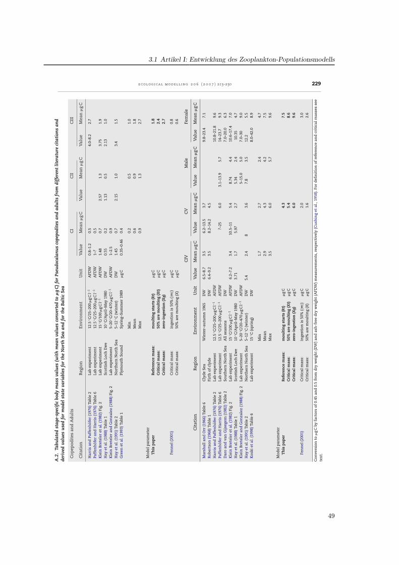
3.1 Artikel I: Entwicklung des Zooplankton-Populationsmodells
e c o l o g i c a l m o d e l l i n g 2 0 6 ( 2 0 0 7 ) 213–230 229
A.2
.Ta
bula
ted
stag
e-sp
ecifi
cbo
dym
ass
valu
es(w
ith
mea
nva
lues
conv
erte
dto
�g
C)
for
Pseu
doca
lan
us
cope
podi
tes
and
adu
lts
from
diff
eren
tlit
erat
ure
cita
tion
san
dde
rive
dva
lues
use
dfo
rm
odel
stat
eva
riab
les
for
the
Nor
thSe
aan
dfo
rth
eBa
ltic
Sea
Cop
epod
ites
and
Ad
ult
sC
IC
IIC
III
Cit
atio
nR
egio
nEn
viro
nm
ent
Un
itV
alu
eM
ean
�g
CV
alu
eM
ean
�g
CV
alu
eM
ean
�g
C
Har
ris
and
Paff
enh
ofer
(197
6)Ta
ble
2La
bex
per
imen
t12
.5◦ C
/25–
200
�g
Cl−
1A
FDW
0.8–
1.2
0.5
4.0–
8.2
2.7
Paff
enh
ofer
and
Har
ris
(197
6)Ta
ble
6La
bex
per
imen
t12
.5◦ C
/25–
200
�g
Cl−
1A
FDW
1–?
0.5
Kle
inB
rete
ler
etal
.(19
82)F
ig.2
Lab
exp
erim
ent
15◦ C
/100
�g
Cl−
1A
FDW
1.48
0.7
2.57
1.3
3.75
1.9
Hay
etal
.(19
88)T
able
1Sc
otti
shLo
chEw
e10
◦ C/A
pri
l–M
ay19
80D
W0.
550.
21.
130.
52.
131.
0K
lein
Bre
tele
ran
dG
onza
lez
(198
8)Fi
g.2
Lab
exp
erim
ent
5–20
◦ C/2
0–47
0�
gC
l−1
AFD
W1–
2.5
0.9
Hay
etal
.(19
91)T
able
2N
orth
ern
Nor
thSe
a5–
12◦ C
(win
ter)
DW
1.45
0.7
2.15
1.0
3.4
1.5
Gre
enet
al.(
1993
)Tab
le1
Plym
outh
Sou
nd
Spri
ng–
Sum
mer
1989
�g
C0.
35–0
.46
0.4
Min
0.2
0.5
1.0
Mea
n0.
60.
91.
8M
ax0.
91.
32.
7
Mod
elp
aram
eter
Th
isp
aper
Ref
eren
cem
ass:
mou
ltin
gst
arts
(Rt)
�g
C1.
8C
riti
cal
mas
s:50
%ar
em
oult
ing
(Xt)
�g
C2.
4C
riti
cal
mas
s:ze
ro-i
nge
stio
n(X
g)�
gC
2.7
Fen
nel
(200
1)C
riti
calm
ass:
inge
stio
nis
50%
(〈m〉)
�g
C0.
8C
riti
calm
ass:
50%
are
mou
ltin
g(X
)�
gC
0.6
CIV
CV
Mal
eFe
mal
e
Cit
atio
nR
egio
nEn
viro
nm
ent
Un
itV
alu
eM
ean
�g
CV
alu
eM
ean
�g
CV
alu
eM
ean
�g
CV
alu
eM
ean
�g
C
Mar
shal
lan
dO
rr(1
966)
Tabl
e6
Cly
de
Sea
Win
ter–
autu
mn
1965
DW
6.5–
8.7
3.5
6.2–
13.5
3.7
9.8–
23.4
7.1
Rob
erts
on(1
968)
Tabl
e1
Firt
hof
clyd
eD
W6.
4–9.
23.
58.
2–14
.24.
5H
arri
san
dPa
ffen
hof
er(1
976)
Tabl
e2
Lab
exp
erim
ent
12.5
◦ C/2
5–20
0�
gC
l−1
AFD
W10
.8–2
1.8
9.6
Paff
enh
ofer
and
Har
ris
(197
6)Ta
ble
6La
bex
per
imen
t12
.5◦ C
/25–
200
�g
Cl−
1A
FDW
?–25
6.0
3.1–
13.9
5.7
14–2
3.7
9.3
Dar
oan
dva
nG
ijse
gem
(198
2)Ta
ble
2So
uth
ern
Nor
thSe
aA
llse
ason
sD
W7.
0–20
.06.
3K
lein
Bre
tele
ret
al.(
1982
)Fig
.2La
bex
per
imen
t15
◦ C/1
00�
gC
l−1
AFD
W6.
2–7.
23.
410
.5–1
15.
48.
744.
410
.6–1
7.4
7.0
Hay
etal
.(19
88)T
able
1Sc
otti
shLo
chEw
e10
◦ C/A
pri
l–M
ay19
80D
W3.
711.
75.
972.
75.
342.
410
.35
4.7
Kle
inB
rete
ler
and
Gon
zale
z(1
988)
Fig.
2La
bex
per
imen
t5–
20◦ C
/20–
470
�g
Cl−
1A
FDW
5–15
.05.
07.
0–30
9.0
Hay
etal
.(19
91)T
able
2N
orth
ern
Nor
thSe
a5–
12◦ C
(win
ter)
DW
5.4
2.4
83.
67.
83.
512
.25.
5K
oski
etal
.(19
98)T
able
6La
bex
per
imen
t15
◦ C(s
pri
ng)
DW
8.0–
42.0
8.9
Min
1.7
2.7
2.4
4.7
Mea
n2.
94.
34.
27.
5M
ax3.
56.
05.
79.
6
Mod
elp
aram
eter
Th
isp
aper
Ref
eren
cem
ass:
mou
ltin
gst
arts
(Rt)
�g
C4.
37.
5C
riti
cal
mas
s:50
%ar
em
oult
ing
(Xt)
�g
C5.
48.
6C
riti
cal
mas
s:ze
ro-i
nge
stio
n(X
g)�
gC
6.0
9.6
Fen
nel
(200
1)C
riti
calm
ass:
inge
stio
nis
50%
(〈m〉)
�g
C2.
03.
0C
riti
calm
ass:
50%
are
mou
ltin
g(X
)�
gC
1.6
2.6
Con
vers
ion
to�
gC
byfa
ctor
sof
0.45
and
0.5
from
dry
wei
ght
(DW
)an
das
h-f
ree
dry
wei
ght
(AFD
W)
mea
sure
men
ts,r
esp
ecti
vely
(Cu
shin
get
al.,
1958
).Fo
rd
efin
itio
nof
refe
ren
cean
dcr
itic
alm
asse
sse
ete
xt.
49
3 Parametrisierung, Validation und Auswertung des Modells
230 e c o l o g i c a l m o d e l l i n g 2 0 6 ( 2 0 0 7 ) 213–230
r e f e r e n c e s
Becker, G.A., Schulz, A., 2000. Atlas of North Sea SurfaceTemperatures. Weekly and Monthly Means for the Period 1969to 1993. Dtsch. Hydrogr. Z. Suppl. 11, 1–79.
Carlotti, F., Sciandra, A., 1989. Population dynamics model ofEuterpina acutifrons (Copepoda: Harpacticoida) couplingindividual growth and larval development. Mar. Ecol. Progr.Ser. 56, 225–242.
Carlotti, F., Radach, G., 1996. Seasonal dynamics of phytoplanktonand Calanus finmarchicus in the North Sea as revealed by acoupled one-dimensional model. Limnol. Oceanogr. 41 (3),522–539.
Carlotti, J., Giske, J., Werner, F., 2000. Modeling zooplanktondynamics. In: Harris, R., Wiebe, P., Lenz, J., Skjordal, H.-R.,Huntley, M. (Eds.), ICES Zooplankton Methodology Manual.Academic Press, London, pp. 571–667.
Colebrook, J.M., 1982. Continuous plankton records: seasonalvariations in the distribution and abundance of plankton inthe North Atlantic Ocean and the North Sea. J. Plankton Res. 4(3), 435–462.
Colebrook, J.M., Robinson, G.A., 1961. The seasonal cycle of theplankton in the North Sea and the north-eastern Atlantic. J.Conseil 26, 156–165.
Corkett, C.J., McLaren, I.A., 1978. The biology of Pseudocalanus.Adv. Mar. Biol. 15, 1–231.
Continuous Plankton Recorder Survey Team, 2004. ContinuousPlankton Records: Plankton atlas of the North Atlantic Ocean(1958–1999). Mar. Ecol. Progr. Ser., Suppl., 1–75.
Cushing, D.H., Humphrey, G.F., Banse, K., Laevastu, T., 1958.Report of the committee on terms and equivalents. Rapp. p-v.Reun. (Dan) 144, 15–16.
Daro, H.M., van Gijsegem, B., 1982. Ecological factors affectingfive dominant copepods in the southern bight of the NorthSea, as regards in their seasonal variations of weight. In: ICESSymposium on Biological Productivity of Continental Shelvesin the Temperate Zone of the North Atlantic, ICES:21, pp. 1–25.
Dzierzbicka-Glowacka, L., 2004. The dependence of body weightin copepodite stages of Pseudocalanus spp. on variations ofambient temperature and food concentration. Oceanologia 46(1), 45–63.
Eiane, K., Ohman, M.D., 2004. Stage-specific mortality of Calanusfinmarchicus, Pseudocalanus elongatus and Oithona similis onFladen Ground, North Sea, during a spring bloom. Mar. Ecol.Progr. Ser. 268, 183–193.
Fennel, W., 2001. Modelling of copepods with links to circulationmodels. J. Plankton Res. 23 (11), 1217–1232.
Fennel, W., Neumann, T., 2003. Variability of copepods as seen ina coupled physical-biological model of the Baltic Sea. ICESMar. Sci. Symp. 219, 208–219.
Fransz, H.G., Colebrook, J.M., Gamble, J.C., Krause, M., 1991. Thezooplankton of the North Sea. Neth. J. Sea Res. 28 (1/2), 1–52.
Frost, B.W., 1989. A taxonomy of the marine calanoid copepodgenus Pseudocalanus. Can. J. Zool. 67, 525–551.
Gentleman, W., Leising, A., Frost, B., Strom, S., Murray, J., 2003.Functional responses for zooplankton feeding on multipleresources: a review of assumptions and biological dynamics.Deep-Sea Res. Pt. II 50, 2847–2875.
Green, E.P., Harris, R.P., Duncan, A., 1993. The seasonalabundance of the copepodite stages of Calanus helgolandicusand Pseudocalanus elongatus off Plymouth. J. Mar. Biol. Assn.U.K. 73, 109–122.
Halsband, C., Hirche, H.J., 2001. Reproductive cycles of dominantcalanoid copepods in the North Sea. Mar. Ecol. Progr. Ser. 209,219–229.
Harris, R.P., Paffenhofer, G.-A., 1976. The effect of foodconcentration on cumulative ingestion and growth efficiencyof two small marine planktonic copepods. J. Mar. Biol. Assn.U.K. 56, 875–888.
Hay, S.J., Evans, G.T., Gamble, J.C., 1988. Birth, growth and deathrates for enclosed populations of calanoid copepods. J.Plankton Res. 10 (3), 431–454.
Hay, S.J., Kiørboe, T., Matthews, A., 1991. Zooplankton biomassand production in the North Sea during the AutumnCirculation Experiment, October 1987–March 1988. Cont.Shelf. Res. 11 (12), 1453–1476.
Janssen, F., Schrum, C., Backhaus, J.O., 1999. A ClimatologicalData Set of Temperature and Salinity for the Baltic Sea andthe North Sea. Dtsch. Hydrogr. Z. Suppl. 9, 245.
Kiørboe, T., Nielsen, T.G., 1994. Regulation of zooplanktonbiomass and production in a temperate, coastal ecosystem. 1.Copepods. Limnol. Oceanogr. 39 (3), 493–507.
Kiørboe, T., Mohlenberg, F., Riisgard, H.U., 1985. In situ feedingrates of planktonic copepods: a comparison of four methods.J. Exp. Mar. Biol. Ecol. 88, 67–81.
Klein Breteler, W.C.M., Gonzalez, S.R., 1988. Influence oftemperature and food concentration on body size, weight andlipid content of two Calanoid copepod species. Hydrobiologia167/168, 201–210.
Klein Breteler, W.C.M., Fransz, H.G., Gonzales, S.R., 1982. Growthand development of four calanoid copepod species underexperimental and natural conditions. Neth. J. Sea Res. 16,195–207.
Klein Breteler, W.C.M., Gonzales, S.R., Schogt, N., 1995.Development of Pseudocalanus elongatus (Copepoda,Calanoida) cultured at different temperature and foodconditions. Mar. Ecol. Progr. Ser. 119, 99–110.
Koski, M., Klein Breteler, W., Schogt, N., 1998. Effect of foodquality on rate of growth and development of the pelagiccopepod Pseudocalanus elongatus (Copepoda, Calanoida). Mar.Ecol. Progr. Ser. 170, 169–187.
Krause, M., Fock, H., Greve, W., Winkler, G., 2003.North Sea Zooplankton: a review. Senckenb. Marit. 33 (1/2),71–204.
Lee, Ban, Ikeda, Matsuishi, 2003. Effect of temperature ondevelopment, growth and reproduction in the marinecopepod Pseudocalanus newmani at satiating food condition. J.Plankton Res. 25 (3), 261–271.
Marshall, S.M., Orr, A.P., 1966. Respiration and feeding in somesmall copepods. J. Mar. Biol. Assn. U.K. 46, 513–530.
Mauchline, J., 1998. The Biology of Calanoid Copepods. AcademicPress, San Diego, pp. 710.
Ohman, M.D., Runge, J.A., Durbin, E.G., Field, D.B., Niehoff, B.,2002. On birth and death in the sea. Hydrobiologia 480,55–68.
Paffenhofer, G.A., Harris, R.P., 1976. Feeding, growth andreproduction of the marine planktonic copepod Pseudocalanuselongatus. J. Mar. Biol. Assn. U.K. 56, 327–344.
Radach, G., Patsch, J., 1997. Climatological annual cycles ofnutrients and chlorophyll in the North Sea. J. Sea Res. 38,231–248.
Robertson, A., 1968. The continuous plankton recorder: A methodfor studying the biomass of calanoid copepods. Bull. Mar. Ecol.6, 185–223.
Thompson, B.M., 1982. Growth and development of Pseudocalanuselongatus and Calanus sp. in the laboratory. J. Mar. Biol. Assn.U.K. 62, 359–372.
Vidal, J., 1980. Physioecology of zooplankton. I. Effects ofphytoplankton concentration, temperature, and body size onthe growth rate of Calanus pacificus and Pseudocalanus sp. Mar.Biol. 56, 111–134.
50
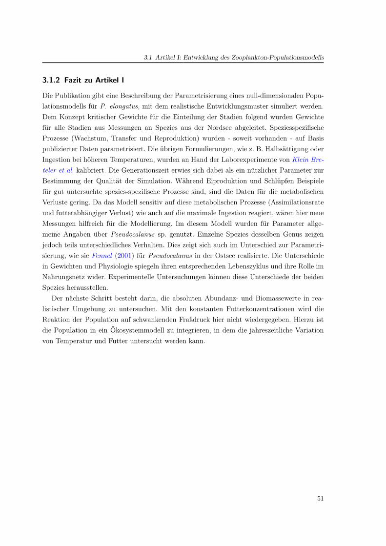
3.1 Artikel I: Entwicklung des Zooplankton-Populationsmodells
3.1.2 Fazit zu Artikel I
Die Publikation gibt eine Beschreibung der Parametrisierung eines null-dimensionalen Popu-lationsmodells für P. elongatus, mit dem realistische Entwicklungsmuster simuliert werden.Dem Konzept kritischer Gewichte für die Einteilung der Stadien folgend wurden Gewichtefür alle Stadien aus Messungen an Spezies aus der Nordsee abgeleitet. SpeziesspezifischeProzesse (Wachstum, Transfer und Reproduktion) wurden - soweit vorhanden - auf Basispublizierter Daten parametrisiert. Die übrigen Formulierungen, wie z. B. Halbsättigung oderIngestion bei höheren Temperaturen, wurden an Hand der Laborexperimente von Klein Bre-teler et al. kalibriert. Die Generationszeit erwies sich dabei als ein nützlicher Parameter zurBestimmung der Qualität der Simulation. Während Eiproduktion und Schlüpfen Beispielefür gut untersuchte spezies-spezifische Prozesse sind, sind die Daten für die metabolischenVerluste gering. Da das Modell sensitiv auf diese metabolischen Prozesse (Assimilationsrateund futterabhängiger Verlust) wie auch auf die maximale Ingestion reagiert, wären hier neueMessungen hilfreich für die Modellierung. Im diesem Modell wurden für Parameter allge-meine Angaben über Pseudocalanus sp. genutzt. Einzelne Spezies desselben Genus zeigenjedoch teils unterschiedliches Verhalten. Dies zeigt sich auch im Unterschied zur Parametri-sierung, wie sie Fennel (2001) für Pseudocalanus in der Ostsee realisierte. Die Unterschiedein Gewichten und Physiologie spiegeln ihren entsprechenden Lebenszyklus und ihre Rolle imNahrungsnetz wider. Experimentelle Untersuchungen können diese Unterschiede der beidenSpezies herausstellen.
Der nächste Schritt besteht darin, die absoluten Abundanz- und Biomassewerte in rea-listischer Umgebung zu untersuchen. Mit den konstanten Futterkonzentrationen wird dieReaktion der Population auf schwankenden Fraßdruck hier nicht wiedergegeben. Hierzu istdie Population in ein Ökosystemmodell zu integrieren, in dem die jahreszeitliche Variationvon Temperatur und Futter untersucht werden kann.
51
3 Parametrisierung, Validation und Auswertung des Modells
3.2 Artikel II: Test der Populationsdynamik im Jahresgang
Dieser Artikel beschreibt den Ansatz, ein strukturiertes Zooplanktonmodell mit Zustandsva-riablen für Eier, Nauplien, zwei Copepoditstadien und Adulte für Pseudocalanus elongatusmit dem Ökosystemmodell ECOHAM2 mit 13 Zustandsvariablen für den Kohlenstoff- undStickstoffkreislauf zu koppeln. Unterschiedliche Temperatur- und Futterszenarien aus La-borexperimenten wurden genutzt, um die Parametrisierung der stadienabhängigen Entwick-lungsprozesse der Copepoden zu unterstützen. Um den Jahresgang unter realistischen Um-weltbedingungen zu untersuchen, wurde das Ökosystem-Zooplanktonmodell an einer Was-sersäule in der nördlichen Nordsee angewandt. Die Zustandsvariablen des Ökosystemmodellswurden zunächst gegen gemessene Monatsmittelwerte validiert. Vertikalprofile ausgewählterVariablen wurden hinsichtlich des physikalischen Antriebs verglichen, um die Unterschiedezwischen Zooplankton als einzelne Zustandsvariable oder als Population zu herauszuarbeiten.Die Generationszeiten wurden stärker durch die Temperatur als durch Schwankungen in derFutterkonzentration beeinflußt, mit Ausnahme der Frühjahrsblüte. Im Jahresgang wurdensechs simulierte Generationen ermittelt.
52
3.2 Artikel II: Test der Populationsdynamik im Jahresgang
3.2.1 Publikation II: Moll und Stegert (2007)
Titel:
Modelling Pseudocalanus elongatus stage-structured population dynamics
embedded in a water column ecosystem model for the northern North Sea
Autoren:
Andreas Moll und Christoph Stegert
Veröffentlicht in:
Journal of Marine Systems 64 (2007), Seiten 35-46
53
3 Parametrisierung, Validation und Auswertung des Modells
Modelling Pseudocalanus elongatus stage-structured populationdynamics embedded in a water column ecosystem
model for the northern North Sea
Andreas Moll ⁎, Christoph Stegert
Institut für Meereskunde (IfM), Universität Hamburg (ZMK-ZMAW), Bundesstr. 53, 20146 Hamburg, Germany
Received 23 January 2006; received in revised form 17 March 2006; accepted 31 March 2006Available online 7 July 2006
Abstract
This paper outlines an approach to couple a structured zooplankton population model with state variables for eggs, nauplii, twocopepodites stages and adults adapted to Pseudocalanus elongatus into the complex marine ecosystem model ECOHAM2 with 13state variables resolving the carbon and nitrogen cycle. Different temperature and food scenarios derived from laboratory culturestudies were examined to improve the process parameterisation for copepod stage dependent development processes. To study annualcycles under realistic weather and hydrographic conditions, the coupled ecosystem–zooplankton model is applied to a water columnin the northern North Sea. The main ecosystem state variables were validated against observed monthly mean values. Then verticalprofiles of selected state variables were compared to the physical forcing to study differences between zooplankton as one biomassstate variable or partitioned into five population state variables. Simulated generation times are more affected by temperature thanfood conditions except during the spring phytoplankton bloom. Up to six generations within the annual cycle can be discerned in thesimulation.© 2006 Elsevier B.V. All rights reserved.
Keywords: Stage-structured population model; Copepod biomass; Generation time; Ecosystem model; ECOHAM2; North Sea
1. Introduction
Copepods form a major part of the North Sea zoo-plankton (Fransz et al., 1991). They are the functionalgroup of consumers of phytoplankton and on the otherside they are food for fish larvae and many other marineanimals. The international project GLOBEC (GLOBECet al., 1999) with its German contribution ‘aims at abetter understanding of the trophodynamic interactionsbetween zooplankton and fish under the influence ofphysical processes in order to elucidate the principal
mechanisms accounting for the high variability of cope-pod production’ (Alheit, 2004). Therefore, the influenceof physical processes on copepods, mainly temperatureand stratification, have to be complemented with biolo-gical processes concerning food availability to studythe development of a copepod population. A modellingapproach to this problem is presented in this paper.
Modelling seasonality in zooplankton populations oftemperate marine environments have a long tradition,e.g., on Georges Bank (Riley and Bumpus, 1946; Davis,1984) and in the North Sea (Steele, 1974; Hendersonand Steele, 1995). Currently, only a few space-resolvedmodels for the North Sea include zooplankton (Moll andRadach, 2003). They include zooplankton as a
Journal of Marine Systems 64 (2007) 35–46www.elsevier.com/locate/jmarsys
⁎ Corresponding author.E-mail address: [email protected] (A. Moll).
0924-7963/$ - see front matter © 2006 Elsevier B.V. All rights reserved.doi:10.1016/j.jmarsys.2006.03.015
54
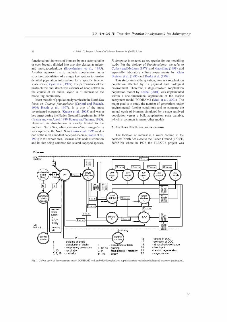
3.2 Artikel II: Test der Populationsdynamik im Jahresgang
functional unit in terms of biomass by one state variableor even broadly divided into two size classes as micro-and mesozooplankton (Broekhuizen et al., 1995).Another approach is to include zooplankton as astructured population of a single key species to resolvedetailed population information for a specific time orspace scale (Bryant et al., 1997). The performance of theunstructured and structured variants of zooplankton inthe course of an annual cycle is of interest to themodelling community.
Most models of population dynamics in the North Seafocus on Calanus finmarchicus (Carlotti and Radach,1996; Heath et al., 1997). It is one of the mostinvestigated copepods (Krause et al., 2003) and was akey target during the Fladen Ground Experiment in 1976(Fransz and van Arkel, 1980; Krause and Trahms, 1983).However, its distribution is mostly limited to thenorthern North Sea, while Pseudocalanus elongatus iswide-spread in the North Sea (Krause et al., 1995) and isone of the most abundant copepod species (Fransz et al.,1991) in this whole area. Because of its wide distributionand its size being common for several copepod species,
P. elongatus is selected as key species for our modellingstudy. For the biology of Pseudocalanus, we refer toCorkett and McLaren (1978) and Mauchline (1998), andespecially laboratory culture experiments by KleinBreteler et al. (1995) and Koski et al. (1998).
This study aims at the question, how is a zooplanktonpopulation affected by its physical and biologicalenvironment. Therefore, a stage-resolved zooplanktonpopulation model by Fennel (2001) was implementedwithin a one-dimensional application of the marineecosystem model ECOHAM2 (Moll et al., 2003). Themajor goal is to study the number of generations underenvironmental forcing conditions and to compare theannual cycle of biomass simulated by a stage-resolvedpopulation versus a bulk zooplankton state variable,which is common in many other models.
2. Northern North Sea water column
The location of interest is a water column in thenorthern North Sea close to the Fladen Ground (0°35′E,58°55′N) where in 1976 the FLEX'76 project was
Fig. 1. Carbon cycle of the ecosystem model ECOHAM2 with embedded zooplankton population state variables (circles) and processes (rectangles).
36 A. Moll, C. Stegert / Journal of Marine Systems 64 (2007) 35–46
55
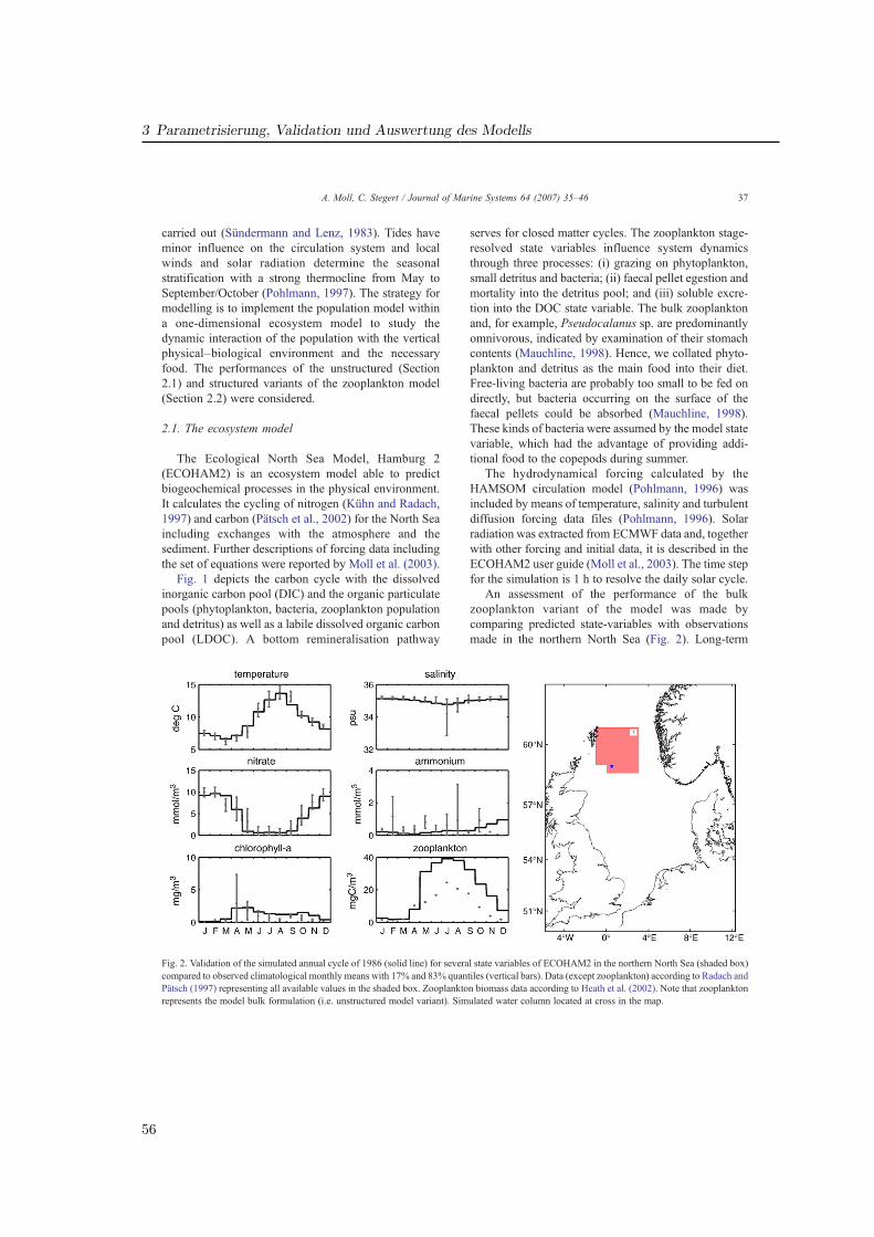
3 Parametrisierung, Validation und Auswertung des Modells
carried out (Sündermann and Lenz, 1983). Tides haveminor influence on the circulation system and localwinds and solar radiation determine the seasonalstratification with a strong thermocline from May toSeptember/October (Pohlmann, 1997). The strategy formodelling is to implement the population model withina one-dimensional ecosystem model to study thedynamic interaction of the population with the verticalphysical–biological environment and the necessaryfood. The performances of the unstructured (Section2.1) and structured variants of the zooplankton model(Section 2.2) were considered.
2.1. The ecosystem model
The Ecological North Sea Model, Hamburg 2(ECOHAM2) is an ecosystem model able to predictbiogeochemical processes in the physical environment.It calculates the cycling of nitrogen (Kühn and Radach,1997) and carbon (Pätsch et al., 2002) for the North Seaincluding exchanges with the atmosphere and thesediment. Further descriptions of forcing data includingthe set of equations were reported by Moll et al. (2003).
Fig. 1 depicts the carbon cycle with the dissolvedinorganic carbon pool (DIC) and the organic particulatepools (phytoplankton, bacteria, zooplankton populationand detritus) as well as a labile dissolved organic carbonpool (LDOC). A bottom remineralisation pathway
serves for closed matter cycles. The zooplankton stage-resolved state variables influence system dynamicsthrough three processes: (i) grazing on phytoplankton,small detritus and bacteria; (ii) faecal pellet egestion andmortality into the detritus pool; and (iii) soluble excre-tion into the DOC state variable. The bulk zooplanktonand, for example, Pseudocalanus sp. are predominantlyomnivorous, indicated by examination of their stomachcontents (Mauchline, 1998). Hence, we collated phyto-plankton and detritus as the main food into their diet.Free-living bacteria are probably too small to be fed ondirectly, but bacteria occurring on the surface of thefaecal pellets could be absorbed (Mauchline, 1998).These kinds of bacteria were assumed by the model statevariable, which had the advantage of providing addi-tional food to the copepods during summer.
The hydrodynamical forcing calculated by theHAMSOM circulation model (Pohlmann, 1996) wasincluded by means of temperature, salinity and turbulentdiffusion forcing data files (Pohlmann, 1996). Solarradiation was extracted from ECMWF data and, togetherwith other forcing and initial data, it is described in theECOHAM2 user guide (Moll et al., 2003). The time stepfor the simulation is 1 h to resolve the daily solar cycle.
An assessment of the performance of the bulkzooplankton variant of the model was made bycomparing predicted state-variables with observationsmade in the northern North Sea (Fig. 2). Long-term
Fig. 2. Validation of the simulated annual cycle of 1986 (solid line) for several state variables of ECOHAM2 in the northern North Sea (shaded box)compared to observed climatological monthly means with 17% and 83% quantiles (vertical bars). Data (except zooplankton) according to Radach andPätsch (1997) representing all available values in the shaded box. Zooplankton biomass data according to Heath et al. (2002). Note that zooplanktonrepresents the model bulk formulation (i.e. unstructured model variant). Simulated water column located at cross in the map.
37A. Moll, C. Stegert / Journal of Marine Systems 64 (2007) 35–46
56
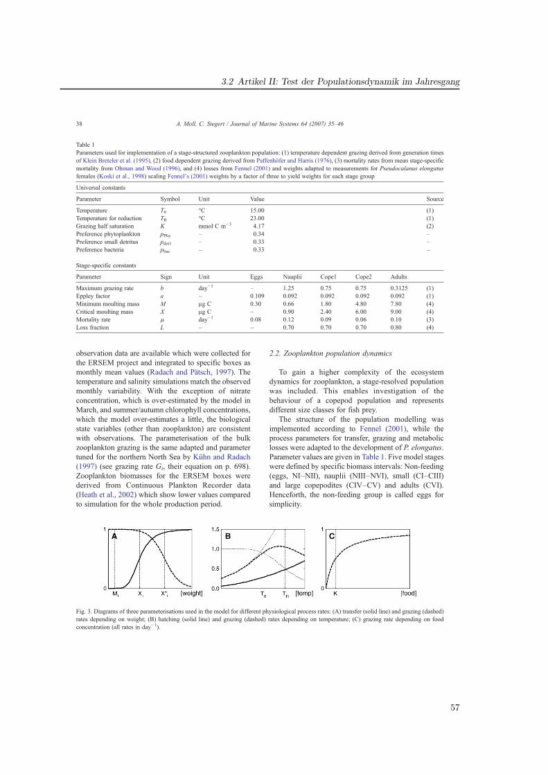
3.2 Artikel II: Test der Populationsdynamik im Jahresgang
observation data are available which were collected forthe ERSEM project and integrated to specific boxes asmonthly mean values (Radach and Pätsch, 1997). Thetemperature and salinity simulations match the observedmonthly variability. With the exception of nitrateconcentration, which is over-estimated by the model inMarch, and summer/autumn chlorophyll concentrations,which the model over-estimates a little, the biologicalstate variables (other than zooplankton) are consistentwith observations. The parameterisation of the bulkzooplankton grazing is the same adapted and parametertuned for the northern North Sea by Kühn and Radach(1997) (see grazing rate Gi, their equation on p. 698).Zooplankton biomasses for the ERSEM boxes werederived from Continuous Plankton Recorder data(Heath et al., 2002) which show lower values comparedto simulation for the whole production period.
2.2. Zooplankton population dynamics
To gain a higher complexity of the ecosystemdynamics for zooplankton, a stage-resolved populationwas included. This enables investigation of thebehaviour of a copepod population and representsdifferent size classes for fish prey.
The structure of the population modelling wasimplemented according to Fennel (2001), while theprocess parameters for transfer, grazing and metaboliclosses were adapted to the development of P. elongatus.Parameter values are given in Table 1. Five model stageswere defined by specific biomass intervals: Non-feeding(eggs, NI–NII), nauplii (NIII–NVI), small (CI–CIII)and large copepodites (CIV–CV) and adults (CVI).Henceforth, the non-feeding group is called eggs forsimplicity.
Table 1Parameters used for implementation of a stage-structured zooplankton population: (1) temperature dependent grazing derived from generation timesof Klein Breteler et al. (1995), (2) food dependent grazing derived from Paffenhöfer and Harris (1976), (3) mortality rates from mean stage-specificmortality from Ohman and Wood (1996), and (4) losses from Fennel (2001) and weights adapted to measurements for Pseudocalanus elongatusfemales (Koski et al., 1998) scaling Fennel's (2001) weights by a factor of three to yield weights for each stage group
Universal constants
Parameter Symbol Unit Value Source
Temperature T0 °C 15.00 (1)Temperature for reduction TR °C 23.00 (1)Grazing half saturation K mmol C m−3 4.17 (2)Preference phytoplankton pPhy – 0.34 –Preference small detritus pdet1 – 0.33 –Preference bacteria pbac – 0.33 –
Stage-specific constants
Parameter Sign Unit Eggs Nauplii Cope1 Cope2 Adults
Maximum grazing rate b day−1 – 1.25 0.75 0.75 0.3125 (1)Eppley factor a – 0.109 0.092 0.092 0.092 0.092 (1)Minimum moulting mass M μg C 0.30 0.66 1.80 4.80 7.80 (4)Critical moulting mass X μg C – 0.90 2.40 6.00 9.00 (4)Mortality rate μ day−1 0.08 0.12 0.09 0.06 0.10 (3)Loss fraction L – – 0.70 0.70 0.70 0.80 (4)
Fig. 3. Diagrams of three parameterisations used in the model for different physiological process rates: (A) transfer (solid line) and grazing (dashed)rates depending on weight; (B) hatching (solid line) and grazing (dashed) rates depending on temperature; (C) grazing rate depending on foodconcentration (all rates in day−1).
38 A. Moll, C. Stegert / Journal of Marine Systems 64 (2007) 35–46
57
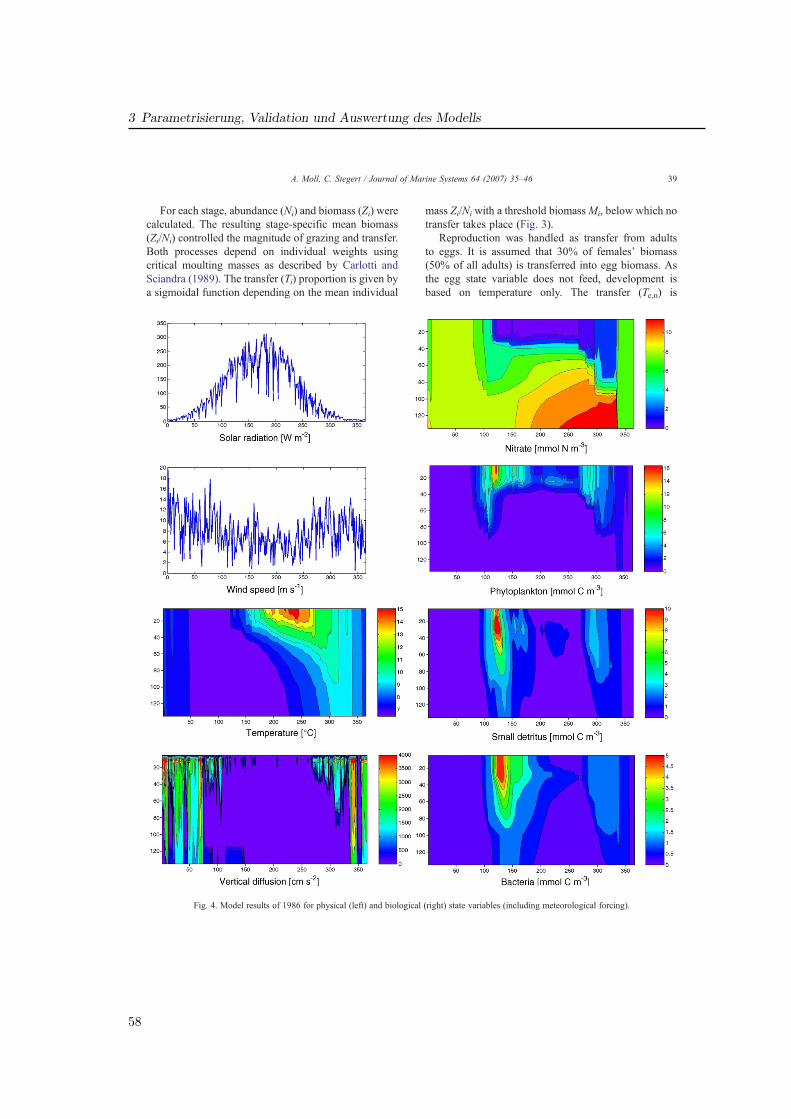
3 Parametrisierung, Validation und Auswertung des Modells
For each stage, abundance (Ni) and biomass (Zi) werecalculated. The resulting stage-specific mean biomass(Zi/Ni) controlled the magnitude of grazing and transfer.Both processes depend on individual weights usingcritical moulting masses as described by Carlotti andSciandra (1989). The transfer (Ti) proportion is given bya sigmoidal function depending on the mean individual
mass Zi/Ni with a threshold biomassMi, below which notransfer takes place (Fig. 3).
Reproduction was handled as transfer from adultsto eggs. It is assumed that 30% of females' biomass(50% of all adults) is transferred into egg biomass. Asthe egg state variable does not feed, development isbased on temperature only. The transfer (Te,n) is
Fig. 4. Model results of 1986 for physical (left) and biological (right) state variables (including meteorological forcing).
39A. Moll, C. Stegert / Journal of Marine Systems 64 (2007) 35–46
58
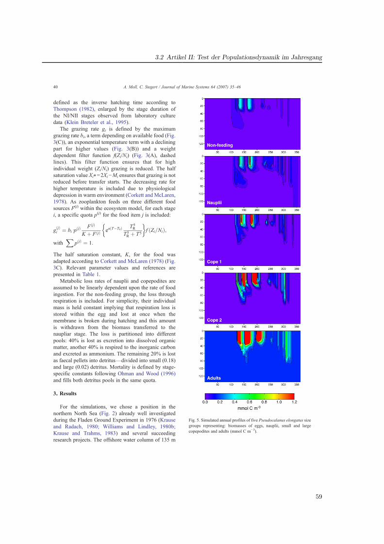
3.2 Artikel II: Test der Populationsdynamik im Jahresgang
defined as the inverse hatching time according toThompson (1982), enlarged by the stage duration ofthe NI/NII stages observed from laboratory culturedata (Klein Breteler et al., 1995).
The grazing rate gi is defined by the maximumgrazing rate bi, a term depending on available food (Fig.3(C)), an exponential temperature term with a decliningpart for higher values (Fig. 3(B)) and a weightdependent filter function f(Zi/Ni) (Fig. 3(A), dashedlines). This filter function ensures that for highindividual weight (Zi/Ni) grazing is reduced. The halfsaturation value Xi⁎=2Xi−Mi ensures that grazing is notreduced before transfer starts. The decreasing rate forhigher temperature is included due to physiologicaldepression in warm environment (Corkett and McLaren,1978). As zooplankton feeds on three different foodsources F(j) within the ecosystem model, for each stagei, a specific quota p(j) for the food item j is included:
gðjÞi ¼ bidpðjÞ FðjÞ
K þ FðjÞ eaðT�T0Þ T5R
T5R þ T5
� �f Zi=Nið Þ;
withX
pðjÞ ¼ 1:
The half saturation constant, K, for the food wasadapted according to Corkett and McLaren (1978) (Fig.3C). Relevant parameter values and references arepresented in Table 1.
Metabolic loss rates of nauplii and copepodites areassumed to be linearly dependent upon the rate of foodingestion. For the non-feeding group, the loss throughrespiration is included. For simplicity, their individualmass is held constant implying that respiration loss isstored within the egg and lost at once when themembrane is broken during hatching and this amountis withdrawn from the biomass transferred to thenaupliar stage. The loss is partitioned into differentpools: 40% is lost as excretion into dissolved organicmatter, another 40% is respired to the inorganic carbonand excreted as ammonium. The remaining 20% is lostas faecal pellets into detritus—divided into small (0.18)and large (0.02) detritus. Mortality is defined by stage-specific constants following Ohman and Wood (1996)and fills both detritus pools in the same quota.
3. Results
For the simulations, we chose a position in thenorthern North Sea (Fig. 2) already well investigatedduring the Fladen Ground Experiment in 1976 (Krauseand Radach, 1980; Williams and Lindley, 1980b;Krause and Trahms, 1983) and several succeedingresearch projects. The offshore water column of 135 m
Fig. 5. Simulated annual profiles of five Pseudocalanus elongatus sizegroups representing: biomasses of eggs, nauplii, small and largecopepodites and adults (mmol C m−3).
40 A. Moll, C. Stegert / Journal of Marine Systems 64 (2007) 35–46
59
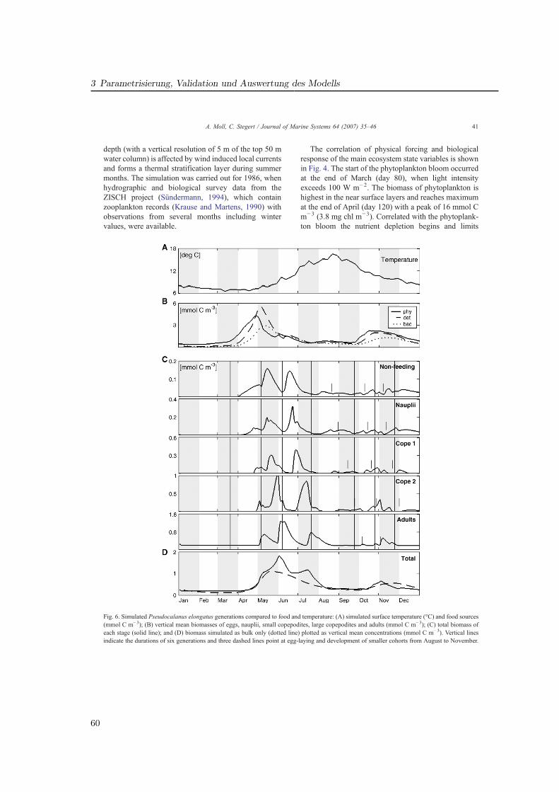
3 Parametrisierung, Validation und Auswertung des Modells
depth (with a vertical resolution of 5 m of the top 50 mwater column) is affected by wind induced local currentsand forms a thermal stratification layer during summermonths. The simulation was carried out for 1986, whenhydrographic and biological survey data from theZISCH project (Sündermann, 1994), which containzooplankton records (Krause and Martens, 1990) withobservations from several months including wintervalues, were available.
The correlation of physical forcing and biologicalresponse of the main ecosystem state variables is shownin Fig. 4. The start of the phytoplankton bloom occurredat the end of March (day 80), when light intensityexceeds 100 W m−2. The biomass of phytoplankton ishighest in the near surface layers and reaches maximumat the end of April (day 120) with a peak of 16 mmol Cm−3 (3.8 mg chl m−3). Correlated with the phytoplank-ton bloom the nutrient depletion begins and limits
Fig. 6. Simulated Pseudocalanus elongatus generations compared to food and temperature: (A) simulated surface temperature (°C) and food sources(mmol C m−3); (B) vertical mean biomasses of eggs, nauplii, small copepodites, large copepodites and adults (mmol C m−3); (C) total biomass ofeach stage (solid line); and (D) biomass simulated as bulk only (dotted line) plotted as vertical mean concentrations (mmol C m−3). Vertical linesindicate the durations of six generations and three dashed lines point at egg-laying and development of smaller cohorts from August to November.
41A. Moll, C. Stegert / Journal of Marine Systems 64 (2007) 35–46
60
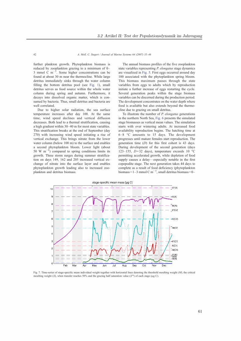
3.2 Artikel II: Test der Populationsdynamik im Jahresgang
further plankton growth. Phytoplankton biomass isreduced by zooplankton grazing to a minimum of 0–3 mmol C m−3. Some higher concentrations can befound at about 30 m near the thermocline. While largedetritus immediately sinks through the water columnfilling the bottom detritus pool (see Fig. 1), smalldetritus serves as food source within the whole watercolumn during spring and autumn. Furthermore, itdecays into dissolved organic matter, which is con-sumed by bacteria. Thus, small detritus and bacteria arewell correlated.
Due to higher solar radiation, the sea surfacetemperature increases after day 100. At the sametime, wind speed declines and vertical diffusiondecreases. Both lead to a thermal stratification, causinga high gradient within 30–40 m for most state variables.This stratification breaks at the end of September (day270) with increasing wind speed initiating a rise ofvertical exchange. This brings nitrate from the lowerwater column (below 100 m) to the surface and enablesa second phytoplankton bloom. Lower light (about50 W m−2) compared to spring conditions limits itsgrowth. Three storm surges during summer stratifica-tion on days 149, 162 and 205 increased vertical ex-change of nitrate into the surface layer and enablesphytoplankton growth leading also to increased zoo-plankton and detritus biomass.
The annual biomass profiles of the five zooplanktonstate variables representing P. elongatus stage dynamicsare visualized in Fig. 5. First eggs occurred around day100 associated with the phytoplankton spring bloom.This biomass maximum passes through the statevariables from eggs to adults which by reproductioninitiate a further increase of eggs restarting the cycle.Several generation peaks within the stage biomassvariables can be discerned during the production period.The development concentrates on the water depth wherefood is available but also extends beyond the thermo-cline due to grazing on small detritus.
To illustrate the number of P. elongatus generationsin the northern North Sea, Fig. 6 presents the simulatedstage biomasses as vertical mean values. The simulationstarts with over wintering adults. At increased foodavailability reproduction begins. The hatching time at6–8 °C amounts to 15 days. The developmentprogresses until mature females start reproduction. Thegeneration time (D) for this first cohort is 43 days.During development of the second generation (days123–155, D=32 days), temperature exceeds 10 °Cpermitting accelerated growth, while depletion of foodsupply causes a delay—especially notable in the firstcopepodite stage. The next generation takes 44 days tocomplete as a result of food deficiency (phytoplanktonbiomass=1–3 mmol C m−3, small detritus biomass=0–
Fig. 7. Time-series of stage-specific mean individual weight together with horizontal lines denoting the threshold moulting weight (M), the criticalmoulting weight (X), when transfer reaches 50% and the grazing half saturation value (X⁎) of each stage (μg C).
42 A. Moll, C. Stegert / Journal of Marine Systems 64 (2007) 35–46
61
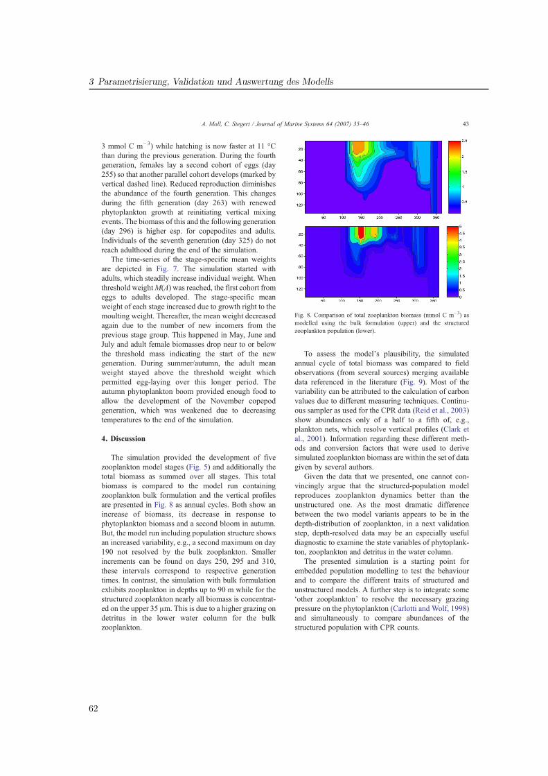
3 Parametrisierung, Validation und Auswertung des Modells
3 mmol C m−3) while hatching is now faster at 11 °Cthan during the previous generation. During the fourthgeneration, females lay a second cohort of eggs (day255) so that another parallel cohort develops (marked byvertical dashed line). Reduced reproduction diminishesthe abundance of the fourth generation. This changesduring the fifth generation (day 263) with renewedphytoplankton growth at reinitiating vertical mixingevents. The biomass of this and the following generation(day 296) is higher esp. for copepodites and adults.Individuals of the seventh generation (day 325) do notreach adulthood during the end of the simulation.
The time-series of the stage-specific mean weightsare depicted in Fig. 7. The simulation started withadults, which steadily increase individual weight. Whenthreshold weightM(A) was reached, the first cohort fromeggs to adults developed. The stage-specific meanweight of each stage increased due to growth right to themoulting weight. Thereafter, the mean weight decreasedagain due to the number of new incomers from theprevious stage group. This happened in May, June andJuly and adult female biomasses drop near to or belowthe threshold mass indicating the start of the newgeneration. During summer/autumn, the adult meanweight stayed above the threshold weight whichpermitted egg-laying over this longer period. Theautumn phytoplankton boom provided enough food toallow the development of the November copepodgeneration, which was weakened due to decreasingtemperatures to the end of the simulation.
4. Discussion
The simulation provided the development of fivezooplankton model stages (Fig. 5) and additionally thetotal biomass as summed over all stages. This totalbiomass is compared to the model run containingzooplankton bulk formulation and the vertical profilesare presented in Fig. 8 as annual cycles. Both show anincrease of biomass, its decrease in response tophytoplankton biomass and a second bloom in autumn.But, the model run including population structure showsan increased variability, e.g., a second maximum on day190 not resolved by the bulk zooplankton. Smallerincrements can be found on days 250, 295 and 310,these intervals correspond to respective generationtimes. In contrast, the simulation with bulk formulationexhibits zooplankton in depths up to 90 m while for thestructured zooplankton nearly all biomass is concentrat-ed on the upper 35 μm. This is due to a higher grazing ondetritus in the lower water column for the bulkzooplankton.
To assess the model's plausibility, the simulatedannual cycle of total biomass was compared to fieldobservations (from several sources) merging availabledata referenced in the literature (Fig. 9). Most of thevariability can be attributed to the calculation of carbonvalues due to different measuring techniques. Continu-ous sampler as used for the CPR data (Reid et al., 2003)show abundances only of a half to a fifth of, e.g.,plankton nets, which resolve vertical profiles (Clark etal., 2001). Information regarding these different meth-ods and conversion factors that were used to derivesimulated zooplankton biomass are within the set of datagiven by several authors.
Given the data that we presented, one cannot con-vincingly argue that the structured-population modelreproduces zooplankton dynamics better than theunstructured one. As the most dramatic differencebetween the two model variants appears to be in thedepth-distribution of zooplankton, in a next validationstep, depth-resolved data may be an especially usefuldiagnostic to examine the state variables of phytoplank-ton, zooplankton and detritus in the water column.
The presented simulation is a starting point forembedded population modelling to test the behaviourand to compare the different traits of structured andunstructured models. A further step is to integrate some‘other zooplankton’ to resolve the necessary grazingpressure on the phytoplankton (Carlotti and Wolf, 1998)and simultaneously to compare abundances of thestructured population with CPR counts.
Fig. 8. Comparison of total zooplankton biomass (mmol C m−3) asmodelled using the bulk formulation (upper) and the structuredzooplankton population (lower).
43A. Moll, C. Stegert / Journal of Marine Systems 64 (2007) 35–46
62
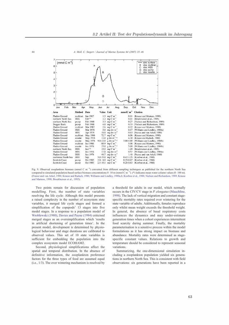
3.2 Artikel II: Test der Populationsdynamik im Jahresgang
Two points remain for discussion of populationmodelling. First, the number of state variablesresolving the life cycle: Although this model presentsa raised complexity in the number of ecosystem statevariables, it merged life cycle stages and formed asimplification of the copepods' 13 stages into fivemodel stages. In a response to a population model ofWroblewski (1980), Davies and Payne (1984) criticisedmerged stages as an oversimplification which ‘resultsin artificial shortening of generation times’. In thepresent model, development is determined by physio-logical behaviour and stage durations are calibrated toobserved values. This set of 10 state variables issufficient for embedding the population into thecomplex ecosystem model ECOHAM2.
Second, physiological simplifications affect thespatial and temporal distribution. In the absence ofdefinitive information, the zooplankton preferencefactors for the three types of food are assumed equal(i.e., 1/3). The over wintering mechanism is resolved by
a threshold for adults in our model, which normallyoccurs in the CIV/CV stage in P. elongatus (Mauchline,1998). The lack of vertical migration and constant stage-specific mortality rates required over wintering for thestate variable of adults. Additionally, females reproduceonly whilst mean weight exceeds the threshold weight.In general, the absence of basal respiratory costsinfluences the dynamics and may under-estimategeneration times when a cohort experiences intermittentfood scarcity during summer. Finally, the mortalityparameterisation is a sensitive process within the modelformulations as it has strong impact on biomass andabundance. Mortality rates were determined as stage-specific constant values. Relations to growth andtemperature should be considered to represent seasonalvariations.
Summarizing, the one-dimensional simulation in-cluding a zooplankton population yielded six genera-tions in northern North Sea. This is consistent with fieldobservations: six generations have been reported in a
Fig. 9. Observed zooplankton biomass (mmol C m−3) converted from different sampling techniques as published for the northern North Seacompared to simulated population-based surface biomass concentrations 0–10 m (mmol C m−3). (*) indicates mean water column values (0–100 m).(Fransz and van Arkel, 1980; Krause and Radach, 1980; Williams and Lindley, 1980a,b; Kiorboe et al., 1988; Nielsen and Richardson, 1989; Krauseand Martens, 1990; Broekhuizen et al., 1995).
44 A. Moll, C. Stegert / Journal of Marine Systems 64 (2007) 35–46
63
3 Parametrisierung, Validation und Auswertung des Modells
Scottish Loch and five in the western North Sea(Mauchline, 1998). The total zooplankton biomass isin agreement with observations. The next task in modelimprovement is simulating realistic abundances of P.elongatus using sets of observations.
Acknowledgements
This work was done within the BMBF funded projectGLOBEC- Germany. We acknowledge the help on theecosystem model ECOHAM2 by Dr. Johannes Pätschand the help on the population model by Prof. WolfgangFennel and Prof. Francois Carlotti within the PROCOPEcooperation programme supported by the DAAD. Forthe conversion of northern North Sea observations andPseudocalanus elongatus body weights, we thank Dr.Michael Krause. Furthermore, we thank two anonymousreviewers for constructive comments, which improvedthe manuscript.
References
Alheit, J., 2004. The German GLOBEC project. InternationalGLOBEC Newsletter 10, 9–10.
Broekhuizen, N., Heath, M.R., Hay, S.J., Gurney, W.S.C., 1995.Modelling the dynamics of the North Sea's mesozooplankton.Netherlands Journal of Sea Research 33 (3–4), 381–406.
Bryant, A.D., Heath, M., Gurney, W.S.G., Beare, D.J., Robertson, W.,1997. The seasonal dynamics ofCalanus finmarchicus: developmentof a three-dimensional structured populationmodel and application tothe northern North Sea. Journal of Sea Research 38, 361–379.
Carlotti, F., Radach, G., 1996. Seasonal dynamics of phytoplanktonand Calanus finmarchicus in the North Sea as revealed by acoupled one-dimensional model. Limnology and Oceanography41 (3), 522–539.
Carlotti, F., Sciandra, A., 1989. Population dynamics model ofEuterpina acutifrons (Copepoda: Harpacticoida) coupling individ-ual growth and larval development. Marine Ecology. ProgressSeries 56, 225–242.
Carlotti, F., Wolf, K.-U., 1998. A Lagrangian ensemble model ofCalanus finmarchicus coupled with a 1-D ecosystem model.Fisheries Oceanography 7 (3–4), 191–204.
Clark, R.A., Frid, C.L.J., Batten, S., 2001. A critical comparison oftwo long-term zooplankton time series from the central-west NorthSea. Journal of Plankton Research 23 (1), 27–39.
Corkett, C.J., McLaren, I.A., 1978. The biology of Pseudocalanus.Advances in Marine Biology 15, 1–231.
Davies, J.M., Payne, R., 1984. Supply of organic matter in the northernNorth Sea during a spring phytoplankton bloom. Marine Biology(78), 315–324.
Davis, C.S., 1984. Predatory control of copepod seasonal cycles onGeorges Bank. Marine Biology 82, 31–40.
Fennel, W., 2001. Modelling of copepods with links to circulationmodels. Journal of Plankton Research 23 (11), 1217–1232.
Fransz, H.G., van Arkel, W.G., 1980. Zooplankton activity during andafter the phytoplankton spring bloom at the central station in theFLEX box, northern North Sea, with special reference to the
calanoid copepod Calanus finmarchicus. Meteor-Forschungser-gebnisse, A 22, 112–121.
Fransz, H.G., Colebrook, J.M., Gamble, J.C., Krause, M., 1991. Thezooplankton of the North Sea. Netherlands Journal of Sea Research28 (1/2), 1–52.
GLOBEC, et al., 1999. Ocean ecosystem dynamics (GLOBEC):implementation plan. IGBP Report Series (International Geo-sphere–Biosphere Programme) 47, 1–207.
Heath, M.R., Robertson, W., Mardaljevic, J., Gurney, W.S.G., 1997.Modelling the population dynamics of Calanus in the Fair Islecurrent off northern Scotland. Journal of Sea Research 38,381–412.
Heath, M.R., Edwards, A.C., Pätsch, J., Turrell, W.R., 2002.Modelling the behaviour of nutrient in the coastal waters ofScotland. Report of the Fisheries Research Services 10, 1–106.
Henderson, E.W., Steele, J.H., 1995. Comparing models andobservations of shelf plankton. Journal of Plankton Research 17(8), 1679–1692.
Kiorboe, T., Munk, P., Richardson, K., Christensen, V., Paulsen, H.,1988. Plankton dynamics and larval herring growth, drift andsurvival in a frontal area. Marine Ecology. Progress Series 44,205–219.
Klein Breteler, W.C.M., Gonzales, S.R., Schogt, N., 1995. Develop-ment of Pseudocalanus elongatus (Copepoda, Calanoida) culturedat different temperature and food conditions. Marine Ecology.Progress Series 119, 99–110.
Koski, M., Klein Breteler, W., Schogt, N., 1998. Effect of food qualityon rate of growth and development of the pelagic copepodPseudocalanus elongatus (Copepoda Calanoida). Marine Ecology.Progress Series 170, 169–187.
Krause, M., Martens, P., 1990. Distribution patterns of mesozoo-plankton biomass in the North Sea. Helgoländer Meeresuntersu-chungen 44, 295–327.
Krause, M., Radach, G., 1980. On the succession of developmentalstages of herbivorous zooplankton in the North Sea during FLEX'76: 1. First statements about the main groups of the zooplanktoncommunity. Meteor-Forschungsergebnisse. Reihe A, Allgemeines,Physik und Chemie des Meeres 22, 133–149.
Krause, M., Trahms, J., 1983. Zooplankton dynamics duringFLEX'76. In: Sündermann, J., Lenz, W. (Eds.), North SeaDynamics. Springer Verlag, Berlin, pp. 632–661.
Krause, M., Dippner, J.W., Beil, J., 1995. A review of hydrographiccontrols on the distribution of zooplankton biomass and species inthe North Sea with particular reference to a survey conducted inJanuary–March 1987. Progress in Oceanography 35, 81–152.
Krause, M., Fock, H., Greve, W., Winkler, G., 2003. North Seazooplankton: a review. Senckenbergiana Maritima 33 (1–2),71–204.
Kühn, W., Radach, G., 1997. A one-dimensional physical–biologicalmodel study of pelagic nitrogen cycling during the spring bloom inthe northern North Sea (FLEX'76). Journal of Marine Research 55,687–734.
Mauchline, J., 1998. The Biology of Calanoid Copepods. AcademicPress, San Diego. 710 pp.
Moll, A., Radach, G., 2003. Review of three-dimensionalecological modelling related to the North Sea shelf system:Part 1. Models and their results. Progress in Oceanography 57(2), 175–217.
Moll, A., Pätsch, J., Kühn, W., 2003. ECOHAM2 User Guide—TheEcological North Sea Model, Hamburg, Version 2. TechnicalReports 02-2003. Institut für Meereskunde, Hamburg, Germany.38 pp.
45A. Moll, C. Stegert / Journal of Marine Systems 64 (2007) 35–46
64
3.2 Artikel II: Test der Populationsdynamik im Jahresgang
Nielsen, T.G., Richardson, K., 1989. Food chain structure of the NorthSea plankton communities: seasonal variations of the role of themicrobial loop. Marine Ecology. Progress Series 56 (1–2), 75–87.
Ohman, M.D., Wood, S.N., 1996. Mortality estimation for planktoniccopepods: Pseudocalanus newmani in a temperate fjord. Limnol-ogy and Oceanography 41 (1), 126–135.
Paffenhöfer, G.A., Harris, R.P., 1976. Feeding, growth and reproduc-tion of the marine planktonic copepod Pseudocalanus elongatus.Journal of the Marine Biological Association of the UnitedKingdom 56, 327–344.
Pätsch, J., et al., 2002. Interannual variability of carbon fluxes at theNorth Atlantic station ESTOC. Deep-Sea Research. Part II 49(1–3), 253–288.
Pohlmann, T., 1996. Calculating the development of the thermal verticalstratification in the North Sea with a three-dimensional barocliniccirculation model. Continental Shelf Research 16 (2), 163–194.
Pohlmann, T., 1997. Estimating the influence of advection duringFLEX'76 by means of a three-dimensional shelf sea circulationmodel. Deutsche Hydrographische Zeitschrift 49 (2/3), 215–226.
Radach, G., Pätsch, J., 1997. Climatological annual cycles of nutrientsand chlorophyll in the North Sea. Journal of Sea Research 38,231–248.
Reid, P.C., Colebrook, J.M., Matthews, J.B.L., Aiken, J., 2003. TheContinuous Plankton Recorder: concepts and history, from
Plankton Indicator to undulating recorders. Progress in Oceanog-raphy 58 (2–4), 117–173.
Riley, G.A., Bumpus, D.F., 1946. Phytoplankton–zooplanktonrelationships on Georges Bank. Journal of Marine Research 6(1), 33–47.
Steele, J.H., 1974. The Structure of Marine Ecosystems. HarvardUniversity Press, Cambridge, MA. 128 pp.
Sündermann, J. (Ed.), 1994. Circulation and Contaminant Fluxes inthe North Sea. InSpringer-Verlag, Berlin. 654 pp.
Sündermann, J., Lenz, W., 1983. North Sea Dynamics. SpringerVerlag, Berlin. 693 pp.
Thompson, B.M., 1982. Growth and development of Pseudocalanuselongatus and Calanus sp. in the laboratory. Journal of the MarineBiological Association of the United Kingdom 62, 359–372.
Williams, R., Lindley, J.A., 1980a. Plankton of the Fladen Groundduring FLEX 76: I. Spring development of the planktoncommunity. Marine Biology 57, 73–78.
Williams, R., Lindley, J.A., 1980b. Plankton of the Fladen Groundduring FLEX 76: III. Vertical distribution, population dynamicsand production of Calanus finmarchicus (Crustacea: Copepoda).Marine Biology (60), 47–56.
Wroblewski, J.S., 1980. A simulation of the distribution of Acartiaclausi during Oregon upwelling August 1973. Journal of PlanktonResearch 2 (1), 43–68.
46 A. Moll, C. Stegert / Journal of Marine Systems 64 (2007) 35–46
65
3 Parametrisierung, Validation und Auswertung des Modells
3.2.2 Fazit zu Artikel II
Die Simulation beschreibt die Entwicklung der fünf Stadien im Zooplanktonmodell, die inder Summe die gesamte Zooplanktonbiomasse repräsentieren. Der Vergleich zu einer Simu-lation mit Bulk-Formulierung zeigt für beide Varianten ein starkes Maximum in Reaktionauf die Phytoplanktonbiomasse und einen zweiten kleineren Anstieg im Herbst. Zusätzlichweist der Lauf mit Population eine höhere Variabilität der Biomasse auf. Vier kleinere Erhö-hungen in Abständen, welche den Generationszeiten entsprechen, sind zu finden. Währenddie Population vorwiegend in den oberen 35 m vorkommt, ist das Zooplankton in der Bulk-Formulierung bis in 80 m Tiefe in höherer Konzentration zu finden. Die variable Präferenzdes Futters ermöglicht in dieser Variante höhere Aufnahme der alternativen FutterquellenDetritus und Bakterien.
Mit den fünf Stadiengruppen im Modell läßt sich das Verhalten und die Entwicklung vonPseudocalanus elongatus im komplexen Ökosystemmodell ECOHAM2 beschreiben. Dabeiwurden teilweise vereinfachte Beschreibungen genutzt (wie die Überwinterung und konstanteMortalitätsraten). Die Simulation bildet einen wichtigen Test zum Verhalten der Populati-on in einem komplexen Ökosystemmodell. Ein nächster Schritt besteht darin, das restlicheZooplankton zu integrieren, um den Fraßdruck auf das Phytoplankton beizubehalten undgleichzeitig mit Messungen vergleichbare Abundanzen zu simulieren.
66
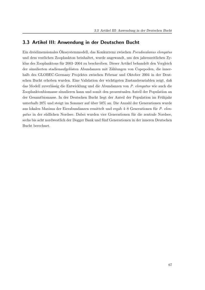
3.3 Artikel III: Anwendung in der Deutschen Bucht
3.3 Artikel III: Anwendung in der Deutschen Bucht
Ein dreidimensionales Ökosystemmodell, das Konkurrenz zwischen Pseudocalanus elongatusund dem restlichen Zooplankton beinhaltet, wurde angewandt, um den jahreszeitlichen Zy-klus des Zooplanktons für 2003–2004 zu beschreiben. Dieser Artikel behandelt den Vergleichder simulierten stadienaufgelösten Abundanzen mit Zählungen von Copepoden, die inner-halb des GLOBEC-Germany Projektes zwischen Februar und Oktober 2004 in der Deut-schen Bucht erhoben wurden. Eine Validation der wichtigsten Zustandsvariablen zeigt, daßdas Modell zuverlässig die Entwicklung und die Abundanzen von P. elongatus wie auch dieZooplanktonbiomasse simulieren kann und somit den prozentualen Anteil der Population ander Gesamtbiomasse. In der Deutschen Bucht liegt der Anteil der Population im Frühjahrunterhalb 20% und steigt im Sommer auf über 50% an. Die Anzahl der Generationen wurdeaus lokalen Maxima der Eierabundanzen ermittelt und ergab 4–8 Generationen für P. elon-gatus in der südlichen Nordsee. Dabei wurden vier Generationen für die zentrale Nordsee,sechs bis acht nordwestlich der Dogger Bank und fünf Generationen in der inneren DeutschenBucht berechnet.
67
3 Parametrisierung, Validation und Auswertung des Modells
3.3.1 Publikation III: Stegert et al. (eingereicht)
Titel:
Validation of the three-dimensional ECOHAM model in the German Bight
for 2004 including population dynamics of Pseudocalanus elongatus
Autoren:
Christoph Stegert, Andreas Moll und Markus Kreus
Eingereicht bei:
Journal of Sea Research, 02. Mai 2008
68
3.3 Artikel III: Anwendung in der Deutschen Bucht
Validation of the three-dimensional ECOHAM model in the GermanBight for 2004 including population dynamics of Pseudocalanus
elongatus
Christoph Stegert a,∗ Andreas Moll a Markus Kreus a,1
aInstitut fur Meereskunde, Universitat Hamburg (ZMK-ZMAW), Bundesstr. 53, 20146 Hamburg, Germany
Abstract
A three-dimensional ecosystem model for the North Sea which includes competition between Pseudocalanus elongatusand the rest of the zooplankton biomass was applied to describe the seasonal cycle of zooplankton in 2003-2004. Thepaper presents the comparison of simulated stage-resolved abundances with copepod counts at several stations inthe German Bight during the GLOBEC-Germany project from February to October 2004. A validation of influentialstate variables gives confidence that the model is able to calculate reliably the stage development and abundancesof P. elongatus as well as the range of bulk zooplankton biomass, and thus the ratio of population biomass to totalbiomass. In the German Bight, the population is below 20% in spring. The ratio increases up to 50% during summer.The number of generations was estimated from peaks in egg abundance to about 4-8 generations of P. elongatus inthe southern North Sea. A mean of four generations per year were estimated in the central North Sea, six to eightgenerations northwest of the Dogger Bank (tails end) and five generations in the German Bight.
Key words: Stage-structured zooplankton population model, copepod biomass, generation time, Pseudocalanus elongatus,
ecosystem model, ECOHAM, North Sea, German Bight
1. Introduction
Copepods as part of the zooplankton bear an im-portant role in the marine food web as mediators be-tween lower (i.e. phytoplankton) and higher (i.e. fishand larval fish) trophic levels. They also affect therecruitment success of larval fish, which undergoesstrong inter-annual variability (Alheit et al., 2005).Thus, copepods have been investigated intensely inthe North Sea during the last decades (Krause et al.,2003). In 2003-2005 an elaborate program of sam-
∗ Corresponding author.Email address: [email protected] (Andreas
Moll).1 Now at: GKSS Forschungszentrum, Max-Planck-Str. 1,
21502 Geesthacht, Germany
pling and field studies in the German Bight was im-plemented within the GLOBEC-Germany project,which included studies on zooplankton: its devel-opment, the influence of physical processes and thetrophodynamic processes linked to larval fish (i.e.herring and sprat) (Alheit, 2007).
In 2004 zooplankton investigations took placeduring seven cruises between February to October(Renz et al., 2008). This paper describes a three-dimensional ecosystem model used for a detailedstudy of zooplankton and copepod population dy-namics and the influence of physical and biologicalenvironmental factors.
Zooplankton population modelling has alreadybeen done in the North Sea at different spatialscales: Slagstad and Tande (1981) developed a pro-cess model for studying the ecophysiology of cope-
Preprint submitted to Journal of Sea Research 2 May 2008
69
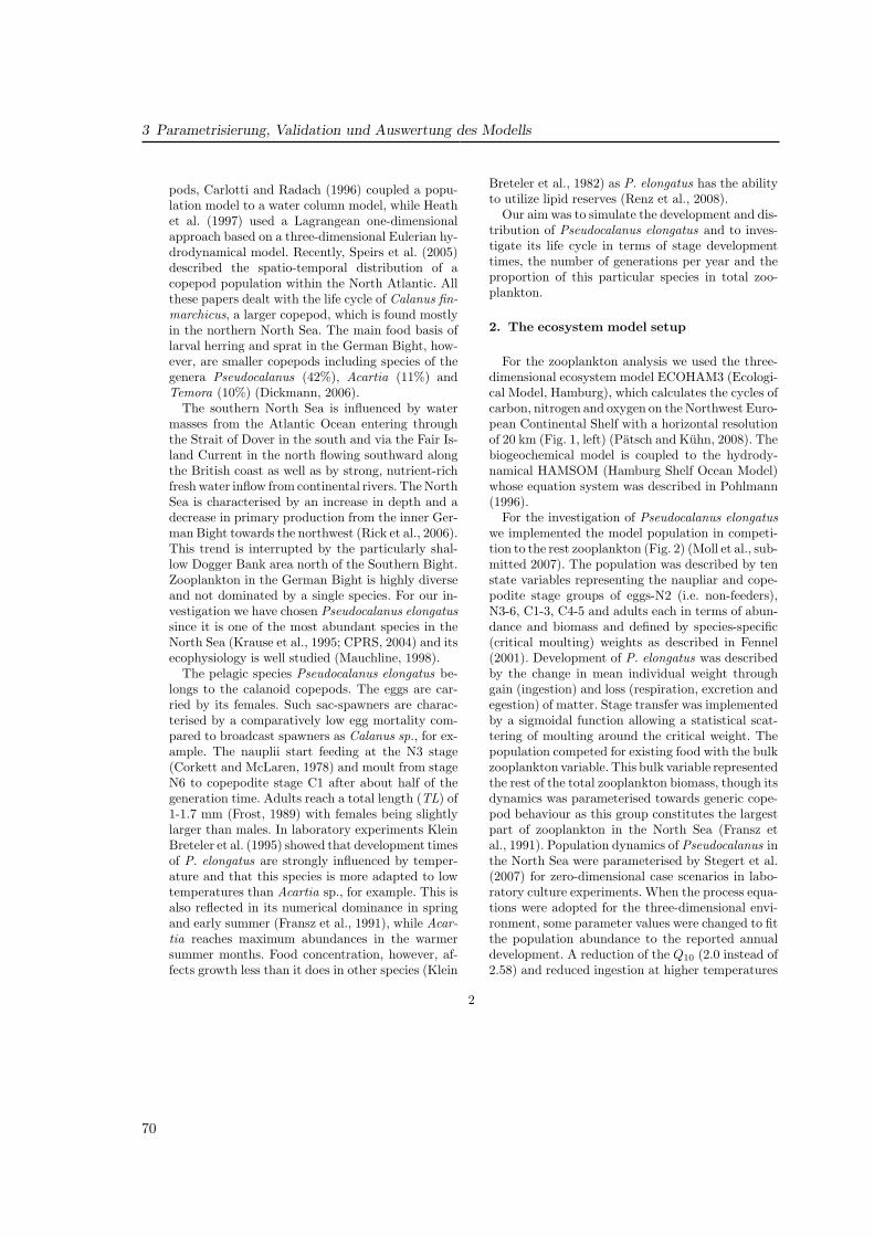
3 Parametrisierung, Validation und Auswertung des Modells
pods, Carlotti and Radach (1996) coupled a popu-lation model to a water column model, while Heathet al. (1997) used a Lagrangean one-dimensionalapproach based on a three-dimensional Eulerian hy-drodynamical model. Recently, Speirs et al. (2005)described the spatio-temporal distribution of acopepod population within the North Atlantic. Allthese papers dealt with the life cycle of Calanus fin-marchicus, a larger copepod, which is found mostlyin the northern North Sea. The main food basis oflarval herring and sprat in the German Bight, how-ever, are smaller copepods including species of thegenera Pseudocalanus (42%), Acartia (11%) andTemora (10%) (Dickmann, 2006).
The southern North Sea is influenced by watermasses from the Atlantic Ocean entering throughthe Strait of Dover in the south and via the Fair Is-land Current in the north flowing southward alongthe British coast as well as by strong, nutrient-richfresh water inflow from continental rivers. The NorthSea is characterised by an increase in depth and adecrease in primary production from the inner Ger-man Bight towards the northwest (Rick et al., 2006).This trend is interrupted by the particularly shal-low Dogger Bank area north of the Southern Bight.Zooplankton in the German Bight is highly diverseand not dominated by a single species. For our in-vestigation we have chosen Pseudocalanus elongatussince it is one of the most abundant species in theNorth Sea (Krause et al., 1995; CPRS, 2004) and itsecophysiology is well studied (Mauchline, 1998).
The pelagic species Pseudocalanus elongatus be-longs to the calanoid copepods. The eggs are car-ried by its females. Such sac-spawners are charac-terised by a comparatively low egg mortality com-pared to broadcast spawners as Calanus sp., for ex-ample. The nauplii start feeding at the N3 stage(Corkett and McLaren, 1978) and moult from stageN6 to copepodite stage C1 after about half of thegeneration time. Adults reach a total length (TL) of1-1.7 mm (Frost, 1989) with females being slightlylarger than males. In laboratory experiments KleinBreteler et al. (1995) showed that development timesof P. elongatus are strongly influenced by temper-ature and that this species is more adapted to lowtemperatures than Acartia sp., for example. This isalso reflected in its numerical dominance in springand early summer (Fransz et al., 1991), while Acar-tia reaches maximum abundances in the warmersummer months. Food concentration, however, af-fects growth less than it does in other species (Klein
Breteler et al., 1982) as P. elongatus has the abilityto utilize lipid reserves (Renz et al., 2008).
Our aim was to simulate the development and dis-tribution of Pseudocalanus elongatus and to inves-tigate its life cycle in terms of stage developmenttimes, the number of generations per year and theproportion of this particular species in total zoo-plankton.
2. The ecosystem model setup
For the zooplankton analysis we used the three-dimensional ecosystem model ECOHAM3 (Ecologi-cal Model, Hamburg), which calculates the cycles ofcarbon, nitrogen and oxygen on the Northwest Euro-pean Continental Shelf with a horizontal resolutionof 20 km (Fig. 1, left) (Patsch and Kuhn, 2008). Thebiogeochemical model is coupled to the hydrody-namical HAMSOM (Hamburg Shelf Ocean Model)whose equation system was described in Pohlmann(1996).
For the investigation of Pseudocalanus elongatuswe implemented the model population in competi-tion to the rest zooplankton (Fig. 2) (Moll et al., sub-mitted 2007). The population was described by tenstate variables representing the naupliar and cope-podite stage groups of eggs-N2 (i.e. non-feeders),N3-6, C1-3, C4-5 and adults each in terms of abun-dance and biomass and defined by species-specific(critical moulting) weights as described in Fennel(2001). Development of P. elongatus was describedby the change in mean individual weight throughgain (ingestion) and loss (respiration, excretion andegestion) of matter. Stage transfer was implementedby a sigmoidal function allowing a statistical scat-tering of moulting around the critical weight. Thepopulation competed for existing food with the bulkzooplankton variable. This bulk variable representedthe rest of the total zooplankton biomass, though itsdynamics was parameterised towards generic cope-pod behaviour as this group constitutes the largestpart of zooplankton in the North Sea (Fransz etal., 1991). Population dynamics of Pseudocalanus inthe North Sea were parameterised by Stegert et al.(2007) for zero-dimensional case scenarios in labo-ratory culture experiments. When the process equa-tions were adopted for the three-dimensional envi-ronment, some parameter values were changed to fitthe population abundance to the reported annualdevelopment. A reduction of the Q10 (2.0 instead of2.58) and reduced ingestion at higher temperatures
2
70
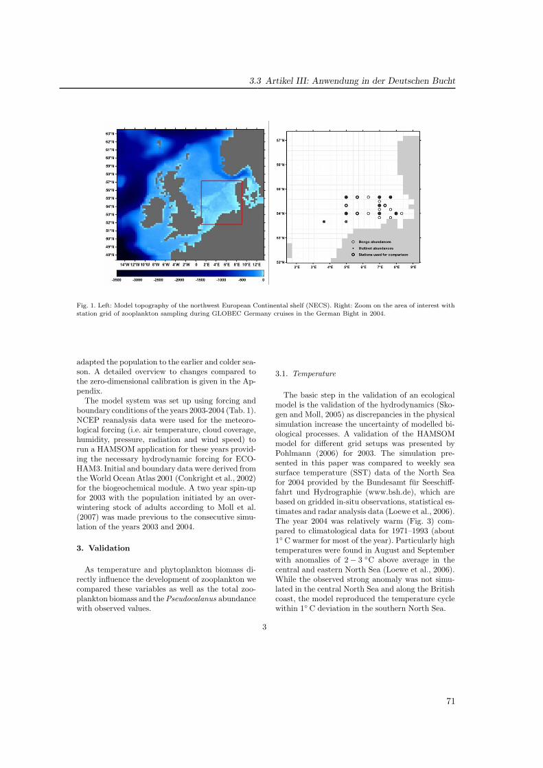
3.3 Artikel III: Anwendung in der Deutschen Bucht
Fig01.doc
Fig01.doc
Fig. 1. Left: Model topography of the northwest European Continental shelf (NECS). Right: Zoom on the area of interest withstation grid of zooplankton sampling during GLOBEC Germany cruises in the German Bight in 2004.
adapted the population to the earlier and colder sea-son. A detailed overview to changes compared tothe zero-dimensional calibration is given in the Ap-pendix.
The model system was set up using forcing andboundary conditions of the years 2003-2004 (Tab. 1).NCEP reanalysis data were used for the meteoro-logical forcing (i.e. air temperature, cloud coverage,humidity, pressure, radiation and wind speed) torun a HAMSOM application for these years provid-ing the necessary hydrodynamic forcing for ECO-HAM3. Initial and boundary data were derived fromthe World Ocean Atlas 2001 (Conkright et al., 2002)for the biogeochemical module. A two year spin-upfor 2003 with the population initiated by an over-wintering stock of adults according to Moll et al.(2007) was made previous to the consecutive simu-lation of the years 2003 and 2004.
3. Validation
As temperature and phytoplankton biomass di-rectly influence the development of zooplankton wecompared these variables as well as the total zoo-plankton biomass and the Pseudocalanus abundancewith observed values.
3.1. Temperature
The basic step in the validation of an ecologicalmodel is the validation of the hydrodynamics (Sko-gen and Moll, 2005) as discrepancies in the physicalsimulation increase the uncertainty of modelled bi-ological processes. A validation of the HAMSOMmodel for different grid setups was presented byPohlmann (2006) for 2003. The simulation pre-sented in this paper was compared to weekly seasurface temperature (SST) data of the North Seafor 2004 provided by the Bundesamt fur Seeschiff-fahrt und Hydrographie (www.bsh.de), which arebased on gridded in-situ observations, statistical es-timates and radar analysis data (Loewe et al., 2006).The year 2004 was relatively warm (Fig. 3) com-pared to climatological data for 1971–1993 (about1◦ C warmer for most of the year). Particularly hightemperatures were found in August and Septemberwith anomalies of 2− 3 ◦C above average in thecentral and eastern North Sea (Loewe et al., 2006).While the observed strong anomaly was not simu-lated in the central North Sea and along the Britishcoast, the model reproduced the temperature cyclewithin 1◦ C deviation in the southern North Sea.
3
71
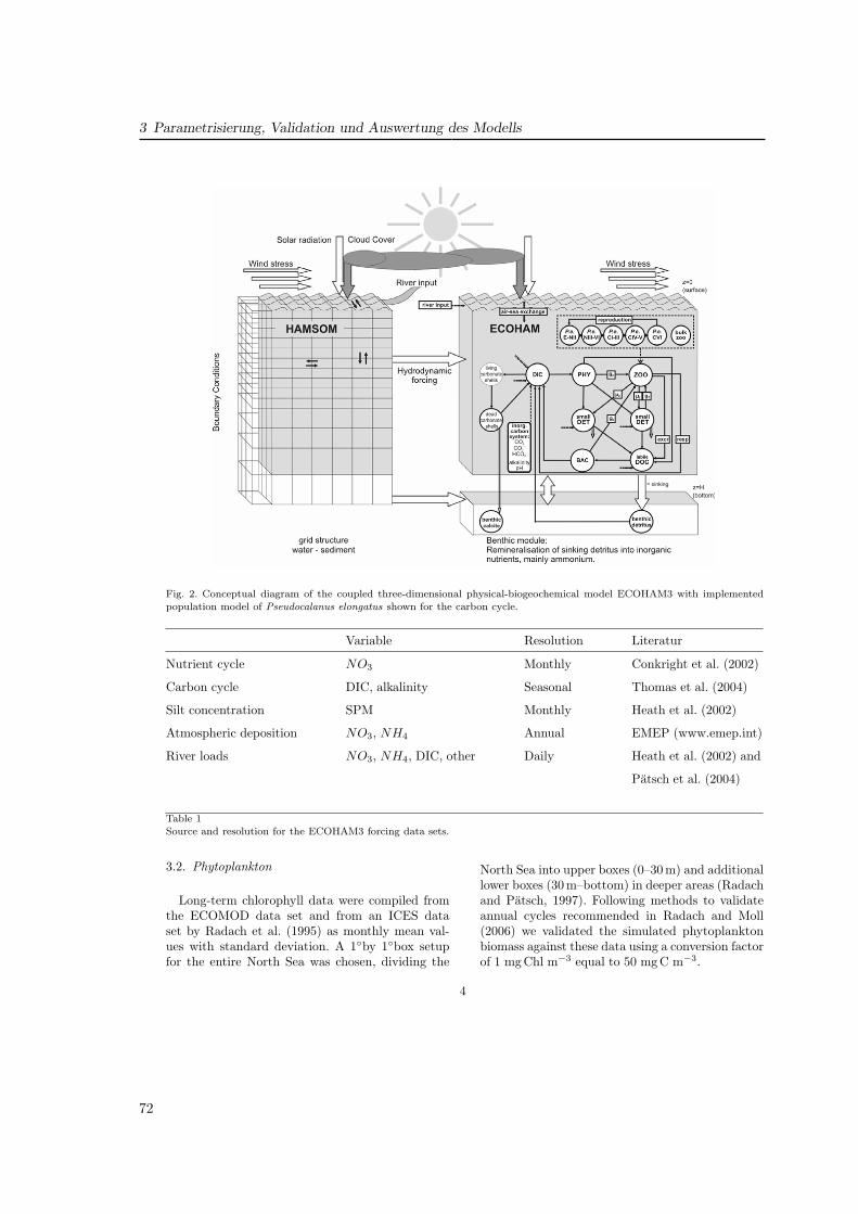
3 Parametrisierung, Validation und Auswertung des Modells
Fig02.doc
Fig02.doc
Fig. 2. Conceptual diagram of the coupled three-dimensional physical-biogeochemical model ECOHAM3 with implemented
population model of Pseudocalanus elongatus shown for the carbon cycle.
Variable Resolution Literatur
Nutrient cycle NO3 Monthly Conkright et al. (2002)
Carbon cycle DIC, alkalinity Seasonal Thomas et al. (2004)
Silt concentration SPM Monthly Heath et al. (2002)
Atmospheric deposition NO3, NH4 Annual EMEP (www.emep.int)
River loads NO3, NH4, DIC, other Daily Heath et al. (2002) and
Patsch et al. (2004)
Table 1
Source and resolution for the ECOHAM3 forcing data sets.
3.2. Phytoplankton
Long-term chlorophyll data were compiled fromthe ECOMOD data set and from an ICES dataset by Radach et al. (1995) as monthly mean val-ues with standard deviation. A 1◦by 1◦box setupfor the entire North Sea was chosen, dividing the
North Sea into upper boxes (0–30 m) and additionallower boxes (30 m–bottom) in deeper areas (Radachand Patsch, 1997). Following methods to validateannual cycles recommended in Radach and Moll(2006) we validated the simulated phytoplanktonbiomass against these data using a conversion factorof 1 mg Chl m−3 equal to 50 mgC m−3.
4
72
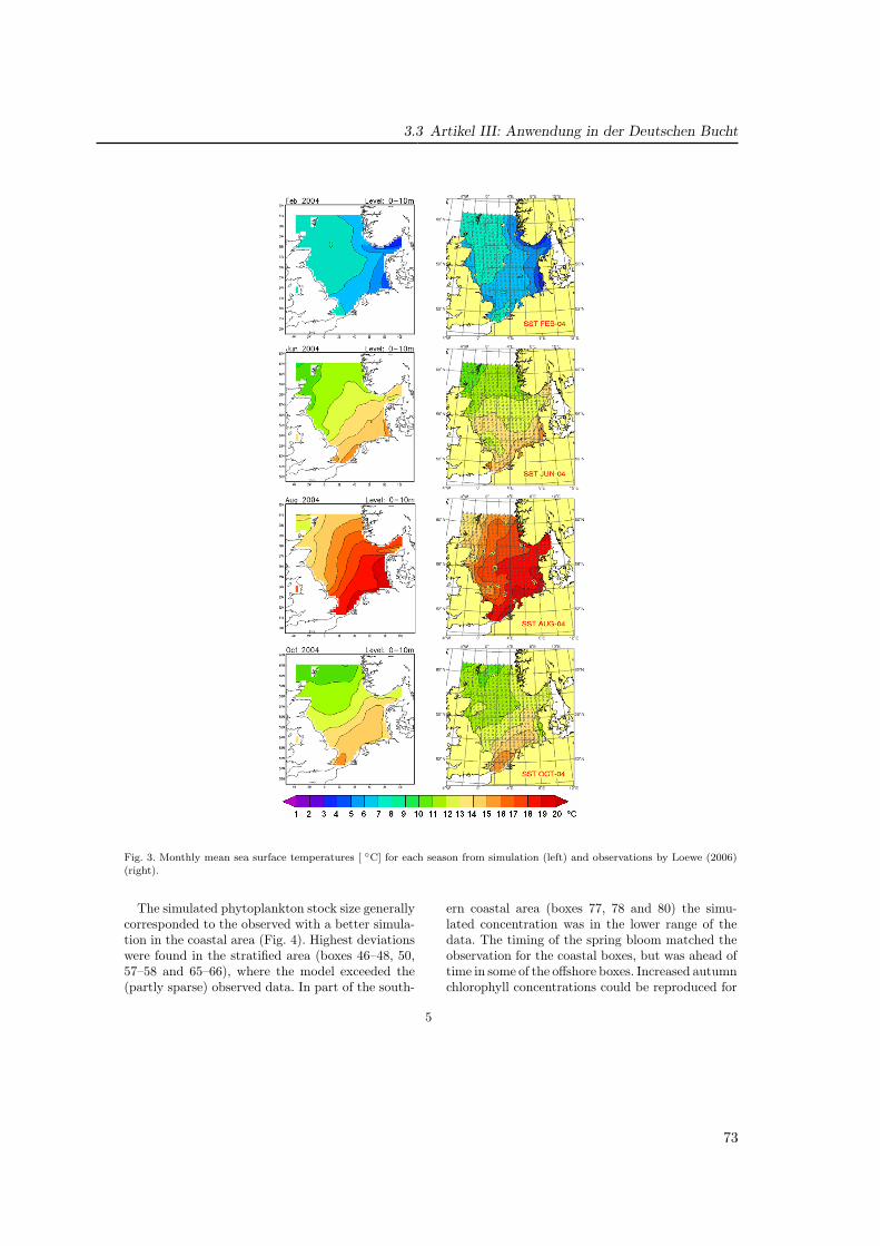
3.3 Artikel III: Anwendung in der Deutschen Bucht
Fig03.doc
Fig03.doc
Fig. 3. Monthly mean sea surface temperatures [ ◦C] for each season from simulation (left) and observations by Loewe (2006)
(right).
The simulated phytoplankton stock size generallycorresponded to the observed with a better simula-tion in the coastal area (Fig. 4). Highest deviationswere found in the stratified area (boxes 46–48, 50,57–58 and 65–66), where the model exceeded the(partly sparse) observed data. In part of the south-
ern coastal area (boxes 77, 78 and 80) the simu-lated concentration was in the lower range of thedata. The timing of the spring bloom matched theobservation for the coastal boxes, but was ahead oftime in some of the offshore boxes. Increased autumnchlorophyll concentrations could be reproduced for
5
73
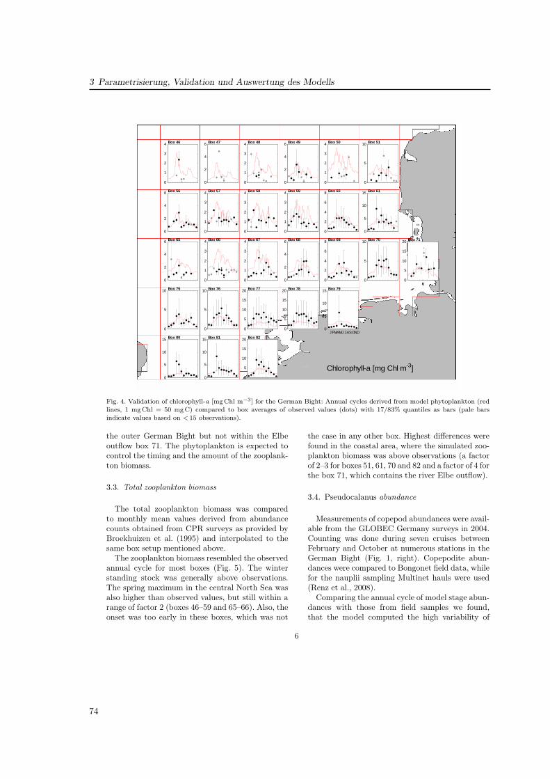
3 Parametrisierung, Validation und Auswertung des ModellsFig04.doc
Chlorophyll-a [mg Chl m-3]
0
1
2
3
4 Box 46
0
2
4
6 Box 47
0
1
2
3
4 Box 48
0
2
4
6 Box 49
0
1
2
3
4 Box 50
0
5
10 Box 51
0
2
4
6 Box 56
0
1
2
3
4 Box 57
0
1
2
3
4 Box 58
0
1
2
3
4 Box 59
0
2
4
6
8 Box 60
0
5
10
15 Box 61
0
2
4
6 Box 65
0
1
2
3
4 Box 66
0
1
2
3
4 Box 67
0
2
4
6 Box 68
0
2
4
6
8 Box 69
0
5
10 Box 70
0
5
10
15
20 Box 71
0
5
10 Box 75
0
5
10 Box 76
0
5
10
15
20 Box 77
0
5
10
15
20 Box 78
J F M A M J J A S O N D 0
5
10
15 Box 79
0
5
10
15 Box 80
0
5
10
15 Box 81
0
5
10
15
20 Box 82
Fig04.doc
Fig. 4. Validation of chlorophyll-a [mgChl m−3] for the German Bight: Annual cycles derived from model phytoplankton (red
lines, 1 mg Chl = 50 mgC) compared to box averages of observed values (dots) with 17/83% quantiles as bars (pale bars
indicate values based on < 15 observations).
the outer German Bight but not within the Elbeoutflow box 71. The phytoplankton is expected tocontrol the timing and the amount of the zooplank-ton biomass.
3.3. Total zooplankton biomass
The total zooplankton biomass was comparedto monthly mean values derived from abundancecounts obtained from CPR surveys as provided byBroekhuizen et al. (1995) and interpolated to thesame box setup mentioned above.
The zooplankton biomass resembled the observedannual cycle for most boxes (Fig. 5). The winterstanding stock was generally above observations.The spring maximum in the central North Sea wasalso higher than observed values, but still within arange of factor 2 (boxes 46–59 and 65–66). Also, theonset was too early in these boxes, which was not
the case in any other box. Highest differences werefound in the coastal area, where the simulated zoo-plankton biomass was above observations (a factorof 2–3 for boxes 51, 61, 70 and 82 and a factor of 4 forthe box 71, which contains the river Elbe outflow).
3.4. Pseudocalanus abundance
Measurements of copepod abundances were avail-able from the GLOBEC Germany surveys in 2004.Counting was done during seven cruises betweenFebruary and October at numerous stations in theGerman Bight (Fig. 1, right). Copepodite abun-dances were compared to Bongonet field data, whilefor the nauplii sampling Multinet hauls were used(Renz et al., 2008).
Comparing the annual cycle of model stage abun-dances with those from field samples we found,that the model computed the high variability of
6
74
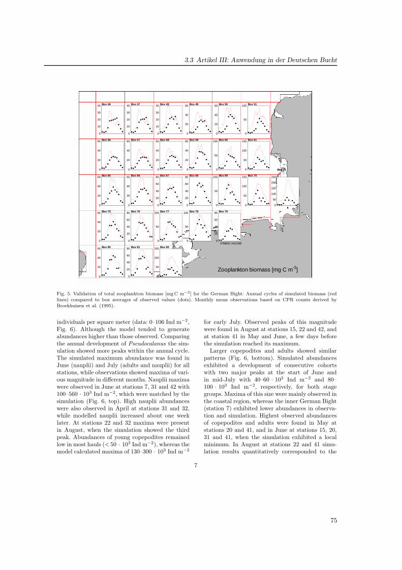
3.3 Artikel III: Anwendung in der Deutschen Bucht
Fig05.doc
Zooplankton biomass [mg C m-3]
0
10
20
30
40 Box 46
0
10
20
30
40 Box 47
0
10
20
30
40 Box 48
0
20
40
60 Box 49
0
20
40
60 Box 50
0
50
100 Box 51
0
20
40
60 Box 56
0
20
40
60 Box 57
0
20
40
60 Box 58
0
20
40
60 Box 59
0
50
100 Box 60
0
50
100
150 Box 61
0
20
40
60 Box 65
0
20
40
60 Box 66
0
20
40
60
80 Box 67
0
20
40
60
80 Box 68
0
50
100 Box 69
0
50
100
150 Box 70
0
50
100
150
200
250
Box 71
0
20
40
60 Box 75
0
20
40
60
80 Box 76
0
50
100 Box 77
0
50
100 Box 78
J F M A M J J A S O N D 0
20
40
60
80 Box 79
0
20
40
60 Box 80
0
20
40
60
80 Box 81
0
50
100
150 Box 82
Fig05.doc
Fig. 5. Validation of total zooplankton biomass [mgC m−3] for the German Bight: Annual cycles of simulated biomass (red
lines) compared to box averages of observed values (dots). Monthly mean observations based on CPR counts derived by
Broekhuizen et al. (1995).
individuals per square meter (data: 0–106 Ind m−2,Fig. 6). Although the model tended to generateabundances higher than those observed. Comparingthe annual development of Pseudocalanus the sim-ulation showed more peaks within the annual cycle.The simulated maximum abundance was found inJune (nauplii) and July (adults and nauplii) for allstations, while observations showed maxima of vari-ous magnitude in different months. Nauplii maximawere observed in June at stations 7, 31 and 42 with100–560 · 103 Ind m−2, which were matched by thesimulation (Fig. 6, top). High nauplii abundanceswere also observed in April at stations 31 and 32,while modelled nauplii increased about one weeklater. At stations 22 and 32 maxima were presentin August, when the simulation showed the thirdpeak. Abundances of young copepodites remainedlow in most hauls (< 50 · 103 Ind m−2), whereas themodel calculated maxima of 130–300 · 103 Ind m−2
for early July. Observed peaks of this magnitudewere found in August at stations 15, 22 and 42, andat station 41 in May and June, a few days beforethe simulation reached its maximum.
Larger copepodites and adults showed similarpatterns (Fig. 6, bottom). Simulated abundancesexhibited a development of consecutive cohortswith two major peaks at the start of June andin mid-July with 40–60 · 103 Ind m−2 and 80–100 · 103 Ind m−2, respectively, for both stagegroups. Maxima of this size were mainly observed inthe coastal region, whereas the inner German Bight(station 7) exhibited lower abundances in observa-tion and simulation. Highest observed abundancesof copepodites and adults were found in May atstations 20 and 41, and in June at stations 15, 20,31 and 41, when the simulation exhibited a localminimum. In August at stations 22 and 41 simu-lation results quantitatively corresponded to the
7
75
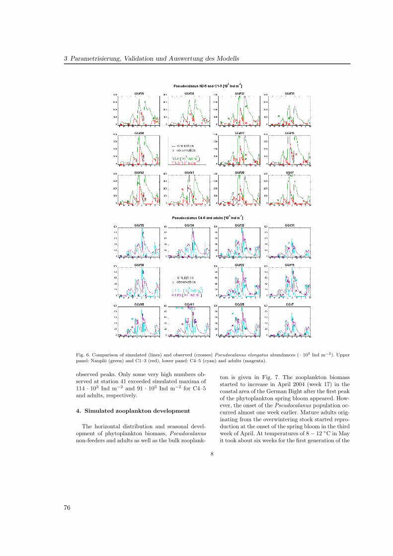
3 Parametrisierung, Validation und Auswertung des ModellsFig06.doc
Fig06.doc
Fig. 6. Comparison of simulated (lines) and observed (crosses) Pseudocalanus elongatus abundances ( · 103 Ind m−2). Upperpanel: Nauplii (green) and C1–3 (red), lower panel: C4–5 (cyan) and adults (magenta).
observed peaks. Only some very high numbers ob-served at station 41 exceeded simulated maxima of114 · 103 Ind m−2 and 91 · 103 Ind m−2 for C4–5and adults, respectively.
4. Simulated zooplankton development
The horizontal distribution and seasonal devel-opment of phytoplankton biomass, Pseudocalanusnon-feeders and adults as well as the bulk zooplank-
ton is given in Fig. 7. The zooplankton biomassstarted to increase in April 2004 (week 17) in thecoastal area of the German Bight after the first peakof the phytoplankton spring bloom appeared. How-ever, the onset of the Pseudocalanus population oc-curred almost one week earlier. Mature adults orig-inating from the overwintering stock started repro-duction at the onset of the spring bloom in the thirdweek of April. At temperatures of 8− 12 ◦C in Mayit took about six weeks for the first generation of the
8
76
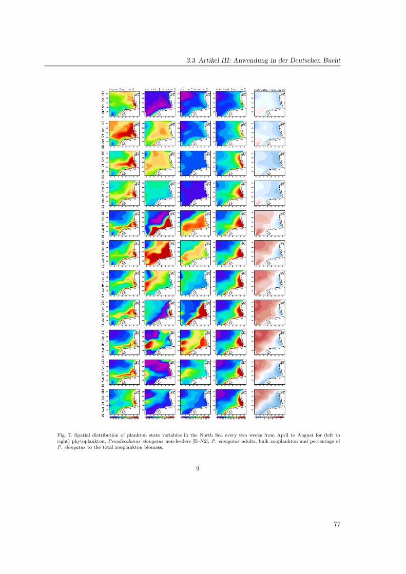
3.3 Artikel III: Anwendung in der Deutschen Bucht
Fig07.doc
Fig07.doc Fig. 7. Spatial distribution of plankton state variables in the North Sea every two weeks from April to August for (left to
right) phytoplankton, Pseudocalanus elongatus non-feeders [E–N2], P. elongatus adults, bulk zooplankton and percentage ofP. elongatus to the total zooplankton biomass.
9
77
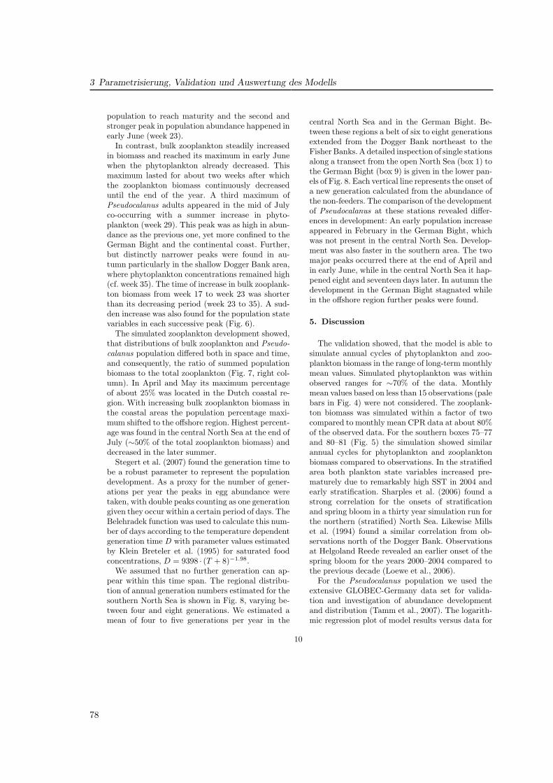
3 Parametrisierung, Validation und Auswertung des Modells
population to reach maturity and the second andstronger peak in population abundance happened inearly June (week 23).
In contrast, bulk zooplankton steadily increasedin biomass and reached its maximum in early Junewhen the phytoplankton already decreased. Thismaximum lasted for about two weeks after whichthe zooplankton biomass continuously decreaseduntil the end of the year. A third maximum ofPseudocalanus adults appeared in the mid of Julyco-occurring with a summer increase in phyto-plankton (week 29). This peak was as high in abun-dance as the previous one, yet more confined to theGerman Bight and the continental coast. Further,but distinctly narrower peaks were found in au-tumn particularly in the shallow Dogger Bank area,where phytoplankton concentrations remained high(cf. week 35). The time of increase in bulk zooplank-ton biomass from week 17 to week 23 was shorterthan its decreasing period (week 23 to 35). A sud-den increase was also found for the population statevariables in each successive peak (Fig. 6).
The simulated zooplankton development showed,that distributions of bulk zooplankton and Pseudo-calanus population differed both in space and time,and consequently, the ratio of summed populationbiomass to the total zooplankton (Fig. 7, right col-umn). In April and May its maximum percentageof about 25% was located in the Dutch coastal re-gion. With increasing bulk zooplankton biomass inthe coastal areas the population percentage maxi-mum shifted to the offshore region. Highest percent-age was found in the central North Sea at the end ofJuly (∼50% of the total zooplankton biomass) anddecreased in the later summer.
Stegert et al. (2007) found the generation time tobe a robust parameter to represent the populationdevelopment. As a proxy for the number of gener-ations per year the peaks in egg abundance weretaken, with double peaks counting as one generationgiven they occur within a certain period of days. TheBelehradek function was used to calculate this num-ber of days according to the temperature dependentgeneration time D with parameter values estimatedby Klein Breteler et al. (1995) for saturated foodconcentrations, D = 9398 · (T + 8)−1.98.
We assumed that no further generation can ap-pear within this time span. The regional distribu-tion of annual generation numbers estimated for thesouthern North Sea is shown in Fig. 8, varying be-tween four and eight generations. We estimated amean of four to five generations per year in the
central North Sea and in the German Bight. Be-tween these regions a belt of six to eight generationsextended from the Dogger Bank northeast to theFisher Banks. A detailed inspection of single stationsalong a transect from the open North Sea (box 1) tothe German Bight (box 9) is given in the lower pan-els of Fig. 8. Each vertical line represents the onset ofa new generation calculated from the abundance ofthe non-feeders. The comparison of the developmentof Pseudocalanus at these stations revealed differ-ences in development: An early population increaseappeared in February in the German Bight, whichwas not present in the central North Sea. Develop-ment was also faster in the southern area. The twomajor peaks occurred there at the end of April andin early June, while in the central North Sea it hap-pened eight and seventeen days later. In autumn thedevelopment in the German Bight stagnated whilein the offshore region further peaks were found.
5. Discussion
The validation showed, that the model is able tosimulate annual cycles of phytoplankton and zoo-plankton biomass in the range of long-term monthlymean values. Simulated phytoplankton was withinobserved ranges for ∼70% of the data. Monthlymean values based on less than 15 observations (palebars in Fig. 4) were not considered. The zooplank-ton biomass was simulated within a factor of twocompared to monthly mean CPR data at about 80%of the observed data. For the southern boxes 75–77and 80–81 (Fig. 5) the simulation showed similarannual cycles for phytoplankton and zooplanktonbiomass compared to observations. In the stratifiedarea both plankton state variables increased pre-maturely due to remarkably high SST in 2004 andearly stratification. Sharples et al. (2006) found astrong correlation for the onsets of stratificationand spring bloom in a thirty year simulation run forthe northern (stratified) North Sea. Likewise Millset al. (1994) found a similar correlation from ob-servations north of the Dogger Bank. Observationsat Helgoland Reede revealed an earlier onset of thespring bloom for the years 2000–2004 compared tothe previous decade (Loewe et al., 2006).
For the Pseudocalanus population we used theextensive GLOBEC-Germany data set for valida-tion and investigation of abundance developmentand distribution (Tamm et al., 2007). The logarith-mic regression plot of model results versus data for
10
78
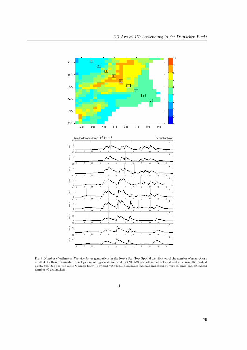
3.3 Artikel III: Anwendung in der Deutschen BuchtFig08.doc
J F M A M J J A S O N D 0
10
205
box
9
J F M A M J J A S O N D 0
10
205
box
8
J F M A M J J A S O N D 0
10
205
box
7
J F M A M J J A S O N D 0
5
107
box
6
J F M A M J J A S O N D 0
5
108
box
5
J F M A M J J A S O N D 0
5
108
box
4
J F M A M J J A S O N D 0
5
107
box
3
J F M A M J J A S O N D 0
5
104
box
2
J F M A M J J A S O N D 0
5
104
box
1
Non-feeder abundance [103 Ind m-3] Generation/year:
Fig08.doc
Fig. 8. Number of estimated Pseudocalanus generations in the North Sea. Top: Spatial distribution of the number of generations
in 2004. Bottom: Simulated development of eggs and non-feeders (N1–N2) abundance at selected stations from the centralNorth Sea (top) to the inner German Bight (bottom) with local abundance maxima indicated by vertical lines and estimated
number of generations.
11
79
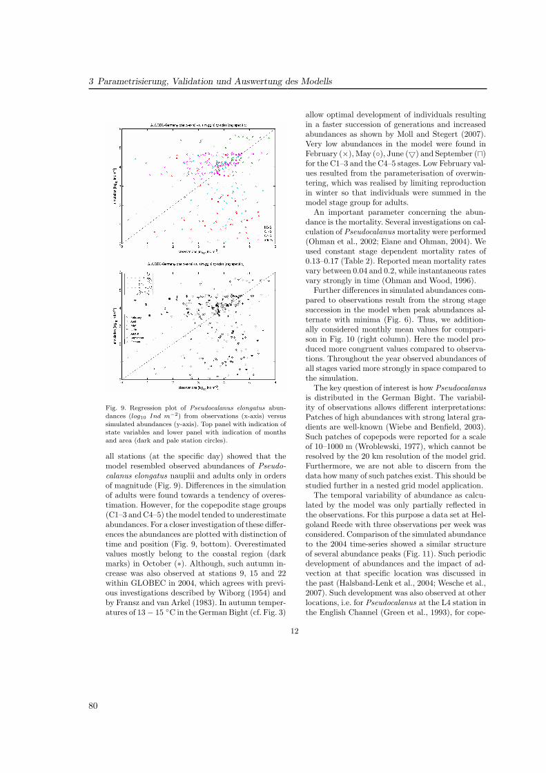
3 Parametrisierung, Validation und Auswertung des Modells
Fig09.doc
Fig09.doc Fig. 9. Regression plot of Pseudocalanus elongatus abun-
dances (log10 Ind m−2) from observations (x-axis) versus
simulated abundances (y-axis). Top panel with indication ofstate variables and lower panel with indication of months
and area (dark and pale station circles).
all stations (at the specific day) showed that themodel resembled observed abundances of Pseudo-calanus elongatus nauplii and adults only in ordersof magnitude (Fig. 9). Differences in the simulationof adults were found towards a tendency of overes-timation. However, for the copepodite stage groups(C1–3 and C4–5) the model tended to underestimateabundances. For a closer investigation of these differ-ences the abundances are plotted with distinction oftime and position (Fig. 9, bottom). Overestimatedvalues mostly belong to the coastal region (darkmarks) in October (∗). Although, such autumn in-crease was also observed at stations 9, 15 and 22within GLOBEC in 2004, which agrees with previ-ous investigations described by Wiborg (1954) andby Fransz and van Arkel (1983). In autumn temper-atures of 13− 15 ◦C in the German Bight (cf. Fig. 3)
allow optimal development of individuals resultingin a faster succession of generations and increasedabundances as shown by Moll and Stegert (2007).Very low abundances in the model were found inFebruary (×), May (◦), June (5) and September (u)for the C1–3 and the C4–5 stages. Low February val-ues resulted from the parameterisation of overwin-tering, which was realised by limiting reproductionin winter so that individuals were summed in themodel stage group for adults.
An important parameter concerning the abun-dance is the mortality. Several investigations on cal-culation of Pseudocalanus mortality were performed(Ohman et al., 2002; Eiane and Ohman, 2004). Weused constant stage dependent mortality rates of0.13–0.17 (Table 2). Reported mean mortality ratesvary between 0.04 and 0.2, while instantaneous ratesvary strongly in time (Ohman and Wood, 1996).
Further differences in simulated abundances com-pared to observations result from the strong stagesuccession in the model when peak abundances al-ternate with minima (Fig. 6). Thus, we addition-ally considered monthly mean values for compari-son in Fig. 10 (right column). Here the model pro-duced more congruent values compared to observa-tions. Throughout the year observed abundances ofall stages varied more strongly in space compared tothe simulation.
The key question of interest is how Pseudocalanusis distributed in the German Bight. The variabil-ity of observations allows different interpretations:Patches of high abundances with strong lateral gra-dients are well-known (Wiebe and Benfield, 2003).Such patches of copepods were reported for a scaleof 10–1000 m (Wroblewski, 1977), which cannot beresolved by the 20 km resolution of the model grid.Furthermore, we are not able to discern from thedata how many of such patches exist. This should bestudied further in a nested grid model application.
The temporal variability of abundance as calcu-lated by the model was only partially reflected inthe observations. For this purpose a data set at Hel-goland Reede with three observations per week wasconsidered. Comparison of the simulated abundanceto the 2004 time-series showed a similar structureof several abundance peaks (Fig. 11). Such periodicdevelopment of abundances and the impact of ad-vection at that specific location was discussed inthe past (Halsband-Lenk et al., 2004; Wesche et al.,2007). Such development was also observed at otherlocations, i.e. for Pseudocalanus at the L4 station inthe English Channel (Green et al., 1993), for cope-
12
80
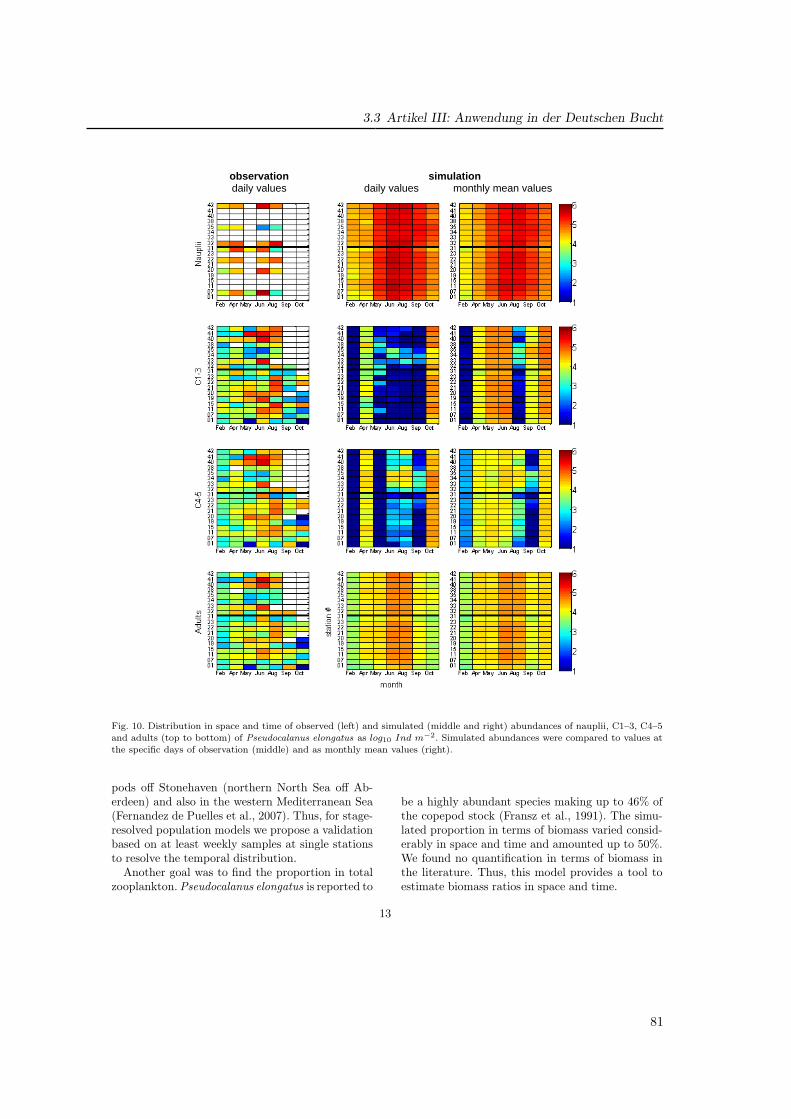
3.3 Artikel III: Anwendung in der Deutschen BuchtFig10.doc
observation simulation daily values daily values monthly mean values
Fig10.doc
Fig. 10. Distribution in space and time of observed (left) and simulated (middle and right) abundances of nauplii, C1–3, C4–5
and adults (top to bottom) of Pseudocalanus elongatus as log10 Ind m−2. Simulated abundances were compared to values atthe specific days of observation (middle) and as monthly mean values (right).
pods off Stonehaven (northern North Sea off Ab-erdeen) and also in the western Mediterranean Sea(Fernandez de Puelles et al., 2007). Thus, for stage-resolved population models we propose a validationbased on at least weekly samples at single stationsto resolve the temporal distribution.
Another goal was to find the proportion in totalzooplankton. Pseudocalanus elongatus is reported to
be a highly abundant species making up to 46% ofthe copepod stock (Fransz et al., 1991). The simu-lated proportion in terms of biomass varied consid-erably in space and time and amounted up to 50%.We found no quantification in terms of biomass inthe literature. Thus, this model provides a tool toestimate biomass ratios in space and time.
13
81
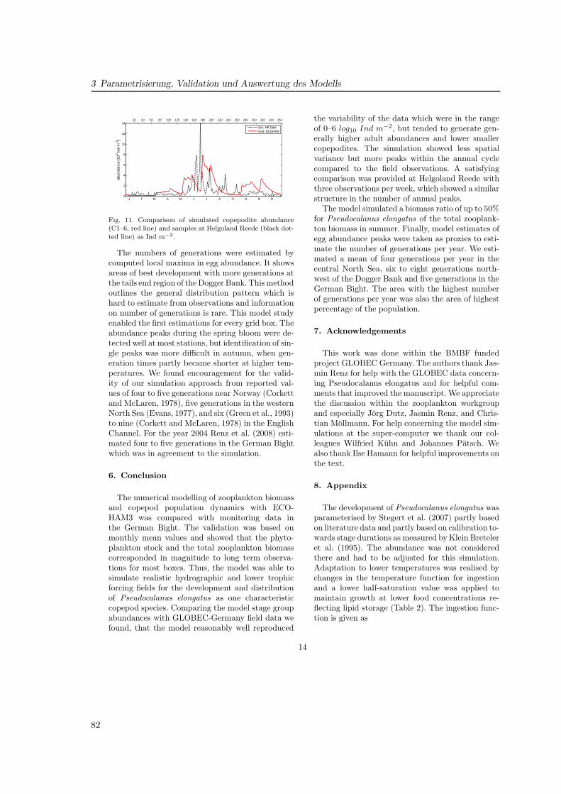
3 Parametrisierung, Validation und Auswertung des Modells
Fig11.doc
J F M A M J J A S O N D 0
2
4
6
8
10
12
14
abun
danc
e [1
03 Ind
m-2
]
obs: HR Datamod: ECOHAM
20 40 60 80 100 120 140 160 180 200 220 240 260 280 300 320 340 360
Fig11.doc
Fig. 11. Comparison of simulated copepodite abundance
(C1–6, red line) and samples at Helgoland Reede (black dot-ted line) as Ind m−2.
The numbers of generations were estimated bycomputed local maxima in egg abundance. It showsareas of best development with more generations atthe tails end region of the Dogger Bank. This methodoutlines the general distribution pattern which ishard to estimate from observations and informationon number of generations is rare. This model studyenabled the first estimations for every grid box. Theabundance peaks during the spring bloom were de-tected well at most stations, but identification of sin-gle peaks was more difficult in autumn, when gen-eration times partly became shorter at higher tem-peratures. We found encouragement for the valid-ity of our simulation approach from reported val-ues of four to five generations near Norway (Corkettand McLaren, 1978), five generations in the westernNorth Sea (Evans, 1977), and six (Green et al., 1993)to nine (Corkett and McLaren, 1978) in the EnglishChannel. For the year 2004 Renz et al. (2008) esti-mated four to five generations in the German Bightwhich was in agreement to the simulation.
6. Conclusion
The numerical modelling of zooplankton biomassand copepod population dynamics with ECO-HAM3 was compared with monitoring data inthe German Bight. The validation was based onmonthly mean values and showed that the phyto-plankton stock and the total zooplankton biomasscorresponded in magnitude to long term observa-tions for most boxes. Thus, the model was able tosimulate realistic hydrographic and lower trophicforcing fields for the development and distributionof Pseudocalanus elongatus as one characteristiccopepod species. Comparing the model stage groupabundances with GLOBEC-Germany field data wefound, that the model reasonably well reproduced
the variability of the data which were in the rangeof 0–6 log10 Ind m−2, but tended to generate gen-erally higher adult abundances and lower smallercopepodites. The simulation showed less spatialvariance but more peaks within the annual cyclecompared to the field observations. A satisfyingcomparison was provided at Helgoland Reede withthree observations per week, which showed a similarstructure in the number of annual peaks.
The model simulated a biomass ratio of up to 50%for Pseudocalanus elongatus of the total zooplank-ton biomass in summer. Finally, model estimates ofegg abundance peaks were taken as proxies to esti-mate the number of generations per year. We esti-mated a mean of four generations per year in thecentral North Sea, six to eight generations north-west of the Dogger Bank and five generations in theGerman Bight. The area with the highest numberof generations per year was also the area of highestpercentage of the population.
7. Acknowledgements
This work was done within the BMBF fundedproject GLOBEC Germany. The authors thank Jas-min Renz for help with the GLOBEC data concern-ing Pseudocalanus elongatus and for helpful com-ments that improved the manuscript. We appreciatethe discussion within the zooplankton workgroupand especially Jorg Dutz, Jasmin Renz, and Chris-tian Mollmann. For help concerning the model sim-ulations at the super-computer we thank our col-leagues Wilfried Kuhn and Johannes Patsch. Wealso thank Ilse Hamann for helpful improvements onthe text.
8. Appendix
The development of Pseudocalanus elongatus wasparameterised by Stegert et al. (2007) partly basedon literature data and partly based on calibration to-wards stage durations as measured by Klein Breteleret al. (1995). The abundance was not consideredthere and had to be adjusted for this simulation.Adaptation to lower temperatures was realised bychanges in the temperature function for ingestionand a lower half-saturation value was applied tomaintain growth at lower food concentrations re-flecting lipid storage (Table 2). The ingestion func-tion is given as
14
82
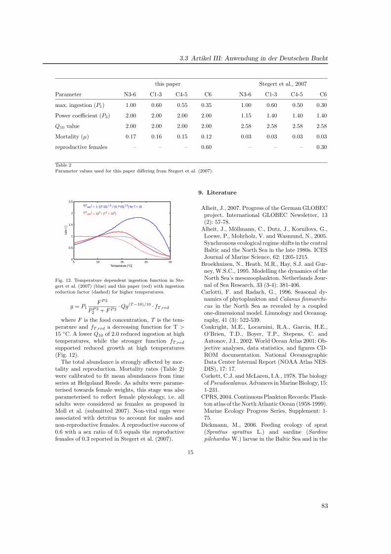
3.3 Artikel III: Anwendung in der Deutschen Bucht
this paper Stegert et al., 2007
Parameter N3-6 C1-3 C4-5 C6 N3-6 C1-3 C4-5 C6
max. ingestion (P1) 1.00 0.60 0.55 0.35 1.00 0.60 0.50 0.30
Power coefficient (P3) 2.00 2.00 2.00 2.00 1.15 1.40 1.40 1.40
Q10 value 2.00 2.00 2.00 2.00 2.58 2.58 2.58 2.58
Mortality (µ) 0.17 0.16 0.15 0.12 0.03 0.03 0.03 0.03
reproductive females – – – 0.60 – – – 0.30
Table 2Parameter values used for this paper differing from Stegert et al. (2007).
Fig12.doc
5 10 15 20 250
0.5
1
1.5
2
2.5
Temperature [°C]
rate
[ ]
= 1- [(T-15) 1.5 / (0.7*15)1.5] for T > 15
= 189 / (T9 + 189)
f(Tred )
f(Tred )
Fig12.doc
Fig. 12. Temperature dependent ingestion function in Ste-
gert et al. (2007) (blue) and this paper (red) with ingestionreduction factor (dashed) for higher temperatures.
g = P1FP3
PP32 + FP3
·Qg(T−10)/10 · fT,red
where F is the food concentration, T is the tem-perature and fT,red a decreasing function for T >15 ◦C. A lower Q10 of 2.0 reduced ingestion at hightemperatures, while the stronger function fT,red
supported reduced growth at high temperatures(Fig. 12).
The total abundance is strongly affected by mor-tality and reproduction. Mortality rates (Table 2)were calibrated to fit mean abundances from timeseries at Helgoland Reede. As adults were parame-terised towards female weights, this stage was alsoparameterised to reflect female physiology, i.e. alladults were considered as females as proposed inMoll et al. (submitted 2007). Non-vital eggs wereassociated with detritus to account for males andnon-reproductive females. A reproductive success of0.6 with a sex ratio of 0.5 equals the reproductivefemales of 0.3 reported in Stegert et al. (2007).
9. Literature
Alheit, J., 2007. Progress of the German GLOBECproject. International GLOBEC Newsletter, 13(2): 57-78.
Alheit, J., Mollmann, C., Dutz, J., Kornilovs, G.,Loewe, P., Mohrholz, V. and Wasmund, N., 2005.Synchronous ecological regime shifts in the centralBaltic and the North Sea in the late 1980s. ICESJournal of Marine Science, 62: 1205-1215.
Broekhuizen, N., Heath, M.R., Hay, S.J. and Gur-ney, W.S.C., 1995. Modelling the dynamics of theNorth Sea’s mesozooplankton. Netherlands Jour-nal of Sea Research, 33 (3-4): 381-406.
Carlotti, F. and Radach, G., 1996. Seasonal dy-namics of phytoplankton and Calanus finmarchi-cus in the North Sea as revealed by a coupledone-dimensional model. Limnology and Oceanog-raphy, 41 (3): 522-539.
Conkright, M.E., Locarnini, R.A., Garcia, H.E.,O’Brien, T.D., Boyer, T.P., Stepens, C. andAntonov, J.I., 2002. World Ocean Atlas 2001: Ob-jective analyses, data statistics, and figures CD-ROM documentation. National OceanographicData Center Internal Report (NOAA Atlas NES-DIS), 17: 17.
Corkett, C.J. and McLaren, I.A., 1978. The biologyof Pseudocalanus. Advances in Marine Biology, 15:1-231.
CPRS, 2004. Continuous Plankton Records: Plank-ton atlas of the North Atlantic Ocean (1958-1999).Marine Ecology Progress Series, Supplement: 1-75.
Dickmann, M., 2006. Feeding ecology of sprat(Sprattus sprattus L.) and sardine (Sardinepilchardus W.) larvae in the Baltic Sea and in the
15
83
3 Parametrisierung, Validation und Auswertung des Modells
North Sea. Ph.D. Thesis, University of Rostock,Rostock.
Eiane, K. and Ohman, M.D., 2004. Stage-specificmortality of Calanus finmarchicus, Pseudo-calanus elongatus and Oithona similis on FladenGround, North Sea, during a spring bloom. Ma-rine Ecology Progress Series, 268: 183-193.
Evans, G.T., 1977. A two layer shear diffusionmodel. Deep-Sea Research, 24 (10): 931-936.
Fennel, W., 2001. Modelling of copepods with linksto circulation models. Journal of Plankton Re-search, 23 (11): 1217-1232.
Fernandez de Puelles, M.L., Alemany, F. andJansa, J., 2007. Zooplankton time-series in theBalearic Sea (Western Mediterranean): Variabil-ity during the decade 1994-2003. Progress inOceanography, 74: 329-354.
Fransz, H.G., Colebrook, J.M., Gamble, J.C. andKrause, M., 1991. The zooplankton of the NorthSea. Netherlands Journal of Sea Research, 28(1/2): 1-52.
Fransz, H.G. and van Arkel, W.G., 1983. Fluctu-ation and succession of common pelagic copepodspecies in the Dutch Wadden Sea. OceanologicaActa, Vol. spec: 78-91.
Frost, B.W., 1989. A taxonomy of the marinecalanoid copepod genus Pseudocalanus. CanadianJournal of Zoology, 67: 525-551.
Green, E.P., Harris, R.P. and Duncan, A., 1993.The seasonal abundance of the copepodite stagesof Calanus helgolandicus and Pseudocalanus elon-gatus off Plymouth. Journal of the Marine Biolog-ical Association of the United Kingdom, 73: 109-122.
Halsband-Lenk, C., Carlotti, F. and Greve, W.,2004. Life-history strategies of calanoid congenersunder two different climate regimes: a compari-son. ICES Journal of Marine Science, 61: 709-720.
Heath, M.R., Edwards, A.C., Patsch, J. and Tur-rell, W.R., 2002. Modelling the behaviour of nu-trient in the coastal waters of Scotland. Report ofthe Fisheries Research Services, 10: 1-106.
Heath, M.R., Robertson, W., Mardaljevic, J. andGurney, W.S.G., 1997. Modelling the populationdynamics of Calanus in the Fair Isle current offnorthern Scotland. Journal of Sea Research, 38:381-412.
Klein Breteler, W.C.M., Fransz, H.G. and Gonza-les, S.R., 1982. Growth and development of fourcalanoid copepod species under experimental andnatural conditions. Netherlands Journal of SeaResearch, 16: 195-207.
Klein Breteler, W.C.M., Gonzales, S.R. andSchogt, N., 1995. Development of Pseudocalanuselongatus (Copepoda, Calanoida) cultured at dif-ferent temperature and food conditions. MarineEcology Progress Series, 119: 99-110.
Krause, M., Dippner, J.W. and Beil, J., 1995. Areview of hydrographic controls on the distribu-tion of zooplankton biomass and species in theNorth Sea with particular reference to a surveyconducted in Jan-Mar 1987. Progress in Oceanog-raphy, 35: 81-152.
Krause, M., Fock, H., Greve, W. and Winkler, G.,2003. North Sea Zooplankton: a review. Sencken-bergiana Maritima, 33 (1-2): 71-204.
Loewe, P., Becker, G., Brockmann, U., Dick, S.,Frohse, A., Hermann, J., Klein, B., Klein, H.,Nies, H., Schmolke, S., Schrader, D., Schulz, A.,Theobald, N. and Weigelt, S., 2006. Nordseezu-stand 2004, Bundesamt fur Seeschiffahrt undHydrographie (BSH), Hamburg.
Mauchline, J., 1998. The biology of Calanoid Cope-pods. Academic Press, San Diego, 710 pp.
Mills, D.K., Tett, P.B. and Vovrino, G., 1994. Thespring bloom in the south western North Sea in1989. Netherlands Journal of Sea Research, 33 (1):65-80.
Moll, A., Kreus, M., Kuhn, W., Krause, M. andGreve, W., submitted 2007. Seasonal dynamics ofPseudocalanus elongatus in the North Sea usingthe ecosystem model ECOHAM3 with competingbulk zooplankton. Part 1: Description and valida-tion of the embedded population model. Journalof Marine Systems.
Moll, A. and Stegert, C., 2007. Modelling Pseu-docalanus elongatus population dynamics embed-ded in a water column ecosystem model for thenorthern North Sea. Journal of Marine Systems,64 (1-4): 35-46.
Ohman, M.D., Runge, J.A., Durbin, E.G., Field,D.B. and Niehoff, B., 2002. On birth and death inthe sea. Hydrobiologia, 480: 55-68.
Ohman, M.D. and Wood, S.N., 1996. Mortality es-timation for planktonic copepods: Pseudocalanusnewmani in a temperate fjord. Limnology andOceanography, 41 (1): 126-135.
Patsch, J. and Kuhn, W., 2008. Nitrogen and car-bon cycling in the North Sea and exchange withthe North Atlantic - a model study, Part I. Ni-trogen budget and fluxes. Continental Shelf Re-search, doi:10.1016/j.csr.2007.12.013.
Patsch, J. and Lenhart, H.-J., 2004. Daily loadsof nutrients, total alkalinity, dissolved inorganic
16
84
3.3 Artikel III: Anwendung in der Deutschen Bucht
carbon and dissolved organic carbon of the Eu-ropean continental rivers for the years 1977-2002.Berichte aus dem Zentrum fur Meeres- und Kli-maforschung. Reihe B: Ozeanographie, 48: 159.
Pohlmann, T., 1996. Predicting the thermoclinein a circulation model of the North Sea - PartI: Model description, calibration and verification.Continental Shelf Research, 16 (2): 131-146.
Pohlmann, T., 2006. A meso-scale model of the cen-tral and southern North Sea: Consequences of animproved resolution. Continental Shelf Research,26: 2367-2385.
Radach, G. and Moll, A., 2006. Review of three-dimensional ecological modelling related to theNorth Sea shelf system. Part II: Model validationand data needs. Oceanography and Marine Biol-ogy: An Annual Review, 44: 1-60.
Radach, G. and Patsch, J., 1997. Climatologicalannual cycles of nutrients and chlorophyll in theNorth Sea. Journal of Sea Research, 38: 231-248.
Radach, G., Patsch, J., Gekeler, J. and Herbig, K.,1995. Annual cycles of nutrients and chlorophyllin the North Sea (Part 1). Berichte aus dem Zen-trum fur Meeres- und Klimaforschung. Reihe B:Ozeanographie, 20 (1): 172.
Renz, J., Mengedoht, D. and Hirche, H.-J., 2008.Reproduction, growth and secondary productionof Pseudocalanus elongatus Boeck (Copepoda,Calanoida) in the southern North Sea. Journal ofPlankton Research, doi: 10.1093/plankt/fbn016.
Rick, H.-J., Rick, S., Tillmann, U., Brockmann, U.,Gartner, U., Durselen, C.-D. and Sundermann, J.,2006. Primary productivity in the German Bight(1994-1996). Estuaries and Coasts, 29 (1): 4-23.
Sharples, J., Ross, O.N., Scott, B.E., Greenstreet,S.P.R. and Fraser, H., 2006. Inter-annual variabil-ity in the timing of stratification and the springbloom in the North-western North Sea. Continen-tal Shelf Research, 26: 733-751.
Skogen, M.D. and Moll, A., 2005. Importance ofocean circulation in ecological modelling: An ex-ample from the North Sea. Journal of Marine Sys-tems, 57 (3-4): 289-300.
Slagstad, D. and Tande, K.S., 1981. A mathemati-cal model of the assimilation process in the cope-pod Calanus finmarchicus (Gunnerus): computersimulations discusses in relation to experimentalresults. Kieler Meeresforschungen Sonderhefte, 5:229-239.
Speirs, D.C., Gurney, W.S.C., Heath, M.R. andWood, S.N., 2005. Modelling the basin-scale de-mography of Calanus finmarchicus in the north-
east Atlantic. Fisheries Oceanography, 14 (5):333-358.
Stegert, C., Kreus, M., Carlotti, F. and Moll, A.,2007. Parameterisation of a zooplankton popu-lation model for Pseudocalanus elongatus usingstage duration laboratory experiments. Ecologi-cal Modelling, 206 (3-4): 214-234.
Tamm, S., Moll, A. and Zabanski, S., 2007. TheGLOBEC-Germany database. GLOBEC Interna-tional Newsletter, 13 (2): 57-58.
Thomas, H., Bozec, Y., Elkalay, K. and de Baar,H.J.W., 2004. Enhanced open ocean storage ofCO2 from shelf sea pumping. Science, 304 (14 May2004): 1005-1008.
Wesche, A., Wiltshire, K.A. and J., H.H., 2007.Overwintering strategies of dominant calanoidcopepods in the German Bight, southern NorthSea. Marine Biology, 151 (4): 1309-1320.
Wiborg, K.F., 1954. Investigations on zooplank-ton in coastal and offshore waters of western andnorthwestern Norway with special reference to thecopepods. Fisk Dir. Skr. (Ser. Havunders.), 11 (1):1-246.
Wiebe, P.H. and Benfield, M.C., 2003. From theHensen net toward four-dimensional biologicaloceanography. Progress in Oceanography, 56:7-136.
Wroblewski, J.S., 1977. Vertically migrating her-bivorous plankton - their possible role in thecreation of small scale phytoplankton patchinessin the ocean. In: N. Andersen and B. Zahuranee(Editors), Oceanic sound scattering prediction.Plenum Press, pp. 817-847.
17
85

3 Parametrisierung, Validation und Auswertung des Modells
86
3.3 Artikel III: Anwendung in der Deutschen Bucht
3.3.2 Fazit zu Artikel III
Die Ergebnisse der numerischen Modellierung der Zooplanktonbiomasse sowie der Populati-onsdynamik der Copepoden mit ECOHAM3 wurde mit Meßdaten in der Deutschen Buchtverglichen. Die Validation von Phytoplankton- und gesamter Zooplanktonbiomasse zeigtegenerelle Übereinstimmung mit Monatsmittelwerten aus Langzeitmessungen. Somit wurdenmit dem Modell hydrographische Antriebsfelder sowie die untere trophische Stufe erfolgreichsimuliert und bereitgestellt, um die Entwicklung und Verteilung von Pseudocalanus elon-gatus als ein charakteristischer Copepode zu untersuchen. Im Vergleich der Abundanz derModell-Stadiengruppen mit Feldmessungen in GLOBEC-Germany ergab, daß die simulierteAbundanz die Variabilität der Messungen in der Größenordnung 0–6 log10 Ind m−2 wieder-gibt, wobei generell eine höhere Anzahl an Adulten und geringere Abundanz der Copepoditenmodelliert wurden.
Die Entwicklung in Raum und Zeit ergab im Vergleich zu Messungen geringere räum-liche Variabilität, dafür aber mehrere Maxima im Jahresverlauf als im Feld gemessen. Einzufrieden stellender Vergleich wurde zu den Zeitreihendaten bei Helgoland Reede erzielt.Die Simulation ergab einen Anteil bis zu 50% der Population an der Gesamtbiomasse. DieVerteilungsmuster von Pseudocalanus elongatus als eine wichtige Futterquelle für Sprotten-larven geben wichtige Hinweise über die Habitatvoraussetzungen und lassen sich für dieModellierung der Entwicklung von Fischlarven nutzen.
87

3 Parametrisierung, Validation und Auswertung des Modells
88
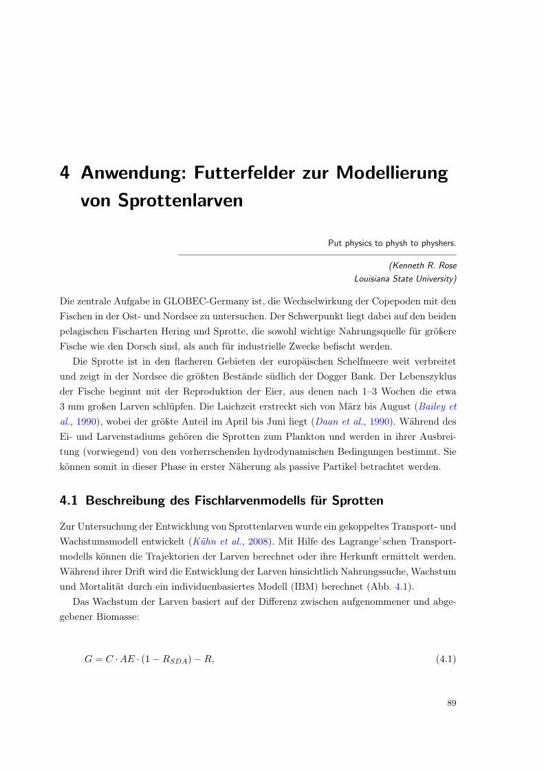
4 Anwendung: Futterfelder zur Modellierung
von Sprottenlarven
Put physics to physh to physhers.
(Kenneth R. Rose
Louisiana State University)
Die zentrale Aufgabe in GLOBEC-Germany ist, die Wechselwirkung der Copepoden mit denFischen in der Ost- und Nordsee zu untersuchen. Der Schwerpunkt liegt dabei auf den beidenpelagischen Fischarten Hering und Sprotte, die sowohl wichtige Nahrungsquelle für größereFische wie den Dorsch sind, als auch für industrielle Zwecke befischt werden.
Die Sprotte ist in den flacheren Gebieten der europäischen Schelfmeere weit verbreitetund zeigt in der Nordsee die größten Bestände südlich der Dogger Bank. Der Lebenszyklusder Fische beginnt mit der Reproduktion der Eier, aus denen nach 1–3 Wochen die etwa3 mm großen Larven schlüpfen. Die Laichzeit erstreckt sich von März bis August (Bailey etal., 1990), wobei der größte Anteil im April bis Juni liegt (Daan et al., 1990). Während desEi- und Larvenstadiums gehören die Sprotten zum Plankton und werden in ihrer Ausbrei-tung (vorwiegend) von den vorherrschenden hydrodynamischen Bedingungen bestimmt. Siekönnen somit in dieser Phase in erster Näherung als passive Partikel betrachtet werden.
4.1 Beschreibung des Fischlarvenmodells fur Sprotten
Zur Untersuchung der Entwicklung von Sprottenlarven wurde ein gekoppeltes Transport- undWachstumsmodell entwickelt (Kühn et al., 2008). Mit Hilfe des Lagrange’ schen Transport-modells können die Trajektorien der Larven berechnet oder ihre Herkunft ermittelt werden.Während ihrer Drift wird die Entwicklung der Larven hinsichtlich Nahrungssuche, Wachstumund Mortalität durch ein individuenbasiertes Modell (IBM) berechnet (Abb. 4.1).
Das Wachstum der Larven basiert auf der Differenz zwischen aufgenommener und abge-gebener Biomasse:
G = C ·AE · (1−RSDA)−R, (4.1)
89
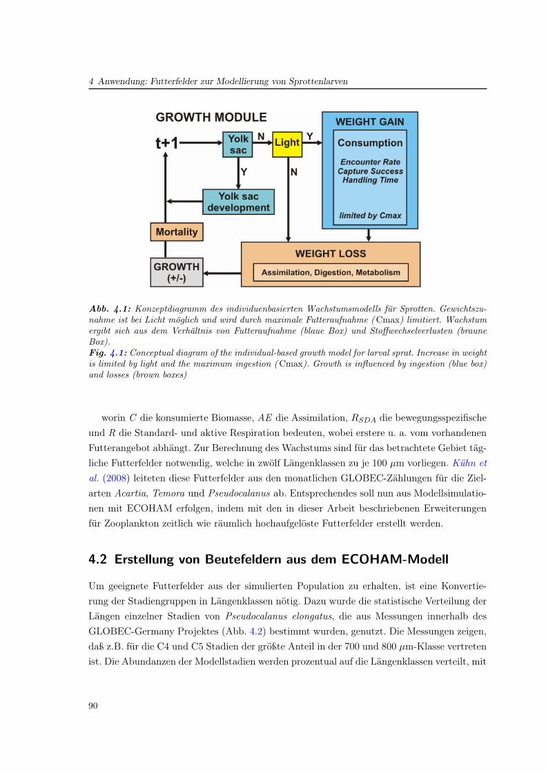
4 Anwendung: Futterfelder zur Modellierung von SprottenlarvenDissertation Christoph Stegert Fassung vom 22.05.2008
Seite 64/106
Abb. 12: Konzeptdiagramm des individuenbasierten Wachstumsmodells für
Sprotten. Gewichtszunahme ist bei Licht möglich und wird durch maximale
Futteraufnahme (Cmax) limitiert. Wachstum ergibt sich aus dem Verhältnis von
Futteraufnahme (blaue Box) und Stoffwechselverlusten (braune Box).
4.1 Beschreibung des Fischlarvenmodells für Sprotten
Zur Untersuchung der Entwicklung von Sprottenlarven wurde ein gekoppeltes
Transport- und Wachstumsmodell entwickelt (Kühn et al., 2008). Mit Hilfe des
Lagrange'schen Transportmodells können die Trajektorien der Larven berechnet
oder ihre Herkunft ermittelt werden. Während ihrer Drift wird die Entwicklung
der Larven hinsichtlich Nahrungssuche, Wachstum und Mortalität durch ein
individuenbasiertes Modell (IBM) berechnet.
Abb. 4.1: Konzeptdiagramm des individuenbasierten Wachstumsmodells fur Sprotten. Gewichtszu-nahme ist bei Licht moglich und wird durch maximale Futteraufnahme (Cmax) limitiert. Wachstumergibt sich aus dem Verhaltnis von Futteraufnahme (blaue Box) und Stoffwechselverlusten (brauneBox).Fig. 4.1: Conceptual diagram of the individual-based growth model for larval sprat. Increase in weightis limited by light and the maximum ingestion (Cmax). Growth is influenced by ingestion (blue box)and losses (brown boxes)
worin C die konsumierte Biomasse, AE die Assimilation, RSDA die bewegungsspezifischeund R die Standard- und aktive Respiration bedeuten, wobei erstere u. a. vom vorhandenenFutterangebot abhängt. Zur Berechnung des Wachstums sind für das betrachtete Gebiet täg-liche Futterfelder notwendig, welche in zwölf Längenklassen zu je 100 µm vorliegen. Kühn etal. (2008) leiteten diese Futterfelder aus den monatlichen GLOBEC-Zählungen für die Ziel-arten Acartia, Temora und Pseudocalanus ab. Entsprechendes soll nun aus Modellsimulatio-nen mit ECOHAM erfolgen, indem mit den in dieser Arbeit beschriebenen Erweiterungenfür Zooplankton zeitlich wie räumlich hochaufgelöste Futterfelder erstellt werden.
4.2 Erstellung von Beutefeldern aus dem ECOHAM-Modell
Um geeignete Futterfelder aus der simulierten Population zu erhalten, ist eine Konvertie-rung der Stadiengruppen in Längenklassen nötig. Dazu wurde die statistische Verteilung derLängen einzelner Stadien von Pseudocalanus elongatus, die aus Messungen innerhalb desGLOBEC-Germany Projektes (Abb. 4.2) bestimmt wurden, genutzt. Die Messungen zeigen,daß z.B. für die C4 und C5 Stadien der größte Anteil in der 700 und 800 µm-Klasse vertretenist. Die Abundanzen der Modellstadien werden prozentual auf die Längenklassen verteilt, mit
90
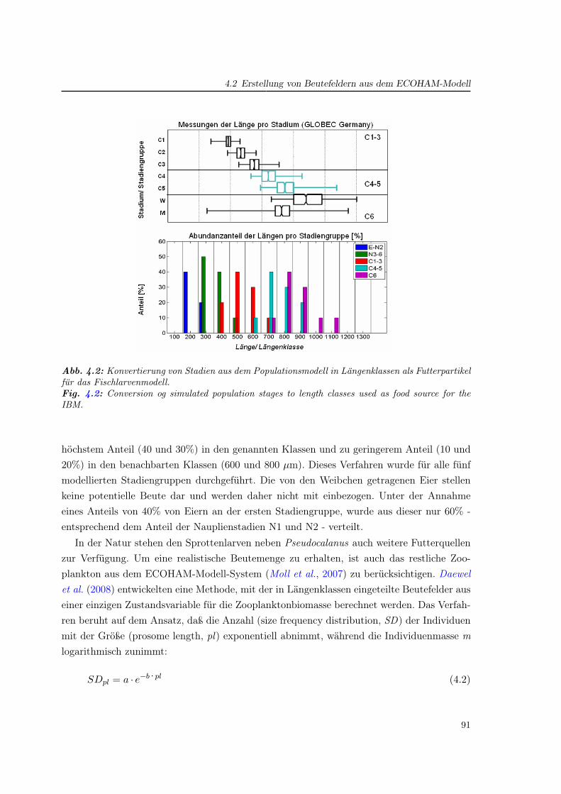
4.2 Erstellung von Beutefeldern aus dem ECOHAM-Modell
Dissertation Christoph Stegert Fassung vom 22.05.2008
Seite 66/106
Abundanzen der Modellstadien werden prozentual auf die Längenklassen
verteilt, mit höchstem Anteil (40 und 30%) in den genannten Klassen und zu
geringerem Anteil (10 und 20%) in den benachbarten Klassen (600 und 800
µm). Dieses Verfahren wurde für alle fünf modellierten Stadiengruppen
durchgeführt. Die von den Weibchen getragenen Eier stellen keine potentielle
Beute dar und werden daher nicht mit einbezogen. Unter der Annahme eines
Anteils von 40% von Eiern an der ersten Stadiengruppe, wurde aus dieser nur
60% – entsprechend dem Anteil der Nauplienstadien N1 und N2 – verteilt.
Abb. 13: Konvertierung von Stadien aus dem Populationsmodell in Abb. 4.2: Konvertierung von Stadien aus dem Populationsmodell in Langenklassen als Futterpartikelfur das Fischlarvenmodell.Fig. 4.2: Conversion og simulated population stages to length classes used as food source for theIBM.
höchstem Anteil (40 und 30%) in den genannten Klassen und zu geringerem Anteil (10 und20%) in den benachbarten Klassen (600 und 800 µm). Dieses Verfahren wurde für alle fünfmodellierten Stadiengruppen durchgeführt. Die von den Weibchen getragenen Eier stellenkeine potentielle Beute dar und werden daher nicht mit einbezogen. Unter der Annahmeeines Anteils von 40% von Eiern an der ersten Stadiengruppe, wurde aus dieser nur 60% -entsprechend dem Anteil der Nauplienstadien N1 und N2 - verteilt.
In der Natur stehen den Sprottenlarven neben Pseudocalanus auch weitere Futterquellenzur Verfügung. Um eine realistische Beutemenge zu erhalten, ist auch das restliche Zoo-plankton aus dem ECOHAM-Modell-System (Moll et al., 2007) zu berücksichtigen. Daewelet al. (2008) entwickelten eine Methode, mit der in Längenklassen eingeteilte Beutefelder auseiner einzigen Zustandsvariable für die Zooplanktonbiomasse berechnet werden. Das Verfah-ren beruht auf dem Ansatz, daß die Anzahl (size frequency distribution, SD) der Individuenmit der Größe (prosome length, pl) exponentiell abnimmt, während die Individuenmasse mlogarithmisch zunimmt:
SDpl = a · e−b · pl (4.2)
91
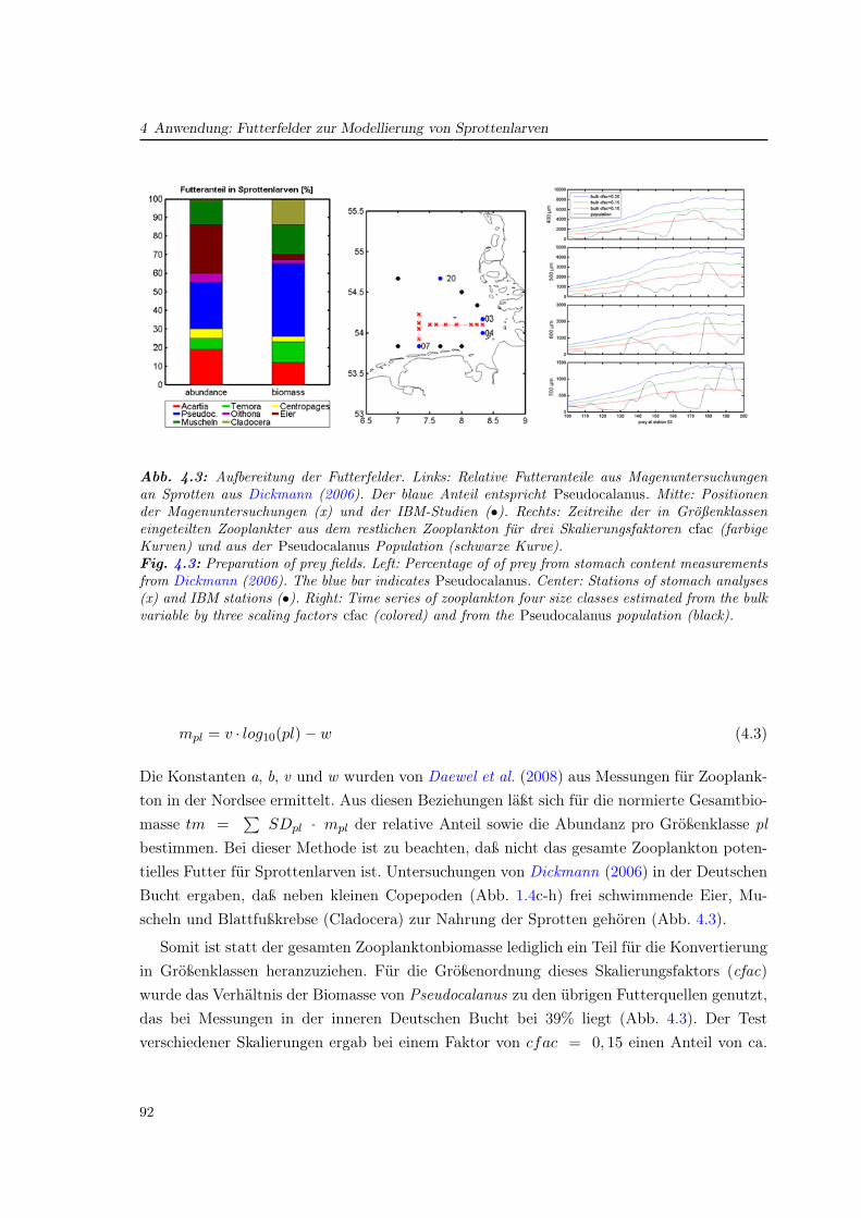
4 Anwendung: Futterfelder zur Modellierung von SprottenlarvenDissertation Christoph Stegert Fassung vom 22.05.2008
Seite 68/106
Abb. 14: Aufbereitung der Futterfelder. Links: Relative Futteranteile aus
Magenuntersuchungen an Sprotten nach Dickmann (2006). Der blaue Anteil
entspricht Pseudocalanus. Mitte: Positionen der Magenuntersuchungen (rot)
und der IBM-Studien. Rechts: Zeitreihe der in Größenklassen eingeteilten
Zooplankter aus dem restlichen Zooplankton für drei Skalierungsfaktoren cfac
(farbige Kurven) und aus der Pseudocalanus Population (schwarze Kurve).
Somit ist statt der gesamten Zooplanktonbiomasse lediglich ein Teil für die
Konvertierung in Größenklassen heranzuziehen. Für die Größenordnung dieses
Skalierungsfaktors (cfac) wurde das Verhältnis der Biomasse von
Pseudocalanus zu den übrigen Futterquellen genutzt, das bei Messungen in der
inneren Deutschen Bucht bei 39% liegt (Abb. 14). Der Test verschiedener
Skalierungen ergab bei einem Faktor von cfac = 0,15 einen Anteil von ca. 37%
der Population am Gesamtfutter (als 100-Tage-Mittel der umgebenden Stationen
3, 4, 7 und 20). Aus der modellierten restlichen Zooplanktonbiomasse Z
berechnet sich die Abundanz je Größenklasse pl somit durch:
Abb. 4.3: Aufbereitung der Futterfelder. Links: Relative Futteranteile aus Magenuntersuchungenan Sprotten aus Dickmann (2006). Der blaue Anteil entspricht Pseudocalanus. Mitte: Positionender Magenuntersuchungen (x) und der IBM-Studien (•). Rechts: Zeitreihe der in Großenklasseneingeteilten Zooplankter aus dem restlichen Zooplankton fur drei Skalierungsfaktoren cfac (farbigeKurven) und aus der Pseudocalanus Population (schwarze Kurve).Fig. 4.3: Preparation of prey fields. Left: Percentage of of prey from stomach content measurementsfrom Dickmann (2006). The blue bar indicates Pseudocalanus. Center: Stations of stomach analyses(x) and IBM stations (•). Right: Time series of zooplankton four size classes estimated from the bulkvariable by three scaling factors cfac (colored) and from the Pseudocalanus population (black).
mpl = v · log10(pl)− w (4.3)
Die Konstanten a, b, v und w wurden von Daewel et al. (2008) aus Messungen für Zooplank-ton in der Nordsee ermittelt. Aus diesen Beziehungen läßt sich für die normierte Gesamtbio-masse tm =
∑SDpl · mpl der relative Anteil sowie die Abundanz pro Größenklasse pl
bestimmen. Bei dieser Methode ist zu beachten, daß nicht das gesamte Zooplankton poten-tielles Futter für Sprottenlarven ist. Untersuchungen von Dickmann (2006) in der DeutschenBucht ergaben, daß neben kleinen Copepoden (Abb. 1.4c-h) frei schwimmende Eier, Mu-scheln und Blattfußkrebse (Cladocera) zur Nahrung der Sprotten gehören (Abb. 4.3).
Somit ist statt der gesamten Zooplanktonbiomasse lediglich ein Teil für die Konvertierungin Größenklassen heranzuziehen. Für die Größenordnung dieses Skalierungsfaktors (cfac)wurde das Verhältnis der Biomasse von Pseudocalanus zu den übrigen Futterquellen genutzt,das bei Messungen in der inneren Deutschen Bucht bei 39% liegt (Abb. 4.3). Der Testverschiedener Skalierungen ergab bei einem Faktor von cfac = 0, 15 einen Anteil von ca.
92
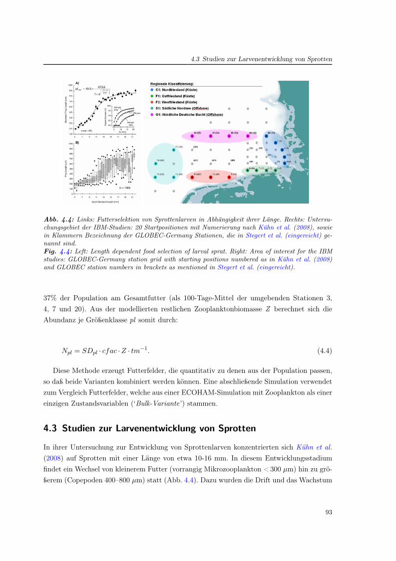
4.3 Studien zur Larvenentwicklung von SprottenDissertation Christoph Stegert Fassung vom 22.05.2008
Seite 70/106
Abb. 15: Links: Futterselektion von Sprottenlarven in Abhängigkeit ihrer
Länge. Rechts: Untersuchungsgebiet des IBM: 20 Startpositionen mit
Numerierung nach Kühn et al. (2008), sowie in Klammern Bezeichnung der
GLOBEC-Germany Stationen, die in Stegert et al. (submitted) genannt sind.
- Die Larvenentwicklung im Verlauf des Frühjahrs und des Sommers.
Dazu werden Szenarienläufe zwischen April (Tag 102) und August (Tag
241) durchgeführt. Dies entspricht den Zeitpunkten der in Stegert et al.
(submitted) (Artikel III) gezeigten Phyto- und Zooplanktonverteilung
(dortige Abb. 7). Hier werden Larven an fünf Stationen repräsentativ für
verschiedene Regionen aus Abb. 15 betrachtet. Anhand der erreichten
Länge nach zehn Tagen wird der saisonale Verlauf untersucht.
- Räumliche Unterschiede in der Larvenentwicklung im Juni. Dieser Monat
stellt einen typischen Zeitraum für Sprottenlarven dieser Größe dar
(Munk, 1993). Hier werden in drei aufeinander folgenden Zeiträumen
Abb. 4.4: Links: Futterselektion von Sprottenlarven in Abhangigkeit ihrer Lange. Rechts: Untersu-chungsgebiet der IBM-Studien: 20 Startpositionen mit Numerierung nach Kuhn et al. (2008), sowiein Klammern Bezeichnung der GLOBEC-Germany Stationen, die in Stegert et al. (eingereicht) ge-nannt sind.Fig. 4.4: Left: Length dependent food selection of larval sprat. Right: Area of interest for the IBMstudies: GLOBEC-Germany station grid with starting positions numbered as in Kuhn et al. (2008)and GLOBEC station numbers in brackets as mentioned in Stegert et al. (eingereicht).
37% der Population am Gesamtfutter (als 100-Tage-Mittel der umgebenden Stationen 3,4, 7 und 20). Aus der modellierten restlichen Zooplanktonbiomasse Z berechnet sich dieAbundanz je Größenklasse pl somit durch:
Npl = SDpl · cfac ·Z · tm−1. (4.4)
Diese Methode erzeugt Futterfelder, die quantitativ zu denen aus der Population passen,so daß beide Varianten kombiniert werden können. Eine abschließende Simulation verwendetzum Vergleich Futterfelder, welche aus einer ECOHAM-Simulation mit Zooplankton als einereinzigen Zustandsvariablen (‘Bulk-Variante’) stammen.
4.3 Studien zur Larvenentwicklung von Sprotten
In ihrer Untersuchung zur Entwicklung von Sprottenlarven konzentrierten sich Kühn et al.(2008) auf Sprotten mit einer Länge von etwa 10-16 mm. In diesem Entwicklungsstadiumfindet ein Wechsel von kleinerem Futter (vorrangig Mikrozooplankton < 300 µm) hin zu grö-ßerem (Copepoden 400–800 µm) statt (Abb. 4.4). Dazu wurden die Drift und das Wachstum
93
4 Anwendung: Futterfelder zur Modellierung von Sprottenlarven
der Larven mit einer Anfangslänge von 10 mm über einen Zeitraum von zehn Tagen und star-tend an 20 Stationen in der Deutschen Bucht (Abb. 4.4) simuliert. Diese Szenarienauswahlwird auch in den folgenden Beispielanwendungen wiederholt. Um die Wirkung der aus derPopulation ermittelten Futterfelder auf die Entwicklung der Sprottenlarven zu untersuchen,werden zwei Studien durchgeführt:
• Die Larvenentwicklung im Verlauf des Frühjahrs und des Sommers. Dazu werden Szena-rienläufe zwischen April (Tag 102) und August (Tag 241) durchgeführt. Dies entsprichtden Zeitpunkten der in Artikel III gezeigten Phyto- und Zooplanktonverteilung (dor-tige Abb. 2.2). Hier werden Larven an fünf Stationen repräsentativ für verschiedeneRegionen aus Abb. 4.4 betrachtet. Anhand der erreichten Länge nach zehn Tagen wirdder saisonale Verlauf untersucht.
• Räumliche Unterschiede in der Larvenentwicklung im Juni. Dieser Monat stellt einentypischen Zeitraum für Sprottenlarven dieser Größe dar (Munk , 1993). Hier werdenin drei aufeinander folgenden Zeiträumen (startend an den Tagen 155, 165 und 175)alle Stationen vergleichend betrachtet, sowie zwei Positionen (küstennah/ablandig) imDetail untersucht. Hier wird der Einfluß der kurzzeitigen Schwankungen der Populationherausgearbeitet.
Für zwei Positionen wird abschließend die Entwicklung der Fischlarven bei Verwendungvon verschiedenen Futterfeldern aus der Population und der Biomassevariablen verglichen.
4.3.1 Das Wachstum zu verschiedenen Jahreszeiten
In der Abundanz der Größenklassen (Abb. 4.5) spiegelt sich die Generationsabfolge der Po-pulation wider. Entsprechend ist die Entwicklung der Larven in den untersuchten Zeiträumenverschieden. Anfang April kann sich keine der Larven entwickeln, da die Futterkonzentrationzu gering ist. In den weiteren Simulationen nimmt bei steigender Temperatur (10−−20 ◦C)auch die maximal erreichte Larvenlänge von ca. 12 mm Ende April auf 17 mm Anfang Au-gust zu. Im zweiten und dritten 10-Tage-Lauf im August (Simulationen 10 und 11) wirktwiederum das Futter limitierend und die Entwicklung ist stark gehemmt. Neben der Ab-hängigkeit von der Temperatur zeigt sich in den übrigen Simulationen auch der Einfluß derFutterverfügbarkeit in der Variabilität zwischen den einzelnen Stationen.
Der Wechsel von hohen und geringen Abundanzen in der Zooplanktonpopulation - alsodem Futter - führt zu lokalen Minima bei den Sprottenlarven. Ein solches Minimum findetsich z. B. in der 5. Simulation (ab Tag 158) an den nördlichen und westlichen Stationen (9,13 und 17). Die Folge ist jeweils eine trotz steigender Temperatur geringere Endlänge der
94
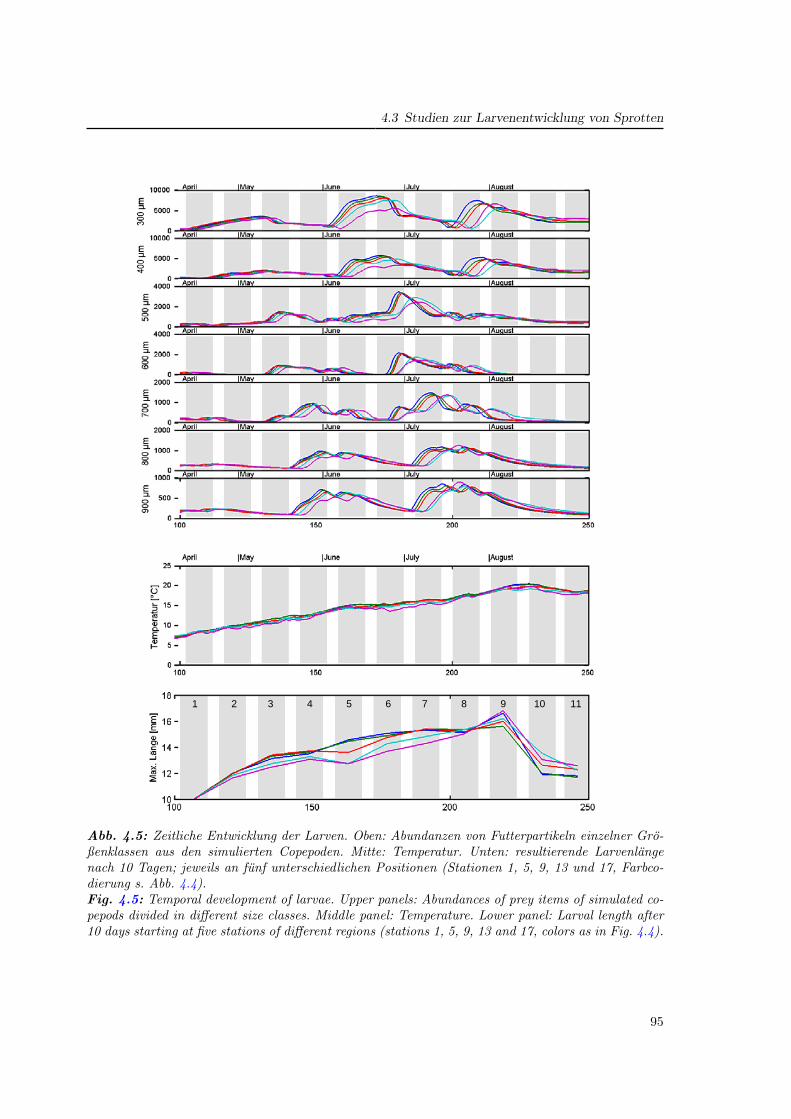
4.3 Studien zur Larvenentwicklung von SprottenDissertation Christoph Stegert Fassung vom 22.05.2008
Seite 72/106
Abb. 16: Zeitliche Entwicklung: Oben: Abundanzen von Futterpartikeln
einzelner Größenklassen aus den simulierten Copepoden. Mitte: Temperatur.
Unten: resultierende Larvenlänge nach 10 Tagen; jeweils an fünf
unterschiedlichen Positionen (Stationen 1, 5, 9, 13 und 17, Farbcodierung s.
Abb. 15).
1 2 3 4 5 6 7 8 9 10 11
Abb. 4.5: Zeitliche Entwicklung der Larven. Oben: Abundanzen von Futterpartikeln einzelner Gro-ßenklassen aus den simulierten Copepoden. Mitte: Temperatur. Unten: resultierende Larvenlangenach 10 Tagen; jeweils an funf unterschiedlichen Positionen (Stationen 1, 5, 9, 13 und 17, Farbco-dierung s. Abb. 4.4).Fig. 4.5: Temporal development of larvae. Upper panels: Abundances of prey items of simulated co-pepods divided in different size classes. Middle panel: Temperature. Lower panel: Larval length after10 days starting at five stations of different regions (stations 1, 5, 9, 13 and 17, colors as in Fig. 4.4).
95
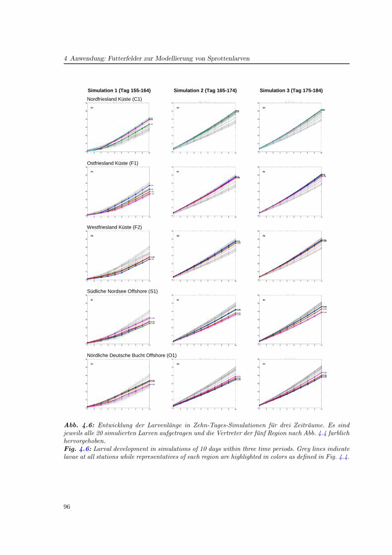
4 Anwendung: Futterfelder zur Modellierung von Sprottenlarven
Dissertation Christoph Stegert Fassung vom 22.05.2008
Seite 74/106
Simulation 1 (Tag 155-164) Simulation 2 (Tag 165-174) Simulation 3 (Tag 175-184)
Nordfriesland Küste (C1)
Ostfriesland Küste (F1)
Westfriesland Küste (F2)
Südliche Nordsee Offshore (S1)
Nördliche Deutsche Bucht Offshore (O1)
Abb. 17: Entwicklung der Larvenlänge in Zehn-Tages-Simulationen für drei
Zeiträume. Es sind jeweils alle 20 simulierten Larven aufgetragen und die
Vertreter der fünf Region nach Abb. 15 farblich hervorgehoben.
Abb. 4.6: Entwicklung der Larvenlange in Zehn-Tages-Simulationen fur drei Zeitraume. Es sindjeweils alle 20 simulierten Larven aufgetragen und die Vertreter der funf Region nach Abb. 4.4 farblichhervorgehoben.Fig. 4.6: Larval development in simulations of 10 days within three time periods. Grey lines indicatelavae at all stations while representatives of each region are highlighted in colors as defined in Fig. 4.4.
96
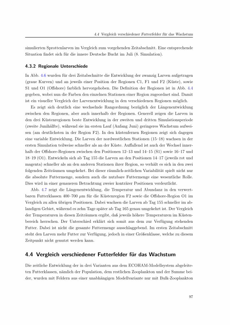
4.4 Vergleich verschiedener Futterfelder fur das Wachstum
simulierten Sprottenlarven im Vergleich zum vorgehenden Zeitabschnitt. Eine entsprechendeSituation findet sich für die innere Deutsche Bucht im Juli (8. Simulation).
4.3.2 Regionale Unterschiede
In Abb. 4.6 wurden für drei Zeitabschnitte die Entwicklung der zwanzig Larven aufgetragen(graue Kurven) und an jeweils einer Position der Regionen C1, F1 und F2 (Küste), sowieS1 und O1 (Offshore) farblich hervorgehoben. Die Definition der Regionen ist in Abb. 4.4gegeben, wobei nun die Farben den einzelnen Stationen einer Region zugeordnet sind. Damitist ein visueller Vergleich der Larvenentwicklung in den verschiedenen Regionen möglich.
Es zeigt sich deutlich eine wechselnde Rangordnung bezüglich der Längenentwicklungzwischen den Regionen, aber auch innerhalb der Regionen. Generell zeigen die Larven inden drei Küstenregionen beste Entwicklung in der zweiten und dritten Simulationsperiode(zweite Junihälfte), während sie im ersten Lauf (Anfang Juni) geringeres Wachstum aufwei-sen (am deutlichsten in der Region F2). In den küstenfernen Regionen zeigt sich dagegeneine variable Entwicklung. Die Larven der nordwestlichen Stationen (15–18) wachsen in derersten Simulation teilweise schneller als an der Küste. Auffallend ist auch der Wechsel inner-halb der Offshore-Regionen zwischen den Positionen 12–13 und 14–15 (S1) sowie 16–17 und18–19 (O1). Entwickeln sich ab Tag 155 die Larven an den Positionen 14–17 (jeweils rot undmagenta) schneller als an den anderen Stationen ihrer Region, so verhält es sich in den zweifolgenden Zeiträumen umgekehrt. Bei dieser räumlich-zeitlichen Variabilität spielt nicht nurdie absolute Futtermenge, sondern auch die nutzbare Futtermenge eine wesentliche Rolle.Dies wird in einer genaueren Betrachtung zweier konträrer Positionen verdeutlicht.
Abb. 4.7 zeigt die Längenentwicklung, die Temperatur und Abundanz in den verwert-baren Futterklassen 400–700 µm für die Küstenregion F2 sowie die Offshore-Region O1 imVergleich zu allen übrigen Positionen. Dabei wachsen die Larven ab Tag 155 schneller im ab-landigen Gebiet, während es zehn Tage später ab Tag 165 genau umgekehrt ist. Der Vergleichder Temperaturen in diesen Zeiträumen ergibt, daß jeweils höhere Temperaturen im Küsten-bereich herrschen. Der Unterschied erklärt sich somit aus dem zur Verfügung stehendenFutter. Dabei ist nicht die gesamte Futtermenge ausschlaggebend. Im ersten Zeitabschnittsteht den Larven mehr Futter zur Verfügung, jedoch in einer Größenklasse, welche zu diesemZeitpunkt nicht genutzt werden kann.
4.4 Vergleich verschiedener Futterfelder fur das Wachstum
Die zeitliche Entwicklung der in drei Varianten aus dem ECOHAM-Modellsystem abgeleite-ten Futterklassen, nämlich der Population, dem restlichen Zooplankton und der Summe bei-der, wurden mit Feldern aus einer unabhängigen Modellvariante nur mit Bulk-Zooplankton
97
4 Anwendung: Futterfelder zur Modellierung von Sprottenlarven
Dissertation Christoph Stegert Fassung vom 22.05.2008
Seite 76/106
Tag 155-164
Tag 165-174
Abb. 18: Vergleich der Larvenlänge, der Temperatur und der
Futterbedingungen für zwei Zeiträume an den Positionen 9 und 17 (s. Abb. 15).
Abb. 18 zeigt die Längenentwicklung, die Temperatur und Abundanz in den
verwertbaren Futterklassen 400-700 µm für die Küstenregion F2 sowie die
Offshore-Region O1 im Vergleich zu allen übrigen Positionen. Dabei wachsen
die Larven ab Tag 155 schneller im ablandigen Gebiet, während es zehn Tage
Abb. 4.7: Vergleich der Larvenlange, der Temperatur und der Futterbedingungen fur zwei Zeitraumean den Positionen 9 und 17 (s. Abb. 4.4).Fig. 4.7: Comparison of larval length, temperature and food conditions for two time periods atstations 9 and 17 (s. Fig. 4.4).
in Abb. 4.8 verglichen. Es zeigt sich, daß die ausgeprägte zeitliche Variabilität der Popu-lation (schwarz) in den Futterfeldern aus Bulk-Zooplankton nicht zu finden ist. Vielmehrist die zeitliche Entwicklung in allen Längenklassen identisch, lediglich die Abundanzwertesind unterschiedlich. Dagegen zeigt die Population zwischen den Maxima der Längenklas-sen einen zeitlichen Versatz, der in der sukzessiven Stadienentwicklung begründet ist. InAbb. 4.9 (links) werden die Längenentwicklungen der Sprottenlarven mit den verschiedenenFutterfeldern noch einmal detailliert für diese zwei Positionen gezeigt.
Trotz unterschiedlicher Abundanz mit Ausnahme der Population im ersten Lauf führenalle Futterfelder zu gleichen Larvenentwicklungen. Die Ursache liegt in der Begrenzung derFutteraufnahme im Wachstummodell durch den Maximalwert Cmax (s. Abb. 4.1). DieserWert sorgt im IBM dafür, daß die Larven bei sehr hohen Futterwerten nicht überproportio-nal schnell wachsen. Das bedeutet an dieser Stelle, daß mit allen simulierten Beutefeldern
98
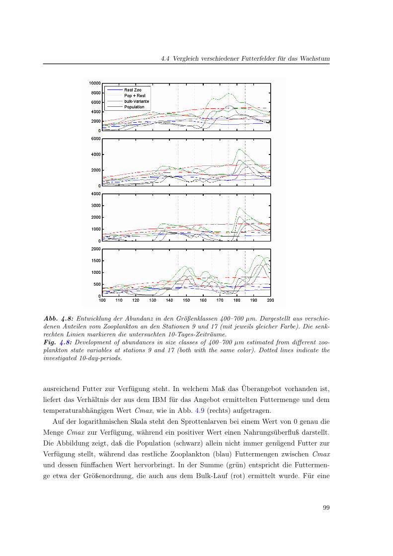
4.4 Vergleich verschiedener Futterfelder fur das Wachstum
Dissertation Christoph Stegert Fassung vom 22.05.2008
Seite 78/106
4.4 Vergleich verschiedener Futterfelder für das Wachstum
Abb. 19: Entwicklung der Abundanz in den Größenklassen 400-700 µm.
Dargestellt aus verschiedenen Anteilen vom Zooplankton an den Stationen 9
und 17 (mit jeweils gleicher Farbe). Die senkrechten Linien markieren die
untersuchten 10-Tages-Zeiträume.
Abb. 4.8: Entwicklung der Abundanz in den Großenklassen 400–700 µm. Dargestellt aus verschie-denen Anteilen vom Zooplankton an den Stationen 9 und 17 (mit jeweils gleicher Farbe). Die senk-rechten Linien markieren die untersuchten 10-Tages-Zeitraume.Fig. 4.8: Development of abundances in size classes of 400–700 µm estimated from different zoo-plankton state variables at stations 9 and 17 (both with the same color). Dotted lines indicate theinvestigated 10-day-periods.
ausreichend Futter zur Verfügung steht. In welchem Maß das Überangebot vorhanden ist,liefert das Verhältnis der aus dem IBM für das Angebot ermittelten Futtermenge und demtemperaturabhängigen Wert Cmax, wie in Abb. 4.9 (rechts) aufgetragen.
Auf der logarithmischen Skala steht den Sprottenlarven bei einem Wert von 0 genau dieMenge Cmax zur Verfügung, während ein positiver Wert einen Nahrungsüberfluß darstellt.Die Abbildung zeigt, daß die Population (schwarz) allein nicht immer genügend Futter zurVerfügung stellt, während das restliche Zooplankton (blau) Futtermengen zwischen Cmaxund dessen fünffachen Wert hervorbringt. In der Summe (grün) entspricht die Futtermen-ge etwa der Größenordnung, die auch aus dem Bulk-Lauf (rot) ermittelt wurde. Für eine
99
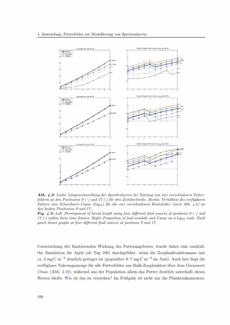
4 Anwendung: Futterfelder zur Modellierung von Sprottenlarven
Dissertation Christoph Stegert Fassung vom 22.05.2008
Seite 80/106
Abb. 20: Links: Längenentwicklung der Sprottenlarven bei Nutzung von vier
verschiedenen Futterfeldern an den Positionen 9 (–) und 17 (:) für drei
Zeitabschnitte. Rechts: Verhältnis des verfügbaren Futters zum Schwellwert
Cmax (log10) für die vier verschiedenen Beutefelder (nach Abb. 19) an den
beiden Positionen 9 und 17.
Abb. 4.9: Links: Langenentwicklung der Sprottenlarven bei Nutzung von vier verschiedenen Futter-feldern an den Positionen 9 (–) und 17 (:) fur drei Zeitabschnitte. Rechts: Verhaltnis des verfugbarenFutters zum Schwellwert Cmax (log10) fur die vier verschiedenen Beutefelder (nach Abb. 4.8) anden beiden Positionen 9 und 17.Fig. 4.9: Left: Development of larval length using four different food sources at positions 9 (–) and17 (:) within three time frames. Right: Proportion of food availabe and Cmax on a log10 scale. Eachpanel shows graphs at four different food sources at positions 9 and 17.
Untersuchung der limitierenden Wirkung des Futterangebotes, wurde daher eine zusätzli-che Simulation für April (ab Tag 100) durchgeführt, wenn die Zooplanktonbiomasse mitca. 2 mg C m−3 deutlich geringer ist (gegenüber 6–7 mg C m−3 im Juni). Auch hier liegt dieverfügbare Nahrungsmenge für alle Futterfelder aus Bulk-Zooplankton über dem GrenzwertCmax (Abb. 4.10), während aus der Population allein das Futter deutlich unterhalb diesesWertes bleibt. Wie ist das zu verstehen? Im Frühjahr ist nicht nur die Planktonkonzentra-
100
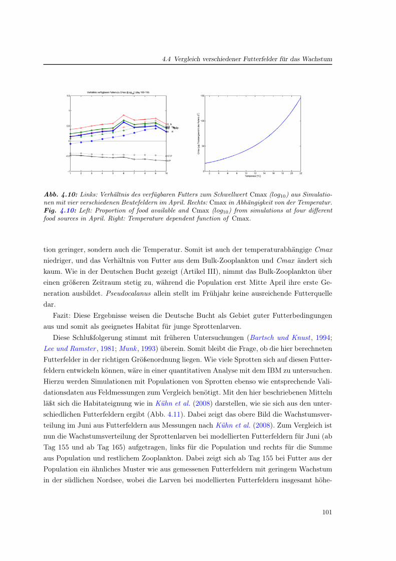
4.4 Vergleich verschiedener Futterfelder fur das Wachstum
Dissertation Christoph Stegert Fassung vom 22.05.2008
Seite 82/106
Fazit: Diese Ergebnisse weisen die Deutsche Bucht als Gebiet guter
Futterbedingungen aus und somit als geeignetes Habitat für junge
Sprottenlarven.
Abb. 21: Links: Verhältnis des verfügbaren Futters zum Schwellwert Cmax
(log10) aus Simulationen mit vier verschiedenen Beutefeldern im April. Rechts:
Cmax. in Abhängigkeit von der Temperatur.
Abb. 4.10: Links: Verhaltnis des verfugbaren Futters zum Schwellwert Cmax (log10) aus Simulatio-nen mit vier verschiedenen Beutefeldern im April. Rechts: Cmax in Abhangigkeit von der Temperatur.Fig. 4.10: Left: Proportion of food available and Cmax (log10) from simulations at four differentfood sources in April. Right: Temperature dependent function of Cmax.
tion geringer, sondern auch die Temperatur. Somit ist auch der temperaturabhängige Cmaxniedriger, und das Verhältnis von Futter aus dem Bulk-Zooplankton und Cmax ändert sichkaum. Wie in der Deutschen Bucht gezeigt (Artikel III), nimmt das Bulk-Zooplankton übereinen größeren Zeitraum stetig zu, während die Population erst Mitte April ihre erste Ge-neration ausbildet. Pseudocalanus allein stellt im Frühjahr keine ausreichende Futterquelledar.
Fazit: Diese Ergebnisse weisen die Deutsche Bucht als Gebiet guter Futterbedingungenaus und somit als geeignetes Habitat für junge Sprottenlarven.
Diese Schlußfolgerung stimmt mit früheren Untersuchungen (Bartsch und Knust , 1994;Lee und Ramster , 1981; Munk , 1993) überein. Somit bleibt die Frage, ob die hier berechnetenFutterfelder in der richtigen Größenordnung liegen. Wie viele Sprotten sich auf diesen Futter-feldern entwickeln können, wäre in einer quantitativen Analyse mit dem IBM zu untersuchen.Hierzu werden Simulationen mit Populationen von Sprotten ebenso wie entsprechende Vali-dationsdaten aus Feldmessungen zum Vergleich benötigt. Mit den hier beschriebenen Mittelnläßt sich die Habitateignung wie in Kühn et al. (2008) darstellen, wie sie sich aus den unter-schiedlichen Futterfeldern ergibt (Abb. 4.11). Dabei zeigt das obere Bild die Wachstumsver-teilung im Juni aus Futterfeldern aus Messungen nach Kühn et al. (2008). Zum Vergleich istnun die Wachstumsverteilung der Sprottenlarven bei modellierten Futterfeldern für Juni (abTag 155 und ab Tag 165) aufgetragen, links für die Population und rechts für die Summeaus Population und restlichem Zooplankton. Dabei zeigt sich ab Tag 155 bei Futter aus derPopulation ein ähnliches Muster wie aus gemessenen Futterfeldern mit geringem Wachstumin der südlichen Nordsee, wobei die Larven bei modellierten Futterfeldern insgesamt höhe-
101
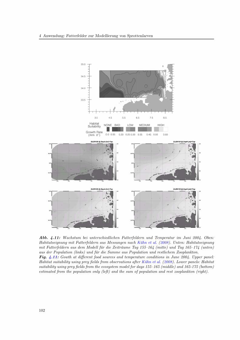
4 Anwendung: Futterfelder zur Modellierung von Sprottenlarven
Dissertation Christoph Stegert Fassung vom 22.05.2008
Seite 84/106
Abb. 22: Wachstum bei unterschiedlichen Futterfeldern und Temperatur im Juni
2004. Oben: Habitatseignung mit Futterfeldern aus Messungen nach Kühn et al.
(2008). Unten: Habitatseignung mit Futterfeldern aus dem Modell für fie
Zeiträume Tag 155-164 (mitte) und Tag 165-174 (unten) aus der Population
(links) und für die Summe aus Population und restlichem Zooplankton.
Abb. 4.11: Wachstum bei unterschiedlichen Futterfeldern und Temperatur im Juni 2004. Oben:Habitatseignung mit Futterfeldern aus Messungen nach Kuhn et al. (2008). Unten: Habitatseignungmit Futterfeldern aus dem Modell fur die Zeitraume Tag 155–164 (mitte) und Tag 165–174 (unten)aus der Population (links) und fur die Summe aus Population und restlichem Zooplankton.Fig. 4.11: Gowth at different food sources and temperature conditions in June 2004. Upper panel:Habitat suitability using prey fields from observations after Kuhn et al. (2008). Lower panels: Habitatsuitability using prey fields from the ecosystem model for days 155–165 (middle) and 165-175 (bottom)estimated from the population only (left) and the sum of population and rest zooplankton (right).
102
4.4 Vergleich verschiedener Futterfelder fur das Wachstum
res Wachstum aufweisen. Hier liegt das Minimum bei 0,25 mm d−1. Unter Zunahme desrestlichen Zooplanktons zeigen die Larven im Küstenbereich mittleres bis hohes Wachstum(0,45–0,5 mm d−1) und bei geringerer Temperatur im Offshore-Bereich mittleres Wachstum(0,35–0,4 mm d−1).
103

4 Anwendung: Futterfelder zur Modellierung von Sprottenlarven
104
5 Diskussion und Schlußfolgerungen
Die Modellierung sollte kein Ende in sich selbst haben -
Um nutzlich zu sein, sollte sie Teil eines großeren Zusammenhangs sein,
um spezifische Fragen zu beantworten.
(Paul J. Somerfield
Plymouth Marine Laboratory)
Die vorliegende Dissertation beschreibt die Parametrisierung einer Zooplanktonpopulationsowie die Implementierung und Anwendung eines entsprechenden Moduls innerhalb einesÖkosystemmodells. Während in GLOBEC auf internationaler Ebene Calanus sp. als domi-nanter und vielfach erforschter Copepode als eine Hauptschlüsselart betrachtet wurde, demsich viele Modelle widmeten (vgl. Kapitel 1.4), wurde für die Untersuchungen in GLOBEC-Germany auf Grund seiner Bedeutung für die Deutsche Bucht die kleine CopepodenartPseudocalanus elongatus ausgewählt (s. Kapitel 3).
In der Modellentwicklung wurde dem Ansatz des internationalen GLOBEC-Programms(www.globec.org) gefolgt, wonach die Komplexität in der Auflösung von Zooplankton schritt-weise erhöht werden soll (Abb. 5.1). Die Untersuchungen führten zu folgenden drei Veröf-fentlichungen: Die erste Struktur (trophic structure 1 in Abb. 5.1) wurde mit einem Popu-lationsmodell basierend auf dem Modell von Fennel (2001) in Stegert et al. (2007) realisiert(Artikel I). Es handelt sich dabei um die Pseudocalanus elongatus Population, die eine spezi-fische Futtermenge zur Verfügung hat und in ihrem Zuwachs durch Mortalität begrenzt wird.Die Einbindung in das Ökosystemmodell ECOHAM mit Nährstoffkreislauf, Phytoplanktonals Futter und der Zooplanktonpopulation als trophischem Abschluß wurde in Moll undStegert (2007) umgesetzt (Artikel II). Pseudocalanus elongatus als omnivore Copepodenartwurde selektiver Fraß auf Phytoplankton, Bakterien und Detritus ermöglicht und bildet dietrophic structure 2 aus Abb. 5.1. Die dritte Struktur, die regionale Verteilung in Konkurrenzzum ‘restlichen’ Zooplankton, wurde schließlich in Stegert et al. (eingereicht) untersucht undist als Manuskript eingereicht worden (Artikel III). Die letzte Struktur (trophic structure 4in Abb. 5.1) bildet eine Idealisierung mit Wechselwirkungen basierend auf einem Größen-spektrum von vielen verschiedenen Phyto- und Zooplanktonpopulationen.
Für die Population von Pseudocalanus elongatus konnten mit Hilfe des ModellsystemsErgebnisse zur Entwicklung, zur räumlich-zeitlichen Verteilung sowie ihrer Bedeutung im
105
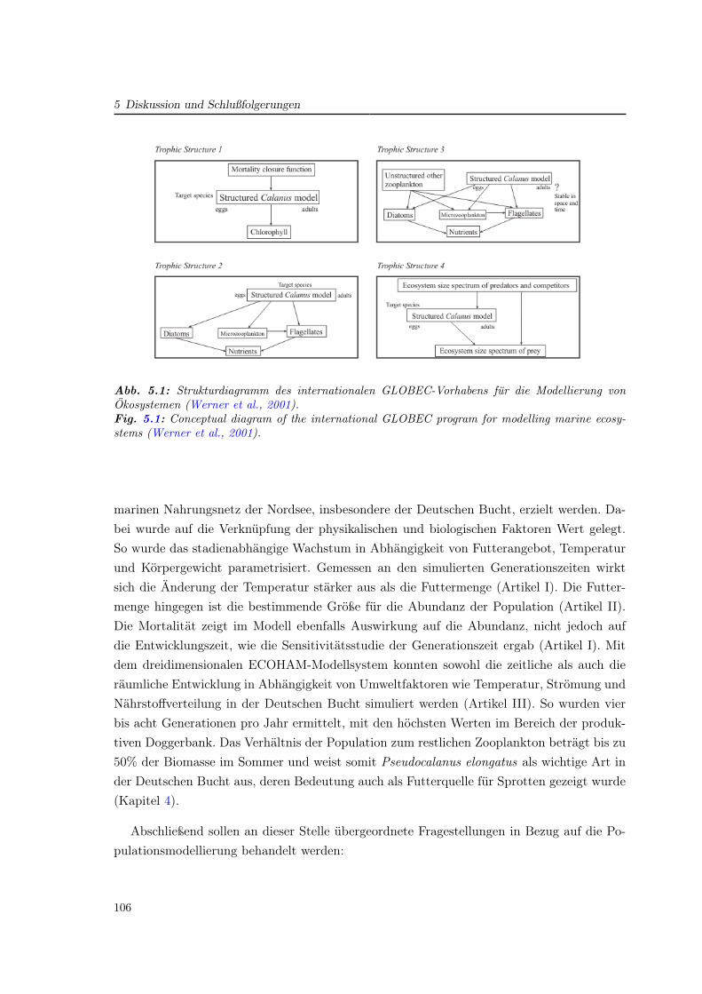
5 Diskussion und Schlußfolgerungen
Dissertation Christoph Stegert Fassung vom 22.05.2008
Seite 86/106
Stegert (2007) umgesetzt (Artikel II). Pseudocalanus elongatus als omnivore
Copepodenart wurde selektiver Fraß auf Phytoplankton, Bakterien und Detritus
ermöglicht und bildet die "trophic structure 2" aus Abb. 23. Die dritte Struktur,
die regionale Verteilung in Konkurrenz zum "restlichen" Zooplankton, wurde
schließlich in Stegert et al. (submitted) untersucht und ist als Manuskript
eingereicht worden (Artikel III).
Die letzte Struktur ("trophic structure 4" in Abb. 23) bildet eine Idealisierung
mit Wechselwirkungen basierend auf einem Größenspektrum von vielen
verschiedenen Phyto- und Zooplanktonpopulationen.
Abb. 23: Strukturdiagramm des internationalen GLOBEC-Vorhabens für die
Modellierung von Ökosystemen (Werner et al., 2001).
Abb. 5.1: Strukturdiagramm des internationalen GLOBEC-Vorhabens fur die Modellierung vonOkosystemen (Werner et al., 2001).Fig. 5.1: Conceptual diagram of the international GLOBEC program for modelling marine ecosy-stems (Werner et al., 2001).
marinen Nahrungsnetz der Nordsee, insbesondere der Deutschen Bucht, erzielt werden. Da-bei wurde auf die Verknüpfung der physikalischen und biologischen Faktoren Wert gelegt.So wurde das stadienabhängige Wachstum in Abhängigkeit von Futterangebot, Temperaturund Körpergewicht parametrisiert. Gemessen an den simulierten Generationszeiten wirktsich die Änderung der Temperatur stärker aus als die Futtermenge (Artikel I). Die Futter-menge hingegen ist die bestimmende Größe für die Abundanz der Population (Artikel II).Die Mortalität zeigt im Modell ebenfalls Auswirkung auf die Abundanz, nicht jedoch aufdie Entwicklungszeit, wie die Sensitivitätsstudie der Generationszeit ergab (Artikel I). Mitdem dreidimensionalen ECOHAM-Modellsystem konnten sowohl die zeitliche als auch dieräumliche Entwicklung in Abhängigkeit von Umweltfaktoren wie Temperatur, Strömung undNährstoffverteilung in der Deutschen Bucht simuliert werden (Artikel III). So wurden vierbis acht Generationen pro Jahr ermittelt, mit den höchsten Werten im Bereich der produk-tiven Doggerbank. Das Verhältnis der Population zum restlichen Zooplankton beträgt bis zu50% der Biomasse im Sommer und weist somit Pseudocalanus elongatus als wichtige Art inder Deutschen Bucht aus, deren Bedeutung auch als Futterquelle für Sprotten gezeigt wurde(Kapitel 4).
Abschließend sollen an dieser Stelle übergeordnete Fragestellungen in Bezug auf die Po-pulationsmodellierung behandelt werden:
106
• Inwieweit ist die Verknüpfung von Population und restlichem Zooplankton stabil inRaum und Zeit (Abb. 5.1, 3)?
• Welchen Einfluß hat die Erweiterung der Komplexität innerhalb der trophischen Stufenauf das Modell und seine Beschreibung des Zooplanktons (Abb. 5.1, 4)?
• Was ist für die Nutzung des Zooplanktons als Futterquelle für die Modellierung vonFischlarven zu beachten?
Dies soll mit Hilfe des ECOHAM-Modellsystems beantwortet werden.
Betrachtung des zeitlichen Gleichgewichtes der Zooplanktongruppen
Die Simulation für 2003–2004 zeigte, daß die Zu- und Abnahme beider Zooplanktongruppendurch die gegebenen physikalischen und biologischen Faktoren reguliert werden. Sowohl diePopulation als auch das restliche Zooplankton werden im Winter durch Temperatur- undFutterbedingungen reduziert (Abb. 5.2). Wie verhält sich die Zooplanktonbiomasse, wenndie Population nicht explizit berechnet wird, sondern das gesamte Zooplankton durch eineZustandsvariable beschrieben wird, die oft als Bulk-Variante bezeichnet wird und Gegen-stand von Modellvergleichen ist (Radach und Moll , 2006)?
In Abb. 5.2 sind die verschiedenen Bestandteile der Zooplanktonbiomasse an einer Stati-on in der Deutschen Bucht (GLOBEC Station GG#32) über zwei Jahre aufgetragen. Dabeibeschreiben die blauen Kurven den Verlauf für die Population, das restliche Zooplanktonund die Summe aus beiden aus der Simulation, die in Artikel III ausgewertet wurden, unddie grüne Kurve zeigt die Biomasse aus der oben benannten Bulk-Variante mit zum restli-chen Zooplankton des Populationslaufs identischer Parametrisierung. Im Vergleich der zweisimulierten Jahre zeigen sich Merkmale, die in beiden Varianten auftreten, wie z.B. derBiomasseanstieg im März/April, aber auch zwischenjährige Unterschiede, wie das geringereMaximum im Herbst 2003 gegenüber 2004 oder der stärkere zweite Peak nach dem Früh-jahr im Juli 2004. Betrachtet man die Unterschiede zwischen den Versionen, so zeigt sichfolgendes Phänomen:
Das gesamte Zooplankton im Simulationslauf mit Population ist höher als in der von vie-len anderen Modellen verwendeten Bulk-Variante. Vielmehr ist diese für einen großen Zeit-raum sehr ähnlich zum Verlauf des restlichen Zooplanktons (blau gestrichelt). Dies erklärtsich durch ausreichend Futter und seltene Zeiten der Futterlimitierung. Die Biomasseent-wicklung des Bulk-Zooplanktons ist somit durch die maximale Futterrate und den von derTemperatur abhängigen Term begrenzt, welche für beide Simulationen nahezu identisch sind.Unterschiede treten mit zunehmendem Anteil der Population im Herbst auf, wenn der Kon-
107
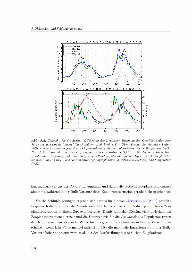
5 Diskussion und Schlußfolgerungen
Dissertation Christoph Stegert Fassung vom 22.05.2008
Seite 89/106
bezeichnet wird und Gegenstand von Modellvergleichen ist (Radach and Moll,
2006)?
Abb. 24: Zeitreihe für die Station GG#32 in der Deutschen Bucht an der
Oberfläche über zwei Jahre aus dem Populationslauf (blau) und dem Bulk-Lauf
(grün). Oben: Zooplanktonbiomasse. Unten: Futtermenge (zusammengesetzt
aus Phytoplankton, Detritus und Bakterien) und Temperatur (rot).
In Abb. 24 sind die verschiedenen Bestandteile der Zooplanktonbiomasse an
einer Station in der Deutschen Bucht (GLOBEC Station 32) über zwei Jahre
aufgetragen. Dabei stellen die blauen Kurven den Verlauf für die Population,
Abb. 5.2: Zeitreihe fur die Station GG#32 in der Deutschen Bucht an der Oberflache uber zweiJahre aus dem Populationslauf (blau) und dem Bulk-Lauf (grun). Oben: Zooplanktonbiomasse. Unten:Futtermenge (zusammengesetzt aus Phytoplankton, Detritus und Bakterien) und Temperatur (rot).Fig. 5.2: Biannual time series of surface values at station GG#32 in the German Bight fromsimulation runs with population (blue) and without population (green). Upper panel: Zooplanktonbiomass. Lower panel: Food concentration (of phytoplankton, detritus and bacteria) and temperature(red).
kurrenzdruck seitens der Population zunimmt und damit die restliche Zooplanktonbiomasseabnimmt, während in der Bulk-Variante diese Konkurrenzsituation gerade nicht gegeben ist.
Welche Schlußfolgerungen ergeben sich daraus für die von Werner et al. (2001) gestellteFrage nach der Stabilität der Simulation? Durch Konkurrenz um Nahrung sind beide Zoo-planktongruppen in ihrem Zuwachs begrenzt. Damit wird das Gleichgewicht zwischen denZooplanktonversionen erzielt und die Unterschiede für die Pseudocalanus Population tretendeutlich hervor. Um identische Werte für das gesamte Zooplankton in beiden Varianten zuerhalten, wenn kein Futtermangel auftritt, müßte die maximale Ingestionsrate in der Bulk-Variante höher angesetzt werden als bei der Beschreibung des restlichen Zooplanktons.
108
Betrachtung der Komplexitat im Modell
Nach dem Ansatz von GLOBEC (Abb. 5.1) beinhaltet die vierte trophische Struktur einSpektrum an Prädatoren, welche die Mortalität der Population bestimmt und das Nah-rungsnetz durch die trophische Stufe der Fische schließt. Die Arbeiten dazu wurden in Ka-pitel 4 beschrieben und sollen nun diskutiert werden. Ansätze, Fischpopulationen mit denunteren trophischen Stufen explizit zu verbinden, wurden in den letzten Jahren z. B. vonFennel (2008) für die Ostsee und Megrey et al. (2007) für den Nordpazifik vorgenommen. Ineiner dekadischen Simulation verglichen Rose et al. (2004) eine entkoppelte Variante, d. h.Zooplanktonfelder werden gespeichert und wie bei Kühn et al. (2008) in das Fischmodell ein-gelesen, mit der gekoppelten Simulation, die in Megrey et al. (2007) beschrieben wurde. Diegekoppelte Variante zeigte dabei ein geringeres mittleres Gewicht der Fische ebenso wie einestärkere Reduktion der Zooplanktonbestände im Herbst, die sich bis auf die Phytoplankton-bestände und die Nährstoffkonzentrationen auswirkte. Welche Auswirkungen können damitfür das Modellsystem in der Nordsee diskutieret werden? Für das Populationsmodell wur-den in der vorliegenden Arbeit konstante Mortalitätsraten angenommen. Wie in Artikel IIIdiskutiert, ist jedoch die Mortalität zeitlich variabel (Ohman und Wood , 1996). Mit der Ein-bindung einer höheren trophischen Stufe könnte auch eine zeitlich dynamische Mortalität aufdas Zooplankton realisiert werden. Eine Folge wäre nach Rose et al. (2004) eine Reduktionder Zooplanktonbiomasse im Herbst. Hierin liegt eine mögliche Erklärung der beobachtetenreduzierten Abundanz bei Helgoland Reede Stegert et al. (eingereicht, Abb. 11) im Spätsom-mer, die im ECOHAM-Zooplankton-Modellsystem über reduzierte Nahrungsaufnahme beihöheren Temperaturen realisiert wurde.
Das Einbinden der Fische wäre jedoch mit einer erheblichen Erhöhung der Komplexitätim Modell verbunden, die zur Zeit für dreidimensionale Anwendungen nicht bewältigt wer-den kann. Als eine sinnvolle Balance zwischen nötiger Auflösung und möglicher Komplexitätempfehlen de Young et al. (2004) einen sogenannten Rhomboid-Ansatz (Abb. 5.3). Diesersieht eine hohe Auflösung auf der jeweils fokussierten trophischen Stufe vor. Für die Un-tersuchungen von Copepoden unterstützt dieser Ansatz die in dieser Arbeit vorgenommeneAuflösung der Population, schlägt aber eine (geringer aufgelöste) höhere trophische Stufevor. Liegt der Fokus auf Populationen von Fischen, so wird wiederum eine vereinfachte Be-schreibung des Zooplanktons als Futterquelle empfohlen. Doch wie kann diese Vereinfachungausfallen? Dies führt zum dritten Aspekt:
Ansatze fur die Aufbereitung des Zooplanktons als Futter
Man kann einerseits von der Gesamtzooplanktonmasse ausgehen. Daewel et al. (2008) schla-gen in ihrem Ansatz die Verwendung einer Zustandsvariable vor, aus der das Futterspek-
109
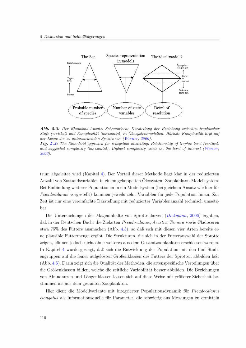
5 Diskussion und Schlußfolgerungen
Dissertation Christoph Stegert Fassung vom 22.05.2008
Seite 93/106
aufgelöste) höhere trophische Stufe vor. Liegt der Fokus auf Populationen von
Fischen, so wird wiederum eine vereinfachte Beschreibung des Zooplanktons als
Futterquelle empfohlen. Doch wie kann diese Vereinfachung ausfallen? Dies
führt zum dritten Aspekt:
Abb. 25: Der Rhomboid-Ansatz: Schematische Darstellung der Beziehung
zwischen trophischer Stufe (vertikal) und Komplexität (horizontal) in
Ökosystemmodellen. Höchste Komplexität liegt auf der Ebene der zu
untersuchenden Spezies (Werner, 2000).
Abb. 5.3: Der Rhomboid-Ansatz: Schematische Darstellung der Beziehung zwischen trophischerStufe (vertikal) und Komplexitat (horizontal) in Okosystemmodellen. Hochste Komplexitat liegt aufder Ebene der zu untersuchenden Spezies vor (Werner, 2000).Fig. 5.3: The Rhomboid approach for ecosystem modelling: Relationship of trophic level (vertical)and suggested complexity (horizontal). Highest complexity exists on the level of interest (Werner,2000).
trum abgeleitet wird (Kapitel 4). Der Vorteil dieser Methode liegt klar in der reduziertenAnzahl von Zustandsvariablen in einem gekoppelten Ökosystem-Zooplankton-Modellsystem.Bei Einbindung weiterer Populationen in ein Modellsystem (bei gleichem Ansatz wie hier fürPseudocalanus vorgestellt) kommen jeweils zehn Variablen für jede Population hinzu. ZurZeit ist nur eine vereinfachte Darstellung mit reduzierter Variablenanzahl technisch umsetz-bar.
Die Untersuchungen der Mageninhalte von Sprottenlarven (Dickmann, 2006) ergaben,daß in der Deutschen Bucht die Zielarten Pseudocalanus, Acartia, Temora sowie Cladocerenetwa 75% des Futters ausmachen (Abb. 4.3), so daß sich mit diesen vier Arten bereits ei-ne plausible Futtermenge ergibt. Die Strukturen, die sich in der Futterauswahl der Sprottezeigen, können jedoch nicht ohne weiteres aus dem Gesamtzooplankton erschlossen werden.In Kapitel 4 wurde gezeigt, daß sich die Entwicklung der Population mit den fünf Stadi-engruppen auf die feiner aufgelösten Größenklassen des Futters der Sprotten abbilden läßt(Abb. 4.5). Darin zeigt sich die Qualität der Methoden, die artenspezifische Verteilungen überdie Größenklassen bilden, welche die zeitliche Variabilität besser abbilden. Die Beziehungenvon Abundanzen und Längenklassen lassen sich auf diese Weise mit größerer Sicherheit be-stimmen als aus dem gesamten Zooplankton.
Hier dient die Modellvariante mit integrierter Populationsdynamik für Pseudocalanuselongatus als Informationsquelle für Parameter, die schwierig aus Messungen zu ermitteln
110
sind (wie auch in Artikel III dargestellt). So lassen sich mit einem Modell mit Physiologie dieMuster einer allgemeinen Parametrisierung ableiten. Ein möglicher Parameter ist die Anzahlvon Generationen von Pseudocalanus elongatus im Jahresgang, die aus dem Modell auch inihren räumlichen Unterschieden aufgelöst werden kann. Mit dem ECOHAM-Zooplankton-Modellsystem liegt ein generisches Mittel vor, derartige Parameter auch für andere Artenzu ermitteln und mit zunehmender Rechnerkapazität diese zusammenzuführen. Hierin liegtdie Schnittstelle der Zooplankton-Populationsmodellierung zu den Fischereiwissenschaften,um Aussagen zur Rekrutierung von Jungfischen basierend auf der Futterverfügbarkeit zutreffen.

6 Danksagung
Mein Dank gilt allen Menschen, die mir bei der Erstellung dieser Arbeit geholfen haben undmit in den vergangenen drei Jahren zur Seite gestanden haben.
An Prof. Dr. Jens Meincke richte ich meinen herzlichen Dank, der sich der Betreuungdieser Arbeit angenommen hat und mich zuvor durch das Studium begleitet hat. Fürdie Offenheit gegenüber der biologischen Ausrichtung und für die Unterstützung in derzeitlichen wie inhaltlichen Gestaltung der Arbeit.
Dr. Andreas Moll danke ich für seine Betreuung der Arbeit, die Hilfe und Struktur gab,um die Arbeit voranzubringen und Offenheit und Freiheit, eigene Ideen und Methodeneinzubringen und die Arbeit zu gestalten. Danke für ein stets offenes Ohr und Ver-ständnis für alle Dinge, die über fachliche Belange weit hinausgingen. Danke für dieOffenheit und Ehrlichkeit, die aus der Betreuung eine Freundschaft werden ließ.
Der Gruppe der Ökosystemmodellierung am IfM danke ich für alle Unterstützung und‘Mitbetreuung’:
Dr. Hermann-Josef Lenhart, der auch in persönlichen Fragen und Überlegungen dawar, sich Zeit genommen hat.
Dr. Wilfried Kühn, durch den ich - und damit auch die Arbeit - den Bezug zur Fische-reiwissenschaft bekommen habe und bei der Erstellung des Kapitel 4 behilflichwar und der wie auch
Dr. Johannes Pätsch in technischen Fragen geduldig zur Seite stand.
Markus Kreus, der in den zweieinhalb Jahren als Zimmergenosse das Populationsmo-dell mit weitergeführt und gestaltet hat, für die weiterbringenden Diskussionenund für eine wundervolle Fahrt nach Marseille.
Bente Tiedje, die im vergangenen Jahr dafür sorgte, daß es im Zimmer nicht zu einsamist, für Ihre Aufmerkamkeit und Mitversorgung.
Dr. Susanne Tamm und Dr. Larissa Müller für ihre morlaische Unterstützung undHilfe in vielen Verwaltungs- und amtlichen Belangen.
Silke Hinze, Petra Nerge und Christian für ihre Anteilnahme und ihr Mitfiebern.
113
Sie alle hatten stets ein offenes Ohr und Zeit für mich und haben mich so aufgenommenwie ich bin.
Ebenso danke ich allen Kollegen und Kommilitonen, die Interesse an meiner Arbeit hattenund mich unterstütz haben. Besonderer Dank gilt dabei
Prof. Dr. Michael St. John und Prof. Myron Peck für die Unterstützung beim Stipen-dienantrag, sowie Ute Daewel vom Institut für Hydrobiologie und Fischereiwis-senschaft.
Prof. Dr. Jan Backhaus und den Kollegen aus der Schelfmeerozeanographie.
Dr. Thomas Pohlmann für die Hilfe bei der Aufbereitung der NCEP-Daten.
Dr. Ilse Hamann von der DGM-Geschäftsstelle für die Unterstützung bei der Formu-lierung englischer Texte.
Dank auch an alle GLOBEC-Kollegen, insbesondere
Dr. Jasmin Renz für die gute und fruchtbare Zusammenarbeit, für das Hinterfragenund den biologischen Input.
Prof. Dr. Wolfgang Fennel und Dr. Thomas Neumann vom IO Warnemünde für denAustausch in der Modellierun, für die Bereitstellung des Populaitonsmodells unddie Unterstützung.
allen, die Interesse an der Modellierung gezeigt haben.
Einen ganz besonderen Dank richte ich an Prof. Dr. François Carlotti, von dem ich imRahmen des PROCOPE-Austauschs sehr viel lernen durfte und in drei Aufenthaltenin Lyon und Marseille viel erleben konnte. Danke für die wunderbare Aufnahme unddie fruchtbare Zusammenarbeit, sowie die hilfreichen Ergänzungen im Parametrisie-rungsartikel.
Schließlich danke ich meiner Familie von ganzem Herzen für die treue Unterstützung, füralles Mitfiebern, Mitleiden und Mitfreuen. Danke, daß Ihr mir stets zur Seite standetund ich so den nötigen Freiraum für die Arbeit haben konnte.
7 Beitrag zu den Publikationen
Artikel I
Die Parametrisierung wurde im Rahmen des DAAD-Austauschprogramms PROCOPE zu-sammen mit den Co-Autoren erarbeitet. Die gezeigten Simulationsläufe habe ich durchge-führt und den Text unter Mithilfe der Co-Autoren verfaßt. Die Sensitivitätsanalyse wurdevon mir durchgeführt und ausgewertet.
Artikel II
Der Einbau der Pseudocalanus Population in das ECOHAM-Modell in der hier dargestelltenForm wurde von mir durchgeführt. Text und Inhalt wurde von den Autoren gemeinsamerarbeitet und die Abbildungen von mir erstellt.
Artikel III
Erweiterungen des Programmteils für die Population wurden von Markus Kreus (Erweite-rungen zu ECOHAM3 mit Competition) und mir (Einbindung in die aktuelle ECOHAM-Umgebung, genutzte Parametrisierung) eingearbeitet. Der Modellauf für 2003–2004 wurdevon mir vorbereitet (Aufbereitung der meteorologischen und hydrodynamischen Antriebs-daten) und auf dem DKRZ-Großrechner durchgeführt. Der Inhalt der Auswertung wurdevon den beiden ersten Autoren erarbeitet und von mir umgesetzt. Der Text wurde von mirverfaßt und von den Co-Autoren ergänzt.
Kapitel 4
Die Methodik der Aufbereitung von Futterfeldern wurde zusammen mit Dr. Andreas Moll er-arbeitet und von mir umgesetzt. Die IBM-Läufe wurden von Dr. Wilfried Kühn durchgeführtund unter seiner Mithilfe von mir ausgewertet.
115

Literaturverzeichnis
Alheit, J. (2007), Progress of the German GLOBEC project, International GLOBECNewsletter, 13, 57–78.
Arakawa, A., und V. R. Lamb (1977), Computational design of the basic dynamical processesof the UCLA general circulation model, Methods in computational Physics, 16, 173–263.
Backhaus, J. O. (1985), A Three–Dimensional Model for the Simulation of Shelf Sea Dyna-mics, Deutsche hydrographische Zeitschrift, 38 (4), 165–187.
Bailey, R. S., E. Bakken, J. Alheit, O. Hagström, S. A. Iversen, P. O. Johnson, K. P. Madsen,D. W. McKay, und G. Naevdal (1990), Report of the Sprat Biology Workshop, Tech. ber.,Food and Agriculture Organization of the United Nations – Fisheries Department, ICESCooperative Research Report.
Baretta, J. W., W. Ebenhöh, und P. Ruardij (1995), The European Regional Seas Ecosy-stem Model (ERSEM), a complex marine ecosystem model, Netherlands Journal of SeaResearch, 33 (3-4), 233–246.
Bartsch, J., und R. Knust (1994), Simulating the dispersion of vertically migrating spratlarvae (Sprattus sprattus) in the German Bight with a circulation and transport modelsystem, Fisheries Oceanography, 3 (2), 92–105.
Barz, K., und H.-J. Hirche (2006), Abundance, distribution and prey composition of scypho-medusae in the southern North Sea, Marine Biology, 151 (3), 1021–1033.
Batchelder, H. P., C. A. Edwards, und T. M. Powell (2002), Individual-based models ofcopepod populations in coastal upwelling regions: implications of physiologically and en-vironmentally influenced diel vertical migration on demographic success and nearshoreretention, Progress in Oceanography, 53, 307–333.
Beaugrand, G. (2004), Continuous Plankton Records: Plankton atlas of the North AtlanticOcean (1958-1999). I. Introduction and methodology, Marine Ecology Progress Series,Suppl., 3–10.
Brockmann, U. H., R. W. P. M. Laane, und H. Postma (1990), Cycling of nutrient elementsin the North Sea, Netherlands Journal of Sea Research, 26, 239–264.
Bryant, A. D., M. Heath, W. S. G. Gurney, D. J. Beare, und W. Robertson (1997), Theseasonal dynamics of Calanus finmarchicus: development of a three-dimensional structuredpopulation model and application to the northern North Sea, Journal of Sea Research, 38,361–379.
117
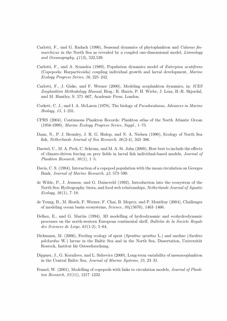
Carlotti, F., und G. Radach (1996), Seasonal dynamics of phytoplankton and Calanus fin-marchicus in the North Sea as revealed by a coupled one-dimensional model, Limnologyand Oceanography, 41 (3), 522,539.
Carlotti, F., und A. Sciandra (1989), Population dynamics model of Euterpina acutifrons(Copepoda: Harpacticoida) coupling individual growth and larval development, MarineEcology Progress Series, 56, 225–242.
Carlotti, F., J. Giske, und F. Werner (2000), Modeling zooplankton dynamics, in: ICESZooplankton Methodology Manual, Hrsg.: R. Harris, P. H. Wiebe, J. Lenz, H.-R. Skjordal,und M. Huntley, S. 571–667, Academic Press, London.
Corkett, C. J., und I. A. McLaren (1978), The biology of Pseudocalanus, Advances in MarineBiology, 15, 1–231.
CPRS (2004), Continuous Plankton Records: Plankton atlas of the North Atlantic Ocean(1958-1999), Marine Ecology Progress Series, Suppl., 1–75.
Daan, N., P. J. Bromley, J. R. G. Hislop, und N. A. Nielsen (1990), Ecology of North Seafish, Netherlands Journal of Sea Research, 26 (2-4), 343–386.
Daewel, U., M. A. Peck, C. Schrum, und M. A. St. John (2008), How best to include the effectsof climate-driven forcing on prey fields in larval fish individual-based models, Journal ofPlankton Research, 30 (1), 1–5.
Davis, C. S. (1984), Interaction of a copepod population with the mean circulation on GeorgesBank, Journal of Marine Research, 42, 573–590.
de Wilde, P., J. Jenness, und G. Duineveld (1992), Introduction into the ecosystem of theNorth Sea: Hydrography, biota, and food web relationships, Netherlands Journal of AquaticEcology, 26 (1), 7–18.
de Young, B., M. Heath, F. Werner, F. Chai, B. Megrey, und P. Montfray (2004), Challengesof modeling ocean basin ecosystems, Science, 304 (5676), 1463–1466.
Delhez, E., und G. Martin (1994), 3D modelling of hydrodynamic and ecohydrodynamicprocesses on the north-western European continental shelf, Bulletin de la Societe Royaledes Sciences de Liege, 63 (1-2), 5–64.
Dickmann, M. (2006), Feeding ecology of sprat (Sprattus sprattus L.) and sardine (Sardinepilchardus W.) larvae in the Baltic Sea and in the North Sea, Dissertation, UniversitätRostock, Institut fär Ostseeforschung.
Dippner, J., G. Kornilovs, und L. Sidrevics (2000), Long-term variability of mesozooplanktonin the Central Baltic Sea, Journal of Marine Systems, 25, 23–31.
Fennel, W. (2001), Modelling of copepods with links to circulation models, Journal of Plank-ton Research, 23 (11), 1217–1232.
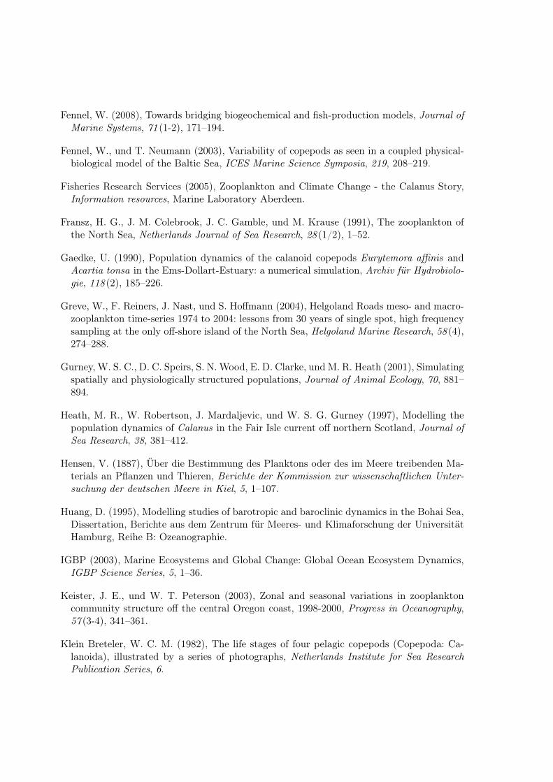
Fennel, W. (2008), Towards bridging biogeochemical and fish-production models, Journal ofMarine Systems, 71 (1-2), 171–194.
Fennel, W., und T. Neumann (2003), Variability of copepods as seen in a coupled physical-biological model of the Baltic Sea, ICES Marine Science Symposia, 219, 208–219.
Fisheries Research Services (2005), Zooplankton and Climate Change - the Calanus Story,Information resources, Marine Laboratory Aberdeen.
Fransz, H. G., J. M. Colebrook, J. C. Gamble, und M. Krause (1991), The zooplankton ofthe North Sea, Netherlands Journal of Sea Research, 28 (1/2), 1–52.
Gaedke, U. (1990), Population dynamics of the calanoid copepods Eurytemora affinis andAcartia tonsa in the Ems-Dollart-Estuary: a numerical simulation, Archiv für Hydrobiolo-gie, 118 (2), 185–226.
Greve, W., F. Reiners, J. Nast, und S. Hoffmann (2004), Helgoland Roads meso- and macro-zooplankton time-series 1974 to 2004: lessons from 30 years of single spot, high frequencysampling at the only off-shore island of the North Sea, Helgoland Marine Research, 58 (4),274–288.
Gurney, W. S. C., D. C. Speirs, S. N. Wood, E. D. Clarke, und M. R. Heath (2001), Simulatingspatially and physiologically structured populations, Journal of Animal Ecology, 70, 881–894.
Heath, M. R., W. Robertson, J. Mardaljevic, und W. S. G. Gurney (1997), Modelling thepopulation dynamics of Calanus in the Fair Isle current off northern Scotland, Journal ofSea Research, 38, 381–412.
Hensen, V. (1887), Über die Bestimmung des Planktons oder des im Meere treibenden Ma-terials an Pflanzen und Thieren, Berichte der Kommission zur wissenschaftlichen Unter-suchung der deutschen Meere in Kiel, 5, 1–107.
Huang, D. (1995), Modelling studies of barotropic and baroclinic dynamics in the Bohai Sea,Dissertation, Berichte aus dem Zentrum für Meeres- und Klimaforschung der UniversitätHamburg, Reihe B: Ozeanographie.
IGBP (2003), Marine Ecosystems and Global Change: Global Ocean Ecosystem Dynamics,IGBP Science Series, 5, 1–36.
Keister, J. E., und W. T. Peterson (2003), Zonal and seasonal variations in zooplanktoncommunity structure off the central Oregon coast, 1998-2000, Progress in Oceanography,57 (3-4), 341–361.
Klein Breteler, W. C. M. (1982), The life stages of four pelagic copepods (Copepoda: Ca-lanoida), illustrated by a series of photographs, Netherlands Institute for Sea ResearchPublication Series, 6.
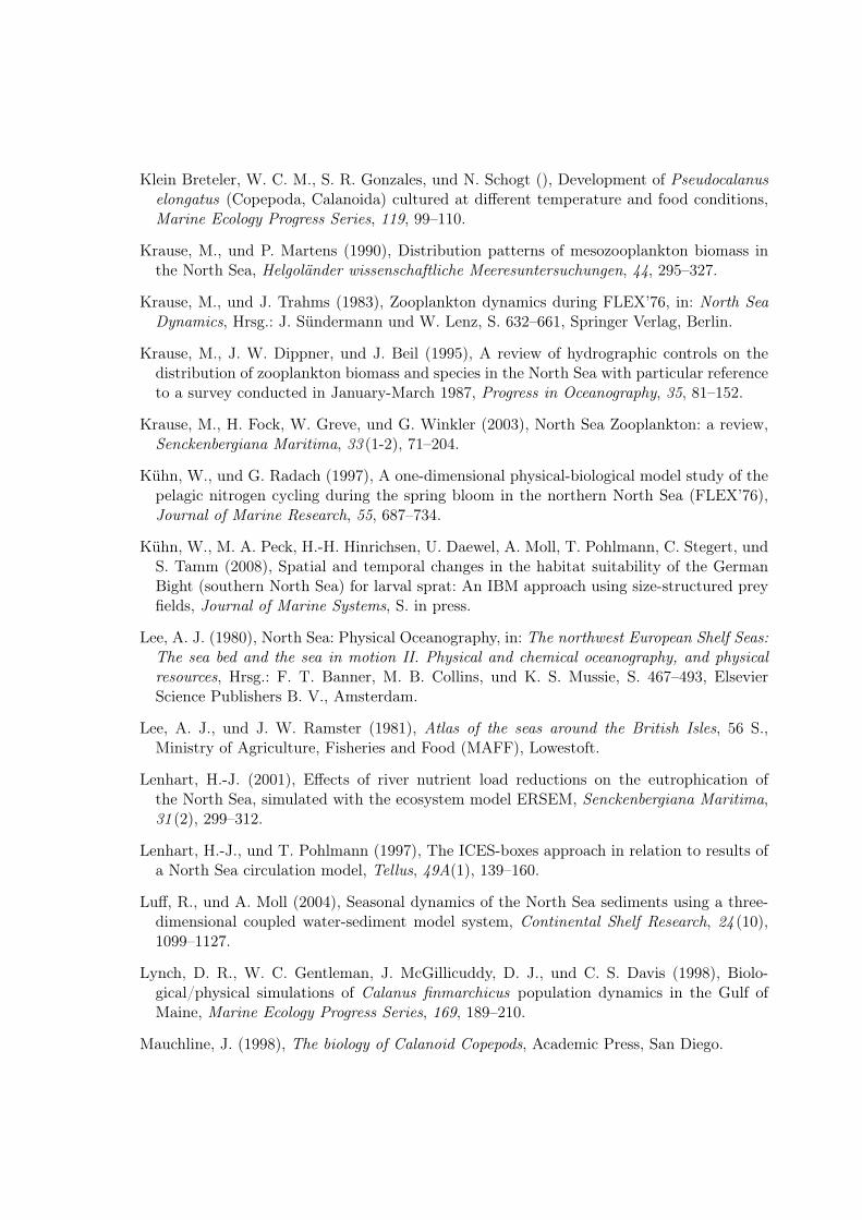
Klein Breteler, W. C. M., S. R. Gonzales, und N. Schogt (), Development of Pseudocalanuselongatus (Copepoda, Calanoida) cultured at different temperature and food conditions,Marine Ecology Progress Series, 119, 99–110.
Krause, M., und P. Martens (1990), Distribution patterns of mesozooplankton biomass inthe North Sea, Helgoländer wissenschaftliche Meeresuntersuchungen, 44, 295–327.
Krause, M., und J. Trahms (1983), Zooplankton dynamics during FLEX’76, in: North SeaDynamics, Hrsg.: J. Sündermann und W. Lenz, S. 632–661, Springer Verlag, Berlin.
Krause, M., J. W. Dippner, und J. Beil (1995), A review of hydrographic controls on thedistribution of zooplankton biomass and species in the North Sea with particular referenceto a survey conducted in January-March 1987, Progress in Oceanography, 35, 81–152.
Krause, M., H. Fock, W. Greve, und G. Winkler (2003), North Sea Zooplankton: a review,Senckenbergiana Maritima, 33 (1-2), 71–204.
Kühn, W., und G. Radach (1997), A one-dimensional physical-biological model study of thepelagic nitrogen cycling during the spring bloom in the northern North Sea (FLEX’76),Journal of Marine Research, 55, 687–734.
Kühn, W., M. A. Peck, H.-H. Hinrichsen, U. Daewel, A. Moll, T. Pohlmann, C. Stegert, undS. Tamm (2008), Spatial and temporal changes in the habitat suitability of the GermanBight (southern North Sea) for larval sprat: An IBM approach using size-structured preyfields, Journal of Marine Systems, S. in press.
Lee, A. J. (1980), North Sea: Physical Oceanography, in: The northwest European Shelf Seas:The sea bed and the sea in motion II. Physical and chemical oceanography, and physicalresources, Hrsg.: F. T. Banner, M. B. Collins, und K. S. Mussie, S. 467–493, ElsevierScience Publishers B. V., Amsterdam.
Lee, A. J., und J. W. Ramster (1981), Atlas of the seas around the British Isles, 56 S.,Ministry of Agriculture, Fisheries and Food (MAFF), Lowestoft.
Lenhart, H.-J. (2001), Effects of river nutrient load reductions on the eutrophication ofthe North Sea, simulated with the ecosystem model ERSEM, Senckenbergiana Maritima,31 (2), 299–312.
Lenhart, H.-J., und T. Pohlmann (1997), The ICES-boxes approach in relation to results ofa North Sea circulation model, Tellus, 49A(1), 139–160.
Luff, R., und A. Moll (2004), Seasonal dynamics of the North Sea sediments using a three-dimensional coupled water-sediment model system, Continental Shelf Research, 24 (10),1099–1127.
Lynch, D. R., W. C. Gentleman, J. McGillicuddy, D. J., und C. S. Davis (1998), Biolo-gical/physical simulations of Calanus finmarchicus population dynamics in the Gulf ofMaine, Marine Ecology Progress Series, 169, 189–210.
Mauchline, J. (1998), The biology of Calanoid Copepods, Academic Press, San Diego.
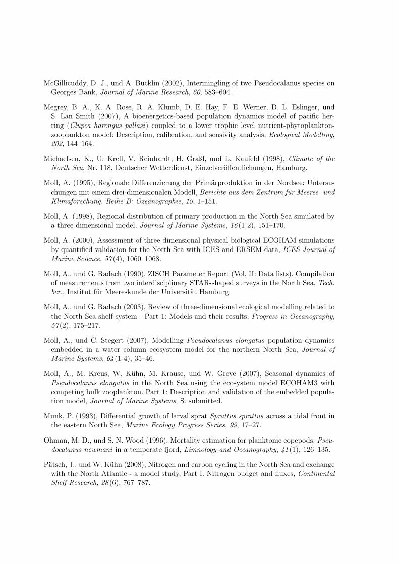
McGillicuddy, D. J., und A. Bucklin (2002), Intermingling of two Pseudocalanus species onGeorges Bank, Journal of Marine Research, 60, 583–604.
Megrey, B. A., K. A. Rose, R. A. Klumb, D. E. Hay, F. E. Werner, D. L. Eslinger, undS. Lan Smith (2007), A bioenergetics-based population dynamics model of pacific her-ring (Clupea harengus pallasi) coupled to a lower trophic level nutrient-phytoplankton-zooplankton model: Description, calibration, and sensivity analysis, Ecological Modelling,202, 144–164.
Michaelsen, K., U. Krell, V. Reinhardt, H. Graßl, und L. Kaufeld (1998), Climate of theNorth Sea, Nr. 118, Deutscher Wetterdienst, Einzelveröffentlichungen, Hamburg.
Moll, A. (1995), Regionale Differenzierung der Primärproduktion in der Nordsee: Untersu-chungen mit einem drei-dimensionalen Modell, Berichte aus dem Zentrum für Meeres- undKlimaforschung. Reihe B: Ozeanographie, 19, 1–151.
Moll, A. (1998), Regional distribution of primary production in the North Sea simulated bya three-dimensional model, Journal of Marine Systems, 16 (1-2), 151–170.
Moll, A. (2000), Assessment of three-dimensional physical-biological ECOHAM simulationsby quantified validation for the North Sea with ICES and ERSEM data, ICES Journal ofMarine Science, 57 (4), 1060–1068.
Moll, A., und G. Radach (1990), ZISCH Parameter Report (Vol. II: Data lists). Compilationof measurements from two interdisciplinary STAR-shaped surveys in the North Sea, Tech.ber., Institut für Meereskunde der Universität Hamburg.
Moll, A., und G. Radach (2003), Review of three-dimensional ecological modelling related tothe North Sea shelf system - Part 1: Models and their results, Progress in Oceanography,57 (2), 175–217.
Moll, A., und C. Stegert (2007), Modelling Pseudocalanus elongatus population dynamicsembedded in a water column ecosystem model for the northern North Sea, Journal ofMarine Systems, 64 (1-4), 35–46.
Moll, A., M. Kreus, W. Kühn, M. Krause, und W. Greve (2007), Seasonal dynamics ofPseudocalanus elongatus in the North Sea using the ecosystem model ECOHAM3 withcompeting bulk zooplankton. Part 1: Description and validation of the embedded popula-tion model, Journal of Marine Systems, S. submitted.
Munk, P. (1993), Differential growth of larval sprat Sprattus sprattus across a tidal front inthe eastern North Sea, Marine Ecology Progress Series, 99, 17–27.
Ohman, M. D., und S. N. Wood (1996), Mortality estimation for planktonic copepods: Pseu-docalanus newmani in a temperate fjord, Limnology and Oceanography, 41 (1), 126–135.
Pätsch, J., und W. Kühn (2008), Nitrogen and carbon cycling in the North Sea and exchangewith the North Atlantic - a model study, Part I. Nitrogen budget and fluxes, ContinentalShelf Research, 28 (6), 767–787.
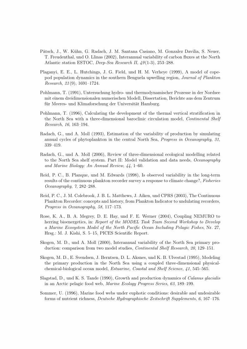
Pätsch, J., W. Kühn, G. Radach, J. M. Santana Casiano, M. Gonzalez Davilia, S. Neuer,T. Freudenthal, und O. Llinas (2002), Interannual variability of carbon fluxes at the NorthAtlantic station ESTOC, Deep-Sea Research II, 49 (1-3), 253–288.
Plaganyi, E. E., L. Hutchings, J. G. Field, und H. M. Verheye (1999), A model of cope-pod population dynamics in the southern Benguela upwelling region, Journal of PlanktonResearch, 21 (9), 1691–1724.
Pohlmann, T. (1991), Untersuchung hydro- und thermodynamischer Prozesse in der Nordseemit einem dreidimensionalen numerischen Modell, Dissertation, Berichte aus dem Zentrumfür Meeres- und Klimaforschung der Universität Hamburg.
Pohlmann, T. (1996), Calculating the development of the thermal vertical stratification inthe North Sea with a three-dimensional baroclinic circulation model, Continental ShelfResearch, 16, 163–194.
Radach, G., und A. Moll (1993), Estimation of the variability of production by simulatingannual cycles of phytoplankton in the central North Sea, Progress in Oceanography, 31,339–419.
Radach, G., und A. Moll (2006), Review of three-dimensional ecological modelling relatedto the North Sea shelf system. Part II: Model validation and data needs, Oceanographyand Marine Biology: An Annual Review, 44, 1–60.
Reid, P. C., B. Planque, und M. Edwards (1998), Is observed variability in the long-termresults of the continuous plankton recorder survey a response to climate change?, FisheriesOceanography, 7, 282–288.
Reid, P. C., J. M. Colebrook, J. B. L. Matthews, J. Aiken, und CPRS (2003), The ContinuousPlankton Recorder: concepts and history, from Plankton Indicator to undulating recorders,Progress in Oceanography, 58, 117–173.
Rose, K. A., B. A. Megrey, D. E. Hay, und F. E. Werner (2004), Coupling NEMURO toherring bioenergetics, in: Report of the MODEL Task Team Second Workshop to Developa Marine Ecosystem Model of the North Pacific Ocean Including Pelagic Fishes, Nr. 27,Hrsg.: M. J. Kishi, S. 5–15, PICES Scientific Report.
Skogen, M. D., und A. Moll (2000), Interannual variability of the North Sea primary pro-duction: comparison from two model studies, Continental Shelf Research, 20, 129–151.
Skogen, M. D., E. Svendsen, J. Berntsen, D. L. Aksnes, und K. B. Ulvestad (1995), Modelingthe primary production in the North Sea using a coupled three-dimensional physical-chemical-biological ocean model, Estuarine, Coastal and Shelf Science, 41, 545–565.
Slagstad, D., und K. S. Tande (1990), Growth and production dynamics of Calanus glacialisin an Arctic pelagic food web, Marine Ecology Progress Series, 63, 189–199.
Sommer, U. (1996), Marine food webs under euphotic conditions: desirable and undesirableforms of nutrient richness, Deutsche Hydrographische Zeitschrift Supplements, 6, 167–176.
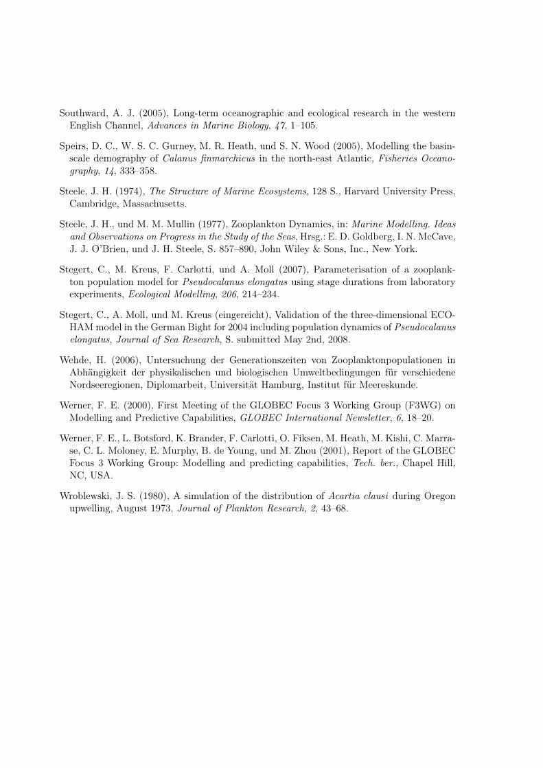
Southward, A. J. (2005), Long-term oceanographic and ecological research in the westernEnglish Channel, Advances in Marine Biology, 47, 1–105.
Speirs, D. C., W. S. C. Gurney, M. R. Heath, und S. N. Wood (2005), Modelling the basin-scale demography of Calanus finmarchicus in the north-east Atlantic, Fisheries Oceano-graphy, 14, 333–358.
Steele, J. H. (1974), The Structure of Marine Ecosystems, 128 S., Harvard University Press,Cambridge, Massachusetts.
Steele, J. H., und M. M. Mullin (1977), Zooplankton Dynamics, in: Marine Modelling. Ideasand Observations on Progress in the Study of the Seas, Hrsg.: E. D. Goldberg, I. N. McCave,J. J. O’Brien, und J. H. Steele, S. 857–890, John Wiley & Sons, Inc., New York.
Stegert, C., M. Kreus, F. Carlotti, und A. Moll (2007), Parameterisation of a zooplank-ton population model for Pseudocalanus elongatus using stage durations from laboratoryexperiments, Ecological Modelling, 206, 214–234.
Stegert, C., A. Moll, und M. Kreus (eingereicht), Validation of the three-dimensional ECO-HAM model in the German Bight for 2004 including population dynamics of Pseudocalanuselongatus, Journal of Sea Research, S. submitted May 2nd, 2008.
Wehde, H. (2006), Untersuchung der Generationszeiten von Zooplanktonpopulationen inAbhängigkeit der physikalischen und biologischen Umweltbedingungen für verschiedeneNordseeregionen, Diplomarbeit, Universität Hamburg, Institut für Meereskunde.
Werner, F. E. (2000), First Meeting of the GLOBEC Focus 3 Working Group (F3WG) onModelling and Predictive Capabilities, GLOBEC International Newsletter, 6, 18–20.
Werner, F. E., L. Botsford, K. Brander, F. Carlotti, O. Fiksen, M. Heath, M. Kishi, C. Marra-se, C. L. Moloney, E. Murphy, B. de Young, und M. Zhou (2001), Report of the GLOBECFocus 3 Working Group: Modelling and predicting capabilities, Tech. ber., Chapel Hill,NC, USA.
Wroblewski, J. S. (1980), A simulation of the distribution of Acartia clausi during Oregonupwelling, August 1973, Journal of Plankton Research, 2, 43–68.