Embed Size (px)
Citation preview
MODELLING THEHOLOCENE SEDIMENT
BUDGET OF THERHINE SYSTEM
DISSERTATION
zurErlangung des Doktorgrades (Dr. rer. nat.)
derMathematisch-Naturwissenschaftlichen Fakultat
derRheinischen Friedrich-Wilhelms-Universitat Bonn
vorgelegt von
THOMAS HOFFMANN
ausWitten a.d. Ruhr
Bonn 2006

Angefertigt mit Genehmigung der Mathematisch-NaturwissenschaftlichenFakultat der Rheinischen Friedrich-Wilhelms-Universitat Bonn
1. Referent: Richard Dikau2. Referent: Lothar Schrott
Tag der Promotion: 13. Februar 2007
Diese Dissertation ist auf dem Hochschulschriftenserver der ULB Bonnhttp://hss.ulb.uni-bonn.de/diss online elektronisch publiziert
Abstract
Rivers transport large amounts of water, sediments, nutrients and carbonfrom the continents to the oceans. Thus, they are important links withinthe global biogeochemical cycle. To understand biogeochemical fluxes inriver channels, holistic system-based approaches are needed that considerriver channels and their corresponding catchments. Sediment fluxes in fluvialsystems change in consequence of changing external controls (land use andclimate). However, the system’s response to land use and climate changevaries depending on internal controls (e.g. catchment size and structure).While forcing-response mechanisms of small catchments are reasonably wellunderstood, the response of larger drainage basins is less clear. In particular,the impact of land use and climate change on the Rhine system is poorlyknown owing to the catchment size (185 000 km2) and the long history ofhuman cultivation, which started approx. 7500 years ago.
A sediment budget is calculated to specify the amount of alluvial sedi-ment and total organic carbon that deposited during the Holocene and toestimate long term soil erosion rates. The focus was driven to floodplainsbecause they act as important sinks in terms of sediment and carbon fluxand therefore, provide a range of potential sites of palaeoecological data.To obtain information on the temporal development of the Rhine system, adatabase of 14C-ages taken from colluvial and alluvial deposits was compiledand analysed in terms of i) cumulative frequency distributions of the agesand ii) changing sedimentation rates on floodplains and in palaeochannels.
The results of the sediment budget suggest that 59±14×109 t of Holocenealluvial sediment is stored in the non-alpine part of the Rhine catchment(South and Central Germany, Eastern France, The Netherlands). About50 % of Holocene alluvial sediment is deposited along the trunk valley andthe delta (Upper Rhine, Lower Rhine, coastal plain), while the rest is storedalong the tributary valleys. The floodplain sediment storage corresponds to amean erosion rate of 0.55± 0.16 t ha−1year−1 (38.5± 10.7 mm kyr−1) acrossthe Rhine catchment outside the Alps. This Holocene-averaged estimateamounts for sediments that were delivered to the channel network and is at
i
ii
the lower limit of erosion rates from other studies of different methodology.The statistical analysis of 1948 organic carbon measurements in different
parts of the Rhine catchment suggest a strong influence of the sedimentary fa-cies on the organic carbon content. The analysis allowed the development ofa conceptual carbon budget model of fluvial systems, which was coupled withthe alluvial sediment storage, to estimate the Holocene sequestration rates ofcarbon storage in floodplains. Averaged over the Rhine catchment the sedi-mentary carbon sequestration ranges between 3.4 to 25.4 g m−2 year−1 withmore reasonable values between 5.3 to 17.7 g m−2 year−1. Compared to therecent particulate carbon export, these values are in the same order of magni-tude but somewhat smaller indicating that approximately the same amountof the exported carbon may be stored in floodplains. However, comparedto sedimentary carbon sequestration rates obtained elsewhere, the presentedvalues are at the lower limit, corresponding to the lower mean Holocene soilerosion and floodplain accumulation rates.
Based on the cumulative frequency distributions of the 14C-ages eightperiods of geomorphic activity are identified (peaking at 8.2 kyr, 7.54 kyr,5.6 kyr, 4.2 kyr, 3.3 kyr, 2.8 kyr, 2.3 kyr and since 1075 years BP). Theseperiods were compared with climatic, palaeohydrological and human impactproxy data. Until 4200 years BP, events of geomorphic activity are mainlycoupled to wetter and/or cooler climatic phases. Between 3300 and 2770years BP, the increased geomorphic activity cannot unequivocally be relatedto climate. The growing population and the intensification of agriculturalactivities must be considered as an additional control during the Bronzeage. Since 1075 years BP the growing population density is considered asthe major external forcing. Additionally, it could be shown that the newlydeveloped approach has major advantages compared to the approach usedto analyse the 14C-database of Great Britain, Spain and Poland.
Concerning the changing sedimentation rates on floodplains and in palaeo-channels, three phases were identified, during the last 14 000 years: i) theLate Glacial-Holocene with medium sedimentation rates, ii) the HoloceneClimatic Optimum with slightly decreasing rates and iii) the last 4000 years,which are characterised by increasing sedimentation rates. The results arein good correspondence with a conceptual model of the Holocene floodplaindevelopment in Europe.
Until now, the spatially distributed sediment and carbon budgets and thetemporal analysis of the 14C-database are analysed based on linear relation-ships of causes and effects. However, to understand the nonlinear responseof the Rhine system to changes of land use and climate impacts during theHolocene, it is necessary to couple the temporal and spatial approaches thatwere developed in this thesis.
Vorwort
Die vorliegenden Dissertation entstand im Rahmen des Projektes ”Model-lierung des holozanen Sedimenthaushalts fluvialer Systeme”, welches Teildes DFG-Projektbundels ”Mensch-Umwelt-Einflusse auf das fluviale Sys-tem des Rheins seit Beginn der landwirtschaftlichen Nutzung (RheinLU-CIFS)” war. Das RheinLUCIFS Bundel bot einen wunderbaren interdiszi-plinaren Rahmen, in dem lebhaft die Fragestellungen der Geomorphologie,Archaologie, Palaobotanik und historischen Geographie mit den Kollegendes Bundels diskutiert werden konnten. Ich mochte allen Teilnehmern desBundels danken, die zum Gelingen der Arbeit in diesem Bundel beigetragenhaben.
Allen voran mochte ich mich bei Prof. Richard Dikau fur die Finanzierung,die vielseitige Betreuung und sein Interesse bedanken. Erst durch Ihn undsein Vertrauen in meine Arbeit wurde diese Dissertation ermoglicht. Dielebhaften und offenen Diskussionen zur Thematik des fluvialen Sediment-transportes und der Komplexitat und Nicht-Linearitat geomorphologischerSysteme waren wichtige Inspirationsquellen meiner Arbeit.
Meinen Kollegen der Arbeitsguppe Dikau mochte ich fur den guten Zusam-menhalt und den offenen Umgang innerhalb der Gruppe danken. Ihre Hilfs-bereitschaft und die vielen kreativen Diskussionen zur Thematik und anderenDingen des Lebens und der Wissenschaft haben meine Motivation zur Ar-beit stets positiv beeinflußt. Jan, Frank, Michael + Michael und Rainerihr seid super Jungs!!!!! Meinen Helferinnen Manuela Schlummer und JuliaGerz danke ich fur ihr unendliches Leidenspotential, die fehlende Langeweile;-) und das Ertragen der vielen, oft monotonen Arbeiten. Ich weiß gar nicht,was ich ohne Euch hatte machen sollen.
Fur die Datenbereitstellung, vielseitigen Hilfestellungen und Einblicke inden Umgang mit 14C-Datierungen, Kohlenstoff-Analysen und archaologischenDaten danke ich Andreas Lang (Liverpool), Peter Houben und Jurgen Wun-derlich (beide Uni Frankfurt), Stefan Glatzel (Uni Rostock), Jochen Seidel(Uni Freiburg) sowie Andreas Zimmermann und Karl Peter Wendt (beideUni Koln).
iii
iv
Meinen niederlandischen Kollegen, Gilles Erkens, Kim Cohen, freakyFreek Buschers und Hans Middelkoop (Uni Utrecht) danke ich fur die kreati-ven Diskussionen und die unkonventionellen Gedanken zur holozanen Se-dimentbilanzierung. Ich hoffe, dass noch ganz viel Wasser den Rhein herunterfliesen wird und die begonnen Kooperationen nicht versiegen lasst.
Erik Sprokkereef (International Commission fort he Hydrology of theRhine basin, CHR/KHR) stellte dankenswerterweise Daten aus dem Rhein-einzugsgebiet zur Verfugung.
Last but not least, danke ich Mr. Andrews (alias Herr Mister) fur dieDurchsicht des Manuskripts und der Nachsicht mit meinem englischen Schreib-stil.
Bonn im Dezember 2006Thomas Hoffmann
Contents
1 Introduction 1
2 Scientific framework 72.1 Fluvial Systems . . . . . . . . . . . . . . . . . . . . . . . . . . 9
2.1.1 The Hillslope System . . . . . . . . . . . . . . . . . . . 102.1.2 Sediment transport in river channels . . . . . . . . . . 122.1.3 Floodplains . . . . . . . . . . . . . . . . . . . . . . . . 152.1.4 Importance of carbon flux in fluvial systems . . . . . . 19
2.2 Holocene environmental change . . . . . . . . . . . . . . . . . 212.2.1 Climate change . . . . . . . . . . . . . . . . . . . . . . 212.2.2 Human Impact . . . . . . . . . . . . . . . . . . . . . . 24
2.3 Fluvial response . . . . . . . . . . . . . . . . . . . . . . . . . . 282.3.1 Climate impacts on fluvial systems . . . . . . . . . . . 282.3.2 Human impact on fluvial systems . . . . . . . . . . . . 322.3.3 The internal configurational state . . . . . . . . . . . . 352.3.4 Relative importance of land use and climate impact . . 44
3 Study site: Rhine catchment 473.1 General geographical setting . . . . . . . . . . . . . . . . . . . 493.2 Geological and geomorphological setting . . . . . . . . . . . . 493.3 Climate, hydrology and modern sediment flux . . . . . . . . . 513.4 Human Impact . . . . . . . . . . . . . . . . . . . . . . . . . . 553.5 Holocene valley development . . . . . . . . . . . . . . . . . . . 573.6 Human impact on sediment fluxes . . . . . . . . . . . . . . . . 59
4 Concept and methods 614.1 Problems, needs and aims . . . . . . . . . . . . . . . . . . . . 634.2 Holocene fluvial sediment budget . . . . . . . . . . . . . . . . 67
4.2.1 Estimation of Holocene floodplain volumes . . . . . . . 674.2.2 Calculation of hinterland volume . . . . . . . . . . . . 684.2.3 Calculation of the delta volume . . . . . . . . . . . . . 71
v
vi CONTENTS
4.2.4 Erosion rate calculations . . . . . . . . . . . . . . . . . 734.3 Holocene fluvial TOC budget . . . . . . . . . . . . . . . . . . 75
4.3.1 Data analysis . . . . . . . . . . . . . . . . . . . . . . . 754.3.2 Conceptual carbon budget model . . . . . . . . . . . . 78
4.4 14C-database analysis . . . . . . . . . . . . . . . . . . . . . . . 804.4.1 Cumulative frequency distributions . . . . . . . . . . . 814.4.2 Sedimentation rates . . . . . . . . . . . . . . . . . . . . 85
5 Results 875.1 Holocene fluvial sediment budget . . . . . . . . . . . . . . . . 89
5.1.1 Alluvial sediment storage . . . . . . . . . . . . . . . . . 895.1.2 Holocene erosion rates . . . . . . . . . . . . . . . . . . 91
5.2 TOC storage in floodplains . . . . . . . . . . . . . . . . . . . 935.2.1 Sample depth and clay content . . . . . . . . . . . . . 935.2.2 Depositional environment and sedimentary facies . . . 93
5.3 Holocene alluvial TOC budget . . . . . . . . . . . . . . . . . . 1015.3.1 TOC flux related to channel bed erosion and deposition1015.3.2 TOC storage related to overbank deposition . . . . . . 102
5.4 14C-database analysis . . . . . . . . . . . . . . . . . . . . . . . 1045.4.1 Cumulative frequency distributions . . . . . . . . . . . 1045.4.2 Sedimentation rates . . . . . . . . . . . . . . . . . . . . 108
6 Discussion 1116.1 Holocene fluvial sediment budget . . . . . . . . . . . . . . . . 113
6.1.1 Quantification of sediment storage . . . . . . . . . . . . 1136.1.2 Quantification of mean Holocene erosion rate . . . . . . 1146.1.3 Comparison of the erosion rate with other studies . . . 116
6.2 Holocene alluvial carbon budget . . . . . . . . . . . . . . . . . 1186.2.1 Limitations and uncertainties . . . . . . . . . . . . . . 1186.2.2 Significance and perspective . . . . . . . . . . . . . . . 119
6.3 14C-database analysis . . . . . . . . . . . . . . . . . . . . . . . 1206.3.1 Cumulative frequency distributions . . . . . . . . . . . 1206.3.2 Sedimentation rates . . . . . . . . . . . . . . . . . . . . 125
7 Conclusion and Perspectives 1297.1 Holocene fluvial sediment budget . . . . . . . . . . . . . . . . 1317.2 Holocene alluvial TOC budget . . . . . . . . . . . . . . . . . . 1317.3 14C-database analysis . . . . . . . . . . . . . . . . . . . . . . . 1327.4 Concluding summary and perspectives . . . . . . . . . . . . . 132
List of Figures
1.1 Greenhouse gas concentrations during the last 400 ka BP. . . . 21.2 Coupling sediment budgets and geoarchives. . . . . . . . . . . 3
2.1 Zones of erosion, transportation and deposition within the flu-vial system. . . . . . . . . . . . . . . . . . . . . . . . . . . . . 9
2.2 Simplified sediment budget of fluvial systems. . . . . . . . . . 102.3 Hysteresis in sediment concentration curves. . . . . . . . . . . 132.4 Floodplain landorms associated with meandering rivers . . . . 162.5 Channel patterns, taken from Berendsen & Stouthamer (2001). 172.6 Quaternary temperature variability at different time scales . . 222.7 Holocene temperature variability . . . . . . . . . . . . . . . . 242.8 Chronology of cultural periods in various regions of Europe . . 252.9 Population growth during the last 14 000 years in Central Europe 262.10 Upstream, local and downstream controls of fluvial response . 292.11 Spatial and temporal scales of forms and components of fluvial
systems . . . . . . . . . . . . . . . . . . . . . . . . . . . . . . 292.12 Phases of increased deposition during the Holocene . . . . . . 312.13 Floodplain sedimentation rates of the Mississippi and Yellow
River . . . . . . . . . . . . . . . . . . . . . . . . . . . . . . . . 362.14 Simplified representation of unbalanced response of fluvial sys-
tems . . . . . . . . . . . . . . . . . . . . . . . . . . . . . . . . 372.15 Influence of drainage basin area on the relative magnitude
(Smax/Smin) of change in response to human impact . . . . . . 382.16 Conceptual model of external impact and scaled dependent
response of fluvial system. . . . . . . . . . . . . . . . . . . . . 402.17 Spatial scaling of landscape connectivity in fluvial systems . . 412.18 Scale linkages in the hierarchy of catchments . . . . . . . . . . 432.19 Soil erosion and land use in Central Europe during the last
1400 years . . . . . . . . . . . . . . . . . . . . . . . . . . . . . 45
3.1 The Rhine catchment and its main tributaries . . . . . . . . . 50
vii
viii LIST OF FIGURES
3.2 Long profile of the River Rhine . . . . . . . . . . . . . . . . . 523.3 Mean annual precipitation in the Rhine catchment . . . . . . . 533.4 Seasonal variation of daily discharge at different gauging stations 543.5 Rectification of the Upper Rhine valley near Breisach . . . . . 563.6 Valley bottom architecture in Central Europe . . . . . . . . . 583.7 Conceptual model of hillslope-channel coupling during the pe-
riod of agriculture in Central Europe . . . . . . . . . . . . . . 60
4.1 The component of historical explanation required to explaingeomorphological systems . . . . . . . . . . . . . . . . . . . . 65
4.2 Simplified flowchart of the RheinLUCIFS concept . . . . . . . 654.3 Schematic representation of the applied sediment budget ap-
proach . . . . . . . . . . . . . . . . . . . . . . . . . . . . . . . 684.4 Flowchart for calculations yielding the Holocene floodplain
fines volume of the Hinterland . . . . . . . . . . . . . . . . . . 694.5 Floodplain width (w) vs. upstream catchment area (Ad) . . . 704.6 Catchment-wide Holocene thickness of floodplain fines . . . . . 724.7 Shaded relief map of Germany with TOC sampling locations
indicated. . . . . . . . . . . . . . . . . . . . . . . . . . . . . . 764.8 C-cycle with focus on the sediment transfer in fluvial systems 794.9 Shaded relief map of Germany with 14C sampling locations
indicated . . . . . . . . . . . . . . . . . . . . . . . . . . . . . . 824.10 Example of 14C-calibration . . . . . . . . . . . . . . . . . . . . 84
5.1 TOC content versus depth. . . . . . . . . . . . . . . . . . . . 955.2 Clay content versus TOC content. . . . . . . . . . . . . . . . . 965.3 TOC versus depositional environment. . . . . . . . . . . . . . 985.4 TOC versus sedimentary facies . . . . . . . . . . . . . . . . . 985.5 Comparison of TOC content of sedimentary facies . . . . . . . 995.6 CPF of activity, stability and transitional ages . . . . . . . . . 1055.7 Phases of increased activity and stability. . . . . . . . . . . . . 1065.8 Sensitivity analysis of activity and stability CPFs . . . . . . . 1075.9 Sedimentation rates of floodplains and palaeochannels . . . . . 109
6.1 Size of Holocene alluvial sediment storages vs. subcatchmentarea . . . . . . . . . . . . . . . . . . . . . . . . . . . . . . . . 114
6.2 Comparison of estimates of long-term erosion rates. . . . . . . 1176.3 Activity and stability CPFs plotted alongside independent
palaeohydrological indicators and population data . . . . . . . 1216.4 Comparing CPF of equally distributed 14C-ages and reanal-
ysed CPDFs of ’change dates’ from Europe . . . . . . . . . . . 124
List of Tables
2.1 Six chronological phases of river use and the managementmethods . . . . . . . . . . . . . . . . . . . . . . . . . . . . . . 33
3.1 Areas of the Rhine catchment shared by different states andof major tributaries . . . . . . . . . . . . . . . . . . . . . . . . 51
4.1 Studied region, number of TOC measurements and drill loca-tions and used TOC estimation method of analysed publications. 75
4.2 English and German names and abbreviations of sedimentaryfacies used for the classification of TOC measurements. . . . . 77
4.3 Number of 14C data taken from different depositional environ-ments and sedimentary facies . . . . . . . . . . . . . . . . . . 83
5.1 Holocene alluvial sediment storage within the Rhine catch-ment and its tributaries . . . . . . . . . . . . . . . . . . . . . 90
5.2 Total Holocene alluvial sediment storage for different time sce-narios. . . . . . . . . . . . . . . . . . . . . . . . . . . . . . . . 91
5.3 Quantification of erosion and erosion rates based of differentscenarios for the input parameters. . . . . . . . . . . . . . . . 92
5.4 Number of TOC measurements taken from different publica-tions and sedimentary facies . . . . . . . . . . . . . . . . . . . 94
5.5 Results of Kruskal-Wallis test of TOC in different sedimentaryfacies and depositional environments . . . . . . . . . . . . . . 97
5.6 Comparison of TOC -means in different sedimentary facies . . 1005.7 Wilcox test on NT and CBS facies . . . . . . . . . . . . . . . 1035.8 TOC budget of the Rhine catchment based on floodplain de-
position . . . . . . . . . . . . . . . . . . . . . . . . . . . . . . 103
ix

Abbreviations
AD Anno DominiBP Before Present (reference year = 1950 AD)C CarbonCND Complex Nonlinear DynamicsCPDF Cumulative Probability Difference FunctionCPF Cumulative Probability FunctionCSDR Channel Sediment Delivery RatioDEM Digital Elevation ModelDFG Deutsche Forschungs GesellschaftER Erosion RateGIS Geographical Information SystemGK Geological MapGK25 Geological Map (mapscale 1:25 000)GK200 Geological Map (mapscale 1:200 000)HSDR Hillslope Sediment Delivery RatioIGBP International Global Geosphere-Biosphere ProgrammeIRD Ice Rafted Debriskyr BP years Before Present (in thousand years)LUCIFS Land Use and Climate Impacts on Fluvial Systems
during the period of agriculturePAGES Past Global changESSDR Sediment Delivery RatioSRTM Shuttle Radar Topography MissionSR Sedimentation RateSY Sediment YieldSSY Specific Sediment YieldTOC Total Organic Carbon
xi

Chapter 1
Introduction
Rivers are major transport agents of water, sediments, nutrients and carbon(Hay, 1998; Meybeck et al., 2003; Meybeck, 2003; Milliman & Syvistki, 1992;Syvitski, 2003). Many landscapes are predominantly formed by running wa-ter in rivers. The holistic explanation of landform evolution must thereforeinvolve a description of fluvial systems as an important component of thegeomorphological system. Besides their geomorphological significance, riversperform many essential functions in societal and ecosystem terms, includ-ing water consumption, energy production, agricultural, navigational and,industrial uses. Rivers have always played an important role in human af-fairs. Due to the availability of water and their function as transport agent,all of the early great civilizations arose on the banks of large rivers. Thusrivers are important links within the global biogeochemical cycle (Slaymaker& Spencer, 1998).
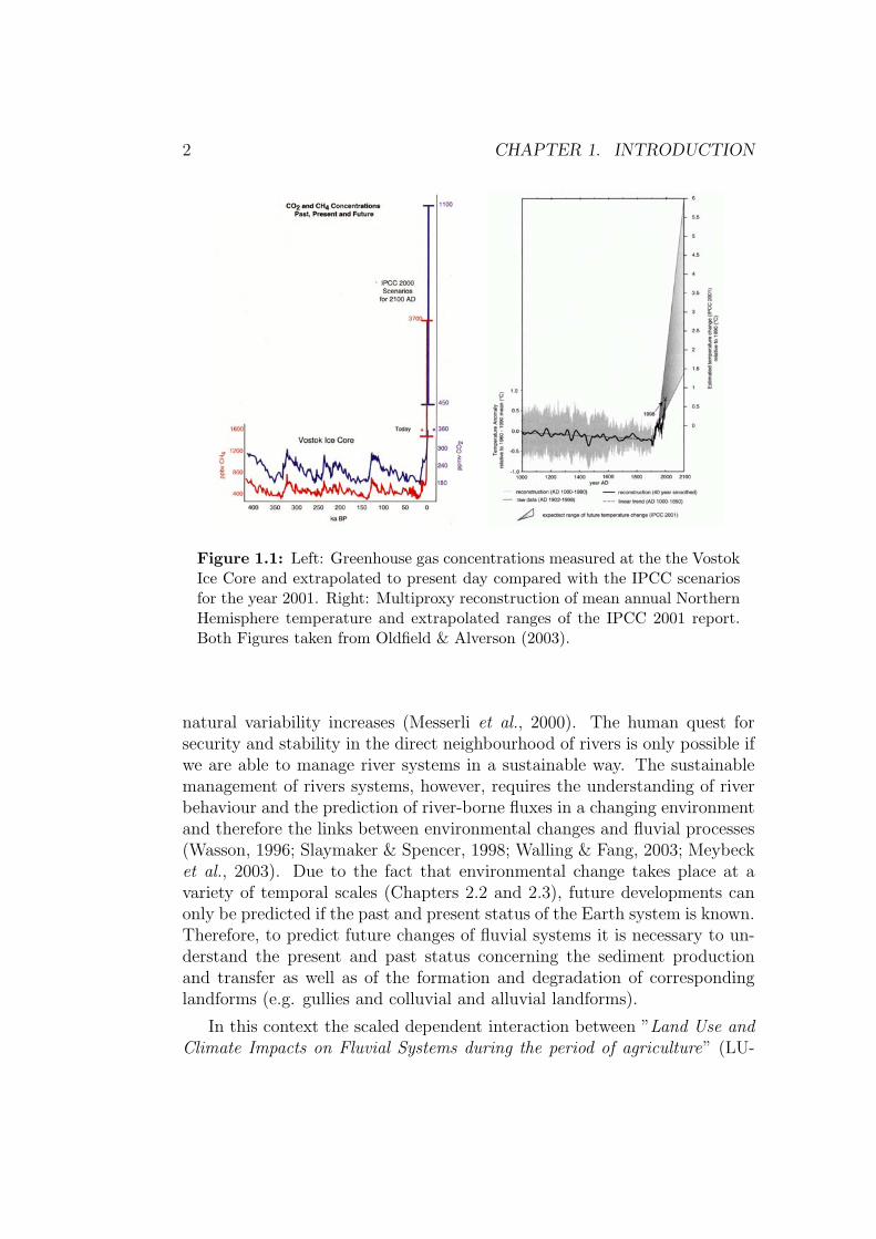
During the last 7500 years, human impact has profoundly altered thenatural functioning of rivers. While natural Earth system drivers, such aslithology, relief, climate and vegetation had a major impact on Earth’s riversbefore the Holocene, it is now believed that anthropogenic forcing is the dom-inant agent of environmental change (Meybeck, 2003). However, the increas-ing human pressure is not limited to fluvial systems but can be attributed tothe Earth’s environment as a whole, causing Crutzen & Stroemer (2000) tocall the time during which human activities have altered the greenhouse gasconcentration in the atmosphere (last 200 years) the ”Anthropocene”. Asshown in Fig. 1.1 the Anthropocene is marked by an extreme rise in meanannual Northern Hemisphere temperature and by greenhouse gas levels welloutside the range of at least the last 400 000 years (Oldfield & Alverson,2003).
Due to the increasing population density, land use pressure and climatechange the vulnerability of societies and economies to extreme events and
1
2 CHAPTER 1. INTRODUCTION
Figure 1.1: Left: Greenhouse gas concentrations measured at the the VostokIce Core and extrapolated to present day compared with the IPCC scenariosfor the year 2001. Right: Multiproxy reconstruction of mean annual NorthernHemisphere temperature and extrapolated ranges of the IPCC 2001 report.Both Figures taken from Oldfield & Alverson (2003).
natural variability increases (Messerli et al., 2000). The human quest forsecurity and stability in the direct neighbourhood of rivers is only possible ifwe are able to manage river systems in a sustainable way. The sustainablemanagement of rivers systems, however, requires the understanding of riverbehaviour and the prediction of river-borne fluxes in a changing environmentand therefore the links between environmental changes and fluvial processes(Wasson, 1996; Slaymaker & Spencer, 1998; Walling & Fang, 2003; Meybecket al., 2003). Due to the fact that environmental change takes place at avariety of temporal scales (Chapters 2.2 and 2.3), future developments canonly be predicted if the past and present status of the Earth system is known.Therefore, to predict future changes of fluvial systems it is necessary to un-derstand the present and past status concerning the sediment productionand transfer as well as of the formation and degradation of correspondinglandforms (e.g. gullies and colluvial and alluvial landforms).
In this context the scaled dependent interaction between ”Land Use andClimate Impacts on Fluvial Systems during the period of agriculture” (LU-
3
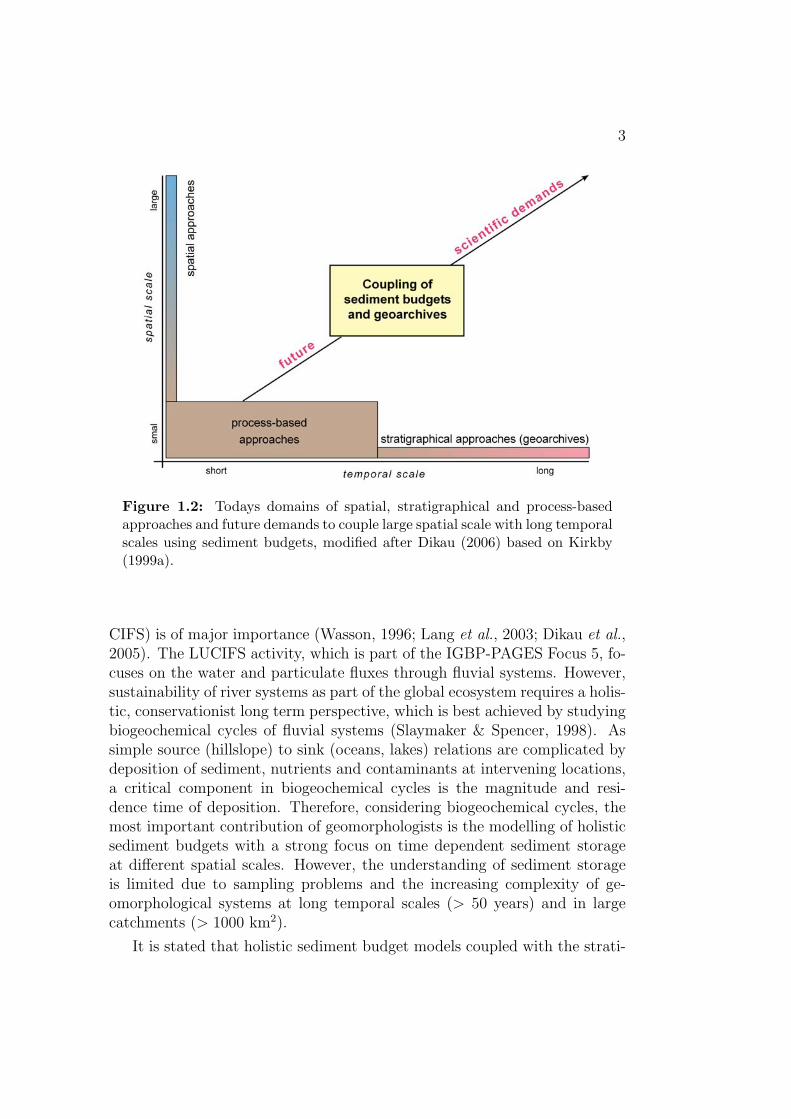
Figure 1.2: Todays domains of spatial, stratigraphical and process-basedapproaches and future demands to couple large spatial scale with long temporalscales using sediment budgets, modified after Dikau (2006) based on Kirkby(1999a).
CIFS) is of major importance (Wasson, 1996; Lang et al., 2003; Dikau et al.,2005). The LUCIFS activity, which is part of the IGBP-PAGES Focus 5, fo-cuses on the water and particulate fluxes through fluvial systems. However,sustainability of river systems as part of the global ecosystem requires a holis-tic, conservationist long term perspective, which is best achieved by studyingbiogeochemical cycles of fluvial systems (Slaymaker & Spencer, 1998). Assimple source (hillslope) to sink (oceans, lakes) relations are complicated bydeposition of sediment, nutrients and contaminants at intervening locations,a critical component in biogeochemical cycles is the magnitude and resi-dence time of deposition. Therefore, considering biogeochemical cycles, themost important contribution of geomorphologists is the modelling of holisticsediment budgets with a strong focus on time dependent sediment storageat different spatial scales. However, the understanding of sediment storageis limited due to sampling problems and the increasing complexity of ge-omorphological systems at long temporal scales (> 50 years) and in largecatchments (> 1000 km2).
It is stated that holistic sediment budget models coupled with the strati-
4 CHAPTER 1. INTRODUCTION
graphical record preserved in geoarchives provide an important approach tofill the gap of studies at large spatial and long temporal scales (Fig. 1.2). Ad-ditionally, long term perspectives are of major importance to solve the prob-lems of river restoration projects, which are generally based on inadequatedata on natural systems suggesting the need to investigate the ”natural” sta-tus of fluvial system by palaeohydrological and palaeoecological approaches(Brown, 2002).
In the case of the RheinLUCIFS project, which focuses on the Rhinecatchment with a 7500 year long history of human impact, sedimentarygeoarchives are used as proxies of sediment flux within fluvial systems (Houbenet al., 2006; Lang et al., 2003). Therefore, the RheinLUCIFS objectives arethe reconstruction of i) scale-dependent dynamic sediment budget modelsand ii) the external controls (e.g. climate, population, land use and veg-etation) (Fig. 4.2). Based on these independent chronologies of externalcontrols and fluvial response, a better understanding of the scale dependentnonlinear response of fluvial systems will be achieved.
The thesis ”Modelling the Holocene Sediment Budgets of theRhine System” is part of the RheinLUCIFS project bundle, which wasfounded by the German Research Foundation (DFG). Despite the substan-tial numbers of detail geomorphological studies at small scales, attempts toestimate sediment fluxes (and storage) at large spatial scales are rare (Wallinget al., 1998). Therefore, the thesis focuses on the modelling of the Holocenealluvial sediment and associated carbon storage in large catchments.
Due to the large spatial scale of the Rhine catchment it was not possibleto gather new data. However, it is stated that scale-related sediment budgetmodels can be developed based on the numerous available data in the Rhinecatchment. In fact, a main objective of this thesis is to draw conclusions andintegrate data from the multitude of local geomorphological studies and touse suitably simplified budget models at the Rhine catchment scale. In termsof a top down approach that is applied in the RheinLUCIFS activity (Houbenet al., 2006), the results obtained at large spatial and long temporal scalesfix the boundary conditions for more detailed studies in space and time. Thethesis therefore follows the statement of Kirkby (1999b, p. 514):
The present trend in fluvial geomorphology is towards increas-ingly detailed understanding of smaller and smaller features moreand more about less and less. The variety of fluvial forms ... il-lustrates the very limited way in which detailed fluvial researchhas been able to contribute to a broad understanding of rivers andchannelways. It is time to draw conclusions from all that has beenlearned in the past 50 years, and apply them, in a suitably sim-
5
plified way and at relevant scales, to entire fluvial systems, andto studying how such systems have evolved over time.
Therefore the main objectives of the thesis are:
• Developing new approaches to model large scale and long term sedimentbudgets based on published data and evaluating the implications forlarge scale modelling.
• Modelling of a time averaged Holocene sediment budget of the nonalpine Rhine catchment below Lake Constance (size of the Rhine catch-ment below Lake Constance = 125 000 km2).
• Modelling of a long term fluvial carbon budget based on the Holocenesediment budget to evaluate the impact of sediment storage on flood-plains on the global carbon cycle.
• Compiling a database on published 14C ages from fluvial and colluvialsystems i) to reconstruct phases of increased activity and stability ofgeomorphological systems in Germany during the last 12 000 years andii) to calculate time dependent rates of floodplain deposition.

Chapter 2
Scientific framework
7

2.1 Fluvial Systems
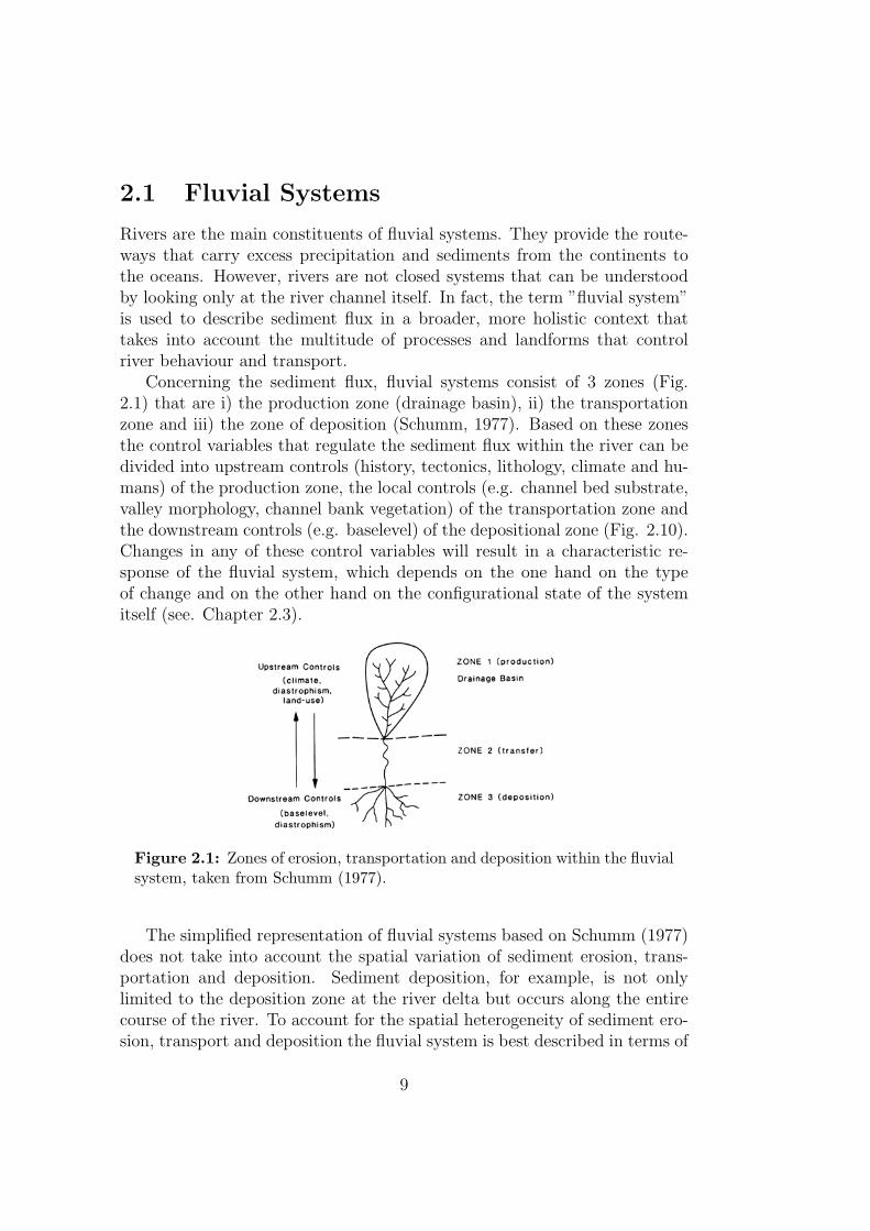
Rivers are the main constituents of fluvial systems. They provide the route-ways that carry excess precipitation and sediments from the continents tothe oceans. However, rivers are not closed systems that can be understoodby looking only at the river channel itself. In fact, the term ”fluvial system”is used to describe sediment flux in a broader, more holistic context thattakes into account the multitude of processes and landforms that controlriver behaviour and transport.
Concerning the sediment flux, fluvial systems consist of 3 zones (Fig.2.1) that are i) the production zone (drainage basin), ii) the transportationzone and iii) the zone of deposition (Schumm, 1977). Based on these zonesthe control variables that regulate the sediment flux within the river can bedivided into upstream controls (history, tectonics, lithology, climate and hu-mans) of the production zone, the local controls (e.g. channel bed substrate,valley morphology, channel bank vegetation) of the transportation zone andthe downstream controls (e.g. baselevel) of the depositional zone (Fig. 2.10).Changes in any of these control variables will result in a characteristic re-sponse of the fluvial system, which depends on the one hand on the typeof change and on the other hand on the configurational state of the systemitself (see. Chapter 2.3).
Figure 2.1: Zones of erosion, transportation and deposition within the fluvialsystem, taken from Schumm (1977).
The simplified representation of fluvial systems based on Schumm (1977)does not take into account the spatial variation of sediment erosion, trans-portation and deposition. Sediment deposition, for example, is not onlylimited to the deposition zone at the river delta but occurs along the entirecourse of the river. To account for the spatial heterogeneity of sediment ero-sion, transport and deposition the fluvial system is best described in terms of
9
10 CHAPTER 2. SCIENTIFIC FRAMEWORK
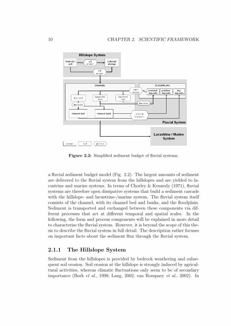
Figure 2.2: Simplified sediment budget of fluvial systems.
a fluvial sediment budget model (Fig. 2.2). The largest amounts of sedimentare delivered to the fluvial system from the hillslopes and are yielded to la-custrine and marine systems. In terms of Chorley & Kennedy (1971), fluvialsystems are therefore open dissipative systems that build a sediment cascadewith the hillslope- and lacustrine-/marine system. The fluvial system itselfconsists of the channel, with its channel bed and banks, and the floodplain.Sediment is transported and exchanged between these components via dif-ferent processes that act at different temporal and spatial scales. In thefollowing, the form and process components will be explained in more detailto characterise the fluvial system. However, it is beyond the scope of this the-sis to describe the fluvial system in full detail. The description rather focuseson important facts about the sediment flux through the fluvial system.
2.1.1 The Hillslope System
Sediment from the hillslopes is provided by bedrock weathering and subse-quent soil erosion. Soil erosion at the hillslope is strongly induced by agricul-tural activities, whereas climatic fluctuations only seem to be of secondaryimportance (Bork et al., 1998; Lang, 2002; van Rompaey et al., 2002). In
2.1. FLUVIAL SYSTEMS 11
Central Europe the beginning of soil erosion correlates with the first agricul-tural activities of the Neolithic Revolution 7500 years BP (e.g. Evans, 1990;Favis-Mortlock et al., 1997; Lang, 2002). The spatial and temporal variationof soil erosion rates varies between 0 and 458 t ha−1year−1 (with a medianof 2.75 t ha−1year−1) is rather large as shown in a review of recent erosionrates in Germany (Auerswald & Dikau, 2006). This variation mainly resultsfrom the impacts of single rain storms that may have a great impact on shortterm measurement. In contrast, long-term mean Holocene erosion rates vary”only” between 1 and 10 t ha−1year−1 as shown in chapter 6.1.
The most important soil erosion processes are sheet (interrill), rill andgully erosion. The relative importance of sheet and gully erosion is predom-inantly a question of scale (Poesen et al., 2003), with dominant sheet andrill erosion at small scales (rill domain) and gully erosion prevailing at largerscale (gully domain). Other factors controlling the soil erosion rate and therelative importance of the two process domains are i) soil type, ii) land use,iii) climate and weather and iv) topography. Data collected from differentparts of the world suggest that gully erosion represent from a minimum of10 % up to 94 % of the total sediment yield (Poesen et al., 2003).
The eroded sediment may not be immediately yielded from the hillslopesto the channel but is stored as colluvial deposit on the slopes or at theirfoot (Lang & Honscheidt, 1999; Lang et al., 2003; Rommens et al., 2005).Colluvial storage may last several thousand years (depending on the land useinduced soil erosion) and therefore influences the coupling between hillslopeand channels on a long temporal scale. The degree of hillslope-channel cou-pling is typically expressed in terms of the sediment delivery ratio (SDR),which is the ratio between the mass or volume of sediment yielded from thehillslope to the channel and the sediment that was eroded1
SDR =sediment yield
sediment erosion. (2.1)
Results from small hillslope catchments suggest that more than 60 % ofsediment eroded is redeposited on the slope and did not reach the channelsystem (e.g. Houben et al., 2006; Preston, 2001; Rommens et al., 2005). Atthe event scale, even 97 % may be deposited at the hillslope (Slattery et al.,2002). These findings, which suggest a limited hillslope-channel coupling,have strong implications for the history of channel systems. If sediment
1According to Asselman et al. (2003), the hillslope SDR (HSDR) as described abovemust be differentiated from the channel SDR (CSDR), which is the percentage of sedimentthat reached the outlet of a catchment and that entered the channel (for more details seechapter 4.2).
12 CHAPTER 2. SCIENTIFIC FRAMEWORK
input from the hillslopes is low, rivers are insensitive to external factors thatchange sediment fluxes on hillslopes.
Important factors that control the SDR are the spatial and temporalscales. Generally, SDRs decrease with increasing catchment size, due to theincreasing storage potential and the decreasing erosion of larger catchments.While short term SDRs may be close to zero, long-term SDRs must ulti-mately approximate unity, otherwise hillslopes would be progressively fillwith sediments (Slattery et al., 2002). Apart from the spatial and temporalscales, variations in SDRs can also be attributed to land use pattern, thetype of soil erosion and the configurational state of the system. The varyingdegree of hillslope-channel coupling for catchments in Central Europe duringthe last 7500 years is explained by variations in land use patterns by Langet al. (2003)(see also Chapter 3.6).
Different types of soil erosion result in different SDRs. Sediment erodedby sheet or rill erosion is transported only limited distances resulting in lowSDRs (Houben et al., 2006). In contrast, gullies are effective links betweenthe upland hillslope and the permanent channel. Therefore, they increase thehillslope-channel connectivity and deliver a large fraction of eroded materialto the channels (Poesen et al., 2003). The systems configuration (e.g. hy-draulic conductivity of soils, (micro-) topography, cultivation direction andtransient boundaries), influences the flow paths and hence controls the traveldistance and process types on the hillslope.
Due to the short transportation distance at the hillslope scale, there is adirect link between sediment erosion and colluvial deposition. In combinationwith the short reaction time, colluvial deposits are effective geoarchives toreconstruct land use and climate impacts on the hillslope system. However,due to the nonlinear relation between the external impact and the resultingerosion (Boardman & Favis-Mortlock, 1999), the magnitude of the externalimpact can not directly be inferred from the amount of colluvial storage.
2.1.2 Sediment transport in river channels
Once the sediment enters the river channel it is transported as bed load,suspended load and/or dissolved load. Due to the effective transport throughriver catchments, suspended and dissolved loads are of major importance,regarding the denudation of catchments. In contrast, bed load transportrequires high transport energy because of its larger grain size, suggesting alimited impact on catchment denudation. However, bed load is an importantfactor controlling the adjustment of channel forms (Knighton, 1998).
The amount of suspended and dissolved load are strongly dependent onthe weathering and erosion rate on the hillslopes, while the amount of bed
2.1. FLUVIAL SYSTEMS 13
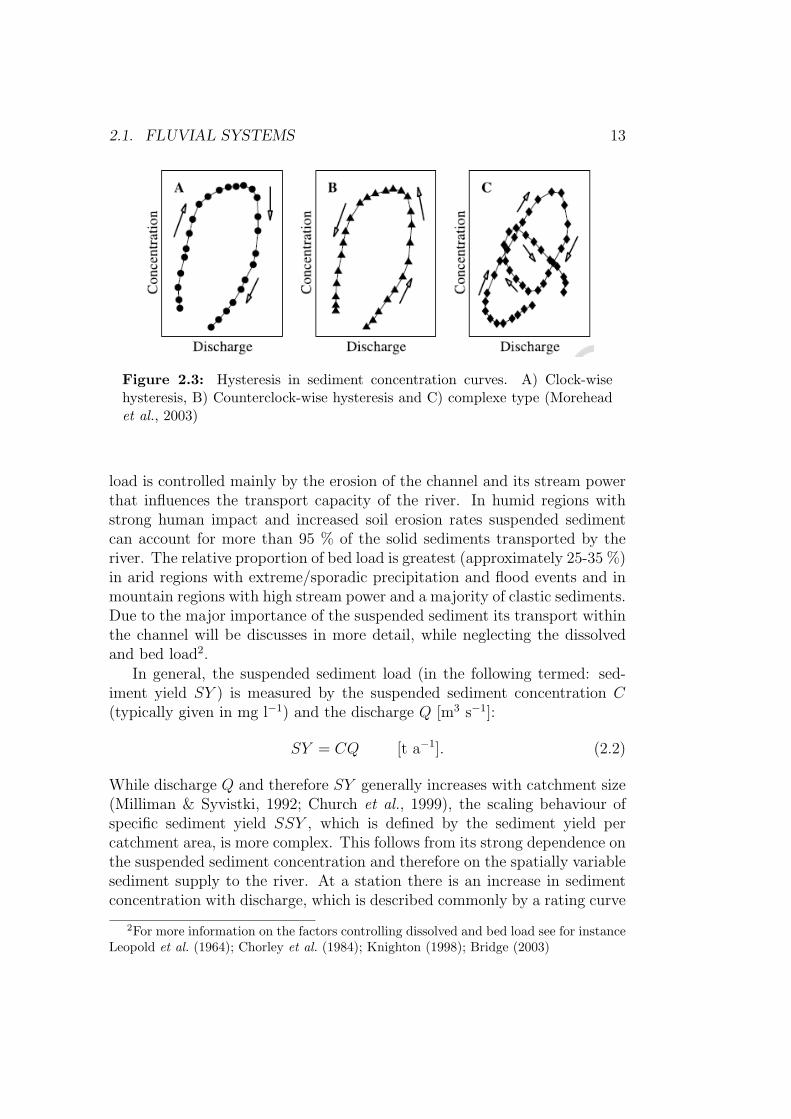
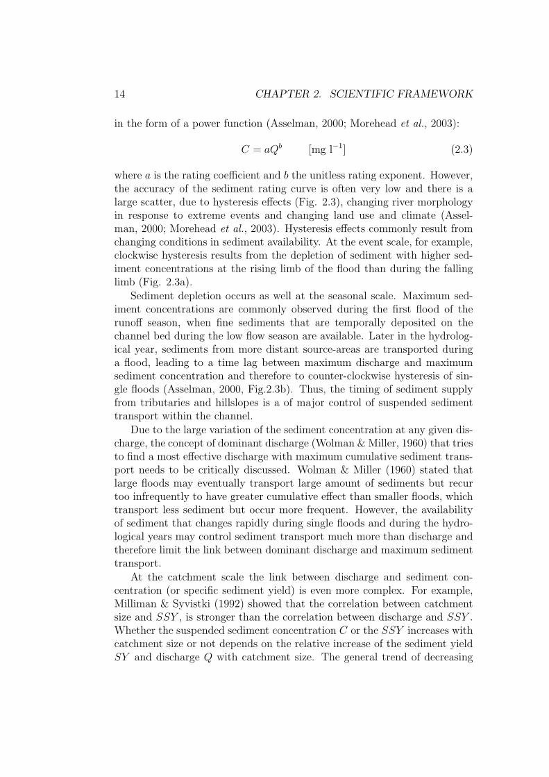
Figure 2.3: Hysteresis in sediment concentration curves. A) Clock-wisehysteresis, B) Counterclock-wise hysteresis and C) complexe type (Moreheadet al., 2003)
load is controlled mainly by the erosion of the channel and its stream powerthat influences the transport capacity of the river. In humid regions withstrong human impact and increased soil erosion rates suspended sedimentcan account for more than 95 % of the solid sediments transported by theriver. The relative proportion of bed load is greatest (approximately 25-35 %)in arid regions with extreme/sporadic precipitation and flood events and inmountain regions with high stream power and a majority of clastic sediments.Due to the major importance of the suspended sediment its transport withinthe channel will be discusses in more detail, while neglecting the dissolvedand bed load2.
In general, the suspended sediment load (in the following termed: sed-iment yield SY ) is measured by the suspended sediment concentration C(typically given in mg l−1) and the discharge Q [m3 s−1]:
SY = CQ [t a−1]. (2.2)
While discharge Q and therefore SY generally increases with catchment size(Milliman & Syvistki, 1992; Church et al., 1999), the scaling behaviour ofspecific sediment yield SSY , which is defined by the sediment yield percatchment area, is more complex. This follows from its strong dependence onthe suspended sediment concentration and therefore on the spatially variablesediment supply to the river. At a station there is an increase in sedimentconcentration with discharge, which is described commonly by a rating curve
2For more information on the factors controlling dissolved and bed load see for instanceLeopold et al. (1964); Chorley et al. (1984); Knighton (1998); Bridge (2003)
14 CHAPTER 2. SCIENTIFIC FRAMEWORK
in the form of a power function (Asselman, 2000; Morehead et al., 2003):
C = aQb [mg l−1] (2.3)
where a is the rating coefficient and b the unitless rating exponent. However,the accuracy of the sediment rating curve is often very low and there is alarge scatter, due to hysteresis effects (Fig. 2.3), changing river morphologyin response to extreme events and changing land use and climate (Assel-man, 2000; Morehead et al., 2003). Hysteresis effects commonly result fromchanging conditions in sediment availability. At the event scale, for example,clockwise hysteresis results from the depletion of sediment with higher sed-iment concentrations at the rising limb of the flood than during the fallinglimb (Fig. 2.3a).
Sediment depletion occurs as well at the seasonal scale. Maximum sed-iment concentrations are commonly observed during the first flood of therunoff season, when fine sediments that are temporally deposited on thechannel bed during the low flow season are available. Later in the hydrolog-ical year, sediments from more distant source-areas are transported duringa flood, leading to a time lag between maximum discharge and maximumsediment concentration and therefore to counter-clockwise hysteresis of sin-gle floods (Asselman, 2000, Fig.2.3b). Thus, the timing of sediment supplyfrom tributaries and hillslopes is a of major control of suspended sedimenttransport within the channel.
Due to the large variation of the sediment concentration at any given dis-charge, the concept of dominant discharge (Wolman & Miller, 1960) that triesto find a most effective discharge with maximum cumulative sediment trans-port needs to be critically discussed. Wolman & Miller (1960) stated thatlarge floods may eventually transport large amount of sediments but recurtoo infrequently to have greater cumulative effect than smaller floods, whichtransport less sediment but occur more frequent. However, the availabilityof sediment that changes rapidly during single floods and during the hydro-logical years may control sediment transport much more than discharge andtherefore limit the link between dominant discharge and maximum sedimenttransport.
At the catchment scale the link between discharge and sediment con-centration (or specific sediment yield) is even more complex. For example,Milliman & Syvistki (1992) showed that the correlation between catchmentsize and SSY , is stronger than the correlation between discharge and SSY .Whether the suspended sediment concentration C or the SSY increases withcatchment size or not depends on the relative increase of the sediment yieldSY and discharge Q with catchment size. The general trend of decreasing
2.1. FLUVIAL SYSTEMS 15
sediment concentrations and specific sediment yields (SSY ), which followsfrom a smaller increase of SY compared to Q, is primarily explained by theincreasing storage capacity of larger catchments (Milliman & Syvistki, 1992;Walling, 1983; Walling & Webb, 1996). To a large extent the increasing stor-age capacity may result from the construction of reservoirs that hold backalmost all suspended sediments and alter the sediment flux of fluvial systems(Vorosmarty et al., 2003; Walling & Fang, 2003). As shown by Dedkov (2004)the general trend of decreasing SSY is, however, only characteristic of inten-sively cultivated basins of the temperate belts, while catchments with limitedcultivation within the Eurasian belt show increasing SSY s with catchmentsize. In addition to drainage area and human impact, relief (e.g. maximumelevation, mean catchment slope), tectonics, precipitation (rather variabilitythan mean value), vegetation, temperature and time are important factorscontrolling the sediment flux in fluvial systems (Milliman & Syvistki, 1992;Hay, 1998; Harrison, 2000; Kirchner et al., 2001; von Blanckenburg, 2005).
To summarize the above discussion, suspended load within the river chan-nel is supply-limited and not capacity-limited, suspended sediment concentra-tion is generally controlled by the sediment supply to the river and there-fore by hillslope erosion rather than the transport capacity. The findings ofDedkov (2004) once more suggest the importance of the human impact andtherefore human induced sediment supply to rivers. Measurements of the SYhave formed the bases for most of the estimates of land degradation rates.However, the link between SY and land degradation is limited by sedimentstorage within the catchment, resulting in decreasing specific sediment yieldsand sediment delivery ratio SDR with catchment size (Walling, 1983).
2.1.3 Floodplains
A floodplain is that part of the landsurface in direct contact with the riverthat is or has been inundated by floods. Floodplains support particularlyrich ecosystems and thus are important areas for human recreation, as habi-tats and corridor for wildlife. The high biodiversity of floodplain resultsfrom the dynamic fluvial processes that control the topography and grainsize of the deposits and thus the hydrology, nutrient levels and finally thevegetation. However, due to their proximity to the river, floodplains are ar-eas of major human impact, which has lead to increased flood-related risks.From a geomorphological point of view, floodplains are major sinks of sus-pended sediment (Walling et al., 1996; Brown, 1996; Walling et al., 1998),nutrients (Burt, 1996; Owens & Walling, 2003; van der Lee et al., 2004),heavy metals (Taylor, 1996; Macklin et al., 1997; Martin, 2000; Middelkoopet al., 2002) and carbon (Walling et al., 2006). In contrast to the channels in
16 CHAPTER 2. SCIENTIFIC FRAMEWORK
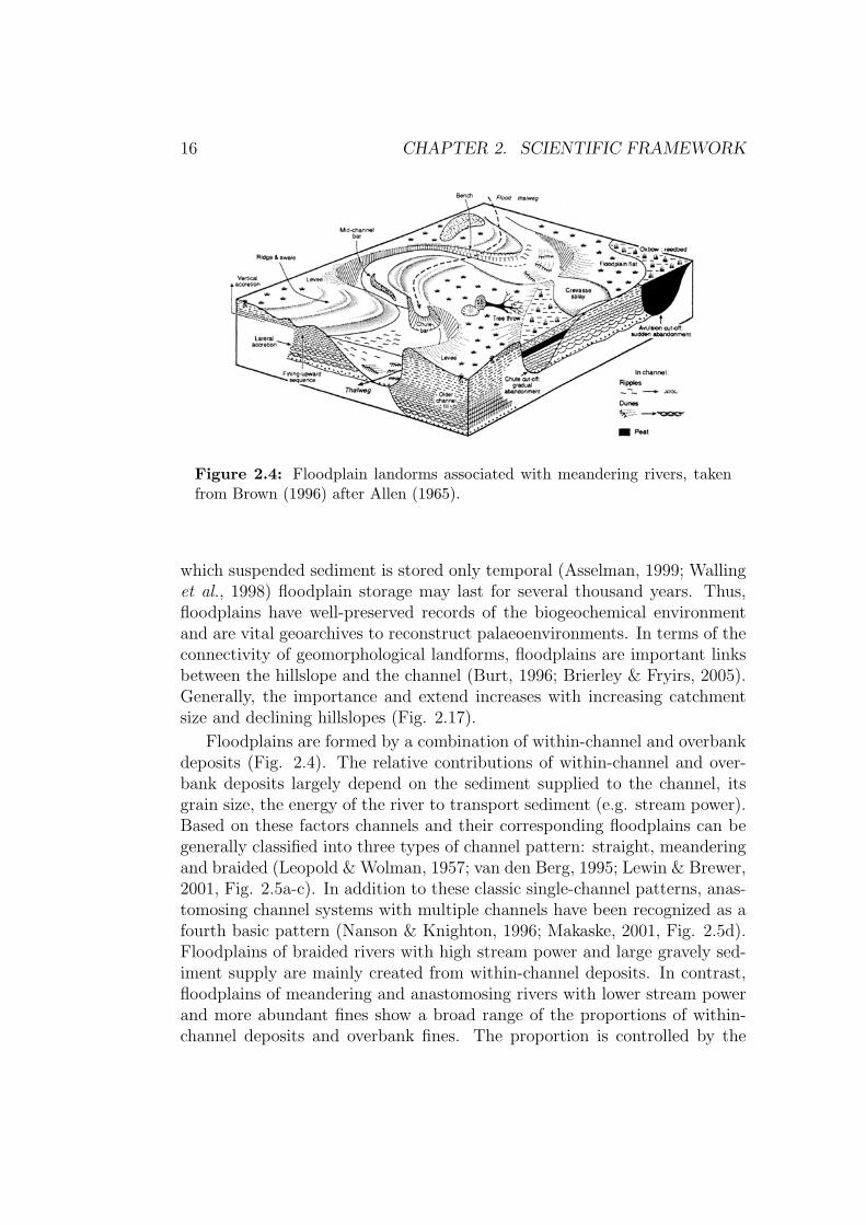
Figure 2.4: Floodplain landorms associated with meandering rivers, takenfrom Brown (1996) after Allen (1965).
which suspended sediment is stored only temporal (Asselman, 1999; Wallinget al., 1998) floodplain storage may last for several thousand years. Thus,floodplains have well-preserved records of the biogeochemical environmentand are vital geoarchives to reconstruct palaeoenvironments. In terms of theconnectivity of geomorphological landforms, floodplains are important linksbetween the hillslope and the channel (Burt, 1996; Brierley & Fryirs, 2005).Generally, the importance and extend increases with increasing catchmentsize and declining hillslopes (Fig. 2.17).
Floodplains are formed by a combination of within-channel and overbankdeposits (Fig. 2.4). The relative contributions of within-channel and over-bank deposits largely depend on the sediment supplied to the channel, itsgrain size, the energy of the river to transport sediment (e.g. stream power).Based on these factors channels and their corresponding floodplains can begenerally classified into three types of channel pattern: straight, meanderingand braided (Leopold & Wolman, 1957; van den Berg, 1995; Lewin & Brewer,2001, Fig. 2.5a-c). In addition to these classic single-channel patterns, anas-tomosing channel systems with multiple channels have been recognized as afourth basic pattern (Nanson & Knighton, 1996; Makaske, 2001, Fig. 2.5d).Floodplains of braided rivers with high stream power and large gravely sed-iment supply are mainly created from within-channel deposits. In contrast,floodplains of meandering and anastomosing rivers with lower stream powerand more abundant fines show a broad range of the proportions of within-channel deposits and overbank fines. The proportion is controlled by the
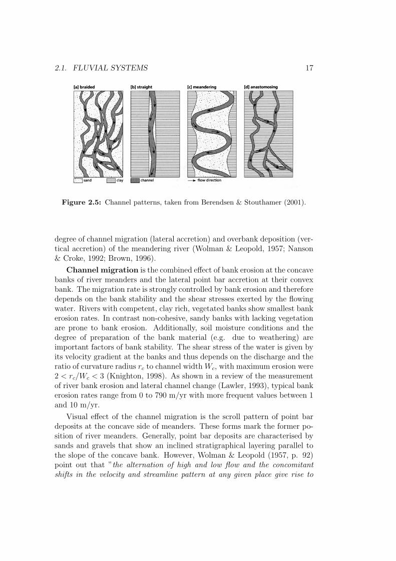
2.1. FLUVIAL SYSTEMS 17
Figure 2.5: Channel patterns, taken from Berendsen & Stouthamer (2001).
degree of channel migration (lateral accretion) and overbank deposition (ver-tical accretion) of the meandering river (Wolman & Leopold, 1957; Nanson& Croke, 1992; Brown, 1996).
Channel migration is the combined effect of bank erosion at the concavebanks of river meanders and the lateral point bar accretion at their convexbank. The migration rate is strongly controlled by bank erosion and thereforedepends on the bank stability and the shear stresses exerted by the flowingwater. Rivers with competent, clay rich, vegetated banks show smallest bankerosion rates. In contrast non-cohesive, sandy banks with lacking vegetationare prone to bank erosion. Additionally, soil moisture conditions and thedegree of preparation of the bank material (e.g. due to weathering) areimportant factors of bank stability. The shear stress of the water is given byits velocity gradient at the banks and thus depends on the discharge and theratio of curvature radius rc to channel width Wc, with maximum erosion were2 < rc/Wc < 3 (Knighton, 1998). As shown in a review of the measurementof river bank erosion and lateral channel change (Lawler, 1993), typical bankerosion rates range from 0 to 790 m/yr with more frequent values between 1and 10 m/yr.
Visual effect of the channel migration is the scroll pattern of point bardeposits at the concave side of meanders. These forms mark the former po-sition of river meanders. Generally, point bar deposits are characterised bysands and gravels that show an inclined stratigraphical layering parallel tothe slope of the concave bank. However, Wolman & Leopold (1957, p. 92)point out that ”the alternation of high and low flow and the concomitantshifts in the velocity and streamline pattern at any given place give rise to
18 CHAPTER 2. SCIENTIFIC FRAMEWORK
considerable heterogeneity in the point bar deposits”. Therefore they empha-sis the difficulty involved in distinguishing point bar and overbank depositsfrom grain size analysis alone.
Wolman & Leopold (1957) concluded that lateral accretion is the dom-inant process and therefore disregarded flood deposition in their classicalmodel of floodplain formation. However, it has been shown that it is of majorimportance along certain low-gradient, single-thread and anastomosing chan-nels (Nanson & Croke, 1992; Brown, 1996; Walling et al., 1996; Knighton,1998). These channel types are characterised by abundant suspended loadand a high frequency over bankful discharge and therefore promote floodplaindeposition by vertical accretion.
Vertical accretion results from the overbank deposition of sedimentduring floods. Sediment is transported from the channel to the floodplaini) by water flow perpendicular to the channel, e.g. in cut-off channels thatare reactivated during the floods and/or ii) by turbulent diffusion3. In gen-eral, the rate of overbank deposition depends on the frequency of inundatingflows and their sediment load. Due to changing sediment loads with time,floods of similar size do not necessarily deposit a similar amount of overbanksediments (Benedetti, 2003). At the local scale, major factors that controloverbank deposition are: i) flow velocity (mainly controlled by floodplaintopography and distance from channel), ii) duration of inundation (mainlycontrolled by floodplain topography) and iii) roughness of the floodplain sur-face (mainly controlled by floodplain vegetation). In the case of turbulentdiffusion there is a strong decreasing tendency of the amount and grain sizeof sediments deposited on the floodplain with channel distance (Pizzuto,1987; Asselman & Middelkoop, 1995; Walling et al., 1998). However, inmost situations sediment transfer is the effect of a combination of turbulentdiffusion and convection. In this case, floodplain topography (Asselman &Middelkoop, 1995) and the distribution and nature of vegetation may be ofmajor importance.
A very broad spread of deposition rates is reported in various papers. Dur-ing a single flood, sediment deposition of 0.82 mm and 0.47 mm was estimatedby Asselman & Middelkoop (1995) for small study site at the Waal and theMeuse in the Netherlands. At the Mississippi Gomez et al. (1997) reportedvalues between 2 and 200 mm of a flood event that happened in 1993. Longterm deposition rates are measured based on 137Cs-concentrations. These
3Turbulent diffusion is the transport of sediment from areas with high sediment con-centrations to areas with low sediment concentrations (Pizzuto, 1987; Nicholas & Walling,1997). In the case of flooded channel systems, turbulent diffusion results in sedimenttransport from the channel (high sediment concentration) to the floodplain (low sedimentconcentration)
2.1. FLUVIAL SYSTEMS 19
measurements integrate over the last 40 years, since maximum 137Cs-fallout.At the River Ouse (Yorkshire, UK), for example, Walling et al. (1998) es-timated overbank sedimentation rates ranging from 0.08 to 5.2 mm year−1
(mean ≈ 1.6 mm year−1) that corresponded to 39% of the suspended sedi-ment yield of the River Ouse. 137Cs-measurements on the Upper MississippiRiver resulted in larger values ranging from 4.4 up to 14.4 mm year−1 witha mean of 12.5 mm year−1 (Benedetti, 2003). The high values are the effectof intense agricultural land disturbance, as compared the mean values of 1.4mm year−1 estimated based on 14C-measurements at the same locations. Formore values of vertical accretion rates see Rumsby (2000), who gives a shortreview over a broad range of spatial temporal scales and applied methods.
Due to the successive raising of floodplains resulting from the accumula-tion of overbank fines, the magnitude of successive floods leading to overbankdeposition must continuously increase to inundate the floodplain. Therefore,there is a limit of overbank deposition that results in equilibrium of floodplaingeometry and flow regime. The interacting balance of the two fundamentalprocesses (lateral and vertical accretion) causes a fining-upward sequence ofgravely channel lag deposits, sandy point bar deposits and silty overbankdeposits on top.
However, the equilibrium of floodplain geometry and flow regime is dis-turbed by high energy floods that complicate the general picture of flood-plains. Crevasse splays, which form at levee breaks, chute scour, chute cut-offs and chute fills (palaeochannel fills) are created by geomorphic effectivefloods and are therefore important styles of deposition in high energy flood-plains (Nanson & Croke, 1992, Fig. 2.4). In cases of confined channels withneglecting channel migration and catastrophic floods, floodplains developin disequilibrium with longer episodes of vertical accretion and single floodevents with catastrophic stripping (Nanson, 1986; Kemp, 2004). In activegeomorphic regions with steep slopes rockfalls, landslides, debris cones andmudflow deposits may exist in floodplain environments and obscure theirclassical geometry as shown in Fig. 2.4 (Brown, 1996).
2.1.4 Importance of carbon flux in fluvial systems
The amount of carbon dioxide (CO2) in the atmosphere has increased bymore than 30 % since pre-industrial times and is still increasing at an un-precedented rate on average 0.4 % per year, due to anthropogenic transfor-mation of fossil fuels and land use change (compare Fig. 1.1). However, thegrowth rate of CO2 in the atmosphere is presently less than half of whatwould be expected from anthropogenic CO2 release into the atmosphere.The missing carbon in the atmosphere results from CO2 absorption of the
20 CHAPTER 2. SCIENTIFIC FRAMEWORK
oceans and the terrestrial biospheres (plants and soils), which are major sinksfor anthropogenic carbon (Sarmiento & Gruber, 2002). Especially soils thathold about 1500 Gt organic carbon (twice as much as stored within the at-mosphere as CO2) are an important link in the global carbon cycle (Knorret al., 2005; Lal & Kimble, 1999; Powlson, 2005). Therefore, minor changesin organic carbon content in soils can significantly change the CO2 concen-tration in the atmosphere and accelerate climate change. There has beenan increasing recognition of the role that soil erosion plays in cycling carbonthrough landscapes (Lal, 2004, 2005; Quinton et al., 2006). Onsite, erosionacts as mechanism for the removal of carbon from soils exposing carbonaterich subsoil. Offsite, soil erosion acts as a transport agent, adding carbonthrough sediment accumulation to colluvial storage and to the fluvial system.
Beside the soil erosion processes on the hillslope, the transport of waterand sediment in fluvial systems is an important link in the global carbon cycleand a major input of organic carbon to the oceans (Ludwig et al., 1996; Mey-beck, 1993; Schlunz & Schneider, 2000). At short-terms, rivers are sourcesfor atmospheric CO2 due to the high riverine CO2 concentrations, especiallyin humid tropics, which can be 5-30 times supersaturated with respect toatmospheric equilibrium (Mayorga et al., 2005). High CO2 concentrationsin rivers result from the high CO2 concentrations of the groundwater inputand the heterotrophic CO2 production within the channel. Important factorscontrolling the riverine CO2 concentration and therefore the amount of CO2
exported to the atmosphere are authochtonous primary production withinthe channel and allochthonous organic carbon import to river system fromterrestrial ecosystem (Cole & Caraco, 2001). At long-terms, fluvial systemsacts as a major sink for atmospheric CO2 due to the long-term depositionof organic carbon in floodplains and wetlands (Macaire et al., 2006; Wallinget al., 2006, compare also Chapter 4.3.2).
2.2 Holocene environmental change
The last 2.5 million years (the Quaternary period) are characterised by ex-treme climate variability at different time scales (Fig. 2.6). At long timescales, gradual trends of warming and cooling were driven by tectonic pro-cesses, which resulted in the changing distribution of the continental massesand the building of large mountains. At shorter time scales, fluctuationsof the earths orbital parameters (with typical periods of 100, 41, 23 and19 kyr) lead to periodic changes and the development of glacial and inter-glacial conditions (Wilson et al., 1999). The Holocene is the youngest partof the Earth’s history and the latest series of warmer intervals that inter-rupted colder climates during the Quaternary. Although the beginning ofthe Holocene is marked by a strong temperature increase at the end of thelate glacial, approximately 11 700 years ago (Adams et al., 1999; Litt et al.,2001; Rasmussen et al., 2006), it would be quite wrong to assume that theHolocene is characterised by a constant warm climate with stable geomor-phological systems (e.g. landforms) and ecosystems. Furthermore and incontrast to the former interglacials of the Pleistocene epoch, the Holocene ischaracterised by the emergence and evolution of the human race (Roberts,1998).
Geoscientists generally consider the human impact as an independentfactor that controls the environmental systems. However, there is growingevidence that there are complex feedbacks between natural systems on theone hand and social systems on the other hand. With respect to these com-plex feedbacks, there is a growing debate on the impact of climate changeon prehistoric and historic cultures. Even though the complex feedbacksbetween the natural and social systems must be considered to understandlong-term development of the Earths system, these will not be discussed inmore detailed here. Good introductions to this topic are given by Redman(1999); deMenocal (2001) and Diamond (2005). However, in the followingchapter a short introduction of the changes of the Holocene climate and ofthe human activities will be given.
2.2.1 Climate change
Holocene climate changes in Europe are characterised by long-term trends,centennial to millennial fluctuations and multi-annual and multi-decadalevents (Adams et al., 1999; Huntley et al., 2002; Negendank, 2004, Fig.2.7).The first half of the Holocene has witnessed a general increase of the meanannual temperature that peaked around 5 kyr BP at a value approximately2.5◦C higher than today (Holocene thermal maximum). The warmer tem-
21
22 CHAPTER 2. SCIENTIFIC FRAMEWORK
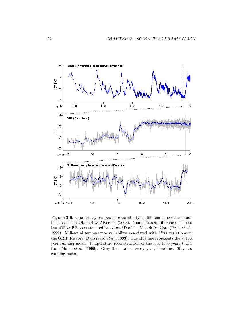
Figure 2.6: Quaternary temperature variability at different time scales mod-ified based on Oldfield & Alverson (2003). Temperature differences for thelast 400 ka BP reconstructed based on δD of the Vostok Ice Core (Petit et al.,1999). Millennial temperature variability associated with δ18O variations inthe GRIP Ice core (Dansgaard et al., 1993). The blue line represents the ≈ 100year running mean. Temperature reconstruction of the last 1000-years takenfrom Mann et al. (1999). Gray line: values every year, blue line: 30-yearsrunning mean.
2.2. HOLOCENE ENVIRONMENTAL CHANGE 23
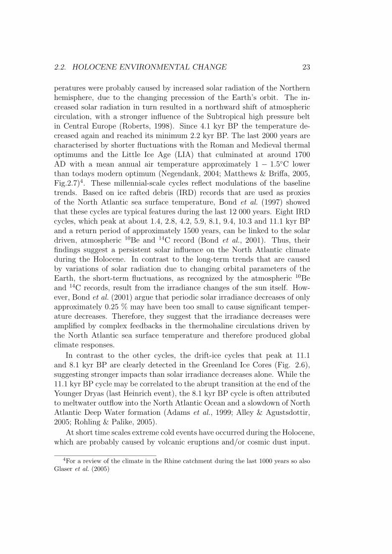
peratures were probably caused by increased solar radiation of the Northernhemisphere, due to the changing precession of the Earth’s orbit. The in-creased solar radiation in turn resulted in a northward shift of atmosphericcirculation, with a stronger influence of the Subtropical high pressure beltin Central Europe (Roberts, 1998). Since 4.1 kyr BP the temperature de-creased again and reached its minimum 2.2 kyr BP. The last 2000 years arecharacterised by shorter fluctuations with the Roman and Medieval thermaloptimums and the Little Ice Age (LIA) that culminated at around 1700AD with a mean annual air temperature approximately 1 − 1.5◦C lowerthan todays modern optimum (Negendank, 2004; Matthews & Briffa, 2005,Fig.2.7)4. These millennial-scale cycles reflect modulations of the baselinetrends. Based on ice rafted debris (IRD) records that are used as proxiesof the North Atlantic sea surface temperature, Bond et al. (1997) showedthat these cycles are typical features during the last 12 000 years. Eight IRDcycles, which peak at about 1.4, 2.8, 4.2, 5.9, 8.1, 9.4, 10.3 and 11.1 kyr BPand a return period of approximately 1500 years, can be linked to the solardriven, atmospheric 10Be and 14C record (Bond et al., 2001). Thus, theirfindings suggest a persistent solar influence on the North Atlantic climateduring the Holocene. In contrast to the long-term trends that are causedby variations of solar radiation due to changing orbital parameters of theEarth, the short-term fluctuations, as recognized by the atmospheric 10Beand 14C records, result from the irradiance changes of the sun itself. How-ever, Bond et al. (2001) argue that periodic solar irradiance decreases of onlyapproximately 0.25 % may have been too small to cause significant temper-ature decreases. Therefore, they suggest that the irradiance decreases wereamplified by complex feedbacks in the thermohaline circulations driven bythe North Atlantic sea surface temperature and therefore produced globalclimate responses.
In contrast to the other cycles, the drift-ice cycles that peak at 11.1and 8.1 kyr BP are clearly detected in the Greenland Ice Cores (Fig. 2.6),suggesting stronger impacts than solar irradiance decreases alone. While the11.1 kyr BP cycle may be correlated to the abrupt transition at the end of theYounger Dryas (last Heinrich event), the 8.1 kyr BP cycle is often attributedto meltwater outflow into the North Atlantic Ocean and a slowdown of NorthAtlantic Deep Water formation (Adams et al., 1999; Alley & Agustsdottir,2005; Rohling & Palike, 2005).
At short time scales extreme cold events have occurred during the Holocene,which are probably caused by volcanic eruptions and/or cosmic dust input.
4For a review of the climate in the Rhine catchment during the last 1000 years so alsoGlaser et al. (2005)
24 CHAPTER 2. SCIENTIFIC FRAMEWORK
Figure 2.7: Holocene temperature variability taken from Negendank (2004).O = temperature optimum, P = temperature minimum, PO = Piora Oscilla-tion, OR = Roman Optimum, PV = pessimum of the Migration time, MO =Medieval optimum, KE = Little Ice Age.
For example, in approximately 1410 years BP (AD 540) global tree ringchronologies record the joint second worst growth year in the last 1500, whichmay correspond to the increased hazard arising from the fragments of deadcomets that intersected the Earths orbit (Huntley et al., 2002).
2.2.2 Human Impact
While natural Earth system drivers, such as lithology, relief, climate andvegetation had a major impact on Earth’s environment during the precedentPleistocene, it is now believed that anthropogenic forcing is the dominantagent of environmental change during the Later Holocene. The impact ofhuman activities has increasingly changed the Earth’s environment since thebeginning of the Neolithic Revolution, the transition from hunting and gath-ering to agricultural activities.
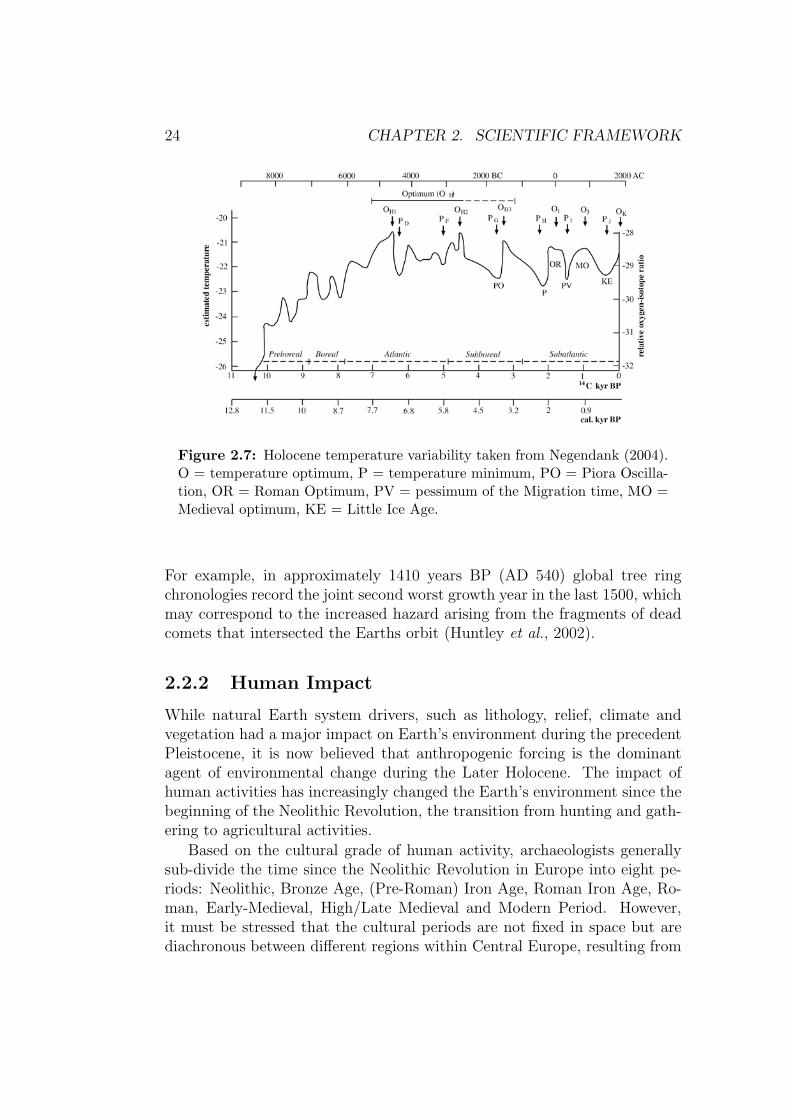
Based on the cultural grade of human activity, archaeologists generallysub-divide the time since the Neolithic Revolution in Europe into eight pe-riods: Neolithic, Bronze Age, (Pre-Roman) Iron Age, Roman Iron Age, Ro-man, Early-Medieval, High/Late Medieval and Modern Period. However,it must be stressed that the cultural periods are not fixed in space but arediachronous between different regions within Central Europe, resulting from
2.2. HOLOCENE ENVIRONMENTAL CHANGE 25
Figure 2.8: Chronology of cultural periods in various regions of Europe(Huntley et al., 2002).
26 CHAPTER 2. SCIENTIFIC FRAMEWORK
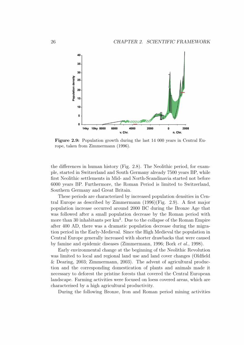
Figure 2.9: Population growth during the last 14 000 years in Central Eu-rope, taken from Zimmermann (1996).
the differences in human history (Fig. 2.8). The Neolithic period, for exam-ple, started in Switzerland and South Germany already 7500 years BP, whilefirst Neolithic settlements in Mid- and North-Scandinavia started not before6000 years BP. Furthermore, the Roman Period is limited to Switzerland,Southern Germany and Great Britain.
These periods are characterized by increased population densities in Cen-tral Europe as described by Zimmermann (1996)(Fig. 2.9). A first majorpopulation increase occurred around 2000 BC during the Bronze Age thatwas followed after a small population decrease by the Roman period withmore than 30 inhabitants per km2. Due to the collapse of the Roman Empireafter 400 AD, there was a dramatic population decrease during the migra-tion period in the Early-Medieval. Since the High Medieval the population inCentral Europe generally increased with shorter drawbacks that were causedby famine and epidemic diseases (Zimmermann, 1996; Bork et al., 1998).
Early environmental change at the beginning of the Neolithic Revolutionwas limited to local and regional land use and land cover changes (Oldfield& Dearing, 2003; Zimmermann, 2003). The advent of agricultural produc-tion and the corresponding domestication of plants and animals made itnecessary to deforest the pristine forests that covered the Central Europeanlandscape. Farming activities were focused on loess covered areas, which arecharacterised by a high agricultural productivity.
During the following Bronze, Iron and Roman period mining activities
2.2. HOLOCENE ENVIRONMENTAL CHANGE 27
and metalworking had a major impact on the development of the early civ-ilizations and therefore on the colonised landscapes (Roberts, 1998). Thedevelopment of the plough made it possible to extend agricultural land useinto upland areas that were until then not favourable for agriculture andsettlement (e.g. the Black Forest, Rhenish Slate Massive). In most loesscovered areas (e.g. the Upper Rhine Graben around Freiburg, the Kraichgauand the Lower Rhine) that were already populated the complete forests werecut and transformed to agricultural land.
Furthermore, urbanisation and water management put additional pres-sure on the Earth’s environment. For example, Herget (2000) described thebuilding of towpaths along the River Lippe already during the Roman pe-riod 2000 years ago, which may have changed the natural channel planformfrom an anastomosing to a meandering river. Regarding the River Rhine,first embankments in the Rhine delta, were build in 1150 AD (Ten Brinke,2005). Since the early 19th century the River Rhine and its tributaries havebeen strongly regulated (Herget et al., 2005). Channelization, the large-scaleconstruction of embankments and dams resulted in a decreasing sedimentexchange of the river channels and their neighbouring floodplains.
Since the beginning of the Industrial Revolution (mid 18th century) thecombustion of fossil fuels for industrial or domestic usage, biomass burning,and land use change (mainly deforestation) produced greenhouse gases andaerosols which affect the global composition of the atmosphere. The amountof carbon dioxide (CO2) in the atmosphere has increased by more than 30% since pre-industrial times and is still increasing at an unprecedented rateon average 0.4 % per year Houghton et al. (2001), resulting in a warmer at-mosphere and stronger climatic extremes. The increase of the global averagesurface temperature over the 20th century by about 0.6◦ C is likely to havebeen the largest during the last 1 000 years (Fig. 2.6) and even since thebeginning of the Holocene, suggesting that human activities can no longer beneglected to influence the environment at a global scale. However, in contrastto the prevailing opinion, Ruddiman (2003) proposed that the global humanimpact started much earlier, when humans reversed a natural decrease ofCO2 (after 8000 years ago) and methane (after 5000 years ago) by startingto clear forests and by irrigating rice, respectively.
While the history of past cultures is well known, mainly based on archae-ological evidences, the major question of the timing and extent woodlandtransformation to arable land and pasture needs to be answered (Bork &Lang, 2003; Herget et al., 2005). Only if we know the impact of human ac-tivity on land use changes are we able to understand the human impact onfluvial systems. However, first results that may help to answer this questionare presented by Zimmermann et al. (2004).
2.3 Fluvial response to environmental change
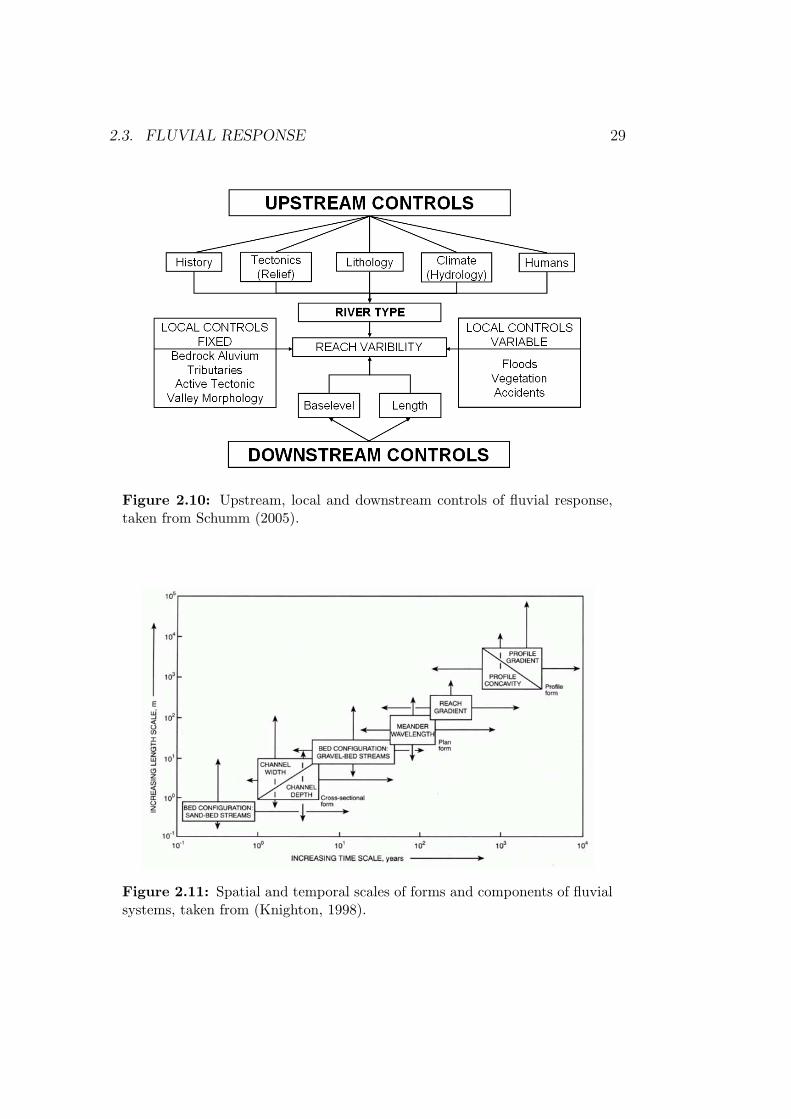
Although there is considerable order in fluvial systems5, river characteris-tics can vary greatly in time and space (Schumm, 2005). For example, ameandering reach can be connected to a braiding reach separated by only afew kilometres. Furthermore, a meander that is currently part of the activechannel may be deactivated during a single flood. The large variability ofrivers results from i) the numerous controls acting on river morphology andbehaviour that change in time and space at different scales (Fig. 2.10), ii)from the discontinuous character of river networks at junctions of two riversegments and iii) different timescales of adjustment of form components offluvial systems (Fig. 2.11). Regarding the external controls, lithology, soilsand baselevel (especially sea level) vary on long terms (e.g. 103 to 106 years),while climate, hydrology and land use can even change on very short tem-poral time scales (approx. 100 to 102 years). The timescale of adjustment ofthe form components to these external changes strongly correlates with theircharacteristic length scale (Fig. 2.11). For example, the bed configuration(e.g. ripples and dunes) with characteristic lengths of 100 m may changewithin seconds. In contrast, the longitudinal profile form of the river witha characteristic length scale of 103 to 104 m adjusts on times scales of 104
years. Based on Knighton (1998) the adjustment of the channel geometry toexternal controls can be considered in terms of four degrees of freedom thatare: i) configuration of the channel bed (e.g. grain size, form like ripples anddunes), ii) the cross section of the channel (e.g. its size and form), iii) chan-nel pattern (compare Chapter 2.1) and iv) the channel slope (longitudinalprofile).
Changes of fluvial systems are of major importance to the human dimen-sion, due to the direct linkages between human activities and fluvial pro-cesses. These changes are driven by the external controls and the effects ofthe internal configurational state. Therefore their impacts on fluvial systemswill be discussed in the following sections.
2.3.1 Climate impacts on fluvial systems
The importance of low frequency, large magnitude climate changes on riverdevelopment during the Pleistocene is now well established. Pleistocene riveraggradational episodes coincide with glacial and stadial events, while phasesof river incision occur during interglacial or interstadial (e.g. Rohdenburg,
5For example, the Horton law describing the structure of channel networks or thedownstream increasing channel width with discharge show strong regularities.
28
2.3. FLUVIAL RESPONSE 29
Figure 2.10: Upstream, local and downstream controls of fluvial response,taken from Schumm (2005).
Figure 2.11: Spatial and temporal scales of forms and components of fluvialsystems, taken from (Knighton, 1998).
30 CHAPTER 2. SCIENTIFIC FRAMEWORK
1970; Mol, 1997; Vandenberghe & Maddy, 2001; Macklin et al., 2002). De-spite their greater aridity glacial and stadial events are characterised by en-hanced geomorphological activity and effective hillslope channel coupling dueto increased frost shattering, the high efficiency of glacial, aeolian and solifluc-tion processes. Considering the fluvial transport, the shift towards more aridconditions and the high surface runoff due to permanently frozen grounds,increased the frequency of large floods. Based on Molnar (2001) such a shift,despite a decrease in precipitation and discharge, could have doubled incisionrates and increased fluvial transport capacity.
A large number of studies focus on the Late Glacial and the Late Glacial-Holocene transition, which is characterised by strong climate changes andconsiderable fluvial responses; global warming, moister conditions, denservegetation cover and reduced sediment supply caused a shift of braiding tomeandering associated with channel incision (e.g Tebbens et al., 1999; Andreset al., 2001; Starkel, 2002b; Bogaart et al., 2003; Litt et al., 2003; Leigh, 2006).
The significance of more frequent changes during Holocene, however, isstill under dispute. Evidences of climate impacts have been shown by dif-ferent authors. For example, Aalto et al. (2003) identified a correlation be-tween the El Nino/Southern Oscillation cycle and the formation of the Bo-livian floodplains. The Southern Oscillation modulates downstream deliveryof sediments as well as associated carbon, nutrients and pollutants to theAmazon main stem.
Starkel (2002a) qualitatively describes the response of Poland Rivers tochanging frequencies of floods. Phases of increased floods are characterised bystraightening and widening of channels followed by a tendency to braidingand avulsions. In contrast, narrow and deeper meanders are developed intimes with less frequent floods. Whether the rivers incise or aggradate dependon the sediment supply that is mainly determined by vegetation cover andland use.
Large scale simultaneous river incision on the climate-sensitive, prairie-grassland of the Great Plains occurred around 1000 years BP (Daniels &Knox, 2005). Based on a proxy records of palaeohydrologic conditions inand around the Great Plains, Daniels & Knox (2005) suggest that widespreaddroughts that coincide with the Mediaeval Warm Period caused this incisionphase.
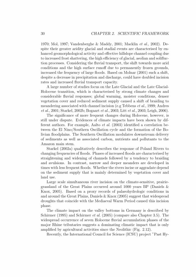
The climate impact on the valley bottoms in Germany is described bySchirmer (1995) and Schirmer et al. (2005) (compare also Chapter 3.5). Thewidespread occurrence of seven Holocene fluvial accumulation phases of themajor Rhine tributaries suggests a dominating climatic impact that is onlyamplified by agricultural activities since the Neolithic (Fig. 2.12).
Recently, the International Council for Science (ICSU) project ”Past Hy-
2.3. FLUVIAL RESPONSE 31
Figure 2.12: Phases of increased deposition during the Holocene as describedby (Schirmer, 1995). NT1-NT3 = lower terrace levels deposited during theLate Glacial. H1-H7 = Holocene terrace levels. For more details see (Schirmer,1995).
32 CHAPTER 2. SCIENTIFIC FRAMEWORK
drological Events Related to Understanding Global Change” provided theframework to analyse and compare Holocene river sequences in Europe in asystematic manner (Gregory et al., 2006; Macklin et al., 2006). Cumulativeprobability distribution functions (CPDF) of 14C ages obtained on Holocenefluvial units were compiled and analysed for different countries (UK, Polandand Spain) and compared to identify possible large-scale hydro climatic tele-connections. The techniques developed by Macklin & Lewin (2003); Lewinet al. (2005) and Johnstone et al. (2006) using 14C ages from Great Britainwere applied by Starkel et al. (2006) for Poland and Thorndycraft & Ben-ito (2006b,a) for Spain. A comparison of the results from Great Britain,Spain and Poland is given by Macklin et al. (2006). 15 Holocene periods ofmajor flooding are identified by peaks in the CPDFs that occur in two ormore areas simultaneously. These periods are interpreted as hydroclimaticteleconnections across Europe and therefore suggest a synchronous climateimpact on fluvial systems during the Holocene. However, due to shortcom-ings in the applied methods, these results must be interpreted with care (formore details see Chapter 4.4.1, 5.4.1 and 6.3.1).
At shorter time scales, the impact of the Little Ice Age (LIA) on fluvialsystems in Central Europe is reviewed by Rumsby & Macklin (1996). Theauthors suggest that at the beginning and the end of the LIA (1250-1550AD and 1750-1900 AD) North, West and Central Europe experienced en-hanced fluvial activity. However, fluvial activity decreased during the mostsevere phase of the last neoglacial. In New South Wales channels respondedto alternating from flood-dominated to drought-dominated regimes duringthe last 100 years (Erskine & Warner, 1999). During catastrophic floods,bank erosion (causing channel widening) generates almost the complete sed-iment yield. In contrast, in-channel sediment storage occurs during drought-dominated regimes. Due to the frequent changes of the flood regime andthe delayed and buffered response, Erskine & Warner (1999) suggest thatchannels in New South Wales are in a state of ”cyclical disequilibrium”, asthey are not able to adjust to a new equilibrium before a new change of theflood regime occurs.
2.3.2 Human impact on fluvial systems
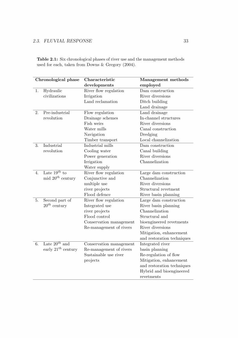
Humans have had a plethora of impacts on fluvial systems, either directlyor indirectly (Gregory, 2006). Direct impacts concern the modification ofthe river channels in terms of river management, e.g. channelization, theconstruction of dams and embankments, diversion and culverting. Indirectimpacts include upstream land use changes such as deforestation, intensiveagriculture, mining, incidence of fire, and urbanisation. Downs & Gregory
2.3. FLUVIAL RESPONSE 33
Table 2.1: Six chronological phases of river use and the management methodsused for each, taken from Downs & Gregory (2004).
Chronological phase Characteristic Management methodsdevelopments employed
1. Hydraulic River flow regulation Dam constructioncivilizations Irrigation River diversions
Land reclamation Ditch buildingLand drainage
2. Pre-industrial Flow regulation Land drainagerevolution Drainage schemes In-channel structures
Fish weirs River diversionsWater mills Canal constructionNavigation DredgingTimber transport Local channelization
3. Industrial Industrial mills Dam constructionrevolution Cooling water Canal building
Power generation River diversionsIrrigation ChannelizationWater supply
4. Late 19th to River flow regulation Large dam constructionmid 20th century Conjunctive and Channelization
multiple use River diversionsriver projects Structural revetmentFlood defence River basin planning
5. Second part of River flow regulation Large dam construction20th century Integrated use River basin planning
river projects ChannelizationFlood control Structural andConservation management bioengineered revetmentsRe-management of rivers River diversions
Mitigation, enhancementand restoration techniques
6. Late 20th and Conservation management Integrated riverearly 21th century Re-management of rivers basin planning
Sustainable use river Re-regulation of flowprojects Mitigation, enhancement
and restoration techniquesHybrid and bioengineeredrevetments

34 CHAPTER 2. SCIENTIFIC FRAMEWORK
(2004) summarize the history of human impact on river channels over thelast 5000 years using six chronological phases (Tab. 2.1).
The effects of the direct impacts on the river channels on the sedimentflux are of opposed character. Some impacts cause sediment loads to in-crease, whilst others cause decreased sediment fluxes (Gregory, 2006, Tab.3there). Concerning the recent global sediment flux by rivers to the ocean,reservoir construction is probably the most important influence that maybuffer increased sediment fluxes caused by increased soil erosion (Walling &Fang, 2003). Based on a global study of 633 of the world’s largest reser-voirs, Vorosmarty et al. (2003) estimated that more than 50% of the basin-scale sediment flux in regulated basins is potentially trapped in artificialimpoundments. Therefore, the global sediment flux to the oceans is reducedby 25-30%, causing significant impacts on the world’s coastal zones. Whilesedimentation occurs upstream of the reservoirs, downstream regions sufferfrom severe channel incision and the subsequently lowering of the groundwa-ter table.
In contrast, channelization and the building of embankments, for exam-ple, may enhance the sediment throughput. Downstream effects of chan-nelization, which are bank erosion and increased sediment flux, arise fromincreased flow velocities and stream power. Furthermore, channelization andthe construction of embankments reduce the channel-floodplain connectiv-ity and therefore the river’s ability to store sediments along its floodplains(Kesel, 2003; Verstraeten et al., 2003; Wohl, 2005).
Indirect human impacts on fluvial systems concern the change in sedimentsupply from the hillslopes due to changing land use and their effects on theriver channels and floodplains. The enhanced conversion of natural vegeta-tion to agricultural land during the last 200 years generally increased soil ero-sion rates by an order of magnitudes or more (Morgan, 1986). Increased soilerosion, in turn, is recognized by increased sediment yields and floodplain de-position of the rivers (Walling & Webb, 1996; Panin, 2004). Over the last 100years, the human impact has been evidenced by direct measurements of thesuspended sediment yield (Walling, 1999; Walling & Fang, 2003). However,increased sediment yields caused by land use changes were only measuredat a limited number of sites, due to the buffering effect of fluvial systems(e.g. by the construction of reservoirs). At longer time scales, acceleratedsedimentation rates on floodplains are correlated with the increasing humanpressure (Fig. 2.13). In the Upper Mississippi Valley (Driftless Area, USA),the shift from natural land cover to landscapes dominated by agriculturalland use of the last 200 years increased rates of floodplain deposition by anorder of magnitude (Knox, 2006, Fig. 2.13a). This shift caused the mostdramatic change of the fluvial activity of the Mississippi and its tributaries
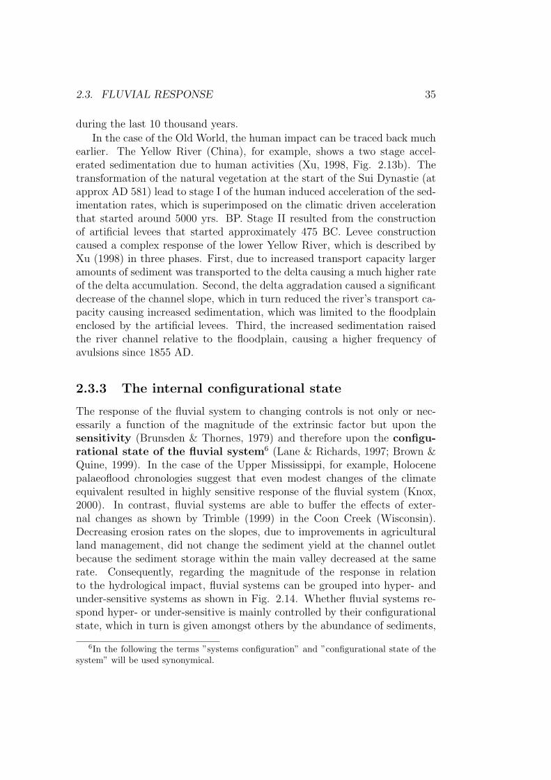
2.3. FLUVIAL RESPONSE 35
during the last 10 thousand years.
In the case of the Old World, the human impact can be traced back muchearlier. The Yellow River (China), for example, shows a two stage accel-erated sedimentation due to human activities (Xu, 1998, Fig. 2.13b). Thetransformation of the natural vegetation at the start of the Sui Dynastie (atapprox AD 581) lead to stage I of the human induced acceleration of the sed-imentation rates, which is superimposed on the climatic driven accelerationthat started around 5000 yrs. BP. Stage II resulted from the constructionof artificial levees that started approximately 475 BC. Levee constructioncaused a complex response of the lower Yellow River, which is described byXu (1998) in three phases. First, due to increased transport capacity largeramounts of sediment was transported to the delta causing a much higher rateof the delta accumulation. Second, the delta aggradation caused a significantdecrease of the channel slope, which in turn reduced the river’s transport ca-pacity causing increased sedimentation, which was limited to the floodplainenclosed by the artificial levees. Third, the increased sedimentation raisedthe river channel relative to the floodplain, causing a higher frequency ofavulsions since 1855 AD.
2.3.3 The internal configurational state
The response of the fluvial system to changing controls is not only or nec-essarily a function of the magnitude of the extrinsic factor but upon thesensitivity (Brunsden & Thornes, 1979) and therefore upon the configu-rational state of the fluvial system6 (Lane & Richards, 1997; Brown &Quine, 1999). In the case of the Upper Mississippi, for example, Holocenepalaeoflood chronologies suggest that even modest changes of the climateequivalent resulted in highly sensitive response of the fluvial system (Knox,2000). In contrast, fluvial systems are able to buffer the effects of exter-nal changes as shown by Trimble (1999) in the Coon Creek (Wisconsin).Decreasing erosion rates on the slopes, due to improvements in agriculturalland management, did not change the sediment yield at the channel outletbecause the sediment storage within the main valley decreased at the samerate. Consequently, regarding the magnitude of the response in relationto the hydrological impact, fluvial systems can be grouped into hyper- andunder-sensitive systems as shown in Fig. 2.14. Whether fluvial systems re-spond hyper- or under-sensitive is mainly controlled by their configurationalstate, which in turn is given amongst others by the abundance of sediments,
6In the following the terms ”systems configuration” and ”configurational state of thesystem” will be used synonymical.
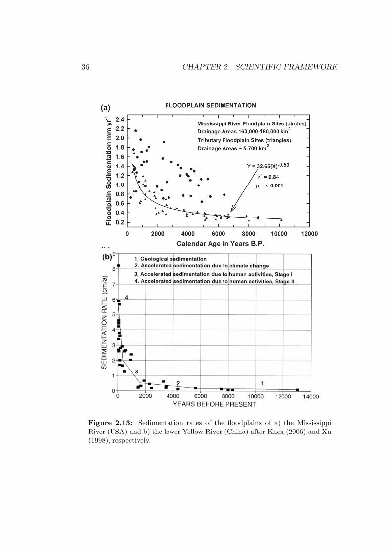
36 CHAPTER 2. SCIENTIFIC FRAMEWORK
Figure 2.13: Sedimentation rates of the floodplains of a) the MississippiRiver (USA) and b) the lower Yellow River (China) after Knox (2006) and Xu(1998), respectively.
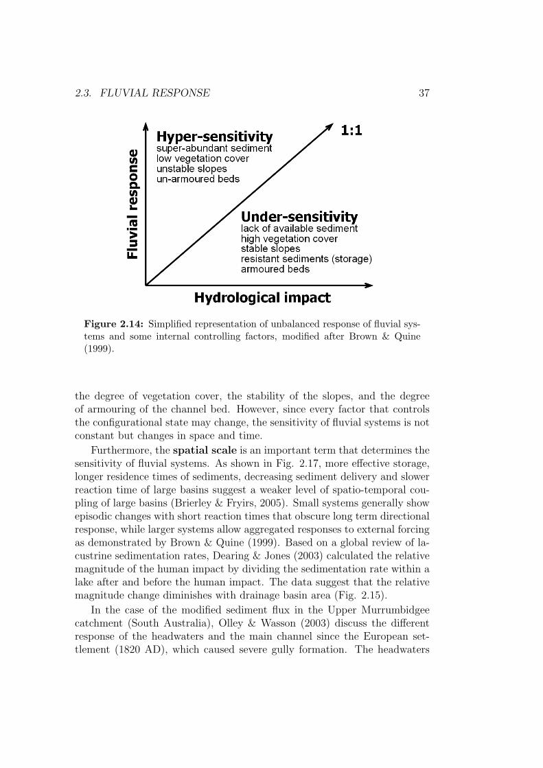
2.3. FLUVIAL RESPONSE 37
Figure 2.14: Simplified representation of unbalanced response of fluvial sys-tems and some internal controlling factors, modified after Brown & Quine(1999).
the degree of vegetation cover, the stability of the slopes, and the degreeof armouring of the channel bed. However, since every factor that controlsthe configurational state may change, the sensitivity of fluvial systems is notconstant but changes in space and time.
Furthermore, the spatial scale is an important term that determines thesensitivity of fluvial systems. As shown in Fig. 2.17, more effective storage,longer residence times of sediments, decreasing sediment delivery and slowerreaction time of large basins suggest a weaker level of spatio-temporal cou-pling of large basins (Brierley & Fryirs, 2005). Small systems generally showepisodic changes with short reaction times that obscure long term directionalresponse, while larger systems allow aggregated responses to external forcingas demonstrated by Brown & Quine (1999). Based on a global review of la-custrine sedimentation rates, Dearing & Jones (2003) calculated the relativemagnitude of the human impact by dividing the sedimentation rate within alake after and before the human impact. The data suggest that the relativemagnitude change diminishes with drainage basin area (Fig. 2.15).
In the case of the modified sediment flux in the Upper Murrumbidgeecatchment (South Australia), Olley & Wasson (2003) discuss the differentresponse of the headwaters and the main channel since the European set-tlement (1820 AD), which caused severe gully formation. The headwaters
38 CHAPTER 2. SCIENTIFIC FRAMEWORK
Figure 2.15: Influence of drainage basin area on the relative magnitude(Smax/Smin) of change in response to human impact, taken from Dearing& Jones (2003). Smax = sedimentation rate after human impact. Smin =sedimentation rate before human impact.
showed a rapid 250 fold increase of sediment yield and a almost completedecline until 1950 after the stabilisation of the gullies. The main channel’ssediment yield increased more slowly by a factor of 200. In contrast to theheadwaters, the decline of the sediment yield is still in progress and is bynow 100 times the pre-European rate.
On the Russian Plain, Sidorchuk & Golosov (2003) observed a similartime lag between soil erosion and floodplain sedimentation. While soil ero-sion stabilised after 1980, the floodplain sedimentation in smaller rivers stillincrease.
In Central Europe, Lang et al. (2003); Houben (2006) and Rommenset al. (2006) recognized long time lags between the onset of the floodplaindeposition and the increased soil erosion on the slope. Due to the limitedslope-channel coupling before the Iron Age, sediment erosion, transport anddeposition was restricted to the slopes. Floodplain sedimentation did notstart before the Iron Age, when agricultural activities intensified and soilerosion dramatically increased (Lang et al., 2003, there Fig. 8).
At even longer time scales, fluvial systems may still adapt to the impactsof the Late Pleistocene. In contrast to the general model of declining specificsediment yields with catchment size, data from British Columbian riversreveal a pattern of increasing specific sediment yield at all spatial scales up
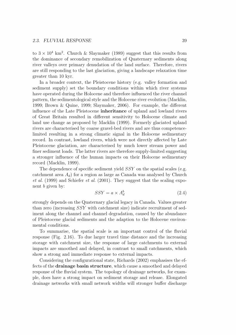
2.3. FLUVIAL RESPONSE 39
to 3 × 10⁴ km2. Church & Slaymaker (1989) suggest that this results fromthe dominance of secondary remobilization of Quaternary sediments alongriver valleys over primary denudation of the land surface. Therefore, riversare still responding to the last glaciation, giving a landscape relaxation timegreater than 10 kyr.
In a broader context, the Pleistocene history (e.g. valley formation andsediment supply) set the boundary conditions within which river systemshave operated during the Holocene and therefore influenced the river channelpattern, the sedimentological style and the Holocene river evolution (Macklin,1999; Brown & Quine, 1999; Slaymaker, 2006). For example, the differentinfluence of the Late Pleistocene inheritance of upland and lowland riversof Great Britain resulted in different sensitivity to Holocene climate andland use change as proposed by Macklin (1999). Formerly glaciated uplandrivers are characterised by coarse gravel-bed rivers and are thus competence-limited resulting in a strong climatic signal in the Holocene sedimentaryrecord. In contrast, lowland rivers, which were not directly affected by LatePleistocene glaciation, are characterised by much lower stream power andfiner sediment loads. The latter rivers are therefore supply-limited suggestinga stronger influence of the human impacts on their Holocene sedimentaryrecord (Macklin, 1999).
The dependence of specific sediment yield SSY on the spatial scales (e.g.catchment area Ad) for a region as large as Canada was analysed by Churchet al. (1999) and Schiefer et al. (2001). They suggest that the scaling expo-nent b given by:
SSY = a× Abd (2.4)
strongly depends on the Quaternary glacial legacy in Canada. Values greaterthan zero (increasing SSY with catchment size) indicate recruitment of sed-iment along the channel and channel degradation, caused by the abundanceof Pleistocene glacial sediments and the adaption to the Holocene environ-mental conditions.
To summarise, the spatial scale is an important control of the fluvialresponse (Fig. 2.16). To due larger travel time distance and the increasingstorage with catchment size, the response of large catchments to externalimpacts are smoothed and delayed, in contrast to small catchments, whichshow a strong and immediate response to external impacts.
Considering the configurational state, Richards (2002) emphasises the ef-fects of the drainage basin structure, which cause a smoothed and delayedresponse of the fluvial system. The topology of drainage networks, for exam-ple, does have a strong impact on sediment storage and release. Elongateddrainage networks with small network widths will stronger buffer discharge
40 CHAPTER 2. SCIENTIFIC FRAMEWORK
Figure 2.16: Conceptual model of external impact and scaled dependentresponse of fluvial system.
and therefore sediment yield than compact drainage networks with a largernetwork width.
Beside the disproportionate response that results from the varying sen-sitivity of fluvial systems, the adaption to a new equilibrium is not alwaysstraight forward. As described by Schumm (1979) the lowering of the baselevel caused a complex response of fluvial system with several cut and fill-phases that result in the formation of a complex staircase of fluvial terraces.Therefore, system response may by ”highly” nonlinear with a complex change(with several ups and downs) to a single impact. In the case of the complexresponse, nonlinearity follows from the sediment storage that obscure thecorrelation between causes and effects (Phillips, 2003).
Nonlinear system behaviour corresponding to storage is also shown atshorter temporal scales, for example, in clockwise hysteresis of discharge -sediment concentration plots of single floods as described earlier (Chapter2.1): On the rising limb of the flood, sediment concentrations are higher,due to the availability of sediments, than at the falling limb where sedimentconcentrations are lower, due to the sediment clearance of the channels afterthe flood peak.
In addition to the effects of sediment storage, thresholds are an impor-tant source of nonlinearity in fluvial systems (Schumm, 1979; Phillips, 2003).Thresholds generally are an expression of a system’s resistance to externalforces. For example, bed load is not transported unless the shear stress ex-
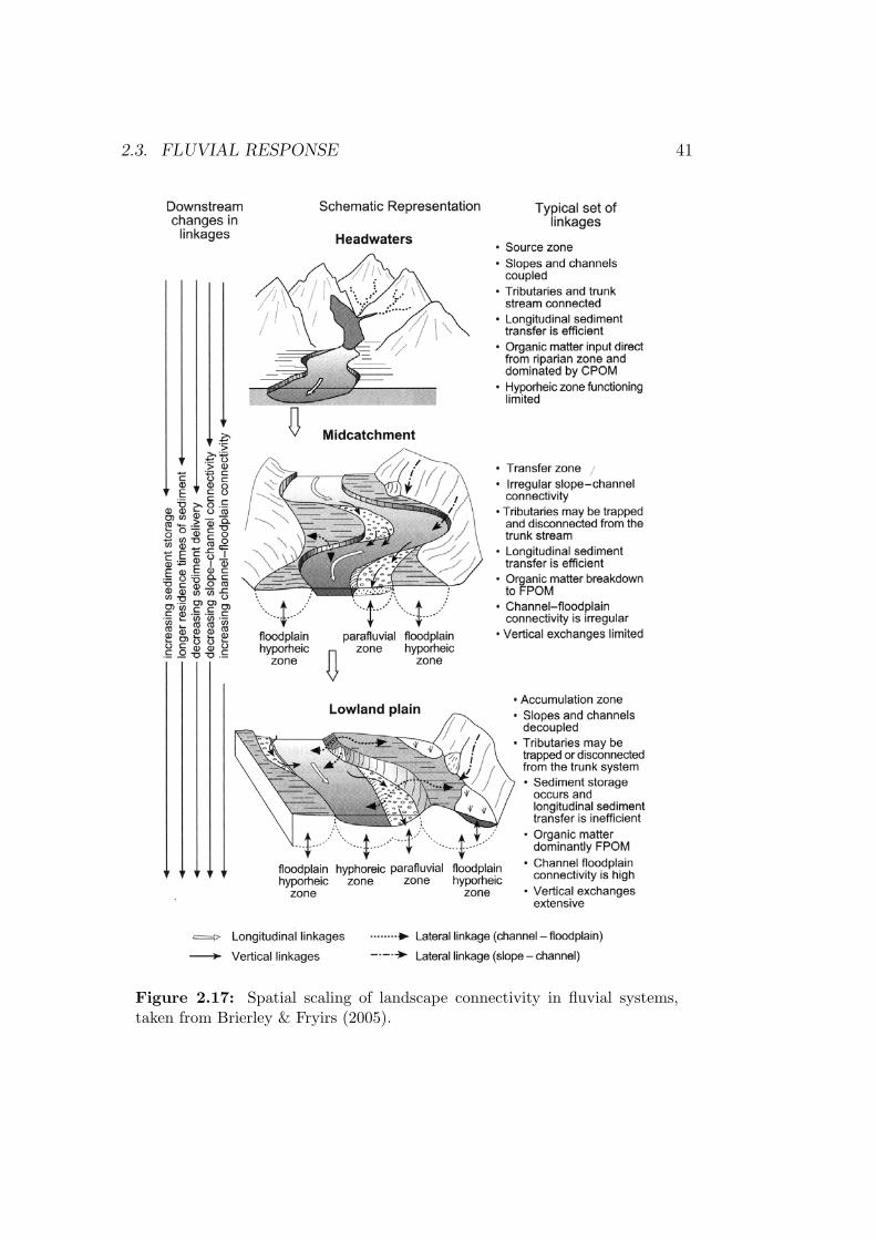
2.3. FLUVIAL RESPONSE 41
Figure 2.17: Spatial scaling of landscape connectivity in fluvial systems,taken from Brierley & Fryirs (2005).
42 CHAPTER 2. SCIENTIFIC FRAMEWORK
erted by the running water exceeds a critical shear stress threshold, which isdetermined by armouring and the grain size of the channel bed. Consideringchannel migration, thresholds control the occurrence of bank failures. Slipsand slab failures as the major bank erosion processes take place if the shearstresses (mainly controlled by the bank slope and the soil moisture content)exceed the threshold of bank stability (given by the cohesion of the bankmaterial and type and degree of the vegetation) (Knighton, 1998; Fonstad &Marcus, 2003).
If system response is controlled by thresholds the correlation betweenmagnitude of the impact and the magnitude of response is obscured. Whenthe system is stable (far away from a threshold) large impacts may have alimited or no impact on the system. In contrast, when a system is near athreshold, small perturbations may cause dramatic responses. In the latercase, the dynamical instabilities result in chaotic behaviour of the system’sresponse (Phillips, 2003).
In general fluvial systems change their morphology and behaviour in re-sponse to environmental change. However, autogenic adjustments occurwithout any change of the external controls (Brown & Quine, 1999) but arepart of the dynamic equilibrium of the system that may follow from theinteraction of the system components at small scales. For example, flat orirregular channel beds are transformed into regular ripples and dunes by thecollective behaviour of sand grains caused by the action of running water.At larger scales, straight channels form regular meanders that are initiatedby the unstable growth of small flow perturbations (Knighton, 1998; Hooke,2003). The meanders will grow, narrow their necks and finally be cut off fromthe current river leading to the formation of oxbow lakes, without changesof the external conditions.
As a result of the collective nonlinear interaction of system componentsat small scales, fluvial systems are able to (self-) organize order that emergesat larger scale (Phillips, 2006). The concept of self organised critically(Bak, 1988, 1996), which explains the complexity of natural systems using aholistic approach was recently applied to bank erosion processes and mean-der development in fluvial systems (Stolum, 1996; Fonstad & Marcus, 2003;Hooke, 2003). Hooke (2003), for example, observed an increasing sinuosityof the River Bollin (UK) to a maximum value of approximately 3 during thelast 100 years. Since 1984 a series of meander cut-offs rapidly reduced thesinuosity. Here, findings suggest that rivers develop to a supercritical sinu-osity at which a larger numbers of cut-offs occur, which are not simply dueto increased occurrence of floods, but are caused by self-organization of thefluvial system.
In self organized systems each larger scale level includes the cumulative
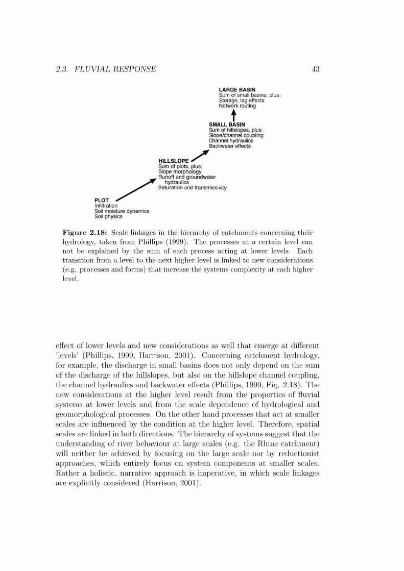
2.3. FLUVIAL RESPONSE 43
Figure 2.18: Scale linkages in the hierarchy of catchments concerning theirhydrology, taken from Phillips (1999). The processes at a certain level cannot be explained by the sum of each process acting at lower levels. Eachtransition from a level to the next higher level is linked to new considerations(e.g. processes and forms) that increase the systems complexity at each higherlevel.
effect of lower levels and new considerations as well that emerge at different’levels’ (Phillips, 1999; Harrison, 2001). Concerning catchment hydrology,for example, the discharge in small basins does not only depend on the sumof the discharge of the hillslopes, but also on the hillslope channel coupling,the channel hydraulics and backwater effects (Phillips, 1999, Fig. 2.18). Thenew considerations at the higher level result from the properties of fluvialsystems at lower levels and from the scale dependence of hydrological andgeomorphological processes. On the other hand processes that act at smallerscales are influenced by the condition at the higher level. Therefore, spatialscales are linked in both directions. The hierarchy of systems suggest that theunderstanding of river behaviour at large scales (e.g. the Rhine catchment)will neither be achieved by focusing on the large scale nor by reductionistapproaches, which entirely focus on system components at smaller scales.Rather a holistic, narrative approach is imperative, in which scale linkagesare explicitly considered (Harrison, 2001).
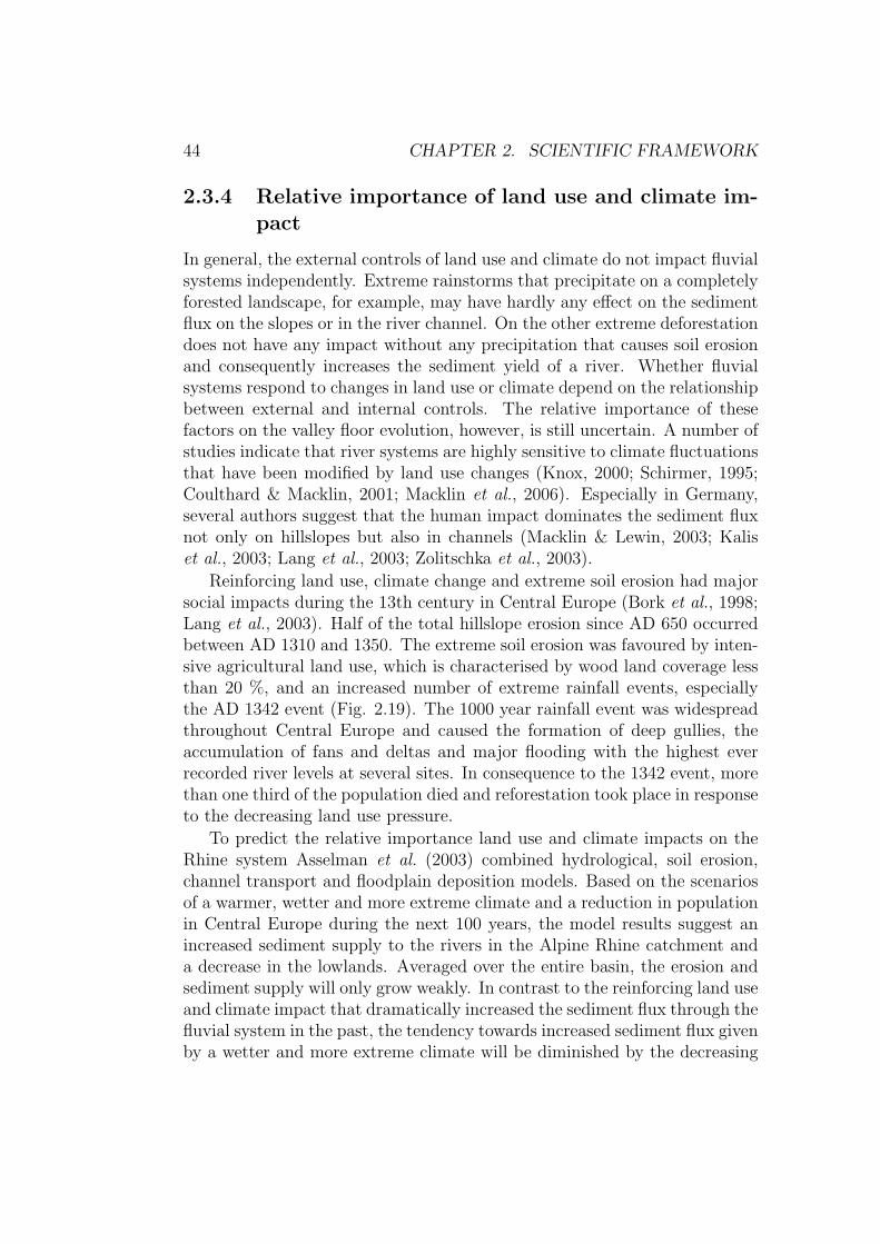
44 CHAPTER 2. SCIENTIFIC FRAMEWORK
2.3.4 Relative importance of land use and climate im-pact
In general, the external controls of land use and climate do not impact fluvialsystems independently. Extreme rainstorms that precipitate on a completelyforested landscape, for example, may have hardly any effect on the sedimentflux on the slopes or in the river channel. On the other extreme deforestationdoes not have any impact without any precipitation that causes soil erosionand consequently increases the sediment yield of a river. Whether fluvialsystems respond to changes in land use or climate depend on the relationshipbetween external and internal controls. The relative importance of thesefactors on the valley floor evolution, however, is still uncertain. A number ofstudies indicate that river systems are highly sensitive to climate fluctuationsthat have been modified by land use changes (Knox, 2000; Schirmer, 1995;Coulthard & Macklin, 2001; Macklin et al., 2006). Especially in Germany,several authors suggest that the human impact dominates the sediment fluxnot only on hillslopes but also in channels (Macklin & Lewin, 2003; Kaliset al., 2003; Lang et al., 2003; Zolitschka et al., 2003).
Reinforcing land use, climate change and extreme soil erosion had majorsocial impacts during the 13th century in Central Europe (Bork et al., 1998;Lang et al., 2003). Half of the total hillslope erosion since AD 650 occurredbetween AD 1310 and 1350. The extreme soil erosion was favoured by inten-sive agricultural land use, which is characterised by wood land coverage lessthan 20 %, and an increased number of extreme rainfall events, especiallythe AD 1342 event (Fig. 2.19). The 1000 year rainfall event was widespreadthroughout Central Europe and caused the formation of deep gullies, theaccumulation of fans and deltas and major flooding with the highest everrecorded river levels at several sites. In consequence to the 1342 event, morethan one third of the population died and reforestation took place in responseto the decreasing land use pressure.
To predict the relative importance land use and climate impacts on theRhine system Asselman et al. (2003) combined hydrological, soil erosion,channel transport and floodplain deposition models. Based on the scenariosof a warmer, wetter and more extreme climate and a reduction in populationin Central Europe during the next 100 years, the model results suggest anincreased sediment supply to the rivers in the Alpine Rhine catchment anda decrease in the lowlands. Averaged over the entire basin, the erosion andsediment supply will only grow weakly. In contrast to the reinforcing land useand climate impact that dramatically increased the sediment flux through thefluvial system in the past, the tendency towards increased sediment flux givenby a wetter and more extreme climate will be diminished by the decreasing
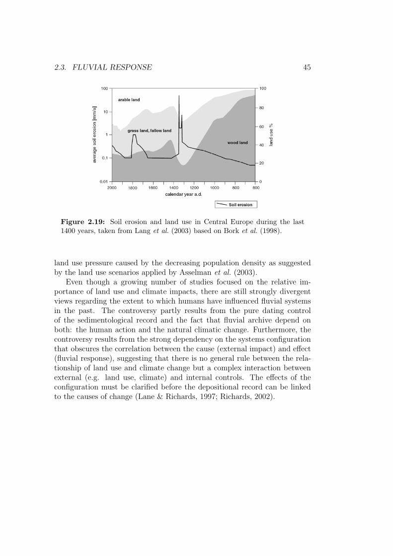
2.3. FLUVIAL RESPONSE 45
Figure 2.19: Soil erosion and land use in Central Europe during the last1400 years, taken from Lang et al. (2003) based on Bork et al. (1998).
land use pressure caused by the decreasing population density as suggestedby the land use scenarios applied by Asselman et al. (2003).
Even though a growing number of studies focused on the relative im-portance of land use and climate impacts, there are still strongly divergentviews regarding the extent to which humans have influenced fluvial systemsin the past. The controversy partly results from the pure dating controlof the sedimentological record and the fact that fluvial archive depend onboth: the human action and the natural climatic change. Furthermore, thecontroversy results from the strong dependency on the systems configurationthat obscures the correlation between the cause (external impact) and effect(fluvial response), suggesting that there is no general rule between the rela-tionship of land use and climate change but a complex interaction betweenexternal (e.g. land use, climate) and internal controls. The effects of theconfiguration must be clarified before the depositional record can be linkedto the causes of change (Lane & Richards, 1997; Richards, 2002).

Chapter 3
Study site: Rhine catchment
47

3.1 General geographical setting
The River Rhine drains large parts (≈ 185 000 km2) of Central Europebetween the European Alps (highest elevation 4275 m asl) and the NorthSea (Fig. 3.1). The Rhine basin is shared by nine countries (Tab. 3.1). TheRiver Rhine runs 1320 km from its source in the Swiss Alps (Lake Toma,2344 masl) to its outlet near Rotterdam (NL). Regarding the landscapesthat are passed by the River Rhine, the river is subdivided into six majorsections: the Alpine Rhine, the High Rhine (between Lake Constance andBasel), the Upper Rhine, the Middle Rhine (between Bingen and Bonn), theLower Rhine and the Rhine Delta (Fig. 3.1).
3.2 Geological and geomorphological setting
The Rhine basin comprises a large number of landforms ranging from theEuropean Alps in the South to lowlands in the North. Above Basel, the majorlandscapes are the Alps, the Alpine foothills, the Swiss Midland and the SwissJura. At Basel, the River Rhine enters the Upper Rhine Graben. With anoverall length of 300 km and a mean width of 40 km it forms the majorsegment of the Cenozoic Rift system of Western Europe. Since its formation,the Upper Rhine Graben is filled with Tertiary and Quaternary sediments,which are up to several kilometers thick1. At Bingen, the river enters theMiddle Rhine Gorge in the Rhenish Slate Massive. The River Rhine incisedan approximately 250 m deep antecedent valley since the tectonic uplift ofthe Rhenish Slate Massive that started during the Oligocene (Andres, 1989).North of Bonn, the River Rhine passes the Lower Rhine Embayment and theDutch delta.
Along its path to the North Sea the River Rhine is fed by several majortributaries (Fig. 3.1 and Tab. 3.1 left). The tributaries of the Rhine drainlarge part of the German Central Uplands (e.g. Rhenish Slate Massive, Oden-wald) and Depressions (e.g. the Hessian Depression) and the South GermanEscarpments. The latter is formed by slightly tilted Mesozoic sedimentarylayers of different rock stability and erodibility (Bremer, 1989).
The large scale morphological structure of the Rhine basin, which resultsmainly from the tectonic activity, is an important factor controlling the formof the longitudinal profile of the Rhine. As shown in Fig. 3.2, three largesedimentary basins (Lake Constance, the Upper Rhine Graben and the LowerRhine Embayment-Southern North Sea Basin) act as major sediment sinks
1For more details on the evolution and neotectonics of the Upper Rhine Graben see forinstance the project summary of the EURO-URGENT project (Behrmann et al., 2005)
49
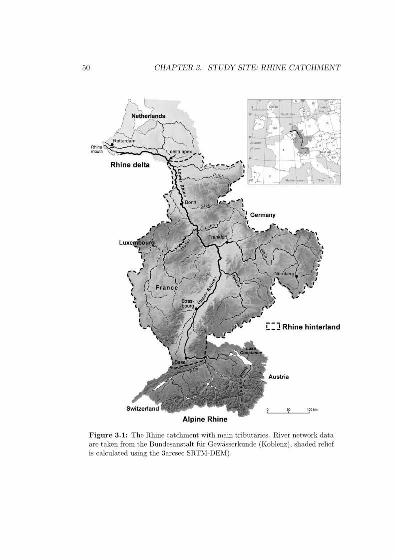
50 CHAPTER 3. STUDY SITE: RHINE CATCHMENT
Figure 3.1: The Rhine catchment with main tributaries. River network dataare taken from the Bundesanstalt fur Gewasserkunde (Koblenz), shaded reliefis calculated using the 3arcsec SRTM-DEM).
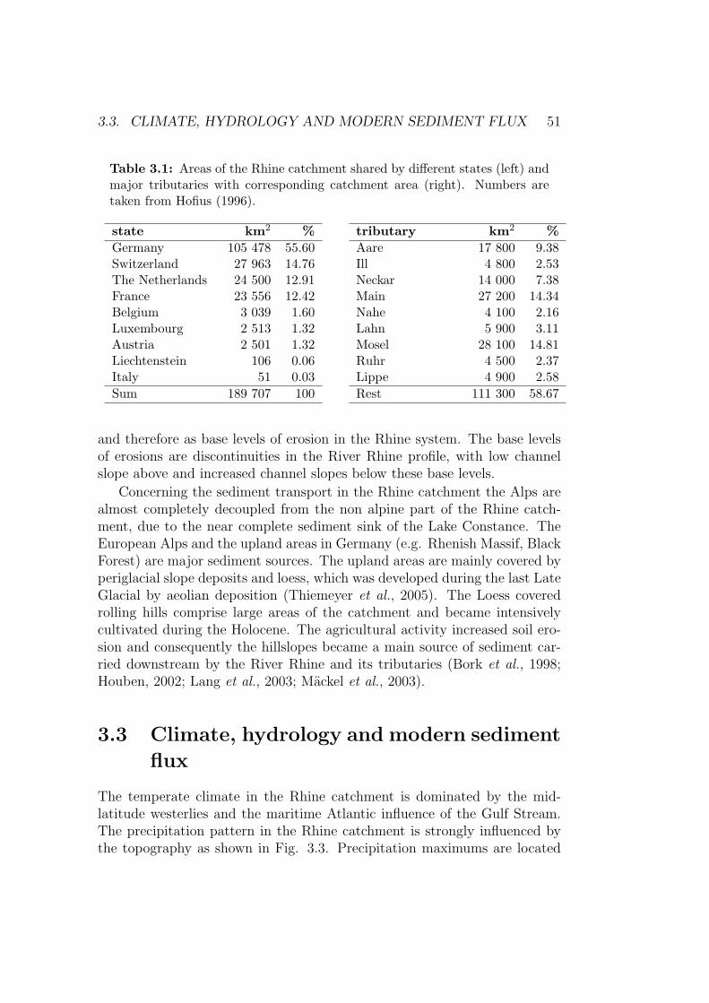
3.3. CLIMATE, HYDROLOGY AND MODERN SEDIMENT FLUX 51
Table 3.1: Areas of the Rhine catchment shared by different states (left) andmajor tributaries with corresponding catchment area (right). Numbers aretaken from Hofius (1996).
state km2 %Germany 105 478 55.60Switzerland 27 963 14.76The Netherlands 24 500 12.91France 23 556 12.42Belgium 3 039 1.60Luxembourg 2 513 1.32Austria 2 501 1.32Liechtenstein 106 0.06Italy 51 0.03Sum 189 707 100
tributary km2 %Aare 17 800 9.38Ill 4 800 2.53Neckar 14 000 7.38Main 27 200 14.34Nahe 4 100 2.16Lahn 5 900 3.11Mosel 28 100 14.81Ruhr 4 500 2.37Lippe 4 900 2.58Rest 111 300 58.67
and therefore as base levels of erosion in the Rhine system. The base levelsof erosions are discontinuities in the River Rhine profile, with low channelslope above and increased channel slopes below these base levels.
Concerning the sediment transport in the Rhine catchment the Alps arealmost completely decoupled from the non alpine part of the Rhine catch-ment, due to the near complete sediment sink of the Lake Constance. TheEuropean Alps and the upland areas in Germany (e.g. Rhenish Massif, BlackForest) are major sediment sources. The upland areas are mainly covered byperiglacial slope deposits and loess, which was developed during the last LateGlacial by aeolian deposition (Thiemeyer et al., 2005). The Loess coveredrolling hills comprise large areas of the catchment and became intensivelycultivated during the Holocene. The agricultural activity increased soil ero-sion and consequently the hillslopes became a main source of sediment car-ried downstream by the River Rhine and its tributaries (Bork et al., 1998;Houben, 2002; Lang et al., 2003; Mackel et al., 2003).
3.3 Climate, hydrology and modern sediment
flux
The temperate climate in the Rhine catchment is dominated by the mid-latitude westerlies and the maritime Atlantic influence of the Gulf Stream.The precipitation pattern in the Rhine catchment is strongly influenced bythe topography as shown in Fig. 3.3. Precipitation maximums are located
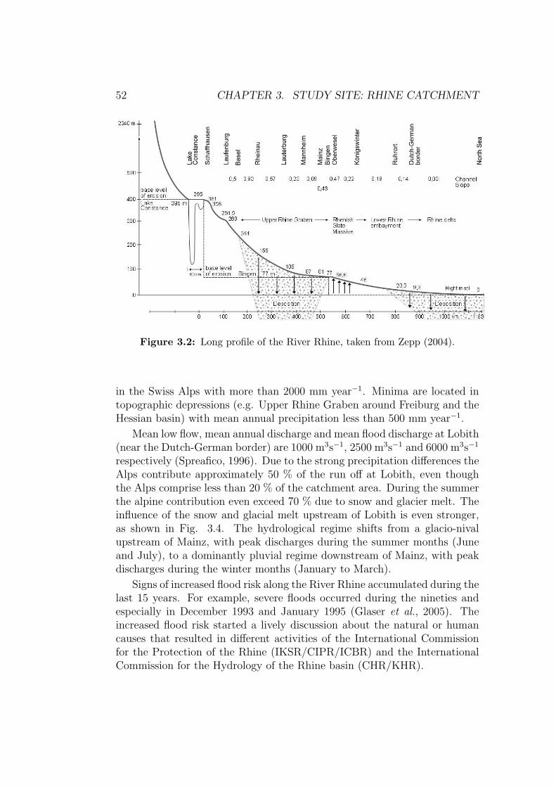
52 CHAPTER 3. STUDY SITE: RHINE CATCHMENT
Figure 3.2: Long profile of the River Rhine, taken from Zepp (2004).
in the Swiss Alps with more than 2000 mm year−1. Minima are located intopographic depressions (e.g. Upper Rhine Graben around Freiburg and theHessian basin) with mean annual precipitation less than 500 mm year−1.
Mean low flow, mean annual discharge and mean flood discharge at Lobith(near the Dutch-German border) are 1000 m3s−1, 2500 m3s−1 and 6000 m3s−1
respectively (Spreafico, 1996). Due to the strong precipitation differences theAlps contribute approximately 50 % of the run off at Lobith, even thoughthe Alps comprise less than 20 % of the catchment area. During the summerthe alpine contribution even exceed 70 % due to snow and glacier melt. Theinfluence of the snow and glacial melt upstream of Lobith is even stronger,as shown in Fig. 3.4. The hydrological regime shifts from a glacio-nivalupstream of Mainz, with peak discharges during the summer months (Juneand July), to a dominantly pluvial regime downstream of Mainz, with peakdischarges during the winter months (January to March).
Signs of increased flood risk along the River Rhine accumulated during thelast 15 years. For example, severe floods occurred during the nineties andespecially in December 1993 and January 1995 (Glaser et al., 2005). Theincreased flood risk started a lively discussion about the natural or humancauses that resulted in different activities of the International Commissionfor the Protection of the Rhine (IKSR/CIPR/ICBR) and the InternationalCommission for the Hydrology of the Rhine basin (CHR/KHR).
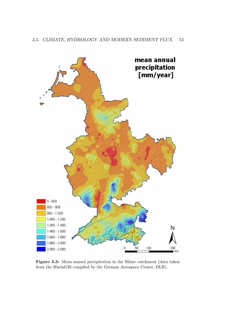
3.3. CLIMATE, HYDROLOGY AND MODERN SEDIMENT FLUX 53
Figure 3.3: Mean annual precipitation in the Rhine catchment (data takenfrom the RheinGIS compiled by the German Aerospace Center, DLR).
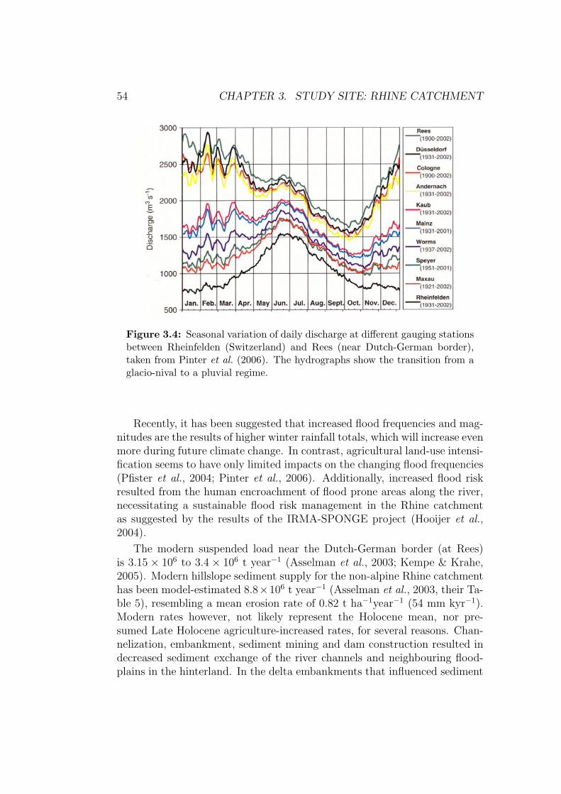
54 CHAPTER 3. STUDY SITE: RHINE CATCHMENT
Figure 3.4: Seasonal variation of daily discharge at different gauging stationsbetween Rheinfelden (Switzerland) and Rees (near Dutch-German border),taken from Pinter et al. (2006). The hydrographs show the transition from aglacio-nival to a pluvial regime.
Recently, it has been suggested that increased flood frequencies and mag-nitudes are the results of higher winter rainfall totals, which will increase evenmore during future climate change. In contrast, agricultural land-use intensi-fication seems to have only limited impacts on the changing flood frequencies(Pfister et al., 2004; Pinter et al., 2006). Additionally, increased flood riskresulted from the human encroachment of flood prone areas along the river,necessitating a sustainable flood risk management in the Rhine catchmentas suggested by the results of the IRMA-SPONGE project (Hooijer et al.,2004).
The modern suspended load near the Dutch-German border (at Rees)is 3.15 × 10⁶ to 3.4 × 10⁶ t year−1 (Asselman et al., 2003; Kempe & Krahe,2005). Modern hillslope sediment supply for the non-alpine Rhine catchmenthas been model-estimated 8.8×10⁶ t year−1 (Asselman et al., 2003, their Ta-ble 5), resembling a mean erosion rate of 0.82 t ha−1year−1 (54 mm kyr−1).Modern rates however, not likely represent the Holocene mean, nor pre-sumed Late Holocene agriculture-increased rates, for several reasons. Chan-nelization, embankment, sediment mining and dam construction resulted indecreased sediment exchange of the river channels and neighbouring flood-plains in the hinterland. In the delta embankments that influenced sediment
3.4. HUMAN IMPACT 55
exchange exist since the 12th century AD (Berendsen & Stouthamer, 2001).Widespread reforestation in the last centuries and modern agricultural prac-tice has counteracted the intense erosion associated to earlier agriculturalpractice.
3.4 Human Impact
The River Rhine basin is one of the most populated areas in the world.Today, about 50 Mio. people (equivalent to a population density of about250 people/km2) live in the whole basin (Hofius, 1996, compare Fig. 2.9).However, the population is not evenly distributed across the Rhine basinbut is strongly concentrated in industrial agglomerations along the Rhineand its major tributaries (e.g. Rhine-Ruhr agglomeration and the Rhine-Neckar region). As a consequence of the large population and its economicactivities, the Rhine catchment has been strongly impacted by agricultureand river engineering. Today, only 36 % of the catchment is covered byforests. Agricultural land (pasture 24 % and arable crop land 28 %) coversthe largest part of the catchment area and as much as 6 % is urban area.
Human impact on the Rhine catchment is not limited to the last fewhundred years, but already started 7500 years ago2. Concerning the riverchannel, the strong human impact on the Rhine and its tributaries is shownby the ubiquity of bank stabilisation, flood protection (mainly Alpine andLower Rhine), river regulation (mainly Upper Rhine), navigation improve-ments (Upper Rhine and Middle Rhine) and hydro-electric power stations(mainly Upper Rhine) (e.g. Kalweit, 1993; Herget et al., 2005). Particu-larly, the river rectification by Gottfried Tulla since 1815 and the subsequentconstruction of 12 locks that improved navigation and gained hydro-electricpower are often cited as major impacts on the Upper Rhine (Fig. 3.5). To-day, the River Rhine is not only one of the most important waterways of theworld, with a transport volume of about 290 million tones per year (Wetzel,1996), but also one of the best studied rivers in the world. The numerousstudies from a number of disciplines (amongst others: geology, hydrology, ar-chaeology, climatology and geomorphology) highlight the importance of theRhine catchment to investigate the LUCIFS objective that is the ”Land useand Climate Impact on Fluvial Systems during the period of agriculture”.
2For a brief introduction to the Holocene history of human impact see Chapter 2.2.2
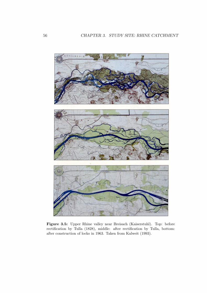
56 CHAPTER 3. STUDY SITE: RHINE CATCHMENT
Figure 3.5: Upper Rhine valley near Breisach (Kaiserstuhl). Top: beforerectification by Tulla (1828), middle: after rectification by Tulla, bottom:after construction of locks in 1963. Taken from Kalweit (1993).
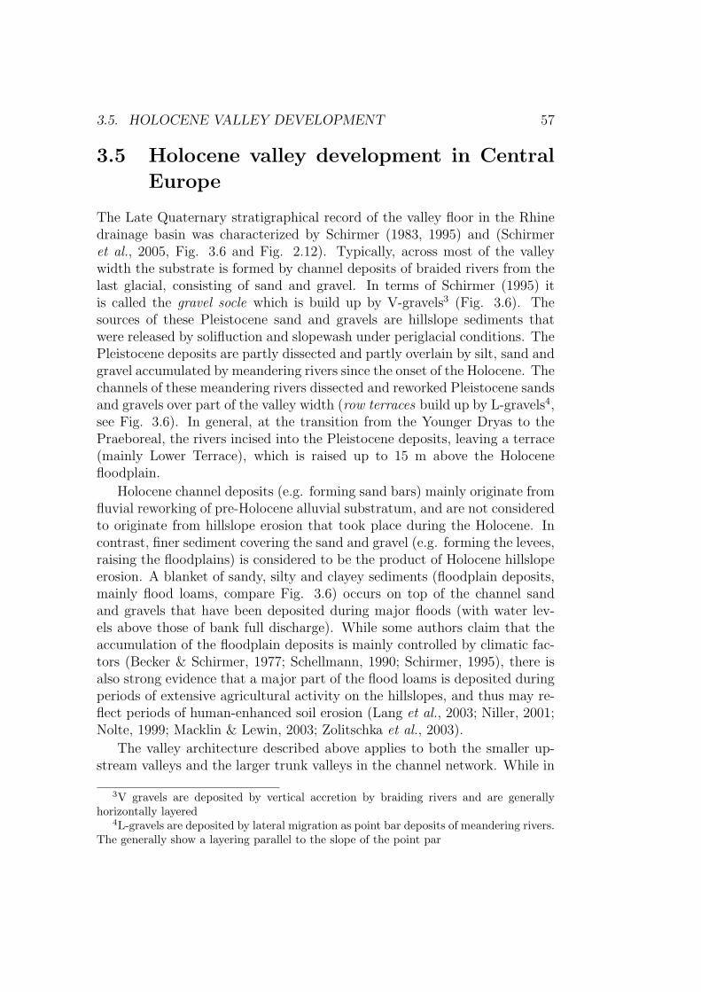
3.5. HOLOCENE VALLEY DEVELOPMENT 57
3.5 Holocene valley development in Central
Europe
The Late Quaternary stratigraphical record of the valley floor in the Rhinedrainage basin was characterized by Schirmer (1983, 1995) and (Schirmeret al., 2005, Fig. 3.6 and Fig. 2.12). Typically, across most of the valleywidth the substrate is formed by channel deposits of braided rivers from thelast glacial, consisting of sand and gravel. In terms of Schirmer (1995) itis called the gravel socle which is build up by V-gravels3 (Fig. 3.6). Thesources of these Pleistocene sand and gravels are hillslope sediments thatwere released by solifluction and slopewash under periglacial conditions. ThePleistocene deposits are partly dissected and partly overlain by silt, sand andgravel accumulated by meandering rivers since the onset of the Holocene. Thechannels of these meandering rivers dissected and reworked Pleistocene sandsand gravels over part of the valley width (row terraces build up by L-gravels4,see Fig. 3.6). In general, at the transition from the Younger Dryas to thePraeboreal, the rivers incised into the Pleistocene deposits, leaving a terrace(mainly Lower Terrace), which is raised up to 15 m above the Holocenefloodplain.
Holocene channel deposits (e.g. forming sand bars) mainly originate fromfluvial reworking of pre-Holocene alluvial substratum, and are not consideredto originate from hillslope erosion that took place during the Holocene. Incontrast, finer sediment covering the sand and gravel (e.g. forming the levees,raising the floodplains) is considered to be the product of Holocene hillslopeerosion. A blanket of sandy, silty and clayey sediments (floodplain deposits,mainly flood loams, compare Fig. 3.6) occurs on top of the channel sandand gravels that have been deposited during major floods (with water lev-els above those of bank full discharge). While some authors claim that theaccumulation of the floodplain deposits is mainly controlled by climatic fac-tors (Becker & Schirmer, 1977; Schellmann, 1990; Schirmer, 1995), there isalso strong evidence that a major part of the flood loams is deposited duringperiods of extensive agricultural activity on the hillslopes, and thus may re-flect periods of human-enhanced soil erosion (Lang et al., 2003; Niller, 2001;Nolte, 1999; Macklin & Lewin, 2003; Zolitschka et al., 2003).
The valley architecture described above applies to both the smaller up-stream valleys and the larger trunk valleys in the channel network. While in
3V gravels are deposited by vertical accretion by braiding rivers and are generallyhorizontally layered
4L-gravels are deposited by lateral migration as point bar deposits of meandering rivers.The generally show a layering parallel to the slope of the point par
58 CHAPTER 3. STUDY SITE: RHINE CATCHMENT
Figure 3.6: Top: block diagramme showing the general picture of valleybottoms in Central Europe. Bottom: Concept of ”fluviatile series” of L- andV-gravels. L-gravels are deposited by lateral migration of river meanders atthe point bar. In contrast, V gravels are deposited by vertical accretion bybraiding rivers. Both figures taken from Schirmer et al. (2005).
3.6. HUMAN IMPACT ON SEDIMENT FLUXES 59
smaller valleys the majority of floodplain deposits are rather young, consid-erable amounts of Late Glacial and Earliest Holocene floodplain deposits arepreserved in the trunk valleys. In the latter valleys, these commonly formseparate terrace surfaces (row terraces according to Schirmer) adjacent tothe Holocene channel belt.
At the downstream end of the river system, the Rhine delta in the Nether-lands consists of Holocene fluvial deposits up to 20 m thick at the presentriver mouth. Sedimentation in the delta is accommodated by sea level riseand tectonic subsidence (Cohen, 2005), but is most importantly the prod-uct of sediment delivery from the hinterland. The deltaic area has been anear-complete sediment trap for Rhine and Meuse sediments since the onsetof deltaic deposition approximately 9000 years ago (Beets & Van der Spek,2000; Erkens et al., 2006).
3.6 Human impact on sediment fluxes in the
Rhine catchment
Agricultural activities in the Rhine drainage basin date back to the EarlyNeolithic approximately 7500 years ago (Dix et al., 2005; Kalis et al., 2003;Zimmermann, 2003; Zimmermann et al., 2004). Farming activity during theNeolithic was restricted to small areas within the loess-covered area andhad limited impact (i.e. only locally) on soil erosion and deposition (Langet al., 2003; Kalis et al., 2003, Fig 3.7). In the Bronze Age (from 2200 to800 BC) and Iron Age (from 800 to 1 BC) agricultural areas extended andploughing techniques changed. There are indications that the major sedimentre-distribution due to soil erosion was still limited to the slopes during thattime (Lang et al., 2003). Dramatic (episodic) soil erosion and associateddeposition of colluvial and alluvial sediments, is known from the Iron Ageand from the Roman period (1 - 375 AD). Amongst others Andres (1998),Bibus & Wesler (1995) and Niller (2001) showed that the accumulation of theflood loams started during the Iron Age, which is assumed to relate to intenseagricultural activities, widespread deforestation and a growing populationdensity in Central Europe (Zimmermann, 1996). The medieval period (450- 1450 AD) is characterized by a strongly intensified impact, culminating inheavy gullying during extreme rainfall events in the 14th and 18th centurieswith high accumulation rates on hillslopes and floodplain over a significantpart of the catchment. The majority of soil-erosion-derived alluvial sedimentin upper tributary reaches originates from this period (Lang et al., 2003, Fig3.7).
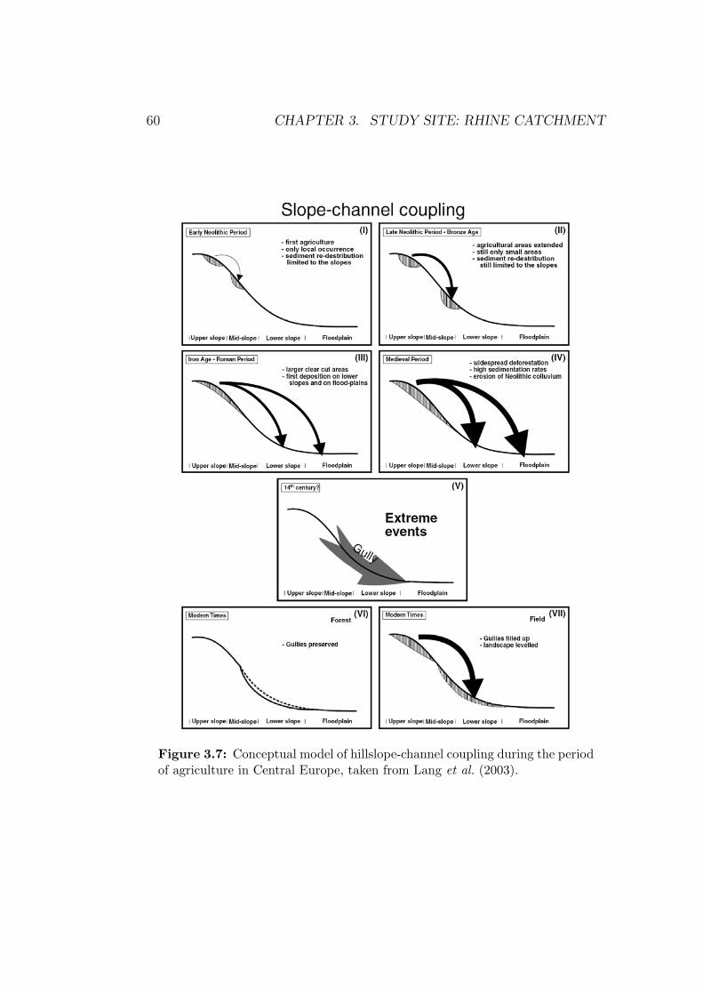
60 CHAPTER 3. STUDY SITE: RHINE CATCHMENT
Figure 3.7: Conceptual model of hillslope-channel coupling during the periodof agriculture in Central Europe, taken from Lang et al. (2003).
Chapter 4
Concept and methods
61

4.1 Problems, needs and aims
The preceding chapters discussed climate variability at different temporalscales and the general trend of increasing human impact during the Holocene.However, Holocene climate change and human activity did not develop inde-pendently but interdependently. In other words there is a causal relationshipbetween climate change and human activity and therefore they change at thesame time.
Fluvial systems responded to the complex pattern of land use and climateimpact. However, sediment flux in fluvial systems is not only forced by exter-nal controls but additionally depends on the systems configuration (internalcontrols). According to Phillips (2003), fluvial systems show complex non-linear dynamics (CND) that are described in terms of thresholds, storages,buffers, saturation and depletion, negative and positive feedbacks, multiplemodes of adjustments, self-organisation and emergence. Consequently, thereare considerable time lags between causes and effects and the configurationalstate in turn is modified by the fluvial processes (feedbacks). Furthermore,the behaviour of fluvial systems is scale dependent in time and space. How-ever, the temporal and spatial scales are not independent from each other butappear to be coupled: i) processes that act at small spatial scales are condi-tions by the properties of the fluvial system at larger scales and in turn theproperties at the larger scale are changed by the cumulative effects at smallerscales; ii) short-term process are connected to the long-term behaviour of thesystem and in turn long-term trends are influenced by short-term processes.Concerning this behaviour, rivers and their corresponding catchments repre-sent hierarchical systems or in other words ”rivers are physical systems witha history” (Schumm, 1977).
To understand the behaviour of rivers in the whole range of conditions andprocesses that controlled and will control their development and to evaluatethe importance of their legacy, a long-term perspective at different spatialscales is needed (e.g. Oldfield & Alverson, 2003; Dearing et al., 2006; Dikau,2006; Gregory et al., 2006). In most (if not in all) cases the record lengthof direct measurements and monitoring programmes is too short to coverthe whole range of Holocene conditions of river response. Therefore, pale-oenvironmental reconstructions based on colluvial and alluvial proxies are anecessary prerequisite to understand the relative importance of human andnatural drivers on fluvial systems. Floodplains provide a range of potentialsites in different stages of development at one time and of different ages thatoffer paleoecological data (Brown, 1996). Their frequent presence in a largevariety of ecological conditions is of great advantage compared to the infre-quent distribution of lakes and swamps. In contrast to lakes and swamps,
63
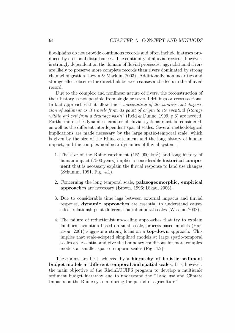
64 CHAPTER 4. CONCEPT AND METHODS
floodplains do not provide continuous records and often include hiatuses pro-duced by erosional disturbances. The continuity of alluvial records, however,is strongly dependent on the domain of fluvial processes: aggradational riversare likely to preserve more complete records than rivers dominated by strongchannel migration (Lewin & Macklin, 2003). Additionally, nonlinearities andstorage effect obscure the direct link between causes and effects in the alluvialrecord.
Due to the complex and nonlinear nature of rivers, the reconstruction oftheir history is not possible from single or several drillings or cross sections.In fact approaches that allow the ”...accounting of the sources and disposi-tion of sediment as it travels from its point of origin to its eventual (storagewithin or) exit from a drainage basin” (Reid & Dunne, 1996, p.3) are needed.Furthermore, the dynamic character of fluvial systems must be considered,as well as the different interdependent spatial scales. Several methodologicalimplications are made necessary by the large spatio-temporal scale, whichis given by the size of the Rhine catchment and the long history of humanimpact, and the complex nonlinear dynamics of fluvial systems:
1. The size of the Rhine catchment (185 000 km2) and long history ofhuman impact (7500 years) implies a considerable historical compo-nent that is necessary explain the fluvial response to land use changes(Schumm, 1991, Fig. 4.1).
2. Concerning the long temporal scale, palaeogeomorphic, empiricalapproaches are necessary (Brown, 1996; Dikau, 2006).
3. Due to considerable time lags between external impacts and fluvialresponse, dynamic approaches are essential to understand cause-effect relationships at different spatiotemporal scales (Wasson, 2002).
4. The failure of reductionist up-scaling approaches that try to explainlandform evolution based on small scale, process-based models (Har-rison, 2001) suggests a strong focus on a top-down approach. Thisimplies that scale-adopted simplified models at large spatio-temporalscales are essential and give the boundary conditions for more complexmodels at smaller spatio-temporal scales (Fig. 4.2).
These aims are best achieved by a hierarchy of holistic sedimentbudget models at different temporal and spatial scales. It is, however,the main objective of the RheinLUCIFS program to develop a multiscalesediment budget hierarchy and to understand the ”Land use and ClimateImpacts on the Rhine system, during the period of agriculture”.
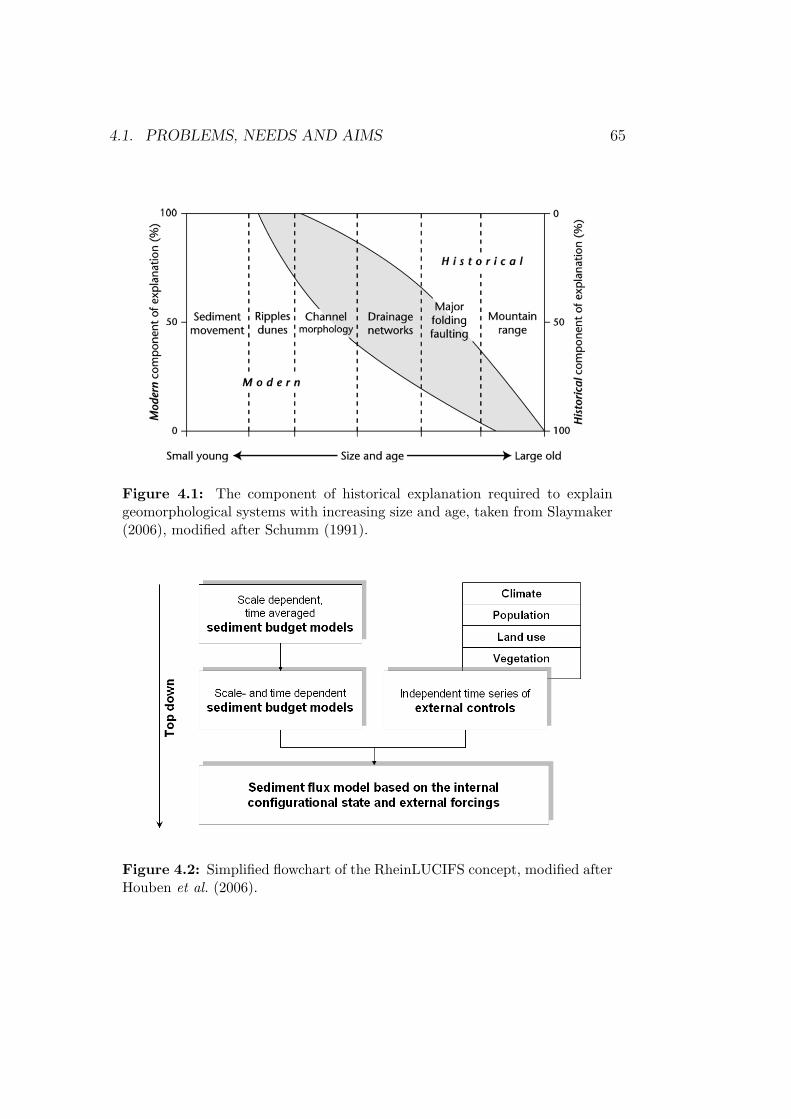
4.1. PROBLEMS, NEEDS AND AIMS 65
Figure 4.1: The component of historical explanation required to explaingeomorphological systems with increasing size and age, taken from Slaymaker(2006), modified after Schumm (1991).
Figure 4.2: Simplified flowchart of the RheinLUCIFS concept, modified afterHouben et al. (2006).
66 CHAPTER 4. CONCEPT AND METHODS
Sediment fluxes are an important component of biogeochemical cycles(Slaymaker & Spencer, 1998). The understanding of the sediment flux andstorage at different spatio-temporal scales, therefore, allows the evaluationof biochemical fluxes that are associated with the sediment transport in thefluvial system. With respect to its effect on the global climate change, the car-bon cycle is of special interest. There are numerous geomorphological stud-ies on alluvial and colluvial sediment storage in the River Rhine catchment,which include the measurement of organic carbon content in these storages(e.g. Dambeck, 2005; Dotterweich et al., 2003c; Houben, 2002; Seidel, 2004).However, little is known on long-term carbon storage in these sediments. Un-til now, the information available from these geomorphological studies hasnot been exploited in terms of biogeochemical cycles. A combined analysisof organic carbon content in alluvial and colluvial storages with large-scaleHolocene sediment budgets can help to understand the long-term effect ofsediment storage on the organic carbon cycle (Walling et al., 2006). Dueto the close relation of exogenic sediments and the endogenic production oforganic matter on floodplains, the seperate analysis of sediment and organicmatter on floodplains helps to interpret more accurately the environmentalfactors controlling the origin of floodplain sediments (Macaire et al., 2006).
Based on the previous considerations, the present thesis will focus onthe largest spatial scale of the RheinLUCIFS initiative, which is given bythe size of the Rhine catchment, and on the entire period since the onset ofagriculture. Therefore, three aims will be followed:
1. The main aim of the thesis is the modelling of a sediment budget of thenon-alpine part of the Rhine catchment that integrates the sedimentfluxes during the entire Holocene. However, as the focus is driven on thequantification of the floodplain storage it is assumed that floodplainsare the major sediment storages at large spatial scales.
2. To evaluate the importance of floodplains as storages of organic carbonwithin the global carbon cycle, a conceptional fluvial carbon budgetmodel is developed. Therefore, the storage of organic carbon in flood-plains of the non-alpine Rhine catchment is estimated and comparedto similar studies and short-term carbon yields.
3. To resolve temporal variations of the activity of the Rhine system, adatabase on 14C-ages taken from colluvial and alluvial sediment stor-ages is compiled and analysed in terms of cumulative frequency distri-butions and of changing sedimentation rates.
The development of empirical methods, to achieve the presented aims, wasadapted to the large spatial and long temporal scale and therefore, focused
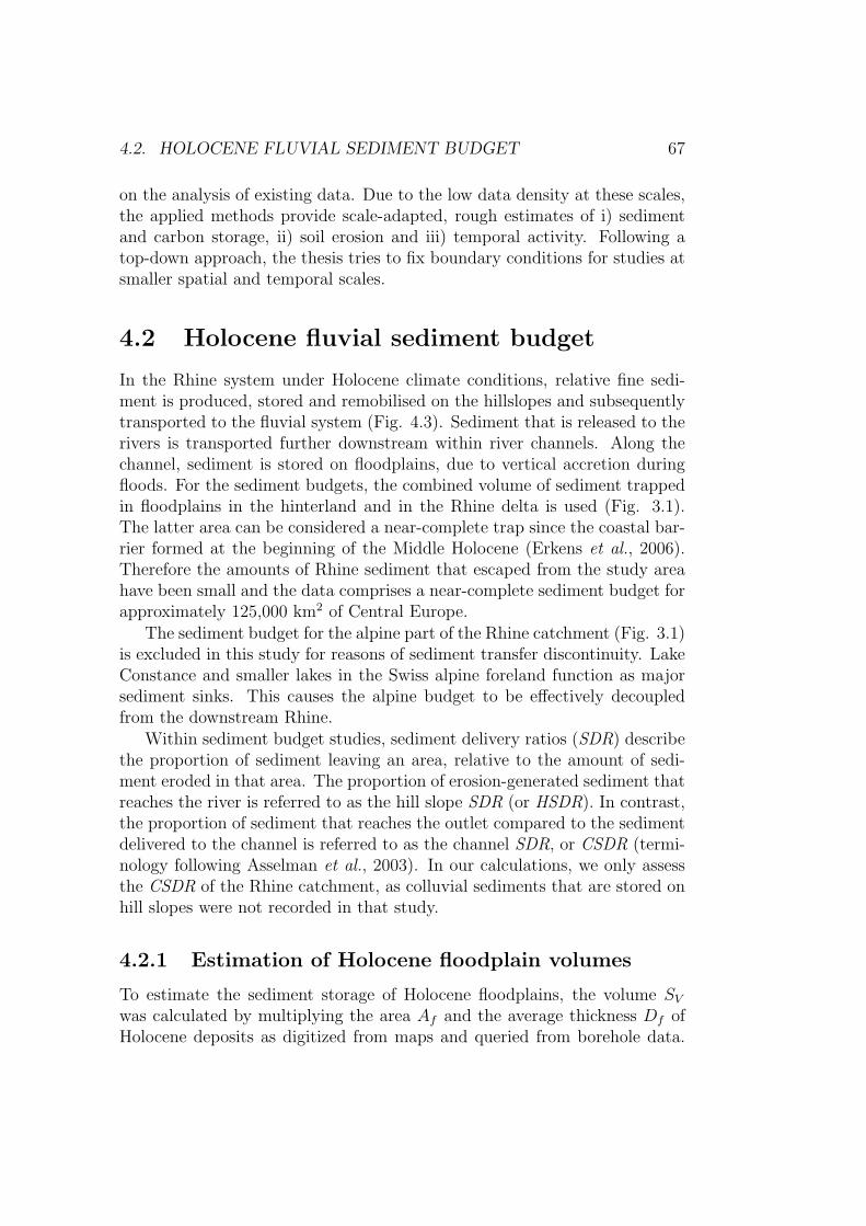
4.2. HOLOCENE FLUVIAL SEDIMENT BUDGET 67
on the analysis of existing data. Due to the low data density at these scales,the applied methods provide scale-adapted, rough estimates of i) sedimentand carbon storage, ii) soil erosion and iii) temporal activity. Following atop-down approach, the thesis tries to fix boundary conditions for studies atsmaller spatial and temporal scales.
4.2 Holocene fluvial sediment budget
In the Rhine system under Holocene climate conditions, relative fine sedi-ment is produced, stored and remobilised on the hillslopes and subsequentlytransported to the fluvial system (Fig. 4.3). Sediment that is released to therivers is transported further downstream within river channels. Along thechannel, sediment is stored on floodplains, due to vertical accretion duringfloods. For the sediment budgets, the combined volume of sediment trappedin floodplains in the hinterland and in the Rhine delta is used (Fig. 3.1).The latter area can be considered a near-complete trap since the coastal bar-rier formed at the beginning of the Middle Holocene (Erkens et al., 2006).Therefore the amounts of Rhine sediment that escaped from the study areahave been small and the data comprises a near-complete sediment budget forapproximately 125,000 km2 of Central Europe.
The sediment budget for the alpine part of the Rhine catchment (Fig. 3.1)is excluded in this study for reasons of sediment transfer discontinuity. LakeConstance and smaller lakes in the Swiss alpine foreland function as majorsediment sinks. This causes the alpine budget to be effectively decoupledfrom the downstream Rhine.
Within sediment budget studies, sediment delivery ratios (SDR) describethe proportion of sediment leaving an area, relative to the amount of sedi-ment eroded in that area. The proportion of erosion-generated sediment thatreaches the river is referred to as the hill slope SDR (or HSDR). In contrast,the proportion of sediment that reaches the outlet compared to the sedimentdelivered to the channel is referred to as the channel SDR, or CSDR (termi-nology following Asselman et al., 2003). In our calculations, we only assessthe CSDR of the Rhine catchment, as colluvial sediments that are stored onhill slopes were not recorded in that study.
4.2.1 Estimation of Holocene floodplain volumes
To estimate the sediment storage of Holocene floodplains, the volume SV
was calculated by multiplying the area Af and the average thickness Df ofHolocene deposits as digitized from maps and queried from borehole data.
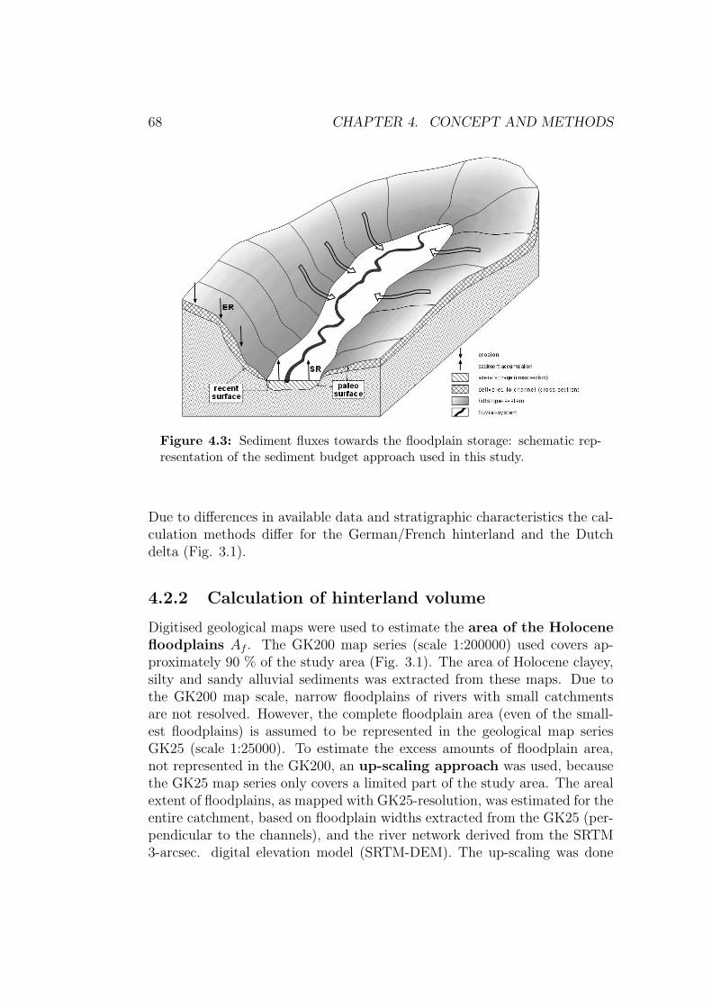
68 CHAPTER 4. CONCEPT AND METHODS
Figure 4.3: Sediment fluxes towards the floodplain storage: schematic rep-resentation of the sediment budget approach used in this study.
Due to differences in available data and stratigraphic characteristics the cal-culation methods differ for the German/French hinterland and the Dutchdelta (Fig. 3.1).
4.2.2 Calculation of hinterland volume
Digitised geological maps were used to estimate the area of the Holocenefloodplains Af . The GK200 map series (scale 1:200000) used covers ap-proximately 90 % of the study area (Fig. 3.1). The area of Holocene clayey,silty and sandy alluvial sediments was extracted from these maps. Due tothe GK200 map scale, narrow floodplains of rivers with small catchmentsare not resolved. However, the complete floodplain area (even of the small-est floodplains) is assumed to be represented in the geological map seriesGK25 (scale 1:25000). To estimate the excess amounts of floodplain area,not represented in the GK200, an up-scaling approach was used, becausethe GK25 map series only covers a limited part of the study area. The arealextent of floodplains, as mapped with GK25-resolution, was estimated for theentire catchment, based on floodplain widths extracted from the GK25 (per-pendicular to the channels), and the river network derived from the SRTM3-arcsec. digital elevation model (SRTM-DEM). The up-scaling was done
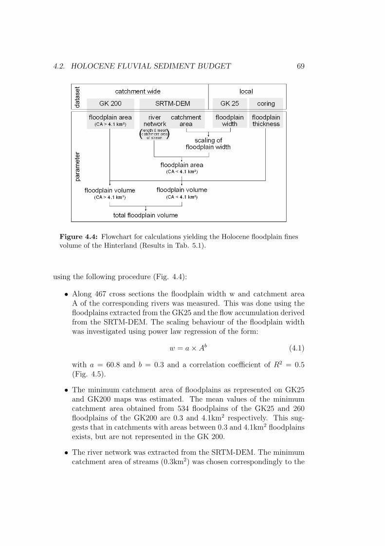
4.2. HOLOCENE FLUVIAL SEDIMENT BUDGET 69
Figure 4.4: Flowchart for calculations yielding the Holocene floodplain finesvolume of the Hinterland (Results in Tab. 5.1).
using the following procedure (Fig. 4.4):
• Along 467 cross sections the floodplain width w and catchment areaA of the corresponding rivers was measured. This was done using thefloodplains extracted from the GK25 and the flow accumulation derivedfrom the SRTM-DEM. The scaling behaviour of the floodplain widthwas investigated using power law regression of the form:
w = a× Ab (4.1)
with a = 60.8 and b = 0.3 and a correlation coefficient of R2 = 0.5(Fig. 4.5).
• The minimum catchment area of floodplains as represented on GK25and GK200 maps was estimated. The mean values of the minimumcatchment area obtained from 534 floodplains of the GK25 and 260floodplains of the GK200 are 0.3 and 4.1km2 respectively. This sug-gests that in catchments with areas between 0.3 and 4.1km2 floodplainsexists, but are not represented in the GK 200.
• The river network was extracted from the SRTM-DEM. The minimumcatchment area of streams (0.3km2) was chosen correspondingly to the
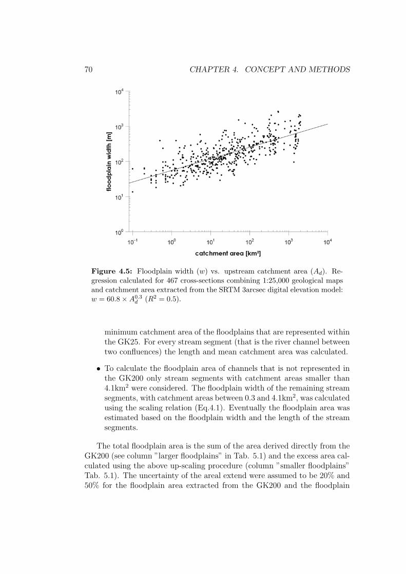
70 CHAPTER 4. CONCEPT AND METHODS
Figure 4.5: Floodplain width (w) vs. upstream catchment area (Ad). Re-gression calculated for 467 cross-sections combining 1:25,000 geological mapsand catchment area extracted from the SRTM 3arcsec digital elevation model:w = 60.8×A0.3
d (R2 = 0.5).
minimum catchment area of the floodplains that are represented withinthe GK25. For every stream segment (that is the river channel betweentwo confluences) the length and mean catchment area was calculated.
• To calculate the floodplain area of channels that is not represented inthe GK200 only stream segments with catchment areas smaller than4.1km2 were considered. The floodplain width of the remaining streamsegments, with catchment areas between 0.3 and 4.1km2, was calculatedusing the scaling relation (Eq.4.1). Eventually the floodplain area wasestimated based on the floodplain width and the length of the streamsegments.
The total floodplain area is the sum of the area derived directly from theGK200 (see column ”larger floodplains” in Tab. 5.1) and the excess area cal-culated using the above up-scaling procedure (column ”smaller floodplains”Tab. 5.1). The uncertainty of the areal extend were assumed to be 20% and50% for the floodplain area extracted from the GK200 and the floodplain
4.2. HOLOCENE FLUVIAL SEDIMENT BUDGET 71
area calculated using the up-scaling approach, respectively.The average thickness of floodplain deposits Df for the Holocene
was estimated based on published core data, from 563 drillings from differentlocations in various floodplains across the Rhine catchment. A database wasset up, to allow for spatial analysis of the core data and assess suitability ofthe core data for estimating Df . A large number of core data originate fromthe work of several German geological surveys (Geologische Landesdienste).The base of Holocene floodplain deposits was queried from the core data.Hereto we used the transition from (dominantly) silty clay / clayey silt to(dominantly) sandy and gravely substrate, corresponding to the transitionbetween overbank deposits and deposits of former river beds. For the areaof Holocene floodplains (see above), in our calculations the full thickness offloodplain deposits is attributed a Holocene age. For a selection of boreholes,mainly from the wider trunk valleys (e.g. data from Houben, 2002; Nolte,1999; Shala, 2001), it is known more exactly what proportion of the thicknessis of Holocene age and only that proportion entered the calculations. Theresulting data set yielded a mean Df of 1.6 m, with a standard deviation of0.4 m. Quantification of the thickness of floodplain deposits is probably lessaccurate than the floodplain area calculation, because of difficulties differen-tiating Holocene and Pleistocene sediments, limited availability of core dataand consequently a biased and clustered distribution of available data. Nosignificant difference in Df for different catchments nor a relation between Df
and upstream catchment area Ad were discovered within the dataset (Fig.4.6). Because floodplain sediment thickness varies over short distances asmuch as it does over large distances, the average thickness can be used tocalculate sediment volumes. Thus we used one value for floodplain thicknessfor all subcatchments (Tab. 5.1), independent of their size. The relativelarge number of boreholes considering catchment size, still results in a rea-sonable estimate of overall mean thickness. For now, an error of 25% of Df
was assigned in the calculations. As part of the sensitivity test, volumesusing an extreme thin (1 m) and extreme thick (2 m) floodplain covers werecalculated.
The volume of floodplain deposits was calculated by multiplying Af
and Df for all subcatchments (Tab. 5.1), including for error propagations involume and thickness estimates.
4.2.3 Calculation of the delta volume
To assess floodplain sediment storage in the delta, the starting point was tocalculate the total amount of Rhine and Meuse sediment trapped behind thecoastal barrier in the Netherlands (Erkens et al., 2006). In contrast to the
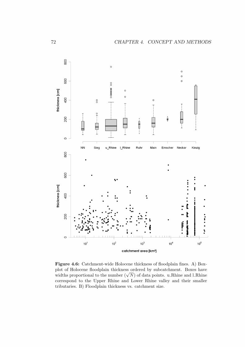
72 CHAPTER 4. CONCEPT AND METHODS
Figure 4.6: Catchment-wide Holocene thickness of floodplain fines. A) Box-plot of Holocene floodplain thickness ordered by subcatchment. Boxes havewidths proportional to the number (
√N) of data points. u Rhine and l Rhine
correspond to the Upper Rhine and Lower Rhine valley and their smallertributaries. B) Floodplain thickness vs. catchment size.
4.2. HOLOCENE FLUVIAL SEDIMENT BUDGET 73
upstream valleys where the floodplain cover is of relative constant thickness,the delta volume is wedge or prism shaped. The delta volume is enveloped bythe buried surface of the last glacial Rhine palaeovalley and by the modernland surface. Extensive borehole data (Berendsen & Stouthamer, 2001) wereused to create a DEM of the Late Pleistocene surface (cell size 250x250 m).A second DEM (same cell size) was created for the modern surface, by resam-pling a high resolution DEM available from laser altimetry (data from TheNetherlands Ministry of Transport, Public Works and Water Management).Calculating their difference yields the thickness of the Holocene deposits foreach cell, which after summation gives the total volume of the Holocene prism(Cohen, 2005; Erkens et al., 2006). We defined the northern and southernlimits of our prism as the zone where floodplain deposits were less than ameter thick. Palaeogeographical reconstruction (Berendsen & Stouthamer,2001) has revealed that in the SE of the delta, sediments are derived from theadjacent Meuse catchment. This area was excluded in the volume estimates(Erkens et al., 2006). The Dutch-German border is at the apex of the to-day’s deltaic channels and was taken as an upstream boundary. Downstreamtowards the modern coast, fluvial delta deposits grade into tidally influenceddeposits (estuaries, inlets, lagoons). Fine grained fluvio-lagoonal deposits inthe central Netherlands are included in the delta sediment volume, becausethese are probably all Rhine derived. Sandy channel belts and coastal sandsare excluded because these are bed-load derived and do not originate fromHolocene erosion of hinterland hillslopes. Peat occurs extensively in centralparts of the lagoon, marking an area that was starved from both tidal andfluvial sediments. The western limit of the delta was defined as where peatamounts for a maximum proportion of total Holocene thickness. Because de-position in the delta is limited to the last 9000 years, we multiplied volumesby 10/9 to simulate a 10000 years volume. In additional calculations, we usework on groundwater level rise (Cohen, 2005) to estimate the proportionsof the total deltaic volume, associated to shorter timeframes (T=7000, 5000and 3000 years). This builds upon the insight that sedimentation in the deltawas governed by accommodation provided by sea level and groundwater-rise(Tab. 5.2).
4.2.4 Erosion rate calculations
Assuming that large amounts of sediments related to hillslope soil erosionare stored within floodplains, the volume of the accumulated flood loam is aproxy parameter for the sediment volume that has left the hillslope systemduring the Holocene. Defining hillslope erosion as the amount of materialthat is delivered to the channel network, the erosion rate ER can be estimated
74 CHAPTER 4. CONCEPT AND METHODS
based on the sediment volume SV stored on the floodplains in a time intervalT .
Based on the work of Einsele & Hinderer (1998) and Hinderer (2001),we calculate erosion rates E∗
R and ER (in mm kyr−1 and t ha−1 year−1,respectively) as:
E∗R =
SV
T × (Ad − Af )× 1
1− CSDR[LT−1] (4.2)
ER = ρB × E∗R [ML−2T−1] (4.3)
with Af=floodplain area, Ad=catchment area and Ad − Af = erosive area(that is the catchment area without the floodplains, as quantified in Tab.5.1) and ρB=bulk density of the alluvial sediment. The channel sedimentdelivery ratio CSDR in Eq.4.2 describes the proportion of the eroded materialleaving the river at the downstream end of the studied area (as a percentageof the amount of sediment delivered to the channel network over the sametimeframe).
The time interval T , over which E∗R is averaged, is arbitrarily chosen to
be 10000 years (i.e. the Holocene from the Boreal chronozone onwards). Toresolve the issue of response to growing human impact, we also performedcalculations for T=7000, 5000 and 3000 years. The latter calculations explorea hypothesised impact of agriculture-induced leading to gradually increasingrates of sediment supply, by considering a bias in the average age of floodplainsediments towards the younger side, especially in smaller catchments in thehinterland. To evaluate the impact of unknown amount of sediment that hasleft the Rhine catchment during the Holocene, scenarios of CSDRs of 0%,10%, and 30% were calculated. For all the scenarios, the estimations errorswere calculated following Gaussian laws of error propagation.
Colluvial sediment that is still on the slopes has not yet contributed to-wards the floodplains, and hence is not accounted for by our results. Erosionrates calculated from floodplain volumes therefore are expected to be smallerthan erosion rates resulting from e.g. soil profile truncation studies for thesame system. The latter method has been widely applied to estimate long-term soil erosion across Rhine tributary catchments (e.g. Bork et al., 1998;Lang et al., 2003; Preston, 2001; Seidel, 2004). In a comparison, our ratesshould be considered a minimum estimate of total erosion.
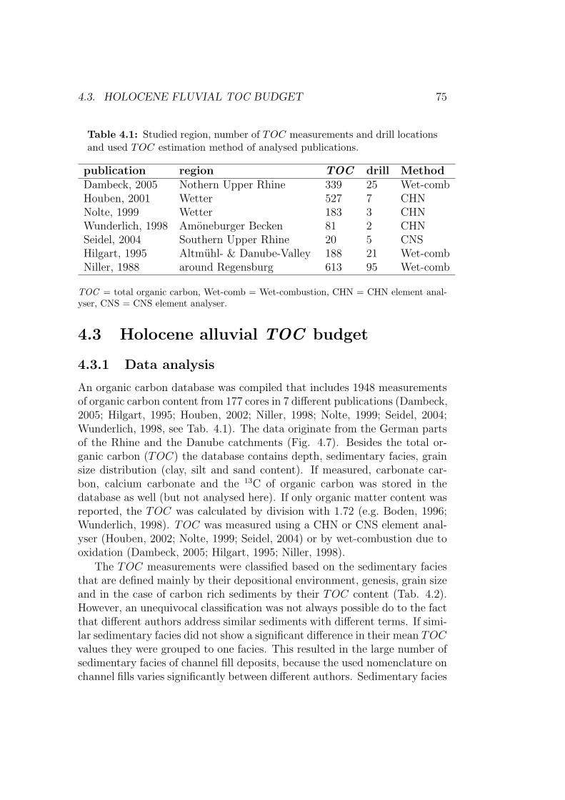
4.3. HOLOCENE FLUVIAL TOC BUDGET 75
Table 4.1: Studied region, number of TOC measurements and drill locationsand used TOC estimation method of analysed publications.
publication region TOC drill MethodDambeck, 2005 Nothern Upper Rhine 339 25 Wet-combHouben, 2001 Wetter 527 7 CHNNolte, 1999 Wetter 183 3 CHNWunderlich, 1998 Amoneburger Becken 81 2 CHNSeidel, 2004 Southern Upper Rhine 20 5 CNSHilgart, 1995 Altmuhl- & Danube-Valley
around Regensburg188 21 Wet-comb
Niller, 1988 613 95 Wet-comb
TOC = total organic carbon, Wet-comb = Wet-combustion, CHN = CHN element anal-yser, CNS = CNS element analyser.
4.3 Holocene alluvial TOC budget
4.3.1 Data analysis
An organic carbon database was compiled that includes 1948 measurementsof organic carbon content from 177 cores in 7 different publications (Dambeck,2005; Hilgart, 1995; Houben, 2002; Niller, 1998; Nolte, 1999; Seidel, 2004;Wunderlich, 1998, see Tab. 4.1). The data originate from the German partsof the Rhine and the Danube catchments (Fig. 4.7). Besides the total or-ganic carbon (TOC) the database contains depth, sedimentary facies, grainsize distribution (clay, silt and sand content). If measured, carbonate car-bon, calcium carbonate and the 13C of organic carbon was stored in thedatabase as well (but not analysed here). If only organic matter content wasreported, the TOC was calculated by division with 1.72 (e.g. Boden, 1996;Wunderlich, 1998). TOC was measured using a CHN or CNS element anal-yser (Houben, 2002; Nolte, 1999; Seidel, 2004) or by wet-combustion due tooxidation (Dambeck, 2005; Hilgart, 1995; Niller, 1998).
The TOC measurements were classified based on the sedimentary faciesthat are defined mainly by their depositional environment, genesis, grain sizeand in the case of carbon rich sediments by their TOC content (Tab. 4.2).However, an unequivocal classification was not always possible do to the factthat different authors address similar sediments with different terms. If simi-lar sedimentary facies did not show a significant difference in their mean TOCvalues they were grouped to one facies. This resulted in the large number ofsedimentary facies of channel fill deposits, because the used nomenclature onchannel fills varies significantly between different authors. Sedimentary facies
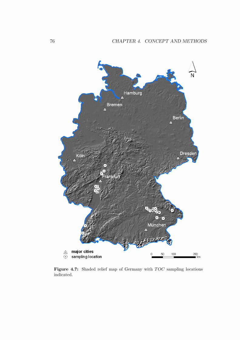
76 CHAPTER 4. CONCEPT AND METHODS
Figure 4.7: Shaded relief map of Germany with TOC sampling locationsindicated.
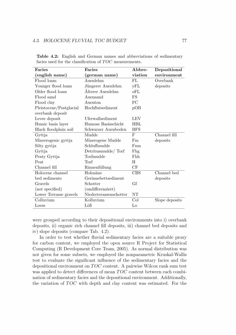
4.3. HOLOCENE FLUVIAL TOC BUDGET 77
Table 4.2: English and German names and abbreviations of sedimentaryfacies used for the classification of TOC measurements.
Facies Facies Abbre- Depositional(english name) (german name) viation environmentFlood loam Auenlehm FL OverbankYounger flood loam Jungerer Auenlehm yFL depositsOlder flood loam Alterer Auenlehm oFLFlood sand Auensand FSFlood clay Auenton FCPleistocene/Postglacialoverbank deposit
Hochflutsediment pOB
Levee deposit Uferwallsediment LEVHumic basis layer Humose Basisschicht HBLBlack floodplain soil Schwarzer Auenboden BFSGyttja Mudde F Channel fillMinrerogenic gyttja Minerogene Mudde Fm depositsSilty gyttja Schluffmudde FmuGyttja Detritusmudde/ Torf FhgPeaty Gyttja Torfmudde FhhPeat Torf HChannel fill Rinnenfullung CFHolocene channel Holozane CBS Channel bedbed sediments Gerinnebettsediment depositsGravels Schotter Gf(not specified) (undifferenziert)Lower Terrasse gravels Niederterassenschotter NTColluvium Kolluvium Col Slope depositsLoess Loß Lo
were grouped according to their depositional environments into i) overbankdeposits, ii) organic rich channel fill deposits, iii) channel bed deposits andiv) slope deposits (compare Tab. 4.2).
In order to test whether fluvial sedimentary facies are a suitable proxyfor carbon content, we employed the open source R Project for StatisticalComputing (R Development Core Team, 2005). As normal distribution wasnot given for some subsets, we employed the nonparametric Kruskal-Wallistest to evaluate the significant influence of the sedimentary facies and thedepositional environment on TOC content. A pairwise Wilcox rank sum testwas applied to detect differences of mean TOC content between each combi-nation of sedimentary facies and the depositional environment. Additionally,the variation of TOC with depth and clay content was estimated. For the
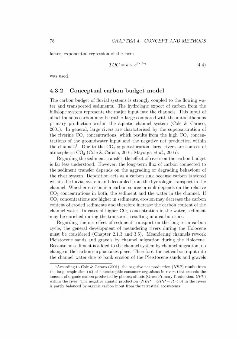
78 CHAPTER 4. CONCEPT AND METHODS
latter, exponential regression of the form
TOC = a× eb×clay (4.4)
was used.
4.3.2 Conceptual carbon budget model
The carbon budget of fluvial systems is strongly coupled to the flowing wa-ter and transported sediments. The hydrologic export of carbon from thehillslope system represents the major input into the channels. This input ofallochthonous carbon may be rather large compared with the autochthonousprimary production within the aquatic channel system (Cole & Caraco,2001). In general, large rivers are characterised by the supersaturation ofthe riverine CO2 concentrations, which results from the high CO2 concen-trations of the groundwater input and the negative net production withinthe channels1. Due to the CO2 supersaturation, large rivers are sources ofatmospheric CO2 (Cole & Caraco, 2001; Mayorga et al., 2005).
Regarding the sediment transfer, the effect of rivers on the carbon budgetis far less understood. However, the long-term flux of carbon connected tothe sediment transfer depends on the aggrading or degrading behaviour ofthe river system. Deposition acts as a carbon sink because carbon is storedwithin the fluvial system and decoupled from the hydrologic transport in thechannel. Whether erosion is a carbon source or sink depends on the relativeCO2 concentrations in both, the sediment and the water in the channel. IfCO2 concentrations are higher in sediments, erosion may decrease the carboncontent of eroded sediments and therefore increase the carbon content of thechannel water. In cases of higher CO2 concentration in the water, sedimentmay be enriched during the transport, resulting in a carbon sink.
Regarding the net effect of sediment transport on the long-term carboncycle, the general development of meandering rivers during the Holocenemust be considered (Chapter 2.1.3 and 3.5). Meandering channels reworkPleistocene sands and gravels by channel migration during the Holocene.Because no sediment is added to the channel system by channel migration, nochange in the carbon surplus takes place. Therefore, the net carbon input intothe channel water due to bank erosion of the Pleistocene sands and gravels
1According to Cole & Caraco (2001), the negative net production (NEP) results fromthe large respiration (R) of heterotrophic consumer organisms in rivers that exceeds theamount of organic carbon producted by photosynthesis (Gross Primary Production; GPP)within the river. The negative aquatic production (NEP = GPP − R < 0) in the riversis partly balanced by organic carbon input from the terrestrial ecosystems.
4.3. HOLOCENE FLUVIAL TOC BUDGET 79
Figure 4.8: C-cycle with focus on the sediment transfer in fluvial systems.PIC = particulate inorganic carbon, POC = particulate organic carbon, DIC= dissolved inorganic carbon, DOC = dissolved organic carbon, GPP = grossprimary production, R = heterotrophic respiration.
during the Holocene depends on the difference between the Pleistocene andthe Holocene channel bed sediments. As shown by the analysis of the TOCcontent of the different sedimentary facies (Chapter 5.2.2), bank erosion inthe Rhine system can be neglected as a source or sink of riverine carbon.
In contrast to the sands and gravels of the channel bed deposits, over-bank deposits that result from the vertical accretion on top of channel beddeposits are considered to be the product of Holocene hillslope erosion (com-pare Chapters 2.1.3 and 4.2). Therefore, vertical accretion results in anincrease of TOC. In other words, long-term storage on the floodplain leadto carbon sequestration within the fluvial system (Fig. 4.8).
To estimate Holocene TOC storage related to overbank and channel filldeposits in the Rhine catchment, it is necessary to know the mass of thesedeposits. It is likely that channel fill deposits are characterised by significanthigher TOC-values than overbank deposits. Therefore, the ratio of over-bank and channel fill deposits need to be considered. However, the alluvialsediment budget described in Chapter 4.2 results in a cumulative mass ofoverbank and channel fill deposits and does not consider the relative con-tributions of these deposits. Thus the relative contributions of overbank
80 CHAPTER 4. CONCEPT AND METHODS
and channel fill deposits was roughly estimated based on nine cross sectionsalong the Wetter (Houben, 2002; Nolte, 1999), one cross section of the KleineLaaber (Niller, 1998) and along the lower Rhine (pers. comm.. G. Erkens).However, the analysed cross sections are very limited in number and there-fore do not represent the entire Rhine catchment. While the cross sectionsare mainly derived from loess covered areas, cross sections from the RhenishSlate Massif or the Black Forest are missing. Because the relative contri-butions of the depositional environments give only rough estimates and notprecise numbers, a calculation of different scenarios was performed.
4.4 14C-database analysis
The sediment and carbon budget of the Rhine catchment integrates theHolocene period and does not consider temporal variations during the Holocene.However, to obtain knowledge of the temporal development of the Rhinebasin a 14C-database from 14C samples of colluvial and alluvial sediments inGermany was compiled and analysed in terms of i) cumulative frequency dis-tributions of the 14C ages and ii) changing sedimentation rates on floodplainsand in palaeochannels.
The database of 432 published 14C ages contains: depositional environ-ments and facies, catchment area, sampling depth, lab code, type of or-ganic material sampled, 13C values, conventional (as measured) radiocarbonages and calibrated radiocarbon ages (using INTCAL04 Reimer et al., 2004).The data originates from the German parts of the Rhine, Danube, Weser,and Elbe catchments (Fig. 4.9). The 14C ages range from the Late Pleis-tocene (max. age 26.000 a BP) to less than 200 a BP. The database and allpublication references are available at www.giub.uni-bonn.de\hoffmann\
phd\phd.html2 Here only the last 14.000 a cal BP were analysed. To pre-vent bias towards land use, 14C ages directly correlated with archaeologicalsites were excluded and only 401 14C ages of organic remains sampled from al-luvial and colluvial sediments are used. Following depositional environmentswere considered: channel-beds, palaeochannels, floodplains, slopes, gullies,alluvial fans and subrosion depressions (Tab. 4.3). The 14C-ages were classi-fied according to the sedimentary facies:
2The login is currently password protected
4.4. 14C-DATABASE ANALYSIS 81
1. floodplain fines (loam and sand),2. sands and gravels of meandering and braiding river systems,3. colluvium,4. gyttja, organic rich sediments,5. fossil soils and6. peat.
4.4.1 Cumulative frequency distributions
To analyse the data in terms of cumulative frequency distributions of fluvialactivity they were grouped based on their sedimentary facies. While datafrom colluvium, floodplain fines, sand and gravels are considered to representactivity phases of colluvial and fluvial systems, 14C data of organic deposits,fossil soils and peat are assumed to represent more stable systems with limitedclastic sediment flux. This classification is questionable in places where 14Cages were obtained on gyttja and organic rich sediments sampled from thebase of palaeochannel fills. Rather than stability, such ages represent activitytransition just after channel abandonment at the beginning of channel infill.Subsequently, these ages (facies 4) will be called ”transitional”, to distinguishthem from clear indicators of activity (facies 1 to 3) or stability (facies 5 and6).
Based on the sedimentary context, Lewin et al. (2005) classify 14C agesas relating to (1) the termination or onset of a fluvial unit or (2) a changein sedimentation rate within a unit. Cases (1) and (2), termed ”changedate”, allow identification of geomorphologically significant changes, and areattributed to major floods. Here, 14C-ages were classified as change dataonly if the organic remains were sampled near the contact of two sedimentaryunits. Type (2) change data that mark a change in sedimentation rate (Lewinet al., 2005) where not considered, due to difficulties in establishing changesin sedimentation rates.
For data analysis the grouped 14C data were calibrated using OxCal(V3.10 Bronk Ramsey, 1995, 2001) and the IntCal04 calibration data set(Reimer et al., 2004). All ages are given in calibrated years before 1950AD. The calibration results in a probability function of each age as shownin Fig. 4.10. Cumulative probability functions (CPFs) were calculated foreach group (activity-, stability and transitional ages) by adding the prob-ability density functions of each group. CPFs are not only influenced bythe frequency distribution of the 14C data but also by the shape of the cal-ibration curve. Plateau regions in the calibration curve result in relativelyhigher probabilities in the calibrated data set. This effect is shown in Fig.
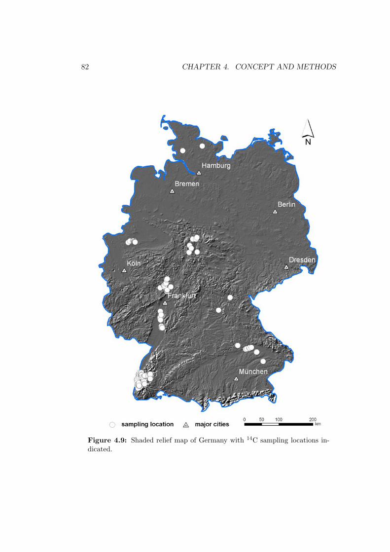
82 CHAPTER 4. CONCEPT AND METHODS
Figure 4.9: Shaded relief map of Germany with 14C sampling locations in-dicated.

4.4. 14C-DATABASE ANALYSIS 83
Table 4.3: Number of 14C data taken from different depositional environ-ments (colums) and sedimentary facies (rows). Sedimentary facies are orderedaccording to activity status.
Facies Col Col/FP GF AF FP ACF PC SD AS NN∑
Activity 148FPF 1 46 7 54CBS 3 19 4 26Col 38 13 13 4 2 68Stability 106BFS 2 12 7 21FS 1 7 1 9Peat 12 6 4 23 16 14 1 76Transitional 155Gyttja 5 7 28 54 9 103ORS 3 32 12 5 52LST 1 1NN 4 9 8 1 22∑
53 29 13 5 131 28 120 35 16 2 432
Col = colluvium, Col/FP = interfingering between colluvial and floodplain, FP = flood-plain, GF = gullyfill, AF= alluvial fan, ACF = active channelfill, PC = palaeochannel,SD = subrosion depression, AS = archaeological site, NN = unknown, FPF = floodplainfines, CBS = channel bed sediments, BFS = black floodplain soil, FS = fossil soil, ORS= organic rich sediments, LST = Laacher lake tephra.
5.6a as CPF of (n = 140) equally spaced synthetic 14C data. To minimizethese effects Lewin et al. (2005); Johnstone et al. (2006) and Thorndycraft& Benito (2006a,b), subtract the CPF computed from a similar sized setof equally spaced data from the group CPFs. The subtraction resulted incumulative probability density functions (CPDFs)(Lewin et al., 2005). Be-sides the effects of the calibration curve, there is typically a strong increasein the probability density towards young ages (see complete dataset in Fig.5.6b). This results from better preservation of younger materials and highersampling probability of shallower sediments, and is not necessarily a result ofincreasing fluvial activity. To eliminate this bias we suggest a normalisationprocedure that differs from the one used by Lewin et al. (2005). We dividethe grouped relative CPFs by the relative CPF of the complete dataset (Fig.5.6e). This normalisation should eliminate both effects (e.g. wiggles of thecalibration curve and the young age bias) at a time.
For comparing the German data set to the results from Great Britain,
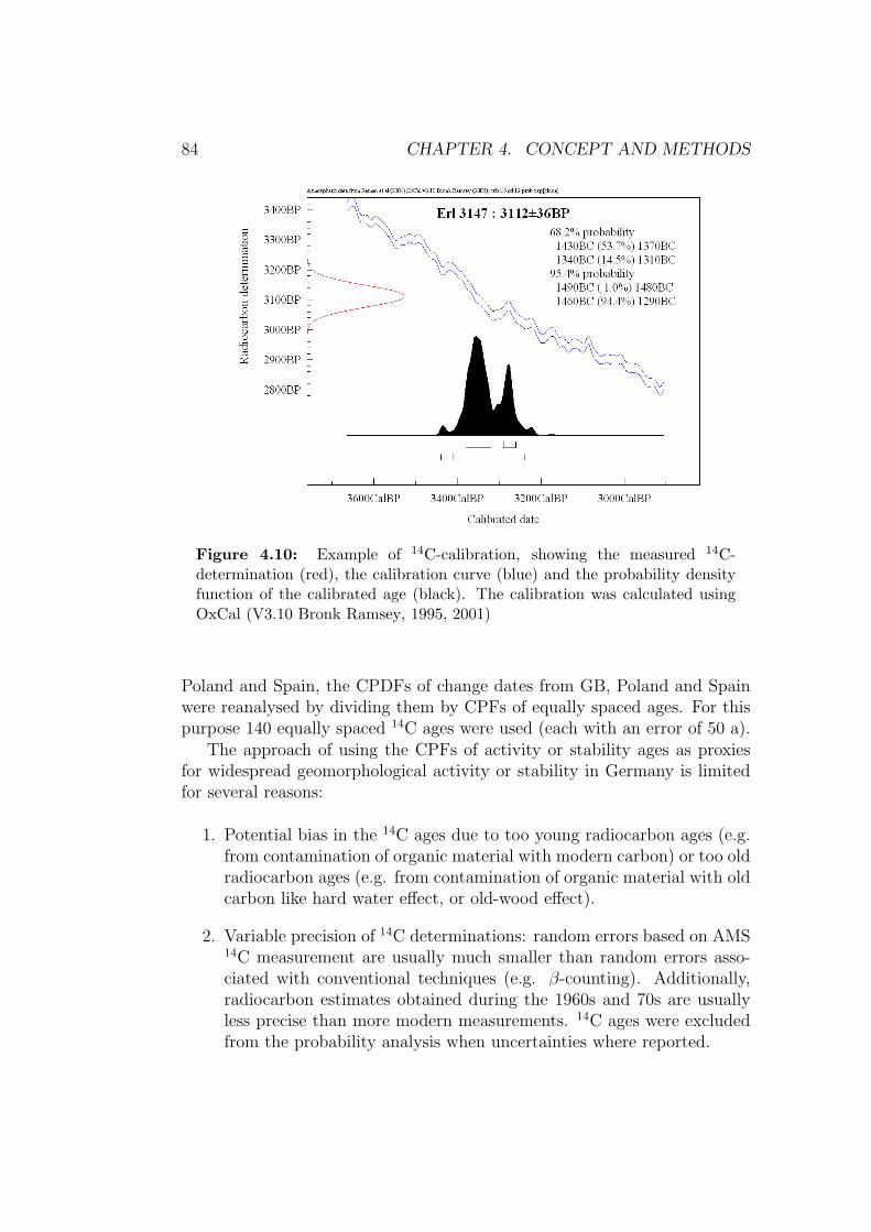
84 CHAPTER 4. CONCEPT AND METHODS
Figure 4.10: Example of 14C-calibration, showing the measured 14C-determination (red), the calibration curve (blue) and the probability densityfunction of the calibrated age (black). The calibration was calculated usingOxCal (V3.10 Bronk Ramsey, 1995, 2001)
Poland and Spain, the CPDFs of change dates from GB, Poland and Spainwere reanalysed by dividing them by CPFs of equally spaced ages. For thispurpose 140 equally spaced 14C ages were used (each with an error of 50 a).
The approach of using the CPFs of activity or stability ages as proxiesfor widespread geomorphological activity or stability in Germany is limitedfor several reasons:
1. Potential bias in the 14C ages due to too young radiocarbon ages (e.g.from contamination of organic material with modern carbon) or too oldradiocarbon ages (e.g. from contamination of organic material with oldcarbon like hard water effect, or old-wood effect).
2. Variable precision of 14C determinations: random errors based on AMS14C measurement are usually much smaller than random errors asso-ciated with conventional techniques (e.g. β-counting). Additionally,radiocarbon estimates obtained during the 1960s and 70s are usuallyless precise than more modern measurements. 14C ages were excludedfrom the probability analysis when uncertainties where reported.
4.4. 14C-DATABASE ANALYSIS 85
3. Reworking and redeposition of organic material results in a time lagbetween the death of the organism (that is determined by 14C dating)and its burial in the fluvial sediments. In strict sense, 14C ages onlyrepresent minimum ages for sediment deposition.
4. Sampling bias: Statistical analysis should be based on random samples.In case of the database used here, and in addition to the young-age biasdiscussed above, it is obvious that many 14C samples were not takenrandomly but following specific spatial and temporal preferences of theresearch agenda a time.
To test the limitations of the dataset and the significance of the finds,statistical tests and sensitivity analysis were employed.
4.4.2 Sedimentation rates
The analysis of CPFs does not allow the calculation of sediment fluxes, ero-sion or sedimentations rates. However, the integration of the sampling depthin the 14C database does allow the calculation of the sedimentation rate SR:
SRi =Di −Di−1
Ti − Ti−1
(4.5)
where Di and Ti are the depth and age of a 14C sample and Di−1 and Ti−1
are the depth and age of the next upper 14C sample. Di represents the meanvalue of the 2σ-age range given by the calibrated age. In the case of the uppermost 14C sample i = 1 and D0 = 0 and T0 = 0. The calculated sedimentationrate SRi corresponds to the mean rate between to successive ages during thetime Ti and Ti−1. Due to different sedimentation rates in different deposi-tional environments, sedimentation rates during the last 14 000 years werecalculated based on 115 floodplain samples and 104 palaeochannel samplesseparately. 14C samples with age reversal3 were excluded from the analysis.
3Age reversals are characterised by younger 14C ages below older ages. Age reversalsmay result from dated material that is older than the deposition ages or from contamina-tion of the dated sample with 12C rich carbon.


Chapter 5
Results
87

5.1 Holocene fluvial sediment budget
5.1.1 Alluvial sediment storage
The quantification of alluvial sediment storage in the Rhine catchment issummarised in Tab. 5.1. Over all a volume of 37.6 ± 8.3 km3, correspondingto a total mass of 53.5± 12.4× 10⁹ t is stored within the Rhine catchment.These values correspond to an eroded volume of 41.9 ± 9.3 km3 (59.5 ±13.9 × 10⁹ t), assuming a channel sediment delivery ratio (CSDR) at theriver mouth of 10 % and T = 10 000 years. Assuming more extreme valuesfor mean sediment thickness (1-2 m), total amounts vary between 26.5 - 45km3 (37−64.6×10⁹ t). Assuming extreme values for CSDRs (0 - 30 %), thiscorresponds to Holocene eroded sediment amounts ranging 26.5 - 64.2 km3
(36.9− 92.3× 10⁹ t).
Regarding the hinterland, Tab. 5.1 shows that the amount of sedimenttrapped in floodplains not resolved by GK200 (9.2 × 10⁹ t) is a significantvolume. Quantification of floodplains based only on the GK200 (neglectingnarrow floodplains) would have resulted in significant underestimation, miss-ing 31 % of the total of stored sediment. Especially in catchments that arelocated in the Rhenish Massif (i.e. Ahr, Sieg and Wupper), a large propor-tion of the sediment storage is not represented in the GK200. In the case ofthe Ahr catchment, the contribution from the upscaling calculations is evenlarger than that obtained from the GK200.
In the Rhine delta a volume of 8.1 km3 or 9.3 × 10⁹ t is estimated forT = 10 000 years. Of this volume, 67 %, 33 % and 25 % had been createdsince 7000, 5000, 3000 years BP, respectively. In our calculations, theseproportions of accommodation space (room for sedimentation) are assumedto apply to 1:1 to deltaic sedimentation (filling with sediment) in Tab. 5.1.Probably that assumption results in underestimation of Late Holocene (since3000 BP) volumes, because of peat formation, compaction and delayed fillingof accommodation space (see Cohen, 2005; Erkens et al., 2006).
Considering the spatial distribution of the sediment storage (Tab. 5.1),roughly 50 % of floodplain sediment is stored in the Rhine trunk valley anddelta, highlighting these areas as the major sedimentary sinks. The alluvialsediment volume along the tributaries strongly correlates with catchmentsize (Fig. 5.4). The Ill catchment has an exceptionally large storage capacity(it hosts 7 % of the total storage, while draining only 3.5 % of the totalcatchment). This results from its location within the Upper Rhine Grabenand confirms the function of the Rhine Graben as a major sedimentary sink.
89
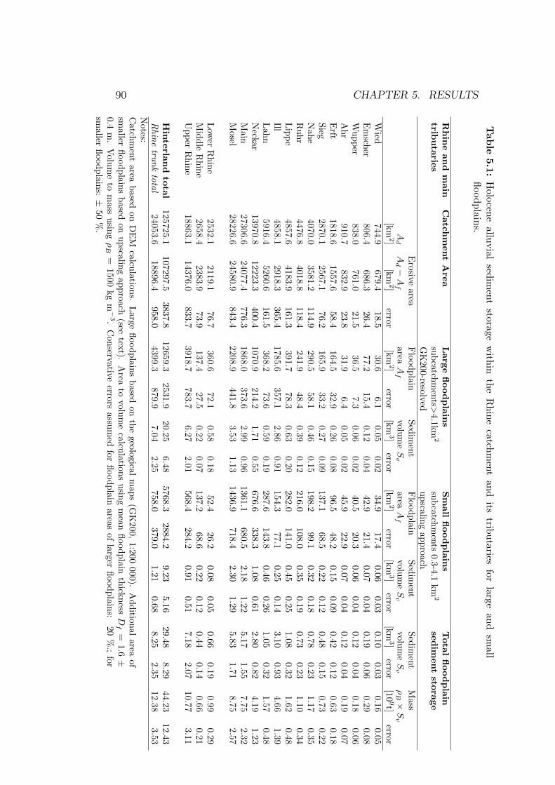
90 CHAPTER 5. RESULTS
Tab
le5.1:
Holocene
alluvialsedim
entstorage
within
theR
hinecatchm
entand
itstributaries
forlarge
andsm
allfloodplains.
Rhin
ean
dm
ainC
atchm
ent
Area
Large
floodplain
sSm
allfloodplain
sTotal
floodplain
tributaries
subcatchments>
4.1km2
subcatchments
0.3-4.1km
2sed
imen
tstorage
GK
200-resolvedupscaling
approachE
rosivearea
Floodplain
Sediment
Floodplain
Sediment
Sediment
Mass
Ad
Ad−
Af
areaA
fvolum
eS
varea
Af
volume
Sv
volume
Sv
ρB×
Sv
[km2]
[km2]
error[km
2]error
[km3]
error[km
2]error
[km3]
error[km
3]error
[109t]
errorW
ied744.9
679.418.5
30.66.1
0.050.02
34.917.4
0.060.03
0.100.03
0.160.05
Em
scher806.4
686.326.4
77.215.4
0.120.04
42.921.4
0.070.04
0.190.06
0.290.08
Wupper
838.0761.0
21.536.5
7.30.06
0.0240.5
20.30.06
0.040.12
0.040.18
0.06A
hr910.7
832.923.8
31.96.4
0.050.02
45.922.9
0.070.04
0.120.04
0.190.07
Erft
1818.61557.6
58.4164.5
32.90.26
0.0896.5
48.20.15
0.090.42
0.120.63
0.18Sieg
2870.12567.1
76.2165.9
33.20.27
0.09137.1
68.50.22
0.120.48
0.150.73
0.22N
ahe4070.0
3581.2114.9
290.558.1
0.460.15
198.299.1
0.320.18
0.780.23
1.170.35
Ruhr
4476.84018.8
118.4241.9
48.40.39
0.12216.0
108.00.35
0.190.73
0.231.10
0.34Lippe
4857.64183.9
161.3391.7
78.30.63
0.20282.0
141.00.45
0.251.08
0.321.62
0.48Ill
4858.12918.3
365.41785.6
357.12.86
0.91154.3
77.10.25
0.143.10
0.934.66
1.39Lahn
5916.45260.6
161.5368.2
73.60.59
0.19287.6
143.80.46
0.261.05
0.321.57
0.48N
eckar13970.8
12223.3400.4
1070.9214.2
1.710.55
676.6338.3
1.080.61
2.800.82
4.191.23
Main
27306.624077.4
776.31868.0
373.62.99
0.961361.1
680.52.18
1.225.17
1.557.75
2.32M
osel28226.6
24580.9843.4
2208.9441.8
3.531.13
1436.9718.4
2.301.29
5.831.71
8.752.57
Low
erR
hine2532.1
2119.176.7
360.672.1
0.580.18
52.426.2
0.080.05
0.660.19
0.990.29
Middle
Rhine
2658.42383.9
73.9137.4
27.50.22
0.07137.2
68.60.22
0.120.44
0.140.66
0.21U
pperR
hine18863.1
14376.0833.7
3918.7783.7
6.272.01
568.4284.2
0.910.51
7.182.07
10.773.11
Hin
terland
total125725.1
107297.53837.8
12659.32531.9
20.256.48
5768.32884.2
9.235.16
29.488.29
44.2312.43
Rhine
trunktotal
24053.618896.4
958.04399.3
879.97.04
2.25758.0
379.01.21
0.688.25
2.3512.38
3.53N
otes:C
atchment
areabased
onD
EM
calculations.Large
floodplainsbased
onthe
geologicalm
aps(G
K200,
1:200000).
Additional
areaof
smaller
floodplainsbased
onupscaling
approach(see
text).A
reato
volume
calculationsusing
mean
floodplainthickness
Df
=1.6
±0.4
m.
Volum
eto
mass
usingρ
B=
1500kg
m−
3.C
onservativeerrors
assumed
forfloodplain
areasof
largerfloodplains:
20%
.;for
smaller
floodplains:±
50%
.
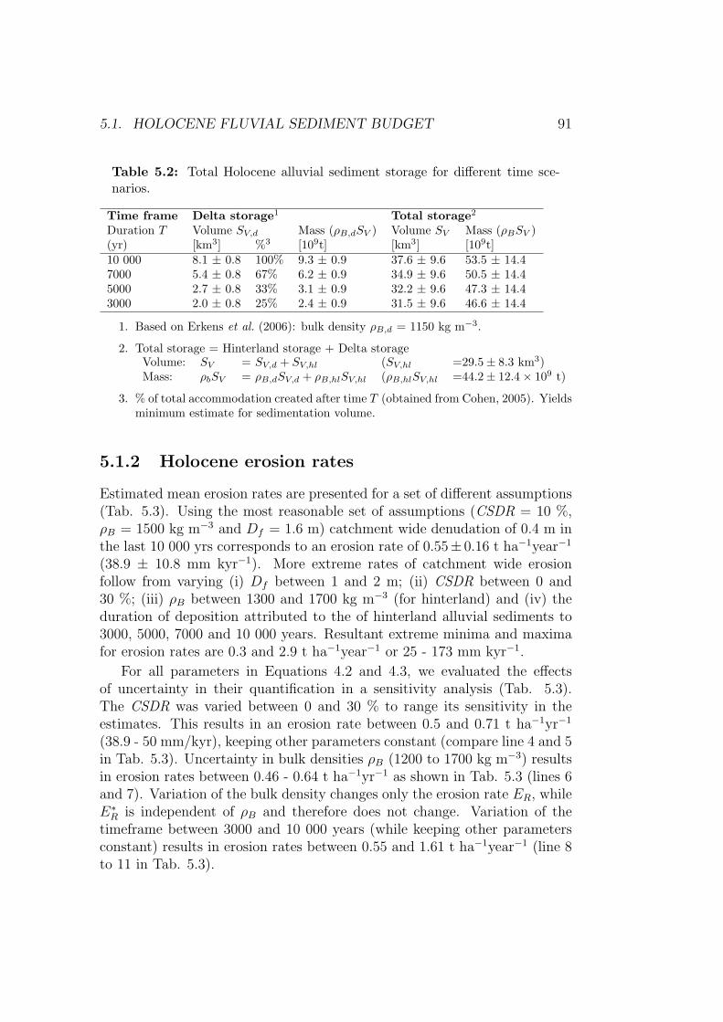
5.1. HOLOCENE FLUVIAL SEDIMENT BUDGET 91
Table 5.2: Total Holocene alluvial sediment storage for different time sce-narios.
Time frame Delta storage1 Total storage2
Duration T Volume SV,d Mass (ρB,dSV ) Volume SV Mass (ρBSV )(yr) [km3] %3 [109t] [km3] [109t]10 000 8.1 ± 0.8 100% 9.3 ± 0.9 37.6 ± 9.6 53.5 ± 14.47000 5.4 ± 0.8 67% 6.2 ± 0.9 34.9 ± 9.6 50.5 ± 14.45000 2.7 ± 0.8 33% 3.1 ± 0.9 32.2 ± 9.6 47.3 ± 14.43000 2.0 ± 0.8 25% 2.4 ± 0.9 31.5 ± 9.6 46.6 ± 14.4
1. Based on Erkens et al. (2006): bulk density ρB,d = 1150 kg m−3.
2. Total storage = Hinterland storage + Delta storageVolume: SV = SV,d + SV,hl (SV,hl =29.5± 8.3 km3)Mass: ρbSV = ρB,dSV,d + ρB,hlSV,hl (ρB,hlSV,hl =44.2± 12.4× 10⁹ t)
3. % of total accommodation created after time T (obtained from Cohen, 2005). Yieldsminimum estimate for sedimentation volume.
5.1.2 Holocene erosion rates
Estimated mean erosion rates are presented for a set of different assumptions(Tab. 5.3). Using the most reasonable set of assumptions (CSDR = 10 %,ρB = 1500 kg m−3 and Df = 1.6 m) catchment wide denudation of 0.4 m inthe last 10 000 yrs corresponds to an erosion rate of 0.55± 0.16 t ha−1year−1
(38.9 ± 10.8 mm kyr−1). More extreme rates of catchment wide erosionfollow from varying (i) Df between 1 and 2 m; (ii) CSDR between 0 and30 %; (iii) ρB between 1300 and 1700 kg m−3 (for hinterland) and (iv) theduration of deposition attributed to the of hinterland alluvial sediments to3000, 5000, 7000 and 10 000 years. Resultant extreme minima and maximafor erosion rates are 0.3 and 2.9 t ha−1year−1 or 25 - 173 mm kyr−1.
For all parameters in Equations 4.2 and 4.3, we evaluated the effectsof uncertainty in their quantification in a sensitivity analysis (Tab. 5.3).The CSDR was varied between 0 and 30 % to range its sensitivity in theestimates. This results in an erosion rate between 0.5 and 0.71 t ha−1yr−1
(38.9 - 50 mm/kyr), keeping other parameters constant (compare line 4 and 5in Tab. 5.3). Uncertainty in bulk densities ρB (1200 to 1700 kg m−3) resultsin erosion rates between 0.46 - 0.64 t ha−1yr−1 as shown in Tab. 5.3 (lines 6and 7). Variation of the bulk density changes only the erosion rate ER, whileE∗
R is independent of ρB and therefore does not change. Variation of thetimeframe between 3000 and 10 000 years (while keeping other parametersconstant) results in erosion rates between 0.55 and 1.61 t ha−1year−1 (line 8to 11 in Tab. 5.3).
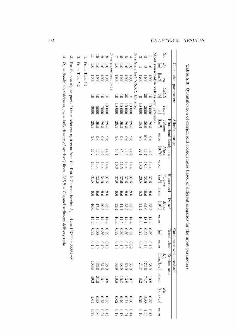
92 CHAPTER 5. RESULTS
Tab
le5.3:
Quantification
oferosion
anderosion
ratesbased
ofdifferent
scenariosfor
theinput
parameters.
Calculation
parameters
Alluvial
storageC
atchment
wide
erosion3
Hinterland
floodplains1
Hinterland
+D
elta2
Denudation
Erosion
rateN
r.D
fρ
BC
SDR
Tim
eVolum
eM
assVolum
eM
assE∗R
ER
[m]
[kg/l][%
][yr]
[km3]
error[10
9t]error
[km3]
error[10
9t]error
[m]
error[m
m/kyr]
error[t/ha/yr]
errorM
ostreason
able
values
andextrem
es1
1.61500
1010
00029.5
9.644.2
14.437.6
9.653.5
14.40.39
0.1038.9
10.80.55
0.162
21700
303000
36.910.6
62.718.1
38.910.6
65.018.1
0.520.14
172.674.7
2.881.26
31
12000
10000
18.48.3
22.110.0
26.58.3
31.410.0
0.250.08
24.78.2
0.290.10
Sensitivitytest
(CSD
R,D
ensity)4
1.61500
010
00029.5
9.644.2
14.437.6
9.653.5
14.40.35
0.0935.0
9.70.50
0.145
1.61500
3010
00029.5
9.644.2
14.437.6
9.653.5
14.40.50
0.1350.0
13.80.71
0.216
1.61200
1010
00029.5
9.635.4
11.537.6
9.644.7
11.50.39
0.1038.9
10.80.46
0.137
1.61700
1010
00029.5
9.650.1
16.337.6
9.659.4
16.30.39
0.1038.9
10.80.62
0.18T
ime
frame
scenarios8
1.61500
1010
00029.5
9.644.2
14.437.6
9.653.5
14.40.39
0.1038.9
10.80.55
0.169
1.61500
107000
29.59.6
44.214.4
34.99.6
50.514.4
0.360.10
51.616.1
0.750.24
101.6
150010
500029.5
9.644.2
14.432.2
9.647.3
14.40.33
0.1066.6
24.00.98
0.3611
1.61500
103000
29.59.6
44.214.4
31.59.6
46.614.4
0.330.10
108.849.3
1.610.73
1.From
Tab.
5.1
2.From
Tab.
5.2
3.For
thenon-alpine
partof
thecatchm
entupstream
fromthe
Dutch-G
erman
borderA
d−
Af
=107300
±3838k
m2
4.D
f=
floodplainthickness,
ρB
=bulk
densityof
overbankfines,
CSD
R=
Channel
sediment
deliveryratio
5.2. TOC STORAGE IN FLOODPLAINS 93
5.2 TOC storage in floodplains
Table 5.4 lists the number of 1948 TOC measurements and the measuredsedimentary facies. 767 measurements were taken from overbank deposits,373 from channel fill deposits, 327 from channel bed deposits and 489 mea-surements originate from slope deposits (Tab. 5.4). The spatial distributionof the measurements is illustrated in Fig. 4.7. The data are not evenly dis-tributed but show strong clusters i) around Freiburg in the Black Forest andthe southern Upper Rhine Graben, ii) around Frankfurt in the Nidda Catch-ment, the Amoneburger Becken and in the northern Upper Rhine Grabenand iii) at the Altmuhl and Danube rivers close to Regensburg.
5.2.1 Sample depth and clay content
The relation of the TOC content to the sample depth and the clay contentis shown in Fig. 5.1 and Figure 5.2, respectively. While there is no corre-lation between TOC and sample depth, TOC exponentially increases withincreasing clay content except for the dataset of Niller (1998). The strongestcorrelation and largest increase is shown in the dataset of Dambeck (2005)with a correlation coefficient R2 = 0.45 and an exponent b = 0.052 followedby the dataset of Houben (2002) with R2 = 0.31 and b = 0.042 and Seidel(2004) with R2 = 0.32 and b = 0.035 (compare Figure 5.2). The datasetsfrom the Danube catchment (Hilgart, 1995; Niller, 1998) show no or only aweak correlation.
In general, TOC increases linearly with clay content at regional and globalscales (Parton et al., 1993; Schimel et al., 1994). The observed weak or absentcorrelation between clay and TOC content could be due to a differing claymineral composition (Rasmussen et al., 2005). In the Danube catchment, claymineral distribution is strongly influenced by kaolinitic weathering residuesfrom the adjacent limestone ridge.
5.2.2 Depositional environment and sedimentary fa-cies
The results of the statistical analysis of the TOC versus sedimentary faciesand depositional environment are shown in Fig. 5.3 - 5.5. The boxplotsand the results of the Kruskal-Wallis tests, which are summarized in Tab.5.5, suggest a significant influence of the sedimentary facies and the deposi-tional environments on the TOC content for the entire dataset as well as foreach subset at 1%-significance level. Furthermore, the result of the pairwiseWilcox test suggests that the mean TOC values of each combination of paired
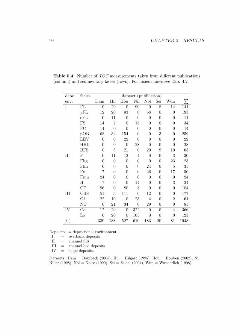
94 CHAPTER 5. RESULTS
Table 5.4: Number of TOC measurements taken from different publications(column) and sedimentary facies (rows). For facies names see Tab. 4.2
depo. facies dataset (publication)env. Dam Hil Hou Nil Nol Sei Wun
∑I FL 0 29 0 90 0 8 14 141
yFL 12 20 93 0 68 0 0 193oFL 0 11 0 0 0 0 0 11FS 14 2 0 18 0 0 0 34FC 14 0 0 0 0 0 0 14pOB 68 34 154 0 0 3 0 259LEV 0 0 22 0 0 0 0 22HBL 0 0 0 28 0 0 0 28BFS 0 5 21 0 20 9 10 65
II F 0 11 12 4 0 0 3 30Fhg 0 0 0 0 0 0 23 23Fhh 6 0 0 0 24 0 5 35Fm 7 0 0 0 26 0 17 50Fmu 24 0 0 0 0 0 0 24H 7 0 0 14 0 0 3 24CF 96 0 80 8 0 0 0 184
III CBS 51 3 111 0 12 0 0 177Gf 22 10 0 23 4 0 2 61NT 0 21 34 0 29 0 0 85
IV Col 12 20 0 322 0 0 4 366Lo 0 20 0 103 0 0 0 123∑
339 188 527 610 183 20 81 1948
Depo.env. = depositional environmentI = overbank depositsII = channel fillsIII = channel bed depositsIV = slope deposits.
Datasets: Dam = Dambeck (2005), Hil = Hilgart (1995), Hou = Houben (2002), Nil =Niller (1998), Nol = Nolte (1999), Sei = Seidel (2004), Wun = Wunderlich (1998)
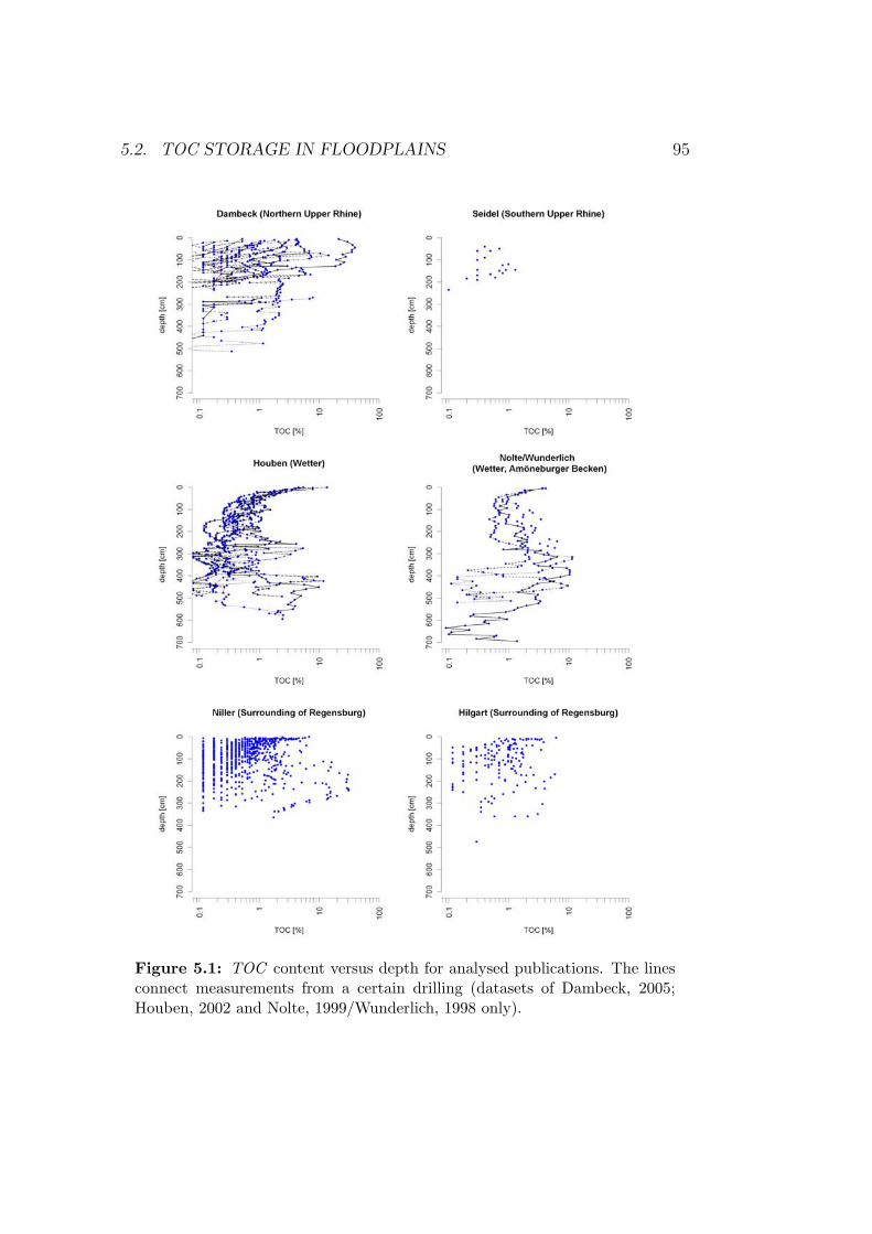
5.2. TOC STORAGE IN FLOODPLAINS 95
Figure 5.1: TOC content versus depth for analysed publications. The linesconnect measurements from a certain drilling (datasets of Dambeck, 2005;Houben, 2002 and Nolte, 1999/Wunderlich, 1998 only).
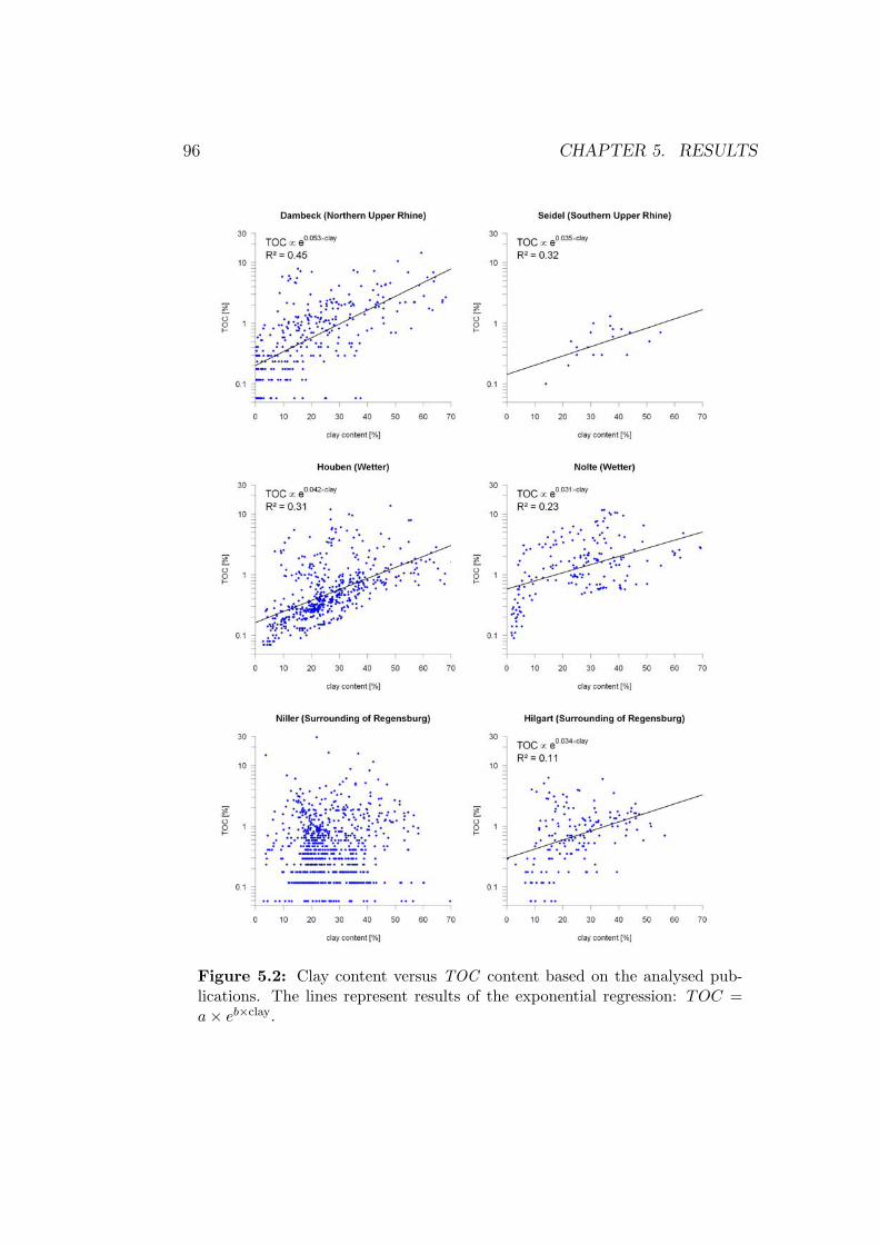
96 CHAPTER 5. RESULTS
Figure 5.2: Clay content versus TOC content based on the analysed pub-lications. The lines represent results of the exponential regression: TOC =a× eb×clay.
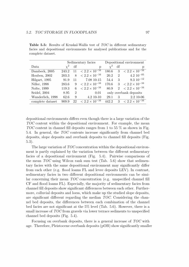
5.2. TOC STORAGE IN FLOODPLAINS 97
Table 5.5: Results of Kruskal-Wallis test of TOC in different sedimentaryfacies and depositional environments for analysed publications and for thecomplete dataset.
Sedimentary facies Depositional environmentData χ2 df p χ2 df pDambeck, 2005 243.2 11 < 2.2× 10⁻¹⁶ 180.6 3 < 2.2× 10⁻¹⁶
Houben, 2002 203.3 8 < 2.2× 10⁻¹⁶ 20.2 2 4.2 10−05
Hilgart, 1995 91.9 11 7.08 10-15 54.4 3 9.3 10−12
Niller, 1998 283.6 9 < 2.2× 10⁻¹⁶ 170.6 3 < 2.2× 10⁻¹⁶
Nolte, 1999 119.3 6 < 2.2× 10⁻¹⁶ 80.9 2 < 2.2× 10⁻¹⁶
Seidel, 2004 8.95 2 0.01 only overbank depositsWunderlich, 1998 62.6 9 4.2 10-10 29.1 3 2.2 10-06complete dataset 909.9 22 < 2.2× 10⁻¹⁶ 442.2 3 < 2.2× 10⁻¹⁶
depositional environments differs even though there is a large variation of theTOC content within the depositional environment. For example, the meanTOC content in channel fill deposits ranges from 1 to 55 % as shown in Fig.5.4. In general, the TOC contents increase significantly from channel beddeposits, slope deposits and overbank deposits to channel fill deposits (Fig.5.3).
The large variation of TOC concentration within the depositional environ-ment is partly explained by the variation between the different sedimentaryfacies of a depositional environment (Fig. 5.4). Pairwise comparisons ofthe mean TOC using Wilcox rank sum test (Tab. 5.6) show that sedimen-tary facies with the same depositional environment may significantly differfrom each other (e.g. flood loams FL and levee deposits LEV). In contrast,sedimentary facies in two different depositional environments can be simi-lar concerning their mean TOC concentration (e.g. unspecified channel fillCF and flood loams FL). Especially, the majority of sedimentary facies fromchannel fill deposits show significant differences between each other. Further-more, colluvial deposits and loess, which make up the studied slope deposits,are significant different regarding the median TOC. Considering the chan-nel bed deposits, the differences between each combination of the channelbed facies are not significant at the 5% level (Tab. 5.6). However, there is asmall increase of TOC from gravels via lower terrace sediments to unspecifiedchannel bed deposits (Fig. 5.4).
Focusing on overbank deposits, there is a general increase of TOC withage. Therefore, Pleistocene overbank deposits (pOB) show significantly smaller
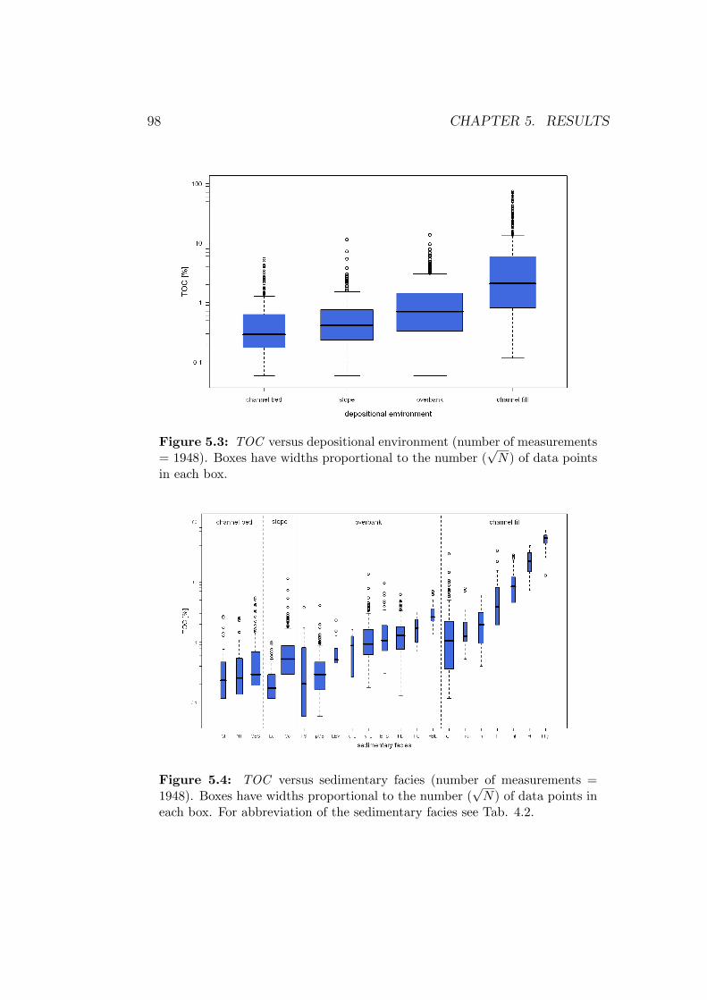
98 CHAPTER 5. RESULTS
Figure 5.3: TOC versus depositional environment (number of measurements= 1948). Boxes have widths proportional to the number (
√N) of data points
in each box.
Figure 5.4: TOC versus sedimentary facies (number of measurements =1948). Boxes have widths proportional to the number (
√N) of data points in
each box. For abbreviation of the sedimentary facies see Tab. 4.2.
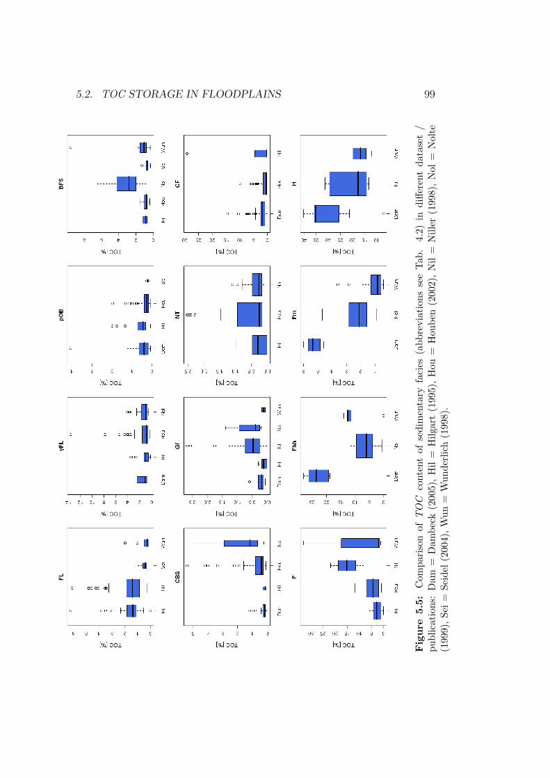
5.2. TOC STORAGE IN FLOODPLAINS 99
Fig
ure
5.5:
Com
pari
son
ofT
OC
cont
ent
ofse
dim
enta
ryfa
cies
(abb
revi
atio
nsse
eTab
.4.
2)in
diffe
rent
data
set
/pu
blic
atio
ns:
Dam
=D
ambe
ck(2
005)
,H
il=
Hilg
art
(199
5),H
ou=
Hou
ben
(200
2),N
il=
Nill
er(1
998)
,N
ol=
Nol
te(1
999)
,Se
i=
Seid
el(2
004)
,W
un=
Wun
derl
ich
(199
8).
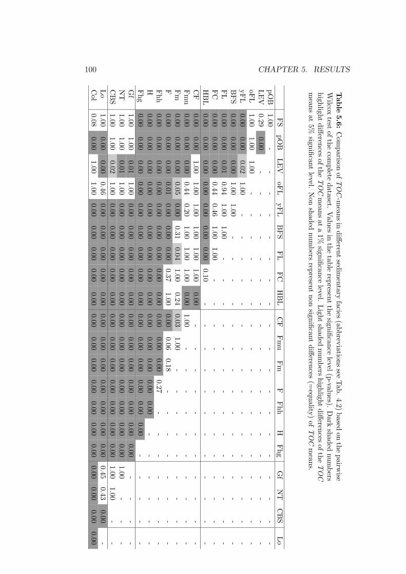
100 CHAPTER 5. RESULTSTab
le5.6:
Com
parisonofT
OC
-means
indifferent
sedimentary
facies(abbreviations
seeTab.
4.2)based
onthe
pairwise
Wilcox
testofthe
complete
dataset.V
aluesin
thetable
representthe
significancelevel(p-values).
Dark
shadednum
bershighlight
differencesofthe
TO
Cm
eansat
a1%
significancelevel.
Light
shadednum
bershighlight
differencesofthe
TO
Cm
eansat
5%significant
level.N
onshaded
numbers
representnon
significantdifferences
(=equality)
ofT
OC
means.
FS
pOB
LE
VoF
LyF
LB
FS
FL
FC
HB
LC
FFm
uFm
FFhh
HFhg
Gf
NT
CB
SLo
pOB
1.00-
--
--
--
--
--
--
--
--
--
LE
V0.29
0.00-
--
--
--
--
--
--
--
--
-oF
L1.00
1.001.00
--
--
--
--
--
--
--
--
-yF
L0.00
0.000.02
1.00-
--
--
--
--
--
--
--
-B
FS
0.000.00
0.001.00
1.00-
--
--
--
--
--
--
--
FL
0.000.00
0.010.94
1.001.00
--
--
--
--
--
--
--
FC
0.000.00
0.000.44
0.461.00
1.00-
--
--
--
--
--
--
HB
L0.00
0.000.00
0.000.00
0.000.00
0.10-
--
--
--
--
--
-C
F0.00
0.001.00
1.001.00
1.001.00
1.000.00
--
--
--
--
--
-Fm
u0.00
0.000.00
0.440.20
1.001.00
1.000.00
1.00-
--
--
--
--
-Fm
0.000.00
0.000.05
0.000.31
0.041.00
0.240.03
1.00-
--
--
--
--
F0.00
0.000.00
0.010.00
0.000.00
0.371.00
0.000.06
0.18-
--
--
--
-Fhh
0.000.00
0.000.00
0.000.00
0.000.00
0.000.00
0.000.00
0.27-
--
--
--
H0.00
0.000.00
0.000.00
0.000.00
0.000.00
0.000.00
0.000.00
0.00-
--
--
-Fhg
0.000.00
0.000.00
0.000.00
0.000.00
0.000.00
0.000.00
0.000.00
0.00-
--
--
Gf
1.001.00
0.011.00
0.000.00
0.000.00
0.000.00
0.000.00
0.000.00
0.000.00
--
--
NT
1.001.00
0.011.00
0.000.00
0.000.00
0.000.00
0.000.00
0.000.00
0.000.00
1.00-
--
CB
S1.00
1.000.02
1.000.00
0.000.00
0.000.00
0.000.00
0.000.00
0.000.00
0.001.00
1.00-
-Lo
1.000.00
0.000.46
0.000.00
0.000.00
0.000.00
0.000.00
0.000.00
0.000.00
0.450.43
0.00-
Col
0.080.00
1.001.00
0.000.00
0.000.00
0.000.00
0.000.00
0.000.00
0.000.00
0.000.00
0.000.00
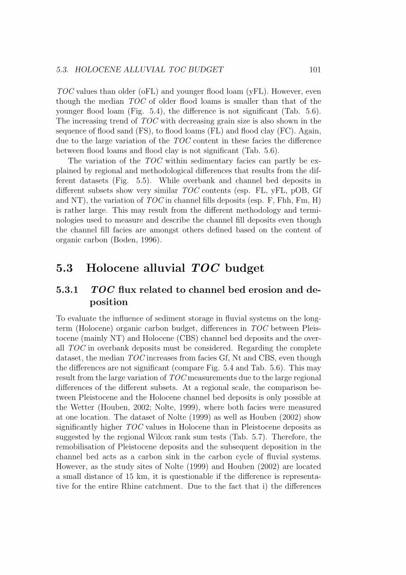
5.3. HOLOCENE ALLUVIAL TOC BUDGET 101
TOC values than older (oFL) and younger flood loam (yFL). However, eventhough the median TOC of older flood loams is smaller than that of theyounger flood loam (Fig. 5.4), the difference is not significant (Tab. 5.6).The increasing trend of TOC with decreasing grain size is also shown in thesequence of flood sand (FS), to flood loams (FL) and flood clay (FC). Again,due to the large variation of the TOC content in these facies the differencebetween flood loams and flood clay is not significant (Tab. 5.6).
The variation of the TOC within sedimentary facies can partly be ex-plained by regional and methodological differences that results from the dif-ferent datasets (Fig. 5.5). While overbank and channel bed deposits indifferent subsets show very similar TOC contents (esp. FL, yFL, pOB, Gfand NT), the variation of TOC in channel fills deposits (esp. F, Fhh, Fm, H)is rather large. This may result from the different methodology and termi-nologies used to measure and describe the channel fill deposits even thoughthe channel fill facies are amongst others defined based on the content oforganic carbon (Boden, 1996).
5.3 Holocene alluvial TOC budget
5.3.1 TOC flux related to channel bed erosion and de-position
To evaluate the influence of sediment storage in fluvial systems on the long-term (Holocene) organic carbon budget, differences in TOC between Pleis-tocene (mainly NT) and Holocene (CBS) channel bed deposits and the over-all TOC in overbank deposits must be considered. Regarding the completedataset, the median TOC increases from facies Gf, Nt and CBS, even thoughthe differences are not significant (compare Fig. 5.4 and Tab. 5.6). This mayresult from the large variation of TOC measurements due to the large regionaldifferences of the different subsets. At a regional scale, the comparison be-tween Pleistocene and the Holocene channel bed deposits is only possible atthe Wetter (Houben, 2002; Nolte, 1999), where both facies were measuredat one location. The dataset of Nolte (1999) as well as Houben (2002) showsignificantly higher TOC values in Holocene than in Pleistocene deposits assuggested by the regional Wilcox rank sum tests (Tab. 5.7). Therefore, theremobilisation of Pleistocene deposits and the subsequent deposition in thechannel bed acts as a carbon sink in the carbon cycle of fluvial systems.However, as the study sites of Nolte (1999) and Houben (2002) are locateda small distance of 15 km, it is questionable if the difference is representa-tive for the entire Rhine catchment. Due to the fact that i) the differences
102 CHAPTER 5. RESULTS
between Pleistocene and Holocene channel beds are not large and not welldefined and ii) a budget of the stored mass of Holocene channel bed sedimentfor the entire Rhine catchment is still missing, TOC fluxes due to the remo-bilisation of Pleistocene channel bed sediments are not taken into account inthis study.
5.3.2 TOC storage related to overbank deposition
In total 53.5 ± 14 × 109 t of Holocene floodplain sediment is stored in thenon-alpine part of the Rhine catchment (Tab. 5.1). Based on the analysedcross sections 85 % (with an assumed range of 70 - 95 %) of the Holocenefloodplain sediments correspond to overbank deposition and 15 % (with anassumed range of 5 - 30 %) to channel fills. The mean TOC values of thesedepositional environments 1.1 % and 7.5 % (with 95 % confidence intervalsof 1.0 - 1.2 % and 6.1 - 8.9 %, respectively), resulting in a stored TOCmass of 0.5 × 10⁹ t and 0.6 × 10⁹ t, respectively (Tab. 5.8). Even thoughthe sediment mass of channel fill deposits is much smaller than that of theoverbank deposits, they store almost the same amount of TOC, due to theirhigher TOC. Therefore, 1.1 × 10⁹ t TOC is sequestered by the non-alpineRhine catchment within floodplains during the period of floodplain deposi-tion. Considering the minimum and maximum values of the stored sedimentmasses and the 95 % confidence intervals of the TOC-measurements, TOCstorage in the floodplains may range between 0.7 and 1.6 × 10⁹ t. Corre-sponding Holocene mean sequestration rates range from 3.4 to 25.4 g m−2
year−1, depending the used time scenario (10 000, 7000, 5000 and 3000 years)since floodplain deposition started.
When comparing the TOC content of alluvial sediments to colluvial de-posits, the processes leading to sedimentation need to be considered. Alluvialsediments may have been subjected to prolonged transport in rivers leadingto graded texture; colluviation may lead to poorly graded deposits, althougheasily eroding texture classes dominate. Furthermore, colluvial deposits gen-erally originate from humus rich topsoil while alluvial deposits may be tracedback to different types of soils or sediment. Despite potentially high miner-alization rates of soil organic matter during the erosion process (Beyer et al.,1993), fresh colluvial deposits can be expected to have higher TOC contentsthan recent alluvial deposits. The degree of in situ C accumulation dependson relief position (Glatzel & Sommer, 2005) and conditions of aerobic min-eralization. According to calculations by Glatzel & Stahr (2002), ripariancolluvial deposits in a south-west German phragmition store 39 g C cm−2
due to waterlogged conditions.
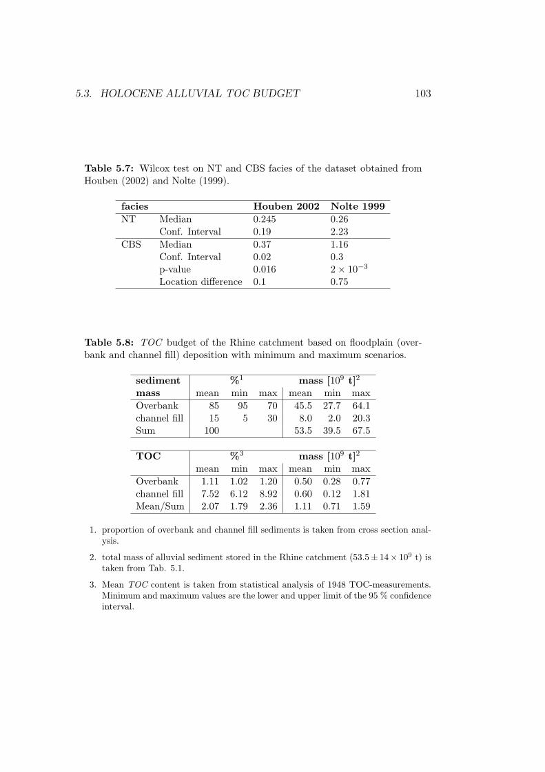
5.3. HOLOCENE ALLUVIAL TOC BUDGET 103
Table 5.7: Wilcox test on NT and CBS facies of the dataset obtained fromHouben (2002) and Nolte (1999).
facies Houben 2002 Nolte 1999NT Median 0.245 0.26
Conf. Interval 0.19 2.23CBS Median 0.37 1.16
Conf. Interval 0.02 0.3p-value 0.016 2× 10⁻³
Location difference 0.1 0.75
Table 5.8: TOC budget of the Rhine catchment based on floodplain (over-bank and channel fill) deposition with minimum and maximum scenarios.
sediment %1 mass [109 t]2
mass mean min max mean min maxOverbank 85 95 70 45.5 27.7 64.1channel fill 15 5 30 8.0 2.0 20.3Sum 100 53.5 39.5 67.5
TOC %3 mass [109 t]2
mean min max mean min maxOverbank 1.11 1.02 1.20 0.50 0.28 0.77channel fill 7.52 6.12 8.92 0.60 0.12 1.81Mean/Sum 2.07 1.79 2.36 1.11 0.71 1.59
1. proportion of overbank and channel fill sediments is taken from cross section anal-ysis.
2. total mass of alluvial sediment stored in the Rhine catchment (53.5± 14× 109 t) istaken from Tab. 5.1.
3. Mean TOC content is taken from statistical analysis of 1948 TOC-measurements.Minimum and maximum values are the lower and upper limit of the 95 % confidenceinterval.
104 CHAPTER 5. RESULTS
5.4 14C-database analysis
5.4.1 Cumulative frequency distributions
The number of 14C-data from fluvial deposits in Germany is listed in Tab.4.3 according to the depositional environments and sedimentary facies fromwhich the organic material was retrieved. The largest number of data isderived from floodplains (N = 131) and palaeochannels (N = 120). Thesedimentary facies used most frequently are gyttja (N = 103), peat (N =76) and colluvium (N = 68). Based on the different facies, 148 14C-dataare classified as activity ages, 106 as stability ages and 155 as transitionalages. The spatial distribution of the 432 14C-data is illustrated in Fig. 4.9.The data are not evenly distributed throughout Germany but show strongclusters i) around Freiburg in the Black Forest and the southern Upper RhineGraben, ii) around Frankfurt in the Nidda Catchment, the AmoneburgerBecken and in the northern Upper Rhine Graben, iii) at the Danube riverclose to Regensburg, iv) at the Weserbergland and v) at the Lippe valley.
The CPF analysis is presented in Fig. 5.6. In Fig. 5.6a the CPF of140 synthetic equally spaced 14C-ages (assumed uncertainty of ±100 yearsfor each datum) is shown. The shape of the CPF results mainly from theshape of the 14C calibration curve. The CPF of the complete set of 432 14C-data is shown in Fig. 5.6b, and the CPF of the 14C-ages taken to representactivity in Fig. 5.6c. Different ways of data treatment are depicted in Fig.5.6d and 5.6e: The CPDF of all activity data divided by CPF of the equallyspaced data is shown in Fig. 5.6d and the CPF of all activity data divided bythe CPF of the complete dataset is shown in Fig. 5.6e. The results indicatesuccessful rectification of the young age bias using the proposed normalisationprocedure. Compared to Fig. 5.6d in Fig. 5.6e the probabilities are moreuniformly distributed during the last 14 000 years and should provide a moreaccurate picture.
The normalised CPFs that were constructed by dividing the CPF of adata subset by the CPF of the full dataset, and that were used for furtheranalysis and interpretation, are shown in Fig. 5.7: Radiocarbon ages repre-senting activity in Fig. 5.7a, stability in Fig. 5.7b and transition in Fig. 5.7c.Following Macklin et al. (2005) phases of increased flooding are representedby ’change dates’. In the Rhine dataset 127 ’change dates’ were identifiedand the resulting CPF is plotted in Fig. 5.7d.
Periods where the relative probabilities are larger than the mean relativeprobability and that indicate phases of increased geomorphic activity or sta-bility are shaded in gray in Fig. 5.7. The results of the probability frequencyanalysis suggest a tendency towards stable fluvial and colluvial systems dur-
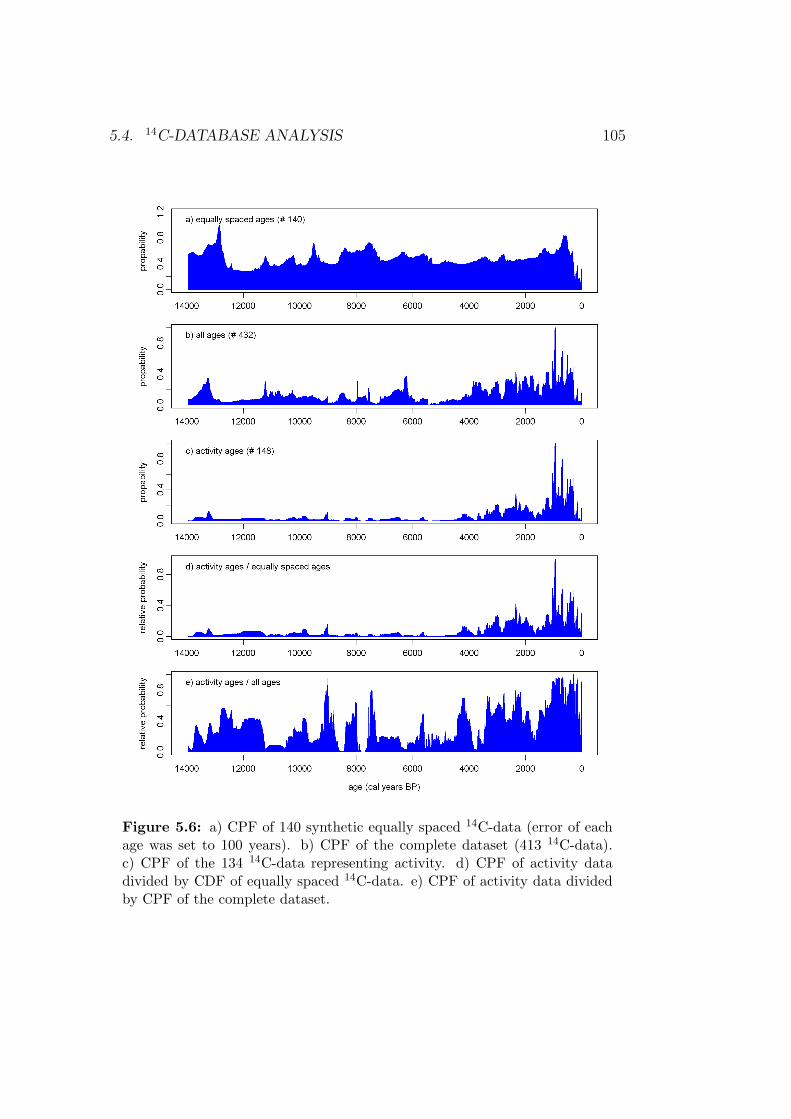
5.4. 14C-DATABASE ANALYSIS 105
Figure 5.6: a) CPF of 140 synthetic equally spaced 14C-data (error of eachage was set to 100 years). b) CPF of the complete dataset (413 14C-data).c) CPF of the 134 14C-data representing activity. d) CPF of activity datadivided by CDF of equally spaced 14C-data. e) CPF of activity data dividedby CPF of the complete dataset.
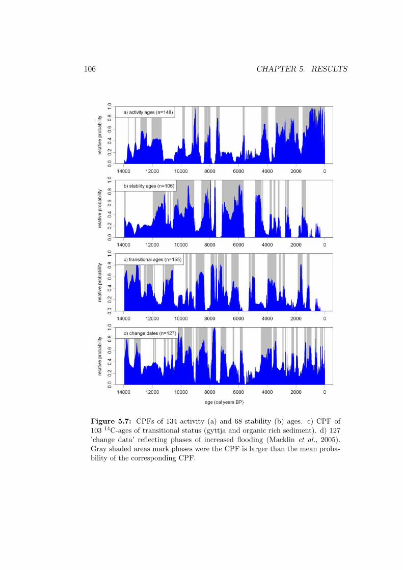
106 CHAPTER 5. RESULTS
Figure 5.7: CPFs of 134 activity (a) and 68 stability (b) ages. c) CPF of103 14C-ages of transitional status (gyttja and organic rich sediment). d) 127’change data’ reflecting phases of increased flooding (Macklin et al., 2005).Gray shaded areas mark phases were the CPF is larger than the mean proba-bility of the corresponding CPF.
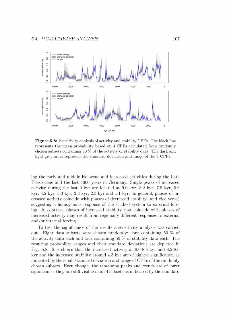
5.4. 14C-DATABASE ANALYSIS 107
Figure 5.8: Sensitivity analysis of activity and stability CPFs. The black linerepresents the mean probability based on 4 CPFs calculated from randomlychosen subsets containing 50 % of the activity or stability data. The dark andlight grey areas represent the standard deviation and range of the 4 CPFs.
ing the early and middle Holocene and increased activities during the LatePleistocene and the last 4000 years in Germany. Single peaks of increasedactivity during the last 9 kyr are located at 9.0 kyr, 8.2 kyr, 7.5 kyr, 5.6kyr, 4.2 kyr, 3.3 kyr, 2.8 kyr, 2.3 kyr and 1.1 kyr. In general, phases of in-creased activity coincide with phases of decreased stability (and vice versa)suggesting a homogenous response of the studied system to external forc-ing. In contrast, phases of increased stability that coincide with phases ofincreased activity may result from regionally different responses to externaland/or internal forcing.
To test the significance of the results a sensitivity analysis was carriedout. Eight data subsets were chosen randomly: four containing 50 % ofthe activity data each and four containing 50 % of stability data each. Theresulting probability ranges and their standard deviations are depicted inFig. 5.8. It is shown that the increased activity at 9.0-8.5 kyr and 8.2-8.0kyr and the increased stability around 4.3 kyr are of highest significance, asindicated by the small standard deviation and range of CPFs of the randomlychosen subsets. Even though, the remaining peaks and trends are of lowersignificance, they are still visible in all 4 subsets as indicated by the standard
108 CHAPTER 5. RESULTS
deviation and range (grey shaded areas in Fig. 5.8), which closely follow thetrend of the mean values (blue line in Fig. 5.8).
5.4.2 Sedimentation rates
The calculated sedimentation rates of 115 floodplain and 104 palaeochannelsamples range between 0.02 and 9 mm year−1 (Fig. 5.9). The large scattercertainly results from the large spatial scale (compare Fig. 4.9) and the largesmall scale variation that influences the floodplain deposition. Even thoughthere is a large scatter of three orders of magnitude, the data reveal threephases of changing sedimentation during the last 14 000 years:
1. During the Late Glacial / Early Holocene (e.g. from 14 000 to ≈8000 years BP) sedimentation rates range between 0.1 and 1.0 mmyear−1. Palaeochannel data show slightly higher sedimentation ratesthan floodplain samples.
2. From ≈ 8000 to ≈ 4000 years BP sedimentation rates slight decrease.In the case of the floodplain samples, the decrease is more pronouncedby the lower boundary (lower dashed line in Fig. 5.9 top). Thepalaeochannel data are characterised by a stronger decrease of the highsedimentation rates (upper higher dashed line in Fig. 5.9 bottom). Ingeneral, this phase coincidences with the Holocene climatic optimum.
3. From 4000 years BP onwards, sedimentation rates strongly increaseup to 9 mm year−1. In contrast to the preceding decline, the increaseis shown by the lower and upper limit of the range. However, theincrease is more distinct in the case of the floodplain samples than thepalaeochannel data.
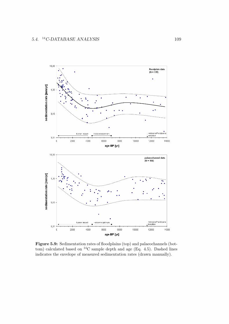
5.4. 14C-DATABASE ANALYSIS 109
Figure 5.9: Sedimentation rates of floodplains (top) and palaeochannels (bot-tom) calculated based on 14C sample depth and age (Eq. 4.5). Dashed linesindicates the envelope of measured sedimentation rates (drawn manually).


Chapter 6
Discussion
111

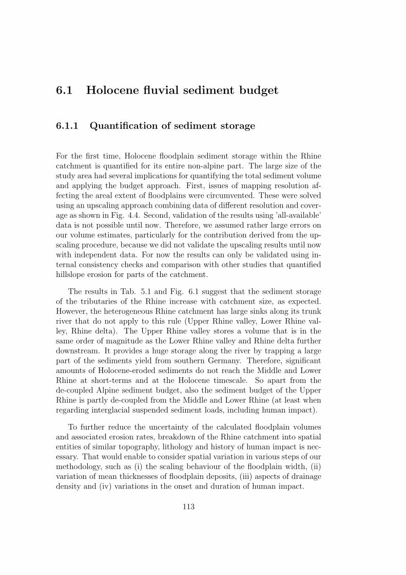
6.1 Holocene fluvial sediment budget
6.1.1 Quantification of sediment storage
For the first time, Holocene floodplain sediment storage within the Rhinecatchment is quantified for its entire non-alpine part. The large size of thestudy area had several implications for quantifying the total sediment volumeand applying the budget approach. First, issues of mapping resolution af-fecting the areal extent of floodplains were circumvented. These were solvedusing an upscaling approach combining data of different resolution and cover-age as shown in Fig. 4.4. Second, validation of the results using ’all-available’data is not possible until now. Therefore, we assumed rather large errors onour volume estimates, particularly for the contribution derived from the up-scaling procedure, because we did not validate the upscaling results until nowwith independent data. For now the results can only be validated using in-ternal consistency checks and comparison with other studies that quantifiedhillslope erosion for parts of the catchment.
The results in Tab. 5.1 and Fig. 6.1 suggest that the sediment storageof the tributaries of the Rhine increase with catchment size, as expected.However, the heterogeneous Rhine catchment has large sinks along its trunkriver that do not apply to this rule (Upper Rhine valley, Lower Rhine val-ley, Rhine delta). The Upper Rhine valley stores a volume that is in thesame order of magnitude as the Lower Rhine valley and Rhine delta furtherdownstream. It provides a huge storage along the river by trapping a largepart of the sediments yield from southern Germany. Therefore, significantamounts of Holocene-eroded sediments do not reach the Middle and LowerRhine at short-terms and at the Holocene timescale. So apart from thede-coupled Alpine sediment budget, also the sediment budget of the UpperRhine is partly de-coupled from the Middle and Lower Rhine (at least whenregarding interglacial suspended sediment loads, including human impact).
To further reduce the uncertainty of the calculated floodplain volumesand associated erosion rates, breakdown of the Rhine catchment into spatialentities of similar topography, lithology and history of human impact is nec-essary. That would enable to consider spatial variation in various steps of ourmethodology, such as (i) the scaling behaviour of the floodplain width, (ii)variation of mean thicknesses of floodplain deposits, (iii) aspects of drainagedensity and (iv) variations in the onset and duration of human impact.
113
114 CHAPTER 6. DISCUSSION
Figure 6.1: Size of Holocene alluvial sediment storages vs. subcatchmentarea (Tab. 5.1). The regression lines calculated is based on a power law:SV = 7× 10⁻⁵A1.13
d (R2 = 0.93)
6.1.2 Quantification of mean Holocene erosion rate
The sediment budget approach was used to calculate the Holocene erosionrates for the non-alpine Rhine catchment. Most reasonable calculations yielda mean erosion rate of 0.55±0.16 t ha−1yr−1 (38.5±10.7 mm kyr−1), averagedover the last 10 000 years. Mean Holocene erosion rates calculated fromequations 1 and 2 are, based on (1) quantified alluvial sediment volumes SV ,(2) the time T attributed to deposition of this volume, (3) assumed CSDRof the river system and (4) the bulk density ρB of the sediment. All theseparameters are estimated or assumed with some uncertainty. The appliedsensitivity analysis allowed evaluating the influence of the uncertainties tothe calculated erosion rate (Tab. 5.3). The erosion rate linearly depends onthe sediment volume. Therefore, the uncertainty of the calculated sedimentvolume (≈ 30 %) accounts for an uncertainty of 30 % of the calculatederosion rate. However, this value does not account for the neglected colluvialstorage. Similar, the uncertainty of the bulk density (≈ 13 %) accounts foran uncertainty of 13 % of the calculated erosion rate. The large variation of
6.1. HOLOCENE FLUVIAL SEDIMENT BUDGET 115
the CSDR between 0 and 30 % results in an uncertainty of only 16 % of theerosion rate, due to the nonlinear effect of CSDR in Eq. 4.2. The variationof time between 3000 and 10 000 yrs. results in an uncertainty of the erosionrate of approximately 50 %.
To summarise, the sensitivity analysis showed that the largest uncertaintyof the erosion rate results from the large uncertainty of the timing of flood-plain deposition, followed by the uncertainty of the alluvial sediment volume.Therefore, timing is the most critical factor in the calculation of mean ero-sion rates. However, considering the neglected amount of colluvial storage,which was not considered in the sensitivity analysis, the uncertainty of thesediment storage may be even bigger. Though the CSDR is varied for a largerange its impact on the uncertainty of the erosion rate rather low.
The large uncertainty in the onset of the timing of floodplain deposition,especially in the tributary valleys in the hinterland, follows from the factthat floodplain thicknesses were estimated based on the lithological bound-ary from sand/gravel to fines. The beginning of the Holocene sedimentation,which is marked by this lithological boundary, may strongly vary withinthe Rhine catchment, leading to highly variable sedimentation rates. ThePleistocene-Holocene transition had a major impact on river systems in cen-tral Europe, and the top of Pleistocene deposits is well resolved. However, itis debatable whether Holocene floodplain sediment accumulation was rathersteady throughout the last 10 000 years (as appears the case in the large sinksalong the trunk valley) or is a matter of mainly Late Holocene sedimentation(as appears to be the case for in the smaller tributary catchments). Themaximum duration of 10 000 years results in a rather low erosion rate andis a rather safe estimate for minimum mean rates of erosion/sediment deliv-ery. Considering the increasing erosion rates towards the Late Holocene (e.g.Lang et al., 2003), most floodplain sediments are assumed to be younger.
An important parameter controlling the magnitude of the erosion esti-mate is the CSDR. Including the hinterland and the delta, our CSDR appliesto the present river mouth (at the Dutch coast) at which location it couldbe considered small. Asselman et al. (2003) in their modelling of the modernsituation consider the CSDR at the Dutch-German border (the delta apex)for which they derive a value of approx. 36 % (calculated over the non-alpineRhine catchment; 27 % including the Alpes). We can use this to assess our es-timate of the CSDR at the river mouth, assuming that the delta-apex CSDRunder modern conditions is at the upper end of the delta apex CSDR rangewhen averaged over the Holocene (because of river ’normalisation’ measuresfor navigational and flood management purposes; see introduction). If thedelta apex CSDR was 36 % or less during the Holocene, this implies thatthe delta mouth CSDR (i.e. full Rhine catchment CSDR) ranged between 0
116 CHAPTER 6. DISCUSSION
and 30 %. This underpins our choice of CSDR ranges in Tab. 5.3. From thecalculations, we conclude that the delta volume is somewhat underestimated:likely clayey tidal-lagoonal and estuarine deposits that occur adjacent to thefluvial delta within the Dutch coastal wedge should also be considered Rhinederived. We consider a river mouth CSDR of 10-20 % most realistic, whenconsidering the volumes in Tab. 5.2. If additional (’tidal Rhine alluvium’Erkens et al., 2006) volumes are added to the budget analysis, the CSDRfurther drops.
6.1.3 Comparison of the erosion rate with other stud-ies
To evaluate the mean Holocene erosion rate derived for the Rhine catch-ment, it is compared with results obtained for different temporal and spatialscales, from different catchments across Central Europe (Fig. 6.2). The dataset in Fig. 6.2 is cross-correlated, which introduces a bias in Fig. 6.2B:short-term erosion rates have been obtained for smaller catchments, whereaslong-term rates have been obtained from larger catchments. Furthermore,the estimates are obtained using different methods, which has introducedadditional variance. Nevertheless, the declining trends of the erosion rate forincreasing time frame, have been attributed to (human-induced) increasingsoil erosion towards the present (Bork et al., 1998; Dotterweich, 2005; Lang& Honscheidt, 1999; Thiemeyer et al., 2005). The reduction of erosion rateswith increasing catchment size may partly reflect the reduction in mean slopefor larger catchments (as an additional effect next to the increase over time),but that effect cannot be differentiated in the current dataset. We derive(roughly 50 %) lower erosion rates (Fig. 6.2A), than studies based on at-the-site-of-erosion measurements (e.g. truncated soil profiles), and attribute thedifference to the colluvial storage. Comparing the calculated erosion rateswith those obtained in other studies (Fig. 6.2B), the T = 7000 scenario fitsbest into the declining trend of erosion rates with increased catchment size.However, as the colluvial storage is neglected (reducing the calculated ero-sion rate), the T = 10 000 scenario may yield better estimates for the 10 000year averaged-rate for sediment reaching rivers.
To further improve quantifications of erosion rates building upon thesediment budget approach described above, uncertainties in the timing ofthe onset of sediment erosion and floodplain deposition across the hinter-land should be reduced through better floodplain chronologies. Additionally,colluvial storage must be considered to evaluate possible effects of relativechanges in the exchange between hillslope and channel systems. Spatially
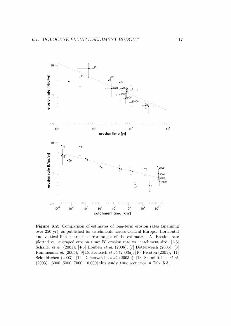
6.1. HOLOCENE FLUVIAL SEDIMENT BUDGET 117
Figure 6.2: Comparison of estimates of long-term erosion rates (spanningover 250 yr), as published for catchments across Central Europe. Horizontaland vertical lines mark the error ranges of the estimates. A) Erosion rateplotted vs. averaged erosion time; B) erosion rate vs. catchment size. [1-3]Schaller et al. (2001); [4-6] Houben et al. (2006); [7] Dotterweich (2005); [8]Rommens et al. (2005); [9] Dotterweich et al. (2003a); [10] Preston (2001); [11]Schmidtchen (2003). [12] Dotterweich et al. (2003b); [13] Schmidtchen et al.(2003). [3000, 5000, 7000, 10,000] this study, time scenarios in Tab. 5.3.
118 CHAPTER 6. DISCUSSION
disaggregating the calculations can further constrain estimates. Such wouldallow quantifying and dating increased floodplain deposition, and assess thespatial and temporal variation of the CSDR. Future research should thus in-clude colluvial storage and focus on resolving erosion and deposition withinthe floodplains over Holocene timescales, to obtain better grip on changingintensities of erosion on the hillslopes. Such can further validate the estimatesof effective erosion rates of this paper.
6.2 Holocene alluvial carbon budget
The results presented here are the first steps towards the utilization of thewealth of organic measurements available from case studies focusing on theHolocene dynamics of geomorphological systems in Germany. The approachclassifies the TOC measurements based on depositional environments andsedimentary facies, which both have a significant influence on the TOC con-tent.
6.2.1 Limitations and uncertainties
The approach is limited by the uncertainties caused by the spatial clusteringof the TOC sampling sites, the measurement of TOC and the unambiguousterminology used to describe sedimentary facies in geomorphological systems.The TOC sites are strongly clustered at loess covered areas, the NorthernUpper Rhine Graben and the area around Regensburg. Upland areas (e.g.Rhenish Slate Massif, Black Forest) are missing in the compiled database.As there are no data from these areas up to now the effects of this spatialbias can not be discussed. TOC measurements from the ”missing” areas areclearly required in order to establish a more representative picture of TOCstorage and the carbon sequestration on floodplains in the Rhine catchment.
As the TOC concentrations, which are compiled in this study, are mea-sured by different methods, it must be considered that TOC content obtainedby wet-combustion generally result in smaller values than those obtained withelement analysers due to incomplete carbon oxidation (Schlichting et al.,1995). In order to limit uncertainties due to different techniques of carboncombustion (Niller, 1998; Nolte, 1999; Seidel, 2004), we did not include losson ignition measurements in our analysis. Still, TOC concentrations of or-ganic samples were determined by combustion at 550 to 600◦C. Therefore,mineral samples were oxidized by K2CR2O7 and colorimetric determinationof Cr3+ or by spectrometric analysis of CO2. The applied measurements dif-fer especially for sediments with high TOC values (e.g. channel fills) and for
6.2. HOLOCENE ALLUVIAL CARBON BUDGET 119
clay rich samples, which may release crystal water. However, it is assumedthat the errors are smaller than the local variability and are therefore notdiscussed further (Nolte, 1999; Seidel, 2004).
6.2.2 Significance and perspective
In a first approach, the analysed TOC measurements are used to calculatethe TOC mass stored within floodplain deposits. The calculation is basedon a simplified carbon budget and a Holocene sediment floodplain storagebudget for the non-alpine Rhine catchment. Overall 1.1 × 10⁹ t (with min.and max. values ranging between 0.7 and 1.6 × 10⁹ t) TOC is stored bythe non-alpine Rhine catchment within floodplains since the beginning offloodplain deposition of overbank fines and channel fills. Therefore, meanHolocene sequestration rates range between 0.07 and 0.53 × 10⁶ t year−1 or3.4 to 25.4 g m−2year−1.
To the authors knowledge this is the first estimate of carbon sequestra-tions rates obtained for floodplains in Germany. Interestingly, these valuesare in the same order of magnitude as the modern TOC transport at 0.65×10⁶
t year−1 of the river Rhine measured at the gauging station at Lobith from1975 to 1978 (Kempe et al., 1991; Kempe & Krahe, 2005). Although the val-ues obtained from the long-term TOC storage are smaller than the modernTOC export, they suggest the major importance of the floodplain storagefor the fluvial carbon cycle (Fig. 4.8). Concerning the increased modern soilerosion and floodplain deposition compared to mean Holocene rates (Tab.5.3) and considering the different temporal scales (modern vs. Holocene) theimportance of TOC storage within the floodplains may even increase further.
The long-term sequestration rates from the Rhine catchment can be com-pared with the few data available on carbon sequestration on floodplains (Noe& Hupp, 2005; Walling et al., 2006). Walling et al. (2006) estimated carbonsequestration rates along six rivers in southern England based on TOC mea-surements and sedimentation rates obtained from 137Cs measurements. Theestimated values, which range between 69.2 and 114.3 g m−2year−1, corre-spond to mean values since 1963. Noe & Hupp (2005) measured the carbonsequestration along three rivers within the Atlantic Coastal Plain (USA)using feldspar marker horizons over a period of 3-6 years. The carbon ac-cumulation rates reported for the different sites ranged from 61 to 212 gm−2year−1. The estimated sequestration rates reported from the UK andUSA are both an order of magnitude larger than those presented here. How-ever, the values given by Noe & Hupp (2005) and Walling et al. (2006) couldbe expected to be higher than those reported in this paper, since the formerrepresent recent values that correspond to increased recent soil erosion and
120 CHAPTER 6. DISCUSSION
floodplain accumulation rates compared to mean Holocene rates (see above).To investigate the controls of carbon sequestration in more detail, a spatiallyand temporally resolved C-budget is necessary. Additionally, the integrationof colluvial budgets is necessary to evaluated the impact of soil erosion onthe global carbon cycle (Lal, 2005; Walling et al., 2006).
6.3 14C-database analysis
6.3.1 Cumulative frequency distributions
The results presented here are the first step towards an utilization of thewealth of radiocarbon data available from case studies focused on the Holocenedynamics of geomorphological systems in Germany. The technique used toconstruct frequency distributions of 14C-ages by dividing the relative CPFsof the subsets by the relative CPF of the complete dataset allows reducingambiguities originating from 14C calibration curve wiggles and the samplingbias towards younger 14C-ages (Fig. 5.6d and 5.6e).
The approach is limited by the uncertainties involved with radiocarbondating and the assumptions underlying the use of 14C-probabilities as a proxyof fluvial activity or stability. Issues associated include reworking of organicsediments and erroneous 14C-analysis. Especially for periods of strong hu-man impact reworking of charcoal and other organic remains is commonplace(Lang & Honscheidt, 1999; Edwards & Whittington, 2001). Due to the largenumber of ages included in the analysis the impact of erroneous 14C-analysisare probably negligible: The sensitivity analysis (Fig. 5.8) suggests thatgeneral trends of the calculated CPFs are significant. The interpretation ofnarrow peaks in the CPFs should be undertaken with care as they may resultfrom a small number of 14C-ages only and may therefore represent exclusivelylocal events. Sensitivity analysis are especially important if small data setsare to be analysed, as e.g. for regional CPFs used to unravel regionally dif-ferent response to external forcing (Macklin et al., 2005). Smaller numbersof 14C-ages increase the weight of a single measurement and may bias theresults towards incorrect ages. At present it is unclear to which level theassumptions of large number statistics can be relaxed (the minimum numberof data points needed) to still obtain significant results. The sensitivity anal-ysis of the 106 stability ages shows that significant results can be obtainedusing approx. 100 14C-ages only. The effects of spatial heterogeneities forthe analysis are also still difficult to judge. Therefore, further work must becarried out to expand the 14C-database at the national scale and to fill thegaps between the regional clusters.
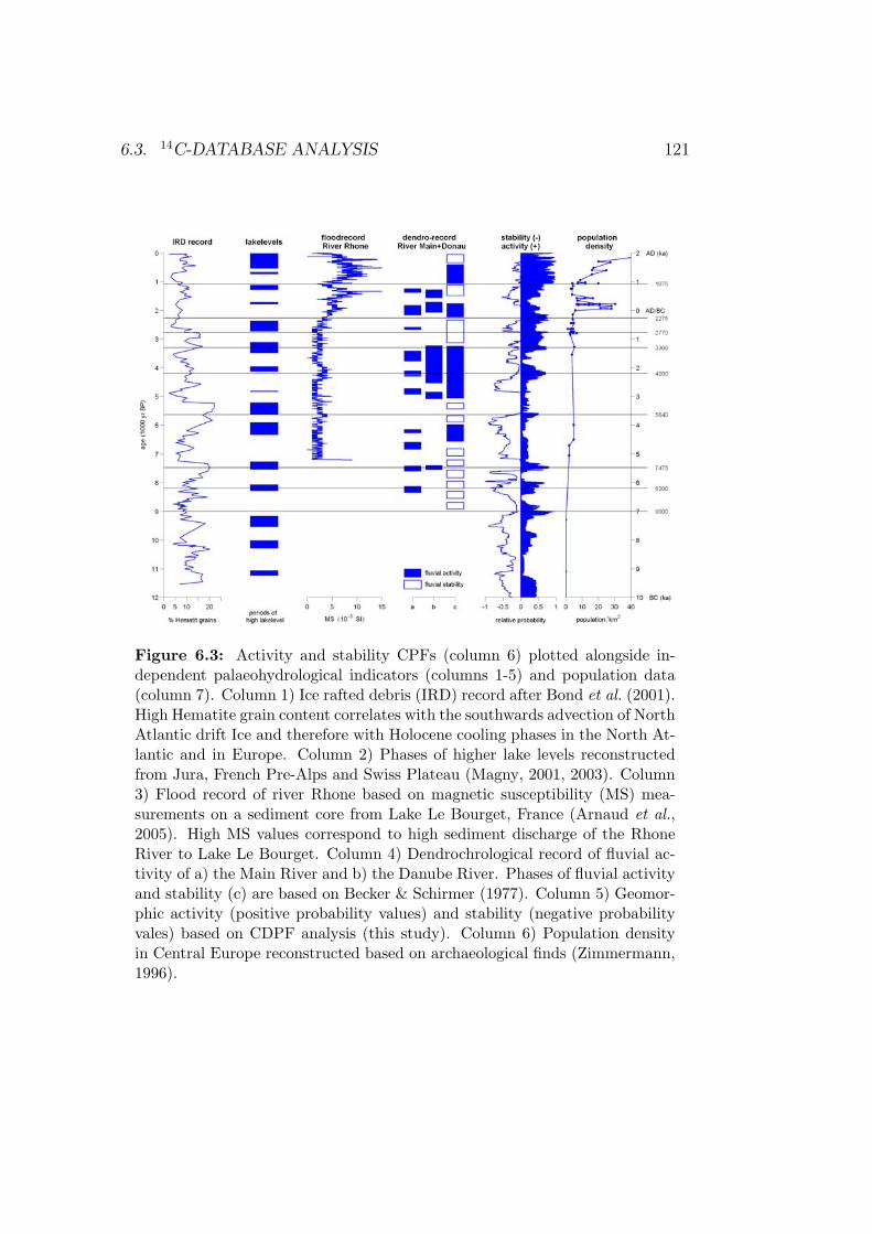
6.3. 14C-DATABASE ANALYSIS 121
Figure 6.3: Activity and stability CPFs (column 6) plotted alongside in-dependent palaeohydrological indicators (columns 1-5) and population data(column 7). Column 1) Ice rafted debris (IRD) record after Bond et al. (2001).High Hematite grain content correlates with the southwards advection of NorthAtlantic drift Ice and therefore with Holocene cooling phases in the North At-lantic and in Europe. Column 2) Phases of higher lake levels reconstructedfrom Jura, French Pre-Alps and Swiss Plateau (Magny, 2001, 2003). Column3) Flood record of river Rhone based on magnetic susceptibility (MS) mea-surements on a sediment core from Lake Le Bourget, France (Arnaud et al.,2005). High MS values correspond to high sediment discharge of the RhoneRiver to Lake Le Bourget. Column 4) Dendrochrological record of fluvial ac-tivity of a) the Main River and b) the Danube River. Phases of fluvial activityand stability (c) are based on Becker & Schirmer (1977). Column 5) Geomor-phic activity (positive probability values) and stability (negative probabilityvales) based on CDPF analysis (this study). Column 6) Population densityin Central Europe reconstructed based on archaeological finds (Zimmermann,1996).
122 CHAPTER 6. DISCUSSION
Comparison to other archives of Holocene environmental change
To evaluate the relative importance of climate and land use change (LU-CIFS) the 14C chronology of fluvial activity and stability is compared withindependent archives of Holocene environmental change (Fig. 6.3). For thecomparison following archives and proxy data for climate and human impactin Central Europe were chosen: the ice drifted debris record (IRD) from theNorth Atlantic (Bond et al., 2001), lake levels in the northern Alps (Magny,2001), floods of the alpine Rhone river (Arnaud et al., 2005), fluvial activ-ity of the Danube and the Main rivers reconstructed from a subfossil oak1
chronology (Becker & Schirmer, 1977) and the population density (Zimmer-mann, 1996). Even though very different in nature, the archives are believedto represent the most reliable and complete reconstructions of climate andhuman impact during large parts of the Holocene in Central Europe.
Unfortunately, not all archives cover the same time span. Especially forthe period before BC 7000 the activity/stability record can only be comparedto IRD and lake levels (Fig. 6.3). With the exception of the 9 kyr BP peak,all activity peaks (at around 8.2 kyr, 7.5 kyr, 5.6 kyr, 4.2 kyr, 3.3 kyr, 2.7 kyr,2.3 kyr and after 1.1 kyr) coincide with changing environmental conditionsrecognized at least in one alternative recorded. The prominent cooling at8200 year BP (e.g. Alley et al., 1997; Prasad et al., 2006) that started ataround 8600 years and ended after 8000 years (Rohling & Palike, 2005) isclearly seen by increased probability densities of the activity data as well asin the dendrochronological record of the Main (Becker & Schirmer, 1977) andhigher lake levels in the alpine foreland (Magny, 2001). The following phaseof increased activity reaches its maximum at 7475 years and again correlateswith higher lake levels and Rannen-deposits. In contrast to the 8200 yearsBP event, the 7475 years BP event is also characterised by high percentagesof Hematite grains of the IRD-record (Bond et al., 2001), suggesting a coolerclimate during that phase. The increased activity at around 5640 yearsBP may result from cooler and/or wetter climate conditions as evidencedby the IRD and lake level records as well as by the flood record of theRiver Rhone (Arnaud et al., 2005). Another prominent event of cooler andwetter climatic conditions following the Holocene Climatic Optimum canbe recognized in all palaeohydrological records: The increased geomorphicactivity that started at around 4400 years and ended approximately at 3900
1Subfossil oaks that were frequently found in gravel bed deposits of Central Europeanrivers are called Rannen. Using dendrochronological techniques, the Rannen were datedand their ages were analysed in terms of frequency distributions by Becker & Schirmer(1977). Times with high frequencies of Rannen deposits are generally interpreted as phasesof increased river activity.
6.3. 14C-DATABASE ANALYSIS 123
years BP coincidences with higher lake levels, increased flood activity and ahigh number of deposited Rannen in the Main and Donau catchments.
Wide spread human impact occurred for the first time during the BronzeAge. The activity maximum at 3300 years BP coincides with cooler/wetterclimatic conditions (e.g. high percentages of hematite grains, high lake levels,increased flooding of the Rhone and a large number of deposited Rannen inthe Donau catchment) and falls in a period that is associated with growingpopulation densities (Fig. 6.3), changing agricultural practices and increasedarable land use (Zimmermann, 1996)). Deciphering the relative role of cli-matic variability and human impact during that period is rather difficult. Forexample, the small peak at 2770 years coincides with increased populationdensity and agricultural activity as well as a cold phase at 2650 a (Van Geelet al., 1998) that resulted in a marked glacier advance in the European Alpsfrom 2800 a to 2600 years (Holzhauser et al., 2005). A differing pattern canbe seen for the broad peak of fluvial activity at 2275 years (ranging from2300-2100 years BP). This maximum does not coincide with a change in cli-mate or population density but coincides with a shift in landuse techniquesduring the pre-Roman Iron Age.
Increasing probabilities in the activity record after 1075 years seem tobe associated with the rising population density that resulted in enhancedagricultural activities. This correlates with the general increasing trend inthe flood record of the River Rhone, which is interpreted to results fromgrowing sediment yield due to increasing human impact since at least theIron Age (Arnaud et al., 2005).
To summarise, before 4200 years BP, events of fluvial activity are mainlycoupled with wetter and/or cooler climatic phases. Due to the growing pop-ulation and intensified agricultural activities from the Bronze ages onwards,the increase in geomorphologic activity between 3300 years and 2770 yearsBP can not unequivocally be related to climate. From approximately 1075years BP onwards the growing population density and the associated changesin land use are considered as the major external forcing of river activity. Thehuman impact significantly increased the sensitivity of the fluvial systems toclimatic events so that even relatively low intensity rainfalls result in severflooding.
Comparisons of change data
To evaluate the concept of ’change data’ and their CPDF as a proxy of pasthydrological events (Macklin et al., 2006), the CPFs of change data from theGerman database are compared to the records from Poland, Great Britainand Spain (Macklin et al., 2006, Fig. 6.4).
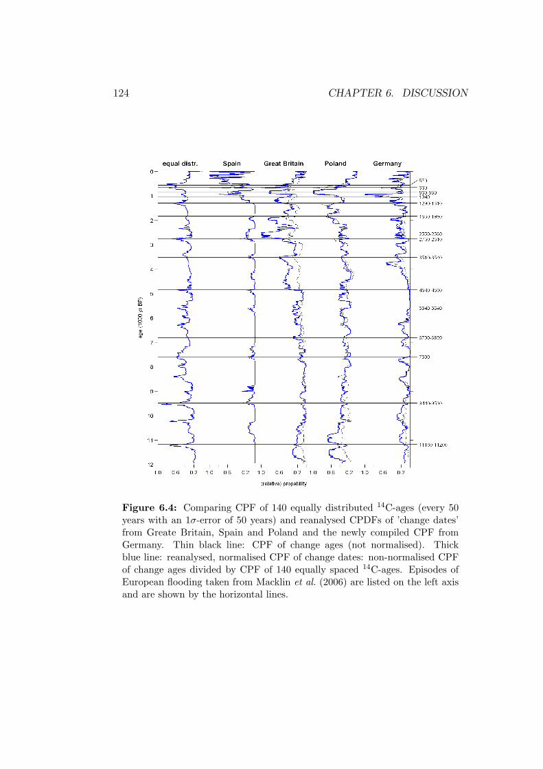
124 CHAPTER 6. DISCUSSION
Figure 6.4: Comparing CPF of 140 equally distributed 14C-ages (every 50years with an 1σ-error of 50 years) and reanalysed CPDFs of ’change dates’from Greate Britain, Spain and Poland and the newly compiled CPF fromGermany. Thin black line: CPF of change ages (not normalised). Thickblue line: reanalysed, normalised CPF of change dates: non-normalised CPFof change ages divided by CPF of 140 equally spaced 14C-ages. Episodes ofEuropean flooding taken from Macklin et al. (2006) are listed on the left axisand are shown by the horizontal lines.
6.3. 14C-DATABASE ANALYSIS 125
In Fig. 6.4 the CPF of the 140 equally distributed ages (left graph)is plotted along with the normalised CPFs (thick lines) of changes datesfrom Spain, Greate Britain, Poland and Germany. Thin lines represent non-normalised CPFs of the change ages. Episodes of European flooding takenfrom Macklin et al. (2006) are listed on the right-hand axis and are shown byhorizontal lines. It must be considered that episodes of European floodingare reconstructed by Macklin et al. (2006) based on the probability differ-ences as described above. As can be seen from the comparison with theCPDF of equally spaced 14C-ages, periods of major flooding in Europe 2 areassociated with plateaus of the 14C calibration curve (peaks in the CPDFof the equally spaced ages) (Fig. 6.4). Thus, the calculation of probabilitydifference curves based on Macklin et al. (2006) seems not to fully removeinfluences from variations in atmospheric 14C. The approach used here basedon dividing the relative CPFs of change data by the relative CPFs of equallyspaced 14C-ages seems mathematically more sound compared to the analysisof (Macklin et al., 2006). Concerning the reanalysed data, which are notinfluenced by the form of the calibration curve, the correlation between thedatasets is questionable. Except for the 7.5 kyr BP event, there are no ma-jor peaks in the CPFs that coincide in more than two countries. Therefore,synchronous response of the fluvial systems in the four different countries tolarge-scale climatic change can not be detected. The results obtained fromthe analysis of the CPDFs of the change data challenges the major findingsby Macklin et al. (2006). The CPDF-concept is not suitable to reconstructmajor periods of flooding. In fact, the change in sedimentation style, whichis analysed by the change date concept, does not correlated to periods ofmajor flooding. It is stated that change in sedimentation style is dominantlycontrolled by internal forcing and not by major flooding. Furthermore, the’change date’ concept uses only 50 % of the data in each database, whilethe above described approach of activity and stability data uses as muchinformation of the database as possible.
6.3.2 Sedimentation rates
The estimated range of sedimentation rates between 0.01 and 10 mm year−1
agrees well with rates estimated from similar floodplain environments in dif-ferent parts of the Earth (Walling et al., 1998; Rumsby, 2000; Knox, 2006,compare also Chapter 2.1.3). However, the values are an order of magni-tude smaller than those estimated for the Yellow River in China (Xu, 1998,
2Periods of major flooding are defined by flood events that occur in more than onecountry (Macklin et al., 2006)
126 CHAPTER 6. DISCUSSION
compare also Fig. 2.13).The large scatter of the sedimentation rates, however, is the result of
i) the complex configuration of floodplains with a large spatial variabilityof the depositional environment, ii) the large spatial scales that is coveredby the compiled 14C-database and iii) the problems that correspond to the14C-dating of fluvial sediments.
Despite the large scatter, three phases can be assigned regarding thechanges in floodplain and palaeochannel sedimentation, during the last 14000 years: i) the Late Glacial-Holocene with medium sedimentation rates, ii)Holocene Climatic Optimum with a slightly decreasing rates and iii) the last4000 years, which are characterised by a remarkable increase in sedimenta-tion rates. In general, the results agree with the model of Holocene floodplaindevelopments explained by Brown (1996). Therefore, the slightly increasedsedimentation rates before approximately 8000 years BP coincide with thedisequilibrium and colonization of the early Holocene floodplains that resultfrom the rapid climate change during the Late Glacial-Holocene transitionof European floodplains (Brown, 1996). The equilibrium and stability of themiddle Holocene floodplains is shown by decreasing sedimentation. Due tothe large scatter, the differences between these two phases are only very lim-ited and must be carefully discussed. The results, therefore, suggest onlya minor change of floodplain sedimentation due to the natural environmen-tal change. The last 4000 years, however, are characterised by a significantincreasing rate that is caused by strong human impact on floodplain sedi-mentation.
For the first time, the wealth of radiocarbon data available from floodplaindeposits in Germany is utilized to show the increasing floodplain depositionduring the last 4000 years. It appears to be a large-scale signal, which oc-curred in almost all floodplains in the Rhine and neighbouring catchments.Similar results were obtained from the Yellow River in China (Xu, 1998),where the transformation of the natural vegetation at the start of the SuiDynastie (at approx AD 581) caused human induced acceleration of the flood-plain deposition by an order of magnitude from approximately 0.5 cm year−1
to more than 9 cm year−1. However, the sedimentation rates are an order ofmagnitude larger than those reported here, resulting from the large extendof erodable loess areas in the Yellow River catchment.
In the case of the Mississippi (Knox, 2006), the increasing floodplaindeposition due to human impact started much later and turn out to be muchsmaller (max. rates are smaller than 2.2 mm year−1). Additionally, there isa general increase of floodplain deposition during the last 8000 years, whichis dominantly caused by climate shift during the Holocene. The Mississippidata suggest a less significant human impact but a more pronounced climate

6.3. 14C-DATABASE ANALYSIS 127
impact than inherent in the data obtained from Germany and the YellowRiver.


Chapter 7
Conclusion and Perspectives
129

7.1 Holocene fluvial sediment budget
For the first time a Holocene-averaged sediment budget for the Rhine catch-ment is presented. This provides useful information on the efficiency of flood-plains as major sedimentary sinks along the drainage network of large catch-ments. To quantify the sediment stored in the fluvial system, a multi-scalebudgeting approach was used. Therefore, average thickness of floodplain sed-iment accumulations were calculated across the catchment. Furthermore, anupscaling method was developed to deal with partial data coverage regard-ing maps that resolve the spatial extent of smaller sediment storages. Theresults were used as complementary data to larger floodplains that had beenmapped catchment wide at lower resolution maps. By including the volumestrapped in the Rhine delta at the downstream end of the system, problemsof sediment loss and unclosed budgets were minimized, although still 10-20% of the total eroded volume can be considered to be yielded to the NorthSea during the Holocene.
The sediment budget resulted in a total mass of Holocene alluvial sedi-ments of 58.9±13.7×10⁹ t, corresponding to a mean erosion rate of 0.55±0.14t ha−1year−1 (38.9 ± 10.8 mm kyr−1), averaged over last 10 000 years. Thisvalue is low compared to other estimates of long-term erosion rates acrossCentral Europe, for several reasons: (1) the quantification excludes colluvialstorage on hillslopes, (2) a linear average was calculated whereas erosion ratesand accumulation of floodplain sediments were most probably increasing overthe Holocene. To account the problems of timing several time scenarios wereexplored.
7.2 Holocene alluvial TOC budget
To the authors’ knowledge, for the first time mean Holocene carbon seques-trations rates were estimated for floodplains of the Rhine catchment. Thesequestration rates were calculated based on the Holocene alluvial sedimentstorage of the Rhine. This provides useful information on the coupling ofcarbon flux to sediment transfers in fluvial systems and the efficiency offloodplains as major carbon sinks along the drainage network of large catch-ments. The estimated total Holocene carbon sequestration rate ranges be-tween 3.4 to 25.4 g m2 year−1 with more reasonable values between 5.3 to17.7 g m2 year−1. Compared to recent particulate carbon export, these val-ues are in the same order of magnitude but somewhat smaller indicatingthat approximately the same amount of the exported carbon may be storedin floodplains. However, compared to carbon sequestration rates obtained
131
132 CHAPTER 7. CONCLUSION AND PERSPECTIVES
elsewhere, the presented values are at the lower limit, corresponding to thelower mean Holocene soil erosion and floodplain accumulation rates.
7.3 14C-database analysis
For the first time, a database of 506 fluvial and colluvial 14C-ages from Ger-many is complied and analysed to reconstruct phases of geomorphic activityand stability. 8 periods of activity are identified (peaking at 8.2 kyr, 7.54 kyr,5.6 kyr, 4.2 kyr, 3.3 kyr, 2.8 kyr, 2.3 kyr and since 1075 years BP) and arecompared with climatic, palaeohydrological and human impact proxy data.Until 4200 years BP, events of geomorphic activity are mainly coupled to wet-ter and/or cooler climatic phases. Due to growing population and intensiveagricultural activities during the Bronze ages the increased geomorphologicactivity between 3300 and 2770 years cannot unequivocally be related to cli-mate. Since 1075 years the growing population density is considered as themajor external forcing.
Concerning the changing sedimentation rates on floodplains and in palaeo-channels, three phases were identified, during the last 14 000 years: i) theLate Glacial-Holocene with medium sedimentation rates, ii) Holocene Cli-matic Optimum with a slightly decreasing rates and iii) the last 4000 years,which are characterised by increasing sedimentation rates. The results arein good correspondence with a conceptual model of the Holocene floodplaindevelopment in Europe.
Work is continued, to further expand the database and to test the effectsof the spatial clustering of sampling localities. In the future, the databaseshould allow analysing fluvial system response (1) within sub-catchmentsof similar physiographic setting or land use history and (2) across ratherhomogeneous sub-catchments. This should allow an improved understandingof forcing - response relationships and will form an important step towardsa temporally resolved sediment budget for the Rhine.
7.4 Concluding summary and perspectives
To understand the relative importance of land use and climate impacts onfluvial systems during the period of agriculture is the main objective of thePAGES Focus 5 - LUCIFS. In this context, the modelling of the Holocenesediment budget of the Rhine systems is the major concern of this thesis,which contributes to the German RheinLUCIFS initiative. The main aimwas to test whether the numerous small scale geomorphological studies can
7.4. CONCLUDING SUMMARY AND PERSPECTIVES 133
be used in combination with nationwide geological maps to provide newinformation of the large scale Rhine system. Therefore the focus was driventowards:
1. the spatially distributed modelling of the mean Holocene sediment andcarbon storage in floodplain deposits of the non alpine part of the Rhinecatchment and
2. the temporal variable activity status of geomorphological systems inGermany and the changing floodplain sedimentation rates.
The results show the great potential of scale-related approaches that arebased on numerous available data from the Rhine catchment. However, fo-cusing at large systems it must be considered that uncertainties increasewith catchment size. Therefore, a detailed error analysis and/or the mod-elling of scenarios are/is essential when working at these scales. In the caseof the spatial budgeting of sediment and carbon, this was done by estimatingthe uncertainties of the data and assumptions and by calculating the errorpropagation. To estimate the uncertainties of the 14C-chronology, a sensi-tivity analysis was applied to test the significance of the results. Synthetic14C-dataset constructed fluvial landform evolution models (e.g. CEASAR,CHILD)1 and with well defined boundary conditions can be used to furthertest the assumptions made.
Considering the LUCIFS objectives, it is now necessary to model spa-tially distributed and dynamic sediment budgets. Time dependent sedimentbudget models are a necessary prerequisite to understand the nonlinear be-haviour of fluvial systems (Wasson, 2002). Only, when independent timeseries of external controls and time dependent sediment fluxes are known, isit possible to estimate the time lag between cause and effect and the changesof fluvial systems that are caused by internal feedback.
Concerning time-dependent sediment budgets at smaller spatial scales,Erkens et al. (2006) and Houben (2006) developed promising approaches forthe Rhine Delta and a small catchment in the Hessian Basin, respectively.It is planned to extend the work of Erkens et al. (2006) to the German partof the Lower Rhine Embayment. Therefore, first time-dependent sedimentbudget analyses were already started by the author, which are based on theextensive database of the Geological Service of North Rhine-Westphalia.
1The CEASAR model is developed by Coulthard et al. (1999); Coulthard & Macklin(2001) to model long-term sediment fluxes in fluvial systems. The latest version (Coulthard& Van De Wiel, 2006) includes a module that allows the modelling of meander migrationand therefore of floodplain evolution. Similar, the CHILD model is developed to modellong-term landform evolution with a strong focus on the fluvial component (Tucker et al.,2001)
134 CHAPTER 7. CONCLUSION AND PERSPECTIVES
The estimation of time-dependent erosion rates has always been a criticalcomponent of long-term sediment budgets. In most sediment budgets ero-sion is estimated based on the corresponding sediment depositions assuminga linear correlation between erosion and deposition. Recently, terrestrial cos-mogenic nuclides (TCN, especially 10Be and 26Al) were applied to directlyestimate hillslope erosion (for reviews see Cockburn & Summerfield, 2004;von Blanckenburg, 2006).
Additionally, the quantification of long-term, dynamic sediment budgetsbenefits from the development of new dating methods. Recently, opticallystimulated luminescence dating (OSL) has been successfully applied to fluvialdeposits over the Holocene and Pleistocene periods (see e.g. Wallinga et al.,2001). Using OSL, it is for the first time possible to estimate the time ofsediment deposition and therefore relax the limitations of the 14C-technique2
To model time-dependent sediment budgets, the spatial and temporalapproaches, which were applied in this thesis, need to be coupled. Based onthe discussion above, this can be achieved by:
1. focusing on smaller spatial scales (up to a few 1000 km2) at whichbetter dating control is possible
2. including missing components of the sediment budget (e.g. independentestimates of soil erosion and colluvial storage)
3. combining classical sediment budgets with new techniques (e.g. OSLand 10Be)
4. evaluating the impacts of soil erosion and colluvial sediment storage onthe long-term carbon cycle in fluvial systems
5. constructing regional 14C-chronologies for different depositional envi-ronments
6. constructing scale-dependent 14C-chronologies (e.g. the grouping ofactivity ages based on their contributing catchment size)
The erosion measurements based on TCN in combination with sedimentbudget approaches and new dating techniques provide a powerful tool tomodel dynamic, time-dependent sediment budget of fluvial systems.
2Using 14C-dating the time of death of the dated sample is estimated and not the timesince deposition.
Bibliography
Aalto, R., Maurice-Bourgoin, L., Dunne, T., Montgomery, D. R., Nittrouer,C. A., & Guyot, J. L. (2003). Episodic sediment accumulation on Ama-zonian flood plains influenced by El Nino/Southern Oscillation. Nature,425(6957), 493–497.
Adams, J., Maslin, M., & Thomas, E. (1999). Sudden climate transitionsduring the Quaternary. Progress in Physical Geography, 23(1), 1–36.
Allen, J. R. L. (1965). A review of the origin and characteristics of recentalluvial sediment. Sedimentology, 5, 89–191.
Alley, R. B. & Agustsdottir, A. M. (2005). The 8k event: cause and conse-quences of a major Holocene abrupt climate change. Quaternary ScienceReviews, 24(10-11), 1123–1149.
Alley, R. B., Mayewski, P. A., Sowers, T., Stuiver, M., Taylor, K. C., & Clark,P. U. (1997). Holocene climatic instability: A prominent, widespread event8200 yr ago. Geology, 25(6), 483–486.
Andres, W. (1989). The Central German Uplands. In F. Ahnert (Hrsg.),Landorms and landform evolution in West Germany, pp. 25–44. CatenaSupplement 15.
Andres, W. (1998). Terrestrische Sedimente als Zeugen naturlicher und an-thropogener Umweltveranderungen seit der letzten Eiszeit. In R. Dikau,G. Heinritz, & R. Wiessner (Hrsg.), Global Change - Konsequenzen fur dieUmwelt, pp. 118–133. Steiner, Stuttgart.
Andres, W., Bos, J. A. A., Houben, P., Kalis, A. J., Nolte, S., Rittweger,H., & Wunderlich, J. (2001). Environmental change and fluvial activityduring the Younger Dryas in central Germany. Quaternary International,79, 89–100.
135
136 BIBLIOGRAPHY
Arnaud, F., Revel, M., Chapron, E., Desmet, M., & Tribovillard, N. (2005).7200 years of Rhone river flooding activity in Lake Le Bourget, France: ahigh-resolution sediment record of NW Alps hydrology. Holocene, 15(3),420–428.
Asselman, N. E. M. (1999). Suspended sediment dynamics in a large drainagebasin: the River Rhine. Hydrological Processes, 13(10), 1437–1450.
Asselman, N. E. M. (2000). Fitting and interpretation of sediment ratingcurves. Journal of Hydrology, 234(3-4), 228–248.
Asselman, N. E. M. & Middelkoop, H. (1995). Floodplain sedimentation:quantities, patterns and processes. Earth Surface Processes and Land-forms, 20, 481–499.
Asselman, N. E. M., Middelkoop, H., & van Dijke, P. (2003). The impact ofchanges in climate and land use on soil erosion, transport and depositionof suspended sediment in the River Rhine. Hydrological Processes, 17,3225–3244.
Auerswald, K. & Dikau, R. (2006). Review of erosion measurements.
Bak, P. (1988). Self-organized criticality. Physical Review A, 38(1), 364–374.
Bak, P. (1996). How nature works: the science of self organized criticality.Springer-Verlag, New York.
Becker, B. & Schirmer, W. (1977). Palaeoecological study on the Holocenevalley developement of the River Main, Southern Germany. Boreas, 6,303–321.
Beets, D. & Van der Spek, A. (2000). The Holocene evolution of the barrierand the back-barrier basins of Belgium and the Netherlands as a functionof late Weichselian morphology, relative sea-level rise and sediment supply.Netherlands Journal of Geosciences, 79, 3–16.
Behrmann, J. H., Ziegler, P. A., Schmid, S. M., Heck, B., & Granet, M.(2005). The EUCOR-URGENT Project. Upper Rhine Graben: evolutionand neotectonics. International Journal of Earth Sciences, 94(4), 505–506.
Benedetti, M. M. (2003). Controls on overbank deposition in the upperMississippi River. Geomorphology, 56(3-4), 271–290.
Berendsen, H. & Stouthamer, E. (2001). Palaeogeographical development ofthe Rhine-Meuse delta, The Netherlands. Van Gorcum, Assen.
BIBLIOGRAPHY 137
Beyer, L., Frund, R., Schleuss, U., & Wachendorf, C. (1993). Colluvisolsunder Cultivation in Schleswig-Holstein .2. Carbon Distribution and SoilOrganic-Matter Composition. Zeitschrift fur Pflanzenernahrung und Bo-denkunde, 156(3), 213–217.
Bibus, E. & Wesler, J. (1995). The middle Neckar as an example of fluvio-morphological provesses during the Middle and Late Quaternary period.Zeitschrift fur Geomorphologie N.F., Suppl.-Bd., 100, 15–26.
Boardman, J. & Favis-Mortlock, D. (1999). Frequency-magnitude distri-butions for soil erosion, runoff and rainfall - a comparative analysis.Zeitschrift fur Geomorphologie N.F., Suppl.-Bd., 115, 51–70.
Boden, A. (1996). Bodenkundliche Kartieranleitung. Schweizerbartsche Ver-lagsbuchhandlung, Hannover, 4 edition.
Bogaart, P. W., Van Balen, R. T., Kasse, C., & Vandenberghe, J. (2003).Process-based modelling of fluvial system response to rapid climate changeII. Application to the river Maas (the Netherlands) during the Last Glacial-Interglacial Transition. Quaternary Science Reviews, 22(20), 2097–2110.
Bond, G., Showers, W., Cheseby, M., Lotti, R., Almasi, P., deMenocal,P., Priore, P., Cullen, H., Hajdas, I., & Bonani, G. (1997). A perva-sive millennial-scale cycle in North Atlantic Holocene and glacial climates.Science, 278(5341), 1257–1266.
Bond, G., Kromer, B., Beer, J., Muscheler, R., Evans, M. N., Showers, W.,Hoffmann, S., Lotti-Bond, R., Hajdas, I., & Bonani, G. (2001). Persistentsolar influence on north Atlantic climate during the Holocene. Science,294(5549), 2130–2136.
Bork, H.-R. & Lang, A. (2003). Quantification of past soil erosion and landuse / land cover changes in Germany. In A. Lang, K. Hennrich, & R. Dikau(Hrsg.), Long Term Hillslope and Fluvial System Modelling. Concepts andCase Studies from the Rhine River Catchment, Lecture Notes in EarthSciences, pp. 231–240. Springer, Heidelberg.
Bork, H.-R., Bork, H., Dalchow, C., Faust, B., Piorr, H.-P., & Schatz, T.(1998). Landschaftsentwicklung in Mitteleuropa. Klett-Perthes, Gotha,Stuttgart.
Bremer, H. (1989). On the geomorphology of the South German scarplands.In F. Ahnert (Hrsg.), Landorms and landform evolution in West Germany.,pp. 45–68. Catena Supplement 15.
138 BIBLIOGRAPHY
Bridge, J. (2003). Rivers and Floodplains. Backwell, Malden.
Brierley, G. & Fryirs, K. (2005). Geomorphology and River Management.Applications of the River Styles Framework. Blackwell, Malden.
Bronk Ramsey, C. (1995). Radiocarbon Calibration and Analysis of Stratig-raphy: The OxCal Program. Radiocarbon, 37, 425–430.
Bronk Ramsey, C. (2001). Development of the Radiocarbon Program OxCal.Radiocarbon, 43, 355–363.
Brown, A. & Quine, T. (1999). Fluvial Processes and Environmental Change:An Overview. In A. Brown & T. Quine (Hrsg.), Fluvial Processes andEnvironmental Change, pp. 1–27. John Wiley & Sons Ltd.
Brown, A. G. (1996). Floodplain environments. In M. G. Anderson, D. E.Walling, & P. Bates (Hrsg.), Floodplain Processes, pp. 95–138. John Wiley& Sons Ltd., Chichester.
Brown, A. G. (2002). Learning from the past: palaeohydrology and palaeoe-cology. Freshwater Biology, 47, 817–829.
Brunsden, D. & Thornes, J. (1979). Landscape sensitivity and change. Trans-actions Institute of British Geographers (New Series), 4(4), 463–484.
Burt, T. (1996). Linking Hillslopes to Flooplains. In M. G. Anderson, D. E.Walling, & P. Bates (Hrsg.), Floodplain Processes, pp. 461–492. John Wiley& Sons Ltd., Chichester.
Chorley, R. & Kennedy, B. (1971). Physical geography - A systems approach.London.
Chorley, R., Schumm, S., & Sugden, D. E. (1984). Geomorphology. Methuen,London, New York.
Church, M. & Slaymaker, O. (1989). Disequilibrium of Holocene sedimentyield in glaciated British Columbia. Nature, 337(2), 452–454.
Church, M., Ham, D., Hassan, M., & Slaymaker, O. (1999). Fluvial clasticsediment yield in Canada: scaled analysis. Canadian Journal of EarthSciences, 36(8), 1267–1280.
Cockburn, H. A. P. & Summerfield, M. A. (2004). Geomorphological appli-cations of cosmogenic isotope analysis. Progress in Physical Geography,28(1), 1–42.
BIBLIOGRAPHY 139
Cohen, K. (2005). 3D Geostatistical interpolation and geological interpreta-tion of paleo-groundwater rise in the Holocene coastal prism in the Nether-lands. In L. Giosan & J. Bhattacharya (Hrsg.), River Deltas - Concepts,models, and examples. SEPM Special Publication, 83, pp. 341–364.
Cole, J. J. & Caraco, N. F. (2001). Carbon in catchments: connecting ter-restrial carbon losses with aquatic metabolism. Marine and FreshwaterResearch, 52(1), 101–110.
Coulthard, T. J. & Macklin, M. G. (2001). How sensitive are river systemsto climate and land-use changes? A model-based evaluation. Journal ofQuaternary Science, 16(4), 347–351.
Coulthard, T. J. & Van De Wiel, M. (2006). A cellular model of river mean-dering. Earth Surface Processes and Landforms, 31, 123–132.
Coulthard, T. J., Kirkby, M., & Macklin, M. (1999). Modelling the Impactsof Holocene Environmental Change in an Upland River Catchment, UsingCellular Atomaton Approach. In A. Brown & T. Quine (Hrsg.), FluvialProcesses and Environmental Change, pp. 31–46. John Wiley & Sons Ltd.
Crutzen, P. J. & Stroemer, E. (2000). The Anthropocene. IGBP Newsletter,41, 12.
Dambeck, R. (2005). Beitrage zur spat- und postglazialen Fluß- und Land-schaftsgeschichte im nordlichen Oberrheingraben. Dissertation, JohannWolfgang Goethe-University.
Daniels, J. M. & Knox, J. C. (2005). Alluvial stratigraphic evidence forchannel incision during the Mediaeval Warm Period on the central GreatPlains, USA. Holocene, 15(5), 736–747.
Dansgaard, W., Johnsen, S., Clausen, H., Dahl-Jensen, D., Gundestrup, N.,Hammer, C., Hvidberg, C., Steffensen, J., Sveinbjornsdttir, A., Jouzel, J.,& Bond, G. (1993). Evidence for general instability of past climate froma 250 kyr ice-core record. Nature, 264, 218–220.
Dearing, J. A. & Jones, R. T. (2003). Coupling temporal and spatial dimen-sions of global sediment flux through lake and marine sediment records.Global and Planetary Change, 39(1-2), 147–168.
Dearing, J. A., Battarbee, R. W., Dikau, R., Larocque, I., & Oldfield, F.(2006). Human-environment interactions: learning from the past. RegionalEnvironmental Change, 6(1-2), 1–16.
140 BIBLIOGRAPHY
Dedkov, A. (2004). The relationship between sediment yield and drainagebasin area. IAHS Publ., 288, 197–204.
deMenocal, P. B. (2001). Cultural responses to climate change during theLate Holocene. Science, 292(5517), 667–673.
Diamond, J. (2005). Collapse. How Societies Choose to Fail or Succeed.Penguin Group, New York.
Dikau, R. (2006). Oberflachenprozesse - ein altes oder neues Thema? Geo-graphica Helvetica, 61(3), 170–180.
Dikau, R., Herget, J., & Hennrich, K. (2005). Land use and climate im-pacts on fluvial systems during the period of agriculture in the river Rhinecatchmen (RhineLUCIFS) - An introduction. Erdkunde, 59(3/4), 177–183.
Dix, A., Burggraaff, P., Kleefeld, K.-D., Kuster, H., Schirmer, W., & Zim-mermann, A. (2005). Human impact and vegetation change as triggersfor sediment dynamics in the river Rhine catchment. Erdkunde, 59(3/4),276–293.
Dotterweich, M. (2005). High-resolution reconstruction of a 1300 year oldgully system in northern Bavaria, Germany: a basis for modelling long-term human-induced landscape evolution. Holocene, 15(7), 994–1005.
Dotterweich, M., Schmitt, A., Bork, H., & Schmidtchen, G. (2003a).Jungholozane Bodenerosion und Kerbenbildung im Wolfsgraben bei Bam-berg. Forschungen zur Deutschen Landeskunde, 253, 129–164.
Dotterweich, M., Haberstroh, J., & Bork, H. (2003b). Mittel- undjungholozane Siedlungsentwicklung, Landnutzung, Bodenbildung und Bo-denerosion an einer mittelalterlichen Wustung bei Friesen, Landkreis Kro-nach in Oberfranken. Forschungen zur Deutschen Landeskunde, 253, 17–56.
Dotterweich, M., Schmitt, A., Schmidtchen, G., & Bork, H.-R. (2003c).Quantifying historical gully erosion in northern Bavaria. Catena, 50, 135–150.
Downs, P. & Gregory, K. J. (2004). River Channel Management. Towardssustainable catchment hydrosystems. Arnold, London.
Edwards, K. J. & Whittington, G. (2001). Lake sediments, erosion andlandscape change during the Holocene in Britain and Ireland. Catena,42(2-4), 143–173.
BIBLIOGRAPHY 141
Einsele, G. & Hinderer, M. (1998). Quantifying denudation and sediment-accumulation systems (open and closed lakes): basic concepts and firstresults. Palaeogeography Palaeoclimatology Palaeoecology, 140(1-4), 7–21.
Erkens, G., Cohen, K. M., Gouw, M., Middelkoop, H., & Hoek, W. (2006).Holocene sediment budgets of the Rhine delta (the Netherlands): A recordof changing sediment delivery. IAHS Publ., 206, 406–415.
Erskine, W. & Warner, R. (1999). Significance of river bank erosion as a sed-iment scource in the alternating flood regimes of South-eastern Australia.In A. Brown & T. Quine (Hrsg.), Fluvial Processes and EnvironmentalChange, pp. 139–164. John Wiley & Sons Ltd.
Evans, R. (1990). Soil erosion: its impacts on the English and Welsh land-scape since woodland clearance. In J. Boardman, I. Foster, & J. Dearing(Hrsg.), Soil Erosion on Agricultural Land, pp. 232–254. John Wiley &Sons Ltd., Chichester.
Favis-Mortlock, D., Boardman, J., & Bell, M. (1997). Modelling long-termanthropogenic erosion of a loess cover: South Downs, UK. Holocene, 7(1),79–89.
Fonstad, M. & Marcus, W. A. (2003). Self-organized criticality in riverbanksystems. Annals of the Association of American Geographers, 93(2), 281–296.
Glaser, R., Ammann, B., Brauer, A., Heiri, O., Jacobeit, J., Lotter, A.,Luterbacher, J., Maisch, M., Magny, M., Pfister, C., Tinner, W., Veit, H.,& Wanner, H. (2005). Palaeoclimate within the River Rhine catchmentduring Holocene and historic times. Erdkunde, 59(3/4), 251–275.
Glatzel, S. & Sommer, M. (2005). Colluvial soils and landscape position: fieldstudies on greenhouse gas exchange and related ecologfical characteristics.Zeitschrift fur Geomorphologie N.F., Suppl.-Bd., 139, 87–99.
Glatzel, S. & Stahr, K. (2002). The greenhouse gas exchange of a pondmargin in South Germany. In G. Broll, W. Merbach, & E. Pfeiffer (Hrsg.),Wetlands in Central Europe. Soil Organisms, soil ecological processes andtrace gas emissions, pp. 215–233. Springer, Stuttgart.
Gomez, B., Phillips, J. D., Magilligan, F. J., & James, L. A. (1997). Flood-plain sedimentation and sensitivity: summer 1993 flood, Upper MississippiRiver Valley. Earth Surface Processes and Landforms, 22(923-936).
142 BIBLIOGRAPHY
Gregory, K., Benito, G., Dikau, R., Golosov, V., Johnstone, E., Jones, J.,Macklin, M. G., Parsons, A., Passmore, D. G., Poesen, J., Soja, R., Starkel,L., Thorndycraft, V. R., & Walling, D. E. (2006). Past hydrological eventsand global change. Hydrological Processes, 20, 199–204.
Gregory, K. J. (2006). The human role in changing river channels. Geomor-phology, 79, 172–191.
Harrison, C. G. A. (2000). What factors control mechanical erosion rates?International Journal of Earth Sciences, 88(4), 752–763.
Harrison, S. (2001). On reductionism and emergence in geomorphology.Transactions of the Institute of British Geographers, 26(3), 327–339.
Hay, W. W. (1998). Detrital sediment fluxes from continents to oceans.Chemical Geology, 145(3-4), 287–323.
Herget, J. (2000). Holocene development of the River Lippe Valley, Germany:A case study of anthropogenic influence. Earth Surface Processes andLandforms, 25(3), 293–305.
Herget, J., Bremer, E., Coch, T., Dix, A., Eggenstein, G., & Ewald, K.(2005). Engeneering impact on river channels in the Rhine catchment.Erdkunde, 59(3/4), 294–319.
Hilgart, M. (1995). Die geomorphologische Entwicklung des Altmuhl- undDonautales im Raum Dietfurt-Kelheim-Regensburg im jungeren Quartar.Forschungen zur Deutschen Landeskunde, 242. Selbstverlag, Trier.
Hinderer, M. (2001). Late Quaternary denudation of the Alps, valley andlake fillings and modern river loads. Geodinamica Acta, 14, 231–263.
Hofius, K. (1996). The River Rhine: Geography and its catchment area. InIHP/OHP (Hrsg.), The River Rhine - Developement and Management, pp.3–12. Koblenz.
Holzhauser, H., Magny, M., & Zumbuhl, H. J. (2005). Glacier and lake-levelvariations in west-central Europe over the last 3500 years. Holocene, 15(6),789–801.
Hooijer, A., Klijn, F., Pedroli, B., & Van Os, A. (2004). Towards sustainableflood risk management in the Rhine and the Meuse River basins: synopsisof the findings of the IRMA-SPONGE. River Research and Applications,20(3), 343–357.
BIBLIOGRAPHY 143
Hooke, J. (2003). River meander behaviour and instability: a framework foranalysis. Transactions Institute of British Geographers (New Series), 28,238–253.
Houben, P. (2002). Die raumlich-zeitlich veranderte Reaktion des fluvialenSystems auf jungquartare Klimaanderungen. Eine Fallstudie aus der Hes-sischen Senke. Dissertation, Universitat Frankfurt.
Houben, P. (2006). A Holocene sediment budget for Rockenberg catchment.Fieldguid to the Open LUCIFS Workshop may 11, 2006.
Houben, P., Hoffmann, T., Zimmermann, A., & Dikau, R. (2006). Land useand climatic impacts on the Rhine system (RheinLUCIFS): Quantifyingsediment fluxes and human impact with available data. Catena, 66, 42–52.
Houghton, J., Ding, Y., Griggs, D., Noguer, M., van der Linden, P., Dai,X., Maskell, K., & Johnson, C. (2001). Climate change 2001: The Scien-tific Basis: Contribution of the Working Group I to the Third AssessmentReport of the IPCC, 2001. University Press, Cambridge.
Huntley, B., Baillie, M., Grove, J., Hammer, C., Harrison, S. P., Jacomet, S.,Jansen, E., Karlen, W., Koc, N., Luterbacher, J., Negendank, J. F. W., &Schibler, J. (2002). Holocene palaeoenvironmental changes in Nort-WestEurope: Climatic implications and the human dimension. In G. Wefer,W. Berger, K.-E. Behre, & E. Jansen (Hrsg.), Climate Development andHistory of the North Atlantic Realm, pp. 259–298. Springer, Berlin.
Johnstone, E., Macklin, M. G., & Lewin, J. (2006). The development andapplication of a database of radiocarbon-dated Holocene fluvial depositsin Greate Britain. Catena, 66, 14–23.
Kalis, A., Merkt, J., & Wunderlich, J. (2003). Environmental changes duringthe Holocene climatic optimum in central Europe - human impact andnatural causes. Quaternary Science Reviews, 22, 33–79.
Kalweit, H. (Hrsg.) (1993). Der Rhein unter der Einwirkung des Menschen:Ausbau, Schiffahrt, Wasserwirtschaft. Lelystadt.
Kemp, J. (2004). Flood channel morphology of a quiet river, the Lachlandownstream from Cowra, southeastern Australia. Geomorphology, 60(1-2),171–190.
Kempe, S. & Krahe, P. (2005). Water and biogeochemical fluxes in the riverRhine catchment. Erdkunde, 59, 216–250.
144 BIBLIOGRAPHY
Kempe, S., Pettine, M., & Cauwet, G. (1991). Biogeochemistry of EuropeanRivers. In E. Degens, S. Kempe, & J. E. Richey (Hrsg.), SCOPE 42:Biogeochemistry of Major World Rivers, pp. 169–212. John Wiley & Sons,Chichester.
Kesel, R. H. (2003). Human modifications to the sediment regime of theLower Mississippi River flood plain. Geomorphology, 56(3-4), 325–334.
Kirchner, J. W., Finkel, R. C., Riebe, C. S., Granger, D. E., Clayton, J. L.,King, J. G., & Megahan, W. F. (2001). Mountain erosion over 10 yr, 10k.y., and 10 m.y. time scales. Geology, 29(7), 591–594.
Kirkby, M. (1999a). Landscape Modelling at Regional to Continental Scales.In S. Hergarten & H. J. Neugebauer (Hrsg.), Process Modelling andLandform Evolution. Lecture Notes in Earth Sciences, 78, pp. 189–204.Springer-Verlag, Heidelberg.
Kirkby, M. (1999b). Towards an Understanding of Varieties of Fluvial Form.In A. Miller & A. Gupta (Hrsg.), Varieties of Fluvial Form, pp. 507–514.John Wiley & Sons Ltd., Chichester.
Knighton, A. D. (1998). Fluvial forms and processes. Arnold, London.
Knorr, W., Prentice, I., House, J., & Holland, E. (2005). Long-term sensi-tivity of soil carbon turnover to warming. Nature, 433, 298–301.
Knox, J. C. (2000). Sensitivity of modern and Holocene floods to climatechange. Quaternary Science Reviews, 19(1-5), 439–457.
Knox, J. C. (2006). Floodplain sedimentation in the Upper Mississippi Valley:Natural versus human accelerated. Geomorphology, 79, 286–310.
Lal, R. (2004). Managing soil carbon. Science, 304, 393.
Lal, R. (2005). Soil erosion and carbon dynamics. Soil & Tillage Research,81(2), 137–142.
Lal, R. & Kimble, J. (1999). Pedogenic carbonates and the global carboncycle. In R. Lal, J. Kimble, H. Eswaran, & B. Stewart (Hrsg.), Globalclimate change and pedogenic carbonates, pp. 1–14. Lewis, Boca Raton,London, New York, Washington D.C.
Lane, S. N. & Richards, K. S. (1997). Linking river channel form and pro-cess: Time, space and causality revisited. Earth Surface Processes andLandforms, 22(3), 249–260.
BIBLIOGRAPHY 145
Lang, A. (2002). Phases of soil erosion-derived colluviation in the loess hillsof South Germany. Catena, 51, 209–221.
Lang, A. & Honscheidt, S. (1999). Age and source of colluvial sediments atVaihingen-Enz, Germany. Catena, 38(2), 89–107.
Lang, A., Bork, H.-R., Mackel, R., Preston, N., Wunderlich, J., & Dikau,R. (2003). Changes in sediment flux and storage within a fluvial system:some examples from the Rhine chatchment. Hydrological Processes, 17,3321–3334.
Lawler, D. (1993). The measurement of river bank erosion and lateral channelchange, a review. Earth Surface Processes and Landforms, 18, 777–821.
Leigh, D. S. (2006). Terminal Pleistocene braided to meandering transitionin rivers of the Southeastern USA. Catena, 66(1-2), 155–160.
Leopold, L. & Wolman, M. G. (1957). River channel pattern: braided, me-andering and straight. United States Geological Survey Professional Paper,282-B, 85 pp.
Leopold, L. B., Wolman, M. G., & Miller, J. (1964). Fluvial Processes inGeomorphology. Freemann and Company, San Francisco.
Lewin, J. & Brewer, P. A. (2001). Predicting channel patterns. Geomorphol-ogy, 40(3-4), 329–339.
Lewin, J. & Macklin, M. G. (2003). Preservation potential for Late Quater-nary river alluvium. Quaternary Science Reviews, 18(2), 107–120.
Lewin, J., Macklin, M. G., & Johnstone, E. (2005). Interpreting alluvialarchives: sedimentological factors in the British Holocene fluvial record.Quaternary Science Reviews, 24, 1973–1889.
Litt, T., Brauer, A., Goslar, T., Merkt, J., Balaga, K., Muller, H., Ralska-Jasiewiczowa, M., Stebich, M., & Negendank, J. F. W. (2001). Correlationand synchronisation of Lateglacial continental sequences in northern cen-tral Europe based on annually laminated lacustrine sediments. QuaternaryScience Reviews, 20(11), 1233–1249.
Litt, T., Schmincke, H.-U., & Kromer, B. (2003). Environmental responseto climatic and volcanic events in central Europe during the WeichselianLateglacial. Quaternary Science Reviews, 22, 7–32.
146 BIBLIOGRAPHY
Ludwig, W., Probst, J. L., & Kempe, S. (1996). Predicting the oceanic inputof organic carbon by continental erosion. Global Biogeochemical Cycles,10(1), 23–41.
Macaire, J. J., Bernard, J., Di-Giovanni, C., Hinschberger, F., Limondin-Lozouet, N., & Visset, L. (2006). Quantification and regulation of or-ganic and mineral sedimentation in a late-Holocene floodplain as a resultof climatic and human impacts (Taligny marsh, Parisian Basin, France).Holocene, 16(5), 647–660.
Mackel, R., Schneider, R., & Seidel, J. (2003). Anthropogenic impact onthe landscape of the southern Badenia (Germany) during the Holocene- documented by colluvial and alluvial sediments. Archaeometry, 45(3),497–511.
Macklin, M. G. (1999). Holocene river environments in prehistoric Britain:Human interaction and impact. Quaternary Proceedings, 7, 521–530.
Macklin, M. G. & Lewin, J. (2003). River sediments, great floods andcentennial-scale Holocene climate change. Journal of Quaternary Science,18(2), 101–105.
Macklin, M. G., HudsonEdwards, K. A., & Dawson, E. J. (1997). The signif-icance of pollution from historic metal mining in the Pennine orefields onriver sediment contaminant fluxes to the North Sea. Science of the TotalEnvironment, 194, 391–397.
Macklin, M. G., Fuller, I., Lewin, J., Maas, G., Passmore, D., Rose, J.,Woodward, J., Black, S., Hamlin, R., & Rowan, J. (2002). Correlationof fluvial sequences in the Mediterranean basin over the last 200 ka andtheir relationship to climate change. Quaternary Science Reviews, 21,1633a1641.
Macklin, M. G., Johnstone, E., & Lewin, J. (2005). Pervasive and long-term forcing of Holocene river stability and flooding in Greate Britian bycentennial-scale climate change. The Holocene, 15(7), 937–943.
Macklin, M. G., Benito, G., Gregory, K., Johnstone, E., Lewin, J., Michczyn-ska, D., Soja, R., Starkel, L., & Thorndycraft, V. R. (2006). Past hydro-logical events reflected in the Holocene fluvial record of Europe. Catena,66, 145–154.
Magny, M. (2001). Palaeohydrological changes as reflected by lake-level fluc-tuations in the Swiss Plateau, the Jura Mountains and the northern French
BIBLIOGRAPHY 147
Pre-Alps during the Last Glacial-Holocene transition: a regional synthesis.Global and Planetary Change, 30(1-2), 85–101.
Magny, M. (2003). Holocene climatic variability as reflected by mid-Europeanlake-level fluctuations, and its probable impact on prehistoric human set-tlements. Quaternary International, 113(1), 65–79.
Makaske, B. (2001). Anastomosing rivers: a review of their classification,origin and sedimentary products. Earth-Science Reviews, 53(3-4), 149–196.
Mann, M., Bradley, R., & Hughes, M. (1999). Northern hemisphere tempera-tures during the past millennium: inferences, uncertainties and limitations.Geophysical Research Letters, 26, 759–762.
Martin, C. W. (2000). Heavy metal trends in floodplain sediments and valleyfill, River Lahn, Germany. Catena, 39(1), 53–68.
Matthews, J. A. & Briffa, K. (2005). The ’Little Ice Age’: re-evaluation ofan evolving concept. Geografiska Annaler, 87A, 17–36.
Mayorga, E., Aufdenkampe, A. K., Masiello, C. A., Krusche, A. V., Hedges,J. I., Quay, P. D., Richey, J. E., & Brown, T. A. (2005). Young organicmatter as a source of carbon dioxide outgassing from Amazonian rivers.Nature, 436(7050), 538–541.
Messerli, B., Grosjean, M., Hofer, T., Nunez, L., & Pfister, C. (2000). Fromnature-dominated to human-dominated environmental changes. Quater-nary Science Reviews, 19(1-5), 459–479.
Meybeck, M. (1993). C, N, P and S in rivers: from sources to global inputs.In R. Wollast, F. Mackenzie, & L. Chou (Hrsg.), Interactions of C, N,P and S: biogeochemical cycles and global change., pp. 163–193. Springer,Berlin, Heidelberg, New York.
Meybeck, M. (2003). Global analysis of river systems: from Earth systemcontrols to Anthropocene syndromes. Philosophical Transactions of theRoyal Society of London Series B-Biological Sciences, 358(1440), 1935–1955.
Meybeck, M., Laroche, L., Durr, H. H., & Syvitski, J. P. M. (2003). Globalvariability of daily total suspended solids and their fluxes in rivers. Globaland Planetary Change, 39(1-2), 65–93.
148 BIBLIOGRAPHY
Middelkoop, H., Thonon, I., & Van der Perk, M. (2002). Effective dischargefor heavy metal deposition on lower River Rhine flood plains. In Thestructure, function and managemant of fluvial sedimentary systems. IAHSPubl., 276, pp. 151–159, Alice Springs, Australia.
Milliman, J. & Syvistki, J. P. (1992). Geomorphic / tectonic control ofsediment discharge to the ocean: the importance of small mountainousrivers. The Journal of Geology, 100, 525–544.
Mol, J. (1997). Fluvial response to Weichselian climate changes in the Nieder-lausitz (Germany). Journal of Quaternary Science, 12(1), 43–60.
Molnar, P. (2001). Climate change, flooding in arid environments, and erosionrates. Geology, 29(12), 1071–1074.
Morehead, M. D., Syvitski, J. P., Hutton, E. W. H., & Peckham, S. D. (2003).Modeling the temporal variability in the flux of sediment from ungaugedriver basins. Global and Planetary Change, 39(1-2), 95–110.
Morgan, R. P. C. (1986). Soil erosion and conservation. Longman, Harlow.
Nanson, G. (1986). Episodes of vertical accretion and catastrophic stripping:a model of disequilibrium flood-plain development. Geological Society ofAmerica Bulletin, 97, 1467–1475.
Nanson, G. C. & Croke, J. (1992). A genetic classification of floodplains.Geomorphology, 4, 459–486.
Nanson, G. C. & Knighton, A. D. (1996). Anabranching rivers: Theircause, character and classification. Earth Surface Processes and Land-forms, 21(3), 217–239.
Negendank, J. F. W. (2004). The Holocene: Considerations with regard toits climate and climate archives. In H. Fischer, T. Kumke, G. Lohmann,G. Flosser, H. Miller, H. von Storch, & J. F. W. Negendank (Hrsg.), TheClimate in Histroical Times. Towards a Synthesis of Holocene Data andClimate Models., pp. 1–12. Springer, Berlin.
Nicholas, A. P. & Walling, D. E. (1997). Modelling flood hydraulics andoverbank deposition on river floodplains. Earth Surface Processes andLandforms, 22(1), 59–77.
Niller, H. (1998). Prahistorische Landschaften im Losgebiet bei Regensburg.Kolluvien, Auenlehme und Boden als Archive der Palaoumwelt. Regens-burger Geographische Schriften, 31. Regensburg.
BIBLIOGRAPHY 149
Niller, H. (2001). Wandel prahistorischer Landschaften. Kolluvien, Auen-lehme und Boden: Archive zur Rekonstruktion vorgeschichtlicher anthro-pogener Landschaftsveranderungen in Losgebiet bei Regensburg. Erd-kunde, 55, 32–48.
Noe, G. B. & Hupp, C. R. (2005). Carbon, nitrogen, and phosphorus accu-mulation in floodplains of Atlantic Coastal Plain rivers, USA. EcologicalApplications, 15(4), 1178–1190.
Nolte, S. (1999). Auensedimente der Wetter als Indikatoren fur diespatglaziale und holozane fluviale Morphodynamik in der nordlichen Wet-terau. Dissertation, Friedrich Wilhelm.
Oldfield, F. & Alverson, K. (2003). The societal relevance of paleoenvi-ronmental research. In K. Alverson, R. Bradley, & T. Pedersen (Hrsg.),Paleoclimate, global change and the future, pp. 1–11. Springer, Berlin.
Oldfield, F. & Dearing, J. A. (2003). The role of human activities in pastenvironmental change. In K. Alverson, R. Bradley, & T. Pedersen (Hrsg.),Paleoclimate, global change and the future, pp. 143–162. Springer, Berlin.
Olley, J. M. & Wasson, R. (2003). Changes in the flux of sediment in theUpper Murrumbidgee catchment, Southeastern Australia, since Europeansettlement. Hydrological Processes, 17, 3307–3320.
Owens, P. N. & Walling, D. E. (2003). Temporal changes in the metal andphosphorus content of suspended sediment transported by Yorkshire rivers,UK over the last 100 years, as recorded by overbank floodplain deposits.Hydrobiologia, 494(1-3), 185–191.
Panin, A. (2004). Landaocean sediment transfer in palaeotimes, and impli-cations for present-day natural fluvial fluxes. IAHS Publ., 288, 115–124.
Parton, W. J., Scurlock, J. M. O., Ojima, D. S., Gilmanov, T. G., Scholes,R. J., Schimel, D. S., Kirchner, T., Menaut, J. C., Seastedt, T., Moya,E. G., Kamnalrut, A., & Kinyamario, J. I. (1993). Observations and Mod-eling of Biomass and Soil Organic-Matter Dynamics for the GrasslandBiome Worldwide. Global Biogeochemical Cycles, 7(4), 785–809.
Petit, J., Jouzel, J., Raynaud, D., Barkov, N., Barnola, J.-M., Basile, I.,Benders, M., Chappellaz, J., Davis, M., Delayque, G., Delmotte, M.,Kotlyakov, V., Legrand, M., Lipenkov, V., Lorius, C., Ppin, L., Ritz, C.,Saltzman, E., & Stievenard, M. (1999). Climate and atmospheric history
150 BIBLIOGRAPHY
of the past 420,000 years from the Vostok ice core, Antarctica. Nature,399, 429–436.
Pfister, L., Kwadijk, J., Musy, A., Bronstert, A., & Hoffmann, L. (2004).Climate change, land use change and runoff prediction in the Rhine-Meusebasins. River Research and Applications, 20(3), 229–241.
Phillips, J. D. (1999). Earth Surface Systems. Complexity, Order, and Scale.Blackwell, Oxford.
Phillips, J. D. (2003). Sources of nonlinearity and complexity in geomorphicsystems. Progress in Physical Geography, 27(1), 1–23.
Phillips, J. D. (2006). Deterministic chaos and historical geomorphology: areview and look forward. Geomorphology, 76, 109–121.
Pinter, N., van der Ploeg, R., Schweigert, P., & Hoefer, G. (2006). Floodmagnification on the River Rhine. Hydrological Processes, 20, 147–164.
Pizzuto, J. (1987). Sediment diffusion during overbank flows. Sedimentology,34, 301–317.
Poesen, J., Nachtergaele, J., Verstraeten, G., & Valentin, C. (2003).Gully erosion and environmental change: importance and research needs.Catena, 50, 91–133.
Powlson, D. (2005). Will soil amplify climate change? Nature, 433, 204–205.
Prasad, S., Brauer, A., Rein, B., & Negendank, J. F. W. (2006). Rapid cli-mate change during the early Holocene in western Europe and Greenland.Holocene, 16(2), 153–158.
Preston, N. J. (2001). Geomorphic response to environmental change: the in-print to deforestation and agricultural land-use on the contemporary land-scape of the Pleiser Hugelland, Bonn, Germany. Dissertation, RheinischeFriedrichs-Wilhelms-University.
Quinton, J. N., Catt, J. A., Wood, G. A., & Steer, J. (2006). Soil carbon lossesby water erosion: Experimentation and modeling at field and nationalscales in the UK. Agriculture Ecosystems & Environment, 112(1), 87–102.
Rasmussen, C., Torn, M. S., & Southard, R. J. (2005). Mineral assemblageand aggregates control carbon dynamics in a California conifer forest. SoilScience Society of America Journal, 69(6), 1711–1721.
BIBLIOGRAPHY 151
Rasmussen, S. O., Andersen, K. K., Svensson, A. M., Steffensen, J. P.,Vinther, B. M., Clausen, H. B., Siggaard-Andersen, M.-L., Johnsen, S. J.,Larsen, L. B., Dahl-Jensen, D., Bigler, M., Rothlisberger, R., Fischer, H.,Goto-Azuma, K., Hansson, M. E., & Ruth, U. (2006). A new Greenlandice core chronology for the last glacial termination. Journal of GeophysicalResearch, 111, D06102.
Redman, C. (1999). Human Impact on Ancient Environments. The Univer-sity of Arizona Press, Tuscon.
Reid, L. & Dunne, T. (1996). Rapid evaluation of sediment budgets. GeoE-cology paperback. Catena, Reiskirchen.
Reimer, P., Baillie, M., Bard, E., Bayliss, A., Beck, J., Bertrand, C., Black-well, P., Buck, C., Burr, G., Cutler, K., Damon, P., Edwards, R., Fair-banks, R., Friedrich, M., Guilderson, T., Hughen, K., Kromer, B., Mc-Cormac, F., Manning, S., Bronk Ramsey, C., Reimer, R., Remmele, S.,Southon, J., Stuiver, M., Talamo, S., Taylor, F., van der Plicht, J., &Weyhenmeyer, C. (2004). INTCAL04 Terrestrial radiocarbon age calibra-tion, 0-26 cal kyr BP. Radiocarbon, 46, 1029–1058.
Richards, K. S. (2002). Drainage basin structure, sediment delivery andthe response to environmental change. In S. Jones & L. Frostick (Hrsg.),Sediment flux to basins: causes, controls and conseqoences.. Special Publi-cations, 191, pp. 149–160. Geological Society, London.
Roberts, N. (1998). The Holocene: An Environmental History. Blackwell, 2edition.
Rohdenburg, H. (1970). Morphodynamische Aktivitats- und Stabilitatszeitstatt Pluvial- und Interpluvialzeiten. Eiszeitalter und Gegenwart, 21, 81–96.
Rohling, E. J. & Palike, H. (2005). Centennial-scale climate cooling with asudden cold event around 8,200 years ago. Nature, 434(7036), 975–979.
Rommens, T., Verstraeten, G., Poesen, J., Govers, G., Van Rompaey, A.,Peeters, I., & A., L. (2005). Soil erosion and sediment deposition in thBelgian loess belt during the Holocene: establishing a sediment budget fora small agricultural catchment. The Holocene, 15(7), 1032–1043.
Rommens, T., Verstraeten, G., Bogman, P., Peeters, I., Poesen, J., Govers,G., Van Rompaey, A., & Lang, A. (2006). Holocene alluvial sediment
152 BIBLIOGRAPHY
storage in a small river catchment in the loess area of central Belgium.Geomorphology, 77(1-2), 187–201.
Ruddiman, W. F. (2003). The anthropogenic greenhouse era began thousandsof years ago. Climatic Change, 61(3), 261–293.
Rumsby, B. (2000). Vertical accretion rates in fluvial systems: A comparisonof volumetric and depth-based estimates. Earth Surface Processes andLandforms, 25(6), 617–631.
Rumsby, B. & Macklin, M. G. (1996). River response to the last neoglacial(the Little Ice Age) in northern, western and central Europe. In J. Bran-son, A. G. Brown, & K. J. Gregory (Hrsg.), Global Continental Change:the context of Palaeohydrology, pp. 217–233. Geological Society SpecialPublication.
Sarmiento, J. & Gruber, N. (2002). Sinks for anthropogenic carbon. Physicstoday, 55(8), 30–36.
Schaller, M., von Blanckenburg, F., Hovius, N., & Kubik, P. W. (2001).Large-scale erosion rates from in situ-produced cosmogenic nuclides in Eu-ropean river sediments. Earth and Planetary Science Letters, 188(3-4),441–458.
Schellmann, G. (1990). Fluviale Geomorphodynamik im jungeren Quartardes unteren Isar- und angrenzenden Donautales. Dusseldorfer Geographis-che Schriften, 29.
Schiefer, E., Slaymaker, O., & Klinkenberg, B. (2001). Physiographicallycontrolled allometry of specific sediment yield in the Canadian Cordillera:A lake sediment-based approach. Geografiska Annaler, 83A(1-2), 55–65.
Schimel, D. S., Braswell, B. H., Holland, E. A., McKeown, R., Ojima, D. S.,Painter, T. H., Parton, W. J., & Townsend, A. R. (1994). Climatic,Edaphic, and Biotic Controls over Storage and Turnover of Carbon inSoils. Global Biogeochemical Cycles, 8(3), 279–293.
Schirmer, W. (1983). Symposium ”Franken”: Ergebnisse zur holozanen Tal-entwicklung und Ausblick. Geologisches Jahrbuch, A71, 355–370.
Schirmer, W. (1995). Valley bottoms in the late Quaternary. Zeitschrift furGeomorphologie N.F., Suppl.-Bd., 100, 27–51.
BIBLIOGRAPHY 153
Schirmer, W., Bos, J., Dambeck, R., Hinderer, M., Preston, N., Schulte, A.,Schwalb, A., & Wessels, M. (2005). Holocene fluviatile processes and valleyhistory in the river Rhine catchment. Erdkunde, 59(3/4), 199–215.
Schlichting, E., Blume, H., & Stahr, K. (1995). Bodenkundliches Praktikum.Blackwell Wissenschafts-Verlag, Berlin, Wien.
Schlunz, B. & Schneider, R. (2000). Transport of terrestrial organic carbonto the oceans by rivers: re-estimating lux- and burial rates. InternationalJournal of Earth Sciences, 88, 599–606.
Schmidtchen, G. (2003). Hang- und Moorentwicklung in der KnicklandschaftOstholtsteins - das Profil Kiel-Schlusbeck. Forschungen zur DeutschenLandeskunde, 253, 251–268.
Schmidtchen, G., Liese, C., & Bork, H. (2003). Boden- und Reliefentwick-lung am Woseriner See in Mecklenburg-Vorpommern. Forschungen zurDeutschen Landeskunde, 253, 213–228.
Schumm, S. (1977). The fluvial system. John Wiley & Sons Ltd., New York.
Schumm, S. (1979). Geomorphic thresholds: the concept and ist application.Transactions Institute of British Geographers (New Series), 4(4), 485–515.
Schumm, S. (1991). To interpret the Earth. Ten ways to be wrong. CambridgUniversity Press, Cambridge.
Schumm, S. (2005). River variability and complexity. Cambridge, UniversityPress.
Seidel, J. (2004). Massenbilanzen holozaner Sedimente am sudlichen undmittleren Oberrhein. Dissertation, Albert-Ludwigs-Universitat.
Shala, B. (2001). Jungquartare Talgeschichte des Rheins zwischen Krefeldund Dinslaken. Dissertation, Heinrich-Heine-Universitat.
Sidorchuk, A. Y. & Golosov, V. N. (2003). Erosion and sedimentation onthe Russian Plain, II: the history of erosion and sedimentation during theperiod of intensive agriculture. Hydrological Processes, 17(16), 3347–3358.
Slattery, M. C., Gares, P. A., & Phillips, J. D. (2002). Slope-channel linkageand sediment delivery on North Carolina coastal plain Cropland. EarthSurface Processes and Landforms, 27(13), 1377–1387.
154 BIBLIOGRAPHY
Slaymaker, O. (2006). Towards the identification of scaling relations indrainage basin sediment budgets. Geomorphology, 80, 8–19.
Slaymaker, O. & Spencer, T. (1998). Physical Geography and Global Envi-ronmental Change. Addison Wesley Longman, Essex.
Spreafico, M. (1996). Hydrology of the Rhine basin. In IHP/OHP (Hrsg.),The River Rhine - Developement and Management, pp. 13–25. Koblenz.
Starkel, L. (2002a). Change in the frequency of extreme events as the indi-cator of climatic change in the Holocene (in fluvial systems). QuaternaryInternational, 91, 25–32.
Starkel, L. (2002b). Younger Dryas - Preboreal transition documented in thefluvial environment of Polish rivers. Global and Planetary Change, 2002,157–167.
Starkel, L., Soja, R., & Michczynska, D. (2006). Past hydrological eventsreflected in the Holocene history of Polish rivers. Catena, 66, 24–33.
Stolum, H. (1996). River meandering as a self-organisation process. Science,271, 1710–1713.
Syvitski, J. P. M. (2003). Supply and flux of sediment along hydrologicalpathways: research for the 21st century. Global and Planetary Change,39(1-2), 1–11.
Taylor, M. P. (1996). The variability of heavy metals in floodplain sediments:A case study from mid Wales. Catena, 28(1-2), 71–87.
Tebbens, L., Veldkamp, A., Westerhoff, W., & Kroonenberg, S. (1999). Flu-vial incision and channel downcuttingas a response to Late-glacial andEarly Holocene climate change: the lower reach of the River Meuse (Maas),The Netherlands. Journal of Quaternary Science, 14(1), 59a75.
Ten Brinke, W. (2005). The Dutch Rhine: A restrained river. Veen Maga-zines, Diemen.
Thiemeyer, H., Blumel, W., Dambeck, R., Dieckmann, B., Eberle, J., Glade,T., Hecht, S., Houben, P., Moldenhauer, K.-M., Schrott, L., Schulte, A.,Vogt, R., & Wunderlich, J. (2005). Soils, sediments and slope porcesses andtheir effects on sediment fluxes into the river Rhine. Erdkunde, 59(3/4),184–198.
BIBLIOGRAPHY 155
Thorndycraft, V. & Benito, G. (2006a). Late Holocene fluvial chronolgy ofSpain: The role of climate variability and human impact. Catena, 66,34–41.
Thorndycraft, V. R. & Benito, G. (2006b). The Holocene fluvial chronology ofSpain: evidence from a newly compiled radiocarbon database. QuaternaryScience Reviews, 25, 223–234.
Trimble, S. W. (1999). Decreased rates of alluvial sediment storage in theCoon Creek Basin, Wisconsin, 1975-93. Science, 285(5431), 1244–1246.
Tucker, G. E., Lancaster, S., Gasparini, N., & Bras, R. L. (2001). TheChannel-Hillslope Integrated Landscape Development Model (CHILD). InR. Harmon & W. Doe III (Hrsg.), Landscape Erosion and Evolution Mod-eling, pp. 349–388. Kluwer Academic/Plenum Publishers, New York.
van den Berg, J. (1995). Prediction of alluvial channel pattern of perennialrivers. Geomorphology, 12, 259–279.
van der Lee, G. E. M., Venterink, H. O., & Asselman, N. E. M. (2004). Nutri-ent retention in floodplains of the Rhine distributaries in The Netherlands.River Research and Applications, 20(3), 315–325.
Van Geel, B., Van der Plicht, J., Kilian, M. R., Klaver, E. R., Kouwenberg, J.H. M., Renssen, H., Reynaud-Farrera, I., & Waterbolk, H. T. (1998). Thesharp rise of Delta C-14 ca. 800 cal BC: Possible causes, related climaticteleconnections and the impact on human environments. Radiocarbon,40(1), 535–550.
van Rompaey, A. J. J., Govers, G., & Puttemans, C. (2002). Modelling landuse changes and their impact on soil erosion and sediment supply to rivers.Earth Surface Processes and Landforms, 27(5), 481–494.
Vandenberghe, J. & Maddy, D. (2001). The response of river systems toclimate change. Quaternary International, 79, 1–3.
Verstraeten, G., Van Rompaey, A., Poesen, J., Van Oost, K., & Govers,G. (2003). Evaluating the impact of watershed management scenarios onchanges in sediment delivery to rivers? Hydrobiologia, 494(1-3), 153–158.
von Blanckenburg, F. (2005). The control mechanisms of erosion and weath-ering at basin scale from cosmogenic nuclides in river sediment. Earth andPlanetary Science Letters, 237(3-4), 462–479.

156 BIBLIOGRAPHY
von Blanckenburg, F. (2006). The control mechanisms of erosion and weath-ering at basin scale from cosmogenic nuclides in river sediment (vol 237,pg 462, 2005). Earth and Planetary Science Letters, 242(3-4), 223–239.
Vorosmarty, C. J., Meybeck, M., Fekete, B., Sharma, K., Green, P., & Syvit-ski, J. P. M. (2003). Anthropogenic sediment retention: major global im-pact from registered river impoundments. Global and Planetary Change,39(1-2), 169–190.
Walling, D. E. (1983). The sediment delivery problem. Journal of Hydrology,65, 209–237.
Walling, D. E. (1999). Linking land use, erosion and sediment yields in riverbasins. Hydrobiologia, 410, 223–240.
Walling, D. E. & Fang, D. (2003). Recent trends in the suspended sedimentloads of the world’s rivers. Global and Planetary Change, 39(1-2), 111–126.
Walling, D. E. & Webb, B. (1996). Erosion and sediment yield: a globaloverview. IAHS Publ., 236, 3–19.
Walling, D. E., He, Q. P., & Nicholas, A. P. (1996). Flooplains as SuspendedSediment Sinks. In M. G. Anderson, D. E. Walling, & P. Bates (Hrsg.),Floodplain Processes, pp. 399–440. John WIley & Sons Ltd., Chichester.
Walling, D. E., Owens, P. N., & Leeks, G. J. L. (1998). The role of channeland floodplain storage in the suspended sediment budget of the River Ouse,Yorkshire, UK. Geomorphology, 22(3-4), 225–242.
Walling, D. E., Fang, D., Nicholas, A. P., & Sweet, R. J. (2006). Riverfloodplains as carbon sinks. IAHS Publ., 306, 460–470.
Wallinga, J., Murray, A. S., Duller, G. A. T., & Tornqvist, T. E. (2001).Testing optically stimulated luminescence dating of sand-sized quartz andfeldspar from fluvial deposits. Earth and Planetary Science Letters, 193(3-4), 617–630.
Wasson, R. (1996). Land use and climate impacts on fluvial systems duringthe period of agriculture. Recommendations for a research porject and itsimplementation.. PAGES Workshop Report, Series 96-2.
Wasson, R. (2002). Sediment budgets, dynamics, and variability: new ap-proaches and techniques. IAHS Publ., 276, 471–478.
BIBLIOGRAPHY 157
Wetzel, V. (1996). The River Rhine - Navigation and water power, engineer-ing works, economical and ecological aspects, management. In IHP/OHP(Hrsg.), The River Rhine - Developement and Management, pp. 63–77.Koblenz.
Wilson, R., Drury, S., & Chapman, J. (1999). The Greate Ice Age. Climatechange and life. Routledge.
Wohl, E. (2005). Disconnected rivers: Human impacts to rivers in the UnitedStates. In J. Ehlen, W. Haneberg, & R. Larson (Hrsg.), Humans as Geo-logic Agents. Reviews in Engineering Geology, XVI, pp. 19–34. GeologicalSociety of America, Boulder, Colorado.
Wolman, M. & Miller, J. (1960). Magnitude and frequency of forces ongeomorphic processes. Journal of Geology, 68(1), 54–74.
Wolman, M. G. & Leopold, l. B. (1957). River flood plains: some observationson their formation. United States Geological Survey Professional Paper,282C, 87–107.
Wunderlich, J. (1998). Palaookologische Untersuchungen zur spatglazialenund holozanen Entwicklung im Bereich der Hessischen Senke. EinBeitrag zur internationalen Global Change-Forschung. Habilitationsschrift,Philipps-Universitat Marburg.
Xu, J. X. (1998). Naturally and anthropogenically accelerated sedimentationin the Lower Yellow River, China, over the past 13,000 years. GeografiskaAnnaler, 80 A, 67–78.
Zepp, H. (2004). Geomorphologie. Grundris Allgemeine Geographie. UTB,Stuttgart.
Zimmermann, A. (1996). Zur Bevolkerungsdichte in der Urgeschichte Mit-teleuropas. In I. Campen, J. Hahn, & M. Uerpmann (Hrsg.), FestschriftMuller-Beck. Spuren der Jagd - Die Jagd nach Spuren. Tubinger Mono-graphien zur Urgeschichte, 11, pp. 46–61.
Zimmermann, A. (2003). Der Beginn der Landwirtschaft in Mitteleuropa.Evolution oder Revolution? In W. Menghin & D. Planck (Hrsg.), Men-schen, Zeiten, Raume - Archaologie in Deutschland, pp. 133–134. KonradTheiss Verlag, Stuttgart.
158 BIBLIOGRAPHY
Zimmermann, A., Richter, J., Frank, T., & Wendt, K.-P. (2004).Landschaftarchaologie 2. uberlegungen zu Prinzipien einer Landschaft-sarchaologie. Berichte der Romisch-Germanischen Kommission, 85, 37–95.
Zolitschka, B., Behre, K.-E., & Schneider, J. (2003). Human and climaticimpact on the environment as derived from colluvial, fluvial and lacus-trine archives - examples from the Bronze Age to the Migration period,Germany. Quaternary Science Reviews, 22, 81–100.


![Seesedimente als Phosphor-Senke und Ansatzpunkt für ... · Diagenese [Jahr] Sediment Diagenese [Jahr] Sediment Belüftung Nitratzugabe Fällung Abdeckung Beeinflussung der Phosphor-Retention](https://img.pdfslide.org/doc/110x75/5e1306caf09abd4e6b30309b/seesedimente-als-phosphor-senke-und-ansatzpunkt-fr-diagenese-jahr-sediment.jpg)