Embed Size (px)
Citation preview
Modularity and Neural
Integration in Large-Vocabulary
Continuous Speech Recognition
zur Erlangung des akademischen Grades eines
Doktors der Ingenieurwissenschaften
von der Fakultat fur Informatik
des Karlsruher Instituts fur Technologie (KIT)
genehmigte
Dissertation
von
Kevin Kilgour
aus Glasgow
Tag der mundlichen Prufung: 09.06.2015
Erster Gutachter: Prof. Dr. Alexander Waibel
Zweiter Gutachter: Prof. Dr. Florian Metze

Ich erklare hiermit, dass ich die vorliegende Arbeit selbstandig verfasst und keine
anderen als die angegebenen Quellen und Hilfsmittel verwendet habe, sowie dass ich
die wortlich oder inhaltlich ubernommenen Stellen als solche kenntlich gemacht habe
und die Satzung des KIT, ehem. Universitat Karlsruhe (TH), zur Sicherung guter
wissenschaftlicher Praxis in der jeweils gultigen Fassung beachtet habe.
Karlsruhe, den 21.04.2015
Kevin Kilgour

Abstract
Recent advances in deep neural networks (DNNs) have seen automatic speech
recognition (ASR) technology mature and start to become mainstream. Many systems
visibly employ ASR technology for services such as voice search and many more systems
employ it in back-end systems to index online videos or to generate television subtitles.
Speech recognition is a multifaceted problem that can, and, in order to perform
well, must be, tackled at many levels. Deep neural networks are very powerful tools for
classification and can be used at the word level to predict the probability of a word in a
given context as well as at the phonetic level to classify feature vectors extracted from
the speech signal into acoustic units. Deep neural networks can also be used to help
extract good features from the speech signal by leveraging their hidden layer’s ability
to learn new representations of inputs and setting such a hidden layer to the desired
feature size.
These separate levels are, however, often addressed independently from one another.
This thesis hopes to remedy that problem and presents a modular deep neural network
for acoustic unit classification that can combine multiple well trained feature extraction
networks into its topology. A word prediction deep neural network is also presented
that functions at the lower subword level.
The use of multiple similar and yet still, to a certain extent, complementary
features in deep feature extraction networks is investigated and demonstrated to be
a good method of feature combination. Using multiple different input features is also
shown to improve deep neural networks acoustic units classification ability. Despite
the recent advances in deep neural networks the selection of these acoustic units used
as classification targets is still performed using older non neural network modeling
methods. In this thesis an approach is presented that alleviates this requirement and
demonstrates how a deep neural network can be used in lieu of the older method.
v
The proposed modular deep neural network exploits the already well trained deep
feature extraction networks, that can make use of multiple input features, in order to
improve its classification ability. In principle, the modular deep neural network design
is not limited by the number of different feature extraction networks included within it.
This thesis evaluates the inclusion of up to seven of them and compares the results to
post recognition combinations of normal deep neural networks using the same variety
of input features.
Another problem addressed in the thesis is that of long compound words in German.
Speech recognition systems require a vocabulary of all the words they can possibly
recognize. The aspect of the the German language to allow multiple words to be
combined to form new words results in those words being unrecognizable. The proposed
solution uses a subword vocabulary in which some of the subwords are marked with
an intraword symbol allowing for a deterministic construction of the fullword sentence
after recognition. A neural network that predicts word probabilities is adapted for use
at the subword level.
A final neural network is investigated that combines the output of the subword
prediction model with the output of the modular deep neural network.
vi
Zusammenfassung
Moderne Spracherkennungssysteme bestehen aus vier Komponenten, der
Vorverarbeitung, dem akustischen Modell (AM), dem Sprachmodell (SM) und
dem Dekoder. Im Rahmen dieser Arbeit werden diese einzelnen Komponenten
durch neuronale Netze ersetzt oder erganzt. Neuronale Netze haben sich bei einer
Vielzahl von Lernaufgaben als sehr nutzlich erwiesen. Es wird gezeigt, wie mit einem
neuronalen Netz (NN) bessere Merkmalsvektoren aus einer Kombination verschiedener
Vorverarbeitungsmethoden gewonnen werden konnen. Darauf aufbauende, durch
modulare neuronale Netze modulierte, akustische Modelle werden untersucht und
ihre Leistungsfahigkeit demonstriert. In Verbindung mit einem durch ein neuronales
Netz moduliertes Subwortsprachmodell konnen weitere Verbesserungen erreicht
werden. Ein neuronales Netz zum Kombinieren der beiden Modelle im Dekoder
wird vorgestellt und analysiert. Die Integration dieser neuronalen Netze in ein
Vorlesungsubersetzungssystem wird untersucht und fur die dabei auftretenden
Probleme werden Losungen prasentiert. Deutliche Fehlerreduzierungen und Erfolge
bei internationalen Evaluationskampagnen belegen die Effektivitat dieser Arbeit.
Vorverarbeitung Die Vorverarbeitung extrahiert aus einem Audiosignal
eine Sequenz von Merkmalsvektoren. Man kann beobachten, dass
Spracherkennungssysteme, die unterschiedliche Vorverarbeitungsmethoden verwenden,
unterschiedliche Fehler produzieren. Durch Kombinationsalgorithmen konnen die
Ausgaben solcher Systeme verwendet werden, um eine Gesamthypothese zu erzeugen,
die weniger Fehler enthalt als die beste Einzelsystemausgabe. Es wird ein neuronales
Netz vorgestellt, welches diese Kombination in der Vorverarbeitung durchfuhrt und
eine Sequenz von kombinierten Merkmalsvektoren erzeugt. Die Wichtigkeit der
verschiedenen Parameter wird experimentell untersucht und optimiert.
vii
Akustische Modellierung Auch in der akustischen Modellierung werden neuronale
Netze verwendet. Diese Netze bestehen aus derselben Eingabeschicht wie die Netze
der Vorverarbeitung, enthalten aber keinen Bottleneck. Die Ausgabeschicht enthalt
pro akustischer Einheit ein Neuron. Die besten Netze verwenden ca. 18000
kontextabhangige akustische Einheiten. Es wird gezeigt, wie ein solches Netz modular
aufgebaut werden kann, indem zuerst ein Netz zur Bottleneckmerkmalsextraktion
uber ein Zeitfenster des Audiosignals verschoben mehrfach angewandt wird. Es wird
experimentell gezeigt, dass solche Netze die Erkennungsleistung erheblich verbessern
und die Fehlerrate um uber 10%, im Vergleich zu einem herkommliches NN-AM,
reduzieren konnen. Des Weiteren wird eine Methode vorgestellt, mit der ohne Gaußsche
Mixturmodelle kontextabhangige akustische Einheiten ausgewahlt werden konnen.
Sprachmodellierung In einem weiteren Teil der Arbeit wird ein Subwort-NN-SM
gebaut und dessen Fahigkeit analysiert mit den vielen Wortzusammensetzungen im
Deutschen umzugehen. Es wird Subwortvokabular ausgewahlt werden, das sowohl
Subworter als auch vollstandige Worter enthalt. Das Subwort-NN-SM erhalt in
der Eingabeschicht einen Kontext von drei, als Vektoren kodierte, Subwortern und
berechnet die Wahrscheinlichkeit des Folgesubwortes. Das Subwort-NN-SM erweist
sich als deutlich leistungsfahiger als sowohl ein statistisches SM als auch ein normales
NN-SM.
Neuronale Kombination aus Sprachmodell und akustischem Modell Der
Dekoder verwendet die Ausgaben vom SM und vom AM, um die beste Wortsequenz zu
finden. Diese werden normalerweise loglinear mit Gewichten kombiniert, die auf einem
Entwicklungsdatensatz optimiert werden. Es wird ein NN vorgestellt, welches diese
Kombination ubernehmen kann und das nur auf den Trainingsdaten des AMs trainiert
ist. Es enthalt keine Gewichtungsparameter, die auf einem Entwicklungsdatensatz
optimiert werden mussen.
viii

To Kira (& bump)

Acknowledgements
I would like to thank everyone who has supported and helped me during my work on this
thesis. In particular I would like to thank Alex Waibel for giving me the opportunity to
perform the research leading to this thesis, for his advice, our discussions about neural
networks, and for providing me with any equipment that I asked him for. Working
at the Interactive Systems Laboratories, first as a HiWi and later as a researcher has
been a joy. I would also like to extend my thanks to Prof. Florian Metze for being the
co-advisor of my thesis. I always enjoyed my visits to him where he simply made me
feel as part of the team.
For getting me interesed in Speech Recognition I would like to thank my former
diploma thesis advisor Florian Kraft, who, after we became colleages was still always
there for me and helped me learn about speech recognition. And Sebastian Stuker for
helping me learn the Janus Recognition Toolkit and being there when I had questions
about it. I would like to extend my thanks to all the past and present members
of the ASR team with whom I have worked over the years: Jonas Gehring, Michael
Heck, Christian Mohr, Markus Muller, Huy Van Nguyen, Bao Quoc Nguyen, Thai
Son Nguyen, Christian Saam, Matthias Sperber, Yury Titov and Joshua Winebarger.
Speech recognition is a hard problem that is nigh on impossible to tackle alone so
thanks for being part of a great team.
As well as the ASR team I would also like to thank the members of the MT and
Dialog teams as well as the former research team Mobile Technology with whom I
had many fruitful discussion during my time at the lab: Jan Niehues, Eunah Cho,
Thanh-Le Ha, Silja Hildebrand, Teresa Herrmann, Christian Fugen, Muntsin Kolss,
Narine Kokhlikyan, Thilo Kohler, Mohammed Mediani, Kay Rottmann, Rainer Saam,
Maria Schmidt, Carsten Schnober, Isabel Slawik, Liang Guo Zhang, and Yuqi Zhang. In
general, the open and inclusive atmosphere in lab has made working on projects across
iii

teams easy and enjoyable. So thank you for being part of a working environment that I
enjoy to come to every morning, and to Eunah: thank you for being there for me and for
all our fun times. My thanks also goes out to all secretarial, technical, administrative
and other support staff: Silke Dannenmaier, Sarah Funfer, Klaus Joas, Bastian Kruger,
Patricia Lichtblau, Margit Rodder, Virginia Roth, and Mirjam Simantzik. Without you
this lab would cease to function so thanks for keeping everything running and for your
support.
I also have to thank my father and Kira for proofreading and helping to correct
this thesis. Thanks go also to my mother, sister and friends for their support and
encouragement. And last but not least I would like to thank my, at this moment,
pregnant wife Kira for her patience and support when had to stay at work late and
over the weekends.
iv
Contents
Abstract v
Zusammenfassung vii
Acknowledgements iii
Contents v
List of Figures xi
List of Tables xiii
1 Introduction 1
1.1 Contributions . . . . . . . . . . . . . . . . . . . . . . . . . . . . . . . . . 7
1.2 Overview and Structure . . . . . . . . . . . . . . . . . . . . . . . . . . . 8
2 Theory und Related Work 11
2.1 Neural Network Basics . . . . . . . . . . . . . . . . . . . . . . . . . . . . 11
2.1.1 Perceptron . . . . . . . . . . . . . . . . . . . . . . . . . . . . . . 12
2.1.2 Multilayer Neural Networks . . . . . . . . . . . . . . . . . . . . . 13
2.1.3 Backpropagation Algorithm . . . . . . . . . . . . . . . . . . . . . 15
2.1.4 Hyperparameters in Neural Networks . . . . . . . . . . . . . . . 15
2.1.4.1 Error Functions . . . . . . . . . . . . . . . . . . . . . . 15
2.1.4.2 Activation Functions . . . . . . . . . . . . . . . . . . . 16
2.1.4.3 Learning Rate Schedule . . . . . . . . . . . . . . . . . . 17
2.1.5 Autoencoders and Pre-Training of Deep Neural Networks . . . . 19
2.2 Overview of Automatic Speech Recognition . . . . . . . . . . . . . . . . 22
2.2.1 Language Model . . . . . . . . . . . . . . . . . . . . . . . . . . . 23
v
CONTENTS
2.2.2 Acoustic Model . . . . . . . . . . . . . . . . . . . . . . . . . . . . 25
2.2.2.1 Hidden Markov Model (HMM) . . . . . . . . . . . . . . 25
2.2.2.2 HMM/GMM Acoustic Models . . . . . . . . . . . . . . 26
2.2.2.3 HMM/DNN Acoustic Models . . . . . . . . . . . . . . . 27
2.2.2.4 Context Dependent Acoustic Models and Cluster Trees 28
2.2.3 Decoder . . . . . . . . . . . . . . . . . . . . . . . . . . . . . . . . 30
2.3 Related Work . . . . . . . . . . . . . . . . . . . . . . . . . . . . . . . . . 32
3 Speech Recognition Tasks 35
3.1 Quaero . . . . . . . . . . . . . . . . . . . . . . . . . . . . . . . . . . . . . 35
3.2 International Workshop on Spoken Language Translation (IWSLT) . . . 36
3.3 Lecture Translation . . . . . . . . . . . . . . . . . . . . . . . . . . . . . . 36
3.4 Test Sets . . . . . . . . . . . . . . . . . . . . . . . . . . . . . . . . . . . 37
3.4.1 Quaero Test set (eval2010) . . . . . . . . . . . . . . . . . . . . . 37
3.4.2 IWSLT TED Test set (dev2012) . . . . . . . . . . . . . . . . . . 37
3.5 Training Data . . . . . . . . . . . . . . . . . . . . . . . . . . . . . . . . . 38
3.5.1 Audio . . . . . . . . . . . . . . . . . . . . . . . . . . . . . . . . . 38
3.5.2 Text . . . . . . . . . . . . . . . . . . . . . . . . . . . . . . . . . . 39
3.6 Baseline System . . . . . . . . . . . . . . . . . . . . . . . . . . . . . . . . 44
3.6.1 Language Model and Search Vocabulary . . . . . . . . . . . . . . 44
3.6.2 Acoustic Model . . . . . . . . . . . . . . . . . . . . . . . . . . . . 45
3.6.3 System Combination . . . . . . . . . . . . . . . . . . . . . . . . . 45
3.7 Neural Network Training . . . . . . . . . . . . . . . . . . . . . . . . . . . 46
4 Neural Network Feature Extraction 47
4.1 Features for Speech Recognition . . . . . . . . . . . . . . . . . . . . . . . 48
4.1.1 Log-MEL Features (lMEL) . . . . . . . . . . . . . . . . . . . . . 48
4.1.2 Mel Frequency Cepstral Coefficients (MFCC) . . . . . . . . . . . 49
4.1.3 Minimum Variance Distortionless Response (MVDR) Spectrum . 49
4.1.4 Tonal Features . . . . . . . . . . . . . . . . . . . . . . . . . . . . 49
4.1.4.1 Pitch Features . . . . . . . . . . . . . . . . . . . . . . . 50
4.1.4.2 Fundamental Frequency Variation (FFV) Features . . . 50
4.2 Bottleneck Features . . . . . . . . . . . . . . . . . . . . . . . . . . . . . 52
4.2.1 Related Work . . . . . . . . . . . . . . . . . . . . . . . . . . . . . 53
vi
CONTENTS
4.3 Combining Features with a Bottleneck MLP . . . . . . . . . . . . . . . . 54
4.3.1 Experimental Optimization of MFCC+MVDR-BNF Features . . 54
4.3.1.1 MLP Topology . . . . . . . . . . . . . . . . . . . . . . . 54
4.3.1.2 MLP Integration . . . . . . . . . . . . . . . . . . . . . . 55
4.3.1.3 Sytem Training . . . . . . . . . . . . . . . . . . . . . . 56
4.3.1.4 Results . . . . . . . . . . . . . . . . . . . . . . . . . . . 56
4.3.2 Deep Bottleneck based Feature Combination . . . . . . . . . . . 59
4.3.2.1 Deep MVDR+MFCC Bottleneck Features . . . . . . . 61
4.3.2.2 Exploring Additional Features . . . . . . . . . . . . . . 62
4.3.3 Integration Level . . . . . . . . . . . . . . . . . . . . . . . . . . . 64
4.3.3.1 Late: As Parallel Features . . . . . . . . . . . . . . . . 64
4.3.3.2 Early: At the MLP Feature Level . . . . . . . . . . . . 64
4.3.3.3 Integration Level Experiments . . . . . . . . . . . . . . 65
4.4 Optimized BNF based Acoustic Model Training . . . . . . . . . . . . . . 66
4.5 Summary . . . . . . . . . . . . . . . . . . . . . . . . . . . . . . . . . . . 68
4.5.1 Evaluation Usage . . . . . . . . . . . . . . . . . . . . . . . . . . . 68
5 Neural Network Acoustic Models 69
5.1 Deep Neural Networks . . . . . . . . . . . . . . . . . . . . . . . . . . . . 70
5.1.1 Multifeature DNN . . . . . . . . . . . . . . . . . . . . . . . . . . 72
5.1.1.1 Results . . . . . . . . . . . . . . . . . . . . . . . . . . . 72
5.2 Modular DNN-AM . . . . . . . . . . . . . . . . . . . . . . . . . . . . . . 73
5.2.1 Multifeature Modular DNN . . . . . . . . . . . . . . . . . . . . . 76
5.2.1.1 Results . . . . . . . . . . . . . . . . . . . . . . . . . . . 76
5.2.2 Modular DNNs with multiple BNF-modules . . . . . . . . . . . . 77
5.2.2.1 Results . . . . . . . . . . . . . . . . . . . . . . . . . . . 79
5.3 DNN based Clustertrees . . . . . . . . . . . . . . . . . . . . . . . . . . . 80
5.3.1 CI DNN based Weighted Entropy Distance . . . . . . . . . . . . 81
5.3.2 Evaluation . . . . . . . . . . . . . . . . . . . . . . . . . . . . . . 82
5.3.3 Gaussian Free mDNN Flatstart . . . . . . . . . . . . . . . . . . . 82
5.4 Growing a DNN with Singular Value Decomposition . . . . . . . . . . . 84
5.4.1 Singular Value Decomposition based Layer Initialization . . . . . 85
5.4.2 Applications of SVD based Layer Initialization . . . . . . . . . . 86
vii
CONTENTS
5.4.2.1 Experimental Setup . . . . . . . . . . . . . . . . . . . . 87
5.4.2.2 Full Size Layer Initialization . . . . . . . . . . . . . . . 87
5.4.2.3 Half Size Layer Initialization . . . . . . . . . . . . . . . 88
5.4.2.4 Small Layer Initialization . . . . . . . . . . . . . . . . . 90
5.4.2.5 Decomposing the Connections to the Output Layer . . 90
5.4.2.6 Insertion of a Bottleneck Layer . . . . . . . . . . . . . . 91
5.4.3 Multistep SVD Restructuring . . . . . . . . . . . . . . . . . . . . 92
6 Subword Neural Network Language Models 93
6.1 Error Analysis . . . . . . . . . . . . . . . . . . . . . . . . . . . . . . . . 94
6.1.1 Related Work . . . . . . . . . . . . . . . . . . . . . . . . . . . . . 95
6.2 Subword Ngram Language Model . . . . . . . . . . . . . . . . . . . . . . 96
6.2.1 Subword Vocabulary . . . . . . . . . . . . . . . . . . . . . . . . . 96
6.2.2 Query Vocabulary Enhancement . . . . . . . . . . . . . . . . . . 97
6.2.3 OOV Analysis . . . . . . . . . . . . . . . . . . . . . . . . . . . . 98
6.2.4 Offline Evaluation . . . . . . . . . . . . . . . . . . . . . . . . . . 100
6.3 Subword Neural Network Language Model . . . . . . . . . . . . . . . . . 101
6.3.1 Training Text Selection . . . . . . . . . . . . . . . . . . . . . . . 102
6.3.2 Decoder Integration . . . . . . . . . . . . . . . . . . . . . . . . . 102
6.3.3 Offline Evaluation . . . . . . . . . . . . . . . . . . . . . . . . . . 103
6.4 Integration into the KIT Online Lecture Translation System . . . . . . . 104
6.5 Summary . . . . . . . . . . . . . . . . . . . . . . . . . . . . . . . . . . . 106
7 Neural Network Combination of LM and AM 107
7.1 Loglinear Model Combination . . . . . . . . . . . . . . . . . . . . . . . . 107
7.2 Combination Neural Network . . . . . . . . . . . . . . . . . . . . . . . . 108
7.2.1 Maximum Mutual Information Estimation Error Function . . . . 109
7.3 Experimental Setup and Results . . . . . . . . . . . . . . . . . . . . . . 110
7.4 Summary . . . . . . . . . . . . . . . . . . . . . . . . . . . . . . . . . . . 110
8 Results Summary 111
8.1 Neural Network Feature Extraction . . . . . . . . . . . . . . . . . . . . . 112
8.2 Modular Deep Neural Network Acoustic Models . . . . . . . . . . . . . . 113
8.3 Deep Neural Network based Clustertrees . . . . . . . . . . . . . . . . . . 114
viii
CONTENTS
8.4 Growing a DNN with Singular Value Decomposition . . . . . . . . . . . 115
8.5 Subword Neural Network Language Model . . . . . . . . . . . . . . . . . 115
8.6 Neural Network AM & LM Combination . . . . . . . . . . . . . . . . . . 116
8.7 Evaluation Results and Applications . . . . . . . . . . . . . . . . . . . . 116
8.8 Results Overview . . . . . . . . . . . . . . . . . . . . . . . . . . . . . . . 117
9 Conclusion 119
Bibliography 123
Appendices 139
A Language Model Data 141
B Backpropagation Outline 145
C MMIE Error Function 149
C.1 Terminology . . . . . . . . . . . . . . . . . . . . . . . . . . . . . . . . . . 150
C.2 MMIE . . . . . . . . . . . . . . . . . . . . . . . . . . . . . . . . . . . . . 150
ix

List of Figures
1.1 3D model of a cortical column in a rat’s brain. Source: [OdKB+12] . . . 6
2.1 An MLP . . . . . . . . . . . . . . . . . . . . . . . . . . . . . . . . . . . . 13
2.2 The sigmoid activation function . . . . . . . . . . . . . . . . . . . . . . . 16
2.3 Denoising autoencoder . . . . . . . . . . . . . . . . . . . . . . . . . . . . 20
2.4 ASR system setup . . . . . . . . . . . . . . . . . . . . . . . . . . . . . . 23
2.5 Example clustertree . . . . . . . . . . . . . . . . . . . . . . . . . . . . . 29
4.1 Visualization of Fundamental Frequency Variation (FFV) features . . . 51
4.2 Example MLP architecture (4kx2k) . . . . . . . . . . . . . . . . . . . . . 52
4.3 BNF topologies evaluation . . . . . . . . . . . . . . . . . . . . . . . . . . 57
4.4 An example DBNF with 4 hidden layers prior to the bottleneck layer . 60
4.5 Late versus early integration . . . . . . . . . . . . . . . . . . . . . . . . . 64
5.1 Example DNN AM . . . . . . . . . . . . . . . . . . . . . . . . . . . . . . 70
5.2 Baseline DNN setup . . . . . . . . . . . . . . . . . . . . . . . . . . . . . 71
5.3 Example mDNN . . . . . . . . . . . . . . . . . . . . . . . . . . . . . . . 74
5.4 Example modular DNNs with multiple BNF-modules . . . . . . . . . . . 78
5.5 A comparison of our DNN base cluster tree with a baseline GMM based
cluster tree. We built cluster trees of various sizes between 3k leaves to
21k leaves and tested them on the IWSLT 2012 development set. Source:
[Zhu15] . . . . . . . . . . . . . . . . . . . . . . . . . . . . . . . . . . . . 83
5.6 An example application of SVD . . . . . . . . . . . . . . . . . . . . . . . 86
5.7 Neural network before applying SVD. Image source: [Tse] . . . . . . . . 88
5.8 Neural network after applying SVD restructuring on the weight matrices
connecting all the hidden layers. Image source: [Tse] . . . . . . . . . . . 89
xi
LIST OF FIGURES
6.1 The subword vocabulary selection process. . . . . . . . . . . . . . . . . . 97
6.2 OOVs of subword vocabularies with various values of valid subwords for
splitting. . . . . . . . . . . . . . . . . . . . . . . . . . . . . . . . . . . . . 99
6.3 The 4gram neural network language model. . . . . . . . . . . . . . . . . 101
6.4 OOVs of the baseline vocabulary, the query vocabulary, subword
vocabulary and a combined subword query vocabulary. . . . . . . . . . . . 105
7.1 Schematic of a combination neural network. . . . . . . . . . . . . . . . . 109
8.1 DBNF Res . . . . . . . . . . . . . . . . . . . . . . . . . . . . . . . . . . 112
8.2 Multi-feature deep neural network bottleneck feature results overview . 112
8.3 Modular deep neural network acoustic model results overview . . . . . . 113
8.4 Neural network language model results . . . . . . . . . . . . . . . . . . . 116
xii
List of Tables
1.1 Levels of Speech . . . . . . . . . . . . . . . . . . . . . . . . . . . . . . . . 3
3.1 List of all text sources . . . . . . . . . . . . . . . . . . . . . . . . . . . 43
4.1 LDA test tested on the German Quaero 2010 evaluation data on inputs
from 1 to 13 frames. . . . . . . . . . . . . . . . . . . . . . . . . . . . . 55
4.2 BNF frontend comparison . . . . . . . . . . . . . . . . . . . . . . . . . . 56
4.3 BNF frontends with and without pretraining . . . . . . . . . . . . . . . . 58
4.4 BNF with CD targets . . . . . . . . . . . . . . . . . . . . . . . . . . . . . 58
4.5 Comparison of the 2011 evaluation setup with the 2012 evaluation setup 61
4.6 Results of MVDR+MFCC DBNFs test with 1 to 6 hidden layers . . . . 62
4.7 Results of multifeature DBNFs . . . . . . . . . . . . . . . . . . . . . . . 63
4.8 Results obtained on a Vietnamese test set in Word Error Rate (WER).
[MSW+13a] . . . . . . . . . . . . . . . . . . . . . . . . . . . . . . . . . . 66
4.9 Runtime of different training steps comparing use of tmpfs (RAM disk)
and shared network memory (NAS). . . . . . . . . . . . . . . . . . . . . 67
4.10 Runtime of different training steps comparing the use of tmpfs (RAM
disk) with and without feature caching. . . . . . . . . . . . . . . . . . . 68
5.1 Evaluation of 5x1.6k and 4x2k DNNs using various combinations of
MFCC, MVDR, TONE and lMEL input features. Result presented on
the IWSLT dev2012 and Quaero eval2010 test sets. . . . . . . . . . . . . 73
5.2 Multifeature Modular DNN Evaulation . . . . . . . . . . . . . . . . . . . 76
5.3 Comparison of mDNNs using multiple BNF-modules . . . . . . . . . . . 79
5.4 SVD restructuring with k=50% . . . . . . . . . . . . . . . . . . . . . . . 90
xiii
LIST OF TABLES
5.5 Results of performing SVD restructuring on the weight matrix connecting
the final hidden layer to the output layer. Source: [Tse] . . . . . . . . . 91
5.6 Result of step-by-step fine tuning experiment . . . . . . . . . . . . . . . 92
6.1 OOV error analysis . . . . . . . . . . . . . . . . . . . . . . . . . . . . . 94
6.2 Sub-word language model evaluated on the 2010 Quaero evaluation set
and the 2012 IWSLT development set. . . . . . . . . . . . . . . . . . . . 100
6.3 Baseline and Subword language models evaluated on the German IWSLR
development set. All neural network LMs used a projection layer with
100 neurons per word except for the final one which has 200 neurons per
word. . . . . . . . . . . . . . . . . . . . . . . . . . . . . . . . . . . . . . . 103
6.4 Overview of the WERs on 4 Lecturers recorded at the KIT using both the
baseline full word language model and the subword language augmented
with a query vocabulary. . . . . . . . . . . . . . . . . . . . . . . . . . . . 105
8.1 Multi module modular deep neural network acoustic models . . . . . . . 114
8.2 Results Summary . . . . . . . . . . . . . . . . . . . . . . . . . . . . . . . 118
A.1 Text sources used for the IWSLT language model . . . . . . . . . . . . 142
A.2 Text sources used for the Quaero language model . . . . . . . . . . . . 143
xiv
Chapter 1
Introduction
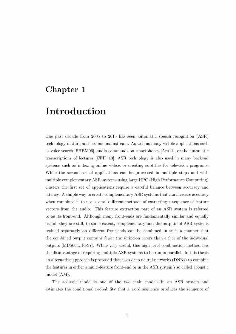
The past decade from 2005 to 2015 has seen automatic speech recognition (ASR)
technology mature and become mainstream. As well as many visible applications such
as voice search [FHBM06], audio commands on smartphones [Aro11], or the automatic
transcriptions of lectures [CFH+13], ASR technology is also used in many backend
systems such as indexing online videos or creating subtitles for television programs.
While the second set of applications can be processed in multiple steps and with
multiple complementary ASR systems using large HPC (High Performance Computing)
clusters the first set of applications require a careful balance between accuracy and
latency. A simple way to create complementary ASR systems that can increase accuracy
when combined is to use several different methods of extracting a sequence of feature
vectors from the audio. This feature extraction part of an ASR system is referred
to as its front-end. Although many front-ends are fundamentally similar and equally
useful, they are still, to some extent, complementary and the outputs of ASR systems
trained separately on different front-ends can be combined in such a manner that
the combined output contains fewer transcription errors than either of the individual
outputs [MBS00a, Fis97]. While very useful, this high level combination method has
the disadvantage of requiring multiple ASR systems to be run in parallel. In this thesis
an alternative approach is proposed that uses deep neural networks (DNNs) to combine
the features in either a multi-feature front-end or in the ASR system’s so called acoustic
model (AM).
The acoustic model is one of the two main models in an ASR system and
estimates the conditional probability that a word sequence produces the sequence of
1
1. INTRODUCTION
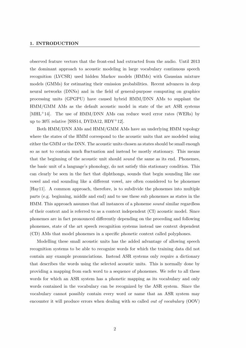
observed feature vectors that the front-end had extracted from the audio. Until 2013
the dominant approach to acoustic modeling in large vocabulary continuous speech
recognition (LVCSR) used hidden Markov models (HMMs) with Gaussian mixture
models (GMMs) for estimating their emission probabilities. Recent advances in deep
neural networks (DNNs) and in the field of general-purpose computing on graphics
processing units (GPGPU) have caused hybrid HMM/DNN AMs to supplant the
HMM/GMM AMs as the default acoustic model in state of the art ASR systems
[MHL+14]. The use of HMM/DNN AMs can reduce word error rates (WERs) by
up to 30% relative [SSS14, DYDA12, HDY+12].
Both HMM/DNN AMs and HMM/GMM AMs have an underlying HMM topology
where the states of the HMM correspond to the acoustic units that are modeled using
either the GMM or the DNN. The acoustic units chosen as states should be small enough
so as not to contain much fluctuation and instead be mostly stationary. This means
that the beginning of the acoustic unit should sound the same as its end. Phonemes,
the basic unit of a language’s phonology, do not satisfy this stationary condition. This
can clearly be seen in the fact that diphthongs, sounds that begin sounding like one
vowel and end sounding like a different vowel, are often considered to be phonemes
[Hay11]. A common approach, therefore, is to subdivide the phonemes into multiple
parts (e.g. beginning, middle and end) and to use these sub phonemes as states in the
HMM. This approach assumes that all instances of a phoneme sound similar regardless
of their context and is referred to as a context independent (CI) acoustic model. Since
phonemes are in fact pronounced differently depending on the proceding and following
phonemes, state of the art speech recognition systems instead use context dependent
(CD) AMs that model phonemes in a specific phonetic context called polyphones.
Modelling these small acoustic units has the added advantage of allowing speech
recognition systems to be able to recognize words for which the training data did not
contain any example pronunciations. Instead ASR systems only require a dictionary
that describes the words using the selected acoustic units. This is normally done by
providing a mapping from each word to a sequence of phonemes. We refer to all these
words for which an ASR system has a phonetic mapping as its vocabulary and only
words contained in the vocabulary can be recognized by the ASR system. Since the
vocabulary cannot possibly contain every word or name that an ASR system may
encounter it will produce errors when dealing with so called out of vocabulary (OOV)
2
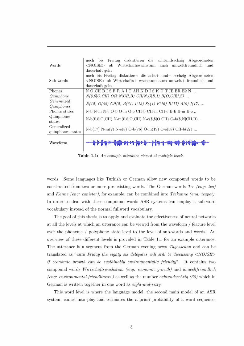
Wordsnoch bis Freitag diskutieren die achtundsechzig Abgeordneten<NOISE> ob Wirtschaftswachstum auch umweltfreundlich unddauerhaft geht
Sub-wordsnoch bis Freitag diskutieren die acht+ und+ sechzig Abgeordneten<NOISE> ob Wirtschafts+ wachstum auch umwelt+ freundlich unddauerhaft geht
Phones N O CH B I S F R A I T AH K D I S K U T IE ER E2 N ...Quinphone N($,$|O,CH) O($,N|CH,B) CH(N,O|B,I) B(O,CH|I,S) ...GeneralizedQuinphones
N(12) O(88) CH(2) B(61) I(13) S(41) F(16) R(77) A(9) I(17) ...
Phones states N-b N-m N-e O-b O-m O-e CH-b CH-m CH-e B-b B-m B-e ..Quinphonesstates
N-b($,$|O,CH) N-m($,$|O,CH) N-e($,$|O,CH) O-b($,N|CH,B) ...
Generalizedquinphones states
N-b(17) N-m(2) N-e(8) O-b(76) O-m(19) O-e(38) CH-b(27) ...
Waveform
Table 1.1: An example utterance viewed at multiple levels.
words. Some languages like Turkish or German allow new compound words to be
constructed from two or more pre-existing words. The German words Tee (eng: tea)
and Kanne (eng: canister), for example, can be combined into Teekanne (eng: teapot).
In order to deal with these compound words ASR systems can employ a sub-word
vocabulary instead of the normal fullword vocabulary.
The goal of this thesis is to apply and evaluate the effectiveness of neural networks
at all the levels at which an utterance can be viewed from the waveform / feature level
over the phoneme / polyphone state level to the level of sub-words and words. An
overview of these different levels is provided in Table 1.1 for an example utterance.
The utterance is a segment from the German evening news Tagesschau and can be
translated as ”until Friday the eighty six delegates will still be discussing <NOISE>
if economic growth can be sustainably environmentally friendly”. It contains two
compound words Wirtschaftswachstum (eng: economic growth) and umweltfreundlich
(eng: environmental friendliness ) as well as the number achtundsechzig (68) which in
German is written together in one word as eight-and-sixty.
This word level is where the language model, the second main model of an ASR
system, comes into play and estimates the a priori probability of a word sequence.
3
1. INTRODUCTION
This is important because certain words or phrases sound similar and the only way to
differentiate them is to look at the linguistic context. Consider the sentence they’re
over there, since there, their and they’re are all pronounced identically prior knowledge
about their usage in sentences is required in order to decide which word was spoken. In
practice this is done by using a model that estimates the probability of the next word
based on the preceding few words. Statistical language models that use the last n− 1
words are called ngram language models and are trained on large amounts of text data
that do not necessarily have to have any audio associated with them. Besides ngram
language models, neural network based language models have been shown to be very
effective at language modeling. In this work the methods of neural networks are applied
at the sub-word level and a sub-word neural network language model is developed for
German that greatly reduces its OOV and significantly improves the WER.
The next part of Table 1.1 shows the sentence represented at the level of phones
and polyphones. Polyphones that consider a context of one phone to the right and
one to the left are called tri-phones and when, like here, two phones to the right and
left are taken into consideration the polyphone is called a quinphone. The notation
CH(N,O|B,I) indicates that the center phone CH is proceeded by the phones N and O,
and followed by the phones B and I. On the phone state level the three states beginning,
middle and end are marked by appending -b, -m or -e to the phone or quinphone. The
phoneset used in this example contains 46 different phonemes with 3 states each as well
as an extra silence phoneme modeled using only a single state which results in over 600
million quinphone states.
Training models to robustly estimate the emission probabilities of over 600 million
states is impossible given the amounts of acoustic model training data currently
available. Most states would have to be estimated using only a few samples and
many states would not contain any examples at all in the training corpus. The models
would also become very large and unwieldy with the HMM/DNN AM requiring a DNN
with a 600 million neuron output layer and 600 million GMMs being necessary for
the HMM/GMM AM. Overcoming this problem requires clustering the quinphones
into clusters of similarly pronounced quinphones called generalized quinphones (e.g.
CH(2) - generalized quinphone with CH as the center phone no. 2) Modeling the
generalized quinphones in multiple states can be done by either first clustering the
phones into generalized quinphones and then using multiple states per generalized
4
quniphone or instead by beginning with the phone states and clustering them into
generalized quinphone states, often called senons. The second approach is the more
popular as it provides more flexibility during clustering [Hua92].
The emission probabilities for each quinphone state in a generalized quinphone state
are the same and are learned using all their examples in the training data. This means
that the number of clusters chosen to group the quinphones into directly determines the
number of GMMs a HMM/GMM AM requires and the size of the output layer in DNN
AM. The standard method of clustering is with the help of classification and regression
trees (cluster trees) that pose questions regarding the properties of the phonetic context
of a phoneme. They require a distance measure between clusters of polyphones in
order to choose the best question to ask for any given context. A commonly used
distance measure is the weighted entropy distance. This is calculated on the mixture
weights from a semi-continuous HMM/GMM system in which a GMM is trained for each
polyphone state encountered during training and all polyphone states with the same
center state use the same set of Gaussians. An equally powerful alternative approach is
presented in this thesis that uses an HMM/DNN AM and allows the weighted entropy
distance to be calculated without either training or evaluating any Gaussians.
The leaves of the cluster tree represent the states in the HMM and correspond to
the neurons in the output layer of the DNN. The other important aspects of a DNN AM
are its topology and the input features on which it is trained. In contrast to the default
topology which consists of just a feed forward neural network with an input layer for
the features, a number of equally sized hidden layers that are fully connected to their
neighbours and an output layer, this thesis proposes a new modular topology. It involves
training deep, possibly multi-stream, feature extractors using a multilayer perceptron
(MLP) containing a so called bottleneck which is a hidden layer that is reduced in size
to the dimension of the desired feature vector. After training, all layers following the
bottleneck are discarded. The remaining network maps the input features to so called
bottleneck features (BNFs) or to deep bottleneck features (DBNFs). The proposed
modular DNN AM uses one or more pretrained DBNF networks and combines the
outputs from multiple neighbouring time frames as the input to a further feed forward
neural network. During the joint training, weight sharing is used to average the changes
accumulated by a DBNF network at various time frames.
5
1. INTRODUCTION
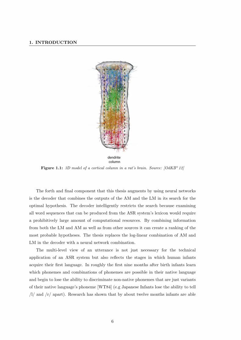
Figure 1.1: 3D model of a cortical column in a rat’s brain. Source: [OdKB+12]
The forth and final component that this thesis augments by using neural networks
is the decoder that combines the outputs of the AM and the LM in its search for the
optimal hypothesis. The decoder intelligently restricts the search because examining
all word sequences that can be produced from the ASR system’s lexicon would require
a prohibitively large amount of computational resources. By combining information
from both the LM and AM as well as from other sources it can create a ranking of the
most probable hypotheses. The thesis replaces the log-linear combination of AM and
LM in the decoder with a neural network combination.
The multi-level view of an utterance is not just necessary for the technical
application of an ASR system but also reflects the stages in which human infants
acquire their first language. In roughly the first nine months after birth infants learn
which phonemes and combinations of phonemes are possible in their native language
and begin to lose the ability to discriminate non-native phonemes that are just variants
of their native language’s phoneme [WT84] (e.g Japanese Infants lose the ability to tell
/l/ and /r/ apart). Research has shown that by about twelve months infants are able
6
1.1 Contributions
to recognize from about a dozen to over a hundred individual words as well as some
short phrases like “come here” [FDR+94, CBC+95] and their vocabulary will continue
to steadily increase. Children learn various simple multi-word utterances from about
1-2 years of age [Bro73] and then from about the age of three begin to understand
the structure of sentences [NRP11a]. Both their vocabulary and their knowledge of
grammar continues to improve as they grow older.
The deep neural networks used in this work are themselves inspired by the structure
of the nervous system. Like their biological counterparts the individual artificial neurons
contain a number of inputs from other neurons that can cause them to activate (fire)
sending a signal on to their downstream neurons. Figure 1.1 depicts a 3D model of a
cortical column, a group of neurons in the cerebral cortex or outer layer of the brain,
that appears structurally similar to a feed forward deep neural network.
Despite these similarities and the their biological motivation there are still major
differences between the artificial neural networks and biological neural networks that
connot be ignored. Artificial neural networks run synchronously in discrete time steps
but biological neural networks work asynchronously. Depending on the activation
function the output of an artificial neuron can have many possible values whereas
real neurons can only either fire or not fire and therefore convey information using the
frequency with which they fire. Further differences can be found in the way the weights
are learned in artificial neural network and how the connections are formed and pruned
in biological neural networks.
The analogy of speech recognition technology to the development of language
understanding in humans should not be carried too far. Human brains do not learn
language perception in isolation: Speech production and perception complement each
other and unlike ASR systems, words are also learned and associated with certain real
world objects or actions.
1.1 Contributions
As eluded to earlier this thesis is concerned with the improvement to or introduction
of neural networks to the four major components of an ASR system:
7
1. INTRODUCTION
� Front-end: Existing techniques for deep bottleneck are expanded upon to build
multi-stream bottleneck features that combine several different front-ends. Their
topologies are optimized and their performances evaluated.
� Acoustic model: Introduction of multi-stream deep neural network acoustic
models that also combine several different front-ends and improve upon DNNs
that only use a single input feature. Modular deep neural network acoustic models
are presented which use one or more multi-stream bottleneck networks applied at
multiple time frames as the basis of the deep neural network, and are shown to
significantly improve the performance of DNN AMs. A method of constructing a
cluster tree using a CD DNN AM is described and is shown to be slightly better
than the GMM AM based approach. Contributions are also made in the use of
singular value decomposition (SVD) in initializing new layers in DNNs, where
this thesis evaluates some of its applications and shows how it can both increase
the performance of a DNN as well as reduce the number of its parameters.
� Language model: A sub-word vocabulary is proposed and shown to be very
effective at reducing both the OOV rate and the WER of German ASR systems.
A standard approach for building word level language models is adapted and used
to build a sub-word neural network language model. An error analysis shows how
it noticeably reduces the number of errors from compound words.
� Decoder: A combination neural network is designed to optimally combine the
outputs of the language model and acoustic model as well as other features such
as word count. It is integrated into the ASR system as a replacement for the
standard log linear model combination and can be trained directly on the system’s
training data without the need of a development set to optimize the interpolation
parameters.
1.2 Overview and Structure
This thesis is structured as follows. The required theoretical background knowledge is
covered in chapter 2 with section 2.1 presenting an overview of neural networks, their
training methods and the parameters that affect their performance. An overview of
the structure of an ASR system, including a description of its four major components,
8
1.2 Overview and Structure
is given in section 2.2 as well as an explanation of the metric used to evaluate the
performance of ASR systems. The chapter continues with an overview of the related
research and concludes by explaining how this thesis fits into the context of that related
work.
Chapter 3 explores the speech recognition tasks on which the achievements of the
thesis are evaluated, with section 3.4 introducing the data sets on which the WER are
measured and section 3.5 examining and analysing the various training corpera. This
chapter also discusses the structure of our baseline ASR system in section 3.6 with an
overview of our neural network training presented in section 3.7.
Feature extraction using neural networks is discussed in chapter 4. It begins in
section 4.1 with an overview of the 4 different features, lMEL, MFCC, MVDR and
tonal features used in the following experiments. After a general introduction to
bottleneck features the first initial experiments on combining two feature streams,
MVDR and MFCC, are discussed in section 4.3. This is followed in section 4.3.2.1 by
an investigation into the optimal topology for a deep MVDR+MFCC bottleneck MLP
and section 4.3.2.2 where various combinations of the 4 input features are compared to
each other. Integration level experiments are performed in section 4.3.3 and section 4.4
presents optimized training strategies for large DBNF based GMM AMs.
Chapter 5 is devoted to the analysis of neural network acoustic models. It begins
with an analysis of the effects of different input feature combinations to the deep neural
network in section 5.2.1 and moves on to present the modular deep neural network in
section 5.2.2. This is followed in section 5.3 by a method of building cluster trees using
DNNs and section 5.4 which shows how new hidden layers can be initialized using SVD.
A subword language model is presented in chapter 6. The proposed subword
vocabulary, explained in section 6.2.1, is designed to alleviate the errors found in the
error analysis in section 6.1. After analyzing the performance on an ngram language
model in section 6.2.4 the proposed subword neural network language model is described
and evaluated in section 6.3. The chapter is finished with a discussion of the subword
vocabulary’s integration into the lecture translation system installed at the KIT in
section 6.4.
Chapter 7 describes a neural network that can be used to combine the output of an
AM and an LM. Its topology is presented in section 7.2 and the error function required
to train it is explained in section 7.2.1. The results are then discussed in section 7.3
9

1. INTRODUCTION
The thesis in concluded with a short summary in chapter 9 and contains appendices
with additional information on the language model data and the backpropagation
algorithm as well as a detailed derivative of MMIE error function required to train
the combination neural network.
10
Chapter 2
Theory und Related Work
This chapter briefly lays out the required theoretical foundations in the fields of
automatic speech recognition (ASR) and artificial neural networks (ANN) on which
the experiments performed in this thesis are based. It covers the design and training of
neural networks, explains the parameters that have to be considered when training a
neural network and how neural networks can be used in various ASR components. An
overview of the structure of an ASR system is given together with an introduction of
its major components.
Since neural networks have seen many uses in ASR over the years an overview and
description of approaches similar to the ones examined in the thesis is also presented
in this chapter followed by a discussion on how this thesis fits into the context of that
related work.
2.1 Neural Network Basics
Artificial neural networks are biologically motived statistical models that can be trained
using data to solve various different problems such as character recognition, playing
backgammon or controlling a robot arm. They consist of a number of individual
artificial neurons that are connected to each other, often organized into layers. Some
neurons are referred to as input neurons and instead of possessing incoming connections
they allow their values to be set, thereby acting as the inputs to the neural network.
Analogously output neurons do not forward their output to other neurons but instead
present it as the output of the neural network. The character recognition neural
11
2. THEORY UND RELATED WORK
network, for example, might have 1024 input neurons mapped to the pixels of a 32
pixel by 32 pixel image and 26 output neurons, one for each letter in the English
alphabet.
2.1.1 Perceptron
A neural network consisting of only a single neuron is called a perceptron. The model
has m inputs x0..xm − 1 that can be real numbers and are connected to the neuron
together with an extra input xm that is always set to +1. Each connection is associated
with a weight w0..wm. The weight wm that is always connected to +1 is called the
bias. The output y of the perceptron is computed by multiplying each input with its
connection’s weight, adding all these values together and then applying a so called
activation function ϕ.
y = ϕ
m∑j=0
wjxj
(2.1)
There are many possible activation functions and while the original model proposed by
Rosenblatt [Ros57] uses the heaviside step function the sigmoid activation is currently
more popular due to its useful properties in multilayer neural networks:
ϕstep(x) =
{1 if x > 0
0 if x ≤ 0(2.2)
ϕsig(x) = sigmoid(x) =1
1 + e−x(2.3)
The perceptron model is a form of nonparametric supervised classification and requires
a set of labeled training examples (x1, t1)..(xn, tn) on which the optimal weights can
be learned. For the original perceptron model using the Heaviside step function as the
activation function the following weight update rule can be used for all weights wi:
ws+1i = wsi + η(tj − yj)xj,i (2.4)
where yt is the output of the network for the input xi, η is the learning rate with
0 < η ≤ 1 and s the current iteration. The update rule is repeated either until
convergence or for a certain number of iterations. Due to its simplicity the perceptron
12
2.1 Neural Network Basics
x0 x1 xm-1
W12
W23
W34
hidden layer 1 with bias b2
hidden layer 2 with bias b3
o1 o2 on
output layer with bias b4
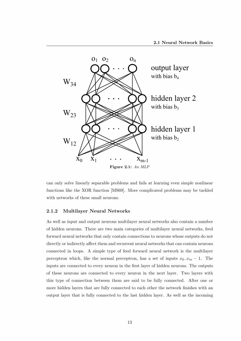
Figure 2.1: An MLP
can only solve linearly separable problems and fails at learning even simple nonlinear
functions like the XOR function [MS69]. More complicated problems may be tackled
with networks of these small neurons.
2.1.2 Multilayer Neural Networks
As well as input and output neurons multilayer neural networks also contain a number
of hidden neurons. There are two main categories of multilayer neural networks, feed
forward neural networks that only contain connections to neurons whose outputs do not
directly or indirectly affect them and recurrent neural networks that can contain neurons
connected in loops. A simple type of feed forward neural network is the multilayer
perceptron which, like the normal perceptron, has a set of inputs x0..xm − 1. The
inputs are connected to every neuron in the first layer of hidden neurons. The outputs
of these neurons are connected to every neuron in the next layer. Two layers with
this type of connection between them are said to be fully connected. After one or
more hidden layers that are fully connected to each other the network finishes with an
output layer that is fully connected to the last hidden layer. As well as the incoming
13
2. THEORY UND RELATED WORK
connections each neuron also has its own bias and activation function.
An example MLP with 2 hidden layers is presented in Figure 2.1. Such MLPs are
often referred to as having 4 layers: an input layer, 2 hidden layers and an output
layer. Since the input layer doesn’t contain any functionality it is often ignored and the
network is said to have 3 layers. This thesis uses the more common 4 layer description.
If we look at the transition between two layers where the first layer has n1 neurons and
the second layer has n2 then there will be n1×n2 weights connecting the two layers as
well as n2 biases. Using a vector notation we can write the outputs y1 of the first layer
as y1 ∈ Rn1 , the outputs y2 of the second layer as y2 ∈ Rn2 , the weights wi,j connecting
the two layers can be thought of as a matrix W1,2 ∈ Rn2×n1 and the biases as the vector
b2 ∈ Rn2 allowing their relationship to be expressed using this equation:
y2 = ϕ (W1,2 · y1 + b2) (2.5)
Applying the activation function ϕ to a vector is defined as applying it separately
to each component. The example MLP in Figure 2.1 can now be described using three
weight matrices W1,2,W2,3,W3,4 and three vectors b2, b3, b4:
h1 =ϕ (W1,2 · x+ b2) (2.6)
h2 =ϕ (W2,3 · h1 + b3) (2.7)
o =ϕ (W3,4 · h2 + b4) (2.8)
where x is the input vector, h1 and h2 are the outputs of the hidden layers and o
is the output vector of the MLP. When used for classification it is common to have
one output neuron per class and use the one of n encoding for the class labels. The
one of n encoding represents the class j as an n dimensional vector with a 1 in
position j and zeros everywhere else. As in the case of the simple perceptron these
parameters (weights and biases) have to be trained using a set of labeled training
examples (x1, tx1)...(xN , txN ) which is typically performed using the backpropagation
algorithm.
14
2.1 Neural Network Basics
2.1.3 Backpropagation Algorithm
The backpropagation algorithm is a two phase supervised method for training neural
networks by first, in the forward phase, sending examples through the network and
accumulating the errors made by the network and then, in the backward phase,
propagating the error back though the network while using it to update the network’s
weights. It is, therefore, sometimes called backward propagation of errors.
A summary of the algorithm is ommited here but can be found in appendex B.
Using the derived δk the update rule can now be written as:
ws+1ji ← wsji + ηδkxji (2.9)
This works for any feed forward neural network topology. The algorithm, however,
cannot decide how the topology should look, which error function and which activations
to use or what to set the learning rate η to. These, so called hyperparameters, have to
be optimized independently of the learning algorithm.
2.1.4 Hyperparameters in Neural Networks
Neural networks depend on two types of parameters: weights ~w and Hyperparameters
~θ. Weights ~w can be learned by acquiring a set X of labeled examples and performing
backpropagation in order to find the weights ~w that minimize an error function.
Hyperparameters have to be intelligently selected by the neural network designer before
the neural network can be trained. This section will cover three hyperparameters that
are relevant to this thesis, the error and activation functions as well as how to choose
the best learning rate and why a constant learning rate may not be the best choice.
2.1.4.1 Error Functions
The two most common error functions are the mean squared error (MSE) error function
and the cross entropy (CE) error function [B+95]. The MSE error function defined in
equation B.1 penalizes large differences more than small differences and performs well
on tasks such as function approximation and in cases where the outputs of the NN are
real values and do not simply lie between 0 and 1.
15
2. THEORY UND RELATED WORK
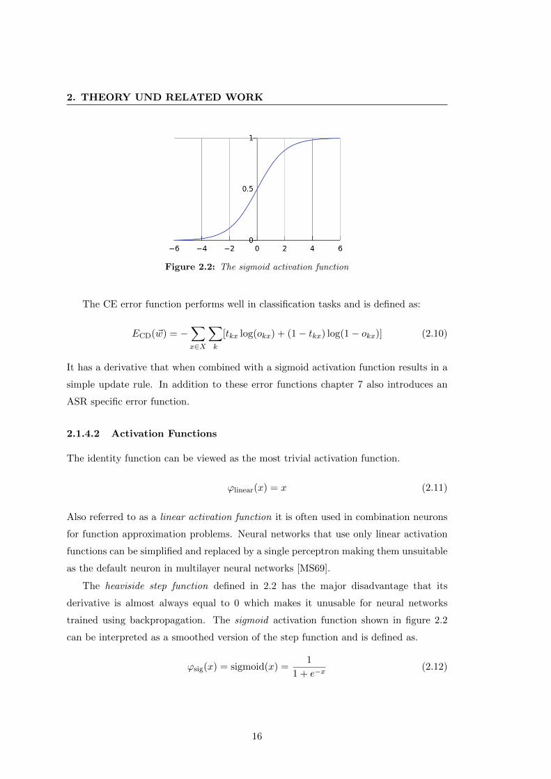
Figure 2.2: The sigmoid activation function
The CE error function performs well in classification tasks and is defined as:
ECD(~w) = −∑x∈X
∑k
[tkx log(okx) + (1− tkx) log(1− okx)] (2.10)
It has a derivative that when combined with a sigmoid activation function results in a
simple update rule. In addition to these error functions chapter 7 also introduces an
ASR specific error function.
2.1.4.2 Activation Functions
The identity function can be viewed as the most trivial activation function.
ϕlinear(x) = x (2.11)
Also referred to as a linear activation function it is often used in combination neurons
for function approximation problems. Neural networks that use only linear activation
functions can be simplified and replaced by a single perceptron making them unsuitable
as the default neuron in multilayer neural networks [MS69].
The heaviside step function defined in 2.2 has the major disadvantage that its
derivative is almost always equal to 0 which makes it unusable for neural networks
trained using backpropagation. The sigmoid activation function shown in figure 2.2
can be interpreted as a smoothed version of the step function and is defined as.
ϕsig(x) = sigmoid(x) =1
1 + e−x(2.12)
16
2.1 Neural Network Basics
It is easy to differentiate (dϕ(x)dx = ϕ(x)(1−ϕ(x))) and has a tendency to saturate which
happens when the input is either very large or very small thereby putting it in a state
where its derivative will be very close to zero which then leads to very small weight
updates. Depending upon where and when it happens this saturation effect can have
either positive or negative consequences.
The sigmoid activation function can be generalized to a group of neurons in such a
way that their output sums to one and forms a discrete probability distribution.
ϕsoftmax(netj) =enetj∑k e
netk(2.13)
This is called the softmax activation function and is common in classification tasks
where the goal is to use a neural network to find the probability P (c|f) that a particular
input f is a member of a certain class ci.
All real activation functions discussed so far have only had possible output values
between 0 and 1. In cases where negative outputs are also required the hyperbolic
tangent is often a good choice:
ϕtanh(x) = tanh(x) =ex − e−x
ex + e−x(2.14)
It has the added advantage of not changing the mean of the input from 0 if the input
already has a mean of 0.
In recent years rectified linear units have become quite popular in deep neural
networks [NH10]. They are neurons with an easy to compute activation function:
ϕReLU(x) = =
{x if x > 0
0 if x ≤ 0(2.15)
A neural network using these neurons will only have about half its neurons active (6= 0)
at any particular time making it more sparse than networks not using rectified linear
units.
2.1.4.3 Learning Rate Schedule
The learning rate determines by how much a weight parameter is updated each iteration:
wji ← wji + ηδjxji (2.16)
17
2. THEORY UND RELATED WORK
Choosing a constant learning rate can be problematic because if a large learning rate
is chosen then it may quickly saturate some of the neurons and it could also lead to
the learning algorithm constantly jumping past the minimum. If, on the other hand,
a very small learning rate is chosen then the learning procedure will slow down and it
may get stuck in a local minimum. For these reasons it is advisable to use a learning
rate schedule instead of a constant learning rate.
We can observe that starting with a high learning rate and reducing it later results
in our learning algorithm both converging fast and tending to find a better minimum.
We can accomplish this using various learning rate strategies:
� Predetermined piecewise constant learning rate: Use a predetermined
sequence of ηi. After ever epoch (or every n training examples) the learning
rate is replaced with the next one in the list. This has the disadvantage that we
have to set a whole list of learning rates.
� Exponentially decaying learning rate: Multiply an initial learning rate by a
constant factor α ( 0 < α < 1 ) after ever epoch: ηt = ηt−1 ∗ α = η0 ∗ αt
� Performance scheduling: Periodically measure the error on a cross validation
set and decrease the learning rate when the learning routine stops showing
improvements on the cross validation set.
� Weight dependent learning rate methods: Use a different learning rate
for parameter (weight or bias). Algorithms like AdaGrad and AdaDec can be
employed to compute and decay η on a per-parameter basis.
� Newbob learning rate schedule: The newbob learning rate schedule is a
combination of the performance scheduling and exponentially decaying learning
rate. At first the learning rate is kept constant and the performance of the
neural network is measured on a validation set every epoch (or every n training
examples). A soon as the validation error shows that the network’s improvement
has dropped below a predetermined threshold it switches to an exponentially
decaying learning rate schedule and decays the learning rate every epoch. The
performance on the validation set is still measured and used as a termination
criterion when the network’s improvement again dips below a predetermined
threshold.
18
2.1 Neural Network Basics
Most of the neural networks trained in this thesis use the Newbob learning rate
schedule.
2.1.5 Autoencoders and Pre-Training of Deep Neural Networks
Neural networks with multiple hidden layers are often referred to as deep neural
networks (DNNs). Since the introduction of deep belief networks (DBN) by Hinton et
al. in 2006 [HOT06], DNNs have become very popular in the field of machine learning
and have outperformed other approaches in many machine learning and classification
tasks making them the default technique for solving complex or high dimensional
classification problems [Ben09]. The exact point at which a neural network becomes a
deep neural network is not well defined [Sch15] but in general DNNs will have some of
the following properties:
� Multiple hidden layers: A neural network requires at least 2 hidden layers in order
to be considered deep. In some cases, as in bottleneck feature MLPs, deep neural
networks will have at least 4 hidden layers [Geh12]. The multiple hidden layers
in a DNN should allow it to represent complex functions with fewer weights than
shallow DNNs.
� Large layers: While the individual layers in a DNN may be somewhat smaller
than the layers in a shallow NN designed for the same purpose, they will not be
multiple orders of magnitude smaller. With multiple fully connected layers the
number of weight parameters in a DNN will be quite high: From a few tens of
thousands of parameters to well over a few tens of millions of parameters.
� Large training sets: DNNs tend to be trained on large amounts of annotated
data. This property is very task dependent and in part related to the necessity of
a large amount of data being required to train the large number of parameters.
� Trained on GPUs: The consequence of having many parameters and a large set of
training examples is that training becomes very computationally expensive and
time consuming. GPU based backpropagation implementations have been shown
to be several orders of magnitude faster than basic CPU based implementations
[JO+13] allowing networks to be trained in hours or days instead of weeks or
19
2. THEORY UND RELATED WORK
x ~x
hidden layer
z
corruption
autoencoder
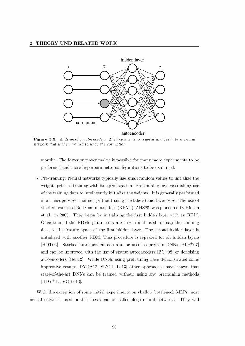
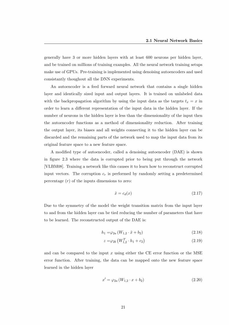
Figure 2.3: A denoising autoencoder. The input x is corrupted and fed into a neuralnetwork that is then trained to undo the corruption.
months. The faster turnover makes it possible for many more experiments to be
performed and more hyperparameter configurations to be examined.
� Pre-training: Neural networks typically use small random values to initialize the
weights prior to training with backpropagation. Pre-training involves making use
of the training data to intelligently initialize the weights. It is generally performed
in an unsupervised manner (without using the labels) and layer-wise. The use of
stacked restricted Boltzmann machines (RBMs) [AHS85] was pioneered by Hinton
et al. in 2006. They begin by initializing the first hidden layer with an RBM.
Once trained the RBMs parameters are frozen and used to map the training
data to the feature space of the first hidden layer. The second hidden layer is
initialized with another RBM. This procedure is repeated for all hidden layers
[HOT06]. Stacked autoencoders can also be used to pretrain DNNs [BLP+07]
and can be improved with the use of sparse autoencoders [BC+08] or denoising
autoencoders [Geh12]. While DNNs using pretraining have demonstrated some
impressive results [DYDA12, SLY11, Le13] other approaches have shown that
state-of-the-art DNNs can be trained without using any pretraining methods
[HDY+12, VGBP13].
With the exception of some initial experiments on shallow bottleneck MLPs most
neural networks used in this thesis can be called deep neural networks. They will
20
2.1 Neural Network Basics
generally have 3 or more hidden layers with at least 600 neurons per hidden layer,
and be trained on millions of training examples. All the neural network training setups
make use of GPUs. Pre-training is implemented using denoising autoencoders and used
consistantly thoughout all the DNN experiments.
An autoencoder is a feed forward neural network that contains a single hidden
layer and identically sized input and output layers. It is trained on unlabeled data
with the backpropagation algorithm by using the input data as the targets tx = x in
order to learn a different representation of the input data in the hidden layer. If the
number of neurons in the hidden layer is less than the dimensionality of the input then
the autoencoder functions as a method of dimensionality reduction. After training
the output layer, its biases and all weights connecting it to the hidden layer can be
discarded and the remaining parts of the network used to map the input data from its
original feature space to a new feature space.
A modified type of autoencoder, called a denoising autoencoder (DAE) is shown
in figure 2.3 where the data is corrupted prior to being put through the network
[VLBM08]. Training a network like this causes it to learn how to reconstruct corrupted
input vectors. The corruption cr is performed by randomly setting a predetermined
percentage (r) of the inputs dimensions to zero:
x = cd(x) (2.17)
Due to the symmetry of the model the weight transition matrix from the input layer
to and from the hidden layer can be tied reducing the number of parameters that have
to be learned. The reconstructed output of the DAE is:
h1 =ϕ2a (W1,2 · x+ b2) (2.18)
z =ϕ2b
(W T
1,2 · h1 + c2)
(2.19)
and can be compared to the input x using either the CE error function or the MSE
error function. After training, the data can be mapped onto the new feature space
learned in the hidden layer
x′ = ϕ2a (W1,2 · x+ b2) (2.20)
21
2. THEORY UND RELATED WORK
and the procedure repeated using x′ as the input to the DAE:
x′ = cd(x′) (2.21)
h2 =ϕ3a
(W2,3 · x′ + b3
)(2.22)
z′ =ϕ3b
(W T
2,3 · h2 + c3)
(2.23)
where z′ is now compared to x′ in this DEA’s error function. After all hidden layers
have been pre-trained a final classification output layer can be added and the whole
stack of autoencoders transformed into a DNN. This setup has been demonstrated to
work well in both image recognition [VLL+10] and speech recognition tasks [Geh12]
2.2 Overview of Automatic Speech Recognition
Automatic speech recognition systems aim to extract the sequence of words spoken in
an audio signal or audio file. In both cases microphones are used to measure variations
in air pressure that are then digitized and either saved to file or sent directly to the
ASR system. When the digitized audio is sent directly to the ASR system we talk
about online ASR and in the other case, where recorded audio files are processed, it is
called offline or batch ASR.
The audio signal or file is then feed to the front-end of an ASR system which
analyzes it and converts it into a sequence of feature vectors X. We now wish to find
the most probable sequence of words W , given this sequence of feature vectors X.
W = argmaxW
P (W |X) (2.24)
The application of the Bayes’ rule to this probability gives us the fundamental formula
of speech recognition, where the prior probability p(X) of the feature sequence X can
be ignored due it being constant for all word sequences.
W = argmaxW
P (W |X) = argmaxW
p(X|W )P (W )
p(X)(2.25)
= argmaxW
P (X|W )P (W ) (2.26)
Individual parts of this formula correspond to the four main components of an ASR
that was informally discussed in chapter 1. The front-end extracts the feature vectors
22
2.2 Overview of Automatic Speech Recognition
"Hallo"
"can you hear me"
"is this thing switched on"
Language
Model
Acoustic
Model
Feature
ExtractionDecoder
Transcribed TextSpeech Input
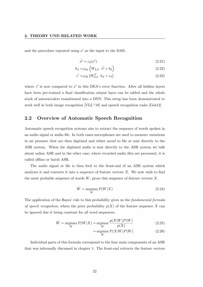
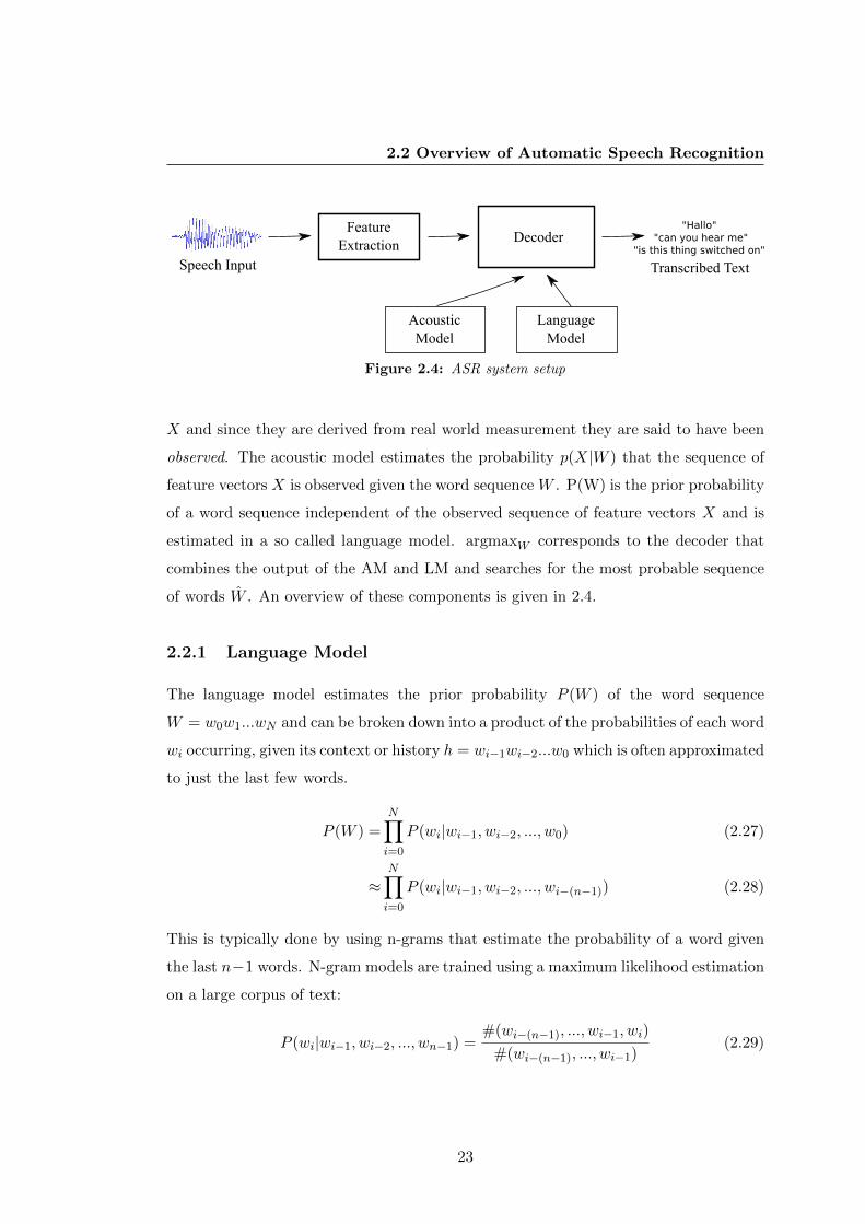
Figure 2.4: ASR system setup
X and since they are derived from real world measurement they are said to have been
observed. The acoustic model estimates the probability p(X|W ) that the sequence of
feature vectors X is observed given the word sequence W . P(W) is the prior probability
of a word sequence independent of the observed sequence of feature vectors X and is
estimated in a so called language model. argmaxW corresponds to the decoder that
combines the output of the AM and LM and searches for the most probable sequence
of words W . An overview of these components is given in 2.4.
2.2.1 Language Model
The language model estimates the prior probability P (W ) of the word sequence
W = w0w1...wN and can be broken down into a product of the probabilities of each word
wi occurring, given its context or history h = wi−1wi−2...w0 which is often approximated
to just the last few words.
P (W ) =N∏i=0
P (wi|wi−1, wi−2, ..., w0) (2.27)
≈N∏i=0
P (wi|wi−1, wi−2, ..., wi−(n−1)) (2.28)
This is typically done by using n-grams that estimate the probability of a word given
the last n−1 words. N-gram models are trained using a maximum likelihood estimation
on a large corpus of text:
P (wi|wi−1, wi−2, ..., wn−1) =#(wi−(n−1), ..., wi−1, wi)
#(wi−(n−1), ..., wi−1)(2.29)
23
2. THEORY UND RELATED WORK
Depending on the value of n we speak of uni-grams (n = 1), bi-grams (n = 2), tri-gram
(n = 3), 4-grams (n = 4) and so on. In ASR, language models normally use values of
n from about 3 to 5 but even for the smaller bi-grams it would be impossible to find
training examples for each word in every possible context, leading to some estimates
being 0. Sentences containing these n-grams could never be recognized by the ASR
system because the LM would give them a prior probability of 0. Statistical n-gram
models use two techniques to combat this problem discounting and smoothing.
Discounting reduces the probabilities of the nonzero estimates by a small amount
and smoothing intelligently redistributes this discounted probability mass across the
other the ngrams for which no training example are given. This can be done by backing
off to the estimate of a lower order n-gram or even to the unigram if none of the lower
order ngrams are non-zero. Alternatively an ngram model can be interpolated with all
of its lower order models [CG96].
Neural network language models on the other hand do not suffer from this sparseness
problem as they begin by mapping the n − 1 words in the history of the n-gram into
a continuous vector space such as Rm, where similar words are closer together. The
n − 1 word vectors are concatenated together and used as the input layer to a DNN
where the softmax output layer contains a neuron for every word [Sch07]. While more
powerful than ngram-LMs NN LMs have some disadvantages: they take at lot longer
to train, require a method of word vectorization (embedding), are much slower than
ngram-LMs at runtime and it is infeasible to have an output layer that is as large as
the typical vocabulary used in LVCSR.
The training time can be reduced by only using the most useful training data and
not all the available data. Word embedding can either be performed prior to training
the NN using a dedicated algorithm (or external tool like word2vec [MCCD13]) or
while training the NN by providing the words using the 1-of-n-encoding and learning a
shared projection matrix. When the vocabulary becomes to large for the output layer
to handle, it can be reduced to a shortlist that covers 80-95% of the expected words
and the remaining words are modeled using a normal n-gram LM [Sch07]. NN LMs can
be speeded up a bit during decoding by caching the whole output layer or alternatively,
methods exist that can convert them into backoff ngram LMs [AKV+14]. If they are
only used in a second pass after all contexts required for an utterance are already known
then these can be efficiently precomputed in batch mode.
24
2.2 Overview of Automatic Speech Recognition
Two broad catagories of neural networks are used for language modelling, recurrent
neural networks [SSN12, MKB+10] where a hidden layer depends on the previous word’s
hidden layer and the vector representation of the current word to predict its successor
and feed forward neural networks [Sch07] which have a fixed input context of word
representations.
2.2.2 Acoustic Model
The acoustic model estimates the conditional probability p(X|W ) that the sequence
of observed feature vectors X = x0, ..., xT is produced by the word sequence
W = w0, ..., wN . Its units of modeling are, as discussed in chapter 1, at the subphoneme
level which are assumed to be stationary, i.e the observations will be constant for a
period time spanned by one or more feature vectors or frames. Both common types of
acoustic models HMM/DNNs and HMM/GMMs use hidden Markov models to model
their structure and to describe how the subphoneme acoustic units are concatenated
together to form the sequence of words [Rab89].
2.2.2.1 Hidden Markov Model (HMM)
An HMM models a system where a sequence of visible observations o0, o1, ..., oT depend
on an internal sequence of hidden states s0, s1, ..., sT . The Markov assumption of this
model means that the probability of transitioning to a state depends only on the current
state. They are defined over a vocabulary V and a set of states S = s1, s2, .... [Fuk13]
For each state si there is a probability p(sj |sj) of transitioning to sj and each state
has an emission probability distribution that describes the emission probabilities of the
symbols in the Vocabulary V after transitioning to the state. When applied to ASR
systems that vocabulary V is the set of all possible feature vectors, typically Rn. Due
to its continuous nature the emission probabilities are estimated using the probability
density function p(xt|st). The transition probabilities between the states are defined
by the HMM’s topology which often limits the possible transitions by setting some of
them to 0. In a three state (beginning, middle, end) topology, for example, a particular
phoneme’s beginning state may only have non-zero connections to itself and to the
phoneme’s middle state while the end state would have connections to itself and to all
other phonemes’ beginning states.
25
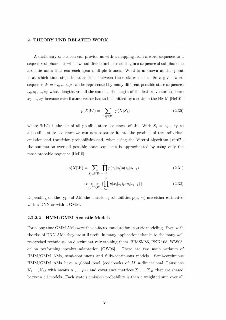
2. THEORY UND RELATED WORK
A dictionary or lexicon can provide us with a mapping from a word sequence to a
sequence of phonemes which we subdivide further resulting in a sequence of subphoneme
acoustic units that can each span multiple frames. What is unknown at this point
is at which time step the transitions between these states occur. So a given word
sequence W = w0, ..., wN can be represented by many different possible state sequences
s0, s1, ..., sT whose lengths are all the same as the length of the feature vector sequence
x0, ..., xT because each feature vector has to be emitted by a state in the HMM [Hei10]:
p(X|W ) =∑
Sj∈S(W )
p(X|Sj) (2.30)
where S(W ) is the set of all possible state sequences of W . With Sj = s0, ...sT as
a possible state sequence we can now separate it into the product of the individual
emission and transition probabilities and, when using the Viterbi algorithm [Vit67],
the summation over all possible state sequences is approximated by using only the
most probable sequence [Hei10].
p(X|W ) =∑
Sj∈S(W )
T∏t=1
p(xt|st)p(st|st−1) (2.31)
≈ maxSj∈S(W )
{T∏t=1
p(xt|st)p(st|st−1)} (2.32)
Depending on the type of AM the emission probabilities p(xt|st) are either estimated
with a DNN or with a GMM.
2.2.2.2 HMM/GMM Acoustic Models
For a long time GMM AMs were the de-facto standard for acoustic modeling. Even with
the rise of DNN AMs they are still useful in many applications thanks to the many well
researched techniques on discriminatively training them [BBdSM86, PKK+08, WW03]
or on performing speaker adaptation [GW96]. There are two main variants of
HMM/GMM AMs, semi-continuous and fully-continuous models. Semi-continuous
HMM/GMM AMs have a global pool (codebook) of M n-dimensional Gaussians
N1, ...,NM with means µ1, ..., µM and covariance matrices Σ1, ...,ΣM that are shared
between all models. Each state’s emission probability is then a weighted sum over all
26
2.2 Overview of Automatic Speech Recognition
the Gaussians.
p(xi|si) =M∑j=1
aijNj(xi, µj ,Σj) (2.33)
Fully continuous HMM/GMM AMs differ by not having a global pool of Gaussians and
instead use a separate set Gaussians for each state.
p(xi|si) =M∑j=1
aijNji(xi, µji,Σji) (2.34)
In some systems both approaches are combined by having codebooks that are shared
by only some states, e.g. all variants of a phone state in a CD-AM.
It is beneficial for feature vectors to be augmented by either their differences with
neighbouring features or by using a window of feature vectors instead of a single feature
vector. In both cases the dimension of the feature vector sequence sent to the ASR
system can easily become very large resulting in larger dimensional Gaussians that
require more parameters. Dimensionality reduction techniques are therefore required
in order to still benefit from the stacked feature vectors without inflating the number
of parameters in the GMM AM. A common method for performing this dimensionality
reduction is the principal component analysis (PCA) which can be learned without
labels and performs a linear transformation of the features into a decorrelated feature
space where the first few dimensions contain most of the variance. Linear discriminant
analysis (LDA) is an alternative linear approach that is trained with label information
and is optimized for class separability [Fuk13]. Chapter 4 will present and expand on
another common method that uses an MLP with a small hidden layer for dimensionality
reduction.
2.2.2.3 HMM/DNN Acoustic Models
HMM/DNN AMs do not have a problem with large feature vectors and can, without
resorting to dimensionality reduction preprocessing steps, even use very large windows
of stacked features. They are modeled with a DNN that uses the (stacked) feature
vector as the input layer and, after multiple hidden layers, have an output layer whose
neurons correspond to the states in the HMM. Using the softmax activation function
27
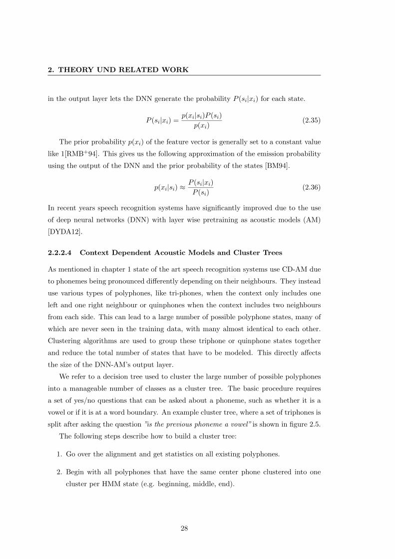
2. THEORY UND RELATED WORK
in the output layer lets the DNN generate the probability P (si|xi) for each state.
P (si|xi) =p(xi|si)P (si)
p(xi)(2.35)
The prior probability p(xi) of the feature vector is generally set to a constant value
like 1[RMB+94]. This gives us the following approximation of the emission probability
using the output of the DNN and the prior probability of the states [BM94].
p(xi|si) ≈P (si|xi)P (si)
(2.36)
In recent years speech recognition systems have significantly improved due to the use
of deep neural networks (DNN) with layer wise pretraining as acoustic models (AM)
[DYDA12].
2.2.2.4 Context Dependent Acoustic Models and Cluster Trees
As mentioned in chapter 1 state of the art speech recognition systems use CD-AM due
to phonemes being pronounced differently depending on their neighbours. They instead
use various types of polyphones, like tri-phones, when the context only includes one
left and one right neighbour or quinphones when the context includes two neighbours
from each side. This can lead to a large number of possible polyphone states, many of
which are never seen in the training data, with many almost identical to each other.
Clustering algorithms are used to group these triphone or quinphone states together
and reduce the total number of states that have to be modeled. This directly affects
the size of the DNN-AM’s output layer.
We refer to a decision tree used to cluster the large number of possible polyphones
into a manageable number of classes as a cluster tree. The basic procedure requires
a set of yes/no questions that can be asked about a phoneme, such as whether it is a
vowel or if it is at a word boundary. An example cluster tree, where a set of triphones is
split after asking the question ”is the previous phoneme a vowel” is shown in figure 2.5.
The following steps describe how to build a cluster tree:
1. Go over the alignment and get statistics on all existing polyphones.
2. Begin with all polyphones that have the same center phone clustered into one
cluster per HMM state (e.g. beginning, middle, end).
28
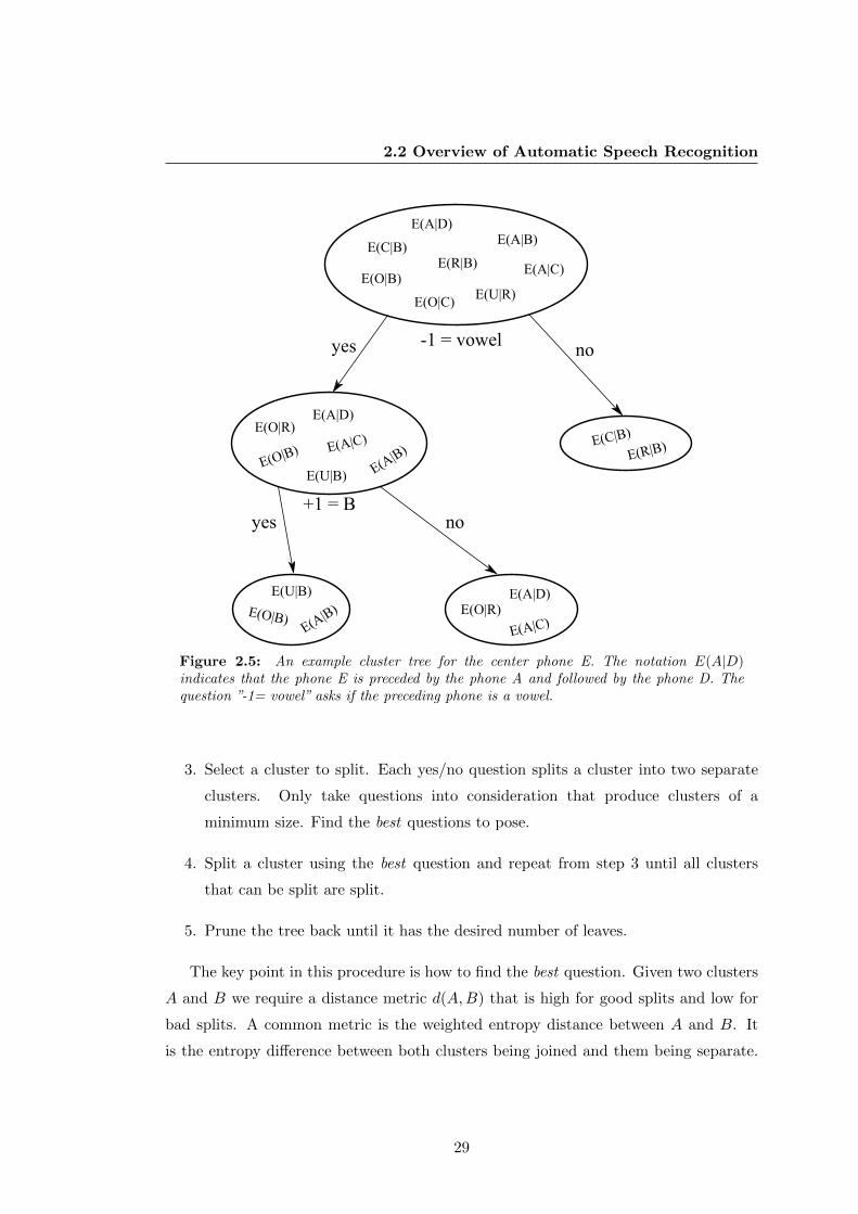
2.2 Overview of Automatic Speech Recognition
E(A|B)
E(R|B)E(O|B)
E(A|C)
E(A|D)
E(U|R)E(O|C)
E(C|B)
E(R|B)E(C|B)
-1 = vowelyes no
+1 = Byes no
E(A|B
)E(O|B) E(A|C)
E(A|D)
E(U|B)
E(O|R)
E(A|C)
E(A|D)E(O|R)
E(A|B
)E(O|B)
E(U|B)
Figure 2.5: An example cluster tree for the center phone E. The notation E(A|D)indicates that the phone E is preceded by the phone A and followed by the phone D. Thequestion ”-1= vowel” asks if the preceding phone is a vowel.
3. Select a cluster to split. Each yes/no question splits a cluster into two separate
clusters. Only take questions into consideration that produce clusters of a
minimum size. Find the best questions to pose.
4. Split a cluster using the best question and repeat from step 3 until all clusters
that can be split are split.
5. Prune the tree back until it has the desired number of leaves.
The key point in this procedure is how to find the best question. Given two clusters
A and B we require a distance metric d(A,B) that is high for good splits and low for
bad splits. A common metric is the weighted entropy distance between A and B. It
is the entropy difference between both clusters being joined and them being separate.
29
2. THEORY UND RELATED WORK
Let the number of occurrences of each cluster be nA and nB, then the weighted entropy
distance can be defined as:
d(A,B) = (nA + nB)H(A ∪B)− nAH(B)− nAH(B) (2.37)
where H(A) is the entropy of cluster A, H(B) is the entropy of cluster B and H(A∪B)
is the entropy of the merged cluster. Using the equation
H(p) =
k∑i=1
p(i) log p(i) (2.38)
we can compute the entropy of a k dimensional probability distribution. Furthermore,
given probability distributions (over the same probability space) pA and pB for both
clusters the probability distribution of the merged cluster can be computed as:
pA∪B(i) =nA pA(i) + nA pB(i)
nA + nB(2.39)
The required probability distributions can be defined in multiple ways. One method
would be to train a single Gaussian on the training examples belonging to a particular
cluster. In this case the probability space would be the feature space. Another approach
uses the discrete mixture weights of a shared codebook of Gaussians as the feature
space. This GMM based approach requires a semi continuous CI HMM/GMM system,
where each phone (monophone) state is modeled using a weighted mixture of a set of
Gaussians trained specifically for that phone state. For all polyphone states appearing
in the training data derived from the same monophone state a new GMM is trained by
only learning the mixture weights and keeping the codebook of the monophone. The
normalized mixture weights of the polyphone states can be regarded as the probabilities
of a discrete distribution which can be used in the entropy distance measure.
2.2.3 Decoder
The decoder uses the outputs of the LM and AM to find the most probable word
sequence given the observed sequence of feature vectors. It is generally limited by
a predetermined search vocabulary V and it contains all the possible words the ASR
system could potentially recognize. Even for a small search vocabulary the total amount
of possible word sequences for a short utterance would be so large that they could not
30
2.2 Overview of Automatic Speech Recognition
all be evaluated. A search vocabulary containing 10000 words would allow for 1080
possible sentences containing exactly 20 words, which is about the same number as
our current best estimate for the total number of atoms in the observable universe.
Instead of evaluating every possible hypothesis the decoder builds them up state by
state and only follows the most likely partial hypotheses at any time and marks the
others as dead ends. The marking of partial hypotheses as dead ends is call pruning and
generating new partial hypotheses by evaluating the next possible states of a current
partial hypothesis is referred to as expanding it. Partial hypotheses that have neither
been pruned nor expanded are considered to still be active.
There are two main types of decoders: synchronous and asynchronous.
Asynchronous decoders have a list of the possible partial hypotheses. In each step
they expand the best one and sort the new partial expanded hypotheses back into
the list. The individual partial hypotheses can have different lengths. In synchronous
decoders each time step generates a new set of partial hypotheses based on the partial
hypotheses of the previous time step. In both cases the set or list of active partial
hypothesis has to be limited by either a maximum size, or through use of a relative
cutoff that prunes partial hypotheses that are less probable, the probability of the
best partial hypotheses multiplied by a factor or beam. Both pruning methods can be
combined allowing the decoder to prune a lot and speed up in cases where it is very sure
of current best partial hypotheses (their probabilities are much higher than competing
ones) and if it is unsure then the maximum amount of partial hypotheses prevents it
from slowing down too much.
When computing the probability of partial hypotheses the decoder has to
compensate for the fact that while the language model is estimating a real probability
P (W ) the acoustic model has to deal with X ∈ Rn and supplies a continuous probability
distribution. As these two values are not directly comparable, a scaling factor has
to be applied. Other problems that the decoder has to deal with are the varying
utterance lengths, the very small probabilities that occur when many small probabilities
are multiplied together and the non-word acoustic events like laughing, coughs or
background noise. A further word penalty term can be added to the speech recognition
equation to deal with the varying utterance lengths and because the word sequence
that maximizes the probability of P (W |X) also maximizes its logarithm logP (W |X)
31
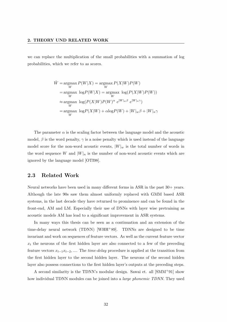
2. THEORY UND RELATED WORK
we can replace the multiplication of the small probabilities with a summation of log
probabilities, which we refer to as scores.
W = argmaxW
P (W |X) = argmaxW
P (X|W )P (W )
= argmaxW
logP (W |X) = argmaxW
log(P (X|W )P (W ))
≈ argmaxW
log(P (X|W )P (W )α e|W |wβ e|W |nγ)
= argmaxW
logP (X|W ) + αlogP (W ) + |W |wβ + |W |nγ
The parameter α is the scaling factor between the language model and the acoustic
model, β is the word penalty, γ is a noise penalty which is used instead of the language
model score for the non-word acoustic events, |W |w is the total number of words in
the word sequence W and |W |n is the number of non-word acoustic events which are
ignored by the language model [OTI98].
2.3 Related Work
Neural networks have been used in many different forms in ASR in the past 30+ years.
Although the late 90s saw them almost uniformly replaced with GMM based ASR
systems, in the last decade they have returned to prominence and can be found in the
front-end, AM and LM. Especially their use of DNNs with layer wise pretraining as
acoustic models AM has lead to a significant improvement in ASR systems.
In many ways this thesis can be seen as a continuation and an extension of the
time-delay neural network (TDNN) [WHH+89]. TDNNs are designed to be time
invariant and work on sequences of feature vectors. As well as the current feature vector
xt the neurons of the first hidden layer are also connected to a few of the preceding
feature vectors xt−1xt−2, .... The time-delay procedure is applied at the transition from
the first hidden layer to the second hidden layer. The neurons of the second hidden
layer also possess connections to the first hidden layer’s outputs at the preceding steps.
A second similarity is the TDNN’s modular design. Sawai et. all [SMM+91] show
how individual TDNN modules can be joined into a large phonemic TDNN. They used
32
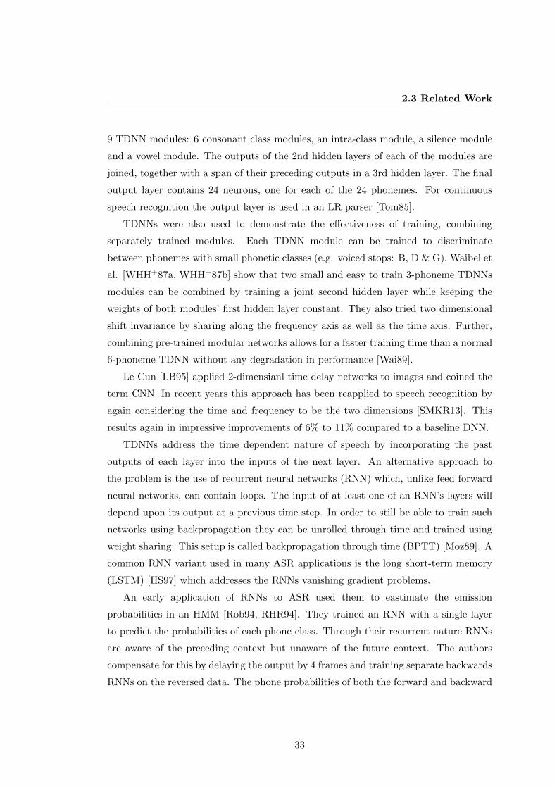
2.3 Related Work
9 TDNN modules: 6 consonant class modules, an intra-class module, a silence module
and a vowel module. The outputs of the 2nd hidden layers of each of the modules are
joined, together with a span of their preceding outputs in a 3rd hidden layer. The final
output layer contains 24 neurons, one for each of the 24 phonemes. For continuous
speech recognition the output layer is used in an LR parser [Tom85].
TDNNs were also used to demonstrate the effectiveness of training, combining
separately trained modules. Each TDNN module can be trained to discriminate
between phonemes with small phonetic classes (e.g. voiced stops: B, D & G). Waibel et
al. [WHH+87a, WHH+87b] show that two small and easy to train 3-phoneme TDNNs
modules can be combined by training a joint second hidden layer while keeping the
weights of both modules’ first hidden layer constant. They also tried two dimensional
shift invariance by sharing along the frequency axis as well as the time axis. Further,
combining pre-trained modular networks allows for a faster training time than a normal
6-phoneme TDNN without any degradation in performance [Wai89].
Le Cun [LB95] applied 2-dimensianl time delay networks to images and coined the
term CNN. In recent years this approach has been reapplied to speech recognition by
again considering the time and frequency to be the two dimensions [SMKR13]. This
results again in impressive improvements of 6% to 11% compared to a baseline DNN.
TDNNs address the time dependent nature of speech by incorporating the past
outputs of each layer into the inputs of the next layer. An alternative approach to
the problem is the use of recurrent neural networks (RNN) which, unlike feed forward
neural networks, can contain loops. The input of at least one of an RNN’s layers will
depend upon its output at a previous time step. In order to still be able to train such
networks using backpropagation they can be unrolled through time and trained using
weight sharing. This setup is called backpropagation through time (BPTT) [Moz89]. A
common RNN variant used in many ASR applications is the long short-term memory
(LSTM) [HS97] which addresses the RNNs vanishing gradient problems.
An early application of RNNs to ASR used them to eastimate the emission
probabilities in an HMM [Rob94, RHR94]. They trained an RNN with a single layer
to predict the probabilities of each phone class. Through their recurrent nature RNNs
are aware of the preceding context but unaware of the future context. The authors
compensate for this by delaying the output by 4 frames and training separate backwards
RNNs on the reversed data. The phone probabilities of both the forward and backward
33
2. THEORY UND RELATED WORK
models are weighted equally and interpolated. This combination of output probabilities
can be extended by further RNNs trained on different input features.
A recurrent neural network is used by Plahl et. al to directly combine three different
feature streams [PKSN13]. The features are stacked and used as the input to a shallow
RNN which is trained to classify the phone targets. In a 2nd step the output layer of
the RNN is augmented by its input features, stacked in a window of up to 9 frames and
used as the input to a shallow MLP which is also trained to classify phone targets. A
GMM-AM is then trained using the output of this MLP.
Both this RNN feature extraction setup and the RNN phone probability estimater
rely on having prior knowledge of the sequence labels as states in the HMM. This is lost
when an RNN is used to replace the HMM and trained to directly convert a sequence
of feature vectors to a sequence of phonemes. In [GFGS06] Graves et al. introduce a
method of learning such networks called connectionist temporal classification. At each
time step the RNN produces a probability distribution over its possible output symbols
P (p|t), the language’s phonemes and null symbol. Given the input feature vectors of a
whole utterance it can generate a probability distribution over all possible phoneme
sequences P (p|x) by summing up the probability of x generating each phoneme
sequence or path. A sequence of symbols becomes a path after removing subsequent
multiple activations of the same symbol and all null symbols. The error function is
the log-probability P (z|x) of the RNN producing target phoneme sequences provide by
the training data. Using a LSTM-RNN this setup is able to outperform HMM based
systems on the phoneme recognition test set TIMIT [GJ14]. In [HCC+14] an RNN
based ASR system is presented that outperforms many tradional HMM based system.
That paper, however, also clearly demonstrates the current limitations of this approach.
In order to compete with state of the are DNNs and CNNs trained on 300hours of data
they have to train their RNN on over 2000 hours of data.
34
Chapter 3
Speech Recognition Tasks
This chapter introduces the datasets on which the approaches presented in the following
chapters are trained and tested. Speech recognition systems can be used in a variety of
different application scenarios. Although the main focus of this thesis is on the offline
recognition of recorded speech like podcasts, the possible application of the developed
methods to an online low latency speech recognition task is also investigated. All offline
tests are performed on development sets from both the Quaero project and the IWSLT
evaluation campaign.
3.1 Quaero
Quaero1 was a French lead research project running from 2008 to 2013 with
German participation. During the project multimedia and multilingual indexing and
management tools were developed for automatic analysis, classification, extraction,
and exploitation of information. Within the project, work was performed on search
engines for multimedia, professional audiovisual asset management, personalized video
selection and distribution, enhancing access services to audiovisual content [SKK12a]
and digitalization and enrichment of library content. Basic research organized into the
Core Technology Cluster (CTC), was performed to supply the target applications with
the necessary underlying technologies such as speech recognition.
During the project six evaluations of the participating speech recognition partners
were performed from 2008 to 2013. The evaluation sets were typically reused as the
1Quaero: http://www.quaero.org
35
3. SPEECH RECOGNITION TASKS
development set for the following year’s evaluation which is why the Quaero 2011
development set is referred to as the Quaero 2010 evaluation set (or eval2010) in this
thesis.
3.2 International Workshop on Spoken Language
Translation (IWSLT)
The International Workshop on Spoken Language Translation (IWSLT)1 is a workshop
that organizes a yearly evaluation campaign on spoken language translation [CNS+13].
In recent years it has focused on the transcription and translation of TED and TEDx
talks and operates tracks on machine translation (MT), spoken language translation
(SLT) and automatic speech recognition.
TED2 which stands for Technology, Entertainment, Design is a recurring conference
where speakers give short 5-20min talks, called TED talks, on a plethora of different
topics in English. Due to the prestigious nature of the event the speakers are generally
very well prepared and the event is recorded in a very high quality. TEDx conferences
are events set up in the same manner as a TED conference but independently organized.
TEDx talks and recordings may not necessarily be of the same quality as normal TED
talks but the independent organizers can choose to allow the talk in languages other
than English like German. TED also hosts the Open Translation Project which allows
volunteers to help transcribe and translate TED and TEDx talks.
3.3 Lecture Translation
In 2011 the Karlsruhe Institute of Technology became the first university to install
an online low-latency lecture translation system [CFH+13]. In 2012 the system began
operation in 3 lecture halls and provides students with a textual translation of the
lecture to their laptops, tablets or smart phones via a website with a delay that is
typically only a few seconds long. Its goal is to help foreign students, who are attending
German lectures, to follow the lecture even if they still lack the required level of German
proficiency.
1IWSLT: http://workshop2014.iwslt.org/2http://www.ted.com/
36
3.4 Test Sets
It is set up in a distributed manner with the only requirements for the lecture
hall being internet access, a microphone for the lecturer and a small laptop or pc that
streams the audio to a mediator. The mediator then coordinates individual workers that
perform the subtasks such as ASR, punctuation prediction and sentence segmentation
and MT. The resulting translation is displayed on a website next to the ASR output
after it has been post processed by a punctuation prediction component.
3.4 Test Sets
During the course of this thesis experiments were performed on multiple test sets and
the techniques developed were also applied to other languages besides German. Most
experiments, however, were performed on either the Quaero 2010 evaluation set or the
IWSLT 2012 development set. In many cases the experiments were performed on both
sets to demonstrate that results of the presented systems are generalizable.
3.4.1 Quaero Test set (eval2010)
The German 2010 Quaero evaluation set [SKK12a] contains 3 hours and 34 minutes of
broadcast news (5 files) and conversational speech (6 files). It was collected between
the 19th and 26th of March 2010 from NDR, HeuteNews, Tagesschau and SWR2 and
contains 135 speakers. 88 of them are male and 45 female. The reference transcriptions
contain 32231 words. The results of the systems are measured using WER and reported
with an accuracy of two decimal places.
3.4.2 IWSLT TED Test set (dev2012)
With a reference length of 17913 words and a runtime of 2 hours the German IWSLT
2012 development set is a bit smaller then the Quaero test set. It consists of 7
German TEDx talks by 7 separate speakers. The IWSLT evaluation campaign imposes
restrictions on the text data that can be used for build language models and only allows
sources explicitly listed on the webpage of the evaluation campaign. The relatively small
size of the IWSLT 2012 development set means that providing WER with any more
accuracy than one decimal place would not be useful because changes there would not
have a high likelihood of being significant. With the exception of the initial experiments
on shallow BNFs all design decisions were made using test set.
37
3. SPEECH RECOGNITION TASKS
3.5 Training Data
The acoustic and language models trained in this system use data from numerous
different sources. This section sheds some light on what data sets exist and where they
stem from.
3.5.1 Audio
Well transcribed audio data is hard to come by, especially if it one wishes it to be in a
particular domain and language. In order to gather training data for the KIT lecture
translation system a large corpus of lectures was gathered in-house, transcribed and
translated. In total, 197 hours and 26 minutes of lectures given by 44 lecturers were
recorded and 86 hours and 21 minutes of them were transcribed. Most lecturers were
male and the majority (185h) of the recorded data stemmed from computer science
lectures. While over 110 hours of CS data remained untranscribed only 35 minutes of
non-CS data was not transcribed.[SKM+12]. The final transcriptions contained 831k
words of which 712k were from CS lectures.
During the course of the Quaero project, audio files collected from publicly available
sources, and their transcripts were released in yearly batches. The Quaero project used
two types of transcriptions, detailed and quick. Quick transcriptions were automatically
preprocessed and segmented into estimated speaker turns which the transcriber did
not have to correct while transcribing the audio. Detailed transcriptions on the other
hand are correctly segmented into speaker turns and, unlike the quick transcripts, have
annotated noises. The whole corpus contains 214 hours of data (detailed: 130:20h /
quick 83:45h).
Most of the collected data is in the form of broadcast conversations where
multiple people are talking with each person being individually recorded. Talk shows
and podcasts are often in this format. A small amount of broadcast news data
(Tagesthemen, Tagesschau and Heute Journal) as well as some recordings from the
European parliament’s plenary sessions are also included. The broadcast conversation
data was collected from NDR, SWR2, ARD, ZDF, Radio Eins, Dradio and SR3.
A further corpus contains 18 hours and 35 minutes of broadcast news collected from
the news program Tagesschau prior to 2008.
38
3.5 Training Data
The Landtag (parliament) of the German state Baden-Wurttemberg has publicly
available transcripts and recordings of their plenary sessions. As well as lacking
timestamps the transcripts are also often heavily edited and therefore sometimes only
roughly match the recordings. Of the over 400 hours of recordings just over 123 hours
of well aligned segments were extracted.
This thesis uses the following collections (databases) of corpora:
� Lecture DB: Contains only the lecture corpus.
� Quaero partial DB: Contains all the Quaero data released prior to 2012 and the
Tagesschau corpus (197:09h).
� Quaero DB: Only contains the full Quaero data (214 hours). The Tagesschau
corpus is no longer included.
� Quaero extended DB: Consists of all the Quaero data released prior to 2012, the
Tagesschau corpus and the Landtag corpus (320:09 h)
3.5.2 Text
Although some text corporas, such as those provided by the WMT, are available in a
format and encoding that allows them to be used to train an LM most them require
some form of preprocessing. Text from websites is generally the hardest to extract
clean text from because it may still contain HTML tags, encoding is often incorrect or
inconsistent and it sometimes contains English text instead of German. The complete
cleaning setup involves:
� Encoding Normalization: Large corpora often contain data from different
sources with possibly different encodings (e.g utf-8, ISO 8859-1, HTML entities,
...). This can sometimes also be seen on websites where a user can contribute text.
It is, therefore, important to perform encoding checking and normalization at the
paragraph level and not at the document level. Even then, texts can sometimes
be seriously messed up. Sometimes uft-8 encoded files are opened as if their
contents were ascii and then converted from ascii to utf-8 and saved again resulting
in words like f\xc3\x83\xc2\xBcr (fur) Gr\xc3\x83\xc2\xB6\xc3\x83\xc2\x9fer
(Großer). Common encoding errors like these can be fixed using a lookup table.
39
3. SPEECH RECOGNITION TASKS
� Character Normalization: Sometimes encodings allow for multiple
representations of a single character. In utf-8 an a, for example, can either be
its own unique letter or it could be the letter a with a modifier. A consistent
normalization has to be chosen to allow for string comparisons. Punctuation
marks almost always require normalization as there are many different types of
quotes, dashes etc. It helps to have a predetermined set of punctuation marks and
all other punctuation marks are either mapped to one from that set or removed.
� Identify and remove junk: If the correct encodings can’t be found, the data
we are trying to process isn’t text, or if it is text but unsuitable for language
modeling (e.g. football result, code snippets, ...) then it should be removed.
� Sentence segmentation: Language model toolkits generally require one
sentence per line. [Koe05]
� Number normalization: Text sources tend to have numbers represented using
digits which are pronounced differently depending upon what they represent:
dates, times, cardinal numbers, etc. This step replaced the digits with their
context dependent written form.
� Word normalization: acronyms, initialisms, words with hyphens and words
with multiple spellings also have to be normalized to a consistent token. Common
spelling mistakes can also be corrected.
In most cases preprocessing a raw text source will reduce the number of tokens.
Only a fraction of the token in a raw dump of a websites, for example, will turn out to
be usable. Some steps like number normalization or word normalization may increase
the total number of tokens by replacing a single token like UN with multiple tokens
like U. N..
The text corpora used in this thesis originate from many different sources. A full
list can be found in Table 3.1 including the raw word counts of the text corpora, their
sizes after cleaning and the dates when the original texts included in the corpora were
first published. The most notable corpora are:
� A query based webdump: This webdump was originally performed in order
to collect data for a language model used in human robot interaction1. From the
1SFB 588 Humanoid Robots: http://www.sfb588.uni-karlsruhe.de
40
3.5 Training Data
small amount of existing in-domain data 30k short phrases were extracted and
used as search terms in an online search engine1. The websites in the top search
results were downloaded and cleaned.
� ODP Crawl: The Open Directory Project2 is a collection of over 4 Million
links which have been sorted into over 1 Million relevant categories by human
editors and has a hierarchical structure. Volunteer editors extend and maintain
the directory. The raw data of the ODP can be downloaded as a large XML file.
This corpus contains all the German websites linked to by the ODP in March of
2009. [Kil09]
� Baden-Wurttemberg Landtag transcripts: The state of
Baden-Wurttemberg is the 3rd largest in Germany and this corpus contains the
transcripts from the plenary discussions of their state parliament in Stuttgart
from the 12th, 13th and the first half of the 14th legislative periods3.
� GeneralNews: An old collection of German news articles first published prior
to the 10th of September 1998 from the German Associated Press4, Agence
France-Presse5, Deutsche Presse-Agentur6, Frankfurter Allgemeine Zeitung7 and
the Suddeutsche Zeitung8.
� LM data from the Quaero project: Over the course of the Quaero project a
large amount a language modeling data was collected mostly from news websites
and blogs and then released in multiple stages [LCD+11]. The sources are
Zeit Online, Aachener Nachrichten9, Overblog10, Bild11, Nordkurier12, Spiegel13,
1Google: https://www.google.com2ODP http://www.dmoz.org3BW Landtag: https://www.landtag-bw.de/cms/home/dokumente/plenarprotokolle.html4Acquired by the ddp in 2009 and now operates as the DAPD - Deutscher
Auslands-Depeschendienst: https://www.dapd.de/5AFP: https://www.afp.com/6DPA: http://www.dpa.de/7Frankfurter Allgemeine Zeitung: http://www.faz.net/8Suddeutsche Zeitung: http://www.sueddeutsche.de/9Aachener Nachrichten: http://www.aachener-nachrichten.de/
10Overblog: https://de.over-blog.com/11Bild: http://www.bild.de/12http://www.nordkurier.de/13Welt: http://www.spiegel.de/
41
3. SPEECH RECOGNITION TASKS
TAZ1 and Welt2, many of which were released together as a single corpus, labeled
Various News Websites in the table.
� AM data transcripts: Although very small, the transcripts of the acoustic
model training data can be very useful for multiple reasons. Unlike webdumps or
newspaper articles it contains actual spoken data and is therefore relevant for LM
in ASR systems. The AM training data is often collected in the domain we wish
our system to be deployed so it may also be in domain data. This is especially
the case for the Quaero task.
� WMT Data: The workshop on statistical machine translation organises a yearly
evaluation campaign on statistical machine translation and provide both parallel
and monolingual data3.
� European Language Newspaper Text: A corpus containing German
newspaper articles published by AFP, AP and DP prior to 1995. [GF94]
� German Political Speeches Corpus: A corpus of the speeches made by the
German presidents from 1984 to 2011 and by the German chancellors from 1998
to 2011. [Bar12]
� Google Web and Book ngrams: Unlike the other corpora, the Google web4
and book5 ngrams are not provided as raw text but instead as ngram counts.
1TAZ: http://www.taz.de/2Welt: http://www.welt.de/3http://www.statmt.org/wmt14/translation-task.html4Google Web 1T 5-gram, 10 European Languages: https://catalog.ldc.upenn.edu/LDC2009T255Google Books Ngrams: http://storage.googleapis.com/books/ngrams/books/datasetsv2.html
42
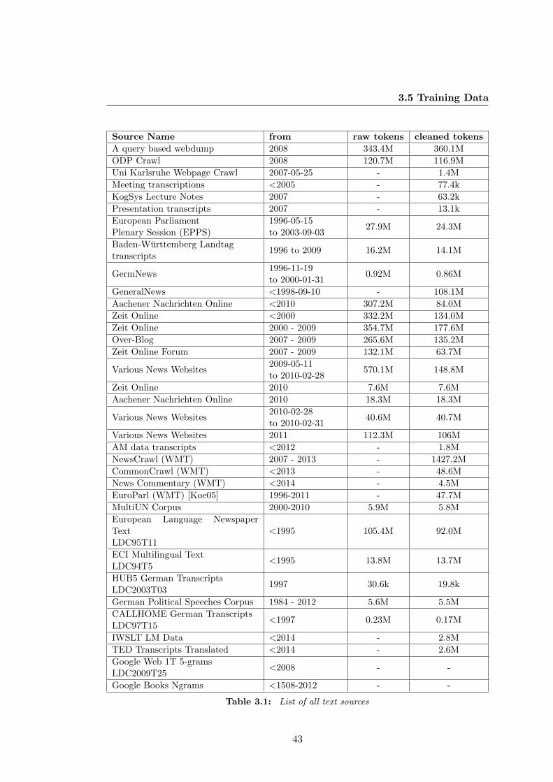
3.5 Training Data
Source Name from raw tokens cleaned tokens
A query based webdump 2008 343.4M 360.1M
ODP Crawl 2008 120.7M 116.9M
Uni Karlsruhe Webpage Crawl 2007-05-25 - 1.4M
Meeting transcriptions <2005 - 77.4k
KogSys Lecture Notes 2007 - 63.2k
Presentation transcripts 2007 - 13.1k
European ParliamentPlenary Session (EPPS)
1996-05-15to 2003-09-03
27.9M 24.3M
Baden-Wurttemberg Landtagtranscripts
1996 to 2009 16.2M 14.1M
GermNews1996-11-19to 2000-01-31
0.92M 0.86M
GeneralNews <1998-09-10 - 108.1M
Aachener Nachrichten Online <2010 307.2M 84.0M
Zeit Online <2000 332.2M 134.0M
Zeit Online 2000 - 2009 354.7M 177.6M
Over-Blog 2007 - 2009 265.6M 135.2M
Zeit Online Forum 2007 - 2009 132.1M 63.7M
Various News Websites2009-05-11to 2010-02-28
570.1M 148.8M
Zeit Online 2010 7.6M 7.6M
Aachener Nachrichten Online 2010 18.3M 18.3M
Various News Websites2010-02-28to 2010-02-31
40.6M 40.7M
Various News Websites 2011 112.3M 106M
AM data transcripts <2012 - 1.8M
NewsCrawl (WMT) 2007 - 2013 - 1427.2M
CommonCrawl (WMT) <2013 - 48.6M
News Commentary (WMT) <2014 - 4.5M
EuroParl (WMT) [Koe05] 1996-2011 - 47.7M
MultiUN Corpus 2000-2010 5.9M 5.8M
European Language NewspaperTextLDC95T11
<1995 105.4M 92.0M
ECI Multilingual TextLDC94T5
<1995 13.8M 13.7M
HUB5 German TranscriptsLDC2003T03
1997 30.6k 19.8k
German Political Speeches Corpus 1984 - 2012 5.6M 5.5M
CALLHOME German TranscriptsLDC97T15
<1997 0.23M 0.17M
IWSLT LM Data <2014 - 2.8M
TED Transcripts Translated <2014 - 2.6M
Google Web 1T 5-gramsLDC2009T25
<2008 - -
Google Books Ngrams <1508-2012 - -
Table 3.1: List of all text sources
43
3. SPEECH RECOGNITION TASKS
3.6 Baseline System
The decoding and GMM AM training uses the Janus Recognition Tool-kit (JRTk)
with the Ibis single pass decoding developed at Karlsruhe Institute of Technology in
cooperation with Carnegie Mellon University [SMFW01].
3.6.1 Language Model and Search Vocabulary
The data usage restrictions imposed by the IWSLT campaign result in different text
sources being used to train the language models for both tasks which we refer to as
the QuaeroLM and the IwsltLM. A full list of which sources went into which LM is
provided in appendix A. The tuning set for the QuaeroLM is derived from the acoustic
model transcripts of the Quaero data from which roughly 628k words are used. The
remaining acoustic model transcripts become a training source. In lieu of the Quaero
audio data transcripts the IwsltLM uses the example data provided by the campaign
organizers. 240k words of this data are used as the tuning set and the rest used as a
training source.
Both the IwsltLM and the QuaeroLM use the same vocabulary method and the
same approaches to language model building. Only their text sources and tuning sets
differ and all other parameters are kept the same. Some of the larger corpora listed
in table 3.1, like the NewsCrawl, are split into multiple smaller text sources based on
publication year or source.
For each of these text sources a Witten-Bell smoothed unigram language model is
built using the union of the text sources’ vocabulary as the language models’ vocabulary
(global vocabulary). With the help of the maximum likelihood count estimation method
described in [VW03] the best mixture weights are found for representing the tuning
set’s vocabulary as a weighted mixture of the sources’ word counts thereby giving us a
ranking of all the words in the global vocabulary by their relevance to the tuning set.
The top 300k words are then used as the vocabulary.
With the selected vocabulary, a 4gram case sensitive language model with modified
Kneser-Ney smoothing is built for each of the used text sources. This is done using the
SRI Language Modeling Toolkit [Sto02]. The language models are then interpolated
using interpolation weights estimated on the tuning set resulting in a large >10 GByte
language model. Because even compressed in an easy to load binary format the language
44
3.6 Baseline System
model uses up a lot memory it is loaded into a region of shared memory which allows
multiple decoder instances running on the same server to share it.
All experiments in chapter 4 and chapter 5 are performed using the subword
vocabulary developed in chapter 6 but not the neural network subword language model
which is the culmination of that chapter.
3.6.2 Acoustic Model
All acoustic models use left to right HMM without skip states where each of the 46
normal phonemes have three HMM states and the silence phoneme has only a single
state. The initial cluster tree is built using the method described in section 2.2.2.4 with
6016 leaves.
The baseline GMM AM setup uses codebooks with 128 Gaussians per model. The
CD AM is trained using multiple steps. First an LDA trained to reduce the input
feature’s dimension to 42 then GMM models are trained using incremental splitting of
Gaussians (MAS) training, followed by the training of a global STC matrix and two
rounds of Viterbi training [SKK12a]. All models use vocal tract length normalization
(VTLN [ZW97]) and feature space constraint MLLR (cMLLR) [FLBG07] speaker
adaptive training.
Boosted MMIE (bMMIE), an updated version of MMIE,[PKK+08] where the lattice
confusions with the largest phone error are given more weight (boosted), in order to
improve the discriminative capability of the acoustic model, consistently improves all
trained GMM AMs. It is, however, not included in many experiments due its high
demand for computational resources. Its consistent gains allow it to be skipped when
evaluting front-end features.
The JrTk [SMFW01] is extended with a DNN AM object that implements the same
interface to the Ibis decoder as the existing GMM AM. A diverse range of topologies
are supported by allowing their computation to be controlled by a tcl script.
3.6.3 System Combination
The outputs of multiple systems can be combined using confusion network combination
(cnc) to produce a combined output with a lower error rate. The individual system’s
lattices are merged into a confusion network which consists of a sequence of slots
containing the possible words including the null word that, according to the lattices,
45
3. SPEECH RECOGNITION TASKS
could occur in that part of the utterance. At the same time the posterior probability
of each word in a slot is calculated and then used to select the sequence of words that
should result in the lowest word error rate [MBS00b].
3.7 Neural Network Training
Some training of shallow MLPs is preformed with a consistent [Joh04] toolkit that
allows for fast network training on GPUs. Quicknet, however, can only train networks
with up to 3 hidden layers. In order to train networks with more hidden layers an
inhouse solution based on Theano[BBB+10] was developed. In his master thesis Jonas
Gehring, explored the application of denoising autoencoders as a method of pre-training
DNNs for feature extraction. Using Theano he implemented a flexible DNN training
setup that included multiple forms of pretraining, various error functions, activation
functions and layer types. All DNN experiments trained in chapters 4 through 6 used
either this setup or a modified and extended version of this setup. Due to the novel
error function and the tight integration with a lattice rescoring setup the DNNs trained
in chapter 7 required their own specialized training setup, which was also based on
Theano.
Pretraining was consistently performed layerwise using denoising autoencoders. A
normal setup would use 2M of mini batches with a corruption of 20%, a constant
learning rate and the sigmoid activation function. Because the input data to the
network is mean normalized the first denoising autoencoder has to use the tanh
activation function in its output layer. It still uses the sigmoid activation function
in its hidden layer so that all further layers only have inputs between 0 and 1, allowing
them to use the sigmoid activation function in their output layers and the CE error
function. The first hidden layer has to use the MSE error function. Pretrained hidden
layers can be cached and reused in experiments that only change the output layer or
the total number of hidden layers. After pretraining the final layer(s) can be added,
with the output layer using the softmax activation function. The full DNN is then
fine-tuned using the newbob learning rate schedule.
46
Chapter 4
Neural Network Feature
Extraction
This chapter deals with the uses of neural networks in the feature extraction process.
Good features can significantly improve the performance of HMM/GMM AM based
ASR systems. The origins of this approach stem from a time when HMM/GMM AMs
were fast becoming the dominant approach to acoustic modeling. In 2000 Hermansky
et al. [HES00] successfully used the MLP output of a context independent hybrid
system as the input to a GMM based AM (Tandem approach). After an error analysis
[RGE02] showed that systems using MLP features and systems using cepstral features
produced different errors, attempts were undertaken to combine both features at the
input level to the GMM. In [BBC+01] PCA is performed independently on both MLP
and cepstral features while for [ZCM+04] performing HLDA on the cepstral features
and PCA on the MLP features resulted in the best system when using MLLR speaker
adaptation. Since these neural network based features are only augmenting the existing
cepstral features in the input to the GMMs, techniques designed to improve GMM based
systems like MLLR speaker adaptation and MMIE discriminative training can also be
leveraged to improve systems using neural network features. Similar approaches have
been used to clean up noisy audio signals [TW88]. This chapter starts off with a quick
overview of the relevant initial front-end features from which the neural network based
features will be extracted and goes on to explain how MLPs can be used to extract
so called bottleneck features. Experiments on MVDR in particular show how to make
the best use of bottleneck features. Further experiments show how multiple front-end
47
4. NEURAL NETWORK FEATURE EXTRACTION
features can be combined using bottleneck features and improved with the use of deep
bottleneck features.
4.1 Features for Speech Recognition
In the past, a myriad of input features have been tested in ASR, and no single feature
found to be the best in all circumstances. Input features are often considered to
be good if they were simple to compute, discarded irrelevant information, such as
who is speaking or where they’re speaking, and preserved or enhanced the distinctive
properties of the speech signal. In many cases the input features were also required to
be robust against distortions like echos or background noises. Many feature extraction
algorithms have been inspired by the physiology of the human ear. In the outer ear
an incoming sound wave is filtered and focused on the eardrum. The vibrations of
which are transmitted, with the help of 3 small bones, to the fluid in the cochlea.
Different frequencies of vibrations resonate in different places within the cochlea and
cause the hair cells in those places to release a neurotransmitter resulting in neurons
of the auditory nerve sending a signal to the brain [Kal15]. This can conceptually be
thought of as analogous to a short-time Fourier transform (STFT) of the audio signal,
which computes the Fourier transformation on a small window of the audio signal, often
referred to as a frame. While human hearing is asynchronous, the STFT performed
when extracting features for speech recognition uses a fixed window size (normally
16-32ms) and a fixed frameshift (8-40ms). Plotting the magnitude of an STFT results
in a spectrogram where the Y-Axis represents the frequency and the X-axis the time.
4.1.1 Log-MEL Features (lMEL)
Also motivated by the physiology of human hearing is the mel scale developed by
[SVN37]. Humans find it easier to distinguish frequency differences at lower frequencies
than at higher frequencies. We can assume from this that the lower frequencies contain
more speech relevant information. To emulate this a filterbank of triangular window
functions is applied to each frame after performing a short-time Fourier transform. The
windows are smaller and closer together at lower frequencies and larger and further
apart at higher frequencies. Each window function corresponds to a coefficient in the
feature vector. The final step involves taking the log of each coefficient. By taking the
48
4.1 Features for Speech Recognition
logarithm we are able to transform convolutional noise of the audio signal that became
multiplicative noise after the Fourier transformation into additive noise that is much
easier to handle.
4.1.2 Mel Frequency Cepstral Coefficients (MFCC)
Applying an inverse Fourier transformation to the lMEL features preserves the additive
nature of the originally convolutional noise in the cepstrum. Under the assumption
that, while the speech signal varies, the noise is constant during an utterance, it can
estimated using the average signal over the timeframe of the utterance and compensated
by subtracting it from each utterance. A discrete cosine transformation is generally
used instead of a the inverse Fourier transformation. Mel frequency ceptral coefficients
(MFCC) have established themselves as the most common front end feature in speech
recognition.
4.1.3 Minimum Variance Distortionless Response (MVDR) Spectrum
Some alternative feature extraction methods are based on linear predictive coding
that aims to estimate samples as a linear combination of the preceding n samples
[Her90]. Basic linear prediction tends to overemphasize the harmonic peaks seen in
medium and high pitched voices. Minimum variance distortionless response [MR00]
(MVDR) solves this problem and is improved by (mel)-warping the frequency axis
prior to spectral estimation. This allows for more parameters in the low frequency
regions of the spectrum and fewer in the high frequency regions [WM05]. In some
circumstances warped Minimum Variance Distortionless Response (MVDR) features
for speech recognition have been shown to be better [WMW03] than MFCC features.
4.1.4 Tonal Features
The use of pitch in languages to distinguish between words, their inflections or
grammatical meaning is refereed to as tone. Pitch information is generally not
considered to be very useful in speech recognition systems for non-tonal languages.
Even for tonal languages like Mandarin, Cantonese, and Vietnamese, that use tones
to represent phone level distinctions [Bao99] and therefore make them essential to
distinguish between words, tonal features only provide a modest boost to performance
49
4. NEURAL NETWORK FEATURE EXTRACTION
[VS09, CW95]. Modeling tones and integrating tonal features into a recognition system
is challenging and often optimized to the particularities of the language the system is
designed for. [CGM+97, LGL+11].
In non-tonal languages like German and English, pitch can be considered a prosodic
feature along with rhythm (phoneme duration) and loudness (acoustic intensity). These
are generally only useful for modeling information in speech beyond the word level such
as emotion, emphasis or intonation [Pie80, Hir83]. On a word level pitch may contribute
a small part to lexical stress but only a small number of word pairs exist that require
lexical stress to distinguish them: for example INcline (sloped surface) vs inCLIne
(tendency to do something) [Wai88].
In work performed together with Metze, Gehring and others [MSW+13a] various
tonal models and methods of integrating tonal features are analyzed on both tonal and
non tonal languages. That work reports, for the first time, results of using fundamental
frequency variation [LHE08] features for speech recognition of tonal languages.
4.1.4.1 Pitch Features
The pitch features in this work use the approach described by Kjell Schubert in his
thesis [Sch98]. The distinguishing information in many tonal languages is not so much
the absolute pitch height but more its change or contour. In Mandarin, for example,
the word chun contains a flat tone and can be translated into English as spring. Simply
altering the tone contour to a falling-rising tone (chun) changes the meaning of the word
to stupid. Good tonal features should, therefore, detect rising, falling, or otherwise
marked pitch contours.
Kjell’s pitch features use dynamic programming over a cepstrogram with a window
length of 32 ms to find the best pitch for each frame without exceeding certain
constraints, such as the maximum pitch difference between two frames. Using the
three right and left neighbours delta and double delta features are computed. Together
with an optimal frame-based cross-correlation feature, this results in 8 coefficients.
4.1.4.2 Fundamental Frequency Variation (FFV) Features
Normal pitch features have problems in dealing with silent segments of speech where
pitch isn’t defined. FFV features, on the other hand, can handle silent segments and
have been successful in tasks like speaker verification. A geometric interpretation
50
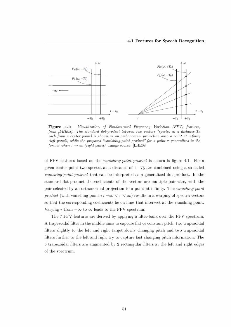
4.1 Features for Speech Recognition
Figure 4.1: Visualization of Fundamental Frequency Variation (FFV) features,from [LHE08]: The standard dot-product between two vectors (spectra at a distance T0each from a center point) is shown as an orthonormal projection onto a point at infinity(left panel), while the proposed “vanishing-point product” for a point τ generalizes to theformer when τ →∞ (right panel). Image source: [LHE08]
of FFV features based on the vanishing-point product is shown is figure 4.1. For a
given center point two spectra at a distance of +- T0 are combined using a so called
vanishing-point product that can be interpreted as a generalized dot-product. In the
standard dot-product the coefficients of the vectors are multiple pair-wise, with the
pair selected by an orthonormal projection to a point at infinity. The vanishing-point
product (with vanishing point τ : −∞ < τ <∞) results in a warping of spectra vectors
so that the corresponding coefficients lie on lines that intersect at the vanishing point.
Varying τ from −∞ to ∞ leads to the FFV spectrum.
The 7 FFV features are derived by applying a filter-bank over the FFV spectrum.
A trapezoidal filter in the middle aims to capture flat or constant pitch, two trapezoidal
filters slightly to the left and right target slowly changing pitch and two trapezoidal
filters further to the left and right try to capture fast changing pitch information. The
5 trapezoidal filters are augmented by 2 rectangular filters at the left and right edges
of the spectrum.
51
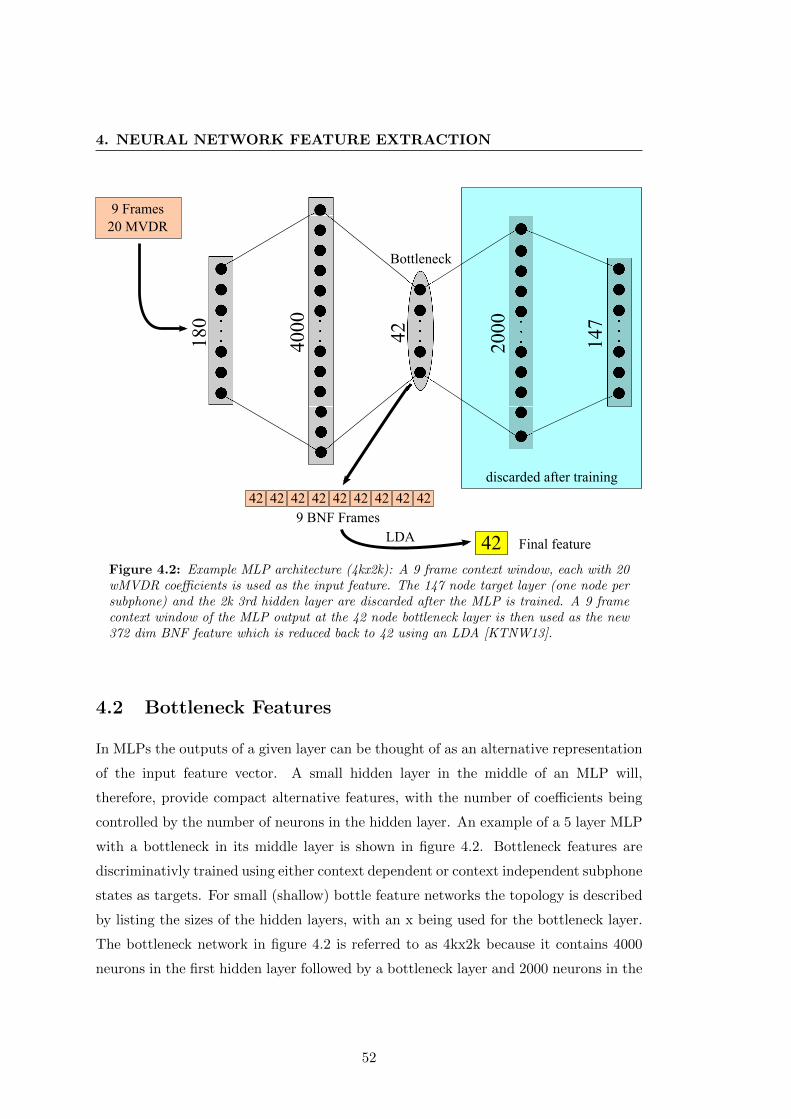
4. NEURAL NETWORK FEATURE EXTRACTION
18
0
40
00
20
00
42
14
7
9 Frames
20 MVDR
discarded after training
Bottleneck
9 BNF Frames
42 42 42 42 42 42 42 42 42
LDA 42 Final feature
Figure 4.2: Example MLP architecture (4kx2k): A 9 frame context window, each with 20wMVDR coefficients is used as the input feature. The 147 node target layer (one node persubphone) and the 2k 3rd hidden layer are discarded after the MLP is trained. A 9 framecontext window of the MLP output at the 42 node bottleneck layer is then used as the new372 dim BNF feature which is reduced back to 42 using an LDA [KTNW13].
4.2 Bottleneck Features
In MLPs the outputs of a given layer can be thought of as an alternative representation
of the input feature vector. A small hidden layer in the middle of an MLP will,
therefore, provide compact alternative features, with the number of coefficients being
controlled by the number of neurons in the hidden layer. An example of a 5 layer MLP
with a bottleneck in its middle layer is shown in figure 4.2. Bottleneck features are
discriminativly trained using either context dependent or context independent subphone
states as targets. For small (shallow) bottle feature networks the topology is described
by listing the sizes of the hidden layers, with an x being used for the bottleneck layer.
The bottleneck network in figure 4.2 is referred to as 4kx2k because it contains 4000
neurons in the first hidden layer followed by a bottleneck layer and 2000 neurons in the
52
4.2 Bottleneck Features
final hidden layer.
4.2.1 Related Work
This 5 layer bottleneck MLP was first introduced by Greszl et al. in 2007 [GKKC07]
where it was shown to outperform both an HLDA dimensionality reduction on the
input features and the posterior phoneme probabilities used by the traditional tandem
systems. They saw further improvements by using phone states as targets instead of
phones [GF08], using a topology with twice as many neurons in the first hidden layer
than in the second hidden layer and by adding delta features to their input.
Temporal Pattern (TRAP) features proposed by Hermansky [HS98] use multiple
small MLPs trained on long, (up to 1s) temporal features that each correspond to a
frequency band in the spectrum. The individual MLPs can then be joined in a further
MLP and its output used as in the tandem system setup. In a similar setup Valente
et al. [VVP+07] describe a hierarchical approach to neural feature extraction where an
MLP is trained on spectral features spanning a short temporal context. Its output is
then combined with spectral features spanning a long temporal context and used as the
input to a further MLP. In [PSN10] this approach is extended by adding bottlenecks
to both of the MLPs and is shown to be significantly better than a normal bottleneck
MLP on the same features, the hierarchical setup without a bottleneck and the TRAP
features.
A method of using BNFs to combine multiple feature streams proposed in [PSN11],
shows that combining MFCC, PLP and gammatone features in the input layer of an
MLP can lead to a system that performs better than the system combination of the
lattices of the individual systems. The MLP using the combined input feature also
outperforms the best single feature MLP by a small amount. In contrast to this work
they, however, only look at shallow networks. Instead they focus on integrating the
multiple features into a shallow RNN [PKSN13] trained to classify the phone targets.
In [YS11] bottleneck features are pretrained using stacked restricted Boltzmann
machines which improve the performance of the subsequently trained MLP. An
approach using denoising autoencoders instead of restricted Boltzmann machines also
shows impressive reductions in WER [Geh12]. Both case’s setups allow the number of
hidden layers prior to the bottleneck layer to be increased and improve the quality of
the BNFs.
53
4. NEURAL NETWORK FEATURE EXTRACTION
4.3 Combining Features with a Bottleneck MLP
The initial experiments to ascertain if this approach is feasible and what sort of input
contexts should be used are performed on MFCC and MVDR features using a small
bottleneck network with only 3 hidden layers. The results of these experiments motivate
the setup of the later experiments on combining multiple features using deep bottleneck
feature networks.
4.3.1 Experimental Optimization of MFCC+MVDR-BNF Features
Intuitively one may assume that larger input vectors, derived from a larger stack on
consecutive frames, should contain more information and should therefore result in
better BNFs. Especially when the results of the TRAP features [HS98] are taken
into consideration which show that useful information can be found in contexts up
to 1s. On the flip side larger input vectors mean more parameters which can also
cause problems. In this section the effects of various input feature sizes is examined
on MFCC+MVDR-BNF feature networks of different topologies compared with both
MVDR-BNF and MFCC-BNF features. Since feature stacking can also be performed
in the LDA prior to GMM training the size of the feature stack is also scrutinized.
4.3.1.1 MLP Topology
All MLPs use a 42 node bottleneck as the 2nd hidden layer. The 2k MLPs contain a
2000 node hidden layer between the bottleneck layer and the input layer. This layer has
4000 nodes in the 4kx2k MLPs which also include a 3rd hidden layer with 2000 nodes
between the bottleneck and output layers. Further increases in layer sizes decreased the
MLPs performance. The ratio of 2:1 between the 1st and 3rd hidden layers is motivated
by [GKKC07]. We performed pretraining on the German MLPs by training first on all
available German audio data (sets 1+2) and then fine-tuning with only the in-domain
data (set 1).
All audio is sampled at 16 kHz with a 16 ms window size, 10 ms frame shift and a
frame size of 20 coefficients. Between 1 and 15 consecutive frames are concatenated
to form the input of the MLP. To provide a comparison both an MFCC-BNF system
and a MVDR-BNF system using the same parameters are trained in parallel for each
54
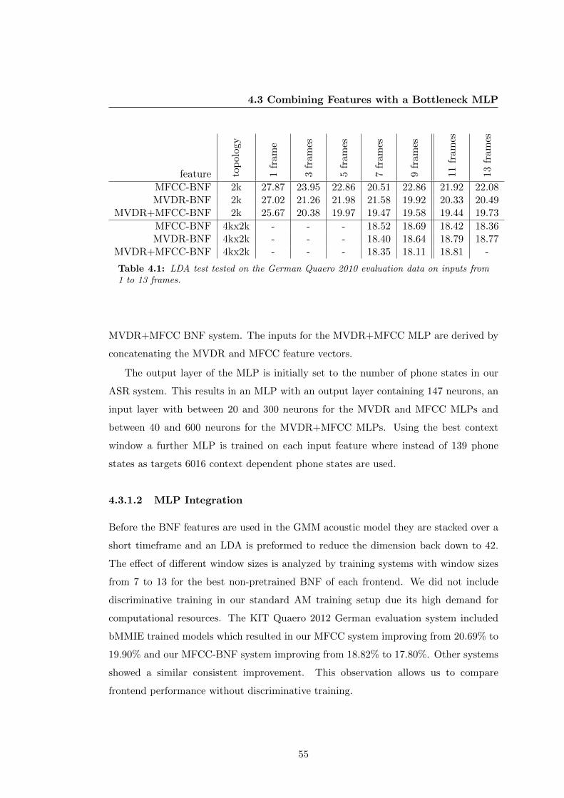
4.3 Combining Features with a Bottleneck MLP
feature top
ology
1fr
am
e
3fr
am
es
5fr
am
es
7fr
am
es
9fr
am
es
11fr
am
es
13fr
ames
MFCC-BNF 2k 27.87 23.95 22.86 20.51 22.86 21.92 22.08MVDR-BNF 2k 27.02 21.26 21.98 21.58 19.92 20.33 20.49
MVDR+MFCC-BNF 2k 25.67 20.38 19.97 19.47 19.58 19.44 19.73
MFCC-BNF 4kx2k - - - 18.52 18.69 18.42 18.36MVDR-BNF 4kx2k - - - 18.40 18.64 18.79 18.77
MVDR+MFCC-BNF 4kx2k - - - 18.35 18.11 18.81 -
Table 4.1: LDA test tested on the German Quaero 2010 evaluation data on inputs from1 to 13 frames.
MVDR+MFCC BNF system. The inputs for the MVDR+MFCC MLP are derived by
concatenating the MVDR and MFCC feature vectors.
The output layer of the MLP is initially set to the number of phone states in our
ASR system. This results in an MLP with an output layer containing 147 neurons, an
input layer with between 20 and 300 neurons for the MVDR and MFCC MLPs and
between 40 and 600 neurons for the MVDR+MFCC MLPs. Using the best context
window a further MLP is trained on each input feature where instead of 139 phone
states as targets 6016 context dependent phone states are used.
4.3.1.2 MLP Integration
Before the BNF features are used in the GMM acoustic model they are stacked over a
short timeframe and an LDA is preformed to reduce the dimension back down to 42.
The effect of different window sizes is analyzed by training systems with window sizes
from 7 to 13 for the best non-pretrained BNF of each frontend. We did not include
discriminative training in our standard AM training setup due its high demand for
computational resources. The KIT Quaero 2012 German evaluation system included
bMMIE trained models which resulted in our MFCC system improving from 20.69% to
19.90% and our MFCC-BNF system improving from 18.82% to 17.80%. Other systems
showed a similar consistent improvement. This observation allows us to compare
frontend performance without discriminative training.
55
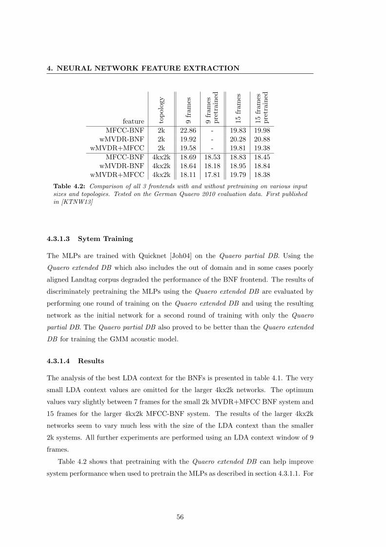
4. NEURAL NETWORK FEATURE EXTRACTION
feature top
olo
gy
9fr
ames
9fr
ames
pre
train
ed
15
fram
es
15
fram
espre
train
ed
MFCC-BNF 2k 22.86 - 19.83 19.98wMVDR-BNF 2k 19.92 - 20.28 20.88
wMVDR+MFCC 2k 19.58 - 19.81 19.38
MFCC-BNF 4kx2k 18.69 18.53 18.83 18.45wMVDR-BNF 4kx2k 18.64 18.18 18.95 18.84
wMVDR+MFCC 4kx2k 18.11 17.81 19.79 18.38
Table 4.2: Comparison of all 3 frontends with and without pretraining on various inputsizes and topologies. Tested on the German Quaero 2010 evaluation data. First publishedin [KTNW13]
4.3.1.3 Sytem Training
The MLPs are trained with Quicknet [Joh04] on the Quaero partial DB. Using the
Quaero extended DB which also includes the out of domain and in some cases poorly
aligned Landtag corpus degraded the performance of the BNF frontend. The results of
discriminately pretraining the MLPs using the Quaero extended DB are evaluated by
performing one round of training on the Quaero extended DB and using the resulting
network as the initial network for a second round of training with only the Quaero
partial DB. The Quaero partial DB also proved to be better than the Quaero extended
DB for training the GMM acoustic model.
4.3.1.4 Results
The analysis of the best LDA context for the BNFs is presented in table 4.1. The very
small LDA context values are omitted for the larger 4kx2k networks. The optimum
values vary slightly between 7 frames for the small 2k MVDR+MFCC BNF system and
15 frames for the larger 4kx2k MFCC-BNF system. The results of the larger 4kx2k
networks seem to vary much less with the size of the LDA context than the smaller
2k systems. All further experiments are performed using an LDA context window of 9
frames.
Table 4.2 shows that pretraining with the Quaero extended DB can help improve
system performance when used to pretrain the MLPs as described in section 4.3.1.1. For
56
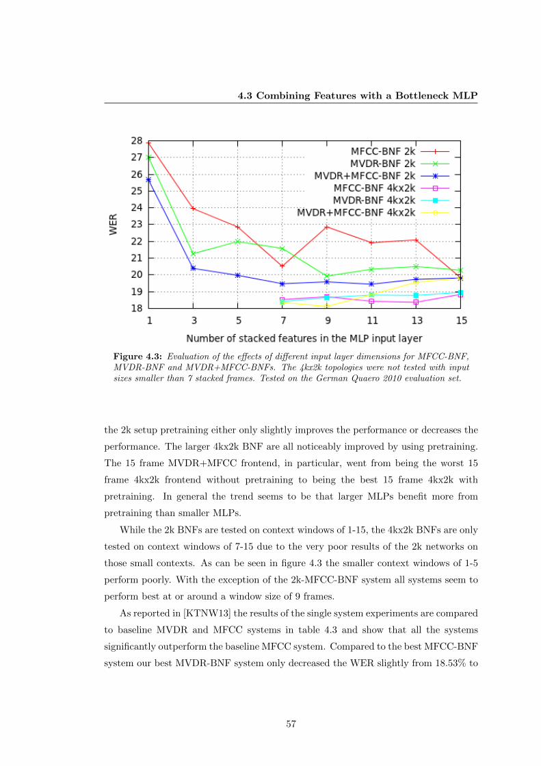
4.3 Combining Features with a Bottleneck MLP
Figure 4.3: Evaluation of the effects of different input layer dimensions for MFCC-BNF,MVDR-BNF and MVDR+MFCC-BNFs. The 4kx2k topologies were not tested with inputsizes smaller than 7 stacked frames. Tested on the German Quaero 2010 evaluation set.
the 2k setup pretraining either only slightly improves the performance or decreases the
performance. The larger 4kx2k BNF are all noticeably improved by using pretraining.
The 15 frame MVDR+MFCC frontend, in particular, went from being the worst 15
frame 4kx2k frontend without pretraining to being the best 15 frame 4kx2k with
pretraining. In general the trend seems to be that larger MLPs benefit more from
pretraining than smaller MLPs.
While the 2k BNFs are tested on context windows of 1-15, the 4kx2k BNFs are only
tested on context windows of 7-15 due to the very poor results of the 2k networks on
those small contexts. As can be seen in figure 4.3 the smaller context windows of 1-5
perform poorly. With the exception of the 2k-MFCC-BNF system all systems seem to
perform best at or around a window size of 9 frames.
As reported in [KTNW13] the results of the single system experiments are compared
to baseline MVDR and MFCC systems in table 4.3 and show that all the systems
significantly outperform the baseline MFCC system. Compared to the best MFCC-BNF
system our best MVDR-BNF system only decreased the WER slightly from 18.53% to
57
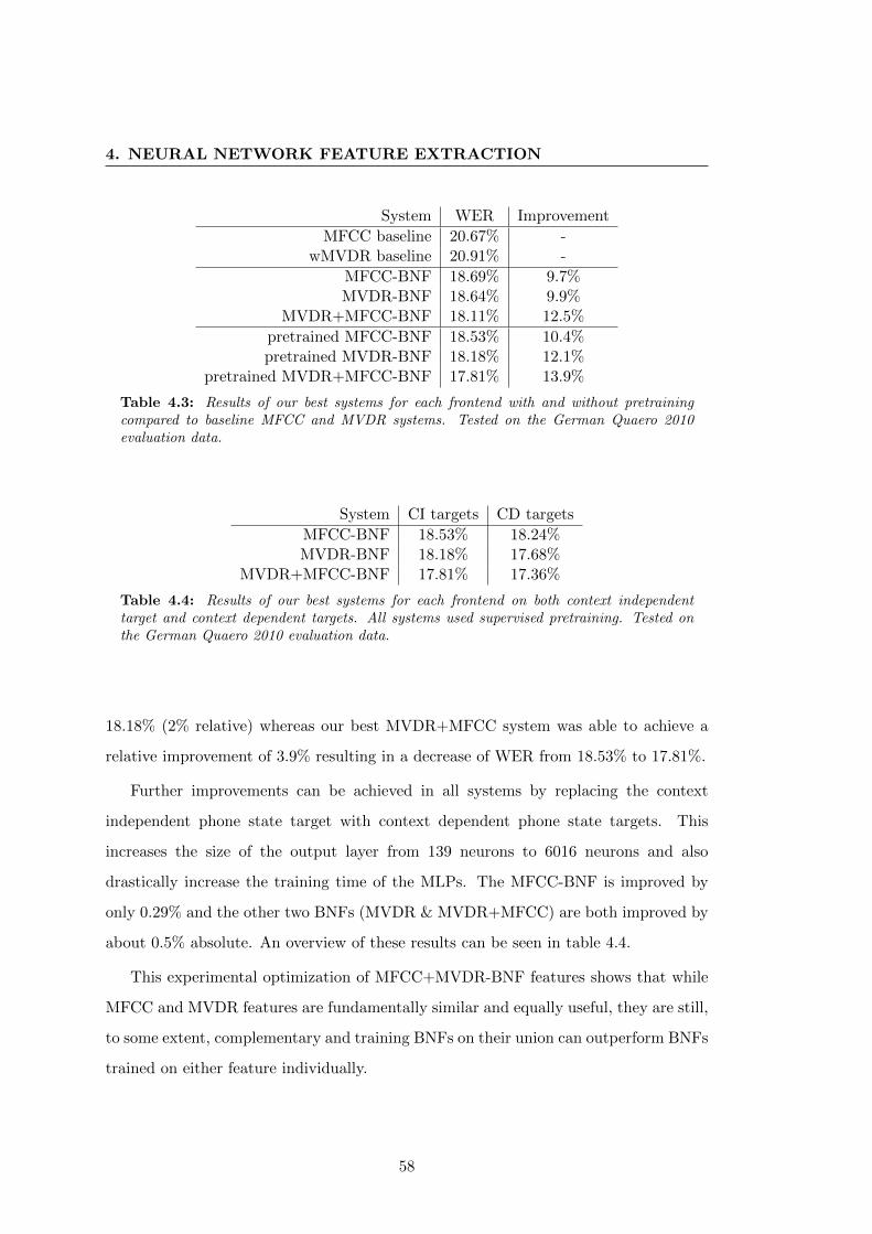
4. NEURAL NETWORK FEATURE EXTRACTION
System WER Improvement
MFCC baseline 20.67% -wMVDR baseline 20.91% -
MFCC-BNF 18.69% 9.7%MVDR-BNF 18.64% 9.9%
MVDR+MFCC-BNF 18.11% 12.5%
pretrained MFCC-BNF 18.53% 10.4%pretrained MVDR-BNF 18.18% 12.1%
pretrained MVDR+MFCC-BNF 17.81% 13.9%
Table 4.3: Results of our best systems for each frontend with and without pretrainingcompared to baseline MFCC and MVDR systems. Tested on the German Quaero 2010evaluation data.
System CI targets CD targets
MFCC-BNF 18.53% 18.24%MVDR-BNF 18.18% 17.68%
MVDR+MFCC-BNF 17.81% 17.36%
Table 4.4: Results of our best systems for each frontend on both context independenttarget and context dependent targets. All systems used supervised pretraining. Tested onthe German Quaero 2010 evaluation data.
18.18% (2% relative) whereas our best MVDR+MFCC system was able to achieve a
relative improvement of 3.9% resulting in a decrease of WER from 18.53% to 17.81%.
Further improvements can be achieved in all systems by replacing the context
independent phone state target with context dependent phone state targets. This
increases the size of the output layer from 139 neurons to 6016 neurons and also
drastically increase the training time of the MLPs. The MFCC-BNF is improved by
only 0.29% and the other two BNFs (MVDR & MVDR+MFCC) are both improved by
about 0.5% absolute. An overview of these results can be seen in table 4.4.
This experimental optimization of MFCC+MVDR-BNF features shows that while
MFCC and MVDR features are fundamentally similar and equally useful, they are still,
to some extent, complementary and training BNFs on their union can outperform BNFs
trained on either feature individually.
58
4.3 Combining Features with a Bottleneck MLP
4.3.2 Deep Bottleneck based Feature Combination
In the previous section the effects of different sizes of inputs are analyzed on both
single feature and multifeature BNF networks. This section expands on those results
by increasing the number of hidden layers in the neural networks for BNF extraction
and examines the effects of also integrating lMEL and tonal features. We refer to BNFs
whose neural networks contain two or more hidden layers prior to the bottleneck layer
as deep bottleneck features (DBNF). An example of such a network with 4 hidden layers
prior to the bottleneck layer is given in Figure 4.4. The input, output and bottleneck
layers remain unchanged but the number of hidden layers between the input layer and
the output layer has increased from one to four. In order to avoid increasing the number
of parameters too drastically the size of the hidden layers is reduced. The largest
network analyzed so far uses an input feature vector of 600 followed by a 4000 neuron
hidden layer, a bottleneck layer with 42 neurons, a final smaller hidden layer of 2000
neurons and a 6016 neuron output layer. Since all layers are fully connected the network
contains 14 684 000 connections. Adding an extra hidden layer with 4000 neurons just
prior to the bottleneck would increase the number of connections by 16 000 000 to
30 684 000, more than doubling them. By reducing the size of the hidden layers to 1200
neurons we can build a deep bottleneck network with 5 hidden layers between the input
and the bottleneck that contains only 13 800 000 connections. With the exception of
the bottleneck all hidden layers in a DBNF are the same size and the hidden layers
prior to the bottleneck are referred to as the main hidden layers. This allows us to
name the example network 5x1.2k where the 5 refers to its number of hidden layers
and 1.2k refers to its size.
The experiments on DBNFs are evaluated on both the IWSLT dev2012 test set and
the Quaero eval2010 test set. Although the results are reported together the tests were
initially run on dev2012 and all design decisions based on those results. Only after all
DBNF experiments were evaluated on dev2012 are the same models used to evaluate
the eval2010 test set. The test sets are dissimilar enough so that improvements and
trends that then also show up the in eval2010 can be considered real improvements and
not merely test set tuning.
While the results in section 4.3 are obtained using the Quaero 2011 evaluation
system the results in this section employ both the Quaero 2012 evaluation system
59
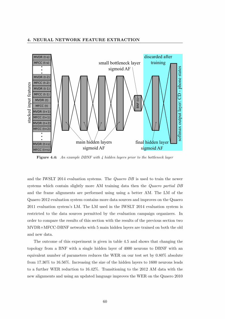
4. NEURAL NETWORK FEATURE EXTRACTION
main hidden layers
sigmoid AF
MVDR (t)
MFCC (t)
MVDR (t-1)
MFCC (t-1)
MVDR (t+1)
MFCC (t+1)
MVDR (t+2)
MFCC (t+2)
MVDR (t-2)
MFCC (t-2)
MVDR (t-s)
MFCC (t-s)
MVDR (t+s)
MFCC (t+s)
small bottleneck layer
sigmoid AF
final hidden layer
sigmoid AF
soft
max
ou
tpu
t la
yer
: C
D -
ph
on
e st
ates
discarded after
training
BN
F (
t)
stac
ked
in
pu
t fe
atu
res
Figure 4.4: An example DBNF with 4 hidden layers prior to the bottleneck layer
and the IWSLT 2014 evaluation systems. The Quaero DB is used to train the newer
systems which contain slightly more AM training data then the Quaero partial DB
and the frame alignments are performed using using a better AM. The LM of the
Quaero 2012 evaluation system contains more data sources and improves on the Quaero
2011 evaluation system’s LM. The LM used in the IWSLT 2014 evaluation system is
restricted to the data sources permitted by the evaluation campaign organizers. In
order to compare the results of this section with the results of the previous section two
MVDR+MFCC-DBNF networks with 5 main hidden layers are trained on both the old
and new data.
The outcome of this experiment is given in table 4.5 and shows that changing the
topology from a BNF with a single hidden layer of 4000 neurons to DBNF with an
equivalent number of parameters reduces the WER on our test set by 0.80% absolute
from 17.36% to 16.56%. Increasing the size of the hidden layers to 1600 neurons leads
to a further WER reduction to 16.42%. Transitioning to the 2012 AM data with the
new alignments and using an updated language improves the WER on the Quaero 2010
60
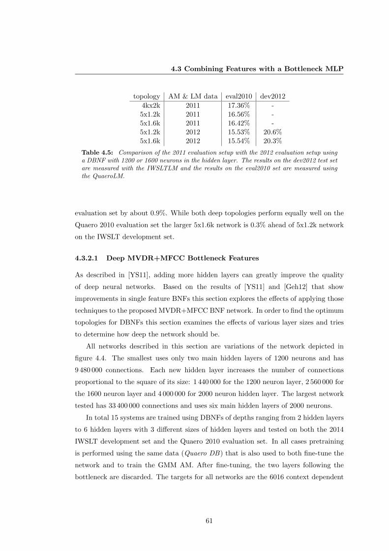
4.3 Combining Features with a Bottleneck MLP
topology AM & LM data eval2010 dev2012
4kx2k 2011 17.36% -5x1.2k 2011 16.56% -5x1.6k 2011 16.42% -5x1.2k 2012 15.53% 20.6%5x1.6k 2012 15.54% 20.3%
Table 4.5: Comparison of the 2011 evaluation setup with the 2012 evaluation setup usinga DBNF with 1200 or 1600 neurons in the hidden layer. The results on the dev2012 test setare measured with the IWSLTLM and the results on the eval2010 set are measured usingthe QuaeroLM.
evaluation set by about 0.9%. While both deep topologies perform equally well on the
Quaero 2010 evaluation set the larger 5x1.6k network is 0.3% ahead of 5x1.2k network
on the IWSLT development set.
4.3.2.1 Deep MVDR+MFCC Bottleneck Features
As described in [YS11], adding more hidden layers can greatly improve the quality
of deep neural networks. Based on the results of [YS11] and [Geh12] that show
improvements in single feature BNFs this section explores the effects of applying those
techniques to the proposed MVDR+MFCC BNF network. In order to find the optimum
topologies for DBNFs this section examines the effects of various layer sizes and tries
to determine how deep the network should be.
All networks described in this section are variations of the network depicted in
figure 4.4. The smallest uses only two main hidden layers of 1200 neurons and has
9 480 000 connections. Each new hidden layer increases the number of connections
proportional to the square of its size: 1 440 000 for the 1200 neuron layer, 2 560 000 for
the 1600 neuron layer and 4 000 000 for 2000 neuron hidden layer. The largest network
tested has 33 400 000 connections and uses six main hidden layers of 2000 neurons.
In total 15 systems are trained using DBNFs of depths ranging from 2 hidden layers
to 6 hidden layers with 3 different sizes of hidden layers and tested on both the 2014
IWSLT development set and the Quaero 2010 evaluation set. In all cases pretraining
is performed using the same data (Quaero DB) that is also used to both fine-tune the
network and to train the GMM AM. After fine-tuning, the two layers following the
bottleneck are discarded. The targets for all networks are the 6016 context dependent
61
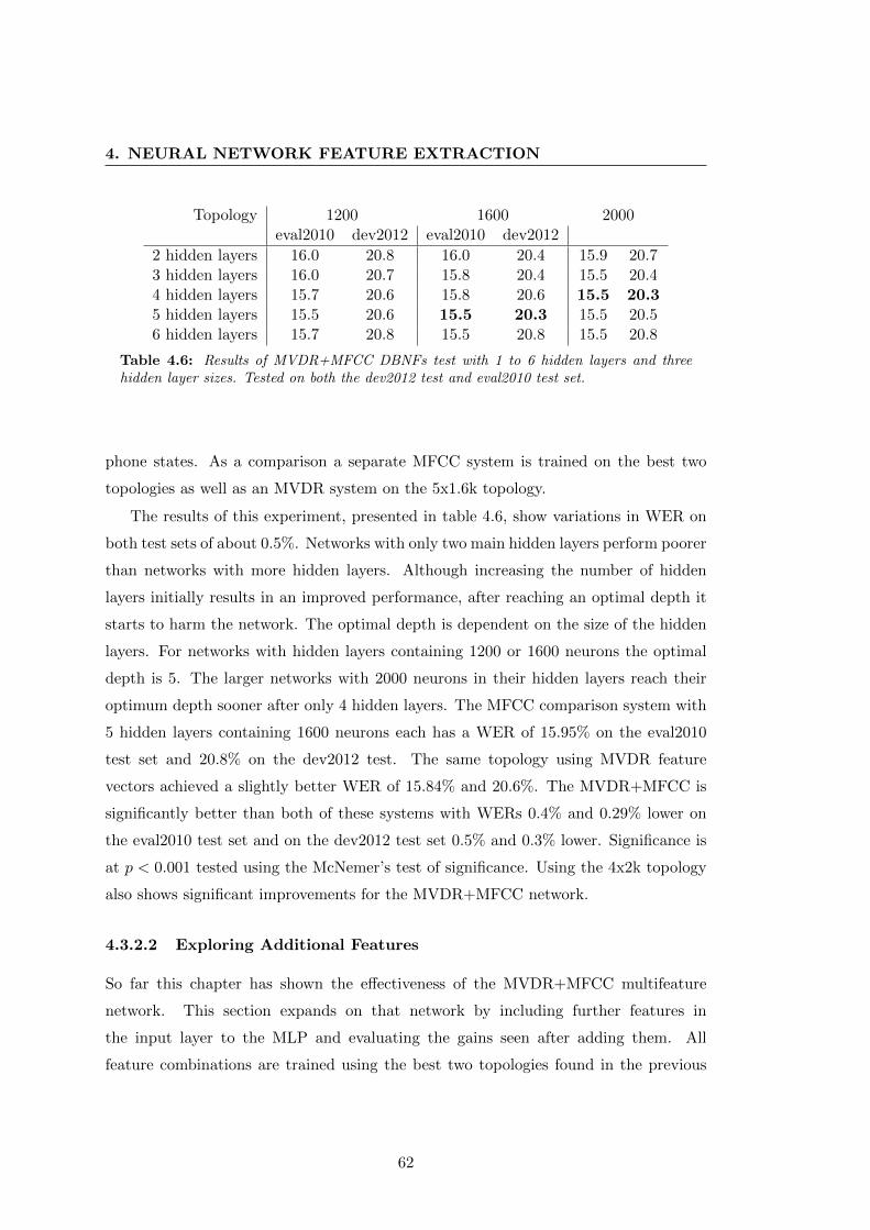
4. NEURAL NETWORK FEATURE EXTRACTION
Topology 1200 1600 2000eval2010 dev2012 eval2010 dev2012
2 hidden layers 16.0 20.8 16.0 20.4 15.9 20.73 hidden layers 16.0 20.7 15.8 20.4 15.5 20.44 hidden layers 15.7 20.6 15.8 20.6 15.5 20.35 hidden layers 15.5 20.6 15.5 20.3 15.5 20.56 hidden layers 15.7 20.8 15.5 20.8 15.5 20.8
Table 4.6: Results of MVDR+MFCC DBNFs test with 1 to 6 hidden layers and threehidden layer sizes. Tested on both the dev2012 test and eval2010 test set.
phone states. As a comparison a separate MFCC system is trained on the best two
topologies as well as an MVDR system on the 5x1.6k topology.
The results of this experiment, presented in table 4.6, show variations in WER on
both test sets of about 0.5%. Networks with only two main hidden layers perform poorer
than networks with more hidden layers. Although increasing the number of hidden
layers initially results in an improved performance, after reaching an optimal depth it
starts to harm the network. The optimal depth is dependent on the size of the hidden
layers. For networks with hidden layers containing 1200 or 1600 neurons the optimal
depth is 5. The larger networks with 2000 neurons in their hidden layers reach their
optimum depth sooner after only 4 hidden layers. The MFCC comparison system with
5 hidden layers containing 1600 neurons each has a WER of 15.95% on the eval2010
test set and 20.8% on the dev2012 test. The same topology using MVDR feature
vectors achieved a slightly better WER of 15.84% and 20.6%. The MVDR+MFCC is
significantly better than both of these systems with WERs 0.4% and 0.29% lower on
the eval2010 test set and on the dev2012 test set 0.5% and 0.3% lower. Significance is
at p < 0.001 tested using the McNemer’s test of significance. Using the 4x2k topology
also shows significant improvements for the MVDR+MFCC network.
4.3.2.2 Exploring Additional Features
So far this chapter has shown the effectiveness of the MVDR+MFCC multifeature
network. This section expands on that network by including further features in
the input layer to the MLP and evaluating the gains seen after adding them. All
feature combinations are trained using the best two topologies found in the previous
62
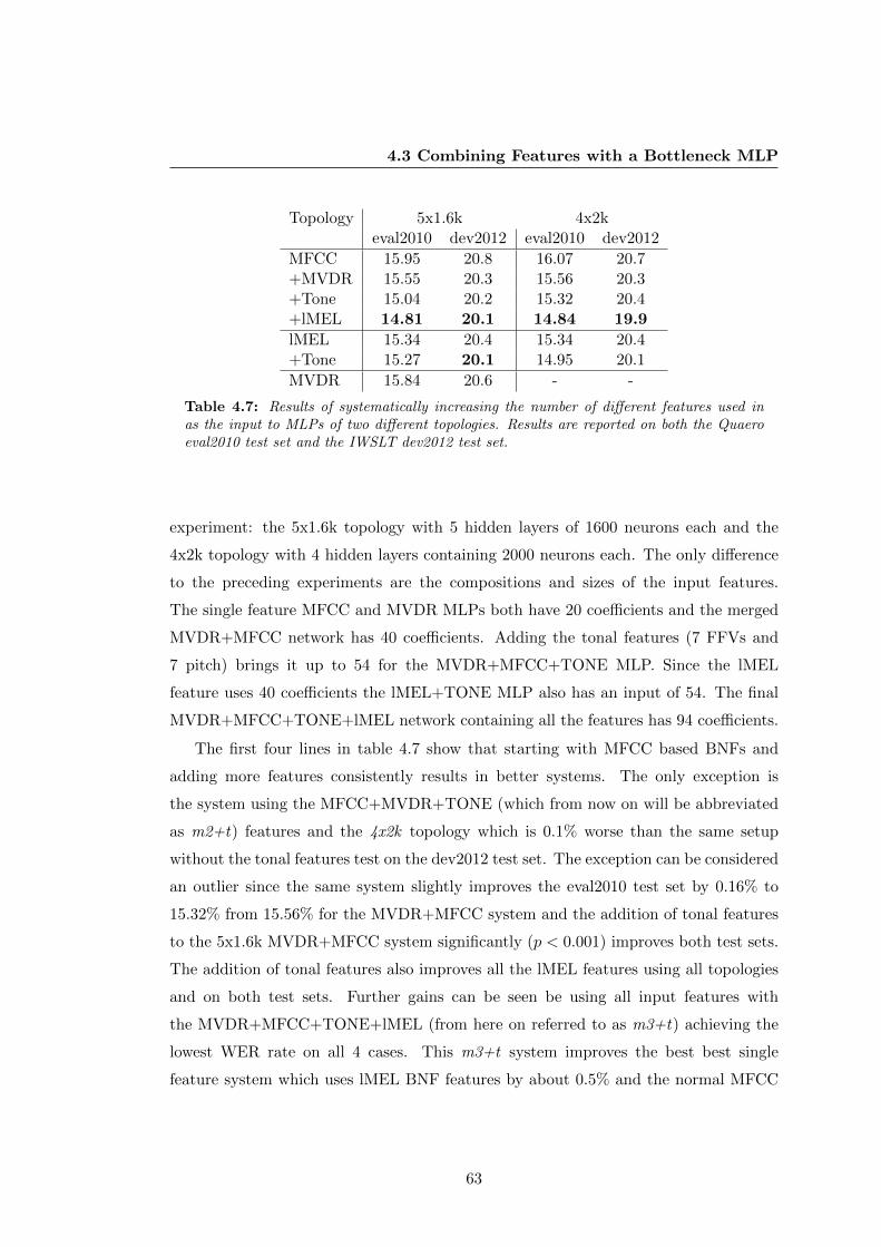
4.3 Combining Features with a Bottleneck MLP
Topology 5x1.6k 4x2keval2010 dev2012 eval2010 dev2012
MFCC 15.95 20.8 16.07 20.7+MVDR 15.55 20.3 15.56 20.3+Tone 15.04 20.2 15.32 20.4+lMEL 14.81 20.1 14.84 19.9
lMEL 15.34 20.4 15.34 20.4+Tone 15.27 20.1 14.95 20.1
MVDR 15.84 20.6 - -
Table 4.7: Results of systematically increasing the number of different features used inas the input to MLPs of two different topologies. Results are reported on both the Quaeroeval2010 test set and the IWSLT dev2012 test set.
experiment: the 5x1.6k topology with 5 hidden layers of 1600 neurons each and the
4x2k topology with 4 hidden layers containing 2000 neurons each. The only difference
to the preceding experiments are the compositions and sizes of the input features.
The single feature MFCC and MVDR MLPs both have 20 coefficients and the merged
MVDR+MFCC network has 40 coefficients. Adding the tonal features (7 FFVs and
7 pitch) brings it up to 54 for the MVDR+MFCC+TONE MLP. Since the lMEL
feature uses 40 coefficients the lMEL+TONE MLP also has an input of 54. The final
MVDR+MFCC+TONE+lMEL network containing all the features has 94 coefficients.
The first four lines in table 4.7 show that starting with MFCC based BNFs and
adding more features consistently results in better systems. The only exception is
the system using the MFCC+MVDR+TONE (which from now on will be abbreviated
as m2+t) features and the 4x2k topology which is 0.1% worse than the same setup
without the tonal features test on the dev2012 test set. The exception can be considered
an outlier since the same system slightly improves the eval2010 test set by 0.16% to
15.32% from 15.56% for the MVDR+MFCC system and the addition of tonal features
to the 5x1.6k MVDR+MFCC system significantly (p < 0.001) improves both test sets.
The addition of tonal features also improves all the lMEL features using all topologies
and on both test sets. Further gains can be seen be using all input features with
the MVDR+MFCC+TONE+lMEL (from here on referred to as m3+t) achieving the
lowest WER rate on all 4 cases. This m3+t system improves the best best single
feature system which uses lMEL BNF features by about 0.5% and the normal MFCC
63
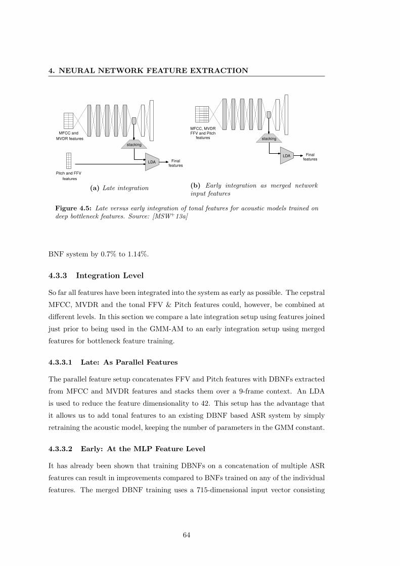
4. NEURAL NETWORK FEATURE EXTRACTION
LDA
MFCC andMVDR features
Pitch and FFVfeatures
Finalfeatures
stacking
(a) Late integration
MFCC, MVDRFFV and Pitch
features
LDA Finalfeatures
stacking
(b) Early integration as merged networkinput features
Figure 4.5: Late versus early integration of tonal features for acoustic models trained ondeep bottleneck features. Source: [MSW+13a]
BNF system by 0.7% to 1.14%.
4.3.3 Integration Level
So far all features have been integrated into the system as early as possible. The cepstral
MFCC, MVDR and the tonal FFV & Pitch features could, however, be combined at
different levels. In this section we compare a late integration setup using features joined
just prior to being used in the GMM-AM to an early integration setup using merged
features for bottleneck feature training.
4.3.3.1 Late: As Parallel Features
The parallel feature setup concatenates FFV and Pitch features with DBNFs extracted
from MFCC and MVDR features and stacks them over a 9-frame context. An LDA
is used to reduce the feature dimensionality to 42. This setup has the advantage that
it allows us to add tonal features to an existing DBNF based ASR system by simply
retraining the acoustic model, keeping the number of parameters in the GMM constant.
4.3.3.2 Early: At the MLP Feature Level
It has already been shown that training DBNFs on a concatenation of multiple ASR
features can result in improvements compared to BNFs trained on any of the individual
features. The merged DBNF training uses a 715-dimensional input vector consisting
64
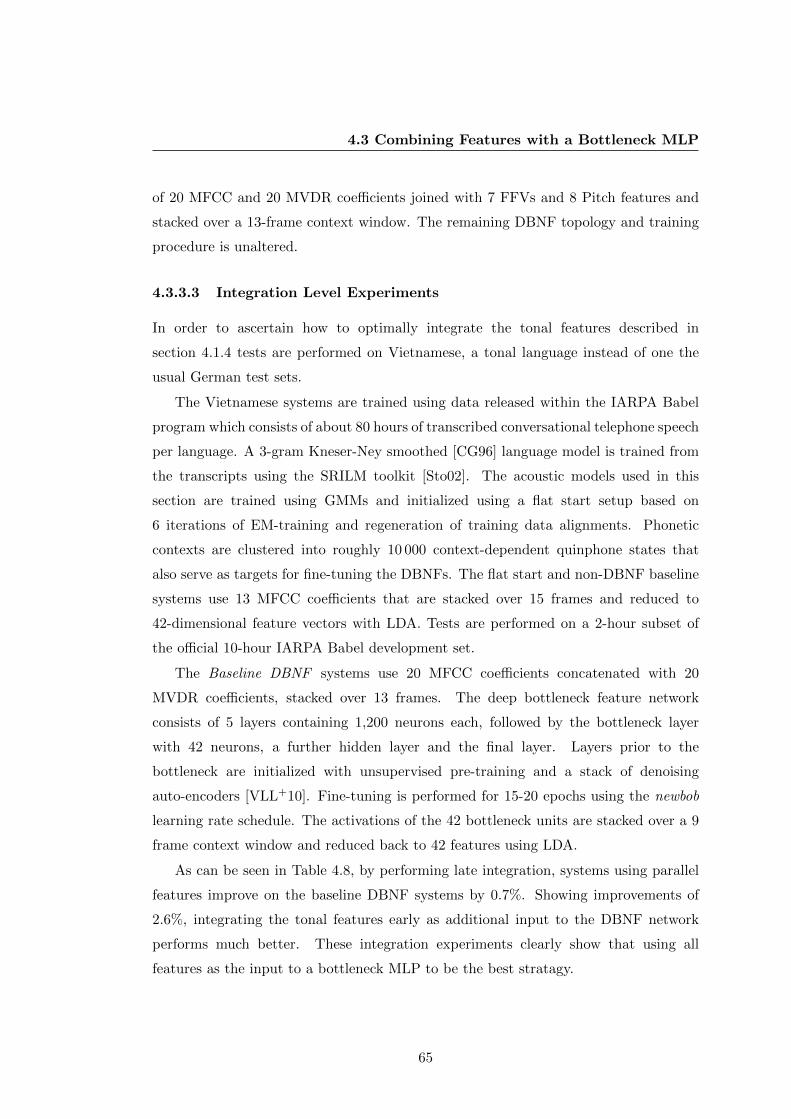
4.3 Combining Features with a Bottleneck MLP
of 20 MFCC and 20 MVDR coefficients joined with 7 FFVs and 8 Pitch features and
stacked over a 13-frame context window. The remaining DBNF topology and training
procedure is unaltered.
4.3.3.3 Integration Level Experiments
In order to ascertain how to optimally integrate the tonal features described in
section 4.1.4 tests are performed on Vietnamese, a tonal language instead of one the
usual German test sets.
The Vietnamese systems are trained using data released within the IARPA Babel
program which consists of about 80 hours of transcribed conversational telephone speech
per language. A 3-gram Kneser-Ney smoothed [CG96] language model is trained from
the transcripts using the SRILM toolkit [Sto02]. The acoustic models used in this
section are trained using GMMs and initialized using a flat start setup based on
6 iterations of EM-training and regeneration of training data alignments. Phonetic
contexts are clustered into roughly 10 000 context-dependent quinphone states that
also serve as targets for fine-tuning the DBNFs. The flat start and non-DBNF baseline
systems use 13 MFCC coefficients that are stacked over 15 frames and reduced to
42-dimensional feature vectors with LDA. Tests are performed on a 2-hour subset of
the official 10-hour IARPA Babel development set.
The Baseline DBNF systems use 20 MFCC coefficients concatenated with 20
MVDR coefficients, stacked over 13 frames. The deep bottleneck feature network
consists of 5 layers containing 1,200 neurons each, followed by the bottleneck layer
with 42 neurons, a further hidden layer and the final layer. Layers prior to the
bottleneck are initialized with unsupervised pre-training and a stack of denoising
auto-encoders [VLL+10]. Fine-tuning is performed for 15-20 epochs using the newbob
learning rate schedule. The activations of the 42 bottleneck units are stacked over a 9
frame context window and reduced back to 42 features using LDA.
As can be seen in Table 4.8, by performing late integration, systems using parallel
features improve on the baseline DBNF systems by 0.7%. Showing improvements of
2.6%, integrating the tonal features early as additional input to the DBNF network
performs much better. These integration experiments clearly show that using all
features as the input to a bottleneck MLP to be the best stratagy.
65
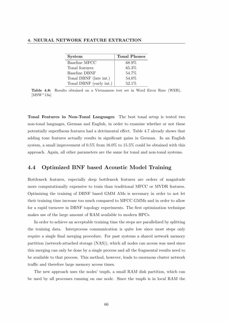
4. NEURAL NETWORK FEATURE EXTRACTION
System Tonal Phones
Baseline MFCC 68.9%Tonal features 65.3%Baseline DBNF 54.7%Tonal DBNF (late int.) 54.0%Tonal DBNF (early int.) 52.1%
Table 4.8: Results obtained on a Vietnamese test set in Word Error Rate (WER).[MSW+13a]
Tonal Features in Non-Tonal Languages The best tonal setup is tested two
non-tonal languages, German and English, in order to examine whether or not these
potentially superfluous features had a detrimental effect. Table 4.7 already shows that
adding tone features actually results in significant gains in German. In an English
system, a small improvement of 0.5% from 16.0% to 15.5% could be obtained with this
approach. Again, all other parameters are the same for tonal and non-tonal systems.
4.4 Optimized BNF based Acoustic Model Training
Bottleneck features, especially deep bottleneck features are orders of magnitude
more computationally expensive to train than traditional MFCC or MVDR features.
Optimizing the training of DBNF based GMM AMs is necessary in order to not let
their training time increase too much compared to MFCC GMMs and in order to allow
for a rapid turnover in DBNF topology experiments. The first optimization technique
makes use of the large amount of RAM available to modern HPCs.
In order to achieve an acceptable training time the steps are parallelized by splitting
the training data. Interprocess communication is quite low since most steps only
require a single final merging procedure. For past systems a shared network memory
partition (network-attached storage (NAS)), which all nodes can access was used since
this merging can only be done by a single process and all the fragmental results need to
be available to that process. This method, however, leads to enormous cluster network
traffic and therefore large memory access times.
The new approach uses the nodes’ tmpfs, a small RAM disk partition, which can
be used by all processes running on one node. Since the tmpfs is in local RAM the
66
4.4 Optimized BNF based Acoustic Model Training
Step tmpfs NAS (1 node) NAS (4 nodes)
LDAs ≈ 16 min ≈ 20 min ≈ 5 minSamples ≈ 9 min ≈ 68 min ≈ 17 minMAS ≈ 9 min ≈ 104 min ≈ 26 minOFS ≈ 116 min ≈ 184 min ≈ 46 minViterbi ≈ 54 min ≈ 80 min ≈ 20 min
total ≈ 204 min ≈ 456 min ≈ 114 min
Table 4.9: Runtime of different training steps comparing use of tmpfs (RAM disk) andshared network memory (NAS). All training steps using tmpfs are run on a single node,training steps using NAS are run on 4 nodes. The middle column, NAS (1 node), wascomputed from the NAS (4 node) column in order to better demonstrate the resourcessaved by using tmpfs. Source: [KSM+11]
access times are short and there is no need to send data over the network. We limit
the maximal number of processes per step to the number of cores in a node. Table 4.9
compares the training time of several training steps of a non-BNF system computed
on one node with 16 cores using tmpfs to their runtime using shared network memory
and more nodes, with an extra column showing the hypothetical runtime of the NAS
setup if only a single node is used. It can be seen that most steps are absolutely
faster using tmpfs or at least relatively faster according to the number of processes.
The steps performed during GMM training involve first training an LDA matrix after
which samples are written in order to build the initial GMM models using incremental
splitting of Gaussians (MAS ) training, followed by the training of a global STC matrix
and two rounds of Viterbi training. In total the tmpfs approach requires only about
half as many cluster node minutes as the NAS approach. The presented numbers are
from a time of low cluster traffic. At times of high cluster traffic the NAS approach is
slowed down even more.
The second optimization directly addresses the issue raised by the botteneck
features. Caching them locally in RAM for the duration of the whole training process
means that their increased computational cost only has to be paid once. This, however,
comes at the expense of requiring machines with a large amount of RAM. For smaller
machines a compromise solution that caches them on a local disk is implemented.
Table 4.10 clearly shows that the computation of the DBNF features dominates the
GMM training process and that caching the features reduced the training time by a
67
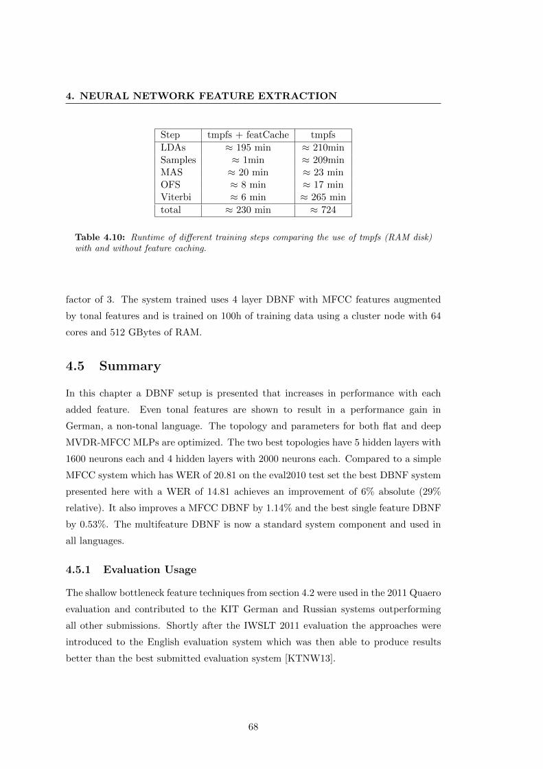
4. NEURAL NETWORK FEATURE EXTRACTION
Step tmpfs + featCache tmpfs
LDAs ≈ 195 min ≈ 210minSamples ≈ 1min ≈ 209minMAS ≈ 20 min ≈ 23 minOFS ≈ 8 min ≈ 17 minViterbi ≈ 6 min ≈ 265 min
total ≈ 230 min ≈ 724
Table 4.10: Runtime of different training steps comparing the use of tmpfs (RAM disk)with and without feature caching.
factor of 3. The system trained uses 4 layer DBNF with MFCC features augmented
by tonal features and is trained on 100h of training data using a cluster node with 64
cores and 512 GBytes of RAM.
4.5 Summary
In this chapter a DBNF setup is presented that increases in performance with each
added feature. Even tonal features are shown to result in a performance gain in
German, a non-tonal language. The topology and parameters for both flat and deep
MVDR-MFCC MLPs are optimized. The two best topologies have 5 hidden layers with
1600 neurons each and 4 hidden layers with 2000 neurons each. Compared to a simple
MFCC system which has WER of 20.81 on the eval2010 test set the best DBNF system
presented here with a WER of 14.81 achieves an improvement of 6% absolute (29%
relative). It also improves a MFCC DBNF by 1.14% and the best single feature DBNF
by 0.53%. The multifeature DBNF is now a standard system component and used in
all languages.
4.5.1 Evaluation Usage
The shallow bottleneck feature techniques from section 4.2 were used in the 2011 Quaero
evaluation and contributed to the KIT German and Russian systems outperforming
all other submissions. Shortly after the IWSLT 2011 evaluation the approaches were
introduced to the English evaluation system which was then able to produce results
better than the best submitted evaluation system [KTNW13].
68
Chapter 5
Neural Network Acoustic Models
This chapter examines acoustic models that use neural networks to estimate their
emission probabilities. This approach was first introduced in 1993 by Bourlard
[BM94] and is explained in section 2.2.2.3. Initially only phone states or a very
small number of context dependent phone states could be used as targets for the
neural network. In recent years, with the advent of powerful graphics processing
units and NN training algorithms that make use of them [BBB+10], the number of
context dependent phone states that can reasonably be used has increased to well
over 10 000. The increased output layer size coupled with bigger and deeper networks
trained on a lot of data has lead to impressive reductions in WER by up to 30% relative
[SSS14, DYDA12, HDY+12]. The multiple feature streams, introduced in chapter 4 as
inputs to DBNF networks, are applied to DNNs in this chapter and the actual DBNF
networks evaluated there are reused as building blocks for a larger modular DNNs. This
chapter also investigates how to train a cluster tree without using a GMM based AM
and how SVD based layer initialization can be applied to DNNs.
69
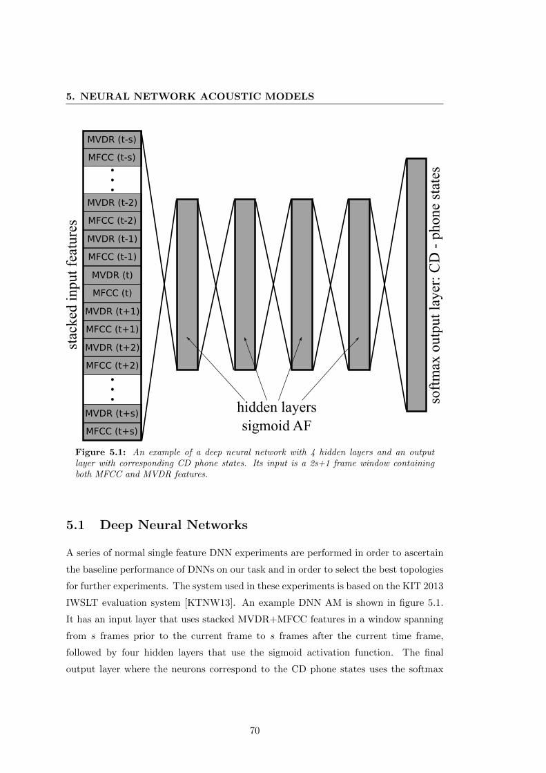
5. NEURAL NETWORK ACOUSTIC MODELS
hidden layers
sigmoid AF
MVDR (t)
MFCC (t)
MVDR (t-1)
MFCC (t-1)
MVDR (t+1)
MFCC (t+1)
MVDR (t+2)
MFCC (t+2)
MVDR (t-2)
MFCC (t-2)
MVDR (t-s)
MFCC (t-s)
MVDR (t+s)
MFCC (t+s)
stac
ked
input
feat
ure
s
soft
max
outp
ut
layer
: C
D -
phone
stat
esFigure 5.1: An example of a deep neural network with 4 hidden layers and an outputlayer with corresponding CD phone states. Its input is a 2s+1 frame window containingboth MFCC and MVDR features.
5.1 Deep Neural Networks
A series of normal single feature DNN experiments are performed in order to ascertain
the baseline performance of DNNs on our task and in order to select the best topologies
for further experiments. The system used in these experiments is based on the KIT 2013
IWSLT evaluation system [KTNW13]. An example DNN AM is shown in figure 5.1.
It has an input layer that uses stacked MVDR+MFCC features in a window spanning
from s frames prior to the current frame to s frames after the current time frame,
followed by four hidden layers that use the sigmoid activation function. The final
output layer where the neurons correspond to the CD phone states uses the softmax
70
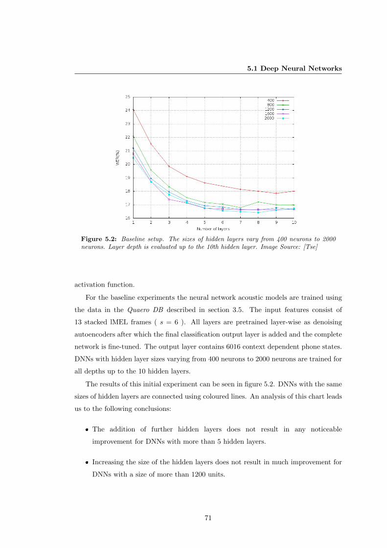
5.1 Deep Neural Networks
Figure 5.2: Baseline setup. The sizes of hidden layers vary from 400 neurons to 2000neurons. Layer depth is evaluated up to the 10th hidden layer. Image Source: [Tse]
activation function.
For the baseline experiments the neural network acoustic models are trained using
the data in the Quaero DB described in section 3.5. The input features consist of
13 stacked lMEL frames ( s = 6 ). All layers are pretrained layer-wise as denoising
autoencoders after which the final classification output layer is added and the complete
network is fine-tuned. The output layer contains 6016 context dependent phone states.
DNNs with hidden layer sizes varying from 400 neurons to 2000 neurons are trained for
all depths up to the 10 hidden layers.
The results of this initial experiment can be seen in figure 5.2. DNNs with the same
sizes of hidden layers are connected using coloured lines. An analysis of this chart leads
us to the following conclusions:
� The addition of further hidden layers does not result in any noticeable
improvement for DNNs with more than 5 hidden layers.
� Increasing the size of the hidden layers does not result in much improvement for
DNNs with a size of more than 1200 units.
71
5. NEURAL NETWORK ACOUSTIC MODELS
� Networks with hidden layer sizes between 1200 and 2000 neurons deteriorate
when more than 8 hidden layers are used and from about 4 hidden layers only
very modest gains can be seen by adding further hidden layers.
The results of the baseline experiment are consistent with similar experiments, such as
by Mohamed et al. [MDH12], who also found that adding more than four hidden layers
to their DNN AM does not show any significant improvement. As with the DBNF
experiment the two topologies 5x1.6k (5 hidden layer with 1600 neurons each) and
4x2k (4 hidden layer with 2000 neurons each) are used for further experiments.
5.1.1 Multifeature DNN
This experiment mirrors the DBNF experiment in section 4.3.2.2 where multifeature
DBNFs are compared. Each feature combination is trained on the 5x1.6k topology as
well as on the 4x2k topology. Both the MVDR and MFCC features use 20 coefficients
while the lMEL features have 40 coefficients and are the same size as the merged
MVDR+MFCC feature vector. The addition of 14 tonal features brings the input sizes
up to 54 for both the MVDR+MFCC+TONE (m2+t) and the lMEL+TONE (lmel+t)
networks. The final MVDR+MFCC+TONE+lMEL (m3+t) MLP that contains all
available features has an input of 94. All other MLP parameters are the same in the
baseline experiment.
5.1.1.1 Results
As with the DBNFs, combining the MVDR and MFCC input features results in a
network with a significantly (p < 0.005 for 5x1.6k ) lower WER than either of the
individual features and is about on par with networks using the lMEL feature that
have the same number of coefficients. The 5x1.6k lMEL system is 0.06% better on
the eval2010 test set but 0.2% poorer on the dev2012 test set. A pattern in the results
shown in table 5.1 can be found that suggests that input features using more coefficients
tend to perform better. Both m2+t topologies reduce the WER compared to their
MVDR+MFCC equivalents on the dev2012 test set by 0.1% and on the eval2010 test
set by 0.5%. The addition of tonal feature to the lMEL networks proved to be even more
useful with improvements of 0.61% on eval2010 and 0.5% on dev2012 for the 5x1.6k
topology and for the 4x2k topology 0.45% on eval2010 and 0.4% on dev2012. The best
72
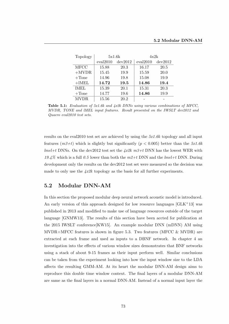
5.2 Modular DNN-AM
Topology 5x1.6k 4x2keval2010 dev2012 eval2010 dev2012
MFCC 15.88 20.3 16.17 20.5+MVDR 15.45 19.9 15.59 20.0+Tone 14.96 19.8 15.08 19.9+lMEL 14.72 19.5 14.86 19.4
lMEL 15.39 20.1 15.31 20.3+Tone 14.77 19.6 14.86 19.9
MVDR 15.56 20.2 - -
Table 5.1: Evaluation of 5x1.6k and 4x2k DNNs using various combinations of MFCC,MVDR, TONE and lMEL input features. Result presented on the IWSLT dev2012 andQuaero eval2010 test sets.
results on the eval2010 test set are achieved by using the 5x1.6k topology and all input
features (m3+t) which is slightly but significantly (p < 0.005) better than the 5x1.6k
lmel+t DNNs. On the dev2012 test set the 4x2k m3+t DNN has the lowest WER with
19.4% which is a full 0.5 lower than both the m2+t DNN and the lmel+t DNN. During
development only the results on the dev2012 test set were measured so the decision was
made to only use the 4x2k topology as the basis for all further experiments.
5.2 Modular DNN-AM
In this section the proposed modular deep neural network acoustic model is introduced.
An early version of this approach designed for low resource languages [GLK+13] was
published in 2013 and modified to make use of language resources outside of the target
language [GNMW13]. The results of this section have been accted for publication at
the 2015 IWSLT conference[KW15]. An example modular DNN (mDNN) AM using
MVDR+MFCC features is shown in figure 5.3. Two features (MFCC & MVDR) are
extracted at each frame and used as inputs to a DBNF network. In chapter 4 an
investigation into the effects of various window sizes demonstrates that BNF networks
using a stack of about 9-15 frames as their input perform well. Similar conclusions
can be taken from the experiment looking into how the input window size to the LDA
affects the resulting GMM-AM. At its heart the modular DNN-AM design aims to
reproduce this double time window context. The final layers of a modular DNN-AM
are same as the final layers in a normal DNN-AM. Instead of a normal input layer the
73
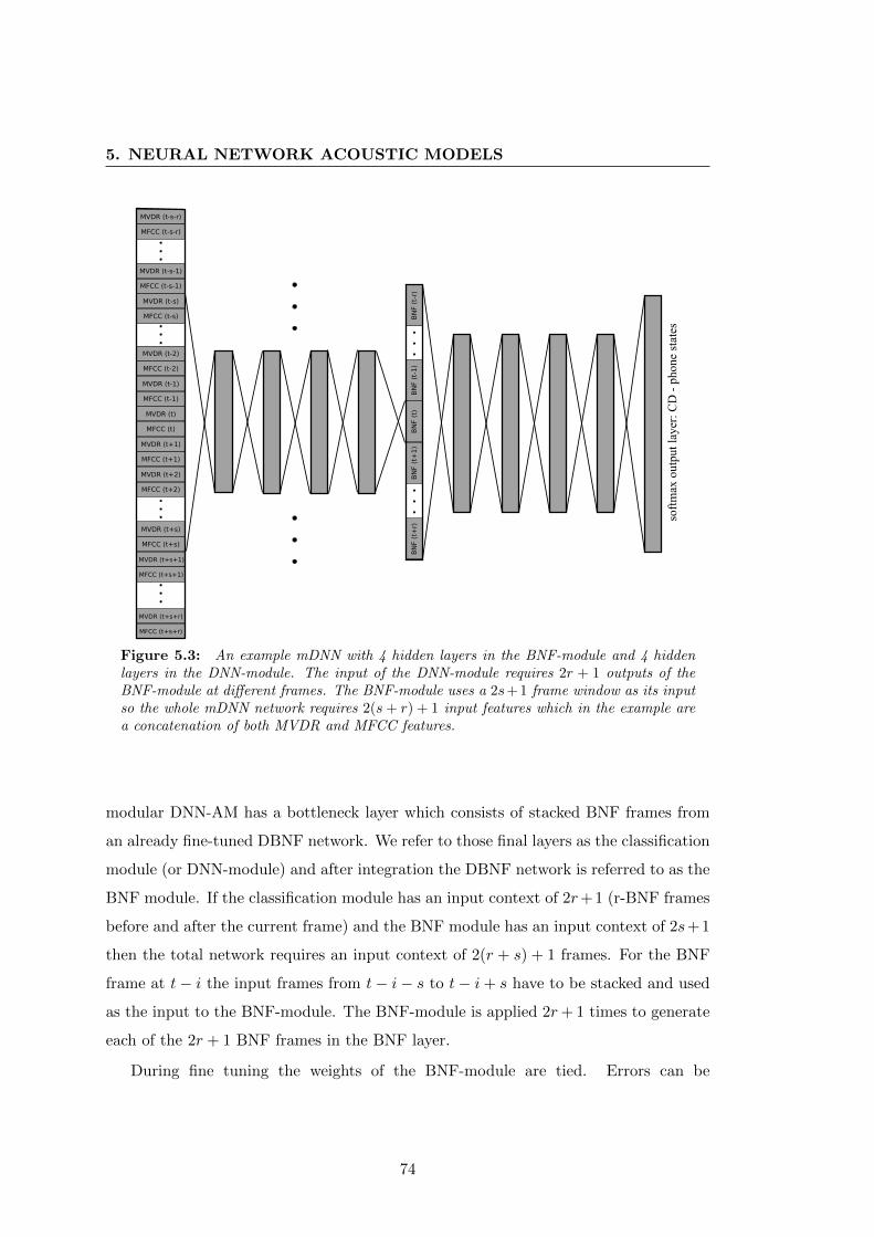
5. NEURAL NETWORK ACOUSTIC MODELS
soft
max
outp
ut
layer
: C
D -
phone
stat
es
MVDR (t)
MFCC (t)
MVDR (t-1)
MFCC (t-1)
MVDR (t+1)
MFCC (t+1)
MVDR (t+2)
MFCC (t+2)
MVDR (t-2)
MFCC (t-2)
MVDR (t-s)
MFCC (t-s)
MVDR (t+s)
MFCC (t+s)
MVDR (t-s-r)
MFCC (t-s-r)
MVDR (t-s-1)
MFCC (t-s-1)
MVDR (t+s+1)
MFCC (t+s+1)
MVDR (t+s+r)
MFCC (t+s+r)
BN
F (
t)B
NF (
t-1
)B
NF (
t+1
)B
NF (
t-r)
BN
F (
t+r)
Figure 5.3: An example mDNN with 4 hidden layers in the BNF-module and 4 hiddenlayers in the DNN-module. The input of the DNN-module requires 2r + 1 outputs of theBNF-module at different frames. The BNF-module uses a 2s+1 frame window as its inputso the whole mDNN network requires 2(s+ r) + 1 input features which in the example area concatenation of both MVDR and MFCC features.
modular DNN-AM has a bottleneck layer which consists of stacked BNF frames from
an already fine-tuned DBNF network. We refer to those final layers as the classification
module (or DNN-module) and after integration the DBNF network is referred to as the
BNF module. If the classification module has an input context of 2r+1 (r-BNF frames
before and after the current frame) and the BNF module has an input context of 2s+1
then the total network requires an input context of 2(r + s) + 1 frames. For the BNF
frame at t− i the input frames from t− i− s to t− i+ s have to be stacked and used
as the input to the BNF-module. The BNF-module is applied 2r+ 1 times to generate
each of the 2r + 1 BNF frames in the BNF layer.
During fine tuning the weights of the BNF-module are tied. Errors can be
74
5.2 Modular DNN-AM
propagated back past the BNF-layer into all applications. Weight tying allows the
modular DNN-AM to continue on using a single BNF-module while it continues to
learn and have its weight updated using the average update:
∆wj =
2r+1∑k=1
∆wkj (5.1)
Such a single BNF-module learns to produce good BNFs that can be used in any part
of a stacked BNF layer.
Although the total computation cost for a single frame is very high, the BNF frames
can be cached a reused for the next frame. At frame t the DNN-module of the example
mDNN in figure 5.3 requires the output of the BNF-module for 2r + 1 different inputs
from t − r to t + r. For frame t − 1 it requires outputs from the BNF-module for the
inputs from t−1−r to t−1+r. So with the exception of the output of the BNF-module
at t+ r all of the required outputs for frame t have already been produced and cached.
The BNF-module is simply used to convert a stream (or multiple streams) of input
features into a stream of DBNF features which are then used as the input stream
for the DNN-module. In an offline setting the stream of input feature vectors from
an utterance forms a matrix and the BNF-module converts this matrix into a matrix
where the columns are BNFs.
Because it is faster to perform a single matrix times matrix operation using a fast
BLAS (Basic Linear Algebra Subprograms) library than it is to perform many vector
times matrix operations, it makes sense to compute the first hidden layer for all features
at the same time. So in an mDNN, if T features are extracted from the wavefile of
an utterance they are first transformed into T activations of the first hidden layer of
the BNF-module, then to T activations of the 2nd, 3rd and so on hidden layers and
then to T bottleneck features followed by T activations of the first hidden layer of
the DNN-module. After transitioning though all the hidden layers the T probability
distributions over the CD phone states are all produced at the same time.
If T features are extracted from the utterance then computing the BNF at frames
t = T or t = 1 could be problematic since these frames require information about the
features at t = T + r or t = −r. To solve this, every requested feature vector prior to
the first one is set to the value of the first feature and the final feature vector is used
75
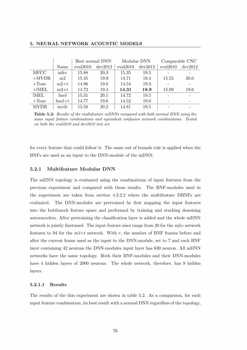
5. NEURAL NETWORK ACOUSTIC MODELS
Best normal DNN Modular DNN Comparable CNCName eval2010 dev2012 eval2010 dev2012 eval2010 dev2012
MFCC mfcc 15.88 20.3 15.35 19.5 - -+MVDR m2 15.45 19.9 14.71 19.4 15.55 20.0+Tone m2+t 14.96 19.8 14.54 19.3 - -+lMEL m3+t 14.72 19.4 14.31 18.9 15.09 19.6
lMEL lmel 15.31 20.1 14.72 19.5 - -+Tone lmel+t 14.77 19.6 14.52 19.0 - -
MVDR mvdr 15.58 20.2 14.81 19.5 - -
Table 5.2: Results of the multifeature mDNNs compared with both normal DNN using thesame input feature combinations and equivalent confusion network combinations. Testedon both the eval2010 and dev2012 test set.
for every feature that could follow it. The same out of bounds rule is applied when the
BNFs are used as an input to the DNN-module of the mDNN.
5.2.1 Multifeature Modular DNN
The mDNN topology is evaluated using the combinations of input features from the
previous experiment and compared with those results. The BNF-modules used in
the experiment are taken from section 4.3.2.2 where the multifeature DBNFs are
evaluated. The DNN-modules are pretrained by first mapping the input features
into the bottleneck feature space and performed by training and stacking denoising
autoencoders. After pretraining the classification layer is added and the whole mDNN
network is jointly finetuned. The input feature sizes range from 20 for the mfcc network
features to 94 for the m3+t network. With r, the number of BNF frames before and
after the current frame used as the input to the DNN-module, set to 7 and each BNF
layer containing 42 neurons the DNN-modules input layer has 630 neuron. All mDNN
networks have the same topology. Both their BNF-modules and their DNN-modules
have 4 hidden layers of 2000 neurons. The whole network, therefore, has 9 hidden
layers.
5.2.1.1 Results
The results of the this experiment are shown in table 5.2. As a comparison, for each
input feature combination, its best result with a normal DNN regardless of the topology,
76
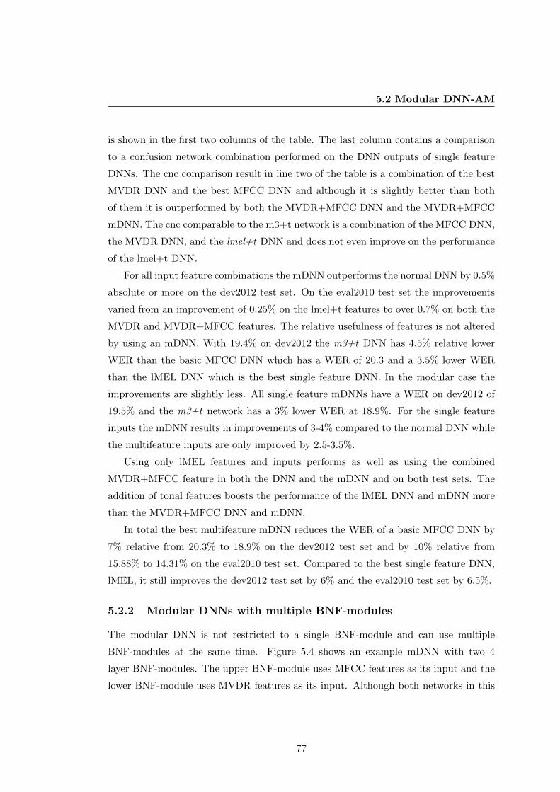
5.2 Modular DNN-AM
is shown in the first two columns of the table. The last column contains a comparison
to a confusion network combination performed on the DNN outputs of single feature
DNNs. The cnc comparison result in line two of the table is a combination of the best
MVDR DNN and the best MFCC DNN and although it is slightly better than both
of them it is outperformed by both the MVDR+MFCC DNN and the MVDR+MFCC
mDNN. The cnc comparable to the m3+t network is a combination of the MFCC DNN,
the MVDR DNN, and the lmel+t DNN and does not even improve on the performance
of the lmel+t DNN.
For all input feature combinations the mDNN outperforms the normal DNN by 0.5%
absolute or more on the dev2012 test set. On the eval2010 test set the improvements
varied from an improvement of 0.25% on the lmel+t features to over 0.7% on both the
MVDR and MVDR+MFCC features. The relative usefulness of features is not altered
by using an mDNN. With 19.4% on dev2012 the m3+t DNN has 4.5% relative lower
WER than the basic MFCC DNN which has a WER of 20.3 and a 3.5% lower WER
than the lMEL DNN which is the best single feature DNN. In the modular case the
improvements are slightly less. All single feature mDNNs have a WER on dev2012 of
19.5% and the m3+t network has a 3% lower WER at 18.9%. For the single feature
inputs the mDNN results in improvements of 3-4% compared to the normal DNN while
the multifeature inputs are only improved by 2.5-3.5%.
Using only lMEL features and inputs performs as well as using the combined
MVDR+MFCC feature in both the DNN and the mDNN and on both test sets. The
addition of tonal features boosts the performance of the lMEL DNN and mDNN more
than the MVDR+MFCC DNN and mDNN.
In total the best multifeature mDNN reduces the WER of a basic MFCC DNN by
7% relative from 20.3% to 18.9% on the dev2012 test set and by 10% relative from
15.88% to 14.31% on the eval2010 test set. Compared to the best single feature DNN,
lMEL, it still improves the dev2012 test set by 6% and the eval2010 test set by 6.5%.
5.2.2 Modular DNNs with multiple BNF-modules
The modular DNN is not restricted to a single BNF-module and can use multiple
BNF-modules at the same time. Figure 5.4 shows an example mDNN with two 4
layer BNF-modules. The upper BNF-module uses MFCC features as its input and the
lower BNF-module uses MVDR features as its input. Although both networks in this
77
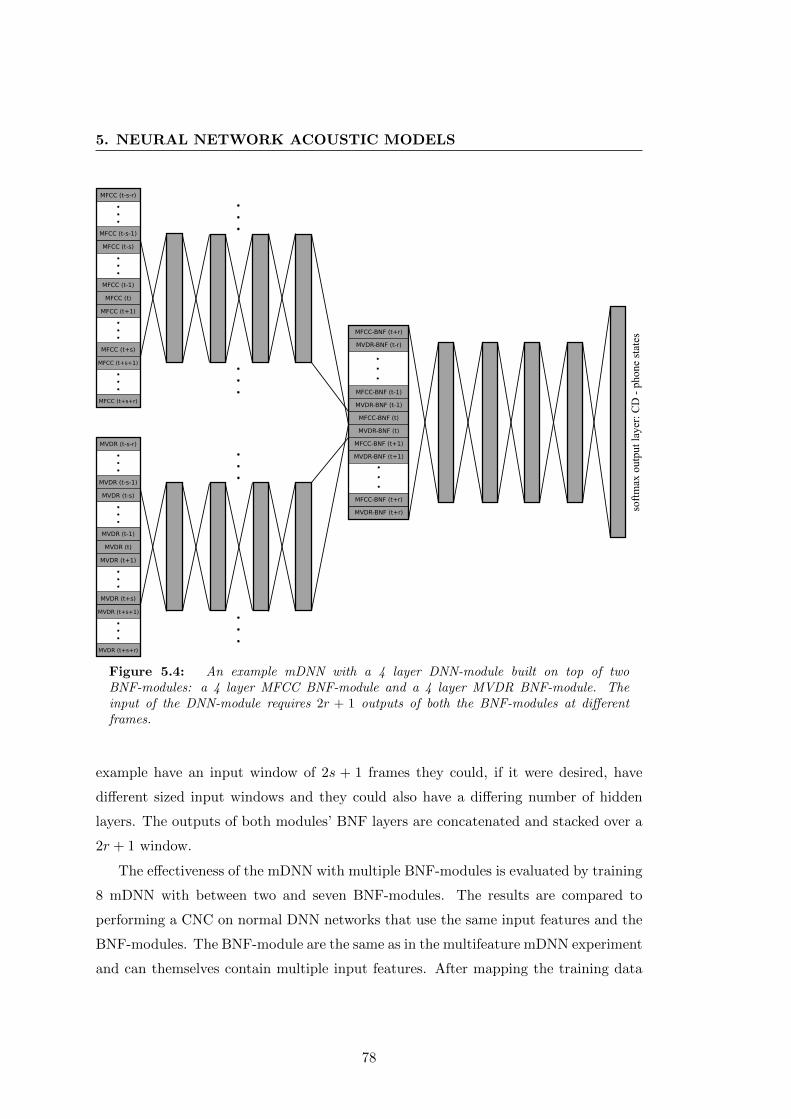
5. NEURAL NETWORK ACOUSTIC MODELS
soft
max
ou
tpu
t la
yer
: C
D -
ph
on
e st
ates
MFCC (t)
MFCC (t-1)
MFCC (t+1)
MFCC (t-s-r)
MFCC (t-s)
MFCC (t-s-1)
MFCC (t+s)
MFCC (t+s+1)
MFCC (t+s+r)
MVDR (t)
MVDR (t-1)
MVDR (t+1)
MVDR (t-s-r)
MVDR (t-s)
MVDR (t-s-1)
MVDR (t+s)
MVDR (t+s+1)
MVDR (t+s+r)
MVDR-BNF (t+r)
MVDR-BNF (t+1)
MVDR-BNF (t-1)
MVDR-BNF (t)
MFCC-BNF (t)
MFCC-BNF (t-1)
MFCC-BNF (t+1)
MFCC-BNF (t+r)
MVDR-BNF (t-r)
MFCC-BNF (t+r)
Figure 5.4: An example mDNN with a 4 layer DNN-module built on top of twoBNF-modules: a 4 layer MFCC BNF-module and a 4 layer MVDR BNF-module. Theinput of the DNN-module requires 2r + 1 outputs of both the BNF-modules at differentframes.
example have an input window of 2s + 1 frames they could, if it were desired, have
different sized input windows and they could also have a differing number of hidden
layers. The outputs of both modules’ BNF layers are concatenated and stacked over a
2r + 1 window.
The effectiveness of the mDNN with multiple BNF-modules is evaluated by training
8 mDNN with between two and seven BNF-modules. The results are compared to
performing a CNC on normal DNN networks that use the same input features and the
BNF-modules. The BNF-module are the same as in the multifeature mDNN experiment
and can themselves contain multiple input features. After mapping the training data
78
5.2 Modular DNN-AM
Modular DNN Comparable CNCName eval2010 dev2012 eval2010 dev2012
mfcc 15.35 19.5 - -⊕ mvdr sys01 14.54 19.2 15.55 20.0⊕ m2 sys03 14.73 19.3 15.44 19.9
mfcc ⊕ mvdr ⊕ lmel+t sys02 14.24 18.7 15.09 19.6
m2+t ⊕ lmel+t sys04 14.19 18.8 14.68 19.4⊕ m3+t sys08 14.06 18.7 14.45 19.2⊕ mfcc ⊕ mvdr sys06 14.33 18.9 14.83 19.4⊕ m2 ⊕ lmel sys05 14.44 18.8 14.69 19.4
m2 ⊕ lmel sys07 14.34 19.1 15.07 19.8
Table 5.3: Comparison of mDNNs using multiple BNF-modules with confusion networkcombinations of normal DNNs using the same input features. The ⊕ is used to indicatethat multiple BNF-modules are combined in a single mDNN.
into the bottleneck feature spaces of all BNF-modules used. The DNN-module is
pretrained on the merged BNF features. All other training parameters are the same as
in the previous experiments.
5.2.2.1 Results
In all cases the mDNN outperformed the confusion network combination of DNN
systems using the same input features. The best mDNN with multiple BNF-modules
m2+t ⊕ lmel+t ⊕ m3+t (⊕ is used to indicate that a combination of BNF-modules)
improves the best single module mDNN by 0.2% from a WER 18.9% to 18.7% on the
dev2012 test set and by 0.25% from 4.31% to 14.06% on the eval2010 test set. Using
McNemar’s significance test this is found to be significant at p < 0.005. The overview
of the results given in table 5.3 begins with single BNF-module mDNN using mfcc
input features that achieves a WER of 15.35% on eval2010 and 19.5% on dev2012. The
next entry augments that mDNN with an MVDR BNF-module and improves dev2012
by 0.3% to 19.2% and eval by 0.81% from 15.35% to 14.54%. The further addition
of the MVDR+MFCC BNF-module degraded the dev2012 test set to 19.3% and the
eval2010 test set to 14.73%. In place of the MVDR+MFCC BNF-module the lmel+t
BNF-module is added to the mfcc ⊕ mvdr. mDNN is then further improved to 14.24%
on eval2010 and 18.7% on dev2012.
79
5. NEURAL NETWORK ACOUSTIC MODELS
The best mDNN with two BNF-modules is the m2+t ⊕ lmel+t mDNN which has
a WER of 14.19% on eval2010 and 18.8% on dev2012. The addition of an m3+t
BNF-module improves it slightly by 0.13% to 14.06% on the eval2010 test set and by
0.1% to 18.7% on the dev2012. The further inclusion of both the MVDR BNF-module
and the MFCC BNF-module slightly increases the WER on both sets. Increasing the
number of BNF-modules to 7 by also including the m2 and lmel BNF-modules into the
mDNN results in another slight increase in WER.
The usefulness of tonal features can be clearly seen by comparing the m2 ⊕ lmel
mDNN to the m2+t ⊕ lmel+t DNN which add tonal features to the input to both
of the BNF-modules. They are able to improve the dev2012 test set by 0.3% and the
eval2010 test set by 0.15%.
Using an mDNN with multiple BNF-modules increases the mDNN’s overall
improvement compared to an MFCC-DNN by 8% relative on the dev2012 test and
by 11.5% on the eval2010 test set. Compared to an lMEL DNN it reduced the WER
by 7% relative from 20.1% to 18.7% on dev2012 and by 8% relative from 15.31% to
14.07%.
5.3 DNN based Clustertrees
This section examines in more detail the output layer of the DNN AM. As discussed
in chapter 2 the neurons in the output layer of DNN AM each correspond to a context
dependent phone state which are leaves in a cluster tree. Section 2.2.2.4 explains how a
cluster tree can be used to cluster all the possible polyphones into a predetermined
number of generalized polyphones. At its heart the clustering algorithm uses the
weighted entropy distance defined as
d(A,B) = (nA + nB)H(A ∪B)− nAH(B)− nAH(B) (5.2)
in order to compute the distance between two classes A and B and decide which question
(cluster devision) to use. The entropy of a cluster
H(p) =
k∑i=1
p(i) log p(i) (5.3)
80
5.3 DNN based Clustertrees
requires a probability distribution over a feature space. The GMM based approach uses
discrete mixture weights of a shared codebook of Gaussians as the feature space.
This means that a GMM AM has to be trained before a cluster tree can be
built which is required in order to train a CD DNN AM. Another prerequisite to
training a DNN is the alignment of feature vectors to HMM states. This is normally
performed with the Viterbi algorithm and is necessary due to the fact that the training
data is only aligned at an utterance level. Despite the superiority of HMM/DNN
AMs most ASR systems still rely on HMM/GMM AMs to generate this alignment
[MHL+14]. A solution proposed by Senior et. al. [SHBL14] shows that this does
not have to be the case and demonstrates how to flat-start an HMM/DNN AM by
using a randomly initialized context independent HMM/DNN AM to generate an
initial alignment. However, after successfully bootstrapping a CI HMM/DNN AM they
“accumulate sufficient statistics to model each context dependent state with a diagonal
covariance Gaussian” in order to build the cluster tree. While their setup avoids the
use of any HMM/GMM AMs they still train Gaussians during clustering making their
setup not Gaussian free. Together with Zhu [Zhu15, ZKSW15] an alternative approach
was investigated that is truly Gaussian free.
5.3.1 CI DNN based Weighted Entropy Distance
A context independent DNN that uses phone states as targets can be trained without
the use of a cluster tree. If desired, the alignment can be flat-started without using a
GMM system by applying either the setup of [SHBL14] or the setup described below.
For each input feature the output of the CI DNN is a discrete probability distribution
of the target phonestates.
The probability distribution which can be used to replace the mixture weights of a
GMM is the average CI DNN output for all features extracted from the training data
which correspond to that polyphone. The assumption is that similar polyphone states
will also have similar average CI DNN outputs.
Therefore, entropy distance between polyphone states can be measured based on
their average CI DNN outputs:
81
5. NEURAL NETWORK ACOUSTIC MODELS
pA(i) =1
nA
nA∑j=1
PDNN (si, Fj) (5.4)
PDNN (si, Fj) is the probability distribution generated by the CI DNN for the feature
Fj . All features Fj are examples of the polyphone cluster A. After calculating its
entropy using the weighted entropy distance d(A,B) between two classes it can now be
computed without using any Gaussians.
5.3.2 Evaluation
The effectiveness of the proposed DNN based cluster tree is evaluated by building
quinphone cluster trees of various sizes from 3k leaves to 21k leaves and comparing
them to cluster trees built using the baseline GMM approach. An mDNN AM is
trained with the appropriate output layer for each of the models. As can be seen in
Figure 5.5 the larger cluster trees outperform the smaller cluster trees up to a size of
18k leaves. The WER reduction appears to be almost linear until about 12k leaves
after which more leaves lead to less of an improvement.
The baseline GMM based approach performed slightly better than the DNN based
approach for the smaller cluster trees but for the larger and better cluster trees the
DNN based approach consistently outperformed the GMM based approach. Using the
McNemar statistical test we compared the aligned hypothesis of both 18k systems and
found the system using the DNN based cluster tree to be significantly better than the
GMM based cluster tree with p < 0.005.
These results shows that the DNN based cluster trees are not only a simple
replacement for GMM based cluster trees in situations where CI-GMM AMs are not
available but can also outperform them.
5.3.3 Gaussian Free mDNN Flatstart
The previous section used alignments from a CI HMM/GMM AM to train the CI AM.
In order to demonstrate the claim of truly Gaussian Free training, fresh alignments are
initialized on the training data using a simple energy based speech/non-speech detection
scheme. The Quaero DB described in section 3.5 is used for the training data and these
82
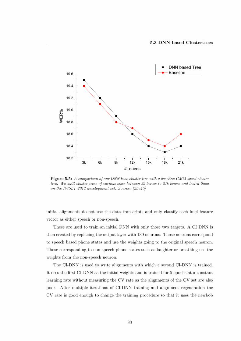
5.3 DNN based Clustertrees
3k 6k 9k 12k 15k 18k 21k18.2
18.4
18.6
18.8
19.0
19.2
19.4
19.6
WER%
#Leaves
DNN based Tree Baseline
Figure 5.5: A comparison of our DNN base cluster tree with a baseline GMM based clustertree. We built cluster trees of various sizes between 3k leaves to 21k leaves and tested themon the IWSLT 2012 development set. Source: [Zhu15]
initial alignments do not use the data transcripts and only classify each lmel feature
vector as either speech or non-speech.
These are used to train an initial DNN with only those two targets. A CI DNN is
then created by replacing the output layer with 139 neurons. Those neurons correspond
to speech based phone states and use the weights going to the original speech neuron.
Those corresponding to non-speech phone states such as laughter or breathing use the
weights from the non-speech neuron.
The CI-DNN is used to write alignments with which a second CI-DNN is trained.
It uses the first CI-DNN as the initial weights and is trained for 5 epochs at a constant
learning rate without measuring the CV rate as the alignments of the CV set are also
poor. After multiple iterations of CI-DNN training and alignment regeneration the
CV rate is good enough to change the training procedure so that it uses the newbob
83
5. NEURAL NETWORK ACOUSTIC MODELS
learning rate schedule and 4 more iterations are performed.
With the flatstarted CI-DNN a cluster tree is built which is then used to train a
CD-mDNN system with 4 hidden layers of 1600 neurons each. This system has a WER
of 20.3% on the dev2012 test set which is close to results of similar systems shown in
table 5.2.
5.4 Growing a DNN with Singular Value Decomposition
Figure 5.2 shows that for a fixed training corpus the performance gains from adding new
layers to a DNN taper off after a certain number of layers. For the Quaero DB examined
in that table, NN-AMs with 5 to 8 hidden layers had roughly the same performance.
Adding further hidden layers eventually started to degrade the performance.
Another problem with large DNNs is that the number of connections between the
hidden layers scales with the square of their size, so two hidden layers with 2000 neurons
each will have 4 million connections between them. The output layer of the DNN AM
typically models context dependent phone states and can contain upwards of 18000
neurons with 36 million connections to the final hidden layer.
Section 2.1.2 explains how the transition from layer i to layer i + 1 in a DNN can
be interpreted as a the multiplication of a vector with a matrix followed by a vector
addition and the element-wise application of the activation function.
xi+1 = φ(Wi,i+1xi + bi+1) (5.5)
Here xi is the output of layer i, bi+1 the bias of layer i + 1, φ the activation function
(computed elementwise), and Wi,i+1 the weight matrix representing the connections
between layers i and i+ 1.
The number of parameters that such large DNNs require can be reduced by applying
singular value decomposition (SVD) to simplify the matrix multiplication step. The
transition matrices Wi,i+1 can be decomposed into two smaller matrices. While
[XLG13] successfully reduces the number of parameters in a DNN without degrading its
performance this section shows how this decomposition can also be used to initialize new
layers with their own activation functions and biases between existing layers, thereby
84
5.4 Growing a DNN with Singular Value Decomposition
allowing us to grow an existing DNN while at the same time possibly also reducing the
number of parameters.
The approach presented in the section was developed together with I. Iseyzer and
first published in [Tse].
5.4.1 Singular Value Decomposition based Layer Initialization
SVD is a factorization method for matrices. An m × n matrix A can be decomposed
as:
Am×n = Um×nΣm×nVTn×n, (5.6)
where U is a unitary matrix, which is a matrix that when multiplied by its conjugate
transposed results in the identity matrix. Σ is a diagonal matrix. V T is the conjugate
transpose of another unitary matrix V . A can be approximated by Ak by setting all but
the highest k singular values in Σ to zeros. The row and columns in u and V T that are
now ignored can be removed and V T combined with Σ to form W (Wk×n = Σk×kVTk×n)
Ak =Um×kΣk×kVTk×n (5.7)
Am×n = Um×kWk×n. (5.8)
Now let Am×n be the weight matrix connecting layers i (containing m neurons) and
j (containing n neurons). After applying SVD to matrix Am×n, we have two matrices
of a smaller size Um×k and Wk×n, which we can interpret as a new layer containing k
neurons with linear activation functions and without biases inserted between layers i
and j. This process is illustrated in figure 5.6. Adding a nonlinear activation function
and learnable biases results in it becoming a fully functional layer. The original idea of
applying SVD to DNN AMs was introduced by [XLG13]. They are able to significantly
reduce the number of parameters in a DNN while incurring no or negligible accuracy
loss. This SVD application here expands on their approach by using it to initialize a
new layer.
85
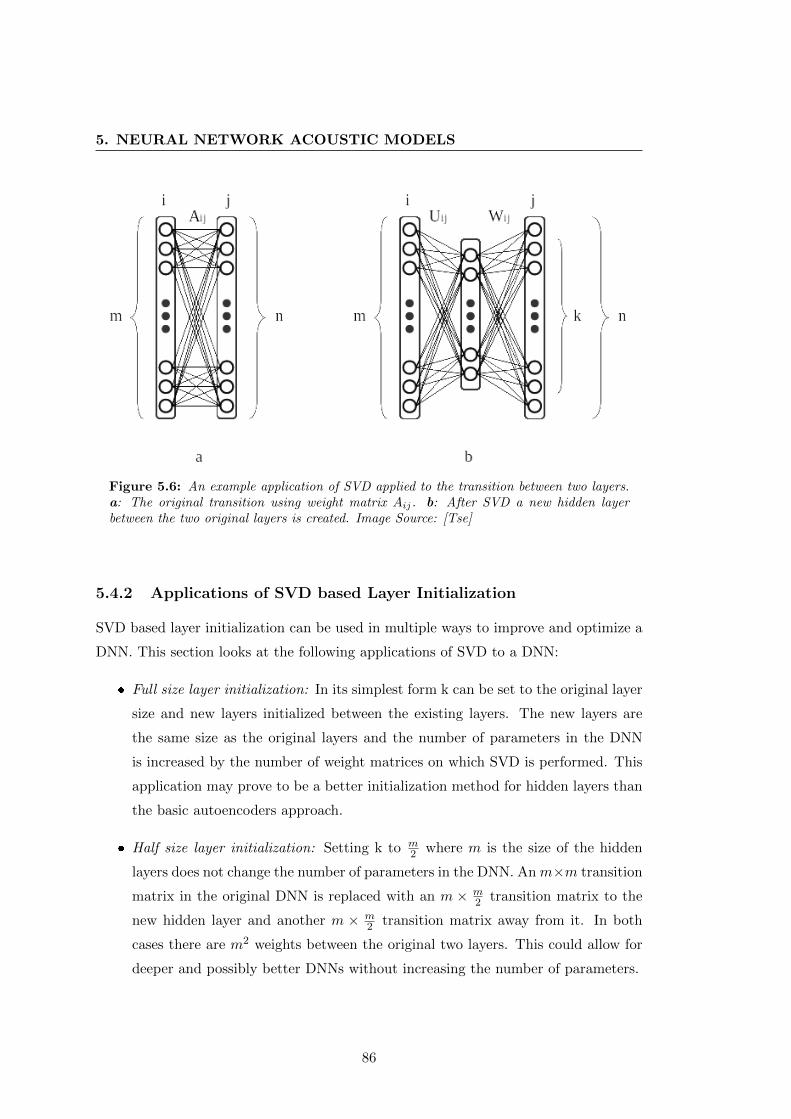
5. NEURAL NETWORK ACOUSTIC MODELS
Figure 5.6: An example application of SVD applied to the transition between two layers.a: The original transition using weight matrix Aij. b: After SVD a new hidden layerbetween the two original layers is created. Image Source: [Tse]
5.4.2 Applications of SVD based Layer Initialization
SVD based layer initialization can be used in multiple ways to improve and optimize a
DNN. This section looks at the following applications of SVD to a DNN:
� Full size layer initialization: In its simplest form k can be set to the original layer
size and new layers initialized between the existing layers. The new layers are
the same size as the original layers and the number of parameters in the DNN
is increased by the number of weight matrices on which SVD is performed. This
application may prove to be a better initialization method for hidden layers than
the basic autoencoders approach.
� Half size layer initialization: Setting k to m2 where m is the size of the hidden
layers does not change the number of parameters in the DNN. An m×m transition
matrix in the original DNN is replaced with an m × m2 transition matrix to the
new hidden layer and another m × m2 transition matrix away from it. In both
cases there are m2 weights between the original two layers. This could allow for
deeper and possibly better DNNs without increasing the number of parameters.
86
5.4 Growing a DNN with Singular Value Decomposition
� Small layer initialization: The total number parameters in the DNN can be
reduced by applying SVD with k < m2 in one or more of its layer transitions.
� Decomposing the connections to the output layer: The output layer has a relatively
large size due to the use of CD phone states as targets. Decomposing the
connections between the final hidden layer and the output layer could significantly
reduce the number of connections in the whole network.
� Insertion of a bottleneck layer: Inserting a small hidden layer with SVD near the
end of the network can transform a DNN into DBNF.
5.4.2.1 Experimental Setup
All experiments in this section are again performed on the Quaero DB described
in section 3.5. lMEL input features are used for all DNNs. The original DNNs,
prior to inserting new hidden layer with SVD, are trained using the setup described
in section 5.1. After fine-tuning, one or more new hidden layers are inserted by
decomposing the transition matrices. The resulting DNN is then retrained. The
retraining procedure uses the same setup and parameters as the original fine-tuning.
All tests are performed on the eval2010 test set. When listing the number of parameters
in a DNN any biases present are neglected as they only grow linearly with the number
of neurons while the transition weights grow quadratically and therefore make up most
of the weights in a DNN.
5.4.2.2 Full Size Layer Initialization
This application is tested by applying SVD restructuring with k = m to the transitions
between the hidden layers in a DNN with 5 hidden layers of 1200 neurons each. A
new DNN with 9 hidden layers consisting of 1200 neurons each is created. The original
network contains 13.18M parameters and the new network contains 18.67M parameters.
A separate DNN with 9 hidden layers initialize using the normal layerwise pretraining
setup is trained as a comparison. The SVD initialized network reduces the WER
by 3.1% from 16.92% to 16.39% compared to the original network and by 2.2% in
comparison to the network with the same topology.
87
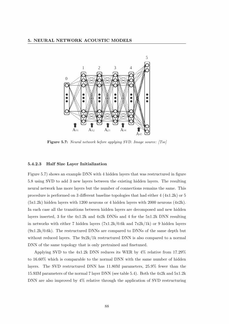
5. NEURAL NETWORK ACOUSTIC MODELS
Figure 5.7: Neural network before applying SVD. Image source: [Tse]
5.4.2.3 Half Size Layer Initialization
Figure 5.7) shows an example DNN with 4 hidden layers that was restructured in figure
5.8 using SVD to add 3 new layers between the existing hidden layers. The resulting
neural network has more layers but the number of connections remains the same. This
procedure is performed on 3 different baseline topologies that had either 4 (4x1.2k) or 5
(5x1.2k) hidden layers with 1200 neurons or 4 hidden layers with 2000 neurons (4x2k).
In each case all the transitions between hidden layers are decomposed and new hidden
layers inserted, 3 for the 4x1.2k and 4x2k DNNs and 4 for the 5x1.2k DNN resulting
in networks with either 7 hidden layers (7x1.2k/0.6k and 7x2k/1k) or 9 hidden layers
(9x1.2k/0.6k). The restructured DNNs are compared to DNNs of the same depth but
without reduced layers. The 9x2k/1k restructured DNN is also compared to a normal
DNN of the same topology that is only pretrained and finetuned.
Applying SVD to the 4x1.2k DNN reduces its WER by 4% relative from 17.29%
to 16.60% which is comparable to the normal DNN with the same number of hidden
layers. The SVD restructured DNN has 11.80M parameters, 25.9% fewer than the
15.93M parameters of the normal 7 layer DNN (see table 5.4). Both the 4x2k and 5x1.2k
DNN are also improved by 4% relative through the application of SVD restructuring
88
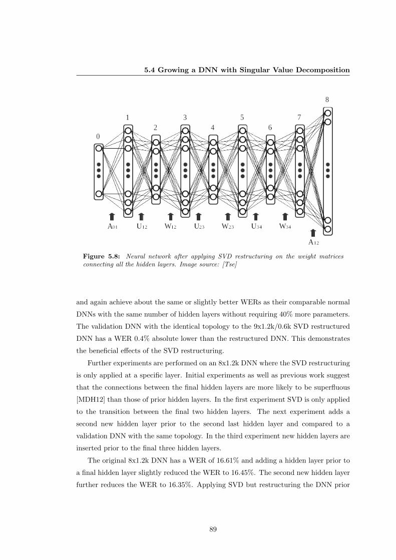
5.4 Growing a DNN with Singular Value Decomposition
Figure 5.8: Neural network after applying SVD restructuring on the weight matricesconnecting all the hidden layers. Image source: [Tse]
and again achieve about the same or slightly better WERs as their comparable normal
DNNs with the same number of hidden layers without requiring 40% more parameters.
The validation DNN with the identical topology to the 9x1.2k/0.6k SVD restructured
DNN has a WER 0.4% absolute lower than the restructured DNN. This demonstrates
the beneficial effects of the SVD restructuring.
Further experiments are performed on an 8x1.2k DNN where the SVD restructuring
is only applied at a specific layer. Initial experiments as well as previous work suggest
that the connections between the final hidden layers are more likely to be superfluous
[MDH12] than those of prior hidden layers. In the first experiment SVD is only applied
to the transition between the final two hidden layers. The next experiment adds a
second new hidden layer prior to the second last hidden layer and compared to a
validation DNN with the same topology. In the third experiment new hidden layers are
inserted prior to the final three hidden layers.
The original 8x1.2k DNN has a WER of 16.61% and adding a hidden layer prior to
a final hidden layer slightly reduced the WER to 16.45%. The second new hidden layer
further reduces the WER to 16.35%. Applying SVD but restructuring the DNN prior
89
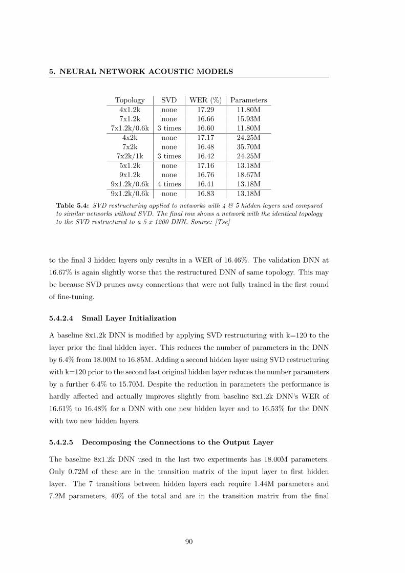
5. NEURAL NETWORK ACOUSTIC MODELS
Topology SVD WER (%) Parameters
4x1.2k none 17.29 11.80M7x1.2k none 16.66 15.93M
7x1.2k/0.6k 3 times 16.60 11.80M
4x2k none 17.17 24.25M7x2k none 16.48 35.70M
7x2k/1k 3 times 16.42 24.25M
5x1.2k none 17.16 13.18M9x1.2k none 16.76 18.67M
9x1.2k/0.6k 4 times 16.41 13.18M
9x1.2k/0.6k none 16.83 13.18M
Table 5.4: SVD restructuring applied to networks with 4 & 5 hidden layers and comparedto similar networks without SVD. The final row shows a network with the identical topologyto the SVD restructured to a 5 x 1200 DNN. Source: [Tse]
to the final 3 hidden layers only results in a WER of 16.46%. The validation DNN at
16.67% is again slightly worse that the restructured DNN of same topology. This may
be because SVD prunes away connections that were not fully trained in the first round
of fine-tuning.
5.4.2.4 Small Layer Initialization
A baseline 8x1.2k DNN is modified by applying SVD restructuring with k=120 to the
layer prior the final hidden layer. This reduces the number of parameters in the DNN
by 6.4% from 18.00M to 16.85M. Adding a second hidden layer using SVD restructuring
with k=120 prior to the second last original hidden layer reduces the number parameters
by a further 6.4% to 15.70M. Despite the reduction in parameters the performance is
hardly affected and actually improves slightly from baseline 8x1.2k DNN’s WER of
16.61% to 16.48% for a DNN with one new hidden layer and to 16.53% for the DNN
with two new hidden layers.
5.4.2.5 Decomposing the Connections to the Output Layer
The baseline 8x1.2k DNN used in the last two experiments has 18.00M parameters.
Only 0.72M of these are in the transition matrix of the input layer to first hidden
layer. The 7 transitions between hidden layers each require 1.44M parameters and
7.2M parameters, 40% of the total and are in the transition matrix from the final
90
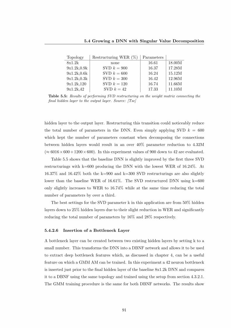
5.4 Growing a DNN with Singular Value Decomposition
Topology Restructuring WER (%) Parameters
8x1.2k none 16.61 18.00M9x1.2k,0.9k SVD k = 900 16.37 17.28M9x1.2k,0.6k SVD k = 600 16.24 15.12M9x1.2k,0.3k SVD k = 300 16.42 12.96M9x1.2k,120 SVD k = 120 16.74 11.66M9x1.2k,42 SVD k = 42 17.33 11.10M
Table 5.5: Results of performing SVD restructuring on the weight matrix connecting thefinal hidden layer to the output layer. Source: [Tse]
hidden layer to the output layer. Restructuring this transition could noticeably reduce
the total number of parameters in the DNN. Even simply applying SVD k = 600
which kept the number of parameters constant when decomposing the connections
between hidden layers would result in an over 40% parameter reduction to 4.32M
(≈ 6016×600+1200×600). In this experiment values of 900 down to 42 are evaluated.
Table 5.5 shows that the baseline DNN is slightly improved by the first three SVD
restructurings with k=600 producing the DNN with the lowest WER of 16.24%. At
16.37% and 16.42% both the k=900 and k=300 SVD restructurings are also slightly
lower than the baseline WER of 16.61%. The SVD restructured DNN using k=600
only slightly increases to WER to 16.74% while at the same time reducing the total
number of parameters by over a third.
The best settings for the SVD parameter k in this application are from 50% hidden
layers down to 25% hidden layers due to their slight reduction in WER and significantly
reducing the total number of parameters by 16% and 28% respectively.
5.4.2.6 Insertion of a Bottleneck Layer
A bottleneck layer can be created between two existing hidden layers by setting k to a
small number. This transforms the DNN into a DBNF network and allows it to be used
to extract deep bottleneck features which, as discussed in chapter 4, can be a useful
feature on which a GMM AM can be trained. In this experiment a 42 neuron bottleneck
is inserted just prior to the final hidden layer of the baseline 8x1.2k DNN and compares
it to a DBNF using the same topology and trained using the setup from section 4.3.2.1.
The GMM training procedure is the same for both DBNF networks. The results show
91
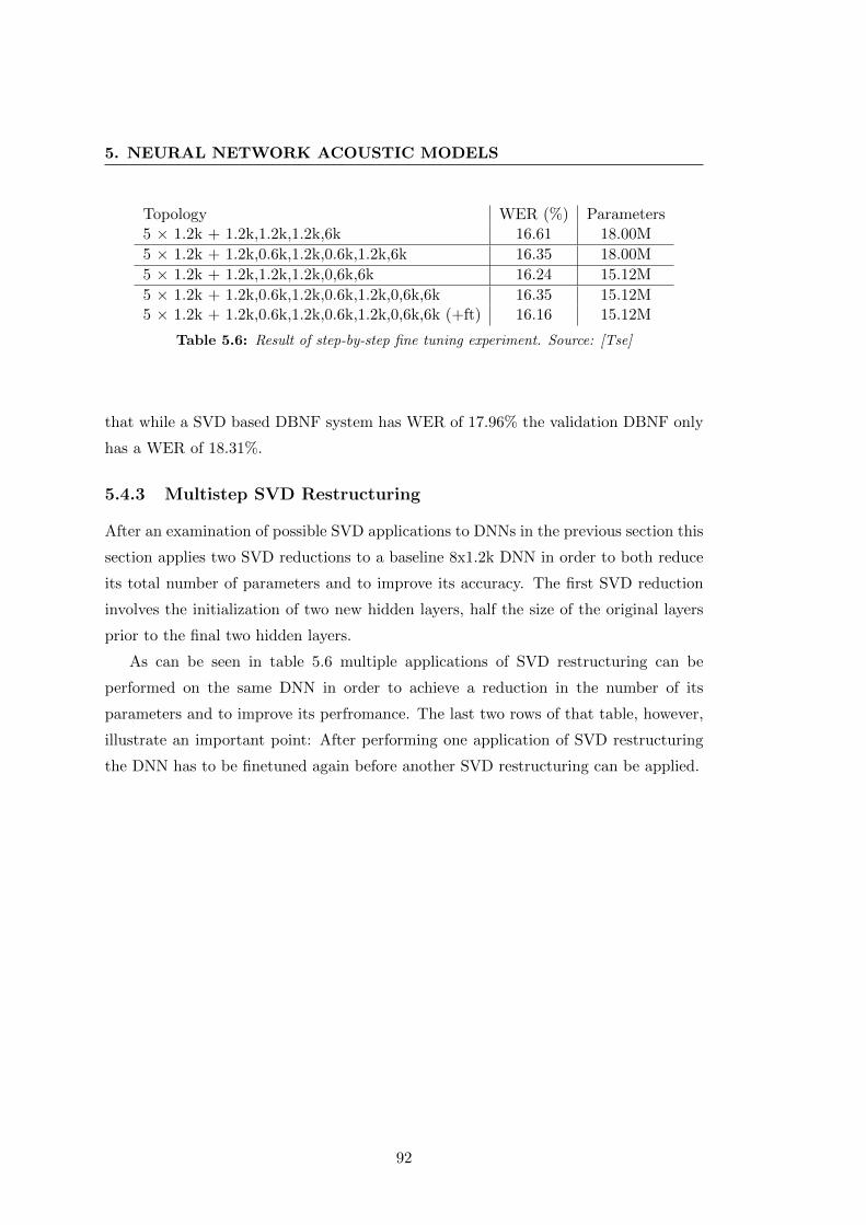
5. NEURAL NETWORK ACOUSTIC MODELS
Topology WER (%) Parameters5 × 1.2k + 1.2k,1.2k,1.2k,6k 16.61 18.00M
5 × 1.2k + 1.2k,0.6k,1.2k,0.6k,1.2k,6k 16.35 18.00M
5 × 1.2k + 1.2k,1.2k,1.2k,0,6k,6k 16.24 15.12M
5 × 1.2k + 1.2k,0.6k,1.2k,0.6k,1.2k,0,6k,6k 16.35 15.12M5 × 1.2k + 1.2k,0.6k,1.2k,0.6k,1.2k,0,6k,6k (+ft) 16.16 15.12M
Table 5.6: Result of step-by-step fine tuning experiment. Source: [Tse]
that while a SVD based DBNF system has WER of 17.96% the validation DBNF only
has a WER of 18.31%.
5.4.3 Multistep SVD Restructuring
After an examination of possible SVD applications to DNNs in the previous section this
section applies two SVD reductions to a baseline 8x1.2k DNN in order to both reduce
its total number of parameters and to improve its accuracy. The first SVD reduction
involves the initialization of two new hidden layers, half the size of the original layers
prior to the final two hidden layers.
As can be seen in table 5.6 multiple applications of SVD restructuring can be
performed on the same DNN in order to achieve a reduction in the number of its
parameters and to improve its perfromance. The last two rows of that table, however,
illustrate an important point: After performing one application of SVD restructuring
the DNN has to be finetuned again before another SVD restructuring can be applied.
92
Chapter 6
Subword Neural Network
Language Models
In this chapter neural network language modelling techniques are applied to a German
subword vocabulary. For a long time language models were built primarily using ngram
based methods. Although some early success was made by using neural networks to
predict word classes [NS88] is wasn’t until 2007 [Sch07], however, that the use of neural
network based language models started to become become more common. These come
in two varieties: feed forward neural networks which like traditional ngram methods
only base their prediction of the next word on a short history and recurrent neural
networks that predict the next word based on the previous word and the activation of
the networks’ hidden layer for the previous word [SSN12, MKB+10]. This recurrent
nature can be useful as it allows RNNs to base their predictions on a much larger
context but it comes at the price of no longer being able to recombine language model
histories and is, therefore, hard to integrate into a decoder. They are often either
only used to rescore existing lattices [HBG+12] or unrolled and converted into back-off
ngram language models [AKV+14]. As a seamless decoder integration is desired for the
proposed subword neural network language model a feed forward topology is chosen.
After an error analysis of a non subword German system an overview of other proposed
solutions is presented followed by a description of the subword selection process. Initial
experiments are performed using the subword vocabulary in an ngram language model
and its compatibility with the KIT lecture translation system is investigated. The
neural network LM is then introduced and its integration into the decoder explained.
93
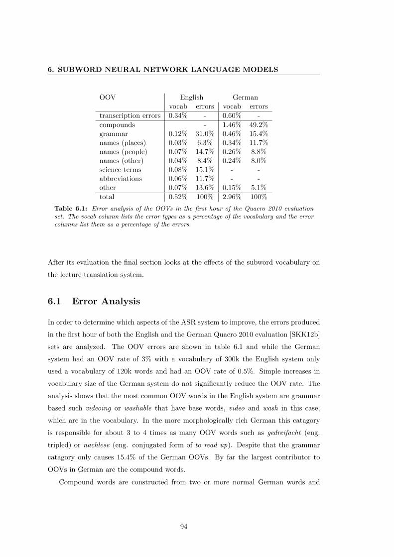
6. SUBWORD NEURAL NETWORK LANGUAGE MODELS
OOV English Germanvocab errors vocab errors
transcription errors 0.34% - 0.60% -
compounds - 1.46% 49.2%grammar 0.12% 31.0% 0.46% 15.4%names (places) 0.03% 6.3% 0.34% 11.7%names (people) 0.07% 14.7% 0.26% 8.8%names (other) 0.04% 8.4% 0.24% 8.0%science terms 0.08% 15.1% - -abbreviations 0.06% 11.7% - -other 0.07% 13.6% 0.15% 5.1%
total 0.52% 100% 2.96% 100%
Table 6.1: Error analysis of the OOVs in the first hour of the Quaero 2010 evaluationset. The vocab column lists the error types as a percentage of the vocabulary and the errorcolumns list them as a percentage of the errors.
After its evaluation the final section looks at the effects of the subword vocabulary on
the lecture translation system.
6.1 Error Analysis
In order to determine which aspects of the ASR system to improve, the errors produced
in the first hour of both the English and the German Quaero 2010 evaluation [SKK12b]
sets are analyzed. The OOV errors are shown in table 6.1 and while the German
system had an OOV rate of 3% with a vocabulary of 300k the English system only
used a vocabulary of 120k words and had an OOV rate of 0.5%. Simple increases in
vocabulary size of the German system do not significantly reduce the OOV rate. The
analysis shows that the most common OOV words in the English system are grammar
based such videoing or washable that have base words, video and wash in this case,
which are in the vocabulary. In the more morphologically rich German this catagory
is responsible for about 3 to 4 times as many OOV words such as gedreifacht (eng.
tripled) or nachlese (eng. conjugated form of to read up). Despite that the grammar
catagory only causes 15.4% of the German OOVs. By far the largest contributor to
OOVs in German are the compound words.
Compound words are constructed from two or more normal German words and
94
6.1 Error Analysis
considered to be normal German words. The words Tee (eng: tea) and Kanne (eng:
canister) for example can be combined into Teekanne (eng: tea pot). Although roughly
66% of all compound words are constructed by simply combining the individual words
some require an extra linking morpheme in between [Mar06]:
� 19% -s: Gehaltserhohung (eng: increase in pay)
� 7% -n: Tassenhalter (eng: cup holder)
� 3% -en: Sternenkarte (eng: sky map)
� all other linking morphemes occur in less than 2% of the compound words.
Some of these compound words appear to have multiple possible origins (splits). The
word Konsumentenumfrage is a compound of Konsument (eng: consumer) and Umfrage
(eng: questionnaire) taking an en as a linking morpheme this could also be split into
Konsum Enten Umfrage (eng: consume duck questionnaire).
When an ASR system recognizes all n component words of a compound word but
fails to merge them into a single word it will be penalized with n errors: a substitution
error and n − 1 insertion errors. In this paper we present a Subword Neural Network
Language Model that addresses this problem.
On the Quaero 2010 evaluation set the KIT baseline system had a WER of 24.17%,
10.21% of which (2.47% absolute) came from not correctly merging compound words
whose component words were correctly recognized. These high OOV rates also cause
problems for our online German to English lecture translation system.
6.1.1 Related Work
The only other similar approach that could be found in the literature is a neural network
based subword language model [MSD+12] from Mikolov which improves upon a baseline
4gram full word language model. It uses a vocabulary that only contains high frequency
words. Low frequency words are split into syllables and low frequency syllables are split
into characters. They only use a small output vocabulary of 1000 words, 2000 syllables
and 26 letters. It is able to outperform a 4gram language model by 0.2%.
In addition to the subword neural network paper discussed in section 2.3 other non
neural network works have tackled the problem of German subwords.
95
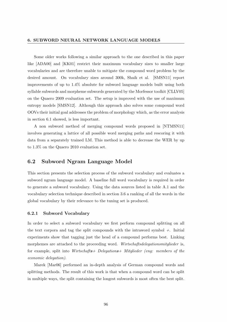
6. SUBWORD NEURAL NETWORK LANGUAGE MODELS
Some older works following a similar approach to the one described in this paper
like [ADA00] and [KK01] restrict their maximum vocabulary sizes to smaller large
vocabularies and are therefore unable to mitigate the compound word problem by the
desired amount. On vocabulary sizes around 300k, Shaik et al. [SMSN11] report
improvements of up to 1.4% absolute for subword language models built using both
syllable subwords and morpheme subwords generated by the Morfessor toolkit [CLLV05]
on the Quaero 2009 evaluation set. The setup is improved with the use of maximum
entropy models [SMSN12]. Although this approach also solves some compound word
OOVs their initial goal addresses the problem of morphology which, as the error analysis
in section 6.1 showed, is less important.
A non subword method of merging compound words proposed in [NTMSN11]
involves generating a lattice of all possible word merging paths and rescoring it with
data from a separately trained LM. This method is able to decrease the WER by up
to 1.3% on the Quaero 2010 evaluation set.
6.2 Subword Ngram Language Model
This section presents the selection process of the subword vocabulary and evaluates a
subword ngram language model. A baseline full word vocabulary is required in order
to generate a subword vocabulary. Using the data sources listed in table A.1 and the
vocabulary selection technique described in section 3.6 a ranking of all the words in the
global vocabulary by their relevance to the tuning set is produced.
6.2.1 Subword Vocabulary
In order to select a subword vocabulary we first perform compound splitting on all
the text corpora and tag the split compounds with the intraword symbol +. Initial
experiments show that tagging just the head of a compound performs best. Linking
morphemes are attached to the proceeding word. Wirtschaftsdelegationsmitglieder is,
for example, split into Wirtschafts+ Delegations+ Mitglieder (eng: members of the
economic delegation).
Marek [Mar06] performed an in-depth analysis of German compound words and
splitting methods. The result of this work is that when a compound word can be split
in multiple ways, the split containing the longest subwords is most often the best split.
96
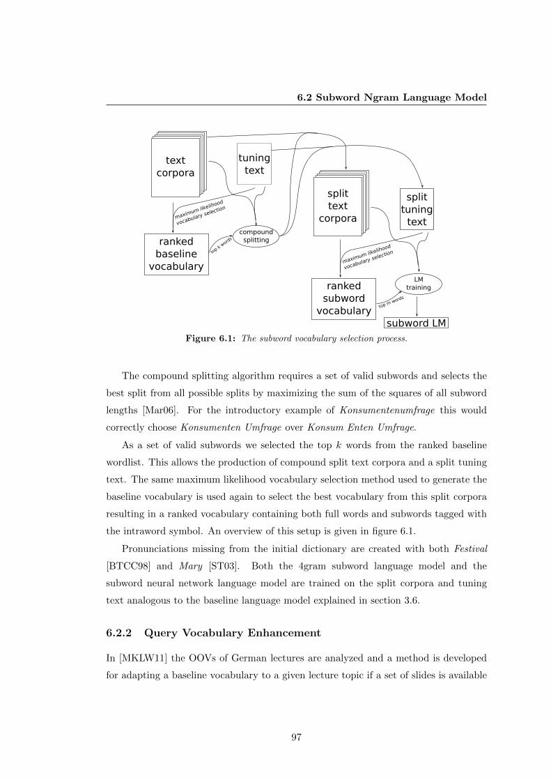
6.2 Subword Ngram Language Model
text
corpora
tuning
text
maximum likelihood
vocabulary selection
ranked
baseline
vocabulary
compound
splitting
top k
word
s
split
tuning
text
split
text
corpora
maximum likelihood
vocabulary selection
ranked
subword
vocabulary
LM
training
top m words
subword LM
Figure 6.1: The subword vocabulary selection process.
The compound splitting algorithm requires a set of valid subwords and selects the
best split from all possible splits by maximizing the sum of the squares of all subword
lengths [Mar06]. For the introductory example of Konsumentenumfrage this would
correctly choose Konsumenten Umfrage over Konsum Enten Umfrage.
As a set of valid subwords we selected the top k words from the ranked baseline
wordlist. This allows the production of compound split text corpora and a split tuning
text. The same maximum likelihood vocabulary selection method used to generate the
baseline vocabulary is used again to select the best vocabulary from this split corpora
resulting in a ranked vocabulary containing both full words and subwords tagged with
the intraword symbol. An overview of this setup is given in figure 6.1.
Pronunciations missing from the initial dictionary are created with both Festival
[BTCC98] and Mary [ST03]. Both the 4gram subword language model and the
subword neural network language model are trained on the split corpora and tuning
text analogous to the baseline language model explained in section 3.6.
6.2.2 Query Vocabulary Enhancement
In [MKLW11] the OOVs of German lectures are analyzed and a method is developed
for adapting a baseline vocabulary to a given lecture topic if a set of slides is available
97
6. SUBWORD NEURAL NETWORK LANGUAGE MODELS
in advance. Queries are extracted from the lecture slides and sent to the search engine
Bing to produce a list of websites related to the lecture. On a set of lectures recorded
at the KIT this method reduces the baseline OOV rate of 3.1% to 1.2% for a 300k
vocabulary. The query vocabulary selection setup is rebuilt and adapted to make use
of subwords:
� the baseline subword language model is built (baseline subword vocab)
� the vocabulary from the slides is extracted (slide vocab)
� a set of queries is extracted from the slides
� for each query the resulting top 40 links from google search are downloaded
� the cleaning procedure described in section 3.5.2 is performed on each downloaded
webpage (and linked files such as pdfs)
� compound splitting is performed on the cleaned webpages
� all subwords occurring in the downloaded webpages words are ranked based on
how many of those websites they occur in and how often they occur in total (query
subword vocab)
� baseline subword vocabulary is interpolated with the query subword vocab, the
top 300k subwords selected are all then augmented by all the missing slide
vocabulary words
� the baseline subword LM is rebuilt
� an LM is built on the downloaded split webpages and interpolated with baseline
subword LM
This procedure is performed separately for each lecture.
6.2.3 OOV Analysis
The subword vocabulary requires the valid subwords for compound splitting to be
specified. OOVs of subword vocabularies are measured by splitting the reference text
in the same manner as the training text for the particular subword vocabulary was split.
98
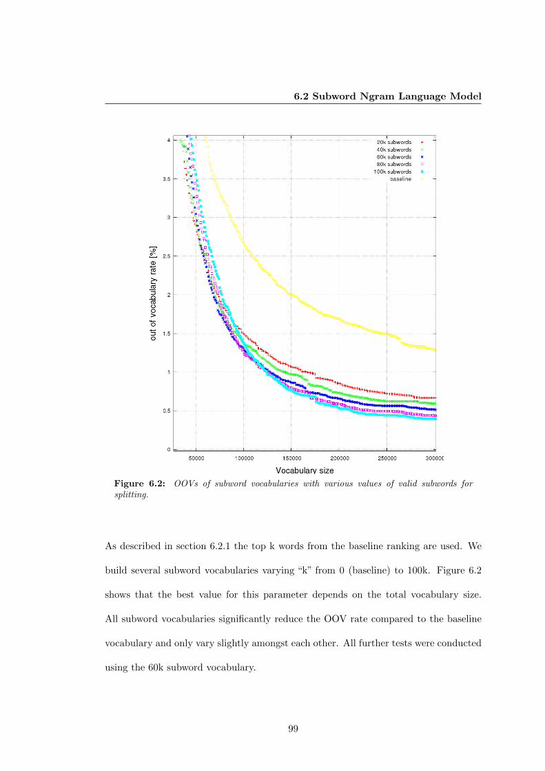
6.2 Subword Ngram Language Model
Figure 6.2: OOVs of subword vocabularies with various values of valid subwords forsplitting.
As described in section 6.2.1 the top k words from the baseline ranking are used. We
build several subword vocabularies varying “k” from 0 (baseline) to 100k. Figure 6.2
shows that the best value for this parameter depends on the total vocabulary size.
All subword vocabularies significantly reduce the OOV rate compared to the baseline
vocabulary and only vary slightly amongst each other. All further tests were conducted
using the 60k subword vocabulary.
99
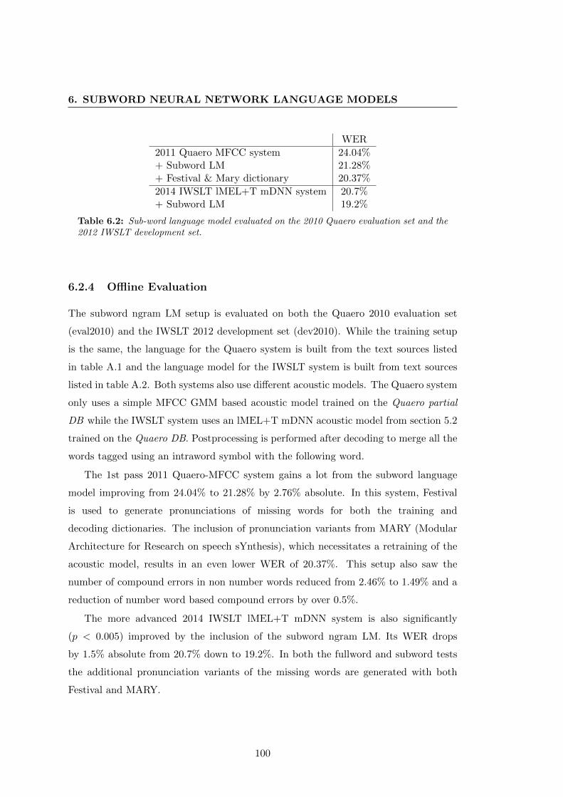
6. SUBWORD NEURAL NETWORK LANGUAGE MODELS
WER
2011 Quaero MFCC system 24.04%+ Subword LM 21.28%+ Festival & Mary dictionary 20.37%
2014 IWSLT lMEL+T mDNN system 20.7%+ Subword LM 19.2%
Table 6.2: Sub-word language model evaluated on the 2010 Quaero evaluation set and the2012 IWSLT development set.
6.2.4 Offline Evaluation
The subword ngram LM setup is evaluated on both the Quaero 2010 evaluation set
(eval2010) and the IWSLT 2012 development set (dev2010). While the training setup
is the same, the language for the Quaero system is built from the text sources listed
in table A.1 and the language model for the IWSLT system is built from text sources
listed in table A.2. Both systems also use different acoustic models. The Quaero system
only uses a simple MFCC GMM based acoustic model trained on the Quaero partial
DB while the IWSLT system uses an lMEL+T mDNN acoustic model from section 5.2
trained on the Quaero DB. Postprocessing is performed after decoding to merge all the
words tagged using an intraword symbol with the following word.
The 1st pass 2011 Quaero-MFCC system gains a lot from the subword language
model improving from 24.04% to 21.28% by 2.76% absolute. In this system, Festival
is used to generate pronunciations of missing words for both the training and
decoding dictionaries. The inclusion of pronunciation variants from MARY (Modular
Architecture for Research on speech sYnthesis), which necessitates a retraining of the
acoustic model, results in an even lower WER of 20.37%. This setup also saw the
number of compound errors in non number words reduced from 2.46% to 1.49% and a
reduction of number word based compound errors by over 0.5%.
The more advanced 2014 IWSLT lMEL+T mDNN system is also significantly
(p < 0.005) improved by the inclusion of the subword ngram LM. Its WER drops
by 1.5% absolute from 20.7% down to 19.2%. In both the fullword and subword tests
the additional pronunciation variants of the missing words are generated with both
Festival and MARY.
100
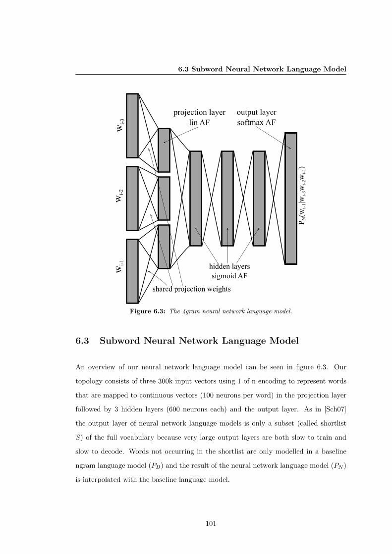
6.3 Subword Neural Network Language Model
wi-
1w
i-2
wi-
3
PN(w
i-1|w
i-3w
i-2w
i-1)
projection layer
lin AF
output layer
softmax AF
hidden layers
sigmoid AF
shared projection weights
Figure 6.3: The 4gram neural network language model.
6.3 Subword Neural Network Language Model
An overview of our neural network language model can be seen in figure 6.3. Our
topology consists of three 300k input vectors using 1 of n encoding to represent words
that are mapped to continuous vectors (100 neurons per word) in the projection layer
followed by 3 hidden layers (600 neurons each) and the output layer. As in [Sch07]
the output layer of neural network language models is only a subset (called shortlist
S) of the full vocabulary because very large output layers are both slow to train and
slow to decode. Words not occurring in the shortlist are only modelled in a baseline
ngram language model (PB) and the result of the neural network language model (PN )
is interpolated with the baseline language model.
101
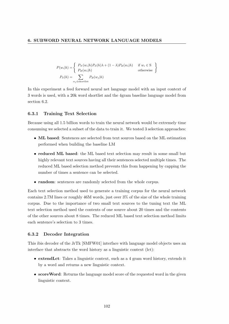
6. SUBWORD NEURAL NETWORK LANGUAGE MODELS
P (wi|h) =
{PN (wi|h)PS(h)λ+ (1− λ)PB(wi|h) if wi ∈ S
PB(wi|h) otherwise
}PS(h) =
∑wj∈shortlist
PB(wj |h)
In this experiment a feed forward neural net language model with an input context of
3 words is used, with a 20k word shortlist and the 4gram baseline language model from
section 6.2.
6.3.1 Training Text Selection
Because using all 1.5 billion words to train the neural network would be extremely time
consuming we selected a subset of the data to train it. We tested 3 selection approaches:
� ML based: Sentences are selected from text sources based on the ML estimation
performed when building the baseline LM
� reduced ML based: the ML based text selection may result in some small but
highly relevant text sources having all their sentences selected multiple times. The
reduced ML based selection method prevents this from happening by capping the
number of times a sentence can be selected.
� random: sentences are randomly selected from the whole corpus.
Each text selection method used to generate a training corpus for the neural network
contains 2.7M lines or roughly 46M words, just over 3% of the size of the whole training
corpus. Due to the importance of two small text sources to the tuning text the ML
text selection method used the contents of one source about 20 times and the contents
of the other sources about 8 times. The reduced ML based text selection method limits
each sentence’s selection to 3 times.
6.3.2 Decoder Integration
This ibis decoder of the JrTk [SMFW01] interface with language model objects uses an
interface that abstracts the word history as a linguistic context (lct):
� extendLct: Takes a linguistic context, such as a 4 gram word history, extends it
by a word and returns a new linguistic context.
� scoreWord: Returns the language model score of the requested word in the given
linguistic context.
102
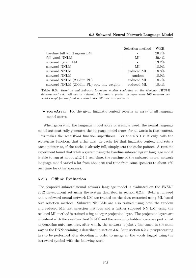
6.3 Subword Neural Network Language Model
Selection method WER
baseline full word ngram LM - 20.7%full word NNLM ML 20.4%subword ngram LM - 19.2%subword NNLM ML 18.9%subword NNLM reduced ML 18.8%subword NNLM random 18.9%subword NNLM (200dim PL) reduced ML 18.7%subword NNLM (200dim PL) opt. int. weights reduced ML 18.4%
Table 6.3: Baseline and Subword language models evaluated on the German IWSLRdevelopment set. All neural network LMs used a projection layer with 100 neurons perword except for the final one which has 200 neurons per word.
� scoreArray: For the given linguistic context returns an array of all language
model scores.
When generating the language model score of a single word, the neural language
model automatically generates the language model scores for all words in that context.
This makes the scoreWord function superfluous. For the NN LM it only calls the
scoreArray function, that either fills the cache for that linguistic context and sets a
cache pointer or, if the cache is already full, simply sets the cache pointer. A runtime
experiment found that while a system using the baseline subword ngram language model
is able to run at about x1.2-1.4 real time, the runtime of the subword neural network
language model varied a lot from about x8 real time from some speakers to about x30
real time for other speakers.
6.3.3 Offline Evaluation
The proposed subword neural network language model is evaluated on the IWSLT
2012 development set using the system described in section 6.2.4. Both a fullword
and a subword neural network LM are trained on the data extracted using ML based
text selection method. Subword NN LMs are also trained using both the random
and reduced ML text selection methods and a further subword NN LM, using the
reduced ML method is trained using a larger projection layer. The projection layers are
initialized with the word2vec tool [GL14] and the remaining hidden layers are pretrained
as denoising auto encoders, after which, the network is jointly fine-tuned in the same
way as the DNNs training is described in section 3.6. As in section 6.2.4, postprocessing
has to be performed after decoding in order to merge all the words tagged using the
intraword symbol with the following word.
103
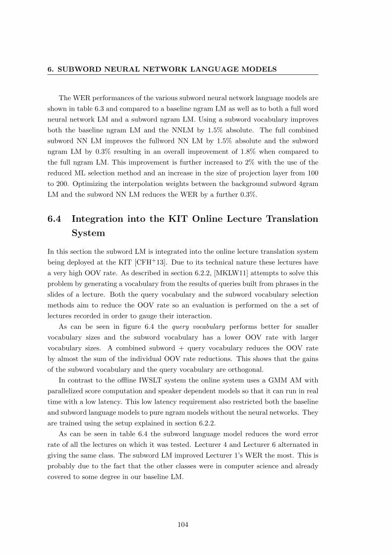
6. SUBWORD NEURAL NETWORK LANGUAGE MODELS
The WER performances of the various subword neural network language models are
shown in table 6.3 and compared to a baseline ngram LM as well as to both a full word
neural network LM and a subword ngram LM. Using a subword vocabulary improves
both the baseline ngram LM and the NNLM by 1.5% absolute. The full combined
subword NN LM improves the fullword NN LM by 1.5% absolute and the subword
ngram LM by 0.3% resulting in an overall improvement of 1.8% when compared to
the full ngram LM. This improvement is further increased to 2% with the use of the
reduced ML selection method and an increase in the size of projection layer from 100
to 200. Optimizing the interpolation weights between the background subword 4gram
LM and the subword NN LM reduces the WER by a further 0.3%.
6.4 Integration into the KIT Online Lecture Translation
System
In this section the subword LM is integrated into the online lecture translation system
being deployed at the KIT [CFH+13]. Due to its technical nature these lectures have
a very high OOV rate. As described in section 6.2.2, [MKLW11] attempts to solve this
problem by generating a vocabulary from the results of queries built from phrases in the
slides of a lecture. Both the query vocabulary and the subword vocabulary selection
methods aim to reduce the OOV rate so an evaluation is performed on the a set of
lectures recorded in order to gauge their interaction.
As can be seen in figure 6.4 the query vocabulary performs better for smaller
vocabulary sizes and the subword vocabulary has a lower OOV rate with larger
vocabulary sizes. A combined subword + query vocabulary reduces the OOV rate
by almost the sum of the individual OOV rate reductions. This shows that the gains
of the subword vocabulary and the query vocabulary are orthogonal.
In contrast to the offline IWSLT system the online system uses a GMM AM with
parallelized score computation and speaker dependent models so that it can run in real
time with a low latency. This low latency requirement also restricted both the baseline
and subword language models to pure ngram models without the neural networks. They
are trained using the setup explained in section 6.2.2.
As can be seen in table 6.4 the subword language model reduces the word error
rate of all the lectures on which it was tested. Lecturer 4 and Lecturer 6 alternated in
giving the same class. The subword LM improved Lecturer 1’s WER the most. This is
probably due to the fact that the other classes were in computer science and already
covered to some degree in our baseline LM.
104
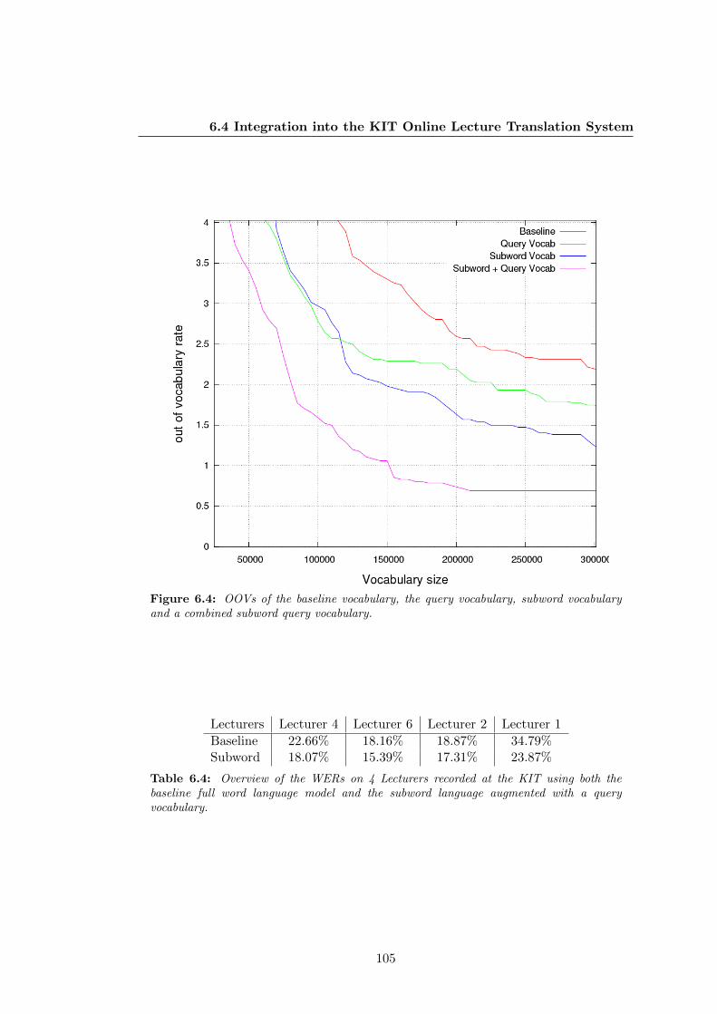
6.4 Integration into the KIT Online Lecture Translation System
Figure 6.4: OOVs of the baseline vocabulary, the query vocabulary, subword vocabularyand a combined subword query vocabulary.
Lecturers Lecturer 4 Lecturer 6 Lecturer 2 Lecturer 1
Baseline 22.66% 18.16% 18.87% 34.79%Subword 18.07% 15.39% 17.31% 23.87%
Table 6.4: Overview of the WERs on 4 Lecturers recorded at the KIT using both thebaseline full word language model and the subword language augmented with a queryvocabulary.
105
6. SUBWORD NEURAL NETWORK LANGUAGE MODELS
6.5 Summary
This chapter presents a simple yet very effective method of selecting and integrating
a German subword vocabulary. An error analysis shows that the majority of the
OOV words in a German ASR stem from compound words. When used in an ngram
language model the subword vocabulary reduces the WER by 1.5% on the IWSLT
2012 development set and by 2.76% on the Quaero 2010 evaluation set. Integrated into
the KIT lecture translation system and augmented with query vocabulary it reduces
the WER of all four tested lecturers. An analysis of the OOV reductions shows that
its improvements are orthogonal to those of the query vocabulary. A neural network
language model is trained to estimate the probability of subwords for a given subword
context and is efficiently integrated into the speech recognition system with the help
of a score cache. Using the best text section method it decreases the word error rate
by a further 0.8% absolute from 19.2% to 18.4% on the IWSLT 2012 development set
resulting in a total improvement of 2.3%.
The German subword vocabulary has proven to be so effective that is has been
used in all systems built by our lab since 2011 and has, therefore, contributed to every
evaluation since then. Its initial integration into the 2011 Quaero evaluation system
helped our system achieve the lowest word error rate in that evaluation. It is also
currently running in the KIT lecture translation system that is being used to translate
a number of selected lectures from German into English so that foreign students can
follow them. To my knowledge the subword neural network language’s WER of 18.4%
on the IWSLT development set is lower then any result that can be found in the
literature and is only beaten by the results in section 5.3.
106
Chapter 7
Neural Network Combination of
LM and AM
This chapter presents a method of combining an acoustic model and a language model
with a neural network and thereby joining all neural networks together in a speech
recognition system. The setup involves using the output scores of both the acoustic
model and the language model as the input to a neural network that is trained to
produce an optimal combined score. The setup of Graves et al. [GJ14] has a similar
goal of combining the whole speech recognition process in a neural network, but while
they use a recurrent neural network the setup proposed here continues to make use
of an HMM structure. This allows the individual acoustic and language models to be
trained independently of each other. Most speech recognition systems currently use a
form of loglinear combination.
7.1 Loglinear Model Combination
Recall the task of the decoder, described in section 2.2.3 that aims find the most
probable sequence of words:
W = argmaxW
logP (X|W ) + αlogP (W ) + |W |wβ + |W |nγ
Working at a word level, where the acoustic model scores for the words are known, this
can be seen as a form of loglinear combination [Hei10].
W = argmaxW
∑w∈W
∑i
λi · fi (7.1)
107
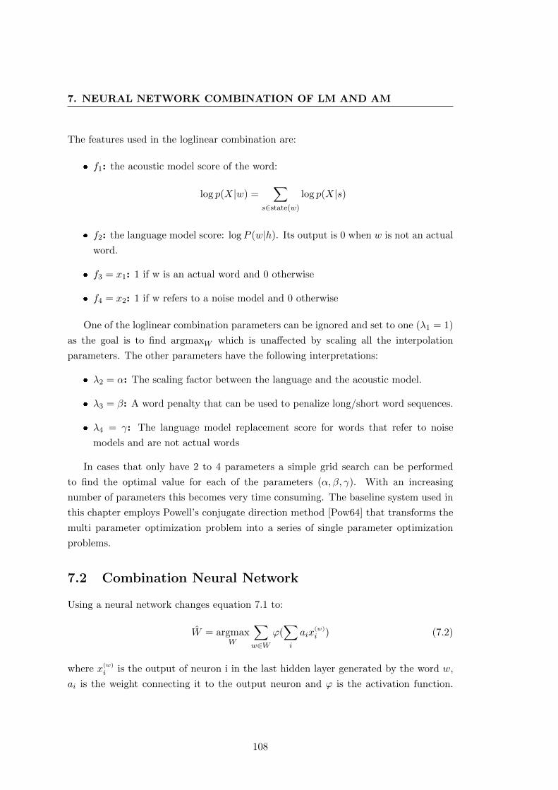
7. NEURAL NETWORK COMBINATION OF LM AND AM
The features used in the loglinear combination are:
� f1: the acoustic model score of the word:
log p(X|w) =∑
s∈state(w)
log p(X|s)
� f2: the language model score: logP (w|h). Its output is 0 when w is not an actual
word.
� f3 = x1: 1 if w is an actual word and 0 otherwise
� f4 = x2: 1 if w refers to a noise model and 0 otherwise
One of the loglinear combination parameters can be ignored and set to one (λ1 = 1)
as the goal is to find argmaxW which is unaffected by scaling all the interpolation
parameters. The other parameters have the following interpretations:
� λ2 = α: The scaling factor between the language and the acoustic model.
� λ3 = β: A word penalty that can be used to penalize long/short word sequences.
� λ4 = γ: The language model replacement score for words that refer to noise
models and are not actual words
In cases that only have 2 to 4 parameters a simple grid search can be performed
to find the optimal value for each of the parameters (α, β, γ). With an increasing
number of parameters this becomes very time consuming. The baseline system used in
this chapter employs Powell’s conjugate direction method [Pow64] that transforms the
multi parameter optimization problem into a series of single parameter optimization
problems.
7.2 Combination Neural Network
Using a neural network changes equation 7.1 to:
W = argmaxW
∑w∈W
ϕ(∑i
aix(w)
i ) (7.2)
where x(w)
i is the output of neuron i in the last hidden layer generated by the word w,
ai is the weight connecting it to the output neuron and ϕ is the activation function.
108
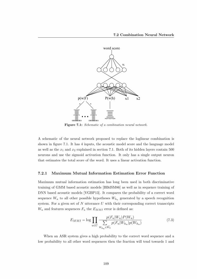
7.2 Combination Neural Network
p(w|F)
+ +
...
x1 x2P(w|h)
word score
ai
MV
DR
(t)
MFC
C (
t)
MV
DR
(t-
1)
MFC
C (
t-1
)
MV
DR
(t+
1)
MFC
C (
t+1
)
MV
DR
(t+
2)
MFC
C (
t+2
)
MV
DR
(t-
2)
MFC
C (
t-2
)
MV
DR
(t-
s)
MFC
C (
t-s)
MV
DR
(t+
s)
MFC
C (
t+s)
MV
DR
(t-
s-r
)
MFC
C (
t-s-r
)
MV
DR
(t-
s-1
)
MFC
C (
t-s-1
)
MV
DR
(t+
s+
1)
MFC
C (
t+s+
1)
MV
DR
(t+
s+
r)
MFC
C (
t+s+
r)
BNF (t)BNF (t-1) BNF (t+1)BNF (t-r) BNF (t+r)
MV
DR
(t)
MFC
C (
t)
MV
DR
(t-
1)
MFC
C (
t-1
)
MV
DR
(t+
1)
MFC
C (
t+1
)
MV
DR
(t+
2)
MFC
C (
t+2
)
MV
DR
(t-
2)
MFC
C (
t-2
)
MV
DR
(t-
s)
MFC
C (
t-s)
MV
DR
(t+
s)
MFC
C (
t+s)
MV
DR
(t-
s-r
)
MFC
C (
t-s-r
)
MV
DR
(t-
s-1
)
MFC
C (
t-s-1
)
MV
DR
(t+
s+
1)
MFC
C (
t+s+
1)
MV
DR
(t+
s+
r)
MFC
C (
t+s+
r)
BNF (t)BNF (t-1) BNF (t+1)BNF (t-r) BNF (t+r)
wi-1wi-2wi-3
Figure 7.1: Schematic of a combination neural network.
A schematic of the neural network proposed to replace the loglinear combination is
shown in figure 7.1. It has 4 inputs, the acoustic model score and the language model
as well as the x1 and x2 explained in section 7.1. Both of its hidden layers contain 500
neurons and use the sigmoid activation function. It only has a single output neuron
that estimates the total score of the word. It uses a linear activation function.
7.2.1 Maximum Mutual Information Estimation Error Function
Maximum mutual information estimation has long been used in both discriminative
training of GMM based acoustic models [BBdSM86] as well as in sequence training of
DNN based acoustic models [VGBP13]. It compares the probability of a correct word
sequence Wu to all other possible hypotheses Whu generated by a speech recognition
system. For a given set of N utterance U with their corresponding correct transcripts
Wu and features sequences Fu the EMMI error is defined as:
EMMI = log∏u∈U
p(Fu|Wu)P (Wu)∑Whu∈Wu
p(Fu|Whu)p(Whu)(7.3)
When an ASR system gives a high probability to the correct word sequence and a
low probability to all other word sequences then the fraction will tend towards 1 and
109
7. NEURAL NETWORK COMBINATION OF LM AND AM
the error towards 0. The full derivative ∂EMMI∂ai
the MMIE error function is presented
in appendix C which shows that
∂EMMI
∂ai=(δw|Wu
− Υ (w))
x(w)
i (7.4)
and that the δj required for the update rule of the backpropagation algorithm is:
δj = δw|Wu− Υ (w) (7.5)
This error function is implemented in a separate neural network training tool that
can learn from the word lattice and the weights are initialized by performing a simple
function approximation to the existing loglinear function.
7.3 Experimental Setup and Results
The proposed method is evaluated and compared to a traditional loglinear approach
where the parameters are estimated on a development set. The combination neural
network is trained on the Quaero DB using lattices generated with the LM from
chapter 6 and a lMEL+T mDNN described in chapter 5. It is trained for 5 epochs
with a constant learning rate.
The loglinear parameters are optimized on the IWSLT 2012 development set
resulting in a WER of 18.3%. A test run using the same parameters on the Quaero 2010
evaluation set has a WER of 14.22%. Using the combination neural network reduced
this WER by 0.11% to 14.11% which is equates to only 40 more correct words. It
is, however, still a significant improvement with p < 0.005. An oracle experiment is
performed by optimizing the loglinear parameters on the Quaero 2010 evaluation set.
Its results in a WER of 14.03% which is slightly better than the combination neural
network.
7.4 Summary
This chapter has introduced a possible combination network that goes beyond the
traditional loglinear approach and uses a neural network to combine the outputs of
both the acoustic model and the language model. The neural network is trained on
the lattices of the training using the MMIE error function. It is able to slightly reduce
the WER on the Quaero 2010 evaluation set when compared to the loglinear approach
using parameters estimated on the IWSLT 2012 development set.
110
Chapter 8
Results Summary
This thesis has touched on many aspects of automatic speech recognition and shown
how they can be further improved by the use of neural networks. This chapter will
present an overview of the most important results from these techniques as well as
their applications and combination effects.
Section 8.1 begins with the results the examination of multiple input features for
deep neural network bottleneck features. The results of the multi-feature modular deep
neural network acoustic model are presented in section 8.2. The results of the other
acoustic model experiments on the decision tree and using singular value decomposition
follow in sections 8.3 & 8.4. Section 8.5 tackles the key results from the subword neural
network language model experiments and the combination tests are summarized in
section 8.6.
The results of this thesis have been successfully used in multiple evaluation
campaigns aandre are being used in a deployed product. A summary of these
applications is provided in section 8.7. The chapter concludes with section 8.8 showing
the absolute improvements of the key techniques from this thesis as well as their
combined improvements.
111
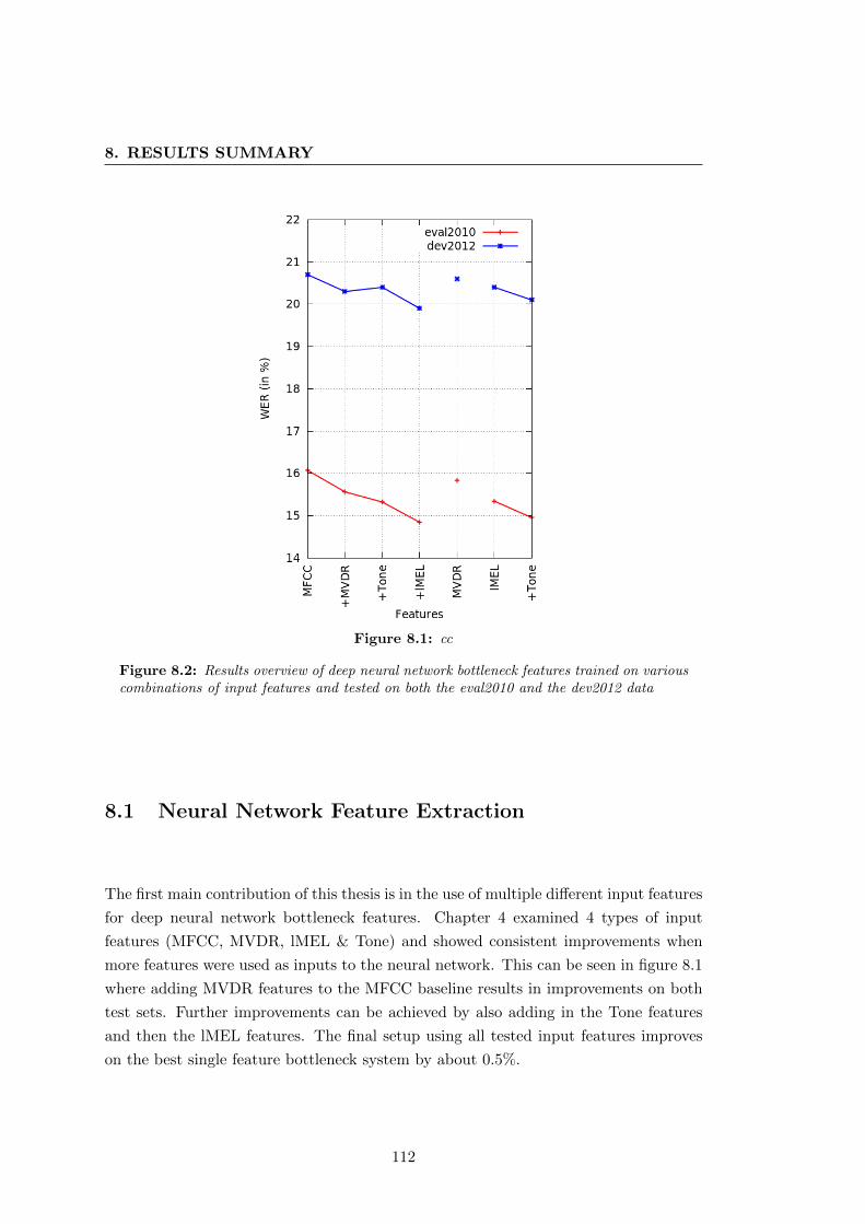
8. RESULTS SUMMARY
Figure 8.1: cc
Figure 8.2: Results overview of deep neural network bottleneck features trained on variouscombinations of input features and tested on both the eval2010 and the dev2012 data
8.1 Neural Network Feature Extraction
The first main contribution of this thesis is in the use of multiple different input features
for deep neural network bottleneck features. Chapter 4 examined 4 types of input
features (MFCC, MVDR, lMEL & Tone) and showed consistent improvements when
more features were used as inputs to the neural network. This can be seen in figure 8.1
where adding MVDR features to the MFCC baseline results in improvements on both
test sets. Further improvements can be achieved by also adding in the Tone features
and then the lMEL features. The final setup using all tested input features improves
on the best single feature bottleneck system by about 0.5%.
112
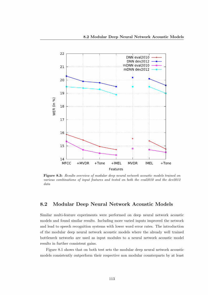
8.2 Modular Deep Neural Network Acoustic Models
Figure 8.3: Results overview of modular deep neural network acoustic models trained onvarious combinations of input features and tested on both the eval2010 and the dev2012data
8.2 Modular Deep Neural Network Acoustic Models
Similar multi-feature experiments were performed on deep neural network acoustic
models and found similar results. Including more varied inputs improved the network
and lead to speech recognition systems with lower word error rates. The introduction
of the modular deep neural network acoustic models where the already well trained
bottleneck networks are used as input modules to a neural network acoustic model
results in further consistent gains.
Figure 8.1 shows that on both test sets the modular deep neural network acoustic
models consistently outperform their respective non modular counterparts by at least
113
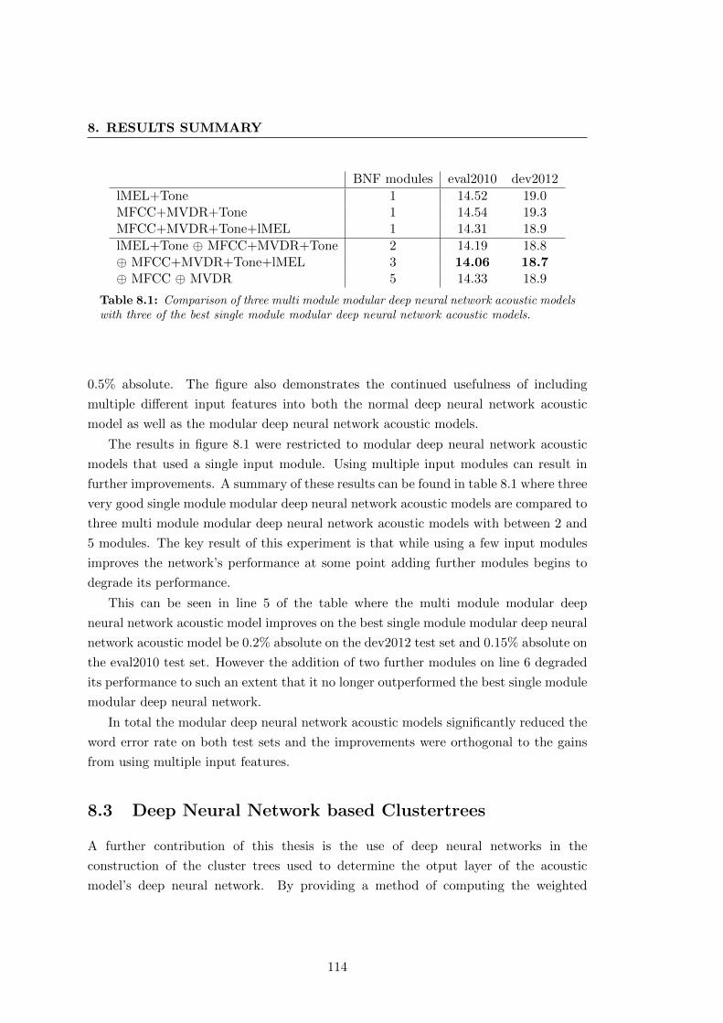
8. RESULTS SUMMARY
BNF modules eval2010 dev2012
lMEL+Tone 1 14.52 19.0MFCC+MVDR+Tone 1 14.54 19.3MFCC+MVDR+Tone+lMEL 1 14.31 18.9
lMEL+Tone ⊕ MFCC+MVDR+Tone 2 14.19 18.8⊕ MFCC+MVDR+Tone+lMEL 3 14.06 18.7⊕ MFCC ⊕ MVDR 5 14.33 18.9
Table 8.1: Comparison of three multi module modular deep neural network acoustic modelswith three of the best single module modular deep neural network acoustic models.
0.5% absolute. The figure also demonstrates the continued usefulness of including
multiple different input features into both the normal deep neural network acoustic
model as well as the modular deep neural network acoustic models.
The results in figure 8.1 were restricted to modular deep neural network acoustic
models that used a single input module. Using multiple input modules can result in
further improvements. A summary of these results can be found in table 8.1 where three
very good single module modular deep neural network acoustic models are compared to
three multi module modular deep neural network acoustic models with between 2 and
5 modules. The key result of this experiment is that while using a few input modules
improves the network’s performance at some point adding further modules begins to
degrade its performance.
This can be seen in line 5 of the table where the multi module modular deep
neural network acoustic model improves on the best single module modular deep neural
network acoustic model be 0.2% absolute on the dev2012 test set and 0.15% absolute on
the eval2010 test set. However the addition of two further modules on line 6 degraded
its performance to such an extent that it no longer outperformed the best single module
modular deep neural network.
In total the modular deep neural network acoustic models significantly reduced the
word error rate on both test sets and the improvements were orthogonal to the gains
from using multiple input features.
8.3 Deep Neural Network based Clustertrees
A further contribution of this thesis is the use of deep neural networks in the
construction of the cluster trees used to determine the otput layer of the acoustic
model’s deep neural network. By providing a method of computing the weighted
114
8.4 Growing a DNN with Singular Value Decomposition
entropy distance directly from a context independent deep neural network acoustic
model without the use of Gaussians or Gaussian mixture models this approach allows
for a streamlining of the acoustic model training procedure without the need for legacy
Gaussian mixture models code.
The experiments showed that the alternative weighted entropy distance from a
context independent deep neural network acoustic model performed at least as well as
the traditional weighted entropy distance and in some cases even resulted in a slight
improvement.
8.4 Growing a DNN with Singular Value Decomposition
Another technique that has more practical applications then just reducing the word
error rate is the use of singular value decomposition to reduce the number of parameters
in a deep neural network without harming its performance, thereby resulting in a
network that can be computed faster. This is especially important in scenarios like
the lecture translator where a low latency response is critical.
A reduction of parameters from 18 million to 11 million is shown to be possible
without a significant loss in performance. However, intelligently reducing the
parameters to 15.12 million even resulted in a slight improvement of 0.4% absolute.
8.5 Subword Neural Network Language Model
The subword neural network language model is a big contributing factor to the total
reduction in word error rate achieved within this thesis. The introduction of the
subword language model was necessary to combat the high out of vocabulary rate seen
in German systems where it is not unusual for a 300k word German speech recognition
system to have an out of vocabulary rate of over 3% while a 120k English speech
recognition system may only have an out of vocabulary rate of 0.5%. While a basic
ngram based subword language model already resulted in a very good improvement
of 1.5% when compared to a baseline fullword ngram language model. Using the
subword vocabulary in a neural network language model resulted in synergistic and an
improvement of 2.0% over a baseline fullword neural network language model. These
results are shown in figure 8.4 where it can be clearly seen that the gains from the
combined subword and neural network language model are more than the sum of the
individual gains.
115
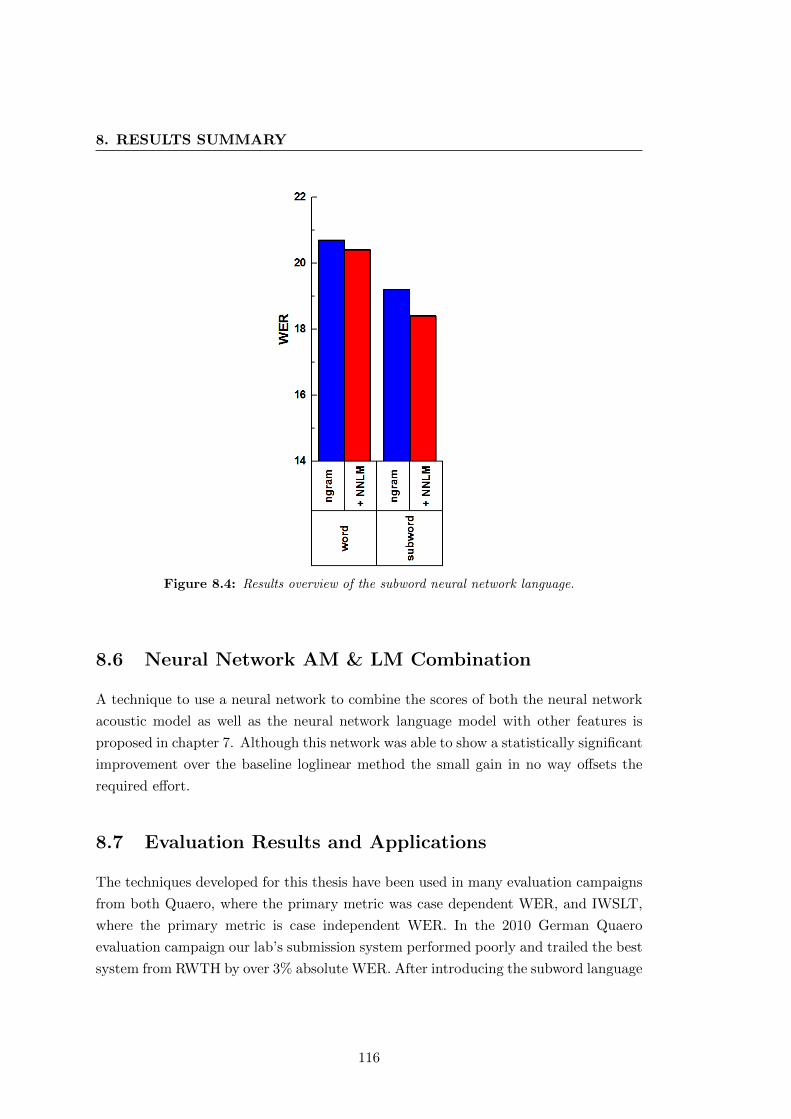
8. RESULTS SUMMARY
Figure 8.4: Results overview of the subword neural network language.
8.6 Neural Network AM & LM Combination
A technique to use a neural network to combine the scores of both the neural network
acoustic model as well as the neural network language model with other features is
proposed in chapter 7. Although this network was able to show a statistically significant
improvement over the baseline loglinear method the small gain in no way offsets the
required effort.
8.7 Evaluation Results and Applications
The techniques developed for this thesis have been used in many evaluation campaigns
from both Quaero, where the primary metric was case dependent WER, and IWSLT,
where the primary metric is case independent WER. In the 2010 German Quaero
evaluation campaign our lab’s submission system performed poorly and trailed the best
system from RWTH by over 3% absolute WER. After introducing the subword language
116
8.8 Results Overview
model and the first generation of multi-feature bottleneck neural network feature
extractors our submission system for the 2011 German Quaero evaluation campaign
was over 5% absolute better than previous year’s. This improvement was enough to
outperform all other participants in 2011, with our WER being just 0.1% ahead of
the submission from RWTH. Further improvements to the multi-feature bottleneck
neural network feature extractors and larger language models allowed us to repeat that
performance in the 2012 German Quaero evaluation campaign where our system again
had the lowest word error rate.
The multi-feature modular deep neural network acoustic models were introduced
for the both 2013 German Quaero and the 2013 German IWSLT evaluation campaigns.
The further boost in performance allowed our submission to the Quaero evaluation to
again outperform the other participants’ systems. In the IWSLT evaluation campaign
the submission from RWTH proved to be slightly better than ours resulting in us only
placing 2nd. However in 2014, after further optimizing the multi-feature modular deep
neural network acoustic models, our submission to the 2014 Germany IWSLT evaluation
campaign came out on top.
Besides being used in evaluation systems many of the techniques developed for
this thesis have also been integrated into our online lecture translation system. Here
the subword language model has turned out to be very important due the complected
vocabulary used in some lectures. On a mechanical engineering lecture, for example,
the subword language model was over 10% absolute better than the fullword language
model. Besides the language model the multi feature deep neural network acoustic
model also plays an important part in the lecture translator. Thanks to the singular
value decomposition based network growing and parameter reduction this deep neural
network acoustic model can be computed fast enough to ensure a low latency output
of the whole system.
Besides German the techniques developed in this thesis have also been used in
other projects to build systems for other languages such as English, Spanish, Pashto
and many more.
8.8 Results Overview
This final results overview section presents the individual and combined effects of the
techniques decribed in this thesis when applied to the IWSLT 2012 development set.
A baseline setup using a basic single feature deep neural network acoustic model and a
normal word ngram language model produced a WER of 21.4%. Upgrading this setup
117
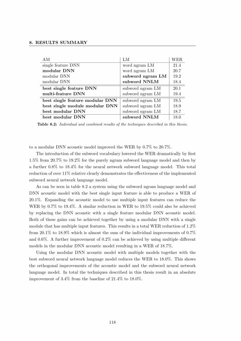
8. RESULTS SUMMARY
AM LM WER
single feature DNN word ngram LM 21.4modular DNN word ngram LM 20.7modular DNN subword ngram LM 19.2modular DNN subword NNLM 18.4
best single feature DNN subword ngram LM 20.1multi-feature DNN subword ngram LM 19.4
best single feature modular DNN subword ngram LM 19.5best single module modular DNN subword ngram LM 18.9best modular DNN subword ngram LM 18.7
best modular DNN subword NNLM 18.0
Table 8.2: Individual and combined results of the techniques described in this thesis.
to a modular DNN acoustic model improved the WER by 0.7% to 20.7%.
The introduction of the subword vocabulary lowered the WER dramatically by first
1.5% from 20.7% to 19.2% for the purely ngram subword language model and then by
a further 0.8% to 18.4% for the neural network subword language model. This total
reduction of over 11% relative clearly demonstrates the effectiveness of the implemented
subword neural network language model.
As can be seen in table 8.2 a system using the subword ngram language model and
DNN acoustic model with the best single input feature is able to produce a WER of
20.1%. Expanding the acoustic model to use multiple input features can reduce the
WER by 0.7% to 19.4%. A similar reduction in WER to 19.5% could also be achieved
by replacing the DNN acoustic with a single feature modular DNN acoustic model.
Both of these gains can be achieved together by using a modular DNN with a single
module that has multiple input features. This results in a total WER reduction of 1.2%
from 20.1% to 18.9% which is almost the sum of the individual improvements of 0.7%
and 0.6%. A further improvement of 0.2% can be achieved by using multiple different
models in the modular DNN acoustic model resulting in a WER of 18.7%.
Using the modular DNN acoustic model with multiple models together with the
best subword neural network language model reduces the WER to 18.0%. This shows
the orthogonal improvements of the acoustic model and the subword neural network
language model. In total the techniques described in this thesis result in an absolute
improvement of 3.4% from the baseline of 21.4% to 18.0%.
118
Chapter 9
Conclusion
This thesis investigates the application and improvement of neural networks on all
levels of a speech recognition system. It begins with the feature level where deep neural
networks can be employed to extract useful features from the speech signal using their
hidden layer’s ability to learn new representations of inputs and by setting the hidden
layer to a desired feature size.
An investigation into the ability of these networks to combine and utilize multiple
different features is performed. This experiment show,s that while the normal
non-tonal features are very similar and in most cases interchangeable, they are also
complementary. Augmenting the input feature or feature combination with tonal
features proves to be beneficial in all evaluated settings. A similar experiment on
deep neural network acoustic models shows the same pattern: Adding more features to
the input of the neural network improves its classification ability.
The modular deep neural network acoustic model presented in this thesis
incorporates well trained feature extraction networks using multiple input features. It is
initially evaluated using only a single feature extraction module. This evaluation again
demonstrates the usefulness of using multiple different input feature vectors. Modular
deep neural networks, whose sole feature extraction network uses multiple features,
outperform those using fewer features or a single feature.
Using two or more different feature extraction networks as modules in the same
modular deep neural network results in further improvement. The best approaches use
three feature extraction networks that are, in turn, each trained using multiple input
features. The best modular deep neural network is able to reduce the word error rate
on the test data sets by up to 11.5% relative improvement compared to a baseline deep
neural network.
119
9. CONCLUSION
A further problem addressed in this thesis is the reliance on older, non neural
network based modeling methods for the selection of the acoustic units which are used
as targets in the training of these modular deep neural network acoustic models. It is
shown that the probability distribution required by the clustering algorithm, in order to
measure the weighted entropy distance, can be generated using the average activation
of a context independent neural network acoustic model.
Furthermore, experiments are performed using singular value decomposition to
initialize new hidden layers in a deep neural network. An investigation of its possible
applications shows it to be useful for increasing the depth and performance of the neural
networks while at the same time allowing for a reduction in the number of parameters.
The parameter reduction is especially large when singular value decomposition is used
to initialize a small hidden layer just prior to the output layer.
A deep neural network is also used to build a subword neural network language
model. An error analysis concludes, that in German speech recognition systems,
compound words are a major source of errors. To solve this problem a subword
vocabulary selection method is developed that keeps normal words and splits compound
words. The use of an intraword tag allows a recognized sequence of subwords to
be easily combined into a sequence of words. This proves to be very effective and
results in a large gain when used in both a neural network language model and in an
ngram language model. As well as numerous applications in evaluation systems the
subword vocabulary is currently integrated into the KIT lecture translation system
and actively used to help foreign students to follow lectures held in German. This
integration requires the subword vocabulary to function together with a query based
vocabulary selection method that extracts queries from lecture slides. It uses a
search engine to find related documents and webpages and analyses them in order
to broaden the system’s vocabulary. An OOV analysis of the integrated system shows
that they complement each other well and give orthogonal gains. Performance issues,
unfortunately, prevent the integration of the subword neural network language model
into the lecture translation system.
In order to combine the outputs of both the acoustic model and the language model
a combination neural network is trained. It uses, as inputs, the acoustic model score
and the language model score of the word, for which it estimates the combined score.
Information about whether the word is a lexical word or noise word is also taken into
consideration. The network is trained using the lattices of the acoustic model training
data to minimize the MMIE error function. The training procedure is implemented
in a separate tool. It is evaluated and shown to be slight improvement on a normal
120

loglinear combination.
Throughout this thesis various neural network techniques were presented that
improved the overall performance of the speech recognition system. Their usage in
evaluations help our systems achieve numerous placements the best German system.
When combined together in a single system the improvements on both language model
and the acoustic model reduce the word error rate by roughly 20% when compared to
a baseline system with a normal neural network language model and a normal deep
neural network acoustic model.
121

Bibliography
[ADA00] M. Adda-Decker and G. Adda. Morphological decomposition for asr in
german. In Workshop on Phonetics and Phonology in Automatic Speech
Recognition, pages 129–143, 2000. 96
[AHS85] David H Ackley, Geoffrey E Hinton, and Terrence J Sejnowski. A learning
algorithm for boltzmann machines*. Cognitive science, 9(1):147–169,
1985. 20
[AKV+14] Heike Adel, Katrin Kirchhoff, Ngoc Thang Vu, Dominic Telaar, and Tanja
Schultz. Comparing approaches to convert recurrent neural networks into
backoff language models for efficient decoding. In Proc. of Interspeech,
2014. 24, 93
[Aro11] Jacob Aron. How innovative is apple’s new voice assistant, siri? New
Scientist, 212(2836):24, 2011. 1
[B+95] M Bishop, Christopher et al. Neural networks for pattern recognition.
1995. 15, 145
[Bao99] Zhiming Bao. The Structure of Tone. Oxford University Press, 1999. 49
[Bar12] Adrien Barbaresi. German political speeches-corpus and visualization. In
DGfS-CL poster session, 2012. 42
[BBB+10] James Bergstra, Olivier Breuleux, Frederic Bastien, Pascal Lamblin,
Razvan Pascanu, Guillaume Desjardins, Joseph Turian, David
Warde-Farley, and Yoshua Bengio. Theano: a CPU and GPU math
expression compiler. In Proceedings of the Python for Scientific Computing
Conference (SciPy), June 2010. Oral Presentation. 46, 69
[BBC+01] Carmen Benıtez, Lukas Burget, Barry Chen, Stephane Dupont, Hari
Garudadri, Hynek Hermansky, Pratibha Jain, Sachin Kajarekar, Nelson
123

BIBLIOGRAPHY
Morgan, and Sunil Sivadas. Robust asr front-end using spectral-based
and discriminant features: experiments on the aurora tasks. In Proc. of
EUROSPEECH, pages 429–432. Citeseer, 2001. 47
[BBdSM86] Lalit Bahl, Peter Brown, Peter V de Souza, and Robert Mercer. Maximum
mutual information estimation of hidden markov model parameters for
speech recognition. In Acoustics, Speech, and Signal Processing, IEEE
International Conference on ICASSP’86., volume 11, pages 49–52. IEEE,
1986. 26, 109
[BC+08] Y-lan Boureau, Yann L Cun, et al. Sparse feature learning for deep belief
networks. In Advances in neural information processing systems, pages
1185–1192, 2008. 20
[Ben09] Yoshua Bengio. Learning deep architectures for ai. Foundations and
trends® in Machine Learning, 2(1):1–127, 2009. 19
[BLP+07] Yoshua Bengio, Pascal Lamblin, Dan Popovici, Hugo Larochelle, et al.
Greedy layer-wise training of deep networks. Advances in neural
information processing systems, 19:153, 2007. 20
[BM94] Herve A Bourlard and Nelson Morgan. Connectionist speech recognition:
a hybrid approach, volume 247. Springer Science & Business Media, 1994.
28, 69
[Bro73] Roger Brown. A first language: The early stages. Harvard U. Press, 1973.
7
[BTCC98] A. Black, P. Taylor, R. Caley, and R. Clark. The festival speech synthesis
system, 1998. 97
[CBC+95] Maria Cristina Caselli, Elizabeth Bates, Paola Casadio, Judi Fenson,
Larry Fenson, Lisa Sanderl, and Judy Weir. A cross-linguistic study of
early lexical development. Cognitive Development, 10(2):159–199, 1995. 7
[CFH+13] Eunah Cho, Christian Fugen, Teresa Herrmann, Kevin Kilgour,
Mohammed Mediani, Christian Mohr, Jan Niehues, Kay Rottmann,
Christian Saam, Sebastian Stuker, et al. A real-world system for
simultaneous translation of german lectures. In INTERSPEECH, pages
3473–3477, 2013. 1, 36, 104
124
BIBLIOGRAPHY
[CG96] Stanley F Chen and Joshua Goodman. An empirical study of smoothing
techniques for language modeling. In Proceedings of the 34th annual
meeting on Association for Computational Linguistics, pages 310–318.
Association for Computational Linguistics, 1996. 24, 65
[CGM+97] C. Julian Chen, Ramesh A. Gopinath, Michael D. Monkowski, Michael A.
Picheny, and Katherine Shen. New methods in continuous Mandarin
speech recognition. In Proc. EUROSPEECH, Rhodes, Greece, September
1997. ISCA. 50
[CLLV05] M. Creutz, K. Lagus, K. Linden, and S. Virpioja. Morfessor and
hutmegs: Unsupervised morpheme segmentation for highly-inflecting and
compounding languages. 2005. 96
[CNS+13] Mauro Cettolo, Jan Niehues, Sebastian Stuker, Luisa Bentivogli, and
Marcello Federico. Report on the 10th iwslt evaluation campaign.
In Proceedings of the International Workshop on Spoken Language
Translation, Heidelberg, Germany, 2013. 36
[CW95] Sin-Horng Chen and Yih-Ru Wang. Tone recognition of continuous
Mandarin speech based on neural networks. IEEE Transactions on
Acoustics, Speech, and Signal Processing, 1995. 50
[DYDA11] George E Dahl, Dong Yu, Li Deng, and Alex Acero. Large vocabulary
continuous speech recognition with context-dependent dbn-hmms.
In Acoustics, Speech and Signal Processing (ICASSP), 2011 IEEE
International Conference on, pages 4688–4691. IEEE, 2011.
[DYDA12] George E Dahl, Dong Yu, Li Deng, and Alex Acero. Context-dependent
pre-trained deep neural networks for large-vocabulary speech recognition.
Audio, Speech, and Language Processing, IEEE Transactions on,
20(1):30–42, 2012. 2, 20, 28, 69
[FDR+94] Larry Fenson, Philip S Dale, J Steven Reznick, Elizabeth Bates, Donna J
Thal, Stephen J Pethick, Michael Tomasello, Carolyn B Mervis, and Joan
Stiles. Variability in early communicative development. Monographs of
the society for research in child development, pages i–185, 1994. 7
[FHBM06] Alexander Mark Franz, Monika H Henzinger, Sergey Brin, and
Brian Christopher Milch. Voice interface for a search engine, April 11
2006. US Patent 7,027,987. 1
125
BIBLIOGRAPHY
[Fis97] Jonathan G Fiscus. A post-processing system to yield reduced word error
rates: Recognizer output voting error reduction (rover). In Automatic
Speech Recognition and Understanding, 1997. Proceedings., 1997 IEEE
Workshop on, pages 347–354. IEEE, 1997. 1
[FLBG07] Marc Ferras, Cheung Chi Leung, Claude Barras, and J Gauvain.
Constrained mllr for speaker recognition. In Acoustics, Speech and
Signal Processing, 2007. ICASSP 2007. IEEE International Conference
on, volume 4, pages IV–53. IEEE, 2007. 45
[Fuk13] Keinosuke Fukunaga. Introduction to statistical pattern recognition.
Academic press, 2013. 25, 27
[Geh12] Jonas Gehring. Training Deep Neural Networks for Bottleneck Feature
Extraction. PhD thesis, National Research Center, 2012. 19, 20, 22, 53,
61
[GF94] David Graff and Rebecca Finch. Multilingual text resources at
the linguistic data consortium. In Proceedings of the workshop on
Human Language Technology, pages 18–22. Association for Computational
Linguistics, 1994. 42
[GF08] Frantisek Grezl and Petr Fousek. Optimizing bottle-neck features for
lvcsr. In Acoustics, Speech and Signal Processing, 2008. ICASSP 2008.
IEEE International Conference on, pages 4729–4732. IEEE, 2008. 53
[GFGS06] Alex Graves, Santiago Fernandez, Faustino Gomez, and Jurgen
Schmidhuber. Connectionist temporal classification: labelling
unsegmented sequence data with recurrent neural networks. In Proceedings
of the 23rd international conference on Machine learning, pages 369–376.
ACM, 2006. 34
[GJ14] Alex Graves and Navdeep Jaitly. Towards end-to-end speech recognition
with recurrent neural networks. In Proceedings of the 31st International
Conference on Machine Learning (ICML-14), pages 1764–1772, 2014. 34,
107
[GKKC07] Frantisek Grezl, Martin Karafiat, Stanislav Kontar, and J Cernocky.
Probabilistic and bottle-neck features for lvcsr of meetings. In Acoustics,
Speech and Signal Processing, 2007. ICASSP 2007. IEEE International
Conference on, volume 4, pages IV–757. IEEE, 2007. 53, 54
126
BIBLIOGRAPHY
[GL14] Yoav Goldberg and Omer Levy. word2vec explained: deriving mikolov et
al.’s negative-sampling word-embedding method. CoRR, abs/1402.3722,
2014. 103
[GLK+13] Jonas Gehring, Wonkyum Lee, Kevin Kilgour, Ian R Lane, Yajie Miao,
Alex Waibel, and Silicon Valley Campus. Modular combination of deep
neural networks for acoustic modeling. In INTERSPEECH, pages 94–98,
2013. 73
[GNMW13] Jonas Gehring, Quoc Bao Nguyen, Florian Metze, and Alex Waibel. Dnn
acoustic modeling with modular multi-lingual feature extraction networks.
In Automatic Speech Recognition and Understanding (ASRU), 2013 IEEE
Workshop on, pages 344–349. IEEE, 2013. 73
[GW96] Mark JF Gales and Philip C Woodland. Mean and variance adaptation
within the mllr framework. Computer Speech & Language, 10(4):249–264,
1996. 26
[Hay11] Bruce Hayes. Introductory phonology, volume 32. John Wiley & Sons,
2011. 2
[HBG+12] Eva Hasler, Peter Bell, Arnab Ghoshal, Barry Haddow, Philipp Koehn,
Fergus McInnes, Steve Renals, Pawel Swietojanski, Fergus R McInnes,
Sharon J Goldwater, et al. The uedin system for the iwslt 2012 evaluation.
In Proc. International Workshop on Spoken Language Translation, 2012.
93
[HCC+14] Awni Hannun, Carl Case, Jared Casper, Bryan Catanzaro, Greg Diamos,
Erich Elsen, Ryan Prenger, Sanjeev Satheesh, Shubho Sengupta, Adam
Coates, et al. Deepspeech: Scaling up end-to-end speech recognition.
arXiv preprint arXiv:1412.5567, 2014. 34
[HDY+12] Geoffrey Hinton, Li Deng, Dong Yu, George E Dahl, Abdel-rahman
Mohamed, Navdeep Jaitly, Andrew Senior, Vincent Vanhoucke, Patrick
Nguyen, Tara N Sainath, et al. Deep neural networks for acoustic modeling
in speech recognition: The shared views of four research groups. Signal
Processing Magazine, IEEE, 29(6):82–97, 2012. 2, 20, 69
[Hei10] Georg Heigold. A log-linear discriminative modeling framework for speech
recognition. PhD thesis, Universitatsbibliothek, 2010. 26, 107
127
BIBLIOGRAPHY
[Her90] Hynek Hermansky. Perceptual linear predictive (plp) analysis of speech.
the Journal of the Acoustical Society of America, 87(4):1738–1752, 1990.
49
[HES00] Hynek Hermansky, Daniel PW Ellis, and Sangita Sharma. Tandem
connectionist feature extraction for conventional hmm systems. In
Acoustics, Speech, and Signal Processing, 2000. ICASSP’00. Proceedings.
2000 IEEE International Conference on, volume 3, pages 1635–1638.
IEEE, 2000. 47
[Hir83] Daniel Hirst. Structures and categories in prosodic representations. In
Prosody: Models and measurements, pages 93–109. Springer, 1983. 50
[HOT06] Geoffrey Hinton, Simon Osindero, and Yee-Whye Teh. A fast learning
algorithm for deep belief nets. Neural computation, 18(7):1527–1554, 2006.
19, 20
[HS97] Sepp Hochreiter and Jurgen Schmidhuber. Long short-term memory.
Neural computation, 9(8):1735–1780, 1997. 33
[HS98] Hynek Hermansky and Sangita Sharma. Traps-classifiers of temporal
patterns. In ICSLP, 1998. 53, 54
[Hua92] XD Huang. Phoneme classification using semicontinuous hidden markov
models. Signal Processing, IEEE Transactions on, 40(5):1062–1067, 1992.
5
[JO+13] Zhenyu Hou Jian Ouyang, Lei Jia et al. A practical implementation of gpu
based accelerator for deep neural networks. In 4th Workshop on SoCs,
Heterogeneous Architectures and Workloads,2013., 2013. 19
[Joh04] D Johnson. Quicknet, speech group at icsi, berkeley, 2004. 46, 56
[Kal15] James Kalat. Biological psychology. Cengage Learning, 2015. 48
[Kil09] Kevin Kilgour. Language model adaptation using interlinked semantic
data. Master’s thesis, Karlsruhe University, Germany, 2009. 41
[KK01] J. Kneissler and D. Klakow. Speech recognition for huge vocabularies
by using optimized sub-word units. In Seventh European Conference on
Speech Communication and Technology, 2001. 96
128
BIBLIOGRAPHY
[Koe05] Philipp Koehn. Europarl: A parallel corpus for statistical machine
translation. In MT summit, volume 5, pages 79–86, 2005. 40, 43, 142
[KSM+11] Kevin Kilgour, Christian Saam, Christian Mohr, Sebastian Stuker, and
Alex Waibel. The 2011 kit quaero speech-to-text system for spanish. In
IWSLT, pages 199–205, 2011. 67
[KTNW13] Kevin Kilgour, Igor Tseyzer, Quoc Bao Nguyen, and Alex Waibel. Warped
minimum variance distortionless response based bottle neck features for
lvcsr. In Acoustics, Speech and Signal Processing (ICASSP), 2013 IEEE
International Conference on, pages 6990–6994. IEEE, 2013. 52, 56, 57,
68, 70
[KW15] Kevin Kilgour and Alex Waibel. Multi-feature modular deep neural
network acoustic models. 2015. 73
[LB95] Yann LeCun and Yoshua Bengio. Convolutional networks for images,
speech, and time series. The handbook of brain theory and neural networks,
3361:310, 1995. 33
[LCD+11] Lori Lamel, Sandrine Courcinous, Julien Despres, Jean-Luc Gauvain,
Yvan Josse, Kevin Kilgour, Florian Kraft, Viet Bac Le, Hermann Ney,
Markus Nußbaum-Thom, et al. Speech recognition for machine translation
in quaero. In IWSLT, pages 121–128, 2011. 41
[Le13] Quoc V Le. Building high-level features using large scale unsupervised
learning. In Acoustics, Speech and Signal Processing (ICASSP), 2013
IEEE International Conference on, pages 8595–8598. IEEE, 2013. 20
[LGL+11] Lori Lamel, Jean-Luc Gauvain, Viet Bac Le, Ilya Oparin, and Sha Meng.
Improved models for Mandarin speech-to-text transcription. In Proc.
ICASSP, Prague; Czech Republic, May 2011. IEEE. 50
[LGRN09] Honglak Lee, Roger Grosse, Rajesh Ranganath, and Andrew Y Ng.
Convolutional deep belief networks for scalable unsupervised learning
of hierarchical representations. In Proceedings of the 26th Annual
International Conference on Machine Learning, pages 609–616. ACM,
2009.
129
BIBLIOGRAPHY
[LHE08] Kornel Laskowski, Mattias Heldner, and Jens Edlund. The fundamental
frequency variation spectrum. Proceedings of FONETIK 2008, pages
29–32, 2008. 50, 51
[Mar06] T. Marek. Analysis of german compounds using weighted finite state
transducers. Bachelor thesis, University of Tubingen, 2006. 95, 96, 97
[MBS00a] Lidia Mangu, Eric Brill, and Andreas Stolcke. Finding consensus in speech
recognition: word error minimization and other applications of confusion
networks. Computer Speech & Language, 14(4):373–400, 2000. 1
[MBS00b] Lidia Mangu, Eric Brill, and Andreas Stolcke. Finding consensus in speech
recognition: word error minimization and other applications of confusion
networks. Computer Speech & Language, 14(4):373–400, 2000. 46
[MCCD13] Tomas Mikolov, Kai Chen, Greg Corrado, and Jeffrey Dean. Efficient
estimation of word representations in vector space. arXiv preprint
arXiv:1301.3781, 2013. 24
[MCZS04] Nelson Morgan, BY Chenl, Qifeng Zhu, and Andreas Stolcke.
Trapping conversational speech: Extending trap/tandem approaches to
conversational telephone speech recognition. In Acoustics, Speech, and
Signal Processing, 2004. Proceedings.(ICASSP’04). IEEE International
Conference on, volume 1, pages I–537. IEEE, 2004.
[MDH12] Abdel-rahman Mohamed, George E Dahl, and Geoffrey Hinton. Acoustic
modeling using deep belief networks. Audio, Speech, and Language
Processing, IEEE Transactions on, 20(1):14–22, 2012. 72, 89
[MHL+14] Andrew L Maas, Awni Y Hannun, Christopher T Lengerich, Peng Qi,
Daniel Jurafsky, and Andrew Y Ng. Increasing deep neural network
acoustic model size for large vocabulary continuous speech recognition.
arXiv preprint arXiv:1406.7806, 2014. 2, 81
[Mit97] Tom M Mitchell. Machine learning. 1997. Burr Ridge, IL: McGraw Hill,
45, 1997. 145
[MKB+10] Tomas Mikolov, Martin Karafiat, Lukas Burget, Jan Cernocky, and
Sanjeev Khudanpur. Recurrent neural network based language model.
In INTERSPEECH, pages 1045–1048, 2010. 25, 93
130
BIBLIOGRAPHY
[MKLW11] P. Maergner, K. Kilgour, I. Lane, and A. Waibel. Unsupervised vocabulary
selection for simultaneous lecture translation. 2011. 97, 104
[Moz89] Michael C Mozer. A focused back-propagation algorithm for temporal
pattern recognition. Complex systems, 3(4):349–381, 1989. 33
[MR00] Manohar N Murthi and Bhaskar D Rao. All-pole modeling of speech based
on the minimum variance distortionless response spectrum. Speech and
Audio Processing, IEEE Transactions on, 8(3):221–239, 2000. 49
[MS69] Marvin Minsky and Papert Seymour. Perceptrons. 1969. 13, 16
[MSD+12] Tomas Mikolov, Ilya Sutskever, Anoop Deoras, Hai-Son Le, Stefan
Kombrink, and J Cernocky. Subword language modeling with neural
networks. preprint (http://www. fit. vutbr. cz/imikolov/rnnlm/char. pdf),
2012. 95
[MSW+13a] Florian Metze, Zaid AW Sheikh, Alex Waibel, Jonas Gehring, Kevin
Kilgour, Quoc Bao Nguyen, and Van Huy Nguyen. Models of tone for
tonal and non-tonal languages. In Automatic Speech Recognition and
Understanding (ASRU), 2013 IEEE Workshop on, pages 261–266. IEEE,
2013. xiii, 50, 64, 66
[MSW+13b] Florian Metze, Zaid AW Sheikh, Alex Waibel, Jonas Gehring, Kevin
Kilgour, Quoc Bao Nguyen, and Van Huy Nguyen. Models of tone for
tonal and non-tonal languages. In Automatic Speech Recognition and
Understanding (ASRU), 2013 IEEE Workshop on, pages 261–266. IEEE,
2013.
[NH10] Vinod Nair and Geoffrey E Hinton. Rectified linear units improve
restricted boltzmann machines. In Proceedings of the 27th International
Conference on Machine Learning (ICML-10), pages 807–814, 2010. 17
[NRP11a] Claire H Noble, Caroline F Rowland, and Julian M Pine. Comprehension
of argument structure and semantic roles: Evidence from english-learning
children and the forced-choice pointing paradigm. Cognitive Science,
35(5):963–982, 2011. 7
[NRP11b] Claire H Noble, Caroline F Rowland, and Julian M Pine. Comprehension
of argument structure and semantic roles: Evidence from english-learning
131
BIBLIOGRAPHY
children and the forced-choice pointing paradigm. Cognitive Science,
35(5):963–982, 2011.
[NS88] Masami Nakamura and Kiyohiro Shikano. A study of english word
category prediction based on neural networks. The Journal of the
Acoustical Society of America, 84(S1):S60–S61, 1988. 93
[NTMSN11] M. Nußbaum-Thom, A.E.D. Mousa, R. Schluter, and H. Ney. Compound
word recombination for german lvcsr. In Twelfth Annual Conference of
the International Speech Communication Association, 2011. 96
[OdKB+12] Marcel Oberlaender, Christiaan PJ de Kock, Randy M Bruno, Alejandro
Ramirez, Hanno S Meyer, Vincent J Dercksen, Moritz Helmstaedter,
and Bert Sakmann. Cell type–specific three-dimensional structure of
thalamocortical circuits in a column of rat vibrissal cortex. Cerebral cortex,
22(10):2375–2391, 2012. xi, 6
[OTI98] Atsunori Ogawa, Kazuya Takeda, and Fumitada Itakura. Balancing
acoustic and linguistic probabilities. In Acoustics, Speech and Signal
Processing, 1998. Proceedings of the 1998 IEEE International Conference
on, volume 1, pages 181–184. IEEE, 1998. 32
[Pie80] Janet Pierrehumbert. The Phonetics and Phonology of English Intonation.
PhD thesis, Massachusetts Institute of Technology, 1980. 50
[PKK+08] Daniel Povey, Dimitri Kanevsky, Brian Kingsbury, Bhuvana
Ramabhadran, George Saon, and Karthik Visweswariah. Boosted
mmi for model and feature-space discriminative training. In Acoustics,
Speech and Signal Processing, 2008. ICASSP 2008. IEEE International
Conference on, pages 4057–4060. IEEE, 2008. 26, 45
[PKSN13] Christian Plahl, Michal Kozielski, R Schluter, and Hermann Ney. Feature
combination and stacking of recurrent and non-recurrent neural networks
for lvcsr. In Acoustics, Speech and Signal Processing (ICASSP), 2013
IEEE International Conference on, pages 6714–6718. IEEE, 2013. 34, 53
[Pow64] Michael JD Powell. An efficient method for finding the minimum of a
function of several variables without calculating derivatives. The computer
journal, 7(2):155–162, 1964. 108
132
BIBLIOGRAPHY
[PSN10] Christian Plahl, Ralf Schluter, and Hermann Ney. Hierarchical bottle neck
features for lvcsr. In Interspeech, pages 1197–1200, 2010. 53
[PSN11] Christian Plahl, Ralf Schluter, and Hermann Ney. Improved acoustic
feature combination for lvcsr by neural networks. In INTERSPEECH,
pages 1237–1240, 2011. 53
[Rab89] Lawrence Rabiner. A tutorial on hidden markov models and
selected applications in speech recognition. Proceedings of the IEEE,
77(2):257–286, 1989. 25
[RGE02] Manuel Reyes-Gomez and Daniel PW Ellis. Error visualization for tandem
acoustic modeling on the aurora task. In ICASSP 2002. International
Conference on Acoustics, Speech, and Signal Processing, 2002. 47
[RHR94] Tony Robinson, Mike Hochberg, and Steve Renals. Ipa: Improved phone
modelling with recurrent neural networks. In Acoustics, Speech, and Signal
Processing, 1994. ICASSP-94., 1994 IEEE International Conference on,
volume 1, pages I–37. IEEE, 1994. 33
[RMB+94] Steve Renals, Nelson Morgan, Herve Bourlard, Michael Cohen, and
Horacio Franco. Connectionist probability estimators in hmm speech
recognition. Speech and Audio Processing, IEEE Transactions on,
2(1):161–174, 1994. 28
[Rob94] Anthony J Robinson. An application of recurrent nets to phone probability
estimation. Neural Networks, IEEE Transactions on, 5(2):298–305, 1994.
33
[Ros57] Frank Rosenblatt. The perceptron, a perceiving and recognizing automaton
Project Para. Cornell Aeronautical Laboratory, 1957. 12
[Sch98] Kjell Schubert. Pitch tracking and his application on speech recognition.
PhD thesis, Diploma Thesis at University of Kalsruhe (TH), Germany,
1998. 50
[Sch07] Holger Schwenk. Continuous space language models. Computer Speech &
Language, 21(3):492–518, 2007. 24, 25, 93, 101
[Sch15] Jurgen Schmidhuber. Deep learning in neural networks: An overview.
Neural Networks, 61:85–117, 2015. 19
133
BIBLIOGRAPHY
[SHBL14] Andrew Senior, Georg Heigold, Michiel Bacchiani, and Hank Liao.
Gmm-free dnn training. In Proc. IEEE Int. Conf. on Acoustics, Speech,
and Signal Processing, 2014. 81
[SKK12a] Sebastian Stuker, Kevin Kilgour, and Florian Kraft. Quaero 2010
speech-to-text evaluation systems. In High Performance Computing in
Science and Engineering’11, pages 607–618. Springer, 2012. 35, 37, 45
[SKK12b] Sebastian Stuker, Kevin Kilgour, and Florian Kraft. Quaero 2010
speech-to-text evaluation systems. In High Performance Computing in
Science and Engineering’11, pages 607–618. Springer, 2012. 94
[SKM+12] Sebastian Stuker, Florian Kraft, Christian Mohr, Teresa Herrmann,
Eunah Cho, and Alex Waibel. The kit lecture corpus for speech
translation. In LREC, pages 3409–3414, 2012. 38
[SLY11] Frank Seide, Gang Li, and Dong Yu. Conversational speech transcription
using context-dependent deep neural networks. In Interspeech, pages
437–440, 2011. 20
[SMFW01] Hagen Soltau, Florian Metze, Christian Fugen, and Alex Waibel. A
one-pass decoder based on polymorphic linguistic context assignment. In
Automatic Speech Recognition and Understanding, 2001. ASRU’01. IEEE
Workshop on, pages 214–217. IEEE, 2001. 44, 45, 102
[SMK+12a] Christian Saam, Christian Mohr, Kevin Kilgour, Michael Heck, Matthias
Sperber, Keigo Kubo, Sebastian Stuker, Sakriani Sakti, Graham Neubig,
Tomoki Toda, et al. The 2012 kit and kit-naist english asr systems for the
iwslt evaluation. In IWSLT, pages 87–90, 2012.
[SMK+12b] Christian Saam, Christian Mohr, Kevin Kilgour, Michael Heck, Matthias
Sperber, Keigo Kubo, Sebastian Stuker, Sakriani Sakti, Graham Neubig,
Tomoki Toda, et al. The 2012 kit and kit-naist english asr systems for the
iwslt evaluation. In IWSLT, pages 87–90, 2012.
[SMKR13] Tara N Sainath, A-r Mohamed, Brian Kingsbury, and Bhuvana
Ramabhadran. Deep convolutional neural networks for lvcsr. In Acoustics,
Speech and Signal Processing (ICASSP), 2013 IEEE International
Conference on, pages 8614–8618. IEEE, 2013. 33
134
BIBLIOGRAPHY
[SMM+91] Hidefumi SAWAI, Yasuhiro MINAMI, Masanori MIYATAKE, Alex
WAIBEL, and Kiyohiro SHIKANO. Connectionist approaches to large
vocabulary continuous speech recognition. IEICE TRANSACTIONS on
Fundamentals of Electronics, Communications and Computer Sciences,
74(7):1834–1844, 1991. 32
[SMSN11] M.A.B. Shaik, A.E.D. Mousa, R. Schluter, and H. Ney. Hybrid language
models using mixed types of sub-lexical units for open vocabulary
german lvcsr. In Twelfth Annual Conference of the International Speech
Communication Association, 2011. 96
[SMSN12] M Ali Basha Shaik, Amr El-Desoky Mousa, Ralf Schluter, and Hermann
Ney. Investigation of maximum entropy hybrid language models for open
vocabulary german and polish lvcsr. In INTERSPEECH, 2012. 96
[SSN12] Martin Sundermeyer, Ralf Schluter, and Hermann Ney. Lstm neural
networks for language modeling. In INTERSPEECH, 2012. 25, 93
[SSS14] Hagen Soltau, George Saon, and Tara N Sainath. Joint training of
convolutional and non-convolutional neural networks. to Proc. ICASSP,
2014. 2, 69
[SSW91] Masahide Sugiyama, Hidehumi Sawai, and Alexander H Waibel. Review
of tdnn (time delay neural network) architectures for speech recognition.
In Circuits and Systems, 1991., IEEE International Sympoisum on, pages
582–585. IEEE, 1991.
[ST03] M. Schroder and J. Trouvain. The german text-to-speech synthesis system
mary: A tool for research, development and teaching. International
Journal of Speech Technology, 6(4):365–377, 2003. 97
[Sto02] A. Stolcke. Srilm-an extensible language modeling toolkit. In Seventh
International Conference on Spoken Language Processing, 2002. 44, 65
[SVN37] Stanley Smith Stevens, John Volkmann, and Edwin B Newman. A scale
for the measurement of the psychological magnitude pitch. The Journal
of the Acoustical Society of America, 8(3):185–190, 1937. 48
[Tom85] Masaru Tomita. Efficient parsing for natural language: A fast algorithm
for practical systems, volume 8. Springer Science & Business Media, 1985.
33
135
BIBLIOGRAPHY
[Tse] Igor Tseyzer. An optimization of deep neural networks in asr using
singular value decomposition. xi, xiv, 71, 85, 86, 88, 89, 90, 91, 92
[TW88] Shin’Ichi Tamura and Alex Waibel. Noise reduction using connectionist
models. In Acoustics, Speech, and Signal Processing, 1988. ICASSP-88.,
1988 International Conference on, pages 553–556. IEEE, 1988. 47
[VGBP13] Karel Vesely, Arnab Ghoshal, Lukas Burget, and Daniel Povey.
Sequence-discriminative training of deep neural networks. In
INTERSPEECH, pages 2345–2349, 2013. 20, 109, 149
[Vit67] Andrew J Viterbi. Error bounds for convolutional codes and an
asymptotically optimum decoding algorithm. Information Theory, IEEE
Transactions on, 13(2):260–269, 1967. 26
[VLBM08] Pascal Vincent, Hugo Larochelle, Yoshua Bengio, and Pierre-Antoine
Manzagol. Extracting and composing robust features with denoising
autoencoders. In Proceedings of the 25th international conference on
Machine learning, pages 1096–1103. ACM, 2008. 21
[VLL+10] Pascal Vincent, Hugo Larochelle, Isabelle Lajoie, Yoshua Bengio, and
Pierre-Antoine Manzagol. Stacked denoising autoencoders: Learning
useful representations in a deep network with a local denoising criterion.
The Journal of Machine Learning Research, 11:3371–3408, 2010. 22, 65
[VS09] Ngoc Thang Vu and Tanja Schultz. Vietnamese large vocabulary
continuous speech recognition. In Automatic Speech Recognition &
Understanding, 2009. ASRU 2009. IEEE Workshop on, pages 333–338.
IEEE, 2009. 50
[VVP+07] Fabio Valente, Jithendra Vepa, Christian Plahl, Christian Gollan, Hynek
Hermansky, and Ralf Schluter. Hierarchical neural networks feature
extraction for lvcsr system. In INTERSPEECH, pages 42–45, 2007. 53
[VW03] Anand Venkataraman and Wen Wang. Techniques for effective vocabulary
selection. arXiv preprint cs/0306022, 2003. 44
[Wai88] Alex Waibel. Prosody and speech recognition. Morgan Kaufmann, 1988.
50
[Wai89] Alex Waibel. Modular construction of time-delay neural networks for
speech recognition. Neural computation, 1(1):39–46, 1989. 33
136
BIBLIOGRAPHY
[Wai14] Kilgour Waibel. Vorlesung: Neuronale netze. University Lecture, 2014.
145
[WHH+87a] Alexander Waibel, Toshiyuki Hanazawa, Geoffrey Hinton, Kiyohiro
Shikano, and Kevin J Lang. Phoneme recognition using time-delay neural
networks. In Meeting of the Institute of Electrical, Information and
Communication Engineers (IEICE), pages SP87–100. IEICE, 1987. 33
[WHH+87b] Alexander Waibel, Toshiyuki Hanazawa, Geoffrey Hinton, Kiyohiro
Shikano, and Kevin J Lang. Phoneme recognition using time-delay
neural networks. Technical report, ATR, 1987. ATR Technical Report,
TR-I-0006. 33
[WHH+88] Alexander Waibel, Toshiyuki Hanazawa, Geoffrey Hinton, Kiyohiro
Shikano, and K Lang. Phoneme recognition: neural networks vs. hidden
markov models vs. hidden markov models. In Acoustics, Speech, and
Signal Processing, 1988. ICASSP-88., 1988 International Conference on,
pages 107–110. IEEE, 1988.
[WHH+89] Alex Waibel, Toshiyuki Hanazawa, Geoffrey Hinton, Kiyohiro Shikano,
and Kevin J Lang. Phoneme recognition using time-delay neural
networks. Acoustics, Speech and Signal Processing, IEEE Transactions
on, 37(3):328–339, 1989. 32
[WM05] Matthias Wolfel and John McDonough. Minimum variance distortionless
response spectral estimation. Signal Processing Magazine, IEEE,
22(5):117–126, 2005. 49
[WMW03] Matthias Wolfel, John W McDonough, and Alex Waibel. Minimum
variance distortionless response on a warped frequency scale. In
INTERSPEECH, 2003. 49
[WT84] Janet F Werker and Richard C Tees. Cross-language speech perception:
Evidence for perceptual reorganization during the first year of life. Infant
behavior and development, 7(1):49–63, 1984. 6
[WW03] L Wang and PC Woodland. Discriminative adaptive training using the
mpe criterion. In Automatic Speech Recognition and Understanding, 2003.
ASRU’03. 2003 IEEE Workshop on, pages 279–284. IEEE, 2003. 26
137
BIBLIOGRAPHY
[XLG13] Jian Xue, Jinyu Li, and Yifan Gong. Restructuring of deep neural network
acoustic models with singular value decomposition. In INTERSPEECH,
pages 2365–2369, 2013. 84, 85
[YS11] Dong Yu and Michael L Seltzer. Improved bottleneck features using
pretrained deep neural networks. In INTERSPEECH, volume 237, page
240, 2011. 53, 61
[ZCM+04] Qifeng Zhu, Barry Y Chen, Nelson Morgan, Andreas Stolcke, et al. On
using mlp features in lvcsr. In INTERSPEECH, 2004. 47
[Zhu15] Linchen Zhu. Gmm free asr using dnn based cluster trees. Master’s thesis,
Karlsruhe Institute of technology, Germany, 2015. xi, 81, 83
[ZKSW15] Linchen Zhu, Kevin Kilgour, Sebastian Stuker, and Alex Waibel.
Gaussian free cluster tree construction using deep neural network. In
Sixteenth Annual Conference of the International Speech Communication
Association, 2015. 81
[ZW97] Puming Zhan and Alex Waibel. Vocal tract length normalization for
large vocabulary continuous speech recognition. Technical report, DTIC
Document, 1997. 45
[ZW14] Chao Zhang and PC Woodland. Standalone training of context-dependent
deep neural network acoustic models. In Acoustics, Speech and Signal
Processing (ICASSP), 2014 IEEE International Conference on, pages
5597–5601. IEEE, 2014.
138

Appendices
139

Appendix A
Language Model Data
The data sources for the IWSLT language model are given in Table A.1. There are far
fewer sources because of evaluation campaign organizers restrict the allowable training
text to a list of publicly available corpera.
The two language models used in this thesis are trained of different training sources.
Table A.2 lists the text sources used for the Quaero language model from the 2012
Quaero evaluation. The 2011 Quaero evaluation systems uses almost exactly the same
sources. The various news websites from 2011 are omitted and it also does not contain
the newer parts of the AM data transcripts.
141
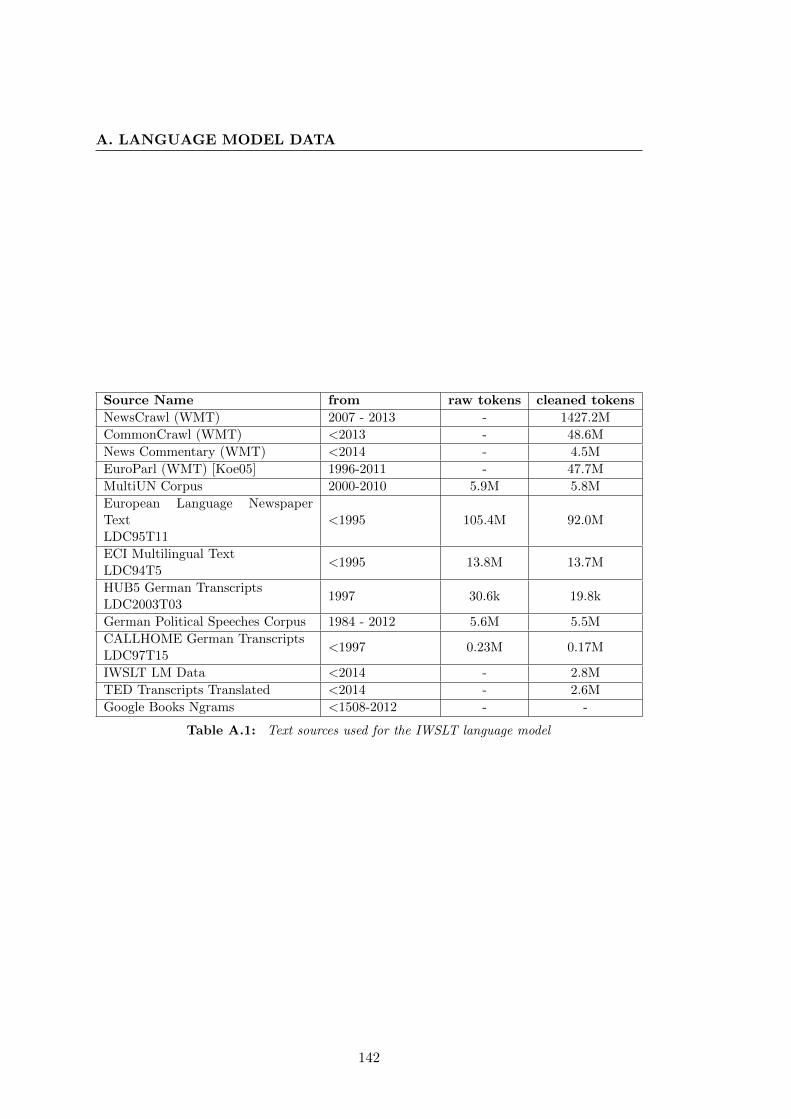
A. LANGUAGE MODEL DATA
Source Name from raw tokens cleaned tokens
NewsCrawl (WMT) 2007 - 2013 - 1427.2M
CommonCrawl (WMT) <2013 - 48.6M
News Commentary (WMT) <2014 - 4.5M
EuroParl (WMT) [Koe05] 1996-2011 - 47.7M
MultiUN Corpus 2000-2010 5.9M 5.8M
European Language NewspaperTextLDC95T11
<1995 105.4M 92.0M
ECI Multilingual TextLDC94T5
<1995 13.8M 13.7M
HUB5 German TranscriptsLDC2003T03
1997 30.6k 19.8k
German Political Speeches Corpus 1984 - 2012 5.6M 5.5M
CALLHOME German TranscriptsLDC97T15
<1997 0.23M 0.17M
IWSLT LM Data <2014 - 2.8M
TED Transcripts Translated <2014 - 2.6M
Google Books Ngrams <1508-2012 - -
Table A.1: Text sources used for the IWSLT language model
142
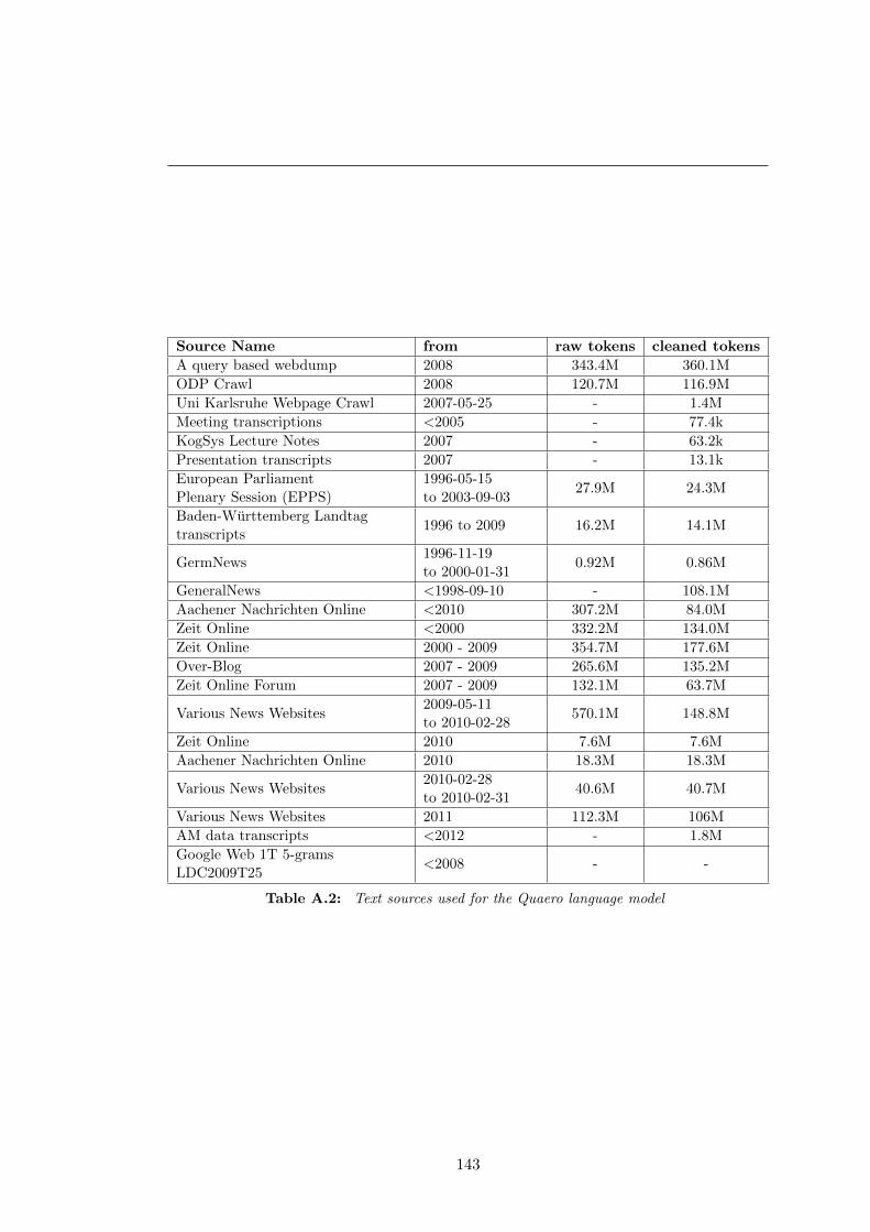
Source Name from raw tokens cleaned tokens
A query based webdump 2008 343.4M 360.1M
ODP Crawl 2008 120.7M 116.9M
Uni Karlsruhe Webpage Crawl 2007-05-25 - 1.4M
Meeting transcriptions <2005 - 77.4k
KogSys Lecture Notes 2007 - 63.2k
Presentation transcripts 2007 - 13.1k
European ParliamentPlenary Session (EPPS)
1996-05-15to 2003-09-03
27.9M 24.3M
Baden-Wurttemberg Landtagtranscripts
1996 to 2009 16.2M 14.1M
GermNews1996-11-19to 2000-01-31
0.92M 0.86M
GeneralNews <1998-09-10 - 108.1M
Aachener Nachrichten Online <2010 307.2M 84.0M
Zeit Online <2000 332.2M 134.0M
Zeit Online 2000 - 2009 354.7M 177.6M
Over-Blog 2007 - 2009 265.6M 135.2M
Zeit Online Forum 2007 - 2009 132.1M 63.7M
Various News Websites2009-05-11to 2010-02-28
570.1M 148.8M
Zeit Online 2010 7.6M 7.6M
Aachener Nachrichten Online 2010 18.3M 18.3M
Various News Websites2010-02-28to 2010-02-31
40.6M 40.7M
Various News Websites 2011 112.3M 106M
AM data transcripts <2012 - 1.8M
Google Web 1T 5-gramsLDC2009T25
<2008 - -
Table A.2: Text sources used for the Quaero language model
143

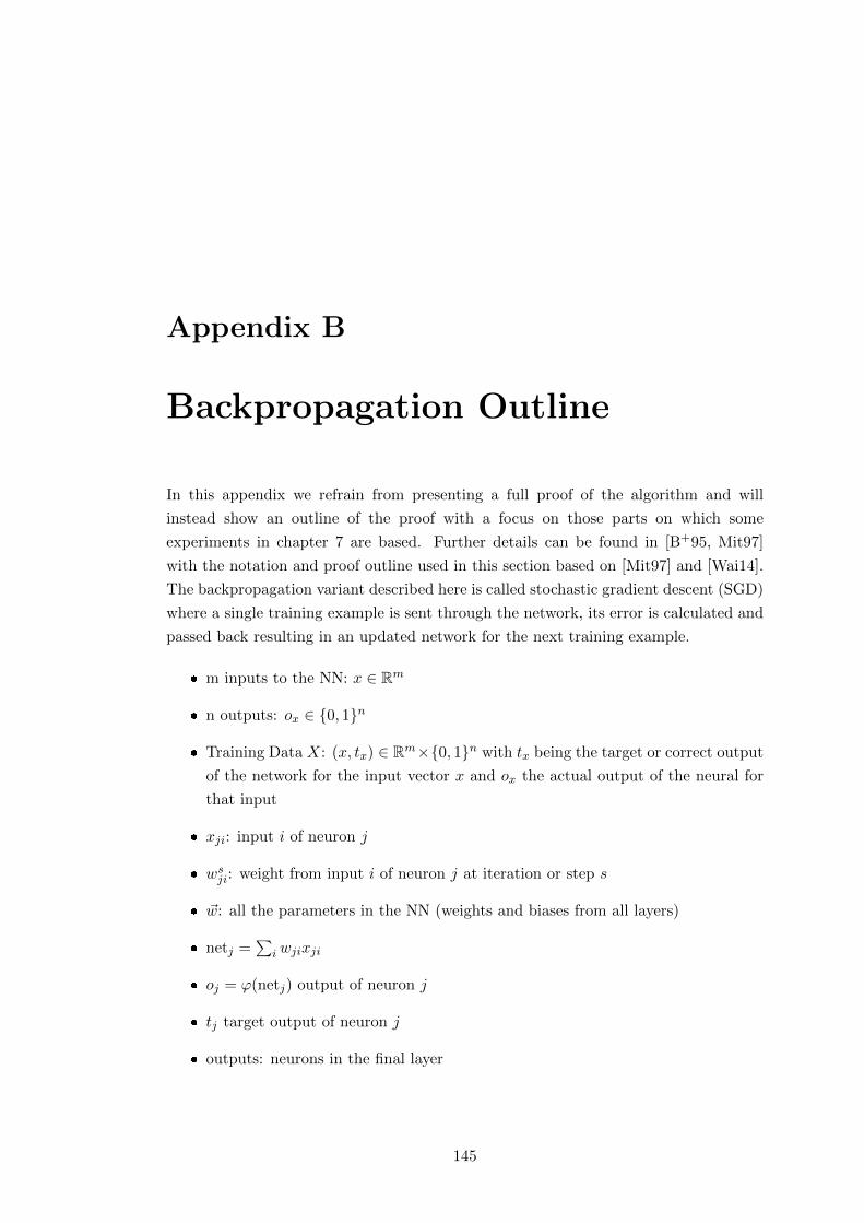
Appendix B
Backpropagation Outline
In this appendix we refrain from presenting a full proof of the algorithm and will
instead show an outline of the proof with a focus on those parts on which some
experiments in chapter 7 are based. Further details can be found in [B+95, Mit97]
with the notation and proof outline used in this section based on [Mit97] and [Wai14].
The backpropagation variant described here is called stochastic gradient descent (SGD)
where a single training example is sent through the network, its error is calculated and
passed back resulting in an updated network for the next training example.
� m inputs to the NN: x ∈ Rm
� n outputs: ox ∈ {0, 1}n
� Training Data X: (x, tx) ∈ Rm×{0, 1}n with tx being the target or correct output
of the network for the input vector x and ox the actual output of the neural for
that input
� xji: input i of neuron j
� wsji: weight from input i of neuron j at iteration or step s
� ~w: all the parameters in the NN (weights and biases from all layers)
� netj =∑
iwjixji
� oj = ϕ(netj) output of neuron j
� tj target output of neuron j
� outputs: neurons in the final layer
145
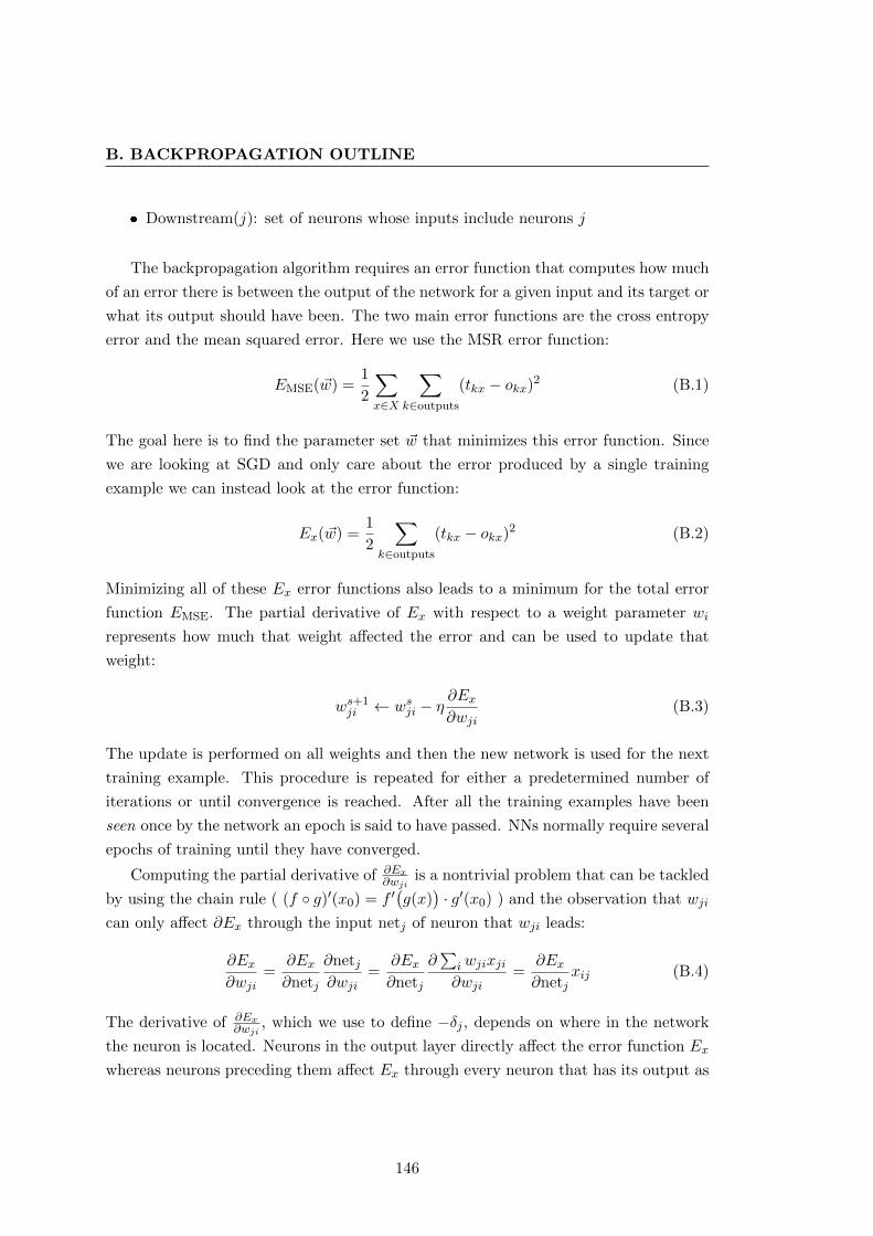
B. BACKPROPAGATION OUTLINE
� Downstream(j): set of neurons whose inputs include neurons j
The backpropagation algorithm requires an error function that computes how much
of an error there is between the output of the network for a given input and its target or
what its output should have been. The two main error functions are the cross entropy
error and the mean squared error. Here we use the MSR error function:
EMSE(~w) =1
2
∑x∈X
∑k∈outputs
(tkx − okx)2 (B.1)
The goal here is to find the parameter set ~w that minimizes this error function. Since
we are looking at SGD and only care about the error produced by a single training
example we can instead look at the error function:
Ex(~w) =1
2
∑k∈outputs
(tkx − okx)2 (B.2)
Minimizing all of these Ex error functions also leads to a minimum for the total error
function EMSE. The partial derivative of Ex with respect to a weight parameter wi
represents how much that weight affected the error and can be used to update that
weight:
ws+1ji ← wsji − η
∂Ex∂wji
(B.3)
The update is performed on all weights and then the new network is used for the next
training example. This procedure is repeated for either a predetermined number of
iterations or until convergence is reached. After all the training examples have been
seen once by the network an epoch is said to have passed. NNs normally require several
epochs of training until they have converged.
Computing the partial derivative of ∂Ex∂wji
is a nontrivial problem that can be tackled
by using the chain rule ( (f ◦ g)′(x0) = f ′(g(x)
)· g′(x0) ) and the observation that wji
can only affect ∂Ex through the input netj of neuron that wji leads:
∂Ex∂wji
=∂Ex∂netj
∂netj∂wji
=∂Ex∂netj
∂∑
iwjixji∂wji
=∂Ex∂netj
xij (B.4)
The derivative of ∂Ex∂wji
, which we use to define −δj , depends on where in the network
the neuron is located. Neurons in the output layer directly affect the error function Ex
whereas neurons preceding them affect Ex through every neuron that has its output as
146
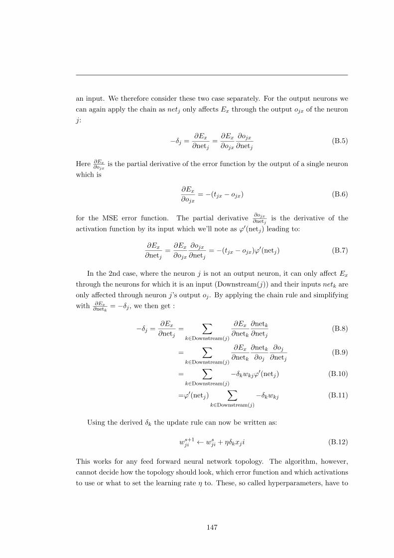
an input. We therefore consider these two case separately. For the output neurons we
can again apply the chain as netj only affects Ex through the output ojx of the neuron
j:
−δj =∂Ex∂netj
=∂Ex∂ojx
∂ojx∂netj
(B.5)
Here ∂Ex∂ojx
is the partial derivative of the error function by the output of a single neuron
which is
∂Ex∂ojx
= −(tjx − ojx) (B.6)
for the MSE error function. The partial derivative∂ojx∂netj
is the derivative of the
activation function by its input which we’ll note as ϕ′(netj) leading to:
∂Ex∂netj
=∂Ex∂ojx
∂ojx∂netj
= −(tjx − ojx)ϕ′(netj) (B.7)
In the 2nd case, where the neuron j is not an output neuron, it can only affect Ex
through the neurons for which it is an input (Downstream(j)) and their inputs netk are
only affected through neuron j’s output oj . By applying the chain rule and simplifying
with ∂Ex∂netk
= −δj , we then get :
−δj =∂Ex∂netj
=∑
k∈Downstream(j)
∂Ex∂netk
∂netk∂netj
(B.8)
=∑
k∈Downstream(j)
∂Ex∂netk
∂netk∂oj
∂oj∂netj
(B.9)
=∑
k∈Downstream(j)
−δkwkjϕ′(netj) (B.10)
=ϕ′(netj)∑
k∈Downstream(j)
−δkwkj (B.11)
Using the derived δk the update rule can now be written as:
ws+1ji ← wsji + ηδkxji (B.12)
This works for any feed forward neural network topology. The algorithm, however,
cannot decide how the topology should look, which error function and which activations
to use or what to set the learning rate η to. These, so called hyperparameters, have to
147

B. BACKPROPAGATION OUTLINE
be optimized independently of the learning algorithm.
148
Appendix C
MMIE Error Function
This appendix contains the full derivative the MMIE error function used in the chapter
on neural network based AM and LM combination. This is similar to the MMIE
derivative used for sequences training in [VGBP13].
149
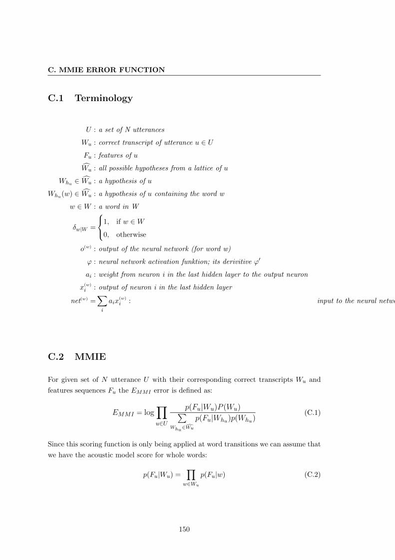
C. MMIE ERROR FUNCTION
C.1 Terminology
U : a set of N utterances
Wu : correct transcript of utterance u ∈ U
Fu : features of u
Wu : all possible hypotheses from a lattice of u
Whu ∈ Wu : a hypothesis of u
Whu(w) ∈ Wu : a hypothesis of u containing the word w
w ∈W : a word in W
δw|W =
1, if w ∈W
0, otherwise
o(w) : output of the neural network (for word w)
ϕ : neural network activation funktion; its derivitive ϕ′
ai : weight from neuron i in the last hidden layer to the output neuron
x(w)
i : output of neuron i in the last hidden layer
net(w) =∑i
aix(w)
i : input to the neural network
C.2 MMIE
For given set of N utterance U with their corresponding correct transcripts Wu and
features sequences Fu the EMMI error is defined as:
EMMI = log∏u∈U
p(Fu|Wu)P (Wu)∑Whu∈Wu
p(Fu|Whu)p(Whu)(C.1)
Since this scoring function is only being applied at word transitions we can assume that
we have the acoustic model score for whole words:
p(Fu|Wu) =∏w∈Wu
p(Fu|w) (C.2)
150
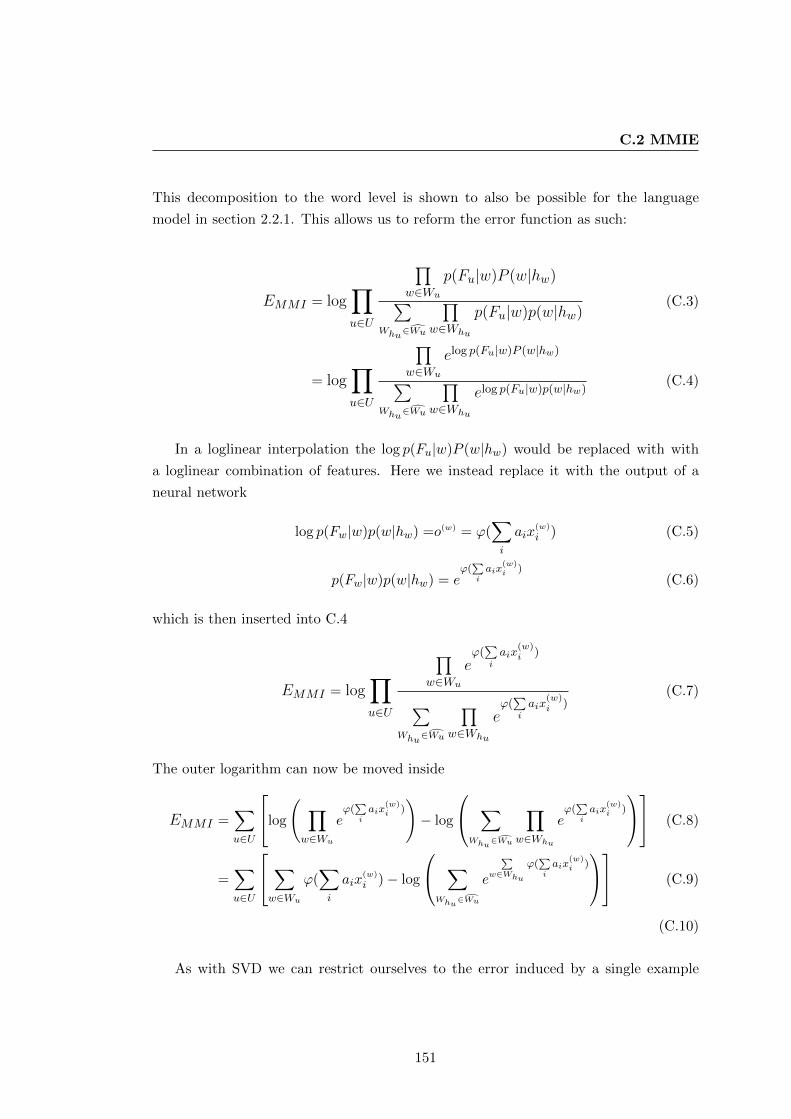
C.2 MMIE
This decomposition to the word level is shown to also be possible for the language
model in section 2.2.1. This allows us to reform the error function as such:
EMMI = log∏u∈U
∏w∈Wu
p(Fu|w)P (w|hw)∑Whu∈Wu
∏w∈Whu
p(Fu|w)p(w|hw)(C.3)
= log∏u∈U
∏w∈Wu
elog p(Fu|w)P (w|hw)∑Whu∈Wu
∏w∈Whu
elog p(Fu|w)p(w|hw)(C.4)
In a loglinear interpolation the log p(Fu|w)P (w|hw) would be replaced with with
a loglinear combination of features. Here we instead replace it with the output of a
neural network
log p(Fw|w)p(w|hw) =o(w) = ϕ(∑i
aix(w)
i ) (C.5)
p(Fw|w)p(w|hw) = eϕ(
∑iaix
(w)i )
(C.6)
which is then inserted into C.4
EMMI = log∏u∈U
∏w∈Wu
eϕ(
∑iaix
(w)i )
∑Whu∈Wu
∏w∈Whu
eϕ(
∑iaix
(w)i )
(C.7)
The outer logarithm can now be moved inside
EMMI =∑u∈U
log
( ∏w∈Wu
eϕ(
∑iaix
(w)i ))− log
∑Whu
∈Wu
∏w∈Whu
eϕ(
∑iaix
(w)i )
(C.8)
=∑u∈U
∑w∈Wu
ϕ(∑i
aix(w)
i )− log
∑Whu
∈Wu
e
∑w∈Whu
ϕ(∑iaix
(w)i ) (C.9)
(C.10)
As with SVD we can restrict ourselves to the error induced by a single example
151
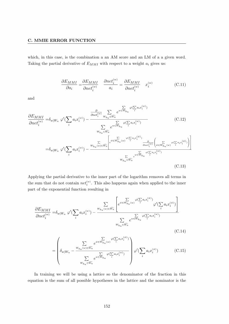
C. MMIE ERROR FUNCTION
which, in this case, is the combination a an AM score and an LM of a a given word.
Taking the partial derivative of EMMI with respect to a weight ai gives us:
∂EMMI
∂ai=∂EMMI
∂net(w)
i
∂net(w)
i
ai=
∂EMMI
∂net(w)
i
x(w)
i (C.11)
and
∂EMMI
∂net(w)
i
=δw|Wuϕ′(∑i
aix(w)
i )−
∂
∂net(w)i
∑Whu
∈Wu
e
∑w∈Whu
ϕ(∑iaix
(w)i )
∑Whu
∈Wu
e
∑w∈Whu
ϕ(∑iaix
(w)i )
(C.12)
=δw|Wuϕ′(∑i
aix(w)
i )−
∑Whu
(w)∈Wu
e
∑w∈Whu
(w)ϕ(
∑i
aix(w)i
)
∂
∂net(w)i
∑w∈Whu
(w)ϕ(
∑i
aix(w)i
)
∑Whu
∈Wu
e
∑w∈Whu
ϕ(∑i
aix(w)i
)
(C.13)
Applying the partial derivative to the inner part of the logarithm removes all terms in
the sum that do not contain net(w)
i . This also happens again when applied to the inner
part of the exponential function resulting in
∂EMMI
∂net(w)
i
=δw|Wuϕ′(∑i
aix(w)
i )−
∑Whu
(w)∈Wu
e ∑w∈Whu
(w)
ϕ(∑iaix
(w)i )
ϕ′(∑iaix
(w)
i )
∑
Whu∈Wu
e
∑w∈Whu
ϕ(∑iaix
(w)i )
(C.14)
=
δw|Wu−
∑Whu
(w)∈Wu
e
∑w∈Whu
(w)
ϕ(∑iaix
(w)i )
∑Whu
∈Wu
e
∑w∈Whu
ϕ(∑iaix
(w)i )
ϕ′(∑i
aix(w)
i ) (C.15)
In training we will be using a lattice so the denominator of the fraction in this
equation is the sum of all possible hypotheses in the lattice and the nominator is the
152
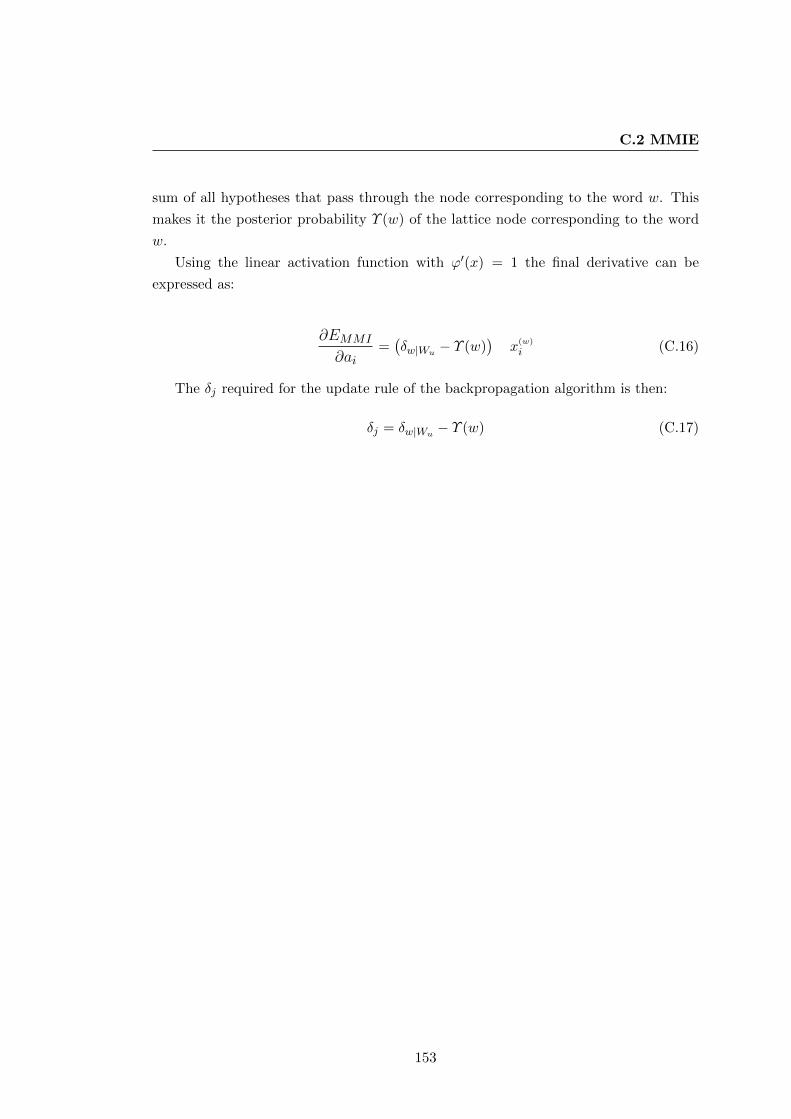
C.2 MMIE
sum of all hypotheses that pass through the node corresponding to the word w. This
makes it the posterior probability Υ (w) of the lattice node corresponding to the word
w.
Using the linear activation function with ϕ′(x) = 1 the final derivative can be
expressed as:
∂EMMI
∂ai=(δw|Wu
− Υ (w))
x(w)
i (C.16)
The δj required for the update rule of the backpropagation algorithm is then:
δj = δw|Wu− Υ (w) (C.17)
153