Multivariate Multifractal Models: Estimation of Parameters ... · Multivariate Multifractal Models: Estimation of Parameters and Applications to Risk Management als Inaugural-Dissertation

$Page 1: Multivariate Multifractal Models: Estimation of Parameters ... · Multivariate Multifractal Models: Estimation of Parameters and Applications to Risk Management als Inaugural-Dissertation$
Multivariate Multifractal Models:

Estimation of Parameters and

Applications to Risk Management

als Inaugural-Dissertation

zur Erlangung des akademischen Grades eines Doktors

der Wirtschafts- und Sozialwissenschaftlichen Fakultat

der Christian-Albrechts-Universitat zu Kiel

vorgelegt von

MBA Ruipeng Liu

aus V.R. China, geb. 13 Juni 1977

Melbourne, September 2008

Gedruckt mit Genehmigung der

Wirtschafts- und Sozialwissenschaftlichen Fakultat

der Christian-Albrechts-Universitat zu Kiel

Dekan: Prof. Dr. Helmut Herwartz

Erstberichterstattender: Prof. Dr. Thomas Lux

Zweitberichterstattender: Prof. Dr. Roman Liesenfeld

Tag der Abgabe der Arbeit: 29. September 2008

Tag der mundlichen Prufung: 18. November 2008

ACKNOWLEDGEMENTS

First of all I would like to express my sincere gratitude to Professor Dr. Thomas Lux,

who brought me into the world of fractals, and shared with me his expertise and research

insight, which have been invaluable to me. I also wish to express my appreciation to Pro-

fessor Dr. Roman Liesenfeld, who made many valuable suggestions and gave constructive

advice, which helped improve of this thesis. I particularly acknowledge the encouragement

from Professor Dr. Stefan Mittnik during my starting stage of my Ph.D in the University

of Kiel.

I am tempted to individually thank all of my friends which, have joined me in the

discovery of what is life about and how to make the best of it. However, because the list

might be too long and by fear of leaving someone out, I will simply say thank you very much

to you all.

I cannot finish without saying how grateful I am with my entire extended family, par-

ticular thanks, of course, to my parents, who bore me, raised me, supported me, and loved

me. Last but not least, to my wife and my son. To them I dedicate this thesis.

Table of Contents

Table of Contents 4

1 Introduction 1

2 Fractal and Multifractal models 72.1 Introduction to fractals . . . . . . . . . . . . . . . . . . . . . . . . . . . . . 7

2.1.1 Self-similarity and fractals . . . . . . . . . . . . . . . . . . . . . . . . 82.1.2 Principles of fractal geometry . . . . . . . . . . . . . . . . . . . . . . 92.1.3 Rescaled range analysis . . . . . . . . . . . . . . . . . . . . . . . . . 13

2.2 Modelling long memory in financial time series . . . . . . . . . . . . . . . . 202.2.1 Introduction . . . . . . . . . . . . . . . . . . . . . . . . . . . . . . . 202.2.2 Fractality and long memory . . . . . . . . . . . . . . . . . . . . . . . 222.2.3 Long memory models . . . . . . . . . . . . . . . . . . . . . . . . . . 25

2.3 Multifractal models . . . . . . . . . . . . . . . . . . . . . . . . . . . . . . . . 322.3.1 Introduction . . . . . . . . . . . . . . . . . . . . . . . . . . . . . . . 322.3.2 Multifractal model of asset returns . . . . . . . . . . . . . . . . . . . 332.3.3 Scaling estimators . . . . . . . . . . . . . . . . . . . . . . . . . . . . 342.3.4 Uni-fractals and multifractals . . . . . . . . . . . . . . . . . . . . . . 39

3 The Bivariate Markov Switching Multifractal Models 433.1 Introduction . . . . . . . . . . . . . . . . . . . . . . . . . . . . . . . . . . . . 433.2 Bivariate multifractal (BMF) models . . . . . . . . . . . . . . . . . . . . . . 47

3.2.1 Calvet/Fisher/Thompson model . . . . . . . . . . . . . . . . . . . . 473.2.2 Liu/Lux model . . . . . . . . . . . . . . . . . . . . . . . . . . . . . . 49

3.3 Exact maximum likelihood estimation . . . . . . . . . . . . . . . . . . . . . 513.4 Simulation based ML estimation . . . . . . . . . . . . . . . . . . . . . . . . 643.5 Generalized method of moments . . . . . . . . . . . . . . . . . . . . . . . . 70

3.5.1 Binomial model . . . . . . . . . . . . . . . . . . . . . . . . . . . . . . 733.5.2 Lognormal model . . . . . . . . . . . . . . . . . . . . . . . . . . . . . 81

3.6 Empirical estimates . . . . . . . . . . . . . . . . . . . . . . . . . . . . . . . . 88

4

5

4 Beyond the Bivariate case: Higher Dimensional Multifractal Models 1094.1 Tri-variate (higher dimensional) multifractal models . . . . . . . . . . . . . 1094.2 Maximum likelihood estimation . . . . . . . . . . . . . . . . . . . . . . . . . 1114.3 Simulation based maximum likelihood estimation . . . . . . . . . . . . . . . 1124.4 GMM Estimation . . . . . . . . . . . . . . . . . . . . . . . . . . . . . . . . . 1154.5 Empirical estimates . . . . . . . . . . . . . . . . . . . . . . . . . . . . . . . . 120

5 Risk Management Applications of Bivariate MF Models 1355.1 Introduction . . . . . . . . . . . . . . . . . . . . . . . . . . . . . . . . . . . . 1355.2 Data description . . . . . . . . . . . . . . . . . . . . . . . . . . . . . . . . . 1365.3 Multivariate GARCH model . . . . . . . . . . . . . . . . . . . . . . . . . . . 1375.4 Unconditional coverage . . . . . . . . . . . . . . . . . . . . . . . . . . . . . . 1405.5 Value-at-Risk . . . . . . . . . . . . . . . . . . . . . . . . . . . . . . . . . . . 1535.6 Conditional Expected shortfall . . . . . . . . . . . . . . . . . . . . . . . . . 166

6 Conclusion 172

7 Appendix 1757.1 Moment conditions for the Liu/Lux model . . . . . . . . . . . . . . . . . . . 175

7.1.1 Binomial case . . . . . . . . . . . . . . . . . . . . . . . . . . . . . . . 1767.1.2 Lognormal case . . . . . . . . . . . . . . . . . . . . . . . . . . . . . . 188

7.2 Moment conditions for the Calvet/Fisher/Thompson model . . . . . . . . . 1947.2.1 Binomial case . . . . . . . . . . . . . . . . . . . . . . . . . . . . . . . 1947.2.2 Lognormal case . . . . . . . . . . . . . . . . . . . . . . . . . . . . . . 200

7.3 (Numerical) Solutions of the moments for the log of (bivariate) Normal variates203

Bibliography 219

List of Tables

2.1 KPSS and Hurst exponent H values for absolute value of returns . . . . . . 20

3.1 ML estimation for the Calvet/Fisher/Thompson model . . . . . . . . . . . . 62

3.2 ML estimation for the Liu/Lux model . . . . . . . . . . . . . . . . . . . . . 63

3.3 Simulation based ML estimation for the Calvet/Fisher/Thompson model . . 67

3.4 Simulation based ML estimation for the Calvet/Fisher/Thompson model . . 68

3.5 Simulation based ML estimation for the Liu/Lux model . . . . . . . . . . . 69

3.6 Simulation based ML estimation for the Liu/Lux model . . . . . . . . . . . 70

3.7 GMM estimations of the Liu/Lux (Binomial) model . . . . . . . . . . . . . 76

3.8 GMM estimation of the Calvet/Fisher/Thompson model . . . . . . . . . . . 78

3.9 GMM estimation of the bivariate MF (Binomial) model . . . . . . . . . . . 79

3.10 GMM estimation of the bivariate MF (Binomial) model . . . . . . . . . . . 80

3.11 GMM estimation of the bivariate MF (Lognormal) model . . . . . . . . . . 85

3.12 GMM estimation of the bivariate MF (Lognormal) Model . . . . . . . . . . 86

3.13 GMM estimation of the Calvet/Fisher/Thompson (Lognormal) model . . . 87

3.14 ML estimates of the Calvet/Fisher/Thompson model . . . . . . . . . . . . . 94

3.15 ML estimates of the Liu/Lux (Binomial) model . . . . . . . . . . . . . . . . 95

3.16 SML estimates of the Calvet/Fisher/Thompson model . . . . . . . . . . . . 96

3.17 SML estimates of the Liu/Lux (Binomial) model . . . . . . . . . . . . . . . 97

3.18 GMM estimates of the Calvet/Fisher/Thompson model . . . . . . . . . . . 98



3.21 GMM estimates of the Liu/Lux (Binomial) model . . . . . . . . . . . . . . 101


6

7



3.25 GMM estimates of the Liu/Lux (Lognormal) model . . . . . . . . . . . . . 105




4.1 Comparison between ML and GMM estimators . . . . . . . . . . . . . . . . 122

4.2 Comparison between SML and GMM estimators . . . . . . . . . . . . . . . 123

4.3 GMM estimation for the trivariate multifractal (Binomial) model . . . . . . 124

4.4 GMM estimation for the trivariate multifractal (Lognormal) model . . . . 126

4.5 ML estimates of the tri-variate (Binomial) MF model . . . . . . . . . . . . . 129

4.6 SML estimates of the tri-variate (Binomial) MF model . . . . . . . . . . . . 130

4.7 GMM estimates of the tri-variate MF (Binomial) model . . . . . . . . . . . 131

4.8 GMM estimates of the tri-variate MF (Binomial) model . . . . . . . . . . . 132

4.9 GMM estimates of the tri-variate MF (Lognormal) model . . . . . . . . . . 133

4.10 GMM estimates of the tri-variate MF (Lognormal) model . . . . . . . . . . 134

5.1 Descriptive statistics for empirical daily (in-sample) returns rt . . . . . . . . 137

5.2 CC-GARCH(1, 1) model estimates (in-sample data) . . . . . . . . . . . . . 140

5.3 GMM estimates for Liu/Lux model (in-sample data) . . . . . . . . . . . . . 143

5.4 GMM estimates for Calvet/Fisher/ Thompson model (in-sample data) . . . 144

5.5 ML estimates for Liu/Lux model (in-sample data) . . . . . . . . . . . . . . 145

5.6 ML estimates for Calvet/Fisher/Thompson model (in-sample data) . . . . . 146

5.7 Multi-period unconditional coverage (Liu/Lux model) . . . . . . . . . . . . 149

5.8 Multi-period coverage (Liu/Lux model) . . . . . . . . . . . . . . . . . . . . 150

5.9 Multi-period unconditional coverage (Calvet/Fisher/Thompson model) . . . 151

5.10 Multi-period unconditional coverage (Calvet/Fisher/Thompson model) . . . 152

5.11 SML estimates for Liu/Lux model (in-sample data) . . . . . . . . . . . . . . 157

5.12 SML estimates for Calvet/Fisher/Thompson model (in-sample data) . . . . 158

5.13 Failure rates for multi-period Value-at-Risk forecasts (Liu/Lux model) . . . 163

8

5.14 Failure rates for multi-period Value-at-Risk forecasts (Calvet/Fisher/Thompson

model) . . . . . . . . . . . . . . . . . . . . . . . . . . . . . . . . . . . . . . . 164

5.15 Failure rates for multi-period Value-at-Risk forecasts (CC-GARCH) . . . . 165

5.16 Multi-period Expected shortfall forecasts (Liu/Lux model) . . . . . . . . . . 169

5.17 Multi-period Expected shortfall forecasts (Calvet/Fisher/Thompson model) 170

5.18 Multi-period Expected shortfall forecasts (CC-GARCH model) . . . . . . . 171

List of Figures

2.1 Koch curve. . . . . . . . . . . . . . . . . . . . . . . . . . . . . . . . . . . . . 10

2.2 Sierpinski Triangle. . . . . . . . . . . . . . . . . . . . . . . . . . . . . . . . . 11

2.3 Fractal dimension for Euclidean objects. . . . . . . . . . . . . . . . . . . . . 12

2.4 Hurst’s R/S analysis for U.S. Dollar to British Pound exchange rate (March

1973 to February 2004). . . . . . . . . . . . . . . . . . . . . . . . . . . . . . 15

2.5 Lo’s R/S for U.S. Dollar to British Pound exchange rate (March 1973 to

February 2004). . . . . . . . . . . . . . . . . . . . . . . . . . . . . . . . . . 17

2.6 The periodogram of U.S. Dollar to British Pound exchange rate (March 1973

to February 2004). . . . . . . . . . . . . . . . . . . . . . . . . . . . . . . . . 24

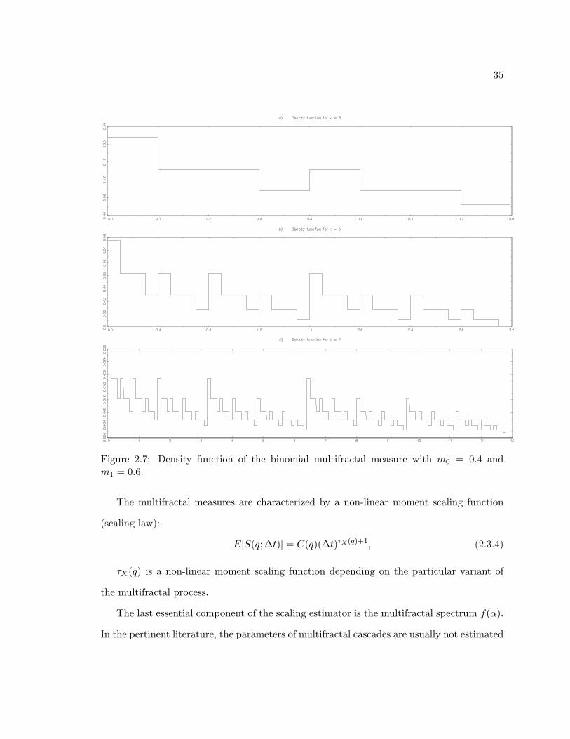
2.7 Density function of the binomial multifractal measure with m0 = 0.4 and

m1 = 0.6. . . . . . . . . . . . . . . . . . . . . . . . . . . . . . . . . . . . . . 35

2.8 Partition functions of U.S. Dollar to British Pound exchange rate (March

1973 to February 2004) for different moments. . . . . . . . . . . . . . . . . . 41

2.9 The scaling function for U.S. Dollar to British Pound exchange rate (March

1973 to February 2004). . . . . . . . . . . . . . . . . . . . . . . . . . . . . . 42

2.10 The f(α) spectrum of U.S. Dollar to British Pound exchange rate (March

1973 to February 2004). . . . . . . . . . . . . . . . . . . . . . . . . . . . . . 42

3.1 Local instantaneous volatility of the simulated bivariate MF (Binomial) time

series. . . . . . . . . . . . . . . . . . . . . . . . . . . . . . . . . . . . . . . . 51

3.2 Simulation of the bivariate multifractal (Binomial) model. . . . . . . . . . . 52

3.3 ACF for the simulations of the BMF (Binomial) Model above. . . . . . . . . 53

3.4 The distribution of p values for the test of over-identification restrictions for

a binomial BMF model. . . . . . . . . . . . . . . . . . . . . . . . . . . . . . 83

9

10


a Lognormal BMF model. . . . . . . . . . . . . . . . . . . . . . . . . . . . . 84

3.6 Empirical time series: Dow and Nik. . . . . . . . . . . . . . . . . . . . . . 91

3.7 Empirical time series: US and DM . . . . . . . . . . . . . . . . . . . . . . . 92

3.8 Empirical time series: TB1 and TB2. . . . . . . . . . . . . . . . . . . . . . 93

4.1 The distribution of p value for the test of over-identification restrictions (bi-

nomial trivariate MF model). . . . . . . . . . . . . . . . . . . . . . . . . . . 125


a Lognormal trivariate MF model. . . . . . . . . . . . . . . . . . . . . . . . 127

4.3 Empirical time series: Japanese Yen to British Pound exchange rate. . . . 128

5.1 This graph shows the probability density function (pdf) of empirical DOW

(left panel), and log-log plot of the complementary cumulative distribution of

empirical DOW (right panel), for comparison, the dashed lines give the pdf

and complementary of the cumulative distribution of Gaussian distribution. 141

5.2 Empirical equal-weighted portfolio returns. . . . . . . . . . . . . . . . . . . 148

5.3 One-step ahead VaR predictions for α = 1% under the Liu/Lux model. . . 160

5.4 One-step ahead VaR predictions for α= 1% under the Calvet/Fisher/Thompson

model. . . . . . . . . . . . . . . . . . . . . . . . . . . . . . . . . . . . . . . . 161

5.5 One-step ahead VaR predictions for α = 1% under the CC-GARCH(1, 1)

model. . . . . . . . . . . . . . . . . . . . . . . . . . . . . . . . . . . . . . . . 162

Chapter 1

Introduction

Numerous empirical studies have found non-normal moments in the (unconditional) distri-

butions of returns in financial markets. One early example is Fama (1965), who reports

evidence of excess kurtosis in the unconditional distribution of daily returns of Dow Jones

listed stocks, there are also more recent studies such as those by Ding et al. (1993), Pagan

(1996), Guillaume et al. (2000), Cont (2001), Lo and MacKinlay (2001) and so on.

More traces have revealed the so-called abnormal phenomena in the distribution of

financial time series (though some of them are viewed as stylized facts of financial markets):

(1) Fat tail – the distribution is ‘fatter’ at the extremes (‘tails’) than a truly Normal

one. The fat tail property implies that the unconditional distribution of price changes

(returns) has more probability mass in the tails and the center than the standard

Normal distribution. This also means that extreme changes occur more often than

would be expected under the assumption of Normality of relative price changes.

(2) Volatility clustering, which means that periods of quiescence and turbulence tend to

cluster together. Hence, the volatility (conditional variance) of the financial market

is not homogeneous over time, but is itself subject to temporal variation.

(3) Long-term dependence (long-range dependence or long memory), which describes the

correlation structure of a time series at long lags. If a series exhibits long memory,

1

2

there is persistent temporal dependence even between distant observations. Such se-

ries are characterized by distinct but nonperiodic cyclical patterns. The presence of

long memory in returns would provide evidence against the efficient markets hypothe-

ses (EMH) since long memory implies nonlinear dependence and hence a potentially

predictable component in the series dynamics. It would also raise issues regarding

linear modeling, statistical testing and forecasting of pricing models based on tradi-

tional standard statistical methods, such as the capital asset pricing model (CAPM).

However, long memory is typically found in higher moments only, e.g. squared re-

turn, which is often viewed as a proxy of financial volatility, therefore, the ability of

replicating long-term dependence in return volatility becomes one of the important

criteria for financial modelling assessments.

In addition, other features in financial time series are also recognized, e.g., (multi)scaling,

leverage effect and volume and volatility correlation, see Weron et al. (1999), Lux and

Marchesi (1999), Lux and Marchesi (2000), Black (1976), Bouchaud and Potters (2001),

and Lobato and Velasco (2000). Consequently, various approaches based on a wide range

of theoretical analyses, such as non-linear dynamic theory, behavioural finance and agent-

based models have provided further insights into the mechanisms of the financial markets.

See, Kirman (1993), Lux (1995), Brock and Hommes (1997), Lux (1998), Chiarella and He

(2001) and Iori (2002).

An important contribution was made by Benoit Mandelbrot, the famous father of fractals

who proposed a multifractal model of asset returns (MMAR), a theory which inherits all

the hallmarks of Mandelbrot’s earlier work that has emerged since the 1960s. A fractal

is an irregular or fragmented geometric shape that can be subdivided into parts, each of

which is, at least approximately and qualitatively, a reduced copy of the whole. Natural

fractals are characterized by their so called fractal dimension depending on the scale, and

a multifractal is composed of many fractals with different fractal dimensions.

3

The major innovation of the MMAR model is the use of a multifractal cascade as a

transformation of chronological time into ‘business time’, with the multifractal component

interpreted as a process governing local instantaneous volatility. Adapting multifractal

(MF) processes to financial economics presents major challenges for researchers working in

this area. The original MF processes in statistical physics are combinatorial operations on

probability measures, which suffer from non-stationarity due to being limited to a bounded

interval and to non-convergent moments in the continuous time limit. A more convenient

model for financial data would have to be cast in the format of a stochastic process. This

task has been achieved by introducing iterative versions of multifractal models, which can

be viewed as new types of stochastic models for the volatility dynamics of asset prices (com-

modity or stock prices, foreign exchange rates and so on). These preserve the hierarchical

multiplicative structure of volatility components with different characteristic time scales,

and their time series are in harmony with the stylized facts of financial time series, such

as fat/thin tails, excess kurtosis and volatility clustering. Particularly, the essential new

feature of MF models is their ability to generate different degrees of long-term dependence

in various powers of returns – a feature that pervades empirical financial data, and as a

result, they have been introduced as a competitive alternative to long memory models; cf.

Calvet and Fisher (2001, 2004), Lux (2007).

Current MF studies are mainly confined to univariate models; however, for many im-

portant questions, a multivariate setting would be preferable. Some of the reasons include:

(1) It has been well accepted that financial markets or assets are correlated, and their

volatilities move together over time across markets and assets. It is this correlation that

gives rise to the financial uncertainties that can subsequently result in worldwide financial

disasters. So, this is particularly important when considering asset allocation, Value-at-Risk

and portfolio hedging strategies.

(2) The literature has been relatively silent on the source of long-range dependence

4

within volatility processes; multivariate (bivariate) models may provide additional infor-

mation about the factors responsible for long memory. For example, by taking account of

the observed strong relationship between stock price volatility and trading volume, bivari-

ate mixture models assume volatility and trading volume are jointly directed by the latent

number of information arrivals based on the mixture distribution hypothesis, see Andersen

(1996), Liesenfeld (1998) and Liesenfeld (2001). This implies that the dynamics of both

variables are restricted to depend only on the behavior of the information arrival process.

Therefore, trading volume may provide information about the factors which generate the

volatility persistence.

In this thesis, we concentrate on developing multivariate multifractal models, and im-

plement their estimation via different approaches. We then apply our new multivariate MF

processes to empirically relevant topics, such as portfolio risk measurement and manage-

ment.

The rest of the thesis is organized as follows:

Chapter 2 of this thesis provides a background and introduction to fractals and multi-

fractals, including the definition of fractals and fractal geometry. Since fractals imply long

memory, some traditional methods of fractal analysis and well-known long memory mod-

els are reviewed. They include, the Rescaled Range analysis (R/S), Fractional Brownian

motion, the Fractional Integrated Autoregressive Moving Average (ARFIMA) model, the

Fractional Integrated Autoregressive Conditional Heteroskedasticity (FIGARCH) model,

and the long memory stochastic volatility (LMSV) model. In the last section of the chap-

ter, the multifractal model of asset returns (MMAR) by Mandelbrot et al. (1997) is revisited,

together with earlier estimation attempts and empirical studies.

The first section of Chapter 3 gives a review of one iterative MF version – the Markov

switching multifractal (MSM) model. By discarding the combinatorial nature, the MSM

5

model preserves the multifractal and stochastic properties, and it conceives the local instan-

taneous volatility as the product of volatility components. As a simple alternative to the

recently proposed bivariate MF model by Calvet et al. (2006), an alternative bivariate mul-

tifractal model with a more parsimonious setting is introduced. We estimate both bivariate

models with a maximum likelihood approach and simulation-based inference via particle fil-

ter algorithm, which are discussed in Calvet et al. (2006). To overcome the computational

limit of the likelihood approach (particularly in the case of models with continuous distri-

bution of volatility components), we adopt the GMM (Generalized Method of Moments)

approach formalized by Hansen (1982), which for its implementation requires analytical mo-

ment conditions. Monte Carlo experiments are undertaken to examine the performance of

our GMM estimator. These results demonstrate the capability of GMM and its advantage

when increasing the number of cascade levels, particularly for the continuous (Lognormal)

bivariate MF model. In the last section of this chapter, we present empirical studies of

bivariate multifractal models for different types of financial data, including stock exchange

indices, foreign exchange rates and government bond maturity rates. By using three estima-

tion approaches (ML, simulation based ML and GMM), empirical estimates of multifractal

parameters are reported with various cascade levels. We also provide a heuristic method

for specifying the number of cascade levels, by matching the simulated long memory index

with the empirical one.

Chapter 4 focuses on higher-dimensional multifractal models. In this chapter we present

Monte Carlo results and empirical estimates via the three different approaches introduced

in Chapter 3; GMM does not suffer from the very high dimensionality because it allows each

pair of time series to be treated as a bivariate case. The maximum likelihood approach again

encounters the restriction of an upper limit to the number of cascade levels; a simulation

based inference is implemented. We demonstrate the advantage of GMM by comparing

estimators in terms of the efficiency and applicability when increasing the dimensionality

6

of the multifractal model. The last section of Chapter 4 is an empirical study of tri-variate

MF models. We also report ML, SML and GMM estimates by considering a portfolio of

three foreign exchange rates.

Chapter 5 is an empirical study of the multivariate multifractal models on financial risk

measurement and management. Based on the number of cascade levels specified in the

last section of Chapter 3, we re-estimate our bivariate MF model as well as the model by

Calvet et al. (2006) using in-sample data, we then conduct out-sample forecast assessments

by employing two popular tools, namely, Value-at-Risk and Expected Shortfall. To demon-

strate the applicability of multivariate multifractal processes, we also compare their forecast

performances with a benchmark multivariate GARCH model.

Chapter 6 contains additional summaries of results and conclusions from our study, and

some suggestions for worthwhile future work in the field of multifractal models.

The Appendix at the end of this thesis provides the analytical moment conditions for

our Binomial and Lognormal bivariate MF models, followed by the moment conditions for

the bivariate MF Model of Calvet et al. (2006). In addition, some numerical solutions of

the moments of the log of absolute (bivariate) Normal variates which are used within GMM

estimation are presented.

Chapter 2

Fractal and Multifractal models

2.1 Introduction to fractals

The Gaussian hypothesis was questioned and seriously criticized by the famous mathemati-

cian Benoit Mandelbrot (e.g. Mandelbrot (1963)), who advanced the hypothesis that price

change distributions are stable Paretian, or what is called Levy stable. The hypothesis was

subsequently supported by empirical evidence in Mandelbrot (1967b) with time series of

commodity markets (cotton and wheat price variations), railroad stock prices and some fi-

nancial rates (interest rate on call money, Dollar-Sterling exchange rate), see Cootner (1964)

and Shiller (1989) for further discussions. There are more empirical studies on the stable

Paretian Hypothesis of asset returns and detailed description of stable Paretian models in

finance, cf. Upton and Shannon (1979), Lux (1996b), and Rachev and Mittnik (2000).

The definition of stable Paretians implies that the distribution of sums of independent,

identically-distributed stable Paretical variables is itself stable Paretian. Fractals somehow

share this ‘stable’ property. The term fractal first appeared in Mandelbrot’s papers, and it

was defined together with his arguments on traditional geometry, in “The idea of the fractal

dimension” as part of the November 1975 issue of Scientific American, and then republished

in “The Fractal Geometry of Nature, Chapter 1”:

Why is geometry often described as cold and dry? One reason lies in its inability to

7

8

describe the shape of a cloud, a mountain, a coastline, a tree. Clouds are not spheres,

mountains are not cones, coastlines are not circles, and bark is not smooth, nor does light-

ning travel in a straight line. Nature exhibits not simply a higher degree but an altogether

different level of complexity. The number of distinct scales of length of patterns is for all

purposes infinite. The existence of these patterns challenges us to study these forms that

Euclid leaves aside as being ‘formless’, to investigate the morphology of the ‘amorphous’.

Mathematicians have disdained this challenge, however, and have increasingly chosen to flee

from nature by devising theories unrelated to anything we can see or feel.

2.1.1 Self-similarity and fractals

A random process X(t) that satisfies:

X(ct1), . . . , X(ctn) ' cHX(t1), . . . , cHX(tn), (2.1.1)

(where ' represents ‘equal in terms of distribution’) for c, n, t1, . . . , tn ≥ 0, is called self-

similar with the self-similarity parameter H, which will often be called the scaling exponent

or Hurst exponent in the following sections.

Therefore, the term ‘self-similarity’ tells us that the partial processes look qualitatively

the same irrespective of their size (strictly, it does not mean exactly the same, but similar in

terms of the distribution’s properties), where cH denotes the scaling property (power law).

In this way, self-similarity implies a scaling that describes a specific relationship between

data samples of different time scales. Mandelbrot (1963) presents some earlier empirical

evidence graphically, by examining cotton price changes in terms of different time periods

(1880-1958) and different time frequencies, which are revisited in Mandelbrot (2001).

Other plausible definition of self-similarity focuses on the increment of X(t):

X(t+ c4t)−X(t) 'M(c)[X(t+4t)−X(t)],

M(c) is a random variable whose distribution does not depend on t but c, and it is called

9

the scaling factor. Nevertheless, self-similarity is the key characteristic property of fractals,

and since a fractal is an object in which individual parts are similar to the whole, it is a

particularly interesting class of self-similar objects.

2.1.2 Principles of fractal geometry

Fractal theory has generated a great deal of interest, which has been fuelled by the intuitive

observation that the world around us is filled with fractal shapes showing the property of

self-similarity.

A fractal can be constructed by taking a generating rule and iterating it over and over

again: one example is the branching network in a tree; each branching is different, as are

the successive smaller ones, but all are qualitatively similar to the structure of the whole

tree. Other examples commonly used to illustrate this idea include the triadic Koch curve,

Sierpinski Triangle, Cantor Dust, and so on.

One way to describe a fractal shape is to calculate its fractal dimension, a number that

quantitatively describes how an object fills its space. Traditional Euclidean geometry applies

to objects which are solid and continuous, have no holes or gaps, and have a dimensionality

that is an integer. According to Euclidean geometry, we have a clear understanding of

dimensionality; that is, a line has dimension one , and a plane and a space have dimensions

two and three respectively.

Fractals are rough and often discontinuous, like the Sierpinski Triangle, and so have

fractional, or fractal dimensions. One way of calculating fractal dimension uses rulers of

varying lengths. For the example of a coast line, one can count the number of circles with a

certain diameter that will cover the coastline, then decrease (or increase) the diameter for

another round, and again count the number of circles, and so on · · · . The fractal dimension

D can be revealed by the relationship between the radius 1/r of the circles or other rulers,

10

and the number of units (length, area, or volume) N according to:

N = rD, (2.1.2)

which can be transformed to:

D =logNlog r

. (2.1.3)

So, the fractal dimension can be calculated by taking the limit of the quotient of the log

change in object size and the log change in measurement scale, as the measurement scale

approaches zero. We can take some simple and straightforward examples, the Koch Curve

(Figure 2.1) and the Sierpinski Triangle (Figure 2.2).

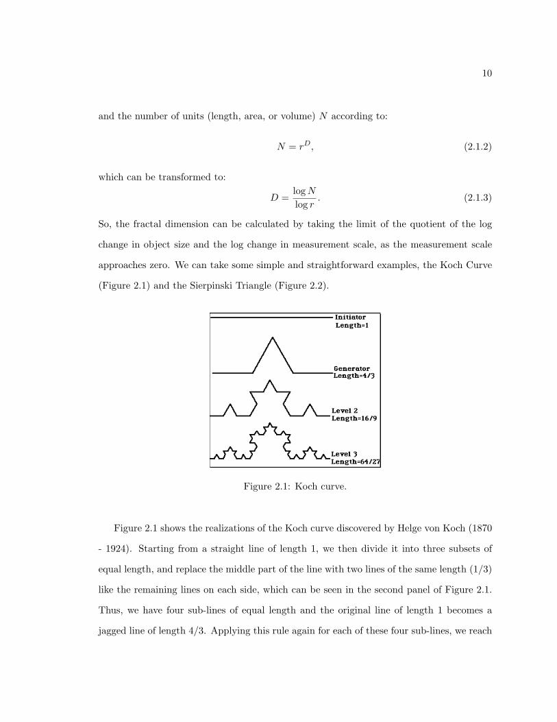
Figure 2.1: Koch curve.

Figure 2.1 shows the realizations of the Koch curve discovered by Helge von Koch (1870

- 1924). Starting from a straight line of length 1, we then divide it into three subsets of

equal length, and replace the middle part of the line with two lines of the same length (1/3)

like the remaining lines on each side, which can be seen in the second panel of Figure 2.1.

Thus, we have four sub-lines of equal length and the original line of length 1 becomes a

jagged line of length 4/3. Applying this rule again for each of these four sub-lines, we reach

11

the third level of Figure 2.1; repeating the same rule once again leads to the the fourth

level of Figure 2.1. One can see that each level is 4/3 times longer than the previous one,

therefore, the fractal dimension obtained from D = log 4log 3 = 1.26. Similarly, the Sierpinski

Triangle is constructed by iterating equilateral triangles inwardly (Figure 2.2); consequently

doubling the length of the sides gives us three times the number of triangles, and it has

dimension log 3log 2 = 1.585.

Figure 2.2: Sierpinski Triangle.

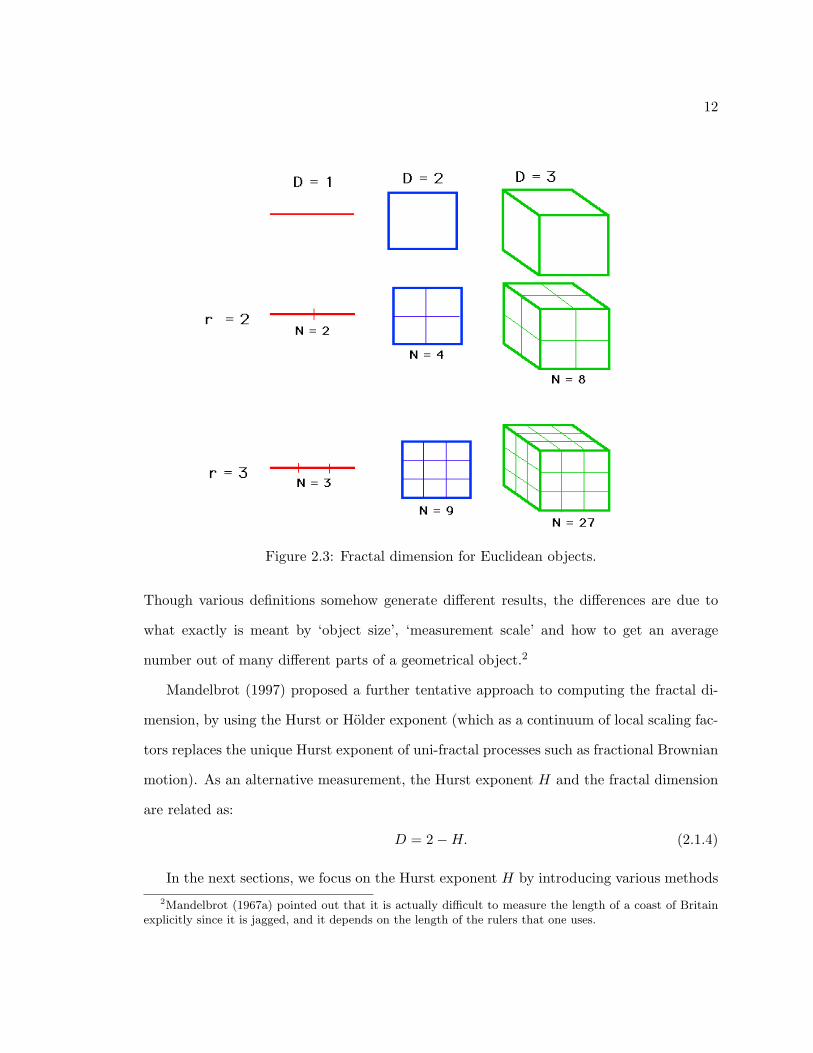
Eq. (2.1.3) can also be applied to Euclidean objects by reducing their linear sizes by

1/r in each spatial direction; so that, for a straight line, for example, scaling it by a factor

of two, so that it is now twice as long as before, gives log 2log 2 = 1, a dimensionality of 1; for

a square figure, scale up the square by a factor of two, and the square is now 4 times as

large (i.e. 4 original squares can be placed on the original square) and log 4log 2 = 2, gives a

dimension of 2; likewise, for a cube log 8log 2 = 3, (see Figure 2.3).

The determination of fractal dimensions above belongs to the category of Hausdorff

dimensions,1 which are more general algorithms used by mathematicians and physicists.1Some mathematics sources refer to them as Minkowski-Bouligand dimensions.

12

Figure 2.3: Fractal dimension for Euclidean objects.

Though various definitions somehow generate different results, the differences are due to

what exactly is meant by ‘object size’, ‘measurement scale’ and how to get an average

number out of many different parts of a geometrical object.2

Mandelbrot (1997) proposed a further tentative approach to computing the fractal di-

mension, by using the Hurst or Holder exponent (which as a continuum of local scaling fac-

tors replaces the unique Hurst exponent of uni-fractal processes such as fractional Brownian

motion). As an alternative measurement, the Hurst exponent H and the fractal dimension

are related as:

D = 2−H. (2.1.4)

In the next sections, we focus on the Hurst exponent H by introducing various methods2Mandelbrot (1967a) pointed out that it is actually difficult to measure the length of a coast of Britain

explicitly since it is jagged, and it depends on the length of the rulers that one uses.

13

which are used to calculating H.

2.1.3 Rescaled range analysis

The Hurst exponent is named after the well-known hydrologist, Harold E. Hurst(1900 -

1978), who worked on projects involving the design of reservoirs along the Nile River water

storage using a statistical method – Rescaled range analysis (R/S analysis) in 1950s. It

was firstly introduced in Hurst (1951), later refined in Mandelbrot and Wallis (1969b), as

well as in Mandelbrot and Taqqu (1979). These became popular in finance due to the clear

exposition of the methods in Feder (1988) and the empirical work of Peters (1994).

The widely used R/S analysis is based on a heuristic graphical approach, whereby the

basic idea is to compare the minimum and maximum values of running sums of deviations

from the sample mean, then re-normalized by the sample standard deviation. The following

is a summary of Hurst’s R/S statistic:

(1) Divide the N -length of time series Yt into A × n sub periods with length n; each

sub-period is denoted Na, a = 1, · · ·A, for each observation in Na is labeled yk,a,

k = 1, · · · , n;, then calculate the mean value for each Na of length n, that is

Ma =1n

n∑k=1

yk,a. (2.1.5)

(2) The time series of accumulated departures (yk,a) from the mean value for each sub-

period Na is given by:

Xk,a =k∑

i=1

(yi,a −Ma), k = 1, 2, · · · , n; (2.1.6)

(3) The range (R) is defined as the maximum minus the minimum value of Xk,a within

each sub-period Na:

RNa = max1≤k≤n

(Xk,a)− min1≤k≤n

(Xk,a); k = 1, 2, · · · , n; (2.1.7)

14

(4) The sample standard deviation is calculated for each sub-period:

SNa =

√√√√ 1n

n∑k=1

(yk,a −Ma)2.

Each range RNa is then normalized by SNa , so we have the rescaled range for each Na

sub-period, which is equal to RNa/SNa . The calculations from the second step must be

repeated for different time horizons, and we have A sub-periods with equal length n. The

average R/S value for each n is defined as:

(R/S)n =1A

A∑a=1

RNa

SNa

. (2.1.8)

Applying Hurst’s Empirical Law for different values of n:

log (R/S)n = C +H · log(n), (2.1.9)

and running an ordinary least square (OLS) regression we get the Hurst exponent H; the

intercept is the estimator for the constant C.

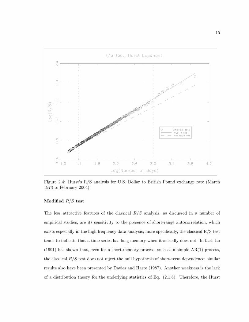
Figure 2.4 shows the graphical result for returns of U.S. Dollar to British Pound exchange

rate (March 1973 to February 2004), with a Hurst exponent estimator of H = 0.59, by

applying Hurst’s empirical law (Eq. 2.1.9) via the OLS regression.

Using the classical R/S approach, Peters (1994) finds that stock and bond markets follow

a biased random walk, indicating that the information ripples forward in time, instead of

being reflected immediately in prices. This would be interpreted as an evidence against the

efficient market hypothesis (EMH). However, some later studies indicate that financial asset

returns do not significantly deviate from H = 0.5, see Mills (1993), Crato and De Lima

(1994) and Lux (1996a). Other earlier applications of R/S analysis include Mandelbrot and

Wallis (1969a), Mandelbrot and Wallis (1969b), as well as some empirical studies: Greene

and Fielitz (1977) (stock returns data for securities listed on the New York Stock Exchange);

Booth and Kaen (1979) (Gold prices); Booth et al. (1982) (foreign exchange rates); Helms

et al. (1995) (commodity futures contracts).

15

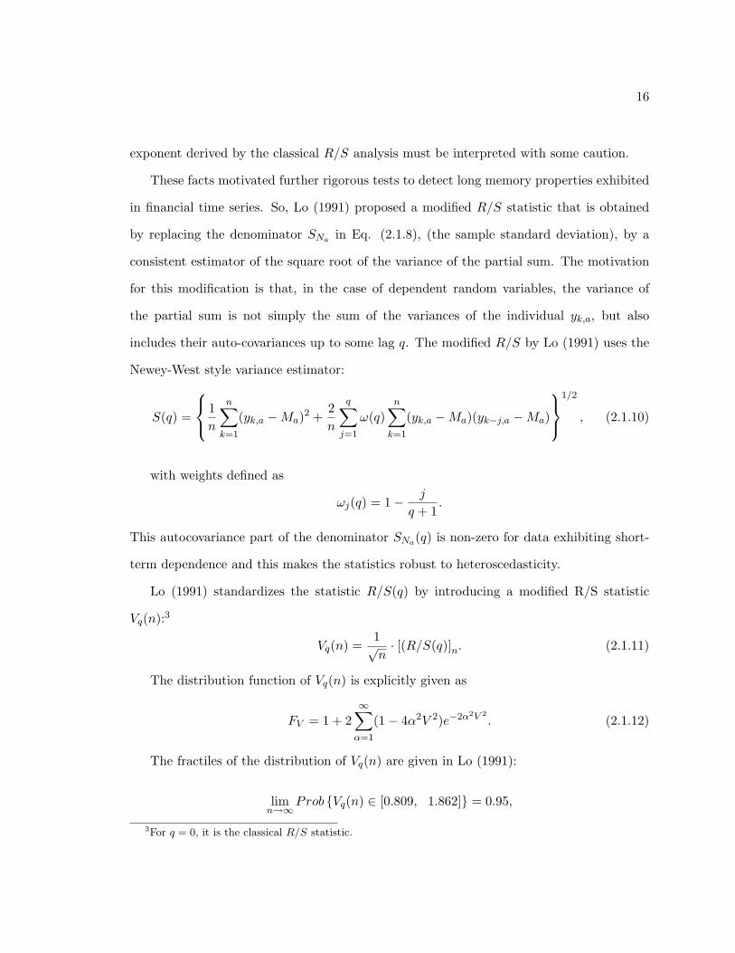
Figure 2.4: Hurst’s R/S analysis for U.S. Dollar to British Pound exchange rate (March1973 to February 2004).

Modified R/S test

The less attractive features of the classical R/S analysis, as discussed in a number of

empirical studies, are its sensitivity to the presence of short-range autocorrelation, which

exists especially in the high frequency data analysis; more specifically, the classical R/S test

tends to indicate that a time series has long memory when it actually does not. In fact, Lo

(1991) has shown that, even for a short-memory process, such as a simple AR(1) process,

the classical R/S test does not reject the null hypothesis of short-term dependence; similar

results also have been presented by Davies and Harte (1987). Another weakness is the lack

of a distribution theory for the underlying statistics of Eq. (2.1.8). Therefore, the Hurst

16

exponent derived by the classical R/S analysis must be interpreted with some caution.

These facts motivated further rigorous tests to detect long memory properties exhibited

in financial time series. So, Lo (1991) proposed a modified R/S statistic that is obtained

by replacing the denominator SNa in Eq. (2.1.8), (the sample standard deviation), by a

consistent estimator of the square root of the variance of the partial sum. The motivation

for this modification is that, in the case of dependent random variables, the variance of

the partial sum is not simply the sum of the variances of the individual yk,a, but also

includes their auto-covariances up to some lag q. The modified R/S by Lo (1991) uses the

Newey-West style variance estimator:

S(q) =

1n

n∑k=1

(yk,a −Ma)2 +2n

q∑j=1

ω(q)n∑

k=1

(yk,a −Ma)(yk−j,a −Ma)

1/2

, (2.1.10)

with weights defined as

ωj(q) = 1− j

q + 1.

This autocovariance part of the denominator SNa(q) is non-zero for data exhibiting short-

term dependence and this makes the statistics robust to heteroscedasticity.

Lo (1991) standardizes the statistic R/S(q) by introducing a modified R/S statistic

Vq(n):3

Vq(n) =1√n· [(R/S(q)]n. (2.1.11)

The distribution function of Vq(n) is explicitly given as

FV = 1 + 2∞∑

α=1

(1− 4α2V 2)e−2α2V 2. (2.1.12)

The fractiles of the distribution of Vq(n) are given in Lo (1991):

limn→∞

Prob Vq(n) ∈ [0.809, 1.862] = 0.95,

3For q = 0, it is the classical R/S statistic.

17

which gives the 95 percent confidence interval (more can be found in the Table II of Lo

(1991)), when testing the null hypothesis that there is no long memory in the given time

series; specifically, if Vq(n) lies within this interval of [0.809, 1.862], one infers that the data

are not characterized by long-term dependence.

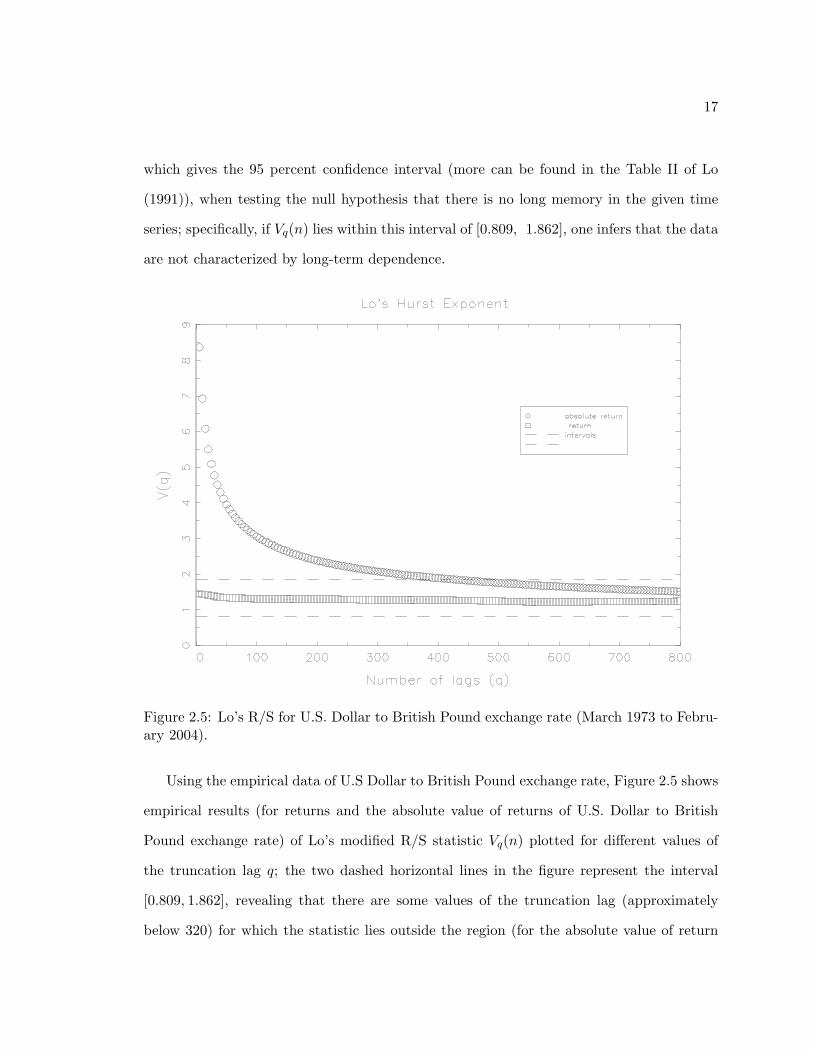
Figure 2.5: Lo’s R/S for U.S. Dollar to British Pound exchange rate (March 1973 to Febru-ary 2004).

Using the empirical data of U.S Dollar to British Pound exchange rate, Figure 2.5 shows

empirical results (for returns and the absolute value of returns of U.S. Dollar to British

Pound exchange rate) of Lo’s modified R/S statistic Vq(n) plotted for different values of

the truncation lag q; the two dashed horizontal lines in the figure represent the interval

[0.809, 1.862], revealing that there are some values of the truncation lag (approximately

below 320) for which the statistic lies outside the region (for the absolute value of return

18

data). According to Lo’s rule, the test accepts the hypothesis of long memory up to q, but

the opposite inference would be made for a larger value of q. While, for the raw return time

series, it fails to reject the null hypothesis of no long memory for all truncation lags q.

Lo’s method represents a theoretical improvement over the classic Rescaled range statis-

tic, but its practical application requires care. There have been long-standing debates on

this modified R/S version. Moody and Wu (1996) further propose the so-called robust R/S

estimates, by defining the denominator as (σ(n) is the standard deviation):

S(q) =

1 + 2

q∑j=1

ωj(q)n− j

n2

σ2(n) +2n

q∑j=1

ω(q)n∑

k=1

(yk,a−,Ma)(yk−j,a −Ma)

1/2

.

(2.1.13)

Willinger et al. (1999) argue that Lo’sR/S statistic shows strong preference for accepting

the null hypothesis: no long-term dependence, irrespective of whether long memory is

present in the empirical data or not, which implies the evidence is not absolutely conclusive;

Teverovsky et al. (1999) perform Monte Carlo simulations with long-range and short-range

dependent time series, and find the selection of q is critical. These studies strongly advise

against its use as the sole technique for testing long-term dependence in empirical data.

KPSS test

Kwiatkowski et al. (1992) proposed a so-called Kwiatkowski-Phillips-Schmidt-Shin (KPSS)

test which is based on the second moment of Xk (defined as Eq. (2.1.6) in the second step

of Hurst’s R/S analysis). the KPSS test is then defined as

KPSSq(n) =1

n2 · S(q)2

n∑k=1

(Xk)2. (2.1.14)

Originally, KPSS proposed a test of the null hypothesis of stationarity. However, the

distribution theory under the null hypothesis assumes that the series in question has short

19

memory; that is, its partial sum satisfies an invariance principle. Lee and Schmidt (1996)

shows that the KPSS test is consistent against stationary long memory alternatives, such

as I(d) processes for d ∈ (−0.5, 0.5) , d 6= 0. It has been shown that under the null null

hypothesis of I(0), this statistic asymptotically converges to a well-defined random variable

KPSSq(n) →∫ 1

0V (t)2,

where V (t) is the so-called Brownian bridge (see Lee and Schmidt (1996) for details).4 It

can therefore be used to distinguish short memory and long memory stationary processes.

The power of the KPSS test in finite samples is found to be comparable to that of Lo’s

modified rescaled range test. Similar to Hurst’s empirical law of Eq. (2.1.9), Giraitis et al.

(2000) extend the “pox-plot” analysis to the KPSS statistics for the estimation of the Hurst

exponent by claiming the following regression:

logKPSSq(n) = α+ β · log(n), (2.1.15)

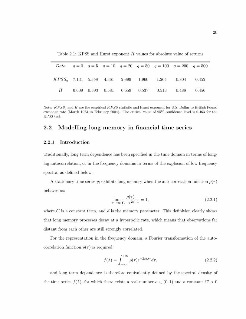
and the Hurst exponent is then obtained via H = 0.5 + 0.5 × β. An empirical study

of U.S. Dollar to British Pound exchange rate (March 1973 to February 2004) is presented

in Table 2.1. Base on the KPSS statistic provided by Kwiatkowski et al. (1992), one may

conclude that long-term dependence exhibits given the empirical statistic above the critical

value, that is, rejecting the null hypothesis of short memory at certain confidence levels.

For instance, at 95% confidence level, the critical value is 0.463 according to Kwiatkowski

et al. (1992), therefore, we can conclude that long memory exists for the truncation lag

q = 200 at the 95% confidence level based on the results in Table 2.1 (KPSS200 = 0.804),

but vanishes when considering more time lags, e.g. q = 500 (KPSS500 = 0.452); other

applications can be found in Kirman and Teyssiere (2001).

4Marmol (1997) shows that the KPSS test is also consistent against I(d)-processes with d > 0.5; andSibbertsen and Kramer (2006) focus on I(1 + d) processes.

20

Table 2.1: KPSS and Hurst exponent H values for absolute value of returns

Data q = 0 q = 5 q = 10 q = 20 q = 50 q = 100 q = 200 q = 500

KPSSq 7.131 5.358 4.361 2.899 1.960 1.264 0.804 0.452

H 0.609 0.593 0.581 0.559 0.537 0.513 0.488 0.456

Note: KPSSq and H are the empirical KPSS statistic and Hurst exponent for U.S. Dollar to British Poundexchange rate (March 1973 to February 2004). The critical value of 95% confidence level is 0.463 for theKPSS test.

2.2 Modelling long memory in financial time series

2.2.1 Introduction

Traditionally, long term dependence has been specified in the time domain in terms of long-

lag autocorrelation, or in the frequency domains in terms of the explosion of low frequency

spectra, as defined below.

A stationary time series yt exhibits long memory when the autocorrelation function ρ(τ)

behaves as:

limτ→∞

ρ(τ)C · τ2d−1

= 1, (2.2.1)

where C is a constant term, and d is the memory parameter. This definition clearly shows

that long memory processes decay at a hyperbolic rate, which means that observations far

distant from each other are still strongly correlated.

For the representation in the frequency domain, a Fourier transformation of the auto-

correlation function ρ(τ) is required:

f(λ) =∫ +∞

−∞ρ(τ)e−2πiλτdτ, (2.2.2)

and long term dependence is therefore equivalently defined by the spectral density of

the time series f(λ), for which there exists a real number α ∈ (0, 1) and a constant C ′ > 0

21

such that:

limλ→0

f(λ)C ′|λ|−α

= 1. (2.2.3)

Long memory processes have been pervasively observed in hydrology, climatology and

other natural phenomena. In addition, Leland et al. (1994) analyzed the long memory

property of the network traffic flows. It also has been applied in social science, such as,

Byers et al. (1997) modelled long-term dependence in opinion poll series; Dolado et al. (2003)

investigated Spanish political polls, as well as in some studies on partisanship measures.

In particular, the presence of long-term dependence has important implications for many

of the paradigms used in modern financial economics. For example, optimal consump-

tion/savings and portfolio decisions may become extremely sensitive to the investment

horizon if stock returns would exhibit long memory. Problems also arise in the pricing

of derivative securities (such as options and futures) with martingale methods, since the

class of continuous time stochastic processes most commonly employed are inconsistent with

long-term dependence. Traditional tests of the capital asset pricing model and the arbi-

trage pricing theory are no longer valid since the usual forms of statistical inference do not

apply to time series exhibiting such persistence. The conclusions of ‘the efficient markets

hypotheses’ or stock market rationality also hang precariously on the presence or absence

of long memory in raw returns.

Among the first to have considered the possibility and implications of persistent sta-

tistical dependence in asset returns was Mandelbrot (1971). Since then, several empirical

studies have lent further support to Mandelbrot’s findings. Baillie et al. (1996) found long

memory in the volatility of the DM-USD exchange rate; long-term dependence in the Ger-

man DAX was found by Lux (1996a); as well as stock market trading volume by Lobato

and Velasco (2000), examining 30 stocks in the Dow Jones Industrial Average index. In

addition, Chung (2002) and Zumbach (2004) also provide convincing evidence in favour of

long memory models. Besides research on developed financial markets, there are also dozens

22

of papers on smaller and less developed markets: the stock market in Finland is analyzed by

Tolvi (2003); Madhusoodanan (1998) provides evidence on the individual stocks in Indian

Stock Exchange and Nath (2002) also gives significant indication of long-term dependence

for all time lags in the Indian market; similar evidence on the Greek financial market is given

by Barkoulas and Baum (2000); Cavalcante and Assaf (2002) demonstrate long memory in

the Brazilian stock market.

2.2.2 Fractality and long memory

In contrast to the inference made by most hydrologists that the Nile’s water inflow was

a random process that had no underlying order and revealed no patterns between obser-

vations, Hurst (1951) found the existence of persistence – that is, large overflows tend to

be followed by further larger overflows – by studying recorded data covering almost a mil-

lennium. Equipped with the Rescaled-range analysis and Hurst exponent value H, a time

series can be classified into three categories:

(1) H = 0.5 indicates a random process.

(2) 0 < H < 0.5 indicates an anti-persistent time series.

(3) 0.5 < H < 1 indicates a persistent (long memory) time series.

An anti-persistent series has a characteristic of mean-reverting, which means an up

value is more likely to be followed by a down value, and vice versa. The strength of “mean-

reversion” increases as the Hurst exponent value approaches 0. A persistent time series

indicates long memory, sometimes it is roughly called trend reinforcing, which means the

direction (up or down compared to the last observation) of the next one is more likely the

same as current value. The strength of trend increases as H approaches 1.0.

Beside the traditional R/S analysis, some alternative methods for estimating the Hurst

exponent have also been developed, for instance Detrended Fluctuation Analysis (see, Peng

23

et al. (1994) and Peng et al. (1994)) and Wavelet Spectral Density inference (see, Jensen

(1999)). The fact that fractals are characterized by long memory processes is widely ac-

cepted, and dozens of empirical works are using statistical inference methods to detect the

persistence property in financial time series, such as Greene and Fielitz (1977), Booth and

Kaen (1979), Booth et al. (1982), Helms et al. (1995).

There has been considerable recent interest in the estimation of long memory in fre-

quency domain. One widely used method for this purpose was introduced by Geweke and

Porter-Hudak (1983), hence it is known in the literature as the GPH estimator. The GPH

estimator of persistence in volatility is based on an ordinary linear regression of the log pe-

riodigram of a time series xt, which serves as a proxy for volatility, such as absolute returns,

squared returns, or log squared returns of a financial asset. The single explanatory variable

in the regression is log frequency for small Fourier frequencies in a neighbourhood, which

degenerates towards zero frequency as the sample size T increases.

This procedure, based on least squares regression in the spectral domain, exploits the

simple form of the pole of the spectral density (recall Eq. 2.2.3) at the origin:

f(λ) ∼ |λ|−α, λ→∞,

with the jth periodigram I(λj) such that

I(λj) =1

2πT

∣∣∣∣∣T∑

t=1

xteiλjt

∣∣∣∣∣2

(2.2.4)

where λj = 2πj/T represents the pertinent Fourier frequency, T is the number of ob-

servations, and j = 1, ...,m; m T is the number of considered Fourier frequencies, that

is the number of periodogram ordinates. The long memory parameter is estimated via the

following regression:

log[I(λj)] = α0 + α log[4sin2(λj/2)

]+ εt, (2.2.5)

24

Under some conditions summarized by the band condition 1m + m

T → 0 as T → +∞,

the estimator of α can be obtained via OLS regression and −α provides the long memory

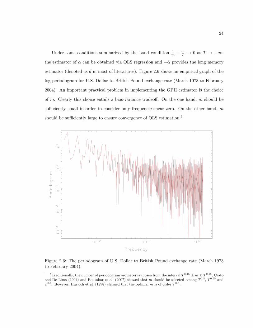
estimator (denoted as d in most of literatures). Figure 2.6 shows an empirical graph of the

log periodogram for U.S. Dollar to British Pound exchange rate (March 1973 to February

2004). An important practical problem in implementing the GPH estimator is the choice

of m. Clearly this choice entails a bias-variance tradeoff. On the one hand, m should be

sufficiently small in order to consider only frequencies near zero. On the other hand, m

should be sufficiently large to ensure convergence of OLS estimation.5

Figure 2.6: The periodogram of U.S. Dollar to British Pound exchange rate (March 1973to February 2004).

5Traditionally, the number of periodogram ordinates is chosen from the interval T 0.45 ≤ m ≤ T 0.55; Cratoand De Lima (1994) and Boutahar et al. (2007) showed that m should be selected among T 0.5, T 0.55 andT 0.6. However, Hurvich et al. (1998) claimed that the optimal m is of order T 0.8.

25

Geweke and Porter-Hudak (1983) also provided the asymptotic distribution of the esti-

mator:

m1/2(α− α) → N

(0,

π2

6∑m

j=1(Zj − Z)

)(2.2.6)

with Zj = log[4sin2(λj/2)

], Z being the mean of Zj , with j = 1, . . .m. Applications

of GPH in the context of financial volatility have been presented in, for example, Andersen

and Bollerslev (1996), Ray and Tsay (2001).

We recognize that the empirical determination of the long-term dependence property of

a time series is a difficult problem. The reason is that the strong autocorrelation of long

memory processes makes statistical fluctuations very large. Thus tests for long memory

tend to require large quantities of data and can often give inconclusive results. Furthermore,

different methods of statistical analysis often give contradictory results.

2.2.3 Long memory models

The material dealt with in the last section has inspired much debate as to the existence of

long memory in financial time series. In this section, some popular long memory models in

econometrics and their estimation issues are briefly reviewed; they are fractional Brownian

motion, Fractional Integrated Autoregressive Moving Average (ARFIMA) model, Fractional

Integrated Autoregressive Conditional Heteroskedasticity (FIGARCH) model, and the long

memory stochastic volatility model.

Fractional Brownian motion

Fractional Brownian motion6 (FBM) is presented by Granger and Joyeux (1980), Hosking

(1981), where the process is defined as:

(1− L)dyt = εt, (2.2.7)6Given here is the discrete time version; a more detailed summary of the continuous version can be found

in Baillie (1996).

26

for simplicity a zero mean is assumed, and εt is white noise. L is an operator that shifts

the time index of a time series variable backwards by one unit of time. The process yt

is stationary if the fractional parameter d < 0.5 and invertible if d > −0.5. Granger and

Joyeux (1980), Hosking (1981) also demonstrate its long memory property by transforming

FBM to an infinite autoregressive (AR) process (Eq. 2.2.8) or infinite moving average (MA)

representation (Eq. 2.2.9) as follows:

yt =∞∑

τ=0

ψτyt−τ + εt, (2.2.8)

with ψτ = Γ(τ−d)Γ(τ+1)Γ(−d) ∼

1Γ(−d)τ

−d−1 as τ → ∞, Γ(·) denoting the gamma function.

Alternatively,

yt =∞∑

τ=0

ψτ εt−τ , (2.2.9)

with ψτ = Γ(τ+d)Γ(τ+1)Γ(d) ∼

1Γ(d)τ

d−1, as τ →∞.

ARFIMA model

Let us start with ARMA models. An autoregressive process of order p, AR(p), is defined

as:

yt = a1yt−1 + a2yt−2 + · · ·+ apyt−p + εt, (2.2.10)

where εt ∼ N(0, σ2ε ). AR(p) models a time series yt, such that the level of its current

observations depends on the level of its lagged observations.

A moving average model of order q, MA(q), can be written as:

yt = εt + b1εt−1 + b2εt−2 + · · ·+ bqεt−q. (2.2.11)

In an MA(q) process, the observations of a random variable at time t are not only affected

by the shock at time t, but also by the shocks that have taken place before time t. We

27

combine these two models and get a general Autoregressive Moving Average, ARMA(p, q)

model:

yt = a1yt−1 + a2yt−2 + · · ·+ apyt−p + εt + b1εt−1 + b2εt−2 + · · ·+ bqεt−q. (2.2.12)

With the appropriate modification, a non-stationary series is handled by the Autore-

gressive Integrated Moving Average model, ARIMA(p, 1, q) which essentially begins with

first order differencing to convert the original non-stationary series to a stationary series:

A(L)(1− L)yt = B(L)εt, (2.2.13)

Lp is an operator that shifts the time index of a time series variable backwards by p unit

of time, that is Lpyt = yt−p, and AR lag polynomials A(L) = 1− a1L− · · · − apLp; MA lag

polynomials B(L)) = 1 + b1(L) + · · ·+ bqLq.

One flexible and popular econometric long memory time series model is the Fraction-

ally Integrated Autoregressive Moving Average model ARFIMA (p, d, q), with a fractional

differencing parameter d. It is introduced in the papers of Granger and Joyeux (1980), and

Hosking (1981). Considering a time series observation yt,

A(L)(1− L)dyt = B(L)εt, (2.2.14)

(1− L)d is the dth fractional difference operator defined by:

(1− L)d = 1− dL− d(1− d)2!

L2 − d(1− d)(2− d)3!

L3 − . . . =∞∑

k=0

Γ(k − d)Lk

Γ(−d)Γ(k + 1). (2.2.15)

For a stationary process with d ∈ (−0.5, 0.5) and d 6= 0, Hosking (1981) proves that

the autocorrelations of an ARFIMA process decay hyperbolically to zero, in contrast to the

faster geometric decay of a stationary ARMA process.7 Nonzero values of the fractional

parameter imply strong dependence between distant observations.7Corresponding to d = 0.

28

Several estimation techniques have been proposed for ARFIMA(p, d, q) processes (see

e.g. Sowell (1992)). Recalling the GPH, it is helpful to construct a two-step procedure:

in the first step, the fractional differencing parameter d is found; and the AR and MA

parameters are then estimated in the second step.

The parameters of ARFIMA model can also be jointly estimated through a maximum

likelihood approach, under the assumption of Normality of the disturbances εt with variance

σ2ε . The log-likelihood then can be written:

LogL(Θ; ytt=1,...T ) = −T2log(2π)− 1

2log(|Ξ|)− 1

2y′Ξ−1y, (2.2.16)

Θ is the vector of parameters to be estimated, and Ξ = Ξ(Θ, σ2ε ) is the covariance matrix

depending on Θ and σ2ε .

FIGARCH model

Analogous to the way that ARFIMA (p, d, q) constitutes an intermediary between ARMA

and ARIMA processes, Baillie (1996) and Baillie et al. (1996) have presented a Frac-

tional Integrated Autoregressive Conditional Heteroskedasticity model - FIGARCH (p, d, q)

by combining the fractionally integrated processes of the regular GARCH process for the

conditional variance.

We begin with the ARCH (Autoregressive Conditional Heteroskedasticity) process by

Engle (1982):

εt = σt · ηt, (2.2.17)

where ηt is white noise, and σt is conditional variance, postulated to be a linear function of

the lagged squared innovations:

σ2t = ω + α(L)ε2t . (2.2.18)

The ARCH model can be generalized by extending it with autoregressive terms of the

volatility. Bollerslev (1986) provides a more flexible lag structure in the GARCH model,

29

the GARCH(p, q) model, defined by

σ2t = ω + α(L)ε2t + β(L)σ2

t . (2.2.19)

Alternatively, it can also be expressed as an ARMA process in ε2t :8

[1− α(L)− β(L)]ε2t = ω + [1− β(L)](ε2t − σ2t ), (2.2.20)

ε2t − σ2t can be interpreted as the innovations of σ2

t . Then the corresponding Integrated

GARCH model is given as:9

φ(L)(1− L)ε2t = ω + [1− β(L)](ε2t − σ2t ), (2.2.21)

with φ(L) = [1− α(L)− β(L)](1− L)−1.

The FIGARCH model is obtained by replacing the first difference operator by the dth

fractional difference operator, by rearranging the conditional variance of εt:

[1− β(L)]σ2t = ω +

[1− β(L)− φ(L)(1− L)d

]ε2t . (2.2.22)

Baillie et al (1996) showed that the FIGARCH process also implies a slow hyperbolic

rate of decay for lagged squared innovations and persistent impulse response weights. One

remark that may be necessary is that here d is constraint within d ∈ (0, 1), which is different

from the case of ARFIMA model; its log-likelihood has the form:

LogL(Θ; εtt=1,...T ) = −T2log(2π)− 1

2

T∑t=1

log(σ2t )−

12

T∑t=1

(ε2t · σ−2t ). (2.2.23)

To have the proper order, ie. p, q, information criteria (IC) are required for model

identification and specification, such as Akaike IC, Hannan-Quinn IC, Schwarz IC, Shibata

IC.10

8It is an ARMA(q′, p) process with q′ = max(p, q).9Here it is the GARCH(q′ − 1, p) process.

10They are constructed with different approaches but their structures are very similar in the end, withthe only difference being the penalization term.

30

Long memory stochastic volatility model

During the last decade, there has been an increasing interest in modelling the dynamic

evolution of the volatility of financial time series using stochastic volatility (SV) models.

The main distinction between ARCH type models and SV model relies on whether volatility

is observable. In the standard stochastic volatility model, the volatility is modelled as an

unobserved latent variable, and this characteristic feature coincides with other theoretical

models in finance which build on the concept of unobservable latent factors generating

asset returns, for example information flow interpretations of the mixture of distribution

hypothesis, see Andersen (1996), Liesenfeld (1998).

The standard stochastic volatility model introduced by Taylor (1982) assumes a stochas-

tic process yt, such that

yt = σ · exp(ht/2) · εt

ht = µ0 + µ1ht−1 + ση · ηt, (2.2.24)

and the logarithm of volatility ht is an AR(1) process. σ is a scale parameter, and

µ0 is a constant term.11 εt and ηt are mutually independent standard Normals (although

it is rather common to assume that the error components have a Gaussian distribution,

several authors have also considered heavy-tailed distributions, e.g. Liesenfeld and Jung

(2000).). The volatility of the log-volatility process, ση measures the uncertainty about

future volatility.

By adopting the ARFIMA process, the traditional standard Stochastic Volatility (SV)

model can also be extended to a long memory SV model (LMSV) replacing the AR process

in the state equation with a fractional differencing operator, cf. Harvey (1993) and Breidt11Some simplified SV version assumes σ = 1 and the constant term µ0 being set to zero without loss of

generality.

31

et al. (1998). LMSV is then defined as:

yt = σ · exp(ht/2) · εt

(1− L)dht = µ0 + ση · ηt, (2.2.25)

the log volatility ht at time t follows a stationary fractionally integrated process with the

long-memory parameter, d < 1/2, and L is the lag operator as introduced in the previous

fractional integrated models.

SV models are attractive because they are close to the models often used in financial

theory (e.g. Black-Scholes option pricing model) to represent the behaviour of financial

prices whose statistical properties are easy to derive using well-known results on the Log-

normal distribution. However, until recently, their empirical applications have been very

limited mainly because the exact likelihood function is difficult to evaluate and Maximum

Likelihood (ML) estimation of the parameters is not straightforward. Nevertheless, several

estimation methods have been proposed and the literature on SV models has grown sub-

stantially. These include simple moment matching by Taylor (1986); simulated method of

moment by Gourieroux et al. (1993); Generalized Method of Moments by Melino and Turn-

bull (1990) and Andersen and Sorensen (1996); quasi-maximum likelihood by Harvey et al.

(1994); simulation based maximum likelihood by Danielsson and Richard (1993), Liesenfeld

and Richard (2003); the Markov Chain Monte Carlo (MCMC) approach by Shephard (1993)

and Jacquier et al. (1994). By means of an extensive Monte Carlo study, Jacquier et al.

(1994) show that MCMC is more efficient than both quasi-maximum likelihood (QML) and

GMM estimators.

In addition, some important studies have been made on the estimation of the long mem-

ory SV model, which cover the quasi-maximum likelihood estimator of Breidt et al. (1998)

and GMM estimation by Wright (1999). Kim et al. (1998) also provide a simulation-based

method on the estimation and diagnostics of the LMSV model employing MCMC, and So

32

(1999) develops a new algorithm based on the state space formulation of Gaussian time

series models with additive noise where full Bayesian inference is implemented through

MCMC techniques. The MCMC algorithm creates a Markov chain on the blocks of the

unknown parameters, latent volatilities, and state mixing variables, whereby, on repeated

sampling from the distribution of each block conditioned on the current values of the remain-

ing blocks, the chain geometrically converges to the desired multivariate posterior density.

The main attraction of MCMC procedures is that they permit to obtain simultaneously

sample inference about the parameters, smooth estimates of the unobserved variances and

predictive distributions of multi-step forecasts of volatility. In any case, noticed that an im-

portant advantage of the MCMC estimators is that the inference is based on finite sample

distributions and, consequently, the asymptotic approximation is not needed.

2.3 Multifractal models

2.3.1 Introduction

Financial markets display some properties in common with fluid turbulence. For example,

both fluid turbulence and financial fluctuations display intermittency at all scales. A cascade

of energy flux is known to occur from the large scale of injection to the small scale of

dissipation, which is typically modelled by a multiplicative cascade, which then leads to

a multifractal concept; see Lux (2001) ‘Turbulence in Financial Markets: The Surprising

Explanatory Power of Simple Cascade Models’.

A stochastic process X(t) is called multifractal if it has stationary increments and sat-

isfies (cf. Mandelbrot et al. (1997), Calvet and Fisher (2002)):

E[|X(t)|q] = c(q)tτ(q)+1, (2.3.1)

where τ(q) is called the scaling function, and c(q) is some deterministic function of q.

33

2.3.2 Multifractal model of asset returns

The development of the multifractal approach goes back to Benoit Mandelbrot’s work on

turbulent processes in statistical physics (see Mandelbrot (1974)). One widespread influen-

tial contribution is Mandelbrot et al. (1997), which, by introducing the multifractal model

of asset returns (MMAR), translates the approach from physics into finance. In the MMAR

model, returns r(t) are assumed to follow a compound process:

r(t) = BH [θ(t)] , (2.3.2)

in which, BH [·] represents an incremental fractional Brownian motion with Hurst expo-

nent index H (we know already that it is ordinary Brownian motion for H = 0.5); θ(t) is

an increasing function of chronological time t. Both BH [·] and θ(t) are independent.

The MMAR provides a fundamentally new class of stochastic processes to financial

economists. It is able to generate fat tails in the unconditional distribution of financial

returns, and it also has long memory in the absolute value of returns (FIGARCH model

and the Long Memory Stochastic Volatility (LMSV) model characterize long memory in

squared returns). In addition, the multifractal process has appealing temporal aggregation

properties and is parsimoniously consistent with the moment scaling of financial data - in the

sense that a well-defined rule relates returns over different sampling intervals. Mandelbrot

(1963) suggested that the shape of the distribution of returns should be the same when the

time scale is changed (as defined in Eq. (2.1.1)). Finally, one essential feature of MMAR is

the compounding of θ(t) as trading time or time deformation process, and it is characterized

by the cumulative distribution function of a multifractal measure, first introduced and used

in Mandelbrot (1974), when modelling the distribution of energy in turbulent dissipation.

The simplest way to create a multifractal measure is as a “binomial multifractal” con-

structed on a unit interval [0; 1] with uniform density. One proceeds as follows: divide the

interval into two parts of equal length, and let m0 and m1 be two positive numbers adding

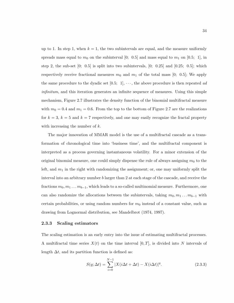
34

up to 1. In step 1, when k = 1, the two subintervals are equal, and the measure uniformly

spreads mass equal to m0 on the subinterval [0; 0.5] and mass equal to m1 on [0.5; 1], in

step 2, the sub-set [0; 0.5] is split into two subintervals, [0; 0.25] and [0.25; 0.5]; which

respectively receive fractional measures m0 and m1 of the total mass [0; 0.5]; We apply

the same procedure to the dyadic set [0.5; 1], · · · , the above procedure is then repeated ad

infinitum, and this iteration generates an infinite sequence of measures. Using this simple

mechanism, Figure 2.7 illustrates the density function of the binomial multifractal measure

with m0 = 0.4 and m1 = 0.6. From the top to the bottom of Figure 2.7 are the realizations

for k = 3, k = 5 and k = 7 respectively, and one may easily recognize the fractal property

with increasing the number of k.

The major innovation of MMAR model is the use of a multifractal cascade as a trans-

formation of chronological time into ‘business time’, and the multifractal component is

interpreted as a process governing instantaneous volatility. For a minor extension of the

original binomial measure, one could simply dispense the rule of always assigning m0 to the

left, and m1 in the right with randomizing the assignment; or, one may uniformly split the

interval into an arbitrary number b larger than 2 at each stage of the cascade, and receive the

fractionsm0,m1 . . .mb−1, which leads to a so-called multinomial measure. Furthermore, one

can also randomize the allocations between the subintervals, taking m0,m1 . . .mb−1 with

certain probabilities, or using random numbers for m0 instead of a constant value, such as

drawing from Lognormal distribution, see Mandelbrot (1974, 1997).

2.3.3 Scaling estimators

The scaling estimation is an early entry into the issue of estimating multifractal processes.

A multifractal time series X(t) on the time interval [0, T ], is divided into N intervals of

length ∆t, and its partition function is defined as:

S(q;∆t) =N−1∑i=0

|X(i∆t+ ∆t)−X(i∆t)|q. (2.3.3)

35

Figure 2.7: Density function of the binomial multifractal measure with m0 = 0.4 andm1 = 0.6.

The multifractal measures are characterized by a non-linear moment scaling function

(scaling law):

E[S(q;∆t)] = C(q)(∆t)τX(q)+1, (2.3.4)

τX(q) is a non-linear moment scaling function depending on the particular variant of

the multifractal process.

The last essential component of the scaling estimator is the multifractal spectrum f(α).

In the pertinent literature, the parameters of multifractal cascades are usually not estimated

36

directly from the scaling function τ(q), but rather from its Legendre transformation:

fθ(α) = Inf [αq − τX(q)], (2.3.5)

that allows an estimation of the MF process by matching the empirical and hypothetical

spectra of the Holder exponents (a continuum of local scaling factors replaces the unique

Hurst exponent of uni-fractal processes such as fractional Brownian motion). One may

notice the subscript of θ in Eq. (2.3.5), which refers to the spectrum of θ(t), and the shape

of the spectrum carries over from the multifractal time transformation to returns in the

compound process via the equations:12

τX(q) = τθ(Hq). (2.3.6)

fX(α) = fθ(α/H). (2.3.7)

Eq. (2.3.6) allows the estimation of the Hurst Index H in empirical work by using the

relationship:13

τX(1/H) = τθ(1) = 0. (2.3.8)

However, most studies restrict the price process assuming that the logs of prices follow

a Brownian motion with arbitrary H = 0.5 instead of fractal Brownian motion. The reason

is that empirical evidence of long-term dependence (which give an estimator of H > 0.5) is

confined to various powers of returns, but is almost absent in the raw data, and statistical

tests can usually not reject the null hypothesis of H = 0.5 for raw returns. Hence, one does

not need to assume a fractional Brownian motion of returns.

Mandelbrot et al. (1997) derived the analytical solution of the scaling function and

multifractal spectrum with respect to the binomial and Lognormal MF; the pertinent τ(q)

and f(α) functions are obtained as below:12More technical details about Legendre transforms are provided by Harte (2001): Multifractal: Theory

and Applications. and Mandelbrot et al. (1997).13The proof of this result can be found in Mandelbrot et al. (1997).

37

For the Binomial distribution with m0 ≥ 0.5, the scaling function has the form:

τ(q) = − log2(mq0 + (1−m0)q), (2.3.9)

and the spectrum f(α) is:

fθ(α) = − αmax − α

αmax − αminlog2

(αmax − α

αmax − αmin

)− α− αmin

αmax − αminlog2

(α− αmin

αmax − αmin

),

(2.3.10)

with αmin = − log2(m0); αmax = − log2(1−m0).

For the Lognormal (LN) distribution MF, that is

M(i)t ∼ LN(−λ, σ2

m), (2.3.11)

and conservation of mass imposes that E[Mt] = 1/b, or equivalently σ2m = 2 ln b(λ− 1),

which leaves us only one parameter to estimate. For b = 2, Mandelbrot et al. (1997)

presented the scaling function is

τ(q) = qλ− q2(λ− 1)− 1, (2.3.12)

and the pertinent multifractal spectrum has the form of:

fθ(α) = 1− (α− λ)2

4(λ− 1). (2.3.13)

Figure 2.8 to 2.10 illustrate the traditional method of estimation of the multifractal

process with Lognormal cascades. One starts with the empirical partition functions S(q;∆t)

in Eq. (2.3.3) given a set of positive moments q and time scales ∆t of the data, and the

partition functions are then plotted against ∆t in logarithmic scales. Regression estimates

of the slopes then provide the corresponding scaling function τ(q) from Eq. (2.3.4). Figure

2.8 shows a selection of partition functions for some low (up) and higher moments (down)

for U.S. Dollar to British Pound exchange rate (March 1973 to February 2004). As can be

observed, the empirical behavior is very close to the presumed linear shape for moments of

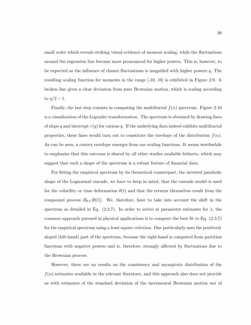
38

small order which reveals striking visual evidence of moment scaling, while the fluctuations

around the regression line become more pronounced for higher powers. This is, however, to

be expected as the influence of chance fluctuations is magnified with higher powers q. The

resulting scaling function for moments in the range [-10, 10] is exhibited in Figure 2.9. A

broken line gives a clear deviation from pure Brownian motion, which is scaling according

to q/2− 1.

Finally, the last step consists in computing the multifractal f(α) spectrum. Figure 2.10

is a visualization of the Legendre transformation. The spectrum is obtained by drawing lines

of slope q and intercept τ(q) for various q. If the underlying data indeed exhibits multifractal

properties, these lines would turn out to constitute the envelope of the distribution f(α).

As can be seen, a convex envelope emerges from our scaling functions. It seems worthwhile

to emphasize that this outcome is shared by all other studies available hitherto, which may

suggest that such a shape of the spectrum is a robust feature of financial data.

For fitting the empirical spectrum by its theoretical counterpart, the inverted parabolic

shape of the Lognormal cascade, we have to keep in mind, that the cascade model is used

for the volatility or time deformation θ(t) and that the returns themselves result from the

compound process B0.5 [θ(t)]. We, therefore, have to take into account the shift in the

spectrum as detailed in Eq. (2.3.7). In order to arrive at parameter estimates for λ, the

common approach pursued in physical applications is to compute the best fit to Eq. (2.3.7)

for the empirical spectrum using a least square criterion. One particularly uses the positively

sloped (left-hand) part of the spectrum, because the right-hand is computed from partition

functions with negative powers and is, therefore, strongly affected by fluctuations due to

the Brownian process.

However, there are no results on the consistency and asymptotic distribution of the

f(α) estimates available in the relevant literature, and this approach also does not provide

us with estimates of the standard deviation of the incremental Brownian motion nor of

39

the number of steps k to be used in the cascade. The later omission is somewhat natural

since the underlying physical models assume an infinite progression of the cascade which is

also the reason for their initially scale free approach. Besides that, the τ(q) and f(α) fits

also require judgmental selection of the number and location of steps used for the scaling

estimates of the moments and the non-linear least square fit of the spectrum.

2.3.4 Uni-fractals and multifractals

The issue of distinguishing between uni-fractal and multifractal models lies in the linearity

or non-linearity of the scaling function τ(q). A uni-fractal process is characterized by a

linear scaling function, which can be derived by recalling the self-similar fractal process in

Eq. (2.1.1), implying that X(ct) ' cHX(t1). We have:

E[|X(t)|q] = tHqE[|X(1)|q]. (2.3.14)

Recalling the scaling law in Eq. (2.3.4), we then end up with τ(q) + 1 = Hq. Therefore an

uni-fractal process is characterized by its scaling function such that:

τ(q) = Hq − 1. (2.3.15)

One may also reach the well-known uni-fractal relationship for the case of Brownian motion:

τ(q) =q

2− 1, (2.3.16)

(see Parisi and Frisch (1985), Fisher et al. (1997), Schmitt et al. (2000)).14

There are uni-fractal limiting cases for both Binomial and Lognormal multifractal pro-

cesses. In the former case, the limit is obtained when m0 = 0.5, and it is easy to see that

this means a split of mass with probabilities 0.5. In the Lognormal case, this limit is given

by λ = 1 due to the vanishing variance.14Note that, in practice, simulations of uni-fractal processes would hardly give this perfectly linear

relationship.

40

In contrast, a multifractal process has a nonlinear scaling function; other descriptions

state that a uni-fractal process is characterized by a single exponent H, whereas multifractal

processes have varying H. By this way, the traditional long memory time series models, for

instance fractional Brownian motion (FBM) model, as well as the ARFIMA, FIGARCH,

LMSV models, are all in the category of uni-fractal models.

Empirical evidences for (multi)fractal in financial economics

Dozens of financial markets have been examined for their fractal properties: Naslund (1990)

analyzes the fractal structure of capital markets; Fang et al. (1994) studies fractal structure

in currency futures price dynamics; Batten and Ellis (1996), Gallucio et al. (1997), and

Mulligan (2000) present evidence of fractals for various foreign exchange rates. Similar

research has been conducted by Matsushita et al. (2003), which shows the fractal structure

in the Chinese Yuan/US Dollar exchange rate; Mulligan (2004) focuses on technology stocks

as representatives of highly volatile markets.

There are also a number of works on multifractal properties, they include: Demos and

Vassilicos (1994), who show the multifractal structure of high-frequency foreign exchange

rate fluctuations; Fisher et al. (1997) provide evidence for the multifractality of the Ger-

man Mark (DM) - U.S. Dollar exchange rate. By means of Monte Carlo simulations with

Kolmogorov-Smirnov criterion, Lux (2001) demonstrates the success of the multifractal

model in comparison with the GARCH model in matching various empirical financial mar-

ket data; Fillol (2003) also shows the multifractal properties of the French stock exchange

(CAC40) and its Monte Carlo simulations prove that the multifractal model of asset returns

(MMAR) is a better model to replicate the scaling properties observed in the CAC40 series

than traditional models like GARCH and FIGARCH.

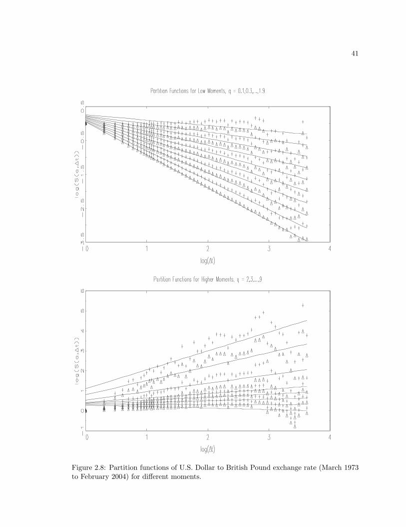
41

Figure 2.8: Partition functions of U.S. Dollar to British Pound exchange rate (March 1973to February 2004) for different moments.

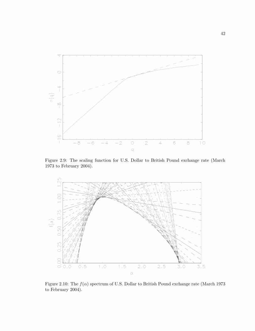
42

Figure 2.9: The scaling function for U.S. Dollar to British Pound exchange rate (March1973 to February 2004).

Figure 2.10: The f(α) spectrum of U.S. Dollar to British Pound exchange rate (March 1973to February 2004).

Chapter 3

The Bivariate Markov SwitchingMultifractal Models

3.1 Introduction

MMAR provides us with a new model for financial time series with attractive stochastic

properties, which take into account stylized facts of the financial market, such as fat tail,

volatility clustering, long-term dependence and multi-scaling.

However, the practical applicability of MMAR suffers from its combinatorial nature and

from its non-stationarity due to the restriction to a bounded interval. Taking a binomial

example with an underlying binary cascade extending over k steps, there are exactly 2k

realizations of different subintervals at our disposal; consequently we are limited to ‘time

series’ no longer than 2k; in addition, the model suffers from a dearth of applicable statistical

methods, see Mandelbrot et al. (1997).

These limitations have been overcome by introducing iterative versions of MF models.

Calvet and Fisher (2001) present a multifractal model with random times for the changes

of the multipliers (Poisson multifractal), demonstrating weak convergence of a discretized

version of this process to its continuous-time limit. Iterative MF models preserve the multi-

fractal and stochastic properties, in particular they make econometric analysis applicable.

In the Markov-switching multifractal model (cf. Calvet and Fisher (2004), Lux (2008)),

43

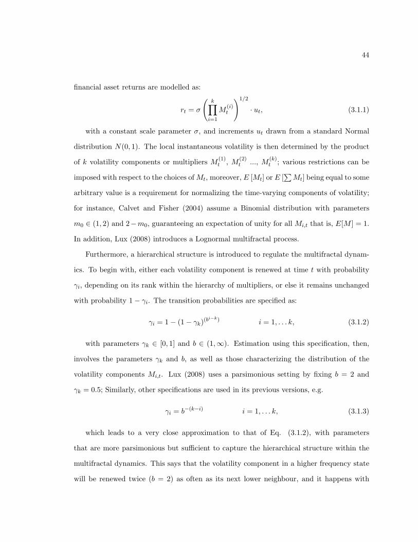
44

financial asset returns are modelled as:

rt = σ

(k∏

i=1

M(i)t

)1/2

· ut, (3.1.1)

with a constant scale parameter σ, and increments ut drawn from a standard Normal

distribution N(0, 1). The local instantaneous volatility is then determined by the product

of k volatility components or multipliers M (1)t , M (2)

t ..., M (k)t ; various restrictions can be

imposed with respect to the choices ofMt, moreover, E [Mt] or E [∑Mt] being equal to some

arbitrary value is a requirement for normalizing the time-varying components of volatility;

for instance, Calvet and Fisher (2004) assume a Binomial distribution with parameters

m0 ∈ (1, 2) and 2−m0, guaranteeing an expectation of unity for all Mi,t that is, E[M ] = 1.

In addition, Lux (2008) introduces a Lognormal multifractal process.

Furthermore, a hierarchical structure is introduced to regulate the multifractal dynam-

ics. To begin with, either each volatility component is renewed at time t with probability

γi, depending on its rank within the hierarchy of multipliers, or else it remains unchanged

with probability 1− γi. The transition probabilities are specified as:

γi = 1− (1− γk)(bi−k) i = 1, . . . k, (3.1.2)

with parameters γk ∈ [0, 1] and b ∈ (1,∞). Estimation using this specification, then,

involves the parameters γk and b, as well as those characterizing the distribution of the

volatility components Mi,t. Lux (2008) uses a parsimonious setting by fixing b = 2 and

γk = 0.5; Similarly, other specifications are used in its previous versions, e.g.

γi = b−(k−i) i = 1, . . . k, (3.1.3)

which leads to a very close approximation to that of Eq. (3.1.2), with parameters

that are more parsimonious but sufficient to capture the hierarchical structure within the

multifractal dynamics. This says that the volatility component in a higher frequency state

will be renewed twice (b = 2) as often as its next lower neighbour, and it happens with

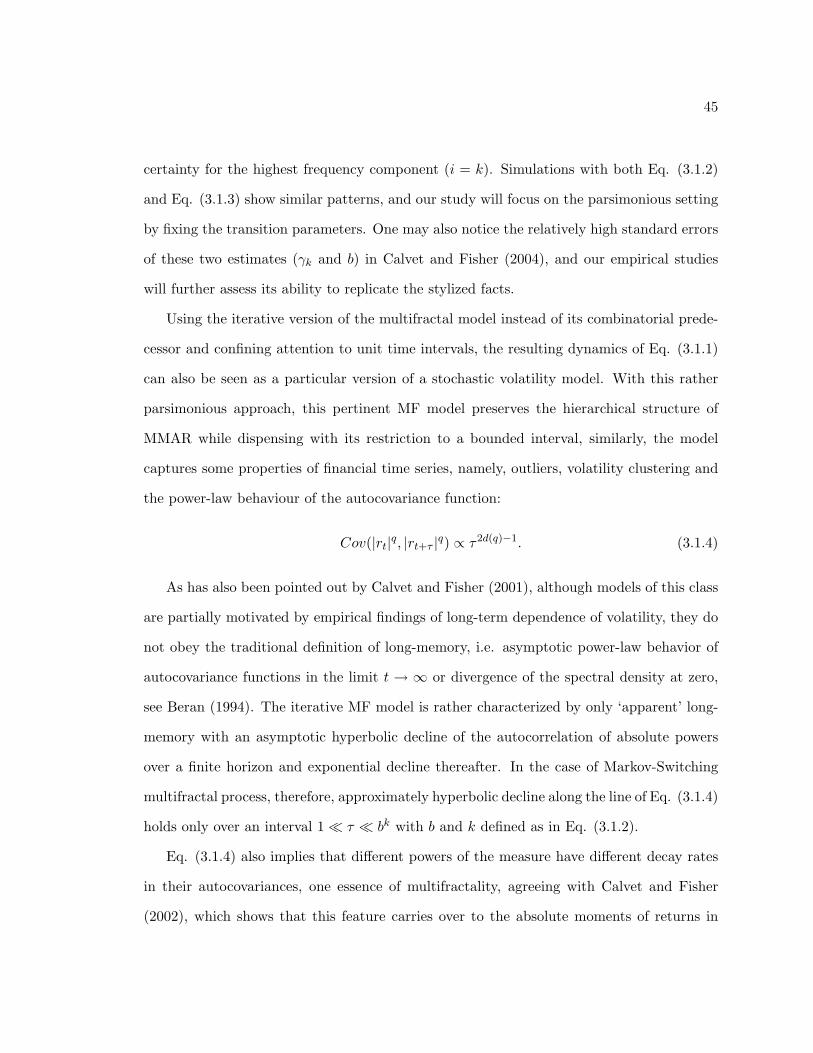
45

certainty for the highest frequency component (i = k). Simulations with both Eq. (3.1.2)

and Eq. (3.1.3) show similar patterns, and our study will focus on the parsimonious setting

by fixing the transition parameters. One may also notice the relatively high standard errors

of these two estimates (γk and b) in Calvet and Fisher (2004), and our empirical studies

will further assess its ability to replicate the stylized facts.

Using the iterative version of the multifractal model instead of its combinatorial prede-

cessor and confining attention to unit time intervals, the resulting dynamics of Eq. (3.1.1)

can also be seen as a particular version of a stochastic volatility model. With this rather

parsimonious approach, this pertinent MF model preserves the hierarchical structure of

MMAR while dispensing with its restriction to a bounded interval, similarly, the model

captures some properties of financial time series, namely, outliers, volatility clustering and

the power-law behaviour of the autocovariance function:

Cov(|rt|q, |rt+τ |q) ∝ τ2d(q)−1. (3.1.4)

As has also been pointed out by Calvet and Fisher (2001), although models of this class

are partially motivated by empirical findings of long-term dependence of volatility, they do

not obey the traditional definition of long-memory, i.e. asymptotic power-law behavior of

autocovariance functions in the limit t → ∞ or divergence of the spectral density at zero,

see Beran (1994). The iterative MF model is rather characterized by only ‘apparent’ long-

memory with an asymptotic hyperbolic decline of the autocorrelation of absolute powers

over a finite horizon and exponential decline thereafter. In the case of Markov-Switching

multifractal process, therefore, approximately hyperbolic decline along the line of Eq. (3.1.4)

holds only over an interval 1 τ bk with b and k defined as in Eq. (3.1.2).

Eq. (3.1.4) also implies that different powers of the measure have different decay rates

in their autocovariances, one essence of multifractality, agreeing with Calvet and Fisher

(2002), which shows that this feature carries over to the absolute moments of returns in

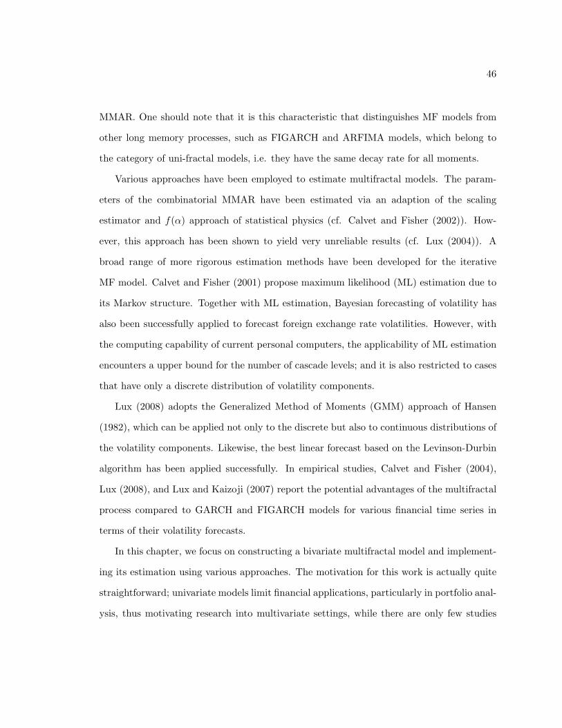
46

MMAR. One should note that it is this characteristic that distinguishes MF models from

other long memory processes, such as FIGARCH and ARFIMA models, which belong to

the category of uni-fractal models, i.e. they have the same decay rate for all moments.

Various approaches have been employed to estimate multifractal models. The param-

eters of the combinatorial MMAR have been estimated via an adaption of the scaling

estimator and f(α) approach of statistical physics (cf. Calvet and Fisher (2002)). How-

ever, this approach has been shown to yield very unreliable results (cf. Lux (2004)). A

broad range of more rigorous estimation methods have been developed for the iterative

MF model. Calvet and Fisher (2001) propose maximum likelihood (ML) estimation due to

its Markov structure. Together with ML estimation, Bayesian forecasting of volatility has

also been successfully applied to forecast foreign exchange rate volatilities. However, with

the computing capability of current personal computers, the applicability of ML estimation

encounters a upper bound for the number of cascade levels; and it is also restricted to cases

that have only a discrete distribution of volatility components.

Lux (2008) adopts the Generalized Method of Moments (GMM) approach of Hansen

(1982), which can be applied not only to the discrete but also to continuous distributions of

the volatility components. Likewise, the best linear forecast based on the Levinson-Durbin

algorithm has been applied successfully. In empirical studies, Calvet and Fisher (2004),

Lux (2008), and Lux and Kaizoji (2007) report the potential advantages of the multifractal

process compared to GARCH and FIGARCH models for various financial time series in

terms of their volatility forecasts.

In this chapter, we focus on constructing a bivariate multifractal model and implement-

ing its estimation using various approaches. The motivation for this work is actually quite

straightforward; univariate models limit financial applications, particularly in portfolio anal-

ysis, thus motivating research into multivariate settings, while there are only few studies

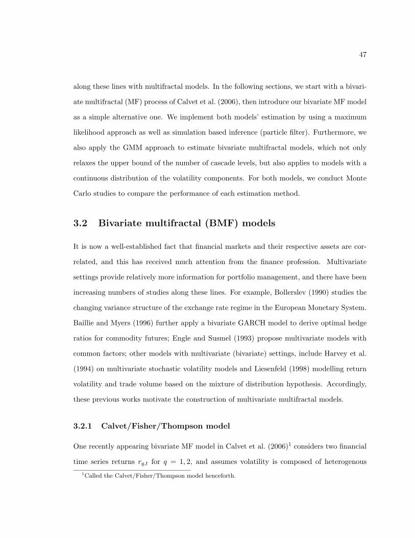
47

along these lines with multifractal models. In the following sections, we start with a bivari-

ate multifractal (MF) process of Calvet et al. (2006), then introduce our bivariate MF model

as a simple alternative one. We implement both models’ estimation by using a maximum

likelihood approach as well as simulation based inference (particle filter). Furthermore, we

also apply the GMM approach to estimate bivariate multifractal models, which not only

relaxes the upper bound of the number of cascade levels, but also applies to models with a

continuous distribution of the volatility components. For both models, we conduct Monte

Carlo studies to compare the performance of each estimation method.

3.2 Bivariate multifractal (BMF) models

It is now a well-established fact that financial markets and their respective assets are cor-

related, and this has received much attention from the finance profession. Multivariate

settings provide relatively more information for portfolio management, and there have been

increasing numbers of studies along these lines. For example, Bollerslev (1990) studies the

changing variance structure of the exchange rate regime in the European Monetary System.

Baillie and Myers (1996) further apply a bivariate GARCH model to derive optimal hedge

ratios for commodity futures; Engle and Susmel (1993) propose multivariate models with

common factors; other models with multivariate (bivariate) settings, include Harvey et al.

(1994) on multivariate stochastic volatility models and Liesenfeld (1998) modelling return

volatility and trade volume based on the mixture of distribution hypothesis. Accordingly,

these previous works motivate the construction of multivariate multifractal models.

3.2.1 Calvet/Fisher/Thompson model

One recently appearing bivariate MF model in Calvet et al. (2006)1 considers two financial

time series returns rq,t for q = 1, 2, and assumes volatility is composed of heterogenous1Called the Calvet/Fisher/Thompson model henceforth.

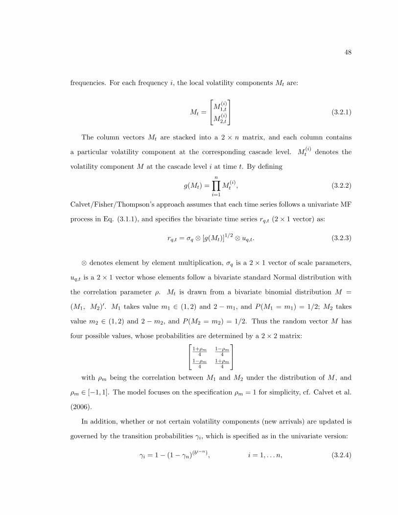
48

frequencies. For each frequency i, the local volatility components Mt are:

Mt =

M (i)1,t

M(i)2,t

(3.2.1)

The column vectors Mt are stacked into a 2 × n matrix, and each column contains

a particular volatility component at the corresponding cascade level. M(i)t denotes the

volatility component M at the cascade level i at time t. By defining

g(Mt) =n∏

i=1

M(i)t , (3.2.2)

Calvet/Fisher/Thompson’s approach assumes that each time series follows a univariate MF

process in Eq. (3.1.1), and specifies the bivariate time series rq,t (2× 1 vector) as:

rq,t = σq ⊗ [g(Mt)]1/2 ⊗ uq,t. (3.2.3)

⊗ denotes element by element multiplication, σq is a 2 × 1 vector of scale parameters,

uq,t is a 2 × 1 vector whose elements follow a bivariate standard Normal distribution with

the correlation parameter ρ. Mt is drawn from a bivariate binomial distribution M =

(M1, M2)′. M1 takes value m1 ∈ (1, 2) and 2 − m1, and P (M1 = m1) = 1/2; M2 takes

value m2 ∈ (1, 2) and 2 −m2, and P (M2 = m2) = 1/2. Thus the random vector M has

four possible values, whose probabilities are determined by a 2× 2 matrix:1+ρm

41−ρm

41−ρm

41+ρm

4

with ρm being the correlation between M1 and M2 under the distribution of M , and

ρm ∈ [−1, 1]. The model focuses on the specification ρm = 1 for simplicity, cf. Calvet et al.

(2006).

In addition, whether or not certain volatility components (new arrivals) are updated is

governed by the transition probabilities γi, which is specified as in the univariate version:

γi = 1− (1− γn)(bi−n), i = 1, . . . n, (3.2.4)

49

with parameters γn ∈ (0, 1) and b ∈ (1,∞). It defines the probability of a new arrival

happening at the cascade level i, i.e., whether a volatility component M (i)t is updated by a

new arrival or not. Furthermore, arrivals across two series are characterized by a correlation

parameter λm ∈ [0, 1]. New arrivals are independent if λm = 0 and simultaneous if λm = 1.

Therefore, estimating of Calvet/Fisher/Thompson model involves overall eight parameters,

which are σ1, σ2,m1,m2, ρ, b, γn, λm.

3.2.2 Liu/Lux model

In this section, a bivariate multifractal model2 is introduced as a simple alternative of Cal-

vet/Fisher/Thompson model with a more parsimonious setting. It assumes that two time

series have a certain number of joint cascade levels in common. The economic intuition is

that the observed correlation between different markets/assets can either be due to common

news processes, or to common factors, such as the business cycle or technology shocks. We

model the bivariate asset returns rq,t as

rq,t = σq ⊗[g′(Mt)

]1/2 ⊗ uq,t. (3.2.5)

q = 1, 2 refers to the two time series respectively, having n levels of their volatility

cascades. ⊗ denotes element by element multiplication, σq is the vector of scale parameters

(unconditional standard deviations); uq,t is a 2× 1 vector whose elements follow a bivariate

standard Normal distribution, with an unknown correlation parameter ρ. In our model, we

assume for the column vector Mt that

g′(Mt) =k∏

i=1

M(i)t ⊗

n∏j=k+1

M(j)q,t , (3.2.6)

n∏j=k+1

M(j)q,t stands for M (k+1)

t ⊗M (k+2)t · · · , that means, both time series share k number

of joint cascades that govern the strength of their volatility correlation. Consequently, the2Called the Liu/Lux model henceforth.

50

larger the k, the higher the correlation between them. After k joint multiplications, each

series has additional separate multifractal components.

Furthermore, the restriction for the specification of the transition probabilities is arbi-

trarily imposed. In our model, we allow two starting cascades within each time series (the

multifractal process starts again after the joint cascade level k), that is

γi = 2−(k−i), for i = 1, . . . k; (3.2.7)

γi = 2−(n−i), for i = k + 1, . . . n.

Each component is either renewed at time t with probability γi, depending on its rank i

within the hierarchy of multipliers, or remains unchanged with probability 1− γi, following

the hierarchical structure, which implies that the one at a higher cascade level has a higher

probability of being updated. With regard to the heterogeneous multipliers, we follow the

published routine in specifying them to be random draws from either a Binomial or Lognor-

mal distribution. In the Binomial case, it is assumed that each volatility component within

the column vector Mt is drawn from Mt ∼ m0, m1 for m0 ∈ (0, 2) and alternatively

m1 = 2−m0; For the latter, we assume −log2Mt ∼ N(λ, σ2m).

Simulations of our bivariate MF model (k = 4, n = 15) are depicted in Figure 3.1 to

3.3. Figure 3.1 is the local instantaneous volatility of the simulated bivariate MF time

series; Figure 3.2 shows simulations of the corresponding returns, together with their au-

tocorrelation functions of returns and absolute returns in Figure 3.3. The dot dashed lines

are roughly fitted by power functions of 0.5τ−β (time lags τ) with β approximately being

0.371 and 0.413 respectively. The simulations are seen to have some of the stylized facts

of financial time series, namely: outliers, volatility clustering and hyperbolical decay of the

autocorrelation function (long-term dependence). It is impressive to consider the remark-

able ‘long memory’ depicted in Figure 3.3, and one also easily recognizes the correlation of

the volatilities between each of the simulated time series.

51

Figure 3.1: Local instantaneous volatility of the simulated bivariate MF (Binomial) timeseries.

3.3 Exact maximum likelihood estimation

The extension from univariate multifractal process to bivariate one trivially guarantee the

positive semi-definiteness of the covariance matrix of the bivariate time series, and the like-

lihood function can be written in closed-form which allows maximum likelihood estimation

to be implemented for a certain size of state spaces, see Calvet et al. (2006).

The dynamics of MF can be taken as a special case of a Markov-switching process

which makes ML estimation feasible. Since the state spaces are finite when the multipliers

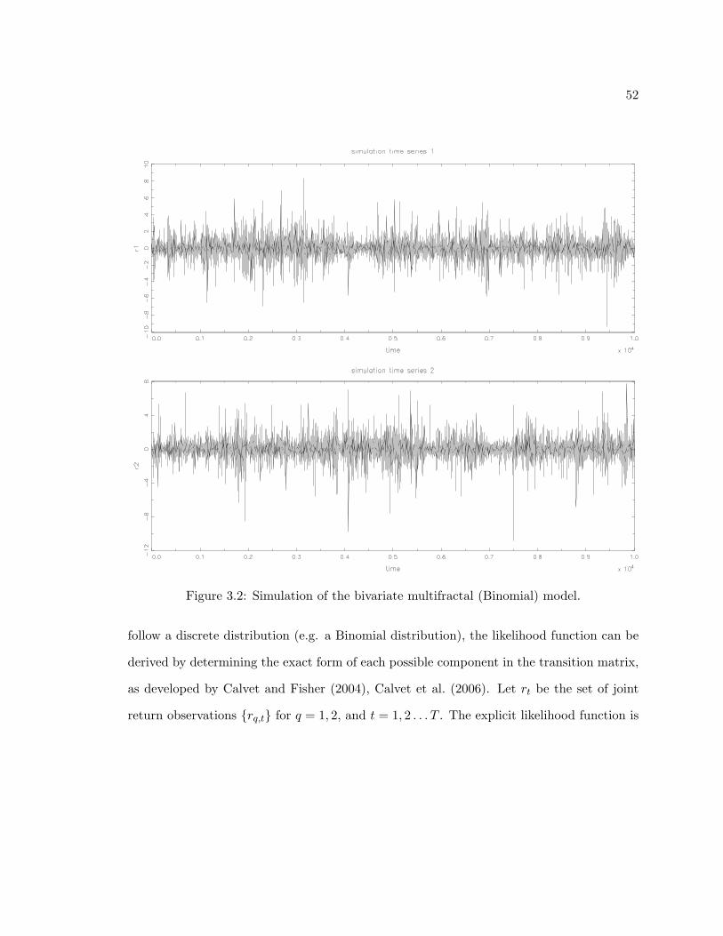
52

Figure 3.2: Simulation of the bivariate multifractal (Binomial) model.

follow a discrete distribution (e.g. a Binomial distribution), the likelihood function can be

derived by determining the exact form of each possible component in the transition matrix,

as developed by Calvet and Fisher (2004), Calvet et al. (2006). Let rt be the set of joint

return observations rq,t for q = 1, 2, and t = 1, 2 . . . T . The explicit likelihood function is

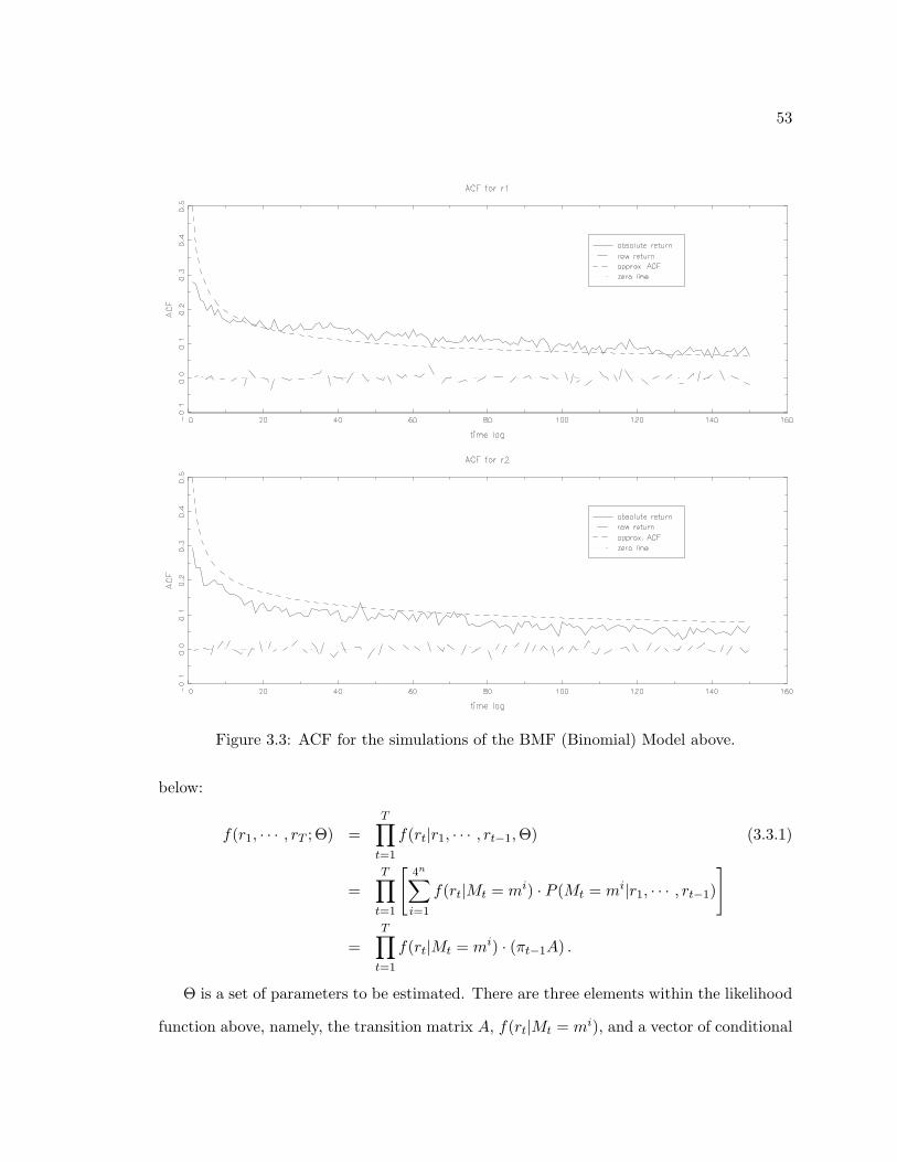
53

Figure 3.3: ACF for the simulations of the BMF (Binomial) Model above.

below:

f(r1, · · · , rT ; Θ) =T∏

t=1

f(rt|r1, · · · , rt−1,Θ) (3.3.1)

=T∏

t=1

[4n∑i=1

f(rt|Mt = mi) · P (Mt = mi|r1, · · · , rt−1)

]

=T∏

t=1

f(rt|Mt = mi) · (πt−1A) .

Θ is a set of parameters to be estimated. There are three elements within the likelihood

function above, namely, the transition matrix A, f(rt|Mt = mi), and a vector of conditional

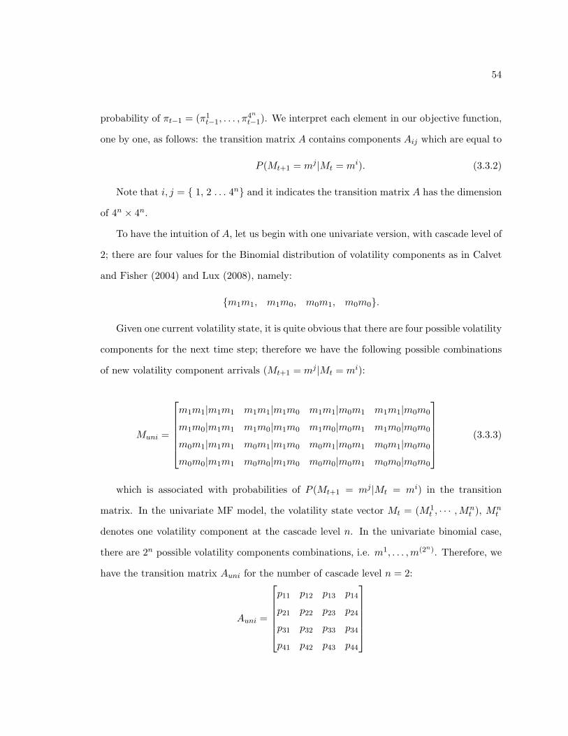
54

probability of πt−1 = (π1t−1, . . . , π

4n

t−1). We interpret each element in our objective function,

one by one, as follows: the transition matrix A contains components Aij which are equal to

P (Mt+1 = mj |Mt = mi). (3.3.2)

Note that i, j = 1, 2 . . . 4n and it indicates the transition matrix A has the dimension

of 4n × 4n.

To have the intuition of A, let us begin with one univariate version, with cascade level of

2; there are four values for the Binomial distribution of volatility components as in Calvet

and Fisher (2004) and Lux (2008), namely:

m1m1, m1m0, m0m1, m0m0.

Given one current volatility state, it is quite obvious that there are four possible volatility

components for the next time step; therefore we have the following possible combinations

of new volatility component arrivals (Mt+1 = mj |Mt = mi):

Muni =

m1m1|m1m1 m1m1|m1m0 m1m1|m0m1 m1m1|m0m0




(3.3.3)

which is associated with probabilities of P (Mt+1 = mj |Mt = mi) in the transition

matrix. In the univariate MF model, the volatility state vector Mt = (M1t , · · · ,Mn

t ), Mnt

denotes one volatility component at the cascade level n. In the univariate binomial case,

there are 2n possible volatility components combinations, i.e. m1, . . . ,m(2n). Therefore, we

have the transition matrix Auni for the number of cascade level n = 2:

Auni =

p11 p12 p13 p14

p21 p22 p23 p24

p31 p32 p33 p34

p41 p42 p43 p44

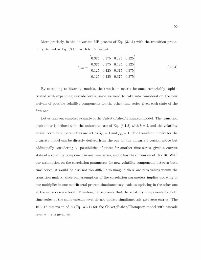
55

More precisely, in the univariate MF process of Eq. (3.1.1) with the transition proba-

bility defined as Eq. (3.1.3) with b = 2, we get

Auni =

0.375 0.375 0.125 0.125

0.375 0.375 0.125 0.125

0.125 0.125 0.375 0.375

0.125 0.125 0.375 0.375

(3.3.4)

By extending to bivariate models, the transition matrix becomes remarkably sophis-

ticated with expanding cascade levels, since we need to take into consideration the new

arrivals of possible volatility components for the other time series given each state of the

first one.

Let us take one simplest example of the Calvet/Fisher/Thompson model. The transition

probability is defined as in the univariate case of Eq. (3.1.3) with b = 2, and the volatility

arrival correlation parameters are set as λm = 1 and ρm = 1. The transition matrix for the

bivariate model can be directly derived from the one for the univariate version above but

additionally considering all possibilities of states for another time series, given a current

state of a volatility component in one time series, and it has the dimension of 16×16. With

our assumption on the correlation parameters for new volatility components between both

time series, it would be also not too difficult to imagine there are zero values within the

transition matrix, since our assumption of the correlation parameters implies updating of

one multiplier in one multifractal process simultaneously leads to updating in the other one

at the same cascade level. Therefore, those events that the volatility components for both

time series at the same cascade level do not update simultaneously give zero entries. The

16 × 16 dimension of A (Eq. 3.3.1) for the Calvet/Fisher/Thompson model with cascade

level n = 2 is given as:

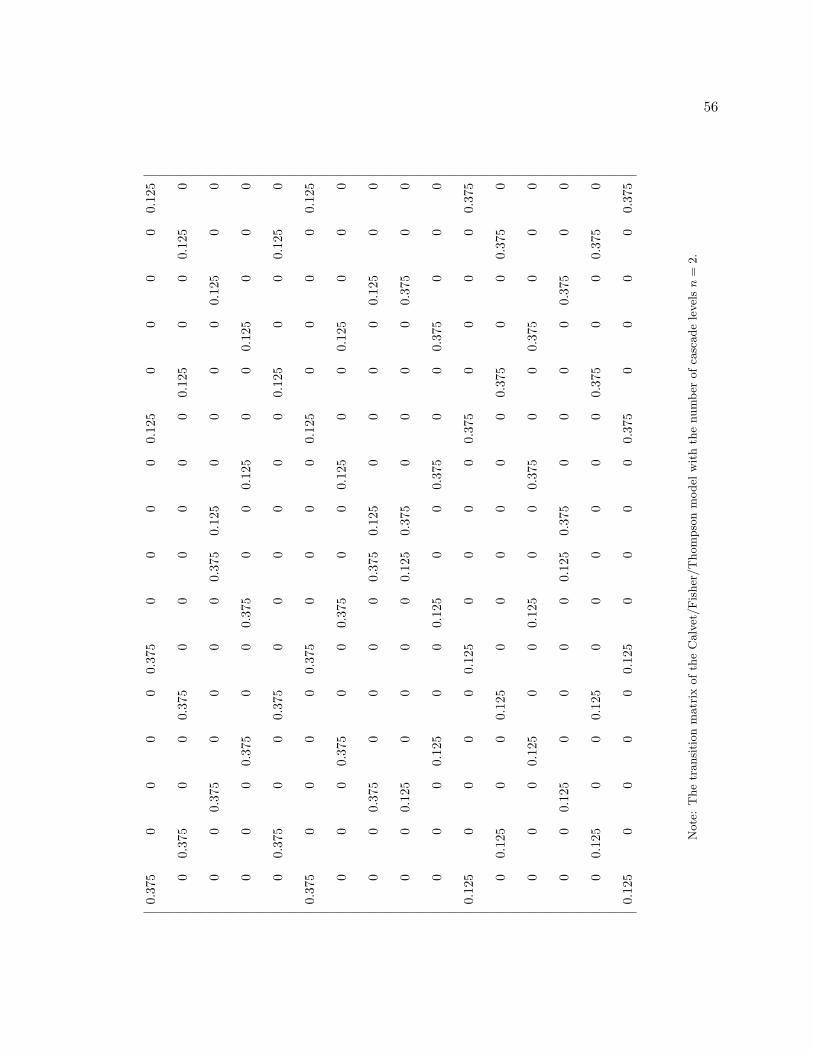
56

0.37

50

00

00.

375

00

00

0.12

50

00

00.

125

00.

375

00

0.37

50

00

00

00.

125

00

0.12

50

00

0.37

50

00

00.

375

0.12

50

00

00.

125

00

00

00.

375

00

0.37

50

00.

125

00

0.12

50

00

00.

375

00

0.37

50

00

00

00.

125

00

0.12

50

0.37

50

00

00.

375

00

00

0.12

50

00

00.

125

00

00.

375

00

0.37

50

00.

125

00

0.12

50

00

00

0.37

50

00

00.

375

0.12

50

00

00.

125

00

00

0.12

50

00

00.

125

0.37

50

00

00.

375

00

00

00.

125

00

0.12

50

00.

375

00

0.37

50

00

0.12

50

00

00.

125

00

00

0.37

50

00

00.

375

00.

125

00

0.12

50

00

00

00.

375

00

0.37

50

00

00.

125

00

0.12

50

00.

375

00

0.37

50

00

00

0.12

50

00

00.

125

0.37

50

00

00.

375

00

00.

125

00

0.12

50

00

00

00.

375

00

0.37

50

0.12

50

00

00.

125

00

00

0.37

50

00

00.

375

Note

:T

he

transi

tion

matr

ixofth

eC

alv

et/Fis

her

/T

hom

pso

nm

odel

wit

hth

enum

ber

ofca

scade

level

sn

=2.

57

From the simple example of the Calvet/Fisher/Thompson model, each element within

the transition matrix is associated with the probabilities of (mama|mama), given (mbmb|mbmb)

(denoted 〈mama|mama〉〈mbmb|mbmb〉 henceforth); a and b correspond the bivariate time

series; ma and mb are drawn from the Binomial distributions. More specifically, let’s refer to

the univariate case in the matrix 3.3.3, i.e. Muni, therefore the matrix for the bivariate case

can be implicitly viewed as Kronecker product of Muni with another one for the second time

series, and we arrive the dimension of 16× 16 transition matrix. For instance, the first ele-

ment of 0.375, which is calculated as the probability for 〈ma1m

a1|ma

1ma1〉〈mb

1mb1|mb

1mb1〉, and

it implies 0.375×1 due to the assumption of simultaneous updating of volatility components.

Let’s then take the second element (the first row and second column), which corresponds to

the probability for the occurrence of 〈ma1m

a1|ma

1ma1〉〈mb

1mb1|mb

1mb0〉, and it means the volatil-

ity components for time series 1 remain the same at both cascade levels, but the volatility

component for time series 2 is updated at the second cascade level, which implies the zeros

entry due to violating the assumption of the simultaneous updating. In the same way, we

calculate the third element (the first row and third column) of 〈ma1m

a1|ma

1ma1〉〈mb

1mb1|mb

0mb1〉

with zero value, as well as the fourth component 〈ma1m

a1|ma

1ma1〉〈mb

1mb1|mb

0mb0〉, and one may

also easily obtain all other entries whin this transition matrix.

Turning to the Liu/Lux model with n = 2 and joint cascade level k = 1. In this parsimo-

nious version of bivariate models, we actually have two combined multifractal processes with

cascade level of 1, since it starts again after the first cascade level as defined in our model.

Likewise, the transition matrix for the bivariate model can be obtained by considering all

possibilities of states for one time series, given a current state of a volatility component

in another time series. Apart from the Calvet/Fisher/Thompson model, the zero entries

in the transition matrix are corresponding to those events of non-identical volatility com-

ponents within the joint cascades of both time series, by recalling our assumption of joint

cascades. For example, the probability for the occurrence of 〈m1m1|m1m1〉〈m1m1|m1m1〉

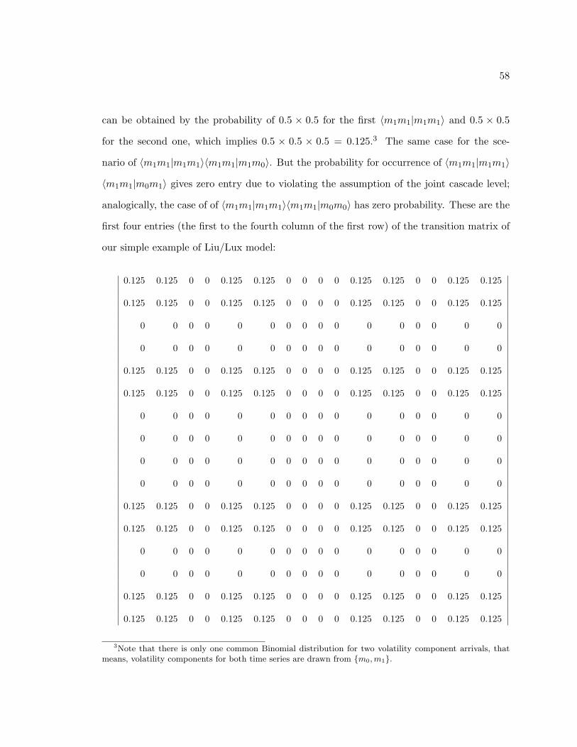
58

can be obtained by the probability of 0.5 × 0.5 for the first 〈m1m1|m1m1〉 and 0.5 × 0.5

for the second one, which implies 0.5 × 0.5 × 0.5 = 0.125.3 The same case for the sce-

nario of 〈m1m1|m1m1〉〈m1m1|m1m0〉. But the probability for occurrence of 〈m1m1|m1m1〉

〈m1m1|m0m1〉 gives zero entry due to violating the assumption of the joint cascade level;

analogically, the case of of 〈m1m1|m1m1〉〈m1m1|m0m0〉 has zero probability. These are the

first four entries (the first to the fourth column of the first row) of the transition matrix of

our simple example of Liu/Lux model:

0.125 0.125 0 0 0.125 0.125 0 0 0 0 0.125 0.125 0 0 0.125 0.125

0.125 0.125 0 0 0.125 0.125 0 0 0 0 0.125 0.125 0 0 0.125 0.125

0 0 0 0 0 0 0 0 0 0 0 0 0 0 0 0

0 0 0 0 0 0 0 0 0 0 0 0 0 0 0 0

0.125 0.125 0 0 0.125 0.125 0 0 0 0 0.125 0.125 0 0 0.125 0.125

0.125 0.125 0 0 0.125 0.125 0 0 0 0 0.125 0.125 0 0 0.125 0.125

0 0 0 0 0 0 0 0 0 0 0 0 0 0 0 0

0 0 0 0 0 0 0 0 0 0 0 0 0 0 0 0

0 0 0 0 0 0 0 0 0 0 0 0 0 0 0 0

0 0 0 0 0 0 0 0 0 0 0 0 0 0 0 0

0.125 0.125 0 0 0.125 0.125 0 0 0 0 0.125 0.125 0 0 0.125 0.125

0.125 0.125 0 0 0.125 0.125 0 0 0 0 0.125 0.125 0 0 0.125 0.125

0 0 0 0 0 0 0 0 0 0 0 0 0 0 0 0

0 0 0 0 0 0 0 0 0 0 0 0 0 0 0 0

0.125 0.125 0 0 0.125 0.125 0 0 0 0 0.125 0.125 0 0 0.125 0.125

0.125 0.125 0 0 0.125 0.125 0 0 0 0 0.125 0.125 0 0 0.125 0.125

3Note that there is only one common Binomial distribution for two volatility component arrivals, thatmeans, volatility components for both time series are drawn from m0, m1.

59

We easily recognize the regular appearance of zero entries due to our assumption of joint

cascade levels. Practicably, we can remove all these zeros by excluding the scenarios that

violate the model’s assumption, which reduces the dimension of the transition matrix from

4n × 4n to 22n−k × 22n−k. For example, in the case of n = 3 and joint cascade level k = 2,

we only need to evaluate the 16 × 16 matrix instead of 64 × 64 matrix (without excluding

the zero entries). As illustrated in previous pages, all possible combinations of volatility

components can be viewed as the Kronecker product of two univariate ones (we skip it for

the case of three cascade levels due to the page size limit). Let us start with the scenario of

〈m1m1m1|m1m1m1〉〈m1m1m1|m1m1m1〉, we know the probability of 〈m1m1m1|m1m1m1〉

for the first time series is (0.5+0.5×0.5)×0.5×0.5 = 0.1875.4 Since we have the joint cascade

levels of two, which implies the probability of 〈m1m1m1|m1m1m1〉〈m1m1m1|m1m1m1〉 is

0.1875×0.5 = 0.094; it is the same for the case of 〈m1m1m1|m1m1m1〉〈m1m1m1|m1m1m0〉.

But for cases of

〈m1m1m1|m1m1m1〉〈m1m1m1|m1m0m1〉 and

〈m1m1m1|m1m1m1〉〈m1m1m1|m1m0m0〉, we obtain a probability of zero. The same

applies to those scenarios where the volatility components at the first cascade level for the

time series one remain unchange, while the ones for the second time series would change:

〈m1m1m1|m1m1m1〉〈m1m1m1|m0m1m1〉,

〈m1m1m1|m1m1m1〉〈m1m1m1|m0m1m0〉,

〈m1m1m1|m1m1m1〉〈m1m1m1|m0m0m1〉,

〈m1m1m1|m1m1m1〉〈m1m1m1|m0m0m0〉, etc.

By removing all those zeros entries, we arrive at the 16× 16 transition matrix:

4It is calculated via Πnk=1[(1− γk)1

mik=m

jk

+ γkP (M = mjk)]. Note that, here, mi

k is the mth component

of vector mi, and 1mi

k=m

jk

is the dummy variable equal to 1 if mik = mj

k and zero otherwise, c.f. Calvet and

Fisher (2002). In our case, we have γ1 = 1/2, γ2 = 1; γ3 = 1 by recalling Eq. 3.1.3.

60

0.09

40.

094

0.09

40.

094

0.03

10.

031

0.03

10.

031

0.09

40.

094

0.09

40.

094

0.03

10.

031

0.03

10.

031

0.09

40.

094

0.09

40.

094

0.03

10.

031

0.03

10.

031

0.09

40.

094

0.09

40.

094

0.03

10.

031

0.03

10.

031

0.09

40.

094

0.09

40.

094

0.03

10.

031

0.03

10.

031

0.09

40.

094

0.09

40.

094

0.03

10.

031

0.03

10.

031

0.09

40.

094

0.09

40.

094

0.03

10.

031

0.03

10.

031

0.09

40.

094

0.09

40.

094

0.03

10.

031

0.03

10.

031

0.03

10.

031

0.03

10.

031

0.09

40.

094

0.09

40.

094

0.03

10.

031

0.03

10.

031

0.09

40.

094

0.09

40.

094

0.03

10.

031

0.03

10.

031

0.09

40.

094

0.09

40.

094

0.03

10.

031

0.03

10.

031

0.09

40.

094

0.09

40.

094

0.03

10.

031

0.03

10.

031

0.09

40.

094

0.09

40.

094

0.03

10.

031

0.03

10.

031

0.09

40.

094

0.09

40.

094

0.03

10.

031

0.03

10.

031

0.09

40.

094

0.09

40.

094

0.03

10.

031

0.03

10.

031

0.09

40.

094

0.09

40.

094

0.09

40.

094

0.09

40.

094

0.03

10.

031

0.03

10.

031

0.09

40.

094

0.09

40.

094

0.03

10.

031

0.03

10.

031

0.09

40.

094

0.09

40.

094

0.03

10.

031

0.03

10.

031

0.09

40.

094

0.09

40.

094

0.03

10.

031

0.03

10.

031

0.09

40.

094

0.09

40.

094

0.03

10.

031

0.03

10.

031

0.09

40.

094

0.09

40.

094

0.03

10.

031

0.03

10.

031

0.09

40.

094

0.09

40.

094

0.03

10.

031

0.03

10.

031

0.09

40.

094

0.09

40.

094

0.03

10.

031

0.03

10.

031

0.03

10.

031

0.03

10.

031

0.09

40.

094

0.09

40.

094

0.03

10.

031

0.03

10.

031

0.09

40.

094

0.09

40.

094

0.03

10.

031

0.03

10.

031

0.09

40.

094

0.09

40.

094

0.03

10.

031

0.03

10.

031

0.09

40.

094

0.09

40.

094

0.03

10.

031

0.03

10.

031

0.09

40.

094

0.09

40.

094

0.03

10.

031

0.03

10.

031

0.09

40.

094

0.09

40.

094

0.03

10.

031

0.03

10.

031

0.09

40.

094

0.09

40.

094

0.03

10.

031

0.03

10.

031

0.09

40.

094

0.09

40.

094

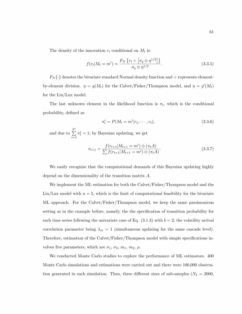
61

The density of the innovation rt conditional on Mt is:

f(rt|Mt = mi) =FN

rt ÷

[σq ⊗ η1/2

]σq ⊗ η1/2

. (3.3.5)

FN· denotes the bivariate standard Normal density function and ÷ represents element-

by-element division. η = g(Mt) for the Calvet/Fisher/Thompson model, and η = g′(Mt)

for the Liu/Lux model.

The last unknown element in the likelihood function is πt, which is the conditional

probability, defined as

πit = P (Mt = mi|r1, · · · , rt), (3.3.6)

and due to4n∑i=1

πit = 1; by Bayesian updating, we get

πt+1 =f(rt+1|Mt+1 = mi)⊗ (πtA)∑f(rt+1|Mt+1 = mi)⊗ (πtA)

. (3.3.7)

We easily recognize that the computational demands of this Bayesian updating highly

depend on the dimensionality of the transition matrix A.

We implement the ML estimation for both the Calvet/Fisher/Thompson model and the

Liu/Lux model with n = 5, which is the limit of computational feasibility for the bivariate

ML approach. For the Calvet/Fisher/Thompson model, we keep the same parsimonious

setting as in the example before, namely, the the specification of transition probability for

each time series following the univariate case of Eq. (3.1.3) with b = 2; the volatility arrival

correlation parameter being λm = 1 (simultaneous updating for the same cascade level).

Therefore, estimation of the Calvet/Fisher/Thompson model with simple specifications in-

volves five parameters, which are σ1, σ2, m1, m2, ρ.

We conducted Monte Carlo studies to explore the performance of ML estimators. 400

Monte Carlo simulations and estimations were carried out and there were 100,000 observa-

tion generated in each simulation. Then, three different sizes of sub-samples (N1 = 2000,

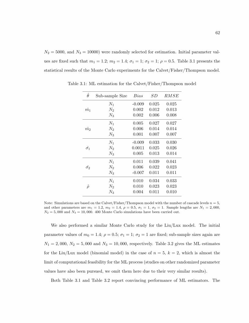
62

N2 = 5000, and N3 = 10000) were randomly selected for estimation. Initial parameter val-

ues are fixed such that m1 = 1.2; m2 = 1.4; σ1 = 1; σ2 = 1; ρ = 0.5. Table 3.1 presents the

statistical results of the Monte Carlo experiments for the Calvet/Fisher/Thompson model.

Table 3.1: ML estimation for the Calvet/Fisher/Thompson model

θ Sub-sample Size Bias SD RMSE

N1 -0.009 0.025 0.025m1 N2 0.002 0.012 0.013

N3 0.002 0.006 0.008

N1 0.005 0.027 0.027m2 N2 0.006 0.014 0.014

N3 0.001 0.007 0.007

N1 -0.009 0.033 0.030σ1 N2 0.0011 0.025 0.026

N3 0.005 0.013 0.014

N1 0.011 0.039 0.041σ2 N2 0.006 0.022 0.023

N3 -0.007 0.011 0.011

N1 0.010 0.034 0.033ρ N2 0.010 0.023 0.023

N3 0.004 0.011 0.010

Note: Simulations are based on the Calvet/Fisher/Thompson model with the number of cascade levels n = 5,and other parameters are m1 = 1.2, m2 = 1.4, ρ = 0.5, σ1 = 1, σ2 = 1. Sample lengths are N1 = 2, 000,N2 = 5, 000 and N3 = 10, 000. 400 Monte Carlo simulations have been carried out.

We also performed a similar Monte Carlo study for the Liu/Lux model. The initial

parameter values of m0 = 1.4; ρ = 0.5; σ1 = 1; σ2 = 1 are fixed; sub-sample sizes again are

N1 = 2, 000, N2 = 5, 000 and N3 = 10, 000, respectively. Table 3.2 gives the ML estimates

for the Liu/Lux model (binomial model) in the case of n = 5, k = 2, which is almost the

limit of computational feasibility for the ML process (studies on other randomized parameter

values have also been pursued, we omit them here due to their very similar results).

Both Table 3.1 and Table 3.2 report convincing performance of ML estimators. The

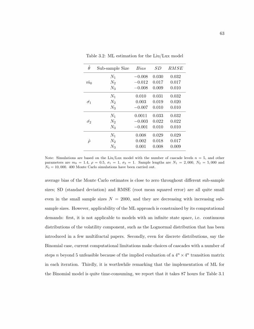
63

Table 3.2: ML estimation for the Liu/Lux model


N1 −0.008 0.030 0.032m0 N2 −0.012 0.017 0.017

N3 −0.008 0.009 0.010

N1 0.010 0.031 0.032σ1 N2 0.003 0.019 0.020

N3 −0.007 0.010 0.010

N1 0.0011 0.033 0.032σ2 N2 −0.003 0.022 0.022

N3 −0.001 0.010 0.010

N1 0.008 0.029 0.029ρ N2 0.002 0.018 0.017

N3 0.001 0.008 0.009

Note: Simulations are based on the Liu/Lux model with the number of cascade levels n = 5, and otherparameters are m0 = 1.4, ρ = 0.5, σ1 = 1, σ2 = 1. Sample lengths are N1 = 2, 000, N2 = 5, 000 andN3 = 10, 000. 400 Monte Carlo simulations have been carried out.

average bias of the Monte Carlo estimates is close to zero throughout different sub-sample

sizes; SD (standard deviation) and RMSE (root mean squared error) are all quite small

even in the small sample sizes N = 2000, and they are decreasing with increasing sub-

sample sizes. However, applicability of the ML approach is constrained by its computational

demands: first, it is not applicable to models with an infinite state space, i.e. continuous

distributions of the volatility component, such as the Lognormal distribution that has been

introduced in a few multifractal papers. Secondly, even for discrete distributions, say the

Binomial case, current computational limitations make choices of cascades with a number of

steps n beyond 5 unfeasible because of the implied evaluation of a 4n×4n transition matrix

in each iteration. Thirdly, it is worthwhile remarking that the implementation of ML for

the Binomial model is quite time-consuming, we report that it takes 87 hours for Table 3.1

64

and 116.5 hours for Table 3.2 which involve 400 Monte Carlo simulations and estimations.5

3.4 Simulation based ML estimation

As pointed out in the last section, there is an upper limit of n = 5 in ML estimation of

bivariate MF models; to overcome this restriction, a simulation based inference is proposed.

Recalling the Bayesian updating in Eq. (3.3.7) above, we can think of πtA, which is

4n∑j=1

P (Mt+1 = mi|Mt = mj)P (Mt = mj |rt) (3.4.1)

as a prior probability of

P (Mt+1 = mi|rt), (3.4.2)

then combine it with the conditional density

f(rt+1|Mt+1 = mi) (3.4.3)

to generate a posterior, that it is

πt+1 = P (Mt+1 = mi|rt+1). (3.4.4)

This procedure can also be expressed as a repeated application of a two-stage procedure:

(1) considering the conditional probabilities of current states πt as an input, passing

through a system of dynamic transformations, the transition probability matrix A here, to

propagate the prediction density Eq. (3.4.2);

(2) one then uses the Bayesian updating to produce the conditional probabilities of

future states πt+1 as output.

This procedure is called filtering. This is straightforward if P (Mt+1 = mi|Mt = mj) has

a reasonable size of finite discrete elements as the previous calculation can be computed

explicitly.5Note: All simulation and estimations are pursued by using a PC with Pentiumr IV Processor.

65

As one may realize, the bivariate multifractal process has the dimension of the transition

(filtering) probability matrix increasing exponentially with increasing number of cascade

levels n. Furthermore, there is an infinite number of states if the distribution of the volatility

components is continuous. This implies that it would be difficult (or impossible for the

continuous version) to evaluate the procedure above exactly, and some numerical methods

must be used. Numerous attempts have been made to provide algorithms that approximate

these filtering probabilities, cf. Gordon et al. (1993), Jacquier et al. (1994), Berzuini et al.

(1997), Kim et al. (1998). We use a so-called particle filter, which is a class of simulation-

based filters that recursively approximate the filtering of random variable by a certain finite

number of particles, which are discrete points viewed as approximated samples from the

prior. In our case, we evaluate Eq. (3.3.7) by combining the conditional density with Eq.

(3.4.1) up to proportionality (for R = 4n):

πit+1 ∝ f(rt+1|Mt+1 = mi)

R∑j=1

P (Mt+1 = mi|Mt = mj)πjt . (3.4.5)

As particle filters treat the discrete support generated by the particles as the ‘true’

filtering density, this allows us to produce an approximation to the prediction probability

density P (Mt+1 = mit|rt), by using the discrete support of the number B of particles, and

then the one-step-ahead conditional probability is


1B

B∑b=1

P (Mt+1 = mi|Mt = m(b)). (3.4.6)

This leaves only one issue – how to design the finite number of B draws? We adopt

Sampling/Importance Resampling (SIR) introduced by Rubin (1987); Pitt and Shephard

(1999). This algorithm generates M (b)t B

b=1 recursively with updating information:

Starting from t = 0 with the initial condition π0, and M(1)0 , . . . ,M

(B)0 are drawn. For

t = 1, we simulate each M (b)t B

b=1 independently and reweighting to obtain the importance

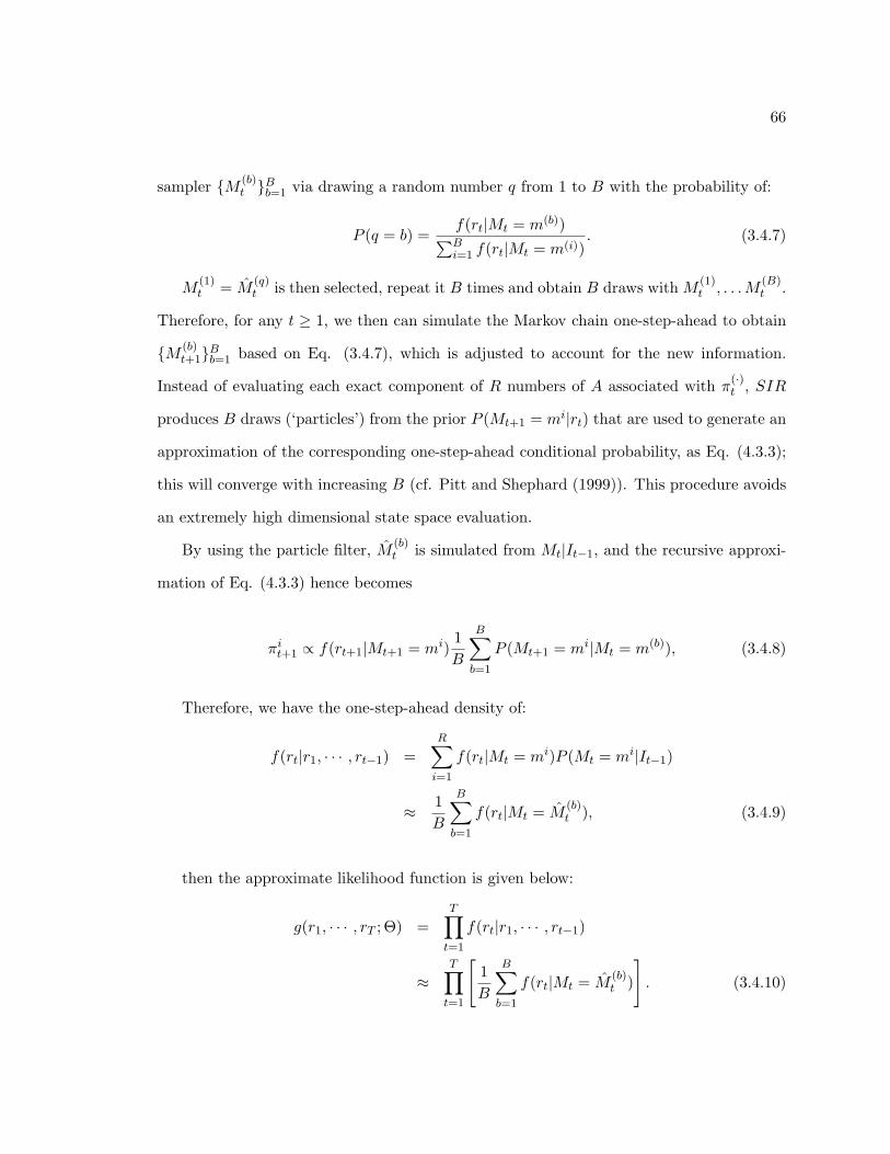
66

sampler M (b)t B

b=1 via drawing a random number q from 1 to B with the probability of:

P (q = b) =f(rt|Mt = m(b))∑Bi=1 f(rt|Mt = m(i))

. (3.4.7)

M(1)t = M

(q)t is then selected, repeat it B times and obtain B draws with M (1)

t , . . .M(B)t .

Therefore, for any t ≥ 1, we then can simulate the Markov chain one-step-ahead to obtain

M (b)t+1B

b=1 based on Eq. (3.4.7), which is adjusted to account for the new information.

Instead of evaluating each exact component of R numbers of A associated with π(·)t , SIR

produces B draws (‘particles’) from the prior P (Mt+1 = mi|rt) that are used to generate an

approximation of the corresponding one-step-ahead conditional probability, as Eq. (4.3.3);

this will converge with increasing B (cf. Pitt and Shephard (1999)). This procedure avoids

an extremely high dimensional state space evaluation.

By using the particle filter, M (b)t is simulated from Mt|It−1, and the recursive approxi-

mation of Eq. (4.3.3) hence becomes


1B

B∑b=1

P (Mt+1 = mi|Mt = m(b)), (3.4.8)

Therefore, we have the one-step-ahead density of:

f(rt|r1, · · · , rt−1) =R∑

i=1

f(rt|Mt = mi)P (Mt = mi|It−1)

≈ 1B

B∑b=1

f(rt|Mt = M(b)t ), (3.4.9)

then the approximate likelihood function is given below:

g(r1, · · · , rT ; Θ) =T∏

t=1

f(rt|r1, · · · , rt−1)

≈T∏

t=1

[1B

B∑b=1

f(rt|Mt = M(b)t )

]. (3.4.10)

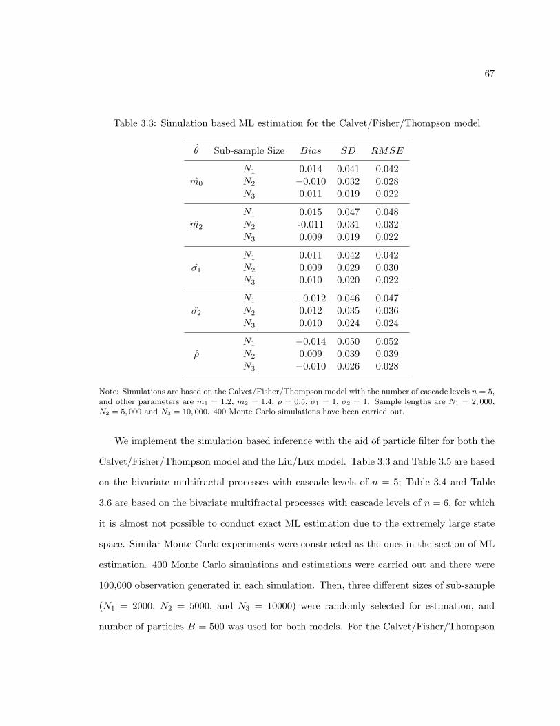
67

Table 3.3: Simulation based ML estimation for the Calvet/Fisher/Thompson model


N1 0.014 0.041 0.042m0 N2 −0.010 0.032 0.028

N3 0.011 0.019 0.022

N1 0.015 0.047 0.048m2 N2 -0.011 0.031 0.032

N3 0.009 0.019 0.022

N1 0.011 0.042 0.042σ1 N2 0.009 0.029 0.030

N3 0.010 0.020 0.022

N1 −0.012 0.046 0.047σ2 N2 0.012 0.035 0.036

N3 0.010 0.024 0.024

N1 −0.014 0.050 0.052ρ N2 0.009 0.039 0.039

N3 −0.010 0.026 0.028


We implement the simulation based inference with the aid of particle filter for both the

Calvet/Fisher/Thompson model and the Liu/Lux model. Table 3.3 and Table 3.5 are based

on the bivariate multifractal processes with cascade levels of n = 5; Table 3.4 and Table

3.6 are based on the bivariate multifractal processes with cascade levels of n = 6, for which

it is almost not possible to conduct exact ML estimation due to the extremely large state

space. Similar Monte Carlo experiments were constructed as the ones in the section of ML

estimation. 400 Monte Carlo simulations and estimations were carried out and there were

100,000 observation generated in each simulation. Then, three different sizes of sub-sample

(N1 = 2000, N2 = 5000, and N3 = 10000) were randomly selected for estimation, and

number of particles B = 500 was used for both models. For the Calvet/Fisher/Thompson

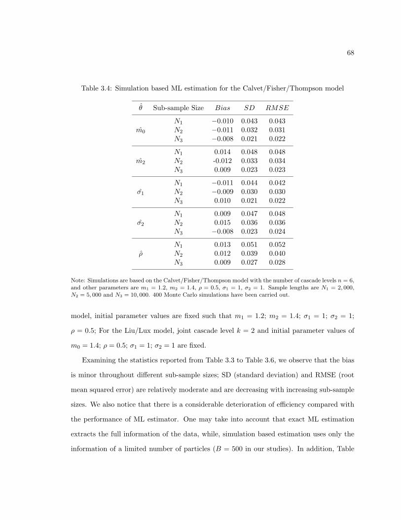
68

Table 3.4: Simulation based ML estimation for the Calvet/Fisher/Thompson model


N1 −0.010 0.043 0.043m0 N2 −0.011 0.032 0.031

N3 −0.008 0.021 0.022

N1 0.014 0.048 0.048m2 N2 -0.012 0.033 0.034

N3 0.009 0.023 0.023

N1 −0.011 0.044 0.042σ1 N2 −0.009 0.030 0.030

N3 0.010 0.021 0.022

N1 0.009 0.047 0.048σ2 N2 0.015 0.036 0.036

N3 −0.008 0.023 0.024

N1 0.013 0.051 0.052ρ N2 0.012 0.039 0.040

N3 0.009 0.027 0.028


model, initial parameter values are fixed such that m1 = 1.2; m2 = 1.4; σ1 = 1; σ2 = 1;

ρ = 0.5; For the Liu/Lux model, joint cascade level k = 2 and initial parameter values of

m0 = 1.4; ρ = 0.5; σ1 = 1; σ2 = 1 are fixed.

Examining the statistics reported from Table 3.3 to Table 3.6, we observe that the bias

is minor throughout different sub-sample sizes; SD (standard deviation) and RMSE (root

mean squared error) are relatively moderate and are decreasing with increasing sub-sample

sizes. We also notice that there is a considerable deterioration of efficiency compared with

the performance of ML estimator. One may take into account that exact ML estimation

extracts the full information of the data, while, simulation based estimation uses only the

information of a limited number of particles (B = 500 in our studies). In addition, Table

69

3.4 and Table 3.6 involve a higher cascade level of n = 6 (Table 3.1 and Table 3.2 using

n = 5). One extra point of the empirical issue is that, simulation based maximum likelihood

estimation (particle filter) is still not very economic in terms of its computation time; for

example, it costs 112 hours to execute the Monte Carlo experiment in Table 3.6.

Table 3.5: Simulation based ML estimation for the Liu/Lux model


N1 0.013 0.039 0.041m1 N2 -0.010 0.031 0.030

N3 -0.009 0.020 0.019

N1 -0.010 0.041 0.041σ1 N2 0.019 0.028 0.029

N3 0.005 0.015 0.015

N1 0.014 0.041 0.041σ2 N2 0.010 0.028 0.028

N3 0.010 0.019 0.019

N1 0.013 0.040 0.039ρ N2 -0.011 0.027 0.028

N3 0.010 0.018 0.019

Note: Simulations are based on the Liu/Lux model with the number of cascade levels n = 5 and k = 2,other parameters are m0 = 1.4, ρ = 0.5, σ1 = 1, σ2 = 1. Sample lengths are N1 = 2, 000, N2 = 5, 000 andN3 = 10, 000. 400 Monte Carlo simulations have been carried out.

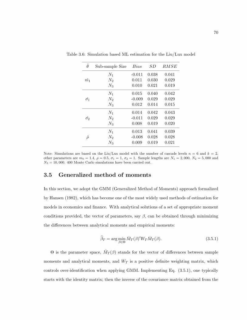
70

Table 3.6: Simulation based ML estimation for the Liu/Lux model


N1 -0.011 0.038 0.041m1 N2 0.011 0.030 0.029

N3 0.010 0.021 0.019

N1 0.015 0.040 0.042σ1 N2 -0.009 0.029 0.029

N3 0.012 0.014 0.015

N1 0.014 0.042 0.043σ2 N2 -0.011 0.029 0.029

N3 0.008 0.019 0.020

N1 0.013 0.041 0.039ρ N2 -0.008 0.028 0.028

N3 0.009 0.019 0.021

Note: Simulations are based on the Liu/Lux model with the number of cascade levels n = 6 and k = 2,other parameters are m0 = 1.4, ρ = 0.5, σ1 = 1, σ2 = 1. Sample lengths are N1 = 2, 000, N2 = 5, 000 andN3 = 10, 000. 400 Monte Carlo simulations have been carried out.

3.5 Generalized method of moments

In this section, we adopt the GMM (Generalized Method of Moments) approach formalized

by Hansen (1982), which has become one of the most widely used methods of estimation for

models in economics and finance. With analytical solutions of a set of appropriate moment

conditions provided, the vector of parameters, say β, can be obtained through minimizing

the differences between analytical moments and empirical moments:

βT = arg minβ∈Θ

MT (β)′WT MT (β). (3.5.1)

Θ is the parameter space, MT (β) stands for the vector of differences between sample

moments and analytical moments, and WT is a positive definite weighting matrix, which

controls over-identification when applying GMM. Implementing Eq. (3.5.1), one typically

starts with the identity matrix; then the inverse of the covariance matrix obtained from the

71

first round estimation is used as the weighting matrix in the next step; and this procedure

continues until the estimates converge. Advocated by Newey and West (1987), the weighting

matrix is estimated by the Bartlett kernel using a fixed lag length of 12×(N/100)0.25 with N

being the sample size (we found the arbitrary choice of the lag length is not much sensitive

in our studies).

As is well-known, βT is consistent and asymptotically Normal if suitable ‘regularity

conditions’ are fulfilled (sets of which are detailed, for example, in Harris and Matyas

(1999)). βT then converges to

T 1/2(βT − β0) ∼ N(0,Ξ), (3.5.2)

with covariance matrix Ξ = (F ′T V−1T FT )−1 in which β0 is the true parameter vector,

V −1T = TvarMT (β) is the covariance matrix of the moment conditions, FT (β) = ∂MT (β)

∂β is

the matrix of first derivatives of the moment conditions, and VT and FT are the constant

limiting matrices to which VT and FT converge.

Hansen (1982) also develops the J-statistic, which refers to the value of the GMM objec-

tive function evaluated using an efficient GMM estimator J = J(β(W−1),W−1), aiming to

verify whether over-identification exists. Let K, L denote the number of moment conditions

used and the number of parameters to be estimated, in a well specified over-identified model

with valid moment conditions, the J-statistic behaves like a chi-square random variable with

degrees of freedom equal to the number of over-identifying restrictions (for K > L):

J ∼ χ2(K − L). (3.5.3)

Hence, if the model is mis-specified, the J-statistic will be large relative to a chi-square

random variable with K − L degree of freedom.

The applicability of GMM to multifractal models and the detailed regularity conditions

have been discussed by Lux (2008). Markov-Switching multifractal models do not obey the

72

traditional definition of long memory, i.e. asymptotic power-law behavior of autocovari-

ance functions in the limit t → ∞ or divergence of the spectral density at zero, see Beran

(1994), and they are rather characterized by only ‘apparent’ long-memory with an asymp-

totic hyperbolic decline of the auto-correlation of absolute powers over a finite horizon and

exponential decline thereafter. Although the applicability of GMM is not hampered by this

type of “long memory on a bounded interval”, the proximity to ‘true’ long memory might

rise practical concerns. In particular, if a larger cascade level is employed, say k = 15, the

extent of the power law might exceed the size of most available daily financial data. In finite

samples, application of GMM to the multifractal models could yield inferior results since

usual estimates of the covariance matrix VT might show large pre-asymptotic variation.

We follow the practical solution in Lux (2008) by using the log differences of absolute

observations, together with the pertinent analytical moment conditions, i.e. transforming

the observed return data rt into τth log differences:

Xt,τ = ln |r1,t| − ln |r1,t−τ |

=

(0.5

k∑i=1

ε(i)1,t + 0.5

n∑j=k+1

ε(j)1,t + ln|u1,t|

)−

(0.5

k∑i=1

ε(i)1,t−τ + 0.5

n∑j=k+1

ε(j)1,t−τ + ln|u1,t−τ |

)

= 0.5k∑

i=1(ε(i)1,t − ε

(i)1,t−τ ) + 0.5

n∑j=k+1

(ε(j)1,t − ε(j)1,t−τ ) + (ln|u1,t| − ln|u1,t−τ |)

(3.5.4)

with ε(i)t = ln(M

(i)t

), and in the same way defining the second time series, say Yt,τ :

Yt,τ = ln |r2,t| − ln |r2,t−τ |

= 0.5k∑

i=1(ε(i)1,t − ε

(i)2,t−τ ) + 0.5

n∑j=k+1

(ε(j)2,t − ε(j)2,t−τ ) + (ln|u2,t| − ln|u2,t−τ |)

(3.5.5)

We recognize the transformation above excluding the scale parameters σ1 and σ2, while

estimating the scale parameters can be pursued by adding additional moment conditions

(e.g. unconditional moments of rt). In our practice, we use the second moment of empirical

73

data by considering each observation’s contribution to the standard deviation of the sample

returns.

Unlike maximum likelihood (ML) estimation, GMM does not require complete knowl-

edge of the distribution of the data, instead, only specified moment conditions derived from

an underlying model are needed. In order to exploit information from the bivariate mul-

tifractal models as much as possible, the moment conditions to be considered include two

groups: the first set of conditions is obtained by deriving the moments as in the univariate

time series (autocovariance), the second set considers the moment conditions for covariances

of Xt and Yt. In particular, we select moment conditions for the powers of Xt,τ and Yt,τ ,

i.e. moments of the raw transformed observations and squared transformed observations;

these two groups of moments are described as below:

Cov[Xt+τ,τ , Xt,τ ], Cov[Yt+τ,τ , Yt,τ ], Cov[X2t+τ,τ , X

2t,τ ], Cov[Y 2

t+τ,τ , Y2t,τ ];

and

Cov[Xt+τ,τ , Yt,τ ], Cov[Xt+τ,τ , Yt,τ ], Cov[X2t+τ,τ , Y

2t,τ ], Cov[X2

t+τ,τ , Y2t,τ ].

We focus on the time lag of τ = 1, and the detailed eight analytical moments solutions

of our bivariate MF model are given in the Appendix 7.1.6 We consider two particular

variants of multifractal processes, namely, one discrete version (Binomial model) and one

continuous version (Lognormal model).

3.5.1 Binomial model

Our bivariate binomial MF model is characterized by binomial random draws taking the

values of m0 (1 ≤ m0 ≤ 2) and 2 − m0 with equal probability. As in the combinatorial

setting, it is necessary to preserve the average mass of the interval [0, 1] during the evolution

of the cascade, thus preventing non-stationarity.6Moment conditions for τ > 1 (say, τ = 5, 10, 20) are cumbersome, and we leave them for future work.

74

We proceed by first applying our GMM approach to relatively small numbers of cas-

cade levels, and eight moment conditions as in Appendix 7.1 and two additional moment

conditions for the scale parameters (by considering each observation’s contribution to the

standard deviation). Monte Carlo studies were undertaken to compare the estimation per-

formances between GMM and the other two approaches we applied for bivariate MF models.

For the Liu/Lux model, by recalling Table 3.2 for maximum likelihood estimation, and Ta-

ble 3.6 for simulation based inference (particle filter), we use the same numbers of cascade

levels n = 5 and n = 6, and implement the estimations with initial parameters of m0 = 1.4;

σ1 = 1; σ2 = 1 and ρ = 0.5. For each scenario, 400 Monte Carlo simulations and estima-

tions were carried out, and there were 100,000 observations generated in each simulation;

subsequently three different sizes of sub-samples (N1 = 2000, N2 = 5000, and N3 = 10000)

were randomly selected for estimation. The performance is reported in Table 3.7.7

Monte Carlo studies were also carried out to demonstrate the performance of GMM es-

timator for the Calvet/Fisher/Thompson model. We simulated population sizes of 100, 000

with initial parameter values m1 = 1.2; m2 = 1.4; σ1 = 1; σ2 = 1; ρ = 0.5, and estimations

were conducted with respect to three different sub-sample sizes (N1 = 2000, N2 = 5000,

and N3 = 10000) randomly selected; eight moment conditions (detailed analytical solutions

for the Calvet/Fisher/Thompson model are given in the second section of the Appendix

7.2) and two additional moment conditions for the scale parameters are used. Table 3.8

presents the statistics of 400 simulations and estimations for the number of cascade level

n = 5 and n = 6, for the purpose of comparing with the performances of ML and simulated

ML with particle filter algorithm (in Table 3.1 and 3.4).

Looking through Table 3.7 and Table 3.8 (part n = 5), biases are moderate and ap-

proaching zero with increasing sub-sample sizes. In addition, we observe that there are

considerable distortions for small sample size (N1), but the performances are significantly7Studies on other randomized parameter values have also been pursued, we omit them here due to their

very similar results but keep the same parameter values as ones in the ML and SML estimations.

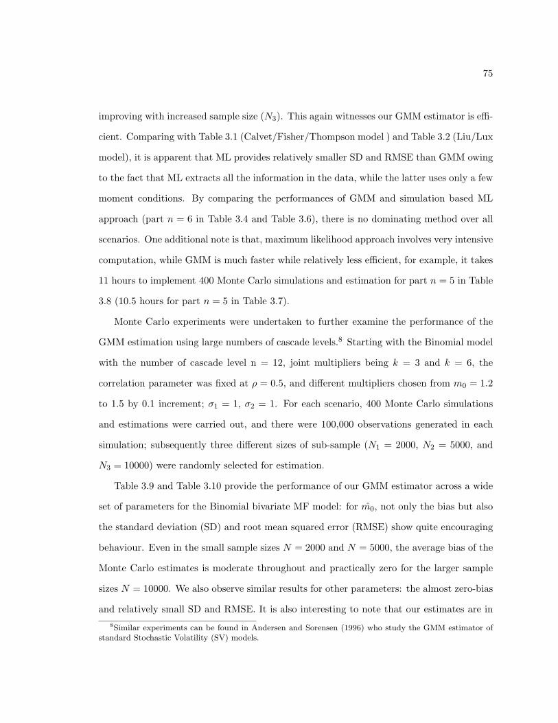
75

improving with increased sample size (N3). This again witnesses our GMM estimator is effi-

cient. Comparing with Table 3.1 (Calvet/Fisher/Thompson model ) and Table 3.2 (Liu/Lux

model), it is apparent that ML provides relatively smaller SD and RMSE than GMM owing

to the fact that ML extracts all the information in the data, while the latter uses only a few

moment conditions. By comparing the performances of GMM and simulation based ML

approach (part n = 6 in Table 3.4 and Table 3.6), there is no dominating method over all

scenarios. One additional note is that, maximum likelihood approach involves very intensive

computation, while GMM is much faster while relatively less efficient, for example, it takes

11 hours to implement 400 Monte Carlo simulations and estimation for part n = 5 in Table

3.8 (10.5 hours for part n = 5 in Table 3.7).

Monte Carlo experiments were undertaken to further examine the performance of the

GMM estimation using large numbers of cascade levels.8 Starting with the Binomial model

with the number of cascade level n = 12, joint multipliers being k = 3 and k = 6, the

correlation parameter was fixed at ρ = 0.5, and different multipliers chosen from m0 = 1.2

to 1.5 by 0.1 increment; σ1 = 1, σ2 = 1. For each scenario, 400 Monte Carlo simulations

and estimations were carried out, and there were 100,000 observations generated in each

simulation; subsequently three different sizes of sub-sample (N1 = 2000, N2 = 5000, and

N3 = 10000) were randomly selected for estimation.

Table 3.9 and Table 3.10 provide the performance of our GMM estimator across a wide

set of parameters for the Binomial bivariate MF model: for m0, not only the bias but also

the standard deviation (SD) and root mean squared error (RMSE) show quite encouraging

behaviour. Even in the small sample sizes N = 2000 and N = 5000, the average bias of the

Monte Carlo estimates is moderate throughout and practically zero for the larger sample

sizes N = 10000. We also observe similar results for other parameters: the almost zero-bias

and relatively small SD and RMSE. It is also interesting to note that our estimates are in8Similar experiments can be found in Andersen and Sorensen (1996) who study the GMM estimator of

standard Stochastic Volatility (SV) models.

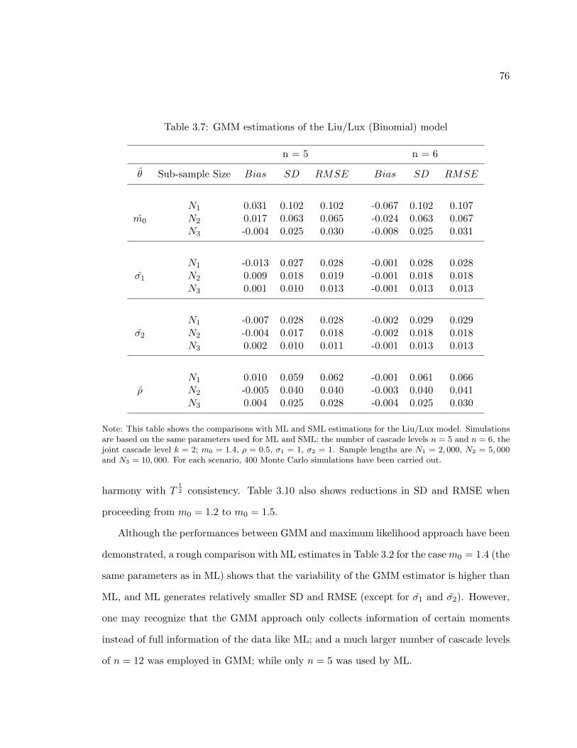
76

Table 3.7: GMM estimations of the Liu/Lux (Binomial) model

n = 5 n = 6

θ Sub-sample Size Bias SD RMSE Bias SD RMSE

N1 0.031 0.102 0.102 -0.067 0.102 0.107m0 N2 0.017 0.063 0.065 -0.024 0.063 0.067

N3 -0.004 0.025 0.030 -0.008 0.025 0.031

N1 -0.013 0.027 0.028 -0.001 0.028 0.028σ1 N2 0.009 0.018 0.019 -0.001 0.018 0.018

N3 0.001 0.010 0.013 -0.001 0.013 0.013

N1 -0.007 0.028 0.028 -0.002 0.029 0.029σ2 N2 -0.004 0.017 0.018 -0.002 0.018 0.018

N3 0.002 0.010 0.011 -0.001 0.013 0.013

N1 0.010 0.059 0.062 -0.001 0.061 0.066ρ N2 -0.005 0.040 0.040 -0.003 0.040 0.041

N3 0.004 0.025 0.028 -0.004 0.025 0.030

Note: This table shows the comparisons with ML and SML estimations for the Liu/Lux model. Simulationsare based on the same parameters used for ML and SML: the number of cascade levels n = 5 and n = 6, thejoint cascade level k = 2; m0 = 1.4, ρ = 0.5, σ1 = 1, σ2 = 1. Sample lengths are N1 = 2, 000, N2 = 5, 000and N3 = 10, 000. For each scenario, 400 Monte Carlo simulations have been carried out.

harmony with T12 consistency. Table 3.10 also shows reductions in SD and RMSE when

proceeding from m0 = 1.2 to m0 = 1.5.

Although the performances between GMM and maximum likelihood approach have been

demonstrated, a rough comparison with ML estimates in Table 3.2 for the casem0 = 1.4 (the

same parameters as in ML) shows that the variability of the GMM estimator is higher than

ML, and ML generates relatively smaller SD and RMSE (except for σ1 and σ2). However,

one may recognize that the GMM approach only collects information of certain moments

instead of full information of the data like ML; and a much larger number of cascade levels

of n = 12 was employed in GMM; while only n = 5 was used by ML.

77

In addition, we also have witnessed each simulation and estimation over 400 iterations,

and they all ended up with convergence in all scenarios, (note that, there are certain cases of

non-convergence that occur in smaller sample size cases in Andersen and Sorensen (1996)

when studying the GMM estimator of the SV model). We recognize there is a limited

number of parameters estimated within the multifractal processes, and fixing of constant

parameters in the transition probability (e.g. b= 2) that might be responsible for a relatively

decent performance in the small sample (N = 2000) exercises. Nevertheless, all these results

can be viewed as a positive indication of the log transformation in practice, furthermore,

we can also see that there is almost no significant difference between k = 3 (Table 3.9)

and k = 6 (Table 3.10); the very slight sensitivity of the estimates of m0 with respect to

the number of joint cascades might even be viewed as a very welcome phenomenon since

it implies that the estimation is barely affected by the potential mis-specification of joint

cascade level k.

We also check the performance of Hansen’s J test to examine the issue of over-identification.

Our Monte Carlo simulation setting is ideal for an investigation of the standard χ2 test for

goodness of fit of the over-identification problem. We calculate the χ2 test statistic and

evaluate the associate p value in the appropriate χ2(K − L) distribution. The findings are

qualitatively similar across different scenarios, so, for the sake of brevity, we present only

one case of m0 = 1.3. Figure 3.4 displays the fraction of p values that fall within the 2%

interval fractiles for different sample sizes. The three graphs from top to bottom correspond

to three different sample sizes: N1 = 2, 000, N2 = 5, 000 and N3 = 10, 000. We observe

that increasing the sample size leads to a leftward shift in the entire distribution. Indeed,

the leftward shifting suggests that the size distortion of the χ2 test statistic is growing as

the sample size expands. In particular, the fractiles from 1% to 10% shed light on the size

of these goodness-of-fit test from the asymptotic 1% to 10% levels, and the mass located in

these fractiles increases.

78

Table 3.8: GMM estimation of the Calvet/Fisher/Thompson model

n = 5 n = 6


N1 0.037 0.110 0.118 0.017 0.126 0.134m1 N2 -0.015 0.085 0.091 -0.010 0.090 0.096

N3 0.006 0.062 0.067 -0.007 0.060 0.068

N1 0.054 0.130 0.137 -0.050 0.136 0.144m2 N2 -0.025 0.084 0.089 0.033 0.104 0.108

N3 -0.012 0.058 0.062 0.004 0.058 0.062

N1 0.021 0.108 0.117 -0.040 0.116 0.124σ1 N2 -0.029 0.083 0.088 -0.036 0.080 0.084

N3 0.016 0.050 0.053 -0.010 0.051 0.053

N1 -0.033 0.093 0.098 0.031 0.100 0.106σ2 N2 -0.015 0.063 0.068 -0.017 0.066 0.070

N3 0.009 0.025 0.028 -0.009 0.024 0.027

N1 0.024 0.105 0.117 -0.038 0.116 0.123ρ N2 0.010 0.074 0.079 0.030 0.081 0.086

N3 -0.004 0.046 0.049 0.011 0.050 0.054

Note: This table shows the comparisons with ML and SML estimation for the Calvet/Fisher/Thompsonmodel. Simulations are based on the same parameters used for ML and SML: the number of cascade levelsn = 5 and n = 6; m1 = 1.2, m2 = 1.4, ρ = 0.5, σ1 = 1, σ2 = 1. Sample lengths are N1 = 2, 000, N2 = 5, 000and N3 = 10, 000. For each scenario, 400 Monte Carlo simulations have been carried out.

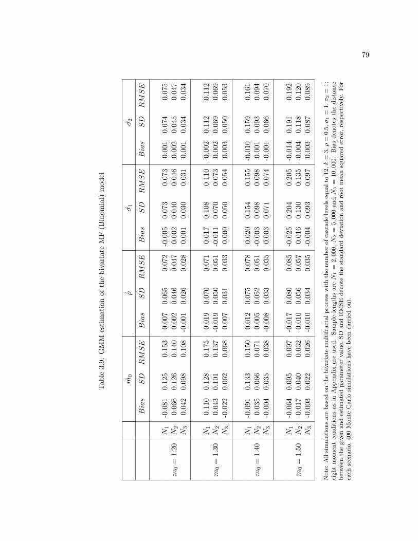
79

Tab

le3.

9:G

MM

esti

mat

ion

ofth

ebi

vari

ate

MF

(Bin

omia

l)m

odel

m0

ρσ

1σ

2

Bias

SD

RMSE

Bias

SD

RMSE

Bias

SD

RMSE

Bias

SD

RMSE

N1

-0.0

810.

125

0.15

30.

007

0.06

50.

072

-0.0

050.

073

0.07

30.

001

0.07

40.

075

m0

=1.

20N

20.

066

0.12

60.

140

0.00

20.

046

0.04

70.

002

0.04

00.

046

0.00

20.

045

0.04

7N

30.

042

0.09

80.

108

-0.0

010.

026

0.02

80.

001

0.03

00.

031

0.00

10.

034

0.03

4

N1

0.11

00.

128

0.17

50.

019

0.07

00.

071

0.01

70.

108

0.11

0-0

.002

0.11

20.

112

m0

=1.

30N

20.

043

0.10

10.

137

-0.0

190.

050

0.05

1-0

.011

0.07

00.

073

0.00

20.

069

0.06

9N

3-0

.022

0.06

20.

068

0.00

70.

031

0.03

30.

000

0.05

00.

054

0.00

30.

050

0.05

3

N1

-0.0

910.

133

0.15

00.

012

0.07

50.

078

0.02

00.

154

0.15

5-0

.010

0.15

90.

161

m0

=1.

40N

20.

035

0.06

60.

071

0.00

50.

052

0.05

1-0

.003

0.09

80.

098

0.00

10.

093

0.09

4N

3-0

.004

0.03

50.

038

-0.0

080.

033

0.03

50.

003

0.07

10.

074

-0.0

010.

066

0.07

0

N1

-0.0

640.

095

0.09

7-0

.017

0.08

00.

085

-0.0

250.

204

0.20

5-0

.014

0.19

10.

192

m0

=1.

50N

2-0

.017

0.04

00.

032

-0.0

100.

056

0.05

70.

016

0.13

00.

135

-0.0

040.

118

0.12

0N

3-0

.003

0.02

20.

026

-0.0

100.

034

0.03

5-0

.004

0.09

30.

097

0.00

30.

087

0.08

9

Note

:A

llsi

mula

tions

are

base

don

the

biv

ari

ate

mult

ifra

ctalpro

cess

wit

hth

enum

ber

ofca

scade

level

seq

ualto

12,k

=3,ρ

=0.5

,σ

1=

1,σ

2=

1;

eight

mom

ent

condit

ions

as

inA

ppen

dix

are

use

d.

Sam

ple

length

sare

N1

=2,0

00,

N2

=5,0

00

and

N3

=10,0

00.

Bia

sden

ote

sth

edis

tance

bet

wee

nth

egiv

enand

esti

mate

dpara

met

erva

lue,

SD

and

RM

SE

den

ote

the

standard

dev

iati

on

and

root

mea

nsq

uare

der

ror,

resp

ecti

vel

y.For

each

scen

ari

o,400

Monte

Carl

osi

mula

tions

hav

ebee

nca

rrie

dout.

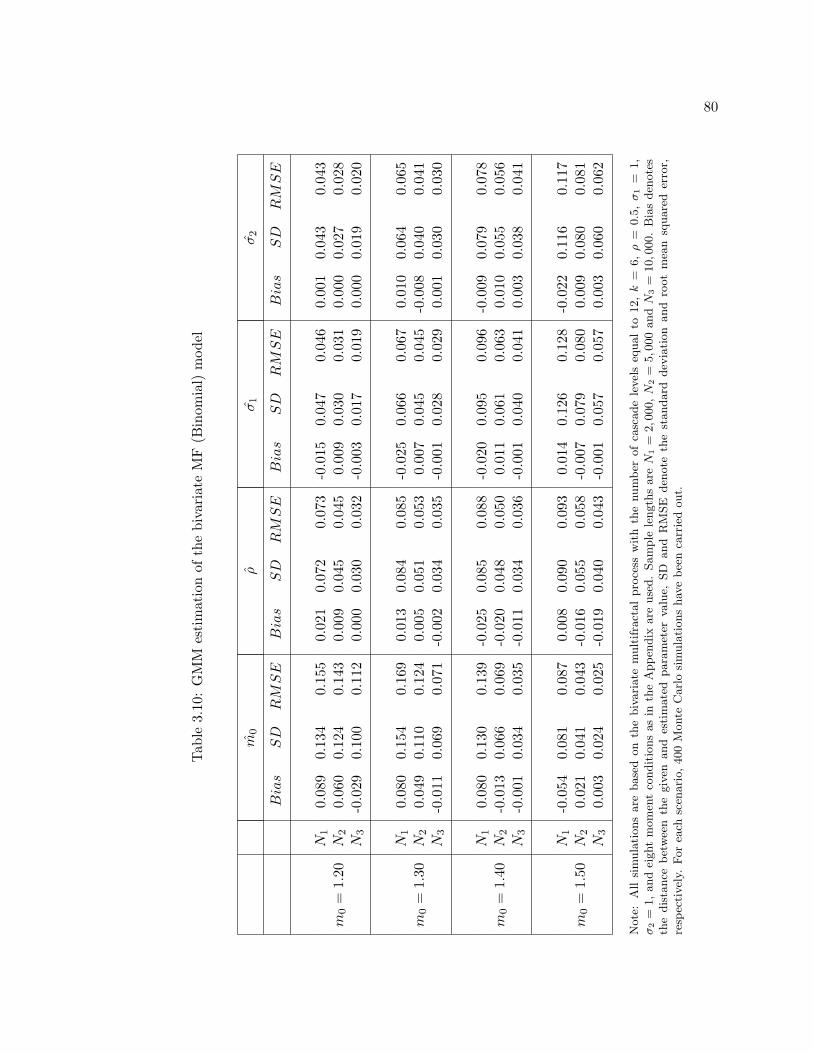
80

Tab

le3.

10:

GM

Mes

tim

atio

nof

the

biva

riat

eM

F(B

inom

ial)

mod

el

m0

ρσ

1σ

2

Bias

SD

RMSE

Bias

SD

RMSE

Bias

SD

RMSE

Bias

SD

RMSE

N1

0.08

90.

134

0.15

50.

021

0.07

20.

073

-0.0

150.

047

0.04

60.

001

0.04

30.

043

m0

=1.

20N

20.

060

0.12

40.

143

0.00

90.

045

0.04

50.

009

0.03

00.

031

0.00

00.

027

0.02

8N

3-0

.029

0.10

00.

112

0.00

00.

030

0.03

2-0

.003

0.01

70.

019

0.00

00.

019

0.02

0

N1

0.08

00.

154

0.16

90.

013

0.08

40.

085

-0.0

250.

066

0.06

70.

010

0.06

40.

065

m0

=1.

30N

20.

049

0.11

00.

124

0.00

50.

051

0.05

30.

007

0.04

50.

045

-0.0

080.

040

0.04

1N

3-0

.011

0.06

90.

071

-0.0

020.

034

0.03

5-0

.001

0.02

80.

029

0.00

10.

030

0.03

0

N1

0.08

00.

130

0.13

9-0

.025

0.08

50.

088

-0.0

200.

095

0.09

6-0

.009

0.07

90.

078

m0

=1.

40N

2-0

.013

0.06

60.

069

-0.0

200.

048

0.05

00.

011

0.06

10.

063

0.01

00.

055

0.05

6N

3-0

.001

0.03

40.

035

-0.0

110.

034

0.03

6-0

.001

0.04

00.

041

0.00

30.

038

0.04

1

N1

-0.0

540.

081

0.08

70.

008

0.09

00.

093

0.01

40.

126

0.12

8-0

.022

0.11

60.

117

m0

=1.

50N

20.

021

0.04

10.

043

-0.0

160.

055

0.05

8-0

.007

0.07

90.

080

0.00

90.

080

0.08

1N

30.

003

0.02

40.

025

-0.0

190.

040

0.04

3-0

.001

0.05

70.

057

0.00

30.

060

0.06

2

Note

:A

llsi

mula

tions

are

base

don

the

biv

ari

ate

mult

ifra

ctal

pro

cess

wit

hth

enum

ber

of

casc

ade

level

seq

ual

to12,

k=

6,

ρ=

0.5

,σ

1=

1,

σ2

=1,and

eight

mom

ent

condit

ions

as

inth

eA

ppen

dix

are

use

d.

Sam

ple

length

sare

N1

=2,0

00,N

2=

5,0

00

and

N3

=10,0

00.

Bia

sden

ote

sth

edis

tance

bet

wee

nth

egiv

enand

esti

mate

dpara

met

erva

lue,

SD

and

RM

SE

den

ote

the

standard

dev

iati

on

and

root

mea

nsq

uare

der

ror,

resp

ecti

vel

y.For

each

scen

ari

o,400

Monte

Carl

osi

mula

tions

hav

ebee

nca

rrie

dout.

81

3.5.2 Lognormal model

To accommodate our bivariate multifractal model with continuous distribution of volatility

components, we next turn to the Lognormal model. This means that when a new multiplier

Mt is needed at any cascade level, it will be determined via a random draw from a Lognormal

distribution with parameters λ and σm, i.e.,

−log2Mt ∼ N(λ, σ2m). (3.5.6)

We adopt the one used in Mandelbrot et al. (1997) by assigning E[M (i)t ] = 0.5 on the

Lognormal model (E[M (i)t ] = 1 is used in Lux (2008)).9 It implies:

exp[−λ ln 2 + 0.5σ2m(ln 2)2] = 0.5, (3.5.7)

which leads to

σ2m = 2(λ− 1)/ln2, (3.5.8)

Hence, we end up with a one-parameter family of multifractal models as in the Bino-

mial case. Unlike the Binomial model, multifractal processes with continuous distribution

of volatility components imply an infinite dimension of the transitional matrix, and the

exact form of likelihood function can not be identified explicitly. Therefore, the maximum

likelihood approach is not applicable to the Lognormal model.10 GMM provides a solution

for estimating multifractal processes with continuous state spaces. Moment conditions for

the Lognormal model are given in Appendix. Note that the admissible parameter space for

the location parameter λ is λ ∈ [1,∞) where in the borderline case λ = 1 the volatility

process collapses to a constant (as m0 = 1 in Binomial model).

Analogously, the Calvet/Fisher/Thompson model can also be extended to the continuous

case by allowing two Lognormal distributions for the volatility components of the bivariate9To avoid the non-stationarity in the data generating process, a factor of 2n is multiplied for compensating

the mean of multipliers being 0.5.10Simulation based maximum likelihood could be applicable, and we leave it for future work.

82

multifractal processes, namely, −log2M1 ∼ N(λ1, σ2m1), and −log2M2 ∼ N(λ2, σ

2m2). We

have also derived the pertinent moment conditions in the Appendix.

The Monte Carlo study reported in Table 3.11 and Table 3.12, covers parameter values

λ = 1.10, 1.20, 1.30 and 1.40; σ1 = 1, σ2 = 1 and ρ = 0.5. The numbers of joint multiplier

levels, the population and sub-sample sizes are set as in the Binomial case above. As can be

seen, results are not too different from those obtained with the binomial BMF model: biases

are very close to zero again; SD and RMSE are moderate and decrease with increase in the

sub-sample size. We also observe the similar behaviour in the Calvet/Fisher/Thompson

(Lognormal) model, cf. Table 3.13. All in all, these results from both the Binomial and

Lognormal Monte Carlo simulations and estimations show that GMM works quite well for

the bivariate multifractal process, with both discrete and continuous state spaces.

We then examine Hansen’s J test for the bivariate Lognormal model. The case of

λ = 1.3 is presented due to the qualitative similarity across different scenarios. Figure 3.5

displays the fraction of p values that fall within the 2% interval fractiles. Three graphs from

top to bottom corresponding to three different sample sizes: N1 = 2, 000, N2 = 5, 000 and

N3 = 10, 000. We again observe that increasing the sample size leads to a leftward shift

within the entire distribution.

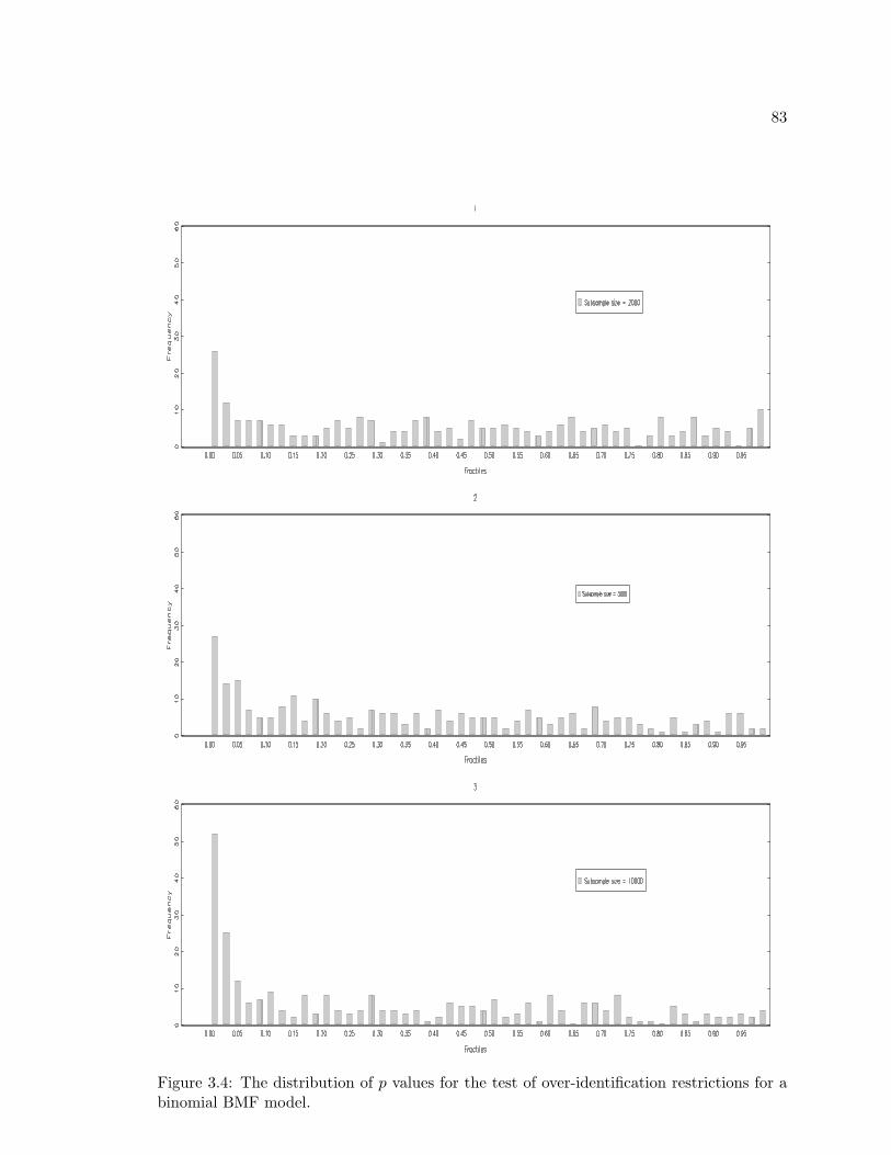
83

Figure 3.4: The distribution of p values for the test of over-identification restrictions for abinomial BMF model.

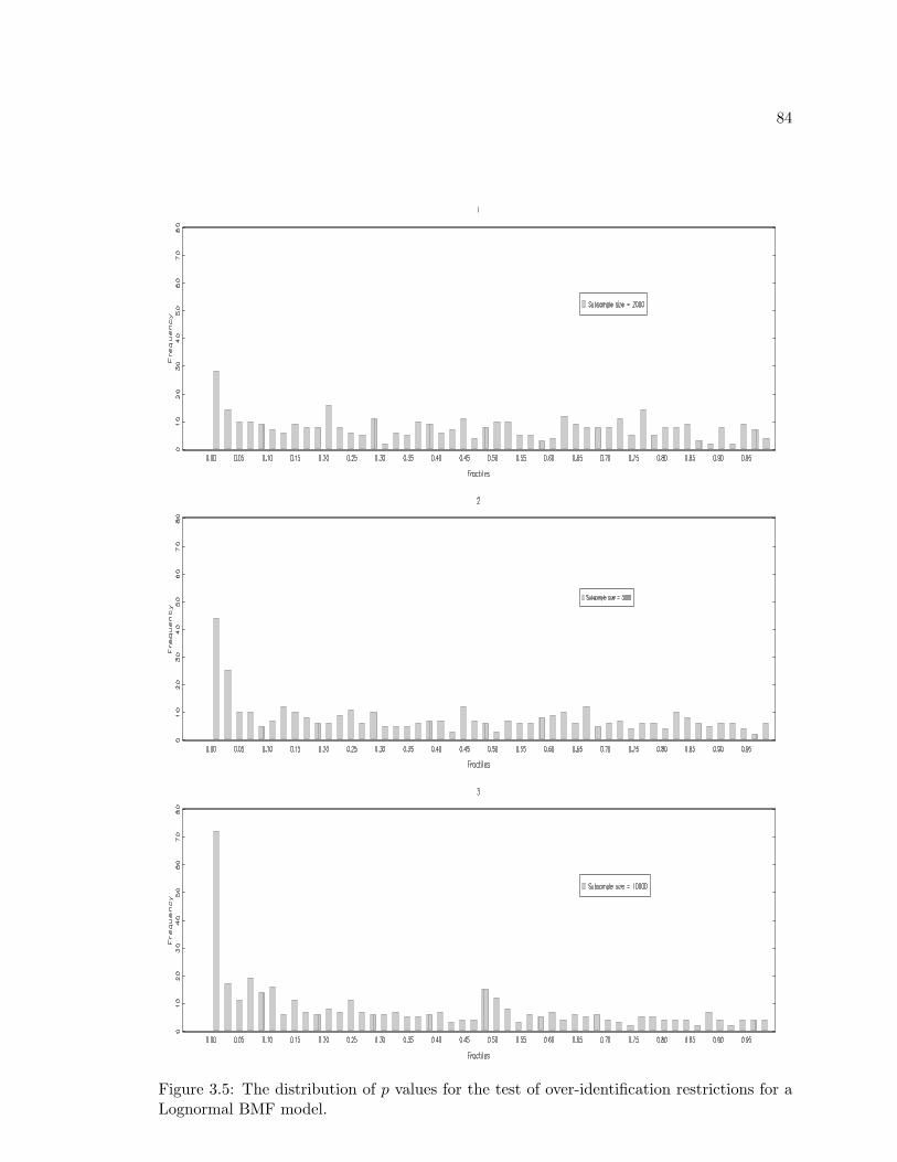
84

Figure 3.5: The distribution of p values for the test of over-identification restrictions for aLognormal BMF model.

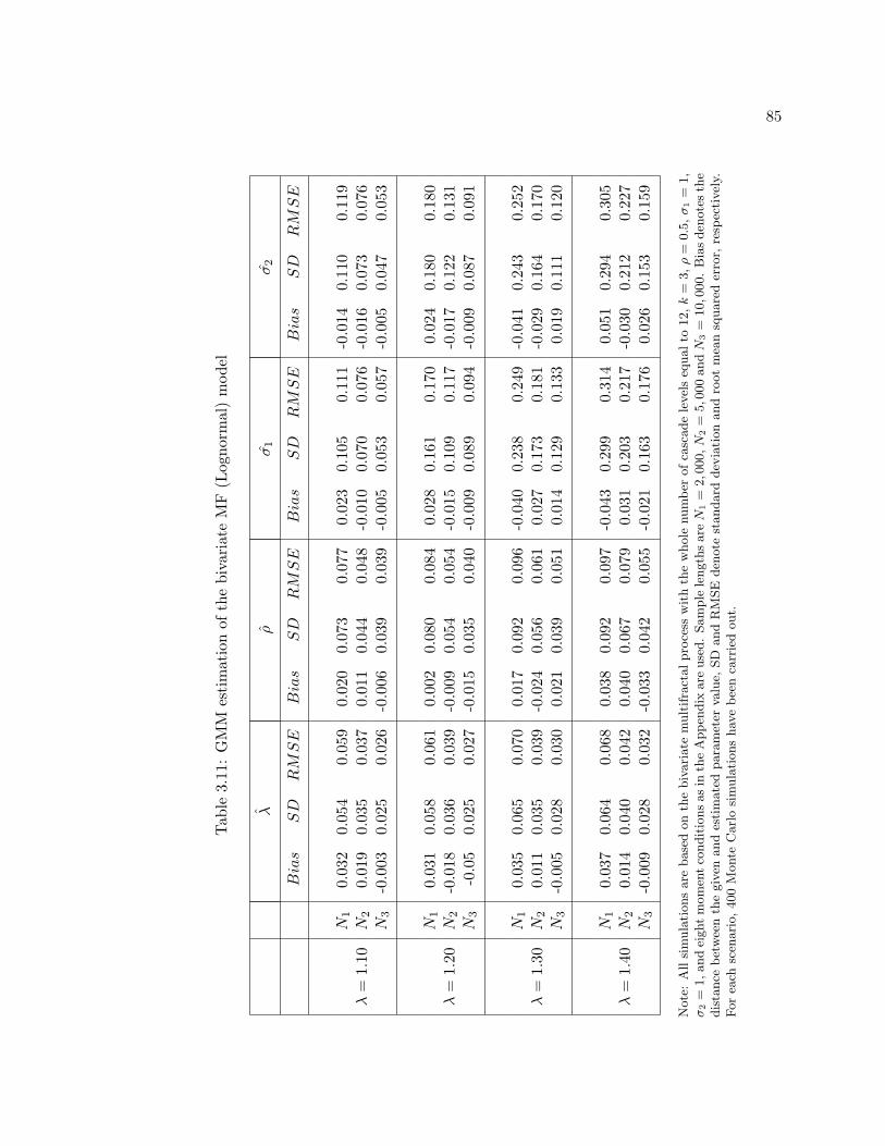
85

Tab

le3.

11:

GM

Mes

tim

atio

nof

the

biva

riat

eM

F(L

ogno

rmal

)m

odel

λρ

σ1

σ2

Bias

SD

RMSE

Bias

SD

RMSE

Bias

SD

RMSE

Bias

SD

RMSE

N1

0.03

20.

054

0.05

90.

020

0.07

30.

077

0.02

30.

105

0.11

1-0

.014

0.11

00.

119

λ=

1.10

N2

0.01

90.

035

0.03

70.

011

0.04

40.

048

-0.0

100.

070

0.07

6-0

.016

0.07

30.

076

N3

-0.0

030.

025

0.02

6-0

.006

0.03

90.

039

-0.0

050.

053

0.05

7-0

.005

0.04

70.

053

N1

0.03

10.

058

0.06

10.

002

0.08

00.

084

0.02

80.

161

0.17

00.

024

0.18

00.

180

λ=

1.20

N2

-0.0

180.

036

0.03

9-0

.009

0.05

40.

054

-0.0

150.

109

0.11

7-0

.017

0.12

20.

131

N3

-0.0

50.

025

0.02

7-0

.015

0.03

50.

040

-0.0

090.

089

0.09

4-0

.009

0.08

70.

091

N1

0.03

50.

065

0.07

00.

017

0.09

20.

096

-0.0

400.

238

0.24

9-0

.041

0.24

30.

252

λ=

1.30

N2

0.01

10.

035

0.03

9-0

.024

0.05

60.

061

0.02

70.

173

0.18

1-0

.029

0.16

40.

170

N3

-0.0

050.

028

0.03

00.

021

0.03

90.

051

0.01

40.

129

0.13

30.

019

0.11

10.

120

N1

0.03

70.

064

0.06

80.

038

0.09

20.

097

-0.0

430.

299

0.31

40.

051

0.29

40.

305

λ=

1.40

N2

0.01

40.

040

0.04

20.

040

0.06

70.

079

0.03

10.

203

0.21

7-0

.030

0.21

20.

227

N3

-0.0

090.

028

0.03

2-0

.033

0.04

20.

055

-0.0

210.

163

0.17

60.

026

0.15

30.

159

Note

:A

llsi

mula

tions

are

base

don

the

biv

ari

ate

mult

ifra

ctalpro

cess

wit

hth

ew

hole

num

ber

ofca

scade

level

seq

ualto

12,k

=3,ρ

=0.5

,σ

1=

1,

σ2

=1,and

eightm

om

entco

ndit

ionsasin

the

Appen

dix

are

use

d.

Sam

ple

length

sare

N1

=2,0

00,N

2=

5,0

00

and

N3

=10,0

00.

Bia

sden

ote

sth

edis

tance

bet

wee

nth

egiv

enand

esti

mate

dpara

met

erva

lue,

SD

and

RM

SE

den

ote

standard

dev

iati

on

and

root

mea

nsq

uare

der

ror,

resp

ecti

vel

y.For

each

scen

ari

o,400

Monte

Carl

osi

mula

tions

hav

ebee

nca

rrie

dout.

86

Tab

le3.

12:

GM

Mes

tim

atio

nof

the

biva

riat

eM

F(L

ogno

rmal

)M

odel

λρ

σ1

σ2

Bias

SD

RMSE

Bias

SD

RMSE

Bias

SD

RMSE

Bias

SD

RMSE

N1

0.03

70.

054

0.06

0-0

.012

0.08

70.

087

0.01

90.

082

0.08

5-0

.010

0.08

50.

091

λ=

1.10

N2

0.01

40.

035

0.03

7-0

.009

0.04

70.

052

0.01

80.

050

0.05

4-0

.002

0.05

70.

061

N3

-0.0

030.

023

0.02

20.

009

0.03

60.

036

-0.0

040.

037

0.03

7-0

.005

0.03

00.

037

N1

-0.0

210.

057

0.06

40.

017

0.08

90.

089

0.02

80.

150

0.15

7-0

.022

0.14

00.

148

λ=

1.20

N2

0.01

50.

036

0.03

8-0

.012

0.05

00.

058

-0.0

130.

086

0.09

5-0

.009

0.08

00.

088

N3

-0.0

070.

025

0.02

50.

015

0.03

70.

042

-0.0

050.

071

0.07

1-0

.002

0.06

20.

069

N1

-0.0

180.

061

0.06

60.

037

0.10

40.

107

-0.0

140.

301

0.30

1-0

.031

0.20

50.

222

λ=

1.30

N2

0.01

00.

035

0.04

0-0

.030

0.05

50.

064

-0.0

090.

212

0.21

2-0

.023

0.13

50.

145

N3

0.01

10.

027

0.02

9-0

.022

0.04

40.

055

-0.0

080.

154

0.15

4-0

.015

0.08

90.

100

N1

-0.0

260.

067

0.07

1-0

.051

0.10

90.

115

0.03

40.

299

0.30

2-0

.046

0.29

10.

307

λ=

1.40

N2

-0.0

040.

041

0.04

30.

040

0.06

70.

078

-0.0

220.

216

0.21

7-0

.024

0.21

80.

230

N3

0.01

50.

028

0.03

3-0

.033

0.04

20.

062

0.01

90.

160

0.16

1-0

.013

0.17

60.

185

Note

:A

llsi

mula

tions

are

base

don

the

biv

ari

ate

mult

ifra

ctalpro

cess

wit

hth

ew

hole

num

ber

ofca

scade

level

seq

ualto

12,k

=6,ρ

=0.5

,σ

1=

1,

σ2

=1,and

eightm

om

entco

ndit

ionsasin

the

Appen

dix

are

use

d.

Sam

ple

length

sare

N1

=2,0

00,N

2=

5,0

00

and

N3

=10,0

00.

Bia

sden

ote

sth

edis

tance

bet

wee

nth

egiv

enand

esti

mate

dpara

met

erva

lue,

SD

and

RM

SE

den

ote

standard

dev

iati

on

and

root

mea

nsq

uare

der

ror,

resp

ecti

vel

y.For

each

scen

ari

o,400

Monte

Carl

osi

mula

tions

hav

ebee

nca

rrie

dout.

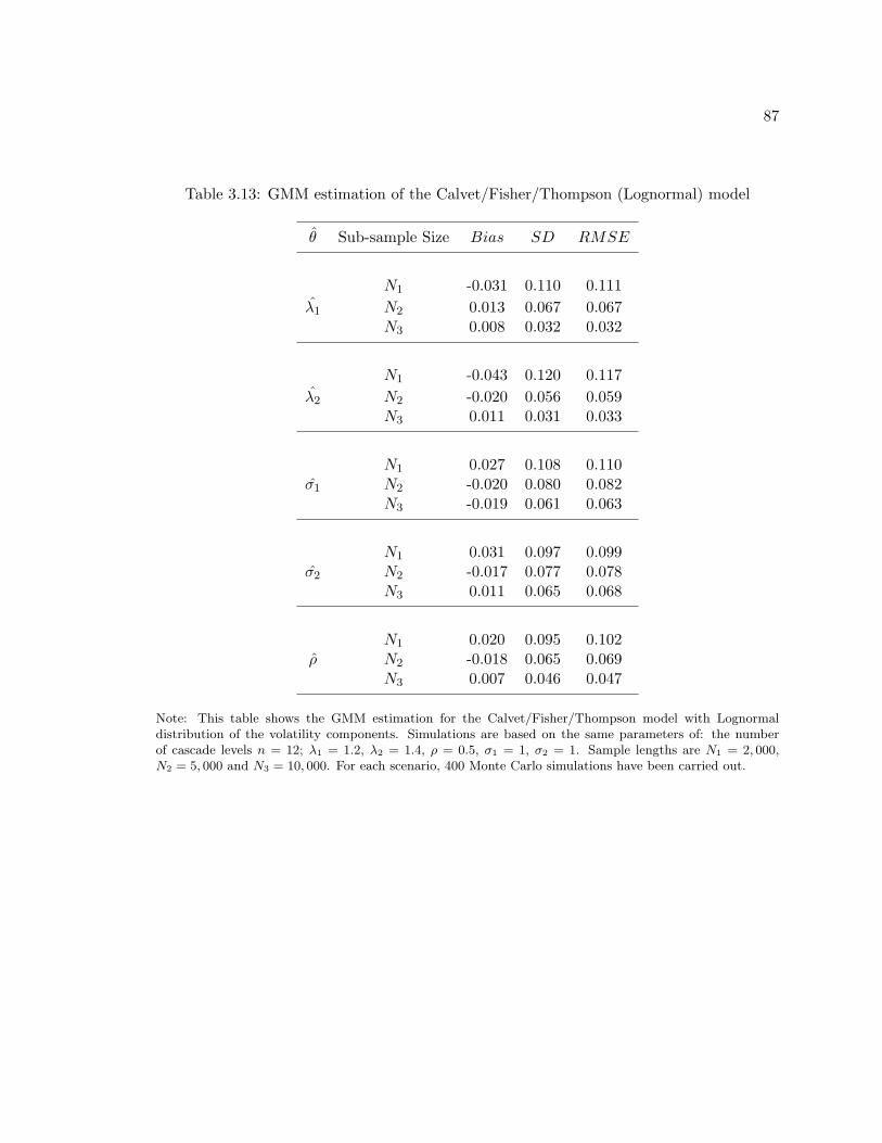
87

Table 3.13: GMM estimation of the Calvet/Fisher/Thompson (Lognormal) model


N1 -0.031 0.110 0.111λ1 N2 0.013 0.067 0.067

N3 0.008 0.032 0.032

N1 -0.043 0.120 0.117λ2 N2 -0.020 0.056 0.059

N3 0.011 0.031 0.033

N1 0.027 0.108 0.110σ1 N2 -0.020 0.080 0.082

N3 -0.019 0.061 0.063

N1 0.031 0.097 0.099σ2 N2 -0.017 0.077 0.078

N3 0.011 0.065 0.068

N1 0.020 0.095 0.102ρ N2 -0.018 0.065 0.069

N3 0.007 0.046 0.047

Note: This table shows the GMM estimation for the Calvet/Fisher/Thompson model with Lognormaldistribution of the volatility components. Simulations are based on the same parameters of: the numberof cascade levels n = 12; λ1 = 1.2, λ2 = 1.4, ρ = 0.5, σ1 = 1, σ2 = 1. Sample lengths are N1 = 2, 000,N2 = 5, 000 and N3 = 10, 000. For each scenario, 400 Monte Carlo simulations have been carried out.

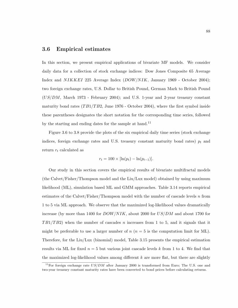
88

3.6 Empirical estimates

In this section, we present empirical applications of bivariate MF models. We consider

daily data for a collection of stock exchange indices: Dow Jones Composite 65 Average

Index and NIKKEI 225 Average Index (DOW/NIK, January 1969 - October 2004);

two foreign exchange rates, U.S. Dollar to British Pound, German Mark to British Pound

(US/DM , March 1973 - February 2004); and U.S. 1-year and 2-year treasury constant

maturity bond rates (TB1/TB2, June 1976 - October 2004), where the first symbol inside

these parentheses designates the short notation for the corresponding time series, followed

by the starting and ending dates for the sample at hand.11

Figure 3.6 to 3.8 provide the plots of the six empirical daily time series (stock exchange

indices, foreign exchange rates and U.S. treasury constant maturity bond rates) pt and

return rt calculated as

rt = 100× [ln(pt)− ln(pt−1)].

Our study in this section covers the empirical results of bivariate multifractal models

(the Calvet/Fisher/Thompson model and the Liu/Lux model) obtained by using maximum

likelihood (ML), simulation based ML and GMM approaches. Table 3.14 reports empirical

estimates of the Calvet/Fisher/Thompson model with the number of cascade levels n from

1 to 5 via ML approach. We observe that the maximized log-likelihood values dramatically

increase (by more than 1400 for DOW/NIK, about 2000 for US/DM and about 1700 for

TB1/TB2) when the number of cascades n increases from 1 to 5, and it signals that it

might be preferable to use a larger number of n (n = 5 is the computation limit for ML).

Therefore, for the Liu/Lux (binomial) model, Table 3.15 presents the empirical estimation

results via ML for fixed n = 5 but various joint cascade levels k from 1 to 4. We find that

the maximized log-likelihood values among different k are more flat, but there are slightly11For foreign exchange rate US/DM after January 2000 is transformed from Euro; The U.S. one and

two-year treasury constant maturity rates have been converted to bond prices before calculating returns.

89

higher values when k = 2 for DOW/NIK and TB1/TB2, k = 1 for US/DM .

Next, we move to the simulation based maximum likelihood estimation using particle

filter (with the number of particles of B = 500). Table 3.16 gives the empirical estimates of

the Calvet/Fisher/Thompson model with a choice of n = 8 as in Calvet et al. (2006). For

the Liu/Lux (binomial) model, Table 3.17 gives the empirical results for a range of joint

cascade levels k from 1 to 7 (n = 8). To specify an optimal choice of cascade levels for

different assets, we also provide a heuristic method as below:

(1) For each bivariate time series, we take its equal-weight portfolio, for an example of

DOW/NIK, the stock exchange portfolio is 0.5×DOW + 0.5×NIK.

(2) By using the GPH approach by Geweke and Porter-Hudak (1983) (see details in

Section 2.2.2), the empirical long memory estimator d for the absolute returns of equally-

weighted portfolio is calculated.

(3) Based on the empirical estimates with different numbers of cascade levels, 100 sim-

ulations are conducted for each asset; and long memory parameter d is calculated for each

simulated equally-weighted portfolio.

(4) We then select the case of the cascade level whose mean value of d is close to the

empirical GPH estimator d.

In Table 3.17, we find the case of k = 3 whose arithmetic mean of d is relatively close

to the empirical one for DOW/NIK, also k = 2 for US/DM and k = 5 for TB1/TB2

respectively.

Table 3.18 to Table 3.20 are GMM estimates of the Calvet/Fisher/Thompson model.

By using the specification method introduced above, we observe these cases which have

relatively close d to empirical ones: n = 10 for DOW/NIK, n = 12 for US/DM and

n = 10 for TB1/TB2.

For the GMM application to Liu/Lux models, we take the choices for the number of

cascade levers n obtained from the Calvet/Fisher/Thompson model as references. Let us

90

begin with the Binomial model, by fixing n = 10, Table 3.21 presents the empirical estimates

for the stock exchange indices (DOW/NIK) with different numbers of joint cascade levels

k from 1 to 9, as well as the corresponding mean values of simulated GPH estimator d.

We observe that the case of k = 4 (d = 0.249) has the relatively closest value of d to the

empirical one. Since it rather deviates from the empirical value of d = 0.295, we then try

large numbers of n in order to minimize this distance. Table 3.22 provides the empirical

results for a range of n from 5 to 20 with fixing k = 4, and we find that the case of n = 14

gives the closest value of d to the empirical GPH estimator. Table 3.23 reports the results

for the exchange rates US/DM for a range of joint cascade level of k from 1 to 11 (n = 12).

We find that the deviations between the simulated d and empirical one are within the

reasonable size and the case having close values of d to empirical one is k = 6. Table 3.24

gives GMM estimates of U.S. bond rates TB1/TB2 for various joint cascade levels k from

1 to 9 (n = 10), and we find that the cases having close values of d to empirical one are

k = 3 and k = 4.

Since GMM approach allows multifractal processes with continuous state space appli-

cable, we also have pursued the empirical studies for the Lognormal model introduced in

Section 3.5.2. Table 3.25 presents the empirical results for DOW/NIK with different num-

bers of joint cascade levels k from 1 to 9 (n = 10); like in the Binomial case, d at k = 4 is

comparatively close to the empirical one but with considerable deviation. Again, we also

report the empirical estimates for different numbers of cascade levels n from 5 to 20 but

fixing k = 4 in Table 3.26 and it suggests us an optimal choice of cascade levels for the stock

indices is n = 15. Table 3.27 gives the empirical results for the exchange rates US/DM

with different numbers of joint cascade levels k from 1 to 11 (n = 12); we observe the case

of k = 6 has a close value to empirical one. Table 3.28 reports the empirical estimates for

U.S. bond rates TB1/TB2 by fixing n = 10 but various numbers of joint cascade k from 1

to 9, and it provides that the case having close values of d to empirical ones is k = 3.

91

Figure 3.6: Empirical time series: Dow and Nik.

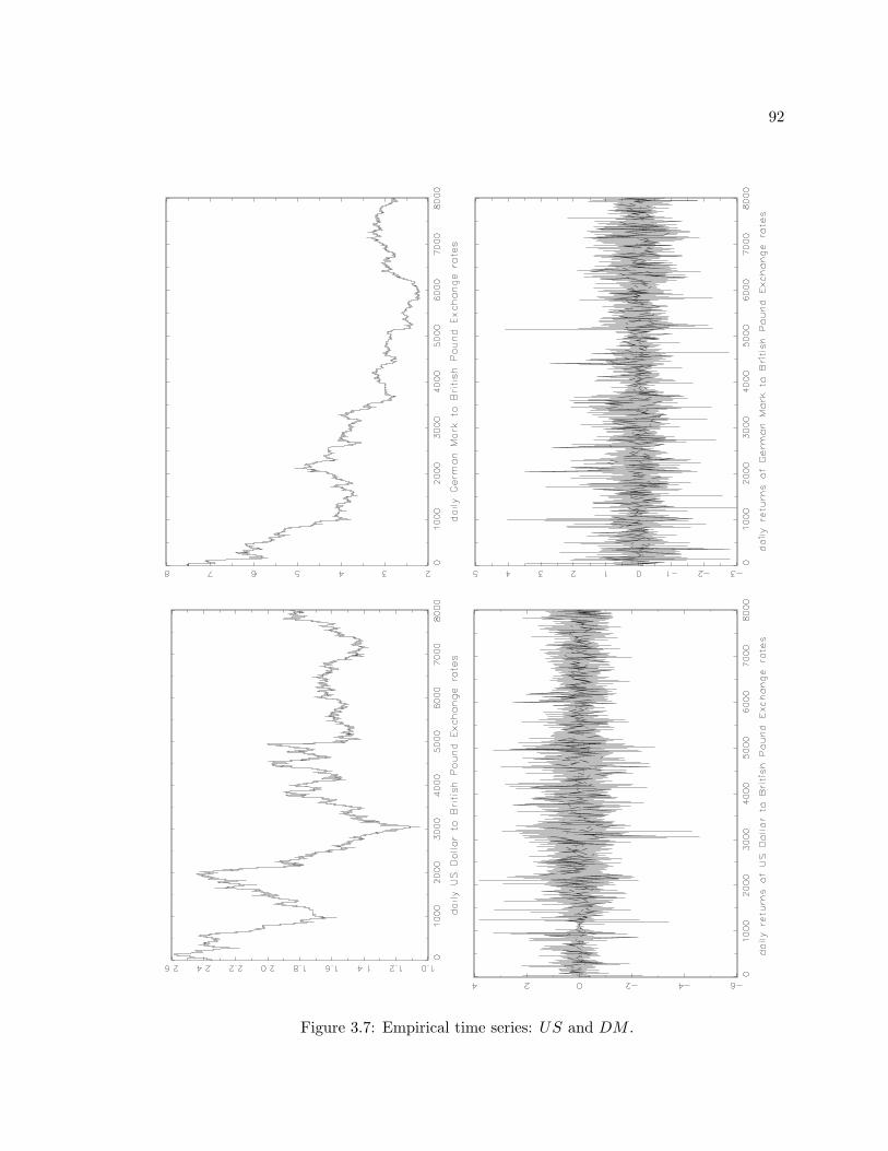
92

Figure 3.7: Empirical time series: US and DM .

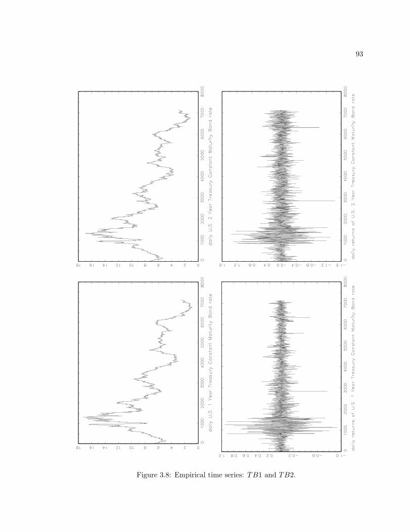
93

Figure 3.8: Empirical time series: TB1 and TB2.

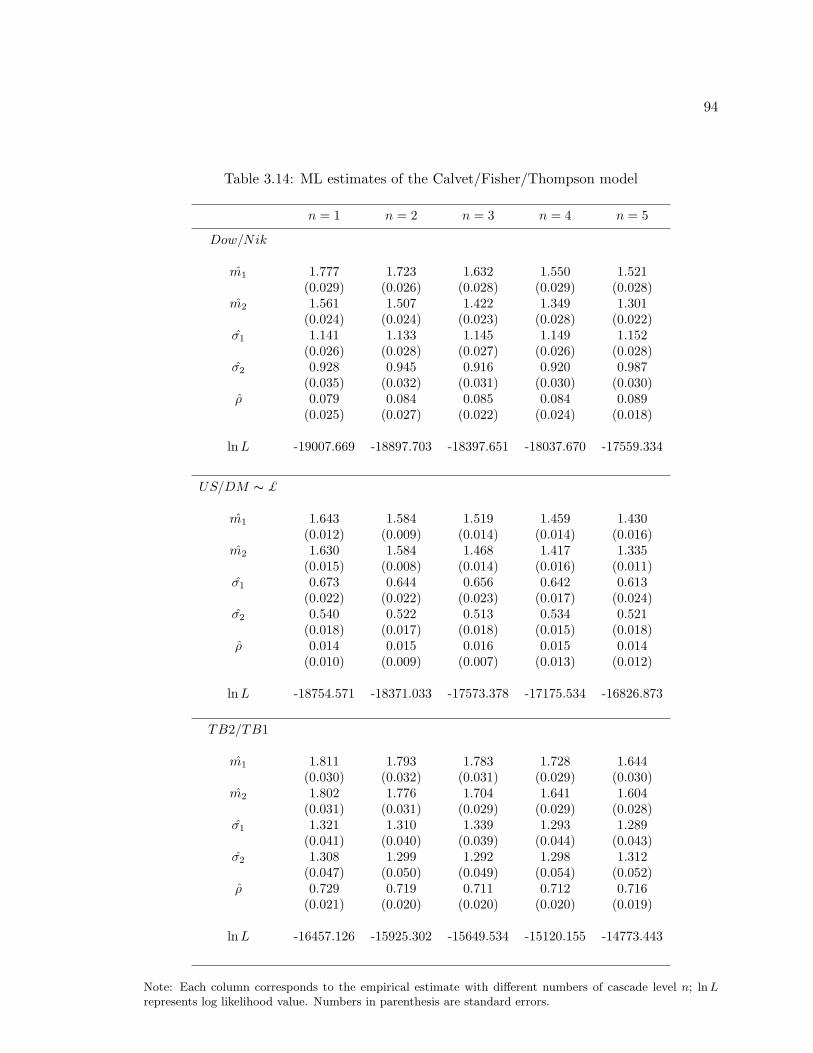
94

Table 3.14: ML estimates of the Calvet/Fisher/Thompson model

n = 1 n = 2 n = 3 n = 4 n = 5

Dow/Nik

m1 1.777 1.723 1.632 1.550 1.521(0.029) (0.026) (0.028) (0.029) (0.028)

m2 1.561 1.507 1.422 1.349 1.301(0.024) (0.024) (0.023) (0.028) (0.022)

σ1 1.141 1.133 1.145 1.149 1.152(0.026) (0.028) (0.027) (0.026) (0.028)

σ2 0.928 0.945 0.916 0.920 0.987(0.035) (0.032) (0.031) (0.030) (0.030)

ρ 0.079 0.084 0.085 0.084 0.089(0.025) (0.027) (0.022) (0.024) (0.018)

lnL -19007.669 -18897.703 -18397.651 -18037.670 -17559.334

US/DM ∼ £

m1 1.643 1.584 1.519 1.459 1.430(0.012) (0.009) (0.014) (0.014) (0.016)

m2 1.630 1.584 1.468 1.417 1.335(0.015) (0.008) (0.014) (0.016) (0.011)

σ1 0.673 0.644 0.656 0.642 0.613(0.022) (0.022) (0.023) (0.017) (0.024)

σ2 0.540 0.522 0.513 0.534 0.521(0.018) (0.017) (0.018) (0.015) (0.018)

ρ 0.014 0.015 0.016 0.015 0.014(0.010) (0.009) (0.007) (0.013) (0.012)

lnL -18754.571 -18371.033 -17573.378 -17175.534 -16826.873

TB2/TB1

m1 1.811 1.793 1.783 1.728 1.644(0.030) (0.032) (0.031) (0.029) (0.030)

m2 1.802 1.776 1.704 1.641 1.604(0.031) (0.031) (0.029) (0.029) (0.028)

σ1 1.321 1.310 1.339 1.293 1.289(0.041) (0.040) (0.039) (0.044) (0.043)

σ2 1.308 1.299 1.292 1.298 1.312(0.047) (0.050) (0.049) (0.054) (0.052)

ρ 0.729 0.719 0.711 0.712 0.716(0.021) (0.020) (0.020) (0.020) (0.019)

lnL -16457.126 -15925.302 -15649.534 -15120.155 -14773.443

Note: Each column corresponds to the empirical estimate with different numbers of cascade level n; ln Lrepresents log likelihood value. Numbers in parenthesis are standard errors.

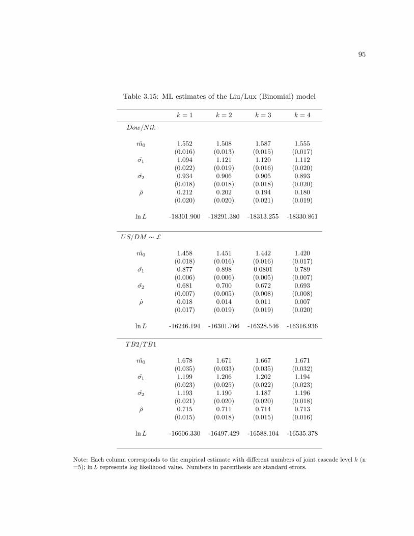
95

Table 3.15: ML estimates of the Liu/Lux (Binomial) model

k = 1 k = 2 k = 3 k = 4

Dow/Nik

m0 1.552 1.508 1.587 1.555(0.016) (0.013) (0.015) (0.017)

σ1 1.094 1.121 1.120 1.112(0.022) (0.019) (0.016) (0.020)

σ2 0.934 0.906 0.905 0.893(0.018) (0.018) (0.018) (0.020)

ρ 0.212 0.202 0.194 0.180(0.020) (0.020) (0.021) (0.019)

lnL -18301.900 -18291.380 -18313.255 -18330.861

US/DM ∼ £

m0 1.458 1.451 1.442 1.420(0.018) (0.016) (0.016) (0.017)

σ1 0.877 0.898 0.0801 0.789(0.006) (0.006) (0.005) (0.007)

σ2 0.681 0.700 0.672 0.693(0.007) (0.005) (0.008) (0.008)

ρ 0.018 0.014 0.011 0.007(0.017) (0.019) (0.019) (0.020)

lnL -16246.194 -16301.766 -16328.546 -16316.936

TB2/TB1

m0 1.678 1.671 1.667 1.671(0.035) (0.033) (0.035) (0.032)

σ1 1.199 1.206 1.202 1.194(0.023) (0.025) (0.022) (0.023)

σ2 1.193 1.190 1.187 1.196(0.021) (0.020) (0.020) (0.018)

ρ 0.715 0.711 0.714 0.713(0.015) (0.018) (0.015) (0.016)

lnL -16606.330 -16497.429 -16588.104 -16535.378

Note: Each column corresponds to the empirical estimate with different numbers of joint cascade level k (n=5); ln L represents log likelihood value. Numbers in parenthesis are standard errors.

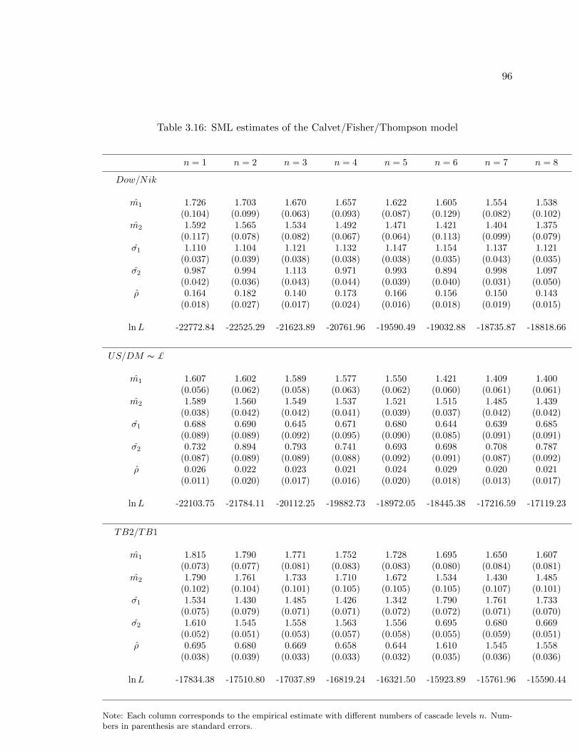
96

Table 3.16: SML estimates of the Calvet/Fisher/Thompson model

n = 1 n = 2 n = 3 n = 4 n = 5 n = 6 n = 7 n = 8

Dow/Nik

m1 1.726 1.703 1.670 1.657 1.622 1.605 1.554 1.538(0.104) (0.099) (0.063) (0.093) (0.087) (0.129) (0.082) (0.102)

m2 1.592 1.565 1.534 1.492 1.471 1.421 1.404 1.375(0.117) (0.078) (0.082) (0.067) (0.064) (0.113) (0.099) (0.079)

σ1 1.110 1.104 1.121 1.132 1.147 1.154 1.137 1.121(0.037) (0.039) (0.038) (0.038) (0.038) (0.035) (0.043) (0.035)

σ2 0.987 0.994 1.113 0.971 0.993 0.894 0.998 1.097(0.042) (0.036) (0.043) (0.044) (0.039) (0.040) (0.031) (0.050)

ρ 0.164 0.182 0.140 0.173 0.166 0.156 0.150 0.143(0.018) (0.027) (0.017) (0.024) (0.016) (0.018) (0.019) (0.015)

lnL -22772.84 -22525.29 -21623.89 -20761.96 -19590.49 -19032.88 -18735.87 -18818.66

US/DM ∼ £

m1 1.607 1.602 1.589 1.577 1.550 1.421 1.409 1.400(0.056) (0.062) (0.058) (0.063) (0.062) (0.060) (0.061) (0.061)

m2 1.589 1.560 1.549 1.537 1.521 1.515 1.485 1.439(0.038) (0.042) (0.042) (0.041) (0.039) (0.037) (0.042) (0.042)

σ1 0.688 0.690 0.645 0.671 0.680 0.644 0.639 0.685(0.089) (0.089) (0.092) (0.095) (0.090) (0.085) (0.091) (0.091)

σ2 0.732 0.894 0.793 0.741 0.693 0.698 0.708 0.787(0.087) (0.089) (0.089) (0.088) (0.092) (0.091) (0.087) (0.092)

ρ 0.026 0.022 0.023 0.021 0.024 0.029 0.020 0.021(0.011) (0.020) (0.017) (0.016) (0.020) (0.018) (0.013) (0.017)

lnL -22103.75 -21784.11 -20112.25 -19882.73 -18972.05 -18445.38 -17216.59 -17119.23

TB2/TB1

m1 1.815 1.790 1.771 1.752 1.728 1.695 1.650 1.607(0.073) (0.077) (0.081) (0.083) (0.083) (0.080) (0.084) (0.081)

m2 1.790 1.761 1.733 1.710 1.672 1.534 1.430 1.485(0.102) (0.104) (0.101) (0.105) (0.105) (0.105) (0.107) (0.101)

σ1 1.534 1.430 1.485 1.426 1.342 1.790 1.761 1.733(0.075) (0.079) (0.071) (0.071) (0.072) (0.072) (0.071) (0.070)

σ2 1.610 1.545 1.558 1.563 1.556 0.695 0.680 0.669(0.052) (0.051) (0.053) (0.057) (0.058) (0.055) (0.059) (0.051)

ρ 0.695 0.680 0.669 0.658 0.644 1.610 1.545 1.558(0.038) (0.039) (0.033) (0.033) (0.032) (0.035) (0.036) (0.036)

lnL -17834.38 -17510.80 -17037.89 -16819.24 -16321.50 -15923.89 -15761.96 -15590.44

Note: Each column corresponds to the empirical estimate with different numbers of cascade levels n. Num-bers in parenthesis are standard errors.

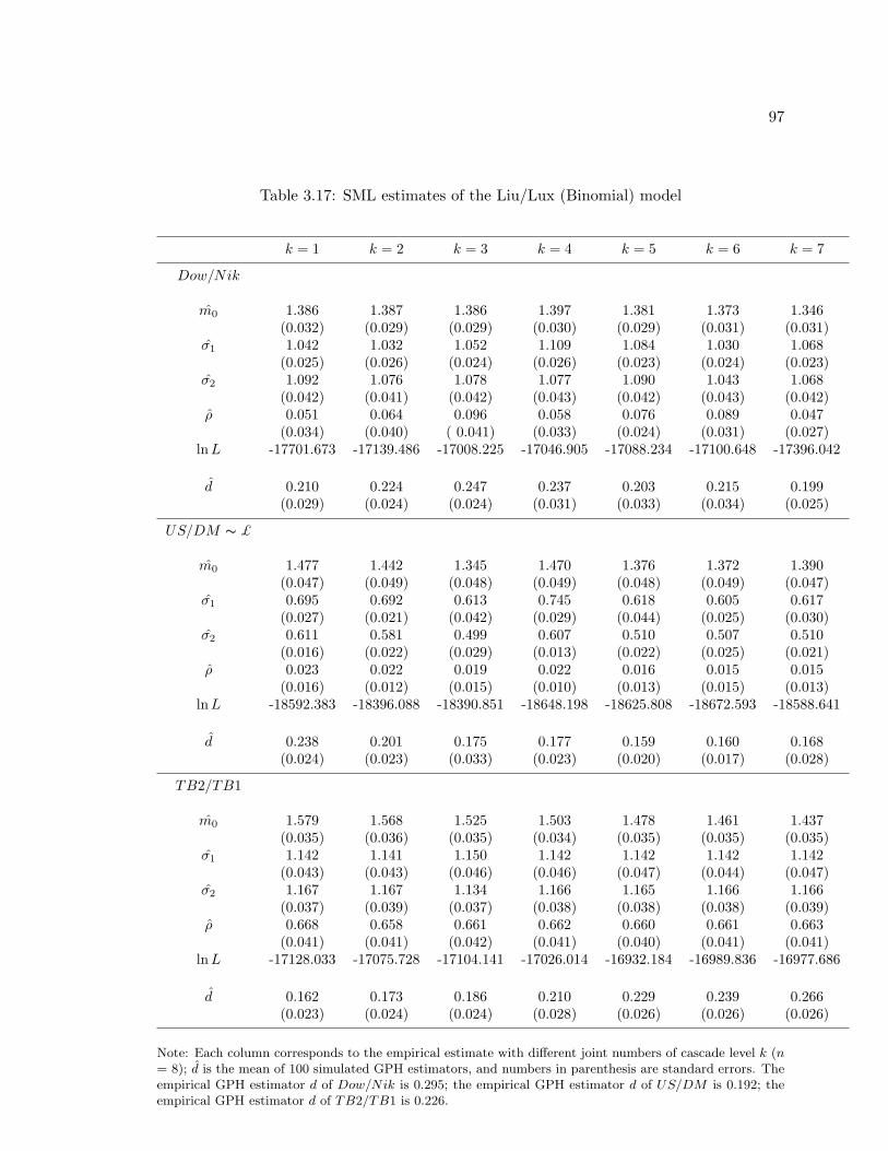
97

Table 3.17: SML estimates of the Liu/Lux (Binomial) model

k = 1 k = 2 k = 3 k = 4 k = 5 k = 6 k = 7

Dow/Nik

m0 1.386 1.387 1.386 1.397 1.381 1.373 1.346(0.032) (0.029) (0.029) (0.030) (0.029) (0.031) (0.031)

σ1 1.042 1.032 1.052 1.109 1.084 1.030 1.068(0.025) (0.026) (0.024) (0.026) (0.023) (0.024) (0.023)

σ2 1.092 1.076 1.078 1.077 1.090 1.043 1.068(0.042) (0.041) (0.042) (0.043) (0.042) (0.043) (0.042)

ρ 0.051 0.064 0.096 0.058 0.076 0.089 0.047(0.034) (0.040) ( 0.041) (0.033) (0.024) (0.031) (0.027)

lnL -17701.673 -17139.486 -17008.225 -17046.905 -17088.234 -17100.648 -17396.042

d 0.210 0.224 0.247 0.237 0.203 0.215 0.199(0.029) (0.024) (0.024) (0.031) (0.033) (0.034) (0.025)

US/DM ∼ £

m0 1.477 1.442 1.345 1.470 1.376 1.372 1.390(0.047) (0.049) (0.048) (0.049) (0.048) (0.049) (0.047)

σ1 0.695 0.692 0.613 0.745 0.618 0.605 0.617(0.027) (0.021) (0.042) (0.029) (0.044) (0.025) (0.030)

σ2 0.611 0.581 0.499 0.607 0.510 0.507 0.510(0.016) (0.022) (0.029) (0.013) (0.022) (0.025) (0.021)

ρ 0.023 0.022 0.019 0.022 0.016 0.015 0.015(0.016) (0.012) (0.015) (0.010) (0.013) (0.015) (0.013)

lnL -18592.383 -18396.088 -18390.851 -18648.198 -18625.808 -18672.593 -18588.641

d 0.238 0.201 0.175 0.177 0.159 0.160 0.168(0.024) (0.023) (0.033) (0.023) (0.020) (0.017) (0.028)

TB2/TB1

m0 1.579 1.568 1.525 1.503 1.478 1.461 1.437(0.035) (0.036) (0.035) (0.034) (0.035) (0.035) (0.035)

σ1 1.142 1.141 1.150 1.142 1.142 1.142 1.142(0.043) (0.043) (0.046) (0.046) (0.047) (0.044) (0.047)

σ2 1.167 1.167 1.134 1.166 1.165 1.166 1.166(0.037) (0.039) (0.037) (0.038) (0.038) (0.038) (0.039)

ρ 0.668 0.658 0.661 0.662 0.660 0.661 0.663(0.041) (0.041) (0.042) (0.041) (0.040) (0.041) (0.041)

lnL -17128.033 -17075.728 -17104.141 -17026.014 -16932.184 -16989.836 -16977.686

d 0.162 0.173 0.186 0.210 0.229 0.239 0.266(0.023) (0.024) (0.024) (0.028) (0.026) (0.026) (0.026)

Note: Each column corresponds to the empirical estimate with different joint numbers of cascade level k (n= 8); d is the mean of 100 simulated GPH estimators, and numbers in parenthesis are standard errors. Theempirical GPH estimator d of Dow/Nik is 0.295; the empirical GPH estimator d of US/DM is 0.192; theempirical GPH estimator d of TB2/TB1 is 0.226.

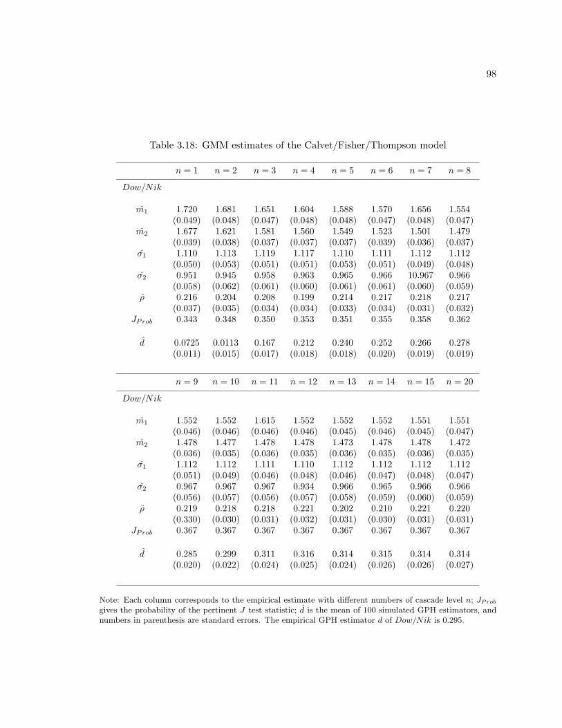
98

Table 3.18: GMM estimates of the Calvet/Fisher/Thompson model

n = 1 n = 2 n = 3 n = 4 n = 5 n = 6 n = 7 n = 8

Dow/Nik

m1 1.720 1.681 1.651 1.604 1.588 1.570 1.656 1.554(0.049) (0.048) (0.047) (0.048) (0.048) (0.047) (0.048) (0.047)

m2 1.677 1.621 1.581 1.560 1.549 1.523 1.501 1.479(0.039) (0.038) (0.037) (0.037) (0.037) (0.039) (0.036) (0.037)

σ1 1.110 1.113 1.119 1.117 1.110 1.111 1.112 1.112(0.050) (0.053) (0.051) (0.051) (0.053) (0.051) (0.049) (0.048)

σ2 0.951 0.945 0.958 0.963 0.965 0.966 10.967 0.966(0.058) (0.062) (0.061) (0.060) (0.061) (0.061) (0.060) (0.059)

ρ 0.216 0.204 0.208 0.199 0.214 0.217 0.218 0.217(0.037) (0.035) (0.034) (0.034) (0.033) (0.034) (0.031) (0.032)

JProb 0.343 0.348 0.350 0.353 0.351 0.355 0.358 0.362

d 0.0725 0.0113 0.167 0.212 0.240 0.252 0.266 0.278(0.011) (0.015) (0.017) (0.018) (0.018) (0.020) (0.019) (0.019)

n = 9 n = 10 n = 11 n = 12 n = 13 n = 14 n = 15 n = 20

Dow/Nik

m1 1.552 1.552 1.615 1.552 1.552 1.552 1.551 1.551(0.046) (0.046) (0.046) (0.046) (0.045) (0.046) (0.045) (0.047)

m2 1.478 1.477 1.478 1.478 1.473 1.478 1.478 1.472(0.036) (0.035) (0.036) (0.035) (0.036) (0.035) (0.036) (0.035)

σ1 1.112 1.112 1.111 1.110 1.112 1.112 1.112 1.112(0.051) (0.049) (0.046) (0.048) (0.046) (0.047) (0.048) (0.047)

σ2 0.967 0.967 0.967 0.934 0.966 0.965 0.966 0.966(0.056) (0.057) (0.056) (0.057) (0.058) (0.059) (0.060) (0.059)

ρ 0.219 0.218 0.218 0.221 0.202 0.210 0.221 0.220(0.330) (0.030) (0.031) (0.032) (0.031) (0.030) (0.031) (0.031)

JProb 0.367 0.367 0.367 0.367 0.367 0.367 0.367 0.367

d 0.285 0.299 0.311 0.316 0.314 0.315 0.314 0.314(0.020) (0.022) (0.024) (0.025) (0.024) (0.026) (0.026) (0.027)

Note: Each column corresponds to the empirical estimate with different numbers of cascade level n; JProb

gives the probability of the pertinent J test statistic; d is the mean of 100 simulated GPH estimators, andnumbers in parenthesis are standard errors. The empirical GPH estimator d of Dow/Nik is 0.295.

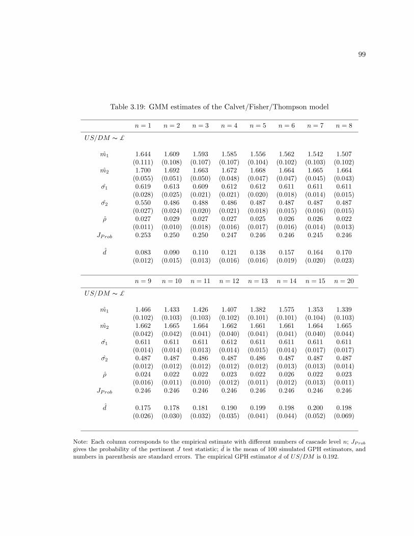
99


n = 1 n = 2 n = 3 n = 4 n = 5 n = 6 n = 7 n = 8

US/DM ∼ £

m1 1.644 1.609 1.593 1.585 1.556 1.562 1.542 1.507(0.111) (0.108) (0.107) (0.107) (0.104) (0.102) (0.103) (0.102)

m2 1.700 1.692 1.663 1.672 1.668 1.664 1.665 1.664(0.055) (0.051) (0.050) (0.048) (0.047) (0.047) (0.045) (0.043)

σ1 0.619 0.613 0.609 0.612 0.612 0.611 0.611 0.611(0.028) (0.025) (0.021) (0.021) (0.020) (0.018) (0.014) (0.015)

σ2 0.550 0.486 0.488 0.486 0.487 0.487 0.487 0.487(0.027) (0.024) (0.020) (0.021) (0.018) (0.015) (0.016) (0.015)

ρ 0.027 0.029 0.027 0.027 0.025 0.026 0.026 0.022(0.011) (0.010) (0.018) (0.016) (0.017) (0.016) (0.014) (0.013)

JProb 0.253 0.250 0.250 0.247 0.246 0.246 0.245 0.246

d 0.083 0.090 0.110 0.121 0.138 0.157 0.164 0.170(0.012) (0.015) (0.013) (0.016) (0.016) (0.019) (0.020) (0.023)

n = 9 n = 10 n = 11 n = 12 n = 13 n = 14 n = 15 n = 20

US/DM ∼ £

m1 1.466 1.433 1.426 1.407 1.382 1.575 1.353 1.339(0.102) (0.103) (0.103) (0.102) (0.101) (0.101) (0.104) (0.103)

m2 1.662 1.665 1.664 1.662 1.661 1.661 1.664 1.665(0.042) (0.042) (0.041) (0.040) (0.041) (0.041) (0.040) (0.044)

σ1 0.611 0.611 0.611 0.612 0.611 0.611 0.611 0.611(0.014) (0.014) (0.013) (0.014) (0.015) (0.014) (0.017) (0.017)

σ2 0.487 0.487 0.486 0.487 0.486 0.487 0.487 0.487(0.012) (0.012) (0.012) (0.012) (0.012) (0.013) (0.013) (0.014)

ρ 0.024 0.022 0.022 0.023 0.022 0.026 0.022 0.023(0.016) (0.011) (0.010) (0.012) (0.011) (0.012) (0.013) (0.011)

JProb 0.246 0.246 0.246 0.246 0.246 0.246 0.246 0.246

d 0.175 0.178 0.181 0.190 0.199 0.198 0.200 0.198(0.026) (0.030) (0.032) (0.035) (0.041) (0.044) (0.052) (0.069)


gives the probability of the pertinent J test statistic; d is the mean of 100 simulated GPH estimators, andnumbers in parenthesis are standard errors. The empirical GPH estimator d of US/DM is 0.192.

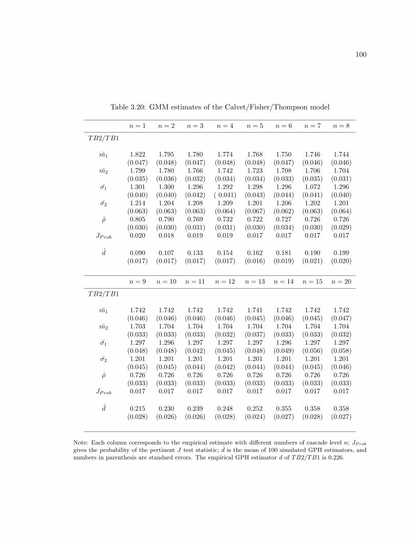
100


n = 1 n = 2 n = 3 n = 4 n = 5 n = 6 n = 7 n = 8

TB2/TB1

m1 1.822 1.795 1.780 1.774 1.768 1.750 1.746 1.744(0.047) (0.048) (0.047) (0.048) (0.048) (0.047) (0.046) (0.046)

m2 1.799 1.780 1.766 1.742 1.723 1.708 1.706 1.704(0.035) (0.036) (0.032) (0.034) (0.034) (0.033) (0.035) (0.031)

σ1 1.301 1.300 1.296 1.292 1.298 1.296 1.072 1.296(0.040) (0.040) (0.042) ( 0.041) (0.043) (0.044) (0.041) (0.040)

σ2 1.214 1.204 1.208 1.209 1.201 1.206 1.202 1.201(0.063) (0.063) (0.063) (0.064) (0.067) (0.062) (0.063) (0.064)

ρ 0.805 0.790 0.769 0.732 0.722 0.727 0.726 0.726(0.030) (0.030) (0.031) (0.031) (0.030) (0.034) (0.030) (0.029)

JProb 0.020 0.018 0.019 0.019 0.017 0.017 0.017 0.017

d 0.090 0.107 0.133 0.154 0.162 0.181 0.190 0.199(0.017) (0.017) (0.017) (0.017) (0.016) (0.019) (0.021) (0.020)

n = 9 n = 10 n = 11 n = 12 n = 13 n = 14 n = 15 n = 20

TB2/TB1

m1 1.742 1.742 1.742 1.742 1.741 1.742 1.742 1.742(0.046) (0.046) (0.046) (0.046) (0.045) (0.046) (0.045) (0.047)

m2 1.703 1.704 1.704 1.704 1.704 1.704 1.704 1.704(0.033) (0.033) (0.033) (0.032) (0.037) (0.033) (0.033) (0.032)

σ1 1.297 1.296 1.297 1.297 1.297 1.296 1.297 1.297(0.048) (0.048) (0.042) (0.045) (0.048) (0.049) (0.056) (0.058)

σ2 1.201 1.201 1.201 1.201 1.201 1.201 1.201 1.201(0.045) (0.045) (0.044) (0.042) (0.044) (0.044) (0.045) (0.046)

ρ 0.726 0.726 0.726 0.726 0.726 0.726 0.726 0.726(0.033) (0.033) (0.033) (0.033) (0.033) (0.033) (0.033) (0.033)

JProb 0.017 0.017 0.017 0.017 0.017 0.017 0.017 0.017

d 0.215 0.230 0.239 0.248 0.252 0.355 0.358 0.358(0.028) (0.026) (0.026) (0.028) (0.024) (0.027) (0.028) (0.027)


gives the probability of the pertinent J test statistic; d is the mean of 100 simulated GPH estimators, andnumbers in parenthesis are standard errors. The empirical GPH estimator d of TB2/TB1 is 0.226.

101

Table 3.21: GMM estimates of the Liu/Lux (Binomial) model

k = 1 k = 2 k = 3 k = 4 k = 5 k = 6 k = 7

Dow/Nik

m0 1.446 1.437 1.428 1.379 1.381 1.385 1.422(0.020) (0.021) (0.022) (0.022) (0.024) (0.025) (0.031)

σ1 1.144 1.126 1.123 1.121 1.120 1.120 1.119(0.034) (0.031) (0.031) (0.031) (0.030) (0.031) (0.029)

σ2 0.922 0.919 0.914 0.907 0.904 0.902 0.901(0.034) (0.030) (0.027) (0.024) (0.024) (0.022) (0.020)

ρ 0.204 0.193 0.202 0.196 0.199 0.207 0.202(0.015) (0.015) (0.013) (0.013) (0.012) (0.012) (0.011)

JProb 0.272 0.266 0.266 0.269 0.268 0.268 0.269

d 0.241 0.244 0.247 0.251 0.246 0.240 0.239(0.018) (0.021) (0.020) (0.018) (0.019) (0.018) (0.020)

k = 8 k = 9

Dow/Nik

m0 1.411 1.420(0.028) (0.028)

σ1 1.119 1.119(0.033) (0.034)

σ2 0.901 0.901(0.021) (0.021)

ρ 0.201 0.202(0.010) (0.010)

JProb 0.269 0.269

d 0.236 0.232(0.019) (0.019)

Note: Each column corresponds to the empirical estimate with different joint numbers of cascade level k(n = 10); JProb gives the probability of the pertinent J test statistic; d is the mean of 100 simulated GPHestimators, and numbers in parenthesis are standard errors. The empirical GPH estimator d of Dow/Nik is0.295.

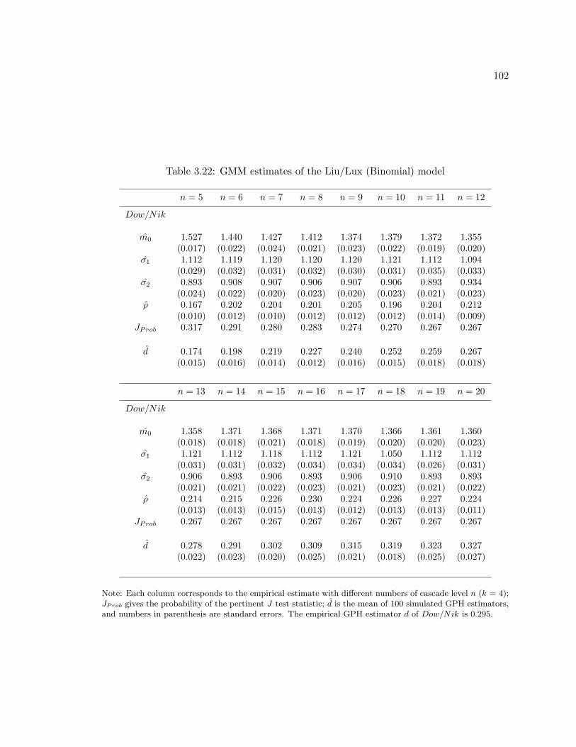
102


n = 5 n = 6 n = 7 n = 8 n = 9 n = 10 n = 11 n = 12

Dow/Nik

m0 1.527 1.440 1.427 1.412 1.374 1.379 1.372 1.355(0.017) (0.022) (0.024) (0.021) (0.023) (0.022) (0.019) (0.020)

σ1 1.112 1.119 1.120 1.120 1.120 1.121 1.112 1.094(0.029) (0.032) (0.031) (0.032) (0.030) (0.031) (0.035) (0.033)

σ2 0.893 0.908 0.907 0.906 0.907 0.906 0.893 0.934(0.024) (0.022) (0.020) (0.023) (0.020) (0.023) (0.021) (0.023)

ρ 0.167 0.202 0.204 0.201 0.205 0.196 0.204 0.212(0.010) (0.012) (0.010) (0.012) (0.012) (0.012) (0.014) (0.009)

JProb 0.317 0.291 0.280 0.283 0.274 0.270 0.267 0.267

d 0.174 0.198 0.219 0.227 0.240 0.252 0.259 0.267(0.015) (0.016) (0.014) (0.012) (0.016) (0.015) (0.018) (0.018)

n = 13 n = 14 n = 15 n = 16 n = 17 n = 18 n = 19 n = 20

Dow/Nik

m0 1.358 1.371 1.368 1.371 1.370 1.366 1.361 1.360(0.018) (0.018) (0.021) (0.018) (0.019) (0.020) (0.020) (0.023)

σ1 1.121 1.112 1.118 1.112 1.121 1.050 1.112 1.112(0.031) (0.031) (0.032) (0.034) (0.034) (0.034) (0.026) (0.031)

σ2 0.906 0.893 0.906 0.893 0.906 0.910 0.893 0.893(0.021) (0.021) (0.022) (0.023) (0.021) (0.023) (0.021) (0.022)

ρ 0.214 0.215 0.226 0.230 0.224 0.226 0.227 0.224(0.013) (0.013) (0.015) (0.013) (0.012) (0.013) (0.013) (0.011)

JProb 0.267 0.267 0.267 0.267 0.267 0.267 0.267 0.267

d 0.278 0.291 0.302 0.309 0.315 0.319 0.323 0.327(0.022) (0.023) (0.020) (0.025) (0.021) (0.018) (0.025) (0.027)

Note: Each column corresponds to the empirical estimate with different numbers of cascade level n (k = 4);JProb gives the probability of the pertinent J test statistic; d is the mean of 100 simulated GPH estimators,and numbers in parenthesis are standard errors. The empirical GPH estimator d of Dow/Nik is 0.295.

103


k = 1 k = 2 k = 3 k = 4 k = 5 k = 6 k = 7

US/DM ∼ £

m0 1.343 1.340 1.264 1.250 1.250 1.260 1.234(0.076) (0.070) (0.075) (0.088) (0.073) (0.072) (0.079)

σ1 0.607 1.000 0.607 0.633 0.634 0.743 0.691(0.024) (0.021) (0.029) (0.029) (0.024) (0.028) (0.028)

σ2 0.524 0.539 0.555 0.524 0.568 0.672 0.596(0.018) (0.017) (0.018) ( 0.013) ( 0.018) (0.014) (0.013)

ρ 0.019 0.022 0.021 0.021 0.021 0.021 0.021(0.012) (0.017) (0.016) (0.015) (0.012) (0.010) (0.012)

JProb 0.271 0.272 0.274 0.274 0.274 0.274 0.274

d 0.209 0.181 0.174 0.178 0.189 0.198 0.198(0.018) (0.018) (0.016) (0.018) (0.018) (0.018) (0.017)

k = 8 k = 9 k = 10 k = 11

US/DM ∼ £

m0 1.251 1.260 1.255 1.250(0.087) (0.086) (0.078) (0.079)

σ1 0.605 0.622 0.630 0.609(0.021) (0.024) (0.025) (0.022)

σ2 0.587 0.572 0.584 0.582(0.014) (0.015) (0.017) (0.015)

ρ 0.021 0.022 0.020 0.019(0.013) (0.011) (0.013) (0.013)

JProb 0.274 0.274 0.274 0.274

d 0.199 0.204 0.187 0.181(0.014) (0.014) (0.015) (0.017)

Note: Each column corresponds to the empirical estimate with different joint numbers of cascade level k(n = 12); JProb gives the probability of the pertinent J test statistic; d is the mean of 100 simulated GPHestimators, and numbers in parenthesis are standard errors. The empirical GPH estimator d of US/DM is0.192.

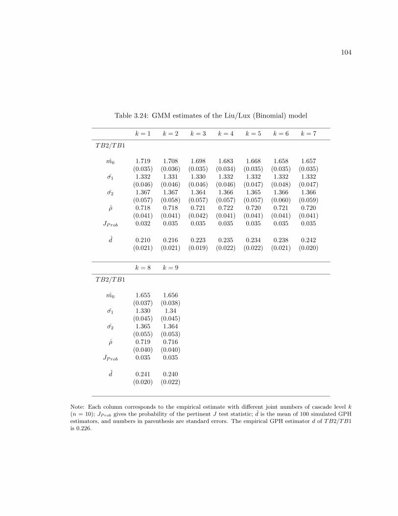
104


k = 1 k = 2 k = 3 k = 4 k = 5 k = 6 k = 7

TB2/TB1

m0 1.719 1.708 1.698 1.683 1.668 1.658 1.657(0.035) (0.036) (0.035) (0.034) (0.035) (0.035) (0.035)

σ1 1.332 1.331 1.330 1.332 1.332 1.332 1.332(0.046) (0.046) (0.046) (0.046) (0.047) (0.048) (0.047)

σ2 1.367 1.367 1.364 1.366 1.365 1.366 1.366(0.057) (0.058) (0.057) (0.057) (0.057) (0.060) (0.059)

ρ 0.718 0.718 0.721 0.722 0.720 0.721 0.720(0.041) (0.041) (0.042) (0.041) (0.041) (0.041) (0.041)

JProb 0.032 0.035 0.035 0.035 0.035 0.035 0.035

d 0.210 0.216 0.223 0.235 0.234 0.238 0.242(0.021) (0.021) (0.019) (0.022) (0.022) (0.021) (0.020)

k = 8 k = 9

TB2/TB1

m0 1.655 1.656(0.037) (0.038)

σ1 1.330 1.34(0.045) (0.045)

σ2 1.365 1.364(0.055) (0.053)

ρ 0.719 0.716(0.040) (0.040)

JProb 0.035 0.035

d 0.241 0.240(0.020) (0.022)

Note: Each column corresponds to the empirical estimate with different joint numbers of cascade level k(n = 10); JProb gives the probability of the pertinent J test statistic; d is the mean of 100 simulated GPHestimators, and numbers in parenthesis are standard errors. The empirical GPH estimator d of TB2/TB1is 0.226.

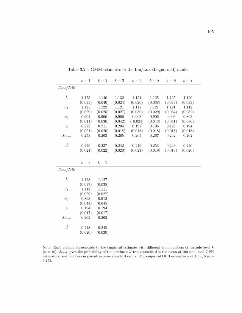
105

Table 3.25: GMM estimates of the Liu/Lux (Lognormal) model

k = 1 k = 2 k = 3 k = 4 k = 5 k = 6 k = 7

Dow/Nik

λ 1.153 1.140 1.132 1.124 1.125 1.125 1.126(0.035) (0.040) (0.024) (0.020) (0.038) (0.033) (0.033)

σ1 1.125 1.122 1.121 1.117 1.121 1.121 1.112(0.029) (0.025) (0.027) (0.030) (0.029) (0.034) (0.032)

σ2 0.904 0.906 0.906 0.908 0.906 0.906 0.893(0.041) (0.036) (0.042) ( 0.024) (0.043) (0.041) (0.036)

ρ 0.222 0.211 0.204 0.197 0.195 0.195 0.194(0.021) (0.020) (0.018) (0.018) (0.018) (0.018) (0.018)

JProb 0.253 0.263 0.265 0.265 0.267 0.262 0.262

d 0.229 0.237 0.242 0.246 0.253 0.243 0.246(0.021) (0.022) (0.020) (0.021) (0.019) (0.019) (0.020)

k = 8 k = 9

Dow/Nik

λ 1.128 1.127(0.037) (0.038)

σ1 1.112 1.111(0.029) (0.027)

σ2 0.893 0.912(0.044) (0.045)

ρ 0.194 0.194(0.017) (0.017)

JProb 0.262 0.262

d 0.248 0.245(0.020) (0.020)

Note: Each column corresponds to the empirical estimate with different joint numbers of cascade level k(n = 10); JProb gives the probability of the pertinent J test statistic; d is the mean of 100 simulated GPHestimators, and numbers in parenthesis are standard errors. The empirical GPH estimator d of Dow/Nik is0.295.

106


n = 5 n = 6 n = 7 n = 8 n = 9 n = 10 n = 11 n = 12

Dow/Nik

λ 1.137 1.229 1.128 1.125 1.125 1.124 1.123 1.123(0.021) (0.020) (0.021) (0.020) (0.020) (0.020) (0.020) (0.020)

σ1 1.133 1.126 1.122 1.120 1.118 1.117 1.115 1.115(0.030) (0.031) (0.030) (0.029) (0.030) (0.031) (0.031) (0.030)

σ2 0.920 0.915 0.916 0.912 0.911 0.908 0.907 0.907(0.026) (0.025) (0.023) (0.023) (0.022) (0.020) (0.022) (0.023)

ρ 0.220 0.219 0.212 0.204 0.205 0.197 0.195 0.195(0.020) (0.023) (0.022) (0.020) (0.019) (0.018) (0.018) (0.018)

JProb 0.377 0.368 0.320 0.289 0.2710 0.265 0.265 0.265

d 0.144 0.190 0.208 0.223 0.240 0.246 0.264 0.275(0.017) (0.017) (0.018) (0.019) (0.020) (0.020) (0.021) (0.020)

n = 13 n = 14 n = 15 n = 16 n = 17 n = 18 n = 19 n = 20

Dow/Nik

λ 1.122 1.122 1.123 1.123 1.122 1.122 1.122 1.122(0.020) (0.020) (0.021) (0.020) (0.021) (0.020) (0.021) (0.020)

σ1 1.115 1.115 1.115 1.115 1.115 1.115 1.115 1.115(0.030) (0.031) (0.031) (0.030) (0.029) (0.030) (0.030) (0.031)

σ2 0.907 0.907 0.907 0.907 0.907 0.907 0.907 0.907(0.023) (0.022) (0.022) (0.020) (0.021) (0.024) (0.022) (0.022)

ρ 0.195 0.195 0.195 0.195 0.195 0.195 0.195 0.195(0.018) (0.018) (0.018) (0.018) (0.018) (0.018) (0.018) (0.018)

JProb 0.265 0.265 0.265 0.265 0.265 0.265 0.265 0.265

d 0.281 0.289 0.296 0.304 0.307 0.305 0.305 0.305(0.020) (0.020) (0.021) (0.021) (0.021) (0.021) (0.020) (0.020)

Note: Each column corresponds to the empirical estimate with different numbers of cascade level n (k = 4);JProb gives the probability of the pertinent J test statistic; d is the mean of 100 simulated GPH estimators,and numbers in parenthesis are standard errors. The empirical GPH estimator d of Dow/Nik is 0.295.

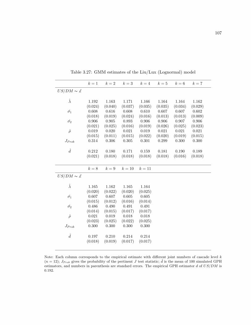
107


k = 1 k = 2 k = 3 k = 4 k = 5 k = 6 k = 7

US/DM ∼ £

λ 1.192 1.163 1.171 1.166 1.164 1.164 1.162(0.024) (0.040) (0.037) (0.035) (0.035) (0.034) (0.029)

σ1 0.608 0.616 0.608 0.610 0.607 0.607 0.602(0.018) (0.019) (0.024) (0.016) (0.013) (0.013) (0.009)

σ2 0.906 0.905 0.893 0.906 0.906 0.907 0.906(0.021) (0.025) (0.016) (0.019) (0.026) (0.025) (0.023)

ρ 0.019 0.020 0.021 0.019 0.021 0.021 0.021(0.015) (0.011) (0.015) (0.022) (0.020) (0.019) (0.015)

JProb 0.314 0.306 0.305 0.301 0.299 0.300 0.300

d 0.212 0.180 0.171 0.159 0.181 0.190 0.189(0.021) (0.018) (0.018) (0.018) (0.018) (0.016) (0.018)

k = 8 k = 9 k = 10 k = 11

US/DM ∼ £

λ 1.165 1.162 1.165 1.164(0.020) (0.022) (0.020) (0.025)

σ1 0.607 0.607 0.605 0.605(0.015) (0.012) (0.016) (0.014)

σ2 0.486 0.490 0.491 0.491(0.014) (0.015) (0.017) (0.017)

ρ 0.021 0.019 0.018 0.018(0.023) (0.025) (0.022) (0.025)

JProb 0.300 0.300 0.300 0.300

d 0.197 0.210 0.214 0.214(0.018) (0.019) (0.017) (0.017)

Note: Each column corresponds to the empirical estimate with different joint numbers of cascade level k(n = 12); JProb gives the probability of the pertinent J test statistic; d is the mean of 100 simulated GPHestimators, and numbers in parenthesis are standard errors. The empirical GPH estimator d of US/DM is0.192.

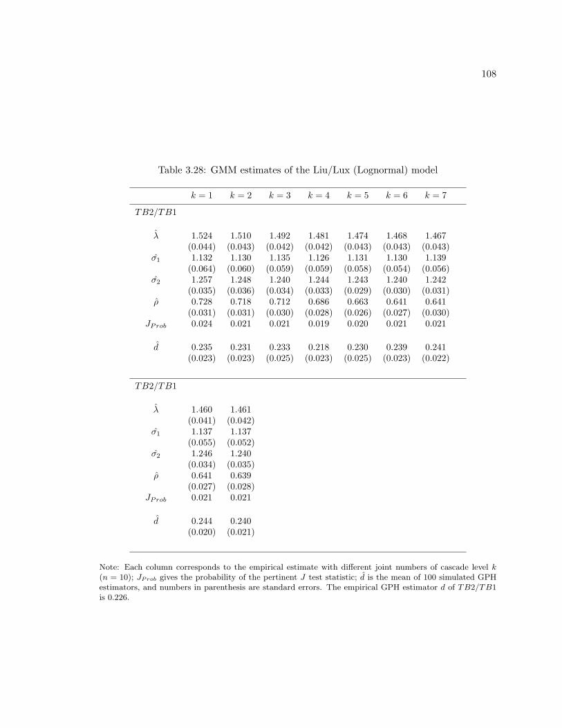
108


k = 1 k = 2 k = 3 k = 4 k = 5 k = 6 k = 7

TB2/TB1

λ 1.524 1.510 1.492 1.481 1.474 1.468 1.467(0.044) (0.043) (0.042) (0.042) (0.043) (0.043) (0.043)

σ1 1.132 1.130 1.135 1.126 1.131 1.130 1.139(0.064) (0.060) (0.059) (0.059) (0.058) (0.054) (0.056)

σ2 1.257 1.248 1.240 1.244 1.243 1.240 1.242(0.035) (0.036) (0.034) (0.033) (0.029) (0.030) (0.031)

ρ 0.728 0.718 0.712 0.686 0.663 0.641 0.641(0.031) (0.031) (0.030) (0.028) (0.026) (0.027) (0.030)

JProb 0.024 0.021 0.021 0.019 0.020 0.021 0.021

d 0.235 0.231 0.233 0.218 0.230 0.239 0.241(0.023) (0.023) (0.025) (0.023) (0.025) (0.023) (0.022)

TB2/TB1

λ 1.460 1.461(0.041) (0.042)

σ1 1.137 1.137(0.055) (0.052)

σ2 1.246 1.240(0.034) (0.035)

ρ 0.641 0.639(0.027) (0.028)

JProb 0.021 0.021

d 0.244 0.240(0.020) (0.021)

Note: Each column corresponds to the empirical estimate with different joint numbers of cascade level k(n = 10); JProb gives the probability of the pertinent J test statistic; d is the mean of 100 simulated GPHestimators, and numbers in parenthesis are standard errors. The empirical GPH estimator d of TB2/TB1is 0.226.

Chapter 4

Beyond the Bivariate case: HigherDimensional Multifractal Models

4.1 Tri-variate (higher dimensional) multifractal models

The bivariate MF model deals with only two financial time series, whereas an investment

portfolio could be allocated to more than two assets. Analogously to the bivariate case, a

multivariate ML model assumes N assets (time series) that have the same overall number of

volatility cascades containing k joint cascade levels; after the kth level, each time series in-

dependently has separate additional multifractal processes. Our parsimonious multivariate

multifractal model is given by

rq,t = σq ⊗ [G(Mt)]1/2 ⊗ uq,t. (4.1.1)

rq,t are asset returns with q = 1, 2, · · · , N being the number of assets. σq are scale

parameters (unconditional standard deviations) of the return series, and both rq,t and σq

are N × 1 vector; ⊗ denotes element by element multiplication; uq,t is a N × 1 vector,

whose elements are multivariate standard Normal distributions. Considering a three-asset

109

110

portfolio, N = 3, it is the trivariate standard Normal with correlation matrix1 ρ12 ρ13

ρ12 1 ρ23

ρ13 ρ23 1

The multifractal process denoted by G(Mt) is assumed to be

G(Mt) =k∏

i=1

M(i)t ⊗

n∏j=k+1

M(j)q,t , (4.1.2)

and it defines the number of joint cascade levels k within multivariate multifractal

processes. In addition, we restrict the specification of the transition probabilities as the one

in the bivariate setting:

γi = 2−(k−i), for i = 1, . . . k; (4.1.3)

γi = 2−(n−i), for i = k + 1, . . . n.

This specification allows each multifractal process having two starting cascades, that is,

it starts again after the joint cascade level k. Each component is either renewed at time t

with probability γi, depending on its rank i within the hierarchy of multipliers, or remains

unchanged with probability 1− γi.

For the distribution of the multifractal volatility components Mt, we specify the multi-

pliers to be random draws from either a binomial or Lognormal distribution. In the binomial

(discrete) case, we assume two volatility component draws, m0 ∈ (0, 2) and the alternative

m1 = 2 −m0; for the Lognormal (continuous) version, we preserve the assumption as the

one in the bivariate case by setting

−log2M ∼ N(λ, σ2m). (4.1.4)

111

We impose an additional restriction of E[M (i)t ] = 0.5, which leads to exp[−λ ln 2 +

0.5σ2m(ln 2)2] = 0.5, and we arrive at

σ2m = 2(λ− 1)/ln2. (4.1.5)

This transformation reduces the estimation of λ and σm in Eq. (4.1.4) to one parameter.

4.2 Maximum likelihood estimation

We expand the likelihood approach from the bivariate model to the more general multivari-

ate setting. Let rt be the set of N assets’ joint return observations rq,t for q = 1, 2 . . . N

and t = 1, 2 . . . T ; Θ be the unknown parameters to be estimated, the exact likelihood

function has the form like in Eq. (3.3.1):

f(r1, · · · , rT ; Θ) =T∏

t=1

(πt−1A) · f(rt|Mt = mi). (4.2.1)

A is the transition matrix, which specifies the dynamics of each possible state of

P (Mt+1 = mj |Mt = mi), (4.2.2)

both Mt and m(·) are vectors, which contain the combinations of each possible volatility

component. For multifractal processes with discrete distribution of volatility components,

say the Binomial model, i, j ∈ 1, 2 . . . (2N )n , for N being the number of assets allocated

and n being the number of cascade levels. It indicates that the transition matrix A has the

dimension of (2N )n × (2N )n.

f(rt|Mt = mi) is the density of the innovation rt conditional on Mt, which is

f(rt|Mt = mi) =FN

rt ÷

[σ ⊗ η1/2

]σ ⊗ η1/2

, (4.2.3)

FN· denotes the multivariate standard Normal density function (trivariate standard

Normal for three assets) and η = G(Mt); ÷ represents element-by-element division. πt

112

denotes the conditional probability defined by

πit = P (Mt = mi|r1, · · · , rt). (4.2.4)

For Binomial model, we knowR∑

i=1πi

t = 1 for R = (2N )n and the one-step-ahead condi-

tional probabilities of πt+1 can be obtained by the Bayesian updating:

πt+1 =f(rt+1|Mt+1 = mi)⊗ (πtA)∑f(rt+1|Mt+1 = mi)⊗ (πtA)

. (4.2.5)

We easily recognize that this recursive process is highly dependent on the dimensions of

the transition matrix, as highlighted in the bivariate MF models. In the trivariate case, the

maximization of the likelihood function implies to evaluate the size of 8n × 8n dimensions

of A in each iteration for the binomial model, and current computational limitations make

choices of n beyond 3 unfeasible. Besides, it is not applicable for models with continuous

distributions of the multipliers such as Lognormal distribution, because these imply an

infinite number of states.

4.3 Simulation based maximum likelihood estimation

We recognize that ML estimation is constrained by its immense computational demands, in

particular for higher dimensional multifractal models. The maximization process depends

strongly on the dimension of the transition (filtering) probability matrix, which increases

exponentially with the rate of (2N )n for binomial multifractal processes, and one can imagine

the intensive computations when evaluating a 4096×4096 transition matrix in each iteration

for the trivariate model with number of cascade levels n = 4.

In this section, we also implement simulation based inference via particle filter, which is

introduced in Chapter 3. The essence of this algorithm is to avoid formalizing and evaluating

the exact form of the transition matrix, which is required to generate πt+1 given πt through

113

the Bayesian updating. Instead, some limited number of importance samples (particles) are

employed to pass the filtering process

R∑j=1

P (Mt+1 = mi|Mt = mj)P (Mt = mj |rt), (4.3.1)

by adopting Sampling/Importance Resampling (SIR), the method developed by Rubin

(1987) and further analyzed by Pitt and Shephard (1999). The SIR algorithm assists to

generate independent draws M (b)t B

b=1 from the conditional distribution πt, and given new

information rt+1, an approximation of Bayesian updating provides simulations of M (b)t+1B

b=1

recursively.

As detailed in Section 3.4, we complete the approximation by simulating each M (b)t one

step forward and re-weighting using an importance sampler: simulate the Markov Chain

one step ahead with B draws M (1)t+1, M

(2)t+1, . . . , M

(B)t+1 , which are taken independently from

the prior; this preliminary step only uses information available at time t, therefore these

draws have to account for new return rt+1. Under SIR, each of these draws is chosen by

draw a random number q from 1 to B with the probability of:

P (q = b) =f(rt+1|Mt+1 = M

(b)t+1)∑B

i=1 f(rt+1|Mt+1 = m(i)), (4.3.2)

then M(1)t+1 = M

(q)t+1 is a draw from πt+1. Repeating B times, we obtain B draws

M(1)t+1, . . .M

(B)t+1 which have been adjusted to account for the new information.

As particle filters treat the discrete support generated by the particles as the “true”

filtering density, this allows us to produce an approximation to the prediction probability

density P (Mt+1 = mit|rt), by using the discrete support of the particles, and then one-step-

ahead conditional probability is


1B

B∑b=1

P (Mt+1 = mi|Mt = M(b)t ) (4.3.3)

114

Thus one step ahead density hence becomes:

f(rt|r1, · · · , rt−1) ≈ 1B

B∑b=1

f(rt|Mt = M(b)t ), (4.3.4)

and this implies that we maximize the approximate likelihood function:

g(r1, · · · , rT ; Θ) ≈T∏

t=1

[1B

B∑b=1

f(rt|Mt = M(b)t )

]. (4.3.5)

We can use these calculations to carry out simulated likelihood estimation of higher

dimensional multifractal processes, whose Monte Carlo studies are reported in the following

section.

115

4.4 GMM Estimation

Generalized Method of Moments (GMM) approach by Hansen (1982) assists us to obtain

the vector of parameters β by minimizing the distance between the analytical moments and

empirical moments:

βT = arg minβ∈Θ

MT (β)′WT MT (β), (4.4.1)

with Θ being the admissible parameter space. MT (β) stands for the vector of differences

between sample moments and analytical moments, and WT is a positive definite weighting

matrix, which controls over-identification when applying GMM. Implementing Eq. (4.4.1),

one typically starts with the identity matrix; then the inverse of the covariance matrix

obtained from the first round estimation is used as the weighting matrix in the next step;

and this procedure continues until the estimates converge.

The applicability of GMM for multifractal models has been discussed in Chapter 3, and

we follow the same practical solution by transforming the observed return data rt into τth

log differences::

Rt,τ = ln |rt| − ln |rt−τ |

= 0.5k∑

i=1(ε(i)t − ε

(i)t−τ ) + 0.5

n∑j=k+1

(ε(j)t − ε(j)t−τ ) + (ln|ut| − ln|ut−τ |)

(4.4.2)

One may notice that in the transformation above the scale parameter σ1 and σ2 drops

out, while estimating the scale parameters can be pursued by adding additional moment

conditions (e.g. unconditional moments of rt). In our practice, we use the moments as in

bivariate models by considering each observation’s contribution to the standard deviation

of the sample return time series.

GMM provides a more convenient and efficient way towards the estimation of higher

dimensional MF models as it allows us to treat each pair of time series as a bivariate case.

116

In order to exploit as much information as possible, the moment conditions that we consider

include two categories:

The first category of moment conditions is the moments for individual time series’

autocovariance, which contains the moments of raw transformed observations and squared

transformed observations:1

Cov[Rt,1, Rt−1,1]; Cov[R2t,1, R

2t−1,1];

in the trivariate case, let Xt,τ , Yt,τ and Zt,τ be transformed time series through Eq.

(4.4.2), and the pertinent moment conditions are

Cov[Xt,1, Xt−1,1]; Cov[Yt,1, Yt−1,1]; Cov[Zt,1, Zt−1,1];

and

Cov[X2t,1, X

2t−1,1]; Cov[Y 2

t,1, Y2t−1,1]; Cov[Z2

t,1, Z2t−1,1];

The second category of conditions is obtained by considering moment conditions of

covariances (moments of raw transformed observations and squared transformed observa-

tions):

Cov[Rt,1, R−t,1]; Cov[Rt,1, R

−t−1,1];

and

Cov[R2t,1, (R

−t,1)

2]; Cov[R2t,1, (R

−t−1,1)

2];

R−t,1 represents any one other time series rather than Rt,1. In the trivariate case, we have

six moment conditions corresponding to six pairs of time series for raw transformed obser-

vations, namely,

Cov[Xt,1, Yt,1]; Cov[Xt,1, Zt,1]; Cov[Yt,1, Zt,1];

Cov[Xt,1, Yt−1,1]; Cov[Xt,1, Zt−1,1]; Cov[Yt,1, Zt−1,1];

1As in the bivariate case, we leave moment conditions of Cov[Rt+τ,τ , Rt,τ ] with τ > 1 for future work.

117

plus six moment conditions for squared transformed observations, these 12 moment con-

ditions provide additional information for the correlation parameters ρij for i, j = 1, 2, 3.

Altogether, we use 18 moment conditions when implementing GMM for tri-variate multi-

fractal models, and the detailed analytical moments are given in the Appendix for both

Binomial model and Lognormal model.

We firstly apply GMM approach to our trivariate MF model with relatively small num-

bers of cascade levels to compare their performances with the likelihood approach and

simulation base inference. Table 4.1 reports the comparison of ML and GMM estimations

with Monte Carlo studies (designed as in previous sections). Initial settings include n = 3

(the limit of computational feasibility for ML), k = 1, m0 = 1.3, σ1 = 1, σ2 = 1, σ3 = 1,

ρ12 = 0.3, ρ23 = 0.5, ρ13 = 0.7. It should be not too surprising that the ML estimators

are more efficient than GMM since ML extracts all the information in the data. Obviously,

variability of estimates with GMM is much higher particularly in small sub-sample size, but

dramatically decreases in the case of larger sub-sample size; for example, it is from around

4 times that of the ML estimator for m0’s. While we also observe that the efficiency of

σ from GMM is pretty close to ML, which shows that there is no loss of efficiency using

moment conditions of sample standard deviation for σ within GMM. One additional gain

for GMM is that it takes only a small fraction of computation time that ML costs; they are

12.5 and 109 hours for GMM and ML, respectively.

Table 4.2 reports the comparison of simulation based ML and GMM estimation with

Monte Carlo studies: initial settings includes n = 4, k = 2, m0 = 1.3, σ1 = 1, σ2 = 1,

σ3 = 1, ρ12 = 0.3, ρ23 = 0.5, ρ13 = 0.7. We used B = 500 particles for SML estimation.

Let us begin with the estimator of m0, variability of estimates with GMM is higher only in

small sub-sample size (SD and RMSE), but dramatically decreases in the case of larger sub-

sample size; we also observe that the efficiency of the σ estimates from GMM (by considering

sample standard deviation) is almost identical to that from SML; for correlation estimators,

118

a mixed picture shows that GMM estimator of ρ12 is dominated by the one from SML, but

is opposite in the cases of ρ23 and ρ13. As in the ML section, we report the computation

time needed for implementing 400 Monte Carlo simulations and estimations in Table 4.2;

they are 14 and 120.5 hours for GMM and SML respectively.

Note that there is no constraint to the number of cascade levels within our higher

dimensional multifractal processes for GMM approach. Next, we proceed by reporting

further results of Monte Carlo experiments designed to explore the performance of our GMM

estimator for trivariate multifractal models with larger numbers of cascade levels. We fixed

n = 12 with number of joint cascades k = 3, the scale parameters σ1 = σ2 = σ3 = 1, and the

increment correlation matrix is set as ρ12 = 0.3, ρ23 = 0.5, ρ13 = 0.7. As before,we begin

by simulating 100,000 observations in each iteration, and randomly choose three different

sub-samples with sample sizes N1 = 2000, N2 = 5000, and N3 = 10000, which is a robust

design to assess the estimation performance. Let us start with the Binomial model with

parameter value m0 = 1.3.2 Table 4.3 shows the statistical result of the GMM estimator:

for Binomial distribution parameter m0, not only the bias but also the standard deviation

and root mean squared error show quite encouraging behavior. It is also the case for other

parameters, even in the small sample size N = 2000 and N = 5000, the average bias of

the Monte Carlo estimates is moderate, and particularly close to zero for the larger sample

sizes N = 10000. One also easily observe that it is asymptotically efficient with increasing

the sub-sample size and in harmony with T12 efficiency which further underscores the good

performance of the log transformation within our GMM estimation.

One advantage of GMM is that it allows to estimate multifractal processes with contin-

uous distributions of volatility components. Following the work of Mandelbrot et al. (1997)2Studies on other parameter values have also been pursued, we omit them here due to their qualitatively

similar results.

119

and Calvet and Fisher (2002), we use the same Lognormal distribution of

−log2M ∼ N(λ, σ2m)

in the tri-variate case, and Eq. (4.1.5) provides the relationship between λ and σm by

assigning a restriction of E[M ] = 0.5.3 In our Monte Carlo simulations and estimations

reported in Table 4.4, we cover parameter values λ = 1.20, and other initial setting as in

the Binomial model, namely σ1 = 1, σ2 = 1, σ3 = 1, ρ12 = 0.3, ρ23 = 0.5, ρ13 = 0.7. As

can be seen, the picture is not too different from that obtained in the Binomial case: Biases

are moderate again, SD and RMSE significantly decrease with increasing the sub-sample

size. Monte Carlo studies towards other different choice of parameter values have also

been conducted, we skip them for saving some space as no significant deviation is observed

comparing with the performance above.

Figure 4.1 and Figure 4.2 present the fraction of p values that fall within the 2% in-

terval fractiles from Hansen’s J tests of over-identification restrictions (three figures from

up to down corresponding to three different sample sizes: N1 = 2, 000, N2 = 5, 000 and

N3 = 10, 000). There are much more significant left-shifts compared with the bivariate

cases, Especially, we observe the sharp left-shift in the Lognormal model. All in all, the

Monte Carlo studies again show the satisfactory behaviour of our GMM estimator for higher

dimensional multifractal models with both discrete and continuous state spaces.

3A factor of 2n is multiplied for compensating the mean of multipliers being 0.5.

120

4.5 Empirical estimates

For empirical applications of the multivariate multifractal models, we consider daily data for

a equally weighted portfolio of three foreign exchange rates, U.S. Dollar to British Pound,

German Mark to British Pound, and Japanese Yen to British Pound (US/DM/JP , March

1973 - February 2004), where the first symbol inside these parentheses designates the short

notation for the corresponding time series, followed by the starting and ending dates for

the sample at hand. Figure 4.3 is the plot of Japanese Yen to British Pound exchange rate

pt and return rt = 100 × [ln(pt) − ln(pt−1)] (Figure 3.7 gives a plot of empirical exchange

rates and returns for U.S. Dollar to British Pound and German Mark to British Pound).

Table 4.5 presents the empirical estimates of the trivariate multifractal model with n = 3

(it is the computational limit) via the maximum likelihood estimation. There is not much

different for the parameter m0 with two different joint cascade levels; one may also observe

that the correlation parameter estimates for U.S. Dollar to British Pound and German Mark

to British Pound ρ12 is a bit deviated with the one from the bivariate case which has been

reported in the last chapter. It is actually plausible by considering the fact that different

total number of the cascade levels n are used. We also find the maximized log-likelihood

values are quite close between k = 1 and k = 2 with only slightly higher values when k = 1.

Indeed, one would prefer to have more comparisons among various joint cascade levels (k)

in the case for larger number of cascades n.

By using particle filter, we are allowed to employ relatively more cascade levels. Table

4.6 reports empirical estimates of the trivariate MF model with the number of cascade levels

of n = 5 via simulation based maximum likelihood approach. With the fixed total cascade

levels, there are not much fluctuations for the estimates among different joint cascade levels

k, but one may aware the maximized log-likelihood values increases about 1100 from the

case k = 1 to k = 2. Practically, we find that the computation is still very intensive even

121

when using a relatively small number of particles of B = 500 in the trivatiate model.

In order to remove the upper limit of cascade levels of multivariate MF processes, we

also present the empirical estimates for higher numbers of n via the GMM approach; and

moment conditions described in Section 4.2 are used. With fixed joint cascade level k = 4,

Table 4.7 provides the empirical results for the Binomial model with a range of numbers of

cascade levels n from 5 to 20. It shows the estimates for m0 is decreasing with the number of

cascade levels n increasing, but then almost keep constant after the case n = 12; while other

estimates are relatively stable, as well as the J-test statistic. Table 4.8 reports the empirical

results with different numbers of joint cascade levels k but n = 20 fixed. In contrast to

Table 4.7, there are only slight variations for m0 (among k = 1 to k = 5). To demonstrate

the applicability of GMM to the MF process with continuous state space, Table 4.9 and

Table 4.10 give the empirical estimates for the Lognormal model with various numbers of

cascade levels, and similar picture is observed comparing with the Binomial case.

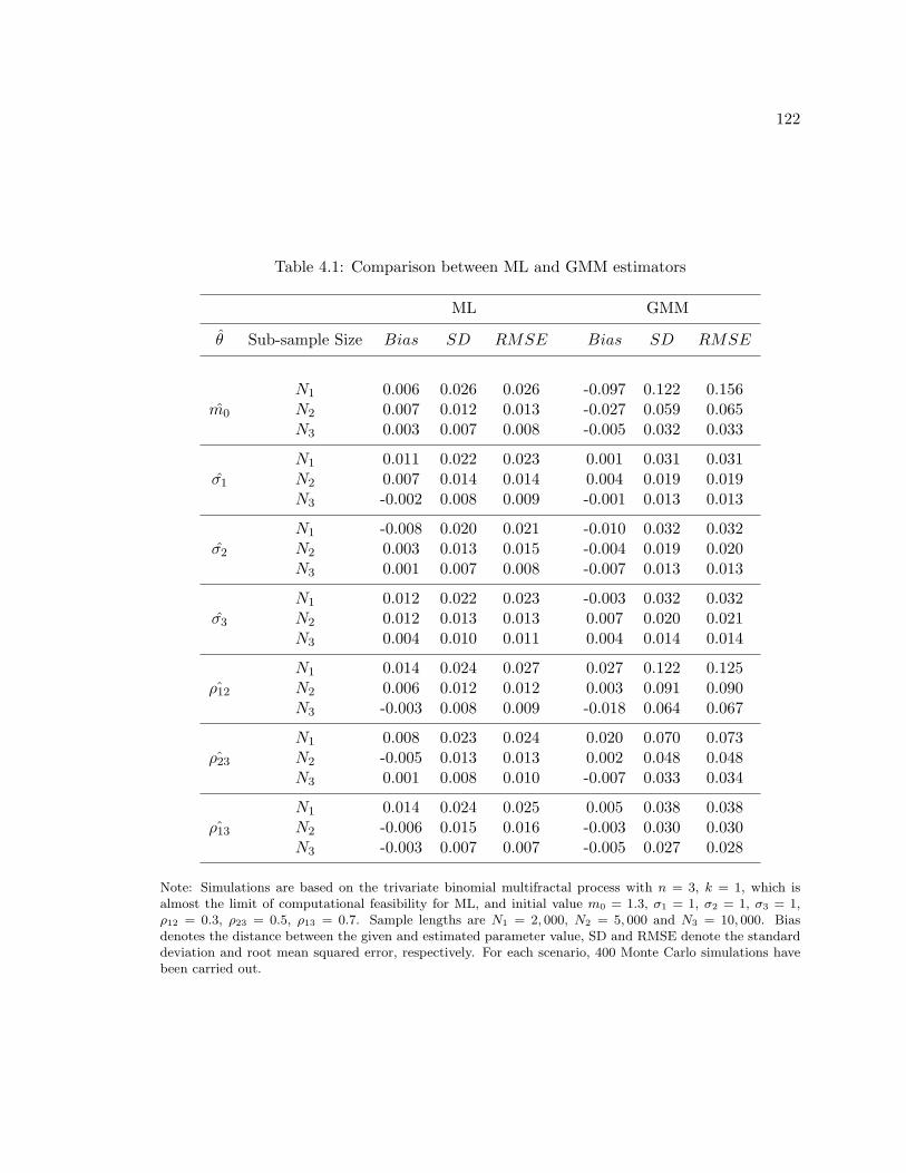
122

Table 4.1: Comparison between ML and GMM estimators

ML GMM


N1 0.006 0.026 0.026 -0.097 0.122 0.156m0 N2 0.007 0.012 0.013 -0.027 0.059 0.065

N3 0.003 0.007 0.008 -0.005 0.032 0.033

N1 0.011 0.022 0.023 0.001 0.031 0.031σ1 N2 0.007 0.014 0.014 0.004 0.019 0.019

N3 -0.002 0.008 0.009 -0.001 0.013 0.013

N1 -0.008 0.020 0.021 -0.010 0.032 0.032σ2 N2 0.003 0.013 0.015 -0.004 0.019 0.020

N3 0.001 0.007 0.008 -0.007 0.013 0.013

N1 0.012 0.022 0.023 -0.003 0.032 0.032σ3 N2 0.012 0.013 0.013 0.007 0.020 0.021

N3 0.004 0.010 0.011 0.004 0.014 0.014

N1 0.014 0.024 0.027 0.027 0.122 0.125ρ12 N2 0.006 0.012 0.012 0.003 0.091 0.090

N3 -0.003 0.008 0.009 -0.018 0.064 0.067

N1 0.008 0.023 0.024 0.020 0.070 0.073ρ23 N2 -0.005 0.013 0.013 0.002 0.048 0.048

N3 0.001 0.008 0.010 -0.007 0.033 0.034

N1 0.014 0.024 0.025 0.005 0.038 0.038ρ13 N2 -0.006 0.015 0.016 -0.003 0.030 0.030

N3 -0.003 0.007 0.007 -0.005 0.027 0.028

Note: Simulations are based on the trivariate binomial multifractal process with n = 3, k = 1, which isalmost the limit of computational feasibility for ML, and initial value m0 = 1.3, σ1 = 1, σ2 = 1, σ3 = 1,ρ12 = 0.3, ρ23 = 0.5, ρ13 = 0.7. Sample lengths are N1 = 2, 000, N2 = 5, 000 and N3 = 10, 000. Biasdenotes the distance between the given and estimated parameter value, SD and RMSE denote the standarddeviation and root mean squared error, respectively. For each scenario, 400 Monte Carlo simulations havebeen carried out.

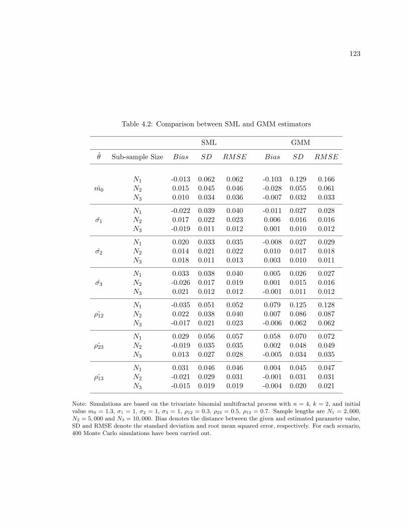
123

Table 4.2: Comparison between SML and GMM estimators

SML GMM


N1 -0.013 0.062 0.062 -0.103 0.129 0.166m0 N2 0.015 0.045 0.046 -0.028 0.055 0.061

N3 0.010 0.034 0.036 -0.007 0.032 0.033

N1 -0.022 0.039 0.040 -0.011 0.027 0.028σ1 N2 0.017 0.022 0.023 0.006 0.016 0.016

N3 -0.019 0.011 0.012 0.001 0.010 0.012

N1 0.020 0.033 0.035 -0.008 0.027 0.029σ2 N2 0.014 0.021 0.022 0.010 0.017 0.018

N3 0.018 0.011 0.013 0.003 0.010 0.011

N1 0.033 0.038 0.040 0.005 0.026 0.027σ3 N2 -0.026 0.017 0.019 0.001 0.015 0.016

N3 0.021 0.012 0.012 -0.001 0.011 0.012

N1 -0.035 0.051 0.052 0.079 0.125 0.128ρ12 N2 0.022 0.038 0.040 0.007 0.086 0.087

N3 -0.017 0.021 0.023 -0.006 0.062 0.062

N1 0.029 0.056 0.057 0.058 0.070 0.072ρ23 N2 -0.019 0.035 0.035 0.002 0.048 0.049

N3 0.013 0.027 0.028 -0.005 0.034 0.035

N1 0.031 0.046 0.046 0.004 0.045 0.047ρ13 N2 -0.021 0.029 0.031 -0.001 0.031 0.031

N3 -0.015 0.019 0.019 -0.004 0.020 0.021

Note: Simulations are based on the trivariate binomial multifractal process with n = 4, k = 2, and initialvalue m0 = 1.3, σ1 = 1, σ2 = 1, σ3 = 1, ρ12 = 0.3, ρ23 = 0.5, ρ13 = 0.7. Sample lengths are N1 = 2, 000,N2 = 5, 000 and N3 = 10, 000. Bias denotes the distance between the given and estimated parameter value,SD and RMSE denote the standard deviation and root mean squared error, respectively. For each scenario,400 Monte Carlo simulations have been carried out.

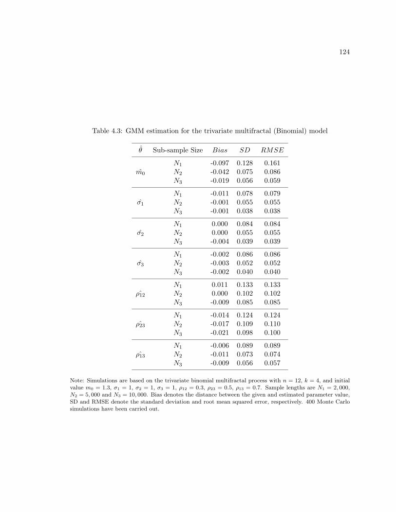
124

Table 4.3: GMM estimation for the trivariate multifractal (Binomial) model


N1 -0.097 0.128 0.161m0 N2 -0.042 0.075 0.086

N3 -0.019 0.056 0.059

N1 -0.011 0.078 0.079σ1 N2 -0.001 0.055 0.055

N3 -0.001 0.038 0.038

N1 0.000 0.084 0.084σ2 N2 0.000 0.055 0.055

N3 -0.004 0.039 0.039

N1 -0.002 0.086 0.086σ3 N2 -0.003 0.052 0.052

N3 -0.002 0.040 0.040

N1 0.011 0.133 0.133ρ12 N2 0.000 0.102 0.102

N3 -0.009 0.085 0.085

N1 -0.014 0.124 0.124ρ23 N2 -0.017 0.109 0.110

N3 -0.021 0.098 0.100

N1 -0.006 0.089 0.089ρ13 N2 -0.011 0.073 0.074

N3 -0.009 0.056 0.057

Note: Simulations are based on the trivariate binomial multifractal process with n = 12, k = 4, and initialvalue m0 = 1.3, σ1 = 1, σ2 = 1, σ3 = 1, ρ12 = 0.3, ρ23 = 0.5, ρ13 = 0.7. Sample lengths are N1 = 2, 000,N2 = 5, 000 and N3 = 10, 000. Bias denotes the distance between the given and estimated parameter value,SD and RMSE denote the standard deviation and root mean squared error, respectively. 400 Monte Carlosimulations have been carried out.

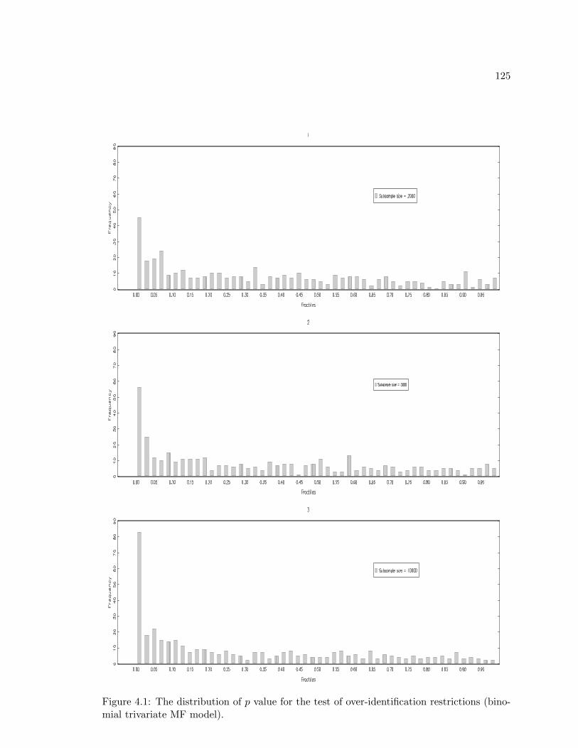
125

Figure 4.1: The distribution of p value for the test of over-identification restrictions (bino-mial trivariate MF model).

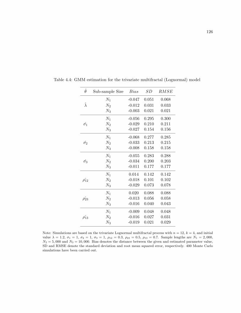
126

Table 4.4: GMM estimation for the trivariate multifractal (Lognormal) model


N1 -0.047 0.051 0.068λ N2 -0.012 0.031 0.033

N3 -0.003 0.021 0.021

N1 -0.056 0.295 0.300σ1 N2 -0.029 0.210 0.211

N3 -0.027 0.154 0.156

N1 -0.068 0.277 0.285σ2 N2 -0.033 0.213 0.215

N3 -0.008 0.158 0.158

N1 -0.055 0.283 0.288σ3 N2 -0.034 0.200 0.203

N3 -0.011 0.177 0.177

N1 0.014 0.142 0.142ρ12 N2 -0.018 0.101 0.102

N3 -0.029 0.073 0.078

N1 0.020 0.088 0.088ρ23 N2 -0.013 0.056 0.058

N3 -0.016 0.040 0.043

N1 -0.009 0.048 0.048ρ13 N2 -0.016 0.027 0.031

N3 -0.019 0.021 0.029

Note: Simulations are based on the trivariate Lognormal multifractal process with n = 12, k = 4, and initialvalue λ = 1.2, σ1 = 1, σ2 = 1, σ3 = 1, ρ12 = 0.3, ρ23 = 0.5, ρ13 = 0.7. Sample lengths are N1 = 2, 000,N2 = 5, 000 and N3 = 10, 000. Bias denotes the distance between the given and estimated parameter value,SD and RMSE denote the standard deviation and root mean squared error, respectively. 400 Monte Carlosimulations have been carried out.

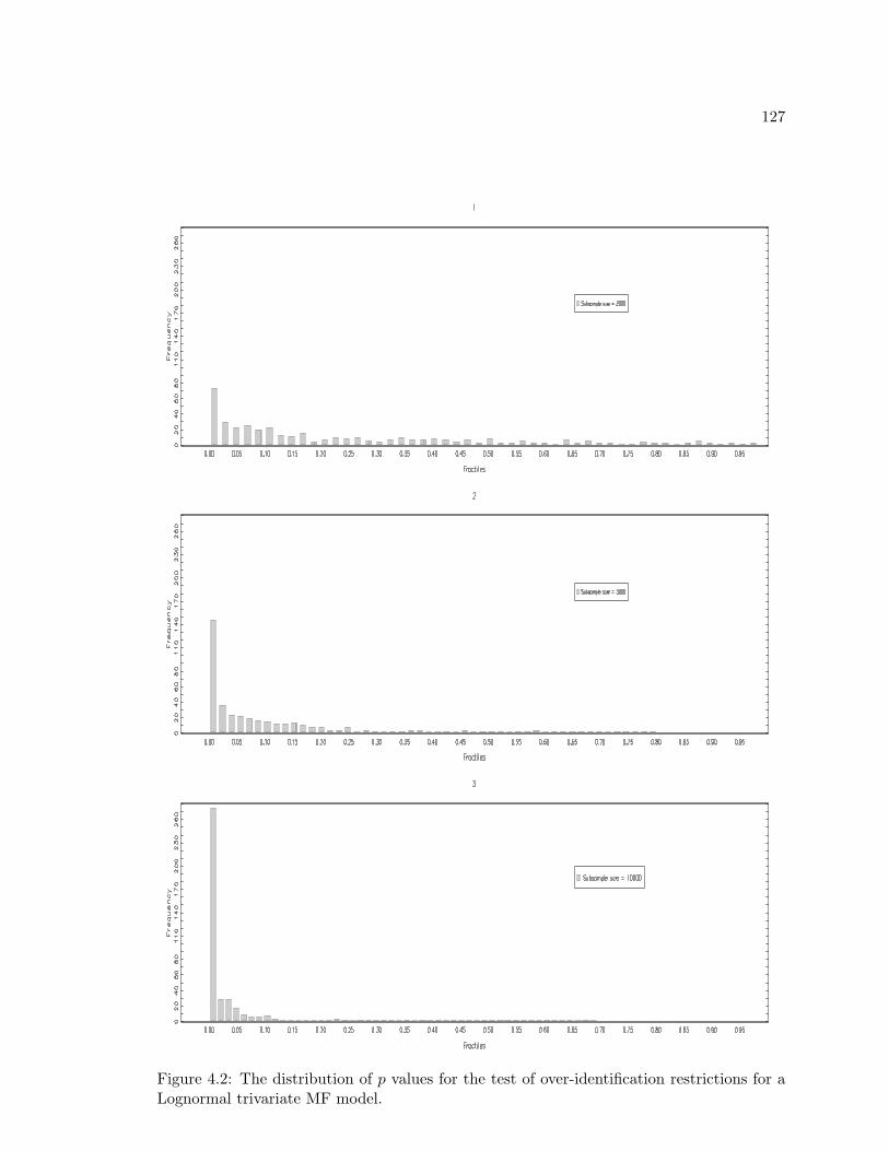
127

Figure 4.2: The distribution of p values for the test of over-identification restrictions for aLognormal trivariate MF model.

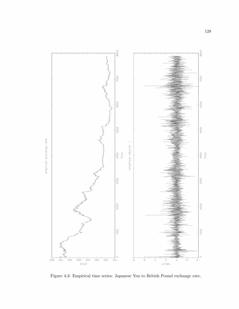
128

Figure 4.3: Empirical time series: Japanese Yen to British Pound exchange rate.

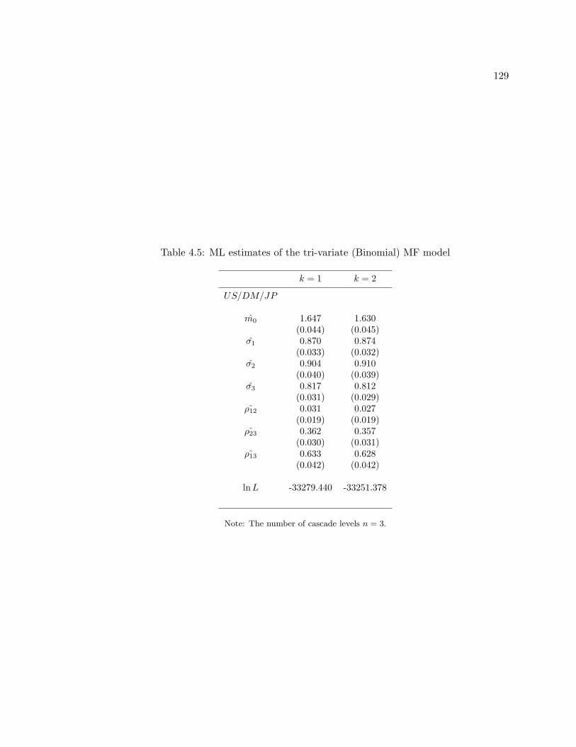
129

Table 4.5: ML estimates of the tri-variate (Binomial) MF model

k = 1 k = 2

US/DM/JP

m0 1.647 1.630(0.044) (0.045)

σ1 0.870 0.874(0.033) (0.032)

σ2 0.904 0.910(0.040) (0.039)

σ3 0.817 0.812(0.031) (0.029)

ρ12 0.031 0.027(0.019) (0.019)

ρ23 0.362 0.357(0.030) (0.031)

ρ13 0.633 0.628(0.042) (0.042)

lnL -33279.440 -33251.378

Note: The number of cascade levels n = 3.

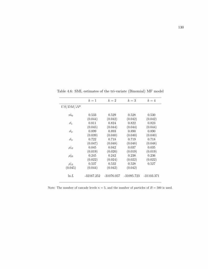
130

Table 4.6: SML estimates of the tri-variate (Binomial) MF model

k = 1 k = 2 k = 3 k = 4

US/DM/JP

m0 0.533 0.529 0.528 0.530(0.044) (0.042) (0.042) (0.042)

σ1 0.811 0.824 0.822 0.823(0.045) (0.044) (0.044) (0.044)

σ2 0.899 0.893 0.890 0.890(0.039) (0.040) (0.040) (0.040)

σ3 0.722 0.718 0.719 0.718(0.047) (0.048) (0.048) (0.048)

ρ12 0.045 0.042 0.037 0.035(0.019) (0.020) (0.019) (0.019)

ρ23 0.245 0.242 0.238 0.236(0.022) (0.024) (0.022) (0.022)

ρ13 0.537 0.532 0.528 0.527(0.045) (0.044) (0.042) (0.042)

lnL -32167.252 -31076.057 -31095.723 -31103.371

Note: The number of cascade levels n = 5, and the number of particles of B = 500 is used.

131

Table 4.7: GMM estimates of the tri-variate MF (Binomial) model

n = 5 n = 6 n = 7 n = 8 n = 9 n = 10 n = 11 n = 12

US/DM/JP

m0 1.538 1.472 1.436 1.400 1.387 1.361 1.352 1.333(0.041) (0.041) (0.042) (0.041) (0.041) (0.041) (0.041) (0.041)

σ1 0.794 0.791 0.790 0.795 0.791 0.791 0.791 0.794(0.047) (0.047) (0.047) (0.047) (0.047) (0.047) (0.047) (0.047)

σ2 0.910 0.894 0.893 0.911 0.893 0.894 0.898 0.897(0.047) (0.047) (0.048) (0.048) (0.048) (0.048) (0.048) (0.048)

σ3 0.711 0.714 0.713 0.711 0.713 0.714 0.718 0.717(0.053) (0.053) (0.053) (0.054) (0.053) (0.054) (0.054) (0.054)

ρ12 0.046 0.045 0.045 0.041 0.042 0.041 0.040 0.040(0.019) (0.020) (0.019) (0.018) (0.018) (0.018) (0.018) (0.018)

ρ23 0.223 0.225 0.223 0.221 0.221 0.221 0.222 0.223(0.020) (0.021) (0.021) (0.021) (0.021) (0.021) (0.021) (0.021)

ρ13 0.526 0.527 0.527 0.519 0.519 0.521 0.519 0.518(0.045) (0.044) (0.044) (0.043) (0.044) (0.044) (0.043) (0.043)

JProb 0.033 0.030 0.031 0.031 0.031 0.030 0.030 0.030

n = 9 n = 10 n = 11 n = 12 n = 13 n = 14 n = 15 n = 20

m0 1.330 1.329 1.329 1.329 1.329 1.328 1.329 1.328(0.040) (0.041) (0.041) (0.041) (0.041) (0.041) (0.041) (0.041)

σ1 0.792 0.793 0.795 0.793 0.795 0.795 0.795 0.793(0.047) (0.047) (0.047) (0.047) (0.047) (0.047) (0.047) (0.047)

σ2 0.909 0.894 0.893 0.907 0.899 0.899 0.899 0.912(0.048) (0.048) (0.048) (0.048) (0.048) (0.048) (0.048) (0.048)

σ3 0.729 0.724 0.723 0.727 0.723 0.723 0.723 0.723(0.054) (0.054) (0.054) (0.054) (0.054) (0.054) (0.054) (0.054)

ρ12 0.046 0.045 0.043 0.041 0.041 0.041 0.040 0.040(0.019) (0.019) (0.018) (0.018) (0.018) (0.018) (0.018) (0.018)

ρ23 0.226 0.225 0.223 0.221 0.221 0.221 0.220 0.220(0.021) (0.021) (0.021) (0.021) (0.021) (0.021) (0.021) (0.021)

ρ13 0.520 0.517 0.518 0.516 0.515 0.511 0.515 0.516(0.043) (0.043) (0.043) (0.043) (0.043) (0.043) (0.043) (0.043)

JProb 0.030 0.030 0.030 0.030 0.030 0.030 0.030 0.030

Note: The number of joint cascade levels k = 4.

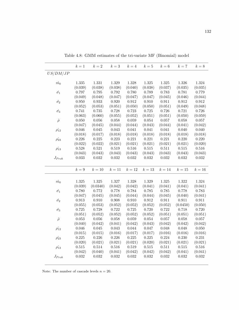
132

Table 4.8: GMM estimates of the tri-variate MF (Binomial) model

k = 1 k = 2 k = 3 k = 4 k = 5 k = 6 k = 7 k = 8

US/DM/JP

m0 1.335 1.331 1.329 1.328 1.325 1.325 1.326 1.324(0.039) (0.038) (0.038) (0.040) (0.038) (0.037) (0.035) (0.035)

σ1 0.797 0.795 0.792 0.780 0.789 0.783 0.781 0.779(0.049) (0.048) (0.047) (0.047) (0.047) (0.045) (0.046) (0.044)

σ2 0.950 0.933 0.920 0.912 0.910 0.911 0.912 0.912(0.052) (0.053) (0.051) (0.050) (0.050) (0.051) (0.049) (0.048)

σ3 0.741 0.735 0.728 0.723 0.725 0.726 0.721 0.726(0.063) (0.060) (0.055) (0.052) (0.051) (0.051) (0.050) (0.059)

ρ 0.050 0.056 0.058 0.059 0.054 0.057 0.058 0.057(0.047) (0.045) (0.044) (0.044) (0.043) (0.044) (0.041) (0.042)

ρ12 0.046 0.045 0.043 0.041 0.041 0.041 0.040 0.040(0.018) (0.017) (0.018) (0.018) (0.018) (0.018) (0.018) (0.018)

ρ23 0.226 0.225 0.223 0.221 0.221 0.221 0.220 0.220(0.022) (0.022) (0.021) (0.021) (0.021) (0.021) (0.021) (0.020)

ρ13 0.528 0.521 0.519 0.516 0.515 0.511 0.515 0.516(0.043) (0.043) (0.043) (0.043) (0.043) (0.043) (0.043) (0.043)

JProb 0.033 0.032 0.032 0.032 0.032 0.032 0.032 0.032

k = 9 k = 10 k = 11 k = 12 k = 13 k = 14 k = 15 k = 16

m0 1.325 1.325 1.327 1.328 1.329 1.325 1.322 1.324(0.039) (0.0340) (0.042) (0.042) (0.041) (0.041) (0.041) (0.041)

σ1 0.780 0.772 0.778 0.784 0.785 0.785 0.778 0.783(0.047) (0.045) (0.045) (0.044) (0.044) (0.045) (0.040) (0.041)

σ2 0.913 0.910 0.908 0.910 0.912 0.911 0.911 0.911(0.055) (0.053) (0.052) (0.052) (0.052) (0.052) (0.0450) (0.050)

σ3 0.725 0.728 0.722 0.725 0.720 0.722 0.718 0.720(0.051) (0.052) (0.052) (0.052) (0.052) (0.051) (0.051) (0.051)

ρ 0.053 0.056 0.058 0.059 0.054 0.057 0.058 0.057(0.040) (0.042) (0.041) (0.042) (0.043) (0.042) (0.042) (0.042)

ρ12 0.046 0.045 0.043 0.044 0.047 0.048 0.048 0.050(0.015) (0.015) (0.016) (0.017) (0.017) (0.016) (0.016) (0.016)

ρ23 0.225 0.226 0.226 0.225 0.225 0.224 0.230 0.231(0.020) (0.021) (0.021) (0.021) (0.020) (0.021) (0.021) (0.021)

ρ13 0.515 0.514 0.516 0.519 0.515 0.511 0.515 0.516(0.042) (0.040) (0.041) (0.042) (0.042) (0.042) (0.041) (0.041)

JProb 0.032 0.032 0.032 0.032 0.032 0.032 0.032 0.032


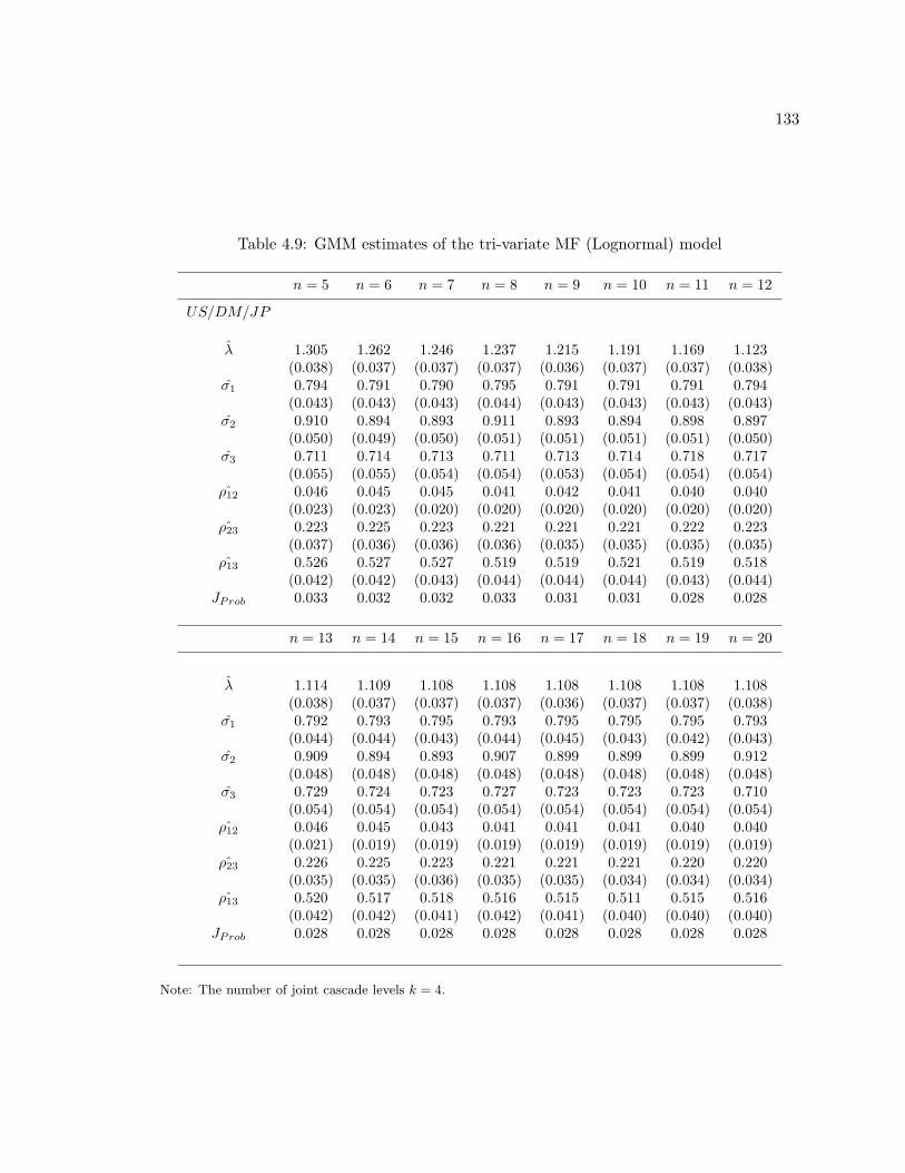
133

Table 4.9: GMM estimates of the tri-variate MF (Lognormal) model

n = 5 n = 6 n = 7 n = 8 n = 9 n = 10 n = 11 n = 12

US/DM/JP

λ 1.305 1.262 1.246 1.237 1.215 1.191 1.169 1.123(0.038) (0.037) (0.037) (0.037) (0.036) (0.037) (0.037) (0.038)

σ1 0.794 0.791 0.790 0.795 0.791 0.791 0.791 0.794(0.043) (0.043) (0.043) (0.044) (0.043) (0.043) (0.043) (0.043)

σ2 0.910 0.894 0.893 0.911 0.893 0.894 0.898 0.897(0.050) (0.049) (0.050) (0.051) (0.051) (0.051) (0.051) (0.050)

σ3 0.711 0.714 0.713 0.711 0.713 0.714 0.718 0.717(0.055) (0.055) (0.054) (0.054) (0.053) (0.054) (0.054) (0.054)

ρ12 0.046 0.045 0.045 0.041 0.042 0.041 0.040 0.040(0.023) (0.023) (0.020) (0.020) (0.020) (0.020) (0.020) (0.020)

ρ23 0.223 0.225 0.223 0.221 0.221 0.221 0.222 0.223(0.037) (0.036) (0.036) (0.036) (0.035) (0.035) (0.035) (0.035)

ρ13 0.526 0.527 0.527 0.519 0.519 0.521 0.519 0.518(0.042) (0.042) (0.043) (0.044) (0.044) (0.044) (0.043) (0.044)

JProb 0.033 0.032 0.032 0.033 0.031 0.031 0.028 0.028

n = 13 n = 14 n = 15 n = 16 n = 17 n = 18 n = 19 n = 20

λ 1.114 1.109 1.108 1.108 1.108 1.108 1.108 1.108(0.038) (0.037) (0.037) (0.037) (0.036) (0.037) (0.037) (0.038)

σ1 0.792 0.793 0.795 0.793 0.795 0.795 0.795 0.793(0.044) (0.044) (0.043) (0.044) (0.045) (0.043) (0.042) (0.043)

σ2 0.909 0.894 0.893 0.907 0.899 0.899 0.899 0.912(0.048) (0.048) (0.048) (0.048) (0.048) (0.048) (0.048) (0.048)

σ3 0.729 0.724 0.723 0.727 0.723 0.723 0.723 0.710(0.054) (0.054) (0.054) (0.054) (0.054) (0.054) (0.054) (0.054)

ρ12 0.046 0.045 0.043 0.041 0.041 0.041 0.040 0.040(0.021) (0.019) (0.019) (0.019) (0.019) (0.019) (0.019) (0.019)

ρ23 0.226 0.225 0.223 0.221 0.221 0.221 0.220 0.220(0.035) (0.035) (0.036) (0.035) (0.035) (0.034) (0.034) (0.034)

ρ13 0.520 0.517 0.518 0.516 0.515 0.511 0.515 0.516(0.042) (0.042) (0.041) (0.042) (0.041) (0.040) (0.040) (0.040)

JProb 0.028 0.028 0.028 0.028 0.028 0.028 0.028 0.028

Note: The number of joint cascade levels k = 4.

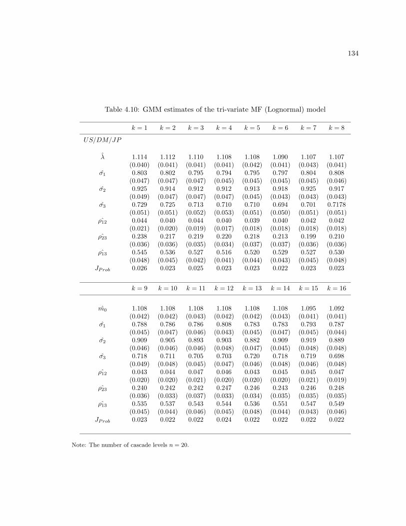
134

Table 4.10: GMM estimates of the tri-variate MF (Lognormal) model

k = 1 k = 2 k = 3 k = 4 k = 5 k = 6 k = 7 k = 8

US/DM/JP

λ 1.114 1.112 1.110 1.108 1.108 1.090 1.107 1.107(0.040) (0.041) (0.041) (0.041) (0.042) (0.041) (0.043) (0.041)

σ1 0.803 0.802 0.795 0.794 0.795 0.797 0.804 0.808(0.047) (0.047) (0.047) (0.045) (0.045) (0.045) (0.045) (0.046)

σ2 0.925 0.914 0.912 0.912 0.913 0.918 0.925 0.917(0.049) (0.047) (0.047) (0.047) (0.045) (0.043) (0.043) (0.043)

σ3 0.729 0.725 0.713 0.710 0.710 0.694 0.701 0.7178(0.051) (0.051) (0.052) (0.053) (0.051) (0.050) (0.051) (0.051)

ρ12 0.044 0.040 0.044 0.040 0.039 0.040 0.042 0.042(0.021) (0.020) (0.019) (0.017) (0.018) (0.018) (0.018) (0.018)

ρ23 0.238 0.217 0.219 0.220 0.218 0.213 0.199 0.210(0.036) (0.036) (0.035) (0.034) (0.037) (0.037) (0.036) (0.036)

ρ13 0.545 0.536 0.527 0.516 0.520 0.529 0.527 0.530(0.048) (0.045) (0.042) (0.041) (0.044) (0.043) (0.045) (0.048)

JProb 0.026 0.023 0.025 0.023 0.023 0.022 0.023 0.023

k = 9 k = 10 k = 11 k = 12 k = 13 k = 14 k = 15 k = 16

m0 1.108 1.108 1.108 1.108 1.108 1.108 1.095 1.092(0.042) (0.042) (0.043) (0.042) (0.042) (0.043) (0.041) (0.041)

σ1 0.788 0.786 0.786 0.808 0.783 0.783 0.793 0.787(0.045) (0.047) (0.046) (0.043) (0.045) (0.047) (0.045) (0.044)

σ2 0.909 0.905 0.893 0.903 0.882 0.909 0.919 0.889(0.046) (0.046) (0.046) (0.048) (0.047) (0.045) (0.048) (0.048)

σ3 0.718 0.711 0.705 0.703 0.720 0.718 0.719 0.698(0.049) (0.048) (0.045) (0.047) (0.046) (0.048) (0.046) (0.048)

ρ12 0.043 0.044 0.047 0.046 0.043 0.045 0.045 0.047(0.020) (0.020) (0.021) (0.020) (0.020) (0.020) (0.021) (0.019)

ρ23 0.240 0.242 0.242 0.247 0.246 0.243 0.246 0.248(0.036) (0.033) (0.037) (0.033) (0.034) (0.035) (0.035) (0.035)

ρ13 0.535 0.537 0.543 0.544 0.536 0.551 0.547 0.549(0.045) (0.044) (0.046) (0.045) (0.048) (0.044) (0.043) (0.046)

JProb 0.023 0.022 0.022 0.024 0.022 0.022 0.022 0.022


Chapter 5

Risk Management Applications of

Bivariate MF Models

5.1 Introduction

In general, risk management is the process of measuring or assessing risk, and then devel-

oping strategies to manage and control it. Conventional risk management focuses on risks

stemming from physical or legal causes, such as natural disasters, accidents, and lawsuits.

Financial risk management, on the other hand, focuses on risks that can be managed

by using practical financial instruments. With the aid of modern technology, information is

instantaneously available, which means that change, and subsequent market reactions, occur

very quickly. Financial markets can also be very quickly affected by changes in other stock

prices, exchange rates and interest rates. In addition, the fact that financial markets and

their individual assets are correlated attracts considerable attention of finance professionals;

it is this correlation that accelerates financial uncertainties that can subsequently result in

worldwide financial disasters. As an example, (1) take the market crash in 1987: The

stock market crash of 1987 was the largest one day stock market crash in history. The

135

136

Dow Jones index dropped 22.6% on the 19th of October 1987, and 500 billion dollars have

been evaporated within one day. Markets in most countries around the world collapsed

in the same fashion. (2) Southeast Asian financial crises in 1990s: It started with the

devaluation of Thai Baht, which took place on July 2nd 1997, a 15% to 20% devaluation

that occurred two months after this currency started to suffer from a massive speculative

attack. The devaluation of the Thai Baht was soon followed by that of the Philippine Peso,

the Malaysian Ringgit, the Indonesian Rupiah and, to a lesser extent, the Singapore Dollar.

The currency turmoil erupted in Southeast Asia, in turn triggering the market collapse on

Wall Street on October 27, 1997.

In this Chapter, we present empirical applications of bivariate MF models using empiri-

cal financial time series, including stock indices, foreign exchange rates, and U.S. government

bond maturity rates. Firstly the unconditional distribution of simulated data including

portfolios are studied based on bivariate MF models. In particular we focus on the tail

part which describes the most extreme outliers which are the interest of risk measurement

and management. We then conduct assessments in terms of two widely applied risk instru-

ments, namely Value-at-Risk and Expected Shortfall, comparing to the ones implied from

traditional GARCH type model.

5.2 Data description

Recalling the six empirical financial markets data in Section 3.6, we separate each time

series into two subsets (in-sample data used for estimation, out-of-sample data for forecast

assessment); for the in-sample periods we use for DOW/NIK: January 1969 - February

1988; US/DM : March 1973 - January 1990; TB1/TB2: June 1976 - May 1991. For the out-

of-sample subset, we use for DOW/NIK: March 1988 - October 2004; US/DM : February

1990 - February 2004; TB1/TB2: June 1991 - October 2004. The relevant descriptive

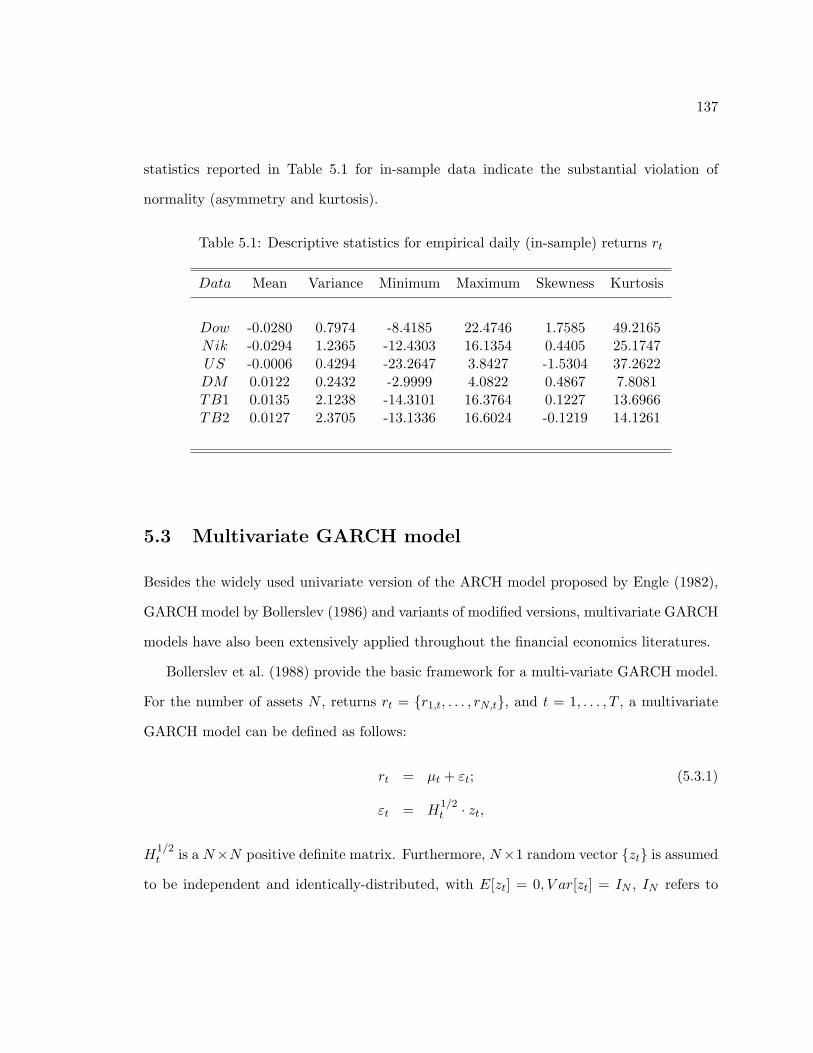
137

statistics reported in Table 5.1 for in-sample data indicate the substantial violation of

normality (asymmetry and kurtosis).

Table 5.1: Descriptive statistics for empirical daily (in-sample) returns rt

Data Mean Variance Minimum Maximum Skewness Kurtosis

Dow -0.0280 0.7974 -8.4185 22.4746 1.7585 49.2165Nik -0.0294 1.2365 -12.4303 16.1354 0.4405 25.1747US -0.0006 0.4294 -23.2647 3.8427 -1.5304 37.2622DM 0.0122 0.2432 -2.9999 4.0822 0.4867 7.8081TB1 0.0135 2.1238 -14.3101 16.3764 0.1227 13.6966TB2 0.0127 2.3705 -13.1336 16.6024 -0.1219 14.1261

5.3 Multivariate GARCH model

Besides the widely used univariate version of the ARCH model proposed by Engle (1982),

GARCH model by Bollerslev (1986) and variants of modified versions, multivariate GARCH

models have also been extensively applied throughout the financial economics literatures.

Bollerslev et al. (1988) provide the basic framework for a multi-variate GARCH model.

For the number of assets N , returns rt = r1,t, . . . , rN,t, and t = 1, . . . , T , a multivariate

GARCH model can be defined as follows:

rt = µt + εt; (5.3.1)

εt = H1/2t · zt,

H1/2t is a N×N positive definite matrix. Furthermore, N×1 random vector zt is assumed

to be independent and identically-distributed, with E[zt] = 0, V ar[zt] = IN , IN refers to

138

the identity matrix of order N and

E[rt|Ωt−1] = µt; (5.3.2)

V ar(rt|Ωt−1) = H1/2t (H1/2

t )′,

Ωt−1 is the information set available till time t − 1, Ht = hij,t (i, j = 1, 2, . . . , N refers

to different time series). Bollerslev et al. (1988) propose a general formulation of Ht by

extending the GARCH representation in the univariate case to the vectorized conditional-

variance matrix (VEC model). In the general VEC model, each element of Ht is a linear

function of the lagged squared errors and cross-products of errors and lagged values of the

elements of Ht. The VEC(1,1) model is defined as:

ht = C +Aε2t−1 +Ght−1, (5.3.3)

where

ht = vech(Ht), (5.3.4)

εt = vech(εtεt)′, (5.3.5)

and vech(·) denotes the operator that stacks the lower triangular portion of a N × N

matrix as a N(N + 1)/2 × 1 vector. A and G are square parameter matrices of order

N(N + 1)/2 and C is a N(N + 1)/2× 1 constant parameter vector.

However this vectorized representation involves a large number of parameters which is

equal to N(N + 1)(N(N + 1) + 1)/2. Empirical applications require further restrictions

and simplifications. One useful member of the vech-representation family is the diago-

nal form. Under the diagonal form, each variance-covariance term is postulated to follow a

GARCH-type equation with the lagged variance-covariance term and the product of the cor-

responding lagged residuals as the right-hand-side variables in the conditional-(co)variance

equation.

139

It is often difficult to verify the condition that the variance-covariance matrix of an

estimated multi-variate GARCH model is positive definite. Furthermore, such conditions

are often very difficult to impose during the optimization of the log-likelihood function. A

constant correlation GARCH (CC-GARCH) model proposed by Bollerslev (1990) overcomes

these difficulties. The CC-GARCH (1, 1) model assumes constant cross correlations,1 such

that:

hii,t = ωi + αiε2t−1 + βihii,t−1 i = 1, 2, . . . , N, (5.3.6)

hij,t = ρij

√hi,thj,t ∀i 6= j.

The normality assumption implies that the log-likelihood has the form:

logL(θ) = −T2log(2π)− 1

2

T∑t=1

log(Ht)−12

T∑t=1

(rt − µt)′H−1t (rt − µt). (5.3.7)

With the assumption of constant correlations, the maximum likelihood (ML) estimate

of the correlation matrix is equal to the sample correlation matrix, which is always positive

semi-definite; the positive semi-definiteness of the conditional variance-covariance matrix

can be ensured when the conditional variances are all positive. In addition, when the

correlation matrix is concentrated out of the likelihood function, further simplification is

achieved in the optimization by the fact that the Gaussian ML estimator is consistent,

provided that the conditional mean and variance are correctly specified. Table 5.2 reports

the empirical CC-GARCH(1, 1) parameters with respect to the in-sample data described

in the previous section.

1Instead of assuming correlations to be time invariant, Engle and Kroner (1995) propose a class ofmultivariate GARCH model called the BEKK (named after Baba, Engle, Kraft and Kroner) model, andprovide some theoretical analysis related to the vech-representation form which also ensures the conditionof a positive definite conditional-variance matrix in the process of optimization. More details on differentversions of multivariate GARCH models can be found in Gourieroux (1997) (Chapter 6).

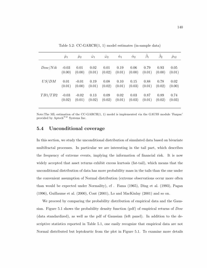
140

Table 5.2: CC-GARCH(1, 1) model estimates (in-sample data)

µ1 µ2 ω1 ω2 α1 α2 β1 β2 ρ12

Dow/Nik -0.03 0.01 0.02 0.01 0.19 0.06 0.79 0.93 0.05(0.00) (0.00) (0.01) (0.02) (0.01) (0.00) (0.01) (0.00) (0.01)

US/DM 0.01 -0.01 0.19 0.08 0.10 0.15 0.88 0.78 0.02(0.01) (0.00) (0.01) (0.02) (0.01) (0.03) (0.01) (0.02) (0.00)

TB1/TB2 -0.03 -0.02 0.13 0.09 0.02 0.03 0.87 0.89 0.74(0.02) (0.01) (0.02) (0.02) (0.01) (0.03) (0.01) (0.02) (0.03)

Note:The ML estimation of the CC-GARCH(1, 1) model is implemented via the GAUSS module ‘Fanpac’provided by AptechTM Systems Inc.

5.4 Unconditional coverage

In this section, we study the unconditional distribution of simulated data based on bivariate

multifractal processes. In particular we are interesting in the tail part, which describes

the frequency of extreme events, implying the information of financial risk. It is now

widely accepted that asset returns exhibit excess kurtosis (fat-tail), which means that the

unconditional distribution of data has more probability mass in the tails than the one under

the convenient assumption of Normal distribution (extreme observations occur more often

than would be expected under Normality), cf . Fama (1965), Ding et al. (1993), Pagan

(1996), Guillaume et al. (2000), Cont (2001), Lo and MacKinlay (2001) and so on.

We proceed by comparing the probability distribution of empirical data and the Gaus-

sian. Figure 5.1 shows the probability density function (pdf) of empirical returns of Dow

(data standardized), as well as the pdf of Gaussian (left panel). In addition to the de-

scriptive statistics reported in Table 5.1, one easily recognize that empirical data are not

Normal distributed but leptokurtic from the plot in Figure 5.1. To examine more details

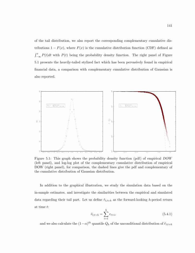
141

of the tail distribution, we also report the corresponding complementary cumulative dis-

tributions 1 − F (x), where F (x) is the cumulative distribution function (CDF) defined as∫ x−∞ P (t)dt with P (t) being the probability density function. The right panel of Figure

5.1 presents the heavily-tailed stylized fact which has been pervasively found in empirical

financial data, a comparison with complementary cumulative distribution of Gaussian is

also reported.

Figure 5.1: This graph shows the probability density function (pdf) of empirical DOW(left panel), and log-log plot of the complementary cumulative distribution of empiricalDOW (right panel), for comparison, the dashed lines give the pdf and complementary ofthe cumulative distribution of Gaussian distribution.

In addition to the graphical illustration, we study the simulation data based on the

in-sample estimates, and investigate the similarities between the empirical and simulated

data regarding their tail part. Let us define rt,t+h as the forward-looking h-period return

at time t:

rt,t+h =h∑

i=1

rt+i, (5.4.1)

and we also calculate the (1−α)th quantile Qh of the unconditional distribution of rt:t+h

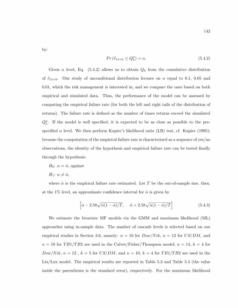
142

by:

Pr (rt:t+h ≤ Qαh) = α. (5.4.2)

Given α level, Eq. (5.4.2) allows us to obtain Qh from the cumulative distribution

of rt:t+h. Our study of unconditional distribution focuses on α equal to 0.1, 0.05 and

0.01, which the risk management is interested in, and we compare the ones based on both

empirical and simulated data. Thus, the performance of the model can be assessed by

computing the empirical failure rate (for both the left and right tails of the distribution of

returns). The failure rate is defined as the number of times returns exceed the simulated

Qαh . If the model is well specified, it is expected to be as close as possible to the pre-

specified α level. We then perform Kupiec’s likelihood ratio (LR) test, cf. Kupiec (1995);

because the computation of the empirical failure rate is characterized as a sequence of yes/no

observations, the identity of the hypothesis and empirical failure rate can be tested finally

through the hypothesis:

H0: α = α, against

H1: α 6= α,

where α is the empirical failure rate estimated. Let T be the out-of-sample size, then,

at the 1% level, an approximate confidence interval for α is given by

[α− 2.58

√α(1− α)/T , α+ 2.58

√α(1− α)/T

](5.4.3)

We estimate the bivariate MF models via the GMM and maximum likelihood (ML)

approaches using in-sample data. The number of cascade levels is selected based on our

empirical studies in Section 3.6, namely: n = 10 for Dow/Nik, n = 12 for US/DM , and

n = 10 for TB1/TB2 are used in the Calvet/Fisher/Thompson model; n = 14, k = 4 for

Dow/Nik, n = 12 , k = 5 for US/DM , and n = 10, k = 4 for TB1/TB2 are used in the

Liu/Lux model. The empirical results are reported in Table 5.3 and Table 5.4 (the value

inside the parentheses is the standard error), respectively. For the maximum likelihood

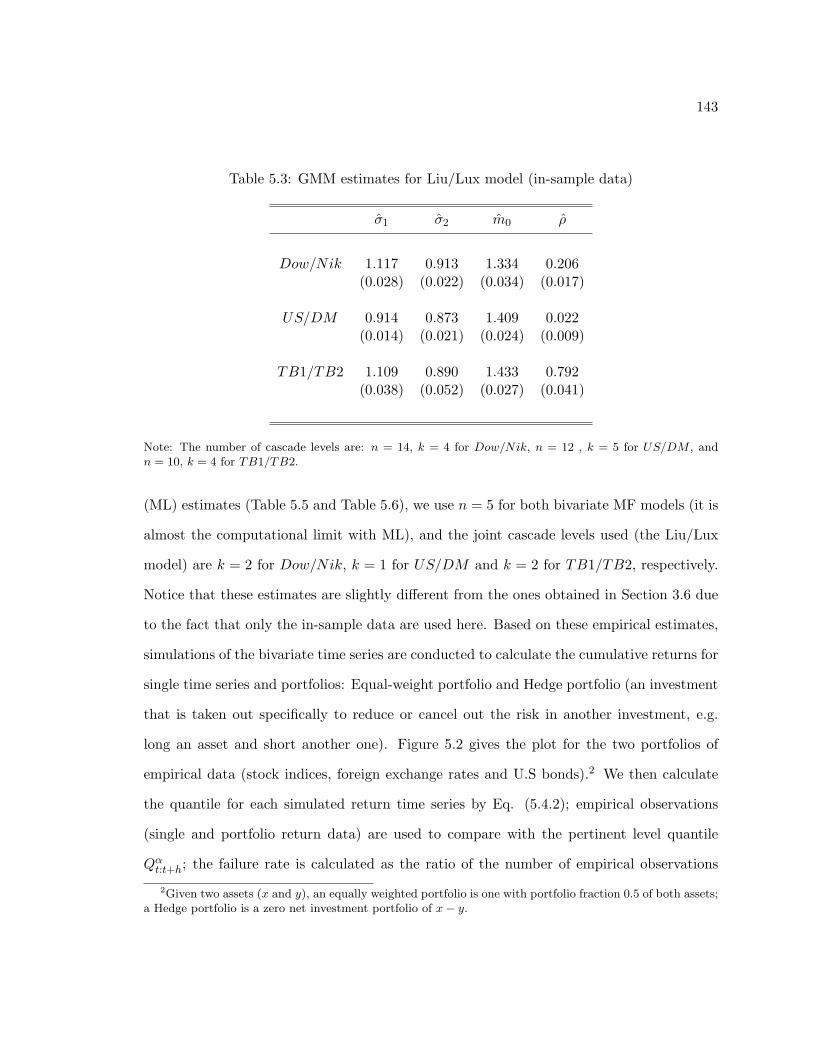
143

Table 5.3: GMM estimates for Liu/Lux model (in-sample data)

σ1 σ2 m0 ρ

Dow/Nik 1.117 0.913 1.334 0.206(0.028) (0.022) (0.034) (0.017)

US/DM 0.914 0.873 1.409 0.022(0.014) (0.021) (0.024) (0.009)

TB1/TB2 1.109 0.890 1.433 0.792(0.038) (0.052) (0.027) (0.041)

Note: The number of cascade levels are: n = 14, k = 4 for Dow/Nik, n = 12 , k = 5 for US/DM , andn = 10, k = 4 for TB1/TB2.

(ML) estimates (Table 5.5 and Table 5.6), we use n = 5 for both bivariate MF models (it is

almost the computational limit with ML), and the joint cascade levels used (the Liu/Lux

model) are k = 2 for Dow/Nik, k = 1 for US/DM and k = 2 for TB1/TB2, respectively.

Notice that these estimates are slightly different from the ones obtained in Section 3.6 due

to the fact that only the in-sample data are used here. Based on these empirical estimates,

simulations of the bivariate time series are conducted to calculate the cumulative returns for

single time series and portfolios: Equal-weight portfolio and Hedge portfolio (an investment

that is taken out specifically to reduce or cancel out the risk in another investment, e.g.

long an asset and short another one). Figure 5.2 gives the plot for the two portfolios of

empirical data (stock indices, foreign exchange rates and U.S bonds).2 We then calculate

the quantile for each simulated return time series by Eq. (5.4.2); empirical observations

(single and portfolio return data) are used to compare with the pertinent level quantile

Qαt:t+h; the failure rate is calculated as the ratio of the number of empirical observations

2Given two assets (x and y), an equally weighted portfolio is one with portfolio fraction 0.5 of both assets;a Hedge portfolio is a zero net investment portfolio of x− y.

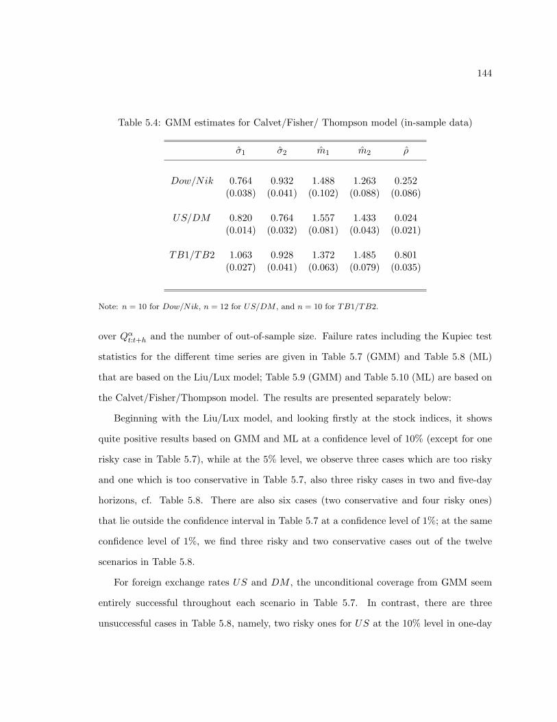
144

Table 5.4: GMM estimates for Calvet/Fisher/ Thompson model (in-sample data)

σ1 σ2 m1 m2 ρ

Dow/Nik 0.764 0.932 1.488 1.263 0.252(0.038) (0.041) (0.102) (0.088) (0.086)

US/DM 0.820 0.764 1.557 1.433 0.024(0.014) (0.032) (0.081) (0.043) (0.021)

TB1/TB2 1.063 0.928 1.372 1.485 0.801(0.027) (0.041) (0.063) (0.079) (0.035)

Note: n = 10 for Dow/Nik, n = 12 for US/DM , and n = 10 for TB1/TB2.

over Qαt:t+h and the number of out-of-sample size. Failure rates including the Kupiec test

statistics for the different time series are given in Table 5.7 (GMM) and Table 5.8 (ML)

that are based on the Liu/Lux model; Table 5.9 (GMM) and Table 5.10 (ML) are based on

the Calvet/Fisher/Thompson model. The results are presented separately below:

Beginning with the Liu/Lux model, and looking firstly at the stock indices, it shows

quite positive results based on GMM and ML at a confidence level of 10% (except for one

risky case in Table 5.7), while at the 5% level, we observe three cases which are too risky

and one which is too conservative in Table 5.7, also three risky cases in two and five-day

horizons, cf. Table 5.8. There are also six cases (two conservative and four risky ones)

that lie outside the confidence interval in Table 5.7 at a confidence level of 1%; at the same

confidence level of 1%, we find three risky and two conservative cases out of the twelve

scenarios in Table 5.8.

For foreign exchange rates US and DM , the unconditional coverage from GMM seem

entirely successful throughout each scenario in Table 5.7. In contrast, there are three

unsuccessful cases in Table 5.8, namely, two risky ones for US at the 10% level in one-day

145

Table 5.5: ML estimates for Liu/Lux model (in-sample data)

σ1 σ2 m0 ρ

Dow/Nik 1.014 0.913 1.512 0.207(0.031) (0.024) (0.027) (0.018)

US/DM 0.849 0.901 1.397 0.020(0.021) (0.020) (0.017) (0.011)

TB1/TB2 1.275 1.032 1.711 0.730(0.023) (0.027) (0.022) (0.033)

Note: The number of cascade levels n = 5. We use the number of joint cascade level k = 2 for Dow/Nik,k = 1 for US/DM and k = 2 for TB1/TB2, respectively.

and two-day horizon, respectively; another conservative one for EW at the 1% level in

five-day horizon.3

For U.S. treasury bond maturity rates, we find that results based on GMM and ML

in both tables are successful at confidence level of 10%, except for the conservative hedge

portfolios. At 5% level, there are two risky cases for TB2 and equal-weighted portfolio in

Table 5.7, and risky EW in Table 5.8 at both two and five-day horizons, again, all HG

are too conservative; of course, excessive conservativeness (as in the most cases of hedge

portfolios) is also not an indication of superior risk management. At 1% level, we observe

the positive results for individual TB1 and TB2 (except one risky TB2 at two-day horizon

in Table 5.7).

We then move to the results from the Calvet/Fisher/Thompson model. For the stock

indices, it shows the reasonable success for the individual Nikkei index in all scenarios and

HG portfolio in two and five-day horizons in Table 5.9, but there are entirely unsuccessful3One may notice there are insignificant estimates of ρ for the foreign exchange rates in Table 5.4, 5.5 and

5.6; we have conducted the study by setting ρ = 0 and we omit these supplementary tables here due to verysimilar picture of the results.

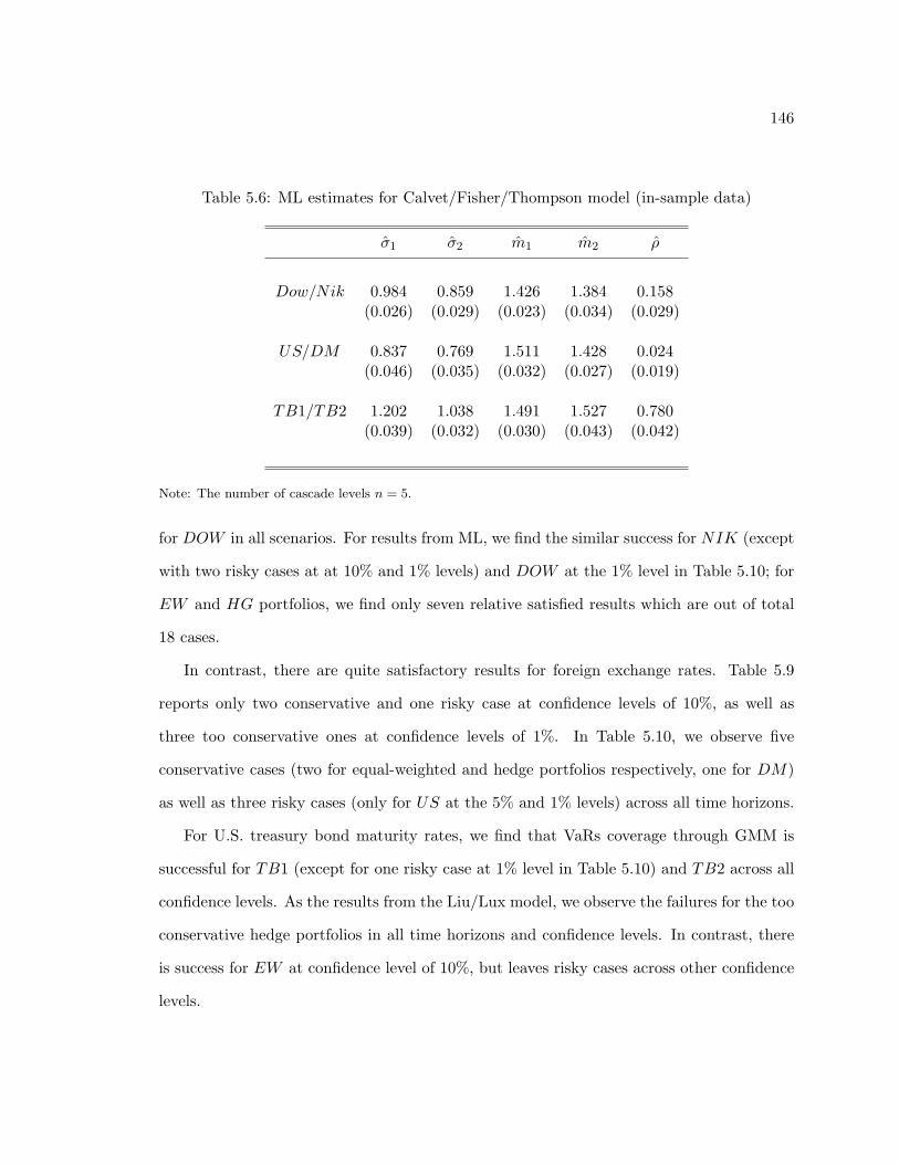
146

Table 5.6: ML estimates for Calvet/Fisher/Thompson model (in-sample data)

σ1 σ2 m1 m2 ρ

Dow/Nik 0.984 0.859 1.426 1.384 0.158(0.026) (0.029) (0.023) (0.034) (0.029)

US/DM 0.837 0.769 1.511 1.428 0.024(0.046) (0.035) (0.032) (0.027) (0.019)

TB1/TB2 1.202 1.038 1.491 1.527 0.780(0.039) (0.032) (0.030) (0.043) (0.042)


for DOW in all scenarios. For results from ML, we find the similar success for NIK (except

with two risky cases at at 10% and 1% levels) and DOW at the 1% level in Table 5.10; for

EW and HG portfolios, we find only seven relative satisfied results which are out of total

18 cases.

In contrast, there are quite satisfactory results for foreign exchange rates. Table 5.9

reports only two conservative and one risky case at confidence levels of 10%, as well as

three too conservative ones at confidence levels of 1%. In Table 5.10, we observe five

conservative cases (two for equal-weighted and hedge portfolios respectively, one for DM)

as well as three risky cases (only for US at the 5% and 1% levels) across all time horizons.

For U.S. treasury bond maturity rates, we find that VaRs coverage through GMM is

successful for TB1 (except for one risky case at 1% level in Table 5.10) and TB2 across all

confidence levels. As the results from the Liu/Lux model, we observe the failures for the too

conservative hedge portfolios in all time horizons and confidence levels. In contrast, there

is success for EW at confidence level of 10%, but leaves risky cases across other confidence

levels.

147

In summary, from Table 5.7 to 5.10, the bivariate MF models show rather satisfactory

performances, particularly with remarkable findings for foreign exchange rates. By com-

paring between Table 5.7 and Table 5.9 with a total of 108 scenarios in each, we find that

the Liu/Lux model (24 failure cases) outperforms the Calvet/Fisher/Thompson model (40

failure cases), which signals that our more parsimonious design of multivariate MF model

performs quite well. note that, the Liu/Lux model with only one common choice of the dis-

tribution for volatility components, that is two draws of Mt ∈ m0, m1, with m0 ∈ (0, 2)

and the alternative m1 = 2−m0; The Calvet/Fisher/Thompson approach uses two separate

choices, namely two binomial distributions: m1, 2−m1 and m2, 2−m2 for the bivariate

assets. The results also reveal that the simulated data based on GMM show better fit with

empirical time series than the ones based on ML estimation. This is actually plausible:

there are larger numbers of cascade levels (n = 10 for Nik/Dow and TB1/TB2, n = 12

for US/DM) employed within BMF models for GMM, while only n = 5number of cascade

levels is used for ML due to its computational limitation.

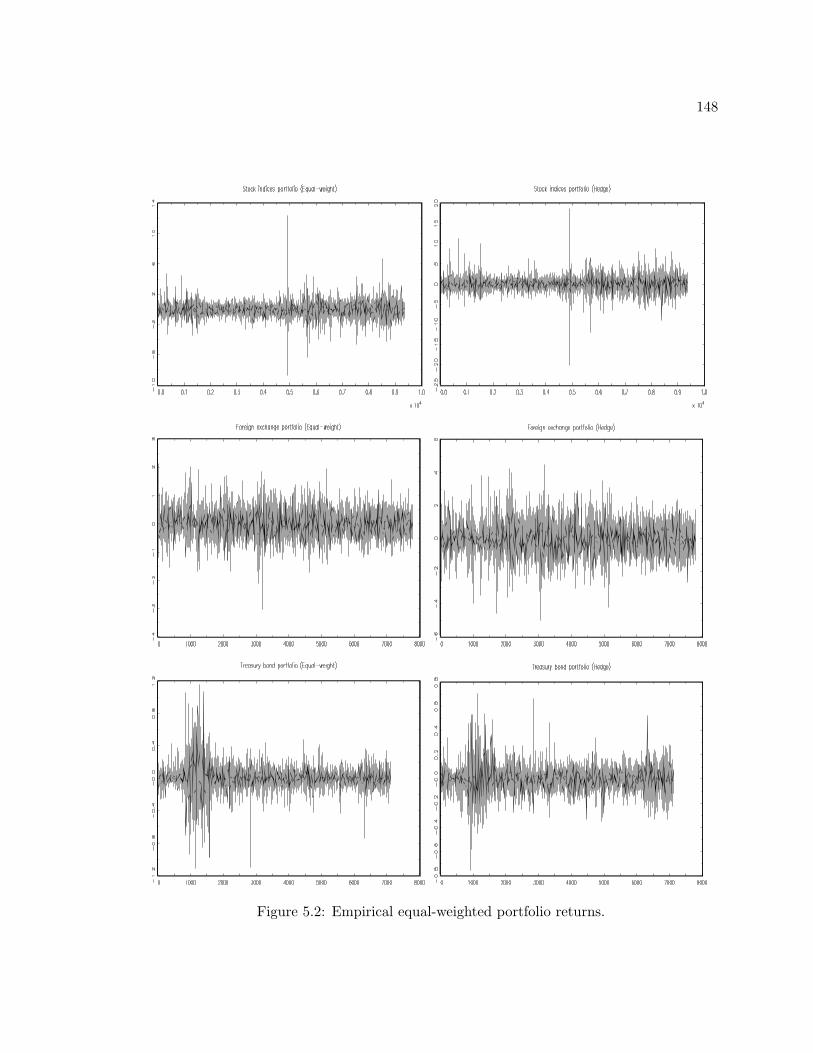
148

Figure 5.2: Empirical equal-weighted portfolio returns.

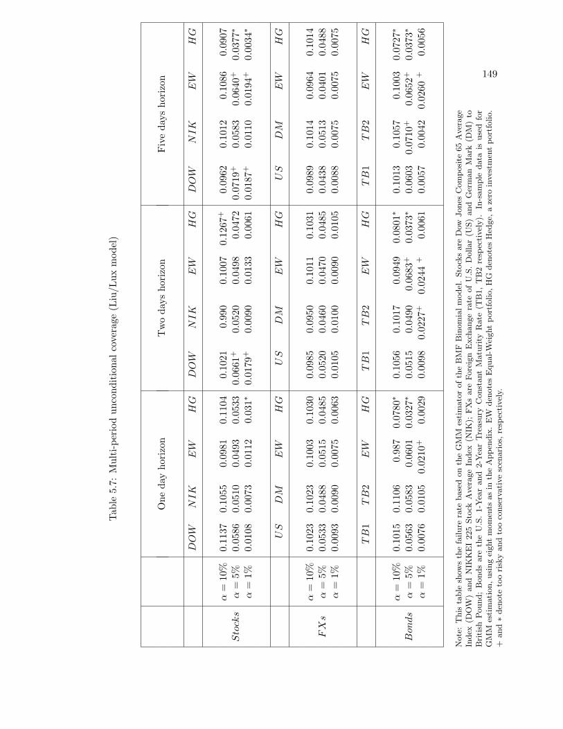
149

Tab

le5.

7:M

ulti

-per

iod

unco

ndit

iona

lco

vera

ge(L

iu/L

uxm

odel

)

One

day

hori

zon

Tw

oda

ysho

rizo

nFiv

eda

ysho

rizo

n

DOW

NIK

EW

HG

DOW

NIK

EW

HG

DOW

NIK

EW

HG

α=

10%

0.11

370.

1055

0.09

810.

1104

0.10

210.

990

0.10

070.

1267

+0.

0962

0.10

120.

1086

0.09

07Stocks

α=

5%0.

0586

0.05

100.

0493

0.05

330.

0661

+0.

0520

0.04

980.

0472

0.07

19+

0.05

830.

0640

+0.

0377∗

α=

1%0.

0108

0.00

730.

0112

0.03

1∗0.

0179

+0.

0090

0.01

330.

0061

0.01

87+

0.01

100.

0194

+0.

0034∗

US

DM

EW

HG

US

DM

EW

HG

US

DM

EW

HG

α=

10%

0.10

230.

1023

0.10

030.

1030

0.09

850.

0950

0.10

110.

1031

0.09

890.

1014

0.09

640.

1014

FXs

α=

5%0.

0533

0.04

880.

0515

0.04

850.

0520

0.04

600.

0470

0.04

850.

0438

0.05

130.

0401

0.04

88α

=1%

0.00

930.

0090

0.00

750.

0063

0.01

050.

0100

0.00

900.

0105

0.00

880.

0075

0.00

750.

0075

TB

1TB

2EW

HG

TB

1TB

2EW

HG

TB

1TB

2EW

HG

α=

10%

0.10

150.

1106

0.98

70.

0780∗

0.10

560.

1017

0.09

490.

0801∗

0.10

130.

1057

0.10

030.

0727∗

Bonds

α=

5%0.

0563

0.05

830.

0601

0.03

27∗

0.05

150.

0490

0.06

83+

0.03

73∗

0.06

030.

0710

+0.

0652

+0.

0373∗

α=

1%0.

0076

0.01

050.

0210

+0.

0029

0.00

980.

0227

+0.

0244

+0.

0061

0.00

570.

0042

0.02

60+

0.00

56

Note

:T

his

table

show

sth

efa

ilure

rate

base

don

the

GM

Mes

tim

ato

rofth

eB

MF

Bin

om

ialm

odel

.Sto

cks

are

Dow

Jones

Com

posi

te65

Aver

age

Index

(DO

W)

and

NIK

KE

I225

Sto

ckA

ver

age

Index

(NIK

);FX

sare

Fore

ign

Exch

ange

rate

of

U.S

.D

ollar

(US)

and

Ger

man

Mark

(DM

)to

Bri

tish

Pound;

Bonds

are

the

U.S

.1-Y

ear

and

2-Y

ear

Tre

asu

ryC

onst

ant

Matu

rity

Rate

(TB

1,

TB

2re

spec

tivel

y).

In-s

am

ple

data

isuse

dfo

rG

MM

esti

mati

on,usi

ng

eight

mom

ents

as

inth

eA

ppen

dix

.E

Wden

ote

sE

qual-W

eight

port

folio,H

Gden

ote

sH

edge,

aze

roin

ves

tmen

tport

folio.

+and∗

den

ote

too

risk

yand

too

conse

rvati

ve

scen

ari

os,

resp

ecti

vel

y.

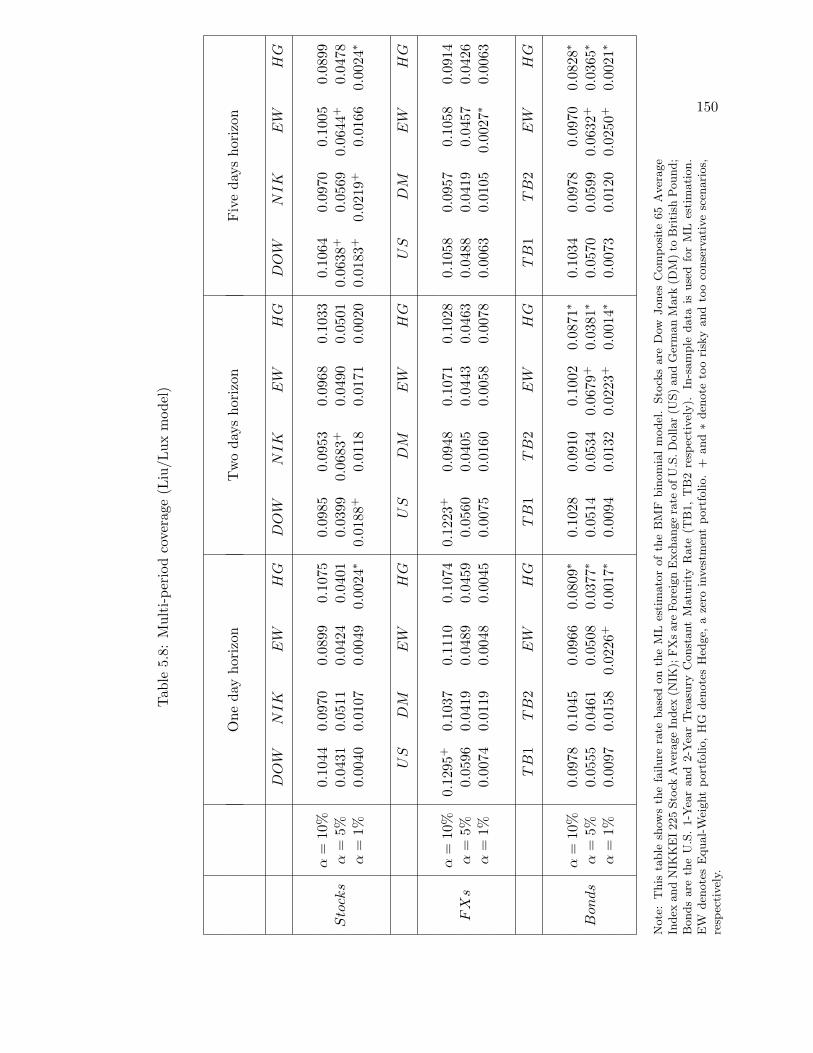
150

Tab

le5.

8:M

ulti

-per

iod

cove

rage

(Liu

/Lux

mod

el)

One

day

hori

zon

Tw

oda

ysho

rizo

nFiv

eda

ysho

rizo

n

DOW

NIK

EW

HG

DOW

NIK

EW

HG

DOW

NIK

EW

HG

α=

10%

0.10

440.

0970

0.08

990.

1075

0.09

850.

0953

0.09

680.

1033

0.10

640.

0970

0.10

050.

0899

Stocks

α=

5%0.

0431

0.05

110.

0424

0.04

010.

0399

0.06

83+

0.04

900.

0501

0.06

38+

0.05

690.

0644

+0.

0478

α=

1%0.

0040

0.01

070.

0049

0.00

24∗

0.01

88+

0.01

180.

0171

0.00

200.

0183

+0.

0219

+0.

0166

0.00

24∗

US

DM

EW

HG

US

DM

EW

HG

US

DM

EW

HG

α=

10%

0.12

95+

0.10

370.

1110

0.10

740.

1223

+0.

0948

0.10

710.

1028

0.10

580.

0957

0.10

580.

0914

FXs

α=

5%0.

0596

0.04

190.

0489

0.04

590.

0560

0.04

050.

0443

0.04

630.

0488

0.04

190.

0457

0.04

26α

=1%

0.00

740.

0119

0.00

480.

0045

0.00

750.

0160

0.00

580.

0078

0.00

630.

0105

0.00

27∗

0.00

63

TB

1TB

2EW

HG

TB

1TB

2EW

HG

TB

1TB

2EW

HG

α=

10%

0.09

780.

1045

0.09

660.

0809∗

0.10

280.

0910

0.10

020.

0871∗

0.10

340.

0978

0.09

700.

0828∗

Bonds

α=

5%0.

0555

0.04

610.

0508

0.03

77∗

0.05

140.

0534

0.06

79+

0.03

81∗

0.05

700.

0599

0.06

32+

0.03

65∗

α=

1%0.

0097

0.01

580.

0226

+0.

0017∗

0.00

940.

0132

0.02

23+

0.00

14∗

0.00

730.

0120

0.02

50+

0.00

21∗

Note

:T

his

table

show

sth

efa

ilure

rate

base

don

the

ML

esti

mato

rof

the

BM

Fbin

om

ialm

odel

.Sto

cks

are

Dow

Jones

Com

posi

te65

Aver

age

Index

and

NIK

KE

I225

Sto

ckA

ver

age

Index

(NIK

);FX

sare

Fore

ign

Exch

ange

rate

ofU

.S.D

ollar(U

S)and

Ger

man

Mark

(DM

)to

Bri

tish

Pound;

Bonds

are

the

U.S

.1-Y

ear

and

2-Y

ear

Tre

asu

ryC

onst

ant

Matu

rity

Rate

(TB

1,

TB

2re

spec

tivel

y).

In-s

am

ple

data

isuse

dfo

rM

Les

tim

ati

on.

EW

den

ote

sE

qual-W

eight

port

folio,H

Gden

ote

sH

edge,

aze

roin

ves

tmen

tport

folio.

+and∗

den

ote

too

risk

yand

too

conse

rvati

ve

scen

ari

os,

resp

ecti

vel

y.

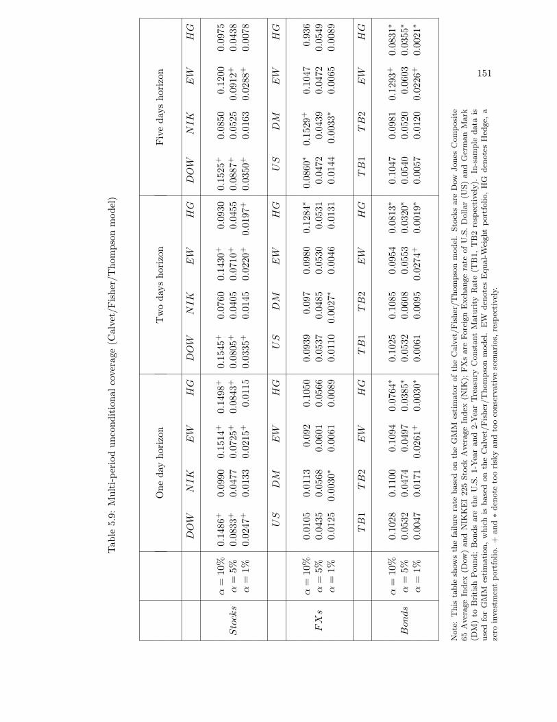
151

Tab

le5.

9:M

ulti

-per

iod

unco

ndit

iona

lco

vera

ge(C

alve

t/Fis

her/

Tho

mps

onm

odel

)

One

day

hori

zon

Tw

oda

ysho

rizo

nFiv

eda

ysho

rizo

n

DOW

NIK

EW

HG

DOW

NIK

EW

HG

DOW

NIK

EW

HG

α=

10%

0.14

86+

0.09

900.

1514

+0.

1498

+0.

1545

+0.

0760

0.14

30+

0.09

300.

1525

+0.

0850

0.12

000.

0975

Stocks

α=

5%0.

0833

+0.

0477

0.07

25+

0.08

43+

0.08

05+

0.04

050.

0710

+0.

0455

0.08

87+

0.05

250.

0912

+0.

0438

α=

1%0.

0247

+0.

0133

0.02

15+

0.01

150.

0335

+0.

0145

0.02

20+

0.01

97+

0.03

50+

0.01

630.

0288

+0.

0078

US

DM

EW

HG

US

DM

EW

HG

US

DM

EW

HG

α=

10%

0.01

050.

0113

0.09

20.

1050

0.09

390.

097

0.09

800.

1284∗

0.08

60∗

0.15

29+

0.10

470.

936

FXs

α=

5%0.

0435

0.05

680.

0601

0.05

660.

0537

0.04

850.

0530

0.05

310.

0472

0.04

390.

0472

0.05

49α

=1%

0.01

250.

0030∗

0.00

610.

0089

0.01

100.

0027∗

0.00

460.

0131

0.01

440.

0033∗

0.00

650.

0089

TB

1TB

2EW

HG

TB

1TB

2EW

HG

TB

1TB

2EW

HG

α=

10%

0.10

280.

1100

0.10

940.

0764∗

0.10

250.

1085

0.09

540.

0813∗

0.10

470.

0981

0.12

93+

0.08

31∗

Bonds

α=

5%0.

0532

0.04

740.

0497

0.03

85∗

0.05

320.

0608

0.05

530.

0320∗

0.05

400.

0520

0.06

030.

0355∗

α=

1%0.

0047

0.01

710.

0261

+0.

0030∗

0.00

610.

0095

0.02

74+

0.00

19∗

0.00

570.

0120

0.02

26+

0.00

21∗

Note

:T

his

table

show

sth

efa

ilure

rate

base

don

the

GM

Mes

tim

ato

rofth

eC

alv

et/Fis

her

/T

hom

pso

nm

odel

.Sto

cks

are

Dow

Jones

Com

posi

te65

Aver

age

Index

(Dow

)and

NIK

KE

I225

Sto

ckA

ver

age

Index

(NIK

);FX

sare

Fore

ign

Exch

ange

rate

of

U.S

.D

ollar

(US)

and

Ger

man

Mark

(DM

)to

Bri

tish

Pound;

Bonds

are

the

U.S

.1-Y

ear

and

2-Y

ear

Tre

asu

ryC

onst

ant

Matu

rity

Rate

(TB

1,

TB

2re

spec

tivel

y).

In-s

am

ple

data

isuse

dfo

rG

MM

esti

mati

on,

whic

his

base

don

the

Calv

et/Fis

her

/T

hom

pso

nm

odel

.E

Wden

ote

sE

qual-W

eight

port

folio,

HG

den

ote

sH

edge,

aze

roin

ves

tmen

tport

folio.

+and∗

den

ote

too

risk

yand

too

conse

rvati

ve

scen

ari

os,

resp

ecti

vel

y.

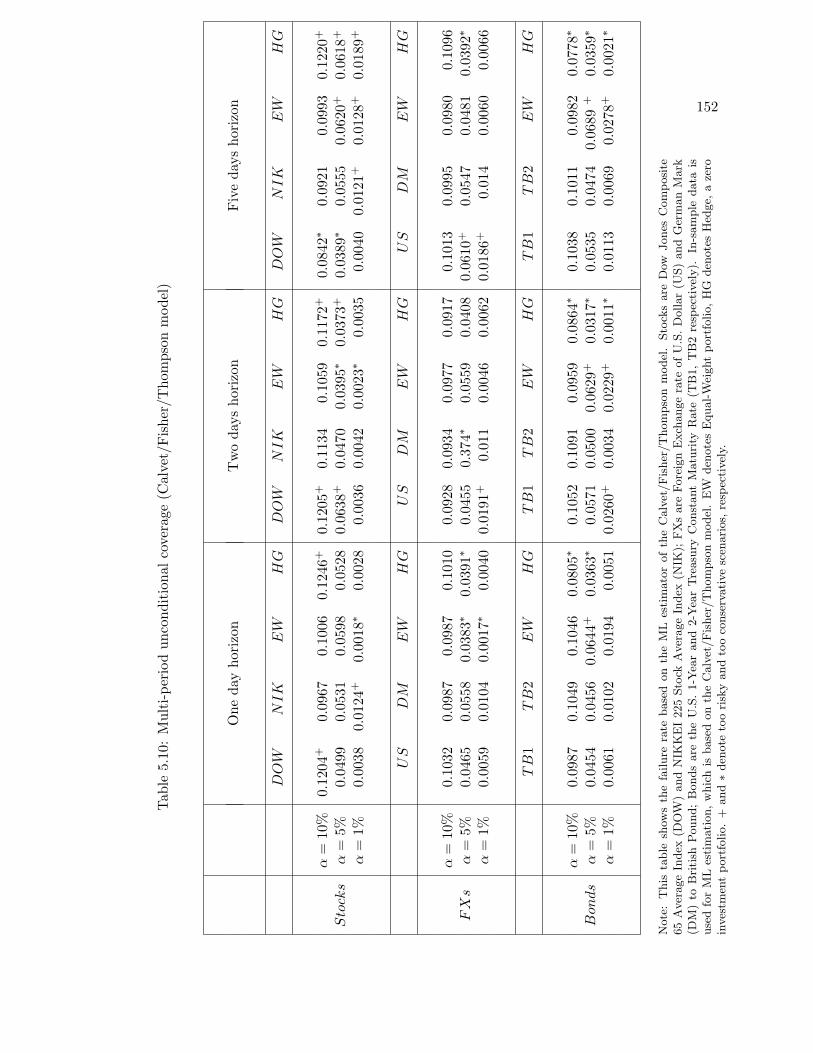
152

Tab

le5.

10:

Mul

ti-p

erio

dun

cond

itio

nalco

vera

ge(C

alve

t/Fis

her/

Tho

mps

onm

odel

)

One

day

hori

zon

Tw

oda

ysho

rizo

nFiv

eda

ysho

rizo

n

DOW

NIK

EW

HG

DOW

NIK

EW

HG

DOW

NIK

EW

HG

α=

10%

0.12

04+

0.09

670.

1006

0.12

46+

0.12

05+

0.11

340.

1059

0.11

72+

0.08

42∗

0.09

210.

0993

0.12

20+

Stocks

α=

5%0.

0499

0.05

310.

0598

0.05

280.

0638

+0.

0470

0.03

95∗

0.03

73+

0.03

89∗

0.05

550.

0620

+0.

0618

+

α=

1%0.

0038

0.01

24+

0.00

18∗

0.00

280.

0036

0.00

420.

0023∗

0.00

350.

0040

0.01

21+

0.01

28+

0.01

89+

US

DM

EW

HG

US

DM

EW

HG

US

DM

EW

HG

α=

10%

0.10

320.

0987

0.09

870.

1010

0.09

280.

0934

0.09

770.

0917

0.10

130.

0995

0.09

800.

1096

FXs

α=

5%0.

0465

0.05

580.

0383∗

0.03

91∗

0.04

550.

374∗

0.05

590.

0408

0.06

10+

0.05

470.

0481

0.03

92∗

α=

1%0.

0059

0.01

040.

0017∗

0.00

400.

0191

+0.

011

0.00

460.

0062

0.01

86+

0.01

40.

0060

0.00

66

TB

1TB

2EW

HG

TB

1TB

2EW

HG

TB

1TB

2EW

HG

α=

10%

0.09

870.

1049

0.10

460.

0805∗

0.10

520.

1091

0.09

590.

0864∗

0.10

380.

1011

0.09

820.

0778∗

Bonds

α=

5%0.

0454

0.04

560.

0644

+0.

0363∗

0.05

710.

0500

0.06

29+

0.03

17∗

0.05

350.

0474

0.06

89+

0.03

59∗

α=

1%0.

0061

0.01

020.

0194

0.00

510.

0260

+0.

0034

0.02

29+

0.00

11∗

0.01

130.

0069

0.02

78+

0.00

21∗

Note

:T

his

table

show

sth

efa

ilure

rate

base

don

the

ML

esti

mato

rof

the

Calv

et/Fis

her

/T

hom

pso

nm

odel

.Sto

cks

are

Dow

Jones

Com

posi

te65

Aver

age

Index

(DO

W)

and

NIK

KE

I225

Sto

ckA

ver

age

Index

(NIK

);FX

sare

Fore

ign

Exch

ange

rate

ofU

.S.D

ollar

(US)

and

Ger

man

Mark

(DM

)to

Bri

tish

Pound;

Bonds

are

the

U.S

.1-Y

ear

and

2-Y

ear

Tre

asu

ryC

onst

ant

Matu

rity

Rate

(TB

1,

TB

2re

spec

tivel

y).

In-s

am

ple

data

isuse

dfo

rM

Les

tim

ati

on,w

hic

his

base

don

the

Calv

et/Fis

her

/T

hom

pso

nm

odel

.E

Wden

ote

sE

qual-W

eight

port

folio,H

Gden

ote

sH

edge,

aze

roin

ves

tmen

tport

folio.

+and∗

den

ote

too

risk

yand

too

conse

rvati

ve

scen

ari

os,

resp

ecti

vel

y.

153

5.5 Value-at-Risk

To measure and control the potential movements of financial markets, there has been ex-

tensive research into this issue by academics and financial institutions. In ideal financial

risk management, a prioritization process is followed, by which the risks with the greatest

loss and the greatest probability of occurrence are handled first. For instance, according

to the Basle Committee (1996), the risk capital of a bank must be sufficient to cover losses

on the banks’ trading portfolio over a 10-day holding period on 99% of occasions, this is

termed Value-at-Risk (VaR), one of the best-known tools used to measure, gear and control

financial market risks. One alternative measure of financial risk is the so-called Expected

Shortfall (ES), which refers to the expected loss conditional on the losses exceeding the VaR

at the target period horizon.

With the increasing demand for reliable quantitative risk measurement and manage-

ment instruments, Value-at-Risk (VaR) has emerged as one of the most prominent tools of

downside market risk. It was defined in Riskmetrics,4 and was claimed to be proportional to

the computed standard deviation of the pertinent portfolio (often assuming normality); it

provides a quantitative and synthetic measure of financial risk. Numerous applications have

appeared since VaR was introduced, some financial institutions and related organizations

have recommended VaR as an alternative to the traditional mean-variance efficient frontiers

for portfolio selection; other applications of VaR have been used in the risk management

framework of internal supervision in order to mitigate the agency problem.

In response to the increasing interest from both academia and industry, various VaR

approaches have been introduced; existing methodologies for calculating VaR differ in a

number of respects, namely: non-parametric historical simulation methods which estimate

VaR by using the sample quantile estimate based on historic return data;5 fully parametric4J. P Morgan. 3rd edn. 1995, Riskmetrics Technical Document.5There are several varieties of this method with advantages and disadvantages, see Dowd (2002) and

Christoffersen (2003).

154

methods based on econometric models for volatility dynamics which often impose certain

distribution assumptions, such as GARCH type processes; and other methods based on

extreme value theory (EVT) which is concerned with the distribution of the smallest and

largest order statistics and focuses only on the tails of the return distribution.6 Some recent

works including McNeil and Frey (2000), Holton (2003), Kuester et al. (2006). Despite these

variations, they share a common point which is related to the inference of the profit-and-

loss distribution of given portfolios; in particular, it measures the worst loss over a specified

target horizon within a given statistical confidence level, or, from a mathematical viewpoint,

VaR represents a quantile of an estimated profit-loss distribution.

Recalling the studies we have conducted in the previous section, the unconditional cover-

age of out of sample data based on the in-sample estimates might be viewed as an implicit

Value-at-Risk ‘forecast’, by assuming that observations are equally likely for the out of

sample window (i.e. independent and identically-distributed, iid). However, this unrealistic

assumption of future returns in a particular period being equally likely, fails to be satisfied,

since the unconditional probabilities would not respond to the arrival of changing informa-

tion and the condition of an i.i.d is clearly violated by the fact – the distribution of portfolio

returns typically changing over time.

As a result, we further extrapolate value-at-risk by using multifractal process approaches,

and exam their performances regarding to the forecasting ability. Instead of assuming that

VaR is one particular quantile of the unconditional distribution of portfolio returns, it is

more plausible to construct VaR forecasts based on current information. Let It be the in-

formation set until time t, the forward looking h-period return at time t being rt,t+h (note

that, we use the cumulative return rt,t+h as in Eq. 5.4.1 in the unconditional coverage

instead), and Value-at-Risk at the h-period horizon be defined by:6A comprehensive overview of EVT is provided by Embrechts et al. (1997).

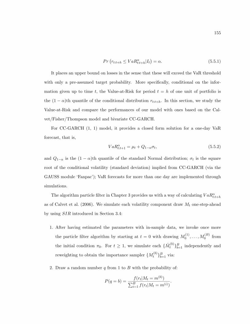
155

Pr(rt:t+h ≤ V aRα

t:t+h|It)

= α. (5.5.1)

It places an upper bound on losses in the sense that these will exceed the VaR threshold

with only a pre-assumed target probability. More specifically, conditional on the infor-

mation given up to time t, the Value-at-Risk for period t = h of one unit of portfolio is

the (1 − α)th quantile of the conditional distribution rt:t+h. In this section, we study the

Value-at-Risk and compare the performances of our model with ones based on the Cal-

vet/Fisher/Thompson model and bivariate CC-GARCH.

For CC-GARCH (1, 1) model, it provides a closed form solution for a one-day VaR

forecast, that is,

V aRαt:t+1 = µt +Q1−ασt, (5.5.2)

and Q1−α is the (1 − α)th quantile of the standard Normal distribution; σt is the square

root of the conditional volatility (standard deviation) implied from CC-GARCH (via the

GAUSS module ‘Fanpac’); VaR forecasts for more than one day are implemented through

simulations.

The algorithm particle filter in Chapter 3 provides us with a way of calculating V aRαt:t+h

as of Calvet et al. (2006). We simulate each volatility component draw Mt one-step-ahead

by using SIR introduced in Section 3.4:

1. After having estimated the parameters with in-sample data, we invoke once more

the particle filter algorithm by starting at t = 0 with drawing M (1)0 , . . . ,M

(B)0 from

the initial condition π0. For t ≥ 1, we simulate each M (b)t B

b=1 independently and

reweighting to obtain the importance sampler M (b)t B

b=1 via:

2. Draw a random number q from 1 to B with the probability of:

P (q = b) =f(rt|Mt = m(b))∑Bi=1 f(rt|Mt = m(i))

.

156

3. M (1)t = M

(q)t is then selected, repeat Step 2 B times and obtain B draws with

M(1)t , . . .M

(B)t .

4. After the last iteration of the in-sample series (say time t) by reaching Mt, we simu-

late the Markov chain one-step-ahead to obtain M(1)t+1 given M

(1)t , repeat B times to

generate draws M (b)t+1B

b=1, i.e., M (1)t+1, . . . , M

(B)t+1 , which are used for one-step ahead

forecast, i.e., to move from t to forecast for t+ 1.

5. For h-period forecast given information up to time t, iterating the particles obtained

from importance resampling at time t h times to obtain h-period ahead volatility

draws M (1)t+h, . . . , M

(B)t+h, which are used to forecast for t+ h from t. For all cases. we

use B = 10000 simulated draws.

6. Simulate bivariate Normal innovations, which need to be combined with new volatility

draws drawn to calculate VaR.

7. For the next one-step ahead forecast, i.e., to move from t+1 to forecast for t+2, apply

the SIR via Step 2 and Step 3 to obtain importance sampler M (b)t+1B

b=1, then simulate

the Markov chain one-step-ahead to generate draws M (b)t+2B

b=1 given M (b)t+1B

b=1.

This recursive procedure provides a discrete approximation to Bayesian updating, which

assists to simulate the bivariate series forward other h-day horizons. Thus, we calculate

V aRαt:t+h as the (1− α)th simulated quantile.

Table 5.11 and Table 5.12 report the empirical estimates from the particle filter for

bivariate MF models by using in-sample data. For the Calvet/Fisher/Thompson model,

we fixed n = 8 as in Calvet et al. (2006); For Liu/Lux model, we set the number of joint

cascade suggested in the empirical study of Section 3.6, namely k = 3 for Dow/Nik; k = 2

for US/DM and k = 5 for TB1/TB2. We assess the models’ performances by computing

the failure rate for the individual returns, equal weight portfolio and hedge portfolio. By

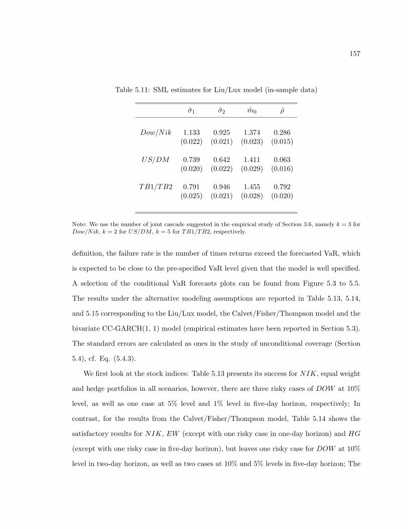
157

Table 5.11: SML estimates for Liu/Lux model (in-sample data)

σ1 σ2 m0 ρ

Dow/Nik 1.133 0.925 1.374 0.286(0.022) (0.021) (0.023) (0.015)

US/DM 0.739 0.642 1.411 0.063(0.020) (0.022) (0.029) (0.016)

TB1/TB2 0.791 0.946 1.455 0.792(0.025) (0.021) (0.028) (0.020)

Note: We use the number of joint cascade suggested in the empirical study of Section 3.6, namely k = 3 forDow/Nik, k = 2 for US/DM , k = 5 for TB1/TB2, respectively.

definition, the failure rate is the number of times returns exceed the forecasted VaR, which

is expected to be close to the pre-specified VaR level given that the model is well specified.

A selection of the conditional VaR forecasts plots can be found from Figure 5.3 to 5.5.

The results under the alternative modeling assumptions are reported in Table 5.13, 5.14,

and 5.15 corresponding to the Liu/Lux model, the Calvet/Fisher/Thompson model and the

bivariate CC-GARCH(1, 1) model (empirical estimates have been reported in Section 5.3).

The standard errors are calculated as ones in the study of unconditional coverage (Section

5.4), cf. Eq. (5.4.3).

We first look at the stock indices: Table 5.13 presents its success for NIK, equal weight

and hedge portfolios in all scenarios, however, there are three risky cases of DOW at 10%

level, as well as one case at 5% level and 1% level in five-day horizon, respectively; In

contrast, for the results from the Calvet/Fisher/Thompson model, Table 5.14 shows the

satisfactory results for NIK, EW (except with one risky case in one-day horizon) and HG

(except with one risky case in five-day horizon), but leaves one risky case for DOW at 10%

level in two-day horizon, as well as two cases at 10% and 5% levels in five-day horizon; The

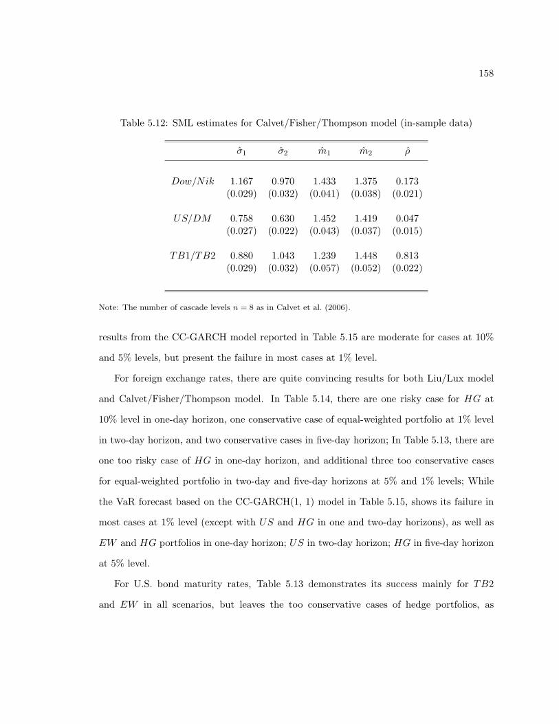
158

Table 5.12: SML estimates for Calvet/Fisher/Thompson model (in-sample data)

σ1 σ2 m1 m2 ρ

Dow/Nik 1.167 0.970 1.433 1.375 0.173(0.029) (0.032) (0.041) (0.038) (0.021)

US/DM 0.758 0.630 1.452 1.419 0.047(0.027) (0.022) (0.043) (0.037) (0.015)

TB1/TB2 0.880 1.043 1.239 1.448 0.813(0.029) (0.032) (0.057) (0.052) (0.022)

Note: The number of cascade levels n = 8 as in Calvet et al. (2006).

results from the CC-GARCH model reported in Table 5.15 are moderate for cases at 10%

and 5% levels, but present the failure in most cases at 1% level.

For foreign exchange rates, there are quite convincing results for both Liu/Lux model

and Calvet/Fisher/Thompson model. In Table 5.14, there are one risky case for HG at

10% level in one-day horizon, one conservative case of equal-weighted portfolio at 1% level

in two-day horizon, and two conservative cases in five-day horizon; In Table 5.13, there are

one too risky case of HG in one-day horizon, and additional three too conservative cases

for equal-weighted portfolio in two-day and five-day horizons at 5% and 1% levels; While

the VaR forecast based on the CC-GARCH(1, 1) model in Table 5.15, shows its failure in

most cases at 1% level (except with US and HG in one and two-day horizons), as well as

EW and HG portfolios in one-day horizon; US in two-day horizon; HG in five-day horizon

at 5% level.

For U.S. bond maturity rates, Table 5.13 demonstrates its success mainly for TB2

and EW in all scenarios, but leaves the too conservative cases of hedge portfolios, as

159

well as other five cases of TB1 across three time horizons. For the results from the Cal-

vet/Fisher/Thompson model, Table 5.14 reports some similar results, namely, too conser-

vative cases for HG portfolio, also conservative ones of TB1 in five-day horizon at all levels,

as well as additional ones at 10% and 5% levels in one-day and two-day horizons; Again,

there are number of failures for HG in all scenarios found in the VaR forecasts based on

the bivariate CC-GARCH(1, 1) model, while all TB2 are successful.

The pictures from the conditional VaR forecasts with different models are quite en-

couraging, in particular for the stock indices and foreign exchange rates results based on

multifractal models (both Table 5.13 and Table 5.14), though there are a couple of cases

tending to underestimate the frequency of extreme returns, as well as certain overestimation

(too conservative predictions) scenarios for U.S. treasury bond rate, e.g., hedge portfolio

forecasts. A glance at these results suggests that the performances based on both multifrac-

tal models clearly dominate the one based on CC-GARCH model. Indeed, VaR can help

risk managers to estimate the cost of positions, allowing them to allocate risk in a more

efficient way. Also the Basle Committee on Banking Supervision (1996) requires financial

institutions such as, banks and investment firms to use VaR to measure their capital oper-

ations. However, if the underlying risk is not properly estimated, these requirements may

lead to overestimation (or underestimation) of market risks and consequently to maintaining

excessively high (low) capital levels.

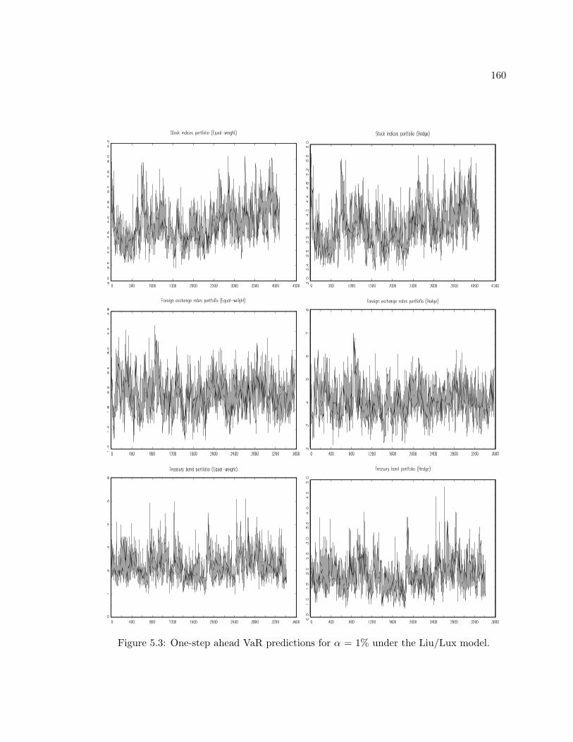
160

Figure 5.3: One-step ahead VaR predictions for α = 1% under the Liu/Lux model.

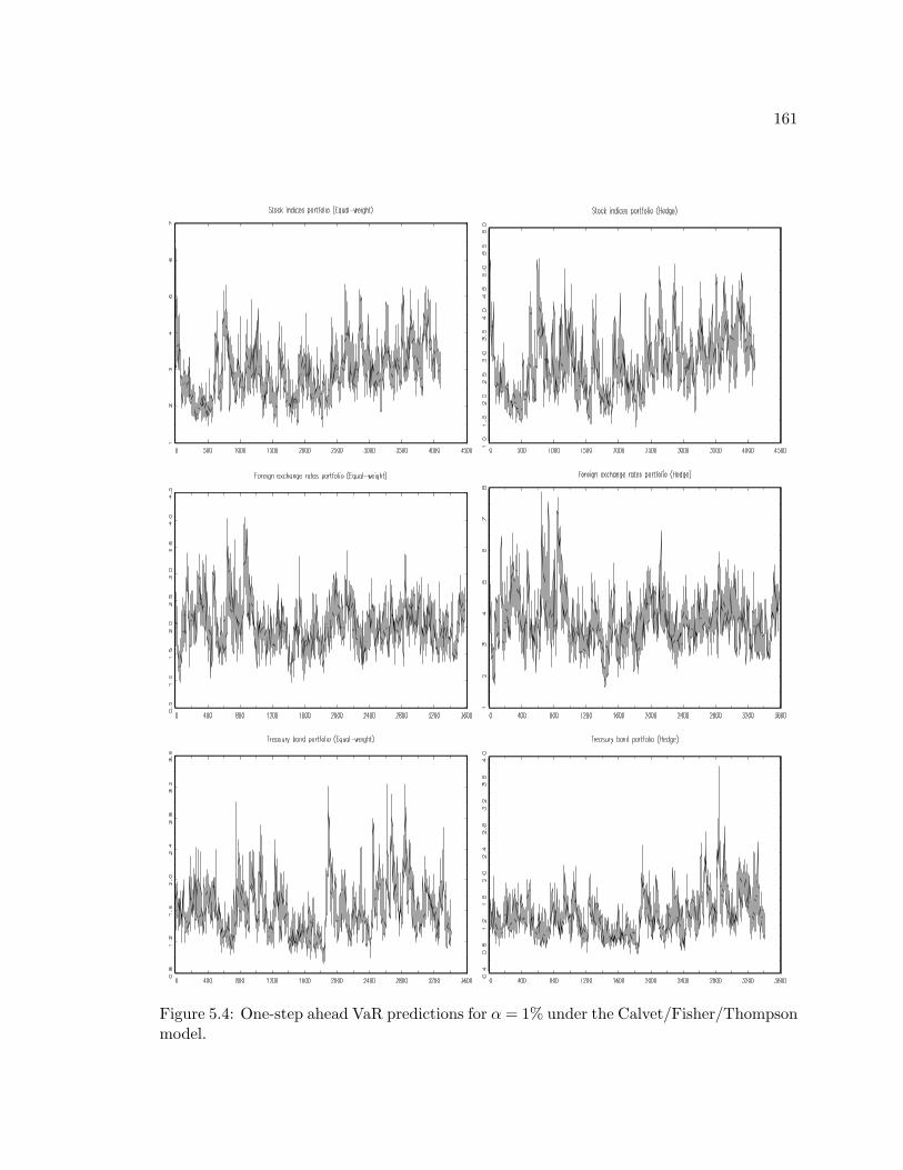
161

Figure 5.4: One-step ahead VaR predictions for α = 1% under the Calvet/Fisher/Thompsonmodel.

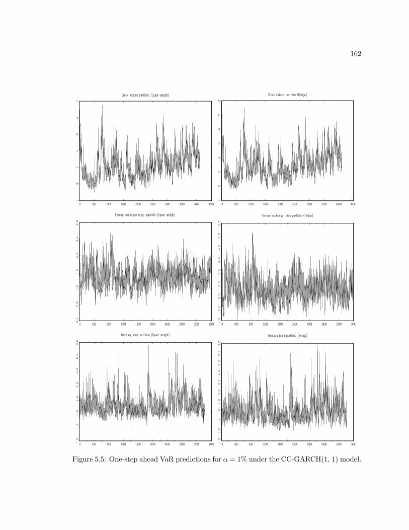
162

Figure 5.5: One-step ahead VaR predictions for α = 1% under the CC-GARCH(1, 1) model.

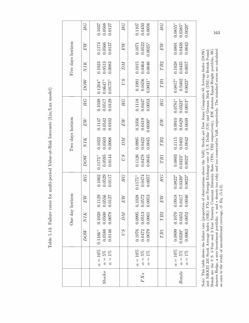
163

Tab

le5.

13:

Failu

rera

tes

for

mul

ti-p

erio

dV

alue

-at-

Ris

kfo

reca

sts

(Liu

/Lux

mod

el)

One

day

hori

zon

Tw

oda

ysho

rizo

nFiv

eda

ysho

rizo

n

DOW

NIK

EW

HG

DOW

NIK

EW

HG

DOW

NIK

EW

HG

α=

10%

0.11

66+

0.10

200.

1129

0.10

020.

1173

+0.

1022

0.11

470.

1039

0.12

04+

0.10

230.

1174

0.10

37Stocks

α=

5%0.

0588

0.05

000.

0556

0.05

290.

0595

0.05

030.

0542

0.05

170.

0647

+0.

0513

0.05

660.

0568

α=

1%0.

0146

0.00

780.

0127

0.01

170.

0144

0.00

680.

0102

0.01

290.

0173

+0.

0083

0.01

370.

0127

US

DM

EW

HG

US

DM

EW

HG

US

DM

EW

HG

α=

10%

0.10

760.

0995

0.10

280.

1175

+0.

1126

0.09

950.

1056

0.11

180.

1091

0.10

150.

1071

0.11

07FXs

α=

5%0.

0472

0.05

130.

0572

0.04

740.

0478

0.04

220.

0419

0.04

470.

0456

0.04

640.

0522

0.04

50α

=1%

0.00

790.

0061

0.00

530.

0057

0.00

450.

0045

0.00

30∗

0.00

530.

0031∗

0.00

460.

0025∗

0.00

56

TB

1TB

2EW

HG

TB

1TB

2EW

HG

TB

1TB

2EW

HG

α=

10%

0.08

990.

1070

0.09

180.

0822∗

0.08

930.

1115

0.09

100.

0781∗

0.08

17∗

0.10

280.

0891

0.08

55∗

Bonds

α=

5%0.

0320∗

0.04

520.

0417

0.03

39∗

0.03

23∗

0.04

020.

0429

0.03

23∗

0.04

020.

0435

0.04

380.

0385∗

α=

1%0.

0063

0.00

520.

0046

0.00

23∗

0.00

23∗

0.00

420.

0049

0.00

13∗

0.00

22∗

0.00

570.

0043

0.00

20∗

Note

:T

his

table

show

sth

efa

ilure

rate

(pro

port

ion

ofobse

rvati

ons

abov

eth

eV

aR

).Sto

cks

are

Dow

Jones

Com

posi

te65

Aver

age

Index

(DO

W)

and

NIK

KE

I225

Sto

ckA

ver

age

Index

(NIK

);FX

sare

Fore

ign

Exch

ange

rate

of

U.S

.D

ollar

(US)

and

Ger

man

Mark

(DM

)to

Bri

tish

Pound;

Bonds

are

the

U.S

.1-Y

ear

and

2-Y

ear

Tre

asu

ryC

onst

ant

Matu

rity

Rate

(TB

1,

TB

2re

spec

tivel

y).

EW

den

ote

sE

qual-W

eight

port

folio,

HG

den

ote

sH

edge,

aze

roin

ves

tmen

tport

folio.

+and∗

den

ote

too

risk

yand

too

conse

rvati

ve

VaR

,re

spec

tivel

y.T

he

standard

erro

rsare

calc

ula

ted

as

ones

inth

est

udy

ofunco

ndit

ionalco

ver

age,

cf.

Eq.

(5.4

.3).

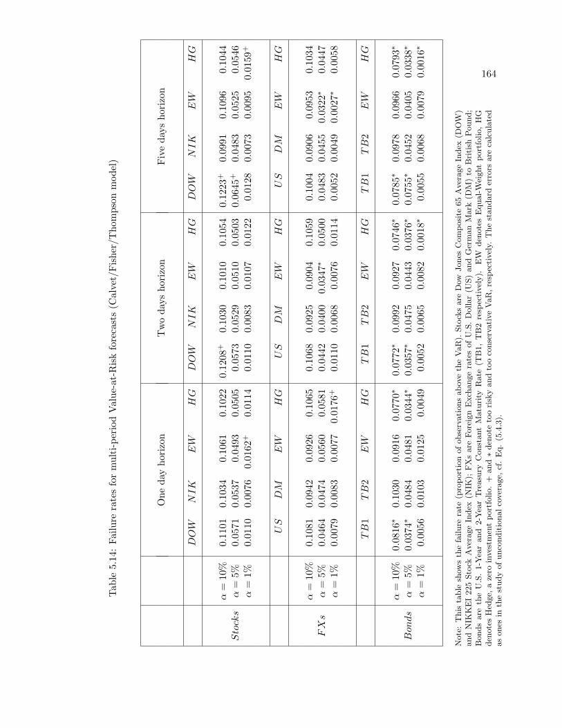
164

Tab

le5.

14:

Failu

rera

tes

for

mul

ti-p

erio

dV

alue

-at-

Ris

kfo

reca

sts

(Cal

vet/

Fis

her/

Tho

mps

onm

odel

)

One

day

hori

zon

Tw

oda

ysho

rizo

nFiv

eda

ysho

rizo

n

DOW

NIK

EW

HG

DOW

NIK

EW

HG

DOW

NIK

EW

HG

α=

10%

0.11

010.

1034

0.10

610.

1022

0.12

08+

0.10

300.

1010

0.10

540.

1223

+0.

0991

0.10

960.

1044

Stocks

α=

5%0.

0571

0.05

370.

0493

0.05

050.

0573

0.05

290.

0510

0.05

030.

0645

+0.

0483

0.05

250.

0546

α=

1%0.

0110

0.00

760.

0162

+0.

0114

0.01

100.

0083

0.01

070.

0122

0.01

280.

0073

0.00

950.

0159

+

US

DM

EW

HG

US

DM

EW

HG

US

DM

EW

HG

α=

10%

0.10

810.

0942

0.09

260.

1065

0.10

680.

0925

0.09

040.

1059

0.10

040.

0906

0.09

530.

1034

FXs

α=

5%0.

0464

0.04

740.

0560

0.05

810.

0442

0.04

000.

0347∗

0.05

000.

0483

0.04

550.

0322∗

0.04

47α

=1%

0.00

790.

0083

0.00

770.

0176

+0.

0110

0.00

680.

0076

0.01

140.

0052

0.00

490.

0027∗

0.00

58

TB

1TB

2EW

HG

TB

1TB

2EW

HG

TB

1TB

2EW

HG

α=

10%

0.08

16∗

0.10

300.

0916

0.07

70∗

0.07

72∗

0.09

920.

0927

0.07

46∗

0.07

85∗

0.09

780.

0966

0.07

93∗

Bonds

α=

5%0.

0374∗

0.04

840.

0481

0.03

44∗

0.03

57∗

0.04

750.

0443

0.03

76∗

0.07

55∗

0.04

520.

0405

0.03

38∗

α=

1%0.

0056

0.01

030.

0125

0.00

490.

0052

0.00

650.

0082

0.00

18∗

0.00

550.

0068

0.00

790.

0016∗

Note

:T

his

table

show

sth

efa

ilure

rate

(pro

port

ion

ofobse

rvati

ons

abov

eth

eV

aR

).Sto

cks

are

Dow

Jones

Com

posi

te65

Aver

age

Index

(DO

W)

and

NIK

KE

I225

Sto

ckA

ver

age

Index

(NIK

);FX

sare

Fore

ign

Exch

ange

rate

sof

U.S

.D

ollar

(US)

and

Ger

man

Mark

(DM

)to

Bri

tish

Pound;

Bonds

are

the

U.S

.1-Y

ear

and

2-Y

ear

Tre

asu

ryC

onst

ant

Matu

rity

Rate

(TB

1,

TB

2re

spec

tivel

y).

EW

den

ote

sE

qual-W

eight

port

folio,

HG

den

ote

sH

edge,

aze

roin

ves

tmen

tport

folio.

+and∗

den

ote

too

risk

yand

too

conse

rvati

ve

VaR

,re

spec

tivel

y.T

he

standard

erro

rsare

calc

ula

ted

as

ones

inth

est

udy

ofunco

ndit

ionalco

ver

age,

cf.

Eq.

(5.4

.3).

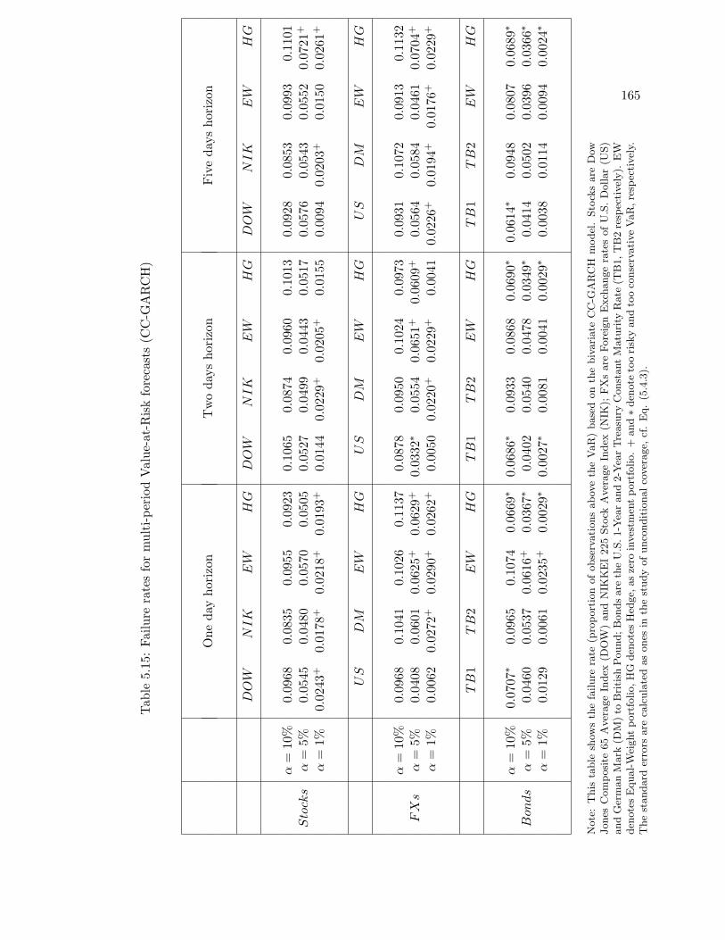
165

Tab

le5.

15:

Failu

rera

tes

for

mul

ti-p

erio

dV

alue

-at-

Ris

kfo

reca

sts

(CC

-GA

RC

H)

One

day

hori

zon

Tw

oda

ysho

rizo

nFiv

eda

ysho

rizo

n

DOW

NIK

EW

HG

DOW

NIK

EW

HG

DOW

NIK

EW

HG

α=

10%

0.09

680.

0835

0.09

550.

0923

0.10

650.

0874

0.09

600.

1013

0.09

280.

0853

0.09

930.

1101

Stocks

α=

5%0.

0545

0.04

800.

0570

0.05

050.

0527

0.04

990.

0443

0.05

170.

0576

0.05

430.

0552

0.07

21+

α=

1%0.

0243

+0.

0178

+0.

0218

+0.

0193

+0.

0144

0.02

29+

0.02

05+

0.01

550.

0094

0.02

03+

0.01

500.

0261

+

US

DM

EW

HG

US

DM

EW

HG

US

DM

EW

HG

α=

10%

0.09

680.

1041

0.10

260.

1137

0.08

780.

0950

0.10

240.

0973

0.09

310.

1072

0.09

130.

1132

FXs

α=

5%0.

0408

0.06

010.

0625

+0.

0629

+0.

0332∗

0.05

540.

0651

+0.

0609

+0.

0564

0.05

840.

0461

0.07

04+

α=

1%0.

0062

0.02

72+

0.02

90+

0.02

62+

0.00

500.

0220

+0.

0229

+0.

0041

0.02

26+

0.01

94+

0.01

76+

0.02

29+

TB

1TB

2EW

HG

TB

1TB

2EW

HG

TB

1TB

2EW

HG

α=

10%

0.07

07∗

0.09

650.

1074

0.06

69∗

0.06

86∗

0.09

330.

0868

0.06

90∗

0.06

14∗

0.09

480.

0807

0.06

89∗

Bonds

α=

5%0.

0460

0.05

370.

0616

+0.

0367∗

0.04

020.

0540

0.04

780.

0349∗

0.04

140.

0502

0.03

960.

0366∗

α=

1%0.

0129

0.00

610.

0235

+0.

0029∗

0.00

27∗

0.00

810.

0041

0.00

29∗

0.00

380.

0114

0.00

940.

0024∗

Note

:T

his

table

show

sth

efa

ilure

rate

(pro

port

ion

ofobse

rvati

ons

abov

eth

eV

aR

)base

don

the

biv

ari

ate

CC

-GA

RC

Hm

odel

.Sto

cks

are

Dow

Jones

Com

posi

te65

Aver

age

Index

(DO

W)

and

NIK

KE

I225

Sto

ckA

ver

age

Index

(NIK

);FX

sare

Fore

ign

Exch

ange

rate

sof

U.S

.D

ollar

(US)

and

Ger

man

Mark

(DM

)to

Bri

tish

Pound;B

onds

are

the

U.S

.1-Y

ear

and

2-Y

ear

Tre

asu

ryC

onst

antM

atu

rity

Rate

(TB

1,T

B2

resp

ecti

vel

y).

EW

den

ote

sE

qual-W

eightport

folio,H

Gden

ote

sH

edge,

as

zero

inves

tmen

tport

folio.

+and∗

den

ote

too

risk

yand

too

conse

rvati

ve

VaR

,re

spec

tivel

y.T

he

standard

erro

rsare

calc

ula

ted

as

ones

inth

est

udy

ofunco

ndit

ionalco

ver

age,

cf.

Eq.

(5.4

.3).

166

5.6 Conditional Expected shortfall

Value-at-Risk seems to have become a standard tool used in financial risk management with

three main attributes: it allows the potential loss associated with a decision to be quantified;

it summarizes complex positions in a single figure; and it is intuitive - expressing loss in

monetary terms.7 However, there are a few shortcomings of VaR. For example, Artzner

et al. (1997) argues that:

(1) VaR reports only percentiles of profit-loss distributions, thus disregarding any loss

beyond the VaR level (this is called the ‘tail risk’ problem);

(2) VaR is not coherent, since it is not sub-additive. A risk measure is sub-additive

when the risk of the total position is less than or equal to the sum of the risk of individual

portfolios. It may be troublesome to base a risk-management system solely on VaR limits

for individual books.

Conditional Expected Shortfall (ES) has been proposed to alleviate the arguments in-

herent in VaR; it is defined as the expected losses conditional on exceeding the VaR, at the

h-period horizon. The conditional Expected Shortfall is hence given by:

ESαt:t+h = E[

(rt:t+h|rt:t+h ≤ V aRα

t:t+h

)|It]. (5.6.1)

Thus, by the definition of Eq. (5.6.1), ES considers the loss beyond the VaR level, in

particular, it gives information about the size of the potential losses, given that loss larger

than VaR occurred. It has been shown to be sub-additive (the appendix of Acerbi et al.

(2001) gives the details) which assures its coherence as a risk measure. On these grounds, a

number of studies turned their attention towards Expected Shortfall. Although it has not

become a standard in the financial industry, conditional ES is likely to play a major role as

it currently does in the insurance industry, see Embrechts et al. (1997). Also, conditional

ES is used in credit risk studies, see Bucay and Rosen (1996). Some recent works include:7Despite its conceptual simplicity, the measurement of VaR is a very challenging statistical problem and

none of the methodologies developed so far gives satisfactory solutions, see Engle and Manganelli (2002).

167

McNeil and Frey (2000), who presents both unconditional and conditional VaR and ES, and

advocates conditional ES as an alternative tool with good theoretical properties by fitting

different GARCH type models; Yamai and Yoshiba (2002) provides an overview of studies

comparing VaR and ES by drawing implications for financial risk measurement, and also

illustrates practical problems among various back-testing methods.

In this section, we assess bivariate multifractal models in terms of the performance of

the multi-period ES forecasts. For comparison, conditional Expected Shortfall forecasts

based on the Calvet/Fisher/Thompson model and the CC-GARCH(1, 1) model were also

computed. The forecasting results are reported in Table 5.16 to 5.18, respectively. Numbers

inside the parentheses are the empirical ESs; numbers without parentheses are the simulated

ESs based on these three models; bold numbers show those cases for which we cannot reject

identity of the empirical and simulated ES, i.e. the empirical value fall into the range

between the 2.5 to 97.5 percent quantile of the simulated ones, which are corresponding to

successful forecasts. We summarize those positive results as below:

Table 5.16 reports the ES forecast based on the Liu/Lux model, which shows quite

positive results for stock indices in one-day horizon, except with one risky case of equal-

weighted portfolio at the 1% level, in five-day horizon it shows two failure cases of DOW ;

For foreign exchange rates, the ES forecasts are quite successful, and there are only one risky

cases for equal-weighted at 1% level and two risky hedge portfolios in five-day horizon; For

U.S. bonds, it reports the too conservative results (the simulated ES above empirical one)

for all HG scenarios, as well as individual TB1 at 10% and 5% level in five-day horizon.

The performance of the Calvet/Fisher/Thompson model in Table 5.17 shows pretty

similar positive scenario with the one of Liu/Lux model for stock indices, except with one

risky EW at the 1% level in one-day horizon, two risky forecasts of EW and HG portfolios

at the 1% level in fiver-day horizon; The results for foreign exchange rates present the

success at all cases of 10% and 5% levels; but at the 1% level, we observe the risky HG

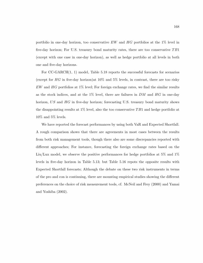
168

portfolio in one-day horizon, too conservative EW and HG portfolios at the 1% level in

five-day horizon; For U.S. treasury bond maturity rates, there are too conservative TB1

(except with one case in one-day horizon), as well as hedge portfolio at all levels in both

one and five-day horizons.

For CC-GARCH(1, 1) model, Table 5.18 reports the successful forecasts for scenarios

(except for HG in five-day horizon)at 10% and 5% levels, in contrast, there are too risky

EW and HG portfolios at 1% level; For foreign exchange rates, we find the similar results

as the stock indices, and at the 1% level, there are failures in DM and HG in one-day

horizon, US and HG in five-day horizon; forecasting U.S. treasury bond maturity shows

the disappointing results at 1% level, also the too conservative TB1 and hedge portfolio at

10% and 5% levels.

We have reported the forecast performances by using both VaR and Expected Shortfall.

A rough comparison shows that there are agreements in most cases between the results

from both risk management tools, though there also are some discrepancies reported with

different approaches; For instance, forecasting the foreign exchange rates based on the

Liu/Lux model, we observe the positive performances for hedge portfolios at 5% and 1%

levels in five-day horizon in Table 5.13; but Table 5.16 repots the opposite results with

Expected Shortfall forecasts; Although the debate on these two risk instruments in terms

of the pro and con is continuing, there are mounting empirical studies showing the different

preferences on the choice of risk measurement tools, cf. McNeil and Frey (2000) and Yamai

and Yoshiba (2002).

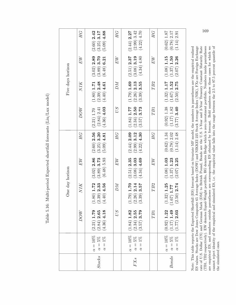
169

Tab

le5.

16:

Mul

ti-p

erio

dE

xpec

ted

shor

tfal

lfo

reca

sts

(Liu

/Lux

mod

el)

One

day

hori

zon

Fiv

eda

ysho

rizo

n

DOW

NIK

EW

HG

DOW

NIK

EW

HG

α=

10%

(2.2

1)1.

79(1

.80)

1.72

(3.0

2)2.

86(2

.60)

2.56

(2.2

1)1.

70(1

.80)

1.71

(3.0

2)2.

89(2

.60)

2.42

Stocks

α=

5%(2

.84)

2.65

(2.3

9)2.

33(3

.89)

3.73

(3.2

5)3.

20(2

.84)

2.41

(2.3

9)2.

48(3

.89)

3.70

(3.2

5)3.

17α

=1%

(4.3

6)4.

18(4

.40)

4.56

(6.4

8)5.

93(5

.09)

4.81

(4.3

6)4.

03(4

.40)

4.61

(6.4

8)6.

21(5

.09)

4.88

US

DM

EW

HG

US

DM

EW

HG

α=

10%

(1.8

4)1.

82(1

.79)

1.70

(2.5

1)2.

35(2

.44)

2.09

(1.8

4)1.

77(1

.79)

1.69

(2.5

1)2.

37(2

.44)

2.27

FXs

α=

5%(2

.34)

2.55

(2.2

6)2.

14(3

.08)

3.03

(2.9

9)3.

12(2

.34)

2.50

(2.2

6)2.

13(3

.08)

3.19

(2.9

9)3.

42α

=1%

(3.5

7)3.

79(3

.39)

3.57

(4.3

4)4.

69(4

.22)

4.30

(3.5

7)3.

73(3

.39)

3.55

(4.3

4)4.

80(4

.22)

4.70

TB

1TB

2EW

HG

TB

1TB

2EW

HG

α=

10%

(0.9

2)1.

22(1

.32)

1.25

(1.0

8)1.

03(0

.62)

1.34

(0.9

2)1.

38(1

.32)

1.17

(1.0

8)1.

15(0

.62)

1.87

Bonds

α=

5%(1

.17)

1.49

(1.6

7)1.

77(1

.37)

1.23

(0.7

8)2.

02(1

.17)

1.82

(1.6

7)1.

52(1

.37)

1.50

(0.7

8)2.

17α

=1%

(1.7

7)2.

03(2

.50)

2.74

(2.0

7)2.

25(1

.14)

2.48

(3.7

7)3.

40(2

.50)

2.75

(2.0

7)2.

26(1

.14)

2.91

Note

:T

his

table

report

sth

eE

xpec

ted

Short

fall

(ES)

fore

cast

base

don

biv

ari

ate

MF

model

,th

enum

ber

sin

pare

nth

eses

are

the

empir

icalre

alize

dE

Sva

lues

.Sto

cks

are

Dow

Jones

Com

posi

te65

Aver

age

Index

(DO

W)

and

NIK

KE

I225

Sto

ckA

ver

age

Index

(NIK

),FX

sare

Fore

ign

Exch

ange

rate

of

U.S

.D

ollar

(US)

and

Ger

man

Mark

(DM

)to

Bri

tish

Pound,

Bonds

are

the

U.S

.1-Y

ear

and

2-Y

ear

Tre

asu

ryC

onst

ant

Matu

rity

Rate

(TB

1,T

B2

resp

ecti

vel

y).

EW

den

ote

sE

qual-W

eight

port

folio,H

Gden

ote

sH

edge

whic

his

zero

inves

tmen

tport

folio.

Num

ber

sin

side

pare

nth

eses

are

empir

ical

ES,

and

num

ber

souts

ide

pare

nth

eses

are

corr

espondin

gE

Sobta

ined

by

fore

cast

.B

old

num

ber

ssh

owth

ose

case

sfo

rw

hic

hw

eca

nnot

reje

ctid

enti

tyofth

eem

pir

icaland

sim

ula

ted

ES,i.e.

the

empir

icalva

lue

falls

into

the

range

bet

wee

nth

e2.5

to97.5

per

cent

quanti

leof

the

sim

ula

ted

ones

.

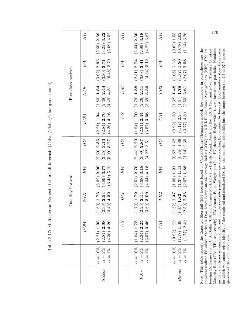
170

Tab

le5.

17:

Mul

ti-p

erio

dE

xpec

ted

shor

tfal

lfo

reca

sts

(Cal

vet/

Fis

her/

Tho

mps

onm

odel

)

One

day

hori

zon

Fiv

eda

ysho

rizo

n

DOW

NIK

EW

HG

DOW

NIK

EW

HG

α=

10%

(2.2

1)1.

95(1

.80)

1.73

(3.0

2)2.

90(2

.60)

2.35

(2.2

1)1.

94(1

.80)

1.84

(3.0

2)2.

95(2

.60)

2.39

Stocks

α=

5%(2

.84)

2.98

(2.3

9)2.

54(3

.89)

3.77

(3.2

5)3.

13(2

.84)

2.76

(2.3

9)2.

44(3

.89)

3.71

(3.2

5)3.

22α

=1%

(4.3

6)4.

20(4

.40)

4.32

(6.4

8)5.

10(5

.09)

5.27

(4.3

6)4.

16(4

.40)

4.51

(6.4

8)5.

70(5

.09)

4.52

US

DM

EW

HG

US

DM

EW

HG

α=

10%

(1.8

4)1.

78(1

.79)

1.72

(2.5

1)2.

70(2

.44)

2.20

(1.8

4)1.

70(1

.79)

1.88

(2.5

1)2.

74(2

.44)

2.30

FXs

α=

5%(2

.34)

2.25

(2.2

6)2.

14(3

.08)

3.18

(2.9

9)2.

87(2

.34)

2.44

(2.2

6)2.

41(3

.08)

3.41

(2.9

9)3.

18α

=1%

(3.5

7)3.

46(3

.39)

3.09

(4.3

4)4.

18(4

.22)

3.51

(3.5

7)3.

66(3

.39)

3.50

(4.3

4)5.

12(4

.22)

3.87

TB

1TB

2EW

HG

TB

1TB

2EW

HG

α=

10%

(0.9

2)1.

29(1

.32)

1.47

(1.0

8)1.

21(0

.62)

1.42

(0.9

2)1.

50(1

.32)

1.48

(1.0

8)1.

13(0

.62)

1.55

Bonds

α=

5%(1

.17)

1.49

(1.6

7)1.

82(1

.37)

1.41

(0.7

8)1.

89(1

.17)

2.25

(1.6

7)1.

78(1

.37)

1.50

(0.7

8)2.

02α

=1%

(1.7

7)2.

40(2

.50)

2.35

(2.0

7)1.

88(1

.14)

2.30

(3.7

7)4.

30(2

.50)

2.61

(2.0

7)2.

08(1

.14)

3.26

Note

:T

his

table

report

sth

eE

xpec

ted

Short

fall

(ES)

fore

cast

base

don

Calv

et/Fis

her

/T

hom

pso

nm

odel

,th

enum

ber

sin

pare

nth

eses

are

the

empir

icalre

alize

dE

Sva

lues

.Sto

cks

are

Dow

Jones

Com

posi

te65

Aver

age

Index

(DO

W)

and

NIK

KE

I225

Sto

ckA

ver

age

Index

(NIK

),FX

sare

Fore

ign

Exch

ange

rate

ofU

.S.D

ollar

(US)

and

Ger

man

Mark

(DM

)to

Bri

tish

Pound,B

onds

are

the

U.S

.1-Y

ear

and

2-Y

ear

Tre

asu

ryC

onst

ant

Matu

rity

Rate

(TB

1,

TB

2re

spec

tivel

y).

EW

den

ote

sE

qual-W

eight

port

folio,

HG

den

ote

sH

edge

whic

his

zero

inves

tmen

tport

folio.

Num

ber

sin

side

pare

nth

eses

are

empir

icalE

S,and

num

ber

souts

ide

pare

nth

eses

are

corr

espondin

gE

Sobta

ined

by

fore

cast

.B

old

num

ber

ssh

owth

ose

case

sfo

rw

hic

hw

eca

nnot

reje

ctid

enti

tyofth

eem

pir

icaland

sim

ula

ted

ES,i.e.

the

empir

icalva

lue

falls

into

the

range

bet

wee

nth

e2.5

to97.5

per

cent

quanti

leofth

esi

mula

ted

ones

.

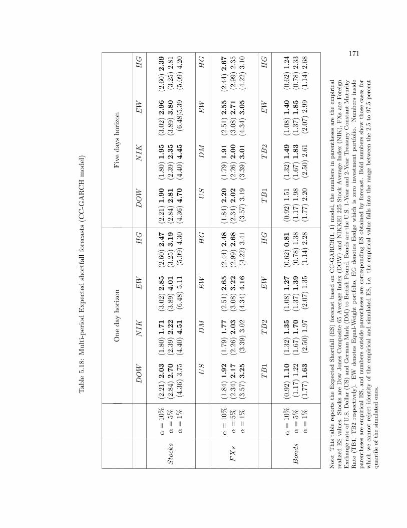
171

Tab

le5.

18:

Mul

ti-p

erio

dE

xpec

ted

shor

tfal

lfo

reca

sts

(CC

-GA

RC

Hm

odel

)

One

day

hori

zon

Fiv

eda

ysho

rizo

n

DOW

NIK

EW

HG

DOW

NIK

EW

HG

α=

10%

(2.2

1)2.

03(1

.80)

1.71

(3.0

2)2.

85(2

.60)

2.47

(2.2

1)1.

90(1

.80)

1.95

(3.0

2)2.

96(2

.60)

2.39

Stocks

α=

5%(2

.84)

2.70

(2.3

9)2.

22(3

.89)

4.01

(3.2

5)3.

19(2

.84)

2.81

(2.3

9)2.

35(3

.89)

3.80

(3.2

5)2.

81α

=1%

(4.3

6)3.

75(4

.40)

4.51

(6.4

8)5.

11(5

.09)

4.30

(4.3

6)4.

70(4

.40)

4.45

(6.4

8)5.

39(5

.09)

4.20

US

DM

EW

HG

US

DM

EW

HG

α=

10%

(1.8

4)1.

92(1

.79)

1.77

(2.5

1)2.

65(2

.44)

2.48

(1.8

4)2.

20(1

.79)

1.91

(2.5

1)2.

55(2

.44)

2.67

FXs

α=

5%(2

.34)

2.17

(2.2

6)2.

03(3

.08)

3.22

(2.9

9)2.

68(2

.34)

2.02

(2.2

6)2.

00(3

.08)

2.71

(2.9

9)2.

35α

=1%

(3.5

7)3.

25(3

.39)

3.02

(4.3

4)4.

16(4

.22)

3.41

(3.5

7)3.

19(3

.39)

3.01

(4.3

4)3.

05(4

.22)

3.10

TB

1TB

2EW

HG

TB

1TB

2EW

HG

α=

10%

(0.9

2)1.

10(1

.32)

1.35

(1.0

8)1.

27(0

.62)

0.81

(0.9

2)1.

51(1

.32)

1.49

(1.0

8)1.

40(0

.62)

1.24

Bonds

α=

5%(1

.17)

1.22

(1.6

7)1.

70(1

.37)

1.39

(0.7

8)1.

38(1

.17)

1.98

(1.6

7)1.

83(1

.37)

1.85

(0.7

8)2.

33α

=1%

(1.7

7)1.

63(2

.50)

1.97

(2.0

7)1.

35(1

.14)

2.28

(1.7

7)2.

20(2

.50)

2.61

(2.0

7)2.

99(1

.14)

2.68

Note

:T

his

table

report

sth

eE

xpec

ted

Short

fall

(ES)

fore

cast

base

don

CC

-GA

RC

H(1

,1)

model

,th

enum

ber

sin

pare

nth

eses

are

the

empir

ical

realize

dE

Sva

lues

.Sto

cks

are

Dow

Jones

Com

posi

te65

Aver

age

Index

(DO

W)

and

NIK

KE

I225

Sto

ckA

ver

age

Index

(NIK

),FX

sare

Fore

ign

Exch

ange

rate

ofU

.S.D

ollar

(US)

and

Ger

man

Mark

(DM

)to

Bri

tish

Pound,B

onds

are

the

U.S

.1-Y

ear

and

2-Y

ear

Tre

asu

ryC

onst

ant

Matu

rity

Rate

(TB

1,

TB

2re

spec

tivel

y).

EW

den

ote

sE

qual-W

eight

port

folio,

HG

den

ote

sH

edge

whic

his

zero

inves

tmen

tport

folio.

Num

ber

sin

side

pare

nth

eses

are

empir

icalE

S,and

num

ber

souts

ide

pare

nth

eses

are

corr

espondin

gE

Sobta

ined

by

fore

cast

.B

old

num

ber

ssh

owth

ose

case

sfo

rw

hic

hw

eca

nnot

reje

ctid

enti

tyof

the

empir

icaland

sim

ula

ted

ES,i.e.

the

empir

icalva

lue

falls

into

the

range

bet

wee

nth

e2.5

to97.5

per

cent

quanti

leofth

esi

mula

ted

ones

.

Chapter 6

Conclusion

In this thesis, we have reviewed fractal and multifractal concepts arising from the natu-

ral science and considered their implications for financial economics. Since fractals imply

long memory, we briefly covered some traditional methods of fractal analysis (various Hurst

exponent methods) and well-known long memory models, e.g. fractional Brownian mo-

tion, Fractional Integrated Autoregressive Moving Average (ARFIMA) model, Fractional

Integrated Autoregressive Conditional Heteroskedasticity (FIGARCH) model, and the long

memory stochastic volatility (LMSV) model. To gain a better impression of the interpre-

tation of (multi)fractals in fields ranging from physics to finance, the multifractal model

of asset returns (MMAR) of Mandelbrot et al. (1997) has been revisited, together with its

scaling estimator. As one variation of the MF model, the Markov-switching multifractal

model was proposed by Mandelbrot’s former students L. Calvet and A. Fisher, with the

intention of overcoming the limitations in practical applicability of MMAR.

The main contribution of this thesis is the development of a bivariate multifractal model

as an extension to the univariate Markov-switching multifractal model. Indeed, there are

few contributions going beyond univariate multifractal processes, except for the model of

Calvet/Fisher/Thompson (2006). We present a relatively parsimonious bivariate MF model

172

173

as a simple alternative. Since the scaling estimator for combinatorial multifractal process

yields unreliable results (cf. Lux (2004)), estimating the parameters of multivariate multi-

fractal models is a challenging task. Various approaches have been applied such as maxi-

mum likelihood, simulation based ML with particle filter algorithm and GMM approaches,

which have been implemented in this thesis for the purpose of comparison. Furthermore, a

higher dimensional ML model for N > 2 assets has been analogously introduced, and the

three different approaches (GMM, ML and SML) have also been employed for the model’s

estimation.

To investigate the performance of different estimation approaches, Monte Carlo studies

were carried out, indicating that: (1) there is no disadvantage for GMM compared to the

ML estimator, although the latter had been expected to be more efficient; (2) there is

no restrictions on the choice of the number of cascade levels with GMM, in contrast to

the upper bound of about 5 cascade levels for ML; (3) furthermore, for the computational

view, GMM is much faster compared to the very time-consuming ML process, and the

particle filter algorithm when larger numbers of particles are employed. As an extension, a

higher dimensional MF model with parsimonious design was defined, and three estimation

approaches, as used in the bivariate model, have been implemented by taking as example

a tri-variate version, which further demonstrates the advantages of GMM when increasing

the dimensions of the MF model.

To demonstrate the applicability of our multivariate MF model, two well-known mea-

sures used in financial risk management, namely Value-at-Risk (VaR) and Expected Short-

fall (ES) have been used to assess the performance of our model. We considered various

empirical financial time series, including stock exchange indices, foreign exchange rates and

U.S. treasury bond maturity rates, and compared the performance of BMF models (Liu/Lux

model, Calvet/Fisher/Thompson model) and the CC-GARCH model. It has been demon-

strated that bivariate multifractal models outperform the CC-GARCH model in calculating

174

the failure rate of VaR forecasts, particularly in the case of foreign exchange rates. For

the ES forecast, bivariate MF models also provide far better results, even though, in VaR

forecasting, the ES forecast performances of the CC-GARCH model is better in comparison.

With the bivariate MF models examined in this thesis, our studies have provided sup-

portive evidences for this formalism in financial time series analysis, and opened up a broad

outlook on the rich variety of volatility models available in the financial risk manager’s tool

box. Additionally, we suggest that further studies in this direction are likely to offer new

insights:

(1) Other variant MF models can be defined, by replacing the increment with some non-

Gaussian such as the t-distribution, to improve its ability to capture the stylized facts

in financial markets; also different transition probabilities may be introduced into the

volatility component updating mechanism.

(2) To contribute the understanding of the correlation in terms of the cascade level, we

presented a heuristic method for specifying the number of joint cascade levels, by

matching the simulated GPH estimator with the empirical one. More robust specifi-

cation tests for the number of joint frequencies are worth developing.

(3) As in forthcoming studies on volatility forecasting of the univariate MF model, fol-

lowing the introduction of best linear forecast by Lux (2008) with the aid of the

Levinson-Durbin algorithm by Brockwell and Dahlhaus (2004), volatility forecasts

based on multivariate (bivariate) MF models can be explored by developing that al-

gorithm with multivariate settings.

(4) Other future areas of work may include implementing a particle filter for multifractal

processes with continuous distributions of volatility components; as well as applying

alternative efficient algorithms for simulation based inferences, other than the SIR

method with particle filter.

Chapter 7

Appendix

7.1 Moment conditions for the Liu/Lux model

Recall the model from Chapter 3. Let ε(·)t = ln(M (·)t ), and we compute the first log differ-

ence:

Xt,1 = ln(|r1,t|)− ln(|r1,t−1|)

=

(12

k∑i=1

ε(i)t + 1

2

n∑l=k+1

ε(l)t + ln|u1,t|

)−

(12

k∑i=1

ε(i)t−1 + 1

2

n∑l=k+1

ε(l)t−1 + ln|u1,t−1|

)

= 12

k∑i=1

(ε(i)t − ε

(i)t−1

)+ 1

2

n∑l=k+1

(ε(l)t − ε

(l)t−1

)+ (ln|u2,t| − ln|u1,t−1|)

Yt,1 = ln(|r2,t|)− ln(|r2,t−1|)

=

(12

k∑i=1

ε(i)t + 1

2

n∑h=k+1

ε(h)t + ln|u2,t|

)−

(12

k∑i=1

ε(i)t−1 + 1

2

n∑h=k+1

ε(h)t−1 + ln|u2,t−1|

)

= 12

k∑i=1

(ε(i)t − ε

(i)t−1

)+ 1

2

n∑h=k+1

(ε(h)t − ε

(h)t−1

)+ (ln|u2,t| − ln|u2,t−1|)

175

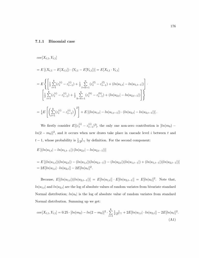
176

7.1.1 Binomial case

cov[Xt,1, Yt,1]

= E [(Xt,1 − E[Xt,1]) · (Yt,1 − E[Yt,1])] = E[Xt,1 · Yt,1]

= E

[12

k∑i=1

(ε(i)t − ε(i)t−1) + 1

2

n∑l=k+1

(ε(l)t − ε(l)t−1) + (ln|u1,t| − ln|u1,t−1|)

]·[

12

k∑i=1

(ε(i)t − ε(i)t−1) + 1

2

n∑h=k+1

(ε(h)t − ε

(h)t−1) + (ln|u2,t| − ln|u2,t−1|)

]

= 14E

[(k∑

i=1(ε(i)t − ε

(i)t−1)

)2]

+ E [(ln|u1,t| − ln|u1,t−1|) · (ln|u2,t| − ln|u2,t−1|)] .

We firstly consider E[(ε(i)t − ε(i)t−1)

2], the only one non-zero contribution is [ln(m0) −

ln(2 − m0)]2, and it occurs when new draws take place in cascade level i between t and

t− 1, whose probability is 12

12k−i by definition. For the second component:

E [(ln|u1,t| − ln|u1,t−1|) (ln|u2,t| − ln|u2,t−1|)]

= E [(ln|u1,t|)(ln|u2,t|)− (ln|u1,t|)(ln|u2,t−1|)− (ln|u2,t|)(ln|u1,t−1|) + (ln|u1,t−1|)(ln|u2,t−1|)]= 2E[ln|u1,t| · ln|u2,t|]− 2E[ln|ut|]2.

Because, E[(ln|u1,t|)(ln|u2,t−1|)] = E[ln|u1,t|] · E[ln|u2,t−1|] = E[ln|ut|]2. Note that,

ln|u1,t| and ln|u2,t| are the log of absolute values of random variates from bivariate standard

Normal distribution; ln|ut| is the log of absolute value of random variates from standard

Normal distribution. Summing up we get:

cov[Xt,1, Yt,1] = 0.25 · [ln(m0)− ln(2−m0)]2 ·k∑

i=1

12

12k−i + 2E[ln|u1,t| · ln|u2,t|]− 2E[ln|ut|]2.

(A1)

177

cov[Xt+1,1, Yt,1]

= E

[12

k∑i=1

(ε(i)t+1 − ε(i)t ) + 1

2

n∑l=k+1

(ε(l)t+1 − ε(l)t ) + (ln|u1,t+1| − ln|u1,t|)

]·[

12

k∑i=1

(ε(i)t − ε(i)t−1) + 1

2

n∑h=k+1

(ε(h)t − ε

(h)t−1) + (ln|u2,t| − ln|u2,t−1|)

]

= 14E

[k∑

i=1

(ε(i)t+1 − ε

(i)t

)·

k∑i=1

(ε(i)t − ε

(i)t−1

)]+ E[ln|ut|]2 − E[ln|u1,t| · ln|u2,t|].

For (ε(i)t+1 − ε(i)t )(ε(i)t − ε

(i)t−1), the non-zero value only occurs in case of two changes of

the multiplier from time t+ 1 to time t− 1, the probability of this occurrence is (12

12k−i )2.

So, we have the result:

cov[Xt+1,1, Yt,1]

= 0.25 · [2ln(m0) · ln(2−m0)− (ln(m0))2 − (ln(2−m0))2] ·k∑

i=1(12

12k−i )2

+E[ln|ut|]2 − E[ln|u1,t| · ln|u2,t|].(A2)

Then, we look at the moment condition for one single time series:

cov[Xt+1,1, Xt,1]

= E

[12

k∑i=1

(ε(i)t+1 − ε(i)t ) + 1

2

n∑l=k+1

(ε(l)t+1 − ε(l)t ) + (ln|u1,t+1| − ln|u1,t|)

]·[

12

k∑i=1

(ε(i)t − ε(i)t−1) + 1

2

n∑l=k+1

(ε(l)t − ε(l)t−1) + (ln|u1,t| − ln|u1,t−1|)

]

= 14E

[k∑

i=1

(ε(i)t+1 − ε

(i)t

)·

k∑i=1

(ε(i)t − ε

(i)t−1

)]+ 1

4E

[n∑

l=k+1

(ε(l)t+1 − ε

(l)t

)·

n∑l=k+1

(ε(l)t − ε

(l)t−1

)]

+E [ln|ut|]2 − E[ln|ut|2

].

(A3)

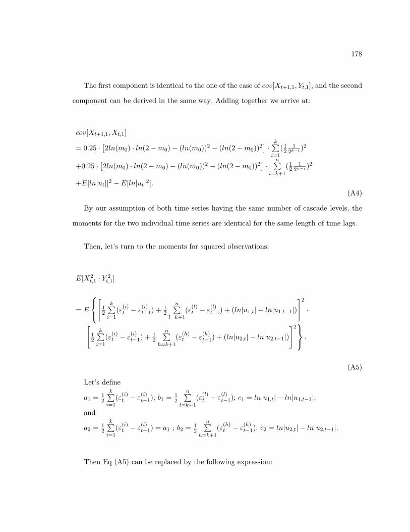
178

The first component is identical to the one of the case of cov[Xt+1,1, Yt,1], and the second

component can be derived in the same way. Adding together we arrive at:

cov[Xt+1,1, Xt,1]

= 0.25 ·[2ln(m0) · ln(2−m0)− (ln(m0))2 − (ln(2−m0))2

]·

k∑i=1

(12

12k−i )2

+0.25 ·[2ln(m0) · ln(2−m0)− (ln(m0))2 − (ln(2−m0))2

]·

n∑i=k+1

(12

12n−i )2

+E[ln|ut|]2 − E[ln|ut|2].(A4)

By our assumption of both time series having the same number of cascade levels, the

moments for the two individual time series are identical for the same length of time lags.

Then, let’s turn to the moments for squared observations:

E[X2t,1 · Y 2

t,1]

= E

[

12

k∑i=1

(ε(i)t − ε(i)t−1) + 1

2

n∑l=k+1

(ε(l)t − ε(l)t−1) + (ln|u1,t| − ln|u1,t−1|)

]2

·

[12

k∑i=1

(ε(i)t − ε(i)t−1) + 1

2

n∑h=k+1

(ε(h)t − ε

(h)t−1) + (ln|u2,t| − ln|u2,t−1|)

]2 .

(A5)

Let’s define

a1 = 12

k∑i=1

(ε(i)t − ε(i)t−1); b1 = 1

2

n∑l=k+1

(ε(l)t − ε(l)t−1); c1 = ln|u1,t| − ln|u1,t−1|;

and

a2 = 12

k∑i=1

(ε(i)t − ε(i)t−1) = a1 ; b2 = 1

2

n∑h=k+1

(ε(h)t − ε

(h)t−1); c2 = ln|u2,t| − ln|u2,t−1|.

Then Eq (A5) can be replaced by the following expression:

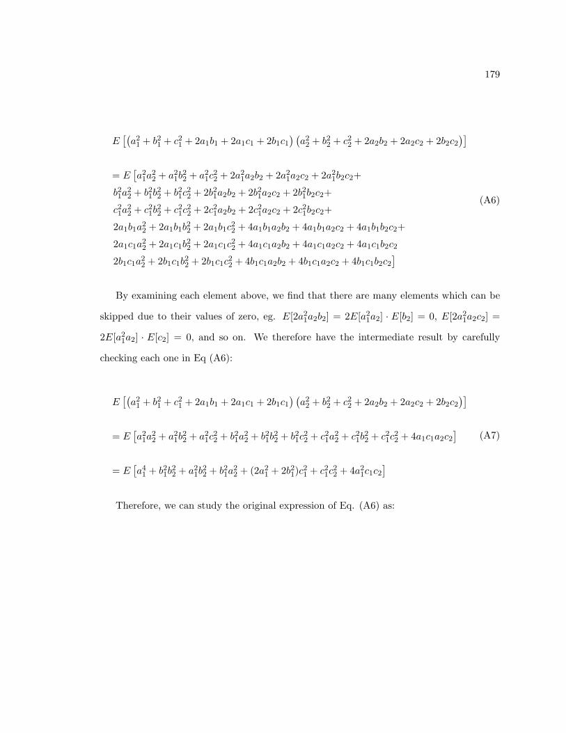
179

E[(a2

1 + b21 + c21 + 2a1b1 + 2a1c1 + 2b1c1) (a2

2 + b22 + c22 + 2a2b2 + 2a2c2 + 2b2c2)]

= E[a2

1a22 + a2

1b22 + a2

1c22 + 2a2

1a2b2 + 2a21a2c2 + 2a2

1b2c2+

b21a22 + b21b

22 + b21c

22 + 2b21a2b2 + 2b21a2c2 + 2b21b2c2+

c21a22 + c21b

22 + c21c

22 + 2c21a2b2 + 2c21a2c2 + 2c21b2c2+

2a1b1a22 + 2a1b1b

22 + 2a1b1c

22 + 4a1b1a2b2 + 4a1b1a2c2 + 4a1b1b2c2+

2a1c1a22 + 2a1c1b

22 + 2a1c1c

22 + 4a1c1a2b2 + 4a1c1a2c2 + 4a1c1b2c2

2b1c1a22 + 2b1c1b22 + 2b1c1c22 + 4b1c1a2b2 + 4b1c1a2c2 + 4b1c1b2c2

]

(A6)

By examining each element above, we find that there are many elements which can be

skipped due to their values of zero, eg. E[2a21a2b2] = 2E[a2

1a2] · E[b2] = 0, E[2a21a2c2] =

2E[a21a2] · E[c2] = 0, and so on. We therefore have the intermediate result by carefully

checking each one in Eq (A6):

E[(a2

1 + b21 + c21 + 2a1b1 + 2a1c1 + 2b1c1) (a2

2 + b22 + c22 + 2a2b2 + 2a2c2 + 2b2c2)]

= E[a2

1a22 + a2

1b22 + a2

1c22 + b21a

22 + b21b

22 + b21c

22 + c21a

22 + c21b

22 + c21c

22 + 4a1c1a2c2

]= E

[a4

1 + b21b22 + a2

1b22 + b21a

22 + (2a2

1 + 2b21)c21 + c21c

22 + 4a2

1c1c2]

(A7)

Therefore, we can study the original expression of Eq. (A6) as:

180

E[X2t,1 · Y 2

t,1]

= 116E

[(k∑

i=1(ε(i)t − ε

(i)t−1)

)4]

+ 116E

( n∑l=k+1

(ε(l)t − ε(l)t−1)

)2(n∑

h=k+1

(ε(h)t − ε

(h)t−1)

)2

+ 116E

( k∑i=1

(ε(i)t − ε(i)t−1)

)2(

n∑h=k+1

(ε(h)t − ε

(h)t−1)

)2

+ 116E

( k∑i=1

(ε(i)t − ε(i)t−1)

)2(

n∑l=k+1

(ε(l)t − ε(l)t−1)

)2

+14

2E

[(k∑

i=1(ε(i)t − ε

(i)t−1)

)2]

+ 2E

( n∑l=k+1

(ε(l)t − ε(l)t−1)

)2 · E

[(ln|u1,t| − ln|u1,t−1|)2

]

+E[(ln|u1,t| − ln|u1,t−1|)2 (ln|u2,t| − ln|u2,t−1|)2

]

+E

[(k∑

i=1(ε(i)t − ε

(i)t−1)

)2]· E [(ln|u1,t| − ln|u1,t−1|) (ln|u2,t| − ln|u2,t−1|)] .

(A8)

We begin by studying the first component E

[(k∑

i=1(ε(i)t − ε

(i)t−1)

)4]. The non-zero con-

tribution comes from:

(1) [ln (m0)− ln (2−m0)]4 when ε

(i)t 6= ε

(i)t−1, and the possibilities for this occurrence is

equal tok∑

i=1

12

12k−i ,

(2) [ln (m0)− ln (2−m0)]2 [ln (m0)− ln (2−m0)]

2 when ε(i)t 6= ε(i)t−1 and ε(j)t 6= ε

(j)t−1, (for

i 6= j), and the possibilities of its occurrence isk∑

i=1

(1

2k−i

k∑j=1,j 6=i

12k−j

).

therefore, the corresponding value of the first component is

[ln (m0)− ln (2−m0)]4

k∑i=1

12

12k−i

+k∑

i=1

12k−i

k∑j=1,j 6=i

12k−j

.

181

Then we have a look at the second component in Eq. (A8), that is

E

( n∑l=k+1

(ε(l)t − ε(l)t−1)

)2( n∑h=k+1

(ε(h)t − ε

(h)t−1)

)2 .

Because of the independence between two multifractal processes after k joint cascade

levels, let us examine E

( n∑l=k+1

(ε(l)t − ε(l)t−1)

)2 firstly, whose non-zero contribution comes

from [ln (m0)− ln (2−m0)]2 with probability of

n∑i=k+1

12

12n−i , and the same way for

E

( n∑h=k+1

(ε(h)t − ε

(h)t−1)

)2. Then we have the result:

[ln (m0)− ln (2−m0)]4 ·

n∑i=k+1

12

12n−i

n∑j=k+1

12

12n−j

.

For the third component in Eq. (A8), we have

E

( n∑i=k

(ε(i)t − ε(i)t−1)

)2( n∑h=k+1

(ε(h)t − ε

(h)t−1)

)2 = E

( n∑i=k

(ε(i)t − ε(i)t−1)

)2·E

( n∑h=k+1

(ε(h)t − ε

(h)t−1)

)2 ,

and it equals to

[ln (m0)− ln (2−m0)]4 ·

n∑i=k

12

12n−i

n∑j=k+1

12

12n−j

.

Since the forth component has the same structure like the third one, we directly move

to the fifth component, which is

2E

( k∑i=1

(ε(i)t − ε(i)t−1)

)2+ 2E

( n∑l=k+1

(ε(l)t − ε(l)t−1)

)2 · E

[(ln|u1,t| − ln|u1,t−1|)2

].

182

We know E[(ln|u1,t| − ln|u1,t−1|)2

]= 2E[ln|ut|2]− 2E[ln|ut|]2, and by combining with

the calculations of the previous two components, it is not difficult to find the result for it,

that is:

[ln (m0)− ln (2−m0)]2 ·

(k∑

i=1

12

12k−i

+n∑

i=k+1

12

12n−i

)·(E[ln|ut|2]− E[ln|ut|]2

).

We also have the solution for the sixth component:

E[(ln|u1,t| − ln|u1,t−1|)2 (ln|u2,t| − ln|u2,t−1|)2

]

= 2E[(ln|u1,t|)2 · (ln|u2,t|)2]− 8E[(ln|u1,t|)2 · ln|u2,t|] · E[ln|ut|] + 4E[ln|u1,t| · ln|u2,t|]2 + 2E[(ln|ut|)2]2.

For the last component:

E

( k∑i=1

(ε(i)t − ε(i)t−1)

)2 · E [(ln|u1,t| − ln|u1,t−1|) (ln|u2,t| − ln|u2,t−1|)] ,

by recalling the calculations of the previous moments of Eq. (A1) and A(2), we have its

non-zero value which is

[ln (m0)− ln (2−m0)]2 ·

k∑i=1

12

12k−i

(2E[ln|u1,t| · ln|u2,t|]− 2E[ln|ut|]2

).

Therefore, we sum up the solutions for each component in Eq. (A8), and arrive to the

final result:

183

E[X2t,1 · Y 2

t,1]

= 116 [ln (m0)− ln (2−m0)]

4 ·

[k∑

i=1

12

12k−i +

k∑i=1

(1

2k−i

k∑j=1,j 6=i

12k−j

)]

+ 116 [ln (m0)− ln (2−m0)]

4 ·n∑

i=k+1

(12

12n−i

n∑j=k+1

12

12n−j

)

+2× 116 [ln (m0)− ln (2−m0)]

4 ·k∑

i=1

(12

12k−i

n∑j=k+1

12

12n−j

)

+ [ln (m0)− ln (2−m0)]2 ·

(k∑

i=1

12

12k−i +

n∑i=k+1

12

12n−i

)·(E[ln|ut|2]− E[ln|ut|]2

)

+2E[(ln|u1,t|)2 · (ln|u2,t|)2]− 8E[(ln|u1,t|)2 · ln|u2,t|] · E[ln|ut|]

+4E[ln|u1,t| · ln|u2,t|]2 + 2E[(ln|ut|)2]2

+ [ln (m0)− ln (2−m0)]2 ·

k∑i=1

12

12k−i

(2E[ln|u1,t| · ln|u2,t|]− 2E[ln|ut|]2

).

(A9)

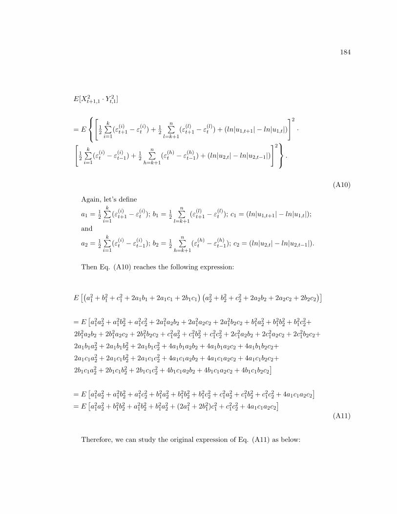
184

E[X2t+1,1 · Y 2

t,1]

= E

[

12

k∑i=1

(ε(i)t+1 − ε(i)t ) + 1

2

n∑l=k+1

(ε(l)t+1 − ε(l)t ) + (ln|u1,t+1| − ln|u1,t|)

]2

·

[12

k∑i=1

(ε(i)t − ε(i)t−1) + 1

2

n∑h=k+1

(ε(h)t − ε

(h)t−1) + (ln|u2,t| − ln|u2,t−1|)

]2 .

(A10)

Again, let’s define

a1 = 12

k∑i=1

(ε(i)t+1 − ε(i)t ); b1 = 1

2

n∑l=k+1

(ε(l)t+1 − ε(l)t ); c1 = (ln|u1,t+1| − ln|u1,t|);

and

a2 = 12

k∑i=1

(ε(i)t − ε(i)t−1); b2 = 1

2

n∑h=k+1

(ε(h)t − ε

(h)t−1); c2 = (ln|u2,t| − ln|u2,t−1|).

Then Eq. (A10) reaches the following expression:

E[(a2

1 + b21 + c21 + 2a1b1 + 2a1c1 + 2b1c1) (a2

2 + b22 + c22 + 2a2b2 + 2a2c2 + 2b2c2)]

= E[a2

1a22 + a2

1b22 + a2

1c22 + 2a2

1a2b2 + 2a21a2c2 + 2a2

1b2c2 + b21a22 + b21b

22 + b21c

22+

2b21a2b2 + 2b21a2c2 + 2b21b2c2 + c21a22 + c21b

22 + c21c

22 + 2c21a2b2 + 2c21a2c2 + 2c21b2c2+

2a1b1a22 + 2a1b1b

22 + 2a1b1c

22 + 4a1b1a2b2 + 4a1b1a2c2 + 4a1b1b2c2+

2a1c1a22 + 2a1c1b

22 + 2a1c1c

22 + 4a1c1a2b2 + 4a1c1a2c2 + 4a1c1b2c2+

2b1c1a22 + 2b1c1b22 + 2b1c1c22 + 4b1c1a2b2 + 4b1c1a2c2 + 4b1c1b2c2

]= E

[a2

1a22 + a2

1b22 + a2

1c22 + b21a

22 + b21b

22 + b21c

22 + c21a

22 + c21b

22 + c21c

22 + 4a1c1a2c2

]= E

[a2

1a22 + b21b

22 + a2

1b22 + b21a

22 + (2a2

1 + 2b21)c21 + c21c

22 + 4a1c1a2c2

](A11)

Therefore, we can study the original expression of Eq. (A11) as below:

185

E[X2t+1,1 · Y 2

t,1]

= 116E

[(k∑

i=1(ε(i)t+1 − ε

(i)t ))2( k∑

i=1(ε(i)t − ε

(i)t−1)

)2]

+ 116E

( n∑l=k+1

(ε(l)t+1 − ε(l)t )

)2(n∑

h=k+1

(ε(h)t − ε

(h)t−1)

)2

+ 116E

( k∑i=1

(ε(i)t+1 − ε(i)t ))2(

n∑h=k+1

(ε(h)t − ε

(h)t−1)

)2

+ 116E

( k∑i=1

(ε(i)t − ε(i)t−1)

)2(

n∑l=k+1

(ε(l)t+1 − ε(l)t )

)2

+14

2E

[(k∑

i=1(ε(i)t+1 − ε

(i)t ))2]

+ 2E

( n∑l=k+1

(ε(l)t − ε(l)t−1)

)2 ·

(2E[ln|ut|2]− 2E[ln|ut|]2

)

+E[(ln|u1,t+1| − ln|u1,t|)2 (ln|u2,t| − ln|u2,t−1|)2

]

+E[(

k∑i=1

(ε(i)t+1 − ε(i)t ))(

k∑i=1

(ε(i)t − ε(i)t−1)

)](E[ln|ut|]2 − E[ln|u1,t| · ln|u2,t|]).

(A12)

After checking each component in Eq. (A12), we see the only unfamiliar one is the first

term:

E

[(k∑

i=1(ε(i)t+1 − ε

(i)t ))2

·(

k∑i=1

(ε(i)t − ε(i)t−1)

)2], and there are three different forms to be

considered:

(1)(ε(i)t+1 − ε

(i)t

)2 (ε(i)t − ε

(i)t−1

)2, which have non-zero value only if ε(i)t+1 6= ε

(i)t 6= ε

(i)t−1.

and this possibility is (12

12k−i )2, combining with the non-zero expectation value,

we have(

k∑i=1

(12

12k−i )2

)· [ln (m0)− ln (2−m0)]

4 .

186

(2)(ε(j)t+1 − ε

(j)t

)2 (ε(i)t − ε

(i)t−1

)2, which are non-zero for i 6= j, ε(j)t+1 6= ε

(j)t and ε(i)t 6= ε

(i)t−1,

the probability of its occurrence isk∑

i=1

(1

2k−i

k∑j=1,j 6=i

12k−j

).

Putting together these two possible forms we get

[ln (m0)− ln (2−m0)]4 ·

(k∑

i=1

12

12k−i

k∑j=1

12

12k−j

).

(3) Form(ε(j)t+1 − ε

(j)t

)(ε(i)t+1 − ε

(i)t

)(ε(j)t − ε

(j)t−1

)(ε(i)t − ε

(i)t−1

), which for i 6= j and ε(n)

t+1 6=

ε(n)t 6= ε

(n)t−1, n = i, j are non-zero, and which implies

2

k∑

i=1

(( 12k−i )2

k∑j=1,j 6=i

( 12k−j )2

)· [ln (m0)− ln (2−m0)]

4.

Then we have the solution for the first component in the above moment condition:

E

[(k∑

i=1(ε(i)t+1 − ε

(i)t ))2

·(

k∑i=1

(ε(i)t − ε(i)t−1)

)2]

= [ln (m0)− ln (2−m0)]4

[k∑

i=1

12

12k−i

k∑j=1

12

12k−j + 2

k∑i=1

(12

12k−i )2

k∑j=1,j 6=i

(12

12k−j )2

]

The other components can be solved by recalling previous calculations. All in all, we

finally arrive at:

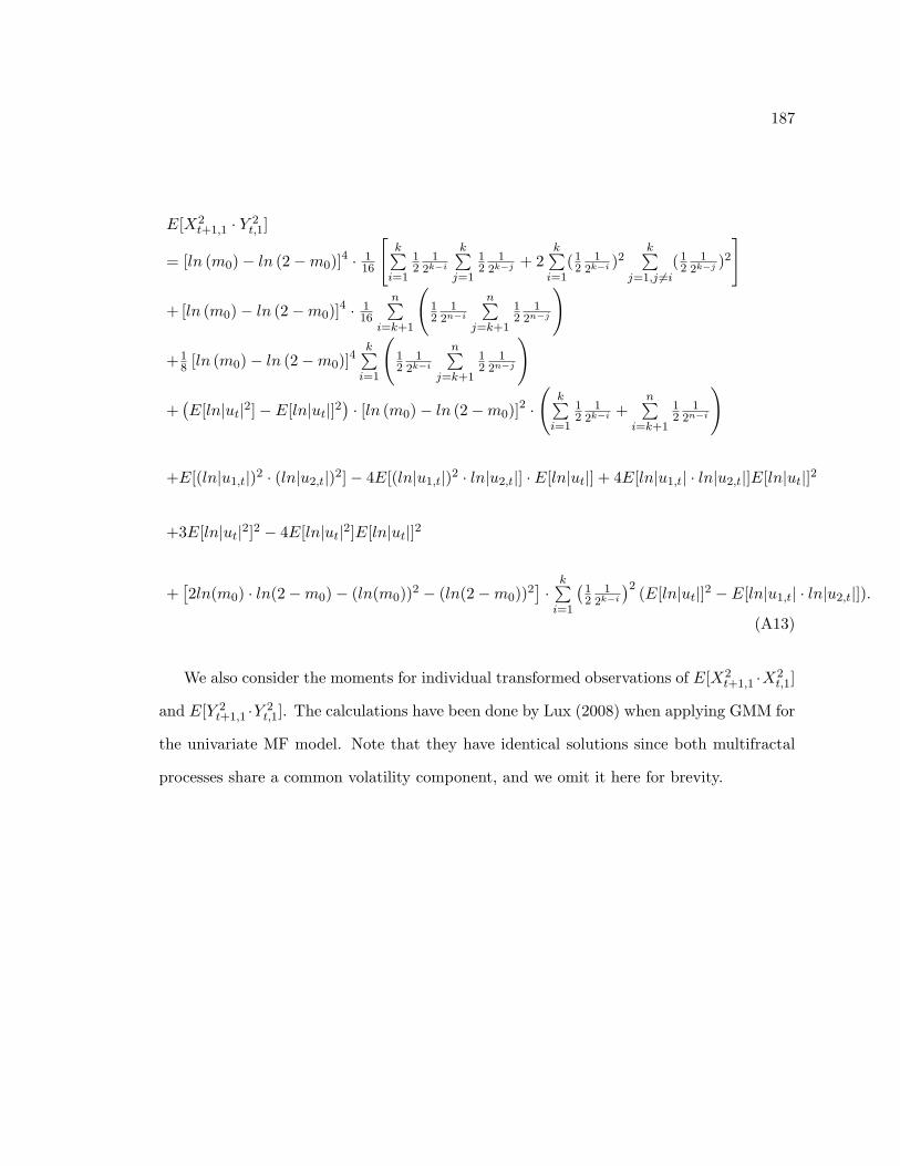
187

E[X2t+1,1 · Y 2

t,1]

= [ln (m0)− ln (2−m0)]4 · 1

16

[k∑

i=1

12

12k−i

k∑j=1

12

12k−j + 2

k∑i=1

(12

12k−i )2

k∑j=1,j 6=i

(12

12k−j )2

]

+ [ln (m0)− ln (2−m0)]4 · 1

16

n∑i=k+1

(12

12n−i

n∑j=k+1

12

12n−j

)

+18 [ln (m0)− ln (2−m0)]

4k∑

i=1

(12

12k−i

n∑j=k+1

12

12n−j

)

+(E[ln|ut|2]− E[ln|ut|]2

)· [ln (m0)− ln (2−m0)]

2 ·

(k∑

i=1

12

12k−i +

n∑i=k+1

12

12n−i

)

+E[(ln|u1,t|)2 · (ln|u2,t|)2]− 4E[(ln|u1,t|)2 · ln|u2,t|] · E[ln|ut|] + 4E[ln|u1,t| · ln|u2,t|]E[ln|ut|]2

+3E[ln|ut|2]2 − 4E[ln|ut|2]E[ln|ut|]2

+[2ln(m0) · ln(2−m0)− (ln(m0))2 − (ln(2−m0))2

]·

k∑i=1

(12

12k−i

)2 (E[ln|ut|]2 − E[ln|u1,t| · ln|u2,t|]).

(A13)

We also consider the moments for individual transformed observations of E[X2t+1,1 ·X2

t,1]

and E[Y 2t+1,1 ·Y 2

t,1]. The calculations have been done by Lux (2008) when applying GMM for

the univariate MF model. Note that they have identical solutions since both multifractal

processes share a common volatility component, and we omit it here for brevity.

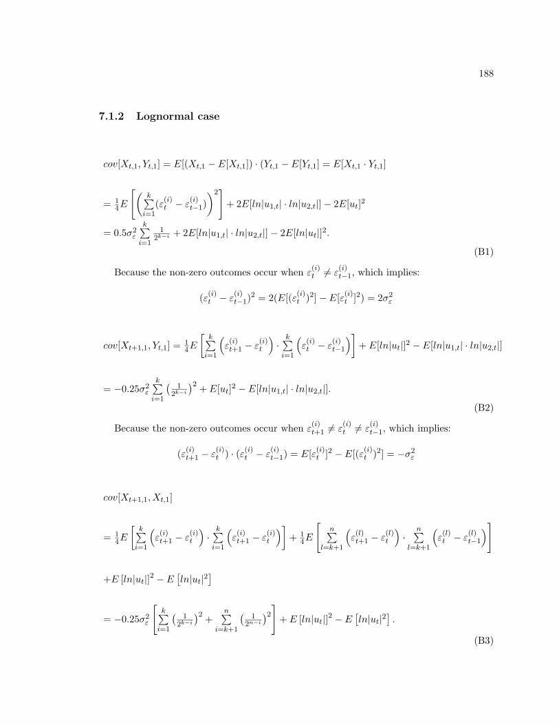
188

7.1.2 Lognormal case

cov[Xt,1, Yt,1] = E[(Xt,1 − E[Xt,1]) · (Yt,1 − E[Yt,1] = E[Xt,1 · Yt,1]

= 14E

[(k∑

i=1(ε(i)t − ε

(i)t−1)

)2]

+ 2E[ln|u1,t| · ln|u2,t|]− 2E[ut]2

= 0.5σ2ε

k∑i=1

12k−i + 2E[ln|u1,t| · ln|u2,t|]− 2E[ln|ut|]2.

(B1)

Because the non-zero outcomes occur when ε(i)t 6= ε(i)t−1, which implies:

(ε(i)t − ε(i)t−1)

2 = 2(E[(ε(i)t )2]− E[ε(i)t ]2) = 2σ2ε

cov[Xt+1,1, Yt,1] = 14E

[k∑

i=1

(ε(i)t+1 − ε

(i)t

)·

k∑i=1

(ε(i)t − ε

(i)t−1

)]+ E[ln|ut|]2 − E[ln|u1,t| · ln|u2,t|]

= −0.25σ2ε

k∑i=1

(1

2k−i

)2 + E[ut]2 − E[ln|u1,t| · ln|u2,t|].

(B2)

Because the non-zero outcomes occur when ε(i)t+1 6= ε(i)t 6= ε

(i)t−1, which implies:

(ε(i)t+1 − ε(i)t ) · (ε(i)t − ε

(i)t−1) = E[ε(i)t ]2 − E[(ε(i)t )2] = −σ2

ε

cov[Xt+1,1, Xt,1]

= 14E

[k∑

i=1

(ε(i)t+1 − ε

(i)t

)·

k∑i=1

(ε(i)t+1 − ε

(i)t

)]+ 1

4E

[n∑

l=k+1

(ε(l)t+1 − ε

(l)t

)·

n∑l=k+1

(ε(l)t − ε

(l)t−1

)]


]

= −0.25σ2ε

[k∑

i=1

(1

2k−i

)2 +n∑

i=k+1

(1

2n−i

)2]+ E [ln|ut|]2 − E[ln|ut|2

].

(B3)

189

For the moments of squared observations, we recall the semi-final results of Eq. (A6)

and Eq. (A11) for E[X2t,1 · Y 2

t,1] and E[X2t+1,1 · Y 2

t,1].

E[X2t,1 · Y 2

t,1]

= 116E

[(k∑

i=1(ε(i)t − ε

(i)t−1)

)4]

+ 116E

( n∑l=k+1

(ε(l)t − ε(l)t−1)

)2(n∑

h=k+1

(ε(h)t − ε

(h)t−1)

)2

+ 116E

( k∑i=1

(ε(i)t − ε(i)t−1)

)2(

n∑h=k+1

(ε(h)t − ε

(h)t−1)

)2

+ 116E

( k∑i=1

(ε(i)t − ε(i)t−1)

)2(

n∑l=k+1

(ε(l)t − ε(l)t−1)

)2

+14

2E

[(k∑

i=1(ε(i)t − ε

(i)t−1)

)2]

+ 2E

( n∑l=k+1

(ε(l)t − ε(l)t−1)

)2 ·


)


+4E[ln|u1,t| · (ln|u2,t|]2 + 2E[(ln|ut|)2]2

+E

[(k∑

i=1(ε(i)t − ε

(i)t−1)

)2]

(2E[ln|u1,t| · ln|u2,t|]− 2E[ln|ut|]2).

(B4)

For the first term E

[(k∑

i=1(ε(i)t − ε

(i)t−1)

)4], let’s begin with E

[(ε(i)t − ε

(i)t−1

)4], we know

that the non-zero contributions come from:

(1) E[(ε(i)t − ε

(i)t−1

)4]

= 2E[ε(i)t ]4+6E[(ε(i)t )2]2−8E[(ε(i)t )3]E[ε(i)t ] = 12σ4ε , and this occurs

with probability 21

k−i . Then we have the solution:

E

( k∑i=1

(ε(i)t − ε(i)t−1)

)4 = 12σ4

ε ·k∑

i=1

12k−i

.

190

(2) E[(ε(i)t − ε

(i)t−1

)2 (ε(j)t − ε

(j)t−1

)2]

= 4σ4ε , for ε(i)t 6= ε

(i)t−1 and ε

(j)t 6= ε

(j)t−1, (i 6= j), with

the possibilities of its occurrence isk∑

i=1

(1

2k−i

k∑j=1,j 6=i

12k−j

). Therefore,

E

[(ε(i)t − ε

(i)t−1

)2 (ε(j)t − ε

(j)t−1

)2]

= 4σ4ε ·

k∑i=1

(1

2k−i

k∑j=1,j 6=i

12k−j

).

E[X2t,1 · Y 2

t,1]

= 0.75σ4ε

k∑i=1

12k−i + 0.25σ4

ε

k∑i=1

(1

2k−i

k∑j=1,j 6=i

12k−j

)+ 0.25σ4

ε

n∑l=k+1

12n−l

n∑h=k+1

12n−h

+0.25σ4ε

k∑i=1

12k−i

n∑h=k+1

12n−h + 0.25σ4

ε

k∑i=1

12k−i

n∑l=k+1

12n−l

+2σ2ε

(E[ln|ut|2]− E[ln|ut|]2

)·

(k∑

i=1

12k−i +

n∑l=k+1

12n−l

)


+4E[ln|u1,t| · (ln|u2,t|]2 + 2E[(ln|ut|)2]2

+2σ2ε ·

k∑i=1

12k−i (2E[ln|u1,t| · ln|u2,t|]− 2E[ln|ut|]2).

(B5)

With the aid of semi-final results in Eq. (A11), E[X2t+1,1 · Y 2

t,1] can be computed as

follows:

191

E[X2t+1,1 · Y 2

t,1]

= 116E

[(k∑

i=1(ε(i)t+1 − ε

(i)t ))2

·(

k∑i=1

(ε(i)t − ε(i)t−1)

)2]

+ 116E

( n∑l=k+1

(ε(l)t+1 − ε(l)t )

)2(n∑

h=k+1

(ε(h)t − ε

(h)t−1)

)2

+ 116E

( k∑i=1

(ε(i)t+1 − ε(i)t ))2(

n∑h=k+1

(ε(h)t − ε

(h)t−1)

)2

+ 116E

( k∑i=1

(ε(i)t − ε(i)t−1)

)2(

n∑l=k+1

(ε(l)t+1 − ε(l)t )

)2

+14

2E

[(k∑

i=1(ε(i)t − ε

(i)t−1)

)2]

+ 2E

( n∑l=k+1

(ε(l)t − ε(l)t−1)

)2 ·


)

+E[(ln|u1,t|)2 · (ln|u2,t|)2]− 4E[(ln|u1,t|)2 · ln|u2,t|] · E[ln|ut|] + 4E[ln|u1,t| · (ln|u2,t|]E[ln|ut|]2

+3E[ln|ut|2]2 − 4E[ln|ut|2]E[ln|ut|]2

+E[(

k∑i=1

(ε(i)t+1 − ε(i)t ))(

k∑i=1

(ε(i)t − ε(i)t−1)

)](E[ln|ut|]2 − E[ln|u1,t| · ln|u2,t|]).

For the first term E

[(k∑

i=1(ε(i)t+1 − ε

(i)t ))2

·(

k∑i=1

(ε(i)t − ε(i)t−1)

)2], there are three different

possible forms:

(1)(ε(i)t+1 − ε

(i)t

)2 (ε(i)t − ε

(i)t−1

)2, has non-zero value only if ε(i)t+1 6= ε

(i)t 6= ε

(i)t−1. then

E

[(ε(i)t+1 − ε

(i)t

)2 (ε(i)t − ε

(i)t−1

)2]

= E[ε4t ] + 3E[ε2t ]2 − 4E[ε3t ]E[εt] = 6σ4

ε . (E[ε3t ] =

3λσ2ε + λ3 and E[ε4t ] = 3σ4

ε + 6λ2σ2ε + λ4,) and the probability of this occurrence is

( 12k−i )2. Putting together we get

[k∑

i=1

(1

2k−i

)2] · 6σ4ε .

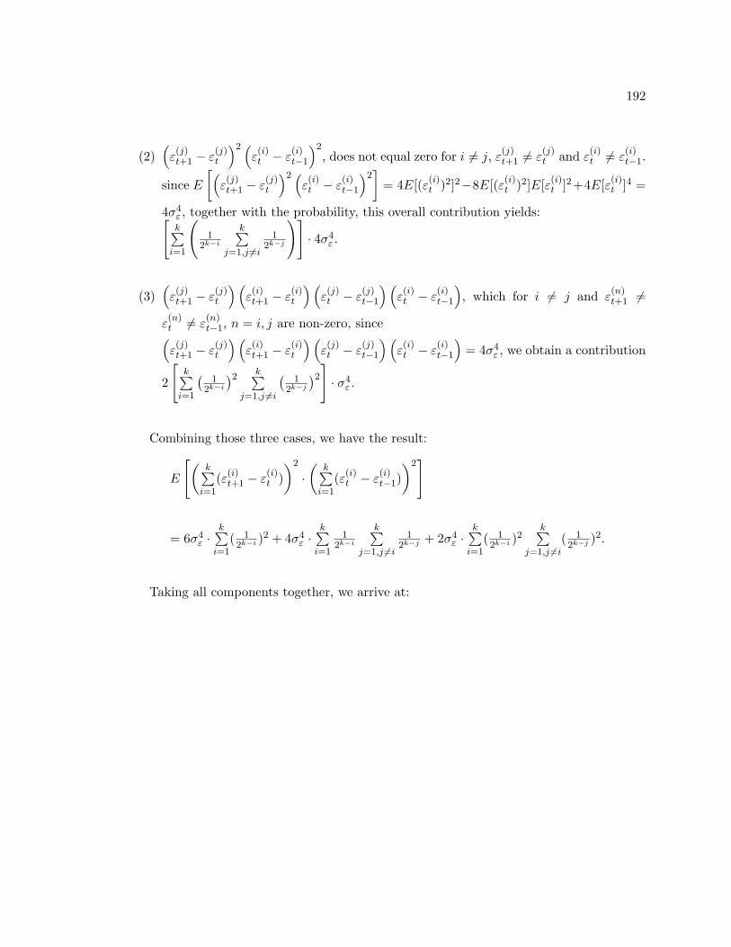
192

(2)(ε(j)t+1 − ε

(j)t

)2 (ε(i)t − ε

(i)t−1

)2, does not equal zero for i 6= j, ε(j)t+1 6= ε

(j)t and ε(i)t 6= ε

(i)t−1.

since E[(ε(j)t+1 − ε

(j)t

)2 (ε(i)t − ε

(i)t−1

)2]

= 4E[(ε(i)t )2]2−8E[(ε(i)t )2]E[ε(i)t ]2+4E[ε(i)t ]4 =

4σ4ε , together with the probability, this overall contribution yields:[k∑

i=1

(1

2k−i

k∑j=1,j 6=i

12k−j

)]· 4σ4

ε .

(3)(ε(j)t+1 − ε

(j)t

)(ε(i)t+1 − ε

(i)t

)(ε(j)t − ε

(j)t−1

)(ε(i)t − ε

(i)t−1

), which for i 6= j and ε

(n)t+1 6=

ε(n)t 6= ε

(n)t−1, n = i, j are non-zero, since(

ε(j)t+1 − ε

(j)t

)(ε(i)t+1 − ε

(i)t

)(ε(j)t − ε

(j)t−1

)(ε(i)t − ε

(i)t−1

)= 4σ4

ε , we obtain a contribution

2

[k∑

i=1

(1

2k−i

)2 k∑j=1,j 6=i

(1

2k−j

)2] · σ4ε .

Combining those three cases, we have the result:

E

[(k∑

i=1(ε(i)t+1 − ε

(i)t ))2

·(

k∑i=1

(ε(i)t − ε(i)t−1)

)2]

= 6σ4ε ·

k∑i=1

( 12k−i )2 + 4σ4

ε ·k∑

i=1

12k−i

k∑j=1,j 6=i

12k−j + 2σ4

ε ·k∑

i=1( 12k−i )2

k∑j=1,j 6=i

( 12k−j )2.

Taking all components together, we arrive at:

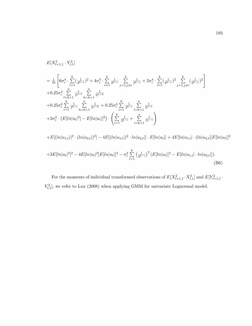
193

E[X2t+1,1 · Y 2

t,1]

= 116

[6σ4

ε ·k∑

i=1( 12k−i )2 + 4σ4

ε ·k∑

i=1

12k−i

k∑j=1,j 6=i

12k−j + 2σ4

ε ·k∑

i=1( 12k−i )2

k∑j=1,j 6=i

( 12k−j )2

]+0.25σ4

ε

n∑l=k+1

12n−l

n∑h=k+1

12n−h

+0.25σ4ε

k∑i=1

12k−i

n∑h=k+1

12n−h + 0.25σ4

ε

k∑i=1

12k−i

n∑l=k+1

12n−l

+2σ2ε ·(E[ln|ut|2]− E[ln|ut|]2

)·

(k∑

i=1

12k−i +

n∑i=k+1

12n−i

)

+E[(ln|u1,t|)2 · (ln|u2,t|)2]− 4E[(ln|u1,t|)2 · ln|u2,t|] · E[ln|ut|] + 4E[ln|u1,t| · (ln|u2,t|]E[ln|ut|]2

+3E[ln|ut|2]2 − 4E[ln|ut|2]E[ln|ut|]2 − σ2ε

k∑i=1

(1

2k−i

)2 (E[ln|ut|]2 − E[ln|u1,t| · ln|u2,t|]).

(B6)

For the moments of individual transformed observations of E[X2t+1,1 ·X2

t,1] and E[Y 2t+1,1 ·

Y 2t,1], we refer to Lux (2008) when applying GMM for univariate Lognormal model.

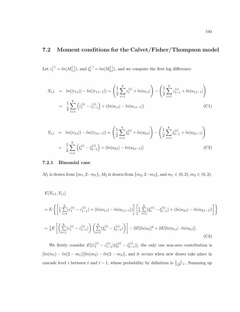
194

7.2 Moment conditions for the Calvet/Fisher/Thompson model

Let ε(·)t = ln(M (·)1,t), and ξ(·)t = ln(M (·)

2,t), and we compute the first log difference:

Xt,1 = ln(|r1,t|)− ln(|r1,t−1|) =

(12

k∑i=1

ε(i)t + ln|u1,t|

)−

(12

k∑i=1

ε(i)t−1 + ln|u1,t−1|

)

=12

k∑i=1

(ε(i)t − ε

(i)t−1

)+ (ln|u1,t| − ln|u1,t−1|) (C1)

Yt,1 = ln(|r2,t|)− ln(|r2,t−1|) =

(12

k∑i=1

ξ(i)t + ln|u2,t|

)−

(12

k∑i=1

ξ(i)t−1 + ln|u2,t−1|

)

=12

k∑i=1

(ξ(i)t − ξ

(i)t−1

)+ (ln|u2,t| − ln|u2,t−1|) (C2)

7.2.1 Binomial case

M1 is drawn from m1, 2−m1, M2 is drawn from m2, 2−m2, andm1 ∈ (0, 2), m2 ∈ (0, 2).

E[Xt,1, Yt,1]

= E

[12

k∑i=1

(ε(i)t − ε(i)t−1) + (ln|u1,t| − ln|u1,t−1|)

] [12

k∑i=1

(ξ(i)t − ξ(i)t−1) + (ln|u2,t| − ln|u2,t−1|)

]

= 14E

[(k∑

i=1(ε(i)t − ε

(i)t−1)

)(k∑

i=1(ξ(i)t − ξ

(i)t−1)

)]− 2E[ln|ut|]2 + 2E[ln|u1,t| · ln|u2,t|].

(C3)

We firstly consider E[(ε(i)t − ε(i)t−1)(ξ

(i)t − ξ

(i)t−1)], the only one non-zero contribution is

[ln(m1) − ln(2 −m1)][ln(m2) − ln(2 −m2)], and it occurs when new draws take place in

cascade level i between t and t− 1, whose probability by definition is 12

12k−i . Summing up

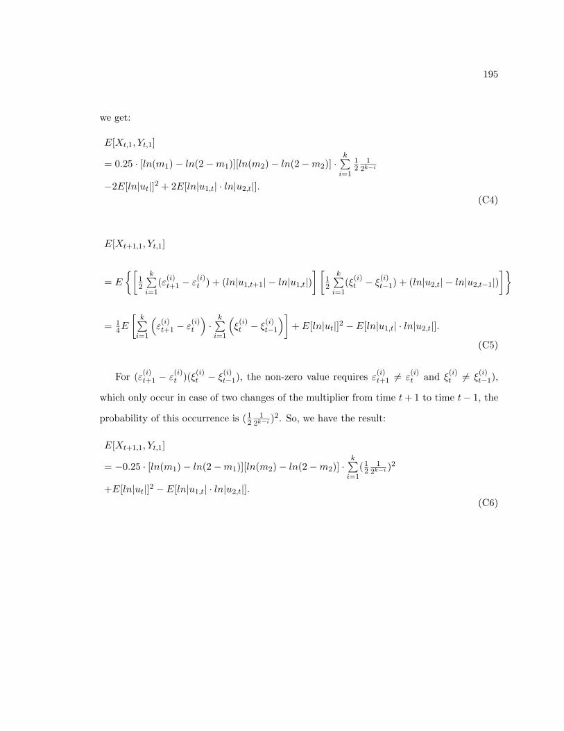
195

we get:

E[Xt,1, Yt,1]

= 0.25 · [ln(m1)− ln(2−m1)][ln(m2)− ln(2−m2)] ·k∑

i=1

12

12k−i

−2E[ln|ut|]2 + 2E[ln|u1,t| · ln|u2,t|].(C4)

E[Xt+1,1, Yt,1]

= E

[12

k∑i=1

(ε(i)t+1 − ε(i)t ) + (ln|u1,t+1| − ln|u1,t|)

] [12

k∑i=1

(ξ(i)t − ξ(i)t−1) + (ln|u2,t| − ln|u2,t−1|)

]

= 14E

[k∑

i=1

(ε(i)t+1 − ε

(i)t

)·

k∑i=1

(ξ(i)t − ξ

(i)t−1

)]+ E[ln|ut|]2 − E[ln|u1,t| · ln|u2,t|].

(C5)

For (ε(i)t+1 − ε(i)t )(ξ(i)t − ξ

(i)t−1), the non-zero value requires ε(i)t+1 6= ε

(i)t and ξ

(i)t 6= ξ

(i)t−1),

which only occur in case of two changes of the multiplier from time t+ 1 to time t− 1, the

probability of this occurrence is (12

12k−i )2. So, we have the result:

E[Xt+1,1, Yt,1]

= −0.25 · [ln(m1)− ln(2−m1)][ln(m2)− ln(2−m2)] ·k∑

i=1(12

12k−i )2

+E[ln|ut|]2 − E[ln|u1,t| · ln|u2,t|].(C6)

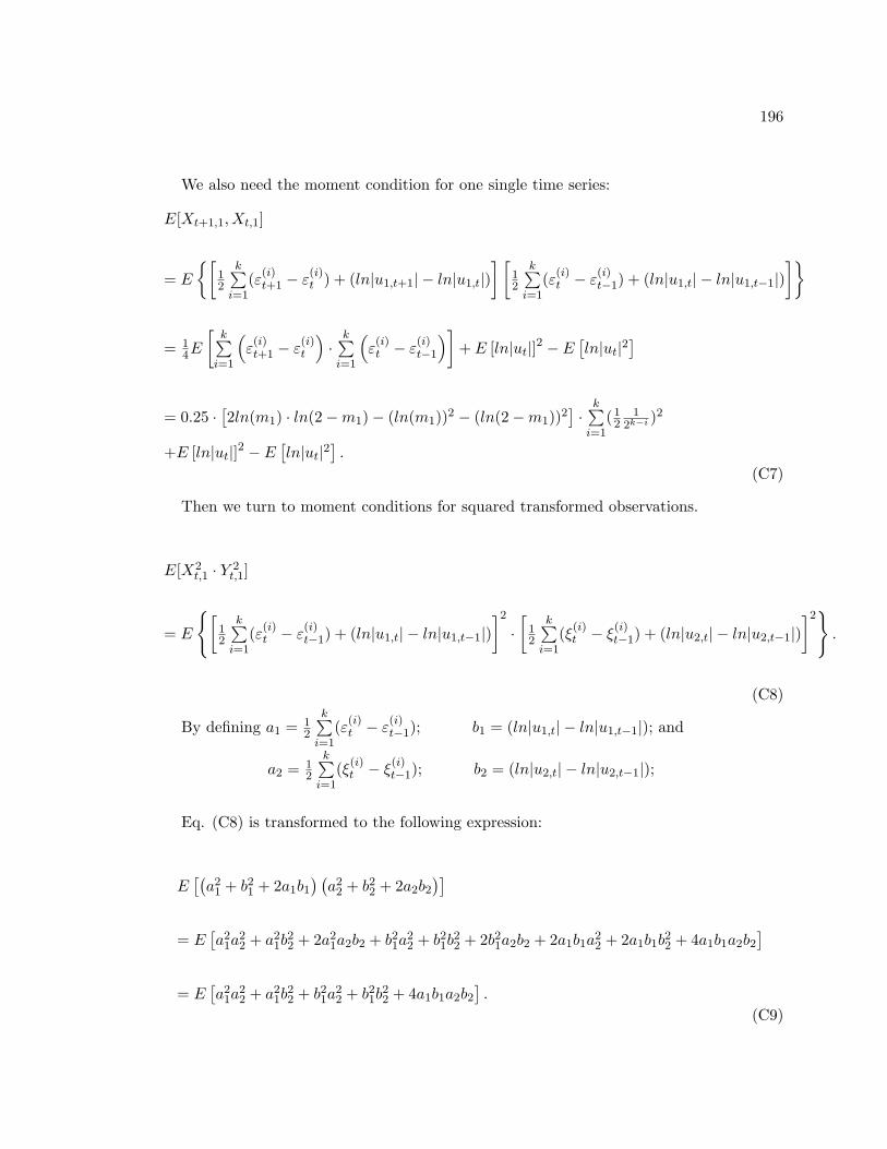
196

We also need the moment condition for one single time series:

E[Xt+1,1, Xt,1]

= E

[12

k∑i=1

(ε(i)t+1 − ε(i)t ) + (ln|u1,t+1| − ln|u1,t|)

] [12

k∑i=1

(ε(i)t − ε(i)t−1) + (ln|u1,t| − ln|u1,t−1|)

]

= 14E

[k∑

i=1

(ε(i)t+1 − ε

(i)t

)·

k∑i=1

(ε(i)t − ε

(i)t−1

)]+ E [ln|ut|]2 − E

[ln|ut|2

]

= 0.25 ·[2ln(m1) · ln(2−m1)− (ln(m1))2 − (ln(2−m1))2

]·

k∑i=1

(12

12k−i )2


].

(C7)

Then we turn to moment conditions for squared transformed observations.

E[X2t,1 · Y 2

t,1]

= E

[12

k∑i=1

(ε(i)t − ε(i)t−1) + (ln|u1,t| − ln|u1,t−1|)

]2

·[

12

k∑i=1

(ξ(i)t − ξ(i)t−1) + (ln|u2,t| − ln|u2,t−1|)

]2.

(C8)

By defining a1 = 12

k∑i=1

(ε(i)t − ε(i)t−1); b1 = (ln|u1,t| − ln|u1,t−1|); and

a2 = 12

k∑i=1

(ξ(i)t − ξ(i)t−1); b2 = (ln|u2,t| − ln|u2,t−1|);

Eq. (C8) is transformed to the following expression:

E[(a2

1 + b21 + 2a1b1) (a2

2 + b22 + 2a2b2)]

= E[a2

1a22 + a2

1b22 + 2a2

1a2b2 + b21a22 + b21b

22 + 2b21a2b2 + 2a1b1a

22 + 2a1b1b

22 + 4a1b1a2b2

]= E

[a2

1a22 + a2

1b22 + b21a

22 + b21b

22 + 4a1b1a2b2

].

(C9)

197

Therefore, we have

E[X2t,1 · Y 2

t,1]

= 116E

[(k∑

i=1(ε(i)t − ε

(i)t−1)

)2( k∑i=1

(ξ(i)t − ξ(i)t−1)

)2]

+14E

[(k∑

i=1(ε(i)t − ε

(i)t−1)

)2

(ln|u2,t| − ln|u2,t−1|)2]

+14E

[(k∑

i=1(ξ(i)t − ξ

(i)t−1)

)2

(ln|u1,t| − ln|u1,t−1|)2]

+E[(

12

k∑i=1

(ε(i)t − ε(i)t−1)

)(ln|u1,t| − ln|u1,t−1|)

(12

k∑i=1

(ξ(i)t − ξ(i)t−1)

)(ln|u2,t| − ln|u2,t−1|)

]


].

(C10)

We examine each component in Eq. (C10) based on the experiences of previous calcu-

lations, and get the final solution for E[X2t,1 · Y 2

t,1] as below:

E[X2t,1 · Y 2

t,1]

= 116 [ln (m1)− ln (2−m1)]

2 · [ln (m2)− ln (2−m2)]2

k∑i=1

12

12k−i

+14 [ln (m1)− ln (2−m1)]

2k∑

i=1

12

12k−i · E[(ln|ut| − ln|ut−1|)2]

+14 [ln (m2)− ln (2−m2)]

2k∑

i=1

12

12k−i · E[(ln|ut| − ln|ut−1|)2]

+ [ln (m1)− ln (2−m1)] · [ln (m2)− ln (2−m2)]k∑

i=1

12

12k−i ·

(2E[ln|u1,t|ln|u2,t| − 2E[ln|ut|]2]

)+2E[(ln|u1,t|)2 · (ln|u2,t|)2]− 8E[(ln|u1,t|)2 · ln|u2,t|] · E[ln|ut|]

+4E[ln|u1,t| · (ln|u2,t|]2 + 2E[(ln|ut|)2]2.(C11)

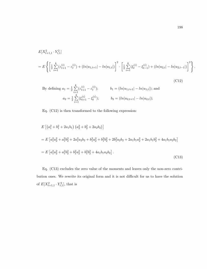
198

E[X2t+1,1 · Y 2

t,1]

= E

[12

k∑i=1

(ε(i)t+1 − ε(i)t ) + (ln|u1,t+1| − ln|u1,t|)

]2

·[

12

k∑i=1

(ξ(i)t − ξ(i)t−1) + (ln|u2,t| − ln|u2,t−1|)

]2.

(C12)

By defining a1 = 12

k∑i=1

(ε(i)t+1 − ε(i)t ); b1 = (ln|u1,t+1| − ln|u1,t|); and

a2 = 12

k∑i=1

(ξ(i)t+1 − ξ(i)t ); b2 = (ln|u2,t+1| − ln|u2,t|);

Eq. (C12) is then transformed to the following expression:

E[(a2

1 + b21 + 2a1b1) (a2

2 + b22 + 2a2b2)]

= E[a2

1a22 + a2

1b22 + 2a2

1a2b2 + b21a22 + b21b

22 + 2b21a2b2 + 2a1b1a

22 + 2a1b1b

22 + 4a1b1a2b2

]= E

[a2

1a22 + a2

1b22 + b21a

22 + b21b

22 + 4a1b1a2b2

].

(C13)

Eq. (C13) excludes the zero value of the moments and leaves only the non-zero contri-

bution ones. We rewrite its original form and it is not difficult for us to have the solution

of E[X2t+1,1 · Y 2

t,1], that is

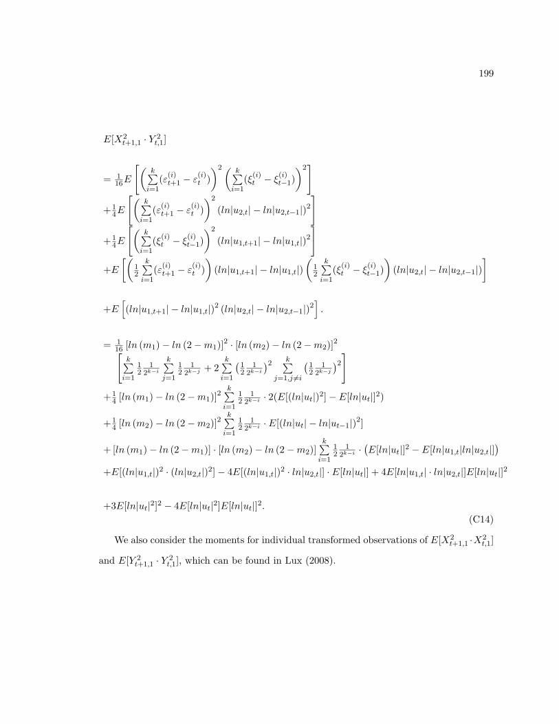
199

E[X2t+1,1 · Y 2

t,1]

= 116E

[(k∑

i=1(ε(i)t+1 − ε

(i)t ))2( k∑

i=1(ξ(i)t − ξ

(i)t−1)

)2]

+14E

[(k∑

i=1(ε(i)t+1 − ε

(i)t ))2

(ln|u2,t| − ln|u2,t−1|)2]

+14E

[(k∑

i=1(ξ(i)t − ξ

(i)t−1)

)2

(ln|u1,t+1| − ln|u1,t|)2]

+E[(

12

k∑i=1

(ε(i)t+1 − ε(i)t ))

(ln|u1,t+1| − ln|u1,t|)(

12

k∑i=1

(ξ(i)t − ξ(i)t−1)

)(ln|u2,t| − ln|u2,t−1|)

]


].

= 116 [ln (m1)− ln (2−m1)]

2 · [ln (m2)− ln (2−m2)]2[

k∑i=1

12

12k−i

k∑j=1

12

12k−j + 2

k∑i=1

(12

12k−i

)2 k∑j=1,j 6=i

(12

12k−j

)2]+1

4 [ln (m1)− ln (2−m1)]2

k∑i=1

12

12k−i · 2(E[(ln|ut|)2]− E[ln|ut|]2)

+14 [ln (m2)− ln (2−m2)]

2k∑

i=1

12

12k−i · E[(ln|ut| − ln|ut−1|)2]

+ [ln (m1)− ln (2−m1)] · [ln (m2)− ln (2−m2)]k∑

i=1

12

12k−i ·

(E[ln|ut|]2 − E[ln|u1,t|ln|u2,t|]

)+E[(ln|u1,t|)2 · (ln|u2,t|)2]− 4E[(ln|u1,t|)2 · ln|u2,t|] · E[ln|ut|] + 4E[ln|u1,t| · ln|u2,t|]E[ln|ut|]2

+3E[ln|ut|2]2 − 4E[ln|ut|2]E[ln|ut|]2.(C14)


t,1]

and E[Y 2t+1,1 · Y 2

t,1], which can be found in Lux (2008).

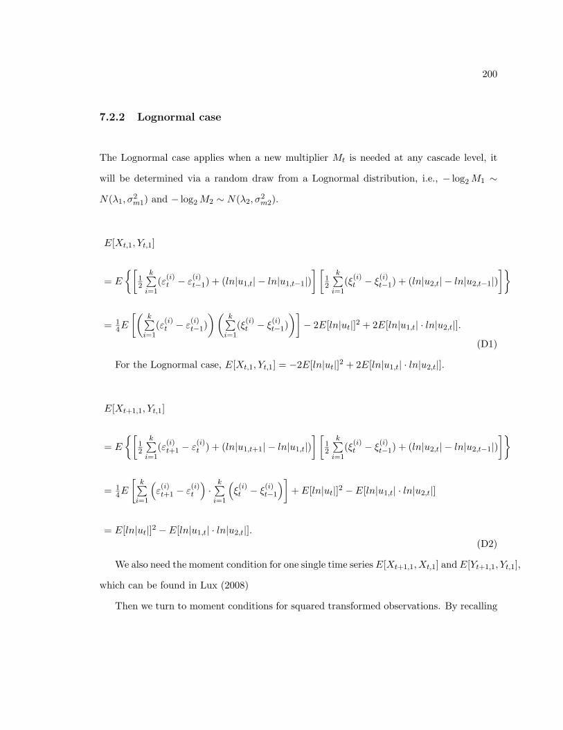
200

7.2.2 Lognormal case

The Lognormal case applies when a new multiplier Mt is needed at any cascade level, it

will be determined via a random draw from a Lognormal distribution, i.e., − log2M1 ∼

N(λ1, σ2m1) and − log2M2 ∼ N(λ2, σ

2m2).

E[Xt,1, Yt,1]

= E

[12

k∑i=1

(ε(i)t − ε(i)t−1) + (ln|u1,t| − ln|u1,t−1|)

] [12

k∑i=1

(ξ(i)t − ξ(i)t−1) + (ln|u2,t| − ln|u2,t−1|)

]

= 14E

[(k∑

i=1(ε(i)t − ε

(i)t−1)

)(k∑

i=1(ξ(i)t − ξ

(i)t−1)

)]− 2E[ln|ut|]2 + 2E[ln|u1,t| · ln|u2,t|].

(D1)

For the Lognormal case, E[Xt,1, Yt,1] = −2E[ln|ut|]2 + 2E[ln|u1,t| · ln|u2,t|].

E[Xt+1,1, Yt,1]

= E

[12

k∑i=1

(ε(i)t+1 − ε(i)t ) + (ln|u1,t+1| − ln|u1,t|)

] [12

k∑i=1

(ξ(i)t − ξ(i)t−1) + (ln|u2,t| − ln|u2,t−1|)

]

= 14E

[k∑

i=1

(ε(i)t+1 − ε

(i)t

)·

k∑i=1

(ξ(i)t − ξ

(i)t−1

)]+ E[ln|ut|]2 − E[ln|u1,t| · ln|u2,t|]

= E[ln|ut|]2 − E[ln|u1,t| · ln|u2,t|].(D2)

We also need the moment condition for one single time series E[Xt+1,1, Xt,1] andE[Yt+1,1, Yt,1],

which can be found in Lux (2008)

Then we turn to moment conditions for squared transformed observations. By recalling

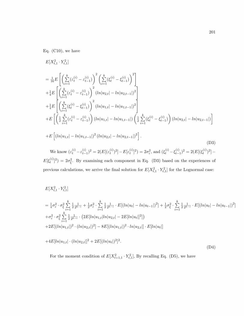
201

Eq. (C10), we have

E[X2t,1 · Y 2

t,1]

= 116E

[(k∑

i=1(ε(i)t − ε

(i)t−1)

)2( k∑i=1

(ξ(i)t − ξ(i)t−1)

)2]

+14E

[(k∑

i=1(ε(i)t − ε

(i)t−1)

)2

(ln|u2,t| − ln|u2,t−1|)2]

+14E

[(k∑

i=1(ξ(i)t − ξ

(i)t−1)

)2

(ln|u1,t| − ln|u1,t−1|)2]

+E[(

12

k∑i=1

(ε(i)t − ε(i)t−1)

)(ln|u1,t| − ln|u1,t−1|)

(12

k∑i=1

(ξ(i)t − ξ(i)t−1)

)(ln|u2,t| − ln|u2,t−1|)

]


].

(D3)

We know (ε(i)t −ε(i)t−1)2 = 2(E[(ε(i)t )2]−E[ε(i)t ]2) = 2σ2

ε , and (ξ(i)t −ξ(i)t−1)2 = 2(E[(ξ(i)t )2]−

E[ξ(i)t ]2) = 2σ2ξ . By examining each component in Eq. (D3) based on the experiences of

previous calculations, we arrive the final solution for E[X2t,1 · Y 2

t,1] for the Lognormal case:

E[X2t,1 · Y 2

t,1]

= 14σ

2ε · σ2

ξ

k∑i=1

12

12k−i + 1

2σ2ε ·

k∑i=1

12

12k−i · E[(ln|ut| − ln|ut−1|)2] + 1

2σ2ξ ·

k∑i=1

12

12k−i · E[(ln|ut| − ln|ut−1|)2]

+σ2ε · σ2

ξ

k∑i=1

12

12k−i ·

(2E[ln|u1,t|ln|u2,t| − 2E[ln|ut|]2]

)+2E[(ln|u1,t|)2 · (ln|u2,t|)2]− 8E[(ln|u1,t|)2 · ln|u2,t|] · E[ln|ut|]

+4E[ln|u1,t| · (ln|u2,t|]2 + 2E[(ln|ut|)2]2.(D4)

For the moment condition of E[X2t+1,1 · Y 2

t,1], By recalling Eq. (D5), we have

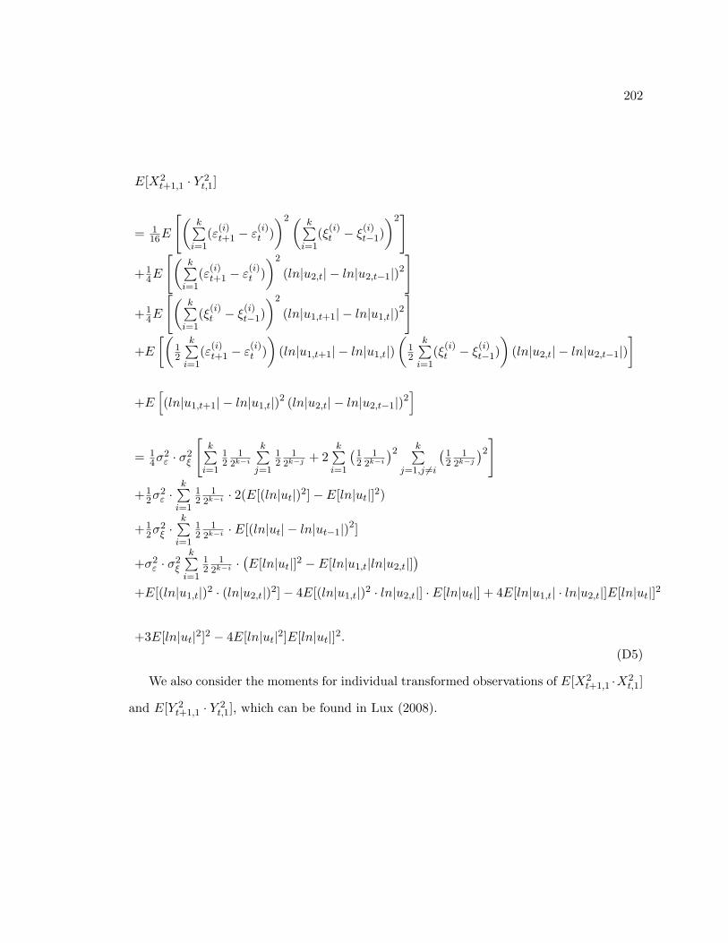
202

E[X2t+1,1 · Y 2

t,1]

= 116E

[(k∑

i=1(ε(i)t+1 − ε

(i)t ))2( k∑

i=1(ξ(i)t − ξ

(i)t−1)

)2]

+14E

[(k∑

i=1(ε(i)t+1 − ε

(i)t ))2

(ln|u2,t| − ln|u2,t−1|)2]

+14E

[(k∑

i=1(ξ(i)t − ξ

(i)t−1)

)2

(ln|u1,t+1| − ln|u1,t|)2]

+E[(

12

k∑i=1

(ε(i)t+1 − ε(i)t ))

(ln|u1,t+1| − ln|u1,t|)(

12

k∑i=1

(ξ(i)t − ξ(i)t−1)

)(ln|u2,t| − ln|u2,t−1|)

]


]

= 14σ

2ε · σ2

ξ

[k∑

i=1

12

12k−i

k∑j=1

12

12k−j + 2

k∑i=1

(12

12k−i

)2 k∑j=1,j 6=i

(12

12k−j

)2]+1

2σ2ε ·

k∑i=1

12

12k−i · 2(E[(ln|ut|)2]− E[ln|ut|]2)

+12σ

2ξ ·

k∑i=1

12

12k−i · E[(ln|ut| − ln|ut−1|)2]

+σ2ε · σ2

ξ

k∑i=1

12

12k−i ·

(E[ln|ut|]2 − E[ln|u1,t|ln|u2,t|]

)+E[(ln|u1,t|)2 · (ln|u2,t|)2]− 4E[(ln|u1,t|)2 · ln|u2,t|] · E[ln|ut|] + 4E[ln|u1,t| · ln|u2,t|]E[ln|ut|]2

+3E[ln|ut|2]2 − 4E[ln|ut|2]E[ln|ut|]2.(D5)


t,1]

and E[Y 2t+1,1 · Y 2

t,1], which can be found in Lux (2008).

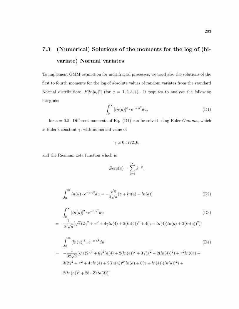
203

7.3 (Numerical) Solutions of the moments for the log of (bi-

variate) Normal variates

To implement GMM estimation for multifractal processes, we need also the solutions of the

first to fourth moments for the log of absolute values of random variates from the standard

Normal distribution: E[ln|ut|q] (for q = 1, 2, 3, 4). It requires to analyze the following

integrals: ∫ ∞

0[ln(u)]q · e−a·u2

du, (D1)

for a = 0.5. Different moments of Eq. (D1) can be solved using Euler Gamma, which

is Euler’s constant γ, with numerical value of

γ ' 0.577216,

and the Riemann zeta function which is

Zeta(x) =∞∑

k=1

k−x.

∫ ∞

0ln(u) · e−a·u2

du = −√π

4√a(γ + ln(4) + ln(a)) (D2)

∫ ∞

0[ln(u)]2 · e−a·u2

du (D3)

=1

16√a[√π(2γ2 + π2 + 4γln(4) + 2(ln(4))2 + 4(γ + ln(4))ln(a) + 2(ln(a))2)]

∫ ∞

0[ln(u)]3 · e−a·u2

du (D4)

= − 132√a[√π(2γ3 + 6γ2ln(4) + 2(ln(4))2 + 3γ(π2 + 2(ln(4))2) + π2ln(64) +

3(2γ2 + π2 + 4γln(4) + 2(ln(4))2)ln(a) + 6(γ + ln(4))(ln(a))2) +

2(ln(a))3 + 28 · Zeta(3))]

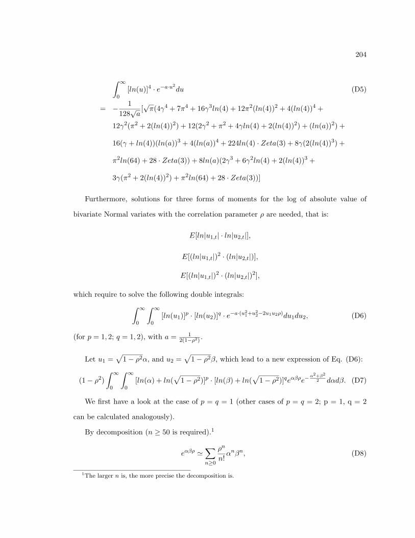
204

∫ ∞

0[ln(u)]4 · e−a·u2

du (D5)

= − 1128

√a[√π(4γ4 + 7π4 + 16γ3ln(4) + 12π2(ln(4))2 + 4(ln(4))4 +

12γ2(π2 + 2(ln(4))2) + 12(2γ2 + π2 + 4γln(4) + 2(ln(4))2) + (ln(a))2) +

16(γ + ln(4))(ln(a))3 + 4(ln(a))4 + 224ln(4) · Zeta(3) + 8γ(2(ln(4))3) +

π2ln(64) + 28 · Zeta(3)) + 8ln(a)(2γ3 + 6γ2ln(4) + 2(ln(4))3 +

3γ(π2 + 2(ln(4))2) + π2ln(64) + 28 · Zeta(3))]

Furthermore, solutions for three forms of moments for the log of absolute value of

bivariate Normal variates with the correlation parameter ρ are needed, that is:

E[ln|u1,t| · ln|u2,t|],

E[(ln|u1,t|)2 · (ln|u2,t|)],

E[(ln|u1,t|)2 · (ln|u2,t|)2],

which require to solve the following double integrals:∫ ∞

0

∫ ∞

0[ln(u1)]p · [ln(u2)]q · e−a·(u2

1+u22−2u1u2ρ)du1du2, (D6)

(for p = 1, 2; q = 1, 2), with a = 12(1−ρ2)

.

Let u1 =√

1− ρ2α, and u2 =√

1− ρ2β, which lead to a new expression of Eq. (D6):

(1− ρ2)∫ ∞

0

∫ ∞

0[ln(α) + ln(

√1− ρ2)]p · [ln(β) + ln(

√1− ρ2)]qeαβρe−

α2+β2

2 dαdβ. (D7)

We first have a look at the case of p = q = 1 (other cases of p = q = 2; p = 1, q = 2

can be calculated analogously).

By decomposition (n ≥ 50 is required).1

eαβρ '∑n≥0

ρn

n!αnβn, (D8)

1The larger n is, the more precise the decomposition is.

205

Eq. (D7) is transformed to

(1− ρ2)∑n≥0

ρn

n!

(∫ ∞

0(ln(α) + ln(

√1− ρ2)αne−

α2

2 dα

)(∫ ∞

0(ln(β) + ln(

√1− ρ2)βne−

β2

2 dβ

)

= (1− ρ2)∑n≥0

ρn

n!

(∫ ∞

0(ln(α) + ln(

√1− ρ2) · αn · e−

α2

2 dα

)2

= (1− ρ2)∑n≥0

ρn

n!

(Pn +Qn · ln(

√1− ρ2)

)2, (D9)

where, Pn =∫∞0 ln(α) · αn · e−

α2

2 dα, and Qn =∫∞0 αn · e−

α2

2 dα, which can be solved by

recurrences, cf. Gradshteyn et al. (2000):

Pn+2 = (n+ 1)Pn +Qn, (D10)

Qn+2 = (n+ 1)Qn, (D11)

Implementing Eq. (D10) and Eq. (D11) requires the initial conditions of P0, P1, Q0,

and Q1, which are given below:

P0 =∫ ∞

0ln(α) · e−

α2

2 dα = −0.5√π

2(γ + ln(2)) , (D12)

P1 =∫ ∞

0ln(α) · α · e−

α2

2 dα = −0.5 (γ − ln(2)) , (D13)

Q0 =∫ ∞

0e−

α2

2 dα =√π

2, (D14)

Q1 =∫ ∞

0α · e−

α2

2 dα = 1. (D15)

Gradshteyn et al. (2000) “Table of Integrals, Series, and Products”, (Academic Press)

provides the (numerical) solutions of various integrals above. And they can be verified by

the fully integrated technical computing package – Mathematicar.

Bibliography

Acerbi, C., Nordio, C., and Sirtori, C. (2001). Expected shortfall as a tool for financial

risk management. Working paper of Italian Association for financial risk management.

Manuscript.

Andersen, T. G. (1996). Return volatility and trading volume: An information flow inter-

pretation of stochastic volatility. Journal of Finance, 60:169–204.

Andersen, T. G. and Bollerslev, T. (1996). Intraday periodicity and volatility persistence

in financial markets. Journal of Empirical Finance, 4:115–158.

Andersen, T. G. and Sorensen, B. E. (1996). GMM estimation of a Stochastic Volatility

Model: A Monte Carlo study. Journal of Business and Economic Statistics, 14:328–352.

Artzner, P., Delbean, F., Eber, M., and Heath, D. (1997). Thinking coherently. Risk,

10:68–71.

Baillie, R. (1996). Long memory process and fractionally integration in econometrics. Jour-

nal of Econometrics, 73:5–59.

Baillie, R. T., Bollerslev, T., and Mikkelsen, H. (1996). Fractionally integrated generalized

autoregressive conditional heteroskedasticity. Journal of Econometrics, 74:3–30.

Baillie, R. T. and Myers, R. J. (1996). Bivariate garch estimation of the optimal commodity

futures hedge. Journal of Applied Econometrics, 6:109 – 124.

206

207

Barkoulas, J. and Baum, C. (2000). Long memory in the Greek stock market. Applied

Financial Economics, 10:177–184.

Batten, J. and Ellis, C. (1996). Fractal structures in currency markets : evidence from the

spot Australian/US dollar. Advances in Pacific Basin financial markets, 2A:173–181.

Beran, J. (1994). Statistics for Long-Memory Processes. Chapman & Hall, New York.

Berzuini, C., Best, N. B., Gilks, W. R., and Larizza, C. (1997). Dynamic conditional

independence models and Markov Chain Monte Carlo methods. Journal of the American

Statistical Association, 92:1403–1412.

Black, F. (1976). Studies of stock price volatility changes. Proceedings of the 1976 American

Statistical Association, Business and Economical Statistics Section. 177.

Bollerslev, T. (1986). Generalized autoregressive conditional heteroskedasticity. Journal of

Econometrics, 31:307–327.

Bollerslev, T. (1990). Modelling the coherence in short-run nominal exchange rates: A

multivariate generalized ARCH model. Review of Economics and Statistics, 72:498–505.

Bollerslev, T., Engle, R., and Wooldridge, J. (1988). A capital asset pricing model with

time-varying covariances. Journal of Political Economy, 96:116–131.

Booth, G. and Kaen, F. (1979). Gold and silver spot prices and market information effi-

ciency. Financial Review, 14:21–26.

Booth, G., Kaen, F., and Koveos, P. (1982). R/s analysis of foreign exchange rates under

two international monetary regimes. Journal of Monetary Economics, 10:407–415.

Bouchaud, J. P. and Potters, M. (2001). More stylized facts of financial markets: leverage

effect and downside correlations. Physica A, 266:60–70.

208

Boutahar, M., Marimoutou, V., and Nouira, L. (2007). Estimation methods of the long

memory parameter: Monte carlo analysis and application. Journal of Applied Statistics,

34:261–301.

Breidt, F., Crato, N., and de Lima, P. (1998). On the detection and estimation of long

memory in stochastic volatility. Journal of Econometrics, 83:325–348.

Brock, W. A. and Hommes, C. H. (1997). A rational route to randomness. Econometrica,

65:1059–1095.

Brockwell, P. J. and Dahlhaus, R. (2004). Generalized levinson- durbin and burg algorithms.

Journal of Econometrics, 118:129–149.

Bucay, N. and Rosen, D. (1996). Credit risk of an international bond portfolio: a case

study. ALGO Research Quarterly, 2:9–29.

Byers, D., Davidson, J., and Peel, D. (1997). Modelling political popularity: An analysis

of long-range dependence in opinion poll series. Journal of Royal Statistical Society,

160:471–490.

Calvet, L. and Fisher, A. (2001). Forecasting multifractal volatility. Journal of Economet-

rics, 105:27–58.

Calvet, L. and Fisher, A. (2002). Multi-fractality in asset returns: Theory and evidence.

Review of Economics and Statistics, 84:381–406.

Calvet, L. and Fisher, A. (2004). How to forecast long-run volatility: Regime switching and

the estimation of multifractal processes. Journal of Financial Econometrics, 2:49–83.

Calvet, L., Fisher, A., and Thompson, S. (2006). Volatility comovement: A multifrequency

approach. Journal of Econometrics, 131:179–215.

209

Cavalcante, J. and Assaf, A. (2002). Long range dependence in the returns and volatility

of the brazilian stock market. Rio de Janeiro. Manuscript.

Chiarella, C. and He, X. Z. (2001). Asset price and wealth dynamics under heterogeneous

expectations. Quantitative Finance, 1:509–526.

Christoffersen, P. F. (2003). Elements of Financial Risk Management. Academic press,

Amsterdam.

Chung, C.-F. (2002). Estimating the fractionally integrated garch model. Mimeo: Academia

Sinica.

Cont, R. (2001). Empirical properties of asset returns: Stylized facts and statistical issues.

Quantitative Finance, 1:1–14.

Cootner, P. (1964). The random character of stock market price. MIT press, Cambridge,

MA.

Crato, N. and De Lima, P. J. F. (1994). Long-range dependence in the conditional variance

of stocks returns. Economics Letters, 45:281–285.

Danielsson, J. and Richard, J. F. (1993). Accelerated gaussian importance sampler with

application to dynamic latent variable models. Journal of Applied Econometrics, 8:153–

173.

Davies, R. and Harte, D. (1987). Test for Hurst effect. Biometrika, 74:95–101.

Demos, A. and Vassilicos, C. (1994). The multifractal structure of high frequency for-

eign exchange rate fluctuations. LSE Financial Markets Group Disscussion Paper Series

No.15.

Ding, Z., Engle, R., and Granger, C. (1993). A long memory property of stock market

returns and a new model. Journal of Empirical Finance, 1:83–106.

210

Dolado, J., Gonzalo, J., and Mayoral, L. (2003). Long-range dependence in spanish political

opinion poll series. Journal of Applied Econometrics, 18:137–155.

Dowd, K. (2002). Measuring Market Risk. John Wiley and Sons, New York.

Embrechts, P., Klueppelberg, C., and Mikosch, T. (1997). Modelling Extremal Events for

Insurance and Finance. Springer, Berlin.

Engle, R. F. (1982). Autoregressive conditional heteroskedasticity with estimates of the

variance of UK inflation. Econometrica, 50:987–1008.

Engle, R. F. and Kroner, K. F. (1995). Multivariate simultaneous generalized arch. Econo-

metric Theory, 11:122–150.

Engle, R. F. and Manganelli, S. (2002). Caviar: Conditional autoregressive value at risk by

regression quantiles. University of California, San Diego.

Engle, R. F. and Susmel, R. (1993). Common volatility in international equity markets.

Journal of Business and Economic Statistics, 11:167–176.

Fama, E. F. (1965). The behavior of stock market prices. Journal of Bussiness, 38:34–105.

Fang, H., Lai, K. S., and Lai, M. (1994). Fractal structure in currency futures price dy-

namics. The Journal of Futures Markets, 14:169–181.

Feder, J. (1988). Fractals. Plenum Press, New York.

Fillol, J. (2003). Multifractality: Theory and evidence an application to the french stock

market. Economics Bulletin, 3:1–12.

Fisher, A., Calvet, L., and Mandelbrot, B. (1997). Multifractality of deutschmark/US dollar

exchange rate. Cowles Foundation Disscussion paper 1165. Manuscript.

211

Gallucio, S., Caldarelli, G., Marsili, M., and Zhang, Y. C. (1997). Scaling in currency

exchange. Physica A, 245:423–436.

Geweke, J. and Porter-Hudak, S. (1983). The estimation and application of long memory

time series models. Journal of Time Series, 4:221–238.

Giraitis, L., Kokoszka, P., Leipus, R., and Teyssiere, G. (2000). Semiparametric estima-

tion of the intensity of long memory in conditional heteroskedasticity. Mathematics and

Statistics, 3:113–128.

Gordon, N. J., Salmond, D. J., and Smith, A. (1993). Anovel approach to non-linear and

non-gaussian bayesian state estimation. IEEE Proceedings F, 140:107–113.

Gourieroux, C. (1997). ARCH Models and Financial Applications. Springer, New York.

Gourieroux, C., Monfort, A., and Renault, E. (1993). Indirect inference. Journal of Applied

Econometrics, 8:85–118.

Gradshteyn, I. S., Ryzhik, I. M., Jeffrey, A., and Zwillinger, D. (2000). Table of Integrals,

Series, and Products. Academic Press, London. Sixth Edition.

Granger, C. W. J. and Joyeux, R. (1980). A introduction to long-memory time series models

and fractional differencing. Journal of Time Series Analysis, 1:15–29.

Greene, M. T. and Fielitz, B. D. (1977). Long-term dependence in common stock market.

Journal of Financial Economics, 4:339–349.

Guillaume, D., Dacorogna, M., Dave, R., Muller, U., Olsen, R., and Pictet, O. (2000).

From the birds eye view to the microscope: A survey of new stylized facts of the intraday

foreign exchange markets. Finance and Stochastics, 1:95–131.

Hansen, L. (1982). Large sample properties of generalized method of moments estimators.

Econometrica, 50:1029–1054.

212

Harris, D. and Matyas, L. (1999). Generalized Method of Moments Estimation. Cambridge,

University Press. Chap. 1.

Harte, D. (2001). Multifractals: Theory and Applications. Chapman and Hall, London.

Harvey, A. C. (1993). Long memory in stochastic volatility. Unpublished manuscript.

Harvey, A. C., Ruiz, E., and Shephard, N. (1994). Multivariate stochastic variance models.

Review of Economic Studies, 61:247–264.

Helms, B., Kaen, F., and Rosenman, R. (1995). Memory in commodity futures markets.

Journal of Futures Markets, 4:559–567.

Holton, G. A. (2003). Value-at-Risk: Theory and Practice. Academic Press, California.

Hosking, J. R. M. (1981). Fractional differencing. Biometrika, 68:165–176.

Hurst, E. (1951). Long term storage capacity of reservoirs. Transactions on American

Society of Civil Engineering, 116:770–808.

Hurvich, C. M., Deo, R. S., and Brodsky, J. (1998). The mean squared error of geweke and

porter-hudaks estimator of the memory parameter of a long-memory time series. Journal

of Time Series Analysis, 19:19–46.

Iori, G. (2002). A micro-simulation of traders’ activity in the stock market: the rule of

heterogeneity , agents’ interactions and trade friction. Journal of Economic Behaviour

and Organisation, 49:269–285.

Jacquier, E., Polson, N., and Rossi, P. (1994). Bayesian analysis of stochastic volatility

models. Journal of Business and Economic Statistics, 12:371–389.

Jensen, M. (1999). Using wavelets to obtain a consistent ordinary least squares estimator

of the long memory parameter. Journal of Forecasting, 18:17–32.

213

Kim, S., Shephard, N., and Chilb, S. (1998). Stochastic volatility: likelihood inference and

comparison with ARCH model. Review of Economic Studies, 65:361–393.

Kirman, A. (1993). Ants, rationality, and recruitment. Quarterly Journal of Economics,

108:137–156.

Kirman, A. and Teyssiere, G. (2001). Microeconomic models for long memory in the volatil-

ity of financial time series. Studies in Nonlinear Dynamics and Econometrics, 5:281–302.

Kuester, K., Mittnik, S., and Paolella, M. S. (2006). Value-at-risk prediction: A comparison

of alternative strategies. Journal of Financial Econometrics, 4:53–89.

Kupiec, P. H. (1995). Techniques for verifying the accuracy of risk measurement models.

Journal of Derivatives, 3:73–84.

Kwiatkowski, D., Phillips, P., Schmidl, P., and Shin, Y. (1992). Testing the null hypothesis

of stationarity against the alternative era unit root: How sure are we that economic time

series have a unit root? Journal of Econometrics, 54:159–178.

Lee, D. and Schmidt, P. (1996). On the power of the kpss test of stationarity against

fractionally-integrated alternatives. Journal of Econometrics, 73:285–302.

Leland, W. E., Taqqu, M. S., Willinger, W., and Wilson, D. V. (1994). On the self-similar

nature of ethernet traffic (extended version). IEEE/ACM Transactions on Networking,

2:1–15.

Liesenfeld, R. (1998). Dynamic bivariate mixture models: modeling the behavior of prices

and trading volume. Journal of Business and Economic Statistics, 16:101–109.

Liesenfeld, R. (2001). A generalized bivariate mixture model for stock price volatility and

trading volume. Journal of Econometrics, 104:141–178.

214

Liesenfeld, R. and Jung, R. C. (2000). Stochastic volatility models: conditional normality

versus heavy-tailed distributions. Journal of Applied Econometrics, 15:137–160.

Liesenfeld, R. and Richard, J. F. (2003). Univariate and multivariate stochastic volatility

models: estimation and diagnostics. Journal of Empirical Finance, 207:1–27.

Lo, A. W. (1991). Long-term memory in stock market prices. Econometrica, 59:1279–1313.

Lo, A. W. and MacKinlay, A. C. (2001). A Non-Random Walk Down Wall Street. Princeton

University Press.

Lobato, I. N. and Velasco, C. (2000). Long memory in stock-market trading volume. Journal

of Business and Economic Statistics, 18:410–427.

Lux, T. (1995). Herd behaviour, bubbles and crashes. Economic Journal, 105:881–896.

Lux, T. (1996a). Long-term stochastic dependence in financial prices: Evidence from the

German stock market. Applied Economics Letters, 3:701–706.

Lux, T. (1996b). The stable Paretian hypothesis and the frequency of large returns: An

examination of major German stocks. Applied Financial Economics, 6:463–475.

Lux, T. (1998). The socio-economic dynamics of speculative markets: Interacting agents,

chaos, and the fat tails of return distributions. Journal of Economic Behavior and Orga-

nization, 33:143–165.

Lux, T. (2001). Turbulence in financial markets: The surprising explanatory power of simple

cascade models. Quantitative Finance, 1:632–640.

Lux, T. (2004). Detecting multi-fractal properties in asset returns: The failure of the

“scaling estimator”. International Journal of Modern Physics, 15:481–491.

215

Lux, T. (2008). The Markov-switching multi-fractal model of asset returns: GMM esti-

mation and linear forecasting of volatility. Journal of Business and Economic Statistics,

26:194–210.

Lux, T. and Kaizoji, T. (2007). Forecasting volatility and volume in the Tokyo stock

market: Long-memory, fractality and regime switching. Journal of Economic Dynamics

and Control, 31:1808 – 1843.

Lux, T. and Marchesi, M. (1999). Scaling and criticality in a stochastic multi-agent model

of a financial market. Nature, 397:498–500.

Lux, T. and Marchesi, M. (2000). Volatility clustering in financial markets: A micro-

simulation of interacting agents. International Journal of Theoretical and Applied Fi-

nance, 3:67–702.

Madhusoodanan, T. P. (1998). Long-term dependence in Indian stock market. Journal of

Financial Studies, 5:33–53.

Mandelbrot, B. (1963). The variation of certain speculative prices. Journal of Business,

35:394–419.

Mandelbrot, B. (1967a). How long is the coast of Britain? statistical self-similarity and

fractional dimension. Science, 156:936–938.

Mandelbrot, B. (1967b). The variation of the prices of cotton, wheat, and railroad stocks,

and of some finacial rates. Journal of Business, 40:393–413.

Mandelbrot, B. (1971). When can price be arbitrage efficiency? a limit to the validity of the

random walk and martingale models. Review of Economics and Statistics, 53:225–236.

Mandelbrot, B. (1974). Intermittent turbulence in self similar cascades: Divergence of high

moments and dimension of carrier. Journal of Fluid Mechanics, 62:331–358.

216

Mandelbrot, B. (1997). Three fractal models in finance : discontinuity, concentration, risk.

Economic notes : economic review of Banca Monte dei Paschi di Siena. Oxford Blackwell,

26:171–211.

Mandelbrot, B. (2001). Scaling in financial prices: Tails and dependence. Quantitative

Finance, 1:113–123.

Mandelbrot, B., Fisher, A., and Calvet, L. (1997). A multifractal model of asset returns.

Cowles Foundation for Research and Economics. Manuscript.

Mandelbrot, B. and Taqqu, M. S. (1979). Robust R/S analysis of long-run serial correlation.

Bulletin of the International Statistical Institute, 48:69–104.

Mandelbrot, B. and Wallis, J. R. (1969a). Computer experiments with fractional gaussian

noise. Water Resources Research, 5:228–267.

Mandelbrot, B. and Wallis, J. R. (1969b). Robustness of the rescaled range R/S in the

measurement of non noncyclic long-run statistical dependence. Water Resources Research,

5:967–988.

Marmol, F. (1997). Searching for fractional evidence using unit root tests. Universidad

Carlos III, Madrid. Mimeo.

Matsushita, R., Gleria, I., Figueiredo, A., and Da Silva, S. (2003). Fractal structure in the

Chinese yuan/US dollar rate. Economic Bulletin, 7:1–13.

McNeil, A. J. and Frey, R. (2000). Estimation of tail-related risk measures for heteroscedas-

tic financial time series: an extreme value approach. Journal of Empirical Finance,

7:271–300.

Melino, A. and Turnbull, S. M. (1990). Pricing foreign currency options with stochastic

volatility. Journal of Econometrics, 45:239–265.

217

Mills, T. (1993). Is there long-term memory in UK stock returns? Appllied Financial

Economics, 3:303–306.

Moody, J. and Wu, L. (1996). Improved estimates for the rescaled range and hurst expo-

nents. Appears in ”Neural Networks in the Capital Markets”, World Scientific, London.

Mulligan, R. F. (2000). A fractal analysis of foreign exchange markets. International

Advances in Economic Research, 26:33–49.

Mulligan, R. F. (2004). Fractal analysis of highly volatile markets: an application to tech-

nology equities. The Quarterly Review of Economics and Finance, 44:155–179.

Naslund, B. (1990). A fractal analysis of capital structure. Research paper: Ekonomiska

Forskningsinstitutet, Handelshoegskolan in Stockholm No.6425.

Nath, G. C. (2002). Long memory and indian stock market - an empirical evidence. WDM

Dept, Mumbai. Manuscript.

Newey, W. K. and West, K. D. (1987). A simple, positive semi-definite, heteroskedasticity

and autocorrelation consistent covariance matrix. Econometrica, 55:703–708.

Pagan, A. (1996). The econometrics of financial markets. Journal of Empirical Finance,

3:15–102.

Parisi, G. and Frisch, U. (1985). Turbulence and predictability in geophysical fluid dynamics

and climate dynamics. In Ghil, M., editor, A multifractal model of intermittency, pages

84–92. North-Holland.

Peng, C. K., Buldyrev, S. V., Havlin, S., Simons, M., Stanley, H. E., and Goldberger, A. L.

(1994). Mosaic organization of DNA nucleotidies. Physical Review E, 49:1685–1689.

Peters, E. E. (1994). Fractal Market Analysis: Applying Chaos Theory to Investment and

Economics. John Wiley and Sons, US.

218

Pitt, M. and Shephard, N. (1999). Filtering via simulation: Auxiliary particle filter. Journal

of the American Statistical Association, 94:590–599.

Rachev, S. T. and Mittnik, S. (2000). Stable Paretian Models in Finance. John Wiley &

Sons, Chichester.

Ray, B. K. and Tsay, R. (2001). Long-range dependence in daily stock volatilities. Journal

of Business and Economic Statistics, 18:254–262.

Rubin, D. B. (1987). Comment: A noniterative Sampling/Importance Resampling alterna-

tive to the data augmentation algorithm for creating a few imputations when fractions of

missing information are modest: The SIR algorithm. Journal of the American Statistical

Association, 82:543–546.

Schmitt, F., Schertzer, D., and Lovejoy, S. (2000). Multifractal fluctuations in finance.

International Journal of Theoretical and Applied Finance, 3:361–364.

Shephard, N. G. (1993). Fitting non-linear time series models, with application to stochastic

variance models. Journal of Applied Econometrics, 8:135–152.

Shiller, R. J. (1989). Market volatility. MIT Press, Cambridge.

Sibbertsen, P. and Kramer, W. (2006). The power of the kpss - test for cointegration when

residuals are fractionally integrated. Economics Letters, 91:321–324.

So, M. P. (1999). Time series with additive noise. Biometrika, 86:474–482.

Sowell, F. (1992). Maximum likelihood estimation of stationary univariate fractionally

integrated time series models. Journal of Econometrics, 53:165–188.

Taylor, S. J. (1982). Financial returns modelled by the product of two stochastic processes

- a study of daily sugar price 1961-79. In Anderson, O. D., editor, Time series analysis:

Theory and Practice, pages 203–226. North-Holland, Amsterdam.

219

Taylor, S. J. (1986). Modelling Financial Time Series. John Wiley, UK.

Teverovsky, V., Taqqu, M. S., and Willinger, W. (1999). A critical look at Lo’s modified

R/S statistic. Journal of Statistical Planning and Inference, 80:211–227.

Tolvi, J. (2003). Long-term momory in a small stockt market. Economics Bulletin, 7:1–13.

Upton, D. and Shannon, D. (1979). The stable paretian distribution, subordinated stochas-

tic processes, and asymptotic lognormality: an empirical investigation. Journal of Fi-

nance, 34(4):1031–1039.

Weron, R., Weron, K., and Weron, A. (1999). A conditionally exponential decay approach

to scaling in finance. Physica A, 267:551–561.

Willinger, W., Taqqu, S., and Teverovsky, V. (1999). Stock market prices and long-range

dependence. Finance and Stochastics, 3:1–13.

Wright, J. H. (1999). A new estimator of the fractionally integrated stochastic volatility

model. Economics Letter, 63:295–303.

Yamai, Y. and Yoshiba, T. (2002). On the validity of Value-at-Risk: comparative analysis

with expected shortfall. Monetary and Economic Studies, 20:57–86.

Zumbach, G. (2004). Volatility processes and volatility forecast with long memory. Quan-

titative Finance, 4:70–86.

220

Ich erklare hiermit an Eides Statt, dass ich meine Doktorarbeit “Multivariate Multifrac-

tal Models: Estimation of Parameters and Applications to Risk Management” selbststandig

angefertigt habe und dass ich alle von anderen Autoren wortlich ubernommenen Stellen,

wie auch die sich an die Gedanken anderer Autoren eng anlehnenden Ausfuhrungen meiner

Arbeit, besonders gekennzeichnet und die Quellen zitiert habe.

(Ruipeng Liu)

Melbourne, September 2008

Documents

Multivariate Multifractal Models: Estimation of Parameters ... · Multivariate Multifractal Models: Estimation of Parameters and Applications to Risk Management als Inaugural-Dissertation