432

New design parameters for biparabolic beach profiles (SW Cadiz, Spain)

Antonio Contreras de Villar (Main and Corresponding Author)

Grupo de Investigación de Ingeniería Costera, Universidad de Cadiz Puerto Real, 11510, Cadiz (Spain) antonio.contreras@uca.es

Gregorio Gómez-Pina Grupo de Investigación de Ingeniería Costera, Universidad de Cadiz Puerto Real, 11510, Cadiz (Spain) gregoriogpina@yahoo.es

Juan José Muñoz-Pérez Grupo de Investigación de Ingeniería Costera, Universidad de Cadiz Puerto Real, 11510, Cadiz (Spain) juanjose.munoz@uca.es

Francisco Contreras Grupo de Investigación de Ingeniería Costera, Universidad de Cadiz Puerto Real, 11510, Cadiz (Spain) francisco.contreras@uca.es

Patricia López-García Grupo de Investigación de Ingeniería Costera, Universidad de Cadiz Puerto Real, 11510, Cadiz (Spain) patricia.lopezgarcia@uca.es

Verónica Ruiz-Ortiz Grupo de Geociencias, Universidad de Cadiz Puerto Real, 11510, Cadiz (Spain) veronica.ruiz@uca.es

Manuscript Code: 1182 Date of Acceptance/Reception: 07.11.2019/18.09.2018 DOI: 10.7764/RDLC.18.3.432 Abstract 165 profiles of seventy-one beaches along the Gulf of Cadiz (SW, Spain) were studied to improve the formulation of the beach profile in tidal seas. Maritime climate, degree of energy exposure and size of the sand grains were taken into account to study the two sections of the biparabolic profile. The objective of the study was the determination of more accurate formulations of the design parameters for the equilibrium profile that involves tidal seas. These formulations were modelled and validated based on existing profiles to quantify the error existing between the real profile and the modelling. This comparative analysis was extended by considering the formulations proposed by other authors. The best results were obtained with the proposal presented herein. Keywords: Beaches, equilibrium profile, biparabolic, tide, sediment size, nourishment.

Introduction

Houston (1996) and other authors (King, 1999; Muñoz-Perez et al., 2003) have studied the economic importance of beaches and their direct link to tourism in some countries. Moreover, generalized coastal erosion is going on worldwide (Valderrama-Landeros et al., 2019). This erosion is attributed to sea-level rise, retention of sand in dams, occupation of dry beaches by urbanized areas and removal of sand as a material for building construction (Gomez-Pina et al., 2005). Thus, a need for beach regeneration, in general, exists everywhere. Therefore, after the regression of a stretch of beach and once the causes have been analysed, it is necessary to draft an artificial sand nourishment project. The project author must follow a series of aspects within the project to meet the desired expectations. These aspects must include at least (Gómez-Pina, 2001) technical, environmental, integration in the environment (physical and social), aesthetic, sustainability, economic, archaeological, compliance with the specific Shore Act of each country and integration in the Coastal Management strategy.

433

Within the technical aspects, once the compatibility of borrowed sediment with native is established by comparing both grain size distributions (Krumbein & James, 1965; Stauble, 2007; Pranzini et al., 2018), the most important point is to quantify the nourishment volume. However, in addition to quantifying the volume of sand, the engineer author of the project must try to minimize this volume, guaranteeing the stability of the regenerated profile. To do this, knowledge of the fundamental parameters that define the beach profile is necessary, and, thus, the equilibrium profile can be determined.

Description of the Problem Design parameters are always applied for beach nourishments, but these parameters, if not correct, result in a faulty design of the beach profile with a wrong quantification of the nourishment volume. Thus, these parameters must be adjusted to find the best possible fit that minimizes the nourishment volume.

State of the Art A beach regeneration project requires identifying the fundamental parameters that define the equilibrium profile. Different authors (Fenneman, 1902; Johnson, 1919; Schwartz, 1982; Moore, 1982; Larson & Kraus, 1989; Larson, 1991; Kriebel et al., 1991; Pilkey et al., 1993) have defined the concept of equilibrium profile. In general, the equilibrium profile can be defined as the situation, or state, to which a beach profile arrives in a situation of constant swell and over a sufficient period of time. Dean (1977) obtained the widely used mathematical formulation for the equilibrium beach profile after analysing 504 beach profiles along the Atlantic Coast of the United States, from Long Island to Mexico, and by using a least-squares adjustment to the exponential function proposed by Bruun (1954):

h = A ∙ x2/3 1 where h is the depth, x the distance from the edge (origin of coordinates) and A is a shape parameter related to the velocity of the grain fall (w), given by:

A = 0.51 ∙ w0.44 2 However, the previous formula does not fit tidal seas well. To solve this problem, numerous authors have developed several modifications, including Masselink & Short (1993), Inman et al. (1993), Gonzalez (1995), Gómez-Pina (2001) and Bernabeu et al. (2002). These authors presented a formulation of the equilibrium profile in two sections, namely the emerged profile (surf profile) and submerged profile (shoaling profile), which has been referred to as a biparabolic profile. The cyclical variation of the sea level (tide) produces changes that affect the morphodynamics of the beaches and the equilibrium profile (Muñoz-Perez & Medina, 2005). However, the design parameters of the previous biparabolic profiles do not fit adequately to the actual offshore profiles of SW Spain, so it was necessary to define new parameters that best fit the natural or native profile. The new parameters may depend on the energetic conditions to which the profile is subject, the sedimentological characteristics of the sand and the tide level. The objective of this article is determining a methodology to find better calibration values for the parameters in the existing formulations of the equilibrium profile for tidal seas. These parameters can be applied to future projects for beach regeneration on the coast of the Gulf of Cadiz but the adjustment methodology can be applied worldwide.

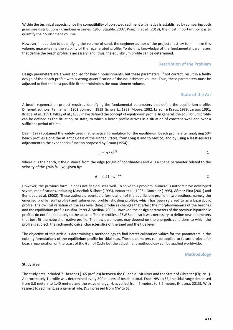
Methodology Study area The study area included 71 beaches (165 profiles) between the Guadalquivir River and the Strait of Gibraltar (Figure 1). Approximately 1 profile was determined every 800 meters of beach littoral. From NW to SE, the tidal range decreased from 3.8 meters to 1.40 meters and the wave energy, Hs,12, varied from 5 meters to 3.5 meters (Hidtma, 2013). With respect to sediment, as a general rule, D50 increased from NW to SE.

434

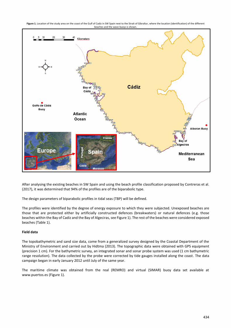
Figure 1. Location of the study area on the coast of the Gulf of Cadiz in SW Spain next to the Strait of Gibraltar, where the location (identification) of the different beaches and the wave buoys is shown.

After analysing the existing beaches in SW Spain and using the beach profile classification proposed by Contreras et al. (2017), it was determined that 94% of the profiles are of the biparabolic type. The design parameters of biparabolic profiles in tidal seas (TBP) will be defined. The profiles were identified by the degree of energy exposure to which they were subjected. Unexposed beaches are those that are protected either by artificially constructed defences (breakwaters) or natural defences (e.g. those beaches within the Bay of Cadiz and the Bay of Algeciras, see Figure 1). The rest of the beaches were considered exposed beaches (Table 1). Field data The topobathymetric and sand size data, come from a generalized survey designed by the Coastal Department of the Ministry of Environment and carried out by Hidtma (2013). The topographic data were obtained with GPS equipment (precision 1 cm). For the bathymetric survey, an integrated sonar and sonar probe system was used (1 cm bathymetric range resolution). The data collected by the probe were corrected by tide gauges installed along the coast. The data campaign began in early January 2012 until July of the same year. The maritime climate was obtained from the real (REMRO) and virtual (SIMAR) buoy data set available at www.puertos.es (Figure 1).

435

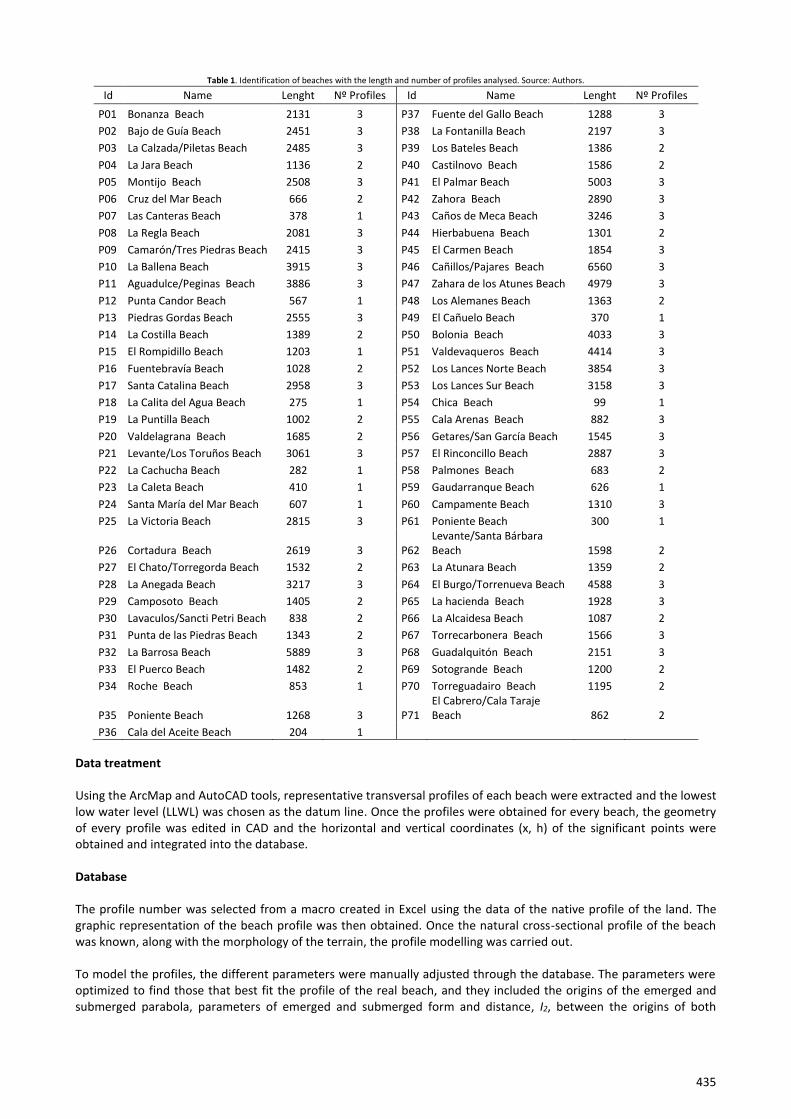
Table 1. Identification of beaches with the length and number of profiles analysed. Source: Authors.

Id Name Lenght Nº Profiles Id Name Lenght Nº Profiles

P01 Bonanza Beach 2131 3 P37 Fuente del Gallo Beach 1288 3

P02 Bajo de Guía Beach 2451 3 P38 La Fontanilla Beach 2197 3

P03 La Calzada/Piletas Beach 2485 3 P39 Los Bateles Beach 1386 2

P04 La Jara Beach 1136 2 P40 Castilnovo Beach 1586 2

P05 Montijo Beach 2508 3 P41 El Palmar Beach 5003 3

P06 Cruz del Mar Beach 666 2 P42 Zahora Beach 2890 3

P07 Las Canteras Beach 378 1 P43 Caños de Meca Beach 3246 3

P08 La Regla Beach 2081 3 P44 Hierbabuena Beach 1301 2

P09 Camarón/Tres Piedras Beach 2415 3 P45 El Carmen Beach 1854 3

P10 La Ballena Beach 3915 3 P46 Cañillos/Pajares Beach 6560 3

P11 Aguadulce/Peginas Beach 3886 3 P47 Zahara de los Atunes Beach 4979 3

P12 Punta Candor Beach 567 1 P48 Los Alemanes Beach 1363 2

P13 Piedras Gordas Beach 2555 3 P49 El Cañuelo Beach 370 1

P14 La Costilla Beach 1389 2 P50 Bolonia Beach 4033 3

P15 El Rompidillo Beach 1203 1 P51 Valdevaqueros Beach 4414 3

P16 Fuentebravía Beach 1028 2 P52 Los Lances Norte Beach 3854 3

P17 Santa Catalina Beach 2958 3 P53 Los Lances Sur Beach 3158 3

P18 La Calita del Agua Beach 275 1 P54 Chica Beach 99 1

P19 La Puntilla Beach 1002 2 P55 Cala Arenas Beach 882 3

P20 Valdelagrana Beach 1685 2 P56 Getares/San García Beach 1545 3

P21 Levante/Los Toruños Beach 3061 3 P57 El Rinconcillo Beach 2887 3

P22 La Cachucha Beach 282 1 P58 Palmones Beach 683 2

P23 La Caleta Beach 410 1 P59 Gaudarranque Beach 626 1

P24 Santa María del Mar Beach 607 1 P60 Campamente Beach 1310 3

P25 La Victoria Beach 2815 3 P61 Poniente Beach 300 1

P26 Cortadura Beach 2619 3 P62 Levante/Santa Bárbara Beach 1598 2

P27 El Chato/Torregorda Beach 1532 2 P63 La Atunara Beach 1359 2

P28 La Anegada Beach 3217 3 P64 El Burgo/Torrenueva Beach 4588 3

P29 Camposoto Beach 1405 2 P65 La hacienda Beach 1928 3

P30 Lavaculos/Sancti Petri Beach 838 2 P66 La Alcaidesa Beach 1087 2

P31 Punta de las Piedras Beach 1343 2 P67 Torrecarbonera Beach 1566 3

P32 La Barrosa Beach 5889 3 P68 Guadalquitón Beach 2151 3

P33 El Puerco Beach 1482 2 P69 Sotogrande Beach 1200 2

P34 Roche Beach 853 1 P70 Torreguadairo Beach 1195 2

P35 Poniente Beach 1268 3 P71 El Cabrero/Cala Taraje Beach 862 2

P36 Cala del Aceite Beach 204 1

Data treatment Using the ArcMap and AutoCAD tools, representative transversal profiles of each beach were extracted and the lowest low water level (LLWL) was chosen as the datum line. Once the profiles were obtained for every beach, the geometry of every profile was edited in CAD and the horizontal and vertical coordinates (x, h) of the significant points were obtained and integrated into the database. Database The profile number was selected from a macro created in Excel using the data of the native profile of the land. The graphic representation of the beach profile was then obtained. Once the natural cross-sectional profile of the beach was known, along with the morphology of the terrain, the profile modelling was carried out. To model the profiles, the different parameters were manually adjusted through the database. The parameters were optimized to find those that best fit the profile of the real beach, and they included the origins of the emerged and submerged parabola, parameters of emerged and submerged form and distance, I2, between the origins of both

436

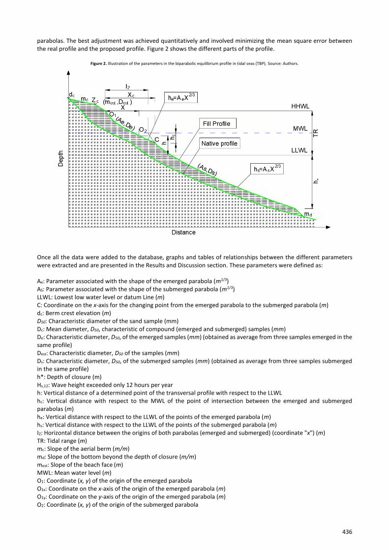
parabolas. The best adjustment was achieved quantitatively and involved minimizing the mean square error between the real profile and the proposed profile. Figure 2 shows the different parts of the profile.

Figure 2. Illustration of the parameters in the biparabolic equilibrium profile in tidal seas (TBP). Source: Authors.

Once all the data were added to the database, graphs and tables of relationships between the different parameters were extracted and are presented in the Results and Discussion section. These parameters were defined as: Ae: Parameter associated with the shape of the emerged parabola (m1/3) AS: Parameter associated with the shape of the submerged parabola (m1/3) LLWL: Lowest low water level or datum Line (m) C: Coordinate on the x-axis for the changing point from the emerged parabola to the submerged parabola (m) dc: Berm crest elevation (m) D50: Characteristic diameter of the sand sample (mm) Dc: Mean diameter, D50, characteristic of compound (emerged and submerged) samples (mm) De: Characteristic diameter, D50, of the emerged samples (mm) (obtained as average from three samples emerged in the same profile) Dest: Characteristic diameter, D50 of the samples (mm) Ds: Characteristic diameter, D50, of the submerged samples (mm) (obtained as average from three samples submerged in the same profile) h*: Depth of closure (m) Hs,12: Wave height exceeded only 12 hours per year h: Vertical distance of a determined point of the transversal profile with respect to the LLWL hc: Vertical distance with respect to the MWL of the point of intersection between the emerged and submerged parabolas (m) he: Vertical distance with respect to the LLWL of the points of the emerged parabola (m) hs: Vertical distance with respect to the LLWL of the points of the submerged parabola (m) I2: Horizontal distance between the origins of both parabolas (emerged and submerged) (coordinate "x") (m) TR: Tidal range (m) mc: Slope of the aerial berm (m/m) md: Slope of the bottom beyond the depth of closure (m/m) mest: Slope of the beach face (m) MWL: Mean water level (m) O1: Coordinate (x, y) of the origin of the emerged parabola O1x: Coordinate on the x-axis of the origin of the emerged parabola (m) O1y: Coordinate on the y-axis of the origin of the emerged parabola (m) O2: Coordinate (x, y) of the origin of the submerged parabola

437

O2x: Coordinate on the x-axis of the origin of the submerged parabola (m) O2y: Coordinate on the y-axis of the origin of the submerged parabola (m) HHWL: Highest high water level (m) X: Distance of a determined point of the transversal profile with respect to the reference origin Xc: Distance in the coordinate "x" between the origin of the emerged parabola and the change of curvature between the emerged and submerged parabola Zc: Coronation height of the beach face (m) The exponent (2/3) of the parabola equations was not adjusted because it was already well fitted to the profile. Adjusting the origins of emerged and submerged parabolas Once the database was generated, the previous parameters were modified until the modelled profile was adjusted to obtain the minimum error when compared to the real profile. The definition of the emerged (Ae) and submerged (As) shape parameters depended on identifying the origin of the emerged (O1) and submerged (O2) parabolas. Depending on where each of the parabola origins was located, different form parameters were obtained for the same profile. Therefore, as a first step, it was necessary to identify the origin of both parabolas. To identify the origin of the emerged parabola, a coefficient of the emerged parabola origin (CO1) was defined as the relationship between the elevation of the emerged parabola origin (O1) and the value of the HHWL for each of the profiles studied. If the coefficient (CO1) had a value of 1, the origin of the emerged parabola (O1) coincided with the HHWL. If its value was 0, the origin of the emerged parabola was located in the LLWL. If the coefficient was greater than 1, the origin (O1) was above the HHWL. In mathematical form:

CO1 =O1y

HHWL

3

To identify the origin of the submerged parabola, the coefficient of the origin of the submerged parabola (CO2) was defined as the relationship between the level of the submerged parabola origin and the mean water level (MWL). A coefficient of the origin of the submerged parabola (CO2) of 1 indicated that the origin of the submerged parabola was in the middle level of the sea. If the value was 0, then the origin of the submerged parabola was on the LLWL. In mathematical form:

CO2 =O2y

MWL

4

Modelling the parameters deduced from the real profiles The parameters derived from the relationships discussed above, which defined the emerged and submerged beach profiles, were applied to the same real profiles. The error between the modelled and real beach profiles was then quantitatively determined. This error was determined using Equation 5 below. The origins on the x-axis for the emerged and submerged parabolas in the modelised profile were both taken from the same real profile. The modelling methodology was also carried out with the design parameters set forth by other authors so that errors between the different theories can be compared. For comparative analysis of the different models of the studied beach profiles, the mean square error between the proposed model and the real profile was determined using Eq. 5.

Error =1

n ∑

(hireal − hi

model)2

hireal

n

i=1

5

where n is the number of profile points analysed and hireal and hi

model are the real and model ground levels, respectively, at point “i” of the profile. The calculated error has units of metres. To make it dimensionless and comparable to the single-parabolic model initially proposed by Dean, the relationship between the error of each of the models was determined with respect to the error of Dean's model (Eq. 6). These data, already dimensionless, indicate the improvements of the proposed model with

438

respect to the one proposed by Dean. Therefore, a dimensionless error of 1 indicates that the model did not improve anything compared to that proposed by Dean, while a dimensionless error of 0 indicates that the model fits the real profile perfectly:

Error (dimensionless) =(Error)Model

(Error)Dean 6

For qualitative analysis of the profiles, a distinction was made between those profiles that visually adapt better or worse to the real profile. In this way, depending on the degree of adaptation to the real beach profile, the profiles have been classified into R for regular adaptation, G for good adaptation and VG for very good adaptation. New formulations for beach regeneration could, therefore, be obtained from the methodology presented herein.

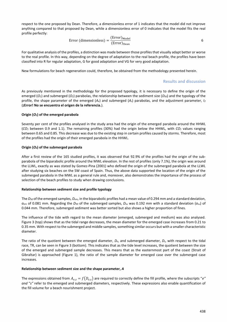
Results and discussion As previously mentioned in the methodology for the proposed typology, it is necessary to define the origin of the emerged (O1) and submerged (O2) parabolas, the relationship between the sediment size (D50) and the typology of the profile, the shape parameter of the emerged (Ae) and submerged (As) parabolas, and the adjustment parameter, I2 (¡Error! No se encuentra el origen de la referencia.). Origin (O1) of the emerged parabola Seventy per cent of the profiles analysed in the study area had the origin of the emerged parabola around the HHWL (CO1 between 0.9 and 1.1). The remaining profiles (30%) had the origin below the HHWL, with CO1 values ranging between 0.65 and 0.85. This decrease was due to the existing step in certain profiles caused by storms. Therefore, most of the profiles had the origin of their emerged parabola in the HHWL. Origin (O2) of the submerged parabola After a first review of the 165 studied profiles, it was observed that 92.9% of the profiles had the origin of the sub-parabola of the biparabolic profile around the MWL elevation. In the rest of profiles (only 7.1%), the origin was around the LLWL, exactly as was stated by Gomez-Pina (2001) who defined the origin of the submerged parabola at the LLWL after studying six beaches on the SW coast of Spain. Thus, the above data supported the location of the origin of the submerged parabola in the MWL as a general rule and, moreover, also demonstrates the importance of the process of selection of the beach profiles to study when drawing conclusions. Relationship between sediment size and profile typology The D50 of the emerged samples, Dem, in the biparabolic profiles had a mean value of 0.294 mm and a standard deviation, σem of 0.081 mm. Regarding the D50 of the submerged samples, Dsu was 0.192 mm with a standard deviation (σsu) of 0.044 mm. Therefore, submerged sediment was better sorted but also shows a higher proportion of fines. The influence of the tide with regard to the mean diameter (emerged, submerged and medium) was also analysed. Figure 3 (top) shows that as the tidal range decreases, the mean diameter for the emerged case increases from 0.21 to 0.35 mm. With respect to the submerged and middle samples, something similar occurs but with a smaller characteristic diameter. The ratio of the quotient between the emerged diameter, De, and submerged diameter, Ds, with respect to the tidal race, TR, can be seen in Figure 3 (bottom). This indicates that as the tide level increases, the quotient between the size of the emerged and submerged sample decreases. This means that as the easternmost part of the coast (Strait of Gibraltar) is approached (Figure 1), the ratio of the sample diameter for emerged case over the submerged case increases. Relationship between sediment size and the shape parameter, A

The expressions obtained from 𝐴𝑒,𝑠 = 𝑓(𝐷𝑒,𝑠) are required to correctly define the fill profile, where the subscripts “e”

and “s” refer to the emerged and submerged diameters, respectively. These expressions also enable quantification of the fill volume for a beach nourishment project.

439

In the subsequent paragraphs, the A vs D functions are compared with the theoretical value of the A shape parameter from Dean. The trend lines, representative of the A-D relationship, have been fitted to a parabolic function as Dean did.

Figure 3. Top image: Mean diameter emerged (Dem) and submerged (Dsu) depending on the tidal range (TR) for biparabolic profiles in tidal seas (TBP). Bottom image: Relationship between the quotient of the mean diameter emerged and submerged with respect to the tidal range also for TBP. Source: Authors.

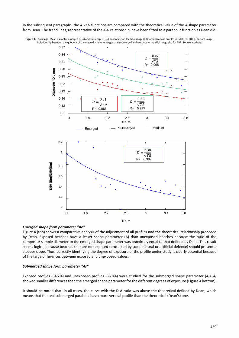
Emerged shape form parameter "Ae" Figure 4 (top) shows a comparative analysis of the adjustment of all profiles and the theoretical relationship proposed by Dean. Exposed beaches have a lesser shape parameter (A) than unexposed beaches because the ratio of the composite-sample diameter to the emerged shape parameter was practically equal to that defined by Dean. This result seems logical because beaches that are not exposed (protected by some natural or artificial defence) should present a steeper slope. Thus, correctly identifying the degree of exposure of the profile under study is clearly essential because of the large differences between exposed and unexposed values. Submerged shape form parameter "As" Exposed profiles (64.2%) and unexposed profiles (35.8%) were studied for the submerged shape parameter (As). As

showed smaller differences than the emerged shape parameter for the different degrees of exposure (Figure 4 bottom). It should be noted that, in all cases, the curve with the D-A ratio was above the theoretical defined by Dean, which means that the real submerged parabola has a more vertical profile than the theoretical (Dean’s) one.

Gráfico del Modelo Ajustado

Diámetro medio, mm = 1/(2,18057*sqrt(Carrera de marea, m))

1,4 1,8 2,2 2,6 3 3,4 3,8

Carrera de marea, m

0,1

0,13

0,16

0,19

0,22

0,25

0,28

0,31

0,34

0,37D

iám

etr

o m

ed

io, m

m

𝐷 =0. 5

R= 0.998

𝐷 =0. 1

R= 0.986

𝐷 =0.

R= 0.995

Dia

me

tre

"D",

mm

Emerged Submerged Medium

TR, m

4 1.8 2.2 2.6 3 3.4 3.8

0.37

0.34

0.31

0.28

0.25

0.22

0.19

0.16

0.13

0.1

Gráfico del Modelo Ajustado

D50 (Em)/D50(Sm) = 1/(0,423429*sqrt(PMVE))

1,4 1,8 2,2 2,6 3 3,4 3,8

PMVE

1

1,2

1,4

1,6

1,8

2

2,2

D5

0 (

Em

)/D

50

(Sm

)

𝐷 = .

R= 0.989

TR, m

1.4 1.8 2.2 2.6 3 3.4 3.8

2.2

2

1.8

1.6

1.4

1.2

1

440

Parameter “I2” To fully define the biparabolic profile, it is necessary to know the centre of the submerged parabola. Parameter I2 indicates the distance between the focus of the emerged and submerged parabolas Figure 2.

Figure 4. Top Image: Comparative analysis of the fit to a power or parabolic function between the emerged mean diameter, De, vs the emerged parameter, Ae, on exposed and unexposed beaches in complete biparabolic profiles in tidal seas (TBP). The theoretical profile of Dean is also represented. Bottom image: the same for

submerged profiles. Source: Authors.

The I2 parameter was initially defined by Gonzalez (1995), and Gomez-Pina (1995) validated it but did not provide good

results. It was Bernabeu (1999) who later proposed the new theoretical formulation of parameter I2 (I2TB ) as:

Ae = 0.197 De0,5

Ae = 0.299 De0,5

Ae = 0.231 De0,5

Ae = 0.214 De0,484

0.000

0.000

0.000

0.000

0.000

0.000

0.000

0.000

0.000

0.000

0.000

0,1 0,2 0,3 0,4 0,5

Ae

m 1

/3

De, mm

Párametro de forma "Ae"

comparativo todas tipologías

Perfiles expuestos Perfiles no expuestos

Perfiles expuestos y no expuestos Perfil teórico de Dean

0.1 0.2 0.3 0.4 0.5

0.200

0.180

0.160

0.140

0.120

0.100

0.080

0.060

0.040

0.020

0.000

As = 0.286 Ds0,5

As = 0.265 Ds0,5

As = 0.282 Ds0,5

As = 0.214 Ds0,484

0.000

0.000

0.000

0.000

0.000

0.000

0.000

0.000

0.000

0.000

0.000

0,1 0,2 0,3 0,4 0,5

As,

m 1

/3

Ds, mm

Párametro de forma "As"

comparativo todas tipologías

Perfiles expuestos Perfiles no expuestos

Perfiles expuestos y no expuestos Perfil teórico de Dean

0.1 0.2 0.3 0.4 0.5

0.200

0.180

0.160

0.140

0.120

0.100

0.080

0.060

0.040

0.020

0.000

441

I2TB = (

hc +M

Ae)

32⁄

− (hcAs)

32⁄

7

where M is the HHWL. In this theoretical formulation, the C correction factors have been provided and depend on the different tidal coastline (Gomez-Pina, 2001):

I2 = I2TB ∗ CFace 8

In the present article, the coefficient C has been analysed again with the purpose of a better adjustment thanks to a higher number of analysed profiles. Table 2 shows the correction coefficient according to the degree of exposure for the beach.

Table 2. Correction factor “C" for exposed, unexposed and both sets of beaches on the coast of Cadiz. Source: Authors.

Degree of exposure for the beaches Correction coefficient “C”

Exposed 1.006

Unexposed 0.821

Exposed and unexposed 0.983

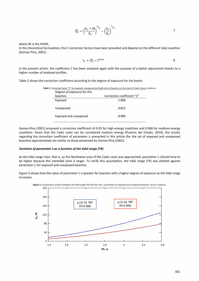
Gomez-Pina (2001) proposed a corrective coefficient of 0.93 for high-energy coastlines and 0.968 for medium-energy coastlines. Given that the Cadiz coast can be considered medium energy (Puertos del Estado, 2014), the results regarding the correction coefficient of parameter I2 presented in this article (for the set of exposed and unexposed beaches) approximately are similar to those presented by Gomez-Pina (2001). Variation of parameter I2 as a function of the tidal range (TR) As the tidal range rises, that is, as the Northwest area of the Cadiz coast was approached, parameter I2 should tend to be higher because the intertidal zone is larger. To verify this assumption, the tidal range (TR) was plotted against parameter I2 for exposed and unexposed beaches. Figure 5 shows how the value of parameter I2 is greater for beaches with a higher degree of exposure as the tidal range increases.

Figure 5. Comparative analysis between the tidal range (TR) and the real I2 parameter on exposed and unexposed beaches. Source: Authors.

TR, m

Gráfico del Modelo Ajustado

Parámetro I2, m = (3,00676*PMVE, m)^2

1,4 1,8 2,2 2,6 3 3,4 3,80

40

80

120

160

200

240

Pa

rám

etr

o I

2,

m

I2=9.74 TR2

R=0.969

I2=5.42 TR2

R=0.954

I 2, m

1.4 1.8 2.2 2.6 3 3.4 3.8

442

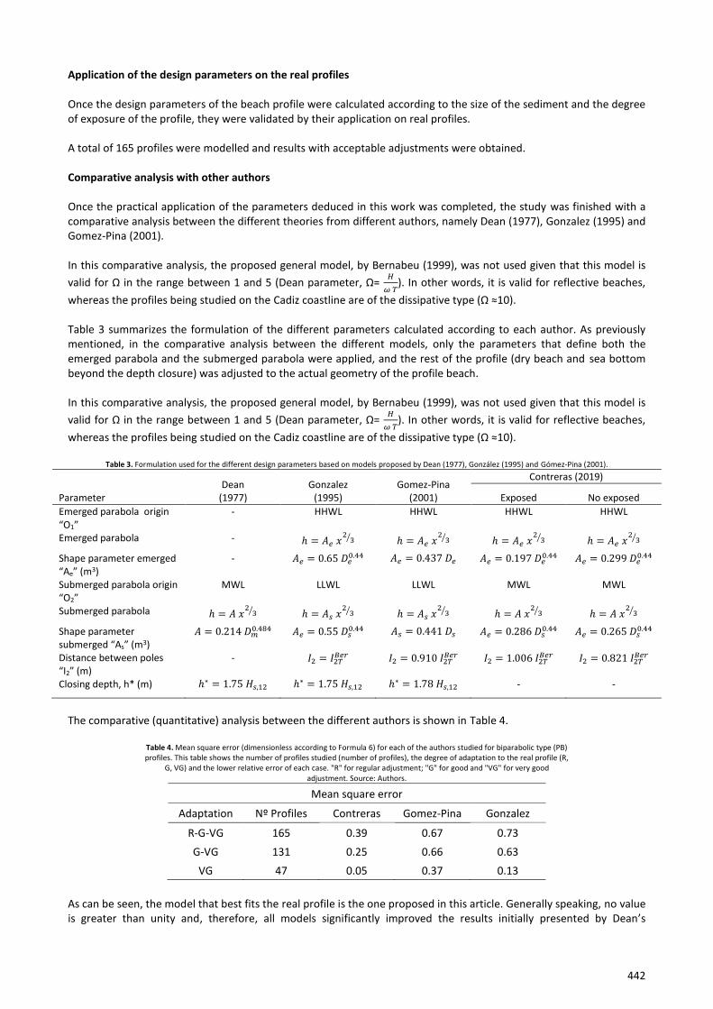
Application of the design parameters on the real profiles Once the design parameters of the beach profile were calculated according to the size of the sediment and the degree of exposure of the profile, they were validated by their application on real profiles. A total of 165 profiles were modelled and results with acceptable adjustments were obtained. Comparative analysis with other authors Once the practical application of the parameters deduced in this work was completed, the study was finished with a comparative analysis between the different theories from different authors, namely Dean (1977), Gonzalez (1995) and Gomez-Pina (2001). In this comparative analysis, the proposed general model, by Bernabeu (1999), was not used given that this model is

valid for Ω in the range between 1 and 5 (Dean parameter, Ω= 𝐻

𝜔 𝑇). In other words, it is valid for reflective beaches,

whereas the profiles being studied on the Cadiz coastline are of the dissipative type (Ω ≈10). Table 3 summarizes the formulation of the different parameters calculated according to each author. As previously mentioned, in the comparative analysis between the different models, only the parameters that define both the emerged parabola and the submerged parabola were applied, and the rest of the profile (dry beach and sea bottom beyond the depth closure) was adjusted to the actual geometry of the profile beach. In this comparative analysis, the proposed general model, by Bernabeu (1999), was not used given that this model is

valid for Ω in the range between 1 and 5 (Dean parameter, Ω= 𝐻

𝜔 𝑇). In other words, it is valid for reflective beaches,

whereas the profiles being studied on the Cadiz coastline are of the dissipative type (Ω ≈10).

Table 3. Formulation used for the different design parameters based on models proposed by Dean (1977), González (1995) and Gómez-Pina (2001).

Parameter Dean

(1977) Gonzalez

(1995) Gomez-Pina

(2001)

Contreras (2019)

Exposed No exposed

Emerged parabola origin “O1”

- HHWL HHWL HHWL HHWL

Emerged parabola - ℎ = 𝐴𝑒 𝑥23⁄ ℎ = 𝐴𝑒 𝑥

23⁄ ℎ = 𝐴𝑒 𝑥

23⁄ ℎ = 𝐴𝑒 𝑥

23⁄

Shape parameter emerged “Ae” (m3)

- 𝐴𝑒 = 0.65 𝐷𝑒0.44 𝐴𝑒 = 0. 7 𝐷𝑒 𝐴𝑒 = 0.197 𝐷𝑒

0.44 𝐴𝑒 = 0. 99 𝐷𝑒0.44

Submerged parabola origin “O2”

MWL LLWL LLWL MWL MWL

Submerged parabola ℎ = 𝐴 𝑥23⁄ ℎ = 𝐴𝑠 𝑥

23⁄ ℎ = 𝐴𝑠 𝑥

23⁄ ℎ = 𝐴 𝑥

23⁄ ℎ = 𝐴 𝑥

23⁄

Shape parameter submerged “As” (m3)

𝐴 = 0. 1 𝐷𝑚0.484 𝐴𝑒 = 0.55 𝐷𝑠

0.44 𝐴𝑠 = 0. 1 𝐷𝑠 𝐴𝑒 = 0. 6 𝐷𝑠0.44 𝐴𝑒 = 0. 65 𝐷𝑠

0.44

Distance between poles “I2” (m)

- 𝐼2 = 𝐼2𝑇𝐵𝑒𝑟 𝐼2 = 0.910 𝐼2𝑇

𝐵𝑒𝑟 𝐼2 = 1.006 𝐼2𝑇𝐵𝑒𝑟 𝐼2 = 0. 1 𝐼2𝑇

𝐵𝑒𝑟

Closing depth, h* (m) ℎ∗ = 1.75 𝐻𝑠,12 ℎ∗ = 1.75 𝐻𝑠,12 ℎ∗ = 1.7 𝐻𝑠,12 - -

The comparative (quantitative) analysis between the different authors is shown in Table 4.

Table 4. Mean square error (dimensionless according to Formula 6) for each of the authors studied for biparabolic type (PB) profiles. This table shows the number of profiles studied (number of profiles), the degree of adaptation to the real profile (R,

G, VG) and the lower relative error of each case. "R" for regular adjustment; "G" for good and "VG" for very good adjustment. Source: Authors.

Mean square error

Adaptation Nº Profiles Contreras Gomez-Pina Gonzalez

R-G-VG 165 0.39 0.67 0.73

G-VG 131 0.25 0.66 0.63

VG 47 0.05 0.37 0.13

As can be seen, the model that best fits the real profile is the one proposed in this article. Generally speaking, no value is greater than unity and, therefore, all models significantly improved the results initially presented by Dean’s

443

formulation. Among them, the models by Gomez-Pina (2001) and Gonzalez (1995) presented very similar results but a worse adjustment than the model proposed here.

Conclusions Dean (1967) defined the profile of beaches without a tidal race through a parabolic function. Beach profiles in tidal seas resemble a biparabolic beach profile based on the models of authors such as Inman et al. (1993), Gonzalez (1995), Bernabeu (1999) and Gomez-Pina (2001). The beach profile is composed of emerged and submerged parts. In the case of tidal beaches, there is a difference between the emerged, the intertidal and the submerged parts. Given that the energy conditions across the studied zone (SW coast of Spain) are very similar, the 165 profiles considered must be classified according to their degree of exposure (exposed and unexposed beaches). Applying the proposed formulations, the mean square error ranges from 0.05 to 0.39, taking as a reference the error with Dean’s formulation (1), versus Gonzalez (0.13–0.63) and Gomez-Pina (0.37–0.67). The emerged part of the biparabolic profile has its origin at O1, developing to the point of change of curvature, c, located between the emerged and submerged parabola. The origin, O1, is in the HHWL. The shape of the parabola is of the Dean type, he = Ae x2/3, where Ae is the parameter of emergent shape directly related to the sediment diameter Ae=f(De). For exposed profiles, Ae = 0.197 De

0.5. For unexposed profiles, Ae=0.299 De0.5. The submerged part of the profile is of the

parabolic (Dean) type, where hs = As x2/3, As is the submerged shape parameter directly related to the sediment diameter and As=f(De). For exposed profiles, As = 0,265 Ds

0,5. For unexposed profiles, As = 0.286 Ds0.5.

The biparabolic profile model is similar to that presented by other authors (eg Gonzalez (1995) and Gomez-Pina (2001)), with the difference of providing new design parameters. The application of these new parameters was accurately adapted to the existing real profiles. When the design parameters proposed by other authors (e.g. Dean (1977), González (1995) and Gómez-Pina (2001)) were compared and applied to real profiles, the model presented in this study was an improvement. Thus, the proposed parameters will help optimize the volume of fill sand in future beach regeneration projects in SW Spain, although the methodology based on topobathymetric data, sediment and marine climate, can be applied worldwide.

Acknowledgements The authors wish to thank the Atlantic Andalusia Coastal Demarcation (Cadiz, Spain) for their collaboration in providing data for the preparation of this article.

References

Bernabeu-Tello, A., Muñoz-Pérez, J., & Medina-Santamaria, R. (2002). Influence of a rocky platform in the profile morphology: Victoria Beach, Cadiz (Spain). Ciencias Marinas, 28(2), 181–192.

Bernabeu, A. (1999). Desarrollo, validación y aplicaciones de un modelo general de perfil de equilibrio en playas. PhD thesis. Universidad de Cantabria. Santander (Spain).

Bruun, P. (1954). Coast erosion and the development of beach profiles. Beach Erosion Board, US Army Corps of Eng., Tech.Mem. 44: 1-79

Contreras, A., Gómez-Pina, G., Muñoz-Perez, J., & Chamorro, G. (2017). Tipologías de perfiles de playa en el litoral de la Provincia de Cádiz. XIV Jornadas Españolas de Ingeniería de Costas Y Puertos.71-82. Alicante (Spain).

Dean, R. G. (1977). Equilibrium Beach Profiles: U.S. Atlantic and Gulf Coast. Newark, DE, USA.

Fenneman, N. M. (1902). Development of the Profile of Equilibrium of the Subaqueous Shore Terrace. The Journal of Geology, 10(1), 1–32. Retrieved from http://www.jstor.org/stable/30055541

Gómez-Pina, G. (2001). Modelo biparabólico de cuantificación de perfiles de playa en mares con marea basado en datos de campo del litoral español. PhD thesis. Universidad Politécnica de Madrid. Madrid (Spain).

Gonzalez, E. M. (1995). Morfología de playas en equilibrio, planta y perfil. PhD thesis. Universidad de Cantabria. Santander (Spain).

Hidtma (2013). UTE Ecoatlántico. Estudio ecocartográfico del litoral de la provincia de Cadiz. Referencia 28-4983. Cádiz (Spain)

Houston, J.R. (1996). International tourism and U.S. beaches. Coastal Engineering Research Center Vicksburg MS. Vol CERC-96-2. 1-3.

444

King, P. (1999). The fiscal impact of beaches in California. Public Research Institute, San Francisco State Univ., San Francisco (USA).

Inman, D. L., Elwany, M. ., & Jenkin, S. (1993). Shorerise and Bar-berm Profiles on Ocean Beaches. Journal of Geophysical Research, 98(C10), 18181–18199.

Johnson, D. W. (1919). Shore Processes and Shoreline Development. Columbia Univ. Press, New York (Hafner Facsimile ed., 1952.).

Kriebel, D. L., Kraus, N. C., & Larson, M. (1991). Engineering Methods for Predicting Beach Profile Response. Proc. Coastal sediments´91 ASCE, 557–571.

Krumbein, W.C., & James, W.R. (1965). A Lognormal Size Distribution Model for Estimating Stability of Beach Fill Material. T.M. 16. US Army Corps of Engineers, Beach Erosion Board.

Larson, M. (1991). Equilibrium Profile of a Beach with varying Grain Size. Proc. Coastal sediments´91 ASCE, 905–919.

Larson, M., & Kraus, N. C. (1989). SBEACH: Numerical Model to Simulate Storm-Induced Beach Change. Tech. Report CERC-89-9, U.S. Army Corps of Engs. Waterway Experiment Station, Vicksburg, Mississippi.

Masselink, G., & Short, A. D. (1993). The effect of tide range on beach morphodynamics and morphology: a conceptual beach model. Journal of Coastal Research, 9,3, 785–800.

Moore, B. (1982). Beach Profile Evolution in Response to Changes in Water Level and Wave Height. University of Delaware.

Muñoz-Pérez, J. J., Gutiérrez-Mas, J. M., Moreno, J., Español, L., Moreno, L., & Bernabéu, A. (2003). Portable meter system for dry weight control in dredging hoppers. Journal of waterway, port, coastal, and ocean engineering, 129(2), 79-85.

Muñoz-Pérez, J., & Medina, R. (2005). Short-term variability on reef protected beach profiles: An analysis using EOF. Coastal Dynamics 2005: State of the Practice ASCE ISBN: 978-0-7844-0855-1.

Pilkey, O., Young, S. R., Riggs, S. R., Smith, W. S., & Wu y W. D. (1993). The Concept os Shore Face Profile of Equilibrium: A Critical Review. Journal of Coastal Research, 9(1).

Pranzini, E., Anfuso, G., & Muñoz-Pérez, J.J. (2018). A probabilistic approach to borrow sediment selection in beach nourishment projects. Coastal Engineering, 139, 32-35.

Puertos del Estado. (2014). Puertos del Estado. Boya de Golfo de Cádiz. https://puertos.es

Schwartz, M. L. (1982). The Encyclopaedia of Beach and Coastal Environments. Stroudsburg: Hutchinson.

Stauble, D.K., 2007. Assessing beach fill compatibility through project performance evaluation. In: Costal Sediments' 07, pp. 2418–2431.

Valderrama-Landeros, L.H., Martell-Dubois, R., Ressl, R., Silva-Casarín, R., Cruz, C.J., & Muñoz-Pérez, J.J. (2019). Dynamics of coastline changes in Mexico. Journal of Geographical Sciences, 1-18.