Embed Size (px)
Citation preview
Non-Cartesian Parallel Magnetic Resonance Imaging
Dissertation zur Erlangung des naturwissenschaftlichen Doktorgrades
der Bayerischen Julius-Maximilians-Universität Würzburg
vorgelegt von Robin Heidemann
aus München
Würzburg 2007
Eingereicht am: bei der Fakultät für Physik und Astronomie 1. Gutachter: Prof. Dr. rer. nat. Peter M. Jakob 2. Gutachter: Prof. Dr. Dr. med. Wolfgang R. Bauer der Dissertation. 1. Prüfer: Prof. Dr. rer. nat. Peter M. Jakob 2. Prüfer: Prof. Dr. rer. nat. Georg Reents im Promotionskolloquium. Tag des Promotionskolloquiums: Doktorurkunde ausgehändigt am:
Contents
CONTENTS ....................................................................................................... 1
1 INTRODUCTION ........................................................................................ 3
2 BASIC PRINCIPLES OF MRI..................................................................... 9 2.1 THE NUCLEAR MAGNETIC RESONANCE PHENOMENON .......................................................... 9
2.1.1 Nuclei in a Magnetic Field ................................................................................................ 9 2.1.2 Radiofrequency Field...................................................................................................... 10 2.1.3 MR Signal ......................................................................................................................... 11 2.1.4 Magnetic Field Gradients ............................................................................................... 12
2.2 MAGNETIC RESONANCE IMAGING .......................................................................................... 12 2.2.1 Slice-selective excitation ................................................................................................ 12 2.2.2 Phase-encoding............................................................................................................... 13 2.2.3 Frequency-encoding ....................................................................................................... 13
2.3 K-SPACE CONCEPT ................................................................................................................. 15 2.4 K-SPACE SAMPLING................................................................................................................. 16
2.4.1 Cartesian trajectories ...................................................................................................... 16 2.4.2 Non-Cartesian trajectories ............................................................................................. 18
3 BASIC PRINCIPLES OF PARALLEL MRI............................................... 21 3.1 INTRODUCTION........................................................................................................................ 21 3.2 A SHORT HISTORY OF PARALLEL MRI .................................................................................. 25 3.3 K-SPACE BASED PARALLEL MRI............................................................................................ 27 3.4 CARTESIAN GRAPPA ............................................................................................................ 37
4 A FAST METHOD FOR 1D NON-CARTESIAN PARALLEL MRI............ 41 4.1 INTRODUCTION........................................................................................................................ 41 4.2 THEORY AND METHODS ......................................................................................................... 43
4.2.1 Cartesian trajectories and pMRI.................................................................................... 43 4.2.2 1D non-Cartesian trajectories........................................................................................ 45 4.2.3 1D non-Cartesian pMRI k-space reconstruction......................................................... 49 4.2.4 1D non-Cartesian GRAPPA coil weights ..................................................................... 51 4.2.5 Imaging experiments ...................................................................................................... 54
4.3 RESULTS ................................................................................................................................. 55 4.4 DISCUSSION............................................................................................................................ 60 4.5 SUMMARY ............................................................................................................................... 66
5 A DIRECT METHOD FOR SPIRAL PARALLEL MRI .............................. 67 5.1 INTRODUCTION........................................................................................................................ 67 5.2 THEORY AND METHODS ......................................................................................................... 68
5.2.1 Spiral trajectories............................................................................................................. 68 5.2.2 Interpolation of data along the spiral trajectory ........................................................... 72 5.2.3 Reordering of k-space data into a new hybrid space................................................. 73
Contents
2
5.2.4 Modified GRAPPA Reconstruction ............................................................................... 76 5.2.5 Imaging experiments....................................................................................................... 78
5.3 RESULTS ................................................................................................................................. 80 5.4 DISCUSSION ............................................................................................................................ 90 5.5 SUMMARY................................................................................................................................ 93
6 CONCLUSIONS AND PERSPECTIVES................................................... 95
7 BIBLIOGRAPHY....................................................................................... 99
8 SUMMARY.............................................................................................. 107
9 ZUSAMMENFASSUNG .......................................................................... 111
10 PUBLICATIONS ..................................................................................... 115
11 CURRICULUM VITAE............................................................................. 117
12 ACKNOWLEDGMENTS ......................................................................... 119
1 Introduction
In 1946, two articles were published from different groups in the 69th issue of
Physical Review describing the phenomenon of nuclear magnetic resonance
(NMR). Although the discovery of NMR by Purcell [1] and Bloch [2] was the
beginning of an extensive development, it took nearly 30 years until this effect
was used for the first time for imaging by Lauterbur [3]. Since then, magnetic
resonance imaging (MRI) has progressed at a spectacular rate and started to
become an important tool for clinical diagnosis with the first clinical trials in
1980.
Today, MRI is well-established in clinical routine, but still represents a
continually evolving medical technology. With its excellent spatial resolution and
its inherent high tissue contrast, MRI has surpassed computer assisted
tomography for many clinical applications. However, this development did not
occur overnight. Due to initial methodological constraints such as acquisition
“dead times” imposed due to long T1 relaxation times and technical constraints
like radiofrequency (RF) and gradient hardware, main magnetic field strength,
and field homogeneity, the first MRI methods required several minutes to nearly
an hour to produce a two dimensional image of the human body with a
resolution in the range of centimeters. The long scan times restricted the
application of MRI as a diagnostic tool, increased the cost of scanning by
limiting patient throughput, and led to image artifacts from patient motion during
Introduction
4
scans. Early progress was in the improvement of signal-to-noise ratio (SNR) to
reduce the need for signal averaging.
Since then, the evolution of MRI has been one of continued reduction in
imaging time with numerous proposals to reduce the scan time. Besides
advances in the technology of magnet construction, RF and gradient hardware,
the development of fast imaging methods have drastically reduced scan times.
With fast imaging sequences such as echo planar imaging (EPI) [4], fast low
angle shot (FLASH) [5], turbo spin echo (TSE) [6] and fast imaging with steady
precession (FISP) [7], complete MR images may be obtained hundreds to
thousands of times faster than in the early years with comparable or even
improved spatial resolution and contrast. Today, imaging times of a few
seconds, yielding a resolution on the order of a millimeter, are common for
clinical MRI. Based on these advances, new clinical applications have been
developed, including real-time imaging of cardiac motion, multi-section imaging
of the brain in a few seconds, and functional brain imaging (such as imaging of
perfusion, diffusion and cortical activation). Fast imaging techniques have
become the methods of choice for many applications, since they "freeze out"
the effects of macroscopic motion, allowing a high scan efficiency and improved
resolution.
Besides the image contrast, imaging speed is still probably the most important
consideration in clinical MRI. Unfortunately, current MRI systems already
operate at the limits of potential imaging speed, due to the technical and
physiological problems associated with rapidly switched gradient systems.
Recently, a quantum leap in speed has been provided through the advent of
parallel MRI (pMRI) [8]-[22]. Instead of relying on increased gradient
performance for increased imaging speed, pMRI extracts extra spatial
information from an array of surface coils, resulting in an accelerated image
acquisition. The acquisition speed of the current generation of pMRI scanners is
Introduction
5
up to 2-4 times higher than traditional MR systems which rely solely on
gradients for image encoding. Acquisitions have been increased by up to a
factor of 8-16 at research sites using specialized hardware. These MRI
scanners have provided the greatest gain in imaging speed since the
development of fast MRI methods in the 1980s.
Over the past ten years, pMRI has improved with higher speed-up factors,
automatic coil sensitivity calibration mechanisms, and improved reconstruction
algorithms. Additionally, during this time, the MR scanners themselves have
also improved. The more advanced MR scanners today are equipped with an
increased number of independent receiver channels, improved RF coil
geometries and higher field strengths. Even though these developments have
greatly improved the image quality and the robustness of pMRI acquisitions,
there are still problems in the use of pMRI in many clinical applications. The
strongest constraint for the use of pMRI is SNR. Applications which are already
at the limit of SNR are clearly not suitable for acceleration by pMRI. As a rule of
thumb, the use of pMRI will reduce the attainable SNR by a factor of at least the
square root of the acceleration factor. Besides the SNR issue, residual fold-over
artifacts, originating from inaccurate pMRI reconstructions, are a second source
of problems. There is a complicated relationship between the accuracy of a
pMRI reconstruction and the imaging set up, which is not yet well understood.
Since it is not possible to model this relationship and find a simple and robust
solution for this problem, dedicated pMRI reconstructions are necessary for
certain applications.
One possible solution to those problems is the synergy of a combination of
more advanced sampling schemes such as non-Cartesian sampling strategies
and pMRI. Although pMRI can benefit from the advantages of non-Cartesian
trajectories and vice versa, the combination of these acquisition schemes with
parallel imaging has yet not entered routine use. The main reason is the long
Introduction
6
reconstruction time due to the complex calculations necessary for non-
Cartesian parallel imaging.
This thesis is a summary of my developments and results on the research topic
of fast non-Cartesian pMRI methods. The ideas presented in this work have led
to new reconstruction algorithms enabling pMRI reconstruction times on the
order of those for conventional Cartesian pMRI. The results of these advanced
pMRI methods indicate the possibility to obtain higher acceleration factors or
improved image quality compared to standard Cartesian pMRI.
In the first section of this thesis, the basic principles of MRI are introduced, i.e.,
the phenomenon of nuclear magnetic resonance, signal creation and spatial
encoding of the signal using magnetic field gradients. Further, the k-space
concept will be introduced and Cartesian and non-Cartesian k-space sampling
strategies will be described briefly. A more specific description of those
trajectories is given in the corresponding chapters about non-Cartesian pMRI.
Chapter 3 is intended to be introductory to parallel MRI; it begins with the basic
features of parallel imaging using arrays of RF coils, followed by a brief history
of the development in this field. In the next sub section of chapter 3, a detailed
introduction to parallel MRI is given. The last sub section of chapter 3 is devoted
to the Cartesian GRAPPA technique.
In chapter 4, the new concept of a fast one dimensional (1D) non-Cartesian
GRAPPA method is introduced. It is shown that 1D non-Cartesian GRAPPA is
more robust compared to Cartesian GRAPPA. Compared to previous non-
Cartesian pMRI methods, the reconstruction time is in the range of the time
required for Cartesian pMRI reconstructions.
Chapter 5 deals with a new concept of a direct spiral GRAPPA technique. This
new method allows one to obtain significantly improved single shot spiral
acquisitions compared to conventional spiral imaging. In this new method, the
Introduction
7
reconstruction time is reduced to the same or even less than the time required
for conventional data gridding.
Finally, the results and the significance of fast and direct pMRI methods with
non-Cartesian sampling strategies are discussed.
Introduction
8
2 Basic Principles of MRI
2.1 The Nuclear Magnetic Resonance Phenomenon
2.1.1 Nuclei in a Magnetic Field
Nuclear magnetic resonance (NMR) is the basic underlying phenomenon
behind MRI. An object, e.g. a human being, is placed into a strong magnetic
field. This field is typically in the range of 0.5 to 3.0 Tesla in clinical settings,
which is ten to sixty thousand times the strength of the earth’s magnetic field.
Such a strong magnetic field causes the nuclear spins of certain atoms within
the body, namely those atoms that have a nuclear spin dipole moment, to orient
themselves parallel or anti-parallel to the static main magnetic field (B0). The
nuclei spins precess about B0 with a frequency, called the resonance or Larmor
frequency (ω0), which is directly proportional to B0:
00 Bγω = (2.1)
where γ is the gyromagnetic ratio, a fundamental physical constant for each
nuclear species, which is listed for a few nuclei in Table 2.1. The Larmor
relationship given by Equation 2.1 is the fundamental MR equation. Since the
proton nucleus (1H) has a high sensitivity (a result of its high gyromagnetic ratio,
42.58 MHz/Tesla) and a high natural abundance, it is currently the nucleus of
choice for MRI. Due to the fact that the parallel state is the state of lower
energy, slightly more spins reside in the parallel state than in the anti-parallel
Basic Principles of MRI
10
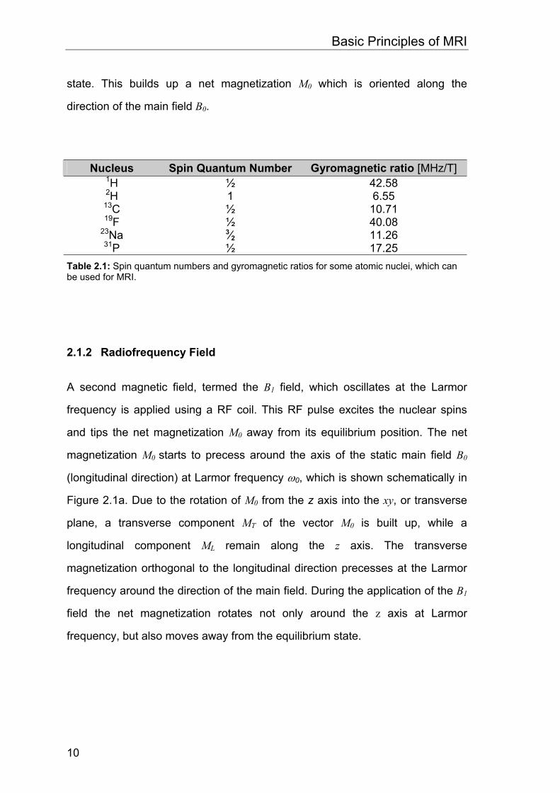
state. This builds up a net magnetization M0 which is oriented along the
direction of the main field B0.
Nucleus Spin Quantum Number Gyromagnetic ratio [MHz/T] 1H ½ 42.58 2H 1 6.55
13C ½ 10.71 19F ½ 40.08
23Na 3⁄2 11.26 31P ½ 17.25
Table 2.1: Spin quantum numbers and gyromagnetic ratios for some atomic nuclei, which can be used for MRI.
2.1.2 Radiofrequency Field
A second magnetic field, termed the B1 field, which oscillates at the Larmor
frequency is applied using a RF coil. This RF pulse excites the nuclear spins
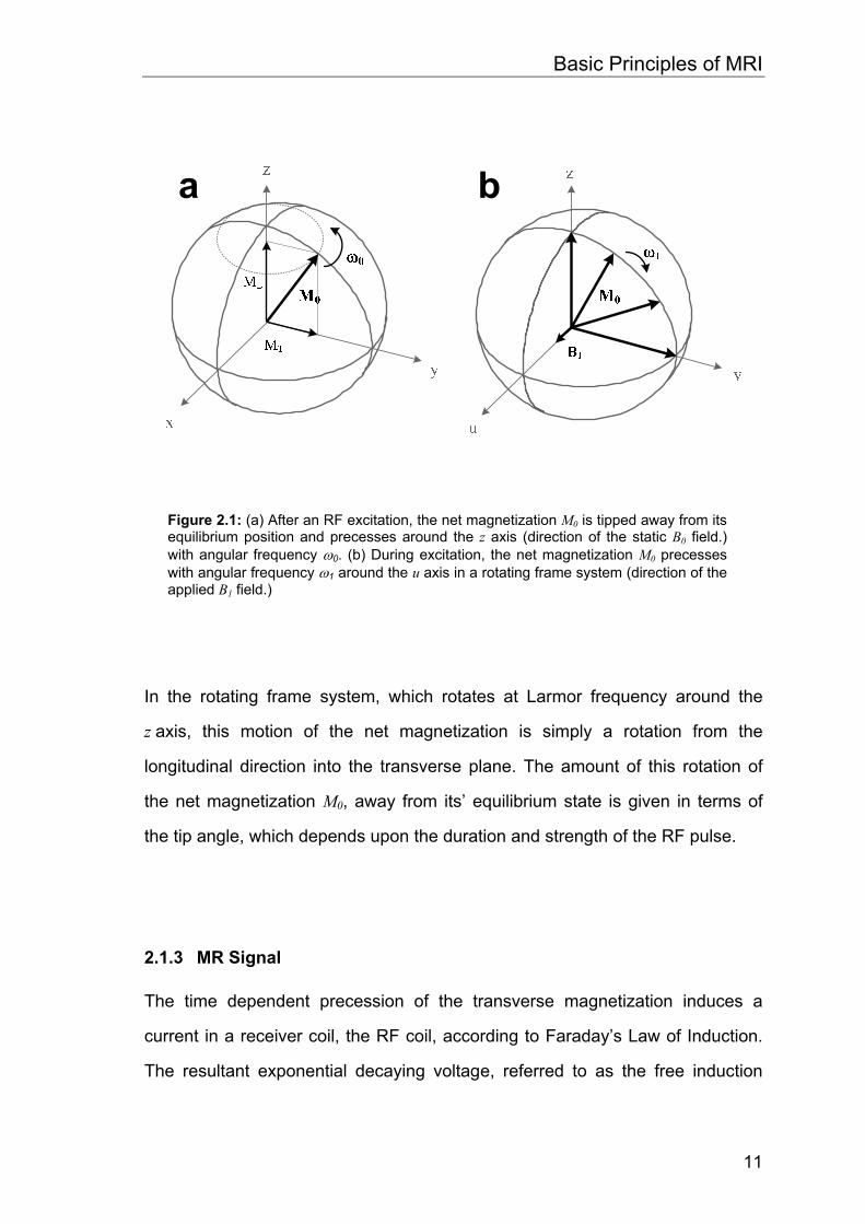
and tips the net magnetization M0 away from its equilibrium position. The net
magnetization M0 starts to precess around the axis of the static main field B0
(longitudinal direction) at Larmor frequency ω0, which is shown schematically in
Figure 2.1a. Due to the rotation of M0 from the z axis into the xy, or transverse
plane, a transverse component MT of the vector M0 is built up, while a
longitudinal component ML remain along the z axis. The transverse
magnetization orthogonal to the longitudinal direction precesses at the Larmor
frequency around the direction of the main field. During the application of the B1
field the net magnetization rotates not only around the z axis at Larmor
frequency, but also moves away from the equilibrium state.
Basic Principles of MRI
11
In the rotating frame system, which rotates at Larmor frequency around the
z axis, this motion of the net magnetization is simply a rotation from the
longitudinal direction into the transverse plane. The amount of this rotation of
the net magnetization M0, away from its’ equilibrium state is given in terms of
the tip angle, which depends upon the duration and strength of the RF pulse.
2.1.3 MR Signal
The time dependent precession of the transverse magnetization induces a
current in a receiver coil, the RF coil, according to Faraday’s Law of Induction.
The resultant exponential decaying voltage, referred to as the free induction
Figure 2.1: (a) After an RF excitation, the net magnetization M0 is tipped away from its equilibrium position and precesses around the z axis (direction of the static B0 field.) with angular frequency ω0. (b) During excitation, the net magnetization M0 precesses with angular frequency ω1 around the u axis in a rotating frame system (direction of the applied B1 field.)
Basic Principles of MRI
12
decay (FID), constitutes the MR signal which can be described by the following
equation:
{ } rdertS ti 30)()( ∫ Φ+= ωρ v (2.2)
where )(rrρ is the three dimensional spin density of e.g. protons inside the
volume d3r.
2.1.4 Magnetic Field Gradients
By applying a linear magnetic field gradient along a single direction, the
magnetic field strength is now directly related to the position along that
direction. We have now created a spatially dependent magnetic field strength,
which corresponds according to Equation 2.1 to a spatially dependent
resonance or Larmor frequency, which can be used for spatial encoding of the
MR signal.
2.2 Magnetic Resonance Imaging
2.2.1 Slice-selective excitation
The first dimension is encoded by a so-called slice-selective excitation, which
means that only spins from a well-defined slice of the object contribute to the
MR signal. This is achieved by applying a magnetic field gradient along the
z axis during an RF excitation pulse with a specific frequency bandwidth. When
the slice-select gradient, GSlice, is applied along the z axis, the resonance
frequencies of the protons become linearly related to the position along the z
axis. Individual resonance frequencies correspond to individual planes of nuclei.
In this example, these planes are oriented perpendicular to the z axis. When the
Basic Principles of MRI
13
frequency-selective RF pulse is applied while GSlice is on, only nuclei in the
plane with corresponding frequencies will be excited; thus a slice will be
selected. The frequency bandwidth of the excitation pulse, together with the
gradient, confines the excitation to the nuclei in the slice. No signals are excited
from areas outside the defined slice.
2.2.2 Phase-encoding
After the slice-selective excitation, the next step is to encode the two
dimensions within this slice. This is realized by imposing a spatially dependent
phase on the signal from the precessing protons (phase-encoding) and by
creating a spatially dependent frequency during signal reception (frequency-
encoding). A spatially dependent phase can be created by applying a variable
phase-encoding gradient, GPhase, before the signal is received. If the direction of
GPhase is denoted by y, during the phase-encoding period, nuclei along the y
direction experience different magnetic fields and therefore precess with
different Larmor frequencies. After a certain period the phase-encoding gradient
is turned off before data acquisition begins. After GPhase is turned off, all nuclei
revert to the resonance frequency determined by the main magnetic field. The
net effect of applying GPhase is to introduce a spatially dependent phase shift into
the signal.
2.2.3 Frequency-encoding
The final spatial dimension, the x direction, can be encoded into the signal by
applying a gradient during the acquisition of the signal. The application of this
gradient creates a spatially dependent Larmor frequency; therefore, this
Basic Principles of MRI
14
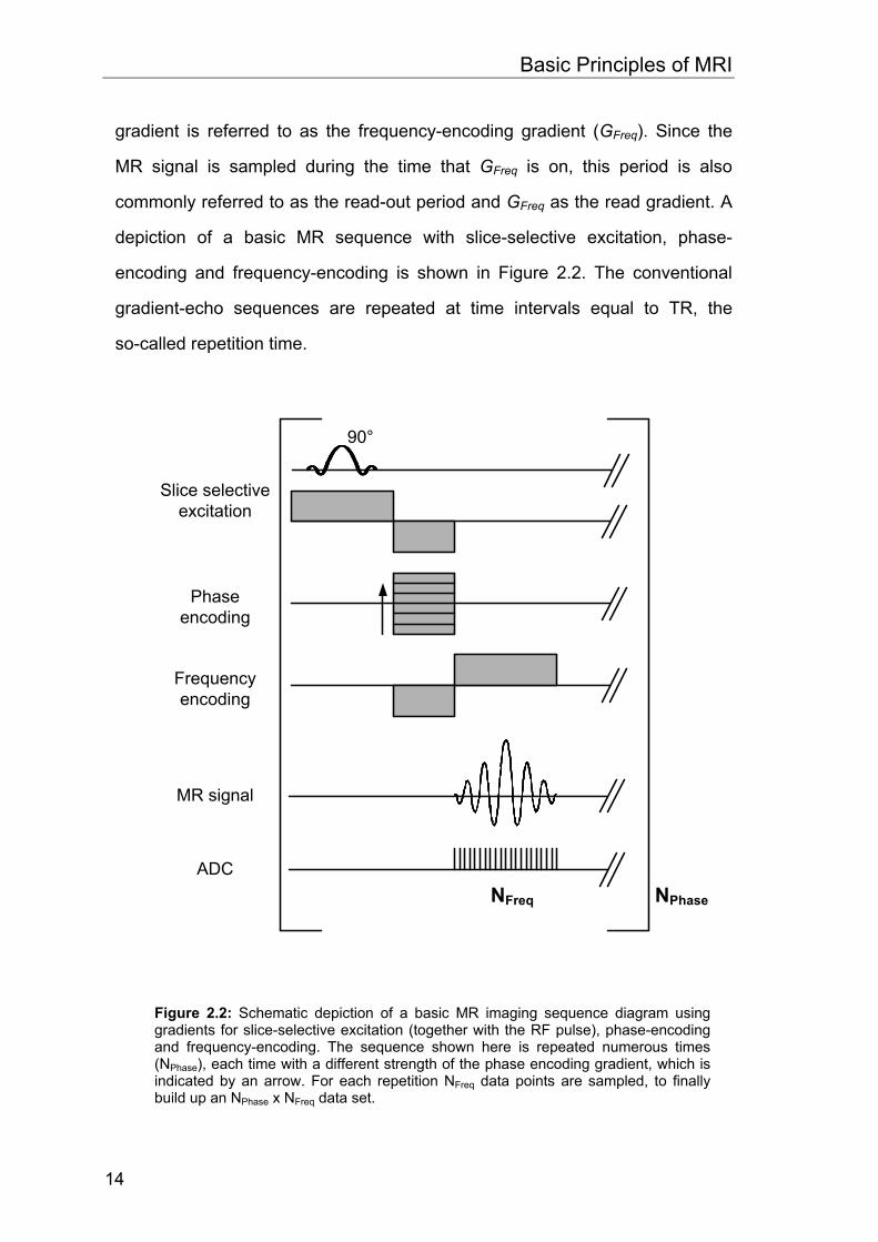
gradient is referred to as the frequency-encoding gradient (GFreq). Since the
MR signal is sampled during the time that GFreq is on, this period is also
commonly referred to as the read-out period and GFreq as the read gradient. A
depiction of a basic MR sequence with slice-selective excitation, phase-
encoding and frequency-encoding is shown in Figure 2.2. The conventional
gradient-echo sequences are repeated at time intervals equal to TR, the
so-called repetition time.
90°
Slice selectiveexcitation
Phase encoding
Frequencyencoding
MR signal
ADCNFreq NPhase
Figure 2.2: Schematic depiction of a basic MR imaging sequence diagram using gradients for slice-selective excitation (together with the RF pulse), phase-encoding and frequency-encoding. The sequence shown here is repeated numerous times (NPhase), each time with a different strength of the phase encoding gradient, which is indicated by an arrow. For each repetition NFreq data points are sampled, to finally build up an NPhase x NFreq data set.
Basic Principles of MRI
15
The number of times the sequence is repeated (for one average) is determined
by the desired spatial resolution, which is proportional to the number of voxels
along the phase-encoding direction and is equal to the number of phase-
encoding steps (NPhase). For a certain number of averages (NAV) the total time
required to obtain an image slice is: TR x NPhase x NAV. Typical parameters for a
conventional spin-echo sequence are a TR of 2000 ms and 256 phase encoding
steps without averaging giving a total acquisition time of 8.5 min.
2.3 k-space concept
As shown in the previous chapter, the MR signal can be spatially encoded, after
the slice-selective excitation, by applying magnetic field gradients in the
remaining two dimensions. If it is assumed that the position of the magnetization
with respect to the coils does not change with time (patient does not move),
then the signal can be written as,
dydxeyxdydxeyxtS
PEt
y
T
x ydtGixdtGiyitxi ∫ ∫∫ ∫
∞+
∞−
∞+
∞−
+∞+
∞−
∞+
∞−
Φ+∫∫
== 00),(),()( )()(γγ
ω ρρ (2.3)
Making the following substitution,
∫ ∫==T t
yyxx
PE
dttGkdttGk0 0
)()( γγ and (2.4)
Basic Principles of MRI
16
then Equation 2.3 becomes
dydxeyxkkS yikxikyx
yx∫ ∫+∞
∞−
+∞
∞−
+= ),(),( ρ (2.5)
This signal, in the so-called k-space, is the 2D Fourier transform of the spin
density distribution, ρ(x,y), created by applying gradients in two dimensions. It
represents the frequency spectrum of the spin density distribution of the
underlying object. A measure of this spin density distribution, an image
corresponding to the spatial variation in proton density, can be obtained by
taking an inverse two dimensional Fourier transformation of the collected
signals. The k-space concept was first described by Ljunggren [23].
2.4 k-space sampling
2.4.1 Cartesian trajectories
In general, the whole of k-space data is not sampled after a single excitation.
There are physical limitations such as a finite relaxation time and the SNR and
there are technical limitations such as the slew rate of the gradients. Thus
k-space is sampled in a sequential way by repeating a sequence NPhase times.
During each repetition a signal is sampled along a line in k-space corresponding
to a certain position nky in k-space, which is depicted in Figure 2.3. This k-space
sampling method is referred to as 2D Fourier or spin-warp imaging [24].
There are some important relationships between the sampled data in k-space
and the corresponding image in the image domain.
Basic Principles of MRI
17
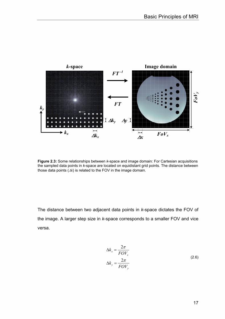
The distance between two adjacent data points in k-space dictates the FOV of
the image. A larger step size in k-space corresponds to a smaller FOV and vice
versa.
yy
xx
FOVk
FOVk
π
π
2
2
=∆
=∆
(2.6)
FT
FT -1
kx
ky y
xkx
ky
FoV
y
FoVx
k-space Image domain
Figure 2.3: Some relationships between k-space and image domain: For Cartesian acquisitions the sampled data points in k-space are located on equidistant grid points. The distance between those data points (∆k) is related to the FOV in the image domain.
Basic Principles of MRI
18
Further, the k-space extent which is covered by the sampled data defines the
resolution in the image and is given by:
yPhase
xFreq
kNy
kNx
∆=∆
∆=∆
π
π
2
2
(2.7)
One of the most important advantages of Fourier imaging is that the
reconstruction can be performed with a simple and fast inverse Fourier
transformation. A requirement of the Fourier transformation is that the k-space
data are obtained on a rectangular grid with equidistant step size in each of the
directions. Those sampling schemes with constant distance between measured
data points in each direction are named Cartesian trajectories.
2.4.2 Non-Cartesian trajectories
Compared to 2D Fourier imaging with Cartesian trajectories, data acquired on
non-Cartesian trajectories are not aligned on a rectangular grid with equidistant
sampling density. For those sampling schemes, first described by Twieg
[25],[26], reconstruction has to be performed with methods different than the
Fourier transformation.
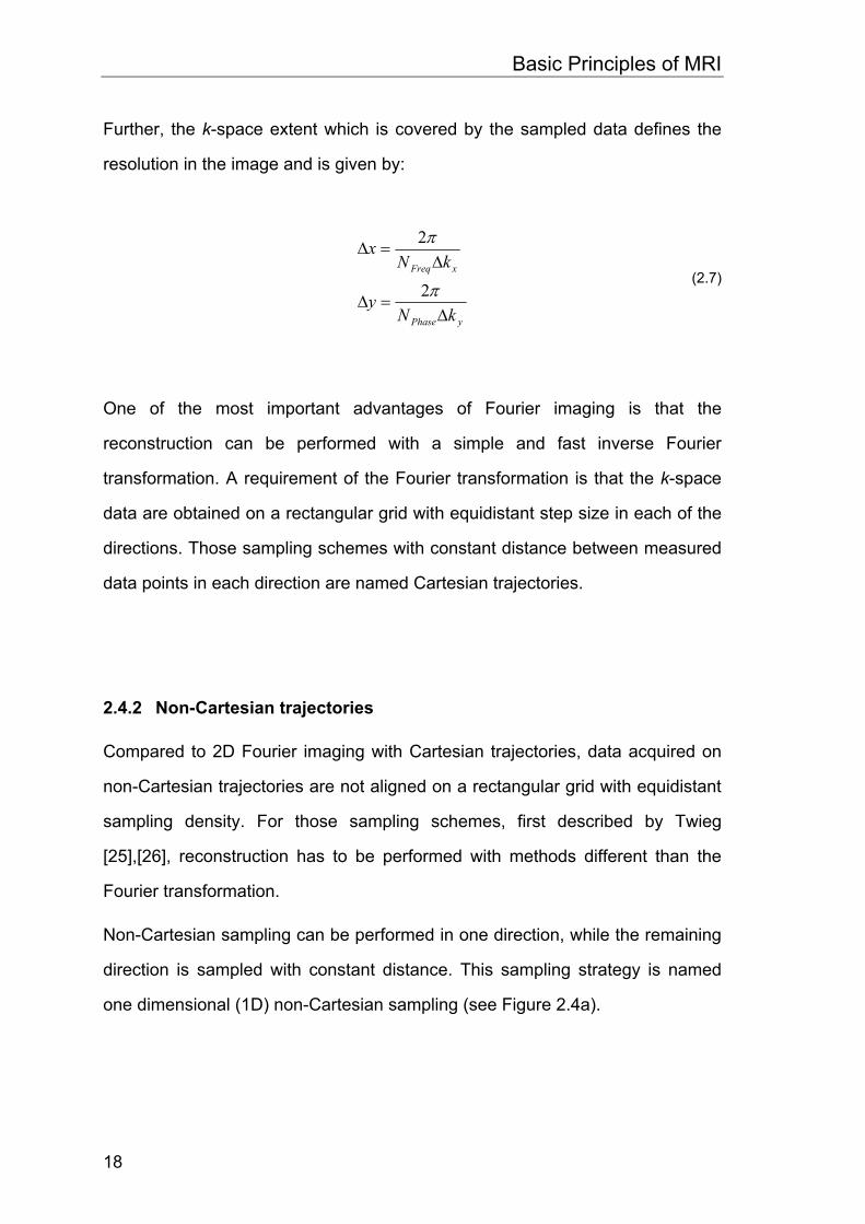
Non-Cartesian sampling can be performed in one direction, while the remaining
direction is sampled with constant distance. This sampling strategy is named
one dimensional (1D) non-Cartesian sampling (see Figure 2.4a).
Basic Principles of MRI
19
There are numerous two dimensional (2D) non-Cartesian trajectories. In
Figure 2.4 two common 2D non-Cartesian trajectories are depicted. A radial
sampling scheme is shown in Figure 2.4b and a spiral trajectory is shown in
Figure 2.4c.
Both trajectories enable fast dynamic acquisition methods especially used e.g.
for cardiac cine imaging or functional MRI. A detailed description of the 1D non-
Cartesian trajectory will be given in chapter 4.2.2, while the spiral trajectory is
described in detail in chapter 5.2.1
a b ca b c
Figure 2.4: Schematic depiction of different non-Cartesian k-space sampling schemes (a) 1D non-Cartesian (b) radial and (c) spiral trajectory.
Basic Principles of MRI
20
3 Basic Principles of Parallel MRI
3.1 Introduction
The basic idea how the data acquisition can be accelerated with parallel
imaging in MRI, is rather simple. The acquisition time is directly dependent on
the amount of data to be acquired for an MR image. By reducing the amount of
image data needed to create the image, the acquisition time is also reduced.
The idea of reducing the amount of k-space data is not new; as a rule, the
resolution, and therefore the extent of k-space, is tailored specifically to the type
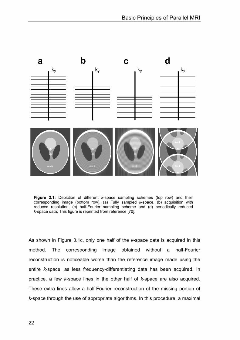
of diagnostic analysis being performed. In Figure 3.1, this idea is explained
schematically. It is assumed that k-space is acquired in a sequential way line-
by-line, which is the case in most MR sequences used for clinical exams. As
explained in chapter 2.4.1, the distance between neighboring k-space lines is
determined by the desired FOV in the image domain. A larger FOV corresponds
to a smaller separation between k-space points. In order to make a high-
resolution image with a specific FOV (Figure 3.1a), the extent of k-space
acquired must be greater than for a low-resolution image with the same FOV
(Figure 3.1b). An image with a lower resolution shows not only blurring but also
other image artifacts, most noticeably Gibbs ringing.
A common method for shortening the image acquisition time without reducing
the resolution is the use of half-Fourier procedures [27],[28].
Basic Principles of Parallel MRI
22
As shown in Figure 3.1c, only one half of the k-space data is acquired in this
method. The corresponding image obtained without a half-Fourier
reconstruction is noticeable worse than the reference image made using the
entire k-space, as less frequency-differentiating data has been acquired. In
practice, a few k-space lines in the other half of k-space are also acquired.
These extra lines allow a half-Fourier reconstruction of the missing portion of
k-space through the use of appropriate algorithms. In this procedure, a maximal
Figure 3.1: Depiction of different k-space sampling schemes (top row) and their corresponding image (bottom row). (a) Fully sampled k-space, (b) acquisition with reduced resolution, (c) half-Fourier sampling scheme and (d) periodically reduced k-space data. This figure is reprinted from reference [70].
Basic Principles of Parallel MRI
23
“acceleration factor” of two is possible, as the acquisition of less than half of the
k-space data makes the reconstruction of missing data points impossible.
Unlike in half-Fourier imaging, parallel imaging or parallel MRI (pMRI), functions
by reducing the k-space data by increasing the distance between neighboring
lines. The FOV in the image domain is thus reduced, leading to fold-over
artifacts, otherwise known as aliasing, when the object to be imaged is larger
than the decreased FOV. As an example, Figure 3.1d shows a k-space reduced
by a factor of two, where every second line has been left out. Such an
acquisition scheme is known as “reduced k-space,” where the reduction factor,
which is also known in pMRI as the acceleration factor (AF), is denoted by the
letter R. By using a reduced sampling with R=2, the FOV in the image domain is
reduced by half, and it is possible that the original image no longer fits into the
smaller FOV. A simulation of such a case is shown in Figure 3.1d. All portions
of the object outside of the FOV are folded back into the FOV because the
Nyquist criterion has not been fulfilled for the complete image. In comparison
with the reference image in Figure 3.1a, the acquisition time for such a folded
image is reduced by a factor of two in comparison to a fully-acquired image, but
it is obvious that images with these severe aliasing artifacts are not usable in
clinical diagnosis. In general, parallel imaging works by removing aliasing
artifacts through the reconstruction of the missing k-space lines or by
“unfolding” the folded image. To this effect, parallel imaging necessitates the
use of several independent coils and a corresponding number of receiver
channels on the MR system. In order to employ the coil set-up as spatial
information for the pMRI reconstruction, the k-space data from each coil must
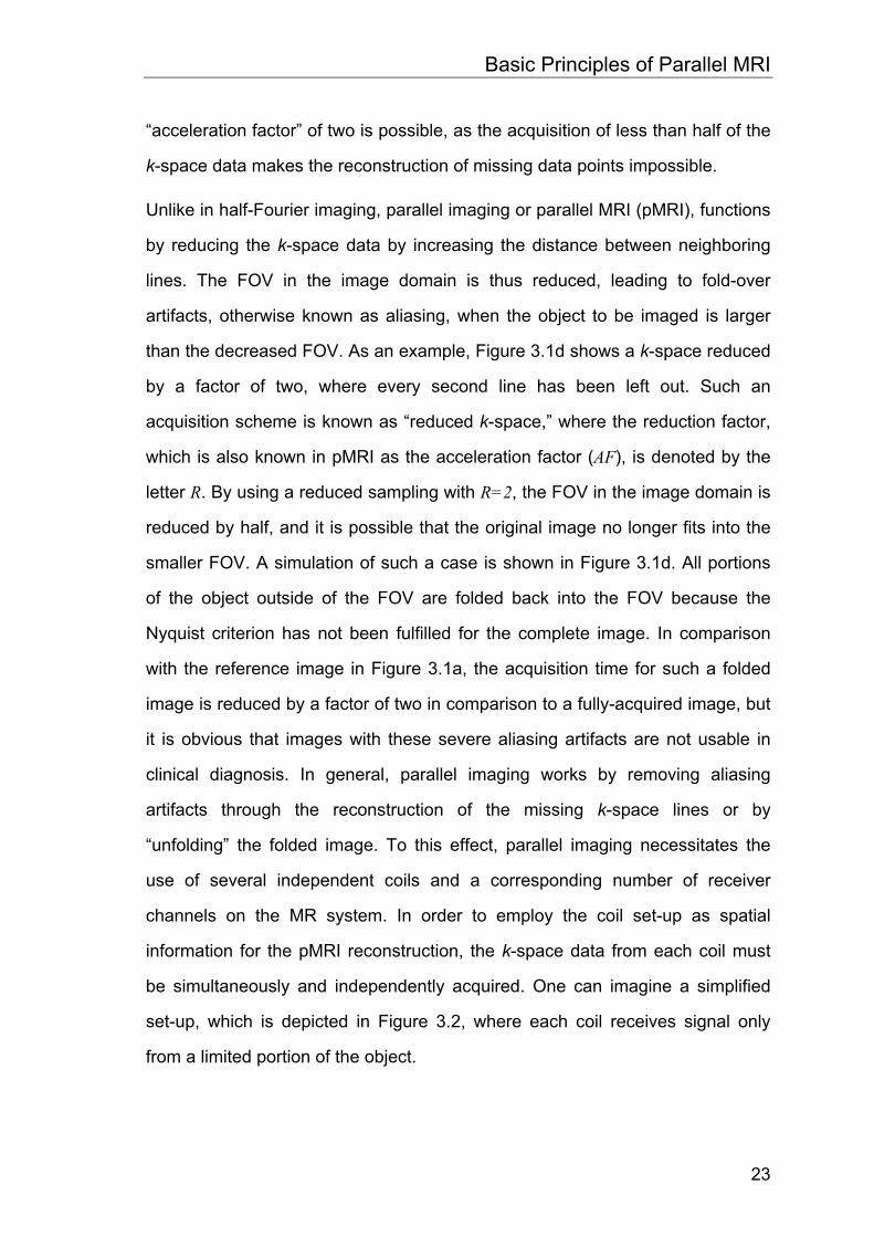
be simultaneously and independently acquired. One can imagine a simplified
set-up, which is depicted in Figure 3.2, where each coil receives signal only
from a limited portion of the object.
Basic Principles of Parallel MRI
24
phase encoding direction
Coil 1 Coil 2
Coil 1 image
Coil 2 image
Full FOV acquisitions Half FOV acquisitions
Coil 1 image
Coil 2 image
a b
c d e
Combined coilimage
Figure 3.2: Schematic depiction of a simplified parallel imaging procedure. (a) Full acquisition using a volume coil, NPhase phase encoding steps are required. (b) Two surface coils, each with a boxcar-like sensitivity profile over the FOV in phase encoding direction. (c) Full acquisitions with these surface coils. The range of sensitivity covers approximately half of the FOV. (d) Half FOV acquisition with NPhase/2 phase encoding steps. (e) Combination of the two images to obtain a full FOV image. This figure is reprinted from reference [71].
Basic Principles of Parallel MRI
25
The acquisition covers a reduced FOV in the image domain, and thus a reduced
k-space, but does so simultaneously for several receiver coils which acquire
information from different spatial locations in the object separately.
If the individual coil images are examined together, an image of the complete
object can be obtained. This method of arriving at a complete image using the
reduced k-space data from multiple coils is the simplest form of pMRI, and is
known as PILS [22]. This straightforward technique only works for coils with
localized sensitivities, thus in most cases, only small coils. For the coils
normally used in clinical MR scanners, more advanced techniques which take
the variations in coil sensitivity into account more accurately than PILS must be
used.
3.2 A Short History of Parallel MRI
In parallel imaging the number of phase-encoding steps and therefore the
acquisition time is reduced compared to conventional imaging. Due to the
parallel imaging reconstruction procedure the same field of view with the same
spatial resolution as in conventional MRI can be obtained even with reduced
phase-encoding steps. This is possible, because multiple independent receiver
coils are used, and the spatial information content of the coils in the array is
exploited to encode and detect multiple MR echoes simultaneously. The key
element of any pMRI system is the application of multiple independent receiver
coils with distinct sensitivities across the object. Traditionally, the main purpose
of this so called phased array technology [29],[30] was to distribute the high
SNR performance of their small component coils over a larger area covered by
the entire array, with no increase in imaging time. Whereas in conventional
Basic Principles of Parallel MRI
26
imaging phased array technology has been used to improve image quality
within the same acquisition time, pMRI techniques are using phased array
technology to provide a significant reduction of MR scan time.
In 1988, before the introduction of the phased array technology in MRI, an early
theoretical proposal for a massively parallel imaging strategy was made [8]. The
phase-encoding gradient steps were entirely replaced by the use of multiple
detectors. In this approach the number of coils in the underlying coil array
approached the number of k-space lines to be acquired for an image. A
subsequent proposal [9],[10] for massively parallel imaging included a more
detailed investigation of feasibility issues, although no image data were
presented.
In current pMRI techniques, the number of coils is significantly smaller than in
the early massively parallel approaches, and therefore technically feasible and
much cheaper. The aim of the pMRI approach is to partially replace the time
consuming gradient encoding steps for image formation. An early proposal for
pMRI using a coil array was made in 1989 [11]. A similar approach was
subsequently described [12], and the first phantom images demonstrating the
underlying principle were presented. This pMRI principle, dubbed subencoding,
involves an “unaliasing” of reduced FOV images. This is achieved by applying
the knowledge of individual coil sensitivity functions in combination with a pixel-
by-pixel matrix inversion to the (reduced FOV) component coil images. This
“unaliasing”-procedure is performed in image space. An optimized and more
general approach of subencoding named SENSE (sensitivity encoding) [13]
was presented in 1999.
The first description of a pMRI technique performed in k-space was presented
in 1987 [14], and a further approach, where missing k-space lines were
generated from a series expansion of reduced k-space raw data sets in two
coils with distinct sensitivities (one homogeneous volume coil and one coil with
Basic Principles of Parallel MRI
27
a constant sensitivity gradient), was presented in 1993 [15]. Even though these
methods never fully worked, they paved the way for the first successful in vivo
pMRI implementation, the SiMultaneous Acquisition of Spatial Harmonics
(SMASH) [16]. Since the introduction of SMASH in 1997 many new approaches
have been proposed to perform in vivo parallel imaging in k-space with greater
robustness and with less effort. One year later, in 1998 the first self-calibrating
technique named AUTO-SMASH [17] was introduced. This method avoids the
necessity of coil sensitivity estimation and therefore works completely in
k-space. These regenerative k-space pMRI techniques, namely SMASH and
AUTO-SMASH, were further developed and improved [18]-[20].
Besides the regenerative k-space and the image domain based pMRI
techniques, a third group of so named hybrid techniques, the method Sensitivity
Profiles from an Array of Coils for Encoding and Reconstruction In Parallel
(SPACE RIP), was introduced in 2000 [21]. To summarize, all modern parallel
imaging methods can be classified into three groups, namely image domain
based techniques (SENSE, PILS), hybrid techniques (SPACE RIP) and
regenerative k-space methods (SMASH, AUTO-SMASH, GRAPPA). In this
classification, the self-calibrating techniques play a special role, because these
techniques do not rely upon accurate knowledge of coil sensitivities.
3.3 k-Space Based Parallel MRI
In order to understand the Cartesian and the non-Cartesian GRAPPA methods,
we first summarize the basic concepts of the k-space based pMRI techniques
SMASH, AUTO-SMASH and VD-AUTO-SMASH.
Basic Principles of Parallel MRI
28
In the original SMASH manuscript [16], it was shown that it is possible to
reconstruct many lines of k-space from a single acquired line. SMASH achieves
this encoding efficiency in that it uses combinations of signals from an array of
surface coils to mimic directly the spatial-encoding normally performed by
phase-encoding gradients. In this approach signals from the various array
components are combined by appropriate linear combinations of component
coil signal with different complex weights )(mln , to generate composite coil
sensitivity profiles CompmC with sinusoidal spatial sensitivity variations (spatial
harmonics of order m) on top of the original coil sensitivity profile CompC0 :
{ }ykimCyxCnyxC yComp
L
ll
ml
Compm ∆== ∑
=
exp),(),( 01
)( (3.1)
Here Cl is the coil sensitivity function of coil l at position ),( yx , where l counts
from one to L for an array coil with L elements and m is an integer which
specifies the spatial harmonic number. If the composite sensitivity profiles
generated in this way match the spatial harmonic modulations of the
phase-encoding gradients, the resulting signal of such a combination is a k-space signal shifted by precisely the same amount ( ykm∆ ) as would have
resulted from a traditional gradient step:
{ }=+= ∫∫ yikxikyxdxdyCkkS yxCompmyx
Compm exp),(),( ρ
( ){ }ykmkixikyxdxdyC yyxComp ∆++= ∫∫ exp),(0 ρ (3.2)
For accurate reconstruction, the SMASH technique relies upon accurate
knowledge or estimation of the relative RF coil sensitivities of the component
coils in the array in order to determine the optimal complex weights )(mln .
Basic Principles of Parallel MRI
29
Therefore, the most important step in a practical SMASH implementation is to
measure the sensitivities of the various array elements. This is a non-trivial
problem in vivo, since many factors affect the NMR signal besides coil
sensitivity variations, making extraction of coil sensitivity information difficult.
There may be additional effects of coil loading that are subject dependent which
can not be easily modeled and may result in unpredictable behavior. In general,
in vivo coil sensitivity calibration can be a problematic, inaccurate and also time
consuming procedure in many cases, especially in the situation of low SNR and
tissue motion. This problem occurs in all pMRI methods based on either the
SMASH or the SENSE approaches.
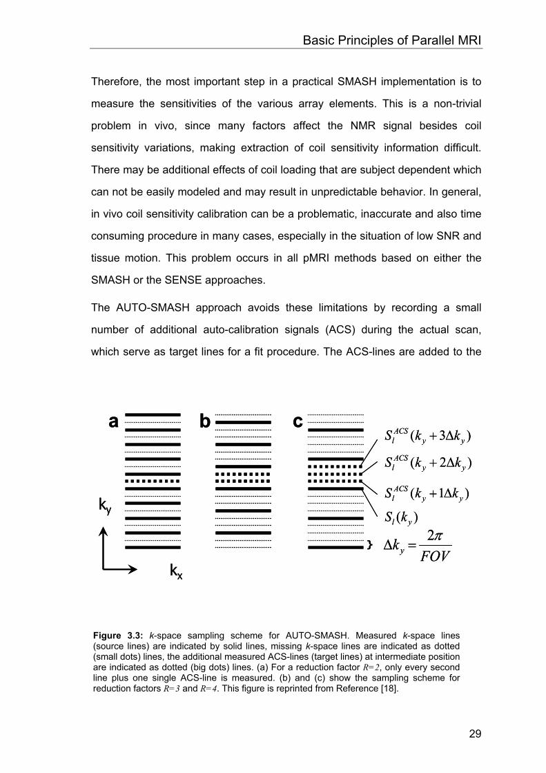
The AUTO-SMASH approach avoids these limitations by recording a small
number of additional auto-calibration signals (ACS) during the actual scan,
which serve as target lines for a fit procedure. The ACS-lines are added to the
kx
ky
a b c
FOVky
π2=∆
)( yl kS
)3( yyACS
l kkS ∆+
}
)2( yyACS
l kkS ∆+
)1( yyACS
l kkS ∆+
kx
ky
a b c
FOVky
π2=∆
)( yl kS
)3( yyACS
l kkS ∆+
}
)2( yyACS
l kkS ∆+
)1( yyACS
l kkS ∆+
Figure 3.3: k-space sampling scheme for AUTO-SMASH. Measured k-space lines (source lines) are indicated by solid lines, missing k-space lines are indicated as dotted (small dots) lines, the additional measured ACS-lines (target lines) at intermediate position are indicated as dotted (big dots) lines. (a) For a reduction factor R=2, only every second line plus one single ACS-line is measured. (b) and (c) show the sampling scheme for reduction factors R=3 and R=4. This figure is reprinted from Reference [18].
Basic Principles of Parallel MRI
30
acquisition, which is shown schematically in Figure 3.3 for reduction factors
from 2-4 (Figure 3.3a - Figure 3.3c).
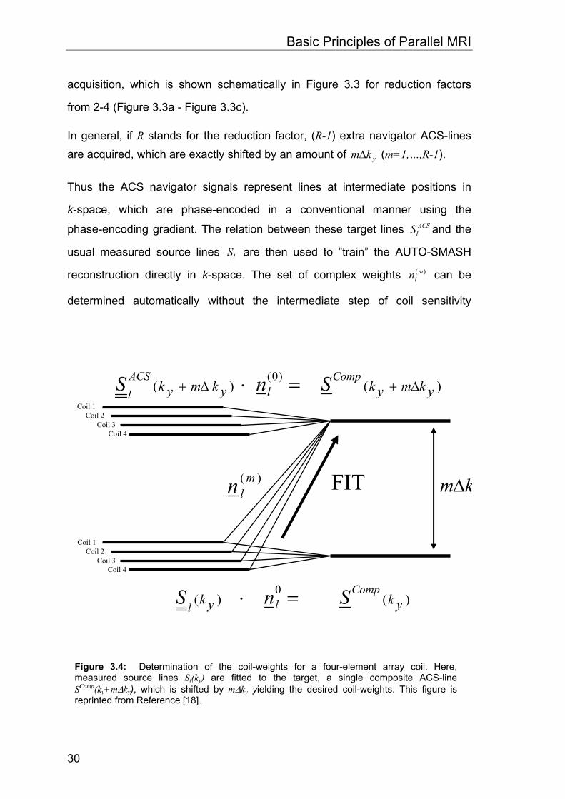
In general, if R stands for the reduction factor, (R-1) extra navigator ACS-lines are acquired, which are exactly shifted by an amount of ykm∆ (m=1,…,R-1).
Thus the ACS navigator signals represent lines at intermediate positions in
k-space, which are phase-encoded in a conventional manner using the
phase-encoding gradient. The relation between these target lines ACSlS and the
usual measured source lines lS are then used to ”train” the AUTO-SMASH
reconstruction directly in k-space. The set of complex weights )(mln can be
determined automatically without the intermediate step of coil sensitivity
)( mln FIT km∆
)()()0(
ykmykykmykComp
lACSl
SnS ∆+∆+ =⋅
)()(0
ykykComp
llSnS =⋅
Coil 1 Coil 2
Coil 3 Coil 4
Coil 1 Coil 2
Coil 3 Coil 4
Figure 3.4: Determination of the coil-weights for a four-element array coil. Here, measured source lines Sl(ky) are fitted to the target, a single composite ACS-line SComp(ky+m∆ky), which is shifted by m∆ky yielding the desired coil-weights. This figure is reprinted from Reference [18].
Basic Principles of Parallel MRI
31
measurements, by using the relations between the conventional acquired data
set and the extra acquired ACS-data. A schematic depiction of this procedure is
shown in Figure 3.4 for a four-element array.
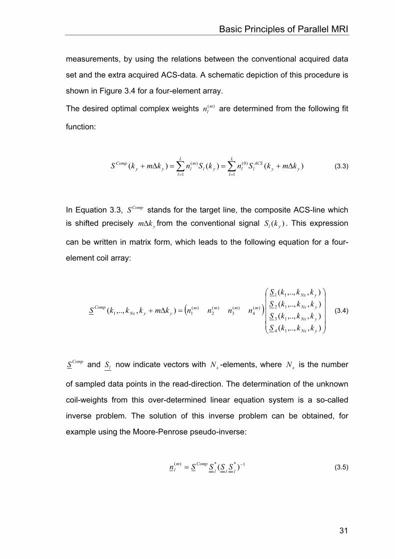
The desired optimal complex weights )(mln are determined from the following fit
function:
∑ ∑= =
∆+==∆+L
l
L
lyy
ACSllyl
mlyy
Comp kmkSnkSnkmkS1 1
)0()( )()()( (3.3)
In Equation 3.3, CompS stands for the target line, the composite ACS-line which
is shifted precisely ykm∆ from the conventional signal )( yl kS . This expression
can be written in matrix form, which leads to the following equation for a four-
element coil array:
( )⎟⎟⎟⎟⎟
⎠
⎞
⎜⎜⎜⎜⎜
⎝
⎛
=∆+
),,..,(),,..,(),,..,(),,..,(
),,..,(
14
13
12
11
)(4
)(3
)(2
)(11
yNx
yNx
yNx
yNx
mmmmyyNx
Comp
kkkSkkkSkkkSkkkS
nnnnkmkkkS (3.4)
CompS and lS now indicate vectors with xN -elements, where xN is the number
of sampled data points in the read-direction. The determination of the unknown
coil-weights from this over-determined linear equation system is a so-called
inverse problem. The solution of this inverse problem can be obtained, for
example using the Moore-Penrose pseudo-inverse:
1**)( )( −=lll
Compml SSSSn (3.5)
Basic Principles of Parallel MRI
32
In Equation 3.5, )(mln stands for the vector of the l complex coil-weights, CompS is
the vector of the target-line, composite auto-calibration signal and *l
S is the
transposed complex conjugate matrix of the l-source lines. Implementation of
the problem in this way also facilitates the incorporation of numerical
conditioning into the process.
In summary, the AUTO-SMASH self-calibration procedure replaces an
experimentally cumbersome and potentially inaccurate coil sensitivity
measurement with a targeted acquisition of a few extra lines of NMR signal
data. Acquisition of the extra (R-1) navigator lines adds only a very small
amount to the total acquisition time, and allows direct ”sensitivity calibration” for
each image, even in regions of inhomogeneous spin density and regardless of
coil loading. If flexible coil arrays are used, AUTO-SMASH can provide accurate
calibrations even if array positions change from scan to scan.
Further improvements of the AUTO-SMASH technique were achieved by using
a variable density acquisition scheme, which is based on the assumption that
some parts of k-space can be measured with more accuracy than others. In
most imaging situations, the signal energy content of k-space lines decreases
with increasing phase-encoding values. This is the essential basis for many
imaging concepts and also the essential basis for the variable density
(VD-) AUTO-SMASH approach [18]. VD-AUTO-SMASH is in spirit similar to the
work presented by Luk et al. [31], who addresses flow artifacts in echo-planar
imaging, Weiger et al. [32], who addresses respiratory motion artifacts and
Chi-Ming Tsai [33] who addresses aliasing artifacts using a variable density
k-space sampling trajectory. Since AUTO-SMASH is a pure k-space related
PPA technique, it is well suited to variable density sampling. In this approach
we reduce residual aliasing artifacts by exploiting the property that in most
images the energy is concentrated around the k-space origin.
Basic Principles of Parallel MRI
33
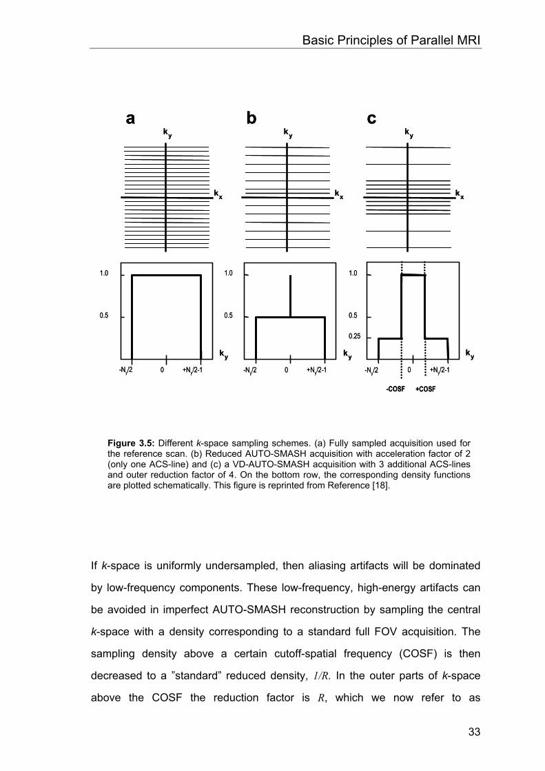
If k-space is uniformly undersampled, then aliasing artifacts will be dominated
by low-frequency components. These low-frequency, high-energy artifacts can
be avoided in imperfect AUTO-SMASH reconstruction by sampling the central
k-space with a density corresponding to a standard full FOV acquisition. The
sampling density above a certain cutoff-spatial frequency (COSF) is then
decreased to a ”standard” reduced density, 1/R. In the outer parts of k-space
above the COSF the reduction factor is R, which we now refer to as
a b c
0.5
1.0
ky
kx
ky
kx
ky
kx
+COSF-COSF
0.5
1.0
ky
0 +Ny/2-1-Ny/2
ky
0 +Ny/2-1-Ny/2
0.5
1.0
ky
0 +Ny/2-1-Ny/2
0.25
a b c
0.5
1.0
ky
kx
ky
kx
ky
kx
+COSF-COSF
0.5
1.0
ky
0 +Ny/2-1-Ny/2
ky
0 +Ny/2-1-Ny/2
0.5
1.0
ky
0 +Ny/2-1-Ny/2
0.25
Figure 3.5: Different k-space sampling schemes. (a) Fully sampled acquisition used for the reference scan. (b) Reduced AUTO-SMASH acquisition with acceleration factor of 2 (only one ACS-line) and (c) a VD-AUTO-SMASH acquisition with 3 additional ACS-lines and outer reduction factor of 4. On the bottom row, the corresponding density functions are plotted schematically. This figure is reprinted from Reference [18].
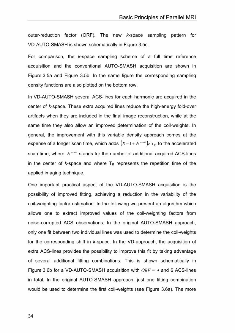
Basic Principles of Parallel MRI
34
outer-reduction factor (ORF). The new k-space sampling pattern for
VD-AUTO-SMASH is shown schematically in Figure 3.5c.
For comparison, the k-space sampling scheme of a full time reference
acquisition and the conventional AUTO-SMASH acquisition are shown in
Figure 3.5a and Figure 3.5b. In the same figure the corresponding sampling
density functions are also plotted on the bottom row.
In VD-AUTO-SMASH several ACS-lines for each harmonic are acquired in the
center of k-space. These extra acquired lines reduce the high-energy fold-over
artifacts when they are included in the final image reconstruction, while at the
same time they also allow an improved determination of the coil-weights. In
general, the improvement with this variable density approach comes at the
expense of a longer scan time, which adds ( ) Rextra TNR ×+−1 to the accelerated
scan time, where extraN stands for the number of additional acquired ACS-lines
in the center of k-space and where TR represents the repetition time of the
applied imaging technique.
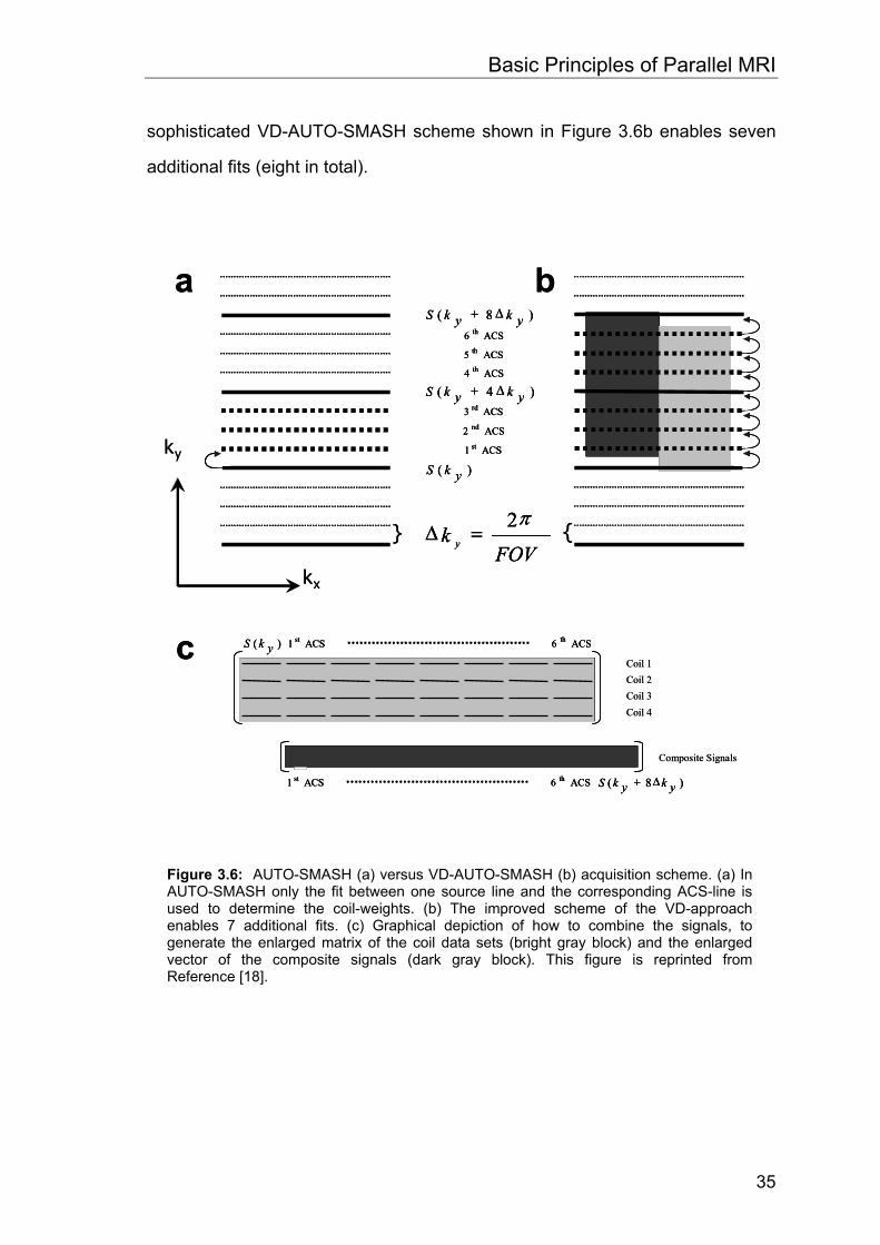
One important practical aspect of the VD-AUTO-SMASH acquisition is the
possibility of improved fitting, achieving a reduction in the variability of the
coil-weighting factor estimation. In the following we present an algorithm which
allows one to extract improved values of the coil-weighting factors from
noise-corrupted ACS observations. In the original AUTO-SMASH approach,
only one fit between two individual lines was used to determine the coil-weights
for the corresponding shift in k-space. In the VD-approach, the acquisition of
extra ACS-lines provides the possibility to improve this fit by taking advantage
of several additional fitting combinations. This is shown schematically in
Figure 3.6b for a VD-AUTO-SMASH acquisition with ORF = 4 and 6 ACS-lines
in total. In the original AUTO-SMASH approach, just one fitting combination
would be used to determine the first coil-weights (see Figure 3.6a). The more
Basic Principles of Parallel MRI
35
sophisticated VD-AUTO-SMASH scheme shown in Figure 3.6b enables seven
additional fits (eight in total).
kx
ky
a b
{
ACS2 nd
ACS4 th
FOVk y
π2=∆
)( ykS
)4( ykykS ∆+
)8( ykykS ∆+
ACS1 st
ACS3 rd
ACS5 th
ACS6 th
}
cCoil 1Coil 2Coil 3Coil 4
)( ykS ACS1 st ACS6 th
ACS1 st ACS6 th )8( ykykS ∆+
Composite Signals
kx
ky
a b
{
ACS2 nd ACS2 nd
ACS4 th ACS4 th
FOVk y
π2=∆
FOVk y
π2=∆
)( ykS )( ykS
)4( ykykS ∆+ )4( ykykS ∆+
)8( ykykS ∆+ )8( ykykS ∆+
ACS1 st ACS1 st
ACS3 rd ACS3 rd
ACS5 th ACS5 th
ACS6 th ACS6 th
}
cCoil 1Coil 2Coil 3Coil 4
)( ykS )( ykS ACS1 st ACS1 st ACS6 th ACS6 th
ACS1 st ACS1 st ACS6 th ACS6 th )8( ykykS ∆+ )8( ykykS ∆+
Composite Signals
Figure 3.6: AUTO-SMASH (a) versus VD-AUTO-SMASH (b) acquisition scheme. (a) In AUTO-SMASH only the fit between one source line and the corresponding ACS-line is used to determine the coil-weights. (b) The improved scheme of the VD-approach enables 7 additional fits. (c) Graphical depiction of how to combine the signals, to generate the enlarged matrix of the coil data sets (bright gray block) and the enlarged vector of the composite signals (dark gray block). This figure is reprinted from Reference [18].
Basic Principles of Parallel MRI
36
One straightforward approach would be to simply average these 8 sets of fitted
coil-weights. The main drawback of this approach is, however, that the
estimation of coil-weights with ACS-lines from the outer part of k-space, with
significantly reduced SNR, is strongly affected by noise, see [17].
A weighted averaging scheme takes the signal energy content of each
particular k-space line into account. It is depicted in Figure 3.6b. The two regular measured source lines )( yyl kmkS ∆+ (with 4,0=m ) and the 6 ACS-lines
)( yyl kmkS ∆+ (with 7,6,5,3,2,1=m ) are composed in a way such that these 8 coil
data sets built an Coilx NN ×⋅8 coil data matrix, where xN is the number of
sampled points in read-direction and CoilN is the number of coils in the array.
This is shown schematically in Figure 3.6c, where the data sets of the above
described lines, which are indicated by the bright gray block, are stacked into a
matrix. The vector of the composite signals is constructed in the same manner, but every line is shifted by yk∆ (indicated by the dark gray block in Figure 3.6c).
The estimation of the coil-weights is then performed with a fit between the
enlarged matrix and the enlarged vector. In this example, the matrix and the
vector are eight times larger compared to those vectors shown in Figure 3.4. In Figure 3.6 only the estimation of the coil-weights, )1(
ln , for a shift about yk∆ is
indicated.
However, it is straightforward to apply the same procedure for larger shifts in
k-space. By computing the Moore-Penrose pseudoinverse in this way, the
relative contribution of the different lines are weighted by the square of their
intensity, which is equivalent to the energy of the respective k-space lines.
Basic Principles of Parallel MRI
37
3.4 Cartesian GRAPPA
A more generalized implementation of the VD-AUTO-SMASH approach [18] is
the GeneRalized Autocalibrating Partially Parallel Acquisitions (GRAPPA)
method. The major difference in GRAPPA is the possibility to reconstruct
uncombined coil images for each coil in the array. Further, compared to
VD-AUTO-SMASH, more data are incorporated into the fit procedure, which
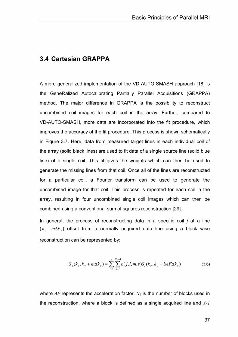
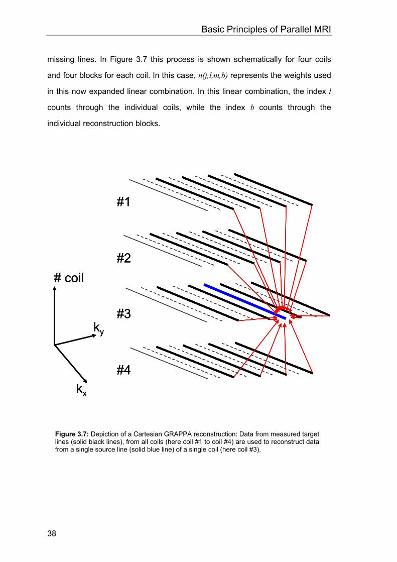
improves the accuracy of the fit procedure. This process is shown schematically
in Figure 3.7. Here, data from measured target lines in each individual coil of
the array (solid black lines) are used to fit data of a single source line (solid blue
line) of a single coil. This fit gives the weights which can then be used to
generate the missing lines from that coil. Once all of the lines are reconstructed
for a particular coil, a Fourier transform can be used to generate the
uncombined image for that coil. This process is repeated for each coil in the
array, resulting in four uncombined single coil images which can then be
combined using a conventional sum of squares reconstruction [29].
In general, the process of reconstructing data in a specific coil j at a line ( yy kmk ∆+ ) offset from a normally acquired data line using a block wise
reconstruction can be represented by:
∑ ∑=
−
=
∆+=∆+L
lyyxl
N
byyxj kbAFkkSbmljnkmkkS
b
1
1
0),(),,,(),( (3.6)
where AF represents the acceleration factor. Nb is the number of blocks used in
the reconstruction, where a block is defined as a single acquired line and A-1
Basic Principles of Parallel MRI
38
missing lines. In Figure 3.7 this process is shown schematically for four coils
and four blocks for each coil. In this case, n(j,l,m,b) represents the weights used
in this now expanded linear combination. In this linear combination, the index l
counts through the individual coils, while the index b counts through the
individual reconstruction blocks.
#1
#4
#3
#2
kx
ky
# coil
#1
#4
#3
#2
kx
ky
# coil
Figure 3.7: Depiction of a Cartesian GRAPPA reconstruction: Data from measured target lines (solid black lines), from all coils (here coil #1 to coil #4) are used to reconstruct data from a single source line (solid blue line) of a single coil (here coil #3).
Basic Principles of Parallel MRI
39
The GRAPPA reconstruction described in Equation 3.6 is formulated as a
discrete shift. However, Equation 3.6 can be reformulated as a convolution on
the k-space data [52]:
( )∑∑∑=
−−=∆+L
lyyxxlyxyyxj
x y
kkSnkmkkS1
1 ),(,),(τ τ
ττττ (3.7)
In this more general description, the coil weights are represented by a two
dimensional convolution kernel. A more detailed description of the choice of the
GRAPPA kernel size and the influence on the final reconstruction will be given
in the corresponding chapters about non-Cartesian GRAPPA.

Basic Principles of Parallel MRI
40
4 A Fast Method for 1D Non-Cartesian Parallel MRI
4.1 Introduction
It has been shown, e.g. in [33]-[35], that non-Cartesian sampling trajectories can
offer inherent advantages for MRI compared to Cartesian acquisition schemes.
Spiral trajectories, for example, make optimal use of the gradient performance
of an MR system, while radial sampling schemes are known to be very robust
even in the case of vast undersampling. Radial and spiral trajectories are two-
dimensional (2D) non-Cartesian sampling strategies. However, the use of
trajectories which are non-Cartesian along one dimension in k-space and
Cartesian along the other can also be advantageous. These so-called one-
dimensional (1D) non-Cartesian trajectories can be designed and optimized for
a robust fold-over artifact behavior. Even though the advantages of non-
Cartesian trajectories are well-known, these trajectories are not in common use
in clinical MRI. In comparison, it is standard in clinical routine to use parallel
imaging [13],[19] to speed up the acquisition of MR examinations. However,
parallel MRI (pMRI) is not without its limitations. All pMRI acquisitions are
affected by an inherent SNR loss, which is, as a rule of thumb, at least
proportional to the square root of the acceleration factor. Additionally, noise
introduced by imperfections in the coil geometry and reconstruction algorithms
further degrades the SNR. In the SENSE method [13], reconstruction is
A Fast Method for 1D Non-Cartesian Parallel MRI
42
performed in the image domain on a pixel-by-pixel basis. Therefore, errors in
this procedure are local and appear as a kind of noise enhancement in the
image. In comparison, the GRAPPA reconstruction [19] is performed in k-space
using a fit procedure between adjacent k-space lines or data points. Since a
single data line or data point in k-space affects the whole image in the image
domain, errors in this procedure are global and appear as remaining fold-over
artifacts in the final image. Therefore, the more relaxed fold-over artifact
behavior of non-Cartesian trajectories is beneficial for such pMRI
reconstructions. Non-Cartesian trajectories have another advantage for pMRI.
Whenever they are designed to oversample a certain part or several parts of
k-space, they are inherently autocalibrated. The autocalibration approach [17] is
a method in which a few k-space data lines or points are sampled densely
enough to fulfill the Nyquist criterion (and may be sampled so densely that they
surpass the Nyquist criterion). The densely-sampled k-space data, otherwise
known as the autocalibration signal (ACS), are then used to derive the
reconstruction parameters, i.e. the coil weights. The ACS data can be acquired
before, after, or during the actual accelerated scan. The acquisition of the ACS
data during the accelerated scan as suggested in [18], the so-called variable
density (VD) approach, has the advantage that the ACS data can be
incorporated into the reconstructed data set. This can significantly increase the
overall image quality of the reconstruction. From the VD approach in [18], where
two different sampling densities were mainly used, it is a logical step to move to
a continuously variable density sampling scheme using a 1D non-Cartesian
trajectory. The more relaxed fold-over artifact behavior of non-Cartesian imaging
makes such a trajectory an ideal complement to pMRI. Although parallel
imaging can benefit from the advantages of non-Cartesian trajectories described
above, and vice versa, the combination of these acquisition schemes with
parallel imaging has yet not entered routine use. The main reason for that are
A Fast Method for 1D Non-Cartesian Parallel MRI
43
the long reconstruction times due to the complex calculations necessary for
non-Cartesian parallel imaging.
In this chapter, which is based on the ideas presented at the 11th ISMRM
Meeting in Toronto [36] and at the 20th ESMRMB Meeting in Rotterdam [37] in
2003, it is shown that one can greatly reduce complexity of the reconstruction
procedure of 1D non-Cartesian pMRI, which is directly related to the
reconstruction times. This is achieved by exploiting a specific property of the
reconstruction parameters used for parallel imaging in k-space. The method
presented here is a promising approach to overcome computational limits,
which are still a hindrance for the use of non-Cartesian pMRI in clinical routine.
4.2 Theory and Methods
4.2.1 Cartesian trajectories and pMRI
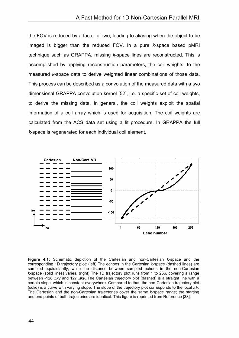
Even though discrete data points are sampled, it is common to depict the
k-space coverage as a line by line acquisition as shown on the left side of
Figure 4.1. Neglecting the dwell time, the Cartesian trajectory can be described
by a one-dimensional function in k-space with a constant slope (dashed line on
the right side of Figure 4.1). The distance between two adjacent sampling points
along such a linear function is constant. This equidistant sampling corresponds
to a constant sampling density in k-space, which is related to a certain FOV. In
parallel imaging, the distance between measured adjacent data lines in k-space,
the slope of the function, is increased by periodically skipping some fraction of
the lines to be measured. Directly related to that is the acquisition speed or the
acceleration factor (AF), when the resolution, the k-space coverage, is
preserved. For example, measuring only every second line would result in an AF
of two. On the other hand, due to the increased sampling distance in k-space
A Fast Method for 1D Non-Cartesian Parallel MRI
44
the FOV is reduced by a factor of two, leading to aliasing when the object to be
imaged is bigger than the reduced FOV. In a pure k-space based pMRI
technique such as GRAPPA, missing k-space lines are reconstructed. This is
accomplished by applying reconstruction parameters, the coil weights, to the
measured k-space data to derive weighted linear combinations of those data.
This process can be described as a convolution of the measured data with a two
dimensional GRAPPA convolution kernel [52], i.e. a specific set of coil weights,
to derive the missing data. In general, the coil weights exploit the spatial
information of a coil array which is used for acquisition. The coil weights are
calculated from the ACS data set using a fit procedure. In GRAPPA the full
k-space is regenerated for each individual coil element.
kx
ky
Cartesian Non-Cart. VD
1 65 129 193 256
-100
-50
0
50
100
Echo numberkx
ky
Cartesian Non-Cart. VD
1 65 129 193 256
-100
-50
0
50
100
Echo number
Figure 4.1: Schematic depiction of the Cartesian and non-Cartesian k-space and the corresponding 1D trajectory plot: (left) The echoes in the Cartesian k-space (dashed lines) are sampled equidistantly, while the distance between sampled echoes in the non-Cartesian k-space (solid lines) varies. (right) The 1D trajectory plot runs from 1 to 256, covering a range between -128 ∆ky and 127 ∆ky. The Cartesian trajectory plot (dashed) is a straight line with a certain slope, which is constant everywhere. Compared to that, the non-Cartesian trajectory plot (solid) is a curve with varying slope. The slope of the trajectory plot corresponds to the local AF. The Cartesian and the non-Cartesian trajectories cover the same k-space range; the starting and end points of both trajectories are identical. This figure is reprinted from Reference [38].
A Fast Method for 1D Non-Cartesian Parallel MRI
45
4.2.2 1D non-Cartesian trajectories
In comparison to the above, 1D non-Cartesian trajectories can be described as
functions with a variable sampling density. Since the distance between
measured data lines is no longer constant, a local acceleration factor (LAF)
must now be defined as the slope of the function at a specific position. As
depicted on the right side of Figure 4.1, the Cartesian and the non-Cartesian
trajectory cover the same k-space range (from -128 to +127) with the same
number of echoes or k-space lines (from 1 to 256.) The non-Cartesian
trajectories used for this study were designed to fulfill the following
requirements:
1. The central part of the trajectory is a linear function, which is
sampled at least at the Nyquist rate (or even more densely).
2. The sampling density of the outer parts of the trajectory decreases
continuously.
3. The k-space position of the outermost point of the non-linear
function is determined by the resolution, i.e. the desired k-space
range.
4. The slope of this function at that specific point, or in other words,
the distance between the two outermost points, which is the
maximum local acceleration factor (LAFMax), should not exceed a
certain value.
5. The linear and the non-linear function should fit together smoothly
(i.e. no discontinuities in the trajectory).
A Fast Method for 1D Non-Cartesian Parallel MRI
46
Since the trajectory itself is point wise symmetric around zero, only the functions
describing the positive part of the trajectory are discussed. Assuming that the
k-space step size ∆ky corresponds to a Nyquist sampling rate, ∆ky is normalized
to one and the trajectory is defined by the following two basic functions:
[ ] 1,0)( ≥=⋅
== OSandnnAFOS
nSDnnf LinearLinear (4.1)
[ ]CubicCubic nnDCnBnAnnf ,0)( 23 =+++= (4.2)
Here, the parameter n is an integer counter of the echoes or k-space lines which
belong to the linear or to the non-linear part of the trajectory. SD is the sampling
density of the linear trajectory. AF is the desired overall acceleration factor
which is controlled by the choice of the FOV in the phase-encoding direction,
and OS is the oversampling factor of the central linear trajectory. To ensure that
the linear trajectory is always oversampled, or sampled at least according to the
Nyquist criterion, even in the case of an overall accelerated acquisition, AF has
to be taken into account in Equation 4.1. For the non-linear trajectory, a cubic
function was chosen, because this type of function offers sufficient degrees of
freedom to adapt this function to the requirements described above. The linear
function in Equation 4.1 has a constant sampling distance between points along
this trajectory. In comparison, the sampling distance of the non-linear function in
Equation 4.2 has a sampling distance which depends upon the echo
number (n). The sampling distance or the local acceleration factor can be
defined as the slope of the function at a specific position.
A Fast Method for 1D Non-Cartesian Parallel MRI
47
11)( ≥⋅
=′ OSAFOS
nf Linear (4.3)
[ ]LinearCubic nnCBnAnnLAFnf ,023)()( 2 =++==′ (4.4)
To meet the requirements defined above, the following set of equations can be
defined using Equation 4.1 – Equation 4.4:
nLinear nTot
yRef kn Λ⋅
yLinear k
AFOSn
Λ⋅⋅
nRef
n
k
nLinear nTot
yRef kn Λ⋅
yLinear k
AFOSn
Λ⋅⋅
nRef
n
k
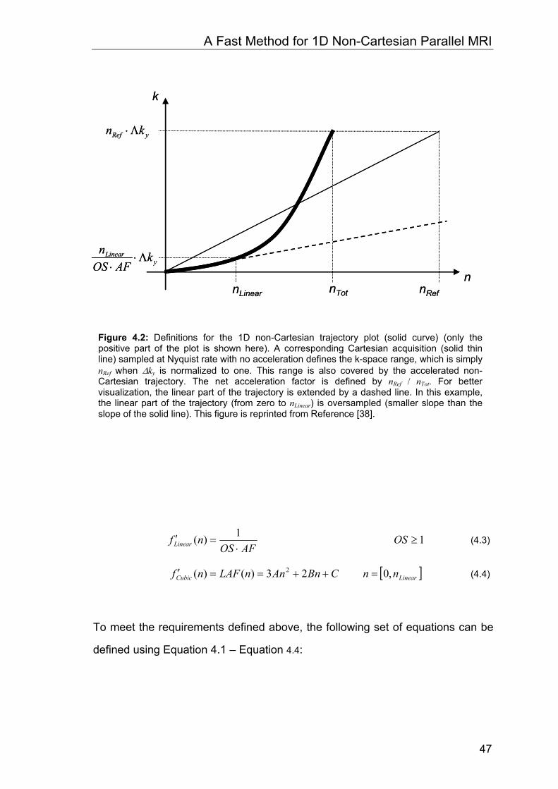
Figure 4.2: Definitions for the 1D non-Cartesian trajectory plot (solid curve) (only the positive part of the plot is shown here). A corresponding Cartesian acquisition (solid thin line) sampled at Nyquist rate with no acceleration defines the k-space range, which is simply nRef when ∆ky is normalized to one. This range is also covered by the accelerated non-Cartesian trajectory. The net acceleration factor is defined by nRef / nTot. For better visualization, the linear part of the trajectory is extended by a dashed line. In this example, the linear part of the trajectory (from zero to nLinear) is oversampled (smaller slope than the slope of the solid line). This figure is reprinted from Reference [38].
A Fast Method for 1D Non-Cartesian Parallel MRI
48
)0()( CubicLinearLinear fnf = (4.5)
RefCubicCubic nnf =)( (4.6)
MinCubicLinearLinear LAFfnf =′≤′ )0()( (4.7)
MaxCubicCubic LAFnf =′ )( (4.8)
The properties of these expressions are depicted in Figure 4.2. A linear
reference function (thin straight line in Figure 4.2) covers a k-space range of
nRef · ∆ky, where nRef is the number of echoes of the positive reference trajectory
without undersampling. Since ∆ky is normalized to one, the slope of this function
is one. The value nRef, corresponds to one-half of the base resolution specified in
the user interface of the MR scanner. In the example of Figure 4.2, the linear
part of the non-Cartesian trajectory runs from zero to nLinear and is oversampled.
The dotted straight line is the extension of this function. Its slope is smaller than
the slope of the linear reference function.
This system of equations, Equation 4.5 – Equation 4.8, can be solved to find the
expressions for the coefficients of the cubic function of Equation 4.2:
32 2Cubic
LinearRef
Cubic
MinMax
nAFOS
nn
nLAFLAFA
⎟⎠⎞
⎜⎝⎛
⋅−
⋅−+
= (4.9)
Cubic
MaxMin
Cubic
LinearRef
nLAFLAF
nAFOS
nnB +⋅
−⎟⎠⎞
⎜⎝⎛
⋅−
⋅=23 2 (4.10)
MinLAFC = (4.11)
AFOS
nD Linear
⋅= (4.12)
A Fast Method for 1D Non-Cartesian Parallel MRI
49
The properties of the trajectory for a pMRI acquisition are controlled by the
choice of the number of linearly sampled data lines (nLinear), the oversampling
factor (OS) of the linear part of the trajectory, the maximum local acceleration
factor (LAFMax) of the non-linear part of the trajectory, and finally the overall
acceleration factor (AF).
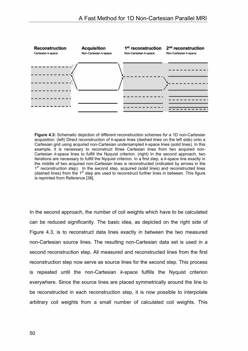
4.2.3 1D non-Cartesian pMRI k-space reconstruction
There are two primary ways to perform a 1D non-Cartesian pMRI reconstruction
in k-space. The first possibility is to reconstruct the data directly onto a
Cartesian grid, which fulfills the Nyquist criterion, as depicted on the left side of
Figure 4.3. From a pair of acquired non-Cartesian lines, termed source lines,
several Cartesian k-space lines are reconstructed. Each reconstructed line with
a different distance, or a different shift, from the source lines. In the example
shown here, three Cartesian k-space lines are reconstructed. This procedure is
advantageous in that it is not necessary to regrid the data; instead one can use
a conventional fast Fourier-Transformation (FFT) to obtain the final image from
the reconstructed Cartesian k-space. The disadvantage of this procedure is that
for each Cartesian k-space line a corresponding set of reconstruction
parameters for the different shifts, the coil weights, has to be calculated. In other
words, for a reconstructed Cartesian data set with nRef number of lines, it is
necessary to calculate nRef sets of coil weights.
A Fast Method for 1D Non-Cartesian Parallel MRI
50
In the second approach, the number of coil weights which have to be calculated
can be reduced significantly. The basic idea, as depicted on the right side of
Figure 4.3, is to reconstruct data lines exactly in between the two measured
non-Cartesian source lines. The resulting non-Cartesian data set is used in a
second reconstruction step. All measured and reconstructed lines from the first
reconstruction step now serve as source lines for the second step. This process
is repeated until the non-Cartesian k-space fulfills the Nyquist criterion
everywhere. Since the source lines are placed symmetrically around the line to
be reconstructed in each reconstruction step, it is now possible to interpolate
arbitrary coil weights from a small number of calculated coil weights. This
ReconstructionCartesian k-space
1st reconstructionNon-Cartesian k-space
AcquisitionNon-Cartesian k-space
2nd reconstructionNon-Cartesian k-space
ReconstructionCartesian k-space
1st reconstructionNon-Cartesian k-space
AcquisitionNon-Cartesian k-space
2nd reconstructionNon-Cartesian k-space
Figure 4.3: Schematic depiction of different reconstruction schemes for a 1D non-Cartesian acquisition: (left) Direct reconstruction of k-space lines (dashed lines on the left side) onto a Cartesian grid using acquired non-Cartesian undersampled k-space lines (solid lines). In this example, it is necessary to reconstruct three Cartesian lines from two acquired non-Cartesian k-space lines to fulfill the Nyquist criterion. (right) In the second approach, two iterations are necessary to fulfill the Nyquist criterion. In a first step, a k-space line exactly in the middle of two acquired non-Cartesian lines is reconstructed (indicated by arrows in the 1st reconstruction step). In the second step, acquired (solid lines) and reconstructed lines (dashed lines) from the 1st step are used to reconstruct further lines in between. This figure is reprinted from Reference [38].
A Fast Method for 1D Non-Cartesian Parallel MRI
51
method can be used as long as the function of the coil weights versus the shift
is a smooth function.
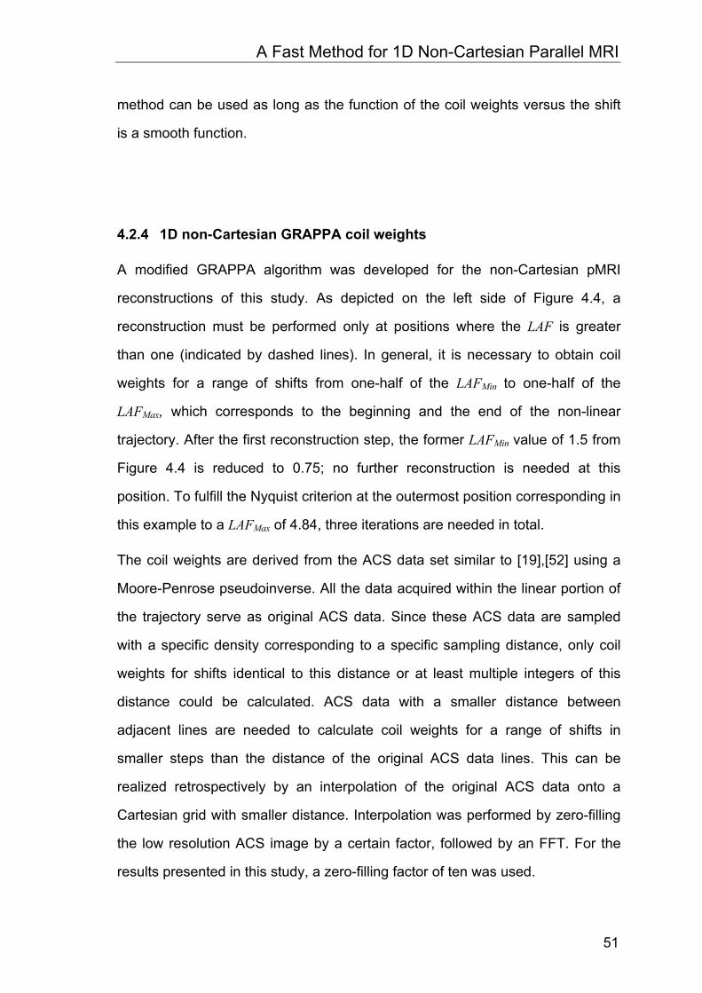
4.2.4 1D non-Cartesian GRAPPA coil weights
A modified GRAPPA algorithm was developed for the non-Cartesian pMRI
reconstructions of this study. As depicted on the left side of Figure 4.4, a
reconstruction must be performed only at positions where the LAF is greater
than one (indicated by dashed lines). In general, it is necessary to obtain coil
weights for a range of shifts from one-half of the LAFMin to one-half of the
LAFMax, which corresponds to the beginning and the end of the non-linear
trajectory. After the first reconstruction step, the former LAFMin value of 1.5 from
Figure 4.4 is reduced to 0.75; no further reconstruction is needed at this
position. To fulfill the Nyquist criterion at the outermost position corresponding in
this example to a LAFMax of 4.84, three iterations are needed in total.
The coil weights are derived from the ACS data set similar to [19],[52] using a
Moore-Penrose pseudoinverse. All the data acquired within the linear portion of
the trajectory serve as original ACS data. Since these ACS data are sampled
with a specific density corresponding to a specific sampling distance, only coil
weights for shifts identical to this distance or at least multiple integers of this
distance could be calculated. ACS data with a smaller distance between
adjacent lines are needed to calculate coil weights for a range of shifts in
smaller steps than the distance of the original ACS data lines. This can be
realized retrospectively by an interpolation of the original ACS data onto a
Cartesian grid with smaller distance. Interpolation was performed by zero-filling
the low resolution ACS image by a certain factor, followed by an FFT. For the
results presented in this study, a zero-filling factor of ten was used.
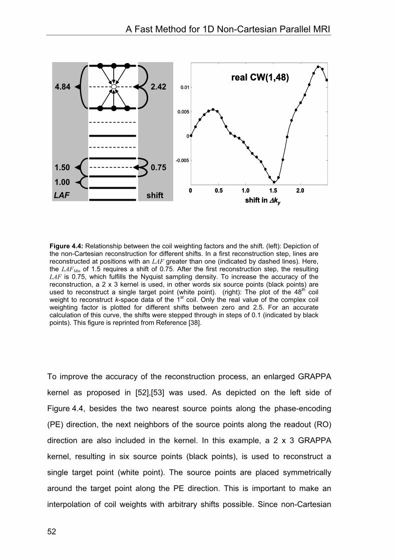
A Fast Method for 1D Non-Cartesian Parallel MRI
52
To improve the accuracy of the reconstruction process, an enlarged GRAPPA
kernel as proposed in [52],[53] was used. As depicted on the left side of
Figure 4.4, besides the two nearest source points along the phase-encoding
(PE) direction, the next neighbors of the source points along the readout (RO)
direction are also included in the kernel. In this example, a 2 x 3 GRAPPA
kernel, resulting in six source points (black points), is used to reconstruct a
single target point (white point). The source points are placed symmetrically
around the target point along the PE direction. This is important to make an
interpolation of coil weights with arbitrary shifts possible. Since non-Cartesian
2.42
0.75
shift shift in ∆ky
real CW(1,48)
0 0.5 1.0 1.5 2.0
-0.005
0
0.005
0.014.84
1.50
LAF1.00
2.42
0.75
shift shift in ∆ky
real CW(1,48)
0 0.5 1.0 1.5 2.0
-0.005
0
0.005
0.014.84
1.50
LAF1.00
Figure 4.4: Relationship between the coil weighting factors and the shift. (left): Depiction of the non-Cartesian reconstruction for different shifts. In a first reconstruction step, lines are reconstructed at positions with an LAF greater than one (indicated by dashed lines). Here, the LAFMin of 1.5 requires a shift of 0.75. After the first reconstruction step, the resulting LAF is 0.75, which fulfills the Nyquist sampling density. To increase the accuracy of the reconstruction, a 2 x 3 kernel is used, in other words six source points (black points) are used to reconstruct a single target point (white point). (right): The plot of the 48th coil weight to reconstruct k-space data of the 1st coil. Only the real value of the complex coil weighting factor is plotted for different shifts between zero and 2.5. For an accurate calculation of this curve, the shifts were stepped through in steps of 0.1 (indicated by black points). This figure is reprinted from Reference [38].
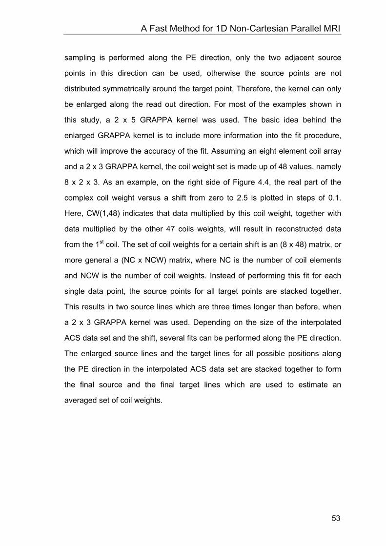
A Fast Method for 1D Non-Cartesian Parallel MRI
53
sampling is performed along the PE direction, only the two adjacent source
points in this direction can be used, otherwise the source points are not
distributed symmetrically around the target point. Therefore, the kernel can only
be enlarged along the read out direction. For most of the examples shown in
this study, a 2 x 5 GRAPPA kernel was used. The basic idea behind the
enlarged GRAPPA kernel is to include more information into the fit procedure,
which will improve the accuracy of the fit. Assuming an eight element coil array
and a 2 x 3 GRAPPA kernel, the coil weight set is made up of 48 values, namely
8 x 2 x 3. As an example, on the right side of Figure 4.4, the real part of the
complex coil weight versus a shift from zero to 2.5 is plotted in steps of 0.1.
Here, CW(1,48) indicates that data multiplied by this coil weight, together with
data multiplied by the other 47 coils weights, will result in reconstructed data
from the 1st coil. The set of coil weights for a certain shift is an (8 x 48) matrix, or
more general a (NC x NCW) matrix, where NC is the number of coil elements
and NCW is the number of coil weights. Instead of performing this fit for each
single data point, the source points for all target points are stacked together.
This results in two source lines which are three times longer than before, when
a 2 x 3 GRAPPA kernel was used. Depending on the size of the interpolated
ACS data set and the shift, several fits can be performed along the PE direction.
The enlarged source lines and the target lines for all possible positions along
the PE direction in the interpolated ACS data set are stacked together to form
the final source and the final target lines which are used to estimate an
averaged set of coil weights.
A Fast Method for 1D Non-Cartesian Parallel MRI
54
4.2.5 Imaging experiments
Imaging studies were performed on a 1.5 T and a 3.0 T whole body scanner
(Magnetom Avanto and Magnetom TIM Trio, Siemens Medical Solutions,
Erlangen, Germany). For signal reception a 12 channel receive-only head coil
array and body coil array was used (Head Matrix and Body Matrix, Siemens
Medical Solutions, Erlangen, Germany).
A 1D non-Cartesian FLASH and a 1D non-Cartesian spin echo sequence were
developed and implemented on the MR scanners using the IDEA software
(Siemens Medical Solutions, Erlangen, Germany).
Healthy volunteers were examined and informed consent was obtained before
each study. The following MR imaging protocol was used:
FLASH: TR = 250 ms, TE = 5.2 ms, alpha = 70°, slice thickness 3.0 mm,
FOV 220 mm, image matrix = 256 x 256.
SE: TR = 300 ms, TE = 15 ms, slice thickness 3.0 mm, FOV 220 mm,
image matrix = 256 x 256.
Image reconstruction was performed off-line using the Matlab programming
environment (The Mathworks, Natick, MA, USA) installed on a conventional PC
with a 2.66 GHz Pentium IV processor and 512 MByte RAM.
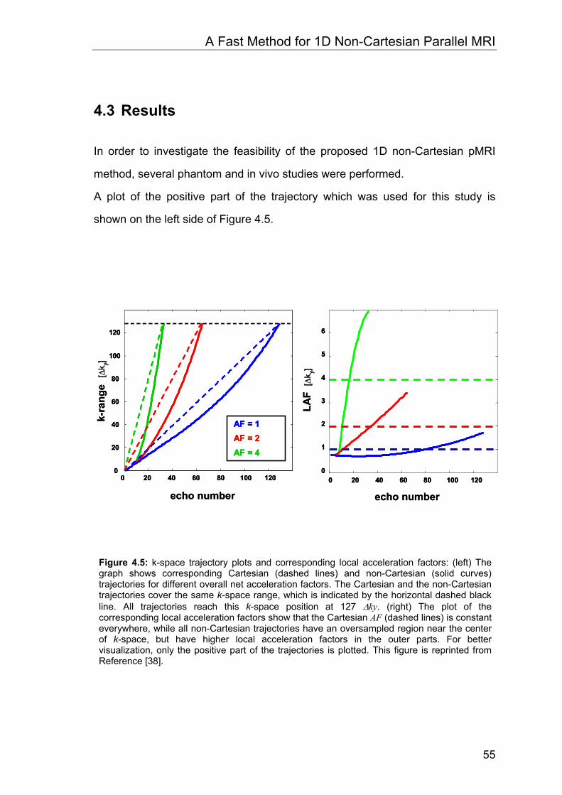
A Fast Method for 1D Non-Cartesian Parallel MRI
55
4.3 Results
In order to investigate the feasibility of the proposed 1D non-Cartesian pMRI
method, several phantom and in vivo studies were performed.
A plot of the positive part of the trajectory which was used for this study is
shown on the left side of Figure 4.5.
LAF
[∆k y
]
echo number0 20 40 60 80 100 120
0
1
2
3
4
5
6
AF = 1AF = 2AF = 4
0 20 40 60 80 100 1200
20
40
60
80
100
120
k-ra
nge
[∆k y
]
echo number
LAF
[∆k y
]
echo number0 20 40 60 80 100 120
0
1
2
3
4
5
6
0 20 40 60 80 100 1200
1
2
3
4
5
6
AF = 1AF = 2AF = 4
0 20 40 60 80 100 1200
20
40
60
80
100
120
AF = 1AF = 2AF = 4
0 20 40 60 80 100 1200
20
40
60
80
100
120
k-ra
nge
[∆k y
]
echo number
Figure 4.5: k-space trajectory plots and corresponding local acceleration factors: (left) The graph shows corresponding Cartesian (dashed lines) and non-Cartesian (solid curves) trajectories for different overall net acceleration factors. The Cartesian and the non-Cartesian trajectories cover the same k-space range, which is indicated by the horizontal dashed black line. All trajectories reach this k-space position at 127 ∆ky. (right) The plot of the corresponding local acceleration factors show that the Cartesian AF (dashed lines) is constant everywhere, while all non-Cartesian trajectories have an oversampled region near the center of k-space, but have higher local acceleration factors in the outer parts. For better visualization, only the positive part of the trajectories is plotted. This figure is reprinted from Reference [38].
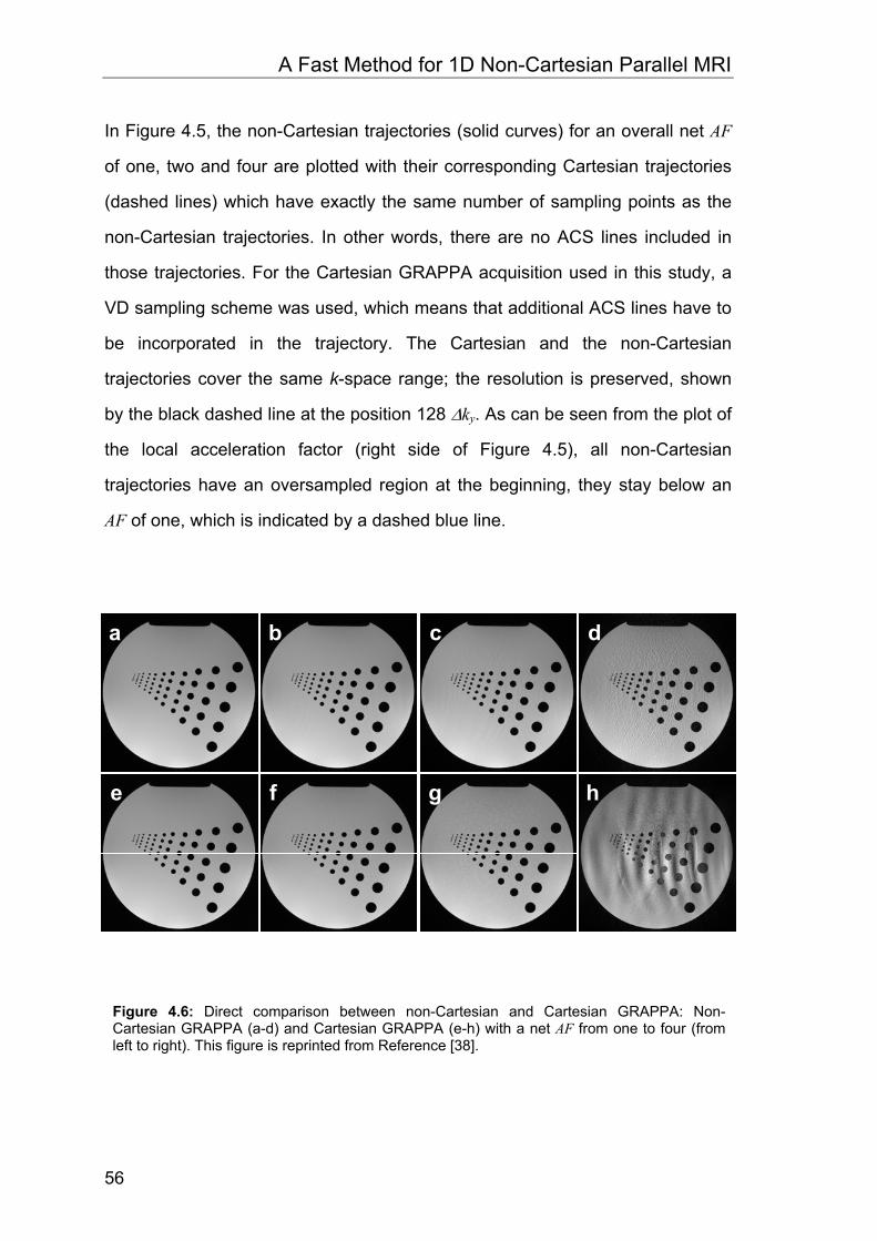
A Fast Method for 1D Non-Cartesian Parallel MRI
56
In Figure 4.5, the non-Cartesian trajectories (solid curves) for an overall net AF
of one, two and four are plotted with their corresponding Cartesian trajectories
(dashed lines) which have exactly the same number of sampling points as the
non-Cartesian trajectories. In other words, there are no ACS lines included in
those trajectories. For the Cartesian GRAPPA acquisition used in this study, a
VD sampling scheme was used, which means that additional ACS lines have to
be incorporated in the trajectory. The Cartesian and the non-Cartesian
trajectories cover the same k-space range; the resolution is preserved, shown
by the black dashed line at the position 128 ∆ky. As can be seen from the plot of
the local acceleration factor (right side of Figure 4.5), all non-Cartesian
trajectories have an oversampled region at the beginning, they stay below an
AF of one, which is indicated by a dashed blue line.
a b c d
e f g h
aa bb cc dd
ee ff gg hh
Figure 4.6: Direct comparison between non-Cartesian and Cartesian GRAPPA: Non-Cartesian GRAPPA (a-d) and Cartesian GRAPPA (e-h) with a net AF from one to four (from left to right). This figure is reprinted from Reference [38].
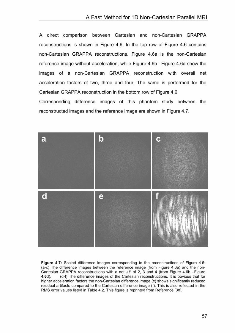
A Fast Method for 1D Non-Cartesian Parallel MRI
57
A direct comparison between Cartesian and non-Cartesian GRAPPA
reconstructions is shown in Figure 4.6. In the top row of Figure 4.6 contains
non-Cartesian GRAPPA reconstructions. Figure 4.6a is the non-Cartesian
reference image without acceleration, while Figure 4.6b –Figure 4.6d show the
images of a non-Cartesian GRAPPA reconstruction with overall net
acceleration factors of two, three and four. The same is performed for the
Cartesian GRAPPA reconstruction in the bottom row of Figure 4.6.
Corresponding difference images of this phantom study between the
reconstructed images and the reference image are shown in Figure 4.7.
a b c
d e f
aa bb cc
dd ee ff
Figure 4.7: Scaled difference images corresponding to the reconstructions of Figure 4.6: (a-c) The difference images between the reference image (from Figure 4.6a) and the non-Cartesian GRAPPA reconstructions with a net AF of 2, 3 and 4 (from Figure 4.6b –Figure 4.6d). (d-f) The difference images of the Cartesian reconstructions. It is obvious that for higher acceleration factors the non-Cartesian difference image (c) shows significantly reduced residual artifacts compared to the Cartesian difference image (f). This is also reflected in the RMS error values listed in Table 4.2. This figure is reprinted from Reference [38].
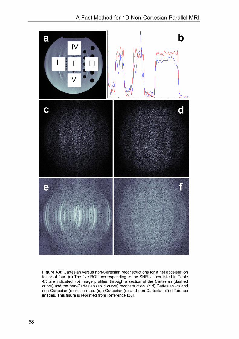
A Fast Method for 1D Non-Cartesian Parallel MRI
58
I II III
IV
V
ba
c
e
d
f
I II III
IV
V
I II III
IV
V
I II III
IV
V
ba
c
e
d
f
Figure 4.8: Cartesian versus non-Cartesian reconstructions for a net acceleration factor of four: (a) The five ROIs corresponding to the SNR values listed in Table 4.3 are indicated. (b) Image profiles, through a section of the Cartesian (dashed curve) and the non-Cartesian (solid curve) reconstruction. (c,d) Cartesian (c) and non-Cartesian (d) noise map. (e,f) Cartesian (e) and non-Cartesian (f) difference images. This figure is reprinted from Reference [38].
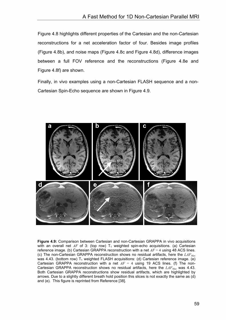
A Fast Method for 1D Non-Cartesian Parallel MRI
59
Figure 4.8 highlights different properties of the Cartesian and the non-Cartesian
reconstructions for a net acceleration factor of four. Besides image profiles
(Figure 4.8b), and noise maps (Figure 4.8c and Figure 4.8d), difference images
between a full FOV reference and the reconstructions (Figure 4.8e and
Figure 4.8f) are shown.
Finally, in vivo examples using a non-Cartesian FLASH sequence and a non-
Cartesian Spin-Echo sequence are shown in Figure 4.9.
Figure 4.9: Comparison between Cartesian and non-Cartesian GRAPPA in vivo acquisitions with an overall net AF of 3: (top row) T1 weighted spin-echo acquisitions. (a) Cartesian reference image. (b) Cartesian GRAPPA reconstruction with a net AF = 4 using 48 ACS lines. (c) The non-Cartesian GRAPPA reconstruction shows no residual artifacts, here the LAFMax was 4.43. (bottom row) T1 weighted FLASH acquisitions: (d) Cartesian reference image. (e) Cartesian GRAPPA reconstruction with a net AF = 4 using 19 ACS lines. (f) The non-Cartesian GRAPPA reconstruction shows no residual artifacts, here the LAFMax was 4.43. Both Cartesian GRAPPA reconstructions show residual artifacts, which are highlighted by arrows. Due to a slightly different breath hold position this slices is not exactly the same as (d) and (e). This figure is reprinted from Reference [38].
A Fast Method for 1D Non-Cartesian Parallel MRI
60
4.4 Discussion
The non-Cartesian trajectory used for this study was optimized to acquire a
sufficient number of ACS lines and to cover exactly the same k-space range as
a corresponding Cartesian trajectory for comparison. However, other 1D non-
Cartesian trajectories can be designed for different purposes [21], [39]-[43], as
for example, to improve the point-spread-function [43]. For all non-Cartesian
acquisitions, 21 ACS lines, including the center line, were acquired with the
linear part of the trajectory. Those lines were acquired at the Nyquist sampling
rate, but it is also possible to oversample this region slightly to make the
calculation of the coil weights more robust. Whenever the FOV is chosen to be
too small, prefolding artifacts would appear in the ACS image and interpolation
via zero-filling in the image domain, or an interpolation directly in k-space will
fail. An oversampling of the center of k-space makes the reconstruction more
robust by preventing possible prefolding.
There are some important differences between the Cartesian and the non-
Cartesian GRAPPA acquisitions, which are listed in Table 4.1. The values listed
in Table 4.1 were used for the phantom study assuming a 256 x 256 image
matrix with a square FOV. Slightly different values were used for the in vivo
abdominal acquisitions (see Figure 4.9) because a rectangular FOV was used.
To achieve a certain overall net acceleration factor for Cartesian GRAPPA, it is
necessary to acquire the data using a higher acceleration factor. This is due to
the fact that in the VD-sampling approach, the ACS lines and the actual
accelerated data are acquired in the same scan. In other words, to achieve a
net acceleration factor of two for a Cartesian GRAPPA acquisition, it is
necessary to acquire the data with an AF of three and 80 ACS lines in the
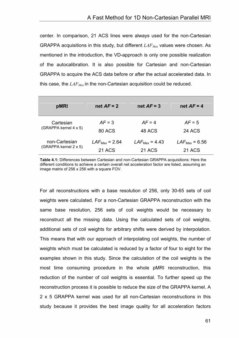
A Fast Method for 1D Non-Cartesian Parallel MRI
61
center. In comparison, 21 ACS lines were always used for the non-Cartesian
GRAPPA acquisitions in this study, but different LAFMax values were chosen. As
mentioned in the introduction, the VD-approach is only one possible realization
of the autocalibration. It is also possible for Cartesian and non-Cartesian
GRAPPA to acquire the ACS data before or after the actual accelerated data. In
this case, the LAFMax in the non-Cartesian acquisition could be reduced.
pMRI net AF = 2 net AF = 3 net AF = 4
Cartesian
(GRAPPA kernel 4 x 5)
AF = 3
80 ACS
AF = 4
48 ACS
AF = 5
24 ACS
non-Cartesian (GRAPPA kernel 2 x 5)
LAFMax = 2.64
21 ACS
LAFMax = 4.43
21 ACS
LAFMax = 6.56
21 ACS
Table 4.1: Differences between Cartesian and non-Cartesian GRAPPA acquisitions: Here the different conditions to achieve a certain overall net acceleration factor are listed, assuming an image matrix of 256 x 256 with a square FOV.
For all reconstructions with a base resolution of 256, only 30-65 sets of coil
weights were calculated. For a non-Cartesian GRAPPA reconstruction with the
same base resolution, 256 sets of coil weights would be necessary to
reconstruct all the missing data. Using the calculated sets of coil weights,
additional sets of coil weights for arbitrary shifts were derived by interpolation.
This means that with our approach of interpolating coil weights, the number of
weights which must be calculated is reduced by a factor of four to eight for the
examples shown in this study. Since the calculation of the coil weights is the
most time consuming procedure in the whole pMRI reconstruction, this
reduction of the number of coil weights is essential. To further speed up the
reconstruction process it is possible to reduce the size of the GRAPPA kernel. A
2 x 5 GRAPPA kernel was used for all non-Cartesian reconstructions in this
study because it provides the best image quality for all acceleration factors
A Fast Method for 1D Non-Cartesian Parallel MRI
62
tested, and it provides reconstruction times comparable to Cartesian GRAPPA
reconstructions with a 4 x 5 GRAPPA kernel.
For a net AF of two, it is possible to speed up the reconstruction process, simply
by using a 2 x 3 GRAPPA kernel, without any noticeable loss in image quality.
This is not the case for higher acceleration factors; for example, for a net AF of
four such a smaller kernel results in a reduced image quality. On the other
hand, reconstructions with a larger kernel size than 2 x 5 will only marginally
improve the overall image quality of the reconstruction, but will drastically
increase the reconstruction time (depending upon the CPU and the memory of
the computer system.)
The time necessary to calculate the coil weights for a net AF of two decreases
from 8 s to 3 s when the kernel size is reduced from a 2 x 5 kernel to a 2 x 3
kernel. In comparison, the time necessary to calculate the weights in Cartesian
GRAPPA with a 4 x 5 kernel and 80 ACS lines is 21 s. Of course, such a large
numbers of ACS lines are generally not employed in conjunction with
VD-sampling. One would instead use between 20 and 30 ACS lines for an AF of
two, resulting in a net AF of about 1.8. The time necessary to calculate the
weights would be between 5 s and 8 s, which is comparable to the time needed
to calculate the weights for the non-Cartesian case.
For the reconstruction of the missing data, the situation is different. The non-
Cartesian reconstruction takes about 15 - 25 s depending on the kernel size,
while in the Cartesian case it is about 8 s. The non-Cartesian reconstruction
also includes the direct Fourier Transformation, which takes about 6 s to
compute. Here, the Cartesian reconstruction is faster and takes about 8 s.
Those numbers should not be treated as absolute values; they can only provide
a rough benchmark, as reconstruction times strongly depend upon the
computer hardware and the software used for calculations.
Compared to the reconstruction times, it is easier to measure the image quality,
for example by using the root-mean-square (RMS) error, the SNR, and the
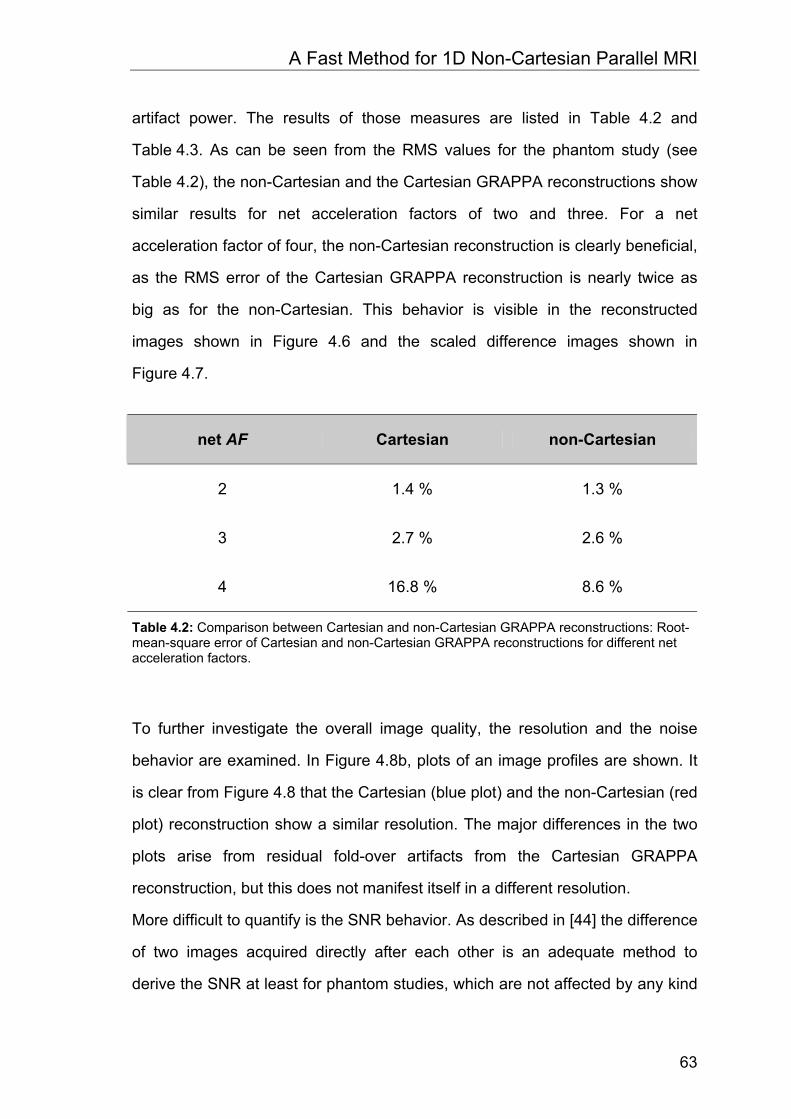
A Fast Method for 1D Non-Cartesian Parallel MRI
63
artifact power. The results of those measures are listed in Table 4.2 and
Table 4.3. As can be seen from the RMS values for the phantom study (see
Table 4.2), the non-Cartesian and the Cartesian GRAPPA reconstructions show
similar results for net acceleration factors of two and three. For a net
acceleration factor of four, the non-Cartesian reconstruction is clearly beneficial,
as the RMS error of the Cartesian GRAPPA reconstruction is nearly twice as
big as for the non-Cartesian. This behavior is visible in the reconstructed
images shown in Figure 4.6 and the scaled difference images shown in
Figure 4.7.
net AF Cartesian non-Cartesian
2 1.4 % 1.3 %
3 2.7 % 2.6 %
4 16.8 % 8.6 %
Table 4.2: Comparison between Cartesian and non-Cartesian GRAPPA reconstructions: Root-mean-square error of Cartesian and non-Cartesian GRAPPA reconstructions for different net acceleration factors.
To further investigate the overall image quality, the resolution and the noise
behavior are examined. In Figure 4.8b, plots of an image profiles are shown. It
is clear from Figure 4.8 that the Cartesian (blue plot) and the non-Cartesian (red
plot) reconstruction show a similar resolution. The major differences in the two
plots arise from residual fold-over artifacts from the Cartesian GRAPPA
reconstruction, but this does not manifest itself in a different resolution.
More difficult to quantify is the SNR behavior. As described in [44] the difference
of two images acquired directly after each other is an adequate method to
derive the SNR at least for phantom studies, which are not affected by any kind
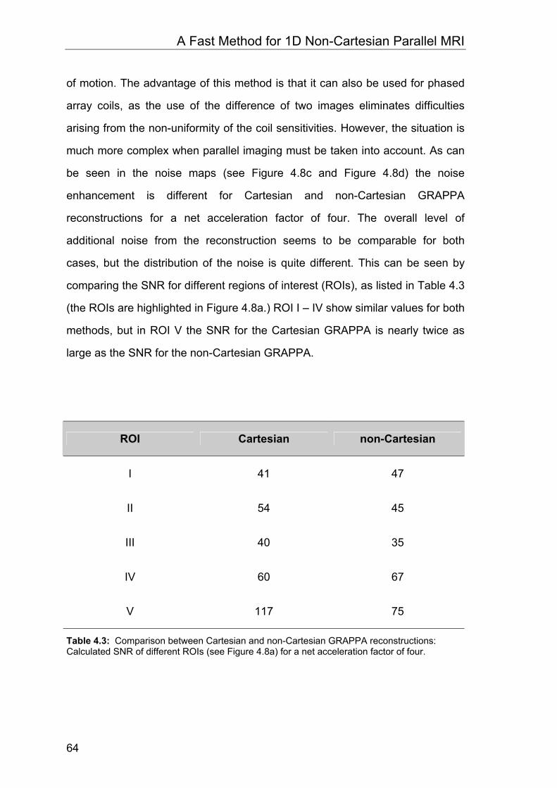
A Fast Method for 1D Non-Cartesian Parallel MRI
64
of motion. The advantage of this method is that it can also be used for phased
array coils, as the use of the difference of two images eliminates difficulties
arising from the non-uniformity of the coil sensitivities. However, the situation is
much more complex when parallel imaging must be taken into account. As can
be seen in the noise maps (see Figure 4.8c and Figure 4.8d) the noise
enhancement is different for Cartesian and non-Cartesian GRAPPA
reconstructions for a net acceleration factor of four. The overall level of
additional noise from the reconstruction seems to be comparable for both
cases, but the distribution of the noise is quite different. This can be seen by
comparing the SNR for different regions of interest (ROIs), as listed in Table 4.3
(the ROIs are highlighted in Figure 4.8a.) ROI I – IV show similar values for both
methods, but in ROI V the SNR for the Cartesian GRAPPA is nearly twice as
large as the SNR for the non-Cartesian GRAPPA.
ROI Cartesian non-Cartesian
I 41 47
II 54 45
III 40 35
IV 60 67
V 117 75
Table 4.3: Comparison between Cartesian and non-Cartesian GRAPPA reconstructions: Calculated SNR of different ROIs (see Figure 4.8a) for a net acceleration factor of four.
A Fast Method for 1D Non-Cartesian Parallel MRI
65
In the non-Cartesian reconstruction, the region of additional noise arising from
the reconstruction process is broader compared to the Cartesian case. Due to
the reconstruction-based additional noise contribution, the SNR can be
significantly different for adjacent ROIs, even when coil sensitivity variations are
accounted for and a homogenous object is imaged. In general, there is a trade
of between SNR and reduction of remaining aliasing artifacts. In the special
case of non-Cartesian pMRI with high acceleration factors presented in this
study, this loss in SNR is obviously more than compensated by the reduction of
the severe aliasing artifacts.
On the other hand the artifact power, as described in [45], is a global quantity of
error in the reconstruction since in addition to the noise due to the pMRI
reconstruction it also takes remaining fold-over artifacts into account. Here, the
benefit of the non-Cartesian GRAPPA strategy is visible. Compared to an
artifact power of 2.9 % for the Cartesian GRAPPA, the artifact power for the
non-Cartesian strategy is only 1.5 %. This behavior is visible in the difference
images shown in Figure 4.8e and Figure 4.8f. Here, the Cartesian/non-
Cartesian GRAPPA reconstructions are subtracted from a full FOV
Cartesian/non-Cartesian reference image.
Finally, in vivo examples using a non-Cartesian spin-echo sequence and a non-
Cartesian gradient-echo sequence are shown in Figure 4.9. An overall net
acceleration factor of 3 was obtained for the Cartesian/non-Cartesian GRAPPA
acquisitions. Remaining fold-over artifacts in the Cartesian GRAPPA images
(highlighted by arrows in Figure 4.9b and Figure 4.9e) are clearly suppressed in
the non-Cartesian GRAPPA reconstructions (Figure 4.9c and Figure 4.9f)
A Fast Method for 1D Non-Cartesian Parallel MRI
66
4.5 Summary
In this chapter, a new approach for 1D non-Cartesian fast GRAPPA
reconstructions has been presented. For this study, gradient echo and spin
echo sequences using an optimized trajectory for 1D non-Cartesian
autocalibrated pMRI were developed. Results from phantom and in vivo
experiments were shown and compared to Cartesian GRAPPA reconstructions.
Compared to previous k-space based non-Cartesian pMRI methods, the
reconstruction time is in the range of the time required for Cartesian pMRI
reconstructions. In addition to this improvement, the non-Cartesian GRAPPA
approach presented in this study shows better results for high acceleration
factors than a corresponding Cartesian GRAPPA reconstruction.
5 A Direct Method for Spiral Parallel MRI
5.1 Introduction
In the last chapter, a fast pMRI reconstruction method for undersampled 1D
non-Cartesian sampled MR data using the GRAPPA technique was introduced.
It was shown that the more relaxed fold-over artifact behavior of the
1D non-Cartesian trajectory is advantageous, especially for high acceleration
factors.
In this chapter, the pMRI reconstruction approach is extended to two
dimensional undersampled non-Cartesian data. Therefore, a new
reconstruction concept is derived compared to the 1D case.
In the past, pMRI reconstructions of 2D non-Cartesian sampling schemes, such
as spiral trajectories, have been reported to require several hours and
sometimes even days to reconstruct the images from a typical fMRI
investigation [54]-[58]. Whereas these previous investigations have performed
the reconstruction using coil sensitivity information from the image domain,
recent approaches for parallel imaging of non-Cartesian k-space sampling by
means of the GRAPPA algorithm [19], work completely in k-space and
represent a promising approach to overcome computational limits [59].
A Direct Method for Spiral Parallel MRI
68
In this chapter, a new reconstruction algorithm for pMRI of non-Cartesian spiral
trajectories is introduced. The algorithm is based on the GRAPPA methodology
and allows the full reconstruction of accelerated data with a computational effort
comparable to Cartesian pMRI. Application of pMRI in fast spiral imaging can
considerably improve image quality through, for example, reduced blurring [57]
and enables high image quality in single-shot spiral images with high spatial
resolution (1x1 mm2 in plane resolution). Potential applications that will benefit
from the improved image quality and/or improved temporal resolution by the
proposed method range from high resolution functional MRI investigations,
arterial spin labeling techniques, and diffusion imaging to cardiac applications
with spiral readout trajectories.
5.2 Theory and Methods
5.2.1 Spiral trajectories
For all acquisitions and calculations in this study, closed form approximate
solutions of Archimedean spirals were used [65]. The kx,ky-trajectories of these
spirals can be described by the following formulas:
))2()1()(2cos()(),(total
actualactualx IItwtatIk πτπτ ⋅−
⋅−+⋅⋅⋅⋅⋅= (5.1)
))2()1()(2sin()(),(total
actualactualy IItwtatIk πτπτ ⋅−
⋅−+⋅⋅⋅⋅⋅= (5.2)
The number of rotations or windings of the spiral is given by w. The parameter a,
an integer, is the maximum k-space radius in multiples of ∆k and determines the
resolution of a spiral acquisition.
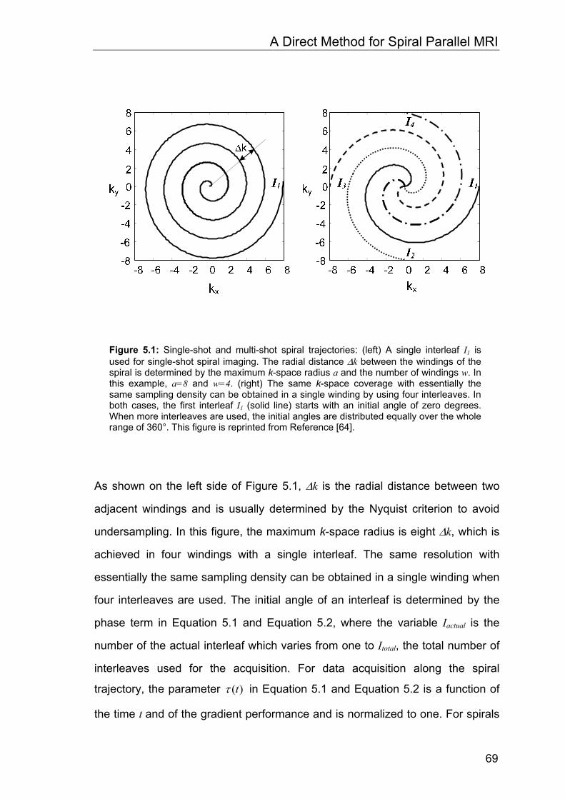
A Direct Method for Spiral Parallel MRI
69
As shown on the left side of Figure 5.1, ∆k is the radial distance between two
adjacent windings and is usually determined by the Nyquist criterion to avoid
undersampling. In this figure, the maximum k-space radius is eight ∆k, which is
achieved in four windings with a single interleaf. The same resolution with
essentially the same sampling density can be obtained in a single winding when
four interleaves are used. The initial angle of an interleaf is determined by the
phase term in Equation 5.1 and Equation 5.2, where the variable Iactual is the
number of the actual interleaf which varies from one to Itotal, the total number of
interleaves used for the acquisition. For data acquisition along the spiral
trajectory, the parameter )(tτ in Equation 5.1 and Equation 5.2 is a function of
the time t and of the gradient performance and is normalized to one. For spirals
Figure 5.1: Single-shot and multi-shot spiral trajectories: (left) A single interleaf I1 is used for single-shot spiral imaging. The radial distance ∆k between the windings of the spiral is determined by the maximum k-space radius a and the number of windings w. In this example, a=8 and w=4. (right) The same k-space coverage with essentially the same sampling density can be obtained in a single winding by using four interleaves. In both cases, the first interleaf I1 (solid line) starts with an initial angle of zero degrees. When more interleaves are used, the initial angles are distributed equally over the whole range of 360°. This figure is reprinted from Reference [64].
A Direct Method for Spiral Parallel MRI
70
running from the center outwards (spiral out), )(tτ runs from zero, with the
acquisition of the center point, to one, the acquisition of the outermost point, in a
pre-defined step size. For the special case that tt =)(τ , the amount of time
which is spent for each winding is constant, regardless of whether the acquired
winding is near the center or in the outer part of the spiral. In other words, the
readout gradients reach their maximum performance at the end of the
acquisition. This acquisition scheme, initially proposed by Ahn et al [66], is
called constant-angular-velocity spiral trajectory. The constant-angular-velocity
spiral trajectory can easily be transformed into a so-called constant-linear-
velocity spiral by the choice of tt =)(τ in Equation 5.1 and Equation 5.2. It has
been shown [67] that the constant-linear-velocity spiral offers some advantages
in terms of SNR and gradient performance as compared to the constant-
angular-velocity spiral.
Although constant-linear-velocity spiral trajectories are more practical, the
constant-angular-velocity spiral trajectories have some interesting properties. In
a constant-angular-velocity Archimedean spiral, the number of sampling points
per winding is constant. If this number is even, all acquired data points are
aligned along straight lines through the origin and are collinear with the center
point, as schematically shown in Figure 5.2. Another important property of such
a spiral is that the distances in k-space between sampled data points along
such a line through the origin are constant, except for those points directly
adjacent to the central k-space point. The symmetry of the constant-angular-
velocity spiral, which is similar to the symmetry of a radial trajectory, was used
by Ahn et al [66] to reconstruct the first spiral images with a convolution-
backprojection algorithm. To emphasize the similarity to radial acquisitions, data
points collected along these lines are further called pseudo-projections. The fast
pMRI approach for spiral imaging presented in this chapter also makes use of
the high symmetry of a constant-angular-velocity trajectory. To benefit from the
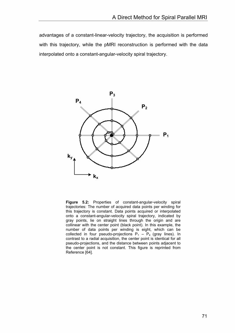
A Direct Method for Spiral Parallel MRI
71
advantages of a constant-linear-velocity trajectory, the acquisition is performed
with this trajectory, while the pMRI reconstruction is performed with the data
interpolated onto a constant-angular-velocity spiral trajectory.
P1
P2
P3
P4
ky
kx
Figure 5.2: Properties of constant-angular-velocity spiral trajectories: The number of acquired data points per winding for this trajectory is constant. Data points acquired or interpolated onto a constant-angular-velocity spiral trajectory, indicated by gray points, lie on straight lines through the origin and are collinear with the center point (black point). In this example, the number of data points per winding is eight, which can be collected in four pseudo-projections P1 – P4 (gray lines). In contrast to a radial acquisition, the center point is identical for all pseudo-projections, and the distance between points adjacent to the center point is not constant. This figure is reprinted from Reference [64].
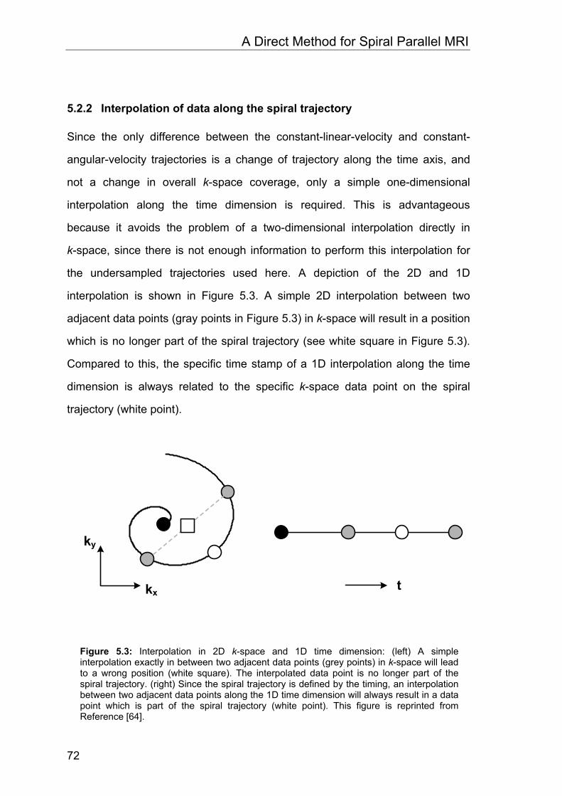
A Direct Method for Spiral Parallel MRI
72
5.2.2 Interpolation of data along the spiral trajectory
Since the only difference between the constant-linear-velocity and constant-
angular-velocity trajectories is a change of trajectory along the time axis, and
not a change in overall k-space coverage, only a simple one-dimensional
interpolation along the time dimension is required. This is advantageous
because it avoids the problem of a two-dimensional interpolation directly in
k-space, since there is not enough information to perform this interpolation for
the undersampled trajectories used here. A depiction of the 2D and 1D
interpolation is shown in Figure 5.3. A simple 2D interpolation between two
adjacent data points (gray points in Figure 5.3) in k-space will result in a position
which is no longer part of the spiral trajectory (see white square in Figure 5.3).
Compared to this, the specific time stamp of a 1D interpolation along the time
dimension is always related to the specific k-space data point on the spiral
trajectory (white point).
ky
kx t
Figure 5.3: Interpolation in 2D k-space and 1D time dimension: (left) A simple interpolation exactly in between two adjacent data points (grey points) in k-space will lead to a wrong position (white square). The interpolated data point is no longer part of the spiral trajectory. (right) Since the spiral trajectory is defined by the timing, an interpolation between two adjacent data points along the 1D time dimension will always result in a data point which is part of the spiral trajectory (white point). This figure is reprinted from Reference [64].
A Direct Method for Spiral Parallel MRI
73
For the 1D interpolation from a constant-linear-velocity spiral trajectory onto a
constant-angular-velocity trajectory it is only necessary to know the timing of
both the original and the target trajectory.
Assuming that the timing is identical for each interleaf, the timing of the
constant-linear-velocity (the original trajectory) can be calculated from the kx, ky
trajectory information by solving Equation 5.1 and Equation 5.2 for the time
function )(tτ .
w
tIktIk
unwrapt actualx
actualy
πτ
2),(),(
arctan)(
⎟⎟⎠
⎞⎜⎜⎝
⎛⎟⎟⎠
⎞⎜⎜⎝
⎛
=⋅ (5.3)
Here, unwrap is a phase unwrap procedure, which adds appropriate multiples of
2π to each phase input to restore the original phase values. As stated earlier,
the timing of the constant-angular-velocity trajectory (the target trajectory) is
simply tt =)(τ .
5.2.3 Reordering of k-space data into a new hybrid space
After interpolation of the data onto a constant-angular-velocity spiral trajectory,
the next step is to exploit the high symmetry of this trajectory to fast pMRI
reconstructions. A simple way to potentially do this is depicted in Figure 5.4.
Data points acquired or interpolated onto such a spiral trajectory can be
regrouped in pseudo-projections. In contrast to the projections of a radial
acquisition, the pseudo-projections P1-P4 in Figure 5.4 all share the same
central k-space point, since it is only acquired once per interleaf in a spiral
acquisition. Further, the distance between the data points adjacent to the central
A Direct Method for Spiral Parallel MRI
74
k-space point is not constant. Due to these inherent asymmetries, this choice of
pseudo-projections can be a problem for pMRI reconstructions.
Different pseudo-projections without these problems can be obtained by simply
changing the data points which constitute the pseudo-projection. The pseudo–
projections, shown on the left side of Figure 5.4, all start with the corresponding
point of the first winding of the spiral and do not share the center point. In
addition, there are now twice as many pseudo-projections (here P1 – P8).
Compared to the pseudo-projections shown in Figure 5.3, the distance between
measured data points is now constant, resulting in a more symmetric
reconstruction.
After specification of the pseudo-projections, the next step is to reorder these
projections from the kx,ky space into a new hybrid space enabling a pseudo-
Cartesian GRAPPA reconstruction of the data. This process can be facilitated
by rearranging the spiral k-space data into a new hybrid space with coordinates
winding (w) and projection angle (Φ), which is shown schematically on the right
side of Figure 5.4. In this hybrid-space, the distance between data points in both
directions is constant. This approach is similar to the radial GRAPPA approach
described in [59], where data points on missing projections between measured
projections are reconstructed in a radius (r) projection angle (Φ) hybrid space. In
comparison to the radial approach where the reconstruction is performed
between different projections, the spiral GRAPPA reconstruction is performed
along a single pseudo-projection. In other words, the orthogonal problem has to
be solved.
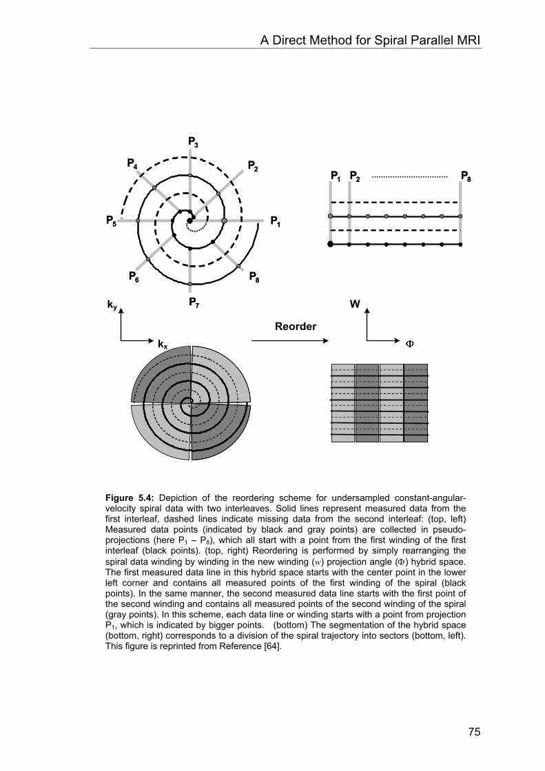
A Direct Method for Spiral Parallel MRI
75
P1
P2
P3
P6
P7
P8
P5
P4P1 P2 P8
P1
P2
P3
P6
P7
P8
P5
P4P1 P2 P8
ky
kx
W
Reorder
Figure 5.4: Depiction of the reordering scheme for undersampled constant-angular-velocity spiral data with two interleaves. Solid lines represent measured data from the first interleaf, dashed lines indicate missing data from the second interleaf: (top, left) Measured data points (indicated by black and gray points) are collected in pseudo-projections (here P1 – P8), which all start with a point from the first winding of the first interleaf (black points). (top, right) Reordering is performed by simply rearranging the spiral data winding by winding in the new winding (w) projection angle (Φ) hybrid space. The first measured data line in this hybrid space starts with the center point in the lower left corner and contains all measured points of the first winding of the spiral (black points). In the same manner, the second measured data line starts with the first point of the second winding and contains all measured points of the second winding of the spiral (gray points). In this scheme, each data line or winding starts with a point from projection P1, which is indicated by bigger points. (bottom) The segmentation of the hybrid space (bottom, right) corresponds to a division of the spiral trajectory into sectors (bottom, left). This figure is reprinted from Reference [64].
A Direct Method for Spiral Parallel MRI
76
5.2.4 Modified GRAPPA Reconstruction
All spiral pMRI reconstructions in this chapter were performed with a modified
Cartesian GRAPPA algorithm [19]. This autocalibrated pMRI method has the
advantage that it does not rely upon accurate coil sensitivity information.
Instead, some fraction of the data is acquired without undersampling, which can
be done before, after or during the actual accelerated acquisition. These so
called autocalibration signals (ACS) are used to derive the pMRI reconstruction
parameters directly in k-space by a fitting procedure [17]-[19]. For each study,
several repetitions without undersampling were acquired. In general, a fully
sampled spiral data set served as ACS signal, while the spiral GRAPPA
reconstruction was performed on undersampled spiral data sets from different
repetitions.
The pMRI reconstruction scheme used for this study is depicted in Figure 5.5.
As shown on the left side of Figure 5.5, several measured data points along the
pseudo-projection P2 are used as source points (black points) to reconstruct a
single missing data point, called the target point (white point). With the above
described reconstruction scheme using four source points along the pseudo-
projection, it would not be possible to reconstruct all missing data in the hybrid
space. At the edges of the hybrid space, it is not possible to reconstruct the
outer most missing data points. Therefore, it is necessary to modify the
reconstruction scheme by simply using a shifted target point position. The target
point can be located at the center position, as shown on the left side of
Figure 5.5, or at any other position (indicated by bright gray points in
Figure 5.5). It is not necessary that the source points are placed symmetrically
around the target point. With the new position of the target point, new
reconstruction parameters have to be calculated.
For all examples in this study, we have used four source points along the
pseudo-projection. More source points will increase the reconstruction times
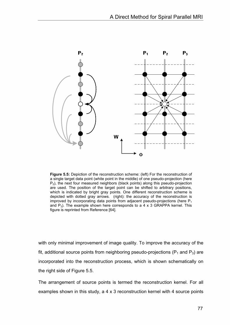
A Direct Method for Spiral Parallel MRI
77
with only minimal improvement of image quality. To improve the accuracy of the
fit, additional source points from neighboring pseudo-projections (P1 and P3) are
incorporated into the reconstruction process, which is shown schematically on
the right side of Figure 5.5.
The arrangement of source points is termed the reconstruction kernel. For all
examples shown in this study, a 4 x 3 reconstruction kernel with 4 source points
Figure 5.5: Depiction of the reconstruction scheme: (left) For the reconstruction of a single target data point (white point in the middle) of one pseudo-projection (here P2), the next four measured neighbors (black points) along this pseudo-projection are used. The position of the target point can be shifted to arbitrary positions, which is indicated by bright gray points. One different reconstruction scheme is depicted with dotted gray arrows. (right): the accuracy of the reconstruction is improved by incorporating data points from adjacent pseudo-projections (here P1 and P3). The example shown here corresponds to a 4 x 3 GRAPPA kernel. This figure is reprinted from Reference [64].
A Direct Method for Spiral Parallel MRI
78
along the pseudo-projection and 3 neighbored projections was used. Instead of
performing the fit for each pseudo- projection, the reconstruction is improved by
using several pseudo-projections to estimate an averaged set of reconstruction
parameters. This is accomplished by dividing the hybrid data set into segments
along the Φ direction, which corresponds to a division of the spiral trajectory into
sectors. This segmentation process is depicted on the bottom of Figure 5.4
using 4 segments in the hybrid space, in other words, 4 sectors in k-space. For
each sector, averaged reconstruction parameters are derived separately; the
total number of sectors was 56 for all examples. An additional segmentation
along the radial direction was not performed, because it was observed that this
does not improve the direct spiral GRAPPA reconstruction.
After reconstructing all missing data points, the complete hybrid space is
reordered back into the normal kx,ky space onto the spiral trajectory. To obtain
the final images, a regridding procedure similar to that described in [68], [69] is
applied to the regenerated spiral data set.
5.2.5 Imaging experiments
Imaging studies were performed on a 1.5 T and on a 3.0 T whole body scanner.
Informed consent was obtained from all subjects prior to the investigations. The
1.5 T MR-scanner (Magnetom Avanto, Siemens Medical Solutions, Erlangen,
Germany) was equipped with 32 independent receiver channels and gradients
achieving peak gradient amplitudes of 45 mT/m and a maximum slew rate of
200 T/m/s. For signal reception a prototype 23 channel receive-only head coil
array was used. The coil elements were mounted on a closely fitting helmet
modeled after the European head standard form EN960/1994 for protective
headgear. The coil circumference is 629 mm, 222 mm maximum in AP, 181 mm
in RL, and 210 mm in SI. The array consisted of 23 overlapped circular surface
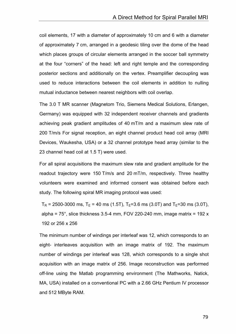
A Direct Method for Spiral Parallel MRI
79
coil elements, 17 with a diameter of approximately 10 cm and 6 with a diameter
of approximately 7 cm, arranged in a geodesic tiling over the dome of the head
which places groups of circular elements arranged in the soccer ball symmetry
at the four “corners” of the head: left and right temple and the corresponding
posterior sections and additionally on the vertex. Preamplifier decoupling was
used to reduce interactions between the coil elements in addition to nulling
mutual inductance between nearest neighbors with coil overlap.
The 3.0 T MR scanner (Magnetom Trio, Siemens Medical Solutions, Erlangen,
Germany) was equipped with 32 independent receiver channels and gradients
achieving peak gradient amplitudes of 40 mT/m and a maximum slew rate of
200 T/m/s For signal reception, an eight channel product head coil array (MRI
Devices, Waukesha, USA) or a 32 channel prototype head array (similar to the
23 channel head coil at 1.5 T) were used.
For all spiral acquisitions the maximum slew rate and gradient amplitude for the
readout trajectory were 150 T/m/s and 20 mT/m, respectively. Three healthy
volunteers were examined and informed consent was obtained before each
study. The following spiral MR imaging protocol was used:
TR = 2500-3000 ms, TE = 40 ms (1.5T), TE=3.6 ms (3.0T) and TE=30 ms (3.0T),
alpha = 75°, slice thickness 3.5-4 mm, FOV 220-240 mm, image matrix = 192 x
192 or 256 x 256
The minimum number of windings per interleaf was 12, which corresponds to an
eight- interleaves acquisition with an image matrix of 192. The maximum
number of windings per interleaf was 128, which corresponds to a single shot
acquisition with an image matrix of 256. Image reconstruction was performed
off-line using the Matlab programming environment (The Mathworks, Natick,
MA, USA) installed on a conventional PC with a 2.66 GHz Pentium IV processor
and 512 MByte RAM.
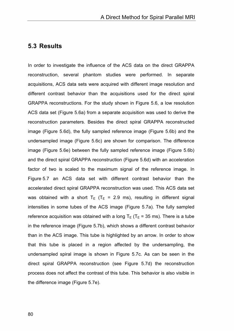
A Direct Method for Spiral Parallel MRI
80
5.3 Results
In order to investigate the influence of the ACS data on the direct GRAPPA
reconstruction, several phantom studies were performed. In separate
acquisitions, ACS data sets were acquired with different image resolution and
different contrast behavior than the acquisitions used for the direct spiral
GRAPPA reconstructions. For the study shown in Figure 5.6, a low resolution
ACS data set (Figure 5.6a) from a separate acquisition was used to derive the
reconstruction parameters. Besides the direct spiral GRAPPA reconstructed
image (Figure 5.6d), the fully sampled reference image (Figure 5.6b) and the
undersampled image (Figure 5.6c) are shown for comparison. The difference
image (Figure 5.6e) between the fully sampled reference image (Figure 5.6b)
and the direct spiral GRAPPA reconstruction (Figure 5.6d) with an acceleration
factor of two is scaled to the maximum signal of the reference image. In
Figure 5.7 an ACS data set with different contrast behavior than the
accelerated direct spiral GRAPPA reconstruction was used. This ACS data set
was obtained with a short TE (TE = 2.9 ms), resulting in different signal
intensities in some tubes of the ACS image (Figure 5.7a). The fully sampled
reference acquisition was obtained with a long TE (TE = 35 ms). There is a tube
in the reference image (Figure 5.7b), which shows a different contrast behavior
than in the ACS image. This tube is highlighted by an arrow. In order to show
that this tube is placed in a region affected by the undersampling, the
undersampled spiral image is shown in Figure 5.7c. As can be seen in the
direct spiral GRAPPA reconstruction (see Figure 5.7d) the reconstruction
process does not affect the contrast of this tube. This behavior is also visible in
the difference image (Figure 5.7e).
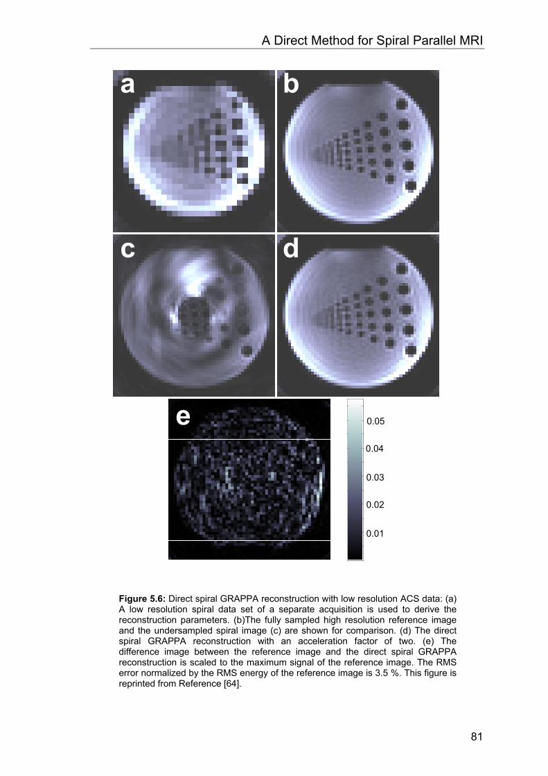
A Direct Method for Spiral Parallel MRI
81
0.05
0.04
0.03
0.02
0.01
Figure 5.6: Direct spiral GRAPPA reconstruction with low resolution ACS data: (a) A low resolution spiral data set of a separate acquisition is used to derive the reconstruction parameters. (b)The fully sampled high resolution reference image and the undersampled spiral image (c) are shown for comparison. (d) The direct spiral GRAPPA reconstruction with an acceleration factor of two. (e) The difference image between the reference image and the direct spiral GRAPPA reconstruction is scaled to the maximum signal of the reference image. The RMS error normalized by the RMS energy of the reference image is 3.5 %. This figure is reprinted from Reference [64].
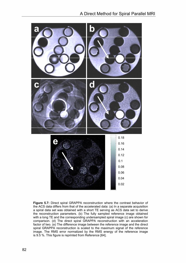
A Direct Method for Spiral Parallel MRI
82
0.02
0.04
0.06
0.08
0.1
0.12
0.14
0.16
0.18
Figure 5.7: Direct spiral GRAPPA reconstruction where the contrast behavior of the ACS data differs from that of the accelerated data: (a) In a separate acquisition a spiral data set was obtained with a short TE serving as ACS data set to derive the reconstruction parameters. (b) The fully sampled reference image obtained with a long TE and the corresponding undersampled spiral image (c) are shown for comparison. (d) The direct spiral GRAPPA reconstruction with an acceleration factor of two. (e) The difference image between the reference image and the direct spiral GRAPPA reconstruction is scaled to the maximum signal of the reference image. The RMS error normalized by the RMS energy of the reference image is 9.5 %. This figure is reprinted from Reference [64].
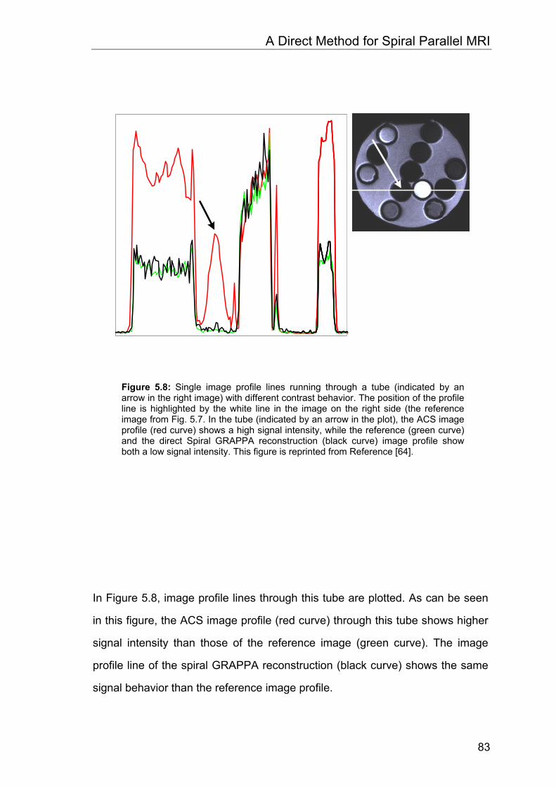
A Direct Method for Spiral Parallel MRI
83
In Figure 5.8, image profile lines through this tube are plotted. As can be seen
in this figure, the ACS image profile (red curve) through this tube shows higher
signal intensity than those of the reference image (green curve). The image
profile line of the spiral GRAPPA reconstruction (black curve) shows the same
signal behavior than the reference image profile.
Figure 5.8: Single image profile lines running through a tube (indicated by an arrow in the right image) with different contrast behavior. The position of the profile line is highlighted by the white line in the image on the right side (the reference image from Fig. 5.7. In the tube (indicated by an arrow in the plot), the ACS image profile (red curve) shows a high signal intensity, while the reference (green curve) and the direct Spiral GRAPPA reconstruction (black curve) image profile show both a low signal intensity. This figure is reprinted from Reference [64].
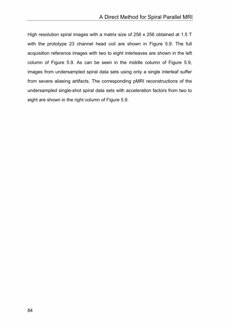
A Direct Method for Spiral Parallel MRI
84
High resolution spiral images with a matrix size of 256 x 256 obtained at 1.5 T
with the prototype 23 channel head coil are shown in Figure 5.9. The full
acquisition reference images with two to eight interleaves are shown in the left
column of Figure 5.9. As can be seen in the middle column of Figure 5.9,
images from undersampled spiral data sets using only a single interleaf suffer
from severe aliasing artifacts. The corresponding pMRI reconstructions of the
undersampled single-shot spiral data sets with acceleration factors from two to
eight are shown in the right column of Figure 5.9.
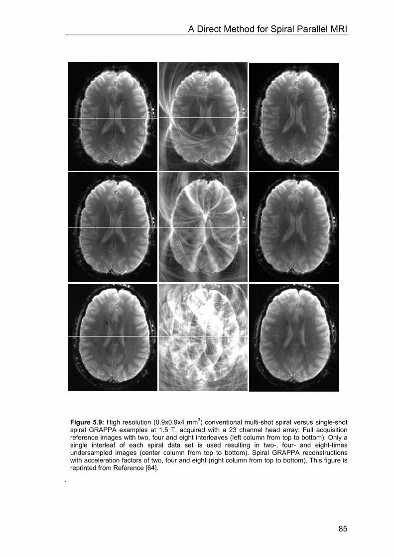
A Direct Method for Spiral Parallel MRI
85
Figure 5.9: High resolution (0.9x0.9x4 mm3) conventional multi-shot spiral versus single-shot spiral GRAPPA examples at 1.5 T, acquired with a 23 channel head array: Full acquisition reference images with two, four and eight interleaves (left column from top to bottom). Only a single interleaf of each spiral data set is used resulting in two-, four- and eight-times undersampled images (center column from top to bottom). Spiral GRAPPA reconstructions with acceleration factors of two, four and eight (right column from top to bottom). This figure is reprinted from Reference [64].
.
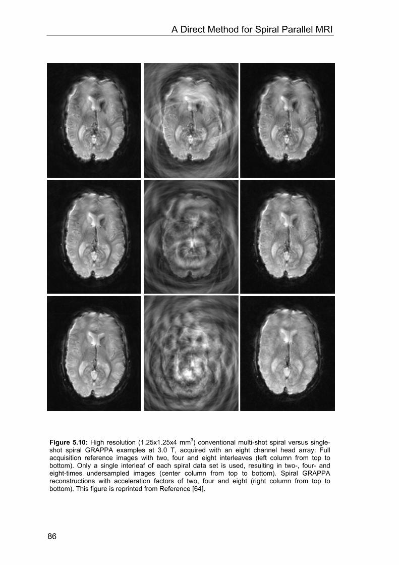
A Direct Method for Spiral Parallel MRI
86
Figure 5.10: High resolution (1.25x1.25x4 mm3) conventional multi-shot spiral versus single-shot spiral GRAPPA examples at 3.0 T, acquired with an eight channel head array: Full acquisition reference images with two, four and eight interleaves (left column from top to bottom). Only a single interleaf of each spiral data set is used, resulting in two-, four- and eight-times undersampled images (center column from top to bottom). Spiral GRAPPA reconstructions with acceleration factors of two, four and eight (right column from top to bottom). This figure is reprinted from Reference [64].
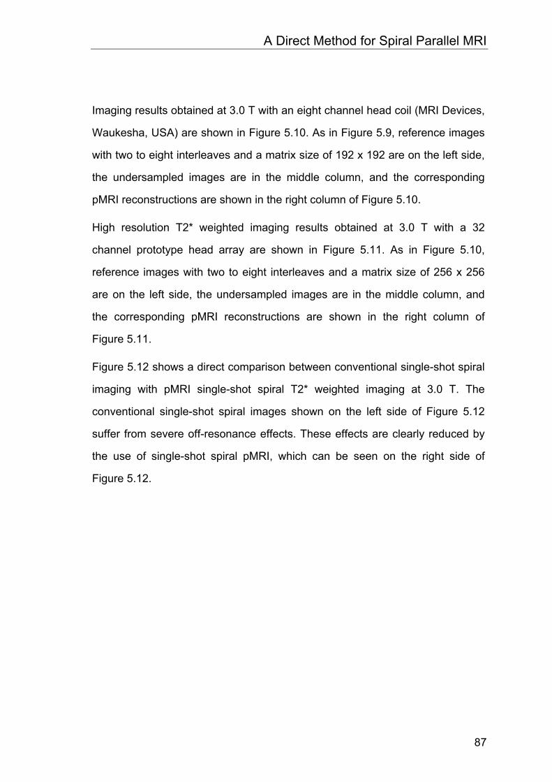
A Direct Method for Spiral Parallel MRI
87
Imaging results obtained at 3.0 T with an eight channel head coil (MRI Devices,
Waukesha, USA) are shown in Figure 5.10. As in Figure 5.9, reference images
with two to eight interleaves and a matrix size of 192 x 192 are on the left side,
the undersampled images are in the middle column, and the corresponding
pMRI reconstructions are shown in the right column of Figure 5.10.
High resolution T2* weighted imaging results obtained at 3.0 T with a 32
channel prototype head array are shown in Figure 5.11. As in Figure 5.10,
reference images with two to eight interleaves and a matrix size of 256 x 256
are on the left side, the undersampled images are in the middle column, and
the corresponding pMRI reconstructions are shown in the right column of
Figure 5.11.
Figure 5.12 shows a direct comparison between conventional single-shot spiral
imaging with pMRI single-shot spiral T2* weighted imaging at 3.0 T. The
conventional single-shot spiral images shown on the left side of Figure 5.12
suffer from severe off-resonance effects. These effects are clearly reduced by
the use of single-shot spiral pMRI, which can be seen on the right side of
Figure 5.12.
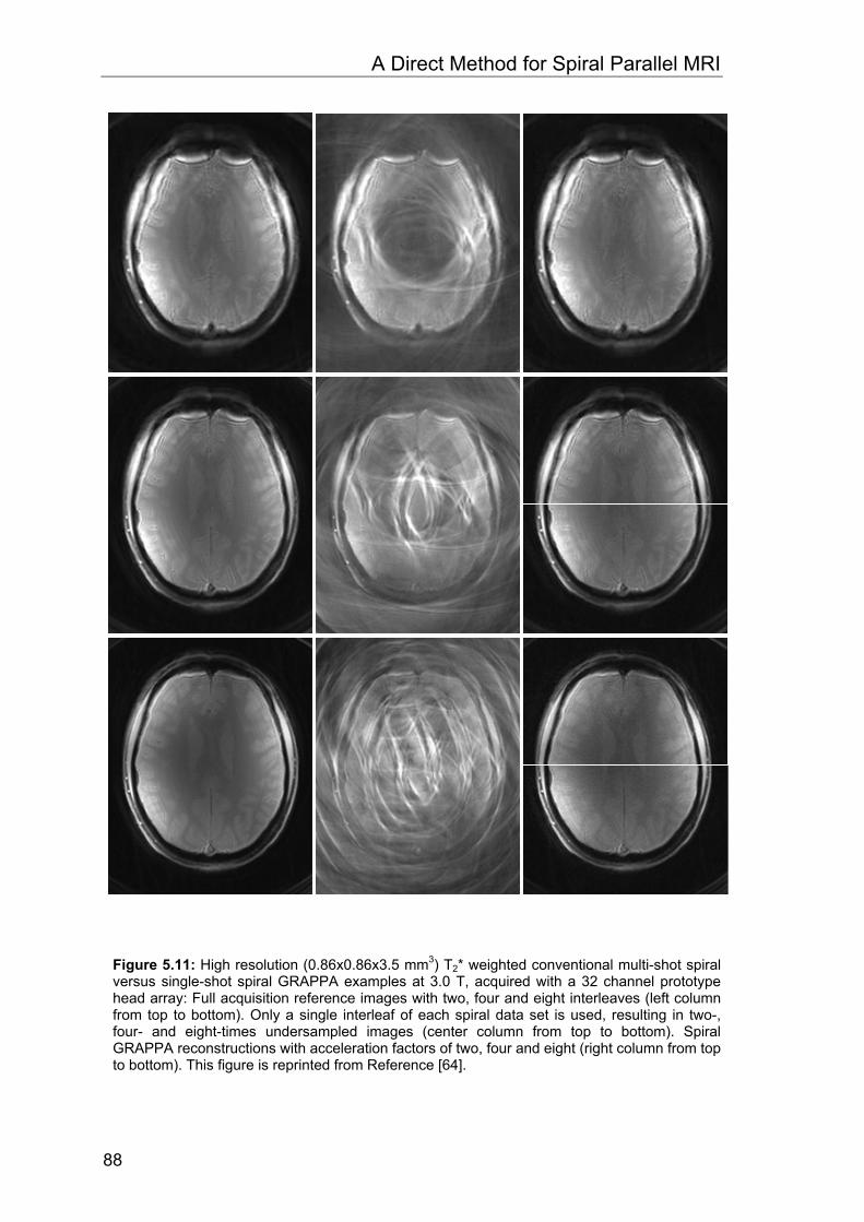
A Direct Method for Spiral Parallel MRI
88
Figure 5.11: High resolution (0.86x0.86x3.5 mm3) T2* weighted conventional multi-shot spiral versus single-shot spiral GRAPPA examples at 3.0 T, acquired with a 32 channel prototype head array: Full acquisition reference images with two, four and eight interleaves (left column from top to bottom). Only a single interleaf of each spiral data set is used, resulting in two-, four- and eight-times undersampled images (center column from top to bottom). Spiral GRAPPA reconstructions with acceleration factors of two, four and eight (right column from top to bottom). This figure is reprinted from Reference [64].
A Direct Method for Spiral Parallel MRI
89
Figure 5.12: High resolution (0.86x0.86x3.5 mm3) T2* weighted single-shot spiral acquisitions at 3.0 T, acquired with a 32 channel prototype head array. Especially in basal regions of the brain, the conventional single-shot spiral acquisition suffers from severe off-resonance artifacts (left column). The single-shot spiral GRAPPA acquisition with acceleration factor of eight shows a significantly improved off-resonance behavior (right column). Two different slices from a healthy volunteer are shown in the top and the bottom row. This figure is reprinted from Reference [64].

A Direct Method for Spiral Parallel MRI
90
5.4 Discussion
Off-resonance effects can severely affect image quality in spiral imaging. Since
these effects scale with the readout duration, the common solution to this
problem is to reduce the readout length. Without undersampling of k-space, this
can be realized by using stronger gradients or several interleaves with
increased total acquisition duration. The effect on the off-resonance artifacts is
clearly visible in the images of Figure 5.9, Figure 5.10 and Figure 5.11. On the
left sides of these figures, fully sampled spiral reference images with two, four
and eight interleaves are shown (from the top to the bottom). The images with
only two interleaves (Figure 5.9, Figure 5.10, and Figure 5.11, upper left corner)
clearly suffer from off-resonance artifacts, in particular in regions near air-tissue
borders. These effects are greatly reduced by increasing the number of
interleaves to four or eight (Figure 5.9, Figure 5.10, and Figure 5.11, center and
bottom row). While off-resonance artifacts are decreased with an increased
number of interleaves, the acquisition time and therefore the sensitivity to flow
and motion are increased. Therefore, the optimal solution for spiral imaging in
this case is a single-shot acquisition with the off-resonance behavior of a multi-
shot approach. With pMRI we are able to come a step closer to this solution as
demonstrated in Figure 5.9, Figure 5.10, and Figure 5.11, where spiral
GRAPPA reconstructions with acceleration factors of two, four and eight are
shown (right column of both figures). Note that all GRAPPA reconstructions in
these figures are single-shot spiral acquisitions. As can be seen in Figure 5.10,
artifacts of the direct spiral GRAPPA approach occurs in image blurring. This is
clearly visible in the extreme case of acceleration factor of eight reconstructions
with only eight coils (see Figure 5.9, bottom row).
A Direct Method for Spiral Parallel MRI
91
A direct comparison between conventional single-shot spiral imaging at 3.0 T
and respective eight-fold accelerated GRAPPA undersampled single-shot
images from two different slices of a healthy volunteer are shown in Figure 5.12.
The long readout duration of 145.5 ms for the conventional single-shot
acquisition (left column of Figure 5.12) with an in-plane resolution of
1.25 x 1.25 mm2 results in severe off-resonance artifacts. With an acceleration
factor of eight (right column of Figure 5.12), the readout duration is reduced to
18.3 ms and the GRAPPA reconstruction shows significantly improved image
quality.
Even though spiral trajectories offer distinct advantages for MRI due to the more
efficient use of the gradient capabilities of the MR system and due to the more
relaxed pMRI artifact behavior, the application of pMRI techniques to spiral
imaging is non-trivial. In general, pMRI reconstructions from undersampled non-
Cartesian data require the solution of large linear equation systems, requiring
long reconstruction times. Recently presented methods [54]-[58] have been
reported to be very time consuming, resulting in reconstruction times for a
typical fMRI data set in the order of a day or even longer. With the approach
presented in this paper, all GRAPPA reconstruction times were in the range or
even less time-consuming than the time needed to perform the gridding
procedure. The most time consuming step in the GRAPPA reconstruction is the
calculation of the coil weights, which was in general several times longer than
the reconstruction of the data itself. In the following two important parameters
are discussed, which can be used to optimize image quality and reconstruction
time for direct spiral GRAPPA:
1. The kernel size of the GRAPPA reconstruction: It was observed that a
4 x 3 kernel size shows the best performance in terms of image
reconstruction time and image quality.
A Direct Method for Spiral Parallel MRI
92
2. Number of segments used for reconstruction: For all examples in this
paper 56 segments were used along the azimuthally direction. An
additional segmentation along the radial direction can potentially
improve the direct GRAPPA reconstruction. However, this also
increases the number of reconstruction parameters, and reduces the
number of reference data for each segment. This, however, may lead to
a reduced quality of the reconstruction parameters and residual artifacts
such as spiral fold-over artifacts in the final image.
For multiple repetitions commonly used in dynamic imaging experiments such
as fMRI, the acquisition of a complete spiral ACS data set and the
determination of the coil weights, the most expensive calculation, have to be
performed only once. The calculated coil weights can then be used to
reconstruct all images from the time series. To increase the accuracy of the fit
over the whole time series, this process could be repeated several times during
the acquisition. The time efficiency of the total acquisition would barely be
affected by the acquisition of a complete spiral ACS data set every hundredth
repetition, for example.
Compared to the method that has been presented recently by Heberlein et al
[60]-[62], which is the direct application of the radial GRAPPA approach [59] on
spiral data, the direct spiral GRAPPA method [63],[64] described in this chapter
includes an optimized GRAPPA reconstruction with an enlarged kernel,
interpolation and reordering of the data. These steps allow one to obtain
accurate single-shot reconstructions. Furthermore, the high symmetry of the
interpolated constant-angular-velocity data makes it possible to improve the fit
process, by increasing the number of data points incorporated into a single fit.
A Direct Method for Spiral Parallel MRI
93
5.5 Summary
In this chapter, a new approach for fast spiral pMRI reconstructions has been
presented. Compared to previous methods, the reconstruction time is reduced
to the same, or even less, time than required for data gridding. The new
approach enables high resolution single-shot spiral pMRI applications even for
T2* weighted fMRI images at high fields. Compared to multi-shot spiral
acquisitions, artifacts from physiological effects (e.g. respiration) are reduced in
the single-shot spiral GRAPPA approach shown here, which is beneficial for
dynamic imaging.
A Direct Method for Spiral Parallel MRI
94
6 Conclusions and Perspectives
Since the first in vivo pMRI implementation, namely SMASH technique in 1997,
the field of parallel imaging has greatly expanded to include a variety of
techniques, each with different advantages and potential areas of clinical
impact. The SENSE technique, introduced in 1998, is the most widespread
parallel imaging technique today. Within the last two years, all of the major MRI
manufacturers, namely Philips (SENSE), Siemens (mSENSE), GE (ASSET)
and Toshiba (SPEEDER), have implemented some type of SENSE algorithm.
The only k-space technique that is currently commercially available is the
GRAPPA method offered by Siemens. However, regardless of the technique is
used, the commercial availability of pMRI means that parallel imaging now has
a broad clinical impact beyond high-end research sites. As mentioned earlier,
the most evident advantage of using pMRI is the shorter total acquisition time
compared to conventional imaging. However, parallel imaging is not without its
limitations. Currently, 2D image acquisitions accelerated by a factor of two to
three are common for many different clinical applications. This holds true even
for the new generation of MR scanners with up to 32 independent receiver
channels, which have the potential for much greater acceleration. Higher
acceleration factors can be achieved under certain conditions, e.g. when a 3D
acquisition is used, exploiting pMRI in two dimensions. As explained in the
Conclusions and Perspectives
96
introduction, there are two potential pitfalls which limit the applicability of pMRI
with high acceleration rates. First, one has to keep in mind that acceleration
with pMRI always incurs an SNR penalty due to the fact that fewer data are
actually acquired. An intrinsic loss of at least the square root of the acceleration
factor has to be expected for all pMRI reconstruction algorithms.
The second important limitation is due to pMRI reconstruction errors, e.g.
residual fold-over artifacts in GRAPPA. This is simply a question of the reliability
of the examination. In the introduction, imaging speed was given as the most
important consideration for clinical application, besides image contrast. At this
point, a third consideration must be added to this list, namely the reliability of
pMRI in daily clinical diagnosis. Depending on the imaging sequence and the
application, the reliability of all parallel imaging methods is reduced if the
acceleration factor reaches a given maximum value.
In this thesis, two new non-Cartesian pMRI methods have been described.
Although the GRAPPA methodology was used, all other k-space based pMRI
techniques can potentially be extended to non-Cartesian acquisitions with the
described methods described. For both methods, it was shown that the synergy of pMRI with non-Cartesian
trajectories is beneficial. The direct comparison between the Cartesian and
1D non-Cartesian GRAPPA reconstructions has shown that the 1D non-
Cartesian GRAPPA method outperforms conventional Cartesian GRAPPA for
high acceleration factors. Residual fold-over artifacts, clearly visible in the
Cartesian GRAPPA reconstruction, are significantly reduced in the
corresponding 1D non-Cartesian GRAPPA method. In general, there is a trade
off between SNR and the reduction of remaining aliasing artifacts. This loss in
Conclusions and Perspectives
97
SNR is obviously more than compensated by the reduction of the severe
aliasing artifacts in the special case of non-Cartesian pMRI with high
acceleration factors presented in this study. The high image quality of the direct
spiral GRAPPA acquisitions, even for high acceleration factors, indicates the
same.
In conclusion, the non-Cartesian pMRI methods described in this thesis have a
more relaxed fold-over artifact behavior, are intrinsically self-calibrating, and
make an effective use of the available gradient performance. Those properties
directly translate into a superior image quality and in a higher reliability as
compared to their Cartesian counterparts. The major hindrance for the use of
pMRI in combination with non-Cartesian trajectories has been reconstruction
time. This burden can now be overcome, clearing the way for non-Cartesian
pMRI in broad clinical use in the near future.
Conclusions and Perspectives
98
7 Bibliography
[1] Purcell EM, Torry HC, Pound RV. Resonance absorption by nuclear
magnetic moments in a solid. Phys Rev, 69:37-38, 1946.
[2] Bloch F, Hansen WW, Packard M. Nuclear induction. Phys Rev, 69:127,
1946.
[3] Lauterbur PC. Image formation by induced local interactions: example
employing nuclear magnetic resonance. Nature, 242:190-191, 1973.
[4] Mansfield P. Multi-planar image formation using NMR spin echoes. J Phys
C Solid State, 10: L55-L58, 1977.
[5] Haase A, Frahm J, Matthaei D, Hänicke W, Merboldt KD. FLASH imaging:
Rapid NMR imaging using low flip-angle pulses. J Magn Reson, 67: 258-
266, 1986.
[6] Hennig J, Nauerth A, Friedburg H. RARE imaging: a fast imaging method
for clinical MR. Magn Reson Med, 3: 823-33, 1986.
[7] Oppelt A, Graumann R, Barfuss H, Fischer H, Hartl W, Schajor W. FISP-a
new fast MRI sequence. Electromedica, 54: 15-18, 1986.
[8] Hutchinson M, Raff U. Fast MRI data acquisition using multiple detectors.
Magn Reson Med, 6: 87-91, 1988.
[9] Kwiat D, Einav S, Navon G. A decoupled coil detector array for fast image
acquisition in magnetic resonance imaging. Med Phys, 18: 251-265, 1991.
[10] Kwiat D, Einav S. Preliminary experimental evaluation of an inverse
source imaging procedure using a decoupled coil detector array in
magnetic resonance imaging. Med Eng Phys, 17: 257-263, 1995.
[11] Kelton JR, Magin RL, Wright SM. An algorithm for rapid image acquisition
using multiple receiver coils. In Proceedings of the 8th Annual Meeting of
SMRM, page 1172, 1989.
Bibliography
100
[12] Ra JB, Rim CY. Fast imaging using subencoding data sets from multiple
detectors. Magn Reson Med, 30: 142-145, 1993.
[13] Pruessmann KP, Weiger M, Scheidegger MB, Boesiger P. SENSE:
Sensitivity encoding for fast MRI. Magn Reson Med, 42: 952-962, 1999.
[14] Carlson JW. An algorithm for NMR imaging reconstruction based on
multiple RF receiver coils. J Magn Reson, 74: 376-380, 1987.
[15] Carlson JW, Minemura T. Imaging time reduction through multiple receiver
coil data acquisition and image reconstruction. Magn Reson Med, 29: 681-
688, 1993.
[16] Sodickson DK, Manning WJ. Simultaneous acquisition of spatial
harmonics (SMASH): Fast imaging with radiofrequency coil arrays. Magn
Reson Med, 38: 591-603, 1997.
[17] Jakob PM, Griswold MA, Edelman RR, Sodickson DK. AUTO-SMASH, a
Self-Calibrating technique for SMASH imaging. MAGMA, 7: 42-54, 1998.
[18] Heidemann RM, Griswold MA, Haase A, Jakob PM. VD-AUTO-SMASH
imaging. Magn Reson Med, 45: 1066-1074, 2001.
[19] Griswold MA, Jakob PM, Heidemann RM, Nittka M, Jellus V, Wang J,
Kiefer B, Haase A. Generalized autocalibrating partially parallel
acquisitions (GRAPPA). Magn Reson Med, 47: 1202-1210, 2002.
[20] Sodickson DK. Tailored SMASH image reconstruction for robust in vivo
parallel MR imaging. Magn Reson Med, 44: 243-251, 2000.
[21] Kyriakos WE, Panych LP, Kacher DK, Westin CF, Bao SM, Mulkern RV,
Jolesz FA. Sensitivity profiles from an array of coils for encoding and
reconstruction in parallel (SPACE RIP). Magn Reson Med, 44: 301-308,
2000.
[22] Griswold MA, Jakob PM, Nittka M, Goldfarb JW, Haase A. Partiallay
parallel imaging with localized sensitivities (PILS). Magn Reson Med, 44:
602-609, 2000.
[23] Ljunggren S. A Simple Graphical Representation of Fourier Based Imaging
Methods. J Magn Reson 54: 338-343, 1983.
[24] Kumar A, Welti D, Ernst RR. NMR Fourier zeugmatography. J Magn
Reson, 18: 69-83, 1975.
Bibliography
101
[25] Twieg DB. Generalized Fourier nuclear magnetic resonance (NMR)
imaging methods. SPIE: 347, 354-364, 1982.
[26] Twieg DB. The k-trajectory formulation of the NMR imaging process with
applications in analysis and synthesis of imaging methods. Med Phys: 10,
610-621, 1983.
[27] Haacke EM, Lindskog ED, Lin W. A fast, iterative, partial-Fourier technique
capable of local phase recovery. J Magn Reson Imaging, 92: 126–145,
1991.
[28] Liang Z-P, Boada F, Constable T, Haacke EM, Lauterbur PC, Smith MR.
Constrained reconstruction methods in MR imaging. Rev Magn Reson
Med, 4: 67–185, 1992.
[29] Roemer PB, Edelstein WA, Hayes CE, Souza SP, Mueller OM. The NMR
phased array. Magn Reson Med, 16: 192-225, 1990.
[30] Hayes CE, Roemer PB. Noise correlations in data simultaneously acquired
from multiple surface coil arrays. Magn Reson Med, 16: 181-191, 1990.
[31] Luk Pat GT, Meyer CH, Pauly JM, Nishimura DG. Reducing Flow Artifacts
in Echo-Planar Imaging. Magn Reson Med, 37: 436-447, 1997.
[32] Weiger M, Börnert P, Proksa R, Schäfer T, Haase A. Motion-Adapted
Gating Based on k-Space Weighting for Reduction of Respiratory Motion
Artifacts. Magn Reson Med, 38: 322-333, 1997.
[33] Tsai C-M, Nishimura DG. Reduced Aliasing Artifacts Using Variable-
Density k-Space Sampling Trajectories. Magn Reson Med, 43: 452-458,
2000.
[34] Boernert P, Stuber M, Botnar RM, Kissinger KV, Koken P, Spuentrup E,
Manning WJ. Direct Comparison of 3D Spiral vs. Cartesian Gradient-Echo
Coronary Magnetic Resonance Angiography. Magn Reson Med, 46: 789-
794, 2001.
[35] Barger AV, Block WF, Toropov Y, Grist TM, Mistretta CA. Time-Resolved
Contrast-Enhanced Imaging With Isotropic Resolution and Broad
Coverage Using an Undersampled 3D Projection Trajectory. Magn Reson
Med, 48: 297–305, 2002.
Bibliography
102
[36] Heidemann RM, Griswold MA, Jakob PM. Fast Parallel Image
Reconstructions with non-Cartesian Trajectories. In Proceedings of the
11th Scientific Meeting ISMRM, Toronto, page 2347, 2003.
[37] Heidemann RM, Griswold MA, Mueller M, Blaimer M, Breuer F, Jakob PM.
Fast non-Cartesian parallel image reconstruction. In Proceedings of the
20th Scientific Meeting ESMRMB, Rotterdam, page 445, 2003.
[38] Heidemann RM, Griswold MA, Seiberlich N, Nittka M, Kannengiesser
SAR, Kiefer B, Jakob PM. A Fast Method for 1D non-Cartesian Parallel
Imaging Using GRAPPA. Magn Reson Med, 57: 1037-1046, 2007.
[39] Aggarwal N, Bresler Y. Optimal sampling in parallel magnetic resonance
imaging. In Proceedings of IEEE International Conference on Image
Processing, Barcelona, page 831-834, 2003.
[40] Jacob M, Xu D, Liang ZP. Optimal selection of phase encodings in parallel
MR imaging. In Proceedings of the 2nd International Workshop on Parallel
Imaging, Zuerich, page 55, 2004.
[41] Hoge WS, Brooks DH, Madore B, Kyriakos WE. A tour of accelerated
parallel MR imaging from a linear systems perspective. Concepts in MR
27A(1):17-37, 2005.
[42] Hoge WS, Kilmer ME, Haker SJ, Brooks DH, Kyriakos WE. Fast
regularized reconstruction of non-uniformly subsampled parallel MRI data.
In Proceedings of the IEEE International Symposium on Biomedical
Imaging, Arlington, page 714-717, 2006.
[43] Geier O, Hahn D, Koestler H. Parallel acquisition for effective density
weighted imaging: PLANED imaging. In Proceedings of the 23rd Scientific
Meeting ESMRMB, Warsaw, page 332, 2006.
[44] Firbank MJ, Coulthard A, Harrison RM, Williams ED. A comparison of two
methods for measuring the signal to noise ratio on MR images. Phys Med
Biol, 44: N261-N264, 1999.
[45] Macgowan CK, Wood ML. Phase-Encode Reordering to Minimize Errors
Caused by Motion. Magn Reson Med, 35: 391-398, 1996.
[46] Constable RT, Gore JC. The loss of small objects in variable TE imaging:
implications for FSE, RARE and EPI. Magn Reson Med, 28: 9-24, 1992.
Bibliography
103
[47] Griswold MA, Jakob PM, Chen Q, Goldfarb J, Manning WJ, Edelman RR,
Sodickson DK. Resolution enhancement in single-shot imaging using
simultaneous acquisition of spatial harmonics (SMASH). Magn Reson
Med, 41: 1236-1245, 1999.
[48] Griswold MA, Jakob PM, Edelman RR, Sodickson DK. Alternative
EPI-acquisition strategies using SMASH. In Proceedings of the 6th Annual
Meeting of the ISMRM, Sidney, Australia, page 423, 1998.
[49] Griswold MA, Jakob PM, Heidemann RM, Nittka M, Wang J, Kiefer B,
Haase A. Off-resonance Artifacts in Single Shot EPI using Partially
Parallel Imaging. In Proceedings of the 9th Annual Meeting of the ISMRM,
Glasgow, Scotland, page 446, 2001.
[50] Heidemann RM, Griswold MA, Porter D, Kiefer B, Nittka M, Wang J,
Haase A, Jakob PM. Minimizing Distortions and Blurring in Diffusion
Weighted Single Shot EPI using High Performance Gradients in
Combination with Parallel Imaging. In Proceedings of the 9th Annual
Meeting of the ISMRM, Glasgow, Scotland, page 169, 2001.
[51] Bammer R, Keeling SL, Augustin M, Pruessmann KP, Wolf R, Stollberger
R, Hartung HP, Fazekas F. Improved diffusion-weighted single-shot echo-
planar imaging (EPI) in stroke using sensitivity encoding (SENSE). Magn
Reson Med, 46: 548–554, 2001.
[52] Griswold MA. “Advanced k-space techniques.” In Proceedings of the 2nd
International Workshop on Parallel Imaging, Zuerich 2004, p 16-18.
[53] Qu P, Shen GX, Wang C, Wu B, Yuan J. Tailored utilization of acquired
k-space points for GRAPPA reconstruction. J Magn Reson, 174: 60-67,
2005.
[54] Kannengiesser SAR, Brenner AR, Noll TG. Accelerated Image
Reconstruction for Sensitivity Encoded Imaging with Arbritrary k-Space
Trajectories. In Proceedings of the 8th Annual Meeting of the ISMRM,
Denver, USA, page 155, 2000.
[55] Pruessmann KP, Weiger M, Börnert P, Boesiger P. Advances in Sensitivity
Encoding With Arbritary k-Space Trajectories. Magn Reson Med, 46: 638-
651, 2001.
Bibliography
104
[56] Yeh EN, Stuber M, McKenzie CA, Ohliger MA, Grant AK, Willig JD,
Sodickson DK. Self-calibrated Spiral Parallel Imaging. In Proceedings of
the 10th Annual Meeting of the ISMRM, Honolulu, USA, page 2390, 2002.
[57] Weiger M, Pruessmann KP, Österbauer R, Börnert P, Boesiger P, Jezzard
P. Sensitivity-Encoded Single-Shot Spiral Imaging for Reduced
Susceptibility Artifacts in BOLD fMRI. Magn Reson Med, 48: 860-866,
2002.
[58] Stenger VA, Sutton BP, Boada FE, Fessler JA, Noll DC. Reversed Spiral
SENSE for fMRI. In Proceedings of the 12th Annual Meeting of the
ISMRM, Kyoto, Japan, page 1024, 2004.
[59] Griswold MA, Heidemann RM, Jakob PM. Direct Parallel Imaging
Reconstruction of Radially Sampled Data Using GRAPPA with Relative
Shifts. In Proceedings of the 11th Annual Meeting of the ISMRM, Toronto,
Canada, page 2349, 2003.
[60] Heberlein KA, Kadah Y, Hu X. Segmented Spiral Parallel Imaging Using
GRAPPA. In Proceedings of the 12th Annual Meeting of the ISMRM,
Kyoto, Japan, page 328, 2004.
[61] Heberlein K, Hu X. Auto-calibrated parallel imaging using dual-density
spirals. In Proceedings of the 2nd International Workshop on Parallel MRI,
Zurich, page 59, 2004.
[62] Heberlein K, Hu X. Auto-calibrated Parallel Spiral Imaging. Magn Reson
Med, 55: 619-625, 2006.
[63] Heidemann RM, Griswold MA, Krüger G, Kannengiesser S, Kiefer B,
Jakob PM. Fast parallel image reconstructions for spiral trajectories. In
Proceedings of the 2nd International Workshop on Parallel MRI, Zurich,
page 27, 2004.
[64] Heidemann RM, Griswold MA, Seiberlich N, Krüger G, Kannengiesser
SAR, Kiefer B, Wiggins G, Wald L, Jakob PM. Direct Parallel Image
Reconstructions for Spiral Trajectories Using GRAPPA. Magn Reson Med,
56: 317-326, 2006.
[65] Glover G. Simple Analytic Spiral k-Space Algorithm. Magn Reson Med, 42:
412-415, 1999.
[66] Ahn CB, Kim JH, Cho ZH. High-speed spiral-scan echo planar NMR
imaging. IEEE Trans Med Imag, MI-5: 2-7, 1986.
Bibliography
105
[67] Macovski A, Meyer C. A novel fast-scanning system. In: Works in progress
of the 5th Annual Meeting of the SMRM, Montreal, Canada, page 156-157,
1986.
[68] Jackson JI, Meyer CH, Nishimura DG, Macovski A. Selection of a
Convolution Function for Fourier Inversion Using Gridding. IEEE Trans
Med Imag, 10: 473-478, 1991.
[69] Meyer CH, Hu BS, Nishimura DG, Macovski A. Fast spiral coronary artery
imaging. Magn Reson Med, 28: 202-213, 1992.
[70] Heidemann RM, Seiberlich N, Griswold MA, Wohlfarth K, Krueger G,
Jakob PM. Perspectives and Limitations of Parallel MR Imaging at High
Field Strengths. Neuroimag Clin N Am, 16: 311–320, 2006.
[71] Heidemann RM, Özsarlak Ö, Parizel PM, Michiels J, Kiefer B, Jellus V,
Müller M, Breuer F, Blaimer M, Griswold MA, Jakob PM. A brief review of
parallel magnetic resonance imaging. Eur Radiol, 13: 2323-2337, 2003.

Bibliography
106
8 Summary Besides image contrast, imaging speed is probably the most important
consideration in clinical magnetic resonance imaging (MRI). MR scanners
currently operate at the limits of potential imaging speed, due to technical and
physiological problems associated with rapidly switched gradient systems.
Parallel imaging (parallel MRI or pMRI) is a method which allows one to
significantly shorten the acquisition time of MR images without changing the
contrast behavior of the underlying MR sequence. The accelerated image
acquisition in pMRI is accomplished without relying on more powerful technical
equipment or exceeding physiological boundaries. Because of these properties,
pMRI is currently employed in many clinical routines, and the number of
applications where pMRI can be used to accelerate imaging is increasing.
However, there is also growing criticism of parallel imaging in certain
applications. The primary reason for this is the intrinsic loss in the SNR due to
the accelerated acquisition. In addition, other effects can also lead to a reduced
image quality. Due to unavoidable inaccuracies in the pMRI reconstruction
process, local and global errors may appear in the final reconstructed image.
The local errors are visible as noise enhancement, while the global errors result
in the so-called fold-over artifacts. The appearance and strength of these
negative effects, and thus the image quality, depend upon different factors,
such as the parallel imaging method chosen, specific parameters in the method,
the sequence chosen, as well as specific sequence parameters. In general, it is
not possible to optimize all of these parameters simultaneously for all
applications. A classic example is functional imaging (fMRI), where one cannot
employ the robust but comparatively slow FLASH sequence. A sequence with a
Summary
108
much shorter acquisition time is essential to achieve a „snap-shot“ image,
where all spurious motion, the so-called physiological noise, is frozen. As a
general rule, the fast Echo-Planer sequence (EPI) is employed, although this
sequence is sensitive to imaging imperfections. For example, typical EPI
artifacts include so-called N/2 ghosts, which can lead to major problems in
parallel imaging reconstructions, even when these artifacts appear less
pronounced in the non-accelerated, conventional acquired image. There are
methods, such as the previously mentioned fMRI EPI sequence, where light
ghosting artifacts are tolerable in conventional images. However, the application
of parallel imaging in these cases can lead to very pronounced image artifacts,
i.e. parallel imaging can amplify errors. On the other hand, there are
applications such as abdominal MR or MR angiography, in which parallel
imaging does not reconstruct images robustly. Thus, the application of parallel
imaging leads to errors. In general, the original euphoria surrounding parallel
imaging in the clinic has been dampened by these problems. The reliability of
the pMRI methods currently implemented is the main criticism. Furthermore, it
has not been possible to significantly increase the maximum achievable
acceleration with parallel imaging despite major technical advances. An
acceleration factor of two is still standard in clinical routine, although the number
of independent receiver channels available on most MR systems (which are a
basic requirement for the application of pMRI) has increased by a factor of 3-6
in recent years.
In this work, a novel and elegant method to address this problem has been
demonstrated. The idea behind the work is to combine two methods in a
synergistic way, namely non-Cartesian acquisition schemes and parallel
imaging. The so-called non-Cartesian acquisition schemes have several
advantages over standard Cartesian acquisitions, in that they are often faster
and less sensitive to physiological noise. In addition, such acquisition schemes
Summary
109
are very robust against fold-over artifacts even in the case of vast
undersampling of k-space.
There are two reasons for the lower sensitivity of such sequence types to fold-
over artifacts. Firstly, fold-over artifacts which are caused by missing or poorly
reconstructed data from the central portion of k-space are very distinct. In most
non-Cartesian acquisition schemes a certain part of the central region of
k-space is oversampled, means the sampling rate is higher than the Nyquist
rate. Through an oversampling of this area in the center of k-space, such high-
signal artifacts can be avoided. In addition, the fact that the k-space lines are
not equidistant in k-space means that the FOV is no longer well-defined, and
that it changes with the position in k-space. The positioning of the resulting fold-
over artifacts then depends on the size of the FOV. As a result of these non-
equidistant lines, the fold-over artifacts are spread over a large area in the
image, and appear less strongly than in Cartesian images.
Despite the advantages described above, non-Cartesian acquisition schemes
are not commonly employed in clinical routines. A reason for that is the
complicated reconstruction techniques which are required to convert the non-
Cartesian data to a Cartesian grid before the fast Fourier transformation can be
employed to arrive at the final MR image. Another reason is that Cartesian
acquisitions are routinely accelerated with parallel imaging, which is not
applicable for non-Cartesian MR acquisitions due to the long reconstruction
times. This negates the speed advantage of non-Cartesian acquisition methods.
Through the development of the methods presented in this thesis,
reconstruction times for accelerated non-Cartesian acquisitions using parallel
imaging now approach those of Cartesian images. In this work, the reliability of
such methods has been demonstrated. In addition, it has been shown that
higher acceleration factors can be achieved with such techniques than possible
with Cartesian imaging.
Summary
110
These properties of the techniques presented here lead the way for an
implementation of such methods on MR scanners, and thus also offer the
possibility for their use in clinical routine. This will lead to shorter examination
times for patients as well as more reliable diagnoses.
9 Zusammenfassung
Neben dem Bildkontrast ist die Aufnahmegeschwindigkeit die entscheidende
Größe für die klinische Anwendung der Magnetresonanz-Tomographie (MRT).
Heutzutage arbeiten MR-Tomographen bereits häufig am Limit dessen, was
technisch möglich und physiologisch noch vertretbar ist. Die parallele
Bildgebung (parallele MRT, pMRT) ist ein Verfahren in der MRT, welches es
ermöglicht, die Aufnahmezeiten von MRT-Bildern signifikant zu verkürzen, ohne
dabei das Kontrastverhalten der zu Grunde liegenden MR-Sequenz zu
verändern. Die beschleunigte Bildakquisition in der pMRT wird erzielt, ohne auf
eine leistungsfähigere technische Ausstattung der MR-Tomographen
angewiesen zu sein und ohne dabei die physiologischen Grenzwerte zu
überschreiten. Wegen dieser Eigenschaften wird die pMRT heutzutage vielfach
in der klinischen Routine eingesetzt. Dabei wächst die Zahl der klinischen
MR-Anwendungen, welche mittels paralleler Bildgebung beschleunigt werden.
Neben dieser Entwicklung ist heutzutage aber auch eine zunehmende Kritik am
Einsatz der parallelen Bildgebung bei bestimmten Applikationen festzustellen.
Ein Hauptgrund dafür ist der intrinsische Verlust an Signal-Rausch-Verhältnis
durch die beschleunigte Akquisition. Es gibt weitere Effekte, welche die
Bildqualität vermindern können. Durch unvermeidbare Ungenauigkeiten bei den
Verfahren der parallelen Bildgebung kann es zu lokalen und zu globalen
Fehlern in den rekonstruierten Bildern kommen. Die lokalen Fehler sind als
Rauschverstärkung sichtbar, wohingegen die globalen Fehler zu so genannten
Faltungsartefakten im Bild führen. Das Auftreten und die Stärke dieser
Zusammenfassung
112
Störeffekte hängen von unterschiedlichen Parametern ab. Es gibt
Abhängigkeiten der Bildqualität von der Wahl der parallelen
Bildgebungsmethode, von spezifischen Parametern dieser Methode, vom
verwendeten Sequenztyp und von verschiedenen Sequenzparametern. Im
Allgemeinen ist es nicht möglich alle diese Abhängigkeiten für jede Applikation
gleichzeitig zu optimieren. Ein klassisches Beispiel, neben vielen anderen, ist
die funktionelle MRT (fMRT). Für die fMRT kann man nicht ohne weiteres eine
robuste, aber vergleichsweise langsame FLASH-Sequenz verwenden. Bei
dieser Applikation ist eine hohe Aufnahmegeschwindigkeit essentiell, um alle
Arten von störenden Bewegungen, das so genannte physiologische Rauschen,
quasi einzufrieren. In der Regel verwendet man deshalb in der fMRT eine
schnelle Echo-Planar-Sequenz (EPI), obwohl diese sehr störanfällig ist.
Typische EPI-Bildstörungen, wie zum Beispiel die so genannten N/2 Geister,
können, auch wenn diese schwach ausgeprägt sind, zu massiven Problemen
bei der parallelen Bildrekonstruktion führen. Es gibt Methoden, wie z.B. die
bereits erwähnte EPI-Sequenz für die fMRT, bei denen ein relativ schwach
ausgeprägter Fehler in den nicht beschleunigten, konventionellen Aufnahmen
toleriert werden kann. Der Einsatz der parallelen Bildgebung führt jedoch in
diesen Fällen zu massiven Bildartefakten, d.h. die parallele Bildgebung kann
Fehler verstärken. Auf der anderen Seite gibt es Applikationen, wie zum
Beispiel die abdominelle MR-Bildgebung oder die MR-Angiographie, bei denen
die parallele Bildgebung nicht zuverlässig funktioniert. Die Anwendung der
parallelen Bildgebung verursacht also erst die Fehler. Ganz allgemein kann im
klinischen Umfeld beobachtet werden, dass die anfängliche Euphorie
gegenüber der parallelen Bildgebung einer gewissen Ernüchterung gewichen
ist. Der Zuverlässigkeit der implementierten pMRT-Methoden gilt dabei die
Hauptkritik. Des Weiteren ist es nicht gelungen, trotz großen technischen
Fortschritts, die maximal zu erreichende Beschleunigung mittels paralleler
Bildgebung signifikant zu erhöhen. Standard in der klinischen Routine ist immer
Zusammenfassung
113
noch ein Beschleunigungsfaktor von zwei, obwohl sich die Anzahl der
unabhängigen Empfangskanäle eines MR-Systems (eine Grundvoraussetzung
für die Verwendung der pMRT) in den letzten Jahren um einen Faktor 3-6
erhöht hat.
In dieser Arbeit wurde erstmalig gezeigt, dass es eine elegante Möglichkeit gibt,
diese Probleme zu adressieren. Die Idee besteht darin, Synergieeffekte zu
nutzen, die aus einer Kombination von so genannten nicht-kartesischen
Abtastverfahren mit der parallelen Bildgebung entstehen. Die so genannten
nicht-kartesischen Aufnahmeverfahren haben gegenüber den herkömmlichen
kartesischen Verfahren einige Vorteile. Sie sind in der Regel schneller und
weniger empfindlich für physiologisches Rauschen als kartesische
Aufnahmeverfahren. Außerdem sind sie sehr robust gegenüber
Faltungsartefakten, selbst bei starker Unterabtastung der k-Raumdaten.
Es gibt zwei Gründe für die geringere Empfindlichkeit gegenüber
Faltungsartefakten bei diesen Sequenztypen. Faltungsartefakte, welche durch
fehlende oder fehlerhaft rekonstruierte Daten aus dem zentralen
k-Raumbereich resultieren, sind besonders stark ausgeprägt. Bei den meisten
nicht-kartesischen Aufnahmeverfahren wird ein Teil des zentralen k-Raumes
überabgetastet, d.h. die Abtastrate ist größer als die Nyquist-Abtastrate. Durch
das Überabtasten dieses Bereichs im k-Raumzentrum werden signalstarke
Faltungsartefakte von vornherein vermieden. Des Weiteren ist durch die nicht
äquidistante Schrittweite im k-Raum das Sichtfeld nicht länger wohl definiert
und ändert sich mit der k-Raumposition. Das Erscheinungsbild der
Faltungsartefakte hängt jedoch von der Größe des Sichtfeldes ab. Als ein
Ergebnis der nicht äquidistanten Schrittweite werden Faltungsartefakte über
einen weiten Bereich verschmiert und erscheinen dadurch weniger stark
ausgeprägt.
Zusammenfassung
114
Trotz der eben beschriebenen Vorteile finden nicht-kartesische
Aufnahmeverfahren kaum Verwendung in der klinischen Routine. Ein Grund
hierfür sind die komplexen Rekonstruktionsverfahren, die an Stelle der
schnellen Fourier-Transformation angewendet werden müssen, um ein MR-Bild
aus nicht-kartesischen Daten zu erzeugen. Ein weiterer Grund liegt darin, dass
kartesische MR-Aufnahmen mittlerweile routinemäßig mit paralleler Bildgebung
beschleunigt werden, wohingegen dies bei nicht-kartesischen MR-Aufnahmen
wegen der langen Rekonstruktionszeiten nicht praktikabel ist. Dadurch wird der
oben erwähnte Geschwindigkeitsvorteil der nicht-kartesischen Verfahren
irrelevant.
Durch die Entwicklung der in dieser Doktorarbeit vorgestellten Methoden
konnten erstmals Rekonstruktionszeiten in der nicht-kartesischen Bildgebung
erzielt werden, die vergleichbar sind mit denen in der kartesischen Bildgebung.
In der vorliegenden Arbeit konnte die höhere Zuverlässigkeit dieser neuen
Verfahren demonstriert werden. Des Weiteren wurde gezeigt, dass höhere
Beschleunigungsfaktoren erzielt werden können als dies mit kartesischen
Verfahren bisher möglich war.
Diese Eigenschaften der vorgestellten Methoden bahnen den Weg für eine
Implementierung solcher Verfahren an MR-Geräten und damit deren
Anwendung in der klinischen Routine. Letztendlich wird dies zu kürzeren
Untersuchungszeiten der Patienten und zuverlässigeren Diagnosen führen.
10 Publications
Papers Robin M. Heidemann, Mark A. Griswold, Nicole Seiberlich, Mathias Nittka, Stephan Kannengiesser, Berthold Kiefer, Peter M. Jakob. A Fast Method for 1D non-Cartesian Parallel Imaging Using GRAPPA. Magn Reson Med, 57:1037-1046.
Martin Blaimer, Felix Breuer, Matthias Müller, Nicole Seiberlich, Dmitry Ebel, Robin M. Heidemann, Mark A. Griswold, Peter M. Jakob. 2D-GRAPPA-operator for faster 3D parallel MRI. Magn Reson Med. 2006 Dec; 56(6):1359-1364.
Robin M. Heidemann, Mark A. Griswold, Nicole Seiberlich, Gunnar Krüger, Stephann Kannengiesser, Berthold Kiefer, Graham Wiggins, Lawrence Wald, Peter M. Jakob. Direct Parallel Image Reconstructions for Spiral Trajectories Using GRAPPA. Magn Reson Med 2006 Aug; 56(2):317-326.
Martin Blaimer, Felix Breuer, Nicole Seiberlich, Mathias Mueller, Robin M. Heidemann, Vladimir Jellus, Graham Wiggins, Lawrence Wald, Mark A. Griswold, Peter M. Jakob. Accelerated volumetric MRI with a SENSE/GRAPPA combination. J Magn Reson Imaging 2006 Aug; 24(2):444-450.
Robin M. Heidemann, Nicole Seiberlich, Mark A. Griswold, Katrin Wohlfarth, Gunnar Krüger, Peter M. Jakob. Perspectives and limitations of parallel MR imaging at high field strengths. Neuroimaging Clin N Am. 2006 May; 16(2):311-320.
Mark A. Griswold, Felix Breuer, Martin Blaimer, Stephan Kannengiesser, Robin M. Heidemann, Mathias Mueller, Mathias Nittka, Vladimir Jellus, Berthold Kiefer, Peter M. Jakob. Autocalibrated coil sensitivity estimation for parallel imaging. NMR Biomed. 2006 May; 19(3):316-324.
Felix Breuer, Martin Blaimer, Matthias Müller, Nicole Seiberlich, Robin M. Heidemann, Mark A. Griswold, Peter M. Jakob. Controlled Aliasing in Volumetric Parallel Imaging (2D CAIPIRINHA). Magn Reson Med. 2006 Mar; 55(3):549-556.
Mark A. Griswold, Martin Blaimer, Felix Breuer, Robin M. Heidemann, Mathias Müller, Peter M. Jakob. Parallel magnetic resonance imaging using the GRAPPA operator formalism. Magn Reson Med. 2005 Dec; 54(6):1553-1556.
Felix Breuer, Martin Blaimer, Robin M. Heidemann, Matthias Müller, Mark A. Griswold, Peter M. Jakob. Controlled Aliasing In Parallel Imaging Results IN Higher Acceleration (CAIPIRINHA) for multi slice imaging. Magn Reson Med. 2005 Mar; 53(3):684-691.
Martin Blaimer, Felix Breuer, Mathias Muelle, Robin M. Heidemann, Mark A. Griswold, Peter M. Jakob. SMASH, SENSE, PILS, GRAPPA: How to choose the optimal method? Top Magn Reson Imaging. 2004 Aug; 15(4):223-236.
Mark A. Griswold, Stephan Kannengiesser, Robin M. Heidemann, Jianmin Wang, Peter M. Jakob. Field-of-view limitations in parallel imaging. Magn Reson Med. 2004 Nov;52(5):1118-1126.
Robin M. Heidemann, Mark A. Griswold, Mathias Müller, Felix Breuer, Martin Blaimer, Berthold Kiefer, Melanie Schmitt, Peter M. Jakob. Möglichkeiten und Grenzen der Parallelen MRT im
Publications
116
Hochfeld. Radiologe. 2004 Jan; 44(1):49-55.
Robin M. Heidemann, Özkan Özsarlak, Paul M. Parizel, Johan Michiels, Berthold Kiefer, Vladimir Jellus, Mathias Müller, Felix Breuer, Martin Blaimer, Mark A. Griswold, Peter M. Jakob. A Brief Review of Parallel Magnetic Resonance Imaging. Eur Radiol. 2003 Oct; 13(10):2323-2337.
Robin M. Heidemann, Mark A. Griswold, Berthold Kiefer, Mathias Nittka, Jianmin Wang, Vladimir Jellus, Peter M. Jakob. Resolution Enhancement in Lung 1H Imaging Using Parallel Imaging Methods. Magn Reson Med. 2003 Feb; 49(2):391-394.
Mark A. Griswold, Peter M. Jakob, Robin M. Heidemann, Mathias Nittka, Vladimir Jellus, Jianmin Wang, Berthold Kiefer, Axel Haase. Generalized Autocalibrating Partially Parallel Acquisitions (GRAPPA). Magn Reson Med. 2002 Jun; 47(6):1202-1210.
Robin M. Heidemann, Mark A. Griswold, Axel Haase, Peter M. Jakob. VD-AUTO-SMASH Imaging. Magn Reson Med. 2001 Jun; 45(6):1066-1074.
Peter M. Jakob, Mark A. Griswold, Claudia. Hillenbrand, Robin M. Heidemann, Dietbert Hahn, Axel Haase. High speed and high resolution cardiac MRI (parallel acquisition techniques & modular imaging). MAGMA. 2000 Nov; 11(1-2):52-54.
Patents Robin M. Heidemann, Mark A. Griswold, Gunnar Krüger. Verfahren zur Magnetresonanz-Bildgebung mittels einer partiellen parallalen Akquisitionstechnik bei nicht-kartesischer Belegung des k-Raumes. Offenlegungsschrift der Erfindung beim Deutschen Patentamt DE 10 2004 024 459 A1 Robin M. Heidemann, Mark A. Griswold, Gunnar Krüger. Magnetic Resonance Imaging using a Partial Parallel Acquisition Technique with non-Cartesian Occupation of k-Space. United States Patent Application Publication US 2005/0264287 A1.
Invited Talks Robin M. Heidemann. Non-Cartesian Parallel Imaging. 318. WE Heraeus Seminar, Bad Honnef 2004.
Robin M. Heidemann, Wacker C. Kardiale MRT-Sequenzen und Anwendungen. 1. Kardio-MRT-Workshop, Würzburg 2003.
Robin M. Heidemann. Parallel Imaging From the k-Space Perspective. Gordon Research Conference on In Vivo Magnetic Resonance, New London (NH, USA) 2002.
Robin M. Heidemann. Spulensensitivitätsbestimmung und Autokalibrierungsverfahren für die Parallele Bildgebung. 4. Doktorandenschulung der Deutschen Sektion der ISMRM, Würzburg 2002.
Robin M. Heidemann. Basics of AUTO-SMASH and Variable Density k-Space Techniques. 1st Würzburg Workshop on Parallel Imaging Basics and Clinical Applications, Würzburg 2001.
Robin M. Heidemann. Variable Density AUTO-SMASH Imaging. 27.NMR-Arbeitskreissitzung der DGMP, Würzburg 2001.
11 Curriculum Vitae
Home Adress Robin Martin Andreas Alexander Heidemann Dorfstr. 7 96129 Strullendorf Germany
Personal Information born May 16th 1969 in Munich
married, one daughter (5 years), one son (14 weeks)
Education 1991 – 1994 University of Wuerzburg 1994 – 1996 University of Tuebingen 1996 – 1999 University of Wuerzburg 1999 – 2000 Master of Science in Physics (Physik-Diplom) at the
University of Wuerzburg 2000 – 2005 PhD student at the University of Wuerzburg 2005 – 2007 Employee of Siemens Medical Solutions,
MR Applications Development, Advanced Neurology, Erlangen
2007 – today Employee of the Max Planck Institute for Human Cognitive and Brain Sciences, Department of Neurophysics, Leipzig
Rossdorf, August 13th 2007 _______________________ (Robin Heidemann)

Curriculum Vitae
118
12 Acknowledgments
My MR life began the moment I entered the office of Peter Jakob to ask for a
topic for my diploma thesis. It was a great decision to start my diploma thesis on
the topic of parallel imaging with Peter Jakob as supervisor. Only a few months
later, a guy from the United States came to our lab to stay for a year or so. It
was a real pleasure to share an office with Mark Griswold for about 6 years. The
next highlight was the arrival of Mark’s old professor from Illinois, who also
ended up sitting in our office. The stay of Andrew Webb was a real highlight of
my Doctoral work, and it turned out that he is not an old professor.
I owe a big “thank you” to these three people, who have influenced my MR life
more than anybody else. If there is anything wrong or poorly explained in this
thesis, it is only because I have not listened carefully enough to their advice.
Further, I wish to thank Professor Axel Haase for the opportunity to do my
diploma and my PhD thesis in his department, and for the unforgettable team
events.
Nicole Seiberlich and Andrew deserve a lot of thanks for correcting most of the
more confusing Fränglish expressions in this manuscript.
A big thanks goes to my former roommates Thomas Neuberger, David Balla,
Mathias Nahrendorf, and Michael Szimtenings.

Acknowledgments
120
It was a pleasure to work in the parallel imaging team together with Peter, Mark,
David, Nicole, Martin Blaimer, Felix Breuer and Mathias Mueller. It was always
helpful for me to discuss all kind of things with you.
The constant support of Siemens Medical Solutions, namely Gunnar Krueger,
Mathias Nittka, Stephan Kannengiesser, Vladimir Jellus and Berthold Kiefer is
the main reason for all the good images in this thesis. Through the collaboration
with Siemens, I came into contact with the following people, who I would also
like to thank:
Professor Paul Parizel and Dr. Oezkan Oezsarlak from the University of
Antwerp for the fruitful cooperation during the work on my first review paper.
Professor Larry Wald and Dr. Graham Wiggins from the MGH in Boston for the
cooperation on the 32 channel spiral GRAPPA results; the coil is a piece of art.
I also wish to thank my new roommates at Siemens, Josef Pfeuffer and Stefan
Huwer for everything they have done for me.
I have probably forgotten to mention several people in this acknowledgment
who also deserve recognition. I am sorry for this!
Finally, at the very end of this thesis… I am grateful to my wife Christine, my
daughter Lea and my son Jannes, simply for being here.
EHRENWÖRTLICHE ERKLÄRUNG
gemäß §5 Abs. 2 Ziff. 2 und 5 der Promotionsordnung der
Fakultät für Physik und Astronomie der Universität Würzburg
Hiermit erkläre ich ehrenwörtlich, dass ich die Dissertation selbstständig und ohne Hilfe eines Promotionsberaters angefertigt und keine anderen als die angegebenen Quellen und Hilfsmittel benutzt habe. Die Dissertation wurde bisher weder vollständig noch teilweise einer anderen Hochschule mit dem Ziel einen akademischen Grad zu erwerben vorgelegt. Im Mai 2000 wurde mir von der Universität Würzburg der akademische Grad „Diplom-Physiker“ verliehen. Weitere akademische Grade habe ich weder erworben noch versucht zu erwerben.
Rossdorf, August 13th 2007 _______________________ (Robin Heidemann)


![Quantitative 3D Analysis of Plant Roots Growing in Soil ... · Quantitative 3D Analysis of Plant Roots Growing in Soil Using Magnetic Resonance Imaging1[OPEN] Dagmar van Dusschoten*,](https://img.pdfslide.org/doc/110x75/5ebda7bf743d581abc30e017/quantitative-3d-analysis-of-plant-roots-growing-in-soil-quantitative-3d-analysis.jpg)