Embed Size (px)
Citation preview
Numerical analysis of Cauchy-type problem
arising in electrical engineering
DISSERTATION
zur Erlangung des akademischen Grades
eines Doktors der Naturwissenschaften
vorgelegt von
Monika Dücker
aus Harbach
eingereicht beim Fachbereich 6 - Mathematik
der Universität Siegen
Siegen April 2010
Gutachter der Dissertation: Prof. Dr. F.-T. Suttmeier (Universität Siegen)
Prof. Dr. H. Blum (Universität Dortmund)
Tag der mündlichen Prüfung: 10. September 2010
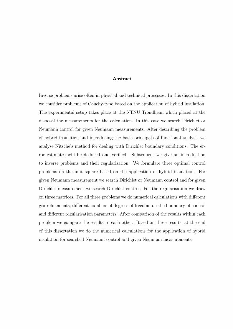
Abstract
Inverse problems arise often in physical and technical processes. In this dissertation
we consider problems of Cauchy-type based on the application of hybrid insulation.
The experimental setup takes place at the NTNU Trondheim which placed at the
disposal the measurements for the calculation. In this case we search Dirichlet or
Neumann control for given Neumann measurements. After describing the problem
of hybrid insulation and introducing the basic principals of functional analysis we
analyse Nitsche’s method for dealing with Dirichlet boundary conditions. The er-
ror estimates will be deduced and verified. Subsequent we give an introduction
to inverse problems and their regularisation. We formulate three optimal control
problems on the unit square based on the application of hybrid insulation. For
given Neumann measurement we search Dirichlet or Neumann control and for given
Dirichlet measurement we search Dirichlet control. For the regularisation we draw
on three matrices. For all three problems we do numerical calculations with different
gridrefinements, different numbers of degrees of freedom on the boundary of control
and different regularisation parameters. After comparison of the results within each
problem we compare the results to each other. Based on these results, at the end
of this dissertation we do the numerical calculations for the application of hybrid
insulation for searched Neumann control and given Neumann measurements.

4
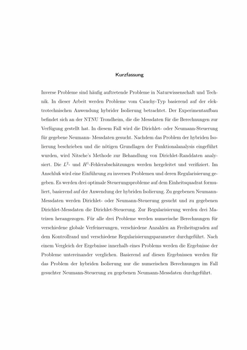
Kurzfassung
Inverse Probleme sind häufig auftretende Probleme in Naturwissenschaft und Tech-
nik. In dieser Arbeit werden Probleme vom Cauchy-Typ basierend auf der elek-
trotechnischen Anwendung hybrider Isolierung betrachtet. Der Experimentaufbau
befindet sich an der NTNU Trondheim, die die Messdaten für die Berechnungen zur
Verfügung gestellt hat. In diesem Fall wird die Dirichlet- oder Neumann-Steuerung
für gegebene Neumann- Messdaten gesucht. Nachdem das Problem der hybriden Iso-
lierung beschrieben und die nötigen Grundlagen der Funktionalanalysis eingeführt
wurden, wird Nitsche’s Methode zur Behandlung von Dirichlet-Randdaten analy-
siert. Die L2- und H1-Fehlerabschätzungen werden hergeleitet und verifiziert. Im
Anschluß wird eine Einführung zu inversen Problemen und deren Regularisierung ge-
geben. Es werden drei optimale Steuerungsprobleme auf dem Einheitsquadrat formu-
liert, basierend auf der Anwendung der hybriden Isolierung. Zu gegebenen Neumann-
Messdaten werden Dirichlet- oder Neumann-Steuerung gesucht und zu gegebenen
Dirichlet-Messdaten die Dirichlet-Steuerung. Zur Regularisierung werden drei Ma-
trizen herangezogen. Für alle drei Probleme werden numerische Berechnungen für
verschiedene globale Verfeinerungen, verschiedene Anzahlen an Freiheitsgraden auf
dem Kontrollrand und verschiedene Regularisierungsparameter durchgeführt. Nach
einem Vergleich der Ergebnisse innerhalb eines Problems werden die Ergebnisse der
Probleme untereinander verglichen. Basierend auf diesen Ergebnissen werden für
das Problem der hybriden Isolierung nur die numerischen Berechnungen im Fall
gesuchter Neumann-Steuerung zu gegebenen Neumann-Messdaten durchgeführt.
Contents
1 Introduction 3
2 Description of the application: Hybrid insulation 13
3 A model problem 19
3.1 Basic principals of functional analysis . . . . . . . . . . . . . . . . . . 19
3.2 The Finite Element Method (FEM) . . . . . . . . . . . . . . . . . . . 24
3.3 Variational formulation . . . . . . . . . . . . . . . . . . . . . . . . . . 25
3.3.1 Numerical Results . . . . . . . . . . . . . . . . . . . . . . . . 36
4 Inverse Problems 41
4.1 The theory of inverse problems . . . . . . . . . . . . . . . . . . . . . 41
4.2 Regularisation . . . . . . . . . . . . . . . . . . . . . . . . . . . . . . . 46
5 The inverse model problem 55
5.1 Description of the problems . . . . . . . . . . . . . . . . . . . . . . . 55
5.2 Numerical methods . . . . . . . . . . . . . . . . . . . . . . . . . . . . 61
6 Numerical results for the model problem 67
6.1 Neumann measurements on ΓO and Neumann control on ΓC . . . . . 68
6.2 Neumann measurements on ΓO and Dirichlet control on ΓC . . . . . . 80
6.3 Dirichlet measurements on ΓO and Dirichlet control on ΓC . . . . . . 94
6.4 Comparison of the results . . . . . . . . . . . . . . . . . . . . . . . . 106
7 Results for the Application 109
i

Contents
8 Conclusion and outlook 119
A More numerical results for the model problem 123
A.1 Results for given ∂nu|ΓOand searched ∂nu|ΓC
. . . . . . . . . . . . . . 124
A.2 Results for given ∂nu|ΓOand searched u|ΓC
. . . . . . . . . . . . . . . 134
A.3 Results for given u|ΓOand searched u|ΓC
. . . . . . . . . . . . . . . . 143
B More numerical results for hybrid insulation 153
1

Contents
2
1 Introduction
In this dissertation we study inverse problems of Cauchy type based on the appli-
cation of hybrid insulation. Frank Mauseth from the NTNU Trondheim deals with
this problem in his PhD thesis [26]. The description of the application in Section 2
and the measurements we need for the calculations in Section 7 are from a private
correspondence with Frank Mauseth and his PhD thesis [26].
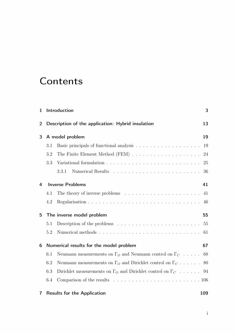
We reduce the three dimensional rotational
symmetric problem to a two dimensional prob-
lem to be solved. The details can be found
in Section 2. Then we have given conflicting
Dirichlet and Neumann boundary data on ΓO
(see Figure 1.1) and search Dirichlet or Neu-
mann control on ΓC . Ivan Cherlenyak deals
also with this problem in his PhD thesis [11].
He used the Laplace-equation in two dimen-
sions for his calculation instead of reducing
the three dimensional problem to a two dimen-
sional what we will do in this dissertation.Figure 1.1: Underlying geometry
of the application.
Before we treat this problem we take a look on a model problem (based on the
application) with the unit square as underlying geometry (see Sections 5 and 6).
As we want to solve inverse problems we first want to introduce when to call a
3
1 Introduction
problem an inverse problem. For given A : X → Y we call the calculation of Ax
with x ∈ X the direct problem. If we want to find x ∈ X for given y ∈ Y , so that
Ax = y, we call this an inverse problem.
Analysing inverse problems mostly leeds to the idea of ill-posed problems (see i.e.
Louis [25] or Rieder [30]):
Definition 1.1. Let A : X → Y be a mapping with the topologic spaces X, Y . The
problem (A,X, Y ) is called well-posed, when
• ∃ a solution to Af = g for all g ∈ Y ,
• the solution is well defined,
• the solution depends continuously on the data, i.e. A−1 is continuous.
If one of these conditions is not satisfied the problem is called ill-posed.
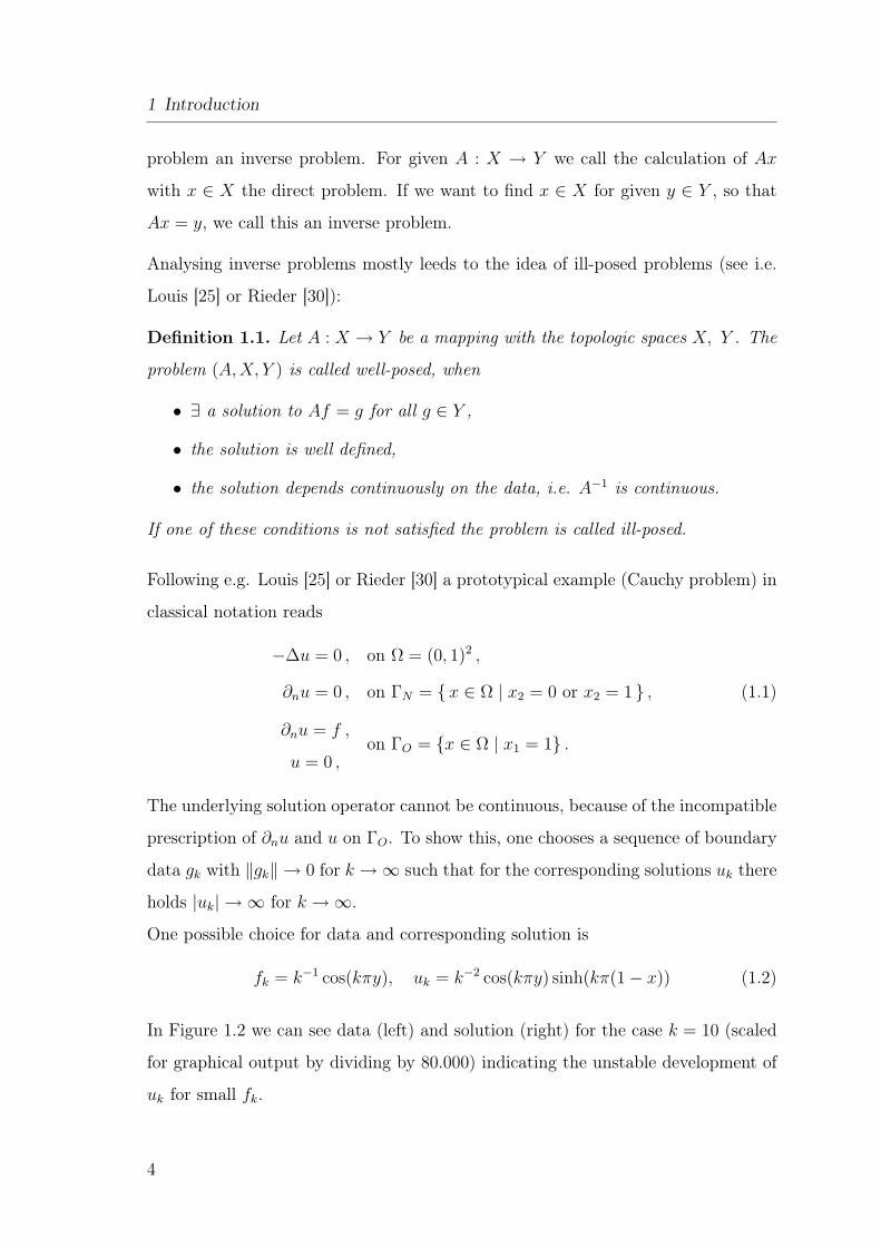
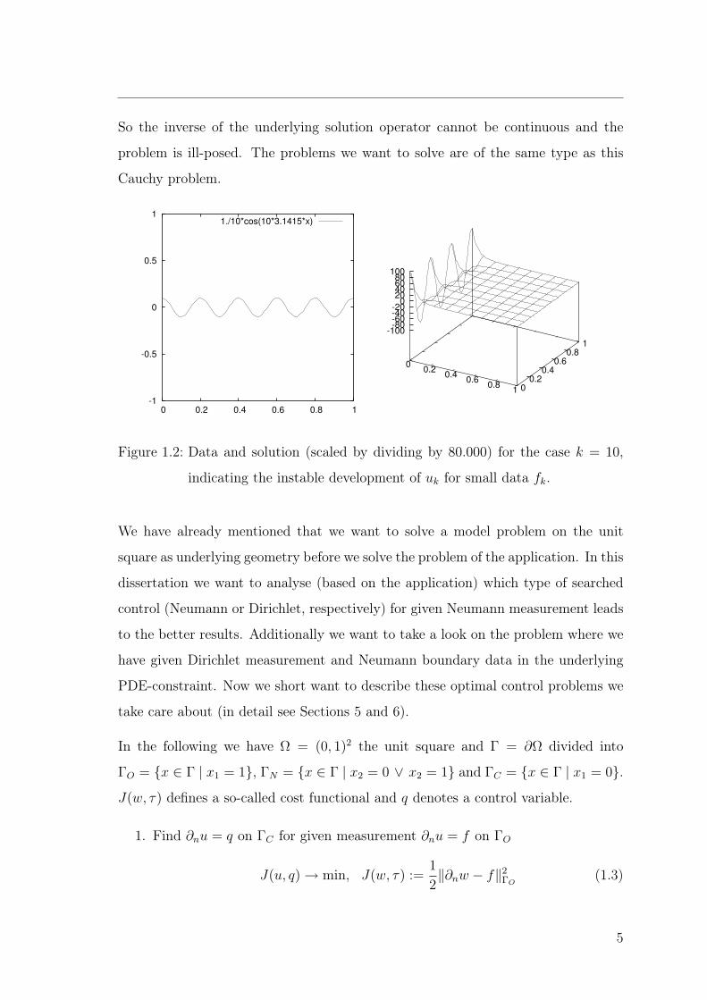
Following e.g. Louis [25] or Rieder [30] a prototypical example (Cauchy problem) in
classical notation reads
−∆u = 0 , on Ω = (0, 1)2 ,
∂nu = 0 , on ΓN = x ∈ Ω | x2 = 0 or x2 = 1 , (1.1)
∂nu = f ,
u = 0 ,on ΓO = x ∈ Ω | x1 = 1 .
The underlying solution operator cannot be continuous, because of the incompatible
prescription of ∂nu and u on ΓO. To show this, one chooses a sequence of boundary
data gk with ‖gk‖ → 0 for k → ∞ such that for the corresponding solutions uk there
holds |uk| → ∞ for k → ∞.
One possible choice for data and corresponding solution is
fk = k−1 cos(kπy), uk = k−2 cos(kπy) sinh(kπ(1 − x)) (1.2)
In Figure 1.2 we can see data (left) and solution (right) for the case k = 10 (scaled
for graphical output by dividing by 80.000) indicating the unstable development of
uk for small fk.
4
So the inverse of the underlying solution operator cannot be continuous and the
problem is ill-posed. The problems we want to solve are of the same type as this
Cauchy problem.
-1
-0.5
0
0.5
1
0 0.2 0.4 0.6 0.8 1
1./10*cos(10*3.1415*x)
0 0.2
0.4 0.6
0.8 1 0
0.2 0.4
0.6 0.8
1
-100-80-60-40-20
0 20 40 60 80
100
Figure 1.2: Data and solution (scaled by dividing by 80.000) for the case k = 10,
indicating the instable development of uk for small data fk.
We have already mentioned that we want to solve a model problem on the unit
square as underlying geometry before we solve the problem of the application. In this
dissertation we want to analyse (based on the application) which type of searched
control (Neumann or Dirichlet, respectively) for given Neumann measurement leads
to the better results. Additionally we want to take a look on the problem where we
have given Dirichlet measurement and Neumann boundary data in the underlying
PDE-constraint. Now we short want to describe these optimal control problems we
take care about (in detail see Sections 5 and 6).
In the following we have Ω = (0, 1)2 the unit square and Γ = ∂Ω divided into
ΓO = x ∈ Γ | x1 = 1, ΓN = x ∈ Γ | x2 = 0 ∨ x2 = 1 and ΓC = x ∈ Γ | x1 = 0.J(w, τ) defines a so-called cost functional and q denotes a control variable.
1. Find ∂nu = q on ΓC for given measurement ∂nu = f on ΓO
J(u, q) → min, J(w, τ) :=1
2‖∂nw − f‖2
ΓO(1.3)
5
1 Introduction
under the PDE-constraint
−∆u = g on Ω,
∂nu = 0 on ΓN ,
u = 0 on ΓO,
∂nu = q on ΓC .
(1.4)
2. Find u = q on ΓC for given measurement ∂nu = f on ΓO
J(u, q) → min, J(w, τ) :=1
2‖∂nw − f‖2
ΓO(1.5)
under the PDE-constraint
−∆u = g on Ω ,
∂nu = 0 on ΓN ,
u = 0 on ΓO ,
u = q on ΓC .
(1.6)
3. Find u = q on ΓC for given measurement u = 0 on ΓO
J(u, q) → min, J(w, τ) :=1
2‖w‖2
ΓO(1.7)
under the PDE-constraint
−∆u = g on Ω ,
∂nu = 0 on ΓN ,
∂nu = f on ΓO ,
u = q on ΓC .
(1.8)
We don’t take care about the possible fourth problem where we have to find ∂nu = q
on ΓC for given measurement u = 0 on ΓO such that
J(u, q) → min, J(w, τ) :=1
2‖w‖2
ΓO(1.9)
under the PDE-constraint
−∆u = g on Ω ,
∂nu = 0 on ΓN ,
∂nu = f on ΓO ,
∂nu = q on ΓC .
(1.10)
6
There the direct problem (1.10) is not uniquely solvable which makes problems in
solving the inverse problem.
For analysing the problems we first introduce in Section 3 basic principals of func-
tional analysis based on [2], [3], [14], [17] and [43] . There we introduce the spaces
Hk(Ω), Hs(Ω), Hs(Γ) with the corresponding inner products and norms.
Then we give a short introduction to the finite element method and analyse Nitsches
method for solving direct problems with Dirichlet boundary data. In order to prepare
an adequate mathematical formulation of the whole problem we first focus on a
suitable formulation of the “forward” problem itself (see Section 3.3).
For handling Dirichlet boundary conditions we cannot use the standard weak for-
mulation of the problem as described in the finite element theory (see e.g. Braess
[8] and Johnson [22]). There the Dirichlet boundary condition q we want to calcu-
late within the computation of the mentioned inverse problems (1.7) and (1.9) is
hidden in the underlying function space of the variational formulation. Because of
this we use the symmetric version of the weak formulation introduced by Nitsche
[29] instead of the standard weak formulation (see also Hansbo [19], or Arnold et al.
[4]).
For the given classical formulation we have to find u ∈ C2(Ω) ∩ C(Ω) for given
f, q ∈ C(Ω) such that
− ∆u = f in Ω (1.11)
u = q on Γ = ∂Ω.
Using Nitsche’s method we have to find uh ∈ Vh ⊂ H1(Ω) such that
ah(uh, v) = (f, v) + (ψ(h)q, v)∂Ω − (q, ∂nv)∂Ω (1.12)
with
ah(u, v) := (∇u,∇v)Ω − (∂nu, v)∂Ω − (u, ∂nv)∂Ω + (ψ(h)u, v)∂Ω. (1.13)
7
1 Introduction
We show that ah(., .) is positive definite for ψ(h) = γh−1 for γ a positive constant
depending on the problem to be solved. After that we derive the error estimates
similar to that of the classical variational formulation:
‖e‖1,Ω ≤ ch‖u‖2,Ω (1.14)
‖e‖0,Ω ≤ ch2‖u‖2,Ω. (1.15)
For this method we obtain an additional error estimation:
‖e‖0,Γ ≤ ch3/2‖u‖2,Ω. (1.16)
As we are interested in solving an inverse problem we introduce in Section 4 the
basic theory of inverse problems (based on Louis [25] and Rieder [30]). There we
formulate among other things that f ∈ X minimzes the residuum ‖Af − g‖Y is
equivalent to f ∈ X solves the normal equation A∗Af = A∗g. In our application
(described in Section 2) we only have measuring data ∂nu|ΓO= f or u|ΓO
= 0 and
we have already seen that the inverse of the underlying solution operator is not
continuous. This leads to errors in the calculation and we have to regularise the
problem. Here we employ the Tikhonov-Phillips-regularisation.
We have formulated the problems as optimal control problems. In general we can
write the three cases in the form (see Lions [24] and Tröltzsch [39]):
J(u, q) → min (1.17)
under the constraint Au = Bq.
As A is invertible we can write
u = A−1Bq. (1.18)
From this there follows that we have to minimise
J(u, q) = J(A−1Bq, q). (1.19)
8
So after all we have to solve the regularised normal equation
(MT M + αRT R)q = MT f. (1.20)
With M depending on the optimal control problem to be solved (for details see
Section 5), α > 0 the regularisation parameter and R the regularisation matrix
from the Tikhonov-Phillips-regularisation.
For the implementation we use DEAL (Differential Equations Analysis Library [1],
see also [36]). As solution algorithm we use the preconditioned conjugate gradient
algorithm (pcg) and the multigrid method as preconditioner (see e.g. [9], [10],[31],
[41]). Both algorithms are described in Section 5.2.
In Section 6 we present the numerical results for our three problems. As a test-
example we use
− ∆u = 12xy2 − 12xy + 2x − 12y2 + 12y − 2. (1.21)
We do the calculations for the three problems with three regularisation matrices
(Id and approximations of the first and second derivative) under different aspects.
First we take a look on the results for the searched control on ΓC for different grid
refinements. The regularisation parameter α is choosen by trial and error. It is not
part of this dissertation to formulate algorithms for the best parameter choice. As
a consequence of this we do not present a detailed error analysis which is dependent
of the parameter choice.
After that we reduce the number of degrees of freedom (DOF) on ΓC as we know we
can regularise the problem by reducing the dimension. Again we do this analysis for
the three matrices R. At last we analyse the influence of the regularisation parameter
α on the solution with reduced number of DOF on ΓC . As a last aspect for each
problem we compare the results for the three regularisation matrices with reduced
number of DOF on ΓC and the corresponding optimal regularisation parameter.
After doing this analysis for each of the three problems (Section 6.1 to Section 6.3) we
compare the results of the three optimal control problems (Section 6.4). Therefore we
9
1 Introduction
use the approximation of the second derivative as regularisation matrix, the reduced
number of DOF on ΓC and the corresponding optimal regularisation parameter we
estimated in the Sections 6.1 to 6.3.
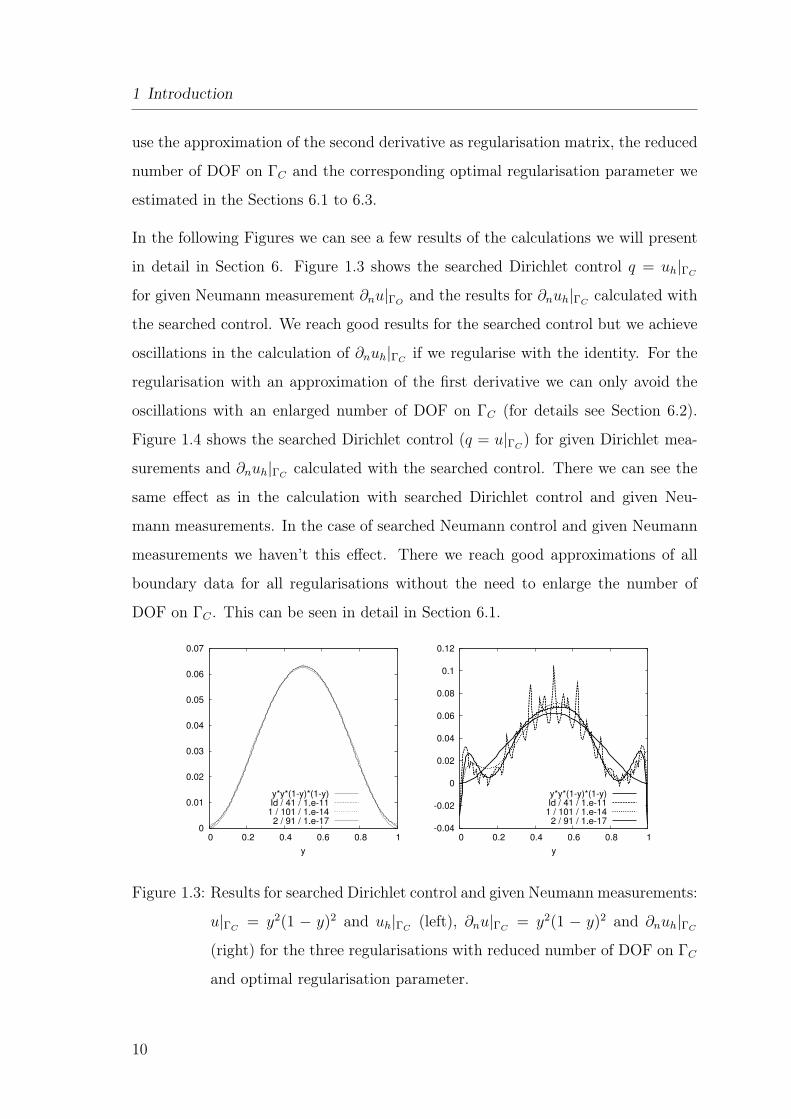
In the following Figures we can see a few results of the calculations we will present
in detail in Section 6. Figure 1.3 shows the searched Dirichlet control q = uh|ΓC
for given Neumann measurement ∂nu|ΓOand the results for ∂nuh|ΓC
calculated with
the searched control. We reach good results for the searched control but we achieve
oscillations in the calculation of ∂nuh|ΓCif we regularise with the identity. For the
regularisation with an approximation of the first derivative we can only avoid the
oscillations with an enlarged number of DOF on ΓC (for details see Section 6.2).
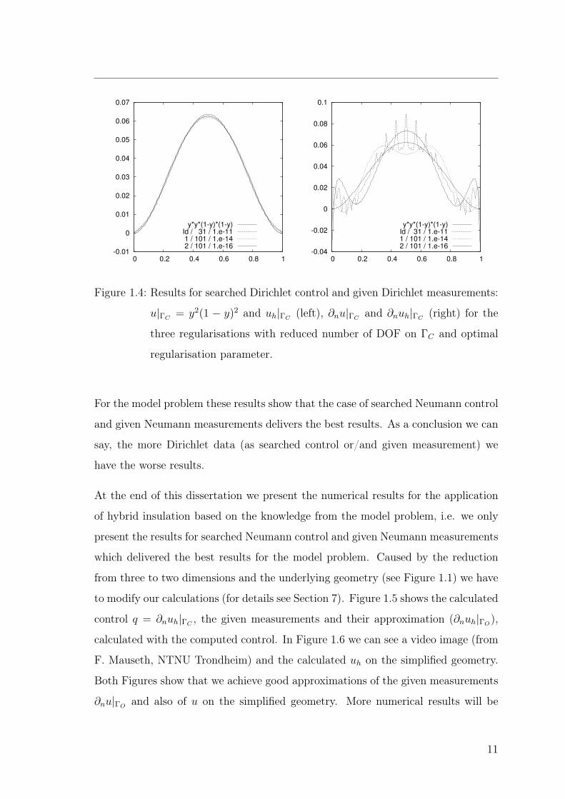
Figure 1.4 shows the searched Dirichlet control (q = u|ΓC) for given Dirichlet mea-
surements and ∂nuh|ΓCcalculated with the searched control. There we can see the
same effect as in the calculation with searched Dirichlet control and given Neu-
mann measurements. In the case of searched Neumann control and given Neumann
measurements we haven’t this effect. There we reach good approximations of all
boundary data for all regularisations without the need to enlarge the number of
DOF on ΓC . This can be seen in detail in Section 6.1.
0
0.01
0.02
0.03
0.04
0.05
0.06
0.07
0 0.2 0.4 0.6 0.8 1
y
y*y*(1-y)*(1-y)Id / 41 / 1.e-111 / 101 / 1.e-142 / 91 / 1.e-17
-0.04
-0.02
0
0.02
0.04
0.06
0.08
0.1
0.12
0 0.2 0.4 0.6 0.8 1
y
y*y*(1-y)*(1-y)Id / 41 / 1.e-11
1 / 101 / 1.e-142 / 91 / 1.e-17
Figure 1.3: Results for searched Dirichlet control and given Neumann measurements:
u|ΓC= y2(1 − y)2 and uh|ΓC
(left), ∂nu|ΓC= y2(1 − y)2 and ∂nuh|ΓC
(right) for the three regularisations with reduced number of DOF on ΓC
and optimal regularisation parameter.
10
-0.01
0
0.01
0.02
0.03
0.04
0.05
0.06
0.07
0 0.2 0.4 0.6 0.8 1
y*y*(1-y)*(1-y)Id / 31 / 1.e-111 / 101 / 1.e-142 / 101 / 1.e-16
-0.04
-0.02
0
0.02
0.04
0.06
0.08
0.1
0 0.2 0.4 0.6 0.8 1
y*y*(1-y)*(1-y)Id / 31 / 1.e-111 / 101 / 1.e-142 / 101 / 1.e-16
Figure 1.4: Results for searched Dirichlet control and given Dirichlet measurements:
u|ΓC= y2(1 − y)2 and uh|ΓC
(left), ∂nu|ΓCand ∂nuh|ΓC
(right) for the
three regularisations with reduced number of DOF on ΓC and optimal
regularisation parameter.
For the model problem these results show that the case of searched Neumann control
and given Neumann measurements delivers the best results. As a conclusion we can
say, the more Dirichlet data (as searched control or/and given measurement) we
have the worse results.
At the end of this dissertation we present the numerical results for the application
of hybrid insulation based on the knowledge from the model problem, i.e. we only
present the results for searched Neumann control and given Neumann measurements
which delivered the best results for the model problem. Caused by the reduction
from three to two dimensions and the underlying geometry (see Figure 1.1) we have
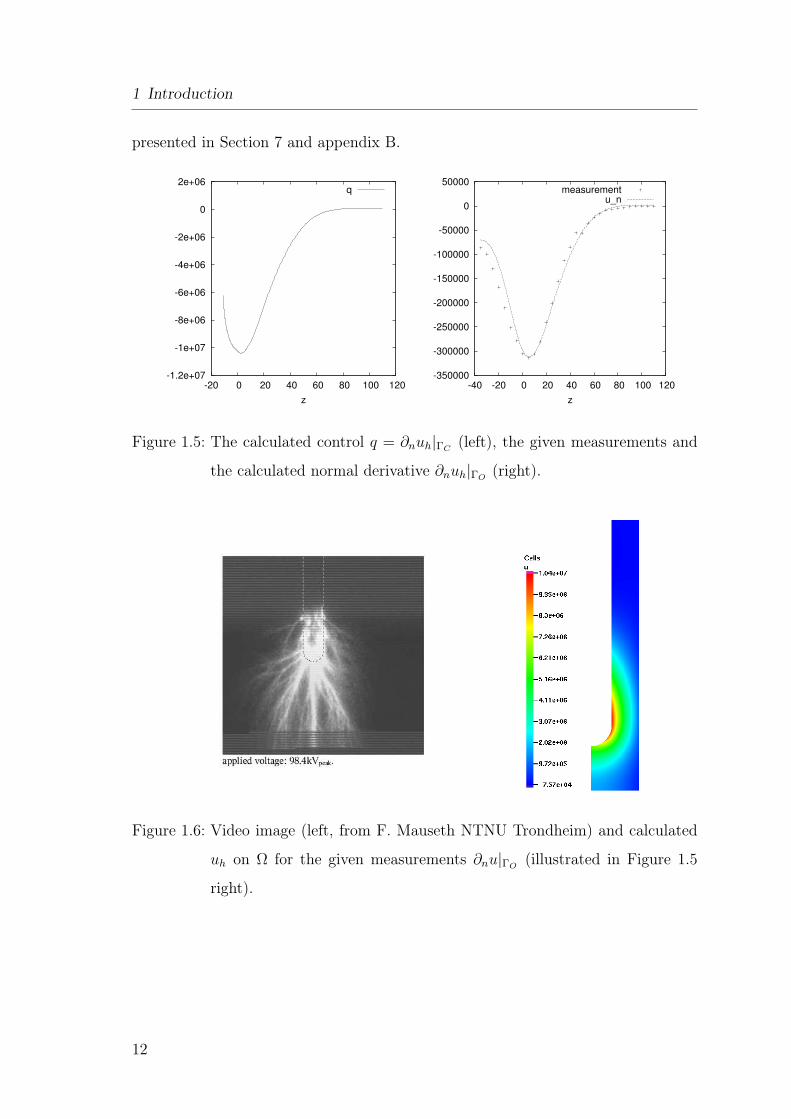
to modify our calculations (for details see Section 7). Figure 1.5 shows the calculated
control q = ∂nuh|ΓC, the given measurements and their approximation (∂nuh|ΓO
),
calculated with the computed control. In Figure 1.6 we can see a video image (from
F. Mauseth, NTNU Trondheim) and the calculated uh on the simplified geometry.
Both Figures show that we achieve good approximations of the given measurements
∂nu|ΓOand also of u on the simplified geometry. More numerical results will be
11
1 Introduction
presented in Section 7 and appendix B.
-1.2e+07
-1e+07
-8e+06
-6e+06
-4e+06
-2e+06
0
2e+06
-20 0 20 40 60 80 100 120
z
q
-350000
-300000
-250000
-200000
-150000
-100000
-50000
0
50000
-40 -20 0 20 40 60 80 100 120
z
measurementu_n
Figure 1.5: The calculated control q = ∂nuh|ΓC(left), the given measurements and
the calculated normal derivative ∂nuh|ΓO(right).
Figure 1.6: Video image (left, from F. Mauseth NTNU Trondheim) and calculated
uh on Ω for the given measurements ∂nu|ΓO(illustrated in Figure 1.5
right).
12

2 Description of the application:
Hybrid insulation
Now we want to describe the application of hybrid insulation which we deal with
the NTNU Trondheim, where they do the measurements. The description is from
Frank Mauseth from the NTNU Trondheim who deals with the problem of hybrid
insulation in his PhD thesis ([26]). We only present the fundamental idea and the
resulting differential equation to be solved when we reduce the problem to a two
dimensional one.
The breakdown voltage of an air gap between two electrodes can be improved consid-
erably if one or both of the electrodes are covered with a thick (several millimeters)
dielectric coating. If free charges are available in the gap or in the air volume
surrounding the structure, charges accumulate in the dielectric surfaces due to elec-
trostatic attraction. As long as there is a driving field this accumulation process
continues.
The electrical field in the hybrid insulation system can be calculated as the vector
sum of the charge induced field and the applied field.
Etotal = Ecapacitive + Echarge induced
13
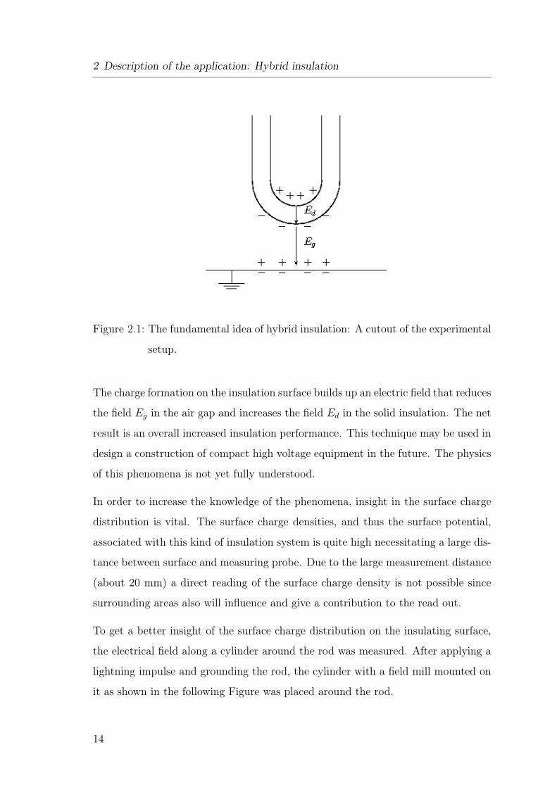
2 Description of the application: Hybrid insulation
Figure 2.1: The fundamental idea of hybrid insulation: A cutout of the experimental
setup.
The charge formation on the insulation surface builds up an electric field that reduces
the field Eg in the air gap and increases the field Ed in the solid insulation. The net
result is an overall increased insulation performance. This technique may be used in
design a construction of compact high voltage equipment in the future. The physics
of this phenomena is not yet fully understood.
In order to increase the knowledge of the phenomena, insight in the surface charge
distribution is vital. The surface charge densities, and thus the surface potential,
associated with this kind of insulation system is quite high necessitating a large dis-
tance between surface and measuring probe. Due to the large measurement distance
(about 20 mm) a direct reading of the surface charge density is not possible since
surrounding areas also will influence and give a contribution to the read out.
To get a better insight of the surface charge distribution on the insulating surface,
the electrical field along a cylinder around the rod was measured. After applying a
lightning impulse and grounding the rod, the cylinder with a field mill mounted on
it as shown in the following Figure was placed around the rod.
14
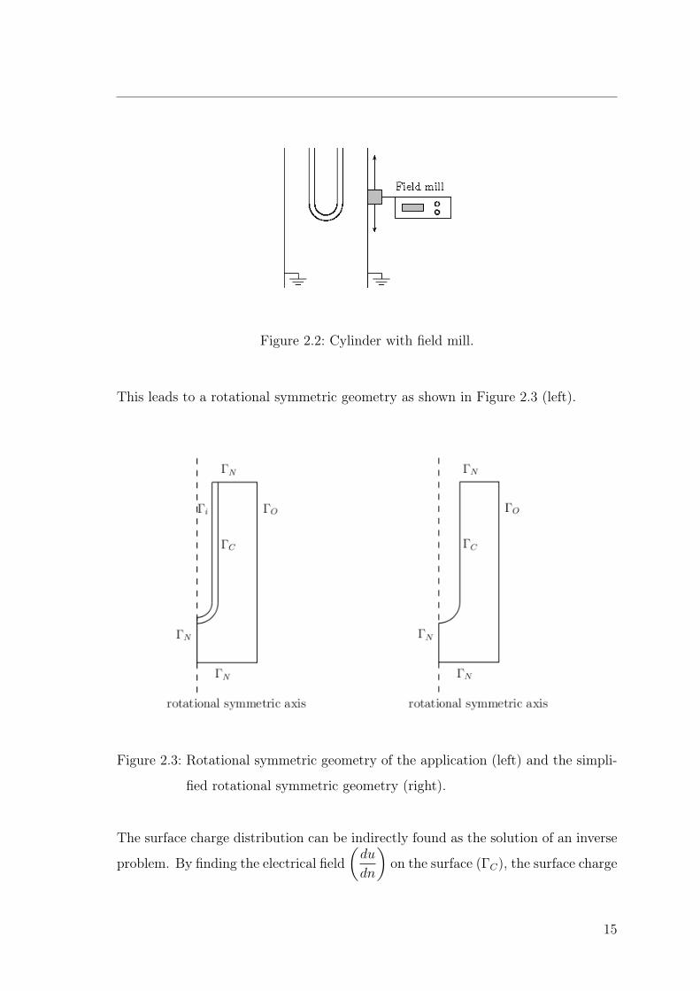
Figure 2.2: Cylinder with field mill.
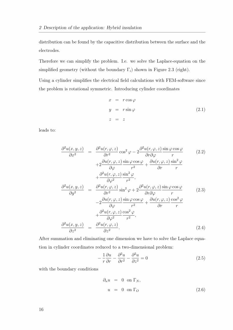
This leads to a rotational symmetric geometry as shown in Figure 2.3 (left).
Figure 2.3: Rotational symmetric geometry of the application (left) and the simpli-
fied rotational symmetric geometry (right).
The surface charge distribution can be indirectly found as the solution of an inverse
problem. By finding the electrical field
(du
dn
)
on the surface (ΓC), the surface charge
15
2 Description of the application: Hybrid insulation
distribution can be found by the capacitive distribution between the surface and the
electrodes.
Therefore we can simplify the problem. I.e. we solve the Laplace-equation on the
simplified geometry (without the boundary Γi) shown in Figure 2.3 (right).
Using a cylinder simplifies the electrical field calculations with FEM-software since
the problem is rotational symmetric. Introducing cylinder coordinates
x = r cos ϕ
y = r sin ϕ (2.1)
z = z
leads to:
∂2u(x, y, z)
∂x2=
∂2u(r, ϕ, z)
∂r2cos2 ϕ − 2
∂2u(r, ϕ, z)
∂r∂ϕ
sin ϕ cos ϕ
r(2.2)
+2∂u(r, ϕ, z)
∂ϕ
sin ϕ cos ϕ
r2+
∂u(r, ϕ, z)
∂r
sin2 ϕ
r
+∂2u(r, ϕ, z)
∂ϕ2
sin2 ϕ
r2,
∂2u(x, y, z)
∂y2=
∂2u(r, ϕ, z)
∂r2sin2 ϕ + 2
∂2u(r, ϕ, z)
∂r∂ϕ
sin ϕ cos ϕ
r(2.3)
−2∂u(r, ϕ, z)
∂ϕ
sin ϕ cos ϕ
r2+
∂u(r, ϕ, z)
∂r
cos2 ϕ
r
+∂2u(r, ϕ, z)
∂ϕ2
cos2 ϕ
r2,
∂2u(x, y, z)
∂z2=
∂2u(r, ϕ, z)
∂z2. (2.4)
After summation and eliminating one dimension we have to solve the Laplace equa-
tion in cylinder coordinates reduced to a two-dimensional problem:
− 1
r
∂u
∂r− ∂2u
∂r2− ∂2u
∂z2= 0 (2.5)
with the boundary conditions
∂nu = 0 on ΓN ,
u = 0 on ΓO (2.6)
16

given measurements ∂nu|ΓO= f and the searched control q on ΓC on the simplified
geometry (Figure 2.3 right).
With equation (2.5) and equation (2.6) we have given the underlying PDE constraint
we need to solve the optimal control problem described later on (see Section 7).
Based on this application there are two possible cases we can solve within the inverse
problem (see Section 5 and Section 7): On the one hand we can calculate the control
q = u|ΓCand on the other hand we can calculate the control q = ∂nu|ΓC
. First we
will do this for a model problem: The Laplace equation on the unit square. Before
we can do this we introduce in the next Section the basic principals of functional
analysis and Nitsche’s method for handling Dirichlet boundary conditions.
17

2 Description of the application: Hybrid insulation
18
3 A model problem
Before we treat the inverse problems mentioned in the introduction we want to take a
look on the direct problem. Therefore we need some principals of functional analysis.
In Section 3.1 we define the spaces Hk(Ω) (k ∈ N), Hs(Ω) and Hs(Γ) (s ∈ R+) which
we need for the analysis of our problem. We also introduce the trace and embedding
theorem.
After that in Section 3.2 we take a short look on the abstract problem and the finite
element method.
In Section 3.3 we study the variational formulation of the forward problem with
Dirichlet boundary data. In the standard weak formulation q = u|Γ is hidden in
the underlying function space, but in view that we have to determine q within the
inverse problem we prefer q to appear more directly. Therefore we use a symmetric
variant of Nitsche´s method (see Nitsche [29], Hansbo [19]).
3.1 Basic principals of functional analysis
First we introduce some spaces we need for the variational formulation of our prob-
lem. This basic principals and their proofs can be found in the literature about
functional analysis (e.g. Hackbusch [17] and Dobrowolski [14]).
Let Ω be a bounded subset of Rd. Then L2(Ω) is defined as the space of functions
where the integral over the square is finite:
19
3 A model problem
Definition 3.1.
L2(Ω) :=
v | v defined on Ω,
∫
Ω
v2 dx < ∞
(3.1)
L2(Ω) is a Hilbert space with the (L2-) inner product
(v, w)0 := (v, w)L2(Ω) =
∫
Ω
vw dx (3.2)
and the corresponding norm
‖v‖L2(Ω) =
∫
Ω
v2 dx
1
2
= (v, v)1
2 . (3.3)
For the following weak derivative we need a multiindex α = (α1, . . . , αn)T with
αi ∈ N0, i = 1, . . . , n for which we have:
|α| =n∑
i=1
αi, xα = xα1
1 . . . xαn
n , Dαu =∂|α|
∂α1x1 . . . ∂αn
xn
u. (3.4)
Definition 3.2. For u ∈ L2(Ω) exists a weak derivative v := Dαu ∈ L2(Ω) if for
v ∈ L2(Ω) holds:
(w, v)0 = (−1)|α|(Dαw, u)0 ∀ w ∈ C∞0 (Ω). (3.5)
Now we define the Sobolev-spaces Hk(Ω) which we need for our variational formu-
lation of the problem.
Definition 3.3. Let k ∈ N ∪ 0.
Hk(Ω) := u ∈ L2(Ω) | ∃ Dαu ∈ L2(Ω) for |α| ≤ k. (3.6)
Hk(Ω) is a Hilbert space with the inner product
(u, v)k := (u, v)Hk(Ω) :=∑
|α|≤k
(Dαu,Dαv)0 (3.7)
20
3.1 Basic principals of functional analysis
and the (Sobolev-) norm
‖u‖k := ‖u‖Hk(Ω) :=
√∑
|α|≤k
‖Dαu‖20. (3.8)
|u|k :=
√∑
α=k
‖Dαu‖20 (3.9)
is called semi norm of Hk.
We can also define Hk(Ω) as completion of X0 := u ∈ C∞(Ω) | ‖u‖k < ∞ in L2(Ω)
with respect to ‖.‖Hk . Hk0 (Ω) is the completion of C∞
0 (Ω) in L2(Ω) corresponding
to (3.8).
Now we define the inner product (., .)s with s ∈ R+0 and the so called Sobolev-
Slobodeckij-norm ‖.‖Hs(Ω). With the Sobolev-Slobodeckij-norm we can define Hs(Ω),
s ∈ R+0 in the same way as Hk(Ω) for k ∈ N0 as completion of X0 with respect to
‖.‖Hs .
Definition 3.4. Let Ω ⊂ Rn, s ≥ 0 with s = k + λ, k ∈ N ∪ 0 and 0 < λ < 1.
Then (u, v)s is defined as
(u, v)s := (u, v)k +∑
|α|=k
(Dαu,Dαv)λ (3.10)
with the known (u, v)k from (3.7) and
(Dαu,Dαv)λ =
∫
Ω
∫
Ω
(Dαu(x) − Dαu(y))(Dαv(x) − Dαv(y))
|x − y|n+2λ. (3.11)
With this inner product we get the Sobolev-Slobodeckij-norm
‖u‖s := ‖u‖Hs(Ω) :=√
(u, u)s. (3.12)
With the Sobolev-Slobodeckij-norm Hs(Ω) is a Banach space. With the inner prod-
uct (., .)s Hs(Ω) is a Hilbert space.
For s ∈ N we have Hs = Hk from definition 3.3. Hs0(Ω) is the completion of C∞
0 (Ω)
in L2(Ω) with respect to ‖.‖Hs(Ω). For these Sobolev-spaces we have the following
features (see Hackbusch [17]):
21
3 A model problem
Theorem 3.1.
1. C∞0 is dense in Hs
0(Ω).
2. u ∈ C∞(Ω) | Tr(u) compact, ‖u‖s < ∞ is dense in Hs(Ω).
3. Hs(Ω) ⊂ H t(Ω), Hs0(Ω) ⊂ H t
0(Ω) for s ≥ t.
4. aDα(bu) ∈ Hs−|α|, for |α| < s, u ∈ Hs(Ω), a ∈ Ct−|α|(Ω), b ∈ Ct(Ω) with
t = s ∈ N ∪ 0 or t > s.
We also need the space Hs(Γ), trace- and embedding operators because of the given
boundary values. Following Hackbusch [17] we first take a look on this function
space and operators with respect to Ω = Rn+ := (x1, . . . , xn) ∈ R
n | xn > 0 with
Γ = ∂Ω = Rn−1 × 0.
Theorem 3.2. Let s ≥ 0. It exists an embedding operator φs ∈ L(Hs(Rn+), Hs(Rn))
so that the embedding u = φsu and u are equal on Rn+ for all u ∈ Hs(Rn
+).
Now we have the embedding operator. The trace operator γ is first defined on
C∞0 (Rn):
γ : C∞0 (Rn) → C∞
0 (Γ) ⊂ L2(Rn−1), γu(x) := u(x) ∀x ∈ Γ = Rn−1 × 0. (3.13)
Then we have the following theorem:
Theorem 3.3. Let s > 1/2. γ from equation (3.13) can be extended to γ ∈L(Hs(Rn), Hs−1/2(Rn−1)). Specially : |γu|s−1/2 ≤ Cs|u|s, u ∈ Hs(Rn).
Corollary 3.1. Let s > 1/2. For γu := u(., 0) we have γ ∈ L(Hs(Rn+), Hs−1/2(Rn−1)).
With the restriction xn = 0 we loose a half order of differentiability. On the other
side with the continuation of w ∈ Hs−1/2(Rn−1) on Rn we gain a half order of
differentiability:
Theorem 3.4. Let s > 1/2, w ∈ Hs−1/2(Rn−1). There exists u ∈ Hs(Rn) with
|u|s ≤ Cs|w|s−1/2 and γu = w, i.e. w = u(., 0).
22
3.1 Basic principals of functional analysis
Until now we only took a look on Hs(Rn+) and Hs(Rn−1), but we need Hs(Γ), Γ = ∂Ω
and Ω ⊂ Rn a general domain. Therefore we need the following definition:
Definition 3.5. Let 0 < t ∈ R ∪ ∞. We call Ω ∈ Ct if for all x ∈ Γ := ∂Ω
there exists a surrounding area U ⊂ Rn, where we can define a bijective mapping
φ : U → K1(0) = ξ ∈ Rn | |ξ| < 1 with
φ ∈ Ct(U), φ−1 ∈ Ct(K1(0)), (3.14)
φ(U ∩ Γ) = ξ ∈ K1(0) | ξn = 0, (3.15)
φ(U ∩ Ω) = ξ ∈ K1(0) | ξn > 0, (3.16)
φ(U ∩ (Rn\Ω)) = ξ ∈ K1(0) | ξn < 0. (3.17)
Lemma 3.1. Let Ω ∈ Ct be a bounded domain. There exists N ∈ N, U i (0 ≤ i ≤N), Ui, αi (1 ≤ i ≤ N) with
U i open, bounded (0 ≤ i ≤ N), Ω ⊂N⋃
i=0
U i, U0 ⊂⊂ Ω, (3.18)
Ui := U i ∩ Γ (1 ≤ i ≤ N),N⋃
i=1
Ui = Γ, (3.19)
αi : Ui → αi(Ui) ⊂ Rn−1 bijective for i = 1, . . . , N, (3.20)
αi α−1j ∈ Ct(αj(Ui ∩ Uj)). (3.21)
On U i (1 ≤ i ≤ N) the mappings φi with the features (3.14)-(3.17) are defined.
Lemma 3.2. (Partition of unity)
U i | 0 ≤ i ≤ N satisfy (3.18). There exist functions σi ∈ C∞0 (Rn), 0 ≤ i ≤ N
with
Tr(σi) ⊂ U i,N∑
i=0
σ2i (x) = 1 ∀x ∈ Ω. (3.22)
With αi and σi we are now able to define Hs(Γ).
Definition 3.6. Let Ω ∈ Ct. (Ui, αi) and σi satisfy (3.17)-(3.20). Let s ≤ t ∈ N
or s < t ∈ N, t > 1. The Sobolev-space Hs(Γ) is the set of all functions u : Γ → R
with (σiu) α−1i ∈ Hs
0(Rn−1) (1 ≤ i ≤ N).
23
3 A model problem
We can now formulate the trace and embedding theorems (3.2, 3.3) on a general
domain Ω:
Theorem 3.5. Let Ω ∈ Ct with 1/2 < s ≤ t ∈ N or 1/2 < s < t.
1. The trace γu of u ∈ Hs(Ω) is element of Hs−1/2(Γ) : γ ∈ L(Hs(Ω), Hs−1/2(Γ)).
2. For every w ∈ Hs−1/2(Γ) there exist an u ∈ Hs(Ω) with w = γu, ‖u‖s ≤Cs‖w‖s−1/2.
3. For every w ∈ Hs(Ω) exists an extension E ∈ L(Hs(Ω), Hs(Rn)) with Ew ∈Hs(Rn).
The dual space of Hs0(Ω) is called H−s(Ω) or H−s
0 (Ω). The norm is then defined as
‖u‖−s := sup
‖(u, v)‖L2(Ω)
‖v‖s
| 0 6= v ∈ Hs0(Ω)
. (3.23)
These are the basics we need for this work. Now we take a look on the abstract
formulation of the problem with the finite element method.
3.2 The Finite Element Method (FEM)
As typical for numerical methods we want to solve the problem approximately. Here
we use the finite element method. Therefore we search the solution uh of the problem
in a finite dimensional subspace. But first we want to introduce the abstract problem
analog to Johnson [22] and Braess [8].
Let V a linear space, a : V × V → R a symmetric, positive definite bilinear form
and l : V → R a linear functional. Then we want to solve:
a(u, v) = (l, v) ∀ v ∈ V. (3.24)
As mentioned before, we don’t search the solution in V but in a finite dimensional
subspace Vh ⊂ V . I.e. we search the discrete solution uh ∈ Vh such that:
a(uh, v) = (l, v) ∀ v ∈ Vh. (3.25)
24
3.3 Variational formulation
Now let ϕ1, . . . , ϕn be basis of Vh. Hence we can illustrate uh and v as linear
combination of ϕi, i = 1, . . . , n. This leads us to the following system of equations,
if uh =n∑
k=1
xkϕk:
n∑
k=1
a(ϕk, ϕi)xk = (l, ϕi), i = 1, . . . , n (3.26)
or in matrix-vector-form:
Ax = b (3.27)
with Aik = a(ϕk, ϕi) and bi = (l, ϕi).
In practice we divide the domain Ω in (finite) subdomains and take a look on func-
tions which are polynoms on every subdomain. These subdomains are called ele-
ments. In this work we use bilinear elements on quadrilaterals.
Let Ω be a polygonal domain which can be divided in triangles or quadrilaterals.
We call the partition T = T1, T2, . . . TN of Ω in triangles or quadrilaterals allowed
if the following properties are fulfilled:
• Ω = ∪Ni=1Ti.
• Is Ti ∩ Tj one point, then this point is vertex of Ti and Tj.
• Is Ti ∩ Tj, i 6= j more than one point, then Ti ∩ Tj is edge of Ti and Tj.
If this is not fulfilled we have hanging nodes.
3.3 Variational formulation
Here we consider the variational formulation of the direct problem. As mentioned
before the Dirichlet boundary in the standard variational formulation is hidden in
the function space. In Section 5 (the inverse problem for a model problem) we want
to calculate the control u|ΓC= q, where ΓC is a part of the boundary Γ. Therefore
we want to appear q in the variational formulation instead of being hidden in the
function space. For this we use a symmetric variant of Nitsche’s method.
25
3 A model problem
Nitsche’s Method
For simplicity we introduce Nitsche’s method for Dirichlet boundary data on the
whole boundary instead of only on parts of it. We show consistency, stability and
reach the error estimates for ‖e‖0,Γ, ‖e‖0,Ω and ‖e‖1,Ω.
For generality we want to solve the potential equation on the unit square with
Dirichlet boundary data, i.e. we search u ∈ C2(Ω) ∩ C(Ω) such that
−∆u = g on Ω = (0, 1)2
u = q on Γ = ∂Ω.(3.28)
In the standard variational formulation we have to find u ∈ V := ϕ ∈ H1(Ω) | ϕ =
q on Γ such that
(∇u,∇ϕ) = (g, ϕ) ∀ ϕ ∈ V. (3.29)
If we use this variational formulation the Dirichlet boundary data is hidden in the
function space V . In Section 5 we have the case that we want to calculate the control
q = u|ΓC. So we want to appear q more directly.
This leads us to Nitsche´s method (see e.g. [29], [19]). Here we use a symmetric
form of it.
Nitsche’s method for (3.28) determines a solution uh ∈ Vh ⊂ H1(Ω) such that
ah(uh, ϕ) = (g, ϕ)0,Ω + (ψ(h)q, ϕ)0,Γ − (q, ∂nϕ)0,Γ ∀ϕ ∈ Vh (3.30)
with
ah(u, ϕ) := (∇u,∇ϕ)0,Ω − (∂nu, ϕ)0,Γ − (u, ∂nϕ)0,Γ + (ψ(h)u, ϕ)0,Γ. (3.31)
The second term of the bilinear form arises from Green’s formula, the third term is
for symmetry and ensures consistency and the penalize last term guarantees stability
which is shown later. Instead of −(u, ∂nϕ)Γ as third term we can also use +(u, ∂nϕ)Γ.
Then the bilinearform is positive definite for each choice of ψ(h) but we have an
unsymmetric problem to be solved (see [4]).
26
3.3 Variational formulation
Now we want to analyse the symmetric version of Nitsche’s method used here ((3.30)
and (3.31)). Later we will show that ‖e‖1,Ω ∈ O(h) and ‖e‖0,Ω ∈ O(h2) as for the
classical variational formulation of problem (3.28). By (3.28) and using Green’s
formula we have consistency with the original problem:
ah(u, ϕ) − (g, ϕ)0,Ω − (ψ(h)q, ϕ)0,Γ + (q, ∂nϕ)0,Γ (3.32)
= (∇u,∇ϕ)0,Ω − (∂nu, ϕ)0,Γ − (g, ϕ)0,Ω ≡ 0.
Next we want to show, that the resulting bilinear form ah(., .) is positive definite.
The ideas are based on the results of Nitsche ([29]). Hansbo ([19]) uses a mesh
dependent norm for the convergence analysis caused by the continuity of ah(., .) in
this norm. In the following estimates c is a positive constant changing in every
estimation.
ah(uh, uh) = ‖∇uh‖20,Ω − (∂nuh, uh)0,Γ − (uh, ∂nuh)0,Γ + ψ(h)‖uh‖2
0,Γ
≥ |uh|21,Ω − 2‖∂nuh‖0,Γ‖uh‖0,Γ + ψ(h)‖uh‖20,Γ. (3.33)
Using the standard inverse estimate as in Hansbo ([19]) (proof: see Thomee [38]).
‖∂nv‖20,Γ ≤ c2
1h−1|v|21,Ω ∀v ∈ Vh (3.34)
we have:
ah(uh, uh) ≥ |uh|21,Ω − 2c1h−1/2|uh|1,Ω‖uh‖0,Γ + ψ(h)‖uh‖2
0,Γ. (3.35)
Now we want to estimate the product of norms (|uh|1,Ω‖uh‖0,Γ) with a sum of these
norms. Therefore we use for real numbers a, b,√
ε 6= 0
ab ≤ ε
2a2 +
1
2εb2 ⇔
(b√ε− a
√ε
)2
≥ 0. (3.36)
With ε = 2 we have in our case
c1h−1/2|uh|1,Ω‖uh‖0,Γ ≤ 1
4|uh|21,Ω + c2
1h−1‖uh‖2
0,Γ. (3.37)
By this we can show that ah(., .) is positive definite depending on ψ(h):
ah(uh, uh) ≥ |uh|21,Ω − 1
2|uh|21,Ω − 2c2
1h−1‖uh‖2
0,Γ + ψ(h)‖uh‖20,Γ (3.38)
=1
2|uh|21,Ω + (ψ(h) − 2c2
1h−1)‖uh‖2
0,Γ
≥ 0 for ψ(h) ≥ 2c21h
−1.
27
3 A model problem
So we have stability in the sense that ah(., .) is a positive definite bilinear form if
ψ(h) ≥ 2c21h
−1. With (3.38) we can now choose ψ(h) = γh−1. With γ ≥ 2c21 we still
have a positive definite bilinear form ah(., .).
Now we have to solve: Find uh ∈ Vh ⊂ H1(Ω), so that:
ah(uh, ϕ) = (g, ϕ)0,Ω + (γh−1q, ϕ)0,Γ − (q, ∂nϕ)0,Γ (3.39)
with
ah(u, ϕ) := (∇u,∇ϕ)0,Ω − (∂nu, ϕ)0,Γ − (u, ∂nϕ)0,Γ + (γh−1u, ϕ)0,Γ. (3.40)
Next we want to do the error analysis. We will show, that
‖e‖0,Γ ≤ ch3/2‖u‖2,Ω and (3.41)
‖e‖1,Ω ≤ ch‖u‖2,Ω.
And later on we proove
‖e‖0,Ω ≤ ch2‖u‖2,Ω. (3.42)
First we take a look on (3.41). Therefore we need the linear interpolant Ihu of u
and the appropriate estimates for the differences u− Ihu on Ω and the boundary Γ:
‖u − Ihu‖k,Ω ≤ ch2−k‖u‖2,Ω (k = 0, 1), (3.43)
‖u − Ihu‖k,Γ ≤ ch3/2−k‖u‖2,Ω (k = 0, 1). (3.44)
Now we take a look on a(e, e). We can write this as:
a(e, e) = (∇e,∇e)0,Ω − (∂ne, e)0,Γ − (e, ∂ne)0,Γ + (γh−1e, e)0,Γ (3.45)
= ‖∇e‖20,Ω − (∂ne, e)0,Γ − (e, ∂ne)0,Γ + γh−1‖e‖2
0,Γ.
We estimate a(e, e) in both directions and can than evaluate |e|1,Ω and ‖e‖0,Γ. We
start with the lower bound. For this we have to estimate (∂ne, e)0,Γ. In the following
we write en instead of ∂ne.
28
3.3 Variational formulation
By addition of Ihu − Ihu we can write∫
Γ
een dΓ in the following sense:
∫
Γ
een dΓ =
∫
Γ
e(u − uh)n dΓ (3.46)
=
∫
Γ
e(u − Ihu + Ihu − uh)n dΓ
=
∫
Γ
(e(u − Ihu)n + e(Ihu − uh)n) dΓ.
We are now able to estimate |∫
een dΓ| by using equation (3.34) and (3.43):∣∣∣∣∣∣
∫
Γ
een dΓ
∣∣∣∣∣∣
≤ ‖e‖0,Γ
(‖(u − Ihu)n‖0,Γ + ‖(Ihu − uh)n‖0,Γ
)(3.47)
(3.34)
≤ c‖e‖0,Γ
(h−1/2|u − Ihu|1,Ω + h−1/2|Ihu − uh|1,Ω
)
≤ c‖e‖0,Γ
(h−1/2‖u − Ihu‖1,Ω + h−1/2|Ihu − uh|1,Ω
)
(3.43)
≤ c‖e‖0,Γ
(h−1/2ch‖u‖2,Ω + h−1/2|Ihu − uh|1,Ω
)
≤ c‖e‖0,Γ
(ch1/2‖u‖2,Ω + h−1/2|Ihu − uh|1,Ω
).
Using again (3.43) for the estimation of |Ihu − uh|1,Ω leads to:
|Ihu − uh|1,Ω = |Ihu − u + u − uh|1,Ω (3.48)
≤ |Ihu − u|1,Ω + |u − uh|1,Ω
≤ ‖Ihu − u‖1,Ω + |e|1,Ω
(3.43)
≤ ch‖u‖2,Ω + |e|1,Ω.
By (3.48) we then have for∫
Γ
eendΓ:
∣∣∣∣∣∣
∫
Γ
een dΓ
∣∣∣∣∣∣
(3.48)
≤ c‖e‖0,Γ
(
h1/2‖u‖2,Ω + h−1/2(ch‖u‖2,Ω + |e|1,Ω
))
(3.49)
≤ c‖e‖0,Γ
(
(1 + c)h1/2‖u‖2,Ω + h−1/2|e|1,Ω
)
≤ ch1/2‖e‖0,Γ‖u‖2,Ω + ch−1/2‖e‖0,Γ|e|1,Ω
≤ ch−1/2‖e‖0,Γ h ‖u‖2,Ω + ch−1/2‖e‖0,Γ|e|1,Ω.
29
3 A model problem
Using (3.36) with ε = 2 this results in:∣∣∣∣∣∣
∫
Γ
een dΓ
∣∣∣∣∣∣
≤ 1
4h−1‖e‖2
0,Γ + c2h2‖u‖22,Ω + ch−1‖e‖2
0,Γ +1
4|e|21,Ω (3.50)
≤ 1
4|e|21,Ω + ch−1‖e‖2
0,Γ + ch2‖u‖22,Ω.
Afterall we have for a(e, e):
a(e, e) = ‖∇e‖20,Ω − 2(en, e)0,Γ + γh−1‖e‖2
0,Γ (3.51)
(3.50)
≥ |e|21,Ω − 2(1
4|e|21,Ω + ch−1‖e‖2
0,Γ + ch2‖u‖22,Ω
)
+ γh−1‖e‖20,Γ
≥ 1
2|e|21,Ω + (γ − 2c)h−1‖e‖2
0,Γ − 2ch2‖u‖22,Ω.
So we have found a lower bound for a(e, e). Now we want to estimate a(e, e) in the
other direction. By addition of zero and Galerkin orthogonality we achieve:
a(e, e) = a(u − uh, u − uh) (3.52)
= a(u − uh, u − Ihu + Ihu − uh)
= a(u − uh, u − Ihu) + a(u − uh, Ihu − uh)︸ ︷︷ ︸
=0
= a(u − uh, u − Ihu)
= (∇e,∇(u − Ihu))0,Ω − (∂ne, u − Ihu)0,Γ − (∂n(u − Ihu), e)0,Γ +
+(γh−1e, u − Ihu)0,Γ
≤ |e|1,Ω|u − Ihu|1,Ω + ‖en‖0,Γ‖u − Ihu‖0,Γ +
+‖(u − Ihu)n‖0,Γ‖e‖0,Γ + γh−1‖e‖0,Γ‖u − Ihu‖0,Γ.
We estimate every summand on its own. For this we will need (3.36), (3.43) and
(3.44).
• |e|1,Ω|u − Ihu|1,Ω: Using (3.43) and (3.36) leads to:
|e|1,Ω|u − Ihu|1,Ω ≤ |e|1,Ω‖u − Ihu‖1,Ω
(3.43)
≤ |e|1,Ω ch‖u‖2,Ω
(3.36)
≤ 1
2ε|e|21,Ω +
ε
2ch2‖u‖2
2,Ω
= c|e|21,Ω + ch2‖u‖22,Ω. (3.53)
30
3.3 Variational formulation
• ‖en‖0,Γ‖u − Ihu‖0,Γ: By (3.34) and (3.44) we have:
‖en‖0,Γ‖u − Ihu‖0,Γ = ‖(u − uh)n‖0,Γ‖u − Ihu‖0,Γ (3.54)
= ‖(u − Ihu + Ihu − uh)n‖0,Γ‖u − Ihu‖0,Γ
≤(‖(u − Ihu)n‖0,Γ + ‖(Ihu − uh)n‖0,Γ
)‖u − Ihu‖0,Γ
= ‖(u − Ihu)n‖0,Γ‖u − Ihu‖0,Γ +
+‖(Ihu − uh)n‖0,Γ‖u − Ihu‖0,Γ
(3.34)
≤ ch−1/2|u − Ihu|1,Ω‖u − Ihu‖0,Γ +
+ch−1/2|Ihu − uh|1,Ω‖u − Ihu‖0,Γ
≤ ch−1/2‖u − Ihu‖1,Ω‖u − Ihu‖0,Γ +
+ch−1/2|Ihu − uh|1,Ω‖u − Ihu‖0,Γ
(3.44)
≤ ch1/2‖u‖2,Ω ch3/2‖u‖2,Ω +
+h−1/2|Ihu − uh|1,Ω ch3/2‖u‖2,Ω
≤ ch2‖u‖22,Ω + ch|Ihu − uh|1,Ω‖u‖2,Ω.
Using (3.48) and (3.36) leads to:
‖en‖0,Γ‖u − Ihu‖0,Γ
(3.48)
≤ ch2‖u‖22,Ω + ch2‖u‖2
2,Ω + ch‖u‖2,Ω|e|1,Ω
(3.36)
≤ ch2‖u‖22,Ω +
ε
2ch2‖u‖2
2,Ω +1
2ε|e|21,Ω
≤ ch2‖u‖22,Ω + c|e|21,Ω. (3.55)
• ‖(u − Ihu)n‖0,Γ‖e‖0,Γ: For this estimation we use (3.34),(3.44) and (3.36).
‖(u − Ihu)n‖0,Γ‖e‖0,Γ
(3.34)
≤ ch−1/2|u − Ihu|1,Ω‖e‖0,Γ (3.56)(3.44)
≤ ch1/2‖u‖2,Ω‖e‖0,Γ
= ch‖u‖2,Ω h−1/2‖e‖0,Γ
(3.36)
≤ 1
2εh−1‖e‖2
0,Γ +ε
2ch2‖u‖2
2,Ω
= ch−1‖e‖20,Γ + ch2‖u‖2
2,Ω.
31
3 A model problem
• γh−1‖e‖0,Γ‖u − Ihu‖0,Γ: Here we use again (3.44) and (3.36).
γh−1‖e‖0,Γ‖u − Ihu‖0,Γ
(3.44)
≤ γh−1‖e‖0,Γ ch3/2‖u‖2,Ω (3.57)
≤ γh−1/2‖e‖0,Γ ch‖u‖2,Ω
(3.36)
≤ 1
2εγh−1‖e‖2
0,Γ +ε
2ch2‖u‖2
2,Ω
≤ cγh−1‖e‖20,Γ + ch2‖u‖2
2,Ω.
By these four inequalities (3.53), (3.55)- (3.57) we are now able to estimate a(e, e):
a(e, e)(3.52)
≤ |e|1,Ω|u − Ihu|1,Ω + ‖en‖0,Γ‖u − Ihu‖0,Γ (3.58)
+‖(u − Ihu)n‖0,Γ‖e‖0,Γ + γh−1‖e‖0,Γ‖u − Ihu‖0,Γ
≤ c|e|21,Ω + ch2‖u‖22,Ω + ch2‖u‖2
2,Ω + c|e|21,Ω + ch−1‖e‖20,Γ
+ch2‖u‖22,Ω + cγh−1‖e‖2
0,Γ + ch2‖u‖22,Ω
≤ c|e|21,Ω + ch2‖u‖22,Ω + cγh−1‖e‖2
0,Γ.
The upper bound from (3.58) together with the lower bound from (3.51) results in
c|e|21,Ω + ch2‖u‖22,Ω + cγh−1‖e‖2
0,Γ ≥ a(e, e) (3.59)
≥ 1
2|e|21,Ω + (γ − 2c)h−1‖e‖2
0,Γ − 2ch2‖u‖22,Ω.
By (3.59) we can now estimate the sum of the error e in the H1-seminorm over Ω
and e in the L2-norm over Γ with u in the H2-norm over Ω:
ch2‖u‖22,Ω ≥ c2|e|21,Ω + c3(γ)h−1‖e‖2
0,Γ. (3.60)
For c2 > 0 and c3 > 0, we achieve the following inequalities:
|e|21,Ω ≤ ch2‖u‖22,Ω, (3.61)
‖e‖20,Γ ≤ ch3‖u‖2
2,Ω (3.62)
and so
‖e‖0,Γ ≤ ch3/2‖u‖2,Ω. (3.63)
32
3.3 Variational formulation
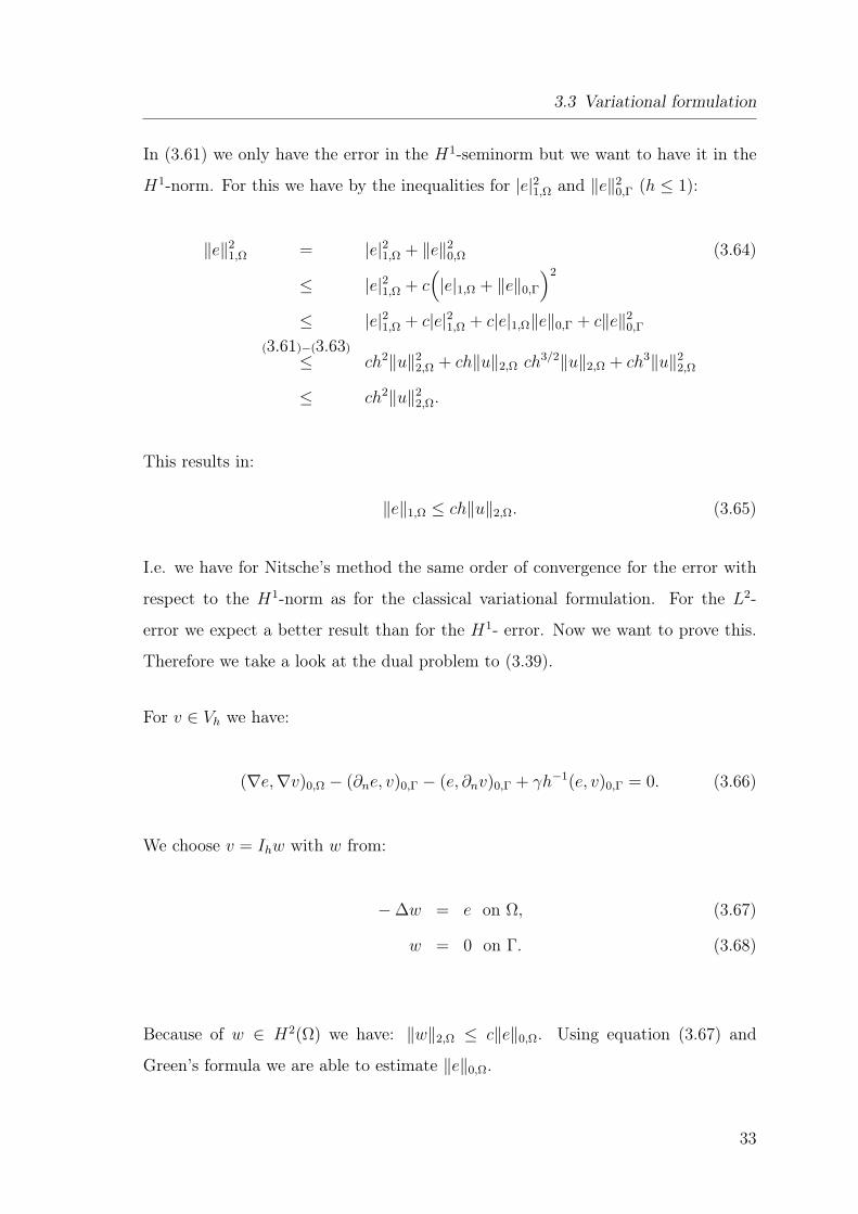
In (3.61) we only have the error in the H1-seminorm but we want to have it in the
H1-norm. For this we have by the inequalities for |e|21,Ω and ‖e‖20,Γ (h ≤ 1):
‖e‖21,Ω = |e|21,Ω + ‖e‖2
0,Ω (3.64)
≤ |e|21,Ω + c(
|e|1,Ω + ‖e‖0,Γ
)2
≤ |e|21,Ω + c|e|21,Ω + c|e|1,Ω‖e‖0,Γ + c‖e‖20,Γ
(3.61)−(3.63)
≤ ch2‖u‖22,Ω + ch‖u‖2,Ω ch3/2‖u‖2,Ω + ch3‖u‖2
2,Ω
≤ ch2‖u‖22,Ω.
This results in:
‖e‖1,Ω ≤ ch‖u‖2,Ω. (3.65)
I.e. we have for Nitsche’s method the same order of convergence for the error with
respect to the H1-norm as for the classical variational formulation. For the L2-
error we expect a better result than for the H1- error. Now we want to prove this.
Therefore we take a look at the dual problem to (3.39).
For v ∈ Vh we have:
(∇e,∇v)0,Ω − (∂ne, v)0,Γ − (e, ∂nv)0,Γ + γh−1(e, v)0,Γ = 0. (3.66)
We choose v = Ihw with w from:
− ∆w = e on Ω, (3.67)
w = 0 on Γ. (3.68)
Because of w ∈ H2(Ω) we have: ‖w‖2,Ω ≤ c‖e‖0,Ω. Using equation (3.67) and
Green’s formula we are able to estimate ‖e‖0,Ω.
33
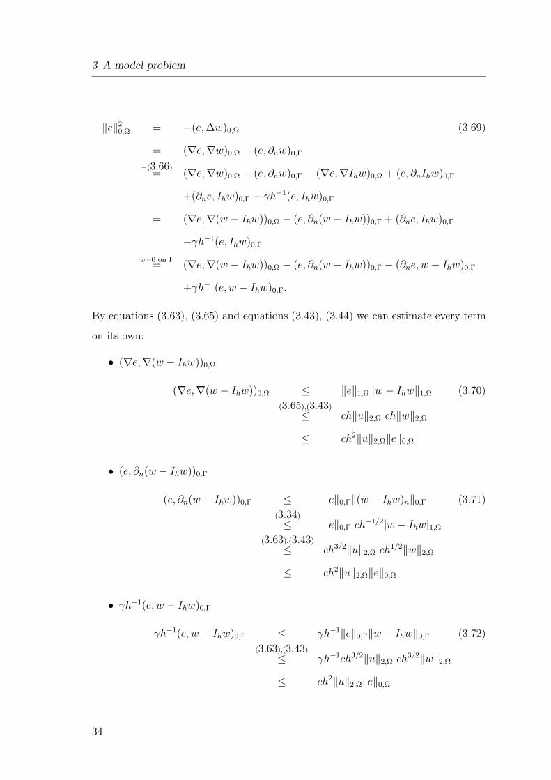
3 A model problem
‖e‖20,Ω = −(e, ∆w)0,Ω (3.69)
= (∇e,∇w)0,Ω − (e, ∂nw)0,Γ
−(3.66)= (∇e,∇w)0,Ω − (e, ∂nw)0,Γ − (∇e,∇Ihw)0,Ω + (e, ∂nIhw)0,Γ
+(∂ne, Ihw)0,Γ − γh−1(e, Ihw)0,Γ
= (∇e,∇(w − Ihw))0,Ω − (e, ∂n(w − Ihw))0,Γ + (∂ne, Ihw)0,Γ
−γh−1(e, Ihw)0,Γ
w=0 on Γ= (∇e,∇(w − Ihw))0,Ω − (e, ∂n(w − Ihw))0,Γ − (∂ne, w − Ihw)0,Γ
+γh−1(e, w − Ihw)0,Γ.
By equations (3.63), (3.65) and equations (3.43), (3.44) we can estimate every term
on its own:
• (∇e,∇(w − Ihw))0,Ω
(∇e,∇(w − Ihw))0,Ω ≤ ‖e‖1,Ω‖w − Ihw‖1,Ω (3.70)(3.65),(3.43)
≤ ch‖u‖2,Ω ch‖w‖2,Ω
≤ ch2‖u‖2,Ω‖e‖0,Ω
• (e, ∂n(w − Ihw))0,Γ
(e, ∂n(w − Ihw))0,Γ ≤ ‖e‖0,Γ‖(w − Ihw)n‖0,Γ (3.71)(3.34)
≤ ‖e‖0,Γ ch−1/2|w − Ihw|1,Ω
(3.63),(3.43)
≤ ch3/2‖u‖2,Ω ch1/2‖w‖2,Ω
≤ ch2‖u‖2,Ω‖e‖0,Ω
• γh−1(e, w − Ihw)0,Γ
γh−1(e, w − Ihw)0,Γ ≤ γh−1‖e‖0,Γ‖w − Ihw‖0,Γ (3.72)(3.63),(3.43)
≤ γh−1ch3/2‖u‖2,Ω ch3/2‖w‖2,Ω
≤ ch2‖u‖2,Ω‖e‖0,Ω
34
3.3 Variational formulation
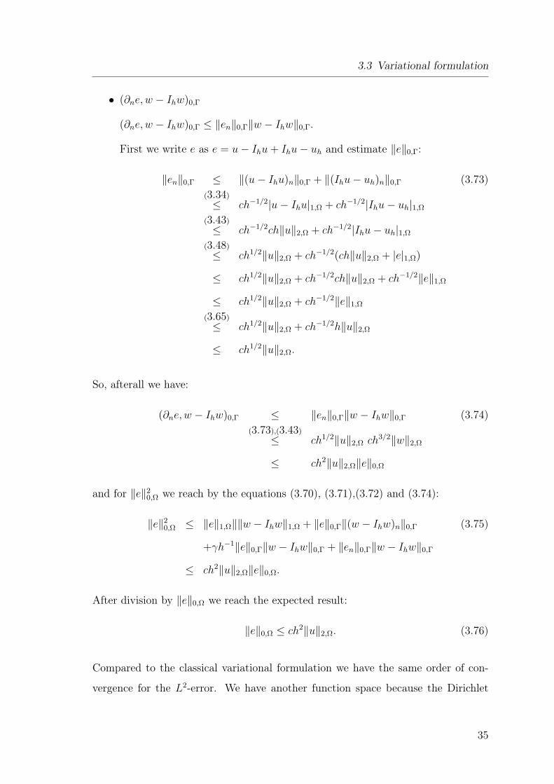
• (∂ne, w − Ihw)0,Γ
(∂ne, w − Ihw)0,Γ ≤ ‖en‖0,Γ‖w − Ihw‖0,Γ.
First we write e as e = u − Ihu + Ihu − uh and estimate ‖e‖0,Γ:
‖en‖0,Γ ≤ ‖(u − Ihu)n‖0,Γ + ‖(Ihu − uh)n‖0,Γ (3.73)(3.34)
≤ ch−1/2|u − Ihu|1,Ω + ch−1/2|Ihu − uh|1,Ω
(3.43)
≤ ch−1/2ch‖u‖2,Ω + ch−1/2|Ihu − uh|1,Ω
(3.48)
≤ ch1/2‖u‖2,Ω + ch−1/2(ch‖u‖2,Ω + |e|1,Ω)
≤ ch1/2‖u‖2,Ω + ch−1/2ch‖u‖2,Ω + ch−1/2‖e‖1,Ω
≤ ch1/2‖u‖2,Ω + ch−1/2‖e‖1,Ω
(3.65)
≤ ch1/2‖u‖2,Ω + ch−1/2h‖u‖2,Ω
≤ ch1/2‖u‖2,Ω.
So, afterall we have:
(∂ne, w − Ihw)0,Γ ≤ ‖en‖0,Γ‖w − Ihw‖0,Γ (3.74)(3.73),(3.43)
≤ ch1/2‖u‖2,Ω ch3/2‖w‖2,Ω
≤ ch2‖u‖2,Ω‖e‖0,Ω
and for ‖e‖20,Ω we reach by the equations (3.70), (3.71),(3.72) and (3.74):
‖e‖20,Ω ≤ ‖e‖1,Ω‖‖w − Ihw‖1,Ω + ‖e‖0,Γ‖(w − Ihw)n‖0,Γ (3.75)
+γh−1‖e‖0,Γ‖w − Ihw‖0,Γ + ‖en‖0,Γ‖w − Ihw‖0,Γ
≤ ch2‖u‖2,Ω‖e‖0,Ω.
After division by ‖e‖0,Ω we reach the expected result:
‖e‖0,Ω ≤ ch2‖u‖2,Ω. (3.76)
Compared to the classical variational formulation we have the same order of con-
vergence for the L2-error. We have another function space because the Dirichlet
35
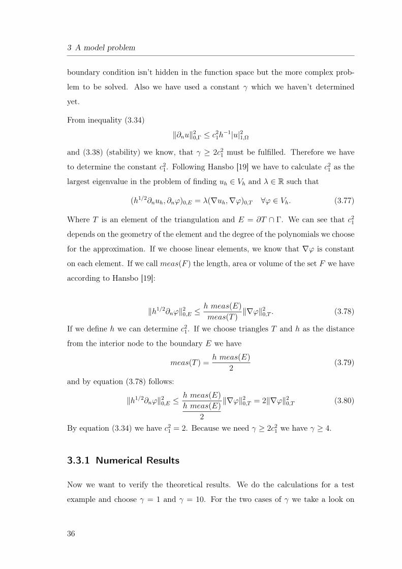
3 A model problem
boundary condition isn’t hidden in the function space but the more complex prob-
lem to be solved. Also we have used a constant γ which we haven’t determined
yet.
From inequality (3.34)
‖∂nu‖20,Γ ≤ c2
1h−1|u|21,Ω
and (3.38) (stability) we know, that γ ≥ 2c21 must be fulfilled. Therefore we have
to determine the constant c21. Following Hansbo [19] we have to calculate c2
1 as the
largest eigenvalue in the problem of finding uh ∈ Vh and λ ∈ R such that
(h1/2∂nuh, ∂nϕ)0,E = λ(∇uh,∇ϕ)0,T ∀ϕ ∈ Vh. (3.77)
Where T is an element of the triangulation and E = ∂T ∩ Γ. We can see that c21
depends on the geometry of the element and the degree of the polynomials we choose
for the approximation. If we choose linear elements, we know that ∇ϕ is constant
on each element. If we call meas(F ) the length, area or volume of the set F we have
according to Hansbo [19]:
‖h1/2∂nϕ‖20,E ≤ h meas(E)
meas(T )‖∇ϕ‖2
0,T . (3.78)
If we define h we can determine c21. If we choose triangles T and h as the distance
from the interior node to the boundary E we have
meas(T ) =h meas(E)
2(3.79)
and by equation (3.78) follows:
‖h1/2∂nϕ‖20,E ≤ h meas(E)
h meas(E)
2
‖∇ϕ‖20,T = 2‖∇ϕ‖2
0,T (3.80)
By equation (3.34) we have c21 = 2. Because we need γ ≥ 2c2
1 we have γ ≥ 4.
3.3.1 Numerical Results
Now we want to verify the theoretical results. We do the calculations for a test
example and choose γ = 1 and γ = 10. For the two cases of γ we take a look on
36
3.3 Variational formulation
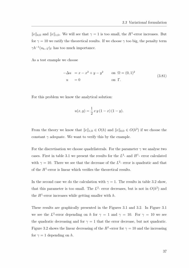
‖e‖0,Ω and ‖e‖1,Ω. We will see that γ = 1 is too small, the H1-error increases. But
for γ = 10 we ratify the theoretical results. If we choose γ too big, the penalty term
γh−1(uh, ϕ)Γ has too much importance.
As a test example we choose
−∆u = x − x2 + y − y2 on Ω = (0, 1)2
u = 0 on Γ.(3.81)
For this problem we know the analytical solution:
u(x, y) =1
2x y (1 − x) (1 − y).
From the theory we know that ‖e‖1,Ω ∈ O(h) and ‖e‖0,Ω ∈ O(h2) if we choose the
constant γ adequate. We want to verify this by the example.
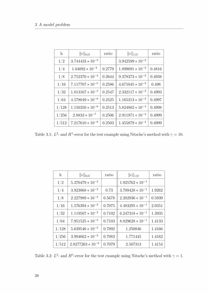
For the discretisation we choose quadrilaterals. For the parameter γ we analyse two
cases. First in table 3.1 we present the results for the L2- and H1- error calculated
with γ = 10. There we see that the decrease of the L2- error is quadratic and that
of the H1-error is linear which verifies the theoretical results.
In the second case we do the calculation with γ = 1. The results in table 3.2 show,
that this parameter is too small. The L2- error decreases, but is not in O(h2) and
the H1-error increases while getting smaller with h.
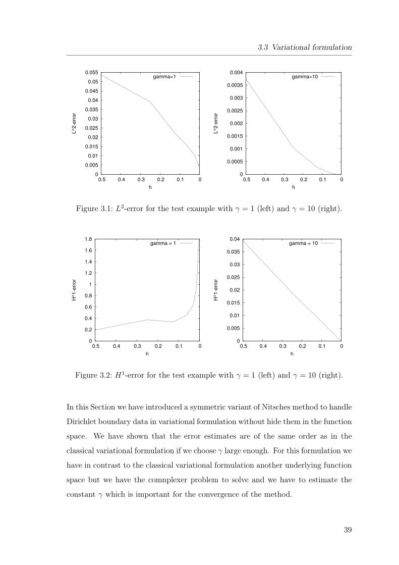
These results are graphically presented in the Figures 3.1 and 3.2. In Figure 3.1
we see the L2-error depending on h for γ = 1 and γ = 10. For γ = 10 we see
the quadratic decreasing and for γ = 1 that the error decrease, but not quadratic.
Figure 3.2 shows the linear decreasing of the H1-error for γ = 10 and the increasing
for γ = 1 depending on h.
37
3 A model problem
h ‖e‖0,Ω ratio ‖e‖1,Ω ratio
1/2 3.744433 ∗ 10−3 3.942599 ∗ 10−2
1/4 1.04092 ∗ 10−3 0.2779 1.899091 ∗ 10−2 0.4816
1/8 2.752370 ∗ 10−4 0.2644 9.378373 ∗ 10−3 0.4938
1/16 7.117707 ∗ 10−5 0.2586 4.671045 ∗ 10−3 0.498
1/32 1.813167 ∗ 10−5 0.2547 2.332117 ∗ 10−3 0.4993
1/64 4.578049 ∗ 10−6 0.2525 1.165313 ∗ 10−3 0.4997
1/128 1.150350 ∗ 10−6 0.2513 5.824802 ∗ 10−4 0.4998
1/256 2.8833 ∗ 10−7 0.2506 2.911971 ∗ 10−4 0.4999
1/512 7.217610 ∗ 10−8 0.2503 1.455879 ∗ 10−4 0.4999
Table 3.1: L2- and H1-error for the test example using Nitsche’s method with γ = 10.
h ‖e‖0,Ω ratio ‖e‖1,Ω ratio
1/2 5.370479 ∗ 10−2 1.925762 ∗ 10−1
1/4 3.923868 ∗ 10−2 0.73 3.709428 ∗ 10−1 1.9262
1/8 2.227989 ∗ 10−2 0.5678 2.202936 ∗ 10−1 0.5939
1/16 1.576394 ∗ 10−2 0.7075 4.483295 ∗ 10−1 2.0351
1/32 1.119507 ∗ 10−2 0.7102 6.247318 ∗ 10−1 1.3935
1/64 7.951525 ∗ 10−3 0.7103 8.829628 ∗ 10−1 1.4133
1/128 5.639546 ∗ 10−3 0.7092 1.250846 1.4166
1/256 3.994662 ∗ 10−3 0.7083 1.771445 1.4162
1/512 2.8277263 ∗ 10−3 0.7079 2.507313 1.4154
Table 3.2: L2- and H1-error for the test example using Nitsche’s method with γ = 1.
38
3.3 Variational formulation
0
0.005
0.01
0.015
0.02
0.025
0.03
0.035
0.04
0.045
0.05
0.055
0 0.1 0.2 0.3 0.4 0.5
L^2
-err
or
h
gamma=1
0
0.0005
0.001
0.0015
0.002
0.0025
0.003
0.0035
0.004
0 0.1 0.2 0.3 0.4 0.5
L^2
-err
or
h
gamma=10
Figure 3.1: L2-error for the test example with γ = 1 (left) and γ = 10 (right).
0
0.2
0.4
0.6
0.8
1
1.2
1.4
1.6
1.8
0 0.1 0.2 0.3 0.4 0.5
H^1
-err
or
h
gamma = 1
0
0.005
0.01
0.015
0.02
0.025
0.03
0.035
0.04
0 0.1 0.2 0.3 0.4 0.5
H^1
-err
or
h
gamma = 10
Figure 3.2: H1-error for the test example with γ = 1 (left) and γ = 10 (right).
In this Section we have introduced a symmetric variant of Nitsches method to handle
Dirichlet boundary data in variational formulation without hide them in the function
space. We have shown that the error estimates are of the same order as in the
classical variational formulation if we choose γ large enough. For this formulation we
have in contrast to the classical variational formulation another underlying function
space but we have the comnplexer problem to solve and we have to estimate the
constant γ which is important for the convergence of the method.
39

3 A model problem
40
4 Inverse Problems
As described in the introduction we want to solve inverse problems. Before we do
this in Section 5 we need some theoretical results about solving inverse problems.
Here we only want to present the basics. For proofs and more information see the
literature, e.g. Louis [25] and Rieder [30] on which this Section is based.
4.1 The theory of inverse problems
In this Section we define what is an inverse problem and when to call it ill-posed.
We reduce solving the inverse problem to solving the normal equation A∗Af = A∗g,
introduce the Moore-Penrose inverse A+ and the singular system which we need in
the next Section for the regularisation methods.
At first we want to recapitulate from the introduction what is an inverse problem
and when we call a problem ill-posed.
For given A : X → Y we call the calculation of Ax with x ∈ X the direct
problem. If we want to find x ∈ X for given y ∈ Y , so that Ax = y, we
call this an inverse problem.
Definition 4.1. Let A : X → Y be a mapping between the topologic spaces X, Y .
The problem (A,X, Y ) is called well-posed, if
• ∀ g ∈ Y ∃ a solution to Af = g.
• The solution is well defined.
41
4 Inverse Problems
• The solution depends continuously on the data, i.e. A−1 is continuous.
If one of these conditions is not satisfied the problem is called ill-posed.
If g /∈ R(A) there doesn’t exist a solution to Af = g. So we have to define a new
solution idea. In the following X and Y are Hilbert spaces. We call f ∈ X solution
to Af = g with g /∈ R(A) if f minimizes the residual
‖Af − g‖Y ≤ ‖Aφ − g‖Y ∀φ ∈ X. (4.1)
For g ∈ R(A) this definition is also valid and results in the solution f .
In theorem 4.1 we formulate equivalent results for reaching this f . Therefore we
need the adjoint operator to A ∈ L(X,Y ) A∗ ∈ L(Y,X) which is characterised by
∀ x ∈ X : (Ax, y)Y = (x,A∗y)X (4.2)
and the orthogonal projector PM ∈ L(Z) from the Hilbert space Z onto a subset
M ⊂ Z. By the following theorem we are able to find f ∈ X which minimizes the
residual by solving the normal equation.
Theorem 4.1. Let g ∈ Y and A ∈ L(X,Y ). Then the following declarations are
equivalent
a) f ∈ X satisfies Af = PR(A)g.
b) f ∈ X minimizes the residual:
‖Af − g‖Y ≤ ‖Aφ − g‖Y ∀φ ∈ X. (4.3)
c) f ∈ X solves the normal equation
A∗Af = A∗g. (4.4)
If we call L(g) := ϕ ∈ X | A∗Aϕ = A∗g the set of solutions of the normal equation,
we can formulate the following properties of the set L(g):
42
4.1 The theory of inverse problems
Lemma 4.1. Let g ∈ Y . Then
• L(g) 6= ∅ ⇔ g ∈ R(A) ⊕ R(A)⊥.
• L(g) is closed and convex.
As we are interested in only one solution of the normal equation, we need a distin-
guished solution in the set L(g). We choose the element with minimal norm.
Lemma 4.2. For g ∈ R(A)⊕R(A)⊥ L(g) contains a well defined f+ with minimal
norm:
‖f+‖X < ‖φ‖X ∀φ ∈ L(g)\f+. (4.5)
By this lemma we have the existence of a unique solution of the normal equation if
g ∈ R(A) ⊕ R(A)⊥.
Definition 4.2. The mapping A+ : D(A+) ⊂ Y → X with D(A+) = R(A)⊕R(A)⊥
which assign every g ∈ D(A+) the well defined element f+ ∈ L(g) with minimal
norm, is called Moore-Penrose-Inverse of A ∈ L(X,Y ).
The element f+ = A+g is called minimum-norm-solution of Af = g.
It can be shown, that f+ = A+g is the unique solution of the normal equation in
N(A)⊥ if g ∈ D(A+). The properties of A+ are listed in the following theorem.
Theorem 4.2. The Moore-Penrose-Inverse A+ for A ∈ L(X,Y ) has the following
qualities:
• A+ is defined on the whole space Y iff R(A) is closed.
• R(A+) = N(A)⊥.
• A+ is linear.
• A+ is continuous iff R(A) = R(A).
43
4 Inverse Problems
A+ is uniquely characterised by the four Moore-Penrose-Axioms:
AA+A = A, A+AA+ = A+,
A+A = PR(A∗), AA+ = PR(A).(4.6)
By A+ and f+ we have a well defined solution to our problem. So the ill-posedness
of the problem is caused by A−1 which is not continuous. This leads us to a new
definition of ill-posedness in the sense of Nashed.
Definition 4.3. We call a problem (A,X, Y ) ill-posed in the sense of Nashed when
R(A) is not closed in Y . Otherwise the problem is called well-posed in the sense of
Nashed.
A typical example for ill-posed problems are problems with compact operators which
have infinite dimensional range. For analytical results we need the singular value
decomposition. Let A ∈ L(X) with X a normed space. A is called self-adjoint if
A∗ = A. σ(A) = λ ∈ C | λI − A is not invertible is called spectrum of A. λ ∈ C
is eigenvalue of A, if there exist x 6= 0 with Ax = λx.
Theorem 4.3. Let X be a Hilbert space and A ∈ K(X) a self-adjoint compact
operator with eigenvalues λn ∈ R and orthonormal eigenvectors vn ∈ X. For every
x ∈ X we have:
Ax =∞∑
n=1
λn〈x, vn〉vn. (4.7)
Now, let A ∈ K(X,Y ) with X,Y Hilbert spaces. Then T = A∗A ∈ K(X) is self-
adjoint. The corresponding eigenvalues λn of T have been arranged according to
size:
λ1 ≥ λ2 ≥ . . . > 0.
With σn := +√
λn and un := σ−1n Avn, n ∈ N we have
Avn = σnun, A∗un = σnvn (4.8)
where un is an orthonormal system for R(A) = N(A∗)⊥ because
〈uj, uk〉Y =1
σjσk
〈Avj, Avk〉Y =1
σjσk
〈A∗Avj, vk〉X =σj
σk
〈vj, vk〉X = δj,k (4.9)
44
4.1 The theory of inverse problems
and vn for R(A∗) = N(A)⊥. With these we are able to define the singular system
of A.
Definition 4.4. vn, un; σnn≥0 ⊂ X × Y × (0,∞) is called singular system of A.
Af =∞∑
n=1
σn〈f, vn〉Xun. (4.10)
is called singular value decomposition.
We can also describe A∗g and A+g as a series with coefficients of the singular system
of A.
If A ∈ K(X,Y ) with singular system vn, un; σn then
A∗g =∞∑
n=1
σn〈g, un〉Y vn (4.11)
A+g =∞∑
n=1
σ−1n 〈g, un〉Y vn for g ∈ D(A+). (4.12)
If R(A) is finite dimensional, A+ is continuous.
Now, let A ∈ K(X,Y ) with singular system vn, un; σn and φ : [0,∞) → R a
piecewise continuous function with jump discontinuity. Therefore we define:
φ(A∗A)x :=∞∑
n=1
φ(σ2n)〈x, vn〉Xvn + φ(0)PN (A)x. (4.13)
For φ(t) = +√
t we call φ(A∗A) absolute value of A:
|A|x := (A∗A)1/2x =∞∑
n=1
σn〈x, vn〉Xvn. (4.14)
For |A∗| we get:
|A∗|y = (AA∗)1/2y =∞∑
n=1
σn〈y, un〉Y un. (4.15)
By this we can represent the range of A∗ as the range of |A| and the range of A as
the range of |A∗|:
45
4 Inverse Problems
Theorem 4.4. Let A ∈ L(X,Y ) with X,Y Hilbert spaces. Then:
R(A∗) = R(|A|) = R((AA∗)1/2).
R(A) = R(|A∗|) = R((A∗A)1/2).(4.16)
For later use we generalise equation (4.14):
|A|2νx := (A∗A)νx =∞∑
n=1
σ2νn 〈x, vn〉Xvn. (4.17)
We need this for the following theory of regularisation.
4.2 Regularisation
In this Section we define a regularisation method, introduce the worst case error and
how to reach a regularisation method by using the singular system. As a special
regularisation which we use for the calculation in the next Section, we introduce the
Tikhonov-Phillips-regularisation.
If R(A) is not closed, the generalized inverse A+ is not continuous. For this problem
we need the regularisation of inverse problems, i.e. an approximation of A+ with
a family of continuous operators Rtt>0 defined on Y . With a suitable choice of t
this leads us to
Definition 4.5. Let A ∈ L(X,Y ) and Rtt>0 a family of continuous (maybe not
linear) operators from Y to X with Rt0 = 0. If there exists a mapping γ : (0,∞) ×Y → (0,∞) so that for all g ∈ R(A)
sup
‖A+g − Rγ(ǫ,gǫ)gǫ‖X
∣∣∣ gǫ ∈ Y, ‖g − gǫ‖Y ≤ ǫ
→ 0 (ǫ → 0) (4.18)
is satisfied, the pair (Rtt>0, γ) is called regularisation or regularisation method for
A+. If all Rt are linear, the regularisation is linear. The mapping γ is a parameter
choice with
limǫ→0
supγ(ǫ, gǫ) | gǫ ∈ Y, ‖g − gǫ‖Y ≤ ǫ = 0. (4.19)
The value γ(ǫ, gǫ) is the regularisation parameter. If it depends only on ǫ it is called
a-priori, else a-posteriori parameter choice.
46
4.2 Regularisation
From equation (4.18) we have the convergence:
limǫ→0
‖Rγ(ǫ,g)g − A+g‖X = 0 ∀ g ∈ R(A). (4.20)
The reconstruction error ‖A+g − Rγgǫ‖X for a linear regularisation is bounded by
the sum of approximation error and data error:
‖A+g − Rγgǫ‖X ≤ ‖A+g − Rγg‖X
︸ ︷︷ ︸
approximation error
+ ‖Rγ(g − gǫ)‖X︸ ︷︷ ︸
data error
(4.21)
For information about the convergence rate of regularisation methods we need ad-
ditional assumptions to the general solution. Therefore we need the spaces Xν ⊂ X
with
Xν := R(|A|ν) = |A|νz | z ∈ N (A)⊥, ν ≥ 0. (4.22)
For these we have Xν ⊂ Xµ for ν ≥ µ and X0 = N (A)⊥. Due to this definition we
can illustrate x ∈ Xν as sum with coefficients of the singular system. For x ∈ Xν
exists z ∈ N (A)⊥ with x = |A|νz =∞∑
k=1
σνk〈z, vk〉Xvk. Now we can define a norm
‖.‖ν :
‖x‖2ν := ‖z‖2
X =∞∑
k=1
σ−2νk |〈x, vk〉X |2, (4.23)
by which we can give an alternative characterisation of the space Xν :
Xν = x ∈ N (A)⊥ | ‖x‖ν < ∞. (4.24)
We call a continuous mapping T : Y → X with T0 = 0 reconstruction method for
solving the operator equation with operator A ∈ L(X,Y ). The question is now,
what is the worst reconstruction error for a smooth solution with noisy data. The
answer is delivered by the following supremum under the assumption f ∈ Xν with
‖f‖ν ≤ ρ:
Eν(ǫ, ρ, T ) := sup‖Tgǫ − A+g‖X | g ∈ R(A), gǫ ∈ Y,
‖g − gǫ‖Y ≤ ǫ, ‖A+g‖ν ≤ ρ (4.25)
= sup‖Tgǫ − x‖X | x ∈ Xν , gǫ ∈ Y, ‖Ax − gǫ‖Y ≤ ǫ, ‖x‖ν ≤ ρ.
47
4 Inverse Problems
The adequate reconstruction method is the method with smallest error Eν(ǫ, ρ, T ).
So we are interested in the error
Eν(ǫ, ρ) := infEν(ǫ, ρ, T ) | T : Y → X continuous, T0 = 0. (4.26)
For A ∈ L(X,Y ) has been shown (see e.g. Louis [25])
Eν(ǫ, ρ) = eν(ǫ, ρ) := sup‖x‖X | x ∈ Xν , ‖Ax‖Y ≤ ǫ, ‖x‖ν ≤ ρ. (4.27)
By eν(ǫ, ρ) we are able to declare the worst case error of the best reconstruction-
method without knowing the reconstruction method if we know the noise level ǫ,
f ∈ Xν and ‖f‖ν is bounded by ρ.
Theorem 4.5. Let A ∈ L(X,Y ) and ν > 0. Then
eν(ǫ, ρ) ≤ ρ1/(ν+1)ǫν/(ν+1). (4.28)
Moreover there exists ǫkk∈N with ǫk → 0 for k → ∞, for which we have
eν(ǫk, ρ) = ρ1/(ν+1)ǫν/(ν+1)k . (4.29)
For a proof see Rieder [30].
By equation (4.28) we are able to establish the new notations optimal and of optimal
order.
Definition 4.6. Let A ∈ L(X,Y ) with an open range. The family of reconstruction
methods Tǫǫ>0 is called of optimal order concerning Xν if there exists a constant
Cν > 1 so that for all ǫ > 0 sufficiently small and ρ ≥ 0:
Eν(ǫ, ρ, Tǫ) ≤ Cνρ1/(ν+1)ǫν/(ν+1). (4.30)
If this estimation is fulfilled with Cν = 1, the reconstruction method is called optimal.
Regularisation methods are reconstruction methods. Due to this the above definition
is also valid for regularisation methods.
48
4.2 Regularisation
Theorem 4.6. Let A ∈ L(X,Y ) with open range. There exists a family of continu-
ous operators Rtt≥0 , Rt : Y → X,Rt0 = 0 and a mapping γ : (0,∞)×Y → (0,∞),
so that Rγ(ǫ,.).ǫ>0 is of optimal order concerning Xν. For b > 1 γb is defined as
γb(ǫ, .) := γ(bǫ, .). Then (Rtt>0, γb) is a regularisation method for A+ which is of
optimal order concerning Xµ for all µ ∈ (0, ν].
Till now we only define regularisation. Now we want to construct some. The follow-
ing notations and definitions are based on Rieder [30] where A+ = (A∗A)−1A∗ and
the series description of A∗ is used to construct regularisation methods. In Louis
[25] the series description of A+ is used for the construction. The resulting methods
are equal because of choosing different filter functions.
For injective A ∈ K(X,Y ) we can illustrate A+ as A+ = (A∗A)−1A∗. For stabilising
(A∗A)−1 (which is not continuous) we use a family of piecewise continuous functions
Fγ : [0, ‖A‖2] → R with jump discontinuity. These functions satisfy
limγ→0
Fγ(λ) =1
λ∀ λ ∈ (0, ‖A‖2]. (4.31)
By this we have a continuous operator Fγ(A∗A) which converges pointwise to (A∗A)−1
for γ → 0. We call Fγγ>0 filter and define:
Rγg := Fγ(A∗A)A∗g. (4.32)
By the singular system vn, un; σn of A and using equation (4.13) we have
Fγ(A∗A)A∗g =
∞∑
n=1
Fγ(σ2n)σn〈g, un〉Y vn + Fγ(0) PN (A)A
∗g︸ ︷︷ ︸
=0 (R(A∗)=N(A)⊥)
. (4.33)
In the following we need another description of A+g − Rγg. Therefore we use, that
A+g solves the normal equation A∗Af = A∗g:
A+g − Rγg = A+g − Fγ(A∗A)A∗g (4.34)
= A+g − Fγ(A∗A)A∗AA+g
= pγ(A∗A)A+g
49
4 Inverse Problems
with
pγ(t) := 1 − tFγ(t). (4.35)
Theorem 4.7. Let A ∈ K(X,Y ). The filter Fγγ>0 satisfies (4.31) and
λ|Fγ(λ)| ≤ CF ∀ λ ∈ [0, ‖A‖2], γ > 0. (4.36)
Then
limγ→0
Fγ(A∗A)A∗g =
A+g g ∈ D(A+)
∞ g /∈ D(A+).
(4.37)
Theorem 4.8. The filter Fγγ>0 satisfies in equation (4.36). Set fγ := Rγg =
Fγ(A∗A)A∗g and f ǫ
γ := Rγgǫ with g, gǫ ∈ Y and ‖g − gǫ‖ ≤ ǫ. Then:
‖Afγ − Af ǫγ‖Y ≤ CF ǫ (4.38)
and
‖fγ − f ǫγ‖X ≤ ǫ
√
CF M(γ) (4.39)
with
M(γ) := supFγ(λ) | λ ∈ [0, ‖A‖2]. (4.40)
As mentioned in equation (4.21) we can split the total error in approximation error
and data error. By theorem 4.8 we are able to estimate the data error:
‖A+g − Rγgǫ‖X ≤ ‖A+g − Rγg‖X + ‖Rγ(g − gǫ)‖X (4.41)
≤ ‖A+g − Rγg‖X + ǫ√
CF M(γ). (4.42)
By theorem 4.7 we have limγ→0
‖A+g − Rγg‖X = 0 but by equation (4.31) we have
divergence for M(γ). As a consequence the total error grows for γ → 0. If we
connect γ and ǫ we can enforce convergence.
Corollary 4.1. The filter Fγγ>0 satisfies equation (4.31) and in equation (4.36).
If we choose γ : (0,∞) → (0,∞) such, that
γ(ǫ) → 0 and ǫ√
M(γ(ǫ)) → 0, for ǫ → 0 (4.43)
then (Rtt>0, γ) is a regularisation method for A+.
50
4.2 Regularisation
This leads us to the definition of a regularising filter:
Definition 4.7. For A ∈ L(X,Y ) we call a family Fγγ>0 of piecewise continuous
functions with jump discontinuity regularising filter if (4.31) and (4.36) are satisfied.
Lemma 4.3. Let the filter Ftt>0 be regularising for A ∈ L(X,Y ). For pt(λ) =
1 − λFt(λ) and µ > 0 exist t0 > 0 and ωµ : (0, t0] → R such that
sup0≤λ≤‖A‖2
λµ/2|pt(λ)| ≤ ωµ(t) ∀ t ∈ (0, t0]. (4.44)
Let g ∈ R(A) and f+ = A+g ∈ Xµ with ‖f+‖µ ≤ ρ. For ft = Rtg and 0 < t ≤ t0 we
then have:
‖f+ − ft‖X ≤ ωµ(t)ρ (4.45)
and
‖Af+ − Aft‖Y ≤ ωµ+1(t)ρ. (4.46)
This leads us to an a-priori parameter choice which results in an regularisation
method of optimal order.
Theorem 4.9. Let Ftt>0 a regularising filter for A ∈ L(X,Y ). For pt(λ) and
µ > 0 exist t0 > 0 and ωµ : (0, t0] → R such that
sup0≤λ≤‖A‖2
λµ/2|pt(λ)| ≤ ωµ(t) ∀ t ∈ (0, t0].
Farther we have
ωµ(t) ≤ Cptµ/2 for t → 0 (4.47)
and
M(t) ≤ CM t−1 for t → 0 (4.48)
with Cp , CM = const > 0. The a-priori parameter choice γ : (0,∞) → (0,∞)
satisfies
Cγ
(ǫ
ρ
) 2
µ+1
≤ γ(ǫ) ≤ CΓ
(ǫ
ρ
) 2
µ+1
for ǫ → 0 (4.49)
with Cγ, CΓ = const > 0.
Then (Rtt>0, γ) is a regularisation method of optimal order for A+ corresponding
Xµ.
51
4 Inverse Problems
We want to define the qualification of a filter before we want to present the idea of
the Tikhonov-Phillips-regularisation.
Definition 4.8. Let Ftt>0 a regularising filter for A ∈ L(X,Y ) with M(t) ≤CM t−1, t → 0. The maximal µ0 so that there exists a constant Cp = Cp(µ) for every
µ ∈ (0, µ0] with
sup0≤λ≤‖A‖2
λµ/2|pt(λ)| ≤ Cptµ/2, t → 0 (4.50)
is called qualification of the filter.
Now we want to present the idea of the Tikhonov-Phillips-regularisation, starting
with the classical method. There the filter
Fγ(λ) =1
λ + γ, γ > 0 (4.51)
is used. By this filter the regularisation is
Rγy = Fγ(A∗A)A∗y, y ∈ Y (4.52)
and Rγy is the unique solution of the regularised normal equation
(A∗A + γI)Rγy = A∗y. (4.53)
It can be shown that the classical Tikhonov-Phillips-regularisation has the qualifi-
cation µ0 = 2 and is of optimal order corresponding to Xµ with 0 < µ ≤ 2 and the
a-priori parameter choice (4.49). By γ(ǫ) = µ−1(ǫ/ρ)2/(µ+1) the Tikhonov-Phillips-
regularisation is optimal for 0 < µ ≤ 2. (see Rieder [30]).
Instead of the classical we want to use the general method of Tikhonov-Phillips
where we replace the identity I by a general operator B.
Let A ∈ L(X,Y ) and B : X → Z a linear, continuous operator where Z is a banach
space. Additionally exists β > 0 with
β‖f‖X ≤ ‖Bf‖Z ∀f ∈ X. (4.54)
52
4.2 Regularisation
Under these constraints exists a unique solution fγ ∈ X to
(A∗A + γB∗B)f = A∗y (4.55)
where fγ depends continuously on y ∈ Y for γ > 0.
We can characterise the solution fγ of equation (4.55) as minimising argument of
the Tikhonov-Phillips-functional
Jγ,yx := ‖Ax − y‖2Y + γ‖Bx‖2
Z , (4.56)
where ‖Bx‖2Z is called penalty term. So, if fγ is the unique solution to equation
(4.55), fγ is the unique minimum of Jγ,y and contrary. By this we can define Rγγ>0
as:
Rγy := fγ = (A∗A + γB∗B)−1A∗y = argminJγ,y(f) | f ∈ Y . (4.57)
53

4 Inverse Problems
54
5 The inverse model problem
In this Section we want to describe the problems to be solved. As underlying PDE-
constraint we have the potential equation on the unit square with different boundary
conditions. After introducing the resulting variational equations to be solved, we
shortly describe the preconditioned cg-method (pcg) and the multigrid method,
which we use for the computation of the solutions.
5.1 Description of the problems
For generality we regard the differential equation −∆u = g on Ω = (0, 1)2 instead
of −∆u = 0, which is the underlying differential equation for the application. Also
we take a look on different boundary conditions and given measurements on ΓO.
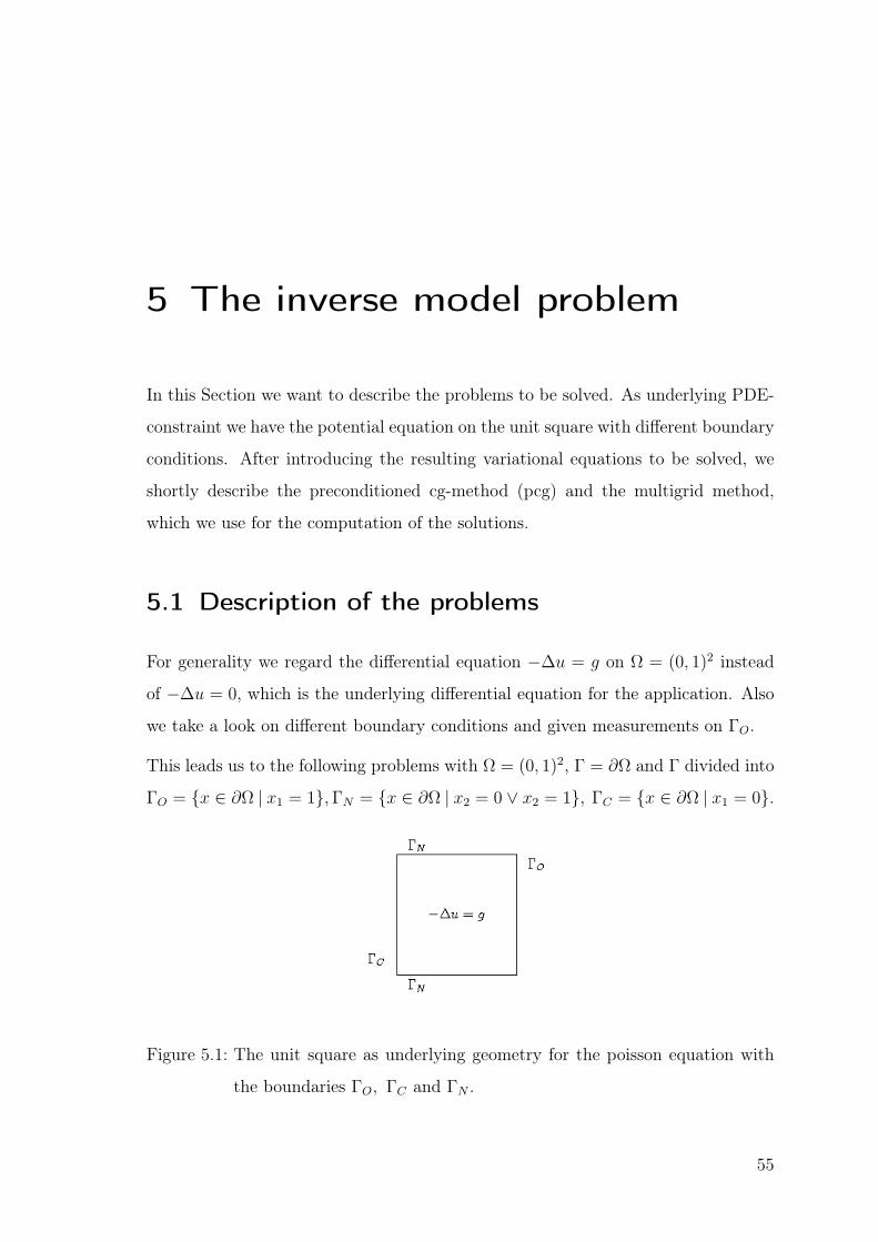
This leads us to the following problems with Ω = (0, 1)2, Γ = ∂Ω and Γ divided into
ΓO = x ∈ ∂Ω | x1 = 1, ΓN = x ∈ ∂Ω | x2 = 0 ∨ x2 = 1, ΓC = x ∈ ∂Ω | x1 = 0.
Figure 5.1: The unit square as underlying geometry for the poisson equation with
the boundaries ΓO, ΓC and ΓN .
55
5 The inverse model problem
We have four possible problems to solve on this geometry. We can search Neumann
or Dirichlet control on ΓC for given Neumann measurement or Dirichlet measure-
ment on ΓO. In the following we will introduce the four cases which we formulate
as optimal control problems, i.e. we search the control q on ΓC to minimise the
difference between the calculated solution and the given measurements on ΓO.
1. Find ∂nu = q on ΓC , for given measurement ∂nu = f on ΓO such that
J(u, q) → min, J(w, τ) :=1
2‖∂nw − f‖2
ΓO(5.1)
under the PDE-constraint
−∆u = g on Ω ,
∂nu = 0 on ΓN ,
u = 0 on ΓO ,
∂nu = q on ΓC .
(5.2)
Where J(w, τ) defines a so-called cost functional and q denotes a control vari-
able.
2. Find u = q on ΓC for given measurement ∂nu = f on ΓO such that
J(u, q) → min, J(w, τ) :=1
2‖∂nw − f‖2
ΓO(5.3)
under the PDE-constraint
−∆u = g on Ω ,
∂nu = 0 on ΓN ,
u = 0 on ΓO ,
u = q on ΓC .
(5.4)
These are the two problems based on the application where we have given Neumann
measurements on ΓO. As another two cases we want to formulate the problems
where we search the control q on ΓC (q = u|ΓCor q = ∂nu|ΓC
) for given Dirichlet
measurements u|ΓO= 0:
56
5.1 Description of the problems
3. Find u = q on ΓC for given measurement u = 0 on ΓO such that
J(u, q) → min, J(w, τ) :=1
2‖w‖2
ΓO(5.5)
under the PDE-constraint
−∆u = g on Ω ,
∂nu = 0 on ΓN ,
∂nu = f on ΓO ,
u = q on ΓC .
(5.6)
Following Lions [24] these problems are uniquely solvable.
4. Find ∂nu = q on ΓC for given measurement u = 0 on ΓO such that
J(u, q) → min, J(w, τ) :=1
2‖w‖2
ΓO(5.7)
under the PDE-constraint
−∆u = g on Ω ,
∂nu = 0 on ΓN ,
∂nu = f on ΓO ,
∂nu = q on ΓC .
(5.8)
In the fourth case we have the problem that the direct problem (5.8) with Neumann
boundary conditions is not uniquely solvable. If exist a solution u of the problem
we know that u + const is also a solution. Because of this we only take care of the
problems 1. to 3.. For the moment we want to take a look on a general problem.
After discretisation and using Nitsche’s method we can write all three problems as
(see e.g. [24] or [39])
J(uh, q) → min (5.9)
Auh = g + Bq. (5.10)
A, B, g and q depending on the problem to be solved with uh and q are unknown.
If A is regular we can write:
uh = A−1g + A−1Bq. (5.11)
57
5 The inverse model problem
We want to solve minimisation problems. From Section 4.1 we know that solving
the minimisation problem is equivalent in solving the normal equation. Following
Louis [25] we can introduce a positive definite matrix C so that we can write
‖Du − f‖21 = (Du − f)∗C(Du − f). (5.12)
In our case D is the identity. Using equations (5.11), (5.12) and the fact we want
to solve a minimisation problem we have:
BT A−T CA−1Bq + BT A−T CA−1g − BT A−T Cf = 0 (5.13)
By the Tikhonov-Phillips regularisation we have to solve in matrix vector notation
(BT A−T CA−1B + α Reg) q = BT A−T (Cf − CA−1g). (5.14)
with α the regularisation parameter and Reg the regularisation matrix from the
Tikhonov-Philips regularisation.
For the determination of A, B and g we take again a look on the direct problems
we have to solve, using Nitsche’s method. If we call n the number of vertices in Ω
and Nq the number of degrees of freedom (DOF) on ΓC we have:
1. In the first case, where we search ∂nu|ΓC= q for given ∂nu|ΓO
= f , we have to
solve for the direct problem in variational formulation ∀ ϕ ∈ Vh:
(∇uh,∇ϕ)0,Ω − (∂nuh, ϕ)0,Γ − (uh, ∂nϕ)0,ΓO+ γh−1(uh, ϕ)0,ΓO
(5.15)
= (gh, ϕ)0,Ω + γh−1(0, ϕ)0,ΓO− (0, ∂nϕ)0,ΓO
In the matrix-vector-notation Auh = g + Bq we have here:
A is a (n × n)-matrix corresponding to (ψ ∈ Vh):
(∇ψ,∇ϕ)0,Ω − (∂nψ, ϕ)0,ΓO− (ψ, ∂nϕ)0,ΓO
+ γh−1(ψ, ϕ)0,ΓO
g is a vector with n rows corresponding to:
(gh, ϕ)0,Ω
58
5.1 Description of the problems
and B is a (n × Nq)-matrix with entries from:
(ψ, ϕ)0,ΓC
The terms (∂nuh, ϕ)0,ΓNand γh−1(0, ϕ)0,ΓO
− (0, ∂nϕ)0,ΓOare zero so they are
ignored in the formulation.
In the calculation of the inverse problem we have in the regularised normal
equation (5.14) resulting from the minimisation problem:
Cf is a vector with n rows and entries from
(∂nψ, ∂nϕ)0,ΓO
and for the (n × n)-matrix C we have the entries from:
(∂nψ, ∂nϕ)0,ΓO.
2. In the second case, where we search u|ΓC= q for given ∂nu|ΓO
= f , we have
to solve in the direct problem using Nitsche’s method:
(∇uh,∇ϕ)0,Ω − (∂nuh, ϕ)0,Γ − (uh, ∂nϕ)0,ΓO∪ΓC+ γh−1(uh, ϕ)0,ΓO∪ΓC
= (gh, ϕ)0,Ω − (0, ∂nϕ)ΓO+ γh−1(0, ϕ)ΓO
(5.16)
+(q, ∂nuϕ)ΓC+ γh−1(q, ϕ)ΓC
In the matrix-vector-notation we have here:
A the (n × n)-matrix corresponding to (ψ ∈ Vh):
(∇ψ,∇ϕ)0,Ω − (∂nψ, ϕ)0,Γ − (ψ, ∂nϕ)0,ΓO∪ΓC+ γh−1(ψ, ϕ)0,ΓO∪ΓC
g the vector with n rows corresponding to:
(gh, ϕ)0,Ω
and B the (n × Nq)-matrix with entries from:
γh−1(ψ, ϕ)0,ΓC− (ψ, ∂nϕ)0,ΓC
.
59
5 The inverse model problem
Again we have caused by the boundary conditions (∂nuh, ϕ)0,ΓN= 0 which is
ignored in the formulation.
In the calculation of the inverse problem we have
Cf the vector with n rows and entries from
(∂nψ, ∂nϕ)0,ΓO
and for the (n × n)-matrix C we use again the entries:
(∂nψ, ∂nϕ)0,ΓO.
3. In the third case where we search u|ΓC= q for given u|ΓO
= 0 we have to solve
in the direct problem in variational formulation:
(∇uh,∇ϕ)0,Ω − (∂nuh, ϕ)0,Γ − (uh, ∂nϕ)0,ΓC+ γh−1(uh, ϕ)0,ΓC
(5.17)
= (gh, ϕ)0,Ω − (qh, ∂nϕ)0,ΓC+ γh−1(qh, ϕ)0,ΓC
A is the (n × n)-matrix corresponding to (ψ ∈ Vh):
(∇ψ,∇ϕ)0,Ω − (∂nψ, ϕ)0,ΓC− (ψ, ∂nϕ)0,ΓC
+ γh−1(ψ, ϕ)0,ΓC
g is the vector with n rows corresponding to:
(gh, ϕ)0,Ω + (∂nψ, ϕ)0,ΓO
and B the (n × Nq)-matrix with the entries:
γh−1(ψ, ϕ)0,ΓC− (ψ, ∂nϕ)0,ΓC
As in the previous cases we have zero Neumann conditions on ΓN and this
term doesn’t appear in the formulation.
In the calculation of the inverse problem we have here
Cf the n-vector with the entries
(∂nψ, ϕ)0,ΓO
and for the (n × n)-matrix C we have here the entries from:
(ψ, ϕ)0,ΓO
60
5.2 Numerical methods
We have introduced A, B, C, f and g depending on the problem to be solved. In
the following we describe how to solve the regularised normal equation
(BT A−T CA−1B + α Reg) q = BT A−T (Cf − CA−1g)
with general given A, B, C, f and g for searched control q.
After initializing and assembling the matrices and vectors we have to do the following
steps:
1. Calculate G := A−1B by using the pcg-method.
2. Compute M := GT CG = BT A−T CA−1B.
3. Calculate A−1g by using the pcg-method.
4. Estimate MtF := GT (Cfh − CA−1g).
5. Use the Gauß-Jordan algorithm for (M + α · Reg) and
6. compute with this q from (M + α · Reg) q = MtF .
7. At last compute uh = A−1(g + Bq) with the calculated q by using the pcg-
method.
The calculation of A−1 occures by the pcg-method where the multigrid method (see
Section 5.2) is used as preconditioner. We want to describe briefly the pcg method
and the multigrid method in the next Section.
5.2 Numerical methods
In this Section we want to present the pcg algorithm and the basics of the multigrid
method the twogrid method respectively. We use the multigrid method as precon-
ditioner in the pcg-method for solving the inverse problem. For more information
see the literature (e.g. [8], [9], [18], [10], [31], [41]).
We start the description of the numerical methods with the preconditioned cg-
method (pcg) (see Braess [8]).
61
5 The inverse model problem
Let us assume we know a positive definite matrix C which is an approximation of
A from the equation Ax = b to be solved. For x0 ∈ Rn we consider
x1 = x0 − αC−1g0 (5.18)
with g0 = Ax0 − b. If we have C = A we have solved the problem in the first step.
This leads us to the pcg-algorithm.
Algorithm 5.1. (PCG)
i) Let x0 ∈ Rn. Set g0 = Ax0 − b, d0 = −h0 = −C−1g0
ii) Calculate for k ≥ 0:
• αk =gT
k hk
dTk Adk
• xk+1 = xk + αkdk
• gk+1 = gk + αkAdk
• hk+1 = C−1gk+1
• βk =gT
k+1hk+1
gTk hk
• dk+1 = −hk+1 + βkdk
The matrix C is the preconditioner, i.e. the approximation of A calculated in our
case by the multigrid method. With C positive definite we have the following prop-
erties:
If we have gk−1 6= 0 holds:
• dk−1 6= 0
• Vk := span[g0, AC−1g0, . . . , (AC−1)k−1g0] = span[g0, g1, . . . , gk−1] and
span[d0, d1, . . . , dk−1] = C−1span[g0, g1, . . . , gk−1]
• The vectors d0, d1, . . . , dk−1 are conjugate.
• f(xk) = minz∈Vk
f(x0 + C−1z).
62
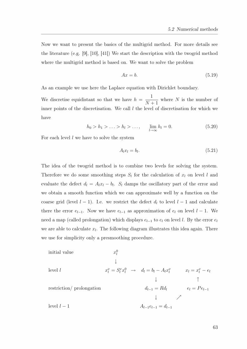
5.2 Numerical methods
Now we want to present the basics of the multigrid method. For more details see
the literature (e.g. [9], [10], [41]) We start the description with the twogrid method
where the multigrid method is based on. We want to solve the problem
Ax = b. (5.19)
As an example we use here the Laplace equation with Dirichlet boundary.
We discretise equidistant so that we have h =1
N + 1where N is the number of
inner points of the discretisation. We call l the level of discretisation for which we
have
h0 > h1 > . . . > hl > . . . , liml→∞
hl = 0. (5.20)
For each level l we have to solve the system
Alxl = bl. (5.21)
The idea of the twogrid method is to combine two levels for solving the system.
Therefore we do some smoothing steps Sl for the calculation of xl on level l and
evaluate the defect dl = Alxl − bl. Sl damps the oscillatory part of the error and
we obtain a smooth function which we can approximate well by a function on the
coarse grid (level l − 1). I.e. we restrict the defect dl to level l − 1 and calculate
there the error el−1. Now we have el−1 as approximation of el on level l − 1. We
need a map (called prolongation) which displays el−1 to el on level l. By the error el
we are able to calculate xl. The following diagram illustrates this idea again. There
we use for simplicity only a presmoothing procedure.
initial value x0l
↓level l xν
l = Sνl x0
l → dl = bl − Alxνl xl = xν
l − el
↓ ↑restriction/ prolongation dl−1 = Rdl el = Pel−1
↓ րlevel l − 1 Al−1el−1 = dl−1
63
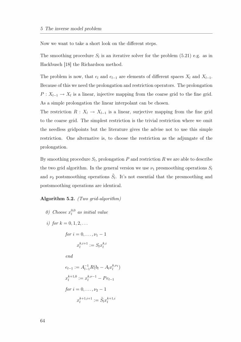
5 The inverse model problem
Now we want to take a short look on the different steps.
The smoothing procedure Sl is an iterative solver for the problem (5.21) e.g. as in
Hackbusch [18] the Richardson method.
The problem is now, that el and el−1 are elements of different spaces Xl and Xl−1.
Because of this we need the prolongation and restriction operators. The prolongation
P : Xl−1 → Xl is a linear, injective mapping from the coarse grid to the fine grid.
As a simple prolongation the linear interpolant can be chosen.
The restriction R : Xl → Xl−1 is a linear, surjective mapping from the fine grid
to the coarse grid. The simplest restriction is the trivial restriction where we omit
the needless gridpoints but the literature gives the advise not to use this simple
restriction. One alternative is, to choose the restriction as the adjungate of the
prolongation.
By smoothing procedure Sl, prolongation P and restriction R we are able to describe
the two grid algorithm. In the general version we use ν1 presmoothing operations Sl
and ν2 postsmoothing operations Sl. It’s not essential that the presmoothing and
postsmoothing operations are identical.
Algorithm 5.2. (Two grid-algorithm)
0) Choose x0,0l as initial value
i) for k = 0, 1, 2, . . .
for i = 0, . . . , ν1 − 1
xk,i+1l := Slx
k,il
end
el−1 := A−1l−1R(bl − Alx
k,ν1
l )
xk+1,0l := xk,ν−1
l − Pel−1
for i = 0, . . . , ν2 − 1
xk+1,i+1l := Slx
k+1,il
64
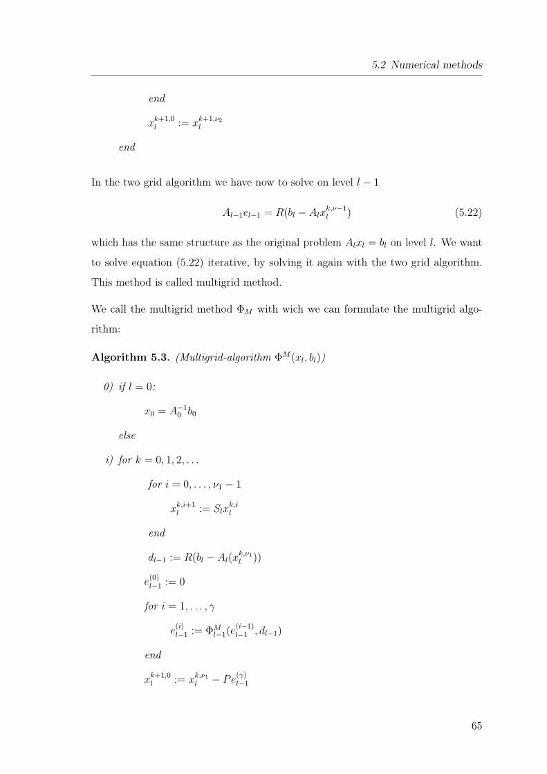
5.2 Numerical methods
end
xk+1,0l := xk+1,ν2
l
end
In the two grid algorithm we have now to solve on level l − 1
Al−1el−1 = R(bl − Alxk,ν−1l ) (5.22)
which has the same structure as the original problem Alxl = bl on level l. We want
to solve equation (5.22) iterative, by solving it again with the two grid algorithm.
This method is called multigrid method.
We call the multigrid method ΦM with wich we can formulate the multigrid algo-
rithm:
Algorithm 5.3. (Multigrid-algorithm ΦM(xl, bl))
0) if l = 0:
x0 = A−10 b0
else
i) for k = 0, 1, 2, . . .
for i = 0, . . . , ν1 − 1
xk,i+1l := Slx
k,il
end
dl−1 := R(bl − Al(xk,ν1
l ))
e(0)l−1 := 0
for i = 1, . . . , γ
e(i)l−1 := ΦM
l−1(e(i−1)l−1 , dl−1)
end
xk+1,0l := xk,ν1
l − Pe(γ)l−1
65
5 The inverse model problem
for i = 0, . . . , ν2 − 1
xk+1,i+1l = Slx
k+1,il
end
xk+1,0l := xk+1,ν2
l
end
In step i) we have a loop over i = 1, . . . , γ which is unknown till now. Following the
literature γ is choosen as 1 or 2. Then we speak of a V-cycle (γ = 1) or a W-cycle
(γ = 2), respectively.
These are the basics of the numerical methods we use for solving the model problems
on the unit square. For convergence analysis and more details see the literature
already cited. In the next Section we want to present the numerical results for the
model problems using a test example.
66
6 Numerical results for the model
problem
In this Section we present the numerical results for the calculation of the model
problem. We set γ = 10 in the terms resulting from Nitsche’s method (Section 3.3).
The special focus lies on the calculation of the searched control q on ΓC . With this
calculated control we compute u on Ω and so we can also analyse how good is the
approximation of the given boundary values u and ∂nu on ΓO and of u|ΓCand ∂nu|ΓC
respectively (which we know from our analytic solution).
As underlying model problem we have
− ∆u = g. (6.1)
with g = 12xy2 − 12xy + 2x− 12y2 + 12y − 2. We know the corresponding analytic
solution of this problem is
u(x, y) = y2(1 − y)2(1 − x). (6.2)
with the outward pointing normals
∂nu|ΓC= y2(1 − y)2, ∂nu|ΓO
= −y2(1 − y)2. (6.3)
We use bilinear elements on quadrilaterals. If we say, we refine three times, we
divide the unit square into (23)2 = 64 cells, i.e we have 23 + 1 vertices on each
boundary. We present the results of calculation for different global grid refinements,
67
6 Numerical results for the model problem
different degrees of freedom on ΓC and different regularisation parameters. For the
calculation we use the three regularisation matrices:
R := Id, R1 :=1
h
−1 1
−1 1. . . . . .
. . . 1
−1
, R2 :=1
h2
2 −1
−1 2 −1. . . . . . . . .
. . . . . . −1
−1 2
We start the analysis of the results for given Neumann measurement on ΓO and
searched Neumann control on ΓC .
6.1 Neumann measurements on ΓO and Neumann
control on ΓC
In this Section we want to find the Neumann control q = ∂nu|ΓCfor given Neumann
measurements f = ∂nu|ΓOsuch that
J(u, q) → min, J(w, τ) =1
2‖∂nw − f‖2
ΓO(6.4)
under the PDE-constraint
−∆u = g on Ω ,
∂nu = 0 on ΓN ,
u = 0 on ΓO ,
∂nu = q on ΓC .
(6.5)
First we analyse the results for the searched control ∂nu|ΓC= q for different grid
refinements and the different regularisation matrices. As regularisation parameter
we choose α = 1.e − 13 and discretise Ω up to eight times (65536 cells). On every
boundary, especially on ΓC we have 2i +1 degrees of freedom (DOF), if we discretise
i times. From the analytic solution (equation (6.2)) we know ∂nu|ΓC= y2(1 − y)2.
68
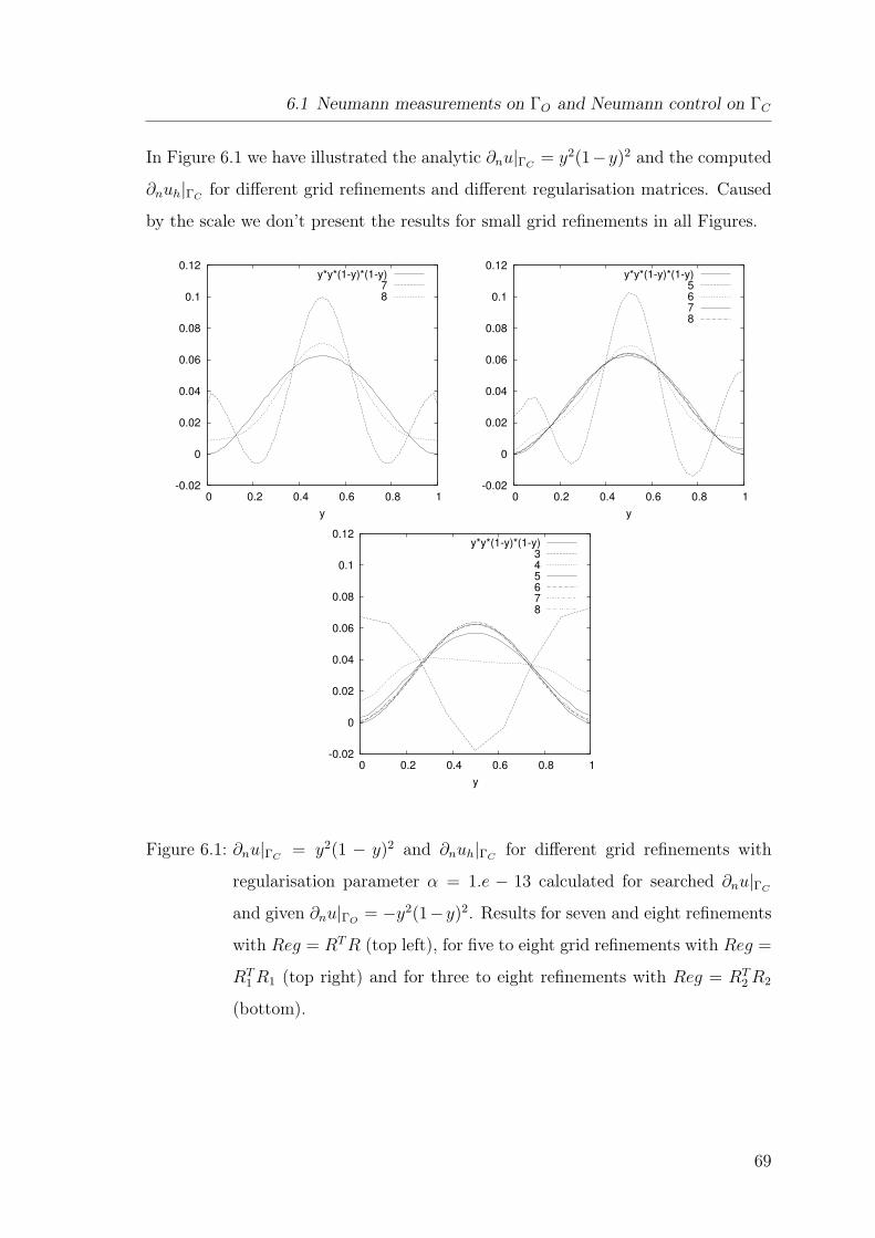
6.1 Neumann measurements on ΓO and Neumann control on ΓC
In Figure 6.1 we have illustrated the analytic ∂nu|ΓC= y2(1−y)2 and the computed
∂nuh|ΓCfor different grid refinements and different regularisation matrices. Caused
by the scale we don’t present the results for small grid refinements in all Figures.
-0.02
0
0.02
0.04
0.06
0.08
0.1
0.12
0 0.2 0.4 0.6 0.8 1
y
y*y*(1-y)*(1-y)78
-0.02
0
0.02
0.04
0.06
0.08
0.1
0.12
0 0.2 0.4 0.6 0.8 1
y
y*y*(1-y)*(1-y)5678
-0.02
0
0.02
0.04
0.06
0.08
0.1
0.12
0 0.2 0.4 0.6 0.8 1
y
y*y*(1-y)*(1-y)345678
Figure 6.1: ∂nu|ΓC= y2(1 − y)2 and ∂nuh|ΓC
for different grid refinements with
regularisation parameter α = 1.e − 13 calculated for searched ∂nu|ΓC
and given ∂nu|ΓO= −y2(1−y)2. Results for seven and eight refinements
with Reg = RT R (top left), for five to eight grid refinements with Reg =
RT1 R1 (top right) and for three to eight refinements with Reg = RT
2 R2
(bottom).
69
6 Numerical results for the model problem
We can see in all three cases that we get better results for finer grids. The un-
symmetric approximation of ∂nu|ΓCin the case of regularising with Reg = RT
1 R1 is
caused by the unsymmetric matrix R1. For the regularisation with Reg = RT2 R2 we
can see that in the surrounding of y = 0.5 we get the best result for six refinements
but near y = 0 and y = 1 we get the better results for finer grids.
For the moment we don’t want to care about the error calculation because this is
also dependent on the regularisation parameter as we will see later. We have seen
that we have to discretise fine enough to get good results for the approximation of
the control ∂nu|ΓC. The disadvantage of this result is, if we discretise i times we
have 2i + 1 DOF on ΓC which is decisive for the runtime of the calculation. The
question is now can we reduce the number of DOF on ΓC for a fine grid on Ω without
loosing quality of the approximation. We will analyse this for the calculation of the
searched control ∂nu|ΓCfor given Neumann measurement ∂nu|ΓO
= −y2(1 − y)2.
For the calculation of ∂nuh|ΓCwe will refine the grid eight times and set α = 1.e−13.
In Figure 6.2 we see the calculations for the different regularisation matrices with
different number of DOF on ΓC . In all graphics we present the results for 257 DOF
on ΓC which is the number of DOF for refining the grid eight times without special
choice of particular DOFs.
We can see that for the regularisation with RT R (Figure 6.2 top left) and RT2 R2
(Figure 6.2 bottom) we reach good results if we reduce the number of DOF on ΓC
to 41 31 respectively. Only for the regularisation with Reg = RT1 R1 (Figure 6.2 top
right) we have to use 91 DOF on ΓC .
We have seen that we can reduce the number of DOF on ΓC without loosing much
quality of the approximation. Again we have only presented the graphical results and
dispense with the error calculation caused by the dependence on the regularisation
parameter. Now we will take a look on the influence of the regularisation parameter
on the results of the calculation. Therefore we will discretise Ω eight times and
use the reduced number of DOF on ΓC for the calculation. Depending on the
regularisation matrix we choose different regularisation parameters. In Figure 6.3
70
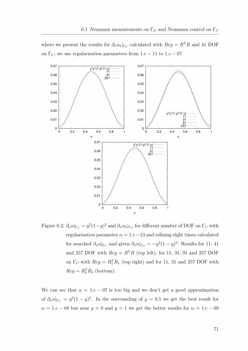
6.1 Neumann measurements on ΓO and Neumann control on ΓC
where we present the results for ∂nuh|ΓCcalculated with Reg = RT R and 41 DOF
on ΓC , we use regularisation parameters from 1.e − 11 to 1.e − 07.
0
0.01
0.02
0.03
0.04
0.05
0.06
0.07
0 0.2 0.4 0.6 0.8 1
y
y*y*(1-y)*(1-y)1141
257
0
0.01
0.02
0.03
0.04
0.05
0.06
0.07
0 0.2 0.4 0.6 0.8 1
y
y*y*(1-y)*(1-y)113191
257
0
0.01
0.02
0.03
0.04
0.05
0.06
0.07
0 0.2 0.4 0.6 0.8 1
y
y*y*(1-y)*(1-y)1131
257
Figure 6.2: ∂nu|ΓC= y2(1−y)2 and ∂nuh|ΓC
for different number of DOF on ΓC with
regularisation parameter α = 1.e−13 and refining eight times calculated
for searched ∂nu|ΓCand given ∂nu|ΓO
= −y2(1 − y)2. Results for 11, 41
and 257 DOF with Reg = RT R (top left), for 11, 31, 91 and 257 DOF
on ΓC with Reg = RT1 R1 (top right) and for 11, 31 and 257 DOF with
Reg = RT2 R2 (bottom).
We can see that α = 1.e − 07 is too big and we don’t get a good approximation
of ∂nu|ΓC= y2(1 − y)2. In the surrounding of y = 0.5 we get the best result for
α = 1.e − 08 but near y = 0 and y = 1 we get the better results for α = 1.e − 09
71
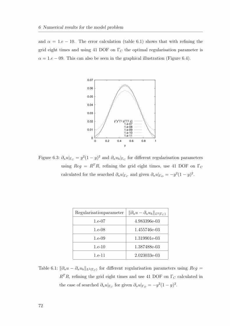
6 Numerical results for the model problem
and α = 1.e − 10. The error calculation (table 6.1) shows that with refining the
grid eight times and using 41 DOF on ΓC the optimal regularisation parameter is
α = 1.e − 09. This can also be seen in the graphical illustration (Figure 6.4).
0
0.01
0.02
0.03
0.04
0.05
0.06
0.07
0 0.2 0.4 0.6 0.8 1
y
y*y*(1-y)*(1-y)1.e-071.e-081.e-091.e-101.e-11
Figure 6.3: ∂nu|ΓC= y2(1 − y)2 and ∂nuh|ΓC
for different regularisation parameters
using Reg = RT R, refining the grid eight times, use 41 DOF on ΓC
calculated for the searched ∂nu|ΓCand given ∂nu|ΓO
= −y2(1 − y)2.
Regularisationparameter ‖∂nu − ∂nuh‖L2(ΓC)
1.e-07 4.983396e-03
1.e-08 1.455746e-03
1.e-09 1.319901e-03
1.e-10 1.387488e-03
1.e-11 2.023033e-03
Table 6.1: ‖∂nu − ∂nuh‖L2(ΓC) for different regularisation parameters using Reg =
RT R, refining the grid eight times and use 41 DOF on ΓC calculated in
the case of searched ∂nu|ΓCfor given ∂nu|ΓO
= −y2(1 − y)2.
72
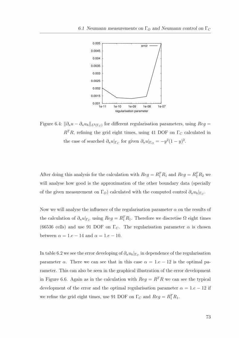
6.1 Neumann measurements on ΓO and Neumann control on ΓC
0.001
0.0015
0.002
0.0025
0.003
0.0035
0.004
0.0045
0.005
1e-11 1e-10 1e-09 1e-08 1e-07
regularisation parameter
error
Figure 6.4: ‖∂nu − ∂nuh‖L2(ΓC) for different regularisation parameters, using Reg =
RT R, refining the grid eight times, using 41 DOF on ΓC calculated in
the case of searched ∂nu|ΓCfor given ∂nu|ΓO
= −y2(1 − y)2.
After doing this analysis for the calculation with Reg = RT1 R1 and Reg = RT
2 R2 we
will analyse how good is the approximation of the other boundary data (specially
of the given measurement on ΓO) calculated with the computed control ∂nuh|ΓC.
Now we will analyse the influence of the regularisation parameter α on the results of
the calculation of ∂nu|ΓCusing Reg = RT
1 R1. Therefore we discretise Ω eight times
(66536 cells) and use 91 DOF on ΓC . The regularisation parameter α is chosen
between α = 1.e − 14 and α = 1.e − 10.
In table 6.2 we see the error developing of ∂nuh|ΓCin dependence of the regularisation
parameter α. There we can see that in this case α = 1.e − 12 is the optimal pa-
rameter. This can also be seen in the graphical illustration of the error development
in Figure 6.6. Again as in the calculation with Reg = RT R we can see the typical
development of the error and the optimal regularisation parameter α = 1.e − 12 if
we refine the grid eight times, use 91 DOF on ΓC and Reg = RT1 R1.
73
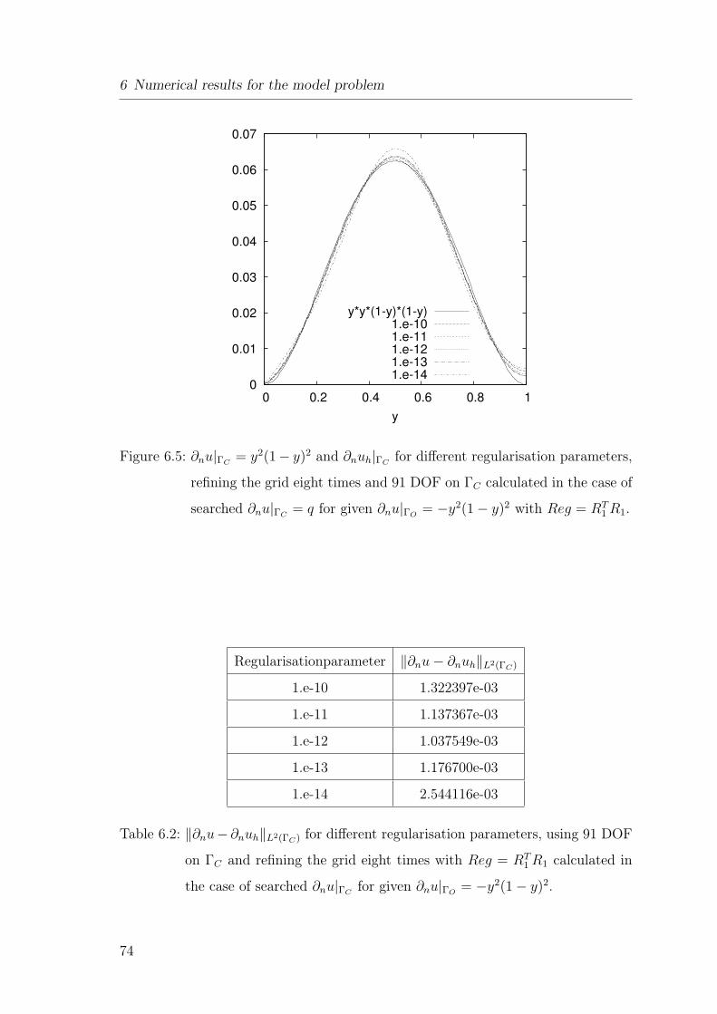
6 Numerical results for the model problem
0
0.01
0.02
0.03
0.04
0.05
0.06
0.07
0 0.2 0.4 0.6 0.8 1
y
y*y*(1-y)*(1-y)1.e-101.e-111.e-121.e-131.e-14
Figure 6.5: ∂nu|ΓC= y2(1− y)2 and ∂nuh|ΓC
for different regularisation parameters,
refining the grid eight times and 91 DOF on ΓC calculated in the case of
searched ∂nu|ΓC= q for given ∂nu|ΓO
= −y2(1 − y)2 with Reg = RT1 R1.
Regularisationparameter ‖∂nu − ∂nuh‖L2(ΓC)
1.e-10 1.322397e-03
1.e-11 1.137367e-03
1.e-12 1.037549e-03
1.e-13 1.176700e-03
1.e-14 2.544116e-03
Table 6.2: ‖∂nu− ∂nuh‖L2(ΓC) for different regularisation parameters, using 91 DOF
on ΓC and refining the grid eight times with Reg = RT1 R1 calculated in
the case of searched ∂nu|ΓCfor given ∂nu|ΓO
= −y2(1 − y)2.
74
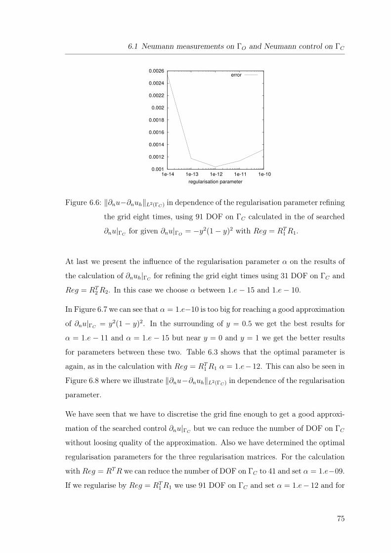
6.1 Neumann measurements on ΓO and Neumann control on ΓC
0.001
0.0012
0.0014
0.0016
0.0018
0.002
0.0022
0.0024
0.0026
1e-14 1e-13 1e-12 1e-11 1e-10
regularisation parameter
error
Figure 6.6: ‖∂nu−∂nuh‖L2(ΓC) in dependence of the regularisation parameter refining
the grid eight times, using 91 DOF on ΓC calculated in the of searched
∂nu|ΓCfor given ∂nu|ΓO
= −y2(1 − y)2 with Reg = RT1 R1.
At last we present the influence of the regularisation parameter α on the results of
the calculation of ∂nuh|ΓCfor refining the grid eight times using 31 DOF on ΓC and
Reg = RT2 R2. In this case we choose α between 1.e − 15 and 1.e − 10.
In Figure 6.7 we can see that α = 1.e−10 is too big for reaching a good approximation
of ∂nu|ΓC= y2(1 − y)2. In the surrounding of y = 0.5 we get the best results for
α = 1.e − 11 and α = 1.e − 15 but near y = 0 and y = 1 we get the better results
for parameters between these two. Table 6.3 shows that the optimal parameter is
again, as in the calculation with Reg = RT1 R1 α = 1.e−12. This can also be seen in
Figure 6.8 where we illustrate ‖∂nu−∂nuh‖L2(ΓC) in dependence of the regularisation
parameter.
We have seen that we have to discretise the grid fine enough to get a good approxi-
mation of the searched control ∂nu|ΓCbut we can reduce the number of DOF on ΓC
without loosing quality of the approximation. Also we have determined the optimal
regularisation parameters for the three regularisation matrices. For the calculation
with Reg = RT R we can reduce the number of DOF on ΓC to 41 and set α = 1.e−09.
If we regularise by Reg = RT1 R1 we use 91 DOF on ΓC and set α = 1.e− 12 and for
75
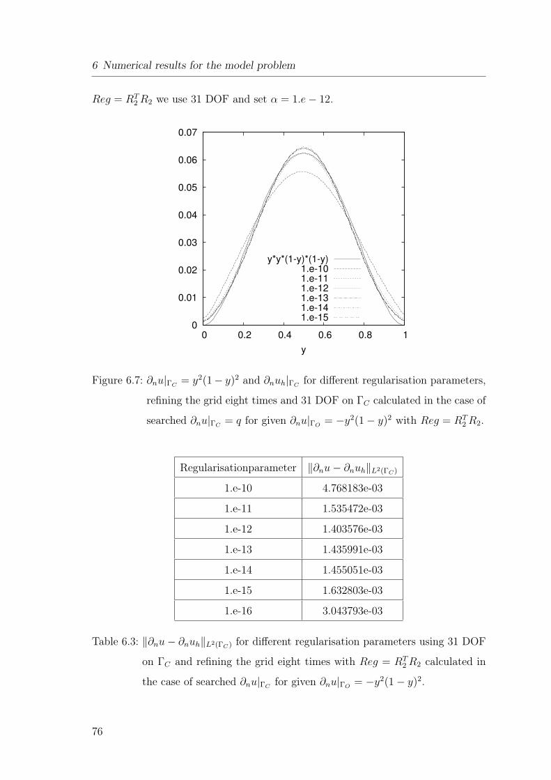
6 Numerical results for the model problem
Reg = RT2 R2 we use 31 DOF and set α = 1.e − 12.
0
0.01
0.02
0.03
0.04
0.05
0.06
0.07
0 0.2 0.4 0.6 0.8 1
y
y*y*(1-y)*(1-y)1.e-101.e-111.e-121.e-131.e-141.e-15
Figure 6.7: ∂nu|ΓC= y2(1− y)2 and ∂nuh|ΓC
for different regularisation parameters,
refining the grid eight times and 31 DOF on ΓC calculated in the case of
searched ∂nu|ΓC= q for given ∂nu|ΓO
= −y2(1 − y)2 with Reg = RT2 R2.
Regularisationparameter ‖∂nu − ∂nuh‖L2(ΓC)
1.e-10 4.768183e-03
1.e-11 1.535472e-03
1.e-12 1.403576e-03
1.e-13 1.435991e-03
1.e-14 1.455051e-03
1.e-15 1.632803e-03
1.e-16 3.043793e-03
Table 6.3: ‖∂nu − ∂nuh‖L2(ΓC) for different regularisation parameters using 31 DOF
on ΓC and refining the grid eight times with Reg = RT2 R2 calculated in
the case of searched ∂nu|ΓCfor given ∂nu|ΓO
= −y2(1 − y)2.
76
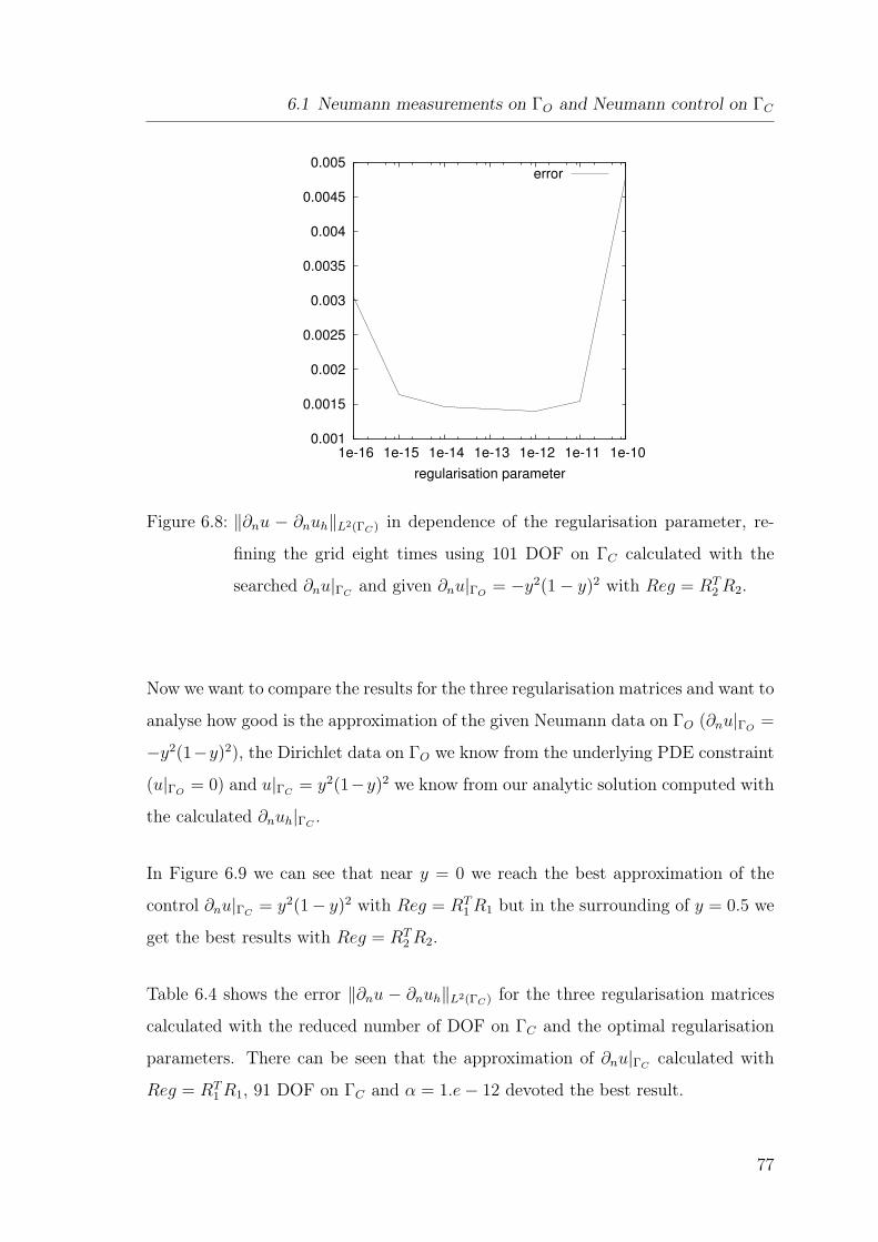
6.1 Neumann measurements on ΓO and Neumann control on ΓC
0.001
0.0015
0.002
0.0025
0.003
0.0035
0.004
0.0045
0.005
1e-16 1e-15 1e-14 1e-13 1e-12 1e-11 1e-10
regularisation parameter
error
Figure 6.8: ‖∂nu − ∂nuh‖L2(ΓC) in dependence of the regularisation parameter, re-
fining the grid eight times using 101 DOF on ΓC calculated with the
searched ∂nu|ΓCand given ∂nu|ΓO
= −y2(1 − y)2 with Reg = RT2 R2.
Now we want to compare the results for the three regularisation matrices and want to
analyse how good is the approximation of the given Neumann data on ΓO (∂nu|ΓO=
−y2(1−y)2), the Dirichlet data on ΓO we know from the underlying PDE constraint
(u|ΓO= 0) and u|ΓC
= y2(1−y)2 we know from our analytic solution computed with
the calculated ∂nuh|ΓC.
In Figure 6.9 we can see that near y = 0 we reach the best approximation of the
control ∂nu|ΓC= y2(1− y)2 with Reg = RT
1 R1 but in the surrounding of y = 0.5 we
get the best results with Reg = RT2 R2.
Table 6.4 shows the error ‖∂nu − ∂nuh‖L2(ΓC) for the three regularisation matrices
calculated with the reduced number of DOF on ΓC and the optimal regularisation
parameters. There can be seen that the approximation of ∂nu|ΓCcalculated with
Reg = RT1 R1, 91 DOF on ΓC and α = 1.e − 12 devoted the best result.
77
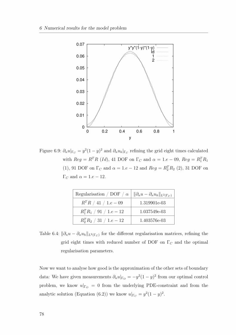
6 Numerical results for the model problem
0
0.01
0.02
0.03
0.04
0.05
0.06
0.07
0 0.2 0.4 0.6 0.8 1
y
y*y*(1-y)*(1-y)Id12
Figure 6.9: ∂nu|ΓC= y2(1− y)2 and ∂nuh|ΓC
refining the grid eight times calculated
with Reg = RT R (Id), 41 DOF on ΓC and α = 1.e − 09, Reg = RT1 R1
(1), 91 DOF on ΓC and α = 1.e − 12 and Reg = RT2 R2 (2), 31 DOF on
ΓC and α = 1.e − 12.
Regularisation / DOF / α ‖∂nu − ∂nuh‖L2(ΓC)
RT R / 41 / 1.e − 09 1.319901e-03
RT1 R1 / 91 / 1.e − 12 1.037549e-03
RT2 R2 / 31 / 1.e − 12 1.403576e-03
Table 6.4: ‖∂nu − ∂nuh‖L2(ΓC) for the different regularisation matrices, refining the
grid eight times with reduced number of DOF on ΓC and the optimal
regularisation parameters.
Now we want to analyse how good is the approximation of the other sets of boundary
data: We have given measurements ∂nu|ΓO= −y2(1 − y)2 from our optimal control
problem, we know u|ΓO= 0 from the underlying PDE-constraint and from the
analytic solution (Equation (6.2)) we know u|ΓC= y2(1 − y)2.
78
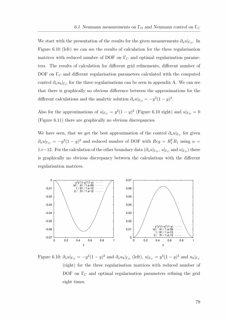
6.1 Neumann measurements on ΓO and Neumann control on ΓC
We start with the presentation of the results for the given measurements ∂nu|ΓO. In
Figure 6.10 (left) we can see the results of calculation for the three regularisation
matrices with reduced number of DOF on ΓC and optimal regularisation parame-
ters. The results of calculation for different grid refinements, different number of
DOF on ΓC and different regularisation parameters calculated with the computed
control ∂nuh|ΓCfor the three regularisations can be seen in appendix A. We can see
that there is graphically no obvious difference between the approximations for the
different calculations and the analytic solution ∂nu|ΓO= −y2(1 − y)2.
Also for the approximations of u|ΓC= y2(1 − y)2 (Figure 6.10 right) and u|ΓO
= 0
(Figure 6.11) there are graphically no obvious discrepancies.
We have seen, that we get the best approximation of the control ∂nu|ΓCfor given
∂nu|ΓO= −y2(1 − y)2 and reduced number of DOF with Reg = RT
1 R1 using α =
1.e−12. For the calculation of the other boundary data (∂nu|ΓO, u|ΓC
and u|ΓO) there
is graphically no obvious discrepancy between the calculations with the different
regularisation matrices.
-0.07
-0.06
-0.05
-0.04
-0.03
-0.02
-0.01
0
0 0.2 0.4 0.6 0.8 1
y
-y*y*(1-y)*(1-y)Id / 41 / 1.e-09
1 / 91 / 1.e-122 / 31 / 1.e-12
0
0.01
0.02
0.03
0.04
0.05
0.06
0.07
0 0.2 0.4 0.6 0.8 1
y
y*y*(1-y)*(1-y)Id / 41 / 1.e-09
1 / 91 / 1.e-122 / 31 / 1.e-12
Figure 6.10: ∂nu|ΓO= −y2(1 − y)2 and ∂nuh|ΓO
(left), u|ΓC= y2(1 − y)2 and uh|ΓC
(right) for the three regularisation matrices with reduced number of
DOF on ΓC and optimal regularisation parameters refining the grid
eight times.
79
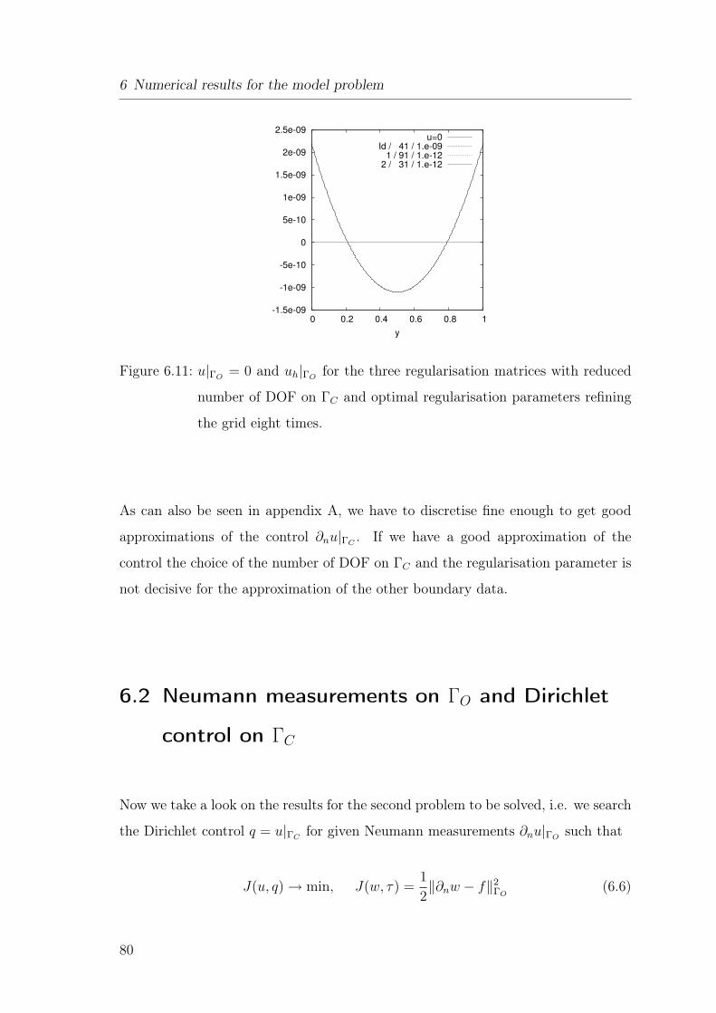
6 Numerical results for the model problem
-1.5e-09
-1e-09
-5e-10
0
5e-10
1e-09
1.5e-09
2e-09
2.5e-09
0 0.2 0.4 0.6 0.8 1
y
u=0Id / 41 / 1.e-09
1 / 91 / 1.e-122 / 31 / 1.e-12
Figure 6.11: u|ΓO= 0 and uh|ΓO
for the three regularisation matrices with reduced
number of DOF on ΓC and optimal regularisation parameters refining
the grid eight times.
As can also be seen in appendix A, we have to discretise fine enough to get good
approximations of the control ∂nu|ΓC. If we have a good approximation of the
control the choice of the number of DOF on ΓC and the regularisation parameter is
not decisive for the approximation of the other boundary data.
6.2 Neumann measurements on ΓO and Dirichlet
control on ΓC
Now we take a look on the results for the second problem to be solved, i.e. we search
the Dirichlet control q = u|ΓCfor given Neumann measurements ∂nu|ΓO
such that
J(u, q) → min, J(w, τ) =1
2‖∂nw − f‖2
ΓO(6.6)
80
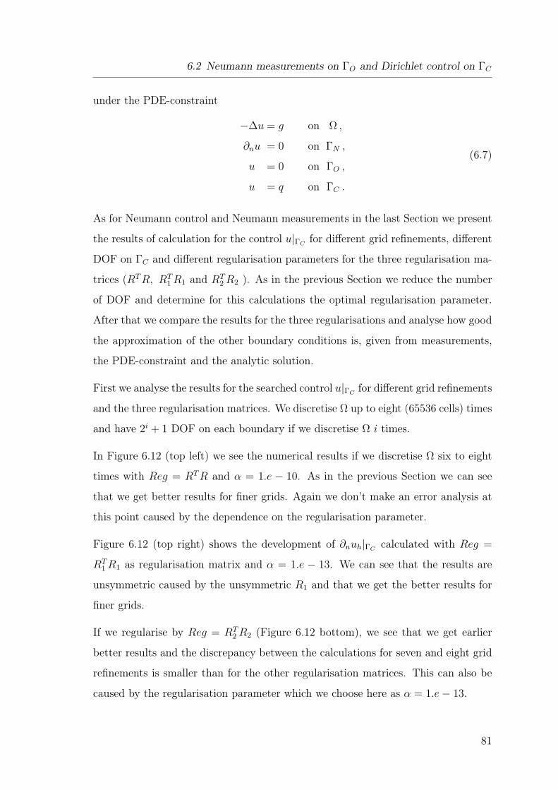
6.2 Neumann measurements on ΓO and Dirichlet control on ΓC
under the PDE-constraint
−∆u = g on Ω ,
∂nu = 0 on ΓN ,
u = 0 on ΓO ,
u = q on ΓC .
(6.7)
As for Neumann control and Neumann measurements in the last Section we present
the results of calculation for the control u|ΓCfor different grid refinements, different
DOF on ΓC and different regularisation parameters for the three regularisation ma-
trices (RT R, RT1 R1 and RT
2 R2 ). As in the previous Section we reduce the number
of DOF and determine for this calculations the optimal regularisation parameter.
After that we compare the results for the three regularisations and analyse how good
the approximation of the other boundary conditions is, given from measurements,
the PDE-constraint and the analytic solution.
First we analyse the results for the searched control u|ΓCfor different grid refinements
and the three regularisation matrices. We discretise Ω up to eight (65536 cells) times
and have 2i + 1 DOF on each boundary if we discretise Ω i times.
In Figure 6.12 (top left) we see the numerical results if we discretise Ω six to eight
times with Reg = RT R and α = 1.e − 10. As in the previous Section we can see
that we get better results for finer grids. Again we don’t make an error analysis at
this point caused by the dependence on the regularisation parameter.
Figure 6.12 (top right) shows the development of ∂nuh|ΓCcalculated with Reg =
RT1 R1 as regularisation matrix and α = 1.e − 13. We can see that the results are
unsymmetric caused by the unsymmetric R1 and that we get the better results for
finer grids.
If we regularise by Reg = RT2 R2 (Figure 6.12 bottom), we see that we get earlier
better results and the discrepancy between the calculations for seven and eight grid
refinements is smaller than for the other regularisation matrices. This can also be
caused by the regularisation parameter which we choose here as α = 1.e − 13.
81
6 Numerical results for the model problem
In general we get the better results for finer grids in all three cases. As in the previous
Section this is bad for the runtime of the program. A reduction of the number of
DOF on ΓC will have a positive effect on the runtime. Now we want to analyse if we
can reduce the number of DOF on ΓC for this problem (Dirichlet control for given
Neumann measurement) without loosing quality of the approximation.
0
0.01
0.02
0.03
0.04
0.05
0.06
0.07
0.08
0 0.2 0.4 0.6 0.8 1
y
y*y*(1-y)*(1-y)678
0
0.01
0.02
0.03
0.04
0.05
0.06
0.07
0.08
0 0.2 0.4 0.6 0.8 1
y
y*y*(1-y)*(1-y)678
0
0.01
0.02
0.03
0.04
0.05
0.06
0.07
0.08
0 0.2 0.4 0.6 0.8 1
y
y*y*(1-y)*(1.y)345678
Figure 6.12: u|ΓC= y2(1 − y)2 and uh|ΓC
for different grid refinements calculated
for searched control u|ΓCand given ∂nu|ΓO
= −y2(1 − y)2. Results
calculated with Reg = RT R and regularisationparameter α = 1.e − 10
(top left) with Reg = RT1 R1 and α = 1.e − 13 (top right) with Reg =
RT2 R2 and α = 1.e − 13 (bottom).
82
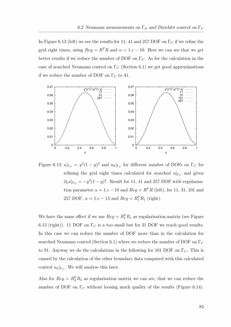
6.2 Neumann measurements on ΓO and Dirichlet control on ΓC
In Figure 6.13 (left) we see the results for 11, 41 and 257 DOF on ΓC if we refine the
grid eight times, using Reg = RT R and α = 1.e − 10. Here we can see that we get
better results if we reduce the number of DOF on ΓC . As for the calculation in the
case of searched Neumann control on ΓC (Section 6.1) we get good approximations
if we reduce the number of DOF on ΓC to 41.
0
0.01
0.02
0.03
0.04
0.05
0.06
0.07
0 0.2 0.4 0.6 0.8 1
y
y*y*(1-y)*(1-y)1141
257
0
0.01
0.02
0.03
0.04
0.05
0.06
0.07
0 0.2 0.4 0.6 0.8 1
y
y*y*(1-y)*(1-y)1131
101257
Figure 6.13: u|ΓC= y2(1 − y)2 and uh|ΓC
for different number of DOFs on ΓC for
refining the grid eight times calculated for searched u|ΓCand given
∂nu|ΓO= −y2(1− y)2. Result for 11, 41 and 257 DOF with regularisa-
tion parameter α = 1.e− 10 and Reg = RT R (left), for 11, 31, 101 and
257 DOF, α = 1.e − 13 and Reg = RT1 R1 (right).
We have the same effect if we use Reg = RT1 R1 as regularisation matrix (see Figure
6.13 (right)). 11 DOF on ΓC is a too small but for 31 DOF we reach good results.
In this case we can reduce the number of DOF more than in the calculation for
searched Neumann control (Section 6.1) where we reduce the number of DOF on ΓC
to 91. Anyway we do the calculations in the following for 101 DOF on ΓC . This is
caused by the calculation of the other boundary data computed with this calculated
control uh|ΓC. We will analyse this later.
Also for Reg = RT2 R2 as regularisation matrix we can see, that we can reduce the
number of DOF on ΓC without loosing much quality of the results (Figure 6.14).
83
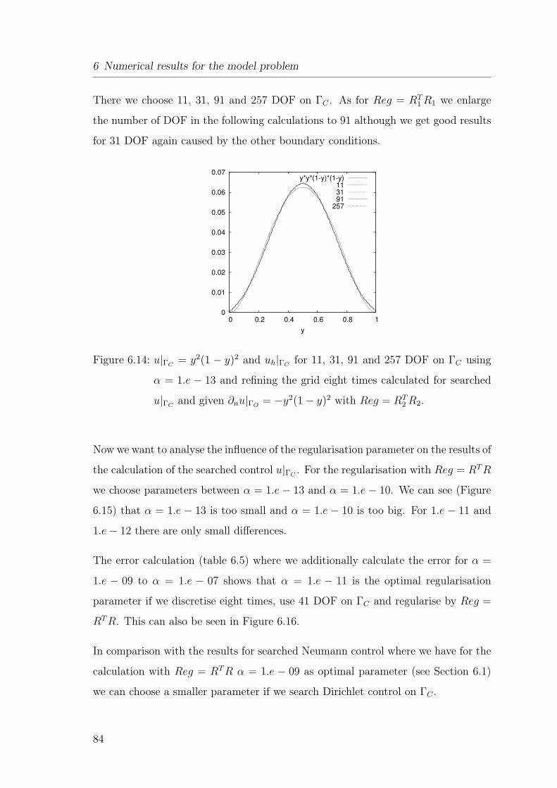
6 Numerical results for the model problem
There we choose 11, 31, 91 and 257 DOF on ΓC . As for Reg = RT1 R1 we enlarge
the number of DOF in the following calculations to 91 although we get good results
for 31 DOF again caused by the other boundary conditions.
0
0.01
0.02
0.03
0.04
0.05
0.06
0.07
0 0.2 0.4 0.6 0.8 1
y
y*y*(1-y)*(1-y)113191
257
Figure 6.14: u|ΓC= y2(1 − y)2 and uh|ΓC
for 11, 31, 91 and 257 DOF on ΓC using
α = 1.e − 13 and refining the grid eight times calculated for searched
u|ΓCand given ∂nu|ΓO
= −y2(1 − y)2 with Reg = RT2 R2.
Now we want to analyse the influence of the regularisation parameter on the results of
the calculation of the searched control u|ΓC. For the regularisation with Reg = RT R
we choose parameters between α = 1.e − 13 and α = 1.e − 10. We can see (Figure
6.15) that α = 1.e − 13 is too small and α = 1.e − 10 is too big. For 1.e − 11 and
1.e − 12 there are only small differences.
The error calculation (table 6.5) where we additionally calculate the error for α =
1.e − 09 to α = 1.e − 07 shows that α = 1.e − 11 is the optimal regularisation
parameter if we discretise eight times, use 41 DOF on ΓC and regularise by Reg =
RT R. This can also be seen in Figure 6.16.
In comparison with the results for searched Neumann control where we have for the
calculation with Reg = RT R α = 1.e − 09 as optimal parameter (see Section 6.1)
we can choose a smaller parameter if we search Dirichlet control on ΓC .
84
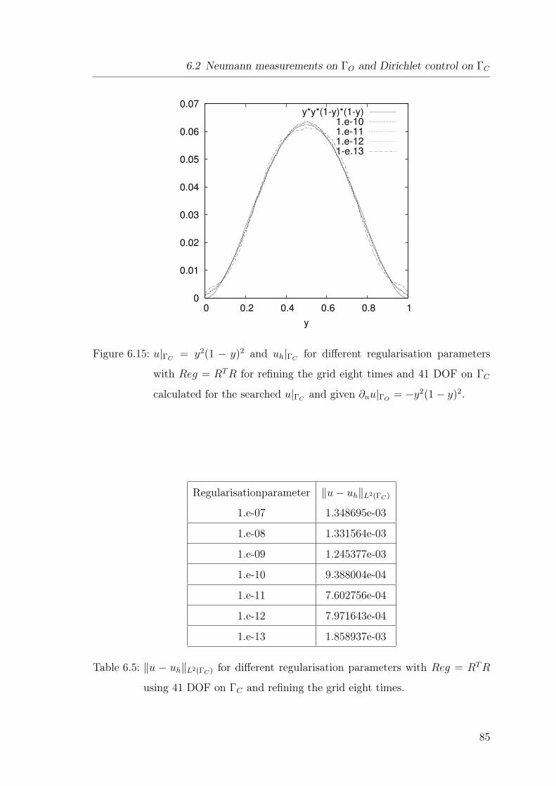
6.2 Neumann measurements on ΓO and Dirichlet control on ΓC
0
0.01
0.02
0.03
0.04
0.05
0.06
0.07
0 0.2 0.4 0.6 0.8 1
y
y*y*(1-y)*(1-y)1.e-101.e-111.e-121-e.13
Figure 6.15: u|ΓC= y2(1 − y)2 and uh|ΓC
for different regularisation parameters
with Reg = RT R for refining the grid eight times and 41 DOF on ΓC
calculated for the searched u|ΓCand given ∂nu|ΓO
= −y2(1 − y)2.
Regularisationparameter ‖u − uh‖L2(ΓC)
1.e-07 1.348695e-03
1.e-08 1.331564e-03
1.e-09 1.245377e-03
1.e-10 9.388004e-04
1.e-11 7.602756e-04
1.e-12 7.971643e-04
1.e-13 1.858937e-03
Table 6.5: ‖u − uh‖L2(ΓC) for different regularisation parameters with Reg = RT R
using 41 DOF on ΓC and refining the grid eight times.
85
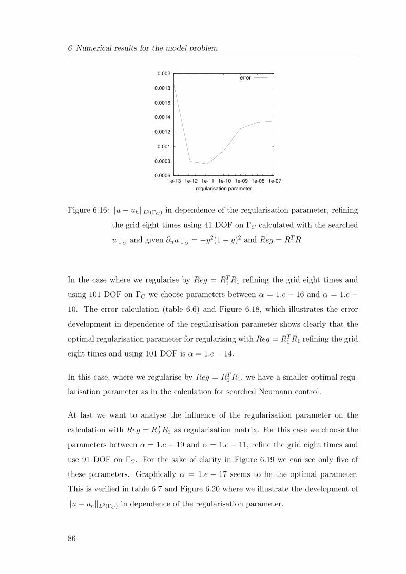
6 Numerical results for the model problem
0.0006
0.0008
0.001
0.0012
0.0014
0.0016
0.0018
0.002
1e-13 1e-12 1e-11 1e-10 1e-09 1e-08 1e-07
regularisation parameter
error
Figure 6.16: ‖u − uh‖L2(ΓC) in dependence of the regularisation parameter, refining
the grid eight times using 41 DOF on ΓC calculated with the searched
u|ΓCand given ∂nu|ΓO
= −y2(1 − y)2 and Reg = RT R.
In the case where we regularise by Reg = RT1 R1 refining the grid eight times and
using 101 DOF on ΓC we choose parameters between α = 1.e − 16 and α = 1.e −10. The error calculation (table 6.6) and Figure 6.18, which illustrates the error
development in dependence of the regularisation parameter shows clearly that the
optimal regularisation parameter for regularising with Reg = RT1 R1 refining the grid
eight times and using 101 DOF is α = 1.e − 14.
In this case, where we regularise by Reg = RT1 R1, we have a smaller optimal regu-
larisation parameter as in the calculation for searched Neumann control.
At last we want to analyse the influence of the regularisation parameter on the
calculation with Reg = RT2 R2 as regularisation matrix. For this case we choose the
parameters between α = 1.e − 19 and α = 1.e − 11, refine the grid eight times and
use 91 DOF on ΓC . For the sake of clarity in Figure 6.19 we can see only five of
these parameters. Graphically α = 1.e − 17 seems to be the optimal parameter.
This is verified in table 6.7 and Figure 6.20 where we illustrate the development of
‖u − uh‖L2(ΓC) in dependence of the regularisation parameter.
86
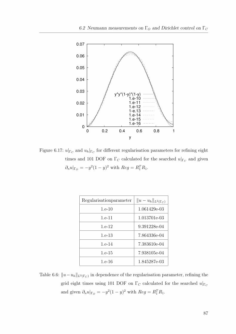
6.2 Neumann measurements on ΓO and Dirichlet control on ΓC
0
0.01
0.02
0.03
0.04
0.05
0.06
0.07
0 0.2 0.4 0.6 0.8 1
y
y*y*(1-y)*(1-y)1.e-101.e-111.e-121-e.131.e-141.e-151.e-16
Figure 6.17: u|ΓCand uh|ΓC
for different regularisation parameters for refining eight
times and 101 DOF on ΓC calculated for the searched u|ΓCand given
∂nu|ΓO= −y2(1 − y)2 with Reg = RT
1 R1.
Regularisationparameter ‖u − uh‖L2(ΓC)
1.e-10 1.061429e-03
1.e-11 1.013701e-03
1.e-12 9.391228e-04
1.e-13 7.864336e-04
1.e-14 7.383610e-04
1.e-15 7.938105e-04
1.e-16 1.845287e-03
Table 6.6: ‖u−uh‖L2(ΓC) in dependence of the regularisation parameter, refining the
grid eight times using 101 DOF on ΓC calculated for the searched u|ΓC
and given ∂nu|ΓO= −y2(1 − y)2 with Reg = RT
1 R1.
87
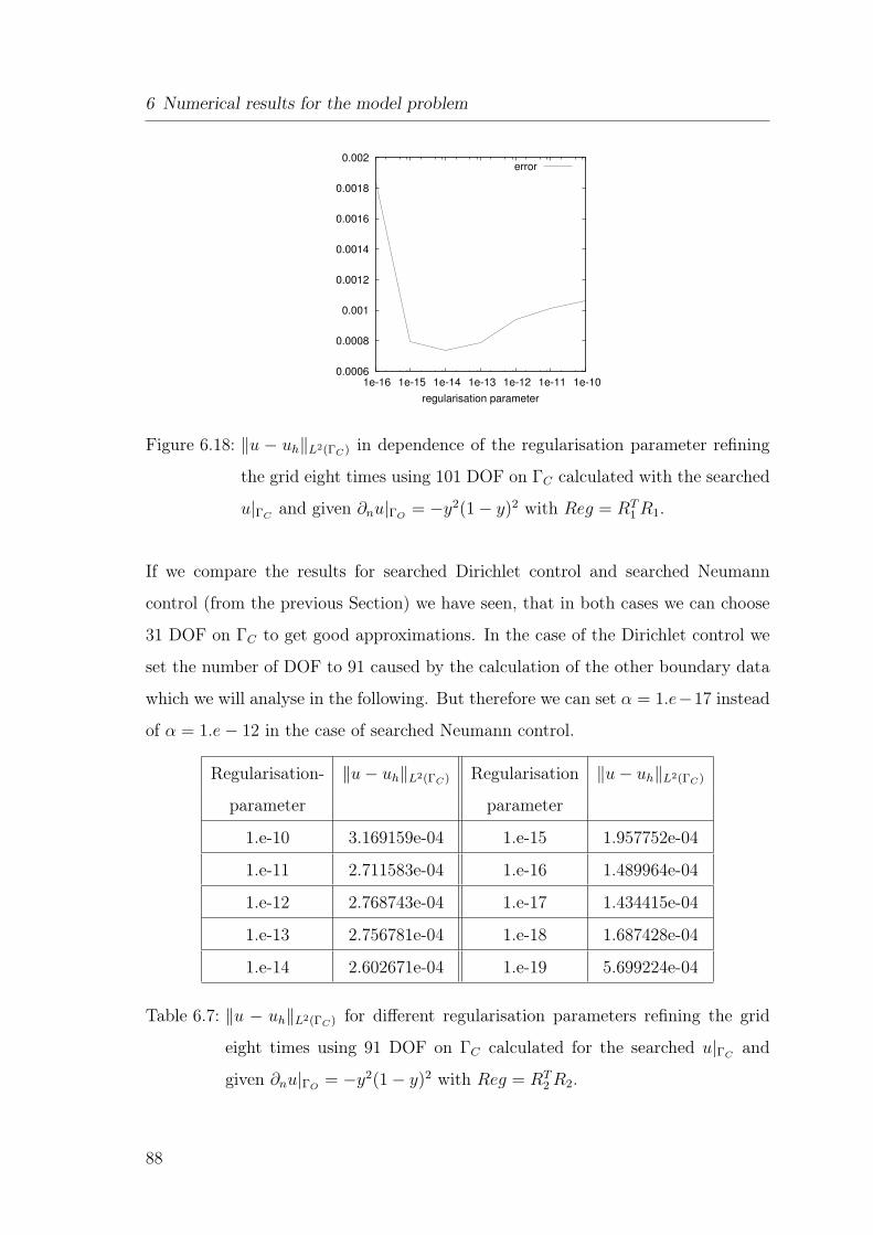
6 Numerical results for the model problem
0.0006
0.0008
0.001
0.0012
0.0014
0.0016
0.0018
0.002
1e-16 1e-15 1e-14 1e-13 1e-12 1e-11 1e-10
regularisation parameter
error
Figure 6.18: ‖u − uh‖L2(ΓC) in dependence of the regularisation parameter refining
the grid eight times using 101 DOF on ΓC calculated with the searched
u|ΓCand given ∂nu|ΓO
= −y2(1 − y)2 with Reg = RT1 R1.
If we compare the results for searched Dirichlet control and searched Neumann
control (from the previous Section) we have seen, that in both cases we can choose
31 DOF on ΓC to get good approximations. In the case of the Dirichlet control we
set the number of DOF to 91 caused by the calculation of the other boundary data
which we will analyse in the following. But therefore we can set α = 1.e−17 instead
of α = 1.e − 12 in the case of searched Neumann control.
Regularisation- ‖u − uh‖L2(ΓC) Regularisation ‖u − uh‖L2(ΓC)
parameter parameter
1.e-10 3.169159e-04 1.e-15 1.957752e-04
1.e-11 2.711583e-04 1.e-16 1.489964e-04
1.e-12 2.768743e-04 1.e-17 1.434415e-04
1.e-13 2.756781e-04 1.e-18 1.687428e-04
1.e-14 2.602671e-04 1.e-19 5.699224e-04
Table 6.7: ‖u − uh‖L2(ΓC) for different regularisation parameters refining the grid
eight times using 91 DOF on ΓC calculated for the searched u|ΓCand
given ∂nu|ΓO= −y2(1 − y)2 with Reg = RT
2 R2.
88
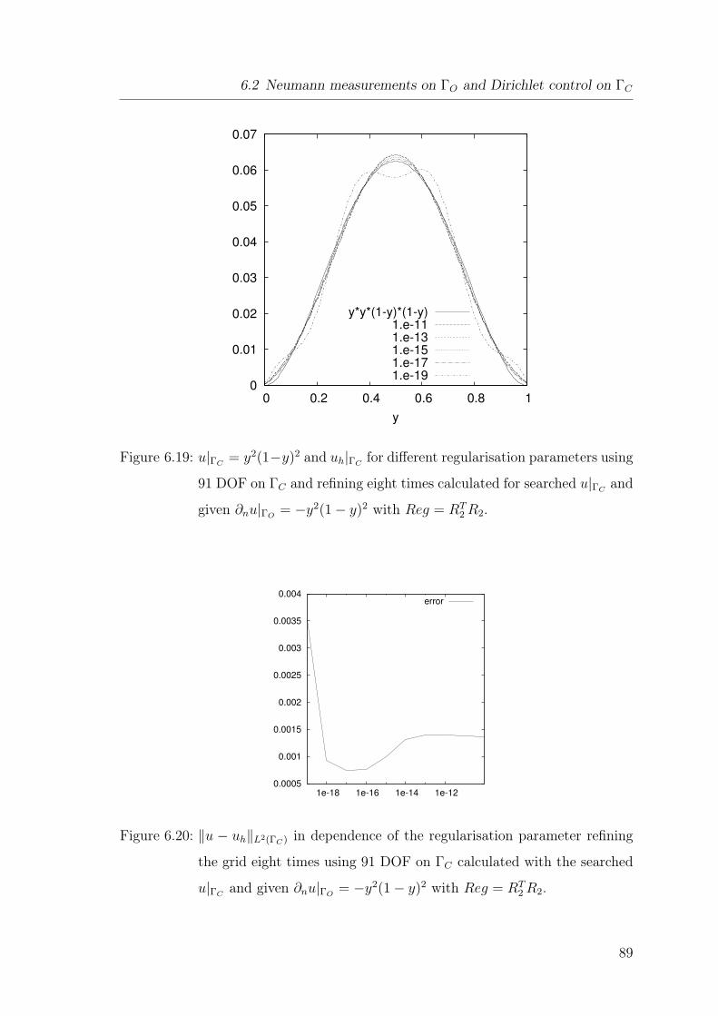
6.2 Neumann measurements on ΓO and Dirichlet control on ΓC
0
0.01
0.02
0.03
0.04
0.05
0.06
0.07
0 0.2 0.4 0.6 0.8 1
y
y*y*(1-y)*(1-y)1.e-111.e-131.e-151.e-171.e-19
Figure 6.19: u|ΓC= y2(1−y)2 and uh|ΓC
for different regularisation parameters using
91 DOF on ΓC and refining eight times calculated for searched u|ΓCand
given ∂nu|ΓO= −y2(1 − y)2 with Reg = RT
2 R2.
0.0005
0.001
0.0015
0.002
0.0025
0.003
0.0035
0.004
1e-18 1e-16 1e-14 1e-12
error
Figure 6.20: ‖u − uh‖L2(ΓC) in dependence of the regularisation parameter refining
the grid eight times using 91 DOF on ΓC calculated with the searched
u|ΓCand given ∂nu|ΓO
= −y2(1 − y)2 with Reg = RT2 R2.
89
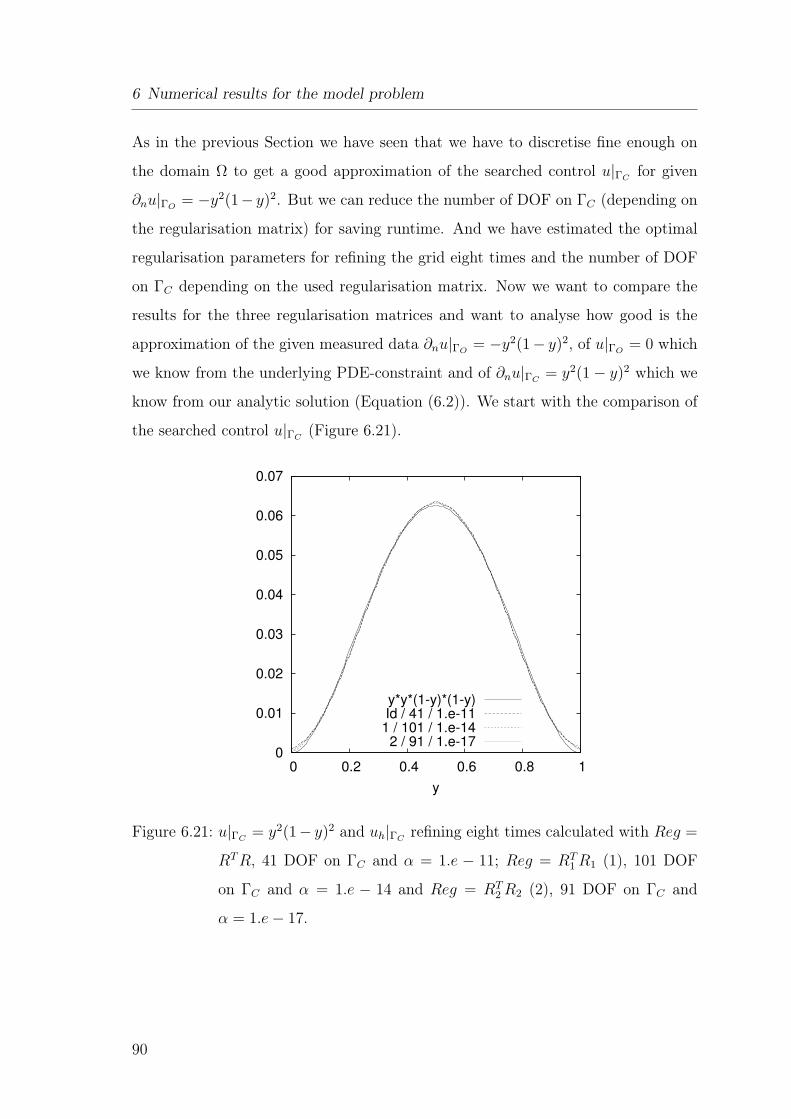
6 Numerical results for the model problem
As in the previous Section we have seen that we have to discretise fine enough on
the domain Ω to get a good approximation of the searched control u|ΓCfor given
∂nu|ΓO= −y2(1− y)2. But we can reduce the number of DOF on ΓC (depending on
the regularisation matrix) for saving runtime. And we have estimated the optimal
regularisation parameters for refining the grid eight times and the number of DOF
on ΓC depending on the used regularisation matrix. Now we want to compare the
results for the three regularisation matrices and want to analyse how good is the
approximation of the given measured data ∂nu|ΓO= −y2(1− y)2, of u|ΓO
= 0 which
we know from the underlying PDE-constraint and of ∂nu|ΓC= y2(1 − y)2 which we
know from our analytic solution (Equation (6.2)). We start with the comparison of
the searched control u|ΓC(Figure 6.21).
0
0.01
0.02
0.03
0.04
0.05
0.06
0.07
0 0.2 0.4 0.6 0.8 1
y
y*y*(1-y)*(1-y)Id / 41 / 1.e-11
1 / 101 / 1.e-142 / 91 / 1.e-17
Figure 6.21: u|ΓC= y2(1− y)2 and uh|ΓC
refining eight times calculated with Reg =
RT R, 41 DOF on ΓC and α = 1.e − 11; Reg = RT1 R1 (1), 101 DOF
on ΓC and α = 1.e − 14 and Reg = RT2 R2 (2), 91 DOF on ΓC and
α = 1.e − 17.
90
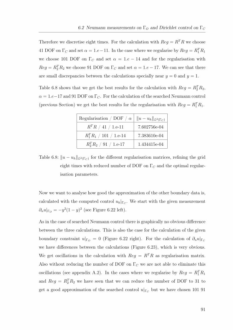
6.2 Neumann measurements on ΓO and Dirichlet control on ΓC
Therefore we discretise eight times. For the calculation with Reg = RT R we choose
41 DOF on ΓC and set α = 1.e−11. In the case where we regularise by Reg = RT1 R1
we choose 101 DOF on ΓC and set α = 1.e − 14 and for the regularisation with
Reg = RT2 R2 we choose 91 DOF on ΓC and set α = 1.e− 17. We can see that there
are small discrepancies between the calculations specially near y = 0 and y = 1.
Table 6.8 shows that we get the best results for the calculation with Reg = RT2 R2,
α = 1.e−17 and 91 DOF on ΓC . For the calculation of the searched Neumann control
(previous Section) we get the best results for the regularisation with Reg = RT1 R1.
Regularisation / DOF / α ‖u − uh‖L2(ΓC)
RT R / 41 / 1.e-11 7.602756e-04
RT1 R1 / 101 / 1.e-14 7.383610e-04
RT2 R2 / 91 / 1.e-17 1.434415e-04
Table 6.8: ‖u − uh‖L2(ΓC) for the different regularisation matrices, refining the grid
eight times with reduced number of DOF on ΓC and the optimal regular-
isation parameters.
Now we want to analyse how good the approximation of the other boundary data is,
calculated with the computed control uh|ΓC. We start with the given measurement
∂nu|ΓO= −y2(1 − y)2 (see Figure 6.22 left).
As in the case of searched Neumann control there is graphically no obvious difference
between the three calculations. This is also the case for the calculation of the given
boundary constraint u|ΓO= 0 (Figure 6.22 right). For the calculation of ∂nu|ΓC
we have differences between the calculations (Figure 6.23), which is very obvious.
We get oscillations in the calculation with Reg = RT R as regularisation matrix.
Also without reducing the number of DOF on ΓC we are not able to eliminate this
oscillations (see appendix A.2). In the cases where we regularise by Reg = RT1 R1
and Reg = RT2 R2 we have seen that we can reduce the number of DOF to 31 to
get a good approximation of the searched control u|ΓCbut we have chosen 101 91
91
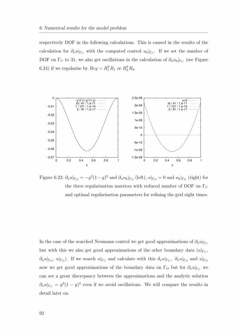
6 Numerical results for the model problem
respectively DOF in the following calculations. This is caused in the results of the
calculation for ∂nu|ΓCwith the computed control uh|ΓC
. If we set the number of
DOF on ΓC to 31, we also get oscillations in the calculation of ∂nuh|ΓC(see Figure
6.24) if we regularise by Reg = RT1 R1 or RT
2 R2.
-0.07
-0.06
-0.05
-0.04
-0.03
-0.02
-0.01
0
0 0.2 0.4 0.6 0.8 1
y
-y*y*(1-y)*(1-y)Id / 41 / 1.e-111 / 101 / 1.e-142 / 91 / 1.e-17
-1.5e-09
-1e-09
-5e-10
0
5e-10
1e-09
1.5e-09
2e-09
2.5e-09
0 0.2 0.4 0.6 0.8 1
y
u=0Id / 41 / 1.e-11
1 / 101 / 1.e-142 / 91 / 1.e-17
Figure 6.22: ∂nu|ΓO= −y2(1−y)2 and ∂nuh|ΓO
(left), u|ΓO= 0 and uh|ΓO
(right) for
the three regularisation matrices with reduced number of DOF on ΓC
and optimal regularisation parameters for refining the grid eight times.
In the case of the searched Neumann control we get good approximations of ∂nu|ΓC
but with this we also get good approximations of the other boundary data (u|ΓC,
∂nu|ΓO, u|ΓO
). If we search u|ΓCand calculate with this ∂nu|ΓC
, ∂nu|ΓOand u|ΓO
now we get good approximations of the boundary data on ΓO but for ∂nu|ΓCwe
can see a great discrepancy between the approximations and the analytic solution
∂nu|ΓC= y2(1 − y)2 even if we avoid oscillations. We will compare the results in
detail later on.
92
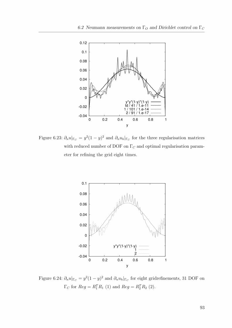
6.2 Neumann measurements on ΓO and Dirichlet control on ΓC
-0.04
-0.02
0
0.02
0.04
0.06
0.08
0.1
0.12
0 0.2 0.4 0.6 0.8 1
y
y*y*(1-y)*(1-y)Id / 41 / 1.e-111 / 101 / 1.e-142 / 91 / 1.e-17
Figure 6.23: ∂nu|ΓC= y2(1 − y)2 and ∂nuh|ΓC
for the three regularisation matrices
with reduced number of DOF on ΓC and optimal regularisation param-
eter for refining the grid eight times.
-0.04
-0.02
0
0.02
0.04
0.06
0.08
0.1
0 0.2 0.4 0.6 0.8 1
y
y*y*(1-y)*(1-y)12
Figure 6.24: ∂nu|ΓC= y2(1 − y)2 and ∂nuh|ΓC
for eight gridrefinements, 31 DOF on
ΓC for Reg = RT1 R1 (1) and Reg = RT
2 R2 (2).
93
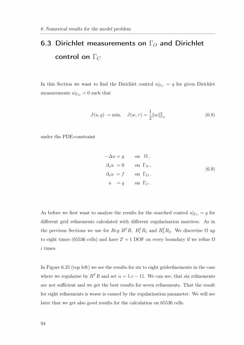
6 Numerical results for the model problem
6.3 Dirichlet measurements on ΓO and Dirichlet
control on ΓC
In this Section we want to find the Dirichlet control u|ΓC= q for given Dirichlet
measurements u|ΓO= 0 such that
J(u, q) → min, J(w, τ) =1
2‖w‖2
ΓO(6.8)
under the PDE-constraint
−∆u = g on Ω ,
∂nu = 0 on ΓN ,
∂nu = f on ΓO ,
u = q on ΓC .
(6.9)
As before we first want to analyse the results for the searched control u|ΓC= q for
different grid refinements calculated with different regularisation matrices. As in
the previous Sections we use for Reg RT R, RT1 R1 and RT
2 R2. We discretise Ω up
to eight times (65536 cells) and have 2i + 1 DOF on every boundary if we refine Ω
i times.
In Figure 6.25 (top left) we see the results for six to eight gridrefinements in the case
where we regularise by RT R and set α = 1.e− 11. We can see, that six refinements
are not sufficient and we get the best results for seven refinements. That the result
for eight refinements is worse is caused by the regularisation parameter. We will see
later that we get also good results for the calculation on 65536 cells.
94
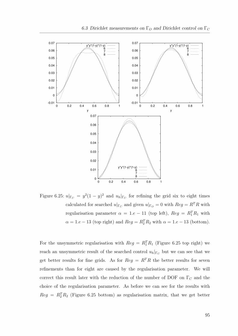
6.3 Dirichlet measurements on ΓO and Dirichlet control on ΓC
-0.01
0
0.01
0.02
0.03
0.04
0.05
0.06
0.07
0 0.2 0.4 0.6 0.8 1
y
y*y*(1-y)*(1-y)678
-0.01
0
0.01
0.02
0.03
0.04
0.05
0.06
0.07
0 0.2 0.4 0.6 0.8 1
y
y*y*(1-y)*(1-y)678
0
0.01
0.02
0.03
0.04
0.05
0.06
0.07
0 0.2 0.4 0.6 0.8 1
y*y*(1-y)*(1-y)678
Figure 6.25: u|ΓC= y2(1 − y)2 and uh|ΓC
for refining the grid six to eight times
calculated for searched u|ΓCand given u|ΓO
= 0 with Reg = RT R with
regularisation parameter α = 1.e − 11 (top left), Reg = RT1 R1 with
α = 1.e− 13 (top right) and Reg = RT2 R2 with α = 1.e− 13 (bottom).
For the unsymmetric regularisation with Reg = RT1 R1 (Figure 6.25 top right) we
reach an unsymmetric result of the searched control uh|ΓCbut we can see that we
get better results for fine grids. As for Reg = RT R the better results for seven
refinements than for eight are caused by the regularisation parameter. We will
correct this result later with the reduction of the number of DOF on ΓC and the
choice of the regularisation parameter. As before we can see for the results with
Reg = RT2 R2 (Figure 6.25 bottom) as regularisation matrix, that we get better
95
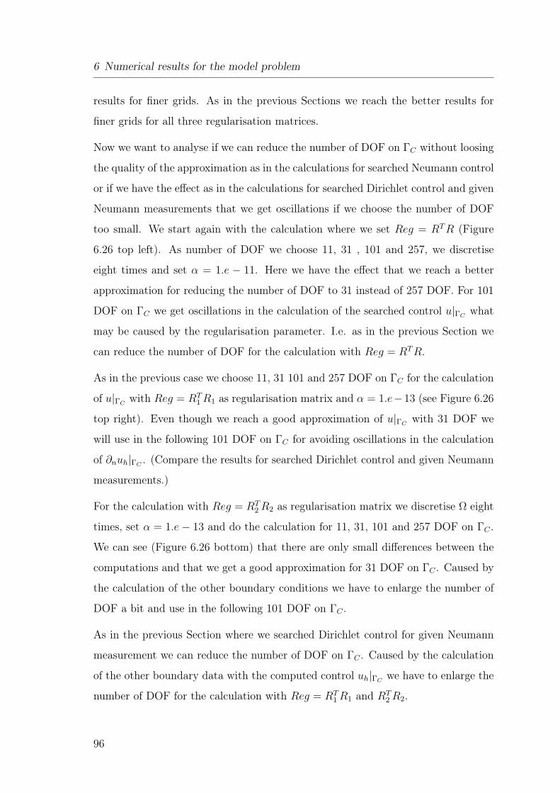
6 Numerical results for the model problem
results for finer grids. As in the previous Sections we reach the better results for
finer grids for all three regularisation matrices.
Now we want to analyse if we can reduce the number of DOF on ΓC without loosing
the quality of the approximation as in the calculations for searched Neumann control
or if we have the effect as in the calculations for searched Dirichlet control and given
Neumann measurements that we get oscillations if we choose the number of DOF
too small. We start again with the calculation where we set Reg = RT R (Figure
6.26 top left). As number of DOF we choose 11, 31 , 101 and 257, we discretise
eight times and set α = 1.e − 11. Here we have the effect that we reach a better
approximation for reducing the number of DOF to 31 instead of 257 DOF. For 101
DOF on ΓC we get oscillations in the calculation of the searched control u|ΓCwhat
may be caused by the regularisation parameter. I.e. as in the previous Section we
can reduce the number of DOF for the calculation with Reg = RT R.
As in the previous case we choose 11, 31 101 and 257 DOF on ΓC for the calculation
of u|ΓCwith Reg = RT
1 R1 as regularisation matrix and α = 1.e−13 (see Figure 6.26
top right). Even though we reach a good approximation of u|ΓCwith 31 DOF we
will use in the following 101 DOF on ΓC for avoiding oscillations in the calculation
of ∂nuh|ΓC. (Compare the results for searched Dirichlet control and given Neumann
measurements.)
For the calculation with Reg = RT2 R2 as regularisation matrix we discretise Ω eight
times, set α = 1.e − 13 and do the calculation for 11, 31, 101 and 257 DOF on ΓC .
We can see (Figure 6.26 bottom) that there are only small differences between the
computations and that we get a good approximation for 31 DOF on ΓC . Caused by
the calculation of the other boundary conditions we have to enlarge the number of
DOF a bit and use in the following 101 DOF on ΓC .
As in the previous Section where we searched Dirichlet control for given Neumann
measurement we can reduce the number of DOF on ΓC . Caused by the calculation
of the other boundary data with the computed control uh|ΓCwe have to enlarge the
number of DOF for the calculation with Reg = RT1 R1 and RT
2 R2.
96
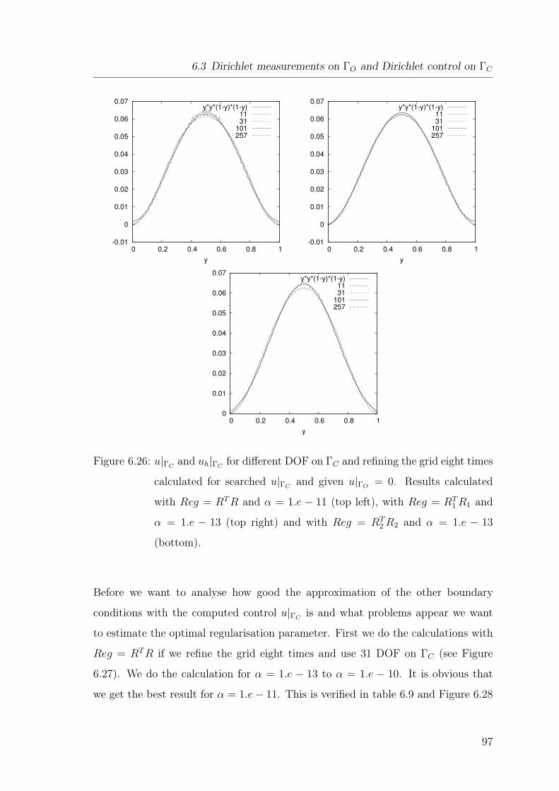
6.3 Dirichlet measurements on ΓO and Dirichlet control on ΓC
-0.01
0
0.01
0.02
0.03
0.04
0.05
0.06
0.07
0 0.2 0.4 0.6 0.8 1
y
y*y*(1-y)*(1-y)1131
101257
-0.01
0
0.01
0.02
0.03
0.04
0.05
0.06
0.07
0 0.2 0.4 0.6 0.8 1
y
y*y*(1-y)*(1-y)1131
101257
0
0.01
0.02
0.03
0.04
0.05
0.06
0.07
0 0.2 0.4 0.6 0.8 1
y
y*y*(1-y)*(1-y)1131
101257
Figure 6.26: u|ΓCand uh|ΓC
for different DOF on ΓC and refining the grid eight times
calculated for searched u|ΓCand given u|ΓO
= 0. Results calculated
with Reg = RT R and α = 1.e − 11 (top left), with Reg = RT1 R1 and
α = 1.e − 13 (top right) and with Reg = RT2 R2 and α = 1.e − 13
(bottom).
Before we want to analyse how good the approximation of the other boundary
conditions with the computed control u|ΓCis and what problems appear we want
to estimate the optimal regularisation parameter. First we do the calculations with
Reg = RT R if we refine the grid eight times and use 31 DOF on ΓC (see Figure
6.27). We do the calculation for α = 1.e − 13 to α = 1.e − 10. It is obvious that
we get the best result for α = 1.e − 11. This is verified in table 6.9 and Figure 6.28
97
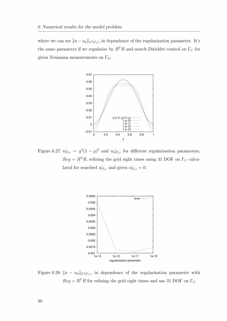
6 Numerical results for the model problem
where we can see ‖u− uh‖L2(ΓC) in dependence of the regularisation parameter. It’s
the same parameter if we regularise by RT R and search Dirichlet control on ΓC for
given Neumann measurements on ΓO.
-0.01
0
0.01
0.02
0.03
0.04
0.05
0.06
0.07
0 0.2 0.4 0.6 0.8 1
y
y*y*(1-y)*(1-y)1.e-101.e-111.e-121.e-13
Figure 6.27: u|ΓC= y2(1 − y)2 and uh|ΓC
for different regularisation parameters,
Reg = RT R, refining the grid eight times using 31 DOF on ΓC calcu-
lated for searched u|ΓCand given u|ΓO
= 0.
0.001
0.0015
0.002
0.0025
0.003
0.0035
0.004
0.0045
0.005
0.0055
1e-13 1e-12 1e-11 1e-10
regularisation parameter
error
Figure 6.28: ‖u − uh‖L2(ΓC) in dependence of the regularisation parameter with
Reg = RT R for refining the grid eight times and use 31 DOF on ΓC .
98
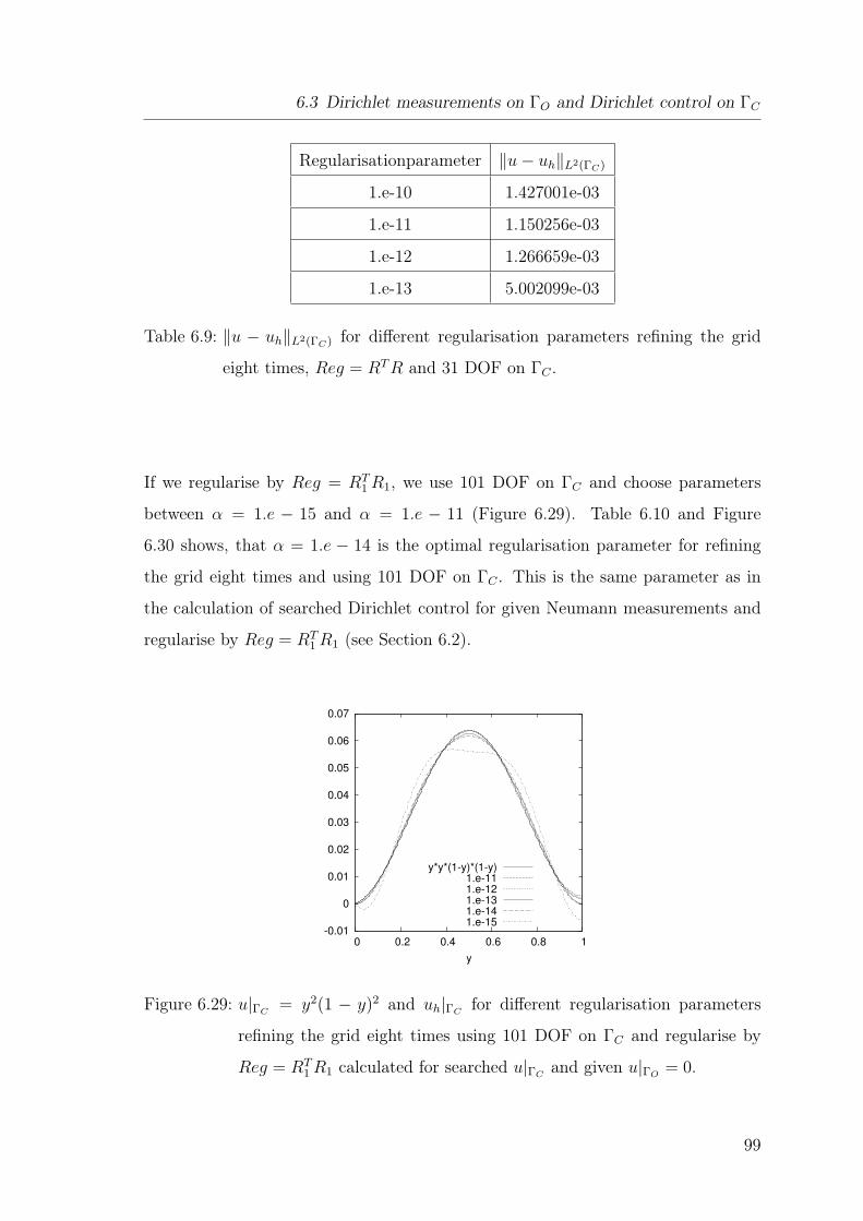
6.3 Dirichlet measurements on ΓO and Dirichlet control on ΓC
Regularisationparameter ‖u − uh‖L2(ΓC)
1.e-10 1.427001e-03
1.e-11 1.150256e-03
1.e-12 1.266659e-03
1.e-13 5.002099e-03
Table 6.9: ‖u − uh‖L2(ΓC) for different regularisation parameters refining the grid
eight times, Reg = RT R and 31 DOF on ΓC .
If we regularise by Reg = RT1 R1, we use 101 DOF on ΓC and choose parameters
between α = 1.e − 15 and α = 1.e − 11 (Figure 6.29). Table 6.10 and Figure
6.30 shows, that α = 1.e − 14 is the optimal regularisation parameter for refining
the grid eight times and using 101 DOF on ΓC . This is the same parameter as in
the calculation of searched Dirichlet control for given Neumann measurements and
regularise by Reg = RT1 R1 (see Section 6.2).
-0.01
0
0.01
0.02
0.03
0.04
0.05
0.06
0.07
0 0.2 0.4 0.6 0.8 1
y
y*y*(1-y)*(1-y)1.e-111.e-121.e-131.e-141.e-15
Figure 6.29: u|ΓC= y2(1 − y)2 and uh|ΓC
for different regularisation parameters
refining the grid eight times using 101 DOF on ΓC and regularise by
Reg = RT1 R1 calculated for searched u|ΓC
and given u|ΓO= 0.
99
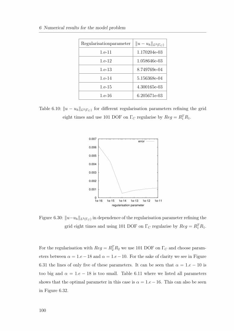
6 Numerical results for the model problem
Regularisationparameter ‖u − uh‖L2(ΓC)
1.e-11 1.170204e-03
1.e-12 1.058646e-03
1.e-13 8.749769e-04
1.e-14 5.156368e-04
1.e-15 4.300165e-03
1.e-16 6.205671e-03
Table 6.10: ‖u − uh‖L2(ΓC) for different regularisation parameters refining the grid
eight times and use 101 DOF on ΓC regularise by Reg = RT1 R1.
0
0.001
0.002
0.003
0.004
0.005
0.006
0.007
1e-16 1e-15 1e-14 1e-13 1e-12 1e-11
regularisation parameter
error
Figure 6.30: ‖u−uh‖L2(ΓC) in dependence of the regularisation parameter refining the
grid eight times and using 101 DOF on ΓC regularise by Reg = RT1 R1.
For the regularisation with Reg = RT2 R2 we use 101 DOF on ΓC and choose param-
eters between α = 1.e−18 and α = 1.e−10. For the sake of clarity we see in Figure
6.31 the lines of only five of these parameters. It can be seen that α = 1.e − 10 is
too big and α = 1.e − 18 is too small. Table 6.11 where we listed all parameters
shows that the optimal parameter in this case is α = 1.e− 16. This can also be seen
in Figure 6.32.
100
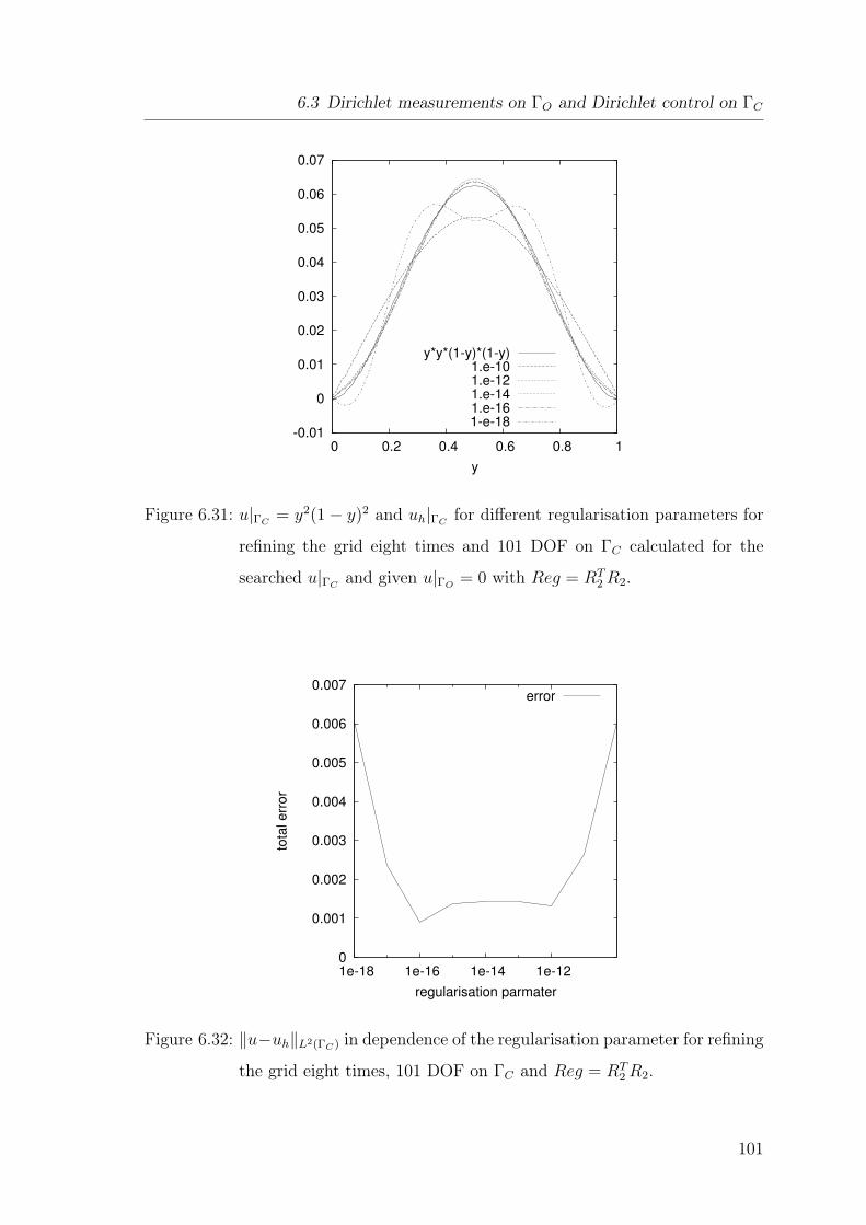
6.3 Dirichlet measurements on ΓO and Dirichlet control on ΓC
-0.01
0
0.01
0.02
0.03
0.04
0.05
0.06
0.07
0 0.2 0.4 0.6 0.8 1
y
y*y*(1-y)*(1-y)1.e-101.e-121.e-141.e-161-e-18
Figure 6.31: u|ΓC= y2(1 − y)2 and uh|ΓC
for different regularisation parameters for
refining the grid eight times and 101 DOF on ΓC calculated for the
searched u|ΓCand given u|ΓO
= 0 with Reg = RT2 R2.
0
0.001
0.002
0.003
0.004
0.005
0.006
0.007
1e-18 1e-16 1e-14 1e-12
tota
l e
rro
r
regularisation parmater
error
Figure 6.32: ‖u−uh‖L2(ΓC) in dependence of the regularisation parameter for refining
the grid eight times, 101 DOF on ΓC and Reg = RT2 R2.
101
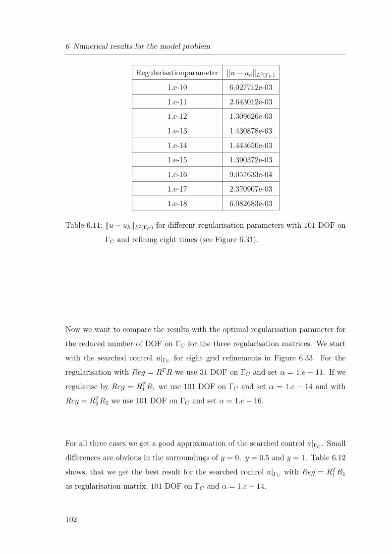
6 Numerical results for the model problem
Regularisationparameter ‖u − uh‖L2(ΓC)
1.e-10 6.027712e-03
1.e-11 2.643012e-03
1.e-12 1.309626e-03
1.e-13 1.430878e-03
1.e-14 1.443650e-03
1.e-15 1.390372e-03
1.e-16 9.057633e-04
1.e-17 2.370907e-03
1.e-18 6.082683e-03
Table 6.11: ‖u − uh‖L2(ΓC) for different regularisation parameters with 101 DOF on
ΓC and refining eight times (see Figure 6.31).
Now we want to compare the results with the optimal regularisation parameter for
the reduced number of DOF on ΓC for the three regularisation matrices. We start
with the searched control u|ΓCfor eight grid refinements in Figure 6.33. For the
regularisation with Reg = RT R we use 31 DOF on ΓC and set α = 1.e − 11. If we
regularise by Reg = RT1 R1 we use 101 DOF on ΓC and set α = 1.e − 14 and with
Reg = RT2 R2 we use 101 DOF on ΓC and set α = 1.e − 16.
For all three cases we get a good approximation of the searched control u|ΓC. Small
differences are obvious in the surroundings of y = 0, y = 0.5 and y = 1. Table 6.12
shows, that we get the best result for the searched control u|ΓCwith Reg = RT
1 R1
as regularisation matrix, 101 DOF on ΓC and α = 1.e − 14.
102
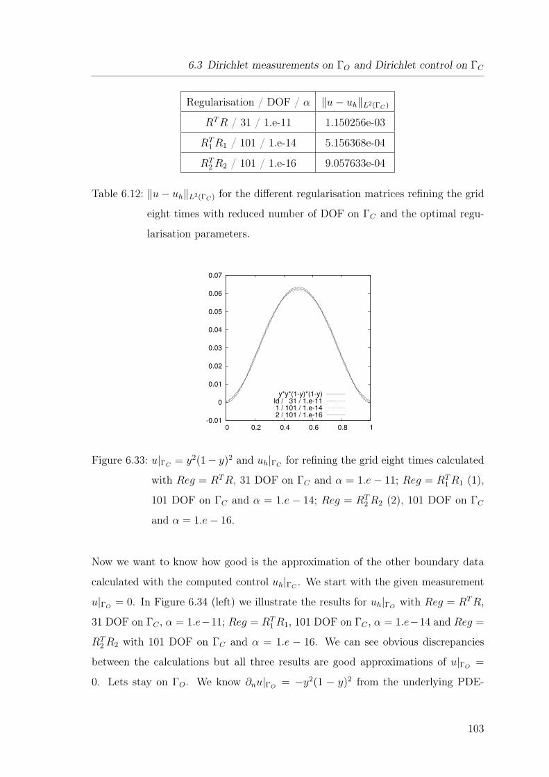
6.3 Dirichlet measurements on ΓO and Dirichlet control on ΓC
Regularisation / DOF / α ‖u − uh‖L2(ΓC)
RT R / 31 / 1.e-11 1.150256e-03
RT1 R1 / 101 / 1.e-14 5.156368e-04
RT2 R2 / 101 / 1.e-16 9.057633e-04
Table 6.12: ‖u − uh‖L2(ΓC) for the different regularisation matrices refining the grid
eight times with reduced number of DOF on ΓC and the optimal regu-
larisation parameters.
-0.01
0
0.01
0.02
0.03
0.04
0.05
0.06
0.07
0 0.2 0.4 0.6 0.8 1
y*y*(1-y)*(1-y)Id / 31 / 1.e-111 / 101 / 1.e-142 / 101 / 1.e-16
Figure 6.33: u|ΓC= y2(1− y)2 and uh|ΓC
for refining the grid eight times calculated
with Reg = RT R, 31 DOF on ΓC and α = 1.e − 11; Reg = RT1 R1 (1),
101 DOF on ΓC and α = 1.e − 14; Reg = RT2 R2 (2), 101 DOF on ΓC
and α = 1.e − 16.
Now we want to know how good is the approximation of the other boundary data
calculated with the computed control uh|ΓC. We start with the given measurement
u|ΓO= 0. In Figure 6.34 (left) we illustrate the results for uh|ΓO
with Reg = RT R,
31 DOF on ΓC , α = 1.e−11; Reg = RT1 R1, 101 DOF on ΓC , α = 1.e−14 and Reg =
RT2 R2 with 101 DOF on ΓC and α = 1.e − 16. We can see obvious discrepancies
between the calculations but all three results are good approximations of u|ΓO=
0. Lets stay on ΓO. We know ∂nu|ΓO= −y2(1 − y)2 from the underlying PDE-
103
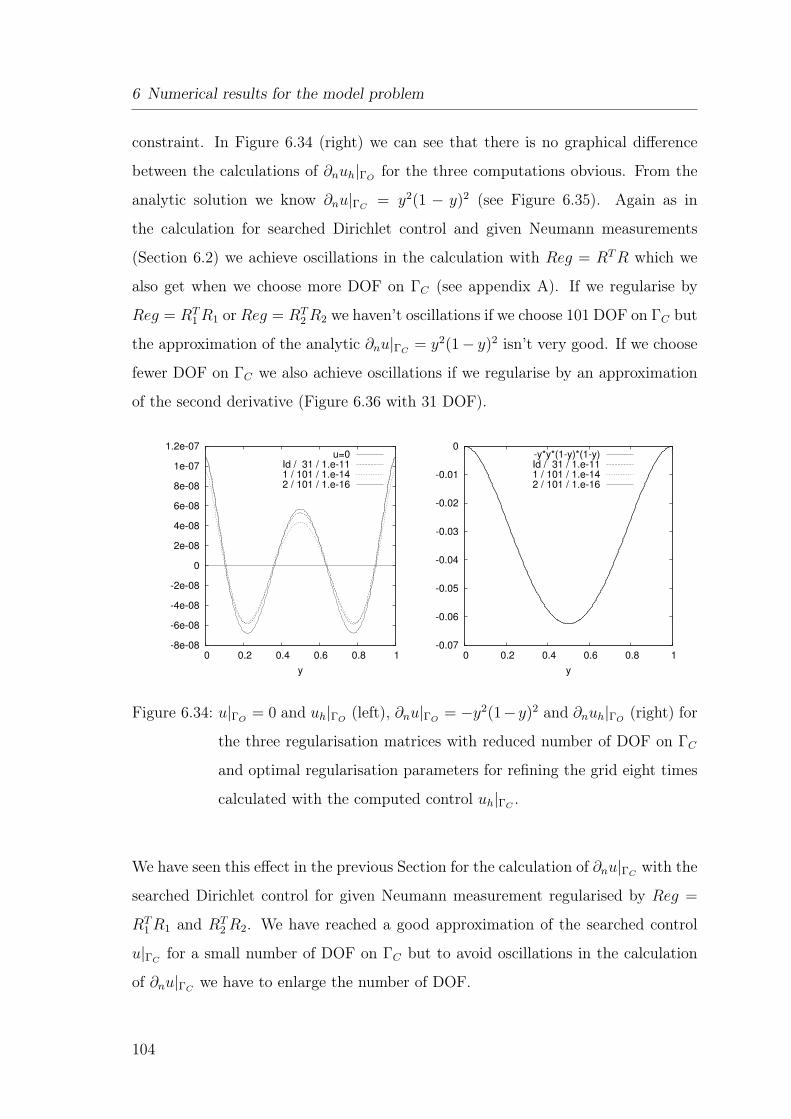
6 Numerical results for the model problem
constraint. In Figure 6.34 (right) we can see that there is no graphical difference
between the calculations of ∂nuh|ΓOfor the three computations obvious. From the
analytic solution we know ∂nu|ΓC= y2(1 − y)2 (see Figure 6.35). Again as in
the calculation for searched Dirichlet control and given Neumann measurements
(Section 6.2) we achieve oscillations in the calculation with Reg = RT R which we
also get when we choose more DOF on ΓC (see appendix A). If we regularise by
Reg = RT1 R1 or Reg = RT
2 R2 we haven’t oscillations if we choose 101 DOF on ΓC but
the approximation of the analytic ∂nu|ΓC= y2(1− y)2 isn’t very good. If we choose
fewer DOF on ΓC we also achieve oscillations if we regularise by an approximation
of the second derivative (Figure 6.36 with 31 DOF).
-8e-08
-6e-08
-4e-08
-2e-08
0
2e-08
4e-08
6e-08
8e-08
1e-07
1.2e-07
0 0.2 0.4 0.6 0.8 1
y
u=0Id / 31 / 1.e-111 / 101 / 1.e-142 / 101 / 1.e-16
-0.07
-0.06
-0.05
-0.04
-0.03
-0.02
-0.01
0
0 0.2 0.4 0.6 0.8 1
y
-y*y*(1-y)*(1-y)Id / 31 / 1.e-111 / 101 / 1.e-142 / 101 / 1.e-16
Figure 6.34: u|ΓO= 0 and uh|ΓO
(left), ∂nu|ΓO= −y2(1−y)2 and ∂nuh|ΓO
(right) for
the three regularisation matrices with reduced number of DOF on ΓC
and optimal regularisation parameters for refining the grid eight times
calculated with the computed control uh|ΓC.
We have seen this effect in the previous Section for the calculation of ∂nu|ΓCwith the
searched Dirichlet control for given Neumann measurement regularised by Reg =
RT1 R1 and RT
2 R2. We have reached a good approximation of the searched control
u|ΓCfor a small number of DOF on ΓC but to avoid oscillations in the calculation
of ∂nu|ΓCwe have to enlarge the number of DOF.
104
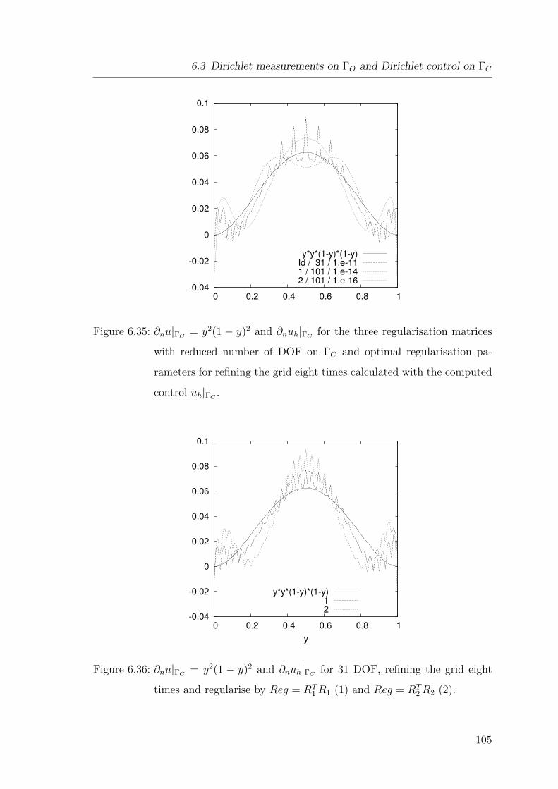
6.3 Dirichlet measurements on ΓO and Dirichlet control on ΓC
-0.04
-0.02
0
0.02
0.04
0.06
0.08
0.1
0 0.2 0.4 0.6 0.8 1
y*y*(1-y)*(1-y)Id / 31 / 1.e-111 / 101 / 1.e-142 / 101 / 1.e-16
Figure 6.35: ∂nu|ΓC= y2(1 − y)2 and ∂nuh|ΓC
for the three regularisation matrices
with reduced number of DOF on ΓC and optimal regularisation pa-
rameters for refining the grid eight times calculated with the computed
control uh|ΓC.
-0.04
-0.02
0
0.02
0.04
0.06
0.08
0.1
0 0.2 0.4 0.6 0.8 1
y
y*y*(1-y)*(1-y)12
Figure 6.36: ∂nu|ΓC= y2(1 − y)2 and ∂nuh|ΓC
for 31 DOF, refining the grid eight
times and regularise by Reg = RT1 R1 (1) and Reg = RT
2 R2 (2).
105
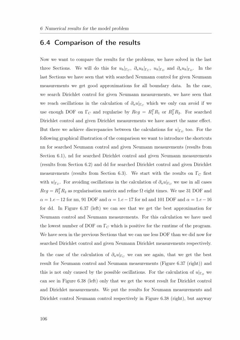
6 Numerical results for the model problem
6.4 Comparison of the results
Now we want to compare the results for the problems, we have solved in the last
three Sections. We will do this for uh|ΓC, ∂nuh|ΓC
, uh|ΓOand ∂nuh|ΓO
. In the
last Sections we have seen that with searched Neumann control for given Neumann
measurements we get good approximations for all boundary data. In the case,
we search Dirichlet control for given Neumann measurements, we have seen that
we reach oscillations in the calculation of ∂nu|ΓCwhich we only can avoid if we
use enough DOF on ΓC and regularise by Reg = RT1 R1 or RT
2 R2. For searched
Dirichlet control and given Dirichlet measurements we have assert the same effect.
But there we achieve discrepancies between the calculations for u|ΓOtoo. For the
following graphical illustration of the comparison we want to introduce the shortcuts
nn for searched Neumann control and given Neumann measurements (results from
Section 6.1), nd for searched Dirichlet control and given Neumann measurements
(results from Section 6.2) and dd for searched Dirichlet control and given Dirichlet
measurements (results from Section 6.3). We start with the results on ΓC first
with u|ΓC. For avoiding oscillations in the calculation of ∂nu|ΓC
we use in all cases
Reg = RT2 R2 as regularisation matrix and refine Ω eight times. We use 31 DOF and
α = 1.e−12 for nn, 91 DOF and α = 1.e−17 for nd and 101 DOF and α = 1.e−16
for dd. In Figure 6.37 (left) we can see that we get the best approximation for
Neumann control and Neumann measurements. For this calculation we have used
the lowest number of DOF on ΓC which is positive for the runtime of the program.
We have seen in the previous Sections that we can use less DOF than we did now for
searched Dirichlet control and given Neumann Dirichlet measurements respectively.
In the case of the calculation of ∂nu|ΓCwe can see again, that we get the best
result for Neumann control and Neumann measurements (Figure 6.37 (right)) and
this is not only caused by the possible oscillations. For the calculation of u|ΓOwe
can see in Figure 6.38 (left) only that we get the worst result for Dirichlet control
and Dirichlet measurements. We put the results for Neumann measurements and
Dirichlet control Neumann control respectively in Figure 6.38 (right), but anyway
106
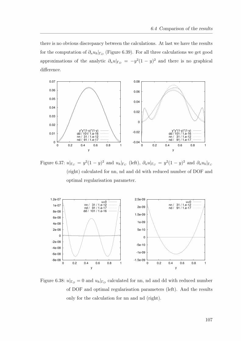
6.4 Comparison of the results
there is no obvious discrepancy between the calculations. At last we have the results
for the computation of ∂nuh|ΓO(Figure 6.39). For all three calculations we get good
approximations of the analytic ∂nu|ΓO= −y2(1 − y)2 and there is no graphical
difference.
0
0.01
0.02
0.03
0.04
0.05
0.06
0.07
0 0.2 0.4 0.6 0.8 1
y
y*y*(1-y)*(1-y)dd / 101/ 1.e-16nn / 31 / 1.e-12nd / 91 / 1.e-17
-0.04
-0.02
0
0.02
0.04
0.06
0.08
0 0.2 0.4 0.6 0.8 1
y
y*y*(1-y)*(1-y)dd / 101 / 1.e-16nn / 31 / 1.e-12nd / 91 / 1.e-17
Figure 6.37: u|ΓC= y2(1 − y)2 and uh|ΓC
(left), ∂nu|ΓC= y2(1 − y)2 and ∂nuh|ΓC
(right) calculated for nn, nd and dd with reduced number of DOF and
optimal regularisation parameter.
-8e-08
-6e-08
-4e-08
-2e-08
0
2e-08
4e-08
6e-08
8e-08
1e-07
1.2e-07
0 0.2 0.4 0.6 0.8 1
y
u=0nn / 31 / 1.e-12nd / 91 / 1.e-17dd / 101 / 1.e-16
-1.5e-09
-1e-09
-5e-10
0
5e-10
1e-09
1.5e-09
2e-09
2.5e-09
0 0.2 0.4 0.6 0.8 1
y
u=0nn / 31 / 1.e-12nd / 91 / 1.e-17
Figure 6.38: u|ΓO= 0 and uh|ΓO
calculated for nn, nd and dd with reduced number
of DOF and optimal regularisation parameters (left). And the results
only for the calculation for nn and nd (right).
107
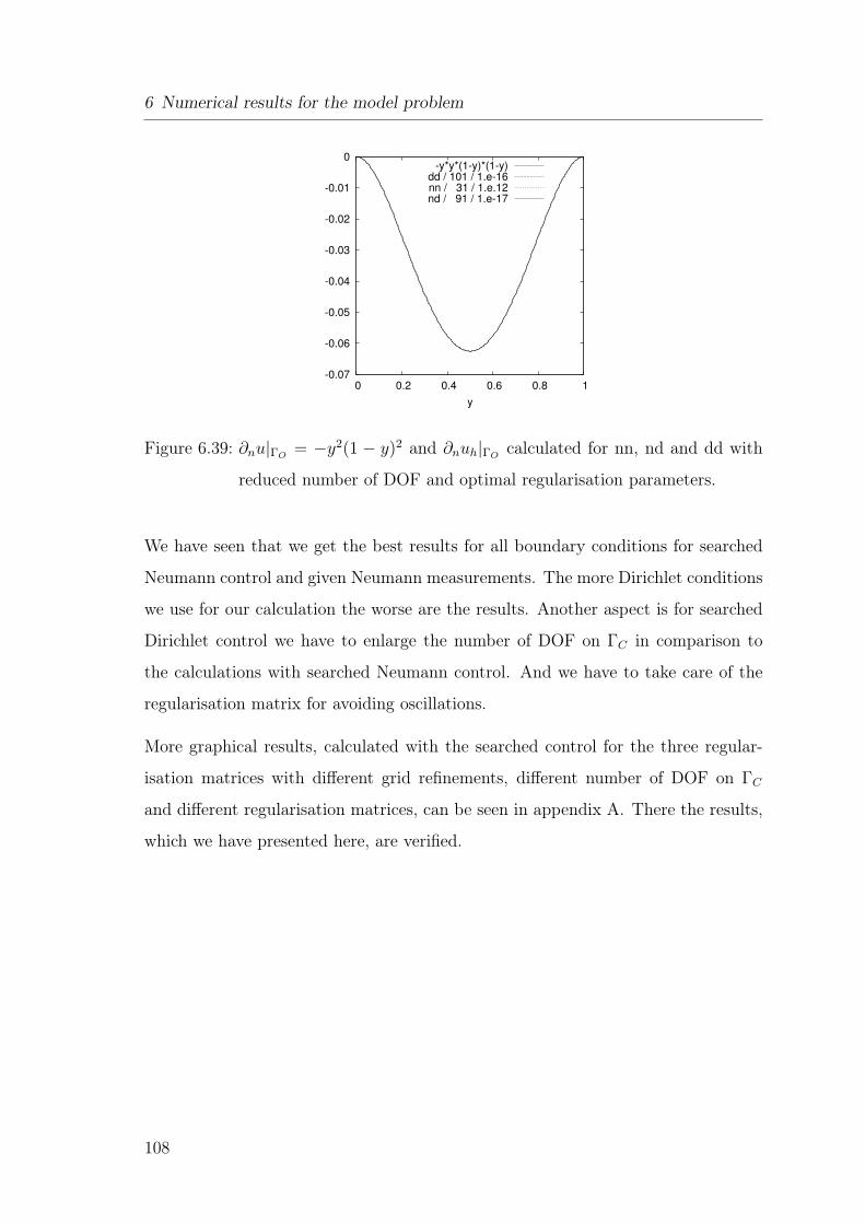
6 Numerical results for the model problem
-0.07
-0.06
-0.05
-0.04
-0.03
-0.02
-0.01
0
0 0.2 0.4 0.6 0.8 1
y
-y*y*(1-y)*(1-y)dd / 101 / 1.e-16nn / 31 / 1.e.12nd / 91 / 1.e-17
Figure 6.39: ∂nu|ΓO= −y2(1 − y)2 and ∂nuh|ΓO
calculated for nn, nd and dd with
reduced number of DOF and optimal regularisation parameters.
We have seen that we get the best results for all boundary conditions for searched
Neumann control and given Neumann measurements. The more Dirichlet conditions
we use for our calculation the worse are the results. Another aspect is for searched
Dirichlet control we have to enlarge the number of DOF on ΓC in comparison to
the calculations with searched Neumann control. And we have to take care of the
regularisation matrix for avoiding oscillations.
More graphical results, calculated with the searched control for the three regular-
isation matrices with different grid refinements, different number of DOF on ΓC
and different regularisation matrices, can be seen in appendix A. There the results,
which we have presented here, are verified.
108
7 Results for the Application
Now we want to present the numerical results for the application, hybrid insulation
described in Section 2. In contrast to the three (four respectively) cases we had
for our model problem (Section 5.1) due to technical conditions of the application
here we only have the two possible cases with given Neumann measurements and
searched Neumann control or given Neumann measurements and searched Dirichlet
control. As we have seen in the previous Section that we get the best results for
given Neumann data and searched Neumann control we consider only this case.
Instead of using the laplace equation in two dimensions for the application of hybrid
insulation as it is done by I. Cherlenyak in his PhD thesis [11] we use here the three
dimensional laplace equation reduced to two dimensions as described in Section 2.
We have to do some modifications compared to the calculations of the model problem
in the previous Sections, where we solved as direct problem the laplace equation on
the unit square.
109
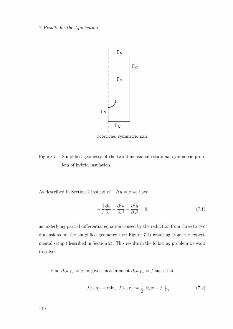
7 Results for the Application
Figure 7.1: Simplified geometry of the two dimensional rotational symmetric prob-
lem of hybrid insulation.
As described in Section 2 instead of −∆u = g we have
− 1
r
∂u
∂r− ∂2u
∂r2− ∂2u
∂z2= 0. (7.1)
as underlying partial differential equation caused by the reduction from three to two
dimensions on the simplified geometry (see Figure 7.1) resulting from the experi-
mental setup (described in Section 2). This results in the following problem we want
to solve:
Find ∂nu|ΓC= q for given measurement ∂nu|ΓO
= f such that
J(u, q) → min, J(w, τ) :=1
2‖∂nw − f‖2
ΓO(7.2)
110
under the PDE-constraint
−1
r
∂u
∂r− ∂2u
∂r2− ∂2u
∂z2= 0 on Ω ,
∂nu = 0 on ΓN ,
u = 0 on ΓO ,
∂nu = q on ΓC .
(7.3)
As we only do the calculations for searched Neumann control we don’t need Nitsches
method and can use the classical variational formulation of the direct problem where
the Dirichlet boundary condition on ΓO is hidden in the function space i.e. we have
u ∈ V = ϕ ∈ H1(Ω) | ϕ = 0 on ΓO. Again we can write the direct problem (see
Section 5) after discretisation as
J(uh, q) → min (7.4)
Auh = Bq
With A regular this leads to
J(uh, q) = J(A−1Bq, q) → min (7.5)
Then we have to solve the regularised normal equation as for the model problem:
(BT A−T CA−1B + α Reg) q = BT A−T Cf. (7.6)
For the discretisation we use bilinear elements on quadrilaterals. In the case we have
n vertices on Ω and Nq vertices on ΓC we have:
B is the (n × Nq)- matrix corresponding to (ϕ, ψ ∈ Vh):
(ψ, ϕ)0,ΓO
C is the (n × n)-matrix corresponding to
(∂nψ, ∂nϕ)0,ΓO
111
7 Results for the Application
and Cf corresponding to (f, ∂nϕ)ΓO.
In contrast to the model problem we have here:
A is the (n × n)-matrix corresponding to:
(∇ψ,∇ϕ)0,Ω −(
1
r∂rψ, ϕ
)
0,Ω
.
As mentioned before we have another geometry (see Figure 7.1) as for the model
problem where we use the unit square as underlying geometry. We have given
measuring data f = ∂nu|ΓOin equidistant measuring points which we interpolate
linear instead of a given function. From the reduction from three to two dimensions
we have the supplementary term −(
1
r∂rψ, ϕ
)
0,Ω
in the matrix A and we use the
classical variational formulation of the direct problem instead of Nitsche’s method.
Caused by the term −(
1
r∂rψ, ϕ
)
0,Γ
we have an unsymmetric problem to be solved.
For this we use the bicgstab-method (see e.g. [34], [15] or [31]) instead of the pcg-
method, described in the following with Ax = b as underlying problem :
Algorithm 7.1. (BICGstab)
Given x0 ∈ Rn with r0 := b − Ax0 6= 0. Choose r0 ∈ R
n such that (r0, r0) 6= 0,
set p0 := r0.
For k = 0, 1, . . .
1) ak :=(r0, rk)
(r0, Apk)
v := Apk, t := As
2) ωk+1 :=(s, t)
(t, t)
xk+1 := xk + akpk + ωk+1s
rk+1 := s − ωk+1
if
‖rk+1‖ is small enough stop
else
112
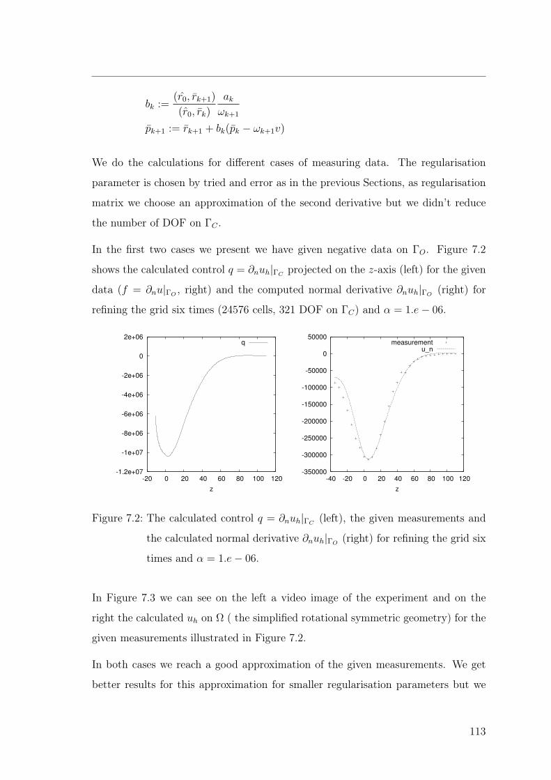
bk :=(r0, rk+1)
(r0, rk)
ak
ωk+1
pk+1 := rk+1 + bk(pk − ωk+1v)
We do the calculations for different cases of measuring data. The regularisation
parameter is chosen by tried and error as in the previous Sections, as regularisation
matrix we choose an approximation of the second derivative but we didn’t reduce
the number of DOF on ΓC .
In the first two cases we present we have given negative data on ΓO. Figure 7.2
shows the calculated control q = ∂nuh|ΓCprojected on the z-axis (left) for the given
data (f = ∂nu|ΓO, right) and the computed normal derivative ∂nuh|ΓO
(right) for
refining the grid six times (24576 cells, 321 DOF on ΓC) and α = 1.e − 06.
-1.2e+07
-1e+07
-8e+06
-6e+06
-4e+06
-2e+06
0
2e+06
-20 0 20 40 60 80 100 120
z
q
-350000
-300000
-250000
-200000
-150000
-100000
-50000
0
50000
-40 -20 0 20 40 60 80 100 120
z
measurementu_n
Figure 7.2: The calculated control q = ∂nuh|ΓC(left), the given measurements and
the calculated normal derivative ∂nuh|ΓO(right) for refining the grid six
times and α = 1.e − 06.
In Figure 7.3 we can see on the left a video image of the experiment and on the
right the calculated uh on Ω ( the simplified rotational symmetric geometry) for the
given measurements illustrated in Figure 7.2.
In both cases we reach a good approximation of the given measurements. We get
better results for this approximation for smaller regularisation parameters but we
113
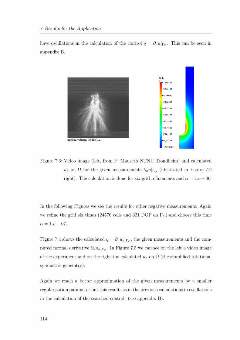
7 Results for the Application
have oscillations in the calculation of the control q = ∂nu|ΓC. This can be seen in
appendix B.
Figure 7.3: Video image (left, from F. Mauseth NTNU Trondheim) and calculated
uh on Ω for the given measurements ∂nu|ΓO(illustrated in Figure 7.2
right). The calculation is done for six grid refinements and α = 1.e−06.
In the following Figures we see the results for other negative measurements. Again
we refine the grid six times (24576 cells and 321 DOF on ΓC) and choose this time
α = 1.e − 07.
Figure 7.4 shows the calculated q = ∂nuh|ΓC, the given measurements and the com-
puted normal derivative ∂nuh|ΓO. In Figure 7.5 we can see on the left a video image
of the experiment and on the right the calculated uh on Ω (the simplified rotational
symmetric geoemtry).
Again we reach a better approximation of the given measurements by a smaller
regularisation parameter but this results as in the previous calculations in oscillations
in the calculation of the searched control. (see appendix B).
114
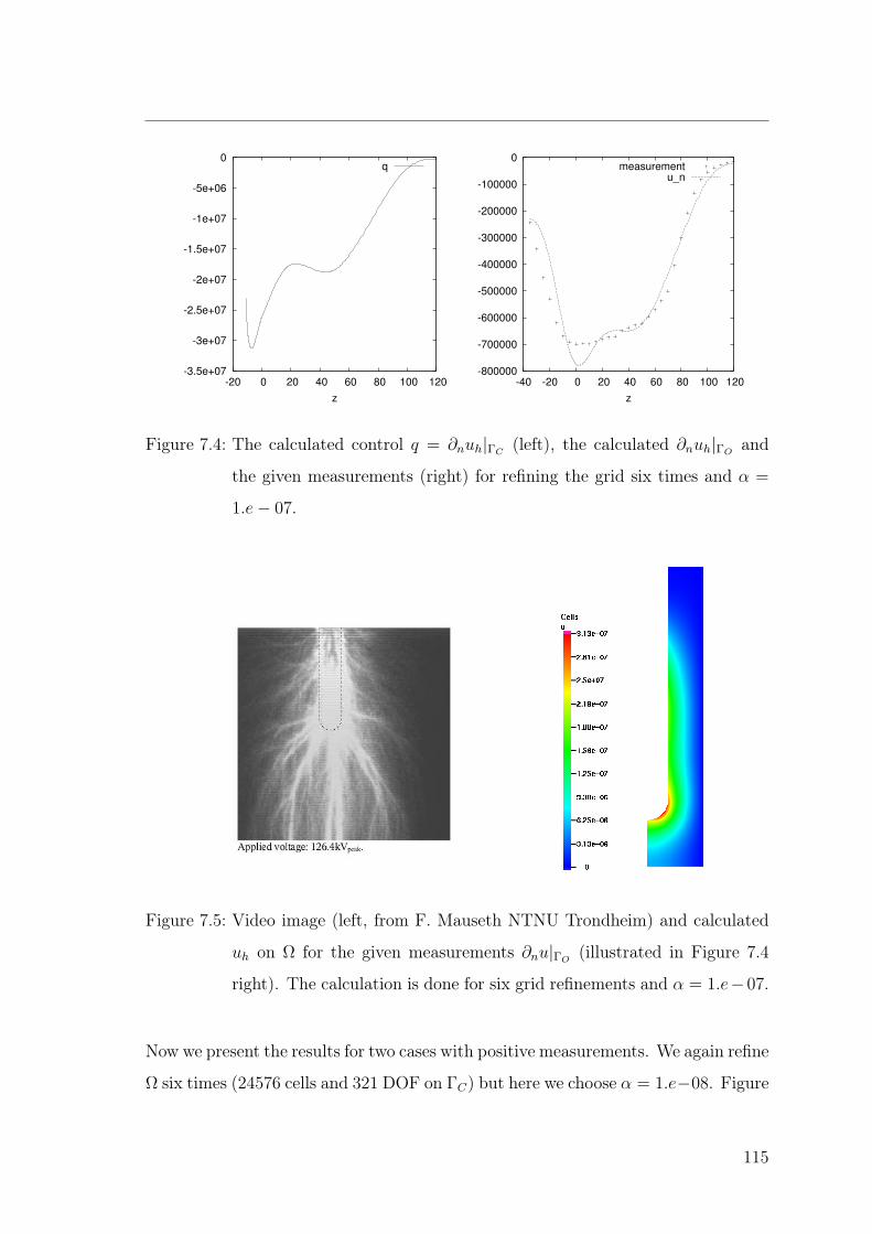
-3.5e+07
-3e+07
-2.5e+07
-2e+07
-1.5e+07
-1e+07
-5e+06
0
-20 0 20 40 60 80 100 120
z
q
-800000
-700000
-600000
-500000
-400000
-300000
-200000
-100000
0
-40 -20 0 20 40 60 80 100 120
z
measurementu_n
Figure 7.4: The calculated control q = ∂nuh|ΓC(left), the calculated ∂nuh|ΓO
and
the given measurements (right) for refining the grid six times and α =
1.e − 07.
Figure 7.5: Video image (left, from F. Mauseth NTNU Trondheim) and calculated
uh on Ω for the given measurements ∂nu|ΓO(illustrated in Figure 7.4
right). The calculation is done for six grid refinements and α = 1.e−07.
Now we present the results for two cases with positive measurements. We again refine
Ω six times (24576 cells and 321 DOF on ΓC) but here we choose α = 1.e−08. Figure
115
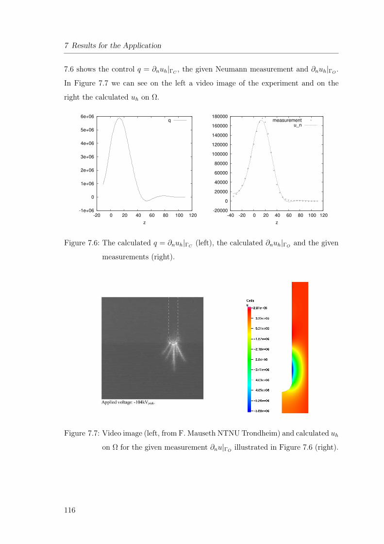
7 Results for the Application
7.6 shows the control q = ∂nuh|ΓC, the given Neumann measurement and ∂nuh|ΓO
.
In Figure 7.7 we can see on the left a video image of the experiment and on the
right the calculated uh on Ω.
-1e+06
0
1e+06
2e+06
3e+06
4e+06
5e+06
6e+06
-20 0 20 40 60 80 100 120
z
q
-20000
0
20000
40000
60000
80000
100000
120000
140000
160000
180000
-40 -20 0 20 40 60 80 100 120
z
measurementu_n
Figure 7.6: The calculated q = ∂nuh|ΓC(left), the calculated ∂nuh|ΓO
and the given
measurements (right).
Figure 7.7: Video image (left, from F. Mauseth NTNU Trondheim) and calculated uh
on Ω for the given measurement ∂nu|ΓOillustrated in Figure 7.6 (right).
116
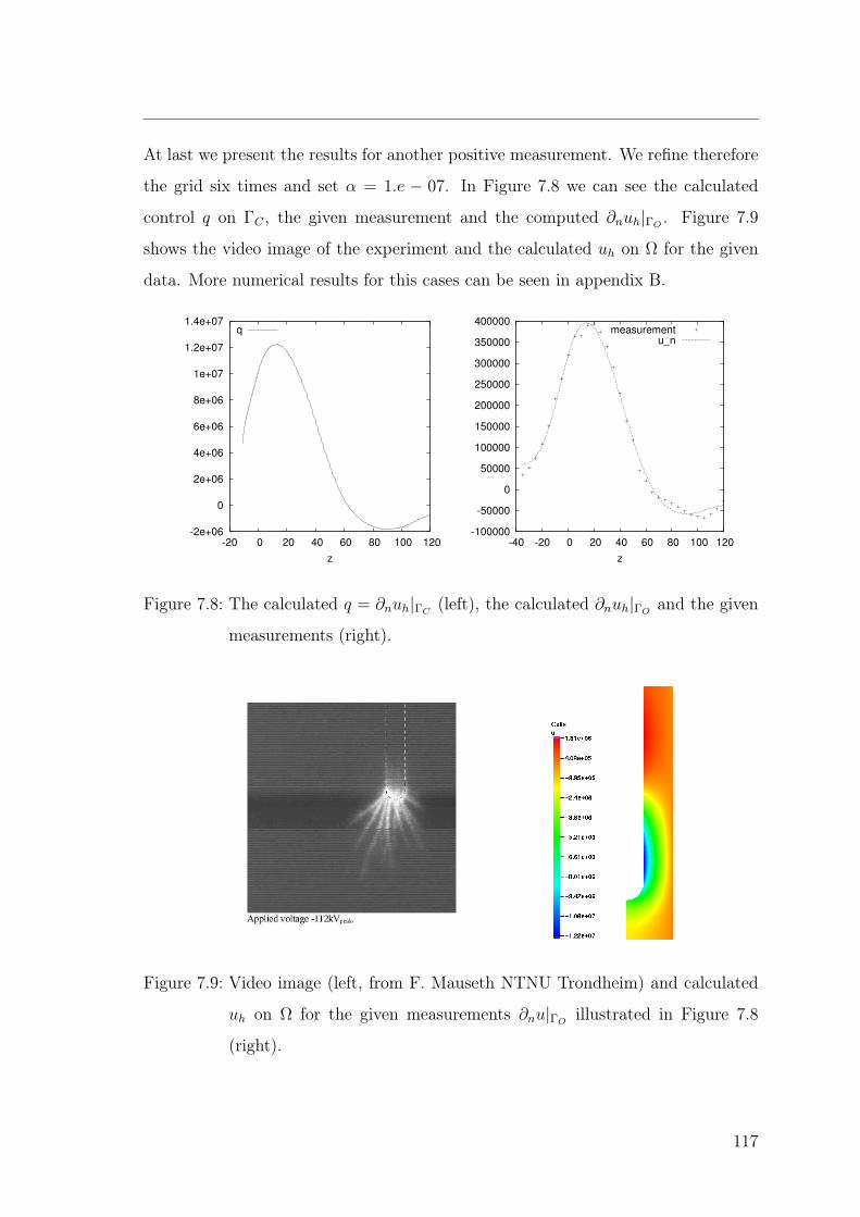
At last we present the results for another positive measurement. We refine therefore
the grid six times and set α = 1.e − 07. In Figure 7.8 we can see the calculated
control q on ΓC , the given measurement and the computed ∂nuh|ΓO. Figure 7.9
shows the video image of the experiment and the calculated uh on Ω for the given
data. More numerical results for this cases can be seen in appendix B.
-2e+06
0
2e+06
4e+06
6e+06
8e+06
1e+07
1.2e+07
1.4e+07
-20 0 20 40 60 80 100 120
z
q
-100000
-50000
0
50000
100000
150000
200000
250000
300000
350000
400000
-40 -20 0 20 40 60 80 100 120
z
measurementu_n
Figure 7.8: The calculated q = ∂nuh|ΓC(left), the calculated ∂nuh|ΓO
and the given
measurements (right).
Figure 7.9: Video image (left, from F. Mauseth NTNU Trondheim) and calculated
uh on Ω for the given measurements ∂nu|ΓOillustrated in Figure 7.8
(right).
117

7 Results for the Application
118
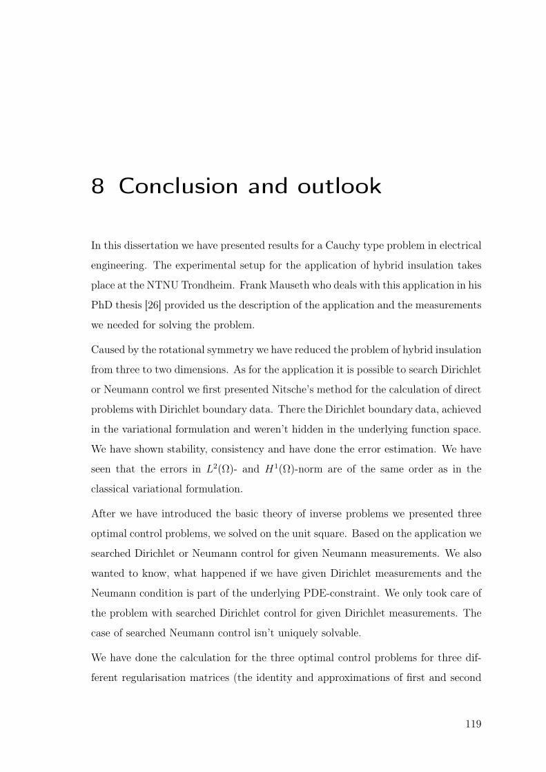
8 Conclusion and outlook
In this dissertation we have presented results for a Cauchy type problem in electrical
engineering. The experimental setup for the application of hybrid insulation takes
place at the NTNU Trondheim. Frank Mauseth who deals with this application in his
PhD thesis [26] provided us the description of the application and the measurements
we needed for solving the problem.
Caused by the rotational symmetry we have reduced the problem of hybrid insulation
from three to two dimensions. As for the application it is possible to search Dirichlet
or Neumann control we first presented Nitsche’s method for the calculation of direct
problems with Dirichlet boundary data. There the Dirichlet boundary data, achieved
in the variational formulation and weren’t hidden in the underlying function space.
We have shown stability, consistency and have done the error estimation. We have
seen that the errors in L2(Ω)- and H1(Ω)-norm are of the same order as in the
classical variational formulation.
After we have introduced the basic theory of inverse problems we presented three
optimal control problems, we solved on the unit square. Based on the application we
searched Dirichlet or Neumann control for given Neumann measurements. We also
wanted to know, what happened if we have given Dirichlet measurements and the
Neumann condition is part of the underlying PDE-constraint. We only took care of
the problem with searched Dirichlet control for given Dirichlet measurements. The
case of searched Neumann control isn’t uniquely solvable.
We have done the calculation for the three optimal control problems for three dif-
ferent regularisation matrices (the identity and approximations of first and second
119
8 Conclusion and outlook
derivative). We have noticed that we have to discretise Ω fine enough to reach good
results. For saving runtime we have reduced the number of DOF on ΓC (the bound-
ary on which we searched the control) without loosing quality of the calculation. As
a last aspect we have done the calculation for different regularisation parameters to
estimate the optimal parameter in dependence of the regularisation matrix and the
number of DOF on ΓC .
In the case of searched Neumann control for given Neumann measurements we have
seen, that we achieved good results for the searched control for all of the regularisa-
tion matrices. We have also seen, that we can reduce the number of DOF on ΓC for
all regularisations (41 DOF for Reg = RT R, 31 DOF for Reg = RT2 R2 and 91 DOF
for Reg = RT1 R1). For the calculation of the other boundary data computed by the
searched control there was graphically no discrepancy obvious.
In the case of searched Dirichlet control for given Neumann measurements we also
achieved good results for the searched control for all three regularisations. But in
this case we had to enlarge the number of DOF (compared to the case of searched
Neumann control) in the case we regularised by an approximation of first (101 DOF)
or second (91 DOF) derivative caused by the calculation of the other boundary data,
especially of ∂nuh|ΓC. There we achieved oscillations if we reduced the number of
DOF too much. If we regularised by the identity we weren’t able to avoid these
oscillations.
A similar effect we have seen in the last case of searched Dirichlet control for given
Dirichlet measurements. There again we achieved good results for the searched
control but we have to enlarge the number of DOF on ΓC compared to the results
for searched and given Neumann data. Again we weren’t able to avoid oscillations
in the calculation of ∂nuh, if we regularise by the identity. Also in the calculation of
uh|ΓOwe have seen discrepancies between the three regularisations.
In the comparison of the three problems, where we used the approximation of the
second derivative for all calculations we have seen, that we get the best results in the
case of searched Neumann control and given Neumann measurement. For this case
120
we have used the smallest number of DOF on ΓC and we didn’t have the problem of
arising oscillations if we regularise by the identity or an approximation of the first
derivative. As a conclusion we can say the results are worse the more Dirichlet data
(as searched control or/and given measurement) we have.
At last we have presented the results for the application of hybrid insulation. Caused
by the results for the model problem, where we achieved the best results for searched
Neumann control and given Neumann measurements we considered only the case
of searched Neumann control. As we have no Dirichlet data to calculate, we used
the classical variational formulation of the direct problem where the Dirichlet data
are hidden in the function space. We have modified the geometry and the matrix A
caused by the rotational symmetry. We have presented the results for four cases of
given measurement. As we only know the measurement this was the only evidence
for the choice of the regularisation parameter.
For the future work one can take a look on the automation of the choice of the
regularisation parameter and, in connection with this, on the possible error analy-
sis. Perhaps the choice of number of DOF on ΓC can be optimised by doing the
calculation adaptivly in the sense of refining the grid without ΓC . Also the choice
of the constant γ for Nitsche’s method could be done by calculating the eigenvalue
as it is mentioned by Hansbo et al. ([19] and [6]).
As hybrid insulation is a problem in three dimensions another possibility is, to do
the calculation in three dimensions. But therefore we need other measurements.
Hybrid insulation isn’t the only application for this problem. Another application is
the control of forming processes illustrated in Figure 8.1. If we simplify this problem
to the unit square we have the model problem (see Section 5) with given Neumann
measurements (the designated martensite concentration).
121
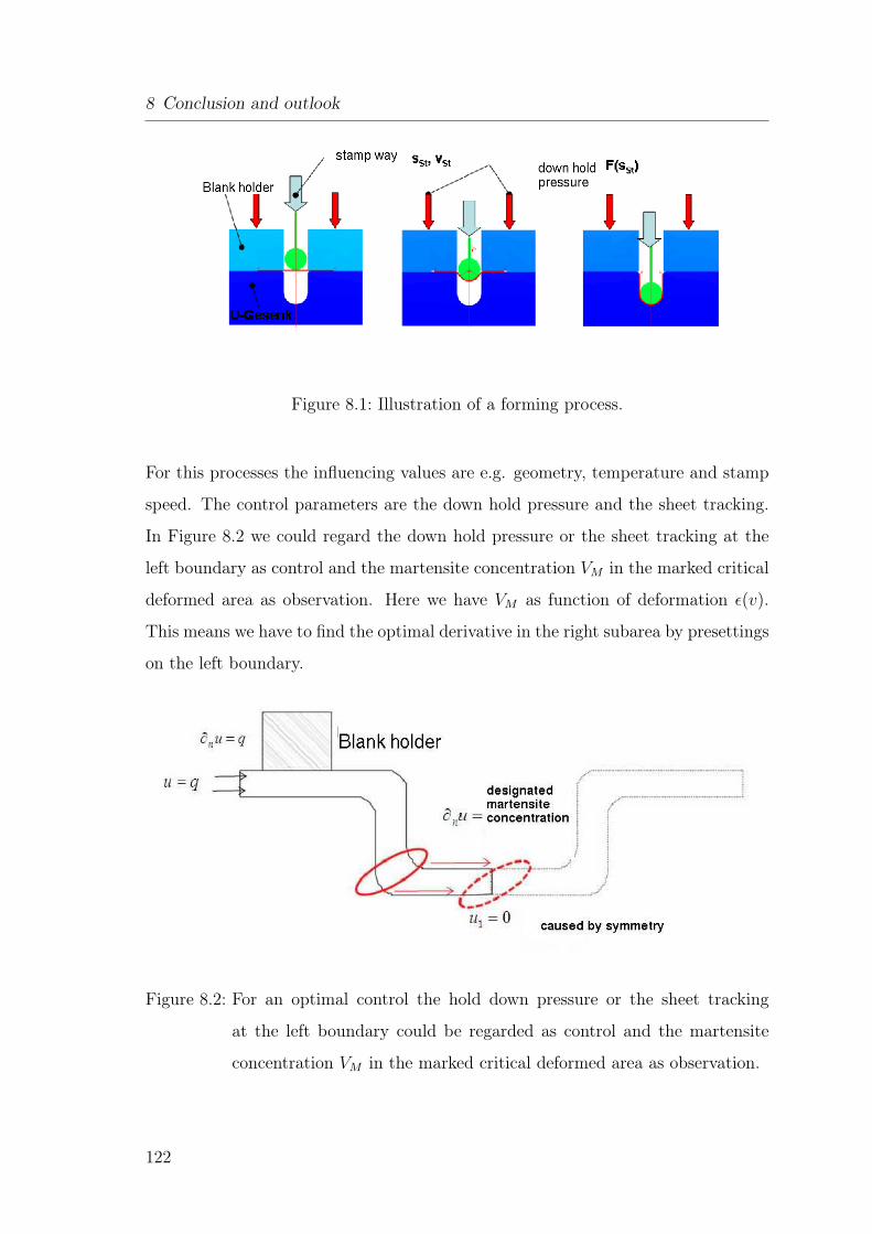
8 Conclusion and outlook
Figure 8.1: Illustration of a forming process.
For this processes the influencing values are e.g. geometry, temperature and stamp
speed. The control parameters are the down hold pressure and the sheet tracking.
In Figure 8.2 we could regard the down hold pressure or the sheet tracking at the
left boundary as control and the martensite concentration VM in the marked critical
deformed area as observation. Here we have VM as function of deformation ǫ(v).
This means we have to find the optimal derivative in the right subarea by presettings
on the left boundary.
Figure 8.2: For an optimal control the hold down pressure or the sheet tracking
at the left boundary could be regarded as control and the martensite
concentration VM in the marked critical deformed area as observation.
122
A More numerical results for the
model problem
In this Section we want to present more numerical results. We will present graphical
results for searched Neumann control and given Neumann measurements, searched
Dirichlet control and given Neumann measurements and searched Dirichlet control
and given Dirichlet measurements. Furthermore we will differ between the results for
the different regularisation matrices, for different grid refinements, different number
of DOFs on ΓC and different regularisation parameters.
Later on we present more numerical results for the application of hybrid insula-
tion. There we do the calculations in the case of searched Neumann control and
given Neumann measurements for different regularisation parameters and present
the results for the searched control q = ∂nu|ΓCand the approximation of the given
measurements ∂nuh|ΓO.
123
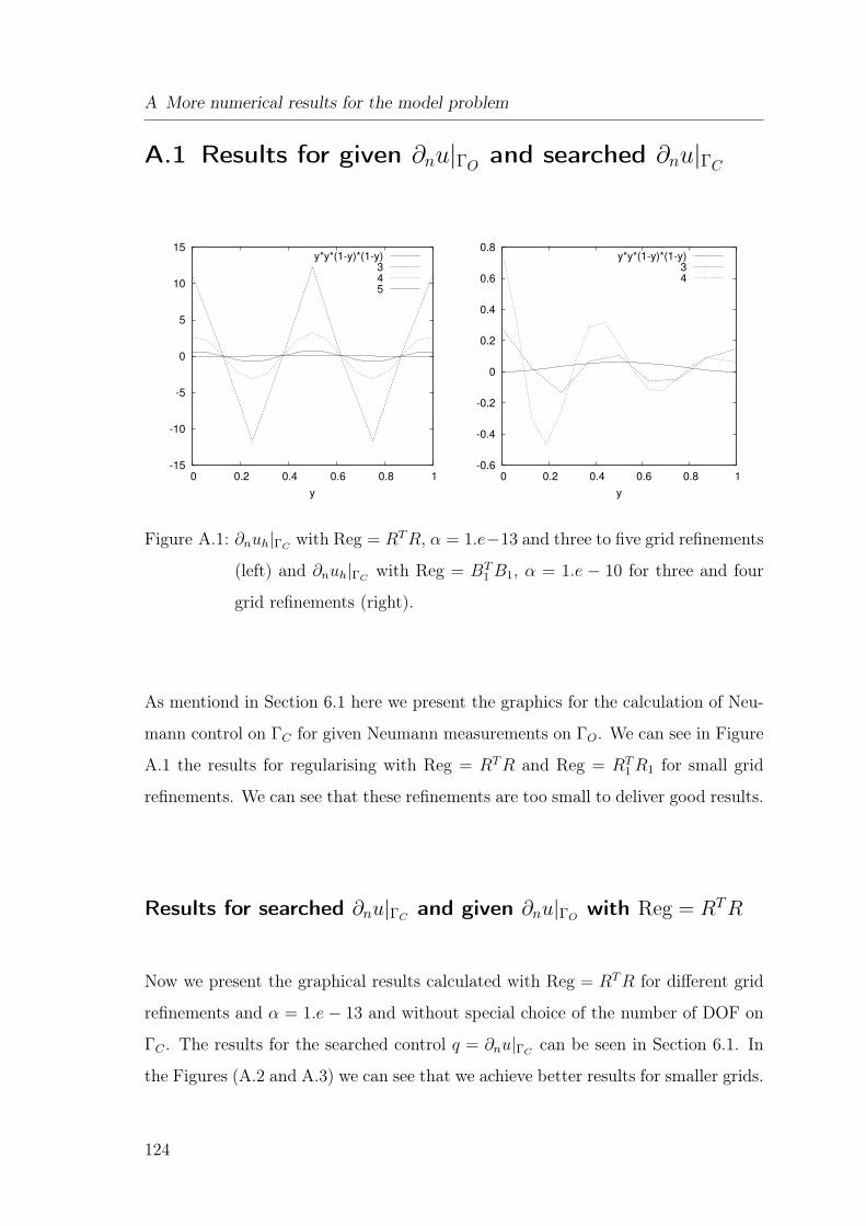
A More numerical results for the model problem
A.1 Results for given ∂nu|ΓOand searched ∂nu|ΓC
-15
-10
-5
0
5
10
15
0 0.2 0.4 0.6 0.8 1
y
y*y*(1-y)*(1-y)345
-0.6
-0.4
-0.2
0
0.2
0.4
0.6
0.8
0 0.2 0.4 0.6 0.8 1
y
y*y*(1-y)*(1-y)34
Figure A.1: ∂nuh|ΓCwith Reg = RT R, α = 1.e−13 and three to five grid refinements
(left) and ∂nuh|ΓCwith Reg = BT
1 B1, α = 1.e − 10 for three and four
grid refinements (right).
As mentiond in Section 6.1 here we present the graphics for the calculation of Neu-
mann control on ΓC for given Neumann measurements on ΓO. We can see in Figure
A.1 the results for regularising with Reg = RT R and Reg = RT1 R1 for small grid
refinements. We can see that these refinements are too small to deliver good results.
Results for searched ∂nu|ΓCand given ∂nu|ΓO
with Reg = RTR
Now we present the graphical results calculated with Reg = RT R for different grid
refinements and α = 1.e − 13 and without special choice of the number of DOF on
ΓC . The results for the searched control q = ∂nu|ΓCcan be seen in Section 6.1. In
the Figures (A.2 and A.3) we can see that we achieve better results for smaller grids.
124
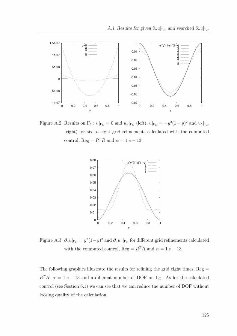
A.1 Results for given ∂nu|ΓOand searched ∂nu|ΓC
-1e-07
-5e-08
0
5e-08
1e-07
1.5e-07
0 0.2 0.4 0.6 0.8 1
y
u=0678
-0.07
-0.06
-0.05
-0.04
-0.03
-0.02
-0.01
0
0 0.2 0.4 0.6 0.8 1
y
-y*y*(1-y)*(1-y)345678
Figure A.2: Results on ΓO: u|ΓO= 0 and uh|ΓO
(left), u|ΓO= −y2(1− y)2 and uh|ΓO
(right) for six to eight grid refinements calculated with the computed
control, Reg = RT R and α = 1.e − 13.
0
0.01
0.02
0.03
0.04
0.05
0.06
0.07
0.08
0 0.2 0.4 0.6 0.8 1
y
y*y*(1-y)*(1-y)678
Figure A.3: ∂nu|ΓC= y2(1−y)2 and ∂nuh|ΓC
for different grid refinements calculated
with the computed control, Reg = RT R and α = 1.e − 13.
The following graphics illustrate the results for refining the grid eight times, Reg =
RT R, α = 1.e − 13 and a different number of DOF on ΓC . As for the calculated
control (see Section 6.1) we can see that we can reduce the number of DOF without
loosing quality of the calculation.
125
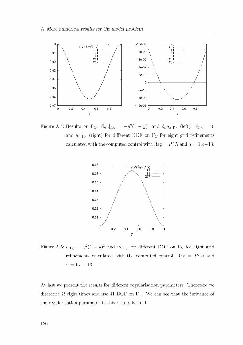
A More numerical results for the model problem
-0.07
-0.06
-0.05
-0.04
-0.03
-0.02
-0.01
0
0 0.2 0.4 0.6 0.8 1
y
-y*y*(1-y)*(1-y)113191
201257
-1.5e-09
-1e-09
-5e-10
0
5e-10
1e-09
1.5e-09
2e-09
2.5e-09
0 0.2 0.4 0.6 0.8 1
y
u=0113191
201257
Figure A.4: Results on ΓO: ∂nu|ΓO= −y2(1 − y)2 and ∂nuh|ΓO
(left), u|ΓO= 0
and uh|ΓO(right) for different DOF on ΓC for eight grid refinements
calculated with the computed control with Reg = RT R and α = 1.e−13.
0
0.01
0.02
0.03
0.04
0.05
0.06
0.07
0 0.2 0.4 0.6 0.8 1
y
y*y*(1-y)*(1-y)1131
257
Figure A.5: u|ΓC= y2(1 − y)2 and uh|ΓC
for different DOF on ΓC for eight grid
refinements calculated with the computed control, Reg = RT R and
α = 1.e − 13.
At last we present the results for different regularisation parameters. Therefore we
discretise Ω eight times and use 41 DOF on ΓC . We can see that the influence of
the regularisation parameter in this results is small.
126
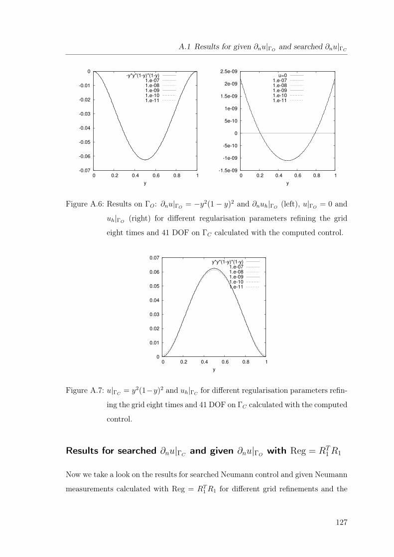
A.1 Results for given ∂nu|ΓOand searched ∂nu|ΓC
-0.07
-0.06
-0.05
-0.04
-0.03
-0.02
-0.01
0
0 0.2 0.4 0.6 0.8 1
y
-y*y*(1-y)*(1-y)1.e-071.e-081.e-091.e-101.e-11
-1.5e-09
-1e-09
-5e-10
0
5e-10
1e-09
1.5e-09
2e-09
2.5e-09
0 0.2 0.4 0.6 0.8 1
y
u=01.e-071.e-081.e-091.e-101.e-11
Figure A.6: Results on ΓO: ∂nu|ΓO= −y2(1 − y)2 and ∂nuh|ΓO
(left), u|ΓO= 0 and
uh|ΓO(right) for different regularisation parameters refining the grid
eight times and 41 DOF on ΓC calculated with the computed control.
0
0.01
0.02
0.03
0.04
0.05
0.06
0.07
0 0.2 0.4 0.6 0.8 1
y
y*y*(1-y)*(1-y)1.e-071.e-081.e-091.e-101.e-11
Figure A.7: u|ΓC= y2(1−y)2 and uh|ΓC
for different regularisation parameters refin-
ing the grid eight times and 41 DOF on ΓC calculated with the computed
control.
Results for searched ∂nu|ΓCand given ∂nu|ΓO
with Reg = RT1R1
Now we take a look on the results for searched Neumann control and given Neumann
measurements calculated with Reg = RT1 R1 for different grid refinements and the
127
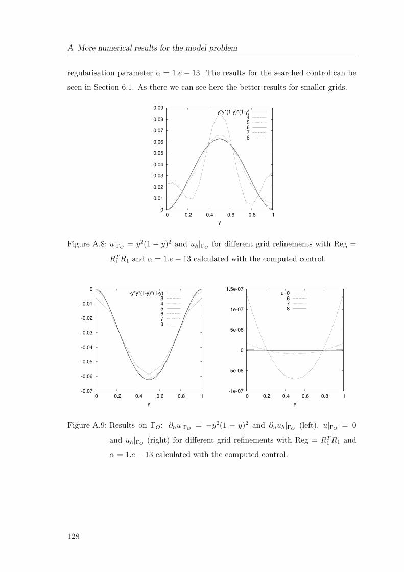
A More numerical results for the model problem
regularisation parameter α = 1.e − 13. The results for the searched control can be
seen in Section 6.1. As there we can see here the better results for smaller grids.
0
0.01
0.02
0.03
0.04
0.05
0.06
0.07
0.08
0.09
0 0.2 0.4 0.6 0.8 1
y
y*y*(1-y)*(1-y)45678
Figure A.8: u|ΓC= y2(1 − y)2 and uh|ΓC
for different grid refinements with Reg =
RT1 R1 and α = 1.e − 13 calculated with the computed control.
-0.07
-0.06
-0.05
-0.04
-0.03
-0.02
-0.01
0
0 0.2 0.4 0.6 0.8 1
y
-y*y*(1-y)*(1-y)345678
-1e-07
-5e-08
0
5e-08
1e-07
1.5e-07
0 0.2 0.4 0.6 0.8 1
y
u=0678
Figure A.9: Results on ΓO: ∂nu|ΓO= −y2(1 − y)2 and ∂nuh|ΓO
(left), u|ΓO= 0
and uh|ΓO(right) for different grid refinements with Reg = RT
1 R1 and
α = 1.e − 13 calculated with the computed control.
128
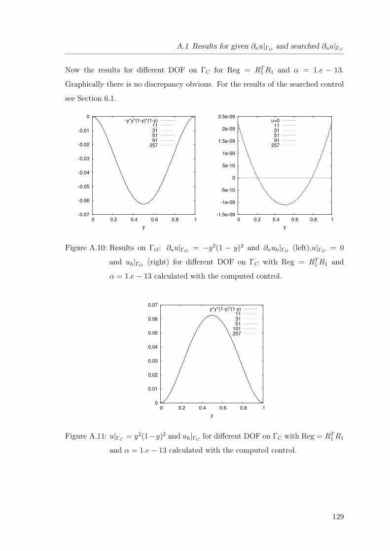
A.1 Results for given ∂nu|ΓOand searched ∂nu|ΓC
Now the results for different DOF on ΓC for Reg = RT1 R1 and α = 1.e − 13.
Graphically there is no discrepancy obvious. For the results of the searched control
see Section 6.1.
-0.07
-0.06
-0.05
-0.04
-0.03
-0.02
-0.01
0
0 0.2 0.4 0.6 0.8 1
y
-y*y*(1-y)*(1-y)11315191
257
-1.5e-09
-1e-09
-5e-10
0
5e-10
1e-09
1.5e-09
2e-09
2.5e-09
0 0.2 0.4 0.6 0.8 1
y
u=011315191
257
Figure A.10: Results on ΓO: ∂nu|ΓO= −y2(1 − y)2 and ∂nuh|ΓO
(left),u|ΓO= 0
and uh|ΓO(right) for different DOF on ΓC with Reg = RT
1 R1 and
α = 1.e − 13 calculated with the computed control.
0
0.01
0.02
0.03
0.04
0.05
0.06
0.07
0 0.2 0.4 0.6 0.8 1
y
y*y*(1-y)*(1-y)113151
101257
Figure A.11: u|ΓC= y2(1−y)2 and uh|ΓC
for different DOF on ΓC with Reg = RT1 R1
and α = 1.e − 13 calculated with the computed control.
129
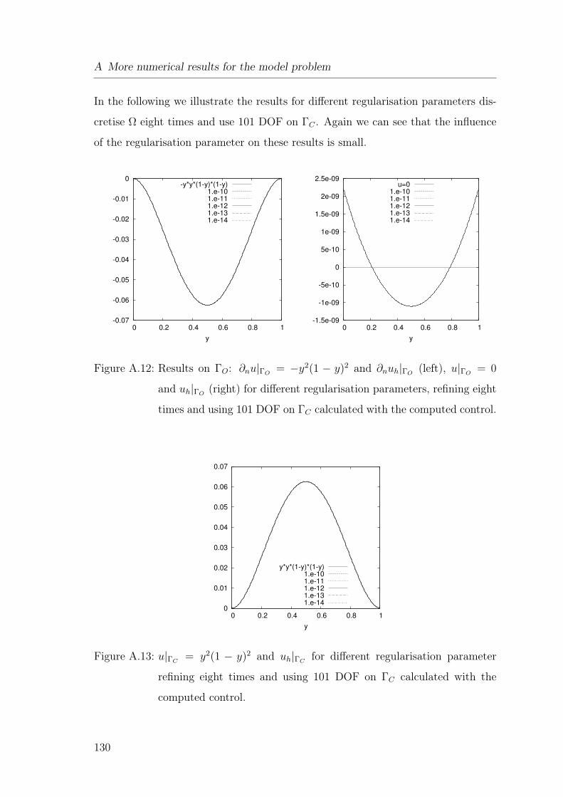
A More numerical results for the model problem
In the following we illustrate the results for different regularisation parameters dis-
cretise Ω eight times and use 101 DOF on ΓC . Again we can see that the influence
of the regularisation parameter on these results is small.
-0.07
-0.06
-0.05
-0.04
-0.03
-0.02
-0.01
0
0 0.2 0.4 0.6 0.8 1
y
-y*y*(1-y)*(1-y)1.e-101.e-111.e-121.e-131.e-14
-1.5e-09
-1e-09
-5e-10
0
5e-10
1e-09
1.5e-09
2e-09
2.5e-09
0 0.2 0.4 0.6 0.8 1
y
u=01.e-101.e-111.e-121.e-131.e-14
Figure A.12: Results on ΓO: ∂nu|ΓO= −y2(1 − y)2 and ∂nuh|ΓO
(left), u|ΓO= 0
and uh|ΓO(right) for different regularisation parameters, refining eight
times and using 101 DOF on ΓC calculated with the computed control.
0
0.01
0.02
0.03
0.04
0.05
0.06
0.07
0 0.2 0.4 0.6 0.8 1
y
y*y*(1-y)*(1-y)1.e-101.e-111.e-121.e-131.e-14
Figure A.13: u|ΓC= y2(1 − y)2 and uh|ΓC
for different regularisation parameter
refining eight times and using 101 DOF on ΓC calculated with the
computed control.
130
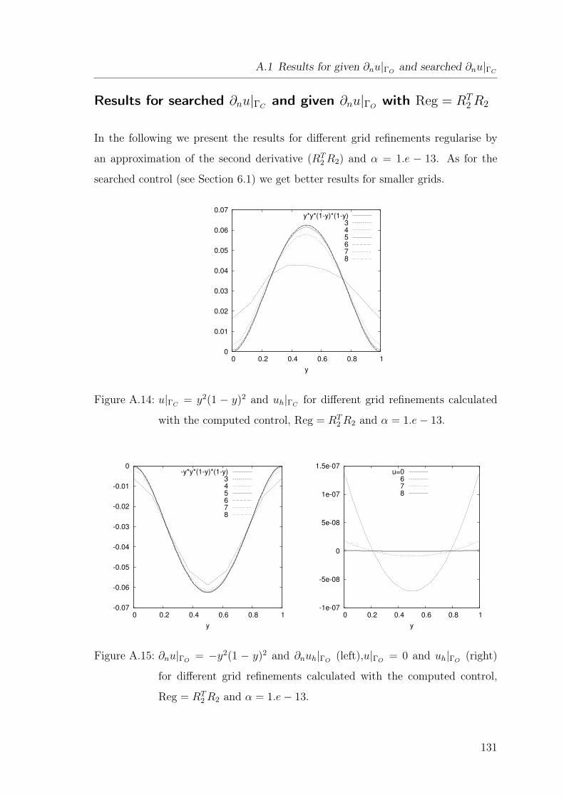
A.1 Results for given ∂nu|ΓOand searched ∂nu|ΓC
Results for searched ∂nu|ΓCand given ∂nu|ΓO
with Reg = RT2R2
In the following we present the results for different grid refinements regularise by
an approximation of the second derivative (RT2 R2) and α = 1.e − 13. As for the
searched control (see Section 6.1) we get better results for smaller grids.
0
0.01
0.02
0.03
0.04
0.05
0.06
0.07
0 0.2 0.4 0.6 0.8 1
y
y*y*(1-y)*(1-y)345678
Figure A.14: u|ΓC= y2(1 − y)2 and uh|ΓC
for different grid refinements calculated
with the computed control, Reg = RT2 R2 and α = 1.e − 13.
-0.07
-0.06
-0.05
-0.04
-0.03
-0.02
-0.01
0
0 0.2 0.4 0.6 0.8 1
y
-y*y*(1-y)*(1-y)345678
-1e-07
-5e-08
0
5e-08
1e-07
1.5e-07
0 0.2 0.4 0.6 0.8 1
y
u=0678
Figure A.15: ∂nu|ΓO= −y2(1 − y)2 and ∂nuh|ΓO
(left),u|ΓO= 0 and uh|ΓO
(right)
for different grid refinements calculated with the computed control,
Reg = RT2 R2 and α = 1.e − 13.
131
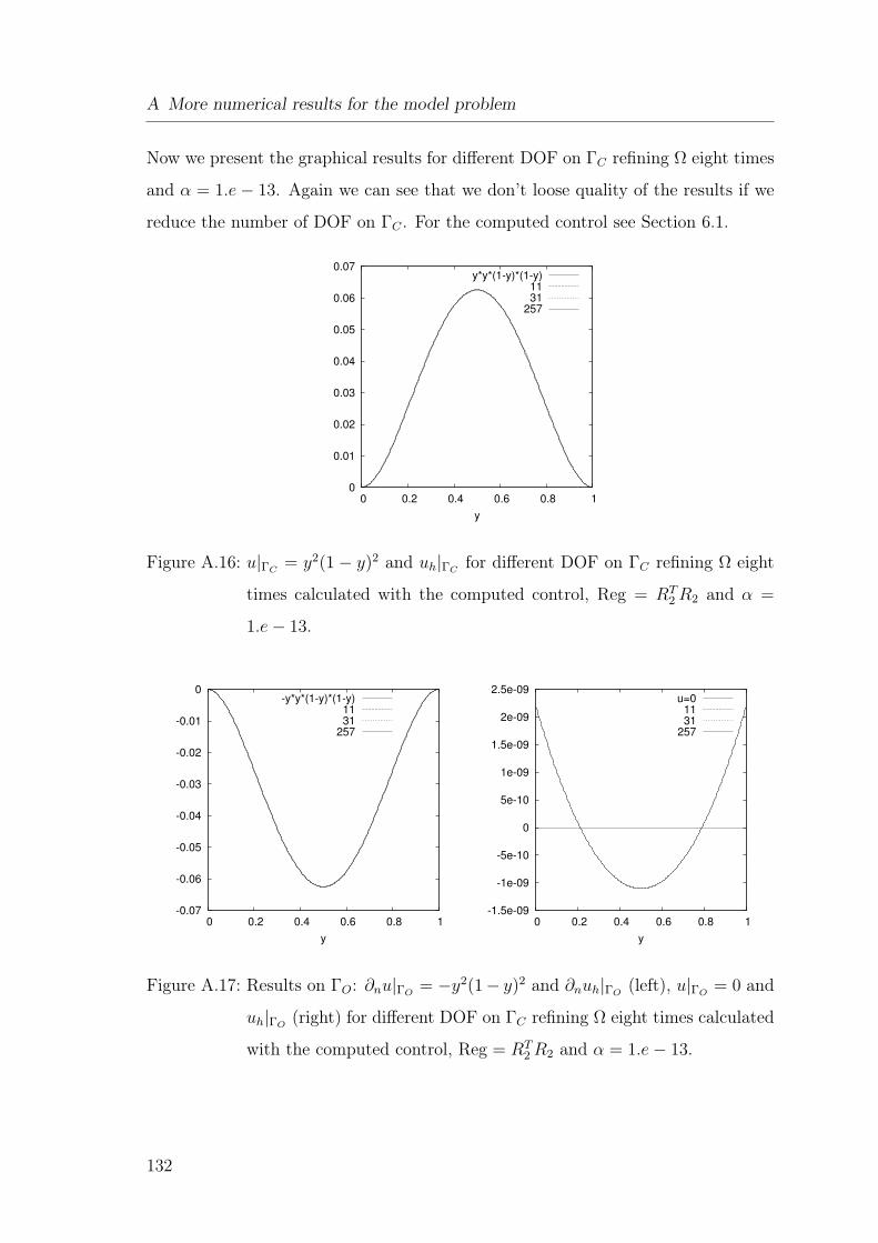
A More numerical results for the model problem
Now we present the graphical results for different DOF on ΓC refining Ω eight times
and α = 1.e − 13. Again we can see that we don’t loose quality of the results if we
reduce the number of DOF on ΓC . For the computed control see Section 6.1.
0
0.01
0.02
0.03
0.04
0.05
0.06
0.07
0 0.2 0.4 0.6 0.8 1
y
y*y*(1-y)*(1-y)1131
257
Figure A.16: u|ΓC= y2(1 − y)2 and uh|ΓC
for different DOF on ΓC refining Ω eight
times calculated with the computed control, Reg = RT2 R2 and α =
1.e − 13.
-0.07
-0.06
-0.05
-0.04
-0.03
-0.02
-0.01
0
0 0.2 0.4 0.6 0.8 1
y
-y*y*(1-y)*(1-y)1131
257
-1.5e-09
-1e-09
-5e-10
0
5e-10
1e-09
1.5e-09
2e-09
2.5e-09
0 0.2 0.4 0.6 0.8 1
y
u=01131
257
Figure A.17: Results on ΓO: ∂nu|ΓO= −y2(1− y)2 and ∂nuh|ΓO
(left), u|ΓO= 0 and
uh|ΓO(right) for different DOF on ΓC refining Ω eight times calculated
with the computed control, Reg = RT2 R2 and α = 1.e − 13.
132
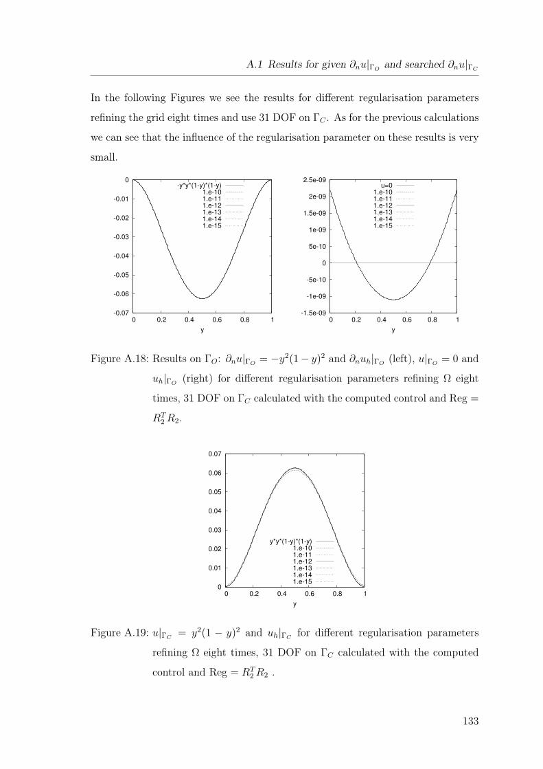
A.1 Results for given ∂nu|ΓOand searched ∂nu|ΓC
In the following Figures we see the results for different regularisation parameters
refining the grid eight times and use 31 DOF on ΓC . As for the previous calculations
we can see that the influence of the regularisation parameter on these results is very
small.
-0.07
-0.06
-0.05
-0.04
-0.03
-0.02
-0.01
0
0 0.2 0.4 0.6 0.8 1
y
-y*y*(1-y)*(1-y)1.e-101.e-111.e-121.e-131.e-141.e-15
-1.5e-09
-1e-09
-5e-10
0
5e-10
1e-09
1.5e-09
2e-09
2.5e-09
0 0.2 0.4 0.6 0.8 1
y
u=01.e-101.e-111.e-121.e-131.e-141.e-15
Figure A.18: Results on ΓO: ∂nu|ΓO= −y2(1− y)2 and ∂nuh|ΓO
(left), u|ΓO= 0 and
uh|ΓO(right) for different regularisation parameters refining Ω eight
times, 31 DOF on ΓC calculated with the computed control and Reg =
RT2 R2.
0
0.01
0.02
0.03
0.04
0.05
0.06
0.07
0 0.2 0.4 0.6 0.8 1
y
y*y*(1-y)*(1-y)1.e-101.e-111.e-121.e-131.e-141.e-15
Figure A.19: u|ΓC= y2(1 − y)2 and uh|ΓC
for different regularisation parameters
refining Ω eight times, 31 DOF on ΓC calculated with the computed
control and Reg = RT2 R2 .
133
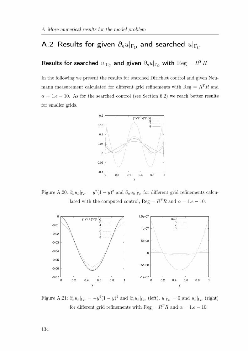
A More numerical results for the model problem
A.2 Results for given ∂nu|ΓOand searched u|ΓC
Results for searched u|ΓCand given ∂nu|ΓO
with Reg = RTR
In the following we present the results for searched Dirichlet control and given Neu-
mann measurement calculated for different grid refinements with Reg = RT R and
α = 1.e − 10. As for the searched control (see Section 6.2) we reach better results
for smaller grids.
-0.1
-0.05
0
0.05
0.1
0.15
0.2
0 0.2 0.4 0.6 0.8 1
y
y*y*(1-y)*(1-y)678
Figure A.20: ∂nuh|ΓC= y2(1 − y)2 and ∂nuh|ΓC
for different grid refinements calcu-
lated with the computed control, Reg = RT R and α = 1.e − 10.
-0.07
-0.06
-0.05
-0.04
-0.03
-0.02
-0.01
0
0 0.2 0.4 0.6 0.8 1
y
-y*y*(1-y)*(1-y)345678
-1e-07
-5e-08
0
5e-08
1e-07
1.5e-07
0 0.2 0.4 0.6 0.8 1
y
u=0678
Figure A.21: ∂nuh|ΓO= −y2(1 − y)2 and ∂nuh|ΓO
(left), u|ΓO= 0 and uh|ΓO
(right)
for different grid refinements with Reg = RT R and α = 1.e − 10.
134
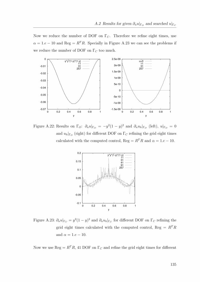
A.2 Results for given ∂nu|ΓOand searched u|ΓC
Now we reduce the number of DOF on ΓC . Therefore we refine eight times, use
α = 1.e − 10 and Reg = RT R. Specially in Figure A.23 we can see the problems if
we reduce the number of DOF on ΓC too much.
-0.07
-0.06
-0.05
-0.04
-0.03
-0.02
-0.01
0
0 0.2 0.4 0.6 0.8 1
y
-y*y*(1-y)*(1-y)1131
257
-1.5e-09
-1e-09
-5e-10
0
5e-10
1e-09
1.5e-09
2e-09
2.5e-09
0 0.2 0.4 0.6 0.8 1
y
u=01131
257
Figure A.22: Results on ΓO: ∂nu|ΓO= −y2(1 − y)2 and ∂nuh|ΓO
(left), u|ΓO= 0
and uh|ΓO(right) for different DOF on ΓC refining the grid eight times
calculated with the computed control, Reg = RT R and α = 1.e − 10.
-0.1
-0.05
0
0.05
0.1
0.15
0.2
0 0.2 0.4 0.6 0.8 1
y
y*y*(1-y)*(1-y)11314191
257
Figure A.23: ∂nu|ΓC= y2(1 − y)2 and ∂nuh|ΓC
for different DOF on ΓC refining the
grid eight times calculated with the computed control, Reg = RT R
and α = 1.e − 10.
Now we use Reg = RT R, 41 DOF on ΓC and refine the grid eight times for different
135
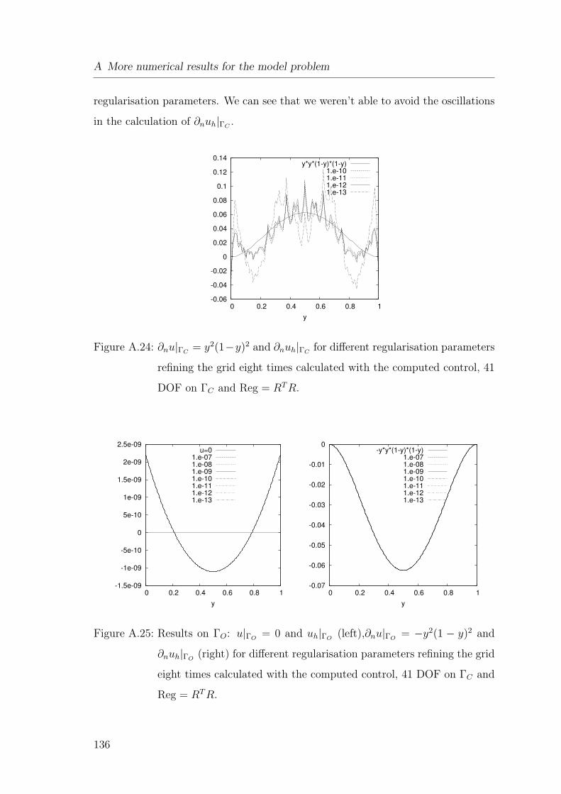
A More numerical results for the model problem
regularisation parameters. We can see that we weren’t able to avoid the oscillations
in the calculation of ∂nuh|ΓC.
-0.06
-0.04
-0.02
0
0.02
0.04
0.06
0.08
0.1
0.12
0.14
0 0.2 0.4 0.6 0.8 1
y
y*y*(1-y)*(1-y)1.e-101.e-111.e-121.e-13
Figure A.24: ∂nu|ΓC= y2(1−y)2 and ∂nuh|ΓC
for different regularisation parameters
refining the grid eight times calculated with the computed control, 41
DOF on ΓC and Reg = RT R.
-1.5e-09
-1e-09
-5e-10
0
5e-10
1e-09
1.5e-09
2e-09
2.5e-09
0 0.2 0.4 0.6 0.8 1
y
u=01.e-071.e-081.e-091.e-101.e-111.e-121.e-13
-0.07
-0.06
-0.05
-0.04
-0.03
-0.02
-0.01
0
0 0.2 0.4 0.6 0.8 1
y
-y*y*(1-y)*(1-y)1.e-071.e-081.e-091.e-101.e-111.e-121.e-13
Figure A.25: Results on ΓO: u|ΓO= 0 and uh|ΓO
(left),∂nu|ΓO= −y2(1 − y)2 and
∂nuh|ΓO(right) for different regularisation parameters refining the grid
eight times calculated with the computed control, 41 DOF on ΓC and
Reg = RT R.
136
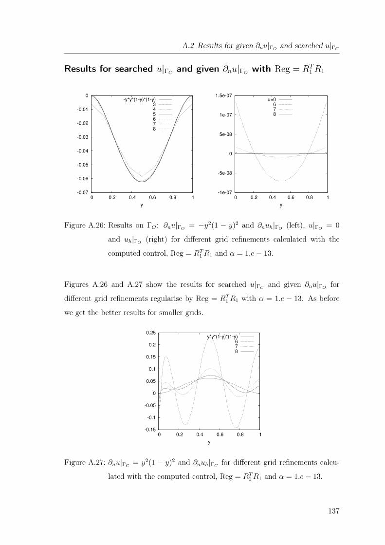
A.2 Results for given ∂nu|ΓOand searched u|ΓC
Results for searched u|ΓCand given ∂nu|ΓO
with Reg = RT1R1
-0.07
-0.06
-0.05
-0.04
-0.03
-0.02
-0.01
0
0 0.2 0.4 0.6 0.8 1
y
-y*y*(1-y)*(1-y)345678
-1e-07
-5e-08
0
5e-08
1e-07
1.5e-07
0 0.2 0.4 0.6 0.8 1
y
u=0678
Figure A.26: Results on ΓO: ∂nu|ΓO= −y2(1 − y)2 and ∂nuh|ΓO
(left), u|ΓO= 0
and uh|ΓO(right) for different grid refinements calculated with the
computed control, Reg = RT1 R1 and α = 1.e − 13.
Figures A.26 and A.27 show the results for searched u|ΓCand given ∂nu|ΓO
for
different grid refinements regularise by Reg = RT1 R1 with α = 1.e − 13. As before
we get the better results for smaller grids.
-0.15
-0.1
-0.05
0
0.05
0.1
0.15
0.2
0.25
0 0.2 0.4 0.6 0.8 1
y
y*y*(1-y)*(1-y)678
Figure A.27: ∂nu|ΓC= y2(1 − y)2 and ∂nuh|ΓC
for different grid refinements calcu-
lated with the computed control, Reg = RT1 R1 and α = 1.e − 13.
137
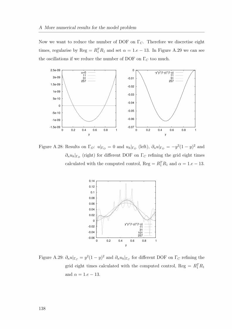
A More numerical results for the model problem
Now we want to reduce the number of DOF on ΓC . Therefore we discretise eight
times, regularise by Reg = RT1 R1 and set α = 1.e − 13. In Figure A.29 we can see
the oscillations if we reduce the number of DOF on ΓC too much.
-1.5e-09
-1e-09
-5e-10
0
5e-10
1e-09
1.5e-09
2e-09
2.5e-09
0 0.2 0.4 0.6 0.8 1
y
u=01131
257
-0.07
-0.06
-0.05
-0.04
-0.03
-0.02
-0.01
0
0 0.2 0.4 0.6 0.8 1
y
-y*y*(1-y)*(1-y)1131
257
Figure A.28: Results on ΓO: u|ΓO= 0 and uh|ΓO
(left), ∂nu|ΓO= −y2(1 − y)2 and
∂nuh|ΓO(right) for different DOF on ΓC refining the grid eight times
calculated with the computed control, Reg = RT1 R1 and α = 1.e − 13.
-0.06
-0.04
-0.02
0
0.02
0.04
0.06
0.08
0.1
0.12
0.14
0 0.2 0.4 0.6 0.8 1
y
y*y*(1-y)*(1-y)1131
101257
Figure A.29: ∂nu|ΓC= y2(1 − y)2 and ∂nuh|ΓC
for different DOF on ΓC refining the
grid eight times calculated with the computed control, Reg = RT1 R1
and α = 1.e − 13.
138
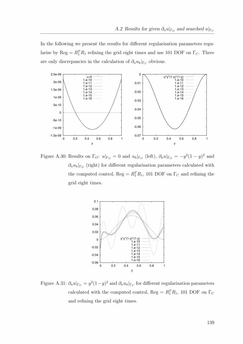
A.2 Results for given ∂nu|ΓOand searched u|ΓC
In the following we present the results for different regularisation parameters regu-
larise by Reg = RT1 R1 refining the grid eight times and use 101 DOF on ΓC . There
are only discrepancies in the calculation of ∂nuh|ΓCobvious.
-1.5e-09
-1e-09
-5e-10
0
5e-10
1e-09
1.5e-09
2e-09
2.5e-09
0 0.2 0.4 0.6 0.8 1
y
u=01.e-101.e-111.e-121.e-131.e-141.e-151.e-16
-0.07
-0.06
-0.05
-0.04
-0.03
-0.02
-0.01
0
0 0.2 0.4 0.6 0.8 1
y
-y*y*(1-y)*(1-y)1.e-101.e-111.e-121.e-131.e-141.e-151.e-16
Figure A.30: Results on ΓO: u|ΓO= 0 and uh|ΓO
(left), ∂nu|ΓO= −y2(1 − y)2 and
∂nuh|ΓO(right) for different regularisation parameters calculated with
the computed control, Reg = RT1 R1, 101 DOF on ΓC and refining the
grid eight times.
-0.06
-0.04
-0.02
0
0.02
0.04
0.06
0.08
0.1
0 0.2 0.4 0.6 0.8 1
y
y*y*(1-y)*(1-y)1.e-101.e-111.e-121.e-131.e-141.e-151.e-16
Figure A.31: ∂nu|ΓC= y2(1−y)2 and ∂nuh|ΓC
for different regularisation parameters
calculated with the computed control, Reg = RT1 R1, 101 DOF on ΓC
and refining the grid eight times.
139
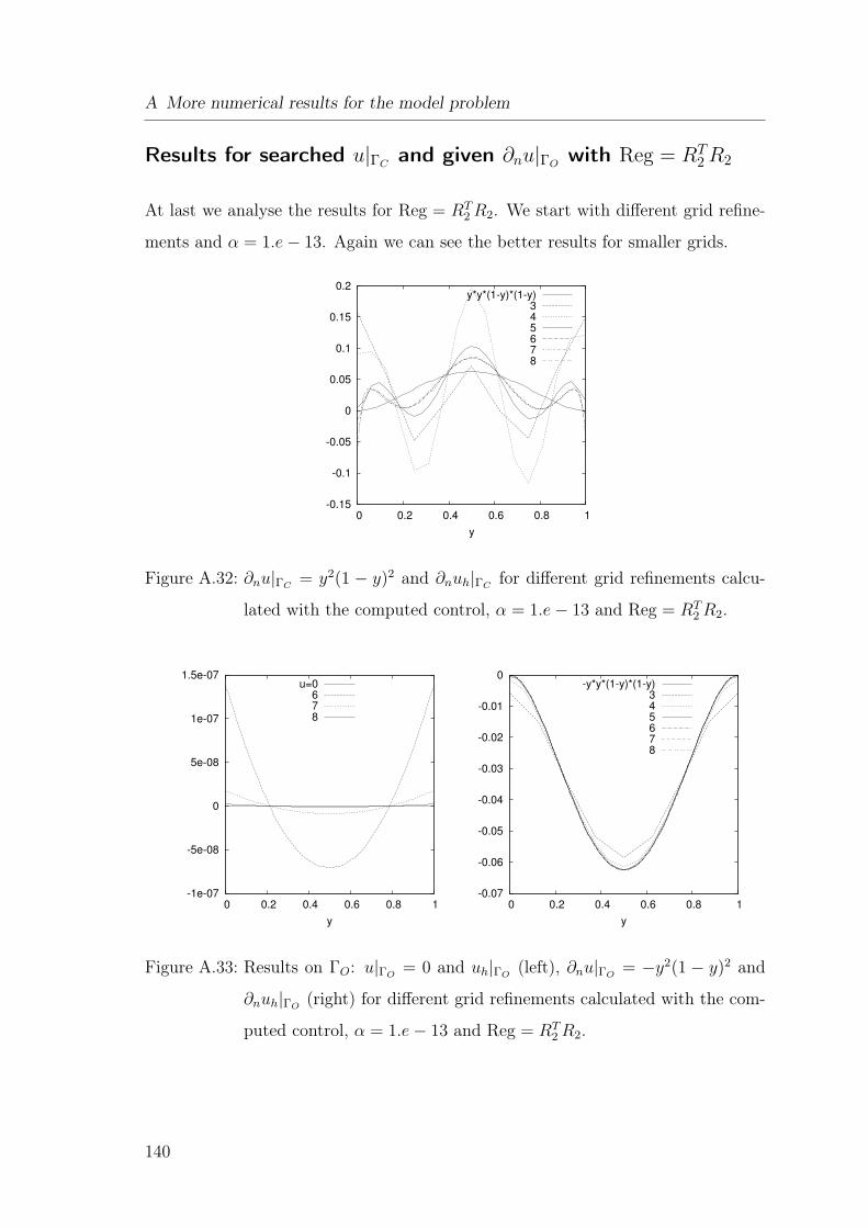
A More numerical results for the model problem
Results for searched u|ΓCand given ∂nu|ΓO
with Reg = RT2R2
At last we analyse the results for Reg = RT2 R2. We start with different grid refine-
ments and α = 1.e − 13. Again we can see the better results for smaller grids.
-0.15
-0.1
-0.05
0
0.05
0.1
0.15
0.2
0 0.2 0.4 0.6 0.8 1
y
y*y*(1-y)*(1-y)345678
Figure A.32: ∂nu|ΓC= y2(1 − y)2 and ∂nuh|ΓC
for different grid refinements calcu-
lated with the computed control, α = 1.e − 13 and Reg = RT2 R2.
-1e-07
-5e-08
0
5e-08
1e-07
1.5e-07
0 0.2 0.4 0.6 0.8 1
y
u=0678
-0.07
-0.06
-0.05
-0.04
-0.03
-0.02
-0.01
0
0 0.2 0.4 0.6 0.8 1
y
-y*y*(1-y)*(1-y)345678
Figure A.33: Results on ΓO: u|ΓO= 0 and uh|ΓO
(left), ∂nu|ΓO= −y2(1 − y)2 and
∂nuh|ΓO(right) for different grid refinements calculated with the com-
puted control, α = 1.e − 13 and Reg = RT2 R2.
140
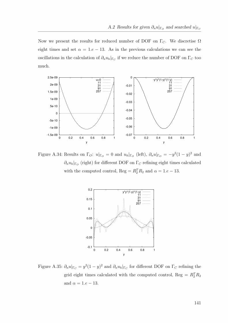
A.2 Results for given ∂nu|ΓOand searched u|ΓC
Now we present the results for reduced number of DOF on ΓC . We discretise Ω
eight times and set α = 1.e − 13. As in the previous calculations we can see the
oscillations in the calculation of ∂nuh|ΓCif we reduce the number of DOF on ΓC too
much.
-1.5e-09
-1e-09
-5e-10
0
5e-10
1e-09
1.5e-09
2e-09
2.5e-09
0 0.2 0.4 0.6 0.8 1
y
u=0113191
257
-0.07
-0.06
-0.05
-0.04
-0.03
-0.02
-0.01
0
0 0.2 0.4 0.6 0.8 1
y
-y*y*(1-y)*(1-y)113191
257
Figure A.34: Results on ΓO: u|ΓO= 0 and uh|ΓO
(left), ∂nu|ΓO= −y2(1 − y)2 and
∂nuh|ΓO(right) for different DOF on ΓC refining eight times calculated
with the computed control, Reg = RT2 R2 and α = 1.e − 13.
-0.1
-0.05
0
0.05
0.1
0.15
0.2
0 0.2 0.4 0.6 0.8 1
y
y*y*(1-y)*(1-y)113191
257
Figure A.35: ∂nu|ΓC= y2(1 − y)2 and ∂nuh|ΓC
for different DOF on ΓC refining the
grid eight times calculated with the computed control, Reg = RT2 R2
and α = 1.e − 13.
141
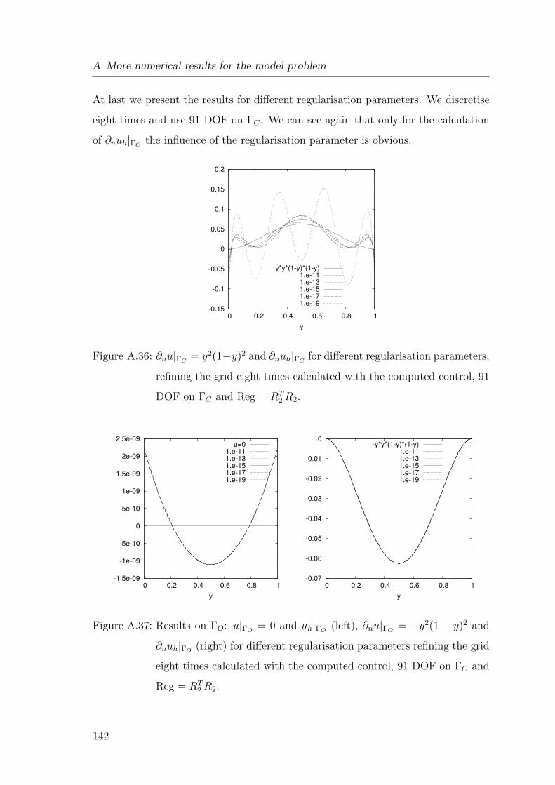
A More numerical results for the model problem
At last we present the results for different regularisation parameters. We discretise
eight times and use 91 DOF on ΓC . We can see again that only for the calculation
of ∂nuh|ΓCthe influence of the regularisation parameter is obvious.
-0.15
-0.1
-0.05
0
0.05
0.1
0.15
0.2
0 0.2 0.4 0.6 0.8 1
y
y*y*(1-y)*(1-y)1.e-111.e-131.e-151.e-171.e-19
Figure A.36: ∂nu|ΓC= y2(1−y)2 and ∂nuh|ΓC
for different regularisation parameters,
refining the grid eight times calculated with the computed control, 91
DOF on ΓC and Reg = RT2 R2.
-1.5e-09
-1e-09
-5e-10
0
5e-10
1e-09
1.5e-09
2e-09
2.5e-09
0 0.2 0.4 0.6 0.8 1
y
u=01.e-111.e-131.e-151.e-171.e-19
-0.07
-0.06
-0.05
-0.04
-0.03
-0.02
-0.01
0
0 0.2 0.4 0.6 0.8 1
y
-y*y*(1-y)*(1-y)1.e-111.e-131.e-151.e-171.e-19
Figure A.37: Results on ΓO: u|ΓO= 0 and uh|ΓO
(left), ∂nu|ΓO= −y2(1 − y)2 and
∂nuh|ΓO(right) for different regularisation parameters refining the grid
eight times calculated with the computed control, 91 DOF on ΓC and
Reg = RT2 R2.
142
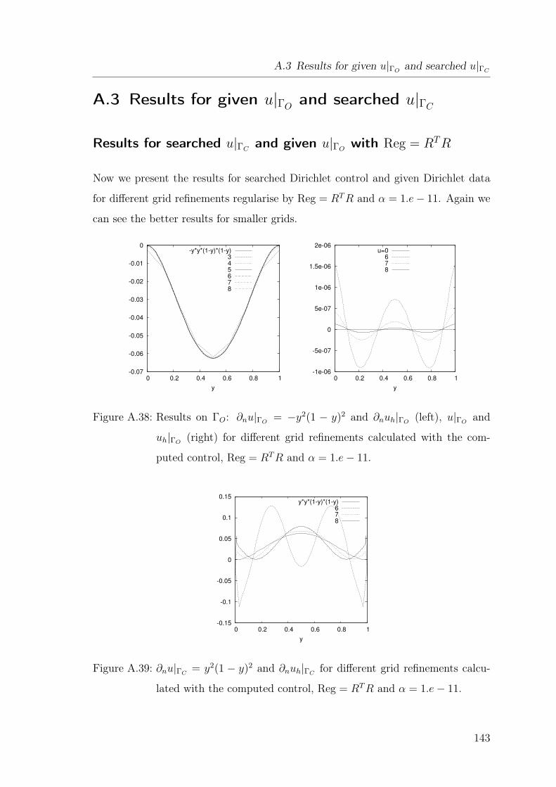
A.3 Results for given u|ΓOand searched u|ΓC
A.3 Results for given u|ΓOand searched u|ΓC
Results for searched u|ΓCand given u|ΓO
with Reg = RTR
Now we present the results for searched Dirichlet control and given Dirichlet data
for different grid refinements regularise by Reg = RT R and α = 1.e − 11. Again we
can see the better results for smaller grids.
-0.07
-0.06
-0.05
-0.04
-0.03
-0.02
-0.01
0
0 0.2 0.4 0.6 0.8 1
y
-y*y*(1-y)*(1-y)345678
-1e-06
-5e-07
0
5e-07
1e-06
1.5e-06
2e-06
0 0.2 0.4 0.6 0.8 1
y
u=0678
Figure A.38: Results on ΓO: ∂nu|ΓO= −y2(1 − y)2 and ∂nuh|ΓO
(left), u|ΓOand
uh|ΓO(right) for different grid refinements calculated with the com-
puted control, Reg = RT R and α = 1.e − 11.
-0.15
-0.1
-0.05
0
0.05
0.1
0.15
0 0.2 0.4 0.6 0.8 1
y
y*y*(1-y)*(1-y)678
Figure A.39: ∂nu|ΓC= y2(1 − y)2 and ∂nuh|ΓC
for different grid refinements calcu-
lated with the computed control, Reg = RT R and α = 1.e − 11.
143
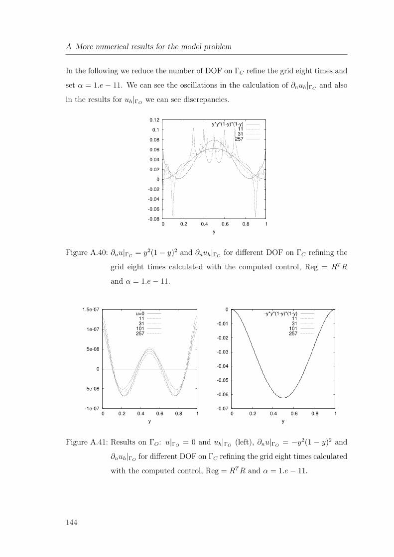
A More numerical results for the model problem
In the following we reduce the number of DOF on ΓC refine the grid eight times and
set α = 1.e − 11. We can see the oscillations in the calculation of ∂nuh|ΓCand also
in the results for uh|ΓOwe can see discrepancies.
-0.08
-0.06
-0.04
-0.02
0
0.02
0.04
0.06
0.08
0.1
0.12
0 0.2 0.4 0.6 0.8 1
y
y*y*(1-y)*(1-y)1131
257
Figure A.40: ∂nu|ΓC= y2(1 − y)2 and ∂nuh|ΓC
for different DOF on ΓC refining the
grid eight times calculated with the computed control, Reg = RT R
and α = 1.e − 11.
-1e-07
-5e-08
0
5e-08
1e-07
1.5e-07
0 0.2 0.4 0.6 0.8 1
y
u=01131
101257
-0.07
-0.06
-0.05
-0.04
-0.03
-0.02
-0.01
0
0 0.2 0.4 0.6 0.8 1
y
-y*y*(1-y)*(1-y)1131
101257
Figure A.41: Results on ΓO: u|ΓO= 0 and uh|ΓO
(left), ∂nu|ΓO= −y2(1 − y)2 and
∂nuh|ΓOfor different DOF on ΓC refining the grid eight times calculated
with the computed control, Reg = RT R and α = 1.e − 11.
144
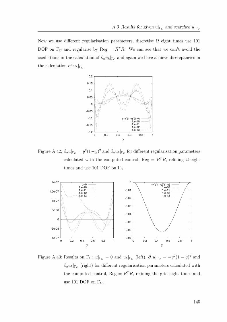
A.3 Results for given u|ΓOand searched u|ΓC
Now we use different regularisation parameters, discretise Ω eight times use 101
DOF on ΓC and regularise by Reg = RT R. We can see that we can’t avoid the
oscillations in the calculation of ∂nuh|ΓCand again we have achieve discrepancies in
the calculation of uh|ΓO.
-0.2
-0.15
-0.1
-0.05
0
0.05
0.1
0.15
0.2
0 0.2 0.4 0.6 0.8 1
y
y*y*(1-y)*(1-y)1.e-101.e-111.e-121.e-13
Figure A.42: ∂nu|ΓC= y2(1−y)2 and ∂nuh|ΓC
for different regularisation parameters
calculated with the computed control, Reg = RT R, refining Ω eight
times and use 101 DOF on ΓC .
-1e-07
-5e-08
0
5e-08
1e-07
1.5e-07
2e-07
0 0.2 0.4 0.6 0.8 1
y
u=01.e-101.e-111.e-121.e-13
-0.07
-0.06
-0.05
-0.04
-0.03
-0.02
-0.01
0
0 0.2 0.4 0.6 0.8 1
y
-y*y*(1-y)*(1-y)1.e-101.e-111.e-121.e-13
Figure A.43: Results on ΓO: u|ΓO= 0 and uh|ΓO
(left), ∂nu|ΓO= −y2(1 − y)2 and
∂nuh|ΓO(right) for different regularisation parameters calculated with
the computed control, Reg = RT R, refining the grid eight times and
use 101 DOF on ΓC .
145
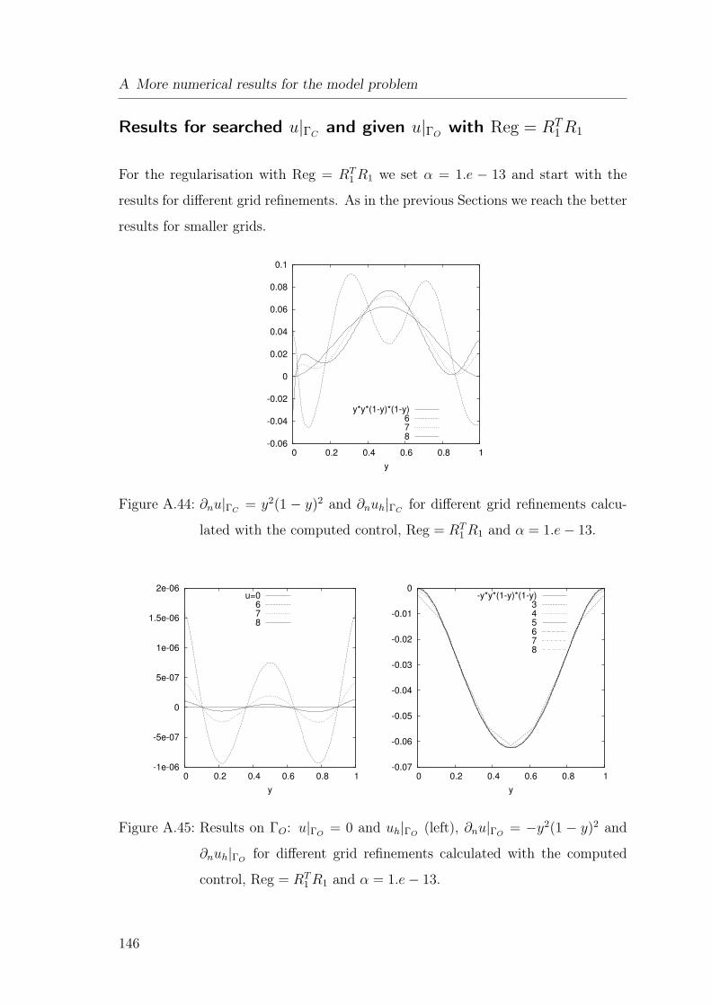
A More numerical results for the model problem
Results for searched u|ΓCand given u|ΓO
with Reg = RT1R1
For the regularisation with Reg = RT1 R1 we set α = 1.e − 13 and start with the
results for different grid refinements. As in the previous Sections we reach the better
results for smaller grids.
-0.06
-0.04
-0.02
0
0.02
0.04
0.06
0.08
0.1
0 0.2 0.4 0.6 0.8 1
y
y*y*(1-y)*(1-y)678
Figure A.44: ∂nu|ΓC= y2(1 − y)2 and ∂nuh|ΓC
for different grid refinements calcu-
lated with the computed control, Reg = RT1 R1 and α = 1.e − 13.
-1e-06
-5e-07
0
5e-07
1e-06
1.5e-06
2e-06
0 0.2 0.4 0.6 0.8 1
y
u=0678
-0.07
-0.06
-0.05
-0.04
-0.03
-0.02
-0.01
0
0 0.2 0.4 0.6 0.8 1
y
-y*y*(1-y)*(1-y)345678
Figure A.45: Results on ΓO: u|ΓO= 0 and uh|ΓO
(left), ∂nu|ΓO= −y2(1 − y)2 and
∂nuh|ΓOfor different grid refinements calculated with the computed
control, Reg = RT1 R1 and α = 1.e − 13.
146
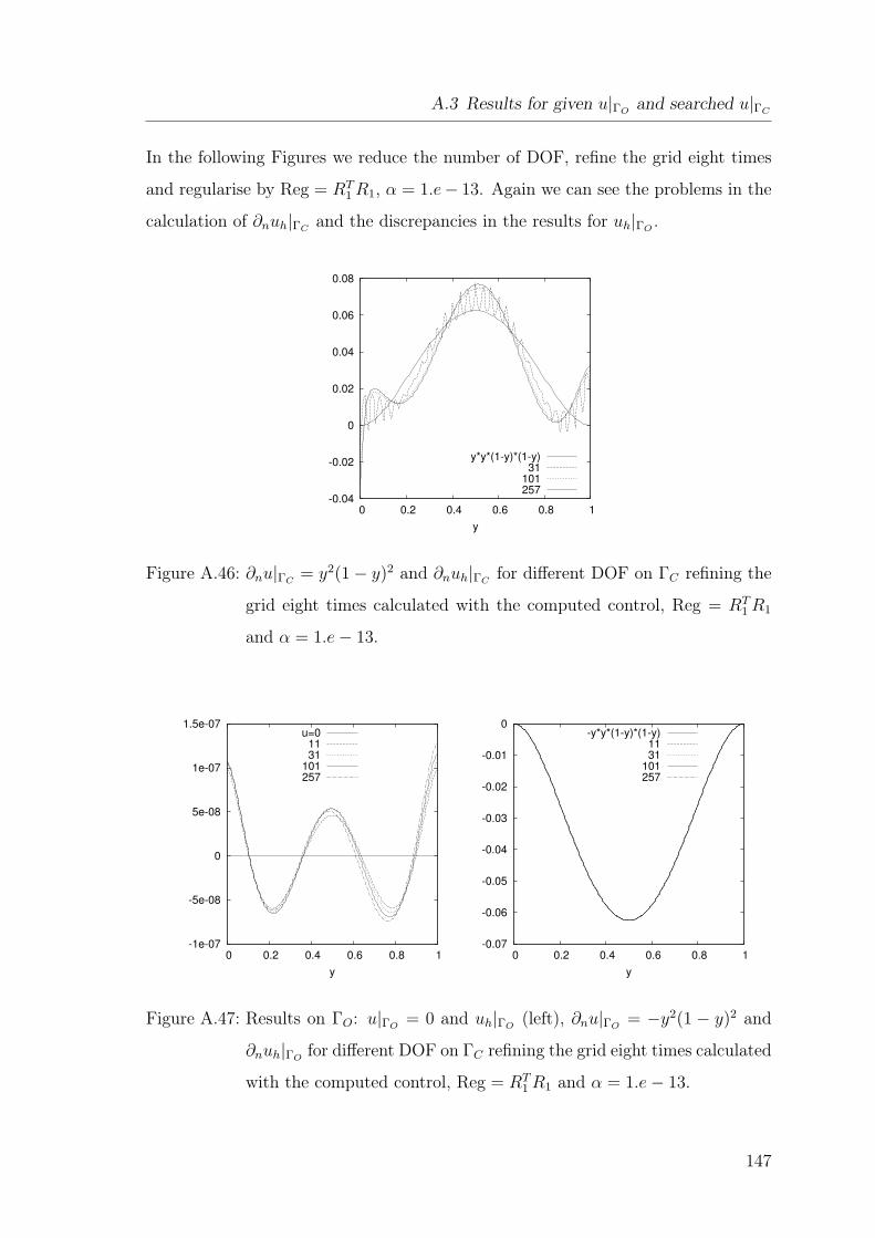
A.3 Results for given u|ΓOand searched u|ΓC
In the following Figures we reduce the number of DOF, refine the grid eight times
and regularise by Reg = RT1 R1, α = 1.e− 13. Again we can see the problems in the
calculation of ∂nuh|ΓCand the discrepancies in the results for uh|ΓO
.
-0.04
-0.02
0
0.02
0.04
0.06
0.08
0 0.2 0.4 0.6 0.8 1
y
y*y*(1-y)*(1-y)31
101257
Figure A.46: ∂nu|ΓC= y2(1 − y)2 and ∂nuh|ΓC
for different DOF on ΓC refining the
grid eight times calculated with the computed control, Reg = RT1 R1
and α = 1.e − 13.
-1e-07
-5e-08
0
5e-08
1e-07
1.5e-07
0 0.2 0.4 0.6 0.8 1
y
u=01131
101257
-0.07
-0.06
-0.05
-0.04
-0.03
-0.02
-0.01
0
0 0.2 0.4 0.6 0.8 1
y
-y*y*(1-y)*(1-y)1131
101257
Figure A.47: Results on ΓO: u|ΓO= 0 and uh|ΓO
(left), ∂nu|ΓO= −y2(1 − y)2 and
∂nuh|ΓOfor different DOF on ΓC refining the grid eight times calculated
with the computed control, Reg = RT1 R1 and α = 1.e − 13.
147
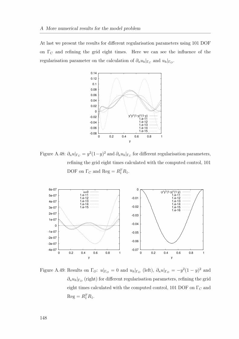
A More numerical results for the model problem
At last we present the results for different regularisation parameters using 101 DOF
on ΓC and refining the grid eight times. Here we can see the influence of the
regularisation parameter on the calculation of ∂nuh|ΓCand uh|ΓO
.
-0.08
-0.06
-0.04
-0.02
0
0.02
0.04
0.06
0.08
0.1
0.12
0.14
0 0.2 0.4 0.6 0.8 1
y
y*y*(1-y)*(1-y)1.e-111.e-121.e-131.e-141.e-15
Figure A.48: ∂nu|ΓC= y2(1−y)2 and ∂nuh|ΓC
for different regularisation parameters,
refining the grid eight times calculated with the computed control, 101
DOF on ΓC and Reg = RT1 R1.
-4e-07
-3e-07
-2e-07
-1e-07
0
1e-07
2e-07
3e-07
4e-07
5e-07
6e-07
0 0.2 0.4 0.6 0.8 1
y
u=01.e-111.e-121.e-131.e-141.e-15
-0.07
-0.06
-0.05
-0.04
-0.03
-0.02
-0.01
0
0 0.2 0.4 0.6 0.8 1
y
-y*y*(1-y)*(1-y)1.e-111.e-121.e-131.e-141.e-151.e-16
Figure A.49: Results on ΓO: u|ΓO= 0 and uh|ΓO
(left), ∂nu|ΓO= −y2(1 − y)2 and
∂nuh|ΓO(right) for different regularisation parameters, refining the grid
eight times calculated with the computed control, 101 DOF on ΓC and
Reg = RT1 R1.
148
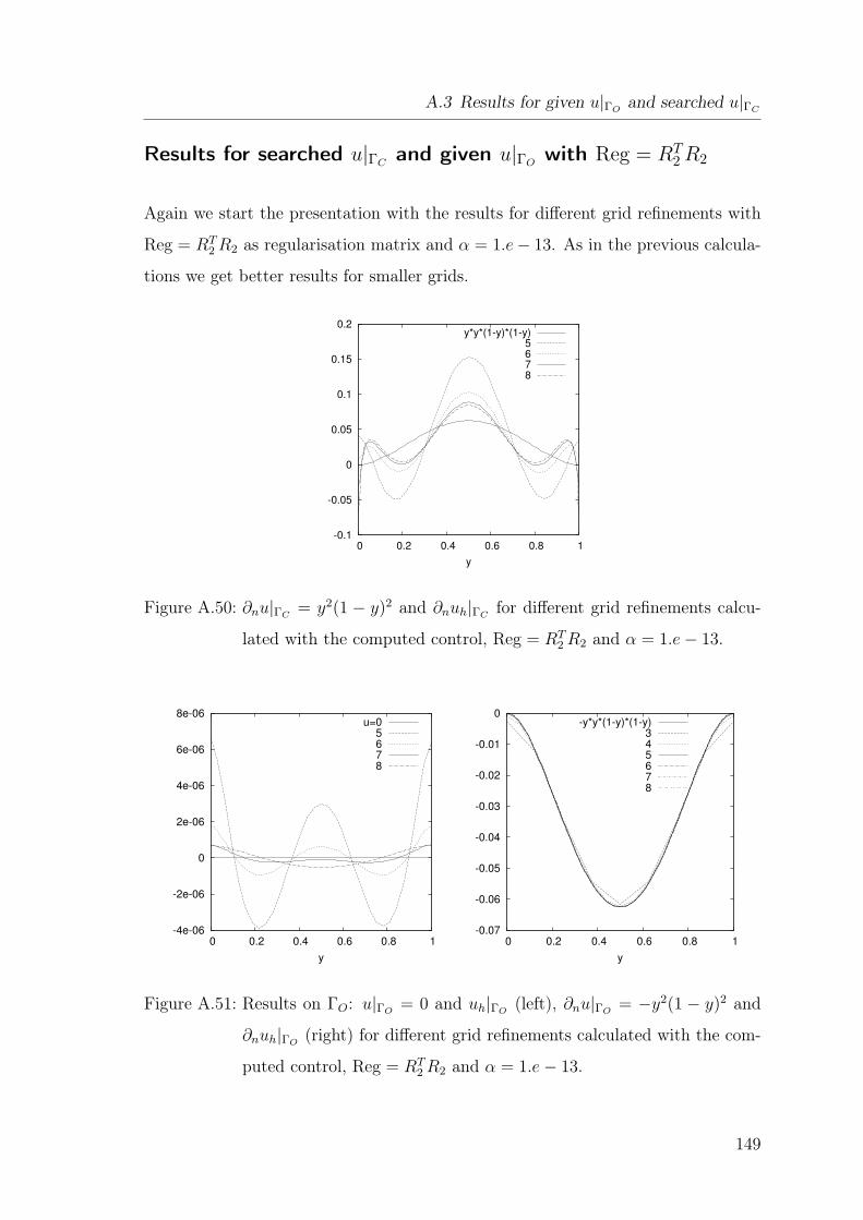
A.3 Results for given u|ΓOand searched u|ΓC
Results for searched u|ΓCand given u|ΓO
with Reg = RT2R2
Again we start the presentation with the results for different grid refinements with
Reg = RT2 R2 as regularisation matrix and α = 1.e− 13. As in the previous calcula-
tions we get better results for smaller grids.
-0.1
-0.05
0
0.05
0.1
0.15
0.2
0 0.2 0.4 0.6 0.8 1
y
y*y*(1-y)*(1-y)5678
Figure A.50: ∂nu|ΓC= y2(1 − y)2 and ∂nuh|ΓC
for different grid refinements calcu-
lated with the computed control, Reg = RT2 R2 and α = 1.e − 13.
-4e-06
-2e-06
0
2e-06
4e-06
6e-06
8e-06
0 0.2 0.4 0.6 0.8 1
y
u=05678
-0.07
-0.06
-0.05
-0.04
-0.03
-0.02
-0.01
0
0 0.2 0.4 0.6 0.8 1
y
-y*y*(1-y)*(1-y)345678
Figure A.51: Results on ΓO: u|ΓO= 0 and uh|ΓO
(left), ∂nu|ΓO= −y2(1 − y)2 and
∂nuh|ΓO(right) for different grid refinements calculated with the com-
puted control, Reg = RT2 R2 and α = 1.e − 13.
149
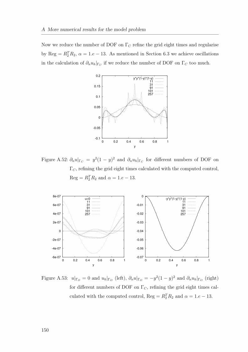
A More numerical results for the model problem
Now we reduce the number of DOF on ΓC refine the grid eight times and regularise
by Reg = RT2 R2, α = 1.e − 13. As mentioned in Section 6.3 we achieve oscillations
in the calculation of ∂nuh|ΓCif we reduce the number of DOF on ΓC too much.
-0.1
-0.05
0
0.05
0.1
0.15
0.2
0 0.2 0.4 0.6 0.8 1
y
y*y*(1-y)*(1-y)113191
101257
Figure A.52: ∂nu|ΓC= y2(1 − y)2 and ∂nuh|ΓC
for different numbers of DOF on
ΓC , refining the grid eight times calculated with the computed control,
Reg = RT2 R2 and α = 1.e − 13.
-6e-07
-4e-07
-2e-07
0
2e-07
4e-07
6e-07
8e-07
0 0.2 0.4 0.6 0.8 1
y
u=0113191
101257
-0.07
-0.06
-0.05
-0.04
-0.03
-0.02
-0.01
0
0 0.2 0.4 0.6 0.8 1
y
-y*y*(1-y)*(1-y)113191
101257
Figure A.53: u|ΓO= 0 and uh|ΓO
(left), ∂nu|ΓO= −y2(1 − y)2 and ∂nuh|ΓO
(right)
for different numbers of DOF on ΓC , refining the grid eight times cal-
culated with the computed control, Reg = RT2 R2 and α = 1.e − 13.
150
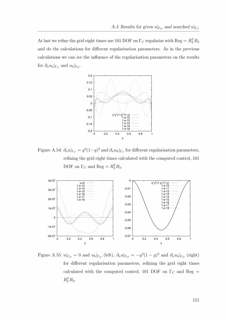
A.3 Results for given u|ΓOand searched u|ΓC
At last we refine the grid eight times use 101 DOF on ΓC regularise with Reg = RT2 R2
and do the calculations for different regularisation parameters. As in the previous
calculations we can see the influence of the regularisation parameters on the results
for ∂nuh|ΓCand uh|ΓO
.
-0.2
-0.15
-0.1
-0.05
0
0.05
0.1
0.15
0.2
0 0.2 0.4 0.6 0.8 1
y
y*y*(1-y)*(1-y)1.e-101.e-121.e-141.e-161.e-18
Figure A.54: ∂nu|ΓC= y2(1−y)2 and ∂nuh|ΓC
for different regularisation parameters,
refining the grid eight times calculated with the computed control, 101
DOF on ΓC and Reg = RT2 R2.
-2e-07
-1e-07
0
1e-07
2e-07
3e-07
4e-07
0 0.2 0.4 0.6 0.8 1
y
u=01.e-131.e-141-e-151.e-161.e-171.e-18
-0.07
-0.06
-0.05
-0.04
-0.03
-0.02
-0.01
0
0 0.2 0.4 0.6 0.8 1
y
-y*y*(1-y)*(1-y)1.e-101.e-111.e-121.e-131.e-141-e-151.e-161.e-171.e-18
Figure A.55: u|ΓO= 0 and uh|ΓO
(left), ∂nu|ΓO= −y2(1 − y)2 and ∂nuh|ΓO
(right)
for different regularisation parameters, refining the grid eight times
calculated with the computed control, 101 DOF on ΓC and Reg =
RT2 R2.
151

A More numerical results for the model problem
152
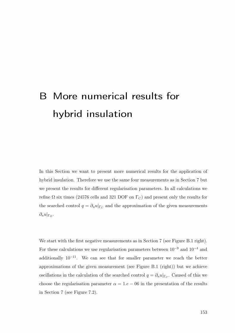
B More numerical results for
hybrid insulation
In this Section we want to present more numerical results for the application of
hybrid insulation. Therefore we use the same four measurements as in Section 7 but
we present the results for different regularisation parameters. In all calculations we
refine Ω six times (24576 cells and 321 DOF on ΓC) and present only the results for
the searched control q = ∂nu|ΓCand the approximation of the given measurements
∂nu|ΓO.
We start with the first negative measurements as in Section 7 (see Figure B.1 right).
For these calculations we use regularisation parameters between 10−9 and 10−4 and
additionally 10−11. We can see that for smaller parameter we reach the better
approximations of the given measurement (see Figure B.1 (right)) but we achieve
oscillations in the calculation of the searched control q = ∂nu|ΓC. Caused of this we
choose the regularisation parameter α = 1.e − 06 in the presentation of the results
in Section 7 (see Figure 7.2).
153
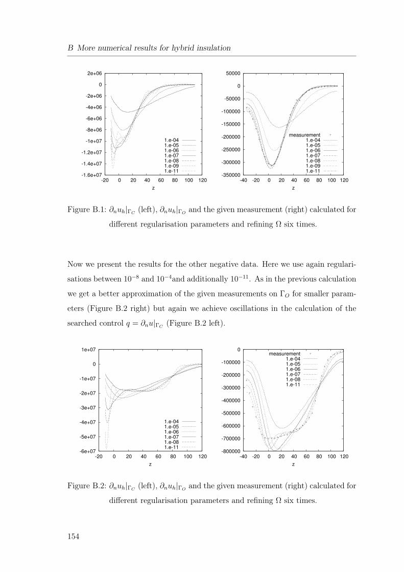
B More numerical results for hybrid insulation
-1.6e+07
-1.4e+07
-1.2e+07
-1e+07
-8e+06
-6e+06
-4e+06
-2e+06
0
2e+06
-20 0 20 40 60 80 100 120
z
1.e-041.e-051.e-061.e-071.e-081.e-091.e-11
-350000
-300000
-250000
-200000
-150000
-100000
-50000
0
50000
-40 -20 0 20 40 60 80 100 120
z
measurement1.e-041.e-051.e-061.e-071.e-081.e-091.e-11
Figure B.1: ∂nuh|ΓC(left), ∂nuh|ΓO
and the given measurement (right) calculated for
different regularisation parameters and refining Ω six times.
Now we present the results for the other negative data. Here we use again regulari-
sations between 10−8 and 10−4and additionally 10−11. As in the previous calculation
we get a better approximation of the given measurements on ΓO for smaller param-
eters (Figure B.2 right) but again we achieve oscillations in the calculation of the
searched control q = ∂nu|ΓC(Figure B.2 left).
-6e+07
-5e+07
-4e+07
-3e+07
-2e+07
-1e+07
0
1e+07
-20 0 20 40 60 80 100 120
z
1.e-041.e-051.e-061.e-071.e-081.e-11
-800000
-700000
-600000
-500000
-400000
-300000
-200000
-100000
0
-40 -20 0 20 40 60 80 100 120
z
measurement1.e-041.e-051.e-061.e-071.e-081.e-11
Figure B.2: ∂nuh|ΓC(left), ∂nuh|ΓO
and the given measurement (right) calculated for
different regularisation parameters and refining Ω six times.
154
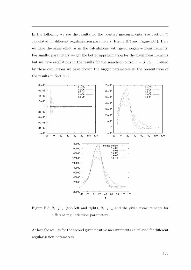
In the following we see the results for the positive measurements (see Section 7)
calculated for different regularisation parameters (Figure B.3 and Figure B.4). Here
we have the same effect as in the calculations with given negative measurements.
For smaller parameters we get the better approximation for the given measurements
but we have oscillations in the results for the searched control q = ∂nu|ΓC. Caused
by these oscillations we have chosen the bigger parameters in the presentation of
the results in Section 7.
-1e+09
-8e+08
-6e+08
-4e+08
-2e+08
0
2e+08
4e+08
6e+08
8e+08
-20 0 20 40 60 80 100 120
z
1.e-051.e-061.e-071.e-081.e-20
-1e+06
0
1e+06
2e+06
3e+06
4e+06
5e+06
6e+06
7e+06
-20 0 20 40 60 80 100 120
z
1.e-051.e-061.e-071.e-081.e-11
-20000
0
20000
40000
60000
80000
100000
120000
140000
160000
180000
-40 -20 0 20 40 60 80 100 120
z
measurement1.e-051.e-061.e-071.e-081.e-11
Figure B.3: ∂nuh|ΓC(top left and right), ∂nuh|ΓO
and the given measurements for
different regularisation parameters.
At last the results for the second given positive measurements calculated for different
regularisation parameters.
155
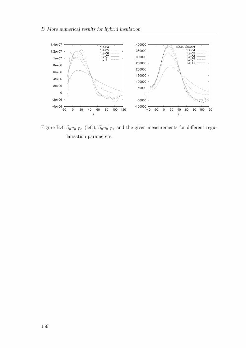
B More numerical results for hybrid insulation
-4e+06
-2e+06
0
2e+06
4e+06
6e+06
8e+06
1e+07
1.2e+07
1.4e+07
-20 0 20 40 60 80 100 120
z
1.e-041.e-051.e-061.e-071.e-11
-100000
-50000
0
50000
100000
150000
200000
250000
300000
350000
400000
-40 -20 0 20 40 60 80 100 120
z
measurement1.e-041.e-051.e-061.e-071.e-11
Figure B.4: ∂nuh|ΓC(left), ∂nuh|ΓO
and the given measurements for different regu-
larisation parameters.
156
Bibliography
[1] DEAL, Differential Equations Analysis Library. http://www.gaia.math.uni-
siegen.de/suttmeier/deal/deal.html, 1992.
[2] Lineare Funktionalanalysis. Springer, 2006.
[3] Robert A. Adams. Sobolev Spaces. Academic Press, 1975.
[4] Douglas N. Arnold, Franco Brezzi, Bernardo Cookburn, and L. Donatelle Maini.
Unified analysis of discontinouos galerkin methods for elliptic problems. SIAM
J. Numer. Anal, 39(5):1749–1779, 2002.
[5] J. Baumeister. Stable Solution of inverse problems. Vieweg, 1987.
[6] R. Becker, P. Hansbo, and R. Stenberg. A finite element method for domain
decomposition with non-matching grids. M2AN, 2003.
[7] Yu. Ya. Belov. Inverse Problems for partial differential equations. VSP, 2002.
[8] Dietrich Braess. Finite Elemente. Springer, 1997.
[9] James H. Bramble. Multigrid methods. Longman scientific and technical, Pit-
man Research Notes in Mathematics series 294, 1993.
[10] S. C. Brenner and L.R. Scott. The mathematical theory of finite element meth-
ods. Springer, 2002.
[11] Ivan Cherlenyak. Numerische Lösungen inverser Probleme bei elliptischen Dif-
ferentialgleichungen. PhD thesis, Universität Siegen, 2009.
[12] D. Colton, R. Ewing, and W. Rundell, editors. Inverse problems in partial
differential equations. Siam, 1989.
157
Bibliography
[13] Gilbarg D. and Trudinger N. Elliptic partial differential equations of second
order. Springer, 1977.
[14] M. Dobrowolski. Angewandte Funktionalanalysis. Springer, 2006.
[15] Gene H. Golub and Charles F. van Loan. Matrix Computations. John Hopkins
University Press, 1996.
[16] C. W. Groetsch. Generalized inverses of linear operators. Dekker, 1977.
[17] W. Hackbusch. Theorie und Numerik elliptischer Differentialgleichungen. Teub-
ner, 1986.
[18] W. Hackbusch. Iterative Lösung großer schwachbesetzter Gleichungssysteme.
Teubner, 1993.
[19] P. Hansbo. Nitsche´s method for interface problems in computational mechan-
ics. pages 183–206, 2005.
[20] P. Hansbo and M. G. Larson. Discontinuous Galerkin methods for incom-
pressible and nearly incompressible elasticity by Nitsche’s method. Computer
methods in applied mechanics and engineering, pages 1895–1908, 2002.
[21] Victor Isakov. Inverse source problems. American Mathematical Society, 1990.
[22] Claes Johnson. Numerical solution of partial differential equations by the finite
element method. Cambridge Univ. Press, 1992.
[23] D. Kinderlehrer and G. Stampacchia. An Introduction to variational inequalities
and their application. Academic Press, 1980.
[24] J.L. Lions. Optimal Control of Systems Governed by Partial Differential Equa-
tions. Springer-Verlag, 1971.
[25] A.K. Louis. Inverse und schlecht gestellte Probleme. Teubner, 1989.
[26] Frank Mauseth. Charge accumulation in rod-plane air gap with covered rod. PhD
thesis, Norwegian University of Science and Technology, Faculty of Information
Technology, Mathematics and Electrical Engineering, 2007.
[27] S. F. McCormick. Multigrid Methods. Siam, 1987.
158
Bibliography
[28] Th. Meis and U. Marcowitz. Numerische Behandlung partieller Differentialgle-
ichungen. Springer, 1978.
[29] J. Nitsche. Über ein Variationsprinzip zur Lösung von Dirichlet-Problemen bei
Verwendung von Teilräumen, die keinen Randbedingungen unterworfen sind.
Abh. Math. Sem., Univ. Hamburg, 36:9–15, 1970/71.
[30] A. Rieder. Keine Problem mit Inversen Problemen. Vieweg, 2003.
[31] Saad. Iterative methods for sparse linear systems. PWS, 1996.
[32] O. Steinbach. Numerische Näherungsverfahren für elliptische Randwertprob-
leme. Teubner, 2003.
[33] Stoer. Numerische Mathematik 1. Springer, 2004.
[34] J. Stoer and R. Bulirsch. Introduction to Numerical Analysis. Springer, 2002.
[35] F. Stummel and K. Hainer. Praktische Mathematik. Teubner Studienbücher,
1971.
[36] F.-T. Suttmeier. On concepts of pde-software: The cellwise oriented approach
in deal. International Mathematical Forum, 2(1):1–20, 2007.
[37] A. Tarantola. Inverse Problem Theory. Elsevier, 1987.
[38] Vidar Thomee. Galerkin Finite Element Methods for Parabolic Problems.
Springer-Verlag, 1984.
[39] F. Tröltzsch. Optimale Steuerung partieller Differentialgleichungen. Vieweg,
2005.
[40] D. Werner. Funktionalanalysis. Springer, 2005.
[41] P. Wesseling. An introduction to multigrid methods. Wiley, 1992.
[42] J. Wloka. Partielle Differentialgleichungen. Teubner, 1982.
[43] K. Yosida. Functional analysis. Springer, 1980.
159