Embed Size (px)
Citation preview

T U B E R G A K A D E M I E F R E I B E R G
Numerical Investigation of Air-Side Heat Transfer and Pressure Drop in Circular Finned-Tube Heat Exchangers
Von der Fakultät für Maschinenbau, Verfahrens- und Energietechnik
der Technischen Universität Bergakademie Freiberg, Germany
genehmigte
Dissertation
vorgelegt von
Mi Sandar Mon

Numerical Investigation of
Air-Side Heat Transfer and Pressure Drop in Circular Finned-Tube Heat Exchangers
Von der Fakultät für Maschinenbau, Verfahrens- und Energietechnik
der Technischen Universität Bergakademie Freiberg, Germany
genehmigte
DISSERTATION
zur Erlangung des akademischen Grades
Doktor-Ingenieur
Dr.-Ing.
vorgelegt
von Mi Sandar Mon (M.E)
geboren am 20.06.1967 in Yangon, Myanmar
Gutachter: Prof. Dr.-Ing. habil. Ulrich Groß, Freiberg
Prof. Dr. rer.nat. habil. Frank Obermeier, Freiberg
Prof. Dr.- Ing. habil. Günter Wozniak, Chemnitz
Tag der Verleihung: 10.02.2003


Acknowledgement
I would like to acknowledge the following people for their guidance and support
during my doctoral study and writing of this dissertation at the Institute of “Wärmetechnik und Thermodynamik”, Technische Universität Bergakademie Freiberg, Germany.
First and foremost, I would like to express my gratitude to Prof. Dr.-Ing. habil. U.
Groß, who accepted to supervise this dissertation. His teaching, patience, and encouragement throughout my doctoral study were invaluable.
I am very grateful to Prof. Dr. rer. nat. habil. F. Obermeier, who accepted to be a
member of my dissertation committee. His constructive comments and suggestions were inestimable to the completion of this dissertation.
I would like also to thank Prof. Dr.-Ing. habil. G. Wozniak, who also accepted to
be a member of my dissertation committee and is highly appreciated.
Many thanks should be ascribed to Dr-Ing. I. Riehl and Dr-Ing. S. Kaminski with whom I had many useful discussions.
I also appreciate the help of Mr. T. Polet, who assists for the problems concerned
with the computers and thanks also go to Mr. M. Brislin who gratefully giving me many important comments on English writing.
Furthermore, I would like to thank all colleagues of the institute for contributing to
such an inspiring and pleasant atmosphere.
I would like also to acknowledge the German Government and DAAD for their benevolence in providing a full scholarship grant for my doctoral study.
Last, but not least, I would like to thank my husband Aung Myat Thu for his
understanding and support, as well as my parents, families and friends' encouragement. Freiberg, May 2003. Mi Sandar Mon
Abstract Numerical Investigation of Air-Side Heat Transfer and Pressure Drop in Circular Finned-Tube Heat Exchangers
The present numerical study has been carried out to investigate the
temperature and velocity profiles in banks with circular finned-tubes in cross flow. The
purpose of this investigation is to develop satisfactory correlations and concurrently
providing complements to the local convective characteristics. The coolant passes
through the tubes, which are maintained at a constant temperature and the dry air is
used as the convective heat transfer medium. To demonstrate the influence of the
geometric parameters, numerical investigations are carried out for different finning
geometries and number of rows. In addition, attempts are made to validate which tube
configuration is more constructive. A large computational effort is involved for the memory access of the computers
and computing time for the simulation of the complex geometries associated with the
dense grids. The available computational fluid dynamics software package FLUENT is
applied to determine the related problems. Renormalization group theory (RNG) based
k - ε turbulence model is allowed to predict the unsteady three-dimensional flow and
the conjugate heat transfer characteristics.
The numerical flow visualization results reveal the important aspects of the local
heat transfer and flow features of the circular finned-tube bundles. These include
boundary layer developments between the fins, the formation of the horseshoe vortex
system, the local variations of the velocity and temperature on the fin geometries and
within the bundles. The boundary layers developments and horseshoe vortices
between the adjacent fins and tube surface are found to be dependent substantially on
the fin spacing and Reynolds number. The local temperature distributions over the fin
surface vary both circumferentially and radially, and there is no significant difference
over the fin surface and in the middle of the fin for both tube arrays.
To determine the optimum dimension of the geometries, comparisons are
prepared in terms of the bundle performance parameter. These data indicate that for
the benefit of pumping power, the in-line array has a better performance than the
staggered arrangement at low Reynolds number. However, the margin between the in-
line and staggered arrays becomes narrower when the Reynolds number is increased.

The average heat transfer and pressure drop results for both tube
configurations are presented. All proposed correlations, based on the numerical and
relevant experimental data, are recommended for a wide range of Reynolds numbers
(based on the air velocity through the minimum free flow area and the tube outside
diameter) from 5 x 10³ to 7 x 10⁴. The heat transfer and pressure drop results agree
well with several existing experimental correlations. The present numerical
investigations suggest a good estimate of the Nusselt number and Euler number for
circular finned-tube heat exchangers.
Kurzfassung Numerische Untersuchungen des luftseitigen Wärmeübergangs und Druckabfalls in Rippenrohrbündeln
Die vorliegenden numerischen Untersuchungen wurden durchgeführt, um die
luftseitigen Temperatur- und Geschwindigkeitsprofile in Bündeln von Kreisrippenrohren
zu untersuchen. Zweck dieser Untersuchungen ist die Entwicklung von Korrelationen
sowie zusätzlich eine Beschreibung des örtlichen Verhaltens der Konvektion. Das
Kühlmittel fließt durch die Rohre, deren Temperatur damit konstant gehalten wird. Um
den Einfluß auf die geometrischen Parameter zu demonstrieren, wurden numerische
Betrachtungen für unterschiedliche Rippengeometrien und eine unterschiedliche
Anzahl von Reihen vorgenommen. Außerdem wurde überprüft, welche
Rohrkonfiguration bessere konstruktive Eigenschaften aufweist.
Ein großer rechentechnischer Aufwand ist in Bezug auf Arbeitsspeicher und
Rechenzeit erforderlich, da die Simulation der komplexen Geometrien durch ein
dichtes Netz geprägt ist. In einigen Fällen (nahe der Wand) mußte ein dichteres Netz
gebildet werden, um die Berechnungen dennoch durchführen zu können. Das
verfügbare (Computational Fluid Dynamics) CFD-Softwarepaket FLUENT wird zur
Lösung dieser Fragestellungen verwendet. Ein k -ε -Turbulenzmodell auf Basis der
Renormalization Group Theory (RNG) wird für die Berechnung der instationären
dreidimensionalen Strömung und ihrer entsprechenden
Wärmeübertragungscharakteristika genutzt.

Die Visualisierung der numerischen Untersuchungen der Strömung verdeutlichen die
bedeutenden Aspekte der lokalen Wärmeübertragung und der
Strömungseigenschaften. Dies umfaßt die Grenzschichtbildung zwischen den Rohren,
die Entstehung von Hufeisenwirbelsystemen, die lokalen Abweichungen der
Geschwindigkeit und der Temperatur abhängig von der Rohrgeometrie und der
geometrischen Struktur der Bündel. Die Grenzschichtbildung und Hufeisenwirbel
zwischen den angrenzenden Rippen und der Oberfläche der Rohre haben sich als sehr
stark abhängig vom Rippenabstand und der Reynoldszahl erwiesen. Die örtliche
Temperaturverteilung über die Rippenoberfläche variiert sowohl an der Peripherie als
auch radial, und es gibt keinen signifikanten Unterschied zwischen der
Rippenoberfläche und der Mitte der Rippe für fluchtenden und versetzten Anordnung
des Rohrbündels.
Zur Bestimmung optimaler geometrischer Parameter, werden Vergleiche in Bezug auf
die Leistungsparameter der Bündel durchgeführt. Diese Daten zeigen, daß bei
niedrigen Reynoldszahlen, die fluchtende Anordnung leistungsfähiger ist als die
versetzte ist insbesondere wenn man die Pumpleistung betrachtet. Jedoch wird die
Abweichung zwischen der fluchtenden und der versetzten Anordnung geringer, wenn
die Reynoldszahl ansteigt.
Die Daten für die mittlere Wärmeübertragung und den Druckverlust werden für beide
Rohrkonfigurationen präsentiert. Alle vorgeschlagenen Korrelationen, welche auf
numerischen und relevanten experimentellen Daten basieren, werden für einen großen
Bereich der Reynoldszahlen (auf Basis der Strömungsgeschwindigkeit der Luft durch
den minimalen freien Strömungsquerschnitt und den Außendurchmesser des Rohres)
von 5 x 10³ bis 7 x 10⁴ empfohlen. Die Ergebnisse für die Wärmeübertragung und den
Druckabfall sind mit verschiedenen existierenden experimentellen Korrelationen sehr
gut vergleichbar. Die vorliegenden numerischen Simulationen erlauben eine gute
Abschätzung der Nusselt- und der Eulerzahl für Wärmeübertrager mit
Kreisrippenrohren.
Table of Contents Nomenclature .................................................................................................................... x 1 Introduction ................................................................................................................. 1 2 Literature Review ........................................................................................................ 3 2.1 Heat Transfer and Flow Characteristics in a Circular Finned-Tube Heat Exchanger ............................................................................... 3 2.2 Local Heat Transfer Behaviour of Circular Finned-Tubes .................................... 5 2.3 Analysis of Geometric and Flow Parameters ........................................................ 9 2.3.1 Effect of Fin Height ...................................................................................... 9 2.3.2 Effect of Fin Spacing.................................................................................. 10 2.3.3 Effect of Fin Thickness .............................................................................. 12 2.3.4 Effect of Tube Outside Diameter ............................................................... 12 2.3.5 Effect of Tube Spacing .............................................................................. 13 2.3.6 Effect of Row.............................................................................................. 15 2.3.7 Effect of Tube Arrangement ...................................................................... 16 2.3.8 Effect of Air Velocity .................................................................................. 17 2.4 Average Heat Transfer Correlations.................................................................... 18 2.5 Pressure Drop Correlations ................................................................................. 20 2.6 Concluding Remarks ........................................................................................... 21 3 Objectives ..................................................................................................................23 4 Numerical Consideration .........................................................................................25 4.1 Governing Equations and CFD models............................................................... 25 4.1.1 The RNG k-ε model ................................................................................... 29
VIII Table of Contents
4.2 Numerical Simulation .......................................................................................... 30 4.2.1 Introduction ............................................................................................... 30 4.2.2 Computational Domains............................................................................ 31 4.2.3 Grid Generation......................................................................................... 34 4.2.4 Choosing the Physical Properties ............................................................. 36 4.2.5 Boundary Conditions................................................................................. 36 4.2.6 Control Parameters ................................................................................... 38 4.2.7 Computing Time........................................................................................ 38 4.2.8 Algorithm ................................................................................................... 39 5 Results and Discussion ........................................................................................... 41 5.1 Evaluation of Nusselt and Euler Numbers .......................................................... 41 5.2 Local Heat Transfer and Flow Results................................................................ 44 5.2.1 Local Flow Behaviour................................................................................ 44 5.2.2 Local Temperature Distribution................................................................. 51
5.2.3 Velocity and Temperature distribution near the fin surface plane and on the mid-plane between the fins..................................................... 59
5.3 Results of Geometric Parameters Effects........................................................... 66 5.3.1 Results of Fin Height Effect....................................................................... 66 5.3.2 Results of Fin Spacing Effect ................................................................... 71 5.3.2 Results of Fin Thickness Effect................................................................. 75 5.3.4 Results of Tube Outside Diameter Effect ................................................. 78 5.3.5 Results of Tube Spacing Effect................................................................. 81 5.3.6 Results of Row Effect ................................................................................ 86 5.3.7 Results of Tube Arrangement Effect......................................................... 94 6 Correlations and Data Comparison ........................................................................ 97 6.1 Heat Transfer Correlations.................................................................................. 97 6.1.1 Staggered Tube Arrangement .................................................................. 98
Table of Contents IX
6.1.2 In-line Tube Arrangement ....................................................................... 101 6.2 Pressure Drop Correlations ............................................................................... 102 6.3 Data Comparison .............................................................................................. 105
6.3.1 Comparison of Heat Transfer Results for Staggered Arrangement ...... 105 6.3.2 Comparison of Heat Transfer Results for the In-line Arrangement ........ 109 6.3.3 Comparison of Pressured Drop Results.................................................. 111 7 Conclusions .............................................................................................................114 References 118 List of Figures 126 List of Tables 130 Appendix ................................................................................................................131 A Physical Properties of Air and Aluminium ..........................................................132 B Further Figures .......................................................................................................133 C Dimensions of Finned-Tube Heat Exchangers ..................................................141 D The Heat Transfer and Pressure Drop Correlations ..........................................143 E Numerical Results 150

Nomenclature
A m2 total heat transfer area
A´ m2/m heat transfer area of unit length finned tube
Af m2 surface area of fin
Aff m2/m minimum free flow area of finned tube per unit length
At m2 outside surface area of tube except fins
cp J/(kg K) specific heat
C1ε, C2ε, Cµ - turbulence model constants
d m tube outside diameter
deq m equivalent diameter
dh m hydraulic diameter
df m fin diameter
E J total energy
Eu - Euler number, 2maxU/pEu ρ∆=
Eum - Euler number, 2mm U/pEu ρ∆=
f - friction factor
F - parameter defined by Equation (6.3)
G kg/sm2 mass velocity based on minimum free flow area
H& W flow rate of enthalpy
h W/(m2K) heat transfer coefficient
h~ J/kg specific enthalpy
hf m fin height
k W/(mK) thermal conductivity
k~ m2/s2 turbulent kinetic energy
K - performance parameter
Lc m characteristic length
LMTD K logarithmic mean temperature difference
m m-1 a fin effectiveness parameter
Nomenclature XI
m& kg/s mass flow rate
Nf fins/m number of fins per unit length
n - number of tube rows in direction of flow
n - exponent
Nu - Nusselt number, Nu = hd/ka
P W power input
p Pa pressure
Pr - Prandtl number, Pr = Cpµ/ka
Q& W heat flow rate
Re - Reynolds number, Re = Umax d /ν
Red, eq - Reynolds number, Red, eq = Umax deq /ν
Redh - Reynolds number, Redh = Umax dh /ν
Reα - Reynolds number, Reα = Uin sf /ν
s m fin spacing
S s-1 the modulus of the mean rate-of-strain tensor
Sij s-1 the mean strain rate
Sd m diagonal tube pitch
Sf m fin pitch
Sl m longitudinal tube pitch
St m transverse tube pitch
St - Stanton number
T K temperature
Tout K outlet temperature
Tref K reference temperature
∆t sec time step
U m/s velocity component in x – direction
Um m/s mean velocity in the finned tube bundle
Umax m/s velocity of air at minimum cross section
V& m3/s volume flow rate
V1, V2, V3 - vortices
x, y ,z m Cartesian coordinates

XII Nomenclature
Greek Letters: αp - inverse Prandtl number
δ m fin thickness
δb m boundary layer thickness
ε m2/s3 turbulent energy dissipation rate
η - fin efficiency
µ kg/(ms) viscosity
ν m2/s kinematic viscosity
θ - angle around the tube, measured from the front
stagnation point
ρ kg/m3 density
τp m distance to the wall from the adjacent node
ψ - factor defined by Equation (5.10)
Subscripts: a air
corr correlation
eff effective
exp experiments
f fin
in inlet
m mean
max maximum
nume numerical
out outlet
ref reference
s solid
t tube, turbulent
w wall
1 INTRODUCTION
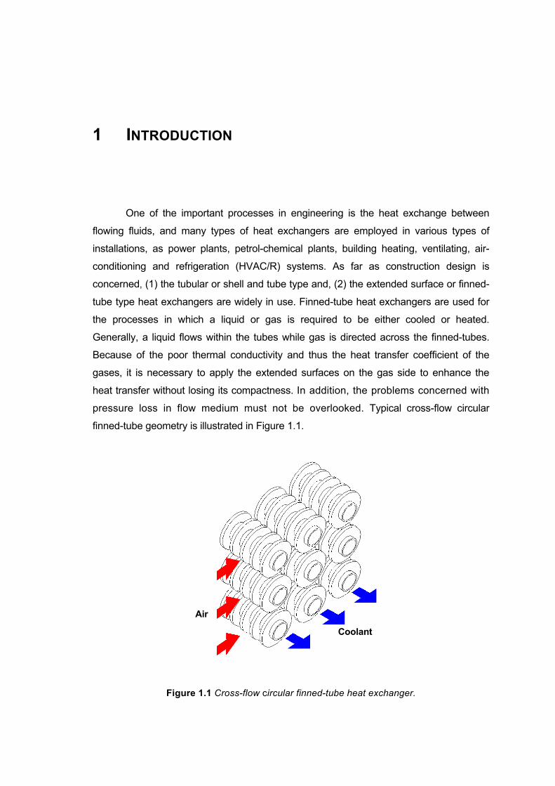
One of the important processes in engineering is the heat exchange between
flowing fluids, and many types of heat exchangers are employed in various types of
installations, as power plants, petrol-chemical plants, building heating, ventilating, air-
conditioning and refrigeration (HVAC/R) systems. As far as construction design is
concerned, (1) the tubular or shell and tube type and, (2) the extended surface or finned-
tube type heat exchangers are widely in use. Finned-tube heat exchangers are used for
the processes in which a liquid or gas is required to be either cooled or heated.
Generally, a liquid flows within the tubes while gas is directed across the finned-tubes.
Because of the poor thermal conductivity and thus the heat transfer coefficient of the
gases, it is necessary to apply the extended surfaces on the gas side to enhance the
heat transfer without losing its compactness. In addition, the problems concerned with
pressure loss in flow medium must not be overlooked. Typical cross-flow circular
finned-tube geometry is illustrated in Figure 1.1.
Figure 1.1 Cross-flow circular finned-tube heat exchanger.
Coolant
Air
2 1 Introduction
There are technical constraints when using the fins in actual applications and the
proper selection of the effective fin geometric parameters, such as the height of fin and
the space between the neighbouring fins, will greatly enhance the performance of a heat
exchanger. Moreover, the flow patterns for the in-line and staggered tube arrays are
complicated and will have to be dealt in the air-cooled heat exchanger design. Thus,
further investigations on the air-side heat transfer enhancement are of broad interest to
design more compact and efficient heat exchangers.
The circular finned-tube bundles are commonly used in the industries. In order to
improve the air-side heat transfer performance of these bundles, such as to increase the
fin efficiency and compactness as well as to reduce the pressure losses, much empirical
work has been done diligently [72]. Investigations are carried out mainly for the
staggered arrangement under the cross flow conditions and numerous correlations have
developed. However, experimental investigations that include a complete coverage of
principle factors are relatively rare. Besides, Xi and Torikoshi [79] noted, “…experimental
studies cannot adequately reveal the flow and thermal characteristics in finned-tube heat
exchangers.” In addition, the heat transfer in a finned-tube heat exchanger is a conjugate
problem [10]. Conjugate heat transfer means computing more than one mode of the heat
transfer simultaneously and it can be established efficiently by the way of numerical
means. For a finned-tube heat exchanger, when the convection effect is intended to
calculate for the fluid through the bundle, the conduction in the fins has to be considered
as well. To provide the better understanding of the most important mechanisms of
heat transfer in flow passing finned-tube exchangers; numerical simulations may be
therefore helpful tool. Especially, one should examine detailed flow structures and
temperature distributions by means of the numerical simulation incorporating the
computational fluid dynamics (CFD) technique.
The review of relevant literature for the circular finned-tube bundles will be stated
in the next chapter follow by the numerical considerations and simulations procedure.
Consecutively, the numerical results are described and examined in the chapter 5, and
also the proposed correlations and data comparisons are presented in the chapter 6
before the conclusive results are finalized.
2 Literature Review
Adding the fins in a heat exchanger is a very common procedure to enhance
the overall heat transfer coefficient. A large number of experimental works has been
performed for this enhancement of air-side heat transfer; however, the flow profiles and
the related heat transfer characteristics in the complex geometries are still needed to
be verified.
2.1 Heat Transfer and Flow Characteristics in a Circular Finned-Tube Heat Exchanger
The fundamental aim in the thermal design of a heat exchanger is to
determine the surface area required to transfer heat at the given fluid temperatures
and flow rates. According to Brauer [7], “the total surface area of the finned-tube
bundle and the heat transfer coefficient h were closely linked and governed by the
layout and the form of fins and tubes.” Therefore, it is important to ensure that an
enlargement of the fin surface area must be implemented without causing the
decrease in heat transfer coefficient. It is evident that the fin surface area can be augmented by increasing the fin
height hf and/or the number of fins per meter. Under this circumstance, it is required
to set up the maximum possible value of the fin height since the magnitude of the
temperature gradient along the radial direction decreases with the fin height. By the
nature of temperature distributions on the fin, the temperature difference between the
ambient air and the fin will also decrease due to the continuous convection losses
from the fin surface. There has also been significant interest in the role of the number
of fins per meter. Narrower fin spacing will produce low heat transfer coefficients and
this trend depends on the boundary layer development, which arises in accordance
with the velocity and turbulence of the flow in the inter fin space. In addition, the
problems concerned with bundle configurations of Figure 2.1 and the bundle depth
effect must not be overlooked.
4 2 Literature Review
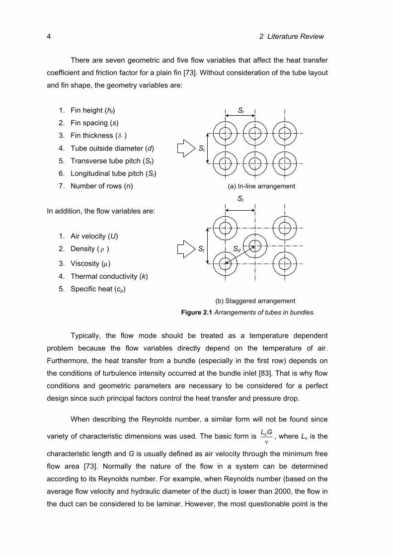
There are seven geometric and five flow variables that affect the heat transfer
coefficient and friction factor for a plain fin [73]. Without consideration of the tube layout
and fin shape, the geometry variables are:
1. Fin height (hf) Sl
2. Fin spacing (s)
3. Fin thickness (δ )
4. Tube outside diameter (d) St
5. Transverse tube pitch (St)
6. Longitudinal tube pitch (Sl)
7. Number of rows (n) (a) In-line arrangement
Sl In addition, the flow variables are:
1. Air velocity (U)
2. Density ( ρ ) St Sd
3. Viscosity (µ)
4. Thermal conductivity (k)
5. Specific heat (cp) (b) Staggered arrangement
Figure 2.1 Arrangements of tubes in bundles.
Typically, the flow mode should be treated as a temperature dependent
problem because the flow variables directly depend on the temperature of air.
Furthermore, the heat transfer from a bundle (especially in the first row) depends on
the conditions of turbulence intensity occurred at the bundle inlet [83]. That is why flow
conditions and geometric parameters are necessary to be considered for a perfect
design since such principal factors control the heat transfer and pressure drop.
When describing the Reynolds number, a similar form will not be found since
variety of characteristic dimensions was used. The basic form is νGLc , where Lc is the
characteristic length and G is usually defined as air velocity through the minimum free
flow area [73]. Normally the nature of the flow in a system can be determined
according to its Reynolds number. For example, when Reynolds number (based on the
average flow velocity and hydraulic diameter of the duct) is lower than 2000, the flow in
the duct can be considered to be laminar. However, the most questionable point is the
2 Literature Review 5
type of flow, which exists in a circular finned-tube bank. Zhukauskas [81] solely stated
that a critical value is Re ≅ 105 for circular finned-tube bundle; however, yet apparently
further verifications on this statement were not sought to date. Jacobi and Shah [22]
discussed that the air flow was likely to exhibit all of possible flow features (e.g., steady
or unsteady, laminar or turbulent) in a single heat exchanger. They suggested that
there were still limitations to the air-side heat transfer performance and a clear
understanding of airflow in the complex passages of heat exchangers was needed so
that surface design can be optimised efficiently.
In designing a heat exchanger, the interactions between the local heat transfer
and flow structure around a circular finned cylinder in cross flow is noteworthy. The
physics of flow are depending on upstream flow condition, the flow along the tube wall
until the separation point and the tube wake condition [62]. The structures of secondary
flow are complicated as the flow is a three-dimensional one. As described in the
introduction, it is still difficult and complicated to predict and visualize the flow and
related heat transfer between the geometrically complex bundles by means of the
experimental investigation. As a result, numerical investigation is being widely used in
recent years to analyse the flow and temperature fields. By using numerical simulation,
one can model physical fluid phenomena that can be easily simulated and one is able
to investigate the fluid and thermal systems more cost effective and faster than by
experiments. Though, a substantial amount of numerical works on plate finned-tube
bundles has been published, only one research work related to the main interest of
current study (circular finned-tubes) was found in Jang et al. [25]. Since little progress has been made by the numerical approach to examine the
heat transfer and pressure drop characteristics for circular finned-tube bundles,
researchers have to rely on the experimental results. Therefore, the relevant
experimental literature on the local heat transfer behaviour of circular finned-tubes will
be reviewed at first.
2.2 Local Heat Transfer Behaviour of Circular Finned-Tubes
The need for heat exchanger designers to associate the demands of enhanced
heat transfer for a given configuration requires clear understanding of the local heat
transfer behaviour. In the literature, several of experimental methods can be found for
detection and measurement of the local heat transfer and for visualization the physics
of flow. It includes:
6 2 Literature Review
1. Point heating model (e.g., Lymer [42], Zhukauskas [81], and Zhukauskas et al.
[82]),
2. Total heating model (e.g., Jones and Russell [27], Legkiy et al. [41], and Neal
and Hitchcock [45]),
3. Naphthalene sublimation technique (e.g., Goldstein and Karni [16], Goldstein et
al. [17], Hu and Jacobi [21], Kearney and Jacobi [32], Sparrow and Chastain
[60], Sung et al. [63], Wong [78]), and
4. Particle Image Velocimetry (PIV) method (e.g., Watel et al. [70, 71]).
To compare between the alternative heating methods, Stasiulevičius and
Skrinska [62] approached an approximate analytical method for a laminar boundary
layer of a smooth tube in cross flow. By this comparison, it is seen that the point
heating method provides an unrealistic boundary condition and overestimates the local
heat transfer coefficients. Besides, Hu and Jacobi [21], and Kearney and Jacobi [32]
suggested that the point heating method could lead to serious errors. Unlike the total
heating method, the thermal boundary layer will not be developed at the fin tips where
both (velocity and thermal) boundary layers should have to develop. Instead, thermal
boundary layer only will develop when the airflow reach to the heated area. According
to [62], depending on the heating models, the heat transfer distribution patterns over
the fin will be dissimilar.
Neal and Hitchcock [45] carried out a comprehensive study on the local heat
transfer and airflow occurring within a circular finned-tube bank in staggered tube
arrangement. Three different tube spacings were examined and instrumented tubes
were installed in row two and six. They found that the heat transfer upstream the fin is
considerably higher, and the heat transfer coefficient decreases at the base of the tube
as the boundary layer increases. However, Hu and Jacobi [21] pointed out that the use
of thermocouples and few sensors might be inadequate for resolving details of the flow
and the heat transfer interaction. By comparing the results of Lymer [42] and Neal and
Hitchcock [45], it is noteworthy that due to the complex flow pattern the local heat
transfer coefficients will vary both circumferentially and radially over the complex
geometry of finned-tubes [62].
Legkiy et al. [41] investigated the local heat transfer on the surface of a single
tube with circular fins cooled by transverse airflow. However, Hu and Jacobi [21]
2 Literature Review 7
discussed that the spatial resolution was insufficient and the results are very limited
because of using a single tube. Another investigation on a single circular fin by mass
transfer method was performed by Sparrow and Chastain [60]. They measured the
variations of the angle of attack by a thin film of a naphthalene sensor. The authors
concluded that the overall heat transfer performance of a circular fin was not
significantly affected by small angles of attack. However, the measurement of the heat
transfer coefficient at only one side may yield erroneous results.
The naphthalene sublimation is the most common implementation of the mass
transfer method to measure the local heat transfer coefficients. Hu and Jacobi [21]
conducted the detailed investigation to the flow conditions and local heat transfer
behaviour on a single row of a circular finned-tube heat exchanger. They established
the fin efficiency differences opposing to Gardner`s solution [13]. Gardner assumed
that the heat transfer coefficient was maintained constant on the fin surface. To the
contrary, Hu and Jacobi [21] calculated the fin efficiency by the assumption of a non-
constant convective heat transfer coefficient. Their conclusion pointed out that there is
a great difference between their calculation and Gardner’s solution while the thermal
conductivity of fin was low. However, the results of [21] were somewhat limited as it
was used only one row and Kearney and Jacobi [32] stated that incorrect choice of the
Lewis number lead to a considerable error. Kearney and Jacobi rectified those results
by securing the correct Lewis number and also recommended that the fin efficiency of
circular fins was less important to the heat transfer coefficient distribution. Kearney and
Jacobi obtained such results for circular finned-tubes in staggered and in-line two-row
bundles.
Recently Watel et al. [70,71] studied the influence of the fin spacing on the
convective heat transfer from a rotating circular finned-tube in transverse airflow. The
fin cooling was monitored by aid of the infrared thermography and the flow field in the
mid-plane between two fins was obtained by Particle Image Velocimetry (PIV) device.
Their results were compared and validated with Schmidt [56], Legkiy et al. [41], and
Sparrow and Samie [59]. However, they tested only for a single tube and it did not
realize the effect of neighbouring tubes. Here, it is necessary to emphasize that the
tube bundle effect should be taken into account in all investigations because
Zhukauskas et al. [82] showed that the heat transfer coefficients over the
circumference were more uniformly distributed on a tube in the bundle rather than on a
single tube.
8 2 Literature Review
One of the influence factors controlling the local heat transfer behaviour from a
finned-tube bundle is the flow condition within. Since the geometry controlled the flow,
the more complex flow in the bundles is expected for the intended circular finned-tubes.
To have the more understanding on the local heat transfer distribution over a fin
surface, detailed knowledge of such a complex flow will be helpful. To describe the flow
patterns, many researchers (Brauer [7], Goldstein and Karni [16], Goldstein et al. [17],
Hu and Jacobi [21], Lymer [42], Neal, and Hitchcock [45], Sung et al. [63]) used
different ways. A comprehensive review on the flow distribution on a single tube and
tube bundles was given by Brauer [7]. According to his achievement, the dead
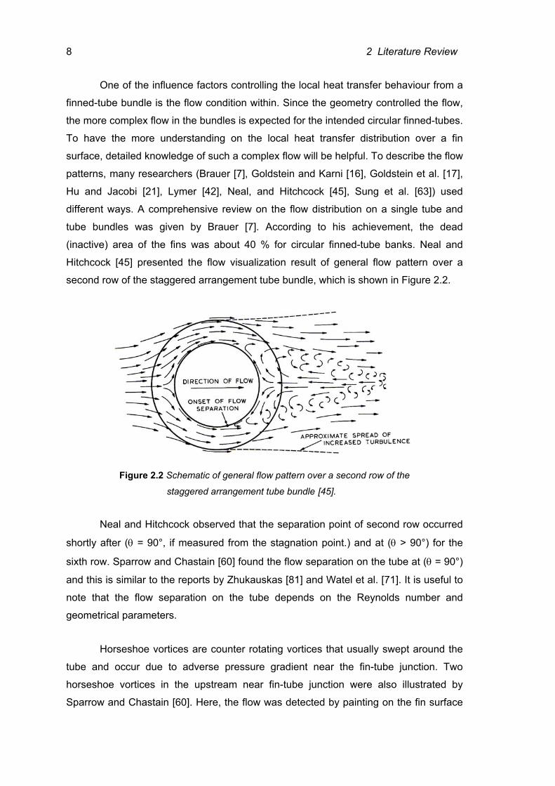
(inactive) area of the fins was about 40 % for circular finned-tube banks. Neal and
Hitchcock [45] presented the flow visualization result of general flow pattern over a
second row of the staggered arrangement tube bundle, which is shown in Figure 2.2.
Figure 2.2 Schematic of general flow pattern over a second row of the
staggered arrangement tube bundle [45].
Neal and Hitchcock observed that the separation point of second row occurred
shortly after (θ = 90°, if measured from the stagnation point.) and at (θ > 90°) for the
sixth row. Sparrow and Chastain [60] found the flow separation on the tube at (θ = 90°)
and this is similar to the reports by Zhukauskas [81] and Watel et al. [71]. It is useful to
note that the flow separation on the tube depends on the Reynolds number and
geometrical parameters.
Horseshoe vortices are counter rotating vortices that usually swept around the
tube and occur due to adverse pressure gradient near the fin-tube junction. Two
horseshoe vortices in the upstream near fin-tube junction were also illustrated by
Sparrow and Chastain [60]. Here, the flow was detected by painting on the fin surface
2 Literature Review 9
with a mixture of lampblack powder and oil. Depending on the angle of attack, the
leading edge flow separation and the reattachment of the flow separated may be
apparent in the upstream region of the fin. They noted that the recirculation of the flow
and the reattachment zones would be impossible without leading edge separation. Hu
and Jacobi [21] also found that when Redh ≥ 9000, there will be of the phenomenon of
the leading edge separation and reattachment. By using naphthalene sublimation
technique, the existence of counter rotating vortices near the corner junction of a
cylinder in cross flow was shown by Goldstein and Karni [16], Goldstein et al. [17] and
Sung et al. [63].
2.3 Analysis of Geometric and Flow Parameters
The distribution of the heat transfer coefficient over a finned-tube is depending
primarily on the flow conditions and the finning geometry. Moreover, there are
significant factors controlling the heat transfer and pressure drop from a finned-tube
bundle and the interaction between such factors creates further complicated designing
problems.
2.3.1 Effect of Fin Height
Enhancement the heat transfer and reduction of the pressure drop from finned-
tubes may necessitate considering the many parameters and first of all, the fin height
effect of the circular finned-tube. Antuf’ev and Gusev [2], Konstantinidis et al. [33],
Mirkovic [43], and Yudin et al. [80] observed that an increase of the fin height of the
staggered tube arrangement provides the decrease of heat transfer coefficient and the
increase of pressure drop. Brauer [6] probed both in-line and staggered arrays and
validated the same trend for pressure drop as others observed. However, different heat
transfer results were revealed since Brauer neglected the fin efficiency effect in the
experiments. It is imperative to note that the nature of flow over the tube bundle with an
increase of fin height comes close to the flow characteristic found along the channel
(Zhukauskas [80]).
Brauer and Zhukauskas documented that because of the thicker boundary layer
developing at the fin base, the heat transfer at the fin tip was higher than at its base.
Zukauskas et al. [82], and Hu and Jacobi [21] reported that the highest value of the
average heat transfer coefficients along the fin height, are found to be near (θ = ± 90°)
10 2 Literature Review
where the narrowest flow passage in the bundle exists. It can be explained that due to
the constriction in the flow passage, the flow velocity reaches maximum and causes a
high local heat transfer. At (θ = 0°) and (θ = 180°) the relative heat transfer coefficient,
i.e. the ratio of local heat transfer coefficient to the averaged heat transfer coefficient
over a fin height, attained its maximum at the fin tip. At (θ = 90°), the relative maximum
heat transfer occurred in the middle of the fin height. Therefore, it is useful to note that
the nature of the local heat transfer distribution over the fin height was changed
according to the angle of fin surface.
According to Hu and Jacobi [21], the mass transfer is also increased near the
fin base (θ = ± 30°) due to the vortex at low Reynolds number. For higher Reynolds
numbers, about Re > 9000, higher mass transfer rates near the fin tip are observed for
(θ = ± 170°). However, it was studied only a single row of circular finned-tubes.
Kearney [31] described that the effects of bundle arrangement and the fin
height on the local and average heat transfer performance are coupled. A low finned-
tube (ddf = 2) may perform better in the staggered arrangement while high finned-
tubes (ddf = 4) are not giving a substantial effect to the bundle arrangement. Kearney
showed that the inactive region covered less of the total fin area for the in-line
arrangement as ddf increases. It has to be understood that the heat transfer coefficient
will decrease and the pressure drop will increase when the fin height increases.
2.3.2 Effect of Fin Spacing
Upon observation of a variety of finned-tube bundles a selection of the correct
spacing between fins is need to emphasize. Experimental results of Antuf’ev and
Gusev [2], Brauer [5, 6], Rabas et al. [47], Rabas and Taborek [48], and Yudin et al.
[80], show that the heat transfer coefficient near the fin base of closer fin spacing is
smaller than the greater fin spacing due to the thicker boundary layer. Generally, the
smaller gap fin spacing creates the thicker boundary layers. The stagnation zone
formation at the root of the fin and the tube surface is swept by a non turbulent flow and
it is excluded from taking part in active heat transfer. Thus, the allowable extent of
reducing the fin spacing will depend on the velocity and turbulence of the flow in the
2 Literature Review 11
inter fin spaces [2]. Zhukauskas [81] found that the heat transfer coefficient increases
when the spacing is raised to 6 mm (the mean distance between the fins = 4.5 mm)
and a further increase of the fin spacing does not necessarily change it for the
Reynolds range of 4.8 x 10⁴ to 7.6 x 10⁵. It is reasonable to expect that the influence of
the effect of the fin spacing on the heat transfer decreases with higher Reynolds
number. However, Rabas et al. [47] gave an important consideration that the thermal
performance is almost independent of the Reynolds number for the larger fin density
(0.98 fins/mm). They observed that the fin density has much stronger impact on the
performance for the larger diameter of tube (d = 31.75 mm). They examined for the low
fins, which is less than 6.35 mm at the range of 1000 ≤ Re ≤ 25000.
For a case of less spacing, a larger pressure drop and worse fouling condition
are expected to occur on the air-side. The increasing of the fin density from 275.6 fins
per meter to 342.5 fins per meter, affected the pressure drop whereas no effect upon
the air-side heat transfer coefficient is found by Jameson [23]. Ward and Young [69]
made the same conclusion that the pressure drop decreases when the fin spacing
increases from 201.97 to 407.87 fins per meter.
Kyuntysh et al. [34] studied the effect of fin height to fin spacing relation
shf
for the staggered tube arrangement. When shf ≤ 1.9, the heat transfer coefficient does
not depend on the relative depth of the inter fin space, and when s
hf >1.9, the Nusselt
number decreased in proportion to 7.0
f
sh −
. They recommended that this
phenomenon was valid from Re = 5 x 10³ to 5 x 10⁴ and s
hf = 1 to 3.5. However,
Briggs and Young [8] and Stasiulevičius and Skrinska [62] found different conditions at 2.0
fsh −
and
14.0f
sh −
respectively. Therefore, no uniform effect of
shf on the heat
transfer coefficient is expected, though showing a same trend as increasing s
hf will
cause the decrease the heat transfer coefficient.
Recently, Watel et al. [70, 71] expressed the effect of the dimensionless ratio of
fin spacing to the tube diameter as Nu = c Rem. The exponent “m” decreases from 0.73
12 2 Literature Review
to 0.59 with increases of ds from 0.034 to 0.103. When
ds
is greater than 0.241, the
exponent remains to 0.55. The effect of the geometrical parameter ds on the heat
transfer coefficient is more significant for low Reynolds numbers. By their results at Re
> 104, there is no significant increase of the Nu number when ds
is varied from 0.069 to
0.103. According to the boundary layer theory, the comparative difference of the
Nusselt number with the spacing must decrease when the Reynolds number increases.
Air velocity and flow patterns also play a critical role when examining the fin spacing
effect. Fin spacing led to the occurrence of boundary layer, which determines the
outcomes of the heat transfer and pressure drop.
2.3.3 Effect of Fin Thickness
A few researchers performed the observation to the effect of fin thickness.
Ward and Young [69] found that the Nusselt number increased with the fin thickness.
However, Briggs and Young [8] obtained the opposite results showing that the heat
transfer coefficient is less dependent upon the fin thickness and will be decreased as
the fin thickness is increased. Three different values of the fin thickness 0.457 mm,
1.06 mm and 2.02 mm of helically finned-tubes were examined and the heat transfer
coefficient of the largest value of fin thickness was approximately 8% less than that of
the thinness one. By means of the analytical approach, Stasiulevičius and Skrinska
[62] showed fin thickness effect is unproductive on the convective heat transfer.
2.3.4 Effect of Tube Outside Diameter
The average heat transfer coefficient depends mainly on the outside diameter
of the tube [69]. The flow will change when the tube diameter is varied. The velocity at
the narrowest cross section is raised to a certain extent with increasing the tube
diameter and the recirculation zone behind the tube is also increased. Jameson [23],
Mirkovic [43] and Torikoshi et al. [65] showed that the pressure drop increases with the
tube diameter. Jameson [23] tested three different tube diameters, (15.875 mm, 19.05
mm and 25.4 mm) of staggered helically finned-tubes. Mirkovic [43] investigated the
heat transfer and pressure drop in an eight-row deep staggered tube bundle for the two
tube diameters 38.1mm and 50.8 mm with constant transverse and longitudinal tube
2 Literature Review 13
pitches. Note that the tube diameter only was changed while other parameters such as
the fin height and fin spacing were kept constant in their investigation. When the tube
diameter increases, the wake region behind the tube will increase and the air-side
pressure drop will rise. Mirkovic [43] also found that the Nusselt number increases for
the larger tube diameter. However, Torikoshi et al. [65] observed no significant
variation of the average heat transfer coefficient. Torikoshi et al. investigated
numerically the tube diameter effect on heat transfer and flow behaviour for a two-row
staggered arrangement of plate finned-tubes. In contrast to the circular finned-tubes,
the plate fin surface is decreased when the tube diameter increases. It is apparent that
the tube diameter effect may be largely ignored for the cases where the diameter is
changed only slightly.
2.3.5 Effect of Tube Spacing
Apart from the tube diameter effect, the turbulence intensity inside the bundle
depends on the tube spacing and the air velocity. Hence, the pressure drop in the tube
bundle will vary according to these parameters. When changing the transverse tube
pitch, there are no significant changes on heat transfer performance; however, a
remarkable effect on the air-side pressure drop was noted by Briggs and Young [8],
Jameson [23], and Stasiulevičius and Skrinska [62]. Nevertheless, Mirkovic [43], Neal
and Hitchcock [45], and Nir [46] indicated the consequence of the transverse tube pitch
to the heat transfer. For the staggered arrangement, the heat transfer is higher for the
closer transverse pitch (Neal and Hitchcock [45], Nir [46], and Sparrow and Samie
[59]). Apparently, the velocity at the narrowest cross-section will become higher when
deceasing the transverse tube pitch and this effect will lead to the higher heat transfer
coefficient and pressure drop. Jameson [23], and Robinson and Briggs [50] showed
that when increasing the transverse pitch, the pressure drop is found to decrease. The
different conclusion is given by Mirkovic [43] with observation of the fact that both
Nusselt and Euler numbers are increasing owing to the larger transverse tube pitch. In
addition, he claimed that an enlargement of longitudinal tube pitch for the staggered
arrangement decreases the Nu and Eu numbers. The similar result for the longitudinal
pitch effect to the heat transfer performance was recorded by Neal and Hitchcock [45],
and Rabas et al. [47], and the pressure drop effect was confirmed to Jameson [23].
For the in-line arrangement, Sparrow and Samie [59] observed that the
pressure drop increases with the longitudinal pitch. It is possible that the tubes will act
14 2 Literature Review
as a single tube if the longitudinal pitch is too wide. Moreover, Rabas et al. [47] discovered that the longitudinal pitch effect depends on the fin density of the low
finned-tube bundle. The heat transfer performance is identical for Sl = 37.12 mm and
50.80 mm with 0.4 fins per mm. However, for the fin density of 0.98 fins per mm, the
heat transfer performance lowered for a larger Sl applied.
For the aspect of equilateral tube arrangements, Briggs and Young [8]
investigated the test for two different tube spacings and found almost identical heat
transfer performance in both cases. The pressure drop increases when the tube
spacing is changed from 111.0 mm to 27.4 mm.
When evaluating the tube spacing effects, some researchers explored the
relationships between the tube spacing and other geometric parameters. The relation
between the tube spacing and the fin diameter was investigated by Sparrow and Samie
[59], and Stasiulevičius and Skrinska [62]. According to [59], decreasing the ratio of
transverse tube spacing to fin diameter (ft
dS
) from 1.52 to 1.07, the Nu number is
increased by about 35 %. For the two- row in-line array, the Nu number increased at
Reα = 8 x 10³ as the longitudinal pitch to fin diameter ratio (f
l
dS
) is increased. At higher
Reynolds numbers (Reα = 3.2 x 10⁴), the Nu number is relatively insensitive to the
longitudinal pitch. For the two-row staggered array, the Nusselt number at first
increased with increasing Sl, attained a maximum value at f
l
dS
= 2.05 and then,
decreased as encountered for the larger pitches over the entire Reynolds number
range from 7.5 x 10³ to 3.2 x 10⁴.
Stasiulevičius and Skrinska [62] tested seven-row tube bundles and the heat
transfer coefficient increased slightly (about 3 %) with an increase in dSt (2.67 to 4.13)
whereas a reduction in dSl (2.14 to 1.46) gives the substantial rise (about 20 %). This
result indicates that the longitudinal changes make more progress on the heat transfer
performance than the transverse ones. The tube spacing effect is directly concerned
with the fin diameter, the fin density, and the Reynolds number.
2 Literature Review 15
2.3.6 Effect of Row
The heat transfer from a finned-tube bundle is mainly based on the flow
patterns. The flow over a single finned-tube is rather different from the cross flow over
the bundle. Zhukauskas et al. [82] observed that a tube within a bundle has a higher
heat transfer rate at the leading edge of the fin than a single tube has with the same
Reynolds number. It is because of the turbulizing effect of the upstream rows. Brauer
[6] showed complex flow visualizations of the different flow patterns of a single finned-
tube, one row finned-tube, and two-row finned-tube banks. It is noted that the flow
condition around the first and the second rows are different [45].
To determine the minimum number of tube rows, the performance of rows
inside the bundle and the relation between such rows were examined by Kuntysh et al.
[34], Kuntysh and Stenin [37], Lapin and Schurig [38], Mirkovic [43], Neal and
Hitchcock [45], Sparrow and Samie [59] and Ward and Young [69]. It is agreed that the
heat transfer coefficient for a first row of the staggered arrangement is about 30 %
smaller than the deeper rows. Neal and Hitchcock determined that the heat transfer
coefficient of the sixth row is remarkably higher than that of the second row.
For the staggered arrangement, the main flow passes through the tube and its
fin surface nearly in the same way for all the rows. The influence of row effect upon
heat transfer for the staggered array is less than for the in-line array and for row
numbers n ≥ 2; the heat transfer and the friction factor remain unchanged (Brauer [6],
Briggs and Young [8], and Gianolio and Cuti [14]). Kuntysh and Stenin [37] drew the
same conclusion by observing that the value of the heat transfer coefficient becomes
constant in the second row of the four-row tube bundle. Weierman et al. [76] observed
also that the friction factor is independent of the number of rows for the staggered
arrangement. Antuf’ev and Gusev [2], and Kuntysh et al. [36] found that the heat
transfers coefficient became constant after the third row while Ward and Young [69]
discovered that the coefficient is not stabilized until the third and fourth row. In addition,
Mirkovic [43], and Neal and Hitchcock [45] observed that the coefficient increases until
the fifth or sixth row. As stated above, there are various findings on the flow stability of
the finned-tube bundle associated with the different circumstances.
Rabas and Taborek [48], and Yudin et al. [80] developed the row correction
factors. It has been assumed [31] that Yudin et al.’s shallow bundle correction factor for
staggered and in-line tube banks are reasonable to apply on other correlations. Yudin
16 2 Literature Review
et al. investigations were performed within 103 ≤ Re ≤ 2 x 10⁴ to prove that the
average heat transfer performance of a bundle increases with a decreasing number of
rows for the in-line arrangement whereas it decreases for a staggered tube bank.
Alternatively, Rabas and Taborek [48] studied on the rows effect of low finned-tube
bundles and presented a shallow bundle correction factor. It means that the factor
increased with the number of rows for low fin density (0.393 fins/mm) but decreased for
high fin density (0.984 fins/mm). For a high fin density tube bank in a staggered array,
some performance characteristics similar to those of the in-line bank are noted. It is
appeared that the heat transfer performances of shallow in-line tube banks always
decreased with row number regardless of the fin density.
Like in case of the staggered arrangement, the experimental results were also
different on the row effects of the in-line tube bundles that seem to play a more
sensitive role than for the staggered bank. The second row heat transfer of the in-line
arrangement is found to be lower than the first row (Brauer [6], and Kuntysh and Stenin
[37]). Contrary to their reports, Kearney [31], and Sparrow and Samie [59] showed the
Nu number of second row is about 35 % greater than that of the first row. The heat
transfer coefficient became constant in the second row of the in-line bank as observed
by Antuf’ev and Gusev [2], and Kuntysh and Stenin [37]. However, Weierman [75]
found that the friction factor is stable in the third row and there are significant changes
for one- and two-row banks. Brauer [6] reported that both heat transfer and pressure
drop are independent of the number of rows for four or more row deep in-line banks.
All studies verified that the heat transfer coefficient around the fin, and from
row-to-row vary in accordance with the bundle depth. It is useful to note that only
limited results with a single tube and very few rows are found, and further studies
applying four and more tube row bundles should follow. On the other hand, some
studies have done to resolve this situation by developing the row correction factors.
2.3.7 Effect of Tube Arrangement
The degree of heat transfer augmentation depends on many other factors
encompassing the tube layout, the turbulence intensity, the fin shape and thermal
conductivity. It is important to note that selecting the suitable arrangement favours in
acquiring better heat transfer rate. A few research on in-line tubes have been pursued
by Brauer [6], Hashizume [20], Kuntysh and Stenin [37], Rabas and Huber [49] and
2 Literature Review 17
Weierman et al. [76], as widely accepted the notion of that the staggered arrangement
has more advantages in terms of thermal behaviours than the in-line arrangement. For
staggered tube bundles, a small recirculation zone only appeared behind the tubes
since its own structure made blockages whereas in the in-line arrangement both
upstream and downstream sites are within the recirculation zone. Consequently, the in-
line banks have had the insufficient mixing and lower heat transfer coefficients. In
addition, the extent of the advantages of staggered banks depends at least on the
effect of fin height, and for high fins (15 mm) Brauer [7] showed that the difference is
100 %. In contrast, Kearney and Jacobi [32] suggested that the high finned in-line
bundle performance is found to be comparable to the staggered arrangement. Rabas
and Huber [49] show a trend that the thermal performance of shallow in-line banks
approaches that of the staggered banks as the Reynolds number increases. On the
other hand, Kuntysh et al. [37] claimed that an arrangement lies between the in-line
and staggered arrays have the better rate of heat transfer.
2.3.8 Effect of Air Velocity
One of the influential factors governing the heat transfer performance in finned-
tubes is the boundary layer development, whose shape is varying according to air
velocity. When the air velocity increases, the formation of horseshoe vortices will
increase and the boundary layer thickness will decrease. It is generally accepted that
the fluid velocity in the recirculation zone is lower than in the main stream and the heat
transfer coefficient therein is reduced.
The selection of flow velocity is important to determine the Reynolds number for
bodies in cross flow. Remember that there is no unanimous agreement on the
characteristic dimension used to define the Reynolds number. The investigators enable
to employ the inlet velocity, mean velocity, and the velocity in the minimum cross
section area as reference velocity. According to the available literature, the reference
velocity is mostly defined as last one. Moreover, the complete design of heat
exchangers involves the method of drafting air. There will be a different performance of
heat transfer and pressure drop of the finned-tube bundle depending on the flow
conditions at the bundle inlet (Gianolio and Cuti [14], and Stasiulevičius and Skrinska
[62]).
18 2 Literature Review
2.4 Average Heat Transfer Correlations The information about existing correlations of the average heat transfer on
circular finned-tube bundles are reviewed here as a second part of the literature review
on the circular finned-tube bundles. As previously mentioned, heat transfer from a
circular finned-tube in a bundle is a function of related geometrical parameters and the
flow variables involved. In order to demonstrate these principal factors, a large number
of heat transfer correlations mostly based on the author’s own data were deduced.
Analysis of the experimental results shows that there will be different results that
depend on the method of the determination of heat transfer coefficients. Generally,
there are two possible ways to obtain the heat transfer from a tube: the local simulation
technique [80, 81 and 83] (only one test tube is heated) and the complete thermal
simulation method (all test tubes heated).
Webb [72] and Nir [46] presented excellent surveys for published data and
correlations of overall heat transfer and pressure drop correlations on circular finned-
tube bundles. The available correlations are incorporated in the Appendix D. Webb [72]
reported that recommendation of a single correlation and direct comparison to the
different correlations was a difficult task. However, Webb recommends the heat
transfer correlation of Briggs and Young [8]. Their investigation was based on a
previous investigation of Ward and Young [69] where seven different staggered finned-
tube bundles were tested and the average Nusselt number for the six-row bundle was
correlated. Later they proceeded their work by extending the database with nine
additional banks of tubes. Briggs and Young’s correlation is widely accepted and used
because of their investigation based on the widest range of parameters. It is reported
that the tube spacing effect is not found in their correlation.
Nir [46] then provided a quantitative comparison of some experimental data with
the Briggs and Young correlation. According to Nir, the available heat transfer data of
tube banks with the plain fin covered the range of ± 20 % of Briggs and Young [8]
correlation. Nir also gave a set of heat transfer and pressure drop correlations based
on his own data and 16 published sources. This correlation corresponds within 10 % of
the most of available test data. However, Nir described for both segmental and plane
fin characteristics in an equation. It is expected that due to the different fin geometries,
the respective boundary layer development may be dissimilar.
2 Literature Review 19
According to available data, most of the investigations were performed in the
Reynolds number range of 103 to 3 x 10⁴ and the investigation based on the widest
range (2 x 10⁴ ≤≤ Re 1.3 x 10⁶) was given by Zhukauskas et al. [82]. They provided an
extensive reference database for heat transfer and pressure drop of finned-tube
bundles in cross flow. Their work covers 21 different seven-row finned-tube bundles.
The heat transfer correlations were obtained from their own data and the experimental
data for the bundles scatter over the range of ± 14 %. Note that the effect of bundle
configuration and the fin parameters are expressed in these correlations except for the
fin thickness effect. The term for bundle depth effect is missing; however, it is
reasonable to accept the fact that their investigations are based on the depth of seven-
row. Unfortunately, they used some dummy tubes (unheated tubes) in their tests and
Nir [46] suggested that this method may lead to errors.
In pursuit of the optimisation of low finned-tube bundles, Rabas and Taborek
[48] surveyed the relevant literature of the heat transfer and pressure drop
performances. Rabas et al. [47] developed heat transfer and friction factor correlations
for low fins and small fin spacing based on 30 different staggered tube bundles.
However, it is limited for the bundles to the fin height of under 6.35 mm.
Yudin et al. [80], Weierman [74], and Gianolio and Guti [14] studied on the
effect of bundle depth. Gianolio and Guti [14] modified the Briggs and Young [8], and
Schmidt [56] correlations by adding an extra term to account for the bundle depth
effect, which was left out in it. They run the test for 17 finned-tube banks of the
equilateral triangular pitch by varying the number of rows ranging from one to six.
Based on their own data, air-side heat transfer coefficient equations for forced draft
were provided.
Alternatively, the effects of bundle arrangement, St and Sl are not stated in both
the Schmidt [56] and the VDI-Wärmeatlas [68] correlations. Their correlations are
prepared for the ratio of the total heat transfer surface area to the exposed base tube
area. Schmidt provided correlations for both arrangements and VDI-Wärmeatlas
presented the average heat transfer correlations for a one to three-row banks and four
or more row banks respectively.
Another set of correlations for the in-line, mixed in-line-staggered and the
staggered tube bundles were provided by Kuntysh and Stenin [37]. They studied the
average heat transfer coefficient on an averaged four-row tube bundle basis and on a
20 2 Literature Review
per row basis respectively. However, no consideration was given to fin efficiency effect
in their study and they did not express anything for the fin parameters and the bundle
effect in the correlations.
2.5 Pressure Drop Correlations
The basic design feature of a heat exchanger is aimed to synchronize heat
transfer rate and pressure drop in the system. A minimum pumping power to overcome
the effect of fluid friction and to move the fluid through the heat exchanger is essential
in designing the compact heat exchanger. For this reason, a number of correlations on
pressure drop of circular finned-tube bundles have been verified and showed that the
pressure drop depends on the number of rows except for the result of Gianolio and
Guti [14]. Jameson [23], Kuntysh et al. [35], Nir [46], Robinson and Briggs [50],
Stasiulevičius and Skrinska [62], and Ward and Young [69] that are based on their own
data, though Gianolio and Guti [14], Gunter and Shaw [18], Haaf [19], and Rabas and
Eckels [47] used wide ranges of data.
Jameson [23] tested the staggered bundles of one to eight rows and varied,
dSt from 1.9 to 3.6 and
dSl from 1.1 to 2.5. However, it should be noted that there is no
effect of the fin parameters in this relation.
Another pressure drop correlation for the staggered arrangement was given by
Ward and Young [69]. This correlation covered for the range of 103 < Re < 3 x 10⁴ and
all influence parameters were related. However, Haaf [19] compared this result with
other experimental data (Brauer [6], Briggs and Young [8], Kays and London [30] and
Weyrauch [77]) and suggested that the heat transfer coefficient of the prediction of [69]
can vary by as much as 100%. Haaf developed a new pressure drop correlation for
both in-line and staggered arrays in terms of the equivalent diameter and mean velocity
in the bundle based on the equation from Ward and Young.
Webb [72] cited his recommendation to Robinson and Briggs [50]’s pressure
drop correlation for a staggered tube layout. This correlation was empirically based on
15 equilateral triangular arrangements and two isosceles triangular arrangements. This
correlation is found to be valid for four and more tube rows and the standard deviation
of this correlation is 10.7 %. However, this equation is questionable for larger fh
s
2 Literature Review 21
values, which included a small range of fin geometry variables fh
s were covered.
Moreover, Nir [46] construed that [50] equation’s accuracy is insufficient when
comparing with his own and other available data. A valid research on the pressure drop
works was done by Nir and then correlated by embracing the important factors like the
ratio of heat transfer area of a row of tubes to free flow area. It is noted that this
correlation was marginalized to within 10% of the data of several authors. However,
these correlations are applicable for staggered arrangement only.
Without considering for the in-line arrangement, Stasiulevičius and Skrinska
[62] gave pressure drop correlations in terms of Eu number for two different Reynolds
number ranges. It is found that the effect of fin parameters apart from the fin thickness
and the transverse and longitudinal pitches are reflected in these correlations. It
should, however, be stressed that the fin thickness effect is found to be negligible for
convective heat transfer but warranted to resolve the problem of pressure drop.
For low fin bundles, Rabas et al. [47] presented the more accurate correlation
based on their own and other published data. The correlation is valid for staggered
bundles; however, it was not suitable for a high finned-tube bundle.
Gianolio and Guti [14] also gave pressure drop correlations for staggered
arrangement under the forced and induced draft modes based on 17 tube banks
having one to six rows. It is surprising to find that the number of rows effect is no
significantly affect on the pressure drop for forced draft mode. Apparently, the effects of
the fin parameter and the longitudinal tube pitch effect have generally overlooked.
2.6 Concluding Remarks
A considerable amount of related data on the local and average heat transfer
and the pressure drop were established and qualitative judgements on circular finned-
tube configurations are rendered. Despite of these earlier developments, this review
indicated that further concentration on the existing problems in designing of optimum
fin geometry and tube arrangements are still necessary. Some conclusion points are,
• Considerably more information on numerical simulation has been published for
plate fins than circular fin tubes.
22 2 Literature Review
• The heat transfer coefficient and flow distribution over a tube in the bundle is
different to a single tube.
• Temperature distributions over the fin surface and the flow structures between
fins are of complex pattern. When the need arises to measure such effects
accurately, it is an experimentally difficult task to do without disturbing the heat
transfer behaviour on a fin surface. Therefore, more precise data on the local
behaviour are necessary.
• Moreover, clearer effects on the visualization are required and numerical
simulations are essential for such complex flow patterns.
• Different results came out of the relevant information regarding the tube spacing
adjustments and number of rows.
• Controlling the parameters and the interaction rendered more intricate problems
and hence, all dominant geometric parameters should be considered to resolve
in the problem.
• All correlations reviewed in the previous section were based on data for a depth
of four and more rows at Re from 103 to 1.3 x 10⁶. Majority of the studies were
carried out for the staggered arrangement and comparatively very few
investigations for the in-line arrangement were found. Moreover, most of the
previous correlations are failed to account for all geometric variables involved.
• Since most correlations were based on their own data, authors gave different
formula for the heat transfer and pressure drop correlations. In addition, the
characteristic dimension to define Reynolds number was dissimilar. Thus, it is
fairly anticipated that to compare directly to experimental correlations is found to
be difficult.
• Finally, all related works for the circular finned-tubes have been correlated
experimental ones and respective correlations have not been verified yet under
numerical simulations. Therefore, additional numerical data are needed in order
to establish improved correlations.
3 Objectives
The objective of the present study is to provide more complete understanding
of the distributions of local and average heat transfer and pressure drop behaviour of
circular finned-tube heat exchangers. Since heat transfer coefficients are much lower
in air than in liquid flows or two-phase fluids, this study will help to solve the problems
associated with the designing of air-side heat transfer enhancement by means of
circular finned-tubes.
This numerical investigation was carried out for the range of Reynolds numbers
(based on air velocity through the minimum free flow area and tube outside diameter)
from 5 x 10³ to 7 x 10⁴. A finite volume numerical scheme is used to predict the
conjugate heat transfer and fluid flow characteristics with the aid of the computational
fluid dynamics (CFD) commercial code, FLUENT. The governing equations for the
energy and momentum conservation were solved numerically with the assumption of
three-dimensional unsteady flow. An improved model, the RNG (Renormalization
group) based k-ε turbulence model was applied in this investigation.
As described in the section 2.6, the available relevant literature is quite limited
with respect to the experiments and it is still difficult to predict the physics of the flow
patterns within the circular finned-tube banks. Also, the flow structure will depend on
the different geometries, and accurate information on this dimensional local transport
phenomenon is required. Therefore, the velocity and temperature distributions over the
fin surface and within the bundle were studied numerically. Regarding to this, the flow
behaviour of the developing boundary layer, the horseshoe vortex system, the flow
separation, and the tube wake region in the circular finned-tube banks will be
visualized. Consequently, the influence of the geometric parameters on heat transfer
and pressure drop are studied and their results are discussed. Hence, the following
geometric parameters were considered in this investigation:
24 3 Objectives
1. Fin Height
2. Fin Spacing
3. Fin Thickness
4. Tube Diameter
5. Tube Spacing (Transverse and Longitudinal)
6. Tube Arrangement (Staggered and In-line) and
7. Number of Rows Effect
The major aim of the present study is to attain reliable correlations. Therefore,
the results are evaluated by comparison with available experimental data and then,
the average heat transfer and pressure drop data are correlated from two to six rows
for staggered tube banks and three to five rows for in-line tube banks in the forms of
Nusselt number Nu and Euler number Eu, respectively.
Rather than detailed investigation of numerical and modelling aspects, to pay
more attention to verify the heat transfer and pressure drop behaviour of circular finned-
tubes by employing the numerical means is the focus of the present work.
4 Numerical Consideration
Due to the advances in computational hardware and available numerical
methods, CFD is a powerful tool for the prediction of the fluid motion in various
situations, thus, enabling a proper design. CFD is a sophisticated way to analyse not
only for fluid flow behaviour but also the processes of heat and mass transfer.
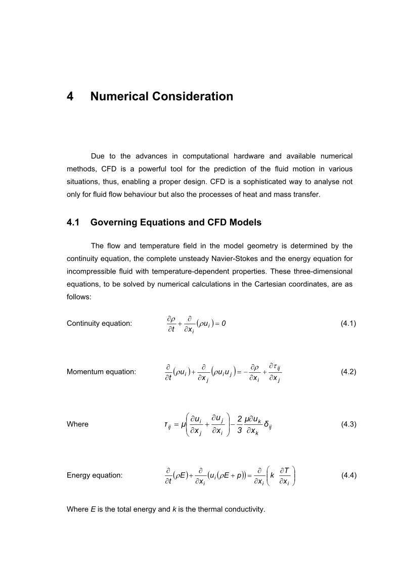
4.1 Governing Equations and CFD Models The flow and temperature field in the model geometry is determined by the
continuity equation, the complete unsteady Navier-Stokes and the energy equation for
incompressible fluid with temperature-dependent properties. These three-dimensional
equations, to be solved by numerical calculations in the Cartesian coordinates, are as
follows:
Continuity equation: ( ) 0uxt i
i=
∂∂
+∂∂
ρρ (4.1)
Momentum equation: ( ) ( )j
ij
iji
ji xx
uux
ut ∂
∂+
∂∂
−=∂∂
+∂∂ τρ
ρρ (4.2)
Where ijk
k
i
j
j
iij δ
xuµ
32
xu
xuµτ
∂∂
−
∂
∂+
∂∂
= (4.3)
Energy equation: ( ) ( )( )
∂∂
∂∂
=+∂∂
+∂∂
iii
i xTk
xpEu
xE
tρρ (4.4)
Where E is the total energy and k is the thermal conductivity.
26 4 Numerical Consideration
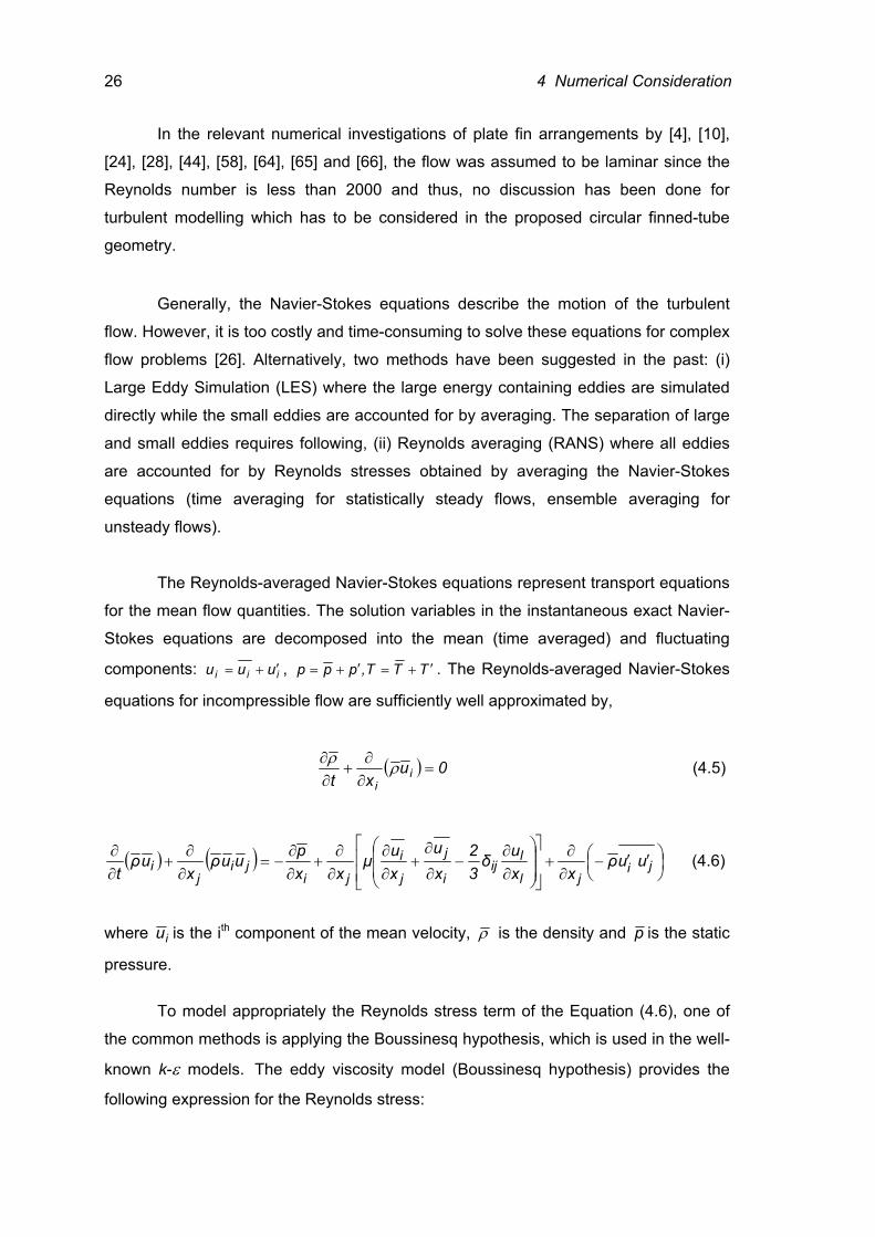
In the relevant numerical investigations of plate fin arrangements by [4], [10],
[24], [28], [44], [58], [64], [65] and [66], the flow was assumed to be laminar since the
Reynolds number is less than 2000 and thus, no discussion has been done for
turbulent modelling which has to be considered in the proposed circular finned-tube
geometry.
Generally, the Navier-Stokes equations describe the motion of the turbulent
flow. However, it is too costly and time-consuming to solve these equations for complex
flow problems [26]. Alternatively, two methods have been suggested in the past: (i)
Large Eddy Simulation (LES) where the large energy containing eddies are simulated
directly while the small eddies are accounted for by averaging. The separation of large
and small eddies requires following, (ii) Reynolds averaging (RANS) where all eddies
are accounted for by Reynolds stresses obtained by averaging the Navier-Stokes
equations (time averaging for statistically steady flows, ensemble averaging for
unsteady flows).
The Reynolds-averaged Navier-Stokes equations represent transport equations
for the mean flow quantities. The solution variables in the instantaneous exact Navier-
Stokes equations are decomposed into the mean (time averaged) and fluctuating
components: iii uuu ′+= , TTT,ppp ′+=′+= . The Reynolds-averaged Navier-Stokes
equations for incompressible flow are sufficiently well approximated by,
( ) 0uxt i
i=
∂∂
+∂∂ ρρ (4.5)
( ) ( )
′′−
∂∂
+
∂∂
−∂
∂+
∂∂
∂∂
+∂∂
−=∂∂
+∂∂
jijl
lij
i
j
j
i
jiji
ji uuρ
xxuδ
32
xu
xuµ
xxpuuρ
xuρ
t (4.6)
where iu is the ith component of the mean velocity, ρ is the density and p is the static
pressure.
To model appropriately the Reynolds stress term of the Equation (4.6), one of
the common methods is applying the Boussinesq hypothesis, which is used in the well-
known k-ε models. The eddy viscosity model (Boussinesq hypothesis) provides the
following expression for the Reynolds stress:
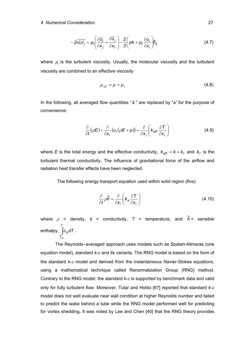
4 Numerical Consideration 27
iji
it
i
j
j
itji δ
xuµkρ
32
xu
xuµuuρ
∂∂
+−
∂
∂+
∂∂
=′′− (4.7)
where tµ is the turbulent viscosity. Usually, the molecular viscosity and the turbulent
viscosity are combined to an effective viscosity
teff µµµ += (4.8)
In the following, all averaged flow quantities “a ” are replaced by “a” for the purpose of
convenience:
( ) ( )( )
∂∂
∂∂
=+∂∂
+∂∂
ieff
ii
i xTk
xpEu
xE
tρρ (4.9)
where E is the total energy and the effective conductivity, teff kkk += and tk is the
turbulent thermal conductivity. The influence of gravitational force of the airflow and
radiation heat transfer effects have been neglected.
The following energy transport equation used within solid region (fins):
∂∂
∂∂
=∂∂
is
i xTk
xh~
tρ (4.10)
where ρ = density, k = conductivity, T = temperature, and h~ = sensible
enthalpy, dTcT
Tp
ref
∫ .
The Reynolds–averaged approach uses models such as Spalart-Allmaras (one
equation model), standard k-ε and its variants. The RNG model is based on the form of
the standard k-ε model and derived from the instantaneous Navier-Stokes equations,
using a mathematical technique called Renormalization Group (RNG) method.
Contrary to the RNG model, the standard k-ε is supported by benchmark data and valid
only for fully turbulent flow. Moreover, Tutar and Holdo [67] reported that standard k-ε
model does not well evaluate near wall condition at higher Reynolds number and failed
to predict the wake behind a tube while the RNG model performed well for predicting
for vortex shedding. It was noted by Lee and Chen [40] that the RNG theory provides
28 4 Numerical Consideration
low Reynolds number effects also, so that it enables to predict the laminar-like
behaviour. Though, the evaluation of such partly turbulent characteristics may be
effective subject to appropriate treatment of near wall region [11].
Moreover, the accuracy of the RNG model was enhanced by adding the term
that accounts for rapidly strained flow and effects of swirling flow ([11], [40]). The RNG
model proved that it has more substantial improvements than the standard model, and
offers more accurate and reliable results for the various flow types. Comparing to the
standard k-ε model, the RNG model will occupy 10 to 15 % more CPU time due to
extra terms and functions in the governing equations [11].
Even though no single and universal model for the turbulent flow in complex
geometry exists, there is another alternative method, which can be employed to
transform the Navier-Stokes equations. LES is a model wherein the equations are
filtered spatially. To compute the flow eddies, the LES provides a time-dependent
simulation by using a set of the filtered equations rather than time averaging. Turbulent
flow is characterized by eddies with a wide range of length and time scale. By filtering,
only small eddies apparently smaller than the filtered size become accessible to move.
It suggested that small eddies are more universal, random, homogeneous and
isotropic, which simplifies to develop the appropriate model. In LES, such small eddies
have to be modelled by a sub grid scale model.
It is necessary to understand that the choice of the turbulence model depends
also on the available computer resource. Contrast to RANS, the LES that may be
necessary to use extremely fine grids and the time required for typical calculations, will
have taken somebody too long to reach for an acceptable solution. Instead FLUENT
generally recommends the Reynolds-averaged approach for the conventional
turbulence models and stressed that the application of LES for industrial fluid
simulations is in its infancy and typical applications to date have been for simple
geometries. In addition, the use of wall functions with LES is an approximation that
requires further validation [11]. On the other hand, under the current computation
power circumstances, the LES is an optional approach for a complex geometry
problem such as supposed circular finned-tube heat exchanger and thus, the
conventional turbulence model employing the Reynolds-averaged approach was
utilized in order to predict the heat and momentum transfer on the circular finned-tube
bundle. In this study, the two-equation RNG model was adopted to solve the turbulence
kinetic energy and its dissipation rate.
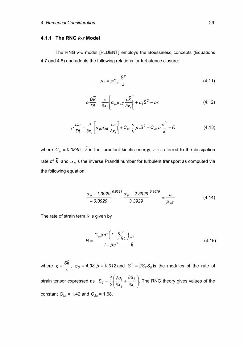
4 Numerical Consideration 29
4.1.1 The RNG k-ε Model
The RNG k-ε model [FLUENT] employs the Boussinesq concepts (Equations
4.7 and 4.8) and adopts the following relations for turbulence closure:
ε
ρµ µ
2
tk~C= (4.11)
ρεµµαρ −+
∂∂
∂∂
= 2t
ieffp
iS
xk~
xDtk~D (4.12)
Rk~
CSk~
CxxDt
D 2
22
t1i
effpi
−−+
∂∂
∂∂
= ∈∈ερµεεµαερ (4.13)
where 0845.0C =µ , k~ is the turbulent kinetic energy, ε is referred to the dissipation
rate of k~ and pα is the inverse Prandtl number for turbulent transport as computed via
the following equation.
eff
3679.0p
6321.0p
3929.33929.2
3929.03929.1
µµαα
=+
−
− (4.14)
The rate of strain term R is given by
k~1
1CR
2
30
3ε
βη
ηηρηµ
+
−
= (4.15)
where ε
η k~S= , 012.0,38.40 == βη and ijij
2 SS2S = is the modules of the rate of
strain tensor expressed as
∂
∂+
∂∂
=i
j
j
iij x
uxu
21S . The RNG theory gives values of the
constant ε1C = 1.42 and ε2C = 1.68.
30 4 Numerical Consideration
4.2 Numerical Simulation
A difficulty for application of the numerical methods in circular finned-tube
exchangers is the fact that one is faced with a complex geometry of the flow
configuration. Furthermore, several geometric parameters directly effecting on the
enhancement of heat transfer.
4.2.1 Introduction
Advances in physical models, numerical analysis and computational power
enable simulation of the heat transfer characteristics in three-dimensional
circumstances. A three dimensional approximation of a turbulent flow is chosen to
explore since the three-dimensional approach is considerably greater than two-
dimensional [4] and moreover, a turbulent flow is fundamentally three-dimensional.
Owing to extremely long computation times, detailed studies on the circular finned-tube
exchanger in three-dimensional flow are very uncommon [25]. Hence, the simulation of
the three-dimensional flow field under complex geometrical conditions is seemingly
intricate and challenging task.
The available computational fluid dynamics software package FLUENT [11] is
used to determine the related problems. FLUENT uses a finite volume method and
requires from the user to supply the grid system, physical properties and the boundary
conditions. When planning to simulate a problem, basic computation model
considerations such as boundary conditions, the size of computational domain, grid
topology, two dimensions or three-dimension model, are necessary. For example,
appropriate choice of the grid type can save the set up time and computational
expense. Moreover, a careful consideration for the selection of physical models and
determination of the solution procedure will produce more efficient results. Dependent
on the problem, the geometry can be created and meshed with a careful consideration
on the size of the computational domain, and shape, density and smoothness of cells.
Once a grid has been fed into FLUENT, check the grids and execute the solution after
setting models, boundary conditions, and material properties. FLUENT provides the
function for post processing the results and if necessary refined the grids is available
and solve again as the above procedure.
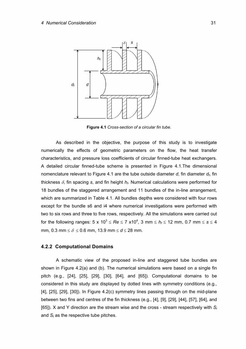
4 Numerical Consideration 31
Figure 4.1 Cross-section of a circular fin tube.
As described in the objective, the purpose of this study is to investigate
numerically the effects of geometric parameters on the flow, the heat transfer
characteristics, and pressure loss coefficients of circular finned-tube heat exchangers.
A detailed circular finned-tube scheme is presented in Figure 4.1.The dimensional
nomenclature relevant to Figure 4.1 are the tube outside diameter d, fin diameter df, fin
thickness δ, fin spacing s, and fin height hf. Numerical calculations were performed for
18 bundles of the staggered arrangement and 11 bundles of the in-line arrangement,
which are summarized in Table 4.1. All bundles depths were considered with four rows
except for the bundle s6 and i4 where numerical investigations were performed with
two to six rows and three to five rows, respectively. All the simulations were carried out
for the following ranges: 5 x 10³ ≤ Re ≤ 7 x10⁴, 3 mm ≤ hf ≤ 12 mm, 0.7 mm ≤ s ≤ 4
mm, 0.3 mm ≤ δ ≤ 0.6 mm, 13.9 mm ≤ d ≤ 28 mm.
4.2.2 Computational Domains
A schematic view of the proposed in-line and staggered tube bundles are
shown in Figure 4.2(a) and (b). The numerical simulations were based on a single fin
pitch (e.g., [24], [25], [29], [30], [64], and [65]). Computational domains to be
considered in this study are displayed by dotted lines with symmetry conditions (e.g.,
[4], [25], [29], [30]). In Figure 4.2(c) symmetry lines passing through on the mid-plane
between two fins and centres of the fin thickness (e.g., [4], [9], [29], [44], [57], [64], and
[65]). X and Y direction are the stream wise and the cross - stream respectively with Sl
and St as the respective tube pitches.
df d
hf
s δ
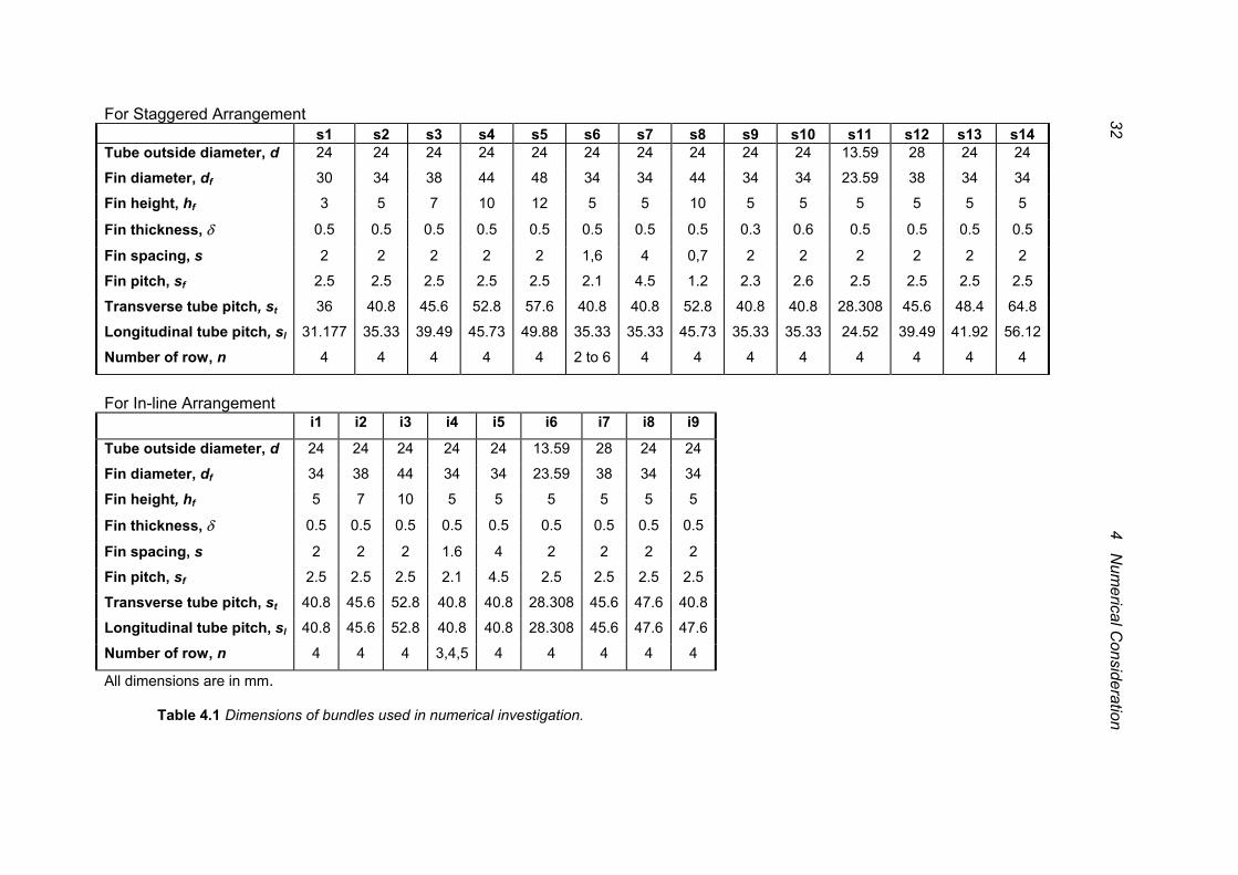
For Staggered Arrangement s1 s2 s3 s4 s5 s6 s7 s8 s9 s10 s11 s12 s13 s14 Tube outside diameter, d 24 24 24 24 24 24 24 24 24 24 13.59 28 24 24
Fin diameter, df 30 34 38 44 48 34 34 44 34 34 23.59 38 34 34
Fin height, hf 3 5 7 10 12 5 5 10 5 5 5 5 5 5
Fin thickness, δ 0.5 0.5 0.5 0.5 0.5 0.5 0.5 0.5 0.3 0.6 0.5 0.5 0.5 0.5
Fin spacing, s 2 2 2 2 2 1,6 4 0,7 2 2 2 2 2 2
Fin pitch, sf 2.5 2.5 2.5 2.5 2.5 2.1 4.5 1.2 2.3 2.6 2.5 2.5 2.5 2.5
Transverse tube pitch, st 36 40.8 45.6 52.8 57.6 40.8 40.8 52.8 40.8 40.8 28.308 45.6 48.4 64.8
Longitudinal tube pitch, sl 31.177 35.33 39.49 45.73 49.88 35.33 35.33 45.73 35.33 35.33 24.52 39.49 41.92 56.12
Number of row, n 4 4 4 4 4 2 to 6 4 4 4 4 4 4 4 4
For In-line Arrangement
i1 i2 i3 i4 i5 i6 i7 i8 i9
Tube outside diameter, d 24 24 24 24 24 13.59 28 24 24
Fin diameter, df 34 38 44 34 34 23.59 38 34 34
Fin height, hf 5 7 10 5 5 5 5 5 5
Fin thickness, δ 0.5 0.5 0.5 0.5 0.5 0.5 0.5 0.5 0.5
Fin spacing, s 2 2 2 1.6 4 2 2 2 2
Fin pitch, sf 2.5 2.5 2.5 2.1 4.5 2.5 2.5 2.5 2.5
Transverse tube pitch, st 40.8 45.6 52.8 40.8 40.8 28.308 45.6 47.6 40.8
Longitudinal tube pitch, sl 40.8 45.6 52.8 40.8 40.8 28.308 45.6 47.6 47.6
Number of row, n 4 4 4 3,4,5 4 4 4 4 4
All dimensions are in mm.
Table 4.1 Dimensions of bundles used in numerical investigation.
32 4 Num
erical Consideration
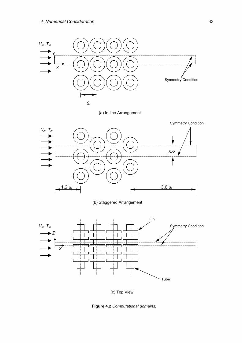
4 Numerical Consideration 33
Uin, Tin
Y
X
Symmetry Condition
Sl
(a) In-line Arrangement Symmetry Condition
Uin, Tin
St/2
1.2 df 3.6 df
(b) Staggered Arrangement
Fin
Uin, Tin Symmetry Condition Z
X
Tube
(c) Top View
Figure 4.2 Computational domains.
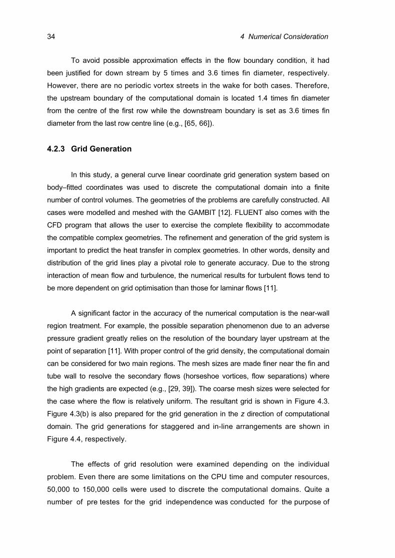
34 4 Numerical Consideration
To avoid possible approximation effects in the flow boundary condition, it had
been justified for down stream by 5 times and 3.6 times fin diameter, respectively.
However, there are no periodic vortex streets in the wake for both cases. Therefore,
the upstream boundary of the computational domain is located 1.4 times fin diameter
from the centre of the first row while the downstream boundary is set as 3.6 times fin
diameter from the last row centre line (e.g., [65, 66]).
4.2.3 Grid Generation
In this study, a general curve linear coordinate grid generation system based on
body–fitted coordinates was used to discrete the computational domain into a finite
number of control volumes. The geometries of the problems are carefully constructed. All
cases were modelled and meshed with the GAMBIT [12]. FLUENT also comes with the
CFD program that allows the user to exercise the complete flexibility to accommodate
the compatible complex geometries. The refinement and generation of the grid system is
important to predict the heat transfer in complex geometries. In other words, density and
distribution of the grid lines play a pivotal role to generate accuracy. Due to the strong
interaction of mean flow and turbulence, the numerical results for turbulent flows tend to
be more dependent on grid optimisation than those for laminar flows [11].
A significant factor in the accuracy of the numerical computation is the near-wall
region treatment. For example, the possible separation phenomenon due to an adverse
pressure gradient greatly relies on the resolution of the boundary layer upstream at the
point of separation [11]. With proper control of the grid density, the computational domain
can be considered for two main regions. The mesh sizes are made finer near the fin and
tube wall to resolve the secondary flows (horseshoe vortices, flow separations) where
the high gradients are expected (e.g., [29, 39]). The coarse mesh sizes were selected for
the case where the flow is relatively uniform. The resultant grid is shown in Figure 4.3.
Figure 4.3(b) is also prepared for the grid generation in the z direction of computational
domain. The grid generations for staggered and in-line arrangements are shown in
Figure 4.4, respectively.
The effects of grid resolution were examined depending on the individual
problem. Even there are some limitations on the CPU time and computer resources,
50,000 to 150,000 cells were used to discrete the computational domains. Quite a
number of pre testes for the grid independence was conducted for the purpose of
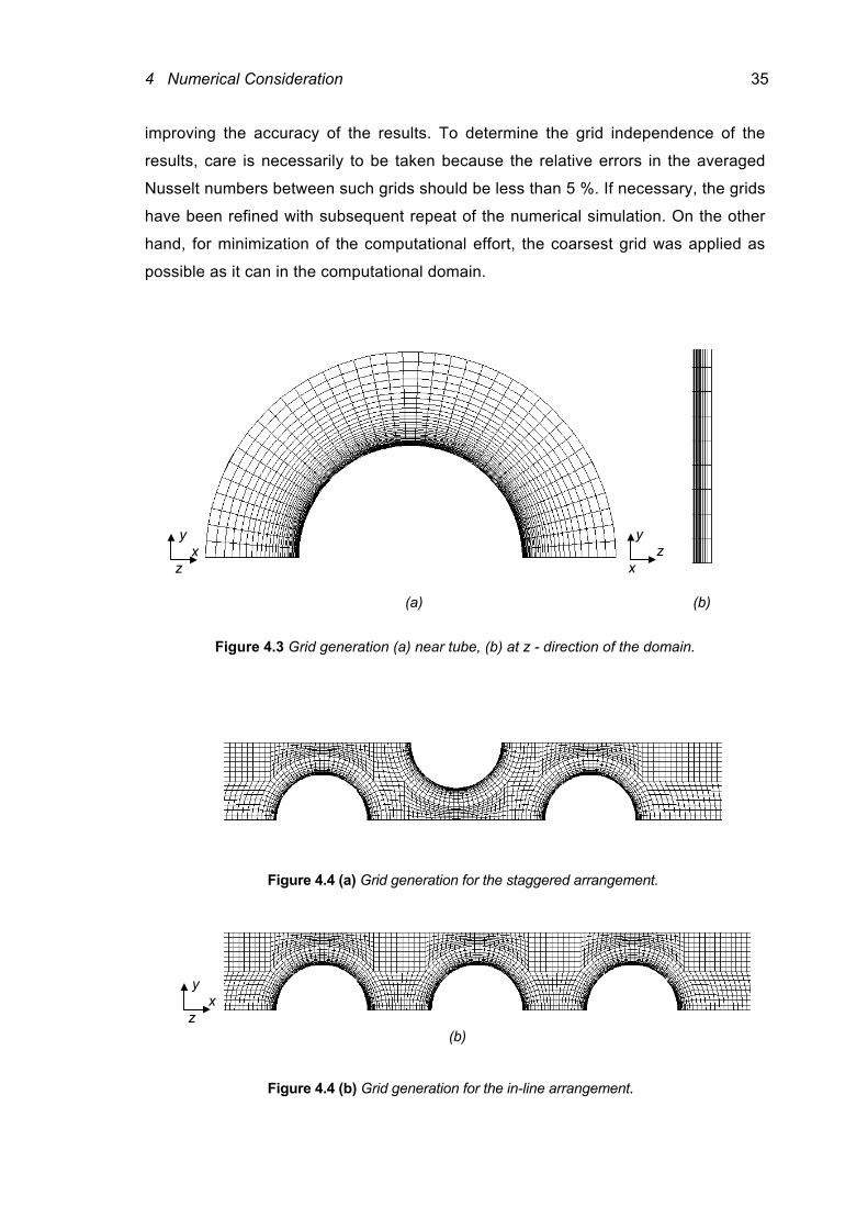
4 Numerical Consideration 35
improving the accuracy of the results. To determine the grid independence of the
results, care is necessarily to be taken because the relative errors in the averaged
Nusselt numbers between such grids should be less than 5 %. If necessary, the grids
have been refined with subsequent repeat of the numerical simulation. On the other
hand, for minimization of the computational effort, the coarsest grid was applied as
possible as it can in the computational domain.
(a) (b)
Figure 4.3 Grid generation (a) near tube, (b) at z - direction of the domain.
Figure 4.4 (a) Grid generation for the staggered arrangement.
(b)
Figure 4.4 (b) Grid generation for the in-line arrangement.
y x z
y z x
y x z
36 4 Numerical Consideration
4.2.4 Choosing the Physical Properties
The definition of physical properties (thermal conductivity, density, viscosity,
specific heat) of fluids and solids is a necessary factor for setting up the model. In this
study, the air is forced to pass between the fins, which transfers heat, and possibly
moisture to the fin and tube surface, from where the heat is conducted to the coolant.
However, in this study, it is assumed to be the dry air and no attempts were prepared
for condensation effects. For the solid’s part, aluminium is chosen for both the tube and
the fin.
4.2.5 Boundary Conditions
In order to evaluate the heat and momentum transfer of circular finned-tube
bundles, some preliminary conditions of the physical model have to be defined
appropriately. For the numerical approach to the problem, the boundary conditions are
required to set for all boundaries of the computational domain. At the upstream boundary
conditions, the air entering the computational domain is assumed to have uniform
velocity Uin, temperature Tin (308.15 K) and turbulent intensity I (1 %). The velocity
components in the y and z directions are considered to be zero. The fluid region consists
of the entrance, outlet, and bundle zone. The solid region includes the fin. At the solid
surfaces, no-slip conditions for the velocity are specified. Heat convection to the fin and
heat conduction in the fin is considered.
Constant temperature Tw (283.15 K) is assigned at the tube surface and all
velocity components are considered to be zero. To simplify the calculation, the flow
and thermal fields are assumed to be symmetric in the mid plane between the fins,
mid plane of the fin itself, centre plane of tube and at the half of the transverse pitch
from this tube as shown in Figure 4.2. At the symmetry planes assume a zero heat
flux. The normal velocity component at the symmetry plane is zero, i.e. no convective
flux across that symmetry plane. Thus, the temperature gradients and tangential
components of the velocity gradients in normal direction are set to be zero.
• Inlet: U = Uin = constant
T = Tin = constant
I = 1%
4 Numerical Consideration 37
• Outlet: Static pressure
• Tube: no-slip condition
T = Tw = constant
• Fin: no-slip condition
Coupling of conduction and convection
• Symmetry Plane: Velocity components in normal direction = 0
Temperature gradients in normal direction = 0
Gradient of tangential components of velocity in
normal direction = 0
The previous investigations of compact heat exchangers are set to be laminar
flow [22] and compared to the turbulent flow, a smaller pressure drop is expected in
laminar region. However, the turbulent flow is supposed to mix well and to get the more
intensive heat transfer while incomplete mixing of the fluid occurs in laminar flow. As
previously described in the literature review, the actual flow patterns of a circular
finned-tube heat exchanger are of the complex entity, which is not easy to figure
exactly. It should be noted that turbulent effects and unsteady conditions should be
considered as well since the flow field is so complex in finned-tube heat exchangers
[29].
When considering for a circular finned-tube heat exchanger under the proposed
range of Reynolds numbers, the flow in the finned-tube bundle has to be assumed to
be a three-dimensional, unsteady, incompressible turbulent flow. For the benefit of
accuracy, pre- tests were made with the turbulent flow condition for the whole domain
and consequently the results were obviously high when comparing with experimental
data. Nir [46] reported that the fins represent 80-95 % of the heat transfer surfaces in
modern finned-tube banks and the heat transfer phenomenon at the fin surface may be
considered as a process in channels. Moreover, Yudin et al. [80] also noted that the
flow in a bundle with high fins comes close to the nature of flow in the channel.
Therefore, for the convenience of calculation, the flow between the fins is considered
as a channel flow to be computed as laminar while the other parts of the bundle will be
treated as turbulent regions.
38 4 Numerical Consideration
4.2.6 Control Parameters
It is noteworthy that proper numerical control and modelling techniques are
necessary for to speed up convergence and stability of the calculation. With a control-
volume-based technique, FLUENT converts the governing equations to algebraic forms
that can be solved numerically. This control volume technique consists of integrating
the governing equations inside each control volume, yielding discrete equations that
conserve each quantity on a control-volume basis [11]. For discretization of equations,
the user needs to select the respective numerical schemes. The first order upwind
numerical scheme is selected to simulate the problems.
For the aspect of pressure-velocity coupling, The Pressure-Implicit with Splitting
of Operators (PISO) is selected. PISO pressure-velocity coupling scheme is a part of
the SIMPLE family and it is highly recommended for all transient flow calculations.
PISO is based on the higher degree of the approximate relation between the
corrections for pressure and velocity. An approach to judging convergence is setting as
the convergence criterion.
4.2.7 Computing Time
It can be easily noted that when dealing with three-dimensional unsteady
turbulent flow, the simulation may take longer than for steady flow problems. One
typical calculation with sufficient mesh sizes took about three days to get an acceptable
solution whereas just a few hours for the laminar flow cases. When simulating of
complex turbulent flows, the complicated geometry of the heat exchanger and
associated grid resolutions may impose restrictions on the computational time step. It
showed that the dense grid resolution would restrict the time step. To determine the
time step size, FLUENT [11] reported that there is no stability criterion that needs to be
met. However, FLUENT recommends that the time step should be at least one order of
magnitude smaller than the smallest time constant in the system being modelled. By
observing the number of iterations needed to converge at each time step, the time step
size is able to be judged. The ideal number of iterations per time step is 10 to 20. For
the purpose of accuracy it should start with a smaller time step. Thus all the tests are
processed with the time increment ∆ t = 0.001 sec at initial condition and then,
gradually it is increased as the calculation proceeds.
4 Numerical Consideration 39
Numerical simulations were performed with a SGI – Indigo 2 (1 CPU R8000,
175 MHz, 256 MB RAM) and Dogbert workstation (2 CPU R12000, 2300 MHz, 768 MB
RAM). Time-marching calculations are stopped when either a steady or periodic flow
was encountered, or in case of a time-periodic solution when it becomes approximately
constant. FLUENT provides for post processing and it is also able to track the
convergence during the solution process.
4.2.8 Algorithm
In order to simulate, the following procedures of analysis are performed:
1. Start the FLUENT with 3D solver
2. Read an existing grid file and feed into FLUENT
3. Check the grid (e.g., concerning the dimension of the calculation domain, the
cell volume, the number of nodes and area of each cell)
4. Choose the suitable type of solver:
Fluent supplies three types of solver for solving the discrete equation. Basically,
the specific characteristics of the investigation (incompressible and mildly
compressible flows) are dealt with “segregated solver”. This solver solves the
continuity, momentum, energy and species equations sequentially (i.e.,
Segregated from one another) while the other two solvers solve these
equations simultaneously (i.e., coupled together) applied for high-speed
compressible flow. Here the segregated solver has been selected.
5. Choose the model:
To calculate the flow field, select the k-ε (RNG) model and for the near fin
treatment, set standard wall functions. For coupling heat transfer (convection
and conduction), activate the energy equation.

40 4 Numerical Consideration
6. Define the properties of following material:
• Components of dry air
• Aluminium
Detailed material properties are shown in the Appendix A.
7. Define the boundary conditions (see section 4.2.5)
8. Define the control parameter:
The following under-relaxation factors are set.
• Pressure 0.3
• Energy 1.0
• Momentum 0.7
• Turbulent kinetic energy 0.8
• Turbulent dissipation rate 0.8
Select the reference of discretization of differential equations,
• For pressure choose, STANDARD
• For momentum choose, First order upwind
• For pressure-velocity coupling choose, PISO
• For energy choose, First order upwind
• For turbulent kinetic energy choose, First order upwind
• For turbulent dissipation rate choose, First order upwind
Set the convergence criteria,
Continuity = 0.001 k = 0.001 ε = 0.001
x, y, z velocity = 0.001 Energy = 1e-6
9. Initialisation of flow field.
10. Calculate the solution.
11. Save the result.

5 Results and Discussion
This chapter mostly deals with the results of the investigations of the main
characteristics that affects the heat transfer and pressure drop of circular finned-tube
banks. In addition to describing the substantial geometric parameters and their
performance characteristics, local heat transfer and flow results are illustrated and
discussed separately.
5.1 Evaluation of Nusselt and Euler Numbers FLUENT evaluates the Nusselt number and Euler number as follows:
The outlet air temperature Tout was calculated as a mass average temperature at
the outlet position of the calculation domain.
∑
∑
∫∫
=
=== n
iiii
n
iiiii
out
Au
A.uT
Ad.u
Ad.uTT
1
1vv
vv
vr
rv
ρ
ρ
ρ
ρ (5.1)
The enthalpy flow rate of air at the inlet and outlet were calculated as,
iii
n
1ii A.uh~Ad.uh~H
vvvv& ρρ∫ ∑=
== (5.2)
with the specific enthalpy
dTch~T
Tp
ref
∫= (5.3)
where FLUENT set as Tref = 298.15 K.
42 5 Results and Discussion
Enthalpy flow rates of the inlet inH& and outlet outH& positions of the
computational domain (Equation 5.2) were determined by the aid of FLUENT and then
the air-side heat transfer rate of the bundle was calculated according to Equation (5.4).
Q& = outH& - inH& (5.4)
By this air-side heat transfer flow rate, the heat transfer coefficient of the air-side
h can be evaluated by means of the Equation (5.5) where At is the tube surface area, Af
is the fin surface area and η is the fin efficiency.
LMTD)AA(Qh
ft
.
η+= (5.5)
In here assume the heat transfer coefficient at the fin and base-tube is the same.
LMTD is the log mean temperature difference,
LMTD
wout
win
outin
TTTTln
TT
−−
−= (5.6)
The inlet air temperature and base-tube surface temperature were set as
boundary condition with Tin = 308.15 K and Tw = 283.15 K (see in section 4.2.5). The
outlet air temperature, Tout was evaluated from the Equation (5.1). The base-tube
surface area, At, and the fin surface area, Af were calculated as
( )n.SdA ft δπ −= , ( ) n.dddA fff
+−= δππ 22
2 (5.7)
The fin efficiency, which is needed for the determination of the heat transfer
coefficient, arises as a result of iterative calculations of Equation (5.8) and (5.9) and the
heat transfer coefficient from the Equation (5.5). As Equation (5.8), the fin efficiency
fη approaches its maximum and minimum values of 1 and 0, respectively, as hf
approaches 0 and ∝. The value of ψ was derived from the Equation (5.10) individually.
( )f
f
ψmhψmhtanhη = (5.8)
5 Results and Discussion 43
δfkhm 2
= (5.9)
dh
..ln(.. f020135001 ++=ψ ) (5.10)
The method for calculation of the fin efficiency was taken from VDI-Wärmeatlas
[68] in which the heat transfer coefficient h over the fin surface is assumed to be a
constant mean value. Though it is not uniform in practice, such uncertainties are not
reflected in Equation. 5.5 (Kearney and Jacobi [32], and Sparrow and Samie [59]).
The dimensionless number for air-side heat transfer in the finned-tube bank was
defined and calculated depending on the Reynolds number and geometric parameters.
For many cases the Nusselt number, the Colburn j factor, Stanton number are used to
express the heat transfer coefficient and the characteristic length is not the same. Tube
outside diameter, hydraulic diameter, fin spacing, equivalent diameter were varied from
experiment to experiment.
In here the Nu number was used as
ak
hdNu = (5.11)
The properties of air (thermal conductivity, dynamic viscosity) at inlet temperature
are displayed in the Appendix A. The influence of geometric parameters and the inlet
air parameter on the pressure loss and resistance for the in-line and staggered bundles
are investigated as
2maxUpEu
ρ∆
= (5.12)
where outin ppp −=∆
The static pressure at the inlet and outlet of the computational domain were
evaluated as
∑
∑
∫∫
=
=== n
1ii
n
1iii
out,in
A
Ap
Ad
Apdp
v
v
v
v
(5.13)
44 5 Results and Discussion
5.2 Local Heat Transfer and Flow Results
The results and discussions are divided into three topics accordingly. The
present study includes the nature of boundary layer developments, local velocity and
temperature variations between the two adjacent fins and over the fin surface, the
horseshoe vortices system, the occurrence of the flow separation on the tube and wake
behind the tube. Since the convection boundary layer development is the most
influential factor of the local heat transfer and flow behaviour, the flow visualization
results particularly concerning the nature of the horseshoe vortex flow patterns will be
discussed firstly. Secondly, the temperature boundary layer development between the
fins and the temperature distributions over the fin surface and within the fins are
outlined. Finally, the flow and temperature distributions near the fin surface and on the
mid-plane between fins will be covered.
5.2.1 Local Flow Behaviour
The temperature and velocity boundary layers on the fin and tube surfaces are
strongly dependent on the spacing between the fins and the corresponding velocity.
Therefore, the numerical results will be presented which are carried out for three
different fin spacings (1.6 mm, 2 mm and 4 mm) for a fixed fin height of 5 mm and tube
diameter of 24 mm. In addition, it may be useful to discuss the natures of velocity
distribution of the first and second rows, respectively.
Staggered Arrangement
Figure 5.1 shows velocity distributions between the fins of the first row for three
different spacings of the staggered array at (θ = 0°) corresponding to the stagnation
point of each tube for Re = 8.6 x 10³. For the narrowest fin spacing of s = 1.6 mm, two
boundary layers grow from the leading edge of the fins. According to the flow
visualization results, the velocity boundary layers at the fin base and tube surface are
seen to be thicker. Owing to the adverse pressure gradient effect, a horseshoe vortex
system is developed near the junction of tube and fins for all three spacing cases. A
boundary layer will be formed when the fluid stream meets the leading edge of the fin
surface. As the fluid goes on, the thickness of the boundary will be amplified. Hence,
the local heat transfer coefficient may change from point to point of the finned surface.
In addition, the velocity is reduced in the upstream region and the flow forms the
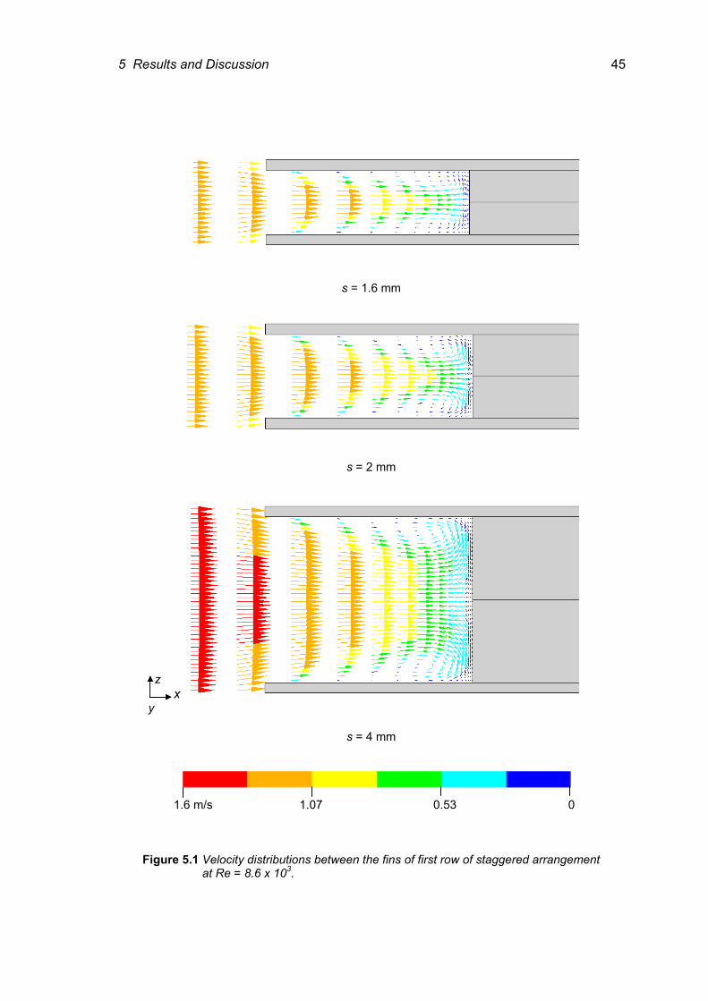
5 Results and Discussion 45
s = 1.6 mm
s = 2 mm
s = 4 mm
Figure 5.1 Velocity distributions between the fins of first row of staggered arrangement at Re = 8.6 x 10³.
1.6 m/s 1.07 0.53 0
z x y
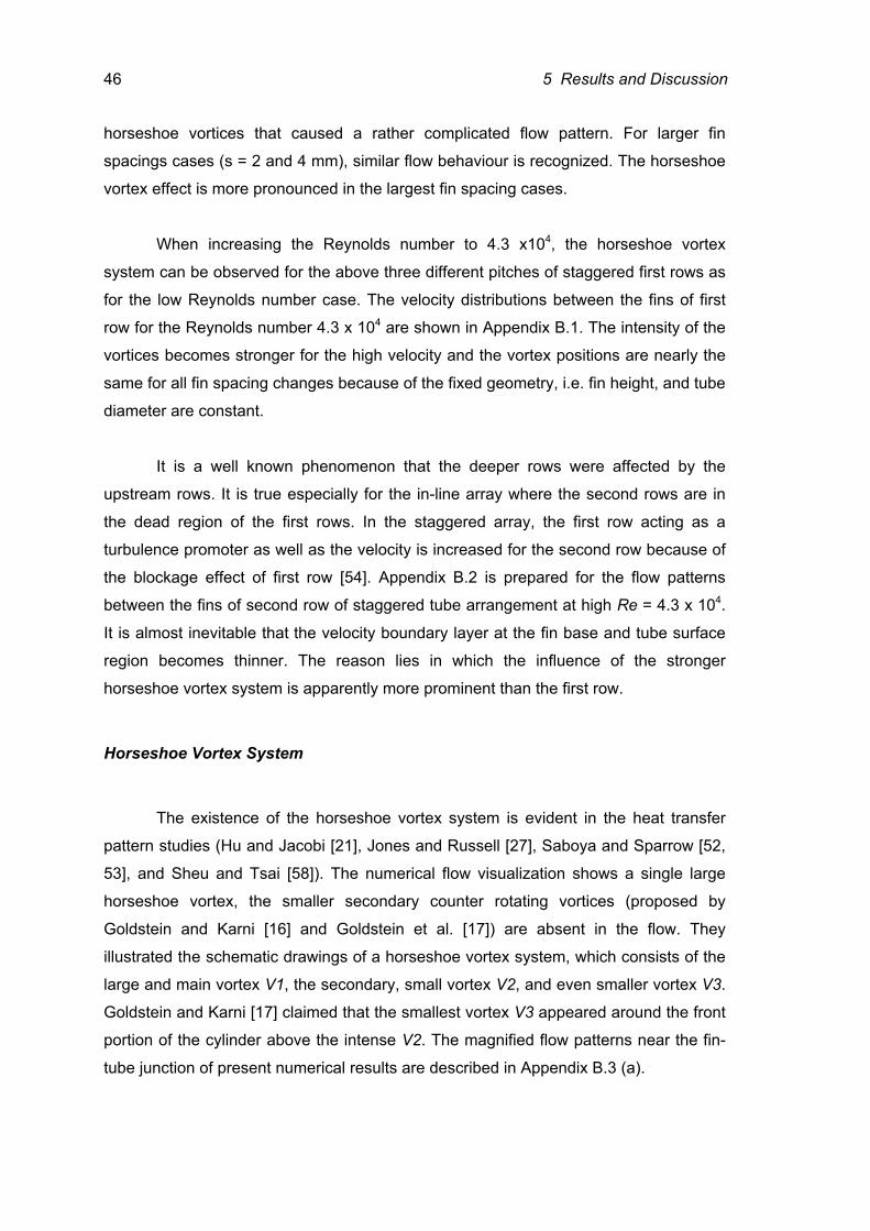
46 5 Results and Discussion
horseshoe vortices that caused a rather complicated flow pattern. For larger fin
spacings cases (s = 2 and 4 mm), similar flow behaviour is recognized. The horseshoe
vortex effect is more pronounced in the largest fin spacing cases.
When increasing the Reynolds number to 4.3 x10⁴, the horseshoe vortex
system can be observed for the above three different pitches of staggered first rows as
for the low Reynolds number case. The velocity distributions between the fins of first
row for the Reynolds number 4.3 x 10⁴ are shown in Appendix B.1. The intensity of the
vortices becomes stronger for the high velocity and the vortex positions are nearly the
same for all fin spacing changes because of the fixed geometry, i.e. fin height, and tube
diameter are constant.
It is a well known phenomenon that the deeper rows were affected by the
upstream rows. It is true especially for the in-line array where the second rows are in
the dead region of the first rows. In the staggered array, the first row acting as a
turbulence promoter as well as the velocity is increased for the second row because of
the blockage effect of first row [54]. Appendix B.2 is prepared for the flow patterns
between the fins of second row of staggered tube arrangement at high Re = 4.3 x 10⁴.
It is almost inevitable that the velocity boundary layer at the fin base and tube surface
region becomes thinner. The reason lies in which the influence of the stronger
horseshoe vortex system is apparently more prominent than the first row.
Horseshoe Vortex System
The existence of the horseshoe vortex system is evident in the heat transfer
pattern studies (Hu and Jacobi [21], Jones and Russell [27], Saboya and Sparrow [52,
53], and Sheu and Tsai [58]). The numerical flow visualization shows a single large
horseshoe vortex, the smaller secondary counter rotating vortices (proposed by
Goldstein and Karni [16] and Goldstein et al. [17]) are absent in the flow. They
illustrated the schematic drawings of a horseshoe vortex system, which consists of the
large and main vortex V1, the secondary, small vortex V2, and even smaller vortex V3.
Goldstein and Karni [17] claimed that the smallest vortex V3 appeared around the front
portion of the cylinder above the intense V2. The magnified flow patterns near the fin-
tube junction of present numerical results are described in Appendix B.3 (a).
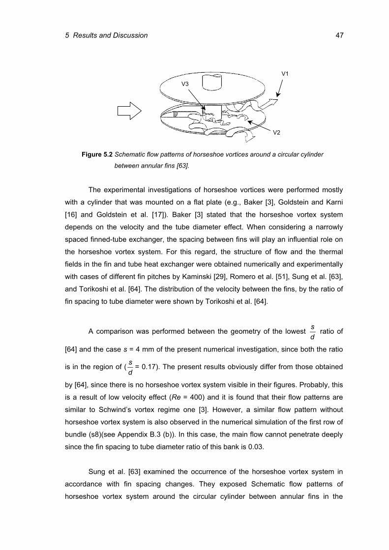
5 Results and Discussion 47
Figure 5.2 Schematic flow patterns of horseshoe vortices around a circular cylinder
between annular fins [63].
The experimental investigations of horseshoe vortices were performed mostly
with a cylinder that was mounted on a flat plate (e.g., Baker [3], Goldstein and Karni
[16] and Goldstein et al. [17]). Baker [3] stated that the horseshoe vortex system
depends on the velocity and the tube diameter effect. When considering a narrowly
spaced finned-tube exchanger, the spacing between fins will play an influential role on
the horseshoe vortex system. For this regard, the structure of flow and the thermal
fields in the fin and tube heat exchanger were obtained numerically and experimentally
with cases of different fin pitches by Kaminski [29], Romero et al. [51], Sung et al. [63],
and Torikoshi et al. [64]. The distribution of the velocity between the fins, by the ratio of
fin spacing to tube diameter were shown by Torikoshi et al. [64].
A comparison was performed between the geometry of the lowest ds ratio of
[64] and the case s = 4 mm of the present numerical investigation, since both the ratio
is in the region of (ds = 0.17). The present results obviously differ from those obtained
by [64], since there is no horseshoe vortex system visible in their figures. Probably, this
is a result of low velocity effect (Re = 400) and it is found that their flow patterns are
similar to Schwind’s vortex regime one [3]. However, a similar flow pattern without
horseshoe vortex system is also observed in the numerical simulation of the first row of
bundle (s8)(see Appendix B.3 (b)). In this case, the main flow cannot penetrate deeply
since the fin spacing to tube diameter ratio of this bank is 0.03.
Sung et al. [63] examined the occurrence of the horseshoe vortex system in
accordance with fin spacing changes. They exposed Schematic flow patterns of
horseshoe vortex system around the circular cylinder between annular fins in the
V1
V2
V3
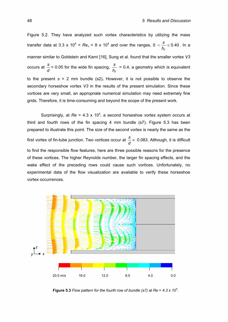
48 5 Results and Discussion
Figure 5.2. They have analyzed such vortex characteristics by utilizing the mass
transfer data at 3.3 x 10⁴ < Reα < 8 x 10⁴ and over the ranges, 0 400.hsf≤< . In a
manner similar to Goldstein and Karni [16], Sung et al. found that the smaller vortex V3
occurs at ds = 0.05 for the wide fin spacing,
fhs = 0.4, a geometry which is equivalent
to the present s = 2 mm bundle (s2). However, it is not possible to observe the
secondary horseshoe vortex V3 in the results of the present simulation. Since these
vortices are very small, an appropriate numerical simulation may need extremely fine
grids. Therefore, it is time-consuming and beyond the scope of the present work.
Surprisingly, at Re = 4.3 x 10⁴, a second horseshoe vortex system occurs at
third and fourth rows of the fin spacing 4 mm bundle (s7). Figure 5.3 has been
prepared to illustrate this point. The size of the second vortex is nearly the same as the
first vortex of fin-tube junction. Two vortices occur at ≈ds 0.083. Although, it is difficult
to find the responsible flow features, here are three possible reasons for the presence
of these vortices. The higher Reynolds number, the larger fin spacing effects, and the
wake effect of the preceding rows could cause such vortices. Unfortunately, no
experimental data of the flow visualization are available to verify these horseshoe
vortex occurrences.
x
20.0 m/s 16.0 12.0 8.0 4.0 0.0
Figure 5.3 Flow pattern for the fourth row of bundle (s7) at Re = 4.3 x 10⁴.
z
y
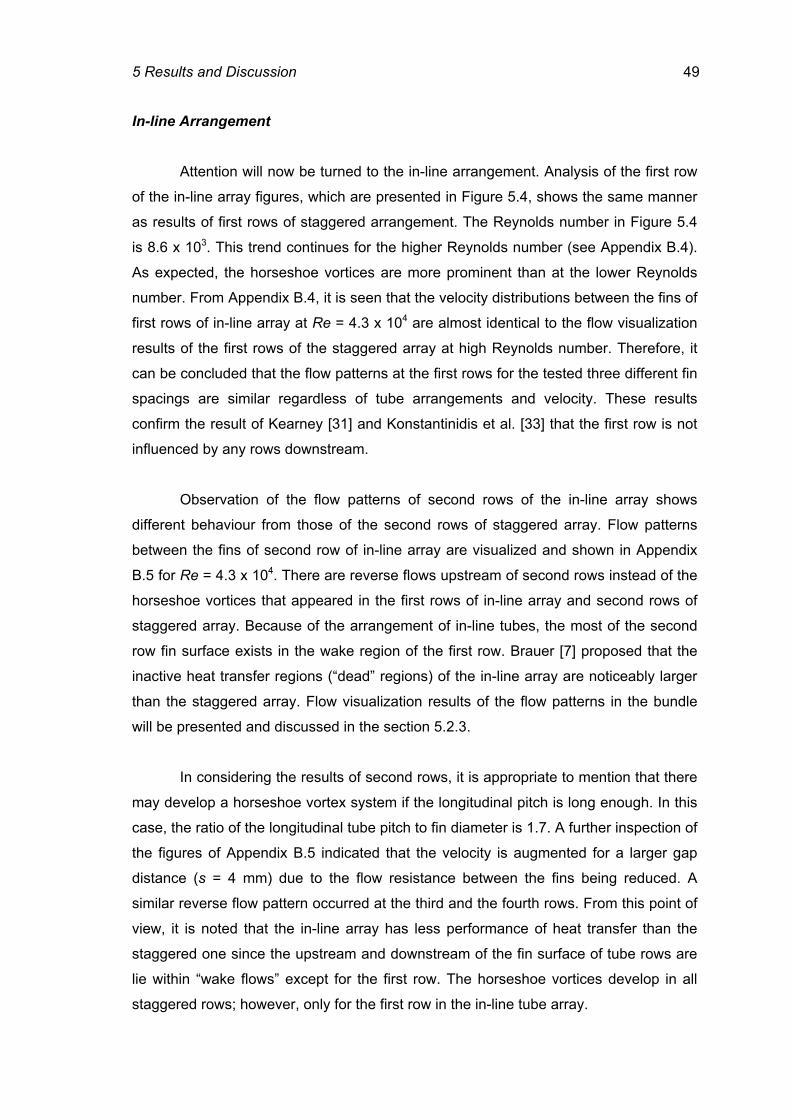
5 Results and Discussion 49
In-line Arrangement
Attention will now be turned to the in-line arrangement. Analysis of the first row
of the in-line array figures, which are presented in Figure 5.4, shows the same manner
as results of first rows of staggered arrangement. The Reynolds number in Figure 5.4
is 8.6 x 10³. This trend continues for the higher Reynolds number (see Appendix B.4).
As expected, the horseshoe vortices are more prominent than at the lower Reynolds
number. From Appendix B.4, it is seen that the velocity distributions between the fins of
first rows of in-line array at Re = 4.3 x 10⁴ are almost identical to the flow visualization
results of the first rows of the staggered array at high Reynolds number. Therefore, it
can be concluded that the flow patterns at the first rows for the tested three different fin
spacings are similar regardless of tube arrangements and velocity. These results
confirm the result of Kearney [31] and Konstantinidis et al. [33] that the first row is not
influenced by any rows downstream.
Observation of the flow patterns of second rows of the in-line array shows
different behaviour from those of the second rows of staggered array. Flow patterns
between the fins of second row of in-line array are visualized and shown in Appendix
B.5 for Re = 4.3 x 10⁴. There are reverse flows upstream of second rows instead of the
horseshoe vortices that appeared in the first rows of in-line array and second rows of
staggered array. Because of the arrangement of in-line tubes, the most of the second
row fin surface exists in the wake region of the first row. Brauer [7] proposed that the
inactive heat transfer regions (“dead” regions) of the in-line array are noticeably larger
than the staggered array. Flow visualization results of the flow patterns in the bundle
will be presented and discussed in the section 5.2.3.
In considering the results of second rows, it is appropriate to mention that there
may develop a horseshoe vortex system if the longitudinal pitch is long enough. In this
case, the ratio of the longitudinal tube pitch to fin diameter is 1.7. A further inspection of
the figures of Appendix B.5 indicated that the velocity is augmented for a larger gap
distance (s = 4 mm) due to the flow resistance between the fins being reduced. A
similar reverse flow pattern occurred at the third and the fourth rows. From this point of
view, it is noted that the in-line array has less performance of heat transfer than the
staggered one since the upstream and downstream of the fin surface of tube rows are
lie within “wake flows” except for the first row. The horseshoe vortices develop in all
staggered rows; however, only for the first row in the in-line tube array.
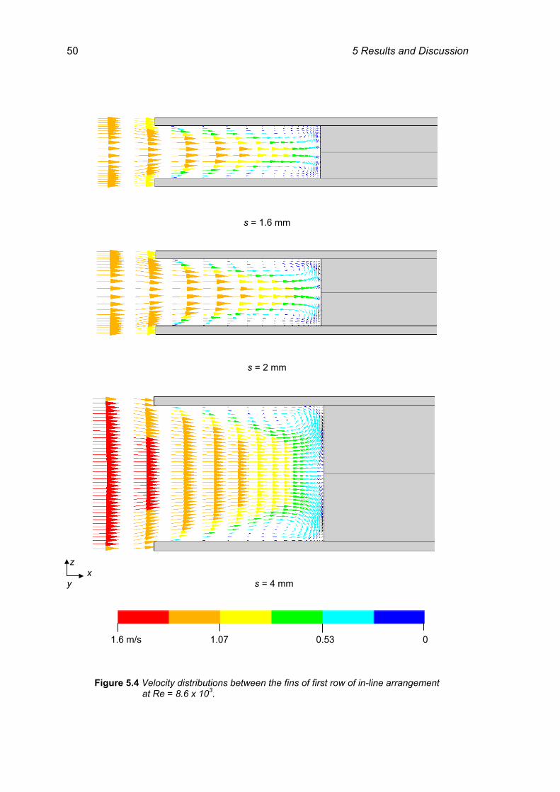
50 5 Results and Discussion
s = 1.6 mm
s = 2 mm
z x y s = 4 mm
Figure 5.4 Velocity distributions between the fins of first row of in-line arrangement at Re = 8.6 x 10³.
1.6 m/s 1.07 0.53 0
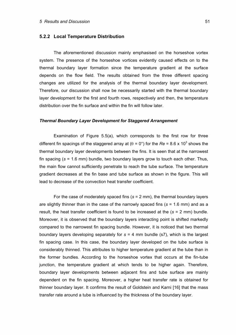
5 Results and Discussion 51
5.2.2 Local Temperature Distribution
The aforementioned discussion mainly emphasised on the horseshoe vortex
system. The presence of the horseshoe vortices evidently caused effects on to the
thermal boundary layer formation since the temperature gradient at the surface
depends on the flow field. The results obtained from the three different spacing
changes are utilized for the analysis of the thermal boundary layer development.
Therefore, our discussion shall now be necessarily started with the thermal boundary
layer development for the first and fourth rows, respectively and then, the temperature
distribution over the fin surface and within the fin will follow later.
Thermal Boundary Layer Development for Staggered Arrangement
Examination of Figure 5.5(a), which corresponds to the first row for three
different fin spacings of the staggered array at (θ = 0°) for the Re = 8.6 x 10³ shows the
thermal boundary layer developments between the fins. It is seen that at the narrowest
fin spacing (s = 1.6 mm) bundle, two boundary layers grow to touch each other. Thus,
the main flow cannot sufficiently penetrate to reach the tube surface. The temperature
gradient decreases at the fin base and tube surface as shown in the figure. This will
lead to decrease of the convection heat transfer coefficient.
For the case of moderately spaced fins (s = 2 mm), the thermal boundary layers
are slightly thinner than in the case of the narrowly spaced fins (s = 1.6 mm) and as a
result, the heat transfer coefficient is found to be increased at the (s = 2 mm) bundle.
Moreover, it is observed that the boundary layers interacting point is shifted markedly
compared to the narrowest fin spacing bundle. However, it is noticed that two thermal
boundary layers developing separately for s = 4 mm bundle (s7), which is the largest
fin spacing case. In this case, the boundary layer developed on the tube surface is
considerably thinned. This attributes to higher temperature gradient at the tube than in
the former bundles. According to the horseshoe vortex that occurs at the fin-tube
junction, the temperature gradient at which tends to be higher again. Therefore,
boundary layer developments between adjacent fins and tube surface are mainly
dependent on the fin spacing. Moreover, a higher heat transfer rate is obtained for
thinner boundary layer. It confirms the result of Goldstein and Karni [16] that the mass
transfer rate around a tube is influenced by the thickness of the boundary layer.
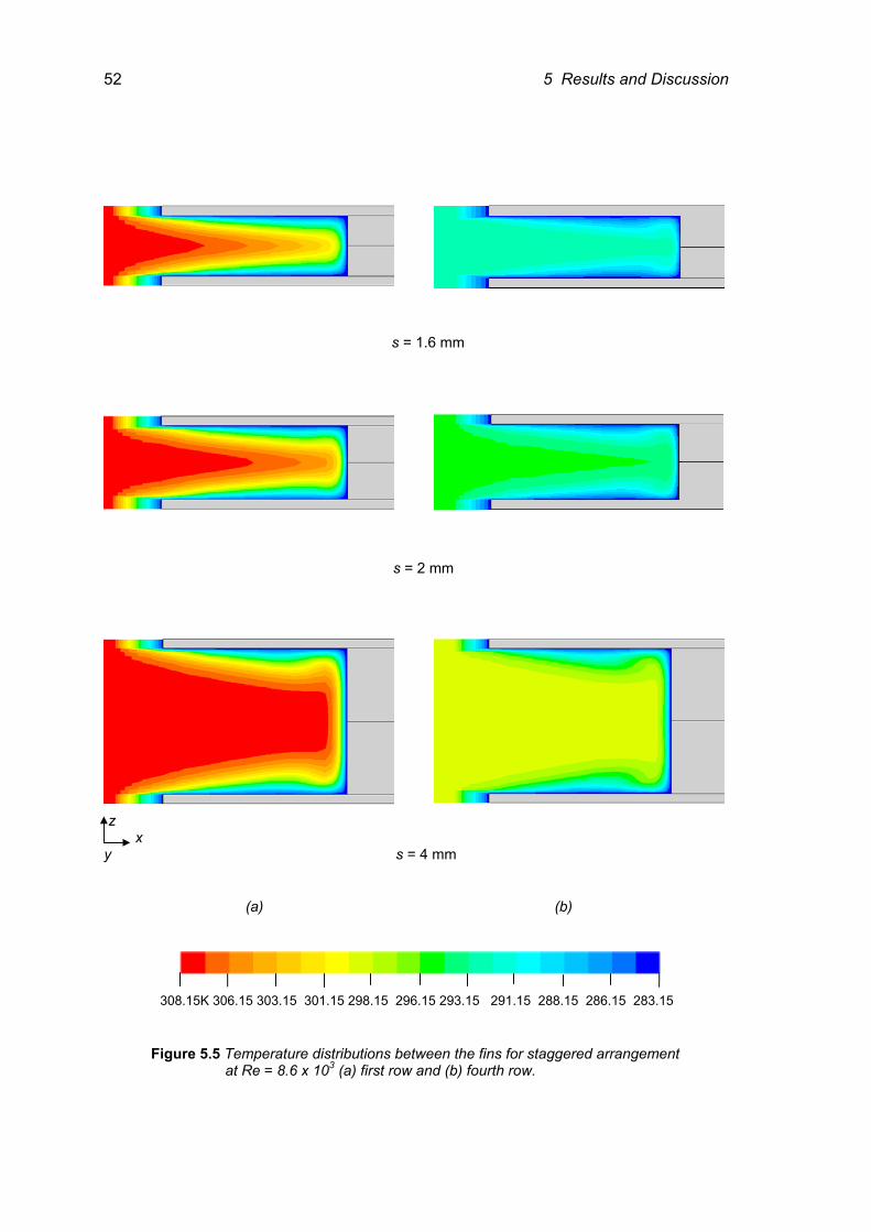
52 5 Results and Discussion
s = 1.6 mm
s = 2 mm
z x y s = 4 mm (a) (b)
308.15K 306.15 303.15 301.15 298.15 296.15 293.15 291.15 288.15 286.15 283.15
Figure 5.5 Temperature distributions between the fins for staggered arrangement at Re = 8.6 x 10³ (a) first row and (b) fourth row.
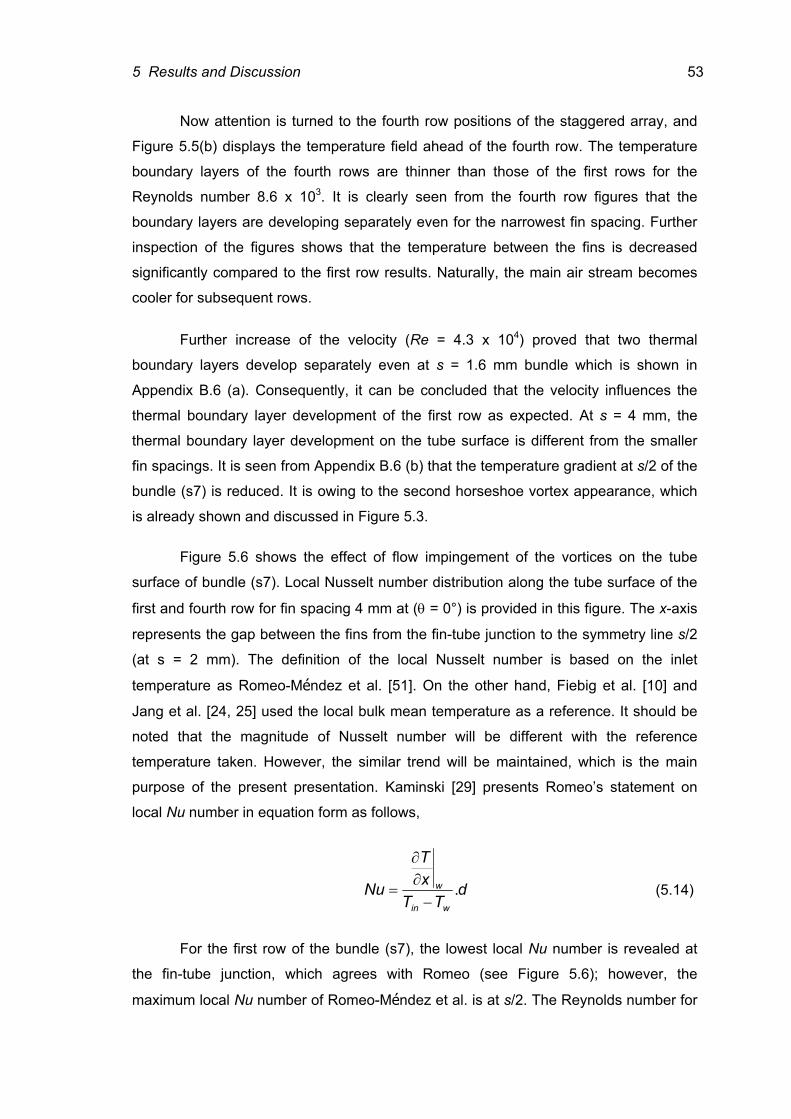
5 Results and Discussion 53
Now attention is turned to the fourth row positions of the staggered array, and
Figure 5.5(b) displays the temperature field ahead of the fourth row. The temperature
boundary layers of the fourth rows are thinner than those of the first rows for the
Reynolds number 8.6 x 10³. It is clearly seen from the fourth row figures that the
boundary layers are developing separately even for the narrowest fin spacing. Further
inspection of the figures shows that the temperature between the fins is decreased
significantly compared to the first row results. Naturally, the main air stream becomes
cooler for subsequent rows.
Further increase of the velocity (Re = 4.3 x 10⁴) proved that two thermal
boundary layers develop separately even at s = 1.6 mm bundle which is shown in
Appendix B.6 (a). Consequently, it can be concluded that the velocity influences the
thermal boundary layer development of the first row as expected. At s = 4 mm, the
thermal boundary layer development on the tube surface is different from the smaller
fin spacings. It is seen from Appendix B.6 (b) that the temperature gradient at s/2 of the
bundle (s7) is reduced. It is owing to the second horseshoe vortex appearance, which
is already shown and discussed in Figure 5.3.
Figure 5.6 shows the effect of flow impingement of the vortices on the tube
surface of bundle (s7). Local Nusselt number distribution along the tube surface of the
first and fourth row for fin spacing 4 mm at (θ = 0°) is provided in this figure. The x-axis
represents the gap between the fins from the fin-tube junction to the symmetry line s/2
(at s = 2 mm). The definition of the local Nusselt number is based on the inlet
temperature as Romeo-Méndez et al. [51]. On the other hand, Fiebig et al. [10] and
Jang et al. [24, 25] used the local bulk mean temperature as a reference. It should be
noted that the magnitude of Nusselt number will be different with the reference
temperature taken. However, the similar trend will be maintained, which is the main
purpose of the present presentation. Kaminski [29] presents Romeo’s statement on
local Nu number in equation form as follows,
dTT
xT
Nuwin
w .−
∂∂
= (5.14)
For the first row of the bundle (s7), the lowest local Nu number is revealed at
the fin-tube junction, which agrees with Romeo (see Figure 5.6); however, the
maximum local Nu number of Romeo-Méndez et al. is at s/2. The Reynolds number for
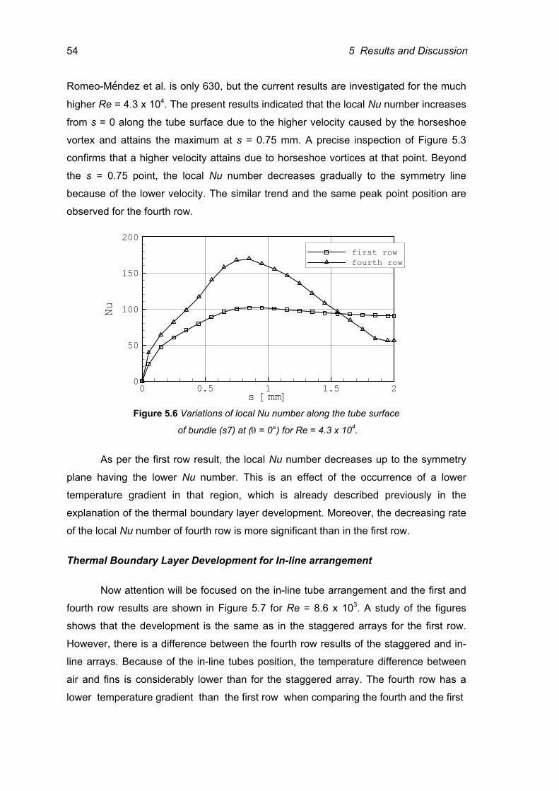
54 5 Results and Discussion
Romeo-Méndez et al. is only 630, but the current results are investigated for the much
higher Re = 4.3 x 10⁴. The present results indicated that the local Nu number increases
from s = 0 along the tube surface due to the higher velocity caused by the horseshoe
vortex and attains the maximum at s = 0.75 mm. A precise inspection of Figure 5.3
confirms that a higher velocity attains due to horseshoe vortices at that point. Beyond
the s = 0.75 point, the local Nu number decreases gradually to the symmetry line
because of the lower velocity. The similar trend and the same peak point position are
observed for the fourth row.
0 0.5 1 1.5 2s [mm]0
50
100
150
200
Nu
first rowfourth row
Figure 5.6 Variations of local Nu number along the tube surface
of bundle (s7) at (θ = 0°) for Re = 4.3 x 10⁴.
As per the first row result, the local Nu number decreases up to the symmetry
plane having the lower Nu number. This is an effect of the occurrence of a lower
temperature gradient in that region, which is already described previously in the
explanation of the thermal boundary layer development. Moreover, the decreasing rate
of the local Nu number of fourth row is more significant than in the first row.
Thermal Boundary Layer Development for In-line arrangement
Now attention will be focused on the in-line tube arrangement and the first and
fourth row results are shown in Figure 5.7 for Re = 8.6 x 10³. A study of the figures
shows that the development is the same as in the staggered arrays for the first row.
However, there is a difference between the fourth row results of the staggered and in-
line arrays. Because of the in-line tubes position, the temperature difference between
air and fins is considerably lower than for the staggered array. The fourth row has a
lower temperature gradient than the first row when comparing the fourth and the first
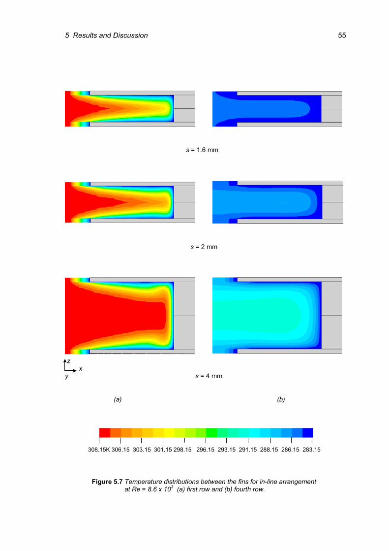
5 Results and Discussion 55
s = 1.6 mm
s = 2 mm
z x y s = 4 mm (a) (b)
308.15K 306.15 303.15 301.15 298.15 296.15 293.15 291.15 288.15 286.15 283.15
Figure 5.7 Temperature distributions between the fins for in-line arrangement at Re = 8.6 x 10³ (a) first row and (b) fourth row.
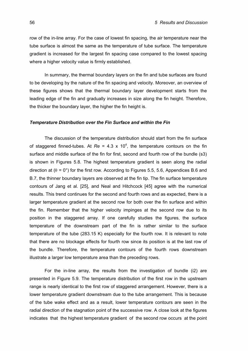
56 5 Results and Discussion
row of the in-line array. For the case of lowest fin spacing, the air temperature near the
tube surface is almost the same as the temperature of tube surface. The temperature
gradient is increased for the largest fin spacing case compared to the lowest spacing
where a higher velocity value is firmly established. In summary, the thermal boundary layers on the fin and tube surfaces are found
to be developing by the nature of the fin spacing and velocity. Moreover, an overview of
these figures shows that the thermal boundary layer development starts from the
leading edge of the fin and gradually increases in size along the fin height. Therefore,
the thicker the boundary layer, the higher the fin height is.
Temperature Distribution over the Fin Surface and within the Fin
The discussion of the temperature distribution should start from the fin surface
of staggered finned-tubes. At Re = 4.3 x 10⁴, the temperature contours on the fin
surface and middle surface of the fin for first, second and fourth row of the bundle (s3)
is shown in Figures 5.8. The highest temperature gradient is seen along the radial
direction at (θ = 0°) for the first row. According to Figures 5.5, 5.6, Appendices B.6 and
B.7, the thinner boundary layers are observed at the fin tip. The fin surface temperature
contours of Jang et al. [25], and Neal and Hitchcock [45] agree with the numerical
results. This trend continues for the second and fourth rows and as expected, there is a
larger temperature gradient at the second row for both over the fin surface and within
the fin. Remember that the higher velocity impinges at the second row due to its
position in the staggered array. If one carefully studies the figures, the surface
temperature of the downstream part of the fin is rather similar to the surface
temperature of the tube (283.15 K) especially for the fourth row. It is relevant to note
that there are no blockage effects for fourth row since its position is at the last row of
the bundle. Therefore, the temperature contours of the fourth rows downstream
illustrate a larger low temperature area than the preceding rows.
For the in-line array, the results from the investigation of bundle (i2) are
presented in Figure 5.9. The temperature distribution of the first row in the upstream
range is nearly identical to the first row of staggered arrangement. However, there is a
lower temperature gradient downstream due to the tube arrangement. This is because
of the tube wake effect and as a result, lower temperature contours are seen in the
radial direction of the stagnation point of the successive row. A close look at the figures
indicates that the highest temperature gradient of the second row occurs at the point
5 Results and Discussion 57
(a) (b)
287.15K 286.15 285.15 284.15 283.15 Figure 5.8 Temperature contours for staggered arrangement at (a) over fin surface and (b)
within fin of bundle (s3) at Re =4.3 x 10⁴.
1st row 1st row
2nd row 2nd row
4th row 4th row
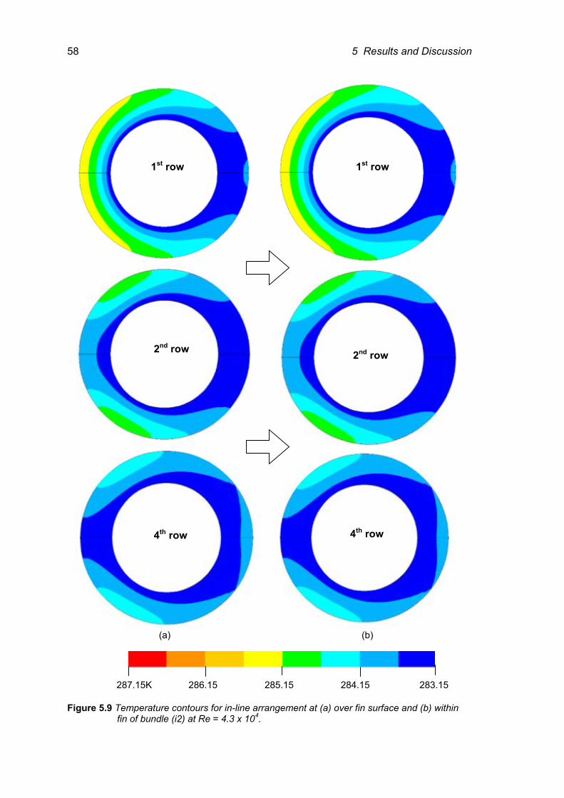
58 5 Results and Discussion
(a) (b)
287.15K 286.15 285.15 284.15 283.15
Figure 5.9 Temperature contours for in-line arrangement at (a) over fin surface and (b) within fin of bundle (i2) at Re = 4.3 x 10⁴.
1st row 1st row
2nd row 2nd row
4th row 4th row
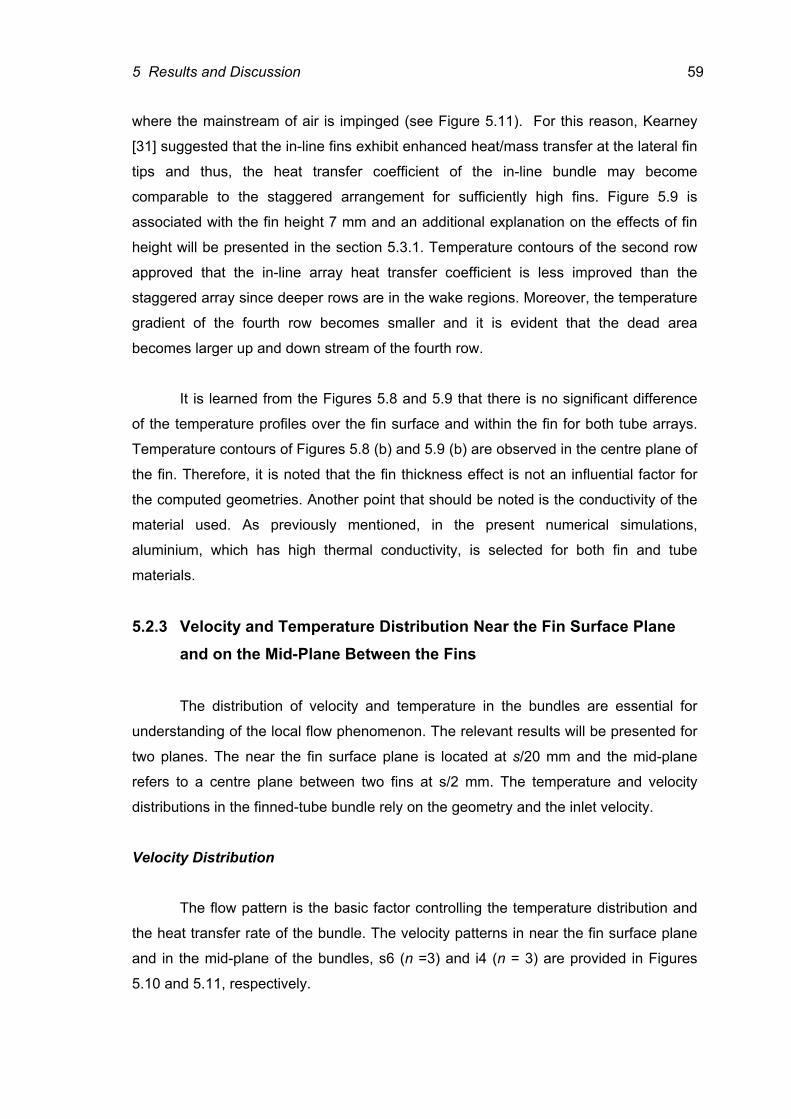
5 Results and Discussion 59
where the mainstream of air is impinged (see Figure 5.11). For this reason, Kearney
[31] suggested that the in-line fins exhibit enhanced heat/mass transfer at the lateral fin
tips and thus, the heat transfer coefficient of the in-line bundle may become
comparable to the staggered arrangement for sufficiently high fins. Figure 5.9 is
associated with the fin height 7 mm and an additional explanation on the effects of fin
height will be presented in the section 5.3.1. Temperature contours of the second row
approved that the in-line array heat transfer coefficient is less improved than the
staggered array since deeper rows are in the wake regions. Moreover, the temperature
gradient of the fourth row becomes smaller and it is evident that the dead area
becomes larger up and down stream of the fourth row.
It is learned from the Figures 5.8 and 5.9 that there is no significant difference
of the temperature profiles over the fin surface and within the fin for both tube arrays.
Temperature contours of Figures 5.8 (b) and 5.9 (b) are observed in the centre plane of
the fin. Therefore, it is noted that the fin thickness effect is not an influential factor for
the computed geometries. Another point that should be noted is the conductivity of the
material used. As previously mentioned, in the present numerical simulations,
aluminium, which has high thermal conductivity, is selected for both fin and tube
materials.
5.2.3 Velocity and Temperature Distribution Near the Fin Surface Plane and on the Mid-Plane Between the Fins
The distribution of velocity and temperature in the bundles are essential for
understanding of the local flow phenomenon. The relevant results will be presented for
two planes. The near the fin surface plane is located at s/20 mm and the mid-plane
refers to a centre plane between two fins at s/2 mm. The temperature and velocity
distributions in the finned-tube bundle rely on the geometry and the inlet velocity.
Velocity Distribution
The flow pattern is the basic factor controlling the temperature distribution and
the heat transfer rate of the bundle. The velocity patterns in near the fin surface plane
and in the mid-plane of the bundles, s6 (n =3) and i4 (n = 3) are provided in Figures
5.10 and 5.11, respectively.
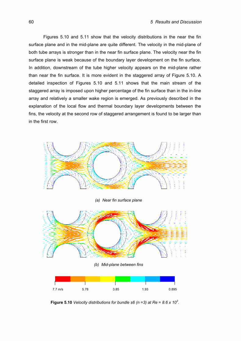
60 5 Results and Discussion
Figures 5.10 and 5.11 show that the velocity distributions in the near the fin
surface plane and in the mid-plane are quite different. The velocity in the mid-plane of
both tube arrays is stronger than in the near fin surface plane. The velocity near the fin
surface plane is weak because of the boundary layer development on the fin surface.
In addition, downstream of the tube higher velocity appears on the mid-plane rather
than near the fin surface. It is more evident in the staggered array of Figure 5.10. A
detailed inspection of Figures 5.10 and 5.11 shows that the main stream of the
staggered array is imposed upon higher percentage of the fin surface than in the in-line
array and relatively a smaller wake region is emerged. As previously described in the
explanation of the local flow and thermal boundary layer developments between the
fins, the velocity at the second row of staggered arrangement is found to be larger than
in the first row.
(a) Near fin surface plane
(b) Mid-plane between fins
7.7 m/s 5.78 3.85 1.93 0.895
Figure 5.10 Velocity distributions for bundle s6 (n =3) at Re = 8.6 x 10³.
5 Results and Discussion 61
As shown in the Figure 5.11, a large portion of the fin surface area of only the
first row of the in-line array is exposed to the main flow. A larger flow recirculation
region or dead zone is formed between the two adjacent tubes for the in-line
arrangement as Brauer [5, 6], Jang et al. [24], Kaminski [29] and Kearney, [31] noted.
Figure 5.11 proves clearly the existence of reverse flow patterns upstream of deeper
rows. Furthermore, these velocity data confirm that a bypass stream exists between
the tubes with the in-line arrangement in accordance with fin tip-to-tip clearance. For
the staggered arrangement, the main flow passes through every finned-tube row and
the flow is mixed well. From an overall inspection of the figures, the first row upstream
region for both tube arrangements is found to be almost identical as expected.
(a) Near fin surface plane
(b) Mid-Plane between fins
7.7 m/s 5.78 3.85 1.93 0.612
Figure 5.11 Velocity distributions for bundle i4 (n =3) at Re = 8.6 x 10³.
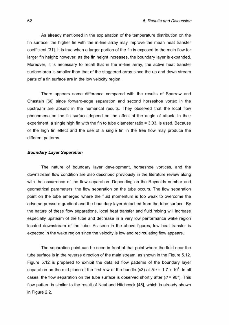
62 5 Results and Discussion
As already mentioned in the explanation of the temperature distribution on the
fin surface, the higher fin with the in-line array may improve the mean heat transfer
coefficient [31]. It is true when a larger portion of the fin is exposed to the main flow for
larger fin height; however, as the fin height increases, the boundary layer is expanded.
Moreover, it is necessary to recall that in the in-line array, the active heat transfer
surface area is smaller than that of the staggered array since the up and down stream
parts of a fin surface are in the low velocity region.
There appears some difference compared with the results of Sparrow and
Chastain [60] since forward-edge separation and second horseshoe vortex in the
upstream are absent in the numerical results. They observed that the local flow
phenomena on the fin surface depend on the effect of the angle of attack. In their
experiment, a single high fin with the fin to tube diameter ratio = 3.03, is used. Because
of the high fin effect and the use of a single fin in the free flow may produce the
different patterns.
Boundary Layer Separation
The nature of boundary layer development, horseshoe vortices, and the
downstream flow condition are also described previously in the literature review along
with the occurrence of the flow separation. Depending on the Reynolds number and
geometrical parameters, the flow separation on the tube occurs. The flow separation
point on the tube emerged where the fluid momentum is too weak to overcome the
adverse pressure gradient and the boundary layer detached from the tube surface. By
the nature of these flow separations, local heat transfer and fluid mixing will increase
especially upsteam of the tube and decrease in a very low performance wake region
located downstream of the tube. As seen in the above figures, low heat transfer is
expected in the wake region since the velocity is low and recirculating flow appears.
The separation point can be seen in front of that point where the fluid near the
tube surface is in the reverse direction of the main stream, as shown in the Figure 5.12.
Figure 5.12 is prepared to exhibit the detailed flow patterns of the boundary layer
separation on the mid-plane of the first row of the bundle (s3) at Re = 1.7 x 10⁴. In all
cases, the flow separation on the tube surface is observed shortly after (θ = 90°). This
flow pattern is similar to the result of Neal and Hitchcock [45], which is already shown
in Figure 2.2.
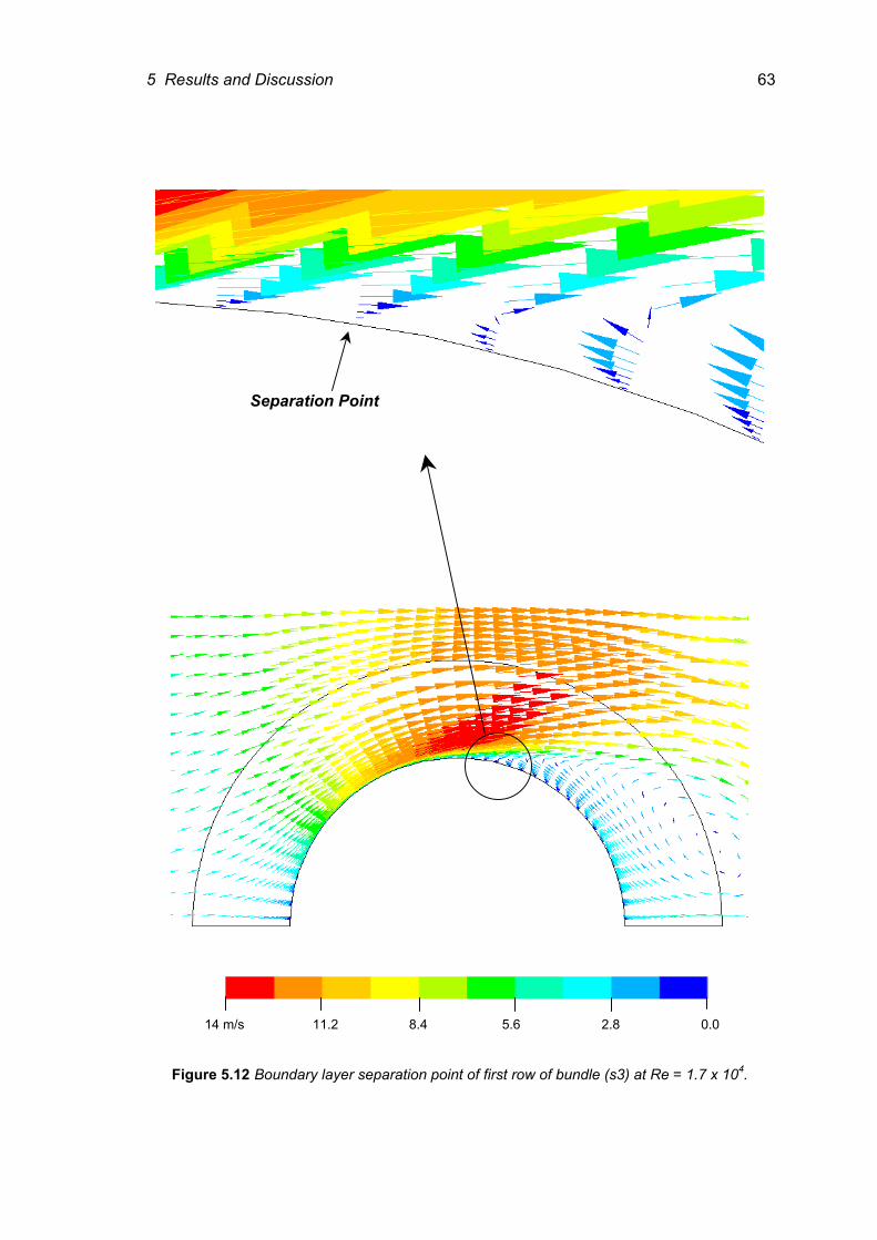
5 Results and Discussion 63
14 m/s 11.2 8.4 5.6 2.8 0.0
Figure 5.12 Boundary layer separation point of first row of bundle (s3) at Re = 1.7 x 10⁴.
Separation Point
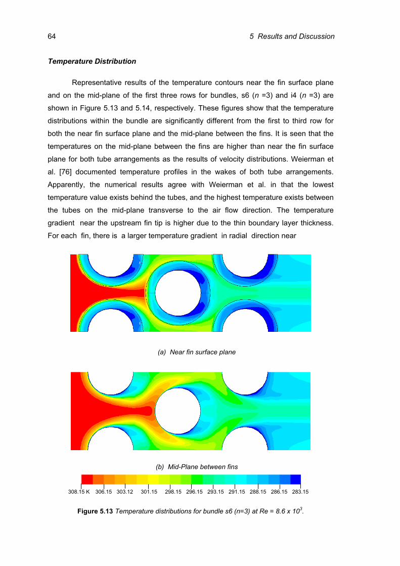
64 5 Results and Discussion
Temperature Distribution
Representative results of the temperature contours near the fin surface plane
and on the mid-plane of the first three rows for bundles, s6 (n =3) and i4 (n =3) are
shown in Figure 5.13 and 5.14, respectively. These figures show that the temperature
distributions within the bundle are significantly different from the first to third row for
both the near fin surface plane and the mid-plane between the fins. It is seen that the
temperatures on the mid-plane between the fins are higher than near the fin surface
plane for both tube arrangements as the results of velocity distributions. Weierman et
al. [76] documented temperature profiles in the wakes of both tube arrangements.
Apparently, the numerical results agree with Weierman et al. in that the lowest
temperature value exists behind the tubes, and the highest temperature exists between
the tubes on the mid-plane transverse to the air flow direction. The temperature
gradient near the upstream fin tip is higher due to the thin boundary layer thickness.
For each fin, there is a larger temperature gradient in radial direction near
(a) Near fin surface plane
(b) Mid-Plane between fins
308.15 K 306.15 303.12 301.15 298.15 296.15 293.15 291.15 288.15 286.15 283.15
Figure 5.13 Temperature distributions for bundle s6 (n=3) at Re = 8.6 x 10³.
5 Results and Discussion 65
the stagnation point for the staggered tube arrangement. For both tube arrangements,
the temperature gradient down stream along the fin is lower than the upstream due to
the wake flow.
As can be observed in Figure 5.14, a high temperature stream passes through
the in-line bundle without mixing well. It is also confirmed that because of the
proceeding rows of in-line array locating in the wake region, the temperature difference
between the fin and air is lower than for the staggered rows. The numerical results are
consistent with the flow visualizations of Jang et al. [25] and Kaminski [29] and also the
experimental investigation of Weierman et al. [76]. Moreover, it is interesting to note
that there will be only a small amount of hot air that can be cooled down at higher
Reynolds number. A long flow path with the inlet air temperature is expected for higher
velocity for both tube arrangements.
(a) Near fin surface plane
(b) Mid-plane between fins
308.15 K 306.15 303.12 301.15 298.15 296.15 293.15 291.15 288.15 286.15 283.15
Figure 5.14 Temperature distributions for bundle i4 (n=3) at Re = 8.6 x 10³.
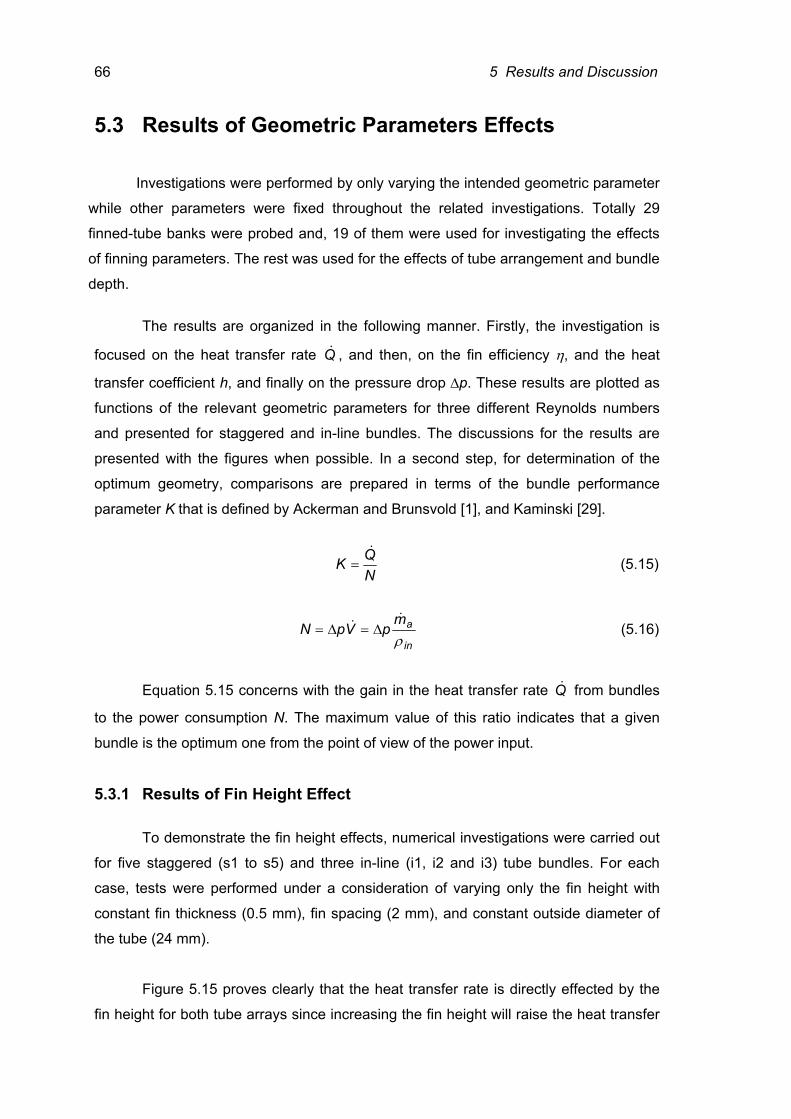
66 5 Results and Discussion
5.3 Results of Geometric Parameters Effects
Investigations were performed by only varying the intended geometric parameter
while other parameters were fixed throughout the related investigations. Totally 29
finned-tube banks were probed and, 19 of them were used for investigating the effects
of finning parameters. The rest was used for the effects of tube arrangement and bundle
depth.
The results are organized in the following manner. Firstly, the investigation is
focused on the heat transfer rate Q& , and then, on the fin efficiency η, and the heat
transfer coefficient h, and finally on the pressure drop ∆p. These results are plotted as
functions of the relevant geometric parameters for three different Reynolds numbers
and presented for staggered and in-line bundles. The discussions for the results are
presented with the figures when possible. In a second step, for determination of the
optimum geometry, comparisons are prepared in terms of the bundle performance
parameter K that is defined by Ackerman and Brunsvold [1], and Kaminski [29].
NQK&
= (5.15)
in
ampVpNρ
&& ∆=∆= (5.16)
Equation 5.15 concerns with the gain in the heat transfer rate Q& from bundles
to the power consumption N. The maximum value of this ratio indicates that a given
bundle is the optimum one from the point of view of the power input.
5.3.1 Results of Fin Height Effect
To demonstrate the fin height effects, numerical investigations were carried out
for five staggered (s1 to s5) and three in-line (i1, i2 and i3) tube bundles. For each
case, tests were performed under a consideration of varying only the fin height with
constant fin thickness (0.5 mm), fin spacing (2 mm), and constant outside diameter of
the tube (24 mm).
Figure 5.15 proves clearly that the heat transfer rate is directly effected by the
fin height for both tube arrays since increasing the fin height will raise the heat transfer
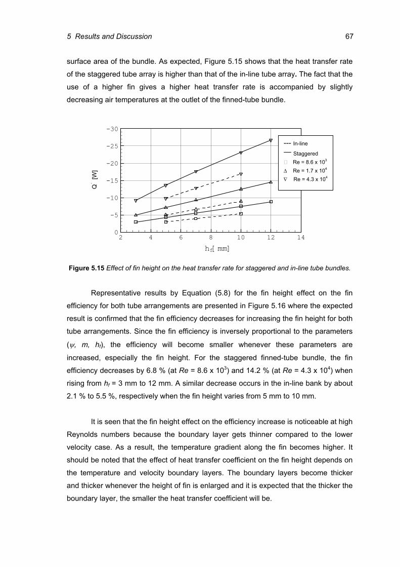
5 Results and Discussion 67
surface area of the bundle. As expected, Figure 5.15 shows that the heat transfer rate
of the staggered tube array is higher than that of the in-line tube array. The fact that the
use of a higher fin gives a higher heat transfer rate is accompanied by slightly
decreasing air temperatures at the outlet of the finned-tube bundle.
2 4 6 8 10 12 14
-30
-25
-20
-15
-10
-5
0
Figure 5.15 Effect of fin height on the heat transfer rate for staggered and in-line tube bundles.
Representative results by Equation (5.8) for the fin height effect on the fin
efficiency for both tube arrangements are presented in Figure 5.16 where the expected
result is confirmed that the fin efficiency decreases for increasing the fin height for both
tube arrangements. Since the fin efficiency is inversely proportional to the parameters
(ψ, m, hf), the efficiency will become smaller whenever these parameters are
increased, especially the fin height. For the staggered finned-tube bundle, the fin
efficiency decreases by 6.8 % (at Re = 8.6 x 10³) and 14.2 % (at Re = 4.3 x 10⁴) when
rising from hf = 3 mm to 12 mm. A similar decrease occurs in the in-line bank by about
2.1 % to 5.5 %, respectively when the fin height varies from 5 mm to 10 mm.
It is seen that the fin height effect on the efficiency increase is noticeable at high
Reynolds numbers because the boundary layer gets thinner compared to the lower
velocity case. As a result, the temperature gradient along the fin becomes higher. It
should be noted that the effect of heat transfer coefficient on the fin height depends on
the temperature and velocity boundary layers. The boundary layers become thicker
and thicker whenever the height of fin is enlarged and it is expected that the thicker the
boundary layer, the smaller the heat transfer coefficient will be.
hf[mm]
Qׂ [W
]
--- In-line Staggered
Re = 8.6 x 10³
∆ Re = 1.7 x 10⁴
∇ Re = 4.3 x 10⁴
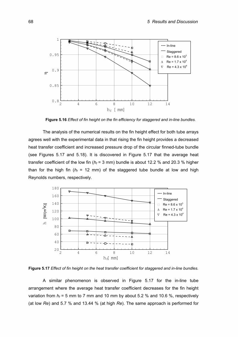
68 5 Results and Discussion
2 4 6 8 10 12 140.8
0.85
0.9
0.95
1
Figure 5.16 Effect of fin height on the fin efficiency for staggered and in-line bundles.
The analysis of the numerical results on the fin height effect for both tube arrays
agrees well with the experimental data in that rising the fin height provides a decreased
heat transfer coefficient and increased pressure drop of the circular finned-tube bundle
(see Figures 5.17 and 5.18). It is discovered in Figure 5.17 that the average heat
transfer coefficient of the low fin (hf = 3 mm) bundle is about 12.2 % and 20.3 % higher
than for the high fin (hf = 12 mm) of the staggered tube bundle at low and high
Reynolds numbers, respectively.
2 4 6 8 10 12 1420406080
100120140160180
Figure 5.17 Effect of fin height on the heat transfer coefficient for staggered and in-line bundles.
A similar phenomenon is observed in Figure 5.17 for the in-line tube
arrangement where the average heat transfer coefficient decreases for the fin height
variation from hf = 5 mm to 7 mm and 10 mm by about 5.2 % and 10.6 %, respectively
(at low Re) and 5.7 % and 13.44 % (at high Re). The same approach is performed for
hf[mm]
h [W
/(m2 K)
]
hf [mm]
η
--- In-line Staggered
Re = 8.6 x 10³
∆ Re = 1.7 x 10⁴
∇ Re = 4.3 x 10⁴
--- In-line Staggered
Re = 8.6 x 10³
∆ Re = 1.7 x 10⁴
∇ Re = 4.3 x 10⁴
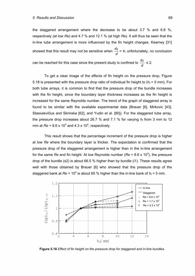
5 Results and Discussion 69
the staggered arrangement where the decrease to be about 3.7 % and 6.8 %,
respectively (at low Re) and 4.7 % and 12.1 % (at high Re). It will thus be seen that the
in-line tube arrangement is more influenced by the fin height changes. Kearney [31]
showed that this result may not be sensitive when ddf = 4; unfortunately, no conclusion
can be reached for this case since the present study is confined to ddf ≤ 2.
To get a clear image of the effects of fin height on the pressure drop, Figure
5.18 is presented with the pressure drop ratio of individual fin height to (hf = 5 mm). For
both tube arrays, it is common to find that the pressure drop of the bundle increases
with the fin height, since the boundary layer thickness increases as the fin height is
increased for the same Reynolds number. The trend of the graph of staggered array is
found to be similar with the available experimental data (Brauer [6], Mirkovic [43],
Stasiulevičius and Skrinska [62], and Yudin et al. [80]). For the staggered tube array,
the pressure drop increases about 26.7 % and 7.1 % for varying hf from 3 mm to 12
mm at Re = 8.6 x 10³ and 4.3 x 10⁴, respectively.
This result shows that the percentage increment of the pressure drop is higher
at low Re where the boundary layer is thicker. The expectation is confirmed that the
pressure drop of the staggered arrangement is higher than in the in-line arrangement
for the same Re and fin height. At low Reynolds number (Re = 8.6 x 10³), the pressure
drop of the bundle (s2) is about 66.5 % higher than by bundle (i1). These results agree
well with those obtained by Brauer [6] who showed that the pressure drop of the
staggered bank at Re = 104 is about 65 % higher than the in-line bank of hf = 5 mm.
2 4 6 8 10 12 140.8
0.9
1
1.1
1.2
Figure 5.18 Effect of fin height on the pressure drop for staggered and in-line bundles.
hf[mm]
(∆p)
hf/(∆p) h
f =5
--- In-line Staggered
Re = 8.6 x 10³
∆ Re = 1.7 x 10⁴
∇ Re = 4.3 x 10⁴
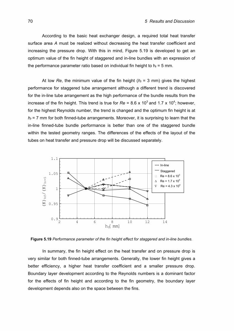
70 5 Results and Discussion
According to the basic heat exchanger design, a required total heat transfer
surface area A must be realized without decreasing the heat transfer coefficient and
increasing the pressure drop. With this in mind, Figure 5.19 is developed to get an
optimum value of the fin height of staggered and in-line bundles with an expression of
the performance parameter ratio based on individual fin height to hf = 5 mm.
At low Re, the minimum value of the fin height (hf = 3 mm) gives the highest
performance for staggered tube arrangement although a different trend is discovered
for the in-line tube arrangement as the high performance of the bundle results from the
increase of the fin height. This trend is true for Re = 8.6 x 10³ and 1.7 x 10⁴; however,
for the highest Reynolds number, the trend is changed and the optimum fin height is at
hf = 7 mm for both finned-tube arrangements. Moreover, it is surprising to learn that the
in-line finned-tube bundle performance is better than one of the staggered bundle
within the tested geometry ranges. The differences of the effects of the layout of the
tubes on heat transfer and pressure drop will be discussed separately.
2 4 6 8 10 12 140.9
0.95
1
1.05
1.1
Figure 5.19 Performance parameter of the fin height effect for staggered and in-line bundles.
In summary, the fin height effect on the heat transfer and on pressure drop is
very similar for both finned-tube arrangements. Generally, the lower fin height gives a
better efficiency, a higher heat transfer coefficient and a smaller pressure drop.
Boundary layer development according to the Reynolds numbers is a dominant factor
for the effects of fin height and according to the fin geometry, the boundary layer
development depends also on the space between the fins.
hf[mm]
(K) h
f/(K) h
f =5
--- In-line Staggered
Re = 8.6 x 10³
∆ Re = 1.7 x 10⁴
∇ Re = 4.3 x 10⁴
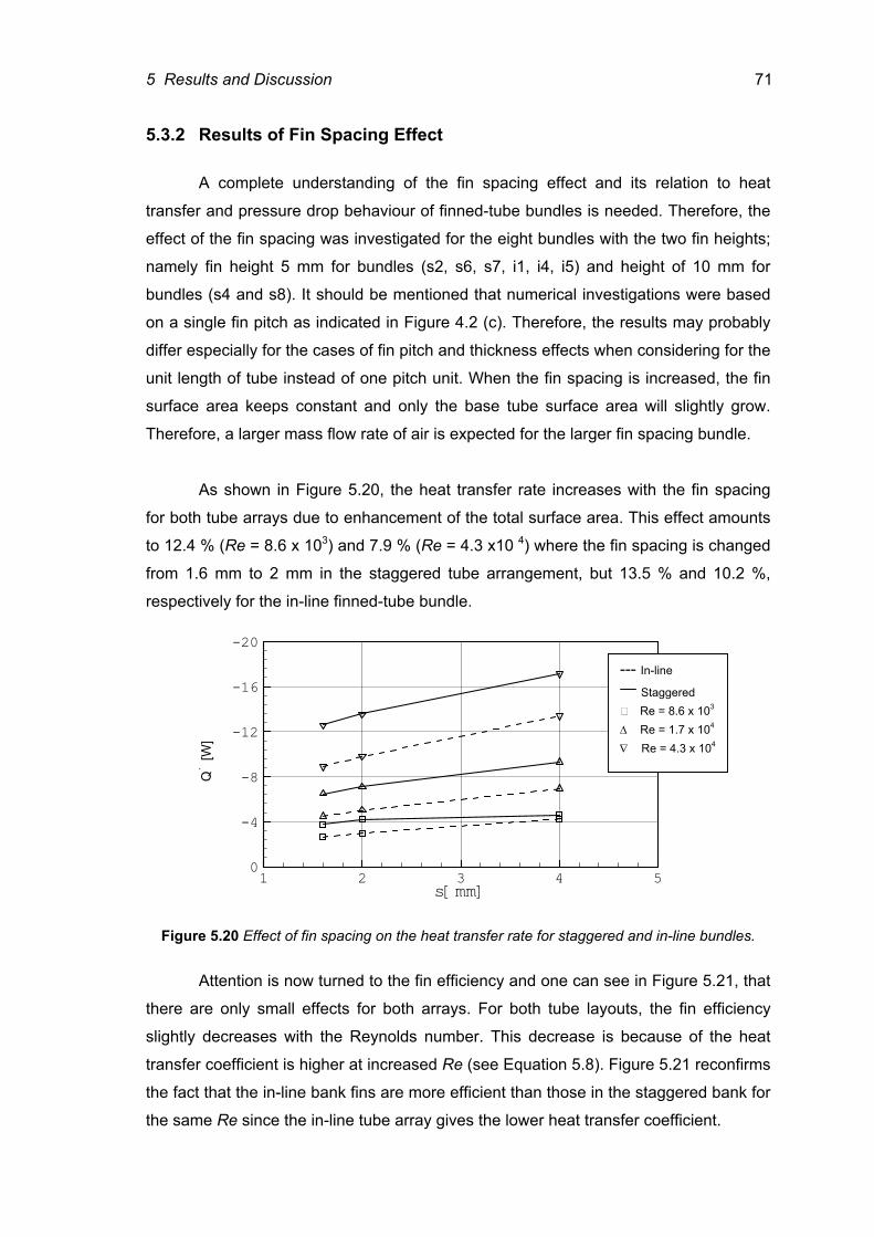
5 Results and Discussion 71
5.3.2 Results of Fin Spacing Effect A complete understanding of the fin spacing effect and its relation to heat
transfer and pressure drop behaviour of finned-tube bundles is needed. Therefore, the
effect of the fin spacing was investigated for the eight bundles with the two fin heights;
namely fin height 5 mm for bundles (s2, s6, s7, i1, i4, i5) and height of 10 mm for
bundles (s4 and s8). It should be mentioned that numerical investigations were based
on a single fin pitch as indicated in Figure 4.2 (c). Therefore, the results may probably
differ especially for the cases of fin pitch and thickness effects when considering for the
unit length of tube instead of one pitch unit. When the fin spacing is increased, the fin
surface area keeps constant and only the base tube surface area will slightly grow.
Therefore, a larger mass flow rate of air is expected for the larger fin spacing bundle.
As shown in Figure 5.20, the heat transfer rate increases with the fin spacing
for both tube arrays due to enhancement of the total surface area. This effect amounts
to 12.4 % (Re = 8.6 x 10³) and 7.9 % (Re = 4.3 x10 4) where the fin spacing is changed
from 1.6 mm to 2 mm in the staggered tube arrangement, but 13.5 % and 10.2 %,
respectively for the in-line finned-tube bundle.
1 2 3 4 5
-20
-16
-12
-8
-4
0
Figure 5.20 Effect of fin spacing on the heat transfer rate for staggered and in-line bundles.
Attention is now turned to the fin efficiency and one can see in Figure 5.21, that
there are only small effects for both arrays. For both tube layouts, the fin efficiency
slightly decreases with the Reynolds number. This decrease is because of the heat
transfer coefficient is higher at increased Re (see Equation 5.8). Figure 5.21 reconfirms
the fact that the in-line bank fins are more efficient than those in the staggered bank for
the same Re since the in-line tube array gives the lower heat transfer coefficient.
s[mm]
Qׂ [W
]
--- In-line Staggered
Re = 8.6 x 10³
∆ Re = 1.7 x 10⁴
∇ Re = 4.3 x 10⁴
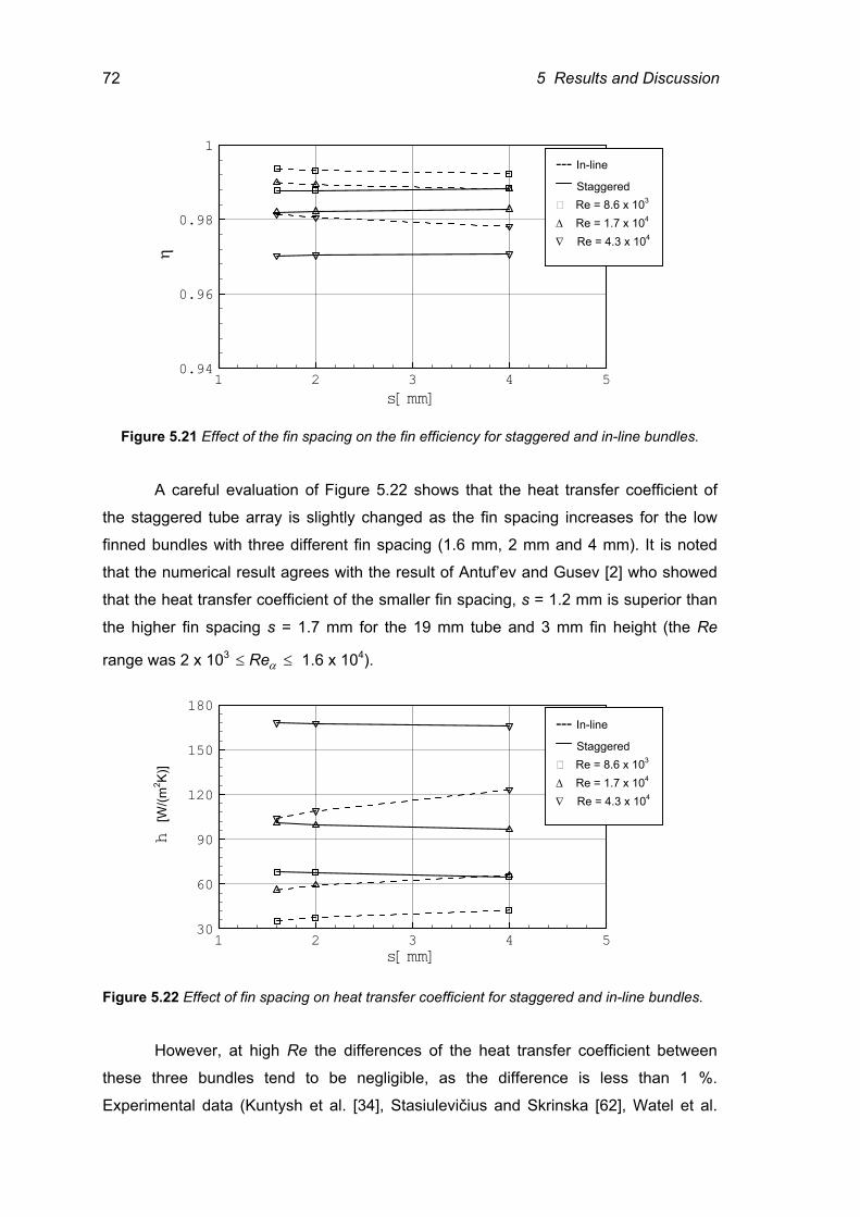
72 5 Results and Discussion
1 2 3 4 50.94
0.96
0.98
1
Figure 5.21 Effect of the fin spacing on the fin efficiency for staggered and in-line bundles.
A careful evaluation of Figure 5.22 shows that the heat transfer coefficient of
the staggered tube array is slightly changed as the fin spacing increases for the low
finned bundles with three different fin spacing (1.6 mm, 2 mm and 4 mm). It is noted
that the numerical result agrees with the result of Antuf’ev and Gusev [2] who showed
that the heat transfer coefficient of the smaller fin spacing, s = 1.2 mm is superior than
the higher fin spacing s = 1.7 mm for the 19 mm tube and 3 mm fin height (the Re
range was 2 x 10³ ≤≤ αRe 1.6 x 10⁴).
1 2 3 4 530
60
90
120
150
180
Figure 5.22 Effect of fin spacing on heat transfer coefficient for staggered and in-line bundles.
However, at high Re the differences of the heat transfer coefficient between
these three bundles tend to be negligible, as the difference is less than 1 %.
Experimental data (Kuntysh et al. [34], Stasiulevičius and Skrinska [62], Watel et al.
s[mm]
η
s[mm]
h [W
/(m2 K)
] --- In-line
Staggered Re = 8.6 x 10³
∆ Re = 1.7 x 10⁴
∇ Re = 4.3 x 10⁴
--- In-line Staggered
Re = 8.6 x 10³
∆ Re = 1.7 x 10⁴
∇ Re = 4.3 x 10⁴
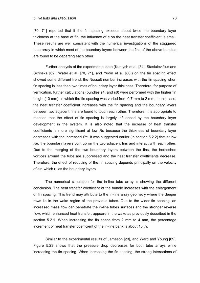
5 Results and Discussion 73
[70, 71] reported that if the fin spacing exceeds about twice the boundary layer
thickness at the base of fin, the influence of s on the heat transfer coefficient is small.
These results are well consistent with the numerical investigations of the staggered
tube array in which most of the boundary layers between the fins of the above bundles
are found to be departing each other.
Further analysis of the experimental data (Kuntysh et al. [34], Stasiulevičius and
Skrinska [62], Watel et al. [70, 71], and Yudin et al. [80]) on the fin spacing effect
showed some different trend: the Nusselt number increases with the fin spacing when
fin spacing is less than two times of boundary layer thickness. Therefore, for purpose of
verification, further calculations (bundles s4, and s8) were performed with the higher fin
height (10 mm), in which the fin spacing was varied from 0.7 mm to 2 mm. In this case,
the heat transfer coefficient increases with the fin spacing and the boundary layers
between two adjacent fins are found to touch each other. Therefore, it is appropriate to
mention that the effect of fin spacing is largely influenced by the boundary layer
development in the system. It is also noted that the increase of heat transfer
coefficients is more significant at low Re because the thickness of boundary layer
decreases with the increased Re. It was suggested earlier (in section 5.2.2) that at low
Re, the boundary layers built up on the two adjacent fins and interact with each other.
Due to the merging of the two boundary layers between the fins, the horseshoe
vortices around the tube are suppressed and the heat transfer coefficients decrease.
Therefore, the effect of reducing of the fin spacing depends principally on the velocity
of air, which rules the boundary layers.
The numerical simulation for the in-line tube array is showing the different
conclusion. The heat transfer coefficient of the bundle increases with the enlargement
of fin spacing. This trend may attribute to the in-line array geometry where the deeper
rows lie in the wake region of the previous tubes. Due to the wider fin spacing, an
increased mass flow can penetrate the in-line tubes surfaces and the stronger reverse
flow, which enhanced heat transfer, appeare in the wake as previously described in the
section 5.2.1. When increasing the fin space from 2 mm to 4 mm, the percentage
increment of heat transfer coefficient of the in-line bank is about 13 %.
Similar to the experimental results of Jameson [23], and Ward and Young [69],
Figure 5.23 shows that the pressure drop decreases for both tube arrays while
increasing the fin spacing. When increasing the fin spacing, the strong interactions of
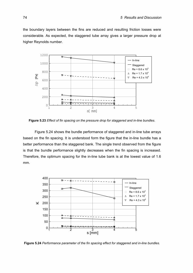
74 5 Results and Discussion
the boundary layers between the fins are reduced and resulting friction losses were
considerable. As expected, the staggered tube array gives a larger pressure drop at
higher Reynolds number.
1 2 3 4 50
200
400
600
800
1000
1200
Figure 5.23 Effect of fin spacing on the pressure drop for staggered and in-line bundles.
Figure 5.24 shows the bundle performance of staggered and in-line tube arrays
based on the fin spacing. It is understood form the figure that the in-line bundle has a
better performance than the staggered bank. The single trend observed from the figure
is that the bundle performance slightly decreases when the fin spacing is increased.
Therefore, the optimum spacing for the in-line tube bank is at the lowest value of 1.6
mm.
1 2 3 4 5s [mm]
0
50
100
150
200
250
300
350
400
K
Figure 5.24 Performance parameter of the fin spacing effect for staggered and in-line bundles.
s[mm]
∆p [P
a]
--- In-line Staggered
Re = 8.6 x 10³
∆ Re = 1.7 x 10⁴
∇ Re = 4.3 x 10⁴
--- In-line Staggered
Re = 8.6 x 10³
∆ Re = 1.7 x 10⁴
∇ Re = 4.3 x 10⁴
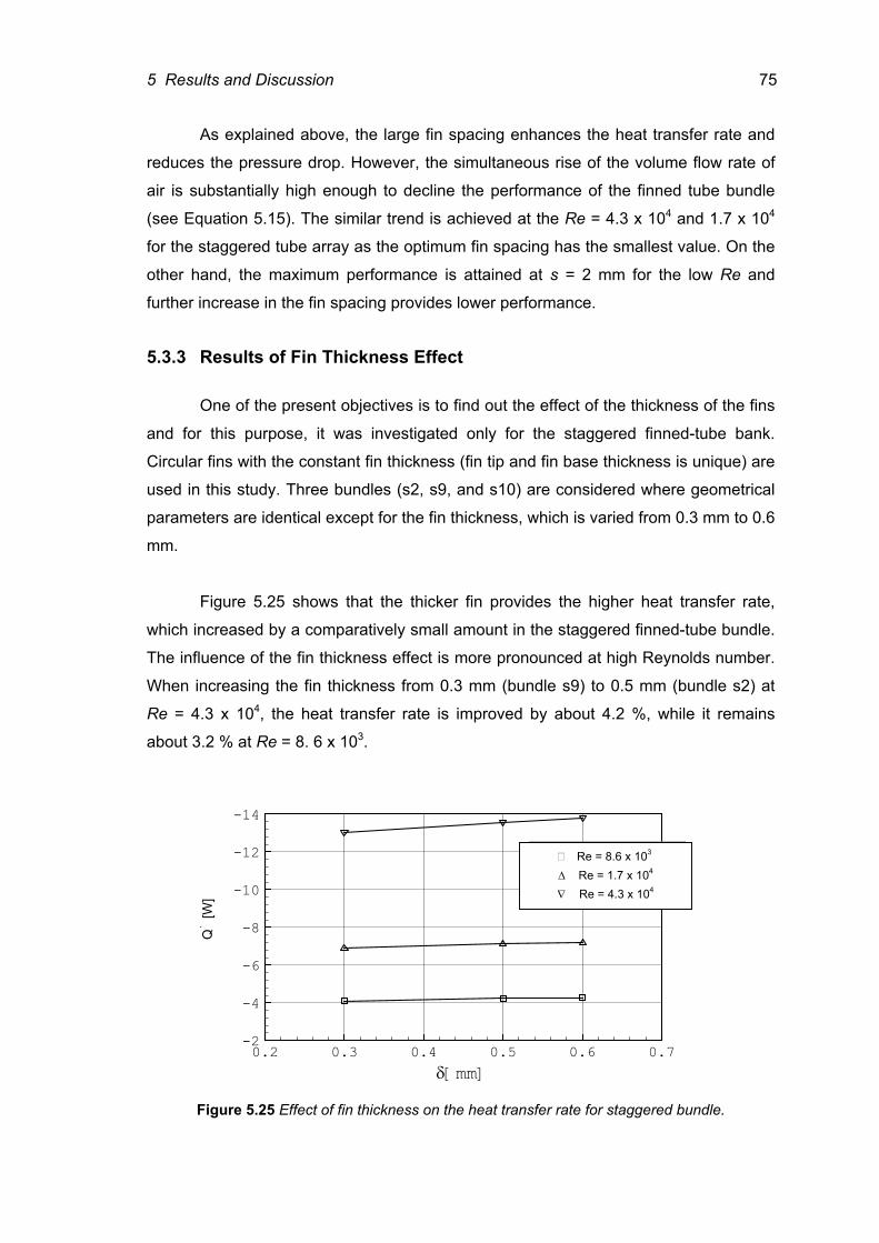
5 Results and Discussion 75
As explained above, the large fin spacing enhances the heat transfer rate and
reduces the pressure drop. However, the simultaneous rise of the volume flow rate of
air is substantially high enough to decline the performance of the finned tube bundle
(see Equation 5.15). The similar trend is achieved at the Re = 4.3 x 10⁴ and 1.7 x 10⁴
for the staggered tube array as the optimum fin spacing has the smallest value. On the
other hand, the maximum performance is attained at s = 2 mm for the low Re and
further increase in the fin spacing provides lower performance.
5.3.3 Results of Fin Thickness Effect
One of the present objectives is to find out the effect of the thickness of the fins
and for this purpose, it was investigated only for the staggered finned-tube bank.
Circular fins with the constant fin thickness (fin tip and fin base thickness is unique) are
used in this study. Three bundles (s2, s9, and s10) are considered where geometrical
parameters are identical except for the fin thickness, which is varied from 0.3 mm to 0.6
mm.
Figure 5.25 shows that the thicker fin provides the higher heat transfer rate,
which increased by a comparatively small amount in the staggered finned-tube bundle.
The influence of the fin thickness effect is more pronounced at high Reynolds number.
When increasing the fin thickness from 0.3 mm (bundle s9) to 0.5 mm (bundle s2) at
Re = 4.3 x 10⁴, the heat transfer rate is improved by about 4.2 %, while it remains
about 3.2 % at Re = 8. 6 x 10³.
0.2 0.3 0.4 0.5 0.6 0.7
-14
-12
-10
-8
-6
-4
-2
Re = 8.6e3Re = 1.7e4Re = 4.3e4
Figure 5.25 Effect of fin thickness on the heat transfer rate for staggered bundle.
δ[mm]
Qׂ [W
]
Re = 8.6 x 10³
∆ Re = 1.7 x 10⁴
∇ Re = 4.3 x 10⁴
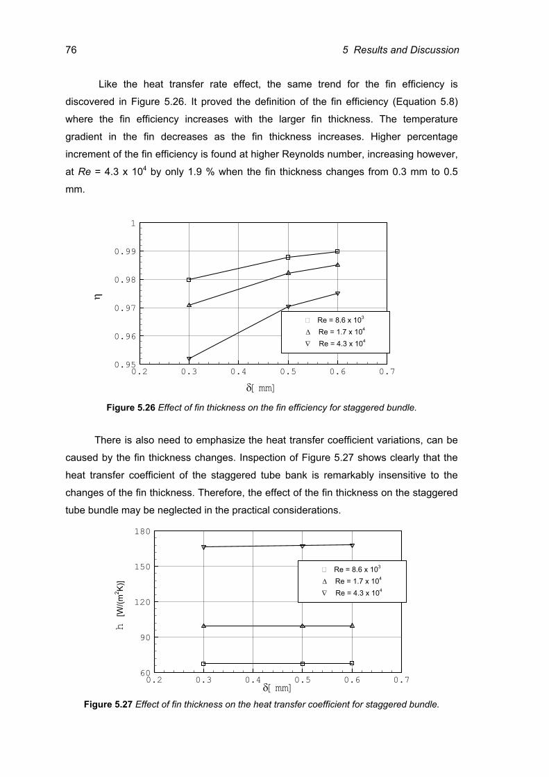
76 5 Results and Discussion
Like the heat transfer rate effect, the same trend for the fin efficiency is
discovered in Figure 5.26. It proved the definition of the fin efficiency (Equation 5.8) where the fin efficiency increases with the larger fin thickness. The temperature
gradient in the fin decreases as the fin thickness increases. Higher percentage
increment of the fin efficiency is found at higher Reynolds number, increasing however,
at Re = 4.3 x 10⁴ by only 1.9 % when the fin thickness changes from 0.3 mm to 0.5
mm.
0.2 0.3 0.4 0.5 0.6 0.70.95
0.96
0.97
0.98
0.99
1
Re = 8.6e3Re = 1.7e4Re = 4.3e4
Figure 5.26 Effect of fin thickness on the fin efficiency for staggered bundle.
There is also need to emphasize the heat transfer coefficient variations, can be
caused by the fin thickness changes. Inspection of Figure 5.27 shows clearly that the
heat transfer coefficient of the staggered tube bank is remarkably insensitive to the
changes of the fin thickness. Therefore, the effect of the fin thickness on the staggered
tube bundle may be neglected in the practical considerations.
0.2 0.3 0.4 0.5 0.6 0.760
90
120
150
180
Re = 8.6e3Re = 1.7e4Re = 4.3e4
Figure 5.27 Effect of fin thickness on the heat transfer coefficient for staggered bundle.
δ[mm]
h [W
/(m2 K)
]
δ[mm]
η
Re = 8.6 x 10³
∆ Re = 1.7 x 10⁴
∇ Re = 4.3 x 10⁴
Re = 8.6 x 10³
∆ Re = 1.7 x 10⁴
∇ Re = 4.3 x 10⁴
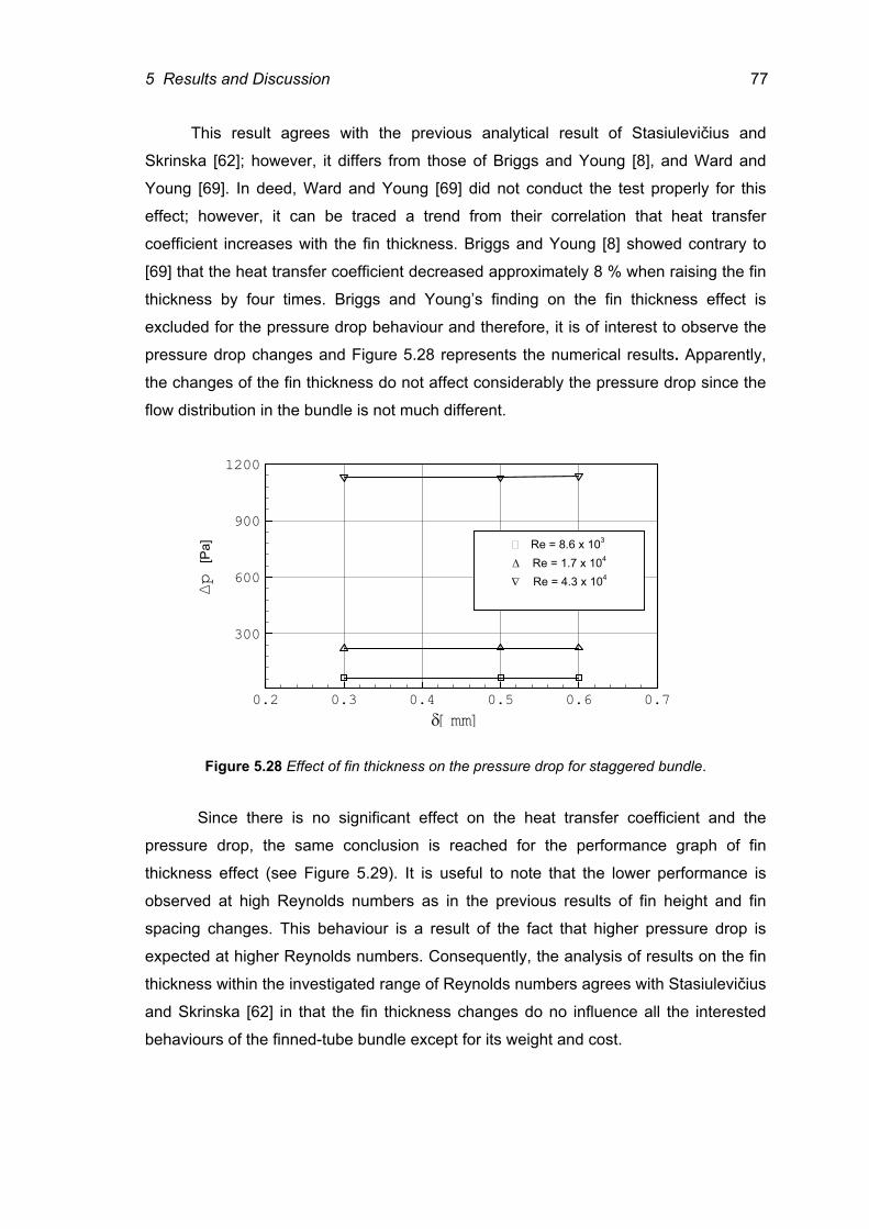
5 Results and Discussion 77
This result agrees with the previous analytical result of Stasiulevičius and
Skrinska [62]; however, it differs from those of Briggs and Young [8], and Ward and
Young [69]. In deed, Ward and Young [69] did not conduct the test properly for this
effect; however, it can be traced a trend from their correlation that heat transfer
coefficient increases with the fin thickness. Briggs and Young [8] showed contrary to
[69] that the heat transfer coefficient decreased approximately 8 % when raising the fin
thickness by four times. Briggs and Young’s finding on the fin thickness effect is
excluded for the pressure drop behaviour and therefore, it is of interest to observe the
pressure drop changes and Figure 5.28 represents the numerical results. Apparently,
the changes of the fin thickness do not affect considerably the pressure drop since the
flow distribution in the bundle is not much different.
0.2 0.3 0.4 0.5 0.6 0.7
300
600
900
1200
Re = 8.6e3Re = 1.7e4Re = 4.3e4
Figure 5.28 Effect of fin thickness on the pressure drop for staggered bundle.
Since there is no significant effect on the heat transfer coefficient and the
pressure drop, the same conclusion is reached for the performance graph of fin
thickness effect (see Figure 5.29). It is useful to note that the lower performance is
observed at high Reynolds numbers as in the previous results of fin height and fin
spacing changes. This behaviour is a result of the fact that higher pressure drop is
expected at higher Reynolds numbers. Consequently, the analysis of results on the fin
thickness within the investigated range of Reynolds numbers agrees with Stasiulevičius
and Skrinska [62] in that the fin thickness changes do no influence all the interested
behaviours of the finned-tube bundle except for its weight and cost.
δ[mm]
∆p [P
a]
Re = 8.6 x 10³
∆ Re = 1.7 x 10⁴
∇ Re = 4.3 x 10⁴
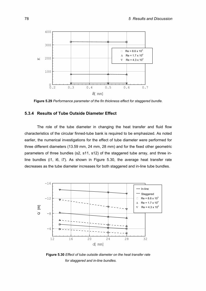
78 5 Results and Discussion
0.2 0.3 0.4 0.5 0.6 0.70
100
200
300
400
Re = 8.6e3Re = 1.7e4Re = 4.3e4
Figure 5.29 Performance parameter of the fin thickness effect for staggered bundle.
5.3.4 Results of Tube Outside Diameter Effect
The role of the tube diameter in changing the heat transfer and fluid flow
characteristics of the circular finned-tube bank is required to be emphasized. As noted
earlier, the numerical investigations for the effect of tube diameter were performed for
three different diameters (13.59 mm, 24 mm, 28 mm) and for the fixed other geometric
parameters of three bundles (s2, s11, s12) of the staggered tube array, and three in-
line bundles (i1, i6, i7). As shown in Figure 5.30, the average heat transfer rate
decreases as the tube diameter increases for both staggered and in-line tube bundles.
12 16 20 24 28 32
-16
-12
-8
-4
Figure 5.30 Effect of tube outside diameter on the heat transfer rate
for staggered and in-line bundles.
δ[mm]
K
d[mm]
Qׂ [W
]
--- In-line Staggered
Re = 8.6 x 10³
∆ Re = 1.7 x 10⁴
∇ Re = 4.3 x 10⁴
Re = 8.6 x 10³
∆ Re = 1.7 x 10⁴
∇ Re = 4.3 x 10⁴
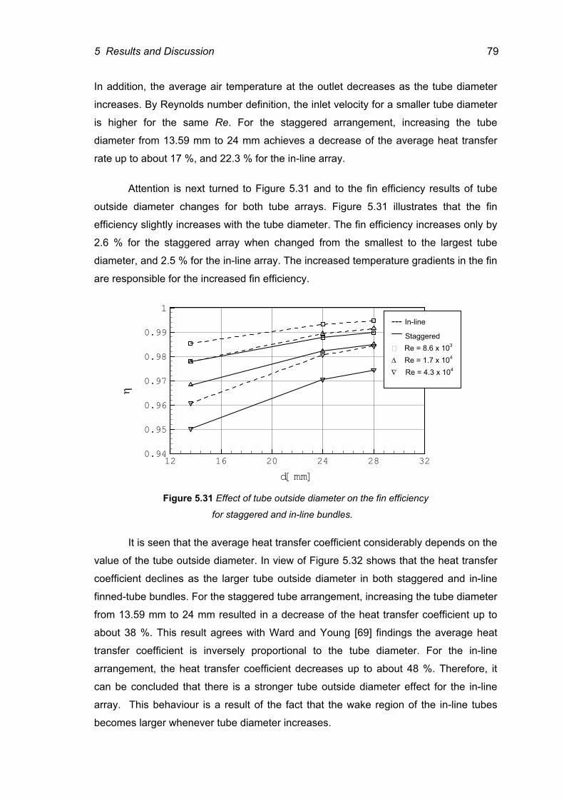
5 Results and Discussion 79
In addition, the average air temperature at the outlet decreases as the tube diameter
increases. By Reynolds number definition, the inlet velocity for a smaller tube diameter
is higher for the same Re. For the staggered arrangement, increasing the tube
diameter from 13.59 mm to 24 mm achieves a decrease of the average heat transfer
rate up to about 17 %, and 22.3 % for the in-line array.
Attention is next turned to Figure 5.31 and to the fin efficiency results of tube
outside diameter changes for both tube arrays. Figure 5.31 illustrates that the fin
efficiency slightly increases with the tube diameter. The fin efficiency increases only by
2.6 % for the staggered array when changed from the smallest to the largest tube
diameter, and 2.5 % for the in-line array. The increased temperature gradients in the fin
are responsible for the increased fin efficiency.
12 16 20 24 28 320.94
0.95
0.96
0.97
0.98
0.99
1
Figure 5.31 Effect of tube outside diameter on the fin efficiency
for staggered and in-line bundles.
It is seen that the average heat transfer coefficient considerably depends on the
value of the tube outside diameter. In view of Figure 5.32 shows that the heat transfer
coefficient declines as the larger tube outside diameter in both staggered and in-line
finned-tube bundles. For the staggered tube arrangement, increasing the tube diameter
from 13.59 mm to 24 mm resulted in a decrease of the heat transfer coefficient up to
about 38 %. This result agrees with Ward and Young [69] findings the average heat
transfer coefficient is inversely proportional to the tube diameter. For the in-line
arrangement, the heat transfer coefficient decreases up to about 48 %. Therefore, it
can be concluded that there is a stronger tube outside diameter effect for the in-line
array. This behaviour is a result of the fact that the wake region of the in-line tubes
becomes larger whenever tube diameter increases.
d[mm]
η
--- In-line Staggered
Re = 8.6 x 10³
∆ Re = 1.7 x 10⁴
∇ Re = 4.3 x 10⁴
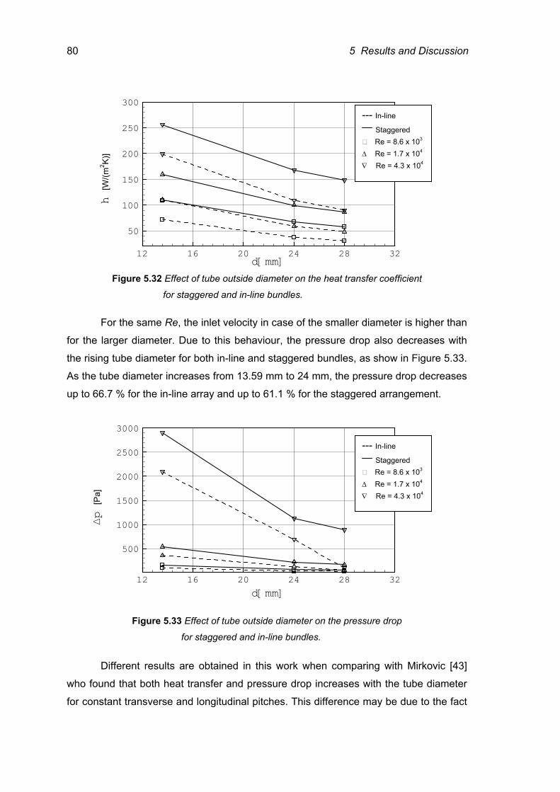
80 5 Results and Discussion
12 16 20 24 28 32
50
100
150
200
250
300
Figure 5.32 Effect of tube outside diameter on the heat transfer coefficient
for staggered and in-line bundles.
For the same Re, the inlet velocity in case of the smaller diameter is higher than
for the larger diameter. Due to this behaviour, the pressure drop also decreases with
the rising tube diameter for both in-line and staggered bundles, as show in Figure 5.33.
As the tube diameter increases from 13.59 mm to 24 mm, the pressure drop decreases
up to 66.7 % for the in-line array and up to 61.1 % for the staggered arrangement.
12 16 20 24 28 32
500
1000
1500
2000
2500
3000
Figure 5.33 Effect of tube outside diameter on the pressure drop
for staggered and in-line bundles.
Different results are obtained in this work when comparing with Mirkovic [43]
who found that both heat transfer and pressure drop increases with the tube diameter
for constant transverse and longitudinal pitches. This difference may be due to the fact
d[mm]
d[mm]
h [W
/(m2 K)
] ∆p [P
a]
--- In-line Staggered
Re = 8.6 x 10³
∆ Re = 1.7 x 10⁴
∇ Re = 4.3 x 10⁴
--- In-line Staggered
Re = 8.6 x 10³
∆ Re = 1.7 x 10⁴
∇ Re = 4.3 x 10⁴
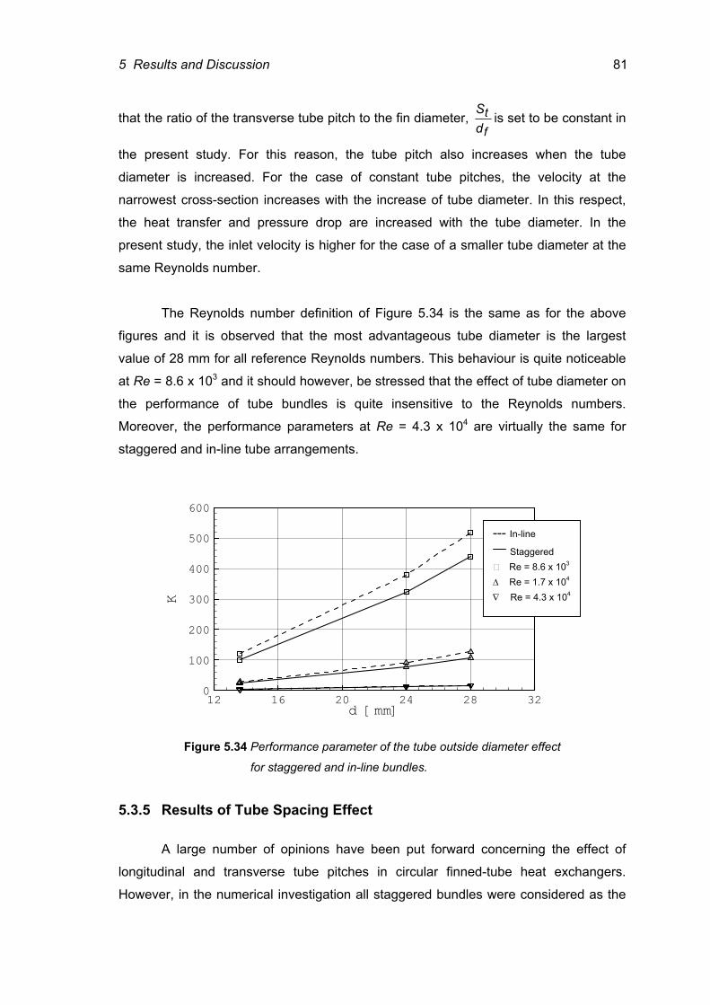
5 Results and Discussion 81
that the ratio of the transverse tube pitch to the fin diameter, ft
dS
is set to be constant in
the present study. For this reason, the tube pitch also increases when the tube
diameter is increased. For the case of constant tube pitches, the velocity at the
narrowest cross-section increases with the increase of tube diameter. In this respect,
the heat transfer and pressure drop are increased with the tube diameter. In the
present study, the inlet velocity is higher for the case of a smaller tube diameter at the
same Reynolds number.
The Reynolds number definition of Figure 5.34 is the same as for the above
figures and it is observed that the most advantageous tube diameter is the largest
value of 28 mm for all reference Reynolds numbers. This behaviour is quite noticeable
at Re = 8.6 x 10³ and it should however, be stressed that the effect of tube diameter on
the performance of tube bundles is quite insensitive to the Reynolds numbers.
Moreover, the performance parameters at Re = 4.3 x 10⁴ are virtually the same for
staggered and in-line tube arrangements.
12 16 20 24 28 32d [mm]0
100
200
300
400
500
600
K
Figure 5.34 Performance parameter of the tube outside diameter effect
for staggered and in-line bundles.
5.3.5 Results of Tube Spacing Effect A large number of opinions have been put forward concerning the effect of
longitudinal and transverse tube pitches in circular finned-tube heat exchangers.
However, in the numerical investigation all staggered bundles were considered as the
--- In-line Staggered
Re = 8.6 x 10³
∆ Re = 1.7 x 10⁴
∇ Re = 4.3 x 10⁴
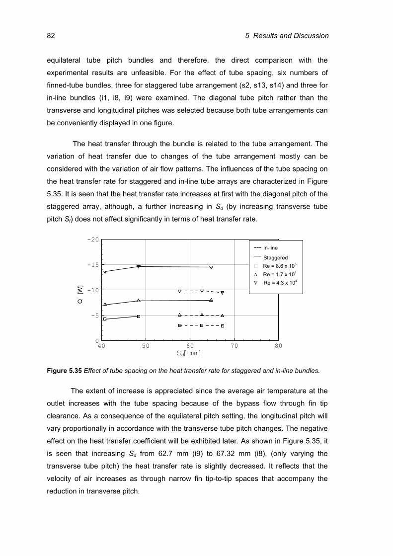
82 5 Results and Discussion
equilateral tube pitch bundles and therefore, the direct comparison with the
experimental results are unfeasible. For the effect of tube spacing, six numbers of
finned-tube bundles, three for staggered tube arrangement (s2, s13, s14) and three for
in-line bundles (i1, i8, i9) were examined. The diagonal tube pitch rather than the
transverse and longitudinal pitches was selected because both tube arrangements can
be conveniently displayed in one figure.
The heat transfer through the bundle is related to the tube arrangement. The
variation of heat transfer due to changes of the tube arrangement mostly can be
considered with the variation of air flow patterns. The influences of the tube spacing on
the heat transfer rate for staggered and in-line tube arrays are characterized in Figure
5.35. It is seen that the heat transfer rate increases at first with the diagonal pitch of the
staggered array, although, a further increasing in Sd (by increasing transverse tube
pitch St) does not affect significantly in terms of heat transfer rate.
40 50 60 70 80
-20
-15
-10
-5
0
Figure 5.35 Effect of tube spacing on the heat transfer rate for staggered and in-line bundles.
The extent of increase is appreciated since the average air temperature at the
outlet increases with the tube spacing because of the bypass flow through fin tip
clearance. As a consequence of the equilateral pitch setting, the longitudinal pitch will
vary proportionally in accordance with the transverse tube pitch changes. The negative
effect on the heat transfer coefficient will be exhibited later. As shown in Figure 5.35, it
is seen that increasing Sd from 62.7 mm (i9) to 67.32 mm (i8), (only varying the
transverse tube pitch) the heat transfer rate is slightly decreased. It reflects that the
velocity of air increases as through narrow fin tip-to-tip spaces that accompany the
reduction in transverse pitch.
Sd[mm]
Qׂ [W
]
--- In-line Staggered
Re = 8.6 x 10³
∆ Re = 1.7 x 10⁴
∇ Re = 4.3 x 10⁴
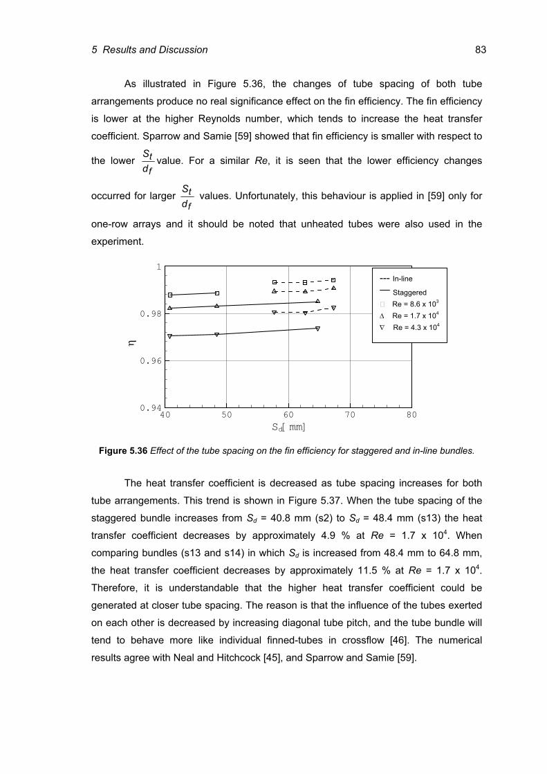
5 Results and Discussion 83
As illustrated in Figure 5.36, the changes of tube spacing of both tube
arrangements produce no real significance effect on the fin efficiency. The fin efficiency
is lower at the higher Reynolds number, which tends to increase the heat transfer
coefficient. Sparrow and Samie [59] showed that fin efficiency is smaller with respect to
the lower ft
dS
value. For a similar Re, it is seen that the lower efficiency changes
occurred for larger ft
dS
values. Unfortunately, this behaviour is applied in [59] only for
one-row arrays and it should be noted that unheated tubes were also used in the
experiment.
40 50 60 70 800.94
0.96
0.98
1
Figure 5.36 Effect of the tube spacing on the fin efficiency for staggered and in-line bundles.
The heat transfer coefficient is decreased as tube spacing increases for both
tube arrangements. This trend is shown in Figure 5.37. When the tube spacing of the
staggered bundle increases from Sd = 40.8 mm (s2) to Sd = 48.4 mm (s13) the heat
transfer coefficient decreases by approximately 4.9 % at Re = 1.7 x 10⁴. When
comparing bundles (s13 and s14) in which Sd is increased from 48.4 mm to 64.8 mm,
the heat transfer coefficient decreases by approximately 11.5 % at Re = 1.7 x 10⁴.
Therefore, it is understandable that the higher heat transfer coefficient could be
generated at closer tube spacing. The reason is that the influence of the tubes exerted
on each other is decreased by increasing diagonal tube pitch, and the tube bundle will
tend to behave more like individual finned-tubes in crossflow [46]. The numerical
results agree with Neal and Hitchcock [45], and Sparrow and Samie [59].
Sd[mm]
η
--- In-line Staggered
Re = 8.6 x 10³
∆ Re = 1.7 x 10⁴
∇ Re = 4.3 x 10⁴
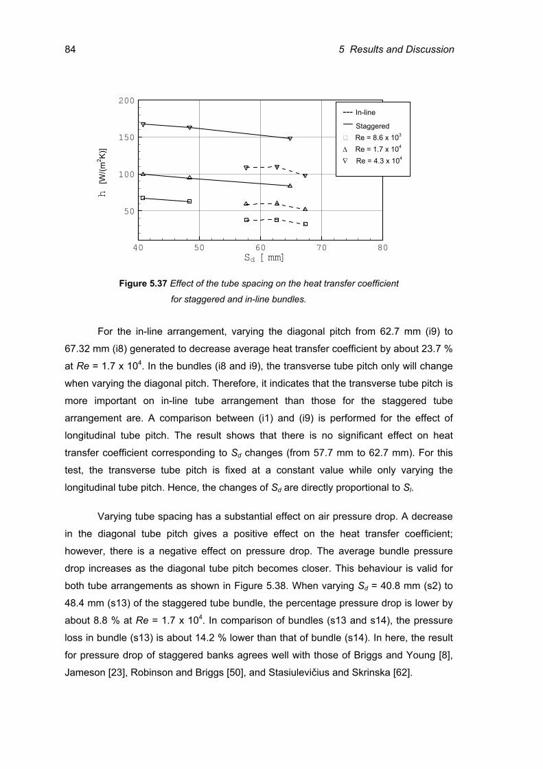
84 5 Results and Discussion
40 50 60 70 80
50
100
150
200
Figure 5.37 Effect of the tube spacing on the heat transfer coefficient
for staggered and in-line bundles.
For the in-line arrangement, varying the diagonal pitch from 62.7 mm (i9) to
67.32 mm (i8) generated to decrease average heat transfer coefficient by about 23.7 %
at Re = 1.7 x 10⁴. In the bundles (i8 and i9), the transverse tube pitch only will change
when varying the diagonal pitch. Therefore, it indicates that the transverse tube pitch is
more important on in-line tube arrangement than those for the staggered tube
arrangement are. A comparison between (i1) and (i9) is performed for the effect of
longitudinal tube pitch. The result shows that there is no significant effect on heat
transfer coefficient corresponding to Sd changes (from 57.7 mm to 62.7 mm). For this
test, the transverse tube pitch is fixed at a constant value while only varying the
longitudinal tube pitch. Hence, the changes of Sd are directly proportional to Sl.
Varying tube spacing has a substantial effect on air pressure drop. A decrease
in the diagonal tube pitch gives a positive effect on the heat transfer coefficient;
however, there is a negative effect on pressure drop. The average bundle pressure
drop increases as the diagonal tube pitch becomes closer. This behaviour is valid for
both tube arrangements as shown in Figure 5.38. When varying Sd = 40.8 mm (s2) to
48.4 mm (s13) of the staggered tube bundle, the percentage pressure drop is lower by
about 8.8 % at Re = 1.7 x 10⁴. In comparison of bundles (s13 and s14), the pressure
loss in bundle (s13) is about 14.2 % lower than that of bundle (s14). In here, the result
for pressure drop of staggered banks agrees well with those of Briggs and Young [8],
Jameson [23], Robinson and Briggs [50], and Stasiulevičius and Skrinska [62].
Sd [mm]
h [W
/(m2 K)
] --- In-line
Staggered Re = 8.6 x 10³
∆ Re = 1.7 x 10⁴
∇ Re = 4.3 x 10⁴
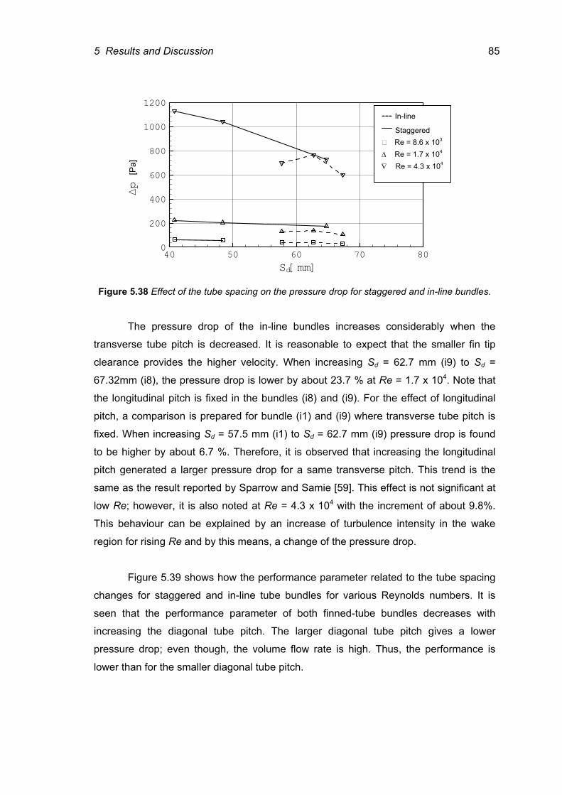
5 Results and Discussion 85
40 50 60 70 800
200
400
600
800
1000
1200
Figure 5.38 Effect of the tube spacing on the pressure drop for staggered and in-line bundles.
The pressure drop of the in-line bundles increases considerably when the
transverse tube pitch is decreased. It is reasonable to expect that the smaller fin tip
clearance provides the higher velocity. When increasing Sd = 62.7 mm (i9) to Sd =
67.32mm (i8), the pressure drop is lower by about 23.7 % at Re = 1.7 x 10⁴. Note that
the longitudinal pitch is fixed in the bundles (i8) and (i9). For the effect of longitudinal
pitch, a comparison is prepared for bundle (i1) and (i9) where transverse tube pitch is
fixed. When increasing Sd = 57.5 mm (i1) to Sd = 62.7 mm (i9) pressure drop is found
to be higher by about 6.7 %. Therefore, it is observed that increasing the longitudinal
pitch generated a larger pressure drop for a same transverse pitch. This trend is the
same as the result reported by Sparrow and Samie [59]. This effect is not significant at
low Re; however, it is also noted at Re = 4.3 x 10⁴ with the increment of about 9.8%.
This behaviour can be explained by an increase of turbulence intensity in the wake
region for rising Re and by this means, a change of the pressure drop.
Figure 5.39 shows how the performance parameter related to the tube spacing
changes for staggered and in-line tube bundles for various Reynolds numbers. It is
seen that the performance parameter of both finned-tube bundles decreases with
increasing the diagonal tube pitch. The larger diagonal tube pitch gives a lower
pressure drop; even though, the volume flow rate is high. Thus, the performance is
lower than for the smaller diagonal tube pitch.
Sd[mm]
∆p [P
a]
--- In-line Staggered
Re = 8.6 x 10³
∆ Re = 1.7 x 10⁴
∇ Re = 4.3 x 10⁴
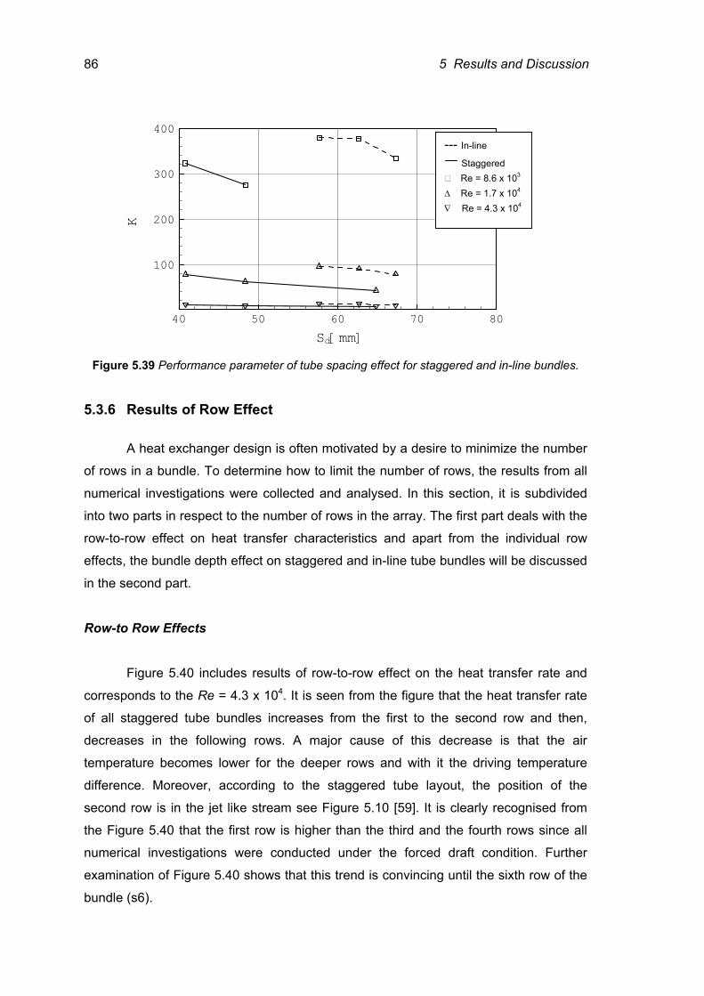
86 5 Results and Discussion
40 50 60 70 80
100
200
300
400
Figure 5.39 Performance parameter of tube spacing effect for staggered and in-line bundles.
5.3.6 Results of Row Effect
A heat exchanger design is often motivated by a desire to minimize the number
of rows in a bundle. To determine how to limit the number of rows, the results from all
numerical investigations were collected and analysed. In this section, it is subdivided
into two parts in respect to the number of rows in the array. The first part deals with the
row-to-row effect on heat transfer characteristics and apart from the individual row
effects, the bundle depth effect on staggered and in-line tube bundles will be discussed
in the second part.
Row-to Row Effects
Figure 5.40 includes results of row-to-row effect on the heat transfer rate and
corresponds to the Re = 4.3 x 10⁴. It is seen from the figure that the heat transfer rate
of all staggered tube bundles increases from the first to the second row and then,
decreases in the following rows. A major cause of this decrease is that the air
temperature becomes lower for the deeper rows and with it the driving temperature
difference. Moreover, according to the staggered tube layout, the position of the
second row is in the jet like stream see Figure 5.10 [59]. It is clearly recognised from
the Figure 5.40 that the first row is higher than the third and the fourth rows since all
numerical investigations were conducted under the forced draft condition. Further
examination of Figure 5.40 shows that this trend is convincing until the sixth row of the
bundle (s6).
Sd[mm]
K --- In-line
Staggered Re = 8.6 x 10³
∆ Re = 1.7 x 10⁴
∇ Re = 4.3 x 10⁴
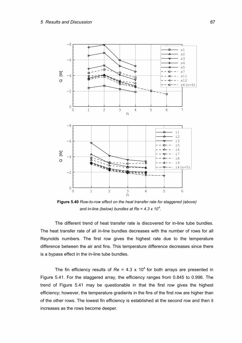
5 Results and Discussion 87
0 1 2 3 4 5 6 7n
-8
-6
-4
-2
0
s1s2s3s4s5s7s11s12s6(n=6)
0 1 2 3 4 5 6n
-8
-6
-4
-2
0
i1i2i3i5i6i7i8i9i4(n=5)
Figure 5.40 Row-to-row effect on the heat transfer rate for staggered (above)
and in-line (below) bundles at Re = 4.3 x 10⁴.
The different trend of heat transfer rate is discovered for in-line tube bundles.
The heat transfer rate of all in-line bundles decreases with the number of rows for all
Reynolds numbers. The first row gives the highest rate due to the temperature
difference between the air and fins. This temperature difference decreases since there
is a bypass effect in the in-line tube bundles.
The fin efficiency results of Re = 4.3 x 10⁴ for both arrays are presented in
Figure 5.41. For the staggered array, the efficiency ranges from 0.845 to 0.996. The
trend of Figure 5.41 may be questionable in that the first row gives the highest
efficiency; however, the temperature gradients in the fins of the first row are higher than
of the other rows. The lowest fin efficiency is established at the second row and then it
increases as the rows become deeper.
Qׂ [W
] Qׂ [W
]
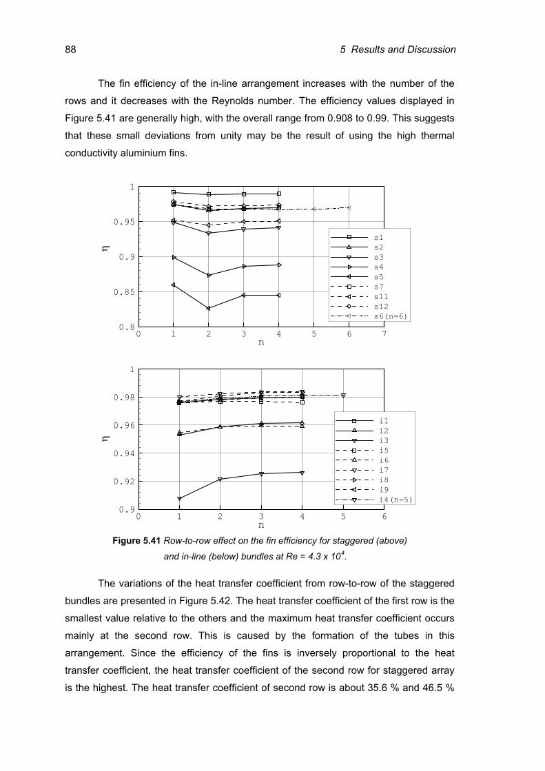
88 5 Results and Discussion
The fin efficiency of the in-line arrangement increases with the number of the
rows and it decreases with the Reynolds number. The efficiency values displayed in
Figure 5.41 are generally high, with the overall range from 0.908 to 0.99. This suggests
that these small deviations from unity may be the result of using the high thermal
conductivity aluminium fins.
0 1 2 3 4 5 6 7n0.8
0.85
0.9
0.95
1
s1s2s3s4s5s7s11s12s6(n=6)
0 1 2 3 4 5 6n0.9
0.92
0.94
0.96
0.98
1
i1i2i3i5i6i7i8i9i4(n=5)
Figure 5.41 Row-to-row effect on the fin efficiency for staggered (above)
and in-line (below) bundles at Re = 4.3 x 10⁴.
The variations of the heat transfer coefficient from row-to-row of the staggered
bundles are presented in Figure 5.42. The heat transfer coefficient of the first row is the
smallest value relative to the others and the maximum heat transfer coefficient occurs
mainly at the second row. This is caused by the formation of the tubes in this
arrangement. Since the efficiency of the fins is inversely proportional to the heat
transfer coefficient, the heat transfer coefficient of the second row for staggered array
is the highest. The heat transfer coefficient of second row is about 35.6 % and 46.5 %
η
η
5 Results and Discussion 89
higher than the first row for the bundle (s6) at Re = 8.6 x 10³ and 4.3 x 10⁴,
respectively, while 23.2 % and 30.5 % for the bundle (s7). However, in the latter bundle
where the fin spacing is increased to 4 mm, the third row heat transfer coefficient is
slightly higher (about 0.6 %) than the second row at Re = 4.3 x 10⁴. This is because of
the second horseshoe vortices that appeared in this case. When concerning on the
number of rows, the fin spacing effect (bundle-s7) shows a different trend to other
geometry changes.
A comparison with the data of Neal and Hitchcock [45] for the second and the
sixth row shows, however, a different trend. The numerical result of the heat transfer
coefficient of the sixth row is about 14.2 % lower than the second row at Re = 4.3 x 10⁴,
=f
tdS
1.2 and =f
ldS 1.04. However, Neal and Hitchcock showed that the heat transfer
coefficient of the sixth row is about 1 % higher than the second row of the equilateral
triangular tube pitch. The Reynolds number used in their investigation was 1.25 x 10⁵
and the transverse and longitudinal pitches to fin diameter ratios were 1.3 and 1.13. It
is unclear which type of air drafting to the system was applied in their [45] experimental
investigation. According to Gianolio and Cuti [14]’s comparison between the forced and
induced draft data, yields different trends for both of them. In the induced draft, the heat
transfer coefficient increases with the rows number. For the forced draft, the heat
transfer coefficient is greatest at the second row and then, decreases gradually with the
row numbers. The numerical simulation results have the same trend as the results in
[14] since the current simulation was under the consideration of a forced draft.
The variations of the heat transfer coefficient with the number of rows of the in-
line bundle are also depicted in Figure. 5.42. Contrasting to the staggered bundle
results, the highest heat transfer coefficient occurs at the first row of every bundle. The
heat transfer coefficient is typically very low in the wake region where the deep rows
are found to lie. This result agrees with the work of Brauer [6], and Kuntysh and Stenin
[37].
For the fin height increase bundles (i1, i2 and i3), the percentage decrease of
the heat transfer coefficient of the first to second row is increased. The same behaviour
for the tube spacing changes (i1, i8 and i9) is also observed in the figure. This
behaviour is more noticeable on the transverse pitch than the longitudinal pitch. It can
be explained that the increased transverse tube pitch gives more bypass flow between
the tubes.
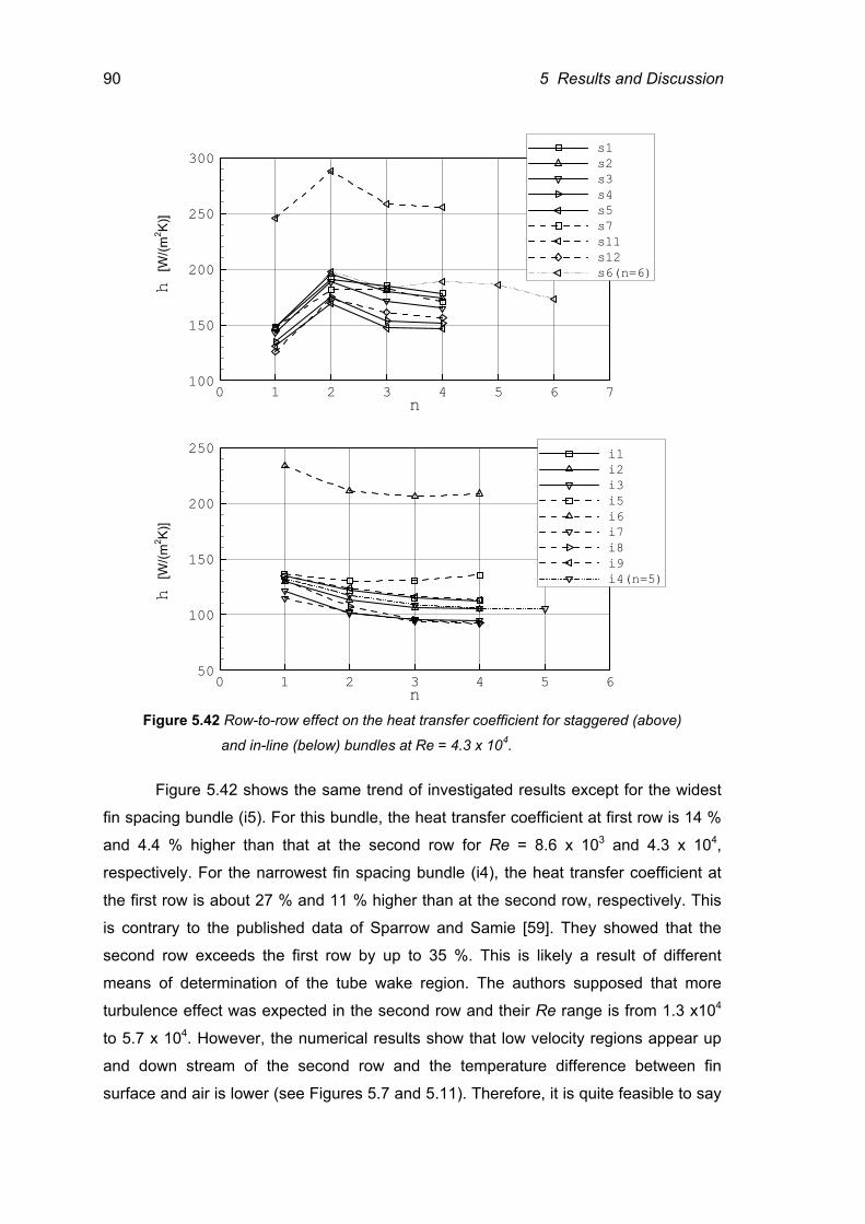
90 5 Results and Discussion
0 1 2 3 4 5 6 7n100
150
200
250
300 s1s2s3s4s5s7s11s12s6(n=6)
0 1 2 3 4 5 6n50
100
150
200
250 i1i2i3i5i6i7i8i9i4(n=5)
Figure 5.42 Row-to-row effect on the heat transfer coefficient for staggered (above)
and in-line (below) bundles at Re = 4.3 x 10⁴. Figure 5.42 shows the same trend of investigated results except for the widest
fin spacing bundle (i5). For this bundle, the heat transfer coefficient at first row is 14 %
and 4.4 % higher than that at the second row for Re = 8.6 x 10³ and 4.3 x 10⁴,
respectively. For the narrowest fin spacing bundle (i4), the heat transfer coefficient at
the first row is about 27 % and 11 % higher than at the second row, respectively. This
is contrary to the published data of Sparrow and Samie [59]. They showed that the
second row exceeds the first row by up to 35 %. This is likely a result of different
means of determination of the tube wake region. The authors supposed that more
turbulence effect was expected in the second row and their Re range is from 1.3 x10⁴
to 5.7 x 10⁴. However, the numerical results show that low velocity regions appear up
and down stream of the second row and the temperature difference between fin
surface and air is lower (see Figures 5.7 and 5.11). Therefore, it is quite feasible to say
h [W
/(m2 K)
] h
[W/(m
2 K)]
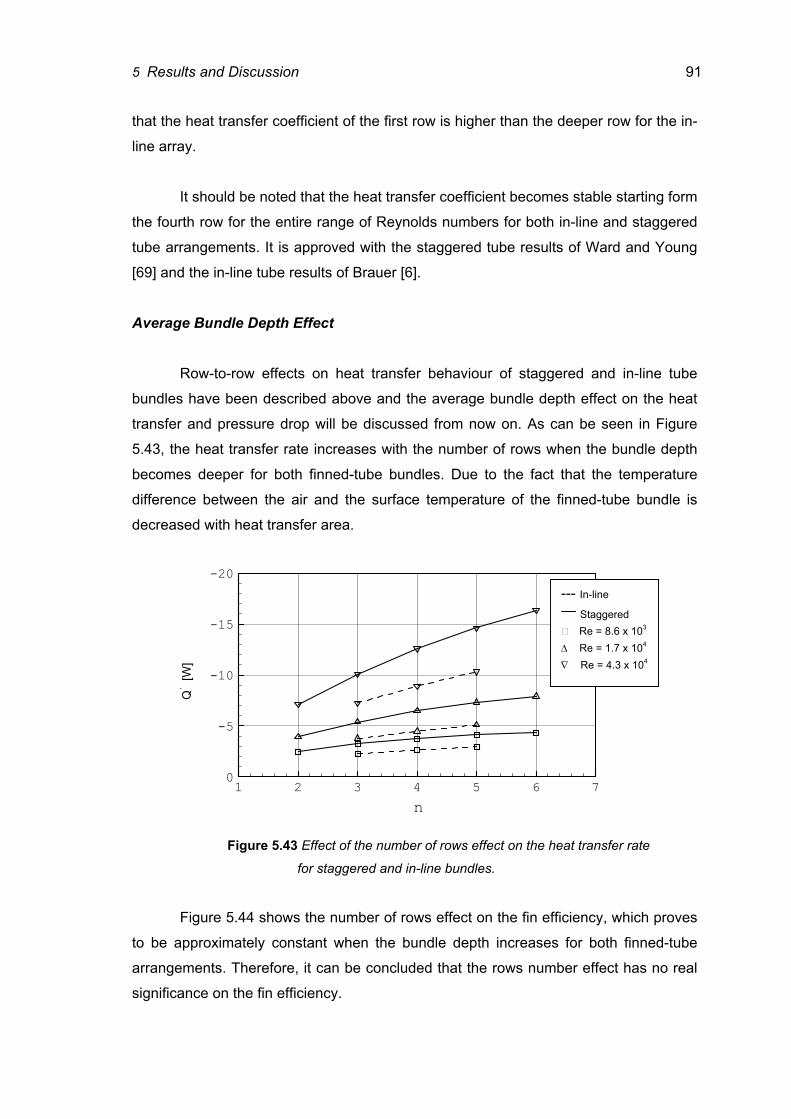
5 Results and Discussion 91
that the heat transfer coefficient of the first row is higher than the deeper row for the in-
line array.
It should be noted that the heat transfer coefficient becomes stable starting form
the fourth row for the entire range of Reynolds numbers for both in-line and staggered
tube arrangements. It is approved with the staggered tube results of Ward and Young
[69] and the in-line tube results of Brauer [6].
Average Bundle Depth Effect Row-to-row effects on heat transfer behaviour of staggered and in-line tube
bundles have been described above and the average bundle depth effect on the heat
transfer and pressure drop will be discussed from now on. As can be seen in Figure
5.43, the heat transfer rate increases with the number of rows when the bundle depth
becomes deeper for both finned-tube bundles. Due to the fact that the temperature
difference between the air and the surface temperature of the finned-tube bundle is
decreased with heat transfer area.
1 2 3 4 5 6 7
-20
-15
-10
-5
0
Figure 5.43 Effect of the number of rows effect on the heat transfer rate
for staggered and in-line bundles.
Figure 5.44 shows the number of rows effect on the fin efficiency, which proves
to be approximately constant when the bundle depth increases for both finned-tube
arrangements. Therefore, it can be concluded that the rows number effect has no real
significance on the fin efficiency.
n
Qׂ [W
]
--- In-line Staggered
Re = 8.6 x 10³
∆ Re = 1.7 x 10⁴
∇ Re = 4.3 x 10⁴
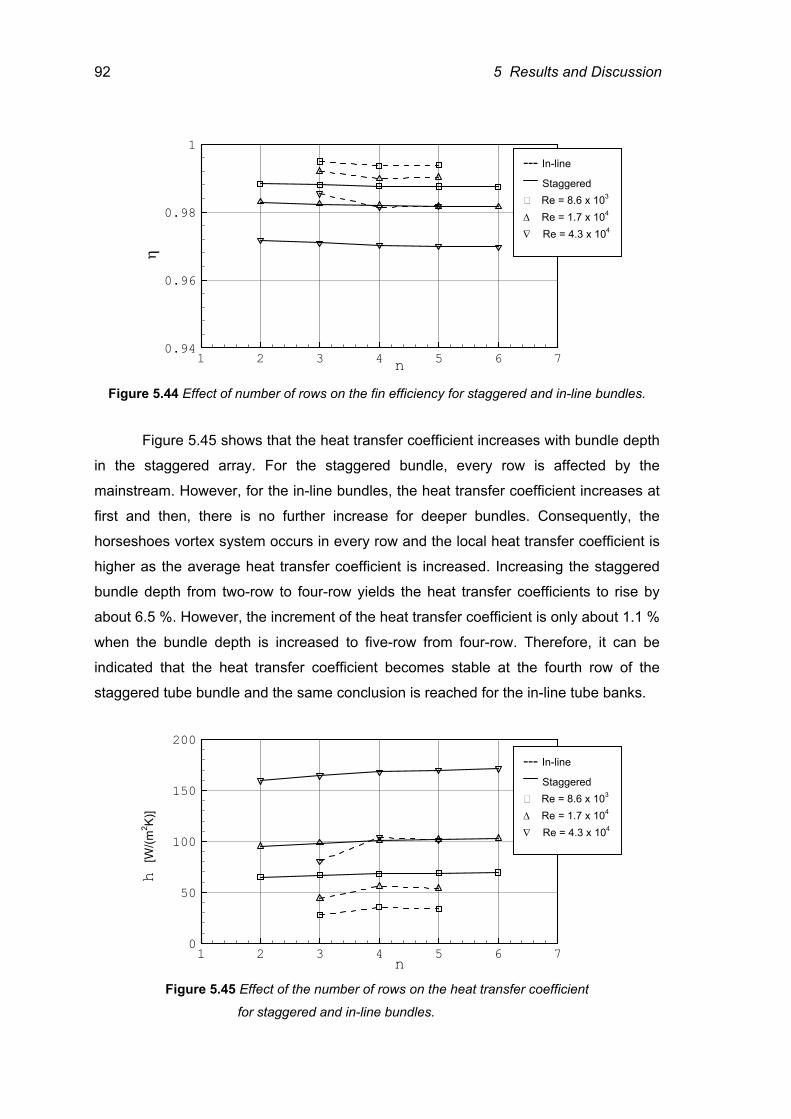
92 5 Results and Discussion
1 2 3 4 5 6 70.94
0.96
0.98
1
Figure 5.44 Effect of number of rows on the fin efficiency for staggered and in-line bundles.
Figure 5.45 shows that the heat transfer coefficient increases with bundle depth
in the staggered array. For the staggered bundle, every row is affected by the
mainstream. However, for the in-line bundles, the heat transfer coefficient increases at
first and then, there is no further increase for deeper bundles. Consequently, the
horseshoes vortex system occurs in every row and the local heat transfer coefficient is
higher as the average heat transfer coefficient is increased. Increasing the staggered
bundle depth from two-row to four-row yields the heat transfer coefficients to rise by
about 6.5 %. However, the increment of the heat transfer coefficient is only about 1.1 %
when the bundle depth is increased to five-row from four-row. Therefore, it can be
indicated that the heat transfer coefficient becomes stable at the fourth row of the
staggered tube bundle and the same conclusion is reached for the in-line tube banks.
1 2 3 4 5 6 70
50
100
150
200
Figure 5.45 Effect of the number of rows on the heat transfer coefficient
for staggered and in-line bundles.
n
n
η
h [W
/(m2 K)
] --- In-line
Staggered Re = 8.6 x 10³
∆ Re = 1.7 x 10⁴
∇ Re = 4.3 x 10⁴
--- In-line Staggered
Re = 8.6 x 10³
∆ Re = 1.7 x 10⁴
∇ Re = 4.3 x 10⁴
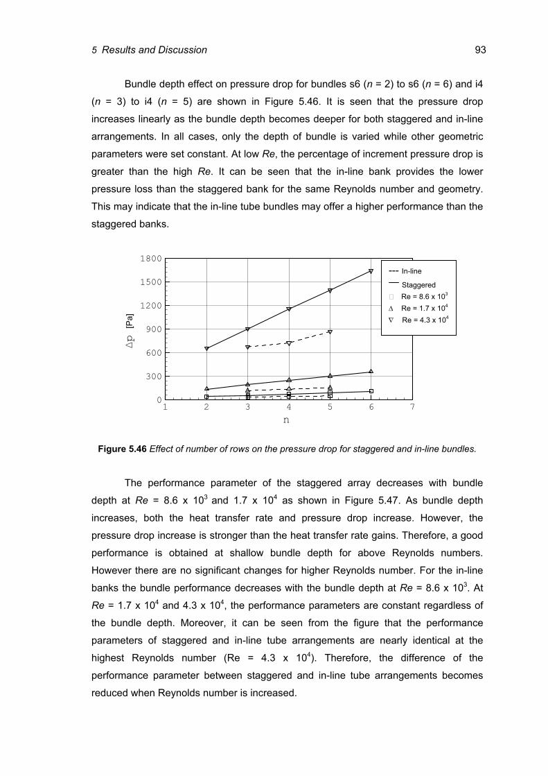
5 Results and Discussion 93
Bundle depth effect on pressure drop for bundles s6 (n = 2) to s6 (n = 6) and i4
(n = 3) to i4 (n = 5) are shown in Figure 5.46. It is seen that the pressure drop
increases linearly as the bundle depth becomes deeper for both staggered and in-line
arrangements. In all cases, only the depth of bundle is varied while other geometric
parameters were set constant. At low Re, the percentage of increment pressure drop is
greater than the high Re. It can be seen that the in-line bank provides the lower
pressure loss than the staggered bank for the same Reynolds number and geometry.
This may indicate that the in-line tube bundles may offer a higher performance than the
staggered banks.
1 2 3 4 5 6 70
300
600
900
1200
1500
1800
Figure 5.46 Effect of number of rows on the pressure drop for staggered and in-line bundles.
The performance parameter of the staggered array decreases with bundle
depth at Re = 8.6 x 10³ and 1.7 x 10⁴ as shown in Figure 5.47. As bundle depth
increases, both the heat transfer rate and pressure drop increase. However, the
pressure drop increase is stronger than the heat transfer rate gains. Therefore, a good
performance is obtained at shallow bundle depth for above Reynolds numbers.
However there are no significant changes for higher Reynolds number. For the in-line
banks the bundle performance decreases with the bundle depth at Re = 8.6 x 10³. At
Re = 1.7 x 10⁴ and 4.3 x 10⁴, the performance parameters are constant regardless of
the bundle depth. Moreover, it can be seen from the figure that the performance
parameters of staggered and in-line tube arrangements are nearly identical at the
highest Reynolds number (Re = 4.3 x 10⁴). Therefore, the difference of the
performance parameter between staggered and in-line tube arrangements becomes
reduced when Reynolds number is increased.
n
∆p [P
a]
--- In-line Staggered
Re = 8.6 x 10³
∆ Re = 1.7 x 10⁴
∇ Re = 4.3 x 10⁴
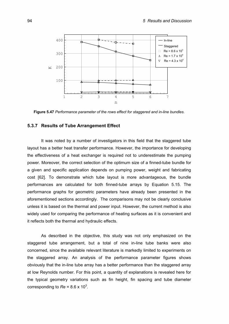
94 5 Results and Discussion
1 2 3 4 5 6 7
100
200
300
400
Figure 5.47 Performance parameter of the rows effect for staggered and in-line bundles.
5.3.7 Results of Tube Arrangement Effect
It was noted by a number of investigators in this field that the staggered tube
layout has a better heat transfer performance. However, the importance for developing
the effectiveness of a heat exchanger is required not to underestimate the pumping
power. Moreover, the correct selection of the optimum size of a finned-tube bundle for
a given and specific application depends on pumping power, weight and fabricating
cost [62]. To demonstrate which tube layout is more advantageous, the bundle
performances are calculated for both finned-tube arrays by Equation 5.15. The
performance graphs for geometric parameters have already been presented in the
aforementioned sections accordingly. The comparisons may not be clearly conclusive
unless it is based on the thermal and power input. However, the current method is also
widely used for comparing the performance of heating surfaces as it is convenient and
it reflects both the thermal and hydraulic effects.
As described in the objective, this study was not only emphasized on the
staggered tube arrangement, but a total of nine in-line tube banks were also
concerned, since the available relevant literature is markedly limited to experiments on
the staggered array. An analysis of the performance parameter figures shows
obviously that the in-line tube array has a better performance than the staggered array
at low Reynolds number. For this point, a quantity of explanations is revealed here for
the typical geometry variations such as fin height, fin spacing and tube diameter
corresponding to Re = 8.6 x 10³.
K
n
--- In-line Staggered
Re = 8.6 x 10³
∆ Re = 1.7 x 10⁴
∇ Re = 4.3 x 10⁴
5 Results and Discussion 95
According to a comparison between the in-line and staggered arrays for a fin
height of 5 mm, the heat transfer rate of staggered array (bundle s2) is about 41.7 %
higher than those of the in-line array (bundle, i1). The same trend is obtained by
Ackerman and Brunsvold [1], Hashizume [20], Kaminski [29], Neal and Hitchcock [45],
Rabas and Huber [49], and Sparrow and Samie [59]. Remember that the bundle
performance not only relies on the heat transfer rate but also on the pressure drop.
Therefore, unless the staggered tube array had better results in the heat transfer rate,
a great loss (66.5 %) of the pressure drop is found for a same Reynolds number. As
stated earlier, the in-line tube array had advantages for low Re and the margin between
the in-line and staggered arrays becomes narrower as the Re is increased and at Re =
4.3 x 10⁴, the performance of both bundles is approximately the same. Once the
velocity is increased, the pressure drop increases stronger than the heat transfer rate
for the in-line array and thus, the lower performance can be obtained.
A comparison of the staggered and in-line array based on the fin spacing shows
that the heat transfer rate of the former is moderately higher. For example, the
maximum enhancement (relative to the in-line array) is 43.2 % for the staggered array
at s = 1.6 mm. However, a comparison of the two arrays reveals marked differences in
terms of the pressure drop results by about 74.3 %. Further examination on the tube
diameter effects show a similar trend as in the previous investigations. At d = 13.59
mm, the pressure drop of the staggered array is 60.2 % higher than the in-line while
only 33 % higher for the heat transfer rate. Therefore, it is confirmed that at low
Reynolds number only in-line tube configuration would be considered as the optimum
surface for a given geometry since the pressure drop severely affected the heat
transfer enhancement.
This result agrees well with the work of Ackerman and Brunsvold [1] and
Kaminski [29] since similar performance criteria were applied in their investigations.
Ackerman and Brunsvold [1] showed that the in-line tube arrangement provides the
higher performance than the staggered arrangement for similar tube geometry.
Moreover, it is found that the performance parameter attains maximum at low Re.
However, this method gives no indication of the amount of surface required by any
arrangement to transfer a given amount of heat [1].
Weierman [76] reported that the staggered array had a good performance
although his comparison was based on four-row staggered and seven-row in-line
bundles with the same pressure drop values. If compared to the same rows number,
96 5 Results and Discussion
i.e., four-row staggered to four-row in-line tubes, the result may be different. However,
Kuntysh and Stenin [37] showed that the four row staggered array has a better
efficiency than the four row in-line array for the same specific power required.
The relevant qualitative findings of these comparisons are:
• The performance parameter of the in-line geometry is higher when compared
under the same condition applied for the staggered array.
• The staggered array clearly yields a higher heat transfer coefficient, while the
pressure drop of the staggered array is generally higher than for the in-line
arrangement.
• The difference of the heat transfer coefficient between the in-line and staggered
arrangement is decreased in the aspect of Reynolds number and fin spacing
are increased, and fin height and tube diameter are decreased.
• The difference is also decreased when the bundle depth of both tube arrays
increases, except for the five-row in-line bundle.
• Generally, the pressure drop of the staggered banks is higher by a factor of 1.8
than the in-line banks at a low Reynolds number. This pressure drop increment
is declined as Reynolds number increases.
The flow characteristics, the local effects on the heat transfer and pressure drop
of the circular finned-tube heat exchangers and the results of geometry variables
effects are already described above. Alternatively, the numerical simulation results
made possible the analysis on the local and average aspects and provides for the more
resourceful correlations on both the heat transfer and pressure drop characteristics.
For this reason, correlating the numerical results to obtain better sense of correlations
will be presented in the next chapter.
6 Correlations and Data Comparison
A set of correlations based on numerical investigation results and available
experimental data is proposed in this chapter. Since different variables were applied in
the reduction of the various experimental data, direct comparison to those correlations
is more or less ambiguous. Even though, this chapter is also concerned with the
comparison of the present numerical results with data in the previous literature and vice
versa.
6.1 Heat Transfer Correlations
Using the power law correlations, most of the experimental results are correlated
in non-dimensional form in a wide range of Reynolds numbers. The Nusselt number Nu,
the Stanton number St, and Prandtl number Pr are typically used for the heat transfer
while the Reynolds number Re is for the flow variables. On the other hand, the Euler
number Eu and friction factor f is often used to express the correlated equation of
pressure drop. For the bundle arrangement, existing experimental investigations for heat
transfer coefficient and pressure drop are classified in Appendix D. Stasiulevičius and
Skrinska [62] indicated that the available heat transfer correlations were based on how
to determine the average convective heat transfer coefficient and ignored the state of
non-uniformity in distributions of heat transfer over the fin surface. Beside being
impracticable to establish a universal correlation, analyzing the numerical results and
discussing with the previous data in the last chapters provide the fact that a correlation
should embrace enough considerations such as all parameters of finning geometry,
bundle configuration, and flow distribution in the bundle. To encounter these effects,
additional terms are used to apply in a preliminary correlation for a single bundle that is
based on the power law equation.
In order to achieve an acceptable correlation, the heat transfer correlations were
based on own numerical results and the experimental data. Dimensions of experimental
finned-tube heat exchangers are shown in Appendix C. However, the heat transfer
98 6 Correlations and Data Comparison
results that were obtained by the local thermal simulation method (only one test tube is
heated) and segmented fin cases were omitted in these correlations. Moreover, cases
with Reynolds number below 4 x 10³ or above 7.5 x 10⁴ are not considered. The results
are reduced in non-dimensional form and average heat transfer correlations for both
staggered and in-line arrangements were prepared.
6.1.1 Staggered Tube Arrangement
Bundles with only one row were not included in this investigation and two
correlations for the staggered arrangement are therefore presented here depending on
the number of rows. The concept of VDI-Wärmeatlas [68] was applied for this
presentation taking the tube diameter and velocity at minimum free flow area as the
reference quantities. The average heat transfer correlation for the staggered finned-
tube bundles with n ≥ 4 has the following form,
[ ]
d
d
tc
68WärmeatlasVDI
b
t
a
SS
FAAPrReCNu 3
1
=
−4444 34444 21
(6.1)
Where =A Total heat transfer area, m2
=tA Outside surface area of tube except fins, m2
=tS Transverse tube spacing, m
=dS Diagonal tube spacing, m
The exponents of Re and the ratio of total heat surface area to base tube area
tAA were set as in the VDI-Wärmeatlas [68] correlation, a = 0.6 and b = - 0.15
respectively (see Appendix D.3). The extra terms, F and d
tSS
were added to the
correlation of VDI-Wärmeatlas. The term d
tSS
was added for a consideration of the
effect of non-equilateral triangular pitch arrangement which has been found in a very
few cases, and F was supplemented for special consideration of the ratio of boundary
layer thickness δb, and characteristic length expressed as the hydraulic diameter dh of
the finned-tub arrangement.
6 Correlations and Data Comparison 99
Following suggestions by Kays and London [30] and later by Nir [46] the
hydraulic diameter may expressed as
A
A.d4d fffh ′= (6.2)
where =ffA minimum free flow area of finned-tube per unit length, m2/m,
( )( )ffft N1dddS δ−−+−=
=′A Heat transfer area of unit length finned-tube, m2/m,
=
+
−+
− δδ
f
22f
ff
f d2
ddSS
1d ππ
By rearranging Equation (6.2) ash
f
ff dd4
AA
=′
, to following expression has been
developed for optimum representation of the above mentioned boundary layer
thickness effects:
1
AA
1F
ff+
′= (6.3)
where
=
=
h
b2
h
f1 d
fddfF
δ.
When increasing the diameter of fins, the boundary layer developed on the
surface of fins becomes thicker and the factor F becomes smaller. Thus, decline of the
heat transfer coefficient and increase of the pressure drop will result.
The correlations are prepared with the results from all numerical configurations
(see Table 4.1) except for the bundles (s9) and (s10), which had undergone the test for
the fin thickness effect along with bundle (s2). However, it is found that the Nu number
difference between these tests is negligible and hence, only bundle (s2) was considered
for this correlation. Finally, the air-side heat transfer correlation for the depth of four and
more rows has been obtained as following by application of the least square method.
For the staggered arrangement, the effect of factor F is of no real significance because
the value of exponent is very small:
06.1
d
t075.015.0
t
6.0
SS
FAAPrRe284.0Nu 3
1
= −
−
(6.4)
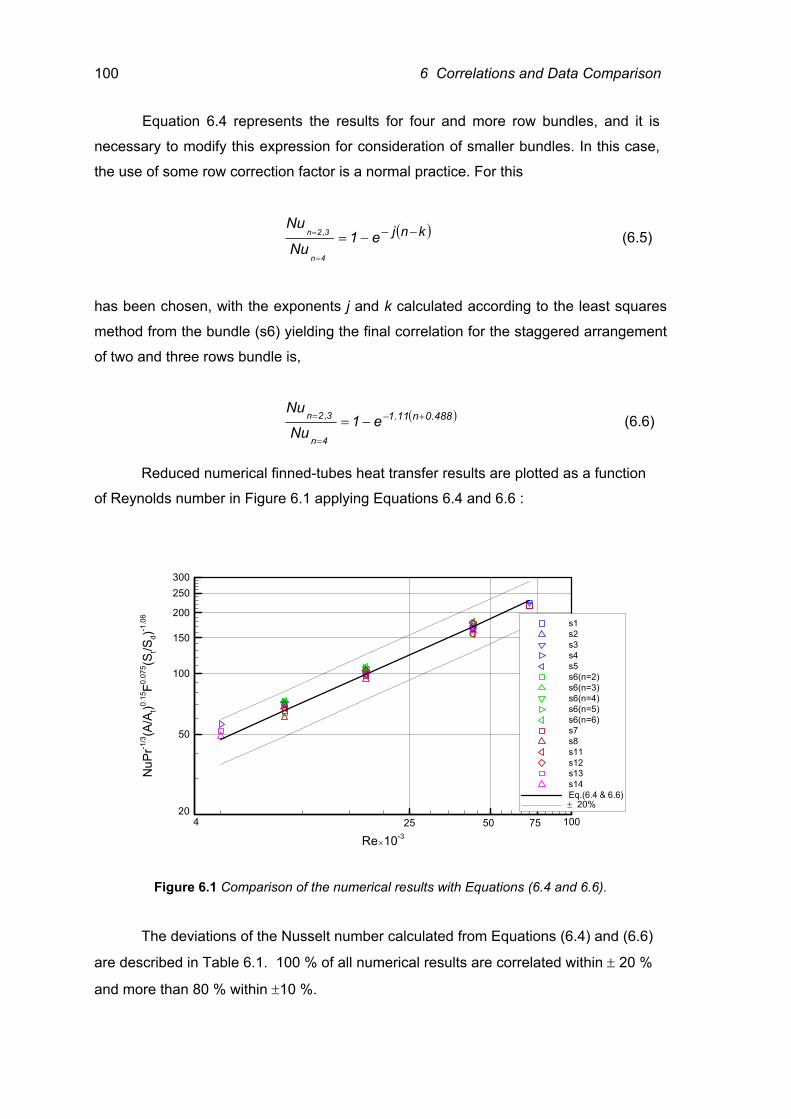
100 6 Correlations and Data Comparison
Equation 6.4 represents the results for four and more row bundles, and it is
necessary to modify this expression for consideration of smaller bundles. In this case,
the use of some row correction factor is a normal practice. For this
( )knje1Nu
Nu
4n
3,2n −−−==
= (6.5)
has been chosen, with the exponents j and k calculated according to the least squares
method from the bundle (s6) yielding the final correlation for the staggered arrangement
of two and three rows bundle is,
( )488.0n11.1e1Nu
Nu
4n
3,2n +−−==
= (6.6)
Reduced numerical finned-tubes heat transfer results are plotted as a function
of Reynolds number in Figure 6.1 applying Equations 6.4 and 6.6 :
Re 10-3
50
100
150
200
250300
NuP
r-1/3(A
/At)0.
15F0.
075 (S
t/Sd)-1
.06
s1s2s3s4s5s6(n=2)s6(n=3)s6(n=4)s6(n=5)s6(n=6)s7s8s11s12s13s14Eq.(6.4 & 6.6)
25 50 75 100420
×
± 20%
Figure 6.1 Comparison of the numerical results with Equations (6.4 and 6.6).
The deviations of the Nusselt number calculated from Equations (6.4) and (6.6)
are described in Table 6.1. 100 % of all numerical results are correlated within ± 20 %
and more than 80 % within ±10 %.
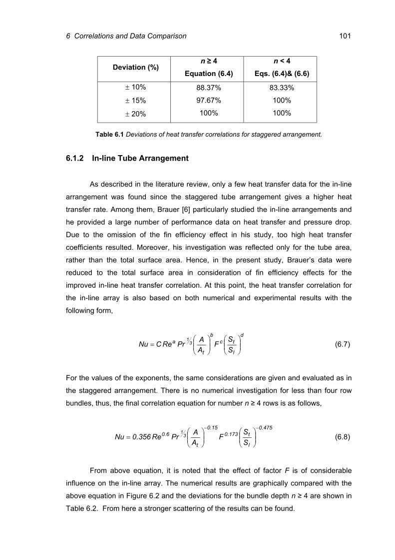
6 Correlations and Data Comparison 101
Deviation (%) n ≥ 4
Equation (6.4) n < 4
Eqs. (6.4)& (6.6)
± 10%
± 15%
± 20%
88.37%
97.67%
100%
83.33%
100%
100%
Table 6.1 Deviations of heat transfer correlations for staggered arrangement.
6.1.2 In-line Tube Arrangement As described in the literature review, only a few heat transfer data for the in-line
arrangement was found since the staggered tube arrangement gives a higher heat
transfer rate. Among them, Brauer [6] particularly studied the in-line arrangements and
he provided a large number of performance data on heat transfer and pressure drop.
Due to the omission of the fin efficiency effect in his study, too high heat transfer
coefficients resulted. Moreover, his investigation was reflected only for the tube area,
rather than the total surface area. Hence, in the present study, Brauer’s data were
reduced to the total surface area in consideration of fin efficiency effects for the
improved in-line heat transfer correlation. At this point, the heat transfer correlation for
the in-line array is also based on both numerical and experimental results with the
following form,
d
l
tcb
t
a
SS
FAAPrReCNu 3
1
= (6.7)
For the values of the exponents, the same considerations are given and evaluated as in
the staggered arrangement. There is no numerical investigation for less than four row
bundles, thus, the final correlation equation for number n ≥ 4 rows is as follows,
475.0
l
t173.015.0
t
6.0
SS
FAAPrRe356.0Nu 3
1−−
= (6.8)
From above equation, it is noted that the effect of factor F is of considerable
influence on the in-line array. The numerical results are graphically compared with the
above equation in Figure 6.2 and the deviations for the bundle depth n ≥ 4 are shown in
Table 6.2. From here a stronger scattering of the results can be found.
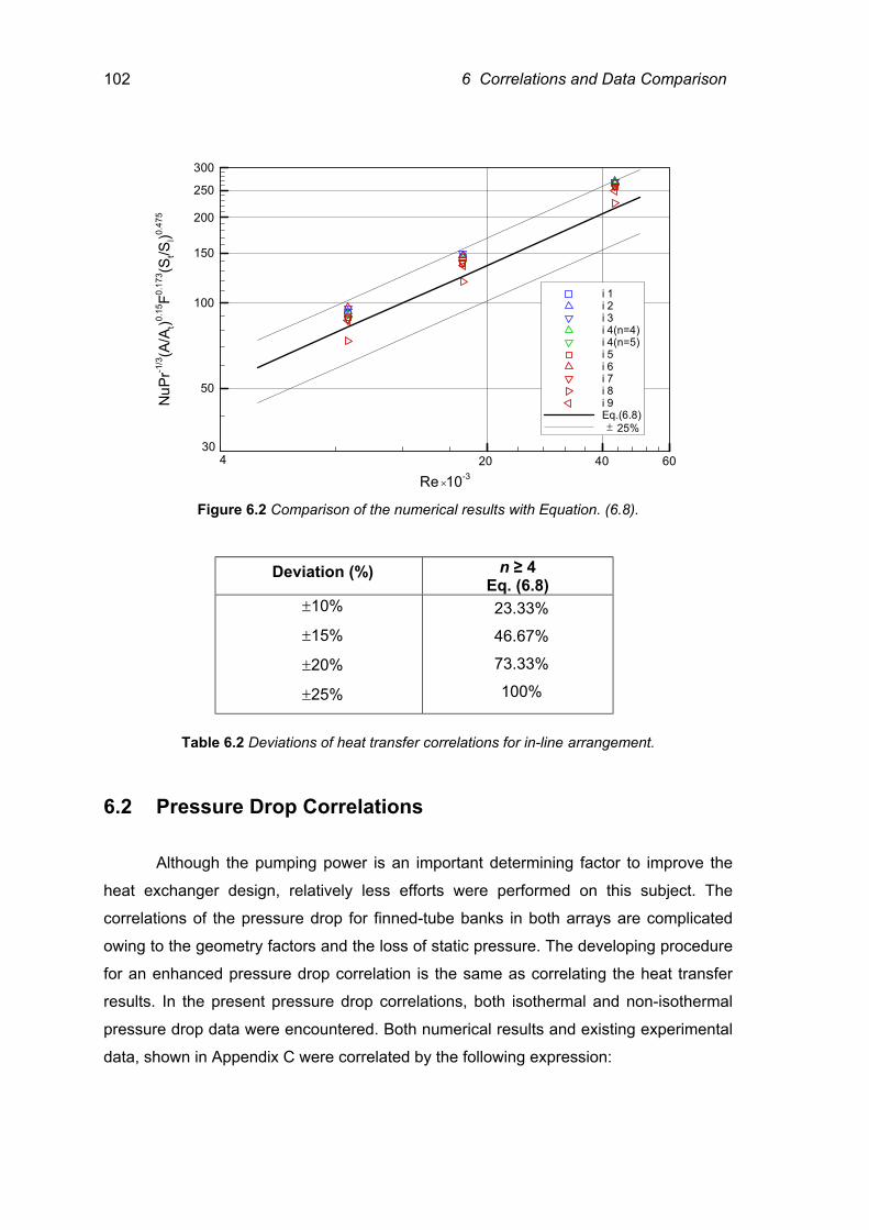
102 6 Correlations and Data Comparison
Re 10-3
50
100
150
200
250
300N
uPr-1
/3(A
/At)0.
15F0.
173 (S
t/Sl)0.
475
i 1i 2i 3i 4(n=4)i 4(n=5)i 5i 6i 7i 8i 9Eq.(6.8)
4 20 40 60
×
30± 25%
Figure 6.2 Comparison of the numerical results with Equation. (6.8).
Table 6.2 Deviations of heat transfer correlations for in-line arrangement.
6.2 Pressure Drop Correlations
Although the pumping power is an important determining factor to improve the
heat exchanger design, relatively less efforts were performed on this subject. The
correlations of the pressure drop for finned-tube banks in both arrays are complicated
owing to the geometry factors and the loss of static pressure. The developing procedure
for an enhanced pressure drop correlation is the same as correlating the heat transfer
results. In the present pressure drop correlations, both isothermal and non-isothermal
pressure drop data were encountered. Both numerical results and existing experimental
data, shown in Appendix C were correlated by the following expression:
Deviation (%) n ≥ 4 Eq. (6.8)
±10%
±15%
±20%
±25%
23.33%
46.67%
73.33%
100%
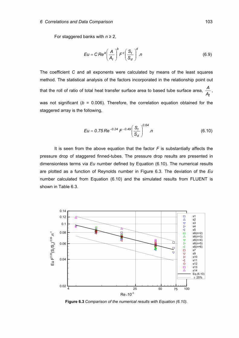
6 Correlations and Data Comparison 103
For staggered banks with n ≥ 2,
n.SS
FAAReCEu
d
d
tcb
t
a
= (6.9)
The coefficient C and all exponents were calculated by means of the least squares
method. The statistical analysis of the factors incorporated in the relationship point out
that the roll of ratio of total heat transfer surface area to based tube surface area, tA
A ,
was not significant (b = 0.006). Therefore, the correlation equation obtained for the
staggered array is the following,
n.SS
FRe75.0Eu64.0
d
t49.024.0
= −− (6.10)
It is seen from the above equation that the factor F is substantially affects the
pressure drop of staggered finned-tubes. The pressure drop results are presented in
dimensionless terms via Eu number defined by Equation (6.10). The numerical results
are plotted as a function of Reynolds number in Figure 6.3. The deviation of the Eu
number calculated from Equation (6.10) and the simulated results from FLUENT is
shown in Table 6.3.
Re 10-3
0.02
0.04
0.06
0.08
0.1
0.12
0.14
EuF0.
49(S
t/Sd)-0
.64 .n
-1
s1s2s3s4s5s6(n=2)s6(n=3)s6(n=4)s6(n=5)s6(n=6)s7s9s10s11s12s13s14Eq.(6.10)
4 25 50 75 100
×
± 25%
Figure 6.3 Comparison of the numerical results with Equation (6.10).
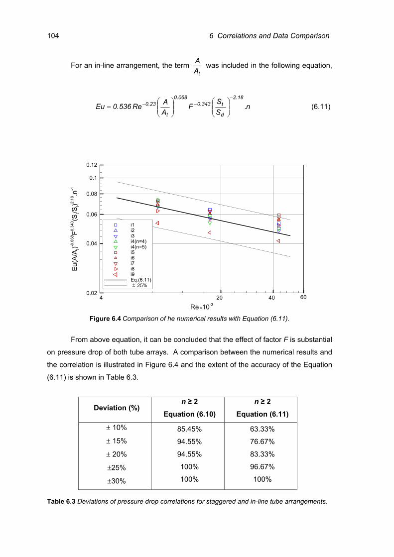
104 6 Correlations and Data Comparison
For an in-line arrangement, the term tA
A was included in the following equation,
n.SS
FAARe536.0Eu
18.2
d
t343.0068.0
t
23.0−
−−
= (6.11)
Re 10-3
0.02
0.04
0.06
0.08
0.1
0.12
Eu(A
/At)-0
.068
F0.34
3 (St/S
l)2.18
.n-1
i1i2i3i4(n=4)i4(n=5)i5i6i7i8i9Eq.(6.11)
4 20 40 60
×
± 25%
Figure 6.4 Comparison of he numerical results with Equation (6.11).
From above equation, it can be concluded that the effect of factor F is substantial
on pressure drop of both tube arrays. A comparison between the numerical results and
the correlation is illustrated in Figure 6.4 and the extent of the accuracy of the Equation
(6.11) is shown in Table 6.3.
Deviation (%) n ≥ 2
Equation (6.10) n ≥ 2
Equation (6.11)
± 10%
± 15%
± 20%
±25%
±30%
85.45%
94.55%
94.55%
100%
100%
63.33%
76.67%
83.33%
96.67%
100%
Table 6.3 Deviations of pressure drop correlations for staggered and in-line tube arrangements.
6 Correlations and Data Comparison 105
6.3 Data Comparison The developments for the enhancement of heat transfer and pressure drop
predictions of circular finned-tube banks have already been described in the literature
review. Moreover, related correlations and their limitations are discussed in section
2.2.3. Most of the experimental investigations were completed for the optimisation of the
finning geometry while a few attentions on the tube spacing effect and the bundle
arrangement. Since the tabulated experimental data covering wide ranges of geometric
variables and Reynolds numbers are not available for the analysis, it was necessary to
read from respective figures regardless of the factual error. Moreover, as noted in the
section 2.1 that no exact information was found in the published literature for the
numerical simulation of circular finned-tube arrays. Therefore, comparisons can be
made only between the present numerical results and the experimental ones. The
results and comparisons are presented by the relative deviations and plotted as a
function of Reynolds number.
6.3.1 Comparison of Heat Transfer Results for Staggered Arrangement
Comparison of the numerical results with the correlations from the literature is
shown in Figure 6.5 as the relative deviation. It is seen that a number of Nu numbers
calculated by the correlations are greater than numerically calculated Nu numbers, even
though some are found to be smaller. Generally, at low Re range, the numerical results
are higher than the experimental data. At this point, it is appropriate to note that present
numerical simulations were under the consideration of the turbulent modeling.
Figure 6.5(a) shows that the Stasiulevičius and Skrinska [62] equation yields
smaller Nu numbers than the numerical results at Re < 104 since their correlation was
based on higher Reynolds number in the range from 2 x 10⁴ to 2 x 10⁵. On the other
hand, at Re = 4.3 x 10⁴, Briggs and Young [8] and [62] predictions are about 28.7% and
26 % higher than the present results of bundle (s7) which is the largest fin spacing case
(s = 4 mm). Their predictions are questionable that the boundary layer becomes thinner
at high Re and therefore, the fin spacing effect may not be the decisive factor on heat
transfer. For the bundles (s11) and (s14), numerical results are found to be lower than
the results of [62]. It is reasonable to accept that the bundle (s11) having the smallest
tube diameter (13.59 mm), which is outside of the applicable range of their tested
geometries. However, for the latter bundle, it is expected that the heat transfer
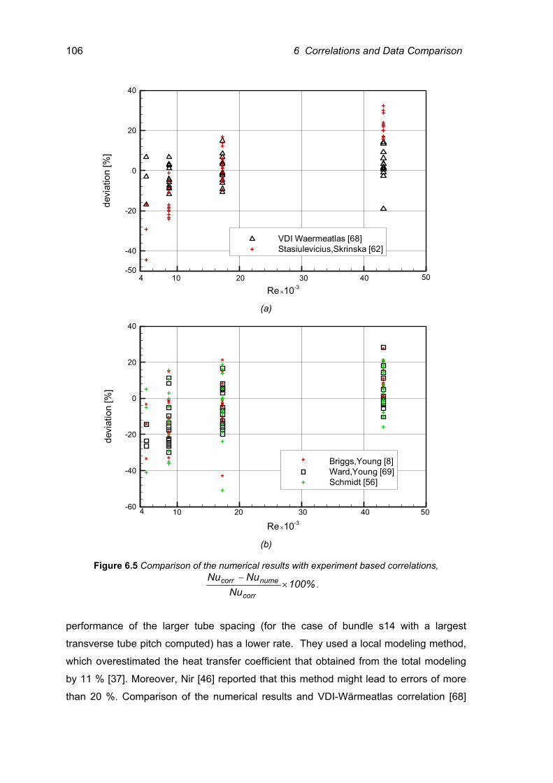
106 6 Correlations and Data Comparison
Re 10-3
-40
-20
0
20
40
devi
atio
n[%
]
+
+
+
+
+++++
++
+
++
++
+++++
+
++
+
+
+
+
++
++++++
++
++
+
++
VDI Waermeatlas [68]Stasiulevicius,Skrinska [62]+
-504 10 20 30 40 50
× (a)
Re 10-3
-60
-40
-20
0
20
40
devi
atio
n[%
]
*
*
* *
*****
*
*
*
*
*
**
******
*
*
*
*
*
*
**
******
**
**
*
**
+
+
++
+
+
+
+
+
+
++
+
+
++
+
+
+
++
+
+
++
+
+
+
++
+
+
+
++
+
++
++
+
++
Briggs,Young [8]Ward,Young [69]Schmidt [56]
*
+
4 10 20 30 40 50
× (b)
Figure 6.5 Comparison of the numerical results with experiment based correlations,
%100Nu
NuNu
corr
numecorr ×−
.
performance of the larger tube spacing (for the case of bundle s14 with a largest
transverse tube pitch computed) has a lower rate. They used a local modeling method,
which overestimated the heat transfer coefficient that obtained from the total modeling
by 11 % [37]. Moreover, Nir [46] reported that this method might lead to errors of more
than 20 %. Comparison of the numerical results and VDI-Wärmeatlas correlation [68]
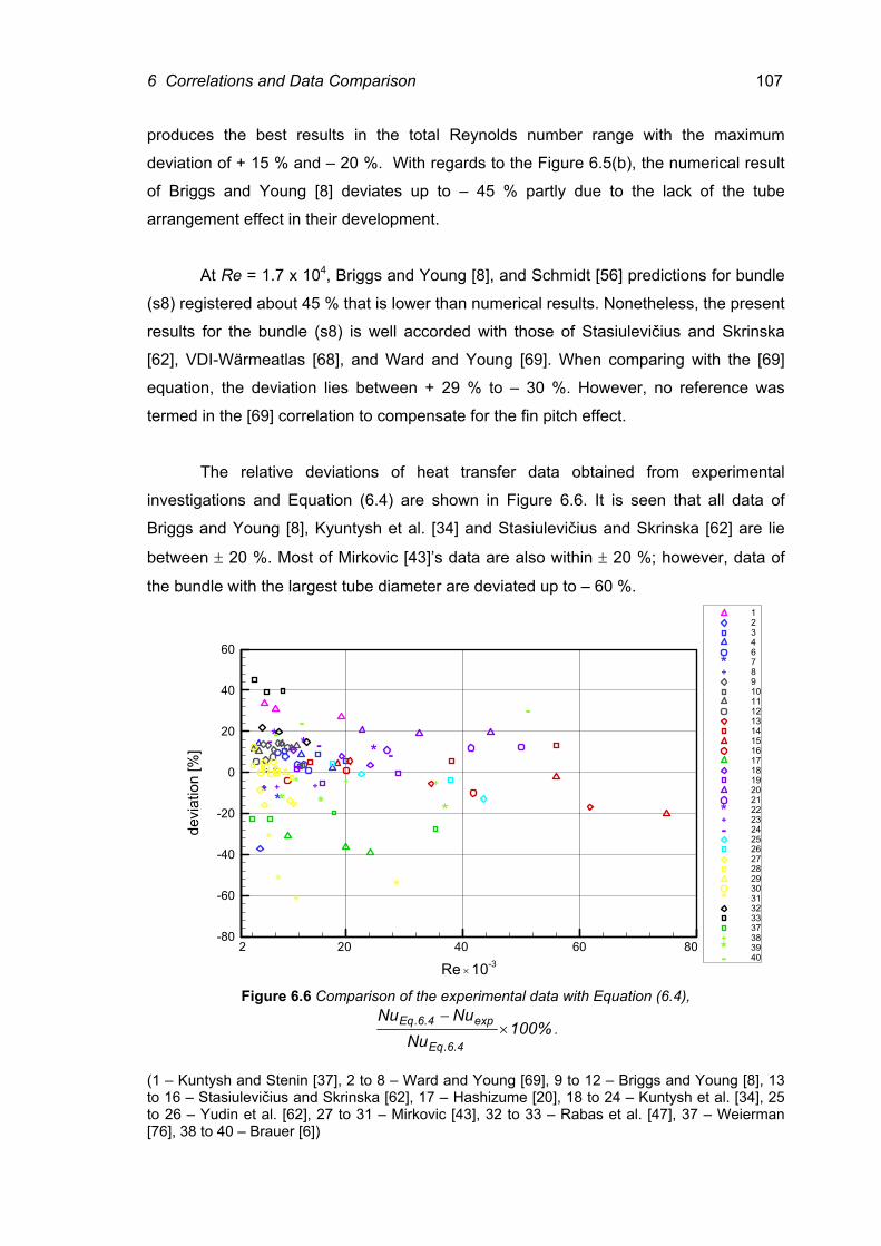
6 Correlations and Data Comparison 107
produces the best results in the total Reynolds number range with the maximum
deviation of + 15 % and – 20 %. With regards to the Figure 6.5(b), the numerical result
of Briggs and Young [8] deviates up to – 45 % partly due to the lack of the tube
arrangement effect in their development.
At Re = 1.7 x 10⁴, Briggs and Young [8], and Schmidt [56] predictions for bundle
(s8) registered about 45 % that is lower than numerical results. Nonetheless, the present
results for the bundle (s8) is well accorded with those of Stasiulevičius and Skrinska
[62], VDI-Wärmeatlas [68], and Ward and Young [69]. When comparing with the [69]
equation, the deviation lies between + 29 % to – 30 %. However, no reference was
termed in the [69] correlation to compensate for the fin pitch effect.
The relative deviations of heat transfer data obtained from experimental
investigations and Equation (6.4) are shown in Figure 6.6. It is seen that all data of
Briggs and Young [8], Kyuntysh et al. [34] and Stasiulevičius and Skrinska [62] are lie
between ± 20 %. Most of Mirkovic [43]’s data are also within ± 20 %; however, data of
the bundle with the largest tube diameter are deviated up to – 60 %.
Re 10-3
-80
-60
-40
-20
0
20
40
60
devi
atio
n[%
]
* *
+ +
* * *
+ + +
- - -
*
**
*
+ + +
* * *
--
-
1234678910111213141516171819202122232425262728293031323337383940
*+
*+-
*
+*-
2 20 40 60 80
× Figure 6.6 Comparison of the experimental data with Equation (6.4),
%100Nu
NuNu
4.6.Eq
exp4.6.Eq ×−
.
(1 – Kuntysh and Stenin [37], 2 to 8 – Ward and Young [69], 9 to 12 – Briggs and Young [8], 13 to 16 – Stasiulevičius and Skrinska [62], 17 – Hashizume [20], 18 to 24 – Kuntysh et al. [34], 25 to 26 – Yudin et al. [62], 27 to 31 – Mirkovic [43], 32 to 33 – Rabas et al. [47], 37 – Weierman [76], 38 to 40 – Brauer [6])
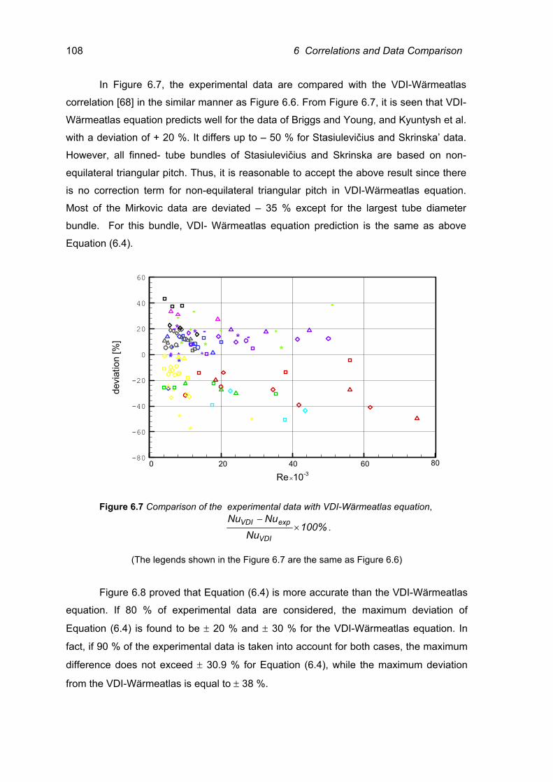
108 6 Correlations and Data Comparison
In Figure 6.7, the experimental data are compared with the VDI-Wärmeatlas
correlation [68] in the similar manner as Figure 6.6. From Figure 6.7, it is seen that VDI-
Wärmeatlas equation predicts well for the data of Briggs and Young, and Kyuntysh et al.
with a deviation of + 20 %. It differs up to – 50 % for Stasiulevičius and Skrinska’ data.
However, all finned- tube bundles of Stasiulevičius and Skrinska are based on non-
equilateral triangular pitch. Thus, it is reasonable to accept the above result since there
is no correction term for non-equilateral triangular pitch in VDI-Wärmeatlas equation.
Most of the Mirkovic data are deviated – 35 % except for the largest tube diameter
bundle. For this bundle, VDI- Wärmeatlas equation prediction is the same as above
Equation (6.4).
Re 10-3
-80
-60
-40
-20
0
20
40
60
devi
atio
n[%
]
* *+ +
* * *+ + +
- - -
*
**
*
+ + +
* * *
- --
0 20 40 60 80
×
Figure 6.7 Comparison of the experimental data with VDI-Wärmeatlas equation,
%100Nu
NuNu
VDI
expVDI ×−
.
(The legends shown in the Figure 6.7 are the same as Figure 6.6)
Figure 6.8 proved that Equation (6.4) is more accurate than the VDI-Wärmeatlas
equation. If 80 % of experimental data are considered, the maximum deviation of
Equation (6.4) is found to be ± 20 % and ± 30 % for the VDI-Wärmeatlas equation. In
fact, if 90 % of the experimental data is taken into account for both cases, the maximum
difference does not exceed ± 30.9 % for Equation (6.4), while the maximum deviation
from the VDI-Wärmeatlas is equal to ± 38 %.
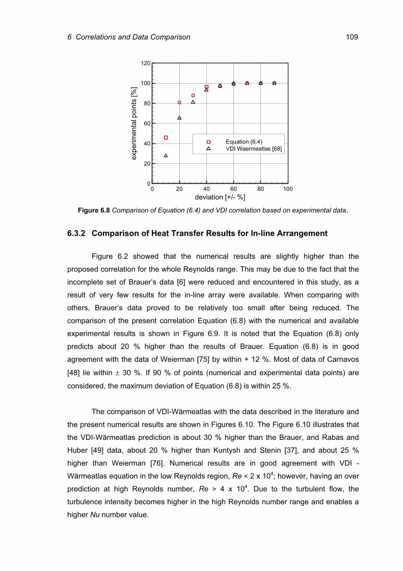
6 Correlations and Data Comparison 109
0 20 40 60 80 100deviation [+/- %]
0
20
40
60
80
100
120
expe
rimen
talp
oint
s[%
]Equation (6.4)VDI Waermeatlas [68]
Figure 6.8 Comparison of Equation (6.4) and VDI correlation based on experimental data.
6.3.2 Comparison of Heat Transfer Results for In-line Arrangement
Figure 6.2 showed that the numerical results are slightly higher than the
proposed correlation for the whole Reynolds range. This may be due to the fact that the
incomplete set of Brauer’s data [6] were reduced and encountered in this study, as a
result of very few results for the in-line array were available. When comparing with
others, Brauer’s data proved to be relatively too small after being reduced. The
comparison of the present correlation Equation (6.8) with the numerical and available
experimental results is shown in Figure 6.9. It is noted that the Equation (6.8) only
predicts about 20 % higher than the results of Brauer. Equation (6.8) is in good
agreement with the data of Weierman [75] by within + 12 %. Most of data of Carnavos
[48] lie within ± 30 %. If 90 % of points (numerical and experimental data points) are
considered, the maximum deviation of Equation (6.8) is within 25 %.
The comparison of VDI-Wärmeatlas with the data described in the literature and
the present numerical results are shown in Figures 6.10. The Figure 6.10 illustrates that
the VDI-Wärmeatlas prediction is about 30 % higher than the Brauer, and Rabas and
Huber [49] data, about 20 % higher than Kuntysh and Stenin [37], and about 25 %
higher than Weierman [76]. Numerical results are in good agreement with VDI -
Wärmeatlas equation in the low Reynolds region, Re < 2 x 10⁴; however, having an over
prediction at high Reynolds number, Re > 4 x 10⁴. Due to the turbulent flow, the
turbulence intensity becomes higher in the high Reynolds number range and enables a
higher Nu number value.
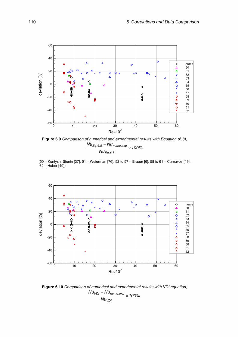
110 6 Correlations and Data Comparison
Re 10-3
-60
-40
-20
0
20
40
60de
viat
ion
[%] * * *
*+ +
+ +
**
*
nume50515253545556575859606162
*+
*
0 10 20 30 40 50 60
× Figure 6.9 Comparison of numerical and experimental results with Equation (6.8),
%100Nu
NuNu
8.6.Eq
exp,nume8.6.Eq ×−
(50 – Kuntysh, Stenin [37], 51 – Weierman [76], 52 to 57 – Brauer [6], 58 to 61 – Carnavos [49],
62 – Huber [49])
Re 10-3
-60
-40
-20
0
20
40
60
devi
atio
n[%
] * * * *
+ ++ +
**
*
nume50515253545556575859606162
*+
*
0 10 20 30 40 50 60
×
Figure 6.10 Comparison of numerical and experimental results with VDI equation,
%100Nu
NuNu
VDI
exp,numeVDI ×−
.
6 Correlations and Data Comparison 111
6.3.3 Comparison of Pressure Drop Results A few correlations were available despite some researchers conducted the tests
for the pressure drop effect and unfortunately no correlations were developed. Therefore
limited comparisons and discussions between these data and related correlations are
reported here.
The numerically calculated Euler numbers compared with available experimental
equations are shown in Figure 6.11(a). At Re > 4 x 10⁴, the numerical results are in good
agreement with the Stasiulevičius and Skrinska [62] prediction, and in the low Re range,
Re < 104, most of the numerical results deviated from the [62] equation by ± 20 %. The
Reynolds range for their work was 104 < Re < 105 and the effects of the tube
arrangement and fin geometry variables except for the fin thickness were reflected in
their correlation.
When comparing Robinson and Briggs [50], and the numerical results, it is found
that there is somewhat different at Re < 2 x 10⁴, due to the absence of the fin geometry
variables such as fin height, fin thickness and fin spacing in their equation. It is noted
that their correlation was very limited ashs varies only from 0.15 to 0.19. In the high
Reynolds range, Robinson and Briggs equation is quite consistent with the numerical
results and this trend continues beyond their tested Reynolds range. Their investigated
Re range was 2 x 10³ < Re < 4 x 10⁴ and it is seen that at high Reynolds number, the fin
geometry variables effects are small. Further analysis of the Figure 6.11(a) provides that
at Re = 5000, the prediction of pressure drop of Ward and Young [69] is up to 50 %
higher. For the rest of the Re range, most of the numerical results are satisfied within +
30 % to – 20 % with the [69] result.
Due to the different Reynolds definitions, a separate comparison was prepared
for numerical results with Haaf [19] correlation in Figure 6.11(b). In Haaf equation (see
appendix D), the average velocity in the bundle and the equivalent diameter were used
as the reference dimensions in the Reynolds number. It is seen that the numerical
results agree well with the Haaf correlation and most of numerical results are between ±
30 %. It is observed from this figure that the maximum deviation from Haaf equation is
the smallest fin height bundle (s1) at high Reynolds number.
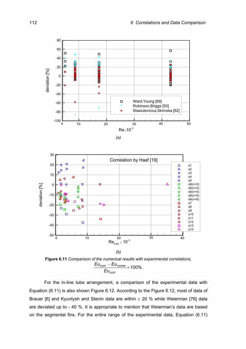
112 6 Correlations and Data Comparison
Re 10-3
-100
-80
-60
-40
-20
0
20
40
60
80
devi
atio
n[%
]
*
*
*
*****
*
*****
*
*****
*****
*
*****
*
******
*****
************
++
+
+++++
++++++
+
+++++
+++++
++++
+
+
+
+++++
+
+++++
+++++
+++++
++
Ward,Young [69]Robinson,Briggs [50]Stasiulevicius,Skrinska [62]
*+
×
4 10 20 30 40 50
(a)
Red,eq 10-3
-50
-40
-30
-20
-10
0
10
20
30
devi
atio
n[%
]
s1s2s3s4s5s6(n=2)s6(n=3)s6(n=4)s6(n=5)s6(n=6)s7s8s9s10s11s12s13s14
0 10 20 30 40×
Correlation by Haaf [19]
(b)
Figure 6.11 Comparison of the numerical results with experimental correlations,
%100Eu
EuEu
corr
numecorr ×−
.
For the in-line tube arrangement, a comparison of the experimental data with
Equation (6.11) is also shown Figure 6.12. According to the Figure 6.12, most of data of
Brauer [6] and Kyuntysh and Stenin data are within ± 20 % while Weierman [76] data
are deviated up to - 40 %. It is appropriate to mention that Weierman’s data are based
on the segmental fins. For the entire range of the experimental data, Equation (6.11)
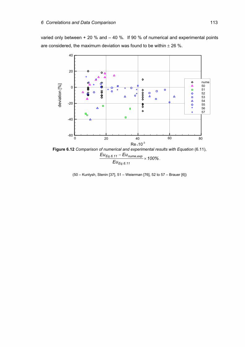
6 Correlations and Data Comparison 113
varied only between + 20 % and – 40 %. If 90 % of numerical and experimental points
are considered, the maximum deviation was found to be within ± 26 %.
Re 10-3
-60
-40
-20
0
20
40de
viat
ion
[%]
* ** * *
++
+ ++
nume5051525354555657
*+
0 20 40 60 80
× Figure 6.12 Comparison of numerical and experimental results with Equation (6.11),
%100Eu
EuEu
11.6.Eq
exp,nume11.6.Eq ×−
.
(50 – Kuntysh, Stenin [37], 51 – Weierman [76], 52 to 57 – Brauer [6])
7 Conclusions
The heat transfer and pressure drop performance on the air-side of circular
finned-tube heat exchangers had been determined numerically. Using the present
numerical investigation and published experimental data, improved heat transfer and
pressure drop correlations (i.e., Equations 6.4, 6.6, 6.8, 6.10 and 6.11) for the air-
cooled heat exchangers have been finally developed.
This study has been performed with 29 bundles having different finning
geometries. 18 bundles containing tubes are placed on equilateral triangular
arrangements and the rest also placed on in-line arrangement.
The present study has also concerned for the local flow and heat transfer
characteristics and the influence of air flow distribution within the bundles. The
numerical flow visualization results for the boundary layer developments and
horseshoe vortex system between the fins, and local velocity and temperature
distributions in the bundles are presented. The boundary layer developments and
horseshoe vortices between the adjacent fins and tube surface of staggered tube
arrangement are found to be strongly dependent on fin spacing and Reynolds number.
The horseshoe vortices develop in all staggered rows; however, only for the first row in
the in-line tube array. There may develop a horseshoe vortex system at the second row
of in-line arrangement and subsequent rows, if the longitudinal pitch is long enough.
However, within the tested geometric parameters range, no horseshoe vortex
appeared upstream of deeper rows and instead of it, a reverse flow due to the wake of
the preceding row is observed. Therefore, improved heat transfer coefficient is
observed for the staggered arrangement.
The horseshoe vortex effect is more obvious in the largest fin spacing and at
the high velocity. The flow visualization results suggest the extent of a new horseshoe
vortex system for the deeper rows of the wider fin spacing of the staggered tube bundle
(s7) at Re = 4.3 x 10⁴.
7 Conclusions 115
Temperature boundary layer developments between the fins are presented
according to the different fin spacings. The temperature gradient decreases at the fin
base and tube surface when two boundary layers are growing to touch each other. This
will lead to a decreased convection heat transfer coefficient. The highest temperature
gradient is revealed along the radial direction at (θ = 0°) for the first row of the both
tube arrays. One interesting finding is that the temperature distributions over the fin
surface and within the fins are rather identical.
The velocity distributions near the fin surface plane and on the mid-plane
between the fins are quite different for the staggered array. The velocity on the mid-
plane of both tube arrays is stronger than near the fin surface plane. The velocity
results of the in-line array show that a strong bypass stream between the tubes is in
accordance with fin tip-to-tip clearance. It is approved by the temperature distribution
figures that a high temperature stream passes through the in-line bundle without mixing
well.
The temperature distributions within the bundle significantly vary from the first to
the third row. The temperature on the mid-plane is higher than near the fin surface
plane. The fin tip temperature at the upstream fin surface is found to be higher due to
the thin boundary layer.
Geometric parameters have been noted regardless of the situation in which
either is favourably or adversely influenced on the heat transfer coefficient and the
pressure drop for both tube arrays at different Reynolds numbers. Respective results
were also presented for the fin efficiency and the heat transfer rate. The relevant
qualitative findings on the finning geometry of this study are:
• Numerical results on the fin height effect for both tube arrays
agrees well with the experimental data in that increasing the fin height provides
decreased heat transfer coefficient and increased pressure drop of the circular
finned-tube bundle.
• Since the fin spacing effect is depending principally on the boundary layer
corresponding with the velocity of air, the influence of the fin spacing on the
heat transfer coefficient is not significant when boundary layers between the
fins are departing from each other for the staggered array. For the in-line array,
the higher rate of heat transfer is observed at the wider spacing.
116 7 Conclusions
• Circular fins of rectangular profile with uniform cross section area are applied
for the fin thickness effect. Changes of the fin thickness are remarkably
insensitive to the heat transfer coefficient and pressure drop of the staggered
tube bank. Therefore, the effect of fin thickness is proved to be insignificant.
• The tube outside diameter effect has more influence on the in-line array. The
heat transfer coefficient and pressure drop for both arrays are inversely
proportional to the tube diameter at a same Reynolds number when St/df is
constant. The effect of tube diameter on the performance of different tube
configurations is quite insensitive to the large Reynolds numbers.
• The heat transfer coefficient and pressure drop are decreased as the tube
spacing increases for both tube arrangements. The effect of the transverse tube
pitch has more influence on the in-line tube arrangement than those for the
staggered tube arrangement. For the same transverse pitch, increasing the
longitudinal pitch of the in-line array provides an increased pressure drop and
no significant effect on the heat transfer coefficient.
• The maximum heat transfer coefficient occurs in the second row for the
staggered arrangement and at the first row for the in-line arrangement,
respectively. For both staggered and in-line arrangements, the heat transfer
coefficient becomes stable downstream the fourth tube row and the pressure
drop increases linearly as the bundle depth becomes deeper.
• The staggered array clearly yields a higher heat transfer coefficient, while the
pressure drop of the staggered array is generally higher than that of the in-line
arrangement. Attempts were made to validate which tube configuration is more
constructive. The in-line array has a better performance than the staggered
arrangement at low Reynolds number. Hopefully this study will leave further
discussion in that direction.
The heat transfer correlations are presented in Equations (6.4) and (6.8) for the
staggered and in-line bundles with n ≥ 4 respectively. For the staggered array, 98% of
the numerical results deviate by ± 15 % while ± 25 % for the in-line array. For the heat
exchangers having n < 4, the Nu number can be calculated according to Equations
(6.4) and (6.6). The numerical results corresponded with the established correlation
7 Conclusions 117
with ± 15 %. The heat transfer correlations obtained by the numerical investigation are
improved in comparison with VDI-Wärmeatlas [68]. The pressure drop correlations are
presented in Equations (6.10) and (6.11), respectively. The numerical results deviate ±
15 % for the staggered tube array and the maximum deviation of the in-line tube array
is ± 30 %.
Attention was devoted to the convective heat transfer from the fins and tubes to
the dry air and hence, further numerical research for the improvement of the circular
finned-tube heat exchanger design with humid air is required. Finally, the hope may be
expressed that the present correlations will contribute to calculate the heat transfer and
pressure drop for circular finned-tube heat exchangers at 5.0 x 10³ ≤ Re ≤ 7.0 x 10⁴.
REFERENCES 1. Ackerman, J. W., and Brunsvold, A. R., “Heat Transfer and Draft Loss
Performance of Extended Surface Tube Banks,” ASME Journal of Heat Transfer, Vol.92, pp.215-220, 1970.
2. Antuf’ev, V. M., and Gusev, E. K., “Intensification of Heat Transfer of Cross-Flow
Finned Surfaces,” Teploenergetika, Vol. 15, No. 7, pp. 31-34, 1968.
3. Baker, C.J., “The Laminar Horseshoe Vortex,” Journal of Fluid Mechanics, Vol.95, pp.347-367, 1979.
4. Bastani, A., Fiebig, M., and Mitra, N. K., “Numerical Simulation of Flow Field in a Fin Tube Heat Exchanger,” ASME Journal of Fluid Engineering, Vol. 101, pp. 91-96, 1990.
5. Brauer, H., “Wärme- und strömungstechnische Untersuchungen an quer angeströmten Rippenrohrbündeln, Teil1; Versuchsanlagen und Meßergebnisse bei höheren Drucken,” Chem.-Ing. Technik, Vol. 33,No. 5, pp. 327-335, 1961.
6. Brauer, H., “Wärme- und strömungstechnische Untersuchungen an quer angeströmten Rippenrohrbündeln, Teil2; Einfluß der Rippen- und der Rohranordung,” Chem.-Ing. Technik, Vol. 33, No.6, pp. 431-438, 1961.
7. Brauer, H., “Compact Heat Exchangers,” Chemical Progress Engineering, London. Vol. 45, No. 8, pp. 451-460, 1964.
8. Briggs, D. E., and Young, E. H., “Convection Heat Transfer and Pressure Drop of Air Flowing Across Triangular Pitch Banks of Finned Tubes,” Chemical Engineering Progress Symposium Series, No. 41, Vol. 59, pp. 1-10, 1963.
9. Faghri, M., and Rao, N., “Numerical Computation of Flow and Heat Transfer in Finned and Unfinned Tube Banks,” International Journal of Heat Mass Transfer, Vol. 30, No. 2, pp. 363-372, 1987.
References 119
10. Fiebig, M., Gorsse-Georgemann, A., Chen, Y., and Mitra, N. K., “Conjugate Heat Transfer of a Finned Tube Part A: Heat Transfer Behaviour and Occurrence of Heat Transfer Reversal,” Numerical Heat transfer, Part A, Vol. 28, pp.133-146, 1995.
11. FLUENT Incorporated, FLUENT 5 User’s Guide, Fluent Incorporated Lebanon, NH-USA, 1998.
12. Gambit Modeling, User’s Manual, Fluent Incorporated Lebanon, NH-USA, 1998.
13. Gardner, K. A., “Efficiency of Extended Surface,” ASME Transactions, Vol. 67, No. 8, pp. 621-631, 1945.
14. Gianolio, E., and Cuti, F., “Heat Transfer Coefficients and Pressure Drops for Air Coolers Under Induced and Forced Draft,” Heat Transfer Engineering, Vol. 3, No. 1, pp. 38-48, 1981.
15. Glück, B., Zustands- und Stoffwerte Wasser Dampf Luft- Verbrennungsrechnung, Berlin : VEB Verlag für Bauwesen, 1986 (Bausteine der Heizungstechnik - Berechnung- software)
16. Goldstein, R. J., and Karni, J., “The Effect of a Wall Boundary Layer on Local Mass Transfer from a Cylinder in Cross Flow,” ASME Journal of Heat Transfer, Vol. 106, pp. 260-270, 1984.
17. Goldstein, R. J., Karni, J., and Zhu, Y., “Effect of Boundary Conditions on Mass Transfer near the Base of a Cylinder in Cross Flow,” ASME Journal of Heat Transfer, Vol. 112, pp. 501-504, 1990.
18. Gunter, A. Y., and Shaw, W. A., “A General Correlation of Friction Factors for Various Types of Surfaces in Cross Flow,” ASME Transactions, Vol. 67, pp. 643-660, 1945.
19. Haaf, S., Wärmeübertragung in Luftkühlern, Handbuch der Kältechnik, Bd. 6, Teil B: Wärmeaustauscher, Berlin u.a. : Springer Verlag, pp. 435-491,1988.
20. Hashizume, K., “Heat Transfer and Pressure Drop of Finned Tubes in Cross Flow,” Heat Transfer Engineering, Vol. 3, No.2, pp. 15-20, 1981.
120 References
21. Hu, X., and Jacobi, A.M., “Local Heat Transfer Behaviour and its Impact on a Single-Row Annularly Finned Tube Heat Exchanger,” ASME Journal of Heat transfer, Vol. 115, pp. 66-74, 1993.
22. Jacobi, A. M., and Shah, R. K., “Air-Side Flow and Heat Transfer in Compact
Heat Exchangers: A discussion of Enhancement Mechanisms,” Heat Transfer Engineering, Vol.19, no.4, pp.29-41, 1998.
23. Jameson, S. L., “Tube Spacing in Finned Tube Banks,” ASME Transactions, Vol.
67, pp. 633-642, 1945. 24. Jang, J. Y., Wu, M. C., and Chang, W. J., “Numerical and Experimental Studies of
Three Dimensional Plate-Fin and Tube Heat Exchangers,” International Journal of Heat Mass Transfer, Vol. 39, No. 14, pp.3057-3066, 1996.
25. Jang, J. Y., Lei, J, T., and Liu, L. C., “The Thermal-Hydraulic Characteristics of Staggered Circular Finned-Tube Heat Exchangers under Dry and Dehumidifying Conditions,” International journal of Heat and Mass Transfer, Vol.41, pp.3321-3337, 1998.
26. Jaw, S. Y., and Chen, C. J., Present Status of k-ε Turbulence Models and their
Achievements, Flow Modeling and Turbulence Measurements VI, Chen, Shih, Lienau & Kung (eds), Balkema Rotterdam. ISBN 90 5410 826 6,1996.
27. Jones, T. V., and Russell, C. M. B., “ Heat Transfer Distribution on Annular Fins,”
ASME Transactions, No.78-HT-30, 1978.
28. Kaminski, S., and Groß, U., “ Luftseitiger Wärmeübergang und Druckverlust in Lamellenrohr-wärmeübertragen,” KI Lust- und Kältetechnik, Vol.1, pp.13-18, 2000.
29. Kaminski, S., “Numerische Simulation der luftseitigen Strömungs- und Wärmetransportvorgänge in Lamellenrohr-Wärmeübertragen,” Freiberger Forschungshefte, A 867 Energie, 2002.
30. Kays, W. M., and London, A. L., Compact Heat Exchangers, McGraw-Hill, New York, 1998.
31. Kearney, S. P., “Local and Average Heat Transfer and Pressure Drop Characteristics of Annularly Finned Tube Heat Exchangers,” M. S. thesis, University of Illinois at Urbana-Champaign, Urbana, IL, 1995.
References 121
32. Kearney, S. P., and Jacobi, A. M., “Local Convective Behavior and Fin Efficiency in Shallow Banks of Inline and Staggered, Annularly Finned Tubes,” ASME Journal of Heat Transfer, Vol. 118, pp.317-326, 1996.
33. Konstantinidis, E., Castiglia, D., and Balabani, S., “On the Flow and Vortex
Shedding Characteristics of an Inline Tube Bundle in Steady and Pulsating Crossflow,” Transactions of IchemE, Vol.78, Part A, pp.1129-1138, 2000.
34. Kuntysh, V. B., Taryan, I. G., and Yokhvedov, F. M., “On the Effect of the Relative
Depth of the Interfin Space on Heat Transfer from Bundles of Finned Tubes,” Heat Transfer- Soviet Research, Vol. 6, No. 6, pp. 5-9, 1974.
35. Kuntysh, V. B., Piir, A. E., Kolobova, L. F., Mirmov, N. I., and Fedotova, L. M.,
“Correlation Equation for Aerodynamic Resistance of Tube Bundles in Air-Cooled Heat Exchangers,” Chemistry and Technology of fuels and Oils, Vol.15, Nr.5-6, pp.341-344, 1979.
36. Kuntysh, V. B., Piir, A. E., Fedotova, L. M., Tal’ ving, T. A., and Varma, K. A.,
“Characteristics of Tube Bundles for Air-Cooled Exchangers,” Chemistry and Technology of fuels and Oils, Vol.16, Nr.5-6, pp.312-315, 1980.
37. Kuntysh, V. B., and Stenin, N. N., “Heat Transfer and Pressure Drop in Cross
Flow Through Mixed Inline-Staggered Finned Tube Bundles,” Thermal Engineering, Vol. 40, No. 2, pp. 126-129, 1993.
38. Lapin, A., and Schurig, W. I., “Heat Transfer Coefficients of Finned Exchangers,”
Ind. Eng. Chem., Vol. 51, No. 8, pp. 941-944, 1959.
39. Launder, B, E., and Massey, T.H., “ The Numerical Prediction of Viscous Flow and Heat Transfer in Tube Banks,” ASME Journal of Heat Transfer, Vol.3, pp.565-571, 1978.
40. Lee, J. W. H., and Chen, G. Q., “ A Numerical Study of Turbulent Line Puffs via the Renormalization Group (RNG) k-ε Model,” International Journal for Numerical Methods in Fluids, Vol. 26, pp.217-234, 1998.
41. Legkiy, V. M., Pavlenko, V. P., Makarov, A. S., and Zheludov, Y. S., “Investigation of Local Heat Transfer in a Tube with Annular Fins in Transverse Air-Flow,” Heat Transfer- Soviet Research, Vol. 6, No. 6, pp.101-107, 1974.
42. Lymer, A., “Finned Tubes and their Performance Characteristics,” Nuclear Engineering, Vol. 2, pp. 504-509, 1957.
122 References
43. Mirkovic, Z., Heat Transfer and Flow Resistance Correlation for Helically Finned and Staggered Tube Banks in Cross Flow, Heat Exchangers: Design and Theory Source Book, (edited by N. H. Afgan and E. U. Schlünder), Hemisphere, Washington, D. C, pp. 559-584, 1974.
44. Mitra, N. K., Bastani, A., and Fiebig, M., “Numerical Simulation of 3D Periodically Fully Developed Flow Between Fins of a Compact Fin-Tube Heat Exchanger,” Advances in Heat Exchanger Design, Radiation, and Combustion, ASME HTD - Vol. 182, pp. 37-41, 1991.
45. Neal, S. B H. C., and Hitchcock, J. A., “A Study of the Heat Transfer Process in Banks of Finned Tube in Cross Flow, Using a Large Scale Model Technique,” Proceeding of the Third International Heat Transfer Conference, Vol. 3, Chicago, IL, pp. 290-298, 1966.
46. Nir, A., “Heat Transfer and Friction Factor Correlations for Cross Flow Over Staggered Finned Tube Banks,” Heat Transfer Engineering, Vol. 12, No. 1, pp. 43-58, 1991.
47. Rabas, T. J., Eckels, P. W., and Sabatino, R. A., “The Effect of Fin Density on the Heat Transfer and Pressure Drop Performance of Low-Finned Tube Banks,” Chemical Engineering Communications, Vol. 10, No.1-3, pp. 127-147, 1981.
48. Rabas, T. J., and Taborek, J., “Survey of Turbulent Forced-Convection Heat Transfer and Pressure Drop Characteristics of Low-Finned Tube Banks in Cross Flow,” Heat Transfer Engineering, Vol. 8, No. 2, pp. 49-62, 1987.
49. Rabas, T. J., and Huber, F. V., “Row Number Effects on the Heat Transfer Performance of Inline Finned Tube Banks,” Heat Transfer Engineering, Vol. 10, No. 4, pp. 19-29, 1989.
50. Robinson, K. K., and Briggs, D. E., “Pressure Drop of Air Flowing Across Triangular Pitch Banks of Finned Tubes,” Chemical Engineering Progress Symposium Series, No. 64, Vol. 62, pp. 177-184, 1965.
51. Romero-Méndez, R., Sen, M., Yang, K. T., and McClain, R., “Effect of Fin Spacing on Convection in a Plate Fin and Tube Heat Exchanger,” International Journal of Heat and Mass Transfer, Vol. 43, pp.39-51, 2000.
References 123
52. Saboya, F. E. M., and Sparrow, E M., “Local and Average Transfer Coefficients for One-Row Plate Fin and Tube Heat Exchanger Configuration,” ASME Journal of Heat Transfer, Series C, Vol. 96, No.3, pp. 265-272, 1974.
53. Saboya, F. E. M., and Sparrow, E M., “Effect of Tube Relocation on the Transfer Capabilities of a Fin and Tube Heat Exchanger,” ASME Journal of Heat Transfer, Vol. 96, pp. 421-422, 1974.
54. Saboya, F. E. M., and Sparrow, E M., “Transfer Characteristics of Two-Row Plate Fin and Tube Heat Exchanger Configurations,” International Journal of Heat Mass Transfer, Vol. 19, pp. 41-49, 1976.
55. Schmidt, E.Th., “Der Wärmeübergang an Rippenrohre und die Berechnung von Rohrbündle-Wärmeaustauschern,” Kältetechnik, Band 15, Heft 4, 1963.
56. Schmidt, E.Th., “Der Wärmeübergang an Rippenrohre und die Berechnung von Rohrbündle-Wärmeaustauschern,” Kältetechnik, Band 15, Heft 12, 1963.
57. Sharatchandra, M. C., and Rhode, D. L., “ Turbulent Flow and Heat Transfer in Staggered Tube Banks With Displaced Tube Rows,” Numerical Heat transfer, Part A, Vol. 31, pp.611-627, 1997.
58. Sheu, T. W. H., and Tsai, S. F., “ A Comparison Study on Fin Surface in Finned-Tube Heat Exchangers,” International Journal of Numerical Methods for Heat & Fluid flow, Vol. 9, No.1, pp.92-106, 1999.
59. Sparrow, E. M., and Samie, F., “Heat Transfer and Pressure Drop Results for One and Two-row Arrays of Finned Tubes,” International Journal of Heat Mass Transfer, Vol. 28, No. 12, pp. 2247-2259, 1985.
60. Sparrow, E. M., and Chastain, S. R., “Effect of Angle of Attack on the Heat Transfer Coefficient for an Annular Fin,” International Journal of Heat Mass Transfer, Vol. 29, pp.1185-1191, 1986.
61. Stasiulevičius, J., and Survila, V.J., “Heat transfer and Hydraulic Drag of Banks of
Finned Tubes at High Reynolds Numbers,” 5th International Heat Transfer Conference, Tokyo, 1974.
62. Stasiulevičius, J., and Skrinska, A., Heat Transfer of Finned Tube Bundles in Crossflow, Hemisphere Publishing, ISBN 3-540-18211-x, 1988.
124 References
63. Sung, H. J., Yang, J. S., and Park, T. S., “Local Convective Mass Transfer on Circular Cylinder with Transverse Annular Fins in Cross Flow,” International Journal of Heat Mass Transfer, Vol. 39, No. 5, pp. 1093-1101, 1996.
64. Torikoshi, K., and Xi, G. N., Nakazawa. Y., and Asano. H., “Flow and Heat Transfer Performance of a Plate-fin and Tube Heat Exchanger (1st report: Effect of fin pitch),” ASME Heat Transfer Division, Vol. 4, pp. 411-416, 1994.
65. Torikoshi, K., and Xi, G. N., “A Numerical Steady of Flow and Thermal Fields in Finned Tube Heat Exchangers (Effect of the Tube Diameter),” IMECE Proceedings of the ASME Heat Transfer Division, HTD-Vol. 317-1, pp. 453-457, 1995.
66. Torikoshi, K., Xi, G. N., Kawabata, K., and Suzuki, K., “Numerical Analysis of Unsteady Flow and Heat Transfer Around Bodies by Making Use of a Compound Grid System,” ASME-JSME Thermal Engineering Conference, Vol.4, pp. 381-388, 1995.
67. Tutar, M., and Holdo, A. E., “ Computational Modelling of Flow around a Circular
Cylinder in Sub-Critical Flow Regime with Various Turbulence Models,”
International Journal for Numerical Methods in Fluids, Vol.35, pp.763-784, 2001.
68. Verein Deutscher Ingenieure., VDI-Wärmeatlas., Berechnungsblätter für den Wärmeübergang, 8. Aufl. Berlin u.a., Springer, 1997.
69. Ward, D. J., and Young, E. H., “ Heat Transfer and Pressure Drop of Air in Forced Convection Across Triangular Pitch Banks of Finned Tubes,” Chemical Engineering Progress Symposium Series, Vol. 55, No. 29, pp.37-44, 1959.
70. Watel, B., Harmand, S., and Desmet, B., “Influence of Flow Velocity and Fin Spacing on the Forced Convective Heat Transfer from an Annular-Finned Tube,” JSME international Journal, series B, Vol. 42, No. 1, pp. 56-64, 1999.
71. Watel, B., Harmand, S., and Desmet, B., “Experimental Study of Convective Heat
Transfer from a Rotating Finned Tube in Transverse Air Flow,” Experiments in Fluids, Vol. 29, No. 1, pp. 79-90, 2000.
72. Webb, R. L., “Air-Side Heat Transfer in Finned Tube Heat Exchanger,” Heat Transfer Engineering, Vol. 1, No. 3, pp. 33-49, 1980.
References 125
73. Webb, R. L., Externally Finned Tubes, Principles of Enhanced Heat Transfer, John Wiley and Sons, Inc, pp. 125-159,1994.
74. Weierman, C., “Correlations Ease the Selection of Finned Tubes,” Oil and Gas Journal, Vol. 74, pp. 94-100, 1976.
75. Weierman, C., “Pressure Drop Data for Heavy-Duty Finned Tubes,” Chemical Engineering Progress, pp. 69-72, 1977.
76. Weierman, C., Taborek, J., and Marner, W. J., “Comparison of Inline and Staggered Banks of Tubes with Segmented Fins,” AIChE Symp, Ser., Vol. 74, No. 174, pp. 39-46, 1978.
77. Weyrauch, E., “ Der Einfluß der Rohranordnung auf den Wärmeübergang und Drukckverlust bei Querstrom von Gasen durch Rippenrohrbündel,” Kältetechnik, Band 21, Heft 3, 1969.
78. Wong, P. W., “Mass and Heat Transfer from Circular Finned Cylinders,” J. Inst. Heat. Vent. Eng., pp.1-23, April 1966.
79. Xi, G.N, and Torikoshi, K., “Computation and Visualization of Flow and Heat Transfer in Finned Tube Heat Exchangers,” International Symposium on Heat Transfer, Tsinghua University, Beijing China,(7.10 – 11.10), pp. 632-637, 1996.
80. Yudin, V F., Tokhtarova, L. S. Lokshin, V., and Tulin, S. N., “Correlation of Experimental Data on Convective Heat Transfer in Cross Flow Over Bundles with Transverse Spiral and Circumferential Fins,” Trudy TsKTI, No. 82, 1968.
81. Zhukauskas, A. A., “Investigation of Heat Transfer in Different Arrangements of Heat Exchanger Surfaces,” Teploenergetika, Vol. 21, No. 5, pp. 40-46, 1974.
82. Zhukauskas, A., Stasiulevičius, J., and Skrinska, A., “Experimental Investigation
of Efficiency of Heat Transfer of a Fin Tube with Spiral Fin in Cross Flow,” Third International Heat Transfer Conference, Chicago, Vol. 3, pp. 299-305, 1966.
83. Zozulya, N. V., Vorob’yev, Y. P., and Khavin, A. A., “Effect of Flow Turbulization on Heat Transfer in a Finned Tube Bundle,” Heat Transfer Soviet Research, Vol. 5, No. 1, pp. 154-156, 1973.
List of Figures
Figure Page 1.1 Cross-flow circular finned-tube heat exchanger ............................................................ 1
2.1 Arrangements of tubes in bundles, (a) In-line arrangement,
(b) Staggered arrangement ............................................................................................ 4
2.2 Schematic of general flow pattern over a second row of the staggered
arrangement tube bundle [45]......................................................................................... 8
4.1 Cross-section of a circular fin tube ............................................................................... 31
4.2 Computational domains, (a) In-line arrangement, (b) Staggered arrangement,
(c) Top view................................................................................................................... 33
4.3 Grid generation (a) near tube, (b) at z - direction of the domain ................................. 35
4.4 Grid generation (a) Staggered arrangement, (b) In-line arrangement ........................ 35
5.1 Velocity distributions between the fins of first row of staggered arrangement
at Re = 8.6 x 10³............................................................................................................ 45
5.2 Schematic flow patterns of horseshoe vortices around a circular cylinder
between annular fins [63] ............................................................................................. 47
5.3 Flow pattern for the fourth row of bundle (s7) at Re = 4.3 x 10⁴.................................. 48
5.4 Velocity distributions between the fins of first row of in-line arrangement
at Re = 8.6 x 10³............................................................................................................ 50
5.5 Temperature distributions between the fins for staggered arrangement
at Re = 8.6 x 10³ (a) first row and (b) fourth row.......................................................... 52
5.6 Variations of local Nu number along the tube surface
of bundle (s7) at (θ = 0°) for Re = 4.3 x 10⁴ ................................................................. 54
5.7 Temperature distributions between the fins for in-line arrangement
at Re = 8.6 x 10³ (a) first row and (b) fourth row......................................................... 55
5.8 Temperature contours for staggered arrangement at (a) over fin surface and
(b) within fin of bundle (s3) at Re =4.3 x 10⁴ ................................................................ 57
5.9 Temperature contours for in-line arrangement at (a) over fin surface and
(b) within fin of bundle (i2) at Re =4.3 x 10⁴ ................................................................. 58
5.10 Velocity distributions for bundle s6 (n = 3) at Re = 8.6 x 10³....................................... 60
5.11 Velocity distributions for bundle i4 (n = 3) at Re = 8.6 x 10³........................................ 61
List of Figures 127
5.12 Boundary layer separation point of first row of bundle (s3)
at Re = 1.7 x 10⁴ ............................................................................................................ 63
5.13 Temperature distributions for bundle s6 (n = 3) at Re = 8.6 x 10³............................... 64
5.14 Temperature distributions for bundle i4 (n = 3) at Re = 8.6 x 10³................................ 65
5.15 Effect of fin height on the heat transfer rate for staggered
and in-line tube bundles ................................................................................................ 67
5.16 Effect of fin height on the fin efficiency for staggered and in-line bundles .................. 68
5.17 Effect of fin height on the heat transfer coefficient for staggered and
in-line bundles................................................................................................................ 68
5.18 Effect of fin height on the pressure drop for staggered and in-line bundles................ 69
5.19 Performance parameter of the fin height effect for staggered and
in-line bundles................................................................................................................ 70
5.20 Effect of fin spacing on the heat transfer rate for staggered and
in-line bundles................................................................................................................ 71
5.21 Effect of the fin spacing on the fin efficiency for staggered and
in-line bundles................................................................................................................ 72
5.22 Effect of fin spacing on heat transfer coefficient for staggered and
in-line bundles................................................................................................................ 72
5.23 Effect of fin spacing on the pressure drop for staggered and in-line bundles ............. 74
5.24 Performance parameter of the fin spacing effect for staggered and
in-line bundles................................................................................................................ 74
5.25 Effect of fin thickness on the heat transfer rate for staggered bundle ......................... 75
5.26 Effect of fin thickness on the fin efficiency for staggered bundle................................. 76
5.27 Effect of fin thickness on the heat transfer coefficient for staggered bundle............... 76
5.28 Effect of fin thickness on the pressure drop for staggered bundle .............................. 77
5.29 Performance parameter of the fin thickness effect for staggered bundle.................... 78
5.30 Effect of tube outside diameter on the heat transfer rate for staggered and
in-line bundles................................................................................................................ 78
5.31 Effect of tube outside diameter on the fin efficiency for staggered and
in-line bundles................................................................................................................ 79
5.32 Effect of tube outside diameter on the heat transfer coefficient for staggered
and in-line bundles ........................................................................................................ 80
5.33 Effect of tube outside diameter on the pressure drop for staggered and
in-line bundles................................................................................................................ 80
5.34 Performance parameter of the tube outside diameter effect
for staggered and in-line bundles.................................................................................. 81
5.35 Effect of tube spacing on the heat transfer rate for staggered and
in-line bundles................................................................................................................ 82
128 List of Figures
128
5.36 Effect of the tube spacing on the fin efficiency for staggered and
in-line bundles ............................................................................................................... 83
5.37 Effect of the tube spacing on the heat transfer coefficient for staggered and
in-line bundles ............................................................................................................... 84
5.38 Effect of the tube spacing on the pressure drop for staggered and
in-line bundles ............................................................................................................... 85
5.39 Performance parameter of tube spacing effect for staggered and
in-line bundles ............................................................................................................... 86
5.40 Row-to-row effect on the heat transfer rate for staggered (above) and
in-line (below) bundles at Re = 4.3 x 10⁴...................................................................... 87
5.41 Row-to-row effect on the fin efficiency for staggered (above) and
in-line (below) bundles at Re = 4.3 x 10⁴...................................................................... 88
5.42 Row-to-row effect on the heat transfer coefficient for staggered (above) and
in-line (below) bundles at Re = 4.3 x 10⁴...................................................................... 90
5.43 Effect of the number of rows effect on the heat transfer rate
for staggered and in-line bundles ................................................................................. 91
5.44 Effect of number of rows on the fin efficiency for staggered and
in-line bundles ............................................................................................................... 92
5.45 Effect of the number of rows on the heat transfer coefficient
for staggered and in-line bundles ................................................................................. 92
5.46 Effect of number of rows on the pressure drop for staggered and
in-line bundles ............................................................................................................... 93
5.47 Performance parameter of the rows effect for staggered and in-line bundles............ 94
6.1 Comparison of the numerical results with Equations (6.4 and 6.6)........................... 100
6.2 Comparison of the numerical results with Equation. (6.8) ......................................... 102
6.3 Comparison of the numerical results with Equation (6.10)........................................ 103
6.4 Comparison of the numerical results with Equation (6.11)........................................ 104
6.5 Comparison of the numerical results with experiment based correlations................ 106
6.6 Comparison of the experimental data with Equation (6.4) ........................................ 107
6.7 Comparison of the experimental data with VDI equation .......................................... 108
6.8 Comparison of Equation (6.4) and VDI correlation based on experimental data ..... 109
6.9 Comparison of numerical and experimental results with Equation (6.8)................... 110
6.10 Comparison of numerical and experimental results with VDI equation..................... 110
6.11 Comparison of the numerical results with experimental correlations........................ 112
6.12 Comparison of numerical and experimental results with Equation (6.11)................. 113
B.1 Velocity distributions between the fins of first row of staggered arrangement
at Re = 4.3 x 10⁴.......................................................................................................... 134
B.2 Velocity distributions between the fins of second row of staggered arrangement
at Re = 4.3 x 10⁴.......................................................................................................... 135
List of Figures 129
B.3(a) Horseshoe Vortex near fin-tube junction at second row of bundle (s11)
for Re = 8.6 x 10³.........................................................................................................136
B.3(b) Flow pattern near fin-tube junction at fist row of bundle (s8)
for Re = 8.6 x 10³.........................................................................................................136
B.4 Velocity distributions between the fins of first row of in-line arrangement
at Re = 4.3 x 10⁴..........................................................................................................137
B.5 Velocity distributions between the fins of second row of in-line arrangement
at Re = 4.3 x 10⁴..........................................................................................................138
B.6 Temperature distributions between the fins for staggered arrangement
at Re = 4.3 x 10⁴ (a) first row and (b) fourth row. .......................................................139
B.7 Temperature distributions between fins for in-line arrangement
at Re = 4.3 x 10⁴ (a) first row and (b) fourth row. .......................................................140

List of Tables
Table Page
4.1 Dimensions of bundles used in numerical investigation ........................32
6.1 Deviations of heat transfer correlations for staggered arrangement....101
6.2 Deviations of heat transfer correlations for in-line arrangement ..........102
6.3 Deviations of pressure drop correlations for staggered and
in-line arrangements .............................................................................104
C.1 Dimensions of finned - tube heat exchangers ......................................141
D.1 Correlations for heat transfer of circular finned - tube
heat exchangers....................................................................................144
D.2 Correlations for heat transfer of circular finned - tube
heat exchangers....................................................................................145
D.3 Correlations for heat transfer of circular finned - tube
heat exchangers....................................................................................146
D.4 Correlations for pressure drop of circular finned - tube
heat exchangers....................................................................................147
D.5 Correlations for pressure drop of circular finned - tube
heat exchangers....................................................................................148
D.6 Correlations for pressure drop of circular finned - tube
heat exchangers....................................................................................149
E.1 Numerical results for bundle depth, n = 2 .............................................150
E.2 Numerical results for bundle depth, n = 3 .............................................150
E.3 Numerical results for bundle depth, n = 4 .............................................151
E.4 Numerical results for bundle depth, n = 4 .............................................152
E.5 Numerical results for bundle depth, n = 5 .............................................153
E.6 Numerical results for bundle depth, n = 6 .............................................153

APPENDIX
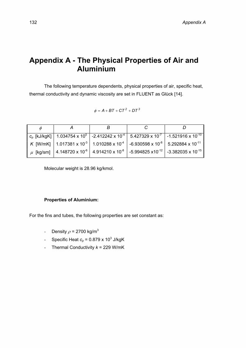
132 Appendix A
Appendix A - The Physical Properties of Air and Aluminium
The following temperature dependents, physical properties of air, specific heat,
thermal conductivity and dynamic viscosity are set in FLUENT as Glück [14].
32 DTCTBTA +++=φ
φ A B C D
cp [kJ/kgK] 1.034754 x 100 -2.412242 x 10⁻⁴ 5.427329 x 10⁻⁷ -1.521916 x 10⁻¹⁰
K [W/mK] 1.017381 x 10⁻³ 1.010288 x 10⁻⁴ -6.930598 x 10⁻⁸ 5.292884 x 10⁻¹¹
µ [kg/sm] 4.148720 x 10⁻⁶ 4.914210 x 10⁻⁸ -5.994825 x10⁻¹² -3.382035 x 10⁻¹⁵
Molecular weight is 28.96 kg/kmol.
Properties of Aluminium:
For the fins and tubes, the following properties are set constant as:
- Density ρ = 2700 kg/m3
- Specific Heat cp = 0.879 x 10³ J/kgK
- Thermal Conductivity k = 229 W/mK

Appendix B – Further Figures
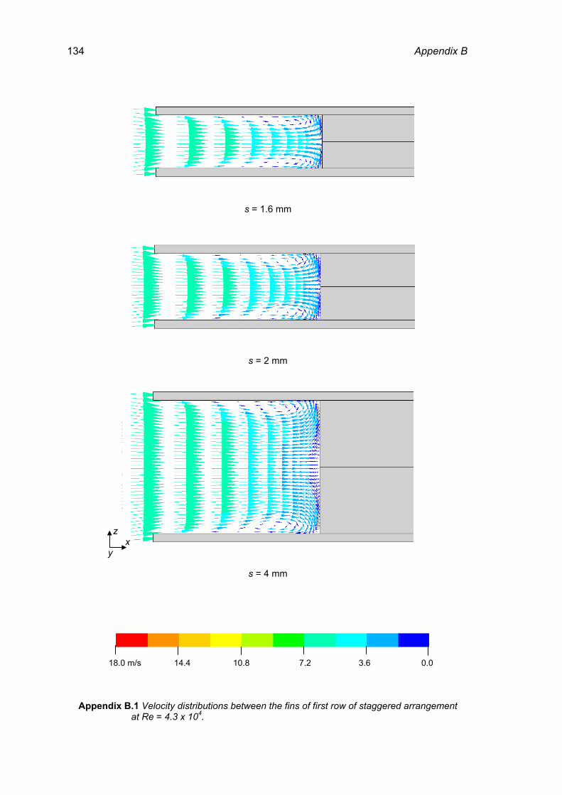
134 Appendix B
s = 1.6 mm
s = 2 mm
s = 4 mm
18.0 m/s 14.4 10.8 7.2 3.6 0.0
Appendix B.1 Velocity distributions between the fins of first row of staggered arrangement at Re = 4.3 x 10⁴.
z x y
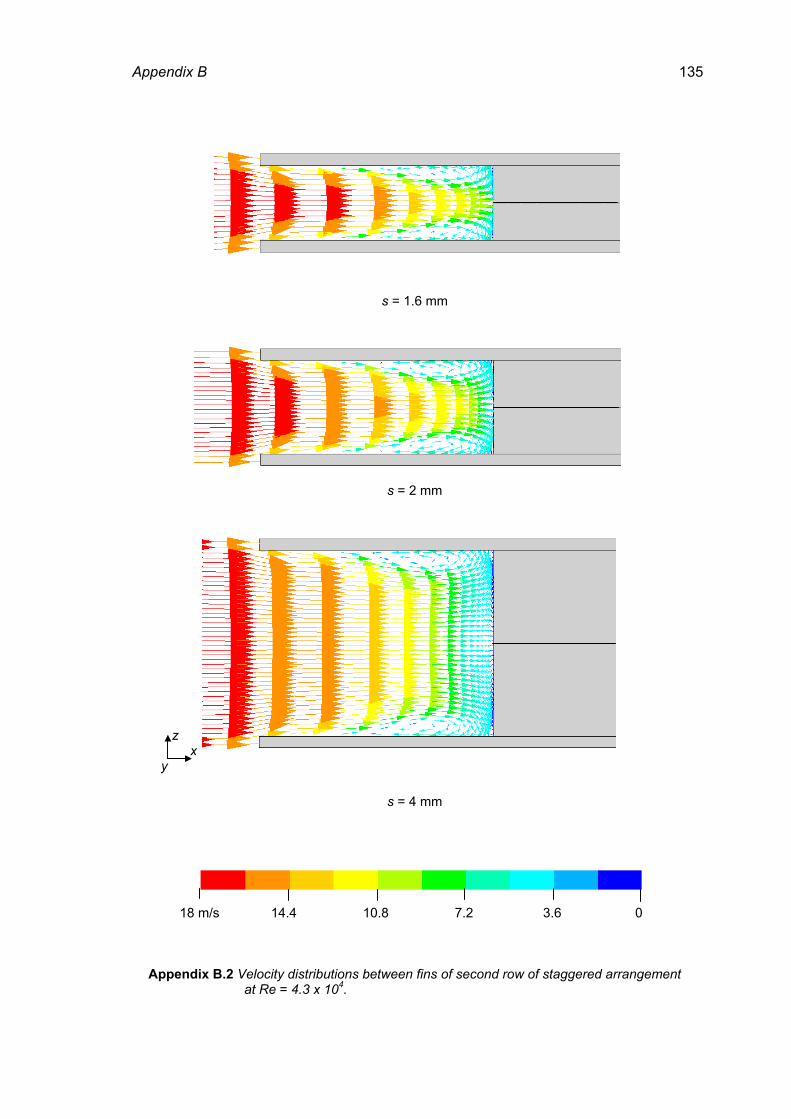
Appendix B 135
s = 1.6 mm
s = 2 mm
s = 4 mm
18 m/s 14.4 10.8 7.2 3.6 0
Appendix B.2 Velocity distributions between fins of second row of staggered arrangement at Re = 4.3 x 10⁴.
z x y
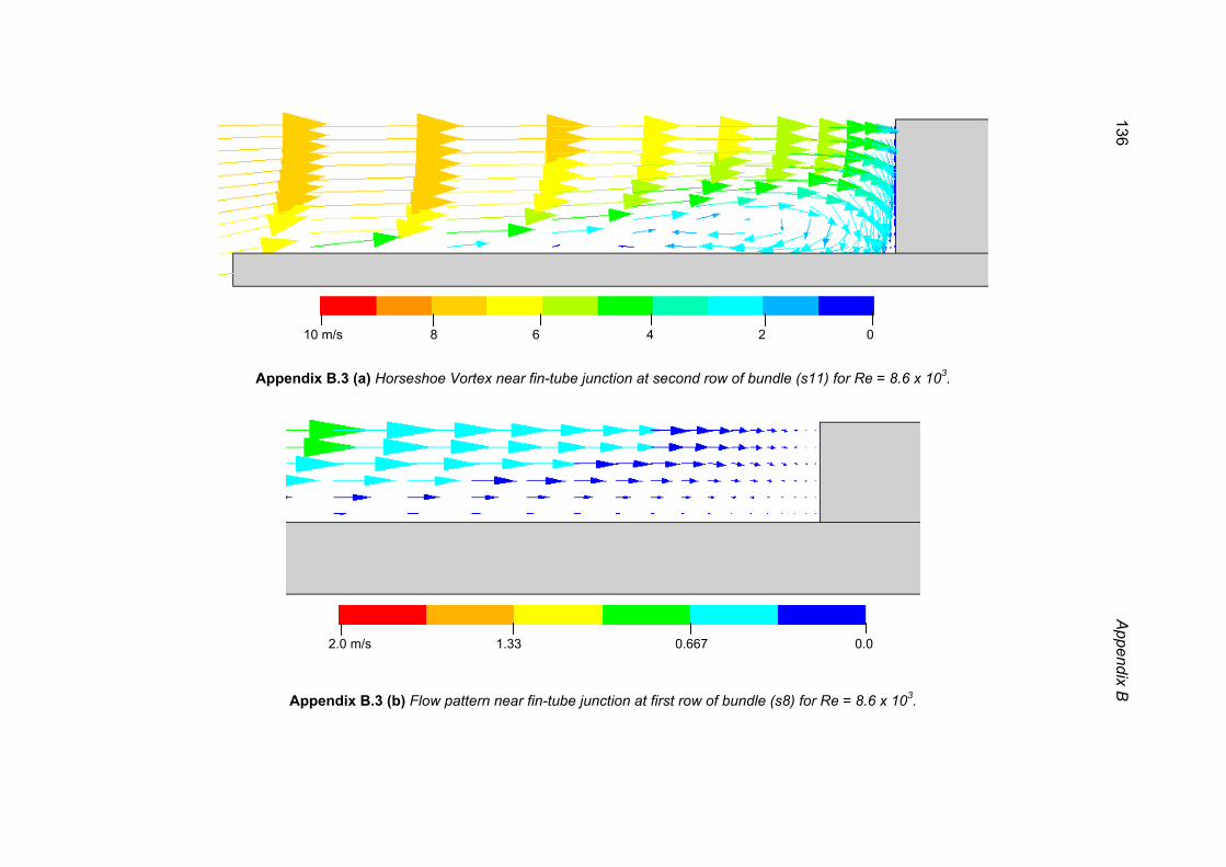
Appendix B.3 (a) Horseshoe Vortex near fin-tube junction at second row of bundle (s11) for Re = 8.6 x 10³.
Appendix B.3 (b) Flow pattern near fin-tube junction at first row of bundle (s8) for Re = 8.6 x 10³.
10 m/s 8 6 4 2 0
2.0 m/s 1.33 0.667 0.0
136 Appendix B
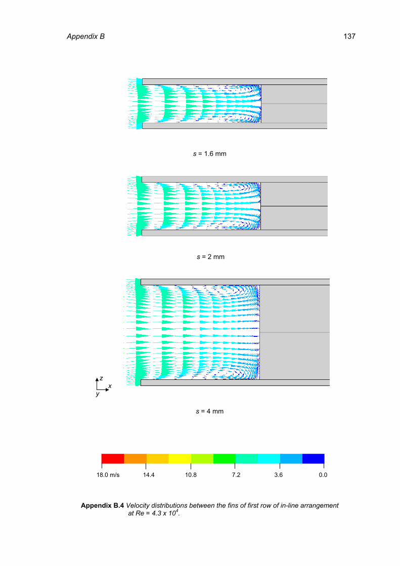
Appendix B 137
s = 1.6 mm
s = 2 mm
s = 4 mm
18.0 m/s 14.4 10.8 7.2 3.6 0.0
Appendix B.4 Velocity distributions between the fins of first row of in-line arrangement at Re = 4.3 x 10⁴.
z x y
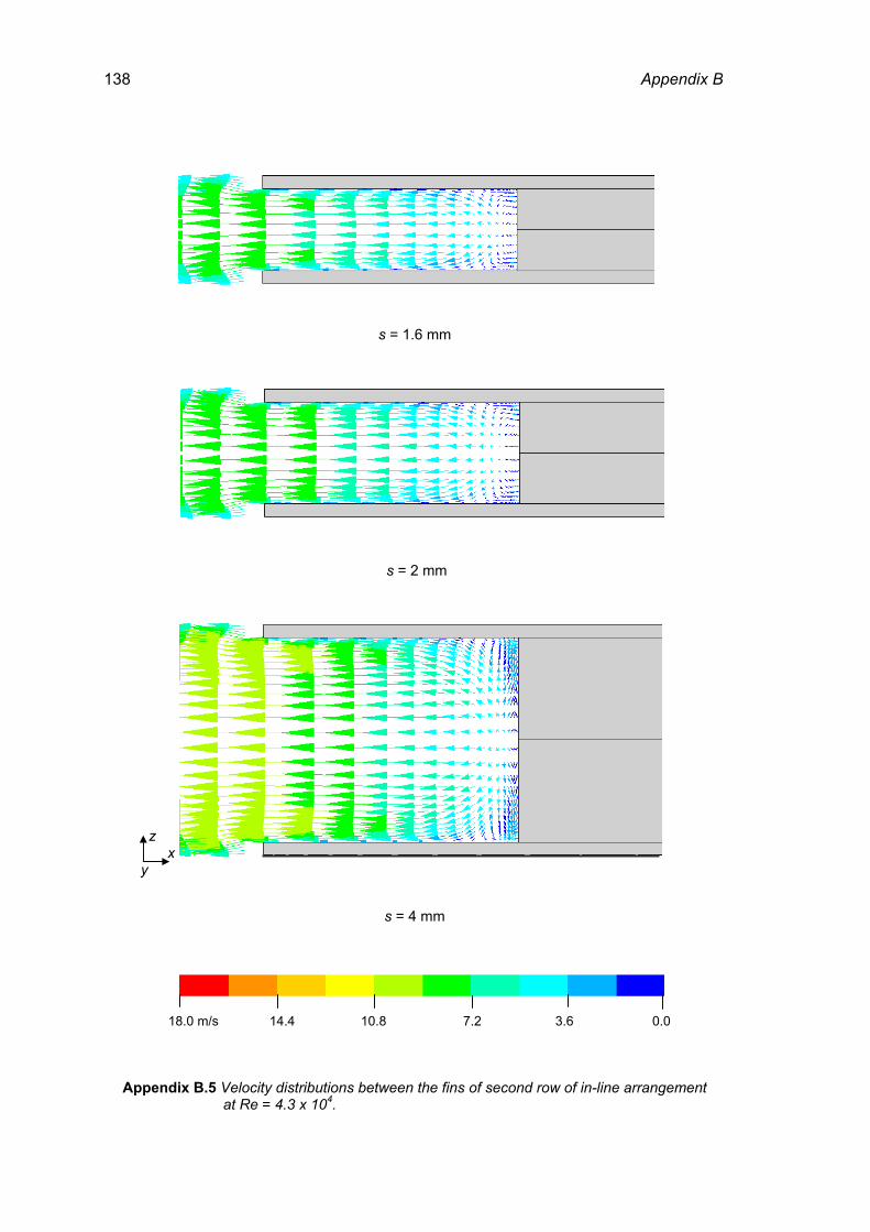
138 Appendix B
s = 1.6 mm
s = 2 mm
s = 4 mm
18.0 m/s 14.4 10.8 7.2 3.6 0.0
Appendix B.5 Velocity distributions between the fins of second row of in-line arrangement at Re = 4.3 x 10⁴.
z x y
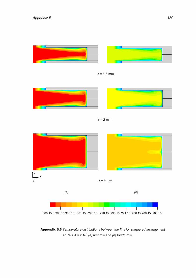
Appendix B 139
s = 1.6 mm
s = 2 mm
z x y s = 4 mm (a) (b)
308.15K 306.15 303.15 301.15 298.15 296.15 293.15 291.15 288.15 286.15 283.15
Appendix B.6 Temperature distributions between the fins for staggered arrangement
at Re = 4.3 x 10⁴ (a) first row and (b) fourth row.
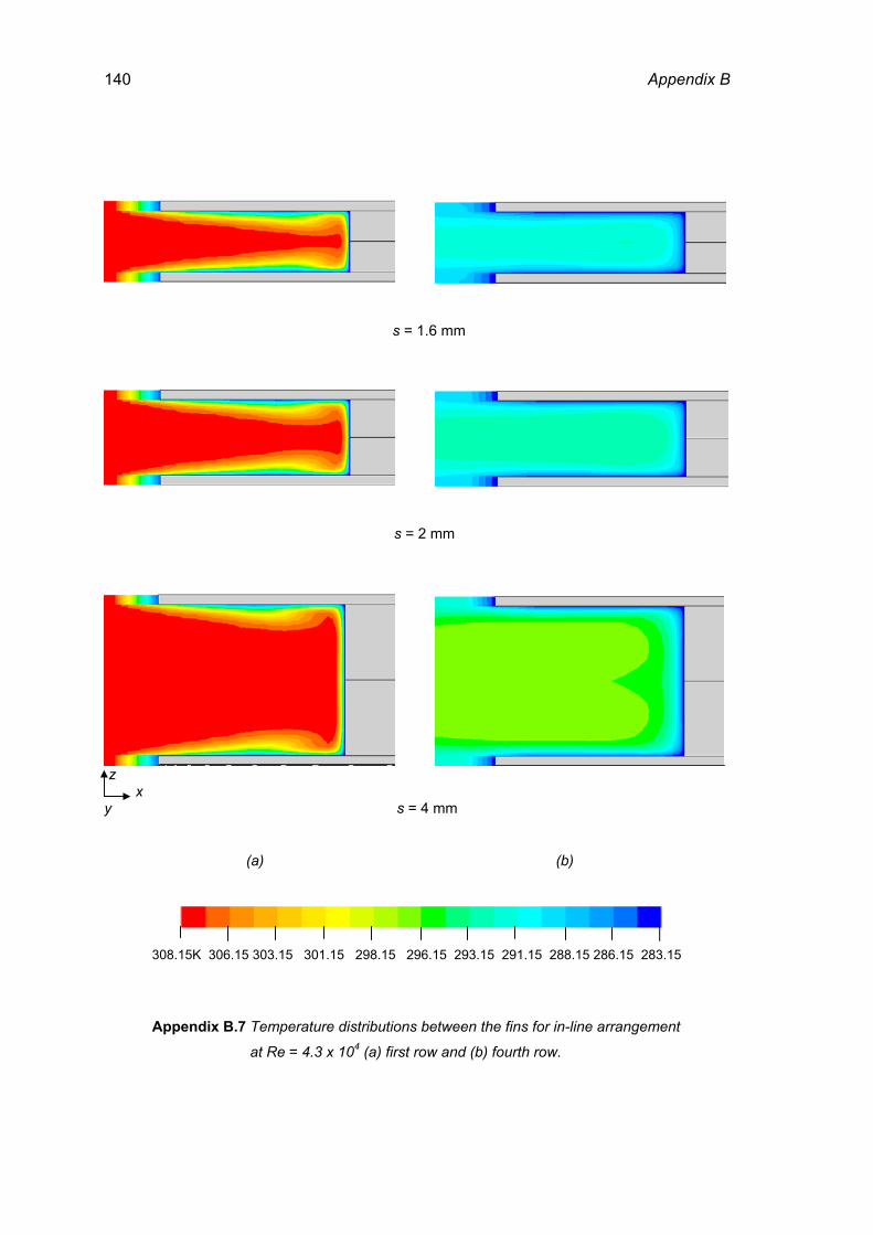
140 Appendix B
s = 1.6 mm
s = 2 mm
z x y s = 4 mm (a) (b)
308.15K 306.15 303.15 301.15 298.15 296.15 293.15 291.15 288.15 286.15 283.15
Appendix B.7 Temperature distributions between the fins for in-line arrangement
at Re = 4.3 x 10⁴ (a) first row and (b) fourth row.
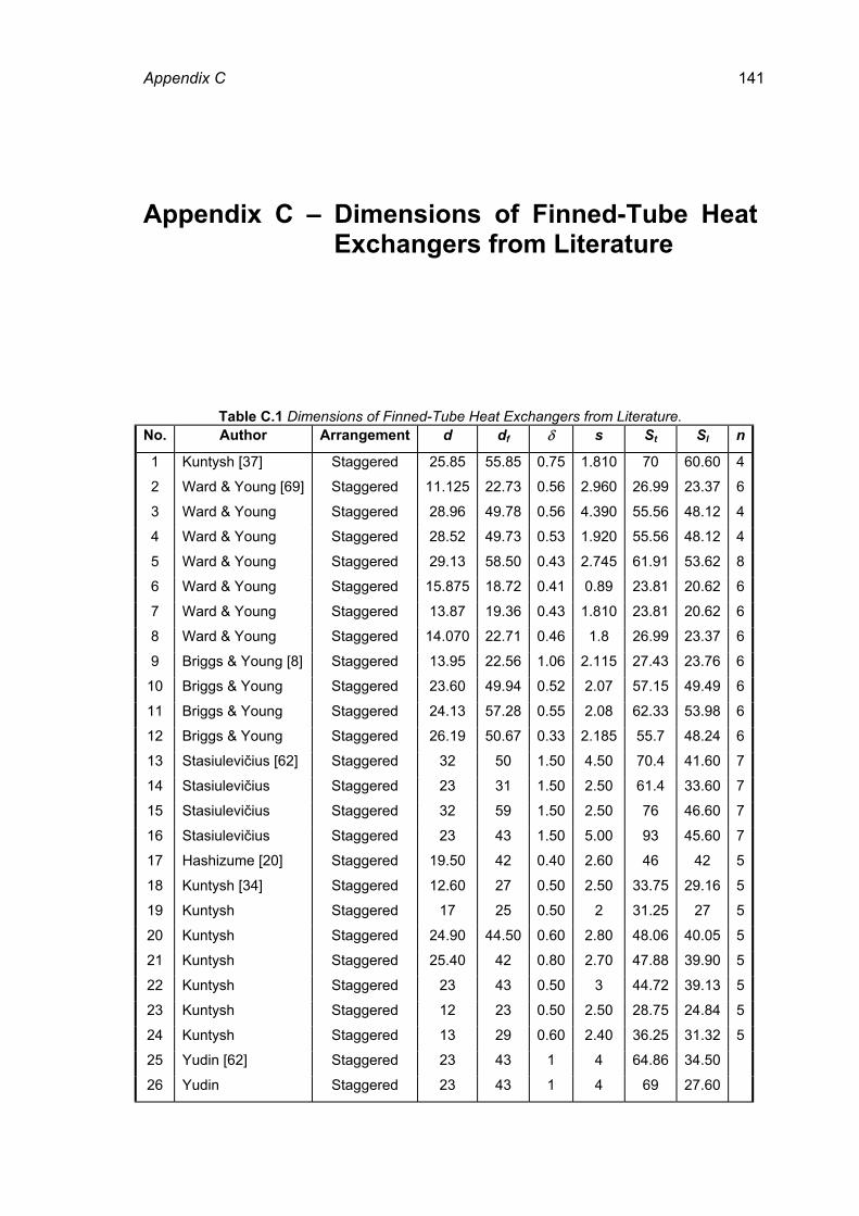
Appendix C 141
Appendix C – Dimensions of Finned-Tube Heat
Exchangers from Literature
Table C.1 Dimensions of Finned-Tube Heat Exchangers from Literature. No. Author Arrangement d df δ s St Sl n
1 Kuntysh [37] Staggered 25.85 55.85 0.75 1.810 70 60.60 4
2 Ward & Young [69] Staggered 11.125 22.73 0.56 2.960 26.99 23.37 6
3 Ward & Young Staggered 28.96 49.78 0.56 4.390 55.56 48.12 4
4 Ward & Young Staggered 28.52 49.73 0.53 1.920 55.56 48.12 4
5 Ward & Young Staggered 29.13 58.50 0.43 2.745 61.91 53.62 8
6 Ward & Young Staggered 15.875 18.72 0.41 0.89 23.81 20.62 6
7 Ward & Young Staggered 13.87 19.36 0.43 1.810 23.81 20.62 6
8 Ward & Young Staggered 14.070 22.71 0.46 1.8 26.99 23.37 6
9 Briggs & Young [8] Staggered 13.95 22.56 1.06 2.115 27.43 23.76 6
10 Briggs & Young Staggered 23.60 49.94 0.52 2.07 57.15 49.49 6
11 Briggs & Young Staggered 24.13 57.28 0.55 2.08 62.33 53.98 6
12 Briggs & Young Staggered 26.19 50.67 0.33 2.185 55.7 48.24 6
13 Stasiulevičius [62] Staggered 32 50 1.50 4.50 70.4 41.60 7
14 Stasiulevičius Staggered 23 31 1.50 2.50 61.4 33.60 7
15 Stasiulevičius Staggered 32 59 1.50 2.50 76 46.60 7
16 Stasiulevičius Staggered 23 43 1.50 5.00 93 45.60 7
17 Hashizume [20] Staggered 19.50 42 0.40 2.60 46 42 5
18 Kuntysh [34] Staggered 12.60 27 0.50 2.50 33.75 29.16 5
19 Kuntysh Staggered 17 25 0.50 2 31.25 27 5
20 Kuntysh Staggered 24.90 44.50 0.60 2.80 48.06 40.05 5
21 Kuntysh Staggered 25.40 42 0.80 2.70 47.88 39.90 5
22 Kuntysh Staggered 23 43 0.50 3 44.72 39.13 5
23 Kuntysh Staggered 12 23 0.50 2.50 28.75 24.84 5
24 Kuntysh Staggered 13 29 0.60 2.40 36.25 31.32 5
25 Yudin [62] Staggered 23 43 1 4 64.86 34.50
26 Yudin Staggered 23 43 1 4 69 27.60
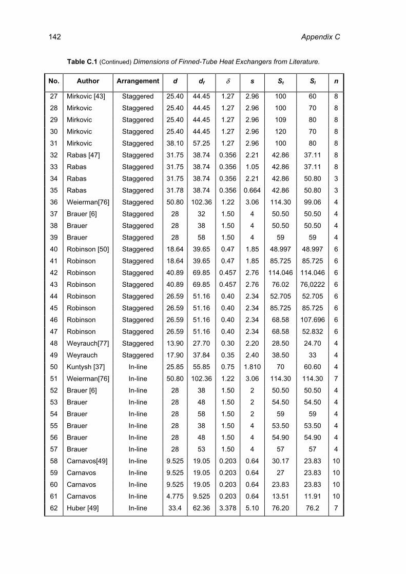
142 Appendix C
Table C.1 (Continued) Dimensions of Finned-Tube Heat Exchangers from Literature.
No. Author Arrangement d df δ s St Sl n
27 Mirkovic [43] Staggered 25.40 44.45 1.27 2.96 100 60 8
28 Mirkovic Staggered 25.40 44.45 1.27 2.96 100 70 8
29 Mirkovic Staggered 25.40 44.45 1.27 2.96 109 80 8
30 Mirkovic Staggered 25.40 44.45 1.27 2.96 120 70 8
31 Mirkovic Staggered 38.10 57.25 1.27 2.96 100 80 8
32 Rabas [47] Staggered 31.75 38.74 0.356 2.21 42.86 37.11 8
33 Rabas Staggered 31.75 38.74 0.356 1.05 42.86 37.11 8
34 Rabas Staggered 31.75 38.74 0.356 2.21 42.86 50.80 3
35 Rabas Staggered 31.78 38.74 0.356 0.664 42.86 50.80 3
36 Weierman[76] Staggered 50.80 102.36 1.22 3.06 114.30 99.06 4
37 Brauer [6] Staggered 28 32 1.50 4 50.50 50.50 4
38 Brauer Staggered 28 38 1.50 4 50.50 50.50 4
39 Brauer Staggered 28 58 1.50 4 59 59 4
40 Robinson [50] Staggered 18.64 39.65 0.47 1.85 48.997 48.997 6
41 Robinson Staggered 18.64 39.65 0.47 1.85 85.725 85.725 6
42 Robinson Staggered 40.89 69.85 0.457 2.76 114.046 114.046 6
43 Robinson Staggered 40.89 69.85 0.457 2.76 76.02 76,0222 6
44 Robinson Staggered 26.59 51.16 0.40 2.34 52.705 52.705 6
45 Robinson Staggered 26.59 51.16 0.40 2.34 85.725 85.725 6
46 Robinson Staggered 26.59 51.16 0.40 2.34 68.58 107.696 6
47 Robinson Staggered 26.59 51.16 0.40 2.34 68.58 52.832 6
48 Weyrauch[77] Staggered 13.90 27.70 0.30 2.20 28.50 24.70 4
49 Weyrauch Staggered 17.90 37.84 0.35 2.40 38.50 33 4
50 Kuntysh [37] In-line 25.85 55.85 0.75 1.810 70 60.60 4
51 Weierman[76] In-line 50.80 102.36 1.22 3.06 114.30 114.30 7
52 Brauer [6] In-line 28 38 1.50 2 50.50 50.50 4
53 Brauer In-line 28 48 1.50 2 54.50 54.50 4
54 Brauer In-line 28 58 1.50 2 59 59 4
55 Brauer In-line 28 38 1.50 4 53.50 53.50 4
56 Brauer In-line 28 48 1.50 4 54.90 54.90 4
57 Brauer In-line 28 53 1.50 4 57 57 4
58 Carnavos[49] In-line 9.525 19.05 0.203 0.64 30.17 23.83 10
59 Carnavos In-line 9.525 19.05 0.203 0.64 27 23.83 10
60 Carnavos In-line 9.525 19.05 0.203 0.64 23.83 23.83 10
61 Carnavos In-line 4.775 9.525 0.203 0.64 13.51 11.91 10
62 Huber [49] In-line 33.4 62.36 3.378 5.10 76.20 76.2 7

Appendix D – Heat Transfer and Pressure Drop Correlations for Circular
Finned - Tube Heat Exchangers from Literature
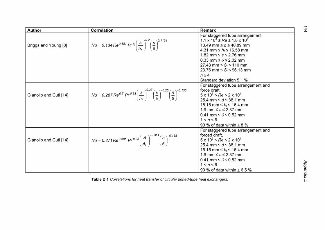
Author Correlation Remark Briggs and Young [8]
1134.02.0
f
681.0 shsPrRe134.0Nu 3
1
=
δ
For staggered tube arrangement, 1.1 x 10³ ≤ Re ≤ 1.8 x 10⁴
13.49 mm ≤ d ≤ 40.89 mm 4.31 mm ≤ hf ≤ 16.58 mm 1.82 mm ≤ s ≤ 2.76 mm 0.33 mm ≤ δ ≤ 2.02 mm 27.43 mm ≤ St ≤ 110 mm 23.76 mm ≤ Sl ≤ 96.13 mm n ≥ 4 Standard deviation 5.1 %
Gianolio and Cuti [14]
136.025.037.0
f
33.07.0
6ns
hsPrRe287.0Nu
−−
=
δ
For staggered tube arrangement and force draft, 5 x 10³ ≤ Re ≤ 2 x 10⁴
25.4 mm ≤ d ≤ 38.1 mm 15.15 mm ≤ hf ≤ 16.4 mm 1.9 mm ≤ s ≤ 2.37 mm 0.41 mm ≤ δ ≤ 0.52 mm 1 < n < 6 90 % of data within ± 8 %
Gianolio and Cuti [14]
138.0311.0
t
33.0685.0
6n
AAPrRe271.0Nu
−−
=
For staggered tube arrangement and forced draft, 5 x 10³ ≤ Re ≤ 2 x 10⁴
25.4 mm ≤ d ≤ 38.1 mm 15.15 mm ≤ hf ≤ 16.4 mm 1.9 mm ≤ s ≤ 2.37 mm 0.41 mm ≤ δ ≤ 0.52 mm 1 < n < 6 90 % of data within ± 6.5 %
Table D.1 Correlations for heat transfer of circular finned-tube heat exchangers.
144 Appendix D
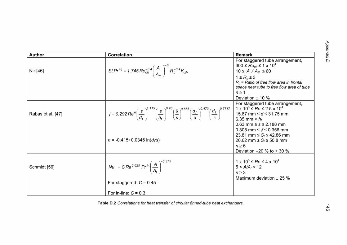
Author Correlation Remark Nir [46]
zh4.0
bff
4.0dh KR
AARe745.1PrSt
32
32 −
−−
′=
For staggered tube arrangement, 300 ≤ Redh ≤ 1 x 10⁴
10 ≤ ffA/A′ ≤ 60 1 ≤ Rb ≤ 3 Rb = Ratio of free flow area in frontal space near tube to free flow area of tube n ≥ 1 Deviation ± 10 %
Rabas et al. [47]
7717.0
f473.0
f666.026.0
f
115.1
f
n ddd
shs
dsRe292.0j
=
δδ
n = -0.415+0.0346 ln(df/s)
For staggered tube arrangement, 1 x 10³ ≤ Re ≤ 2.5 x 10⁴
15.87 mm ≤ d ≤ 31.75 mm 6.35 mm < hf 0.63 mm ≤ s ≤ 2.188 mm 0.305 mm ≤ δ ≤ 0.356 mm 23.81 mm ≤ St ≤ 42.86 mm 20.62 mm ≤ Sl ≤ 50.8 mm n ≥ 6 Deviation –20 % to + 30 %
Schmidt [56]
375.0
t
625.0
AAPrReCNu 3
1−
=
For staggered: C = 0.45 For in-line: C = 0.3
1 x 10³ ≤ Re ≤ 4 x 10⁴
5 < A/At < 12 n ≥ 3 Maximum deviation ± 25 %
Table D.2 Correlations for heat transfer of circular finned-tube heat exchangers.
Appendix D 145
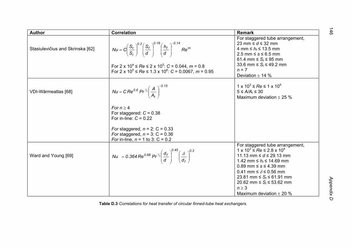
Author Correlation Remark Stasiulevičius and Skrinska [62]
m14.0
f18.0
f2.0
l
t Redh
dS
SS
CNu−
=
For 2 x 10⁴ ≤ Re ≤ 2 x 10⁵: C = 0.044, m = 0.8 For 2 x 10⁵ ≤ Re ≤ 1.3 x 10⁶: C = 0.0067, m = 0.95
For staggered tube arrangement, 23 mm ≤ d ≤ 32 mm 4 mm ≤ hf ≤ 13.5 mm 2.5 mm ≤ s ≤ 6.5 mm 61.4 mm ≤ St ≤ 95 mm 33.6 mm ≤ Sl ≤ 49.2 mm n = 7 Deviation ± 14 %
VDI-Wärmeatlas [68]
15.0
t
6.0
AAPrReCNu 3
1−
=
For n ≥ 4 For staggered: C = 0.38 For in-line: C = 0.22 For staggered, n = 2: C = 0.33 For staggered, n = 3: C = 0.36 For in-line, n = 1 to 3: C = 0.2
1 x 10³ ≤ Re ≤ 1 x 10⁵
5 ≤ A/At ≤ 30 Maximum deviation ± 25 %
Ward and Young [69]
3.0
f
45.0f68.0
dddPrRe364.0Nu 3
1
=
δ
For staggered tube arrangement, 1 x 10³ ≤ Re ≤ 2.8 x 10⁴ 11.13 mm ≤ d ≤ 29.13 mm 1.42 mm ≤ hf ≤ 14.69 mm 0.89 mm ≤ s ≤ 4.39 mm 0.41 mm ≤ δ ≤ 0.56 mm 23.81 mm ≤ St ≤ 61.91 mm 20.62 mm ≤ Sl ≤ 53.62 mm n ≥ 3 Maximum deviation ± 20 %
Table D.3 Correlations for heat transfer of circular finned-tube heat exchangers.
146 Appendix D
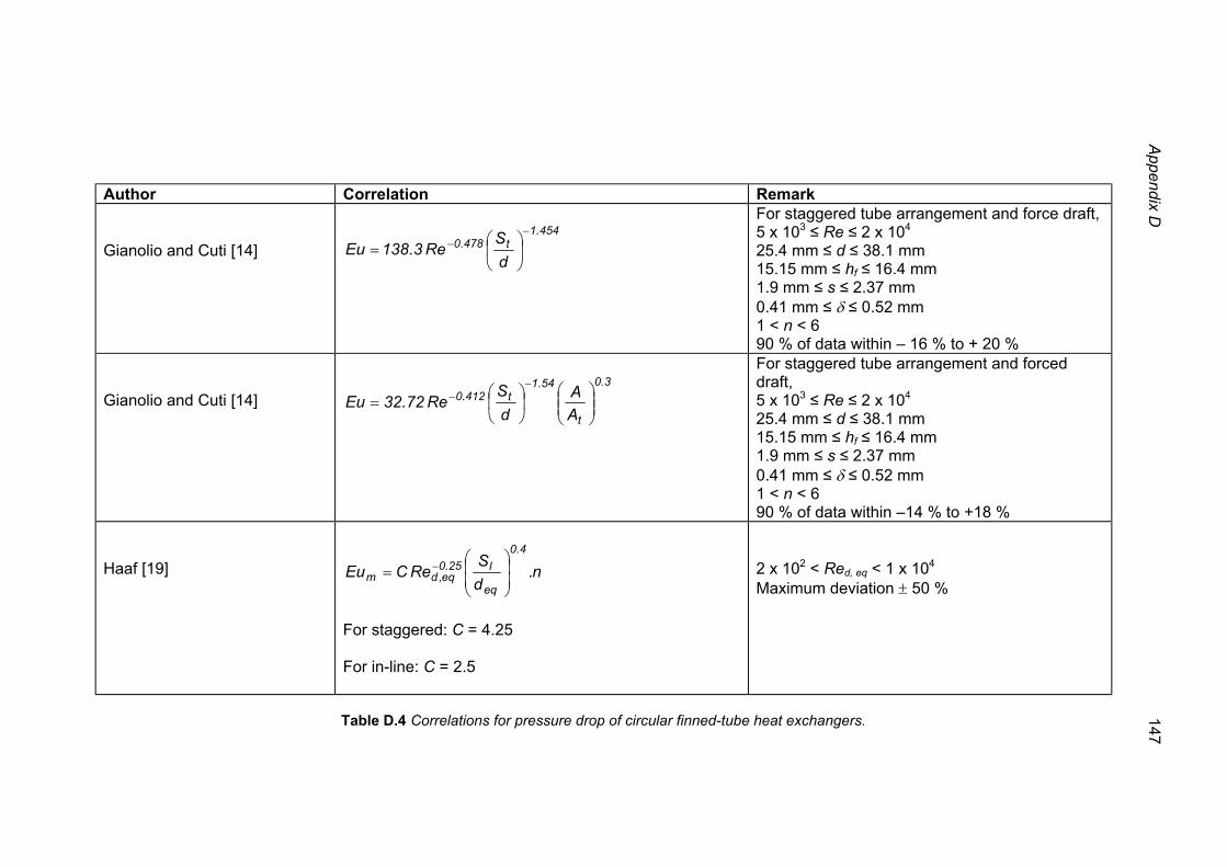
Author Correlation Remark Gianolio and Cuti [14]
454.1
t478.0
dS
Re3.138Eu−
−
=
For staggered tube arrangement and force draft, 5 x 10³ ≤ Re ≤ 2 x 10⁴
25.4 mm ≤ d ≤ 38.1 mm 15.15 mm ≤ hf ≤ 16.4 mm 1.9 mm ≤ s ≤ 2.37 mm 0.41 mm ≤ δ ≤ 0.52 mm 1 < n < 6 90 % of data within – 16 % to + 20 %
Gianolio and Cuti [14]
3.0
t
54.1t412.0
AA
dS
Re72.32Eu
=
−−
For staggered tube arrangement and forced draft, 5 x 10³ ≤ Re ≤ 2 x 10⁴
25.4 mm ≤ d ≤ 38.1 mm 15.15 mm ≤ hf ≤ 16.4 mm 1.9 mm ≤ s ≤ 2.37 mm 0.41 mm ≤ δ ≤ 0.52 mm 1 < n < 6 90 % of data within –14 % to +18 %
Haaf [19]
n.dS
ReCEu4.0
eq
l25.0eq,dm
= −
For staggered: C = 4.25 For in-line: C = 2.5
2 x 10² < Red, eq < 1 x 10⁴
Maximum deviation ± 50 %
Table D.4 Correlations for pressure drop of circular finned-tube heat exchangers.
Appendix D 147
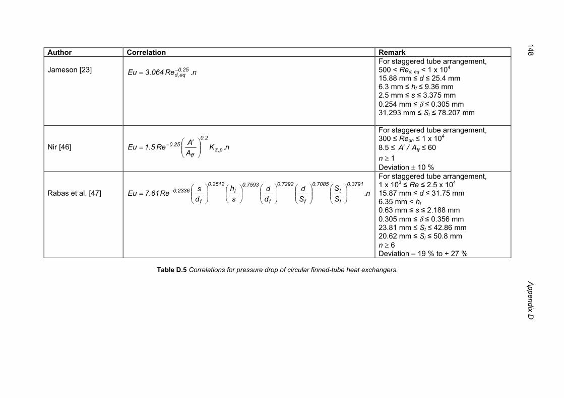
Author Correlation Remark Jameson [23]
n.Re064.3Eu 25.0
eq,d−=
For staggered tube arrangement, 500 < Red, eq < 1 x 10⁴
15.88 mm ≤ d ≤ 25.4 mm 6.3 mm ≤ hf ≤ 9.36 mm 2.5 mm ≤ s ≤ 3.375 mm 0.254 mm ≤ δ ≤ 0.305 mm 31.293 mm ≤ St ≤ 78.207 mm
Nir [46]
n.KAARe5.1Eu p,z
2.0
ff
25.0
′= −
For staggered tube arrangement, 300 ≤ Redh ≤ 1 x 10⁴
8.5 ≤ ffA/A′ ≤ 60 n ≥ 1 Deviation ± 10 %
Rabas et al. [47]
n.SS
Sd
dd
sh
dsRe61.7Eu
3791.0
l
t7085.0
f
7292.0
f
7593.0f
2512.0
f
2336.0
= −
For staggered tube arrangement, 1 x 10³ ≤ Re ≤ 2.5 x 10⁴
15.87 mm ≤ d ≤ 31.75 mm 6.35 mm < hf 0.63 mm ≤ s ≤ 2.188 mm 0.305 mm ≤ δ ≤ 0.356 mm 23.81 mm ≤ St ≤ 42.86 mm 20.62 mm ≤ Sl ≤ 50.8 mm n ≥ 6 Deviation – 19 % to + 27 %
Table D.5 Correlations for pressure drop of circular finned-tube heat exchangers.
148 Appendix D
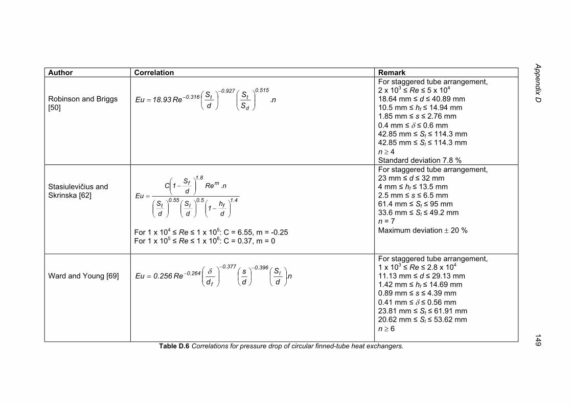
Author Correlation Remark Robinson and Briggs [50]
n.SS
dS
Re93.18Eu515.0
d
t927.0
t316.0
=
−−
For staggered tube arrangement, 2 x 10³ ≤ Re ≤ 5 x 10⁴
18.64 mm ≤ d ≤ 40.89 mm 10.5 mm ≤ hf ≤ 14.94 mm 1.85 mm ≤ s ≤ 2.76 mm 0.4 mm ≤ δ ≤ 0.6 mm 42.85 mm ≤ St ≤ 114.3 mm 42.85 mm ≤ Sl ≤ 114.3 mm n ≥ 4 Standard deviation 7.8 %
Stasiulevičius and Skrinska [62]
4.1f
5.0l
55.0t
m8.1
f
dh
1dS
dS
n.Red
S1C
Eu
−
−
=
For 1 x 10⁴ ≤ Re ≤ 1 x 10⁵: C = 6.55, m = -0.25 For 1 x 10⁵ ≤ Re ≤ 1 x 10⁶: C = 0.37, m = 0
For staggered tube arrangement, 23 mm ≤ d ≤ 32 mm 4 mm ≤ hf ≤ 13.5 mm 2.5 mm ≤ s ≤ 6.5 mm 61.4 mm ≤ St ≤ 95 mm 33.6 mm ≤ Sl ≤ 49.2 mm n = 7 Maximum deviation ± 20 %
Ward and Young [69]
n.dS
ds
dRe256.0Eu l
396.0377.0
f
264.0
=
−−− δ
For staggered tube arrangement, 1 x 10³ ≤ Re ≤ 2.8 x 10⁴ 11.13 mm ≤ d ≤ 29.13 mm 1.42 mm ≤ hf ≤ 14.69 mm 0.89 mm ≤ s ≤ 4.39 mm 0.41 mm ≤ δ ≤ 0.56 mm 23.81 mm ≤ St ≤ 61.91 mm 20.62 mm ≤ Sl ≤ 53.62 mm n ≥ 6
Table D.6 Correlations for pressure drop of circular finned-tube heat exchangers.
Appendix D 149
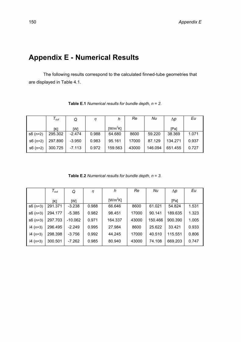
150 Appendix E
Appendix E - Numerical Results The following results correspond to the calculated finned-tube geometries that
are displayed in Table 4.1.
Table E.1 Numerical results for bundle depth, n = 2.
Tout
[K]
Q&
[W]
η h
[W/m2K]
Re Nu p∆
[Pa]
Eu
s6 (n=2) 295.302 -2.474 0.988 64.680 8600 59.220 38.369 1.071
s6 (n=2) 297.890 -3.950 0.983 95.161 17000 87.129 134.271 0.937
s6 (n=2) 300.725 -7.113 0.972 159.563 43000 146.094 651.455 0.727
Table E.2 Numerical results for bundle depth, n = 3.
Tout
[K]
Q&
[W]
η h
[W/m2K]
Re Nu p∆
[Pa]
Eu
s6 (n=3) 291.371 -3.238 0.988 66.646 8600 61.021 54.824 1.531
s6 (n=3) 294.177 -5.385 0.982 98.451 17000 90.141 189.635 1.323
s6 (n=3) 297.703 -10.062 0.971 164.337 43000 150.466 900.390 1.005
i4 (n=3) 296.495 -2.249 0.995 27.984 8600 25.622 33.421 0.933
i4 (n=3) 298.398 -3.756 0.992 44.245 17000 40.510 115.551 0.806
i4 (n=3) 300.501 -7.262 0.985 80.940 43000 74.108 669.203 0.747
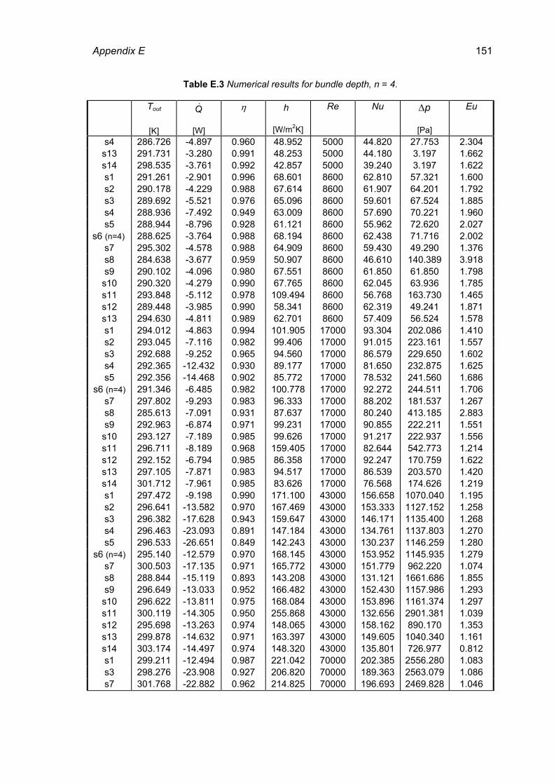
Appendix E 151
Table E.3 Numerical results for bundle depth, n = 4.
Tout
[K]
Q&
[W]
η h
[W/m2K]
Re Nu p∆
[Pa]
Eu
s4 286.726 -4.897 0.960 48.952 5000 44.820 27.753 2.304 s13 291.731 -3.280 0.991 48.253 5000 44.180 3.197 1.662 s14 298.535 -3.761 0.992 42.857 5000 39.240 3.197 1.622 s1 291.261 -2.901 0.996 68.601 8600 62.810 57.321 1.600 s2 290.178 -4.229 0.988 67.614 8600 61.907 64.201 1.792 s3 289.692 -5.521 0.976 65.096 8600 59.601 67.524 1.885 s4 288.936 -7.492 0.949 63.009 8600 57.690 70.221 1.960 s5 288.944 -8.796 0.928 61.121 8600 55.962 72.620 2.027
s6 (n=4) 288.625 -3.764 0.988 68.194 8600 62.438 71.716 2.002 s7 295.302 -4.578 0.988 64.909 8600 59.430 49.290 1.376 s8 284.638 -3.677 0.959 50.907 8600 46.610 140.389 3.918 s9 290.102 -4.096 0.980 67.551 8600 61.850 61.850 1.798 s10 290.320 -4.279 0.990 67.765 8600 62.045 63.936 1.785 s11 293.848 -5.112 0.978 109.494 8600 56.768 163.730 1.465 s12 289.448 -3.985 0.990 58.341 8600 62.319 49.241 1.871 s13 294.630 -4.811 0.989 62.701 8600 57.409 56.524 1.578 s1 294.012 -4.863 0.994 101.905 17000 93.304 202.086 1.410 s2 293.045 -7.116 0.982 99.406 17000 91.015 223.161 1.557 s3 292.688 -9.252 0.965 94.560 17000 86.579 229.650 1.602 s4 292.365 -12.432 0.930 89.177 17000 81.650 232.875 1.625 s5 292.356 -14.468 0.902 85.772 17000 78.532 241.560 1.686
s6 (n=4) 291.346 -6.485 0.982 100.778 17000 92.272 244.511 1.706 s7 297.802 -9.293 0.983 96.333 17000 88.202 181.537 1.267 s8 285.613 -7.091 0.931 87.637 17000 80.240 413.185 2.883 s9 292.963 -6.874 0.971 99.231 17000 90.855 222.211 1.551 s10 293.127 -7.189 0.985 99.626 17000 91.217 222.937 1.556 s11 296.711 -8.189 0.968 159.405 17000 82.644 542.773 1.214 s12 292.152 -6.794 0.985 86.358 17000 92.247 170.759 1.622 s13 297.105 -7.871 0.983 94.517 17000 86.539 203.570 1.420 s14 301.712 -7.961 0.985 83.626 17000 76.568 174.626 1.219 s1 297.472 -9.198 0.990 171.100 43000 156.658 1070.040 1.195 s2 296.641 -13.582 0.970 167.469 43000 153.333 1127.152 1.258 s3 296.382 -17.628 0.943 159.647 43000 146.171 1135.400 1.268 s4 296.463 -23.093 0.891 147.184 43000 134.761 1137.803 1.270 s5 296.533 -26.651 0.849 142.243 43000 130.237 1146.259 1.280
s6 (n=4) 295.140 -12.579 0.970 168.145 43000 153.952 1145.935 1.279 s7 300.503 -17.135 0.971 165.772 43000 151.779 962.220 1.074 s8 288.844 -15.119 0.893 143.208 43000 131.121 1661.686 1.855 s9 296.649 -13.033 0.952 166.482 43000 152.430 1157.986 1.293 s10 296.622 -13.811 0.975 168.084 43000 153.896 1161.374 1.297 s11 300.119 -14.305 0.950 255.868 43000 132.656 2901.381 1.039 s12 295.698 -13.263 0.974 148.065 43000 158.162 890.170 1.353 s13 299.878 -14.632 0.971 163.397 43000 149.605 1040.340 1.161 s14 303.174 -14.497 0.974 148.320 43000 135.801 726.977 0.812 s1 299.211 -12.494 0.987 221.042 70000 202.385 2556.280 1.083 s3 298.276 -23.908 0.927 206.820 70000 189.363 2563.079 1.086 s7 301.768 -22.882 0.962 214.825 70000 196.693 2469.828 1.046
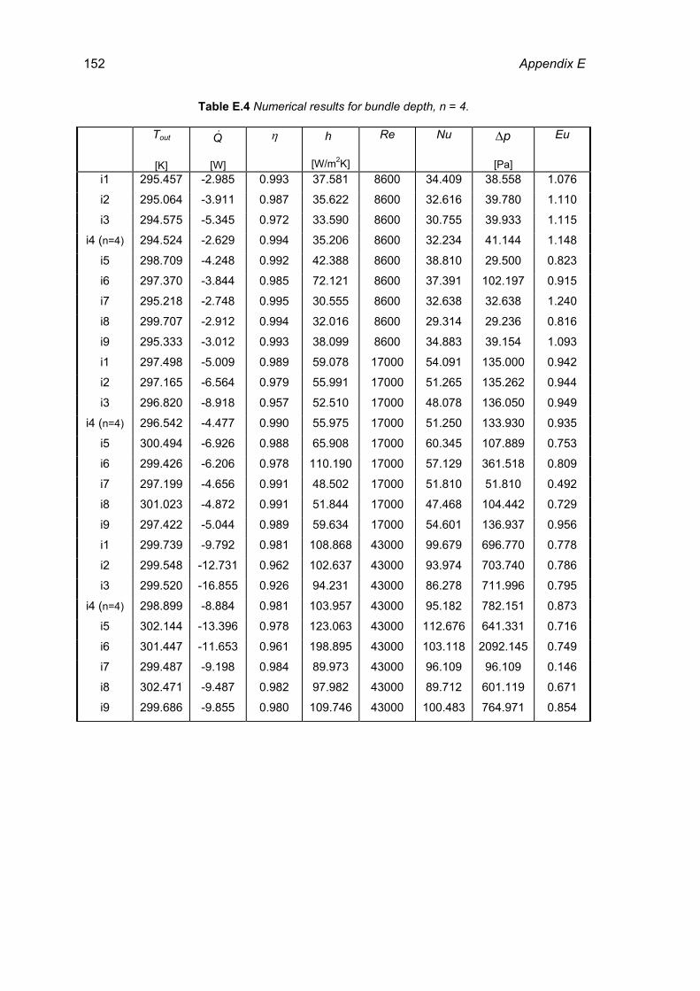
152 Appendix E
Table E.4 Numerical results for bundle depth, n = 4.
Tout
[K]
Q&
[W]
η h
[W/m2K]
Re Nu p∆
[Pa]
Eu
i1 295.457 -2.985 0.993 37.581 8600 34.409 38.558 1.076
i2 295.064 -3.911 0.987 35.622 8600 32.616 39.780 1.110
i3 294.575 -5.345 0.972 33.590 8600 30.755 39.933 1.115
i4 (n=4) 294.524 -2.629 0.994 35.206 8600 32.234 41.144 1.148
i5 298.709 -4.248 0.992 42.388 8600 38.810 29.500 0.823
i6 297.370 -3.844 0.985 72.121 8600 37.391 102.197 0.915
i7 295.218 -2.748 0.995 30.555 8600 32.638 32.638 1.240
i8 299.707 -2.912 0.994 32.016 8600 29.314 29.236 0.816
i9 295.333 -3.012 0.993 38.099 8600 34.883 39.154 1.093
i1 297.498 -5.009 0.989 59.078 17000 54.091 135.000 0.942
i2 297.165 -6.564 0.979 55.991 17000 51.265 135.262 0.944
i3 296.820 -8.918 0.957 52.510 17000 48.078 136.050 0.949
i4 (n=4) 296.542 -4.477 0.990 55.975 17000 51.250 133.930 0.935
i5 300.494 -6.926 0.988 65.908 17000 60.345 107.889 0.753
i6 299.426 -6.206 0.978 110.190 17000 57.129 361.518 0.809
i7 297.199 -4.656 0.991 48.502 17000 51.810 51.810 0.492
i8 301.023 -4.872 0.991 51.844 17000 47.468 104.442 0.729
i9 297.422 -5.044 0.989 59.634 17000 54.601 136.937 0.956
i1 299.739 -9.792 0.981 108.868 43000 99.679 696.770 0.778
i2 299.548 -12.731 0.962 102.637 43000 93.974 703.740 0.786
i3 299.520 -16.855 0.926 94.231 43000 86.278 711.996 0.795
i4 (n=4) 298.899 -8.884 0.981 103.957 43000 95.182 782.151 0.873
i5 302.144 -13.396 0.978 123.063 43000 112.676 641.331 0.716
i6 301.447 -11.653 0.961 198.895 43000 103.118 2092.145 0.749
i7 299.487 -9.198 0.984 89.973 43000 96.109 96.109 0.146
i8 302.471 -9.487 0.982 97.982 43000 89.712 601.119 0.671
i9 299.686 -9.855 0.980 109.746 43000 100.483 764.971 0.854

Appendix E 153
Table E.5 Numerical results for bundle depth, n = 5.
Tout
[K]
Q&
[W]
η h
[W/m2K]
Re Nu p∆
[Pa]
Eu
s6 (n=5) 286.806 -4.110 0.988 69.004 8600 63.180 87.403 2.440
s6 (n=5) 289.248 -7.294 0.982 102.005 17000 93.395 299.164 2.088
s6 (n=5) 293.069 -14.625 0.970 169.759 43000 155.430 1391.268 1.553
i4 (n=5) 292.826 -2.954 0.994 33.906 8600 31.044 47.545 1.327
i4 (n=5) 294.922 -5.095 0.990 53.933 17000 49.380 150.868 1.053
i4 (n=5) 297.357 -10.332 0.982 101.353 43000 92.798 866.267 0.967
Table E.6 Numerical results for bundle depth, n = 6.
Tout
[K]
Q&
[W]
η h
[W/m2K]
Re Nu p∆
[Pa]
Eu
s6 (n=6) 285.605 -4.344 0.987 69.463 8600 63.600 103.634 2.893
s6 (n=6) 287.695 -7.900 0.982 102.814 17000 94.136 353.724 2.468
s6 (n=6) 291.350 -16.351 0.970 171.250 43000 156.796 1637.153 1.828

Lebenslauf
Name: Mi Sandar Mon
Geburtsdatum: 20. 06. 1967
Geburtsort: Yangon, Myanmar
Familienstand: verheiratet
Schulbildung 1972 – 1974: Grundschule in Mawlamyaing, Myanmar
1975 – 1982: Oberschule in Yangon, Myanmar
Hochschulstudium 12/1983 – 11/1992: Maschinenbau
Yangon Institute of Technology, Abschluß: B.E
07/1993 – 09/1996: Maschinenbau
Yangon Institute of Technology, Abschluß: M.E
09/1998 – 05/2003: Stipendiat im Graduiertenkolleg
Technische Universität Bergakademie Freiberg
Berufliche Tätigkeit
06/1994 – 03/1997: Instructor am Yangon Institute of Technology,
Fakultät für Maschinenbau
03/1997 – 08/2002: Assistant Lecturer
an der Yangon Technological University,
Fakultät für Maschinenbau
seit 09/2002: Lecturer an der Yangon Technological University,
Fakultät für Maschinenbau
![Unbenannt-1detailforschung.info/Texte/quick.pdf · Konstruktive Umsetzung der Solarwand Messergebnisse Name Tmax [°C] Heat Flux y1 Heat Flux y2 Heat Flux aussen Heat Flux innen Georg](https://img.pdfslide.org/doc/110x75/5fe58fbd5e888a7169649e0d/unbenannt-konstruktive-umsetzung-der-solarwand-messergebnisse-name-tmax-c-heat.jpg)