On Generalised Statistical Equilibriumand Discrete Quantum Gravity

Dissertationzur Erlangung des akademischen Grades

Doctor rerum naturalium (Dr. rer. nat.)im Fach: Physik

Spezialisierung: Theoretische Physik

eingereicht an derMathematisch-Naturwissenschaftlichen Fakultät

der Humboldt-Universität zu Berlinvon

Isha Kotecha

Präsidentin der Humboldt-Universität zu Berlin:Prof. Dr.-Ing. Dr. Sabine Kunst

Dekan der Mathematisch-Naturwissenschaftlichen Fakultät:Prof. Dr. Elmar Kulke

Betreuer:Dr. Daniele Oriti

Gutachter:Prof. Dr. Hermann NicolaiProf. Dr. Alejandro PerezProf. Dr. Časlav Brukner

Tag der mündlichen Prüfung:15. Oktober 2020

arX

iv:2

010.

1544

5v2

[gr

-qc]

13

Sep

2021

for my grandparents, my guiding starsand my parents, my guiding lights

I declare that I have completed the thesis independently using only the aids andtools specified. I have not applied for a doctor’s degree in the doctoral subject elsewhereand do not hold a corresponding doctor’s degree. I have taken due note of the Faculty ofMathematics and Natural Sciences PhD Regulations, published in the Official Gazetteof Humboldt-Universität zu Berlin Nr. 42/2018 on 11.07.2018.

Ich erkläre, dass ich die Dissertation selbständig und nur unter Verwendung der vonmir gemäß § 7 Abs. 3 der Promotionsordnung der Mathematisch-NaturwissenschaftlichenFakultät, veröffentlicht im Amtlichen Mitteilungsblatt der Humboldt-Universität zuBerlin Nr. 42/2018 am 11.07.2018 angegebenen Hilfsmittel angefertigt habe.

Isha KotechaJune 11, 2020

i

Abstract

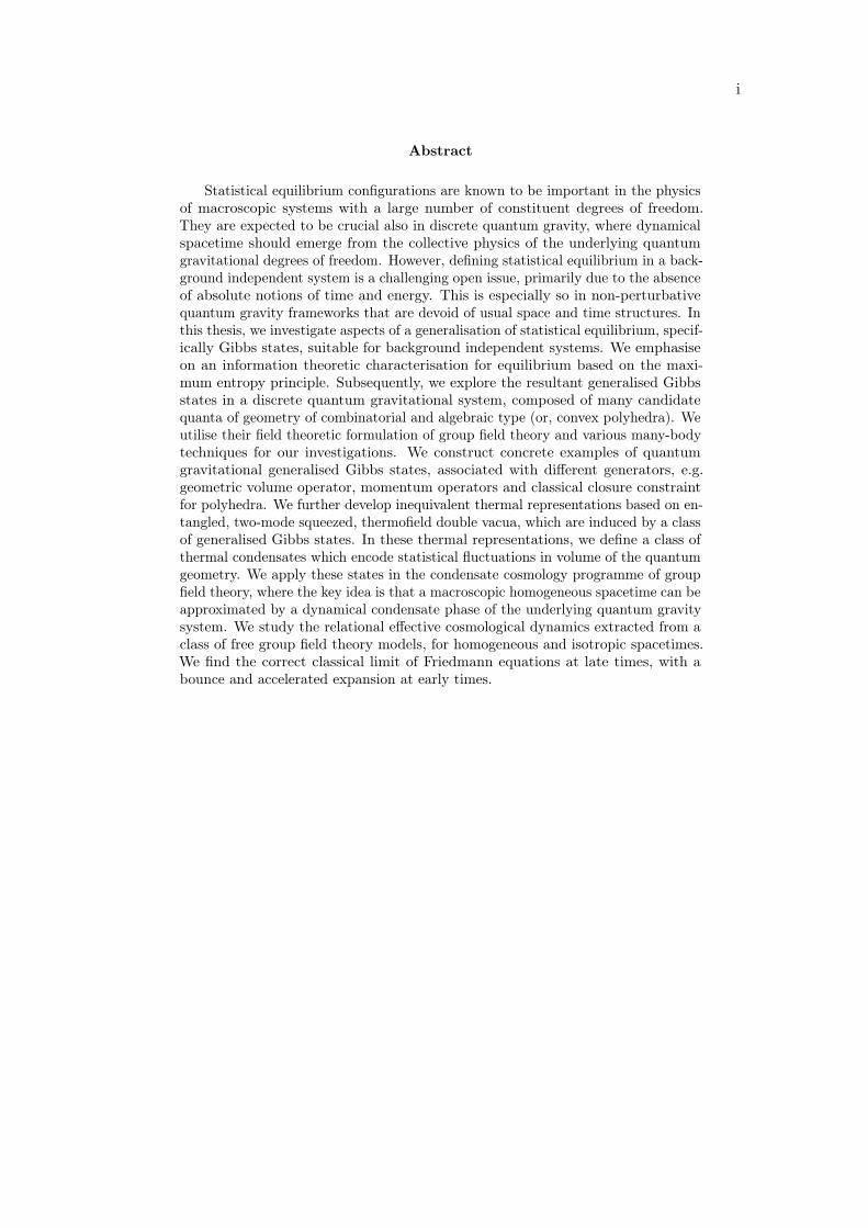
Statistical equilibrium configurations are known to be important in the physicsof macroscopic systems with a large number of constituent degrees of freedom.They are expected to be crucial also in discrete quantum gravity, where dynamicalspacetime should emerge from the collective physics of the underlying quantumgravitational degrees of freedom. However, defining statistical equilibrium in a back-ground independent system is a challenging open issue, primarily due to the absenceof absolute notions of time and energy. This is especially so in non-perturbativequantum gravity frameworks that are devoid of usual space and time structures. Inthis thesis, we investigate aspects of a generalisation of statistical equilibrium, specif-ically Gibbs states, suitable for background independent systems. We emphasiseon an information theoretic characterisation for equilibrium based on the maxi-mum entropy principle. Subsequently, we explore the resultant generalised Gibbsstates in a discrete quantum gravitational system, composed of many candidatequanta of geometry of combinatorial and algebraic type (or, convex polyhedra). Weutilise their field theoretic formulation of group field theory and various many-bodytechniques for our investigations. We construct concrete examples of quantumgravitational generalised Gibbs states, associated with different generators, e.g.geometric volume operator, momentum operators and classical closure constraintfor polyhedra. We further develop inequivalent thermal representations based on en-tangled, two-mode squeezed, thermofield double vacua, which are induced by a classof generalised Gibbs states. In these thermal representations, we define a class ofthermal condensates which encode statistical fluctuations in volume of the quantumgeometry. We apply these states in the condensate cosmology programme of groupfield theory, where the key idea is that a macroscopic homogeneous spacetime can beapproximated by a dynamical condensate phase of the underlying quantum gravitysystem. We study the relational effective cosmological dynamics extracted from aclass of free group field theory models, for homogeneous and isotropic spacetimes.We find the correct classical limit of Friedmann equations at late times, with abounce and accelerated expansion at early times.

iii

Acknowledgments

Science is a journey driven by curiosity and learning. For me, this journey whichbegan many years ago in high school, has reached a personal milestone with thecompletion of this thesis and my PhD. It would have been impossible without thehelp, encouragement and friendship of many people, to whom I am deeply grateful.

It is fortunate, as a young researcher, to be able to immerse in as stimulatingan environment as that of the Albert Einstein Institute and Humboldt University ofBerlin. I am indebted to Daniele Oriti, Hermann Nicolai, Deutscher AkademischerAustauschdienst (DAAD) and International Max Planck Research School for makingthis possible. I am especially thankful to Daniele for his mentorship and constantguidance, which helped me greatly to navigate through research topics and workingsin academia. In addition to patiently guiding me through the dense literature fortackling these questions, he introduced me to important foundational problems inthe field, while also encouraging me to explore topics of personal interest.

My PhD experience was further enriched by the support of several people. Manyspecial thanks are due to my collaborators, Goffredo Chirco and Mehdi Assanioussi,for numerous insightful discussions and friendly advice. I am also sincerely gratefulto Rob Myers and Sylvain Carrozza, for the wonderful opportunity to spend sometime at Perimeter Institute as a visiting graduate fellow. I am thankful to JosephBen Geloun, Axel Kleinschmidt, Sandra Faber, Sumati Surya and Amihay Hananyfor their help, at various different stages during and before the start of my PhD.

My time at AEI was made enjoyable by the presence of many friends andcolleagues. For this, I would like to thank Alexander Kegeles, Claudio Paganini,Johannes Thürigen, Seungjin Lee, Mingyi Zhang, Ana Alonso-Serrano, Olof Ahlén,Alice Di Tucci, Caroline Jonas, Sebastian Bramberger, Lars Kreutzer, Jan Gerkenand Hugo Camargo. I am particularly thankful to Alexander for a thorough readingof an earlier version of this manuscript and valuable comments; and, to Claudiofor help with the German translation of the summary. Working at AEI, living inGermany and completing the PhD was made a lot easier due to the proactive supportof several people, to whom I am very grateful: Anika Rast, Darya Niakhaichykand Constance Münchow at AEI; Bettina Wandel at DAAD; Jennifer Sabernakand Carolin Schneider at Potsdam International Community Center; and, DanielSchaan and Milena Bauer at HU-Berlin.

To my loving family, I am forever grateful. To my parents, Kotecha and Patel,for their open-mindedness and inspiration. To Kishan, Priyanka and Riddhi, forbeing my pillars of strength. Foremost, to my husband Meet, for his relentlesssupport, unwavering faith and for being a true friend, ever since this journey began.

v

Where the voice of the wind calls our wandering feet,Through echoing forest and echoing street,With lutes in our hands ever-singing we roam,All men are our kindred, the world is our home.

—Sarojini Naidu, in Wandering Singers

Contents

1 Introduction 1

2 Generalised Statistical Equilibrium 92.1 Rethinking time in mechanics . . . . . . . . . . . . . . . . . . . . . . . . 10

2.1.1 Preliminaries: Presymplectic mechanics . . . . . . . . . . . . . . 112.1.2 Deparametrization . . . . . . . . . . . . . . . . . . . . . . . . . . 14

2.2 Generalised Gibbs equilibrium . . . . . . . . . . . . . . . . . . . . . . . . 152.2.1 Characterising Gibbs states . . . . . . . . . . . . . . . . . . . . . 152.2.2 Past proposals . . . . . . . . . . . . . . . . . . . . . . . . . . . . 202.2.3 Thermodynamical characterisation . . . . . . . . . . . . . . . . . 212.2.4 Modular flows and stationarity . . . . . . . . . . . . . . . . . . . 232.2.5 Remarks . . . . . . . . . . . . . . . . . . . . . . . . . . . . . . . . 25

2.3 Generalised thermodynamics . . . . . . . . . . . . . . . . . . . . . . . . 272.3.1 Thermodynamic potentials and multivariable temperature . . . . 272.3.2 Single common temperature . . . . . . . . . . . . . . . . . . . . . 282.3.3 Generalised zeroth and first laws . . . . . . . . . . . . . . . . . . 29

Appendices . . . . . . . . . . . . . . . . . . . . . . . . . . . . . . . . . . . . . 312.A Stationarity with respect to constituent generators . . . . . . . . . . . . 31

3 Many-Body Quantum Spacetime 333.1 Atoms of quantum space and kinematics . . . . . . . . . . . . . . . . . . 343.2 Interacting quantum spacetime and dynamics . . . . . . . . . . . . . . . 383.3 Generalised equilibrium states . . . . . . . . . . . . . . . . . . . . . . . . 393.4 Effective statistical group field theory . . . . . . . . . . . . . . . . . . . . 40

4 Group Field Theory 454.1 Bosonic group field theory . . . . . . . . . . . . . . . . . . . . . . . . . . 47

4.1.1 Degenerate vacuum and Fock representation . . . . . . . . . . . . 474.1.2 Useful bases . . . . . . . . . . . . . . . . . . . . . . . . . . . . . . 494.1.3 Weyl algebra . . . . . . . . . . . . . . . . . . . . . . . . . . . . . 514.1.4 Translation automorphisms . . . . . . . . . . . . . . . . . . . . . 53

4.1.4.1 Rn-translations . . . . . . . . . . . . . . . . . . . . . . . 544.1.4.2 Gd-left translations . . . . . . . . . . . . . . . . . . . . 544.1.4.3 Unitary representation . . . . . . . . . . . . . . . . . . 55

4.2 Deparametrization in group field theory . . . . . . . . . . . . . . . . . . 554.2.1 Classical system . . . . . . . . . . . . . . . . . . . . . . . . . . . 56

4.2.1.1 Single-particle . . . . . . . . . . . . . . . . . . . . . . . 56

vii

viii CONTENTS

4.2.1.2 Multi-particle . . . . . . . . . . . . . . . . . . . . . . . 584.2.1.3 Discussion . . . . . . . . . . . . . . . . . . . . . . . . . 61

4.2.2 Quantum system . . . . . . . . . . . . . . . . . . . . . . . . . . . 624.2.2.1 Single-particle . . . . . . . . . . . . . . . . . . . . . . . 634.2.2.2 Multi-particle . . . . . . . . . . . . . . . . . . . . . . . 634.2.2.3 Fock extension . . . . . . . . . . . . . . . . . . . . . . . 64

Appendices . . . . . . . . . . . . . . . . . . . . . . . . . . . . . . . . . . . . . 674.A *-Automorphisms for translations . . . . . . . . . . . . . . . . . . . . . . 674.B Strong continuity of unitary translation group . . . . . . . . . . . . . . . 68

5 Thermal Group Field Theory 715.1 Generalised Gibbs states . . . . . . . . . . . . . . . . . . . . . . . . . . . 73

5.1.1 Positive extensive operators . . . . . . . . . . . . . . . . . . . . . 735.1.1.1 General . . . . . . . . . . . . . . . . . . . . . . . . . . . 735.1.1.2 Spatial volume . . . . . . . . . . . . . . . . . . . . . . . 74

5.1.2 Momentum operators . . . . . . . . . . . . . . . . . . . . . . . . 795.1.2.1 Internal translations . . . . . . . . . . . . . . . . . . . . 805.1.2.2 Clock evolution . . . . . . . . . . . . . . . . . . . . . . 84

5.1.3 Constraint functions . . . . . . . . . . . . . . . . . . . . . . . . . 845.1.3.1 Closure condition . . . . . . . . . . . . . . . . . . . . . 865.1.3.2 Gluing conditions . . . . . . . . . . . . . . . . . . . . . 88

5.2 Thermofield doubles, thermal representations and condensates . . . . . . 955.2.1 Preliminaries: Thermofield dynamics . . . . . . . . . . . . . . . . 965.2.2 Degenerate vacuum and zero temperature phase . . . . . . . . . 995.2.3 Thermal squeezed vacuum and finite temperature phase . . . . . 1015.2.4 Coherent thermal condensates . . . . . . . . . . . . . . . . . . . . 102

5.3 Thermal condensate cosmology . . . . . . . . . . . . . . . . . . . . . . . 1055.3.1 Condensates with volume fluctuations . . . . . . . . . . . . . . . 1055.3.2 Effective group field theory dynamics . . . . . . . . . . . . . . . . 1075.3.3 Smearing functions and reference clocks . . . . . . . . . . . . . . 1085.3.4 Relational functional dynamics . . . . . . . . . . . . . . . . . . . 1105.3.5 Effective cosmology with volume fluctuations . . . . . . . . . . . 113

5.3.5.1 Effective homogeneous and isotropic cosmology . . . . . 1135.3.5.2 Late times evolution . . . . . . . . . . . . . . . . . . . . 1145.3.5.3 Early times evolution . . . . . . . . . . . . . . . . . . . 116

5.3.6 Remarks . . . . . . . . . . . . . . . . . . . . . . . . . . . . . . . . 119Appendices . . . . . . . . . . . . . . . . . . . . . . . . . . . . . . . . . . . . . 1215.A Gibbs states for positive extensive generators . . . . . . . . . . . . . . . 1215.B KMS condition and Gibbs states . . . . . . . . . . . . . . . . . . . . . . 1245.C Strong continuity of map UX . . . . . . . . . . . . . . . . . . . . . . . . 1265.D Normalisation of Gibbs state for closure condition . . . . . . . . . . . . . 127

6 Conclusions 129

Bibliography 139

Introduction 1

To doubt everything or to believe everything are two equally convenientsolutions; both dispense with the necessity of reflection. —Henri Poincaré

Thermal physics, gravity and quantum theory

There are three foundational pillars of physics, namely thermal physics1, gravity andquantum theory. Any fundamental theory of nature must be built atop them.

A deep interplay between the three was unveiled by the discovery of black holeentropy [1–3] and radiation [4]. As a direct consequence, a multitude of new conceptualinsights arose, along with many puzzling questions that continue to be investigated stillafter decades. In particular, a black hole is assigned physical entropy,

S =A

4`2P(1.1)

scaling linearly with the area A of its horizon (to leading order), where `P =√~G/c3

is the Planck length [1, 2, 5–7]. This led to several distinct lines of thoughts, in turnleading to various lines of investigations, like holography [8,9] and thermodynamics ofgravity [10, 11]. Further, early attempts at understanding the physical origin of thisentropy made the relevance of quantum entanglement evident [12, 13], thus contributingsignificantly to the current prolific interest in connections between gravitational physicsand quantum information theory [14–21].

In fact, Bekenstein’s original arguments [2] were also information-theoretic in nature,utilising insights from Jaynes’ realisation [22, 23] of equilibrium statistical mechanicsbased on maximising information entropy under a given set of macrostate constraints2.Black hole entropy was understood as information entropy [2], quantifying our lack ofknowledge about the specifics of the system, here of the detailed configuration of theblack hole with respect to an exterior observer.

For instance, a stationary (Kerr) black hole is classically characterised completely byits mass M , charge Q and angular momentum J . An outside observer could in principlemeasure the macrostate of this peculiar thermodynamic system in terms of this set ofobservables, without detailed knowledge of its quantum gravitational microstate. Theycould write down its entropy as the Shannon or von Neumann entropy [2],

S = −〈ln ρ〉ρ (1.2)

in a statistical state ρ such that 〈M〉ρ = M, 〈Q〉ρ = Q, 〈J 〉ρ = J, whereM,Q and Jare observables defined on some suitable underlying state space of the system, and 〈.〉

1By thermal physics, we mean statistical physics, thermodynamics, and many-body theory in general.For some discussions on the significance of many-body physics in the context of quantum gravity, seefor instance [74].

2As we will see in section 2.2, these same insights are instrumental in our characterisation ofstatistical equilibrium in a background independent context [24,25].

1

1. Introduction

denotes a statistical average. Then, entropy S measures the uncertainty of the systembeing in a particular quantum microstate compatible with the given thermodynamicmacrostate. We will return to a detailed discussion of these, and other related aspects ofJaynes’ method in section 2.2, particularly in the context of background independentsystems. For now, let us mention two important features encountered here, which aswe shall see later, are intrinsic also to the generalised equilibrium statistical mechanicalframework developed as part of this thesis. Firstly, black hole entropy can be understoodas a measure of the lack of knowledge of a given observer about the system, or a measureof inaccessibility of information [2, 12, 26, 27]; and, this inaccessibility of (correlated3)information, here due to the presence of a horizon, is the reason for its thermality.Secondly, the notion of information and statistical states used here is subjective, in thesense that it refers to the state of knowledge of the given observer [2, 22]. Thus, theassociated notion of thermality is inherently observer-dependent.

This brings us to a discussion of some fundamental and universal features related tothermality in gravitational and quantum settings in general, which we think are valuablealso to bear in mind while investigating candidate quantum gravitational systems. Theintriguing connections between thermality, gravity and quantum theory can be succinctlydisplayed in the following equation for the temperature associated with causal horizons,

T =a

2π

~kBc

(1.3)

where a is the acceleration characterising the horizon, and kB is the Boltzmann’s constant.In the context of black holes, this is the well-known Bekenstein-Hawking temperature witha being the surface gravity, while in the setting of Rindler decomposition of Minkowskispacetime, it is the Unruh temperature.

This is a remarkable formula, hinting at several important points. Notice that Tis independent of the precise details of any matter degrees of freedom. Even thoughstandard derivations of this equation utilise some quantum matter field along with achosen dynamical model, the final expression is evidently independent of them. Thissuggests that T could be an inherent property of dynamical spacetime, and even moreso because, besides the fundamental constants, it is completely characterised by thegravitational acceleration parameter a. In other words, this expression suggests thatspacetime is hot, and any other matter field, if present, will then naturally equilibratewith it to acquire the same temperature [28]. This further suggests the existence ofquantum microscopic degrees of freedom underlying a spacetime. Also, this temperatureis intrinsically observer-dependent, due to the observer dependence of a. For instance,different Rindler observers with different accelerations will detect thermal radiation atdifferent temperatures, according to the formula (1.3). In fact, spacetime thermodynamicsis observer-dependent in general [28–30].

A vital feature that is not totally explicit in equation (1.3) is the fact that spacetimethermality is tightly linked to causal horizons, or null surfaces. In other words, it istightly linked to the existence of information barriers, i.e. boundaries beyond which lies

3Correlations between the relevant degrees of freedom across an information barrier is critical forhaving thermality, as we will discuss more below. These correlations could arise due to interactions,say in classical statistical systems coupled to a heat bath, or even purely from entanglement betweentwo quantum statistical systems without any interactions. In fact, in section 5.2 we will construct afamily of thermal vacua, induced by a family of generalised Gibbs states, with entanglement betweenthe underlying quantum gravitational degrees of freedom.

2

information that is inaccessible to a set of observers on the other side. In an algebraicsetup for instance, this would be related to a pair of commuting algebras of observablesassociated with Kubo-Martin-Schwinger (KMS) states [31–33]. More generally, wenotice that thermality originates from having inaccessible or hidden information that iscorrelated with information in a region that is accessed by an observer. In the specialcase of spacetime thermality then, the region of this hidden information is naturallydemarcated by a horizon, which in turn is determined fully by the causal structure.Specifically for the class of equilibrium KMS states, equivalently Gibbs states for finitenumber of degrees of freedom, this thermality is linked further to periodicity in thetwo-point correlation functions of the algebra of observables [31–36].

This connection between quantum correlations, information barriers and thermalitycan be illustrated with a simple, yet important and widely utilised example of a ther-mofield double state [37,38]. Consider the case of two bosonic, non-interacting oscillators,each described in the standard way by its own set of ladder operators, cyclic vacua,Fock Hilbert spaces and free (kinetic energy) Hamiltonians. The composite systemis then given by ladder operators a1, a

†1, a2, a

†2 satisfying the following commutation

algebra, [ai, a†j ] = δij , [ai, aj ] = [a†i , a

†j ] = 0, for i, j = 1, 2. Notice that the algebras

of the two oscillators, generated by these ladder operators, commute with each other.The individual vacua, given by ai |0i〉 = 0, specify a vacuum |Ω〉 = |01〉 ⊗ |02〉 of thecomposite system, which in turn generates the full Hilbert space of a tensor productform. Then, a thermofield double, is a vector state of the full system, defined by

|Ωβ〉 =1√Zβ

∑n

e−β2En |n〉1 ⊗ |n〉2 (1.4)

where |n〉i = (a†i )n |0i〉 /

√n! are the energy eigenstates of the individual oscillators with

spectrum En [37,38]. This is an entangled state, with (maximum4) quantum correlationsbetween the two oscillators. Then, the connection between the three aspects that wenoted above can be demonstrated most directly by the fact that neglecting the degreesof freedom of either one of the oscillators (via partial tracing of the thermofield double)results in a (maximally entropic) thermal Gibbs state at inverse temperature β. In otherwords, any observer restricted5 to either one of these oscillators (in general, subsystems)will measure properties that are compatible with being in a thermal state, via observableaverages of the associated restricted algebra; and, this is a direct consequence of the fullsystem being in an entangled state |Ωβ〉, unlike the separable vacuum |Ω〉.

Such entangled states naturally also occur in systems with many degrees of freedom,including quantum field theories on flat and curved spacetimes. Prime examples arethe relativistic Minkowski vacuum for uniformly accelerated observers, and the Hartle-Hawking vacuum for stationary observers outside a black hole [39–43]. Along the samelines, in the context of holographic theories, thermofield doubles of boundary conformalfield theories are dual to bulk eternal AdS black holes [44]. In the context of discretequantum gravity, we have constructed thermofield double vacua associated with a classof generalised Gibbs states [45], as will be discussed later in section 5.2.

4The entanglement entropy of a bipartite quantum system is maximised by its correspondingthermofield double state, for a given β (see, for instance [38]).

5This restricted access of a given observer to the observables of a subsystem, that commute withthe observables of its complement, can be understood as having an information barrier between the two(in analogy with local observable algebras [31]).

3

1. Introduction

We thus see that the notions of thermality, observer-dependence, quantum correla-tions, and accessibility of information (in turn related to causality when working withspacetime manifolds), all of which we will also encounter in this thesis, become deeplyintertwined at the interface of quantum theory, gravity and thermal physics. It is atthis interface, we believe, that further key insights into the nature of gravity awaitour discovery. Particularly with regards to the topic of this thesis, the formulationand investigation of thermal aspects of candidate quantum gravity frameworks may bevital to gain a more fundamental and detailed understanding of physical systems, likequantum black holes and early cosmological universe that are used often as theoreticallaboratories for foundational research. For example, what ‘hot’ even means at Planckscales, where notions of energy and spacetime may be notably different or even absent,needs to be investigated rigorously.

Why search for quantum gravity

Presently our best description of nature is dichotomous and incomplete. Quantummatter is described by the standard model of particle physics, while classical gravity bygeneral relativity. We are yet to discover a falsifiable theory that consistently merges aquantum theory of matter with gravitational phenomena, despite many advances in thevarious candidate approaches over the past decades [46,47].

Gravity, by its very nature, responds to mass and energy, including quantum fields,i.e. quantum matter and gravity cannot be screened from each other. Thus, physicalphenomena cannot be inherently divided into purely gravitational and quantum sectors.However the two separate theories, as they stand presently, do not accommodate this fact.Moreover, general relativity treats matter, which we know is fundamentally quantum,as classical. Therefore, if physics is to give a fully consistent and accurate accountof our universe, then such a dichotomous description is incomplete at the very least,and certainly cannot reflect any fundamental separability between the quantum andgravitational regimes, even in principle. Thus, it seems that the physical world cannotbe completely described by this disunified set of frameworks. [48,49]

Further, general relativity and quantum field theory are not valid at arbitrary energyscales. For instance in extreme environments, like the early universe or dynamical blackholes, quantum fields will inevitably affect spacetime geometry to a significant extent andvice-versa. Also, even though we might not have data to which we can unambiguouslyassign a quantum gravitational origin, we certainly have phenomena that are still leftunexplained by current theories, e.g. dark matter, dark energy, which could turn outto be low energy, non-perturbative effects of some underlying fundamental theory ofquantum gravity. This further motivates the search for a unified framework [48–51],which is also expected to resolve divergences encountered in general relativity andquantum field theory [50,51].

The path to quantum gravity may also shed light on the open foundational problemof time [50]. Time plays drastically different roles in quantum theory and generalrelativity [52–58]. The two notions are intrinsically incompatible within our present,limited understanding of the concept. In the context of conventional quantum theory,it plays the role of a global, external parameter characterising fully the evolution of asystem. On the other hand in general relativity, both time and space are dynamical. Inparticular, the dynamics is constrained and coordinate time is gauge. It no longer carries

4

the same physical status as that of a non-gravitational system (including relativisticfield theories on a flat background). Similarly, a theory of quantum gravity may also befundamentally ‘timeless’, in the sense that it may be devoid of an unambiguous notion oftime, or may even display a complete absence of any time or clock variable. As we willsee, the topic of this thesis, namely to develop a generalised framework for equilibriumstatistical mechanics with subsequent applications in background independent discretequantum gravity, is tightly linked with this issue. The notions of time, energy andtemperature are inextricably intertwined.

The search for a theory of quantum gravity is thus well-motivated and the need forit is largely acknowledged. But, what this theory is or could be, and how one shouldgo about formulating it attracts numerous diverse methods and reasonings [46, 47],especially regarding which physical principles should be considered as foundational andindispensable to base the theory on. In this thesis, we are strictly concerned withfundamental discrete approaches to quantum gravity. Specifically, we work with thegroup field theory approach [59–65], which is a statistical field theory of candidate quantaof geometry of combinatorial and algebraic type [25, 66, 67], the same type of quantathat are utilised in several other discrete formalisms as will be discussed later.

Outline of the thesis

Background independence is a hallmark of general relativity that has revolutionisedour conception of space and time. The picture of physical reality it paints is that ofan impartial dynamical interplay between matter and gravitational fields. Spacetime isno longer a passive stage on which matter performs, but is an equally active performerin itself. Spacetime coordinates are gauge, thus losing their physical status of non-relativistic settings. In particular, the notion of time is modified drastically. It is nolonger an absolute, global, external parameter uniquely encoding the full dynamics. It isinstead a gauge parameter associated with a Hamiltonian constraint.

On the other hand, the well-established fields of quantum statistical mechanicsand thermodynamics have been of immense use in the physical sciences. From earlyapplications to heat engines and study of gases, to modern day uses in condensed mattersystems and quantum optics, these powerful frameworks have greatly expanded ourknowledge of physical systems. However, a complete extension of them to a backgroundindependent setting, such as that for a gravitational field, remains an open issue [25,68–70].The biggest challenge is the absence of an absolute notion of time, and thus of energy,which is essential to any standard statistical and thermodynamical consideration. Thisissue is particularly exacerbated in the context of defining statistical equilibrium, for thenatural reason that the standard concepts of equilibrium and time are tightly linked.In other words, the constrained dynamics of a background independent system lacks anon-vanishing Hamiltonian in general, which makes formulating (equilibrium) statisticalmechanics and thermodynamics, an especially thorny problem. This is a foundationalissue, and tackling it is important and interesting in its own right. And even more sobecause it could provide useful insights into the very nature of fundamental quantumgravitational systems, and their connections with thermal physics.

The importance of addressing these issues is further intensified in light of the openproblem of emergence of spacetime in quantum gravity [47,71–74]. Having a quantummicrostructure underlying a classical spacetime is a perspective that is shared, to varying

5

1. Introduction

degrees of details, by various approaches to quantum gravity such as loop quantum gravity(and related spin foams, and group field theories), simplicial gravity, and holographictheories, to name a few.

Specifically within discrete non-perturbative approaches, spacetime is replaced bymore fundamental entities that are discrete, quantum and pre-geometric, in the sense thatno notion of smooth metric geometry and continuum manifold exists yet. The collectivedynamics of such quanta of geometry, governed by some theory of quantum gravity isthen thought to give rise to an emergent spacetime, corresponding to specific phases ofthe full theory. For instance, in analogy with condensed matter systems, our universecan be understood as a kind of a condensate that is brought into the existing smoothgeometric form by a phase transition of a quantum gravitational system of pre-geometric‘atoms’ of space, with the cosmological evolution being encoded in effective dynamicalequations for collective variables that are extracted from the underlying microscopictheory [29, 75–80]. Overall, this essentially entails identifying suitable procedures toextract a classical continuum from a quantum discretuum, and reconstructing effectivegeneral relativistic gravitational dynamics coupled with matter (likely with quantumcorrections, potentially related to novel non-perturbative effects). This is the realmof statistical physics, which thus plays a crucial role even from the perspective of anemergent spacetime.

The main technical strategy used in this thesis is to model discrete quantum space-time as a many-body system [81], which in turn complements the view of a classicalspacetime as a coarse-grained, macroscopic thermodynamic system. This formal sug-gestion is advantageous in multiple ways. It allows us to treat extended regions ofquantum spacetime as built out of discrete building blocks, whose dynamics is deter-mined by many-body mechanical models, here of generically non-local, combinatorialand algebraic type. It facilitates exploration of connections of discrete quantum geome-tries with quantum information theory and holography [16, 82–90]. Further, it makespossible implementing other many-body techniques, like algebraic Fock treatments andsqueezing Bogoliubov transformations, for instance to find non-perturbative, possiblyentangled vacua of the quantum gravitational system [45, 91, 92]. It also allows forthe development of a statistical mechanical framework for these candidate quanta ofgeometry (here, of combinatorial and algebraic type), formally based on their many-bodymechanics [24,45,67]. Such a framework naturally admits probabilistic superpositionsof quantum geometries [24, 25, 67]; and facilitates studies of quantum gravitationalstates that incorporate fluctuations in relevant observables of the system, which can beinteresting to study for example in the context of cosmology [45,93–95].

This thesis is devoted to investigations of aspects like these. In particular, we il-lustrate, the potential of and preliminary evidence for, a rewarding exchange betweena suitable background independent generalisation of equilibrium statistical mechan-ics, and discrete quantum gravity based on a many-body framework. These are thetwo facets of interest to us, to which our original contributions belong, as reportedin [24,25,45,67,95,96] and discussed in this thesis. Sections 2.2.4, 4.2.2.3 and 5.1.1.1,and appendices 2.A, 4.A, 5.B and 5.D, in this thesis include details that are not reportedin our previous works.6

6For [24]: Licensed under CC BY [creativecommons.org/licenses/by/3.0]. For [25, 45]: Licensedunder CC BY [creativecommons.org/licenses/by/4.0]. For [67]: Reprinted excerpts and figures with

6

We begin in chapter 2 with a discussion of a potential background independentextension of equilibrium statistical mechanics. In section 2.1, we discuss the topic ofpresymplectic mechanics for many-body systems, in order to review the essentials tobe utilised in later chapters, while also drawing attention to the role played by time insuch systems. In section 2.2.1, we clarify how to comprehensively characterise statisticalstates of the exponential Gibbs form, while placing the discussion within the broadercontext of the issue of background independent statistical equilibrium. After providinga succinct yet complete discussion of past proposals for generalised notions of statisticalequilibrium in 2.2.2, we focus on the so-called thermodynamical characterisation fordefining generalised Gibbs states in section 2.2.3, which is based on a constrainedmaximisation of information entropy. In sections 2.2.4 and 2.2.5, we detail further crucialand favourable properties of this particular characterisation, also in comparison withthe previously recalled proposals. Subsequently in section 2.3, we discuss aspects of ageneralised thermodynamics based directly on the generalised equilibrium setup derivedabove, including statements of the zeroth and first laws. This chapter presents a (partial)general framework, which forms the basis of our subsequent applications in discretequantum gravity in the following chapters.

In chapter 3, we give an overview of the essentials of the many-body setup forthe candidate quanta of geometry. The quanta considered here are combinatorial d-valent patches (elementary building blocks of graphs) dressed with algebraic data, whichgenerate extended labelled graphs as generic boundary states. These types of states(dual to polyhedral complexes) are used in several discrete approaches, like loop quantumgravity, spin foams, group field theories and tensor models, dynamical triangulations andRegge calculus, which has motivated our choice of them also. Specifically in section 3.4,we show that group field theories, in their covariant formulations in terms of field theorypartition functions, arise as effective statistical field theories under a coarse-graining of aclass of generalised Gibbs density operators of the underlying system of an arbitrarilylarge number of these quanta.

A group field theory (GFT) thus being a field theory of such quanta, then its quantumoperator formulation naturally offers a suitable route to a quantum statistical mechanicalframework; or its associated many-body classical phase space formulation, to look intoits corresponding classical statistical mechanics. This is the setting for our investigationsin the subsequent chapters, by utilising the formalism of GFT.

Now, GFTs are background independent, in the radical sense of spacetime-freeapproaches to quantum gravity. However, they also present specific peculiarities, whichare crucial in various analyses, particularly in our development of an equilibrium statisticalmechanical framework for them. The base space for the dynamical fields of GFTs consistsof Lie group manifolds, encoding discrete geometric as well as matter degrees of freedom.This is not spacetime, and all the usual spatiotemporal features associated with thebase manifold of a standard field theory are absent. As in other covariant systems, aphysically sensible strategy for defining equilibrium can be to use internal dynamicalvariables, for example matter fields, as relational clocks with respect to which one defines

permission from [Goffredo Chirco, Isha Kotecha, and Daniele Oriti, Phys. Rev. D, 99, 086011, 2019.DOI: 10.1103/PhysRevD.99.086011]. Copyright 2019 by the American Physical Society. For [95]:Reprinted excerpts and figures with permission from [Mehdi Assanioussi and Isha Kotecha, Phys. Rev.D, 102, 044024, 2020. DOI: 10.1103/PhysRevD.102.044024]. Copyright 2020 by the American PhysicalSociety. Minor modifications are made for better integration into this thesis.

7

1. Introduction

dynamical evolution. Even in this case though, one does not expect the existence of apreferred material clock, nor, having chosen one, that this would provide a perfect clock,mimicking precisely an absolute Newtonian time coordinate. In the end, like standardconstrained systems on spacetime, GFTs too are devoid of an external or even an internalvariable that is clearly identified as a preferred physical evolution parameter. But theclose-to-standard quantum field theoretic language used in GFTs, utilising many-bodytechniques in the presence of a base manifold (the Lie group, with associated metricand topology), imply the availability of some mathematical structures that are cruciallyshared with spacetime-based theories. This, then, allows us to move forward with thetask of investigating their thermal aspects.

In chapter 4, we focus on the details of scalar group field theories, as required forthe purposes of this thesis. In particular, we present the quantum operator formulationof bosonic GFTs associated with a degenerate vacuum i.e. a ‘no-space’ state, with nogeometric and matter degrees of freedom, and detail the construction of its correspondingFock representation in sections 4.1.1 and 4.1.2. Subsequently in sections 4.1.3 and 4.1.4,we provide an abstract Weyl algebraic formulation of the same system, and constructunitarily implementable translation automorphism groups. In sections 4.2.1 and 4.2.2, weaddress the issue of extracting a suitable clock variable, i.e. the issue of deparametrizationin group field theory.

In chapter 5, we illustrate the applicability of the generalised statistical framework indiscrete quantum gravity, based on the above many-body structure of GFTs. We presentseveral concrete examples of classical and quantum generalised Gibbs states in 5.1. Thenfor the class of states associated with positive (semi-bounded in general, see Remark inappendix 5.A) and extensive operator generators, we construct their corresponding classof inequivalent, thermal representations in section 5.2, along with their non-perturbativethermal vacua. These cyclic vacua are thermofield double states, which we came acrossin section 1 above. Our construction is based on the use of Bogoliubov transformationtechniques from the field of thermofield dynamics. We further identify and constructan interesting class of states to describe thermal quantum gravitational condensates insection 5.2.4. Equipped with these thermal condensates, we apply a specific kind ofthem, those which incorporate spatial volume fluctuations in quantum geometry, in thesetting of GFT condensate cosmology in section 5.3. For a free GFT model, we derivethe effective dynamical equations of motion in terms of relational clock functions, insections 5.3.2 - 5.3.4. Subsequently, we use these GFT equations of motion to deriverelational generalised Friedmann equations, with quantum and statistical corrections,for homogeneous and isotropic cosmology in section 5.3.5. At late times, we recover thecorrect classical limit; while at early times, we observe a bounce between a contractingand an expanding phase, along with an early phase of accelerated expansion featuringan increased number of e-folds compared to past studies of the same model.

We conclude in chapter 6 with a summary and outlook.

8

Generalised Statistical Equilibrium 2

Time is what keeps everything from happening at once. —Ray Cummings

What characterises statistical equilibrium? In a non-relativistic system, the answeris unambiguous. Equilibrium states are those which are stable under time evolutiongenerated by the Hamiltonian H of the system. In the algebraic description, theseare the states that satisfy the KMS condition [31, 33–36]. For systems with finitenumber of degrees of freedom, KMS states take the explicit form of Gibbs states, whosedensity operators have the standard form, e−βH (see discussions in appendix 5.B). Thischaracterisation is unambiguous because of the special role of the time variable and itsconjugate energy in standard statistical mechanics, where time is absolute, and modelledas the unique, external parameter encoding the dynamics of the system.

Investigating this question in a background independent context, where the role oftime is modified [52,53,55–57,97], is much more challenging and interesting. A completeframework for statistical mechanics in this setting is still missing. Classical gravity asdescribed by general relativity (GR) is generally covariant. This means that space andtime coordinates are gauge, and are not physical observables. Further, all geometricquantities, in particular temporal intervals, are dynamical, and generic solutions of theGR dynamics do not allow to single out any preferred time or space directions. Thisis the content of background independence in GR, and other modified gravity theorieswith the same symmetry content. Specifically, coordinate time is no longer a universal,physical evolution parameter. The absence of an unambiguous notion of time evolutionis even more conspicuous in some quantum gravity formalisms in which an even moreradical setup is invoked, where the familiar spatiotemporal structures of GR like thedifferential manifold, continuum metric, standard matter fields etc. have disappeared.How can one define an equilibrium thermal state then?

Covariant statistical mechanics [68–70] broadly aims at addressing the issue of defininga statistical framework for constrained systems on spacetime. This issue, especially in thecontext of gravity, was brought to the fore in [68], and developed subsequently in variousstudies of spacetime relativistic systems [68–70,98–101], valuable insights from whichhave also formed the conceptual backbone of our first applications to discrete quantumgravity [24, 67, 96]. In this chapter, we present (tentative) extensions of equilibriumstatistical mechanics to background independent1 systems, laying out different proposalsfor a generalised statistical equilibrium, but emphasising on one in particular, based onwhich further aspects of a generalised thermodynamics are considered.

In section 2.1, we begin with a brief discussion surrounding the role of time inmechanics. The goal is not to give a thorough review of this vast subject of the natureand problem of time (see for example [52, 53, 55, 56]), but to simply introduce the

1In the earlier works mentioned above [68–70, 98–101], such a framework is usually referred toas covariant or general relativistic statistical mechanics. But we will choose to call it backgroundindependent statistical mechanics as our applications to quantum gravity are evident of the fact that themain ideas and structures are general enough to be used in radically background independent systemsdevoid of any spacetime manifold or associated geometric structures and symmetries.

9

2. Generalised Statistical Equilibrium

basic structures of classical constrained systems in terms of their presymplectic andextended phase space descriptions (to be utilised later in sections 4.2 and 5.1.2.2), andimportantly, in the process, to bring to attention some specific features of constrainedsystems, particularly in the context of defining a suitable notion of statistical equilibriumfor them. Since the notions of equilibrium and time are strongly linked, reconsideringthe role of time in mechanics may guide us to understand better its role in statisticalmechanics and thermodynamics, and in fundamental (even, spacetime-free) theories ofquantum gravity.

In section 2.2, we present generalised Gibbs states of the form e−∑a βaOa . We begin in

section 2.2.1 with a detailed discussion of the defining characteristics of Gibbs states withthe aim of generalising them to background independent systems [24]. In section 2.2.2,we touch upon the various proposals for statistical equilibrium put forward in past studieson spacetime covariant systems [68,70,100,102,103], in order to better contextualise ourwork. In section 2.2.3, we focus on the thermodynamical2 characterisation [24], basedon Jaynes’ information-theoretic characterisation of equilibrium [22, 23]. We devotesections 2.2.4 - 2.2.5 to discuss various aspects of the thermodynamical characterisation,including highlighting many of its favourable features [25,67], also compared to the otherproposals. In fact, we point out how this characterisation can comfortably accommodatethe past proposals for Gibbs equilibrium [25].

In section 2.3, we define the basic thermodynamic quantities which can be derivedimmediately from a generalised Gibbs state, without requiring any additional physicaland/or interpretational inputs. We clarify the issue of extracting a single commontemperature for the full system from a set of several of them, and end with the zerothand first laws of a generalised thermodynamics.

2.1 Rethinking time in mechanics

Presymplectic mechanics is a powerful framework that is manifestly covariant, in thesense that it does not require non-relativistic concepts like absolute time to describethe physical dynamics of a system. It is used widely to describe dynamical systemswhich are generally covariant, or more generally are constrained systems with a set ofgauge symmetries and a vanishing canonical Hamiltonian. In this section, we review therequired details of the structure of classical, finite presymplectic systems, based primarilyon discussions in [24,46,57,104–106], to be used subsequently in sections 4.2.1 and 5.1.2.2.Importantly, we draw attention to the role of time in mechanics, and re-emphasise thefact that it requires a rethinking in the context of background independence, especiallyin its connections to equilibrium statistical mechanics. In particular, we stress that timeis what parametrizes a history, and this parametrization is neither absolute, nor global,nor non-dynamical in generic background independent settings.

2Using the terminology of [24], we call this a ‘thermodynamical’ characterisation of equilibrium, tocontrast with the customary KMS condition’s ‘dynamical’ characterisation. For a detailed discussionof these, we refer to section 2.2.1. The main idea is that the various proposals for generalised Gibbsstates can be divided in terms of these two characterisations from an operational standpoint. Whichcharacterisation one chooses to use in a given situation depends on the information or description of thesystem that one has at hand. For instance, if the description includes a 1-parameter flow of physicalinterest, then using the dynamical characterisation, i.e. satisfying the KMS condition with respect to it,will define statistical equilibrium with respect to it. The procedures defining these two characterisationscan thus be seen as ‘recipes’ for constructing a Gibbs state, and which one is more suitable depends onour knowledge of the system.

10

2.1. Rethinking time in mechanics

We discuss a reformulation of standard Hamiltonian mechanics in terms of a presym-plectic system, which is then further described in terms of an extended symplectic phasespace with the dynamics encoded in a Hamiltonian constraint. Using this simple classof standard Hamiltonian systems, which are equipped with a unique global notion oftime, we illustrate the main features of a generic constrained particle system that isdevoid of any such physical evolution parameter. We then move on to a brief discussionof deparametrization (i.e. a procedure to extract a clock variable, where there is none apriori), in order to anticipate the main ideas that will be encountered in the subsequentchapters in the context of quantum gravity. We will be succinct in our presentation, andfocus mainly on the essential takeaways relevant for the topic of this thesis.

2.1.1 Preliminaries: Presymplectic mechanics

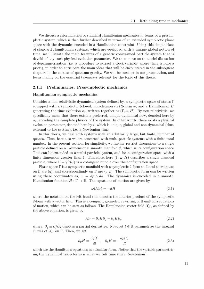
Hamiltonian symplectic mechanics

Consider a non-relativistic dynamical system defined by, a symplectic space of states Γequipped with a symplectic (closed, non-degenerate) 2-form ω, and a Hamiltonian Hgenerating the time evolution αt, written together as (Γ, ω,H). By non-relativistic, wespecifically mean that there exists a preferred, unique dynamical flow, denoted here byαt, encoding the complete physics of the system. In other words, there exists a physicalevolution parameter, denoted here by t, which is unique, global and non-dynamical (thus,external to the system), i.e. a Newtonian time.

In this thesis, we deal with systems with an arbitrarily large, but finite, number ofquanta. Thus, here also we are concerned with multi-particle systems with a finite totalnumber. In the present section, for simplicity, we further restrict discussions to a singleparticle defined on a 1-dimensional smooth manifold C, which is its configuration space.This can be extended to a multi-particle system, and for a configuration space with afinite dimension greater than 1. Therefore, here (Γ, ω,H) describes a single classicalparticle, where Γ = T ∗(C) is a cotangent bundle over the configuration space.

Phase space Γ is a symplectic manifold with a symplectic 2-form ω. Local coordinateson C are (q), and correspondingly on Γ are (q, p). The symplectic form can be writtenusing these coordinates as, ω = dp ∧ dq. The dynamics is encoded in a smooth,Hamiltonian function H : Γ→ R. The equations of motion are given by,

ω(XH) = −dH (2.1)

where the notation on the left hand side denotes the interior product of the symplectic2-form with a vector field. This is a compact, geometric rewriting of Hamilton’s equationsof motion, which can be seen as follows. The Hamiltonian vector field XH , as defined bythe above equation, is given by

XH = ∂pH∂q − ∂qH∂p (2.2)

where, ∂q ≡ ∂/∂q denotes a partial derivative. Now, let t ∈ R parametrize the integralcurves of XH on Γ. Then, we get

∂pH =dq(t)

dt, ∂qH = −dp(t)

dt(2.3)

which are the Hamilton’s equations in a familiar form. Notice that the variable parametriz-ing the dynamical trajectories is what we call time (here, Newtonian).

11

2. Generalised Statistical Equilibrium

Parametrized presymplectic mechanics

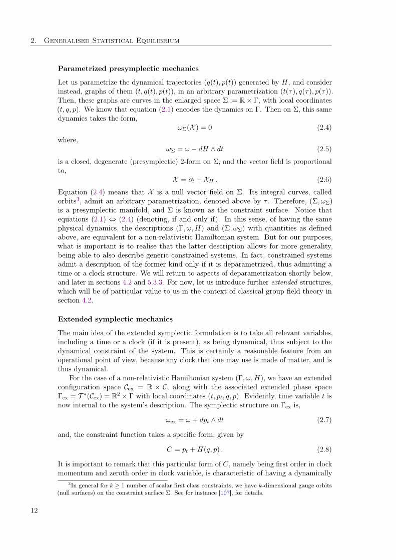
Let us parametrize the dynamical trajectories (q(t), p(t)) generated by H, and considerinstead, graphs of them (t, q(t), p(t)), in an arbitrary parametrization (t(τ), q(τ), p(τ)).Then, these graphs are curves in the enlarged space Σ := R× Γ, with local coordinates(t, q, p). We know that equation (2.1) encodes the dynamics on Γ. Then on Σ, this samedynamics takes the form,

ωΣ(X ) = 0 (2.4)

where,ωΣ = ω − dH ∧ dt (2.5)

is a closed, degenerate (presymplectic) 2-form on Σ, and the vector field is proportionalto,

X = ∂t + XH . (2.6)

Equation (2.4) means that X is a null vector field on Σ. Its integral curves, calledorbits3, admit an arbitrary parametrization, denoted above by τ . Therefore, (Σ, ωΣ)is a presymplectic manifold, and Σ is known as the constraint surface. Notice thatequations (2.1) ⇔ (2.4) (denoting, if and only if). In this sense, of having the samephysical dynamics, the descriptions (Γ, ω,H) and (Σ, ωΣ) with quantities as definedabove, are equivalent for a non-relativistic Hamiltonian system. But for our purposes,what is important is to realise that the latter description allows for more generality,being able to also describe generic constrained systems. In fact, constrained systemsadmit a description of the former kind only if it is deparametrized, thus admitting atime or a clock structure. We will return to aspects of deparametrization shortly below,and later in sections 4.2 and 5.3.3. For now, let us introduce further extended structures,which will be of particular value to us in the context of classical group field theory insection 4.2.

Extended symplectic mechanics

The main idea of the extended symplectic formulation is to take all relevant variables,including a time or a clock (if it is present), as being dynamical, thus subject to thedynamical constraint of the system. This is certainly a reasonable feature from anoperational point of view, because any clock that one may use is made of matter, and isthus dynamical.

For the case of a non-relativistic Hamiltonian system (Γ, ω,H), we have an extendedconfiguration space Cex = R × C, along with the associated extended phase spaceΓex = T ∗(Cex) = R2 × Γ with local coordinates (t, pt, q, p). Evidently, time variable t isnow internal to the system’s description. The symplectic structure on Γex is,

ωex = ω + dpt ∧ dt (2.7)

and, the constraint function takes a specific form, given by

C = pt +H(q, p) . (2.8)

It is important to remark that this particular form of C, namely being first order in clockmomentum and zeroth order in clock variable, is characteristic of having a dynamically

3In general for k ≥ 1 number of scalar first class constraints, we have k-dimensional gauge orbits(null surfaces) on the constraint surface Σ. See for instance [107], for details.

12

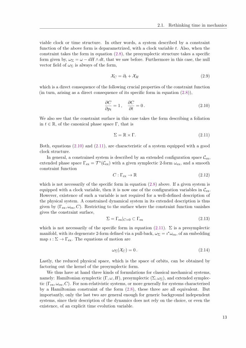
2.1. Rethinking time in mechanics

viable clock or time structure. In other words, a system described by a constraintfunction of the above form is deparametrized, with a clock variable t. Also, when theconstraint takes the form in equation (2.8), the presymplectic structure takes a specificform given by, ωΣ = ω − dH ∧ dt, that we saw before. Furthermore in this case, the nullvector field of ωΣ is always of the form,

XC = ∂t + XH (2.9)

which is a direct consequence of the following crucial properties of the constraint function(in turn, arising as a direct consequence of its specific form in equation (2.8)),

∂C

∂pt= 1 ,

∂C

∂t= 0 . (2.10)

We also see that the constraint surface in this case takes the form describing a foliationin t ∈ R, of the canonical phase space Γ, that is

Σ = R× Γ. (2.11)

Both, equations (2.10) and (2.11), are characteristic of a system equipped with a goodclock structure.

In general, a constrained system is described by an extended configuration space Cex,extended phase space Γex = T ∗(Cex) with a given symplectic 2-form ωex, and a smoothconstraint function

C : Γex → R (2.12)

which is not necessarily of the specific form in equation (2.8) above. If a given system isequipped with a clock variable, then it is now one of the configuration variables in Cex.However, existence of such a variable is not required for a well-defined description ofthe physical system. A constrained dynamical system in its extended description is thusgiven by (Γex, ωex, C). Restricting to the surface where the constraint function vanishesgives the constraint surface,

Σ = Γex|C=0 ⊂ Γex (2.13)

which is not necessarily of the specific form in equation (2.11). Σ is a presymplecticmanifold, with its degenerate 2-form defined via a pull-back, ωΣ = ı∗ωex, of an embeddingmap ı : Σ→ Γex. The equations of motion are

ωΣ(XC) = 0 . (2.14)

Lastly, the reduced physical space, which is the space of orbits, can be obtained byfactoring out the kernel of the presymplectic form.

We thus have at hand three kinds of formulations for classical mechanical systems,namely: Hamiltonian symplectic (Γ, ω,H), presymplectic (Σ, ωΣ), and extended symplec-tic (Γex, ωex, C). For non-relativistic systems, or more generally for systems characterisedby a Hamiltonian constraint of the form (2.8), these three are all equivalent. Butimportantly, only the last two are general enough for generic background independentsystems, since their description of the dynamics does not rely on the choice, or even theexistence, of an explicit time evolution variable.

13

2. Generalised Statistical Equilibrium

2.1.2 Deparametrization

Given a constrained system (Γex, ωex, C), we have stressed above that its description maynot necessarily include a good clock structure. And that even without such a structure,the extended (or presymplectic) formulation describes fully the dynamical system. Insuch a priori ‘timeless’ systems then, we may still want to extract a clock variable. Thisis called deparametrization. In the present context for instance, deparametrization isvaluable to define physical equilibrium states with respect to clock Hamiltonians (seesections 2.2.1, 2.2.2 and 5.1.2.2 for more discussions and examples).

From the above discussions of constrained mechanical systems, especially in compari-son with extended non-relativistic systems, we can identify the core, universal strategybehind deparametrization: to reformulate, either exactly or under certain approximations,the dynamical constraint of the system, to bring it to the form of equation (2.8), i.e.

C 7−→ Cdep = pλ +H(qcan, pcan) (2.15)

where λ is the clock variable, H is the clock Hamiltonian generating evolution in clocktime λ, and (qcan, pcan) denote the phase space variables of the canonical system to whichthe clock variable is external.

A simple illustrative example is a classical relativistic particle on spacetime, with itscovariant dynamics given by,

C = p2 −m2 , (2.16)

which is defined on an extended phase space Γex coordinatised by (xµ, pµ), with µ =0, 1, 2, 3 and signature (+,−,−,−). In this case, the complete dynamical, presymplecticdescription does not require deparametrization, i.e. given the extended phase spacealong with C, its constraint surface is well-defined. But the point is that this systemis deparametrizable, which means that it is possible to bring C to a manifestly non-covariant form, here without changing the physics that is captured completely by theconstraint surface (Σ, ωΣ). The full constraint can be rewritten as

Cdep = p0 +√p2 +m2 (2.17)

which now describes the same relativistic particle system but in a fixed Lorentz framewhere the configuration variable x0 has been chosen as the clock variable and thecorresponding clock dynamics is dictated by the Hamiltonian H =

√p2 +m2.

A different example of a system which by itself is non-deparametrizable, i.e. itdoesn’t naturally admit a good clock without further approximations, is the so-calledtimeless double pendulum [57,104,108]. It is defined by an extended configuration spaceCex = R2 3 (q1, q2), phase space Γex = T ∗(Cex) with ωex =

∑a=1,2 dpa ∧ dqa, and a

dynamical constraint4

C =1

2(q2

1 + q22 + p2

1 + p22)− k (2.18)

for a real constant k. The constraint surface in this case is, Σ = Γex|C=0∼= S3, a 3-sphere

with radius√

2k. Clearly, Σ is compact and does not admit a form (2.11) with a foliationthat is characteristic of having a time structure. Therefore, the system so describeddoes not naturally have any internal variable which can play the role of time, before any

4Notice that this system is fundamentally different from an analogous, non-relativistic one withNewtonian time t, which would instead be given by a constraint of the form, C = pt+

12(q2

1+q22+p2

1+p22)−k.

14

2.2. Generalised Gibbs equilibrium

approximations. For instance, if one were to approximate the dynamics by the followingconstraint function,

Cdep = p2 +1

2(q2

1 + p21)− k ≡ p2 +H(q1, p1) (2.19)

then, in this dynamical regime (if it exists) described by Cdep, variable q2 acts as a goodclock parameter with the physical evolution being generated by H.

Finally, we note that in the case of a system composed of many particles, there maynot exist a single global clock, even if each particle is deparametrized separately andthus equipped with its own individual clock. In this case then, one would expect tohave to sync the different clocks in order to define a single common clock. This issuecan be investigated in a general multi-particle setting, continuing from the discussionsabove [98,101]. However, we will discuss it in detail directly in the context of classicalGFTs [24] in section 4.2.1.

2.2 Generalised Gibbs equilibrium

Equilibrium states are a cornerstone of statistical mechanics and thermodynamics. Theyare vital in the description of macroscopic systems with a large number of microscopicconstituents. In particular, Gibbs states have a vast applicability across a broad rangeof fields such as condensed matter physics, quantum information, tensor networks,and (quantum) gravity, to name a few. They are special, being the unique class ofstates in finite systems satisfying the KMS condition5. Furthermore, usual coarse-graining techniques also rely on the definition of Gibbs measures. In treatments closer tohydrodynamics, one often considers the full (non-equilibrium) system as being composedof many interacting subsystems, each considered to be at local equilibrium. While inthe context of renormalisation group flow treatments, each phase at a given scale, for agiven set of coupling parameters is also naturally understood to be at equilibrium, eachdescribed by (an inequivalent) Gibbs measure. Given this physical interest in Gibbsstates, the question then is how to define them for background independent systems.

2.2.1 Characterising Gibbs states

Let us begin with a discussion on how to characterise completely statistical states of theGibbs form, based on insights from both standard and covariant statistical mechanics [24].This discussion is not restricted to any particular quantum gravity formalism, or even toclassical or quantum sectors for systems on spacetime. Rather, it attempts to presentthe strategies employed in past studies for defining Gibbs states, along with a varietyof examples, in a coherent way. The main goal here is to reconsider the standardcharacterisations that are well-known to us, and attempt to understand them from a

5The algebraic KMS condition [31, 33] is known to provide a comprehensive characterisation ofstatistical equilibrium in systems of arbitrary sizes, as long as there exists a well-defined 1-parameterdynamical group of automorphisms of the system. This latter point, of the required existence ofa preferred time evolution of the system, is exactly the missing ingredient in generic backgroundindependent cases. Moreover, we observe that the automorphism group in the definition of KMScondition does not, technically, need to be identified with time evolution. Thus KMS equilibrium canbe defined for more general symmetries, even though the standard definition would be physically morenatural in systems with a unique definition of time. We refer to sections 2.2.1 and 2.2.5 for more details.

15

2. Generalised Statistical Equilibrium

broader perspective, in order to then generalise them to background independent systems,including discrete quantum gravity.

Gibbs states, ρβ = 1Zβe−βO (where O is not necessarily a Hamiltonian), can be

categorised according to two main criteria, respectively primary and secondary:A. whether or not the state is a result of considering an associated pre-defined flow

or transformation of the system;B. the nature of the functions or operators O in the exponent characterising the

state, specifically whether these quantities encode the physical dynamics of the system,or refer to some structural properties.

Categories A and B are mutually independent, in the sense that a single systemcould simultaneously be both of types A and B. Details of these two categories, theirrespective subclasses and related examples follow.

Let us first look at the primary category A, which can be considered at a higherfooting than the secondary B because the contents of classification under A are theactual construction procedures or ‘recipes’ used to arrive at a resultant Gibbs state.Moreover, it is within A where we observe that the known Jaynes’ entropy maximisationprinciple [22, 23] could prove to be especially useful in background independent contextssuch as in discrete quantum gravity frameworks. Under A, we can identify two recipesto construct, or equivalently, ways to completely characterise, a Gibbs state dependingon the information that we have at hand for a given system.

A1. Dynamical characterisation: Use of Kubo-Martin-Schwinger condition

The KMS condition [31,33–36] is formulated in terms of a 1-parameter group of auto-morphisms of the system.

Let ω be an algebraic state6 over a C*-algebra7 A, and αt be a 1-parameter group of*-automorphisms8 of A. Consider the strip I = z ∈ C | 0 < Im(z) < β, β ∈ R≥0, andlet I denote its closure, such that I = R if β = 0. Then, ω is an α-KMS state at value β,if for any pair A,B ∈ A, there exists a complex function FAB(z) which is analytic on I,and continuous and bounded on I, such that it satisfies the KMS boundary conditions:

FAB(t) = ω[Aαt(B)] , FAB(t+ iβ) = ω[αt(B)A] (2.20)

for all t ∈ R [33]. We note that an α-KMS state satisfies stationarity, i.e. ω[αtA] = ω[A](for all t), which captures the simplest notion of equilibrium (see appendix 5.B for somemore details). If in the given description of a system, one can identify a relevant set oftransformations (not necessarily Hamiltonian) with respect to which one is interested indefining an equilibrium state, then one asks for the state to satisfy the KMS conditionwith respect to a continuous, unitarily implementable 1-parameter (sub-) group of the

6Algebraic states ω : A → C, are complex-valued, linear, positive, normalised functionals over analgebra. Linearity is: ω[z1A+ z2B] = z1ω[A] + z2ω[B] ∀z1, z2 ∈ C. Positivity is: ω[A†A] ≥ 0 ∀A ∈ A.Normalisation is: ω[I] = 1, where I is the identity element of A. [32]

7A C*-algebra is a norm complete *-algebra, equipped with the C*-norm property: ||A∗A|| = ||A||2.A normed *-algebra is a *-algebra equipped with a *-norm. A *-algebra is an algebra (i.e. vector spaceover C, with an associative and distributive multiplication law) equipped with a *-operation (also called,involution or adjoint) such that: A∗∗ = A, (AB)∗ = B∗A∗, and (z1A+ z2B)∗ = z1A

∗+ z2B∗. A *-norm

is a norm ||.|| with one additional property: ||A∗|| = ||A||. We note that in this thesis, we denote the*-operation by a dagger †. [32]

8A *-automorphism is a bijective *-homomorphism of the algebra into itself. We refer to appendix4.A for details. [32]

16

2.2. Generalised Gibbs equilibrium

said transformations. This gives (uniquely, for a certain class of systems as detailed inappendix 5.B, e.g. finite systems on spacetime), a Gibbs state of the form ρ ∝ e−βG ,where G is the self-adjoint generator of the flow, and β ∈ R. Notice that the ‘inversetemperature’ β enters formally as the periodicity in the flow parameter t, regardless ofits interpretation.

Thus, this characterisation is strictly based on the existence of a suitable pre-definedflow of the configurations of the system and then imposing the KMS condition withrespect to it. These transformations could correspond to physical or structural propertiesof the system (see category B below). Simple examples are, respectively, the physicaltime flow eiHt in a non-relativistic system where H is the Hamiltonian, which gives riseto the standard Gibbs equilibrium state of the form e−βH ; and a U(1) gauge flow eiNθ

where N is a number operator, which would lead to an equilibrium state of the forme−βN .

A2. Thermodynamical characterisation: Use of maximum entropy principleunder a given set of constraints

Consider a situation wherein the given description of a system does not include relevantsymmetry transformations, or (even if such symmetries exist, which they usually do) thatwe are interested in those properties of the system which are not naturally associated tosensible flows, in the precise sense of being generators of these flows. Examples of thelatter are observables such as area, volume or mass. Geometric operators like volumeare of special interest in the context of quantum gravity since they may be instrumentalfor statistically extracting macroscopic geometric features of spacetime regions fromquantum gravity microstates. In such cases then, what characterises a Gibbs state andwhat is the notion of equilibrium encoded in it?

In order to construct a Gibbs state here, where operationally we may only haveaccess to a set of constraints fixing the mean values of a set of functions or operators〈Oa〉ρ = Oaa=1,2,...,` (in classical or quantum descriptions respectively), one mustrely on Jaynes’ principle [22, 23] of maximising the entropy S[ρ] = −〈ln ρ〉ρ whilesimultaneously satisfying the above constraints. The angular brackets denote statisticalaverages in a state ρ defined on the state space of the system, be it a phase space in theclassical description or a Hilbert space in the quantum one. Undertaking this procedure,one arrives at a Gibbs state ρ = e−

∑a βaOa (where one of the O’s is the identity fixing

the normalisation of the state as will be detailed below in section 2.2.3). We can seethat here the inverse temperatures βa enter formally as Lagrange multipliers. Also,the averages Oa with parameters βa, and other quantities derived from them, can beunderstood as thermodynamic variables defining a macrostate of the system, and cantake on the same formal roles as in usual statistical mechanics and thermodynamics.But their exact interpretation would depend on the context. The identification andinterpretation of such relevant quantities is in fact the non-trivial aspect of the problem,particularly in quantum gravity.

Notice that this characterisation is strictly independent of the existence of any pre-defined transformations or symmetries of the underlying microscopic system, as longas there is at least one function or operator (identified as relevant) whose statisticalaverage is assumed (or known) to be fixed at a certain value. Consequently, thischaracterisation could be most useful in background independent settings, exactly sinceit is based purely on Jaynes’ information-theoretic method. Finally, we note that in this

17

2. Generalised Statistical Equilibrium

characterisation a notion of equilibrium is implicit in the requirement that a certainset of observable averages remain constant, i.e. it is implicit in the existence of theconstraints 〈Oa〉ρ = Oa (see for example the discussion in section II in [109]). We willundertake a detailed discussion of the thermodynamical characterisation, and formulateaspects of a generalised equilibrium statistical mechanical framework based on it, alongwith basic features of its generalised thermodynamics, in the remaining sections of thischapter.

For now, let us summarise the above classifications and make some additional remarks.If the aim is to construct Gibbs states for a system of many quanta (whatever they maybe), then the two characterisations, dynamical and thermodynamical, under category Aoffer us two formally independent strategies to do so. Based on our knowledge of a givensystem, we may prefer to use one over the other. If there is a known set of symmetrieswith respect to which one is looking to define equilibrium, then the technical route onetakes is to construct a state satisfying the KMS condition with respect to (a 1-parametersubgroup of) the symmetry group. The result of using this recipe in a finite system(cf. remarks in appendix 5.B) is a Gibbs state e−βG , characterised by the generator Gof the 1-parameter flow of these transformations and the periodicity parameter β. Onthe other hand, if one does not have interest in or access to any particular symmetrytransformations of the system, but has a partial knowledge about the system in terms ofa set of observable averages Oa, then one employs the principle of maximising Shannonor von Neumann entropy under the given set of constraints. The resultant statisticalstate is again of a Gibbs exponential form e−

∑a βaOa , now characterised by the set of

observables Oa and Lagrange multipliers βa.Notice that given a Gibbs state, constructed say from recipe A1, then once it is

already defined, it also satisfies the thermodynamic condition of maximum entropy [31,33].Similarly, a Gibbs state defined on the basis of A2, after it is constructed also satisfiesthe KMS condition with respect to a flow that is derived from the state itself (due toTomita-Takesaki theorem [31,33]). For instance, consider the standard non-relativisticGibbs state e−βH , which is constructed by satisfying the KMS condition with respect tounitary time translations eiHt. That is, this state is classified as A1 since its constructionrelies on the KMS condition. But, once this state is defined, it is also the one thatmaximises the entropy under the constraint 〈H〉 = E. Now consider an example of astate e−βV , where V is say spatial volume. This state is derived as a result of maximisingthe information entropy under the constraint 〈V 〉 = v, hence it is classified as A2. Oncethis state is defined, one can extract a flow from the state, with respect to which it willsatisfy the KMS condition.9 This is the modular flow eiβV τ , where τ is the modular flowparameter.10 Therefore, classifications A1 and A2 refer to the construction proceduresemployed as per the situation at hand. Once a Gibbs state is constructed using anyone of the two procedures, then technically it will satisfy both the KMS condition withrespect to a flow,11 and maximisation of entropy.

9In the context of covariant statistical mechanics, the utility of this observation has been presentedin [68–70], and is the crux of the thermal time hypothesis.

10In a classical phase space description of a system, the modular flow is the integral curve of thevector field XV defined by ω(XV ) = −dV , where ω is the symplectic form and V is a smooth function.In this case naturally the flow eτXV is in terms of the vector field XV = ∂τ . In the quantum C*-algebraic description (or in a specific Hilbert space representation of it), the modular flow is that of theTomita-Takesaki theory.

11Whether the flow parameter has a reasonable physical interpretation is a separate issue, and would

18

2.2. Generalised Gibbs equilibrium

Now, given that a Gibbs state can be constructed as a result of either the dynamicalor the thermodynamical recipe, one can consider the nature of the functions or operatorsO that characterise it. This is the content of classification under category B.

B1. Physical state

If O is associated with the physical dynamics of the system, i.e. it dictates, partiallyor completely, the dynamical model of the system, then the associated Gibbs state canbe understood as encoding, partially or completely, a physical notion of equilibrium.In a standard non-covariant system, O would simply be the Hamiltonian. While in acovariant system, if it is deparametrizable with a suitable choice of a good clock, then Owould be the associated clock Hamiltonian. Overall, this particular classification refersexplicitly, and in the definition of the Gibbs state, to the physical dynamical evolution ofthe system. This is encoded in a relevant model-dependent function or operator, whetherit is a conventional Hamiltonian or a deparametrizable constraint.

B2. Structural state

If O are quantities referring to kinematic or structural properties of the system, and notdirectly to the specific physical dynamical model of it, then the associated Gibbs statesare understood to be structural. Examples of structural transformations are genericrotations or translations of the base manifold of the theory. Examples of quantities thatare not necessarily associated to symmetry transformations would be observables likearea or volume.

Examples

Four different types of Gibbs states can be constructed from combinations of classificationsunder categories A and B. Let us mention a variety of examples, including the onesconstructed as part of this thesis.

A1-B1: Gibbs states with respect to physical time translations, as considered instandard statistical mechanics [31,33,110]; with respect to a clock time in deparametrizedsystems, with examples constructed in covariant statistical mechanics on spacetime[70, 101, 102] (section 2.2.2), and in group field theory quantum gravity [24] (section5.1.2.2).

A2-B1: Gibbs states with respect to 4-momenta of relativistic particles in covariantstatistical mechanics [100]; with respect to momentum map associated with diffeo-morphism group for parametrized field theory [111,112]; with respect to a dynamicalprojector [66, 67, 96], and kinetic and vertex operators [25] in group field theory (section3.4).

A1-B2: Gibbs states with respect to U(1) symmetry generated by the number ob-servable in standard statistical mechanics [31,33,110]; with respect to internal translationautomorphisms in algebraic group field theory [24] (section 5.1.2.1).

A2-B2: Souriau’s Gibbs states with respect to kinematical symmetries [105,113];Gibbs states with respect to gauge-invariant observables in covariant statistical mechanicson spacetime [100]; with respect to spatial volume for pressure ensemble in standardstatistical mechanics [22]; with respect to geometric area and volume operators in loop

depend on the specific context.

19

2. Generalised Statistical Equilibrium

quantum gravity [100,114]; with respect to positive, extensive operators in group fieldtheory, e.g. spatial volume operator [24] (section 5.1.1); with respect to classical closureand half-link gluing constraints in group field theory [67,96] (section 5.1.3).

In light of the fact that these classifications comprehensively span all possible kindsof Gibbs states, we call them generalised Gibbs states.

2.2.2 Past proposals

We now give an overview [25] of the different proposals for defining statistical equilibriumbased on studies in covariant statistical mechanics, in order to better contextualise ourproposal of the thermodynamical characterisation which is the focus of the subsequentsections. These proposals rely on various different principles originating in standardnon-relativistic statistical mechanics, extended to a constrained setting.

The first proposal [68, 98] was based on the idea of statistical independence ofarbitrary (small, but macroscopic) subsystems of the full system, in a classical setting.The notion of equilibrium is taken to be characterised by the factorisation property ofthe state,

ρ = ρ1ρ2 (2.21)

for any two subsystems 1 and 2; and where ρ1 and ρ2 are taken to be defined on mutuallyexclusive subregions of the full phase space, so that we additionally have

ρ1, ρ2 = 0 , (2.22)

or equivalently,[Xρ1 ,Xρ2 ] = 0 , (2.23)

where, ω(Xρ1,2) = d ln ρ1,2 , ω is the symplectic form on the phase space of the full system,and ., . is the Poisson bracket. Then, the whole system is said to be at equilibrium ifany one of its subsystems is statistically independent from all the rest. We note that thischaracterisation for equilibrium is related to an assumption of weak interactions [110].

This same dilute gas assumption is integral also to the Boltzmann method of statisticalmechanics. It characterises equilibrium as the most probable distribution, that is one withmaximum entropy. This method is used in [100] to study a gas of constrained particles12.Even though this method relies on maximising the entropy like the thermodynamicalcharacterisation, it is more restrictive than the latter, as will be made clear in section2.2.5.

The work in [70] puts forward a characterisation for a physical equilibrium state.The suggestion is that, ρ (itself a well-defined state on the physical, reduced state space)is said to be a physical Gibbs state if (i) its modular Hamiltonian

h = − ln ρ , (2.24)

is a smooth function on the physical state space, and (ii) h is such that there exists a(local) clock function T (x) on the extended state space, with its conjugate momentumpT (x), such that h is proportional to pT . Importantly, when this is the case the modularflow (‘thermal time’ [68, 69]) is a geometric flow foliating spacetime, in which sense

12We remark that except for this one work, all other studies in spacetime covariant statisticalmechanics are carried out from the Gibbs ensemble point of view.

20

2.2. Generalised Gibbs equilibrium

ρ is said to be ‘physical’. Notice that the built-in strategy here is to define KMSequilibrium in a deparametrized system, since by construction it identifies a state’smodular Hamiltonian with a (local) clock Hamiltonian on the base spacetime manifold.Thus it is an example of using the dynamical characterisation, associated with a clockHamiltonian in a deparametrized system with constraint of the form (2.8).

Another strategy [102] is based on the use of the ergodic principle and introductionof clock subsystems to define clock time averages. This characterisation relies on thevalidity of a postulate, even if traditionally a fundamental one, like two of the previousones that were based on the physical assumption of weak interactions.

Finally, the proposal in [103] interestingly characterises equilibrium by a vanishinginformation flow between interacting histories. The notion of information used is that ofShannon (entropy),

I = lnN, (2.25)

where N is the number of microstates traversed in a given history during interaction.Equilibrium between two histories 1 and 2 is encoded in a vanishing information flow,

δI = I2 − I1 = 0 . (2.26)

This characterisation of equilibrium is evidently information-theoretic, even if relying onan assumption of weak interactions. Moreover it is much closer to our thermodynamicalcharacterisation, because the condition of vanishing δI is nothing but an optimisation ofinformation entropy.

These different proposals, along with the thermal time hypothesis [68,69], have led tosome remarkable results, like recovering the Tolman-Ehrenfest effect [99,101], relativisticJüttner distribution [101] and Unruh effect [115]. However, they all assume the validityof one or more principles, postulates or assumptions about the system. Moreover, none(at least presently) seems to be general enough like the proposal below, so as to beimplemented in a full quantum gravity setup, while also accommodating within it therest of the proposals.

2.2.3 Thermodynamical characterisation

This brings us to the proposal of characterising a generalised Gibbs state based on aconstrained maximisation of information (Shannon or von Neumann) entropy [24, 25, 67,96], along the lines advocated by Jaynes [22,23] purely from the perspective of evidentialstatistical inference. Jaynes’ approach is fundamentally different from other moretraditional ones of statistical physics. So too is the thermodynamical characterisation,compared with the others outlined above, as will be exemplified in the following. It isthus a new proposal for background independent equilibrium [24, 116], which has thepotential of incorporating also the others as special cases, from the point of view ofconstructing a Gibbs state [25].

Consider a macroscopic system with a large number of constituent microscopicdegrees of freedom. Our (partial) knowledge of its macrostate is given in terms of afinite set of averages 〈Oa〉 = Ua of the observables that we have access to. Jaynessuggests that a fitting probability estimate (which, once known, will allow us to infer alsothe other observable properties of the system) is not only one that is compatible withthe given observations, but also that which is least-biased in the sense of not assumingany more information about the system than what we actually have at hand, namely

21

2. Generalised Statistical Equilibrium

Ua. In other words, given a limited knowledge of the system (which is always thecase in practice for any macroscopic system), the least-biased probability distributioncompatible with the given data should be preferred. As shown below, this turns out tobe a Gibbs distribution with the general form (2.31), which we refer to as generalisedGibbs states.

Let Γ be a symplectic phase space (be it extended or reduced), which is a cotangentbundle over a finite-dimensional, smooth configuration manifold. Consider a finite set ofsmooth real-valued functions Oa defined on Γ, with a = 1, 2, ..., `. Denote by ρ a smoothstatistical density (real-valued, positive and normalised function) on Γ, to be determined.Then, the prior on the known macrostate gives a finite number of constraints,

〈Oa〉ρ =

∫Γdλ ρOa = Ua , (2.27)

along with the normalisation constraint for the state,

〈1〉ρ = 1 , (2.28)

where dλ is a Liouville measure on Γ, and the integrals are taken to be well-defined.Further, ρ has an associated Shannon entropy

S[ρ] = −〈ln ρ〉ρ . (2.29)

By understanding S to be a measure of uncertainty quantifying our ignorance about thedetails of the system, the corresponding bias is minimised (compatibly with the priordata) by maximising S (under the set of constraints (2.27) and (2.28)) [22]. Using theLagrange multipliers technique, this amounts to finding a stationary solution for thefollowing auxiliary functional

L[ρ, βa, κ] = S[ρ]−∑a=1

βa(〈Oa〉ρ − Ua)− κ(〈1〉ρ − 1) (2.30)

where βa, κ ∈ R are Lagrange multipliers. Then, requiring stationarity13 of L withrespect to variations in ρ gives a generalised Gibbs state

ρβa =1

Zβae−

∑a=1

βaOa(2.31)

with partition function,

Zβa ≡∫

Γdλ e−

∑a βaOa = e1+κ , (2.32)

where as is usual, normalisation multiplier κ is a function of the remaining multipliers.The partition function Zβa encodes all properties of the system in principle.

Analogous arguments hold for quantum mechanical systems and the above schemecan be implemented directly [23], as long as the operators under consideration are such

13Notice that requiring stationarity of L with variations in the Lagrange multipliers implies fulfilmentof the constraints (2.27) and (2.28). These two ‘equations of motion’ of L along with the one determiningρ (coming from stationarity of L with respect to ρ) provide a complete description of the system athand.

22

2.2. Generalised Gibbs equilibrium

that the relevant traces are finite on a representation Hilbert space. Statistical statesare density operators (self-adjoint, positive, and trace-class operators, with Tr(ρ) = 1)on the Hilbert space. Statistical averages for (self-adjoint) observables Oa are now,

〈Oa〉ρ = Tr(ρ Oa) = Ua . (2.33)

Following the constrained optimisation method again gives a Gibbs density operator,

ρβa =1

Zβae−

∑a=1

βaOa. (2.34)

A generalised Gibbs state can thus be defined, characterised fully by a finite set ofobservables of interest Oa, and their conjugate generalised ‘inverse temperatures’ βa.Given this class of equilibrium states, it should be evident that some thermodynamicquantities (like generalised ‘energies’ Ua) can be identified immediately. Aspects of ageneralised thermodynamics will be discussed in section 2.3.

We note that there are two key features of this characterisation. First is the use ofevidential (epistemic) probabilities, thus taking into account the given evidence Ua.This interpretation, that statistical states are states of knowledge [117–119], is innate toJaynes’ method [22,23]. Second is a preference for the least-biased (or most “honest”)distribution out of all the different ones compatible with the given evidence. It is notenough to arbitrarily choose any that is compatible with the prior data. An awareobserver must also take into account their own ignorance, or lack of knowledge honestly,by maximising the information entropy.

2.2.4 Modular flows and stationarity

Given a generalised Gibbs state, a natural question that arises is, with respect to whichflow or transformations of the system is this state stationary. We know that any densitydistribution or operator is stationary with respect to its own modular flow. In fact bythe Tomita-Takesaki theorem [31,33], any faithful algebraic state over a von Neumannalgebra is KMS with respect to its own 1-parameter modular (Tomita) flow.

In the classical case then, a generalised Gibbs state ρβa of the form (2.31), isstationary with respect to the local flow etXρ (parametrized by t ∈ R) on a givensymplectic phase space Γ, generated by vector field Xρ that is defined by the equation

ω(Xρ) = −dh , (2.35)

where h is the modular Hamiltonian of the state,

h =∑a

βaOa . (2.36)

Then, stationarity with respect to the modular flow is evident from,

Xρ(ρβa) = ρβa, h = 0 (2.37)

where, ., . is a Poisson bracket on the algebra of smooth functions over Γ. Now, theindividual flows generated by Xa are associated with the different observables via thedefining equation

ω(Xa) = −dOa . (2.38)

23

2. Generalised Statistical Equilibrium

Then, we have that the modular vector field is in general a linear superposition of theseparate ones, weighted by their respective inverse temperatures,

Xρ =∑a

βaXa (2.39)

using equations (2.35), (2.38), and, linearities of the symplectic form ω and the exteriorderivative. In particular, ρβa is not stationary in general with respect to the individualflows Xa′ generated by Oa′ , that is

Xa′(ρβa) = ρβa,Oa′ 6= 0 . (2.40)

However, ρβa becomes stationary with respect to each of these individual flows Xa′(in addition to always being stationary with respect to the full modular flow), if thegenerators of the individual flows commute with each other, that is

Oa′′ ,Oa′ = 0 (for all a′, a′′) ⇒ Xa′(ρβa) = 0 (for any a′) . (2.41)

See appendix 2.A for details.In the quantum case, a generalised Gibbs density operator ρβa of the form (2.34),

satisfies the KMS condition with respect to its modular flow14 eiht (parametrized byt ∈ R) on a given Hilbert space, generated by the modular Hamiltonian operator,

h =∑a

βaOa . (2.42)

Then, the state is stationary with respect to the modular flow,

[ρβa, h] = 0 (2.43)

while, it is not at equilibrium with respect to the separate flows in general,

[ρβa, Oa′ ] 6= 0 (2.44)

where, [., .] denotes a commutator bracket. But as before, we have that

[Oa′′ , Oa′ ] = 0 (for all a′, a′′) ⇒ [ρβa, Oa′ ] = 0 (for any a′) . (2.45)

See appendix 2.A for details.Therefore, we see that generalised Gibbs states, both classical and quantum, are

stationary with respect to the modular flow extracted from the state itself, as expectedfrom statistical mechanics. But we also see that none of the individual observables arein any way preferred or special, thus giving a generalised notion of equilibrium, with allthe characterising observables being on an equal footing.

In the special case when the different observable generators Oa are independent ofeach other, then the state is additionally stationary with respect to each of the differentflows generated by them. Also in this case, the individual flows commute with each other.Thus, the system retains its equilibrium properties even when it evolves along any ofthese directions Xa, and not only along the specific direction defined by the superposition(2.39).

14Notice that ∆ ≡ eh is the modular operator of Tomita-Takesaki theory [31,33].

24

2.2. Generalised Gibbs equilibrium

Finally, we remark on one aspect that seems to differentiate the quantum from theclassical case discussed above. For an operational implementation of Jaynes’ procedure ina quantum system, the constraints (2.33) can exist only if the operators Oa all commutewith each other, that is if the observables under study are compatible. One could thusargue, that since this requirement is operationally unavoidable for a quantum system,then a quantum generalised Gibbs state will always satisfy (2.45). A more detailedunderstanding, overall, of fundamental differences between the quantum and classicalcases (for instance, [120]) for generalised Gibbs states requires further investigation, andis left to future work.

2.2.5 Remarks

In this section we make additional remarks about the thermodynamical characterisation,highlighting many of its interesting features [25].

We notice that this notion of equilibrium is inherently observer-dependent becauseof its use of the macrostate thermodynamic description of the system, which in itselfis observer-dependent due to having to choose a coarse-graining, that is the set ofmacroscopic observables [121, 122]. Further, the role of information entropy is shownto be instrumental in defining (local15) equilibrium states.16 It is also interesting tonotice that Bekenstein’s arguments [2] can be observed to be influenced by Jaynes’information-theoretic insights surrounding entropy, and these same insights have nowguided us in the issue of background independent statistical equilibrium.

To be clear, the use of the most probable distributions as characterising statisticalequilibrium is not new in itself. It was used by Boltzmann in the late 19th century, andutilised (also within a Boltzmann interpretation of statistical mechanics) in a constrainedsystem in [100]. Nor is the fact that equilibrium configurations maximise the system’sentropy, which was well known already since the time of Gibbs17. The novelty here is: inthe revival of Jaynes’ information-theoretic perspective, of deriving equilibrium statisticalmechanics in terms of evidential probabilities, solely as a problem of statistical inferencewithout depending on the validity of any further conjectures, physical assumptions orinterpretations [22, 23, 117]; and, in the suggestion that it is general enough to apply togenuinely background independent systems, including quantum gravity. Below we listsome of these more valuable features.

• The procedure is versatile, being applicable to a wide array of cases (both classicaland quantum), technically relying only on a sufficiently well-defined mathemat-ical description in terms of a state space, along with a set of observables withdynamically constant averages Ua defining a suitable macrostate of the system18.

• Evidently, this manner of defining equilibrium statistical mechanics (and from it,thermodynamics) does not lend any fundamental status to energy, nor does it rely

15Local, in the sense of being observer-dependent.16As noted by Jaynes: “...thus entropy becomes the primitive concept with which we work, more

fundamental even than energy...” [22].17But as Jaynes points out in [22], these properties were relegated to side remarks in the past, not

really considered to be fundamental to the theory, nor to the justifications for the methods of statisticalmechanics.

18In fact, in hindsight, we could already have anticipated a possible equilibrium description in termsof these constants, whose existence is assumed from the start.

25

2. Generalised Statistical Equilibrium

on selecting a single, special (energy) observable out of the full set Oa. It canthus be crucial in settings where concepts of time and energy are dubious at theleast, or not defined at all like in non-perturbative quantum gravity.

• It has a technical advantage of not needing any (1-parameter) symmetry (sub-)groups of the system to be defined a priori, unlike the dynamical characterisationbased on the KMS condition.

• It is independent of additional physical assumptions, hypotheses or principlesthat are common to standard statistical physics, and in the present context, tothe other proposals of generalised equilibrium recalled in section 2.2.2. Someexamples of these extra ingredients that we encountered above in section 2.2.2 areergodicity, weak interactions, statistical independence, and often a combination ofthem. These are not required in the thermodynamical characterisation.

• It is independent of any physical interpretations attached (or not) to the observablesinvolved. This further amplifies its appeal for use in quantum gravity where thegeometrical and physical meanings of the quantities involved may not necessarilybe clear from the start.

• One of the main features is the generality in the choice of observables Oa allowednaturally by this characterisation. This also helps accommodate the other proposalsas special cases of this one. In principle, Oa and Ua need only be mathematicallywell-defined in the given description of the system (regardless of whether it iskinematic i.e. working at the extended state space level, or dynamic, i.e. workingwith the physical state space), such that the resultant Gibbs state is normalisable.More standard choices include a Hamiltonian in a non-relativistic system, aclock Hamiltonian in a deparametrized system [24,70, 101,102], and generators ofkinematic symmetries like rotations, or more generally of 1-parameter subgroupsof Lie group actions [105,113]. Some of the more unconventional choices includeobservables like volume [22,24,100] (section 5.1.1), (component functions of the)momentum map associated with geometric closure of classical polyhedra [67,96](section 5.1.3.1), half-link gluing (or face-sharing) constraints of discrete gravity [67](section 5.1.3.2), a projector in group field theory [66, 67], kinetic and vertexoperators in group field theory [25] (section 3.4) and generic gauge-invariantobservables (not necessarily symmetry generators) [100].

For instance, (2.41) shows that the proposal of [68,98] based on statistical inde-pendence, i.e.

[Xρ1 ,Xρ2 ] = 0 (2.46)

can be understood as a special case of this one, when the state is characterised by apair of observables that are defined from the start on mutually exclusive subspacesof the state space. In this case, their respective flows will automatically commuteand the state will be said to satisfy statistical independence.

In section 5.1 we will present several examples of applying such notions of generalisedequilibrium in background independent discrete quantum gravity, and take first stepstowards thermal investigations of these candidate quantum gravitational degrees offreedom subsequently in sections 5.2 and 5.3.

26

2.3. Generalised thermodynamics

2.3 Generalised thermodynamics

Traditional thermodynamics is the study of energy and entropy exchanges. But what is asuitable generalisation of it for background independent systems? This, like the questionof a generalised equilibrium statistical mechanics which we have considered till now, isstill open. In the following, we offer some insights gained from preceding discussions,including identifying certain thermodynamic potentials, and generalised zeroth and firstlaws [25].

2.3.1 Thermodynamic potentials and multivariable temperature

Thermodynamic potentials are vital, particularly in characterising the different phasesof a system. The most important variable is the partition function Zβa, giving the freeenergy of the system

Φ(βa) := − lnZβa . (2.47)

It encodes complete information about the system from which other thermodynamicquantities can be derived in principle. Notice that the standard definition of a freeenergy F comes with an additional factor of a (single, global) temperature, that is, wenormally have Φ = βF . But for now, Φ is the more suitable quantity to define and notF since we do not (yet) have a single common temperature for the full system. We willreturn to this point below in section 2.3.2. Next is the entropy for generalised Gibbsstates of the form (2.31) or (2.34), which is given by

S(Ua) =∑a

βaUa − Φ . (2.48)

Notice that Jaynes’ method [22, 23], which forms the basis of the thermodynamicalcharacterisation, identifies information entropy (given in equation (2.29)) with the abovethermodynamic entropy, since the former is the starting point of this procedure. Also,notice again the lack of a single β scaling the whole equation at this more general levelof equilibrium. Further, a set of generalised heats can be defined by varying S,

dS =∑a

βa(dUa − 〈dOa〉) =:∑a

βa dQa (2.49)

where, dUa are assumed to be independent variations [22]. From this (at least part ofthe19) work done on the system dWa [25, 67], can be identified

dWa := 〈dOa〉 =1

βa

∫Γdλ

δΦ

δOadOa (2.50)

where δ denotes functional derivatives.From the setup of the thermodynamical characterisation presented in section 2.2.3,

we can immediately identify Ua as generalised ‘energies’. Jaynes’ procedure allows these19By this we mean that the term 〈dOa〉, based on the same observables defining the generalised

energies Ua, can be seen as reflecting some work done on the system. But naturally we do not expect orclaim that this is all the work that is/can be performed on the system by external agencies. In otherwords, there could be other work contributions, in addition to the terms dWa. A better understandingof work terms in this background independent setup, will also contribute to a better understanding ofthe generalised first law presented below.

27

2. Generalised Statistical Equilibrium

quantities to democratically play the role of generalised energies. None had to be selectedas being the energy in order to define equilibrium. This a priori democratic status ofthe several conserved quantities can be broken most easily by preferring one over theothers. In turn if its modular flow can be associated with a physical evolution parameter(relational or not), then this observable can play the role of a dynamical Hamiltonian.

Thermodynamic conjugates to these energies are several generalised inverse tem-peratures βa. By construction each βa is the periodicity in the flow of Oa, in additionto being the Lagrange multiplier for the ath constraint in (2.27). Moreover these sameconstraints can determine βa, by inverting the equations

∂Φ

∂βa= Ua , (2.51)

or equivalently from∂S

∂Ua= βa . (2.52)

In general, βa is a multi-variable inverse temperature. In the special case when Oa arecomponent functions of a dual vector, then ~β ≡ (βa) is a vector-valued temperature. Forexample, this is the case when ~O ≡ Oa are dual Lie algebra-valued momentum mapsassociated with Hamiltonian actions of Lie groups, as introduced by Souriau [105,113],and appearing in the context of classical polyhedra in [67,96] (see section 5.1.3.1).

2.3.2 Single common temperature

As we saw above, generalised equilibrium is characterised by several inverse temperatures,but an identification of a single common temperature for the full system is of obviousinterest. This is the case [25,67,98] when the modular Hamiltonian

h =∑a

βaOa (2.53)

satisfies the thermodynamical characterisation via a single constraint

〈h〉 = constant (2.54)

instead of several of them (2.27), resulting in a state associated with a rescaled modularHamiltonian h = βh, now characterised by a single inverse temperature β,

ρβ =1

Zβe−h =

1

Zβe−βh . (2.55)

Clearly, this case is physically distinct from the previous, more general one. Here, wehave a weaker, single constraint corresponding to the situation in which there would bean exchange of information between the different observables (so that they can thermaliseto a single β). This can happen for instance when one observable is special (say, theHamiltonian) and the rest are functionally related to it (like the volume or number ofparticles). Whether such a determination of a single temperature can be brought aboutby a more physically meaningful technique is left to future work. Having said that, itwill not change the general layout of the two cases, with a single β or a set of several βa,as outlined above.

28

2.3. Generalised thermodynamics

One immediate consequence of extracting a single β is regarding the free energy,which can now be written in the familiar form as

Φ = βF . (2.56)

This is most directly seen from the expression for the entropy,

S = −〈ln ρβ〉ρβ = β∑a

βaUa + ln Z ⇔ F = U − β−1S (2.57)

where U =∑

a βaUa is a total energy, and tildes mean that the quantities are associatedwith the state ρβ. Notice that the above equation clearly identifies a single conjugatevariable to entropy, the temperature β−1.

It is important to remark that in the above method to get a single β, we still didn’tneed to choose a special observable, say O′, out of the given set of Oa. If one were todo this, i.e. select O′ as a dynamical energy (so that by extension it is a function ofthe other Oa), then by standard arguments, the rest of the Lagrange multipliers will beproportional to β′, which in turn would then be the common inverse temperature forthe full system. The point is that this latter instance is a special case of the former.

2.3.3 Generalised zeroth and first laws

We end with zeroth and first laws of generalised thermodynamics. The crux of thezeroth law is a definition of equilibrium. Standard statement refers to a thermalisationresulting in a single temperature being shared by any two systems in thermal contact.This can be extended by the statement that at equilibrium, all inverse temperatures βaare equalised. This is in exact analogy with all intensive thermodynamic parameters,such as the chemical potential, being equal at equilibrium.

The standard first law is basically a statement about conservation of energy. In thegeneralised equilibrium case corresponding to a set of individual constraints (2.27), thefirst law is satisfied ath-energy-wise,

dUa = dQa + dWa . (2.58)

The fact that the law holds a-energy-wise is not surprising because the separate constraints(2.27) for each a mean that observables Oa do not exchange any information amongstthemselves. If they did, then their Lagrange multipliers would no longer be mutuallyindependent and we would automatically reduce to the special case of having a single βat equilibrium.

On the other hand, for the case with a single β, variation of the entropy (2.57) gives

dS = β∑a

βa(dUa − 〈dOa〉) =: βdQ (2.59)

giving a first law with a more familiar form, in terms of total energy, total heat andtotal work variations

dU = dQ+ dW . (2.60)

As before, in the even more special case where β is conjugate to a single preferredenergy, then this reduces to the traditional first law. We leave the consideration of thesecond law for the generalised entropy to future work. We also leave a detailed studyof the quantities introduced above and physical consequences of their correspondingthermodynamics to future work.

29

Appendices 2

2.A Stationarity with respect to constituent generators

We show that a generalised Gibbs state is stationary with respect to each of the individ-ual, constituent generators, Oa or Oa, of the full modular hamiltonian, h or h, if thesegenerators of the individual flows all commute with each other.

Lemma 1. For a classical state ρβa given in (2.31), we have

Oa′′ ,Oa′ = 0 (for all a′, a′′) ⇒ Xa′(ρβa) = 0 (for any a′) (2.61)

i.e. implication in (2.41) is true.

Proof 1. The line of reasoning is summarised by the following set of relations: for anya′, a′′

Oa′′ ,Oa′ = 0⇒ h,Oa′ = 0 (2.62)

⇔ hk,Oa′ = 0 (2.63)

⇒ e−h,Oa′ = 0 (2.64)

which are detailed in Lemmas 1.1− 1.3 below.

Lemma 1.1. Oa′′ ,Oa′ = 0⇒ h,Oa′ = 0, as in relation (2.62).

Proof 1.1. Using equation (2.36) and linearity of the Poisson bracket, we have:

h,Oa′ = ∑a′′

βa′′Oa′′ ,Oa′ (2.65)

=∑a′′

βa′′Oa′′ ,Oa′ . (2.66)

Lemma 1.2. h,Oa′ = 0⇔ hk,Oa′ = 0, for k ∈ N, as in relation (2.63).

Proof 1.2. By induction, we have

hk,Oa′ = khk−1h,Oa′ (2.67)

where we have recursively used the product rule for the Poisson bracket, and commuta-tivity of the associative product of the Poisson algebra of smooth functions over Γ. Theimplication “⇐” is true, since the equality in (2.67) holds for arbitrary non-zero k and h.

Lemma 1.3. hk,Oa′ = 0⇒ e−h,Oa′ = 0, as in relation (2.64).

31

2. Generalised Statistical Equilibrium

Proof 1.3. Using the formal exponential expansion, and linearity of the Poisson bracket,we have

e−h,Oa′ = ∞∑k=0

(−1)k

k!hk,Oa′ (2.68)

=∞∑k=0

(−1)k

k!hk,Oa′ . (2.69)

Lemma 2. For a quantum state ρβa given in (2.34), we have

[Oa′′ , Oa′ ] = 0 (for all a′, a′′) ⇒ [ρβa, Oa′ ] = 0 (for any a′) (2.70)

i.e. implication in (2.45) is true.

Proof 2. The proof follows the following line of reasoning: for any a′, a′′

[Oa′′ , Oa′ ] = 0⇒ [h, Oa′ ] = 0 (2.71)

⇒ [hk, Oa′ ] = 0 (2.72)

⇒ [e−h, Oa′ ] = 0 (2.73)

with details of each provided in the following Lemmas 2.1− 2.3, as done previously.

Lemma 2.1. [Oa′′ , Oa′ ] = 0⇒ [h, Oa′ ] = 0, as in relation (2.71).

Proof 2.1. Using equation (2.42) and linearity of the commutator bracket, we have

[h, Oa′ ] = [∑a′′

βa′′Oa′′ , Oa′ ] (2.74)

=∑a′′

βa′′ [Oa′′ , Oa′ ] . (2.75)

Lemma 2.2. [h, Oa′ ] = 0⇒ [hk, Oa′ ] = 0, as in relation (2.72).

Proof 2.2. By induction, we have

[hk, Oa′ ] =

k−1∑j=0

hk−j−1[h, Oa′ ]hj (2.76)

where we have recursively used the commutator identity, [ab, c] = a[b, c] + [a, c]b.

Lemma 2.3. [hk, Oa′ ] = 0⇒ [e−h, Oa′ ] = 0, as in relation (2.73).

Proof 2.3. Using the formal exponential expansion, and linearity of the commutatorbracket, we have

[e−h,Oa′ ] = [

∞∑k=0

(−1)k

k!hk, Oa′ ] (2.77)

=

∞∑k=0

(−1)k

k![hk, Oa′ ] . (2.78)

32

Many-Body Quantum Spacetime 3

The beginnings of all things are small. —Marcus Tullius Cicero

Now that we have presented a potential generalisation of statistical equilibrium inthe previous chapter, we move on to its application in discrete quantum gravity. Asanticipated in section 1, in this thesis a discrete quantum spacetime is modelled asa many-body system composed of a large number of elementary building blocks1, orquanta of space [81].

Specifically, the candidate atoms of space under consideration here are geometricconvex d-polyhedra with d bounding faces, dual to open d-valent nodes with its half-links dressed by suitable algebraic data [123]. This choice is motivated strongly byloop quantum gravity (LQG) [104, 124, 125], spin foams [126, 127], group field theory[59–64,128], dynamical triangulations [129] and lattice quantum gravity [130] approachesin the context of 4d models. Extended discrete quantum space can be built out of thesefundamental ‘atoms’ or ‘particles’, via kinematical compositions (or boundary gluings),and spacetime via dynamical interactions (or bulk bondings). The perspective innate tosuch a many-body quantum spacetime is thus a constructive one, which is then naturallyalso extended to the statistical mechanics based on this many-body mechanics.

As we will see, two types of data specify a mechanical model, combinatorial andalgebraic. States and processes of a model are supported on combinatorial structures,here abstract2 graphs and 2-complexes respectively; and algebraic dressings of thesestructures add discrete geometric and matter information. Thus, different choices ofcombinatorics and algebraic data give different mechanical models. For instance, thesimplest 4d spin foam models (and their associated group field theories) are associatedwith: boundary combinatorics based on a 4-valent node (dual to a tetrahedron, underclosure), bulk combinatorics based on a 4-simplex interaction vertex, and algebraic (orgroup representation) data of SU(2) labelling the boundary 4-valent graphs and bulk2-complexes.

Clearly this is not the only choice, in fact far from it. The vast richness of possiblecombinatorics, compatible with our constructive point of view, is comprehensivelyillustrated in [65]. And the various choices for variables to label the discrete structureswith (so that they may encode some notion of discrete geometry, which notion dependingexactly on the variables chosen and constraints imposed on them) have been an importantsubject of study, starting all the way from Regge [131–136]. Accommodation of thesevarious different choices is yet another appeal of our constructive many-body viewpointand this framework. We clarify further some of these aspects in the following, but oftenchoose to work with simplicial combinatorics and SU(2) holonomy-flux data in thesubsequent chapters.

1We should emphasise that in any non-spacetime-based, background independent setting (likethe present one), elementary quanta of geometry are not “small” in the conventional intuitive sense;and, “large” spacetime is not simply a sum of many “small” building blocks, in the additive sense.Rather, continuum spacetime must emerge from the collective dynamics, coarse graining and compositeproperties of the underlying constituents.

2Thus not necessarily embedded into any continuum spatial manifold.

33

3. Many-Body Quantum Spacetime

In this chapter, we use results from the previous sections to outline a framework ofequilibrium statistical mechanics for these candidate quanta of geometry [24,25,67]. Inparticular, we show that a group field theory arises naturally as an effective statisticalfield theory from a coarse-graining of a class of generalised Gibbs configurations of theunderlying quanta. In addition to providing an explicit quantum statistical basis forgroup field theories, this reinforces their status as being field theories for quanta ofgeometry [59–63]. Motivated by these discussions, we will present aspects of thermalstates in group field theories in the following chapters.

3.1 Atoms of quantum space and kinematics

In the following we will refer to some of the combinatorial structures defined in [65].However we will be content with introducing them in a more intuitive manner, and notrecalling the rigorous definitions as that is not required for the purposes of this thesis.We refer to [65] for details.3

The primary objects of interest to us are boundary patches, which we take as thecombinatorial atoms of space. To put simply, a boundary patch is the most basic unit ofa boundary graph, in the sense that the set of all boundary patches generates the set ofall connected bisected boundary graphs. A bisected boundary graph is simply a directedboundary graph with each of its full links bisected into a pair of half-links, glued atthe bivalent nodes (for instance, see Figure 1). Different kinds of atoms of space arethen the different, inequivalent boundary patches (dressed further with suitable data),and the choice of combinatorics basically boils down to a choice of the set of admissibleboundary patches. Moreover, a model with multiple inequivalent boundary patches canbe treated akin to a statistical system with multiple species of atoms.

The most general types of boundary graphs are those with nodes of arbitrary valence,and including loops. A common and natural restriction is to consider loopless structures,as they can be associated with combinatorial polyhedral complexes [65]. As the namesuggests, loopless boundary patches are those with no loops, i.e. each half-link isbounded on one end by a unique bivalent node (and on the other by the common,multivalent central node). A loopless patch is thus uniquely specified by the numberof incident half-links (or equivalently, by the number of bivalent nodes bounding thecentral node). A d-patch, with d number of incident half-links, is simply a d-valent node.Importantly for us, it is the combinatorial atom that supports geometric states of ad-polyhedron [123,137,138]. A further common restriction is to consider graphs withnodes of a single, fixed valence, that is to consider d-regular loopless structures.

Let’s take an example. Consider the boundary graph of a 4-simplex as shown inFigure 1. The fundamental atom or boundary patch is a 4-valent node. This graph can

3For clarity, we note that the terminology used here is slightly different from that in [65]. Specificallythe dictionary between here ↔ there is: combinatorial atom or particle ↔ boundary patch; interac-tion/bulk vertex ↔ spin foam atom; boundary node ↔ boundary multivalent vertex v; link or full link↔ boundary edge connecting two multivalent vertices v1, v2; half-link ↔ boundary edge connecting amultivalent vertex v and a bivalent vertex v. This minor difference is mainly due to a minor differencein the purpose for the same combinatorial structures. Here we are in a setup where the accessible statesare boundary states, for which a statistical mechanics is defined; and the case of interacting dynamicsis considered as defining a suitable (amplitude) functional over the the boundary state space. On theother hand, the perspective in [65] is more in a spin foam constructive setting, so that modelling the2-complexes as built out of fundamental spin foam atoms is more natural there.

34

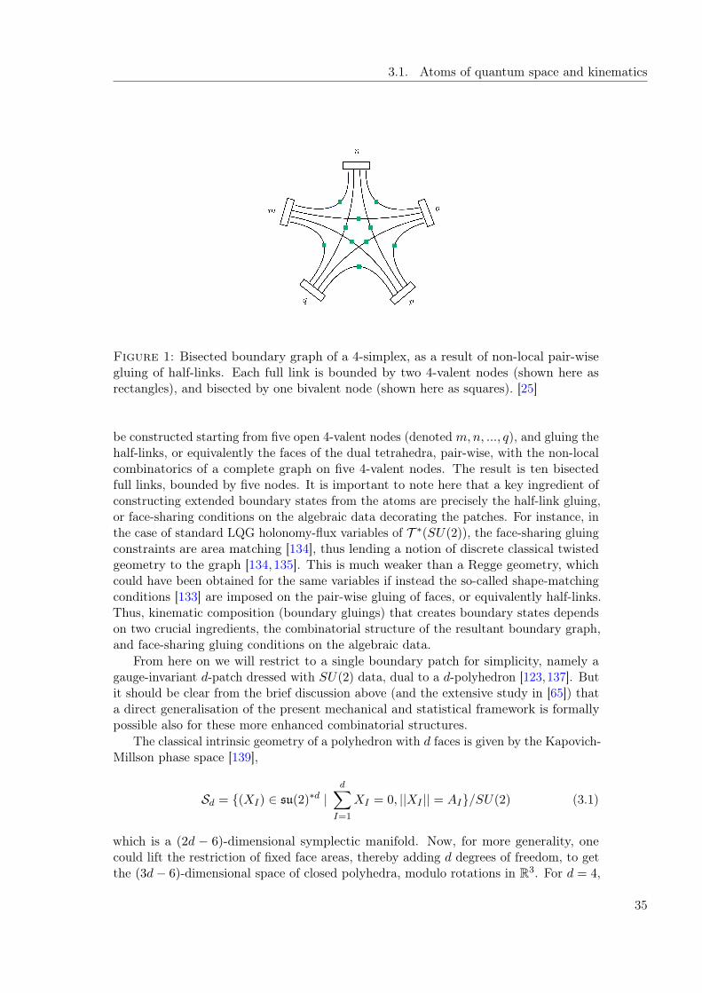
3.1. Atoms of quantum space and kinematics

Figure 1: Bisected boundary graph of a 4-simplex, as a result of non-local pair-wisegluing of half-links. Each full link is bounded by two 4-valent nodes (shown here asrectangles), and bisected by one bivalent node (shown here as squares). [25]

be constructed starting from five open 4-valent nodes (denoted m,n, ..., q), and gluing thehalf-links, or equivalently the faces of the dual tetrahedra, pair-wise, with the non-localcombinatorics of a complete graph on five 4-valent nodes. The result is ten bisectedfull links, bounded by five nodes. It is important to note here that a key ingredient ofconstructing extended boundary states from the atoms are precisely the half-link gluing,or face-sharing conditions on the algebraic data decorating the patches. For instance, inthe case of standard LQG holonomy-flux variables of T ∗(SU(2)), the face-sharing gluingconstraints are area matching [134], thus lending a notion of discrete classical twistedgeometry to the graph [134,135]. This is much weaker than a Regge geometry, whichcould have been obtained for the same variables if instead the so-called shape-matchingconditions [133] are imposed on the pair-wise gluing of faces, or equivalently half-links.Thus, kinematic composition (boundary gluings) that creates boundary states dependson two crucial ingredients, the combinatorial structure of the resultant boundary graph,and face-sharing gluing conditions on the algebraic data.

From here on we will restrict to a single boundary patch for simplicity, namely agauge-invariant d-patch dressed with SU(2) data, dual to a d-polyhedron [123,137]. Butit should be clear from the brief discussion above (and the extensive study in [65]) thata direct generalisation of the present mechanical and statistical framework is formallypossible also for these more enhanced combinatorial structures.

The classical intrinsic geometry of a polyhedron with d faces is given by the Kapovich-Millson phase space [139],

Sd = (XI) ∈ su(2)∗d |d∑I=1

XI = 0, ||XI || = AI/SU(2) (3.1)

which is a (2d − 6)-dimensional symplectic manifold. Now, for more generality, onecould lift the restriction of fixed face areas, thereby adding d degrees of freedom, to getthe (3d− 6)-dimensional space of closed polyhedra, modulo rotations in R3. For d = 4,

35

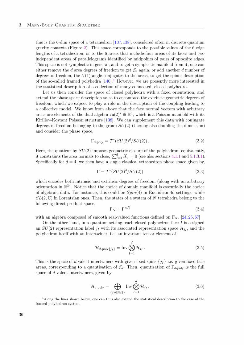
3. Many-Body Quantum Spacetime

this is the 6-dim space of a tetrahedron [137, 138], considered often in discrete quantumgravity contexts (Figure 2). This space corresponds to the possible values of the 6 edgelengths of a tetrahedron, or to the 6 areas that include four areas of its faces and twoindependent areas of parallelograms identified by midpoints of pairs of opposite edges.This space is not symplectic in general, and to get a symplectic manifold from it, one caneither remove the d area degrees of freedom to get Sd again, or add another d number ofdegrees of freedom, the U(1) angle conjugates to the areas, to get the spinor descriptionof the so-called framed polyhedra [140].4 However, we are presently more interested inthe statistical description of a collection of many connected, closed polyhedra.

Let us then consider the space of closed polyhedra with a fixed orientation, andextend the phase space description so as to encompass the extrinsic geometric degrees offreedom, which we expect to play a role in the description of the coupling leading toa collective model. We know from above that the face normal vectors with arbitraryareas are elements of the dual algebra su(2)∗ ∼= R3, which is a Poisson manifold with itsKirillov-Kostant Poisson structure [138]. We can supplement this data with conjugatedegrees of freedom belonging to the group SU(2) (thereby also doubling the dimension)and consider the phase space,

Γd-poly = T ∗(SU(2)d/SU(2)) . (3.2)

Here, the quotient by SU(2) imposes geometric closure of the polyhedron; equivalently,it constraints the area normals to close,

∑dI=1XI = 0 (see also sections 4.1.1 and 5.1.3.1).

Specifically for d = 4, we then have a single classical tetrahedron phase space given by,

Γ = T ∗(SU(2)4/SU(2)) (3.3)

which encodes both intrinsic and extrinsic degrees of freedom (along with an arbitraryorientation in R3). Notice that the choice of domain manifold is essentially the choiceof algebraic data. For instance, this could be Spin(4) in Euclidean 4d settings, whileSL(2,C) in Lorentzian ones. Then, the states of a system of N tetrahedra belong to thefollowing direct product space,

ΓN = Γ×N (3.4)

with an algebra composed of smooth real-valued functions defined on ΓN . [24, 25,67]On the other hand, in a quantum setting, each closed polyhedron face I is assigned

an SU(2) representation label jI with its associated representation space HjI , and thepolyhedron itself with an intertwiner, i.e. an invariant tensor element of

Hd-polyjI = Invd⊗I=1

HjI . (3.5)

This is the space of d-valent intertwiners with given fixed spins jI i.e. given fixed faceareas, corresponding to a quantisation of Sd. Then, quantisation of Γd-poly is the fullspace of d-valent intertwiners, given by

Hd-poly =⊕

jI∈N/2

Invd⊗I=1

HjI . (3.6)

4Along the lines shown below, one can thus also extend the statistical description to the case of theframed polyhedron system.

36

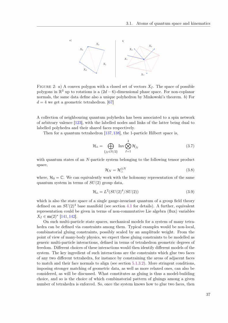
3.1. Atoms of quantum space and kinematics

X1

X2

X3

X4

a) b)

X1

X2

X3

X4

Figure 2: a) A convex polygon with a closed set of vectors XI . The space of possiblepolygons in R3 up to rotations is a (2d− 6)-dimensional phase space. For non-coplanarnormals, the same data define also a unique polyhedron by Minkowski’s theorem. b) Ford = 4 we get a geometric tetrahedron. [67]

A collection of neighbouring quantum polyhedra has been associated to a spin networkof arbitrary valence [123], with the labelled nodes and links of the latter being dual tolabelled polyhedra and their shared faces respectively.

Then for a quantum tetrahedron [137,138], the 1-particle Hilbert space is,

H =⊕

jI∈N/2

Inv4⊗I=1

HjI (3.7)

with quantum states of an N -particle system belonging to the following tensor productspace,

HN = H⊗N (3.8)

where, H0 = C. We can equivalently work with the holonomy representation of the samequantum system in terms of SU(2) group data,

H = L2(SU(2)4/SU(2)) (3.9)

which is also the state space of a single gauge-invariant quantum of a group field theorydefined on an SU(2)4 base manifold (see section 4.1 for details). A further, equivalentrepresentation could be given in terms of non-commutative Lie algebra (flux) variablesXI ∈ su(2)∗ [141,142].

On such multi-particle state spaces, mechanical models for a system of many tetra-hedra can be defined via constraints among them. Typical examples would be non-local,combinatorial gluing constraints, possibly scaled by an amplitude weight. From thepoint of view of many-body physics, we expect these gluing constraints to be modelled asgeneric multi-particle interactions, defined in terms of tetrahedron geometric degrees offreedom. Different choices of these interactions would then identify different models of thesystem. The key ingredient of such interactions are the constraints which glue two facesof any two different tetrahedra, for instance by constraining the areas of adjacent facesto match and their face normals to align (see section 5.1.3.2). More stringent conditions,imposing stronger matching of geometric data, as well as more relaxed ones, can also beconsidered, as will be discussed. What constitutes as gluing is thus a model-buildingchoice, and so is the choice of which combinatorial pattern of gluings among a givennumber of tetrahedra is enforced. So, once the system knows how to glue two faces, then

37

3. Many-Body Quantum Spacetime

the remaining content of a model dictates how the tetrahedra interact non-locally tomake simplicial complexes [25, 67, 96]. More on this will be discussed in sections 3.2 and5.1.3.

Lastly, for a quantum multi-particle system, one can go a step further and define aFock space to accommodate configurations with varying particle numbers. For bosonic5

quanta, each N -particle sector is the symmetric projection of the full N -particle Hilbertspace, so that a Fock space can be defined as,

HF =⊕N≥0

symHN . (3.10)

The associated Fock vacuum state |0 〉 is degenerate with no discrete geometric degreesof freedom, the ‘no space’ state. One choice for the algebra of operators on HF is the vonNeumann algebra of bounded linear operators B(HF ). A more common choice though isthe larger *-algebra generated by ladder operators ϕ, ϕ†, which generate HF by actingon the cyclic Fock vacuum, and satisfy a commutation relations algebra

[ϕ(~g1), ϕ†(~g2)] =

∫SU(2)

dh4∏I=1

δ(g1Ihg−12I ) (3.11)

where ~g ≡ (gI) ∈ SU(2)4 and the integral on the right ensures SU(2) gauge invariance.In fact this is the Fock representation associated with a degenerate vacuum of an algebraicbosonic group field theory defined by a Weyl algebra [24, 66, 91]. We will return to adetailed discussion of these aspects in section 4.1.

Notice that this kind of formulation already hints at a second quantised languagein terms of quantum fields of tetrahedra. This language can indeed be applied tothe generalised statistical mechanics framework we have developed, to get a quantumstatistical mechanics for tetrahedra (polyhedra in general), which will be the focus ofthe rest of the thesis.

3.2 Interacting quantum spacetime and dynamics

Coming now to dynamics, the key ingredients here are the specifications of propagatorsand admissible interaction vertices, including both their combinatorics, and functionaldependences on the algebraic data i.e. their amplitudes.

The combinatorics of propagators and interaction vertices can be packaged neatlywithin two maps, the bonding map and the bulk map respectively [65]. A bonding mapis defined between two bondable boundary patches. Two patches are bondable if theyhave the same number of nodes and links. Then, a bonding map between two bondablepatches identifies each of their nodes and links, under the compatibility condition thatif a bounding bivalent node in one patch is identified with a particular one in another,then their respective half-links (attaching them to their respective central nodes) arealso identified with each other. So a bonding map basically bonds two bulk vertices via

5As for a standard multi-particle system, bosonic statistics corresponds to a symmetry underparticle exchange. For the case when a system of quantum tetrahedra is glued appropriately to forma spin network, then this symmetry is understood as implementing the graph automorphism of noderelabellings.

38

3.3. Generalised equilibrium states

(parts of) their boundary graphs to form a process (with boundary). This is simply abulk edge, or propagator.

The set of interaction vertices can themselves be defined by a bulk map. This mapaugments the set of constituent elements (multivalent nodes, bivalent nodes, and half-links connecting the two) of any bisected boundary graph, by one new vertex (the bulkvertex), a set of links joining each of the original boundary nodes to this vertex, and a setof two dimensional faces bounded by a triple of the bulk vertex, a multivalent boundarynode and a bivalent boundary node. The resulting structure is an interaction vertexwith the given boundary graph.6 The complete dynamics is then given by the chosencombinatorics, supplemented with amplitude functions that reflect the dependence onthe algebraic data.

The interaction vertices can in fact be described by vertex operators on the Fockspace in terms of the ladder operators. An example vertex operator, corresponding tothe 4-simplex boundary graph shown in Figure 1, is

V4sim =

∫SU(2)20

[dg] ϕ†(~g1)ϕ†(~g2)V4sim(~g1, ..., ~g5)ϕ(~g3)ϕ(~g4)ϕ(~g5) (3.12)

where the interaction kernel V4sim = V4sim(gijg−1ji i<j) (for i, j = 1, ..., 5) encodes

the combinatorics of the boundary graph. There are of course other vertex operatorsassociated with the same graph (that is with the same kernel), but including differentcombinations of creation and annihilation operators7.

It must be noted that generic configurations of this system do not admit an in-terpretation as quantised geometric fields. Therefore, geometric configurations cannotbe presumed, and one would have to look for such phases to emerge within the fullstatistical description of the quanta of spacetime. This is an important and difficultopen problem that we do not directly tackle in this thesis.

To summarise, a definition of kinematics entails: defining the state space, whichincludes specifying the combinatorics (choosing the set of allowed boundary patches,which generate the admissible boundary graphs), and the algebraic data (choosing vari-ables to characterise the discrete geometric states supported on the boundary graphs);and, defining the algebra of observables acting on the state space. A definition of dy-namics entails: specifying the propagator and bulk vertex combinatorics and amplitudes.Together they specify the many-body mechanics.

3.3 Generalised equilibrium states

Based on insights from chapter 2 and the mechanical setup laid out above, we canformulate a statistical mechanical framework, and in particular generalised equilibriumstatistical mechanics, for these discrete quantum geometric systems [24,25,67,96].

For a system of many classical tetrahedra (in general, polyhedra), a statistical stateρN can be formally defined on the state space ΓN . As we saw in section 2.2.3, if itsatisfies the thermodynamical characterisation with respect to a set of functions on ΓN

6An interesting aspect is that the bulk map is one-one, so that for every distinct bisected boundarygraph, there is a unique interaction vertex which can be defined from it [65].

7This would generically be true for any second quantised operator [66,143].

39

3. Many-Body Quantum Spacetime

then it will be an equilibrium state. Further, a configuration with a varying number oftetrahedra can be described by a grand-canonical type state of the form

Z =∑N≥0

eµNZN (3.13)

where ZN =∫

ΓNdλ ρN , and µ is a chemical potential [67]. Similarly for a system of

many quantum tetrahedra, a generic statistical state ρ is a density operator on HF [24].Generalised equilibrium states with a varying number of quanta are then given by,

Z = Tr(e−∑a βaOa+µN ) (3.14)

where N =∫d~g ϕ†(~g)ϕ(~g) is the number operator on HF . Such grand-canonical type

boundary states are important because one would expect quantum gravitational dynamicsto not be number conserving in general [66, 67]. Also as pointed out in section 2.2.5,what the precise content of equilibrium is depends crucially on which observables Oaare used to define the state. Operators of natural interest here are the ones encodingthe dynamics, that is vertex and kinetic operators, as considered below in section 3.4.There are many other choices and types of observables one could consider in principle,as will be exemplified in chapter 5. In fact, which ones are the relevant ones in a givensituation is a crucial part of the whole problem.

Given a density operator ρ, then the partition function Z, contains complete statisticalinformation. From Z can be defined an important thermodynamic potential, the freeenergy Φ = − lnZ. Entropy is S = −Tr(ρ ln ρ). These thermodynamic variables arethose whose construction does not really rely on the context in which the statisticalmechanical framework is formulated, as we saw in section 2.3. As emphasised in chapter2 and above, the remaining relevant macrostate variables, like generalised energies 〈O〉,need to be first identified depending on the specific system at hand. Then, a macrostateof the system is characterised by this set of thermodynamic variables (and others derivedfrom them, say via Legendre transforms), whose compatible microstates are naturally thequantum states contributing to the statistical mixture. Having done so at a formal level,naturally the remaining challenging task is to identify a suitable physical interpretationfor them. For example, if a thermodynamic volume potential is defined in analogy withusual quantum field theories, this would refer to the domain manifold of the group fields,i.e. the Lie group manifold. It would not be immediately related to spatial volumes, asdeduced for example by the quantum operator considered later in sections 5.1.1 and5.3.1, which is motivated by the quantum geometric interpretation of the group fieldquanta.

3.4 Effective statistical group field theory

We end this chapter by making a direct link to the definition of group field theoriesusing the above framework. Group field theories [60–64,128] are non-local field theoriesdefined over Lie groups. Most widely studied models are for real or complex scalar fields,over copies of SU(2) or Spin(4). For instance, a complex scalar GFT over SU(2) isdefined by a partition function of the following general form,

ZGFT =

∫[Dµ(ϕ, ϕ)] e−SGFT(ϕ,ϕ) (3.15)

40

3.4. Effective statistical group field theory

where µ is a functional measure which in general is ill-defined, and SGFT is the GFTaction of the form,

SGFT =

∫Gdg1

∫Gdg2 K (g1, g2)ϕ(g1)ϕ(g2) +

∫Gdg1

∫Gdg2 ... V (g1, g2, ...)f(ϕ, ϕ)

(3.16)where g ∈ G, and the kernel V is generically non-local, which convolutes the argumentsof several ϕ and ϕ fields (written here in terms of a single function f). It defines theinteraction vertex of the dynamics by enforcing the combinatorics of its corresponding(unique, via the inverse of the bulk map) boundary graph.

ZGFT defines the covariant dynamics of a group field theory model encoded in SGFT.In this section we show a way to derive such covariant dynamics from a suitable quantumstatistical equilibrium description of a system of quanta of space defined in the previoussections [25]. The following technique of using field coherent states is the same as usedin [66, 67], but with the crucial difference that here we do not claim to define, or aim toachieve any correspondence (even if formal) between a canonical dynamics (in termsof a projector operator, related further to loop quantum gravity [66]) and a covariantdynamics (in terms of a functional integral). Instead we show a quantum statistical basisfor the covariant dynamics itself, and in the process, reinterpret the standard form of theGFT partition function (3.15) as that of an effective statistical field theory arising froma coarse-graining, and further approximations, of the underlying statistical quantumgravity system.

We discussed in 3.2 that the dynamics of the polyhedral atoms of space is encodedin the choices of propagators and interaction vertices, which can be written in terms ofkinetic and vertex operators in the Fock description. In our present considerations witha single type of atom, namely SU(2)-labelled 4-valent node, let us consider the followinggeneric kinetic and vertex operators,

K =

∫SU(2)8

[dg] ϕ†(~g1)K (~g1, ~g2)ϕ(~g2) (3.17)

V =

∫SU(2)4N

[dg] Vγ(~g1, ..., ~gN )f(ϕ, ϕ†) (3.18)

where N > 2 is the number of 4-valent nodes in the boundary graph γ, and f is afunction of the ladder operators with all terms of a single degree N . For example whenN = 3, this function could be f = λ1ϕϕϕ

† + λ2ϕ†ϕϕ†. As we saw before, in principle

a generic model can include several distinct vertex operators. Even though what weconsider here is the simple of case of having only one V, the following treatment can beextended to the general case.

Operators K and V have well-defined actions on the Fock space HF . Using thethermodynamical characterisation, we can consider the formal constraints8 〈K〉 =constant and 〈V〉 = constant, to write down a generalised Gibbs state on HF ,

ρβa =1

Zβae−β1K−β2V (3.19)

where a = 1, 2 and the partition function is,

Zβa = Tr(e−β1K−β2V) . (3.20)8A proper interpretation of these constraints is left to future work.

41

3. Many-Body Quantum Spacetime

An effective field theory can then be extracted from the above by using a basisof coherent states on HF [25, 66, 67, 144]. Field coherent states give a continuousrepresentation on HF where the parameter labelling each state is a wavefunction [144].For the Fock description outlined in section 3.1 (and detailed in the upcoming section4.1), the Fock vacuum is specified by

ϕ(~g) |0 〉 = 0 , ∀~g . (3.21)

The field coherent states are,

|ψ〉 = eϕ†(ψ)−ϕ(ψ) |0 〉 = e−

||ψ||22 eϕ

†(ψ) |0 〉 (3.22)

where ψ ∈ H , ||.|| is the L2 norm in H , and ϕ(ψ) =∫d~g ψϕ along with its adjoint

are the smeared ladder operators. The set of all such states provides an over-completebasis for HF . A very useful property of these states is that they are eigenstates of theannihilation operator,

ϕ(~g) |ψ〉 = ψ(~g) |ψ〉 . (3.23)

This property implies that, for an operator Q(ϕ, ϕ†) as a function of the ladder operators,we have [144],

〈ψ| : Q(ϕ, ϕ†) : |ψ〉 = Q(ψ, ψ) (3.24)

where, : . : denotes normal ordering, i.e. ordering in which all ϕ†’s are to the left of allannihilation operators ϕ’s, and Q is the same function of ψ and ψ, as the operator Q isof ϕ and ϕ† respectively.

The traces for the partition function and other observable averages can then beevaluated in this basis,

Tr(e−β1K−β2VO) =

∫[Dµ(ψ, ψ)] 〈ψ| e−β1K−β2VO |ψ〉 (3.25)

with Zβa = Tr(e−β1K−β2VI) (3.26)

where the resolution of identity and the coherent state functional measure are respectivelygiven by [144],

I =

∫[Dµ(ψ, ψ)] |ψ〉 〈ψ| , (3.27)

Dµ(ψ, ψ) = limK→∞

K∏k=1

dReψk d Imψkπ

. (3.28)

The set of all such observable averages formally defines the complete statistical system.In particular, the quantum statistical partition function can be reinterpreted as thepartition function for a field theory (of complex-valued square-integrable fields) of theunderlying quanta, which here are quantum tetrahedra, as follows [25,66,67].

For simplicity, let us first consider, e−βC , associated with an operator C(ϕ, ϕ†). Then,given C and O as polynomial functions of the generators, with a given (but generic)choice of the operator ordering defining the exponential operator, the integrand of thestatistical averages can be treated as follows:

〈ψ| e−βCO |ψ〉 = 〈ψ|∞∑k=0

(−β)k

k!CkO |ψ〉 (3.29)

= 〈ψ| : e−βCO : |ψ〉+ 〈ψ| : poC,O(ϕ, ϕ†, β) : |ψ〉 (3.30)

42

3.4. Effective statistical group field theory

where to get the second equality, we have used the commutation relations (3.11) on eachCkO, to collect all normal ordered terms : CkO : giving the normal ordered : e−βCO :,and the second term is a collection of the remaining terms arising as a result of swappingϕ’s and ϕ†’s, which will then in general be a normal ordered series in powers of ϕ andϕ†, with coefficient functions of β. The precise form of this series will depend on both Cand O, hence the subscripts. Using equations (3.23) and (3.24), we have:

〈ψ| : e−βCO : |ψ〉 = e−βC[ψ,ψ]O[ψ, ψ] (3.31)

where C[ψ, ψ] = 〈ψ| : C : |ψ〉 and O[ψ, ψ] = 〈ψ| : O : |ψ〉; and,

〈ψ| : poC,O(ϕ, ϕ†, β) : |ψ〉 ≡ 〈ψ| : AC,O(ϕ, ϕ†, β) : |ψ〉 = AC,O[ψ, ψ, β] . (3.32)

Thus, averages can be written as

Tr(e−βCO) =

∫[Dµ(ψ, ψ)]

(e−βC[ψ,ψ]O[ψ, ψ] +AC,O[ψ, ψ, β]

). (3.33)

In particular, the quantum statistical partition function is

Z =

∫[Dµ(ψ, ψ)]

(e−βC[ψ,ψ] +AC,I[ψ, ψ, β]

)=: Z0 + ZO(~) (3.34)

where, by notation O(~) we mean only that this sector of the full theory encodes allhigher orders in quantum terms relative to Z0.9 This full set of observable averages(or correlation functions) (3.33), including the above partition function, defines thusa statistical field theory of quantum tetrahedra (or in general, polyhedra with a fixednumber of boundary faces), characterised by a combinatorially non-local statisticalweight, that is, a group field theory.

If we are further able to either reformulate exactly, or under suitable approximations,AC,O in the following way,

AC,O = AC,I[ψ, ψ, β]O[ψ, ψ] (3.35)

then, the partition function (3.34) defines a statistical field theory for the algebra ofobservables O[ψ, ψ], for a dynamical system of complex-valued square-integrable fieldsψ, defined on the base manifold SU(2)4.

The integrands in (3.25) and (3.26) can then be treated and simplified along thelines above, in particular to get an effective partition function,

Zo =

∫[Dµ(ψ, ψ)] e−β1K [ψ,ψ]−β2V [ψ,ψ] = Zβa − ZO(~) (3.36)

where subscript o indicates that we have neglected higher order terms, collected insideZO(~), resulting from normal orderings of the exponent in Zβa. As before, the functionsin the exponent are K = 〈ψ| : K : |ψ〉 and V = 〈ψ| : V : |ψ〉. It is then evident thatZo has the precise form of a generic GFT partition function of the form (3.15). It thusdefines a group field theory as an effective statistical field theory, that is

ZGFT := Zo . (3.37)9Further investigation into the interpretation, significance and consequences of this rewriting of Z

in discrete quantum gravity is left for future work.

43

3. Many-Body Quantum Spacetime

From this perspective, it is clear that the generalised inverse temperatures (which arebasically the intensive parameters conjugate to the generalised energies in the generalisedthermodynamical setting of section 2.3) are the coupling parameters defining the effectivemodel, thus characterising the phases of the emergent statistical field theory, as would beexpected. Moreover, from this purely statistical standpoint, we can understand the GFTaction more appropriately as Landau-Ginzburg free energy (or effective ‘Hamiltonian’,in the sense that it encodes the effective dynamics), instead of a Euclidean action whichmight imply having Wick rotated a Lorentzian measure, even in an absence of any suchnotions as is the case presently. Lastly, deriving like this the covariant definition ofa group field theory, based entirely on the framework presented here, strengthens thestatement that a group field theory is a field theory of combinatorial and algebraicquanta of space [62,63].

44

Group Field Theory 4

If the space void of all bodies, is not altogether empty; what is it then fullof? Is it full of extended spirits perhaps, or immaterial substances, capableof extending and contracting themselves; which move therein, and penetrateeach other without any inconveniency, as the shadows of two bodies penetrateone another upon the surface of the wall? —Gottfried W. Leibniz 1

We have discussed, in the previous chapter, how group field theories can arise effectivelyfrom a coarse graining of the underlying quantum statistical system. We now turnto GFTs proper, and introduce the structures that are relevant for our subsequentapplications.

Group field theories are field theories of combinatorial and algebraic quanta ofgeometry, formally defined by a statistical partition function

ZGFT =

∫[Dϕκ] e−SGFT(ϕκ) (4.1)

for a set of group fields ϕκ. They are strictly related to various other approaches likeloop quantum gravity [104,124,125], spin foams [126,127], causal dynamical triangulations[129], tensor models [146] and lattice quantum gravity [130]. Like in usual field theories,the kinematics is specified by a choice of the fields ϕκ, each defined in general over adomain space of direct products of Lie groups, and taking values in some target vectorspace. The dynamics is specified by propagators and interaction vertices encoded in afunction SGFT, which can be understood as a Landau-Ginzburg free energy function inthe present statistical context [25]; or as a Euclidean action from the point of view ofstandard quantum field theories [59–63]. However unlike in usual field theories, SGFTis non-local in general with respect to the base manifold. This non-locality is essential,and encodes the non-trivial combinatorial nature of the fundamental degrees of freedomand their dynamics. Moreover, the base manifold is not spacetime, but carries algebraicinformation associated with discrete geometric and matter degrees of freedom. Such acomplete absence of any continuum spacetime structures a priori is a manifestation ofbackground independence in group field theory, like in various other non-perturbativeapproaches to quantum gravity.

The partition function ZGFT perturbatively generates Feynman diagrams that arelabelled 2-complexes (dual to labelled stranded diagrams), with boundary states givenby labelled graphs [59–63]. For the choice of models closer to loop quantum gravityand spin foam setups, the boundary states are abstract spin networks (but organisedin a second quantised Hilbert space, that of a field theory [66]) and bulk processes arespin foams, both of which in turn are dual to polyhedral complexes when restricting to

1As cited in [145], p161.

45

4. Group Field Theory

loopless combinatorics [65,123]. Thus, a group field theory generates discrete quantumspacetimes made of fundamental polyhedral quanta2.

We can describe the same structures from a many-body perspective [81], and treat asmore fundamental an interacting system of many such quanta. This viewpoint enables usto import formal techniques from standard many-body physics for macroscopic systems,by treating a quantum polyhedron or an open spin network node as a single particle ofinterest. In fact, it has allowed for tangible explorations of connections of group fieldtheory with quantum information theory and holography [82,84,87–90], and also withquantum statistical mechanics and thermal physics [24,25,45,67,91,96]. It has furtherallowed for importing ideas and tools from condensed matter theory, which has beencrucial for instance in the development of GFT condensate cosmology [76–79].

This same perspective further leads to a modelling of an extended region of discretequantum space (a labelled graph) as a multi-particle state, and a region of dynamicalquantum spacetime (a labelled 2-complex) as an interaction process. As we haveemphasised before, this is the perspective that we employ throughout the thesis to usetechniques from many-body physics and statistical mechanics, even when working witha radically different kind of system, one that is background independent, and devoidof any standard notion of space, time and other associated geometric structures andstandard matter couplings.

The simplest class of models are scalar theories, with fields ϕ : Gd → C, defined on adirect product of d copies of the local gauge group of gravity. This is the Lorentz groupSL(2,C) in 4d or its Euclidean counterpart Spin(4). SU(2) is often used as the relevantsubgroup in the context of quantum gravity, especially for models connected to LQG.In this thesis, G is taken to be locally compact so that the Haar measure is defined(even though it would be finite only for compact groups); connected (for constructionsin section 5.1.2.1); and, unimodular so that the left- and right-invariant Haar measurescoincide. These properties are satisfied by SU(2),R, Spin(4) and SL(2,C), of which thefirst two are used in some specific examples later in the thesis.

Further, we may be interested in group field theories which generate discrete space-times coupled to discretised real scalar matter fields. One way to couple a single realscalar degree of freedom is by extending the original configuration space Gd, encodingpurely geometric data, by R. By extension, n number of scalar fields can be coupled byconsidering the base manifold Gd × Rn [76–79,147–150]. Doing this we have assignedadditional n real numbers representing the values of the fields, to each quantum of thegroup field. Consequently, a GFT Feynman diagram (labelled 2-complex) is enriched byn scalar fields that are discretised on the vertices of the boundary graphs (equivalently,edges of the bulk 2-complex). Thus we are concerned with a group field,

ϕ : Gd × Rn → C, (~g, ~φ) 7→ ϕ(~g, ~φ) (4.2)

defined for arbitrary natural numbers n ≥ 0 and d > 0 (before any physical restrictionscoming from considerations in discrete quantum gravity).

The main reasons for including matter in GFTs are natural. Any fundamental theoryof gravity must include, or must be able to generate at an effective level, matter degrees

2As discussed previously in chapter 3, a quantised polyhedron with d faces is dual to a gauge-invariantopen d-valent spin network node [123]. The latter is in fact a special case (namely, a d-patch [65]) ofricher combinatorial boundary structures which can be treated analogously in our present setup, but inthat case without related discrete geometric understanding of the same.

46

4.1. Bosonic group field theory

of freedom if it is to eventually realistically describe the universe. Also, material referenceframes can be used to define physical relational observables in background independentsystems [53,151–157]. For instance in GFT, relational reference frames defined by scalarfields have been used in the context of cosmology [76–79,95,147,148,150,158,159]. Inthis thesis, we make use of relational frames in two different contexts. In section 5.1.2, wedefine Gibbs states first with respect to internal translations in ~φ, and then with respectto a clock Hamiltonian associated with one of these φ’s, now being an external clock tothe system after deparametrization as described in section 4.2 below. Later in section 5.3,we first clarify the notion of relational frames in GFT by using smearing functions alongthe φ direction, and then apply them in the context of thermal condensate cosmology inGFT.

In this chapter, we present a quantum operator formulation of bosonic group fieldtheories, detailing those aspects which are relevant for our later constructions. In section4.1.1, we give a Fock space construction based on the degenerate vacuum (which wealso encountered in the previous chapter). In section 4.1.2 we present three orthonormalbases that will be useful for later investigations. Then in section 4.1.3, we give theWeyl algebraic formulation of the same system, along with the construction of theirtranslation *-automorphisms in 4.1.4. Finally in section 4.2, we consider the issue ofdeparametrization in group field theory based on insights and tools from presymplecticmechanics of multi-particle systems.

4.1 Bosonic group field theory

4.1.1 Degenerate vacuum and Fock representation

Adopting a second quantisation scheme [32,33,143], states of a group field ϕ(~g, ~φ) canbe organised in a Fock space HF generated by a Fock vacuum |ΩF 〉 and the ladderoperators3 ϕ,ϕ† [66, 160]. The vacuum is specified by

ϕ(~g, ~φ) |ΩF 〉 = 0 , ∀~g, ~φ . (4.3)

This is a degenerate vacuum, with no quantum geometrical or matter degrees of freedom.It is a state like |0 〉, the ‘no-space’ state, which we encountered previously in section 3.1.We also remark that later in section 5.2, a degenerate vacuum of this kind is denoted by|0〉, in order to declutter the overall notation of the investigation there.

A single quantum is created by acting on |ΩF 〉 with the creation operator,

ϕ†(~g, ~φ) |ΩF 〉 = |~g, ~φ〉 (4.4)

which is the state of a d-valent node whose links are labelled by group elements ~g =(g1, ..., gd) and the node itself by a set of real numbers ~φ = (φ1, ..., φn). Then, a genericsingle-particle state with wavefunction ψ is given by,

|ψ〉 =

∫Gdd~g

∫Rnd~φ ψ(~g, ~φ) |~g, ~φ〉 (4.5)

3Throughout the thesis, we may choose to neglect or reinstate the hat notation for operators withoutnotice, in order to simplify or clarify the notation in the setup at hand.

47

4. Group Field Theory

where ψ is an element of the single-particle Hilbert space. This Hilbert space is givenby4

H = L2(Gd × Rn) (4.6)

or, when the geometric condition of closure is satisfied, by5

H = L2(Gd/G× Rn) ∼= L2(Gd/G)⊗ L2(Rn) . (4.7)

Closure corresponds to the field ϕ being invariant under a diagonal right6 action of Gon Gd, that is

ϕ(gI , φ) = ϕ(gIh, φ) , ∀h ∈ G (4.8)

and allows for understanding the quanta of the field as convex polyhedra (in turn dualto gauge-invariant spin network nodes) [123,137,138]. This invariance effectively reducesthe geometric part of the domain space to Gd/G, as evident in the expression for Habove. In this thesis however, even when imposing closure, we will continue to use aredundant parametrization for convenience and consider the gauge-invariant functionsto be defined on full Gd while explicitly satisfying equation (4.8).

Further, we choose to impose a symmetry under arbitrary particle exchanges on thestates, that is bosonic statistics. In the spin network picture, this condition reflects thegraph automorphism of vertex relabelling and is a natural feature to require. For thecase at hand then, the Hilbert space for bosonic quanta is the Fock space

HF =⊕N≥0

symH⊗N (4.9)

where H⊗N describes the N -particle sector, with H0 = C, and sym refers to thesymmetric projection of it. This is the space that we encountered before in section 3.1.We stress again that this Fock space contains arbitrary spin network excitations [66], thusthe quantum gravity structures are shared with loop quantum gravity even if organisedin a different way. This means that defining proper statistical equilibrium states on thisFock space truly means defining non-perturbative statistical equilibrium states in a fullybackground independent context and within a fundamental theory of quantum gravitybased on spin network states.

The ladder operators that take us between the different multi-particle sectors satisfythe commutation relations algebra,

[ϕ(~g, ~φ), ϕ†(~g′, ~φ′)] = I(~g,~g′)δ(~φ− ~φ′) (4.10)

[ϕ(~g, ~φ), ϕ(~g′, ~φ′)] = [ϕ†(~g, ~φ), ϕ†(~g′, ~φ′)] = 0 (4.11)

4Notice that even for compact G, the base manifold is non-compact along R, which might thendemand appropriate regularisation schemes depending on the case at hand e.g. operator (5.34) in section5.1.2.1.

5We have chosen to denote both these Hilbert spaces by the same H, because our technical resultsare independent of which one we choose. What changes is the interpretation of a single quantum of thegroup field, which can be understood as a convex polyhedron only with the latter choice.

6The right gauge invariance is imposed in order to avail a quantum geometric interpretationof the quanta of the GFT field, as discussed before. An additional left gauge invariance can alsobe imposed, as has been done in studies in the context of homogeneous cosmologies in group fieldtheory [77,80,95,148,161,162]. However, our entire setup, along with the technical results based on it,will mathematically follow through with or without (either or even both) these additional symmetriesand their associated geometric interpretations.

48

4.1. Bosonic group field theory

where, I and δ are delta distributions for functions on Gd and Rn respectively. The deltadistribution on Gd for right gauge-invariant functions takes the form,

I(~g,~g′) =

∫Gdh

d∏I=1

δ(gIhg′−1I ) . (4.12)

The second quantised operators (see [66] for more details in the context of LQG) areelements of the unital *-algebra generated by ϕ,ϕ†, I, where I is the identity operatoron HF , and the adjoint † is the * operation. These elements are in general polynomialsO(ϕ,ϕ†, I) of the three. We denote this algebra by AF , with action on HF .

4.1.2 Useful bases

Spin-momentum

For compact G, by Peter-Weyl theorem, the Hilbert space L2(G) can be decomposedinto a sum of finite-dimensional irreducible representations of G [163, 164]. Then forG = SU(2), a useful basis in L2(SU(2)d) is given by the Wigner modes D~χ, labelledby a set of irreducible representation indices ~χ. Particularly, for right gauge-invariantfunctions on SU(2)d (satisfying (4.8)), this is given by the following set of Wignerfunctions

D~χ(~g) =∑~m′

C~j~m′ι

d∏I=1

DjImIm

′I(gI) (4.13)

where ~χ ≡ (~j, ~m, ι), jI ∈ N/2 are spin irreducible representation indices of SU(2),mI ,m

′I ∈ (−jI , ...,+jI) are matrix indices in representation jI , D

jImIm

′Iare complex-

valued Wigner matrix coefficients (multiplied by a factor of√

dimjI =√

2jI + 1, for

normalisation shown in (4.14) below) in representation jI , and C~j~m′ι are intertwiner

basis elements indexed by ι arising due to the closure condition in (4.8) for SU(2).Orthonormality and completeness are respectively given by,∫

d~g D~χ(~g)D~χ′(~g) = δ~χ~χ′ , (4.14)∑~χ

D~χ(~g)D~χ(~g′) = I(~g,~g′) . (4.15)

While for the coupled matter degrees of freedom in L2(Rn), one can consider the standardFourier basis,

F(~p, ~φ) = e−i~p.~φ . (4.16)

The corresponding basis in H is then of the tensor product form, (D~χ⊗F(~p))(~g, ~φ), andthe algebra generators are given by the appropriate smearing,

ϕ~χ(~p) := ϕ(D~χ ⊗ F(~p)) =

∫d~gd~φ D~χ(~g)F(~p, ~φ)ϕ(~g, ~φ) , (4.17)

ϕ†~χ(~p) = ϕ†(D~χ ⊗ F(~p)) =

∫d~gd~φ D~χ(~g)F(~p, ~φ)ϕ†(~g, ~φ) . (4.18)

49

4. Group Field Theory

The algebra structure in (4.10) is preserved, and now takes the form

[ϕ~χ(~p), ϕ†~χ′(~p′)] = (2π)nδ~χ~χ′δ(~p− ~p′) (4.19)

[ϕ~χ(~p), ϕ~χ′(~p′)] = [ϕ†~χ(~p), ϕ†~χ′(~p

′)] = 0 (4.20)

where δ~χ~χ′ is the Kronecker delta, and δ(~p− ~p′) is a Dirac delta distribution on Rn. TheFock space HF is then generated via actions of ϕ~χ(~p), ϕ†~χ(~p), I on the vacuum |ΩF 〉.

Discrete index

We retain the use of the Wigner basis mentioned above, labelled by discrete indices~χ. For the matter part, let us consider a basis of complex-valued smooth functionsT~α(~φ) in L2(Rn), labelled by a set of discrete indices ~α = (α1, ..., αn) ∈ Nn, satisfyingorthonormality and completeness,∫

d~φ T~α(~φ)T~α′(~φ) = δ~α~α′ , (4.21)∑~α

T~α(~φ)T~α(~φ′) = δ(~φ− ~φ′) . (4.22)

We thus have a complete orthonormal basis on H consisting of functions (D~χ⊗T~α)(~g, ~φ)of the tensor product form. Then as before, the set of mode ladder operators can bedefined by smearing the operators ϕ,ϕ† with this basis,

a~χ~α := ϕ(D~χ ⊗T~α) =

∫d~gd~φ D~χ(~g)T~α(~φ)ϕ(~g, ~φ) , (4.23)

a†~χ~α = ϕ†(D~χ ⊗T~α) =

∫d~gd~φ D~χ(~g)T~α(~φ)ϕ†(~g, φ) . (4.24)

This essentially decomposes the operators ϕ,ϕ† in terms of the modes D~χ ⊗T~α, whichcan be seen directly by inverting the above two equations. The algebra relations are,

[a~χ~α, a†~χ′~α′ ] = δ~χ~χ′δ~α~α′ (4.25)

[a~χ~α, a~χ′~α′ ] = [a†~χ~α, a†~χ′~α′ ] = 0 . (4.26)

We note that due to the choice of a discrete basis T~α(~φ)~α in L2(Rn), the algebracommutator in (4.25) now produces Kronecker deltas, instead of the Dirac delta distribu-tion of the original basis in equation (4.10), or the momentum basis in equation (4.19).The consideration of a regular algebra instead of a distributional one, particularly forthe φ-modes, is an important feature in certain parts of this thesis where we deal withinequivalent representations obtained via thermal Bogoliubov transformations. Namely,the Kronecker delta δαα′ is crucial in order to avoid divergences related to the coincidencelimit φ → φ′ of δ(φ − φ′). As we will see in sections 5.2.4 and 5.3.1, such terms withδ(φ− φ′) arise naturally when calculating thermal expectation values of certain relevantobservables, for example the average thermal number density.

The degenerate vacuum is again specified by,

a~χ~α |ΩF 〉 = 0 , ∀J, α (4.27)

50

4.1. Bosonic group field theory

which generates the symmetric Fock spaceHF by the action of the generators a~χ~α, a†~χ~α, 1.For instance, a single particle (N = 1), single mode state is,

|~χ, ~α〉 ≡ |D~χ ⊗T~α〉 = a†~χ~α |ΩF 〉 (4.28)

while a single particle state with wavefunction ψ(~g, φ) =∑~χ,~α

D~χ ⊗T~α(~g, φ)ψ~χ~α ∈ H is,

|ψ〉 = a†(ψ) |ΩF 〉 =∑~χ,~α

ψ~χ~αa†~χ~α |ΩF 〉 . (4.29)

Occupation number

A good basis to work with in the Fock space is the orthonormal occupation numberbasis. It is particularly useful because it is the eigenbasis of the number operator, andtherefore of all extensive operators, in HF . This basis organises the states according tothe number of particles occupying a given mode (~χ, ~α).

Utilising the commutation algebra relations (4.25), a normalised multi-particle statewith n~χ~α number of particles in a single mode (~χ, ~α) is given by,

|n~χ~α〉 :=1√n~χ~α!

(a†~χ~α)n~χ~α |ΩF 〉 . (4.30)

Then, generic multi-particle states occupying several modes ~χi, ~αi are given by,

|n~χi~αi〉 ≡ |n~χ1~α1, n~χ2~α2

, ..., n~χi~αi , ...〉 :=1√∏

i

(n~χi~αi !

) ∏i

(a†~χi~αi)n~χi~αi |ΩF 〉 (4.31)

where mode index i ∈ N is finite. Orthonormality relations are,

〈n~χ~α|m~χ′~α′〉 = δn~χ~αm~χ′~α′ δ~χ~χ′δ~α~α′ . (4.32)

The number operator for a single mode N~χ~α = a†~χ~αa~χ~α, counts its occupation number

N~χj~αj |n~χi~αi〉 = n~χj~αj |n~χi~αi〉 (4.33)

while the total number operator N =∑~χ,~α

N~χ~α, counts the total number of particles,

N |n~χi~αi〉 =

∑j

n~χj~αj

|n~χi~αi〉 . (4.34)

4.1.3 Weyl algebra

Operator norm is not defined on the *-algebra AF , because of the unboundedness of thebosonic ladder operators ϕ and ϕ† [33]. As is standard practice in algebraic treatmentsof many-body quantum systems, we could work instead with exponentiated versions ofthese resulting in a unital C*-algebra, the Weyl algebra.

The following Weyl reformulation of the GFT system is based on the well-knownliterature in algebraic quantum field theory [32,33,165,166]. For the purposes of this

51

4. Group Field Theory

thesis, this surrounds the Fock representation of many-body, non-relativistic systems,here suitably adapted to define an analogous setup for group field theory [24,91].

The fields ϕ and ϕ† are operator-valued distributions. The corresponding operatorsare defined by smearing them with functions7 f ∈ H,

ϕ(f) :=

∫Gd×Rn

d~g d~φ f(~g, ~φ)ϕ(~g, ~φ) (4.35)

ϕ†(f) =

∫Gd×Rn

d~g d~φ f(~g, ~φ)ϕ†(~g, ~φ) . (4.36)

Depending on the investigation at hand, the smearing functions may also be required tosatisfy additional decay properties (see for instance, equations (5.160) in section 5.3.4).

The commutation relations (4.10) take the following form,

[ϕ(f1), ϕ†(f2)] = (f1, f2) (4.37)

[ϕ(f1), ϕ(f2)] = [ϕ†(f1), ϕ†(f2)] = 0 (4.38)

where(f1, f2) =

∫Gd×Rn

d~g d~φ f1(~g, ~φ)f2(~g, ~φ) (4.39)

is the L2-inner product.Bosonic ladder operators are unbounded in the operator norm on HF , and they

are defined on dense subsets of HF . Therefore, let us define the following self-adjointoperators8 in the common dense domain of ϕ and ϕ†,

Φ(f) :=1√2

(ϕ(f) + ϕ†(f)) (4.40)

Π(f) :=1

i√

2(ϕ(f)− ϕ†(f)) (4.41)

and consider their exponentiations,

WF (f) := eiΦ(f) (4.42)

or equivalently9 WF (f) = eiΠ(f). Then, these exponential operators:

• are unitary, WF (f)† = WF (f)−1 = WF (−f) , and

• satisfy Weyl relations, WF (f1)WF (f2) = e−i2Im(f1,f2)WF (f1 + f2).

In other words, WF (f) | f ∈ H defines a Weyl system [32,33,167] on the Hilbert spaceHF , over the space of test functions f . It defines a unitary representation of the GFTcommutation algebra on HF with generators Φ.

Retaining this algebraic structure and forgetting (for now) the generators Φ whichlend the concrete representation, an abstract bosonic GFT system can be defined by the

7Naturally, the smearing is independent of basis, i.e. ϕ(f) = a(f).8In terms of operators Φ and Π, the commutation relations take the form, [Φ(f1),Π(f2)] =

iRe(f1, f2) , [Φ(f1),Φ(f2)] = [Π(f1),Π(f2)] = i Im(f1, f2).9Since Π(f) = Φ(if), both ϕ and ϕ† can be recovered from Φ or Π alone. By convention then, Φ

are usually chosen as the generators of this representation. [33]

52

4.1. Bosonic group field theory

pair (A,S), where A is the Weyl algebra10 generated by Weyl unitaries W (f), and S isthe space of algebraic states11. The defining relations of this algebra are,

W (f1)W (f2) = W (f2)W (f1) e−i Im(f1,f2) = W (f1 + f2) e−i2Im(f1,f2) (4.43)

where identity is I = W (0), and unitarity isW (f)−1 = W (f)† = W (−f). This is a unitalC*-algebra, equipped with the C*-norm. The benefits of defining a quantum GFT systemwith an abstract Weyl algebra stem from the fact that some general results can be deduced,which are representation-independent (and would apply, for example, also to otherinequivalent representations [45,91]). This allows in particular for exploring structuralsymmetries at the level of the algebra formulated in terms of automorphisms. In theupcoming section 4.1.4, we will consider examples of automorphisms of A correspondingto structural symmetries (translations) of the underlying theory. The KMS condition withrespect to these automorphisms will then lead to a definition of structural equilibriumstates in section 5.1.2.1, which encode stability with respect to the corresponding internalflows of the transformation under consideration.

The Fock system is now generated as the Gelfand-Naimark-Segal (GNS) representa-tion [31–33,166] (πF ,HF ,ΩF ) of the regular Gaussian algebraic state given by

ωF [W (f)] := e−||f ||2

4 . (4.44)

HereHF is the GNS representation space which is identical to the one that we constructedin the previous section directly using the ladder operators, via the following identities

πF (W (f)) = WF (f) = eiΦ(f) (4.45)

for all W (f) ∈ A. The vector state ΩF is the cyclic GNS vacuum generating the

representation space, πF (A) |ΩF 〉dense⊂ HF . It is the same degenerate Fock vacuum that

was introduced earlier, the no-space state.The kinematic system can thus be defined by a pair consisting of, the algebra of

bounded linear operators12 B(HF ) on the Fock space or the algebra AF , both of whichwe encountered before in sections 3.1 and 4.1.1; and, the space of normal states Sn overthe algebra. Normal states are algebraic states ωρ induced by density operators ρ onHF , i.e. ωρ[A] = Tr(ρA).

4.1.4 Translation automorphisms

In section 5.1.2 we will construct Gibbs states which are at equilibrium with respect totranslations of the system along the base manifold, for which the relevant definitionsand constructions are presented below [24].

10Fermionic statistics would correspond to a Clifford algebra.11Recall that algebraic states are linear, positive, normalised, complex-valued functionals over an

algebra (see footnote 6, on page 16).12The von Neumann algebra B(HF ) is the closure of the C*-algebra πF (A) in the weak operator

topology on HF . Weak operator topology is defined by continuity of the map B(HF ) 3 A 7→ (Aψ1, ψ2),for every ψ1, ψ2 ∈ HF . Further, the weak operator topology is weaker (or coarser) than the strongoperator topology i.e. continuity of the map B(HF ) 3 A 7→ ||Aψ||, for every ψ ∈ HF . Thus, B(HF ) isalso strongly closed. [165,166]

53

4. Group Field Theory

4.1.4.1 Rn-translations

The natural translation map on n copies of the real line,

T~φ : Gd × Rn → Gd × Rn, (~g, ~φ′) 7→ (~g, ~φ′ + ~φ) (4.46)

induces a linear map (over C) on square-integrable functions as a shift to the right,

T ∗~φ : f(~g, ~φ′) 7→ (T ∗~φf)(~g, ~φ′) := (f T−~φ)(~g, ~φ′) . (4.47)

This is a regular, unitary representation of Rn on H [163,168]. Notice that T ∗~φ preserves

the L2 inner product due to translation invariance of the Lebesgue measure, i.e. for any~φ ∈ Rn, (T ∗~φ

f1, T∗~φf2) = (f1, f2). Notice also that T ∗~φ is linear on the space of functions f ,

i.e. for any z1, z2 ∈ C, we have T ∗~φ(z1f1 + z2f2) = z1T∗~φf1 + z2T

∗~φf2. Then, let us define

a linear map on the Weyl algebra,

α~φ : A → A, W (f) 7→W (T ∗~φf) . (4.48)

For each φ, the map αφ defines a *-automorphism of A, and the set of maps αφφ∈Rforms a 1-parameter group. This defines a representation α of the group R in thegroup of automorphisms of the algebra Aut(A), i.e. the map α : R→ Aut(A), φ 7→ αφpreserves the algebraic structure of reals, αφ1+φ2 = αφ1αφ2 . Extending this to Rn, themaps α~φ~φ∈Rn now form an n-parameter group, and α defines a representation of Rn

in Aut(A). See appendix 4.A for details.

4.1.4.2 Gd-left translations

The natural left13 translations on a group manifold are diffeomorphisms from G to itself.On Gd, it is given by the smooth map,

L~g : (~g′, ~φ) 7→ (~g.~g′, ~φ) := (g1g′1, ..., gdg

′d,~φ) (4.49)

which induces a map on the space of functions,

L∗~gf(~g′, ~φ) := (f L~g−1)(~g′, ~φ) . (4.50)

This is a left regular, unitary representation of Gd on H [163, 168]. Notice that L∗~gpreserves the L2-inner product, i.e. for any ~g ∈ Gd, (L∗~gf1, L

∗~gf2) = (f1, f2), using

left-translation invariance of Haar measure on Gd. Also notice that L∗~g is linear on thespace of functions f , i.e. for any z1, z2 ∈ C, we have L∗~g(z1f1 +z2f2) = z1L

∗~gf1 +z2L

∗~gf2.

With this, let us define a linear transformation on the Weyl generators,

α~g(W (f)) := W (L∗~gf) . (4.51)

Then, map α~g defines a *-automorphism of A. Also like for Rn-translations, α : Gd →Aut(A) is a representation of Gd in the group of all automorphisms of the algebra as itpreserves the algebraic structure, α~g.~g′ = α~gα~g′ . See appendix 4.A for details.

13Analogous statements hold for right translations.

54

4.2. Deparametrization in group field theory

4.1.4.3 Unitary representation

Using the following known structural properties of GNS representation spaces [31,32],the automorphisms defined above can be implemented by unitary transformations in theFock space HF as follows.

α-Invariant state. Let ω be an α-invariant state, i.e. ω[αA] = ω[A] for all A ∈ A, forsome α ∈ Aut(A). Then it is known that [31,32], α is implemented by unitary operatorsUω in the GNS representation space (πω,Hω,Ωω), defined by Uω πω(A)U †ω = πω(αA)with invariance of the GNS vacuum UωΩω = Ωω. Similarly, for the general case whenω is invariant under a group of automorphisms, then αg (g ∈ G) is implemented by aunitary representation Uω of G in Hω, such that

Uω(g)πω(A)U †ω(g) = πω(αgA) , Uω(g)Ωω = Ωω . (4.52)

Fock state. We recall that the algebraic Fock state over A is given by equation (4.44),with the associated GNS representation (πF ,HF ,ΩF ). Then, any automorphism onA that is defined via a norm-preserving transformation on H will leave ωF invariant.Thus ωF is invariant under the class of norm-preserving transformations of the square-integrable test functions, including the translation automorphisms of the base manifoldas defined above. Thus, automorphisms α~φ and α~g are implemented by groups of unitaryoperators in HF .

From the unitary transformations (4.52) as applied to Weyl generators in the Fockrepresentation πF , it is straightforward to see that the group field operators transformin a familiar way,

UF (~φ′)ϕ(~g, ~φ)UF (~φ′)−1 = ϕ(~g, ~φ+ ~φ′) (4.53)

UF (~g′)ϕ(~g, ~φ)UF (~g′)−1 = ϕ(~g′~g, ~φ) (4.54)

with analogous expressions for their adjoints. From here on the subscript F on theunitary implementations of these translation automorphisms will be dropped with theunderstanding that in this setting U refers only to the unitary representation of somegroup in target space U(HF ) of unitary operators on Fock space. We remark that thesetransformations, defined here for πF (A), being bounded can also be extended to B(HF ).

Further, it is important to note (for subsequent use in section 5.1.2.1) that thecorresponding group homomorphism U : Gd → U(HF ), is strongly continuous in theFock space. See appendix 4.B for details.

Therefore, the system is now equipped with strongly continuous groups of unitaryoperators in the Fock representation that implement internal shifts of the underlyingbase manifold Gd × Rn.

4.2 Deparametrization in group field theory

We have recalled the fundamental difficulties in defining equilibrium in generally covariantsystems, due to the absence of preferred time variables in the previous chapters. Ageneral strategy to solve those issues, in the description of the dynamics of such systemsis to use matter degrees of freedom as relational clocks, under suitable approximations,and recast the general covariant dynamics in terms of a physical Hamiltonian associated

55

4. Group Field Theory

with them. Here also we can consider the same general strategy as a way to tackleour (related) issue of defining statistical equilibrium states in quantum gravity. Thatis, we can consider the construction of states which are at equilibrium with respect torelational clocks, as will be done in section 5.1.2.2.

For this then, we first need to consider in detail aspects of deparametrization ingroup field theory to define a clock variable, which is the content of this section. Basedon insights and tools of presymplectic mechanics as presented in section 2.1, below welay out the essentials for group field theory. As we will see, the resultant deparametrized,relational system will be ‘canonical’ in clock time which now foliates the original GFTsystem discussed up until now. Algebra brackets (4.10) will be replaced with thecorresponding equal-clock-time commutation relations, analogous to the equal-timecommutation relations in a non-covariant system. Our interest in such a setup is naturalbecause GFTs lack a preferred choice of an evolution parameter. The base space Gd×Rnis chosen so as to facilitate a relational description of the system by coupling n scalarfields [147]. However, there are n possible variables to choose from, and none is preferredover the others. By construction then, GFTs have a multi-fingered relational timestructure in this sense.

The way we approach the task of deparametrizing is as follows [24]. We focusfirst on the classical description in section 4.2.1, starting with the case of a singlegroup field particle in section 4.2.1.1 and sketch how deparametrization works at thissimple level, assuming that the GFT dynamics amounts to a specific choice of a scalarHamiltonian constraint. Then in section 4.2.1.2, we consider the extension of the samedeparametrization procedure for a system of many such particles, assumed as non-interacting. We then consider the quantisation of the resulting deparametrized system ofmany group field particles, arriving at the corresponding quantum multi-particle systemin section 4.2.2, which is canonical with respect to a clock time (with respect to whichone can then define relational equilibrium, in section 5.1.2.2). Below we sketch therelevant steps of the overall construction [24], and leave a more detailed analysis of thecorresponding mathematical structures for GFTs to future work.

4.2.1 Classical system

We begin with the investigation of deparametrization for a classical system [24], utilisingthe framework of extended phase space and presymplectic mechanics as discussedin section 2.1. Here, we face a similar issue of background independence with theassociated absence of a preferred evolution parameter. The reason for undertakingclassical considerations first is to utilise the existing knowledge already well-positionedto be imported to GFT due to the common structures encountered in any such multi-particle system, namely an extended symplectic phase space with a set of constraints,including a dynamical Hamiltonian one.

4.2.1.1 Single-particle

The extended classical configuration and phase space for the single-particle sector ingroup field theory is

Cex = Gd × Rn 3 (gI , φa) (4.55)

Γex = T ∗(Cex) ∼= Gd × Rn × g∗d × Rn 3 (gI , φa, XI , pφa) (4.56)

56

4.2. Deparametrization in group field theory

where, g is the Lie algebra of G and g∗ is its dual vector space. Here, by a classicalparticle we mean a point particle living on the group base manifold, thus being describedby a point on its phase space. States and observables are respectively points and smoothfunctions on Γex. Statistical states are smooth positive functions on the phase space,normalised with respect to the Liouville measure. The Poisson bracket on the space ofobservables defines its algebra structure. The symplectic 2-form on Γex is,

ωex = ωG +∑a

dpφa ∧ dφa (4.57)

where ωG is a symplectic form on T ∗(Gd). Let us assume that the covariant14 dynamicsof this simple system is encoded in a smooth constraint function

Cfull : Γex → R , (4.58)

and that there are no additional gauge symmetries. A single classical particle of thegroup field is thus described by (Γex, ωex, Cfull). The null vector field is defined by,

ωex(YCfull) = −dCfull (4.59)

while the constraint surface Σ is characterised by Cfull = 0, with its presymplectic formgiven by, ωΣ = ωex|Σ. The null orbits of ωΣ are the graphs of physical motions encodingunparametrized correlations between the dynamical variables of the theory. These gaugeorbits are integral curves of the vector field YCfull

, satisfying the equations of motion

ωΣ(YCfull) = 0 . (4.60)

The set of all such orbits is the physical phase space Γphy that is projected down fromΣ and is equipped with a symplectic 2-form induced from Σ. Then (Γphy, ωphy) is thespace of solutions of the system and a physical flow means a flow on this space. Wenotice again that here, a canonical time or clock structure is lacking, and is not requireda priori.

Deparametrizing this classical system, with respect to, say, the cth scalar field φc,means reducing the full system to one wherein the field φc acts as a good clock. Asanticipated in section 2.1, this entails the following two separate approximations to Cfull,

Cfull(gI , φa, XI , pφa) ≈ pφc + C(gI , φa, XI , pφα) (4.61)

≈ pφc +H(gI , φα, XI , pφα) (4.62)

where the fixed index c denotes ‘clock’, and index α ∈ 1, 2, ..., n − 1 runs over theremaining scalar field degrees of freedom that are not intended to be used as clocks andremain internal to the system. The first approximation retains terms up to the first orderin clock momentum. At this level of approximation the part denoted by C is a functionof the clock time φc. These two features mean that at this level of approximation φc

behaves as a clock, but only locally since its momentum is not necessarily conservedin the clock time. Furthermore, by linearising in pφc , we have fixed a reference framedefined by the physical matter field φc. At the second level, C is approximated by a

14Throughout sections 4.2.1 and 4.2.2, by ‘covariant’ we simply mean ‘not deparametrized’, withoutany relation to diffeomorphisms on spacetime.

57

4. Group Field Theory

Hamiltonian H that is independent of φc, so that on-shell (i.e. pφc = −H) we haveconservation of the clock momentum

∂φcpφc = 0 . (4.63)

H generates relational dynamics in φc, which now acts as a global clock for this de-parametrized system. We thus have a new system (Γex, ωex, Cdep) after the aboveapproximations, with

Cdep = pφc +H(gI , φα, XI , pφα) (4.64)

now deparametrized with respect to one of the extended configuration variables φc whichtakes on the role of a good clock variable. See also equations (2.10) and the surroundingdiscussion.

The presymplectic setup of this deparametrized system now takes on a structuremirroring that of a parametrized non-relativistic particle with a well-defined time. Theconstraint surface defined by vanishing of the relevant constraint, here Cdep = 0, nowadmits the topology of a foliation in clock time,

Σ = R× Γcan 3 (φc, gI , φα, XI , pφα) . (4.65)

As we have noticed before, this form of Σ is a characteristic feature of a system with aclock structure. The reduced, canonical configuration and phase spaces are now givenby,

Ccan = Gd × Rn−1 , (4.66)

Γcan = T ∗(Ccan) 3 (gI , φα, XI , pφα) . (4.67)

The function H : Γcan → R is the clock Hamiltonian encoding relational dynamics in φc,and one can subsequently define the standard Hamiltonian dynamics with respect to it.

4.2.1.2 Multi-particle

We now want to extend the above deparametrization procedure beyond the one-particlesector. Let us consider the simplest case of two, non-interacting particles [24,98,101].Let

Γ(1,2) = T ∗(C(1,2)ex ) 3 (g(1,2)I , φ(1,2)a, X

(1,2)I , p

(1,2)φa ) (4.68)

be the extended phase spaces of particles 1 and 2 respectively. The extended phase spaceof the composite system is

Γ = Γ(1) × Γ(2) (4.69)

with symplectic 2-form ω = ω(1) + ω(2). Notice that each particle is equipped with npossible clocks. The aim is to select a single common clock for the composite system soas to then be able to define a common equilibrium for the total system.

Let the individual dynamics of each particle be given by constraints C(1,2)full : Γ(1,2) → R.

Deparametrizing particle 1 with respect to say variable φ(1)c1 , and particle 2 with respectto say a different φ(2)c2 , gives the new constraints for each,

C(1) = p(1)φc1 +H(1)(g(1)I , φ(1)α, X

(1)I , p

(1)φα ) (4.70)

C(2) = p(2)φc2 +H(2)(g(2)I , φ(2)α, X

(2)I , p

(2)φα ) (4.71)

58

4.2. Deparametrization in group field theory

where H(1,2) are functions on the individual reduced phase spaces,

Γ(1,2)can = T ∗(C(1,2)

can ) 3 (g(1,2)I , φ(1,2)α, X(1,2)I , p

(1,2)φα ) (4.72)

with symplectic 2-forms,

ω(1,2)can = ω

(1,2)G +

∑α

dp(1,2)φα ∧ dφ(1,2)α . (4.73)

This is a complete theoretical description of the deparametrized 2-particle system.However, it is inconveniently described in terms of two different clocks ascribed to eachparticle separately. We are seeking a single common clock.

Such a clock can be defined by synchronizing the two individual clocks, via theimposition of an additional constraint as follows. Let us choose φ(1)c1 to be the commonclock, and write the second clock as a smooth function of the first, that is

φ(1)c1 = t , φ(2)c2 = F (t) . (4.74)

More generally, we can choose a common clock t ∈ R, and sync the two separate clockswith it via two functions,

Fi : t 7→ φ(i)ci , i = 1, 2 . (4.75)

Any such syncing function, which maps two clocks, is assumed to be a bijection. It isthus invertible. This is done to ensure that the procedure of syncing is consistent andwell-defined. Say, clock 2 is synced with clock 1. What we mean by this is that, everyreading from clock 2 should give a unique reading of clock 1. This is possible only if themap between the readings, that is F , is one-to-one and onto.

We work with the case associated with equations (4.74), for simplicity. Then, syncingthe two clocks can be imposed by a constraint of the form15,

s := φ(1)c1 − F−1(φ(2)c2) . (4.76)

Imposing this constraint, i.e. s = 0, amounts to choosing a 1-parameter flow in the(here, 2-dim) space of the clock variables φ(1)c1 and φ(2)c2 , which can themselves beunderstood as gauge parameters due to their association with dynamical constraints C(1)

and C(2). Thus, this syncing can be seen as gauge fixing [98, 101]. Then the gauge-fixed2-form of Γ is,

ω := ω|s=0 = ωcan + dpt ∧ dt (4.77)

where,pt = p

(1)φc1 + F ′(t)p

(2)φc2 (4.78)

is the clock momentum of the single clock t, and

ωcan = ω(1)can + ω(2)

can (4.79)

is the symplectic form on the canonical reduced phase space Γcan = Γ(1)can × Γ

(2)can of the

composite system. Here, prime ′ denotes a total derivative with respect to t.15In the more general case with two functions F1 and F2, the syncing constraint can be given by,

s = F−11 (φ(1)c1)− F−1

2 (φ(2)c2). In this case, the common clock is t = F−11 (φ(1)c1) = F−1

2 (φ(2)c2), whenthis constraint is imposed.

59

4. Group Field Theory

Now, one can consider a reformulation16 of the constraints C(1) and C(2) [98,101], interms of

C := C(1) + C(2) (4.80)

along with, ∆ := C(1) − C(2). Further, notice that on the constraint surface we have,C(2) = 0⇔ F ′C(2) = 0, for an arbitrary non-zero function F ′. Then, the constraint Ccan be rewritten as, C := C(1) + F ′C(2). We thus have,

C = pt +H(1) + F ′(t)H(2) (4.81)

where the Hamiltonian H(1) + F ′(t)H(2) is independent of clock t iff F ′(t) = k, for kan arbitrary non-zero real constant. In other words, t is a good clock for the choice ofaffine gauge F (t) = kt+ k. This gives,

C = pt +H (4.82)

where,

H = H(1) + kH(2) . (4.83)

Now that the 2-particle system has been brought to the form of a standard Hamil-tonian system with clock time t, the remaining elements for the complete extendedsymplectic description can be identified. The extended configuration and phase spacesare

Cex = R× Ccan 3 (t, g(1)I , φ(1)α, g(2)J , φ(2)γ) (4.84)Γex = T ∗(Cex) (4.85)

with ωex = ω. The constraint function C defines the presymplectic surface

Σ = R× Γcan 3 (t, g(1)I , φ(1)α, X(1)I , p

(1)φα , g

(2)J , φ(2)γ , X(2)J , p

(2)φγ ) (4.86)

with

ωΣ = ωcan − dH ∧ dt . (4.87)

Thus, (Γex, ωex, C) as given above provides a complete description of the 2-particlenon-interacting system equipped with a single relational clock t.

For an N -particle non-interacting system, each with n possible clocks, the extensionof the above procedure is direct. Select any one φ variable as a clock for each individualparticle, i.e. bring the individual full constraints of each particle to deparametrizedforms like in (4.71). Then, given one clock per particle, identifying a global clock forall particles means choosing any one at random (call it t) and synchronizing the restwith this one via affine functions F2(t), ..., FN (t). This defines a relational system onCex 3 (t, g(1)I , φ(1)α, ..., g(N)J , φ(N)γ), Γex = T ∗(Cex), with constraint function C = pt+Hon Γex, and Hamiltonian function H = H(1) + k2H

(2) + ...+ kNH(N) on Γcan.

16We have that C(1) = 0, C(2) = 0 ⇔ C = 0,∆ = 0.

60

4.2. Deparametrization in group field theory

4.2.1.3 Discussion

Before moving on to quantisation, let us pause to make a few important remarks, andsummarise sections 4.2.1.1 and 4.2.1.2 [24]. The following discussion is meant to:

1. clarify that we are dealing with two different, ‘before’ and ‘after’ deparametrization,systems. The former is covariant (or constrained), while the latter is derived fromthe former via the deparametrization approximations in equations (4.61)-(4.62).

In general the two systems are physically distinct. However, it is possible thatdeparametrization does not change the physical content of the theory. Thiscorresponds to the case in which the deparametrization steps in (4.61)-(4.62) donot correspond to approximations of the dynamics, but to an exact re-writing ofit, e.g. a relativistic particle (see section 2.1.2 for simple illustrative examples);

2. clarify that the latter, ‘after’ deparametrization, system, includes within it acanonical system, which is eventually quantised. This system is ‘canonical’ (ornon-relativistic, see section 2.1) with respect to the relational clock that is selectedduring the process of deparametrization;

3. clarify the conceptual (and notational) differences between these systems.

For the 1-particle system the ‘before’ picture is one wherein the system is fullycovariant and the corresponding kinematics consist of the configuration space Ccov

ex =Gd × Rn 3 (gI , φa) and phase space Γcov

ex = T ∗(Ccovex ). Covariant (or constrained)

dynamics is encoded in a dynamical constraint function Cfull defined on Γcovex . Vanishing

of the constraint function defines a constraint hypersurface in Γcovex .

The ‘after’ picture defines the second system, which includes the canonical one. Theextended configuration space of the deparametrized system is Cdep

ex = R× (Gd×Rn−1) 3(t, gI , φα), where the 1-particle canonical configuration space is Ccan = Gd ×Rn−1. Here,we have denoted φc ≡ t. Canonical variables are those dynamical variables of theoriginal covariant system Ccov

ex which are not used as clocks. The extended phase spaceis Γdep

ex = T ∗(Cdepex ). Deparametrized dynamics is encoded in a constraint function C on

Γdepex , of the form, C = pt+H, where H is a smooth function on the canonical phase space

Γcan = T ∗(Ccan).17 It is a genuine Hamiltonian defining dynamical evolution with respectto the relational clock t. The constraint surface (satisfying C = 0) is Σ = R × Γcan,characterised by a foliation consisting of slices Γcan along clock t. This form of Σ andthe existence of the canonical subsystem is a direct consequence of deparametrization.The canonical subsystem is thus absent for a generic non-deparametrized, constrainedsystem (Γcov

ex , ωcovex , Cfull).

Note that for the 1-particle system, the covariant and deparametrized kinematicdescriptions, in the respective configuration spaces Ccov

ex = Gd × Rn and Cdepex = R ×

(Gd × Rn−1), are identical. As will be seen below, this does not hold for an N -particlesystem with N > 1, when seeking a description with a single clock. In this case, theconfiguration spaces are Ccov

ex,N = (Gd × Rn)×N and Cdepex,N = R× (Gd × Rn−1)×N .

For the non-interactingN -particle system, the ‘before’ system consists of the covariantextended configuration space Ccov

ex,N = (Gd × Rn)×N 3 (g(1)I , φ(1)a, ..., g(N)J , φ(N)b) andthe associated phase space Γcov

ex,N = T ∗(Ccovex,N ) = (Γcov

ex )×N . The covariant dynamics is

17See equation (4.64), or (2.15).

61

4. Group Field Theory

encoded in a set of constraints C(1)full, ..., C

(N)full , each defined on the respective copies of

the 1-particle covariant extended phase space Γcovex .

The ‘after’ system is deparametrized with a single clock t. As before, existence ofthis clock structure means that the extended symplectic description takes on the formof a non-relativistic system. The extended configuration space is Cdep

ex,N = R × Ccan,N

where the N -particle reduced configuration space is Ccan,N = (Gd × Rn−1)×N , and theclock t ∈ R is an extended configuration variable. The extended phase space of thedeparametrized system is Γdep

ex,N = T ∗(Cdepex,N ). The deparametrized dynamics is encoded

in a constraint function,

CN = pt +HN

defined on Γdepex,N . Constraint surface Σ = R× Γcan,N is characterised by CN = 0. The

canonical phase space is Γcan,N = T ∗(Ccan,N ). Relational dynamics is encoded in theclock Hamiltonian defined on Γcan,N given by,

HN =

N∑i=1

kiH(i) , (4.88)

for arbitrary real non-zero constants ki which encode the rates of synchronizationbetween the N different clocks, one per particle. Functions H(i) are single-particle clockHamiltonians defined on the respective copies of single-particle reduced phase space Γcan.We can already anticipate that relational canonical Gibbs states are those that are KMSwith respect to the t-flow of a clock Hamiltonian HN .

Finally, notice the similarity in the form of HN in equation (4.88) above, and themodular Hamiltonian with respect to a given set of observables in equation (2.36). Basedon the above discussion, one can understand the generalised temperatures βa in thelatter as the rates at which the individual modular flow parameters, each associatedwith a different Oa, sync with each other, in the case when there exists a single clockcorresponding to the single constraint in equation (2.54).

4.2.2 Quantum system

We now move on to the quantisation of the above deparametrized non-interacting,many-body system. Our treatment is again limited to outlining the basic steps, whichis sufficient at least for our present purposes [24]. In the context of deparametrization,since we are primarily interested in scalar degrees of freedom residing in copies of R,we will continue to be content with omitting rigorous details about the symplecticstructure on T ∗(G), and its subsequent quantisation to a commutator algebra. We shallalso not choose any specific quantisation map, and focus on the general ideas requiredto eventually define a φ-relational Gibbs state. Further details can be found in [169],including examples of quantisation maps for T ∗(G).

Quantisation maps the phase space to a Hilbert space, and the classical algebra ofobservables as smooth (real) functions on the phase space to (self-adjoint) operators onthe Hilbert space, with the Poisson bracket on the former being mapped to a commutatorbracket on the latter.

62

4.2. Deparametrization in group field theory

4.2.2.1 Single-particle

For the covariant 1-particle system, the phase space Γcovex = T ∗(Gd × Rn) maps to,

H ≡ Hcov = L2(Gd × Rn) (4.89)

defined over the extended configuration manifold Ccovex = Gd × Rn. This is the Hilbert

space of a single quantum of geometry that we presented in earlier sections. Observablesare the algebra of real-valued smooth functions on Γcov

ex , which map to operators on H,with the Poisson structure on the former being mapped to the Heisenberg algebra onthe latter. Specifically, for the matter degrees of freedom, this is

φa, pφb = δab [φa, pφb ] = iδab (4.90)

where the hat denotes some quantisation map. Notice here that all n scalar fields arequantised. This is in contrast with the corresponding case of the canonical system,wherein the canonical phase space Γcan = T ∗(Gd × Rn−1) maps to a canonical Hilbertspace,

Hcan = L2(Gd × Rn−1) (4.91)

with the algebra again mapping from functions on Γcan to operators on Hcan. But now,the brackets defining the algebra structure of the system are reduced by one in number,as a direct consequence of the reduction of the base space by one copy of R, to whichthe clock variable belongs. Under quantisation we now have,

φα, pφγ = δαγ [φα, pφγ ] = iδαγ (4.92)

where α, γ = 1, ..., n− 1. The commutator corresponding initially to the clock φ-variableis now identically zero, that is

[φc, pφc ] = 0 , (4.93)

meaning that the corresponding degrees of freedom are treated as entirely classical;moreover, their intrinsic dynamics is trivialised. In other words, this quantum canonicalsystem is one in which there exists a classical clock, which was quantum in the originalquantum covariant system. Dynamics is defined via a Hamiltonian operator H on Hcan

giving evolution with respect to the clock.

4.2.2.2 Multi-particle

For the covariant N -particle system, Γcovex,N = (Γcov

ex )×N is mapped to

HN = H⊗N . (4.94)

Algebra of smooth functions on Γcovex,N is mapped to an operator algebra on HN , whose

quantum matter fields now satisfy

[φ(i)a, p(j)

φb] = iδabδij (4.95)

where i, j = 1, 2, ..., N denote the particle label. This is the multi-particle sector asconsidered in sections 3.1 and 4.1.1. Again, we note that none of the N particles have

63

4. Group Field Theory

chosen a clock yet, that is all n × N number of scalar fields φ are quantum. In thecorresponding canonical quantum system

Hcan,N = H⊗Ncan (4.96)

with the algebra of observables on it, the single clock variable t (which is synced with allthe separate clocks now carried by each particle) is classical. The Hamiltonian operatordefining t-evolution, for fixed N , is given by the operator

HN =N∑i=1

kiH(i) (4.97)

where H(i) are the separate Hamiltonians of each particle scaled by the respective ratesof syncing of the different clocks (or, generalised inverse temperatures [99]), and we haveneglected interactions.

In the multi-particle case, it is worthwhile to also look at the quantised extendeddeparametrized system. This consists of Γdep

ex,N being quantised to HdepN = L2(R×Ccan,N )

and the corresponding Heisenberg algebra has two additional generators (compared to thecanonical system) satisfying [t, pt] = i. Such a system is different from both the quantumextended covariant and the quantum canonical. In the former, there is no single clockvariable. In the latter, there is one but it is no longer quantum. Quantising the extendeddeparametrized system is like quantising a non-relativistic particle at the level of itsextended phase space, which includes Newtonian time and its conjugate momentum asphase space variables. Quantising Newtonian time to define the corresponding operatorcomes with its own set of conceptual and technical problems. However our case isfundamentally different because here t is really a function of degrees of freedom that areunderstood as coupled scalar matter fields [147].

Therefore for a multi-particle system, one ends up with three different quantumsystems: quantum extended covariant, quantum extended deparametrized and quantumcanonical. The last two each have a potential clock parameter, and going from the formerto the latter is the step of making this variable classical and therefore treating it as aperfect, thus idealised, clock. This distinction between quantum extended covariant andextended deparametrized systems is absent in the simple 1-particle system because inthis case deparametrization does not require the extra step of syncing the different clocks(as there is only one). It only requires choosing one out of n so that the kinematics ofboth systems ends up being identical.

4.2.2.3 Fock extension

We arrive now at the quantum Fock systems built out of the above N -particle systems.The covariant Fock system composed of the N -particle quantum extended covariantsystems as described above is the GFT Fock representation as detailed in section 4.1.

On the other hand, a canonical Fock system (associated with a degenerate vacuum)is as follows. The canonical Hilbert space for bosonic quanta can be identified as

Hcan,F =⊕N≥0

symH⊗Ncan , (4.98)

which is generated by ladder operators acting on a cyclic vacuum, and satisfying theequal- (Fock-) clock-time commutation relations,

[ϕ(tF , ~g, φ), ϕ†(tF , ~g′, φ′)] = I(~g,~g′)δ(φ− φ′) (4.99)

64

4.2. Deparametrization in group field theory

with [ϕ, ϕ] = [ϕ†, ϕ†] = 0, and I and δ being the respective delta distributions on Gd

and Rn−1. Notation · has been used to make explicit the difference between variables φin canonical and covariant systems. Here φ ≡ (φ1, ..., φn−1) denotes canonical variableswhereas earlier, ~φ ≡ (φ1, ..., φn) belonged to the covariant system in which all scalar fieldswere internal variables. ~g continues to denote (g1, ..., gd). The associated canonical Weylsystem is now based on test functions which are defined on the reduced configurationspace Ccan = Gd × Rn−1, and analogous constructions to those considered in section4.1.3 follow through. The *-algebra Acan,F now consists of polynomial functions of theabove canonical ladder operators, defined over the reduced base space Gd × Rn−1. Forexample, the number operator now takes the form,

N =

∫Gd×Rn−1

d~g dφ ϕ†(~g, φ)ϕ(~g, φ) . (4.100)

Note that one can understand these quantities also as observables in the full theory, justcomputed at given values of the relational clock variable. The heuristic interpretationis valid, but the actual algebraic properties of these observables would be (potentiallyvery) different.

Particularly, from the point of view of the original non-deparametrized systemdescribed by the algebra (4.10), one can already expect quantities in a φ-frame to havesingularities due to the presence of limφ→φ′ δ(φ− φ′). As we will see in section 5.2, thisfeature is unavoidable in aspects of inequivalent thermal representations induced bygeneralised Gibbs states, and their subsequent applications in GFT condensate cosmology.In section 5.3.3 we will also suggest one possible way of introducing non-singular clockframes, through a class of smearing functions t(φ), and subsequently apply them to deriverelational equations of motion for effective homogeneous and isotropic cosmology [95].

Let us make a further remark regarding deparametrization from the perspective ofthe full quantum non-deparametrized theory. The strategy employed above for a finitedimensional system is to start from a classical constrained system, deparametrize it toget a classical canonical system with respect to a relational clock, and then quantisethe canonical system leaving the clock as classical. A more fundamental constructionleading possibly to a more physical sort of (approximate) deparametrization is to beginfrom the complete quantum theory (in our case, a group field theory) in which allpossible relational scalar fields are quantum. Then deparametrizing would mean toidentify a relevant regime of the full theory in which one of the coupled scalar fieldsbecomes semi-classical, and only then apply the deparametrization approximationsoutlined in the classical case to our full quantum system. For example, such a regimecould be associated with a class of semi-classical coherent states peaking on a specificwould-be clock variable [158]. We will briefly return to this point in sections 5.3.3 and5.3.4, when we discuss in detail our setup of using smearing functions to define clockframes as reported in [95]. We leave further investigation of quantum matter referenceframes and deparametrization in the present quantum gravitational system to futurework [156,170–175].

Lastly, comparing the algebra (4.99) to (4.10), it is evident that the algebra in (4.99)describes a canonical setup. The nature of the time tF requires clarifications, which wenow provide, and more work, which we leave for the future. A canonical Fock systemrequires a global time variable which is common to all the different multi-particle sectors,that is for a varying N . In other words, a clock variable, extracted somehow from theoriginal covariant system, which in the reduced canonical system plays a role similar to

65

4. Group Field Theory

the time in usual many-body quantum physics. In the case of GFTs, as we saw above,this is a relational variable (or a function of several such variables). To get a clock forthe canonical Fock system then, one needs a Hamiltonian constraint operator definingsome model, since the definition of a relational clock is always model-dependent due tothe clock itself being one of the dynamical variables of the full extended system; and theFock time variable must be accessible from all N -particle sectors, that is its constructionand definition must be compatible with changing the total particle number.

To see this, consider a system with two non-interacting particles, each equippedwith its own clocks φc1 and φc2 , along with their clock Hamiltonians H(1) and H(2)

respectively. Let t be the global clock time such that φc1 = F1(t) = k1t + k1 andφc2 = F2(t) = k2t+k2. Equivalently, t = F−1

1 (φc1) = F−12 (φc2). The t-clock Hamiltonian

is H2 = k1H(1)+k2H

(2). Now let’s add a third particle to the mix, such that the resultantsystem remains non-interacting. Then in the new system, the global clock variable t′ willin general be different from t, corresponding to a changed relational dynamics given nowby H3 which has a non-zero contribution from the dynamics of the third particle also.However, notice that if this third particle, besides its own clock φc3 , was also equippedwith additional information, namely a syncing function F3, then it would “know” how tosync with t. Therefore, for an arbitrarily large number N of non-interacting particles, ifeach is equipped with an individual clock φci and a syncing function Fi, then a commonclock time can be defined via,

tF = F−11 (φc1) = F−1

2 (φc2) = ... (4.101)

where, in the present setting as detailed above, the set of functions Fi are essentiallyput in by hand. In fact, we can expect that this syncing information may naturally beencoded within non-trivial interaction terms [101], the investigation of which we leave tofuture work.

66

Appendices 4

4.A *-Automorphisms for translations

We show that the map defined in (4.51) is a *-automorphism of the GFT Weyl algebrawith respect to Gd translations. Notice that the case G = R, d = n is included withinthis more general case. Thus, the following proof is also applicable to the map (4.48).

Let us first recall the required definitions [32]:

Definition. A *-homomorphism between two C*-algebras is a map π : A1 → A2, which

1. is complex linear π(z1A+ z2B) = z1π(A) + z2π(B)

2. preserves algebra composition π(AB) = π(A)π(B)

3. preserves *-operation π(A∗) = π(A)∗

for all A,B ∈ A1 and z1, z2 ∈ C. The *-operation is what we have denoted as the†-operation throughout this thesis.

Definition. A *-isomorphism π is a bijective *-homomorphism, i.e. ker(π) = 0.

Definition. A *-automorphism α is a *-isomorphism of the algebra into itself, i.e.α : A → A, and ker(α) = 0.

Lemma 1. Map α~g as defined in equation (4.51) is a *-homomorphism of the GFTWeyl algebra A.

Proof 1. For the Weyl generators, map α~g (for every ~g ∈ Gd) is:

composition preserving,

α~g(W (f1)W (f2)) = α~g(W (f1 + f2) e−i2Im(f1,f2)) (4.102)

= α~g(W (f1 + f2)) e−i2Im(f1,f2) (4.103)

= W (L∗~g(f1 + f2)) e−i2Im(L∗~gf1, L∗~gf2) (4.104)

= W (L∗~gf1 + L∗~gf2) e−i2Im(L∗~gf1, L∗~gf2) (4.105)

= W (L∗~gf1)W (L∗~gf2) = α~g(W (f1))α~g(W (f2)) (4.106)

*-operation preserving,

α~g(W (f)†) = α~g(W (−f)) = W (−L∗~gf) = W (L∗~gf)† = (α~gW (f))†. (4.107)

α~g satisfies linearity over C by definition. These properties are extended to the fullalgebra by linearity and composition.

67

4. Group Field Theory

Lemma 2. The *-homomorphism α~g : A → A is a *-automorphism, i.e. ker(α~g) = 0.

Proof 2. Recall that, for any ~g ∈ Gd, ker(α~g) = A ∈ A |α~gA = 0. Then, for a genericelement A ∈ A, given by a superposition of the basis elements W (f), we have

α~gA = α~g∑i

ciW (fi) =∑i

ciW (L∗~gfi) (4.108)

where ci ∈ C, i ∈ N. Recall that, L∗ : Gd × H → H is the regular representationof Gd on the space of functions H, which is closed under the action of L∗~g (for all~g ∈ Gd) [163,168]. Thus, W (L∗~gfi) are also elements of the same basis set.18 Then, byusing linear independence of the basis, and by definition of element A, we have∑

i

ciW (L∗~gfi) = 0 ⇔ ci = 0 ∀ i ⇔ A = 0 . (4.109)

Thus, α~gA = 0⇔ A = 0.

Lemma 3. Map α : Gd → Aut(A) is a representation of Gd into the group of allautomorphisms of the algebra A.

Proof 3. For any ~g1, ~g2 ∈ Gd, we have:

(L∗~g1.~g2f)(~g) = f((~g1.~g2)−1.~g) = f(~g−1

2 .~g−11 .~g) = (L∗~g2

f)(~g−11 .~g) = (L∗~g1

L∗~g2f)(~g) (4.110)

and,W (L∗~g1

L∗~g2f) = α~g1

(W (L∗~g2f)) = α~g1

α~g2(W (f)) . (4.111)

Then, composition is preserved by α:

α~g1.~g2(W (f)) = W (L∗~g1.~g2

f) = W (L∗~g1L∗~g2

f) = α~g1α~g2

(W (f)) (4.112)

where, we have used results (4.110) and (4.111). This is extended to the full algebra bylinearity and composition.

4.B Strong continuity of unitary translation group

The existence of unitary groups in HF has been established in section 4.1.4.3, us-ing the invariance of the Fock state ωF under the translation automorphisms. GivenU(~g) ∈ U(HF ), for ~g ∈ Gd, we show below that the map ~g 7→ U(~g) is strongly continuousin HF . Notice that the case G = R, d = n with T ∗ = L∗, is included within this moregeneral case. This proof is along the lines of that reported in [24], but is detailed furtherfor clarity.

Lemma. U(~g) |~g ∈ Gd is a strongly continuous family of operators in HF , i.e.

||(U(~g1)− U(~g2))ψ|| → 0 , as ~g1 → ~g2 (4.113)18Another simple way to see this is: for a given ~g ∈ Gd, L∗~gf := f L~g−1 , i.e. map L∗~g is a composition

of f with left translations on Gd, and these are diffeomorphisms on Gd [163,168].

68

4.B. Strong continuity of unitary translation group

for all ψ ∈ HF , and all ~g1, ~g2 ∈ Gd.

Proof. Let us begin with the set of basis vectors WF (f)ΩF | f ∈ H in HF . Recall:from equation (4.45),

WF (f) = πF (W (f)) , (4.114)

and, from equations (4.52) and (4.51),

U(~g)WF (f)U(~g)−1 = WF (L∗~gf) , U(~g)ΩF = ΩF . (4.115)

Then, for any ~g1, ~g2 ∈ Gd,

||(U(~g1)− U(~g2))WF (f) ΩF ||2 = (U(~g1)WF (f) ΩF , U(~g1)WF (f) ΩF )

+ (U(~g2)WF (f) ΩF , U(~g2)WF (f) ΩF )

− (U(~g1)WF (f) ΩF , U(~g2)WF (f) ΩF )

− (U(~g2)WF (f) ΩF , U(~g1)WF (f) ΩF ) (4.116)

= ||WF (L∗~g1f)ΩF ||2 + ||WF (L∗~g2

f)ΩF ||2

− 2Re (WF (L∗~g2f)ΩF ,WF (L∗~g1

f)ΩF ) . (4.117)

Notice that, for any ~g ∈ Gd,

||WF (L∗~gf))ΩF ||2 ≤ ||WF (L∗~gf)||2 ||ΩF ||2 = ||WF (L∗~gf)||2 = 1 (4.118)

where, the last equality is because WF (f) is a unitary operator, for any f (see equation(4.45)), and, ||πF (.)|| is the operator norm19 on HF . This implies that,

||WF (L∗~g1f)ΩF ||2 + ||WF (L∗~g2

f)ΩF ||2 ≤ 2 . (4.119)

Also, notice that, we have

(WF (L∗~g2f)ΩF ,WF (L∗~g1

f)ΩF ) = (ΩF ,WF (L∗~g2f)†WF (L∗~g1

f)ΩF ) (4.120)

= (ΩF , πF (W (−L∗~g2f)W (L∗~g1

f))ΩF ) (4.121)

= (ΩF , πF (W (−L∗~g2f + L∗~g1

f)e− i

2Im(−L∗~g2f,L

∗~g1f)

) ΩF )

(4.122)

= (ΩF ,WF (L∗~g1f − L∗~g2

f)ei2Im(L∗~g2

f,L∗~g1f)

ΩF ) (4.123)

= ei2Im(L∗~g2

f,L∗~g1f)ωF [W (L∗~g1

f − L∗~g2f)] (4.124)

= ei2Im(L∗~g2

f,L∗~g1f)e−||L∗~g1f−L

∗~g2f ||2/4 (4.125)

and its real component,

Re (WF (L∗~g2f)ΩF ,WF (L∗~g1

f)ΩF ) = Re[ei2Im(L∗~g2

f,L∗~g1f)e−||L∗~g1f−L

∗~g2f ||2/4

](4.126)

= e−||L∗~g1f−L

∗~g2f ||2/4

cos

(1

2Im(L∗~g2

f, L∗~g1f)

). (4.127)

19For any bounded operator A on HF , the operator norm is ||A|| := supΨ∈HF

||AΨ||||Ψ|| .

69

4. Group Field Theory

For the functions f , we have

(L∗~g2f, L∗~g1

f) =

∫Gd×Rn

d~φd~g L∗~g2f(~g)L∗~g1

f(~g) (4.128)

=

∫Gd×Rn

d~φd~g f(~g−12 .~g)f(~g−1

1 .~g) (4.129)

=

∫Gd×Rn

d~φd~h f(~h)f(~g−11 .~g2.~h) (4.130)

−→ (f, f) = ||f ||2 as ~g1 → ~g2 (4.131)

where, translation invariance of Haar measure on Gd gives equality (4.130), and smooth-ness of f and of multiplication map on any Lie group gives (4.131). Further, we have,

||L∗~g1f − L∗~g2

f ||2 = ||L∗~g1f ||2 + ||L∗~g2

f ||2 − 2Re (L∗~g2f, L∗~g1

f) (4.132)

= 2||f ||2 − 2Re (L∗~g2f, L∗~g1

f) (4.133)

−→ 0 as ~g1 → ~g2 (4.134)

using the result (4.131).20 Therefore, for any ~g1, ~g2 ∈ Gd:

||(U(~g1)− U(~g2))WF (f) ΩF ||2 ≤ 2

[1− e−||L

∗~g1f−L∗~g2f ||

2/4cos

(1

2Im(L∗~g2

f, L∗~g1f)

)]−→ 0 as ~g1 → ~g2 (4.135)

using the results (4.117), (4.119), (4.127), (4.131) and (4.134).

Now, consider the dense domain D = SpanWF (f)ΩF | f ∈ H ⊂ HF , and a vectorψ ∈ D written generally as a superposition of the basis vectors,

ψ =∑i

ciWF (fi)ΩF (4.136)

with coefficients ci ∈ C. Then, we have

||(U(~g1)− U(~g2))ψ|| ≤∑i

|ci| ||(U(~g1)− U(~g2))WF (fi)ΩF || (4.137)

−→ 0 as ~g1 → ~g2 (4.138)

using the result (4.135) for each i. Thus, the family of unitary operators U(~g) |~g ∈ Gdis strongly continuous in D.

Finally, notice that U(~g) (for all ~g ∈ Gd) are bounded linear transformations, thusextended naturally to HF . Also, D is dense in HF , i.e. for every Ψ ∈ HF and arbitrarilysmall ε > 0, ∃ψ ∈ D such that ||Ψ− ψ|| < ε. Then,

||U(~g1)Ψ− U(~g2)Ψ|| ≤ ||U(~g1)Ψ− U(~g1)ψ||+ ||(U(~g1)− U(~g2))ψ||+ ||U(~g2)ψ − U(~g2)Ψ|| (4.139)

= 2||Ψ− ψ||+ ||(U(~g1)− U(~g2))ψ|| (4.140)< 2ε+ ||(U(~g1)− U(~g2))ψ|| < 3ε (4.141)

using strong continuity in D for the last inequality. 20We remark that results (4.134) and (4.131) basically show strong continuity of representation L∗

of Gd on H. This is an expected feature of regular representations of locally compact Lie groups, on thespace of square-integrable smooth functions defined on the same group [163].

70

Thermal Group Field Theory 5

All the previously enumerated theorems are strict consequences of asingle proposition: that stable equilibrium corresponds to the maximum ofentropy. That proposition, in turn, follows from the more general one thatin every natural process the sum of the entropies of all participating bodiesis increased. Applied to thermal phenomena this law is the most generalexpression of the second law of the mechanical theory of heat ... —MaxPlanck1

Equipped with the many-body description of an arbitrarily large number of algebraicand combinatorial quanta of geometry from the previous sections, a statistical mechanicsfor them can formally be defined. Given a normal state ωρ, then the quantities ωρ[A] =Tr(ρA) are the quantum statistical averages of operators A. If additionally, A is self-adjoint and has a structure that admits some physical interpretation, then ωρ[A] areensemble averages of observables A. ωρ is a statistical mixture of quantum statesencoding discrete gravitational and scalar matter degrees of freedom associated with thegroup field.2

Equilibrium statistical states are known to play an important role in describingmacroscopic systems. Particularly, Gibbs thermal states are ubiquitous in physics, beingutilised across the spectrum of fields, ranging from phenomenological thermodynamics,condensed matter physics, optics, tensor networks and quantum information, to gravita-tional horizon thermodynamics, AdS/CFT and quantum gravity. Even generic systemsnot at equilibrium may be modelled via the notion of local equilibrium, wherein varioussubsystems of the whole are locally at equilibrium, while the whole system is not. Then,collective variables such as number and temperature densities, vary smoothly across thesedifferent patches, while having constant (equilibrium) values within a given subsystem.This basic idea underlies several techniques for coarse-graining in general, and as suchdisplays again the usefulness of statistical equilibrium descriptions. Thus also in discretequantum gravity, statistical equilibrium states would be of value, in ongoing efforts toget an emergent coarse-grained spacetime, based on techniques from finite-temperaturequantum and statistical field theory. Also, equilibrium statistical mechanics providesa fundamental microscopic foundation for thermodynamics. Therefore, a statisticalframework for some quantum gravitational degrees of freedom would also facilitateidentification of thermodynamic variables with geometric interpretations originating inthe underlying fundamental theory, to then make contact with studies in spacetimethermodynamics. Construction of several different examples of generalised Gibbs statesin the present quantum gravity system is the focus of the first part of this chapter.

Further, an increasing number of studies are hinting toward intimate links betweengeometry and entanglement. Spacetime is thought to be highly entangled, with quantumcorrelations in the underlying quantum gravitational system being crucial. Particularly

1As cited in [176], p16.2Group field theory, being a second quantisation of loop quantum gravity [66], then this reformulation

of spin network degrees of freedom would allow us to define a statistical mechanics for them.

71

5. Thermal Group Field Theory

in discrete approaches, a geometric phase of the universe is expected to emerge from apre-geometric one via a phase transition, which must then also be highly entangled. Theemergent phase must also encode a suitable notion of semi-classicality, for example byintroducing coherent states. Moreover, fluctuations in relevant observables are expectedto be important in the physics of a quantum spacetime, and thus must be includedin the description of the system. In the second part of this chapter, we show how toconstruct quantum gravitational phases in group field theory (for now, kinematically)using techniques from thermofield dynamics, which display all these features, namelyentanglement, coherence and statistical fluctuations in given observables.

Finally, the ultimate goal of any theory of quantum gravity is to describe the knownphysics, while also providing novel falsifiable predictions on a measurable scale. Animportant arena in this respect is cosmology, with features such as singularity resolutionand inflation representing crucial checkpoints for any viable model based on an underlyingtheory of quantum gravity. It is thus important for any candidate theory to find asuitable continuum and semi-classical regime within the full theory, in which standardcosmology can be approximated, up to effective corrections of quantum gravitationalorigin. In group field theory, such a regime has been suggested via a class of condensatephases of the system [76–79]. In the last part of this chapter, we consider a class ofthermal condensates to derive an effective model of homogeneous and isotropic cosmologyfrom non-interacting GFT dynamics, with corrections of quantum and statistical originsto the classical relational Friedmann equations.

We begin in section 5.1, with the construction of different examples of generalisedGibbs states associated with a variety of generators, utilising the many-body formalismintroduced previously. In section 5.1.1, we consider a class of positive, extensive operatorsin the GFT Fock representation induced by a degenerate vacuum. This class includesthe special case of a volume operator. The corresponding states are defined using themaximum entropy principle. We show that these states naturally admit Bose-Einsteincondensation to the single-particle ground state of the generator (which correspondsto a low-spin phase in the spin representation). In section 5.1.2, we consider the KMScondition for Gibbs states. We define equilibrium states with respect to momentumgenerators for translations on the group base manifold, both for internal translationscorresponding to the C*-automorphisms in section 5.1.2.1; and external translationscorresponding to clock Hamiltonians after deparametrization in section 5.1.2.2. In section5.1.3, we use the maximum entropy principle to consider a classical system of tetrahedra,fluctuating in terms of the geometric condition of closure in section 5.1.3.1; and in termsof half-link gluing conditions in section 5.1.3.2, leading to statistically fluctuating twistedgeometries.

In the next section 5.2, we begin with an overview of the relevant essentials of theformalism of thermofield dynamics in 5.2.1. We use this formalism in the subsequentsections to present a systematic extension of group field theories, for constructing finitetemperature equilibrium phases associated with generalised Gibbs states. Using thesetup of bosonic group field theory coupled to a scalar matter field as presented insection 4.1 above, we give a description for the zero temperature phase based on thedegenerate vacuum in 5.2.2. Then focusing on positive extensive operators as generatorsfor generalised Gibbs states, we construct their corresponding thermal vacua (thermofielddouble states), and the inequivalent phases generated by them, in section 5.2.3. Insection 5.2.4 we introduce the class of coherent thermal states and give an overview oftheir useful properties.

72

5.1. Generalised Gibbs states

Finally in section 5.3, we analyse a free GFT model for effective cosmology, basedon the above construction of equilibrium thermal representations, and using coherentthermal states as candidates for thermal quantum gravitational condensates. In section5.3.1, we explicate the choice of the state, based on which we derive the GFT effectiveequations of motion in 5.3.2. In sections 5.3.3 and 5.3.4, we reformulate the effectivedynamics in terms of relational clock functions, implemented as smearing functions alongthe φ direction of the base manifold. We show that this provides a suitable non-singulargeneralisation of the relational frame used in previous works in terms of the coordinateφ. We further derive the effective generalised Friedmann equations for flat homogeneousand isotropic cosmology in section 5.3.5.1, recover the correct classical general relativisticlimit in a late time regime in 5.3.5.2, and characterise the early time evolution through anassessment of singularity resolution and accelerated expansion in 5.3.5.3. We close with adiscussion of some aspects surrounding the inclusion of interactions and its implicationsat the level of the effective thermal GFT models in section 5.3.6.

5.1 Generalised Gibbs states

In the study of bulk properties of a system of many discrete constituents, Gibbs statesprovide the simplest description of the system, that of equilibrium. Generalised Gibbsstates can be written as e−

∑a βaOa , where Oa are operators that are of interest in the

situation at hand whose state averages 〈Oa〉 are fixed, and βa are the correspondingintensive parameters that characterise the equilibrium configuration (see chapter 2for details). Naturally, this leaves open the possibilities for the precise choice of thedifferent observables. In fact, which ones are relevant in any given situation is animportant part of the broader problem of investigating the statistical mechanics ofquantum gravity for an emergent, thermodynamical spacetime with features compatiblewith semi-classical studies. In this section we present examples of generalised Gibbsstates in discrete quantum gravity, by applying insights from discussions on generalisedstatistical equilibrium (as presented in chapter 2) in group field theory (as presented inchapters 3 and 4).

5.1.1 Positive extensive operators

5.1.1.1 General

A particularly interesting class of operators for which the corresponding Gibbs statesare well-defined, are positive extensive operators on HF of the form

P =∑~χ,~α

λ~χ~αa†~χ~αa~χ~α , λ~χ,~α ∈ R≥0 (5.1)

where labels ~χ, ~α denote the discrete basis introduced in section 4.1.2. Notice that Pis self-adjoint, by definition. Further P is an extensive operator, which means that itis proportional to the size of the system [143], i.e. the total number of quanta, or spinnetwork nodes. Also, P is a one-body operator [143] on the Fock space, which meansthat its total action on any multi-particle state is additive, with irreducible contributionscoming from individual actions on a single particle |~χ, ~α〉. Both these features aremanifest in the fact that modes of P scale as the number density operator. A typicalexample of an extensive, one-body operator in a standard many-body quantum system

73

5. Thermal Group Field Theory

is the total kinetic energy. In group field theory, extensive one-body operators are asecond quantisation [143] of those loop quantum gravity operators which are diagonal insome intertwiner basis, such as the spatial volume operator [24, 66,177].

Using the thermodynamical characterisation (section 2.2.3), the corresponding Gibbsstate is

ρβ =1

Zβe−βP . (5.2)

On a Fock space however, it is more natural to define states of the grand-canonical type,with fluctuating particle number, that is

ρβ,µ =1

Zβ,µe−β(P−µN) . (5.3)

These are self-adjoint, positive and trace-class (density) operators on HF , for 0 < β <∞and µ < min(λ~χ~α) for all ~χ and ~α. See appendix 5.A for details. Further, using theoccupation number basis introduced in section 4.1.2, the partition function can beevaluated to give,

Zβ,µ =∏~χ,~α

1

1− e−β(λ~χ~α−µ)(5.4)

as shown in appendix 5.A. This is a grand-canonical state of quanta of the a-operators.Like in standard statistical mechanics, this state essentially describes a gas of thesequanta of space with a changing total number in a given system. Notice that, for aconstant µ, the number operator in (5.3) simply implements a shift in the spectrum ofP by µ, thus allowing for an overall replacement λ~χ~α − µ 7→ λ~χ~α, as will be done laterin sections 5.2 and 5.3.

It is evident that by construction, the parameter β controls the strength of statisticalfluctuations in P, regardless of any other interpretations. Note however, that one canreasonably inquire about its geometric meaning, especially if the operator P, whichis its thermodynamic conjugate, has a clear geometric interpretation. It would thusbe interesting to investigate this aspect in a concrete example where the choice of theobservable is adapted to a physical context, like cosmology (see for instance [95], orsection 5.3 in this thesis).

5.1.1.2 Spatial volume

The volume observable plays a crucial role in quantum gravity. We recall that in loopquantum gravity there exist different proposals for a volume operator (see [123,177–179]and references therein), but in each its spectral values are attached to the nodes of thelabelled graphs. In other words, an elementary quantum of volume of space is assignedto a single node of a boundary graph. Since the GFT Fock space HF is the secondquantisation of the spin network degrees of freedom [66], here a volume eigenvalue isassociated to a quantum of the group field. Let us then consider a Gibbs state withrespect to a volume operator V . As will be clear below, this is a special case of thestates (5.3) defined above, with operator P now chosen to be the volume operator.

We note that classical geometric observables, such as spatial volumes or areas ofhypersurfaces, are not necessarily completely well-defined in a diffeomorphism invari-ant (background independent) context. This is because such quantities are at mostdiffeomorphism covariant, thus failing to represent a physical gauge-invariant observable.

74

5.1. Generalised Gibbs states

This open issue of understanding physical observables in general relativity, arises alsowithin any background independent quantum gravity approach. Having said that, onecould still construct mathematically well-defined quantum operators, formally associatedwith certain classical quantities in a given quantum framework, such as the volume ofspace. In this sense, one could still define operators with a geometric interpretation in abackground independent context, like in group field theory or loop quantum gravity. [45]

In line with the original work reported in [24], here we choose to neglect the scalarmatter degrees of freedom taking values in Rn, but it should be evident from section5.1.1.1 above that an extension to this case is directly possible. The main reasons forthis choice are the following. First, in this example we are not particularly interested inmatter degrees of freedom or any relational reference frames that they may define. Forinstance, in section 5.3 in the context of cosmology, we will reinstate this dependencein order to define relational evolution. Second, the volume of a quantum of space is ageometric quantity expected to depend primarily on the group representation data ~χ.This is not to say that the volume of the corresponding emergent spacetime manifoldwould not depend on matter, which it of course does according to GR. This is also thestandard choice made in LQG. With this in mind, the choice of independence of thevolume observable from matter degrees of freedom should be viewed as a first step thatis simple enough to investigate geometric properties of a theory of fundamental discreteconstituents of spacetime.

Volume Gibbs state

Given a multi-particle boundary (graph) state, the total volume operator should basicallycount the number of particles (nodes) n~χ, in each mode ~χ, and multiply this number bythe volume eigenvalue v~χ associated to a single particle (node) in that mode. It is thusan extensive, one-body operator, given by

V =∑~χ

v~χ a†~χa~χ . (5.5)

As long as the perspective of attaching a quantum of space to a graph node holds, avolume operator in a Fock space formulation of states of labelled graphs will always beof this form. This operator is diagonal in the occupation number basis (section 4.1.2),with action

V |n~χi〉 =

(∑i′

v~χi′n~χi′

)|n~χi〉 . (5.6)

Keeping in mind our understanding of v~χ as the volume of a quantum polyhedronwith faces coloured by SU(2) representation data ~χ, the following reasonable assumptionsare made. First, the single-mode spectrum is chosen to be real and positive, i.e.

v~χ ∈ R>0 (5.7)

for all ~χ. This implies that the spectrum of the total volume operator V is real and non-negative because it is simply a result of scaling v~χ with occupation numbers n~χ ∈ N≥0.Therefore by construction, V is a positive, self-adjoint element of AF . Positivity ensuresboundedness from below and therefore the existence of at least one ground state. Second,

75

5. Thermal Group Field Theory

we assume uniqueness (or, non-degeneracy) of the single-particle ground state, i.e. forv0 := min(v~χ), and V |~χ0〉 = v0 |~χ0〉, we have

v~χ = v0 ⇔ ~χ = ~χ0 . (5.8)

Naturally, the precise value of v0 depends on the specifics of the spectrum v~χ, whichin turn depends on the specific quantisation scheme used to define the operator. Ourresults are independent of these specifics. Notice that the uniqueness assumption wouldfail if the degenerate zero eigenvalue for v~χ is included in the spectrum, because this couldcorrespond to several different spin configurations. We stress however that non-degeneracyof the single-particle ground state |~χ0〉 is assumed only for conceptual consistency inthe upcoming scenario of Bose-Einstein condensation. In fact our technical results,particularly the definition of the state, will hold even without both these assumptions.This is clear from the discussions and proofs presented in section 5.1.1.1 that are validfor spectrum λ~χ,~α ∈ R≥0, thus including possibly degenerate zero eigenvalues.

Then, the corresponding equilibrium state on HF is given by,

ρ =1

Ze−β(V−µN) (5.9)

with real parameters µ and 0 < β <∞, and Z as given in (5.10). The details in appendix5.A show that, for µ < v0, the above ρ is a legitimate density operator.

Let us pause to consider what it means to define such a Gibbs state, as generatedby the volume operator. Referring back to the discussion in section 2.2, specifically tothe thermodynamical characterisation in a background independent setting, a state like(5.9) can be best understood as arising from the principle of maximisation of entropy,S = −〈ln ρ〉 of the system, under the constraints 〈I〉 = 1, 〈V 〉 = V and 〈N〉 = N,without any need for a pre-defined flow. Parameters β and µ enter formally as Lagrangemultipliers. From a purely statistical point of view, the corresponding physical picture,intuitively, would be that of a system in contact with a bath, which exchanges quantitiescorresponding to the operators V and N .3 The macroscopic description of the systemis then given by the averages V and N, along with the intensive parameters β and µ4

which characterise the equilibrium phase.From a more general information-theoretic point of view, the system can be under-

stood as being bi-partite, with the quanta (here, of the a~χ field) in the state ρ describingthe (sub) system of interest. In this case then, the full system can be understood asbeing in an entangled state, with a fixed large number of nodes. Then, partial tracingover the complement would give a (reduced) mixed state for the (sub) system of interest.We will discuss some of these aspects further in section 5.2. A precise characterisationof the complementary subsystem (often interpreted as a thermal bath in statisticalmechanics), boundary effects due to spin network links puncturing the boundary surface,consequences of entanglement across the boundary surface, and, the exact conditionsand process for thermalisation of the subsystem to a Gibbs state are left to future work.

Given our framework, defining a state like (5.9) is justified from both a quantumstatistical and information-theoretic perspectives, as noted above. Now in the context of

3In the case at hand, exchange of particles inevitably leads to exchange of volume (and vice-versa),because the particles themselves carry the quanta of volume. In fact, µ is just a constant shift in thevolume spectrum in this example.

4Formally β and µ parametrise the class of Gibbs states (5.9). Presently no attempt is made toassign/require any additional interpretations to/of them.

76

5.1. Generalised Gibbs states

quantum gravity, such a state could be interesting to consider for the following reason.Instead of an arbitrary pure (spin network) state, a mixed state associated with geometricoperators like volume or area would be expected to better describe the physical state ofa region of space, wherein the corresponding macroscopic volumes or areas of regionsare given by statistical averages, 〈V 〉ρ and 〈A〉ρ; and, such averages characterise, atleast partially, the geometric macrostate (see for instance discussions in [100]). In otherstudies for example, a similar perspective is held with the aim of defining ‘geometric’entropies, with respect to area measurements of boundary spin network links in [114],volume measurements of bulk links in [180], and in various LQG-inspired analyses ofquantum black holes microstates [181,182]. Within the framework described here, suchgeometrical entropies arise naturally as the information (von Neumann) entropy of astatistical state ρ associated with geometric observables.

Condensation to low-spin phase

In addition to the link to macroscopic geometry that such states could provide, we showthat they can lead to interesting phases purely as a result of the collective behaviourof the underlying quanta. Specifically, we show below that the volume Gibbs stateas defined in (5.9) admits a condensed phase that is populated majorly by quanta inthe lowest possible spin configuration ~χ0. We also comment on a special sub-class ofsuch condensates, the commonly encountered spin-1/2 phase, which is characterised byisotropic5 SU(2) spin network nodes and almost all links labelled by the same j = 1/2.

As before, the occupation number basis of HF , being the eigenbasis of (5.5), can beused for computations. From equation (5.4), it is clear that the partition function in(5.9) is given by,

Z =∑n~χi

〈n~χi|∏i

e−β(v~χi−µ)n~χi |n~χi〉 =∏~χ

1

1− e−β(v~χ−µ). (5.10)

This partition function can be observed to have the same form as that of a gas offree non-relativistic bosons in a Gibbs thermal state, which is defined in terms of thestandard free Hamiltonian (total kinetic energy) operator [183]. In our case however,the simplicity of the state is not a statement about its underlying dynamics, or theresult of some controlled approximation of some dynamics6. For the simple case of thevolume operator, unless our geometrical perspective of assigning a quantum of volume toa graph node changes, the corresponding operator will always be a one-body extensiveoperator (of the form (5.5)) in a Fock space formulation, and whose correspondingGibbs partition function will be reminiscent of an ideal Bose gas. As is clear fromsection 5.1.1.1, such a partition function will arise for any operator of the generalform (5.1). Another example is the kinetic part of a GFT action with a Laplacianterm, SK =

∫d~g ϕ†(~g)(−

∑dI=1 ∆gI + m2)ϕ(~g), which is used often in the literature.

This operator would naturally contribute to the system’s Hamiltonian, in cases whena suitable Legendre transform with respect to a chosen clock variable is possible [159].Since the SU(2) Wigner expansion modes D~χ(~g) are eigenstates of the Laplacian, wehave, SK =

∑~χ(A~χ +m2)a†~χa~χ, where A~χ =

∑dI=1 jI(jI + 1).

5All links incident on an isotropic node are labelled by the same spin.6In fact, the present example is without the use of any specific dynamical ingredients.

77

5. Thermal Group Field Theory

Now, the average total number of particles in state (5.9) is7,

N = 〈N〉ρ =∑~χ

1

e+β(v~χ−µ) − 1. (5.11)

It is clear that the dominant term in the above series corresponds to the ground statewith the smallest eigenvalue v0. Therefore, as µ→ v0, the average occupation numberof the ground state,

N0 =1

e+β(v0−µ) − 1(5.12)

diverges, and the system undergoes condensation. This results in a macroscopic occu-pation of the single-particle state |~χ0〉 with volume v0. A low-spin condensate phasethus arises naturally as a quantum statistical process in a system with a large number ofquanta of geometry. Notice that this is analogous to standard Bose-Einstein condensationin a non-relativistic gas of free bosons [183]. The order parameter can now be directlyseen as the non-zero expectation value of the group field operator, i.e.

〈ϕ(~g)〉ρ = 〈∑~χ

ψ~χ(~g)a~χ 〉ρ = 〈ψ~χ0(~g)a~χ0

+∑~χ 6=~χ0

ψ~χ(~g)a~χ 〉ρ (5.13)

µ→v0−→ 〈ψ~χ0(~g)√

N0 〉cond =√N0 ψ~χ0

(~g) (5.14)

where |cond〉 ≈ |N0, 0, ...〉 = |ψ~χ0〉⊗N0 is the condensate state, and we have used the

Bogoliubov approximation8 [183] wherein the ladder operators of the ground state modea~χ0∼√N0 are of the order of the size of the condensed part. ψ~χ0

is the so-calledcondensate wavefunction.

The single-particle state |~χ0〉 characterising the condensate corresponds to a setof SU(2) spin labels, encoding the ground state data of the chosen quantum volumeoperator. A special class of such condensates is then for the choice of isotropic nodes ofand a ground state corresponding to a minimum spin j0 = 1/2. Then, the above is amechanism, which is rooted purely in the quantum statistical mechanics of group fieldquanta, for the emergence of a spin-1/2 phase. This configuration has been identifiedand used often as the relevant sector in LQG for loop quantum cosmology, and also inGFT condensate cosmology.

Finally, we note that given the nice properties of the operator V that mimics theHamiltonian of a system of non-interacting bosons in a box [183], the result that thissystem condenses to the single-particle ground state is not surprising in retrospect. Still,this simple example illustrates the potential of considering collective, statistical featuresthat are inherent in the perspective that spacetime has a fundamental microstructureconsisting of discrete quantum gravity degrees of freedom. It also illustrates the usefulnessof the GFT perspective of a many-body discrete quantum spacetime, and the consequentreformulation of spin network degrees of freedom in a Fock space.

7In terms of the thermodynamic free energy F = 〈V −µN〉ρ−β−1S = − 1β

lnZ, the average particlenumber is, 〈N〉ρ = − ∂F

∂µ, like in standard thermodynamics.

8An intuitive reasoning behind the Bogoliubov approximation is as follows. The action of say theannihilation operator on the condensate state is, a~χ0 |N0, ...〉 =

√N0 |N0 − 1, ...〉. For a large enough

system we have that N0 1, thus giving a~χ0 |N0, ...〉 ≈√N0 |N0, ...〉. Therefore the action of the ladder

operators is simply to multiply the state by√N0. Hence, in this case, the operators can themselves be

approximated by√N0I.

78

5.1. Generalised Gibbs states

For completeness, below we make a few specific remarks, in relation to similarresults of obtaining spin-1/2 phases in the setting of GFT cosmology [184,185]. Thesestudies [184,185] are carried out at a mean field level, in terms of an effective collectivevariable (condensate wavefunction σ) of the underlying theory. While, our analysis asshown above [24] is directly at the level of the microscopic statistical theory, and not atan effective or approximate level. Further, the condensate state here is derived to be|ψ~χ0〉⊗N0 , and not assumed to be a coherent state from the start, which is a standard

choice made in condensate cosmology (thus, also in [184, 185]). In fact, the startingpoint here is a maximally mixed state ρ. Moreover, the result here is more robust,with a low-spin phase arising as a universal model-independent feature of a class ofthermal states characterised by extensive operators. Also, there is no restriction toisotropic nodes, unlike in the aforementioned studies in condensate cosmology. Finally,the low-spin phase is shown here to emerge already for only geometric degrees of freedom,without any coupling to scalar matter field. This is true also for the study in [185], whichhowever, as pointed out above, is still at the mean field level and restricted to isotropicconfigurations, along with the choice of a specific class of models. We contrast this withthe study in [184] wherein a spin-1/2 phase is shown to emerge from the particularwavefunction solution σ(φ), in an asymptotic regime of relational evolution φ→ ±∞.Due to this crucial reliance on the inclusion of scalar matter field φ ∈ R in the GFTbase manifold, it would seem that the consequent analysis is also restricted to modelscoupled to matter.

5.1.2 Momentum operators

In this section, we turn our attention to the KMS condition and Gibbs states. As firstexamples in group field theory, we consider the relatively simple case of translationautomorphisms along the base manifold, here Gd × Rn. The automorphisms, and theirunitary representations U(~φ) and U(~g) on HF , have been defined earlier in section 4.1.4.

Let us begin with an important remark, which is independent of GFT, about therelation between Gibbs states and the KMS condition. In algebraic quantum statisticalmechanics for finite-sized matter systems on spacetime, it is known that the uniquenormal KMS states, with respect to a given well-defined automorphism group, are Gibbsstates (see Remark 1 in appendix 5.B) [31, 186, 187]. Along similar lines in appendix5.B, we have shown that: given an algebraic system, described by a concrete C*-algebraA which is irreducible on a Hilbert space HA, equipped with a strongly continuous1-parameter group of unitary transformations U(t) = eiGt, then the unique normal KMSstate over A, with respect to U(t) at value β, is of the Gibbs form e−βG . It furtherfollows (see the Corollary in appendix 5.B) that this conclusion, of uniqueness of Gibbsstates for a given automorphism group, also holds for an irreducible representation of anabstract C*-algebra.

Since the above result relies solely on certain algebraic structures, we observe that itcan also be applied to the GFT system at hand [24]. Since the Fock representation πF isirreducible on the GFT Weyl algebra A, we have that: given an automorphism group αt,with its strongly continuous unitary representation U(t) on HF , then the unique normalKMS state on πF (A), with respect to αt, is a Gibbs state characterised by the generatorof the transformation. This extends naturally to the algebra B(HF ) of bounded linearoperators on the GFT Fock space. Then, such states provide an explicit realisation of

79

5. Thermal Group Field Theory

KMS states in the present quantum gravitational system.9

5.1.2.1 Internal translations

Let G be a connected Lie group. Recall that any connected Lie group is path-connectedbecause as a smooth manifold it is locally-path-connected [168]. Thus any two points onG can be connected by a continuous curve.10 The natural curves to consider on any Liegroup are the 1-parameter groups generated via the exponential map. Then, let

gX(t) = exp(tX) , X ∈ G, ∀t ∈ R (5.15)

be a 1-parameter subgroup in G, such that

gX(0) = e ,dgXdt

∣∣∣∣t=0

= X (5.16)

where e ∈ G is the identity, and G = TeG is the Lie algebra of G. The generators ofgeneric left translation flows, gX(t, g0) = etXg0 = LetXg0, are the right-invariant vectorfields, X. The set of all such vector fields is isomorphic to the Lie algebra by righttranslations Rg on G, that is

Rg∗X | X ∈ G, g ∈ G = X(g) . (5.17)

The mapgX : R→ G, t 7→ gX(t) (5.18)

is a continuous group homomorphism, preserving additivity of the reals, i.e.

gX(t1)gX(t2) = gX(t1 + t2) . (5.19)

Now, letU : G→ U(H) (5.20)

be a strongly continuous unitary representation of G in a Hilbert space H, where U(H)is the group of unitary operators on H. Then, given the standard setup above [168], themap

UX := U gX : t 7→ U(gX(t)) (5.21)

is a strongly continuous 1-parameter group of unitary operators in U(H). The groupproperty is straightforward to see from,

U(gX(t1))U(gX(t2)) = U(gX(t1)gX(t2)) = U(gX(t1 + t2)) (5.22)

so that in terms of UX , we have the expected form,

UX(t1)UX(t2) = UX(t1 + t2) . (5.23)9Such states also amount to a concrete realisation of the thermal time hypothesis [68, 69], since

they may be understood as defining implicitly a notion of time, when the corresponding automorphismimplements physical evolution. However, much remains to be done in order to elucidate and analyse indetail their physical meaning and potential applications in discrete quantum gravity.

10Notice that the groups relevant in GFT, namely SL(2,C), Spin(4), SU(2) and R, are all connectedand simply connected, so that their direct product groups are also connected spaces.

80

5.1. Generalised Gibbs states

See appendix 5.C for proof of continuity [24]. Applying Stone’s theorem to this stronglycontinuous group of unitary operators leads to the existence of a self-adjoint (notnecessarily bounded) generator GX defined on H, such that

UX(t) = e−iGX t . (5.24)

By construction, operator GX implements infinitesimal translations of quantum states inH, along the direction of the integral flow of X. It is thus understood as a momentumoperator.

Then, given the 1-parameter group of unitary transformations UX(t) in (5.24),equilibrium states on H are states that satisfy the KMS condition with respect to UX(t).Further, if GX has a discrete spectrum xi (e.g. on compact G or on a compact subspace oflocally-compact G) such that

∑i e−βxi converges, and if the algebra under consideration

is irreducible on H, then as detailed in appendix 5.B, this KMS state must be of thefollowing Gibbs form,

ρX =1

Ze−βGX (5.25)

where β is the periodicity in the flow parameter t. Notice that ρX is characterised byboth the periodicity β and the algebra vector X. Therefore, the corresponding notion ofequilibrium has an intrinsic dependence on the curve used to define it.

Further, the construction above holds independently of whether G is abelian, or not.The detailed Lie algebra structure determines whether the system retains its equilibriumproperties on the entire G, or not. In other words, it determines whether the systemis stable under arbitrary translation perturbations. The state ρX , as defined by thecurve gX(t), remains invariant under translations to anywhere on G if and only if Gis abelian. Otherwise, the system is at equilibrium only along the curve which definesit. To see this, let us perturb a system at identity e in state ρX , so that it leaves itsdefining trajectory gX(t), and reaches another point h ∈ G which is not on gX(t), i.e.h /∈ gX(t) | t ∈ R. Since G is connected, any element of it can in general be written asa product of exponentials, i.e.

h = expY1... expYκ (5.26)

for some finite κ ∈ N, and Y1, .., Yκ ∈ G. Given the unitary representation U , lefttranslation by h is implemented in the Hilbert space as,

U(h) = U(expY1)...U(expYκ) = exp(U∗(Y1))... exp(U∗(Yκ)) (5.27)

where, U∗ is an anti-hermitian representation11 of G. This acts on the density operatoras,

U(h)−1ρXU(h) = e−U∗(Yκ)...e−U∗(Y1) e−iβU∗(X) eU∗(Y1)...eU∗(Yκ) (5.28)11For a finite-dimensional H, we recall that [168]: a representation D of a Lie group G on H,

induces a unique representation D∗ of the Lie algebra TeG on H, such that D(expX) = exp(D∗X)(for any X ∈ TeG). In fact, D∗ is a differential map (or, push-forward) corresponding to the Liegroup homomorphism D : G→ GL(H), where GL(H) is the general linear group of all invertible linearoperators on H. Then, for a unitary representation U , the derived representation U∗ is anti-hermitian,i.e. U∗(X)† = −U∗(X), as expected. While for an infinite-dimensional complex Hilbert space H, thereare more subtleties involved (as expected) but similar structures can be defined as long as U is a stronglycontinuous representation of G. Specifically, an anti-hermitian algebra representation U∗ is now definedon a dense subspace of H, the so-called Gårding domain [188]. We do not delve into these details further,mainly because we do not expect them to qualitatively change our result in equation (5.29), and alsobecause these details are outside our scope presently.

81

5. Thermal Group Field Theory

where, GX = iU∗(X). For non-abelian G, clearly [X,Y ] 6= 0 for arbitrary X,Y ∈ G.Thus, we have

U(h)−1ρXU(h) 6= ρX (5.29)

in the general, non-abelian case. While for abelian G, all Lie brackets are zero andequality will hold for arbitrary h, thus leaving the state invariant. So overall, the notionof equilibrium that we have defined here, with respect to translations on G, is curve-wiseor direction-wise, with the “direction” being defined on each point of the manifold bythe vector field X (uniquely associated with a given X ∈ G). For non-abelian G, anequilibrium state can be defined only along a particular direction12.

Applying this to the GFT system, we take: Hilbert space H to be the Fock spaceHF ; Lie group G to be, either Rn for internal scalar field translations, or Gd for groupleft translations, both acting on the base manifold Gd×Rn as detailed in sections 4.1.4.1and 4.1.4.2 respectively; and, the strongly continuous unitary groups U(g) are thoseconstructed in section 4.1.4.3, which implement the translation automorphisms of theGFT Weyl algebra in HF . The form of the generators on the Fock space is,

GX := i

∫Gd×Rn

d~g d~φ ϕ†(~g, ~φ)LXϕ(~g, ~φ) (5.30)

which is motivated from momentum operators for spatial translations in Fock repre-sentations of scalar field theories on spacetime. Here, X is the right-invariant vectorfield on G corresponding to the vector X ∈ G, and related to it by right translations as,X(g) = Rg∗X (for g ∈ G); and, LX denotes the Lie derivative with respect to the vectorfield X. Then, equilibrium states for the GFT system are KMS states with respect to theautomorphism group (5.24), where the generator is given by (5.30). Further, this statewill be of the Gibbs form in (5.25), with generator (5.30) (which is suitably regularisedwhen required, see below for an example).

Equilibrium in internal φ-translations

As a specific example of the momentum Gibbs states considered above, we now presentthose states that are in equilibrium with respect to flows on Rn part of the base space [24].These are of particular interest from a physical perspective. First, we anticipate thatin light of the interpretation of ~φ ≡ (φ1, ..., φa, ..., φn) ∈ Rn as n number of minimallycoupled scalar fields [147,148], the corresponding momenta that generate these internaltranslations are the scalar field momenta, so there is an immediate meaning to thevariables. Second, and more important, the scalar values φ can be used as relationalclocks, as in GFT cosmology [76–78,148], thus their translations can be related directlyto dynamical evolution after deparametrization. This is also the reason why we callthe ~φ-translations here as being internal, to contrast with the case where the system isdeparametrized with respect to one of these scalar fields, so that the resulting translationsalong this clock variable then become external to the system (thus defining relational

12This is also the case, for example, for the Unruh effect treated via the Bisognano-Wichmannconstruction [41]. In that case, the symmetry group G is the Lorentz group, acting on the base manifoldwhich is a Rindler wedge of the Minkowski spacetime, and the KMS state of an accelerated observerdepends on the specific trajectory generated by a 1-parameter flow of boosts (in say x1 direction) takingthe form Λk1(t) = etak1 , where k1 is the boost generator, and acceleration a parametrises the strengthof this boost. Another example from this thesis, is the classical Gibbs distribution with respect to theclosure condition, in section 5.1.3.1.

82

5.1. Generalised Gibbs states

evolution, see section 4.2), and with respect to which then physical clock equilibrium canbe defined (as done below in section 5.1.2.2). The momentum of the clock scalar fielddefined within the reduced, deparametrized system then also gives the clock Hamiltonian.

The basis of invariant vector fields on G = Rn is ∂∂φa in cartesian coordinates (φa).These are generated by the set of basis vectors of the Lie algebra Ea. The full setof invariant vector fields is then generated by linearity. For a generic tangent vector,

X =n∑a=1

λaEa, the corresponding invariant vector field is X =n∑a=1

λa∂a. Then directly

for the basis elements, generators (5.30) take the simple, familiar form,

GEa = i

∫d~g d~φ ϕ†(~g, ~φ)

∂

∂φaϕ(~g, ~φ) (5.31)

=∑~χ

∫d~p

(2π)npa ϕ

†(~χ, ~p)ϕ(~χ, ~p) (5.32)

where pa ∈ R, and we have used the spin-momentum basis introduced in section 4.1.2for the second equality.13 Then, infinitesimal translations of the operators are generatedin the expected way, e.g.

∂φaϕ(~g, ~φ) = i[GEa , ϕ(~g, ~φ)] . (5.33)

Notice that operators GEa have a continuous and unbounded spectrum, as expectedfor any quantum mechanical momentum operator [188–190]. Then in order to considerwell-defined quantities, we naturally need to consider suitable IR and UV regularisations.As per standard practice [189–191], let us: put our system in a finite box of size Ln in Rn,with periodic boundary conditions, which results in a discrete momentum spectrum,14

i.e. for each a, we have pa = 2πLMa, where Ma ∈ Z; and, put a high momentum cut-off,

which renders the spectrum bounded from above, i.e. for each a, ∃ a finite Ma0, suchthat pa0 = 2π

LMa0 = max(pa). Denoting the resultant regularised operator by Pa, wehave

Pa =∑~χ,~p

pa ϕ†(~χ, ~p)ϕ(~χ, ~p) (5.34)

which is diagonal in the occupation number basis,

Pa |n~χi, ~pi〉 =

(∑i′

pa,i′ n~χi′ , ~pi′

)|n~χi, ~pi〉 (5.35)

where pa ∈ 2πL Z, and pa,i is the ath component of the i th mode, i.e. ~pi = (p1, ..., pa, ..., pn)i.

Then, operators

ρa =1

Ze−β(Pa−µN) (5.36)

are generalised Gibbs states for −∞ < β < 0 and µ > pa0. Here, β is negative becausePa is bounded from above (see the Remark in appendix 5.A). Given these Pa along withthe above ranges for β and µ, the proofs for boundedness, positivity and normalisationof ρa proceed in analogy with those in appendix 5.A, to which we refer for details.

13We remark that the operators GEa as constructed above are the same as those used in the GFTcosmology framework, and introduced in [148] for the case a = 1.

14Recall that, from periodicity in momentum eigenfunctions, we have [189–191]: eipφ = eip(φ+L) ⇒eipL = 1⇒ p = 2π

LM (where M ∈ Z).

83

5. Thermal Group Field Theory

Finally, we note that ρa as defined above, would naturally depend on the IR and UVcut-off parameters. Then, like in standard quantum statistical mechanics, one wouldconsider the infinite volume and momentum limits to check the independence (or, specificdependences) of quantities of interest, e.g. correlation functions, on boundary conditionsand regularisation. We leave further investigation of these states to future work.

5.1.2.2 Clock evolution

The states defined above, generated by momenta (5.34), encode equilibrium with respectto internal φa-translations. These flows are structural, and so are the resultant equilib-rium states, being devoid of any physical model-dependent information, in particular ofa specific choice of dynamics. Below we present states, based on discussions in section4.2, that are at equilibrium with respect to a clock Hamiltonian encoding relationaldynamics, wherein the φ-translations take on the role of an external clock evolution [24].

Recall from sections 2.1.2 and 4.2 that obtaining a good canonical structure in termsof a relational clock, i.e. deparametrization, amounts to the approximation

Cfulldeparam.−→ C = pt +HN (5.37)

for a constrained classical system (see section 4.2.1). Then, the constraint surface post-deparametrization is Σ = Γex|C=0 = R× Γcan,N , which has the characteristic structureof foliation in clock time t ∈ R. Clock Hamiltonian is HN , which is a smooth function onΓcan,N . Then, relational Gibbs distributions can in principle be defined on the canonicalphase space Γcan,N , taking the standard form

ρcan =1

Zcane−βHN (5.38)

where β ∈ R and HN are assumed to be such that Zcan converges. This state is atequilibrium with respect to the flow YHN that is parametrized by the clock time t.Equivalently, the state

ρ =1

Ze−βHphy , π∗Hphy = HN (5.39)

is a Gibbs state on the reduced, physical phase space Γphy,N , where π is the projectionfrom constraint surface Σ to Γphy,N . This state is naturally at equilibrium with respectto the flow generated by YHphy . Notice that this flow on Γphy,N is determined by theHamiltonian flow on Σ, that is YHphy = −π∗(∂t), using π∗(YC) = 0 and YC = ∂t+YHN .

In the corresponding quantum system outlined in section 4.2.2, formal constructionsof the corresponding Gibbs density operators follow directly. A relational Gibbs state isa density operator on Hcan,N of the form ρcan ∝ e−βHN , which can further be extendedto the Fock space. Finally we remark that, heuristically we expect these relational statesto be obtained from some reduction of the states defined in section 5.1.2.1 above withrespect to internal φ-translations, through the impositions of the dynamical constraintof the theory (i.e. being on-shell with respect to the given dynamics), and of thedeparametrizing approximations on the same constraint. We leave detailed investigationsof a rigorous link between these two classes of states to future work.

5.1.3 Constraint functions

In this section, we turn briefly to some explorations in a classical setting. Fromtraditional statistical mechanics, we know that an important difference between canonical

84

5.1. Generalised Gibbs states

and microcanonical distributions over a phase space, is that the former includes alsostatistical fluctuations around a constant energy surface. In other words, a microcanonicaldistribution is characterised completely by a single energy shell, H = E, while a canonicaldistribution is characterised by a constant average energy, 〈H〉 = E. Therefore, in acanonical (or a grand-canonical) state, the same amount of internal energy may bedistributed over many more microstates. Further, canonical (and grand-canonical) statesare often technically easier to handle, compared to the microcanonical one, to studyphysical properties of a system.

Motivated by this, one might inquire if statistical distributions may be utilised tostudy the physics of a constrained system more conveniently, in an approximate oreffective way, by considering a weaker constraint equation 〈C〉 = 0, instead of the exactone C = 0 that specifies the presymplectic constraint surface. Then, a generalised Gibbsdistribution with respect to a finite set of scalar constraint functions Caa=1,2,...,k on anextended phase space Γex, would encode statistical fluctuations around the constraintsurface. In this sense, the constraint information might be encoded partially or weakly ina statistical distribution that is defined on the full unconstrained extended state space.

This might be interesting to consider also because in a system with many degreesof freedom, observable averages correspond to statistical averages in generic mixedquantum states. However, in a constrained system it may be difficult to precisely findthe physical state space, i.e. the space of all gauge-invariant states. In this case, we couldconsider instead states that satisfy the dynamical constraint only effectively, by fulfillingthe weaker condition 〈C〉 = 0, instead of the exact one; and subsequently evaluateobservable averages in this approximately physical state. Then, from the maximumentropy principle, one is naturally led to a state of the form (5.40) below.

We say that a system satisfies a set of constraints weakly if 〈Ca〉ρ = Ua, for somestatistical state ρ on an extended phase space Γex, and real constants Ua. Then by thethermodynamical characterisation (section 2.2.3), the state ρ is given by

ρβa =1

Zβae−

k∑a=1

βaCa. (5.40)

On the other hand, we say that a system satisfies a set of constraints strongly ifCa = Ua. This identifies the constraint submanifold Σ = Γex|Ca=Ua ⊂ Γex. From astatistical viewpoint, this same condition can be written in terms of a microcanonicaldensity on Γex,

ρUa =1

ZUa

k∏a=1

δ(Ca − Ua) (5.41)

where ZUa = vol(Σ).15 Then for a fixed b, we have

Cb = Ub ⇔ 〈Cb〉ρUa =

∫Γex

dλ Cb ρUa = Ub . (5.42)

Therefore, the effective and exact impositions of constraints can be seen from astatistical perspective, as respectively either defining a Gibbs state of the form (5.40), or

15Notice that the factorisation property of the state (equivalently, of the full partition function) is aconsequence of the fact that we are considering a system of constraints each defined independently onΓex.

85

5. Thermal Group Field Theory

a microcanonical state of the form (5.41).16 In the following, we consider examples ofthe general form (5.40), in a system of classical tetrahedra.

5.1.3.1 Closure condition

As a first example, we consider the relatively simple case of the closure constraintfor a single classical tetrahedron17 [67, 96]. Recall that the symplectic phase space ofintrinsic geometries of a convex tetrahedron is given by the 2-dim Kapovich-Millsonphase space [137–139],

S4 = (XI) ∈ su(2)∗4 ∼= R3×4 | ||XI || = AI ,4∑I=1

XI = 0/SU(2) (5.43)

where su(2)∗ is the dual space of the Lie algebra su(2); and, XI are the face normals ofthe four triangles in R3, with fixed areas AI (for I = 1, 2, 3, 4). In particular, notice thatthe four co-vectors XI (and the surfaces associated to them, as orthogonal to each ofthem) close, that is

4∑I=1

XI = 0 (5.44)

thus giving a closed convex tetrahedron in R3, modulo rotations. This is the closureconstraint, which allows us to understand geometrically a set of 3d vectors as the normalvectors to the faces of a tetrahedron, and thus to fully capture its intrinsic geometryin terms of them (see figure 2) [137–139,192]. Now along the lines described above, weare interested in imposing this closure constraint effectively (on average) via a Gibbsdistribution defined on an extended phase space. Then from a statistical perspective,we can interpret the strong fulfilment of closure (given above in (5.44)) as defining amicrocanonical state with respect to this constraint, and therefore a generalised Gibbsstate as encoding a weak fulfilment of the same constraint. Below we show that such astate can technically indeed be defined, but further investigation of any possible physicalconsequences of such a definition, in discrete gravity, is left to future work.

Thus, let us remove the closure condition (5.44) from S4, to define the phase spacefor an open tetrahedron,

ΓAI = (XI) ∈ su(2)∗4 ∼= R3×4 | ||XI || = AI (5.45)∼= S2

A1× ...× S2

A4(5.46)

where each S2AI

is a 2-sphere with radius AI ∈ R>0. This is the extended phase space ofinterest, with respect to the closure constraint. It is the space of sets of four orientedtriangles in R3, with face normals XI (and areas AI) that are not constrained to close;and, SU(2) acts on it diagonally by rotation18 [192].

16Like in standard statistical mechanics, these two states, ρβa and ρUa, are related by a Laplacetransform between their respective partition functions, with their scalar component coefficients, βa andUa, being the conjugate variables under the transform, i.e. (LZU )(β) = Z(β) ≡ Zβ .

17The case of a classical d-polyhedron (section 3.1) and its associated closure condition can be treatedin a completely analogous manner to this one.

18This is the adjoint action of SU(2) on ΓAI: SU(2)× ΓAI 3 g, (XI) 7→ (gXIg−1) ∈ ΓAI.

86

5.1. Generalised Gibbs states

On the extended phase space ΓAI, let us write the closure condition as a smoothmap19 J : ΓAI → su(2)∗, defined by

J(m) :=4∑I=1

XI , ||XI || = AI (5.47)

where m = (X1, ..., X4) ∈ ΓAI denotes a point on the extended phase space manifold.We note that the symplectic reduction of ΓAI with respect to the zero level set, J = 0,gives back the Kapovich-Millson phase space S4 = Σ/SU(2), where Σ = J−1(0) = m ∈ΓAI | J(m) = 0 is the constraint surface [139,192].

Then, a generalised Gibbs state with respect to closure for an open tetrahedron canbe defined by: maximising the entropy functional (2.29) under normalisation (2.28), andthe following su(2)∗-valued constraint,

〈J〉ρ =

∫ΓAI

dλ ρJ = U (5.48)

where ρ(m) is a statistical density on ΓAI, and U ∈ su(2)∗ is a constant. Specifically,it can be defined by optimising the function (2.30), which in the present case takes theform,

L[ρ, β, κ] = −〈ln ρ〉ρ − β.(〈J〉ρ − U)− κ(〈1〉ρ − 1) (5.49)

where now the Lagrange multiplier β ∈ su(2) for the constraint on J is algebra-valued[105], and, b.x denotes an inner product between elements b ∈ su(2) of the algebra andx ∈ su(2)∗ of its dual. Then,

δL

δρ= 0 ⇒ ρ = e−(β.J+1+κ) (5.50)

which gives,

ρβ =1

Zβe−β·J . (5.51)

The equilibrium partition function is given by,

Zβ = e1+κ =

∫ΓAI

dλ e−β·J (5.52)

=

4∏I=1

4πAI||β||

sinh(AI ||β||) (5.53)

for which, the details are provided in appendix 5.D.Notice that, β.J : ΓAI → R is a smooth real-valued function on the phase space,

since the components βa and Ja (with a = 1, 2, 3) in any basis of the algebra or its dual,are real-valued, and scalar component functions Ja(m) are smooth. We can further writeit as,

Jβ(m) = β.J(m) (5.54)19In more mathematically inclined literature on classical mechanics, this is known as a moment or

momentum map; it is a generalisation of generators, of Hamiltonian actions on a phase space, to thecase of generic non-abelian Lie groups [105,113, 168]. In the present case, J generates a diagonal actionof SU(2) on ΓAI, i.e. simultaneous rotations of the spheres S2

AI[105,192].

87

5. Thermal Group Field Theory

form ∈ ΓAI.20 Then, it is evident that Jβ is a modular Hamiltonian, i.e. Jβ = −d ln ρβ ,

with respect to which the state ρβ is at equilibrium (cf. discussions in section 2.2.4). Asexpected, Jβ defines a vector field Xβ on ΓAI via the equation,

ω(Xβ) = −dJβ (5.55)

where ω is the symplectic 2-form on ΓAI. Xβ is the fundamental vector field correspond-ing to the vector β ∈ su(2). The state ρβ is at equilibrium with respect to translationsalong the integral curves of Xβ on the base manifold ΓAI. In other words, ρβ encodesequilibrium with respect to the one-parameter flow characterised by β, which is a gener-alised vector-valued temperature [105,113]. As encountered earlier in this thesis too, thisis an expected feature of any equilibrium state associated with an action of a non-abelianLie group (for instance, see section 5.1.2).21 In fact, our construction here [67, 96] is anexample of Souriau’s generalised Gibbs ensembles [105, 113] in a simplicial geometriccontext, associated with a Lie group (diagonal SU(2)) action for a first class (closure)constraint. Applications of the many results and insights from Souriau’s generalisation,and the corresponding Lie group extension of thermodynamics [105, 111–113], in thepresent simplicial geometric setting are left to future work.

5.1.3.2 Gluing conditions

We now turn to a system of many classical closed tetrahedra, and consider gluingconditions which constraint a set of disconnected tetrahedra to form an extendedsimplicial complex [25,67]. The main motivation behind this consideration is the groupfield theory approach, which advocates for a many-body treatment of building blocks ofspacetime, as we have seen repeatedly in this thesis. From this perspective, statisticaldistributions may naturally give rise to discrete quantum gravity partition functions,with the dynamical information being encoded in the statistical weight (cf. section 3.4).Here, we consider statistical weights characterised by gluing constraints on the SU(2)data. The resulting distribution would then be a superposition of simplicial complexes,admitting a notion of a certain type of discrete geometry, on average. We note that ourtreatment below is formal. More work remains to be done for a complete understandingof the resulting distributions, including normalisability and further consequences indiscrete quantum gravity

In the following, the key ingredient is a set of gluing conditions on the state space ofmany disconnected tetrahedra. As we will see, the same gluing process can be encodedin terms of dual graphs, which is the 1-skeleton of the cellular complex (dual to thesimplicial complex) of interest. The geometry of the initial set of tetrahedra, as well asof the resulting simplicial complex, is captured by the T ∗SU(2) data introduced earlierin section 3.1. We will perform our construction in terms of these data first. A morerefined characterisation of the same notion of discrete geometry can be obtained in termsof the so-called twisted geometry decomposition [134,135], which we will connect withat a second stage, to suggest further research directions based on our construction.

20Jβ is the so-called comomentum map, associated with the momentum map J , for any β ∈ su(2) [105].21Another example is the well-known case of accelerated trajectories on Minkowski spacetime, where

thermal equilibrium is established along Rindler orbits defined by the boost isometry, where β encodesthe strength of acceleration and defines the Unruh temperature.

88

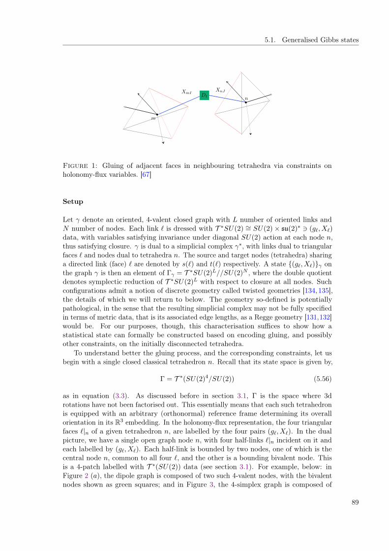
5.1. Generalised Gibbs states

m

n

XmIXnJ

D`

Figure 1: Gluing of adjacent faces in neighbouring tetrahedra via constraints onholonomy-flux variables. [67]

Setup

Let γ denote an oriented, 4-valent closed graph with L number of oriented links andN number of nodes. Each link ` is dressed with T ∗SU(2) ∼= SU(2)× su(2)∗ 3 (g`, X`)data, with variables satisfying invariance under diagonal SU(2) action at each node n,thus satisfying closure. γ is dual to a simplicial complex γ∗, with links dual to triangularfaces ` and nodes dual to tetrahedra n. The source and target nodes (tetrahedra) sharinga directed link (face) ` are denoted by s(`) and t(`) respectively. A state (g`, X`)γ onthe graph γ is then an element of Γγ = T ∗SU(2)L//SU(2)N , where the double quotientdenotes symplectic reduction of T ∗SU(2)L with respect to closure at all nodes. Suchconfigurations admit a notion of discrete geometry called twisted geometries [134,135],the details of which we will return to below. The geometry so-defined is potentiallypathological, in the sense that the resulting simplicial complex may not be fully specifiedin terms of metric data, that is its associated edge lengths, as a Regge geometry [131,132]would be. For our purposes, though, this characterisation suffices to show how astatistical state can formally be constructed based on encoding gluing, and possiblyother constraints, on the initially disconnected tetrahedra.

To understand better the gluing process, and the corresponding constraints, let usbegin with a single closed classical tetrahedron n. Recall that its state space is given by,

Γ = T ∗(SU(2)4/SU(2)) (5.56)

as in equation (3.3). As discussed before in section 3.1, Γ is the space where 3drotations have not been factorised out. This essentially means that each such tetrahedronis equipped with an arbitrary (orthonormal) reference frame determining its overallorientation in its R3 embedding. In the holonomy-flux representation, the four triangularfaces `|n of a given tetrahedron n, are labelled by the four pairs (g`, X`). In the dualpicture, we have a single open graph node n, with four half-links `|n incident on it andeach labelled by (g`, X`). Each half-link is bounded by two nodes, one of which is thecentral node n, common to all four `, and the other is a bounding bivalent node. Thisis a 4-patch labelled with T ∗(SU(2)) data (see section 3.1). For example, below: inFigure 2 (a), the dipole graph is composed of two such 4-valent nodes, with the bivalentnodes shown as green squares; and in Figure 3, the 4-simplex graph is composed of

89

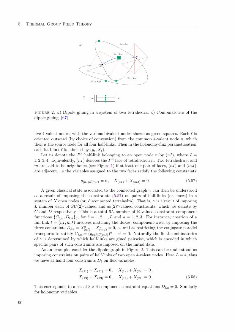
5. Thermal Group Field Theory

m

n

a)

b)m n

(Xm1, Xn1)

(Xm2, Xn2)

(Xm3, Xn3)

(Xm4, Xn4)

D`

Figure 2: a) Dipole gluing in a system of two tetrahedra. b) Combinatorics of thedipole gluing. [67]

five 4-valent nodes, with the various bivalent nodes shown as green squares. Each ` isoriented outward (by choice of convention) from the common 4-valent node n, whichthen is the source node for all four half-links. Then in the holonomy-flux parametrisation,each half-link ` is labelled by (g`, X`).

Let us denote the Ith half-link belonging to an open node n by (nI), where I =1, 2, 3, 4. Equivalently, (nI) denotes the Ith face of tetrahedron n. Two tetrahedra n andm are said to be neighbours (see Figure 1) if at least one pair of faces, (nI) and (mJ),are adjacent, i.e the variables assigned to the two faces satisfy the following constraints,

g(nI)g(mJ) = e , X(nI) +X(mJ) = 0 . (5.57)

A given classical state associated to the connected graph γ can then be understoodas a result of imposing the constraints (5.57) on pairs of half-links (or, faces) in asystem of N open nodes (or, disconnected tetrahedra). That is, γ is a result of imposingL number each of SU(2)-valued and su(2)∗-valued constraints, which we denote byC and D respectively. This is a total 6L number of R-valued constraint componentfunctions C`,a , D`,aγ , for ` = 1, 2, ..., L and a = 1, 2, 3. For instance, creation of afull link ` = (nI,mJ) involves matching the fluxes, component-wise, by imposing thethree constraints D`,a = Xa

(nI) +Xa(mJ) = 0, as well as restricting the conjugate parallel

transports to satisfy C`,a = (g(nI)g(mJ))a − ea = 0. Naturally the final combinatorics

of γ is determined by which half-links are glued pairwise, which is encoded in whichspecific pairs of such constraints are imposed on the initial data.

As an example, consider the dipole graph in Figure 2. This can be understood asimposing constraints on pairs of half-links of two open 4-valent nodes. Here L = 4, thuswe have at hand four constraints D` on flux variables,

X(11) +X(21) = 0 , X(12) +X(22) = 0 ,

X(13) +X(23) = 0 , X(14) +X(24) = 0 . (5.58)

This corresponds to a set of 3× 4 component constraint equations D`,a = 0. Similarlyfor holonomy variables.

90

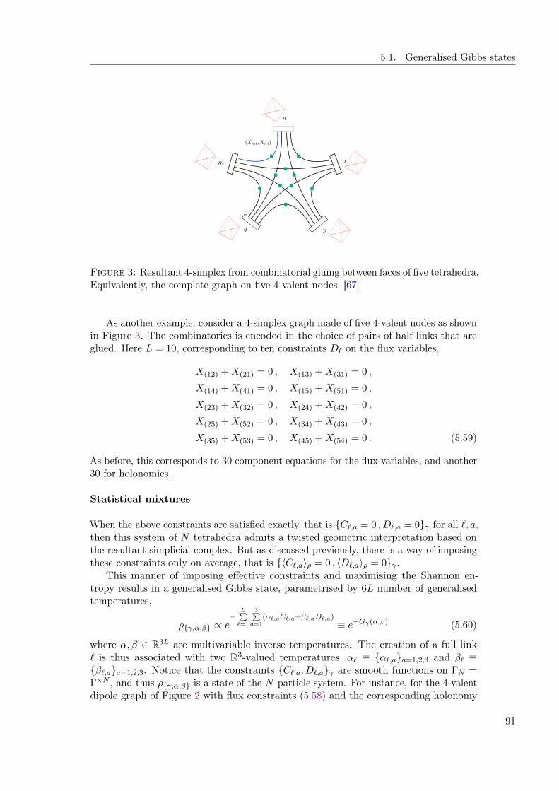
5.1. Generalised Gibbs states

m

n

o

pq

(Xm1, Xn1)

Figure 3: Resultant 4-simplex from combinatorial gluing between faces of five tetrahedra.Equivalently, the complete graph on five 4-valent nodes. [67]

As another example, consider a 4-simplex graph made of five 4-valent nodes as shownin Figure 3. The combinatorics is encoded in the choice of pairs of half links that areglued. Here L = 10, corresponding to ten constraints D` on the flux variables,

X(12) +X(21) = 0 , X(13) +X(31) = 0 ,

X(14) +X(41) = 0 , X(15) +X(51) = 0 ,

X(23) +X(32) = 0 , X(24) +X(42) = 0 ,

X(25) +X(52) = 0 , X(34) +X(43) = 0 ,

X(35) +X(53) = 0 , X(45) +X(54) = 0 . (5.59)

As before, this corresponds to 30 component equations for the flux variables, and another30 for holonomies.

Statistical mixtures

When the above constraints are satisfied exactly, that is C`,a = 0 , D`,a = 0γ for all `, a,then this system of N tetrahedra admits a twisted geometric interpretation based onthe resultant simplicial complex. But as discussed previously, there is a way of imposingthese constraints only on average, that is 〈C`,a〉ρ = 0 , 〈D`,a〉ρ = 0γ .

This manner of imposing effective constraints and maximising the Shannon en-tropy results in a generalised Gibbs state, parametrised by 6L number of generalisedtemperatures,

ργ,α,β ∝ e−

L∑=1

3∑a=1

(α`,aC`,a+β`,aD`,a)≡ e−Gγ(α,β) (5.60)

where α, β ∈ R3L are multivariable inverse temperatures. The creation of a full link` is thus associated with two R3-valued temperatures, α` ≡ α`,aa=1,2,3 and β` ≡β`,aa=1,2,3. Notice that the constraints C`,a, D`,aγ are smooth functions on ΓN =Γ×N , and thus ργ,α,β is a state of the N particle system. For instance, for the 4-valentdipole graph of Figure 2 with flux constraints (5.58) and the corresponding holonomy

91

5. Thermal Group Field Theory

ones, we have

Gdip(α, β) =4∑`=1

3∑a=1

α`,aC`,a(g(1`), g(2`)) + β`,aD`,a(X(1`), X(2`)) . (5.61)

We could further consider the case of assigning a single temperature for all threecomponents a. Then, one pair of R-valued parameters, α` and β`, controls each link `,instead of three pairs. We would thus get,

ργ,α,β ∝ e−

L∑=1α`C`+β`D`

(5.62)

where α, β ∈ RL, C` =∑

aC`,a and D` =∑

aD`,a [67]. Making such different choicesis a non-trivial move (cf. discussions in section 2.3.2); notice that C`,a = 0, D`,a =0γ ⇒ C` = 0, D` = 0γ but the converse is not true. Latter is thus a weakercondition than the former. States (5.60) and (5.62) correspond to these two sets ofconditions respectively, associated with the constraints, s1 = 〈C`,a〉 = 0, 〈D`,a〉 = 0γand s2 = 〈C`〉 = 0, 〈D`〉 = 0γ , in the entropy maximisation procedure.

If we were further to extract a single common temperature, say βγ , then this wouldcorrespond to a set with a single constraint, s3 = 〈Gγ〉 = 0γ (cf. discussions in section2.3.2). Being associated with a sum of all constraints, s3 is in turn weaker than boths1 and s2. Then, the state with respect to s3 is naturally of the form ρβγ ∝ e−βγGγ .Notice that, in the weaker cases s2 and s3, the corresponding microcanonical statescannot be understood as giving back a state in Γγ , i.e. as giving a twisted geometry(unlike s1). This is because making γ requires imposing C`,a = 0, D`,a = 0γ (which isa microcanonical state of s1), and not either of the two weaker conditions.

A state such as (5.60) is a statistical mixture of configurations where the oneswhich are glued with the combinatorics of γ, and thus admit a discrete geometricinterpretation, are weighted exponentially more than those which are not. In this sense,such a state illustrates a statistically approximate notion of discrete (here, twisted)geometry. Notice that states like (5.62) and ρβγ would encode an even weaker notion ofstatistically fluctuating (approximate) geometries, even if that, because in general eventhose configurations satisfying C` = 0, D` = 0 or Gγ = 0 exactly would not necessarilycorrespond to a graph in Γγ .

We can further generalise the above to include different ‘interaction’ terms, eachcorresponding to a given combinatorial pattern of gluings associated with a differentgraph γ. Let us first take into account all possible graphs γN with a fixed number ofnodes N . To each γ in this set corresponds a gluing Gγ(α, β) as a function of severaltemperatures, which control the fluctuations in the internal structure of the graph γ.We can then think of a statistical mixture of the different graphs, each being representedby its corresponding gluing function Gγ and weighted by coupling parameters λγ . Sucha Gibbs distribution can be formally written as,

ρN =1

ZN (λγ , α, β)e−

∑γN

1ksym

λγGγ(α,β)

(5.63)

where ksym factors out any repetitions due to underlying symmetries, say due to graphautomorphisms [67]. The choice of the set γN is a model-building choice, analogous

92

5.1. Generalised Gibbs states

to choosing different interaction terms in the Hamiltonian of a standard many-bodysystem.

This can heuristically be generalised further to a superposition of such internallyfluctuating twisted geometries for an N particle system, but now including contributionsfrom distinct graphs, each composed of in general a variable number of nodes M . Inline with analogous expressions in standard many-body theory, a state of this kind canformally be written as,

ρN =1

ZN (Mmax, λγ , α, β)e−Mmax∑M=2

∑γM

1ksym

λγN∑

i1 6=... 6=iM=1Gγ(~gi1 ,

~Xi1 ,...,~giM , ~XiM ;α,β)

(5.64)

where i is the particle index, and Mmax ≤ N [25]. The value of Mmax and the set γMfor a fixed M are model-building choices. The first sum over M includes contributionsfrom all admissible (depending on the model, determined by Mmax) different M -particlesubgroups of the full N particle system, with the gluing combinatorics of the differentboundary graphs with M nodes. The second sum is a sum over all admissible boundarygraphs γ, with a given fixed number of nodes M . And, the third sum takes into accountall M -particle subgroup gluings (according to a given fixed γ) of the full N particlesystem. We note that the state (5.64) is a further generalisation of the state (5.63)above, specifically the latter is a special case of the former for the case of a single termM = Mmax = N in the first sum. Let us consider a simple example, to understand betterthe definition of (5.64). Let the total number of particles be N = 3; and, the modelbe defined by a single, two-particle interaction, i.e. Mmax = 2. Let this interaction becharacterised by a single 2-particle graph, say a dipole graph, i.e. the set of admissiblegraphs is γdip. Then, in the exponent: the first two sums contribute with a singleterm each; and, the last sum is

3∑i1=1

3∑i2 6=i1=1

Gdip(~gi1 ,~Xi1 , ~gi2 ,

~Xi2 ;α, β) (5.65)

where, Gdip(~g1, ~X1, ~g2, ~X2;α, β) ≡ Gdip(α, β) as given in equation (5.61) above. Thissum consists of six terms in total, which reduce to three for indistinguishable particles.This corresponds to the three possible pairings of the total N = 3 particles, i.e. the threenumber of 2-particle subgroups in a system with total 3 particles; and, each 2-particlesubgroup interacts by Gdip.

Finally, allowing for the system size N to vary, we get a grand-canonical state,

Z(µ,Mmax, λγ , α, β) =∑N≥0

eµNZN (Mmax, λγ , α, β) (5.66)

where µ is the Lagrange parameter for N , and ZN is the canonical partition functionfor a finite number of tetrahedra, but including different graph contributions given bythe state (5.64). The resultant set of parameters µ,Mmax, λγ , α, β are thus directlyderived from the underlying microscopic model, as should be the case in any statisticalconsideration.

Discussion

93

5. Thermal Group Field Theory

Now that we have discussed states for many classical tetrahedra, involving gluingconstraints that impose a discrete geometric interpretation, we conclude with a briefdiscussion of some model-building strategies in the context of simplicial gravity.

Any such strategy would have to be based on a clear understanding of how simplicialgeometry is encoded in the data that is used. For instance, in the case of holonomy-fluxgeometries discussed above, the simplicial geometric content is precisely that of classicaltwisted geometries [134, 135]. In other words, the holonomy-flux variables admit anequivalent parametrisation in terms of twisted geometries variables. This relies on the factthat the link space T ∗SU(2) can be decomposed as S2×S2×T ∗S1 3 (Ns(`),Nt(`), A`, ξ`),modulo null orbits of the latter, and up to a Z2 symmetry. The variables are related bythe following canonical transformations,

g = nseξτ3n−1

t , X = Ansτ3n−1t (5.67)

where ns,t ∈ SU(2) are those elements which in the adjoint representation R rotatethe vector z ≡ (0, 0, 1) to give R3 vectors Ns,t respectively. That is Ns,t = R(ns,t).z,or equivalently ns,tτ3n

−1s,t =

∑3a=1 N

as,tτa respectively for s and t, where τa = − i

2σa aregenerators of su(2), with Pauli matrices σa. Vectors Ns(`) and Nt(`) are unit normals tothe face ` as seen from two arbitrary, different orthonormal reference frames attached tos(`) and t(`) respectively. A` is the area of `, and ξ` is an angle which encodes (partial22)extrinsic curvature information. So, a closed twisted geometry configuration supportedon graph γ is: an element of `T ∗S1

n S4, where S4 is the Kapovich-Millson phasespace of a tetrahedron given a set of face areas; each link of γ is labelled with (A`, ξ`);and each node of γ is labelled with four area normals (in a given reference frame) thatsatisfy closure. [134,135]

A twisted geometry is in general discontinuous across the faces, and so is the onedescribed in terms of holonomy-flux variables, because both contain the same information.Face area A` of a shared triangle is the same as seen from tetrahedron s(`) or t(`) on eitherside, but the edge lengths when approaching from either side may differ in general [134].That is, the shape of the triangle `, as seen from the two tetrahedra sharing it, is notconstrained to match. If additional shape-matching conditions [133] were satisfied, thenwe would instead have a proper Regge (metric) geometry on γ∗, which is then a subclassof twisted geometries. These shape-matching conditions can be related to the so-calledsimplicity constraints, which are central in all model building strategies in the contextof spin foam models, and whose effect is exactly to enforce geometricity (in the sense ofmetric and tetrad geometry) on discrete data of the holonomy-flux type, characterising(continuum and discrete) topological BF theories.

The gluing constraints in equation (5.57), take the form of the following constraintsin twisted geometry variables,

A(nI) −A(mJ) = 0 , ξ(nI) + ξ(mJ) = 0 ,

Ns(nI) −Nt(mJ) = 0 , Nt(nI) −Ns(mJ) = 0 . (5.68)

The result is naturally the same as in the holonomy-flux case: half-links (nI) and (mJ)which satisfy the above set of six component constraint functions (in either of the

22The remaining two degrees of freedom of extrinsic curvature are encoded in the normals Ns(`) andNt(`) [134]. For instance, in the subclass of Regge geometries, ξ` is proportional to the modulus of theextrinsic curvature [135].

94

5.2. Thermofield doubles, thermal representations and condensates

parametrisations) are glued23 to form a single link ` ≡ (nI,mJ). Equivalently, the twofaces of the initially disconnected tetrahedra are now adjacent.

The more refined parametrisation used in the twisted geometry language would allowfor a model-building strategy leading, for example, to statistical states in which onlysome of the gluing conditions are imposed strongly, while others are imposed on average.In the same spirit of achieving greater geometrical significance of the statistical state thatone ends up with, this construction scheme can be applied with additional constraints,beyond the gluing ones that we illustrated above. For instance, starting with the space oftwisted geometries on a given simplicial complex dual to γ, one could consider imposing(on average) also shape-matching constraints, or simplicity constraints, to encode anapproximate notion of a Regge geometry using a Gibbs statistical state. This would bethe statistical counterpart of the construction of spin foam models, i.e. discrete gravitypath integrals in representation theoretic variables [193–195], based on the formulationof gravity as a constrained BF theory. These lines of investigations are left to futurework.

Lastly, we remark that the quantum counterparts of the above states can formally bedefined onHF , and the general discussion above is applicable [66,67]. The basic ingredientof gluing is again to define face sharing conditions. For instance, the classical constraintsof equation (5.57) can be implemented by group averaging of wavefunctions [66],

Ψγ(g(nI)g−1(mJ)) =

∏(nI,mJ)|γ

∫SU(2)

dh(nI,mJ) ψ(g(nI)h(nI,mJ), g(mJ)h(nI,mJ)) (5.69)

where ψ ∈ HN is a wavefunction for a system of generically disconnected N tetrahedra.So, a wavefunction defined over full links (nI,mJ) of a graph γ is a result of averagingover half-links (nI) and (mJ) by SU(2) elements h(nI,mJ). The same can also beimplemented in terms of fluxes X, using a non-commutative Fourier transform betweenthe holonomy and flux variables [66,141,142].

5.2 Thermofield doubles, thermal representations andcondensates

Quantum gravitational phases that display features like entanglement, coherence andobservable statistical fluctuations are important in the study of semi-classical andeffective continuum descriptions of quantum spacetime, especially in physical settingslike cosmology and black holes. In this section, we construct entangled, thermofield doublestates |Ωρ〉, associated with a generalised Gibbs state ρ. These states naturally encodestatistical fluctuations with respect to the given observables of interest, characterisingρ. We further construct their corresponding inequivalent representations. Subsequently,we introduce a family of thermal condensates built upon the thermal vacua |Ωρ〉, ascoherent configurations of the underlying quanta. [45]

23Gluing the two half-links is essentially superposing one over the other in terms of aligning theirrespective reference frames. This is evident from the constraints for the normal vectors N whichsuperposes the target node of one half-link on the source node of the other, and vice-versa.

95

5. Thermal Group Field Theory

5.2.1 Preliminaries: Thermofield dynamics

Thermofield dynamics (TFD) is an operator framework for finite temperature quantumfield theory [37, 38, 196–198]. One of its main advantages lies in the fact that itsformulation parallels that of zero temperature quantum field theory. Thus powerful toolsof the temperature-independent setup can be translated to the thermal case, includingperturbative Feynman diagrammatic techniques, symmetry breaking analyses, and forwhat concerns us here, Fock space techniques. TFD has been applied in various fieldssuch as superconductivity, quantum optics, and string theory.

The core idea of the TFD formalism is to represent statistical ensemble averages astemperature-dependent vacuum expectation values. That is, given a system describedby a Hilbert space h and an algebra of observables Ah on h, one looks for a vector state|Ωρ〉 (thermal vacuum) in a Hilbert space H, corresponding to a density operator ρ on h,such that the following condition holds for all observables A of the system,

Trh(ρAh) = 〈Ωρ|AH |Ωρ〉H (5.70)

where the subscript h or H denotes a suitable representation of the operator in therespective Hilbert spaces. Here, we are mainly concerned with statistical equilibrium,thus with density operators of the Gibbs form e−βOh as discussed in the previous sections.Further, notice that the vector state |Ωρ〉 encodes the same information as the densityoperator ρ, as reflected in equations (5.70) holding for the full algebra. Thus, like instandard treatments of systems in a state ρ, statistical fluctuations in the correspondingstate |Ωρ〉 can be investigated for instance in terms of variances of relevant observablesin this state.

A vector state satisfying equation (5.70) can only be defined in an extended Hilbertspace, by supplementing the original degrees of freedom with the so-called tilde conjugatedegrees of freedom [37]. Importantly, this doubling, or in general an enlargement of thespace of the relevant degrees of freedom, is a characteristic feature of finite temperaturedescription of physical systems. This was discovered also in algebraic quantum fieldtheory for equilibrium statistical mechanics [36]. In fact, equation (5.70) is stronglyreminiscent of the construction of a GNS representation induced by an algebraic statisticalstate [31–33, 187], with the vector state |Ωρ〉 being the cyclic vacuum of a thermalrepresentation. These intuitions have indeed led to tangible relations between the twoformalisms, with the tilde degrees of freedom of TFD being understood as those of theconjugate representation of KMS theory in the algebraic framework [38,196,199–201].

As we have noticed previously, these structures are also encountered commonly inquantum information theory [202], which in turn is utilised heavily in various areas ofmodern theoretical physics, like holography. Specifically, constructing a state |Ωρ〉 issimply a purification of ρ. A prime example of a vector state is the thermofield doublestate, which is the purification of a Gibbs density operator. These states are used exten-sively in studies probing connections between geometry, entanglement, and more recently,complexity [19,203]. For instance in AdS/CFT, this state is important because an eternalAdS black hole bulk is dual to a thermofield double in the boundary quantum theory [44].

We now review the basics of the TFD formalism [37,38,196–198], based on whichwe will later carry out our construction of thermofield doubles and their associatedinequivalent representations in GFT. Here we consider a simple example of an oscillator,

96

5.2. Thermofield doubles, thermal representations and condensates

which will be extended to a field theory setup directly for GFTs in the subsequentsections.

Consider a single bosonic oscillator, described by ladder operators a and a†, satisfyingthe commutation algebra,

[a, a†] = 1 , [a, a] = [a†, a†] = 0 (5.71)

with the a-particle vacuum being specified by

a |0〉 = 0 . (5.72)

A Fock space h is generated by actions of polynomial functions of the ladder operatorson |0〉. Thermal effects are then encoded in density operators defined on h. In particular,an equilibrium state at inverse temperature β is a Gibbs state,

ρβ =1

Ze−βH (5.73)

where H is a Hamiltonian operator on h, possibly of grand-canonical type. But asdiscussed in chapter 2 and section 5.1 above, in the context of background independentsystems one may work (at least formally) with other observables in place of H.

This system is extended by including tilde degrees of freedom, spanning a Hilbertspace h generated by the ladder operators a and a† satisfying the same bosonic algebra,

[a, a†] = 1 , [a, a] = [a†, a†] = 0 (5.74)

acting on the tilde-vacuum given by,

a |0〉 = 0 . (5.75)

All tilde and non-tilde degrees of freedom commute with each other, that is

[a, a] = [a, a†] = [a†, a] = [a†, a†] = 0 . (5.76)

The Hilbert space h is conjugate to the original one via the following tilde conjugationrules of thermofield dynamics (or equivalently, via the action of the modular conjugationoperator of KMS theory [199]): (AB) = AB, (A†) = A†, (A) = A, (z1A+ z2B) =z1A + z2B, and |0〉˜ = |0〉, for all non-tilde and tilde operators defined on h and hrespectively, and z1, z2 ∈ C.

The zero temperature (or the limiting case of its inverse, β =∞) phase of the systemis described by the enlarged Hilbert space,

H∞ = h⊗ h (5.77)

built from the Fock vacuum,|0∞〉 = |0〉 ⊗ |0〉 (5.78)

by actions of the ladder operators a, a†, a, a†, such that

a |0∞〉 = a |0∞〉 = 0 . (5.79)

Temperature is introduced via thermal Bogoliubov transformations of the algebra gener-ators,

a, a†, a, a†β=∞ 7→ b, b†, b, b†0<β<∞ (5.80)

97

5. Thermal Group Field Theory

given by

b = cosh[θ(β)] a− sinh[θ(β)] a† (5.81)

b = cosh[θ(β)] a− sinh[θ(β)] a† (5.82)

along with analogous expressions for their adjoints b† and b†. The Bogoliubov transfor-mations are canonical, thus leaving the algebra unchanged. Then, the β-ladder operatorsalso satisfy bosonic commutations relations, given by

[b, b†] = [b, b†] = 1 (5.83)

[b, b] = [b, b†] = 0 (5.84)

along with their adjoints. The temperature-dependent annihilation operators now specifya thermal vacuum,

b |0β〉 = b |0β〉 = 0 (5.85)

which is cyclic for a thermal Hilbert space Hβ .24

The Hilbert space Hβ can naturally be organised as a Fock space with respect tothe β-dependent ladder operators that create and annihilate b-quanta over the thermalbackground |0β〉. Like in any other Fock space construction, one can define useful classesof states in Hβ. We will return to this point in section 5.2.4 where we define one suchinteresting class of states in the quantum gravity system, namely the coherent thermalstates.

The thermal Bogoliubov transformations (5.81) are parametrized by θ(β), whichmust thus encode complete information about the corresponding statistical state. In thepresent case, it must be uniquely associated with the Gibbs state ρβ, which has a wellknown characteristic Bose number distribution,

Trh(ρβa†a) =1

eβω − 1(5.86)

using a Hamiltonian of the form H = ωa†a, and the number operator N = a†a of theoriginal non-tilde system (which is the physical system of interest, see below). This ishow θ is usually determined in TFD, by using equation (5.70) for the number operator.Then, the right hand side of equation (5.70) for the number operator gives

〈0β| a†a |0β〉Hβ = sinh2[θ(β)] (5.87)

using inverse Bogoliubov transformations. This specifies θ via the equation,

1

eβω − 1= sinh2[θ(β)] . (5.88)

The non-tilde degrees of freedom can be understood as being physically relevantin the sense that they describe the subsystem of interest, which is accessible to anobserver. In other words, it is the subsystem under study in a given situation. Then, thephysically relevant observables are naturally those that belong to the algebra restricted

24We note that |0β〉 is an example of a two-mode squeezed state, which can be restored to its fullgenerality most directly by adding a net phase difference between the cosh and sinh terms in thetransformations (5.81) and (5.82).

98

5.2. Thermofield doubles, thermal representations and condensates

to the non-tilde degrees of freedom, which can be retrieved from the full description bypartially tracing away the complement (here, the tilde degrees of freedom). Thus, one isinterested in observable averages of the form 〈0β| O(a, a†) |0β〉, for operators O that arein general polynomial functions of the generators of the physical (in the above sense)non-tilde algebra. Notable geometric examples include relativistic quantum field vacuain Minkowski and Schwarzschild spacetimes, where the non-tilde algebra has support onspacetime regions exterior to the respective horizons. Here, the tilde subsystems are CPTconjugates of the non-tilde ones, and belong to the interior of the horizons [39,43,204].Another physical interpretation of the tilde subsystem that is more common in condensedmatter theory, is that of a thermal reservoir [187,197].

In the present discrete quantum gravity context, for now we retain the elementary,quantum information-theoretic interpretation of the non-tilde and tilde degrees of freedom,simply as describing a given subsystem and its complement respectively, without assigningany further geometric meanings.

The two sets of ladder operators are related to each other explicitly via equations (5.81)and (5.82). This suggests that their respective vacua are also related by a correspondingtransformation. Indeed they are, via the following unitary transformation25

U(θ) = eθ(β)(a†a†−aa) . (5.89)

In terms of this thermal squeezing operator, we then have

|0β〉 = U(θ) |0∞〉 (5.90)

and

b = U(θ) aU(θ)−1 , (5.91)

b = U(θ) a U(θ)−1 . (5.92)

It is clear then that such unitary operators map the different β-representations intoeach other. In finite quantum systems this is simply a manifestation of von Neumann’suniqueness theorem. However, when extending the above setup to quantum field theory,one would expect that representations at different temperatures are inequivalent. This iscertainly the case for standard physical systems in general. It is also true in the presentquantum gravity case, as we show in section 5.2.3. Lastly, we note that in the fieldtheory extension, equations (5.81)-(5.85) hold mode-wise and still remain well-defined.Together, they describe the β-phase of the system. However, the operator U(θ) isno longer well-defined in general (before any cut-offs). Thus, without any suitableregularisation, equations (5.89)-(5.92) technically do not hold in full field theory.

5.2.2 Degenerate vacuum and zero temperature phase

The zero temperature phase of the system is based on an enlargement of the Fockrepresentation of the bosonic algebra associated with the degenerate vacuum (as describedin sections 3.1 and 4.1), along the lines presented in 5.2.1 above, but generalised here toa field theory.

25The form of this unitary operator, along with equation (5.90), shows that the thermal vacuum |0β〉is a two-mode squeezed state in which aa-pairs have condensed [198].

99

5. Thermal Group Field Theory

We consider here (mainly for convenience of the subsequent application in GFTcosmology in section 5.3) the Hilbert space for a single quantum to be given by the statespace of geometries of a quantum polyhedron with a single real scalar coupling, that is

H = L2(SU(2)d/SU(2))⊗ L2(R) (5.93)

where the quotient by SU(2) ensures closure. Then in the discrete index basis introducedin section 4.1.2, we have the following mode ladder operators

a~χα = ϕ(D~χ ⊗Tα) =

∫SU(2)d×R

d~gdφ D~χ(~g)Tα(φ)ϕ(~g, φ) (5.94)

a†~χα = ϕ†(D~χ ⊗Tα) =

∫SU(2)d×R

d~gdφ D~χ(~g)Tα(φ)ϕ†(~g, φ) (5.95)

which satisfy,[a~χα, a

†~χ′α′ ] = δ~χ~χ′δαα′ (5.96)

and [a, a] = [a†, a†] = 0. As mentioned previously in 4.1.2, we find that the use ofdiscrete indices can help in avoiding δ distributional divergences in relevant quantities.We will return to this point in the upcoming sections. Recall that the vacuum is givenby,

a~χα |0〉 = 0 , ∀ ~χ, α (5.97)

which is the degenerate vacuum ΩF that we have been considering till now, but herewith a notational change |0〉 ≡ |ΩF 〉. It generates the Fock space HF of equation (4.9).

The zero temperature phase is then given by extending the above with the conjugaterepresentation space HF , as discussed in section 5.2.1. This gives the zero temperature(β =∞) description in terms of a Hilbert space,

H∞ = HF ⊗ HF (5.98)

which is a Fock space on the cyclic vacuum

|0∞〉 = |0〉 ⊗ |0〉 (5.99)

with ladder operators a, a†, a, a†~χ,α that satisfy,

[a~χα, a†~χ′α′ ] = δ~χ~χ′δαα′ (5.100)

[a~χα, a†~χ′α′ ] = δ~χ~χ′δαα′ (5.101)

and [a, a] = [a, a] = [a, a] = [a, a†] = 0. The non-tilde operators describing the system ofinterest are those defined in (5.94) and (5.95), while the tilde operators of the complementare given by,

a~χα =

∫SU(2)d×R

d~gdφ D~χ(~g)Tα(φ)ϕ(~g, φ) , (5.102)

a†~χα =

∫SU(2)d×R

d~gdφ D~χ(~g)Tα(φ)ϕ†(~g, φ) . (5.103)

The vacuum satisfiesa~χα |0∞〉 = a~χα |0∞〉 = 0 , ∀ ~χ, α . (5.104)

The action of all polynomial functions of non-tilde and tilde ladder operators on |0∞〉generates H∞, all in complete analogy with standard HF , including the construction ofmulti-particle states, coherent states, squeezed states, and so on.

100

5.2. Thermofield doubles, thermal representations and condensates

5.2.3 Thermal squeezed vacuum and finite temperature phase

The familiar way to include thermal effects is with statistical states, as density operatorsin a given representation. As discussed in section 5.2.1, an equivalent way is with theircorresponding vector states (thermal vacua) in an enlarged representation of the system,in which the additional degrees of freedom are integral for encoding finite temperatureeffects.

Here we are interested in generalised Gibbs density operators for describing equi-librium phases of the quantum gravity system, as discussed in the previous sections.Specifically, we consider the well-behaved class of states defined by extensive, positiveoperators P for group field theories coupled with scalar matter presented in section5.1.1. For these states the above machinery of TFD can be applied directly, to constructvarious different phases characterised by the corresponding thermofield double vacua.In the context of cosmology for instance, we will be interested in choosing P to be aspatial volume operator (see section 5.3) [95]. For now, we leave it as this more generalclass of states, as reported in [45].

From discussions in 5.2.1, we know that the ensemble average for number density isuseful for the construction of the associated thermal representation. For the class of states(5.3) generated by operators (5.1), it is given by the characteristic Bose distribution,

TrHF (ρβ,µa†~χαa~χα) =

1

eβ(λ~χα−µ) − 1(5.105)

from which the average total number 〈N〉 of polyhedral quanta can be obtained bysumming over all ~χ and α. Partial sums over either ~χ or α would give average numberdensities 〈Nα〉 or 〈N~χ〉 respectively. In the context of relational dynamics, for instancein GFT cosmology [76–78, 148], quantities like 〈Nα〉 are strictly related to relationalobservables as functions of the matter variable φ [95], the details of which are includedin section 5.3.3.

Now that we have chosen a suitable class of Gibbs states of equation (5.3), we canproceed to define its associated thermal phase generated by a thermal vacuum |0β〉 andβ-dependent ladder operators b~χα, b†~χα, b~χα, b

†~χαβ, along the lines detailed in section

5.2.1.Thermal Bogoliubov transformations26 give the new ladder operators, mode-wise,

b~χα = cosh[θ~χα(β)] a~χα − sinh[θ~χα(β)] a†~χα (5.106)

b~χα = cosh[θ~χα(β)] a~χα − sinh[θ~χα(β)] a†~χα (5.107)

along with their adjoints b†~χα and b†~χα. Inverse transformations are,

a~χα = cosh[θ~χα(β)] b~χα + sinh[θ~χα(β)] b†~χα (5.108)

a~χα = cosh[θ~χα(β)] b~χα + sinh[θ~χα(β)] b†~χα (5.109)

and their respective adjoints. The β-dependent annihilation operators specify the thermalvacuum via

b~χα |0β〉 = b~χα |0β〉 = 0 , (5.110)26More general two-mode squeezing transformations can also be considered by taking a net phase

difference between the two contributions, say eiδ scaling the sinh terms.

101

5. Thermal Group Field Theory

thus giving the finite temperature Hilbert space Hβ. Notice that the state |0β〉 isa concrete example of a (class of) thermofield double state(s) in discrete quantumgravity. It is an entangled state, with quantum correlations between pairs of a~χα anda~χα polyhedral quanta.

Further, using equations (5.70), (5.105), and

〈0β| a†~χαa~χα |0β〉Hβ = sinh2[θ~χα(β)] , (5.111)

the parameters θ~χα can be determined from

sinh2[θ~χα(β)] =1

eβ(λ~χα−µ) − 1. (5.112)

Note that the singular case in equation (5.112) (or in (5.105)) can be understood asBose-Einstein condensation to the ground state of P (equation (5.1)) in the presentthermal gas of quantum gravitational atoms. Such a phenomenon was reported first inthe context of a volume Gibbs state, and was used to show a model-independent, purelystatistical mechanism for the emergence of a low-spin phase [24] (see section 5.1.1.2).

Lastly, the β-phase that we have constructed here, being described kinematicallyby |0β〉 , b~χα, b†~χα, b~χα, b

†~χα, is inequivalent to the zero temperature phase that is de-

scribed by |0∞〉 , a~χα, a†~χα, a~χα, a†~χα. This can be seen directly from the transformation

equations between the two vacua as follows:

|0β〉 = U(θ) |0∞〉 (5.113)

= e∑~χ,α θ~χα(a†

~χαa†~χα−a~χαa~χα) |0∞〉 (5.114)

= e−∑~χ,α ln cosh θ~χαe

∑~χ,α a

†~χαa†~χα

tanh θ~χα |0∞〉 (5.115)

=∏~χ,α

1

cosh θ~χα× e

∑~χ,α a

†~χαa†~χα

tanh θ~χα |0∞〉 . (5.116)

The pre-factor of the product of inverse cosh functions vanishes in general, withoutany cut-offs in the modes. This means that the overlap between the two vacua is zero,and the two representations built upon them are inequivalent. In other words, thistransformation in field theory is ill-defined in general due to an infinite number of degreesof freedom, giving rise to the inequivalent representations describing distinct phases ofthe system.

5.2.4 Coherent thermal condensates

We now define a family of coherent states in these thermal representations of GFT [45].We understand them as defining thermal quantum gravity condensates, expected tobe relevant in the studies of semi-classical and continuum approximations in discretequantum gravity models based on polyhedral quanta of geometry. Indeed, unlike thepurely thermal state |0β〉, coherent states can encode a notion of semi-classicality, withwhich one can attempt to extract effective dynamics from an underlying quantumgravity model. For instance in group field theory, it has been shown that a coherentcondensate phase of the a-quanta can support FLRW cosmological dynamics, and thusrepresents a viable choice of a quantum gravitational phase relevant in the cosmologicalsector [76–78, 91, 148]. But a coherent state over the degenerate vacuum (5.97) is

102

5.2. Thermofield doubles, thermal representations and condensates

unentangled, and we expect a geometric phase of the universe to be highly entangled.Moreover these states cannot in themselves encode statistical fluctuations in differentobservable quantities. Therefore, from a physical point of view, the construction ofcoherent thermal states is amply justified.

Coherent thermal states [38, 205–207] are a coherent configuration of quanta overthe thermal vacuum, implemented by displacing |0β〉 with displacement operators of theform,

Da(σ) = ea†(σ)−a(σ) (5.117)

for σ ∈ H. To recall, the usual coherent states |σ〉 ∈ HF of a-particles are,

|σ〉 := Da(σ) |0〉 , (5.118)

while |σ〉 ∈ HF for a-particles are,

|σ〉 := Da(σ) |0〉 . (5.119)

The tilde in the ket notation |σ〉 simply means that the state is an element of theconjugate Hilbert space, and Da is a displacement operator of the same form as (5.117)but for tilde ladder operators.

The most useful property of these states is that they are eigenstates of their respectiveannihilation operators,

a~χα |σ〉 = σ~χα |σ〉 (5.120)a~χα |σ〉 = σ~χα |σ〉 (5.121)

which is at the heart of their extensive use as robust, most classical-like, quantum states.Notice that under the tilde conjugation rules stated in section 5.2.1, we have

(|σ〉 ⊗ |0〉) = |0〉 ⊗ |˜σ〉 (5.122)

in H∞. That is, coherent states |σ〉 ∈ HF and |σ〉 ∈ HF , are conjugates of each other.Then, the following state

|σ, σ;∞〉 := |σ〉 ⊗ |˜σ〉 = Da(σ)Da(σ) |0∞〉 ∈ H∞ (5.123)

of the full system at zero temperature is self-conjugate (or conjugate-invariant), i.e.

|σ, σ;∞〉˜= |σ, σ;∞〉 . (5.124)

In the finite temperature phase then, coherent thermal states [38,205–207] are definedas the following self-conjugate27 states encoding coherence in the original a degrees offreedom over the thermal vacuum,

|σ, σ;β〉 := Da(σ)Da(σ) |0β〉 ∈ Hβ . (5.125)

27This is a natural feature to require in coherent thermal states in light of the fact that such stateswhen understood as quantum gravitational vacua along with their associated GNS representations, areexpected to be invariant under the tilde conjugation rule, i.e. |Ωσ,σ;β〉˜= |Ωσ,σ;β〉, as is well-known inalgebraic KMS theory.

103

5. Thermal Group Field Theory

Being elements of Hβ , as expected they are eigenstates of the β-annihilation operatorsb~χα with temperature-dependent eigenfunctions,

b~χα |σ, σ;β〉 = (cosh θ~χα − sinh θ~χα)σ~χα |σ, σ;β〉 , (5.126)

b~χα |σ, σ;β〉 = (cosh θ~χα − sinh θ~χα)σ~χα |σ, σ;β〉 . (5.127)

It is clear from the above eigenstate equations, along with inverse transformations(5.108) and (5.109), that states (5.125) are not eigenstates of the annihilation operator aof the original system. This is precisely how the expectation values of physical non-tildeoperators O(a, a†) display non-trivial thermal and coherence properties simultaneously.For instance, the average number density is,

〈σ, σ;β| a†~χαa~χα |σ, σ;β〉 = |σ~χα|2 + sinh2[θ~χα(β)] (5.128)

which contains both, the usual coherent condensate number density and an additionalthermal contribution associated with the statistical state.

It is important to note that our use of the basis D~χ⊗Tα, in particular of the discretebasis Tαα∈N for L2(R), in order to develop the finite-temperature GFT formalism interms of the ladder operators (equations (5.94)-(5.95) and (5.81)-(5.82)), was crucial.The observables that one might consider in a chosen model must admit domains ofdefinition which contain the sector of Hilbert space that one is interested in, here coherentthermal states. Otherwise, we quickly run into divergences and ill-defined expressions.This in particular applies to φ-dependent operators, not smeared with Tα. For instance,if one considers the number density operator as a function of φ,

N~χ(φ) =

∫d~gd~g′ D~χ(~g′)D~χ(~g)ϕ†(~g, φ)ϕ(~g′, φ) (5.129)

= a†~χ(φ)a~χ(φ) (5.130)

then, the calculation of the expectation value in a coherent thermal state would give,

〈N~χ(φ)〉σ,σ;β = |σ~χ(φ)|2 + sinh2[θ~χ(φ)] δ(φ− φ) (5.131)

which is clearly ill-defined, due to the presence of the Dirac delta distribution δ(0) inthe thermal part evaluated at the singular point. We thus need to consider smearedobservables such as the operator a†~χαa~χα in (5.128), where now the thermal contributioncontains a well-defined Kronecker delta δαα coefficient instead.

Lastly, we note that the use of such condensates, say with respect to a spatialvolume observable in cosmology (see section 5.3), can be understood as implementingboth semi-classical and continuum approximations [76–78,95,148]. Specifically, a semi-classical approximation resides in considering a coherent state, with its characteristicsingle-particle wavefunction being the relevant dynamical collective variable, whilea continuum approximation resides in considering a non-perturbative (inequivalent)condensate phase of the quantum gravity system, with (formally) an infinite number ofunderlying quanta.28 The novel feature of the coherent thermal phase though is thatof having statistical fluctuations associated with the thermal vacuum, in addition toquantum fluctuations inherent in any quantum state. Statistical fluctuations in generalare inevitable in macroscopic systems and could be non-trivial in both the semi-classicaland continuum limits. This is unlike purely quantum fluctuations which are expected tobe negligible in a semi-classical limit, but of significance especially at early times [94].

28In general, identifying suitable semi-classical and continuum limits in discrete quantum gravity is aknown open issue, and we do not address it directly in this thesis.

104

5.3. Thermal condensate cosmology

5.3 Thermal condensate cosmology

In this section, we utilise the results presented above, to discuss an effective cosmologicalmodel incorporating statistical fluctuations of quantum geometry [95]. This investigationbuilds directly on the works in [45,148,208], with the aim of evaluating some preliminaryconsequences of the presence of such fluctuations in cosmological evolution that isextracted from an underlying GFT dynamical model.

This is brought about by the use of thermal condensates [45], which we understandas describing a phase of the universe in which not all quanta have condensed. Such aphase seems likely in any reasonable geometrogenesis scenario, in which the universetransitions from a primordial pre-geometric hot thermal phase, to a phase with anapproximate notion of continuum and macroscopic geometry (here, encoded in thenotion of a condensate [76]), but naturally with a leftover thermal cloud in general,of quanta that have not condensed. In other words, here, we understand a pure, zerotemperature GFT condensate, that has been used extensively in previous works in GFTcosmology [77, 78, 148,208], as describing a suitable macroscopic phase only at very latetimes of the system’s evolution, and not throughout. What we work with instead isan intermediary phase that would be expected to arise in a transition between a hotpre-geometric phase and a pure condensate. Thus in this study, we present a scenariowherein the universe is modelled as a quantum gravitational condensate of elementaryquanta of geometry, along with a thermal cloud of the same quanta over it; and in which,an early time phase that is dominated by the thermal cloud, and a late time phase thatis dominated by the condensate, are generated dynamically.

We start by presenting the effective free GFT dynamics in a condensate phase withfluctuating geometric volume. We then introduce the notion of a reference clock function,and reformulate the setup, including the effective dynamical equations of motion, interms of functional quantities with respect to a generic class of these clock functions.Based on this, we present an effective, relational homogeneous and isotropic cosmologicalmodel, and discuss its late and early times properties.

Specifically, we work with a free GFT model coupled with a real-valued scalar field,and thermal condensates with a static (non-dynamical) thermal cloud. We derive effectivegeneralised evolution equations for homogeneous and isotropic cosmology, which includecorrection terms originating in the underlying quantum gravitational and statisticalproperties of the system. At late times, we recover the correct general relativistic limitof relational Friedmann equations. At early times, we get a bounce between contractingand expanding phases, and a phase of accelerated expansion that is characterised by anincreased number of e-folds compared with previously reported numbers for the sameclass of free models.

5.3.1 Condensates with volume fluctuations

Since we are interested in the homogeneous and isotropic cosmological sector, the mainobservable of interest is the volume operator, in particular the volume associated to a(spatial) hypersurface given by a foliation parametrized by a clock function (see section5.3.3). Recall that (see section 5.1.1.2) the GFT volume operator on HF is,

V :=∑~χ,α

v~χ a†~χαa~χα (5.132)

105

5. Thermal Group Field Theory

where v~χ ∈ R>0 is the volume assigned to a single quantum with a configuration~χ = (~j, ~m, ι), which is the representation data associated with SU(2)4.29 This is anextensive positive operator on HF , and its action on any multi-particle state gives thetotal volume by summing up the volume contribution v~χ from each quantum, as discussedpreviously.

Let us choose a statistical state of the form (5.3) such that the generator is thevolume operator above, i.e. a volume Gibbs state of the form

ρβ =1

Zβe−βV (5.133)

which encodes a statistically fluctuating volume of quantum spacetime [24,25]. Noticethat a constant shift in the spectrum, by the chemical potential µ, is implicit in theabove expression, since it will not be important in the following investigations. We referto section 5.1.1.2 for more discussions surrounding this class of states.

The quantum gravity condensate that we are interested in is a coherent thermal stateof the form (5.125), but associated specifically with the volume Gibbs state in equation(5.133). In other words, we are interested in a state |σ, σ;β〉, which is specified by twofunctions: the condensate wavefunction σ ∈ H, and the Bogoliubov parameter θ~χα(β)that is identified by the Bose number distribution of the state (5.133),

sinh2[θ~χα(β)

]=

1

eβv~χ − 1. (5.134)

Notice that since the spectrum of V is independent of the modes Tα, the functions θ~χαare also independent of them. Thus θ~χα = θ~χ, and we will drop the labels α in quantitiesassociated with θ from here on. Also, notice the following important property of ourchosen state,

limβ→∞

|σ, σ;β〉 = |σ, σ〉 = Da(σ)Da(σ) |0, 0〉 (5.135)

due to which all results of the previous works in GFT cosmology are reproduced here,when the fluctuations are turned off completely.

In the present context of extracting effective cosmological models from a candidatebackground independent theory of quantum gravity, the use of relational observables isof utmost importance. As mentioned previously, past works in GFT cosmology haveinterpreted and used the base manifold coordinate φ as a relational matter clock, andconsidered quantities such as N(φ) as relational observables. However we have alsonoticed that, in the present setting, such quantities (e.g. see equation (5.131)) containdivergences related to occurrences of the ill-defined δ(φ = 0) distributions. This had inturn prompted us to use a discrete basis Tα, as a first step for the inclusion of thermalfluctuations in the context of GFT condensates.30 It follows that in this basis, we areinterested in α-dependent quantities defined by a partial sum over ~χ, such as

Vα =∑~χ

v~χ a†~χαa~χα (5.136)

29In our present application of the results of previous chapters to GFT cosmology, we take the basemanifold to be SU(2)4 × R, in order to facilitate a direct comparison of results with past works whichmake the same choice of the base manifold.

30Further details about this aspect and the definition of a basis-independent clock are discussedbelow in section 5.3.3.

106

5.3. Thermal condensate cosmology

and its statistical average in the thermal condensate,

〈Vα〉σ,σ;β =∑~χ

v~χ(|σ~χα|2 + sinh2[θ~χ(β)

]) (5.137)

which includes statistical fluctuations in volume, in addition to the condensate volume.Finally we note that, since the thermal cloud is modelled in terms of the volume

Gibbs state whose Bose distribution is independent of α (which as we will see in section5.3.3, is strictly related to the evolution parameters for relational dynamics), we areessentially working in a first approximation wherein the thermal cloud is non-dynamical,and only the condensate part of the full system is dynamical. We will return to thispoint later in sections 5.3.5.3 and 5.3.6.

5.3.2 Effective group field theory dynamics

A generic GFT action with a local kinetic term and a non-local interaction term (higherthan quadratic order in the fields) takes the form,

S =

∫d~gdφ ϕ(~g, φ)K (~g, φ)ϕ(~g, φ) + Sint[ϕ, ϕ] (5.138)

and gives the following classical equation of motion,

K (~g, φ)ϕ(~g, φ) +δSint[ϕ, ϕ]

δϕ(~g, φ)= 0 . (5.139)

In the corresponding quantum theory on HF , the operator equation of motion is

K (~g, φ)ϕ(~g, φ) +δSint[ϕ, ϕ]

δϕ(~g, φ)= 0 (5.140)

with some choice of operator ordering (and the hat notation reinstated temporarily). Aneffective equation of motion can then be derived from the above operator equation bytaking its expectation value in a class of quantum states. Here, we take the coherentthermal states introduced above as this class of states, implementing a notion of semi-classical and continuum approximations31. We thus consider,

〈σ, σ;β|K (~g, φ)ϕ(~g, φ) +δSint[ϕ, ϕ]

δϕ(~g, φ)|σ, σ;β〉 = 0 . (5.141)

As a first step to investigate the role of statistical fluctuations of quantum geometryin condensate cosmology, we focus here only on the free part. This would allow usto display clearly the impact of non-zero thermal fluctuations. In other words, anydifference in results that we find, as compared to previous zero temperature free theorystudies, could then be attributed directly to the presence of these statistical fluctuations.Therefore, restricting to the kinetic term, we obtain

〈σ, σ;β|K (~g, φ)ϕ(~g, φ) |σ, σ;β〉 = K (~g, φ)σ(~g, φ) . (5.142)

31In line with previous works, we understand the implementation of semi-classical and continuumapproximations in the specific sense of using the class of coherent states (which are well-known to be themost classical quantum states, with a peak on a pair of classical conjugate variables), and a condensatephase (described by a collective condensate variable, and with a non-zero order parameter), respectively.

107

5. Thermal Group Field Theory

Further using the Peter-Weyl decomposition for σ,

σ(~g, φ) =∑~χ

D~χ(~g)σ~χ(φ) , (5.143)

and considering the following kinetic term (which is a standard choice in studies in GFTcosmology, see for instance [209] and references therein),

K = K0(~g) + K1(~g)∂2φ (5.144)

such that

K0(~g)(D~χ(~g)σ~χ(φ)) = B~χD~χ(~g)σ~χ(φ) (5.145)

K1(~g)∂2φ(D~χ(~g)σ~χ(φ)) = A~χD~χ(~g)∂2

φσ~χ(φ) (5.146)

we obtain the following equations of motion,

∂2φσ~χ(φ)−M~χσ~χ(φ) = 0 , ∀~χ (5.147)

where M~χ := −B~χ/A~χ . Notice that here, the dynamical variable is the φ-dependentcondensate wavefunction, σ(φ).

We see that the free GFT dynamical equation of motion in a coherent thermal statei.e. equation (5.147), is identical to the case in [148], where one considers a simplecoherent state (5.118) in HF with no thermal cloud. But as we can already anticipate,observable averages (like volume) will have thermal contributions in general, consequentlymodifying their evolution equations.

This concludes the derivation of the effective GFT equation of motion using a thermalcoherent state in a φ-basis. However as we saw above, calculations with observablesin this basis leads to singularities in the φ-dependent quantities. This brings us to thequestion of defining and applying a suitable time reference frame (a clock), and offer apreliminary interpretation of the resultant quantities.

5.3.3 Smearing functions and reference clocks

As we have emphasised before, the use of φ as a reference clock is not possible here sincethe quantities of interest, like 〈V (φ)〉, are mathematically ill-defined. This promptedus to define quantities like 〈Vα〉 instead. Below, we generalise this even further andintroduce generic32 square-integrable, complex-valued smooth functions,

t(φ) =∑α

tαTα(φ) (5.148)

in order to define observables and their dynamics as functionals of t(φ) (which will laterbe interpreted as relational). This brings us back to the aspect of smearing.

In the quantum operator setup described in section 5.2, instead of smearing thealgebra generators with a set of basis functions (D~χ ⊗Tα)(~g, φ), we could instead smearwith a complete set of more general smearing functions F (~g, φ) (usually also satisfyingadditional analyticity and sufficient decay properties). In particular for the φ variable,this would amount to smearing with smooth functions, say t(φ). This would result

32While satisfying certain boundary conditions, see equations (5.160).

108

5.3. Thermal condensate cosmology

in an equivalent, but basis-independent algebraic setup, as commonly encountered inWeyl C*-algebraic theory associated with bosonic quanta33. For our actual purposes, weretain the use of the Wigner basis D~χ(~g), in order to retain also the associated geometricinterpretation of (functions of) the spin labels ~χ, which is standard in both GFT andLQG. But, in the φ direction we smear with a function t(φ). We are thus interested insmeared operators of the form,

a~χ(t) =

∫SU(2)4×R

d~gdφD~χ(~g)t(φ)ϕ(~g, φ) (5.149)

a†~χ(t) =

∫SU(2)4×R

d~gdφD~χ(~g)t(φ)ϕ†(~g, φ) (5.150)

which are now understood as functional (relational) ladder operators, with respect tothe function t(φ). By extension, the volume operator now takes the form,

Vt :=∑~χ

v~χ a†~χ(t)a~χ(t) (5.151)

which is interpreted as the operator associated to a spatial slice labeled by the functiont.

Notice that in general, t-relational operators, and their expectation values, are non-local functions of their φ-relational counterparts. For instance, the average volume in athermal condensate state is

〈Vt〉σ,σ;β =∑~χ

v~χ(|σ~χ(t)|2 + sinh2 [θ~χ]||t||2

)(5.152)

where ||t||2 = (t, t)L2(R) and,

σ~χ(t) :=

∫Rdφ t(φ)σ~χ(φ) = (t, σ~χ)L2(R) . (5.153)

Then, the quantity 〈Vt〉σ,σ;β can be expressed in terms of a non-local function of φ, i.e.

〈Vt〉σ,σ;β =∑~χ

v~χ

∫R2

dφdφ′ t(φ)t(φ′) 〈N~χ(φ, φ′)〉σ,σ;β

(5.154)

whereN~χ(φ, φ′) := a†~χ(φ)a~χ(φ′) (5.155)

is the off-diagonal number density operator with expectation value,

〈N~χ(φ, φ′)〉σ,σ;β

= σ~χ(φ)σ~χ(φ′) + sinh2[θ~χ]δ(φ− φ′) . (5.156)

This generic non-locality of t-relational quantities with respect to φ, for instance in(5.154), is reasonable to expect simply as a technical feature that is characteristic ofchanging reference frames in general.

Lastly, the smearing functions t(φ) are understood as defining reference clock frames,the reasons for which are made more clear in the next section. For now, we note that

33See section 4.1.3 for more details on a Weyl algebraic formulation in group field theory [24,91].

109

5. Thermal Group Field Theory

such a treatment is compatible with the fact that at the level of a field theory, which aGFT is, we would expect a relational clock variable to be more reasonably defined as agenuine function, like t(φ), rather than simply a parameter φ (which is here a coordinateof the base manifold). Having said that, we strictly refrain from assigning any furtherphysical interpretation to the function t, especially from the spacetime point of view,unlike the coordinate φ which has been motivated as a minimally coupled scalar matterfield in previous works (see for instance [147]).

5.3.4 Relational functional dynamics

We now come to the important task of expressing the effective GFT equations of motionin terms of the smearing functions. The goal is to arrive at a consistent dynamicaldescription of the present system in a t-relational reference frame. Let us first reiterateour main line of reasoning. Smearing functions t(φ) are used in order to avoid divergencesin the φ-frame, e.g. in relational quantities like 〈V (φ)〉σ,σ;β. This leads to observableslike 〈Vt〉σ,σ;β . The condensate functional σ~χ(t) defined in (5.153), then naturally takes onthe role of the dynamical collective variable, instead of σ~χ(φ). Therefore, the equationsof motion (5.147) in terms of the variable φ, must be rewritten suitably in terms offunctions t, as follows.

We are seeking a differential equation of motion for σ~χ(t), encoding the same dynamicsas (5.147). We begin by noticing that the mass term in (5.147) can be written in termsof σ~χ(t) simply as

M~χσ~χ(t) =

∫RdφM~χt(φ)σ~χ(φ) (5.157)

using the smearing. Therefore, as before, we see that smearing might offer us a wayforward. We then smear the equations (5.147), with an arbitrary square-integrablecomplex-valued smooth function t(φ), obtaining∫

Rdφ t(φ)∂2

φσ~χ(φ)−M~χσ~χ(t) = 0 , ∀~χ . (5.158)

Now, in order to get a description completely in the t-frame, we require a suitablederivative operator with a well-defined action on functionals of t. For this, notice that,∫

Rdφ t(φ)∂2

φσ~χ(φ) =

(−∫Rdφ ∂φt

δ

δt(φ)

)2

σ~χ(t)

=: d2tσ~χ(t) (5.159)

where we have used integration by parts, and the following boundary conditions for thesmearing functions,

limφ→±∞

t(φ) = 0 , limφ→±∞

∂φt(φ) = 0 . (5.160)

The operator dt might seem to be a good choice for the functional derivative [210,211] thatwe are looking for. However, recall that we are working with complex-valued smearingfunctions. Thus, in our context, generic functionals of them depend on both t and t,which are considered to be independent variables, e.g. the norm |σ~χ(t)|2 = σ~χ(t)σ~χ(t)depends on two variables, t and t. The operator dt must thus be extended by theconjugate term to obtain the hermitian differential operator

∇t := −∫Rdφ

(∂φt

δ

δt(φ)+ ∂φt

δ

δt(φ)

). (5.161)

110

5.3. Thermal condensate cosmology

Notice that, as required, we get an equation in terms of ∇t that is analogous to (5.159)above, i.e.

∇2tσ~χ(t) =

∫Rdφ t(φ)∂2

φσ~χ(φ) . (5.162)

Therefore, the equations of motion (5.147) can be equivalently expressed as

∇2tσ~χ(t)−M~χσ~χ(t) = 0 , ∀~χ (5.163)

for all square-integrable smooth functions t(φ) satisfying the boundary conditions (5.160).Note that if one was working with a dynamical model based on higher (than 2) order

derivatives in φ, or in general is interested in extending this setup to include arbitraryhigher order generalisations of equation (5.162) above, then the boundary conditions(5.160) must be supplemented by vanishing of all higher order derivatives of t in the limitφ→ ±∞. In such a case then one could work with the space of Schwartz functions forinstance, as the relevant set of smearing functions. However in the present analysis, wedo not need to restrict to this special subspace of smooth functions, and the conditions(5.160) are sufficient.

Few remarks are in order concerning the operator ∇t and the associated t-relationalsetup. The operator ∇t is a functional differential operator, consisting of functionalderivatives with respect to t and t [210, 211]. The flow induced by it is not on theGFT base manifold (in contrast with φ), nor on a given spacetime, but rather on thespace of smearing functions. Recalling that functional derivatives can be understoodas generalisation of directional derivatives, then ∇t essentially defines a flow withcomponents along the directions of (−∂φt) and (−∂φt). Further, by construction thisoperator satisfies,

∇t`(t) =

∫Rdφ t(φ)∂φ`(φ) (5.164)

for any function `(φ) ∈ L2(R), where `(φ) satisfies (5.160), and `(t) := (t, `)L2(R).Notice that equation (5.164) straightforwardly gives equation (5.162) used above. Theproperty in (5.164) is important because it motivates the use of smearing functions asrelational clock fields. As we have shown above, the t-relational dynamical quantitiesand equations are derived from an appropriate smearing of their (possibly non-local)φ-relational counterparts. In particular, the t-functional equations of motion (5.163) aresimply the smearing of the φ-dependent equations (5.147). The interpretation of thesmearing can then be clarified, as a first step, by considering a limiting case where thet-relational setup reduces to the usual φ-relational one. Namely, if one takes a deltadistribution34 peaked on φ, that is t(φ′) = δ(φ′ − φ), then the full t-relational setupintroduced above naturally reduces to the φ-relational one that is used in all previousworks in GFT cosmology. For instance, all the smeared quantities take their usual formsas functions of φ, e.g. σ~χ(t) = σ(φ), a~χ(t) = a~χ(φ), 〈N~χ(t)〉

σ,σ;β= 〈N~χ(φ)〉

σ,σ;β.

Along these lines, one can motivate specific choices of smooth clock functions peakedaround points of the base manifold, namely values of φ, for instance Gaussian functions.Such choices could then be interpreted as the implementation of a deparametrizationprocedure at the level of the background independent quantum theory. One couldfurther understand the selection of a relational clock as a restriction to a special sector

34Note that a distribution would not satisfy the boundary conditions (5.160), and also the operator∇t would not be well defined. However, this peculiar case is to be understood only as a limit, forinstance by considering the limit of vanishing width for a family of Gaussian functions.

111

5. Thermal Group Field Theory

of physical states in the full (non-deparametrized) quantum theory, as was suggestedin [24]. However, in general, one would expect to be able to realise such mechanismsin possibly different ways. For instance, in the present setting, this would correspondto a special choice of smearing functions t; while a different possibility using coherentstates is explored in [158], in the context of zero temperature (β =∞) GFT condensatecosmology. The complete details of mechanisms for deparametrization, how they relateto each other, and if there could be preferred choices, are interesting queries that areleft for future investigations. In this article however, we proceed without any furtherrestriction to a specific class of t functions, and work with the general case. We notethat the added generality may also allow for potential switching between relationalreference frames in GFT, which is an expected feature of any background independentsystem devoid of an absolute notion of time or space (see for instance [53, 156,212], andreferences therein).

Furthermore, we notice that the t-relational setup presented here is constructed fromthe full non-deparametrized operator formulation of GFT, with the algebra satisfying(4.10), and the deparametrization with respect to a relational clock field is implementedvia introduction of smearing functions t(φ), as discussed above. Specifically, the kinematicdescription of the system is fully covariant, i.e. no preferred clock parameter φ (frompossibly several ones [24,150]) or function t(φ) is chosen as the clock. The dynamicaldescription (equations (5.139)-(5.141)) is derived using the principle of least action,without the use of any relational Hamiltonian. This setup is then technically differentfrom the one used in some recent works like [159,213]. The relational frame used in theseother studies, as in all previous works in GFT cosmology [76–78], is defined with respectto the parameter φ, which as discussed above (see also [45]) may lead to divergences. Also,the studies in [159,213] are based on a canonical quantization of already deparametrizedclassical GFT models. Specifically, the kinematic description is canonical with respect toa chosen clock variable φ, with the algebra based on equal φ-time commutation relations.Subsequently, the dynamical description is derived from a clock Hamiltonian. Havingsaid that, the descriptions based on these two, a priori technically different, setups couldeventually be related, since they encode the physics of a given system before and afterdeparametrization. This question is however tightly connected to the open issue of timein quantum gravity. The investigation of this possible relation may help in addressingthe question of how physical time emerges in the present background independent theoryof quantum gravity.

Returning to the equations of motion (5.163), let us use the standard polar decom-position

σ~χ(t) = ζt~χeiηt~χ (5.165)

where ζt~χ =√σ~χ(t)σ~χ(t) is the modulus and ηt~χ = tan−1

(Imσ~χ(t)

Reσ~χ(t)

)is the phase of the

condensate functional σ~χ(t) ∈ C. Note that the quantities ζt~χ and ηt~χ do not correspond tothe smearing of the modulus ζ~χ(φ) and the phase η~χ(φ) of the condensate function σ~χ(φ),which were used in the context of GFT cosmology in previous works [148]. Separatingthe real and imaginary parts of equations (5.163), we obtain

∇2t ζt~χ − ζ

t~χ(∇tηt~χ)2 −M~χζ

t~χ = 0 (5.166)

2∇tζt~χ∇tηt~χ + ζt~χ∇

2t ηt~χ = 0 (5.167)

112

5.3. Thermal condensate cosmology

for all ~χ. These two equations imply the existence of two constants of motion, as in thecase of β =∞ free theory [148], given by

E~χ = (∇tζt~χ)2 + (ζt~χ)2(∇tηt~χ)2 −M~χ(ζt~χ)2 (5.168)

Q~χ = (ζt~χ)2∇tηt~χ (5.169)

satisfying ∇tE~χ = 0 and ∇tQ~χ = 0.

5.3.5 Effective cosmology with volume fluctuations

5.3.5.1 Effective homogeneous and isotropic cosmology

Our investigation is based on four ingredients: the choice of dynamics (here, free GFT);the choice of quantum states in the full theory as an approximate solution (here, coherentthermal states based on the chosen Gibbs state); the choice of relational observables(here, as functionals of t); and, the choice of a subclass of condensate wave functions.We have addressed the first three points in sections 5.3.1-5.3.4 above. This brings us tothe last one, which we address precisely in line with past studies, as follows. A notion ofhomogeneity in the present non-spatiotemporal background independent setting residesin: (i) using a coherent state, as the relevant condensate phase for studying the effectivecosmology extracted from a GFT model, and (ii) imposing an additional left diagonalsymmetry on the condensate wavefunction, i.e. σ(hgi, φ) = σ(gi, φ), ∀h ∈ SU(2). Inother words, it resides in the facts that: the collective dynamics is encoded in a left-and right-invariant single-particle wavefunction σ, which is also the order parameter ofthe condensate 〈a~χ(t)〉

σ,σ;β= σ~χ(t), where now ~χ ≡ (~j, ιL, ιR); and, each a-quantum in

the condensate is being described by the same wavefunction σ. Further, a notion ofisotropy is implemented by: fixing the spins at each 4-valent node to be equal; fixing thetwo intertwiners ιL, ιR to be equal (the geometric interpretation of which remains to beunderstood); and, choosing a special class of intertwiners, namely the eigenvectors ofthe volume operator with the highest eigenvalue. We refer to past works for detaileddiscussions on these aspects, for instance [76,77,80,148,161,162].

These restrictions imply that the condensate function is entirely determined by thevalue of a single SU(2) spin j. It follows that the equations of motion (5.163) reduce toone equation for each value of the spin label j,

∇2tσj(t)−Mjσj(t) = 0 , ∀j ∈ N/2 . (5.170)

Consequently we have, for all j ∈ N/2

∇2t ζtj − ζtj(∇tηtj)2 −Mjζ

tj = 0 (5.171)

2∇tζtj∇tηtj + ζtj∇2t ηtj = 0 (5.172)

with the same conserved charges (5.168) and (5.169), now labelled by the spin j.Having set all the ingredients for a dynamical analysis, we can now proceed with

the derivation of the effective dynamical equations for the average volume 〈Vt〉 in acoherent thermal state of the form (5.125), which include geometric volume fluctuationsas discussed in 5.3.1. For simplicity of notation, we will drop the label t on relationalquantities (like ζ, η and volume averages) in the following. Relational volume average isgiven by

V := 〈Vt〉 =∑j

vj(ζ2j + s2

j ||t||2) (5.173)

113

5. Thermal Group Field Theory

where sj := sinh [θj(β)]. Using the effective equations of motion (5.171) and (5.172),and the expressions for the constants of motion (5.168) and (5.169), we obtain

V′ := ∇tV = 2∑j

vjζj∇tζj (5.174)

= 2∑j

vjζj sgn(ζ ′j)

√Ej −

Q2j

ζ2j

+Mjζ2j (5.175)

V′′ := ∇2tV = 2

∑j

vj(Ej + 2Mjζ2j ) (5.176)

where we have used ∇t||t||2 = 0. From here on we shall assume ||t||2 = 1 for convenience.Then, the effective generalised Friedmann35 equations, including both quantum

gravitational and statistical volume corrections are

(V′

3V

)2

=4

9

∑

j vjζj sgn(ζ ′j)

√Ej −

Q2j

ζ2j

+Mjζ2j∑

j vjζ2j +

∑j vjs

2j

2

(5.177)

V′′

V=

2∑

j vj(Ej + 2Mjζ2j )∑

j vjζ2j +

∑j vjs

2j

(5.178)

which represent the relational evolution for the volume associated to a foliation labeledby the function t. Compared to the analogous equations obtained in [148], the maindifference arises due to the expression (5.173) for the average volume where there appearsan additional statistical contribution s2

j , which as we have described above, originatesdirectly from the quantum statistical mechanics of the underlying theory.

5.3.5.2 Late times evolution

In the following, we will make use of the quantities below that are formally defined asnumber densities corresponding to the different parameters characterising the differentphases of the system,

nco(j) = ζ2j , nE(j) =

EjMj

, (5.179)

nth(j) = s2j , nQ(j) =

Qj√Mj

. (5.180)

Different physical regimes can then be described in terms of relative strengths of theseparameters. We note that nth (equal to (5.134)) and nco are the actual number densitiesof the thermal and condensate parts of the full system, and are therefore non-negative.

35We recall that the relational Friedmann equations of motion in general relativity, for spatially flatFLRW spacetime, with a minimally coupled massless scalar field φ, are:(

1

3V

dV

dφ

)2

=4πG

3,

1

V

d2V

dφ2= 12πG .

For a short review in the context of GFT cosmology, we refer to the appendix in [148].

114

5.3. Thermal condensate cosmology

The domain, nco(j) nE(j), nQ(j), can be understood as a classical limit where thevolume is large but curvature is small [148]. In this regime, we have

V′ ≈ 2∑j

sgn(ζ ′j) vj√Mj ζ

2j (5.181)

V′′ ≈ 4∑j

vjMjζ2j (5.182)

giving the corresponding generalised evolution equations,(V′

3V

)2

=4

9

(∑j sgn(ζ ′j) vj

√Mj ζ

2j∑

j vjζ2j +

∑j vjs

2j

)2

(5.183)

V′′

V=

4∑

j vjMjζ2j∑

j vjζ2j +

∑j vjs

2j

. (5.184)

Further, notice that the thermal contribution Vth :=∑

j vjnth(j) is invariant undervariations in the time function t, that is ∇tVth = 0. Hence, as the full system evolvessuch that the condensate number density nco(j) increases monotonously in time, theneventually we will reach the domain where the condensate part, Vco :=

∑j vjnco(j),

dominates the thermal cloud, that is Vco Vth. This is the non-thermal limit,nth nco. Together, we thus have a classical and non-thermal, late times regime

nco nth, nQ, nE . (5.185)

Further, let us assume

∀j, sgn(ζ ′j) = ±1 , Mj ≡M = 3πG (5.186)

where G is Newton’s gravitational constant. Then from equations (5.183) and (5.184),we obtain (

V′

3V

)2

=4πG

3(5.187)

V′′

V= 12πG (5.188)

which are the relational Friedmann equations for spatially flat FLRW spacetime ingeneral relativity. We have thus recovered the correct classical limit at late times, whenthe quantum gravity system is in a thermal condensate phase such that both (5.185) and(5.186) hold. Physically, this regime where the condition (5.185) is satisfied, i.e. thecontribution coming from the condensate is dominant while the statistical fluctuationsare subdominant, corresponds to a phase that effectively mimics a system in a zerotemperature condensate36. Consequently, as shown above, in this regime we simply getthe zero temperature condensate cosmology obtained in previous works [77, 148, 214].In this sense, the use of zero temperature condensates like |σ〉 can be understood moregenerally as a thermal quantum gravity condensate being in a dynamical regime wherethe condensate dominates, nco nth.

36Note that there could also be a classical regime where the statistical fluctuations are not subdominant.In other words, statistical fluctuations may be important even in regimes where quantum fluctuationsare negligible. In the present setting, this would correspond to the case when nco nE , nQ holds true,but the interplay between nco and nth is still relevant.

115

5. Thermal Group Field Theory

5.3.5.3 Early times evolution

We now look at the evolution equations (5.177) and (5.178) in a different phase, in whichthe thermal contributions and quantum corrections become relevant. For consistency, thechoice (5.186), which recovers the classical limit giving the correct late time behaviour,is assumed in the following.

Notice that the expression (5.175) for V′ admits roots. Namely, there exist solutionsζoj j such that

V′ = 0 . (5.189)

The solution is given explicitly in terms of M and the constants of motion Ej , Qj as

noco(j) = −1

2nE(j) +

√1

4nE(j)2 + nQ(j)2 , ∀j (5.190)

where we have ignored the negative solutions, since nco is the number density of thecondensate and thus must be non-negative. At this stationary point, the total volume is

Vo =∑j

vj(noco(j) + nth(j)) (5.191)

which is clearly non-zero due to the non-vanishing thermal contribution in the presentfinite β case, even if the condensate contribution were to vanish. However, as it happens,even noco does not vanish as long as E 6= 0. In particular, noco 6= 0 even if Q = 0. Tosee this, notice that if Q = 0, then E < 0, which is evident from their expressions inequations (5.168)-(5.169), assuming a positive M as required by the correct classicallimit (5.186). In this case then, noco = |nE |. In the general case with Q 6= 0, bothpositive and negative E are allowed in principle, but in each case we again have noco > 0.Thus, the expectation value V does not vanish when V′ = 0, implying the existenceof a non-vanishing minimum37 Vo of V throughout the evolution. Physically, in thecontext of homogeneous and isotropic cosmology, this means that the singularity has beenresolved, and that the effective evolution displays a bounce, with a non-zero minimumof the spatial volume.

Further, this ensures a transition between two phases of the universe characterised bythe sign sgn(ζ ′j), describing a contracting universe (sgn(ζ ′j) < 0) and an expanding one(sgn(ζ ′j) > 0). Each of these phases behaves according to the general relativistic FLRWevolution in the classical and non-thermal limits (5.185), that is, when ζj (equivalentlythe condensate contribution nco(j) to the volume) becomes very large with respect to allthe constants of motion and the thermal contributions. However, as expected, these twophases display a non-standard evolution in general, especially when close to the bounce.This is the regime where ζj is comparable in magnitude to the other quantities presentin the model. This leads to the particularly important question about the presence ofaccelerated expansion and its magnitude.

To address this question, we proceed with a simplified analysis, where we make theapproximation of selecting a single spin mode [148, 208], thus dropping the sum overall spins in the various expressions. In this case, the generalised equations of motion

37This is indeed a minimum since 0 < V′′|noco .

116

5.3. Thermal condensate cosmology

(5.177) and (5.178) reduce to,(V′

V

)2

= 4M + 4

(Ejζ

2j −Q2

j − 2Mζ2j s

2j −Ms4

j

(ζ2j + s2

j )2

)(5.192)

V′′

V= 4M + 2

(Ej − 2Ms2

j

ζ2j + s2

j

). (5.193)

Now, the magnitude of a phase of accelerated expansion can be estimated in terms of:the number of e-folds38 [208] given by,

N :=1

3ln

(Vend

Vbeg

)=

1

3ln

(nend

co + nth

nbegco + nth

)(5.194)

where Vbeg and Vend are the average total volumes at the beginning and end of the phaseof accelerated expansion respectively; and, in terms of an acceleration39 parameter [208]given by,

a :=V′′

V− 5

3

(V′

V

)2

. (5.195)

Using equations (5.192) and (5.193) above, we get

a = −8

3M + 2M

(nE − 2nth

nco + nth

)(1− 10

3

nco

nco + nth

)+

20

3M

(n2Q + n2

th

(nco + nth)2

). (5.196)

Assuming that the bounce is the starting point of the expansion phase, we have

nbegco = noco (5.197)

for any j. Then, it is straightforward to check that acceleration is positive at thebeginning, i.e. a|beg > 0, as required.

Now, the end of accelerated expansion is characterised by a|end = 0 , which gives,

nendco =

3

4nth −

7

8nE +

√49

64n2E +

5

2n2Q +

9

16

(n2

th − nEnth)

(5.198)

assuming an expanding phase of the universe, i.e. Vend > Vbeg, and non-negativity ofnend

co even when nth is negligible. The number of e-folds can thus be estimated by,38This is analogous to the standard expression for the number of e-folds in classical general relativity,

N = lnaend

abeg= ln

(Vend

Vbeg

)1/3

where a = V 1/3 is the scale factor in terms of spatial volume.39This is motivated by the expression for acceleration in classical GR. We recall that in spatially flat

Friedmann cosmology with a massless scalar field φ, the relative acceleration with respect to propertime τ , written in terms of φ-derivatives is given by

a

a=

1

3

[V

V− 2

3

(V

V

)2]

=1

3

(πφV

)2[∂2φV

V− 5

3

(∂φV

V

)2]

where, dots denote τ -derivatives, V = a3, πφ is conjugate momentum of scalar field φ, and φ = πφ/Vhas been used to change variables from τ to φ. We refer to [208,215] for details.

117

5. Thermal Group Field Theory

e3N =

74

(nth − 1

2nE)

+√

4964n

2E + 5

2n2Q + 9

16

(n2

th − nEnth)

(nth − 1

2nE)

+√

14n

2E + n2

Q

. (5.199)

Since the quantities nE , nQ and nth are all independent, we can observe threeinteresting regimes, giving approximate numerical values for N :

nth, nQ nE : N ≈ 1

3ln

(7

4

)≈ 0.186 (5.200)

nth, nE nQ : N ≈ 1

6ln

(5

2

)≈ 0.152 (5.201)

nE , nQ nth : N ≈ 1

3ln

(5

2

)≈ 0.305 (5.202)

The upper bound on N in the previous zero temperature free theory analysis [208] is0.186, while here for finite β free theory it is 0.305, achieved in an early time limit. Thisdifference is attributed to the only new aspect that we have introduced in the model,the thermal cloud of quanta of geometry. This shows that the number of e-folds can beincreased, even without a non-linear dynamics. This fact is in contrast with the previousconclusions [208], that non-linear interaction terms in the GFT action are necessary toincrease N . The interaction terms are naturally accompanied by their correspondingcoupling constants. These are free parameters which can then be fine-tuned to essentiallygive the desired value for N , as in [208].

However, it remains true that the increase in N achieved in our present case is veryminimal, and still not sufficient to match the physical estimates of N ∼ 60. Nevertheless,we expect this to be overcome by going beyond a static thermal cloud. In other words, adynamical thermal cloud, which would be expected to be left over from a geometrogenesisphase transition (of an originally unbroken, pre-geometric phase), could have the potentialto provide a viable mechanism for an extended phase of geometric inflation. We notethat the implementation of dynamical statistical fluctuations would require special carein order to avoid pathological behaviours with regards to the use of relational clockfunctions t(φ). This would be in addition to the standard requirement of having astable macroscopic phase, wherein fluctuations in the relevant observables are sufficientlysubdominant or even decaying, throughout the evolution of the universe. We brieflydiscuss the issue of extending to a dynamical thermal cloud in section 5.3.6 below, butits complete investigation is left to future work.

Finally, we expect that removing the restriction to a single spin mode in the calculationabove, would not alter the qualitative conclusion that a static thermal cloud is insufficientto generate a satisfactory number of e-folds to match the observational estimate. However,a relaxation of the condition (5.186) for sgn(ζ ′j), by considering a non-homogeneousdistribution of the sign with respect to the modes j while preserving the classical limitmanifest in the emergence of Friedmann equations at large volumes, might give riseto a larger ratio between the volumes at the end and at the beginning of the phase ofaccelerated expansion, and consequently a larger number of e-folds.

118

5.3. Thermal condensate cosmology

5.3.6 Remarks

We have presented above an effective, relational homogeneous and isotropic cosmologicalmodel based on the use of a condensate phase with fluctuating geometric volume, andan introduction of reference clock functions. In particular, we have considered a non-interacting class of group field theory models, and condensates that are characterised bynon-dynamical thermal clouds. Below, we conclude with some discussions surroundingthese two aspects, namely having an overall free dynamics and considering a thermalcondensate with a static cloud, which are in fact mutually related.

There are three main features of our specific choice of state, namely a coherentthermal state of the form (5.125) at inverse temperature β. Firstly, β is assumed tobe constant. Secondly, the average number of quanta in this state splits neatly into acondensate and a non-condensate part, such that the zero temperature limit gives a pureβ-independent condensate (see also equation (5.135)), i.e.

〈a†a〉β = nco + nnon-co (5.203)

limβ→∞

〈a†a〉β = nco (5.204)

where in the present work the non-condensate part is taken to be thermal and atequilibrium at inverse temperature β. Having such a split is not only convenient indoing computations but also adds clarity to the expressions in subsequent analyses whenconsidering the interplays between the two. Moreover, having this β →∞ limit is crucialfor recovering the results of past studies in GFT cosmology. Thirdly, the expectationvalue of the field operator in a coherent thermal state is temperature independent, i.e.

〈a~χα〉σ,σ;β= σ~χα = 〈a~χα〉σ (5.205)

thus being identical to the zero temperature case. At first sight this seems contrary toour expectation that the condensate would be affected by the presence of a thermalcloud, which is indeed true in general. But what is also true is that, the independence ofσ~χα from β in the present case, is entirely compatible with our current approximationof neglecting interactions and taking β constant. We know that when temperature isswitched on, quanta from the condensate are depleted into the thermal cloud. Now in agenerally interacting case, both the thermal cloud and the condensate are interactingand dynamical by themselves, while also interacting with each other. However, in thecase of free dynamics, the thermal cloud will not interact with the condensate part, inaddition to the quanta also being free within each part separately. Thus even thoughour state includes a thermal cloud, the coherent condensate part (described fully byits order parameter σ) will be unaffected by it, indeed as depicted by equation (5.205)above. This is further reasonable in light of having a constant β, because if temperaturewere to change, say to increase, then we would expect more quanta to be depleted intothe thermal cloud, and thus expect the state of the condensate, i.e. its order parameter,to also change.

So overall, considering this class of states, in which the order parameter is temperatureindependent, is a reasonable approximation when the temperature is constant andinteractions are neglected. Not including interactions ensures that the thermal clouddoesn’t affect the condensate, while constant β ensures that the amount of depletion isalso constant, so together the condensate can indeed be approximated by a β-independent

119

5. Thermal Group Field Theory

order parameter. In such a case we may be missing out on some interesting physics,however we take this case as a first step towards further investigations in the future.

Finally, we note that the interesting case of a dynamically changing β is also left forfuture studies. In such a case, the expected dominance of the condensate part over thethermal cloud at late times would not only be determined by a dynamically increasingcondensate (as is the case in the present work), but also by what would be a dynamicallydecreasing temperature as the universe expands.

120

Appendices 5

5.A Gibbs states for positive extensive generators

We show that the operator e−β(P−µN) (see equation (5.3)) is bounded, positive andtrace-class on HF , and subsequently calculate its trace. Notice that it is self-adjointby definition, due to the self-adjointness of the exponent. In the following, we use theorthonormal occupation number basis |n~χi~αi〉 as introduced in section 4.1.2, anddenote the modes by i ≡ ~χi, ~αi for convenience. [24]

Lemma 1. Operator e−β(P−µN) is bounded in the operator norm on HF , for 0 < β <∞and µ ≤ λ0, where λ0 = min(λ~χ,~α) and P as defined in (5.1).

Proof 1. An operator A is called bounded if there exists a real k ≥ 0 such that||Aψ|| ≤ k||ψ|| for all ψ in the relevant Hilbert space. Recall that,

e−β(P−µN) |ni〉 = e−β∑i′ (λi′−µ)ni′ |ni〉 (5.206)

where, |n~χi~αi〉 are the basis vectors. Then, for a generic state

|ψ〉 =∑ni

cni |ni〉 ∈ HF (5.207)

with coefficients ci ∈ C, we have

||e−β(P−µN)ψ||2 = ||∑ni

cnie−β

∑i(λi−µ)ni |ni〉 ||2 (5.208)

=∑

ni,ni′

cni′cnie−β

∑i′ (λi′−µ)ni′e−β

∑i(λi−µ)ni〈ni′|ni〉

(5.209)

=∑ni

|cni|2e−2β

∑i(λi−µ)ni ≤

∑ni

|cni|2 = ||ψ||2 (5.210)

using orthonormality of basis; and, 0 < e−2β∑i(λi−µ)ni ≤ 1 (since β

∑i(λi − µ)ni ≥ 0,

where µ ≤ λi for all i).

Lemma 2. Operator e−β(P−µN) is positive on HF , for 0 < β <∞ and µ ≤ λ0.

Proof 2. A bounded self-adjoint operator A is positive if 〈ψ|Aψ〉 ≥ 0 for all ψ in therelevant Hilbert space. Then, for any ψ ∈ HF , we have

〈ψ| e−β(P−µN) |ψ〉 =∑

ni,ni′

cni′cni 〈ni| e−β

∑i′ (λi′−µ)ni′ |ni′〉 (5.211)

=∑ni

|cni|2e−β

∑i(λi−µ)ni ≥ 0 . (5.212)

121

5. Thermal Group Field Theory

Lemma 3. Operator e−β(P−µN) is trace-class on HF , for 0 < β < ∞ and µ < λ0.Further, its trace is given by,

Zβ,µ =∏~χ,~α

1

1− e−β(λ~χ~α−µ)(5.213)

as in equation (5.4).

Proof 3.40 A bounded operator A on a Hilbert space is trace-class if Tr(|A|) < ∞,where |A| :=

√A†A. Further, for a self-adjoint positive A, we have41

Tr(A) <∞⇒ Tr(|A|) <∞ . (5.214)

One way to see the validity of (5.214) is as follows [32, 188, 216, 217]. Let ei be anorthonormal basis in a complex Hilbert space, such that A |ei〉 = ai |ei〉. Notice that, forself-adjoint positive A, we have∑

i

||Aei|| =∑i

√(ei, A†Aei) =

∑i

√(ei, A2ei) (5.215)

=∑i

√a2i (5.216)

=∑i

ai = Tr(A) (5.217)

where we have used the self-adjointness of A in (5.215), and positivity in (5.217). Then,

Tr(|A|) =∑i

(ei, |A|ei) ≤∑i

|(ei, |A|ei)| (5.218)

≤∑i

|| |A|ei || (5.219)

=∑i

||Aei|| = Tr(A) (5.220)

where we have used the Cauchy-Schwarz inequality in (5.219), result (5.217) in (5.220),and the following identity [217],

|| |A|ψ ||2 = (ψ, |A|2ψ) = (ψ,A†Aψ) = ||Aψ||2 (5.221)

for any vector ψ in the given Hilbert space. Thus Tr(|A|) ≤ Tr(A), which implies (5.214).In our case with A = e−β(P−µN), it is therefore sufficient to show that Tr(e−β(P−µN))converges in HF .

40This proof is along the lines of that reported in [24], but is detailed here further, for grand-canonical-type states, for clarity and consistency.

41We remark that there is, in fact, an iff equivalence between the following: for any bounded operatorB, and some orthonormal basis en in a complex Hilbert space, we have [188,216]∑

n

||Ben|| <∞⇔ Tr(|B|) <∞ .

However for the purposes of the present proof, we only need the forward implication and the result(5.217), i.e. the implication shown in (5.214).

122

5.A. Gibbs states for positive extensive generators

Then,

Tr(e−β(P−µN)) =∑N≥0

∑ni|N

〈ni| e−β(P−µN) |ni〉 (5.222)

=∑N≥0

∑ni|N

e−βΛniN (5.223)

where we have denoted,ΛniN ≡

∑i

(λi − µ)ni . (5.224)

The second sum in (5.222) is restricted to those microstates |ni〉 with a fixed N =∑i n~χi,~αi . This can be understood as summing over all possible ways of arranging N

particles into an arbitrary number of boxes, each labelled by a single mode i = (~χi, ~αi).Notice that the dominant contribution to this sum comes from the state with theminimum Λ. This is the ground state |N, 0, 0, ...〉, in which all N particles occupy thesingle-particle ground state of P (for a fixed µ) with eigenvalue λ0. Then,

Λ0 = (λ0 − µ)N (5.225)

characterises the N -particle ground state. Let us separate this contribution to rewritethe sum as, ∑

ni|N

e−βΛniN = e−βΛ0 +∑

|ni〉6=|N,0,...〉

e−βΛniN (5.226)

where now all sub-dominant terms are e−βΛniN < e−βΛ0 . Further, we can rearrangethe states in the sum (on the right hand side in (5.226)) according to increasing valuesof Λ, and denote these with tildes in the new sequence, to get∑

|ni〉6=|N,0,...〉

e−βΛniN =∑

Λnil,N>Λ0

e−βΛnil,N ≡

∑Λl,N>Λ0

e−βΛl,N . (5.227)

Index l ∈ 1, 2, 3, ... labels the reorganised list of N -particle states in ascending orderof their eigenvalues, i.e. Λl,N ≤ Λl+1,N , where equality refers to possible degeneracies inadjacent states in the sequence. This can be taken into account explicitly by a furtherrewriting, as ∑

Λl,N>Λ0

e−βΛl,N =∑

ΛL,N>Λ0

gL e−βΛL,N (5.228)

where now, L ∈ 1, 2, 3, ... labels the level set with eigenvalue ΛL, and we have

ΛL,N < ΛL+1,N , ΛL,N < ΛL,N+1 . (5.229)

gL is the degree of degeneracy42 of the level L, which is assumed to be finite for everyL, and such that it increases less than exponentially with increasing Λ.

Together, we have the double series

Tr(e−β(P−µN)) =∑N≥0

∑ΛL,N≥Λ0

gL e−βΛL,N (5.230)

42Degree of degeneracy is the dimension of the eigenspace of the degenerate states, or equivalently,the multiplicity of the corresponding spectral value.

123

5. Thermal Group Field Theory

where now, we have allowed for degeneracy in Λ0 (for generality), and ΛL=0 = Λ0. Each(so-called row and column) series, of the above double series, converges by ratio test,

limL→∞

gL+1

gLe−β(ΛL+1,N−ΛL,N ) < 1 , lim

N→∞e−β(ΛL,N+1−ΛL,N ) < 1 . (5.231)

Therefore, the double series in (5.230) converges absolutely [218].

We remark that the above proof can be applied directly to the analogous case of canonicalstates of the form (5.2), to show that they are trace-class in a given N -particle Hilbertspace [24].

The trace can be evaluated straightforwardly, exactly along the lines of calculation of agrand-canonical partition function for an ideal Bose gas in standard quantum statisticalmechanics. In occupation number basis, we have

Tr(e−β(P−µN)) =∑ni

e−β∑i(λi−µ)ni (5.232)

=∑ni

e−β(λ0−µ)n0e−β(λ1−µ)n1 ... (5.233)

=

∞∑n0=0

e−β(λ0−µ)n0

∞∑n1=0

e−β(λ1−µ)n1 ... (5.234)

=∏~χ,~α

∞∑n~χ~α=0

e−β(λ~χ~α−µ)n~χ~α =∏~χ,~α

1

1− e−β(λ~χ~α−µ). (5.235)

Remark. The above Proofs 1 − 3 are directly applicable to the analogous case ofself-adjoint extensive operators P with discrete spectrum that are semi-bounded onHF , instead of simply being positive. Being semi-bounded essentially means that thespectrum is either bounded from below or from above. In the case when P is boundedfrom below, i.e. ∃ a minimum eigenvalue λ0 (be it non-negative or negative), then thecorresponding grand-canonical state satisfies the above proofs for 0 < β <∞ and µ < λ0.An example of this case is precisely the one that is considered in the above Lemmas.On the other hand, in the case when P is bounded from above, i.e. ∃ a maximumeigenvalue λ0 (be it non-negative or negative), then the corresponding grand-canonicalstate satisfies the above proofs for −∞ < β < 0 and µ > λ0. An example of this case isthe state (5.36) considered in section 5.1.2.1, for the regularised momentum operatorsgenerating internal translations along Rn.

5.B KMS condition and Gibbs states

We consider the question of when Gibbs density operators are the unique normal KMSstates. The statements of the lemma, and of the following corollary, are only slightvariations of the traditional one encountered in standard algebraic quantum statisticalmechanics (see Remark 1 below). The proof is directly in line with the standard ones;specifically, we have made combined use of strategies suggested in [31] and [186].

124

5.B. KMS condition and Gibbs states

Lemma. Let A be a C*-algebra which is irreducible on a Hilbert space HA, i.e.the commutant A′ := A ∈ B(HA) | [A,B] = 0, ∀B ∈ A is a multiple of identity,A′ = CI ≡ cI | c ∈ C. Let αt be a 1-parameter group of *-automorphisms of A whichare implemented on HA by a group of unitary operators U(t) = eiGt, where t ∈ R andG is a self-adjoint operator on HA. Consider a normal algebraic state ωρ on A, i.e.ωρ[A] = Tr(ρA) (for all A ∈ A), where ρ is a density operator on HA. Then, ωρ is anα-KMS state at value β, if and only if the corresponding density operator is of the Gibbsform,

ρ = c e−βG (5.236)

where, c ∈ C\0 and β ∈ R>0.

Proof. Since ωρ is a KMS state, by definition (see page 16) we have a complex functionFAB(z), for every A,B ∈ A, which satisfies the following boundary conditions,

FAB(t) = Tr(ρA eiGtBe−iGt) (5.237)

FAB(t+ iβ) = Tr(ρ eiGtBe−iGtA) (5.238)

where t = Re(z). Further by definition, FAB is analytic on I = z ∈ C | 0 < Im(z) < β,and continuous and bounded on its closure I, for a given 0 < β <∞.

Consider A = I. We can do this because the above conditions must hold for every pairof elements in A, thus also for this simple case. Then, we have an equality

FIB(t) = FIB(t+ iβ) (5.239)

for all t ∈ R and B ∈ A. Since FIB is analytic on I, we can continuously move to anotherpoint, say z = (t+a)+ib ∈ I, where the equality will still hold, i.e. FIB(z) = FIB(z+iβ).By analytic continuation, we see that FIB is analytic on full C, and periodic along theimaginary axis, with period β. Further recall that, FIB is bounded. Therefore, FIB isbounded and analytic on C, and by Liouville’s theorem, it is constant. That is,

Tr(ρ eiGtBe−iGt) = constant . (5.240)

Since this is true for all t and B, we have that the state itself is invariant, i.e.

eiGtρe−iGt = ρ (5.241)

as expected. In this simple setting, we have basically recovered the known result that anyalgebraic KMS state, say ωKMS, is stationary with respect to its defining automorphismgroup, i.e. ωKMS[αA] = ωKMS[A] (for all A). Result (5.241) will be used in the following.

Now for any A,B ∈ A, let us consider the boundary conditions (5.238) and (5.237) asfollows. For (5.238), we have

FAB(t+ iβ) = Tr(eiGte−iGt ρ eiGtBe−iGtA) (5.242)

= Tr(eiGt ρBe−iGtA) (5.243)

= Tr(ρB e−iGtAeiGt) (5.244)

125

5. Thermal Group Field Theory

using (5.241), and cyclicity of trace. For (5.237), by continuity we get

FAB(t)→ FAB(t+ iβ) = Tr(ρA eiG(t+iβ)Be−iG(t+iβ)) (5.245)

= Tr(ρA eiGt e−βG B e−iGt eβG) (5.246)

= Tr(e−βG B eβG e−iGt ρA eiGt) (5.247)

= Tr(e−βG B eβG ρ e−iGtAeiGt) (5.248)

again using (5.241), and cyclicity of trace. Then from (5.248) and (5.244), we have

Tr(e−βG B eβG ρ e−iGtAeiGt) = Tr(ρB e−iGtAeiGt) (5.249)

which, we recall, holds for every A ∈ A, t ∈ R, by definition of a KMS state. Therefore,

e−βGB eβGρ = ρB ⇒ B eβGρ = eβGρB (5.250)

⇒ [eβGρ,B] = 0 (∀B ∈ A) (5.251)

⇒ eβGρ ∈ A′ (5.252)

⇒ eβGρ = cI (5.253)

where the last step is due to irreducibility of A on HA. Validity of the conversestatement, that a Gibbs state satisfies the KMS condition, can be found detailed innumerous standard texts (see, for example [31,186,187], or the original papers [34–36]).

Remark 1. In standard quantum statistical mechanics for material systems on space-time, a commonly encountered example of the above is the case of finite systems, e.g.a box of gas [31,186,187]. In this case, A = B(H) is the algebra of all bounded linearoperators on some Hilbert space, which is naturally irreducible. Then, given the unitarygroup of time translations U(t) = eiHt, we have that canonical Gibbs states e−βH arethe unique normal KMS states, according to the above proof. This can be extended di-rectly for grand-canonical states, by considering instead a generator H = H−µN [31,187].

Remark 2. There are two main features of the system that are vital for this proof:existence of a 1-parameter group of unitary operators U(t) which is strongly continuous(thus, associated with a self-adjoint generator G, by Stone’s theorem); and, irreducibilityof the algebra A on a given Hilbert space. As long as any algebraic system has thesetwo features, the above proof will follow through. Therefore, we have the following:

Corollary. Let A be a C*-algebra, and π be an irreducible representation of A, withGNS Hilbert space Hπ. By irreducibility we have, π(A)′ = CI. Let αt be a 1-parametergroup of automorphisms of A, which are implemented by a strongly continuous group ofunitary operators U(t) = eiGt on Hπ. Then, the unique normal KMS state, with respectto U(t) at value β, on the algebra π(A) is a Gibbs state, of the form e−βG .

5.C Strong continuity of map UX

Lemma. Let G be a Lie group with Lie algebra G, H be a Hilbert space, and U(H) bethe group of unitary operators on H, as considered in section 5.1.2.1. Given a continuous

126

5.D. Normalisation of Gibbs state for closure condition

map gX : R→ G, t→ gX(t), and a strongly continuous map U : G→ U(H), g 7→ U(g),then UX := U gX : t 7→ UX(t) is strongly continuous in H, i.e.

||(UX(t1)− UX(t2))ψ|| → 0 as t1 → t2 (5.254)

for a given X ∈ G, any t1, t2 ∈ R, and all ψ ∈ H. [24]

Proof. Recall that, by strong continuity of U we have

||(U(g1)− U(g2))ψ|| → 0 as g1 → g2 (5.255)

for any g1, g2 ∈ G and all ψ ∈ H. Then, for any t1, t2 ∈ R and all ψ ∈ H, we have

||(UX(t1)− UX(t2))ψ|| = ||(U(gX(t1))− U(gX(t2)))ψ|| (5.256)= ||(U(g1)− U(g2))ψ|| (5.257)

where g1 ≡ gX(t1) and g1 ≡ gX(t2) are arbitrary elements on the curve gX(t) ∈ G. Now,by continuity of gX , we have g1 → g2 as t1 → t2. Then, using strong continuity of U in(5.255), we have

||(U(g1)− U(g2))ψ|| → 0 , as t1 → t2 . (5.258)

5.D Normalisation of Gibbs state for closure condition

Lemma. The partition function for the generalised Gibbs state ρβ (equation (5.51)) onΓAI with respect to the closure condition, is given by

Zβ =4∏I=1

4πAI||β||

sinh(AI ||β||) (5.259)

as in equation (5.53).

Proof. This proof follows the strategy presented in [105], for the analogous case of actionof 3d rotations on a single sphere. Recall that, β ∈ su(2), ΓAI = S2

A1× · · · × S2

A43 m,

and AI ∈ R>0 ; J(m) :=∑4

I=1XI ∈ su(2)∗ is a smooth dual algebra-valued function onΓAI, with ||XI || = AI ; and, β.J(m) is a smooth real-valued function on ΓAI. Then,the partition function is

Zβ =

∫ΓAI

dλ e−β·J (5.260)

=

∫S2A1

· · ·∫S2A4

[dµ]4 e−∑4I=1 β.XI (5.261)

=4∏I=1

∫S2AI

dµ e−β.XI (5.262)

where dµ is an area element on a single 2-sphere with a fixed radius AI .

127

5. Thermal Group Field Theory

We can naturally embed this system in Euclidean R3, by identifying both su(2) andsu(2)∗ with R3,43 and taking the surface measure on a single sphere as that induced byR3. Then, for any b ∈ su(2), x ∈ su(2)∗, the inner product, b.x = ~b.~x, is the usual dotproduct for 3d vectors. Now, let β ≡ ~β be an arbitrary non-zero vector in su(2) ∼= R3.Further, let us choose an orthonormal cartesian frame (~ex, ~ey, ~ez) in R3, such that

~β = ||β||~ez (5.263)

where ||β|| ∈ R>0. Recall that by definition, a point m = (XI) ∈ ΓAI identifies fourpoints (or equivalently, the associated vectors) XI ∈ S2

AI, one each on the individual

2-spheres. Any such vector ~XI can be written in spherical coordinates (θ, φ), for fixedradius AI , as

~XI = AI(sin θ cosφ~ex + sin θ sinφ~ey + cos θ ~ez) (5.264)

where, θ ∈ [0, π], φ ∈ [0, 2π] as per common convention. The standard area element inthis parametrization is

dµ = A2I sin θ dθdφ . (5.265)

Then, the contribution to Zβ from each integral with fixed I is given by,∫S2A

dµ e−~β. ~X = A2

∫ 2π

0dφ

∫ π

0dθ sin θ e−A||β|| cos θ (5.266)

=2πA2

A||β||

∫ A||β||

−A||β||du eu (5.267)

=4πA

||β||

(eA||β|| − e−A||β||

2

)(5.268)

=4πA

||β||sinh(A||β||) (5.269)

where, we have substituted u := −A||β|| cos θ.

43There exists a canonical isomorphism between 3d vectors and rotation matrices (i.e. adjointrepresentation of su(2) or so(3)) given by: R3 3 ~b = (b1, b2, b3) 7→ b =

∑3a=1 baLa ∈ su(2), where La

are matrix generators of 3d rotations. Equivalently, in the standard cartesian basis, the isomorphismis: ~ex, ~ey, ~ez 7→ L1, L2, L3. The Lie bracket structure on R3 is given by the standard cross product:

[b1, b2] = ~b1 ∧~b2 .

128

Conclusions 6

Knowledge is love and light and vision. —Helen Keller

In this thesis, we have discussed: aspects of a generalised framework for equilibriumstatistical mechanics in the context of background independent systems; and, thermalaspects of a candidate quantum spacetime composed of many combinatorial and algebraicquanta, utilising their field theoretic formulation of group field theory. Specifically, wehave focussed on generalisation of Gibbs states. [24,25,45,67,95,96]

Towards generalised equilibrium statistical mechanics

We have presented aspects of a potential extension of equilibrium statistical mechanics forbackground independent systems with an arbitrarily large but finite number of degrees offreedom. In particular, we have focused on the definition of equilibrium states, based ona collection of results and insights from studies of constrained systems on spacetime anddiscrete quantum gravitational systems devoid of standard spacetime-related structures.While various proposals for a generalised notion of statistical equilibrium have beensummarised (sections 2.2.1 and 2.2.2), one in particular, based on the constrainedmaximisation of information entropy has been stressed upon (section 2.2.3). As we havedetailed, this characterisation is in the spirit of Jaynes’ method, wherein the constraintsare average values of a set of macroscopic observables 〈Oa〉 = Ua that an observer hasaccess to, and maximising the entropy under these constraints amounts to finding theleast-biased distribution over the microscopic states such that the statistical averages ofthe same Oa coincide with their given macroscopic values Ua. The resultant state is ageneralised Gibbs density function or operator (equations (2.31) and (2.34) respectively),characterised by a set of several observables and a conjugate multivariable temperature.

Further, we have discussed how this notion of equilibrium in a generalised Gibbs state,and its associated stationarity with respect to the modular flow, is democratic, in that itdoes not require preferring any one of these observables as special over the others (section2.2.4). We have also investigated preliminary aspects of a generalised thermodynamics asdirectly implied by these states, including defining the basic thermodynamic potentials(section 2.3.1), considering the issue of deriving a single common temperature (section2.3.2), and discussing generalised zeroth and first laws (section 2.3.3).

We have argued in favour of the potential of this thermodynamical characterisa-tion based on the maximum entropy principle, by highlighting its many unique andvaluable features (section 2.2.5). For instance, this characterisation is comprehensive,accommodating all past proposals for defining Gibbs states. It is also inherently observer-dependent, being defined using the observed macrostate 〈Oa〉 = Ua. Further, thismethod does not require a pre-defined automorphism to define equilibrium with respectto, unlike the KMS characterisation. Although, once a state has been defined, one can(if one wants) extract its modular flow with respect to which it will satisfy the KMScondition (section 2.2.4). Therefore, this proposal could be especially useful in quantumgravitational contexts (chapter 5), where we may be interested in geometric quantities

129

6. Conclusions

such as area and volume (section 5.1.1) which may not necessarily be generators of someautomorphism of a system a priori.

An important extension of our considerations, for future work, is a suitable inclusion ofconstrained dynamics and its consequences, before any deparametrization. For example,the considerations in section 5.1.3, associated with classical constraint functions, requirea more complete understanding as to their interpretation in terms of effective constraintsand their applications [155, 219–221]. Aspects of generalised thermodynamics alsorequire further development. For instance in the first law as presented in section2.3.3, the additional possible work contributions need to be identified and understood,particularly in the context of background independence, along with the interpretationof generalised heat terms [105, 111–113]. It would also be interesting to understandbetter the roles of and relation to (quantum) information, entropy and (macroscopic)observers in these contexts [18, 54, 119–121, 222–225], and the relation to quantumreference frames [53,170–173,226,227].

Such investigations into generalised statistical and thermodynamical aspects maybenefit from working with some specific, physically motivated example, for examplestationary black holes. For instance, the thermodynamical characterisation could beapplied in a spacetime setting, with respect to the mass, charge and angular momentumobservables, like we alluded to in the Introduction. In addition to clarifying some of theaspects that we mentioned above, such a setting could further help unfold the physicalmechanism for the selection of a single common temperature, thus also of physicaltime and energy, starting from a generalised Gibbs measure where none is preferred apriori. This may also have an illuminating interplay with quantum reference frames inspacetime [53,228–230].

Towards thermal quantum spacetime

Many-body formulation and group field theory

We have considered equilibrium statistical mechanical aspects of a candidate quantumgravitational system, composed of many quanta of geometry. The choice of these quantais inspired directly from boundary structures in various discrete approaches includingloop quantum gravity, spin foams and simplicial gravity. They are the combinatorialbuilding blocks (i.e. boundary patches) of graphs, labelled with algebraic data (usually ofgroup SU(2)) encoding discrete geometric information (sections 3.1 and 4.1), e.g. labelled4-valent nodes or tetrahedra in 4d models. Their many-body dynamics is dictated by non-local interaction vertices (sections 3.2 and 3.4), e.g. 4-simplices in 4d models, resultingin a discrete quantum spacetime, e.g. 4d simplicial complex. Statistical states can thenbe defined on a multi-particle state space e.g. of an arbitrarily large but finite numberof tetrahedra. Then, generalised Gibbs states can be defined using the thermodynamicalcharacterisation in general, or if a suitable 1-parameter group of automorphism existsthen equivalently using the dynamical KMS condition characterisation (sections 3.3 and5.1).

In particular, we have shown that a coarse-graining (using coherent states) of a classof generalised Gibbs states of a system of such quanta of geometry, with respect tothe dynamics-encoding kinetic and vertex operators, naturally gives rise to covariantgroup field theories (section 3.4). In this way, we have interpreted a group field theoryas an effective statistical field theory, extracted from the underlying statistical quan-

130

tum gravitational system, and have thus provided a statistical basis for the standardunderstanding of these quanta as being excitations of group fields.

In this thesis, we have considered complex-valued scalar group fields, defined overa domain space comprised of locally compact, connected and unimodular Lie groups.In particular, we have considered domain manifolds of the general form Gd × Rn, withintegers d ≥ 1 and n ≥ 0 (sections 3.1 and 4.1). In some specific examples, we havechosen G = SU(2), d = 4 and n = 1, corresponding to some common choices for 4-dimGFT models, minimally coupled to a single real-valued scalar matter field (section 4.1).The dynamics of group fields is encoded in an action function (or from a statisticalstandpoint, an effective Hamiltonian or a Landau-Ginzburg free energy function), with anon-local interaction term defining the bulk vertex of the 2-complex (equivalently, of theGFT Feynman diagram), and a local kinetic term defining the propagator associatedwith bulk bondings between these vertices (section 3.2).

The many-body perspective has been our main technical strategy for the devel-opment and investigation of thermal equilibrium aspects of group field theory, in afully background independent context for the fundamental candidate building blocks ofquantum spacetime, and within the full theory as opposed to special approximations.Specifically, this perspective has offered advantages at two levels. First, the suggestedformal description of spacetime as a many-body quantum system has allowed us tohandle these issues within a mathematical formalism that maintains close analogieswith that used for more standard physical systems. This, in a way, has permittedus to move forward without having fully solved all the conceptual issues, especiallysurrounding background independence, implicated in the problem. Second, while GFTsare background independent from the point of view of spacetime physics (in the sensethat spacetime itself has to be reconstructed in most of its features), their mathematicaldefinition as field theories on Lie groups has allowed us to work with the backgroundstructures of the group manifold playing technically a very similar role to what spacetimestructures play in usual field theories, e.g. for condensed matter systems.

Along this line, we have first established the ground work for the system’s classicaland quantum kinematics, to later consider its statistical aspects. Specifically, we havedescribed a Weyl algebraic formulation for the choice of bosonic quanta (section 4.1.3),presented the required details of the Fock representation associated with a degeneratevacuum (sections 4.1.1 and 4.1.2), and constructed groups of unitarily implementabletranslation *-automorphisms (section 4.1.4) to be used later for defining structuralequilibrium states. We have also outlined a procedure to deparametrize an originallyconstrained many-body system, to define from it a canonical Hamiltonian systemequipped with a good clock variable (section 4.2).

Generalised Gibbs states

Based on the above many-body framework, we have constructed examples of statisti-cal Gibbs states for discrete quantum geometries composed of classical and quantumtetrahedra, and in general polyhedra (section 5.1).

As a first example of applying the thermodynamical characterisation, we havepresented a class of Gibbs density operators generated by extensive, positive (moregenerally, semi-bounded either from above or below, see the Remark in appendix 5.A)operators defined on the Fock Hilbert space of the degenerate vacuum (section 5.1.1.1).As a special case, we have discussed a state associated with a geometric volume operator

131

6. Conclusions

(section 5.1.1.2). Such a state can be understood as describing a quantum gravitationalstate underlying a region of space with fixed macroscopic (average) volume. We haveshown that a direct consequence of a system being in such a state, is the occurrence ofBose-Einstein condensation to the single-particle ground state of the volume operator,much like the case of non-relativistic Bose gases characterised by a free Hamiltonian.We have thus presented a model-independent, statistical mechanism for generating a lowspin phase (e.g. spin-1/2, when neglecting the degenerate spin-0 case, for SU(2) data),starting from a thermal state. Such phases are encountered often in studies related togroup field theory and loop quantum gravity.

For further work along this line, it would be interesting to study quantum blackhole states of these degrees of freedom, with thermality potentially associated witharea operators [114, 181, 182, 231, 232]. In general, as we have stressed before, it isimportant to be able to identify suitable observables to characterise an equilibrium stateof physically relevant cases with. Further investigating thermodynamics of quantumgravitational systems would benefit from confrontation with studies of thermodynamicsof spacetime [10,11,28,39]. For this we may need to consider the quantum nature of thedegrees of freedom, and use insights from the field of quantum thermodynamics [233],which itself has interesting links to quantum information theory [234].

Then, we have considered the KMS condition characterisation for generalised Gibbsstates. Along the lines of arguments in standard algebraic quantum statistical mechanics,we have clarified that the unique normal KMS states in an algebraic system (which is notnecessarily GFT) are Gibbs states, when the algebra of observables is irreducible on thegiven Hilbert space and the system is equipped with a strongly continuous 1-parametergroup of unitary transformations (appendix 5.B). Subsequently, we have identified thesame structures in the present GFT system, for the construction of (unique KMS) Gibbsstates.

Specifically, we have constructed two classes of Gibbs states associated with mo-mentum operators (section 5.1.2), which satisfy the KMS condition with respect to1-parameter groups of transformations defined previously in sections 4.1.4 and 4.2. Inthe first (section 5.1.2.1), we have considered 1-parameter groups of translations on thebase manifold Gd × Rn, and have constructed structural Gibbs states associated withtheir corresponding self-adjoint momentum operators. These states encode equilibriumwith respect to internal translations along the base manifold. Since the group manifoldis in general curved, then naturally the corresponding notion of thermality depends onthe trajectory used to define it, just like in the case of Rindler trajectories on Minkowskispacetime. For the second class of states (section 5.1.2.2), we recall that the primaryreason to couple scalar fields, by extending the base manifold of group fields by R degreesof freedom, was to subsequently use them to define relational clock reference frames. Itwas then natural to seek Gibbs states, still generated by the momentum of the scalarfield, but within a deparametrized system thus encoding relational dynamics. With thisin mind, we have presented relational physical Gibbs states defined with respect to clockHamiltonians, based on the result of deparametrization as detailed earlier in section 4.2.

Lastly, we have considered classical equilibrium configurations of a system of manytetrahedra, using the thermodynamical characterisation for constraint functions. Themain idea here is that the imposition of constraints can be understood from a statisticalstandpoint, either being satisfied strongly (i.e. exactly, C = 0) via a microcanonicaldistribution on the extended unconstrained phase space, or effectively (i.e. on aver-age, 〈C〉 = 0) via a canonical Gibbs state (section 5.1.3). We have considered two

132

examples for preliminary investigations. However, further work is required to under-stand physical consequences of our examples in quantum gravity; and to understandbetter the implementation and consequences of effective constraints, 〈C〉, in quantumgravity [155,219–221].

As a first example, we have considered the simple case of the classical closurecondition associated with a single tetrahedron (section 5.1.3.1). The correspondingGibbs distribution then describes a tetrahedron geometry fluctuating in terms of itsclosure; and is characterised by a vector-valued temperature β ∈ su(2). It is an exampleof Souriau’s definition of Gibbs states for Lie group actions [105,113], here associatedwith the closure constraint generating a diagonal SU(2) action. We have left furtherinvestigation of the application of this state in simplicial gravity to future work. Anotherinteresting extension would be to explore aspects of its Lie group thermodynamics, in linewith the studies stemming from Souriau’s generalisation of Gibbs states [105,111–113].

As another example with motivations rooted more directly in simplicial gravity,we have considered formal Gibbs distributions in a system of many tetrahedra, withrespect to area-matching gluing constraints between adjacent triangular faces. This hasproduced fluctuating twisted geometric configurations for connected simplicial complexesformed by the same tetrahedra (section 5.1.3.2). This line of investigation can be usedto explore specific examples of simplicial gravity (or group field theory) models withdirect or stronger geometric interpretation, and thus of greater interest for quantumgravity. For instance, one could consider the state space of geometric (in the sense ofmetric) tetrahedra and utilise a generalised Gibbs state to define the partition functionwith a dynamics encoded by the Regge action [131,132]. Another interesting directionwould be to define a Gibbs density implementing not only gluing constraints but alsoshape-matching constraints [133], or simplicity constraints, on the twisted geometryspace [134,135], thus reducing to a proper Regge geometry starting from SU(2) holonomy-flux data.

Thermofield double vacua and inequivalent representations

In section 5.2, we have constructed finite temperature, equilibrium phases associated witha class of generalised Gibbs states in group field theory, based on their non-perturbativethermal vacua. For this, we have utilised tools from the formalism of thermofield dynamics(section 5.2.1). The vacua are squeezed states encoding entanglement of quantumgeometric data (section 5.2.3), and are unitarily inequivalent to the class of degeneratevacua (section 5.2.2). Entanglement is expected to be a characteristic property of aphysical quantum description of spacetime in general [12–16,18–20,82,85–90]. This setupalso opens the door to using such techniques in discrete quantum gravity, thus facilitatingexploration of the phase structure of quantum gravity models characterised by generalisedthermodynamic parameters βa; and, complementing renormalization investigations ingroup field theory [235–237] and possibly other related approaches [238–240].

Further, we have introduced coherent thermal states which, in addition to carryingstatistical fluctuations in a given set of observables, are also condensates of quantumgeometry (section 5.2.4). Zero temperature coherent states in group field theory havebeen used to obtain an effective description of flat, homogeneous and isotropic cosmology(flat FLRW), where certain quantum corrections arise naturally and generate a dynamicalmodification with respect to classical gravity, preventing the occurrence of a big bangsingularity along with cyclic solutions in general [76–78, 148]. Encouraged by these

133

6. Conclusions

results, the introduction of statistical condensates, like coherent thermal states, maybring further progress to the GFT condensate cosmology program by offering a tangibleand controllable way of incorporating perturbations in relevant observables. Suchconsiderations could be valuable say for understanding the quantum gravitational originof structure formation. They could also lead to modifications during early times in thepreviously studied homogeneous and isotropic flat cosmology models in GFT, such asaltering the inflation rate [95,148,208], as considered later in section 5.3.

The thermal vacua constructed here (section 5.2.3) are thermofield double states[37,39–44]. This setup could thus also be useful for the study of quantum black holes. Ingroup field theory for example, black holes have been modelled as generalised condensates[231,232], which must also possess related thermal properties. Thermal coherent statesmay then provide just the right type of technical structure, in order to study the statisticaland thermal aspects of the corresponding quantum black holes [181,182,231,232].

It would also be interesting to understand better the connection of these vacua withsimilar works in loop quantum gravity concerning kinematical entanglement betweenintertwiners in spin networks, and related further to discrete vector geometries [85,86,92],especially since the squeezed vacua constructed here essentially encode entanglementbetween gauge-invariant spin network nodes (i.e. intertwiners), but at a field theory level.Moreover, our construction can be extended even further to more general two-modesqueezed vacua. For instance, condensates of correlated quanta, like dipole condensates[78], may be straightforwardly constructed and studied in this setup. Consideringcorrelations between different modes of the quanta, which encode quantum geometricdata, might also make comparisons with the studies in LQG mentioned above [85,86,92]more direct.

Finally, by providing quite a straightforward handle on collective, quasi-particlemodes in discrete quantum gravity, while still allowing for access to different inequivalentrepresentations, this framework may bring closer the studies of microscopic theories ofquantum gravity and analogue gravity models [241].

Condensate cosmology with volume fluctuations

As a preliminary application in a more physically relevant setting, we have studied someimplications of the presence of statistical volume fluctuations in the context of groupfield theory by using coherent thermal states for condensate cosmology (section 5.3). Inthe GFT condensate cosmology program, a quantum gravitational phase of the universeis modelled as a condensate. Along these lines, we have considered a thermal condensate(section 5.3.1), consisting of: a pure condensate representing an effective macroscopichomogeneous spacetime, like in previous studies [76–78,148]; and, a static thermal cloudover the pure condensate part, encoding statistical fluctuations of quantum geometry.

The presented model recovers cosmological dynamics of a flat FLRW universe witha minimally coupled scalar field at late times (section 5.3.5.2), when the condensatedominates the thermal cloud. While at early times (section 5.3.5.3), when the thermalpart dominates the condensate, the model displays quantum and statistical corrections,the latter being the primary difference with respect to earlier works based on pure(zero temperature, or non-thermal) condensates. In particular, we have shown that thesingularity is generically resolved with a bounce between a contracting and an expandingphase, and that there exists an early phase of accelerated expansion (section 5.3.5.3). Theexpansion phase is characterised by an increased number of e-folds compared to those

134

achieved in the previous zero temperature analysis of the same class of free GFT models.This increase in the number of e-folds, obtained in absence of interactions, is attributedto the presence of the thermal cloud. This is in contrast to previous conclusions (see [208]and related works) that an increase in the number of e-folds necessarily requires non-zerointeractions. However, the maximum number of e-folds achieved here (≈ 0.3) are stillnegligible. Thus, considering a dynamical thermal cloud and non-trivial interactionswould be expected to result in a sufficiently long period of this geometric inflation. Thesewould be valuable extensions of the present work.

Consideration of a dynamical (non-static) thermal cloud would allow for furtherinvestigations of consequences of the presence of a thermal cloud on the effective physicsof the system, even in free models. Subsequently, it would naturally be interestingto consider an interacting model in the presence of thermal fluctuations. In fact,these aspects of having a dynamical thermal cloud and an overall interacting theoryare intimately related, as discussed briefly in section 5.3.6. In general, one couldsystematically extend the previous studies in GFT condensate cosmology [76–78] to thecase with thermal fluctuations using our setup, and investigate various aspects includingdynamical analysis of fluctuations, perturbations, anistropies and inhomogeneities.

For our analysis, we have introduced a suitable generalisation of relational clockframes in GFT, by considering clock functions t(φ), implemented as smearing functions(section 5.3.3). Consequently, we have formulated the effective equations of motion andthe dynamical quantities as functionals of t (section 5.3.4). In comparison with pastworks where relational quantities are functions of the coordinate φ, the clock framesintroduced here resolve divergences associated with coincidence limits φ1 → φ2. A morecomplete understanding of relational frames in GFT and their precise occurrence from aphysical mechanism of deparametrization is left to future work.

Lastly, we have understood β as a statistical parameter that controls the extent ofdepletion of the condensate into the thermal cloud, and overall the strength of statisticalfluctuations of observables in the system. The question remains whether it also admits ageometrical interpretation. Taking guidance from classical general relativity, we knowthat spatial volume generates a dynamical evolution in constant mean curvature foliations,wherein the temporal evolution is given by the so-called York time parameter. ConstantYork time slices are thus constant extrinsic curvature scalar (mean curvature) slices, andthe two quantities are proportional to each other. In this case, one could attempt tounderstand β as the periodicity in York time, equivalently in scalar extrinsic curvature(both of which are conjugates to the spatial volume). In particular for homogeneous andisotropic spacetimes, York time is further proportional to the Hubble parameter [242].A detailed investigation of such aspects and their implications would be interestingfor future work, also for studying thermodynamical aspects of the present quantumgravitational system.

Final remarks

We have asked the question: can we characterise a macroscopic system as being inequilibrium without there being a notion of time? And we have tentatively answered: yes;if the system has maximum total entropy, compatible with its macrostate (e.g. averagevolume, energy, etc.), then we can say that it is in equilibrium. In traditional statisticalthermodynamics, this is a direct consequence of the second law. Thus, the validity of the

135

6. Conclusions

second law ensures the validity of this characterisation for statistical equilibrium. Butin this thesis, in the context of background independent systems, we have understoodthis “thermodynamical characterisation” as being more fundamental, coinciding withthe understanding of the quality of entropy in a macroscopic dynamical system as beingmore fundamental than an evolution parameter (i.e. time), the latter being a featureonly of the special class of deparametrized (or deparametrizable) constrained systems.We are accustomed to understanding (and subsequently treating) statistical equilibriumas being synonymous with the property of stationarity in time1, often to the extent thatthe property of maximal entropy is understood as simply being an additional featureof an equilibrium configuration that is not fundamental to its definition. However inthe context of dynamically constrained (or time reparametrization-invariant) systems,wherein a preferred, external, global choice of a time variable is absent, the latter propertyof maximal entropy may be more definitive.

The justification of this suggestion must naturally lie in its consequences for phys-ical systems, both gravitational and non-gravitational. Since we have arrived at thissuggestion in our attempts to define Gibbs states (and therefore, also understand theirconstruction procedures) within the context of the present discrete quantum gravita-tional system, our investigations are also limited accordingly. In particular, much like inalmost any approach to quantum gravity, our investigations largely face a disconnectfrom established spacetime physics (even though we have made preliminary attempts atconnecting with a candidate macroscopic phase and cosmology, in sections 5.2 and 5.3).This disconnect is especially stark in more radical approaches that are not based onstandard spacetime structures, and is tied with the difficult open problem of emergence ofspacetime; in this thesis, we have not directly tackled the problem of emergence, howeverour results may provide some useful tools to address it2. Therefore, the following twobroad but important directions call for further work: physical consequences of generalisedstatistical equilibrium in quantum gravity and connection with known spacetime phe-nomena; and, investigation of generalised statistical equilibrium in constrained systemson spacetime3.

Moreover, these tasks of formulating a framework for background independentstatistical mechanics, applicable also to gravity (since like any other dynamical field,gravitational field must also undergo thermal fluctuations), and that of investigatingthe statistical mechanics of quanta of geometry are formally different. We have dealtwith the latter4. The conceptual challenges, like timelessness, that are encounteredwhen considering the statistical mechanics of general relativistic spacetime, and of pre-geometric quanta underlying a spacetime (as defined in some quantum gravity framework)are similar. But they are two separate issues, even if expected to be related eventually5;and, developments in one can lead to a more refined understanding of the other.

Finally, we recognise that insights from statistical mechanics and thermodynamics

1Or, with the property of satisfying Kubo’s correlation functions, i.e. the KMS boundary conditions,with respect to the given time evolution.

2A quantum statistical framework can indeed be used, starting from a given quantum gravitationalmodel, to extract and analyse the collective behaviour of the underlying degrees of freedom. It is at thiscoarse-grained level of description that we expect continuum spacetime and geometry to emerge [72–74].

3We note that this latter case has been studied in some works, e.g. [100,105,111–113].4For efforts toward the former, see for example [68–70,98–101,111,112].5Even then, to uncover this explicit relation, and see the interplay with spacetime physics, would

require tackling the issue of emergence more directly.

136

were crucial for the birth of the quantum hypothesis by Planck6, and thus of quantumtheory. They may prove to be crucial also in our quest for understanding the fundamentalnature of gravity.

6For interesting discussions, see for instance [176,243].

137

Bibliography

[1] Jacob D. Bekenstein. Black holes and the second law. Lett. Nuovo Cim., 4:737–740,1972.

[2] Jacob D. Bekenstein. Black holes and entropy. Phys. Rev., D7:2333–2346, 1973.

[3] Jacob D. Bekenstein. Generalized second law of thermodynamics in black holephysics. Phys. Rev. D, 9:3292–3300, 1974.

[4] S. W. Hawking. Particle Creation by Black Holes. Commun. Math. Phys., 43:199–220, 1975.

[5] Aron C. Wall. A Survey of Black Hole Thermodynamics. 2018. arXiv:1804.10610.

[6] Daniel Harlow. Jerusalem Lectures on Black Holes and Quantum Information.Rev. Mod. Phys., 88:015002, 2016.

[7] S. Carlip. Black Hole Thermodynamics. Int. J. Mod. Phys. D, 23:1430023, 2014.

[8] Gerard ’t Hooft. Dimensional reduction in quantum gravity. Conf. Proc.,C930308:284–296, 1993.

[9] Leonard Susskind. The world as a hologram. J. Math. Phys., 36:6377–6396, 1995.

[10] Ted Jacobson. Thermodynamics of space-time: The Einstein equation of state.Phys. Rev. Lett., 75:1260–1263, 1995.

[11] James M. Bardeen, B. Carter, and S. W. Hawking. The Four laws of black holemechanics. Commun. Math. Phys., 31:161–170, 1973.

[12] Luca Bombelli, Rabinder K. Koul, Joohan Lee, and Rafael D. Sorkin. A QuantumSource of Entropy for Black Holes. Phys. Rev., D34:373–383, 1986.

[13] Mark Srednicki. Entropy and area. Phys. Rev. Lett., 71:666–669, 1993.

[14] Shinsei Ryu and Tadashi Takayanagi. Holographic derivation of entanglemententropy from AdS/CFT. Phys. Rev. Lett., 96:181602, 2006.

[15] Mark Van Raamsdonk. Building up spacetime with quantum entanglement. Gen.Rel. Grav., 42:2323–2329, 2010. [Int. J. Mod. Phys.D19,2429(2010)].

[16] Eugenio Bianchi and Robert C. Myers. On the Architecture of Spacetime Geometry.Class. Quant. Grav., 31:214002, 2014.

139

Bibliography

[17] Ted Jacobson. Entanglement Equilibrium and the Einstein Equation. Phys. Rev.Lett., 116(20):201101, 2016.

[18] Philipp A. Hoehn. Reflections on the information paradigm in quantum andgravitational physics. J. Phys. Conf. Ser., 880(1):012014, 2017.

[19] Mark Van Raamsdonk. Lectures on Gravity and Entanglement. In Proceedings,Theoretical Advanced Study Institute in Elementary Particle Physics: New Frontiersin Fields and Strings (TASI 2015): Boulder, CO, USA, June 1-26, 2015, pages297–351, 2017.

[20] Donald Marolf. The Black Hole information problem: past, present, and future.Rept. Prog. Phys., 80(9):092001, 2017.

[21] Ted Jacobson and Manus Visser. Gravitational Thermodynamics of Causal Dia-monds in (A)dS. SciPost Phys., 7(6):079, 2019.

[22] E. T. Jaynes. Information Theory and Statistical Mechanics. Phys. Rev., 106:620–630, 1957.

[23] E. T. Jaynes. Information Theory and Statistical Mechanics. II. Phys. Rev.,108:171–190, 1957.

[24] Isha Kotecha and Daniele Oriti. Statistical Equilibrium in Quantum Gravity:Gibbs states in Group Field Theory. New J. Phys., 20(7):073009, 2018.

[25] Isha Kotecha. Thermal Quantum Spacetime. Universe, 5(8):187, 2019.

[26] Ted Jacobson. Entropy from Carnot to Bekenstein. In Lars Brink, ViatcheslavMukhanov, Eliezer Rabinovici and K K Phua, editor, Jacob Bekenstein: TheConservative Revolutionary, pages 73–87. 2019.

[27] Jacob D. Bekenstein. Do we understand black hole entropy? In On recentdevelopments in theoretical and experimental general relativity, gravitation, andrelativistic field theories. Proceedings, 7th Marcel Grossmann Meeting, Stanford,USA., pages 39–58, 1994.

[28] T. Padmanabhan. Thermodynamical Aspects of Gravity: New insights. Rept.Prog. Phys., 73:046901, 2010.

[29] T. Padmanabhan. Emergent Gravity Paradigm: Recent Progress. Mod. Phys. Lett.A, 30(03n04):1540007, 2015.

[30] Donald Marolf, Djordje Minic, and Simon F. Ross. Notes on spacetime ther-modynamics and the observer dependence of entropy. Phys. Rev. D, 69:064006,2004.

[31] R. Haag. Local quantum physics: Fields, particles, algebras. Berlin, Germany:Springer, Texts and monographs in physics, 1992.

[32] O. Bratteli and D. W. Robinson. Operator algebras and quantum statisticalmechanics. Vol. 1: C* and W* algebras, Symmetry groups, Decomposition of states(2nd Ed.). Springer-Verlag Berlin Heidelberg, 1987.

140

Bibliography

[33] O. Bratteli and D. W. Robinson. Operator algebras and quantum statisticalmechanics. Vol. 2: Equilibrium states, Models in quantum statistical mechanics(2nd Ed.). Springer-Verlag Berlin Heidelberg, 1997.

[34] Ryogo Kubo. Statistical mechanical theory of irreversible processes. 1. Generaltheory and simple applications in magnetic and conduction problems. J. Phys.Soc. Jap., 12:570–586, 1957.

[35] Paul C. Martin and Julian S. Schwinger. Theory of many particle systems. 1. Phys.Rev., 115:1342–1373, 1959.

[36] R. Haag, N. M. Hugenholtz, and M. Winnink. On the Equilibrium states inquantum statistical mechanics. Commun. Math. Phys., 5:215–236, 1967.

[37] Yasushi Takahasi and Hiroomi Umezawa. Thermo field dynamics. Collect. Phenom.,2:55–80, 1975. Reprint DOI: 10.1142/S0217979296000817.

[38] Faqir C. Khanna, Adolfo P. C. Malbouisson, Jorge M. C. Malbouisson, andAdemir R. Santana. Thermal quantum field theory - Algebraic aspects and applica-tions. World Scientific, New Jersey, 2009.

[39] W. Israel. Thermo field dynamics of black holes. Phys. Lett., A57:107–110, 1976.

[40] W.G. Unruh. Notes on black hole evaporation. Phys. Rev. D, 14:870, 1976.

[41] J. J Bisognano and E. H. Wichmann. On the Duality Condition for QuantumFields. J. Math. Phys., 17:303–321, 1976.

[42] J.B. Hartle and S.W. Hawking. Path Integral Derivation of Black Hole Radiance.Phys. Rev. D, 13:2188–2203, 1976.

[43] Geoffrey L. Sewell. Quantum fields on manifolds: PCT and gravitationally inducedthermal states. Annals Phys., 141:201–224, 1982.

[44] Juan Martin Maldacena. Eternal black holes in anti-de Sitter. JHEP, 04:021, 2003.

[45] Mehdi Assanioussi and Isha Kotecha. Thermal representations in group fieldtheory: squeezed vacua and quantum gravity condensates. JHEP, 20:173, 2020.

[46] Claus Kiefer. Quantum gravity. Int. Ser. Monogr. Phys., 124:1–308, 2004.

[47] Daniele Oriti. Approaches to quantum gravity: Toward a new understanding ofspace, time and matter. Cambridge University Press, 2009.

[48] Nick Huggett and Craig Callender. Why quantize gravity (or any other field forthat matter)? Philosophy of Science, 68(3):S382–S394, 2001.

[49] Christian Wüthrich. To quantize or not to quantize: Fact and folklore in quantumgravity. Philosophy of Science, 72(5):777–788, 2005.

[50] Claus Kiefer. Why quantum gravity? In Ion-Olimpiu Stamatescu and ErhardSeiler, editors, Approaches to Fundamental Physics: An Assessment of CurrentTheoretical Ideas, pages 123–130. Springer Berlin Heidelberg, 2007.

141

Bibliography

[51] Hermann Nicolai. Quantum Gravity: the view from particle physics. Fundam.Theor. Phys., 177:369–387, 2014.

[52] E. Anderson. Problem of time in quantum gravity. Annalen der Physik, 524(12):757–786, 2012.

[53] Philipp A. Hoehn, Alexander R. H. Smith, and Maximilian P. E. Lock. Trinity ofrelational quantum dynamics. Phys. Rev. D, 104(6):066001, 2021.

[54] Časlav Brukner. Quantum causality. Nature Physics, 10(4):259–263, 2014.

[55] Claus Kiefer. Does time exist in quantum gravity? In Dennis Lehmkuhl, GregorSchiemann, and Erhard Scholz, editors, Towards a Theory of Spacetime Theories,pages 287–295. Springer New York, 2017.

[56] Carlo Rovelli. Forget time. Found. Phys., 41:1475–1490, 2011.

[57] Carlo Rovelli. Time in quantum gravity: An hypothesis. Phys. Rev. D, 43:442–456,1991.

[58] William K. Wootters. “Time” replaced by quantum correlations. InternationalJournal of Theoretical Physics, 23(8):701–711, 1984.

[59] Michael P. Reisenberger and Carlo Rovelli. Space-time as a Feynman diagram:The Connection formulation. Class. Quant. Grav., 18:121–140, 2001.

[60] Laurent Freidel. Group field theory: An Overview. Int. J. Theor. Phys., 44:1769–1783, 2005.

[61] Daniele Oriti. Quantum gravity as a quantum field theory of simplicial geometry.In B. Fauser, J. Tolksdorf, and E. Zeidler, editors, Quantum gravity: Mathematicalmodels and experimental bounds, pages 101–126. Birkäuser Verlag, 2007.

[62] Daniele Oriti. The group field theory approach to quantum gravity. In D. Oriti,editor, Approaches to Quantum Gravity: Toward a new understanding of space,time and matter. Cambridge University Press, 2009.

[63] Daniele Oriti. The microscopic dynamics of quantum space as a group field theory.In Proceedings, Foundations of Space and Time: Reflections on Quantum Gravity:Cape Town, South Africa, pages 257–320, 2011.

[64] Thomas Krajewski. Group field theories. PoS, QGQGS2011(005), 2011.

[65] Daniele Oriti, James P. Ryan, and Johannes Thuerigen. Group field theories forall loop quantum gravity. New J. Phys., 17(2):023042, 2015.

[66] Daniele Oriti. Group field theory as the 2nd quantization of Loop QuantumGravity. Class. Quant. Grav., 33(8):085005, 2016.

[67] Goffredo Chirco, Isha Kotecha, and Daniele Oriti. Statistical equilibrium oftetrahedra from maximum entropy principle. Phys. Rev., D99(8):086011, 2019.

[68] Carlo Rovelli. Statistical mechanics of gravity and the thermodynamical origin oftime. Class. Quant. Grav., 10:1549–1566, 1993.

142

Bibliography

[69] A. Connes and Carlo Rovelli. Von Neumann algebra automorphisms and timethermodynamics relation in general covariant quantum theories. Class. Quant.Grav., 11:2899–2918, 1994.

[70] Carlo Rovelli. General relativistic statistical mechanics. Phys. Rev., D87(8):084055,2013.

[71] S. Carlip. Challenges for Emergent Gravity. Stud. Hist. Phil. Sci. B, 46:200–208,2014.

[72] Daniele Oriti. Disappearance and emergence of space and time in quantum gravity.Stud. Hist. Phil. Sci., B46:186–199, 2014.

[73] Daniele Oriti. Levels of spacetime emergence in quantum gravity. 2018.arXiv:1807.04875.

[74] Daniele Oriti. The Bronstein hypercube of quantum gravity. In Keizo MatsubaraNick Huggett and Christian Wüthrich, editors, Beyond Spacetime: The Foundationsof Quantum Gravity. Cambridge University Press, 2020.

[75] B. L. Hu. Can spacetime be a condensate? Int. J. Theor. Phys., 44:1785–1806,2005.

[76] Daniele Oriti. The universe as a quantum gravity condensate. Comptes RendusPhysique, 18:235–245, 2017.

[77] Andreas G. A. Pithis and Mairi Sakellariadou. Group field theory condensatecosmology: An appetizer. Universe, 5(6), 2019.

[78] Steffen Gielen and Lorenzo Sindoni. Quantum Cosmology from Group Field TheoryCondensates: a Review. SIGMA, 12:082, 2016.

[79] Luciano Gabbanelli and Silvia De Bianchi. Cosmological implications of thehydrodynamical phase of group field theory. General Relativity and Gravitation,53(7):66, 2021.

[80] Steffen Gielen. Quantum cosmology of (loop) quantum gravity condensates: Anexample. Class. Quant. Grav., 31:155009, 2014.

[81] Daniele Oriti. Spacetime as a quantum many-body system. In G.G.N Angilellaand C. Amovilli, editors, Many-body Approaches at Different Scales: A Tribute toNorman H. March on the Occasion of his 90th Birthday, pages 365–379. SpringerInternational Publishing, Cham, 2018.

[82] Eugenia Colafranceschi and Daniele Oriti. Quantum gravity states, entanglementgraphs and second-quantized tensor networks. JHEP, 07:052, 2021.

[83] Qian Chen and Etera R. Livine. Loop quantum gravity’s boundary maps. Class.Quant. Grav., 38(15):155019, 2021.

[84] Eugenia Colafranceschi, Goffredo Chirco, and Daniele Oriti. Holographic mapsfrom quantum gravity states as tensor networks. 2021. arXiv:2105.06454.

143

Bibliography

[85] Bekir Baytas, Eugenio Bianchi, and Nelson Yokomizo. Gluing polyhedra withentanglement in loop quantum gravity. Phys. Rev., D98(2):026001, 2018.

[86] Etera R. Livine. Intertwiner Entanglement on Spin Networks. Phys. Rev.,D97(2):026009, 2018.

[87] Goffredo Chirco, Fabio M. Mele, Daniele Oriti, and Patrizia Vitale. Fisher Metric,Geometric Entanglement and Spin Networks. Phys. Rev., D97(4):046015, 2018.

[88] Goffredo Chirco, Alex Goeßmann, Daniele Oriti, and Mingyi Zhang. GroupField Theory and Holographic Tensor Networks: Dynamical Corrections to theRyu-Takayanagi formula. Class. Quant. Grav., 37(9):095011, 2020.

[89] Goffredo Chirco, Daniele Oriti, and Mingyi Zhang. Ryu-Takayanagi Formula forSymmetric Random Tensor Networks. Phys. Rev., D97(12):126002, 2018.

[90] Goffredo Chirco, Daniele Oriti, and Mingyi Zhang. Group field theory and tensornetworks: towards a Ryu-Takayanagi formula in full quantum gravity. Class.Quant. Grav., 35(11):115011, 2018.

[91] Alexander Kegeles, Daniele Oriti, and Casey Tomlin. Inequivalent coherent staterepresentations in group field theory. Class. Quant. Grav., 35(12):125011, 2018.

[92] Eugenio Bianchi, Jonathan Guglielmon, Lucas Hackl, and Nelson Yokomizo.Squeezed vacua in loop quantum gravity. 2016. arXiv:1605.05356.

[93] Luca Marchetti and Daniele Oriti. Quantum fluctuations in the effective relationalgft cosmology. Frontiers in Astronomy and Space Sciences, 8:110, 2021.

[94] Steffen Gielen and Daniele Oriti. Cosmological perturbations from full quantumgravity. Phys. Rev., D98(10):106019, 2018.

[95] Mehdi Assanioussi and Isha Kotecha. Thermal quantum gravity condensates ingroup field theory cosmology. Phys. Rev. D, 102(4):044024, 2020.

[96] Goffredo Chirco and Isha Kotecha. Generalized Gibbs Ensembles in DiscreteQuantum Gravity. In F. Nielsen and F. Barbaresco, editors, Geometric Science ofInformation 2019, Lecture Notes in Computer Science (LNCS). Springer, Cham,2019.

[97] Carlo Rovelli. Analysis of the distinct meanings of the notion of ‘time’, in differentphysical theories. Nuovo Cim. B, 110:81–94, 1995.

[98] Goffredo Chirco, Hal M. Haggard, and Carlo Rovelli. Coupling and thermalequilibrium in general-covariant systems. Phys. Rev., D88:084027, 2013.

[99] Carlo Rovelli and Matteo Smerlak. Thermal time and the Tolman-Ehrenfest effect:temperature as the ‘speed of time’. Class. Quant. Grav., 28:075007, 2011.

[100] Merced Montesinos and Carlo Rovelli. Statistical mechanics of generally covariantquantum theories: A Boltzmann-like approach. Class. Quant. Grav., 18:555–569,2001.

144

Bibliography

[101] Goffredo Chirco and Thibaut Josset. Statistical mechanics of covariant systemswith multi-fingered time. 2016. arXiv:1606.04444.

[102] Goffredo Chirco, Thibaut Josset, and Carlo Rovelli. Statistical mechanics ofreparametrization-invariant systems. It takes three to tango. Class. Quant. Grav.,33(4):045005, 2016.

[103] Hal M. Haggard and Carlo Rovelli. Death and resurrection of the zeroth principleof thermodynamics. Phys. Rev., D87(8):084001, 2013.

[104] Carlo Rovelli. Quantum Gravity. Cambridge Monographs on Mathematical Physics.Cambridge University Press, 2004.

[105] Charles-Michel Marle. From tools in symplectic and poisson geometry to J.-M.Souriau’s theories of statistical mechanics and thermodynamics. Entropy, 18(10),2016.

[106] Carlo Rovelli. A note on the foundation of relativistic mechanics. 2001. arxiv:gr-qc/0111037.

[107] M. Henneaux and C. Teitelboim. Quantization of gauge systems. 1992.

[108] Carlo Rovelli. Quantum mechanics without time: A model. Phys. Rev. D, 42:2638–2646, 1990.

[109] O. C. de Beauregard and M. Tribus. Information theory and thermodynamics.Helv. Phys. Acta., 47(2), 1974.

[110] L. D. Landau and E. M. Lifshitz. Statistical Physics, Part 1, volume 5 of Courseof Theoretical Physics. Butterworth-Heinemann, Oxford, 1980.

[111] Goffredo Chirco, Marco Laudato, and Fabio M. Mele. Covariant Momentum MapThermodynamics for Parametrized Field Theories. Int. J. Geom. Meth. Mod.Phys., 18(02):2150018, 2021.

[112] Goffredo Chirco, Marco Laudato, and Fabio M. Mele. Multi-symplectic lie groupthermodynamics for covariant field theories. In F. Nielsen and F. Barbaresco,editors, Geometric Science of Information. Springer, Cham, 2019.

[113] Jean-Marie Souriau. Structure of dynamical systems: a symplectic view of physics,volume 149. Springer Science & Business Media, 1997. Translation of Structuredes Systemes Dynamiques, 1969, Dunod.

[114] Kirill V. Krasnov. Geometrical entropy from loop quantum gravity. Phys. Rev. D,55:3505–3513, 1997.

[115] Pierre Martinetti and Carlo Rovelli. Diamonds’s temperature: Unruh effect forbounded trajectories and thermal time hypothesis. Class. Quant. Grav., 20:4919–4932, 2003.

[116] Hal M. Haggard. Gibbsing spacetime: a group field theory approach to equilibriumin quantum gravity. New J. Phys., 20(7):071001, 2018.

145

Bibliography

[117] E. T. Jaynes. Where do we stand on maximum entropy? In Raphael D. Levineand Myron Tribus, editor, Maximum entropy formalism. MIT Press, 1979.

[118] Jos Uffink. Subjective probability and statistical physics. In Claus Beisbart andStephan Hartmann, editors, Probabilities in Physics, page 25. Oxford UniversityPress, 2011.

[119] Robert W. Spekkens. Evidence for the epistemic view of quantum states: A toytheory. Phys. Rev. A, 75:032110, 2007.

[120] Robert W. Spekkens. Quasi-quantization: Classical statistical theories with anepistemic restriction. In Giulio Chiribella and Robert W. Spekkens, editors,Quantum Theory: Informational Foundations and Foils, pages 83–135. SpringerNetherlands, Dordrecht, 2016.

[121] E. T. Jaynes. The Gibbs paradox. In C. Ray Smith, Gary J. Erickson, and Paul O.Neudorfer, editors, Maximum Entropy and Bayesian Methods, pages 1–21. SpringerNetherlands, Dordrecht, 1992.

[122] E. T. Jaynes. Gibbs vs. Boltzmann entropies. American Journal of Physics,33(5):391–398, 1965.

[123] Eugenio Bianchi, Pietro Dona, and Simone Speziale. Polyhedra in loop quantumgravity. Phys. Rev. D, 83:044035, 2011.

[124] Abhay Ashtekar and Jerzy Lewandowski. Background independent quantumgravity: A Status report. Class. Quant. Grav., 21:R53, 2004.

[125] Norbert Bodendorfer. An elementary introduction to loop quantum gravity. 2016.arXiv:1607.05129.

[126] Alejandro Perez. The Spin Foam Approach to Quantum Gravity. Living Rev. Rel.,16:3, 2013.

[127] Carlo Rovelli and Francesca Vidotto. Covariant Loop Quantum Gravity: AnElementary Introduction to Quantum Gravity and Spinfoam Theory. CambridgeUniversity Press, 2014.

[128] Steffen Gielen. Frozen formalism and canonical quantization in (group) field theory.2021. arXiv:2105.01100.

[129] R. Loll. Quantum gravity from causal dynamical triangulations: a review. Class.Quant. Grav., 37(1):013002, 2019.

[130] Herbert W. Hamber. Quantum Gravity on the Lattice. Gen. Rel. Grav., 41:817–876,2009.

[131] Tullio Regge. General relativity without coordinates. Nuovo Cim., 19:558–571,1961.

[132] Tullio Regge and Ruth M. Williams. Discrete structures in gravity. J. Math. Phys.,41:3964–3984, 2000.

146

Bibliography

[133] Bianca Dittrich and Simone Speziale. Area-angle variables for general relativity.New J. Phys., 10:083006, 2008.

[134] Laurent Freidel and Simone Speziale. Twisted geometries: A geometric parametri-sation of SU(2) phase space. Phys. Rev. D, 82:084040, 2010.

[135] Carlo Rovelli and Simone Speziale. On the geometry of loop quantum gravity ona graph. Phys. Rev., D82:044018, 2010.

[136] Bianca Dittrich and James P. Ryan. Phase space descriptions for simplicial 4dgeometries. Class. Quant. Grav., 28:065006, 2011.

[137] A. Barbieri. Quantum tetrahedra and simplicial spin networks. Nucl. Phys.,B518:714–728, 1998.

[138] John C. Baez and John W. Barrett. The Quantum tetrahedron in three-dimensionsand four-dimensions. Adv. Theor. Math. Phys., 3:815–850, 1999.

[139] Michael Kapovich and John J. Millson. The symplectic geometry of polygons ineuclidean space. J. Differential Geom., 44(3):479–513, 1996.

[140] Etera R. Livine. Deformations of Polyhedra and Polygons by the Unitary Group.J. Math. Phys., 54:123504, 2013.

[141] Aristide Baratin and Daniele Oriti. Group field theory with non-commutativemetric variables. Phys. Rev. Lett., 105:221302, 2010.

[142] A. Baratin, B. Dittrich, D. Oriti, and J. Tambornino. Non-commutative fluxrepresentation for loop quantum gravity. Class. Quant. Grav., 28:175011, 2011.

[143] A.L. Fetter and J.D. Walecka. Quantum theory of many-particle systems. Interna-tional series in pure and applied physics. McGraw-Hill, 1971.

[144] J. Klauder and B. Skagerstam. Coherent States. World Scientific, 1985.

[145] Mary B. Hesse. Forces and fields: The concept of action at a distance in the historyof physics. Dover Publications Inc., 2005.

[146] Razvan Gurau and James P. Ryan. Colored Tensor Models - a review. SIGMA,8:020, 2012.

[147] Yang Li, Daniele Oriti, and Mingyi Zhang. Group field theory for quantum gravityminimally coupled to a scalar field. Class. Quant. Grav., 34(19):195001, 2017.

[148] Daniele Oriti, Lorenzo Sindoni, and Edward Wilson-Ewing. Emergent Friedmanndynamics with a quantum bounce from quantum gravity condensates. Class. Quant.Grav., 33(22):224001, 2016.

[149] Steffen Gielen. Group field theory and its cosmology in a matter reference frame.Universe, 4(10):103, 2018.

[150] Steffen Gielen and Axel Polaczek. Hamiltonian group field theory with multiplescalar matter fields. Phys. Rev. D, 103(8):086011, 2021.

147

Bibliography

[151] Carlo Rovelli. What Is Observable in Classical and Quantum Gravity? Class.Quant. Grav., 8:297–316, 1991.

[152] Carlo Rovelli and Lee Smolin. The physical hamiltonian in nonperturbativequantum gravity. Phys. Rev. Lett., 72:446–449, 1994.

[153] J. David Brown and Karel V. Kuchar. Dust as a standard of space and time incanonical quantum gravity. Phys. Rev., D51:5600–5629, 1995.

[154] Johannes Tambornino. Relational Observables in Gravity: a Review. SIGMA,8:017, 2012.

[155] Martin Bojowald, Philipp A Hoehn, and Artur Tsobanjan. Effective approach tothe problem of time: general features and examples. Phys. Rev. D, 83:125023,2011.

[156] Philipp A. Höhn and Augustin Vanrietvelde. How to switch between relationalquantum clocks. New J. Phys., 22(12):123048, 2020.

[157] Philipp A. Hoehn, Alexander R. H. Smith, and Maximilian P. E. Lock. Equivalenceof Approaches to Relational Quantum Dynamics in Relativistic Settings. Front. inPhys., 9:181, 2021.

[158] Luca Marchetti and Daniele Oriti. Effective relational cosmological dynamics fromQuantum Gravity. JHEP, 05:025, 2021.

[159] Edward Wilson-Ewing. A relational Hamiltonian for group field theory. Phys.Rev., D99(8):086017, 2019.

[160] Aleksandar R. Mikovic. Quantum field theory of spin networks. Class. Quant.Grav., 18:2827–2850, 2001.

[161] Steffen Gielen, Daniele Oriti, and Lorenzo Sindoni. Cosmology from Group FieldTheory Formalism for Quantum Gravity. Phys. Rev. Lett., 111(3):031301, 2013.

[162] Steffen Gielen, Daniele Oriti, and Lorenzo Sindoni. Homogeneous cosmologies asgroup field theory condensates. JHEP, 06:013, 2014.

[163] Emmanuel Kowalski. An introduction to the representation theory of groups,volume 155 of Graduate studies in mathematics. American Mathematical Society,Providence, RI, 2014.

[164] Pierre Martin-Dussaud. A Primer of Group Theory for Loop Quantum Gravityand Spin-foams. Gen. Rel. Grav., 51(9):110, 2019.

[165] G. L. Sewell. Quantum Mechanics and Its Emergent Macrophysics. PrincetonUniversity Press, 2002.

[166] F. Strocchi. An Introduction to the Mathematical Structure of Quantum Mechanics:A Short Course for Mathematicians. Advanced series in mathematical physics.World Scientific, 2005.

[167] Jan M. Chaiken. Finite-particle representations and states of the canonical com-mutation relations. Annals of Physics, 42(1):23 – 80, 1967.

148

Bibliography

[168] Marián Fecko. Differential Geometry and Lie Groups for Physicists. CambridgeUniversity Press, 2006.

[169] Carlos Guedes, Daniele Oriti, and Matti Raasakka. Quantization maps, algebrarepresentation and non-commutative Fourier transform for Lie groups. J. Math.Phys., 54:083508, 2013.

[170] Flaminia Giacomini, Esteban Castro-Ruiz, and Časlav Brukner. Quantum me-chanics and the covariance of physical laws in quantum reference frames. NatureCommunications, 10(1):494, 2019.

[171] Augustin Vanrietvelde, Philipp A. Hoehn, Flaminia Giacomini, and EstebanCastro-Ruiz. A change of perspective: switching quantum reference frames via aperspective-neutral framework. Quantum, 4:225, 2020.

[172] Anne-Catherine de la Hamette and Thomas D. Galley. Quantum reference framesfor general symmetry groups. Quantum, 4:367, 2020.

[173] Marius Krumm, Philipp A. Hoehn, and Markus P. Mueller. Quantum referenceframe transformations as symmetries and the paradox of the third particle. 2020.arXiv:2011.01951.

[174] Rodolfo Gambini, Rafael Porto, and Jorge Pullin. A Relational solution to theproblem of time in quantum mechanics and quantum gravity induces a fundamentalmechanism for quantum decoherence. New J. Phys., 6:45, 2004.

[175] C. Rovelli. Quantum reference systems. Classical and Quantum Gravity, 8(2):317–331, 1991.

[176] Thomas S Kuhn. Black-body theory and the quantum discontinuity, 1894-1912.University of Chicago Press, 1987.

[177] Abhay Ashtekar and Jerzy Lewandowski. Quantum theory of geometry. 2. Volumeoperators. Adv. Theor. Math. Phys., 1:388–429, 1998.

[178] Hal M. Haggard. Asymptotic Analysis of Spin Networks with Applications toQuantum Gravity. PhD thesis, UC, Berkeley, 2011.

[179] Carlo Rovelli and Lee Smolin. Discreteness of area and volume in quantum gravity.Nucl. Phys., B442:593–622, 1995. [Erratum: Nucl. Phys.B456,753(1995)].

[180] Valerio Astuti, Marios Christodoulou, and Carlo Rovelli. Volume Entropy. Class.Quant. Grav., 36(5):055012, 2019.

[181] Alejandro Perez. Black Holes in Loop Quantum Gravity. Rept. Prog. Phys.,80(12):126901, 2017.

[182] J. Diaz-Polo and D. Pranzetti. Isolated Horizons and Black Hole Entropy In LoopQuantum Gravity. SIGMA, 8:048, 2012.

[183] L. Pitaevskii and S. Stringari. Bose-Einstein Condensation. Oxford UniversityPress, 2003.

149

Bibliography

[184] Steffen Gielen. Emergence of a low spin phase in group field theory condensates.Class. Quant. Grav., 33(22):224002, 2016.

[185] A. G. A. Pithis, M. Sakellariadou, and P. Tomov. Impact of nonlinear effectiveinteractions on group field theory quantum gravity condensates. Phys. Rev.,D94(6):064056, 2016.

[186] G. G. Emch. An algebraic approach for spontaneous symmetry breaking inquantum statistical mechanics. In Peter Kramer and Mario Dal Cin, editors,Groups, Systems and Many-Body Physics, pages 246–284. Vieweg+Teubner Verlag,Wiesbaden, 1980.

[187] Franco Strocchi. Symmetry Breaking. Lect. Notes Phys., 732:pp.1–216, 2008.

[188] Valter Moretti. Spectral theory and quantum mechanics: mathematical foundationsof quantum theories, symmetries and introduction to the algebraic formulation;2nd ed. Unitext. Springer, Cham, 2017.

[189] Peter Woit. Quantum Theory, Groups and Representations. Springer, 2017.

[190] François Gieres. Mathematical surprises and Dirac’s formalism in quantum me-chanics. Reports on Progress in Physics, 63(12):1893–1931, 2000.

[191] Jonathan Dimock. Quantum Mechanics and Quantum Field Theory: A Mathemat-ical Primer. Cambridge University Press, 2011.

[192] Florian Conrady and Laurent Freidel. Quantum geometry from phase spacereduction. J. Math. Phys., 50:123510, 2009.

[193] Alejandro Perez. The new spin foam models and quantum gravity. Papers Phys.,4:040004, 2012.

[194] Aristide Baratin and Daniele Oriti. Group field theory and simplicial gravity pathintegrals: A model for Holst-Plebanski gravity. Phys. Rev., D85:044003, 2012.

[195] Marco Finocchiaro and Daniele Oriti. Spin foam models and the Duflo map. Class.Quant. Grav., 37(1):015010, 2020.

[196] H. Matsumoto. Thermo Field Dynamics and its Development. In H. Ezawaand S. Kamefuchi, editors, Progress In Quantum Field Theory. Elsevier SciencePublishers B. V., 1985.

[197] H. Umezawa, H. Matsumoto, and M. Tachiki. Thermo Field Dynamics andCondensed States. Amsterdam, Netherlands: North-holland, 1982.

[198] H. Umezawa. Advanced field theory: Micro, macro, and thermal physics. NewYork, USA: AIP, 1993.

[199] Izumi Ojima. Gauge Fields at Finite Temperatures: Thermo Field Dynamics,KMS Condition and their Extension to Gauge Theories. Annals Phys., 137:1, 1981.

[200] N. P. Landsman and C. G. van Weert. Real and Imaginary Time Field Theory atFinite Temperature and Density. Phys. Rept., 145:141, 1987.

150

Bibliography

[201] E. Celeghini, S. De Martino, S. De Siena, A. Iorio, M. Rasetti, and GiuseppeVitiello. Thermo field dynamics and quantum algebras. Phys. Lett., A244:455–461,1998.

[202] Michael A. Nielsen and Isaac L. Chuang. Quantum Computation and QuantumInformation. Cambridge University Press, 2010.

[203] Shira Chapman, Jens Eisert, Lucas Hackl, Michal P. Heller, Ro Jefferson, HugoMarrochio, and Robert C. Myers. Complexity and entanglement for thermofielddouble states. SciPost Phys., 6(3):034, 2019.

[204] Bernard S. Kay. The Double Wedge Algebra for Quantum Fields on Schwarzschildand Minkowski Space-times. Commun. Math. Phys., 100:57, 1985.

[205] S. M. Barnett and P. L. Knight. Thermofield analysis of squeezing and statisticalmixtures in quantum optics. Journal of the Optical Society of America B OpticalPhysics, 2:467–479, 1985.

[206] A Mann and M Revzen. Thermal coherent states. Physics Letters A, 134(5):273 –275, 1989.

[207] J. Oz-Vogt, A. Mann, and M. Revzen. Thermal coherent states and thermalsqueezed states. Journal of Modern Optics, 38(12):2339–2347, 1991.

[208] Marco de Cesare, Andreas G. A. Pithis, and Mairi Sakellariadou. Cosmologicalimplications of interacting Group Field Theory models: cyclic Universe andaccelerated expansion. Phys. Rev., D94(6):064051, 2016.

[209] Steffen Gielen. Inhomogeneous universe from group field theory condensate. JCAP,02:013, 2019.

[210] E. Engel and R.M. Dreizler. Density Functional Theory: An Advanced Course.Theoretical and Mathematical Physics. Springer Berlin Heidelberg, 2013.

[211] R.G. Parr and W. Yang. Density-Functional Theory of Atoms and Molecules.Density-functional Theory of Atoms and Molecules. Oxford University Press, USA,1994.

[212] Philipp A. Höhn. Switching Internal Times and a New Perspective on the ‘WaveFunction of the Universe’. Universe, 5(5):116, 2019.

[213] Eugene Adjei, Steffen Gielen, and Wolfgang Wieland. Cosmological evolutionas squeezing: a toy model for group field cosmology. Class. Quant. Grav.,35(10):105016, 2018.

[214] Daniele Oriti, Lorenzo Sindoni, and Edward Wilson-Ewing. Bouncing cosmologiesfrom quantum gravity condensates. Class. Quant. Grav., 34(4):04LT01, 2017.

[215] Marco de Cesare and Mairi Sakellariadou. Accelerated expansion of the Universewithout an inflaton and resolution of the initial singularity from Group FieldTheory condensates. Phys. Lett., B764:49–53, 2017.

151

Bibliography

[216] Enrico G. Beltrametti, Gianni Cassinelli, and Peter A. Carruthers. The Logic ofQuantum Mechanics, volume 15 of Encyclopedia of Mathematics and its Applica-tions. Cambridge University Press, 1984.

[217] M. Reed and B. Simon. Functional Analysis, Volume 1. Methods of ModernMathematical Physics. Elsevier Science, 1981.

[218] Sudhir R Ghorpade and Balmohan V Limaye. A course in multivariable calculusand analysis. Springer Science & Business Media, 2010.

[219] Martin Bojowald, Barbara Sandhofer, Aureliano Skirzewski, and Artur Tsobanjan.Effective Constraints for Quantum Systems. Rev. Math. Phys., 21:111–154, 2009.

[220] Martin Bojowald and Artur Tsobanjan. Effective Constraints for RelativisticQuantum Systems. Phys. Rev. D, 80:125008, 2009.

[221] Martin Bojowald, Philipp A Hoehn, and Artur Tsobanjan. An Effective approachto the problem of time. Class. Quant. Grav., 28:035006, 2011.

[222] Anton Zeilinger. A foundational principle for quantum mechanics. Foundations ofPhysics, 29(4):631–643, 1999.

[223] Časlav Brukner and Anton Zeilinger. Information and fundamental elements ofthe structure of quantum theory. In Lutz Castell and Otfried Ischebeck, editors,Time, Quantum and Information, pages 323–354. Springer Berlin Heidelberg, 2003.

[224] Christopher A. Fuchs. Quantum mechanics as quantum information (and only alittle more), 2002. arXiv:quant-ph/0205039.

[225] Carlo Rovelli. Is Time’s Arrow Perspectival? In Simon Saunders, Joseph Silk,John D. Barrow, and Khalil Chamcham, editors, The Philosophy of Cosmology,pages 285–296. Cambridge University Press, 2017.

[226] Philipp A. Hoehn, Maximilian P. E. Lock, Shadi Ali Ahmad, Alexander R. H. Smith,and Thomas D. Galley. Quantum Relativity of Subsystems. 2021. arXiv:2103.01232.

[227] Stephen D. Bartlett, Terry Rudolph, and Robert W. Spekkens. Reference frames,superselection rules, and quantum information. Rev. Mod. Phys., 79:555–609, 2007.

[228] Flaminia Giacomini. Spacetime Quantum Reference Frames and superpositions ofproper times. Quantum, 5:508, 2021.

[229] Alexander R. H. Smith and Mehdi Ahmadi. Quantum clocks observe classical andquantum time dilation. Nature Commun., 11(1):5360, 2020.

[230] Esteban Castro-Ruiz, Flaminia Giacomini, Alessio Belenchia, and Časlav Brukner.Quantum clocks and the temporal localisability of events in the presence ofgravitating quantum systems. Nature Commun., 11(1):2672, 2020.

[231] Daniele Oriti, Daniele Pranzetti, and Lorenzo Sindoni. Black Holes as QuantumGravity Condensates. Phys. Rev., D97(6):066017, 2018.

[232] Daniele Oriti, Daniele Pranzetti, and Lorenzo Sindoni. Horizon entropy fromquantum gravity condensates. Phys. Rev. Lett., 116:211301, 2016.

152

Bibliography

[233] Sai Vinjanampathy and Janet Anders. Quantum thermodynamics. ContemporaryPhysics, 57(4):545–579, 2016.

[234] John Goold, Marcus Huber, Arnau Riera, Lídia del Rio, and Paul Skrzypczyk.The role of quantum information in thermodynamics—a topical review. Journalof Physics A: Mathematical and Theoretical, 49(14):143001, 2016.

[235] Sylvain Carrozza. Flowing in Group Field Theory Space: a Review. SIGMA,12:070, 2016.

[236] Sylvain Carrozza, Vincent Lahoche, and Daniele Oriti. Renormalizable GroupField Theory beyond melonic diagrams: an example in rank four. Phys. Rev.,D96(6):066007, 2017.

[237] Dario Benedetti, Joseph Ben Geloun, and Daniele Oriti. Functional Renormalisa-tion Group Approach for Tensorial Group Field Theory: a Rank-3 Model. JHEP,03:084, 2015.

[238] Bianca Dittrich, Sebastian Mizera, and Sebastian Steinhaus. Decorated tensornetwork renormalization for lattice gauge theories and spin foam models. New J.Phys., 18(5):053009, 2016.

[239] Benjamin Bahr. On background-independent renormalization of spin foam models.Class. Quant. Grav., 34(7):075001, 2017.

[240] Benjamin Bahr and Sebastian Steinhaus. Numerical evidence for a phase transitionin 4d spin foam quantum gravity. Phys. Rev. Lett., 117(14):141302, 2016.

[241] Carlos Barcelo, Stefano Liberati, and Matt Visser. Analogue gravity. Living Rev.Rel., 8:12, 2005. [Living Rev. Rel.14,3(2011)].

[242] Philipp Roser and Antony Valentini. Classical and quantum cosmology with Yorktime. Class. Quant. Grav., 31(24):245001, 2014.

[243] Max Planck. Eight lectures on theoretical physics. 1909. Translation by A. P. Wills.

153