Embed Size (px)
Citation preview
On Quantum Thermodynamics
of Coupled Light-Matter Systems
Diplomarbeit von
Gerald Waldherr
06.10.2009
Hauptberichter: Günter Mahler
Mitberichter: Hans-Rainer Trebin
1. Institut für Theoretische Physik
Universität Stuttgart
Pfaffenwaldring 57, 70550 Stuttgart

Ehrenwörtliche Erklärung
Ich erkläre, dass ich diese Arbeit selbständig verfaßt und keine anderen als die angegebe-nen Quellen und Hilfsmittel benutzt habe.
Stuttgart, 06.10.2009 Gerald Waldherr

Contents
1 Introduction 1
2 Theoretical Basics 32.1 Quantum Mechanics . . . . . . . . . . . . . . . . . . . . . . . . . . . . . 3
2.1.1 Schrödinger Equation . . . . . . . . . . . . . . . . . . . . . . . . . 32.1.2 Evolution Operator . . . . . . . . . . . . . . . . . . . . . . . . . . 42.1.3 Density Operator . . . . . . . . . . . . . . . . . . . . . . . . . . . 42.1.4 Composed Systems: The Tensor Product . . . . . . . . . . . . . . 52.1.5 Operator Representation . . . . . . . . . . . . . . . . . . . . . . . 62.1.6 Two-Level Systems . . . . . . . . . . . . . . . . . . . . . . . . . . 62.1.7 Harmonic Oscillator . . . . . . . . . . . . . . . . . . . . . . . . . 72.1.8 The Quantum Fidelity . . . . . . . . . . . . . . . . . . . . . . . . 8
2.2 Quantum Optics . . . . . . . . . . . . . . . . . . . . . . . . . . . . . . . 92.2.1 Quantization of the Free Electromagnetic Field . . . . . . . . . . 92.2.2 Atom-Field Interaction . . . . . . . . . . . . . . . . . . . . . . . . 112.2.3 Laser Principle . . . . . . . . . . . . . . . . . . . . . . . . . . . . 132.2.4 Photon Statistics . . . . . . . . . . . . . . . . . . . . . . . . . . . 13
2.3 Thermodynamics and Statistics . . . . . . . . . . . . . . . . . . . . . . . 142.3.1 Phenomenological Thermodynamics . . . . . . . . . . . . . . . . . 142.3.2 Classical Thermostatistics . . . . . . . . . . . . . . . . . . . . . . 162.3.3 Quantum Thermodynamics . . . . . . . . . . . . . . . . . . . . . 18
2.4 Gaussian Unitary Ensemble . . . . . . . . . . . . . . . . . . . . . . . . . 18
3 The Closed Quantum Mechanical Laser Model 213.1 The Model . . . . . . . . . . . . . . . . . . . . . . . . . . . . . . . . . . . 22
3.1.1 Parameter . . . . . . . . . . . . . . . . . . . . . . . . . . . . . . . 253.1.2 Degeneracy Structure . . . . . . . . . . . . . . . . . . . . . . . . . 26
3.2 Lasing Relaxation . . . . . . . . . . . . . . . . . . . . . . . . . . . . . . . 273.2.1 Expected Equilibrium . . . . . . . . . . . . . . . . . . . . . . . . 273.2.2 Dynamics . . . . . . . . . . . . . . . . . . . . . . . . . . . . . . . 29
3.3 Non-Lasing Relaxation . . . . . . . . . . . . . . . . . . . . . . . . . . . . 323.4 Discussion . . . . . . . . . . . . . . . . . . . . . . . . . . . . . . . . . . . 34
4 Optical Coherences and Heat/Work Analysis 354.1 LEMBAS Principle . . . . . . . . . . . . . . . . . . . . . . . . . . . . . . 354.2 Lasing Relaxation . . . . . . . . . . . . . . . . . . . . . . . . . . . . . . . 37
v
Contents
4.3 Energy Flow into the Spin Network . . . . . . . . . . . . . . . . . . . . . 394.4 “Usefulness“ of the Field Energy . . . . . . . . . . . . . . . . . . . . . . . 40
4.4.1 Negative Temperatures and the Second Law . . . . . . . . . . . . 404.4.2 Field Energy . . . . . . . . . . . . . . . . . . . . . . . . . . . . . 41
5 Emergence of Irreversibility in Quantum Systems 455.1 Loschmidt Echo in Quantum Systems . . . . . . . . . . . . . . . . . . . . 46
5.1.1 Fidelity Decay . . . . . . . . . . . . . . . . . . . . . . . . . . . . . 475.1.2 Bipartite Systems . . . . . . . . . . . . . . . . . . . . . . . . . . . 48
5.2 Numerical Studies . . . . . . . . . . . . . . . . . . . . . . . . . . . . . . . 515.2.1 Behavior of the Reduced Fidelity . . . . . . . . . . . . . . . . . . 525.2.2 Emergence of Irreversibility . . . . . . . . . . . . . . . . . . . . . 545.2.3 Reduced Fidelity for Local Control . . . . . . . . . . . . . . . . . 56
6 Summary 59
A Commutation Relation of the Jaynes-Cummings Interaction 61
B Poisson and Thermal Distribution with the Same Entropy 63
C Appendix on Fidelity 65
Bibliography 67
vi
1 Introduction
Phenomenological thermodynamics was mainly developed in the 17-19th century. Basedon very few, intuitively observed state variables, many characteristics of large systemscan be described, independently of the details of the system. One main finding was thatafter a long enough time, every system reaches an equilibrium state, where the statevariables do not alter any more. A fundamental problem is explaining how thermody-namical behavior results from the underlying dynamics, which can only be achieved byintroducing further assumptions (e.g. quasi-ergodicity and coarse graining in classicalmechanics).
In [16, 33, 19], considerable success has been made in explaining how thermodynami-cal behavior emerges from quantum mechanics. The reason for this emergence is mainlyassociated with embedding of an observed system in some kind of environment, andto the thereby occurring entanglement. For entangled systems, a mixed state of onesubsystem naturally results from quantum mechanics without further assumptions. Fora system which is small compared to its environment, the reduced state of the system isapproximately the same for almost all states of the combined system (system + environ-ment). This feature is called typicality, and applies even to systems as small as one spin.Under certain conditions, the reduced state is in accord with classical thermostatistics.
Recently, there has been growing interest in thermodynamics of coupled light-mattersystems [40, 5, 47], where the energy stored in a harmonic oscillator (representing onemode of the radiation field) is used to operate a heat pump. In this thesis, I investigatethe behavior of a closed “laser”-model consisting of one oscillator coupled to a finitespin network. The main questions address the exact state of the oscillator during theevolution for different initial states, the separation of the energy flows into heat andwork, and optical coherences.
There are different approaches on how to separate energy flows into heat and work inquantum mechanics [1, 4, 46]. The problem in [1, 4] is that it is unclear how to applythe definitions for heat and work to internal energy flows within closed systems. In thisthesis, I use the definitions given by the so called LEMBAS-scheme described in [46].
In quantum optics, the state of the radiation field generated by a laser is assumedto be a coherent state [18]. This belief was questioned by K. Mølmer in [30], where heclaims that optical coherences should not exist in common laser sources, meaning thatthe expectation values of the field amplitude operators vanish.
Another point I investigate is irreversibility and the arrow of time in quantum sys-tems subject to unitary dynamics. This phenomenological observed behavior has beenquestioned by the Loschmidt paradox [25], namely that the underlying dynamics are in-variant under time reversal: By reversing the dynamics, the system should evolve backinto the initial state. This paradox can be solved by assuming that the control over
1
1 Introduction
the system needed for the reversal is limited. A further important aspect leading to thearrow of time is “coarse-grained” observation of the system. There is an ongoing debateon such time reversal operations and the arrow of time [14, 11, 10, 26].
In chapter 2, I will give an overview over the theoretical basics, which are necessary formy diploma thesis. They cover the fields of quantum mechanics [7, 8], quantum optics[41, 17, 12] and thermostatistics [39, 16]. In chapter 3, a laser model subject to pureSchrödinger-dynamics and its temporal evolution for different initial states is presented.The following chapter 4 deals with the optical coherences and with the heat and workflows within the model. In chapter 5, the emergence of irreversibility in quantum systemis discussed using recent results of quantum thermodynamics and numerical studies.
Part of this work will be published in [44, 43].
2
2 Theoretical Basics
2.1 Quantum Mechanics
Here, I will briefly introduce the quantum-mechanical concepts. For more detailed in-formation see [7, 8].
2.1.1 Schrödinger Equation
In non-relativistic quantum mechanics, the Schrödinger equation describes the dynamicsof a closed system:
i~ddt|ψ(t)〉 = H|ψ(t)〉. (2.1)
|ψ(t)〉 is a vector with norm one describing the state of the system. All state vectorsbelong to a vector space called Hilbert space H. Measureable physical quantities aregiven by hermitian operators (called observables) acting in the Hilbert space. H iscalled the Hamiltonian and is associated with the total energy of the system. For anon-autonomous system H could be explicitly time-dependent. Any classical systemcan be described in quantum mechanics by suitable symmetrizing the classical Hamiltonfunction and replacing the canonical variables qi and pi by the operators qi and pi withthe canonical commutation relations
[qi, qj ] = [pi, pj] = 0, (2.2)[qi, pj] = i~δij . (2.3)
In this theoretical scheme observations are not yet included. As a remedy one needsadditional postulates: A measurement of an observable A can only yield one of itseigenvalues a, according to
A|ai〉 = a|ai〉. (2.4)
After the measurement of a, the state of the system is projected onto the subspacespanned by all eigenvectors |ai〉 with eigenvalue a. An important quantity concerningobservables is the expectation value
〈A〉ψ = 〈ψ|A|ψ〉, (2.5)
which is the weighted mean value of all possible results of a measurement of A.
3
2 Theoretical Basics
2.1.2 Evolution Operator
Because the transformation between an initial state |ψ(t0)〉 and the state |ψ(t)〉 (obtainedby the Schrödinger equation for an arbitrary time t) is linear, there exists a linearoperator U(t0, t), which is called the evolution operator, such that
|ψ(t)〉 = U(t0, t)|ψ(t0)〉. (2.6)
By inserting equation (2.6) into the Schrödinger equation (2.1), we obtain a differentialequation for the evolution operator:
i~∂
∂tU(t0, t)|ψ(t0)〉 = H(t)U(t0, t)|ψ(t0)〉 (2.7)
⇒ i~∂
∂tU(t0, t) = H(t)U(t0, t) (2.8)
For time independent Hamiltonians, the solution is
U(t0, t) = e−iH(t−t0)/~. (2.9)
For closed systems that are described fully quantum mechanically the Hamiltonian isalways time independent.
2.1.3 Density Operator
In quantum mechanics, there is the need of describing also mixed states, meaning that asystem is in a statistical mixture of different state vectors. This is mostly the case for asubsystem of a bipartite system. In this case, the mixed state does not just express oursubjective lack of knowledge, but the fact that the state of the system is unknowable,even if the initial state and the exact Hamiltonian are known.
A simple superposition |ψ〉 =∑
n cn|un〉 of states is not a mixed state, since a linearcombination of vectors is just a new vector. Therefore, the operator
ρ =∑
i
pi|ψi〉〈ψi| with∑
i
pi = 1, (2.10)
called density operator, is introduced to describe a mixed state. The pi are the relativeweights of the states |ψi〉. The density operator (like any other operator) can be writtenas a matrix (called density matrix) in the basis |un〉 with matrix elements
(ρ)nk = 〈un|ρ|uk〉. (2.11)
The diagonal elements (ρ)nn are the probabilities of finding the system in state |un〉.There are three important features of the density operator:
1. Tr(ρ) = 1,
2. ρ is hermitian,
4
2.1 Quantum Mechanics
3. ρ is positive semidefinite.
The expectation value of an observable for a mixed state is
〈A〉 = Tr(Aρ). (2.12)
The time evolution of the density operator is obtained by inserting the Schrödingerequation (2.1) into the time-derivative of the density operator (2.10):
∂
∂tρ(t) = − i
~[H(t), ρ(t)]. (2.13)
For time independent Hamiltonians one also finds
ρ(t) = U(t)ρ(0)U †(t). (2.14)
An important characteristic quantity of the density operator is the purity
P (ρ) = Tr(ρ2), (2.15)
with P ∈ [ 1D, 1] where D is the dimension of the Hilbert space. P = 1 means that the
system is in a pure state, with one of the weights pi being equal to one and all the othersbeing zero. The maximally mixed state at which all the weights have the same valuepi = 1
Dhas the lowest purity. The purity is invariant under unitary transformations:
P (U ρU †) = P (ρ). (2.16)
Another quantity we will need is the von Neumann entropy
S(ρ) = −kBTr (ρ ln ρ) , (2.17)
where kB is the Boltzmann constant.
2.1.4 Composed Systems: The Tensor Product
The tensor product is a theoretical tool which allows to construct a composed statespace out of different subsystems. For describing the state of two (or more) interactingsubsystems, it is not sufficient to consider the two state spaces H1 and H2 separately; Itis rather necessary to describe the states in the combined state space, which is obtainedvia the tensor product ⊗:
H = H1 ⊗H2 (2.18)
If subsystem 1 is in state |φ1〉 and subsystem 2 in state |χ2〉, then the state of thecomposed system is
|ψ〉 = |φ1〉 ⊗ |χ2〉 = |φ1〉|χ2〉. (2.19)
This is a so called product state, there is no entanglement between the two subsystems.Interacting systems, though, will generally be entangled. In this case, it is impossible to
5
2 Theoretical Basics
determine the state of the composed system based on the local states of the subsystemsalone, because these do not contain information about the correlations between thesubsystems. For a bipartite system, we can always write
ρ = ρ1 ⊗ ρ2 + C12, (2.20)
where ρ1 and ρ2 are the local states of subsystem 1 and 2, and C12 describes all typesof correlations between the two subsystems. Note that C12 6= 0 does not imply entan-glement. The so called reduced states ρ1 and ρ2 are calculated by
ρ1 = Tr2(ρ) =∑
n,n′
∑
p
〈un(1)vp(2)|ρ|un′(1)vp2〉 |un(1)〉〈un′(1)|, (2.21)
and analogously for ρ2. The |un(1)〉 are the basis of subsystem 1 and the |vp(2)〉the basis of subsystem 2.
Also operators have to be defined in the composed state space. An operator A1, whichby itself only acts on e.g. subsystem 1, can be expanded by the tensor product with theidentity operator 12 acting on subsystem 2:
A′1 = A1 ⊗ 12. (2.22)
Often, when it is clear on which subsystem an operator acts, the tensor product fore.g. ⊗12 is not written explicitly. For the sake of simplicity, I will follow this practice.
2.1.5 Operator Representation
By introducing a set of d2 orthonormal operators Qi with
TrQiQ†j = δij, (2.23)
any operator A acting on a d-dimensional Hilbert space can be represented as
A =
d2∑
i=1
QiTrQ†i A, (2.24)
cf. [28]. Common operator representations are e.g. the transition operators and thePauli-operators (introduced in the next section).
2.1.6 Two-Level Systems
The simplest, non-trivial quantum system is a two-level system with the two eigenstates|0〉 and |1〉 of the Hamiltonian. Naturally, the spin of an electron is such a system(which is therefore often called spin). All operators acting on a two-level system can berepresented by four basic matrices, the unit matrix and the three Pauli matrices
σx =
(0 11 0
)
, σy =
(0 −ii 0
)
, σz =
(1 00 −1
)
, (2.25)
6
2.1 Quantum Mechanics
with[σi, σj] = 2iσk, (2.26)
where i, j, k is any cyclic permutation of x, y, z. The Hamiltonian of a spin canalways be written in the form
H =ω
2σz , (2.27)
where ω is the energy splitting of the two eigenstates.Two important operators are the raising and lowering operators
σ+ = σx + iσy = |1〉〈0|, (2.28)σ− = σx − iσy = |0〉〈1|. (2.29)
It is always possible to define an inverse temperature (cf. 2.3.3)
β =1
ωlnρ00
ρ11(2.30)
for a two-level system, which is in a mixed state
ρ = ρ00|0〉〈0| + ρ11|1〉〈1|. (2.31)
2.1.7 Harmonic Oscillator
The one-dimensional harmonic oscillator describes the dynamics of a particle with massm confined in a quadratic potential V (q) = mω2
2q2. The Hamiltonian of the system is
H =1
2mp2 +
mω2
2q2. (2.32)
We can simplify the Hamiltonian by introducing the so called annihilation and creationoperators a and a† with
a=
√mω
2~
(
q +imω
p
)
, (2.33)
a† =
√mω
2~
(
q − imω
p
)
, (2.34)
so that
H = ~ω
(
a†a +1
2
)
= ~ω
(
N +1
2
)
(2.35)
with the hermitian operator N = a†a. The commutation relations between the operatorsa, a†, and N are
[a, a†
]=1, (2.36)
[
N, a]
=−a, (2.37)[
N , a†]
= a†. (2.38)
7
2 Theoretical Basics
By denoting the eigenstates and eigenvalues of N as
N |ni〉 = n|ni〉 (2.39)
and using the commutation relations (2.36-2.38), it can be shown that the eigenspectrumof N is nondegenerate, that the eigenvalues n are non-negative integers, and that
N a†|n〉= (n+ 1)a†|n〉, (2.40)N a|n 6= 0〉= (n− 1)a|n〉. (2.41)
Therefore, the eigenenergies of the harmonic oscillator are
En = ~ω
(
n+1
2
)
(2.42)
with n = 0, 1, 2, ... . The states |n〉 are called number or Fock states. An importantresult is that the energy of the groundstate n = 0 is not zero.
2.1.8 The Quantum Fidelity
The quantum fidelity is a tool to measure distances of states in Hilbert space. For mixedstates, the fidelity is ([22])
F (ρ1, ρ2) =
(
Tr(√
ρ1ρ2
√
ρ1
) 1
2
)2
. (2.43)
A purification of a mixed state ρ, which is defined on Hilbert space HA, is any purestate |Φ〉 in any extended Hilbert space HA ⊗HB, for which ρ = TrB(|Φ〉〈Φ|). With thisdefinition eq. (2.43) becomes
F (ρ1, ρ2) = max|〈Φ1|Φ2〉|2, (2.44)
where the maximum is taken over all possible purifications |Φ1〉 and |Φ2〉 (in the sameHilbert space) of ρ1 and ρ2.
For pure states, the fidelity is
F (|ψ1〉, |ψ2〉) = |〈ψ1|ψ2〉|2, (2.45)
which only depends on the angle between the two state vectors.The quantum fidelity has the following properties:
1. 0 ≤ F (ρ1, ρ2) ≤ 1, and F (ρ1, ρ2) = 1 if and only if ρ1 = ρ2.
2. F (ρ1, ρ2) = F (ρ2, ρ1)
3. F (U ρ1U†, U ρ2U
†) = F (ρ1, ρ2) for any unitary operator U .
4. F (ρ, ασ1 + (1 − α)σ2) ≥ αF (ρ, σ1) + (1 − α)F (ρ, σ2), α ∈ [0, 1]
8
2.2 Quantum Optics
2.2 Quantum Optics
Here, we review the concept of field quantization, the quantized atom-field interaction,the laser principle, and some theoretical tools for characterizing the quantum mechanicalstate of a light field [41, 17, 12].
2.2.1 Quantization of the Free Electromagnetic Field
For quantizing the free electromagnetic field, we start with the classical Maxwell equa-tions (in SI units):
∇× B= ǫ0µ0∂E
∂t, (2.46)
∇×E=−∂B∂t, (2.47)
∇ · B= 0, (2.48)∇ · E= 0, (2.49)
where E, B are the electric and magnetic field vectors, and ǫ0 and µ0 are the free spacepermittivity and permeability with (ǫ0µ0)
− 1
2 = c being the speed of light in vacuum.Because of (2.47) and (2.48) we can introduce the vector potential A and the scalar
potential Φ satisfying
B=∇× A, (2.50)
E=−∇Φ − ∂
∂tA. (2.51)
A and Φ cannot be defined unambiguously, since the gauge transformation
A′ =A −∇χ, (2.52)
Φ′ =Φ − ∂
∂tχ, (2.53)
where χ is an arbitrary scalar field, leaves the physical fields E and B invariant. Toproceed, we use the Coulomb gauge defined by
∇ · A = 0, (2.54)
leading toΦ = 0 (2.55)
because of (2.49).Plugging (2.50) and (2.51) into (2.46) yields the wave equation
∇2A − 1
c2∂2
(∂t)2A = 0. (2.56)
9
2 Theoretical Basics
We now consider the field in a cubic cavity of side length L and volume V with periodicboundary conditions. The general solution of the wave equation (2.56) can be expandedin terms of plane waves
A(r, t) =∑
k,s
ek,s[Ak,se
i(k·r−ωkt) + A∗k,se
−i(k·r−ωkt)]
(2.57)
where k is the wave vector of a cavity mode, s = 1, 2 is a polarization index, r is theposition, ωk = kc (with k = |k|) is the mode frequency, Ak,s is a complex amplitude,and ek,s a normalized polarization vector.
The classical Hamilton function of the radiation field is
H =1
2
∫
V
(
ǫ0E2 +
1
µ0
B2
)
dV = 2ǫ0V∑
k,s
ω2kAk,sA
∗k,s (2.58)
where B and E can be obtained from (2.50) and (2.51) using (2.57). By introducing thecanonical variables pk,s and qk,s as
Ak,s =1
2ωk(ǫ0V )1
2
(ωkqk,s + ipk,s), (2.59)
A∗k,s =
1
2ωk(ǫ0V )1
2
(ωkqk,s − ipk,s), (2.60)
(2.58) becomes a sum over harmonic oscillators of unit mass
H =1
2
∑
k,s
(p2k,s + ω2
kq2k,s
). (2.61)
We can now quantize the field by replacing the variables pk,s and qk,s with the operatorspk,s and qk,s, which allows us to directly apply the results obtained for the harmonicoscillator in Sec. 2.1.7. The Hamilton function (2.58) then becomes the Hamiltonoperator
H =∑
k,s
~ωk
(
a†k,sak,s +
1
2
)
. (2.62)
The quantized energy of the radiation field is
E =∑
k,s
~ωk
(
nk,s +1
2
)
, (2.63)
where nk,s = 0, 1, 2, ... is the excitation number of mode k, s. These excitations arecalled photons.
10
2.2 Quantum Optics
The quantized fields have the form
A(r, t) =∑
k,s
(~
2ωkǫ0V
) 1
2
ek,s
[
ak,sei(k·r−ωkt) + a†
k,se−i(k·r−ωkt)
]
, (2.64)
E(r, t) = i∑
k,s
(~ωk2ǫ0V
) 1
2
ek,s
[
ak,sei(k·r−ωkt) − a†
k,se−i(k·r−ωkt)
]
, (2.65)
B(r, t) =1
c
∑
k,s
1
k(k × ek,s)
(~ωk2ǫ0V
) 1
2
ek,s
[
ak,sei(k·r−ωkt) − a†
k,se−i(k·r−ωkt)
]
. (2.66)
Note that these field operators are time dependent and are given in the Heisenbergpicture.
2.2.2 Atom-Field Interaction
The Hamiltonian of an electron interacting with the electromagnetic field can be derivedfrom a gauge invariance point of view: The value
P (r, t) = |ψ(r, t)|2, (2.67)
which gives the probability density of finding the electron at time t at position r, remainsunaffected by the transformation
ψ′(r, t) = ψ(r, t)eiχ(r,t), (2.68)
for an arbitrary choice of χ(r, t). The Schrödinger equation (2.1), though, is no longersatisfied. The modified Schrödinger equation
− ~2
2m
[
∇− ie
~A(r, t)
]2
+ eΦ(r, t)
ψ(r, t) = i~∂
∂tψ(r, t), (2.69)
is invariant under the transformation (2.68) by setting
A(r, t)→A′(r, t) = A(r, t) +~
e∇χ(r, t), (2.70)
Φ(r, t)→Φ′(r, t) = Φ(r, t) − ~
e
∂
∂tχ(r, t). (2.71)
The functions A(r, t) and Φ(r, t) are identified as the vector and the scalar potential.We now consider an electron bound by a potential V (r) to a nucleus located at r = 0
interacting with a plane electromagnetic wave described by A(r, t) = A(t)eik·r in theCoulomb gauge. In the dipole approximation k · r ≪ 1 the vector potential becomes
A(r, t) ≈ A(t). (2.72)
11
2 Theoretical Basics
We also define a wave function φ(r, t) such that
ψ(r, t) = exp[ie~A(t) · r
]
φ(r, t). (2.73)
By plugging (2.72) and (2.73) into the Schrödinger equation (2.69) we eventually obtain
i~∂
∂tφ(r, t) =
[1
2mp2 + V (r) − er · E(t)
]
φ(r, t) = [H0 − er · E(t)]φ(r, t), (2.74)
where er ·E(t) describes the interaction of the atom with the field.We are going to use the Hamiltonian of (2.74) to describe the dynamics of a two-
level atom with energy splitting ~ω and electric dipole moment d = er coupled to onepolarized mode of the radiation field E with frequency ν. The Hamiltonian is
H = HA + HF − d · E, (2.75)
where
HA =1
2~ωσz (2.76)
is the energy of the atom, and
HF = ~ν
(
a†a+1
2
)
(2.77)
is the energy of the radiation field.The interaction part of the Hamiltonian, d·E can be rewritten using the field operator
(2.65) in the Schrödinger picture
E =
(~ωk2ǫ0V
) 1
2
e(a + a†
), (2.78)
and assuming that the matrix elements of the electric-dipole moment in the basis |i〉 ofthe atom are 〈i|d|j〉 = d (1 − δij) so that
d =∑
i,j
|i〉〈i|d|j〉〈j| = d (σ− + σ+) (2.79)
In the rotating wave approximation (σ−a = σ+a† = 0) we obtain
d · E = g(σ−a
† + σ+a)
= HJC (2.80)
with g =(
~ωk
2ǫ0V
) 1
2
e · d. HJC is called the Jaynes-Cummings interaction.
12
2.2 Quantum Optics
2.2.3 Laser Principle
A common laser basically consists of three elements: A gain medium, an energy pump,and a cavity for the radiation field. The energy pump generates a population inversionbetween two states |1〉 and |2〉 with energies E1 and E2 (effective two-level atom) of thegain medium, which resonantly interacts with one mode of the cavity field.
There are three possible processes occurring from the interaction of a two-level systemwith the radiation field: Induced absorption, induced emission and spontaneous emission.The probabilities of these processes to occur are given by the so called rate equations.By comparing these probabilities and considering cavity losses, the attenuation of anelectromagnetic wave traveling back and forth a cavity can be derived. The wave isamplified, if the emission of photons into the cavity mode exceeds the absorption plusthe cavity losses (threshold condition). This condition typically includes a populationinversion between the two levels |1〉 and |2〉.
2.2.4 Photon Statistics
By quantizing the radiation field the question arises, which states of the field most closelydescribe a classical electromagnetic field. Such a classical field may be generated by aclassical monochromatic current. The field state, which results from a monochromaticdipole oscillating at some frequency, is a “coherent” state |α〉 = eαa
†−α∗a|0〉, where a† anda are the creation and annihilation operator, respectively, and α is a complex parameter.This state turns out to be an eigenstate of the annihilation operator, a|α〉 = α|α〉, witheigenvalue α. In the Fock representation it is given by
|α〉 = e−|α|2/2∞∑
n=0
αn√n!|n〉. (2.81)
This state is also called Glauber state. For such a coherent state the uncertainty of theconjugate field variables is minimal and the shape of the corresponding wave functionin coordinate representation is invariant during its evolution in a harmonic oscillatorpotential.
The set of all coherent states |α〉 is complete:1
π
∫
|α〉〈α| d2α = 1. (2.82)
Two coherent states |α〉 and |α′〉 are not orthogonal, i.e.
|〈α|α′〉|2 = e−|α−α′|2. (2.83)
This indicates that the coherent states are overcomplete.By describing the lasing action fully quantum mechanically (and far above threshold),
a Poissonian photon number distribution is obtained, which is also a feature of thecoherent state:
P (n) = |〈n|α〉|2 = e−〈N〉 〈N〉nn!
, (2.84)
where 〈N〉 = |α|2.
13
2 Theoretical Basics
Second-Order Correlation Function
The photon number distribution of the quantized radiation field depends on the lightsource, by which the field is generated. Examples are thermal light, coherent light, andsingle photon states. These different “types” of light can be distinguished by measuringthe second-order coherences (e.g. with an Hanbury-Brown-Twiss interferometer). For asingle-mode plane-wave field the second-order correlation function is
g(2) =〈a+a+aa〉〈a+a〉2 = 1 +
〈(∆N)2〉 − 〈N〉〈N〉2
, (2.85)
where 〈(∆N)2〉 = 〈N〉2 − 〈N2〉. For thermal light, which is generated by statisticalspontaneous emission, it is g(2) = 2, for coherent light, generated by induced emission,it is g(2) = 1, and for a single photon state g(2) = 0.
Husimi Q Representation
The Husimi Q distribution is a tool to express and represent a quantum state ρ in termsof coherent states |α〉〈α|. It is defined as
Q(α, α∗) =1
π〈α|ρ|α〉. (2.86)
The Q-function is normalized to unity and is proportional to the probability of findingthe system in a coherent state |α〉. Note that the Q-function of a coherent state is nota δ-function, since the coherent states are non-orthogonal.
2.3 Thermodynamics and Statistics
This section is an introduction to the basic concepts of phenomenological thermodynam-ics and classical thermostatistics [39]. Also the common approach to quantum thermo-dynamics is given [16].
2.3.1 Phenomenological Thermodynamics
Phenomenological thermodynamics is based on the observation that the state of macro-scopically large system is given by very few observables, like e.g. temperature, pressure,volume, etc., called state variables. The state variables of a system remain constant intime after a characteristic relaxation time, if the environment, with which the systeminteracts, does not change. This state is called equilibrium state. Thermodynamicsdescribes the equilibrium state and transitions between equilibrium states, called pro-cesses.
There are two types of state variables:
1. Extensive VariablesX, which are proportional to the system size, e.g. total volume.
14
2.3 Thermodynamics and Statistics
2. Intensive Variables ξ, which are independent of the system size, e.g. temperature.
These two types of variables form conjugate pairs Xi, ξi (except the internal energyU), and by choosing one variable of each of these pairs (with at least one extensivevariable) a complete set of independent state variables can be obtained, defining thethermodynamical state of a system. The other variables are then functions of this setof variables.
Fundamental Laws of Thermodynamics
Thermodynamics is based on four phenomenological laws:
1. Zeroth lawThere is an observable called temperature T , which assigns a value to our experi-ence of “hot and cold”. Two systems, which are in thermal equilibrium, have thesame temperature.
2. First lawDuring a process, which changes the equilibrium state of the system, the work δWis performed on the system and the heat δQ is transferred. The amount of workperformed and heat transferred depends on how the process is realized (δW andδQ are non-integrable), but not the change of the internal energy U , which is givenby
dU = δW + δQ, (2.87)
since the internal energy is a state variable.
3. Second lawIn thermodynamics, there are two types of processes: (i) Reversible ones, duringwhich the system is in an equilibrium state virtually at any time, and for whichthere is a reverse process restoring the initial state of system and environment. (ii)Processes, which cannot be reversed are called irreversible and typically describetransitions from non-equilibrium to equilibrium states.
By introducing the quantity S called entropy, with
dS =δQrev
T(2.88)
for reversible processes, one finds that dS is integrable. For irreversible processeswith heat transfer δQ, it is possible to construct a reversible substitute processand observe the quantity
δQ
Text
− δQrev
T=
δQ
Text
− dS, (2.89)
where Text is the temperature of the environment providing the heat δQ. Thesecond law of thermodynamics states that
dS ≥ δQ
Text
, (2.90)
15
2 Theoretical Basics
with the equal sign if and only if the process is reversible.
4. Third lawThe third law formulated by Planck says that
limT→0
S → 0. (2.91)
Note that this is not true for systems with a degenerate groundstate.
Fundamental Equation and Thermodynamical Potentials
For reversible processes, the work performed on or by the system is given by
δW =∑
i
ξidXi, (2.92)
where the ξi, Xi denote all pairs of conjugate variable except temperature and entropyneeded to describe the state of the system. Combining the first (2.87) and the second(2.90) law we obtain the fundamental equation of thermodynamics:
dU = TdS +∑
i
ξidXi. (2.93)
If we know the function U(S, Xi), all intensive state variables can be calculated byderivating U with respect to the respective (independent) conjugate extensive variable.U is then called a thermodynamical potential. One could also choose e.g. U, Xi asindependent variables, then the function S(U, Xi) would provide all the information.
If we want to use intensive state variables in the set of independent variables, we canperform a Legendre transformation
U(Xi) → P (ξl, Xk) = U(ξl, Xk) −∑
l
ξlXl(ξl, Xk), (2.94)
where ξl = ∂U∂Xl
(while holding constant the other independent variables), and obtaina new potential P (ξl, Xk). Replacing all extensive variables with their conjugateintensive ones yields the potential P (ξl) = 0, which means that not all independentvariables can be intensive.
2.3.2 Classical Thermostatistics
By realizing that any macroscopical system consists of a large number of single particles,which obey the classical equations of motion, the question arises, how the fundamentallaws of thermodynamics emerge from classical mechanics. An explanation is based on thequasi-ergodic hypothesis, which states that the trajectory of the state qi, pi of a closedsystem with energy U approaches any point of the hypersurface H(qi, pi) = U in phasespace infinitesimally close. Together with the Hamiltonian equations of motion, it follows
16
2.3 Thermodynamics and Statistics
that the state along its trajectory remains for the same time in any volume element ofequal size. Therefore, the time average of any function f(qi(t), pi(t)) is equal to theinstantaneous average over all states, which satisfy the given microcanonical conditions:
limT→∞
1
T
∫ T
0
f(qi(t), pi(t))dt =1
Ω(U)
∫
f(qi, pi)δH(qi,pi),UΠid3qid3pi. (2.95)
Here Ω(U) is the volume of the hypersurface H(qi, pi) = U . The entirety of all thesestates with equal statistical weight is called microcanonical ensemble.
Another assumption is coarse graining : The phase space is divided into a “coarse”mesh of cells, and it is assumed to be impossible to distinguish two states within thesame cell. For chaotic systems, any initial state distribution will spread over the wholehypersurface (but without changing its volume), and with coarse graining it becomesthe microcanonical distribution.
Statistical Entropy
Boltzmann postulated, that the entropy S of a closed system is given by
S = kB lnM, (2.96)
where kB is the Boltzmann constant, and M is the number of microstates satisfying thegiven microcanonical conditions. By calculating S(Xi) as a function of the extensivevariables Xi, all thermodynamical properties of the system are obtained.
A more general definition for systems with macrocanonical conditions is Shannon’sentropy and Jaynes’ principle
S = Max|wn
[− kB
∑
n
wn lnwn], (2.97)
where wn is the statistical weight of microstate n. The equilibrium state is obtained bymaximizing S with respect to the wn, and by satisfying
∑
nwn = 1 and the macrocanon-ical conditions
∑
nwnXi,n = Xi (where Xi,n is the value of Xi of the microstate n). Thiscan be done with the method of Lagrange multipliers. Eventually, the result has to becompared to the thermodynamical potentials to identify the Lagrangian multipliers.
One important case is when the system can exchange energy with its environment,which leads to the macrocanical condition
∑
nwnEn = U , where En is the energy ofmicrostate n. Then the wn are given by
wn =1
Ze−βEn , (2.98)
where β = 1kBT
is the inverse temperature, and Z =∑
n e−βEn is the partition function.
This is called the canonical state/ensemble.
17
2 Theoretical Basics
2.3.3 Quantum Thermodynamics
By explaining how thermostatistics emerges from classical mechanics, one main problemis to explain why there should be a state ensemble, since a classical state is always welldefined, even though we may not know it (subjective lack of knowledge). For closedquantum systems, there is a similar problem: a pure state can never relax towards anequilibrium state, because of the unitary dynamics. But by observing only a subsystemof a closed quatum system, the state of the subsystem will generally be a mixed state,even if the total state is pure. Such a mixed state is no consequence of any subjectivelack of knowledge, but means that the state of the subsystem is principally unknowable.
Therefore, the common approach is to investigate a bipartite system
H = HA + HB + HAB, (2.99)
where HA and HB only act on system A (the system of interest) and B (called environ-ment), respectively, and HAB is the interaction energy of both subsystems. The state ofthe total system is generally confined in some subspace of the Hilbert space, because ofconservation laws. This subspace is called accessible region. For weak interactions andlarge environments, it has been shown [16, 19] that the majority of states of the totalsystem yield, by tracing out the environment, nearly the same mixed state for subsys-tem A, which is the equilibrium state. If a large enough part of the accessible region isreachable for the initial state, then, after a long enough time elapsed, the state of thesubsystem will most probably be this equilibrium state, because the velocity of a statein Hilbert space is a constant of motion (for a suitable parameterization).
With energy exchange conditions, the equilibrium state of the small subsystem A isgiven by the probabilities PA(EA) to find the subsystem in a state with energy EA:
PA(EA) = gA(EA)∑
E
gB(E −EA)W (E)
gtot(E), (2.100)
where gA and gB are the degeneracy structures of the system and the environment,respectively, E are the possible energies of the total system given by the initial statewith probability W (E), and gtot(E) is the degeneracy of the combined system for energyE. This equilibrium state depends on the initial state (W (E)), but for an exponentialdegeneracy structure of the environment, gB(E) ∝ e−βE , it becomes independent of theinitial state. The equilibrium state is then given by
PA(EA) ∝ gA(EA)e−βEA , (2.101)
which is a canonical state with inverse temperature β.
2.4 Gaussian Unitary Ensemble
The theory of random hermitian matrices is important for modeling large, complexsystems. The probability density P (H) of the Gaussian unitary ensemble (GUE) isuniquely derived by imposing two requirements [15]:
18
2.4 Gaussian Unitary Ensemble
1. P (H) is invariant with respect to unitary transformations P (U †HU) = P (H) and
2. The matrix elements of H are statistically independent.
The obtained probability density is
P (H) = Ce−ATr(H2), (2.102)
where A is some constant with A > 0 and the factor C is for normalization.For a standard deviation
√2, the diagonal elements are given by
Pd(Hii) =1
2√πe−H
2
ii/4, (2.103)
and the offdiagonal elements by
Po(ReHij) =1√2πe−(ReHij)2/2, Po(ImHij) =
1√2πe−(ImHij)2/2, (2.104)
and Hij = H∗ji.
19

2 Theoretical Basics
20
3 The Closed Quantum MechanicalLaser Model
The model presented here is designed to contain the basic elements of a laser: A cavityfield mode, a gain medium coupled to the field mode, and an energy pump, whichprovides energy for the gain medium. We can describe the quantized cavity field modeas a harmonic oscillator. The gain medium is chosen to be a two-level system (spin), andis coupled resonantly to the field mode. The energy pump is formed by a finite numberof spins, and interacts with the interfacing spin so that energy can be transferred. Ifthe interfacing spin shows population inversion, we can expect stimulated emission ofphotons into the field mode.
This model is motivated by the recent interest in light-matter interaction from athermodynamical point of view, especially the heat engine and heat pump models [5, 47]similar to the three-level maser firstly analyzed as a heat engine by Scovil and Schulz-DuBois [40]. This model consists of a central three-level system with levels |1〉, |2〉and |3〉, and E1 < E2 < E3. The transition |1〉 ↔ |2〉 is coupled to a cold heat bath,and transition |1〉 ↔ |3〉 is coupled to a hot heat bath. The third tansition, |2〉 ↔ |3〉is coupled to a field mode via the Jaynes-Cummings interaction. By adjusting theenergies of the three-level system and the temperatures of the heat baths, the occupationprobabilities of the three energy levels can be controlled. This way, it is possible to eitherget (i) a continuous energy flow into the field mode while energy goes from the hot tothe cold heat bath (heat engine), if there is population inversion between |2〉 and |3〉,or (ii) an energy flow out of the field mode such that energy goes from the cold to thehot heat bath (heat pump), if there is no population inversion between |2〉 and |3〉 andenough energy in the field mode. In [47], the authors claim that the occurring processcan essentially be described, from the view of the field mode, as a relaxation process(with heat flow according to LEMBAS (cf. [46] or Sec. 4.1)) of an oscillator coupled toa heat bath with some effective temperature. The partition of this “effective” heat bathinto two reservoirs then leads to the heat engine and heat pump operation. We want toanalyze such a relaxation process of an oscillator coupled to a (finite) bath modeled bya spin network.
It should be noted that these models have an “internal logic” for the energy exchangebetween the baths and the field mode, because of the selective coupling of the baths andthe field mode to the central three-level system. This “logic” makes them highly non-ergodic: Energy flowing out the hot bath is always divided into two parts, one going intothe field mode, and one into the cold heat bath, and vice versa (reverse energy flows).Other processes are not possible. Because of this logic, only a very small subspace ofthe energy shell in Hilbert space is accessible.
21
3 The Closed Quantum Mechanical Laser Model
In this chapter, we will discuss the general properties and relaxation dynamics of themodel. A detailed analysis of work/heat flows and optical coherences will follow in thenext chapter.
3.1 The Model
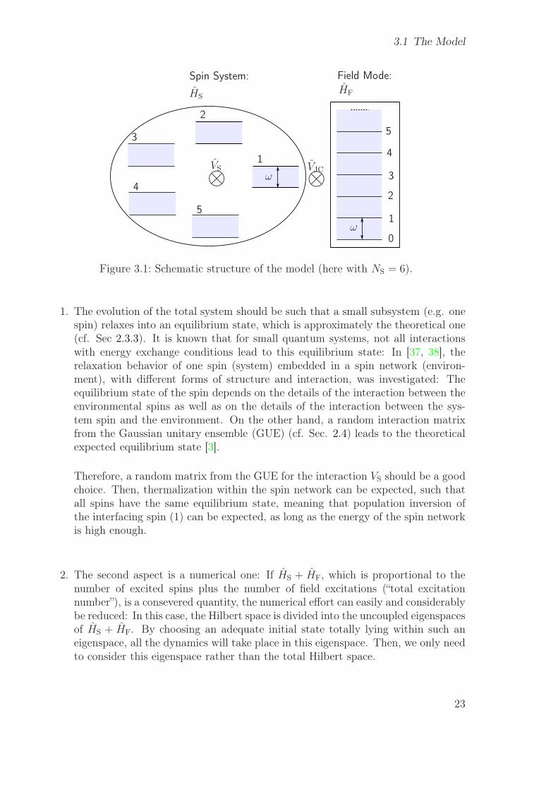
The schematic structure of the system is shown in Fig. 3.1. The oscillator (with energysplitting ω) is coupled resonantly to spin number 1. This interfacing spin (1) is part ofa spin network, which consists of NS spins with energy splitting ω.
The energy of the spins is (~ = 1)
HS =
NS∑
i=1
ω
2σ(i)z +
ωNS
2, (3.1)
where the Pauli matrix σ(i)z acts on spin number i, and the second part (ωNS
2) is just an
energy shift, so that the energy eigenvalues of the spin network are ES,s = sω (withoutinteraction), where s = 0, 1, ..., NS denotes these eigenenergies . The intercation VS
between the spins will be explained later in detail. The Hamiltonian of the field mode is
HF = ωN, (3.2)
where N is the occupation number operator. The vacuum energy is set to zero, andthe energy eigenvalues are EF,n = nω, with n = 0, 1, ... denoting these eigenvalues (inthe following, we will stick to this denotation of eigenvalues/eigenstates, e.g. s alwaysdenotes the eigenvalues of HS and n always denotes the eigenvalues of HF). Withoutloss of generality, we set ω = 1. The interaction between spin 1 and the oscillator is theJaynes-Cummings interaction
VJC = σ(1)− a+ + σ
(1)+ a, (3.3)
where σ(1)− and σ
(1)+ are the lowering and raising operators of spin 1, respectively, and
a+, a the creation and annihilation operators of the field mode, respectively.The total Hamiltonian of the system is
H = HS + HF + aVS + gVJC (3.4)
where a is the coupling strength between the spins, and g the coupling strength betweenspin 1 and the field mode. We will only consider the weak coupling limit, i.e. a, g ≪ 1.
The time evolution of the system is given by
ρ(t) = e−iHtρ(0)eiHt, (3.5)
which is solved numerically by diagonalizing H.For the choice of the interaction VS between the spins we impose the following con-
straints:
22
3.1 The Model
0
1
1
2
2
3
3
4
4
5
5
⊗⊗VS VJC
ω
ω
Spin System:
HS
Field Mode:
HF
Figure 3.1: Schematic structure of the model (here with NS = 6).
1. The evolution of the total system should be such that a small subsystem (e.g. onespin) relaxes into an equilibrium state, which is approximately the theoretical one(cf. Sec 2.3.3). It is known that for small quantum systems, not all interactionswith energy exchange conditions lead to this equilibrium state: In [37, 38], therelaxation behavior of one spin (system) embedded in a spin network (environ-ment), with different forms of structure and interaction, was investigated: Theequilibrium state of the spin depends on the details of the interaction between theenvironmental spins as well as on the details of the interaction between the sys-tem spin and the environment. On the other hand, a random interaction matrixfrom the Gaussian unitary ensemble (GUE) (cf. Sec. 2.4) leads to the theoreticalexpected equilibrium state [3].
Therefore, a random matrix from the GUE for the interaction VS should be a goodchoice. Then, thermalization within the spin network can be expected, such thatall spins have the same equilibrium state, meaning that population inversion ofthe interfacing spin (1) can be expected, as long as the energy of the spin networkis high enough.
2. The second aspect is a numerical one: If HS + HF, which is proportional to thenumber of excited spins plus the number of field excitations (“total excitationnumber”), is a consevered quantity, the numerical effort can easily and considerablybe reduced: In this case, the Hilbert space is divided into the uncoupled eigenspacesof HS + HF. By choosing an adequate initial state totally lying within such aneigenspace, all the dynamics will take place in this eigenspace. Then, we only needto consider this eigenspace rather than the total Hilbert space.
23
3 The Closed Quantum Mechanical Laser Model
The requirements for HS + HF being a conserved quantity are[
HS + HF, VJC
]
=0, (3.6)[
HF, VS
]
=0, (3.7)[
HS, VS
]
=0. (3.8)
The first equation is true for the Jaynes-Cummings interaction with resonant cou-pling (cf. appendix A). The second one is true because VS only acts on the spinnetwork. The last equation is true if only states of the spin network with the sameeigenenergy HS can interact, so that VS becomes block diagonal with each blockacting only on an eigenspace of HS:
VS =∑
s
∑
i,i′
(V(s)S )ii′ |s, i〉〈s, i′| =
V(1)S · · · 0
V(2)S
... . . . ...V
(s)S
0 · · · . . .
, (3.9)
where s denotes the eigenvalues of HS, i and i′ the respective eigenstates, and(V
(s)S )ii′ are the matrix elements of VS. The blocks V (s)
S are then chosen to berandom matrices from the GUE as described in point 1.
In this case, the total Hamiltonian is also block diagonal, with each block actingonly on one eigenspace of HS + HF:
H =∑
k
∑
j,j′
(Hk)jj′|k, j〉〈k, j′| =
H1 · · · 0
H2... . . . ...
Hk
0 · · · . . .
, (3.10)
Here k denotes the eigenvalues of HS+HF, j and j′ the respective eigenstates, and(Hk)jj′ the matrix elements of the Hamiltonian. The Hilbert space decomposesinto the uncoupled subspaces Hk.
Now we can choose an initial state ρ0, which totally lies within such a subspaceHk,
ρ0 =∑
j,j′
ρk,jj′|k, j〉〈k, j′|, (3.11)
where the ρk,jj′ are matrix elements of the density operator. This way, the nu-merical effort for calculating the dynamics of the system is considerably reduced,because we only have to consider this subspace Hk.
24
3.1 The Model
3. This special choice of VS has one drawback: There will be only incoherent energyexchange between the field mode and the spin network, if the initial state is ofthe form (3.11). We can see this, when we calculate the reduced state of the fieldmode by tracing out the spin network:
ρF =∑
n,n′
∑
s,i
〈n; s, i|ρ|n′; s, i〉 |n〉〈n′|, (3.12)
where n and n′ denote the (nondegenerate) eigenstates of HF, s the eigenvalues ofHS and i the respective eigenstates. Because of the structure of VS, the total statecan always be written (using the just introduced notation) as
ρ =∑
n+s=k
∑
n′+s′=k
∑
i,i′
ρk,ii′|n; s, i〉〈n′; s′, i′|, (3.13)
where the first two sums are taken over all n, s, n′, s′ such that n+ s = n′ + s′ = k.Inserting (3.13) into (3.12) yields that (ρF)nn′ is zero if n 6= n′, so that ρF isdiagonal in the Fock representation.
In this chapter, we are only interested in the local energy distribution of the sub-systems (e.g. the field mode or one spin). In the next chapter though, we want todiscuss coherences within the field mode, which are given by the offdiagonal entriesof the reduced density matrix in the energy eigenbasis. Since the special choice ofthe interaction VS directly influences these values, we will use a full random matrixfrom the GUE (full = no special structure).
3.1.1 Parameter
To choose the parameters a and g in (3.4), we first investigate how these parametersinfluence the equilibrium state of a small subsystem. It has been shown that for small,structured systems the relative coupling strength between different subsystems may af-fect the equilibrium state of a subsystem [37, 38]. In our model, the Jaynes-Cummingsinteraction between the field mode and one spin introduces such a structure. To obtaina good choice for the parameters yielding relaxation into the desired equilibrium state,we compare the asymptotical state of the actual dynamics for various values of a
gwith
the theoretical predictions given in Sec. 3.2.1. By doing so for different numbers NS
of spins in the spin network, we can also estimate whether this effect of the structuredinteraction depends on the system size, and maybe vanishes in the thermodynamic limit,as could be expected from classical thermodynamics (details of the interaction shouldnot influence the equilibrium state).
For this purpose, we use the initial conditions described in Sec. 3.2 (lasing relaxation:All spins are excited and the field mode is in the ground state), set g = 0.0001, andnumerically calculate the asymptotical expectation value 〈N〉calc of the photon number.The theoretical value according to (3.23) is 〈N〉theo = NS
2, whereNS is the number of spins
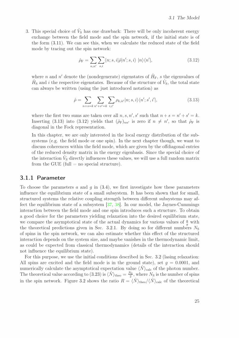
in the spin network. Figure 3.2 shows the ratio R = 〈N〉theo/〈N〉calc of the theoretical
25
3 The Closed Quantum Mechanical Laser Model
0
0.2
0.4
0.6
0.8
1
0.1 1a/g
RNS=12
NS=8
Figure 3.2: Parameter optimization: Dependence of the ratio R = 〈N〉theo/〈N〉calc ona/g for different system sizes.
and the actual value, depending on ag
and for NS = 8, 12 spins in the spin network. Wecan see that for the larger system, the ratio R is closer to the thermodynamical expectedvalue 1 for a wider range of the parameters a and g.
3.1.2 Degeneracy Structure
For calculating the thermodynamically expected equilibrium state (cf. Sec. 2.3.3), weneed the degeneracy structure of the subsystems. For the field mode, the degeneracystructure is
gF(n) = 1, (3.14)
where n denotes the eigenenergies of the field mode. For one spin, the degeneracystructure is
gS1(m) = 1, (3.15)
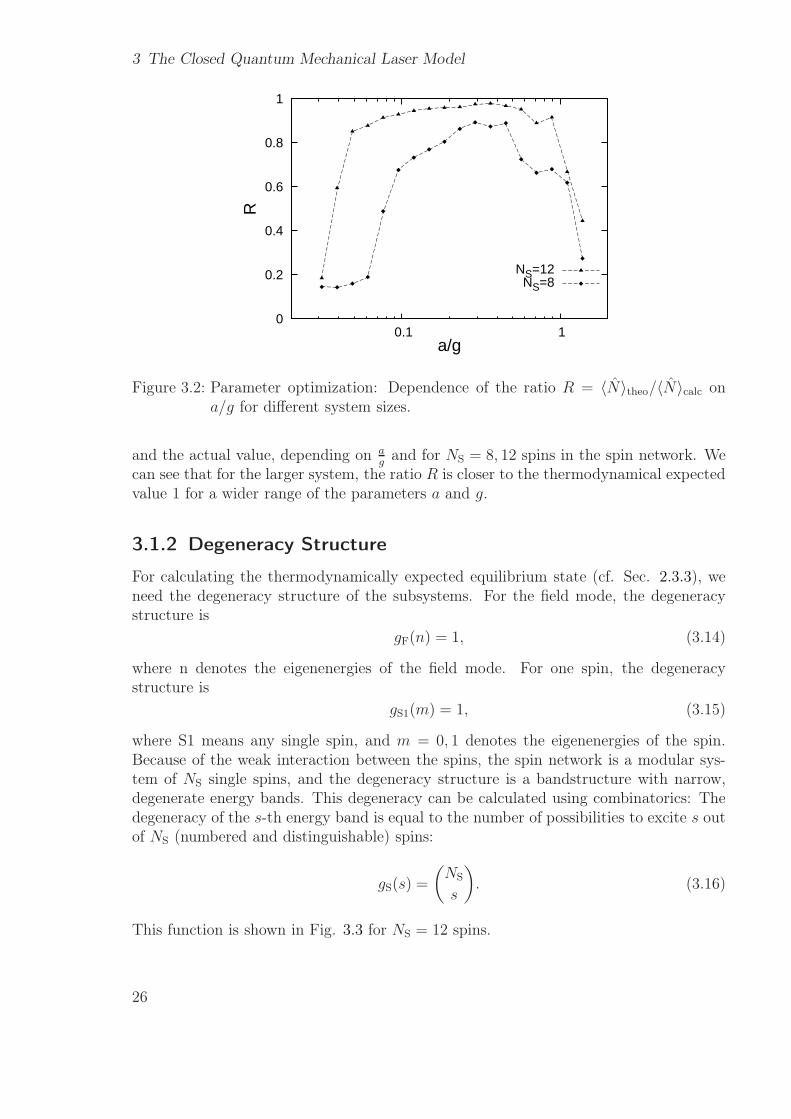
where S1 means any single spin, and m = 0, 1 denotes the eigenenergies of the spin.Because of the weak interaction between the spins, the spin network is a modular sys-tem of NS single spins, and the degeneracy structure is a bandstructure with narrow,degenerate energy bands. This degeneracy can be calculated using combinatorics: Thedegeneracy of the s-th energy band is equal to the number of possibilities to excite s outof NS (numbered and distinguishable) spins:
gS(s) =
(NS
s
)
. (3.16)
This function is shown in Fig. 3.3 for NS = 12 spins.
26
3.2 Lasing Relaxation
0
500
1000
0 2 4 6 8 10 12
g S(s
)
s
Figure 3.3: Degeneracy structure gS(s) of a spin network consisting of NS = 12 spins.
3.2 Lasing Relaxation
At first, we will set up the spin network in the highest energy eigenstate, and thefield mode in the ground state. Because of the resulting population inversion of theinterfacing spin, we expect an energy flow into the field mode with stimulated emissionof photons. Though this process should be lasing, the final equilibrium state of the fieldmode depends on the degeneracy structure of the spin network, and will not necessarilybe a (phase-diffused, cf. Sec. 4) Glauber state. However, a laser is far from being in anequilibrium state, but rather a process, which might thermodynamically be interpretedas a steady-state under continuous pumping and loss. We will see that the transientphoton number distribution during relaxation is, indeed, nearly Poissonian.
3.2.1 Expected Equilibrium
The thermodynamically expected equilibrium state for a small system A (of interest),which is coupled to a large system B (environment) with energy exchange conditions isgiven by (2.100):
PA(EA) = gA(EA)∑
E
gB(E − EA)W (E)
gtot(E). (3.17)
In the following, we neglect the interaction energies VS and VJC, and only consider theenergies HS and HF. Then, we have W (E) = δEtot,E , where Etot = NS (the number ofspins), and discrete systems with EA = a and Etot − EA = NS − a = b, where a andb denote the energy eigenvalues of system A and B, respectively (with energy splittingω = 1). The expected equilibrium state is
PA(a) = gA(a)gB(NS − a)
gtot(NS), (3.18)
27
3 The Closed Quantum Mechanical Laser Model
where again PA(a) is the probability to find system A in a state with energy EA = a,and gA, gB, and gtot are the degeneracy structures of the system, the environment, andthe combined system, respectively.
We consider two (mutually exclusive) perspectives (partitions):
1. System A = one single spin (S1), embedded by B = the other spins and the fieldmode. Then gA(a) = gS1(m) = 1 and m = 0, 1. For the degeneracy of system B atenergy b = Etot −m = NS −m we have
gB(NS −m) =
NS’∑
s′=0
∞∑
n=0
δn+s′,NS−m gS’(s′)gF(n) =
Min[NS’,NS−m]∑
s′=0
gS’(s′), (3.19)
where gS’(s′) is the degeneracy of a spin network S’ with NS’ = NS − 1 spins and
with eigenenergies s′ . The term δn+s′,NS−m ensures that Etot = NS. Here we usedthat gF(n) = 1 . The last sum is actually independent of m, because the highestenergy band of this spin network is, anyway, NS−1, so that gS’(NS) = 0. Inserting(3.19) into (3.18) and using (3.16) we obtain
PS1(m) ∝NS’∑
s′=0
(NS’
s′
)
. (3.20)
In this expected equilibrium state, both eigenstates m = 0, 1 have the same occu-pation probabilities, the energy is ES1 = 1/2, and the inversion is 〈σz〉 = 0, whichformally yields a local temperature T = ∞. Since this consideration applies forany spin, the energy of the total spin network S in equilibrium is expected to beES = NS/2.
2. System A = field mode (F), embedded by B, the spin network (S). Here, we havegA(a) = gF(n) = 1 according to (3.14), and gB(b) = gS(NS − n) =
(NS
NS−n
)accord-
ing to (3.16). Using (3.18) we obtain the expected equilibrium photon numberdistribution
PF(n) =
(NS
NS − n
)
gtot(NS)−1, (3.21)
where the degeneracy of the total system at energy Etot = NS is
gtot(NS) =
NS∑
s=0
∞∑
n=0
δn+s,NSgS(s)gF(n) =
NS∑
s=0
(NS
s
)
, (3.22)
analog to (3.19).
The energy EF of the field mode, which is equal to the expectation value of thephoton number 〈N〉, is
EF = 〈N〉 =∑
n
nPF(n) =NS
2. (3.23)
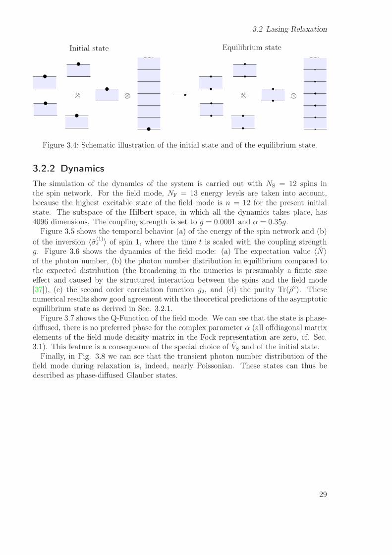
Figure 3.4 illustrates the “equilibrium state” of the total system, as seen from therespective subsystems, which is basically a microcanonical state of the total system, inwhich all states with energy Etot have the same occupation probabilities.
28
3.2 Lasing Relaxation
⊗⊗⊗⊗
Initial state Equilibrium state
Figure 3.4: Schematic illustration of the initial state and of the equilibrium state.
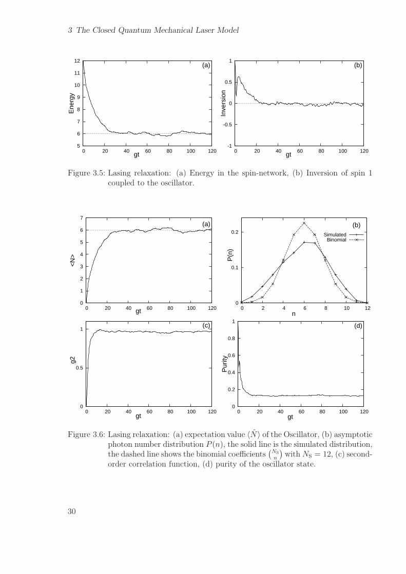
3.2.2 Dynamics
The simulation of the dynamics of the system is carried out with NS = 12 spins inthe spin network. For the field mode, NF = 13 energy levels are taken into account,because the highest excitable state of the field mode is n = 12 for the present initialstate. The subspace of the Hilbert space, in which all the dynamics takes place, has4096 dimensions. The coupling strength is set to g = 0.0001 and α = 0.35g.
Figure 3.5 shows the temporal behavior (a) of the energy of the spin network and (b)of the inversion 〈σ(1)
z 〉 of spin 1, where the time t is scaled with the coupling strengthg. Figure 3.6 shows the dynamics of the field mode: (a) The expectation value 〈N〉of the photon number, (b) the photon number distribution in equilibrium compared tothe expected distribution (the broadening in the numerics is presumably a finite sizeeffect and caused by the structured interaction between the spins and the field mode[37]), (c) the second order correlation function g2, and (d) the purity Tr(ρ2). Thesenumerical results show good agreement with the theoretical predictions of the asymptoticequilibrium state as derived in Sec. 3.2.1.
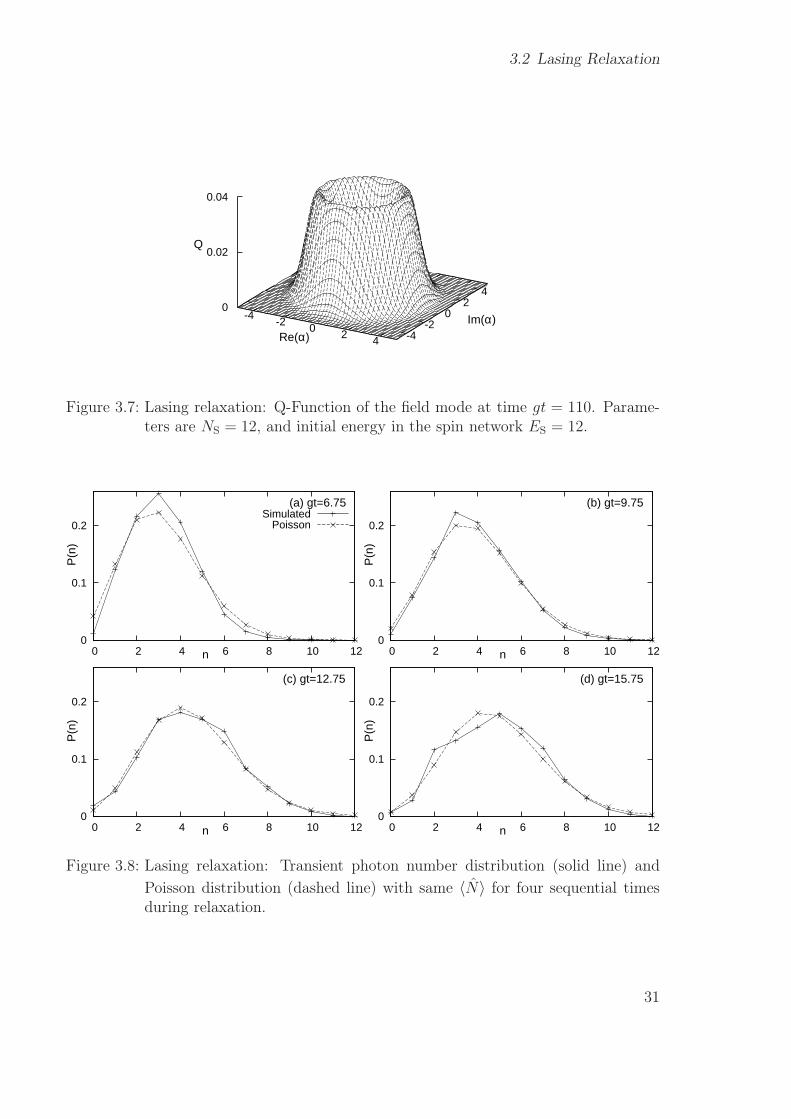
Figure 3.7 shows the Q-Function of the field mode. We can see that the state is phase-diffused, there is no preferred phase for the complex parameter α (all offdiagonal matrixelements of the field mode density matrix in the Fock representation are zero, cf. Sec.3.1). This feature is a consequence of the special choice of VS and of the initial state.
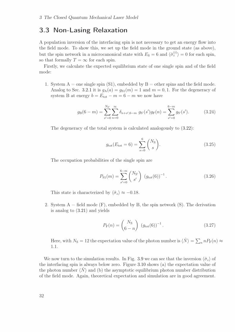
Finally, in Fig. 3.8 we can see that the transient photon number distribution of thefield mode during relaxation is, indeed, nearly Poissonian. These states can thus bedescribed as phase-diffused Glauber states.
29
3 The Closed Quantum Mechanical Laser Model
5
6
7
8
9
10
11
12
0 20 40 60 80 100 120
Ene
rgy
gt
(a)
-1
-0.5
0
0.5
1
0 20 40 60 80 100 120
Inve
rsio
n
gt
(b)
Figure 3.5: Lasing relaxation: (a) Energy in the spin-network, (b) Inversion of spin 1coupled to the oscillator.
0
1
2
3
4
5
6
7
0 20 40 60 80 100 120
<N
>
gt
(a)
0
0.1
0.2
0 2 4 6 8 10 12
P(n
)
n
(b)Simulated
Binomial
0
0.5
1
0 20 40 60 80 100 120
g2
gt
(c)
0
0.2
0.4
0.6
0.8
1
0 20 40 60 80 100 120
Pur
ity
gt
(d)
Figure 3.6: Lasing relaxation: (a) expectation value 〈N〉 of the Oscillator, (b) asymptoticphoton number distribution P (n), the solid line is the simulated distribution,the dashed line shows the binomial coefficients
(NS
n
)withNS = 12, (c) second-
order correlation function, (d) purity of the oscillator state.
30
3.2 Lasing Relaxation
-4-2
02
4Re(α) -4-2
02
4
Im(α) 0
0.02
0.04
Q
Figure 3.7: Lasing relaxation: Q-Function of the field mode at time gt = 110. Parame-ters are NS = 12, and initial energy in the spin network ES = 12.
0
0.1
0.2
0 2 4 6 8 10 12
P(n
)
n
(a) gt=6.75Simulated
Poisson
0
0.1
0.2
0 2 4 6 8 10 12
P(n
)
n
(b) gt=9.75
0
0.1
0.2
0 2 4 6 8 10 12
P(n
)
n
(c) gt=12.75
0
0.1
0.2
0 2 4 6 8 10 12
P(n
)
n
(d) gt=15.75
Figure 3.8: Lasing relaxation: Transient photon number distribution (solid line) andPoisson distribution (dashed line) with same 〈N〉 for four sequential timesduring relaxation.
31
3 The Closed Quantum Mechanical Laser Model
3.3 Non-Lasing Relaxation
A population inversion of the interfacing spin is not necessary to get an energy flow intothe field mode. To show this, we set up the field mode in the ground state (as above),but the spin network in a microcanonical state with ES = 6 and 〈σ(i)
z 〉 = 0 for each spin,so that formally T = ∞ for each spin.
Firstly, we calculate the expected equilibrium state of one single spin and of the fieldmode:
1. System A = one single spin (S1), embedded by B = other spins and the field mode.Analog to Sec. 3.2.1 it is gA(a) = gS1(m) = 1 and m = 0, 1. For the degeneracy ofsystem B at energy b = Etot −m = 6 −m we now have
gB(6 −m) =
NS’∑
s′=0
∞∑
n=0
δn+s′,6−m gS’(s′)gF(n) =
6−m∑
s′=0
gS’(s′). (3.24)
The degeneracy of the total system is calculated analogously to (3.22):
gtot(Etot = 6) =6∑
s=0
(NS
s
)
. (3.25)
The occupation probabilities of the single spin are
PS1(m) =
6−m∑
s′=0
(NS’
s′
)
(gtot(6))−1 . (3.26)
This state is characterized by 〈σz〉 ≈ −0.18.
2. System A = field mode (F), embedded by B, the spin network (S). The derivationis analog to (3.21) and yields
PF(n) =
(NS
6 − n
)
(gtot(6))−1 . (3.27)
Here, withNS = 12 the expectation value of the photon number is 〈N〉 =∑
n nPF(n) ≈1.1.
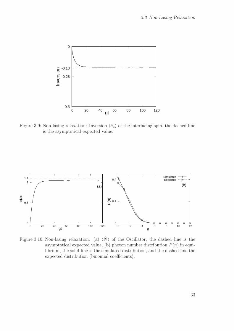
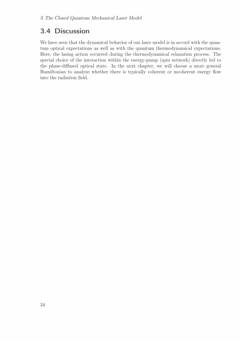
We now turn to the simulation results. In Fig. 3.9 we can see that the inversion 〈σz〉 ofthe interfacing spin is always below zero. Figure 3.10 shows (a) the expectation value ofthe photon number 〈N〉 and (b) the asymptotic equilibrium photon number distributionof the field mode. Again, theoretical expectation and simulation are in good agreement.
32
3.3 Non-Lasing Relaxation
-0.5
-0.25
-0.18
0
0 20 40 60 80 100 120
Inve
rsio
n
gt
Figure 3.9: Non-lasing relaxation: Inversion 〈σz〉 of the interfacing spin, the dashed lineis the asymptotical expected value.
0
0.5
1 1.1
0 20 40 60 80 100 120
<N
>
gt
(a)
0
0.2
0.4
0 2 4 6 8 10 12
P(n
)
n
(b)
SimulatedExpected
Figure 3.10: Non-lasing relaxation: (a) 〈N〉 of the Oscillator, the dashed line is theasymptotical expected value, (b) photon number distribution P (n) in equi-librium, the solid line is the simulated distribution, and the dashed line theexpected distribution (binomial coefficients).
33
3 The Closed Quantum Mechanical Laser Model
3.4 Discussion
We have seen that the dynamical behavior of our laser model is in accord with the quan-tum optical expectations as well as with the quantum thermodynamical expectations.Here, the lasing action occurred during the thermodynamical relaxation process. Thespecial choice of the interaction within the energy-pump (spin network) directly led tothe phase-diffused optical state. In the next chapter, we will choose a more generalHamiltonian to analyze whether there is typically coherent or incoherent energy flowinto the radiation field.
34
4 Optical Coherences andHeat/Work Analysis
In this chapter, we will further investigate the laser model presented in the previouschapter. These studies will address optical coherences [18] and closely related thermo-dynamical aspects, namely the heat and work flows from and to the field mode. In viewof the three-level maser-like heat engines and pumps [40, 5, 47], we will also discuss towhat extend the energy of the radiation field may be “useful”.
In 1997, K. Mølmer suggested [30] that the light emitted by typical laser sources shouldnot be in a coherent Glauber state, but in a phase-diffused Glauber state, meaning thatall offdiagonal entries of the density matrix (in the Fock representation) are zero, and thediagonal entries are near-Poissonian distributed. In this case, there is no preferred phasefor the complex parameter α of the coherent states, and the expectation values of thefield amplitude operators vanish. His assumptions are based on an incoherently pumpedgain medium. With the same argumentation as in Sec. 3.1, the phase-diffused Glauberstate is obtained. He also shows in his work that the results of optical experiments so faronly depend on the diagonal matrix elements, i.e. yield the same result for coherent andfor phase-diffused Glauber states. In another study by T. Rudolph and B. C. Sanders[35], it is claimed that the state of a single-mode laser output (far above threshold)must be represented by a phase-diffused density matrix, since the phase of the fieldis unknown. Contrary to this work, K. Nemoto and S. L. Braunstein suggest in [31]that the phase is not just unknown, but rather unobservable, which means that anyassumption for the phase (respective any distribution thereof) is equally valid, i.e. alsothe coherent state.
4.1 LEMBAS Principle
LEMBAS (local effective measurement basis) [46] is a method to systematically investi-gate the energy change of a system for arbitrary processes, if the dynamics of the systemis given (including the effective dynamics induced by the environment). The energychange is split into an effective coherent and an effective incoherent part. The effectivecoherent part does not alter the local von Neumann entropy, and is therefore assumedto be work. The effective incoherent part, which alters the local von Neumann entropy,is assumed to be heat. Here, I present the important steps we need for calculating thesetwo types of energy change.
To do so, we consider a bipartite system
H = HA + HB + HAB, (4.1)
35
4 Optical Coherences and Heat/Work Analysis
where HA and HB only act on system A (the system of interest) and B (“the rest ofthe universe”), respectively, and HAB is the interaction energy of both subsystems. Ameasurement of the local effective energy of subsystem A then depends on the concretemeasuring procedure, introducing a local effective measurement basis.
The state of the total system can be written as
ρ = ρA ⊗ ρB + CAB, (4.2)
cf. (2.20). The local dynamics of subsystem A is given by
∂
∂tρA = −i[HA + Heff
A , ρA] + Linc(ρ), (4.3)
where ρA is the reduced state of subsystem A, ρ is the state of the total system,
HeffA = TrB
HAB(1A ⊗ ρB)
(4.4)
is an effective Hamiltonian describing the unitary dynamics induced by B on A, and
Linc(ρ) = −iTrB
[HAB, CAB]
(4.5)
describes incoherent processes.By choosing the energy eigenbasis of A as the measurement basis, only parts of Heff
A
that commute with HA affect the local effective energy. For a nondegenerate energyeigenbasis |u〉 of A this part is given by
Heff1 =
∑
u
〈u|HeffA |u〉 |u〉〈u|, (4.6)
with HeffA = Heff
1 + Heff2 and
[HeffA , H
eff1 ] = 0, (4.7)
[HeffA , H
eff2 ] 6= 0, (4.8)
if Heff2 6= 0.
The corresponding operator for an energy measurement in the energy eigenbasis ofHA is
H ′A = HA + Heff
1 (4.9)
Using (4.3) and assuming HA to be time independent, we obtain a formula for calculatingthe effective internal energy change of A:
dUA =ddt
Tr
H ′AρA
dt = Tr
˙H ′
AρA + H ′A
˙ρA
dt
= Tr
˙Heff
1 ρA − i[H ′A, H
eff2 ]ρA + H ′
ALinc(ρ)
dt. (4.10)
36
4.2 Lasing Relaxation
By observing that the first two terms induce unitary dynamics on A, and that only thelast term changes the local von Neumann entropy, we define
δWA = Tr
˙Heff
1 ρA − i[H ′A, H
eff2 ]ρA
dt, (4.11)
δQA = Tr
H ′ALinc(ρ)
dt. (4.12)
Using these formulas, any local energy change can be systematically split into heat andwork.
4.2 Lasing Relaxation
As discussed in Sec. 3.1, we choose the interaction VS between the spins to be a randommatrix from the GUE with no particular structure. We use the same initial state as inSec. 3.2 (all spins are excited and the field mode is in the ground state), and expect lasingaction during relaxation. This time though, we cannot expect the optical coherences tovanish as a consequence of the structure of VS: Coherent energy change of the field modeis in principle possible. The numerical calculations are now carried out with NS = 8 spinsonly and NF = 10 levels of the field mode taken into account (because [HS +HF, VS] 6= 0,more than 8 photons may be excited in the field).
For investigating the optical coherences we calculate the Husimi Q-function (2.86),and the field purity
P = Tr(ρ2F) (4.13)
compared to the purity of the diagonal part
ρdiagF =
∑
n
(ρF)nn|n〉〈n|. (4.14)
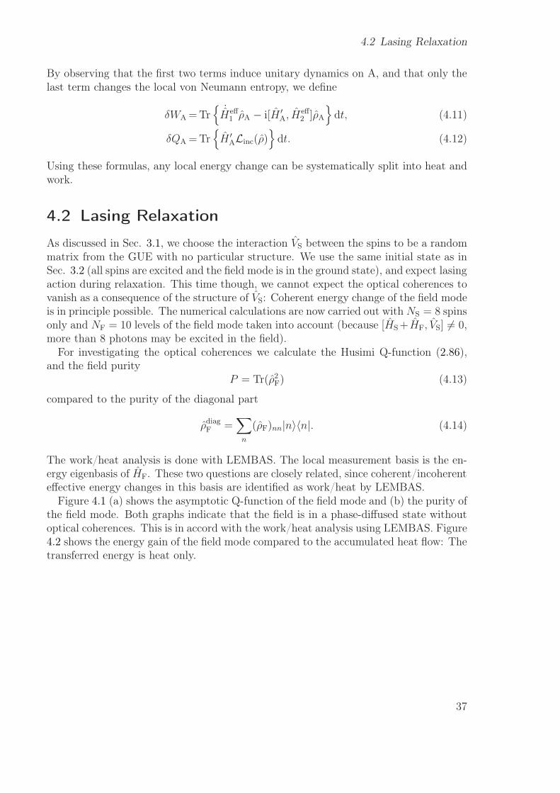
The work/heat analysis is done with LEMBAS. The local measurement basis is the en-ergy eigenbasis of HF. These two questions are closely related, since coherent/incoherenteffective energy changes in this basis are identified as work/heat by LEMBAS.
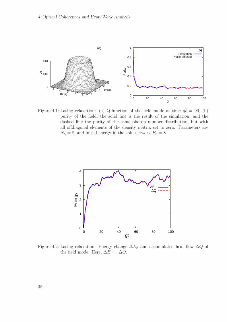
Figure 4.1 (a) shows the asymptotic Q-function of the field mode and (b) the purity ofthe field mode. Both graphs indicate that the field is in a phase-diffused state withoutoptical coherences. This is in accord with the work/heat analysis using LEMBAS. Figure4.2 shows the energy gain of the field mode compared to the accumulated heat flow: Thetransferred energy is heat only.
37
4 Optical Coherences and Heat/Work Analysis
(a)
-4-2
02
4Re(α) -4-2
02
4
Im(α) 0
0.02
0.04
Q
0
0.2
0.4
0.6
0.8
1
0 20 40 60 80 100
Pur
ity
gt
(b)Simulation
Phase-diffused
Figure 4.1: Lasing relaxation: (a) Q-function of the field mode at time gt = 90, (b)purity of the field, the solid line is the result of the simulation, and thedashed line the purity of the same photon number distribution, but withall offdiagonal elements of the density matrix set to zero. Parameters areNS = 8, and initial energy in the spin network ES = 8.
0
1
2
3
4
0 20 40 60 80 100
Ene
rgy
gt
∆EF∆Q
Figure 4.2: Lasing relaxation: Energy change ∆EF and accumulated heat flow ∆Q ofthe field mode. Here, ∆EF = ∆Q.
38
4.3 Energy Flow into the Spin Network
4.3 Energy Flow into the Spin Network
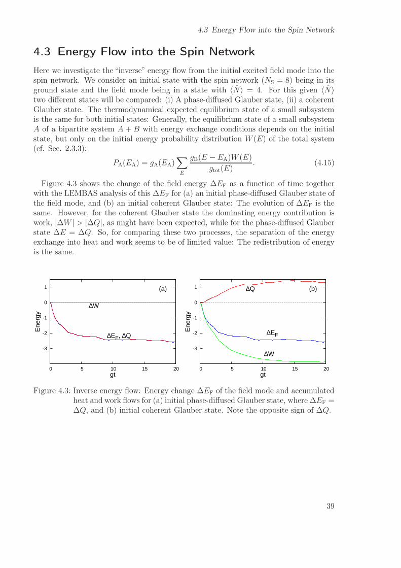
Here we investigate the “inverse” energy flow from the initial excited field mode into thespin network. We consider an initial state with the spin network (NS = 8) being in itsground state and the field mode being in a state with 〈N〉 = 4. For this given 〈N〉two different states will be compared: (i) A phase-diffused Glauber state, (ii) a coherentGlauber state. The thermodynamical expected equilibrium state of a small subsystemis the same for both initial states: Generally, the equilibrium state of a small subsystemA of a bipartite system A + B with energy exchange conditions depends on the initialstate, but only on the initial energy probability distribution W (E) of the total system(cf. Sec. 2.3.3):
PA(EA) = gA(EA)∑
E
gB(E − EA)W (E)
gtot(E). (4.15)
Figure 4.3 shows the change of the field energy ∆EF as a function of time togetherwith the LEMBAS analysis of this ∆EF for (a) an initial phase-diffused Glauber state ofthe field mode, and (b) an initial coherent Glauber state: The evolution of ∆EF is thesame. However, for the coherent Glauber state the dominating energy contribution iswork, |∆W | > |∆Q|, as might have been expected, while for the phase-diffused Glauberstate ∆E = ∆Q. So, for comparing these two processes, the separation of the energyexchange into heat and work seems to be of limited value: The redistribution of energyis the same.
-3
-2
-1
0
1
0 5 10 15 20
∆W
∆EF, ∆Q
Ene
rgy
gt
(a)
-3
-2
-1
0
1
0 5 10 15 20
∆W
∆EF
∆Q
Ene
rgy
gt
(b)
Figure 4.3: Inverse energy flow: Energy change ∆EF of the field mode and accumulatedheat and work flows for (a) initial phase-diffused Glauber state, where ∆EF =∆Q, and (b) initial coherent Glauber state. Note the opposite sign of ∆Q.
39
4 Optical Coherences and Heat/Work Analysis
4.4 “Usefulness“ of the Field Energy
We will see that from a thermodynamical point of view, namely the principle of theincrease of entropy (second law), the energy in the field mode obtained during lasingrelaxation might, to some extent, be directly used to perform work on another system.This is mainly an effect of the local negative temperature (population inversion) of theinterfacing spin, which is necessary to get lasing action.
4.4.1 Negative Temperatures and the Second Law
The temperature of a system in thermal equilibrium can be calculated by
T−1 =
(∂S
∂U
)
X
, (4.16)
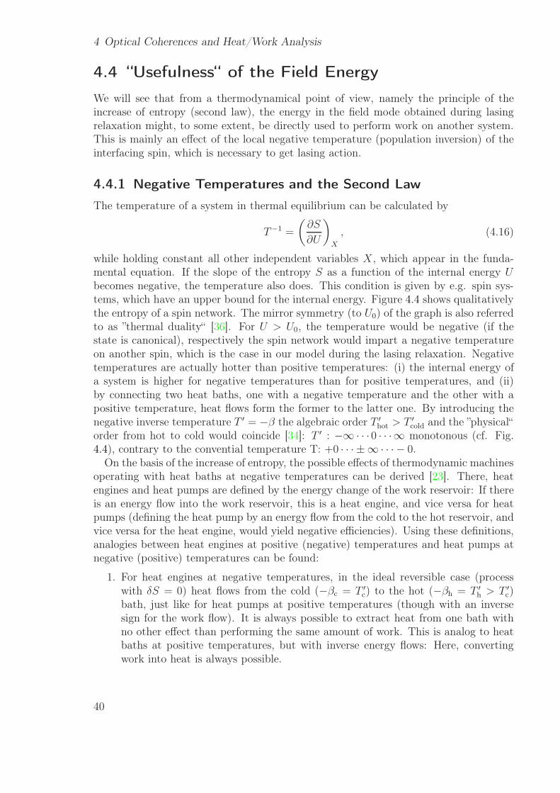
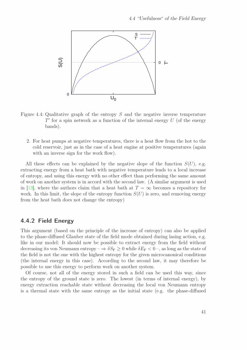
while holding constant all other independent variables X, which appear in the funda-mental equation. If the slope of the entropy S as a function of the internal energy Ubecomes negative, the temperature also does. This condition is given by e.g. spin sys-tems, which have an upper bound for the internal energy. Figure 4.4 shows qualitativelythe entropy of a spin network. The mirror symmetry (to U0) of the graph is also referredto as ”thermal duality“ [36]. For U > U0, the temperature would be negative (if thestate is canonical), respectively the spin network would impart a negative temperatureon another spin, which is the case in our model during the lasing relaxation. Negativetemperatures are actually hotter than positive temperatures: (i) the internal energy ofa system is higher for negative temperatures than for positive temperatures, and (ii)by connecting two heat baths, one with a negative temperature and the other with apositive temperature, heat flows form the former to the latter one. By introducing thenegative inverse temperature T ′ = −β the algebraic order T ′
hot > T ′cold and the ”physical“
order from hot to cold would coincide [34]: T ′ : −∞· · ·0 · · ·∞ monotonous (cf. Fig.4.4), contrary to the convential temperature T: +0 · · · ±∞ · · · − 0.
On the basis of the increase of entropy, the possible effects of thermodynamic machinesoperating with heat baths at negative temperatures can be derived [23]. There, heatengines and heat pumps are defined by the energy change of the work reservoir: If thereis an energy flow into the work reservoir, this is a heat engine, and vice versa for heatpumps (defining the heat pump by an energy flow from the cold to the hot reservoir, andvice versa for the heat engine, would yield negative efficiencies). Using these definitions,analogies between heat engines at positive (negative) temperatures and heat pumps atnegative (positive) temperatures can be found:
1. For heat engines at negative temperatures, in the ideal reversible case (processwith δS = 0) heat flows from the cold (−βc = T ′
c) to the hot (−βh = T ′h > T ′
c)bath, just like for heat pumps at positive temperatures (though with an inversesign for the work flow). It is always possible to extract heat from one bath withno other effect than performing the same amount of work. This is analog to heatbaths at positive temperatures, but with inverse energy flows: Here, convertingwork into heat is always possible.
40
4.4 “Usefulness“ of the Field Energy
0U0
0S
(U)
T’
ST’
Figure 4.4: Qualitative graph of the entropy S and the negative inverse temperatureT ′ for a spin network as a function of the internal energy U (of the energybands).
2. For heat pumps at negative temperatures, there is a heat flow from the hot to thecold reservoir, just as in the case of a heat engine at positive temperatures (againwith an inverse sign for the work flow).
All these effects can be explained by the negative slope of the function S(U), e.g.extracting energy from a heat bath with negative temperature leads to a local increaseof entropy, and using this energy with no other effect than performing the same amountof work on another system is in accord with the second law. (A similar argument is usedin [13], where the authors claim that a heat bath at T = ∞ becomes a repository forwork. In this limit, the slope of the entropy function S(U) is zero, and removing energyfrom the heat bath does not change the entropy)
4.4.2 Field Energy
This argument (based on the principle of the increase of entropy) can also be appliedto the phase-diffused Glauber state of the field mode obtained during lasing action, e.g.like in our model: It should now be possible to extract energy from the field withoutdecreasing its von Neumann entropy – ⇒ δSF ≥ 0 while δEF < 0 –, as long as the state ofthe field is not the one with the highest entropy for the given microcanonical conditions(the internal energy in this case). According to the second law, it may therefore bepossible to use this energy to perform work on another system.
Of course, not all of the energy stored in such a field can be used this way, sincethe entropy of the ground state is zero. The lowest (in terms of internal energy), byenergy extraction reachable state without decreasing the local von Neumann entropyis a thermal state with the same entropy as the initial state (e.g. the phase-diffused
41
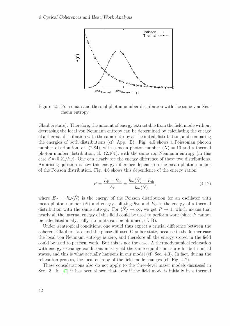
4 Optical Coherences and Heat/Work Analysis
<n>Thermal <n>Poisson
P(n
)
n
PoissonThermal
Figure 4.5: Poissonian and thermal photon number distribution with the same von Neu-mann entropy.
Glauber state). Therefore, the amount of energy extractable from the field mode withoutdecreasing the local von Neumann entropy can be determined by calculating the energyof a thermal distribution with the same entropy as the initial distribution, and comparingthe energies of both distributions (cf. App. B). Fig. 4.5 shows a Poissonian photonnumber distribution, cf. (2.84), with a mean photon number 〈N〉 = 10 and a thermalphoton number distribution, cf. (2.101), with the same von Neumann entropy (in thiscase β ≈ 0.21/~ω). One can clearly see the energy difference of these two distributions.An arising question is how this energy difference depends on the mean photon numberof the Poisson distribution. Fig. 4.6 shows this dependence of the energy ration
P =EP − Eth
EP
=~ω〈N〉 − Eth
~ω〈N〉, (4.17)
where EP = ~ω〈N〉 is the energy of the Poisson distribution for an oscillator withmean photon number 〈N〉 and energy splitting ~ω, and Eth is the energy of a thermaldistribution with the same entropy. For 〈N〉 → ∞, we get P → 1, which means thatnearly all the internal energy of this field could be used to perform work (since P cannotbe calculated analytically, no limits can be obtained, cf. B).
Under isentropical conditions, one would thus expect a crucial difference between thecoherent Glauber state and the phase-diffused Glauber state, because in the former casethe local von Neumann entropy is zero, and therefore all the energy stored in the fieldcould be used to perform work. But this is not the case: A thermodynamical relaxationwith energy exchange conditions must yield the same equilibrium state for both initialstates, and this is what actually happens in our model (cf. Sec. 4.3). In fact, during therelaxation process, the local entropy of the field mode changes (cf. Fig. 4.7).
These considerations also do not apply to the three-level maser models discussed inSec. 3. In [47] it has been shown that even if the field mode is initially in a thermal
42
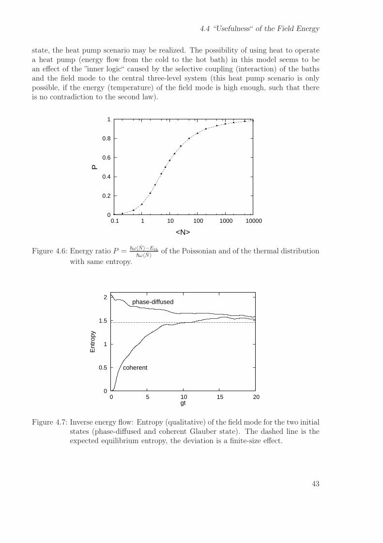
4.4 “Usefulness“ of the Field Energy
state, the heat pump scenario may be realized. The possibility of using heat to operatea heat pump (energy flow from the cold to the hot bath) in this model seems to bean effect of the ”inner logic“ caused by the selective coupling (interaction) of the bathsand the field mode to the central three-level system (this heat pump scenario is onlypossible, if the energy (temperature) of the field mode is high enough, such that thereis no contradiction to the second law).
0
0.2
0.4
0.6
0.8
1
0.1 1 10 100 1000 10000
<N>
P
Figure 4.6: Energy ratio P = ~ω〈N〉−Eth
~ω〈N〉of the Poissonian and of the thermal distribution
with same entropy.
0
0.5
1
1.5
2
0 5 10 15 20
Ent
ropy
gt
coherent
phase-diffused
Figure 4.7: Inverse energy flow: Entropy (qualitative) of the field mode for the two initialstates (phase-diffused and coherent Glauber state). The dashed line is theexpected equilibrium entropy, the deviation is a finite-size effect.
43

4 Optical Coherences and Heat/Work Analysis
44
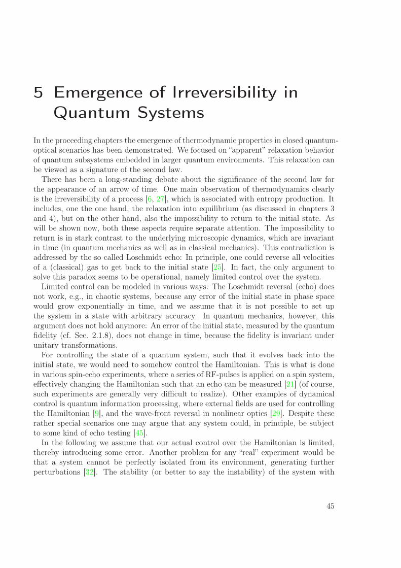
5 Emergence of Irreversibility inQuantum Systems
In the proceeding chapters the emergence of thermodynamic properties in closed quantum-optical scenarios has been demonstrated. We focused on “apparent” relaxation behaviorof quantum subsystems embedded in larger quantum environments. This relaxation canbe viewed as a signature of the second law.
There has been a long-standing debate about the significance of the second law forthe appearance of an arrow of time. One main observation of thermodynamics clearlyis the irreversibility of a process [6, 27], which is associated with entropy production. Itincludes, one the one hand, the relaxation into equilibrium (as discussed in chapters 3and 4), but on the other hand, also the impossibility to return to the initial state. Aswill be shown now, both these aspects require separate attention. The impossibility toreturn is in stark contrast to the underlying microscopic dynamics, which are invariantin time (in quantum mechanics as well as in classical mechanics). This contradiction isaddressed by the so called Loschmidt echo: In principle, one could reverse all velocitiesof a (classical) gas to get back to the initial state [25]. In fact, the only argument tosolve this paradox seems to be operational, namely limited control over the system.
Limited control can be modeled in various ways: The Loschmidt reversal (echo) doesnot work, e.g., in chaotic systems, because any error of the initial state in phase spacewould grow exponentially in time, and we assume that it is not possible to set upthe system in a state with arbitrary accuracy. In quantum mechanics, however, thisargument does not hold anymore: An error of the initial state, measured by the quantumfidelity (cf. Sec. 2.1.8), does not change in time, because the fidelity is invariant underunitary transformations.
For controlling the state of a quantum system, such that it evolves back into theinitial state, we would need to somehow control the Hamiltonian. This is what is donein various spin-echo experiments, where a series of RF-pulses is applied on a spin system,effectively changing the Hamiltonian such that an echo can be measured [21] (of course,such experiments are generally very difficult to realize). Other examples of dynamicalcontrol is quantum information processing, where external fields are used for controllingthe Hamiltonian [9], and the wave-front reversal in nonlinear optics [29]. Despite theserather special scenarios one may argue that any system could, in principle, be subjectto some kind of echo testing [45].
In the following we assume that our actual control over the Hamiltonian is limited,thereby introducing some error. Another problem for any “real” experiment would bethat a system cannot be perfectly isolated from its environment, generating furtherperturbations [32]. The stability (or better to say the instability) of the system with
45
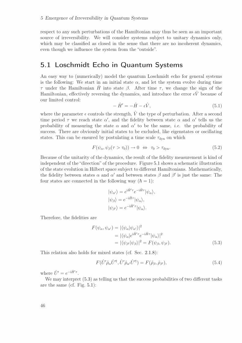
5 Emergence of Irreversibility in Quantum Systems
respect to any such perturbations of the Hamiltonian may thus be seen as an importantsource of irreversibility. We will consider systems subject to unitary dynamics only,which may be classified as closed in the sense that there are no incoherent dynamics,even though we influence the system from the “outside”.
5.1 Loschmidt Echo in Quantum Systems
An easy way to (numerically) model the quantum Loschmidt echo for general systemsis the following: We start in an initial state α, and let the system evolve during timeτ under the Hamiltonian H into state β. After time τ , we change the sign of theHamiltonian, effectively reversing the dynamics, and introduce the error ǫV because ofour limited control:
− H ′ = −H − ǫV , (5.1)
where the parameter ǫ controls the strength, V the type of perturbation. After a secondtime period τ we reach state α′, and the fidelity between state α and α′ tells us theprobability of measuring the state α and α′ to be the same, i.e. the probability ofsuccess. There are obviously initial states to be excluded, like eigenstates or oscillatingstates. This can be ensured by postulating a time scale τdyn on which
F (ψα, ψβ(τ > τ0)) → 0 ⇔ τ0 > τdyn. (5.2)
Because of the unitarity of the dynamics, the result of the fidelity measurement is kind ofindependent of the “direction” of the procedure. Figure 5.1 shows a schematic illustrationof the state evolution in Hilbert space subject to different Hamiltonians. Mathematically,the fidelity between states α and α′ and between states β and β ′ is just the same: Thefour states are connected in the following way (~ = 1):
|ψα′〉 = eiH′τe−iHτ |ψα〉,
|ψβ〉 = e−iHτ |ψα〉,|ψβ′〉 = e−iH′τ |ψα〉.
Therefore, the fidelities are
F (ψα, ψα′) = |〈ψα|ψα′〉|2
= |〈ψα|eiH′τe−iHτ |ψα〉|2
= |〈ψβ′|ψβ〉|2 = F (ψβ , ψβ′). (5.3)
This relation also holds for mixed states (cf. Sec. 2.1.8):
F (U ′ραU′†, U ′ρα′U ′†) = F (ρβ, ρβ′), (5.4)
where U ′ = e−iH′τ .We may interpret (5.3) as telling us that the success probabilities of two different tasks
are the same (cf. Fig. 5.1):
46
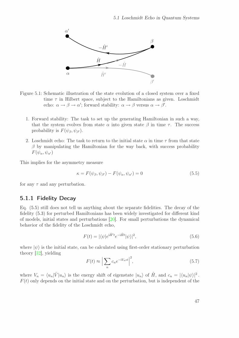
5.1 Loschmidt Echo in Quantum Systems
α
β
α′
β ′
H
−H ′
H ′
−H
Figure 5.1: Schematic illustration of the state evolution of a closed system over a fixedtime τ in Hilbert space, subject to the Hamiltonians as given. Loschmidtecho: α → β → α′; forward stability: α→ β versus α→ β ′.
1. Forward stability: The task to set up the generating Hamiltonian in such a way,that the system evolves from state α into given state β in time τ . The successprobability is F (ψβ, ψβ′).
2. Loschmidt echo: The task to return to the initial state α in time τ from that stateβ by manipulating the Hamiltonian for the way back, with success probabilityF (ψα, ψα′)
This implies for the asymmetry measure
κ = F (ψβ , ψβ′) − F (ψα, ψα′) = 0 (5.5)
for any τ and any perturbation.
5.1.1 Fidelity Decay
Eq. (5.5) still does not tell us anything about the separate fidelities. The decay of thefidelity (5.3) for perturbed Hamiltonians has been widely investigated for different kindof models, initial states and perturbations [20]. For small perturbations the dynamicalbehavior of the fidelity of the Loschmidt echo,
F (t) = |〈ψ|eiH′te−iHt|ψ〉|2, (5.6)
where |ψ〉 is the initial state, can be calculated using first-order stationary perturbationtheory [32], yielding
F (t) ≈∣∣∣
∑
n
cne−iVnǫt
∣∣∣
2
, (5.7)
where Vn = 〈un|V |un〉 is the energy shift of eigenstate |un〉 of H , and cn = |〈un|ψ〉|2 .F (t) only depends on the initial state and on the perturbation, but is independent of the
47
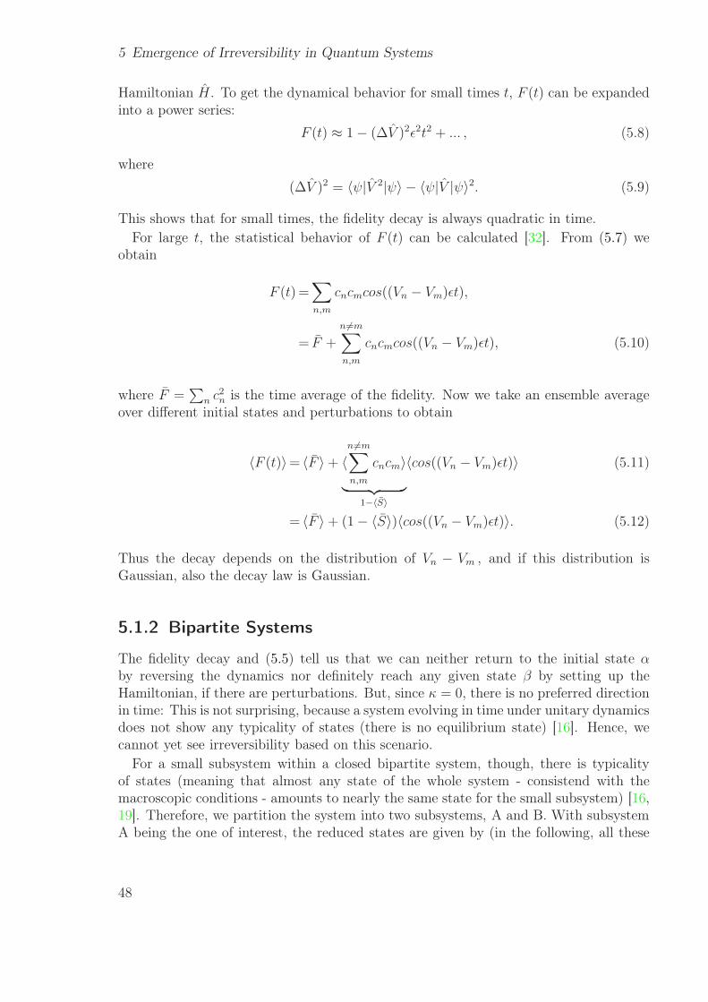
5 Emergence of Irreversibility in Quantum Systems
Hamiltonian H. To get the dynamical behavior for small times t, F (t) can be expandedinto a power series:
F (t) ≈ 1 − (∆V )2ǫ2t2 + ... , (5.8)
where
(∆V )2 = 〈ψ|V 2|ψ〉 − 〈ψ|V |ψ〉2. (5.9)
This shows that for small times, the fidelity decay is always quadratic in time.For large t, the statistical behavior of F (t) can be calculated [32]. From (5.7) we
obtain
F (t) =∑
n,m
cncmcos((Vn − Vm)ǫt),
= F +
n 6=m∑
n,m
cncmcos((Vn − Vm)ǫt), (5.10)
where F =∑
n c2n is the time average of the fidelity. Now we take an ensemble average
over different initial states and perturbations to obtain
〈F (t)〉= 〈F 〉 + 〈n 6=m∑
n,m
cncm〉︸ ︷︷ ︸
1−〈S〉
〈cos((Vn − Vm)ǫt)〉 (5.11)
= 〈F 〉 + (1 − 〈S〉)〈cos((Vn − Vm)ǫt)〉. (5.12)
Thus the decay depends on the distribution of Vn − Vm , and if this distribution isGaussian, also the decay law is Gaussian.
5.1.2 Bipartite Systems
The fidelity decay and (5.5) tell us that we can neither return to the initial state αby reversing the dynamics nor definitely reach any given state β by setting up theHamiltonian, if there are perturbations. But, since κ = 0, there is no preferred directionin time: This is not surprising, because a system evolving in time under unitary dynamicsdoes not show any typicality of states (there is no equilibrium state) [16]. Hence, wecannot yet see irreversibility based on this scenario.
For a small subsystem within a closed bipartite system, though, there is typicalityof states (meaning that almost any state of the whole system - consistend with themacroscopic conditions - amounts to nearly the same state for the small subsystem) [16,19]. Therefore, we partition the system into two subsystems, A and B. With subsystemA being the one of interest, the reduced states are given by (in the following, all these
48
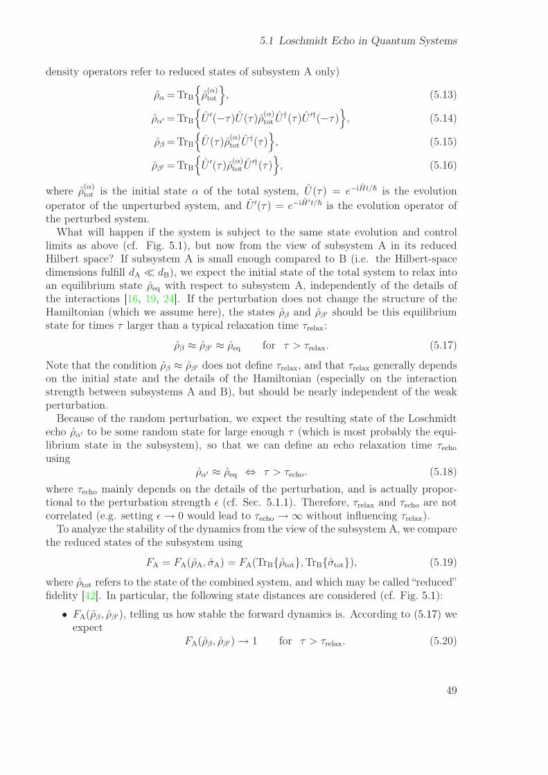
5.1 Loschmidt Echo in Quantum Systems
density operators refer to reduced states of subsystem A only)
ρα =TrB
ρ(α)tot
, (5.13)
ρα′ =TrB
U ′(−τ)U(τ)ρ(α)tot U
†(τ)U ′†(−τ)
, (5.14)
ρβ =TrB
U(τ)ρ(α)tot U
†(τ)
, (5.15)
ρβ′ =TrB
U ′(τ)ρ(α)tot U
′†(τ)
, (5.16)
where ρ(α)tot is the initial state α of the total system, U(τ) = e−iHt/~ is the evolution
operator of the unperturbed system, and U ′(τ) = e−iH′t/~ is the evolution operator ofthe perturbed system.
What will happen if the system is subject to the same state evolution and controllimits as above (cf. Fig. 5.1), but now from the view of subsystem A in its reducedHilbert space? If subsystem A is small enough compared to B (i.e. the Hilbert-spacedimensions fulfill dA ≪ dB), we expect the initial state of the total system to relax intoan equilibrium state ρeq with respect to subsystem A, independently of the details ofthe interactions [16, 19, 24]. If the perturbation does not change the structure of theHamiltonian (which we assume here), the states ρβ and ρβ′ should be this equilibriumstate for times τ larger than a typical relaxation time τrelax:
ρβ ≈ ρβ′ ≈ ρeq for τ > τrelax. (5.17)
Note that the condition ρβ ≈ ρβ′ does not define τrelax, and that τrelax generally dependson the initial state and the details of the Hamiltonian (especially on the interactionstrength between subsystems A and B), but should be nearly independent of the weakperturbation.
Because of the random perturbation, we expect the resulting state of the Loschmidtecho ρα′ to be some random state for large enough τ (which is most probably the equi-librium state in the subsystem), so that we can define an echo relaxation time τecho
usingρα′ ≈ ρeq ⇔ τ > τecho. (5.18)
where τecho mainly depends on the details of the perturbation, and is actually propor-tional to the perturbation strength ǫ (cf. Sec. 5.1.1). Therefore, τrelax and τecho are notcorrelated (e.g. setting ǫ→ 0 would lead to τecho → ∞ without influencing τrelax).
To analyze the stability of the dynamics from the view of the subsystem A, we comparethe reduced states of the subsystem using
FA = FA(ρA, σA) = FA(TrBρtot,TrBσtot), (5.19)
where ρtot refers to the state of the combined system, and which may be called “reduced”fidelity [42]. In particular, the following state distances are considered (cf. Fig. 5.1):
• FA(ρβ , ρβ′), telling us how stable the forward dynamics is. According to (5.17) weexpect
FA(ρβ, ρβ′) → 1 for τ > τrelax. (5.20)
49
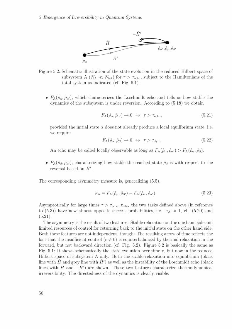
5 Emergence of Irreversibility in Quantum Systems
ρα
ρα′ ,ρβ ,ρβ′
H
−H ′
H ′
Figure 5.2: Schematic illustration of the state evolution in the reduced Hilbert space ofsubsystem A (NA ≪ Ntot) for τ > τecho, subject to the Hamiltonians of thetotal system as indicated (cf. Fig. 5.1).
• FA(ρα, ρα′), which characterizes the Loschmidt echo and tells us how stable thedynamics of the subsystem is under reversion. According to (5.18) we obtain
FA(ρα, ρα′) → 0 ⇔ τ > τecho, (5.21)
provided the initial state α does not already produce a local equilibrium state, i.e.we require
FA(ρα, ρβ) → 0 ⇔ τ > τdyn. (5.22)
An echo may be called locally observable as long as FA(ρα, ρα′) > FA(ρα, ρβ).
• FA(ρβ, ρα′), characterizing how stable the reached state ρβ is with respect to thereversal based on H ′.
The corresponding asymmetry measure is, generalizing (5.5),
κA = FA(ρβ, ρβ′) − FA(ρα, ρα′). (5.23)
Asymptotically for large times τ > τecho, τrelax the two tasks defined above (in referenceto (5.3)) have now almost opposite success probabilities, i.e. κA ≈ 1, cf. (5.20) and(5.21).
The asymmetry is the result of two features: Stable relaxation on the one hand side andlimited resources of control for returning back to the initial state on the other hand side.Both these features are not independent, though: The resulting arrow of time reflects thefact that the insufficient control (ǫ 6= 0) is counterbalanced by thermal relaxation in theforward, but not backward direction (cf. Fig. 5.2). Figure 5.2 is basically the same asFig. 5.1: It shows schematically the state evolution over time τ , but now in the reducedHilbert space of subsystem A only. Both the stable relaxation into equilibrium (blackline with H and grey line with H ′) as well as the instability of the Loschmidt echo (blacklines with H and −H ′) are shown. These two features characterize thermodynamicalirreversibility. The directedness of the dynamics is clearly visible.
50
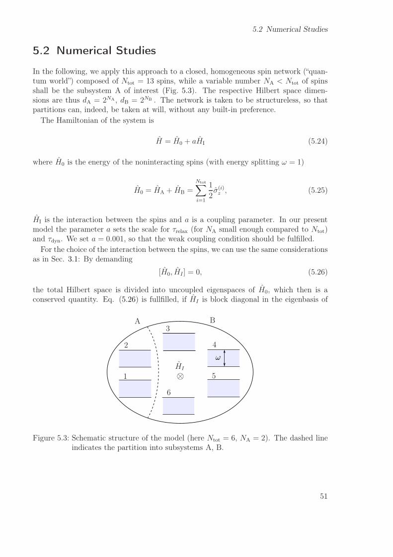
5.2 Numerical Studies
5.2 Numerical Studies
In the following, we apply this approach to a closed, homogeneous spin network (“quan-tum world”) composed of Ntot = 13 spins, while a variable number NA < Ntot of spinsshall be the subsystem A of interest (Fig. 5.3). The respective Hilbert space dimen-sions are thus dA = 2NA , dB = 2NB . The network is taken to be structureless, so thatpartitions can, indeed, be taken at will, without any built-in preference.
The Hamiltonian of the system is
H = H0 + aHI (5.24)
where H0 is the energy of the noninteracting spins (with energy splitting ω = 1)
H0 = HA + HB =Ntot∑
i=1
1
2σ(i)z , (5.25)
HI is the interaction between the spins and a is a coupling parameter. In our presentmodel the parameter a sets the scale for τrelax (for NA small enough compared to Ntot)and τdyn. We set a = 0.001, so that the weak coupling condition should be fulfilled.
For the choice of the interaction between the spins, we can use the same considerationsas in Sec. 3.1: By demanding
[H0, HI ] = 0, (5.26)
the total Hilbert space is divided into uncoupled eigenspaces of H0, which then is aconserved quantity. Eq. (5.26) is fullfilled, if HI is block diagonal in the eigenbasis of
1
2
3
4
5
6
⊗HI
ωω
A B
Figure 5.3: Schematic structure of the model (here Ntot = 6, NA = 2). The dashed lineindicates the partition into subsystems A, B.
51
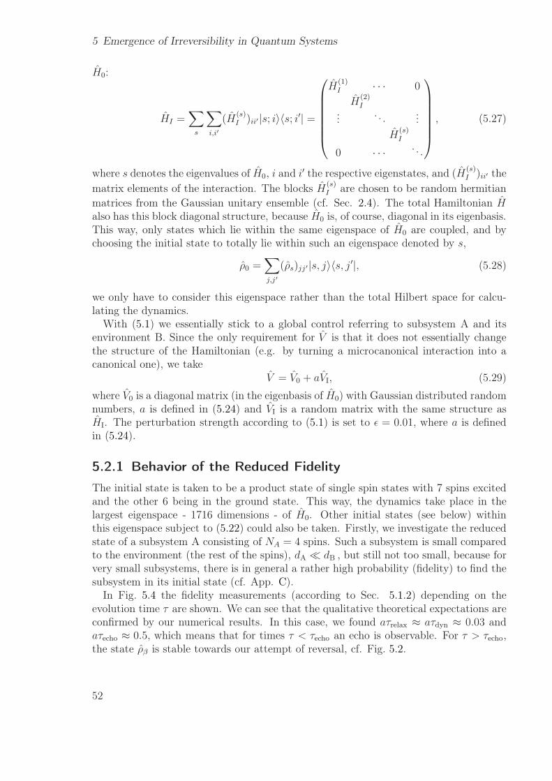
5 Emergence of Irreversibility in Quantum Systems
H0:
HI =∑
s
∑
i,i′
(H(s)I )ii′|s; i〉〈s; i′| =
H(1)I · · · 0
H(2)I
... . . . ...H
(s)I
0 · · · . . .
, (5.27)
where s denotes the eigenvalues of H0, i and i′ the respective eigenstates, and (H(s)I )ii′ the
matrix elements of the interaction. The blocks H(s)I are chosen to be random hermitian
matrices from the Gaussian unitary ensemble (cf. Sec. 2.4). The total Hamiltonian Halso has this block diagonal structure, because H0 is, of course, diagonal in its eigenbasis.This way, only states which lie within the same eigenspace of H0 are coupled, and bychoosing the initial state to totally lie within such an eigenspace denoted by s,
ρ0 =∑
j,j′
(ρs)jj′|s, j〉〈s, j′|, (5.28)
we only have to consider this eigenspace rather than the total Hilbert space for calcu-lating the dynamics.
With (5.1) we essentially stick to a global control referring to subsystem A and itsenvironment B. Since the only requirement for V is that it does not essentially changethe structure of the Hamiltonian (e.g. by turning a microcanonical interaction into acanonical one), we take
V = V0 + aVI, (5.29)
where V0 is a diagonal matrix (in the eigenbasis of H0) with Gaussian distributed randomnumbers, a is defined in (5.24) and VI is a random matrix with the same structure asHI. The perturbation strength according to (5.1) is set to ǫ = 0.01, where a is definedin (5.24).
5.2.1 Behavior of the Reduced Fidelity
The initial state is taken to be a product state of single spin states with 7 spins excitedand the other 6 being in the ground state. This way, the dynamics take place in thelargest eigenspace - 1716 dimensions - of H0. Other initial states (see below) withinthis eigenspace subject to (5.22) could also be taken. Firstly, we investigate the reducedstate of a subsystem A consisting of NA = 4 spins. Such a subsystem is small comparedto the environment (the rest of the spins), dA ≪ dB , but still not too small, because forvery small subsystems, there is in general a rather high probability (fidelity) to find thesubsystem in its initial state (cf. App. C).
In Fig. 5.4 the fidelity measurements (according to Sec. 5.1.2) depending on theevolution time τ are shown. We can see that the qualitative theoretical expectations areconfirmed by our numerical results. In this case, we found aτrelax ≈ aτdyn ≈ 0.03 andaτecho ≈ 0.5, which means that for times τ < τecho an echo is observable. For τ > τecho,the state ρβ is stable towards our attempt of reversal, cf. Fig. 5.2.
52
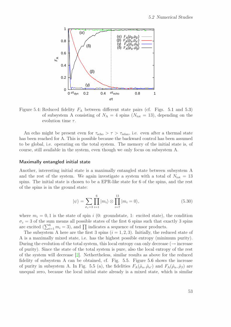
5.2 Numerical Studies
0
0.2
0.4
0.6
0.8
1
0 0.2 0.4 0.8 1
aτ
(β)
(α)
(δ)
(γ)
FA
aτechoaτdyn
(α) FA(ρβ,ρβ’)(β) FA(ρα,ρα’)(γ) FA(ρα,ρβ)(δ) FA(ρα’,ρβ)
Figure 5.4: Reduced fidelity FA between different state pairs (cf. Figs. 5.1 and 5.3)of subsystem A consisting of NA = 4 spins (Ntot = 13), depending on theevolution time τ .
An echo might be present even for τecho > τ > τrelax, i.e. even after a thermal statehas been reached for A. This is possible because the backward control has been assumedto be global, i.e. operating on the total system. The memory of the initial state is, ofcourse, still available in the system, even though we only focus on subsystem A.
Maximally entangled initial state
Another, interesting initial state is a maximally entangled state between subsystem Aand the rest of the system. We again investigate a system with a total of Ntot = 13spins. The initial state is chosen to be a EPR-like state for 6 of the spins, and the restof the spins is in the ground state:
|ψ〉 =∑
σz=3
6∏
i=1
|mi〉 ⊗13∏
i=7
|mi = 0〉, (5.30)
where mi = 0, 1 is the state of spin i (0: groundstate, 1: excited state), the conditionσz = 3 of the sum means all possible states of the first 6 spins such that exactly 3 spinsare excited (
∑6i=1mi = 3), and
∏indicates a sequence of tensor products.
The subsystem A here are the first 3 spins (i = 1, 2, 3). Initially, the reduced state ofA is a maximally mixed state, i.e. has the highest possible entropy (minimum purity).During the evolution of the total system, this local entropy can only decrease (→ increaseof purity). Since the state of the total system is pure, also the local entropy of the restof the system will decrease [2]. Nethertheless, similar results as above for the reducedfidelity of subsystem A can be obtained, cf. Fig. 5.5. Figure 5.6 shows the increaseof purity in subsystem A. In Fig. 5.5 (a), the fidelities FA(ρα, ρα′) and FA(ρα, ρβ) areunequal zero, because the local initial state already is a mixed state, which is similar
53
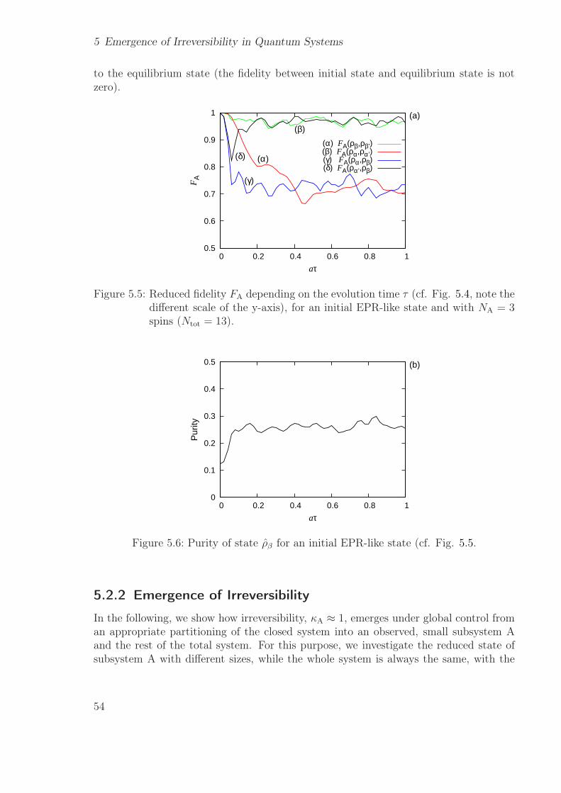
5 Emergence of Irreversibility in Quantum Systems
to the equilibrium state (the fidelity between initial state and equilibrium state is notzero).
0.5
0.6
0.7
0.8
0.9
1
0 0.2 0.4 0.6 0.8 1
aτ
(β)
(α)(δ)
(γ)
(a)
FA
(α) FA(ρβ,ρβ’)(β) FA(ρα,ρα’)(γ) FA(ρα,ρβ)(δ) FA(ρα’,ρβ)
Figure 5.5: Reduced fidelity FA depending on the evolution time τ (cf. Fig. 5.4, note thedifferent scale of the y-axis), for an initial EPR-like state and with NA = 3spins (Ntot = 13).
0
0.1
0.2
0.3
0.4
0.5
0 0.2 0.4 0.6 0.8 1
aτ
Pur
ity
(b)
Figure 5.6: Purity of state ρβ for an initial EPR-like state (cf. Fig. 5.5.
5.2.2 Emergence of Irreversibility
In the following, we show how irreversibility, κA ≈ 1, emerges under global control froman appropriate partitioning of the closed system into an observed, small subsystem Aand the rest of the total system. For this purpose, we investigate the reduced state ofsubsystem A with different sizes, while the whole system is always the same, with the
54
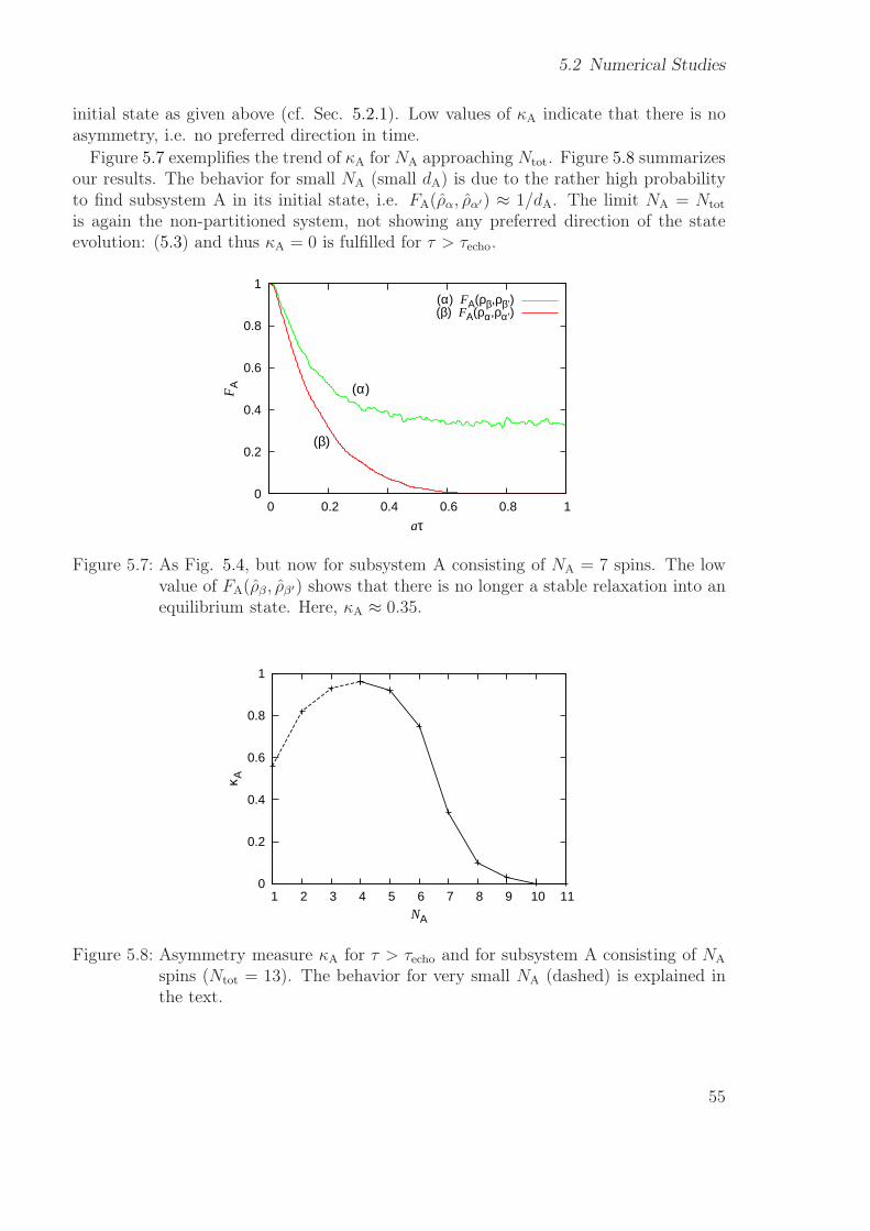
5.2 Numerical Studies
initial state as given above (cf. Sec. 5.2.1). Low values of κA indicate that there is noasymmetry, i.e. no preferred direction in time.
Figure 5.7 exemplifies the trend of κA for NA approaching Ntot. Figure 5.8 summarizesour results. The behavior for small NA (small dA) is due to the rather high probabilityto find subsystem A in its initial state, i.e. FA(ρα, ρα′) ≈ 1/dA. The limit NA = Ntot
is again the non-partitioned system, not showing any preferred direction of the stateevolution: (5.3) and thus κA = 0 is fulfilled for τ > τecho.
0
0.2
0.4
0.6
0.8
1
0 0.2 0.4 0.6 0.8 1
aτ
(β)
(α)FA
(α) FA(ρβ,ρβ’)(β) FA(ρα,ρα’)
Figure 5.7: As Fig. 5.4, but now for subsystem A consisting of NA = 7 spins. The lowvalue of FA(ρβ , ρβ′) shows that there is no longer a stable relaxation into anequilibrium state. Here, κA ≈ 0.35.
0
0.2
0.4
0.6
0.8
1
1 2 3 4 5 6 7 8 9 10 11NA
κ A
Figure 5.8: Asymmetry measure κA for τ > τecho and for subsystem A consisting of NA
spins (Ntot = 13). The behavior for very small NA (dashed) is explained inthe text.
55
5 Emergence of Irreversibility in Quantum Systems
5.2.3 Reduced Fidelity for Local Control
We have seen that the Loschmidt echo remains observable for τ < τecho, if we allowglobal control with a small, global error (homogeneous control) over the system, butonly focus on the dynamics of a subsystem. From this point of view, it seems as if thisis a violation of the second law. But within the total, closed system, there is no loss ofinformation, the entropy stays constant.
Here, we limit our control on only the subsystem, but without any error (inhomoge-neous control), and compare FA(ρα, ρα′) (Loschmidt echo) with FA(ρα, ρβ) (dynamics).The total system, though, is described by the same structureless Hamiltonian as above.
To carry out this local reversal, we first have to split the Hamiltonian into
H = HA + HB + HAB, (5.31)
whereHA =
∑
i
QA,iTrQ†A,iH, (5.32)
and where the QA,i are all orthogonal and normalized operators of the total Hilbert space,which only act on the subsystem A of interest. All these operators can be calculated by
QA =√
2−Ntotσ(1)i1
⊗ σ(2)i2
⊗ · · · ⊗ σNA
iNA
⊗ 1B, (5.33)
where√
2−Ntot is a normalization factor, in = 1, x, y, z, and σ(n)in are the Pauli operators
acting only on spin n (σ1 = 1 shall be a unit operator). 1B is the unit operator actingon HB.
The reversal process is now defined as
H → −H ′ = −HA + HB + HAB = H − 2HA. (5.34)
Because of the high numerical effort needed for solving (5.33), we consider a spin networkconsisting of Ntot = 8 spins only. Otherwise the total Hamiltonian is the same as above(Sec. 5.2). The initial state is a product state with 4 spins excited and the other 4 beingin the ground state.
To see whether an echo may be observed, we compare FA(ρα, ρα′) with FA(ρα, ρβ).Calculating FA(ρβ, ρβ′) does not give the expected result here: The “perturbation” (V =
H ′ − H) of the Hamiltonian is of the same order of magnitude as the Hamiltonian, andbecause of the small size of the system, there is no stable relaxation as in Sec. 5.2.1(FA(ρβ, ρβ′) = 1 was only observed for NA = 1, which is too small for our purposes, cf.Sec. 5.2.1). Figure 5.9 shows the reduced fidelity of the Loschmidt echo (FA(ρα, ρα′))and of the dynamics (FA(ρα, ρβ)), for (a) NA = 3 and (b) NA = 7 spins. We find thatin all these cases τecho ≈ τdyn, so that there is no time window for observing an echo.Actually, the control over the Hamiltonian is very limited, even if NA = 7. As we can seein (5.33), only one fourth of all basis operators of the total Hamiltonian are controlled.This may explain why the two Figs. 5.9 (a) and (b) look nearly the same: In both cases,the influence of the reversal is very weak.
56
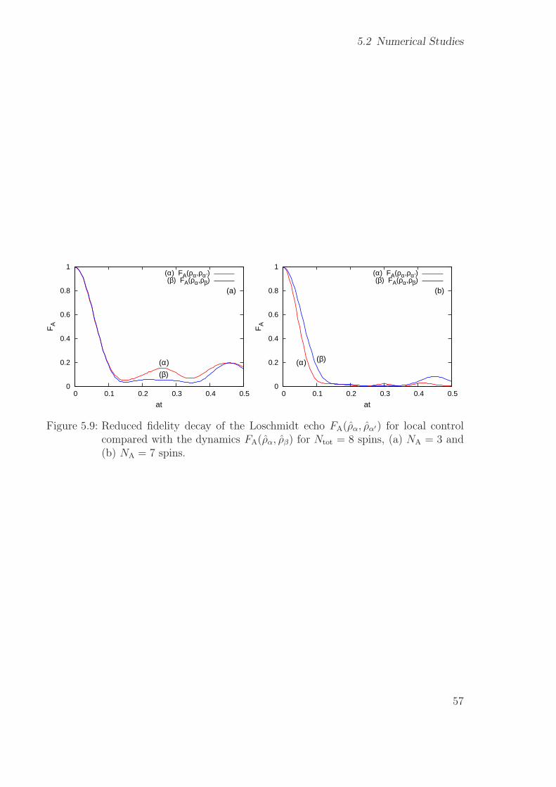
5.2 Numerical Studies
0
0.2
0.4
0.6
0.8
1
0 0.1 0.2 0.3 0.4 0.5
at
(α)
(β)
FA
(a)
(α) FA(ρα,ρα’)(β) FA(ρα,ρβ)
0
0.2
0.4
0.6
0.8
1
0 0.1 0.2 0.3 0.4 0.5
at
(α) (β)
FA
(b)
(α) FA(ρα,ρα’)(β) FA(ρα,ρβ)
Figure 5.9: Reduced fidelity decay of the Loschmidt echo FA(ρα, ρα′) for local controlcompared with the dynamics FA(ρα, ρβ) for Ntot = 8 spins, (a) NA = 3 and(b) NA = 7 spins.
57

5 Emergence of Irreversibility in Quantum Systems
58
6 Summary
We have investigated a closed laser model subject to pure Schrödinger dynamics. Themodel consisted of the three basic elements of a laser: One resonant mode of the radiationfield inside an optical cavity represented by a harmonic oscillator, the gain mediumrepresented by a non-degenerate two-level system (spin) interacting resonantly with thefield mode, and the energy pump modeled by embedding the interfacing spin within afinite spin network with an energy exchange condition.
Depending on the initial state, three special scenarios have been addressed: Lasingrelaxation, non-lasing relaxation and energy back-flow from the field mode. The respec-tive local equilibrium states were in accord with the theory of quantum thermodynamics.The agreement of the numerical results with the thermodynamical expectations is quitegood, considering the relatively small size of the spin network.
For the lasing relaxation, the spin network was set up in the highest energy eigen-state and the field mode in the ground state. We have seen that during relaxation thefield mode of our laser model is in a phase-diffused Glauber state, even for a randominteraction between the gain medium and pump reservoir, so that in principle coherentpumping was possible. The result of the LEMBAS analysis is consistent with this find-ing: The energy change of the field mode is induced by heat flow only, i.e. the effectivedynamics of the field mode induced by the environment is incoherent.
For the energy back-flow, the spin network was initially in the ground state, whilethe field mode was (i) in a phase-diffused Glauber state and (ii) in a coherent Glauberstate. The total energy flow was the same in both cases. The analysis with LEMBAS,however, yielded different results. The reason for this may be that for quantum systems,the concept of local entropy and its change (and thus of heat and work flows) dependson the partition used.
We have seen that it is thermodynamically possible to (partly) extract energy from thefield mode in the phase-diffused Glauber state, and, without any other effect, performthe same amount of work on another system. This generally applies to systems, whichare not in a thermal state. Nevertheless, it is unclear how and whether this possibilitycan be practically used.
Relaxation is not yet the full story: In chapter 5, we have investigated why this processcannot be inverted. We we have seen that the arrow of time in a quantum system withunitary dynamics is not an absolute property of the system but rather a consequence oftwo externally imposed conditions: (i) The system is subject to Hamiltonian perturba-tions, caused by limited control over the system when carrying out the Loschmidt echo.(ii) Within the system one focuses on a small enough part A (thus allowing for localrelaxation).
In order to characterize both instability and irreversibility, we have applied fidelity
59
6 Summary
measurements subject to perturbations. We introduced an asymmetry measure compar-ing the stability of the forward dynamics with the stability of the Loschmidt echo, andhave seen that perturbations and local observation lead to a time-asymmetric evolution.
This approach has been applied to a spin network (the “matter”-part of our quantum-optical scenario) by focusing on part of the spins forming a subsystem, but neverthelessallowing global, imperfect control. This simplified model has the advantage of homogene-ity, i.e. we can choose partitions at will without having to consider physical constraints(e.g. like oscillator versus spin in the laser model)
We found that there is a time window for which an echo is observable, but asymp-totically for large times the reached state is stable towards our attempt of reversal. Byreducing the size of the subsystem, we have seen the emergence of a local time’s arrowand therewith irreversibility within total systems as small as some 10 spins.
Finally, we have limited our control to a local reversal (sign-flip) of the Hamiltonianof the observed subsystem only. In this case, we found that there is no observable echoat all.
60
A Commutation Relation of theJaynes-Cummings Interaction
The total Jaynes-Cummings Hamiltonian for the interaction of a two-level atom withone mode of the quantized radiation field is (cf. Sec. 2.2.2, here for g = 1)
H = HA + HF + VJC =ω
2σz + νN + σ−a
† + σ+a. (A.1)
Using the commutation relations
[σz , σ±] =±2σ±, (A.2)[
N , a]
=−a, (A.3)[
N, a†]
= a†, (A.4)
and remembering that operators, which act on different Hilbert spaces, always commute,we can calculate the commutator
[
HA + HF, VJC
]
=[ω
2σz, σ−a
†]
+[ω
2σz, σ+a
]
+[
νN , σ−a†]
+[
νN , σ+a]
(A.5)
= −ωσ−a† + ωσ+a+ νσ−a† − νσ+a (A.6)
= (ν − ω)σ−a† + (ω − ν)σ+a. (A.7)
If ω = ν we obtain [
HA + HF, VJC
]
= 0. (A.8)
61

A Commutation Relation of the Jaynes-Cummings Interaction
62
B Poisson and Thermal Distributionwith the Same Entropy
The Poisson distribution for a harmonic oscillator is given by
PPoiss(n) = e−〈N〉 〈N〉nn!
, (B.1)
where n = 0, 1, ...,∞ denotes the eigenstates of the number operator N , and PPoiss(n) isthe probability to find the oscillator in state n. The thermal distribution is given by
Pth(n) =1
Ze−β~ωn, (B.2)
where β is the inverse temperature, ω the eigenfrequency of the oscillator and Z =∑
n e−β~ωn is a normalization factor.
We will now calculate how to set the inverse temperature β, such that the thermal dis-tribution and the Poissonian distribution with given 〈N〉 have the same von Neumann en-tropy. To get this inverse temperature, we solve S(Pth) for β and set S(Pth) = S(PPoiss).The von Neumann entropy of the thermal distribution is (with ~ω = 1 and kB = 1)
S(Pth) =−∑
n
Pth(n)ln (Pth(n)) (B.3)
=−∑
n
e−βn
Zln(e−βn
Z
)
(B.4)
=1
Z
∑
n
e−βn (ln(Z) + βn) (B.5)
=1
Z
(
Zln(Z) +∑
n
βne−βn
)
(B.6)
= ln(Z) +1
Z
∑
n
βne−βn. (B.7)
Now we use Z =∑
n e−βn = eβ
eβ−1and
∑
n βne−βn = βeβ
(eβ−1)2:
S(Pth)= ln(
eβ
eβ − 1
)
+eβ − 1
eββeβ
(eβ − 1)2(B.8)
= β − ln(eβ − 1
)+
β
eβ − 1(B.9)
=βeβ
eβ − 1− ln
(eβ − 1
), (B.10)
63
B Poisson and Thermal Distribution with the Same Entropy
which can only be solved numerically for β. For ~ω 6= 1 we would obtain β ′ = β~ω
64
C Appendix on Fidelity
Here we calculate how the fidelity of the Loschmidt echo in a subsystem of a bipartitesystem statictically behaves, depending on the number of dimensions N of the subsystem.The initial state |α〉 given in some basis |ui〉 of the subsystem is
|α〉 =N∑
i
ci|ui〉, withN∑
i
|ci|2 = 1. (C.1)
After the echo, the subsystem generally is in a mixed state
ρ =N∑
i,j
pij |ui〉〈uj|, withN∑
i
pii = 1. (C.2)
The fidelity between these states is
F = 〈α|ρ|α〉
=
N∑
i,j,m,n
c∗i cjpmn〈ui|um〉〈un|uj〉
=N∑
i,j
c∗i cjpij. (C.3)
By averaging (‖ ‖) either over (i) a uniform distribution of initial states,
‖c∗i cj‖ =1
Nδij , (C.4)
or over (ii) a uniform distribution of mixed states ρ,
‖pij‖ =1
Nδij, (C.5)
yields the same result for the fidelity:
(i) ‖F‖ =
N∑
i,j
‖c∗i cj‖pii =
N∑
i
1
Npii =
1
N(C.6)
(ii) ‖F‖ =N∑
i,j
c∗i cj‖pij‖ =N∑
i
1
N|ci|2 =
1
N. (C.7)
This shows that for very small subsystems this fidelity may be considerably larger thanzero.
65

C Appendix on Fidelity
66
Bibliography
[1] Robert Alicki. The quantum open system as a model of the heat engine. J. Phys.A: Math. Gen., 12:L103, 1979.
[2] Huzihiro Araki and Elliott H. Lieb. Entropy Inequalities. Comm. math. Phys.,18:160, 1970.
[3] P. Borowski, J. Gemmer, and G. Mahler. Relaxation into equilibrium under pureSchrödinger dynamics. Eur. Phys. J. B, 35:255, 2003.
[4] E. Boukobza and D. J. Tannor. Termodynamics of bipartite systems: Applicationto light-matter interactions. Phys. Rev. A, 74(063823), 2006.
[5] E. Boukobza and D. J. Tannor. Three-level systems as amplifiers and attenuators:A thermodynamic analysis. Phys. Rev. Lett., 98:240601, 2007.
[6] Patrizia Castiglione, Massimo Falcioni, Annick Lesne, and Angelo Vulpiani. Chaosand Coarse Graining in Statistical Mechanics. Campridge University Press, 2008.
[7] Claude Cohen-Tannoudji, Bernard Diu, and Franck Laloë. Quantum MechanicsVolume I. Hermann, second edition.
[8] Claude Cohen-Tannoudji, Bernard Diu, and Franck Laloë. Quantum MechanicsVolume II. Hermann, second edition.
[9] D. G. Cory, R. Laflamme, E. Knill, L. Viola, T. F. Havel, N. Boulant, G. Boutis,E. Fortunato, S. Lloyd, R. Martinez, C. Negrevergne, M. Pravia, Y. Sharf, G. Tek-lemariam, Y. S. Weinstein, and W. H. Zurek. NMR based quantum informationprocessing: Achievements and prospects. Fortschr. Phys., 48:875, 2000.
[10] Gavin E. Crooks. Quantum operation time reversal. Phys. Rev. A, 77:034101, 2008.
[11] James P. Crutchfield, Christopher J. Ellison, and John R. Mahoney. Time’sbarbed arrow: Irreversibility, crypticity, and stored information. Phys. Rev. Lett.,103:094101, 2009.
[12] Wolfgang Demtröder. Laser Spectroscopy. Springer, third edition.
[13] Massimiliano Esposito, Katja Lindenberg, and Christian Van den Broeck. Univer-sality of Efficiency at Maximum Power. Phys. Rev. Lett., 102:130602, 2009.
67
Bibliography
[14] Edward H. Feng and Gavin E. Crooks. Length of time’s arrow. Phys. Rev. Lett.,101:090602, 2008.
[15] Yan V. Fyodorov. Introduction to the random matrix theory: Gaussian unitaryensemble and beyond. arXiv:math-ph/0412017v1, 2004.
[16] J. Gemmer, M. Michel, and G. Mahler. Quantum Thermodynamics. Springer Verlag,2005.
[17] Christopher Gerry and Peter Knight. Introductory Quantum Optics. CambridgeUniversity Press, first edition.
[18] Roy J. Glauber. Coherent and incoherent state of the radiation field. Phys. Rev.,131:2766, 1963.
[19] Sheldon Goldstein, Joel L. Lebowitz, Roderich Tumulka, and Nino Zanghí. Canon-ical typicality. Phys. Rev. Lett., 96:050403, 2006.
[20] T. Gorin, T. Prosen, T. H. Seligman, and M. Žnidarič. Dynamics of Loschmidtechoes and fidelity decay. Physics Reports, 435:33–156, 2006.
[21] E. L. Hahn. Spin echoes. Phys. Rev., 80(4):580, 1950.
[22] Richard Jozsa. Fidelity for mixed quantum states. J. Mod. Opt., 41:2315, 1994.
[23] P. T. Landsberg. Heat engines and heat pumps at positive and negative absolutetemperatures. J. Phys. A: Math. Gen., 10(10):1773, 1977.
[24] Noah Linden, Sandu Popescu, Anthony J. Short, and Andreas Winter. Quantummechanical evolution towards thermal equilibrium. arXiv:0812.2385v1, 2008.
[25] J. J. Loschmidt. Über den Zustand des Wärmegleichgewichtes eines Systems vonKörpern mit Rücksicht auf die Schwerkraft. Wiener Ber., 73:128, 1876.
[26] Lorenzo Maccone. Quantum solution to the arrow-of-time dilemma. Phys. Rev.Lett., 103:080401, 2009.
[27] M. C. Mackey. Time’s Arrow. Springer, 1992.
[28] Günter Mahler and Volker A. Weberruç. Quantum Networks âĂŞ Dynamics ofOpen Nanostructures. Springer Verlag, 1998.
[29] G. A. Melkov, A. A. Serga, V. S. Tiberkevich, A. N. Oliynyk, and A. N. Slavin.Wave front reversal of a dipolar spin wave pulse in a nonstationary three-waveparametric interaction. Phys. Rev. Lett., 84:3438, 2000.
[30] Klaus Mølmer. Optical coherence: A convenient fiction. Phys. Rev. A, 55(4), 1997.
[31] Kae Nemoto and Samuel L. Braunstein. Quantum coherence: Myth or fact? Phys.Lett. A, 333:378, 2004.
68
Bibliography
[32] A. Peres. Stability of quantum motion in chaotic and regular systems. Phys. Rev.A, 30:1610, 1984.
[33] Sandu Popescu, Anthony J. Short, and Andreas Winter. Entanglement and thefoundations of statistical mechanics. Nature Physics, 2:754, 2006.
[34] N. F. Ramsey. Thermodynamics and statistical mechanics at negative absolutetemperatures. Phys. Rev., 103(1):20, 1956.
[35] Terry Rudolph and Barry C. Sanders. Requirement of optical coherence forcontinuous-varibale quantum teleportation. Phys. Rev. Lett., 87:077903, 2001.
[36] Harry Schmidt. Thermal and Nonthermal Properties of Closed Bipartite QuantumSystems. PhD thesis, Universität Stuttgart, 2007.
[37] Harry Schmidt and Günter Mahler. Control of local relaxation behavior in closedbipartite quantum systems. Phys. Rev. E, 72:016117, 2005.
[38] Harry Schmidt and Günter Mahler. Nonthermal equilibrium states of closed bipar-tite systems. Phys. Rev. E, 75:061111, 2007.
[39] Franz Schwabl. Statistische Mechanik. Springer, 2000.
[40] H. E. D. Scovil and E. O. Schulz-DuBois. Three-level masers as heat enginges.Phys. Rev. Lett., 2(6), 1959.
[41] Marlan O. Scully and M. Suhail Zubairy. Quantum Optics. Cambridge UniversityPress, sixth edition.
[42] Marco Žnidarič and Tomaž Prosen. Fidelity and purity decay in weakly coupledcomposite systems. J. Phys. A: Math. Gen., 36:2463–2481, 2003.
[43] Gerald Waldherr and Günter Mahler. Emergence of irreversibility in quantum sys-tems. In preparation, 2009.
[44] Gerald Waldherr and Günter Mahler. Lasing process in a closed bipartite quantumsystem: A thermodynamical analysis. In preparation, 2009.
[45] J. S. Waugh, W.-K. Rhim, and A. Pines. Spin echoes and loschmidt’s paradox.Pure Appl. Chem., 32:317, 1972.
[46] H. Weimer, M. J. Henrich, F. Rempp, H. Schröder, and G. Mahler. Local effectivedynamics of quantum systmes: A generalized approach to work and heat. EPL,83(30008), 2008.
[47] M. Youssef, G. Mahler, and A.-S. F. Obada. Quantum optical thermodynamicmachines: Lasing as relaxation. 2009.
69

Bibliography
70
Danksagung
Als erstes möchte ich mich bei Prof. Dr. Günter Mahler sehr herzlich bedanken fürdie Betreuung meiner Diplomarbeit, für sein Interesse und für seine richtungsweisendenVorschläge zu meiner Arbeit.
Mein Dank geht auch an Prof. Dr. Hans-Rainer Trebin für die Übernahme des Zweit-berichts meiner Diplomarbeit.
Bedanken möchte ich mich bei den Institutsmitgliedern Heiko Schröder, Kilian Rambach,Jens Teifel, Hendrick Weimer, Thomas Jahnke, Suzanne Lanery und Pedro Vidal fürhilfreiche Diskussionen und für ein angenehmes Arbeitsklima. Besonders bedanke ichmich bei Heiko Schröder, den ich vor allem zu Anfang meiner Diplomarbeit jederzeitmit technischen und physikalischen Fragen befallen habe, und bei Kilian Rambach fürinteressante physikalische Diskussionen.
Ein kleines Dankeschön gebührt auch Florian Rempp, der für kurzweilige Beschäftigungwährend der Mittagspausen gesorgt hat, die ich schon bald vermissen werde.
Bei Matthias Steiner, Stefan Rau, Adam Bühler und Matthias Zimmer bedanke ich michfür abwechslungsreiche Kaffeepausen und für schöne Zeiten während des Studiums.
Für ihre vielseitige Untestützung wärend meines gesamten Studiums danke ich meinenEltern Sigrid und Albin Waldherr.
Bei meiner Frau Ling Waldherr bedanke ich mich dafür, dass sie immer für mich da ist.Dank ihr ist mir diese Arbeit oft leichter gefallen.
71