Embed Size (px)
Citation preview
Online QoS/Revenue Management for Third Generation Mobile Communication Networks
Dissertation
zur Erlangung des Grades eines
D o k t o r s d e r N a t u r w i s s e n s c h a f t e n
der Universität Dortmund am Fachbereich Informatik
von
M a r c o L o h m a n n
Dortmund
2004

Tag der mündlichen Prüfung: 8. Juli 2004
Dekan: Prof. Dr. Bernhard Steffen
Gutachter: Prof. Dr.-Ing. Christoph Lindemann, Prof. Dr. Heiko Krumm


V
Abstract
This thesis shows how online management of both quality of service (QoS) and provider revenue can be performed in third generation (3G) mobile networks by adaptive control of system parameters to changing traffic conditions. As a main result, this approach is based on a novel call admission control and bandwidth degradation scheme for real-time traffic. The admission controller considers real-time calls with two priority levels: calls of high priority have a guaranteed bit-rate, whereas calls of low priority can be temporarily degraded to a lower bit-rate in order to reduce forced termination of calls due to a handover failure. A second contribution constitutes the development of a Markov model for the admission controller that incorporates important features of 3G mobile networks, such as code division multiple access (CDMA) intra- and inter-cell interference and soft handover. Online evaluation of the Markov model enables a periodical adjustment of the threshold for maximal call degradation according to the currently measured traffic in the radio access network and a predefined goal for optimization. Using distinct optimization goals, this allows optimization of both QoS and provider revenue. Performance studies illustrate the effectiveness of the proposed approach and show that QoS and provider revenue can be increased significantly with a moderate degradation of low-priority calls. Compared with existing admission control policies, the overall utilization of cell capacity is significantly improved using the proposed degradation scheme, which can be considered as an “on demand” reservation of cell capacity.
To enable online QoS/revenue management of both real-time and non real-time services, accurate analytical traffic models for non real-time services are required. This thesis identifies the batch Markovian arrival process (BMAP) as the analytically tractable model of choice for the joint characterization of packet arrivals and packet lengths. As a key idea, the BMAP is customized such that different packet lengths are represented by batch sizes of arrivals. Thus, the BMAP enables the “two-dimensional”, i.e., joint, characterization of packet arrivals and packet lengths, and is able to capture correlations between the packet arrival process and the packet length process. A novel expectation maximization (EM) algorithm is developed, and it is shown how to utilize the randomization technique and a stable calculation of Poisson jump probabilities effectively for computing time-dependent conditional expectations of a continuous-time Markov chain required by the expectation step of the EM algorithm. This methodological work enables the EM algorithm to be both efficient and numerical robust and constitutes an important step towards effective, analytically/numerically tractable traffic models. Case studies of measured IP traffic with different degrees of traffic burstiness evidently demonstrate the advantages of the BMAP modeling approach over other widely used analytically tractable models and show that the joint characterization of packet arrivals and packet lengths is decisively for realistic traffic modeling at packet level.

VI

VII
Acknowledgement
Here, I would like to thank all the people, who contributed by their assistance and support substantially to the success of this work. I owe a special debt of gratitude to my thesis advisor, Prof. Dr.-Ing. Christoph Lindemann. My knowledge of effective scientific working is due to him. Beyond his scientific support and introduction to the field of stochastic processes and stochastic modeling, he was always a source of visionary ideas. His experience and initial support in writing scientific publications enabled me to write conference and journal articles on my own. Moreover, I would like to thank all colleagues of the Computer Systems and Performance Evaluation group.
Special thanks are due to my brother Frank and my parents, Karin and Jürgen, to whom I would like to dedicate this thesis. Their support, motivation, and love always encouraged me to work enthusiastically and highly motivated also during challenging periods of my scientific activity.
Danksagung
An dieser Stelle möchte ich mich bei denjenigen bedanken, die durch ihre Hilfe und Unterstützung wesentlich zum Gelingen dieser Arbeit beigetragen haben. Dabei gebührt ein besonderer Dank meinem Mentor, Prof. Dr.-Ing. Christoph Lindemann, dem ich meine Kenntnisse effektiver wissenschaftlicher Arbeitsmethodik verdanke. Er hat mich nicht nur fachlich unterstützt und in das Gebiet stochastischer Prozesse und stochastischer Modellbildung eingeführt, sondern war auch stets ein Quell visionärer Ideen. Erst seine Erfahrung und Unterstützung hat mir das erfolgreiche Erstellen wissenschaftlicher Publikationen für internationale Konferenzen und Zeitschriften ermöglicht. Weiterhin möchte ich mich bei allen Mitarbeitern des Fachgebiets Rechnersysteme und Leistungsbewertung bedanken.
Ein spezieller Dank gebührt meinem Bruder Frank und meinen Eltern, Karin und Jürgen, denen ich diese Arbeit widmen möchte. Nur durch Ihre Unterstützung, Motivation und Liebe konnte ich auch während herausfordernder Abschnitte meiner wissenschaftlichen Tätigkeit stets hoch motiviert und engagiert arbeiten.

VIII
IX
Contents
1 Introduction ......................................................................................................................... 1
1.1 Evolution towards 3G Mobile Communication Networks .......................................... 1
1.2 Previous Results on QoS Management for 3G Mobile Networks ............................... 5
1.3 Previous Results on Traffic Characterization and Modeling ....................................... 9
1.4 Summary of Contributions of this Thesis .................................................................. 12
1.5 Key Publications Making up this Thesis.................................................................... 15
1.6 Thesis Outline ............................................................................................................ 16
2 Online QoS/Revenue Management of Real-Time Services............................................ 19
2.1 Architecture of 3G Communication Networks .......................................................... 19
2.2 QoS/Revenue Management Framework .................................................................... 21
2.3 CDMA Principles....................................................................................................... 22
2.4 Admission Control Based on Bandwidth Degradation .............................................. 23
2.5 Derivation of the Feasibility Function ....................................................................... 29
2.6 Optimization of the Admission Controller................................................................. 31
2.6.1 Markov Chain Analysis of the Admission Controller.................................... 31
2.6.2 Optimization of the Degradation Threshold................................................... 37
2.7 Quantitative Results for the QoS/Revenue Management Framework ....................... 39
2.7.1 Numerical Analysis of the Markov Model..................................................... 39
2.7.2 Calibrating the Soft Handover Queue ............................................................ 40
2.7.3 Evaluation of Optimization Goals.................................................................. 43
2.7.4 Comparison of Degradation Scheme and Guard Channel Scheme................ 50
2.8 QoS/Revenue Management Framework in Practice .................................................. 52
2.8.1 Implementation Issues.................................................................................... 52
2.8.2 Simulation Results for the QoS/Revenue Management Framework ............. 54
2.9 Summary .................................................................................................................... 55
X CONTENTS
3 EM Algorithm for Parameter Estimation of the Batch Markovian Arrival Process.. 59
3.1 The Batch Markovian Arrival Process....................................................................... 59
3.2 The Randomization Technique .................................................................................. 61
3.3 Effective and Stable Calculation of Poisson Probabilities......................................... 62
3.4 The EM Algorithm for the BMAP............................................................................. 64
3.4.1 Fundamentals of the EM Algorithm............................................................... 64
3.4.2 Mathematical Framework .............................................................................. 65
3.4.3 Effective Computational Formulas ................................................................ 67
3.4.4 Detailed Investigations of Conditional Probabilities ..................................... 71
3.4.5 Effective Calculation of Integrals over Matrix Exponentials......................... 73
3.5 Implementation Issues................................................................................................ 75
3.6 Computational Complexity of the EM Algorithm ..................................................... 75
3.7 Convergence Behavior ............................................................................................... 78
3.8 Open Source Toolkit IP2BMAP ................................................................................ 80
3.9 Summary .................................................................................................................... 83
4 Modeling IP Traffic Using the Batch Markovian Arrival Process ............................... 85
4.1 Important Characteristics of IP Traffic ...................................................................... 85
4.1.1 Self-Similarity in IP Traffic Streams ............................................................. 86
4.1.2 TCP Packet Length Characteristics................................................................ 88
4.2 Joint Characterization of Packet Arrivals and Packet Lengths .................................. 89
4.3 The Rescaled Adjusted Range Statistic ..................................................................... 91
4.4 Case Study I: Traffic Modeling of ISP IP Traffic...................................................... 92
4.4.1 Traffic Measurements .................................................................................... 92
4.4.2 Model Specification and Parameter Estimation ............................................. 93
4.4.3 Performance Evaluation ................................................................................. 96
4.5 Case Study II: Traffic Modeling of WAN IP Traffic............................................... 105
4.5.1 Traffic Measurements .................................................................................. 105
4.5.2 Model Specification and Parameter Estimation ........................................... 106
4.5.3 Performance Evaluation ............................................................................... 109
4.6 Summary .................................................................................................................. 117
CONTENTS XI
5 Future Research Directions ............................................................................................ 119
5.1 Online QoS/Revenue Management of Non Real-Time Services............................. 119
5.2 QoS/Revenue Management for B3G Mobile Communication Networks ............... 124
5.3 Further Enhancements of the EM Algorithm for BMAPs ....................................... 127
5.4 EM Algorithm for TCP Optimization in MANET................................................... 129
6 Concluding Remarks....................................................................................................... 131
References ............................................................................................................................. 137


1
1 Introduction
HE THIRD GENERATION of mobile networks is expected to complete the worldwide globalization process of mobile communication. In third generation (3G) mobile
networks, the efficient utilization of scarce radio frequencies by means of code division multiple access (CDMA) provides the foundation for new services with high bandwidth requirements not provided by current second generation networks [KAL+01]. A variety of new services that can be roughly divided into delay-sensitive real-time services (e.g., video conferencing, voice over IP, and audio/video streaming) and delay-tolerant non real-time services (e.g., Web browsing, e-mail, and file transfer) have been introduced and require different quality of service (QoS) demands, e.g., low delay/delay-jitter and guaranteed bandwidth [3GPPc]. In order to support QoS in 3G mobile networks, sophisticated management schemes are required. Network resources should be allocated efficiently to achieve best possible QoS for mobile users, e.g., by means of QoS aware call admission strategies. On the other hand, differentiated pricing of services is an effective tool for optimal resource allocation and utilization. Thus, it seems naturally to combine QoS and provider revenue (QoS/revenue) management. To enable online QoS/revenue management of both real-time and non real-time services, analytically tractable traffic models for non real-time services are required. Whereas real-time services can be characterized by their required bandwidth (which is exclusively reserved due to delay-sensitivity) [CDZ02], [CS02], [DJK+00], [SDB+98], aggregated non real-time traffic is “bursty” in nature and, thus, requires characterization at packet level [LTW+94]. The following describes the evolution towards 3G mobile communication networks and presents previous results on QoS management in 3G mobile networks and traffic characterization and modeling. Finally, the contributions of this thesis are summarized and the thesis outline is presented.
1.1 Evolution towards 3G Mobile Communication Networks
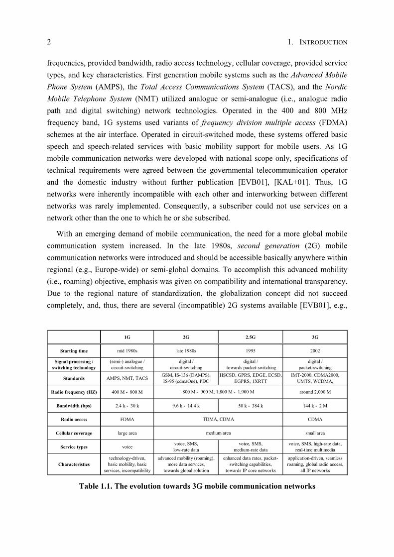
Traditionally, wireless communication networks were considered as an auxiliary approach that was used in regions where it was difficult to build a connection by wireline. With the advent of the first generation (1G) of cellular systems in the mid 1980s, mobile communications has experienced enormous growth during the last twenty years. Table 1.1 summarizes the development process from 1G systems up to 3G systems in terms of starting time, signal processing, switching technology, representative standards, utilized radio
T
2 1. INTRODUCTION
frequencies, provided bandwidth, radio access technology, cellular coverage, provided service types, and key characteristics. First generation mobile systems such as the Advanced Mobile Phone System (AMPS), the Total Access Communications System (TACS), and the Nordic Mobile Telephone System (NMT) utilized analogue or semi-analogue (i.e., analogue radio path and digital switching) network technologies. Operated in the 400 and 800 MHz frequency band, 1G systems used variants of frequency division multiple access (FDMA) schemes at the air interface. Operated in circuit-switched mode, these systems offered basic speech and speech-related services with basic mobility support for mobile users. As 1G mobile communication networks were developed with national scope only, specifications of technical requirements were agreed between the governmental telecommunication operator and the domestic industry without further publication [EVB01], [KAL+01]. Thus, 1G networks were inherently incompatible with each other and interworking between different networks was rarely implemented. Consequently, a subscriber could not use services on a network other than the one to which he or she subscribed.
With an emerging demand of mobile communication, the need for a more global mobile communication system increased. In the late 1980s, second generation (2G) mobile communication networks were introduced and should be accessible basically anywhere within regional (e.g., Europe-wide) or semi-global domains. To accomplish this advanced mobility (i.e., roaming) objective, emphasis was given on compatibility and international transparency. Due to the regional nature of standardization, the globalization concept did not succeed completely, and, thus, there are several (incompatible) 2G systems available [EVB01], e.g.,
1G 2G 2.5G 3G
Starting time mid 1980s late 1980s 1995 2002
Signal processing / switching technology
(semi-) analogue /circuit-switching
digital /circuit-switching
digital / towards packet-switching
digital /packet-switching
Standards AMPS, NMT, TACS GSM, IS-136 (DAMPS),IS-95 (cdmaOne), PDC
HSCSD, GPRS, EDGE, ECSD, EGPRS, 1XRTT
IMT-2000, CDMA2000, UMTS, WCDMA,
Radio frequency (HZ) 400 M - 800 M around 2,000 M
Bandwidth (bps) 2.4 k - 30 k 9.6 k - 14.4 k 50 k - 384 k 144 k - 2 M
Radio access FDMA CDMA
Cellular coverage large area small area
Service types voice voice, SMS,low-rate data
voice, SMS,medium-rate data
voice, SMS, high-rate data,real-time multimedia
Characteristicstechnology-driven,
basic mobility, basic services, incompatibility
advanced mobility (roaming), more data services,
towards global solution
enhanced data rates, packet-switching capabilities,
towards IP core networks
application-driven, seamless roaming, global radio access,
all IP networks
800 M - 900 M, 1,800 M - 1,900 M
TDMA, CDMA
medium area
Table 1.1. The evolution towards 3G mobile communication networks
1.1. EVOLUTION TOWARDS 3G MOBILE COMMUNICATION NETWORKS 3
the Global System for Mobile Communications (GSM, previously known as Groupe Spéciale Mobile), IS-136 or Digital AMPS (DAMPS), IS-95 or cdmaOne, and Personal Digital Cellular (PDC). As a technological revolution, 2G networks are based on digital signal processing techniques. Digital technology has not only improved voice quality and services, but also significantly reduced the cost of handset and infrastructure systems, leading to further acceleration of the telecommunication industry’s growth since the mid 1990s.
The advent of GSM for 2G systems was a huge step forward. GSM is widely deployed throughout the world, is the predominant standard in Europe, and has gained tremendous success during 1990s. Moreover, GSM is recognized as the world leader in terms of number of subscribers. The introduction of the subscriber identity module (SIM) cards and the GSM mobile application part (MAP) protocol enabled seamless interworking between different networks, allowing subscribers to roam worldwide [EVB01]. In its original form, GSM in the 900, 1,800 and 1,900 MHz frequency bands uses a time division multiple access (TDMA) scheme at the air interface. Similarly, IS-136 and PDC utilize TDMA schemes at the air interface, whereas IS-95 relies on CDMA technology. Beside the transmission of digitized speech, 2G networks are able to offer electronic messaging services (e.g., the short message service, SMS), low bit-rate data services (up to 9.6 kbps), and more sophisticated supplementary services (e.g., call forwarding services or call barring services).
Due to the Internet and the (surprisingly) successful electronic messaging, the pressures for mobile data transfer have increased enormously. This development was underestimated at the time when 2G systems were specified. Thus, while the evolution towards the third generation of mobile communication networks continues, many operators upgraded their 2G networks to evolved 2G (2.5G) networks as interim solution [DGA01]. This generation of cellular networks extends 2G systems with enhanced data rates and packet-switching capabilities. The evolution of GSM towards 2.5G systems (also called GSM Phase 2+) is double-tracked [EVB01]. On the one hand, traditional circuit-switched technologies are enhanced such that higher data rates become available for mobile users, e.g., more effective channel coding mechanisms increase the data rate from 9.6 kbps to 14 kbps. To put more data through the air interface High Speed Circuit-Switched Data (HSCSD) has been introduced that uses several traffic channels simultaneously (multi-slot capability) to increase the data rate from 9.6 kbps up to 50 kbps [DGN+98], [KAL+01]. However, circuit-switched network interfaces in 2G systems are designed for symmetric traffic and, consequently, do not take into account traffic asymmetry, i.e., a low data rate in the uplink (terminal to network) and high data rates in the downlink (network to terminal). This and the fact that data traffic is packet-switched in nature motivated the enhancement of 2G systems by packet-switched interfaces.
4 1. INTRODUCTION
Generally, packet-switched enhancements make 2G systems more suitable for effective data transfer and bring IP mobility and the Internet closer to the mobile user. In GSM, the packet-switched General Packet Radio System (GPRS) technology provides data rates of up to 160 kbps and is capable to support asymmetric connections. GPRS is based on packet transmission in the core network, while using the existing GSM/TDMA radio interfaces and radio access network (RAN) technologies. Whenever packet-switched connections are used, QoS is a very essential issue. Whereas GPRS supports QoS in principle, GPRS traffic is considered as low priority traffic in GSM networks and just utilizes otherwise unused voice capacity. Consequently, a certain bandwidth or QoS cannot be guaranteed, and, thus, GPRS can only provide “best effort” services, i.e., delay-tolerant non real-time data services.
Some GSM operators as well as operators of other TDMA-based 2G systems are planning for Enhanced Data Rate for Global Evolution (EDGE). The development of EDGE aims to increase the throughput per time slot for both HSCSD and GPRS [DGA01]. These enhanced standards are called Enhanced Circuit-Switched Data (ECSD) with a data rate up to three times the HSCSD rate and enhanced GPRS (EGPRS) with a data rate of up to 384 kbps. Note that GPRS and EGPRS allow the efficient operation of “always-on” data and Internet services through packet-switched transmission. For IS-95, operators are considering 1XRTT, which provides data rate of up to 144 kbps [DGA01].
The phenomenal growth of high-rate data services and the increasing popularity of multimedia applications were the driving forces for third generation systems that support at least 144 kbps in all radio environments (e.g., for high-mobility users) and up to 2 Mbps for low-mobility and indoor users. While 2G systems have brought mobile telephony to the mass market, 3G systems bring packet-switched, high-speed data and multimedia applications to mobile users (e.g., Web browsing, video conferencing, voice over IP, audio/video streaming, interactive games, etc.). From a technical point of view, this seems to be a mere technological evolution towards packet-switched, high-rate data services, but its potential lies in the promotion of communications not only from person-to-person, but also from person-to-machine and from machine-to-machine [KJ01]. However, the air interface has to cope with variable, asymmetric data rates with different QoS requirements (e.g., low delay/delay-jitter and guaranteed bandwidth). As mobile users with different QoS requirements will coexist in 3G networks, sophisticated radio resource management schemes have to guarantee the required QoS for mobile users in a fair manner [OP98]. High-rate data services together with the lack of radio frequencies motivate the development of more efficient radio technologies. Thus, 3G systems are based on the wideband CDMA (WCDMA, [DGN+98]) technology at the 2,000 MHz frequency band. WCDMA provides a significantly better spectral efficiency than TDMA and is more suitable for packet transfer than TDMA-based radio access [KS01].
1.2. PREVIOUS RESULTS ON QOS MANAGEMENT FOR 3G MOBILE NETWORKS 5
As WCDMA and its radio access equipment are not compatible with existing second generation equipment, additional network equipment is required to enhance 2G or 2.5G networks. To be backward compatible with existing CMDA-based IS-95 (cdmaOne) systems, CDMA2000 (also known as wideband cdmaOne) has been specified as an alternative framework for wideband CDMA [PO98]. Since different parts of the world emphasize different issues of mobile communication, the global term 3G has regional synonyms. In Europe, 3G systems are called Universal Mobile Telecommunication System (UMTS, [KAL+01]) following the European Telecommunications Standards Institute (ETSI) perspective [ETSI]. In the United Stated and Japan, 3G systems often carry the name International Mobile Telecommunications in 2000 (IMT-2000), which comes from the International Telecommunication Union (ITU) development project [ITU].
For the standardization of UMTS, the European industrial players have created the Third Generation Partnership Project (3GPP) [3GPPa]. Relatively soon after the 3GPP an independent organization called Operator Harmonization Group (OHG) was established [KAL+01]. The role of the OHG is to look for compromise solutions for those items the 3GPP cannot handle internally. To ensure that the American point of view will be taken into consideration a separate Third Generation Partnership Project Number 2 (3GPP-2) was founded [3GPP2]. This organization performs specification work from the IS-95 radio technology basis. The common goal for 3GPP, OHG, and 3GPP-2 is to create specifications according to which a global cellular system using wideband radio access could be implemented. While the standardization of 3G is still ongoing, the discussion of technical issues of Beyond 3G (B3G) mobile communication networks has already started and visions for the future of B3G systems have already been proposed (see Section 5 for research challenges in B3G).
1.2 Previous Results on QoS Management for 3G Mobile Networks
There has been a significant amount of research to provide QoS in an efficient and scalable manner in wireline networks. Notably among them are the integrated services (IntServ) / resource reservation protocol (RSVP) model, the differentiated services (DiffServ) model, multiprotocol label switching (MPLS), traffic engineering, and constraint-based routing [XN99]. IntServ is characterized by resource reservation, i.e., real-time applications must first set up paths and reserve resources (by means of the RSVP signaling protocol) before data are transmitted. In DiffServ, packets are marked differently to create several packet classes with different service. MPLS is a forwarding scheme that assigns labels to packets at the ingress of an MPLS-capable domain. Subsequent classification, forwarding, and services of packets are
6 1. INTRODUCTION
based on these labels. Traffic engineering is the process of arranging how traffic flows through the network. Constraint-based routing finds routes that are subject to some constraints, such as bandwidth or delay requirements.
However, the support of multimedia services over wireless channels is more challenging and requires more attention [DGA01]. One of the major challenges is the effective utilization of scarce bandwidth in the radio access network. In CDMA cellular networks (i.e., 3G mobile networks) bandwidth is varying over time due to intra- and inter-cell interference, path-loss, fast fading, and shadowing [Lee91]. Thus, the bit error rate (BER) differs about 7 to 10 orders of magnitude compared with wireline networks [ZCD02]. Additionally, in wireless networks errors are more likely to occur in bursts. Furthermore, user mobility can trigger rapid degradation in delivered QoS during a handover (i.e., an ongoing call moves from one cell to another). These system characteristics result in time-varying QoS for mobile applications, and, thus, the provision of different QoS classes and call priorities is desirable, e.g., as defined by the 3GPP in [3GPPc]. As most QoS results achieved for wireline networks do not directly apply for wireless networks, QoS provisioning in wireless networks has attracted significant attention in recent years. Whereas some researchers try to extend existing methods for QoS management in wireline networks towards wireless networks (e.g., see [MS01]), other develop novel management schemes to achieve best possible QoS for mobile users.
There are two critical QoS parameters in mobile wireless networks [LYW+01], namely the new call blocking probability and the handover failure probability (also known as call handoff dropping probability). Since cell capacity is limited, call attempts may be blocked. The probability that a new call is not admitted into the system is called new call blocking probability. Even after a call is admitted, the network may terminate the call prematurely when a handover is attempted into a cell that has no capacity available. The probability that an already admitted call will be terminated some time before call completion is called handover failure probability. Generally, terminating a call in progress is considered more severe and needs to be kept under control [LYW+01]. Effective QoS management strategies (e.g., call admission control algorithms) have to ensure that handover failure probability is maintained at a predefined level, while minimizing new call blocking probability at the same time, i.e., maximizing bandwidth utilization.
Differentiated pricing of services has proven as an effective tool for optimal resource allocation and utilization. From a system engineer’s point of view, a primary target of differentiated pricing is the prevention of system overload and an optimal resource usage according to different daytimes and different traffic intensities [GSW95], [MMV95]. Thus, pricing should consider multiple call priorities to guarantee different QoS requirements
1.2. PREVIOUS RESULTS ON QOS MANAGEMENT FOR 3G MOBILE NETWORKS 7
according to different service level agreements. In general, pricing policies can be partitioned into usage-based pricing and dynamic pricing [DaS00]. In usage-based pricing policies, a user is charged according to a connection time or traffic volume. Whereas circuit-switched calls (e.g., in GSM) are charged by the connection time, the transferred data volume determines charging in packet-switched services (e.g., in UMTS). Dynamic pricing models take into account the state of the mobile radio network for determining the current price of a service. MacKie-Mason and Varian introduced the concept of congestion-sensitive pricing in their smart market scheme [MMV95]. Under this model, the actual price for each packet is determined based on the current state of network congestion. In [RP98], Rao and Petersen discussed the optimal pricing of priority services. Taking into account that differentiated pricing of services is an effective tool for optimal resource allocation and utilization, it seems naturally to combine both QoS and provider revenue management to provide an effective mechanism for the operation of 3G mobile networks.
For most multimedia applications, e.g., voice over IP or video conferencing, service can be degraded temporarily in case of congestion as long as it is still within the pre-defined range [CDZ02], [CS02], [DJK+00]. For example, generic video conferencing requires 40 kbps, whereas low-motion video conferencing requiring about 25 kbps is acceptable [SDB+98]. Thus, the system could free some radio capacity for new or handover calls by decreasing the QoS level of ongoing calls. Chou and Shin proposed an analytical model for a combined degradation and traffic restriction mechanisms [CS02]. Call degradation is for admission of more new and handover calls in the cell, and, hence, reduces the new call blocking and handover failure probability. However, the number of degraded calls is restricted by a fixed value that is not adjusted according to changing traffic load. In [LRS+00], Lataoui, Rachidi, Samuel, Gruhl, and Yan defined the components of a QoS management structure for packet switched 3G mobile communication networks. They introduced the seamless service descriptor as QoS parameter and specified an admission controller that utilizes this QoS parameter to allow degraded services at multiple levels according to a user specific profile. Das, Jayaram, Kakani, and Sen proposed a framework for QoS provisioning of multimedia services in 3G wireless access networks [DJK+00]. To support a differentiated treatment of real-time and non real-time traffic flows and to guarantee QoS demands, they developed a call admission controller that utilizes different schemes, i.e., channel reservation, bandwidth degradation, and bandwidth compaction. In [SDB+98], Sen et al. introduced a novel framework for cellular networks to degrade calls on demand depending on their bandwidth requirement. They calculated revenue functions and showed that a saturated cell can generate more revenue for the system provider by degrading ongoing calls to be able to admit more calls. Chlamtac, Das, and Záruba studied service degradation with respect to revenue
8 1. INTRODUCTION
optimization [CDZ02]. They proposed an admission control framework for optimal call mix selection to maximize the revenue earned by the service provider.
Several recent studies [CS00], [LK02], [LY01], [ZL01] have been conducted concerning the forced-termination of calls due to handover failure. As dropping of a handover call is generally considered more seriously than blocking of a new call, a certain amount of bandwidth (also called guard channels) is exclusively reserved for handovers. This amount of bandwidth can be either fixed or adaptively controlled with respect to the current traffic load. More precisely, Choi and Shin compared several schemes for reserving bandwidths for handovers and admission control for new connection requests in QoS-sensitive cellular networks [CS00]. Some of these schemes keep handover failure probability below a predefined target (1) by predicting the bandwidth required to handle handovers estimating possible handovers from adjacent cells or (2) by predicting the total required bandwidth in the current cell estimating both incoming and outgoing handovers at each cell. Other schemes guarantee no handover failures due to per connection bandwidth reservation.
In [LK02], Lee and Kim proposed an approach for adaptive bandwidth reservation with admission control for handover calls utilizing network traffic information. Their approach considers both QoS assurance and bandwidth utilization in order to optimize the amount of bandwidth to reserve for handover admissions. In [LY01], Leung and Yu presented call admission control and bandwidth reservation schemes for wireless cellular networks that guarantee a certain amount of handover failure probability by means of statistical prediction of user mobility based on the mobility history of users. Based on this mobility prediction, bandwidth is reserved to guarantee some target handover failure probability. The admission threshold is controlled adaptively to achieve a better balance between guaranteeing handover failure probability and maximizing resource utilization. Zhang and Liu developed an adaptive algorithm for call admission control in wireless networks that is built upon the concept of guard channels and uses an adaptation algorithm to search automatically the optimal number of guard channels to be reserved at each base station [ZL01]. They showed that their algorithm guarantees that the handover failure probability is below a given threshold and, at the same time, minimizes the new call blocking probability.
In [LLT02], Lindemann, Lohmann, and Thümmler introduced an approach that determines the amount of bandwidth to be reserved for handover calls according to a look-up table, which is determined by extensive offline simulations. Based upon this work, Lindemann, Lohmann, and Thümmler extended this approach towards general utility functions depending on online monitored performance measures such as call blocking probability and handover failure probability [LLT03]. Furthermore, the improvement of both quality of service and provider revenue is considered for non real-time traffic. In order to improve the dropping probability of
1.3. PREVIOUS RESULTS ON TRAFFIC CHARACTERIZATION AND MODELING 9
soft handover calls, Ma, Han, and Trivedi considered a stochastic model for an admission controller in CDMA cellular networks that prioritizes soft handover calls using soft guard channels [MHT02]. In summary, none of these previous approaches investigates the prioritization of soft handover calls by applying a graceful degradation scheme that adapts according to changing traffic load.
1.3 Previous Results on Traffic Characterization and Modeling
In the last decade, extensive research effort has been spent on the characterization of measured IP traffic in local area networks (LAN) and wide area networks (WAN), e.g., see [CB97], [CDJ+91], [LTW+94], [PF95], [TMW97], [Wil01], [WTS+97]. Among other characteristics, the most important findings of these studies are (1) the fractal-like nature of packet traffic implying the so-called long-range dependence (LRD) and self-similarity and (2) the “spiky” distribution of transport control protocol (TCP) packet lengths with peaks at common sizes. In particular, these studies have convincingly shown that measured traffic rates, i.e., number of packets or bytes per time unit, in both LAN and WAN environments look statistically the same in the small and in the large (i.e., self-similar), and no natural length of a “burst” is discernible. That is, at every time scale ranging from milliseconds to minutes (and beyond) bursts have the same qualitative appearance and cause the resulting traffic to exhibit fractal-like characteristics [LTW+94], [PF95].
Traffic modeling and understanding is imperative for network design and simulation, for providing QoS to diverse applications, and for network management and control. The central idea of traffic modeling is to construct stochastic models that capture perhaps not all traffic statistics, but those who are important in the sense that they affect the queuing behavior significantly. Many analytical studies have shown that self-similar network traffic can have a detrimental impact on network performance, including queuing delay and packet loss rate [ST99]. A practical effect of self-similarity is that buffers needed at switches or multiplexers must be bigger than those predicted by traditionally queuing analysis and simulation, and, thus, create larger delays in individual streams than originally anticipated.
Self-similar characteristics on network level can be related to high-level system characteristics [LTW+94], [WTS+97]. These papers pointed out that self-similar traffic could be constructed by a large number of ON/OFF sources (or packet trains models) that have ON and OFF period lengths that follow a heavy tailed distribution, respectively. For example, the observed self-similar nature of Ethernet LAN traffic at the aggregated level (i.e., aggregated over all active hosts in the network) can be explained by the superposition of heavy-tailed ON/OFF (or busy/idle) times of individual hosts [LTW+94]. Furthermore, Crovella and
10 1. INTRODUCTION
Bestavros found out that aggregated traffic generated by WWW transfers shows self-similar characteristics primarily due to the distribution of available file sizes in the Web and user “think times” [CB97]. Recent studies [VB00], [VKM+00] indicate instead that traffic properties are originated in the TCP congestion control mechanism, which induces LRD properties in the aggregated traffic stemming from the superposition of independent sources.
The evidence of LRD and self-similarity (and its rich scaling properties) in packet traffic motivated many researchers to abandon usual Markovian assumptions in favor of new and more complex traffic models. Numerous attempts were made to develop traffic models that capture LRD and self-similarity of measured packet traffic authentically. In [WTE96], Willinger, Taqqu, and Erramilli presented a comprehensive overview of stochastic approaches for modeling self-similar phenomena. Following the (assumed) origins of LRD, first attempts mimic LRD properties by superposing a large number of independent traffic sources each of which is modeled by a simple ON/OFF source (renewal-reward process) with heavy-tailed distribution of ON and OFF periods. This approach was originally suggested by Mandelbrot for economic settings [Man69] and was later extended by Taqqu and Levy [TL86]. Leland, Taqqu, Willinger, and Wilson rephrased this approach in the context of traffic modeling [LTW+94], as it provides a “phenomenological” explanation of the observed self-similar nature of aggregated packet traffic. The following touches upon a number of further approaches that (try to) capture LRD and self-similarity in network traffic.
From a modeling point of view, the two major families of self-similar time series models are fractional Gaussian noises (FGN), i.e., the increment processes of fractional Brownian motion (FBM), and fractional auto-regressive integrated moving-average processes (FARIMA), a generalization of the very popular auto-regressive integrated moving-average (ARIMA) models [WTE96]. Originally introduced by Mandelbrot and van Ness [MvN68], FGN models received a lot of attention for modeling LRD, since its Gaussian nature supports studying queuing performance [Nor94], [Nor95]. However, the applicability of FGN models is limited because of the strict auto-correlation structure that fails to capture short-range dependence (SRD) of measured traffic. In fact, network traffic such as variable bit-rate (VBR) video can exhibit a complex mixture of SRD and LRD [BST+95], [GW94]. That is, the corresponding auto-correlation function behaves similarly to that of long-range dependent processes at large lags and to that of short-range dependent processes at small lags. On the other hand, FARIMA models are capable to capture both short-range and long-range correlations in time series and, thus, are very popular in modeling complex traffic structures, e.g., VBR video traffic [GW94], [KM98].
Wavelet analysis has been widely used as a natural approach to study scale invariance [AFT+00], but only recently introduced in the field of data networks [MJ01]. Intuitively, the
1.3. PREVIOUS RESULTS ON TRAFFIC CHARACTERIZATION AND MODELING 11
(deterministic) self-similar structure of wavelets is a natural match to the statistical self-similarity of traffic. One of the main motivations for using wavelets is their ability to reduce the temporal correlation so that wavelet coefficients are less correlated. A radically different approach for modeling self-similar phenomena relies on ideas from the theories of chaos and fractals. Erramilli and Singh proposed chaotic maps for fractal traffic modeling [ES95]. The underlying idea is based on a non-linear map that describes the evolution of a state variable over discrete time governed by a set of dynamical laws. Recently, many research efforts were devoted to multi-fractal models, which are generalizations of self-similar models [RCR+99]. Due to their rich scale-invariant properties, multi-fractal models are suggested as possibly being the best fit to measured data [ENW96], [FGW98], [TTW97], but they are difficult to manage due to their analytical complexity.
However, queuing theoretical techniques developed in the past are hardly applicable for these kinds of models. In order to benefit from the availability of a large number of techniques and tools for computing performance measures, researchers have tried to capture the self-similarity of network traffic in more “traditional” Markovian, i.e., analytically tractable, models that continue to be widely used for performance evaluation purposes with good results, see e.g., [AN98], [RLB97]. Grossglauser and Bolot recently showed that long-range correlations of traffic beyond a certain threshold does not influence the performance of a system, i.e., matching LRD and self-similarity is only required within the time scales of interest for the system under study [GB99]. Because of this result, Markovian traffic models, such as Markov-modulated Poisson processes (MMPP, [FMH93]), with limited correlation can be successfully employed to model traffic exhibiting LRD. As Markovian traffic models are intrinsically not long range dependent, Robert and Le Boudec defined the local Hurst parameter, using an approximate LRD definition, valid on a limited range of time scales [RLB97].
In the last few years, a number of promising approaches based on Markovian traffic models have been developed. All of these different approaches reach similar conclusions using different techniques. The objective is always to take into account as accurately as possible real traffic behavior. Generally, Markovian traffic models, when extended to capture LRD, often result in a complicated structure with many states and parameters. Anderson and Nielsen [AN98] proposed a MMPP model build up as a superposition of independent two-state Markov processes (ON-OFF sources) and a homogeneous Poisson process. Although the model seems to be acceptable for describing second-order traffic properties, it does not appear to be suitable to predict queuing behavior. In [YKT01], Yoshihara, Kasahara, and Takahashi proposed a fitting procedure for MMPPs tailored to self-similar network traffic. Similarly to [AN98], they constructed an MMPP as the superposition of two-state MMPPs and fitted it so
12 1. INTRODUCTION
as to match the variance function over several time scales. Salvador, Valadas, and Pacheco introduced a multi-scale fitting procedure for (discrete-time) MMPPs that leads to accurate estimates of queuing behavior for network traffic exhibiting LRD behavior [SVP03]. Matching both the auto-covariance and marginal distribution of the counting process, their results illustrate that MMPP models can capture LRD up to the time-scales of interest at the expense of a complex structure with numerous states. In an outstanding paper, Muscariello et al. recently proposed a MMPP traffic model that accurately approximates the LRD characteristics of Internet traffic traces over the relevant time scales [MMM+04]. Using the notions of sessions and flows, the proposed MMPP model mimics the real hierarchical behavior of the packet generation process by Internet users and, thus, allows the generation of traffic with desired characteristics by easily setting few input parameters with an intuitive physical meaning.
Surprisingly, while the packet arrival process of measured traffic data has deserved considerable attention, very few works have addressed the packet length process, and, especially, the joint characterization of the packet arrival process and the packet length process [GR99], [SPV04]. Thus, almost all (i.e., Markovian and non-Markovian) traffic models just capture packet arrivals, whereas packet lengths are ignored completely [JMW97], [MMM+04]. When dealing with such models, it is a common practice to assume an average packet length for each packet arrival or to draw packet lengths according to the empirical distribution of the measured traffic. For packet lengths that are uncorrelated with packet arrivals, this approach would be adequately. As shown for a huge number of LAN and WAN traffic measurements [CDJ+91], [TMW97], [Wil01], TCP packet lengths follow a “spiky” distribution with peaks at just a few predominating lengths that are mainly due to protocol and network specific characteristics. This dependence on protocol and network specific characteristics is a first indicator of correlations between the arrival process and the packet length process. In summary, none of these previous approaches derived a Markovian (i.e., analytically tractable) traffic model that jointly captures the packet arrival process, the packet length process, and their correlations.
1.4 Summary of Contributions of this Thesis
The contribution of this thesis is three-fold. First, this thesis shows how online management of both QoS and provider revenue can be performed in 3G mobile networks by adaptive control of system parameters to changing traffic conditions. To enable online QoS/revenue management of both real-time and non real-time services, analytically tractable (i.e., Markovian) traffic models for non real-time services are required. Due to the scarce
1.4. SUMMARY OF CONTRIBUTIONS OF THIS THESIS 13
bandwidth in the radio access network, accurate stochastic modeling of byte-based traffic rates (i.e., bytes per time unit) is essentially. Otherwise, results, gathered in performance studies of 3G mobile networks, may be misleading and, thus, may lead to significant performance losses during the operation of 3G networks in practice. Thus, as a second contribution, this thesis identifies the batch Markovian arrival process (BMAP, [Luc91]) as the analytically tractable model of choice for the joint characterization of packet arrivals and packet lengths. This thesis shows that it is not sufficient to utilize state-of-the-art analytically tractable traffic models (e.g., the Markovian arrival process or the MMPP) that just capture inter-arrival times (ignoring packet lengths completely) and assume an average packet length or draw packet lengths according to the empirical distribution of the measured traffic. As a third and major contribution, this work solves an open research problem and derives a novel expectation maximization (EM, [DLR77]) algorithm for parameter estimation of BMAPs.
Online QoS/Revenue Management for 3G Mobile Communication Networks
The proposed QoS/revenue management approach is based on a novel call admission control and bandwidth degradation scheme for real-time traffic. The admission controller considers real-time calls with two priority levels: calls of high priority have a guaranteed bit-rate, whereas calls of low priority can be temporarily degraded to a lower bit-rate in order to reduce forced termination of calls due to a handover failure. Opposed to previous work [CS02], [LLT03], [MHT02], degradation of bandwidth is performed gracefully in several steps. Furthermore, calls of low priority are degraded equally rather than picking out one call randomly for degradation. Clearly, due to fairness reasons this approach should be preferred over a random choice of calls applied in [CS02]. To enable online QoS/revenue management this work develops a Markov model for the admission controller that incorporates important features of 3G cellular networks, such as CDMA intra- and inter-cell interference, different call priorities and soft handover [KAL+01]. Online evaluation of the Markov model enables a periodical adjustment of the threshold for maximal call degradation according to the currently measured traffic in the radio access network and a predefined goal for optimization. Using distinct optimization goals, this allows optimization of both QoS and provider revenue.
Performance studies illustrate the effectiveness of the proposed approach and show that QoS and provider revenue can be increased significantly with a moderate degradation of low-priority calls. Beside the evaluation of the optimization goals, the proposed degradation scheme is compared with existing admission control policies based on adaptive guard channels [CS00], [ZL01]. It is shown that overall utilization of cell capacity is higher with the degradation scheme that can be considered as an “on demand” reservation of cell capacity, whereas the guard channel scheme implements an “a-priori” reservation. Thus, the
14 1. INTRODUCTION
degradation scheme is the method of choice in future mobile networks that support service degradation, since it guarantees a certain handover failure probability and also high cell capacity utilization. Simulation studies considering a half-day window of a daily usage pattern illustrate the effectiveness of the proposed approach in practice.
Parameter Estimation of the Batch Markovian Arrival Process
The developed EM algorithm for parameter estimation of BMAPs is mathematically very complex and requires the computation of conditional expectations of a continuous-time Markov chain (CTMC, [Lin98]). Extensive calculations show that these conditional expectations can be computed by means of matrix exponentials and integrals over matrix exponentials. Whereas the computation of matrix exponentials can be performed directly using the randomization technique [GM84] and a numerical stable computation of Poisson probabilities [FG88], the computation of integrals over matrix exponentials requires further effort. Previous known EM-based parameter estimation procedures for special cases of the BMAP are numerically unstable, e.g., the EM algorithm for parameter estimation of MMPPs proposed by Ryden in [Ryd96]. Thus, it is shown how to utilize the randomization technique for the computation of integrals over matrix exponentials. This methodological work enables the EM algorithm to be both efficient and numerical robust and constitutes an important step towards effective, analytically/numerically tractable traffic models. Moreover, this thesis analyzes the computational complexity of the EM algorithm given by O(n·l3/2·N2) for an EM iteration and gives some insights in the convergence behavior of the EM algorithm.
Traffic Modeling Using the Batch Markovian Arrival Process
Whereas almost all (analytically tractable) traffic models capture inter-arrival times of measured IP traffic [JMW97], [MMM+04], the BMAP enables “two-dimensional”, i.e., joint, characterization of packet arrivals and packet lengths. The proposed EM algorithm for parameter estimation of BMAPs jointly captures the packet arrival process and the packet length process of measured traffic and, thus, considers correlation structures between packet arrivals and packet lengths naturally given by the BMAP’s capabilities. The key idea is to customize the BMAP such that different packet lengths are represented by different rewards, i.e., batch sizes of arrivals, of the BMAP. This is the first analytically tractable traffic model that jointly captures the packet arrival process, the packet length process, and their correlations. A scaling procedure is proposed that reduces the number of parameters dramatically without changing the BMAP’s quality. This is decisively for the practical utilization of parameterized BMAPs in Markovian performance models, as the solution of these kinds of performance models primarily depends on the number of non-zero entries in
1.5. KEY PUBLICATIONS MAKING UP THIS THESIS 15
the corresponding infinitesimal generator matrix of the underlying CTMC. Case studies of measured IP traffic with different degrees of traffic burstiness evidently demonstrate the advantages of the BMAP modeling approach over other widely used analytically tractable models and show that the joint characterization of packet arrivals and packet lengths is decisively for realistic traffic modeling at packet level. Beyond the case studies of TCP traffic presented in this thesis, the joint characterization of packet arrivals and packet lengths by customized BMAPs has been utilized successfully in practice for aggregated traffic modeling of non real-time traffic in 3G mobile communication networks [KLL01].
1.5 Key Publications Making up this Thesis
This thesis is mainly based on three key publications that have been published in international scientific journals and conference proceedings [KLL02], [KLL03], and [LLT04]. Since these publications constitute joint work with other Ph.D. students, the following outlines the individual contribution of the author.
As published in [LLT04], the online QoS/revenue management for 3G mobile communication networks has been developed jointly with the by-then Ph.D. student Axel Thümmler. In this publication, the author developed the mathematical foundations of the proposed management schemes, derived the underlying Markov model of the admission controller mathematically, and performed the entire set of performance studies. Axel Thümmler mainly developed formulas for CDMA cell capacity and derived statistics of the core and soft handover zone required for iterative balancing.
The novel parameter estimation method for BMAPs has been recently published in [KLL03]. In this joint publication with the Ph.D. student Alexander Klemm, the author derived the entire mathematical framework including the derivation of the EM algorithm and the development of effective computational formulas for conditional expectations of a CTMC. Moreover, the author showed how to compute complex integrals over matrix exponentials and derived the computational complexity of the EM algorithm. Alexander Klemm mainly performed detailed traffic measurements that helped utilizing the EM algorithm in practice.
The ideas of modeling IP traffic using the BMAP have been published jointly with Alexander Klemm [KLL02]. The author found out that packet arrivals and packet lengths are correlated due to protocol and network specific characteristics and derived a framework that utilizes the BMAP as an ideal vehicle to capture these kinds of correlations in a Markovian model. Moreover, the author invented an effective scaling procedure that helps minimizing the number of model parameters and conducted detailed performance studies that illustrate the
16 1. INTRODUCTION
benefit of the proposed traffic modeling framework. As in [KLL03], Alexander Klemm mainly performed detailed traffic measurements required for the conducted case studies.
Furthermore, the author of this thesis is coauthor of some further publications, which are not part of this thesis. In [KLL01], the author developed a mathematical framework to derive effective traffic models for non real-time services in 3G mobile communication networks based on real-world traffic measurements. As a first step towards effective management of QoS (and provider revenue) in 3G networks, management schemes for real-time and non real-time services based on a tailored lookup table and closed-form formulas have been published jointly with Axel Thümmler [LLT02], [LLT03]. In these publications, the author derived the methodology for packet-based modeling of data services and embedded the 3G traffic model [KLL01] in the proposed framework. The publications [LTK+00] and [LTK+02] focus on the performance analysis of time-enhanced UML diagrams based on stochastic processes. Concerning these publications, the author supported the development of the software package DSPNexpress [Lin98] and derived corresponding performance curves. The publications [LLT02], [LLT03], [LTK+00], and [LTK+02] constitute the core of the Ph.D. thesis of Axel Thümmler [Thü03].
1.6 Thesis Outline
This thesis is organized as follows. In Section 2, this thesis presents the online QoS/revenue management framework including a detailed description of the proposed admission controller and the bandwidth degradation scheme. To make this thesis self-contained, this section describes the architecture of 3G communication networks and recalls principles of CDMA-based radio access. Furthermore, this section derives feasibility functions to estimate current available bandwidth and shows how online QoS/revenue management can be performed by periodical optimization of an embedded Markov model. Finally, Section 2 presents quantitative results of the proposed framework in practice.
Section 3 presents the developed EM algorithm for parameter estimation of BMAPs. To make this thesis self-contained, this section first recalls the randomization technique and an efficient method for stable calculations of Poisson probabilities. Beyond the derivation of the EM algorithm and its highly complex mathematical framework, Section 3 outlines key implementation issues, derives the computational complexity the EM algorithm, and gives some insights in the convergence behavior of the EM algorithm.
Section 4 recalls important characteristics of today’s IP traffic, such as self-similarity and TCP packet length characteristics and describes how to utilize the batch Markovian arrival
1.6. THESIS OUTLINE 17
process for IP traffic modeling. Two comprehensive case studies of measured IP traffic with different degrees of traffic burstiness illustrate the effectiveness of the joint characterization of packet arrivals and packet lengths. Furthermore, Section 4 shows how model specification and parameter estimation are performed in practice.
Section 5 outlines future directions of research concerning research areas examined in this thesis. This includes ideas for online QoS/revenue management of both real-time and non real-time services as well as extensions of the QoS/revenue management scheme towards emerging B3G mobile communication networks. Furthermore, future research ideas concerning the EM algorithm for parameter estimation of BMAPs are given, and it is outlined how an EM algorithm could be utilized for effective modeling the state of TCP connections in mobile ad-hoc networks (MANET). Finally, Section 6 sums up major research results presented in this thesis and gives concluding remarks.

19
2 Online QoS/Revenue Management of Real-Time Services
UPPORTING MULTIMEDIA SERVICES over wireless channels presents a number of technical challenges. One of the major challenges is the effective utilization of scarce
bandwidth in the radio access network. For most multimedia applications, e.g., voice over IP or video conferencing, service can be degraded temporarily in case of congestion as long as it is still within the pre-defined range [CDZ02], [CS02], [DJK+00]. For example, generic video conferencing requires 40 kbps, whereas low-motion video conferencing requiring about 25 kbps is acceptable [SDB+98]. Thus, the system could free some radio capacity for new or handover calls by decreasing the QoS level of ongoing calls. This section presents a novel call admission control and bandwidth degradation scheme for real-time data services and shows how online management of both QoS and provider revenue can be performed in 3G mobile networks by adaptive control of system parameters to changing traffic conditions. An efficiently analyzable Markov model enables online optimization of the admission controller and incorporates important features of 3G cellular networks, such as CDMA intra- and inter-cell interference, different call priorities, and soft handover [KAL+01]. Detailed performance studies illustrate the effectiveness of the proposed approach by quantitative analysis of the Markov model and simulation studies. The methodological work including expressive performance studies has been published in the ACM Journal on Wireless Networks (WINET), which is a leading journal in wireless network research [LLT04].
2.1 Architecture of 3G Communication Networks
Third generation mobile communication networks have a cellular structure, where a large area is divided into a number of sub-areas called cells (see Figure 2.1). The cellular concept resolves the basic problems of radio systems in terms of radio system capacity constraints [BGM+98], [KAL+01], but at the same time it encounters other problems such as interference due to the cellular structure (see Sections 2.4 and 2.5), problems due to mobility (handover), i.e., an ongoing call moves from one cell to another, and cell-based radio resource scarcity. As depicted in Figure 2.1, each cell has its own base station (BS), which is able to provide a radio link for a specific number of mobile stations (MS), simultaneously. The BS itself encompasses the technical equipment (e.g., antennas) that is required for radio
S
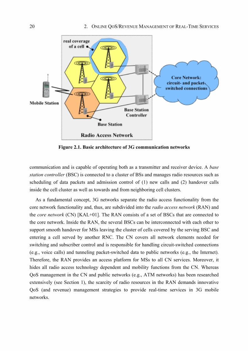
20 2. ONLINE QOS/REVENUE MANAGEMENT OF REAL-TIME SERVICES
Figure 2.1. Basic architecture of 3G communication networks
communication and is capable of operating both as a transmitter and receiver device. A base station controller (BSC) is connected to a cluster of BSs and manages radio resources such as scheduling of data packets and admission control of (1) new calls and (2) handover calls inside the cell cluster as well as towards and from neighboring cell clusters.
As a fundamental concept, 3G networks separate the radio access functionality from the core network functionality and, thus, are subdivided into the radio access network (RAN) and the core network (CN) [KAL+01]. The RAN consists of a set of BSCs that are connected to the core network. Inside the RAN, the several BSCs can be interconnected with each other to support smooth handover for MSs leaving the cluster of cells covered by the serving BSC and entering a cell served by another RNC. The CN covers all network elements needed for switching and subscriber control and is responsible for handling circuit-switched connections (e.g., voice calls) and tunneling packet-switched data to public networks (e.g., the Internet). Therefore, the RAN provides an access platform for MSs to all CN services. Moreover, it hides all radio access technology dependent and mobility functions from the CN. Whereas QoS management in the CN and public networks (e.g., ATM networks) has been researched extensively (see Section 1), the scarcity of radio resources in the RAN demands innovative QoS (and revenue) management strategies to provide real-time services in 3G mobile networks.
2.2. QOS/REVENUE MANAGEMENT FRAMEWORK 21
2.2 QoS/Revenue Management Framework
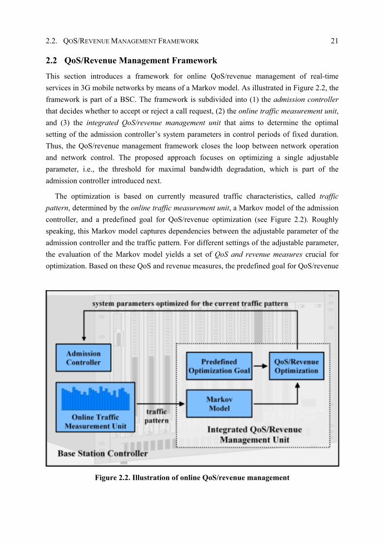
This section introduces a framework for online QoS/revenue management of real-time services in 3G mobile networks by means of a Markov model. As illustrated in Figure 2.2, the framework is part of a BSC. The framework is subdivided into (1) the admission controller that decides whether to accept or reject a call request, (2) the online traffic measurement unit, and (3) the integrated QoS/revenue management unit that aims to determine the optimal setting of the admission controller’s system parameters in control periods of fixed duration. Thus, the QoS/revenue management framework closes the loop between network operation and network control. The proposed approach focuses on optimizing a single adjustable parameter, i.e., the threshold for maximal bandwidth degradation, which is part of the admission controller introduced next.
The optimization is based on currently measured traffic characteristics, called traffic pattern, determined by the online traffic measurement unit, a Markov model of the admission controller, and a predefined goal for QoS/revenue optimization (see Figure 2.2). Roughly speaking, this Markov model captures dependencies between the adjustable parameter of the admission controller and the traffic pattern. For different settings of the adjustable parameter, the evaluation of the Markov model yields a set of QoS and revenue measures crucial for optimization. Based on these QoS and revenue measures, the predefined goal for QoS/revenue
Figure 2.2. Illustration of online QoS/revenue management
22 2. ONLINE QOS/REVENUE MANAGEMENT OF REAL-TIME SERVICES
optimization is evaluated. The parameter setting that maximizes this goal is optimal for the current state of the RAN, i.e., optimal for the current traffic pattern.
2.3 CDMA Principles
In mobile cellular systems, there are three major techniques that can provide multiple access to mobile users, i.e., FDMA, TDMA, and CDMA [KAL+01]. As utilized in 1G cellular networks, FDMA subdivides the available frequency band into a number of channels (in the frequency domain) each of which can be used by a mobile user. The most common multiple access technique in 2G is TDMA, which is a more efficient way to utilize frequency resources and, thus, increases a cellular system’s capacity. In TDMA, the available frequency band is subdivided (in the time domain) into a number of logical channels (timeslots) each of which can serve a call. However, these “traditional” multiple access techniques or combinations of them can only provide a limited capacity in cellular systems. Thus, as discussed in the introduction of this thesis, 3G systems are based on the wideband CDMA.
Unlike in FDMA and TDMA schemes, CDMA allocates radio resources based on code sequences [KAL+01], [PO98]. Each user is assigned a unique code sequence used for encoding its information-bearing signal. Additionally, the encoding process enlarges (i.e., spreads) the small bandwidth of the information-bearing signal to the broad bandwidth of the available frequency band (spread-spectrum signal). Therefore, this kind of modulation is also known as spread-spectrum modulation. The ratio of the total spread bandwidth to the bit-rate of the information bearing-signal is called the processing gain or spreading factor [KS01]. For simultaneous transmissions of multiple users, each user utilizes the same broad frequency band at the same time, and, thus, the receiver gets the spread-spectrum signals of all users. As a consequence, each user can occupy the same frequency band simultaneously without frequency allocation or time slots.
The receiver is able to distinguish between different users since each user has a unique code that has a sufficiently low cross-correlation with the other codes. Correlating the received signal with the code from a certain user will then only despread the signal of this user, while the other spread-spectrum signals will remain spread over a large bandwidth. Nevertheless, from the perspective of a certain user (and its signal), signals stemming from other users contribute to an increased interference (i.e., noise) that is still distributed over a wide spectrum. To provide a certain signal quality, the signal to noise ratio should not fall short of a certain threshold (see Section 2.5 for more detailed considerations). Consequently, the number of users within a cell (and, thus, the cell capacity) is interference limited, while FDMA and TDMA cell capacities are bandwidth limited [KAL+01]. Thus, admission control
2.4. ADMISSION CONTROL BASED ON BANDWIDTH DEGRADATION 23
mechanisms in 3G cellular systems must consider these CDMA-specific characteristics. As the number of users is not fixed in general, but determined by a desired minimum signal quality, the capacity of CDMA is often called soft capacity [Lee91], [PO98].
Because of the coding process and the resulting enlarged bandwidth, spread-spectrum signals have a number of properties that differ from the properties of narrowband signals. This results in the following advantages of CDMA cellular systems over cellular systems based on FDMA or TDMA. From the communication systems point of view, the key advantages of CDMA in cellular systems are the high spectrum efficiency, support of variable bit-rates, interference limited (i.e., soft) capacity (see Sections 2.4 and 2.5) as well as frequency reuse in all neighboring cells, soft handover, and macro diversity (see Section 2.4). In fact, CDMA systems increase cell capacity in the order of 4 to 6 compared with digital TDMA (e.g., GSM) and in the order of 10 compared with analog FDMA (e.g., AMPS) [GJP+91]. As a major advantage of CDMA over FDMA and TMDA in cellular systems, the frequency band of the entire spectrum can be reused in all neighboring cells since there is no concept of frequency allocation in CDMA. This increases the capacity of the CDMA system to a large extent [KAL+01].
2.4 Admission Control Based on Bandwidth Degradation
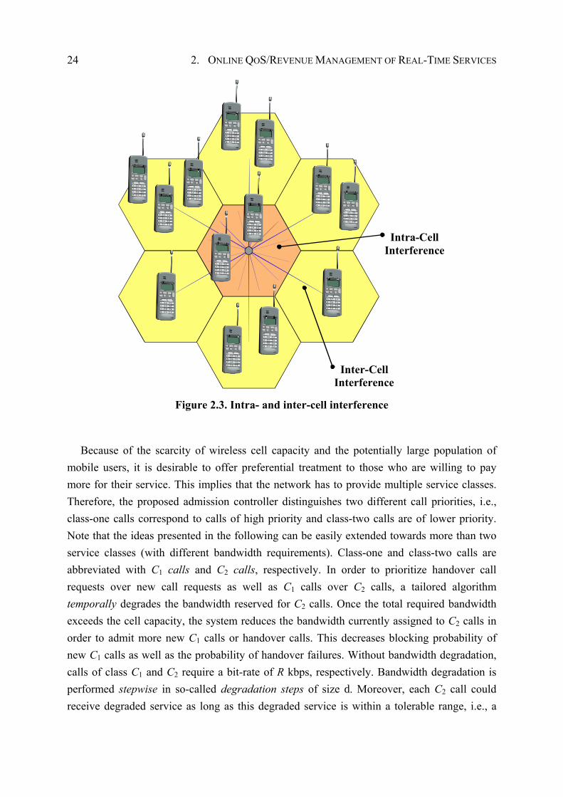
This section describes the proposed admission control and bandwidth degradation scheme that is subject of optimization according to the framework introduced above. Before a mobile user can start a new call, an admission controller decides to accept or reject the user’s request. Generally, this decision is based on the bandwidth requirements of the new call and the network’s current state, e.g., given by currently available bandwidth. As the capacity of CDMA cellular systems is interference limited and each cell uses the same frequency band, the admission decision considers interference in the considered cell, i.e., intra-cell interference, and in the surrounding cells, i.e., other-cell interference (see Figure 2.3). As introduced in the next section, a feasibility function determines whether a given system configuration is feasible in terms of CDMA cell capacity (see equation (2.8)). Intuitively, in a feasible system configuration the demands of all users in the system are satisfied. The admission controller weighs up whether to accept a call request that may result in a QoS degradation of already admitted calls or to reject a call request in order to guarantee ongoing calls a certain QoS. Furthermore, the admission controller prioritizes handover call requests over new call requests, since dropping a handover call is generally considered more serious than blocking of a new call.
24 2. ONLINE QOS/REVENUE MANAGEMENT OF REAL-TIME SERVICES
Inter-CellInterference
Intra-CellInterference
Figure 2.3. Intra- and inter-cell interference
Because of the scarcity of wireless cell capacity and the potentially large population of mobile users, it is desirable to offer preferential treatment to those who are willing to pay more for their service. This implies that the network has to provide multiple service classes. Therefore, the proposed admission controller distinguishes two different call priorities, i.e., class-one calls correspond to calls of high priority and class-two calls are of lower priority. Note that the ideas presented in the following can be easily extended towards more than two service classes (with different bandwidth requirements). Class-one and class-two calls are abbreviated with C1 calls and C2 calls, respectively. In order to prioritize handover call requests over new call requests as well as C1 calls over C2 calls, a tailored algorithm temporally degrades the bandwidth reserved for C2 calls. Once the total required bandwidth exceeds the cell capacity, the system reduces the bandwidth currently assigned to C2 calls in order to admit more new C1 calls or handover calls. This decreases blocking probability of new C1 calls as well as the probability of handover failures. Without bandwidth degradation, calls of class C1 and C2 require a bit-rate of R kbps, respectively. Bandwidth degradation is performed stepwise in so-called degradation steps of size d. Moreover, each C2 call could receive degraded service as long as this degraded service is within a tolerable range, i.e., a
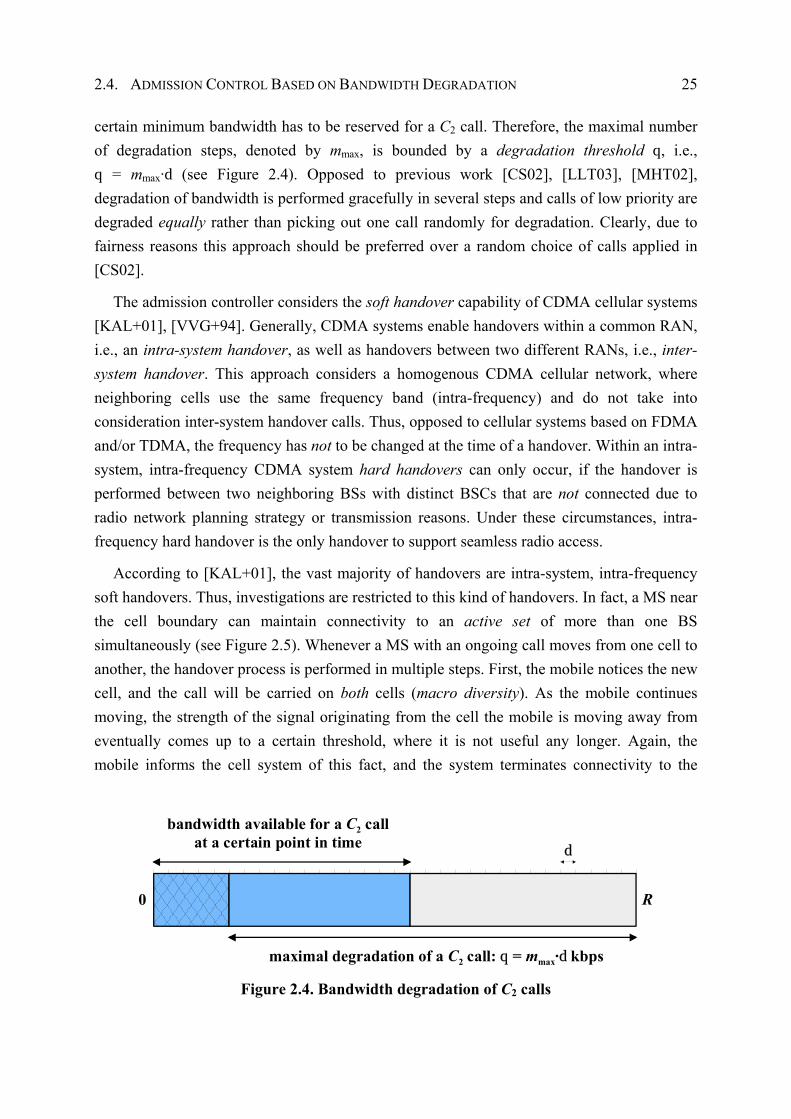
2.4. ADMISSION CONTROL BASED ON BANDWIDTH DEGRADATION 25
certain minimum bandwidth has to be reserved for a C2 call. Therefore, the maximal number of degradation steps, denoted by mmax, is bounded by a degradation threshold q, i.e., q = mmax·d (see Figure 2.4). Opposed to previous work [CS02], [LLT03], [MHT02], degradation of bandwidth is performed gracefully in several steps and calls of low priority are degraded equally rather than picking out one call randomly for degradation. Clearly, due to fairness reasons this approach should be preferred over a random choice of calls applied in [CS02].
The admission controller considers the soft handover capability of CDMA cellular systems [KAL+01], [VVG+94]. Generally, CDMA systems enable handovers within a common RAN, i.e., an intra-system handover, as well as handovers between two different RANs, i.e., inter-system handover. This approach considers a homogenous CDMA cellular network, where neighboring cells use the same frequency band (intra-frequency) and do not take into consideration inter-system handover calls. Thus, opposed to cellular systems based on FDMA and/or TDMA, the frequency has not to be changed at the time of a handover. Within an intra-system, intra-frequency CDMA system hard handovers can only occur, if the handover is performed between two neighboring BSs with distinct BSCs that are not connected due to radio network planning strategy or transmission reasons. Under these circumstances, intra-frequency hard handover is the only handover to support seamless radio access.
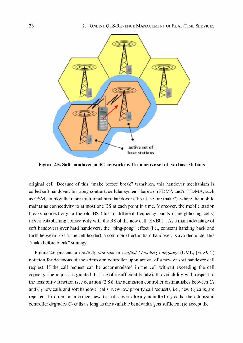
According to [KAL+01], the vast majority of handovers are intra-system, intra-frequency soft handovers. Thus, investigations are restricted to this kind of handovers. In fact, a MS near the cell boundary can maintain connectivity to an active set of more than one BS simultaneously (see Figure 2.5). Whenever a MS with an ongoing call moves from one cell to another, the handover process is performed in multiple steps. First, the mobile notices the new cell, and the call will be carried on both cells (macro diversity). As the mobile continues moving, the strength of the signal originating from the cell the mobile is moving away from eventually comes up to a certain threshold, where it is not useful any longer. Again, the mobile informs the cell system of this fact, and the system terminates connectivity to the
0 R
bandwidth available for a C2 callat a certain point in time
maximal degradation of a C2 call: q = mmax·d kbps
d
Figure 2.4. Bandwidth degradation of C2 calls
26 2. ONLINE QOS/REVENUE MANAGEMENT OF REAL-TIME SERVICES
Figure 2.5. Soft-handover in 3G networks with an active set of two base stations
original cell. Because of this “make before break” transition, this handover mechanism is called soft handover. In strong contrast, cellular systems based on FDMA and/or TDMA, such as GSM, employ the more traditional hard handover (“break before make”), where the mobile maintains connectivity to at most one BS at each point in time. Moreover, the mobile station breaks connectivity to the old BS (due to different frequency bands in neighboring cells) before establishing connectivity with the BS of the new cell [EVB01]. As a main advantage of soft handovers over hard handovers, the “ping-pong” effect (i.e., constant handing back and forth between BSs at the cell border), a common effect in hard handover, is avoided under this “make before break” strategy.
Figure 2.6 presents an activity diagram in Unified Modeling Language (UML, [Fow97]) notation for decisions of the admission controller upon arrival of a new or soft handover call request. If the call request can be accommodated in the cell without exceeding the cell capacity, the request is granted. In case of insufficient bandwidth availability with respect to the feasibility function (see equation (2.8)), the admission controller distinguishes between C1 and C2 new calls and soft handover calls. New low priority call requests, i.e., new C2 calls, are rejected. In order to prioritize new C1 calls over already admitted C2 calls, the admission controller degrades C2 calls as long as the available bandwidth gets sufficient (to accept the
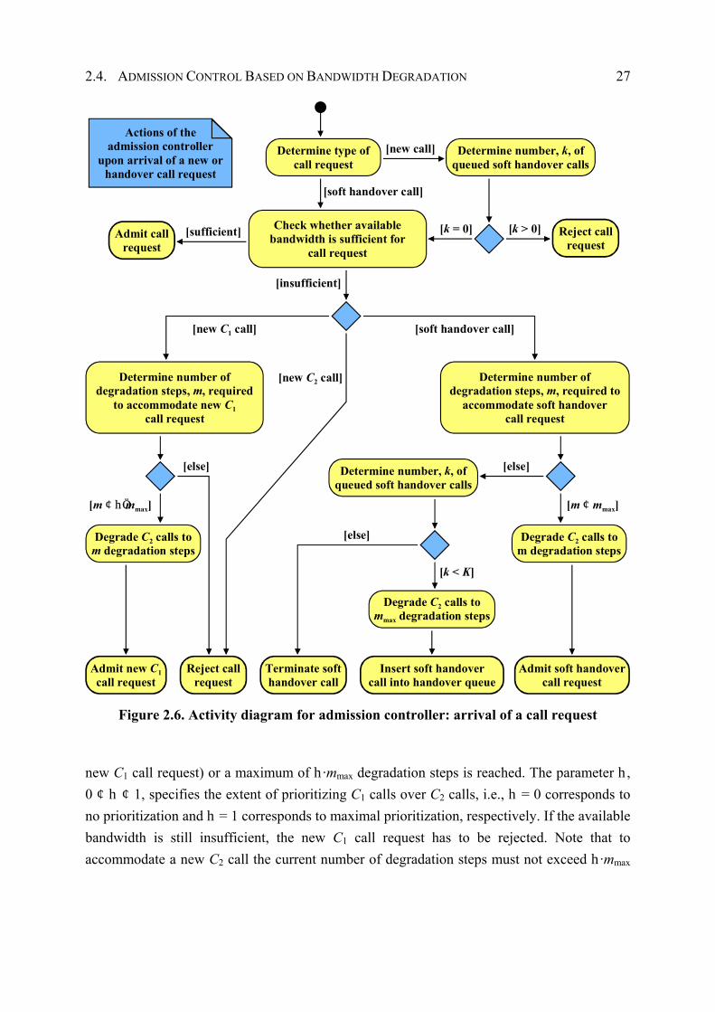
2.4. ADMISSION CONTROL BASED ON BANDWIDTH DEGRADATION 27
Actions of theadmission controller
upon arrival of a new orhandover call request
Determine type ofcall request
Check whether availablebandwidth is sufficient for
call request
[insufficient]
[sufficient]Admit callrequest
Determine number ofdegradation steps, m, required
to accommodate new C1call request
Determine number ofdegradation steps, m, required to
accommodate soft handovercall request
[else] [else]
[new C2 call]
[soft handover call][new C1 call]
[m ¢ hÖmmax] [m ¢ mmax]
Degrade C2 calls tom degradation steps
Degrade C2 calls tommax degradation steps
Degrade C2 calls tom degradation steps
Admit new C1call request
Admit soft handovercall request
Determine number, k, ofqueued soft handover calls
Insert soft handovercall into handover queue
Terminate softhandover call
Reject callrequest
[else]
[k < K]
Determine number, k, ofqueued soft handover calls
[soft handover call]
[new call]
Reject callrequest
[k > 0][k = 0]
Figure 2.6. Activity diagram for admission controller: arrival of a call request
new C1 call request) or a maximum of h·mmax degradation steps is reached. The parameter h, 0 ¢ h ¢ 1, specifies the extent of prioritizing C1 calls over C2 calls, i.e., h = 0 corresponds to no prioritization and h = 1 corresponds to maximal prioritization, respectively. If the available bandwidth is still insufficient, the new C1 call request has to be rejected. Note that to accommodate a new C2 call the current number of degradation steps must not exceed h·mmax
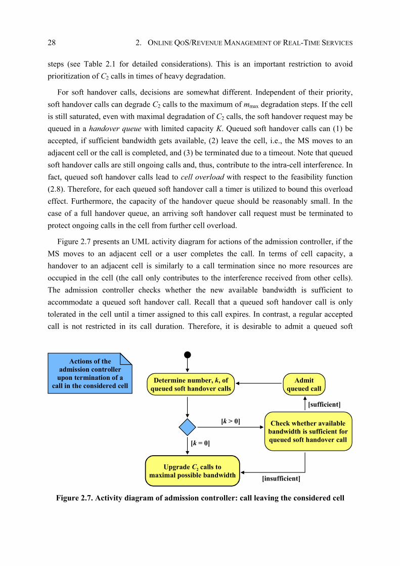
28 2. ONLINE QOS/REVENUE MANAGEMENT OF REAL-TIME SERVICES
steps (see Table 2.1 for detailed considerations). This is an important restriction to avoid prioritization of C2 calls in times of heavy degradation.
For soft handover calls, decisions are somewhat different. Independent of their priority, soft handover calls can degrade C2 calls to the maximum of mmax degradation steps. If the cell is still saturated, even with maximal degradation of C2 calls, the soft handover request may be queued in a handover queue with limited capacity K. Queued soft handover calls can (1) be accepted, if sufficient bandwidth gets available, (2) leave the cell, i.e., the MS moves to an adjacent cell or the call is completed, and (3) be terminated due to a timeout. Note that queued soft handover calls are still ongoing calls and, thus, contribute to the intra-cell interference. In fact, queued soft handover calls lead to cell overload with respect to the feasibility function (2.8). Therefore, for each queued soft handover call a timer is utilized to bound this overload effect. Furthermore, the capacity of the handover queue should be reasonably small. In the case of a full handover queue, an arriving soft handover call request must be terminated to protect ongoing calls in the cell from further cell overload.
Figure 2.7 presents an UML activity diagram for actions of the admission controller, if the MS moves to an adjacent cell or a user completes the call. In terms of cell capacity, a handover to an adjacent cell is similarly to a call termination since no more resources are occupied in the cell (the call only contributes to the interference received from other cells). The admission controller checks whether the new available bandwidth is sufficient to accommodate a queued soft handover call. Recall that a queued soft handover call is only tolerated in the cell until a timer assigned to this call expires. In contrast, a regular accepted call is not restricted in its call duration. Therefore, it is desirable to admit a queued soft
Actions of theadmission controller
upon termination of acall in the considered cell
Upgrade C2 calls to maximal possible bandwidth [insufficient]
[sufficient]
Check whether availablebandwidth is sufficient forqueued soft handover call
[k > 0]
[k = 0]
Admitqueued call
Determine number, k, ofqueued soft handover calls
Figure 2.7. Activity diagram of admission controller: call leaving the considered cell
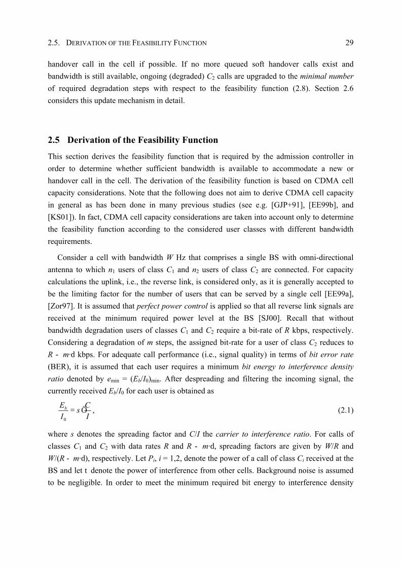
2.5. DERIVATION OF THE FEASIBILITY FUNCTION 29
handover call in the cell if possible. If no more queued soft handover calls exist and bandwidth is still available, ongoing (degraded) C2 calls are upgraded to the minimal number of required degradation steps with respect to the feasibility function (2.8). Section 2.6 considers this update mechanism in detail.
2.5 Derivation of the Feasibility Function
This section derives the feasibility function that is required by the admission controller in order to determine whether sufficient bandwidth is available to accommodate a new or handover call in the cell. The derivation of the feasibility function is based on CDMA cell capacity considerations. Note that the following does not aim to derive CDMA cell capacity in general as has been done in many previous studies (see e.g. [GJP+91], [EE99b], and [KS01]). In fact, CDMA cell capacity considerations are taken into account only to determine the feasibility function according to the considered user classes with different bandwidth requirements.
Consider a cell with bandwidth W Hz that comprises a single BS with omni-directional antenna to which n1 users of class C1 and n2 users of class C2 are connected. For capacity calculations the uplink, i.e., the reverse link, is considered only, as it is generally accepted to be the limiting factor for the number of users that can be served by a single cell [EE99a], [Zor97]. It is assumed that perfect power control is applied so that all reverse link signals are received at the minimum required power level at the BS [SJ00]. Recall that without bandwidth degradation users of classes C1 and C2 require a bit-rate of R kbps, respectively. Considering a degradation of m steps, the assigned bit-rate for a user of class C2 reduces to R - m·d kbps. For adequate call performance (i.e., signal quality) in terms of bit error rate (BER), it is assumed that each user requires a minimum bit energy to interference density ratio denoted by emin = (Eb/I0)min. After despreading and filtering the incoming signal, the currently received Eb/I0 for each user is obtained as
0
bE CsI I
= Ö , (2.1)
where s denotes the spreading factor and C/I the carrier to interference ratio. For calls of classes C1 and C2 with data rates R and R - m·d, spreading factors are given by W/R and W/(R - m·d), respectively. Let Pi, i = 1,2, denote the power of a call of class Ci received at the BS and let t denote the power of interference from other cells. Background noise is assumed to be negligible. In order to meet the minimum required bit energy to interference density
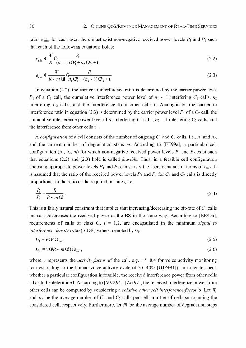
30 2. ONLINE QOS/REVENUE MANAGEMENT OF REAL-TIME SERVICES
ratio, emin, for each user, there must exist non-negative received power levels P1 and P2 such that each of the following equations holds:
1min
1 1 2 2( 1)W PeR n P n P
¢ Ö- Ö + Ö + t
(2.2)
2min
1 1 2 2( 1)W Pe
R m n P n P¢ Ö
- Ö d Ö + - Ö + t (2.3)
In equation (2.2), the carrier to interference ratio is determined by the carrier power level P1 of a C1 call, the cumulative interference power level of n1 - 1 interfering C1 calls, n2 interfering C2 calls, and the interference from other cells t. Analogously, the carrier to interference ratio in equation (2.3) is determined by the carrier power level P2 of a C2 call, the cumulative interference power level of n1 interfering C1 calls, n2 - 1 interfering C2 calls, and the interference from other cells t.
A configuration of a cell consists of the number of ongoing C1 and C2 calls, i.e., n1 and n2, and the current number of degradation steps m. According to [EE99a], a particular cell configuration (n1, n2, m) for which non-negative received power levels P1 and P2 exist such that equations (2.2) and (2.3) hold is called feasible. Thus, in a feasible cell configuration choosing appropriate power levels P1 and P2 can satisfy the users demands in terms of emin. It is assumed that the ratio of the received power levels P1 and P2 for C1 and C2 calls is directly proportional to the ratio of the required bit-rates, i.e.,
1
2
P RP R m
=- Öd
. (2.4)
This is a fairly natural constraint that implies that increasing/decreasing the bit-rate of C2 calls increases/decreases the received power at the BS in the same way. According to [EE99a], requirements of calls of class Ci, i = 1,2, are encapsulated in the minimum signal to interference density ratio (SIDR) values, denoted by Gi:
1 minv R eG = Ö Ö (2.5)
2 min( )v R m eG = Ö - Ö d Ö , (2.6)
where v represents the activity factor of the call, e.g. v º 0.4 for voice activity monitoring (corresponding to the human voice activity cycle of 35-40% [GJP+91]). In order to check whether a particular configuration is feasible, the received interference power from other cells t has to be determined. According to [VVZ94], [Zor97], the received interference power from other cells can be computed by considering a relative other cell interference factor b. Let 1n and 2n be the average number of C1 and C2 calls per cell in a tier of cells surrounding the considered cell, respectively. Furthermore, let m be the average number of degradation steps

2.6. OPTIMIZATION OF THE ADMISSION CONTROLLER 31
in the surrounding cells. Applying equation (2.4), the interference power from other cells can be determined by:
1 1 2 1R mn P n P
R- Ö då õt = b Ö Ö + Ö Öæ ö
ç ÷ (2.7)
Inserting (2.4), (2.5), (2.6), and (2.7) into (2.2) and (2.3), defining 2 min( )v R m eG = Ö - Ö d Ö as the average requirements of C2 calls in the surrounding cells, and using some algebra, results in the following feasibility function:
1 1 2 2 1 1 2 21 2
feasible , if ( 1) ( )( , , )
unfeasible , elsen n n n W
F n n më G + G - +b Ö G + G ¢
= ìí
(2.8)
2.6 Optimization of the Admission Controller
2.6.1 Markov Chain Analysis of the Admission Controller
The optimization of the admission control and bandwidth degradation scheme introduced above is performed by means of a continuous-time Markov chain (CTMC, [Lin98]). In particular, the Markov chain is utilized to determine the optimal value for the degradation threshold q (see Figure 2.4 for a definition of q) with respect to a given traffic pattern and a predefined goal for optimization. This section shows how to analyze the Markov chain efficiently and how to derive QoS and revenue measures that constitute the building blocks for the optimization goals specified in the following.
The Markov model considers the admission controller of one target cell. It is assumed that new call requests of class C1 and C2 arrive according to a spatially uniform Poisson process with arrival rate ln,1 and ln,2, respectively. Furthermore, soft handover requests from ongoing C1 and C2 calls arrive according to a Poisson process with rate lh,1 and lh,2, respectively. The amount of time that a MS with an ongoing call remains within the cell is called dwell time. With respect to the feasibility function (2.8), the dwell time is the time the call contributes to the intra-cell interference. Indeed, a soft handover to an adjacent cell can occur during the dwell time. Then the target cell and the corresponding adjacent cell serve the call simultaneously. If the call is still active after dwell time, it leaves the cell to a neighboring cell without being in soft handover with the target cell anymore. The call duration is defined as the amount of time that the call will be active, assuming it completes without being forced to terminate due to handover failure. It is assumed that the dwell time and the call duration are exponentially distributed random variables with mean 1/mh and 1/md, respectively. The overall rate of calls leaving the considered cell is denoted by m = mh + md. The reciprocal 1/m is called
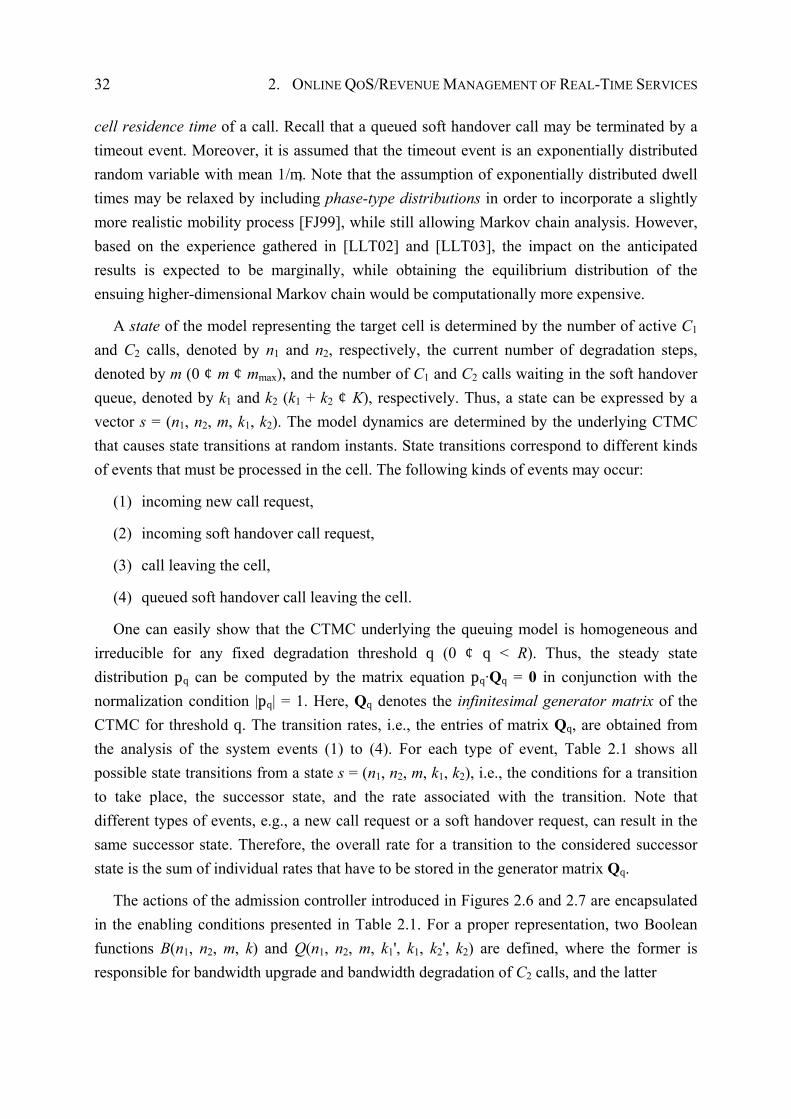
32 2. ONLINE QOS/REVENUE MANAGEMENT OF REAL-TIME SERVICES
cell residence time of a call. Recall that a queued soft handover call may be terminated by a timeout event. Moreover, it is assumed that the timeout event is an exponentially distributed random variable with mean 1/mt. Note that the assumption of exponentially distributed dwell times may be relaxed by including phase-type distributions in order to incorporate a slightly more realistic mobility process [FJ99], while still allowing Markov chain analysis. However, based on the experience gathered in [LLT02] and [LLT03], the impact on the anticipated results is expected to be marginally, while obtaining the equilibrium distribution of the ensuing higher-dimensional Markov chain would be computationally more expensive.
A state of the model representing the target cell is determined by the number of active C1 and C2 calls, denoted by n1 and n2, respectively, the current number of degradation steps, denoted by m (0 ¢ m ¢ mmax), and the number of C1 and C2 calls waiting in the soft handover queue, denoted by k1 and k2 (k1 + k2 ¢ K), respectively. Thus, a state can be expressed by a vector s = (n1, n2, m, k1, k2). The model dynamics are determined by the underlying CTMC that causes state transitions at random instants. State transitions correspond to different kinds of events that must be processed in the cell. The following kinds of events may occur:
(1) incoming new call request,
(2) incoming soft handover call request,
(3) call leaving the cell,
(4) queued soft handover call leaving the cell.
One can easily show that the CTMC underlying the queuing model is homogeneous and irreducible for any fixed degradation threshold q (0 ¢ q < R). Thus, the steady state distribution pq can be computed by the matrix equation pq·Qq = 0 in conjunction with the normalization condition |pq| = 1. Here, Qq denotes the infinitesimal generator matrix of the CTMC for threshold q. The transition rates, i.e., the entries of matrix Qq, are obtained from the analysis of the system events (1) to (4). For each type of event, Table 2.1 shows all possible state transitions from a state s = (n1, n2, m, k1, k2), i.e., the conditions for a transition to take place, the successor state, and the rate associated with the transition. Note that different types of events, e.g., a new call request or a soft handover request, can result in the same successor state. Therefore, the overall rate for a transition to the considered successor state is the sum of individual rates that have to be stored in the generator matrix Qq.
The actions of the admission controller introduced in Figures 2.6 and 2.7 are encapsulated in the enabling conditions presented in Table 2.1. For a proper representation, two Boolean functions B(n1, n2, m, k) and Q(n1, n2, m, k1', k1, k2', k2) are defined, where the former is responsible for bandwidth upgrade and bandwidth degradation of C2 calls, and the latter
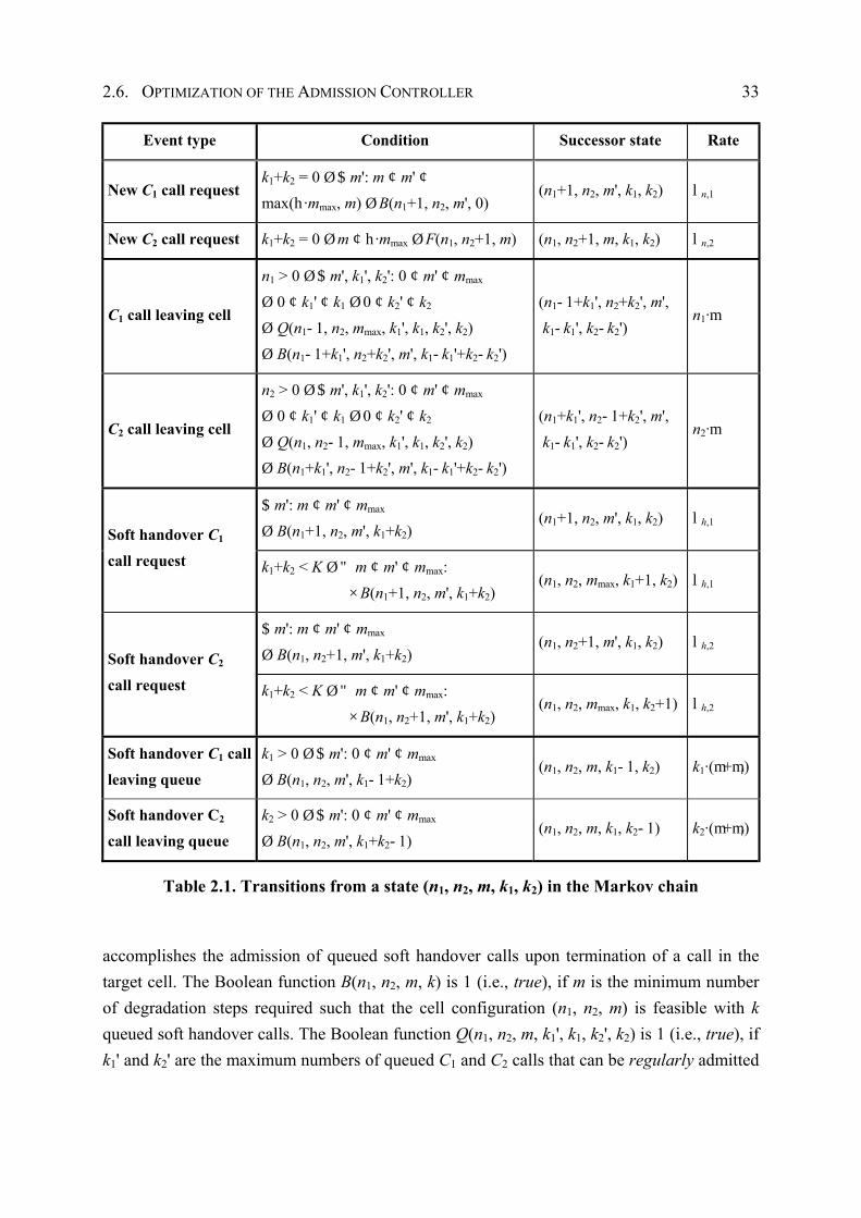
2.6. OPTIMIZATION OF THE ADMISSION CONTROLLER 33
Event type Condition Successor state Rate
New C1 call request k1+k2 = 0 Ø $ m': m ¢ m' ¢ max(h·mmax, m) Ø B(n1+1, n2, m', 0)
(n1+1, n2, m', k1, k2) ln,1
New C2 call request k1+k2 = 0 Ø m ¢ h·mmax Ø F(n1, n2+1, m) (n1, n2+1, m, k1, k2) ln,2
C1 call leaving cell
n1 > 0 Ø $ m', k1', k2': 0 ¢ m' ¢ mmax Ø 0 ¢ k1' ¢ k1 Ø 0 ¢ k2' ¢ k2 Ø Q(n1-1, n2, mmax, k1', k1, k2', k2) Ø B(n1-1+k1', n2+k2', m', k1-k1'+k2-k2')
(n1-1+k1', n2+k2', m', k1-k1', k2-k2')
n1·m
C2 call leaving cell
n2 > 0 Ø $ m', k1', k2': 0 ¢ m' ¢ mmax Ø 0 ¢ k1' ¢ k1 Ø 0 ¢ k2' ¢ k2 Ø Q(n1, n2-1, mmax, k1', k1, k2', k2) Ø B(n1+k1', n2-1+k2', m', k1-k1'+k2-k2')
(n1+k1', n2-1+k2', m', k1-k1', k2-k2')
n2·m
$ m': m ¢ m' ¢ mmax Ø B(n1+1, n2, m', k1+k2)
(n1+1, n2, m', k1, k2) lh,1 Soft handover C1 call request k1+k2 < K Ø " m ¢ m' ¢ mmax:
×B(n1+1, n2, m', k1+k2) (n1, n2, mmax, k1+1, k2) lh,1
$ m': m ¢ m' ¢ mmax Ø B(n1, n2+1, m', k1+k2)
(n1, n2+1, m', k1, k2) lh,2 Soft handover C2 call request k1+k2 < K Ø " m ¢ m' ¢ mmax:
×B(n1, n2+1, m', k1+k2) (n1, n2, mmax, k1, k2+1) lh,2
Soft handover C1 call leaving queue
k1 > 0 Ø $ m': 0 ¢ m' ¢ mmax Ø B(n1, n2, m', k1-1+k2)
(n1, n2, m, k1-1, k2) k1·(m+mt)
Soft handover C2 call leaving queue
k2 > 0 Ø $ m': 0 ¢ m' ¢ mmax Ø B(n1, n2, m', k1+k2-1)
(n1, n2, m, k1, k2-1) k2·(m+mt)
Table 2.1. Transitions from a state (n1, n2, m, k1, k2) in the Markov chain
accomplishes the admission of queued soft handover calls upon termination of a call in the target cell. The Boolean function B(n1, n2, m, k) is 1 (i.e., true), if m is the minimum number of degradation steps required such that the cell configuration (n1, n2, m) is feasible with k queued soft handover calls. The Boolean function Q(n1, n2, m, k1', k1, k2', k2) is 1 (i.e., true), if k1' and k2' are the maximum numbers of queued C1 and C2 calls that can be regularly admitted
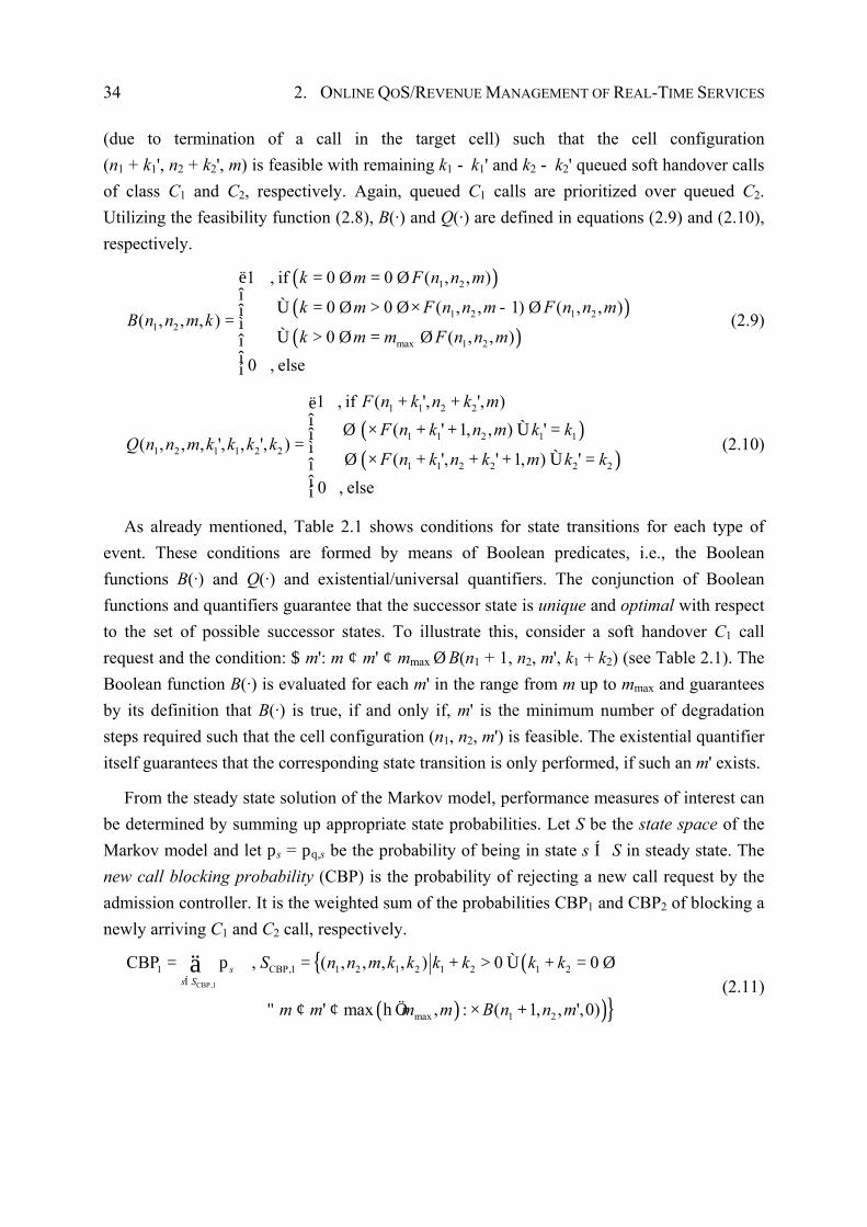
34 2. ONLINE QOS/REVENUE MANAGEMENT OF REAL-TIME SERVICES
(due to termination of a call in the target cell) such that the cell configuration (n1 + k1', n2 + k2', m) is feasible with remaining k1 - k1' and k2 - k2' queued soft handover calls of class C1 and C2, respectively. Again, queued C1 calls are prioritized over queued C2. Utilizing the feasibility function (2.8), B(·) and Q(·) are defined in equations (2.9) and (2.10), respectively.
( )( )( )
1 2
1 2 1 21 2
max 1 2
1 , if 0 0 ( , , )
0 0 ( , , 1) ( , , )( , , , )
0 ( , , )0 , else
k m F n n m
k m F n n m F n n mB n n m k
k m m F n n m
ë = Ø = Øî
Ù = Ø > Ø × - Øî= ìÙ > Ø = Øî
îí
(2.9)
( )( )
1 1 2 2
1 1 2 1 11 2 1 1 2 2
1 1 2 2 2 2
1 , if ( ', ', )( ' 1, , ) '
( , , , ', , ', )( ', ' 1, ) '
0 , else
F n k n k mF n k n m k k
Q n n m k k k kF n k n k m k k
+ +ëî Ø × + + Ù =î= ì
Ø × + + + Ù =îîí
(2.10)
As already mentioned, Table 2.1 shows conditions for state transitions for each type of event. These conditions are formed by means of Boolean predicates, i.e., the Boolean functions B(·) and Q(·) and existential/universal quantifiers. The conjunction of Boolean functions and quantifiers guarantee that the successor state is unique and optimal with respect to the set of possible successor states. To illustrate this, consider a soft handover C1 call request and the condition: $ m': m ¢ m' ¢ mmax Ø B(n1 + 1, n2, m', k1 + k2) (see Table 2.1). The Boolean function B(·) is evaluated for each m' in the range from m up to mmax and guarantees by its definition that B(·) is true, if and only if, m' is the minimum number of degradation steps required such that the cell configuration (n1, n2, m') is feasible. The existential quantifier itself guarantees that the corresponding state transition is only performed, if such an m' exists.
From the steady state solution of the Markov model, performance measures of interest can be determined by summing up appropriate state probabilities. Let S be the state space of the Markov model and let ps = pq,s be the probability of being in state s Í S in steady state. The new call blocking probability (CBP) is the probability of rejecting a new call request by the admission controller. It is the weighted sum of the probabilities CBP1 and CBP2 of blocking a newly arriving C1 and C2 call, respectively.
({
( ) )}CBP,1
1 CBP,1 1 2 1 2 1 2 1 2
max 1 2
CBP , ( , , , , ) 0 0
' max , : ( 1, , ',0)
ss S
S n n m k k k k k k
m m m m B n n m
Í
= p = + > Ù + = Ø
" ¢ ¢ hÖ × +
ä (2.11)
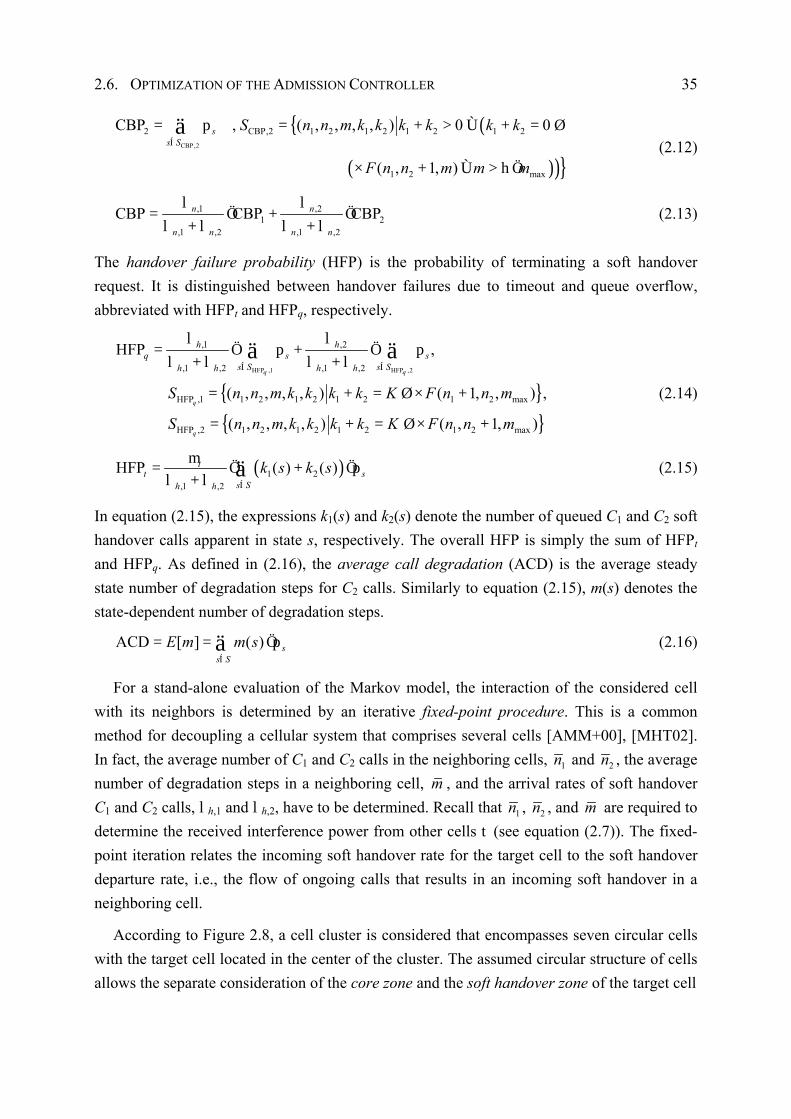
2.6. OPTIMIZATION OF THE ADMISSION CONTROLLER 35
({
( ))}CBP,2
2 CBP,2 1 2 1 2 1 2 1 2
1 2 max
CBP , ( , , , , ) 0 0
( , 1, )
ss S
S n n m k k k k k k
F n n m m m
Í
= p = + > Ù + = Ø
× + Ù > hÖ
ä (2.12)
,1 ,21 2
,1 ,2 ,1 ,2
CBP CBP CBPn n
n n n n
l l= Ö + Öl + l l + l
(2.13)
The handover failure probability (HFP) is the probability of terminating a soft handover request. It is distinguished between handover failures due to timeout and queue overflow, abbreviated with HFPt and HFPq, respectively.
{ }{ }
HFP ,1 HFP ,2
,1 ,2
,1 ,2 ,1 ,2
HFP ,1 1 2 1 2 1 2 1 2 max
HFP ,2 1 2 1 2 1 2 1 2 max
HFP ,
( , , , , ) ( 1, , ) ,
( , , , , ) ( , 1, )
q q
q
q
h hq s s
s S s Sh h h h
S n n m k k k k K F n n m
S n n m k k k k K F n n m
Í Í
l l= Ö p + Ö pl + l l + l
= + = Ø × +
= + = Ø × +
ä ä
(2.14)
( )1 2,1 ,2
HFP ( ) ( )tt s
s Sh h
k s k sÍ
m= Ö + Ö pl + l ä (2.15)
In equation (2.15), the expressions k1(s) and k2(s) denote the number of queued C1 and C2 soft handover calls apparent in state s, respectively. The overall HFP is simply the sum of HFPt and HFPq. As defined in (2.16), the average call degradation (ACD) is the average steady state number of degradation steps for C2 calls. Similarly to equation (2.15), m(s) denotes the state-dependent number of degradation steps.
ACD [ ] ( ) ss S
E m m sÍ
= = Ö pä (2.16)
For a stand-alone evaluation of the Markov model, the interaction of the considered cell with its neighbors is determined by an iterative fixed-point procedure. This is a common method for decoupling a cellular system that comprises several cells [AMM+00], [MHT02]. In fact, the average number of C1 and C2 calls in the neighboring cells, 1n and 2n , the average number of degradation steps in a neighboring cell, m , and the arrival rates of soft handover C1 and C2 calls, lh,1 and lh,2, have to be determined. Recall that 1n , 2n , and m are required to determine the received interference power from other cells t (see equation (2.7)). The fixed-point iteration relates the incoming soft handover rate for the target cell to the soft handover departure rate, i.e., the flow of ongoing calls that results in an incoming soft handover in a neighboring cell.
According to Figure 2.8, a cell cluster is considered that encompasses seven circular cells with the target cell located in the center of the cluster. The assumed circular structure of cells allows the separate consideration of the core zone and the soft handover zone of the target cell

36 2. ONLINE QOS/REVENUE MANAGEMENT OF REAL-TIME SERVICES
Core Zone
Soft Handover Zone
Figure 2.8. Core zone and soft handover zone for a target cell in a cluster of cells
[MHT02]. It is assumed that the core zone covers a portion a of the target cell area and the soft handover zone covers the remaining portion (1 - a). Thus, the radius of the core zone is a times the radius of the target cell as can be shown by a simple calculation. Recall that
new calls originate according to a spatially uniform Poisson process. Under the assumption that MSs move in a straight line at a random angle, the dwell time of terminals in the core zone is ha m .
The soft handover departure rate of Ci calls, i = 1,2, in step j of the fixed-point iteration can be approximated by the average number of Ci calls in the core zone in step j, i.e., ( )[ ] j
iE naÖ , divided by the dwell time in the core zone, i.e., ha m , plus the rate of newly accepted Ci calls in the target cell starting in the soft handover zone:
( )( 1) ( ) ( ), ,(1 ) 1 CBP [ ]j j j
h i n i i h iE n+l = - a Öl Ö - + a Öm Ö , for i = 1,2, (2.17)
where E[ni](j) is the average steady state number of Ci calls in the cell in step j and CBPi(j) is
the steady state probability of rejecting a new Ci call request in step j. For the experiments presented below, a cell overlapping of approximately 10% is considered that corresponds to a = 0.4. Indeed, the area of the core zone is slightly smaller than the area of the soft handover zone. With this assumption the average number of calls and the average number of degradation steps in the neighboring cells can be balanced as follows:
( 1) ( )910 [ ]j j
i in E n+ = Ö , for i = 1,2 (2.18)
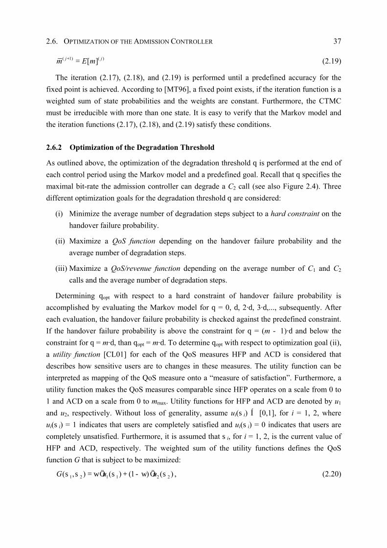
2.6. OPTIMIZATION OF THE ADMISSION CONTROLLER 37
( 1) ( )[ ]j jm E m+ = (2.19)
The iteration (2.17), (2.18), and (2.19) is performed until a predefined accuracy for the fixed point is achieved. According to [MT96], a fixed point exists, if the iteration function is a weighted sum of state probabilities and the weights are constant. Furthermore, the CTMC must be irreducible with more than one state. It is easy to verify that the Markov model and the iteration functions (2.17), (2.18), and (2.19) satisfy these conditions.
2.6.2 Optimization of the Degradation Threshold
As outlined above, the optimization of the degradation threshold q is performed at the end of each control period using the Markov model and a predefined goal. Recall that q specifies the maximal bit-rate the admission controller can degrade a C2 call (see also Figure 2.4). Three different optimization goals for the degradation threshold q are considered:
(i) Minimize the average number of degradation steps subject to a hard constraint on the handover failure probability.
(ii) Maximize a QoS function depending on the handover failure probability and the average number of degradation steps.
(iii) Maximize a QoS/revenue function depending on the average number of C1 and C2 calls and the average number of degradation steps.
Determining qopt with respect to a hard constraint of handover failure probability is accomplished by evaluating the Markov model for q = 0, d, 2·d, 3·d,..., subsequently. After each evaluation, the handover failure probability is checked against the predefined constraint. If the handover failure probability is above the constraint for q = (m - 1)·d and below the constraint for q = m·d, than qopt = m·d. To determine qopt with respect to optimization goal (ii), a utility function [CL01] for each of the QoS measures HFP and ACD is considered that describes how sensitive users are to changes in these measures. The utility function can be interpreted as mapping of the QoS measure onto a “measure of satisfaction”. Furthermore, a utility function makes the QoS measures comparable since HFP operates on a scale from 0 to 1 and ACD on a scale from 0 to mmax. Utility functions for HFP and ACD are denoted by u1 and u2, respectively. Without loss of generality, assume ui(si) Í [0,1], for i = 1, 2, where ui(si) = 1 indicates that users are completely satisfied and ui(si) = 0 indicates that users are completely unsatisfied. Furthermore, it is assumed that si, for i = 1, 2, is the current value of HFP and ACD, respectively. The weighted sum of the utility functions defines the QoS function G that is subject to be maximized:
1 2 1 1 2 2( , ) ( ) (1 ) ( )G u us s = wÖ s + - w Ö s , (2.20)
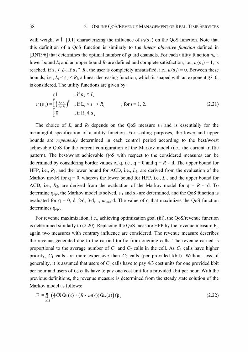
38 2. ONLINE QOS/REVENUE MANAGEMENT OF REAL-TIME SERVICES
with weight w Í [0,1] characterizing the influence of u1(s1) on the QoS function. Note that this definition of a QoS function is similarly to the linear objective function defined in [RNT96] that determines the optimal number of guard channels. For each utility function ui, a lower bound Li and an upper bound Ri are defined and complete satisfaction, i.e., ui(si) = 1, is reached, if si ¢ Li. If si ² Ri, the user is completely unsatisfied, i.e., ui(si) = 0. Between these bounds, i.e., Li < si < Ri, a linear decreasing function, which is shaped with an exponent g ² 0, is considered. The utility functions are given by:
( ) i
i
1 , if
( ) , if L
0 , if R
i i
i i
i i
Ri i i iR L
i
L
u Rg-s
-
s ¢ëîîs = < s <ìî
¢ sîí
, for i = 1, 2. (2.21)
The choice of Li and Ri depends on the QoS measure si and is essentially for the meaningful specification of a utility function. For scaling purposes, the lower and upper bounds are repeatedly determined in each control period according to the best/worst achievable QoS for the current configuration of the Markov model (i.e., the current traffic pattern). The best/worst achievable QoS with respect to the considered measures can be determined by considering border values of q, i.e., q = 0 and q = R - d. The upper bound for HFP, i.e., R1, and the lower bound for ACD, i.e., L2, are derived from the evaluation of the Markov model for q = 0, whereas the lower bound for HFP, i.e., L1, and the upper bound for ACD, i.e., R2, are derived from the evaluation of the Markov model for q = R - d. To determine qopt, the Markov model is solved, s1 and s2 are determined, and the QoS function is evaluated for q = 0, d, 2·d, 3·d,..., mmax·d. The value of q that maximizes the QoS function determines qopt.
For revenue maximization, i.e., achieving optimization goal (iii), the QoS/revenue function is determined similarly to (2.20). Replacing the QoS measure HFP by the revenue measure F, again two measures with contrary influence are considered. The revenue measure describes the revenue generated due to the carried traffic from ongoing calls. The revenue earned is proportional to the average number of C1 and C2 calls in the cell. As C1 calls have higher priority, C1 calls are more expensive than C2 calls (per provided kbit). Without loss of generality, it is assumed that users of C1 calls have to pay 4/3 cost units for one provided kbit per hour and users of C2 calls have to pay one cost unit for a provided kbit per hour. With the previous definitions, the revenue measure is determined from the steady state solution of the Markov model as follows:
( )41 23 ( ) ( ( )) ( ) s
s SR n s R m s n s
Í
F = Ö Ö + - Ö Ö pä (2.22)
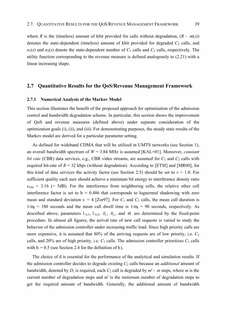
2.7. QUANTITATIVE RESULTS FOR THE QOS/REVENUE MANAGEMENT FRAMEWORK 39
where R is the (timeless) amount of kbit provided for calls without degradation, (R - m(s)) denotes the state-dependent (timeless) amount of kbit provided for degraded C2 calls, and n1(s) and n2(s) denote the state-dependent number of C1 calls and C2 calls, respectively. The utility function corresponding to the revenue measure is defined analogously to (2.21) with a linear increasing shape.
2.7 Quantitative Results for the QoS/Revenue Management Framework
2.7.1 Numerical Analysis of the Markov Model
This section illustrates the benefit of the proposed approach for optimization of the admission control and bandwidth degradation scheme. In particular, this section shows the improvement of QoS and revenue measures (defined above) under separate consideration of the optimization goals (i), (ii), and (iii). For demonstrating purposes, the steady state results of the Markov model are derived for a particular parameter setting.
As defined for wideband CDMA that will be utilized in UMTS networks (see Section 1), an overall bandwidth spectrum of W = 3.84 MHz is assumed [KAL+01]. Moreover, constant bit rate (CBR) data services, e.g., CBR video streams, are assumed for C1 and C2 calls with required bit-rate of R = 32 kbps (without degradation). According to [ETSI] and [MR00], for this kind of data services the activity factor (see Section 2.5) should be set to v = 1.0. For sufficient quality each user should achieve a minimum bit energy to interference density ratio emin = 3.16 (= 5dB). For the interference from neighboring cells, the relative other cell interference factor is set to b = 0.486 that corresponds to lognormal shadowing with zero mean and standard deviation s = 4 [Zor97]. For C1 and C2 calls, the mean call duration is 1/md = 180 seconds and the mean call dwell time is 1/mh = 90 seconds, respectively. As described above, parameters lh,1, lh,2, 1n , 2n , and m are determined by the fixed-point procedure. In almost all figures, the arrival rate of new call requests is varied to study the behavior of the admission controller under increasing traffic load. Since high priority calls are more expensive, it is assumed that 80% of the arriving requests are of low priority, i.e. C2 calls, and 20% are of high priority, i.e. C1 calls. The admission controller prioritizes C1 calls with h = 0.5 (see Section 2.4 for the definition of h).
The choice of d is essential for the performance of the analytical and simulation results. If the admission controller decides to degrade existing C2 calls because an additional amount of bandwidth, denoted by D, is required, each C2 call is degraded by m' - m steps, where m is the current number of degradation steps and m' is the minimum number of degradation steps to get the required amount of bandwidth. Generally, the additional amount of bandwidth
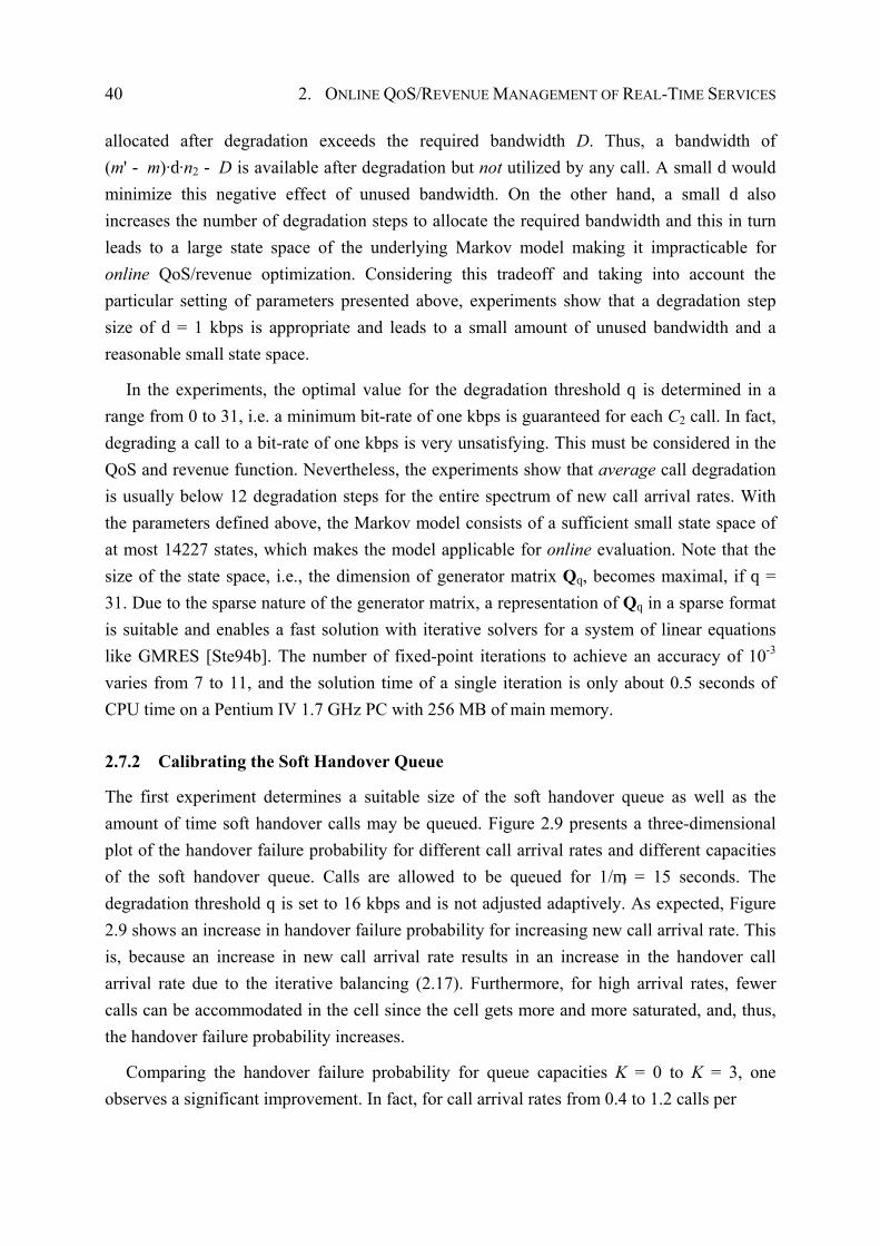
40 2. ONLINE QOS/REVENUE MANAGEMENT OF REAL-TIME SERVICES
allocated after degradation exceeds the required bandwidth D. Thus, a bandwidth of (m' - m)·d·n2 - D is available after degradation but not utilized by any call. A small d would minimize this negative effect of unused bandwidth. On the other hand, a small d also increases the number of degradation steps to allocate the required bandwidth and this in turn leads to a large state space of the underlying Markov model making it impracticable for online QoS/revenue optimization. Considering this tradeoff and taking into account the particular setting of parameters presented above, experiments show that a degradation step size of d = 1 kbps is appropriate and leads to a small amount of unused bandwidth and a reasonable small state space.
In the experiments, the optimal value for the degradation threshold q is determined in a range from 0 to 31, i.e. a minimum bit-rate of one kbps is guaranteed for each C2 call. In fact, degrading a call to a bit-rate of one kbps is very unsatisfying. This must be considered in the QoS and revenue function. Nevertheless, the experiments show that average call degradation is usually below 12 degradation steps for the entire spectrum of new call arrival rates. With the parameters defined above, the Markov model consists of a sufficient small state space of at most 14227 states, which makes the model applicable for online evaluation. Note that the size of the state space, i.e., the dimension of generator matrix Qq, becomes maximal, if q = 31. Due to the sparse nature of the generator matrix, a representation of Qq in a sparse format is suitable and enables a fast solution with iterative solvers for a system of linear equations like GMRES [Ste94b]. The number of fixed-point iterations to achieve an accuracy of 10-3 varies from 7 to 11, and the solution time of a single iteration is only about 0.5 seconds of CPU time on a Pentium IV 1.7 GHz PC with 256 MB of main memory.
2.7.2 Calibrating the Soft Handover Queue
The first experiment determines a suitable size of the soft handover queue as well as the amount of time soft handover calls may be queued. Figure 2.9 presents a three-dimensional plot of the handover failure probability for different call arrival rates and different capacities of the soft handover queue. Calls are allowed to be queued for 1/mt = 15 seconds. The degradation threshold q is set to 16 kbps and is not adjusted adaptively. As expected, Figure 2.9 shows an increase in handover failure probability for increasing new call arrival rate. This is, because an increase in new call arrival rate results in an increase in the handover call arrival rate due to the iterative balancing (2.17). Furthermore, for high arrival rates, fewer calls can be accommodated in the cell since the cell gets more and more saturated, and, thus, the handover failure probability increases.
Comparing the handover failure probability for queue capacities K = 0 to K = 3, one observes a significant improvement. In fact, for call arrival rates from 0.4 to 1.2 calls per
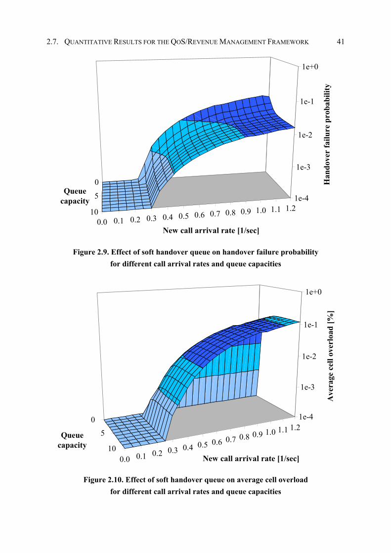
2.7. QUANTITATIVE RESULTS FOR THE QOS/REVENUE MANAGEMENT FRAMEWORK 41
0
5
100.0 0.1 0.2 0.3 0.4 0.5 0.6 0.7 0.8 0.9 1.0 1.1 1.2
1e-4
1e-3
1e-2
1e-1
1e+0
Han
dove
r fa
ilure
pro
babi
lity
Queuecapacity
New call arrival rate [1/sec]
Figure 2.9. Effect of soft handover queue on handover failure probability for different call arrival rates and queue capacities
05
100.0 0.1 0.2 0.3 0.4 0.5 0.6 0.7 0.8 0.9 1.0 1.1 1.2
1e-4
1e-3
1e-2
1e-1
1e+0
Ave
rage
cel
l ove
rloa
d [%
]
Queuecapacity
New call arrival rate [1/sec]
Figure 2.10. Effect of soft handover queue on average cell overload for different call arrival rates and queue capacities
42 2. ONLINE QOS/REVENUE MANAGEMENT OF REAL-TIME SERVICES
second the handover failure probability can be reduced about one order of magnitude. Increasing the queue capacity from K = 4 to K = 10 does not result in further improvements of HFP. This means that for K ² 4 the probability of a handover failure due to queue overflow, HFPq, is insignificantly. Thus, the termination of most handover calls is due to the timeout of 15 seconds for each queued call. This indicates that a queue capacity of K = 3 is sufficient for queuing soft handover calls temporarily (with a queue timeout of 1/mt = 15 seconds).
As discussed in Section 2.4, queued soft handover calls lead to cell overload with respect to the feasibility function (2.8). Figure 2.10 depicts the average cell overload induced by queued soft handover calls for a queue timeout of 1/mt = 15 seconds. In agreement with Figure 2.9, the average cell overload increases significantly for queue capacities K = 0 to K = 3 and is nearly unchanged for queue capacities K ² 4. Fortunately, the average cell overload is very small irrespective of the call arrival rate and the queue capacity, i.e., the maximum average cell overload is about 0.12% for an arrival rate of 1.2 and a queue capacity of K = 10. Note that the average cell overload is tightly coupled with the average queue length that shows qualitative similarities with the evolution of the average cell overload for different call arrival rates and queue capacities.
05
100 5 10 15 20 25 30
1e-4
1e-3
1e-2
1e-1
1e+0
Han
dove
r fa
ilure
pro
babi
lity
Queuecapacity
Soft handover queue timeout [sec]
Figure 2.11. Effect of soft handover queue on handover failure probability for different queue timeouts and queue capacities
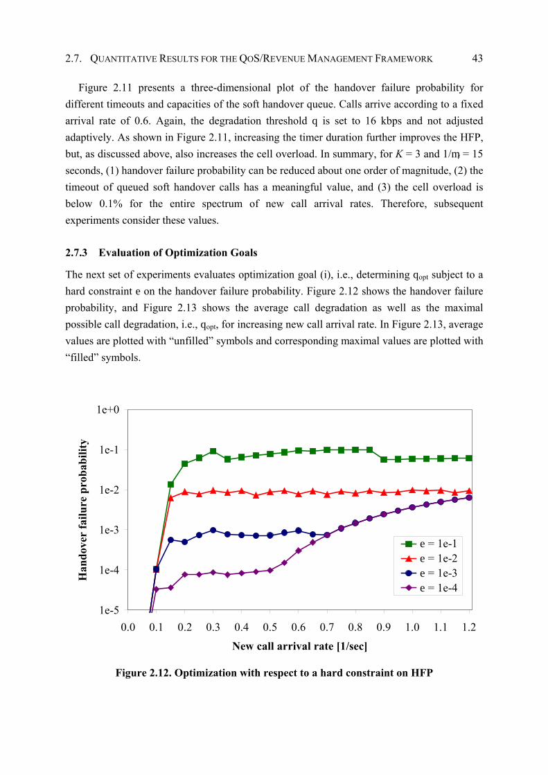
2.7. QUANTITATIVE RESULTS FOR THE QOS/REVENUE MANAGEMENT FRAMEWORK 43
Figure 2.11 presents a three-dimensional plot of the handover failure probability for different timeouts and capacities of the soft handover queue. Calls arrive according to a fixed arrival rate of 0.6. Again, the degradation threshold q is set to 16 kbps and not adjusted adaptively. As shown in Figure 2.11, increasing the timer duration further improves the HFP, but, as discussed above, also increases the cell overload. In summary, for K = 3 and 1/mt = 15 seconds, (1) handover failure probability can be reduced about one order of magnitude, (2) the timeout of queued soft handover calls has a meaningful value, and (3) the cell overload is below 0.1% for the entire spectrum of new call arrival rates. Therefore, subsequent experiments consider these values.
2.7.3 Evaluation of Optimization Goals
The next set of experiments evaluates optimization goal (i), i.e., determining qopt subject to a hard constraint e on the handover failure probability. Figure 2.12 shows the handover failure probability, and Figure 2.13 shows the average call degradation as well as the maximal possible call degradation, i.e., qopt, for increasing new call arrival rate. In Figure 2.13, average values are plotted with “unfilled” symbols and corresponding maximal values are plotted with “filled” symbols.
1e-5
1e-4
1e-3
1e-2
1e-1
1e+0
0.0 0.1 0.2 0.3 0.4 0.5 0.6 0.7 0.8 0.9 1.0 1.1 1.2
New call arrival rate [1/sec]
Han
dove
r fa
ilure
pro
babi
lity
e = 1e-1e = 1e-2e = 1e-3e = 1e-4
e = 1e-1e = 1e-2e = 1e-3e = 1e-4
Figure 2.12. Optimization with respect to a hard constraint on HFP
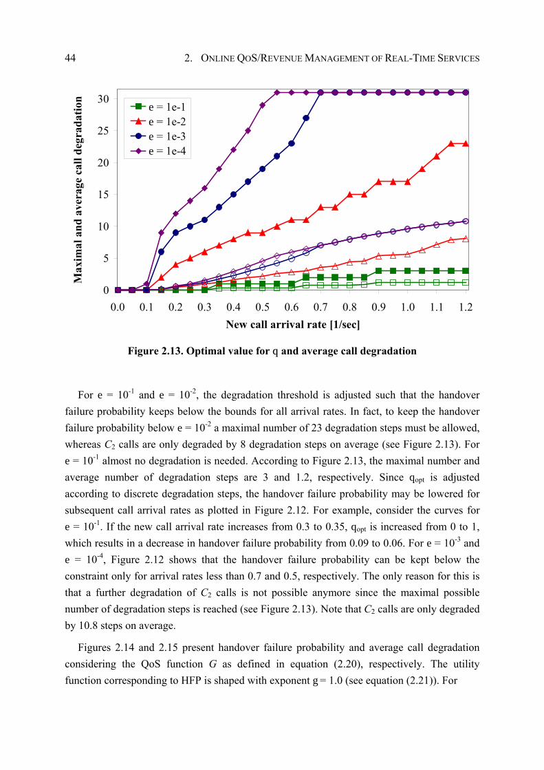
44 2. ONLINE QOS/REVENUE MANAGEMENT OF REAL-TIME SERVICES
0
5
10
15
20
25
30
0.0 0.1 0.2 0.3 0.4 0.5 0.6 0.7 0.8 0.9 1.0 1.1 1.2New call arrival rate [1/sec]
Max
imal
and
ave
rage
cal
l deg
rada
tion
e = 1e-1e = 1e-2e = 1e-3e = 1e-4
e = 1e-1e = 1e-2e = 1e-3e = 1e-4
Figure 2.13. Optimal value for q and average call degradation
For e = 10-1 and e = 10-2, the degradation threshold is adjusted such that the handover failure probability keeps below the bounds for all arrival rates. In fact, to keep the handover failure probability below e = 10-2 a maximal number of 23 degradation steps must be allowed, whereas C2 calls are only degraded by 8 degradation steps on average (see Figure 2.13). For e = 10-1 almost no degradation is needed. According to Figure 2.13, the maximal number and average number of degradation steps are 3 and 1.2, respectively. Since qopt is adjusted according to discrete degradation steps, the handover failure probability may be lowered for subsequent call arrival rates as plotted in Figure 2.12. For example, consider the curves for e = 10-1. If the new call arrival rate increases from 0.3 to 0.35, qopt is increased from 0 to 1, which results in a decrease in handover failure probability from 0.09 to 0.06. For e = 10-3 and e = 10-4, Figure 2.12 shows that the handover failure probability can be kept below the constraint only for arrival rates less than 0.7 and 0.5, respectively. The only reason for this is that a further degradation of C2 calls is not possible anymore since the maximal possible number of degradation steps is reached (see Figure 2.13). Note that C2 calls are only degraded by 10.8 steps on average.
Figures 2.14 and 2.15 present handover failure probability and average call degradation considering the QoS function G as defined in equation (2.20), respectively. The utility function corresponding to HFP is shaped with exponent g = 1.0 (see equation (2.21)). For
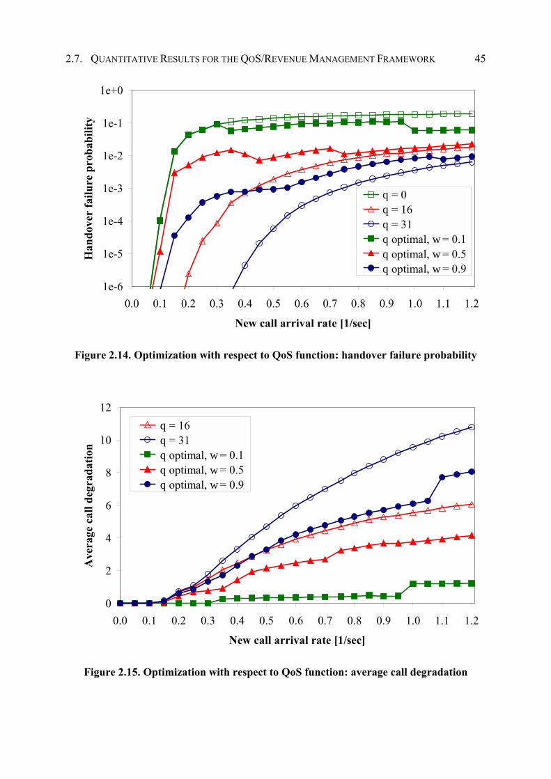
2.7. QUANTITATIVE RESULTS FOR THE QOS/REVENUE MANAGEMENT FRAMEWORK 45
1e-6
1e-5
1e-4
1e-3
1e-2
1e-1
1e+0
0.0 0.1 0.2 0.3 0.4 0.5 0.6 0.7 0.8 0.9 1.0 1.1 1.2
New call arrival rate [1/sec]
Han
dove
r fa
ilure
pro
babi
lity
q = 0q = 16q = 31q optimal, w = 0.1q optimal, w = 0.5q optimal, w = 0.9
q = 0q = 16q = 31q optimal, w = 0.1q optimal, w = 0.5q optimal, w = 0.9
Figure 2.14. Optimization with respect to QoS function: handover failure probability
0
2
4
6
8
10
12
0.0 0.1 0.2 0.3 0.4 0.5 0.6 0.7 0.8 0.9 1.0 1.1 1.2
New call arrival rate [1/sec]
Ave
rage
cal
l deg
rada
tion
q = 16q = 31q optimal, w = 0.1q optimal, w = 0.5q optimal, w = 0.9
q = 16q = 31q optimal, w = 0.1q optimal, w = 0.5q optimal, w = 0.9
Figure 2.15. Optimization with respect to QoS function: average call degradation
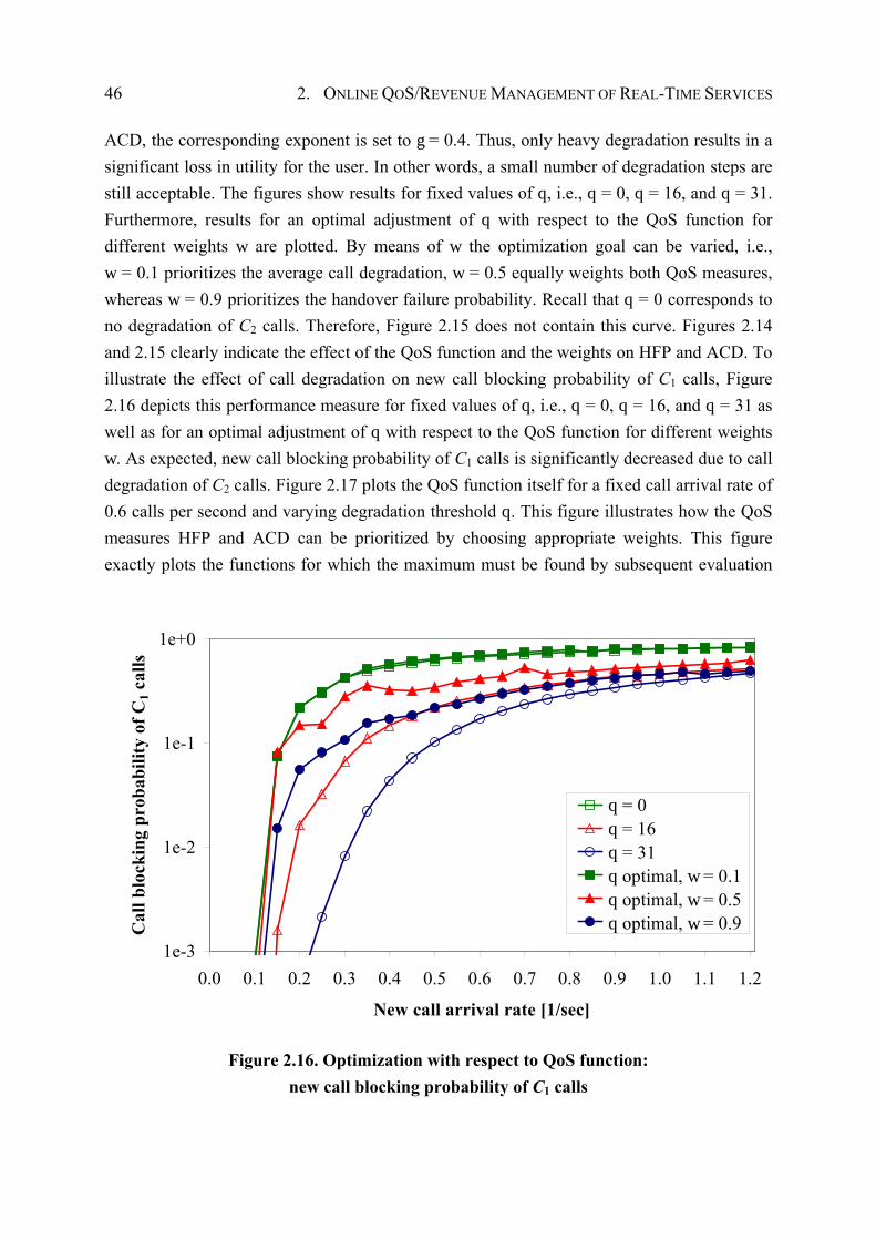
46 2. ONLINE QOS/REVENUE MANAGEMENT OF REAL-TIME SERVICES
ACD, the corresponding exponent is set to g = 0.4. Thus, only heavy degradation results in a significant loss in utility for the user. In other words, a small number of degradation steps are still acceptable. The figures show results for fixed values of q, i.e., q = 0, q = 16, and q = 31. Furthermore, results for an optimal adjustment of q with respect to the QoS function for different weights w are plotted. By means of w the optimization goal can be varied, i.e., w = 0.1 prioritizes the average call degradation, w = 0.5 equally weights both QoS measures, whereas w = 0.9 prioritizes the handover failure probability. Recall that q = 0 corresponds to no degradation of C2 calls. Therefore, Figure 2.15 does not contain this curve. Figures 2.14 and 2.15 clearly indicate the effect of the QoS function and the weights on HFP and ACD. To illustrate the effect of call degradation on new call blocking probability of C1 calls, Figure 2.16 depicts this performance measure for fixed values of q, i.e., q = 0, q = 16, and q = 31 as well as for an optimal adjustment of q with respect to the QoS function for different weights w. As expected, new call blocking probability of C1 calls is significantly decreased due to call degradation of C2 calls. Figure 2.17 plots the QoS function itself for a fixed call arrival rate of 0.6 calls per second and varying degradation threshold q. This figure illustrates how the QoS measures HFP and ACD can be prioritized by choosing appropriate weights. This figure exactly plots the functions for which the maximum must be found by subsequent evaluation
1e-3
1e-2
1e-1
1e+0
0.0 0.1 0.2 0.3 0.4 0.5 0.6 0.7 0.8 0.9 1.0 1.1 1.2
New call arrival rate [1/sec]
Cal
l blo
ckin
g pr
obab
ility
of C
1 cal
ls
q = 0q = 16q = 31q optimal, w = 0.1q optimal, w = 0.5q optimal, w = 0.9
q = 0q = 16q = 31q optimal, w = 0.1q optimal, w = 0.5q optimal, w = 0.9
Figure 2.16. Optimization with respect to QoS function: new call blocking probability of C1 calls
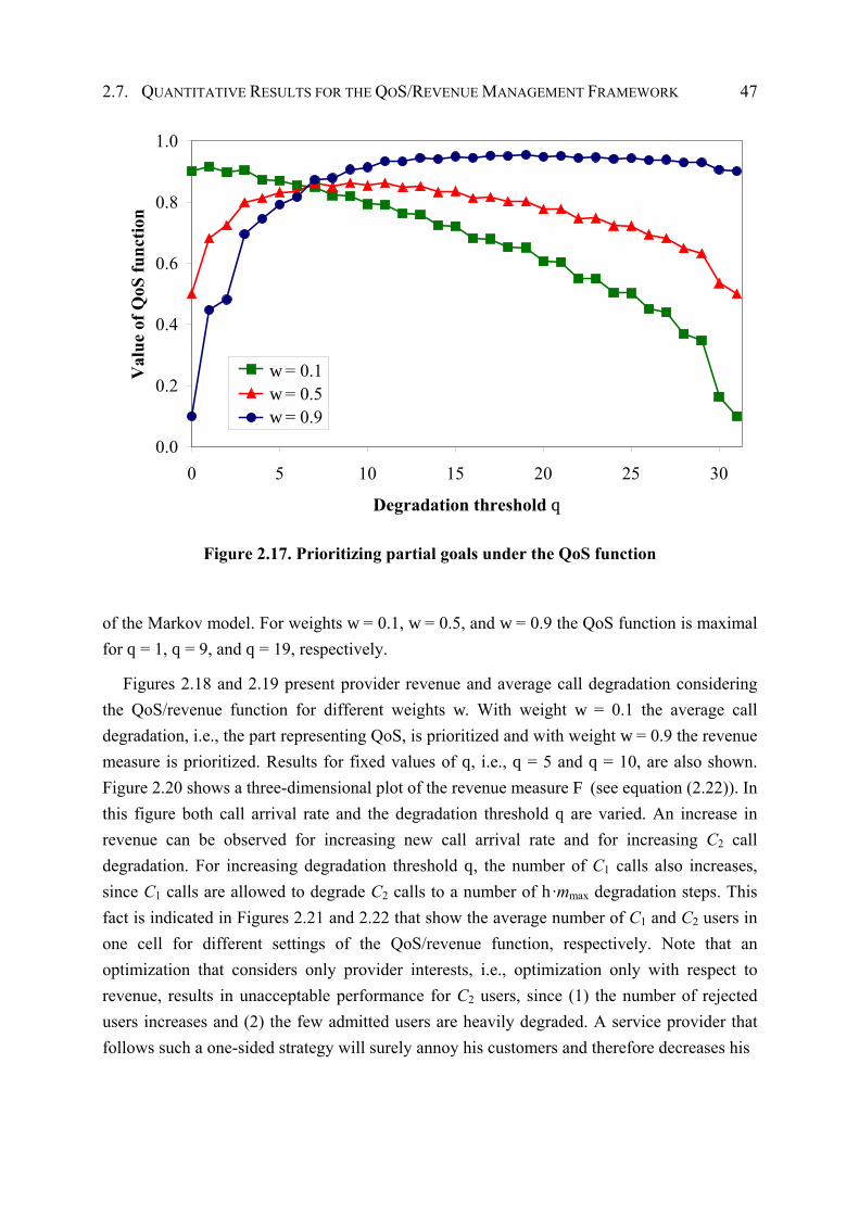
2.7. QUANTITATIVE RESULTS FOR THE QOS/REVENUE MANAGEMENT FRAMEWORK 47
0.0
0.2
0.4
0.6
0.8
1.0
0 5 10 15 20 25 30
Degradation threshold q
Val
ue o
f QoS
func
tion
w = 0.1w = 0.5w = 0.9
w = 0.1w = 0.5w = 0.9
Figure 2.17. Prioritizing partial goals under the QoS function
of the Markov model. For weights w = 0.1, w = 0.5, and w = 0.9 the QoS function is maximal for q = 1, q = 9, and q = 19, respectively.
Figures 2.18 and 2.19 present provider revenue and average call degradation considering the QoS/revenue function for different weights w. With weight w = 0.1 the average call degradation, i.e., the part representing QoS, is prioritized and with weight w = 0.9 the revenue measure is prioritized. Results for fixed values of q, i.e., q = 5 and q = 10, are also shown. Figure 2.20 shows a three-dimensional plot of the revenue measure F (see equation (2.22)). In this figure both call arrival rate and the degradation threshold q are varied. An increase in revenue can be observed for increasing new call arrival rate and for increasing C2 call degradation. For increasing degradation threshold q, the number of C1 calls also increases, since C1 calls are allowed to degrade C2 calls to a number of h·mmax degradation steps. This fact is indicated in Figures 2.21 and 2.22 that show the average number of C1 and C2 users in one cell for different settings of the QoS/revenue function, respectively. Note that an optimization that considers only provider interests, i.e., optimization only with respect to revenue, results in unacceptable performance for C2 users, since (1) the number of rejected users increases and (2) the few admitted users are heavily degraded. A service provider that follows such a one-sided strategy will surely annoy his customers and therefore decreases his
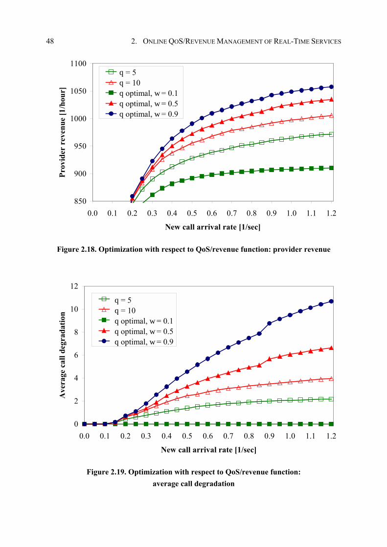
48 2. ONLINE QOS/REVENUE MANAGEMENT OF REAL-TIME SERVICES
850
900
950
1000
1050
1100
0.0 0.1 0.2 0.3 0.4 0.5 0.6 0.7 0.8 0.9 1.0 1.1 1.2
New call arrival rate [1/sec]
Prov
ider
rev
enue
[1/h
our]
q = 5q = 10q optimal, w = 0.1q optimal, w = 0.5q optimal, w = 0.9
q = 5q = 10q optimal, w = 0.1q optimal, w = 0.5q optimal, w = 0.9
Figure 2.18. Optimization with respect to QoS/revenue function: provider revenue
0
2
4
6
8
10
12
0.0 0.1 0.2 0.3 0.4 0.5 0.6 0.7 0.8 0.9 1.0 1.1 1.2
New call arrival rate [1/sec]
Ave
rage
cal
l deg
rada
tion
q = 16q = 31q optimal, w = 0.1q optimal, w = 0.5q optimal, w = 0.9
q = 5q = 10q optimal, w = 0.1q optimal, w = 0.5q optimal, w = 0.9
Figure 2.19. Optimization with respect to QoS/revenue function: average call degradation
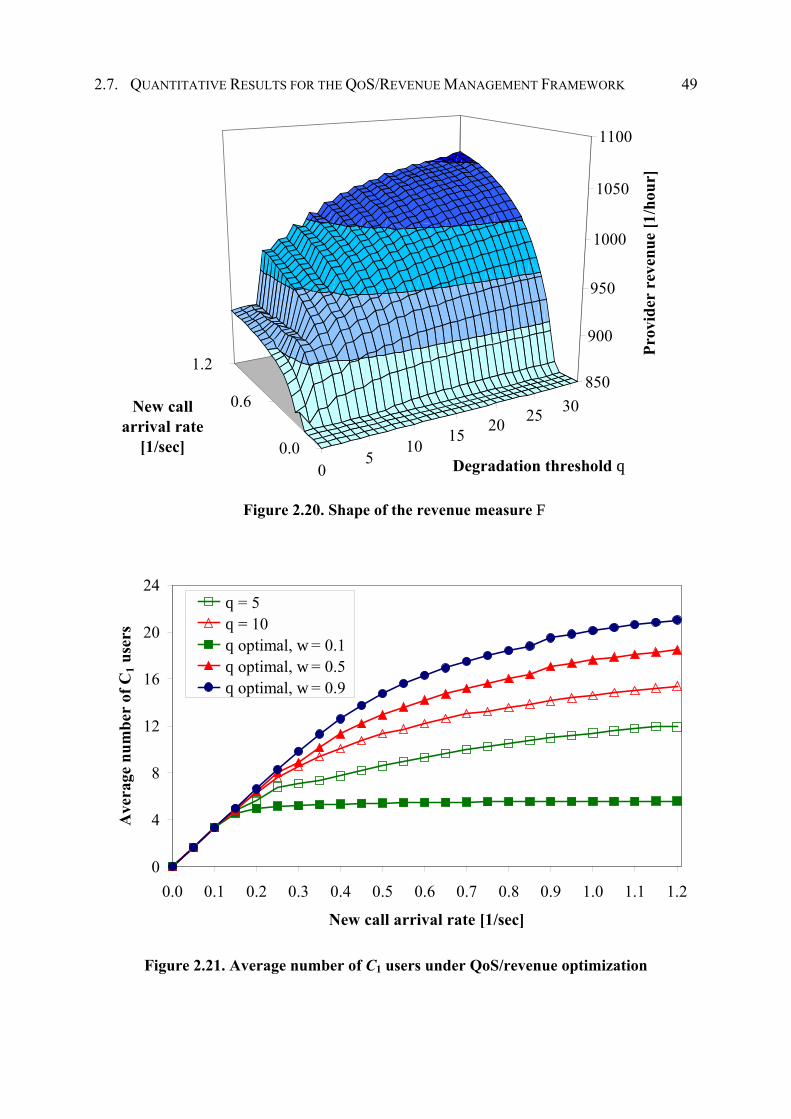
2.7. QUANTITATIVE RESULTS FOR THE QOS/REVENUE MANAGEMENT FRAMEWORK 49
05
1015 20 25 30
0.0
0.6
1.2850
900
950
1000
1050
1100
Prov
ider
rev
enue
[1/h
our]
Degradation threshold q
New call arrival rate
[1/sec]
Figure 2.20. Shape of the revenue measure F
0
4
8
12
16
20
24
0.0 0.1 0.2 0.3 0.4 0.5 0.6 0.7 0.8 0.9 1.0 1.1 1.2
New call arrival rate [1/sec]
Ave
rage
num
ber
of C
1 use
rs
q = 5q = 10q optimal, w = 0.1q optimal, w = 0.5q optimal, w = 0.9
q = 5q = 10q optimal, w = 0.1q optimal, w = 0.5q optimal, w = 0.9
Figure 2.21. Average number of C1 users under QoS/revenue optimization
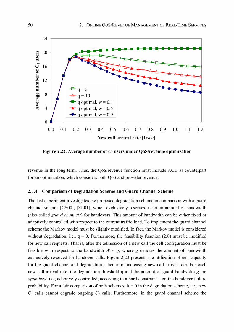
50 2. ONLINE QOS/REVENUE MANAGEMENT OF REAL-TIME SERVICES
0
4
8
12
16
20
24
0.0 0.1 0.2 0.3 0.4 0.5 0.6 0.7 0.8 0.9 1.0 1.1 1.2
New call arrival rate [1/sec]
Ave
rage
num
ber
of C
2 use
rs
q = 5q = 10q optimal, w = 0.1q optimal, w = 0.5q optimal, w = 0.9
q = 5q = 10q optimal, w = 0.1q optimal, w = 0.5q optimal, w = 0.9
Figure 2.22. Average number of C2 users under QoS/revenue optimization
revenue in the long term. Thus, the QoS/revenue function must include ACD as counterpart for an optimization, which considers both QoS and provider revenue.
2.7.4 Comparison of Degradation Scheme and Guard Channel Scheme
The last experiment investigates the proposed degradation scheme in comparison with a guard channel scheme [CS00], [ZL01], which exclusively reserves a certain amount of bandwidth (also called guard channels) for handovers. This amount of bandwidth can be either fixed or adaptively controlled with respect to the current traffic load. To implement the guard channel scheme the Markov model must be slightly modified. In fact, the Markov model is considered without degradation, i.e., q = 0. Furthermore, the feasibility function (2.8) must be modified for new call requests. That is, after the admission of a new call the cell configuration must be feasible with respect to the bandwidth W - g, where g denotes the amount of bandwidth exclusively reserved for handover calls. Figure 2.23 presents the utilization of cell capacity for the guard channel and degradation scheme for increasing new call arrival rate. For each new call arrival rate, the degradation threshold q and the amount of guard bandwidth g are optimized, i.e., adaptively controlled, according to a hard constraint e on the handover failure probability. For a fair comparison of both schemes, h = 0 in the degradation scheme, i.e., new C1 calls cannot degrade ongoing C2 calls. Furthermore, in the guard channel scheme the
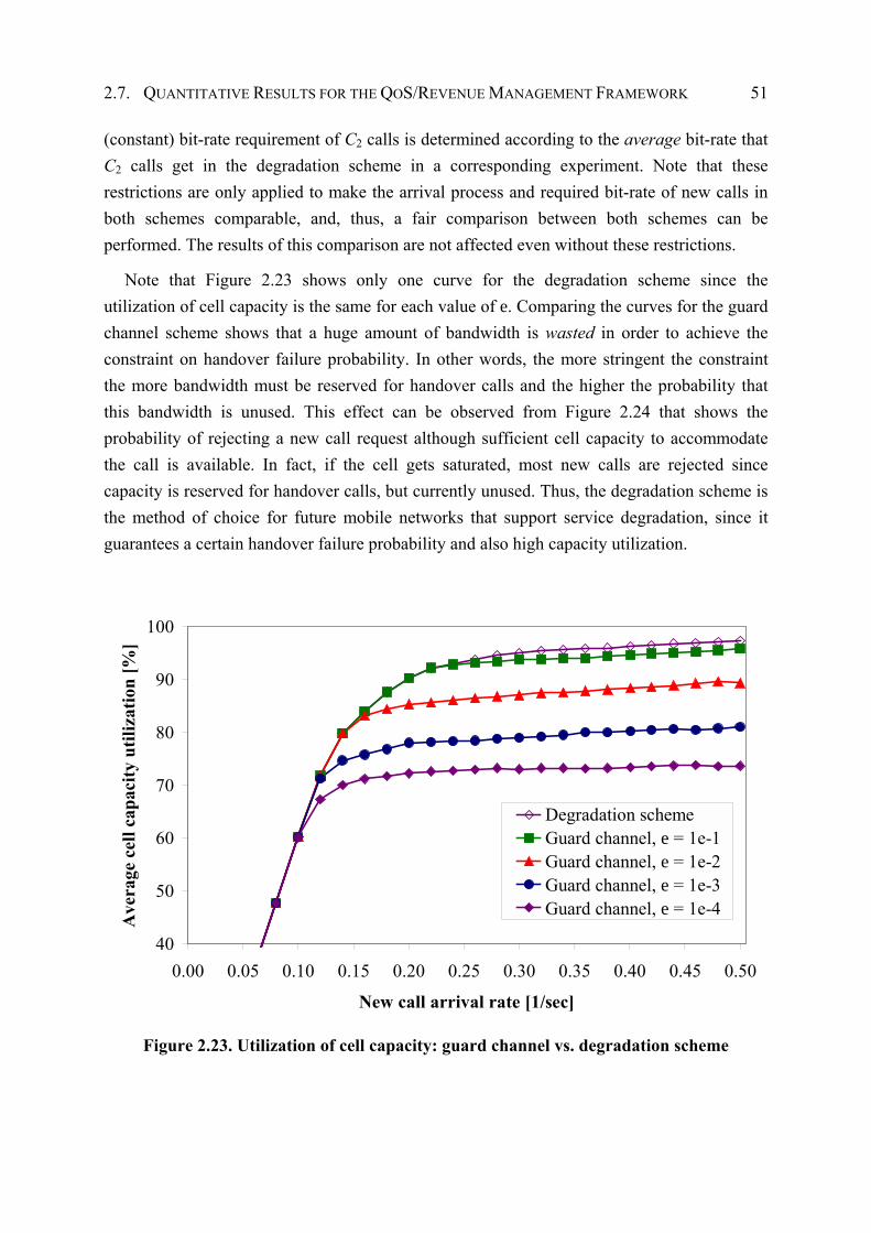
2.7. QUANTITATIVE RESULTS FOR THE QOS/REVENUE MANAGEMENT FRAMEWORK 51
(constant) bit-rate requirement of C2 calls is determined according to the average bit-rate that C2 calls get in the degradation scheme in a corresponding experiment. Note that these restrictions are only applied to make the arrival process and required bit-rate of new calls in both schemes comparable, and, thus, a fair comparison between both schemes can be performed. The results of this comparison are not affected even without these restrictions.
Note that Figure 2.23 shows only one curve for the degradation scheme since the utilization of cell capacity is the same for each value of e. Comparing the curves for the guard channel scheme shows that a huge amount of bandwidth is wasted in order to achieve the constraint on handover failure probability. In other words, the more stringent the constraint the more bandwidth must be reserved for handover calls and the higher the probability that this bandwidth is unused. This effect can be observed from Figure 2.24 that shows the probability of rejecting a new call request although sufficient cell capacity to accommodate the call is available. In fact, if the cell gets saturated, most new calls are rejected since capacity is reserved for handover calls, but currently unused. Thus, the degradation scheme is the method of choice for future mobile networks that support service degradation, since it guarantees a certain handover failure probability and also high capacity utilization.
40
50
60
70
80
90
100
0.00 0.05 0.10 0.15 0.20 0.25 0.30 0.35 0.40 0.45 0.50
New call arrival rate [1/sec]
Ave
rage
cel
l cap
acity
util
izat
ion
[%]
Degradation schemeGuard channel, e = 1e-1Guard channel, e = 1e-2Guard channel, e = 1e-3Guard channel, e = 1e-4
Degradation schemeGuard channel, e = 1e-1Guard channel, e = 1e-2Guard channel, e = 1e-3Guard channel, e = 1e-4
Figure 2.23. Utilization of cell capacity: guard channel vs. degradation scheme
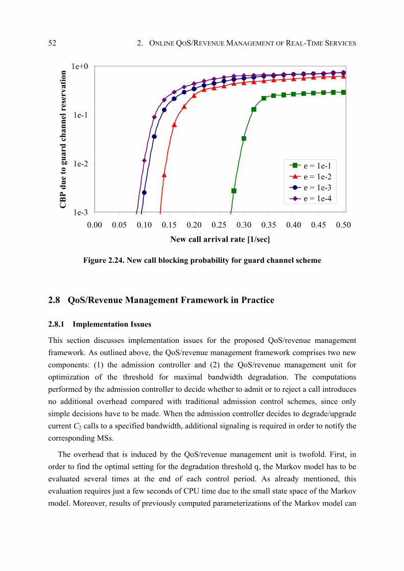
52 2. ONLINE QOS/REVENUE MANAGEMENT OF REAL-TIME SERVICES
1e-3
1e-2
1e-1
1e+0
0.00 0.05 0.10 0.15 0.20 0.25 0.30 0.35 0.40 0.45 0.50
New call arrival rate [1/sec]
CB
P du
e to
gua
rd c
hann
el r
eser
vatio
n
e = 1e-1e = 1e-2e = 1e-3 e = 1e-4
e = 1e-1e = 1e-2e = 1e-3e = 1e-4
Figure 2.24. New call blocking probability for guard channel scheme
2.8 QoS/Revenue Management Framework in Practice
2.8.1 Implementation Issues
This section discusses implementation issues for the proposed QoS/revenue management framework. As outlined above, the QoS/revenue management framework comprises two new components: (1) the admission controller and (2) the QoS/revenue management unit for optimization of the threshold for maximal bandwidth degradation. The computations performed by the admission controller to decide whether to admit or to reject a call introduces no additional overhead compared with traditional admission control schemes, since only simple decisions have to be made. When the admission controller decides to degrade/upgrade current C2 calls to a specified bandwidth, additional signaling is required in order to notify the corresponding MSs.
The overhead that is induced by the QoS/revenue management unit is twofold. First, in order to find the optimal setting for the degradation threshold q, the Markov model has to be evaluated several times at the end of each control period. As already mentioned, this evaluation requires just a few seconds of CPU time due to the small state space of the Markov model. Moreover, results of previously computed parameterizations of the Markov model can
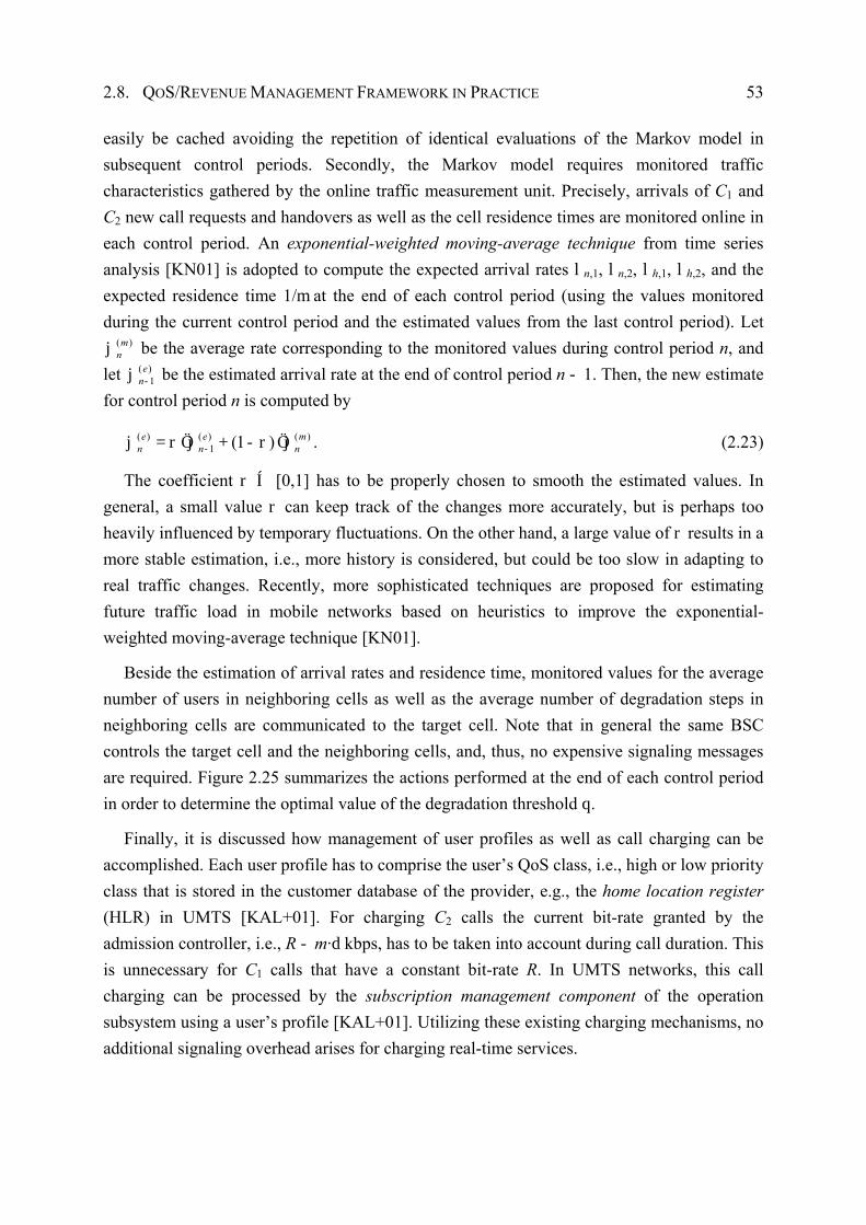
2.8. QOS/REVENUE MANAGEMENT FRAMEWORK IN PRACTICE 53
easily be cached avoiding the repetition of identical evaluations of the Markov model in subsequent control periods. Secondly, the Markov model requires monitored traffic characteristics gathered by the online traffic measurement unit. Precisely, arrivals of C1 and C2 new call requests and handovers as well as the cell residence times are monitored online in each control period. An exponential-weighted moving-average technique from time series analysis [KN01] is adopted to compute the expected arrival rates ln,1, ln,2, lh,1, lh,2, and the expected residence time 1/m at the end of each control period (using the values monitored during the current control period and the estimated values from the last control period). Let
( )mnj be the average rate corresponding to the monitored values during control period n, and
let ( )1
en-j be the estimated arrival rate at the end of control period n - 1. Then, the new estimate
for control period n is computed by
( ) ( ) ( )1 (1 )e e m
n n n-j = r Öj + -r Öj . (2.23)
The coefficient r Í [0,1] has to be properly chosen to smooth the estimated values. In general, a small value r can keep track of the changes more accurately, but is perhaps too heavily influenced by temporary fluctuations. On the other hand, a large value of r results in a more stable estimation, i.e., more history is considered, but could be too slow in adapting to real traffic changes. Recently, more sophisticated techniques are proposed for estimating future traffic load in mobile networks based on heuristics to improve the exponential-weighted moving-average technique [KN01].
Beside the estimation of arrival rates and residence time, monitored values for the average number of users in neighboring cells as well as the average number of degradation steps in neighboring cells are communicated to the target cell. Note that in general the same BSC controls the target cell and the neighboring cells, and, thus, no expensive signaling messages are required. Figure 2.25 summarizes the actions performed at the end of each control period in order to determine the optimal value of the degradation threshold q.
Finally, it is discussed how management of user profiles as well as call charging can be accomplished. Each user profile has to comprise the user’s QoS class, i.e., high or low priority class that is stored in the customer database of the provider, e.g., the home location register (HLR) in UMTS [KAL+01]. For charging C2 calls the current bit-rate granted by the admission controller, i.e., R - m·d kbps, has to be taken into account during call duration. This is unnecessary for C1 calls that have a constant bit-rate R. In UMTS networks, this call charging can be processed by the subscription management component of the operation subsystem using a user’s profile [KAL+01]. Utilizing these existing charging mechanisms, no additional signaling overhead arises for charging real-time services.
54 2. ONLINE QOS/REVENUE MANAGEMENT OF REAL-TIME SERVICES
(1) Determine current traffic pattern by online traffic monitoring according to equation (2.23).
(2) Initialize q = 0 and gmax = 0
(3) Solve the global balance equations pq·Qq = 0 in conjunction with the normalization condition |pq| = 1, for the given traffic pattern and degradation threshold q.
(4) Determine the QoS and revenue measures from the steady state solution of the Markov model according to equations (2.11) to (2.16) and equation (2.22).
(5) Evaluate the QoS/revenue function (2.20) with utility function (2.21) depending on the predefined optimization goal. Let g be the outcome of the QoS/revenue function (2.20).
(6) IF g > gmax THEN DO
(7) gmax = g
(8) qopt = q
(9) OD
(10) q = q + d
(11) IF q < R THEN restart calculation with step (3)
Figure 2.25. Algorithm for determining qopt at the end of each control period
2.8.2 Simulation Results for the QoS/Revenue Management Framework
Using simulation experiments, the following illustrates the benefit of the proposed integrated framework for adaptive online optimization of the admission controller. The simulator considers a cluster of seven cells with the target cell in the center as presented in Figure 2.3. Furthermore, the simulator contains the implementation of the algorithmic procedure presented in Figure 2.25 in order to determine the optimal value qopt for the degradation threshold in control periods of fixed duration Dt. Subsequently, the degradation threshold of the simulator is updated according to the optimal value qopt determined from the Markov model. In [KLL01], measurements have been taken over several weeks in order to derive a typical daily usage pattern, i.e., a traffic model for mean arrival rates of new calls with respect to the daytime. Table 2.2 presents the first part (half-day window) of this daily usage pattern, i.e., the mean arrival rates of new calls for 0 a.m. up to 12 a.m. These arrival rates are utilized in the following experiments in order to evaluate the effectiveness of the proposed adaptive call admission control scheme within a transient scenario.
Figures 2.26 and 2.27 depict the average call degradation in every control period for the transient scenario. Both figures show the average call degradation with knowledge of the
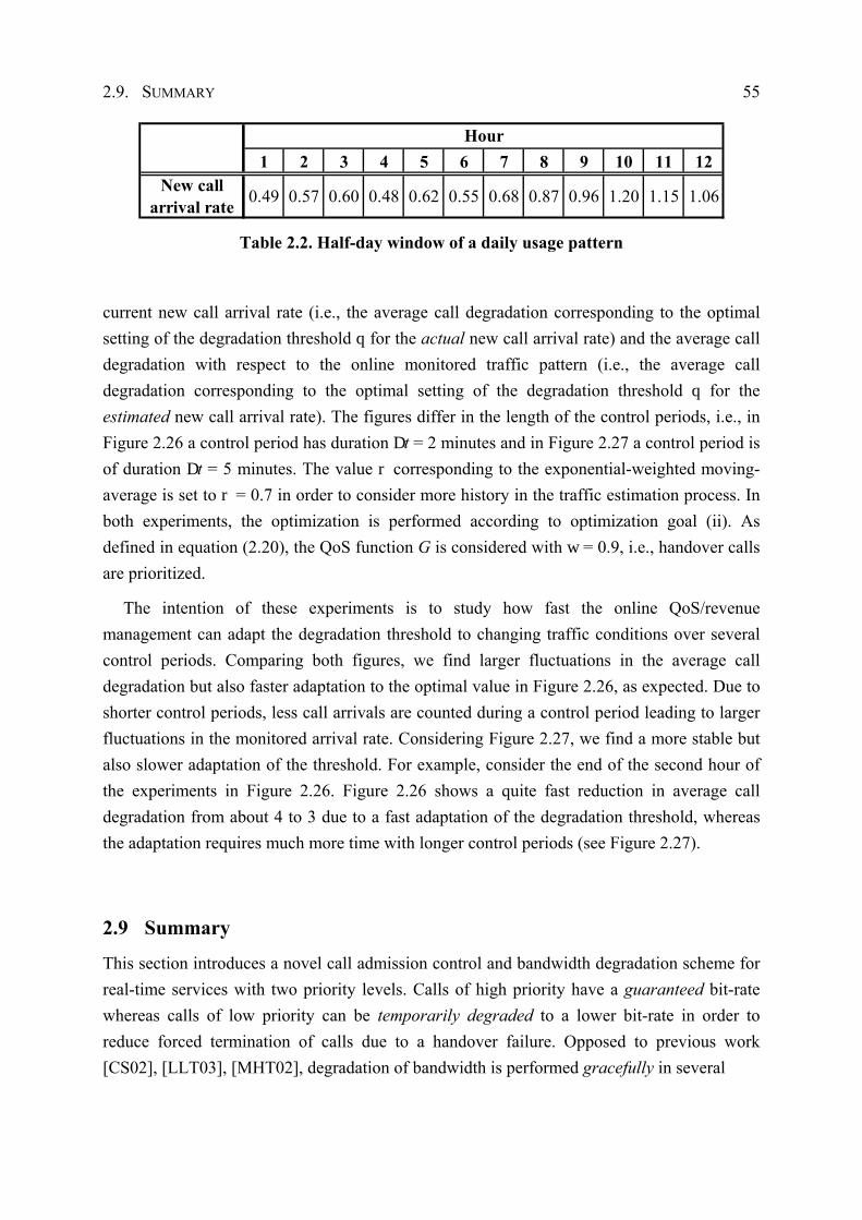
2.9. SUMMARY 55
1 2 3 4 5 6 7 8 9 10 11 12New call
arrival rate 0.49 0.57 0.60 0.48 0.62 0.55 0.68 0.87 0.96 1.20 1.15 1.06
Hour
Table 2.2. Half-day window of a daily usage pattern
current new call arrival rate (i.e., the average call degradation corresponding to the optimal setting of the degradation threshold q for the actual new call arrival rate) and the average call degradation with respect to the online monitored traffic pattern (i.e., the average call degradation corresponding to the optimal setting of the degradation threshold q for the estimated new call arrival rate). The figures differ in the length of the control periods, i.e., in Figure 2.26 a control period has duration Dt = 2 minutes and in Figure 2.27 a control period is of duration Dt = 5 minutes. The value r corresponding to the exponential-weighted moving-average is set to r = 0.7 in order to consider more history in the traffic estimation process. In both experiments, the optimization is performed according to optimization goal (ii). As defined in equation (2.20), the QoS function G is considered with w = 0.9, i.e., handover calls are prioritized.
The intention of these experiments is to study how fast the online QoS/revenue management can adapt the degradation threshold to changing traffic conditions over several control periods. Comparing both figures, we find larger fluctuations in the average call degradation but also faster adaptation to the optimal value in Figure 2.26, as expected. Due to shorter control periods, less call arrivals are counted during a control period leading to larger fluctuations in the monitored arrival rate. Considering Figure 2.27, we find a more stable but also slower adaptation of the threshold. For example, consider the end of the second hour of the experiments in Figure 2.26. Figure 2.26 shows a quite fast reduction in average call degradation from about 4 to 3 due to a fast adaptation of the degradation threshold, whereas the adaptation requires much more time with longer control periods (see Figure 2.27).
2.9 Summary
This section introduces a novel call admission control and bandwidth degradation scheme for real-time services with two priority levels. Calls of high priority have a guaranteed bit-rate whereas calls of low priority can be temporarily degraded to a lower bit-rate in order to reduce forced termination of calls due to a handover failure. Opposed to previous work [CS02], [LLT03], [MHT02], degradation of bandwidth is performed gracefully in several
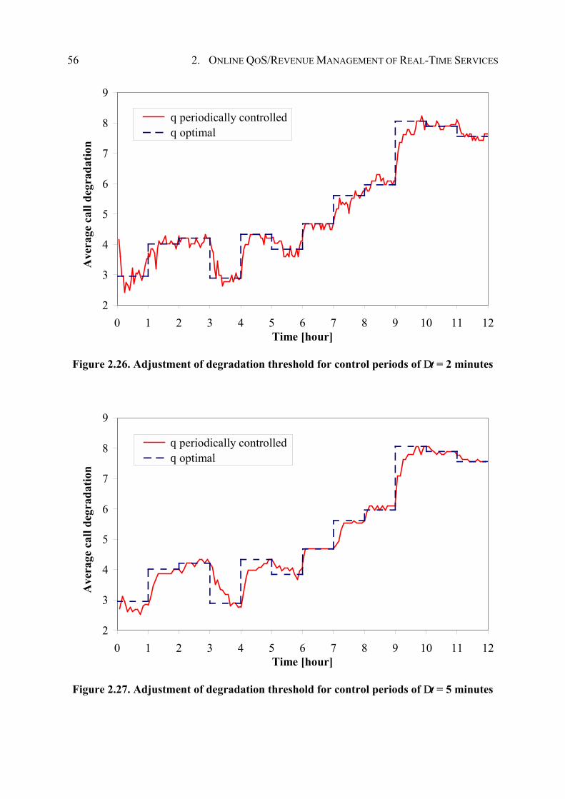
56 2. ONLINE QOS/REVENUE MANAGEMENT OF REAL-TIME SERVICES
2
3
4
5
6
7
8
9
0 1 2 3 4 5 6 7 8 9 10 11 12Time [hour]
Ave
rage
cal
l deg
rada
tion
q periodically controlledq optimalq periodically controlledq optimal
Figure 2.26. Adjustment of degradation threshold for control periods of Dt = 2 minutes
2
3
4
5
6
7
8
9
0 1 2 3 4 5 6 7 8 9 10 11 12Time [hour]
Ave
rage
cal
l deg
rada
tion
q periodically controlledq optimalq periodically controlledq optimal
Figure 2.27. Adjustment of degradation threshold for control periods of Dt = 5 minutes
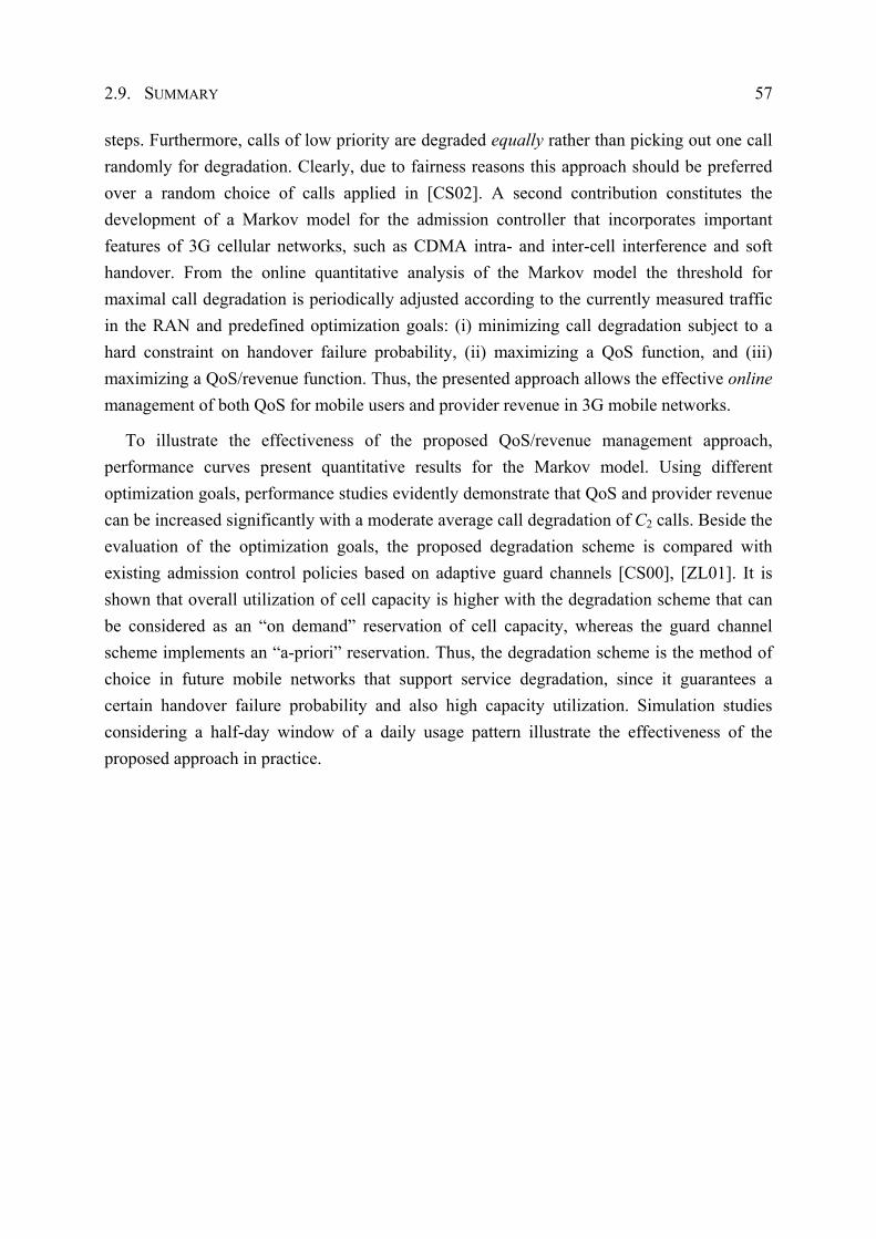
2.9. SUMMARY 57
steps. Furthermore, calls of low priority are degraded equally rather than picking out one call randomly for degradation. Clearly, due to fairness reasons this approach should be preferred over a random choice of calls applied in [CS02]. A second contribution constitutes the development of a Markov model for the admission controller that incorporates important features of 3G cellular networks, such as CDMA intra- and inter-cell interference and soft handover. From the online quantitative analysis of the Markov model the threshold for maximal call degradation is periodically adjusted according to the currently measured traffic in the RAN and predefined optimization goals: (i) minimizing call degradation subject to a hard constraint on handover failure probability, (ii) maximizing a QoS function, and (iii) maximizing a QoS/revenue function. Thus, the presented approach allows the effective online management of both QoS for mobile users and provider revenue in 3G mobile networks.
To illustrate the effectiveness of the proposed QoS/revenue management approach, performance curves present quantitative results for the Markov model. Using different optimization goals, performance studies evidently demonstrate that QoS and provider revenue can be increased significantly with a moderate average call degradation of C2 calls. Beside the evaluation of the optimization goals, the proposed degradation scheme is compared with existing admission control policies based on adaptive guard channels [CS00], [ZL01]. It is shown that overall utilization of cell capacity is higher with the degradation scheme that can be considered as an “on demand” reservation of cell capacity, whereas the guard channel scheme implements an “a-priori” reservation. Thus, the degradation scheme is the method of choice in future mobile networks that support service degradation, since it guarantees a certain handover failure probability and also high capacity utilization. Simulation studies considering a half-day window of a daily usage pattern illustrate the effectiveness of the proposed approach in practice.

59
3 EM Algorithm for Parameter Estimation of the Batch Markovian Arrival Process
ARAMETER ESTIMATION for the batch Markovian arrival process has been an open research problem for years. In this thesis, a novel expectation maximization algorithm for
parameter estimation of BMAPs is presented. This is the first numerical robust parameter estimation procedure for BMAPs published in scientific literature. Whereas Section 4 demonstrates the practical applicability of BMAPs for IP traffic modeling, this section treats the EM algorithm for BMAPs as mathematical framework in its own right. It is shown how the randomization technique and a stable calculation of Poisson jump probabilities can be utilized for computing time-dependent conditional expectations of a continuous-time Markov chain required by the expectation step of the EM algorithm. This methodological work enables the EM algorithm to be both efficient and numerical robust. Moreover, this section analyzes the computational complexity of the EM algorithm and gives some insights in the convergence behavior of the EM algorithm. The EM algorithm has been published in the well-known Performance Evaluation journal [KLL03]. An open source software implementation of the EM algorithm including detailed software documentation is available from the IP2BMAP Web site (http://www.ip2bmap.de).
3.1 The Batch Markovian Arrival Process
The batch Markovian arrival process [Luc91] belongs to the class of Markov renewal processes and was first introduced with alternative notation as the versatile Markovian point process in [Neu79]. The idea of the BMAP is to keep the tractability of the Poisson arrival process but significantly generalize it in ways that allow the inclusion of dependent inter-arrival times, non-exponential inter-arrival time distributions, and correlated batch sizes [Luc93]. BMAPs encompass as special cases both phase-type renewal processes, e.g., Erlang, Ek, and hyperexponential, Hk, renewal processes, and non-renewal processes such as the MMPP and many other processes in the applied probability literature. This wide range of arrival processes as very special cases of the BMAP evidently demonstrates that an efficient and numerical robust parameter estimation procedure shows comprehensive applicability and, thus, is of major interest for applied probability. It has been shown that the BMAP/G/1 queue
P
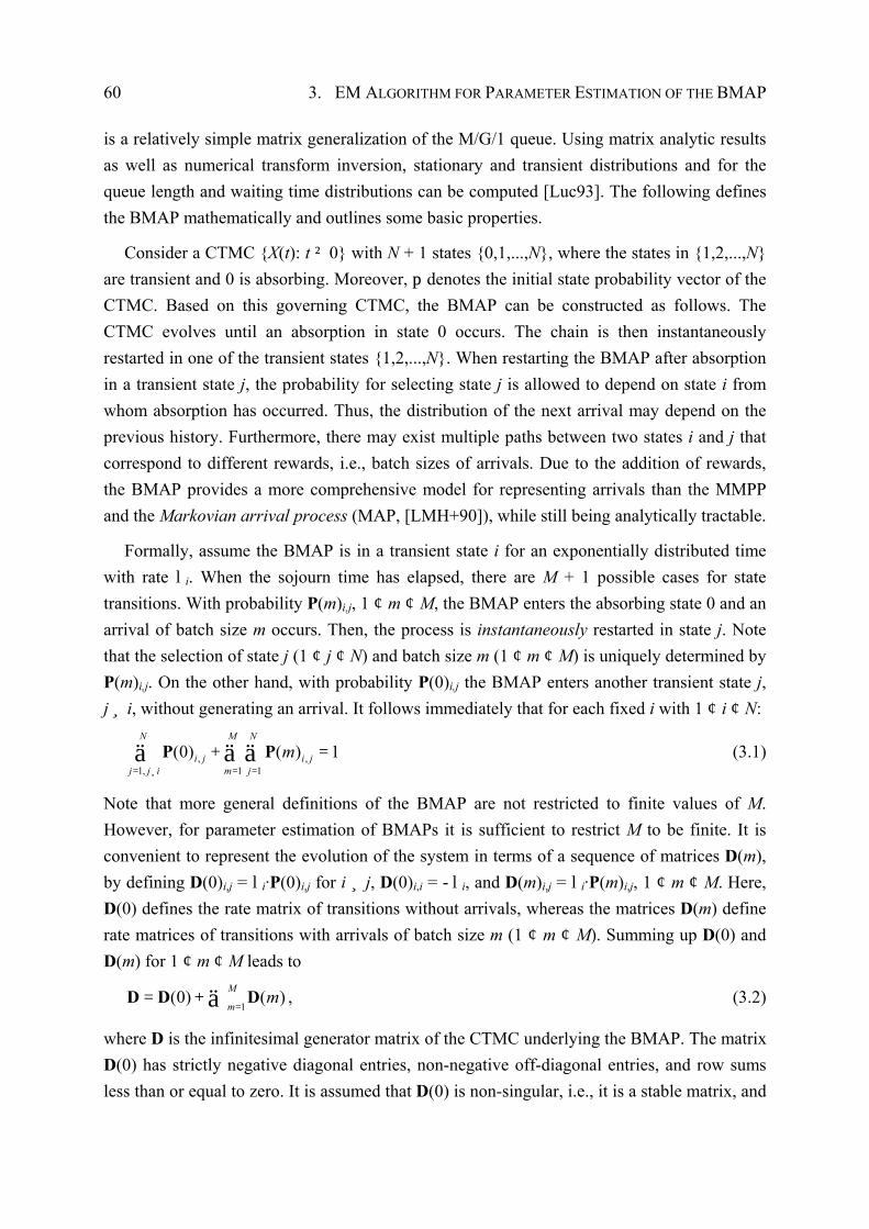
60 3. EM ALGORITHM FOR PARAMETER ESTIMATION OF THE BMAP
is a relatively simple matrix generalization of the M/G/1 queue. Using matrix analytic results as well as numerical transform inversion, stationary and transient distributions and for the queue length and waiting time distributions can be computed [Luc93]. The following defines the BMAP mathematically and outlines some basic properties.
Consider a CTMC {X(t): t ² 0} with N + 1 states {0,1,...,N}, where the states in {1,2,...,N} are transient and 0 is absorbing. Moreover, p denotes the initial state probability vector of the CTMC. Based on this governing CTMC, the BMAP can be constructed as follows. The CTMC evolves until an absorption in state 0 occurs. The chain is then instantaneously restarted in one of the transient states {1,2,...,N}. When restarting the BMAP after absorption in a transient state j, the probability for selecting state j is allowed to depend on state i from whom absorption has occurred. Thus, the distribution of the next arrival may depend on the previous history. Furthermore, there may exist multiple paths between two states i and j that correspond to different rewards, i.e., batch sizes of arrivals. Due to the addition of rewards, the BMAP provides a more comprehensive model for representing arrivals than the MMPP and the Markovian arrival process (MAP, [LMH+90]), while still being analytically tractable.
Formally, assume the BMAP is in a transient state i for an exponentially distributed time with rate li. When the sojourn time has elapsed, there are M + 1 possible cases for state transitions. With probability P(m)i,j, 1 ¢ m ¢ M, the BMAP enters the absorbing state 0 and an arrival of batch size m occurs. Then, the process is instantaneously restarted in state j. Note that the selection of state j (1 ¢ j ¢ N) and batch size m (1 ¢ m ¢ M) is uniquely determined by P(m)i,j. On the other hand, with probability P(0)i,j the BMAP enters another transient state j, j ¸ i, without generating an arrival. It follows immediately that for each fixed i with 1 ¢ i ¢ N:
, ,1, 1 1
(0) ( ) 1N M N
i j i jj j i m j
m= ¸ = =
+ =ä ääP P (3.1)
Note that more general definitions of the BMAP are not restricted to finite values of M. However, for parameter estimation of BMAPs it is sufficient to restrict M to be finite. It is convenient to represent the evolution of the system in terms of a sequence of matrices D(m), by defining D(0)i,j = li·P(0)i,j for i ¸ j, D(0)i,i = -li, and D(m)i,j = li·P(m)i,j, 1 ¢ m ¢ M. Here, D(0) defines the rate matrix of transitions without arrivals, whereas the matrices D(m) define rate matrices of transitions with arrivals of batch size m (1 ¢ m ¢ M). Summing up D(0) and D(m) for 1 ¢ m ¢ M leads to
1(0) ( )M
mm
== +äD D D , (3.2)
where D is the infinitesimal generator matrix of the CTMC underlying the BMAP. The matrix D(0) has strictly negative diagonal entries, non-negative off-diagonal entries, and row sums less than or equal to zero. It is assumed that D(0) is non-singular, i.e., it is a stable matrix, and
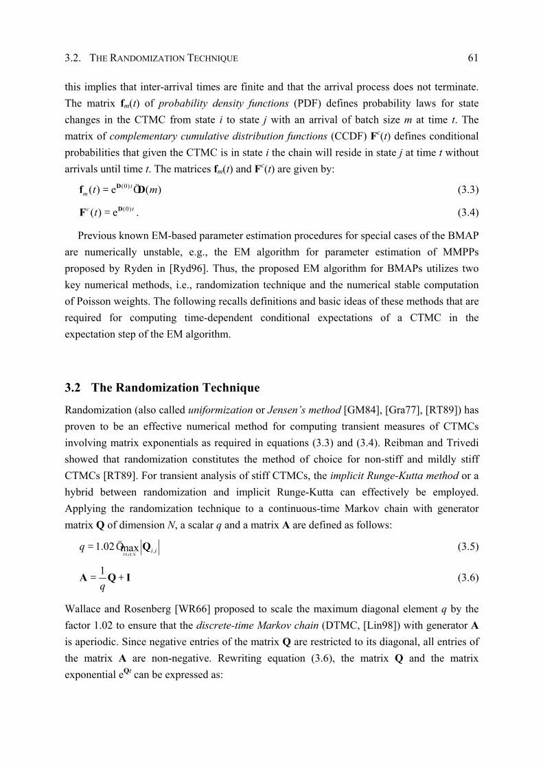
3.2. THE RANDOMIZATION TECHNIQUE 61
this implies that inter-arrival times are finite and that the arrival process does not terminate. The matrix fm(t) of probability density functions (PDF) defines probability laws for state changes in the CTMC from state i to state j with an arrival of batch size m at time t. The matrix of complementary cumulative distribution functions (CCDF) Fc(t) defines conditional probabilities that given the CTMC is in state i the chain will reside in state j at time t without arrivals until time t. The matrices fm(t) and Fc(t) are given by:
(0)( ) e ( )tm t m= ÖDf D (3.3)
(0)( ) ec tt = DF . (3.4)
Previous known EM-based parameter estimation procedures for special cases of the BMAP are numerically unstable, e.g., the EM algorithm for parameter estimation of MMPPs proposed by Ryden in [Ryd96]. Thus, the proposed EM algorithm for BMAPs utilizes two key numerical methods, i.e., randomization technique and the numerical stable computation of Poisson weights. The following recalls definitions and basic ideas of these methods that are required for computing time-dependent conditional expectations of a CTMC in the expectation step of the EM algorithm.
3.2 The Randomization Technique
Randomization (also called uniformization or Jensen’s method [GM84], [Gra77], [RT89]) has proven to be an effective numerical method for computing transient measures of CTMCs involving matrix exponentials as required in equations (3.3) and (3.4). Reibman and Trivedi showed that randomization constitutes the method of choice for non-stiff and mildly stiff CTMCs [RT89]. For transient analysis of stiff CTMCs, the implicit Runge-Kutta method or a hybrid between randomization and implicit Runge-Kutta can effectively be employed. Applying the randomization technique to a continuous-time Markov chain with generator matrix Q of dimension N, a scalar q and a matrix A are defined as follows:
1,1.02 max
i Ni iq
¢ ¢= Ö Q (3.5)
1q
= +A Q I (3.6)
Wallace and Rosenberg [WR66] proposed to scale the maximum diagonal element q by the factor 1.02 to ensure that the discrete-time Markov chain (DTMC, [Lin98]) with generator A is aperiodic. Since negative entries of the matrix Q are restricted to its diagonal, all entries of the matrix A are non-negative. Rewriting equation (3.6), the matrix Q and the matrix exponential eQt can be expressed as:
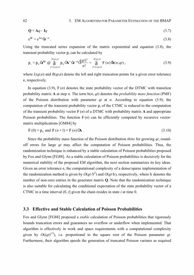
62 3. EM ALGORITHM FOR PARAMETER ESTIMATION OF THE BMAP
q q= -Q A I (3.7)
e e et qt qt-= ÖQ A . (3.8)
Using the truncated series expansion of the matrix exponential and equation (3.8), the transient probability vector pt can be calculated by
( , ) ( , )
0 0( , ) ( , )
( )e e ( ) ( ; )!
nR qt R qtt n qt
tn L qt n L qt
qt n n qtn
e e-
= e = e
= Ö @ Ö Ö Ö = Öbä äQ Ap p p F , (3.9)
where L(qt,e) and R(qt,e) denote the left and right truncation points for a given error tolerance e, respectively.
In equation (3.9), F(n) denotes the state probability vector of the DTMC with transition probability matrix A at step n. The term b(n; qt) denotes the probability mass function (PMF) of the Poisson distribution with parameter qt at n. According to equation (3.9), the computation of the transient probability vector pt of the CTMC is reduced to the computation of the transient probability vector F(n) of a DTMC with probability matrix A and appropriate Poisson probabilities. The function F(n) can be efficiently computed by recursive vector-matrix multiplications [GM84] by
0(0) =F p and ( 1) ( )n n+ = ÖAF F . (3.10)
Since the probability mass function of the Poisson distribution thins for growing qt, round-off errors for large qt may affect the computation of Poisson probabilities. Thus, the randomization technique is enhanced by a stable calculation of Poisson probabilities proposed by Fox and Glynn [FG88]. As a stable calculation of Poisson probabilities is decisively for the numerical stability of the proposed EM algorithm, the next section summarizes its key ideas. Given an error tolerance e, the computational complexity of a dense/sparse implementation of the randomization method is given by O(qt·N2) and O(qt·h), respectively, where h denotes the number of non-zero entries in the generator matrix Q. Note that the randomization technique is also suitable for calculating the conditional expectation of the state probability vector of a CTMC in a time interval (0, t] given the chain resides in state i at time 0.
3.3 Effective and Stable Calculation of Poisson Probabilities
Fox and Glynn [FG88] proposed a stable calculation of Poisson probabilities that rigorously bounds truncation errors and guarantees no overflow or underflow when implemented. That algorithm is effectively in work and space requirements with a computational complexity given by O((qt)1/2), i.e. proportional to the square root of the Poisson parameter qt. Furthermore, their algorithm speeds the generation of truncated Poisson variates as required

3.3. EFFECTIVE AND STABLE CALCULATION OF POISSON PROBABILITIES 63
in equation (3.9) of the randomization technique. The calculation starts at mode m qt= é ùê ú with a weight w(m) ² 1 appropriately chosen so that no overflow can occur in equations (3.13) and (3.14). In the first step, the left and right truncation points L = L(qt,e) and R = R(qt,e) of the summation (3.9) are determined. If the product qt < 25, no left truncation is used, i.e., L = 0, and the weight w(m) is set to 1. If the product qt > 25, the summation in (3.9) starts at some L > 0 determined by equation (3.11) and the left tail of the Poisson distribution is neglected.
1
0
max : ( ; )2
l
nL l n qt
-
=
ë e û= Í b ¢ì ü
í ýä8 (3.11)
Having determined the left truncation point L of formula (3.11), its right truncation point R is determined according to equation (3.12)
min :1 ( ; )r
n LR r n qt
=
ë û= Í - b ¢ eì ü
í ýä8 (3.12)
In the second step, the weights W are derived by recurrence equations (3.13) and (3.14).
( 1) ( ), , 1,..., 1nw n w n n m m Lqt
- = Ö = - + (3.13)
( 1) ( ), , 1,..., 11
qtw n w n n m m Rn
+ = Ö = + -+
(3.14)
Subsequently, the sum of these weights has to be calculated in order to obtain Poisson probabilities.
( )R
n LW w n
=
= ä (3.15)
To minimize the round-off error, the smallest terms near the end points of L and R of the summation in (3.15) are added first. Given the weights by equation (3.13) and (3.14) and the constant W of (3.15), the Poisson probabilities b(n; qt) are determined by:
( ) ( ) ( ); e , , 1,...,!
-b = = = +n
qt qt w nn qt n L L Rn W
(3.16)
Note that due to the recursive computation in (3.13) and (3.14) and subsequent normalization with W, the exponential function e-qt does not need to be computed explicitly. This yields considerable advantages for a numerical computation because underflow is prevented when qt is large (e.g., qt > 700).
Considering the smallest and the largest representable machine number of the computer employed, this computational method for Poisson probabilities ensures that numerical overflow or underflow do not occur. Since equations (3.11) and (3.12) define a bound on the
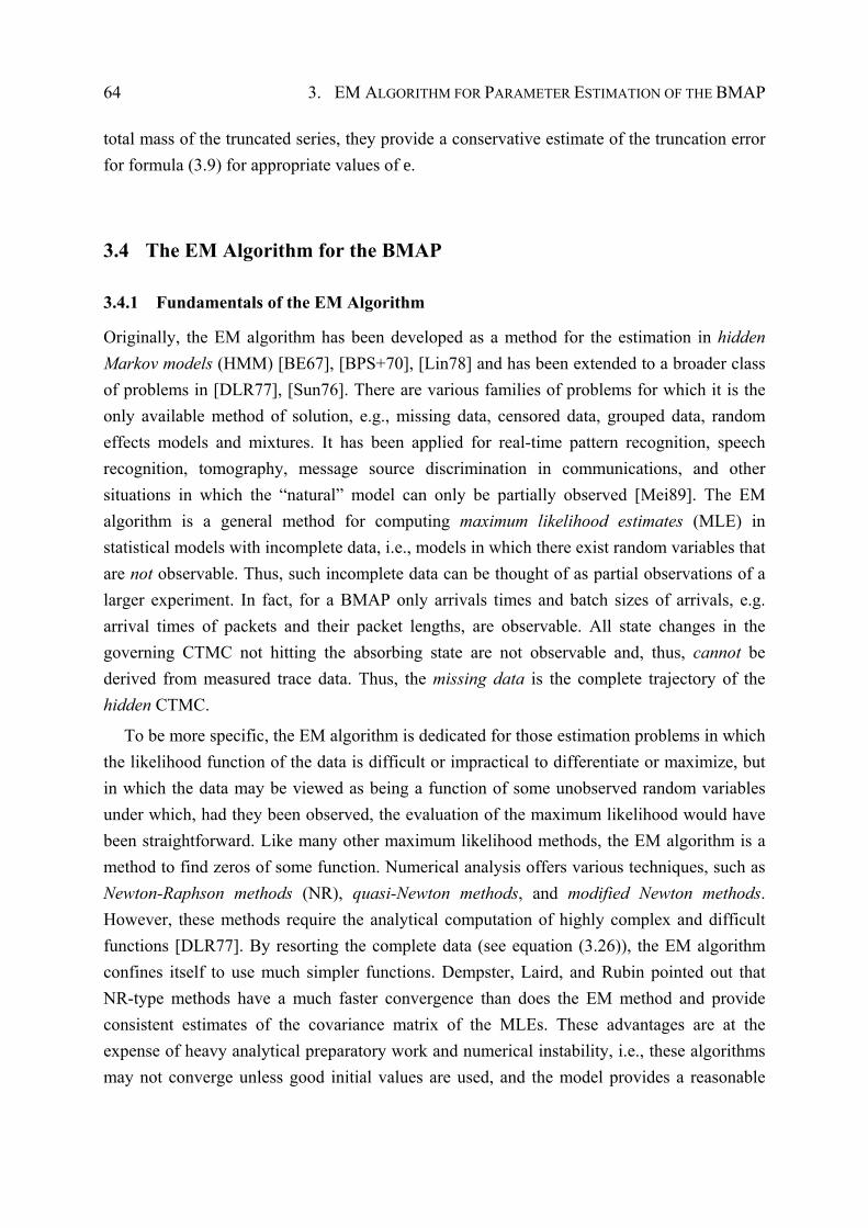
64 3. EM ALGORITHM FOR PARAMETER ESTIMATION OF THE BMAP
total mass of the truncated series, they provide a conservative estimate of the truncation error for formula (3.9) for appropriate values of e.
3.4 The EM Algorithm for the BMAP
3.4.1 Fundamentals of the EM Algorithm
Originally, the EM algorithm has been developed as a method for the estimation in hidden Markov models (HMM) [BE67], [BPS+70], [Lin78] and has been extended to a broader class of problems in [DLR77], [Sun76]. There are various families of problems for which it is the only available method of solution, e.g., missing data, censored data, grouped data, random effects models and mixtures. It has been applied for real-time pattern recognition, speech recognition, tomography, message source discrimination in communications, and other situations in which the “natural” model can only be partially observed [Mei89]. The EM algorithm is a general method for computing maximum likelihood estimates (MLE) in statistical models with incomplete data, i.e., models in which there exist random variables that are not observable. Thus, such incomplete data can be thought of as partial observations of a larger experiment. In fact, for a BMAP only arrivals times and batch sizes of arrivals, e.g. arrival times of packets and their packet lengths, are observable. All state changes in the governing CTMC not hitting the absorbing state are not observable and, thus, cannot be derived from measured trace data. Thus, the missing data is the complete trajectory of the hidden CTMC.
To be more specific, the EM algorithm is dedicated for those estimation problems in which the likelihood function of the data is difficult or impractical to differentiate or maximize, but in which the data may be viewed as being a function of some unobserved random variables under which, had they been observed, the evaluation of the maximum likelihood would have been straightforward. Like many other maximum likelihood methods, the EM algorithm is a method to find zeros of some function. Numerical analysis offers various techniques, such as Newton-Raphson methods (NR), quasi-Newton methods, and modified Newton methods. However, these methods require the analytical computation of highly complex and difficult functions [DLR77]. By resorting the complete data (see equation (3.26)), the EM algorithm confines itself to use much simpler functions. Dempster, Laird, and Rubin pointed out that NR-type methods have a much faster convergence than does the EM method and provide consistent estimates of the covariance matrix of the MLEs. These advantages are at the expense of heavy analytical preparatory work and numerical instability, i.e., these algorithms may not converge unless good initial values are used, and the model provides a reasonable
3.4. THE EM ALGORITHM FOR THE BMAP 65
good fit to the data. On the other hand, careful implementations of the EM algorithm are numerically very stable, but generally slow and, as repeatedly pointed out in [DLR77], [Lou82], compute the MLE of the parameter but no estimate of its variance-covariance matrix.
In recent years, EM algorithms have been successfully developed for some stochastic processes. In [ANO96], Asmussen, Nerman, and Olsson derive an EM algorithm for parameter estimation of phase-type renewal processes. They utilized the notion of sufficient statistics to rearrange complete data [BPR80] and present methods to implement the EM algorithms using a Runge-Kutta method to solve the underlying linear system of homogenous differential equations. Based upon this work, Olsson introduced an EM algorithm for parameter estimation of phase-type distributions of fixed order from censored data [Ols96]. The derived EM algorithm shows strong similarities with the EM algorithm presented in [ANO96] and, again, uses Runge-Kutta methods to solve the underlying linear system of homogenous differential equations. Deng and Mark presented an EM algorithm for parameter estimation of the Markov-modulated Poisson process [DM93]. As a key idea, they employed time-discretization to convert an MMPP from the continuous-time domain into the discrete-time domain and then use the EM algorithm to obtain MLEs of the model parameters. In [Ryd96], Ryden proposed an EM algorithm for parameter estimation of MMPPs and compares it with other maximum likelihood methods for the MMPP [Ryd94]. As in [ANO96], Ryden used the notion of sufficient statistics to simplify the complete data and proposed a diagonalization method to compute matrix exponentials required in the EM algorithm.
3.4.2 Mathematical Framework
Formally, suppose that y is the observable part of a considered experiment. This experiment can be described completely by y and the non-observable data x denoted as the missing data. Let A(f,y) be the likelihood of a parameter set f given the observation y and let ( , , )c x yfA be the so-called complete likelihood of the parameter set f given the missing data x [DLR77]. The likelihood for a parameter set f captures the probability of generating the sequence of observations y using a BMAP with parameter set f. Assume y = {(t1,b1),(t2,b2),...,(tn,bn)} is the observed sequence of arrival times tk and corresponding batch sizes bk. Without loss of generality t0 = 0 and tn = T. For each arrival epoch from tk-1 to tk, 1 ¢ k ¢ n, inter-arrival times are denoted Dtk = tk - tk-1. Then, the likelihood of a BMAP with parameter set f is given by:
1
( , ) ( )k
n
b kk
t=
= Ö D ÖÔy f 1f pA (3.17)
66 3. EM ALGORITHM FOR PARAMETER ESTIMATION OF THE BMAP
Recall that, in equation (3.17), p denotes the initial state probability vector of the CTMC, ( )
kb tf defines the matrix of probability density functions, and f is a specific parameter set for the BMAP comprising p and the transition rate matrices D(0),D(1),...,D(M). The vector 1 denotes a vector of appropriate dimension comprising 1s in each entry. Note that the (logarithm of the) likelihood measures the quality of the estimated parameter set [DLR77].
The EM algorithm iteratively determines estimates of the missing parameter set f of the BMAP. Denote by f(r) the parameter set calculated in the r-th iteration of the EM algorithm. f(r) encompasses p(r) and D(0,r),D(1,r),...,D(M,r) that denote the initial state probability vector as well as the transition rate matrices in the r-th iteration, respectively. Pf and Ef denote the conditional probability and the conditional expectation given the estimate f, respectively. As shown in [DLR77], the estimate
ˆ arg max ( ( )), 0,1,2,...r r= =ff f, fF , (3.18)
where
( )( )( ( )) log ( , , )crr E= x y yff, f fF A (3.19)
satisfies ˆ( , ) ( ( ), )r²y yf fA A and ˆ( 1)r + =f f is the estimate for the parameter set determined in the (r + 1)-th iteration step of the algorithm. In words, given the parameter set f(r) and the observed sequence y, f̂ is the parameter set that maximizes the conditional expectation of equation (3.19). Moreover, the likelihood (i.e., the quality) of the estimated parameter set grows monotonously in each iteration. This iterative procedure is repeated until a predefined maximum number of iterations is reached or until some convergence criteria holds, which can be, for instance, that each component of f(r) and f(r + 1) differs only up to a predefined e, respectively. The computation of the conditional expectation in (3.19) is called the E-step, whereas the derivation of the maximum in (3.18) constitutes the M-step of the EM algorithm. As described in [Ryd96], the likelihood A(f,y) is highly non-linear in f and is difficult to maximize, while the complete likelihood ( , , )c x yfA employed in the M-step can often be computed in closed form. This is the main reason for the widespread use of the EM algorithm. A further advantage of the EM algorithm over other maximum likelihood methods lies in the good convergence behavior of the iterative scheme regardless of the initial estimate f(0).
Already for the MMPP, the practical applicability of the EM algorithm for parameter estimation depends on a stable numerical computation of matrix exponentials as required in equations (3.3) and (3.4). In [Ryd96], Ryden proposed a diagonalization method to compute eQt, but this approach relies on the diagonalization property of the matrix Q. It is well known that decomposition techniques like diagonalization are in general not stable numerical methods for computing matrix exponentials [GM84], [MvL78]. Thus, the following shows

3.4. THE EM ALGORITHM FOR THE BMAP 67
how to employ the randomization technique enhanced by a stable calculation of Poisson probabilities for the numerical computation of matrix exponentials as well as integrals over matrix exponentials introduced by the E-step of the EM algorithm for BMAPs.
3.4.3 Effective Computational Formulas
Recall that the observed data of a BMAP is {(t1,b1),(t2,b2),...,(tn,bn)}, i.e., arrivals times and batch sizes of arrivals, whereas state changes in the governing CTMC not hitting the absorbing state are not observable. Thus, the infinitesimal generator matrix D of the CTMC {X(t): t ² 0} underlying the BMAP constitutes the missing data. The following derives an expression for the complete likelihood with a quite intuitive meaning and presents equations for the E-step and the M-step of the EM algorithm for BMAPs.
First of all, the complete likelihood ( , , )c x yfA of the BMAP using the observed data y and the non-observable data x is defined. Let m(k) be the number of transient states entered during the k-th arrival epoch. Moreover, let il(k) and sl(k) denote the l-th transient state and the sojourn time in the l-th transient state during the k-th arrival epoch, respectively. Then the complete likelihood of the BMAP is given by
( )
0 1
( ) ( )( )
( ) ( ) 0
( ) 1( )
(1) ( ) ( ), ( )1 0
( )( ) ( ), ( 1)
( , , ) e (0)
e ( )
+
--l Ö
= =
-l Ö
+
= ³ l Ö Ö
³l Ö Ö
Ô Ôf p i k ll
l l l
i k m km k
m k m k
m kns kc
i i k i k i kk l
s ki k k i k i kb
x y P
P
A, (3.20)
where P(m) and li are defined as in Section 3.1 and bk is the batch size of the k-th arrival. Note that the inter-arrival time Dtk is given by the sum of sojourn times during the k-th arrival epoch:
( )
0
( )m k
k jj
t s k=
D = ä (3.21)
The first term of the right hand side of equation (3.20) specifies the probability of starting the CTMC in state i0(1). For each arrival epoch of the BMAP, the second term describes the transient trajectory up to a state im(k)(k) from which absorption occurs. The last portion of equation (3.20) represents the transition from the transient state im(k)(k) to the absorbing state 0 and the restart of the CTMC in state i0(k + 1) with an arrival of batch size bk. Recall that P(m)i,j,1 ¢ m ¢ M, is the probability, given the chain is in state i, the CTMC enters the absorbing state 0 and is instantaneously restarted in state j with an arrival of batch size m. Figure 3.1 visualizes the sequence of state transitions within the k-th arrival epoch up to absorption in state 0 after the inter-arrival time Dtk with batch size bk.
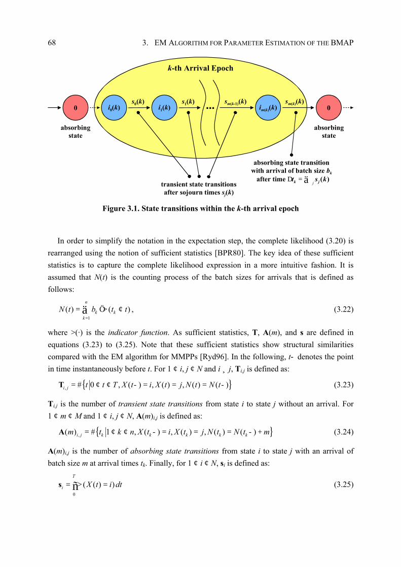
68 3. EM ALGORITHM FOR PARAMETER ESTIMATION OF THE BMAP
...
transient state transitionsafter sojourn times sj(k)
s0(k) s1(k) sm(k-1)(k) sm(k)(k)
k-th Arrival Epoch
absorbingstate
absorbingstate
absorbing state transitionwith arrival of batch size bk
after time Dtk..................
i0(k) i1(k) im(k)(k) 00
jD =ä ( )k jt s k
Figure 3.1. State transitions within the k-th arrival epoch
In order to simplify the notation in the expectation step, the complete likelihood (3.20) is rearranged using the notion of sufficient statistics [BPR80]. The key idea of these sufficient statistics is to capture the complete likelihood expression in a more intuitive fashion. It is assumed that N(t) is the counting process of the batch sizes for arrivals that is defined as follows:
1
( ) ( )n
k kk
N t b t t=
= Ö ¢ä > , (3.22)
where >(·) is the indicator function. As sufficient statistics, T, A(m), and s are defined in equations (3.23) to (3.25). Note that these sufficient statistics show structural similarities compared with the EM algorithm for MMPPs [Ryd96]. In the following, t- denotes the point in time instantaneously before t. For 1 ¢ i, j ¢ N and i ¸ j, Ti,j is defined as:
{ }, # 0 , ( ) , ( ) , ( ) ( )i j t t T X t i X t j N t N t= ¢ ¢ - = = = -T (3.23)
Ti,j is the number of transient state transitions from state i to state j without an arrival. For 1 ¢ m ¢ M and 1 ¢ i, j ¢ N, A(m)i,j is defined as:
{ },( ) # 1 , ( ) , ( ) , ( ) ( )i j k k k k km t k n X t i X t j N t N t m= ¢ ¢ - = = = - +A (3.24)
A(m)i,j is the number of absorbing state transitions from state i to state j with an arrival of batch size m at arrival times tk. Finally, for 1 ¢ i ¢ N, si is defined as:
0
( ( ) )T
i X t i dt= =ñs > (3.25)
3.4. THE EM ALGORITHM FOR THE BMAP 69
si captures the total time the CTMC resides in state i.
Typically, the sufficient statistics can be determined by numerically tractable characteristics of the CTMC. Applying some calculus, these sufficient statistics can be used to rewrite and simplify the expression of the complete likelihood in equation (3.20). That is:
, ,, ( )(0)( (0) ), ,
1 1 1 1, 1 1 1
( , , ) e (0) ( )Ö=
= = = = ¸ = = =
= Ö Ö ÖÔ Ô Ô Ô ÔÔÔf p i j i ji i iN N N N M N N
msc X ii i j i j
i i i j j i m i jmT ADx y D D>A (3.26)
Intuitively, the second product of equation (3.26) symbolizes the sojourn time of the CTMC for each state i. The third product of equation (3.26) captures the behavior for all transient state transitions between states i and j. Similarly, the last product of equation (3.26) represents the absorbing state transitions between states i and j with arrivals of batch size m.
In order to derive the E-step and the M-step of the EM algorithm, it is essential to understand that the observed sequence y of arrival times tk and the corresponding batch sizes bk, is completely captured by the counting process of the batch sizes for arrivals N(t) introduced above. To understand this fundamental insight, consider a point in time t, where N(t) changes its value, i.e., N(t-) ¸ N(t). Thus, the underlying sequence of observations y includes an arrival at time t with batch size b = N(t) - N(t-), and, as a consequence, the sequence of observations y and the counting process of the batch sizes for arrivals N(t) are equivalently. For ease of notation, L(k) and R(k) are defined as:
L(0) = p(r), ( ) ( 1) ( )kb kk k t= - Ö DL L f , for k = 1,...,n (3.27)
R(n + 1) = 1, ( ) ( ) ( 1)kb kk t k= D Ö +R f R , for k = n,...,1. (3.28)
Let 1i and Ti1 denote the i-th unity column and row vector, respectively. As shown in equation
(3.19), the E-step requires taking the logarithm of the complete likelihood ( , , )c x yfA given the parameter set f(r) and the observed sequence y, i.e., the counting process N(t). Thus, inserting the complete likelihood ( , , )c x yfA derived in equation (3.26) and simplifying, directly leads to equation (3.30) with abbreviations (3.31) to (3.34) for ease of notation (presented in Figure 3.2).
Using the constraint (3.29) according the BMAP’s definition for each i and taking into account that the sum of all pi equals 1, it can be easily shown by means of appropriate partial differentiation that equation (3.30) is maximized by the unique maximum given in (3.35).
, , ,1, 1 1
(0) (0) ( )N M N
i i i j i jj j i m j
m= ¸ = =
= - -ä ääD D D (3.29)
Beside the maximization by means of partial differentiation, each expression in equation (3.35) utilizes the maximized sufficient statistics (3.31) to (3.34) in a very intuitive manner.
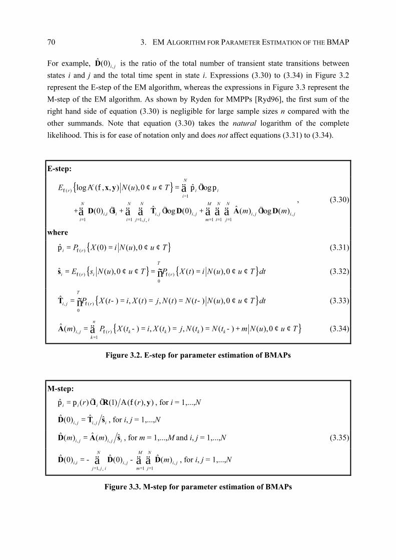
70 3. EM ALGORITHM FOR PARAMETER ESTIMATION OF THE BMAP
For example, ,ˆ (0)i jD is the ratio of the total number of transient state transitions between
states i and j and the total time spent in state i. Expressions (3.30) to (3.34) in Figure 3.2 represent the E-step of the EM algorithm, whereas the expressions in Figure 3.3 represent the M-step of the EM algorithm. As shown by Ryden for MMPPs [Ryd96], the first sum of the right hand side of equation (3.30) is negligible for large sample sizes n compared with the other summands. Note that equation (3.30) takes the natural logarithm of the complete likelihood. This is for ease of notation only and does not affect equations (3.31) to (3.34).
E-step:
{ }( )1
, , , , ,1 1 1, 1 1 1
ˆlog ( , , ) ( ),0 log
ˆˆˆ(0) log (0) ( ) log ( )
Nc
r i ii
N N N M N N
i i i i j i j i j i ji i j j i m i j
E N u u T
m m
=
= = = ¸ = = =
¢ ¢ = Ö
+ Ö + Ö + Ö
ä
ä ä ä äää
x y
D s T D A D
f f p pA, (3.30)
where
{ }( )ˆ (0) ( ),0i rP X i N u u T= = ¢ ¢fp (3.31)
{ } { }( ) ( )0
ˆ ( ),0 ( ) ( ),0T
i r i rE s N u u T P X t i N u u T dt= ¢ ¢ = = ¢ ¢ñs f ff f (3.32)
{ }, ( )0
ˆ ( ) , ( ) , ( ) ( ) ( ),0T
i j rP X t i X t j N t N t N u u T dt= - = = = - ¢ ¢ñT f (3.33)
{ }, ( )1
ˆ ( ) ( ) , ( ) , ( ) ( ) ( ),0n
i j r k k k kk
m P X t i X t j N t N t m N u u T=
= - = = = - + ¢ ¢äA f (3.34)
Figure 3.2. E-step for parameter estimation of BMAPs
M-step:
ˆ ( ) (1) ( ( ), )i i ir r= Ö Ö1 R yp p fA , for i = 1,...,N
, ,ˆ ˆ ˆ(0)i j i j i=D T s , for i, j = 1,...,N
, ,ˆˆ ˆ( ) ( )i j i j im m=D A s , for m = 1,...,M and i, j = 1,...,N (3.35)
, , ,1, 1 1
ˆ ˆ ˆ(0) (0) ( )N M N
i i i j i jj j i m j
m= ¸ = =
= - -ä ääD D D , for i, j = 1,...,N
Figure 3.3. M-step for parameter estimation of BMAPs
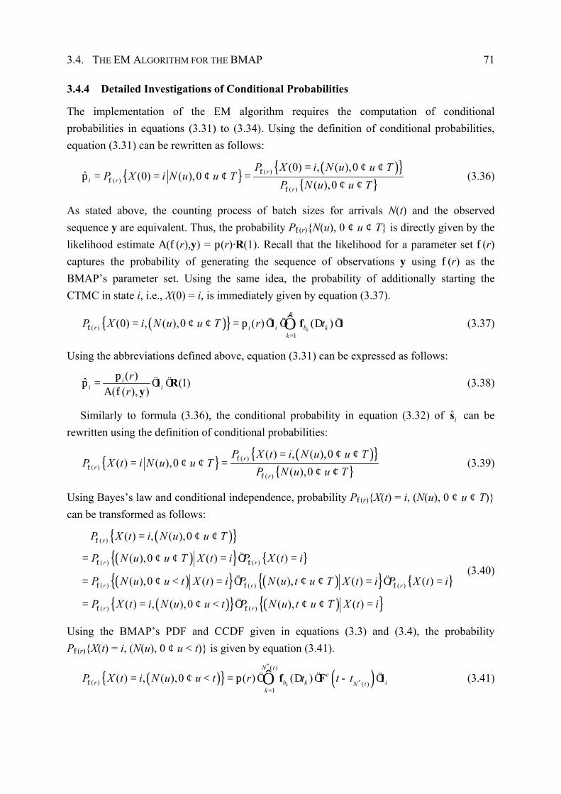
3.4. THE EM ALGORITHM FOR THE BMAP 71
3.4.4 Detailed Investigations of Conditional Probabilities
The implementation of the EM algorithm requires the computation of conditional probabilities in equations (3.31) to (3.34). Using the definition of conditional probabilities, equation (3.31) can be rewritten as follows:
{ } ( ){ }{ }
( )( )
( )
(0) , ( ),0ˆ (0) ( ),0
( ),0r
i rr
P X i N u u TP X i N u u T
P N u u T= ¢ ¢
= = ¢ ¢ =¢ ¢
ff
f
p (3.36)
As stated above, the counting process of batch sizes for arrivals N(t) and the observed sequence y are equivalent. Thus, the probability Pf(r){N(u), 0 ¢ u ¢ T} is directly given by the likelihood estimate A(f(r),y) = p(r)·R(1). Recall that the likelihood for a parameter set f(r) captures the probability of generating the sequence of observations y using f(r) as the BMAP’s parameter set. Using the same idea, the probability of additionally starting the CTMC in state i, i.e., X(0) = i, is immediately given by equation (3.37).
( ){ }( )1
(0) , ( ),0 ( ) ( )k
n
r i i b kk
P X i N u u T r t=
= ¢ ¢ = Ö Ö D ÖÔ1 f 1f p (3.37)
Using the abbreviations defined above, equation (3.31) can be expressed as follows:
( )ˆ (1)( ( ), )
ii i
rr
= Ö Ö1 Ry
pp
fA (3.38)
Similarly to formula (3.36), the conditional probability in equation (3.32) of ˆis can be rewritten using the definition of conditional probabilities:
{ } ( ){ }{ }
( )( )
( )
( ) , ( ),0( ) ( ),0
( ),0r
rr
P X t i N u u TP X t i N u u T
P N u u T= ¢ ¢
= ¢ ¢ =¢ ¢
ff
f
(3.39)
Using Bayes’s law and conditional independence, probability Pf(r){X(t) = i, (N(u), 0 ¢ u ¢ T)} can be transformed as follows:
( ){ }( ){ } { }
( ){ } ( ){ } { }
( ){ } ( ){ }
( )
( ) ( )
( ) ( ) ( )
( ) ( )
( ) , ( ),0
( ),0 ( ) ( )
( ),0 ( ) ( ), ( ) ( )
( ) , ( ),0 ( ), ( )
r
r r
r r r
r r
P X t i N u u T
P N u u T X t i P X t i
P N u u t X t i P N u t u T X t i P X t i
P X t i N u u t P N u t u T X t i
= ¢ ¢
= ¢ ¢ = Ö =
= ¢ < = Ö ¢ ¢ = Ö =
= = ¢ < Ö ¢ ¢ =
f
f ff f
f ff f f
f ff f
(3.40)
Using the BMAP’s PDF and CCDF given in equations (3.3) and (3.4), the probability Pf(r){X(t) = i, (N(u), 0 ¢ u < t)} is given by equation (3.41).
( ){ } ( )*
*
( )
( ) ( )1
( ) , ( ),0 ( ) ( )k
N tc
r b k iN tk
P X t i N u u t r t t t=
= ¢ < = Ö D Ö - ÖÔ f F 1f p (3.41)
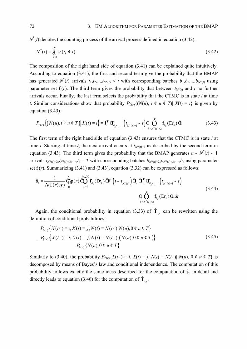
72 3. EM ALGORITHM FOR PARAMETER ESTIMATION OF THE BMAP
N*(t) denotes the counting process of the arrival process defined in equation (3.42).
*
1
( ) ( )n
kk
N t t t=
= ¢ä> (3.42)
The composition of the right hand side of equation (3.41) can be explained quite intuitively. According to equation (3.41), the first and second term give the probability that the BMAP has generated N*(t) arrivals t1,t2,...,tN*(t) < t with corresponding batches b1,b2,...,bN*(t) using parameter set f(r). The third term gives the probability that between tN*(t) and t no further arrivals occur. Finally, the last term selects the probability that the CTMC is in state i at time t. Similar considerations show that probability Pf(r){(N(u), t ¢ u ¢ T)| X(t) = i} is given by equation (3.43).
( ){ } ( )** ( ) 1 *
( ) ( ) 1( ) 2
( ), ( ) ( )kN t
n
r i b b kN tk N t
P N u t u T X t i t t t+ +
= +
¢ ¢ = = Ö - Ö D ÖÔT1 f f 1f (3.43)
The first term of the right hand side of equation (3.43) ensures that the CTMC is in state i at time t. Starting at time t, the next arrival occurs at tN*(t)+1 as described by the second term in equation (3.43). The third term gives the probability that the BMAP generates n - N*(t) - 1 arrivals tN*(t)+2,tN*(t)+3,...,tn = T with corresponding batches bN*(t)+2,bN*(t)+3,...,bn using parameter set f(r). Summarizing (3.41) and (3.43), equation (3.32) can be expressed as follows:
( ) ( )*
* ** ( ) 1
*
( )
( ) ( ) 110
( ) 2
1ˆ ( ) ( )( ( ), )
( )
k N t
k
T N tc
i b k i i bN t N tk
n
b kk N t
r t t t t tr
t dt
+ +=
= +
= Ö Ö D Ö - Ö Ö Ö -
Ö D Ö
Ôñ
Ô
Ts f F 1 1 fy
f 1
pfA
(3.44)
Again, the conditional probability in equation (3.33) of ,ˆ
i jT can be rewritten using the definition of conditional probabilities:
{ }( ){ }
{ }
( )
( )
( )
( ) , ( ) , ( ) ( ) ( ),0
( ) , ( ) , ( ) ( ), ( ),0( ),0
r
r
r
P X t i X t j N t N t N u u T
P X t i X t j N t N t N u u TP N u u T
- = = = - ¢ ¢
- = = = - ¢ ¢=
¢ ¢
f
f
f
(3.45)
Similarly to (3.40), the probability Pf(r){X(t-) = i, X(t) = j, N(t) = N(t-)| N(u), 0 ¢ u ¢ T} is decomposed by means of Bayes’s law and conditional independence. The computation of this probability follows exactly the same ideas described for the computation of ˆis in detail and directly leads to equation (3.46) for the computation of ,
ˆi jT .
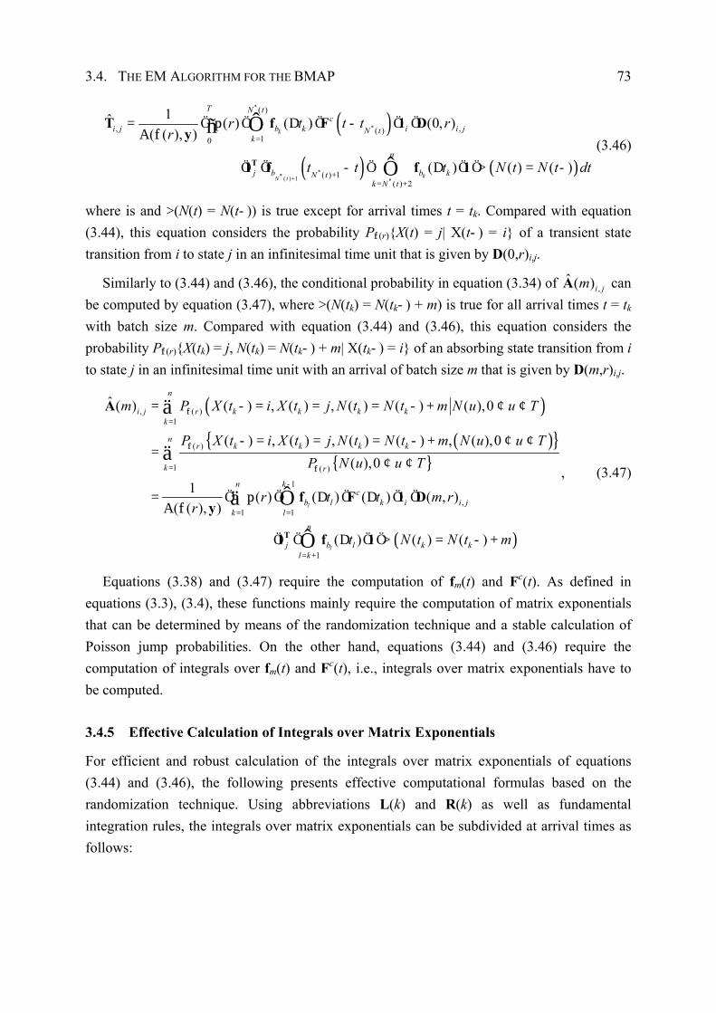
3.4. THE EM ALGORITHM FOR THE BMAP 73
( )
( ) ( )
*
*
** ( ) 1 *
( )
, ,( )10
( ) 1( ) 2
1ˆ ( ) ( ) (0, )( ( ), )
( ) ( ) ( )
k
kN t
T N tc
i j b k i i jN tk
n
j b b kN tk N t
r t t t rr
t t t N t N t dt+
=
+= +
= Ö Ö D Ö - Ö Ö
Ö Ö - Ö D Ö Ö = -
Ôñ
ÔT
T f F 1 Dy
1 f f 1
pfA
> (3.46)
where is and >(N(t) = N(t-)) is true except for arrival times t = tk. Compared with equation (3.44), this equation considers the probability Pf(r){X(t) = j| X(t-) = i} of a transient state transition from i to state j in an infinitesimal time unit that is given by D(0,r)i,j.
Similarly to (3.44) and (3.46), the conditional probability in equation (3.34) of ,ˆ ( )i jmA can
be computed by equation (3.47), where >(N(tk) = N(tk-) + m) is true for all arrival times t = tk with batch size m. Compared with equation (3.44) and (3.46), this equation considers the probability Pf(r){X(tk) = j, N(tk) = N(tk-) + m| X(tk-) = i} of an absorbing state transition from i to state j in an infinitesimal time unit with an arrival of batch size m that is given by D(m,r)i,j.
( )
( ){ }{ }
, ( )1
( )
1 ( )
1
,1 1
ˆ ( ) ( ) , ( ) , ( ) ( ) ( ),0
( ) , ( ) , ( ) ( ) , ( ),0( ),0
1 ( ) ( ) ( ) ( , )( ( ), )
( )
l
l
n
i j r k k k kk
nr k k k k
k r
n kc
b l k i i jk l
j b ll
m P X t i X t j N t N t m N u u T
P X t i X t j N t N t m N u u TP N u u T
r t t m rr
t
=
=
-
= =
= - = = = - + ¢ ¢
- = = = - + ¢ ¢=
¢ ¢
= Ö Ö D Ö D Ö Ö
Ö Ö D
ä
ä
ä ÔT
A
f F 1 Dy
1 f
f
f
f
pfA
( )1
( ) ( )n
k kk
N t N t m= +
Ö Ö = - +Ô 1 >
, (3.47)
Equations (3.38) and (3.47) require the computation of fm(t) and Fc(t). As defined in equations (3.3), (3.4), these functions mainly require the computation of matrix exponentials that can be determined by means of the randomization technique and a stable calculation of Poisson jump probabilities. On the other hand, equations (3.44) and (3.46) require the computation of integrals over fm(t) and Fc(t), i.e., integrals over matrix exponentials have to be computed.
3.4.5 Effective Calculation of Integrals over Matrix Exponentials
For efficient and robust calculation of the integrals over matrix exponentials of equations (3.44) and (3.46), the following presents effective computational formulas based on the randomization technique. Using abbreviations L(k) and R(k) as well as fundamental integration rules, the integrals over matrix exponentials can be subdivided at arrival times as follows:

74 3. EM ALGORITHM FOR PARAMETER ESTIMATION OF THE BMAP
1
1( 1) ( ) ( ) ( 1)k
k
k
tc T
k i j b kt
k t t t t k dt-
-- Ö - Ö Ö Ö - Ö +ñ L F 1 1 f R (3.48)
Appropriately scaling the limits and using the series expansion of the matrix exponential yields equation (3.49).
(0) ( )(0)
0
( )
0 00
0
( 1) e e ( ) ( 1)
( ) ( ( ))( 1) e e ( ) ( 1)! !
( ) ( (( 1) e ( ) ( 1)!
DÖ D -
D ¤ ¤- D --
= =
¤-
=
- Ö Ö Ö Ö Ö Ö +
D -= - Ö Ö Ö Ö Ö Ö Ö Ö Ö Ö +
D= - Ö Ö Ö Ö Ö Ö Ö Ö + Ö
ñ
ä äñ
ä
k
k
k
k
tt tt T
i j k
t m nq t tm qt T n k
i j km n
mm qt T n k
i j km
k b k dt
qt q t tk b k dtm n
qt q tk b km
DDL 1 1 D R
L A 1 1 A D R
L A 1 1 A D R ( )
00
( )
0 00
)) e!
( ) ( ( ))( ) e ( ) e! !
D ¤- D -
=
D ¤ ¤- D --
= =
-Ö
D -= Ö Ö Ö Ö Ö
äñ
ä äñ
k
k
k
k
t nq t t
n
t m nq t tqt k
k km n
t dtn
qt q t ta m b n dtm n
(3.49)
where ak(m) and bk(n) are defined in equations (3.50) and (3.51), respectively.
( ) ( 1) mk ia m k= - Ö ÖL A 1 (3.50)
( ) ( 1)k
T nk j bb n k= Ö Ö Ö +1 A D R (3.51)
Applying some calculus and utilizing the truncated series expansion according to equation (3.9), directly leads to equation (3.52).
( )
0 00
0 0 0
0 0 0
( ) ( ( ))( ) e ( ) e! !
( ) ( ) e ( )! !
( ) ( ) e ( )( )!
( )
D ¤ ¤- D --
= =
D+¤ ¤- D
= =
D+¤ ¤- D
= =
D -Ö Ö Ö Ö Ö
= Ö Ö Ö Ö Ö D -
+å õ= Ö Ö Ö Ö Ö Ö D -æ ö+ ç ÷
= Ö
ä äñ
ää ñ
ää ñ
k
k
k
k
k
k
t m nq t tqt k
k km n
tm nq t m n
k k km n
tm nq t m n
k k km n
k
qt q t ta m b n dtm n
qa m b n t t t dtm n
m nqa m b n t t t dtnm n
a m1
0 0
( , ) ( , )
( )( ) e( )! 1
1( ) ( ) ( 1; )
+ + +¤ ¤- D
= =
D e ¢ + ¢ D e
DÖ Ö Ö
+ + +
@ Ö Ö Öb + + D
ää
ä
k
k k
m n m nq t k
km n
k k kL q t m n R q t
q tb nm n m n
a m b n m n q tq
. (3.52)
According to equation (3.52), integrals over matrix exponential can be efficiently and numerically stable calculated by means of the randomization technique and a stable calculation of Poisson probabilities. In [Lin98], Lindemann utilized a similar approach for computing of integrals over matrix exponentials.
3.5. IMPLEMENTATION ISSUES 75
3.5 Implementation Issues
Based on the computational formulas derived in the previous section, Figure 3.4 presents an iterative scheme for the implementation of the EM algorithm using the forward-backward (Baum-Welch) method [Bau72], [LRS83]. According to the forward-backward method, the forward recursion (3.2) in Figure 3.4 computes the “forward probabilities” and the backward recursion (3.3) in Figure 3.4 computes the “backward probabilities”. As shown above, the detailed expressions of the maximized sufficient statistics ˆis and ,
ˆi jT in equations (3.44) and
(3.46) reveal strong similarities. Thus, the computation of ˆis can be performed by means of
,ˆ
i jT without additional effort (see Figure 3.4, M-step). Furthermore, for calculating the maximized sufficient statistics ˆ ip , ˆis , ,
ˆi jT , ,
ˆ ( )i jmA , and the likelihood estimate A(f(r),y) the scaling procedure proposed by Levinson, Rabiner, and Sondhi in [LRS83] has been adopted. This scaling procedure is necessarily because these quantities can take extremely small or extremely large values. For the computation of Poisson weights, the error tolerance is set to 10-10. Convergence is reached, if each component of f(r) and f(r + 1) differs only up to 10-3.
The initial parameter set f(0) can be determined by different approaches including simple random initialization, precondition according to moment matching methods, and heuristic initialization. Irrespective of the initialization method, zero entries in f(0) are preserved in the corresponding elements of the successive estimates f(r). This property enables the estimation of specialized BMAPs, e.g. MAPs or MMPPs. However, simple random initialization is employed for determining the initial parameter set f(0). A set of initial estimates is generated randomly and f(0) is set to the estimate with the maximum likelihood. In almost all cases, different initial estimates just result in a slightly different number of iterations required for the convergence of the EM algorithm, whereas the quality of different estimated parameter sets is very similarly. The following shows that a careful implementation of the EM algorithm based on the computational formulas presented in this thesis requires for each iteration only a few seconds of CPU time on a modern PC for considerable large trace files. Thus, random initialization is sufficiently for determining initial parameter sets in practice. For a discussion of initialization methods, it is referred to Section 5.
3.6 Computational Complexity of the EM Algorithm
The analysis of the computational complexity is based on a careful implementation of the iterative scheme presented in Figure 3.4 using the computational formulas derived in Section 3.4. Following Figure 3.4, an iteration of the EM algorithm encompasses the E-step, the computation of the likelihood, the M-step, the assignment of the new parameter set, and checking for convergence. According to equation (3.5), let q denote the maximum diagonal
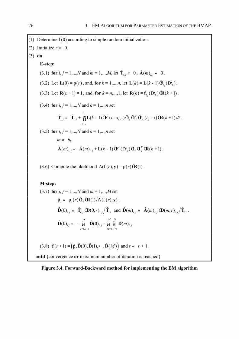
76 3. EM ALGORITHM FOR PARAMETER ESTIMATION OF THE BMAP
(1) Determine f(0) according to simple random initialization.
(2) Initialize r « 0.
(3) do
E-step:
(3.1) for i, j = 1,...,N and m = 1,...,M, let ,ˆ 0i j «T , ,
ˆ ( ) 0i jm «A .
(3.2) Let (0) ( )r=L p , and, for k = 1,...,n, let ( ) ( 1) ( )kb kk k t= - Ö DL L f .
(3.3) Let ( 1)n + =R 1 , and, for k = n,...,1, let ( ) ( ) ( 1)kb kk t k= D Ö +R f R .
(3.4) for i, j = 1,...,N and k = 1,...,n set
1
, , 1ˆ ˆ ( 1) ( ) ( ) ( 1)
k
k
k
tc T
i j i j k i j b kt
k t t t t k dt-
-« + - Ö - Ö Ö Ö - Ö +ñT T L F 1 1 f R .
(3.5) for i, j = 1,...,N and k = 1,...,n set
m « bk.
, ,ˆ ˆ( ) ( ) ( 1) ( ) ( 1)c T
i j i j k i jm m k t k« + - Ö D Ö Ö Ö +A A L F 1 1 R .
(3.6) Compute the likelihood ( ( ), ) ( ) (1)r r= Öy Rf pA .
M-step: (3.7) for i, j = 1,...,N and m = 1,...,M set
ˆ ( ) (1) ( ( ), )i i ir r« Ö Ö1 R yp p fA .
, , , ,ˆ ˆ ˆ(0) (0, )i j i j i j i ir« ÖD T D T and , , , ,
ˆˆ ˆ( ) ( ) ( , )i j i j i j i im m m r« ÖD A D T .
, , ,1, 1 1
ˆ ˆ ˆ(0) (0) ( )N M N
i i i j i jj j i m j
m= ¸ = =
« - -ä ääD D D .
(3.8) ( )ˆ ˆ ˆˆ( 1) , (0), (1), , ( )r M+ = D D Df p > and r « r + 1.
until {convergence or maximum number of iteration is reached}
Figure 3.4. Forward-Backward method for implementing the EM algorithm
3.6. COMPUTATIONAL COMPLEXITY OF THE EM ALGORITHM 77
element of ˆ (0)D . As shown in Section 3.2 and 3.3, the randomization technique as well as the stable computation of Poisson weights depends on the Poisson parameter qDtk. Thus, for different inter-arrival times Dtk, the computational complexity differs and the derivation of an overall computational complexity of the EM algorithm is not tractable. As a consequence, the following assumes that irrespective of Dtk operations are performed for l = q·Dtmax with Dtmax = maxk{Dtk}. This enables the derivation of the worst case computational complexity of the EM algorithm.
Following the enumeration in Figure 3.4, the E-step is subdivided into steps (3.1) to (3.5). The initialization of ,
ˆi jT and ,
ˆ ( )i jmA in step (3.1) for i, j = 1,...,N and m = 1,...,M can be performed with O(M·N2) operations. According to equations (3.3) and (3.27), the computation of L(k) given L(k-1) requires the computation of a matrix exponential and an additional vector-matrix product. Referring to Section 3.2 and using the worst case assumption l = q·Dtmax, the matrix exponential can be computed by means of the randomization technique with computational complexity O(l·N2). Obviously, the vector-matrix product can be computed in time O(N2). Thus, the overall computational complexity of step (3.2) is given by O(n·l·N2). Using the same argumentation, the computation of all R(k), k = n,...,1, in step (3.3) can be performed with an overall computational complexity O(n·l·N2). In step (3.5), the terms L(k-1)·Fc(Dtk) have been determined while computing L(k) in step (3.2). Thus, for fixed i, j, and k the computation of ,
ˆ ( )i jmA requires O(1) operations, and, thus, step (3.5) can be performed with computational complexity O(n·N2).
Determining the computational complexity of step (3.4) requires further effort and detailed analysis. This is mainly due to the fact that step (3.4) computes complex integrals over matrix exponentials for each i, j = 1,...,N and k = 1,...,n. According to equations (3.48) to (3.52), these integrals over matrix exponentials can be computed by means of the randomization technique as given by expression (3.53).
( , ) ( , )
1( ) ( ) ( 1; )k k
k k kL q t m n R q t
a m b n m n q tqD e ¢ + ¢ D e
Ö Ö Öb + + Dä (3.53)
The Poisson weights b(m + n + 1; qDtk) in (3.53) are independent of i and j, and, thus, have to be determined only once for each k. Following the worst case considerations outlined above, this can be performed in time O(l1/2) for each k. According to Fox and Glynn [FG88], for large qDtk the left and right truncation points of the sum in equation (3.53) are given by L(qDtk,e) = qDtk - O((qDtk)1/2) and R(qDtk,e) = qDtk + O((qDtk)1/2), respectively. Taking into account the worst case assumption l = q·Dtmax, this fact has two direct implications utilized in the following discussion. First, R(l,e) is an upper bound of the right truncation point R(qDtk,e), and, secondly, the number of summands in (3.53) is limited by O(l1/2) with truncation points L(l,e) = l - O(l1/2) and R(l,e) = l + O(l1/2).
78 3. EM ALGORITHM FOR PARAMETER ESTIMATION OF THE BMAP
For fixed m + n, the structure of (3.53) implies that m + n + 1 different summands have to be added, e.g., for fixed m + n = 1, two summands arise from m = 0, n = 1 and m = 1, n = 0. Assume that ak(m) and bk(n), required in (3.53), have already been computed. This implies that the computation of each of these m + n + 1 summands takes time O(1). Utilizing this fact and taking into account the truncation points L(l,e) and R(l,e), simple calculations by means of the Gaussian sum show that (3.53) can be computed in time O(l3/2). However, the computation of ak(m) and bk(n) has not been considered so far. Investigating their structure, ak(m) and bk(n) can be determined effectively by successive computations for increasing values of m and n, respectively. Taking into account the upper bound of the right truncation point R(l,e), a careful implementation requires l + O(l1/2) vector-matrix products to compute all ak(m) and bk(n) required in (3.53), i.e., the computational complexity is given by O(l·N2). Note that due to their definitions (see equations (3.50) and (3.51)) these vector-matrix products have to be computed only once for fixed k irrespective of i and j. Summing up these investigations, for fixed k, step (3.4) requires O(l1/2) operations to compute Poisson probabilities, O(l·N2) operations to compute vector-matrix products for ak(m) and bk(n), and O(l3/2·N2) to compute the sum for all i, j = 1,...,N. Thus, step (3.4) can be performed with an overall computational complexity given by O(n·l3/2·N2).
As R(1) has already been computed, the likelihood in step (3.6) can be determined by means of a vector product with computational complexity of O(N). Obviously, the M-step takes time O(M·N2) required for the computation of ,
ˆ ( )i jmD for i, j = 1,...,N and m = 1,...,M. The assignment of the new parameter set in step (3.8) as well as checking for convergence takes time O(M·N2), respectively.
Assume that M is much smaller than the number of observations n, i.e., M << n. Summarizing the computational complexity of steps (3.1) to (3.8), the overall computational complexity of an EM iteration is given by O(n·l3/2·N2). Note that the run-time of each iteration differs as the maximum diagonal element q differs dependent on ˆ (0)D . As described above, random initialization is employed to determine the initial parameter set f(0), where a set of initial estimates is generated randomly, and f(0) is set to the estimate with the maximum likelihood. Computing the likelihood requires the computation of R(1) with the computational complexity of step (3.3). As a consequence, the likelihood of each random estimate is computed in time O(n·l·N2).
3.7 Convergence Behavior
This section demonstrates the convergence behavior of the derived estimation procedure. As specified in the first column of Table 3.1, a 3-state BMAP with M = 4 distinct batch sizes is
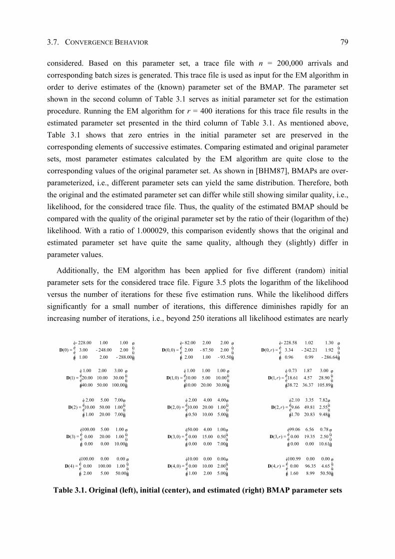
3.7. CONVERGENCE BEHAVIOR 79
considered. Based on this parameter set, a trace file with n = 200,000 arrivals and corresponding batch sizes is generated. This trace file is used as input for the EM algorithm in order to derive estimates of the (known) parameter set of the BMAP. The parameter set shown in the second column of Table 3.1 serves as initial parameter set for the estimation procedure. Running the EM algorithm for r = 400 iterations for this trace file results in the estimated parameter set presented in the third column of Table 3.1. As mentioned above, Table 3.1 shows that zero entries in the initial parameter set are preserved in the corresponding elements of successive estimates. Comparing estimated and original parameter sets, most parameter estimates calculated by the EM algorithm are quite close to the corresponding values of the original parameter set. As shown in [BHM87], BMAPs are over-parameterized, i.e., different parameter sets can yield the same distribution. Therefore, both the original and the estimated parameter set can differ while still showing similar quality, i.e., likelihood, for the considered trace file. Thus, the quality of the estimated BMAP should be compared with the quality of the original parameter set by the ratio of their (logarithm of the) likelihood. With a ratio of 1.000029, this comparison evidently shows that the original and estimated parameter set have quite the same quality, although they (slightly) differ in parameter values.
Additionally, the EM algorithm has been applied for five different (random) initial parameter sets for the considered trace file. Figure 3.5 plots the logarithm of the likelihood versus the number of iterations for these five estimation runs. While the likelihood differs significantly for a small number of iterations, this difference diminishes rapidly for an increasing number of iterations, i.e., beyond 250 iterations all likelihood estimates are nearly
228.00 1.00 1.00(0) 3.00 248.00 2.00
1.00 2.00 288.00
-è øé ù= -é ù
-é ùê ú
D 82.00 2.00 2.00
(0,0) 2.00 87.50 2.002.00 1.00 93.50
-è øé ù= -é ù
-é ùê ú
D 228.58 1.02 1.30
(0, ) 3.34 242.21 1.920.96 0.99 286.64
r-è øé ù= -é ù
-é ùê ú
D
1.00 2.00 3.00(1) 20.00 10.00 30.00
40.00 50.00 100.00
è øé ù= é ùé ùê ú
D 1.00 1.00 1.00
(1,0) 10.00 5.00 10.0010.00 20.00 30.00
è øé ù= é ùé ùê ú
D 0.73 1.87 3.00
(1, ) 18.61 4.57 28.9038.72 36.37 105.89
rè øé ù= é ùé ùê ú
D
2.00 5.00 7.00(2) 10.00 50.00 1.00
1.00 20.00 7.00
è øé ù= é ùé ùê ú
D 2.00 4.00 4.00
(2,0) 10.00 20.00 1.000.50 10.00 5.00
è øé ù= é ùé ùê ú
D 2.10 3.35 7.82
(2, ) 9.66 49.81 2.551.70 20.83 9.48
rè øé ù= é ùé ùê ú
D
100.00 5.00 1.00(3) 0.00 20.00 1.00
0.00 0.00 10.00
è øé ù= é ùé ùê ú
D 50.00 4.00 1.00
(3,0) 0.00 15.00 0.500.00 0.00 7.00
è øé ù= é ùé ùê ú
D 99.06 6.56 0.78
(3, ) 0.00 19.35 2.500.00 0.00 10.61
rè øé ù= é ùé ùê ú
D
100.00 0.00 0.00(4) 0.00 100.00 1.00
2.00 5.00 50.00
è øé ù= é ùé ùê ú
D 10.00 0.00 0.00
(4,0) 0.00 10.00 2.001.00 2.00 5.00
è øé ù= é ùé ùê ú
D 100.99 0.00 0.00
(4, ) 0.00 96.35 4.651.60 8.99 50.50
rè øé ù= é ùé ùê ú
D
Table 3.1. Original (left), initial (center), and estimated (right) BMAP parameter sets
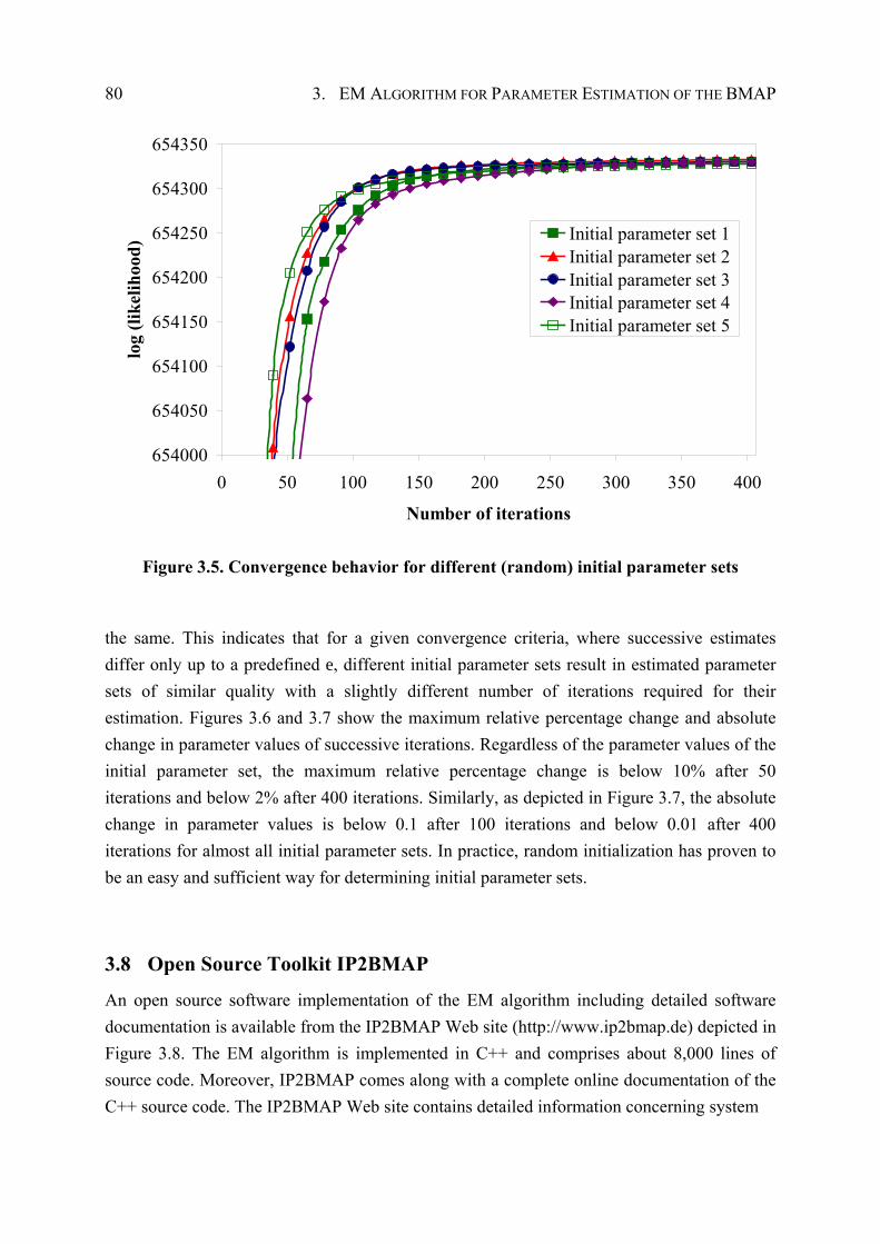
80 3. EM ALGORITHM FOR PARAMETER ESTIMATION OF THE BMAP
654000
654050
654100
654150
654200
654250
654300
654350
0 50 100 150 200 250 300 350 400
Number of iterations
log
(like
lihoo
d)
Initial parameter set 1Initial parameter set 2Initial parameter set 3Initial parameter set 4Initial parameter set 5
Figure 3.5. Convergence behavior for different (random) initial parameter sets
the same. This indicates that for a given convergence criteria, where successive estimates differ only up to a predefined e, different initial parameter sets result in estimated parameter sets of similar quality with a slightly different number of iterations required for their estimation. Figures 3.6 and 3.7 show the maximum relative percentage change and absolute change in parameter values of successive iterations. Regardless of the parameter values of the initial parameter set, the maximum relative percentage change is below 10% after 50 iterations and below 2% after 400 iterations. Similarly, as depicted in Figure 3.7, the absolute change in parameter values is below 0.1 after 100 iterations and below 0.01 after 400 iterations for almost all initial parameter sets. In practice, random initialization has proven to be an easy and sufficient way for determining initial parameter sets.
3.8 Open Source Toolkit IP2BMAP
An open source software implementation of the EM algorithm including detailed software documentation is available from the IP2BMAP Web site (http://www.ip2bmap.de) depicted in Figure 3.8. The EM algorithm is implemented in C++ and comprises about 8,000 lines of source code. Moreover, IP2BMAP comes along with a complete online documentation of the C++ source code. The IP2BMAP Web site contains detailed information concerning system
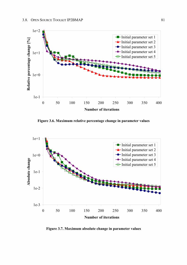
3.8. OPEN SOURCE TOOLKIT IP2BMAP 81
1e-1
1e+0
1e+1
1e+2
0 50 100 150 200 250 300 350 400
Number of iterations
Rel
ativ
e pe
rcen
tage
cha
nge
[%] Initial parameter set 1
Initial parameter set 2Initial parameter set 3Initial parameter set 4Initial parameter set 5
Figure 3.6. Maximum relative percentage change in parameter values
1e-3
1e-2
1e-1
1e+0
1e+1
0 50 100 150 200 250 300 350 400
Number of iterations
Abs
olut
e ch
ange
Initial parameter set 1Initial parameter set 2Initial parameter set 3Initial parameter set 4Initial parameter set 5
Figure 3.7. Maximum absolute change in parameter values
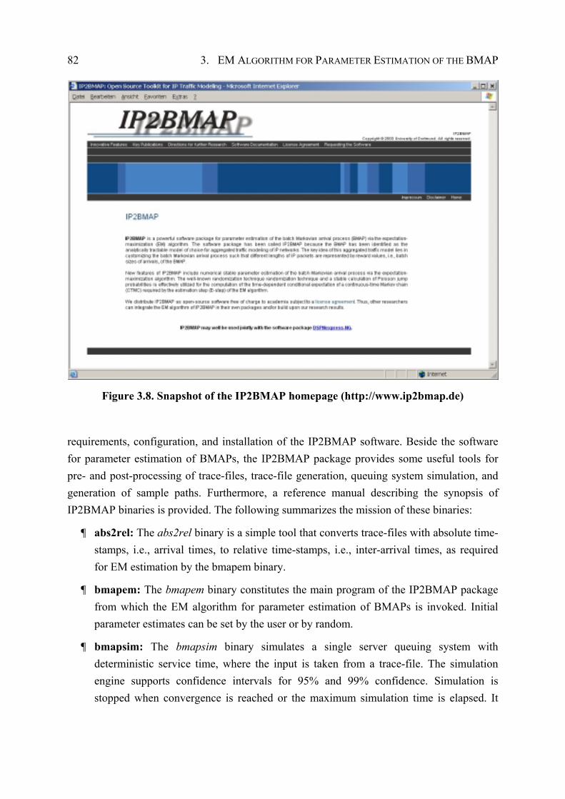
82 3. EM ALGORITHM FOR PARAMETER ESTIMATION OF THE BMAP
Figure 3.8. Snapshot of the IP2BMAP homepage (http://www.ip2bmap.de)
requirements, configuration, and installation of the IP2BMAP software. Beside the software for parameter estimation of BMAPs, the IP2BMAP package provides some useful tools for pre- and post-processing of trace-files, trace-file generation, queuing system simulation, and generation of sample paths. Furthermore, a reference manual describing the synopsis of IP2BMAP binaries is provided. The following summarizes the mission of these binaries:
¶ abs2rel: The abs2rel binary is a simple tool that converts trace-files with absolute time-stamps, i.e., arrival times, to relative time-stamps, i.e., inter-arrival times, as required for EM estimation by the bmapem binary.
¶ bmapem: The bmapem binary constitutes the main program of the IP2BMAP package from which the EM algorithm for parameter estimation of BMAPs is invoked. Initial parameter estimates can be set by the user or by random.
¶ bmapsim: The bmapsim binary simulates a single server queuing system with deterministic service time, where the input is taken from a trace-file. The simulation engine supports confidence intervals for 95% and 99% confidence. Simulation is stopped when convergence is reached or the maximum simulation time is elapsed. It
3.9. SUMMARY 83
was implemented for queuing system analysis that enables effective comparisons of the originally trace-file with traces-files generated according to estimated BMAP parameter sets.
¶ bmaptrace: The bmaptrace binary generates a trace-file of desired length according to an estimated BMAP parameter set.
¶ samplepath: The samplepath binary generates byte-based as well as packet-based sample paths for a given trace-file and a specified resolution.
3.9 Summary
This section presents an efficient and numerical stable EM algorithm for parameter estimation of BMAPs with computational complexity given by O(n·l3/2·N2) for an EM iteration. The derived EM algorithm is mathematically very complex and requires the computation of conditional expectations of a CMTC. Extensive calculations show that these conditional expectations can be computed by means of matrix exponentials and integrals over matrix exponentials. Whereas the computation of matrix exponentials can be performed directly of the randomization technique and a numerical stable computation of Poisson probabilities, the computation of integrals over matrix exponentials required further effort. It is shown how to utilize the randomization technique for computing integrals over matrix exponentials. Beside the iterative implementation of the EM algorithm by means of the forward-backward method, implementation issues as well as initialization methods are discussed. Additionally, this section gives some insights in the convergence behavior of the EM algorithm and introduces an open source software implementation of the EM algorithm available from the IP2BMAP Web site (http://www.ip2bmap.de).

85
4 Modeling IP Traffic Using the Batch Markovian Arrival Process
EASURED IP TRAFFIC encompasses arrival times as well as lengths of IP packets. Usually, almost all traffic models (try to) capture the inter-arrival times of measured
IP traffic data, whereas packet lengths are ignored completely (e.g., see [JMW97], [MMM+04]). For additionally modeling of packet lengths, these traffic models assume an average packet length for each packet arrival or draw packet lengths according to the empirical distribution of the measured traffic. For packet lengths that are uncorrelated with packet arrivals, this approach would be adequately. This section proposes the BMAP as analytically tractable traffic model for the joint characterization of packet arrivals and packet lengths. The BMAP is customized such that different packet lengths are represented by batch sizes of arrivals. Thus, the proposed EM algorithm for parameter estimation of BMAPs can jointly capture the packet arrival process and the packet length process of measured traffic and considers correlation structures between packet arrivals and packet lengths (naturally given by the BMAP’s capabilities). This is the first analytically tractable traffic model that jointly captures the packet arrival process, the packet length process, and their correlations. Case studies of TCP traffic with different degrees of self-similarity evidently demonstrate the advantages of the BMAP modeling approach over other widely used analytically tractable models and show that joint (i.e., correlated) characterization of packet arrivals and packet lengths is decisively for realistic IP traffic modeling. The joint characterization of packet arrivals and packet lengths by customized BMAPs and the case study of ISP IP traffic have been published (with distinct objectives) in the proceedings of the Globecom 2001 conference [KLL01] and the Tools 2002 conference [KLL02].
4.1 Important Characteristics of IP Traffic
In the last decade, extensive research effort has been spent on the characterization of measured IP traffic in local and wide area networks, e.g., see [CDJ+91], [LTW+94], [PF95], [TMW97], [Wil01], [WTS+97]. Using specialized network measurement hardware or software, researchers collect information about network packet transmissions, including their timing structure and contents. Among other characteristics, the most important findings of these studies are (1) the fractal-like behavior of IP traffic streams implying long-range
M
86 4. MODELING IP TRAFFIC USING THE BMAP
dependence and self-similarity and (2) the “spiky” distribution of TCP packet lengths with peaks at common sizes.
4.1.1 Self-Similarity in IP Traffic Streams
Statistical analysis of traffic measurements from a wide range of communication networks have convincingly shown that actual network traffic is (multi-) fractal in nature in that it exhibits statistical properties over many time scales. In particular, these studies have demonstrated that measured traffic rates, i.e., number of packets or bytes per time unit, in both LAN and WAN environments look statistically the same (i.e., self-similar) in the small and in the large, and no natural length of a “burst” is discernible. That is, at every time scale ranging from milliseconds to minutes (and beyond) bursts have the same qualitative appearance and cause the resulting traffic to exhibit fractal-like characteristics [LTW+93]. The following gives a brief description of the concept of self-similar processes, introduces the Hurst parameter as measure of self-similarity, and recalls the causes of self-similarity. For a more detailed discussion of self-similarity concepts and modeling of self-similar phenomena it is referred to [CB97], [LTW+94], [PW00], and [WPT98].
Note that there are a number of different, not equivalent, definitions of self-similarity. This definition tightly follows [Cox84] and [LTW+94]. Consider a covariance-stationary (also called wide-sense stationary) stochastic process X = {Xt: t ² 1}. That is, a process with constant mean, finite variance, and an auto-correlation function
2( ) [( ) ( )] / [( ) ], 0t t k tr k E X X E X k+= -m Ö -m -m ² (4.1)
that only depends on k. Moreover, consider the aggregated process X(m) with level of aggregation m ² 1, defined by:
( )
( 1) 1
1( ) , 1km
mi
i k mX k X k
m = - +
= ²ä (4.2)
Self-similarity concepts relate statistical properties of X to those of X(m). According to Cox [Cox84], X is called exactly self-similar with self-similarity parameter H (also called Hurst parameter), if
1 ( ) , 1, 0 1,H mdX m X m H-= Ö ² < < (4.3)
where the equality =d in (4.3) means that X and m1-H·X(m) have the same finite-dimensional distribution. Moreover, X is called asymptotically self-similar, if (4.3) holds for m ¤, and, X is said to be exactly second-order self-similar or asymptotically second-order self-similar, if X has the same variance and auto-correlation function as m1-H·X(m) for all m or for m ¤, respectively. Mathematically, self-similarity (1/2 < H < 1) manifests itself in a number of
4.1. IMPORTANT CHARACTERISTICS OF IP TRAFFIC 87
equivalent ways, e.g., auto-correlations that decay hyperbolically (i.e., X exhibits long-range dependence), a spectral density that exhibits the 1/f a-phenomenon around the origin, and variances of the arithmetic mean that decrease more slowly than the reciprocal of the sample size (see [LTW+94] for details). However, the most striking feature of (second-order) self-similar processes is that their aggregated processes X(m) possess a non-degenerative auto-correlation function r(m) as m ¤. The existence of a non-degenerative correlation structure of X(m) is in strong contrast to conventional short-range dependent processes, e.g., Markovian processes, with the common property that their aggregated processes X(m) tend to second-order pure noise as m ¤. That is, short-range dependent processes satisfy r(m)(k) 0, k > 0. Historically, the importance of self-similarity processes lies in the fact that they provide an elegant explanation and interpretation of an empirical law that is commonly referred as Hurst effect. Section 4.3 presents further details concerning the Hurst effect.
As self-similarity is believed to have a significant impact on network and queuing performance, understanding the causes of self-similarity is important. As shown in [LTW+94] and [WTS+97], self-similar characteristics on network level can be related to high-level system characteristics. As already mentioned, these papers pointed out that self-similar traffic could be constructed by a large number of ON/OFF sources that have ON and OFF period lengths that follow a heavy tailed distribution, respectively. Recall that a distribution is heavy-tailed if
{ } , as , 0 2P X x x x-a> ¤ < a <- . (4.4)
That is, the asymptotic shape of the distribution follows a power law. Intuitively, a random variable that follows a power law can take extremely large values with non-negligible probability. For example, the observed self-similar nature of Ethernet LAN traffic at the aggregated level (i.e., aggregated over all active hosts in the network) can be explained by the superposition of heavy-tailed ON/OFF (or busy/idle) times of individual hosts [LTW+94]. Furthermore, Crovella and Bestavros have shown that aggregated traffic generated by WWW transfers shows self-similar characteristics [CB97]. They found that (1) transmission times (which determine ON times) of individual WWW clients are heavy-tailed, primarily due to the distribution of available file sizes in the Web, and (2) silent times (which determine OFF times) also follow a heavy-tailed distribution, primarily due to the influence of user “think times”. Recent studies [VB00], [VKM+00] indicate instead that traffic properties are originated in the TCP congestion control mechanism, which induces LRD properties in the aggregated traffic stemming from the superposition of independent sources.
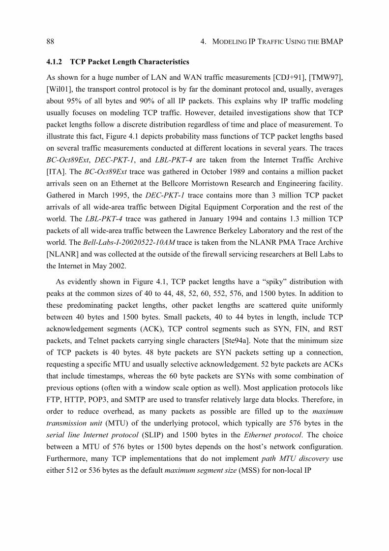
88 4. MODELING IP TRAFFIC USING THE BMAP
4.1.2 TCP Packet Length Characteristics
As shown for a huge number of LAN and WAN traffic measurements [CDJ+91], [TMW97], [Wil01], the transport control protocol is by far the dominant protocol and, usually, averages about 95% of all bytes and 90% of all IP packets. This explains why IP traffic modeling usually focuses on modeling TCP traffic. However, detailed investigations show that TCP packet lengths follow a discrete distribution regardless of time and place of measurement. To illustrate this fact, Figure 4.1 depicts probability mass functions of TCP packet lengths based on several traffic measurements conducted at different locations in several years. The traces BC-Oct89Ext, DEC-PKT-1, and LBL-PKT-4 are taken from the Internet Traffic Archive [ITA]. The BC-Oct89Ext trace was gathered in October 1989 and contains a million packet arrivals seen on an Ethernet at the Bellcore Morristown Research and Engineering facility. Gathered in March 1995, the DEC-PKT-1 trace contains more than 3 million TCP packet arrivals of all wide-area traffic between Digital Equipment Corporation and the rest of the world. The LBL-PKT-4 trace was gathered in January 1994 and contains 1.3 million TCP packets of all wide-area traffic between the Lawrence Berkeley Laboratory and the rest of the world. The Bell-Labs-I-20020522-10AM trace is taken from the NLANR PMA Trace Archive [NLANR] and was collected at the outside of the firewall servicing researchers at Bell Labs to the Internet in May 2002.
As evidently shown in Figure 4.1, TCP packet lengths have a “spiky” distribution with peaks at the common sizes of 40 to 44, 48, 52, 60, 552, 576, and 1500 bytes. In addition to these predominating packet lengths, other packet lengths are scattered quite uniformly between 40 bytes and 1500 bytes. Small packets, 40 to 44 bytes in length, include TCP acknowledgement segments (ACK), TCP control segments such as SYN, FIN, and RST packets, and Telnet packets carrying single characters [Ste94a]. Note that the minimum size of TCP packets is 40 bytes. 48 byte packets are SYN packets setting up a connection, requesting a specific MTU and usually selective acknowledgement. 52 byte packets are ACKs that include timestamps, whereas the 60 byte packets are SYNs with some combination of previous options (often with a window scale option as well). Most application protocols like FTP, HTTP, POP3, and SMTP are used to transfer relatively large data blocks. Therefore, in order to reduce overhead, as many packets as possible are filled up to the maximum transmission unit (MTU) of the underlying protocol, which typically are 576 bytes in the serial line Internet protocol (SLIP) and 1500 bytes in the Ethernet protocol. The choice between a MTU of 576 bytes or 1500 bytes depends on the host’s network configuration. Furthermore, many TCP implementations that do not implement path MTU discovery use either 512 or 536 bytes as the default maximum segment size (MSS) for non-local IP
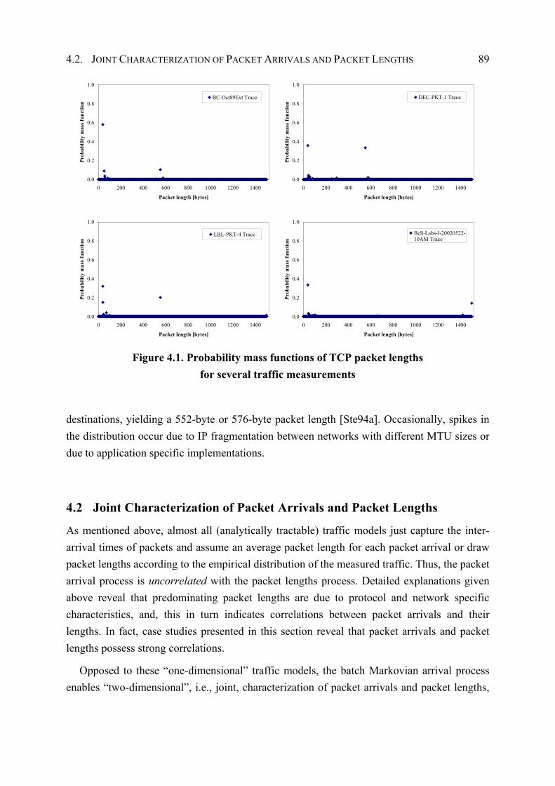
4.2. JOINT CHARACTERIZATION OF PACKET ARRIVALS AND PACKET LENGTHS 89
0.0
0.2
0.4
0.6
0.8
1.0
0 200 400 600 800 1000 1200 1400
Packet length [bytes]
Prob
abili
ty m
ass f
unct
ion
BC-Oct89Ext Trace
0.0
0.2
0.4
0.6
0.8
1.0
0 200 400 600 800 1000 1200 1400
Packet length [bytes]
Prob
abili
ty m
ass f
unct
ion
DEC-PKT-1 Trace
0.0
0.2
0.4
0.6
0.8
1.0
0 200 400 600 800 1000 1200 1400
Packet length [bytes]
Prob
abili
ty m
ass f
unct
ion
LBL-PKT-4 Trace
0.0
0.2
0.4
0.6
0.8
1.0
0 200 400 600 800 1000 1200 1400
Packet length [bytes]
Prob
abili
ty m
ass f
unct
ion
Bell-Labs-I-20020522-10AM Trace
Figure 4.1. Probability mass functions of TCP packet lengths for several traffic measurements
destinations, yielding a 552-byte or 576-byte packet length [Ste94a]. Occasionally, spikes in the distribution occur due to IP fragmentation between networks with different MTU sizes or due to application specific implementations.
4.2 Joint Characterization of Packet Arrivals and Packet Lengths
As mentioned above, almost all (analytically tractable) traffic models just capture the inter-arrival times of packets and assume an average packet length for each packet arrival or draw packet lengths according to the empirical distribution of the measured traffic. Thus, the packet arrival process is uncorrelated with the packet lengths process. Detailed explanations given above reveal that predominating packet lengths are due to protocol and network specific characteristics, and, this in turn indicates correlations between packet arrivals and their lengths. In fact, case studies presented in this section reveal that packet arrivals and packet lengths possess strong correlations.
Opposed to these “one-dimensional” traffic models, the batch Markovian arrival process enables “two-dimensional”, i.e., joint, characterization of packet arrivals and packet lengths,
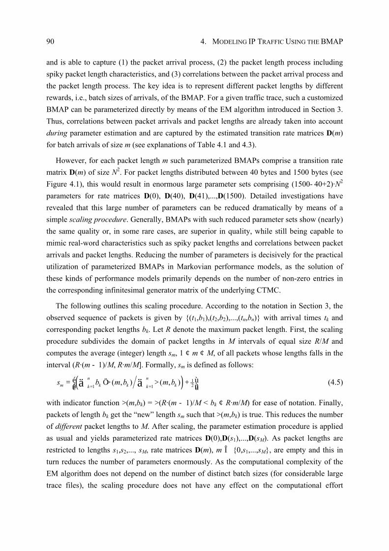
90 4. MODELING IP TRAFFIC USING THE BMAP
and is able to capture (1) the packet arrival process, (2) the packet length process including spiky packet length characteristics, and (3) correlations between the packet arrival process and the packet length process. The key idea is to represent different packet lengths by different rewards, i.e., batch sizes of arrivals, of the BMAP. For a given traffic trace, such a customized BMAP can be parameterized directly by means of the EM algorithm introduced in Section 3. Thus, correlations between packet arrivals and packet lengths are already taken into account during parameter estimation and are captured by the estimated transition rate matrices D(m) for batch arrivals of size m (see explanations of Table 4.1 and 4.3).
However, for each packet length m such parameterized BMAPs comprise a transition rate matrix D(m) of size N2. For packet lengths distributed between 40 bytes and 1500 bytes (see Figure 4.1), this would result in enormous large parameter sets comprising (1500-40+2)·N2 parameters for rate matrices D(0), D(40), D(41),...,D(1500). Detailed investigations have revealed that this large number of parameters can be reduced dramatically by means of a simple scaling procedure. Generally, BMAPs with such reduced parameter sets show (nearly) the same quality or, in some rare cases, are superior in quality, while still being capable to mimic real-word characteristics such as spiky packet lengths and correlations between packet arrivals and packet lengths. Reducing the number of parameters is decisively for the practical utilization of parameterized BMAPs in Markovian performance models, as the solution of these kinds of performance models primarily depends on the number of non-zero entries in the corresponding infinitesimal generator matrix of the underlying CTMC.
The following outlines this scaling procedure. According to the notation in Section 3, the observed sequence of packets is given by {(t1,b1),(t2,b2),...,(tn,bn)} with arrival times tk and corresponding packet lengths bk. Let R denote the maximum packet length. First, the scaling procedure subdivides the domain of packet lengths in M intervals of equal size R/M and computes the average (integer) length sm, 1 ¢ m ¢ M, of all packets whose lengths falls in the interval (R·(m - 1)/M, R·m/M]. Formally, sm is defined as follows:
( ) 121 1
( , ) ( , )n nm k k kk k
s b m b m b= =
é ù= Ö +é ùê úä ä> > (4.5)
with indicator function >(m,bk) = >(R·(m - 1)/M < bk ¢ R·m/M) for ease of notation. Finally, packets of length bk get the “new” length sm such that >(m,bk) is true. This reduces the number of different packet lengths to M. After scaling, the parameter estimation procedure is applied as usual and yields parameterized rate matrices D(0),D(s1),...,D(sM). As packet lengths are restricted to lengths s1,s2,..., sM, rate matrices D(m), m Î {0,s1,...,sM}, are empty and this in turn reduces the number of parameters enormously. As the computational complexity of the EM algorithm does not depend on the number of distinct batch sizes (for considerable large trace files), the scaling procedure does not have any effect on the computational effort
4.3. THE RESCALED ADJUSTED RANGE STATISTIC 91
required for parameter estimation. The question arises how to choose M such that scaling of packet lengths does not affect quality of the estimated BMAP. Numerous empirical studies have shown that M should be chosen such that the predominant packet lengths of the original traffic trace each fall in separate intervals, whereas larger values of M do not result in BMAPs of higher quality.
4.3 The Rescaled Adjusted Range Statistic
As discussed above, long-range dependence and self-similarity are common in today’s IP traffic. Thus, among other characteristics, case studies of TCP traffic presented below compare the degree of self-similarity of the original trace and the traces generated by analytical traffic models. This requires a method for formal analysis of self-similarity. Among other methods for inferring the degree of self-similarity [TT98], the rescaled adjusted range statistic (R/S-statistic) is one of the better-known methods and quite popular in practice [LTW+93], [MT79], [MW69]. The most useful and attractive feature of the R/S-statistic is its relative robustness against changes in the marginal distribution. Historically, the hydrologist Hurst introduced the R/S-statistic during his studies of the level of the river Nile [Hur51].
The objective of the R/S analysis of an empirical record is to infer the degree of self-similarity H for the self-similar process that presumably generated this record. Consider a set of empirical observations Xi, i ² 1, with partial sum
1( ) u
iiY u X
== ä and sample variance S2(u)
given by:
( )22 1
1
1( ) ( ) , 1u
ii
S u X u Y u uu
-
=
= - ²ä (4.6)
The rescaled adjusted range statistics is defined by
( ) ( )00
1( ) max ( ) ( ) min ( ) ( ) , 1( ) t ut u
R u Y t t u Y u Y t t u Y u uS S u ¢ ¢¢ ¢
è ø= - Ö - - Ö ²ê ú (4.7)
Hurst found that many naturally occurring empirical records are well represented by relation (4.8) with typical values of the Hurst parameter H º 0.73 for u ¤ [Hur51].
( ) HRE u c uS
è ø Öé ùê ú- (4.8)
It has been shown that relation (4.8) holds for short-range dependent processes with H = 0.5 [MvN68] and for increment processes of self-similar models with 1/2 < H < 1 [MT79]. This discrepancy is generally referred as the Hurst effect.
When working with empirical data, a practical implementation of the R/S-statistic is based on a heuristic graphic approach that computes the R/S-statistics (4.7) at many different lags u
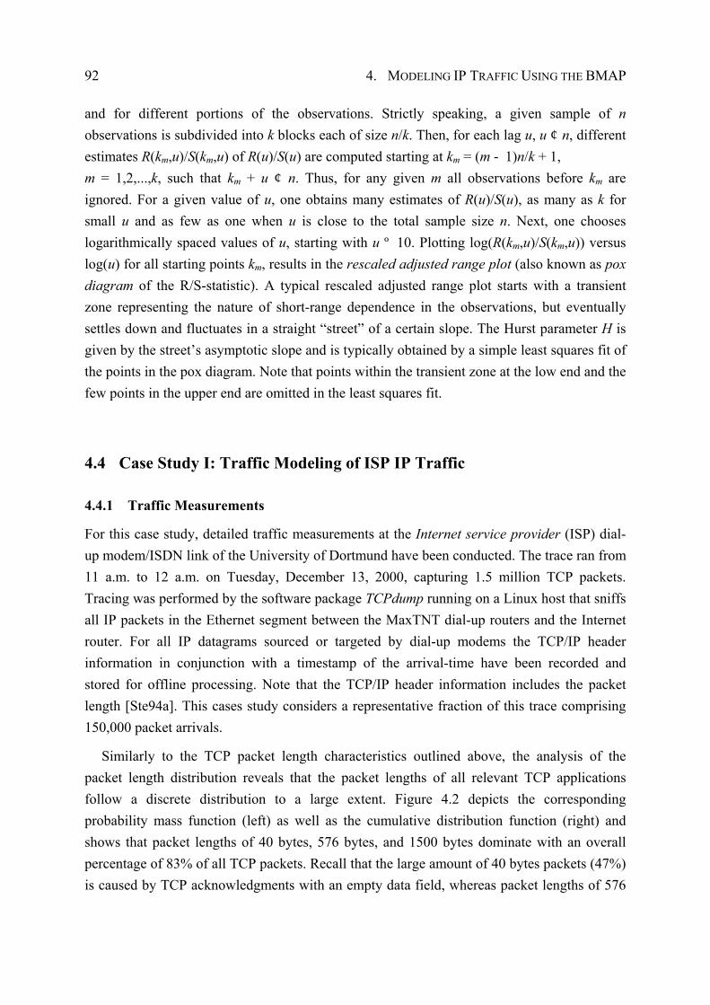
92 4. MODELING IP TRAFFIC USING THE BMAP
and for different portions of the observations. Strictly speaking, a given sample of n observations is subdivided into k blocks each of size n/k. Then, for each lag u, u ¢ n, different estimates R(km,u)/S(km,u) of R(u)/S(u) are computed starting at km = (m - 1)n/k + 1, m = 1,2,...,k, such that km + u ¢ n. Thus, for any given m all observations before km are ignored. For a given value of u, one obtains many estimates of R(u)/S(u), as many as k for small u and as few as one when u is close to the total sample size n. Next, one chooses logarithmically spaced values of u, starting with u º 10. Plotting log(R(km,u)/S(km,u)) versus log(u) for all starting points km, results in the rescaled adjusted range plot (also known as pox diagram of the R/S-statistic). A typical rescaled adjusted range plot starts with a transient zone representing the nature of short-range dependence in the observations, but eventually settles down and fluctuates in a straight “street” of a certain slope. The Hurst parameter H is given by the street’s asymptotic slope and is typically obtained by a simple least squares fit of the points in the pox diagram. Note that points within the transient zone at the low end and the few points in the upper end are omitted in the least squares fit.
4.4 Case Study I: Traffic Modeling of ISP IP Traffic
4.4.1 Traffic Measurements
For this case study, detailed traffic measurements at the Internet service provider (ISP) dial-up modem/ISDN link of the University of Dortmund have been conducted. The trace ran from 11 a.m. to 12 a.m. on Tuesday, December 13, 2000, capturing 1.5 million TCP packets. Tracing was performed by the software package TCPdump running on a Linux host that sniffs all IP packets in the Ethernet segment between the MaxTNT dial-up routers and the Internet router. For all IP datagrams sourced or targeted by dial-up modems the TCP/IP header information in conjunction with a timestamp of the arrival-time have been recorded and stored for offline processing. Note that the TCP/IP header information includes the packet length [Ste94a]. This cases study considers a representative fraction of this trace comprising 150,000 packet arrivals.
Similarly to the TCP packet length characteristics outlined above, the analysis of the packet length distribution reveals that the packet lengths of all relevant TCP applications follow a discrete distribution to a large extent. Figure 4.2 depicts the corresponding probability mass function (left) as well as the cumulative distribution function (right) and shows that packet lengths of 40 bytes, 576 bytes, and 1500 bytes dominate with an overall percentage of 83% of all TCP packets. Recall that the large amount of 40 bytes packets (47%) is caused by TCP acknowledgments with an empty data field, whereas packet lengths of 576
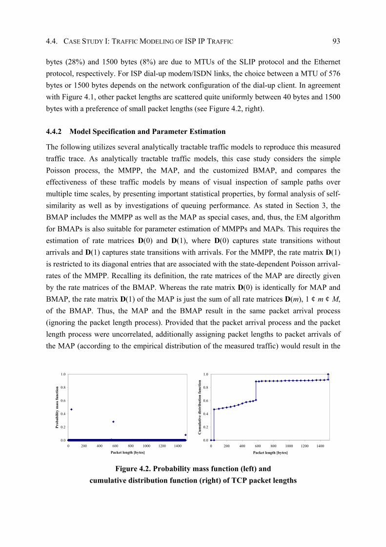
4.4. CASE STUDY I: TRAFFIC MODELING OF ISP IP TRAFFIC 93
bytes (28%) and 1500 bytes (8%) are due to MTUs of the SLIP protocol and the Ethernet protocol, respectively. For ISP dial-up modem/ISDN links, the choice between a MTU of 576 bytes or 1500 bytes depends on the network configuration of the dial-up client. In agreement with Figure 4.1, other packet lengths are scattered quite uniformly between 40 bytes and 1500 bytes with a preference of small packet lengths (see Figure 4.2, right).
4.4.2 Model Specification and Parameter Estimation
The following utilizes several analytically tractable traffic models to reproduce this measured traffic trace. As analytically tractable traffic models, this case study considers the simple Poisson process, the MMPP, the MAP, and the customized BMAP, and compares the effectiveness of these traffic models by means of visual inspection of sample paths over multiple time scales, by presenting important statistical properties, by formal analysis of self-similarity as well as by investigations of queuing performance. As stated in Section 3, the BMAP includes the MMPP as well as the MAP as special cases, and, thus, the EM algorithm for BMAPs is also suitable for parameter estimation of MMPPs and MAPs. This requires the estimation of rate matrices D(0) and D(1), where D(0) captures state transitions without arrivals and D(1) captures state transitions with arrivals. For the MMPP, the rate matrix D(1) is restricted to its diagonal entries that are associated with the state-dependent Poisson arrival-rates of the MMPP. Recalling its definition, the rate matrices of the MAP are directly given by the rate matrices of the BMAP. Whereas the rate matrix D(0) is identically for MAP and BMAP, the rate matrix D(1) of the MAP is just the sum of all rate matrices D(m), 1 ¢ m ¢ M, of the BMAP. Thus, the MAP and the BMAP result in the same packet arrival process (ignoring the packet length process). Provided that the packet arrival process and the packet length process were uncorrelated, additionally assigning packet lengths to packet arrivals of the MAP (according to the empirical distribution of the measured traffic) would result in the
0.0
0.2
0.4
0.6
0.8
1.0
0 200 400 600 800 1000 1200 1400
Packet length [bytes]
Prob
abili
ty m
ass f
unct
ion
0.0
0.2
0.4
0.6
0.8
1.0
0 200 400 600 800 1000 1200 1400
Packet length [bytes]
Cum
ulat
ive
dist
ribu
tion
func
tion
Figure 4.2. Probability mass function (left) and cumulative distribution function (right) of TCP packet lengths
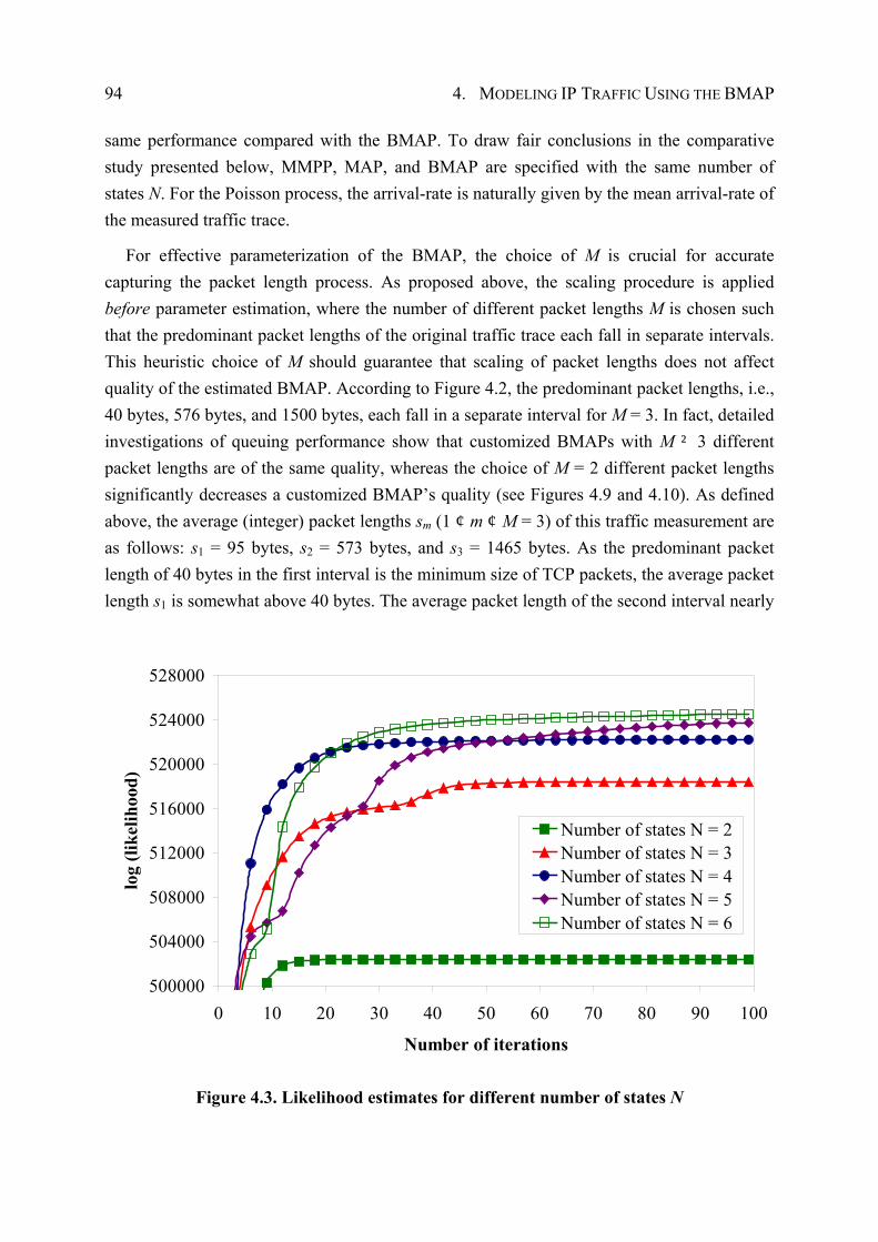
94 4. MODELING IP TRAFFIC USING THE BMAP
same performance compared with the BMAP. To draw fair conclusions in the comparative study presented below, MMPP, MAP, and BMAP are specified with the same number of states N. For the Poisson process, the arrival-rate is naturally given by the mean arrival-rate of the measured traffic trace.
For effective parameterization of the BMAP, the choice of M is crucial for accurate capturing the packet length process. As proposed above, the scaling procedure is applied before parameter estimation, where the number of different packet lengths M is chosen such that the predominant packet lengths of the original traffic trace each fall in separate intervals. This heuristic choice of M should guarantee that scaling of packet lengths does not affect quality of the estimated BMAP. According to Figure 4.2, the predominant packet lengths, i.e., 40 bytes, 576 bytes, and 1500 bytes, each fall in a separate interval for M = 3. In fact, detailed investigations of queuing performance show that customized BMAPs with M ² 3 different packet lengths are of the same quality, whereas the choice of M = 2 different packet lengths significantly decreases a customized BMAP’s quality (see Figures 4.9 and 4.10). As defined above, the average (integer) packet lengths sm (1 ¢ m ¢ M = 3) of this traffic measurement are as follows: s1 = 95 bytes, s2 = 573 bytes, and s3 = 1465 bytes. As the predominant packet length of 40 bytes in the first interval is the minimum size of TCP packets, the average packet length s1 is somewhat above 40 bytes. The average packet length of the second interval nearly
500000
504000
508000
512000
516000
520000
524000
528000
0 10 20 30 40 50 60 70 80 90 100
Number of iterations
log
(like
lihoo
d)
Number of states N = 2Number of states N = 3Number of states N = 4Number of states N = 5Number of states N = 6
Figure 4.3. Likelihood estimates for different number of states N
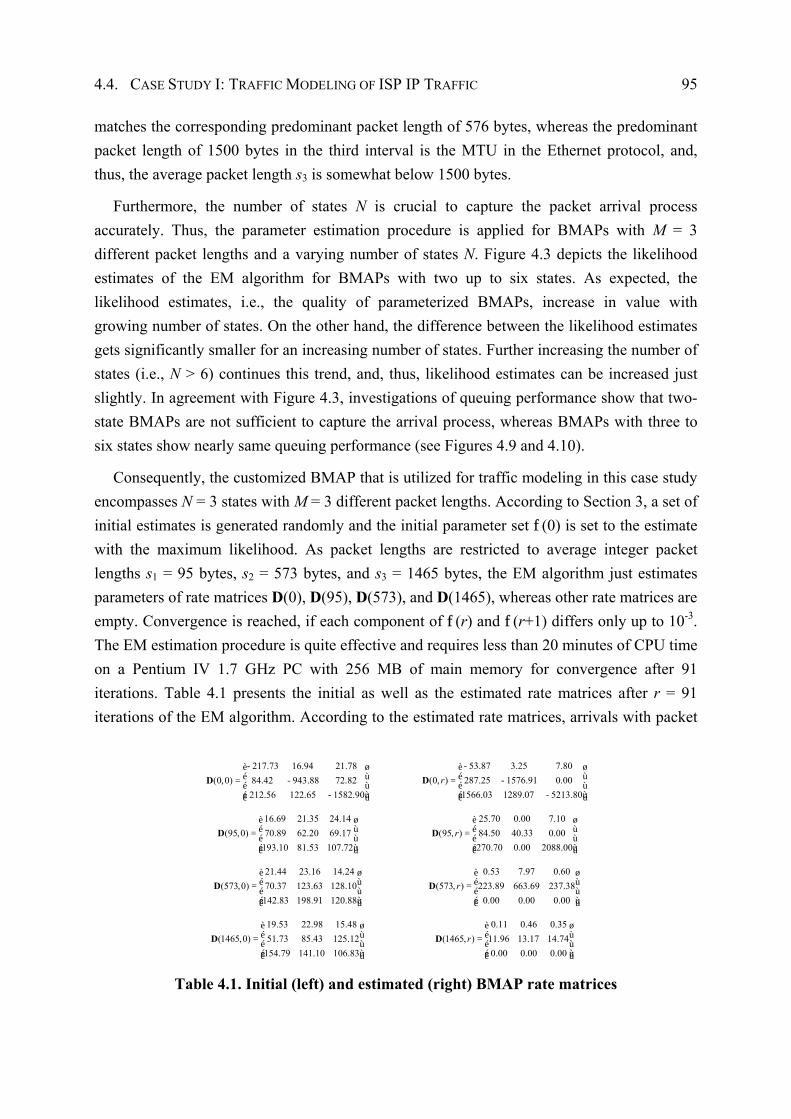
4.4. CASE STUDY I: TRAFFIC MODELING OF ISP IP TRAFFIC 95
matches the corresponding predominant packet length of 576 bytes, whereas the predominant packet length of 1500 bytes in the third interval is the MTU in the Ethernet protocol, and, thus, the average packet length s3 is somewhat below 1500 bytes.
Furthermore, the number of states N is crucial to capture the packet arrival process accurately. Thus, the parameter estimation procedure is applied for BMAPs with M = 3 different packet lengths and a varying number of states N. Figure 4.3 depicts the likelihood estimates of the EM algorithm for BMAPs with two up to six states. As expected, the likelihood estimates, i.e., the quality of parameterized BMAPs, increase in value with growing number of states. On the other hand, the difference between the likelihood estimates gets significantly smaller for an increasing number of states. Further increasing the number of states (i.e., N > 6) continues this trend, and, thus, likelihood estimates can be increased just slightly. In agreement with Figure 4.3, investigations of queuing performance show that two-state BMAPs are not sufficient to capture the arrival process, whereas BMAPs with three to six states show nearly same queuing performance (see Figures 4.9 and 4.10).
Consequently, the customized BMAP that is utilized for traffic modeling in this case study encompasses N = 3 states with M = 3 different packet lengths. According to Section 3, a set of initial estimates is generated randomly and the initial parameter set f(0) is set to the estimate with the maximum likelihood. As packet lengths are restricted to average integer packet lengths s1 = 95 bytes, s2 = 573 bytes, and s3 = 1465 bytes, the EM algorithm just estimates parameters of rate matrices D(0), D(95), D(573), and D(1465), whereas other rate matrices are empty. Convergence is reached, if each component of f(r) and f(r+1) differs only up to 10-3. The EM estimation procedure is quite effective and requires less than 20 minutes of CPU time on a Pentium IV 1.7 GHz PC with 256 MB of main memory for convergence after 91 iterations. Table 4.1 presents the initial as well as the estimated rate matrices after r = 91 iterations of the EM algorithm. According to the estimated rate matrices, arrivals with packet
217.73 16.94 21.78(0,0) 84.42 943.88 72.82
212.56 122.65 1582.90
-è øé ù= -é ù
-é ùê ú
D 53.87 3.25 7.80
(0, ) 287.25 1576.91 0.001566.03 1289.07 5213.80
r-è ø
é ù= -é ù-é ùê ú
D
16.69 21.35 24.14(95,0) 70.89 62.20 69.17
193.10 81.53 107.72
è øé ù= é ùé ùê ú
D 25.70 0.00 7.10
(95, ) 84.50 40.33 0.00270.70 0.00 2088.00
rè øé ù= é ùé ùê ú
D
21.44 23.16 14.24(573,0) 70.37 123.63 128.10
142.83 198.91 120.88
è øé ù= é ùé ùê ú
D 0.53 7.97 0.60
(573, ) 223.89 663.69 237.380.00 0.00 0.00
rè øé ù= é ùé ùê ú
D
19.53 22.98 15.48(1465,0) 51.73 85.43 125.12
154.79 141.10 106.83
è øé ù= é ùé ùê ú
D 0.11 0.46 0.35
(1465, ) 11.96 13.17 14.740.00 0.00 0.00
rè øé ù= é ùé ùê ú
D
Table 4.1. Initial (left) and estimated (right) BMAP rate matrices
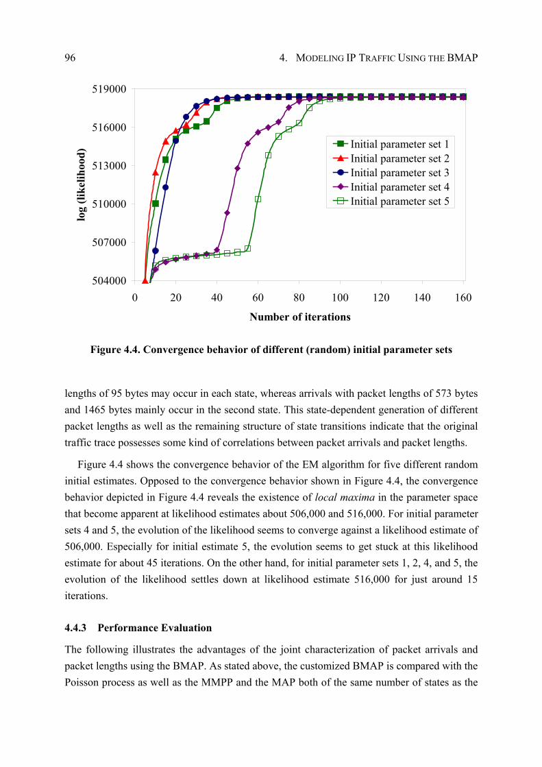
96 4. MODELING IP TRAFFIC USING THE BMAP
504000
507000
510000
513000
516000
519000
0 20 40 60 80 100 120 140 160
Number of iterations
log
(like
lihoo
d)
Initial parameter set 1Initial parameter set 2Initial parameter set 3Initial parameter set 4Initial parameter set 5
Figure 4.4. Convergence behavior of different (random) initial parameter sets
lengths of 95 bytes may occur in each state, whereas arrivals with packet lengths of 573 bytes and 1465 bytes mainly occur in the second state. This state-dependent generation of different packet lengths as well as the remaining structure of state transitions indicate that the original traffic trace possesses some kind of correlations between packet arrivals and packet lengths.
Figure 4.4 shows the convergence behavior of the EM algorithm for five different random initial estimates. Opposed to the convergence behavior shown in Figure 4.4, the convergence behavior depicted in Figure 4.4 reveals the existence of local maxima in the parameter space that become apparent at likelihood estimates about 506,000 and 516,000. For initial parameter sets 4 and 5, the evolution of the likelihood seems to converge against a likelihood estimate of 506,000. Especially for initial estimate 5, the evolution seems to get stuck at this likelihood estimate for about 45 iterations. On the other hand, for initial parameter sets 1, 2, 4, and 5, the evolution of the likelihood settles down at likelihood estimate 516,000 for just around 15 iterations.
4.4.3 Performance Evaluation
The following illustrates the advantages of the joint characterization of packet arrivals and packet lengths using the BMAP. As stated above, the customized BMAP is compared with the Poisson process as well as the MMPP and the MAP both of the same number of states as the
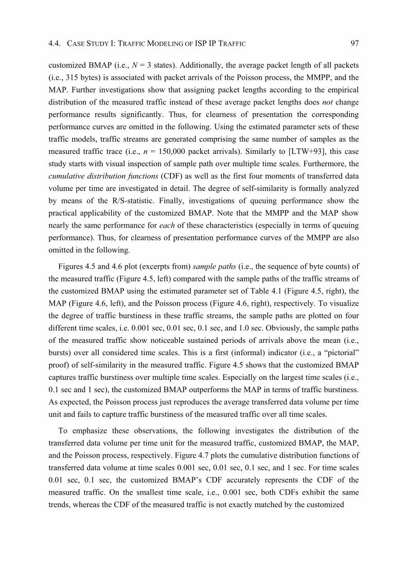
4.4. CASE STUDY I: TRAFFIC MODELING OF ISP IP TRAFFIC 97
customized BMAP (i.e., N = 3 states). Additionally, the average packet length of all packets (i.e., 315 bytes) is associated with packet arrivals of the Poisson process, the MMPP, and the MAP. Further investigations show that assigning packet lengths according to the empirical distribution of the measured traffic instead of these average packet lengths does not change performance results significantly. Thus, for clearness of presentation the corresponding performance curves are omitted in the following. Using the estimated parameter sets of these traffic models, traffic streams are generated comprising the same number of samples as the measured traffic trace (i.e., n = 150,000 packet arrivals). Similarly to [LTW+93], this case study starts with visual inspection of sample path over multiple time scales. Furthermore, the cumulative distribution functions (CDF) as well as the first four moments of transferred data volume per time are investigated in detail. The degree of self-similarity is formally analyzed by means of the R/S-statistic. Finally, investigations of queuing performance show the practical applicability of the customized BMAP. Note that the MMPP and the MAP show nearly the same performance for each of these characteristics (especially in terms of queuing performance). Thus, for clearness of presentation performance curves of the MMPP are also omitted in the following.
Figures 4.5 and 4.6 plot (excerpts from) sample paths (i.e., the sequence of byte counts) of the measured traffic (Figure 4.5, left) compared with the sample paths of the traffic streams of the customized BMAP using the estimated parameter set of Table 4.1 (Figure 4.5, right), the MAP (Figure 4.6, left), and the Poisson process (Figure 4.6, right), respectively. To visualize the degree of traffic burstiness in these traffic streams, the sample paths are plotted on four different time scales, i.e. 0.001 sec, 0.01 sec, 0.1 sec, and 1.0 sec. Obviously, the sample paths of the measured traffic show noticeable sustained periods of arrivals above the mean (i.e., bursts) over all considered time scales. This is a first (informal) indicator (i.e., a “pictorial” proof) of self-similarity in the measured traffic. Figure 4.5 shows that the customized BMAP captures traffic burstiness over multiple time scales. Especially on the largest time scales (i.e., 0.1 sec and 1 sec), the customized BMAP outperforms the MAP in terms of traffic burstiness. As expected, the Poisson process just reproduces the average transferred data volume per time unit and fails to capture traffic burstiness of the measured traffic over all time scales.
To emphasize these observations, the following investigates the distribution of the transferred data volume per time unit for the measured traffic, customized BMAP, the MAP, and the Poisson process, respectively. Figure 4.7 plots the cumulative distribution functions of transferred data volume at time scales 0.001 sec, 0.01 sec, 0.1 sec, and 1 sec. For time scales 0.01 sec, 0.1 sec, the customized BMAP’s CDF accurately represents the CDF of the measured traffic. On the smallest time scale, i.e., 0.001 sec, both CDFs exhibit the same trends, whereas the CDF of the measured traffic is not exactly matched by the customized
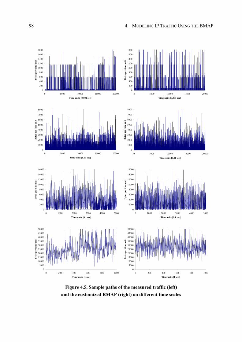
98 4. MODELING IP TRAFFIC USING THE BMAP
0
200
400
600
800
1000
1200
1400
1600
1800
0 5000 10000 15000 20000
Time units [0.001 sec]
Byt
es p
er ti
me
unit
0
200
400
600
800
1000
1200
1400
1600
1800
0 5000 10000 15000 20000
Time units [0.001 sec]
Byt
es p
er ti
me
unit
0
1000
2000
3000
4000
5000
6000
7000
8000
0 5000 10000 15000 20000
Time units [0.01 sec]
Byt
es p
er ti
me
unit
0
1000
2000
3000
4000
5000
6000
7000
8000
0 5000 10000 15000 20000
Time units [0.01 sec]
Byt
es p
er ti
me
unit
0
2000
4000
6000
8000
10000
12000
14000
16000
0 1000 2000 3000 4000 5000
Time units [0.1 sec]
Byt
es p
er ti
me
unit
0
2000
4000
6000
8000
10000
12000
14000
16000
0 1000 2000 3000 4000 5000
Time units [0.1 sec]
Byt
es p
er ti
me
unit
0
5000
10000
15000
20000
25000
30000
35000
40000
45000
50000
0 200 400 600 800 1000
Time units [1 sec]
Byt
es p
er ti
me
unit
0
5000
10000
15000
20000
25000
30000
35000
40000
45000
50000
0 200 400 600 800 1000
Time units [1 sec]
Byt
es p
er ti
me
unit
Figure 4.5. Sample paths of the measured traffic (left) and the customized BMAP (right) on different time scales
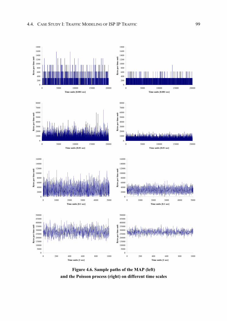
4.4. CASE STUDY I: TRAFFIC MODELING OF ISP IP TRAFFIC 99
0
200
400
600
800
1000
1200
1400
1600
1800
0 5000 10000 15000 20000
Time units [0.001 sec]
Byt
es p
er ti
me
unit
0
200
400
600
800
1000
1200
1400
1600
1800
0 5000 10000 15000 20000
Time units [0.001 sec]
Byt
es p
er ti
me
unit
0
1000
2000
3000
4000
5000
6000
7000
8000
0 5000 10000 15000 20000
Time units [0.01 sec]
Byt
es p
er ti
me
unit
0
1000
2000
3000
4000
5000
6000
7000
8000
0 5000 10000 15000 20000
Time units [0.01 sec]
Byt
es p
er ti
me
unit
0
2000
4000
6000
8000
10000
12000
14000
16000
0 1000 2000 3000 4000 5000
Time units [0.1 sec]
Byt
es p
er ti
me
unit
0
2000
4000
6000
8000
10000
12000
14000
16000
0 1000 2000 3000 4000 5000
Time units [0.1 sec]
Byt
es p
er ti
me
unit
0
5000
10000
15000
20000
25000
30000
35000
40000
45000
50000
0 200 400 600 800 1000
Time units [1 sec]
Byt
es p
er ti
me
unit
0
5000
10000
15000
20000
25000
30000
35000
40000
45000
50000
0 200 400 600 800 1000
Time units [1 sec]
Byt
es p
er ti
me
unit
Figure 4.6. Sample paths of the MAP (left) and the Poisson process (right) on different time scales
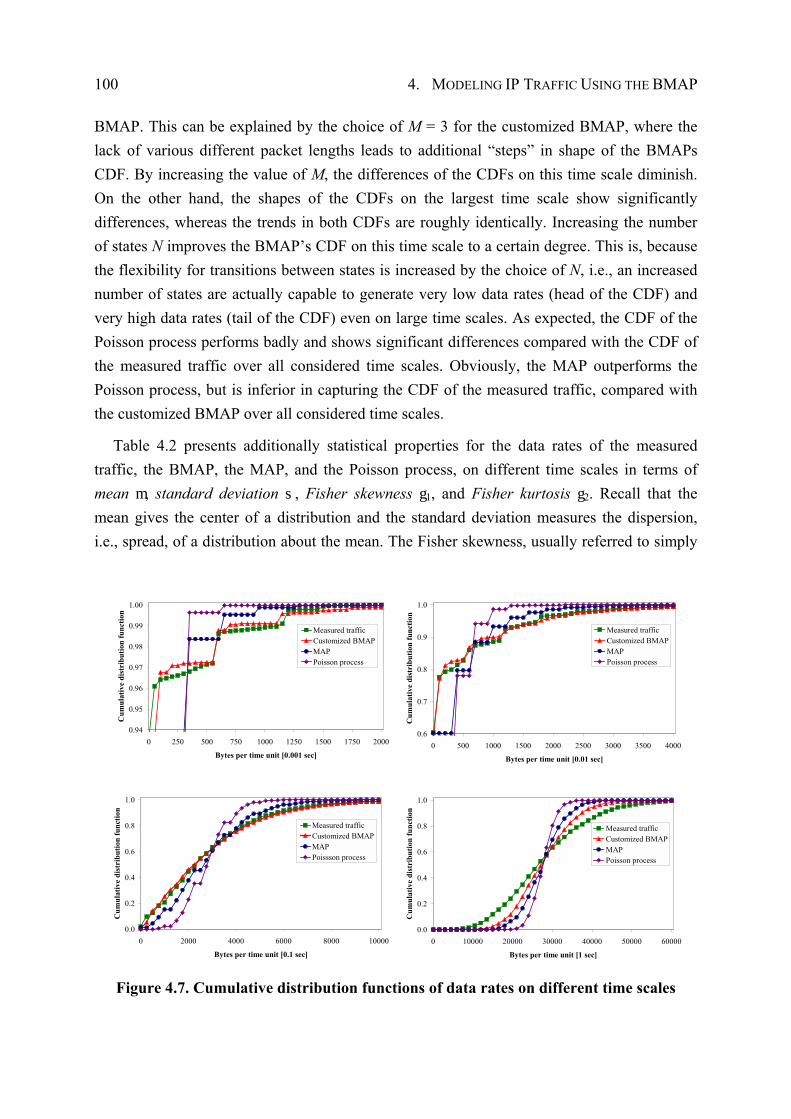
100 4. MODELING IP TRAFFIC USING THE BMAP
BMAP. This can be explained by the choice of M = 3 for the customized BMAP, where the lack of various different packet lengths leads to additional “steps” in shape of the BMAPs CDF. By increasing the value of M, the differences of the CDFs on this time scale diminish. On the other hand, the shapes of the CDFs on the largest time scale show significantly differences, whereas the trends in both CDFs are roughly identically. Increasing the number of states N improves the BMAP’s CDF on this time scale to a certain degree. This is, because the flexibility for transitions between states is increased by the choice of N, i.e., an increased number of states are actually capable to generate very low data rates (head of the CDF) and very high data rates (tail of the CDF) even on large time scales. As expected, the CDF of the Poisson process performs badly and shows significant differences compared with the CDF of the measured traffic over all considered time scales. Obviously, the MAP outperforms the Poisson process, but is inferior in capturing the CDF of the measured traffic, compared with the customized BMAP over all considered time scales.
Table 4.2 presents additionally statistical properties for the data rates of the measured traffic, the BMAP, the MAP, and the Poisson process, on different time scales in terms of mean m, standard deviation s, Fisher skewness g1, and Fisher kurtosis g2. Recall that the mean gives the center of a distribution and the standard deviation measures the dispersion, i.e., spread, of a distribution about the mean. The Fisher skewness, usually referred to simply
0.94
0.95
0.96
0.97
0.98
0.99
1.00
0 250 500 750 1000 1250 1500 1750 2000
Bytes per time unit [0.001 sec]
Cum
ulat
ive
dist
ribu
tion
func
tion
Measured trafficCustomized BMAPMAPPoisson process
0.6
0.7
0.8
0.9
1.0
0 500 1000 1500 2000 2500 3000 3500 4000
Bytes per time unit [0.01 sec]
Cum
ulat
ive
dist
ribu
tion
func
tion
Measured trafficCustomized BMAPMAPPoisson process
0.0
0.2
0.4
0.6
0.8
1.0
0 2000 4000 6000 8000 10000
Bytes per time unit [0.1 sec]
Cum
ulat
ive
dist
ribu
tion
func
tion
Measured trafficCustomized BMAPMAPPoissson process
0.0
0.2
0.4
0.6
0.8
1.0
0 10000 20000 30000 40000 50000 60000
Bytes per time unit [1 sec]
Cum
ulat
ive
dist
ribu
tion
func
tion
Measured trafficCustomized BMAPMAPPoisson process
Figure 4.7. Cumulative distribution functions of data rates on different time scales
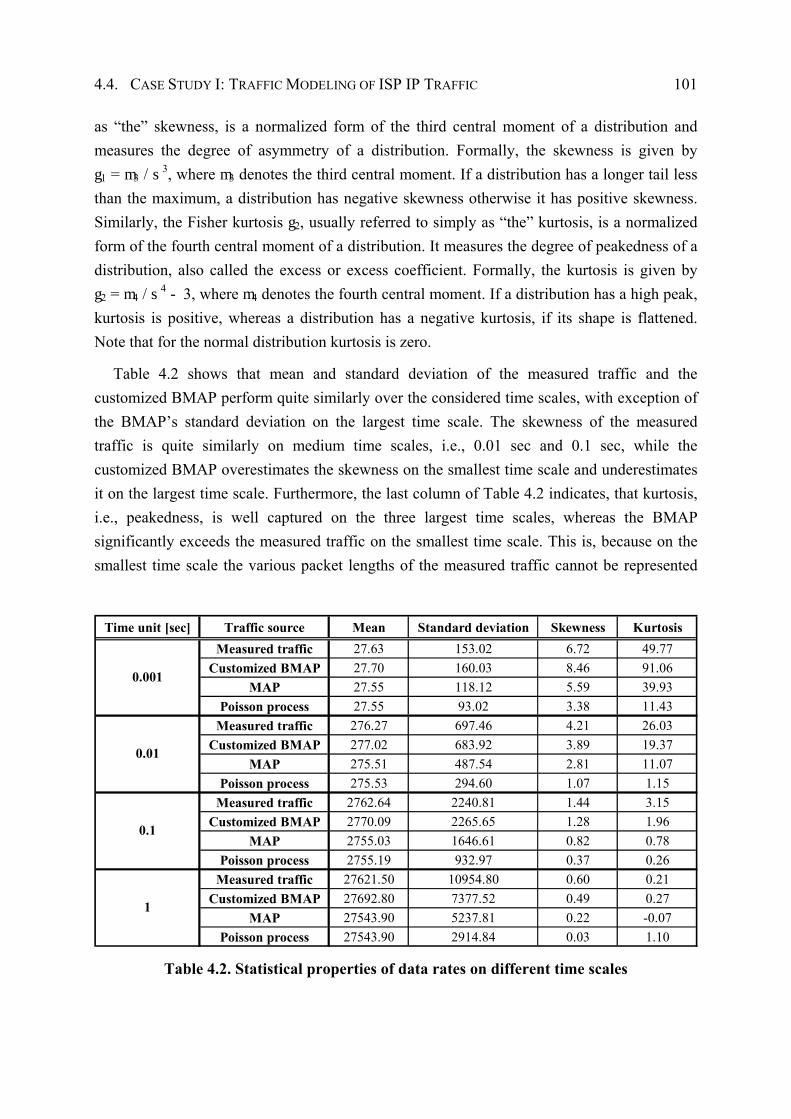
4.4. CASE STUDY I: TRAFFIC MODELING OF ISP IP TRAFFIC 101
as “the” skewness, is a normalized form of the third central moment of a distribution and measures the degree of asymmetry of a distribution. Formally, the skewness is given by g1 = m3 / s3, where m3 denotes the third central moment. If a distribution has a longer tail less than the maximum, a distribution has negative skewness otherwise it has positive skewness. Similarly, the Fisher kurtosis g2, usually referred to simply as “the” kurtosis, is a normalized form of the fourth central moment of a distribution. It measures the degree of peakedness of a distribution, also called the excess or excess coefficient. Formally, the kurtosis is given by g2 = m4 / s4 - 3, where m4 denotes the fourth central moment. If a distribution has a high peak, kurtosis is positive, whereas a distribution has a negative kurtosis, if its shape is flattened. Note that for the normal distribution kurtosis is zero.
Table 4.2 shows that mean and standard deviation of the measured traffic and the customized BMAP perform quite similarly over the considered time scales, with exception of the BMAP’s standard deviation on the largest time scale. The skewness of the measured traffic is quite similarly on medium time scales, i.e., 0.01 sec and 0.1 sec, while the customized BMAP overestimates the skewness on the smallest time scale and underestimates it on the largest time scale. Furthermore, the last column of Table 4.2 indicates, that kurtosis, i.e., peakedness, is well captured on the three largest time scales, whereas the BMAP significantly exceeds the measured traffic on the smallest time scale. This is, because on the smallest time scale the various packet lengths of the measured traffic cannot be represented
Time unit [sec] Traffic source Mean Standard deviation Skewness KurtosisMeasured traffic 27.63 153.02 6.72 49.77
Customized BMAP 27.70 160.03 8.46 91.06MAP 27.55 118.12 5.59 39.93
Poisson process 27.55 93.02 3.38 11.43Measured traffic 276.27 697.46 4.21 26.03
Customized BMAP 277.02 683.92 3.89 19.37MAP 275.51 487.54 2.81 11.07
Poisson process 275.53 294.60 1.07 1.15Measured traffic 2762.64 2240.81 1.44 3.15
Customized BMAP 2770.09 2265.65 1.28 1.96MAP 2755.03 1646.61 0.82 0.78
Poisson process 2755.19 932.97 0.37 0.26Measured traffic 27621.50 10954.80 0.60 0.21
Customized BMAP 27692.80 7377.52 0.49 0.27MAP 27543.90 5237.81 0.22 -0.07
Poisson process 27543.90 2914.84 0.03 1.10
0.001
0.01
0.1
1
Table 4.2. Statistical properties of data rates on different time scales
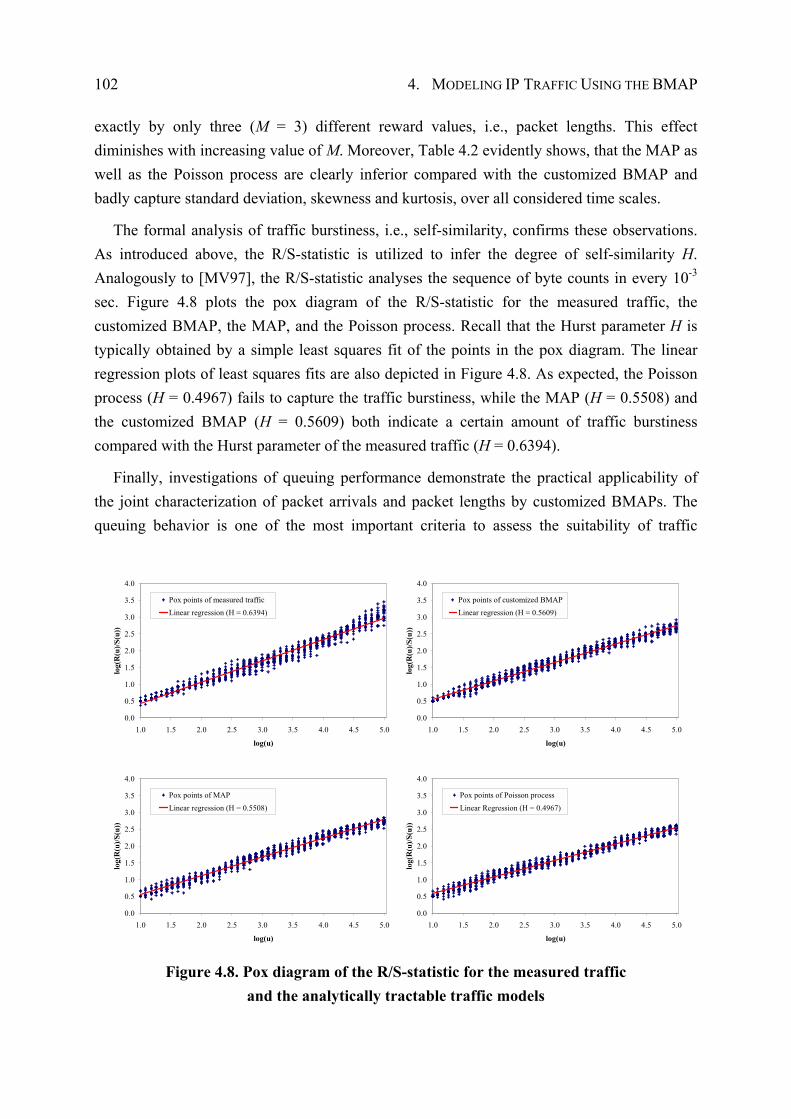
102 4. MODELING IP TRAFFIC USING THE BMAP
exactly by only three (M = 3) different reward values, i.e., packet lengths. This effect diminishes with increasing value of M. Moreover, Table 4.2 evidently shows, that the MAP as well as the Poisson process are clearly inferior compared with the customized BMAP and badly capture standard deviation, skewness and kurtosis, over all considered time scales.
The formal analysis of traffic burstiness, i.e., self-similarity, confirms these observations. As introduced above, the R/S-statistic is utilized to infer the degree of self-similarity H. Analogously to [MV97], the R/S-statistic analyses the sequence of byte counts in every 10-3 sec. Figure 4.8 plots the pox diagram of the R/S-statistic for the measured traffic, the customized BMAP, the MAP, and the Poisson process. Recall that the Hurst parameter H is typically obtained by a simple least squares fit of the points in the pox diagram. The linear regression plots of least squares fits are also depicted in Figure 4.8. As expected, the Poisson process (H = 0.4967) fails to capture the traffic burstiness, while the MAP (H = 0.5508) and the customized BMAP (H = 0.5609) both indicate a certain amount of traffic burstiness compared with the Hurst parameter of the measured traffic (H = 0.6394).
Finally, investigations of queuing performance demonstrate the practical applicability of the joint characterization of packet arrivals and packet lengths by customized BMAPs. The queuing behavior is one of the most important criteria to assess the suitability of traffic
0.0
0.5
1.0
1.5
2.0
2.5
3.0
3.5
4.0
1.0 1.5 2.0 2.5 3.0 3.5 4.0 4.5 5.0
log(u)
log(
R(u
)/S(u
))
Pox points of measured trafficLinear regression (H = 0.6394)
0.0
0.5
1.0
1.5
2.0
2.5
3.0
3.5
4.0
1.0 1.5 2.0 2.5 3.0 3.5 4.0 4.5 5.0
log(u)
log(
R(u
)/S(u
))
Pox points of customized BMAPLinear regression (H = 0.5609)
0.0
0.5
1.0
1.5
2.0
2.5
3.0
3.5
4.0
1.0 1.5 2.0 2.5 3.0 3.5 4.0 4.5 5.0
log(u)
log(
R(u
)/S(u
))
Pox points of MAPLinear regression (H = 0.5508)
0.0
0.5
1.0
1.5
2.0
2.5
3.0
3.5
4.0
1.0 1.5 2.0 2.5 3.0 3.5 4.0 4.5 5.0
log(u)
log(
R(u
)/S(u
))
Pox points of Poisson processLinear Regression (H = 0.4967)
Figure 4.8. Pox diagram of the R/S-statistic for the measured traffic and the analytically tractable traffic models
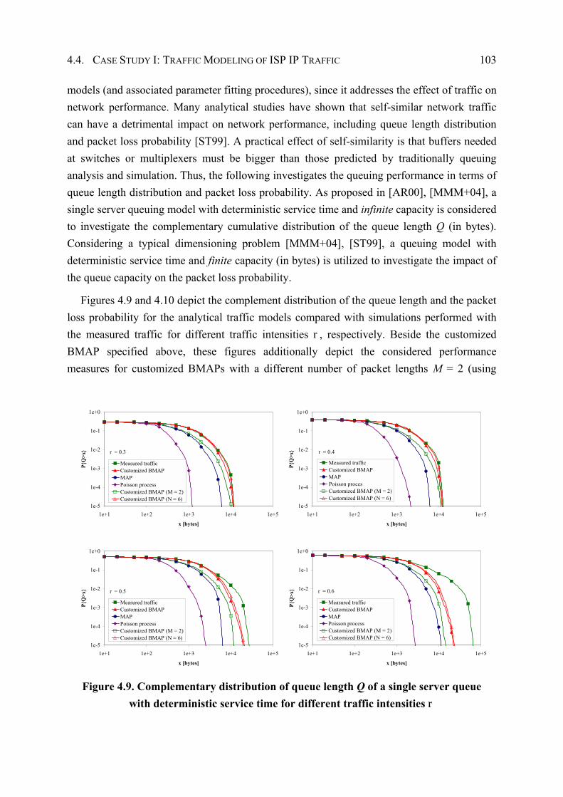
4.4. CASE STUDY I: TRAFFIC MODELING OF ISP IP TRAFFIC 103
models (and associated parameter fitting procedures), since it addresses the effect of traffic on network performance. Many analytical studies have shown that self-similar network traffic can have a detrimental impact on network performance, including queue length distribution and packet loss probability [ST99]. A practical effect of self-similarity is that buffers needed at switches or multiplexers must be bigger than those predicted by traditionally queuing analysis and simulation. Thus, the following investigates the queuing performance in terms of queue length distribution and packet loss probability. As proposed in [AR00], [MMM+04], a single server queuing model with deterministic service time and infinite capacity is considered to investigate the complementary cumulative distribution of the queue length Q (in bytes). Considering a typical dimensioning problem [MMM+04], [ST99], a queuing model with deterministic service time and finite capacity (in bytes) is utilized to investigate the impact of the queue capacity on the packet loss probability.
Figures 4.9 and 4.10 depict the complement distribution of the queue length and the packet loss probability for the analytical traffic models compared with simulations performed with the measured traffic for different traffic intensities r, respectively. Beside the customized BMAP specified above, these figures additionally depict the considered performance measures for customized BMAPs with a different number of packet lengths M = 2 (using
1e-5
1e-4
1e-3
1e-2
1e-1
1e+0
1e+1 1e+2 1e+3 1e+4 1e+5
x [bytes]
P{Q
>x}
Measured trafficCustomized BMAPMAPPoisson processCustomized BMAP (M = 2)Customized BMAP (N = 6)
r = 0.3
1e-5
1e-4
1e-3
1e-2
1e-1
1e+0
1e+1 1e+2 1e+3 1e+4 1e+5
x [bytes]
P{Q
>x}
Measured trafficCustomized BMAPMAPPoisson procesCustomized BMAP (M = 2)Customized BMAP (N = 6)
r = 0.4
1e-5
1e-4
1e-3
1e-2
1e-1
1e+0
1e+1 1e+2 1e+3 1e+4 1e+5
x [bytes]
P{Q
>x}
Measured trafficCustomized BMAPMAPPoisson processCustomized BMAP (M = 2)Customized BMAP (N = 6)
r = 0.5
1e-5
1e-4
1e-3
1e-2
1e-1
1e+0
1e+1 1e+2 1e+3 1e+4 1e+5
x [bytes]
P{Q
>x}
Measured trafficCustomized BMAPMAPPoisson processCustomized BMAP (M = 2)Customized BMAP (N = 6)
r = 0.6
Figure 4.9. Complementary distribution of queue length Q of a single server queue with deterministic service time for different traffic intensities r
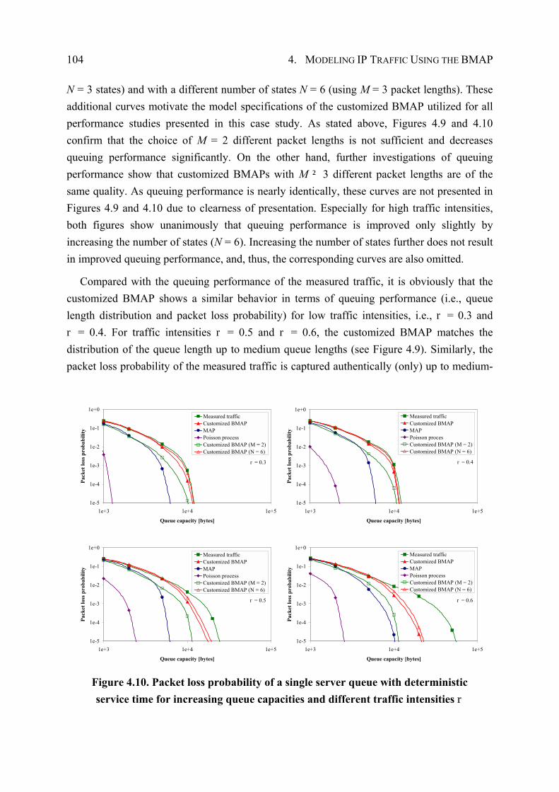
104 4. MODELING IP TRAFFIC USING THE BMAP
N = 3 states) and with a different number of states N = 6 (using M = 3 packet lengths). These additional curves motivate the model specifications of the customized BMAP utilized for all performance studies presented in this case study. As stated above, Figures 4.9 and 4.10 confirm that the choice of M = 2 different packet lengths is not sufficient and decreases queuing performance significantly. On the other hand, further investigations of queuing performance show that customized BMAPs with M ² 3 different packet lengths are of the same quality. As queuing performance is nearly identically, these curves are not presented in Figures 4.9 and 4.10 due to clearness of presentation. Especially for high traffic intensities, both figures show unanimously that queuing performance is improved only slightly by increasing the number of states (N = 6). Increasing the number of states further does not result in improved queuing performance, and, thus, the corresponding curves are also omitted.
Compared with the queuing performance of the measured traffic, it is obviously that the customized BMAP shows a similar behavior in terms of queuing performance (i.e., queue length distribution and packet loss probability) for low traffic intensities, i.e., r = 0.3 and r = 0.4. For traffic intensities r = 0.5 and r = 0.6, the customized BMAP matches the distribution of the queue length up to medium queue lengths (see Figure 4.9). Similarly, the packet loss probability of the measured traffic is captured authentically (only) up to medium-
1e-5
1e-4
1e-3
1e-2
1e-1
1e+0
1e+3 1e+4 1e+5
Queue capacity [bytes]
Pack
et lo
ss p
roba
bilit
y
Measured trafficCustomized BMAPMAPPoisson processCustomized BMAP (M = 2)Customized BMAP (N = 6)
r = 0.3
1e-5
1e-4
1e-3
1e-2
1e-1
1e+0
1e+3 1e+4 1e+5
Queue capacity [bytes]
Pack
et lo
ss p
roba
bilit
y
Measured trafficCustomized BMAPMAPPoisson procesCustomized BMAP (M = 2)Customized BMAP (N = 6)
r = 0.4
1e-5
1e-4
1e-3
1e-2
1e-1
1e+0
1e+3 1e+4 1e+5
Queue capacity [bytes]
Pack
et lo
ss p
roba
bilit
y
Measured trafficCustomized BMAPMAPPoisson processCustomized BMAP (M = 2)Customized BMAP (N = 6)
r = 0.5
1e-5
1e-4
1e-3
1e-2
1e-1
1e+0
1e+3 1e+4 1e+5
Queue capacity [bytes]
Pack
et lo
ss p
roba
bilit
y
Measured trafficCustomized BMAPMAPPoisson processCustomized BMAP (M = 2)Customized BMAP (N = 6)
r = 0.6
Figure 4.10. Packet loss probability of a single server queue with deterministic service time for increasing queue capacities and different traffic intensities r
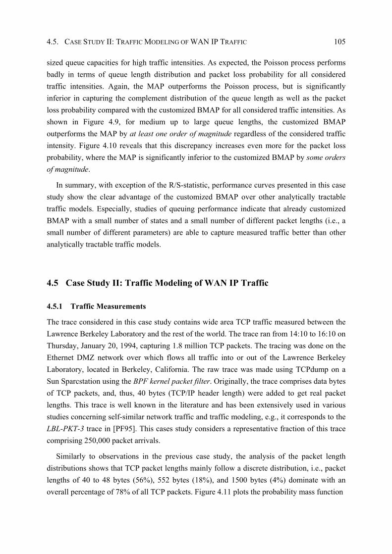
4.5. CASE STUDY II: TRAFFIC MODELING OF WAN IP TRAFFIC 105
sized queue capacities for high traffic intensities. As expected, the Poisson process performs badly in terms of queue length distribution and packet loss probability for all considered traffic intensities. Again, the MAP outperforms the Poisson process, but is significantly inferior in capturing the complement distribution of the queue length as well as the packet loss probability compared with the customized BMAP for all considered traffic intensities. As shown in Figure 4.9, for medium up to large queue lengths, the customized BMAP outperforms the MAP by at least one order of magnitude regardless of the considered traffic intensity. Figure 4.10 reveals that this discrepancy increases even more for the packet loss probability, where the MAP is significantly inferior to the customized BMAP by some orders of magnitude.
In summary, with exception of the R/S-statistic, performance curves presented in this case study show the clear advantage of the customized BMAP over other analytically tractable traffic models. Especially, studies of queuing performance indicate that already customized BMAP with a small number of states and a small number of different packet lengths (i.e., a small number of different parameters) are able to capture measured traffic better than other analytically tractable traffic models.
4.5 Case Study II: Traffic Modeling of WAN IP Traffic
4.5.1 Traffic Measurements
The trace considered in this case study contains wide area TCP traffic measured between the Lawrence Berkeley Laboratory and the rest of the world. The trace ran from 14:10 to 16:10 on Thursday, January 20, 1994, capturing 1.8 million TCP packets. The tracing was done on the Ethernet DMZ network over which flows all traffic into or out of the Lawrence Berkeley Laboratory, located in Berkeley, California. The raw trace was made using TCPdump on a Sun Sparcstation using the BPF kernel packet filter. Originally, the trace comprises data bytes of TCP packets, and, thus, 40 bytes (TCP/IP header length) were added to get real packet lengths. This trace is well known in the literature and has been extensively used in various studies concerning self-similar network traffic and traffic modeling, e.g., it corresponds to the LBL-PKT-3 trace in [PF95]. This cases study considers a representative fraction of this trace comprising 250,000 packet arrivals.
Similarly to observations in the previous case study, the analysis of the packet length distributions shows that TCP packet lengths mainly follow a discrete distribution, i.e., packet lengths of 40 to 48 bytes (56%), 552 bytes (18%), and 1500 bytes (4%) dominate with an overall percentage of 78% of all TCP packets. Figure 4.11 plots the probability mass function
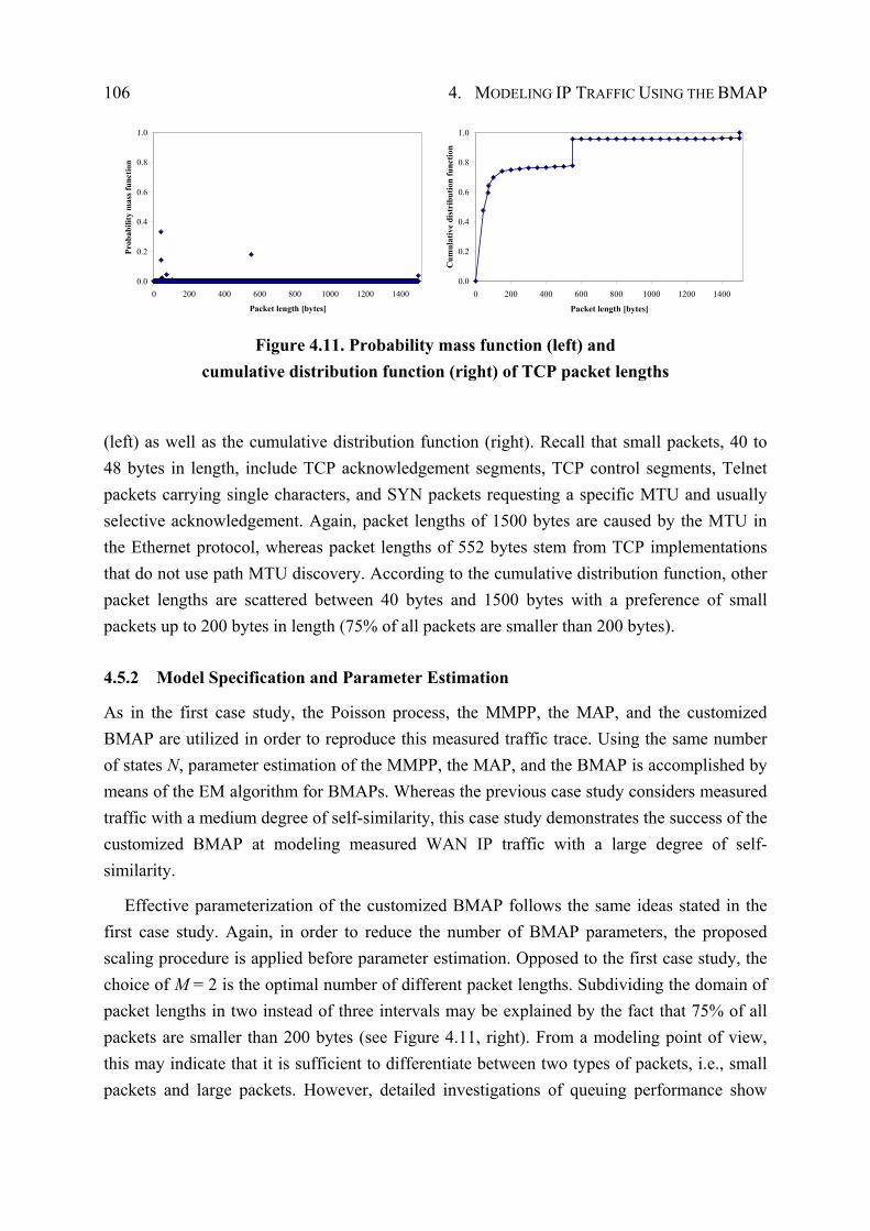
106 4. MODELING IP TRAFFIC USING THE BMAP
0.0
0.2
0.4
0.6
0.8
1.0
0 200 400 600 800 1000 1200 1400
Packet length [bytes]
Prob
abili
ty m
ass f
unct
ion
0.0
0.2
0.4
0.6
0.8
1.0
0 200 400 600 800 1000 1200 1400
Packet length [bytes]
Cum
ulat
ive
dist
ribu
tion
func
tion
Figure 4.11. Probability mass function (left) and cumulative distribution function (right) of TCP packet lengths
(left) as well as the cumulative distribution function (right). Recall that small packets, 40 to 48 bytes in length, include TCP acknowledgement segments, TCP control segments, Telnet packets carrying single characters, and SYN packets requesting a specific MTU and usually selective acknowledgement. Again, packet lengths of 1500 bytes are caused by the MTU in the Ethernet protocol, whereas packet lengths of 552 bytes stem from TCP implementations that do not use path MTU discovery. According to the cumulative distribution function, other packet lengths are scattered between 40 bytes and 1500 bytes with a preference of small packets up to 200 bytes in length (75% of all packets are smaller than 200 bytes).
4.5.2 Model Specification and Parameter Estimation
As in the first case study, the Poisson process, the MMPP, the MAP, and the customized BMAP are utilized in order to reproduce this measured traffic trace. Using the same number of states N, parameter estimation of the MMPP, the MAP, and the BMAP is accomplished by means of the EM algorithm for BMAPs. Whereas the previous case study considers measured traffic with a medium degree of self-similarity, this case study demonstrates the success of the customized BMAP at modeling measured WAN IP traffic with a large degree of self-similarity.
Effective parameterization of the customized BMAP follows the same ideas stated in the first case study. Again, in order to reduce the number of BMAP parameters, the proposed scaling procedure is applied before parameter estimation. Opposed to the first case study, the choice of M = 2 is the optimal number of different packet lengths. Subdividing the domain of packet lengths in two instead of three intervals may be explained by the fact that 75% of all packets are smaller than 200 bytes (see Figure 4.11, right). From a modeling point of view, this may indicate that it is sufficient to differentiate between two types of packets, i.e., small packets and large packets. However, detailed investigations of queuing performance show
4.5. CASE STUDY II: TRAFFIC MODELING OF WAN IP TRAFFIC 107
that customized BMAPs with M ² 3 different packet lengths are of the same quality, respectively, but inferior compared with M = 2 different packet lengths (see Figures 4.18 and 4.19). For M = 2, average (integer) packet lengths after scaling are given by s1 = 157 bytes and s2 = 1493 bytes. These average packet lengths reflect the notion of very small (i.e., below 200 bytes) and very large packets apparent in this traffic trace.
In order to find the number of states N that is suitable to capture the packet arrival process, the EM algorithm is applied for BMAPs with a varying number of states N and M = 2 different packet lengths. Similarly to Figure 4.3, Figure 4.12 plots likelihood estimates for BMAPs with two up to six states. In agreement with the previous case study, the likelihood estimate of two-state BMAPs is significantly smaller than likelihood estimates for BMAPs with three or more states. As already observed in the previous case study, likelihood estimates increase with growing number of states, whereas, compared with the previous case study, differences between likelihood estimates diminish even more for N ² 4 states. Again, studies of queuing performance reveal that BMAPs with two states are unsuitable for capturing the packet arrival process. As illustrated in Figures 4.18 and 4.19, three-state BMAPs show nearly the same performance as BMAPs with N ² 4 states, and, thus, this case study utilizes a three-state BMAP with M = 2 different packet lengths.
1106500
1109000
1111500
1114000
1116500
1119000
1121500
1124000
1126500
1129000
0 10 20 30 40 50 60 70 80 90 100
Number of iterations
log
(like
lihoo
d)
Number of states N = 2Number of states N = 3Number of states N = 4Number of states N = 5Number of states N = 6
Figure 4.12. Likelihood estimates for different number of states N
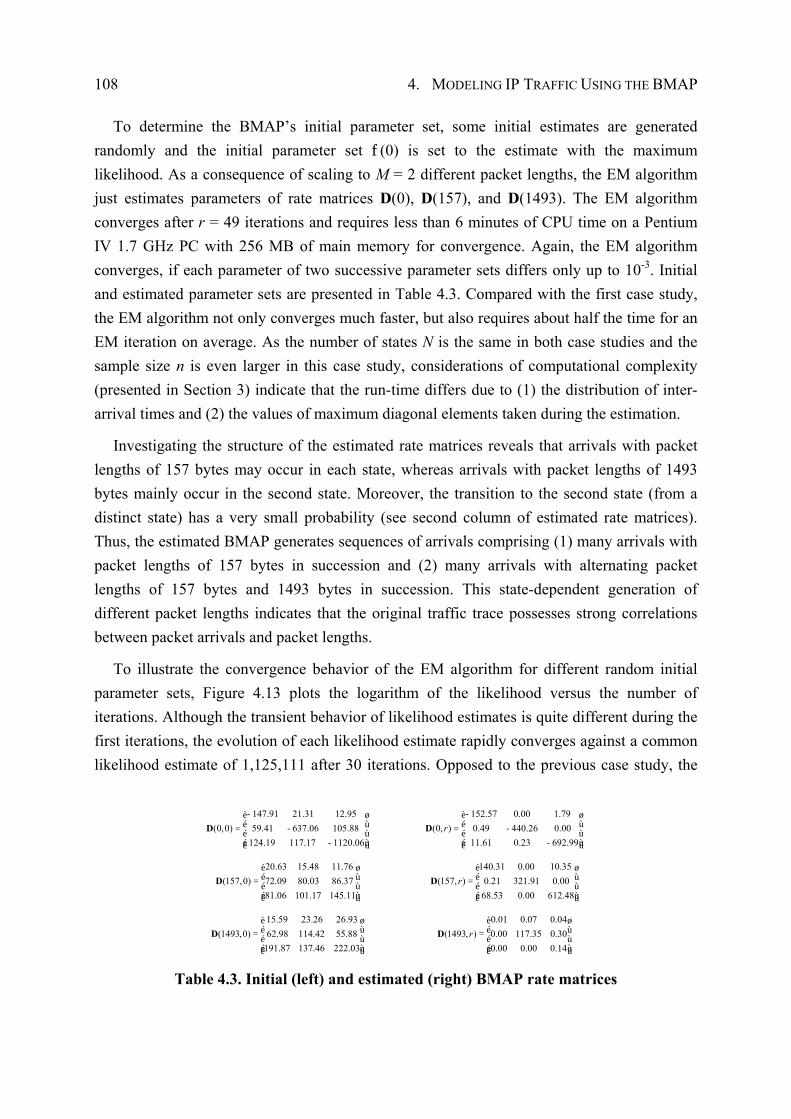
108 4. MODELING IP TRAFFIC USING THE BMAP
To determine the BMAP’s initial parameter set, some initial estimates are generated randomly and the initial parameter set f(0) is set to the estimate with the maximum likelihood. As a consequence of scaling to M = 2 different packet lengths, the EM algorithm just estimates parameters of rate matrices D(0), D(157), and D(1493). The EM algorithm converges after r = 49 iterations and requires less than 6 minutes of CPU time on a Pentium IV 1.7 GHz PC with 256 MB of main memory for convergence. Again, the EM algorithm converges, if each parameter of two successive parameter sets differs only up to 10-3. Initial and estimated parameter sets are presented in Table 4.3. Compared with the first case study, the EM algorithm not only converges much faster, but also requires about half the time for an EM iteration on average. As the number of states N is the same in both case studies and the sample size n is even larger in this case study, considerations of computational complexity (presented in Section 3) indicate that the run-time differs due to (1) the distribution of inter-arrival times and (2) the values of maximum diagonal elements taken during the estimation.
Investigating the structure of the estimated rate matrices reveals that arrivals with packet lengths of 157 bytes may occur in each state, whereas arrivals with packet lengths of 1493 bytes mainly occur in the second state. Moreover, the transition to the second state (from a distinct state) has a very small probability (see second column of estimated rate matrices). Thus, the estimated BMAP generates sequences of arrivals comprising (1) many arrivals with packet lengths of 157 bytes in succession and (2) many arrivals with alternating packet lengths of 157 bytes and 1493 bytes in succession. This state-dependent generation of different packet lengths indicates that the original traffic trace possesses strong correlations between packet arrivals and packet lengths.
To illustrate the convergence behavior of the EM algorithm for different random initial parameter sets, Figure 4.13 plots the logarithm of the likelihood versus the number of iterations. Although the transient behavior of likelihood estimates is quite different during the first iterations, the evolution of each likelihood estimate rapidly converges against a common likelihood estimate of 1,125,111 after 30 iterations. Opposed to the previous case study, the
147.91 21.31 12.95(0,0) 59.41 637.06 105.88
124.19 117.17 1120.06
-è øé ù= -é ù
-é ùê ú
D 152.57 0.00 1.79
(0, ) 0.49 440.26 0.0011.61 0.23 692.99
r-è øé ù= -é ù
-é ùê ú
D
20.63 15.48 11.76(157,0) 72.09 80.03 86.37
81.06 101.17 145.11
è øé ù= é ùé ùê ú
D 140.31 0.00 10.35
(157, ) 0.21 321.91 0.0068.53 0.00 612.48
rè øé ù= é ùé ùê ú
D
15.59 23.26 26.93(1493,0) 62.98 114.42 55.88
191.87 137.46 222.03
è øé ù= é ùé ùê ú
D 0.01 0.07 0.04
(1493, ) 0.00 117.35 0.300.00 0.00 0.14
rè øé ù= é ùé ùê ú
D
Table 4.3. Initial (left) and estimated (right) BMAP rate matrices
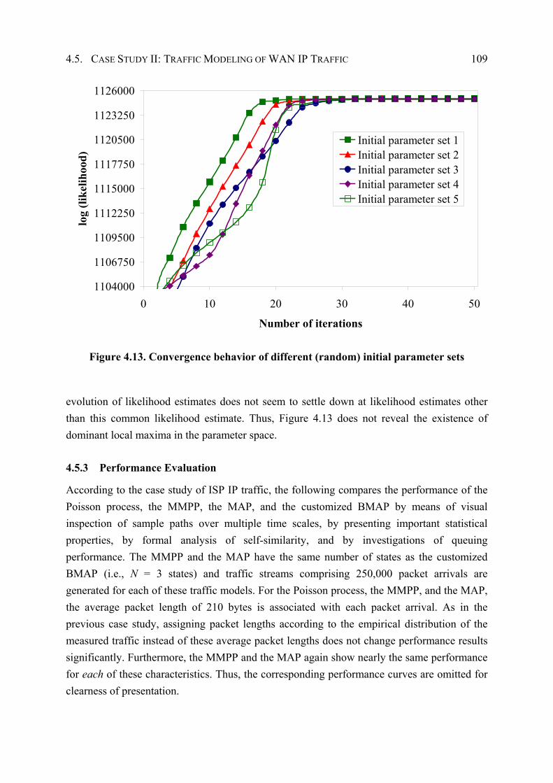
4.5. CASE STUDY II: TRAFFIC MODELING OF WAN IP TRAFFIC 109
1104000
1106750
1109500
1112250
1115000
1117750
1120500
1123250
1126000
0 10 20 30 40 50
Number of iterations
log
(like
lihoo
d)
Initial parameter set 1Initial parameter set 2Initial parameter set 3Initial parameter set 4Initial parameter set 5
Figure 4.13. Convergence behavior of different (random) initial parameter sets
evolution of likelihood estimates does not seem to settle down at likelihood estimates other than this common likelihood estimate. Thus, Figure 4.13 does not reveal the existence of dominant local maxima in the parameter space.
4.5.3 Performance Evaluation
According to the case study of ISP IP traffic, the following compares the performance of the Poisson process, the MMPP, the MAP, and the customized BMAP by means of visual inspection of sample paths over multiple time scales, by presenting important statistical properties, by formal analysis of self-similarity, and by investigations of queuing performance. The MMPP and the MAP have the same number of states as the customized BMAP (i.e., N = 3 states) and traffic streams comprising 250,000 packet arrivals are generated for each of these traffic models. For the Poisson process, the MMPP, and the MAP, the average packet length of 210 bytes is associated with each packet arrival. As in the previous case study, assigning packet lengths according to the empirical distribution of the measured traffic instead of these average packet lengths does not change performance results significantly. Furthermore, the MMPP and the MAP again show nearly the same performance for each of these characteristics. Thus, the corresponding performance curves are omitted for clearness of presentation.
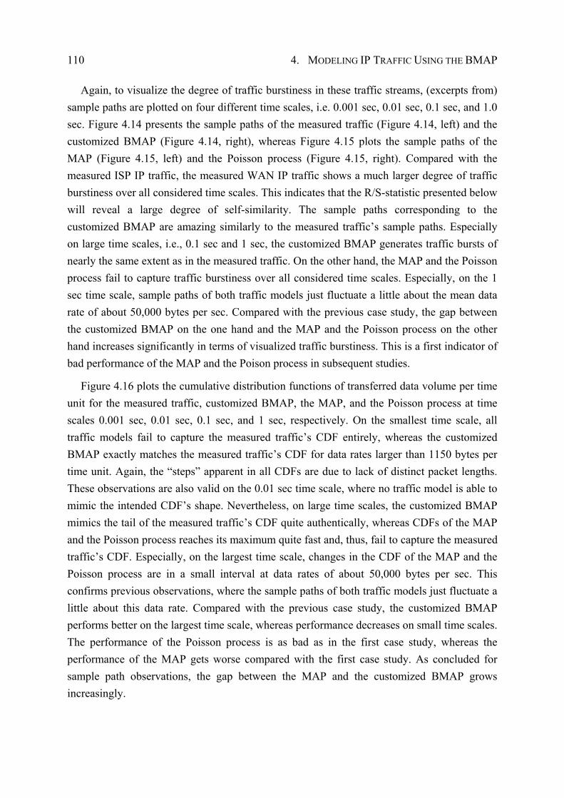
110 4. MODELING IP TRAFFIC USING THE BMAP
Again, to visualize the degree of traffic burstiness in these traffic streams, (excerpts from) sample paths are plotted on four different time scales, i.e. 0.001 sec, 0.01 sec, 0.1 sec, and 1.0 sec. Figure 4.14 presents the sample paths of the measured traffic (Figure 4.14, left) and the customized BMAP (Figure 4.14, right), whereas Figure 4.15 plots the sample paths of the MAP (Figure 4.15, left) and the Poisson process (Figure 4.15, right). Compared with the measured ISP IP traffic, the measured WAN IP traffic shows a much larger degree of traffic burstiness over all considered time scales. This indicates that the R/S-statistic presented below will reveal a large degree of self-similarity. The sample paths corresponding to the customized BMAP are amazing similarly to the measured traffic’s sample paths. Especially on large time scales, i.e., 0.1 sec and 1 sec, the customized BMAP generates traffic bursts of nearly the same extent as in the measured traffic. On the other hand, the MAP and the Poisson process fail to capture traffic burstiness over all considered time scales. Especially, on the 1 sec time scale, sample paths of both traffic models just fluctuate a little about the mean data rate of about 50,000 bytes per sec. Compared with the previous case study, the gap between the customized BMAP on the one hand and the MAP and the Poisson process on the other hand increases significantly in terms of visualized traffic burstiness. This is a first indicator of bad performance of the MAP and the Poison process in subsequent studies.
Figure 4.16 plots the cumulative distribution functions of transferred data volume per time unit for the measured traffic, customized BMAP, the MAP, and the Poisson process at time scales 0.001 sec, 0.01 sec, 0.1 sec, and 1 sec, respectively. On the smallest time scale, all traffic models fail to capture the measured traffic’s CDF entirely, whereas the customized BMAP exactly matches the measured traffic’s CDF for data rates larger than 1150 bytes per time unit. Again, the “steps” apparent in all CDFs are due to lack of distinct packet lengths. These observations are also valid on the 0.01 sec time scale, where no traffic model is able to mimic the intended CDF’s shape. Nevertheless, on large time scales, the customized BMAP mimics the tail of the measured traffic’s CDF quite authentically, whereas CDFs of the MAP and the Poisson process reaches its maximum quite fast and, thus, fail to capture the measured traffic’s CDF. Especially, on the largest time scale, changes in the CDF of the MAP and the Poisson process are in a small interval at data rates of about 50,000 bytes per sec. This confirms previous observations, where the sample paths of both traffic models just fluctuate a little about this data rate. Compared with the previous case study, the customized BMAP performs better on the largest time scale, whereas performance decreases on small time scales. The performance of the Poisson process is as bad as in the first case study, whereas the performance of the MAP gets worse compared with the first case study. As concluded for sample path observations, the gap between the MAP and the customized BMAP grows increasingly.
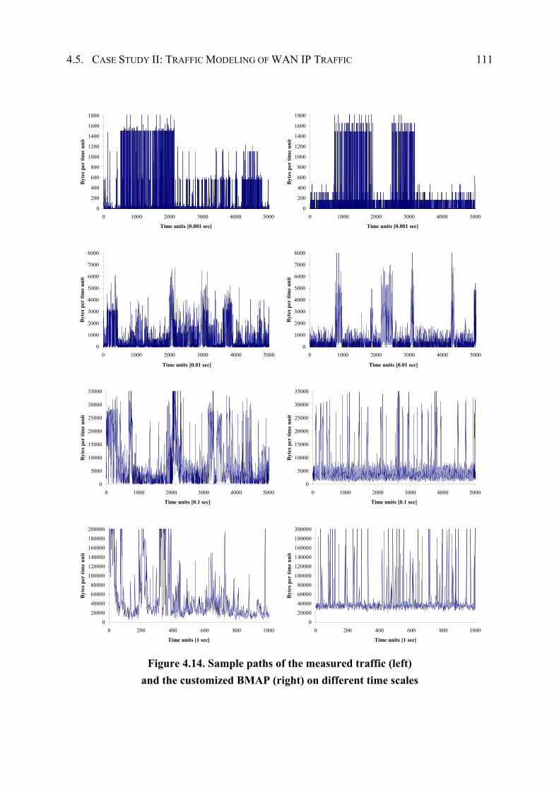
4.5. CASE STUDY II: TRAFFIC MODELING OF WAN IP TRAFFIC 111
0
200
400
600
800
1000
1200
1400
1600
1800
0 1000 2000 3000 4000 5000
Time units [0.001 sec]
Byt
es p
er ti
me
unit
0
200
400
600
800
1000
1200
1400
1600
1800
0 1000 2000 3000 4000 5000
Time units [0.001 sec]
Byt
es p
er ti
me
unit
0
1000
2000
3000
4000
5000
6000
7000
8000
0 1000 2000 3000 4000 5000
Time units [0.01 sec]
Byt
es p
er ti
me
unit
0
1000
2000
3000
4000
5000
6000
7000
8000
0 1000 2000 3000 4000 5000
Time units [0.01 sec]
Byt
es p
er ti
me
unit
0
5000
10000
15000
20000
25000
30000
35000
0 1000 2000 3000 4000 5000
Time units [0.1 sec]
Byt
es p
er ti
me
unit
0
5000
10000
15000
20000
25000
30000
35000
0 1000 2000 3000 4000 5000
Time units [0.1 sec]
Byt
es p
er ti
me
unit
0
20000
40000
60000
80000
100000
120000
140000
160000
180000
200000
0 200 400 600 800 1000
Time units [1 sec]
Byt
es p
er ti
me
unit
0
20000
40000
60000
80000
100000
120000
140000
160000
180000
200000
0 200 400 600 800 1000
Time units [1 sec]
Byt
es p
er ti
me
unit
Figure 4.14. Sample paths of the measured traffic (left) and the customized BMAP (right) on different time scales
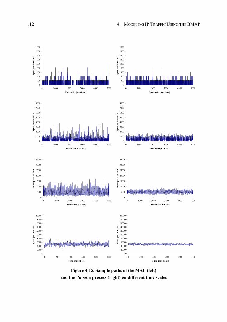
112 4. MODELING IP TRAFFIC USING THE BMAP
0
200
400
600
800
1000
1200
1400
1600
1800
0 1000 2000 3000 4000 5000
Time units [0.001 sec]
Byt
es p
er ti
me
unit
0
200
400
600
800
1000
1200
1400
1600
1800
0 1000 2000 3000 4000 5000
Time units [0.001 sec]
Byt
es p
er ti
me
unit
0
1000
2000
3000
4000
5000
6000
7000
8000
0 1000 2000 3000 4000 5000
Time units [0.01 sec]
Byt
es p
er ti
me
unit
0
1000
2000
3000
4000
5000
6000
7000
8000
0 1000 2000 3000 4000 5000
Time units [0.01 sec]
Byt
es p
er ti
me
unit
0
5000
10000
15000
20000
25000
30000
35000
0 1000 2000 3000 4000 5000
Time units [0.1 sec]
Byt
es p
er ti
me
unit
0
5000
10000
15000
20000
25000
30000
35000
0 1000 2000 3000 4000 5000
Time units [0.1 sec]
Byt
es p
er ti
me
unit
0
20000
40000
60000
80000
100000
120000
140000
160000
180000
200000
0 200 400 600 800 1000
Time units [1 sec]
Byt
es p
er ti
me
unit
0
20000
40000
60000
80000
100000
120000
140000
160000
180000
200000
0 200 400 600 800 1000
Time units [1 sec]
Byt
es p
er ti
me
unit
Figure 4.15. Sample paths of the MAP (left) and the Poisson process (right) on different time scales
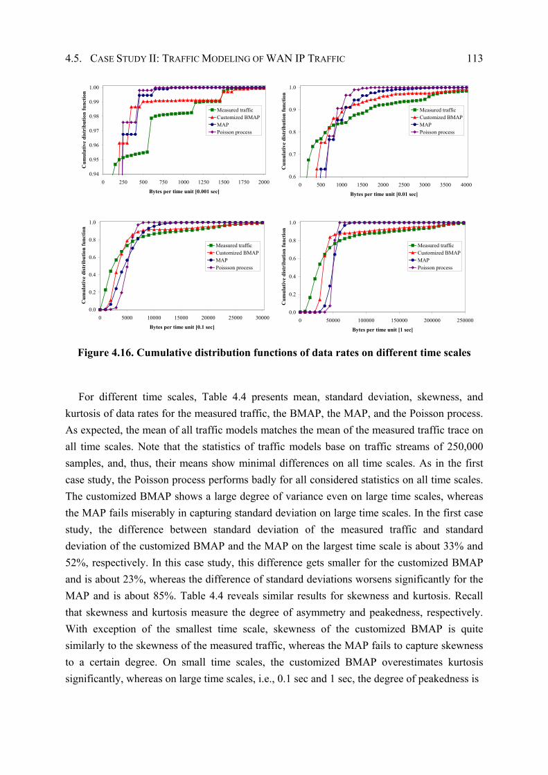
4.5. CASE STUDY II: TRAFFIC MODELING OF WAN IP TRAFFIC 113
0.94
0.95
0.96
0.97
0.98
0.99
1.00
0 250 500 750 1000 1250 1500 1750 2000
Bytes per time unit [0.001 sec]
Cum
ulat
ive
dist
ribu
tion
func
tion
Measured trafficCustomized BMAPMAPPoisson process
0.6
0.7
0.8
0.9
1.0
0 500 1000 1500 2000 2500 3000 3500 4000
Bytes per time unit [0.01 sec]
Cum
ulat
ive
dist
ribu
tion
func
tion
Measured trafficCustomized BMAPMAPPoisson process
0.0
0.2
0.4
0.6
0.8
1.0
0 5000 10000 15000 20000 25000 30000
Bytes per time unit [0.1 sec]
Cum
ulat
ive
dist
ribu
tion
func
tion
Measured trafficCustomized BMAPMAPPoissson process
0.0
0.2
0.4
0.6
0.8
1.0
0 50000 100000 150000 200000 250000
Bytes per time unit [1 sec]
Cum
ulat
ive
dist
ribu
tion
func
tion
Measured trafficCustomized BMAPMAPPoisson process
Figure 4.16. Cumulative distribution functions of data rates on different time scales
For different time scales, Table 4.4 presents mean, standard deviation, skewness, and kurtosis of data rates for the measured traffic, the BMAP, the MAP, and the Poisson process. As expected, the mean of all traffic models matches the mean of the measured traffic trace on all time scales. Note that the statistics of traffic models base on traffic streams of 250,000 samples, and, thus, their means show minimal differences on all time scales. As in the first case study, the Poisson process performs badly for all considered statistics on all time scales. The customized BMAP shows a large degree of variance even on large time scales, whereas the MAP fails miserably in capturing standard deviation on large time scales. In the first case study, the difference between standard deviation of the measured traffic and standard deviation of the customized BMAP and the MAP on the largest time scale is about 33% and 52%, respectively. In this case study, this difference gets smaller for the customized BMAP and is about 23%, whereas the difference of standard deviations worsens significantly for the MAP and is about 85%. Table 4.4 reveals similar results for skewness and kurtosis. Recall that skewness and kurtosis measure the degree of asymmetry and peakedness, respectively. With exception of the smallest time scale, skewness of the customized BMAP is quite similarly to the skewness of the measured traffic, whereas the MAP fails to capture skewness to a certain degree. On small time scales, the customized BMAP overestimates kurtosis significantly, whereas on large time scales, i.e., 0.1 sec and 1 sec, the degree of peakedness is
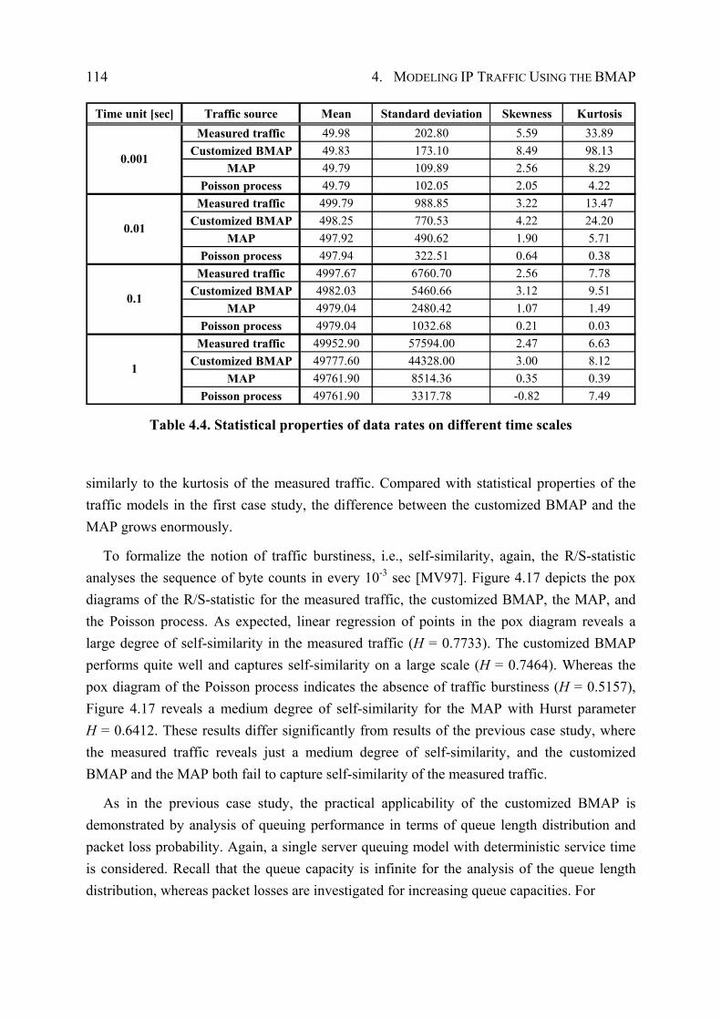
114 4. MODELING IP TRAFFIC USING THE BMAP
Time unit [sec] Traffic source Mean Standard deviation Skewness KurtosisMeasured traffic 49.98 202.80 5.59 33.89
Customized BMAP 49.83 173.10 8.49 98.13MAP 49.79 109.89 2.56 8.29
Poisson process 49.79 102.05 2.05 4.22Measured traffic 499.79 988.85 3.22 13.47
Customized BMAP 498.25 770.53 4.22 24.20MAP 497.92 490.62 1.90 5.71
Poisson process 497.94 322.51 0.64 0.38Measured traffic 4997.67 6760.70 2.56 7.78
Customized BMAP 4982.03 5460.66 3.12 9.51MAP 4979.04 2480.42 1.07 1.49
Poisson process 4979.04 1032.68 0.21 0.03Measured traffic 49952.90 57594.00 2.47 6.63
Customized BMAP 49777.60 44328.00 3.00 8.12MAP 49761.90 8514.36 0.35 0.39
Poisson process 49761.90 3317.78 -0.82 7.49
0.001
0.01
0.1
1
Table 4.4. Statistical properties of data rates on different time scales
similarly to the kurtosis of the measured traffic. Compared with statistical properties of the traffic models in the first case study, the difference between the customized BMAP and the MAP grows enormously.
To formalize the notion of traffic burstiness, i.e., self-similarity, again, the R/S-statistic analyses the sequence of byte counts in every 10-3 sec [MV97]. Figure 4.17 depicts the pox diagrams of the R/S-statistic for the measured traffic, the customized BMAP, the MAP, and the Poisson process. As expected, linear regression of points in the pox diagram reveals a large degree of self-similarity in the measured traffic (H = 0.7733). The customized BMAP performs quite well and captures self-similarity on a large scale (H = 0.7464). Whereas the pox diagram of the Poisson process indicates the absence of traffic burstiness (H = 0.5157), Figure 4.17 reveals a medium degree of self-similarity for the MAP with Hurst parameter H = 0.6412. These results differ significantly from results of the previous case study, where the measured traffic reveals just a medium degree of self-similarity, and the customized BMAP and the MAP both fail to capture self-similarity of the measured traffic.
As in the previous case study, the practical applicability of the customized BMAP is demonstrated by analysis of queuing performance in terms of queue length distribution and packet loss probability. Again, a single server queuing model with deterministic service time is considered. Recall that the queue capacity is infinite for the analysis of the queue length distribution, whereas packet losses are investigated for increasing queue capacities. For
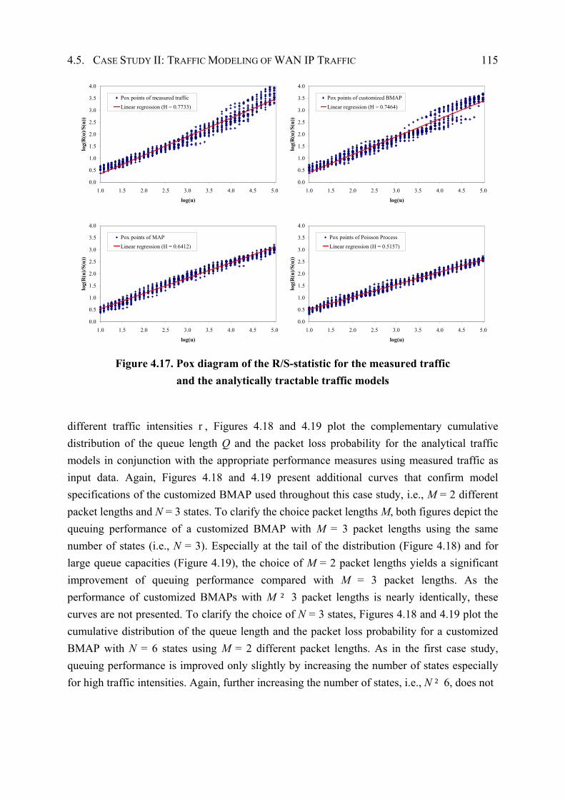
4.5. CASE STUDY II: TRAFFIC MODELING OF WAN IP TRAFFIC 115
0.0
0.5
1.0
1.5
2.0
2.5
3.0
3.5
4.0
1.0 1.5 2.0 2.5 3.0 3.5 4.0 4.5 5.0
log(u)
log(
R(u
)/S(u
))
Pox points of measured trafficLinear regression (H = 0.7733)
0.0
0.5
1.0
1.5
2.0
2.5
3.0
3.5
4.0
1.0 1.5 2.0 2.5 3.0 3.5 4.0 4.5 5.0
log(u)
log(
R(u
)/S(u
))
Pox points of customized BMAPLinear regression (H = 0.7464)
0.0
0.5
1.0
1.5
2.0
2.5
3.0
3.5
4.0
1.0 1.5 2.0 2.5 3.0 3.5 4.0 4.5 5.0
log(u)
log(
R(u
)/S(u
))
Pox points of MAPLinear regression (H = 0.6412)
0.0
0.5
1.0
1.5
2.0
2.5
3.0
3.5
4.0
1.0 1.5 2.0 2.5 3.0 3.5 4.0 4.5 5.0
log(u)
log(
R(u
)/S(u
))
Pox points of Poisson ProcessLinear regression (H = 0.5157)
Figure 4.17. Pox diagram of the R/S-statistic for the measured traffic and the analytically tractable traffic models
different traffic intensities r, Figures 4.18 and 4.19 plot the complementary cumulative distribution of the queue length Q and the packet loss probability for the analytical traffic models in conjunction with the appropriate performance measures using measured traffic as input data. Again, Figures 4.18 and 4.19 present additional curves that confirm model specifications of the customized BMAP used throughout this case study, i.e., M = 2 different packet lengths and N = 3 states. To clarify the choice packet lengths M, both figures depict the queuing performance of a customized BMAP with M = 3 packet lengths using the same number of states (i.e., N = 3). Especially at the tail of the distribution (Figure 4.18) and for large queue capacities (Figure 4.19), the choice of M = 2 packet lengths yields a significant improvement of queuing performance compared with M = 3 packet lengths. As the performance of customized BMAPs with M ² 3 packet lengths is nearly identically, these curves are not presented. To clarify the choice of N = 3 states, Figures 4.18 and 4.19 plot the cumulative distribution of the queue length and the packet loss probability for a customized BMAP with N = 6 states using M = 2 different packet lengths. As in the first case study, queuing performance is improved only slightly by increasing the number of states especially for high traffic intensities. Again, further increasing the number of states, i.e., N ² 6, does not
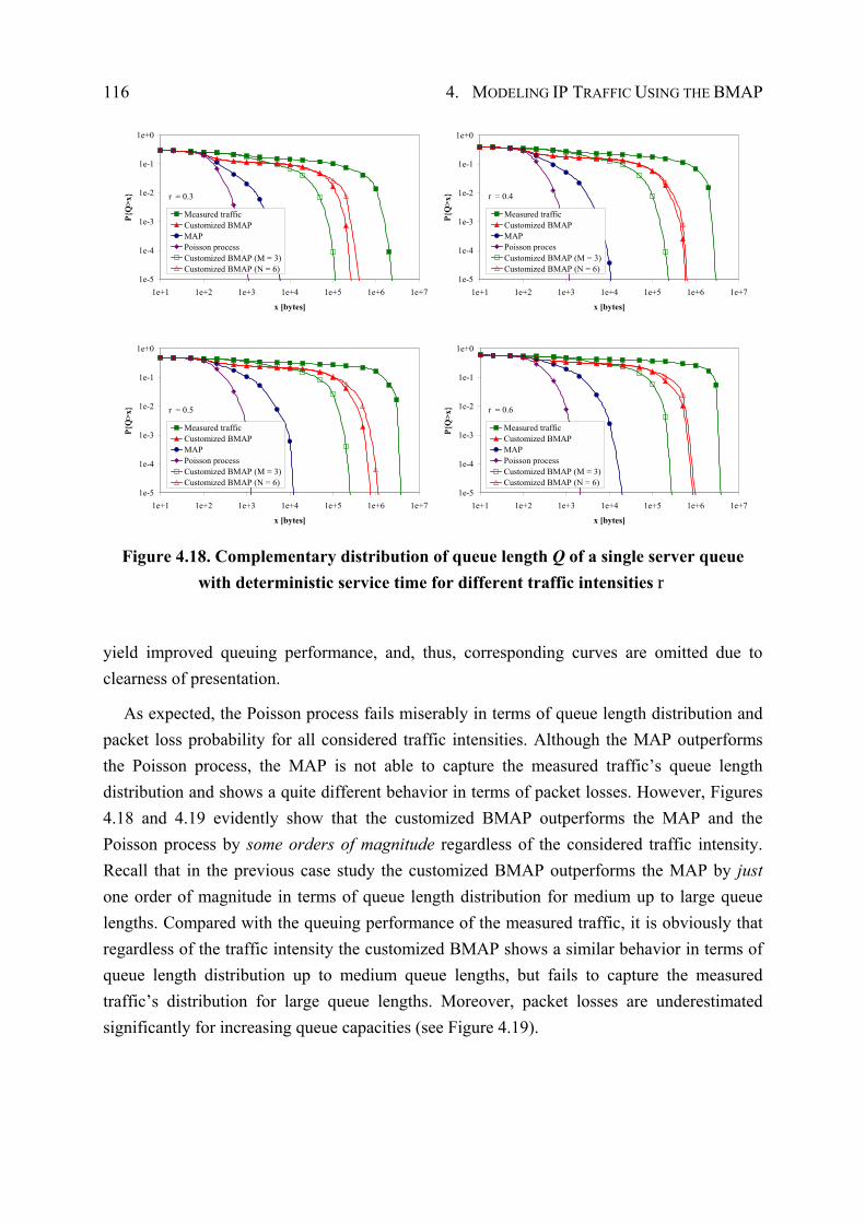
116 4. MODELING IP TRAFFIC USING THE BMAP
1e-5
1e-4
1e-3
1e-2
1e-1
1e+0
1e+1 1e+2 1e+3 1e+4 1e+5 1e+6 1e+7
x [bytes]
P{Q
>x}
Measured trafficCustomized BMAPMAPPoisson processCustomized BMAP (M = 3)Customized BMAP (N = 6)
r = 0.3
1e-5
1e-4
1e-3
1e-2
1e-1
1e+0
1e+1 1e+2 1e+3 1e+4 1e+5 1e+6 1e+7
x [bytes]
P{Q
>x}
Measured trafficCustomized BMAPMAPPoisson procesCustomized BMAP (M = 3)Customized BMAP (N = 6)
r = 0.4
1e-5
1e-4
1e-3
1e-2
1e-1
1e+0
1e+1 1e+2 1e+3 1e+4 1e+5 1e+6 1e+7
x [bytes]
P{Q
>x}
Measured trafficCustomized BMAPMAPPoisson processCustomized BMAP (M = 3)Customized BMAP (N = 6)
r = 0.5
1e-5
1e-4
1e-3
1e-2
1e-1
1e+0
1e+1 1e+2 1e+3 1e+4 1e+5 1e+6 1e+7
x [bytes]
P{Q
>x}
Measured trafficCustomized BMAPMAPPoisson processCustomized BMAP (M = 3)Customized BMAP (N = 6)
r = 0.6
Figure 4.18. Complementary distribution of queue length Q of a single server queue with deterministic service time for different traffic intensities r
yield improved queuing performance, and, thus, corresponding curves are omitted due to clearness of presentation.
As expected, the Poisson process fails miserably in terms of queue length distribution and packet loss probability for all considered traffic intensities. Although the MAP outperforms the Poisson process, the MAP is not able to capture the measured traffic’s queue length distribution and shows a quite different behavior in terms of packet losses. However, Figures 4.18 and 4.19 evidently show that the customized BMAP outperforms the MAP and the Poisson process by some orders of magnitude regardless of the considered traffic intensity. Recall that in the previous case study the customized BMAP outperforms the MAP by just one order of magnitude in terms of queue length distribution for medium up to large queue lengths. Compared with the queuing performance of the measured traffic, it is obviously that regardless of the traffic intensity the customized BMAP shows a similar behavior in terms of queue length distribution up to medium queue lengths, but fails to capture the measured traffic’s distribution for large queue lengths. Moreover, packet losses are underestimated significantly for increasing queue capacities (see Figure 4.19).
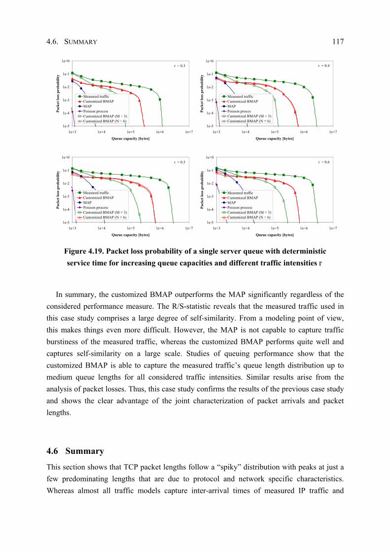
4.6. SUMMARY 117
1e-5
1e-4
1e-3
1e-2
1e-1
1e+0
1e+3 1e+4 1e+5 1e+6 1e+7
Queue capacity [bytes]
Pack
et lo
ss p
roba
bilit
y
Measured trafficCustomized BMAPMAPPoisson processCustomized BMAP (M = 3)Customized BMAP (N = 6)
r = 0.3
1e-5
1e-4
1e-3
1e-2
1e-1
1e+0
1e+3 1e+4 1e+5 1e+6 1e+7
Queue capacity [bytes]
Pack
et lo
ss p
roba
bilit
y
Measured trafficCustomized BMAPMAPPoisson procesCustomized BMAP (M = 3)Customized BMAP (N = 6)
r = 0.4
1e-5
1e-4
1e-3
1e-2
1e-1
1e+0
1e+3 1e+4 1e+5 1e+6 1e+7
Queue capacity [bytes]
Pack
et lo
ss p
roba
bilit
y
Measured trafficCustomized BMAPMAPPoisson processCustomized BMAP (M = 3)Customized BMAP (N = 6)
r = 0.5
1e-5
1e-4
1e-3
1e-2
1e-1
1e+0
1e+3 1e+4 1e+5 1e+6 1e+7
Queue capacity [bytes]
Pack
et lo
ss p
roba
bilit
y
Measured trafficCustomized BMAPMAPPoisson processCustomized BMAP (M = 3)Customized BMAP (N = 6)
r = 0.6
Figure 4.19. Packet loss probability of a single server queue with deterministic service time for increasing queue capacities and different traffic intensities r
In summary, the customized BMAP outperforms the MAP significantly regardless of the considered performance measure. The R/S-statistic reveals that the measured traffic used in this case study comprises a large degree of self-similarity. From a modeling point of view, this makes things even more difficult. However, the MAP is not capable to capture traffic burstiness of the measured traffic, whereas the customized BMAP performs quite well and captures self-similarity on a large scale. Studies of queuing performance show that the customized BMAP is able to capture the measured traffic’s queue length distribution up to medium queue lengths for all considered traffic intensities. Similar results arise from the analysis of packet losses. Thus, this case study confirms the results of the previous case study and shows the clear advantage of the joint characterization of packet arrivals and packet lengths.
4.6 Summary
This section shows that TCP packet lengths follow a “spiky” distribution with peaks at just a few predominating lengths that are due to protocol and network specific characteristics. Whereas almost all traffic models capture inter-arrival times of measured IP traffic and
118 4. MODELING IP TRAFFIC USING THE BMAP
assume an average packet length or draw packet lengths according to the empirical distribution of the measured traffic, the batch Markovian arrival process enables “two-dimensional”, i.e., joint, characterization of packet arrivals and packet lengths. Thus, the BMAP is able to capture (1) the packet arrival process, (2) the packet length process including spiky packet length characteristics, and (3) correlations between the packet arrival process and the packet length process. The key idea is to represent different packet lengths by different rewards, i.e., batch sizes of arrivals, of the BMAP. A scaling procedure is proposed that reduces the number of parameters dramatically without changing the BMAP’s quality. This is decisively for the practical utilization of parameterized BMAP in Markovian performance models, as the solution of these kinds of performance models primarily depends on the number of non-zero entries in the corresponding infinitesimal generator matrix of the underlying CTMC. Such a customized BMAP can be parameterized directly by means of the EM algorithm introduced in Section 3.
Case studies of TCP traffic with different degrees of self-similarity compare performance of the Poisson process, the MMPP, the MAP, and the customized BMAP by means of visual inspection of sample paths, by presenting important statistical properties, by formal analysis of self-similarity, and by investigations of queuing performance. Both case studies show the clear advantage of the customized BMAP over other analytically tractable traffic models and reveal that the difference between the customized BMAP on the one hand and the MAP, the MMPP, and the Poisson process on the other hand is enormously. Especially, results of queuing performance show that it is not sufficient to utilize state-of-the-art Markovian traffic models that just capture inter-arrival times (ignoring packet lengths completely) and assume an average packet length or draw packet lengths according to the empirical distribution of the measured traffic. Beyond these case studies, the joint characterization of packet arrivals and packet lengths using customized BMAPs has been utilized successfully in practice for aggregated traffic modeling of non real-time traffic in 3G mobile communication networks [KLL01].
119
5 Future Research Directions
HIS SECTION presents future directions of research concerning research areas examined in this thesis. The proposed QoS/revenue management scheme could be
extended such that real-time and non real-time services are considered jointly. As a first step into this research direction, a Markov model is outlined that considers packet level traffic of non real-time services, and an effective evaluation method is presented that utilizes special structures in the generator matrix of the underlying Markov chain. Moreover, it seems naturally to extend the introduced QoS/revenue management scheme towards emerging Beyond 3G mobile communication networks. Referring to the EM algorithm for parameter estimation of BMAPs, future research could investigate the determination of initial parameter sets, the acceleration of the EM algorithm itself, and the discrepancy between maximum likelihood and traffic burstiness. Moreover, it is outlined how an EM algorithm could be utilized for effective modeling the state of TCP connections in mobile ad-hoc networks.
5.1 Online QoS/Revenue Management of Non Real-Time Services
This thesis introduces a detailed Markov model for online QoS/revenue management of real-time services that incorporates a novel call admission control and bandwidth degradation scheme and considers important features of 3G cellular networks, such as CDMA intra- and inter-cell interference, different service classes, and soft handover. The compactness of this Markov model enables the online evaluation according to changing traffic load currently measured in the RAN. To enable online QoS/revenue management of both real-time and non real-time services, it seems naturally to enhance the QoS/revenue management scheme by non real-time services that are important in practice.
Whereas real-time services can be characterized by their required bandwidth (which is exclusively reserved due to delay-sensitivity) [CDZ02], [CS02], [DJK+00], [SDB+98], aggregated non real-time traffic is “bursty” in nature and, thus, requires characterization at packet level (see Section 4). Modeling packet traffic for each user session enlarges the Markov model enormously, and, thus, further research effort is required to derive a compact Markov model that considers (1) real-time and non real-time services and (2) important features of 3G mobile communication networks. To reach this challenging goal the following research issues have to be considered:
T
120 5. FUTURE RESEARCH DIRECTIONS
¶ Compact and detailed (Markovian) modeling of non real-time traffic at packet level
¶ Packet scheduling strategies for non real-time traffic of different service classes
¶ Development of a realistic Markov model for online QoS/revenue management that incorporates real-time and non real-time services
¶ Development of an effective evaluation method suitable for online evaluation of the Markov model
As shown in this thesis, it is not sufficient to utilize state-of-the-art Markovian traffic models that just capture inter-arrival times and assume uncorrelated packet lengths for each arrival. Thus, due to the scarce bandwidth in the radio access network, accurate stochastic modeling of byte-based traffic rates (i.e., bytes per time unit) is essentially. Based on this research result, accurate and compact modeling of non real-time traffic can be performed by BMAPs that are parameterized utilizing the proposed EM algorithm (see [KLL01] for details concerning the non real-time traffic model for 3G mobile communication networks). In order to distinguish different priorities of non real-time traffic corresponding to different service classes [3GPPc], the Markov model has to consider a tailored packet scheduling strategy [BLN99], [DJK+00]. In earlier work [LLT03], a mathematical framework for adaptive QoS/revenue management of real-time and non real-time services has been introduced that shows how packet scheduling of non real-time services can be effectively performed in practice. For online evaluation of the Markov model, highly efficient evaluation methods have to be derived that make use of special structures in the generator matrix underlying the Markov chain in order to reduce computational complexity.
The following outlines a first approach of an admission controller and its Markov model that exclusively considers non real-time packet level traffic. Special structures in the generator matrix are identified and an efficient evaluation method based on the linear level reduction is derived. However, this Markov model constitutes just a first step in the desired research direction and does not provide the solution of all research issues outlined above. Especially, packet scheduling for non real-time traffic of different service classes and byte-based modeling of non real-time traffic by means of a BMAP are not considered.
Queuing Model of the Admission Controller
In the queuing model of the admission controller, a base station serves a single cell. User requests for new non real-time sessions and handover requests from ongoing data sessions arrive according to a Poisson process with an overall rate lu. If the session is still active after the dwell time, a handover to an adjacent cell takes place. Dwell time and session duration are assumed to be exponentially distributed random variables with an overall rate mu of data
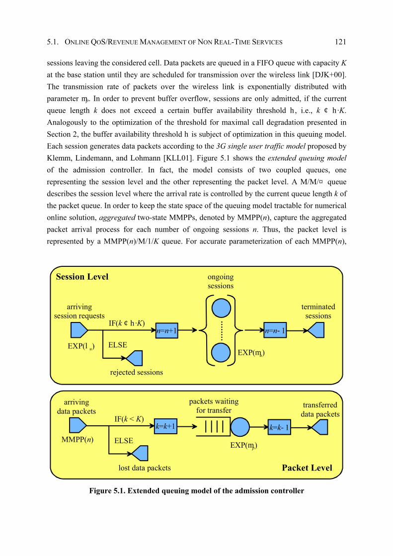
5.1. ONLINE QOS/REVENUE MANAGEMENT OF NON REAL-TIME SERVICES 121
sessions leaving the considered cell. Data packets are queued in a FIFO queue with capacity K at the base station until they are scheduled for transmission over the wireless link [DJK+00]. The transmission rate of packets over the wireless link is exponentially distributed with parameter mp. In order to prevent buffer overflow, sessions are only admitted, if the current queue length k does not exceed a certain buffer availability threshold h, i.e., k ¢ h·K. Analogously to the optimization of the threshold for maximal call degradation presented in Section 2, the buffer availability threshold h is subject of optimization in this queuing model. Each session generates data packets according to the 3G single user traffic model proposed by Klemm, Lindemann, and Lohmann [KLL01]. Figure 5.1 shows the extended queuing model of the admission controller. In fact, the model consists of two coupled queues, one representing the session level and the other representing the packet level. A M/M/¤ queue describes the session level where the arrival rate is controlled by the current queue length k of the packet queue. In order to keep the state space of the queuing model tractable for numerical online solution, aggregated two-state MMPPs, denoted by MMPP(n), capture the aggregated packet arrival process for each number of ongoing sessions n. Thus, the packet level is represented by a MMPP(n)/M/1/K queue. For accurate parameterization of each MMPP(n),
IF(k ¢ h·K)
ELSE
arrivingsession requests
ongoingsessions
EXP(lu)
terminatedsessions
rejected sessions
Session Level
EXP(mu)
n=n-1n=n+1
arrivingdata packets
MMPP(n)
transferreddata packets
ELSE
lost data packets Packet Level
EXP(mp)
k=k-1
packets waitingfor transfer
IF(k < K)k=k+1
Figure 5.1. Extended queuing model of the admission controller
122 5. FUTURE RESEARCH DIRECTIONS
the EM algorithm for BMAPs is applied for aggregated traffic streams each of which is given by the superposition of n individual traffic streams that utilize the 3G single user traffic model presented in [KLL01].
Efficient Numerical Analysis of the Queuing Model
The analysis of the queuing model is performed by means of a CTMC. A state of the queuing model representing the considered scenario is determined by the number of active data sessions n, the number of packets queued at the base station k, and the state of the aggregated two-state MMPP, i.e., MMPP(n). State transitions correspond to different kinds of events that may occur in the cell, i.e., incoming data sessions and handovers, outgoing data sessions due to completion or handover, arrivals of data packets, transfer of data packets, and state changes of the MMPP(n). Transition rates are obtained from the analysis of the system events. Without any restrictions, the number of active data sessions can be infinite, leading to an infinite number of states underlying the model. To make the model analytically tractable, the maximal number of active data sessions is restricted by an upper bound N. This bound must be chosen such that the effect is negligibly compared with the original model. Therefore, the session level model of Figure 5.1 is considered for h = 1, i.e., all session requests are accepted. Then, the session level model reduces to a simple M/M/N/N queuing system where a closed-form solution exists. In fact, the steady-state probability of N ongoing data sessions constitutes Erlang’s loss formula
0
( , )! !
N nN
Bn
A AE A NN n=
= ä (5.1)
with A = lu/mu the offered total traffic in Erlangs. EB(A, N) is monotonically decreasing in N. Thus, an upper bound N = N0 such that EB(A, N0) < e can be computed effectively [HMT01].
One can easily show that the CTMC underlying the queuing model is homogeneous and irreducible for any fixed threshold h (0 ¢ h ¢ 1). Thus, the steady state distribution ph can be computed by the matrix equation ph·Qh = 0 subject to the normalization condition |ph| = 1. Here, Qh denotes the infinitesimal generator matrix for threshold h. Due to the state space size of 2(N + 1)(K + 1) states, a straightforward solution of the matrix equation results in a computational effort that is not feasible for online evaluation. Moreover, the matrix equation has to be solved for several values h in order to find the optimal h value. Therefore, an efficient method based on linear level reduction utilizes the notion of special structures in the generator matrix [GJL84], [LR99]. With appropriate rearranging of the state space, the matrix Qh is of tri-diagonal structure with sub-matrices A, B, C, C , C0, and C 0 of dimension 2(N + 1). Matrices A and B are diagonal matrices comprising transition rates corresponding to an arrival and transfer of a data packet, respectively. Both matrices C and C contain
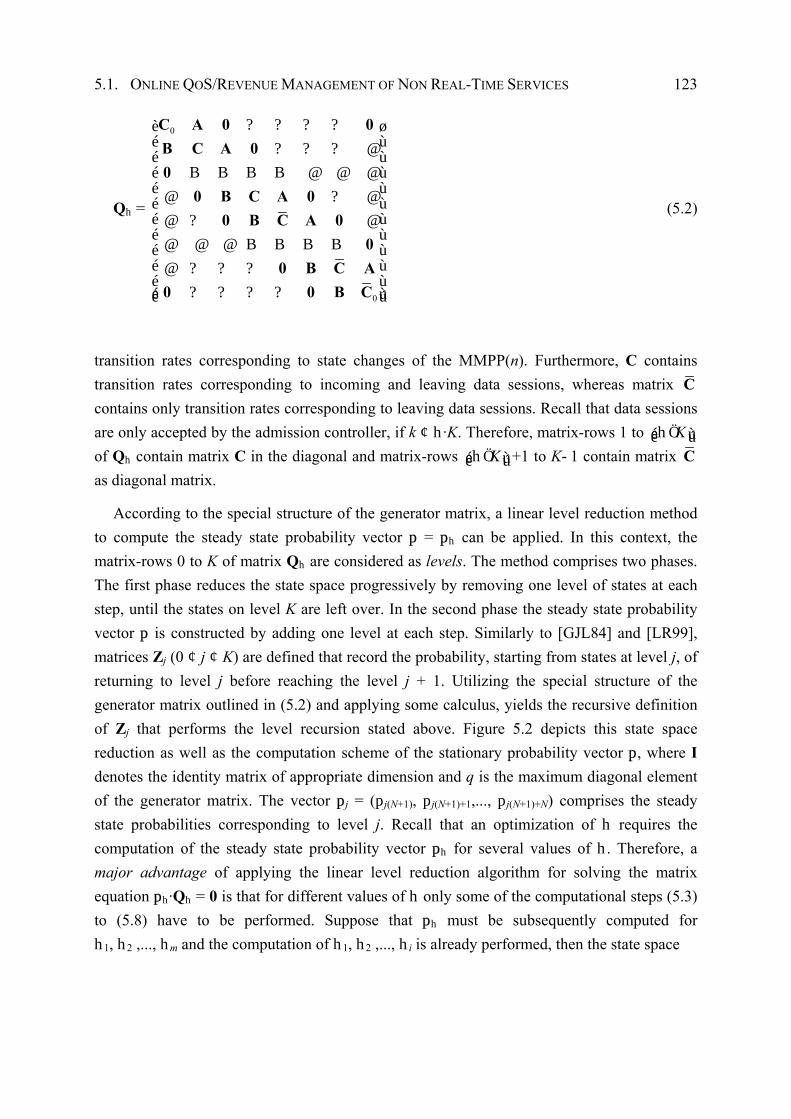
5.1. ONLINE QOS/REVENUE MANAGEMENT OF NON REAL-TIME SERVICES 123
Qh =
0
0
è øé ùé ùé ùé ùé ùé ùé ùé ùé ùé ùé ùê ú
C A 0 0B C A 00
0 B C A 00 B C A 0
00 B C A
0 0 B C
? ? ? ?? ? ? @
B B B B @ @ @@ ? @@ ? @@ @ @ B B B B@ ? ? ?? ? ? ?
(5.2)
transition rates corresponding to state changes of the MMPP(n). Furthermore, C contains transition rates corresponding to incoming and leaving data sessions, whereas matrix C contains only transition rates corresponding to leaving data sessions. Recall that data sessions are only accepted by the admission controller, if k ¢ h·K. Therefore, matrix-rows 1 to KhÖé ùê ú of Qh contain matrix C in the diagonal and matrix-rows KhÖé ùê ú +1 to K-1 contain matrix C as diagonal matrix.
According to the special structure of the generator matrix, a linear level reduction method to compute the steady state probability vector p = ph can be applied. In this context, the matrix-rows 0 to K of matrix Qh are considered as levels. The method comprises two phases. The first phase reduces the state space progressively by removing one level of states at each step, until the states on level K are left over. In the second phase the steady state probability vector p is constructed by adding one level at each step. Similarly to [GJL84] and [LR99], matrices Zj (0 ¢ j ¢ K) are defined that record the probability, starting from states at level j, of returning to level j before reaching the level j + 1. Utilizing the special structure of the generator matrix outlined in (5.2) and applying some calculus, yields the recursive definition of Zj that performs the level recursion stated above. Figure 5.2 depicts this state space reduction as well as the computation scheme of the stationary probability vector p, where I denotes the identity matrix of appropriate dimension and q is the maximum diagonal element of the generator matrix. The vector pj = (pj(N+1), pj(N+1)+1,..., pj(N+1)+N) comprises the steady state probabilities corresponding to level j. Recall that an optimization of h requires the computation of the steady state probability vector ph for several values of h. Therefore, a major advantage of applying the linear level reduction algorithm for solving the matrix equation ph·Qh = 0 is that for different values of h only some of the computational steps (5.3) to (5.8) have to be performed. Suppose that ph must be subsequently computed for h1, h2 ,..., hm and the computation of h1, h2 ,..., hi is already performed, then the state space
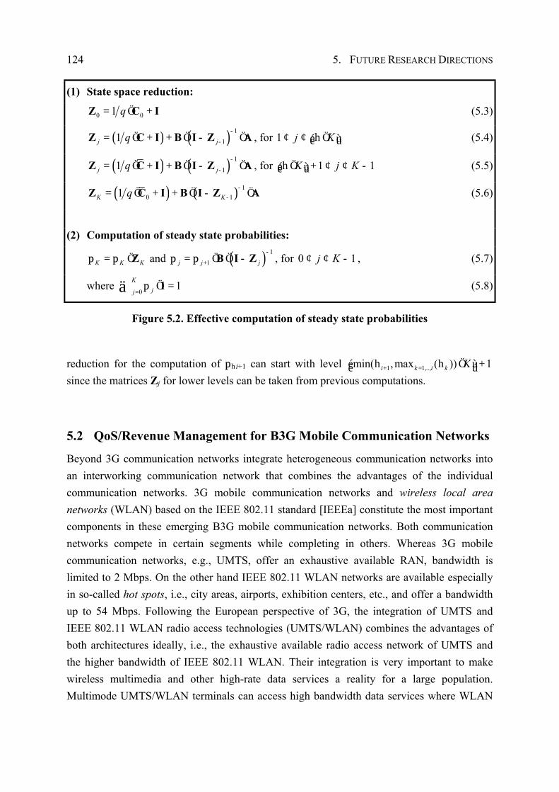
124 5. FUTURE RESEARCH DIRECTIONS
(1) State space reduction:
0 01 q= Ö +Z C I (5.3)
( ) ( ) 1
11j jq-
-= Ö + + Ö - ÖZ C I B I Z A , for 1 j K¢ ¢ hÖé ùê ú (5.4)
( ) ( ) 1
11j jq-
-= Ö + + Ö - ÖZ C I B I Z A , for 1 1K j KhÖ + ¢ ¢ -é ùê ú (5.5)
( ) ( ) 10 11K Kq -
-= Ö + + Ö - ÖZ C I B I Z A (5.6)
(2) Computation of steady state probabilities:
K K K= ÖZp p and ( ) 1
1j j j
-
+= Ö Ö -B I Zp p , for 0 1j K¢ ¢ - , (5.7)
where 0
1Kjj=Ö =ä 1p (5.8)
Figure 5.2. Effective computation of steady state probabilities
reduction for the computation of phi+1 can start with level 1 1,..,min( ,max ( )) 1i k i k K+ =h h Ö +é ùê ú since the matrices Zj for lower levels can be taken from previous computations.
5.2 QoS/Revenue Management for B3G Mobile Communication Networks
Beyond 3G communication networks integrate heterogeneous communication networks into an interworking communication network that combines the advantages of the individual communication networks. 3G mobile communication networks and wireless local area networks (WLAN) based on the IEEE 802.11 standard [IEEEa] constitute the most important components in these emerging B3G mobile communication networks. Both communication networks compete in certain segments while completing in others. Whereas 3G mobile communication networks, e.g., UMTS, offer an exhaustive available RAN, bandwidth is limited to 2 Mbps. On the other hand IEEE 802.11 WLAN networks are available especially in so-called hot spots, i.e., city areas, airports, exhibition centers, etc., and offer a bandwidth up to 54 Mbps. Following the European perspective of 3G, the integration of UMTS and IEEE 802.11 WLAN radio access technologies (UMTS/WLAN) combines the advantages of both architectures ideally, i.e., the exhaustive available radio access network of UMTS and the higher bandwidth of IEEE 802.11 WLAN. Their integration is very important to make wireless multimedia and other high-rate data services a reality for a large population. Multimode UMTS/WLAN terminals can access high bandwidth data services where WLAN
5.2. QOS/REVENUE MANAGEMENT FOR B3G MOBILE COMMUNICATION NETWORKS 125
coverage is offered, while accessing UMTS at other places. To make such multi-access solutions effective, an integrated solution that provides seamless mobility between both access technologies and continuity of existing sessions is required.
Seamless integration of these separately developed architectures is a research issue of current interest [3GPPb], [AHP03], [BCH+03], [LJK+03], [SFP02]. These and other research proposals suggest several degrees of coupling between UMTS and IEEE 802.11 WLAN starting with loosely coupled UMTS/WLAN networks up to tightly coupled UMTS/WLAN networks. In contrast to tightly coupled networks, interworking between loosely coupled UMTS/WLAN networks requires significant administration overhead. These distinct degrees of interworking have to be considered carefully during the development of QoS/revenue management strategies for B3G mobile communication networks. The research results and fundamental ideas for QoS/revenue management in 3G mobile communication networks proposed in this thesis and in [LLT02] and [LLT03] can also be adopted for QoS/revenue management in B3G mobile communication networks. Nevertheless, additional research effort is required for proper interworking of UMTS/WLAN networks. To successfully implement QoS/revenue management in B3G mobile communication networks the following research issues have to be considered in advance:
¶ Development of an adaptive inter-system handover management algorithm for optimal utilization of the available UMTS/WLAN radio resources
¶ Design of inter-system end-to-end QoS management mechanisms for UMTS/WLAN networks
¶ Development of adaptive inter-system call admission control mechanisms tailored to UMTS/WLAN networks
The following outlines some (novel) ideas concerning adaptive inter-system handover management, inter-system end-to-end QoS management, and adaptive call admission control for UMTS/WLAN networks. In [AHP03] and [KH03], ideas concerning other interworking aspects including authentication, security aspects, and billing mechanisms for coupled UMTS/WLAN networks are presented.
Inter-System Handovers
As outlined in the introduction of this thesis, handover management has been studied extensively for 3G mobile communication networks. However, heterogeneous UMTS/WLAN networks require additional effort for seamless inter-system handover management [MAB00], [PKH+00]. The objective for inter-system handovers is two-fold. Inter-system handover management mechanisms intend to guarantee continuity of existing sessions for forced
126 5. FUTURE RESEARCH DIRECTIONS
handoffs between heterogeneous RANs, e.g., an ongoing session leaves a WLAN network due to mobility. On the other hand, inter-system handovers should be triggered explicitly for currently overloaded RANs. This migration of ongoing sessions between UMTS and WLAN networks enables optimal usage of currently available UMTS/WLAN radio resources. Consequently, traffic is reduced in overloaded RANs temporarily and QoS demands of ongoing sessions can be fulfilled. Explicitly triggered inter-system handovers require additional administration (i.e., signalization) overhead dependent on the degree of interworking, i.e., loosely or tightly coupled UMTS/WLAN networks [3GPPb], [BCH+03]. Inter-system handover management research should focus the following research issues:
¶ Redistribution of ongoing UMTS and WLAN sessions with distinct QoS requirements on the available UMTS/WLAN radio resources
¶ Minimization of the administration overhead for loosely and tightly coupled UMTS/WLAN networks
The first research issue includes the definition of services with different UMTS/WLAN QoS requirements and requires the prioritization of individual users. The tradeoff between fulfilling QoS requirements and the administration overhead induced by inter-system handovers may be formalized as an optimization problem. Thus, the redistribution of ongoing calls is determined by the administration overhead and the effort required for solving such an optimization problem.
Inter-System End-To-End QoS
Inter-system end-to-end QoS management mechanisms constitute an important step towards developing adaptive inter-system call admission control mechanisms for UMTS/WLAN networks. This requires the utilization of QoS supporting technologies provided in each RAN. The IEEE 802.11 standard defines several medium access control (MAC) mechanisms to enable QoS in WLAN [IEEEb], [LAS03]. IEEE 802.11a/b defines QoS profiles with different priorities by means of a point coordinator function that coordinates the centralized allocation of access times for a considered WLAN access point. The IEEE 802.11e specification extends this standard by a distributed access method (enhanced distributed coordination function) with eight different priorities. On the other hand, the UMTS standard just defines four QoS classes, i.e., conversational, streaming, interactive, and background, but does not specify methods for technical implementation of these QoS classes within the UMTS radio access network [3GPPc]. Research issues concerning inter-system end-to-end QoS management are as follows:
5.3. FURTHER ENHANCEMENTS OF THE EM ALGORITHM FOR BMAPS 127
¶ Development of mechanisms to map UMTS QoS profiles onto IEEE 802.11 QoS profiles and vise versa
¶ Technical implementation of QoS profiles (comprising bandwidth-, delay-, and loss requirements) subject to UMTS/WLAN radio access technologies
The existence of different QoS profiles in UMTS and IEEE 802.11 requires the development of mechanisms to map UMTS QoS profiles onto IEEE 802.11 QoS profiles and vise versa [FM01]. These mechanisms are fundamental to enable end-to-end QoS and adaptive inter-system call admission control. Technical implementation of QoS profiles in UMTS can be performed by (1) explicit reservation of bandwidth, i.e., the session has guaranteed QoS, or (2) prioritized scheduling of data packet, i.e., QoS is granted relative to other current sessions.
Inter-System Call Admission Control
Similarly to 3G mobile communication networks, inter-system call admission control aims to guarantee QoS demands of ongoing sessions. Dependent on these QoS demands and the current traffic load in the UMTS/WLAN network, new call requests as well as intra- and inter-system handovers must be accepted or rejected. The admission strategies presented in this thesis and in [LLT02] and [LLT03] can be adopted appropriately, i.e., inter-system handover and inter-system end-to-end QoS, as mentioned above, have to be taken in consideration. Research concerning call admission control should focus the following research issues:
¶ Definition of control parameters for the admission controller that enables adaptive adjustment according to current traffic load in the UMTS/WLAN network
¶ Development of an adaptive call admission controller for real-time and non real-time data services that optimizes QoS and provider revenue for UMTS/WLAN networks
For integrated QoS/revenue management, the admission controller considers both QoS demands of the users and revenue earned by the provider and requires developing inter-system accounting strategies. The question arises which control parameters of the admission controller have to be adjusted adaptively to fulfill QoS and provider revenue demands.
5.3 Further Enhancements of the EM Algorithm for BMAPs
As evidently shown in Section 4, the EM algorithm for efficient and numerical stable parameter estimation of BMAPs works quite well in practice for real-world traffic traces. Nevertheless, the EM algorithm could be enhanced concerning the determination of the initial
128 5. FUTURE RESEARCH DIRECTIONS
parameter set. Future research could also investigate possibilities for further acceleration of the EM algorithm. Moreover, the discrepancy between the maximization of the likelihood and the maximization of traffic burstiness needs further research effort. In the following, some remarks and key literature pointers concerning these enhancements are given.
Acceleration of the EM Algorithm
Generally, the EM algorithm has been proven as numerically very stable when implemented carefully. However, extensive experience with parameter estimation of numerous stochastic processes, e.g., the MMPP [Ryd94], revealed that EM algorithms are slow compared with other methods for parameter estimation, e.g., Newton-type or gradient methods. It might be possible to speed up the EM algorithm by using acceleration methods [JJ93], [Lou82], [Mei89]. An acceleration method presented in [Mei89] has been implemented for the EM algorithm presented in this thesis. Roughly speaking, this acceleration method utilizes a fast minimal polynomial extrapolation method based on the last few estimates of the EM algorithm. But so far this acceleration method does not work out quite well, i.e., performance is increased only very slightly.
Determination of Initial Parameters
As described in Section 3, random initialization is used for determining initial parameter sets required by the EM algorithm. Recall that the initial parameter set for the EM algorithm is determined as the best (maximum likelihood) parameter set out of some random initial parameter sets. Performance curves presented in Section 3 and 4 demonstrate that in almost all cases different initial estimates result in a slightly different number of iterations required for convergence, whereas the quality of different estimated parameter sets is nearly identically. Nevertheless, in some rare cases random initialization results in (1) slow convergence behavior of the EM algorithm or (2) convergence in a local (likelihood) optimum. Especially for the MMPP, numerous approaches have been proposed that mainly utilize preconditioning according to moment matching, clustering, or heuristic methods [DM93], [Ryd96]. Moreover, some methods utilize the results of [Cum82] and [DL82] in order to determine initial parameter sets with decreasing values. Beside random initialization, none of these methods has currently been adopted for initialization of BMAP parameter sets.
Maximum Likelihood and Traffic Burstiness
As shown for MMPPs in [AR00], the EM algorithm ends up with the by far largest likelihood compared with other parameter estimation methods. On the other hand, the EM algorithm does not give the best fit with respect to queuing behavior and traffic burstiness. Similar
5.4. EM ALGORITHM FOR TCP OPTIMIZATION IN MANET 129
experience has been gained for BMAP parameter estimation, where BMAPs with a larger number of states result in larger likelihood estimates, but show nearly the same performance in terms of queuing behavior and traffic burstiness. This clearly indicates that it is not as simple as to look at the likelihood only for parameter estimation of bursty traffic traces. This tradeoff between the maximization of the likelihood and the maximization of the traffic burstiness needs further work. Following ideas proposed for MMPPs [AR00], [SVP03], [YKT01], different time scales of the measured traffic could be modeled by different, small BMAPs (each of which is estimated using the EM algorithm proposed in this thesis). Using the Kronecker sum Ä [Luc93], the superposition of these small BMAPs leads to a composed BMAP that may capture traffic burstiness even more accurately.
5.4 EM Algorithm for TCP Optimization in MANET
With the advent of WLAN based on the IEEE 802.11 standard, bandwidth has increased and prices have decreased rapidly for wireless networking solutions. Moreover, wireless communication is enabled not only in areas with explicit communication infrastructure, e.g., 3G mobile communication networks, but also in self-organizing mobile ad-hoc networks with connection to the Internet. Currently known variants of the reliable transport control protocol TCP show very poor performance in MANET environments. Thus, the development of a reliable transport protocol that performs well in hybrid environments consisting of a MANET based on IEEE 802.11 with Internet connection is a research issue of major concern [CXN03], [FZL+03], [LMC03].
TCP and its variants, e.g., TCP NewReno or TCP Vegas [SV03], have been developed for wireline networks and assume that packet losses are only due to network congestion. MANET specific problems, e.g., interference of neighboring single-hop connections and the hidden terminal problem, are not taken into consideration as reasons for packet losses. Additionally, packet losses in wireless MANET connections are more frequently than in wireline connections. As a consequence, the TCP control algorithm adjusts the size of the TCP transmission window according to the degree of packet losses irrespective of their reasons. A first approach towards performance optimization of TCP in MANET with Internet connection is to split TCP connections at the border of both network parts and consider both partial connections separately. Further approaches suggested in the scientific literature can roughly be divided into these two categories: (1) support by bottom layers of the TCP/IP protocol stack, where information concerning reasons of packet losses is transferred from bottom layers to the transport layer explicitly and (2) end-to-end optimizations, where all information taken into account for optimization is known at the connection’s end points.
130 5. FUTURE RESEARCH DIRECTIONS
The following outlines some key ideas of a novel approach for optimization of TCP connections in MANET with Internet connection. TCP connections in this kind of hybrid networks can be in different states that can effectively be characterized by round trip times (RTT) of packets measured at the sender-side of a TCP connection. Dependent on the current connection’s state, the various reasons of packet losses in MANET can be classified more preciously. A similar approach has been successfully utilized for mobile networks with single-hop connections [LMC03]. As a key component, a hidden Markov model (HMM) captures different states of a TCP connection by distinct states of the HMM and describes state transitions by individual probability distributions. Thus, reasons of packet losses can be differentiated according to the HMM’s current state. This enables the sender of a connection to adjust TCP parameters, e.g., size of the TCP transmission window and/or TCP retransmission timeout, adaptively according to the connection’s current state. To implement this approach the following research issues have to be considered:
¶ Definition of the HMM, i.e., definition of its states representing a TCP connection’s states and definition of the probability distributions for state transitions
¶ Development of an EM algorithm for parameter estimation of the HMM
¶ Offline training of the HMM utilizing the EM algorithm
¶ Online state interference using the parameterized HMM and a Viterbi algorithm
In previous approaches, only Gaussian distributions are utilized for state transitions because of mathematical tractability concerning parameter estimation of the underlying HMM. As the BMAP encompasses a wide range of processes as special cases, the algorithmic framework for parameter estimation of BMAPs presented in this thesis may be utilized for developing tailored EM algorithms for complex HMMs that characterize a TCP connection’s state. Therefore, the HMM can reflect the state of a TCP connection more precisely. Utilizing the EM algorithm, the HMM is trained offline (i.e., parameterized) according to observations, i.e., RTTs of packets, gathered in detailed MANET simulation studies. The nature of these simulation studies allows identifying the reasons of packet losses (and its RTTs) and, thus, enables accurate parameterization of the HMM. The Viterbi algorithm [Rab89] tries to seek the most likely state sequence (of the parameterized HMM) for a given sequence of observations, i.e., RTTs of packets, gathered online during TCP data transmission. This enables the TCP control algorithm of the sender to estimate the TCP connection’s current state and to adopt TCP parameters accordingly. Compared with other approaches for TCP optimization in MANET, a major benefit is the compatibility with existing TCP implementations, i.e., TCP has to be modified only in the TCP layer of the sender. Thus, this approach is also suitable for TCP connections between MANET and the Internet.
131
6 Concluding Remarks
HIS THESIS presents novel research results concerning online QoS/revenue management for 3G mobile networks and traffic modeling of IP networks. The proposed
online QoS/revenue management scheme outperforms existing admission control policies significantly and has been published in [LLT04]. It is based on earlier work for integrated QoS/revenue management [LLT02], [LLT03]. The proposed EM algorithm is the first numerical robust parameter estimation procedure for BMAPs and has been published in [KLL03]. Moreover, this thesis shows how to utilize the BMAP for accurate modeling of measured IP traffic, which has been published (with distinct objectives) in [KLL01] and [KLL02]. The following sums up major research results presented in this thesis and gives concluding remarks.
Online QoS/Revenue Management for 3G Mobile Communication Networks
The development of an online QoS and revenue management for 3G mobile communication networks is a challenging task that requires closing the loop between network operation and network control. Moreover, the joint consideration of both QoS and provider revenue is a quite novel research area for 3G mobile networks. Because of missing specifications in 3G standards [3GPPc], practical implementation of management schemes within a RAN has to be taken into consideration carefully. To take a first step in this research direction, Lindemann, Lohmann, and Thümmler proposed a mathematical framework for adaptive QoS/revenue management of real-time and non real-time services [LLT03]. Adaptive control of the mobile network’s system parameters is performed by means of closed-form formulas dependent on online monitored QoS measures. Compared with earlier work [LLT02], the closed-form formulas enable an intuitive adjustment of the adaptive control mechanisms and can easily be adapted to changing configurations of 3G mobile communication networks.
Based on experiences gathered during developing this mathematical framework for adaptive QoS/revenue management, this thesis shows how online management of both QoS and provider revenue can be performed in 3G mobile networks by adaptive control of system parameters to changing traffic conditions. As a main result, this approach is based on a novel call admission control and bandwidth degradation scheme for real-time traffic. The admission controller considers real-time calls with two priority levels. Whereas calls of low priority can be temporarily degraded to a lower bit-rate, calls of high priority have a guaranteed bit-rate.
T
132 6. CONCLUDING REMARKS
The key idea is to reduce handover failure probability due to call degradation of low-priority calls. A Markov model for the admission controller enables the periodical adjustment of the admission controller’s system parameter (i.e., the threshold for maximal call degradation) according to the currently measured traffic in the RAN and a predefined goal for optimization.
It is shown that a dedicated soft handover queue can decrease handover failure probability significantly (see Figure 2.9), whereas the overload of cell capacity induced by this queue is marginally compared with its benefits (see Figure 2.10). Moreover, this thesis describes how to embed the proposed QoS/revenue management scheme in existing 3G base station controllers and illustrates the effectiveness of the proposed approach in practice. Using distinct optimization goals, performance studies evidently demonstrate that QoS and provider revenue can be increased significantly with a moderate average call degradation of low-priority calls (see Figures 2.14 to 2.19). Compared with previous work [CS02], [MHT02], this degradation scheme performs degradation gracefully in multiple steps and degrades all calls of low priority equally, i.e., fairness among calls of low priority is granted. Detailed investigations show that the proposed graceful degradation of bandwidth utilizes currently available CDMA cell capacity significantly better than other approaches based on the (adaptive) guard channel scheme (see Figures 2.23 and 2.24). In fact, guard channel schemes induce a high probability of rejecting new call requests, although bandwidth is still available, i.e., guard channels are (partially) unused. In summary, graceful degradation of bandwidth has proven as the method of choice for prioritization of handover calls in 3G networks with different QoS classes and call priorities.
Beside the exclusive consideration of real-time services, the mathematical framework for QoS/revenue management introduced in [LLT03] and the online QoS/revenue management scheme presented in this thesis differ significantly. Whereas the mathematical framework uses monitored QoS measures (based on several control periods), the online QoS/revenue management scheme utilizes currently measured traffic parameters as input for the adaptive control mechanism. Measured traffic parameters as input for adaptive control are practicable for traffic parameters with small or medium variation only, e.g., measured arrival rates of new call requests or average call duration. Additionally, the mathematical framework [LLT03] does not take into consideration important features of 3G mobile communication networks, such as CDMA intra- and inter-cell interference and soft handover. However, as fundamental difference, the online QoS/revenue management scheme optimizes the considered system parameter of the admission controller in each control period, whereas the mathematical framework is only capable to approximate the optimal values of the considered system parameters based on QoS measures monitored over several control periods.
6. CONCLUDING REMARKS 133
Modeling IP Traffic Using the Batch Markovian Arrival Process
The previous section presents some ideas of how to extend the proposed online QoS/revenue management scheme towards consideration of both real-time and non real-time services. As a key component, analytically tractable (i.e. Markovian) models for non real-time traffic are required. As aggregated non real-time traffic is “bursty” in nature, such Markovian traffic models require traffic characterization at packet level. Due to the scarce bandwidth in the radio access network, very accurate stochastic modeling of byte-based traffic rates (i.e., bytes per time unit) is essentially. Otherwise, results, gathered in performance studies of 3G mobile networks, may be misleading and, thus, may lead to significant performance losses during the operation of 3G networks in practice. This thesis identifies the batch Markovian arrival process as the analytically tractable model of choice for the joint characterization of packet arrivals and packet lengths. As a key idea, the BMAP is customized such that different packet lengths are represented by batch sizes of arrivals. Opposed to other (Markovian) traffic models, the BMAP enables the “two-dimensional”, i.e., joint, characterization of packet arrivals and packet lengths, and is able to capture correlations between the packet arrival process and the packet length process.
For effective parameterization of BMAPs according to measured IP traffic, this thesis presents a novel EM algorithm. In fact, this is the first numerical robust parameter estimation procedure for BMAPs published in scientific literature. Previous known EM-based parameter estimation procedures for special cases of the BMAP are numerically unstable, e.g., the EM algorithm for parameter estimation of MMPPs proposed by Ryden in [Ryd96]. Thus, it is shown how to utilize the randomization technique and a stable calculation of Poisson jump probabilities effectively to compute time-dependent conditional expectations of a CMTC required by the expectation step of the EM algorithm. This methodological work enables the EM algorithm to be both efficient and numerical robust with a computational complexity given by O(n·l3/2·N2) for an EM iteration. As BMAPs encompass (as special cases) both phase-type renewal processes, e.g., Erlang and hyperexponential renewal processes, and non-renewal processes such as the MMPP, and many other processes in the applied probability literature, the presented EM algorithm constitutes an important step towards effective, analytically tractable traffic models. In fact, the numerical robust parameter estimation framework is not restricted to BMAPs only, but can also be applied for a wide range of HMMs that require the joint characterization of arrivals and rewards.
The proposed EM algorithm jointly captures the packet arrival process and the packet length process of measured traffic (already during parameter estimation) and, thus, considers correlation structures between packet arrivals and packet lengths that are due to protocol and network specific characteristics. A scaling procedure is proposed that reduces the number of
134 6. CONCLUDING REMARKS
parameters dramatically without changing the BMAP’s quality. This is decisively for the practical utilization of parameterized BMAP in Markovian performance models, as the solution of these kinds of performance models primarily depends on the number of non-zero entries in the corresponding infinitesimal generator matrix of the underlying CTMC. Case studies of TCP traffic with different degrees of self-similarity evidently demonstrate the advantages of the BMAP modeling approach over other widely used analytically tractable models, e.g., the MMPP or the MAP. In fact, these case studies illustrate the impact of modeling packet lengths and its correlations with packet arrivals and, thus, reveal that joint characterization of packet arrivals and packet lengths is decisively for realistic IP traffic modeling. Especially, for an accurate prediction of the queuing behavior joint characterization is of major importance (e.g., see Figures 4.9, 4.10, 4.18, and 4.19).
Recently, Salvador, Pacheco, and Valadas utilized the ideas for the joint characterization of packet arrivals and packet lengths presented in this thesis and proposed a parameter estimation algorithm for discrete-time BMAPs [SPV04]. Their parameter estimation procedure matches the packet arrival process exactly (at the expense of a enormous large number of states) and additionally estimates corresponding batch sizes, i.e., packet lengths. The large number of states and parameters of estimated discrete-time BMAP limit the practical applicability of this approach. Nevertheless, in agreement with this thesis, their research results reveal that packet arrivals and packet lengths show strong correlations. This emphasizes the conclusions drawn in this thesis and shows the necessity of the joint characterization of packet arrivals and packet lengths for accurate prediction of queuing performance in IP-based networks.
Thus, it seems that modeling IP traffic is more than just capturing the packet arrival process accurately (ignoring packet lengths completely) and to assume an average packet length or to draw packet lengths according to the empirical distribution of the measured traffic. With the advent IPv6 [DH98], the importance of joint characterization of packet arrivals and packet lengths may increase even more, as packet lengths in IPv6 may become considerable large (i.e., jumbograms with more than 64 kbytes), and correlations due to protocol and network specific characteristics will exist further. As very few works have addressed the packet length process, and, especially, the joint characterization of the packet arrival process and the packet length process [GR99], [SPV04], this research area shows significant research potential and is considered to gather considerable attention in future. Section 5 gives some hints of how to improve the proposed parameter estimation procedure such that different time scales of packet arrivals could be modeled by different, small BMAPs (each of which is estimated using the EM algorithm proposed in this thesis). For practical applicability, Markovian performance models may utilize BMAPs in an approximately

6. CONCLUDING REMARKS 135
fashion such that packets are not represented by their exact (i.e., byte-based) length, but packet lengths are given as a multiple of the minimal packet length. As a consequence, the complexity of performance models would be reduced significantly. Assuming a minimal packet length of 40 bytes, these packets would get a length (i.e., batch size) of one, whereas, for example, packets 400 bytes in size would get a length of ten. For intermediate packet lengths, this would result in some kind of inaccuracy, but, nevertheless, correlations between packet arrivals and packet lengths of different extents of would be kept. Of course, this needs further intensive research effort.

137
References
[3GPPa] Third Generation Partnership Project (3GPP), http://www.3gpp.org.
[3GPPb] 3GPP, Feasibility Study on 3GPP System to Wireless Local Area Network (WLAN) Interworking, Technical Specification TR 22.934, 2003.
[3GPPc] 3GPP, QoS Concept and Architecture, Technical Specification TS 23.107, 2002.
[3GPP2] Third Generation Partnership Project Number 2 (3GPP-2), http://www.3gpp2.org.
[AFT+00] P. Abry, P. Flandrin, M.S. Taqqu, and D. Veitch, Wavelet for the Analysis, Estimation and Synthesis on Scaling Data, in: K. Park and W. Willinger (Eds.), Self-Similar Network Traffic and Performance Evaluation, John Wiley & Sons, pp. 39-88, 2000.
[AHP03] K. Ahmavaara, H. Haverinen, and R. Pichna, Internetworking Architecture Between 3GPP and WLAN Systems, IEEE Comm. Magazine 41, pp. 74-81, 2003.
[AMM+00] M. Ajmone Marsan, S. Marano, C. Mastroianni, and M. Meo, Performance Analysis of Cellular Mobile Communication Networks Supporting Multimedia Services, Mobile Networks and Applications 5, pp. 167-177, 2000.
[AN98] A.T. Andersen and B. F. Nielsen, A Markovian Approach for Modeling Packet Traffic with Long-Range Dependence, IEEE Journal on Selected Areas in Comm. 16, pp. 719-732, 1998.
[ANO96] S. Asmussen, O. Nerman, and M. Olsson, Fitting Phase-type Distributions via the EM Algorithm, Scandinavian Journal of Statistics 23, pp. 419-441, 1996.
[AR00] S. Andersson and T. Ryden, Maximum Likelihood Estimation of a Structured MMPP with Applications to Traffic Modeling, Proc. 13th ITC Specialist Seminar on Measurement and Modeling of IP Traffic, Monterey, CA, pp. 20.1-20.10, 2000.
[Bau72] L.E. Baum, An Inequality and Associated Maximization Technique in Statistical Estimation for Probabilistic Functions of a Markov Process, Inequalities 3, pp. 1-8, 1972.
138 REFERENCES
[BCH+03] M. Buddhikot, G. Chandranmenon, S. Han, Y.W. Lee, S. Miller, and L. Salgarelli, Integration of IEEE 802.11 and Third-Generation Wireless Data Networks, Proc. 22nd IEEE Conf. on Computer Comm. (Infocom ’03), San Francisco, pp. 503-512, 2003.
[BE67] L.E. Baum and J.A. Eagon, An Inequality with Applications to Statistical Estimation for Probabilistic Functions of Markov Processes and to a Model for Ecology, Bulletin of the American Mathematical Society 73, pp. 360-363, 1967.
[BGM+98] E. Berruto, M. Gudmundson, R. Menolascino, W. Mohr, and M. Pizarroso, Research Activities on UMTS Radio Interface, Network Architectures, and Planning, IEEE Comm. Magazine 36, pp. 82-95, 1998.
[BHM87] R.F. Botta, C.M. Harris, and W.G. Marchal, Characterizations of Generalized Hyperexponential Distribution Functions, Comm. in Statistics: Stochastic Models 3, pp. 115-148, 1987.
[BLN99] V. Bharghavan, S. Lu, and T. Nandagopal, Fair Queuing in Wireless Networks: Issues and Approaches, IEEE Personal Comm. 6, pp. 44-53, 1999.
[BPR80] I. Basawa and B.L.S. Prakasa Rao, Statistical Interference for Stochastic Processes, Academic Press, 1980.
[BPS+70] L.E. Baum, T. Petrie, G. Soules, and N. Weiss, A Maximization Technique Occurring in the Statistical Analysis of Probabilistic Functions of Markov Chains, Annals of Mathematical Statistics 41, pp. 164-171, 1970.
[BST+95] J. Beran, R. Sherman, M.S. Taqqu, and W. Willinger, Long-Range Dependence in Variable-Bit-Rate Video Traffic, IEEE Trans. on Comm. 43, pp. 1565-1579, 1995.
[CB97] M.E. Crovella and A. Bestavros, Self-Similarity in World Wide Web traffic: Evidence and Possible Causes, IEEE/ACM Trans. on Networking 5, pp. 835-846, 1997.
[CDJ+91] R. Caceres, P. Danzig, S. Jamin, and D. Mitzel, Characteristics of Wide-Area TCP/IP Conversations, Proc. ACM Special Interest Group Data Comm. (SIGCOMM ’91), Zürich, Switzerland, pp. 101-112, 1991.
[CDZ02] I. Chlamtac, S.K. Das, and G. Záruba, A Prioritized Real-Time Wireless Call Degradation Framework for Optimal Call Mix Selection, Mobile Networks and Applications 7, pp. 143-151, 2002.
[CL01] A.T. Campbell and R.R.-F. Liao, A Utility-Based Approach for Quantitative Adaptation in Wireless Packet Networks, Wireless Networks 7, pp. 541-557, 2001.
REFERENCES 139
[Cox84] D.R. Cox, Long-Range Dependence: A Review, in: H.A. David and H.T. David (Eds.), Statistics: An Appraisal, Iowa State University Press, pp. 55-74, 1984.
[CS00] S. Choi and K.G. Shin, A Comparative Study of Bandwidth Reservation and Admission Control Schemes in QoS-Sensitive Cellular Networks, Wireless Networks 6, pp. 289-305, 2000.
[CS02] C.T. Chou and K.G. Shin, Analysis of Combined Adaptive Bandwidth Allocation and Admission Control in Wireless Networks, Proc. 21th IEEE Conf. on Computer Comm. (Infocom ’02), New York, pp. 676-684, 2002.
[Cum82] A. Cumani, On the Canonical Representation of Homogenous Markov Processes Modeling Failure-Time Distributions, Microelectronics Reliability 22, pp. 583-602, 1982.
[CXN03] K. Chen, Y. Xue, and K. Nahrstedt, On Setting TCP’s Congestion Window Limit in Mobile Ad Hoc Networks, Proc. 38th Int. IEEE Conf. on Comm. (ICC ’03), Anchorage, Alaska, 2003.
[DaS00] L.A. DaSilva, Pricing for QoS-Enabled Networks: A Survey, IEEE Comm. Surveys and Tutorials 3, pp. 2-8, 2000.
[DGA01] S. Dixit, Y. Guo, and Z. Antoniou, Resource Management and Quality of Service in Third-Generation Wireless Networks, IEEE Comm. Magazine 39, pp. 125-133, 2001.
[DGN+98] E. Dahlman, B. Gudmundson, M. Nilsson, and J. Sköld, UMTS/IMT-2000 Based on Wideband CDMA, IEEE Comm. Magazine 36, pp. 70-80, 1998.
[DH98] S. Deering and R. Hinden, Internet Protocol, Version 6 (IPv6) Specification, IETF Request for Comments 2460, http://www.ietf.org/rfc/rfc2460.txt, 1998.
[DJK+00] S.K. Das, R. Jayaram, N.K. Kakani, and S.K. Sen, A Call Admission and Control Scheme for Quality-of-Service Provisioning in Next Generation Wireless Networks, Wireless Networks 6, pp. 17-30, 2000.
[DL82] M. Dehon and G. Latouch, A Geometric Interpretation of the Relations between the Exponential and the Generalized Erlang Distributions, Advances in Applied Probability 14, pp. 885-897, 1982.
[DLR77] A.P. Dempster, N.M. Laird, and D.B. Rubin, Maximum Likelihood from Incomplete Data via the EM Algorithm, Journal of the Royal Statistical Society 39, pp. 1-38, 1977.
[DM93] L. Deng and J.W. Mark, Parameter Estimation for Markov-Modulated Poisson Processes via the EM Algorithm with Time-Discretization, Telecomm. Systems 1, pp. 321-338, 1993.
140 REFERENCES
[EE99a] J.S. Evans and D. Everitt, Effective Bandwidth-Based Admission Control for Multiservice CDMA Cellular Networks, IEEE Trans. on Vehicular Technology 48, pp. 36-46, 1999.
[EE99b] J.S. Evans and D. Everitt, On the Teletraffic Capacity of CDMA Cellular Networks, IEEE Trans. on Vehicular Technology 48, pp. 153-165, 1999.
[ENW96] A. Erramilli, O. Narayan, and W. Willinger, Experimental Queueing Analysis with Long-Range Dependent Packet Traffic, IEEE/ACM Trans. on Networking 4, pp. 209-223, 1996.
[ES95] A. Erramilli and R.P. Singh, An Application of Deterministic Chaotic Maps to Model Packet Traffic, Queueing Systems 20, pp. 171-206, 1995.
[ETSI] ETSI, Universal Mobile Telecommunication System (UMTS), Selection Procedures for the Choice of Radio Transmission Technologies of the UMTS, Technical Report TR 101 112 v3.2.0, 1998.
[EVB01] J. Eberspächer, H.J. Vögel, and C. Bettstetter, GSM – Switching, Services and Protocols, Second Edition, John Wiley & Sons, 2001.
[FG88] B.L Fox and P.W. Glynn, Computing Poisson Probabilities, Comm. of the ACM 31, pp. 440-445, 1988.
[FGW98] A. Feldmann, A.C. Gilbert, and W. Willinger, Data Networks as Cascades: Investigating the Multifractal Nature of Internet WAN Traffic, Proc. ACM Special Interest Group Data Comm. (SIGCOMM ’98), Vancouver, Canada, pp. 42–55, 1998.
[FJ99] F. Barceló and J. Jordán, Channel Holding Time Distribution in Public Cellular Telephony, Proc. 16th Int. Teletraffic Congress, Edinburgh, Scotland, pp. 107-116, 1999.
[FM01] S. Faizullah and I. Marsic, Charging for QoS in Internetworks, Proc. IEEE Global Telecomm. Conf. (Globecom ’01), Multimedia and Information Technology Symposium, San Antonio, TX, pp. 1957-1962, 2001.
[FMH93] W. Fischer and K. Meier-Hellstern, The Markov-Modulated Poisson Process (MMPP) Cookbook, Performance Evaluation 18, pp. 149-171, 1993.
[Fow97] M. Fowler, UML Distilled: Applying the Standard Object Modeling Language, Addison-Wesley, 1997.
[FZL+03] Z. Fu, P. Zerfos, H. Lu, L. Zhang, and M. Gerla, The Impact of Multihop Wireless Channel on TCP Throughput and Loss, Proc. 22nd IEEE Conf. on Computer Comm. (Infocom ’03), San Francisco, California, 2003.
REFERENCES 141
[GB99] M. Grossglauser and J.C. Bolot, On the Relevance of Long-Range Dependence in Network Traffic, IEEE/ACM Trans. on Networking 7, pp. 629-640, 1999.
[GJL84] D.P. Gaver, P.A. Jacobs, and G. Latouche, Finite Birth-And-Death Models in Randomly Changing Environments, Advances in Applied Probability 16, pp. 715-731, 1984.
[GJP+91] K.S. Gilhousen, I.M. Jacobs, R. Padovani, A.J. Viterbi, L.A. Weaver, and C.E. Wheatley, On the Capacity of a Cellular CDMA System, IEEE Trans. on Vehicular Technology 40, pp. 303-312, 1991.
[GM84] D. Gross and D.R. Miller, The Randomization Technique as a Modeling Tool and Solution Procedure for Transient Markov Processes, Operations Research 32, pp. 345-361, 1984.
[GR99] J. Gao and I. Rubin, Multifractal Analysis and Modeling of Long-Range Dependent Traffic, Proc. 34th Int. IEEE Conf. on Comm. (ICC ’99), Vancouver, Canada, pp. 382-386, 1999.
[Gra77] W. Grassmann, Transient Solution of Markov Queues, European Journal of Operations Research 1, pp. 396-402, 1977.
[GSW95] A. Gupta, D.O. Stahl, and A.B. Whinston, Priority Pricing of Integrated Services Networks, in: L. McKnight and J. Bailey (Eds.), Internet Economics, MIT Press, pp. 323-378, 1995.
[GW94] M.W. Garrett and W. Willinger, Analysis, Modeling and Generation of Self-Similar VBR Video Traffic, Proc. ACM Special Interest Group Data Comm. (SIGCOMM ’94), London, UK, pp. 269-280, 1994.
[HMT01] G. Haring, R. Marie, and K.S. Trivedi, Loss Formulas and Their Application to Optimization for Cellular Networks, IEEE Trans. on Vehicular Technology 50, pp. 664-673, 2001.
[Hur51] H.E. Hurst, Long Term Storage Capacity of Reservoirs, Trans. of the American Society of Civil Engineers 116, pp. 770-799, 1951.
[IEEEa] IEEE 802.11 WG, http://grouper.ieee.org/groups/802/11/.
[IEEEb] IEEE Computer Society LAN MAN Standards Committee, Wireless LAN Medium Access Control (MAC) and Physical Layer (PHY) Specifications, IEEE Standard 802.11-1997, 1997.
[ITA] The Internet Traffic Archive, http://ita.ee.lbl.gov.
[ITU] International Telecommunication Union (ITU), http://www.itu.int.
142 REFERENCES
[JJ93] M. Jamshidian and R.I. Jennrich, Conjugate Gradient Acceleration of the EM Algorithm, Journal of the American Statistical Association 88, pp. 221-228, 1993.
[JMW97] D.L. Jagerman, B. Melamed, and W. Willinger, Stochastic Modeling of Traffic Processes, in: J. Dshalalow (Edr.), Frontiers in Queuing: Models, Methods and Problems, CRC Press, pp. 271-370, 1997.
[KAL+01] H. Kaaranen, A. Ahtiainen, L. Laitinen, S. Naghian, and V. Niemi, UMTS Networks, Architecture, Mobility and Services, John Wiley & Sons, 2001.
[KH03] G.M. Koien and T. Haslestad, Security Aspects of 3G-WLAN Interworking, IEEE Comm. Magazine 41, pp. 82-88, 2003.
[KJ01] J. Kim and A. Jamalipour, Traffic Management and QoS Provisioning in Future Wireless IP Networks, IEEE Personal Comm. 8, 46-55, 2001.
[KLL01] A. Klemm, C. Lindemann, and M. Lohmann, Traffic Modeling and Characterization for UMTS Networks, Proc. IEEE Global Telecomm. Conf. (Globecom ’01), Internet Performance Symposium, San Antonio, TX, pp. 1741-1746, 2001.
[KLL02] A. Klemm, C. Lindemann, and M. Lohmann, Traffic Modeling of IP Networks Using the Batch Markovian Arrival Process, Proc. 12th Int. Conf. on Modeling Tools and Techniques for Computer and Comm. System Performance Evaluation (Tools ’02), Lecture Notes in Computer Science (LNCS) 2324, pp. 92-110, Springer-Verlag, 2002.
[KLL03] A. Klemm, C. Lindemann, and M. Lohmann, Modeling IP Traffic Using the Batch Markovian Arrival Process, Performance Evaluation 54, pp. 149-173, 2003.
[KM98] M. Krunz and A. Makowski, A Source Model for VBR Video Traffic Based on M/G/¤ Input Processes, Proc. 17th IEEE Conf. on Computer Comm. (Infocom ’98), San Francisco, CA, pp. 1441-1448, 1998.
[KN01] M. Kim and B. Noble, Mobile Network Estimation, Proc. 7th Int. Conf. on Mobile Computing and Networking (MobiCom ’01), Rome, Italy, pp. 298-309, 2001.
[KS01] G. Karmani and K.N. Sivarajan, Capacity Evaluation for CDMA Cellular Systems, Proc. 20th IEEE Conf. on Computer Comm. (Infocom ’01), Anchorage, Alaska, pp. 601-610, 2001.
[LAS03] A. Lindgren, A. Almquist, and O. Schelen, Quality of Service for IEEE 802.11 Wireless LANs - An Evaluation, Mobile Networks and Applications 8, pp. 223-235, 2003.
REFERENCES 143
[Lee91] W.C.Y. Lee, Overview of Cellular CDMA, IEEE Trans. on Vehicular Technology 40, pp. 291-302, 1991.
[Lin78] G. Lindgren, Markov Regime Models for Mixed Distributions and Switching Regressions, Scandinavia Journal of Statistics 5, pp. 81-91, 1978.
[Lin98] C. Lindemann, Performance Modeling with Deterministic and Stochastic Petri Nets, John Wiley & Sons, 1998.
[LJK+03] H. Luo, Z. Jiang, B.J. Kim, N.K. Shankaranarayanan, and P. Henry, Integrating Wireless LAN and Cellular Data for Enterprise, IEEE Internet Computing 7, pp. 25-33, 2003.
[LK02] K.D. Lee and S. Kim, Optimization for Adaptive Bandwidth Reservation in Wireless Multimedia Networks, Computer Networks 38, pp. 631-643, 2002.
[LLT02] C. Lindemann, M. Lohmann, and A. Thümmler, Adaptive Performance Management for UMTS Networks, Computer Networks 38, pp. 477-496, 2002.
[LLT03] C. Lindemann, M. Lohmann, and A. Thümmler, A Unified Approach for Improving QoS and Provider Revenue in 3G Mobile Networks, Mobile Networks and Applications 8, pp. 209-221, 2003.
[LLT04] C. Lindemann, M. Lohmann, and A. Thümmler, Adaptive Call Admission Control for QoS/Revenue Optimization in CDMA Cellular Networks, Wireless Networks 10, pp. 457-472, 2004.
[LMC03] J. Liu, I. Matta, and M. Crovella, End-to-End Inference of Loss Nature in a Hybrid Wired/Wireless Environment, Proc. Workshop on Modeling and Optimization in Mobile, Ad Hoc and Wireless Networks (WiOpt ’03), Sophia-Antipolis, France, 2003.
[LMH+90] D.M. Lucantoni, K.S. Meier-Hellstern, and M.F. Neuts, A Single-Server Queue With Server Vacations and a Class of Non-Renewal Arrival Process, Advances in Applied Probability 22, pp. 676-705, 1990.
[Lou82] T.A. Louis, Finding the Observed Information Matrix when Using the EM Algorithm, Journal of the Royal Statistical Society (Series B) 44, pp. 226-233, 1982.
[LR99] G. Latouche and V. Ramaswami, Introduction to Matrix Analytic Methods in Stochastic Modeling, SIAM, 1999.
[LRS83] S.E. Levinson, L.R. Rabiner, and M.M. Sondhi, An Introduction to the Application of the Theory of Probabilistic Functions of a Markov Process to Automatic Speech Recognition, The Bell System Technical Journal 62, pp. 1035-1074, 1983.
144 REFERENCES
[LRS+00] O. Lataoui, T. Rachidi, L.G. Samuel, S. Gruhl, and R. Yan, A QoS Management Architecture for Packet Switched 3rd Generation Mobile Systems, NetWorld+Inerop2000 - Engineers Conf. on Broadband Internet Access Technologies Systems & Services, 2000.
[LTK+00] C. Lindemann, A. Thümmler, A. Klemm, M. Lohmann, and O. Waldhorst, Quantitative System Evaluation with DSPNexpress 2000, Proc. 2nd Int. Workshop on Software and Performance (WOSP ‘00), Ottawa, Canada, pp. 12-17, 2000.
[LTK+02] C. Lindemann, A. Thümmler, A. Klemm, M. Lohmann, and O. Waldhorst, Performance Analysis of Time-enhanced UML Diagrams Based on Stochastic Processes, Proc. 3rd Int. Workshop on Software and Performance (WOSP ‘02), Rome, Italy, pp. 25-34, 2002.
[LTW+93] W.E Leland, M.S. Taqqu, W. Willinger, and D.V. Wilson, On the Self-Similar Nature of Ethernet Traffic, Proc. ACM Special Interest Group Data Comm. (SIGCOMM ’93), San Francisco, CA, pp. 183-193, 1993.
[LTW+94] W.E. Leland, M.S. Taqqu, W. Willinger, and D.V. Wilson, On the Self-Similar Nature of Ethernet Traffic (Extended Version), IEEE/ACM Trans. on Networking 2, pp. 1-15, 1994.
[Luc91] D.M. Lucantoni, New Results on the Single Server Queue with a Batch Markovian Arrival Process, Comm. in Statistics: Stochastic Models 7, pp. 1-46, 1991.
[Luc93] D.M. Lucantoni, The BMAP/G/1 Queue: A Tutorial, in: Lecture Notes in Computer Science (LNCS) 729, Springer Verlag, pp. 330-358, 1993.
[LY01] V.C.M. Leung and F. Yu, Mobility-Based Predictive Call Admission Control and Bandwidth Reservation in Wireless Cellular Networks, Proc. 20th IEEE Conf. on Computer Comm. (Infocom ’01), Anchorage, Alaska, pp. 518-526, 2001.
[LYW+01] B. Li, L. Yin, K.Y.M. Wong, and S. Wu, An Efficient and Adaptive Bandwidth Allocation Scheme for Mobile Wireless Networks Using an On-Line Local Estimation Technique, Wireless Networks 7, pp. 107-116, 2001.
[MAB00] J. McNair, I.F. Akyildiz, and M.D. Bender, An Inter-System Handoff Technique for the IMT-2000 System, Proc. 19th IEEE Conf. on Computer Comm. (Infocom ’00), Tel Aviv, Israel, pp. 208-216, 2000.
[Man69] B.B. Mandelbrot, Long-Run Linearity, Locally Gaussian Processes, H-Spectra, and Infinite Variances, Int. Economic Review 10, pp. 82-113, 1969.

REFERENCES 145
[Mei89] I. Meilijson, A Fast Improvement to the EM algorithm on its Own Terms, Journal of the Royal Statistical Society (Series B) 51, pp. 127-138, 1989.
[MHT02] Y. Ma, J.J. Han, and K.S. Trivedi, Call Admission Control for Reducing Dropped Calls in Code Division Multiple Access (CDMA) Cellular Systems, Computer Comm. 25, pp. 689-699, 2002.
[MJ01] S. Ma and C. Ji, Modeling Heterogeneous Network Traffic in Wavelet Domain, IEEE/ACM Trans. on Networking 9, pp. 634-649, 2001.
[MMM+04] L. Muscariello, M. Mellia, M. Meo, M. Ajmone Marsan, and R. Lo Cigno, An MMPP Model of Internet Traffic, Submitted to Performance Evaluation Journal, 2004.
[MMV95] J.K. MacKie-Mason and H.R. Varian, Pricing the Internet, in: B. Kahin and J. Keller (Eds.), Public Access to the Internet, MIT-Press, pp. 269-314, 1995.
[MR00] B. Melis and G. Romano, UMTS W-CDMA: Evaluation of Radio Performance By Means of Link Level Simulations, IEEE Personal Comm. 7, pp. 42-49, 2000.
[MS01] I. Mahadevan and K.M. Sivalingam, Architecture and Experimental Framework for Supporting QoS in Wireless Networks Using Differentiated Services, Mobile Networks and Applications 6, pp. 385-395, 2001.
[MT79] B.B. Mandelbrot and M.S. Taqqu, Robust R/S Analysis of Long-Run Serial Correlations, Proc. 42nd Session of the Int. Statistical Institute, Manila, Vol. XLVIII, Book 2, pp. 69-104, 1979.
[MT96] V. Mainkar and K.S. Trivedi, Sufficient Conditions for Existence of a Fixed Point in Stochastic Reward Net-Based Iterative Models, IEEE Trans. on Software Engineering 22, pp. 640-653, 1996.
[MV97] S. Molnár and A. Vidács, On Modeling and Shaping Self-Similar ATM Traffic, Proc. 15th Int. Teletraffic Congress, Washington D.C., pp. 1409-1420, 1997.
[MvL78] C. Moler and C. van Loan, Nineteen Dubious Ways to Compute the Exponential of a Matrix, Siam Review 20, pp. 801-836, 1978.
[MvN68] B.B. Mandelbrot and J.W. van Ness, Fractional Brownian Motions, Fractional Noises and Applications, SIAM Review 10, pp. 422-437, 1968.
[MW69] B.B. Mandelbrot and J.R. Wallis, Computer Experiments with Fractional Gaussian Noises, Water Resources Research 5, pp. 228-267, 1969.
[Neu79] M.F. Neuts, A Versatile Markovian Point Process, Journal of Applied Probability 16, pp. 764-779, 1979.
146 REFERENCES
[NLANR] The National Laboratory for Applied Network Research (NLANR), Passive Measurement and Analysis (PMA) Trace Archive, http://pma.nlanr.net/Traces/.
[Nor94] I. Norros, A Storage Model with Self-Similar Input, Queueing Systems 16, pp. 387-396, 1994.
[Nor95] I. Norros, On the Use of Fractional Brownian Motion in the Theory of Connectionless Networks, IEEE Journal on Selected Areas in Comm. 13, pp. 953-962, 1995.
[Ols96] M. Olsson, Estimation of Phase-type Distributions from Censored Data, Scandinavian Journal of Statistics 23, pp. 443-460, 1996.
[OP98] T. Ojanperä and R. Prasad, An Overview of Third-Generation Wireless Personal Communications: A European Perspective, IEEE Personal Comm. 5, pp. 59-65, 1998.
[PF95] V. Paxson and S. Floyd, The Failure of Poisson Modeling, IEEE/ACM Trans. on Networking 3, pp. 226-244, 1995.
[PKH+00] K. Pahlavan, P. Krishnamurthy, A. Hatami, M. Ylianttila, J.P. Makela, R. Pichna, and J. Vallstrom, Handoff in Hybrid Mobile Data Networks, IEEE Personal Comm. 7, pp. 34-47, 2000.
[PO98] R. Prasad and T. Ojanperä, An Overview of CDMA Evolution Toward Wideband CDMA, IEEE Comm. Surveys and Tutorials 1, pp. 2-29, 1998.
[PW00] K. Park and W. Willinger (Eds.), Self-Similar Network Traffic and Performance Evaluation, John Wiley & Sons, 2000.
[Rab89] L.R. Rabiner, A Tutorial on Hidden Markov Models and Selected Applications in Speech Recognition, Proc. of the IEEE 77, pp. 257-286, 1989.
[RCR+99] H. Riedi, M.S. Crouse, V.J. Ribeiro, and R.G. Baraniuk, A Multi-Fractal Wavelet Model with Application to Data Traffic, IEEE Trans. on Information Theory 45, pp. 992-1018, 1999.
[RLB97] S. Robert and J.Y. Le Boudec, New Models for Pseudo Self-Similar Traffic, Performance Evaluation 30, pp. 57-68, 1997.
[RNT96] R. Ramjee, R. Nagarajan, and D. Towsley, On Optimal Call Admission Control in Cellular Networks, Proc. 15th IEEE Conf. on Computer Comm. (Infocom ’96), San Francisco, CA, pp. 43-50, 1996.
[RP98] S. Rao and E.R. Petersen, Optimal Pricing of Priority Services, Operations Research 46, pp. 46-56, 1998.
REFERENCES 147
[RT89] A. Reibman and K.S. Trivedi, Transient Analysis of Cumulative Measures of Markov Model Behavior, Comm. in Statistics: Stochastic Models 5, pp. 683-710, 1989.
[Ryd94] T. Ryden, Parameter Estimation for Markov-Modulated Poisson Processes, Comm. in Statistics: Stochastic Models 10, pp. 795-829, 1994.
[Ryd96] T. Ryden, An EM Algorithm for Parameter Estimation in Markov-Modulated Poisson Processes, Computational Statistics and Data Analysis 21, pp. 431-447, 1996.
[SDB+98] S.K. Sen, S.K. Das, K. Basu, and J. Jawanda, Quality-of-Service Degradation Strategies in Multimedia Wireless Networks, Proc. 48th IEEE Conf. on Vehicular Technology Conference (VTC ’98), Ottawa, Canada, pp. 1884-1888, 1998.
[SFP02] A. Salkintzis, C. Fors, and R. Pazhyannur, WLAN-GPRS Integration for Next-generation Mobile Data Networks, IEEE Wireless Comm. 9, pp. 112-124, 2002.
[SJ00] D. Shen and C. Ji, Admission Control of Multimedia Traffic in Third Generation CDMA Networks, Proc. 19th IEEE Conf. on Computer Comm. (Infocom ’00), Tel Aviv, Israel, pp. 1077-1086, 2000.
[SPV04] P. Salvador, A. Pacheco, and R. Valadas, Modeling IP Traffic: Joint Characterization of Packet Arrivals and Packet Sizes Using BMAPs, Computer Networks 44, pp. 335-352, 2004.
[ST99] Z. Sahinoglu and S. Tekinay, On Multimedia Networks: Self-Similar Traffic and Network Performance, IEEE Comm. Magazine 37, pp. 48-52, 1999.
[Ste94a] W.R. Stevens, TCP/IP Illustrated, Volume 1: The Protocols, Addison-Wesley, 1994.
[Ste94b] W.J. Stewart, Introduction to the Numerical Solution of Markov Chains, Princeton University Press, 1994.
[Sun76] R. Sundberg, An Iterative Method for Solution of the Likelihood Equations for Incomplete Data from Exponential Families, Comm. in Statistics: Simulation and Computation 5, pp. 55-64, 1976.
[SV03] C. Samios and M. Vernon, Modeling the Throughput of TCP Vegas, Proc. ACM Int. Conf. on Measurement and Modeling of Computer Systems (SIGMETRICS ’03), San Diego, California, pp. 71-81, 2003.
148 REFERENCES
[SVP03] P. Salvador, R. Valadas, and A. Pacheco, Multiscale Fitting Procedure Using Markov-Modulated Poisson Processes, Telecomm. Systems 23, pp. 123-148, 2003.
[Thü03] A. Thümmler, Stochastic Modeling and Analysis of 3G Mobile Communi-cation Systems, Ph.D. Thesis, Department of Computer Science, University of Dortmund, 2003.
[TL86] M.S. Taqqu and J.B. Levy, Using Renewal Processes to Generate Long-Range Dependence and High Variability, in: E. Eberlein and M.S. Taqqu (Eds.), Dependence in Probability and Statistics, Volume 11, Birkhäuser, pp. 73-89, 1986.
[TMW97] K. Thompson, G.J. Miller, and R. Wilder, Wide-Area Internet Traffic Patterns and Characteristics, IEEE Network Magazine 11, pp. 10-23, 1997.
[TT98] M.S. Taqqu and V. Teverovsky, On Estimating the Intensity of Long-Range Dependence in Finite and Infinite Variance Time Series, in: R.J. Adler, R.E. Feldman, and M.S. Taqqu (Eds.), A Practical Guide to Heavy Tails, Chapman & Hall, pp. 177-217, 1998.
[TTW97] M.S. Taqqu, V. Teverovsky, and W. Willinger, Is Network Traffic Self-Similar or Multifractal?, Fractals 5, pp. 63-73, 1997.
[VB00] A. Veres and M. Boda, The Chaotic Nature of TCP Congestion Control, Proc. 19th IEEE Conf. on Computer Comm. (Infocom ’00), Tel Aviv, Israel, pp. 1715-1723, 2000.
[VKM+00] A. Veres, Z. Kenesi, S. Molnar, and G. Vattay, On the Propagation of Long-Range Dependence in the Internet, Proc. ACM Special Interest Group Data Comm. (SIGCOMM ’00), Stockholm, Sweden, pp. 243-254, 2000.
[VVG+94] A.J. Viterbi, A.M. Viterbi, K.S. Gilhousen, and E. Zehavi, Soft Handoff Extends CDMA Cell Coverage and Increases Reverse Link Capacity, IEEE Journal on Selected Areas in Comm. 12, pp. 1281-1288, 1994.
[VVZ94] A.J. Viterbi, A.M. Viterbi, and E. Zehavi, Other-Cell Interference in Cellular Power-Controlled CDMA, IEEE Trans. on Comm. 42, pp. 1501-1504, 1994.
[Wil01] C. Williamson, Internet Traffic Measurement, IEEE Internet Computing 5, pp. 70-74, 2001.
[WPT98] W. Willinger, V. Paxson, and M.S. Taqqu, Self-Similarity and Heavy Tails: Structural Modeling of Network Traffic, in: R.J. Adler, R.E. Feldman, and M.S. Taqqu (Eds.), A Practical Guide to Heavy Tails, Chapman & Hall, pp. 27-53, 1998.
REFERENCES 149
[WR66] V.L. Wallace and R.S. Rosenberg, Markovian Models and Numerical Analysis of Computer Systems Behavior, Proc. Spring Joint Computer Conf., pp. 141-148, 1966.
[WTE96] W. Willinger, M. S. Taqqu, and A. Erramilli, A Bibliographical Guide to Self-Similar Traffic and Performance Modeling for Modern High-Speed Networks, in: F.P. Kelly, S. Zachary, and I. Ziedins (Eds.), Stochastic Networks: Theory and Applications, Clarendon Press, pp. 339-366, 1996.
[WTS+97] W. Willinger, M.S. Taqqu, R. Sherman, and D.V. Wilson, Self-Similarity Through High-Variability: Statistical Analysis of Ethernet LAN Traffic at the Source Level (Extended Version), IEEE/ACM Trans. on Networking 5, pp. 71-86, 1997.
[XN99] X. Xiao and L.M. Ni, Internet QoS: A Big Picture, IEEE Network 13, pp. 8-18, 1999.
[YKT01] T. Yoshihara, S. Kasahara, and Y. Takahashi, Practical Time-Scale Fitting of Self-Similar Traffic with Markov-Modulated Poisson Process, Telecomm. Systems 17, pp. 185-211, 2001.
[ZCD02] G.V. Záruba, I. Chlamtac, and S.K. Das, A Prioritized Real-Time Wireless Call Degradation Framework for Optimal Call Mix Selection, Mobile Networks and Applications 7, pp. 143-151, 2002.
[ZL01] Y. Zhang and D. Liu, An Adaptive Algorithm for Call Admission Control in Wireless Networks, Proc. IEEE Global Telecomm. Conf. (Globecom ’01), Internet Performance Symposium, San Antonio TX, pp. 3628-3632, 2001.
[Zor97] M. Zorzi, On the Analytical Computation of the Interference Statistics with Applications to the Performance Evaluation of Mobile Radio Systems, IEEE Trans. on Comm. 45, pp. 103-109, 1997.