Embed Size (px)
Citation preview
1
Customer Markets and the Real Effects of Monetary Policy Shocks
Inauguraldissertationzur
Erlangung des Doktorgrades
der Wirtschaftswissenschaftlichen Fakultät
der Universität Augsburg
vorgelegt von
Nikolay Hristov
Augsburg, im Dezember 2008
Erstgutachter: Prof. Dr. Alfred Maußner (Universität Augsburg)Zweitgutachter: Prof. Dr. Andreas Schabert (Technische Universität Dortund)Vorsitzender der mündlichen Prüfung: Prof. Dr. Fritz Rahmeyer (Universität Augsburg)
Datum der mündlichen Prüfung: 25.03.2009

2

Contents
1 Introduction 71 Motivation . . . . . . . . . . . . . . . . . . . . . . . . . . . . . . . . . . . . 7
2 Impulse Responses to Monetary Policy Shocks . . . . . . . . . . . . . . . . . 9
2.1 The SVAR-Approach . . . . . . . . . . . . . . . . . . . . . . . . . . 9
2.2 Long-Run Restrictions . . . . . . . . . . . . . . . . . . . . . . . . . 20
2.3 The Non-Econometric Approach . . . . . . . . . . . . . . . . . . . . 21
2.4 Summary of the Results . . . . . . . . . . . . . . . . . . . . . . . . 22
2.5 Critique of the VAR Approach . . . . . . . . . . . . . . . . . . . . . 24
3 Evidence on the Frequency and Size of Price Adjustments . . . . . . . . . . 25
4 The Cyclical Behavior of Markups . . . . . . . . . . . . . . . . . . . . . . . 28
5 The Standard New Keynesian Model with Calvo Price Setting . . . . . . . . 34
5.1 The Model . . . . . . . . . . . . . . . . . . . . . . . . . . . . . . . 34
5.2 Results . . . . . . . . . . . . . . . . . . . . . . . . . . . . . . . . . 37
5.3 Further Critique of the New Keynesian Model with Calvo Pricing . . 42
6 Related Theoretical Studies . . . . . . . . . . . . . . . . . . . . . . . . . . . 46
2 A Monetary Customer Markets Model 491 Introduction . . . . . . . . . . . . . . . . . . . . . . . . . . . . . . . . . . . 49
2 A Model with Fixed Capital and Static Monopolistic Competition . . . . . . 51
2.1 The Theoretical Framework . . . . . . . . . . . . . . . . . . . . . . 51
2.2 Understanding Key Features of the Model . . . . . . . . . . . . . . . 55
3 A Model with Fixed Capital and Market Share Competition . . . . . . . . . . 60
3.1 The Theoretical Framework . . . . . . . . . . . . . . . . . . . . . . 60
3.2 Understanding Key Features of the Model . . . . . . . . . . . . . . . 63
4 Capital Accumulation and Static Monopolistic Competition . . . . . . . . . . 67
4.1 The Theoretical Framework . . . . . . . . . . . . . . . . . . . . . . 67
4.2 Understanding Key Features of the Model . . . . . . . . . . . . . . . 68
5 Capital Accumulation and Market Share Competition . . . . . . . . . . . . . 69
5.1 The Theoretical Framework . . . . . . . . . . . . . . . . . . . . . . 69
3

4 CONTENTS
5.2 Understanding Key Features of the Model . . . . . . . . . . . . . . . 70
5.3 A Customer Markets Model with Adjustment Costs of Capital . . . . 73
6 Calibration . . . . . . . . . . . . . . . . . . . . . . . . . . . . . . . . . . . . 85
7 Business Cycles Moments . . . . . . . . . . . . . . . . . . . . . . . . . . . . 88
8 Conclusion . . . . . . . . . . . . . . . . . . . . . . . . . . . . . . . . . . . . 91
9 Supplement to Chapter 2: Market Share Competition . . . . . . . . . . . . . 93
3 Inflation Aversion and Monetary Policy 951 Introduction . . . . . . . . . . . . . . . . . . . . . . . . . . . . . . . . . . . 95
2 Inflation Aversion . . . . . . . . . . . . . . . . . . . . . . . . . . . . . . . . 97
3 The Model . . . . . . . . . . . . . . . . . . . . . . . . . . . . . . . . . . . . 100
3.1 Theoretical Framework . . . . . . . . . . . . . . . . . . . . . . . . . 100
3.2 Calibration . . . . . . . . . . . . . . . . . . . . . . . . . . . . . . . 108
3.3 Results . . . . . . . . . . . . . . . . . . . . . . . . . . . . . . . . . 109
3.4 Summary of the Results . . . . . . . . . . . . . . . . . . . . . . . . 118
4 Capital Accumulation . . . . . . . . . . . . . . . . . . . . . . . . . . . . . . 119
4.1 The Model . . . . . . . . . . . . . . . . . . . . . . . . . . . . . . . 119
4.2 Impulse Responses to Monetary Shocks . . . . . . . . . . . . . . . . 121
4.3 Adjustment Costs of Capital . . . . . . . . . . . . . . . . . . . . . . 125
5 A Comparison with the New Keynesian Model . . . . . . . . . . . . . . . . . 130
6 Supplement to Section 3. Understanding Key Features of the Model . . . . . 132
6.1 Only Search Activity . . . . . . . . . . . . . . . . . . . . . . . . . . 132
6.2 Only Market Share Competition . . . . . . . . . . . . . . . . . . . . 144
6.3 Market Share Competition And Search Activity Depending on Con-
sumption . . . . . . . . . . . . . . . . . . . . . . . . . . . . . . . . 154
4 GMM Estimation 1571 Introduction . . . . . . . . . . . . . . . . . . . . . . . . . . . . . . . . . . . 157
2 GMM-Estimation . . . . . . . . . . . . . . . . . . . . . . . . . . . . . . . . 158
2.1 Data . . . . . . . . . . . . . . . . . . . . . . . . . . . . . . . . . . . 158
2.2 Reparameterizations of the Model . . . . . . . . . . . . . . . . . . . 167
2.3 Estimation . . . . . . . . . . . . . . . . . . . . . . . . . . . . . . . 168
3 Business Cycles Moments . . . . . . . . . . . . . . . . . . . . . . . . . . . . 181
4 A Comparison with the New Keynesian Model . . . . . . . . . . . . . . . . . 186
5 Conclusion . . . . . . . . . . . . . . . . . . . . . . . . . . . . . . . . . . . . 187
5 Price Dispersion, Search and Monetary Policy 1891 Introduction . . . . . . . . . . . . . . . . . . . . . . . . . . . . . . . . . . . 189
2 The Model . . . . . . . . . . . . . . . . . . . . . . . . . . . . . . . . . . . . 190

CONTENTS 5
3 Technical Discussion . . . . . . . . . . . . . . . . . . . . . . . . . . . . . . 200
4 Calibration . . . . . . . . . . . . . . . . . . . . . . . . . . . . . . . . . . . . 204
5 Results . . . . . . . . . . . . . . . . . . . . . . . . . . . . . . . . . . . . . . 209
5.1 Monetary Shocks . . . . . . . . . . . . . . . . . . . . . . . . . . . . 209
5.2 Technology Shocks . . . . . . . . . . . . . . . . . . . . . . . . . . . 212
6 Capital Accumulation . . . . . . . . . . . . . . . . . . . . . . . . . . . . . . 216
6.1 The Model . . . . . . . . . . . . . . . . . . . . . . . . . . . . . . . 216
6.2 Results . . . . . . . . . . . . . . . . . . . . . . . . . . . . . . . . . 219
7 Shopping-Time Models . . . . . . . . . . . . . . . . . . . . . . . . . . . . . 221
7.1 A Standard Shopping-Time Model . . . . . . . . . . . . . . . . . . . 221
7.2 Shopping-Time and Market Share Competition I . . . . . . . . . . . 222
7.3 Shopping-Time and Market Share Competition II . . . . . . . . . . . 225
7.4 Steady State and Calibration . . . . . . . . . . . . . . . . . . . . . . 226
8 Supplement to Chapter V . . . . . . . . . . . . . . . . . . . . . . . . . . . . 227
6 Conclusion 229
A New Keynesian Model 2431 A Model with Fixed Capital . . . . . . . . . . . . . . . . . . . . . . . . . . . 243
2 A Model with Endogenous Capital . . . . . . . . . . . . . . . . . . . . . . . 245
3 Adjustment Costs of Capital . . . . . . . . . . . . . . . . . . . . . . . . . . 246
B Chapter 2 2491 A Model with Fixed Capital . . . . . . . . . . . . . . . . . . . . . . . . . . . 249
2 A Model with Endogenous Capital . . . . . . . . . . . . . . . . . . . . . . . 251
3 Adjustment Costs of Capital . . . . . . . . . . . . . . . . . . . . . . . . . . 252
C Chapter 3 2551 A Model with Fixed Capital . . . . . . . . . . . . . . . . . . . . . . . . . . . 255
2 A Model with Endogenous Capital . . . . . . . . . . . . . . . . . . . . . . . 257
3 Adjustment Costs of Capital . . . . . . . . . . . . . . . . . . . . . . . . . . 258
D Chapter 5 2611 A Model with Fixed Capital . . . . . . . . . . . . . . . . . . . . . . . . . . . 261
2 A Model with Endogenous Capital . . . . . . . . . . . . . . . . . . . . . . . 264
3 A Shopping-Time Model . . . . . . . . . . . . . . . . . . . . . . . . . . . . 266

6 CONTENTS

Chapter 1
Introduction
1 Motivation
In an interview in the Economic Dynamics Forum given in 2004 Patrick Kehoe sharply criticizes
existing sticky price models and points out their inability to account for the persistence
observable in the data. He argues that the persistence generated by that models is due solely
to the exogenously imposed unrealistically high degree of price stickiness, not consistent with
the empirical observations. Kehoe summarizes his critique as follows:
”...Currently I see a large number of economists writing papers that take the existing sticky price
models as they stand and tries to use them to address a number of issues, especially policy issues. I
think that this is not a productive use of time. A better use of time for the sticky price enthusiasts
is to go back to the drawing board and dream up another version of the model that has a chance at
generating the patterns observed in the Great Depression. Doing so may be difficult, but the payoff
is worth it.”
There is substantial empirical evidence indicating that that monetary shocks induce highly
persistent dynamic responses of inflation, output, consumption and investment, although
nominal prices are very flexible, being adjusted every four months on average. As I show
below, if a standard New Keynesian model is calibrated to match the most recent evidence
on the frequency of price adjustment, it looses its ability to account for the persistence and
the magnitude of the impulse responses to monetary policy shocks observable in the data.
In addition, the implications of the model with respect to the second moments of the most
important macroeconomic aggregates become completely at odds with what is found in the
data.
7
8 CHAPTER 1. INTRODUCTION
In the light of the empirical evidence as well as Kehoe’s critique, I take up the challenge
formulated by him and take a first steps towards developing ”another version of the model”
which provides an endogenous explanation of
• the incomplete response of inflation to monetary shocks without resorting to exoge-
nously imposed unrealistic degrees of price stickiness,
• the cyclical pattern of markups and
• the persistent reactions of most macroeconomic variables to demand and supply side
disturbances.
Some of the most important building blocks of the models developed in this monograph are
assumptions on the utility function. Many macroeconomists do not like theoretical frame-
works in which the specification of the utility function plays a major role. Nonetheless, I would
like to point out that every assumption can be regarded reasonable if, for whatever reason,
we are not able to reject it, and at the same time, this assumption makes the implications of
the model consistent with the relevant empirical evidence.
The monograph proceeds as follows: Chapter 1 reviews the empirical evidence on the effects
of monetary policy shocks, the price setting behavior of firms, the cyclical pattern of average
markups and discusses some of the major shortcomings of the standard New Keynesian model
with Calvo pricing. Since the theoretical literature provides models which are only loosely
related to the ones developed in chapters 2, 3 and 5, I close chapter 1 with a very brief review
of existing theoretical studies. In chapter 2 I develop a model in which firms engage in dynamic
market share competition and money enters non-additively the utility function. Market share
competition substantially improves the qualitative predictions of the MIU1 model. Several of
its exact quantitative implications, however, remain inconsistent with the empirical evidence.
Chapter 3 is devoted to the construction of a more exotic model combining dynamic market
share competition and search activity in the goods market with the assumption that agents
are characterized by inflation aversion. For a broad range of empirically plausible parameter
combinations the Inflation Aversion model performs better (or at least as good as) the New
Keynesian model with regard to the properties of the impulse responses to monetary shocks
as well as the usual business cycles moments. Chapter 4 presents a GMM estimation of
important parameters of the Inflation Aversion model. Chapter 5 develops a model with static
market share competition which rationalizes some of the features of the Inflation Aversion
model. Chapter 6 concludes.
1MIU - Money In the Utility function.
2. IMPULSE RESPONSES TO MONETARY POLICY SHOCKS 9
2 Impulse Responses to Monetary Policy Shocks
In a very comprehensive and exhaustive survey of the empirical literature on the effects of
monetary policy shocks Christiano et al (1999) point out that there are mainly three strategies
for identifying these shocks: First, by specifying a statistical model consisting of one or more
equations, at least one of which can be interpreted as a central bank policy rule, and then
assuming that the variables appearing in the policy rule do not respond contemporaneously
to changes in the policy instrument. In so doing, the statistical residual in the policy rule
can be interpreted as an estimator of the monetary shock. The second strategy is based on
the assumption that monetary policy shocks do not affect the real economic aggregates in
the long run. The third approach involves looking at the data as well as various publications
of the central bank in order to find signals for unsystematic (exogenous) policy changes.2
The last two approaches do not explicitly specify the policy rule of the central bank. In this
section I provide a brief discussion of the results obtained by each of the three identification
strategies.
2.1 The SVAR-Approach
The most popular approach to quantify the effects triggered off by the unsystematic com-
ponent of monetary policy is the estimation and simulation of a so called Structural Vector
Autoregression Model (SVAR). The first step of this procedure is the estimation of a standard
VAR reflecting the dynamic interactions between two or more macroeconomic variables. The
VAR can be written in the following reduced form:
Yt = c +
n∑
i=1
AiYt−i + ut ,
where Yt is anm×1-vector of observable variables while ut denotes them×1-vector containingthe observable (or reduced-form) residuals. Under certain conditions the m× 1-vector c , them ×m-matrices Ai and the contemporaneous covariance matrix of ut , Ω, can be estimated
by Ordinary Least Squares. Ω is symmetric and in general non-diagonal. The latter implies
that the residuals ut are not orthogonal to each other. Therefore, they can not be assigned
a meaningful economic interpretation. However, econometricians often assume that the
observable data has been generated by the following unobservable or structural model:
AYt = c +
n∑
i=1
AiYt−i + Bεt , (I.2.1)
2For example some decisions and announcements of the Federal Open Market Committee in the United
States.
10 CHAPTER 1. INTRODUCTION
where the covariance matrix of the structural residuals εt is diagonal and the matrices A and
B are unknown. The following relation between ut and εt holds:3
ut = A−1Bεt .
Usually, the elements of εt possess a concrete economic interpretation. Since, however, the
contemporaneous covariance matrix of the reduced-form residuals is symmetric, it does not
provide enough information to identify the elements of A and B, and thus, the structural
residuals. This is true even if we assume that one of these two matrices is an identity matrix.
To solve the problem of recovering εt , econometricians usually resort to different kinds of
restrictions on the elements of A and B. Such restrictions are based either on economic
theory or on ad hoc assumptions both of which are subject to debate.
The first attempts to identify the effects of the unsystematic component of monetary policy
within the VAR framework were made in the second half of the 70’s and the early 80’s.
Examples are Sims (1972, 1977, 1978, 1980, 1986), Litterman and Weiss (1983), Leamer
(1985) and many others. In spite of the large differences with respect to the specification
of the VAR, the identification scheme employed as well as the assumption about the policy
instrument4 across these studies, they deliver strikingly similar qualitative predictions regarding
the real effects of monetary policy shocks. Expansionary monetary shocks induce delayed,
positive and hump-shaped responses of the measures of real activity used. The deviations of
the latter from their respective initial levels is in most cases largest after about a year and a
half.
Sims (1980): Sims (1980) considers two VAR models both covering the interwar period
1920-1941 and the postwar one 1948-1978. The first one is a three-dimensional VAR consist-
ing of the log of the monetary aggregate M 1, the log of the level of real industrial production
Y and the log of the wholesale price index P . The second model also includes the short term
nominal interest rate R (the rate on 4-6 month prime commercial paper). Monthly data is
used. Sims (1980) assumes that the money stock M 1 is a good single index of monetary
policy and interprets the lags of the endogenous variables appearing in the equation deter-
mining M 1 as the systematic part of the policy rule. The monetary shock is identified as
the residual of the money supply equation obtained by assuming that the matrix B in the
3c and the Ai -s relate to c and the Ai -s according to:
c = A−1c , Ai = A−1Ai .
4Most of these studies approximate the behavior of the central bank by a money supply rule.
2. IMPULSE RESPONSES TO MONETARY POLICY SHOCKS 11
notation of (I.2.1) is lower triangular while A equals the identity matrix.5 The endogenous
variables are ordered as follows: M 1, Y , P and R, M 1, Y , P in the three- and the four-
dimensional VAR respectively. Placing M 1 first in the former is motivated by the results of
Granger-causality tests indicating that the money stock is causally prior to Y and P . The
ordering of the latter SVAR is chosen to maximize the differences in innovation variances
between the two periods and has a negligible effect on the impulse responses.6 Consider first
the three dimensional SVAR. In the interwar as well as the postwar period monetary policy
innovations induce hump-shaped increases in industrial production Y which peaks at about 18
months and remains for more than six years above its initial level. The response of prices P is
also hump-shaped but less persistent, disappearing after about 4 years. The monetary shock
explains 66% (37%) of the 48-month forecast error of industrial production for the interwar
(postwar) period. The same numbers for prices are 38% and 14%. The inclusion of the short
term interest rate substantially reduces the fraction of forecast error variance, (FEV), in real
activity Y attributable to monetary shocks: 54% and 32% for the two periods.7 The reac-
tions of industrial production and prices induced by these shocks are much weaker, much less
persistent,8 and for the postwar period they are no more hump-shaped. In contrast, interest
rate innovations induce a strong, hump-shaped and persistent impulse response of industrial
production and a similarly persistent but weaker response of prices which the more recent
SVAR literature also discovers and interprets as reactions to monetary policy shocks. Sims
(1980), however, interprets the shocks to the interest rate equation as capturing anticipated
movements in money supply.
Sims (1986): In another paper on the same issue Sims (1986) assumes that B in equation
(I.2.1) is a diagonal matrix and imposes two different sets of restrictions on A which are based
partly on economic theory and partly on institutional characteristics of the Fed’s behavior.
The restrictions on A are such that each shock has a contemporaneous effect on all variables
except investment which is predetermined. A zero restriction on , say, the element ai ,j of A
implies that there is only an indirect contemporaneous link between the j th shock and the i th
endogenous variable. Sims (1986) uses quarterly U.S. data over the period 1948:1 - 1979:3.
The variables are real GNP Y , real business fixed investment I, the GNP price deflator P ,
the monetary aggregate M 1, unemployment U and the Treasury-bill rate R. To separate
the demand and supply of money from each other, the author assumes that the log of M 1,
5Such a specification of A and B represents a specific short run restriction on the contemporaneous effect of
the shocks on the endogenous variables. It is implemented by using the Cholesky factorization of the covariance
matrix of the nonstructural VAR residuals.6See Sims(2008).7Monetary shocks are again identified as the residuals to the equation determining M 1.8The response of industrial production for example lasts for only two years (two quarters) in the interwar
(postwar) period.
12 CHAPTER 1. INTRODUCTION
mt , and the nominal interest rate R are contemporaneously related as follows:
Rt = aR,mmt + ε1,t ,
where aR,m is a coefficient to be estimated while ε1,t denotes the monetary policy (money
supply) shock. This equation rests on the idea that the monetary authority and the private
banks are able to see short term interest rates and indicators of changes in monetary ag-
gregates immediately. As a results, money supply innovations ε1,t are immediately reflected
in interest rate changes, while the remaining variables are only indirectly affected by ε1,t .
Furthermore, according to the money supply equation Rt can only respond to the remaining
variables with a delay.9 The money demand equation is assumed to take either the form
mt = am,yyt + am,ppt + am,RRt + ε2,t ,
or
mt = am,yyt + am,i it + am,ppt + am,RRt + ε2,t ,
where y , p and i are the logs of GNP, prices and investment respectively. Both money
demand schedules as well as the remaining equations determining output, unemployment and
investment are based on versions of the AS-IS-LM model.10 The system is specified so that
the shocks to the monetary sector ε1,t and ε2,t can be transmitted into the reminder of the
model only via interest rates. As Sims (1986) shows, both specifications of money demand
imply virtually the same quantiataive and qualitative predictions. A money supply shock
ε1,t > 0 leads to a sharp temporary increase in nominal interest rates and a persistent decline
of M 1. Output and investment respond negatively in a hump-shaped manner, peaking after
two years and returning to their pre-shock levels after about four years. The peak response of
output (investment) is equal to 0.0086% (0.032%). Furthermore, there is a substantial delay
in the response of prices which is much more persistent than that of output. The reaction of
unemployment is also characterized by a time lag peaking after about two years and returning
to its pre-shock value after about three years. The peak response of unemployment is equal
to 0.27%. Unfortunately, due to their low quality, the figures provided by Sims (1986) do
not allow to measure the delay in the responses of the real variables exactly.
A major shortcoming of these papers, as Sims (1986) also argues, is the use of the money
stock (usually M 1) as a measure of monetary policy instead of some other variable more
closely controlled by the central bank, such as the federal funds rate or the level of non-
borrowed reserves. As is well known, the monetary aggregate M 1 arises as an equilibrium
9The delay is shorter than one quarter since the restrictions are imposed on the matrix A in (I.2.1).10The equations for output, unemployment and investment are not discussed further in this chapter. The
interested reader is referred to Sims (1986).
2. IMPULSE RESPONSES TO MONETARY POLICY SHOCKS 13
result of the interplay between money supply and money demand. Also problematic is the
assumption made by most of the early SVAR-studies that M 1 (or the policy instrument in
general) is causally prior to the other variables in the model. Since central banks have large
sets of extremely frequently updated information (even real data) at their disposal, it is hard
to imagine that a monetary authority will postpone the adjustment of the policy instrument
until next month or even until next quarter instead of reacting contemporaneously to the flows
of new information in order to avoid deviations from its stabilization targets. The statistical
treatment of the time series used in these studies should be also subject to sharp criticism:
The bulk of the early SVAR literature uses the levels or the log-levels of aggregates such as
M 1, GNP or investment which are known to be non-stationary.
To at least partly overcome these shortcomings, the more resent SVAR literature dealing with
the effects of monetary shocks tries to more precisely distinguish between different monetary
policy instruments and their relevance, to more precisely capture the timing structure of
information flows and adjustments of the policy instruments, and to more precisely handle
the statistical properties of the data used. Institutional arguments for using the federal funds
rate FF as a measure of the policy instrument can be found in Bernanke and Blinder11 (1992)
and Sims (1992). Christiano and Eichenbaum (1992) provide an institutional motivation12 for
equating the policy instrument to the level of non-borrowed reserves while Strongin (1995)
suggests using the ratio of non-borrowed reserves to total reserves as a measure of the policy
instrument.13 In the following, I review some of the most interesting recent studies.14
Christiano et al. (1999): Christiano et al. (CEE) (1999) consider a seven-dimensional VAR
consisting of the log of real GDP Y , the log of the implicit price deflator P , the log of the
11Bernanke and Blinder (1992) provide two theoretical and one institutional argument for using the federal
funds rate as a measure of the monetary policy instrument. First, if the federal funds rate is a measure of policy
and at the same time monetary policy matters, then FF should be a good predictor of major macroeconomic
variables. The authors show that FF is a better forecaster of the economy than other interest rates or the
monetary aggregates. Second, if the federal funds rate measures monetary policy, then it should respond to
the Federal Reserve’s perception of the state of the economy. Bernanke and Blinder (1992) show that the
latter is true by estimating monetary policy reaction functions explaining movements in the funds rate by lagged
target variables. Third, the authors find support of the view that FF does reflect policy changes by showing
that the supply curve of non-borrowed reserves between Federal Open Market Committee (FOMC) meetings is
extremely elastic at the target funds rate.12In their view non-borrowed reserves is the monetary aggregate most closely controlled by the Fed, so that
it is plausible to assume that its movements are attributable to monetary policy shocks only. Higher order
aggregates such as M 1 and M 2 also react to money demand disturbances.13Strongin (1995) argues that the demand for total reserves is completely interest inelastic in the short run,
so that initially policy shocks only affect the composition of total reserves between borrowed and non-borrowed
reserves.14The exposition is partly based on Christiano et al. (1999).
14 CHAPTER 1. INTRODUCTION
smoothed change in an index of sensitive commodity prices15 PCOM, the federal funds rate
FF , the log of total reserves TR, the log of non-borrowed reserves NBR and the log of either
M 1 or M 2 denoted by M. The data used by CEE (1999) is quarterly, detrended and covers
the period 1965:3 - 1995:2. The authors identify the monetary policy shock via three alter-
native benchmark specifications. In the first one the monetary policy instrument is measured
by the federal funds rate FF while in the second and third ones this is done by non-borrowed
reserves and the ratio of non-borrowed to total reserves respectively. Each of these specifi-
cations involves the assumption that the matrix A in (I.2.1) governing the contemporaneous
links between the endogenous variables of the model is lower triangular while the matrix B is an
identity matrix. The causal priority assumed is as follows: [Y, P, PCOM,FF,NBR, TR,M],
[Y, P, PCOM,NBR, FF, TR,M] and [Y, P, PCOM,TR,NBR, FF,M]16 within the first, sec-
ond and third SVARs respectively. According to these three orderings output Y , prices P
and the index of sensitive commodity prices PCOM are predetermined with respect to the
policy instrument and can react to movements in it only with a lag. In other words, the
central bank sets the policy instrument as a function of current and lagged values of Y , P
and PCOM and lagged values of the remaining two variables. The monetary policy shock is
identified as the disturbance to the equation determining the evolution of the monetary policy
instrument. In all three cases a contractionary policy shock leads to a persistent decline of
output, and commodity prices, both displaying a hump-shaped pattern. The peak-response
of output (commodity prices) is reached after about four (two) quarters. The FF -model
(NBR-model) implies the strongest (weakest) peak-response of output Y , equal to -0.5%
(-0.25%). By construction Y does not react in the impact period but according to all three
SVARs its response remains insignificant until the end of the third quarter. In all three cases
there is virtually no reaction of the GDP deflator P in the first 4-6 quarters. Then the point
estimate of P smoothly decreases and remains below average for more than twenty quarters.
However, the 95%-confidence bounds indicate that irrespective of the policy measure the
response of P is insignificant at all horizons. What about the other variables? A contrac-
tionary policy shock in the FF -case induces a persistent rise in the federal funds rate and
a persistent decline in non-borrowed reserves. The response of total reserves TR is at all
horizons insignificant. This prediction is consistent with the arguments in Strongin (1995).
M responds negatively with a one quarter delay and returns quickly to its pre-shock level.17
If non-borrowed reserves NBR are used as the policy instrument there is a significant decline
of total reserves for about 3 quarters. Consistent with this reaction the monetary aggregate
15This variable is a component in the Bureau of Economic Analysis’ index of leading indicators.16The assumption that the policy instrument is identical with the ratio of non-borrowed to total reserves is
implemented by making the current value of total reserves TR an element of the information set of the central
bank. The monetary policy shock is then the innovation to the NBR equation.17This result holds irrespective of wether M 1 or M 2 is used.
2. IMPULSE RESPONSES TO MONETARY POLICY SHOCKS 15
M contemporaneously falls and remains below average for about a year. When the policy
instrument is measured by the ratio NBR/TR, TR and M display similar impulse responses
as in the FF -model. CEE (1999) also find that different assumptions with regard to which
variables are predetermined when the policy instrument is set have a negligible effect on the
predictions of each of the three SVARs. CEE (1999) also emphasize that the importance of
monetary socks for output fluctuations depends crucially on the assumptions with regard to
the policy instrument. In the FF -case the monetary shock accounts for 21%, 44% and 38%
of the forecast error variance of output at the 4,8 and 12 quarter horizon respectively. In
contrast, the NBR policy shock accounts for only 7%, 10% and 8% at the 4,8 and 12 quar-
ter horizon. Examples for papers using similar measures of the monetary policy instrument,
similar identification schemes and thus, reaching similar results are Christiano and Eichen-
baum (1992), focusing on the quantification of the liquidity effect of monetary shocks, and
Christiano et al. (1996a), focusing on the responses of firm’s and household’s assets and
liabilities and other financial variables. CEE (1999) further examine the effects of a monetary
disturbance when the policy instrument is measured by by M0, M 1 or M 2. Irrespective of
which of the three monetary aggregates is used to approximate the policy rule, the implied
responses of all variables are much weaker (in most cases even insignificant) and of lower
persistence. As CEE (1999) note, due to the high imprecision in the estimated impulse re-
sponses, it would be a difficult task to reject the hypothesis that monetary policy has no real
effects. While the point estimates of the reactions to a M 2 policy shock are similar to that
obtained in the FF , NBR and NBR/TR models the M 0 and M 1 models deliver predictions
which are quite different. As a reaction to contractionary M 0 shock output increases and
remains above average for about 3-4 quarters. When the policy instrument is approximated
by M 1, initially there is a slight drop in output followed by a persistent increase exhibiting
a hump-shaped pattern. The GDP deflator P falls below average for about 4 to 6 quarters
before returning to its pre-shock level (in the M 0-case) or reaching a slightly above average
level (in the M 1-case). CEE (1999) point out that while the results obtained with the pol-
icy measures FF , NBR, NBR/TR and M 2 are at least partly consistent with some New
Keynesian Models, the predictions of the M 0 and M 1 models can be characterized as more
or less consistent with simple DSGE18 models with flexible prices, motivating money demand
by a simple cash-in-advance constraint or a transactions technology.19
Fisher (1997) and Gertler and Gilchrist (1994): Fisher (1997) examines how different
components of aggregate investment respond to monetary policy shocks. He concludes that
all components of investment decline after a contractionary intervention of the central bank.
18DSGE - Dynamic Stochastic General Equilibrium19For example Cooley and Hansen (1989), Jovanovich (1982), Romer (1986), Lucas and Stokey (1987).
16 CHAPTER 1. INTRODUCTION
However, Fisher (1997) finds important differences with respect to the magnitude of the
responses between the different types of investment. According to his results, residential
investment exhibits the strongest response followed by equipment, durable goods expenditure
and structures. Furthermore, residential investment responds most rapidly to monetary policy
shocks, reaching its peak several quarters before the other variables do. Gertler and Gilchrist
(1994) analyse the effects of monetary policy on the sales and inventories of large as well
as small firms. According to their results, as a consequence of monetary contraction small
firms’ sales drop much more sharply than it is the case for large firms. Furthermore, the
inventories of small firms decline immediately while that of large firms initially increase before
falling below their pre-shock levels.
Christiano et al. (2005): One of the most influential SVAR studies for monetary macroe-
conomics is the one performed by Christiano et al. (CEE) (2005). To identify the monetary
shock as the one associated with the equation for the federal funds rate Rt , the authors
resort to the following recursive ordering of a set of macroeconomic variables. 20
Yt = [Y1,t , Rt , Y2,t ],
where Yt denotes the vector of endogenous variables. Y1,t contains the variables whose time-t
values do not respond contemporaneously to monetary policy shocks. Y2,t is the vector of
variables which can be contemporaneously affected by monetary shocks. Y1,t consists of the
logs of real gross domestic product, real consumption, the GDP deflator, real investment,
the real wage and labor productivity while Y2,t consists of the log of real profits and the
growth rate of M2. In other words the variables in Y1,t are assumed to respond with a one
period lag to monetary disturbances.21 CEE (2005) obtain the following results: Output,
consumption and investment respond in a hump-shaped fashion, peaking after about one and
a half years and returning to their initial levels after about three years. The peak-responses
for output, consumption and investment are about 0.6%, 0.2% and 1% respectively. The
impulse response of inflation is also hump-shaped, but the peak (0.2%) is reached after about
two years. Profits and labor productivity also rise but their reactions are much less persistent.
The response of the real wage is positive but insignificant.
However, it should be noted that the particular recursive ordering underlying the results and
implying that output, consumption or investment are contemporaneously unaffected by the
federal funds rate, is a very strong assumption. The authors are aware of the problem and,
therefore, develop a New Keynesian model incorporating a set of very specific (even unusual)
20I use the same notation as Christiano et al. (2005)21This again is an example of an identification by short run restrictions. More formally, the matrix A in (I.2.1)
is assumed to be lower diagonal.
2. IMPULSE RESPONSES TO MONETARY POLICY SHOCKS 17
timing assumptions so that it is at least partly consistent with the VAR-ordering chosen.
The impulse responses implied by that model are then compared with the estimated ones.
However, most monetary DSGE models with sticky prices suggest that the nominal interest
rate set by the central bank is causal for the current values of the major macroeconomic
aggregates and vice versa. For example, consider a sudden increase in the nominal interest
rate which generates interest income in the next period. If prices are expected to remain
(almost) unchanged, the expected real interest rate will rise. As a results, households, be-
having according to their individual Euler equations, will have an incentive to reduce current
consumption. Thus, current aggregate demand will tend to fall.
Altig et al. (2005): Altig et al. (2005) estimate a larger SVAR containing ten variables
two of which are thought to capture important cointegration relations: the common trend
in the log of labor productivity and the log of the real wage and the stationarity of the
velocity of transaction balances with respect to GDP.22 The monetary shock is identified by
a recursiveness assumption similar to the one used by CEE (2005): The policy instrument,
the federal funds rate, responds not only to lagged but also to current values of capacity
utilization, the log of working hours, the difference between the log of labor productivity and
the log of the real wage, the log of the consumption-output ratio, the log of the investment
output ratio and the growth rates of output, the GDP deflator and the relative price of
investment.23 The innovations to a neutral technology shock and the one to capital embodied
technology are identified via long run restrictions on the matrix A based on implications of the
theoretical model Altig et al. (2005) develop in the same paper. The remaining disturbances
are not given a particular economic interpretation. Altig et al. (2005) obtain the following
impulse responses to a monetary policy shock: The reactions of the money growth rate and
the interest rate are of limited persistence and are completed within roughly one year. The
other variables respond over a longer period of time. Output, consumption, investment,
working hours and capacity utilization all display hump-shaped responses, which peak after
about a year. After an initial fall, inflation rises before reaching its peak response in roughly
two years. The SVAR also predicts the existence of a significant liquidity effect, i.e. the
interest rate and money growth move in opposite directions after a policy shock. Finally,
the real wage and the price of investment do not respond significantly to a monetary policy
shock. The quantitative results in Altig et al. (2005), too, are consistent with the findings
in CEE (2005).
22See Altig et al. (2005) for details regarding the construction of the variable called ”Transaction Balances”.23Formally this is a restriction on the the row of the matrix A in (I.2.1) corresponding to the federal funds
rate.
18 CHAPTER 1. INTRODUCTION
Biovin and Giannoni (2008): Biovin and Giannoni (2008) focus on how the increasing
importance of global forces over the last twenty years has altered key business cycles charac-
teristics and the transmission of monetary policy shocks in the USA. The authors employ a
so called Factor-Augmented VAR (FAVAR), containing unobservable U.S.-specific and global
components (latent factors) reflecting the current state of the economy. To estimate the
unobservable states as well as the parameters of the model, Biovin and Giannoni (2008) re-
sort to a two-stage procedure described in Biovin and Giannoni (2006). The monetary policy
instrument is measured by the federal funds rate. It is assumed to respond contemporane-
ously to the domestic and international factors reflecting the state of the economy, while the
latter can respond to movements in the federal funds rate only with a lag. In other words,
the latent factors are predetermined within the period with respect to monetary policy. The
authors motivate this specification of the policy rule by pointing out that when conducting
monetary policy the central bank is forced to react to variables which are either measured
with error or are unobservable, such as potential output. A perhaps more convincing ratio-
nale for the inclusion of unobservable components, would be to interpret them as subjective
weights attached by the policy maker to the different signals, leading indicators and variables
he observes. These weights can not be observed by the econometrician, and in many cases
they are, probably, also unobservable for the policy maker. Such subjective weights may
change over time as a result of political pressure or deeper, cognitive factors. Biovin and
Giannoni consider two subsamples, 1984:1 to 1999:4 and 2000:1 to 2005:4. The responses
of output, different price indexes, investment and consumption obtained, are qualitatively and
quantitatively similar to that provided by most of the other studies. The authors conclude
that there is no evidence of a significant change in the transmission mechanism of monetary
policy due to global forces. The point estimates, however, suggest that the higher importance
of global factors in the second subsample might have contributed to reducing the persistence
in the responses of the main macroeconomic aggregates. Biovin et al. (2007) also use the
FAVAR-technique but consider only U.S.-variables. Nevertheless, the magnitude, shape and
persistence of the monetary policy-induced reactions of key aggregates are very similar.
Fully Simultaneous Systems: The studies discussed so far assume a particular recursive
ordering of the variables24 or at least that some of them are predetermined.25 In contrast,
Sims and Zha (2006) specify a fully simultaneous system in which each variable can contem-
poraneously affect each other variable. To extract the monetary shock, Sims and Zha assume
that monetary policy affects only a small subset of the endogenous variables directly. The
remaining variables are only indirectly linked to the monetary policy instrument. In particular,
24Sims (1980), Christiano et al. (1999, 2005), Fisher (1997), Gertler and Gilchrist (1994)25Sims (1986), Altig et al. (2005), Biovin and Giannoni (2008)
2. IMPULSE RESPONSES TO MONETARY POLICY SHOCKS 19
the authors use the federal funds rate as a policy measure and assume that the central bank
only sees the current values of the price index of crude materials and a monetary aggre-
gate when setting the current level of the interest rate. Nevertheless, movements in, say,
aggregate output, too, have a contemporaneous effect on the federal funds rate since the
monetary aggregate as well as the price of crude materials are directly linked to the current
level of output. When the monetary aggregate is measured by M 2, the SVAR by Sims and
Zha (2006) delivers results which are consistent with that obtained by CEE (1999): output
and real wages display a persistent and significant decline, even in the period of the shock.
The GDP deflator also responds negatively, but with a substantial delay. If, however, total
reserves are used as the monetary aggregate, the responses of output and real wages become
insignificant. The response of the GDP deflator remains unchanged. Examples for further
SVAR studies which do not assume a recursive structure are Gordon and Leeper (1994) and
Leeper et al. (1996). However, the models constructed in these papers can not be charac-
terized as fully simultaneous since they contain predetermined variables. Thus, these models
are more similar to the one proposed by Sims (1986) rather than to that of Sims and Zha
(2006).
CEE (1999) reproduce the results obtained by Sims and Zha (1995), which is the working-
paper version of Sims and Zha (2006). CEE (1999) use the same economic variables but their
time series include more observations and are partly taken from data sources different from
that used by Sims and Zha (1995). CEE (1999) use M 2 as a measure of the monetary aggre-
gate and claim to find support for the results obtained with their FF , NBR and NBR/TR
models. However, a more careful look at the impulse responses implied by the Sims-Zha
SVAR reproduced by CEE (1999) should have led to a quite different interpretation! As a
reaction to a contractionary monetary policy shock output initially increases. This is the only
significant deviation of output from its long-run level. The point estimate of its response in
the second quarter is also slightly positive but insignificant. In the following quarters output
displays small, almost negligible fluctuations around its initial level. They are all insignificant.
The only significant response of M 2 is a decrease in the quarter after the shock. The GDP
deflator exhibits a persistent but insignificant decrease. The price of crude materials falls on
impact and remains significantly lower than its initial level for about 3 quarters. The real wage
takes an above average value for 1 to 2 quarters, but the deviation is insignificant. In sum,
these results are neither consistent with most of the SVARs presented in CEE (1999) nor
can they be reconciled with most of the modern monetary models of the new keynesian type.
The Sims-Zha responses of output, prices, real wages and M 2 reproduced by CEE (1999)
rather indicate that flexible-price models including cash-in-advance constraints or a plausibly
specified transactions technology should be considered good candidates for explaining the
cyclical patterns induced by monetary shocks.
20 CHAPTER 1. INTRODUCTION
2.2 Long-Run Restrictions
The SVAR studies discussed so far identify the unsystematic component of the monetary
policy rule by restricting the behavior of the system within the period of the shock.26 The
long-run behavior of the system, however, is left unrestricted.
View authors have chosen a different approach for identifying monetary policy shocks. They
impose restrictions on the limiting or long-run effects of particular shocks, in order to recover
the relation between the observable and the structural shocks. To state it in more formal
terms, consider the moving average representation of the VAR defined in (I.2.1):
Yt =
∞∑
j=0
CjA−1Bεt−j = C(L)A−1Bεt = (1−
n∑
i=1
AiLi)−1A−1Bεt ,
where constant terms were dropped and C(L) denotes the infinite lag polynomial implied
by the VAR. L is the lag operator. The long-run effects of the shocks on the endogenous
variables are obtained by setting L = 1:
C(1)A−1B = (1−n∑
i=1
Ai)−1A−1B.
Long-run restrictions are imposed by setting some of the elements of the matrix C(1)A−1B
at particular values, e.g. zero. Usually, A or B is assumed to be an identity matrix. Examples
for such studies are Lastrapes and Selgin (1995), Pagan and Robertson (1995) and Cochrane
(1994).
Lastrapes and Selgin (1995) measure the policy instrument by the monetary aggregate M 0.
Therefore, in their study policy shocks are identical with money supply innovations. To identify
the latter, Lastrapes and Selgin (1995) impose the restriction that a unit money supply shock
causes prices to rise by a unit in the long run. In other words, in the long run real balances do
not change. At the same time, the monetary policy shock is restricted to have a zero long-run
effect on output and interest rates. The remaining shocks are also identified via long-run
restrictions.27 The responses obtained by Lastrapes and Selgin (1995) are not summarized
here since they are similar, although slightly more pronounced, to that provided by CEE
(1999). Pagan and Robertson (1995) examine the sensitivity of the specification proposed
by Lastrapes and Selgin (1995) with respect to different types of restrictions. In particular,
Pagan and Robertson (1995) retain the long-run restriction identifying the monetary policy
shock but substitute some or all of the other restrictions by different short-run constraints,
similar to that used by, e.g., CEE (1999, 2005). They show that if a subset of the Lastrapes-
and-Selgin restrictions is combined with some short-run restrictions, the shape of the impulse
responses remains unchanged but their magnitude becomes substantially smaller.26As already mentioned, such constraints are termed short-run restrictions.27See Lastrapes and Selgin (1995) for details.
2. IMPULSE RESPONSES TO MONETARY POLICY SHOCKS 21
Cochrane (1994) estimates a five dimensional VECM28 containing the log of a monetary
aggregate M, the federal funds rate FF , the log of output Y , the log of consumption C, the
log of the GDP deflator P and the real interest rate R. Cochrane imposes two cointegration
relations. The first one stems from the stationarity of the consumption-output ratio Y − C.When M is set equal to the aggregate M 2, the second cointegration relation is based on
the observation that the velocity Y + P -M 2 does not exhibit a long run trend. In the case
of M=M 1 it is postulated that
M 1− P − Y − αFF
is stationary. α is an element of the cointegration vector. In both cases the monetary
policy shock is identified as that combination of M and FF shocks that has exactly no long-
run effect on output. Unfortunately, Cochrane (1994) does not present the mathematical
implementation of this restriction explicitly. For the sake of comparison the author also
performs some experiments with SVARs containing the same variables but including only
conventional short-run restrictions. Cochrane (1994) shows that the imposition of the long-
run restriction makes the impulse responses of output and consumption less persistent but
increases their magnitude. The latter is partly due to the much stronger liquidity effect29
arising. The peak responses of output and consumption in the case of the long-run restriction
are reached about 2 quarters after the shock. However, when M 1 is used as a measure of the
monetary aggregate the reactions of Y and C can hardly be characterized as hump-shaped.
2.3 The Non-Econometric Approach
The econometric approach discussed above involve many assumptions which can be prob-
lematic or are at least subject to question. For example, the literature proposes different
measures of the policy instrument, each of which may be wrong. Even more debatable is the
specification of the policy rule: Which variables should appear in it? Is it linear at all and if not,
what is the appropriate functional form? To avoid this difficulties some authors have chosen
a non-mathematical but more direct way for identifying the unobservable component(s) of
monetary policy.
Romer and Romer (RR) (1989, 1994) attempt to identify episodes in which the Fed tried
to create a recession to dampen inflation by using the tools available to it. To do that, the
authors analyse the records related to policy meetings of the Federal Reserve. RR interpret
output movements in the immediate aftermath of such episodes as reflecting reactions to
monetary policy rather then responses to other factors. RR motivate their interpretation by
showing that on the one hand, in these episodes inflation did not have a direct effect on28Vector Error Correction Model29The decline in nominal interest rates induced by a monetary loosening is referred as the liquidity effect.
22 CHAPTER 1. INTRODUCTION
output and on the other, in these episodes the inflation movements were not induced by
shocks which also affected output.
Similar work is done by Boshen and Mills (1991). They construct a monetary policy index
based on their reading of the FOMC30 minutes. The authors rate monetary policy on a
discrete scale: −2,−1, 0, 1, 2 ranging from very tight (-2) to very loose (2).
To assess the impact of a Romer-and-Romer episode as well as that of a shift in the Boshen-
Mills index on key macroeconomic variables, CEE (1999) modify their SVAR described above
as follows: In the RR-case they include current and lagged values of a dymmy variable,
assumed to be one during an RR episode and zero otherwise.31 In the Boshen-Mills-case
their policy measure is included as an endogenous variable placed first in the SVAR. The
shape of the impulse responses induced by a Romer-and-Romer and a Boshen-and-Mills
shock is similar to that obtained by CEE (1999) by using FF , NBR or NBR/TR as a
policy measure. However, there are some differences with respect to the magnitude and the
delay of the responses. The reactions induced by the RR shock tend to be about 3 to 10
times larger than that triggered off by a shock to the federal funds rate FF . CEE (1999)
attribute this difference to the fact, that the Romer and Romer episodes coincide with periods
characterized by large increases in the federal funds rate which, in turn, tends to induce more
pronounced changes in the key macroeconomic variables. The responses to a Boshen-and-
Mills shock have the same magnitude as that to a federal funds shock. The former, however,
display much larger delays (about 20 quarters in the case of output) and are in most cases
insignificant.
Critique of the approach adopted by Romer and Romer is found in Leeper (1996). His
econometric results indicate that the RR episodes reflect endogenous responses to changes
in economic conditions and thus, are a poor measure of monetary policy shocks.
2.4 Summary of the Results
The results provided by the SVAR literature, focusing on the dynamic responses of key
variables to monetary policy shocks reviewed in this section, can be summarized as follows:
The bulk of the evidence indicates that contractionary monetary policy shocks trigger off
30Fed’s Open Market Committee31The observable VAR takes the form:
Yt = c +
n∑
i=1
AiYt−i +m∑
j=0
βjdt−j + ut ,
where dt is the value of the dymmy variable in period t. The parameters of the model are estimated by OLS.
2. IMPULSE RESPONSES TO MONETARY POLICY SHOCKS 23
• significant negative reactions of the real aggregates output, consumption, investment
and employment, delayed by 1 to 3 quarters
• significant negative reactions of the key price measures, such as the GDP deflator, the
CPI and various indexes of commodity prices, delayed by 6 to about 20 quarters,
• a negative but insignificant decrease in real wages,
• a significant increase in various short-run interest rates,
• a significant decrease in the monetary aggregates M 0, M 1, M 2.
The impulse responses of prices and real aggregates are very persistent and display a hump-
shaped pattern whereas the development of prices over time is much smoother. These results
can be reconciled with the predictions of some of the New Keynesian models, including various
real rigidities.
However, the empirical literature also provides some important exceptions. For example, the
SVARS run by Christiano et al. (1999) in which the policy instrument is measured by the
monetary aggregates M 0 or M 1, or the Sims-Zha VAR reestimated by Christiano et al.
(1999). These models imply that a contractionary policy shock leads to:
• a temporary increase in output and wages, the latter being insignificant,
• a decrease in prices which is in most cases insignificant,
• a temporary drop in the aggregates M 0 and M 1.
The response of prices is the only one that can be characterized as more or less persistent.
However, as just mentioned, it is in most cases insignificant. These results can be recon-
ciled with the predictions of flexible-price models including a cash-in-advance constraint or
motivating money demand by a transaction technology.
In a number of experiments with different SVAR specifications Cochrane (1994) shows that
the predictions regarding monetary shocks are not robust with respect to the number of
variables included: The higher the dimension of the SVAR, the lower the magnitude as well
as the persistence of the impulse responses, and the lower the importance of the monetary
shock as a driving force of the business cycle. The importance of a shock is measured by the
fraction of the forecast error variance, FEV, of each endogenous variable it is responsible for.
By moving from a three dimensional SVAR to a seven dimensional one the FEV of output
at the 1 (3) year horizon explained by the monetary shock drops form about 25% (45%) to
about 5% (8%) on average.32
32The exact numbers vary slightly across different VAR specifications and identification schemes.
24 CHAPTER 1. INTRODUCTION
2.5 Critique of the VAR Approach
The Lucas-Stokey Critique: The conventional procedure for assessing the performance
of competing theoretical models is by comparing their predictions with that of one or more
SVARs. Lucas and Stokey (1987) disagree33 with this approach because the SVAR implica-
tions and their interpretation depend crucially on a set of identifying restrictions which, in
most cases, are not satisfied in the models under consideration. In other words, the common
approach is subject to a statistical inconsistency. Lucas and Stokey (1987) claim that a
particular SVAR can only guide the choice among a set of competing theories if each of them
is consistent with the identifying restrictions imposed on the VAR. In the same paper Lucas
and Stokey develop a cash-in-advance model with flexible prices which is neither consistent
with any recursive ordering of the variables in the VAR nor with any of the non-recursive
short-run restriction schemes. Inspired by the Lucas-Stokey critique, Kehoe (2006) ironically
suggests that SVAR researchers should always include in an appendix a list of the theoretical
models that satisfy the identifying restrictions used in the estimation. Kehoe (2006) guesses
that in most cases this list will turn to be extremely short.
The Chari-Kehoe-McGrattan Approach: Chari et al. (2006) (henceforth, CKM) and
Kehoe (2006) point to a problem related to the common approach of comparing empirical
impulse responses obtained with an SVAR with the theoretical responses implied by the model
under consideration. Since on the one hand there is only a finite number of observations and
on the other hand for statistical reasons researchers usually use a very small number of lags,
the resulting small-sample bias and lag-truncation bias are in many cases large enough to
make the estimated finite order VAR a poor approximation of the model’s infinite order VAR.
Therefore, CKM suggest to compare the empirical impulse responses to that from identical
structural VARs run on the theoretical data instead of simply comparing the empirical to the
theoretical impulse responses.34 CKM provide examples in which SVARs deliver similar results
when applied to the empirical as well as the theoretical time series. However, the predictions
obtained with the data from the model are quite different from the true predictions of the
theory. According to CKM, the coefficients and the impulse responses estimated by using
the empirical data are sample statistics which should be compared with the same statistics
obtained from the model, irrespective of whether these statistics have some deep economic
interpretation. As CKM note, this would be the same symmetric treatment of empirical and
33The critique can be found in the conclusion of Lucas and Stokey (1987).34CKP refer to this approach as the Sims-Cogley-Nason approach because it has been advocated by Sims
(1989) and applied by Cogley and Nason (1995). However, to the best of my knowledge, this technique was
brought to the profession by Chari et al. 2006. Therefore, I refer to it as the CKM approach.
3. EVIDENCE ON THE FREQUENCY AND SIZE OF PRICE ADJUSTMENTS 25
theoretical time series moments, as the comparison of actual and theoretical variances and
correlations proposed by Kydland and Prescott (1982).
The Leeper-Walker-Yang Warning: Leeper et al. (2008) (henceforth, LWY) show that,
under fairly general conditions, the equilibrium in an economy characterized by fiscal foresight,
e.g. foreseen tax changes, has a non-invertible VARMA representation. The simplest form
of fiscal foresight is the following law of motion for taxes:
τt = τ exp(ut + εt−q), q > 1
where τt is the tax rate at time t, ut is the (unforeseen) tax disturbance, while εt−q denotes the
tax disturbance which is known (or anticipated) at time t − q. ut and εt , both, follow simple
White Noise processes. Non-invertibility of the VARMA representation, in turn, implies that
the fundamental (structural) shocks to fiscal policy can not be recovered from current or past
observable data (e.g. by estimating a VAR), irrespective of how creative the identification
scheme is and how many observations and lags are included. But as LWY point out, the
same is true with regard to technological or monetary policy foresight. Thus, if agents
receive signals about future innovations to monetary policy, then the SVAR technique will be
unable to identify the monetary policy shock. Consequently, most of the results delivered by
the SVARs will be misleading. The typical lag between when a signal about a future shift in
monetary policy is received and when this policy actually gets implemented is probably much
shorter than the typical lag between the signal about a tax change and its implementation.
Nonetheless, it can not be a priory ruled out that there exist such lags with respect to
monetary policy and thus, there is some degree of monetary foresight. Unfortunately, LWY
do not provide a solution to the potential problem they warn of.
3 Evidence on the Frequency and Size of Price Adjustments
This section provides a brief review of the most recent evidence on the behavior of nominal
goods prices obtained with micro-level data. Examples for earlier empirical studies dealing
with the properties of the price adjustment process for particular goods are Cecchetti (1979,
1986), Kashyap (1995), Carlton (1986) and many others. They conclude that prices adjust on
average once a year. In contrast McCallum (1979), Domberger (1979), Rotemberg (1982),
Benabou (1992) and many others use aggregated data and conclude that prices are even
stickier.
Bils and Klenow (2004): Bils and Klenow (BK) (2004) use unpublished monthly and
bimonthly data on prices for 350 categories of consumer goods and services from the CPI
26 CHAPTER 1. INTRODUCTION
Research Data Base provided by the Bureau of Labor Statistics (BLS). The sample covers
the period from 1995 to 1997. BK distinguish between two types of price changes: regular
price changes and transient price changes or sales, which are defined as temporary negative
deviations from the regular price. When sales are included in the sample, the estimated
median frequency of price adjustment equals 20.9%. This figure corresponds to a median
duration of prices equal to 4.3 months which is slightly longer than one quarter. Excluding
sales implies a median frequency of price changes equal to 16.9%, while the implied median
duration of prices is about 5.5 months. A further interesting finding of the BK-study is the
substantial dispersion in the frequency of price changes across product categories. It ranges
from 54.3% for raw goods to 9.4% for medical care. To examine the behavior of product
specific inflation, BK match the 350 categories to available NIPA time series on prices covering
the period from January 1959 to June 2000. The number of resulting categories is 123.35
BK show that for nearly all 123 product categories, inflation is far more volatile and far less
persistent than implied by almost all New Keynesian Models assuming Calvo pricing. The
authors adjust an AR(1) process to the inflation series for each category. They find that he
mean of the autocorrelation coefficient across categories is close to zero at -0.05 (standard
error 0.02), while the mean of the standard deviation of the innovation to the AR(1) process is
0.83 (standard error 0.08). Furthermore, the average correlation between the autocorrelation
coefficient of the AR(1) process and the frequency of price adjustment is positive which is
at odds with the prediction of the Calvo model. The latter implies that a higher fraction
of firms which are not able to adjust their prices within a period and, thus, a lower average
frequency of price adjustments, leads to a higher inflation persistence.
Klenow and Kryvstov (2005): Klenow and Kryvstov (KK) (2005) also use the detailed
monthly CPI data provided by the BLS. The KK panel covers 123 product categories over
the period from January 1988 through December 2003. KK, too, distinguish between periods
with regular prices and periods with sales. The findings of KK with regard to the frequency of
price changes can be summarized as follows: The average frequency of price adjustments on
monthly basis equals 29.3%, when sales are included, and 23.3%, when sales are excluded.
The corresponding average price durations are 3.41 months and 4.29 months respectively. KK
further decompose the variance of inflation into two components: changes in the fraction
of items adjusting their price (extensive margin) and changes in the average size of price
adjustments (intensive margin). The authors find that about 95% of the variance of monthly
inflation is due to the intensive margin, while the fraction of items changing prices fluctuate
much less and are, thus, responsible for only 5% of inflation volatility.
35See Bils and Klenow (2004) for details.
3. EVIDENCE ON THE FREQUENCY AND SIZE OF PRICE ADJUSTMENTS 27
Nakamura and Steinsson (2008): Nakamura and Steinsson (NS) (2008) use monthly data
on individual products’ prices from the CPI and PPI Research Data Bases provided by the
BLS. The data covers the period from 1988 to 2005. NS distinguish between three types
of price changes: regular price changes, sales and price changes associated with product
substitutions, which are defined as price changes due to the introduction of new products,
e.g. when switching from the spring to the fall clothing seasons. The authors hold the
view that sales and product substitutions should be assumed orthogonal to macroeconomic
conditions and thus ”fundamentally different from regular price changes typically emphasized
by macroeconomists” (p. 1417). The results obtained with CPI data can be summarized
as follows: Including sales and product substitutions implies a median frequency of price
changes between 19.4% and 20.3% with a corresponding median duration of prices lying
between 4.4 and 4.6 months. If sales and product substitutions are excluded from the sample,
the respective numbers are between 8.7% and 11.1% for the median frequency of price
changes and between 8.5 and 11 months for the median duration. There is an extremely
large dispersion in the results obtained with PPI data. If product substitutions are excluded,
the median frequency of price adjustments (median duration) are 10.8% (9.3 months) for
finished goods, 13.3% (7.5 months) for intermediate goods and 98.9% (1.01 months) for
crude materials. If product substitutions are included, the respective numbers are 12.1% (8.26
months) for finished goods, 14.9% (6.7 months) for intermediate goods and 98.9% (1.01
months) for crude materials. The median size of price changes within the CPI data equals
10.7% (of the initial level), with a high degree of heterogeneity across product categories.
The corresponding number within the PPI data is 7.7%.
Examples of further studies providing similar evidence are Burstein and Hellwig (2007) and
Chevalier et al. (2007) who use scanner data on retail sales provided by Dominick’s Finer
Food, a large supermarket chain with 86 stores in the Chicago area,36 Gagnon’s (2005) study
of pricing behavior in Mexico between 1990 and 2000 and Dhyne et al. (2005) who investigate
the pricing patterns arising in several European countries.
Kehoe and Midrigan (2008): Kehoe and Midrigan (2008) (henceforth, KM) also use the
scanner data provided by Dominick’s Finer Food, and also distinguish between regular price
changes and sales. The authors document the following six facts:
• Prices change frequently, but most price changes are temporary, and after temporary
changes, prices tend to return to the regular price.37 According to the calculations
performed by KM prices change on average every three weeks (when sales are included).
Excluding sales implies an average price duration of about one year.
36Chevalier et al. (2007) use only the data on the price of Triscuits.37KM (2008), p. 13.

28 CHAPTER 1. INTRODUCTION
• Most temporary changes are cuts, not increases.38
• During a year, prices stay at their annual modal value most of the time. When prices
are not at their mode, they are much more likely to be below it than above it.39
• Price changes are large and dispersed.40 According to KM, the average size of price
changes is 17% of the initial value. The average regular price change is 11%.
• Periods of temporary price cuts account for a disproportionately large share of goods
sold. Quantities sold are more sensitive to prices when prices decline temporarily than
when they decline permanently.41
• Price changes are clustered in time.42 The clustering of prices are measured by the
hazard rate for price changes. For example, if a store has changed the price of a given
product last week, then the probability to change that price again this week is about
38%. KM show that the hazard rate sharply declines in the first two weeks after a price
change and follows a slightly negative trend thereafter.
In sum, the most recent empirical evidence indicates that the degree of price stickiness is
extremely low, or at least much lower than usually assumed in the New Keynesian Models
with Calvo pricing. As we will see later, if the calibration of the standard Calvo model is based
on one of these studies, then the degree of monetary non-neutrality becomes substantially
lower. For example, if one assumes that the average price duration is about 4.3 months,
implying that 70% of all firms adjust their prices within a period, then the magnitude of the
impulse responses in the Calvo economy becomes about five times smaller than when only
25% of all firms are able to set their prices optimally. Finally, if we want to be slightly more
aggressive when interpreting the empirical results presented in this section, then we should
conclude that there is no price stickiness at all!
4 The Cyclical Behavior of Markups
In a comprehensive survey of the empirical studies on the cyclical behavior of prices and
marginal costs Rotemberg and Woodford (1999) emphasized the great importance of markups
for output fluctuations at business cycle frequencies. According to their results, the output
fluctuations attributable to variations of markups, which are orthogonal to fluctuations in-
duced by shifts in the marginal cost curve, account for about 90% of the variance of output
38KM (2008), p. 14.39KM (2008), p. 14.40KM (2008), p. 14.41KM (2008), p. 14.42KM (2008), p. 14.
4. THE CYCLICAL BEHAVIOR OF MARKUPS 29
growth in the short run.43 In addition, it can be easily shown that endogenous markup varia-
tion on the aggregate level has the potential to substantially magnify (or dampen) business
cycles or make them more (or less) persistent.44 Consider for example a positive supply side
shock, e.g. a favorable technology disturbance, in a symmetric equilibrium. If markups remain
constant the shock will have a positive effect on output through shifting the marginal cost
curve downwards. But if the disturbance generates strong enough an incentive for firms to
lower (raise) markups then the output reaction will become stronger (weaker) than in the
constant-markups case. A demand side shock which doesn’t shift the marginal cost curve
will have no impact on aggregate output if firms are unable or unwilling to change markups.
But if firms do lower (rise) markups in response to the demand shock output will rise (fall).
Real marginal costs and, thus, markups are not directly observable on the macro level. Even if
one were able to estimate the cost curve of each individual firm in the economy, aggregation
across all firms would be intractable. For that reason most authors approximate aggregate
marginal costs or aggregate markups by some simple function of the labor share of GDP,
labor costs or labor productivity, the output or unemployment gaps, a fiance variable such as
Tobin’s q, material or energy input prices, inventories or by a combination of two or more of
them.
Rotemberg and Woodford (1999): Rotemberg and Woodford (RW) (1999) use quarterly
NIPA data on various macroeconomic aggregates and economy wide wages and prices over
the period from 1969:1 trough 1993:1. The simplest measure of average markups considered
by RW is based on the following observation. Consider the Cobb-Douglas technology:
Yt = Nωt K
1−ωt , ω ∈ (0, 1),
where Yt , Nt and Kt denote output, labor input and capital input of a typical firm. If the
goods market is monopolistically competitive and, in addition, the equilibrium is symmetric,
then the first order condition with respect to labor input of the firm reads:
µtωYtNt=WtPt,
where µt denotes real marginal costs. Wt and Pt are the nominal wage and the nominal price
level respectively. Since the markup mut equals the inverse of real marginal costs, the last
43Rotemberg and Woodford (1999) decompose output into two components. The fluctuations of the first
result solely from shifts in the marginal cost curve for a constant markup while the second component responds
only to deviations of markups from their steady state values, and hence represents movements along the marginal
cost curve. Rotemberg and Woodford (1999) use the predicted declines of output as measure of the cyclical
component of output and compare it with the two components of output growth they identify.44Rotemberg and Woodford (1999) provide a simple example.
30 CHAPTER 1. INTRODUCTION
equation implies:
mut =1
µt= ω · Yt
(Wt/Pt)Nt︸ ︷︷ ︸:=(st)−1
, (I.4.1)
where st denotes the labor share in output. Thus, the variations in markups can be recovered
from observable variations in the labor share. RW report a small, negative correlation between
the inverse of the labor share in output and HP-filtered GDP, equal to -0.095. The authors
point out that mut (I.4.1) was derived under very strong assumptions (Cobb-Douglas tech-
nology, identity between marginal and average wages) and, thus, should be considered a very
unprecise approximation of the actual markup. Therefore, RW proceed by constructing more
elaborate measures of the true markup. First, RW assume that the aggregate production
technology is given by the less restrictive CES function:
Yt = ωNε−1εt + (1− ω)K
ε−1εt
εε−1 .
The corresponding output elasticity with respect to labor is given by:
νt = 1− (1− ω)(YtKt
)− ε−1ε
.
Defining
ϑ =
(ε− 1ε
)(1− νν
),
where ν is the steady state value of νt and log-linearizing around the steady state yields:
mut = ϑ
(YtKt
)− st , (I.4.2)
where hats denote relative deviations from the stationary equilibrium. RW set the elasticity
of substitution ε at 0.5 and together with the average labor share, 0.7, are able to calibrate
ϑ. The resulting value is ϑ = −4. The correlation of the markup defined in (I.4.2) with
the cyclical component of GDP45 is equal to -0.402. As a further extension, RW consider
overhead labor. In this case the production function is given by
Yt = (Nt − N)ωK1−ωt ,
where N is the amount of overhead labor which must be hired regardless of the quantity of out-
put that is produced. The presence of overhead labor in an otherwise standard Cobb-Douglas
45The cyclical component of GDP is measured by the ”Expected Declines of GDP”. See Rotemberg and
Woodford (1999) for details.
4. THE CYCLICAL BEHAVIOR OF MARKUPS 31
production function implies increasing returns to scale, although marginal cost remains inde-
pendent of scale. The resulting output elasticity with respect to labor is again time varying
and given by:
νt = ω
(Nt
Nt − N
).
With these definitions and results it can be shown that the log deviation of the markup from
its steady state evolves according to:
mut = − νωNt − st (I.4.3)
The correlation between output and the markup approximated according to (I.4.3) equals
-0.212.46 The next extension is the assumption that the wage a typical firm has to pay is an
increasing function of labor input. As a consequence, the marginal wage will be higher than
the average wage.47 RW assume that the dependence of the marginal-to-average wage ratio
Qt on average hours per worker Ht is given by a function proposed by Bils (1987). RW show
that in this case the following equation holds:
mut = −κHt − st , (I.4.4)
κ is the elasticity of the marginal-to-average wage ratio Qt with respect to Ht . The choice
κ = 1.4 is based on estimation results by Bils (1987). The resulting correlation between the
markup and the cyclical component of GDP is equal to -0.372. Finally, RW assume that
there are labor adjustment costs, taking the form πtNtφ(NtNt−1
), where πt is the price of the
input required to make the adjustment. The total cost associated with hiring an additional
worker for one period is then given by:
Wt + πt
(φ
(NtNt−1
)+NtNt−1
φ′(NtNt−1
))−WtEt
ρt,t+1
πt+1πt
N2t+1N2tφ′
(Nt+1Nt
),
where ρt,t+1 denotes the stochastic discount factor. Under the assumption that πtWt
is sta-
tionary the economy wide markup evolves according to:
mut = −φ′′(1) πW(∆Nt − ρgπEt∆Nt+1)− st , (I.4.5)
where ρ and gπ denote the steady state values of ρt,t+1 andπt+1πt
respectively. RW calibrate
the relevant elasticities as follows: φ′′(1) πW= 4 and ρgπ = 0.99. The correlation of the
markup measure defined in (I.4.5) with the cyclical component of GDP is -0.542. RW also
argue that explicitly allowing for labor hoarding also results in markup measures which are
more countercyclical than that defined in (I.4.1).
46See Rotemberg and Woodford (1999) for details on the calibration of overhead labor N and the corre-
sponding ν.47A typical example are the above average wages payed for overtime hours.
32 CHAPTER 1. INTRODUCTION
Boldrin and Horvath (1996), Gomme and Greenwood (1995) and Ambler and Cardia (1996)
also provide negative estimates of the correlation between the output and the labor share.
Bils (1987) also reports countercyclical behavior of markups after controlling for the fact that
higher wages are paid for overtime hours. Using regression analysis he finds that markups fall
by 0.33% for each one-percent increase in employment. Basu’s (1995) measure of markups
based on data on energy and materials inputs is also countercyclical. Galeotti and Shiantarelli
(1998), Bils and Kahn (1996) and Comin and Gertler (2003), too, provide evidence that
markups are countercyclical. Also related to the short run fluctuations of marginal costs
and markups is the VAR evidence provided by Christiano et al. (2005). They show that
an expansionary monetary shock induces an increase in employment48 and real wages. But
if capital is fixed in the short run and there is diminishing marginal product of labor the
positive response of employment can be associated with higher real wages only if markups
fall. Hence, the impulse responses estimated by Christiano et al. (2005) can be seen as
evidence supporting the hypothesis of countercyclical markups.
Gali, Gertler and Lopez-Salido (2002): Gali et al. (2002) (henceforth, GGL) also em-
phasize the importance of markup variations at business cycle frequencies. The authors focus
on the welfare losses due to deviations from zero of the log gap, gt , between the log of the
marginal productivity of labor, mplt , and the log of the marginal rate of substitution between
consumption and leisure, mrst ,
gt = mrst −mplt .
Under the assumption that households are wage setters engaging in monopolistic competition
in the labor market, the following relation between the wage markup muw,t and the marginal
rate of substitution holds:49
muw,t = wt − pt −mrst ,
where wt and pt denote the nominal wage and the nominal price level respectively. The
economy wide price markup, mup,t , is defined as50
mup,t = mplt − (wt − pt).
Combining the last three equations yields:
gt = −(mup,t +muw,t).48In fact, Christiano et al. (2005) estimate the impulse responses of output to monetary shocks. But, as
capital is a predetermined state variable, increases in output can occur only if hours increase.49Precisely speaking, muw,t is the markup rate. The wage markup is usually defined as 1 +muw,t .50Precisely speaking, mup,t is the markup rate. The price markup is usually defined as 1 +mup,t .
4. THE CYCLICAL BEHAVIOR OF MARKUPS 33
Hence, the deviations of the efficiency gap gt from zero are solely due to deviations of mup,tand/or muw,t from zero. Under the assumption that labor is the only factor of production
and at the same time technology is linear in it, the price markup can be written (up to an
additive constant) as:
mup,t = yt − nt − (wt − pt),
where nt is labor input. To measure mrst and thus the wage markup, GGL assume a fairly
standard utility function, implying
muw,t = wt − pt − (ηct + θnt) + ξt ,
where ct denotes the log of consumption. −η and θ denote the coefficient of relative risk
aversion and the Frish-elasticity of labor supply. ξt is a low-frequency preference shifter,
identified as the cubic trend in the marginal rate of substitution mrst . GGL use η = 1 and
θ = 1 as benchmark values but experiment by varying the two parameters. The production
side and thus, the measurement of the price markup is also subject to a sensitivity analysis.
GGL experiment by assuming a CES technology (including capital) or modeling overhead
labor, or assuming a difference between the marginal and the average wage (e.g. due to
overtime hours) or adjustment costs of labor. All these experiments deliver similar results
which can be summarized as follows:51 All specifications imply a strong negative correlation
between the wage markup and GDP, ranging between -0.71 and -0.92. The correlation
between the price markup and GDP is also negative but substantially lower in absolute value,
ranging between -0.02 and -0.21. The lowest value, -0.02, is obtained for the benchmark
case. All other specifications imply that the correlation between mup and GDP is larger than
0.10 in absolute value. Further, the wage markup is much more volatile than the price markup.
The welfare metric constructed by GGL is proportional to the variance of the efficiency gap
gt and indicates that the average yearly welfare loss associated with post war U.S. business
cycles equals 0.01% of average one year’s consumption. The welfare costs associated with
the two recessions of the mid 1970s and of the early 1980s as well as that of the early
1990s, however, are substantial: the loss due to the recessions in the 1970s and 1980s range
between 4.5% and about 8% of average one year’s per capita consumption, depending on the
specification used to measure the gap. The corresponding numbers for the milder recession
of the 1990s are 2% and 3%. These results support the findings in Rotemberg and Woodford
(1999) regarding the importance of markup fluctuations.
51GGL use quarterly National Accounts data provided by the NIPA, covering the period 1960:1 to 2004:4.
34 CHAPTER 1. INTRODUCTION
It should be noted that there is much less empirical evidence indicating that markups are
procyclical. For example Domowitz et al. (1986), Ramey (1991) and Kollman (1996) reach
the conclusion that the correlation between markups and output is positive.52
5 The Standard New Keynesian Model with Calvo Price Setting
Consider the following standard New Keynesian Model.
5.1 The Model
Households
Let agents in this economy have preferences over consumption, real balancesand working
hours given by
U = Et
∞∑t=0
βt(C1−ηt1− η + φ
(Mt/Pt)1−χ
1− χ − b2N2t
), φ, b, η, χ > 0, β ∈ (0, 1),
where Mt/Pt and Nt denote real balances and working hours. In the above expression Ct is
a composite good that includes all varieties:
Ct =
1
n
n∑
i=1
Cθ−1θ
i ,t
θθ−1
, θ > 1. (I.5.1)
The demand function with respect to variety i is given by
Ci ,t =
(Pi ,tPt
)−θ· Ctn, (I.5.2)
where Pi ,t and Pt denote the price of variety i and the aggregate price level respectively. The
corresponding utility-based price index is given by:
Pt =
1
n
n∑
i=1
P 1−θi,t
11−θ
.
The budget restriction of the representative household is given by:
Ct +mt+1 − mtπt=WtPtNt +Πt +
TtPt,
where Wt , πt , Πt , Tt and mt = MtPt−1
denote the nominal wage, the inflation factor, real
profits, nominal net transfers form the government and real balances respectively.52Domowitz et al. (1986) is an example of a cross-sectional study of the behavior of marginal costs. Ramey
(1991) and Kollman (1996) use inventory data to construct their measures of marginal costs.
5. THE STANDARD NEW KEYNESIAN MODEL WITH CALVO PRICE SETTING 35
The first order conditions of the representative household read:
C−ηt = Λt , (I.5.3)
bNt = ΛtWtPt, (I.5.4)
βφm−χt+1Etπχ−1t+1 = Λt − βEtΛt+1πt+1
, (I.5.5)
Ct +mt+1 − mtπt=WtPtNt +Πt +
TtPt. (I.5.6)
Firms
There are n product varieties, each produced by a profit maximizing monopolistic firm ac-
cording to the linear production function
Yi ,t = ZtNi ,t ,
where Ni ,t denotes labor input of firm i . Zt denotes the total factor productivity which follows
a stochastic process given by:
ln(Zt) = ρz ln(Zt−1) + εt ,
where εt follows a White Noise Process with variance σ2ε . Each period a typical firm i faces
a constant probability (1− ϕ) ∈ (0, 1) of being able to choose its price Pi ,t optimally. With
probability ϕ its price is mechanically adjusted according to
Pi ,t = πPi ,t−1,
where π is the steady state inflation factor. If at time t firm i is given the opportunity to
adjust its price, it maximizes the following objective function:
Et
∞∑
j=0
ϕj%t,t+j
(πjP oi,tPt+j
− µt+j)(πjP oi,tPt+j
)−θCt+jn,
with respect to P oi,t , where µt =Wt/PtZt
denotes real marginal costs and %t,t+j = βjC−ηt+jC−ηt
is the
stochastic discount factor. The resulting first order condition can be written as:
P oi,tPt=
θ
θ − 1Et
∑∞j=1 ϕ
jβjC1−ηt+j µt+j(Pt+jπjPt
)θ
Et∑∞j=1 ϕ
jβjC1−ηt+j(Pt+jπjPt
)θ−1
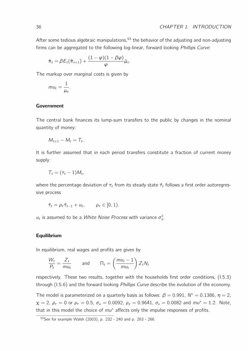
36 CHAPTER 1. INTRODUCTION
After some tedious algebraic manipulations,53 the behavior of the adjusting and non-adjusting
firms can be aggregated to the following log-linear, forward looking Phillips Curve:
πt = βEt(πt+1) +(1− ϕ)(1− βϕ)
ϕµt .
The markup over marginal costs is given by
mut =1
µt.
Government
The central bank finances its lump-sum transfers to the public by changes in the nominal
quantity of money:
Mt+1 −Mt = Tt .
It is further assumed that in each period transfers constitute a fraction of current money
supply:
Tt = (τt − 1)Mt ,
where the percentage deviation of τt from its steady state τt follows a first order autoregres-
sive process
τt = ρτ τt−1 + ut , ρτ ∈ [0, 1).
ut is assumed to be a White Noise Process with variance σ2u.
Equilibrium
In equilibrium, real wages and profits are given by
WtPt=Ztmut
and Πt =
(mut − 1mut
)ZtNt
respectively. These two results, together with the households first order conditions, (I.5.3)
through (I.5.6) and the forward looking Phillips Curve describe the evolution of the economy.
The model is parameterized on a quarterly basis as follows: β = 0.991, N∗ = 0.1386, η = 2,
χ = 2, ρτ = 0 or ρτ = 0.5, σu = 0.0092, ρz = 0.9641, σε = 0.0082 and mu∗ = 1.2. Note,
that in this model the choice of mu∗ affects only the impulse responses of profits.
53See for example Walsh (2003), p. 232 - 240 and p. 263 - 266.
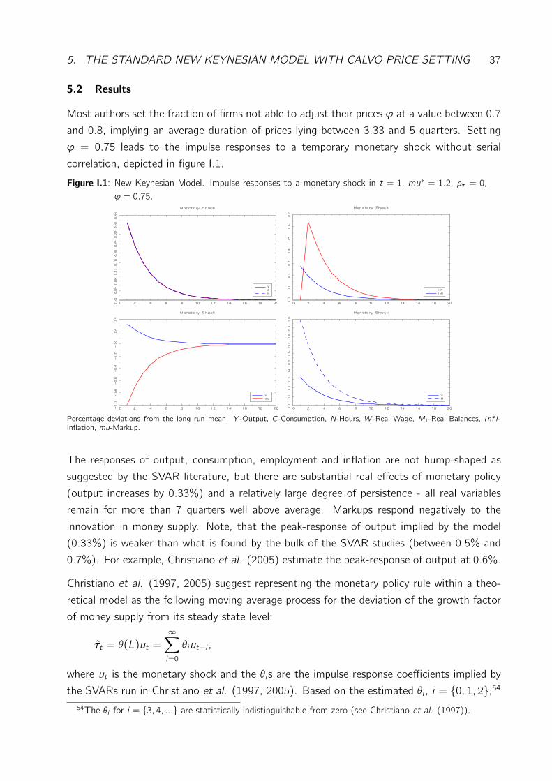
5. THE STANDARD NEW KEYNESIAN MODEL WITH CALVO PRICE SETTING 37
5.2 Results
Most authors set the fraction of firms not able to adjust their prices ϕ at a value between 0.7
and 0.8, implying an average duration of prices lying between 3.33 and 5 quarters. Setting
ϕ = 0.75 leads to the impulse responses to a temporary monetary shock without serial
correlation, depicted in figure I.1.
Figure I.1: New Keynesian Model. Impulse responses to a monetary shock in t = 1, mu∗ = 1.2, ρτ = 0,ϕ = 0.75.
Percentage deviations from the long run mean. Y -Output, C-Consumption, N-Hours, W -Real Wage, M1-Real Balances, Inf l-Inflation, mu-Markup.
The responses of output, consumption, employment and inflation are not hump-shaped as
suggested by the SVAR literature, but there are substantial real effects of monetary policy
(output increases by 0.33%) and a relatively large degree of persistence - all real variables
remain for more than 7 quarters well above average. Markups respond negatively to the
innovation in money supply. Note, that the peak-response of output implied by the model
(0.33%) is weaker than what is found by the bulk of the SVAR studies (between 0.5% and
0.7%). For example, Christiano et al. (2005) estimate the peak-response of output at 0.6%.
Christiano et al. (1997, 2005) suggest representing the monetary policy rule within a theo-
retical model as the following moving average process for the deviation of the growth factor
of money supply from its steady state level:
τt = θ(L)ut =
∞∑
i=0
θiut−i ,
where ut is the monetary shock and the θis are the impulse response coefficients implied by
the SVARs run in Christiano et al. (1997, 2005). Based on the estimated θi , i = 0, 1, 2,5454The θi for i = 3, 4, ... are statistically indistinguishable from zero (see Christiano et al. (1997)).
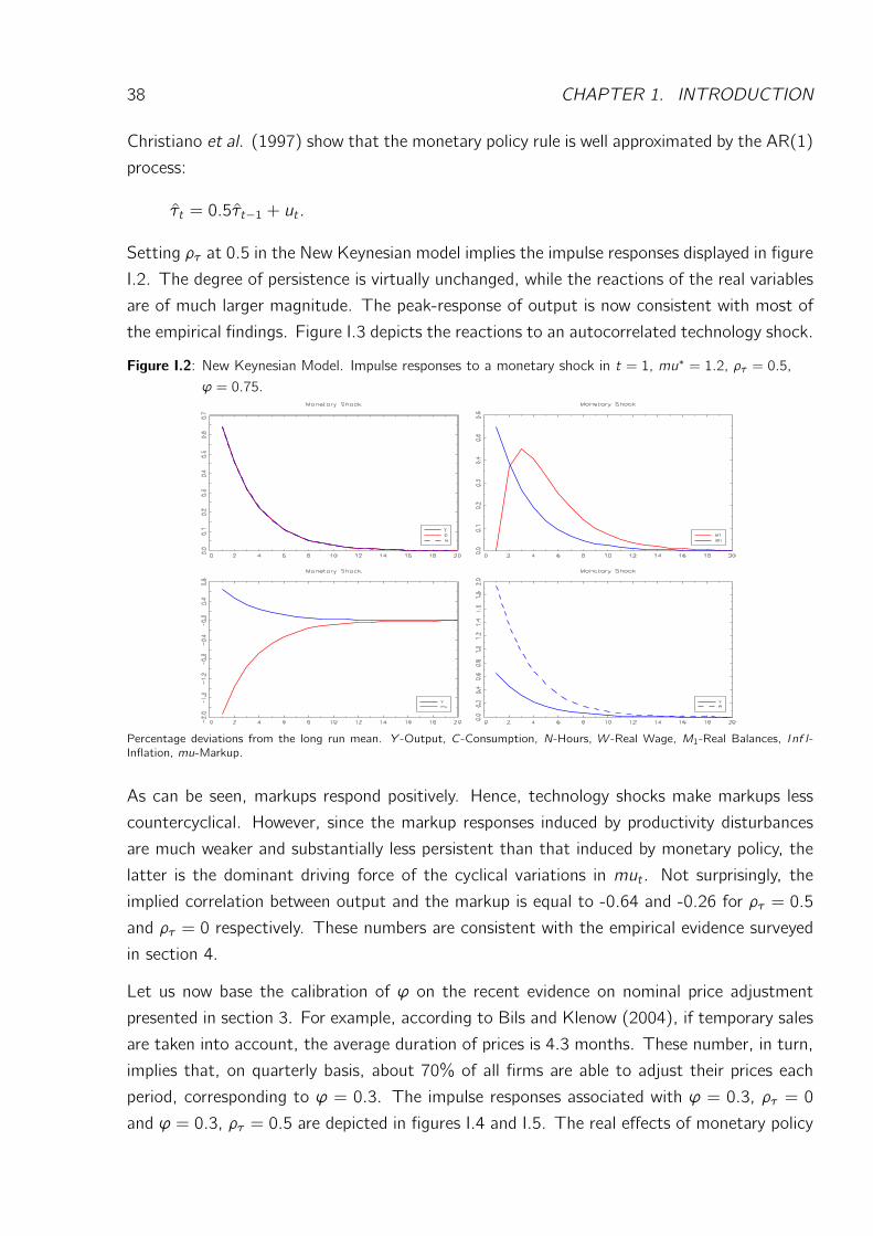
38 CHAPTER 1. INTRODUCTION
Christiano et al. (1997) show that the monetary policy rule is well approximated by the AR(1)
process:
τt = 0.5τt−1 + ut .
Setting ρτ at 0.5 in the New Keynesian model implies the impulse responses displayed in figure
I.2. The degree of persistence is virtually unchanged, while the reactions of the real variables
are of much larger magnitude. The peak-response of output is now consistent with most of
the empirical findings. Figure I.3 depicts the reactions to an autocorrelated technology shock.
Figure I.2: New Keynesian Model. Impulse responses to a monetary shock in t = 1, mu∗ = 1.2, ρτ = 0.5,ϕ = 0.75.
Percentage deviations from the long run mean. Y -Output, C-Consumption, N-Hours, W -Real Wage, M1-Real Balances, Inf l-Inflation, mu-Markup.
As can be seen, markups respond positively. Hence, technology shocks make markups less
countercyclical. However, since the markup responses induced by productivity disturbances
are much weaker and substantially less persistent than that induced by monetary policy, the
latter is the dominant driving force of the cyclical variations in mut . Not surprisingly, the
implied correlation between output and the markup is equal to -0.64 and -0.26 for ρτ = 0.5
and ρτ = 0 respectively. These numbers are consistent with the empirical evidence surveyed
in section 4.
Let us now base the calibration of ϕ on the recent evidence on nominal price adjustment
presented in section 3. For example, according to Bils and Klenow (2004), if temporary sales
are taken into account, the average duration of prices is 4.3 months. These number, in turn,
implies that, on quarterly basis, about 70% of all firms are able to adjust their prices each
period, corresponding to ϕ = 0.3. The impulse responses associated with ϕ = 0.3, ρτ = 0
and ϕ = 0.3, ρτ = 0.5 are depicted in figures I.4 and I.5. The real effects of monetary policy
5. THE STANDARD NEW KEYNESIAN MODEL WITH CALVO PRICE SETTING 39
Figure I.3: New Keynesian Model. Impulse responses to a technology shock in t = 1, mu∗ = 1.2, ρz =0.9641, ϕ = 0.75.
Percentage deviations from the long run mean. Y -Output, C-Consumption, N-Hours, W -Real Wage, M1-Real Balances, Inf l-Inflation, mu-Markup.
are now about 5 times (for ρτ = 0) and 3 times (for ρτ = 0.5) weaker than what is found
empirically. Further, the reactions of Yt , Wt/Pt and mut are much less persistent than in the
case of ϕ = 0.75, and are virtually complete after about two quarters. At the same time,
ϕ = 0.3 implies a slightly stronger response of mut to technology shocks, while that of Yt and
Nt remain virtually unchanged. As a consequence, markups become almost acyclical in the
case of ρτ = 0.5 and even procyclical for ρτ = 0. In the latter case the correlation between
Yt and mut is about 0.18. Further, irrespective of the value of ϕ, the model contains the
counterfactual implication that the reaction of the real wage to monetary shocks is much
stronger than that of output. The reverse is found in the data.55
What about capital accumulation? The standard New Keynesian model with adjustment costs
of capital56 delivers similar results as when there is no capital at all: As long as the fraction
of firms not able to adjust their prices within the period is large (ϕ = 0.75) the predictions
of the model with respect to the magnitude of the impulse responses to monetary shocks
and the cyclical behavior of markups are well in line with the empirical evidence presented
in the previous sections. The responses of the real variables, again, do not display a hump-
55See for example Christiano et al. (2005), Altig et al. (2005), Kydland and Prescott (1982).56In this case capital evolves according to
Kt+1 = φ
(ItKt
)Kt + (1− υ)Kt , υ ∈ (0, 1),
where in each simulation the elasticity of φ′(ItKt
)with respect to It/Kt is calibrated to ensure that investment
is about 4.6 times as volatile as output.
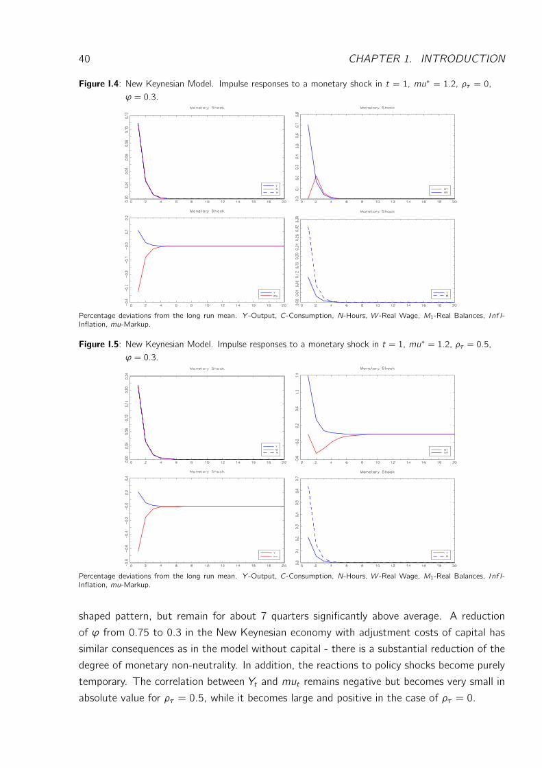
40 CHAPTER 1. INTRODUCTION
Figure I.4: New Keynesian Model. Impulse responses to a monetary shock in t = 1, mu∗ = 1.2, ρτ = 0,ϕ = 0.3.
Percentage deviations from the long run mean. Y -Output, C-Consumption, N-Hours, W -Real Wage, M1-Real Balances, Inf l-Inflation, mu-Markup.
Figure I.5: New Keynesian Model. Impulse responses to a monetary shock in t = 1, mu∗ = 1.2, ρτ = 0.5,ϕ = 0.3.
Percentage deviations from the long run mean. Y -Output, C-Consumption, N-Hours, W -Real Wage, M1-Real Balances, Inf l-Inflation, mu-Markup.
shaped pattern, but remain for about 7 quarters significantly above average. A reduction
of ϕ from 0.75 to 0.3 in the New Keynesian economy with adjustment costs of capital has
similar consequences as in the model without capital - there is a substantial reduction of the
degree of monetary non-neutrality. In addition, the reactions to policy shocks become purely
temporary. The correlation between Yt and mut remains negative but becomes very small in
absolute value for ρτ = 0.5, while it becomes large and positive in the case of ρτ = 0.
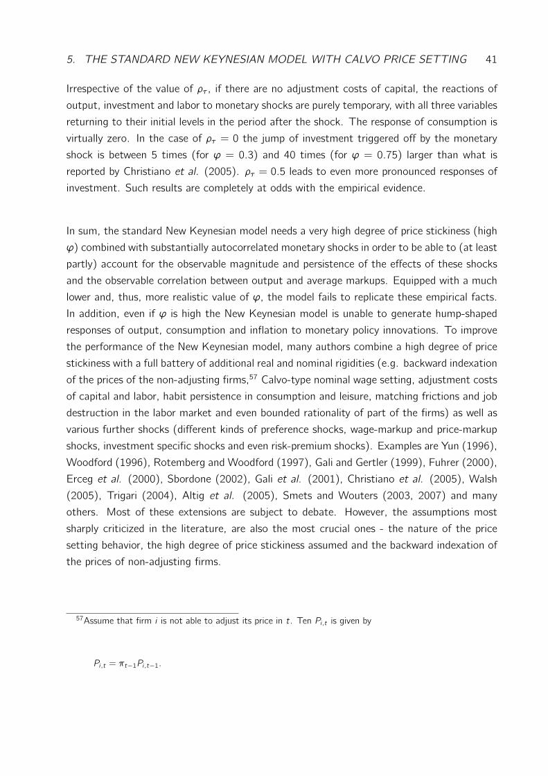
5. THE STANDARD NEW KEYNESIAN MODEL WITH CALVO PRICE SETTING 41
Irrespective of the value of ρτ , if there are no adjustment costs of capital, the reactions of
output, investment and labor to monetary shocks are purely temporary, with all three variables
returning to their initial levels in the period after the shock. The response of consumption is
virtually zero. In the case of ρτ = 0 the jump of investment triggered off by the monetary
shock is between 5 times (for ϕ = 0.3) and 40 times (for ϕ = 0.75) larger than what is
reported by Christiano et al. (2005). ρτ = 0.5 leads to even more pronounced responses of
investment. Such results are completely at odds with the empirical evidence.
In sum, the standard New Keynesian model needs a very high degree of price stickiness (high
ϕ) combined with substantially autocorrelated monetary shocks in order to be able to (at least
partly) account for the observable magnitude and persistence of the effects of these shocks
and the observable correlation between output and average markups. Equipped with a much
lower and, thus, more realistic value of ϕ, the model fails to replicate these empirical facts.
In addition, even if ϕ is high the New Keynesian model is unable to generate hump-shaped
responses of output, consumption and inflation to monetary policy innovations. To improve
the performance of the New Keynesian model, many authors combine a high degree of price
stickiness with a full battery of additional real and nominal rigidities (e.g. backward indexation
of the prices of the non-adjusting firms,57 Calvo-type nominal wage setting, adjustment costs
of capital and labor, habit persistence in consumption and leisure, matching frictions and job
destruction in the labor market and even bounded rationality of part of the firms) as well as
various further shocks (different kinds of preference shocks, wage-markup and price-markup
shocks, investment specific shocks and even risk-premium shocks). Examples are Yun (1996),
Woodford (1996), Rotemberg and Woodford (1997), Gali and Gertler (1999), Fuhrer (2000),
Erceg et al. (2000), Sbordone (2002), Gali et al. (2001), Christiano et al. (2005), Walsh
(2005), Trigari (2004), Altig et al. (2005), Smets and Wouters (2003, 2007) and many
others. Most of these extensions are subject to debate. However, the assumptions most
sharply criticized in the literature, are also the most crucial ones - the nature of the price
setting behavior, the high degree of price stickiness assumed and the backward indexation of
the prices of non-adjusting firms.
57Assume that firm i is not able to adjust its price in t. Ten Pi ,t is given by
Pi ,t = πt−1Pi ,t−1.
42 CHAPTER 1. INTRODUCTION
5.3 Further Critique of the New Keynesian Model with Calvo Pricing
The Lack of Microeconomic Foundation of the Price-Setting Behavior
The major shortcoming of the New Keynesian model with price stickiness of the Calvo-type
is that the latter is imposed exogenously rather than being derived from the interaction of
profit and/or utility maximizing behavior and the market structure. In other words, the heart
of the Calvo model - its pricing assumption - lacks microeconomic foundation. Many New-
Keynesians argue that allowing firms to freely adjust their prices at any point in time, but
assuming small menu costs (fixed costs of changing prices), would provide a rationale for the
Calvo specification. Accordingly, the latter should be viewed as a computationally convenient
short-cut of the analytically more complicated menu-cost model. In menu-cost models it
depends on the current state of the economy wether particular firms will find it optimal
to adjust prices or not. Therefore the price setting in these models is referred to as state
dependent. In contrast, the Calvo specification is an example for time dependent pricing.
The recent menu-cost literature, however, seems to reach the conclusion that the New
Keynesian model with Calvo pricing can not be viewed as an approximation of an otherwise
identical economy with state dependent pricing. Caplin and Spulber (1987) is one of the first
studies emphasizing this point, and showing that the implications of the menu-cost model
can differ dramatically from the predictions of theories with time dependent pricing. Caplin
and Spulber (1987) construct a model in which in each period only a small (nearly constant)
fraction of firms adjust prices. In other words, prices are extremely rigid. Nevertheless,
there is no price stickiness on the aggregate level, and money is neutral. The intuition
for this result is the following: In the model of Caplin and Spulber there is a stationary
distribution of relative prices. Because of the menu costs, when a monetary shock hits the
economy, only the firms with the lowest relative prices find it optimal to change prices.
Since at the same time, there are no pricing complementarities58 in the model, the adjusters
adjust prices by a very large amount,59 implying an increase in the aggregate price level
just sufficient to offset the effects of the monetary expansion. Golosov and Lucas (2007)
extend the Caplin-Spulber model by including idiosyncratic marginal cost shocks. On the one
hand, this assumption makes the model more flexible, enabling the authors to calibrate it
on the basis of the evidence provided by Bils and Klenow (2004). On the other hand, the
idiosyncratic productivity shocks distort the mechanism described above, leading to monetary
non-neutrality in the Caplin-Spulber model. Similar to the latter, the model of Golosov and
Lucas (2007) also implies a virtually constant frequency of price adjustments, easing the
58For example, there is a high degree of pricing complementarity if the following holds: A higher fraction of
firms that do not adjust their prices, implies a lower incentive for each individual firm to change its price, or a
lower desired amount of adjustment.59Precisely speaking, each adjusting firm sets its relative price equal to the highest relative price.

5. THE STANDARD NEW KEYNESIAN MODEL WITH CALVO PRICE SETTING 43
comparison with the standard New Keynesian model with Calvo pricing. Both models, the
menu-cost and the Calvo one, are calibrated so that the implied average frequency of price
adjustment is about 23% per month. The simulations performed by Golosov and Lucas
reveal substantial qualitative and quantitative differences between the menu-cost and the
Calvo model. The former implies weaker and much less persistent reactions of output and
inflation to a one-time monetary expansion. While output in the Calvo model remains above
average for about 2.5 quarters, the menu-cost model implies that output returns after 0.5
quarters (= 1.5 months) to its pre-shock level. Golosov and Lucas (2007) conclude that since
the two models deliver substantially different predictions about the effects of monetary policy,
the menu-cost model is not the microeconomic foundation of the New Keynesian model with
Calvo pricing. Similar work, with similar results is done by Burstein and Hellwig (2007),
Dotsey, King and Wolman (1999), Gertler and Leahy (2006) and Gorodnichenko (2008).
These studies try to increase the degree of monetary non-neutrality in the menu-cost model
by incorporating building blocks which amplify the pricing complementarities. However, as
Burstein and Hellwig (2007) argue, to generate strong and persistent effects of monetary
policy, these models need parameter values which are inconsistent with the micro evidence
on the level of menu costs and the typical magnitude of price adjustments.
Golosov and Lucas (2007) and Bustrein and Hellwig (2007) also point out that macro models
with continuous, convex costs of price adjustment60 are subject to the same critique as the
Calvo one since, in order to generate substantial monetary non-neutrality, these models need
average adjustment costs which are much larger than the empirically observable magnitude
of menu costs.61
Kehoe and Midrigan (2008) extend the Golosov-Lucas model by assuming that firms are
subject to two types of idiosyncratic shocks, a persistent productivity disturbance and a
temporary shock to the elasticity of demand for the firm’s product. There are also two types
of menu-costs - the lower one must be paid when the price is changed for only one period
(temporary sale), while the higher one has to be paid when the price is changed permanently
(adjustment of the regular price). The two types of idiosyncratic shocks combined with the
two types of menu costs generate an explicit incentive for firms to carry out two different
types of price changes and, thus, enables the model to better match the empirical facts
regarding the pattern of regular prices and that of temporary sales. Kehoe and Midrigan
(2008) then calibrate their menu-cost model as well as the Calvo model based on the scanner
data provided by the Dominick’s Finer Foods retail chain. The calibration of the Calvo model
is performed in two different ways - by including and by excluding temporary sales when
60Prominent examples are Rotemberg (1982), Hairault and Portier (1995).61See Burstein and Hellwig (2007) for an estimation of the magnitude of menu costs as well as for a survey
of related literature.
44 CHAPTER 1. INTRODUCTION
computing the frequency of price adjustment. These are the two approaches usually found in
the literature. Kehoe and Midrigan (2008) then argue that neither of the resulting two Calvo
models is a good approximation of their menu-cost model. If temporary sales are included,
the average frequency of price adjustment is too high, so that the Calvo model implies a
lower degree of monetary non-neutrality than the Kehoe-Midrigen model does. If temporary
sales are not taken into account, the resulting average frequency of price adjustment is too
low, so that prices in the Calvo model are too sticky, with the consequence of much stronger
and more persistent impulse responses than predicted by the Kehoe-Midrigan model. Kehoe
and Midrigan (2008) then propose the following solution: If one does not want to work
with the more complicated menu-cost model but rather with a simple short-cut, then he
should set the frequency of price adjustment in the Calvo model at the (intermediate) value
implying that the impulse responses implied by the Calvo model are exactly the same as that
predicted by the menu-cost model. The intermediate value of the average price duration
obtained by Kehoe and Midrigan (2008) is 17 weeks. This number corresponds to ϕ ≈ 0.3in the quarterly Calvo model. The corresponding impulse responses to a monetary shock
are displayed in figures I.4 and I.5. Hence, if we want to reconcile the Calvo model with
the menu-cost model, the former becomes completely inconsistent with the evidence on the
cyclical behavior of markups and the effects of monetary policy shocks.
I disagree with the approach proposed by Kehoe and Midrigan (2008) for two reasons. First,
every time a new building block is incorporated into the New Keynesian model one will have
to carry out the same extension in the menu-cost model in order to determine the value of
ϕ reconciling the two models. But if the cumbersome analytical and numerical analysis of
the menu-cost model have already been done, then it would be extremely irrational to resort
to an approximation such as the Calvo model, instead of using the exact menu-cost model
to perform positive and normative analysis. Second, if we calibrate the Calvo model in the
way proposed by Kehoe and Midrigan (2008), then the price setting in that model will still
lack a microeconomic foundation. Simply because we do not set ϕ at a value consistent
with, say, the Bils-Klenow evidence but rather at a so called ”intermediate” value, in order
to ensure that the impulse responses of the Calvo model are consistent with that of another
theoretical model. But why should the impulse responses predicted by the menu-cost model
be more plausible or more relevant than that estimated by, say, Christiano, Eichenbaum and
Evans (2005)? Why should it be less correct to set ϕ at the value making the Calvo model
consistent with the SVAR evidence, as is actually done by many New Keynesians? After all,
the a priori belief that the SVAR evidence, obtained with empirical data, is closer to reality
than the predictions of the manu-cost model are, appears extremely plausible. In other words,
the right conclusion of the Kehoe-Midrigan paper should be similar to that drawn by Golosov
and Lucas (2007) and many others: The model developed in Kehoe and Midrigan (2008)

5. THE STANDARD NEW KEYNESIAN MODEL WITH CALVO PRICE SETTING 45
does not provide the microeconomic foundation of the price setting behavior assumed in the
New Keynesian model.
The Chari-Kehoe-McGrattan Critique
Chari et al. (2008b) (henceforth, CKMc) criticize some features of the most recent New
Keynesian models. CKMc focus on a model developed by Smets and Wouters (2007) because
on the one hand it is fairly representative and on the other hand, the model is now being used
to guide policy makers at the European Central Bank.
The performance of the Smets and Wouters (2007) hinges critically on the following four
shocks: the wage-markup shock, the price-markup shock, the exogenous-spending shock and
the risk-premium shock. CKMc argue that they are most likely to be non-structural and,
thus, not invariant to monetary policy in general.
• The wage-markup shock in Smets and Wouters (2007) stems from fluctuations in
the elasticity of substitution across different types of labor. CKMc argue that when
expressed in terms of markup, the shock has a mean of 50% and a standard deviation
of 2500% (!!!). The latter is completely unrealistic.
• CKMc argue that the Smets and Wouters (2007) model needs the wage-markup and
the price-markup shocks in order to be able to account for the empirically observable
labor wedge.62 However, CKMc show that the labor wedge can be interpreted as arising
from fluctuations in the bargaining power of unions or shifts in the utility of leisure. In
both cases the labor wedge will be endogenous and, thus, not invariant to monetary
policy. Therefore, the two shocks driving the labor wedge can be hardly interpreted as
structural.
• CKMc also disagree with the interpretation of the expenditure spending shock as a
structural shock to government spending. First, the shock has 3.5 the variance of
government spending. Second, the shock emerges as a residual from the national
income identity, and, thus, captures net exports and other endogenous variables not
explicitly included into the Smets-Wouters model.
• CKMc also stress that the risk-premium shock has an unrealistically high volatility,
having 6 times the variance of short-term nominal rates. Smets and Wouters (2007)
provide only very rough and incomplete interpretation of this shock. CKMc believe that
62Roughly speaking, the labor wedge is the deviation between the marginal product of labor and the marginal
rate of substitution between consumption and leisure. According to CKMc, there is a consensus in modern
macroeconomics on the high importance of the labor wedge for business cycles fluctuations.
46 CHAPTER 1. INTRODUCTION
a more detailed investigation of the sources of such a shock, will reveal that there are
endogenous forces driving the fluctuations of the risk premium, which are, in general,
not invariant to monetary policy.
Two other features common for most modern New Keynesian models are also subject to
critique by CKMc - the backward indexation of the prices of the non-adjusting firms and
the specification of the Taylor rule as an approximation of the central bank’s policy. The
backward indexation is a way to make inflation more persistent in the model. However,
this feature is inconsistent with the recent panel evidence on price setting, part of which
is reviewed in section 3. According to that evidence, firms maintain a so called regular
price for a year or more, frequently deviating from it by temporary setting a lower price.
If actual price setting behavior were characterized by backward indexation, then it would be
impossible to empirically observe such thing as the regular price. CKMc point to the empirical
finance literature indicating that when the short rate changes (or is altered by the central
bank) private agents significantly adjust their long-run expectations of the future short rate.
CKMc interpret these results as indicating that interest rate policy must have a unit-root
component.63 The Taylor rules usually assumed in the macro literature imply that the short
term nominal rate is stationary and ergodic. As a consequence, altering the short-run nominal
rate has no effect on the long-run expectation of future short-run nominal rates.
Chari, Kehoe and McGrattan conclude:64
”We have argued here that New Keynesian models are not yet useful for policy analysis.
Our basic reason is that macroeconomists working in this tradition have added so many free
parameters to their models that those models are dubiously structural.”
The purpose of the following chapters is to develop alternatives to the New Keynesian model
which do not rely on questionable exogenous assumptions on the price setting behavior of
private firms yet are (at least partly) able to account for the magnitude and persistence of
the reactions to monetary policy shocks, the cyclical behavior of markups as well as various
other business cycles facts.
6 Related Theoretical Studies
Since the models constructed in the following chapters a re only loosely related to the existing
literature, this section is extremely short, only briefly pointing to some recent developments.
63The argument is made precise in Atkeson and Kehoe (2008).64Chari et al. (2008b), p. 24.

6. RELATED THEORETICAL STUDIES 47
Endogenous Price Rigidity: Haubrich and King (1991) develop a model providing an en-
dogenous explanation of price stickiness. In that model firms are able to insure against
idiosyncratic monetary shocks by signing nominal contracts. However, as the authors point
out, the price-rigidity equilibrium is only one of the possible outcomes under the specific as-
sumptions on the parameters made. The parameterization of their model, too, is only one of
many plausible ones. Nakamura and Steinsson (2007) construct a model with good-specific
habit persistence in which price stickiness arises as an equilibrium outcome. Price stickiness
can be sustained because it helps firms to solve a time-inconsistency problem. However, there
are again many further equilibria characterized by fully flexible prices. In addition, the results
in Nakamura and Steinsson (2007) should be interpreted with caution because they are de-
rived within a partial equilibrium framework. Thus, it can not be ruled out, that the general
equilibrium predictions of the model (after incorporating the money market) with respect to
the degree of monetary non-neutrality turn to be rather disappointing. The sticky-information
literature proposes an approach slightly different from that adopted in the Calvo model. It
assumes that nominal prices are fully flexible but the flow of information to particular agents
is not. In particular, it is assumed that each firm faces a constant probability ϕ per period
to be able to obtain the most recent information about the state of the economy. The
remaining firms, constituting a fraction equal to 1− ϕ percent, are not able to update their
information within the period and, thus, base production and pricing plans on old (outdated)
information. For example, at time t a firm that was last able to update its information in t−3build expectations about future economic conditions based on the information set available
to the economy at the end of period t − 3. In other words, the sticky-information models
replace the Calvo-type price setting by a Calvo-type updating of information. Some of the
most important studies in this area are Mankiw and Reis (2001, 2006a, 2006b) and Ball et
al. (2003). These authors claim that their models are able to generate endogenous price-
sluggishness and persistent and (at lest partly) hump-shaped impulse responses to monetary
policy shocks. A major shortcoming of the sticky-information models is the fact that their
most crucial component - the process of obtaining information - is exogenously given. To the
best of my knowledge, the Calvo-type updating of information still lacks a microeconomic
foundation.65 Rotemberg (2002, 2004a, 2004b, 2008) assumes that customers become an-
gry if they see the price chosen by a given firm as unfair. Anger, in turn, forces them to punish
the unfair firm by reducing the demand for its product more strongly than it would be the
case without anger. Rotemberg derives conditions ensuring that in order to avoid anger, firms
65Mackowiak and Wiederholt (2007) can be interpreted as an attempt in this direction. In their model
managers can process only a limited amount of information because of cognitive constraints. As a result, in
each period they are forced to decide whether to pay attention to aggregate or to idiosyncratic signals when
setting prices.
48 CHAPTER 1. INTRODUCTION
find it optimal to partly reduce the flexibility of prices. Unfortunately, Rotemberg performs
the analysis within a simple, partial equilibrium framework.
Real Business Cycles Models of Endogenous Markups: A prominent example is the model
developed by Phelps and Winter (1970) which builds the basis of the models constructed in the
next two chapters. In that model markups are endogenized by the assumption of a particular
form of dynamic market share competition in continuous time. The discrete time version of
that structure is used in the models presented below.66 In a series of real business cycles
models based on the partial equilibrium model proposed by Rotemberg and Saloner (1986),
Rotemberg and Woodford67 show that countercyclical markups may arise if firms are able to
collude implicitly. In their models, markups respond negatively to demand side as well as to
supply side shocks. Ravn et al. (2006, 2007) are able to generate countercyclical markups
by introducing good-specific habit formation, the so called deep habits, into a standard RBC-
model with a monopolistically competitive goods market. Edmond and Veldkamp (2008) show
how countercyclical income dispersion can generate countercyclical markups, even without
any price-setting frictions such as nominal price rigidity or slow reactions of the customer
stock. Froot and Klemperer (1989), Klemperer (1987, 1995) and Kleshchelski and Vincent
(2007) develop static models of the goods market in which customers face fixed costs of
switching suppliers. All these models have in common the implication that firm’s current
pricing behavior has an influence on its future profits.
66Rotemberg and Woodford (1992, 1995) also use the discrete-time version of the model for comparison
purposes.67Rotemberg and Woodford (1992), (1995), (1996)

Chapter 2
A Monetary Customer Markets Model
1 Introduction
The empirical evidence reviewed in the previous chapter indicate that positive monetary shocks
are expansionary and induce highly persistent dynamic responses of inflation, output, con-
sumption and investment. Many economists try to explain this pattern by monetary business
cycles models in which they assume some kind of exogenously given price stickiness combined
with a whole battery of real rigidities and additional structural assumptions.1 These models
are extensively used to evaluate monetary and fiscal policy as well as to derive normative con-
clusions and suggestions on how monetary policy should be conducted. Unfortunately, most
of these models perform rather poorly with respect to phenomena other than the impulse
responses to monetary innovations such as the sample moments at business cycle frequencies
of many macroeconomic variables or the reactions to real supply side shocks. This casts
doubt on the appropriateness of the sticky price models for analyzing normative issues. The
sticky-price models also do not provide any endogenous explanation of their most crucial
component - the high degree of price or wage rigidity. The current chapter addresses the
question of the propagation of monetary shocks as well as that of explaining a set of sample
moments of the data by taking a different approach. I employ a model with fully flexible
prices in which monetary nonneutrality is due to the assumption that the utility function
of the representative household is non-additively separable in money and consumption. As
shown below, the intrinsic mechanisms propagating nominal shocks in this baseline model are
pretty weak and lead to predictions which are in many respects counterfactual. However,
introducing market share competition in the goods market as proposed by Phelps and Winter
(1970), and thus, making the markups of prices over marginal costs endogenous, substan-
tially alters the qualitative as well as quantitative predictions of the model. In particular,
1The most widely used model framework in modern macroeconomics is the so called ”New Keynesian Model”
with Calvo price setting. Examples are Christiano et al. (2005), Walsh (2005) and many others.
49
50 CHAPTER 2. A MONETARY CUSTOMER MARKETS MODEL
for a broad range of empirically plausible values of the short run price elasticity of demand,
the average markup and the degree of flexibility of capital accumulation the nonneutrality of
money can be made arbitrarily strong. Furthermore, in these cases the model implies impulse
responses of output, employment and wages displaying a one period delay and a substantial
degree of persistence.
What are the main mechanisms at work in the model developed in this chapter? If the
current utility function of the representative household in an otherwise standard monetary
business cycles model is non-additively separable in money and consumption, and is given by
the following CES-aggregator:
(aC1−bt + (1− a)
(MtPt
)1−b) 11−b
, a ∈ (0, 1), b > 0,
where C,M and P denote consumption, nominal cash balances and the price level respectively,
then monetary expansions tend to be contractionary: They induce a sharp increase in current
inflation which reduces the marginal utility of consumption ”today” relative to its value in
the future. The result is a relatively large negative deviation of labor supply and thus a drop
of output and consumption in the period of the shock. Only in the case of a very high
degree of flexibility of capital accumulation these variables reach above average values in
the period after the shock. Otherwise, they return almost immediately, from below, to their
respective long run levels. This prediction is counterfactual. At the same time, however, the
disturbance of the time path of the marginal utility of consumption just described implies
an increase in the stochastic discount factor which, in turn, leads to an increase in the
present value of firms’ future profits. If the goods market is characterized by the usual static
monopolistic competition, future profits don’t matter for the current pricing decisions of
the firms. In contrast, if firms also engage in market share competition as suggested by
Phelps and Winter (1970), future profits become a crucial determinant of firms’ behavior.
If expected future revenues increase relative to their current level, each firm will tend to
make additional ”investments” in future market shares by lowering its current price and thus
by lowering its current markup. The decrease in markups will have a positive effect on the
real wage and thus on the labor supply decision made by households. As a result, in the
economy characterized by market share competition employment, consumption and output
will tend to be procyclical or at lest less countercyclical than in the case of static monopolistic
competition. As shown below, the lower the short run price elasticity of demand and the higher
the steady state markup, the larger the fall in markups and thus, the more pronounced the
increase in real wages, employment, and output. The persistence generated by the model is
due to the interaction between capital accumulation and markup fluctuations and is described
in sections 4 and 5.

2. A MODEL WITH FIXED CAPITAL AND STATIC MONOPOLISTIC COMPETITION51
In summary, the purpose of this chapter is threefold. First, to stress the importance of markup
fluctuations for the qualitative and quantitative predictions of monetary models with non-
additively separable utility functions. Second, to propose a theoretical framework alternative
to that of the New Keynesian Model, which is able to explain a bunch of business cycles facts.
And third, to understand and explain the model mechanisms leading to the most interesting
and relevant implications and highlight their advantages and disadvantages in a much more
detailed and explicit manner than usually done in the literature.
The chapter is organized as follows. Section 2 describes the baseline monetary model without
capital accumulation while section 3 extends it by the assumption of market share competition
in the goods market. Capital accumulation and adjustment costs of capital are introduced
in sections 4 and 5. In section 7 I evaluate the performance of the model with adjustment
costs of capital with respect to a subset of stylized business cycles facts and compare it with
the performance of the New Keynesian Model. Section 8 concludes.
2 A Model with Fixed Capital and Static Monopolistic Competition
This section provides a short sketch of the baseline Money in the Utility Function Model.
2.1 The Theoretical Framework
Firms
There are n product varieties, each produced by a profit maximizing monopolistic firm ac-
cording to the linear production function
Yi ,t = ZtNi ,t ,
where Ni ,t denotes labor input of firm i . Zt denotes the total factor productivity which follows
a stochastic process given by:
ln(Zt) = ρz ln(Zt−1) + εt ,
where εt follows a White Noise Process with variance σ2ε .
The demand function faced by the producer of variety i is given by
Ci ,t =
(Pi ,tPt
)−θ· Ctn, θ > 0, (II.2.1)
where Ct denotes aggregate consumption expenditure.
52 CHAPTER 2. A MONETARY CUSTOMER MARKETS MODEL
The profit maximizing relative price satisfies the equation
Pi ,tPt=
θ
θ − 1Wt/PtZt,
where WtPt
denotes the real wage and mu = θθ−1 the markup.
Households
Let agents in this economy have preferences over consumption, real balances and working
hours given by2
U = Et
∞∑t=0
βt
(aC1−bt + (1− a)
(MtPt
)1−b) 11−b
− φ2N2t
, φ, b > 0, β, a ∈ (0, 1),
where Mt/Pt and Nt denote real balances and working hours. In the above expression Ct is
a composite good that includes all varieties:
Ct =
1
n
n∑
i=1
Cθ−1θ
i ,t
θθ−1
. (II.2.2)
The corresponding utility-based price index is given by:
Pt =
1
n
n∑
i=1
P 1−θi,t
11−θ
.
For b → 1 the current utility function which I denote by ut reduces to
ut = Cat
(MtPt
)1−a− φ2N2t .
The budget restriction of the representative household is given by:
Ct +mt+1 − mtπt+ bt+1 − bt
πt=WtPtNt +Πt + it
btπt+TtPt,
where Wt , Πt , Tt , bt = BtPt−1
and mt = MtPt−1
denote the nominal wage, real profits, nominal net
transfers form the government, the real value of nominal bonds and real balances respectively.
it is the one-period risk free nominal interest rate.
2A similar specification of the utility function is used by Maussner (2004).
2. A MODEL WITH FIXED CAPITAL AND STATIC MONOPOLISTIC COMPETITION53
Key Assumption I: Non-Separable Utility
The monetary general equilibrium models developed in the last ten years usually assume
that the utility function of the representative agent is separable with respect to money and
consumption, e.g.
C1−ηt1− η +
φ
1− χ(MtPt
)1−χ, for 0 < η,χ 6= 1, φ > 0,
ln(Ct) + φ ln
(MtPt
), for η = χ = 1, φ > 0.
Nonetheless, it is quite well known that almost all separable specifications are just special
cases of more general non-separable, (nested3) Cobb-Douglas or CES4 aggregators com-
bining consumption and real balances. Furthermore, economic theory does not provide any
convincing reason for preferring the separable to the non-separable formulation et vice versa.
The only comparative advantage of the former is perhaps its analytical simplicity. Indeed, in
his seminal paper Sidrauski (1967) assumes that money and consumption enter the utility
function non-separabely, through a Cobb-Douglas aggregator. The early literature inspired by
Sidrauski (1967), e.g. Brock (1974, 1975), Fisher (1979), Asako (1983) and others, dealing
with the stability and the steady state properties of monetary general equilibrium models,
also consider the non-separable utility function to be more important while the separable
specification is only treated as a special case.
Finally, the empirical evidence supports the assumption that utility is non-separable in con-
sumption and real balances: in a more recent study Holman (1998) performs a GMM esti-
mation of the Euler equation for optimal money holdings under different specifications of the
utility function - Cobb-Douglas, CES and nested Cobb-Douglas or CES.5 Based on a series
of tests the author rejects the separable form while the Cobb-Douglas, the CES (used here)
and the nested CES formulation can not be rejected.3The nested Cobb-Douglas specification of the utility function is given by:
(Cαt
(MtPt
)1−α)1−ρ
1− ρ , α ∈ (0, 1), ρ > 0,
while the non-nested case is obtained by setting ρ = 0.4CES - Constant Elasticity of Substitution.5The nested CES specification of the utility function is given by:
(aC1−bt + (1− a)
(MtPt
)1−b) 1−ρ1−b
1− ρ , a ∈ (0, 1), b, ρ > 0,
while the non-nested case is obtained by setting ρ = 0.

54 CHAPTER 2. A MONETARY CUSTOMER MARKETS MODEL
All in all, the assumption that the utility function is non-separable in money and consumption
seems to be at least as plausible as the opposite one. At the same time, the non-nested
CES specification chosen in the current paper, although arbitrary, is not rejected by the data.
As is well known, the non-separability with respect to consumption and real balances can be
interpreted as a short-cut of an environment in which the transaction costs associated with
the purchase of a given amount of consumption goods can be reduced by a higher level of
real cash holdings.
First Order Conditions
The first order conditions of the representative household evaluated at the symmetric equi-
librium read:
aC−bt
(aC1−bt + (1− a)
(mtπt
)1−b) b1−b
= Λt , (II.2.3)
φNt = ΛtWtPt, (II.2.4)
1
1 + it= βEt
Λt+1Λt
1
πt+1
, (II.2.5)
Λt = βEt
(1− a)
m−bt+1π1−bt+1
(aC1−bt+1 + (1− a)
(mt+1πt+1
)1−b) b1−b
+Λt+1πt+1
, (II.2.6)
Ct +mt+1 − mtπt+ bt+1 − bt
πt=WtPtNt +Πt + it
btπt+TtPt. (II.2.7)
(II.2.5) is the bond euler equation and (II.2.6) is the euler equation with respect to money
balances.
Government
The central bank finances its lump-sum transfers to the public by changes in the nominal
quantity of money:
Mt+1 −Mt = Tt .
It is further assumed that in each period transfers constitute a fraction of current money
supply:
Tt = (τt − 1)Mt ,
2. A MODEL WITH FIXED CAPITAL AND STATIC MONOPOLISTIC COMPETITION55
where the percentage deviation of τt from its steady state τt follows a first order autoregres-
sive process
τt = ρτ τt−1 + ut , ρτ ∈ [0, 1).
ut is assumed to be a White Noise Process with variance σ2u.
Equilibrium
In equilibrium, real wages and profits are given by
WtPt=Ztmu
and Πt =
(mu − 1mu
)ZtNt
respectively. These two results, together with the households first order conditions, (II.2.3)
through (II.2.7) describe the evolution of the economy.
2.2 Understanding Key Features of the Model
Figure II.1 depicts the impulse responses to a monetary shock in t = 3 without serial correla-
tion, occurring in the third period.6 The reactions of output, employment, consumption, real
balances and the discount factor can be characterized as purely temporary one-time negative
deviations from the steady state. Hence, the the positive monetary transfer is contractionary.
The only variable deviating for more than one period from its long run level is the rate of
inflation. Its value is above average for two quarters. To understand why there is no per-
sistence in the reactions to monetary expansions, it is instructive to restate the household’s
optimality conditions under the assumption that b = 1:7
Nt = aCa−1t
(mtπt
)1−aWtPt
⇒ C2−at = a
(mtπt
)1−aWtPt
mt+1 = β1− aaEt
Ct+1
Ca−1t+1(mt+1πt+1
)1−a
Ca−1t(mtπt
)1−a
+ βEt
Ca−1t+1
(mt+1πt+1
)1−a
Ca−1t(mtπt
)1−a1
πt+1
.
(II.2.1)
6See section 6 for details on the calibration. The corresponding programm is
”MIU_sim_cm_2d5d_1_i.g” .7In that case the first term in the utility function becomes a Cobb-Douglas aggregator assembling consump-
tion and real balances:
ut = Cat
(mtπt
)1−a− d2N2t .
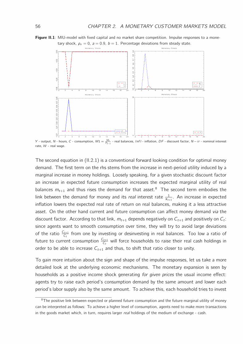
56 CHAPTER 2. A MONETARY CUSTOMER MARKETS MODEL
Figure II.1: MIU-model with fixed capital and no market share competition. Impulse responses to a mone-tary shock, ρτ = 0, a = 0.9, b = 1. Percentage deviations from steady state.
Y - output, N - hours, C - consumption, M1 = MtPt−1 - real balances, Inf l - inflation, DF - discount factor, N− i r - nominal interest
rate, W - real wage.
The second equation in (II.2.1) is a conventional forward looking condition for optimal money
demand. The first term on the rhs stems from the increase in next-period utility induced by a
marginal increase in money holdings. Loosely speaking, for a given stochastic discount factor
an increase in expected future consumption increases the expected marginal utility of real
balances mt+1 and thus rises the demand for that asset.8 The second term embodies the
link between the demand for money and its real interest rate 1πt+1
. An increase in expected
inflation lowers the expected real rate of return on real balances, making it a less attractive
asset. On the other hand current and future consumption can affect money demand via the
discount factor. According to that link, mt+1 depends negatively on Ct+1 and positively on Ct :
since agents want to smooth consumption over time, they will try to avoid large deviations
of the ratio Ct+1Ct
from one by investing or desinvesting in real balances. Too low a ratio of
future to current consumption Ct+1Ct
will force households to raise their real cash holdings in
order to be able to increase Ct+1 and thus, to shift that ratio closer to unity.
To gain more intuition about the sign and shape of the impulse responses, let us take a more
detailed look at the underlying economic mechanisms. The monetary expansion is seen by
households as a positive income shock generating for given prices the usual income effect:
agents try to raise each period’s consumption demand by the same amount and lower each
period’s labor supply also by the same amount. To achieve this, each household tries to invest
8The positive link between expected or planned future consumption and the future marginal utility of money
can be interpreted as follows: To achieve a higher level of consumption, agents need to make more transactions
in the goods market which, in turn, requires larger real holdings of the medium of exchange - cash.
2. A MODEL WITH FIXED CAPITAL AND STATIC MONOPOLISTIC COMPETITION57
the same portion of his additional income in risk free bonds. But since the aggregate supply
of bonds remains unchanged and equal to zero, the desire to increase bond holdings causes
the nominal interest rate to fall just enough to force households to change the composition
of their portfolios by leaving bond holdings unchanged and rising the desired amount of the
other asset available-real balances. Since the marginal utility of consumption depends posi-
tively on real balances, the desired path of consumption expenditure gets altered with future
consumption and labor supply being increased relative to their respective current values.9
At the same time, as the current Zt is given, the planned increase in current consumption
demand accompanied by a lowering of current labor supply leads to an increase in current
and expected nominal wages which, under constant markups, is completely passed through to
nominal prices, leading to an increase in current inflation πt . Expected future nominal wages
and prices will also tend to rise since planned next-period consumption expenditure(labor sup-
ply) also get larger(smaller). But since the reactions of that two variables are affected by the
increase in money holdings in the way just described, the steady state deviation of expected
future inflation might turn to be stronger or weaker than that of present inflation, or even
be negative, depending on whether desired next-period consumption or labor supply responds
more strongly to changes in real money holdings. Note that real balances have two opposing
effects on labor supply: An increase in mt has a positive direct effect on Nt (see the first
equation in the first line of (II.2.1)). At the same time, everything else given, the increase
in labor supply increases labor income and makes a higher level of consumption possible. On
the aggregate level consumption depends on mt according to the second equation in the first
line of (II.2.1). But a higher level of consumption implies a lower marginal utility of that
variable and thus, creates an incentive for households to decrease labor supply. It turns out
that the overall effect of changes in mtπt
on Nt is positive and can be described by the following
equation:
Nt = a12−a
(mtπt
) 1−a2−a
(WtPt
) 12−a.
The increase in current inflation and the reaction of future inflation should be such that in each
period the disparity between aggregate consumption and labor supply and thus production,
is eliminated. Depending on how the inflation path adjusts, both equilibrium consumption
and labor in the present as well as in the future can fall, increase or remain unchanged.10
If Etπt+1 actually changes, the incentive to build up money balances gets altered, starting
a new loop of adjustments in desired current and future consumption demand, labor supply
and inflation, until the new intertemporal equilibrium is reached.
9See the first line in (II.2.1).10Note that only changes in expected future inflation affect the real interest rate of money balances.
58 CHAPTER 2. A MONETARY CUSTOMER MARKETS MODEL
Now observe that consumption depends on current inflation through the ratio mtπt
and thus
money demand mt+1 is affected by πt only via terms of the form mt+1πtmtπt+1
. Log-linearizing one
of that terms and taking expectations as of time t yields:
τt − Etπt+1
which does not depend on current inflation πt . Further, the fact that Ct+1 and πt+1 appear
in the second equation in (II.2.1) just induces an additional, indirect, log-linear link between
mt+1 and mt+1, Etπt+1. To see that, eliminate consumption from the system (II.2.1) and
log-linearize around the nonstochastic steady state under the assumption Zt = 0 ∀t. The
resulting equation reads:
mt+1 = −(2π∗(1− a) + βπ∗ − β
)Etπt+1 +
(1− a)π∗π∗ − β τt . (II.2.2)
The link between current money demand and expected inflation is the result of the overlapping
effects on mt+1 arising through the interdependence between mt+1 and Etπt+1 and current
and next period consumption as well as real balances mentioned above. (II.2.2) is a reduced
form, forward looking money demand equation. Money supply evolves according to
mt+1 = mt − πt + τt . (II.2.3)
(II.2.2) and (II.2.3) constitute a dynamic supply-demand system with an expected time path
of prices given by πt , Etπt+1, Etπt+2, .... In equilibrium the price expectations of money
suppliers should be equal to that of the agents demanding money. So, one can shift (II.2.3)
one period forward in time, take conditional expectations as of time t, take into account that
τt is a White Noise process and then eliminate expected inflation from (II.2.2). The resulting
relationship
mt+1 =2π∗(1− a) + β2π∗(1− a) + π∗︸ ︷︷ ︸
∈(0,1)
Etmt+2 +(1− a)π∗
2π∗(1− a) + π∗ τt
is a stochastic forward looking difference equation which should be solved forward as its root
lies outside the unit circle. The solution is very simple and is computed by each agent in
forming her rational expectations about inflation and other variables:
mt+1 =(1− a)π∗
2π∗(1− a) + π∗ τt .
Hence, the relative deviation of money balances from its steady state level follows a White
Noise process. Now it is straightforward to show that
Etmt+2 = Et τt+1 = 0 = Etmt+3 = Etmt+4 = ...
2. A MODEL WITH FIXED CAPITAL AND STATIC MONOPOLISTIC COMPETITION59
and therefore
Et πt+1 = mt+1, Etπt+2 = 0, Et πt+3 = 0, ...
But if agents expect next-period inflation to rise by the same amount as their real balances,
their expected wealth in t+1 will remain unchanged implying that they will have no incentive
to change next-period consumption which, in turn, leaves the marginal utility of consumption
and thus labor supply in t+1 unchanged.11 Since the expected steady state deviations of real
balances and inflation in all future periods are equal to zero, nobody will expect any positive
or negative wealth effects of real money holdings in that periods.
What happens in the period in which the shock occurs? For a given level of consumption the
large increase in inflation induces a sharp decline in the current marginal utility of consumption.
As a result, labor supply falls even more and leads to a further decline in labor as well as
dividend income. Since at the same time the positive income effect of the monetary shock is
almost offset by the rise of the inflation rate, households have to reduce current consumption.
Since the time path of the marginal utility of consumption is altered agents face an additional,
utility based incentive to lower current consumption relative to its future level. However, the
reduction of Ct is not sufficient to compensate (offset) the negative effect of inflation on the
marginal utility of consumption. Therefore labor supply and thus, output unambiguously fall.
One can see the overall effect of inflation on consumption formally by inspecting the second
equation in the first line of (II.2.1): Since mt is given, the increase in πt lowers consumption
demand. Observe that πt affects Ct through three different channels. The direct one is
negative via the dampening of the income effect of the monetary transfer. The second one
is positive: the lower Ct caused by a higher πt increases the marginal utility of consumption
and the incentive to work. This, in turn, leads to a higher labor income and thus increases
consumption demand. The third one is again negative and results from the direct negative
dependance of the marginal utility of consumption on the rate of inflation.
If utility were additively separable in money and consumption the increase in real balances or
current inflation won’t alter the marginal utility of consumption or that of labor. Therefore
current and future nominal wages will jump by the same amount with the consequence that
in the entire future inflation remains at its steady state level while current inflation rises
by an amount just sufficient to offset the positive income effect of the monetary transfer.
As a result, nothing except current inflation would change in that economy. With utility
non-additively separable in consumption and real balances the pattern of both, desired con-
sumption and labor supply, are altered by changes in real balances mt+1, mt+2, ... and current
and expected inflation πt , Etπt+1, Etπt+2, ....
11See the first equation in (II.2.1).

60 CHAPTER 2. A MONETARY CUSTOMER MARKETS MODEL
Higher values of b as well as lower values of a imply that changes in real balances or inflation
have a stronger impact on the marginal utility of consumption. For that reason changing
the two parameters in that way magnifies the impulse responses to a one time monetary
expansion without changing the qualitative predictions of the model.
The implication that positive monetary disturbances are contractionary is at odds with the
conventional thinking as well as the empirical evidence12 about the effects of monetary policy.
To make the theory more realistic in the next section I extend it by the the assumption of
market share competition in the goods market á la Phelps and Winter (1970).
3 A Model with Fixed Capital and Market Share Competition
I refer to this model as the Customer Markets Model with fixed capital.
3.1 The Theoretical Framework
Key Assumption II: Market Share Competition
Let us assume that the consumption index is given by
Ct =
1
n
n∑
i=1
x1θ
i ,tCθ−1θ
i ,t
θθ−1
, (II.3.1)
where xi ,t is exogenous to the consumer and evolves according to
xi ,t+1 = g
(Pi ,tPt
)· xi ,t (II.3.2)
The demand function for good i resulting from the above consumption aggregator is given
by:
Ci ,t = xi ,t ·(Pi ,tPt
)−θ· Ctn. (II.3.3)
This is basically the assumption underlying the "Customer Markets Model" developed by
Phelps and Winter (1970).
Phelps and Winter (1970) depart from the frictionless specification of the goods market
by assuming that customers can not respond instantaneously to differences in firm specific
prices. As the authors note, there are various rationales for this assumption - information
imperfections, habits as well as costs of decision-making. An immediate consequence of such
12See Christiano et al. (2005).
3. A MODEL WITH FIXED CAPITAL AND MARKET SHARE COMPETITION 61
frictions is that in the (very) short run each firm has some monopoly power over a fraction of
all consumers. This fraction equals the firm’s market share. In particular, Phelps and Winter
(1970) assume that the transmission of information about prices evolves through random
encounters among customers in which they compare recent demand experience. Under this
assumption the probability with which a comparison between any two firms i and j is made
will be approximately proportional to the product of their respective market shares xi ,t and
xj,t . Therefore, one would expect that the time rate of net customer flow from all other
firms to firm i will also be proportional to the product xi ,t(1 − xi ,t). Under the assumption
1− xi ,t ≈ 1. Phelps and Winter formalize this as follows:
zt,i ,∗ = g(Pi ,t , Pt)xi ,t(1− xi ,t) ≈ g(Pi ,t , Pt)xi ,
where zt,i ,∗ is the net flow of customers to firm i from all its competitors and Pt denotes
the average price in the market under consideration. The properties of the function g() are
specified below. Section 9 at the end of this chapter provides more formal details regarding
the last equation and the underlying assumptions. xi ,t can be also interpreted as an indicator
of customers’ satisfaction with the pricing behavior of firm i , or as a measure of the subjective
weight assigned to good i within the consumption bundle. In the current chapter xi ,t is called
market share. I assume that the function g(.) governing its law of motion has the properties:
g (1) = 1, g′(Pi ,tPt
)< 0,
and assume the following functional form for it
g
(Pi ,tPt
)= exp
(γ
(1− Pi ,t
Pt
)),
where γ > 0 is to be calibrated via the steady state of the economy. Because xi ,t depends on
the past pricing behavior of the firm, its profit maximization problem becomes dynamic: In this
economy each firm faces a trade off between maximizing its current profits and maximizing
its future market share.
The dependence of the market share in t + 1 on past pricing behavior introduces a dynamic
aspect into the profit maximization problem of the individual firm. Under dynamic market
share competition the price set in the current period by a monopolistically competitive firm
does not only affect its current profits but also its next-period market share and thus the
expected present value of its future profits. Consequently, the monopolistically competitive
firm faces a trade-off between charging the price that maximizes its current profits but will
probably induce a decline in its next-period market share and charging a lower price, which does
not maximize current profits, but leads to an increase in next-period market share and, thus,
to higher future profits. As a result of this trade-off, markups turn to be lower on average
62 CHAPTER 2. A MONETARY CUSTOMER MARKETS MODEL
than if there were no market share competition. There is also a further channel by which
dynamic market share competition affects markups, and tends to make them countercyclical:
An increase in current consumption demand caused by a positive monetary or technology
shock leads to higher stochastic discount factors and thus lower interest rates. The lower in
absolute value the intertemporal elasticity of substitution, the higher the rise in the expected
present value of future profits caused by the higher discount factor and thus the stronger
the incentive for firms to make additional ”investments” in future market shares by choosing
lower current markups.
Profit Maximization and Markups
Each firm maximizes
maxPi ,t
xi ,t
(Pi ,tPt
)−θCtn
(Pi ,tPt− µt
)+ Et
∞∑
j=1
DFt,t+jxi ,t+j
(Pi ,t+jPt+j
− µt+j)(Pi ,t+jPt+j
)−θCt+j
s. t.
xi ,t+1 = g
(Pi ,tPt
)xi ,t ,
where DFt,t+j = βjΛt+jΛt
denotes the stochastic discount factor between periods t and t + j
which is given to the firm. µt denotes marginal costs. The first order condition of an arbitrary
firm with respect to its relative price reads:
(Pi ,tPt
)−θxi ,tCt − θ
(Pi ,tPt− µt
)(Pi ,tPt
)−θ−1xi ,tCt +
g′(Pi ,tPt
)
g(Pi ,tPt
)Ωt = 0,
where µt denotes marginal costs and
Ωt = Et
∞∑
j=1
βjΛt+jΛtxi ,t+j
(Pi ,t+jPt+j
− µt+j)(Pi ,t+jPt+j
)−θCt+j
=
= Et
βΛt+1Λtxi ,t+1
(Pi ,t+1Pt+1
− µt+1)(Pi ,t+1Pt+1
)−θCt+1
+ Et
βΛt+1ΛtΩt+1
(II.3.4)
is the expected present value of future profits. Defining the markup over marginal costs as
mui ,t =Pi ,tPtµt
, mut =1
µt,
one can write the FOC, evaluated at the symmetric equilibrium, as
mut =−θ
1− θ − γΩtCt
(II.3.5)
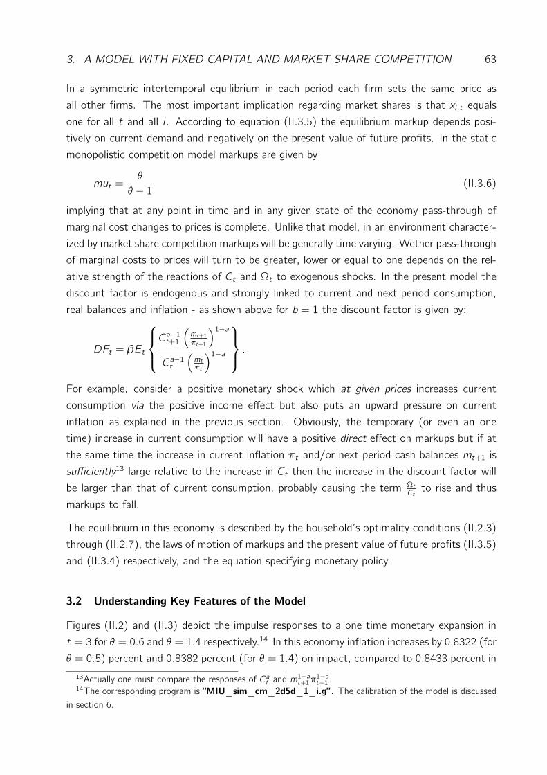
3. A MODEL WITH FIXED CAPITAL AND MARKET SHARE COMPETITION 63
In a symmetric intertemporal equilibrium in each period each firm sets the same price as
all other firms. The most important implication regarding market shares is that xi ,t equals
one for all t and all i . According to equation (II.3.5) the equilibrium markup depends posi-
tively on current demand and negatively on the present value of future profits. In the static
monopolistic competition model markups are given by
mut =θ
θ − 1 (II.3.6)
implying that at any point in time and in any given state of the economy pass-through of
marginal cost changes to prices is complete. Unlike that model, in an environment character-
ized by market share competition markups will be generally time varying. Wether pass-through
of marginal costs to prices will turn to be greater, lower or equal to one depends on the rel-
ative strength of the reactions of Ct and Ωt to exogenous shocks. In the present model the
discount factor is endogenous and strongly linked to current and next-period consumption,
real balances and inflation - as shown above for b = 1 the discount factor is given by:
DFt = βEt
Ca−1t+1
(mt+1πt+1
)1−a
Ca−1t(mtπt
)1−a
.
For example, consider a positive monetary shock which at given prices increases current
consumption via the positive income effect but also puts an upward pressure on current
inflation as explained in the previous section. Obviously, the temporary (or even an one
time) increase in current consumption will have a positive direct effect on markups but if at
the same time the increase in current inflation πt and/or next period cash balances mt+1 is
sufficiently13 large relative to the increase in Ct then the increase in the discount factor will
be larger than that of current consumption, probably causing the term ΩtCt
to rise and thus
markups to fall.
The equilibrium in this economy is described by the household’s optimality conditions (II.2.3)
through (II.2.7), the laws of motion of markups and the present value of future profits (II.3.5)
and (II.3.4) respectively, and the equation specifying monetary policy.
3.2 Understanding Key Features of the Model
Figures (II.2) and (II.3) depict the impulse responses to a one time monetary expansion in
t = 3 for θ = 0.6 and θ = 1.4 respectively.14 In this economy inflation increases by 0.8322 (for
θ = 0.5) percent and 0.8382 percent (for θ = 1.4) on impact, compared to 0.8433 percent in
13Actually one must compare the responses of Cat and m1−at+1π
1−at+1 .
14The corresponding program is ”MIU_sim_cm_2d5d_1_i.g” . The calibration of the model is discussed
in section 6.
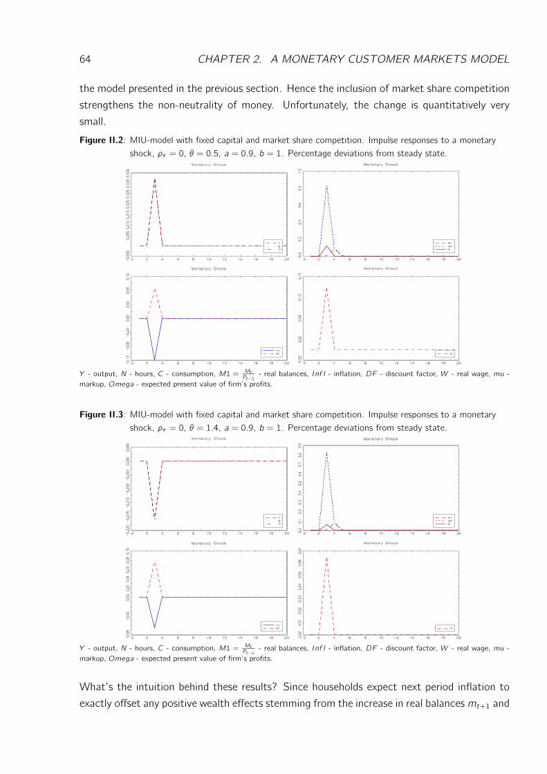
64 CHAPTER 2. A MONETARY CUSTOMER MARKETS MODEL
the model presented in the previous section. Hence the inclusion of market share competition
strengthens the non-neutrality of money. Unfortunately, the change is quantitatively very
small.
Figure II.2: MIU-model with fixed capital and market share competition. Impulse responses to a monetaryshock, ρτ = 0, θ = 0.5, a = 0.9, b = 1. Percentage deviations from steady state.
Y - output, N - hours, C - consumption, M1 = MtPt−1 - real balances, Inf l - inflation, DF - discount factor, W - real wage, mu -
markup, Omega - expected present value of firm’s profits.
Figure II.3: MIU-model with fixed capital and market share competition. Impulse responses to a monetaryshock, ρτ = 0, θ = 1.4, a = 0.9, b = 1. Percentage deviations from steady state.
Y - output, N - hours, C - consumption, M1 = MtPt−1 - real balances, Inf l - inflation, DF - discount factor, W - real wage, mu -
markup, Omega - expected present value of firm’s profits.
What’s the intuition behind these results? Since households expect next period inflation to
exactly offset any positive wealth effects stemming from the increase in real balancesmt+1 and
3. A MODEL WITH FIXED CAPITAL AND MARKET SHARE COMPETITION 65
at the same time all future inflation rates, markups and productivity levels to remain constant
they will have no incentive to set consumption, labor supply and savings at values different
from their respective steady state values. As a consequence, the expected discounted present
value of firm’s profits Ωt changes only because the discount factor DFt changes, while the
latter deviates from its steady state level only because the product C1−at π1−at does. Hence,
the log-deviation of the markup from its steady state level can be represented as:
mut = −ξ((1− a)Ct + (1− a)πt − Ct) = ξaCt − ξ(1− a)πt ,
where ξ = γ Ω∗C∗
γ Ω∗C∗+θ−1
. With a = 0.9 the difference between the log-deviation of the discount
factor and that of current consumption
DF t − Ct = −aCt + (1− a)πt
will be positive as long as the increase in inflation is sufficiently large relative to the reaction
of consumption. The latter is the case in all simulations performed. The optimal reaction
of firms to an increase in Ωt relative to Ct is to lower markups. As a result real wages
(profits) rise (fall) forcing households to increase labor supply. But at the same time, the
higher labor enables the economy to produce and therefore consume more. The potential
to increase consumption as well as the above average inflation reduce the marginal utility of
consumption, generating an incentive for households to reduce labor supply. Whether working
hours will rise or fall depends on the relative strength of the positive effect of the markup
and the negative effect of the fall in the marginal utility of consumption. Which of this two
effects dominates depends on the short run elasticity of demand θ. Why? Optimal labor
supply is given by
Nt = aCa−1t
(mtπt
)1−aWtPt.
Its relative deviation from the steady state can be written as
Nt = −Ct + (ξ − 1)((1− a)πt − aCt︸ ︷︷ ︸:=−mut
),
and by imposing the equilibrium condition Nt = Ct we get:
Nt =(ξ − 1)(1− a)2 + a(ξ − 1) πt . (II.3.1)
Since for θ ∈ (0, 1) ξ > 1, while θ ≥ 1 implies ξ ∈ (0, 1], working hours respond positively
(for θ < 1) and negatively (for θ > 1) to fluctuations of the inflation rate. In the case
of θ ∈ (0, 1) and thus ξ > 1 the slope of the first derivative of the current profit function
is relatively small in absolute value. As a result, when changes of current inflation and/or
current consumption occur firms need a relatively large adjustment of the markup in order
66 CHAPTER 2. A MONETARY CUSTOMER MARKETS MODEL
to ensure that their respective Euler equations are still satisfied. Put differently, if current
demand is relatively inelastic (the case of a low θ) the economy needs a larger adjustment
of the markup to restore equilibrium after a monetary shock. In this case, for a given level
of consumption, the fall of the markup is stronger than the decrease of the marginal utility
of consumption, both caused by the increase in inflation. As a consequence, working hours
increase. The resulting higher labor income for any given real wage as well as higher profits
for any given markup level enable households to increase consumption. The latter, in turn,
dampens the reactions of the markup and the marginal utility of consumption slightly. For
a given level of Ct θ > 1 and thus ξ ∈ (0, 1) implies that the fall in the marginal utility of
consumption is stronger than the increase in the real wage, both caused by the jump of the
inflation rate. Therefore, in that case hours fall shifting income and consumption down. The
reaction of consumption, again, implies a slight weakening of the effects induced by the rise
in πt .
Another way to gain intuition about the key mechanism in this model is as follows: Suppose,
initially firms miss the occurence of the monetary shock and do not adjust the markup. Then
consumption and inflation will react in exactly the same way as in the previous section - there
will be a drop in current consumption and a large jump in current inflation. But can this
situation be an equilibrium? The negative (positive) reaction of consumption (inflation) will
induce an unambiguous15 increase in
Ωt − Ct = DF t − Ct = −aCt + (1− a)πt .
Hence, each firm will find it optimal to lower its markup. As a results the real wage will rise
generating an incentive for households to increase labor supply. Thus, in this model for any
level of consumption, labor supply will be higher than in the one developed in the previous
section. For θ < 1 labor, output and consumption actually increase, otherwise they fall.
According to figures (II.2) and (II.3) the major shortcoming of the model is that the one-time
monetary disturbance induces purely temporary, one-time reactions of the main economic ag-
gregates. This absence of any persistence is at odds with the empirical evidence provided by
a vast number of studies employing structural VARs.16 In the following sections I introduce
different forms of capital accumulation and show that aside from making the production side
of the economy more realistic, the inclusion of capital as a second state variable also substan-
tially increases the persistence as well as magnitude of the responses to monetary shocks.
The latter result contrasts with the results obtained by Heer and Maussner (2007) who
show that extending Walsh’s (2005) New Keynesian model by including capital accumulation
substantially reduces the persistence of the real effects of monetary policy shocks.
15mt+1πt+1
as well as all other future variables are expected to remain unchanged.16See for example Christiano et al. (2005).
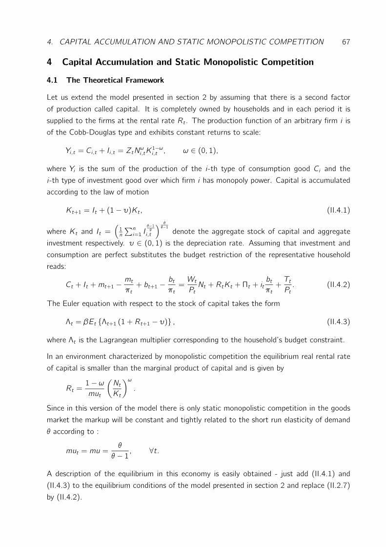
4. CAPITAL ACCUMULATION AND STATIC MONOPOLISTIC COMPETITION 67
4 Capital Accumulation and Static Monopolistic Competition
4.1 The Theoretical Framework
Let us extend the model presented in section 2 by assuming that there is a second factor
of production called capital. It is completely owned by households and in each period it is
supplied to the firms at the rental rate Rt . The production function of an arbitrary firm i is
of the Cobb-Douglas type and exhibits constant returns to scale:
Yi ,t = Ci ,t + Ii ,t = ZtNωi,tK
1−ωi,t , ω ∈ (0, 1),
where Yi is the sum of the production of the i-th type of consumption good Ci and the
i-th type of investment good over which firm i has monopoly power. Capital is accumulated
according to the law of motion
Kt+1 = It + (1− υ)Kt , (II.4.1)
where Kt and It =(1n
∑ni=1 I
θ−1θ
i ,t
) θθ−1
denote the aggregate stock of capital and aggregate
investment respectively. υ ∈ (0, 1) is the depreciation rate. Assuming that investment and
consumption are perfect substitutes the budget restriction of the representative household
reads:
Ct + It +mt+1 − mtπt+ bt+1 − bt
πt=WtPtNt + RtKt +Πt + it
btπt+TtPt. (II.4.2)
The Euler equation with respect to the stock of capital takes the form
Λt = βEt Λt+1 (1 + Rt+1 − υ) , (II.4.3)
where Λt is the Lagrangean multiplier corresponding to the household’s budget constraint.
In an environment characterized by monopolistic competition the equilibrium real rental rate
of capital is smaller than the marginal product of capital and is given by
Rt =1− ωmut
(NtKt
)ω.
Since in this version of the model there is only static monopolistic competition in the goods
market the markup will be constant and tightly related to the short run elasticity of demand
θ according to :
mut = mu =θ
θ − 1 , ∀t.
A description of the equilibrium in this economy is easily obtained - just add (II.4.1) and
(II.4.3) to the equilibrium conditions of the model presented in section 2 and replace (II.2.7)
by (II.4.2).
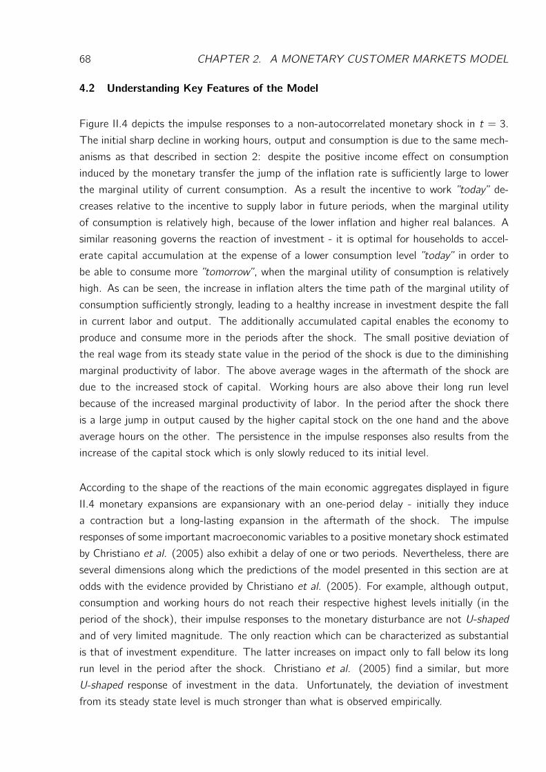
68 CHAPTER 2. A MONETARY CUSTOMER MARKETS MODEL
4.2 Understanding Key Features of the Model
Figure II.4 depicts the impulse responses to a non-autocorrelated monetary shock in t = 3.
The initial sharp decline in working hours, output and consumption is due to the same mech-
anisms as that described in section 2: despite the positive income effect on consumption
induced by the monetary transfer the jump of the inflation rate is sufficiently large to lower
the marginal utility of current consumption. As a result the incentive to work ”today” de-
creases relative to the incentive to supply labor in future periods, when the marginal utility
of consumption is relatively high, because of the lower inflation and higher real balances. A
similar reasoning governs the reaction of investment - it is optimal for households to accel-
erate capital accumulation at the expense of a lower consumption level ”today” in order to
be able to consume more ”tomorrow” , when the marginal utility of consumption is relatively
high. As can be seen, the increase in inflation alters the time path of the marginal utility of
consumption sufficiently strongly, leading to a healthy increase in investment despite the fall
in current labor and output. The additionally accumulated capital enables the economy to
produce and consume more in the periods after the shock. The small positive deviation of
the real wage from its steady state value in the period of the shock is due to the diminishing
marginal productivity of labor. The above average wages in the aftermath of the shock are
due to the increased stock of capital. Working hours are also above their long run level
because of the increased marginal productivity of labor. In the period after the shock there
is a large jump in output caused by the higher capital stock on the one hand and the above
average hours on the other. The persistence in the impulse responses also results from the
increase of the capital stock which is only slowly reduced to its initial level.
According to the shape of the reactions of the main economic aggregates displayed in figure
II.4 monetary expansions are expansionary with an one-period delay - initially they induce
a contraction but a long-lasting expansion in the aftermath of the shock. The impulse
responses of some important macroeconomic variables to a positive monetary shock estimated
by Christiano et al. (2005) also exhibit a delay of one or two periods. Nevertheless, there are
several dimensions along which the predictions of the model presented in this section are at
odds with the evidence provided by Christiano et al. (2005). For example, although output,
consumption and working hours do not reach their respective highest levels initially (in the
period of the shock), their impulse responses to the monetary disturbance are not U-shaped
and of very limited magnitude. The only reaction which can be characterized as substantial
is that of investment expenditure. The latter increases on impact only to fall below its long
run level in the period after the shock. Christiano et al. (2005) find a similar, but more
U-shaped response of investment in the data. Unfortunately, the deviation of investment
from its steady state level is much stronger than what is observed empirically.
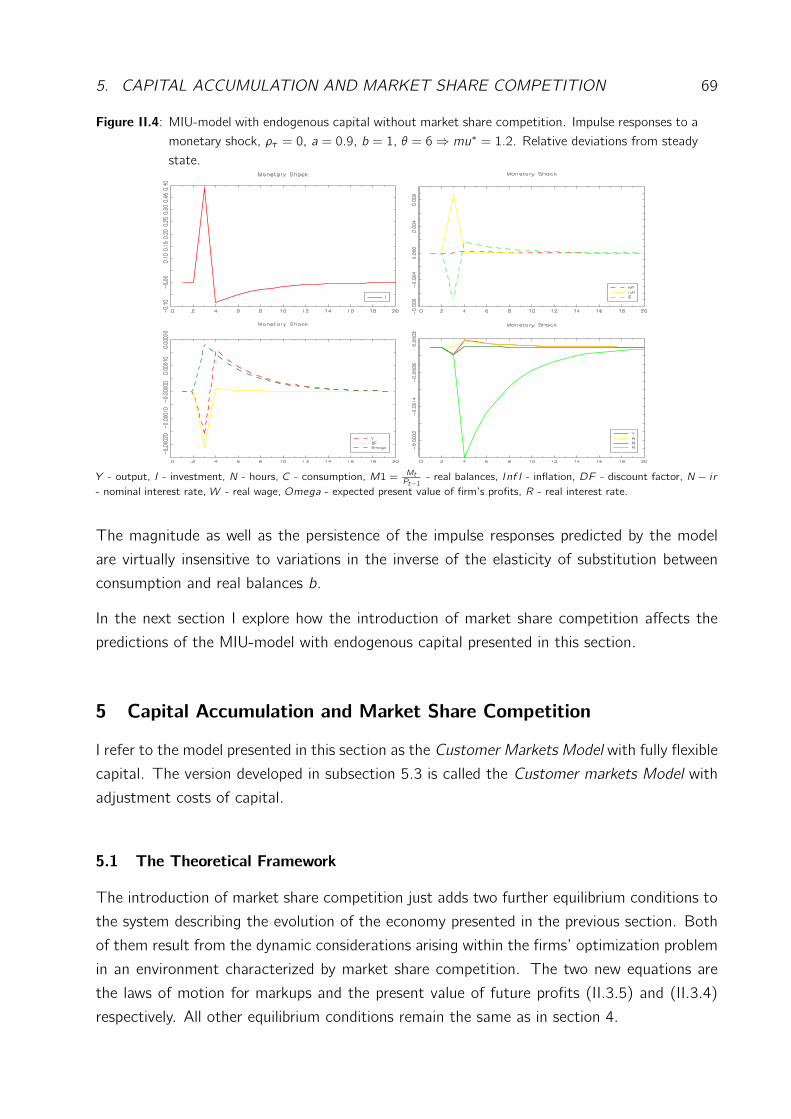
5. CAPITAL ACCUMULATION AND MARKET SHARE COMPETITION 69
Figure II.4: MIU-model with endogenous capital without market share competition. Impulse responses to amonetary shock, ρτ = 0, a = 0.9, b = 1, θ = 6⇒ mu∗ = 1.2. Relative deviations from steadystate.
Y - output, I - investment, N - hours, C - consumption, M1 = MtPt−1 - real balances, Inf l - inflation, DF - discount factor, N − i r
- nominal interest rate, W - real wage, Omega - expected present value of firm’s profits, R - real interest rate.
The magnitude as well as the persistence of the impulse responses predicted by the model
are virtually insensitive to variations in the inverse of the elasticity of substitution between
consumption and real balances b.
In the next section I explore how the introduction of market share competition affects the
predictions of the MIU-model with endogenous capital presented in this section.
5 Capital Accumulation and Market Share Competition
I refer to the model presented in this section as the Customer Markets Model with fully flexible
capital. The version developed in subsection 5.3 is called the Customer markets Model with
adjustment costs of capital.
5.1 The Theoretical Framework
The introduction of market share competition just adds two further equilibrium conditions to
the system describing the evolution of the economy presented in the previous section. Both
of them result from the dynamic considerations arising within the firms’ optimization problem
in an environment characterized by market share competition. The two new equations are
the laws of motion for markups and the present value of future profits (II.3.5) and (II.3.4)
respectively. All other equilibrium conditions remain the same as in section 4.
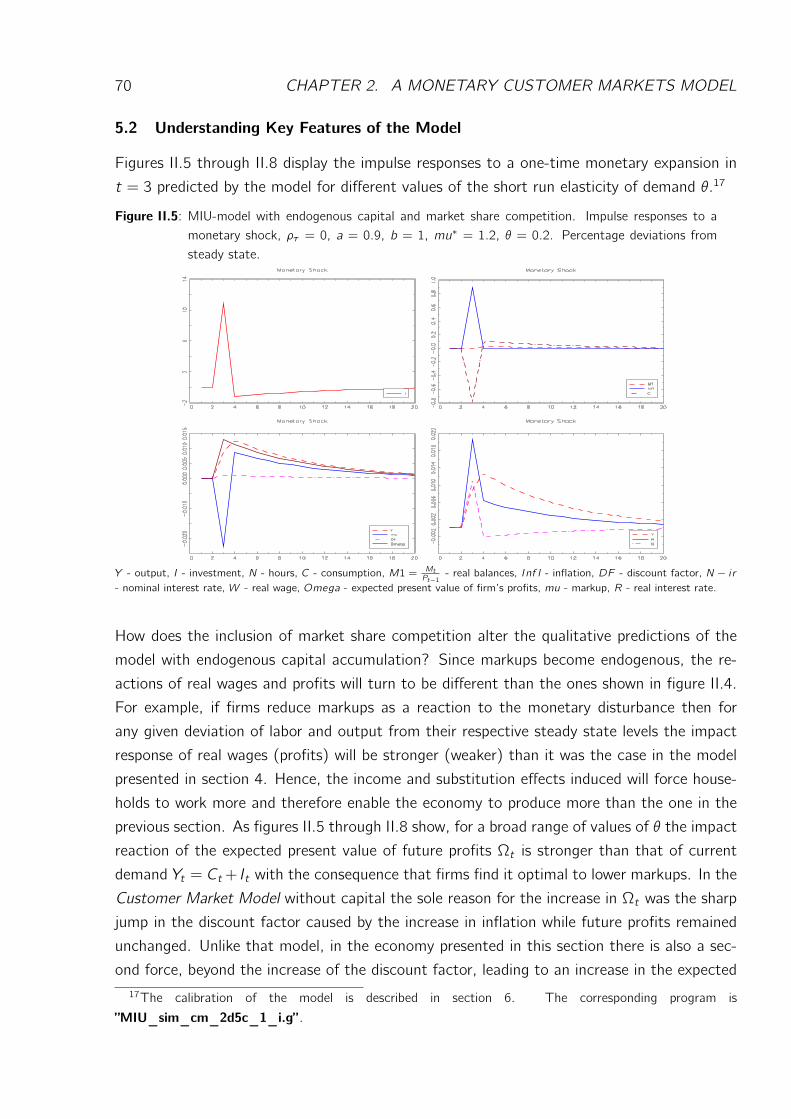
70 CHAPTER 2. A MONETARY CUSTOMER MARKETS MODEL
5.2 Understanding Key Features of the Model
Figures II.5 through II.8 display the impulse responses to a one-time monetary expansion in
t = 3 predicted by the model for different values of the short run elasticity of demand θ.17
Figure II.5: MIU-model with endogenous capital and market share competition. Impulse responses to amonetary shock, ρτ = 0, a = 0.9, b = 1, mu∗ = 1.2, θ = 0.2. Percentage deviations fromsteady state.
Y - output, I - investment, N - hours, C - consumption, M1 = MtPt−1 - real balances, Inf l - inflation, DF - discount factor, N − i r
- nominal interest rate, W - real wage, Omega - expected present value of firm’s profits, mu - markup, R - real interest rate.
How does the inclusion of market share competition alter the qualitative predictions of the
model with endogenous capital accumulation? Since markups become endogenous, the re-
actions of real wages and profits will turn to be different than the ones shown in figure II.4.
For example, if firms reduce markups as a reaction to the monetary disturbance then for
any given deviation of labor and output from their respective steady state levels the impact
response of real wages (profits) will be stronger (weaker) than it was the case in the model
presented in section 4. Hence, the income and substitution effects induced will force house-
holds to work more and therefore enable the economy to produce more than the one in the
previous section. As figures II.5 through II.8 show, for a broad range of values of θ the impact
reaction of the expected present value of future profits Ωt is stronger than that of current
demand Yt = Ct+ It with the consequence that firms find it optimal to lower markups. In the
Customer Market Model without capital the sole reason for the increase in Ωt was the sharp
jump in the discount factor caused by the increase in inflation while future profits remained
unchanged. Unlike that model, in the economy presented in this section there is also a sec-
ond force, beyond the increase of the discount factor, leading to an increase in the expected17The calibration of the model is described in section 6. The corresponding program is
”MIU_sim_cm_2d5c_1_i.g” .
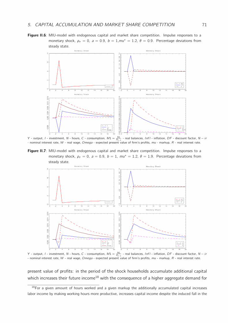
5. CAPITAL ACCUMULATION AND MARKET SHARE COMPETITION 71
Figure II.6: MIU-model with endogenous capital and market share competition. Impulse responses to amonetary shock, ρτ = 0, a = 0.9, b = 1,mu∗ = 1.2, θ = 0.9. Percentage deviations fromsteady state.
Y - output, I - investment, N - hours, C - consumption, M1 = MtPt−1 - real balances, Inf l - inflation, DF - discount factor, N − i r
- nominal interest rate, W - real wage, Omega - expected present value of firm’s profits, mu - markup, R - real interest rate.
Figure II.7: MIU-model with endogenous capital and market share competition. Impulse responses to amonetary shock, ρτ = 0, a = 0.9, b = 1, mu∗ = 1.2, θ = 1.9. Percentage deviations fromsteady state.
Y - output, I - investment, N - hours, C - consumption, M1 = MtPt−1 - real balances, Inf l - inflation, DF - discount factor, N − i r
- nominal interest rate, W - real wage, Omega - expected present value of firm’s profits, mu - markup, R - real interest rate.
present value of profits: in the period of the shock households accumulate additional capital
which increases their future income18 with the consequence of a higher aggregate demand for
18For a given amount of hours worked and a given markup the additionally accumulated capital increases
labor income by making working hours more productive, increases capital income despite the induced fall in the
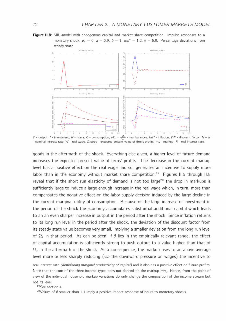
72 CHAPTER 2. A MONETARY CUSTOMER MARKETS MODEL
Figure II.8: MIU-model with endogenous capital and market share competition. Impulse responses to amonetary shock, ρτ = 0, a = 0.9, b = 1, mu∗ = 1.2, θ = 5.9. Percentage deviations fromsteady state.
Y - output, I - investment, N - hours, C - consumption, M1 = MtPt−1 - real balances, Inf l - inflation, DF - discount factor, N − i r
- nominal interest rate, W - real wage, Omega - expected present value of firm’s profits, mu - markup, R - real interest rate.
goods in the aftermath of the shock. Everything else given, a higher level of future demand
increases the expected present value of firms’ profits. The decrease in the current markup
level has a positive effect on the real wage and so, generates an incentive to supply more
labor than in the economy without market share competition.19 Figures II.5 through II.8
reveal that if the short run elasticity of demand is not too large20 the drop in markups is
sufficiently large to induce a large enough increase in the real wage which, in turn, more than
compensates the negative effect on the labor supply decision induced by the large decline in
the current marginal utility of consumption. Because of the large increase of investment in
the period of the shock the economy accumulates substantial additional capital which leads
to an an even sharper increase in output in the period after the shock. Since inflation returns
to its long run level in the period after the shock, the deviation of the discount factor from
its steady state value becomes very small, implying a smaller deviation from the long run level
of Ωt in that period. As can be seen, if θ lies in the empirically relevant range, the effect
of capital accumulation is sufficiently strong to push output to a value higher than that of
Ωt in the aftermath of the shock. As a consequence, the markup rises to an above average
level more or less sharply reducing (via the downward pressure on wages) the incentive to
real interest rate (diminishing marginal productivity of capital) and it also has a positive effect on future profits.
Note that the sum of the three income types does not depend on the markup mut . Hence, from the point of
view of the individual household markup variations do only change the composition of the income stream but
not its level.19See section 4.20Values of θ smaller than 1.1 imply a positive impact response of hours to monetary shocks.
5. CAPITAL ACCUMULATION AND MARKET SHARE COMPETITION 73
work. According to the impulse responses shown, lower values of θ imply stronger reactions
of markups which, in turn, induce a larger increase in working hours in the period of the shock
and than a larger drop of that variable thereafter (compare figure II.5 with figure II.6).
Values of θ near one imply delayed responses of output and employment to monetary inno-
vations with both variables reaching their highest values in the period after the shock. While
such a prediction should be seen as more or less in line with the existing VAR evidence, the
responses of several other variables to monetary disturbances are not consistent with the
patterns found in the data. For example, in the model economy developed in this section a
money supply loosening induces a large short-run contraction of consumption. In the periods
after the shock consumption expenditure reaches an above average value but its deviation
from the steady state level is very small. The responses of investment and real wages also do
not exhibit an U-shaped form. Both variables reach their highest deviation from the stationary
equilibrium in the period in which the monetary innovation occurs. Furthermore, the reaction
of investment is many times larger than measured by any of the existing empirical studies.
In addition, investment is the only variable the response of which can be characterized as a
substantial real effect of monetary policy. The reactions of the remaining real variables are
persistent but of limited magnitude. For example, in the case θ = 0.5 the largest deviation
of output from its steady state, reached in the second period, is equal to 0.014%, which is
much less (about ten times smaller) than what a serially uncorrelated technology shock of
similar size would induce.
Similar to the economy of section 4 the magnitude as well as the persistence of the im-
pulse responses in the current model are virtually insensitive to variations in the elasticity of
substitution between consumption and real balances 1/b.
5.3 A Customer Markets Model with Adjustment Costs of Capital
How does the inclusion of adjustment costs of capital alter the dynamic properties of the
model? The economic intuition suggests that if investment is sufficiently costly households
will be reluctant to accelerate capital accumulation in such a dramatic manner as they do in
the models developed in sections 4 and 5. As a consequence, there will be more resources left
for consumption in the period of the shock, enabling the theory to get rid of the counterfactual
sharp increase (decline) in investment (consumption). In addition, the presence of adjustment
costs of capital will strengthen the incentive to raise future real money holdings mt+1 which,
in turn, will induce a positive wealth effect in t+1, t+2, ... and so, probably, at least partly,
preserve the persistence in the impulse responses. Note that the wealth effect in t+1 induced
by a higher level of real balances triggers off qualitatively the same reactions as the positive
income effect of the monetary disturbance in the period of the shock. Furthermore, because
74 CHAPTER 2. A MONETARY CUSTOMER MARKETS MODEL
the introduction of capital adjustment costs shifts the properties of the model towards the
fixed capital case, one could expect to be able to make the real effects of monetary shocks
arbitrarily large by setting the short run elasticity of demand θ at a sufficiently low value and
the elasticity of substitution between consumption and real balances b at a sufficiently high
value. In other words, since the Customer Markets Model with adjustment costs of capital
represents the intermediate case between the model developed in section 3 and the one
presented in section 5 there is no a priori reason not to expect that it will be a combination
of the favorable properties of the latter two models.
Formal Details: The flexibility of investment is reduced in an ad hoc manner by assuming
that there is an additional adjustment cost of capital represented by the strict concavity of
the strictly increasing function φ(ItKt
)in
Kt+1 = φ
(ItKt
)Kt + (1− υ)Kt . (II.5.1)
Further, φ(.) has the properties:
φ
(I
K
)= φ(υ) = υ, φ′(υ) = 1,
where I and K are the steady state levels of investment and capital respectively.21 The
first assumption ensures that the steady state is characterized by the absence of adjustment
costs while the second implies that in the stationary equilibrium Tobin’s q is equal to one.
Formally the equilibrium conditions (II.2.3) through (II.2.7) ought to be adjusted by including
the household’s first order condition with respect to investment
qt =Λt
φ′(ItKt
) ,
substituting the conventional transition equation for capital by (II.5.1) and replacing the first
order condition with respect to next period’s stock of capital (II.4.3) by
qt = Et
Λt+1
1− ωmut+1
Yt+1Kt+1
+ qt+1
(1− υ + φ
(It+1Kt+1
)− φ′
(It+1Kt+1
)It+1Kt+1
),
where qt denotes the Lagrangean multiplier attached to (II.5.1) and qt/Λt equals Tobin’s q.
The individual firm faces the same optimization problem and thus, behaves according to the
same optimality conditions as in the economy with market share competition and fully flexible
capital described in the first part of section 5.
21The assumed law of motion of capital is also used by Correia et al. (1995), Jerman (1998) and others.
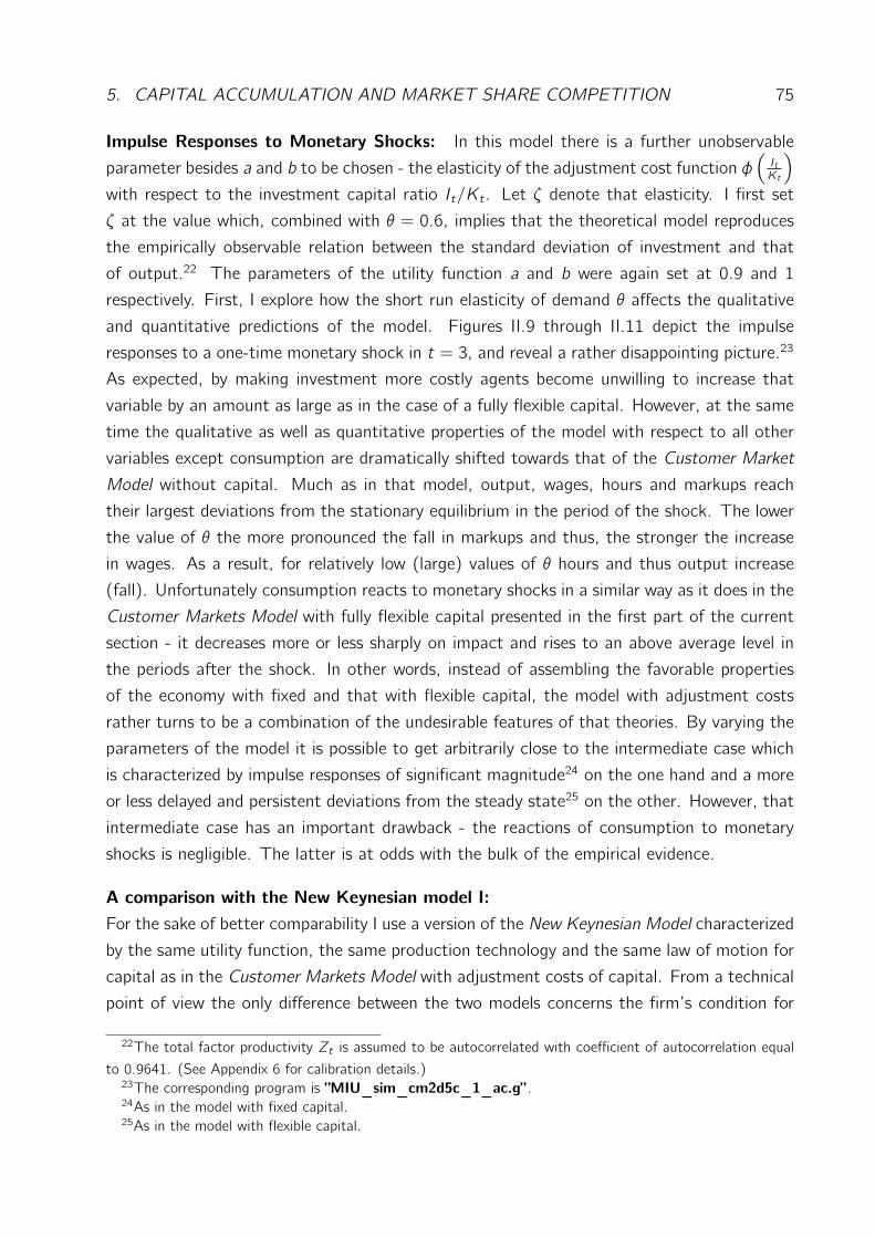
5. CAPITAL ACCUMULATION AND MARKET SHARE COMPETITION 75
Impulse Responses to Monetary Shocks: In this model there is a further unobservable
parameter besides a and b to be chosen - the elasticity of the adjustment cost function φ(ItKt
)
with respect to the investment capital ratio It/Kt . Let ζ denote that elasticity. I first set
ζ at the value which, combined with θ = 0.6, implies that the theoretical model reproduces
the empirically observable relation between the standard deviation of investment and that
of output.22 The parameters of the utility function a and b were again set at 0.9 and 1
respectively. First, I explore how the short run elasticity of demand θ affects the qualitative
and quantitative predictions of the model. Figures II.9 through II.11 depict the impulse
responses to a one-time monetary shock in t = 3, and reveal a rather disappointing picture.23
As expected, by making investment more costly agents become unwilling to increase that
variable by an amount as large as in the case of a fully flexible capital. However, at the same
time the qualitative as well as quantitative properties of the model with respect to all other
variables except consumption are dramatically shifted towards that of the Customer Market
Model without capital. Much as in that model, output, wages, hours and markups reach
their largest deviations from the stationary equilibrium in the period of the shock. The lower
the value of θ the more pronounced the fall in markups and thus, the stronger the increase
in wages. As a result, for relatively low (large) values of θ hours and thus output increase
(fall). Unfortunately consumption reacts to monetary shocks in a similar way as it does in the
Customer Markets Model with fully flexible capital presented in the first part of the current
section - it decreases more or less sharply on impact and rises to an above average level in
the periods after the shock. In other words, instead of assembling the favorable properties
of the economy with fixed and that with flexible capital, the model with adjustment costs
rather turns to be a combination of the undesirable features of that theories. By varying the
parameters of the model it is possible to get arbitrarily close to the intermediate case which
is characterized by impulse responses of significant magnitude24 on the one hand and a more
or less delayed and persistent deviations from the steady state25 on the other. However, that
intermediate case has an important drawback - the reactions of consumption to monetary
shocks is negligible. The latter is at odds with the bulk of the empirical evidence.
A comparison with the New Keynesian model I:For the sake of better comparability I use a version of the New Keynesian Model characterized
by the same utility function, the same production technology and the same law of motion for
capital as in the Customer Markets Model with adjustment costs of capital. From a technical
point of view the only difference between the two models concerns the firm’s condition for
22The total factor productivity Zt is assumed to be autocorrelated with coefficient of autocorrelation equal
to 0.9641. (See Appendix 6 for calibration details.)23The corresponding program is ”MIU_sim_cm2d5c_1_ac.g” .24As in the model with fixed capital.25As in the model with flexible capital.
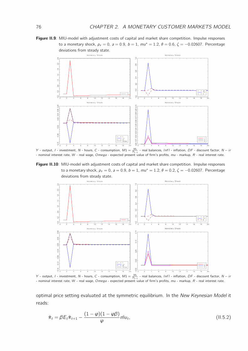
76 CHAPTER 2. A MONETARY CUSTOMER MARKETS MODEL
Figure II.9: MIU-model with adjustment costs of capital and market share competition. Impulse responsesto a monetary shock, ρτ = 0, a = 0.9, b = 1, mu∗ = 1.2, θ = 0.6, ζ = −0.02607. Percentagedeviations from steady state.
Y - output, I - investment, N - hours, C - consumption, M1 = MtPt−1 - real balances, Inf l - inflation, DF - discount factor, N − i r
- nominal interest rate, W - real wage, Omega - expected present value of firm’s profits, mu - markup, R - real interest rate.
Figure II.10: MIU-model with adjustment costs of capital and market share competition. Impulse responsesto a monetary shock, ρτ = 0, a = 0.9, b = 1, mu∗ = 1.2, θ = 0.2, ζ = −0.02607. Percentagedeviations from steady state.
Y - output, I - investment, N - hours, C - consumption, M1 = MtPt−1 - real balances, Inf l - inflation, DF - discount factor, N − i r
- nominal interest rate, W - real wage, Omega - expected present value of firm’s profits, mu - markup, R - real interest rate.
optimal price setting evaluated at the symmetric equilibrium. In the New Keynesian Model it
reads:
πt = βEtπt+1 − (1− ϕ)(1− ϕβ)ϕ
mut , (II.5.2)
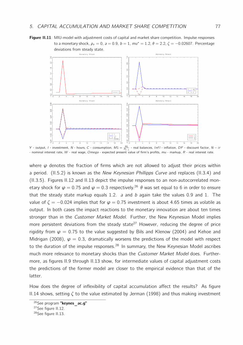
5. CAPITAL ACCUMULATION AND MARKET SHARE COMPETITION 77
Figure II.11: MIU-model with adjustment costs of capital and market share competition. Impulse responsesto a monetary shock, ρτ = 0, a = 0.9, b = 1, mu∗ = 1.2, θ = 2.2, ζ = −0.02607. Percentagedeviations from steady state.
Y - output, I - investment, N - hours, C - consumption, M1 = MtPt−1 - real balances, Inf l - inflation, DF - discount factor, N − i r
- nominal interest rate, W - real wage, Omega - expected present value of firm’s profits, mu - markup, R - real interest rate.
where ϕ denotes the fraction of firms which are not allowed to adjust their prices within
a period. (II.5.2) is known as the New Keynesian Phillipps Curve and replaces (II.3.4) and
(II.3.5). Figures II.12 and II.13 depict the impulse responses to an non-autocorrelated mon-
etary shock for ϕ = 0.75 and ϕ = 0.3 respectively.26 θ was set equal to 6 in order to ensure
that the steady state markup equals 1.2. a and b again take the values 0.9 and 1. The
value of ζ = −0.024 implies that for ϕ = 0.75 investment is about 4.65 times as volatile as
output. In both cases the impact reactions to the monetary innovation are about ten times
stronger than in the Customer Market Model. Further, the New Keynesian Model implies
more persistent deviations from the steady state27 However, reducing the degree of price
rigidity from ϕ = 0.75 to the value suggested by Bils and Klenow (2004) and Kehoe and
Midrigan (2008), ϕ = 0.3, dramatically worsens the predictions of the model with respect
to the duration of the impulse responses.28 In summary, the New Keynesian Model ascribes
much more relevance to monetary shocks than the Customer Market Model does. Further-
more, as figures II.9 through II.13 show, for intermediate values of capital adjustment costs
the predictions of the former model are closer to the empirical evidence than that of the
latter.
How does the degree of inflexibility of capital accumulation affect the results? As figure
II.14 shows, setting ζ to the value estimated by Jerman (1998) and thus making investment
26See program ”keynes_ac.g”27See figure II.12.28See figure II.13.
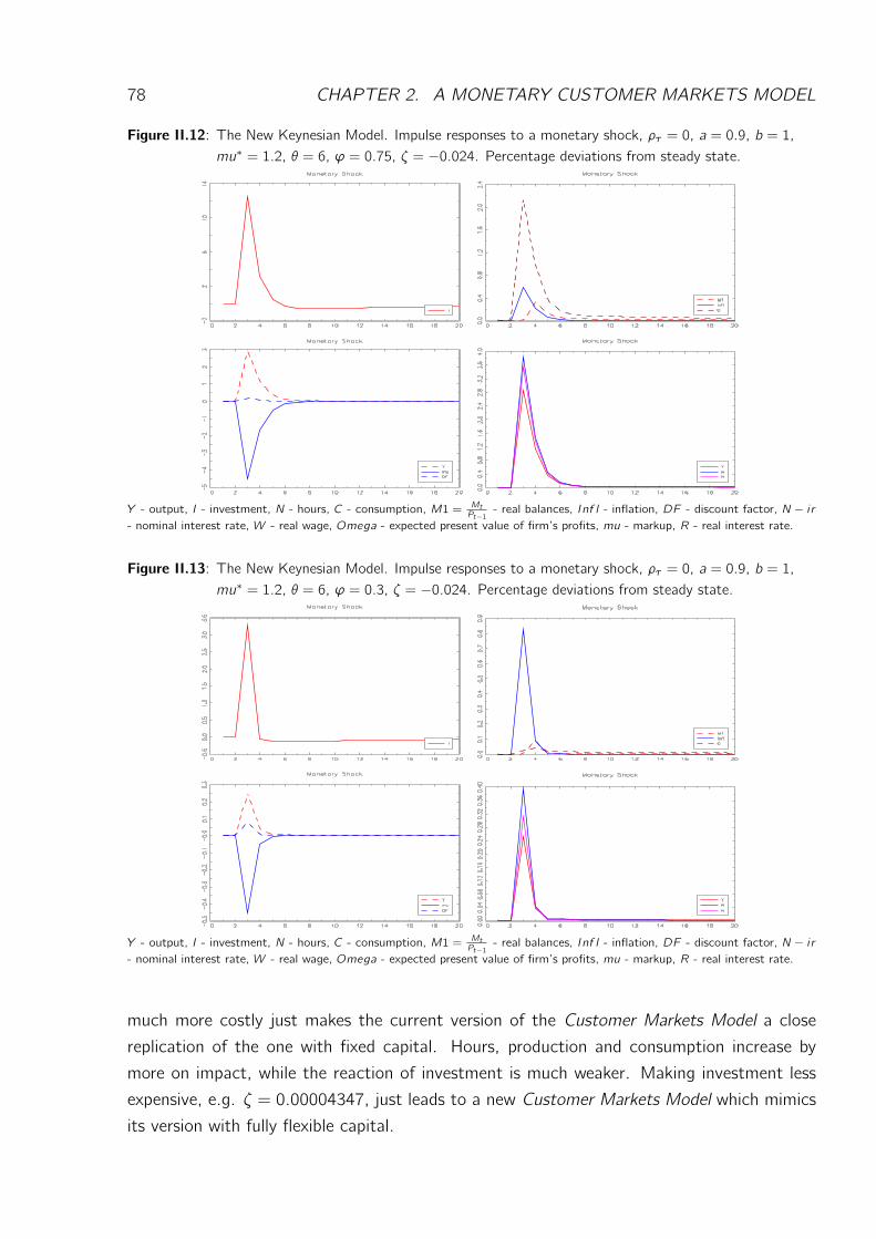
78 CHAPTER 2. A MONETARY CUSTOMER MARKETS MODEL
Figure II.12: The New Keynesian Model. Impulse responses to a monetary shock, ρτ = 0, a = 0.9, b = 1,mu∗ = 1.2, θ = 6, ϕ = 0.75, ζ = −0.024. Percentage deviations from steady state.
Y - output, I - investment, N - hours, C - consumption, M1 = MtPt−1 - real balances, Inf l - inflation, DF - discount factor, N − i r
- nominal interest rate, W - real wage, Omega - expected present value of firm’s profits, mu - markup, R - real interest rate.
Figure II.13: The New Keynesian Model. Impulse responses to a monetary shock, ρτ = 0, a = 0.9, b = 1,mu∗ = 1.2, θ = 6, ϕ = 0.3, ζ = −0.024. Percentage deviations from steady state.
Y - output, I - investment, N - hours, C - consumption, M1 = MtPt−1 - real balances, Inf l - inflation, DF - discount factor, N − i r
- nominal interest rate, W - real wage, Omega - expected present value of firm’s profits, mu - markup, R - real interest rate.
much more costly just makes the current version of the Customer Markets Model a close
replication of the one with fixed capital. Hours, production and consumption increase by
more on impact, while the reaction of investment is much weaker. Making investment less
expensive, e.g. ζ = 0.00004347, just leads to a new Customer Markets Model which mimics
its version with fully flexible capital.
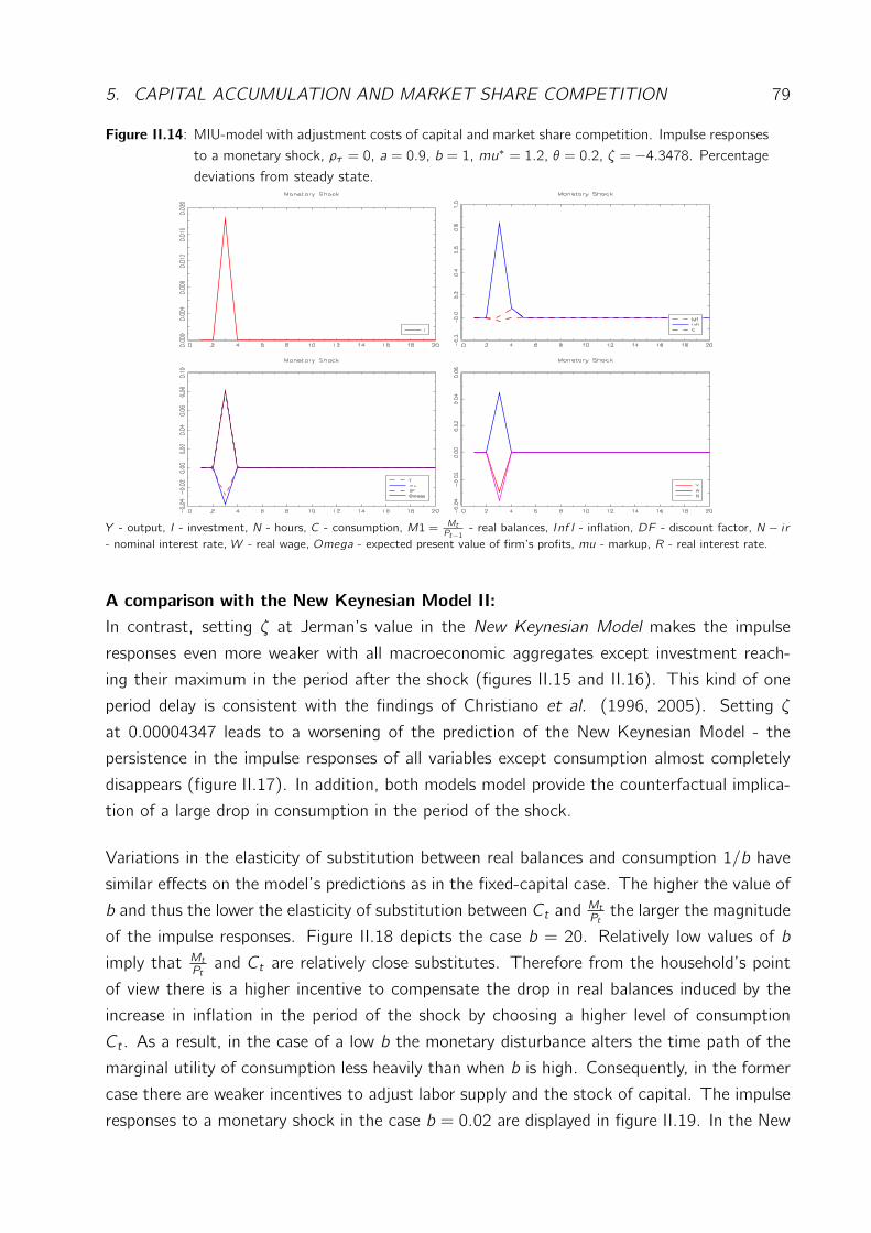
5. CAPITAL ACCUMULATION AND MARKET SHARE COMPETITION 79
Figure II.14: MIU-model with adjustment costs of capital and market share competition. Impulse responsesto a monetary shock, ρτ = 0, a = 0.9, b = 1, mu∗ = 1.2, θ = 0.2, ζ = −4.3478. Percentagedeviations from steady state.
Y - output, I - investment, N - hours, C - consumption, M1 = MtPt−1 - real balances, Inf l - inflation, DF - discount factor, N − i r
- nominal interest rate, W - real wage, Omega - expected present value of firm’s profits, mu - markup, R - real interest rate.
A comparison with the New Keynesian Model II:In contrast, setting ζ at Jerman’s value in the New Keynesian Model makes the impulse
responses even more weaker with all macroeconomic aggregates except investment reach-
ing their maximum in the period after the shock (figures II.15 and II.16). This kind of one
period delay is consistent with the findings of Christiano et al. (1996, 2005). Setting ζ
at 0.00004347 leads to a worsening of the prediction of the New Keynesian Model - the
persistence in the impulse responses of all variables except consumption almost completely
disappears (figure II.17). In addition, both models model provide the counterfactual implica-
tion of a large drop in consumption in the period of the shock.
Variations in the elasticity of substitution between real balances and consumption 1/b have
similar effects on the model’s predictions as in the fixed-capital case. The higher the value of
b and thus the lower the elasticity of substitution between Ct and MtPt the larger the magnitude
of the impulse responses. Figure II.18 depicts the case b = 20. Relatively low values of b
imply that MtPt
and Ct are relatively close substitutes. Therefore from the household’s point
of view there is a higher incentive to compensate the drop in real balances induced by the
increase in inflation in the period of the shock by choosing a higher level of consumption
Ct . As a result, in the case of a low b the monetary disturbance alters the time path of the
marginal utility of consumption less heavily than when b is high. Consequently, in the former
case there are weaker incentives to adjust labor supply and the stock of capital. The impulse
responses to a monetary shock in the case b = 0.02 are displayed in figure II.19. In the New
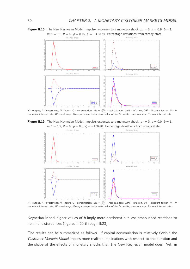
80 CHAPTER 2. A MONETARY CUSTOMER MARKETS MODEL
Figure II.15: The New Keynesian Model. Impulse responses to a monetary shock, ρτ = 0, a = 0.9, b = 1,mu∗ = 1.2, θ = 6, ϕ = 0.75, ζ = −4.3478. Percentage deviations from steady state.
Y - output, I - investment, N - hours, C - consumption, M1 = MtPt−1 - real balances, Inf l - inflation, DF - discount factor, N − i r
- nominal interest rate, W - real wage, Omega - expected present value of firm’s profits, mu - markup, R - real interest rate.
Figure II.16: The New Keynesian Model. Impulse responses to a monetary shock, ρτ = 0, a = 0.9, b = 1,mu∗ = 1.2, θ = 6, ϕ = 0.3, ζ = −4.3478. Percentage deviations from steady state.
Y - output, I - investment, N - hours, C - consumption, M1 = MtPt−1 - real balances, Inf l - inflation, DF - discount factor, N − i r
- nominal interest rate, W - real wage, Omega - expected present value of firm’s profits, mu - markup, R - real interest rate.
Keynesian Model higher values of b imply more persistent but less pronounced reactions to
nominal disturbances (figures II.20 through II.23).
The results can be summarized as follows. If capital accumulation is relatively flexible the
Customer Markets Model implies more realistic implications with respect to the duration and
the shape of the effects of monetary shocks than the New Keynesian model does. Yet, in
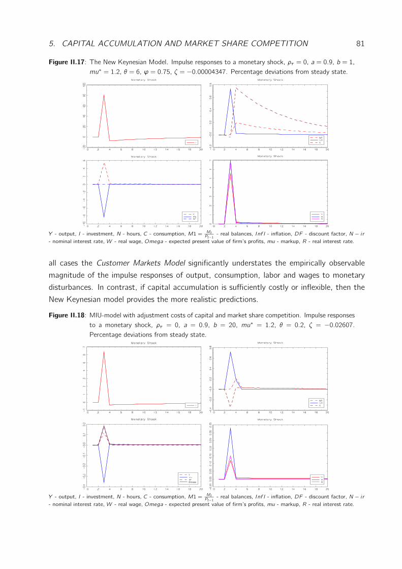
5. CAPITAL ACCUMULATION AND MARKET SHARE COMPETITION 81
Figure II.17: The New Keynesian Model. Impulse responses to a monetary shock, ρτ = 0, a = 0.9, b = 1,mu∗ = 1.2, θ = 6, ϕ = 0.75, ζ = −0.00004347. Percentage deviations from steady state.
Y - output, I - investment, N - hours, C - consumption, M1 = MtPt−1 - real balances, Inf l - inflation, DF - discount factor, N − i r
- nominal interest rate, W - real wage, Omega - expected present value of firm’s profits, mu - markup, R - real interest rate.
all cases the Customer Markets Model significantly understates the empirically observable
magnitude of the impulse responses of output, consumption, labor and wages to monetary
disturbances. In contrast, if capital accumulation is sufficiently costly or inflexible, then the
New Keynesian model provides the more realistic predictions.
Figure II.18: MIU-model with adjustment costs of capital and market share competition. Impulse responsesto a monetary shock, ρτ = 0, a = 0.9, b = 20, mu∗ = 1.2, θ = 0.2, ζ = −0.02607.Percentage deviations from steady state.
Y - output, I - investment, N - hours, C - consumption, M1 = MtPt−1 - real balances, Inf l - inflation, DF - discount factor, N − i r
- nominal interest rate, W - real wage, Omega - expected present value of firm’s profits, mu - markup, R - real interest rate.
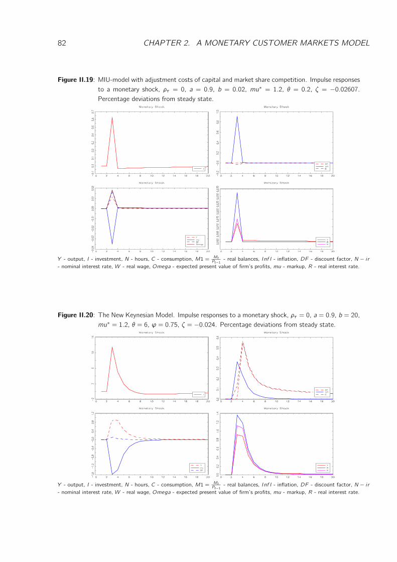
82 CHAPTER 2. A MONETARY CUSTOMER MARKETS MODEL
Figure II.19: MIU-model with adjustment costs of capital and market share competition. Impulse responsesto a monetary shock, ρτ = 0, a = 0.9, b = 0.02, mu∗ = 1.2, θ = 0.2, ζ = −0.02607.Percentage deviations from steady state.
Y - output, I - investment, N - hours, C - consumption, M1 = MtPt−1 - real balances, Inf l - inflation, DF - discount factor, N − i r
- nominal interest rate, W - real wage, Omega - expected present value of firm’s profits, mu - markup, R - real interest rate.
Figure II.20: The New Keynesian Model. Impulse responses to a monetary shock, ρτ = 0, a = 0.9, b = 20,mu∗ = 1.2, θ = 6, ϕ = 0.75, ζ = −0.024. Percentage deviations from steady state.
Y - output, I - investment, N - hours, C - consumption, M1 = MtPt−1 - real balances, Inf l - inflation, DF - discount factor, N − i r
- nominal interest rate, W - real wage, Omega - expected present value of firm’s profits, mu - markup, R - real interest rate.
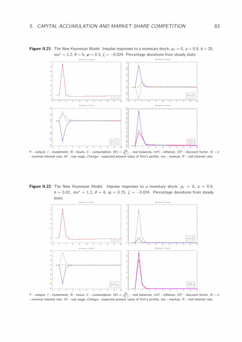
5. CAPITAL ACCUMULATION AND MARKET SHARE COMPETITION 83
Figure II.21: The New Keynesian Model. Impulse responses to a monetary shock, ρτ = 0, a = 0.9, b = 20,mu∗ = 1.2, θ = 6, ϕ = 0.3, ζ = −0.024. Percentage deviations from steady state.
Y - output, I - investment, N - hours, C - consumption, M1 = MtPt−1 - real balances, Inf l - inflation, DF - discount factor, N − i r
- nominal interest rate, W - real wage, Omega - expected present value of firm’s profits, mu - markup, R - real interest rate.
Figure II.22: The New Keynesian Model. Impulse responses to a monetary shock, ρτ = 0, a = 0.9,b = 0.02, mu∗ = 1.2, θ = 6, ϕ = 0.75, ζ = −0.024. Percentage deviations from steadystate.
Y - output, I - investment, N - hours, C - consumption, M1 = MtPt−1 - real balances, Inf l - inflation, DF - discount factor, N − i r
- nominal interest rate, W - real wage, Omega - expected present value of firm’s profits, mu - markup, R - real interest rate.
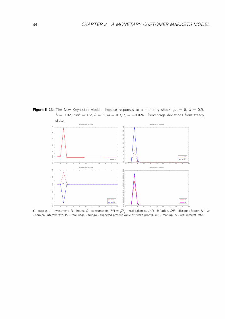
84 CHAPTER 2. A MONETARY CUSTOMER MARKETS MODEL
Figure II.23: The New Keynesian Model. Impulse responses to a monetary shock, ρτ = 0, a = 0.9,b = 0.02, mu∗ = 1.2, θ = 6, ϕ = 0.3, ζ = −0.024. Percentage deviations from steadystate.
Y - output, I - investment, N - hours, C - consumption, M1 = MtPt−1 - real balances, Inf l - inflation, DF - discount factor, N − i r
- nominal interest rate, W - real wage, Omega - expected present value of firm’s profits, mu - markup, R - real interest rate.
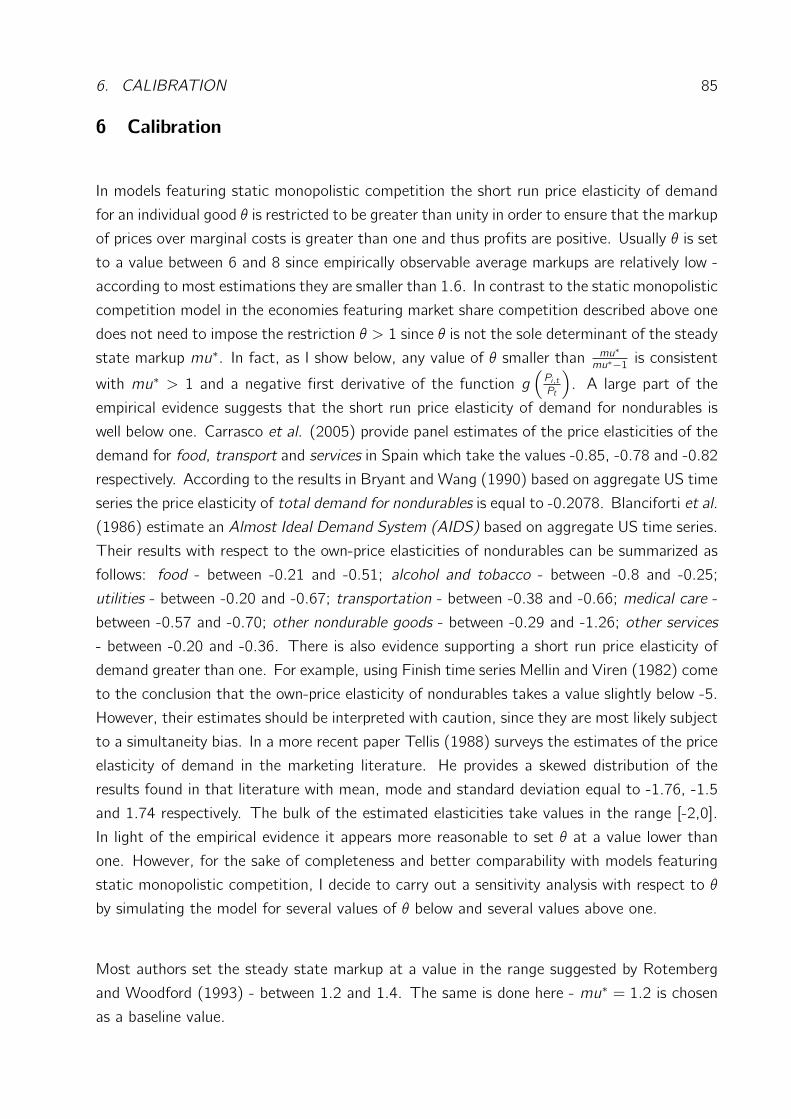
6. CALIBRATION 85
6 Calibration
In models featuring static monopolistic competition the short run price elasticity of demand
for an individual good θ is restricted to be greater than unity in order to ensure that the markup
of prices over marginal costs is greater than one and thus profits are positive. Usually θ is set
to a value between 6 and 8 since empirically observable average markups are relatively low -
according to most estimations they are smaller than 1.6. In contrast to the static monopolistic
competition model in the economies featuring market share competition described above one
does not need to impose the restriction θ > 1 since θ is not the sole determinant of the steady
state markup mu∗. In fact, as I show below, any value of θ smaller than mu∗mu∗−1 is consistent
with mu∗ > 1 and a negative first derivative of the function g(Pi ,tPt
). A large part of the
empirical evidence suggests that the short run price elasticity of demand for nondurables is
well below one. Carrasco et al. (2005) provide panel estimates of the price elasticities of the
demand for food, transport and services in Spain which take the values -0.85, -0.78 and -0.82
respectively. According to the results in Bryant and Wang (1990) based on aggregate US time
series the price elasticity of total demand for nondurables is equal to -0.2078. Blanciforti et al.
(1986) estimate an Almost Ideal Demand System (AIDS) based on aggregate US time series.
Their results with respect to the own-price elasticities of nondurables can be summarized as
follows: food - between -0.21 and -0.51; alcohol and tobacco - between -0.8 and -0.25;
utilities - between -0.20 and -0.67; transportation - between -0.38 and -0.66; medical care -
between -0.57 and -0.70; other nondurable goods - between -0.29 and -1.26; other services
- between -0.20 and -0.36. There is also evidence supporting a short run price elasticity of
demand greater than one. For example, using Finish time series Mellin and Viren (1982) come
to the conclusion that the own-price elasticity of nondurables takes a value slightly below -5.
However, their estimates should be interpreted with caution, since they are most likely subject
to a simultaneity bias. In a more recent paper Tellis (1988) surveys the estimates of the price
elasticity of demand in the marketing literature. He provides a skewed distribution of the
results found in that literature with mean, mode and standard deviation equal to -1.76, -1.5
and 1.74 respectively. The bulk of the estimated elasticities take values in the range [-2,0].
In light of the empirical evidence it appears more reasonable to set θ at a value lower than
one. However, for the sake of completeness and better comparability with models featuring
static monopolistic competition, I decide to carry out a sensitivity analysis with respect to θ
by simulating the model for several values of θ below and several values above one.
Most authors set the steady state markup at a value in the range suggested by Rotemberg
and Woodford (1993) - between 1.2 and 1.4. The same is done here - mu∗ = 1.2 is chosen
as a baseline value.
86 CHAPTER 2. A MONETARY CUSTOMER MARKETS MODEL
The distribution parameter appearing in the utility function a is set at 0.9 assigning a very
high weight to consumption Ct and a very low one to money balances MtPt. I vary the inverse
of the elasticity of substitution between Ct and MtPt, b, by setting it at values in the range
[0.02; 20].
The second part of the calibration involves finding the parameter values of γ and υ as well as
the steady state values C∗, K∗, I∗ and π∗ satisfying the economy’s non-stochastic stationary
equilibrium.
τ∗ = 1 implies that the steady state value of the gross rate of inflation is equal to one. To
be able to determine the value of γ one needs to compute Ω∗D∗ first. To find the value of Ω∗
just observe that the steady state is characterized by the following relationships Λt+1 = Λt ,(PiP
)∗= 1, x∗i = 1 and
PiP−µ∗ = mu∗−1
mu∗ , and then insert them into the definition of Ωt . After
some algebraic manipulations one arrives at
Ω∗
D∗=
β
1− βmu∗ − 1mu∗
.
γ can then be derived from (II.3.5) evaluated at the steady state. This equation is reproduced
here for convenience:
mu∗ =−θ
1− θ − γ Ω∗D∗.
For γ to be positive θ should be smaller than mu∗mu∗−1 which in the case mu∗ = 1.2 is equivalent
to the restriction θ < 6. Next, in the models without capital, for a given value of N∗, C∗ can
be derived from the goods market equilibrium condition
Y ∗ = N∗ = C∗.
The model featuring capital accumulation involves few additional calibration steps. The
production elasticity of labor ω is chosen to satisfy the restriction:
ω = mu∗((W/P )N
Y
),
where((W/P )NY
)denotes the average actual labor share. The empirical estimates for this
variable using US- as well as data for other industrialized countries vary between slightly
below 0.6 and slightly below 0.8. I set labor share at the value estimated in chapter 4, where
based on the methods proposed by Cooleey and Prescott (2005) I obtain the value 0.6747.
The euler equation for optimal investment in capital (II.4.3) evaluated at the stationary
equilibrium then implies
Y ∗
K∗= mu∗
1− β(1− υ)β(1− ω) .
6. CALIBRATION 87
By using this result together with the definition of the production function and a given N∗
one arrives at:
K∗ =N∗
(Y ∗K∗
) 1ω
.
The depreciation rate of capital υ is also set at the value found in Chapter 4, 0.00708. In
the next step the steady state value of investment I∗ is easily derived via the low of motion
for capital:
I∗ = υK∗.
C∗ star then follows from the aggregate resource constraint
C∗ = Y ∗ − I∗.
There is only one additional parameter to be calibrated in the model with adjustment costs
of capital29 - the elasticity of φ(ItKt
)with respect to its argument It/Kt , denoted by ζ.
Jerman (1998) provides a GMM estimate of ζ equal to -1/0.23. Unfortunately, in the
models developed in the current chapter that value implies that investment is less volatile
than output while the reverse is true in the industrialized world: For example, according to
the computations performed chapter 4 in the USA investment is about 4,7 times as volatile
as output. Therefore in subsection 5.3 ζ is chosen so that for a broad range of values of
θ the model is able to replicate the empirically observable relation between the variability of
output and that of investment.
I use the AR(1) process for the Solow-residual estimated by Gomme and Rupert (2006) with
U.S.-data:
ln(Zt) = 0.9641 ln(Zt−1) + εt , (II.6.3)
where εt follows a White Noise process with standard deviation σε equal to 0.0082. The
implied unconditional standard deviation of the Solow-residual, σz , is given by
σz =σε√
1− 0.96412 = 0.03088.
The properties of the money supply process were estimated by fitting an AR(p) process to
the growth rate of the monetary aggregate M1. The process chosen by minimizing the Akaike
information criterion is given by:30
gM1,t = 0.0037∗∗ + 0.5097∗∗gM1,t−1 + 0.2251∗∗gM1,t−2 + ut , (II.6.4)
29See subsection 5.3.30I used quarterly data from 1970:Q1 through 2003:Q3. According to the Ljung-Box-Q statistic and White’s
heteroscedasticity test the estimated residuals display neither serial correlation nor heteroscedasticity.
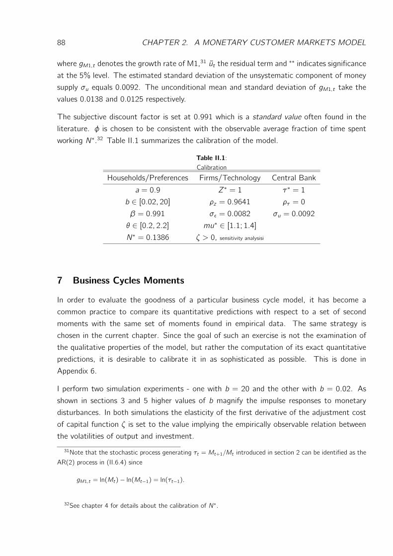
88 CHAPTER 2. A MONETARY CUSTOMER MARKETS MODEL
where gM1,t denotes the growth rate of M1,31 ut the residual term and ∗∗ indicates significance
at the 5% level. The estimated standard deviation of the unsystematic component of money
supply σu equals 0.0092. The unconditional mean and standard deviation of gM1,t take the
values 0.0138 and 0.0125 respectively.
The subjective discount factor is set at 0.991 which is a standard value often found in the
literature. φ is chosen to be consistent with the observable average fraction of time spent
working N∗.32 Table II.1 summarizes the calibration of the model.
Table II.1:Calibration
Households/Preferences Firms/Technology Central Bank
a = 0.9 Z∗ = 1 τ∗ = 1
b ∈ [0.02, 20] ρz = 0.9641 ρτ = 0
β = 0.991 σε = 0.0082 σu = 0.0092
θ ∈ [0.2, 2.2] mu∗ ∈ [1.1; 1.4]N∗ = 0.1386 ζ > 0, sensitivity analysisi
7 Business Cycles Moments
In order to evaluate the goodness of a particular business cycle model, it has become a
common practice to compare its quantitative predictions with respect to a set of second
moments with the same set of moments found in empirical data. The same strategy is
chosen in the current chapter. Since the goal of such an exercise is not the examination of
the qualitative properties of the model, but rather the computation of its exact quantitative
predictions, it is desirable to calibrate it in as sophisticated as possible. This is done in
Appendix 6.
I perform two simulation experiments - one with b = 20 and the other with b = 0.02. As
shown in sections 3 and 5 higher values of b magnify the impulse responses to monetary
disturbances. In both simulations the elasticity of the first derivative of the adjustment cost
of capital function ζ is set to the value implying the empirically observable relation between
the volatilities of output and investment.
31Note that the stochastic process generating τt = Mt+1/Mt introduced in section 2 can be identified as the
AR(2) process in (II.6.4) since
gM1,t = ln(Mt)− ln(Mt−1) = ln(τt−1).
32See chapter 4 for details about the calibration of N∗.
7. BUSINESS CYCLES MOMENTS 89
I ignore the autocorrelation structure of the money supply process and assume that the
percentage deviation of the growth factor of Mt from its long run level τt follows a pure
White Noise process whose standard deviation is identical with that of the unsystematic
component of the money supply process, στ = σu = 0.0092.
Table II.2 summarizes the results obtained from the Customer Market Model. The compu-
tation of the empirical second moments is described in chapter 4. It is readily seen that the
model developed in this chapter has two important shortcomings. First, it implies a large
positive correlation between output and the markup. While as a reaction to a monetary inno-
vation production and output tend to move in opposite directions, technological disturbances
induce strong and persistent comovements of these variables. Obviously, the effects triggered
off by technology shocks dominate. Second, the model performs very poorly with regard to
the autocorrelation of inflation as well as its cross correlation with output. Nevertheless,
the overall performance of the model should be seen as average with a slight tendency to
understate the autocorrelations of most variables. After a large set of simulation exercises
I concluded that the reactions to technology shocks are almost unaffected by variations in
the parameter b. Hence any differences between the two specifications b = 20 and b = 0.02
present in Table II.2 are largely due to the fact that the propagation of monetary disturbances
is substantially affected by changes in b.33
A comparison with the New Keynesian Model:Table II.3 contains the results from the New Keynesian Model obtained under the assumption
of a relatively large degree of price stickiness, ϕ = 0.75. Values of b lower than 18 lead to very
unrealistic model implications with regard to the volatilities of most macroeconomic variables.
For that reason the comparison between the two models only refers to the case b = 20. The
New Keynesian Model performs better than the one developed here with respect to the cross
correlations with output of inflation and the markup. The latter equals 0.52 and is not far
from its empirical counterpart, 0.317. The correlation between output and the markup is too
high in magnitude but has the correct sign. In contrast the Customer Market Model implies
a negative correlation between output and inflation, -0.24, and a large positive one between
output and the markup. Further, the predictions of the New Keynesian Model regarding the
autocorrelations of the individual variables are on average closer to their respective empirical
counterparts than it is the case in the Customer Markets Model. Nevertheless, the latter
performs better with respect to the relative standard deviations of most variables as well as the
cross correlations with output of all variables except inflation and the markup. Furthermore,
the predictions of the Customer Markets Model with regard to the cyclical properties of the
real wage match much better the empirical evidence than it is the case in the New Keynesian
Model. The latter exhibits a drawback typical for most sticky price models - it substantially
33See also sections 3 and 5.
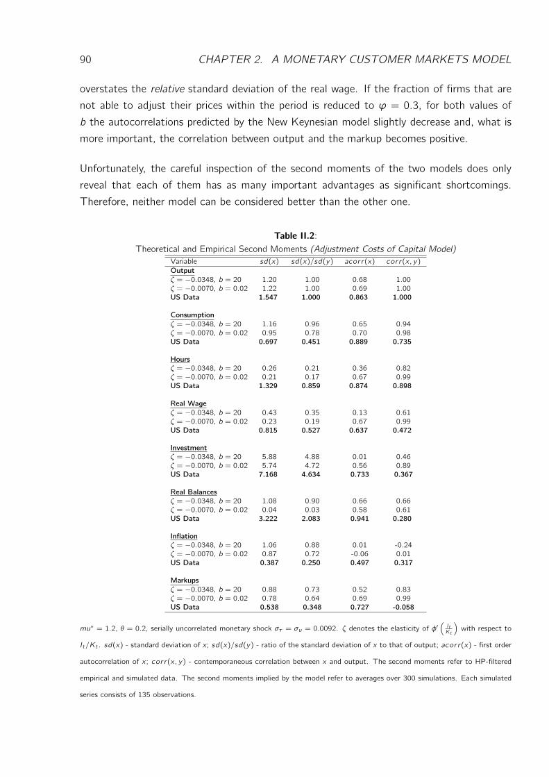
90 CHAPTER 2. A MONETARY CUSTOMER MARKETS MODEL
overstates the relative standard deviation of the real wage. If the fraction of firms that are
not able to adjust their prices within the period is reduced to ϕ = 0.3, for both values of
b the autocorrelations predicted by the New Keynesian model slightly decrease and, what is
more important, the correlation between output and the markup becomes positive.
Unfortunately, the careful inspection of the second moments of the two models does only
reveal that each of them has as many important advantages as significant shortcomings.
Therefore, neither model can be considered better than the other one.
Table II.2:Theoretical and Empirical Second Moments (Adjustment Costs of Capital Model)
Variable sd(x) sd(x)/sd(y) acorr(x) corr(x, y)
Outputζ = −0.0348, b = 20 1.20 1.00 0.68 1.00ζ = −0.0070, b = 0.02 1.22 1.00 0.69 1.00US Data 1.547 1.000 0.863 1.000
Consumptionζ = −0.0348, b = 20 1.16 0.96 0.65 0.94ζ = −0.0070, b = 0.02 0.95 0.78 0.70 0.98US Data 0.697 0.451 0.889 0.735
Hoursζ = −0.0348, b = 20 0.26 0.21 0.36 0.82ζ = −0.0070, b = 0.02 0.21 0.17 0.67 0.99US Data 1.329 0.859 0.874 0.898
Real Wageζ = −0.0348, b = 20 0.43 0.35 0.13 0.61ζ = −0.0070, b = 0.02 0.23 0.19 0.67 0.99US Data 0.815 0.527 0.637 0.472
Investmentζ = −0.0348, b = 20 5.88 4.88 0.01 0.46ζ = −0.0070, b = 0.02 5.74 4.72 0.56 0.89US Data 7.168 4.634 0.733 0.367
Real Balancesζ = −0.0348, b = 20 1.08 0.90 0.66 0.66ζ = −0.0070, b = 0.02 0.04 0.03 0.58 0.61US Data 3.222 2.083 0.941 0.280
Inflationζ = −0.0348, b = 20 1.06 0.88 0.01 -0.24ζ = −0.0070, b = 0.02 0.87 0.72 -0.06 0.01US Data 0.387 0.250 0.497 0.317
Markupsζ = −0.0348, b = 20 0.88 0.73 0.52 0.83ζ = −0.0070, b = 0.02 0.78 0.64 0.69 0.99US Data 0.538 0.348 0.727 -0.058
mu∗ = 1.2, θ = 0.2, serially uncorrelated monetary shock στ = σu = 0.0092. ζ denotes the elasticity of φ′(ItKt
)with respect to
It/Kt . sd(x) - standard deviation of x ; sd(x)/sd(y) - ratio of the standard deviation of x to that of output; acorr(x) - first order
autocorrelation of x ; corr(x, y) - contemporaneous correlation between x and output. The second moments refer to HP-filtered
empirical and simulated data. The second moments implied by the model refer to averages over 300 simulations. Each simulated
series consists of 135 observations.
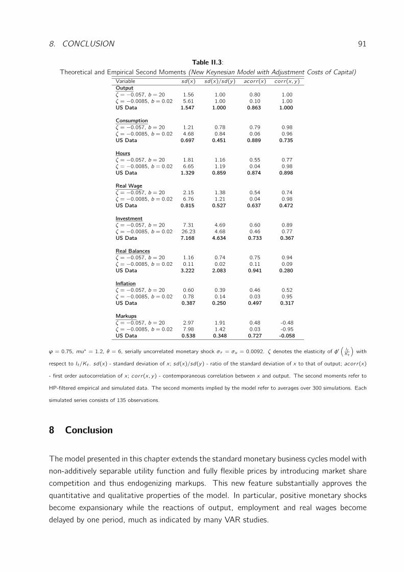
8. CONCLUSION 91
Table II.3:Theoretical and Empirical Second Moments (New Keynesian Model with Adjustment Costs of Capital)
Variable sd(x) sd(x)/sd(y) acorr(x) corr(x, y)
Outputζ = −0.057, b = 20 1.56 1.00 0.80 1.00ζ = −0.0085, b = 0.02 5.61 1.00 0.10 1.00US Data 1.547 1.000 0.863 1.000
Consumptionζ = −0.057, b = 20 1.21 0.78 0.79 0.98ζ = −0.0085, b = 0.02 4.68 0.84 0.06 0.96US Data 0.697 0.451 0.889 0.735
Hoursζ = −0.057, b = 20 1.81 1.16 0.55 0.77ζ = −0.0085, b = 0.02 6.65 1.19 0.04 0.98US Data 1.329 0.859 0.874 0.898
Real Wageζ = −0.057, b = 20 2.15 1.38 0.54 0.74ζ = −0.0085, b = 0.02 6.76 1.21 0.04 0.98US Data 0.815 0.527 0.637 0.472
Investmentζ = −0.057, b = 20 7.31 4.69 0.60 0.89ζ = −0.0085, b = 0.02 26.23 4.68 0.46 0.77US Data 7.168 4.634 0.733 0.367
Real Balancesζ = −0.057, b = 20 1.16 0.74 0.75 0.94ζ = −0.0085, b = 0.02 0.11 0.02 0.11 0.09US Data 3.222 2.083 0.941 0.280
Inflationζ = −0.057, b = 20 0.60 0.39 0.46 0.52ζ = −0.0085, b = 0.02 0.78 0.14 0.03 0.95US Data 0.387 0.250 0.497 0.317
Markupsζ = −0.057, b = 20 2.97 1.91 0.48 -0.48ζ = −0.0085, b = 0.02 7.98 1.42 0.03 -0.95US Data 0.538 0.348 0.727 -0.058
ϕ = 0.75, mu∗ = 1.2, θ = 6, serially uncorrelated monetary shock στ = σu = 0.0092. ζ denotes the elasticity of φ′(ItKt
)with
respect to It/Kt . sd(x) - standard deviation of x ; sd(x)/sd(y) - ratio of the standard deviation of x to that of output; acorr(x)
- first order autocorrelation of x ; corr(x, y) - contemporaneous correlation between x and output. The second moments refer to
HP-filtered empirical and simulated data. The second moments implied by the model refer to averages over 300 simulations. Each
simulated series consists of 135 observations.
8 Conclusion
The model presented in this chapter extends the standard monetary business cycles model with
non-additively separable utility function and fully flexible prices by introducing market share
competition and thus endogenizing markups. This new feature substantially approves the
quantitative and qualitative properties of the model. In particular, positive monetary shocks
become expansionary while the reactions of output, employment and real wages become
delayed by one period, much as indicated by many VAR studies.

92 CHAPTER 2. A MONETARY CUSTOMER MARKETS MODEL
I also evaluate the theoretical framework developed in this chapter by comparing its implica-
tions with that of the New Keynesian Model with Calvo pricing. I conclude that the former
should be considered a useful alternative to the latter for analyzing positive as well as nor-
mative issues. The model also provides many dimensions along which it can be extended.
For example by taking an explicit account of capital accumulation or labor market frictions.
Nevertheless, the framework presented here is by no means better than the New Keynesian
model. Therefore, in search for a theory superior to the New Keynesian one, in what follows,
I sharply deviate from the existing literature.
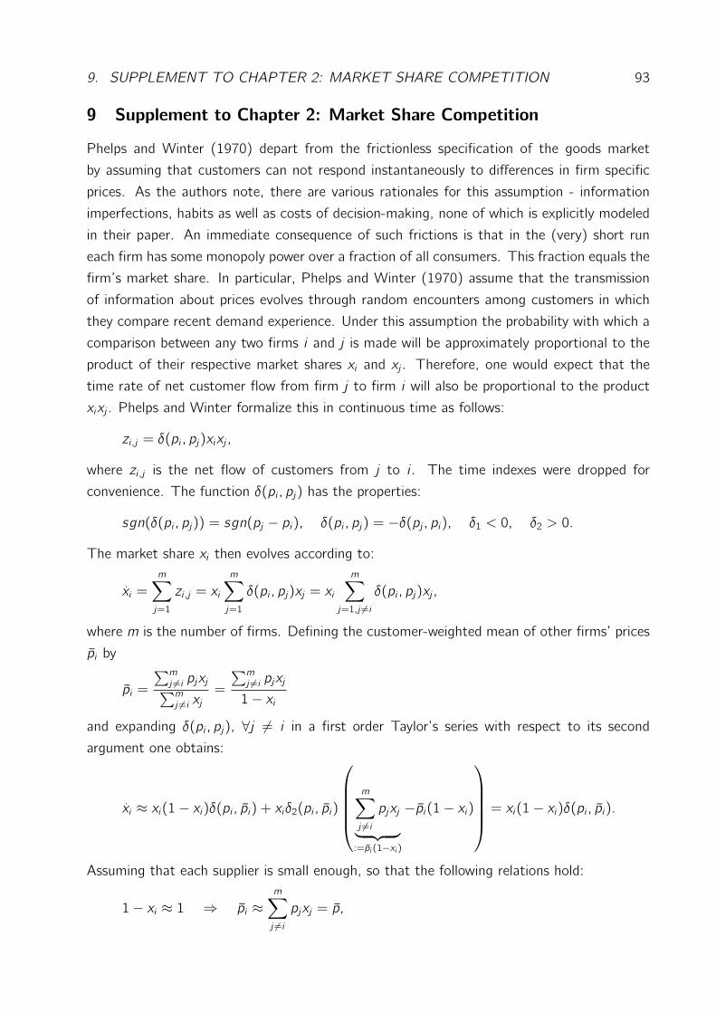
9. SUPPLEMENT TO CHAPTER 2: MARKET SHARE COMPETITION 93
9 Supplement to Chapter 2: Market Share Competition
Phelps and Winter (1970) depart from the frictionless specification of the goods market
by assuming that customers can not respond instantaneously to differences in firm specific
prices. As the authors note, there are various rationales for this assumption - information
imperfections, habits as well as costs of decision-making, none of which is explicitly modeled
in their paper. An immediate consequence of such frictions is that in the (very) short run
each firm has some monopoly power over a fraction of all consumers. This fraction equals the
firm’s market share. In particular, Phelps and Winter (1970) assume that the transmission
of information about prices evolves through random encounters among customers in which
they compare recent demand experience. Under this assumption the probability with which a
comparison between any two firms i and j is made will be approximately proportional to the
product of their respective market shares xi and xj . Therefore, one would expect that the
time rate of net customer flow from firm j to firm i will also be proportional to the product
xixj . Phelps and Winter formalize this in continuous time as follows:
zi ,j = δ(pi , pj)xixj ,
where zi ,j is the net flow of customers from j to i . The time indexes were dropped for
convenience. The function δ(pi , pj) has the properties:
sgn(δ(pi , pj)) = sgn(pj − pi), δ(pi , pj) = −δ(pj , pi), δ1 < 0, δ2 > 0.
The market share xi then evolves according to:
xi =
m∑
j=1
zi ,j = xi
m∑
j=1
δ(pi , pj)xj = xi
m∑
j=1,j 6=iδ(pi , pj)xj ,
where m is the number of firms. Defining the customer-weighted mean of other firms’ prices
pi by
pi =
∑mj 6=i pjxj∑mj 6=i xj
=
∑mj 6=i pjxj1− xi
and expanding δ(pi , pj), ∀j 6= i in a first order Taylor’s series with respect to its second
argument one obtains:
xi ≈ xi(1− xi)δ(pi , pi) + xiδ2(pi , pi)
m∑
j 6=ipjxj
︸ ︷︷ ︸:=pi (1−xi )
−pi(1− xi)
= xi(1− xi)δ(pi , pi).
Assuming that each supplier is small enough, so that the following relations hold:
1− xi ≈ 1 ⇒ pi ≈m∑
j 6=ipjxj = p,
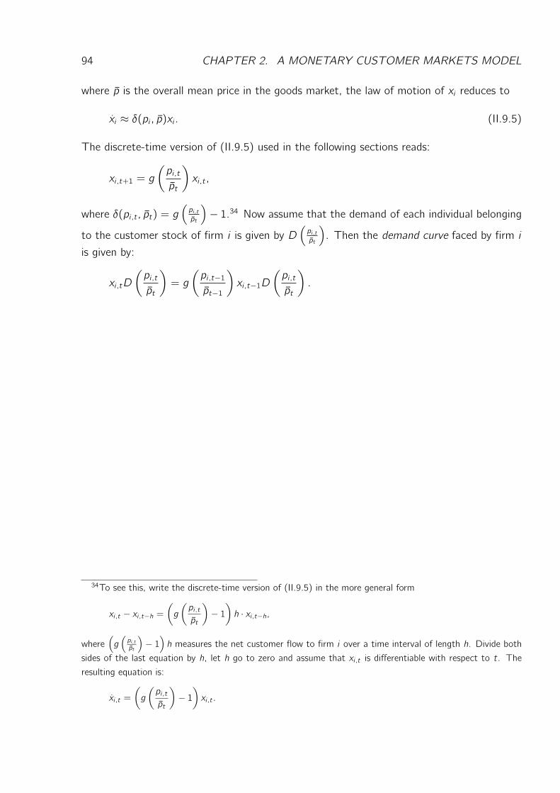
94 CHAPTER 2. A MONETARY CUSTOMER MARKETS MODEL
where p is the overall mean price in the goods market, the law of motion of xi reduces to
xi ≈ δ(pi , p)xi . (II.9.5)
The discrete-time version of (II.9.5) used in the following sections reads:
xi ,t+1 = g
(pi ,tpt
)xi ,t ,
where δ(pi ,t , pt) = g(pi ,tpt
)− 1.34 Now assume that the demand of each individual belonging
to the customer stock of firm i is given by D(pi ,tpt
). Then the demand curve faced by firm i
is given by:
xi ,tD
(pi ,tpt
)= g
(pi ,t−1pt−1
)xi ,t−1D
(pi ,tpt
).
34To see this, write the discrete-time version of (II.9.5) in the more general form
xi ,t − xi ,t−h =(g
(pi ,tpt
)− 1
)h · xi ,t−h,
where(g
(pi ,tpt
)− 1
)h measures the net customer flow to firm i over a time interval of length h. Divide both
sides of the last equation by h, let h go to zero and assume that xi ,t is differentiable with respect to t. The
resulting equation is:
xi ,t =
(g
(pi ,tpt
)− 1
)xi ,t .
Chapter 3
Inflation Aversion and Monetary Policy
1 Introduction
In the light of the fact that on average the monetary customer markets model presented in the
previous chapter does not represent an improvement relative to the New Keynesian model, I
take a second step in developing ”another version of the model” which provides an endogenous
explanation of the incomplete or rigid response of nominal prices to monetary and interest
rate shocks, the cyclical pattern of markups and the strong and persistent reactions of most
macroeconomic variables to demand and supply side disturbances. To achieve these three
goals, I extend a standard monetary business cycles model with monopolistic competition in
the goods market and additively separable utility function along several dimensions.
First, based on the empirical evidence accumulated in research areas closely related to psy-
chology and dramatically deviating from any tradition in the real and monetary business cycles
theory I assume that agents’ behavior is characterized by inflation aversion - current inflation
has a direct negative effect on utility. By intensifying search and switching efforts in the goods
market and thus switching from more expensive to cheaper products an individual household
is able to reduce the direct disutility caused by inflation. The emerging positive relationship
between search efforts and inflation crates a new channel by which nominal disturbances can
be transmitted into the real economy. If an increase in search activity caused by an upward
pressure on current inflation forces firms to pass through to prices only a fraction of the
increase in nominal marginal costs, markups will tend to fall and thus real wages, hours and
output will tend to increase. To ensure such an outcome the structure of the goods market
should be altered in some way. I propose the following extensions of the static monopolistic
competition framework.
First, as in the previous chapter, I assume that firms do not only engage in price competition
but also in dynamic market share competition as proposed by Phelps and Winter (1970) in
95
96 CHAPTER 3. INFLATION AVERSION AND MONETARY POLICY
their customer market model. Second, I assume that the law of motion of the individual
market share is governed by a matching function depending on the pricing behavior of the
firm and the intensity of the search and switching activities households engage in. How does
each individual assumption as well as the combination of them alter the characteristics and
the implications of the model?
Further, I extend the law of motion of market share defined by Phelps and Winter (1970) and
used by Rotemberg and Woodford (1993) by assuming that the function describing the growth
factor of the firm-specific market share does not only depend on the firm’s pricing decision
but also on the intensity of search and switching efforts chosen by consumers. This function
can be interpreted as a matching mechanism in the goods market assigning customers to
suppliers and has the following key implication: If an individual firm charges a lower (higher)
price relative to the overall price level, a higher search activity by households will induce
a stronger increase (decrease) of that firm’s customer stock. Therefore, in times of high
search activity firms will tend to charge lower prices and thus choose lower markups. In
other words, a higher overall search activity implies that households reallocate their demand
more aggressively as a reaction to price differences, therefore firms with relatively high current
prices suffer more severe losses in future market share. From the point of view of an individual
household the intensification of her search for cheaper suppliers as well as the efforts aimed
at the redistribution of her demand by adjusting the weights attached to the individual goods
within the consumption bundle, the representative household is able to respond in a utility
maximizing way to changes in relative goods prices. The costs induced by search activity are
measured in real terms and reduce directly the resources available for consumption.
The assumption that households’ behavior is characterized by inflation aversion and that by
spending more resources on search and switching activities the disutility caused by inflation is
reduced creates a new link between the real and the monetary side of the economy which is
the crucial new feature of the model. As I show below, search activity depends positively on
current inflation. The latter implies that nominal shocks will not be fully absorbed by changes
in nominal prices: A monetary expansion will induce two opposing effects on current inflation
- the usual positive one via the positive income effect on current demand and a new negative
one via the positive effect on search and switching activity. The higher search activity then
forces firms to choose lower current prices and thus lower markups than they would do if
search were independent of inflation. As a consequence, on the one hand overall inflation
rises by less than if there were no dependence between search and inflation and on the other
real wages, hours and output rise. If search efforts were independent on current inflation, the
positive and negative pressures on current markups induced by a monetary disturbance will
exactly offset each other. As a consequence, markups and therefore real wages, hours and
2. INFLATION AVERSION 97
output will remain unchanged and the increase in inflation will be exactly sufficient to offset
the income effect of the monetary shock. In other words, the neutrality of money will hold.
The main findings of this chapter can be summarized as follows. After extending the standard
monetary business cycles model along the three dimensions described above it becomes able
to generate endogenous countercyclical markups which react negatively to monetary as well as
technology shocks, and endogenous sluggishness in nominal prices. Furthermore, the model
provides an endogenous explanation of the persistence in actual business cycles. Hence, the
model of this chapter should be considered a useful alternative to the New Keynesian Model
for analyzing and evaluating monetary and interest rate policy.
The chapter is organized as follows. Section 2 motivates the main assumption of the model.
Section 3 presents the benchmark model and its implications. Section 4 extends it by incor-
porating capital accumulation. Section 5 closes the chapter with a comparison between the
model developed here and the New Keynesian model.
2 Inflation Aversion
According to most economic theories and the view of many economists inflation affects
only indirectly the well-being. Either by reducing the real value of the wealth and income
components denominated in nominal terms or by exacerbating already existing inefficiencies
and therefore leading to a suboptimal distribution of private expenditure.1 Absent these
valuation or expenditure distribution effects, inflation would be of no relevance for the private
economy and therefore of no relevance for policy makers and of no interest for economic
theory. There is a similar consensus about how households’ and firms’ behavior depends on
the variability of the inflation rate - in a purely indirect manner: A higher volatility of the
inflation rate in most cases makes many income components more variable. As a consequence
consumption tends to fluctuate more and hence reduces utility if agents are risk averse.
1In the New Keynesian Models with Calvo-type price setting, for example, higher inflation induces a larger
dispersion of prices for the individual goods produced (and consumed) in the economy. The latter results in an
inefficient dispersion of output and demand among the individual goods. As there is diminishing marginal utility
of consumption of every individual good, the utility derived from consuming more of the cheaper goods is less
than the utility loss from consuming less of the more expensive ones. If there is increasing marginal disutility
of producing an individual good, the utility loss from producing more of the cheaper goods will be higher than
the gain in utility from producing less of the more expensive ones. In these models it is often assumed that the
central bank designs monetary or interest rate policy so as to minimize a quadratic loss function depending on
some measure of the output gap and the inflation rate. As the loss function is just an approximation of the
utility function of the representative agent in the economy, the presence of the inflation rate stems from the
indirect effects on utility just described. (See Woodford (2003), pp. 383-405 and Walsh (2003) pp. 517-558
on this and related issues.)
98 CHAPTER 3. INFLATION AVERSION AND MONETARY POLICY
In contrast to this traditional or mainstream way of thinking about inflation the empirical
evidence accumulated in some research areas closely related to psychology indicates that
consumption (or income) is by no means the only variable directly affecting people’s sub-
jective well-being.2 Other variables such as the overall rate of inflation, the personal un-
employment status, the general unemployment rate as well as the institutional and political
framework seem to have highly significant direct effects on people’s life satisfaction. Frey
and Stutzer (2002) provide an exhaustive survey of Happiness Research, a discipline directly
stemming from psychology. Some of the papers reviewed by the authors provide stylized
facts on the correlation between income and happiness. According to the results, despite the
sharp increase of per capita income in all industrial countries after World War II, in most of
them average subjective well-being has remained unchanged or has even declined. The more
elaborate econometric studies on this issue cited by Frey and Stutzer (2002) go beyond the
purely descriptive analysis by controlling for individual characteristics of households as well as
the effects of inflation, unemployment, institutional and other factors. They all come to the
conclusion that the income level has no, or in rare cases a very limited explanatory power with
respect to private agents’ happiness.3 At the same time inflation tends to have significant
direct effects on life satisfaction. Di Tella et. al., also cited by Frey and Stutzer (2002),
show that after controlling for individual socioeconomic characteristics and the unemploy-
ment rate, an increase of inflation by five percentage points reduces average happiness by
0.05 ”units of satisfaction” which is equivalent to a shift of five percent of the population
from one life-satisfaction level to the next lower one.4 Walton (1979) provides evidence based
on a sample taken by the American Council of Life Insurance (AICL)5 that consumers are
often ”disturbed” , ”frustrated” and ”angry” when confronted with higher prices for particular
products or a higher overall price level.
2Frey and Stutzer (2002) define subjective well-being as follows: It is the scientific term in psychology
for individual’s evaluation of her experienced positive and negative affect, happiness or satisfaction with life.
In psychology they are separable constructs, whereas, to my knowledge, in modern macroeconomics only the
abstract concept of agent’s utility is used. The latter is a cardinal measure summerizing all three psychological
concepts, allowing no precise distinction between them. Therefore the terms subjective well-being, happiness
and life satisfaction are used interchangeably, as synonyms of utility.3As many studies show, the income variable that does have a significant positive effect on subjective well-
being is the relative rather than the absolute income level. The relative income of a person is defined as the
quotient of his own income and a weighted average over all households. There is also for people in richer
countries to be happier.4In Di Tella et. al. (2001) satisfaction is measured by a 4-point scale ranging from ”not at all satisfied”
through ”very satisfied” . To transform the ordinal scale into a cardinal one the numbers 1,2,3 and 4 are attached
to the levels ”not at all satisfied”,... and ”very satisfied” respectively.5To take a sample of people’s opinion about inflation, ACLI placed advertisements in major newspapers and
news magazines urging Americans to express their views on the subject in letters addressed to the author.
2. INFLATION AVERSION 99
In a study inspired by the question wether Okun’s Economic Discomfort Index6 can be re-
garded as a good measure of agents’ disutility Lovell and Tien (1999) come to the conclusion
that current inflation has greater influence on people’s well-being than current unemployment
does, as measured by the elasticities of these two variables with respect to the Index of Con-
sumer Sentiment (ICS).7 Furthermore, once the change in the unemployment rate and/or
the growth rate of GDP are included in the regression equation the coefficient of the rate of
unemployment tends to get insignificant. The latter indicates that by the inclusion of current
unemployment in the disutility index one just approximates the effect of the cyclical compo-
nent of income on agents’ happiness. The relative strength of this effect compared with that
of inflation is consistent with the findings in the papers reviewed by Frey and Stutzer (2002).
Much in line with the evidence provided by Lovell and Tien (1999) as well as that cited by
Frey and Stutzer (2002) are the results in Hymans (1970). He also examines the dependence
of the Index of Consumer Sentiment (ICS) on income, stock price changes and inflation.
His results indicate that all three variables have highly significant direct effects on consumer
sentiment. Since the long run trend as well as recent changes of stock prices provide a fairly
good approximation of the changes in the value of households’ wealth, it is less surprising
that these variables have explanatory power with respect to consumer sentiment. Much
more surprising is the role of inflation as an independent determinant of ICS. The fact that
income is not the sole determinant of consumer sentiment explains why the latter usually has
a significant coefficient in demand regressions in which income was already included. In a
more recent empirical study Franses (2006) also provides evidence supporting the existence
of substantial direct effects of inflation on consumer confidence.
The empirical studies discussed so far examine the relationship between subjective well-being
and the current values of income, inflation, unemployment and other variables. But as most
agents are to some extent forward looking, it can not be ruled out on a priori grounds
that average happiness depends on expected rather than current inflation. Smyth et. al.
(1994) apply a battery of non-nested tests in order to give an answer to the question wether
agents are on average forward or backward looking when deciding on how satisfied they are
with the current economic situation. According to their results, the hypothesis that agents’
satisfaction with the current economic situation depends on expected future inflation and
unemployment is rejected in favor of the one that current inflation and unemployment are
the only significant determinants of people’s subjective well-being.8
6Okun’s Economic Discomfort Index is simply defined as the sum of the inflation and the unemployment
rate.7Lovell and Tien (1999) use the Index of Consumer Sentiment as an approximation of consumers’ subjective
well-being.8Agents’ satisfaction with current economic conditions is approximated by the Gallup’s Index of Presidential
Popularity.
100 CHAPTER 3. INFLATION AVERSION AND MONETARY POLICY
The empirical findings on the determinants of agents’ well-being can be summarized as fol-
lows: The current inflation rate has significant direct effects on utility and is at least as
important as real income. Based on these results, I assume that the utility function of the
representative agent depends directly on the overall rate of inflation. The pain caused by
inflation can be reduced by spending some part of the currently available resources on search
and switching efforts aimed at the reallocation of demand from suppliers charging relatively
high to suppliers charging relatively low prices. As documented by Frey and Stutzer (2002),
the other factors mentioned above e.g. the political situation and many institutional factors
also have greater importance for individual well-being than income has. As none of them is
explicitly taken into account in the model presented below, I do not reproduce the empirical
findings on the effects of these variables on happiness.
Why does utility depend directly on inflation? It is the job of psychologists to give answer to
this question and I do not provide any suggestions or even speculations about the possible
reasons for the direct link between inflation and subjective well-being. In the model described
below I simply assume that households’ behavior is characterized by a property called inflation
aversion.
3 The Model
I refer to this model as the ”Benchmark Model” or the ”CM-Model” .9
3.1 Theoretical Framework
Firms
There are n product varieties, each produced by a profit maximizing monopolistic firm ac-
cording to the linear production function
Yi ,t = ZtNi ,t ,
where Ni ,t denotes labor input of firm i . Zt denotes the total factor productivity which follows
a stochastic process given by:
ln(Zt) = ρz ln(Zt−1) + εt ,
where εt follows a White Noise Process with variance σ2ε .
9CM - Customer Market.
3. THE MODEL 101
The demand function faced by the producer of variety i is given by
Ci ,t = xi ,t ·(Pi ,tPt
)−θ· Dtn, θ > 0, (III.3.1)
where xi ,t is a measure of firm i ’s market share. xi ,t can be also interpreted as a measure
of the subjective relative weight within the consumption bundle attached by households to
product variety i . More precisely, xi ,t is the fraction of aggregate demand firm i would face if
all firms were to choose the same price. Dt and Pt denote, respectively, aggregate demand
and the aggregate price level.10
Firm-specific market share evolves according to
xi ,t+1 = g
(Pi ,tPt, st
)· xi ,t (III.3.2)
where st are aggregate households’ search and switching efforts. Each firm treats st as an
exogenous variable. I assume that the function g(., .) governing the law of motion of market
share has the following properties:
g (1, st) = 1,∂g
(Pi ,tPt, st
)
∂Pi ,t/Pt= g1
(Pi ,tPt, st
)< 0,
∂g(Pi ,tPt, st
)
∂st= g2
(Pi ,tPt, st
)< 0(> 0) for
Pi ,tPt> 1(< 1).
According to these assumptions, higher search activity today leads to a fall (rise) in next-
period market share if the price the firm charges is higher (lower) than the overall price level.
Market shares are bounded by 0 from below and by 1, n or some other positive value from
above. Generally, to ensure that xi remains ∀t within these bounds, one should try to find a
reasonable normalization of xi . This issue will be one of the most important in models with
heterogeneous firms but it does not arise here, since in equilibrium all firms charge the same
price.11 I assume the following functional form of g(., .):
g
(Pi ,tPt, st
)= exp
((1− Pi ,t
Pt
)· st
).
Since, as shown below, st will be positive even though the equilibrium is symmetric, it would
be perhaps more reasonable to interpret this variable as a kind of potential search activity or a
kind of alertness with respect to firms’ behavior, reflecting how well households are informed10The demand function in (III.3.1) is very similar to that proposed by Phelps and Winters (1970). Rotemberg
and Woodford (1993) apply the discrete time version of the ”Customer Market Model” used here to the analysis
of the effects of government spending on private consumption and investment.11See below.
102 CHAPTER 3. INFLATION AVERSION AND MONETARY POLICY
about the goods market. If a consumer is better informed about the price distribution and the
behavior of individual suppliers, she will tend to need less time to discover deviations from the
average price and, thus, will be able to react to them faster by punishing (rewarding) positive
(negative) deviations from the average price level. A consumer who is less informed about
the price distribution, will need more time to infer from the pricing behavior she observes
whether the prices charged for particular goods are actually too high (or too low) or not.
Such a customer will react more slowly (or with a larger lag) to any given deviation from
the average price. Expressing the degree of alertness with respect to the goods market by
the value of st is a convenient short-cut, by which I avoid cumbersome technical details of
which I expect to be of extremely limited importance for the macroeconomic predictions of
the model. In what follows, st is termed search activity or switching efforts.
The dependence of the market share in t + 1 on past pricing behavior introduces a dynamic
aspect into the profit maximization problem of the individual firm. Each firm maximizes
maxPi ,t
xi ,t
(Pi ,tPt
)−θDtn
(Pi ,tPt− µt
)+
+ Et
∞∑
j=1
βjΛt+jΛtxi ,t+j
(Pi ,t+jPt+j
− µt+j)(Pi ,t+jPt+j
)−θDt+j
s. t.
xi ,t+1 = g
(Pi ,tPt, st
)xi ,t ,
where DFt,t+j =βjΛt+jΛt
denotes the stochastic discount factor between periods t and t+ j
which is given to the firm. µt denotes marginal costs. The corresponding first order condition
reads:
(Pi ,tPt
)−θxi ,tDt − θ
(Pi ,tPt− µt
)(Pi ,tPt
)−θ−1xi ,tDt +
g1
(Pi ,tPt, st
)
g(Pi ,tPt, st
) Ωt = 0,
where
Ωt = Et
∞∑
j=1
βjΛt+jΛtxi ,t+j
(Pi ,t+jPt+j
− µt+j)(Pi ,t+jPt+j
)−θDt+j
=
= Et
βΛt+1Λtxi ,t+1
(Pi ,t+1Pt+1
− µt+1)(Pi ,t+1Pt+1
)−θDt+1
+ Et
βΛt+1ΛtΩt+1
.
Defining the markup over marginal costs as
mui ,t =Pi ,tPtµt
, mut =1
µt,
3. THE MODEL 103
one can write the FOC, evaluated at the symmetric equilibrium, as
mut =−θ
1− θ + g1(1, st)ΩtDt(III.3.3)
In a symmetric intertemporal equilibrium in each period each firm sets the same price as all
other firms. The most important implication regarding market shares is that xi ,t equals one
for all t and all i . According to equation (III.3.3) the equilibrium markup depends positively
on current demand and negatively on current search efforts as well as the present value of
future profits. In the static monopolistic competition model markups are given by
mut =θ
θ − 1 (III.3.4)
implying that at any point in time and in any given state of the economy pass-through of
marginal cost changes to prices is complete. Unlike that model, in an environment character-
ized by market share competition markups will be generally time varying. Wether pass-through
of marginal costs to prices will turn to be greater, lower or equal to one depends on the rel-
ative strength of the reactions of Dt ,Ωt and st to exogenous shocks. For example, consider
a positive exogenous shock which increases current consumption. The temporary (or even
an one time) increase in current consumption will have a positive direct effect on markups
through the induced increase in aggregate demand Dt . Based on this result, many microe-
conomic models assuming a constant discount factor reach the conclusion that markups are
procyclical. In the present model, however, the discount factor is endogenous and strongly
linked to current consumption - as shown below the Lagrange-multiplier Λt is given by
Λt = C−ηt .
Other things equal, if η is sufficiently large an increase in current consumption will cause
larger an increase in Ωt via the rise in the discount factor. As a consequence, the markup
will tend to be countercyclical. Further, if search activity depends positively on consumption,
as is the case in this model,12 consumption will also have a second indirect negative effect
on markups via st . Further, equation (III.3.3) implies that markups in this model are always
lower than they would be if there were static monopolistic competition in the goods market.
Households
Let agents in this economy have preferences over consumption, real balances, working hours,
search activity and overall inflation given by
U = Et
∞∑t=0
βt(C1−ηt1− η + φm
(Mt/Pt)1−χ
1− χ − b2N2t −
%
α
πtsαt
), φm, b, %, η, χ > 0, β ∈ (0, 1),
12See below.
104 CHAPTER 3. INFLATION AVERSION AND MONETARY POLICY
where Mt/Pt , Nt and πt denote real balances, working hours and the gross rate of overall
inflation respectively. In the above expression Ct is a composite good that includes all varieties:
Ct =
1
n
n∑
i=1
x1θ
i ,tCθ−1θ
i ,t
θθ−1
,
st =
1
n
n∑
i=1
x1θ
i ,tsθ−1θ
i ,t
θθ−1
.
(III.3.5)
xi ,t evolves according to (III.3.2). The corresponding utility-based price index is given by:
Pt =
1
n
n∑
i=1
xi ,tP1−θi,t
11−θ
.
The last term in the period utility function reflects the assumption that since search activity
usually leads to a reduction (rise) of demand for relatively expensive (cheap) goods, a posi-
tive psychological effect arises, which takes the form of a reduction of the subjective negative
effect on household’s well-being induced by inflation. Such a cognitive effect may arise as
a result of the satisfaction with the fact that by increasing st one is able to more heavily
punish the firms most intensively contributing to the increase in the aggregate price level
- the firms with above average prices. A similar interpretation can be derived from one of
the assumptions underlying the most recent theoretical models developed by Rotemberg13.
Based on experimental evidence he assumes that agents become angry when the prices of
the goods they desire increase by a sufficiently large amount. Similarly, the last term in the
utility function of the current model can be motivated as follows: Inflation makes households
angry. Since anger is an unpleasant feeling, it reduces utility. But the pain induced by anger
can be at least partly dampened by having revenge on firms with relatively high prices via
a more intense search activity st . Unfortunately, as to my knowledge, there is no empirical
evidence supporting or rejecting the assumed dependence of current utility on search activity.
Nevertheless, the good performance of the current model relative to the standard New Key-
nesian Model discussed below as well as the GMM estimations presented in the next chapter
can be seen as an indirect evidence in favor (or at least not against) the last assumption on
the structure of the utility function.
The budget restriction of the representative household is given by:
Ct + st +mt+1 − mtπt=WtPtNt +Πt +
TtPt,
where Wt , Πt , Tt and mt = MtPt−1
denote the nominal wage, real profits, nominal net transfers
form the government and real balances respectively.13Rotemberg (2002, 2004a, 2004b, 2008)
3. THE MODEL 105
Some Reinterpretations of the Model
An Interpretation of xi ,t as subjective weights: Let xi ,t be a measure of the subjective
weight within the consumption bundle an agent assigns to good i . According to equation
(III.3.1) this subjective weight affects the demand for good i for any given level of the relative
price Pi ,t/Pt and household’s total demand Dt . A higher st enables the household to respond
stronger to relative price differences between individual suppliers - the next-period weight of
firms with relatively high (low) prices in the current period are reduced (increased) by a higher
amount. This is a kind of gradual switching from suppliers with high current prices to suppliers
charging lower current prices. It does not take place immediately, but with a one period lag.
In other words, firms are punished (rewarded) in the next period for choosing relatively high
(low) prices today. To be able to undertake such a switch, the household has to reduce the
resources available for consumption. The costs in terms of real resources and the time lag are
an approximation of the fact that it is (or may be) costly, time consuming and even painful
to switch between goods or suppliers. In many cases it is not immediately obvious whether
two goods are perfect substitutes or to what extent the one can be substituted for the other.
For example many services such es consulting, banking as well as educational services contain
components which are not directly observable. That makes comparisons between individual
products costly, as they usually involve the time and resource consuming process of analyzing,
tasting, testing and trying different products. Often it is not an easy task to find the firm
supplying the desired product. The service sector again, provides a vast number of examples.
Habits, too, play an important role in this context, since the switch from one good or supplier
to another one may require a painful break of some habits. Since the same frictions which
make switching between products costly, are also among the most important determinants
making search efforts in the goods market necessary, st can be interpreted as search activity
as well.
An Interpretation of xi ,t and g(Pi ,tPt, st
)as a measure of probability and a matching
function respectively: Assume that at the beginning of each period t each household is
randomly matched with one of the n firms and remains a customer of that firm until the end
of the period. At the beginning of the next period a new round of assigning households to
firms takes place with the result that the household either remains a customer of the same
firm, or is matched with another supplier and so on. Each household faces a probability
equal to xi ,t to become a customer of firm i at the beginning of period t. Assume that
this probability is independent of the firm she was matched to in the previous period. By
intensifying search and switching efforts st the household increases the probability to become
a next-period customer of a firm with a relatively low price in the current period. Accordingly,
a higher st reduces the probability to be attached to the next-period customer base of a
106 CHAPTER 3. INFLATION AVERSION AND MONETARY POLICY
producer charging a relatively high price in t. In other words, firms are punished (rewarded)
with a one period lag for choosing relatively high (low) prices. To be able to increase st , the
household has to reduce the resources available for consumption in the same period. Given
the distribution of prices and other properties of the products supplied, a higher search activity
enables the household to achieve a more desirable allocation of her resources to individual
goods. Under this interpretation of the model each of the two composite goods Ct and strepresents a nonlinear risk aggregator as suggested by Chew and Dekel for valuating state
dependent consumption. To avoid any heterogeneity across households, it can be assumed
that there are complete Arrow-Debreu-markets allowing each household to insure against
idiosyncratic consumption risk. Since there is a continuum of identical households, the law
of large numbers implies that the probability for a household to be matched with firm i , xi ,t ,
is identical with the fraction of households actually becoming customers of firm i in period t.
Alternatively, one can assume that each household is a family consisting of a large number of
members. Each period each member receives the same amount of resources for purchasing
goods as well as engaging in search as any other. The goods purchased are then pooled and
distributed equally among members by the head of the family.
First Order Conditions
The first order conditions of the representative household evaluated at the symmetric equi-
librium read:
C−ηt = Λt , (III.3.6)
bNt = ΛtWtPt, (III.3.7)
%st = π11+αt C
η1+αt , (III.3.8)
βφmm−χt+1Etπχ−1t+1 = Λt − βEt
Λt+1πt+1
, (III.3.9)
Ct + st +mt+1 − mtπt=WtPtNt +Πt +
TtPt. (III.3.10)
Note that the optimality condition with respect to search activity will take exactly the same
form as in (III.3.8) even when there were price dispersion in equilibrium. (III.3.8) states that
at the optimum the marginal utility of consumption should be equal to the marginal utility
of search. The latter is given by %πts−(1+α)t . For a given rate of inflation, an increase in
consumption lowers its marginal utility and so, makes a lower marginal utility of search and
3. THE MODEL 107
thus a higher st and a stronger reduction of the disutility of inflation desirable. For a given
consumption level a higher overall inflation increases the marginal utility of search. As a
consequence households find it optimal to intensify search and switching efforts st . Although
there is a vast number of game theoretic partial equilibrium models assuming costly search or
switching in the goods market in order to explain equilibrium price dispersion, to the best of
my knowledge, there are no empirical investigations of the cyclical properties of households’
search and switching efforts in the goods market. Therefor I am not able to tell if the
predictions of the model are consistent with the patterns of households’ search efforts in
actual economies.
Government
The central bank finances its lump-sum transfers to the public by changes in the nominal
quantity of money:
Mt+1 −Mt = Tt .
It is further assumed that in each period transfers constitute a fraction of current money
supply:
Tt = (τt − 1)Mt ,
where the percentage deviation of τt from its steady state τt follows a first order autoregres-
sive process
τt = ρτ τt−1 + ut , ρτ ∈ [0, 1).
ut is assumed to be a White Noise Process with variance σ2u.
Equilibrium
In equilibrium, real wages and profits are given by
WtPt=Ztmut
and Πt =
(mut − 1mut
)ZtNt
respectively. These two results, together with the households first order conditions, (III.3.6)
through (III.3.10), the firm’s first order condition (III.3.3) evaluated at the symmetric equi-
librium and the definition of Ωt , describe the evolution of the economy.
The inclusion of search activity st as an argument of the function describing the evolution of
firm-specific market share introduces an externality from the point of view of the individual
firm, since st depends on overall inflation and consumption.
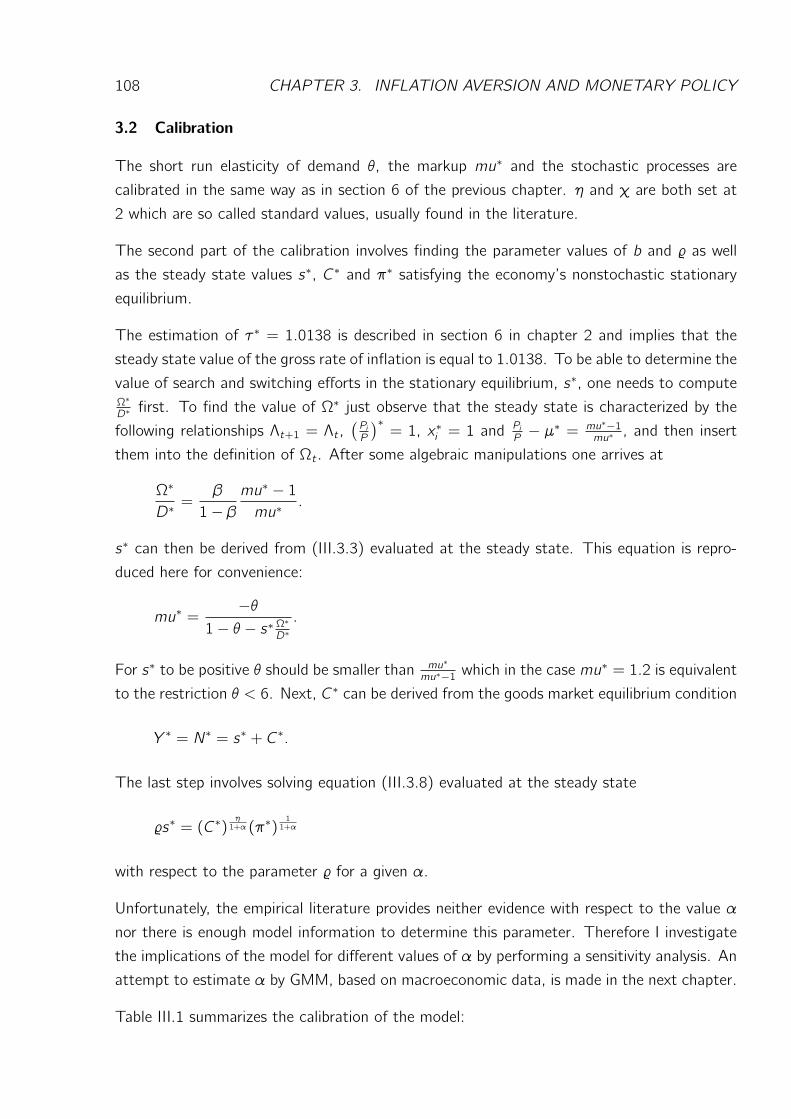
108 CHAPTER 3. INFLATION AVERSION AND MONETARY POLICY
3.2 Calibration
The short run elasticity of demand θ, the markup mu∗ and the stochastic processes are
calibrated in the same way as in section 6 of the previous chapter. η and χ are both set at
2 which are so called standard values, usually found in the literature.
The second part of the calibration involves finding the parameter values of b and % as well
as the steady state values s∗, C∗ and π∗ satisfying the economy’s nonstochastic stationary
equilibrium.
The estimation of τ∗ = 1.0138 is described in section 6 in chapter 2 and implies that the
steady state value of the gross rate of inflation is equal to 1.0138. To be able to determine the
value of search and switching efforts in the stationary equilibrium, s∗, one needs to computeΩ∗D∗ first. To find the value of Ω∗ just observe that the steady state is characterized by the
following relationships Λt+1 = Λt ,(PiP
)∗= 1, x∗i = 1 and
PiP− µ∗ = mu∗−1
mu∗ , and then insert
them into the definition of Ωt . After some algebraic manipulations one arrives at
Ω∗
D∗=
β
1− βmu∗ − 1mu∗
.
s∗ can then be derived from (III.3.3) evaluated at the steady state. This equation is repro-
duced here for convenience:
mu∗ =−θ
1− θ − s∗ Ω∗D∗.
For s∗ to be positive θ should be smaller than mu∗mu∗−1 which in the case mu
∗ = 1.2 is equivalent
to the restriction θ < 6. Next, C∗ can be derived from the goods market equilibrium condition
Y ∗ = N∗ = s∗ + C∗.
The last step involves solving equation (III.3.8) evaluated at the steady state
%s∗ = (C∗)η1+α (π∗)
11+α
with respect to the parameter % for a given α.
Unfortunately, the empirical literature provides neither evidence with respect to the value α
nor there is enough model information to determine this parameter. Therefore I investigate
the implications of the model for different values of α by performing a sensitivity analysis. An
attempt to estimate α by GMM, based on macroeconomic data, is made in the next chapter.
Table III.1 summarizes the calibration of the model:
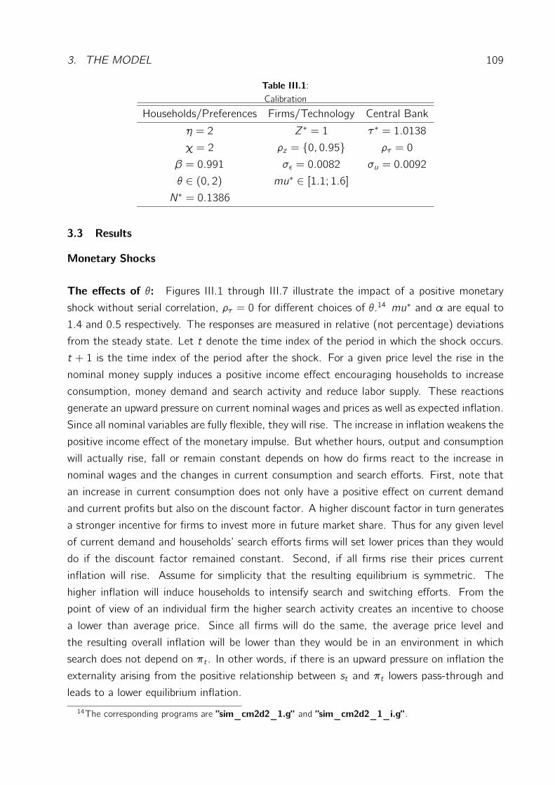
3. THE MODEL 109
Table III.1:Calibration
Households/Preferences Firms/Technology Central Bank
η = 2 Z∗ = 1 τ∗ = 1.0138
χ = 2 ρz = 0, 0.95 ρτ = 0
β = 0.991 σε = 0.0082 σu = 0.0092
θ ∈ (0, 2) mu∗ ∈ [1.1; 1.6]N∗ = 0.1386
3.3 Results
Monetary Shocks
The effects of θ: Figures III.1 through III.7 illustrate the impact of a positive monetary
shock without serial correlation, ρτ = 0 for different choices of θ.14 mu∗ and α are equal to
1.4 and 0.5 respectively. The responses are measured in relative (not percentage) deviations
from the steady state. Let t denote the time index of the period in which the shock occurs.
t + 1 is the time index of the period after the shock. For a given price level the rise in the
nominal money supply induces a positive income effect encouraging households to increase
consumption, money demand and search activity and reduce labor supply. These reactions
generate an upward pressure on current nominal wages and prices as well as expected inflation.
Since all nominal variables are fully flexible, they will rise. The increase in inflation weakens the
positive income effect of the monetary impulse. But whether hours, output and consumption
will actually rise, fall or remain constant depends on how do firms react to the increase in
nominal wages and the changes in current consumption and search efforts. First, note that
an increase in current consumption does not only have a positive effect on current demand
and current profits but also on the discount factor. A higher discount factor in turn generates
a stronger incentive for firms to invest more in future market share. Thus for any given level
of current demand and households’ search efforts firms will set lower prices than they would
do if the discount factor remained constant. Second, if all firms rise their prices current
inflation will rise. Assume for simplicity that the resulting equilibrium is symmetric. The
higher inflation will induce households to intensify search and switching efforts. From the
point of view of an individual firm the higher search activity creates an incentive to choose
a lower than average price. Since all firms will do the same, the average price level and
the resulting overall inflation will be lower than they would be in an environment in which
search does not depend on πt . In other words, if there is an upward pressure on inflation the
externality arising from the positive relationship between st and πt lowers pass-through and
leads to a lower equilibrium inflation.
14The corresponding programs are ”sim_cm2d2_1.g” and ”sim_cm2d2_1_i.g” .
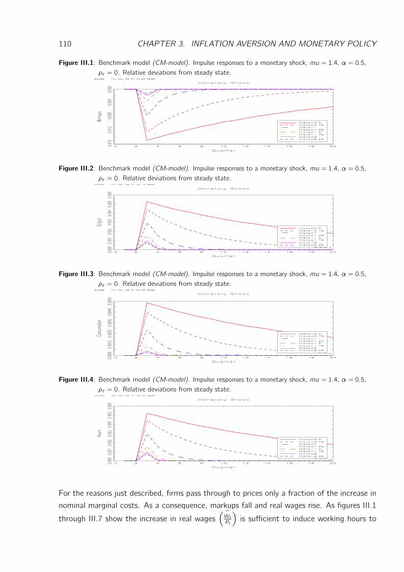
110 CHAPTER 3. INFLATION AVERSION AND MONETARY POLICY
Figure III.1: Benchmark model (CM-model). Impulse responses to a monetary shock, mu = 1.4, α = 0.5,ρτ = 0. Relative deviations from steady state.
Figure III.2: Benchmark model (CM-model). Impulse responses to a monetary shock, mu = 1.4, α = 0.5,ρτ = 0. Relative deviations from steady state.
Figure III.3: Benchmark model (CM-model). Impulse responses to a monetary shock, mu = 1.4, α = 0.5,ρτ = 0. Relative deviations from steady state.
Figure III.4: Benchmark model (CM-model). Impulse responses to a monetary shock, mu = 1.4, α = 0.5,ρτ = 0. Relative deviations from steady state.
For the reasons just described, firms pass through to prices only a fraction of the increase in
nominal marginal costs. As a consequence, markups fall and real wages rise. As figures III.1
through III.7 show the increase in real wagesˆ(WtPt
)is sufficient to induce working hours to
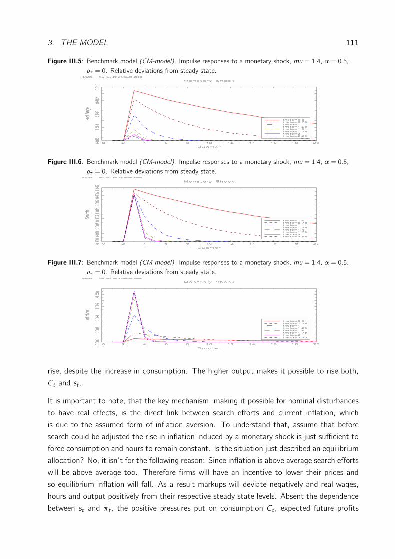
3. THE MODEL 111
Figure III.5: Benchmark model (CM-model). Impulse responses to a monetary shock, mu = 1.4, α = 0.5,ρτ = 0. Relative deviations from steady state.
Figure III.6: Benchmark model (CM-model). Impulse responses to a monetary shock, mu = 1.4, α = 0.5,ρτ = 0. Relative deviations from steady state.
Figure III.7: Benchmark model (CM-model). Impulse responses to a monetary shock, mu = 1.4, α = 0.5,ρτ = 0. Relative deviations from steady state.
rise, despite the increase in consumption. The higher output makes it possible to rise both,
Ct and st .
It is important to note, that the key mechanism, making it possible for nominal disturbances
to have real effects, is the direct link between search efforts and current inflation, which
is due to the assumed form of inflation aversion. To understand that, assume that before
search could be adjusted the rise in inflation induced by a monetary shock is just sufficient to
force consumption and hours to remain constant. Is the situation just described an equilibrium
allocation? No, it isn’t for the following reason: Since inflation is above average search efforts
will be above average too. Therefore firms will have an incentive to lower their prices and
so equilibrium inflation will fall. As a result markups will deviate negatively and real wages,
hours and output positively from their respective steady state levels. Absent the dependence
between st and πt , the positive pressures put on consumption Ct , expected future profits
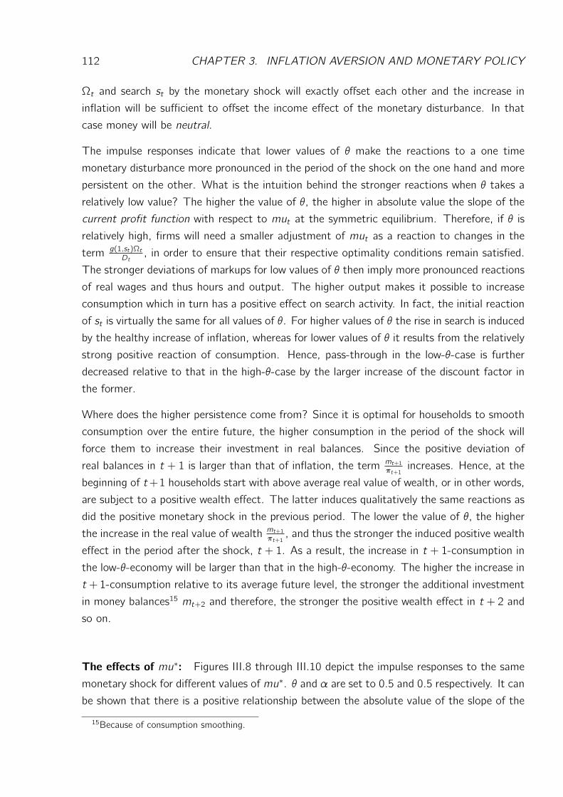
112 CHAPTER 3. INFLATION AVERSION AND MONETARY POLICY
Ωt and search st by the monetary shock will exactly offset each other and the increase in
inflation will be sufficient to offset the income effect of the monetary disturbance. In that
case money will be neutral.
The impulse responses indicate that lower values of θ make the reactions to a one time
monetary disturbance more pronounced in the period of the shock on the one hand and more
persistent on the other. What is the intuition behind the stronger reactions when θ takes a
relatively low value? The higher the value of θ, the higher in absolute value the slope of the
current profit function with respect to mut at the symmetric equilibrium. Therefore, if θ is
relatively high, firms will need a smaller adjustment of mut as a reaction to changes in the
term g(1,st)ΩtDt
, in order to ensure that their respective optimality conditions remain satisfied.
The stronger deviations of markups for low values of θ then imply more pronounced reactions
of real wages and thus hours and output. The higher output makes it possible to increase
consumption which in turn has a positive effect on search activity. In fact, the initial reaction
of st is virtually the same for all values of θ. For higher values of θ the rise in search is induced
by the healthy increase of inflation, whereas for lower values of θ it results from the relatively
strong positive reaction of consumption. Hence, pass-through in the low-θ-case is further
decreased relative to that in the high-θ-case by the larger increase of the discount factor in
the former.
Where does the higher persistence come from? Since it is optimal for households to smooth
consumption over the entire future, the higher consumption in the period of the shock will
force them to increase their investment in real balances. Since the positive deviation of
real balances in t + 1 is larger than that of inflation, the term mt+1πt+1
increases. Hence, at the
beginning of t+1 households start with above average real value of wealth, or in other words,
are subject to a positive wealth effect. The latter induces qualitatively the same reactions as
did the positive monetary shock in the previous period. The lower the value of θ, the higher
the increase in the real value of wealth mt+1πt+1
, and thus the stronger the induced positive wealth
effect in the period after the shock, t + 1. As a result, the increase in t + 1-consumption in
the low-θ-economy will be larger than that in the high-θ-economy. The higher the increase in
t +1-consumption relative to its average future level, the stronger the additional investment
in money balances15 mt+2 and therefore, the stronger the positive wealth effect in t + 2 and
so on.
The effects of mu∗: Figures III.8 through III.10 depict the impulse responses to the same
monetary shock for different values of mu∗. θ and α are set to 0.5 and 0.5 respectively. It can
be shown that there is a positive relationship between the absolute value of the slope of the
15Because of consumption smoothing.
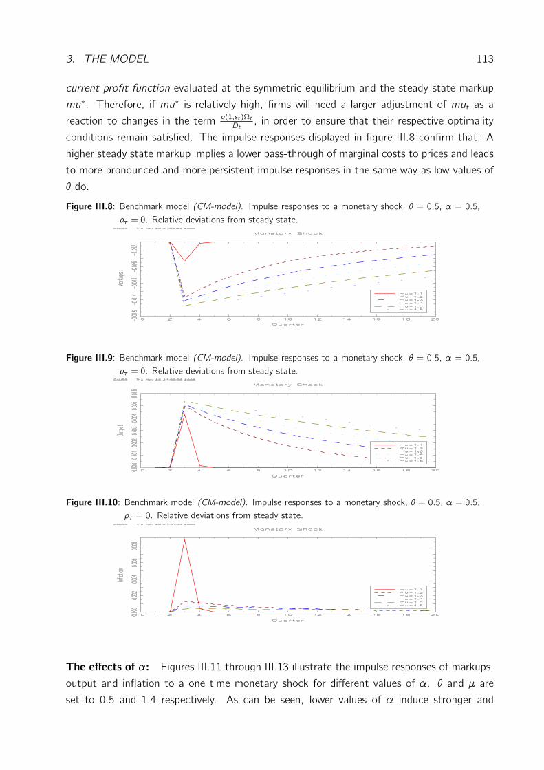
3. THE MODEL 113
current profit function evaluated at the symmetric equilibrium and the steady state markup
mu∗. Therefore, if mu∗ is relatively high, firms will need a larger adjustment of mut as a
reaction to changes in the term g(1,st)ΩtDt
, in order to ensure that their respective optimality
conditions remain satisfied. The impulse responses displayed in figure III.8 confirm that: A
higher steady state markup implies a lower pass-through of marginal costs to prices and leads
to more pronounced and more persistent impulse responses in the same way as low values of
θ do.
Figure III.8: Benchmark model (CM-model). Impulse responses to a monetary shock, θ = 0.5, α = 0.5,ρτ = 0. Relative deviations from steady state.
Figure III.9: Benchmark model (CM-model). Impulse responses to a monetary shock, θ = 0.5, α = 0.5,ρτ = 0. Relative deviations from steady state.
Figure III.10: Benchmark model (CM-model). Impulse responses to a monetary shock, θ = 0.5, α = 0.5,ρτ = 0. Relative deviations from steady state.
The effects of α: Figures III.11 through III.13 illustrate the impulse responses of markups,
output and inflation to a one time monetary shock for different values of α. θ and µ are
set to 0.5 and 1.4 respectively. As can be seen, lower values of α induce stronger and
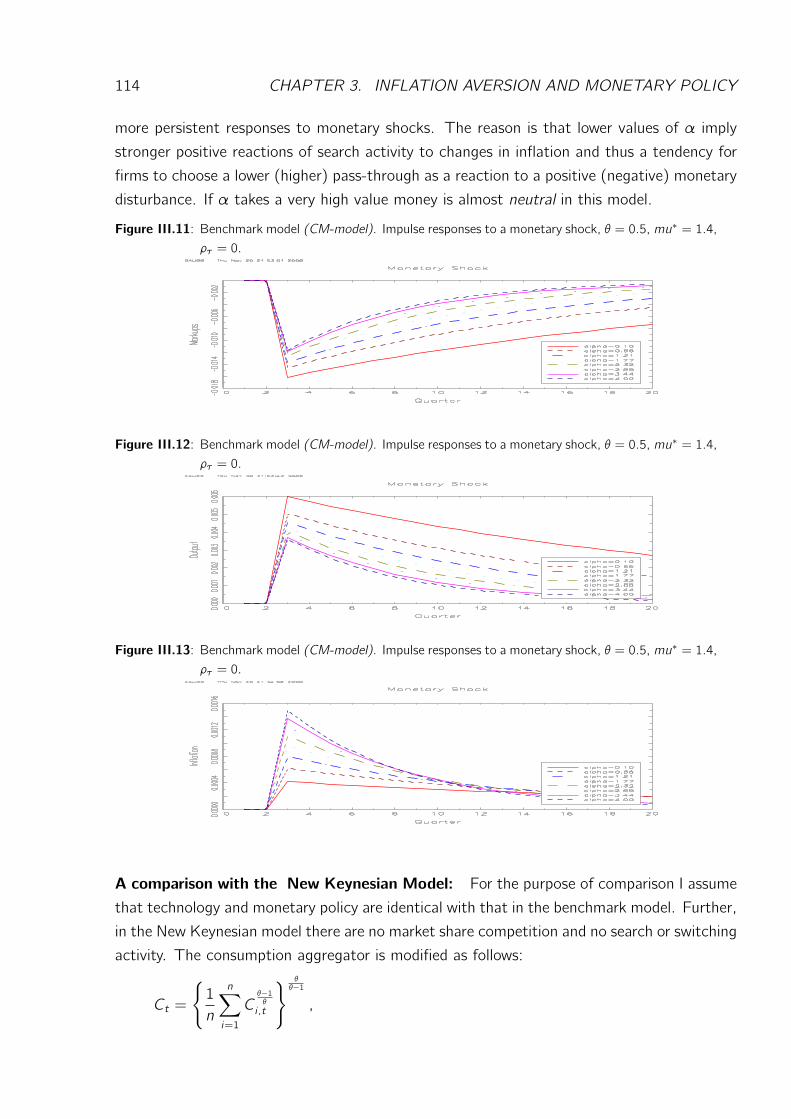
114 CHAPTER 3. INFLATION AVERSION AND MONETARY POLICY
more persistent responses to monetary shocks. The reason is that lower values of α imply
stronger positive reactions of search activity to changes in inflation and thus a tendency for
firms to choose a lower (higher) pass-through as a reaction to a positive (negative) monetary
disturbance. If α takes a very high value money is almost neutral in this model.
Figure III.11: Benchmark model (CM-model). Impulse responses to a monetary shock, θ = 0.5, mu∗ = 1.4,ρτ = 0.
Figure III.12: Benchmark model (CM-model). Impulse responses to a monetary shock, θ = 0.5, mu∗ = 1.4,ρτ = 0.
Figure III.13: Benchmark model (CM-model). Impulse responses to a monetary shock, θ = 0.5, mu∗ = 1.4,ρτ = 0.
A comparison with the New Keynesian Model: For the purpose of comparison I assume
that technology and monetary policy are identical with that in the benchmark model. Further,
in the New Keynesian model there are no market share competition and no search or switching
activity. The consumption aggregator is modified as follows:
Ct =
1
n
n∑
i=1
Cθ−1θ
i ,t
θθ−1
,
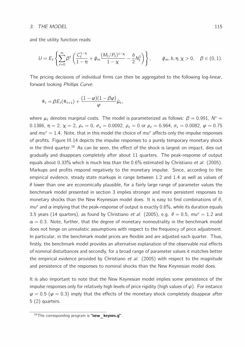
3. THE MODEL 115
and the utility function reads:
U = Et
∞∑t=0
βt(C1−ηt1− η + φm
(Mt/Pt)1−χ
1− χ − b2N2t
), φm, b, η, χ > 0, β ∈ (0, 1).
The pricing decisions of individual firms can then be aggregated to the following log-linear,
forward looking Phillips Curve:
πt = βEt(πt+1) +(1− ϕ)(1− βϕ)
ϕµt ,
where µt denotes marginal costs. The model is parameterized as follows: β = 0.991, N∗ =
0.1386, η = 2, χ = 2, ρτ = 0, σu = 0.0092, ρz = 0 or ρz = 0.964, σε = 0.0082, ϕ = 0.75
and mu∗ = 1.4. Note, that in this model the choice of mu∗ affects only the impulse responses
of profits. Figure III.14 depicts the impulse responses to a purely temporary monetary shock
in the third quarter.16 As can be seen, the effect of the shock is largest on impact, dies out
gradually and disappears completely after about 11 quarters. The peak-response of output
equals about 0.33% which is much less than the 0.6% estimated by Christiano et al. (2005).
Markups and profits respond negatively to the monetary impulse. Since, according to the
empirical evidence, steady state markups in range between 1.2 and 1.4 as well as values of
θ lower than one are economically plausible, for a fairly large range of parameter values the
benchmark model presented in section 3 implies stronger and more persistent responses to
monetary shocks than the New Keynesian model does. It is easy to find combinations of θ,
mu∗ and α implying that the peak-response of output is exactly 0.6%, while its duration equals
3.5 years (14 quarters), as found by Christiano et al. (2005), e.g. θ = 0.5, mu∗ = 1.2 and
α = 0.3. Note, further, that the degree of monetary nonneutrality in the benchmark model
does not hinge on unrealistic assumptions with respect to the frequency of price adjustment.
In particular, in the benchmark model prices are flexible and are adjusted each quarter. Thus,
firstly, the benchmark model provides an alternative explanation of the observable real effects
of nominal disturbances and secondly, for a broad range of parameter values it matches better
the empirical evidence provided by Christiano et al. (2005) with respect to the magnitude
and persistence of the responses to nominal shocks than the New Keynesian model does.
It is also important to note that the New Keynesian model implies some persistence of the
impulse responses only for relatively high levels of price rigidity (high values of ϕ). For instance
ϕ = 0.5 (ϕ = 0.3) imply that the effects of the monetary shock completely disappear after
5 (2) quarters.
16The corresponding program is ”new_keynes.g” .
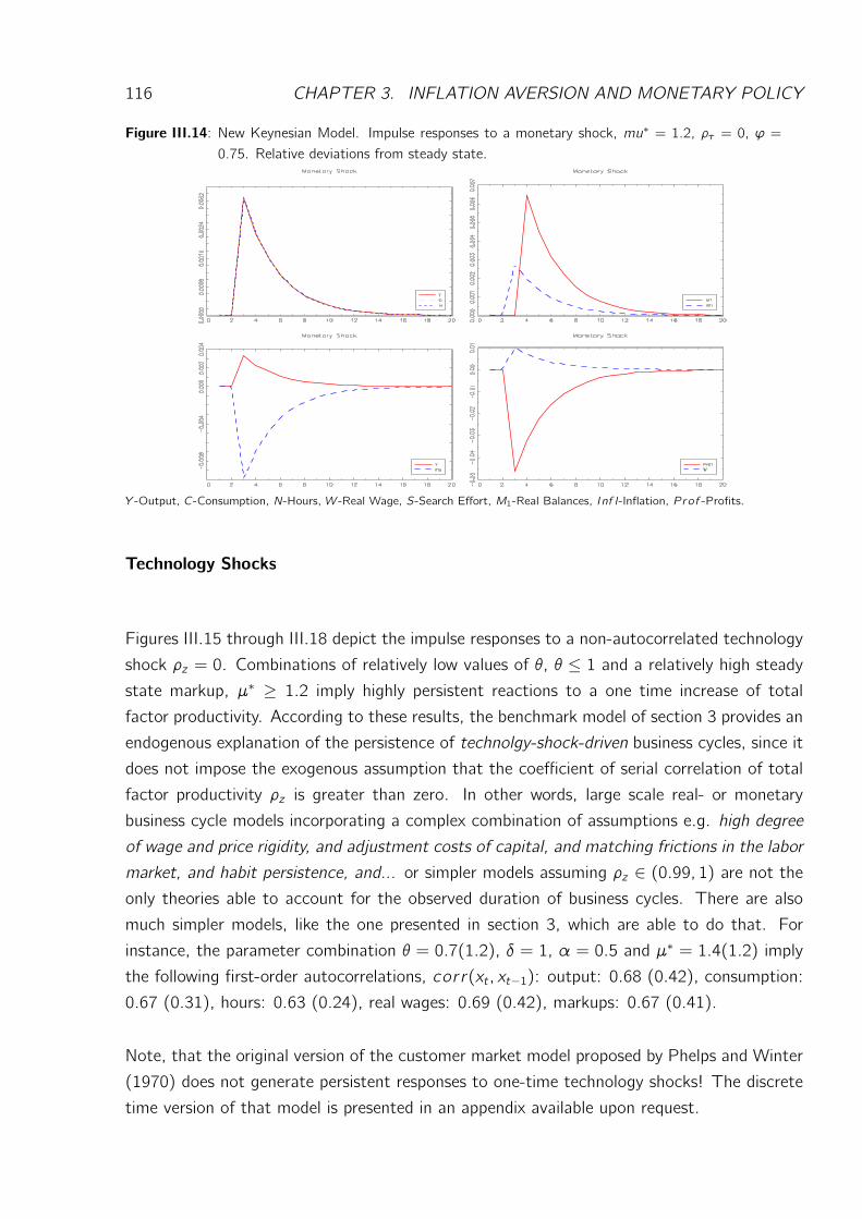
116 CHAPTER 3. INFLATION AVERSION AND MONETARY POLICY
Figure III.14: New Keynesian Model. Impulse responses to a monetary shock, mu∗ = 1.2, ρτ = 0, ϕ =0.75. Relative deviations from steady state.
Y -Output, C-Consumption, N-Hours, W -Real Wage, S-Search Effort, M1-Real Balances, Inf l-Inflation, P rof -Profits.
Technology Shocks
Figures III.15 through III.18 depict the impulse responses to a non-autocorrelated technology
shock ρz = 0. Combinations of relatively low values of θ, θ ≤ 1 and a relatively high steady
state markup, µ∗ ≥ 1.2 imply highly persistent reactions to a one time increase of total
factor productivity. According to these results, the benchmark model of section 3 provides an
endogenous explanation of the persistence of technolgy-shock-driven business cycles, since it
does not impose the exogenous assumption that the coefficient of serial correlation of total
factor productivity ρz is greater than zero. In other words, large scale real- or monetary
business cycle models incorporating a complex combination of assumptions e.g. high degree
of wage and price rigidity, and adjustment costs of capital, and matching frictions in the labor
market, and habit persistence, and... or simpler models assuming ρz ∈ (0.99, 1) are not the
only theories able to account for the observed duration of business cycles. There are also
much simpler models, like the one presented in section 3, which are able to do that. For
instance, the parameter combination θ = 0.7(1.2), δ = 1, α = 0.5 and µ∗ = 1.4(1.2) imply
the following first-order autocorrelations, cor r(xt , xt−1): output: 0.68 (0.42), consumption:
0.67 (0.31), hours: 0.63 (0.24), real wages: 0.69 (0.42), markups: 0.67 (0.41).
Note, that the original version of the customer market model proposed by Phelps and Winter
(1970) does not generate persistent responses to one-time technology shocks! The discrete
time version of that model is presented in an appendix available upon request.
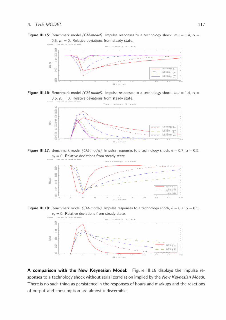
3. THE MODEL 117
Figure III.15: Benchmark model (CM-model). Impulse responses to a technology shock, mu = 1.4, α =0.5, ρz = 0. Relative deviations from steady state.
Figure III.16: Benchmark model (CM-model). Impulse responses to a technology shock, mu = 1.4, α =0.5, ρz = 0. Relative deviations from steady state.
Figure III.17: Benchmark model (CM-model). Impulse responses to a technology shock, θ = 0.7, α = 0.5,ρz = 0. Relative deviations from steady state.
Figure III.18: Benchmark model (CM-model). Impulse responses to a technology shock, θ = 0.7, α = 0.5,ρz = 0. Relative deviations from steady state.
A comparison with the New Keynesian Model: Figure III.19 displays the impulse re-
sponses to a technology shock without serial correlation implied by the New Keynesian Moedl.
There is no such thing as persistence in the responses of hours and markups and the reactions
of output and consumption are almost indiscernible.
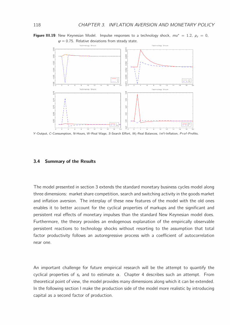
118 CHAPTER 3. INFLATION AVERSION AND MONETARY POLICY
Figure III.19: New Keynesian Model. Impulse responses to a technology shock, mu∗ = 1.2, ρz = 0,ϕ = 0.75. Relative deviations from steady state.
Y -Output, C-Consumption, N-Hours, W -Real Wage, S-Search Effort, M1-Real Balances, Inf l-Inflation, P rof -Profits.
3.4 Summary of the Results
The model presented in section 3 extends the standard monetary business cycles model along
three dimensions: market share competition, search and switching activity in the goods market
and inflation aversion. The interplay of these new features of the model with the old ones
enables it to better account for the cyclical properties of markups and the significant and
persistent real effects of monetary impulses than the standard New Keynesian model does.
Furthermore, the theory provides an endogenous explanation of the empirically observable
persistent reactions to technology shocks without resorting to the assumption that total
factor productivity follows an autoregressive process with a coefficient of autocorrelation
near one.
An important challenge for future empirical research will be the attempt to quantify the
cyclical properties of st and to estimate α. Chapter 4 describes such an attempt. From
theoretical point of view, the model provides many dimensions along which it can be extended.
In the following section I make the production side of the model more realistic by introducing
capital as a second factor of production.
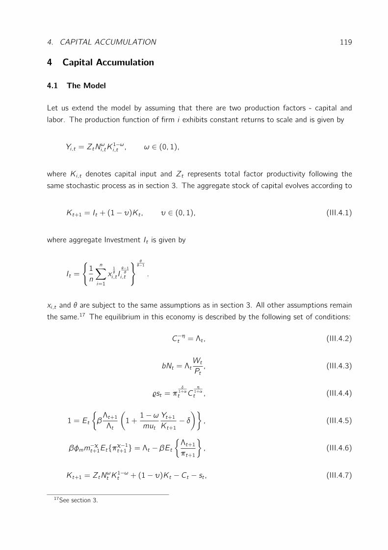
4. CAPITAL ACCUMULATION 119
4 Capital Accumulation
4.1 The Model
Let us extend the model by assuming that there are two production factors - capital and
labor. The production function of firm i exhibits constant returns to scale and is given by
Yi ,t = ZtNωi,tK
1−ωi,t , ω ∈ (0, 1),
where Ki ,t denotes capital input and Zt represents total factor productivity following the
same stochastic process as in section 3. The aggregate stock of capital evolves according to
Kt+1 = It + (1− υ)Kt , υ ∈ (0, 1), (III.4.1)
where aggregate Investment It is given by
It =
1
n
n∑
i=1
x1θ
i ,tIθ−1θ
i ,t
θθ−1
.
xi ,t and θ are subject to the same assumptions as in section 3. All other assumptions remain
the same.17 The equilibrium in this economy is described by the following set of conditions:
C−ηt = Λt , (III.4.2)
bNt = ΛtWtPt, (III.4.3)
%st = πδ1+αt C
η1+αt , (III.4.4)
1 = Et
βΛt+1Λt
(1 +1− ωmut
Yt+1Kt+1
− δ), (III.4.5)
βφmm−χt+1Etπχ−1t+1 = Λt − βEt
Λt+1πt+1
, (III.4.6)
Kt+1 = ZtNωt K
1−ωt + (1− υ)Kt − Ct − st , (III.4.7)
17See section 3.
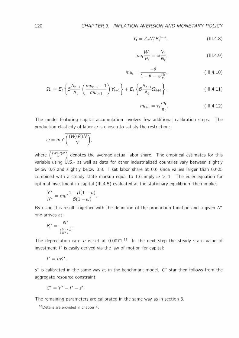
120 CHAPTER 3. INFLATION AVERSION AND MONETARY POLICY
Yt = ZtNωt K
1−ωt , (III.4.8)
mutWtPt= ωYtNt, (III.4.9)
mut =−θ
1− θ − st ΩtYt, (III.4.10)
Ωt = Et
βΛt+1Λt
(mut+1 − 1mut+1
)Yt+1
+ Et
βΛt+1ΛtΩt+1
, (III.4.11)
mt+1 = τtmtπt. (III.4.12)
The model featuring capital accumulation involves few additional calibration steps. The
production elasticity of labor ω is chosen to satisfy the restriction:
ω = mu∗((W/P )N
Y
),
where((W/P )NY
)denotes the average actual labor share. The empirical estimates for this
variable using U.S.- as well as data for other industrialized countries vary between slightly
below 0.6 and slightly below 0.8. I set labor share at 0.6 since values larger than 0.625
combined with a steady state markup equal to 1.6 imply ω > 1. The euler equation for
optimal investment in capital (III.4.5) evaluated at the stationary equilibrium then implies
Y ∗
K∗= mu∗
1− β(1− υ)β(1− ω) .
By using this result together with the definition of the production function and a given N∗
one arrives at:
K∗ =N∗
(Y ∗K∗
) 1ω
.
The depreciation rate υ is set at 0.0071.18 In the next step the steady state value of
investment I∗ is easily derived via the law of motion for capital:
I∗ = υK∗.
s∗ is calibrated in the same way as in the benchmark model. C∗ star then follows from the
aggregate resource constraint
C∗ = Y ∗ − I∗ − s∗.
The remaining parameters are calibrated in the same way as in section 3.18Details are provided in chapter 4.
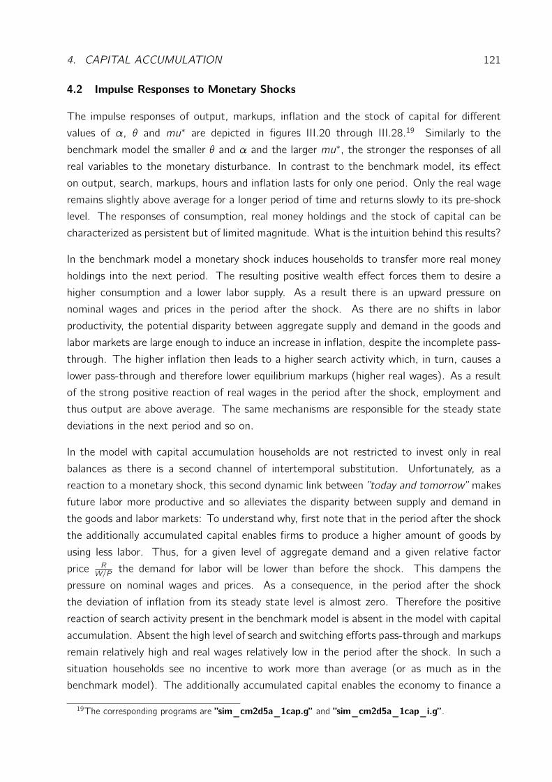
4. CAPITAL ACCUMULATION 121
4.2 Impulse Responses to Monetary Shocks
The impulse responses of output, markups, inflation and the stock of capital for different
values of α, θ and mu∗ are depicted in figures III.20 through III.28.19 Similarly to the
benchmark model the smaller θ and α and the larger mu∗, the stronger the responses of all
real variables to the monetary disturbance. In contrast to the benchmark model, its effect
on output, search, markups, hours and inflation lasts for only one period. Only the real wage
remains slightly above average for a longer period of time and returns slowly to its pre-shock
level. The responses of consumption, real money holdings and the stock of capital can be
characterized as persistent but of limited magnitude. What is the intuition behind this results?
In the benchmark model a monetary shock induces households to transfer more real money
holdings into the next period. The resulting positive wealth effect forces them to desire a
higher consumption and a lower labor supply. As a result there is an upward pressure on
nominal wages and prices in the period after the shock. As there are no shifts in labor
productivity, the potential disparity between aggregate supply and demand in the goods and
labor markets are large enough to induce an increase in inflation, despite the incomplete pass-
through. The higher inflation then leads to a higher search activity which, in turn, causes a
lower pass-through and therefore lower equilibrium markups (higher real wages). As a result
of the strong positive reaction of real wages in the period after the shock, employment and
thus output are above average. The same mechanisms are responsible for the steady state
deviations in the next period and so on.
In the model with capital accumulation households are not restricted to invest only in real
balances as there is a second channel of intertemporal substitution. Unfortunately, as a
reaction to a monetary shock, this second dynamic link between ”today and tomorrow” makes
future labor more productive and so alleviates the disparity between supply and demand in
the goods and labor markets: To understand why, first note that in the period after the shock
the additionally accumulated capital enables firms to produce a higher amount of goods by
using less labor. Thus, for a given level of aggregate demand and a given relative factor
price RW/P
the demand for labor will be lower than before the shock. This dampens the
pressure on nominal wages and prices. As a consequence, in the period after the shock
the deviation of inflation from its steady state level is almost zero. Therefore the positive
reaction of search activity present in the benchmark model is absent in the model with capital
accumulation. Absent the high level of search and switching efforts pass-through and markups
remain relatively high and real wages relatively low in the period after the shock. In such a
situation households see no incentive to work more than average (or as much as in the
benchmark model). The additionally accumulated capital enables the economy to finance a
19The corresponding programs are ”sim_cm2d5a_1cap.g” and ”sim_cm2d5a_1cap_i.g” .
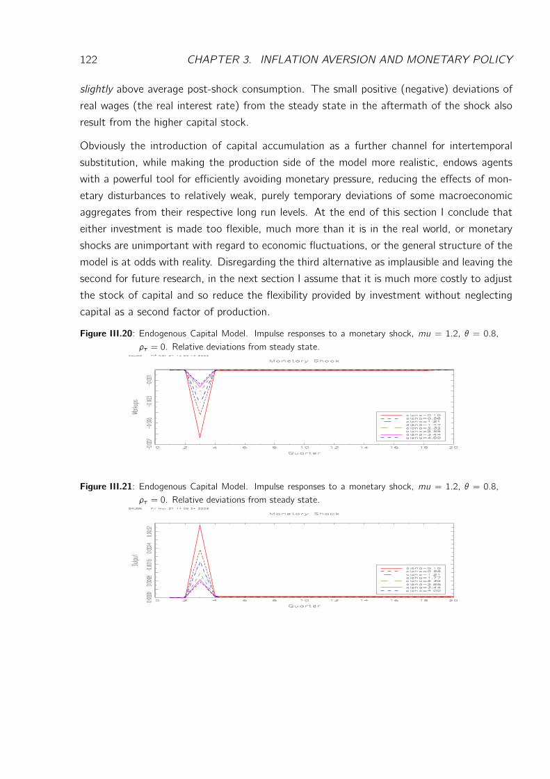
122 CHAPTER 3. INFLATION AVERSION AND MONETARY POLICY
slightly above average post-shock consumption. The small positive (negative) deviations of
real wages (the real interest rate) from the steady state in the aftermath of the shock also
result from the higher capital stock.
Obviously the introduction of capital accumulation as a further channel for intertemporal
substitution, while making the production side of the model more realistic, endows agents
with a powerful tool for efficiently avoiding monetary pressure, reducing the effects of mon-
etary disturbances to relatively weak, purely temporary deviations of some macroeconomic
aggregates from their respective long run levels. At the end of this section I conclude that
either investment is made too flexible, much more than it is in the real world, or monetary
shocks are unimportant with regard to economic fluctuations, or the general structure of the
model is at odds with reality. Disregarding the third alternative as implausible and leaving the
second for future research, in the next section I assume that it is much more costly to adjust
the stock of capital and so reduce the flexibility provided by investment without neglecting
capital as a second factor of production.
Figure III.20: Endogenous Capital Model. Impulse responses to a monetary shock, mu = 1.2, θ = 0.8,ρτ = 0. Relative deviations from steady state.
Figure III.21: Endogenous Capital Model. Impulse responses to a monetary shock, mu = 1.2, θ = 0.8,ρτ = 0. Relative deviations from steady state.
4. CAPITAL ACCUMULATION 123
Figure III.22: Endogenous Capital Model. Impulse responses to a monetary shock, mu = 1.2, θ = 0.8,ρτ = 0. Relative deviations from steady state.
Figure III.23: Endogenous Capital Model. Impulse responses to a monetary shock, mu = 1.2, θ = 0.8,ρτ = 0. Relative deviations from steady state.
Figure III.24: Endogenous Capital Model. Impulse responses to a monetary shock, mu = 1.2, θ = 0.8,ρτ = 0. Relative deviations from steady state.
Figure III.25: Endogenous Capital Model. Impulse responses to a monetary shock, mu = 1.2, α = 0.5,ρτ = 0. Relative deviations from steady state.
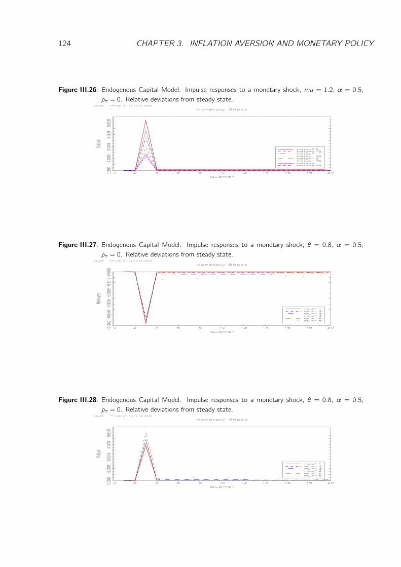
124 CHAPTER 3. INFLATION AVERSION AND MONETARY POLICY
Figure III.26: Endogenous Capital Model. Impulse responses to a monetary shock, mu = 1.2, α = 0.5,ρτ = 0. Relative deviations from steady state.
Figure III.27: Endogenous Capital Model. Impulse responses to a monetary shock, θ = 0.8, α = 0.5,ρτ = 0. Relative deviations from steady state.
Figure III.28: Endogenous Capital Model. Impulse responses to a monetary shock, θ = 0.8, α = 0.5,ρτ = 0. Relative deviations from steady state.
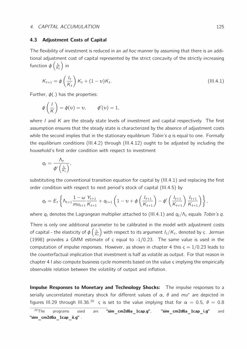
4. CAPITAL ACCUMULATION 125
4.3 Adjustment Costs of Capital
The flexibility of investment is reduced in an ad hoc manner by assuming that there is an addi-
tional adjustment cost of capital represented by the strict concavity of the strictly increasing
function φ(ItKt
)in
Kt+1 = φ
(ItKt
)Kt + (1− υ)Kt . (III.4.1)
Further, φ(.) has the properties:
φ
(I
K
)= φ(υ) = υ, φ′(υ) = 1,
where I and K are the steady state levels of investment and capital respectively. The first
assumption ensures that the steady state is characterized by the absence of adjustment costs
while the second implies that in the stationary equilibrium Tobin’s q is equal to one. Formally
the equilibrium conditions (III.4.2) through (III.4.12) ought to be adjusted by including the
household’s first order condition with respect to investment
qt =Λt
φ′(ItKt
) ,
substituting the conventional transition equation for capital by (III.4.1) and replacing the first
order condition with respect to next period’s stock of capital (III.4.5) by
qt = Et
Λt+1
1− ωmut+1
Yt+1Kt+1
+ qt+1
(1− υ + φ
(It+1Kt+1
)− φ′
(It+1Kt+1
)It+1Kt+1
),
where qt denotes the Lagrangean multiplier attached to (III.4.1) and qt/Λt equals Tobin’s q.
There is only one additional parameter to be calibrated in the model with adjustment costs
of capital - the elasticity of φ(ItKt
)with respect to its argument It/Kt , denoted by ς. Jerman
(1998) provides a GMM estimate of ς equal to -1/0.23. The same value is used in the
computation of impulse responses. However, as shown in chapter 4 this ς = 1/0.23 leads to
the counterfactual implication that investment is half as volatile as output. For that reason in
chapter 4 I also compute business cycle moments based on the value ς implying the empirically
observable relation between the volatility of output and inflation.
Impulse Responses to Monetary and Technology Shocks: The impulse responses to a
serially uncorrelated monetary shock for different values of α, θ and mu∗ are depicted in
figures III.29 through III.36.20 ς is set to the value implying that for α = 0.5, θ = 0.820The programs used are ”sim_cm2d6a_1cap.g” , ”sim_cm2d6a_1cap_i.g” and
”sim_cm2d6a_1cap_ii.g” .
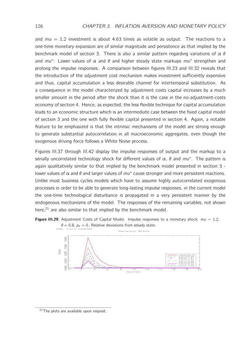
126 CHAPTER 3. INFLATION AVERSION AND MONETARY POLICY
and mu = 1.2 investment is about 4.63 times as volatile as output. The reactions to a
one-time monetary expansion are of similar magnitude and persistence as that implied by the
benchmark model of section 3. There is also a similar pattern regarding variations of α θ
and mu∗: Lower values of α and θ and higher steady state markups mu∗ strengthen and
prolong the impulse responses. A comparison between figures III.23 and III.32 reveals that
the introduction of the adjustment cost mechanism makes investment sufficiently expensive
and thus, capital accumulation a less desirable channel for intertemporal substitution. As
a consequence in the model characterized by adjustment costs capital increases by a much
smaller amount in the period after the shock than it is the case in the no-adjustment-costs
economy of section 4. Hence, as expected, the less flexible technique for capital accumulation
leads to an economic structure which is an intermediate case between the fixed capital model
of section 3 and the one with fully flexible capital presented in section 4. Again, a notable
feature to be emphasized is that the intrinsic mechanisms of the model are strong enough
to generate substantial autocorrelation in all macroeconomic aggregates, even though the
exogenous driving force follows a White Noise process.
Figures III.37 through III.42 display the impulse responses of output and the markup to a
serially uncorrelated technology shock for different values of α, θ and mu∗. The pattern is
again qualitatively similar to that implied by the benchmark model presented in section 3 -
lower values of α and θ and larger values of mu∗ cause stronger and more persistent reactions.
Unlike most business cycles models which have to assume highly autocorrelated exogenous
processes in order to be able to generate long-lasting impulse responses, in the current model
the one-time technological disturbance is propagated in a very persistent manner by the
endogenous mechanisms of the model. The responses of the remaining variables, not shown
here,21 are also similar to that implied by the benchmark model.
Figure III.29: Adjustment Costs of Capital Model. Impulse responses to a monetary shock, mu = 1.2,θ = 0.8, ρτ = 0. Relative deviations from steady state.
21The plots are available upon request.
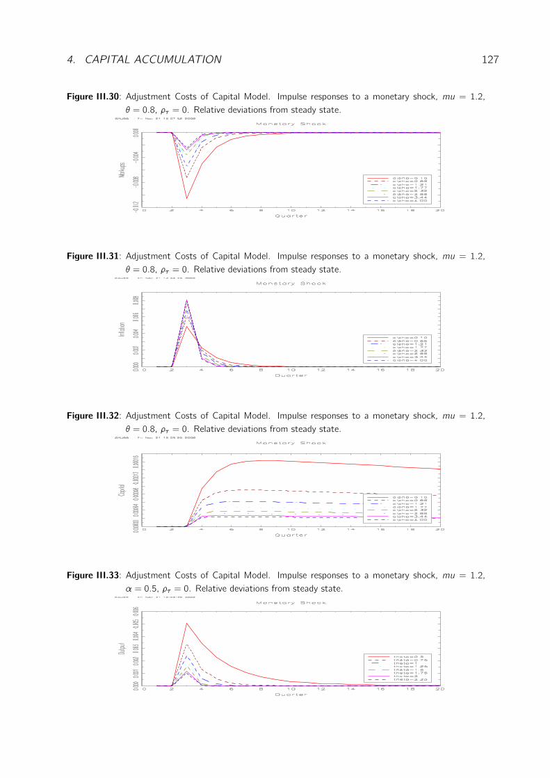
4. CAPITAL ACCUMULATION 127
Figure III.30: Adjustment Costs of Capital Model. Impulse responses to a monetary shock, mu = 1.2,θ = 0.8, ρτ = 0. Relative deviations from steady state.
Figure III.31: Adjustment Costs of Capital Model. Impulse responses to a monetary shock, mu = 1.2,θ = 0.8, ρτ = 0. Relative deviations from steady state.
Figure III.32: Adjustment Costs of Capital Model. Impulse responses to a monetary shock, mu = 1.2,θ = 0.8, ρτ = 0. Relative deviations from steady state.
Figure III.33: Adjustment Costs of Capital Model. Impulse responses to a monetary shock, mu = 1.2,α = 0.5, ρτ = 0. Relative deviations from steady state.
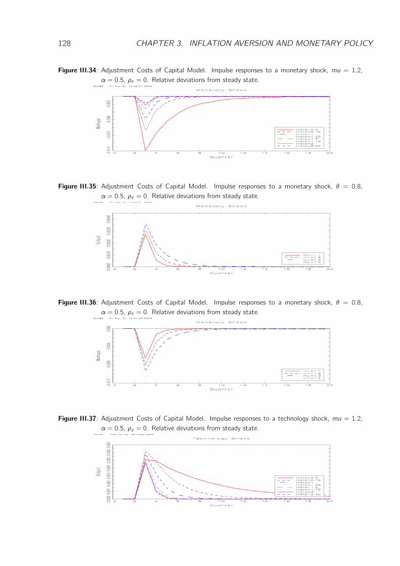
128 CHAPTER 3. INFLATION AVERSION AND MONETARY POLICY
Figure III.34: Adjustment Costs of Capital Model. Impulse responses to a monetary shock, mu = 1.2,α = 0.5, ρτ = 0. Relative deviations from steady state.
Figure III.35: Adjustment Costs of Capital Model. Impulse responses to a monetary shock, θ = 0.8,α = 0.5, ρτ = 0. Relative deviations from steady state.
Figure III.36: Adjustment Costs of Capital Model. Impulse responses to a monetary shock, θ = 0.8,α = 0.5, ρτ = 0. Relative deviations from steady state.
Figure III.37: Adjustment Costs of Capital Model. Impulse responses to a technology shock, mu = 1.2,α = 0.5, ρz = 0. Relative deviations from steady state.
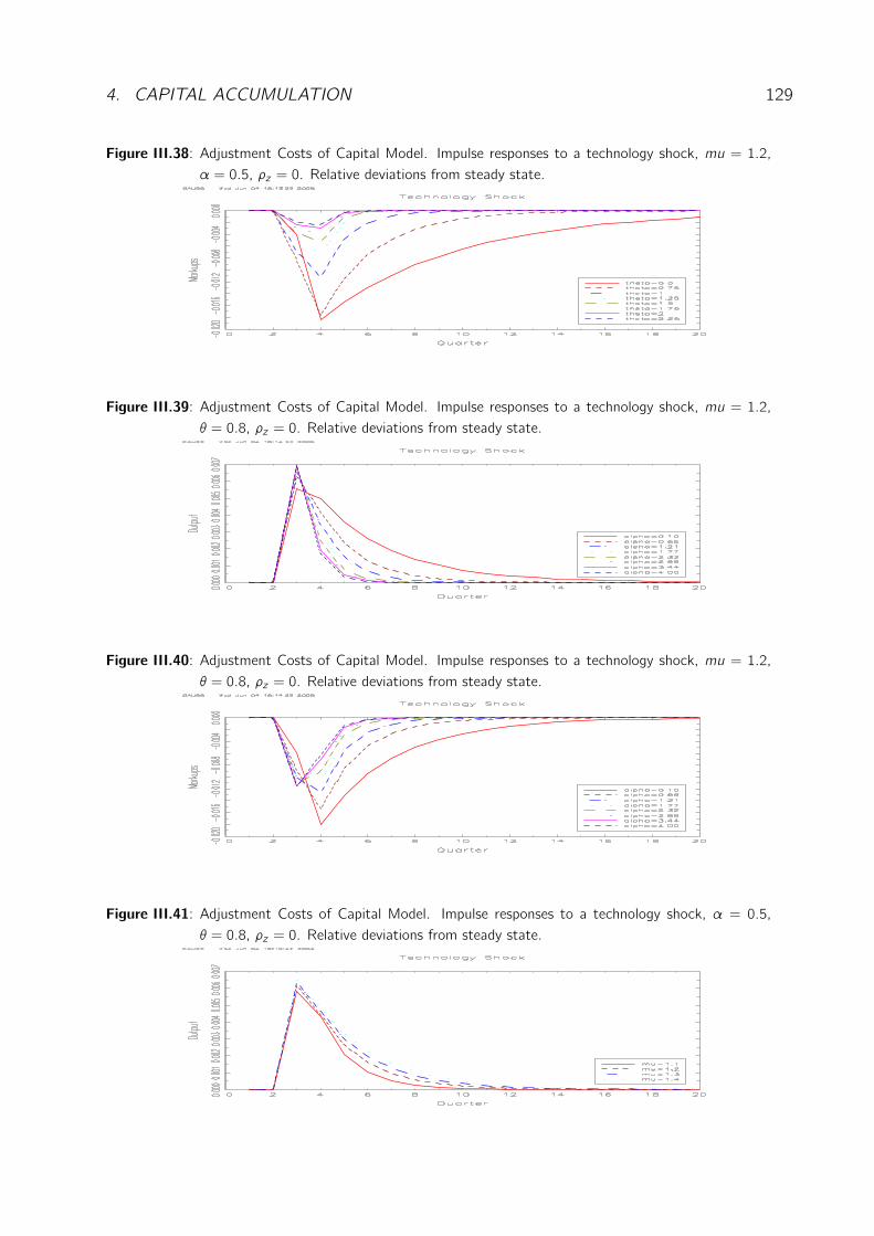
4. CAPITAL ACCUMULATION 129
Figure III.38: Adjustment Costs of Capital Model. Impulse responses to a technology shock, mu = 1.2,α = 0.5, ρz = 0. Relative deviations from steady state.
Figure III.39: Adjustment Costs of Capital Model. Impulse responses to a technology shock, mu = 1.2,θ = 0.8, ρz = 0. Relative deviations from steady state.
Figure III.40: Adjustment Costs of Capital Model. Impulse responses to a technology shock, mu = 1.2,θ = 0.8, ρz = 0. Relative deviations from steady state.
Figure III.41: Adjustment Costs of Capital Model. Impulse responses to a technology shock, α = 0.5,θ = 0.8, ρz = 0. Relative deviations from steady state.
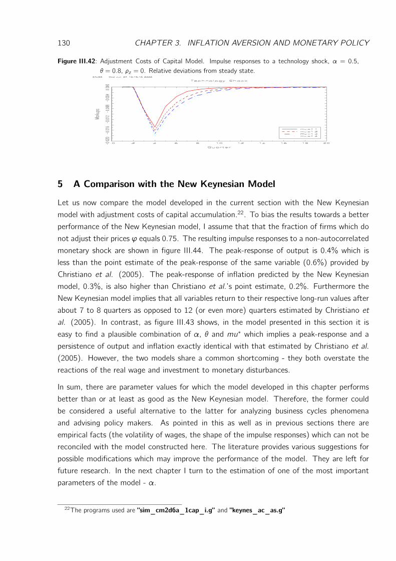
130 CHAPTER 3. INFLATION AVERSION AND MONETARY POLICY
Figure III.42: Adjustment Costs of Capital Model. Impulse responses to a technology shock, α = 0.5,θ = 0.8, ρz = 0. Relative deviations from steady state.
5 A Comparison with the New Keynesian Model
Let us now compare the model developed in the current section with the New Keynesian
model with adjustment costs of capital accumulation.22. To bias the results towards a better
performance of the New Keynesian model, I assume that that the fraction of firms which do
not adjust their prices ϕ equals 0.75. The resulting impulse responses to a non-autocorrelated
monetary shock are shown in figure III.44. The peak-response of output is 0.4% which is
less than the point estimate of the peak-response of the same variable (0.6%) provided by
Christiano et al. (2005). The peak-response of inflation predicted by the New Keynesian
model, 0.3%, is also higher than Christiano et al.’s point estimate, 0.2%. Furthermore the
New Keynesian model implies that all variables return to their respective long-run values after
about 7 to 8 quarters as opposed to 12 (or even more) quarters estimated by Christiano et
al. (2005). In contrast, as figure III.43 shows, in the model presented in this section it is
easy to find a plausible combination of α, θ and mu∗ which implies a peak-response and a
persistence of output and inflation exactly identical with that estimated by Christiano et al.
(2005). However, the two models share a common shortcoming - they both overstate the
reactions of the real wage and investment to monetary disturbances.
In sum, there are parameter values for which the model developed in this chapter performs
better than or at least as good as the New Keynesian model. Therefore, the former could
be considered a useful alternative to the latter for analyzing business cycles phenomena
and advising policy makers. As pointed in this as well as in previous sections there are
empirical facts (the volatility of wages, the shape of the impulse responses) which can not be
reconciled with the model constructed here. The literature provides various suggestions for
possible modifications which may improve the performance of the model. They are left for
future research. In the next chapter I turn to the estimation of one of the most important
parameters of the model - α.
22The programs used are ”sim_cm2d6a_1cap_i.g” and ”keynes_ac_as.g”
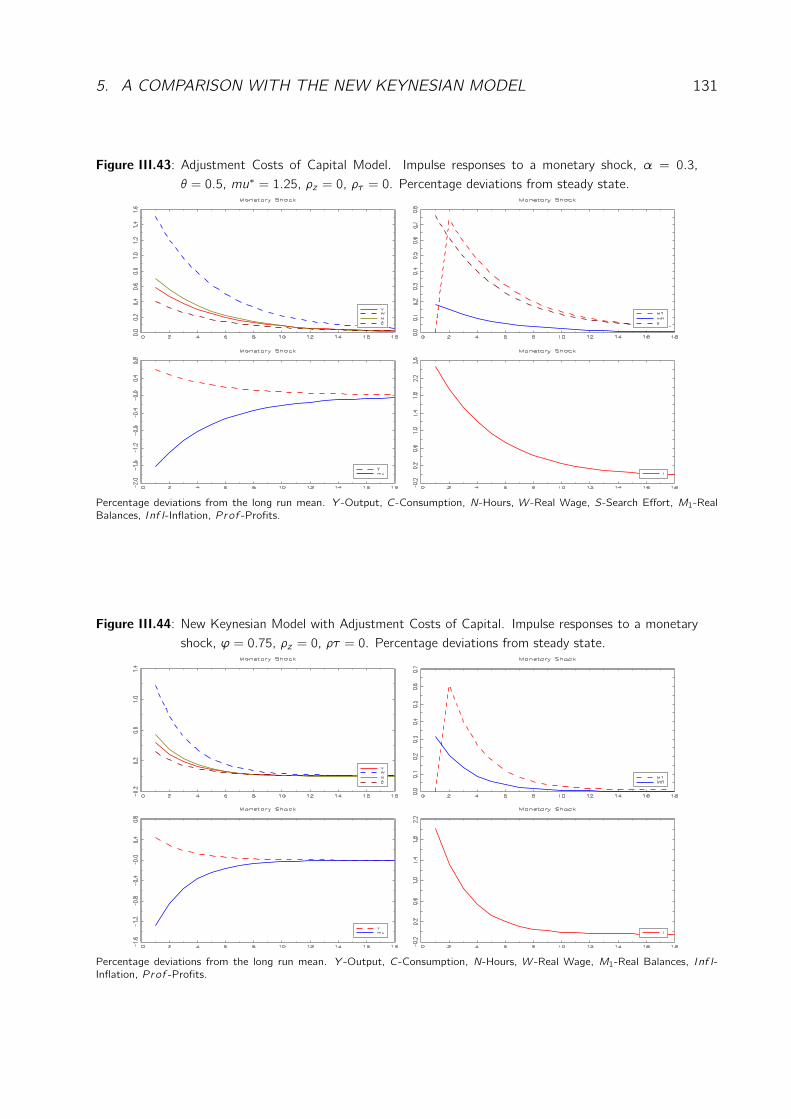
5. A COMPARISON WITH THE NEW KEYNESIAN MODEL 131
Figure III.43: Adjustment Costs of Capital Model. Impulse responses to a monetary shock, α = 0.3,θ = 0.5, mu∗ = 1.25, ρz = 0, ρτ = 0. Percentage deviations from steady state.
Percentage deviations from the long run mean. Y -Output, C-Consumption, N-Hours, W -Real Wage, S-Search Effort, M1-RealBalances, Inf l-Inflation, P rof -Profits.
Figure III.44: New Keynesian Model with Adjustment Costs of Capital. Impulse responses to a monetaryshock, ϕ = 0.75, ρz = 0, ρτ = 0. Percentage deviations from steady state.
Percentage deviations from the long run mean. Y -Output, C-Consumption, N-Hours, W -Real Wage, M1-Real Balances, Inf l-Inflation, P rof -Profits.
132 CHAPTER 3. INFLATION AVERSION AND MONETARY POLICY
6 Supplement to Section 3. Understanding Key Features of theModel
In this section I investigate the role and the importance of the new building blocks in the
following way. First, I look at each of them separately and provide detailed interpretation of
the underlying economic mechanisms. Then I analyze the interaction between the various
assumptions by starting with a very simple model including neither market share competition
nor any form of search activity and then stepwise extending it by introducing new building
blocks, one at a time.
6.1 Only Search Activity
Search Activity Depends Only on Current Consumption:
Let us call this version of the model the OCC Model.23 In this version of the model it is
assumed that the market share of an arbitrary firm evolves according to the same difference
equation
xi ,t+1 = exp
((1− Pi ,t
Pt
)· st
)· xi ,t
as in section 3 but now firms take this law of motion as exogenously given and thus, do not
take account of it when deciding on their respective optimal prices. Hence, each firm solves
a purely static optimization problem leading to the purely static rule for optimal pricing given
below. At the same time households do take the dependence between xi ,t+1 and their search
effort st into consideration. It is easily recognized that this version of the model is identical
with a flexible price money-in-utility model in which the utility function is additively separable
with respect to consumption and real balances. Nevertheless, this model provides a simple
framework for highlighting some important economic mechanisms in a tractable way.
The impulse responses to a purely temporary technology shock, with a no serial correlation,
ρz = 0, are displayed in figure III.45.24 All variables except inflation react purely temporary
returning to their long run levels in the period after the shock. The responses of output,
consumption, profits and real wages are positive, whereas that of hours negative. Only the
response of inflation lasts for two periods. There is a sharp decline of the price level on impact
followed by an increase in the next period. To get some intuition about the economic forces
driving these impulse responses, note that after inserting the optimality condition for labor
23OCC-stands for Only Current Consumption.24The corresponding program is ”sim_cm2d8_1a.g” . The model is calibrated in the same way as in section
3.
6. SUPPLEMENT TO SECTION 3. UNDERSTANDING KEY FEATURES OF THEMODEL133
supply into the household’s budget restriction, one gets the following consumption function
on the individual household’s level(c
y+ ηθ − 1θ+s
y
η
1 + α
)Ct = 2
θ − 1θ
ˆ(WtPt
)+1
θDiv t−m
y(πt + mt+1)+
m
ymt , (III.6.1)
where c/y , s/y , and m/y are the steady state values of the consumption-output, search-
output and real balances-output ratios respectively. Divt denotes dividend payments. All
”hat”-variables denote percentage deviations from the respective values at the stationary
equilibrium. The log-linear approximation of the optimality condition with respect to money
demand reads25
χmt+1 =η
1− β Ct − ηβ
1− βEtCt+1 −(β
1− β + 1− χ)Etπt+1. (III.6.2)
In a symmetric equilibrium every firm sets its price according to the rule:
Pt =θ
θ − 1 ·WtZt, (III.6.3)
or equivalently
WtPt=θ − 1θ· Zt .
For a given nominal wage a positive technology shock reduces nominal marginal costs26 mak-
ing it optimal for every individual firm to charge a lower price. As a consequence there is a
tendency for real wages to rise and for inflation to fall. As can be seen from equation (III.6.1),
for given dividend payments Div t and money demand mt+1 both price changes create an in-
centive for the private household to increase her consumption expenditure and hence intensify
search activity. As long as η is greater than cy+ sy· η1+α
, the income effect of higher real wages
on leisure is stronger than the corresponding intratemporal substitution effect between con-
sumption and leisure implying a lower labor supply for any given real wage.27 Since there are
identical households, aggregate labor supply declines, generating additional (further) pressure
on real wages. Note that the negative effect of declining labor supply on consumption was
already substituted out in equation (III.6.1). The static monopolistic competitive structure of
the goods market implies that current profits are directly proportional to output and thus to
aggregate demand. Hence, if each household increases her consumption expenditure as well
25π∗ is set to one for simplicity.26Marginal costs are given by Wt/Zt .27If η is high enough, the decline in the marginal utility of consumption induced by an increase of the real
wage is stronger than the increase of the real wage itself. As a consequence the utility gain of a marginal
increase of hours worked gets lower than the corresponding utility loss, creating an incentive for households to
lower labor supply. The utility gain of an additional unit of labor supply is given by (Wt/Pt) · C−ηt . The utility
loss is given by Nt .
134 CHAPTER 3. INFLATION AVERSION AND MONETARY POLICY
as her switching effort, aggregate profits will rise, forcing individual consumption (labor sup-
ply) to rise (fall) even more. As long as the elasticity of the marginal disutility of hours worked
with respect to hours is positive28 the decline of labor supply is weaker than the increase of
total factor productivity, implying that equilibrium output also becomes higher. Since the
technology shock is purely temporary and there is no capital accumulation, households an-
ticipate lower future labor and dividend income. Therefore, in order to smooth consumption,
each household will try to transfer some part of her additional current period income into the
future. There are two ways she can do that - by investing in bonds or by building up real
balances. Since all households are identical and the aggregate supply of one period riskless
bonds is zero, the desire to smooth consumption by buying bonds results in a sharp increase
of the real interest rate, just sufficient to discourage any incentives to invest in (or sell)
bonds. The accumulation of real balances provides a second channel for intertemporal sub-
stitution of consumption. According to equation (III.6.2) the demand for real money holdings
depends positively on the gap between current and next-period consumption. The larger the
gap, the stronger the incentive to transfer resources from the current into future periods by
increasing money holdings. A higher expected next-period inflation implies higher opportunity
costs of holding money, reducing the demand for real balances. Since each household will try
to increase her money holdings and since the nominal money supply remains unchanged, the
current price level Pt should fall or expected inflation Et(πt+1) should rise, or both. Intuitively
speaking, Pt should fall relative to Et(Pt+1) in order to encourage current and lower desired
next-period consumption, and hence discourage money demand. More formally, a decline
of Pt is needed for real money supply to increase. A rise in Et(πt+1) is needed for money
demand to be weakened. If both effects are sufficiently strong, for given Ct and Et(Ct+1)
the money market will remain (stay) in equilibrium.
But how can expected future inflation Et(πt+1) rise though the money supply Mt+2 and
the level of technology Zt+1 are expected to remain unchanged? To answer this question,
observe that, if households were able to accumulate additional real money holdings in the
current period and at the same time there would be no inflation in t + 1, πt+1 = 0, next-
period consumption demand and switching effort will tend to be higher due to the positive
wealth effect induced by the additionally accumulated real balances. Since aggregate output is
expected to remain constant, there will be a disequilibrium in the goods market, with demand
being higher than supply, putting positive pressure on the price level Pt+1. Households will
expect that the increase of next-period prices Pt+1 will be just sufficient to offset the positive
wealth effect of the additional money holdings and thus restore equilibrium on the goods
market. In other words households will expect next-period inflation to increase by mt+1
28It is equal to one in our case.
6. SUPPLEMENT TO SECTION 3. UNDERSTANDING KEY FEATURES OF THEMODEL135
because
Etˆ(Mt+1Pt+1
)= Et
ˆ(mt+1πt+1
)= 0
implies
mt+1 = Et(πt+1).
It turns out that the increase in expected inflation Et(πt+1) is noth strong enough, to make
it optimal for households to leave their real money holdings in period t unchanged. To see
this note that each household builds expectations about next-period inflation by exploring
the general equilibrium structure of the economy.29 First, she will realize that aggregate
consumption depends only upon total factor productivity,
Ct =2
cy+ syη1+α+ η· Zt , (III.6.4)
and hence, being informed about the stochastic structure of Zt , will expect that the deviation
of aggregate consumption from its steady state level will be zero. Then, after aggregating
the money demand equation (III.6.2) over all households and eliminating expected inflation by
inserting the low of motion for money supply, she will arrive at the following relation between
mt+1, Et(mt+2) and Ct :
mt+1 =η
χ(1− β)(1 + ς) · Ct +ς
1 + ς· Et(mt+2),
where ς is given by (1/χ) · (β/(1−β)+1−χ) which is positive for χ ≥ 1 and β ∈(χ−1χ, 1
).
By solving this equation forward the household will arrive at
mt+1 =η
χ(1− β)(1 + ς) · Ct .
By inserting this result into the low of motion for money supply and taking into account that
Et(Ct+1) = 0 and mt = 0 she will conclude that
Et(mt+2) = 0
and hence
Et(πt+1) =η
χ(1− β)(1 + ς) · Ct .
Inserting this result into the optimality condition for money demand and then aggregating
over all households implies:
mt+1 =η
χ(1− β)(1 + ς) · Ct =
=2η(
cy+ sy· η1+α+ η
)χ(1− β)(1 + ς)
︸ ︷︷ ︸o1
·Zt .
29It is assumed that all agents have rational expectations.
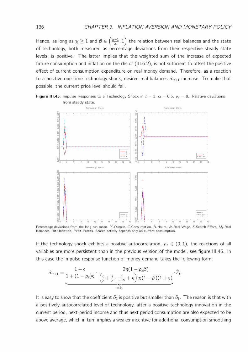
136 CHAPTER 3. INFLATION AVERSION AND MONETARY POLICY
Hence, as long as χ ≥ 1 and β ∈(χ−1χ, 1
)the relation between real balances and the state
of technology, both measured as percentage deviations from their respective steady state
levels, is positive. The latter implies that the weighted sum of the increase of expected
future consumption and inflation on the rhs of (III.6.2), is not sufficient to offset the positive
effect of current consumption expenditure on real money demand. Therefore, as a reaction
to a positive one-time technology shock, desired real balances mt+1 increase. To make that
possible, the current price level should fall.
Figure III.45: Impulse Responses to a Technology Shock in t = 3, α = 0.5, ρz = 0. Relative deviationsfrom steady state.
Percentage deviations from the long run mean. Y -Output, C-Consumption, N-Hours, W -Real Wage, S-Search Effort, M1-RealBalances, Inf l-Inflation, P rof -Profits. Search activity depends only on current consumption.
If the technology shock exhibits a positive autocorrelation, ρz ∈ (0, 1), the reactions of all
variables are more persistent than in the previous version of the model, see figure III.46. In
this case the impulse response function of money demand takes the following form:
mt+1 =1 + ς
1 + (1− ρz)ς ·2η(1− ρzβ)(
cy+ sy· η1+α+ η
)χ(1− β)(1 + ς)
︸ ︷︷ ︸:=o2
·Zt .
It is easy to show that the coefficient o2 is positive but smaller than o1. The reason is that with
a positively autocorrelated level of technology, after a positive technology innovation in the
current period, next-period income and thus next period consumption are also expected to be
above average, which in turn implies a weaker incentive for additional consumption smoothing
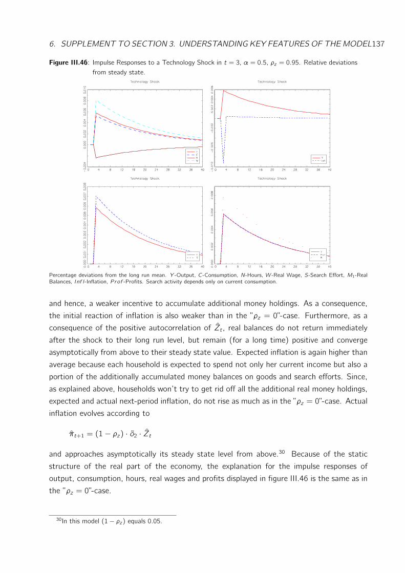
6. SUPPLEMENT TO SECTION 3. UNDERSTANDING KEY FEATURES OF THEMODEL137
Figure III.46: Impulse Responses to a Technology Shock in t = 3, α = 0.5, ρz = 0.95. Relative deviationsfrom steady state.
Percentage deviations from the long run mean. Y -Output, C-Consumption, N-Hours, W -Real Wage, S-Search Effort, M1-RealBalances, Inf l-Inflation, P rof -Profits. Search activity depends only on current consumption.
and hence, a weaker incentive to accumulate additional money holdings. As a consequence,
the initial reaction of inflation is also weaker than in the ”ρz = 0”-case. Furthermore, as a
consequence of the positive autocorrelation of Zt , real balances do not return immediately
after the shock to their long run level, but remain (for a long time) positive and converge
asymptotically from above to their steady state value. Expected inflation is again higher than
average because each household is expected to spend not only her current income but also a
portion of the additionally accumulated money balances on goods and search efforts. Since,
as explained above, households won’t try to get rid off all the additional real money holdings,
expected and actual next-period inflation, do not rise as much as in the ”ρz = 0”-case. Actual
inflation evolves according to
πt+1 = (1− ρz) · o2 · Zt
and approaches asymptotically its steady state level from above.30 Because of the static
structure of the real part of the economy, the explanation for the impulse responses of
output, consumption, hours, real wages and profits displayed in figure III.46 is the same as in
the ”ρz = 0”-case.
30In this model (1− ρz) equals 0.05.
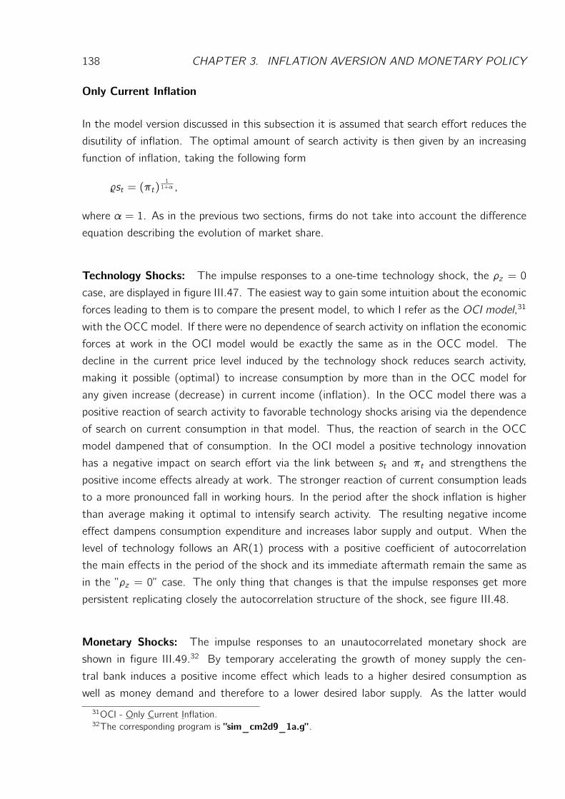
138 CHAPTER 3. INFLATION AVERSION AND MONETARY POLICY
Only Current Inflation
In the model version discussed in this subsection it is assumed that search effort reduces the
disutility of inflation. The optimal amount of search activity is then given by an increasing
function of inflation, taking the following form
%st = (πt)11+α ,
where α = 1. As in the previous two sections, firms do not take into account the difference
equation describing the evolution of market share.
Technology Shocks: The impulse responses to a one-time technology shock, the ρz = 0
case, are displayed in figure III.47. The easiest way to gain some intuition about the economic
forces leading to them is to compare the present model, to which I refer as the OCI model,31
with the OCC model. If there were no dependence of search activity on inflation the economic
forces at work in the OCI model would be exactly the same as in the OCC model. The
decline in the current price level induced by the technology shock reduces search activity,
making it possible (optimal) to increase consumption by more than in the OCC model for
any given increase (decrease) in current income (inflation). In the OCC model there was a
positive reaction of search activity to favorable technology shocks arising via the dependence
of search on current consumption in that model. Thus, the reaction of search in the OCC
model dampened that of consumption. In the OCI model a positive technology innovation
has a negative impact on search effort via the link between st and πt and strengthens the
positive income effects already at work. The stronger reaction of current consumption leads
to a more pronounced fall in working hours. In the period after the shock inflation is higher
than average making it optimal to intensify search activity. The resulting negative income
effect dampens consumption expenditure and increases labor supply and output. When the
level of technology follows an AR(1) process with a positive coefficient of autocorrelation
the main effects in the period of the shock and its immediate aftermath remain the same as
in the ”ρz = 0” case. The only thing that changes is that the impulse responses get more
persistent replicating closely the autocorrelation structure of the shock, see figure III.48.
Monetary Shocks: The impulse responses to an unautocorrelated monetary shock are
shown in figure III.49.32 By temporary accelerating the growth of money supply the cen-
tral bank induces a positive income effect which leads to a higher desired consumption as
well as money demand and therefore to a lower desired labor supply. As the latter would
31OCI - Only Current Inflation.32The corresponding program is ”sim_cm2d9_1a.g” .
6. SUPPLEMENT TO SECTION 3. UNDERSTANDING KEY FEATURES OF THEMODEL139
Figure III.47: Impulse Responses to a Technology Shock in t = 3, α = 0.8, ρz = 0. Relative deviationsfrom steady state.
Y -Output, C-Consumption, N-Hours, W -Real Wage, S-Search Effort, M1-Real Balances, Inf l-Inflation, P rof -Profits. Searchactivity depends only on current inflation.
have a negative effect on aggregate output and thus lead to a disequilibrium on the goods
market, the price level rises. The price increase induces a negative wealth effect on current
consumption by lowering the real value of money holdings. At the same time, for any given
expected next period inflation, it discourages current in favor of future consumption and so
lowers the demand for real balances. In the OCI model there is also a further transmission
channel by which monetary policy can influence private agents’ behavior: The increase in
current inflation makes it optimal for households to allocate a larger part of their income
to search effort. To achieve that, they must lower consumption demand. The higher the
elasticity of search activity st with respect to current inflation, the larger the desired rise in
st for any given increase in inflation and thus the lower the fraction of income that can be
allocated to consumption. The fall in consumption has a positive effect on aggregate labor
supply and production. Note that the whole additional as well as part of average output are
absorbed by the positive deviation of search from its steady state level. To understand the
behavior of real money holdings observe that for given expected next-period inflation and
consumption a decline in current consumption expenditure weakens the incentive to transfer
additional resources from the present into the future by investing in money. So the demand
for money tends to fall leading to a negative wealth effect on consumption in the next period.
Therefore, for a given level of production next period inflation will tend to fall. Households
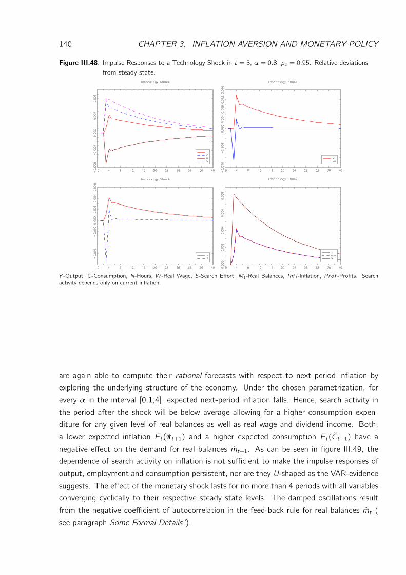
140 CHAPTER 3. INFLATION AVERSION AND MONETARY POLICY
Figure III.48: Impulse Responses to a Technology Shock in t = 3, α = 0.8, ρz = 0.95. Relative deviationsfrom steady state.
Y -Output, C-Consumption, N-Hours, W -Real Wage, S-Search Effort, M1-Real Balances, Inf l-Inflation, P rof -Profits. Searchactivity depends only on current inflation.
are again able to compute their rational forecasts with respect to next period inflation by
exploring the underlying structure of the economy. Under the chosen parametrization, for
every α in the interval [0.1;4], expected next-period inflation falls. Hence, search activity in
the period after the shock will be below average allowing for a higher consumption expen-
diture for any given level of real balances as well as real wage and dividend income. Both,
a lower expected inflation Et(πt+1) and a higher expected consumption Et(Ct+1) have a
negative effect on the demand for real balances mt+1. As can be seen in figure III.49, the
dependence of search activity on inflation is not sufficient to make the impulse responses of
output, employment and consumption persistent, nor are they U-shaped as the VAR-evidence
suggests. The effect of the monetary shock lasts for no more than 4 periods with all variables
converging cyclically to their respective steady state levels. The damped oscillations result
from the negative coefficient of autocorrelation in the feed-back rule for real balances mt (
see paragraph Some Formal Details”).
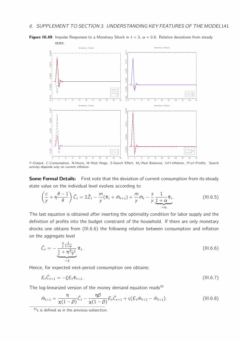
6. SUPPLEMENT TO SECTION 3. UNDERSTANDING KEY FEATURES OF THEMODEL141
Figure III.49: Impulse Responses to a Monetary Shock in t = 3, α = 0.8. Relative deviations from steadystate.
Y -Output, C-Consumption, N-Hours, W -Real Wage, S-Search Effort, M1-Real Balances, Inf l-Inflation, P rof -Profits. Searchactivity depends only on current inflation.
Some Formal Details: First note that the deviation of current consumption from its steady
state value on the individual level evolves according to(c
y+ ηθ − 1θ
)Ct = 2Zt − m
y(πt + mt+1) +
m
ymt − s
y
1
1 + απt
︸ ︷︷ ︸:=st
. (III.6.5)
The last equation is obtained after inserting the optimality condition for labor supply and the
definition of profits into the budget constraint of the household. If there are only monetary
shocks one obtains from (III.6.6) the following relation between consumption and inflation
on the aggregate level
Ct = −sy11+α
cy+ η θ−1
θ︸ ︷︷ ︸:=ξ
πt . (III.6.6)
Hence, for expected next-period consumption one obtains:
EtCt+1 = −ξEt πt+1. (III.6.7)
The log-linearized version of the money demand equation reads33
mt+1 =η
χ(1− β) Ct −ηβ
χ(1− β)EtCt+1 + ς(Etmt+2 − mt+1). (III.6.8)
33ς is defined as in the previous subsection.
142 CHAPTER 3. INFLATION AVERSION AND MONETARY POLICY
Inserting of (III.6.6) and (III.6.7) as well as the law of motion of money supply
mt+1 = mt − πt + µt
into (III.6.8) yields:
mt+1 =ς
1 + ςEtmt+2 − η
χ(1− β) ·ξ
1 + ς︸ ︷︷ ︸ξ1
πt +ηβ
χ(1− β) ·ξ
1 + ς︸ ︷︷ ︸ξ2
Etπt+1.
Substituting πt and Etπt+1 away by the money supply equation and rearranging yields:
(1− β)(χ(1 + ς) + ηξ)mt+1 = (ςχ(1− β)− ηβξ)Etmt+2 − ηξmt − ηξµt . (III.6.9)
For
1
1 + α<(β − (χ− 1)(1− β))( c
y+ η θ−1
θ)
ηβ sy
ςχ(1−β)−ηβξ is positive and smaller than (1−β)(χ(1+ ς)+ηξ). For the parametrization
chosen the latter inequality implies 11+α< 2.15, which is always the case for α > 0. The
easiest and at the same time the most general way to solve equation (III.6.9) is by using the
method of undetermined coefficients. To start the procedure one can guess a solution of the
form
mt+1 = amt + bµt .
Please note that this so called autoregressive solution is by no means the only one for equa-
tion (III.6.9). There is also a solution of the form mt+1 = cµt and also many others. The
autoregressive solution proposed here belongs to the set of solutions consistent with the
assumption that mt is stationary (that the intertemporal budget restriction of the represen-
tative household holds as an equation). Inserting the last equation into (III.6.9) and equating
coefficients yields:
a1,2 =(1− β)(χ(1 + ς) + ηξ)±
√(1− β)2(χ(1 + ς) + ηξ)2 + 4ηξ(ςχ(1− β)− ηβξ)2(ςχ(1− β)− ηβξ) .
Only the solution
a =(1− β)(χ(1 + ς) + ηξ)−
√(1− β)2(χ(1 + ς) + ηξ)2 + 4ηξ(ςχ(1− β)− ηβξ)2(ςχ(1− β)− ηβξ) < 0
is consistent with the assumption that mt is stationary. The parametrization used in this
model implies a ∈ [−0.827, 0). For that values of a, b is negative:
b = − ηξ
(1− β)(χ(1 + ς) + ηξ) + |a|(ςχ(1− β)− ηβξ) < 0.

6. SUPPLEMENT TO SECTION 3. UNDERSTANDING KEY FEATURES OF THEMODEL143
Hence, the initial response of real money holdings to a positive monetary disturbance µt > 0
is given by
mt+1 = bµt < 0,
where mt = 0 was taken into account. According to the law of motion for money supply,
inflation in t + 1 will be given by
πt+1 = mt+1 − mt+2 + µt+1.
Inserting the obtained feed-back rule for mt into this equation and taking expectations as of
period t yields
Et πt+1 = (1− a) · b︸ ︷︷ ︸<0
·µt ,
since 1− a > 0 and b < 0.
144 CHAPTER 3. INFLATION AVERSION AND MONETARY POLICY
6.2 Only Market Share Competition
This version of the model, to which I refer as the OMSC model, is identical to that of
Phelps and Winter (1970). There is only dynamic market share competition between the
monopolistically competitive firms as described in section 3. As explained in that section, an
unexpected increase in total factor productivity rises current demand for every individual good
creating an incentive for firms to rise their prices. At the same time however, the stochastic
discount factor rises making future revenues and thus the investment in market share by
lowering current prices more valuable. As I show below, for the parametrization chosen in
this study, the negative effect of the discount factor dominates. Therefore markups fall. The
decline in markups has a positive effect on the real wage. Its percentage deviation from the
steady state can be written as
WtPt= Zt − mut .
Since working hours evolve according to
Nt =WtPt− ηCt ,
the sign of its response depends on the relative strength of the two opposing effects induced
by the technology shock - the increase of the real wage and the increase of consumption.
Together with the equilibrium condition on the goods market the last equation implies
Nt =1− η1 + η
Zt − 1
1 + ηmut . (III.6.1)
The reactions of the variables of interest to a one time productivity disturbance are given
in figure III.50.34 Under the assumption of a short run elasticity of demand equal to one,
D′(1) = 1, markups fall leading to an increase in real wages which turns out to be sufficient
to offset the negative effect of rising consumption on hours. To gain some intuition about
these reactions and to understand why the assumption on D′(1) and η play an important role
in this version of the model, it is instructive to take a look at the feed-back rules for mut and
Nt first.
After some algebraic manipulations one arrives at the following forward-looking difference
equation describing the behavior of the markup:
mut = ϑEtmut+1 − 2ξ(1− ρz)(η − 1)ξ(1− η) + 1 + η Zt , (III.6.2)
where
ξ =g′(1) β
1−βmu∗−1mu∗
1 +D′(1) + g′(1) β1−β
mu∗−1mu∗
34The corresponding program is ”sim_cm2d_11.g” .
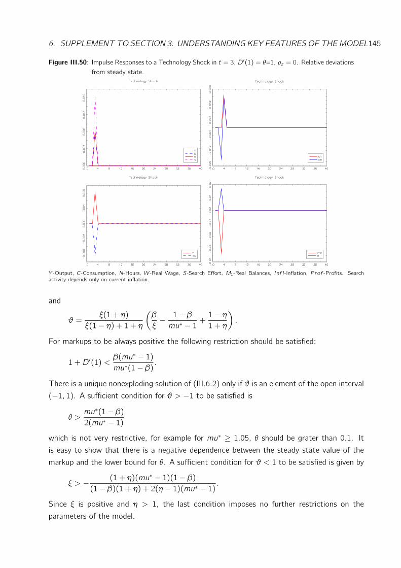
6. SUPPLEMENT TO SECTION 3. UNDERSTANDING KEY FEATURES OF THEMODEL145
Figure III.50: Impulse Responses to a Technology Shock in t = 3, D′(1) = θ=1, ρz = 0. Relative deviationsfrom steady state.
Y -Output, C-Consumption, N-Hours, W -Real Wage, S-Search Effort, M1-Real Balances, Inf l-Inflation, P rof -Profits. Searchactivity depends only on current inflation.
and
ϑ =ξ(1 + η)
ξ(1− η) + 1 + η(β
ξ− 1− βmu∗ − 1 +
1− η1 + η
).
For markups to be always positive the following restriction should be satisfied:
1 +D′(1) <β(mu∗ − 1)mu∗(1− β) .
There is a unique nonexploding solution of (III.6.2) only if ϑ is an element of the open interval
(−1, 1). A sufficient condition for ϑ > −1 to be satisfied is
θ >mu∗(1− β)2(mu∗ − 1)
which is not very restrictive, for example for mu∗ ≥ 1.05, θ should be grater than 0.1. It
is easy to show that there is a negative dependence between the steady state value of the
markup and the lower bound for θ. A sufficient condition for ϑ < 1 to be satisfied is given by
ξ > − (1 + η)(mu∗ − 1)(1− β)(1− β)(1 + η) + 2(η − 1)(mu∗ − 1) .
Since ξ is positive and η > 1, the last condition imposes no further restrictions on the
parameters of the model.
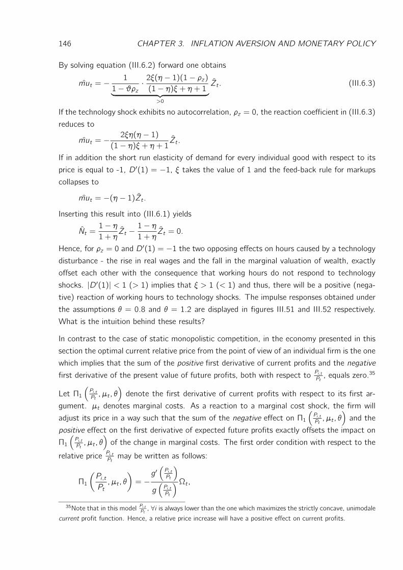
146 CHAPTER 3. INFLATION AVERSION AND MONETARY POLICY
By solving equation (III.6.2) forward one obtains
mut = − 1
1− ϑρz ·2ξ(η − 1)(1− ρz)(1− η)ξ + η + 1︸ ︷︷ ︸>0
Zt . (III.6.3)
If the technology shock exhibits no autocorrelation, ρz = 0, the reaction coefficient in (III.6.3)
reduces to
mut = − 2ξη(η − 1)(1− η)ξ + η + 1Zt .
If in addition the short run elasticity of demand for every individual good with respect to its
price is equal to -1, D′(1) = −1, ξ takes the value of 1 and the feed-back rule for markups
collapses to
mut = −(η − 1)Zt .Inserting this result into (III.6.1) yields
Nt =1− η1 + η
Zt − 1− η1 + η
Zt = 0.
Hence, for ρz = 0 and D′(1) = −1 the two opposing effects on hours caused by a technology
disturbance - the rise in real wages and the fall in the marginal valuation of wealth, exactly
offset each other with the consequence that working hours do not respond to technology
shocks. |D′(1)| < 1 (> 1) implies that ξ > 1 (< 1) and thus, there will be a positive (nega-
tive) reaction of working hours to technology shocks. The impulse responses obtained under
the assumptions θ = 0.8 and θ = 1.2 are displayed in figures III.51 and III.52 respectively.
What is the intuition behind these results?
In contrast to the case of static monopolistic competition, in the economy presented in this
section the optimal current relative price from the point of view of an individual firm is the one
which implies that the sum of the positive first derivative of current profits and the negative
first derivative of the present value of future profits, both with respect to Pi ,tPt, equals zero.35
Let Π1(Pi ,tPt, µt , θ
)denote the first derivative of current profits with respect to its first ar-
gument. µt denotes marginal costs. As a reaction to a marginal cost shock, the firm will
adjust its price in a way such that the sum of the negative effect on Π1(Pi ,tPt, µt , θ
)and the
positive effect on the first derivative of expected future profits exactly offsets the impact on
Π1
(Pi ,tPt, µt , θ
)of the change in marginal costs. The first order condition with respect to the
relative price Pi ,tPt
may be written as follows:
Π1
(Pi ,tPt, µt , θ
)= −g′
(Pi ,tPt
)
g(Pi ,tPt
)Ωt ,
35Note that in this model Pi ,tPt , ∀i is always lower than the one which maximizes the strictly concave, unimodale
current profit function. Hence, a relative price increase will have a positive effect on current profits.
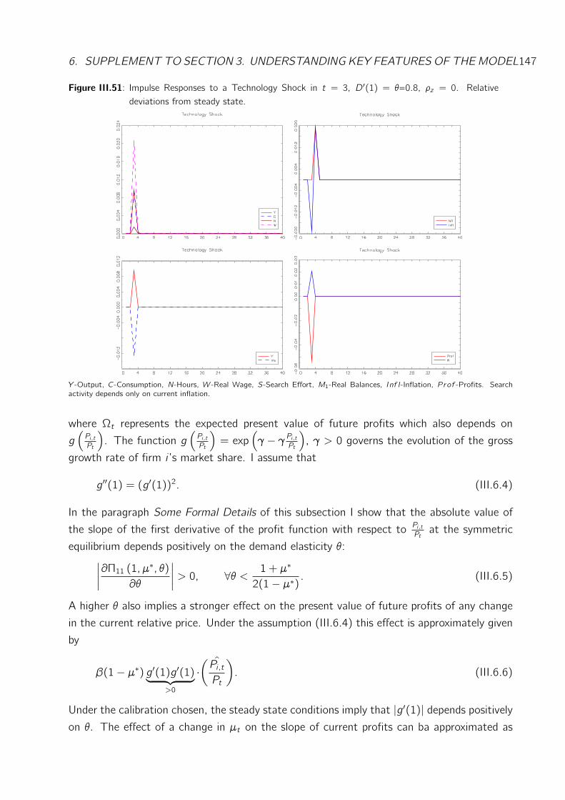
6. SUPPLEMENT TO SECTION 3. UNDERSTANDING KEY FEATURES OF THEMODEL147
Figure III.51: Impulse Responses to a Technology Shock in t = 3, D′(1) = θ=0.8, ρz = 0. Relativedeviations from steady state.
Y -Output, C-Consumption, N-Hours, W -Real Wage, S-Search Effort, M1-Real Balances, Inf l-Inflation, P rof -Profits. Searchactivity depends only on current inflation.
where Ωt represents the expected present value of future profits which also depends on
g(Pi ,tPt
). The function g
(Pi ,tPt
)= exp
(γ − γ Pi ,t
Pt
), γ > 0 governs the evolution of the gross
growth rate of firm i ’s market share. I assume that
g′′(1) = (g′(1))2. (III.6.4)
In the paragraph Some Formal Details of this subsection I show that the absolute value of
the slope of the first derivative of the profit function with respect to Pi ,tPt
at the symmetric
equilibrium depends positively on the demand elasticity θ:∣∣∣∣∂Π11 (1, µ
∗, θ)∂θ
∣∣∣∣ > 0, ∀θ < 1 + µ∗
2(1− µ∗) . (III.6.5)
A higher θ also implies a stronger effect on the present value of future profits of any change
in the current relative price. Under the assumption (III.6.4) this effect is approximately given
by
β(1− µ∗) g′(1)g′(1)︸ ︷︷ ︸>0
·ˆ(Pi ,tPt
). (III.6.6)
Under the calibration chosen, the steady state conditions imply that |g′(1)| depends positivelyon θ. The effect of a change in µt on the slope of current profits can ba approximated as
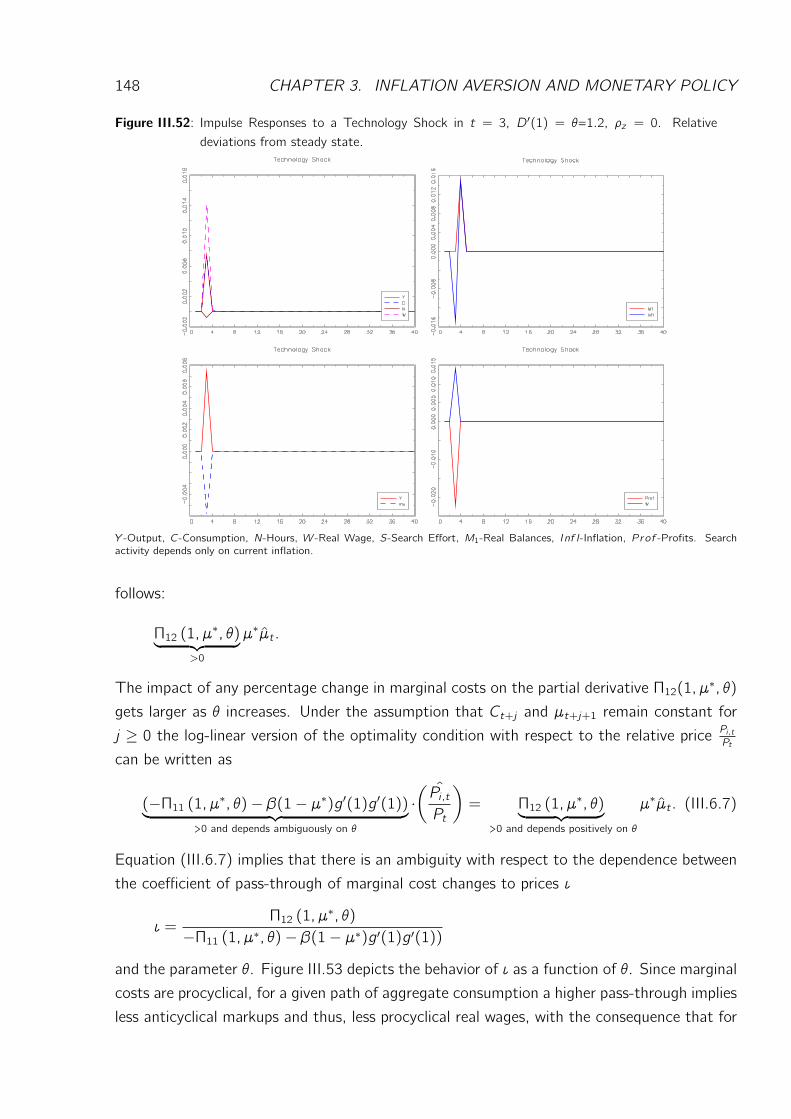
148 CHAPTER 3. INFLATION AVERSION AND MONETARY POLICY
Figure III.52: Impulse Responses to a Technology Shock in t = 3, D′(1) = θ=1.2, ρz = 0. Relativedeviations from steady state.
Y -Output, C-Consumption, N-Hours, W -Real Wage, S-Search Effort, M1-Real Balances, Inf l-Inflation, P rof -Profits. Searchactivity depends only on current inflation.
follows:
Π12 (1, µ∗, θ)︸ ︷︷ ︸
>0
µ∗µt .
The impact of any percentage change in marginal costs on the partial derivative Π12(1, µ∗, θ)
gets larger as θ increases. Under the assumption that Ct+j and µt+j+1 remain constant for
j ≥ 0 the log-linear version of the optimality condition with respect to the relative price Pi ,tPt
can be written as
(−Π11 (1, µ∗, θ)− β(1− µ∗)g′(1)g′(1))︸ ︷︷ ︸>0 and depends ambiguously on θ
·ˆ(Pi ,tPt
)= Π12 (1, µ
∗, θ)︸ ︷︷ ︸>0 and depends positively on θ
µ∗µt . (III.6.7)
Equation (III.6.7) implies that there is an ambiguity with respect to the dependence between
the coefficient of pass-through of marginal cost changes to prices ι
ι =Π12 (1, µ
∗, θ)−Π11 (1, µ∗, θ)− β(1− µ∗)g′(1)g′(1))
and the parameter θ. Figure III.53 depicts the behavior of ι as a function of θ. Since marginal
costs are procyclical, for a given path of aggregate consumption a higher pass-through implies
less anticyclical markups and thus, less procyclical real wages, with the consequence that for
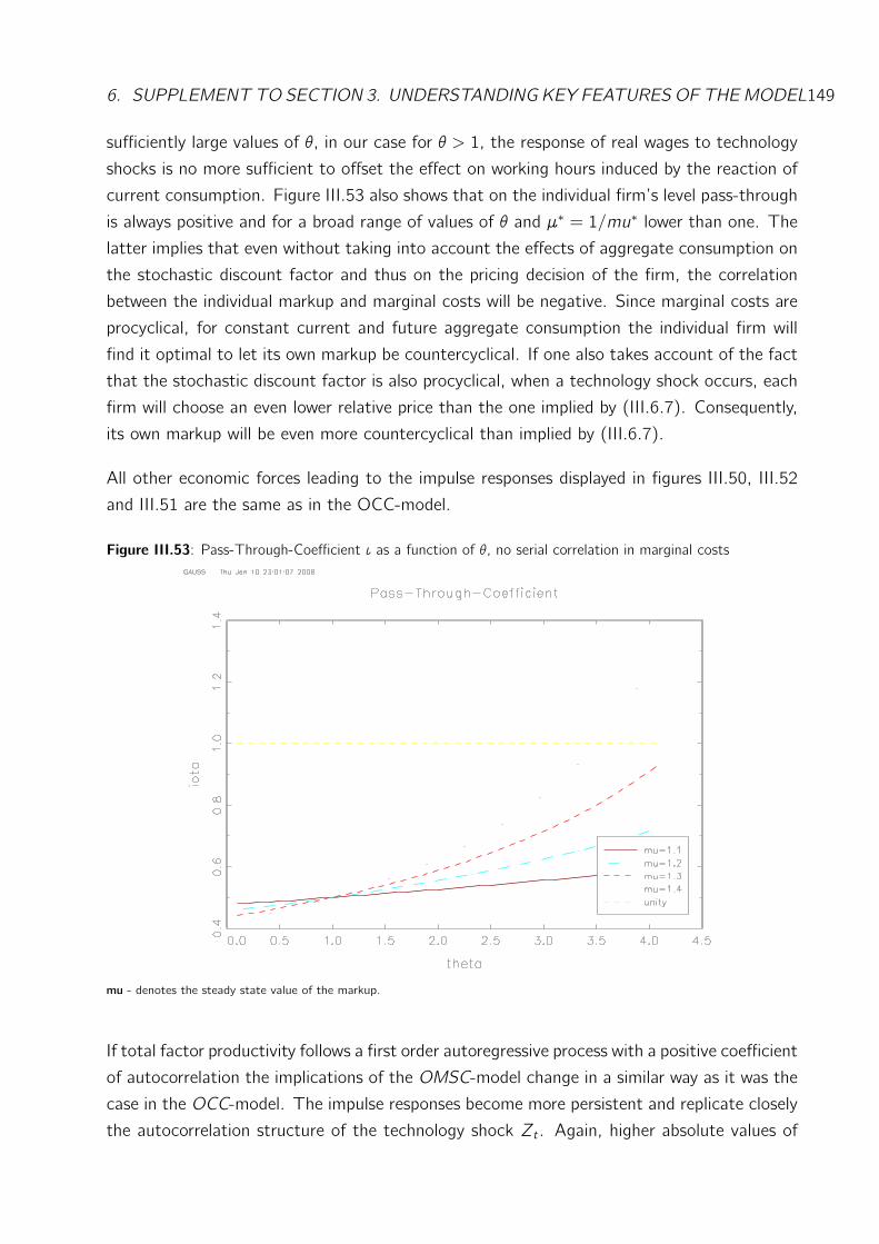
6. SUPPLEMENT TO SECTION 3. UNDERSTANDING KEY FEATURES OF THEMODEL149
sufficiently large values of θ, in our case for θ > 1, the response of real wages to technology
shocks is no more sufficient to offset the effect on working hours induced by the reaction of
current consumption. Figure III.53 also shows that on the individual firm’s level pass-through
is always positive and for a broad range of values of θ and µ∗ = 1/mu∗ lower than one. The
latter implies that even without taking into account the effects of aggregate consumption on
the stochastic discount factor and thus on the pricing decision of the firm, the correlation
between the individual markup and marginal costs will be negative. Since marginal costs are
procyclical, for constant current and future aggregate consumption the individual firm will
find it optimal to let its own markup be countercyclical. If one also takes account of the fact
that the stochastic discount factor is also procyclical, when a technology shock occurs, each
firm will choose an even lower relative price than the one implied by (III.6.7). Consequently,
its own markup will be even more countercyclical than implied by (III.6.7).
All other economic forces leading to the impulse responses displayed in figures III.50, III.52
and III.51 are the same as in the OCC-model.
Figure III.53: Pass-Through-Coefficient ι as a function of θ, no serial correlation in marginal costs
mu - denotes the steady state value of the markup.
If total factor productivity follows a first order autoregressive process with a positive coefficient
of autocorrelation the implications of the OMSC-model change in a similar way as it was the
case in the OCC-model. The impulse responses become more persistent and replicate closely
the autocorrelation structure of the technology shock Zt . Again, higher absolute values of
150 CHAPTER 3. INFLATION AVERSION AND MONETARY POLICY
the demand elasticity θ imply less countercyclical markups and thus less procyclical real wages
and working hours.
Some Formal Details: It is assumed that the consumption bundle is given by the Dixit-
Stiglitz-aggregator with a constant elasticity of substitution. The latter implies a constant
elasticity of demand for every individual good with respect to its own price. I denote this
elasticity by θ = −D′(1). The first order condition of firm i can be written as the following
dynamic system:
(Pi ,tPt
)−θ− θ
(Pi ,tPt− µt
)(Pi ,tPt
)−θ−1=−g′
(Pi ,tPt
)
g(Pi ,tPt
) ΩtCt,
Ωt = Et
(βΛt+1Λt
(Pi ,t+1Pt+1
− µt+1)(Pi ,t+1Pt+1
)−θg
(Pi ,tPt
)Ct+1
)+ Et
(βΛt+1ΛtΩt+1
),
(III.6.8)
where µt are real marginal costs and Ωt is the expected present value of future profits. Using
this two equations one may derive the steady state value of g′(1) as a function of β, θ and
µ∗:
g′(1) =(1− β)(θ(1− µ∗)− 1)
β(1− µ∗) .
It is easily seen that g′(1) increases as θ becomes larger. The slope of the first derivative
with respect to Pi ,t/Pt of current profits at the symmetric equilibrium in the steady state is
given by
Π11 (1, µ∗, θ) = θ2(1− µ∗)− θ(1 + µ∗)
which is negative for
θ <1 + µ∗
1− µ∗ .
The fraction (1+µ∗)/(1−µ∗) is equal to 6; 7.66; 11; 21 for µ∗ = 1.4−1; 1.3−1; 1.2−1; 1.1−1.The first derivative of Π11 (1, µ∗, θ) with respect to θ is given by:
dΠ11 (1, µ∗, θ)
dθ= 2θ(1− µ∗)− (1 + µ∗).
It is negative for
θ <1 + µ∗
2(1− µ∗) .

6. SUPPLEMENT TO SECTION 3. UNDERSTANDING KEY FEATURES OF THEMODEL151
In the OMSC-model pass-through of marginal costs to prices is approximately given by the
coefficient ι in the equation
ˆ(Pi ,tPt
)=
Π12 (1, µ∗, θ)
−Π11 (1, µ∗, θ)− β(1− µ∗)g′(1)g′(1)︸ ︷︷ ︸:=ι
µt ,
where
ι =θµ∗
−θ2(1− µ∗) + θ(1 + µ∗) + (1−β)2(θ(1−µ∗)−1)2β(1−µ∗)
.
The denominator of the first derivative of ι with respect to θ is positive. The numerator ofdιdθ
is given by
(1− (1− β)2)θ2µ∗(1− µ∗)2 + µ∗(1− β)β(1− µ∗) ,
which is positive for all
θ > 0.
Hence, the results provided so far in this subsection can be summarized as follows: A sufficient
condition for the pass-through coefficient ι to depend positively on θ is given by
θ ∈(0,1 + µ∗
1− µ∗).
In addition, there is a positive dependence between the pass-through coefficient ι and θ. If θ
is an element of the open interval
θ ∈(1 + µ∗
2(1− µ∗) ,1 + µ∗
1− µ∗)
ι grows as θ increases and there is no ambiguity with respect to the influence of θ on the
sum
−Π11 (1, µ∗, θ)− β(1− µ∗)g′(1)g′(1).
If marginal costs follow a first order autoregressive process with a positive coefficient of
autocorrelation ρµ > 0 the forward difference equation describing the dependence between
firm i ’s relative price and marginal costs changes to
Pi ,tPt= φ1Et
(Pi ,tPt
)+ φ2µt , (III.6.9)
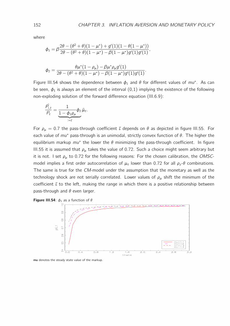
152 CHAPTER 3. INFLATION AVERSION AND MONETARY POLICY
where
φ1 = β2θ − (θ2 + θ)(1− µ∗) + g′(1)(1− θ(1− µ∗))2θ − (θ2 + θ)(1− µ∗)− β(1− µ∗)g′(1)g′(1) ,
φ2 =θµ∗(1− ρµ)− βµ∗ρµg′(1)
2θ − (θ2 + θ)(1− µ∗)− β(1− µ∗)g′(1)g′(1) .
Figure III.54 shows the dependence between φ1 and θ for different values of mu∗. As can
be seen, φ1 is always an element of the interval (0,1) implying the existence of the following
non-exploding solution of the forward difference equation (III.6.9):
Pi ,tPt=
1
1− φ1ρµφ2︸ ︷︷ ︸:=ι
µt .
For ρµ = 0.7 the pass-through coefficient ι depends on θ as depicted in figure III.55. For
each value of mu∗ pass-through is an unimodal, strictly convex function of θ. The higher the
equilibrium markup mu∗ the lower the θ minimizing the pass-through coefficient. In figure
III.55 it is assumed that ρµ takes the value of 0.72. Such a choice might seem arbitrary but
it is not. I set ρµ to 0.72 for the following reasons: For the chosen calibration, the OMSC-
model implies a first order autocorrelation of µt lower than 0.72 for all ρz -θ combinations.
The same is true for the CM-model under the assumption that the monetary as well as the
technology shock are not serially correlated. Lower values of ρµ shift the minimum of the
coefficient ι to the left, making the range in which there is a positive relationship between
pass-through and θ even larger.
Figure III.54: φ1 as a function of θ
mu denotes the steady state value of the markup.
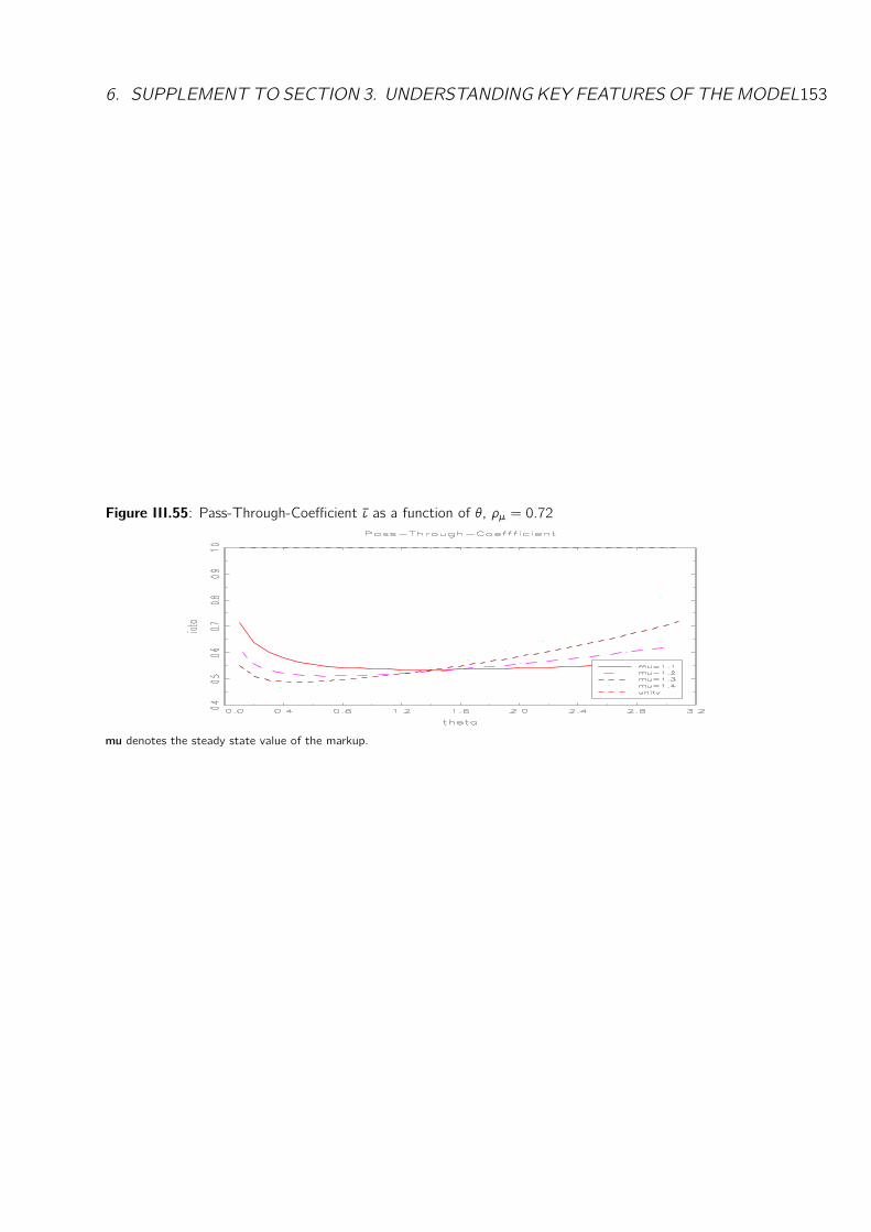
6. SUPPLEMENT TO SECTION 3. UNDERSTANDING KEY FEATURES OF THEMODEL153
Figure III.55: Pass-Through-Coefficient ι as a function of θ, ρµ = 0.72
mu denotes the steady state value of the markup.
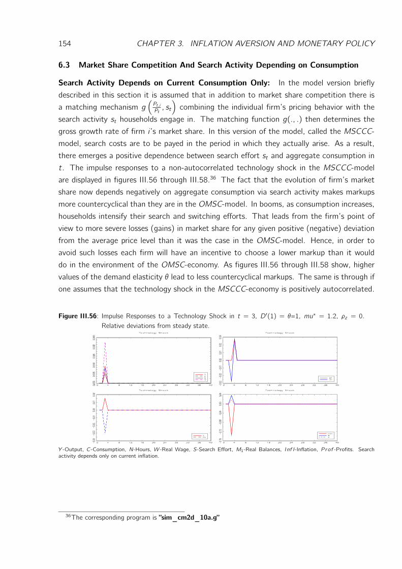
154 CHAPTER 3. INFLATION AVERSION AND MONETARY POLICY
6.3 Market Share Competition And Search Activity Depending on Consumption
Search Activity Depends on Current Consumption Only: In the model version briefly
described in this section it is assumed that in addition to market share competition there is
a matching mechanism g(Pt,iPt, st
)combining the individual firm’s pricing behavior with the
search activity st households engage in. The matching function g(., .) then determines the
gross growth rate of firm i ’s market share. In this version of the model, called the MSCCC-
model, search costs are to be payed in the period in which they actually arise. As a result,
there emerges a positive dependence between search effort st and aggregate consumption in
t. The impulse responses to a non-autocorrelated technology shock in the MSCCC-model
are displayed in figures III.56 through III.58.36 The fact that the evolution of firm’s market
share now depends negatively on aggregate consumption via search activity makes markups
more countercyclical than they are in the OMSC-model. In booms, as consumption increases,
households intensify their search and switching efforts. That leads from the firm’s point of
view to more severe losses (gains) in market share for any given positive (negative) deviation
from the average price level than it was the case in the OMSC-model. Hence, in order to
avoid such losses each firm will have an incentive to choose a lower markup than it would
do in the environment of the OMSC-economy. As figures III.56 through III.58 show, higher
values of the demand elasticity θ lead to less countercyclical markups. The same is through if
one assumes that the technology shock in the MSCCC-economy is positively autocorrelated.
Figure III.56: Impulse Responses to a Technology Shock in t = 3, D′(1) = θ=1, mu∗ = 1.2, ρz = 0.Relative deviations from steady state.
Y -Output, C-Consumption, N-Hours, W -Real Wage, S-Search Effort, M1-Real Balances, Inf l-Inflation, P rof -Profits. Searchactivity depends only on current inflation.
36The corresponding program is ”sim_cm2d_10a.g”

6. SUPPLEMENT TO SECTION 3. UNDERSTANDING KEY FEATURES OF THEMODEL155
Figure III.57: Impulse Responses to a Technology Shock in t = 3, D′(1) = θ=1.2, mu∗ = 1.2, ρz = 0.Relative deviations from steady state.
Y -Output, C-Consumption, N-Hours, W -Real Wage, S-Search Effort, M1-Real Balances, Inf l-Inflation, P rof -Profits. Searchactivity depends only on current inflation.
Figure III.58: Impulse Responses to a Technology Shock in t = 3, D′(1) = θ=0.8, mu∗ = 1.2, ρz = 0.Relative deviations from steady state.
Y -Output, C-Consumption, N-Hours, W -Real Wage, S-Search Effort, M1-Real Balances, Inf l-Inflation, P rof -Profits. Searchactivity depends only on current inflation.

156 CHAPTER 3. INFLATION AVERSION AND MONETARY POLICY
Chapter 4
GMM Estimation
1 Introduction
In the previous chapter I developed a monetary business cycles model in which he extends the
market share competition mechanism proposed in Phelps and Winter (1970) by introducing
search in the goods market and then combining that structure with the assumption that the
overall rate of inflation generates disutility which can be reduced by engaging in more intense
and thus more expensive search activities. The direct dependence of the utility function on
inflation was interpreted as inflation aversion. That dependence is the crucial building block
of his theory. The model is able to generate endogenous countercyclical markups which react
negatively to monetary as well as technology shocks, and endogenous sluggishness in nominal
prices. Furthermore, for a fairly broad range of parameter values the intrinsic mechanisms
of the model are strong enough to imply a substantial degree of persistence in the reactions
to exogenous disturbances, even if the latter follow pure White Noise processes. Thus, his
model provides an endogenous explanation of the observed persistence and autocorrelation
in actual business cycles.
A major shortcoming of the analysis in the previous chapter is the absence of any empirical
estimates with respect to several crucial components of his model: Due to the fact that
search efforts in the goods market are not directly observable there is no evidence about their
cyclical properties as well as with regard to the elasticity of the utility function with respect to
search −α. For that reason I performed a sensitivity analysis with respect to that parameter.
I concluded that lower values of α lead to stronger and more persistent responses of the
major aggregates to serially uncorrelated monetary and technology shocks. But wouldn’t it
be nice to know whether the data support the structure of such an ”exotic” model or not?
Wouldn’t it be nice to know if α is positive at all and what is the empirically relevant range
of that parameter?
157
158 CHAPTER 4. GMM ESTIMATION
The purpose of the current chapter is to provide some empirical evidence supporting or
rejecting the model of the previous chapter as well as to shed light on the relevant range of one
of its most important parameters, α. The version of the model including capital accumulation,
to which I refer as the Inflation Aversion model, is reduced to a set of equations involving
only observable variables. The sample moment restrictions derived from these equations are
used to estimate a set of parameters by the General Method of Moments (GMM). The main
are that the data do not reject the general structure of the Inflation Aversion model and
do not reject the assumption that α lies in the interval (0, 1.5). The GMM estimate of α
is then used to complete the calibration of the model with adjustment costs of capital. Its
second moments, computed under different assumptions on the autocorrelation structure of
the exogenous processes, are then confronted with their empirical counterparts. The model
is able to account for several important features of the observable business cycles pattern
in the U.S. economy. Furthermore, even without any serial correlation in the exogenous
variables, the model explains a substantial part of the observed autocorrelation of the main
macroeconomic aggregates.
The paper is organized as follows. Section 2 is devoted to the construction of the data set
and the GMM estimation. Section 3 provides a comparison between the second moments of
the data and that implied by the model. Section 5 concludes.
2 GMM-Estimation
2.1 Data
The model economy presented in the previous chapter is very abstract and does not take
an explicit account of many features of the real world such as net exports, the government
sector or consumer durables. The definitions of many variables in the model economy de-
viate substantially from the definitions used by institutions such as the NIPA or the OECD
which provide data on the main macroeconomic aggregates. Therefore, before turning to
parameter estimation, it should be a major task to transform the available data into mea-
sures and proxies of the variables of interest which are as close as possible to the definitions
underlying the theoretical model. In doing so I follow the strategy recommended by Cooley
and Prescott (1995). The computations presented in the following subsections are done in
the File ”NIPA_UCapitalIncome_nominal.xls” , Sheets ”CapitalStock_real” , ”Unamb-CapInc” and ”AmbCapInc_DEP” .
2. GMM-ESTIMATION 159
Aggregate Output, Capital Stocks, Consumption
The theoretical model contains only one stock of capital used by the private production sector
for generating the whole aggregate output. Each individual good is produced according
to the same constant returns to scale technology as any other. The individual goods are
then assembled to nondurable consumption, search efforts and investment, the latter three
variables being perfect substitutes. The model economy does not distinguish between different
kinds of capital, between private and government sector, and between durable and nondurable
consumption goods. Accordingly, to make the available data consistent with the theory, one
has to assume that the model’s capital stock includes all kinds of capital accumulated in
the actual economy. Similarly, the model’s output should be assumed to include the output
generated by all kinds of capital. Furthermore, a precise distinction between durables- and
nondurables consumption expenditure should be made, with the former considered a part of
aggregate investment. To transform the available data into the desired form, I proceed as
follows. First, following Cooley and Prescott (1995) I assume that the government produces
according to the same constant returns to scale technology as the private sector. Since in
constructing the GNP-series the NIPA only takes account of the flow of services of household
owned residential structures as well as the income generated by the net foreign position1 the
official series should be adjusted by the flow of services of government fixed capital as well
as the stock of consumer durables. These two flows can be approximated as follows:
YK,G,t = (it + υG)KG,t−1, YK,D,t = (it + υD)KD,t−1,
where YK,G,t and YK,D,t denote the income flow generated by government fixed capital and
the stock of durables respectively. υG and υD are the corresponding rates of depreciation.
it is the real rate of return on capital which is assumed to be identical across all kinds of
capital. KG,t−1 and KD,t−1 are the quarterly end-of-period stocks of government fixed assets
and durable goods respectively. According to the above formulas one needs to construct
proxies of the unobservable variables it , υG and υD. KG,t and KD,t are provided by the NIPA.
To be able to find these proxies, one has first to identify several other variables, not directly
provided by the official institutions - the flow of services of the private stock of capital, the
share of private capital in measured GNP and the correctly measured private stock of capital.
Because, as Cooley and Prescott (1995) show, given the share of private capital income in
measured GNP θP one can easily determine the flow of services of private capital YK,P,t :
YK,P,t = θPGNPt .
1These are are the net factor payments to (or from) the rest of the world.
160 CHAPTER 4. GMM ESTIMATION
Then given the private stock of capital KP r iv ,t and its depreciation DP,t one will be able to
compute the real rate of return it :
it =YK,P,t −DP,tKP r iv ,t
.
Next, provided series for government fixed capital KG,t , the stock of consumer durables
KD,t and their respective depreciations DG,t and DD,t , it will be possible to compute the
depreciation rates
υG,t =DG,t
KG,t−1, υD,t =
DD,t
KD,t−1.
The Share of Private Capital Income in Measured GNP and the Real Interest Rate:Cooley and Prescott (1995) show that the income share of private capital in measured GNP
can be computed as
θP,t =UKIt + GNPt − NNPt
GNPt − AIt ,
with
• UKIt - Unambiguous Capital Income = Rental Income+Corporate Profits+Net Interest,2
• AIt - Ambiguous Income =Proprietors Income+Net National Product -National Income,3
• GNPt - Gross National Product as provided by the NIPA,4
• NNPt - Net National Product as provided by the NIPA.5 6 7
2See NIPA-Table 1.12 National Income by Type of Income3See NIPA-Table 1.12 National Income by Type of Income4See NIPA-Table 1.7.5 Relation of Gross Domestic Product,Gross National Product, Net National Product,
National Income, and Personal Income5The difference between GNPt and NNPt equals Consumption of private fixed capital or depreciation.6See NIPA-Table 1.7.5 Relation of Gross Domestic Product,Gross National Product, Net National Product,
National Income, and Personal Income7Cooley and Prescott (1995) assume that the relation between YK,P and measured GNP can be represented
by the equation
YK,P,t = θPGNPt .
At the same time, by using the NIPA-data YK,P,t can be constructed via
YK,P,t = UKIt + θPAIt + GNPt − NNPt ,
where again they assume that the share of the ambiguous component of private income AIt attributable to the
ownership of capital is equal to private capital’s share in measured GNP θP . Equating the rhs of the last two
equations and solving for θP delivers the expression for θK given in the main text.
2. GMM-ESTIMATION 161
I use the nominal quarterly series of these variables provided by the NIPA. The mean of θP,t ,
denoted by θP corresponding to the time period 1964:Q1 - 2007:Q3 equals 0.2922. YK,P,t at
constant prices can then be computed as
YK,P,t = θPGNPt ,
where GNPt denotes Gross National Product at constant prices.
NIPA provides only annual, current price data for the stocks of private fixed capital8 and
durable goods9. Quarterly series for these two stocks are constructed according to the
following interpolation formula:
Ku,y+1,q = Ku,y +
q∑
j=1
φuIu,y+1,j , (IV.2.1)
where
φu =Ku,y+1 −Ku,y∑4
j=1 Iu,y+1,j.
Ku,y and Ku,y ,q denote the real value of the capital stock of type u = P,D,G at the end of
year y and at the end of quarter q of year y respectively. Iu,y ,q denotes real net investment
in the q-th quarter of year y in the stock of u. Iu,y ,q is constructed by subtracting real
depreciation of the u-th type of capital Du,y ,q form real gross investment in the u-th type of
capital Iu,y,q. (IV.2.1) ensures that Ku,y+1,4 = Ku,y+1 for all y .
The data used in these computations are:
• annual end of period stock of private fixed capital at current costs deflated by the yearly
average of the implicit price deflator of gross private fixed investment,10
• annual end of period stock of government fixed capital at current costs deflated by the
yearly average of the implicit price deflator of gross private fixed investment,11
• annual end of period stock of consumer durables at current costs deflated by the yearly
average of the implicit price deflator of consumption durable expenditure,12
8NIPA Table 1.1. Current-Cost Net Stock of Fixed Assets and Consumer Durable Goods9NIPA Table 1.1. Current-Cost Net Stock of Fixed Assets and Consumer Durable Goods
10NIPA, Table 1.1. Current-Cost Net Stock of Fixed Assets and Consumer Durable Goods and Table 1.1.9.
Implicit Price Deflators for Gross Domestic Product11NIPA, Table 1.1. Current-Cost Net Stock of Fixed Assets and Consumer Durable Goods and Table 1.1.9.
Implicit Price Deflators for Gross Domestic Product12NIPA, Table 1.1. Current-Cost Net Stock of Fixed Assets and Consumer Durable Goods and Table 1.1.9.
Implicit Price Deflators for Gross Domestic Product
162 CHAPTER 4. GMM ESTIMATION
• nominal, quarterly gross private fixed investment and depreciation of private fixed capital
(Consumption of fixed private capital) deflated by the implicit price deflator of gross
private fixed investment,13
• nominal, quarterly gross government fixed investment (Federal defense + Federal non-
defense + State and local investment ) and depreciation of government fixed capital
(Consumption of fixed government capital) deflated by the implicit price deflator of
gross private fixed investment,14
• nominal, quarterly consumer durables expenditure and depreciation of consumer durables
deflated by the implicit price deflator of consumer durables expenditure,15
The NIPA provides quarterly real data on the stock of inventories.16 The last component
of the private capital stock, the NIPA also doesn’t take account of when computing the
stock of private capital, is land. The quarterly current price value of Real Estate is provided
by the Federal Funds Accounts. I deflate this series by the implicit price deflator of GDP.
The correct quarterly real stock of private fixed capital KP r iv can then be computed as the
sum of the quarterly real values of Private Fixed Capital (NIPA-Definition) KP , the stock of
Inventories KInv and the value of Land KL:
KP r iv ,t = KP,t + KInv,t + KL,t .
The quarterly real series for Government Fixed Capital KG and the Stock of Consumer
Durables were also approximated according to (IV.2.1). The economy wide stock of capital
Kt is then given by:
Kt = KP r iv ,t +KG,t +KD,t .
Given KP r iv the quarterly real interest rate can be computed as
it =YK,P,t −DP,tKP r iv ,t−1
,
where DP,t denotes depreciation of private fixed capital. I use data over the period 1970:Q1
through 2003:Q3. The resulting mean real rental rate of capital on quarterly basis i equals
0.0109.13NIPA, Table 1.5.5. Gross Domestic Product, Expanded Detail, Table 5.1. Saving and Investment and
Table 1.1.9. Implicit Price Deflators for Gross Domestic Product14NIPA, Table 1.5.5. Gross Domestic Product, Expanded Detail, Table 5.1. Saving and Investment and
Table 1.1.9. Implicit Price Deflators for Gross Domestic Product15NIPA, Table 1.5.5. Gross Domestic Product, Expanded Detail, Table 5.1. Saving and Investment and
Table 1.1.9. Implicit Price Deflators for Gross Domestic Product16NIPA Table 1AU2. Real Manufacturing and Trade Inventories, Seasonally Adjusted, End of Period and
Table 1BU. Real Manufacturing and Trade Inventories, Seasonally Adjusted, End of Period
2. GMM-ESTIMATION 163
Depreciation Rates: To derive the rate of depreciation of the u-th stock in period t, υu,t I
just divide the real quarterly depreciation Du,t through the real quarterly end-of-period value
of the corresponding stock at the end of the previous period Ku,t−1:
υu,t =Du,t
Ku,t−1.
The same data on depreciation is used as in the construction of the capital stocks. The
average rates of depreciation in the period 1970:Q1 - 2003:Q3 of private fixed capital, gov-
ernment fixed capital, durables and Land equal 0.0104, 0.0089, 0.0509 and 0 respectively.17
The overall rate of depreciation, computed as a weighted average of these three values,
equals 0.00708.18
Economy Wide Capital Share, Aggregate Labor Income and Markups: Having approxi-
mated Ku,t , υu,t and it with u = G,D we are in the position to compute the income flow of
services of the government stock of capital YK,G,t as well as the stock of consumer durables
YK,D,t . The correct measure of aggregate production (income) Yco,t is:
Yco,t = GNPt + YK,G,t + YK,D,t .
The economy wide share of capital income in the correctly measured GNP is then readily
computed as the ratio of overall capital income to Yco,t :
θK,t =YK,P,t + YK,G,t + YK,D,tGNPt + YK,G,t + YK,D,t
.
The mean of θK,t for the period 1964:Q1 - 2007:Q3 equals 0.3253.
In an economy characterized by monopolistic competition in the goods market output equals
the sum of labor income, capital income and pure profits:
Yco,t =WtPtNt + RtKt +Πt ,
where Rt denotes the real rental rate of capital. Under the Cobb-Douglas production function
assumed in the model the last equation can be written as
Yco,t =ω
mutYco,t +
1− ωmut
Yco,t +mut − 1mut
Yco,t ,
17Since there is no ”hard” data available allowing the computation or the approximation of the depreciation of
Land and since presumably it depreciates extremely slowly, the depreciation rate of this component of the capital
stock (Land) is assumed to be zero. Nevertheless, there may be reasons for assuming a positive depreciation
rate of Land, e.g. due to pollution, climate change or other forces worsening the environmental quality.18If the stock of Land is excluded, the resulting average depreciation rate equals 0.0129.
164 CHAPTER 4. GMM ESTIMATION
where ω represents the production elasticity of labor and mut the markup of prices over
marginal costs in the goods market. Since in the real world firm’s profits either flow back as
dividends to the owners of the capital stock or are retained and reinvested and hence increase
the value or the amount of capital owned by the firm’s shareholders, here profits are viewed
as part of capital income. Thus, the sum of the rental income of capital 1−ωmutYco,t and pure
profits mut−1mutYco,t equals total capital income and capital’s share θK,t is given by
θK,t =mut − ωmut
.
Given the mean of θK,t and an estimate of the steady state value of the markup mu∗, one
can use the last equation to compute the implied mean of the production elasticity of capital.
The only measure of aggregate labor income consistent with the theoretical model is that
computed by multiplying the correctly measured Gross National Product Yco,t by labor share
θL = 1− θK:
LIt = (1− θK)Yco,t ,
where LIt denotes aggregate labor income. Any other measure constructed by building linear
combinations of several series reported by the NIPA such as different kinds of compensations
of employees, labor income taxes and social contributions would be more time consuming to
compute, would involve a higher approximation error and probably would be less consistent
with the structure of the model.
To approximate the unobservable markup series, I again resort to economic theory. Observe
that the model implies that the marginal productivity of labor and the real wage are related
to each other as follows:
mut =Wt/PtωYco,t/Nt
.
To substitute the ratio on the rhs of the last equation by observable variables, just multiply
the nominator and the denominator by hours worked Nt :
mut =1
ω· LItYco,t
=1
ω(1− θK,t).
Note that varying the mean of the markup mu∗ only shifts the series mut2003:Q3t=1970:Q1 upwards
or downwards but does not affect its cyclical properties.
Consumption and Inflation: The measure of consumption consistent with the theoretical
model equals the sum of private expenditure on nondurable goods CNd,t and services CS,t and
government consumption expenditure CG,t :
Cco,t = CNd,t + CS,t + CG,t .
2. GMM-ESTIMATION 165
The NIPA provides only nominal quarterly data on these variables. Therefore I deflate them by
the respective implicit price deflators of nondurable goods, services and government consump-
tion expenditure. The NIPA publishes separate implicit price deflators for private nondurables
consumption expenditure and services but only a common price deflator for overall govern-
ment expenditure, corresponding to the sum of government consumption and investment.
Accordingly, I approximate the implicit price deflator of government consumption expenditure
PGC,t as follows: First, I assume that the price deflator of government investment is the same
as that of private fixed investment. Then PGC,t can be computed via:
PGC,t =
(PG,t − IG,t
GtPI,t
)Gt
CG,t,nom,
where PG,t and PI,t denote the implicit price deflator of overall government expenditure and
that of private fixed investment respectively. Gt and IG,t denote nominal overall government
expenditure and nominal government investment respectively. CG,t,nom stands for nominal
government consumption.
The price deflator consistent with Cco,t is computed as a weighted average of the individual
price deflators of CNd,t , CS,t and CG,t :19 20
PC,t =CNd,tCco,t
PNd,t +CS,tCco,t
PS,t +CG,tCco,t
PG,t .
Now, the inflation rate associated with aggregate consumption can be computed as:
πt =PC,tPC,t−1
− 1.
19The deflators of CNd,t and CS,t are taken from NIPA’s Table 1.1.9. Implicit Price Deflators for Gross
Domestic Product20The following series were used:
• the nominal quarterly series, taken from NIPA’s Table 1.5.5. Gross Domestic Product, Expanded Detail,
for
– Personal consumption expenditures/Nondurable goods, Personal consumption expendi-
tures/Services,
– Government.../Federal/National defense/Consumption expenditure,
– Government.../Federal/Nondefense/Consumption expenditure,
– Governemnt.../State and Local/Consumption expenditure.
• the implicit price deflators, taken from NIPA’s Table 1.1.9. Implicit Price Deflators for Gross Domestic
Product, for
– Personal consumption expenditures/Nondurable goods,
– Personal consumption expenditures/Services,
– Gross private domestic investment/Fixed investment,
– Government consumption expenditures and gross investment.
166 CHAPTER 4. GMM ESTIMATION
Hours: To construct the series for working hours I use quarterly data on Total Employ-
ment21 and Average Weekly Hours (Private Industry)22. I assume that average weekly hours
are the same across all sectors of the economy. Further, the individual’s time endowment
is normalized to (90 days)*(16 hours) per quarter. The measure of the economy wide time
endowment per quarter consistent with the theoretical model is then given by (90 days)*(16
hours)*population. The population series is provided by the OECD and is also used to trans-
form all the relevant variables into per capita terms. The fraction of time the ”representative”
individual in the actual economy spends working, N, is given by
N =(90 days) ∗ (Average weekly hours
7) ∗ (Total Employment)
(90 days) ∗ (16 hours) ∗ Population .
The data used span the period from 1970:Q1 through 2003:Q3. The mean of N equals
0.1386.
Real Balances: I use the seasonally adjusted M1 series provided by the Federal Funds
Accounts. Real balances Mt are constructed according to
Mt =M1tPC,t−1
,
where PC,t is the correctly measured implicit price deflator of aggregate consumption.
Investment: Cooley and Prescott (1995) point out that since the measure of the econ-
omy’s capital stock consistent with the theoretical model includes all kinds of capital the
corresponding measure of investment should be also defined as the sum over all kinds of in-
vestment. Hence, aggregate investment It equals the sum of Fixed Private Investment23 IP,t ,
Government Investment24 IG,t , Durable Goods Expenditure25 Id,t , the Change in Inventories26
IInv,t and Net Exports27 INEX,t :
It = IP,t + IG,t + ID,t + IInv,t + INEX,t .
All series were deflated by the corresponding implicit price deflators also provided by the NIPA.21Bureau of Labor Statistics, Series Id. LNS12000000Q22Bureau of Labor Statistics, Series Id. CES050000003623NIPA, Table 1.5.5. Gross Domestic Product, Expanded Detail, Gross domestic private investment/Fixed
investment24NIPA, Table 1.5.5. Gross Domestic Product, Expanded Detail, Government consumption expenditures and
gross investment/National defense, Nondefense and State and Local investment25NIPA, Table 1.5.5. Gross Domestic Product, Expanded Detail, Personal consumption expenditures/Durable
goods26NIPA, Table 1.5.5. Gross Domestic Product, Expanded Detail, Gross domestic private investment/Change
in inventories27NIPA, Table 1.5.5. Gross Domestic Product, Expanded Detail, Net Exports
2. GMM-ESTIMATION 167
2.2 Reparameterizations of the Model
Sometimes, especially when estimating the parameters of nonlinear models, the range of
possible values of particular parameters can be restricted by imposing a reparameterization
of the model. For example suppose that the econometrician is interested in the estimation
of some parameter β about which it is known from economic theory that it lies in the open
interval (0, 1). One possible way to restrict β to that interval is to reformulate the model by
replacing β by exp(γ)1+exp(γ)
or γ2
1+γ2, or another function with range (0, 1) and then estimate the
new parameter γ. Of course, this procedure does not always work, since the applied trans-
formation introduces a (further) nonlinearity into the model, which may lead to (additional)
numerical difficulties. There is also another feature of such nonlinear reparameterizations the
researcher should be aware of. In most cases the transformation affects the values of the
usually applied test statistics.28 For example it may be the case that γ turns out to be highly
significant despite the fact that β is insignificant, if estimated directly.
To see that, consider a statistical model consisting of only one equation with only one pa-
rameter β. Without loss of generality we can assume that the model can be represented by
the elementary zero function f (β, yt), where f (., .) is the value corresponding to the t-th
observation. The vector yt consists of the period t (or earlier) observations of the model
variables at least one of which is endogenous.29 The model imposes the following population
moment restriction on the data:
Ef (β, yt) = 0, (IV.2.1)
where E(.) denotes the unconditional expectations operator. The corresponding sample
moment condition is given by
g(β, YT ) =1
T
T∑t=1
f (β, yt) = 0,
where T denotes the sample size and YT = y1, y2, ..., yT . The GMM estimator is the value
β that makes g(β, YT ) as close as possible to zero. Now assume that β is asymptotically
identified30 and that the assumptions underlying Proposition 14.1 in Hamilton (1994) are met.
Then the GMM estimator βT converges in probability to β and is asymptotically normally
distributed:
√T (βT − β) d−→ N (0, V ), (IV.2.2)
28Hamilton (1994) pp. 146 also points out that in general the standard errors derived from the reparameter-
ized model will be different from the corresponding standard errors in the original model.29If there are more than one endogenous variables yt will also include the instruments corresponding to the
t-th observation.30See Davidson and MacKinnon (1993), Ch. 9.5, pp.367-380 for the notion of asymptotic identification.
168 CHAPTER 4. GMM ESTIMATION
where V denotes the asymptotic variance of βT .
Now assume that the model just described has been reparameterized by substituting β by
a differentiable monotonic function a−1(γ) with the property a(β) = γ and then γ was
estimated by GMM. Lemma 2.5 in Hayashi (2000), (IV.2.2) together with the assumptions
made on a(.) implies
√T (γT − γ) =
√T (a(βT )− a(β)) d−→ N (0, a′(β)V a′(β)T ). (IV.2.3)
Assume that the sample size T is sufficiently large, so that γT ≈ a(βT ). Then, based on the
asymptotic distributions of βT and γT the t-ratios of both parameters can be approximated
by:
tβ =βT√VT/√T, tγ =
a(βT )
a′(βT )√VT/√T,
where VT is a consistent estimator of V . For example, if a(β) is given by β1k with k > 1 one
obtains the following approximation of tγ:
tγ =kβT√VT/√T.
Hence, if k is large enough the standard t-test will yield the result that γT is significant while
βT isn’t.
2.3 Estimation
The econometric methodology adopted here is a variant of Hansen’s (1992) GMM procedure
extensively used in the RBC literature.31 According to this technique the model’s parameters
or at least a subset of them are chosen so as to satisfy a bunch of moment restrictions implied
by the equilibrium conditions of the theoretical economy characterized by inflation aversion,
market share competition and adjustment costs of capital. Since the models presented in
the previous chapter neglect the existence of long run growth trends in most macroeconomic
aggregates, some modifications should be made to make the theoretical economy consistent
with the long run behavior of these same variables in a typical industrialized economy.
Assume that on average consumption Ct , output Yt , the real wage WtPt, the stock of capital
Kt , investment It , search activity st , real balances MtPt−1
and the present value of firm’s profits
Ωt each grow at the same rate as the exogenous and deterministic technological progress:
At+1 = aAt , a > 1.
31See for example Christiano and Eichenbaum (1992), Burnside et. al. (1993), Burnside and Eichenbaum
(1994) and many others.
2. GMM-ESTIMATION 169
Thus, yt = YtAt, ct = Ct
At, wt =
Wt/PtAt
, kt = KtAt, st = st
At, mt =
Mt/Pt−1At
and ωt = ΩtAt
are
stationary. The real interest rate, the inflation factor πt , hours Nt and the markup mut are
assumed to be stationary. To ensure the existence of a balanced growth path, the utility
function should be modified as follows
U = Et
∞∑t=0
βt(C1−ηt1− η + φm
(Mt/Pt)1−χ
1− χ − A1−ηtb
2N2t − A
η−α−11+αt
%
α
πtsαt
),
while the function g(., .) governing the evolution of market share should be redefined as
g
(Pi ,tPt, st
)= exp
((1− Pi ,t
Pt
)· stAt
).
The former assumption ensures that both sides of the optimality conditions with respect to
labor supply and switching efforts:
Aη−α−11+αt %st = C
η1+αt π
11+αt ,
A1−ηt bNt = C−ηt
WtPt
(IV.2.1)
exhibit the same long run trend. The latter assumption ensures that both sides of the
equilibrium condition
mut =−θ
1− θ + g1(1, st)ΩtDt=
−θ1− θ − st
At
ΩtDt
(IV.2.2)
are stationary.
Two-Equation GMM Estimation of α, b and %
An additional issue arising here regards the treatment of aggregate search efforts st within the
economy wide income identity derived from the National Accounts in the previous paragraphs.
Search activity is not directly observable but appears in the theoretical resource constraint.
By construction, however, the National Accounts only consider private and public consump-
tion as well as different kinds of private and public investment (see above). In other words,
there aren’t any components of the actual aggregate income identity which st can be (more
or less) directly linked to. For this reason a further assumption regarding the relationship
between search efforts and one or more of the variables appearing in the actual aggregate
resource constraint is needed. I assume that observable private and government nondurables
consumption expenditure equals the sum of the model’s consumption and switching efforts.
Search and switching efforts mainly consist of tasting and trying new products and comparing
them to already known ones. In most cases these activities involve (or take the form of) using
different kinds of services provided by firms. Therefore it is not implausible to assume that st
170 CHAPTER 4. GMM ESTIMATION
largely appears in measured consumption of nondurables while other observable variables are
less strongly affected. Nevertheless, such an assumption should be viewed as a very rough
approximation of the mechanisms actually at work, and it is left for future research to pro-
vide measures allowing a more precise identification of the search and switching components
of consumption, investment and leisure. A consequence of this assumption is that aggre-
gate consumption in the model does not correspond to the actual aggregate nondurables
consumption expenditure in the U.S. economy. Therefore it is reasonable to view Ct as an
unobservable variable. In sum, one ends up with two variables - consumption Ct and search
efforts st , which are not directly observable and have to be replaced by functions of one or
more observable ones before proceeding to the estimation step.
To do that, I use the first and the second equation in (IV.2.1) to eliminate st and Ct from
the remaining equilibrium conditions. Then (IV.2.2) is used to eliminate Ωt from the firms
intertemporal optimality condition evaluated at the symmetric equilibrium:
Ωt = Et
βC−ηt+1C−ηt
(mut+1 − 1mut+1
)Dt+1
+ Et
βC−ηt+1C−ηtΩt+1
, (IV.2.3)
where Dt = Ct + st + It = Yt denotes overall demand. (IV.2.3) can then be transformed intothe following equation depending only on observable macroeconomic variables:
Et
β
(Wt/PtWt+1/Pt+1
)(At+1At
)1−η (Nt+1Nt
)(mut+1 − 1mut+1
)(Yt+1Yt
)
(Wt/PtAt
) 11+α
π11+α
t
N11+α
t (mut(1− θ) + θ)
1
%b11+α
+
+ Et
β
(Wt/PtWt+1/Pt+1
)1+ 11+α
(At+1At
)1−η+ 11+α
(Nt+1Nt
)1+ 11+α
(mut+1(1− θ) + θmut(1− θ) + θ
)(Yt+1Yt
)(πtπt+1
) 11+α
− 1=
= Eth1,t(ΨT ) = 0,
where h1,t(.) represents the forecasting error corresponding to (IV.2.3).32 ΨT = (ψ1, ψ2, ψ3)
with ψ1 = (1 + α)−1, ψ2 = %−1b−11+α and ψ3 = b
− 1η denotes the vector of parameters to be
32Wt/PtAt=
(WtPt
)cycis identified as the cyclical component of the real wage. Under the assumption that the
real wage evolves according to
WtPt=W
PatWP
eεt , aWP> 1
where WP is its starting value and εt is stationary,(WtPt
)cycis defined by
(WtPt
)cyc=W
Peεt .
WP and aW
Pwere estimated by OLS. The cyclical component of any non-stationary variable in this chapter is
defined and then estimated in a similar manner.
2. GMM-ESTIMATION 171
estimated. T is the sample size. Under rational expectations it should be the case that
Eth1,t(Ψ1,T )z1,t = 0,
where z1,t is a vector of instruments. From a theoretical point of view any variable known
at the time of forecasting (time t) or earlier can be considered a valid instrument. However,
if h1,t(Ψ1,T ) is serially correlated and at the same time endogenous variables are included in
the vector z1,t , it is more appropriate to use values of z1,t lagged by one ore more periods in
order to ensure the validity of the instruments. Since there are plenty of potential instrument
with respect to (IV.2.3) but no theoretical or a priori guidance on which of them should be
used, I choose the instruments implying the most plausible and robust results. In the case of
exact identification these are a constant and the markup mut . Thus the baseline estimation
is based on:
Eth1,t(Ψ1,T )z1,t =(
Eth1,t(ΨT )Eth1,t(ΨT )mut
)=
(Eth1,t(ΨT )Eth2,t(ΨT )
)=
(0
0
), (IV.2.4)
where the purpose of the second to last equation is just to saves on notation. Note that
z1,t consists of two instruments - a constant, corresponding to the first equation in IV.2.4,
and the markup, corresponding to the second equation in IV.2.4. After applying the law of
iterated expectations on the last two equations one can derive the following sample moment
restrictions (resulting from (IV.2.3)):(
EEth1,t(ΨT )EEth1,t(ΨT )mut
)=
(Eh1,t(ΨT )Eh2,t(ΨT )
)=
(0
0
). (IV.2.5)
The last estimation equation stems from the aggregate resource constraint:
Yt = Ct + st + It
and can be represented in the following convenient for estimation form:(YtIt
ItAt
(Wt/PtAt
)−1η
N1η
t −1
%b11+α
(Wt/PtAt
) 11+α− 1η
N1η− 11+α
t π11+α
t −(Wt/PtAt
)− 1η
N1η
t
ItAt
)
︸ ︷︷ ︸:=h2,t
=1
b1η
.
The parameter ψ3 = 1
b1ηis identified as the unconditional mean of ˜h2,t :
E
h2,t − 1
b1η
= Eh3,t(ΨT ) = 0, (IV.2.6)
where the second to last equation again economizes on notation.
(IV.2.5) and (IV.2.6) are the three equations used to estimate the parameter vector Ψ
for given values of β, θ and η. It should be noted that, as Burnside et al. (1993) point
172 CHAPTER 4. GMM ESTIMATION
out, ignoring part of the moment restrictions implied by the theoretical model affects the
asymptotic efficiency of the GMM estimator but not its consistency. As I show below, by
using only (IV.2.5) to estimate the first two elements ofΨ I arrive at similar results with regard
to α and %−1b−11+α as when (IV.2.6) is taken into account. The Euler equation resulting from
the optimal decision with respect to next period money balances can be used to estimate the
utility parameter φm, while the Euler equation for optimal savings can be used to estimate
some other parameter e.g. the rate of depreciation or a parameter representing the initial
level of technology, or parameters describing the adjustment costs of capital. Since I eliminate
consumption via the optimality condition with respect to labor supply, the latter two Euler
equations do not involve any of the parameters in Ψ. At the same time (IV.2.5) and (IV.2.6)
are independent of φm, the depreciation rate υ and the parameters of the production as well
as the adjustment cost function. Hence, the point estimator of ΨT as well as its variance are
independent of whether the last two Euler equations are included into the GMM procedure
or not.33 To control for heteroscedasticity and autocorrelation in the moment restrictions I
use the Newey-West estimator of the weighting matrix with the Bartlett lag window. To the
best of my knowledge, the existing literature does not provide much consistent and useful
guidance on how to choose the lag truncation. Therefore, since quarterly data is used, the
Bartlett window is truncated after four lags. For the sake of completeness I also experiment
with different assumptions on the autocorrelation structure of the moment restrictions. As
shown below, the results are robust with regard to the lag truncation.
The model is reparameterized as follows: Instead of estimating ψ1, ψ2 and ψ3 directly, the
three coefficients are replaced by the continuous, strictly increasing functions ψ51, ψ152 and
ψ153 respectively. Then ψ1, ψ2 and ψ3 are estimated by GMM via (IV.2.5) and (IV.2.6).
As pointed in subsection (2.2) such a reparameterization is not only made for reasons of
convenience but also affects the covariance matrix of the estimated parameters. However,
from a scientific point of view it should not be seen as an attempt to artificially achieve some
degree of significance but as a possible way to discover the parametric structure of the model
33To see that consider a GMM procedure involving only the following two restrictions
f1,T (γ1) = Eh1,t(γ1) = 0, f2,T (γ2) = Eh2,t(γ2) = 0,
where the scalars γ1 and γ2 are the unknown parameters and T is the sample size. Then it is easy to verify
that in the case of no serial correlation the usually employed consistent estimator of the variances of the two
parameters (see Christiano and Eichenbaum (1992)) is given by
V arT (γ1) =1
T
f ′′1,Tf ′1,T f
′1,T
, V arT (γ2) =1
T
f ′′2,Tf ′2,T f
′2,T
,
where the derivatives involved are evaluated at the GMM estimates of γ1 and γ2 respectively. When h1,t(γ1)
and h2,t(γ2) are autocorrelated, V arT (γ1) and V arT (γ2) only depend on the own serial correlation of h1,t(γ1)
and h2,t(γ2) respectively but not on any cross correlation terms.
2. GMM-ESTIMATION 173
that is (most) consistent with the empirical data and so leads to (the most) significant and
(the most) robust estimates. Moreover, to specify the last term in the utility function as %απtsαt
is as arbitrary as the specification
(%
(1 + α)5 − 1)·(
πt
s((1+α)5−1)t
),
where (1 + α) is a free parameter that can be estimated by GMM. Therefore, there is
no a priori reason not to experiment with different assumptions on the functional form of
the model’s building blocks. The same reasoning can be applied to any parameter in the
theoretical model.
Results: Table (IV.1) displays the results of the GMM procedure in the exactly identified
case characterized by the three moment restrictions (IV.2.5) and (IV.2.6). As can also be seen
the statistical significance as measured by the t-ratios increases slightly as the truncation lag
gets lower. The implied value of α is very close to that assumed in the numerical simulations
in the previous chapter. Table IV.2 displays the implied values of α, b and % for different values
of the short run elasticity of demand θ and the average markupmu∗. The lower the former and
the higher the latter, the higher the estimates of α. Note that any positive value of α implies
the same qualitative predictions of the theoretical model with lower values of α leading to
stronger responses of search activity to changes in consumption and inflation and thus to more
pronounced deviations from trend of the macroeconomic aggregates. According to Table
(IV.2) the parameter combinations (mu∗ = 1.2; θ ∈ [0.2, 1]), (mu∗ = 1.3; θ ∈ [0.8, 1.4])and (mu∗ = 1.4; θ ∈ [1, 1.4]) correspond to point estimates of α lower than one. As
shown in chapter 3, values of α in that range lead to strong and persistent reactions of the
macroeconomic aggregates to non-autocorrelated monetary as well as technology shocks.
For example with the parameter combination mu∗ = 1.2, θ = 0.8 and α = 0.3 that model
implies that an one-time monetary shock causes output to remain for more than twelve
quarters above average, jumping by 0.6 per cent initially and then adjusting slowly to its long
run level. Relatively high values of θ and at the same time relatively low markups mu∗ tend
to lead to negative estimates of α, which are at odds with the assumptions underlying the
theoretical economy. The estimates of b and % lie in all cases in the plausible range with
b being almost insensitive to changes in θ and mu∗. Since for the production elasticity of
capital to be positive, the average markup should be smaller than 1.48, the sensitivity analysis
only covers the range mu∗ ∈ [1.1; 1.4] for the steady state markup. All the estimates shown
in Table IV.2 are different from zero at least at the 10% level of significance.
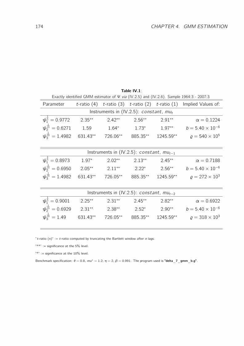
174 CHAPTER 4. GMM ESTIMATION
Table IV.1:Exactly identified GMM estimator of Ψ via (IV.2.5) and (IV.2.6). Sample 1964:3 - 2007:3
Parameter t-ratio (4) t-ratio (3) t-ratio (2) t-ratio (1) Implied Values of:
Instruments in (IV.2.5): constant, mut
ψ151 = 0.9772 2.35∗∗ 2.42∗∗ 2.56∗∗ 2.91∗∗ α = 0.1224
ψ1152 = 0.6271 1.59 1.64∗ 1.73∗ 1.97∗∗ b = 5.40× 10⁻⁶ψ1153 = 1.4982 631.43∗∗ 726.06∗∗ 885.35∗∗ 1245.59∗∗ % = 540× 105
Instruments in (IV.2.5): constant, mut−1
ψ151 = 0.8973 1.97∗ 2.02∗∗ 2.13∗∗ 2.45∗∗ α = 0.7188
ψ1152 = 0.6950 2.05∗∗ 2.11∗∗ 2.22∗ 2.56∗∗ b = 5.40× 10⁻⁶ψ1153 = 1.4982 631.43∗∗ 726.05∗∗ 885.35∗∗ 1245.59∗∗ % = 272× 103
Instruments in (IV.2.5): constant, mut−2
ψ151 = 0.9001 2.25∗∗ 2.31∗∗ 2.45∗∗ 2.82∗∗ α = 0.6922
ψ1152 = 0.6929 2.31∗∗ 2.38∗∗ 2.52∗ 2.90∗∗ b = 5.40× 10⁻⁶ψ1153 = 1.49 631.43∗∗ 726.05∗∗ 885.35∗∗ 1245.59∗∗ % = 318× 103
”t-ratio (n)” := t-ratio computed by truncating the Bartlett window after n lags.
”**” := significance at the 5% level.
”*” := significance at the 10% level.
Benchmark specification: θ = 0.8, mu∗ = 1.2, η = 2, β = 0.991. The program used is ”delta_7_gmm_b.g”.
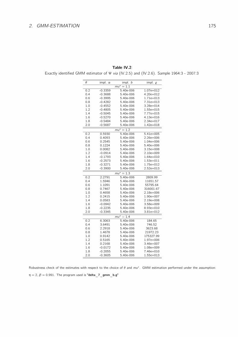
2. GMM-ESTIMATION 175
Table IV.2:Exactly identified GMM estimator of Ψ via (IV.2.5) and (IV.2.6). Sample 1964:3 - 2007:3
θ impl. α impl. b impl. %mu∗ = 1.1
0.2 -0.3359 5.40e-006 1.07e+0120.4 -0.3688 5.40e-006 4.20e+0120.6 -0.3995 5.40e-006 1.71e+0130.8 -0.4282 5.40e-006 7.31e+0131.0 -0.4552 5.40e-006 3.28e+0141.2 -0.4805 5.40e-006 1.55e+0151.4 -0.5045 5.40e-006 7.77e+0151.6 -0.5270 5.40e-006 4.13e+0161.8 -0.5484 5.40e-006 2.34e+0172.0 -0.5687 5.40e-006 1.42e+018
mu∗ = 1.20.2 0.5930 5.40e-006 5.41e+0050.4 0.4093 5.40e-006 2.26e+0060.6 0.2545 5.40e-006 1.04e+0060.8 0.1224 5.40e-006 5.40e+0061.0 0.0082 5.40e-006 3.15e+0081.2 -0.0914 5.40e-006 2.10e+0091.4 -0.1793 5.40e-006 1.64e+0101.6 -0.2573 5.40e-006 1.53e+0111.8 -0.3271 5.40e-006 1.75e+0122.0 -0.3900 5.40e-006 2.52e+013
mu∗ = 1.30.2 2.2791 5.40e-006 2809.990.4 1.5946 5.40e-006 11651.570.6 1.1091 5.40e-006 55795.640.8 0.7467 5.40e-006 316001.671.0 0.4658 5.40e-006 2.18e+0061.2 0.2415 5.40e-006 1.90e+0071.4 0.0583 5.40e-006 2.19e+0081.6 -0.0942 5.40e-006 3.58e+0091.8 -0.2235 5.40e-006 8.93e+0102.0 -0.3345 5.40e-006 3.81e+012
mu∗ = 1.40.2 6.3063 5.40e-006 184.650.4 3.6491 5.40e-006 746.520.6 2.2918 5.40e-006 3623.680.8 1.4678 5.40e-006 21972.231.0 0.9142 5.40e-006 175327.991.2 0.5165 5.40e-006 1.97e+0061.4 0.2168 5.40e-006 3.46e+0071.6 -0.0172 5.40e-006 1.08e+0091.8 -0.2055 5.40e-006 7.46e+0102.0 -0.3605 5.40e-006 1.55e+013
Robustness check of the estimates with respect to the choice of θ and mu∗. GMM estimation performed under the assumption:
η = 2, β = 0.991. The program used is ”delta_7_gmm_b.g”
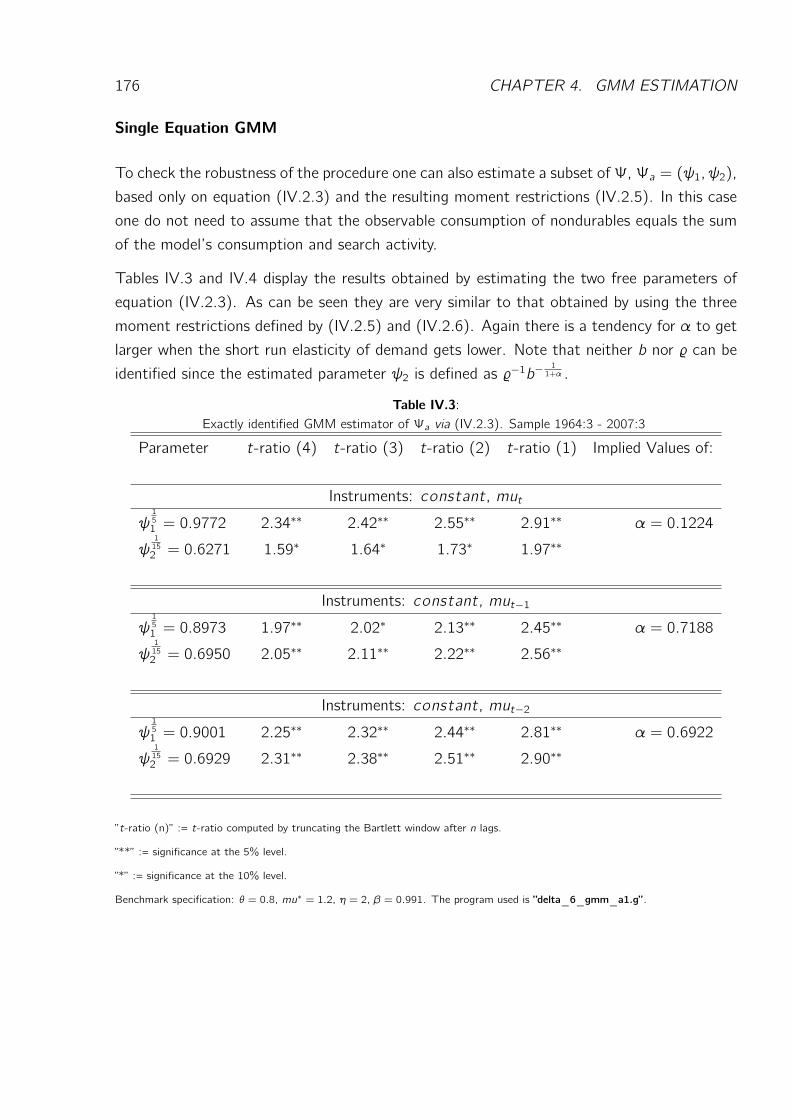
176 CHAPTER 4. GMM ESTIMATION
Single Equation GMM
To check the robustness of the procedure one can also estimate a subset of Ψ, Ψa = (ψ1, ψ2),
based only on equation (IV.2.3) and the resulting moment restrictions (IV.2.5). In this case
one do not need to assume that the observable consumption of nondurables equals the sum
of the model’s consumption and search activity.
Tables IV.3 and IV.4 display the results obtained by estimating the two free parameters of
equation (IV.2.3). As can be seen they are very similar to that obtained by using the three
moment restrictions defined by (IV.2.5) and (IV.2.6). Again there is a tendency for α to get
larger when the short run elasticity of demand gets lower. Note that neither b nor % can be
identified since the estimated parameter ψ2 is defined as %−1b−11+α .
Table IV.3:Exactly identified GMM estimator of Ψa via (IV.2.3). Sample 1964:3 - 2007:3
Parameter t-ratio (4) t-ratio (3) t-ratio (2) t-ratio (1) Implied Values of:
Instruments: constant, mut
ψ151 = 0.9772 2.34∗∗ 2.42∗∗ 2.55∗∗ 2.91∗∗ α = 0.1224
ψ1152 = 0.6271 1.59∗ 1.64∗ 1.73∗ 1.97∗∗
Instruments: constant, mut−1
ψ151 = 0.8973 1.97∗∗ 2.02∗ 2.13∗∗ 2.45∗∗ α = 0.7188
ψ1152 = 0.6950 2.05∗∗ 2.11∗∗ 2.22∗∗ 2.56∗∗
Instruments: constant, mut−2
ψ151 = 0.9001 2.25∗∗ 2.32∗∗ 2.44∗∗ 2.81∗∗ α = 0.6922
ψ1152 = 0.6929 2.31∗∗ 2.38∗∗ 2.51∗∗ 2.90∗∗
”t-ratio (n)” := t-ratio computed by truncating the Bartlett window after n lags.
”**” := significance at the 5% level.
”*” := significance at the 10% level.
Benchmark specification: θ = 0.8, mu∗ = 1.2, η = 2, β = 0.991. The program used is ”delta_6_gmm_a1.g”.
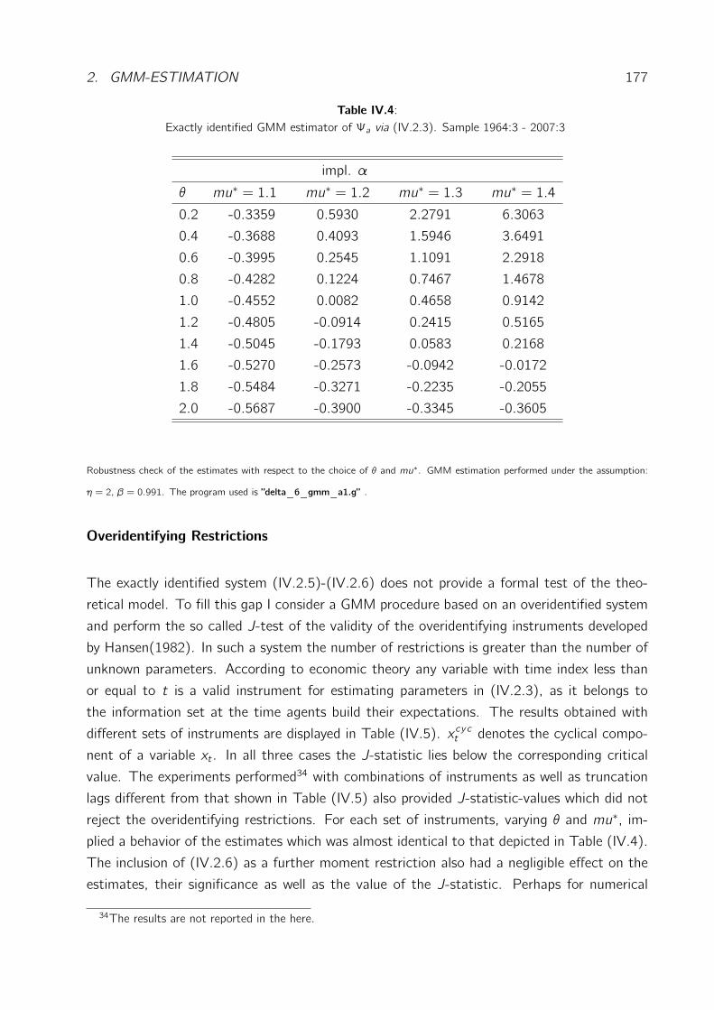
2. GMM-ESTIMATION 177
Table IV.4:Exactly identified GMM estimator of Ψa via (IV.2.3). Sample 1964:3 - 2007:3
impl. α
θ mu∗ = 1.1 mu∗ = 1.2 mu∗ = 1.3 mu∗ = 1.4
0.2 -0.3359 0.5930 2.2791 6.3063
0.4 -0.3688 0.4093 1.5946 3.6491
0.6 -0.3995 0.2545 1.1091 2.2918
0.8 -0.4282 0.1224 0.7467 1.4678
1.0 -0.4552 0.0082 0.4658 0.9142
1.2 -0.4805 -0.0914 0.2415 0.5165
1.4 -0.5045 -0.1793 0.0583 0.2168
1.6 -0.5270 -0.2573 -0.0942 -0.0172
1.8 -0.5484 -0.3271 -0.2235 -0.2055
2.0 -0.5687 -0.3900 -0.3345 -0.3605
Robustness check of the estimates with respect to the choice of θ and mu∗. GMM estimation performed under the assumption:
η = 2, β = 0.991. The program used is ”delta_6_gmm_a1.g” .
Overidentifying Restrictions
The exactly identified system (IV.2.5)-(IV.2.6) does not provide a formal test of the theo-
retical model. To fill this gap I consider a GMM procedure based on an overidentified system
and perform the so called J-test of the validity of the overidentifying instruments developed
by Hansen(1982). In such a system the number of restrictions is greater than the number of
unknown parameters. According to economic theory any variable with time index less than
or equal to t is a valid instrument for estimating parameters in (IV.2.3), as it belongs to
the information set at the time agents build their expectations. The results obtained with
different sets of instruments are displayed in Table (IV.5). xcyct denotes the cyclical compo-
nent of a variable xt . In all three cases the J-statistic lies below the corresponding critical
value. The experiments performed34 with combinations of instruments as well as truncation
lags different from that shown in Table (IV.5) also provided J-statistic-values which did not
reject the overidentifying restrictions. For each set of instruments, varying θ and mu∗, im-
plied a behavior of the estimates which was almost identical to that depicted in Table (IV.4).
The inclusion of (IV.2.6) as a further moment restriction also had a negligible effect on the
estimates, their significance as well as the value of the J-statistic. Perhaps for numerical
34The results are not reported in the here.

178 CHAPTER 4. GMM ESTIMATION
reasons and/or because of multicolinearity it is not possible to perform the estimation with
any arbitrary combination of instruments. There were cases in which the algorithm just did
not converge. But in the cases it did, the estimates were significant at least at the 10% level
and the J-statistic lay below the corresponding critical value. Table (IV.5) also indicates that
the estimate of α is relatively sensitive with respect to the choice of instruments, varying
from slightly above zero to values above 10. Excluding the value of land from the definition of
the economy wide stock of capital did not have a significant impact on the results. However,
there were more cases in which the estimation algorithm failed to converge.
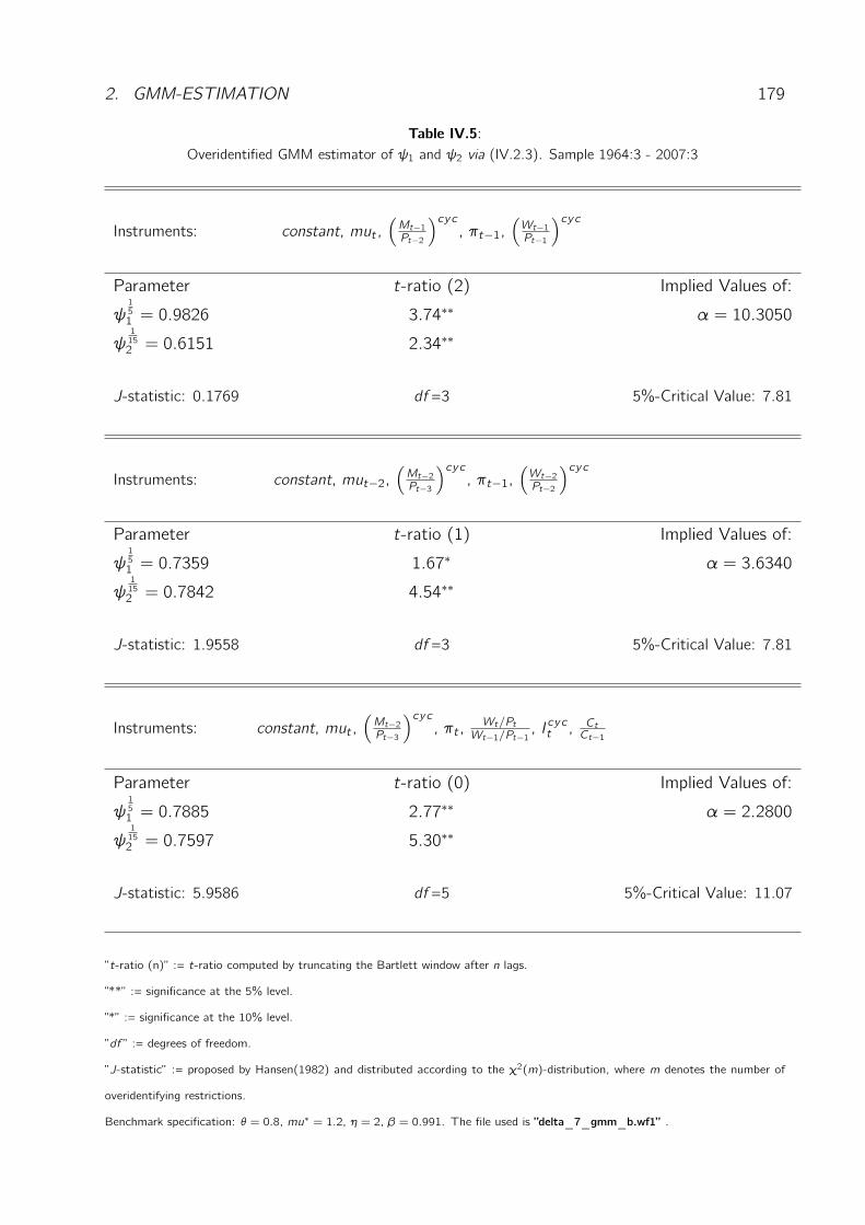
2. GMM-ESTIMATION 179
Table IV.5:Overidentified GMM estimator of ψ1 and ψ2 via (IV.2.3). Sample 1964:3 - 2007:3
Instruments: constant, mut ,(Mt−1Pt−2
)cyc, πt−1,
(Wt−1Pt−1
)cyc
Parameter t-ratio (2) Implied Values of:
ψ151 = 0.9826 3.74∗∗ α = 10.3050
ψ1152 = 0.6151 2.34∗∗
J-statistic: 0.1769 df =3 5%-Critical Value: 7.81
Instruments: constant, mut−2,(Mt−2Pt−3
)cyc, πt−1,
(Wt−2Pt−2
)cyc
Parameter t-ratio (1) Implied Values of:
ψ151 = 0.7359 1.67∗ α = 3.6340
ψ1152 = 0.7842 4.54∗∗
J-statistic: 1.9558 df =3 5%-Critical Value: 7.81
Instruments: constant, mut ,(Mt−2Pt−3
)cyc, πt ,
Wt/PtWt−1/Pt−1 , I
cyct , Ct
Ct−1
Parameter t-ratio (0) Implied Values of:
ψ151 = 0.7885 2.77∗∗ α = 2.2800
ψ1152 = 0.7597 5.30∗∗
J-statistic: 5.9586 df =5 5%-Critical Value: 11.07
”t-ratio (n)” := t-ratio computed by truncating the Bartlett window after n lags.
”**” := significance at the 5% level.
”*” := significance at the 10% level.
”df ” := degrees of freedom.
”J-statistic” := proposed by Hansen(1982) and distributed according to the χ2(m)-distribution, where m denotes the number of
overidentifying restrictions.
Benchmark specification: θ = 0.8, mu∗ = 1.2, η = 2, β = 0.991. The file used is ”delta_7_gmm_b.wf1” .
180 CHAPTER 4. GMM ESTIMATION
GMM Estimation Based on the Fixed Capital Model
In the inflation-aversion model with fixed capital overall demand equals the sum of nondurables
consumption expenditure Ct and switching costs st . In order to put the model in a form
suitable for GMM estimation, one can use equations (IV.2.1) in the same manner as in the
previous two subsections to eliminate the unobservable variables Ct and st .
The moment restrictions (IV.2.5) and (IV.2.6) were modified by replacing GNP as measure
of aggregate output by the sum of private and government nondurables consumption expen-
diture. The appropriate measure of labor income is obtained by multiplying the labor income
series used in the previous subsections by the ratio of aggregate consumption of nondurables
to GNP. Since the estimated version of the model implies that the aggregate production
function is given by
Yt = ZtNt
the markup can be deduced from
mut =ZtWt/Pt
=Yt
Labor Incomet,
where Yt = Ct + st corresponds to aggregate consumption of nondurables and WtPt
denotes
the real wage.
The implied values of α and % are most similar to that obtained in the model with endogenous
capital under the assumption of a relatively high average markup, mu∗ = 1.4. The results
are not reported here but are available upon request.
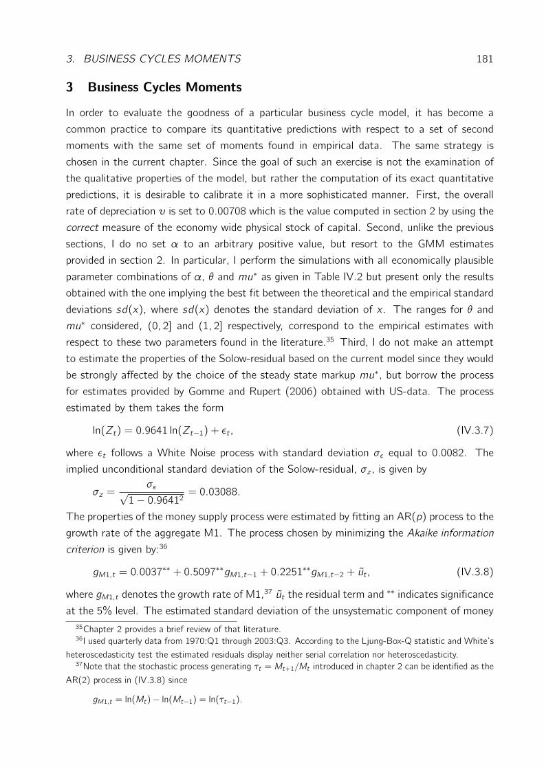
3. BUSINESS CYCLES MOMENTS 181
3 Business Cycles Moments
In order to evaluate the goodness of a particular business cycle model, it has become a
common practice to compare its quantitative predictions with respect to a set of second
moments with the same set of moments found in empirical data. The same strategy is
chosen in the current chapter. Since the goal of such an exercise is not the examination of
the qualitative properties of the model, but rather the computation of its exact quantitative
predictions, it is desirable to calibrate it in a more sophisticated manner. First, the overall
rate of depreciation υ is set to 0.00708 which is the value computed in section 2 by using the
correct measure of the economy wide physical stock of capital. Second, unlike the previous
sections, I do no set α to an arbitrary positive value, but resort to the GMM estimates
provided in section 2. In particular, I perform the simulations with all economically plausible
parameter combinations of α, θ and mu∗ as given in Table IV.2 but present only the results
obtained with the one implying the best fit between the theoretical and the empirical standard
deviations sd(x), where sd(x) denotes the standard deviation of x . The ranges for θ and
mu∗ considered, (0, 2] and (1, 2] respectively, correspond to the empirical estimates with
respect to these two parameters found in the literature.35 Third, I do not make an attempt
to estimate the properties of the Solow-residual based on the current model since they would
be strongly affected by the choice of the steady state markup mu∗, but borrow the process
for estimates provided by Gomme and Rupert (2006) obtained with US-data. The process
estimated by them takes the form
ln(Zt) = 0.9641 ln(Zt−1) + εt , (IV.3.7)
where εt follows a White Noise process with standard deviation σε equal to 0.0082. The
implied unconditional standard deviation of the Solow-residual, σz , is given by
σz =σε√
1− 0.96412 = 0.03088.
The properties of the money supply process were estimated by fitting an AR(p) process to the
growth rate of the aggregate M1. The process chosen by minimizing the Akaike information
criterion is given by:36
gM1,t = 0.0037∗∗ + 0.5097∗∗gM1,t−1 + 0.2251∗∗gM1,t−2 + ut , (IV.3.8)
where gM1,t denotes the growth rate of M1,37 ut the residual term and ∗∗ indicates significance
at the 5% level. The estimated standard deviation of the unsystematic component of money35Chapter 2 provides a brief review of that literature.36I used quarterly data from 1970:Q1 through 2003:Q3. According to the Ljung-Box-Q statistic and White’s
heteroscedasticity test the estimated residuals display neither serial correlation nor heteroscedasticity.37Note that the stochastic process generating τt = Mt+1/Mt introduced in chapter 2 can be identified as the
AR(2) process in (IV.3.8) since
gM1,t = ln(Mt)− ln(Mt−1) = ln(τt−1).
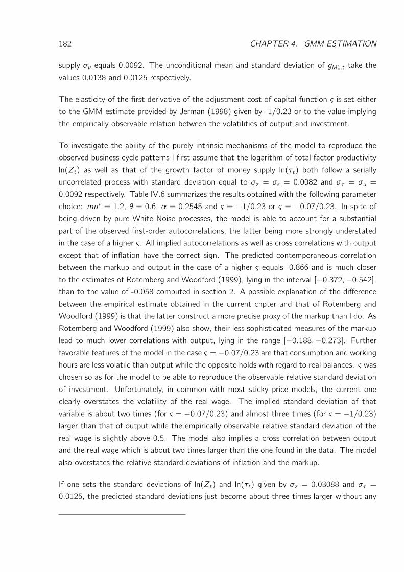
182 CHAPTER 4. GMM ESTIMATION
supply σu equals 0.0092. The unconditional mean and standard deviation of gM1,t take the
values 0.0138 and 0.0125 respectively.
The elasticity of the first derivative of the adjustment cost of capital function ς is set either
to the GMM estimate provided by Jerman (1998) given by -1/0.23 or to the value implying
the empirically observable relation between the volatilities of output and investment.
To investigate the ability of the purely intrinsic mechanisms of the model to reproduce the
observed business cycle patterns I first assume that the logarithm of total factor productivity
ln(Zt) as well as that of the growth factor of money supply ln(τt) both follow a serially
uncorrelated process with standard deviation equal to σz = σε = 0.0082 and στ = σu =
0.0092 respectively. Table IV.6 summarizes the results obtained with the following parameter
choice: mu∗ = 1.2, θ = 0.6, α = 0.2545 and ς = −1/0.23 or ς = −0.07/0.23. In spite of
being driven by pure White Noise processes, the model is able to account for a substantial
part of the observed first-order autocorrelations, the latter being more strongly understated
in the case of a higher ς. All implied autocorrelations as well as cross correlations with output
except that of inflation have the correct sign. The predicted contemporaneous correlation
between the markup and output in the case of a higher ς equals -0.866 and is much closer
to the estimates of Rotemberg and Woodford (1999), lying in the interval [−0.372,−0.542],than to the value of -0.058 computed in section 2. A possible explanation of the difference
between the empirical estimate obtained in the current chpter and that of Rotemberg and
Woodford (1999) is that the latter construct a more precise proxy of the markup than I do. As
Rotemberg and Woodford (1999) also show, their less sophisticated measures of the markup
lead to much lower correlations with output, lying in the range [−0.188,−0.273]. Further
favorable features of the model in the case ς = −0.07/0.23 are that consumption and working
hours are less volatile than output while the opposite holds with regard to real balances. ς was
chosen so as for the model to be able to reproduce the observable relative standard deviation
of investment. Unfortunately, in common with most sticky price models, the current one
clearly overstates the volatility of the real wage. The implied standard deviation of that
variable is about two times (for ς = −0.07/0.23) and almost three times (for ς = −1/0.23)larger than that of output while the empirically observable relative standard deviation of the
real wage is slightly above 0.5. The model also implies a cross correlation between output
and the real wage which is about two times larger than the one found in the data. The model
also overstates the relative standard deviations of inflation and the markup.
If one sets the standard deviations of ln(Zt) and ln(τt) given by σz = 0.03088 and στ =
0.0125, the predicted standard deviations just become about three times larger without any

3. BUSINESS CYCLES MOMENTS 183
notable changes in the implied relative standard deviations, autocorrelations and cross corre-
lations with output.
In the second exercise performed I assume that ln(Zt) and ln(τt) evolve according to the
AR(1) process in (IV.3.7) and the AR(2) process in (IV.3.8) respectively. Table IV.7 provides
the simulation results. The first noteworthy feature is that now all autocorrelations and cross
correlations have the correct sign. Second, the predictions of the model with respect to real
balances and the rate of inflation get better: The autocorrelation of real balances as well as
its correlation with output get for both values of ς very close to their respective empirical
counterparts. The slight increase in the autocorrelations of investment and consumption as
well as that in the standard deviation of output should be also characterized as shifts in the
right direction.
Unfortunately, there are also important dimensions with respect to which the performance of
the model worsens. For both values of ς hours become more volatile than output. The auto-
correlation of output and wages also decrease by amounts which should not be characterized
as negligible. Nevertheless, by imposing the processes (IV.3.7) and (IV.3.8) the overall fit
between the model’s predictions and the empirical observations improves.
Doubtless, the model with adjustment costs of capital is better able to account for the
stylized business cycle facts than do many modern real- and monetary business cycle models
and exhibits stronger endogenous mechanisms than most of those models. Yet, it is by no
means perfect and future research should try to eliminate its shortcomings.
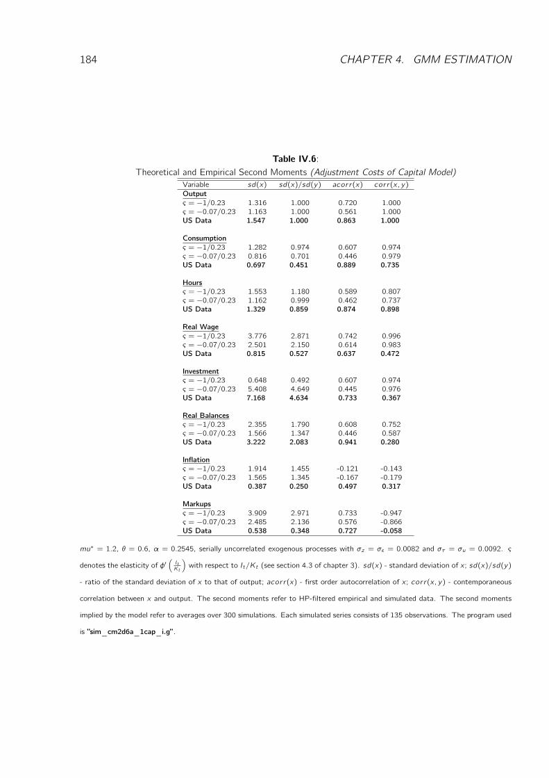
184 CHAPTER 4. GMM ESTIMATION
Table IV.6:Theoretical and Empirical Second Moments (Adjustment Costs of Capital Model)
Variable sd(x) sd(x)/sd(y) acorr(x) corr(x, y)
Outputς = −1/0.23 1.316 1.000 0.720 1.000ς = −0.07/0.23 1.163 1.000 0.561 1.000US Data 1.547 1.000 0.863 1.000
Consumptionς = −1/0.23 1.282 0.974 0.607 0.974ς = −0.07/0.23 0.816 0.701 0.446 0.979US Data 0.697 0.451 0.889 0.735
Hoursς = −1/0.23 1.553 1.180 0.589 0.807ς = −0.07/0.23 1.162 0.999 0.462 0.737US Data 1.329 0.859 0.874 0.898
Real Wageς = −1/0.23 3.776 2.871 0.742 0.996ς = −0.07/0.23 2.501 2.150 0.614 0.983US Data 0.815 0.527 0.637 0.472
Investmentς = −1/0.23 0.648 0.492 0.607 0.974ς = −0.07/0.23 5.408 4.649 0.445 0.976US Data 7.168 4.634 0.733 0.367
Real Balancesς = −1/0.23 2.355 1.790 0.608 0.752ς = −0.07/0.23 1.566 1.347 0.446 0.587US Data 3.222 2.083 0.941 0.280
Inflationς = −1/0.23 1.914 1.455 -0.121 -0.143ς = −0.07/0.23 1.565 1.345 -0.167 -0.179US Data 0.387 0.250 0.497 0.317
Markupsς = −1/0.23 3.909 2.971 0.733 -0.947ς = −0.07/0.23 2.485 2.136 0.576 -0.866US Data 0.538 0.348 0.727 -0.058
mu∗ = 1.2, θ = 0.6, α = 0.2545, serially uncorrelated exogenous processes with σz = σε = 0.0082 and στ = σu = 0.0092. ς
denotes the elasticity of φ′(ItKt
)with respect to It/Kt (see section 4.3 of chapter 3). sd(x) - standard deviation of x ; sd(x)/sd(y)
- ratio of the standard deviation of x to that of output; acorr(x) - first order autocorrelation of x ; corr(x, y) - contemporaneous
correlation between x and output. The second moments refer to HP-filtered empirical and simulated data. The second moments
implied by the model refer to averages over 300 simulations. Each simulated series consists of 135 observations. The program used
is ”sim_cm2d6a_1cap_i.g”.
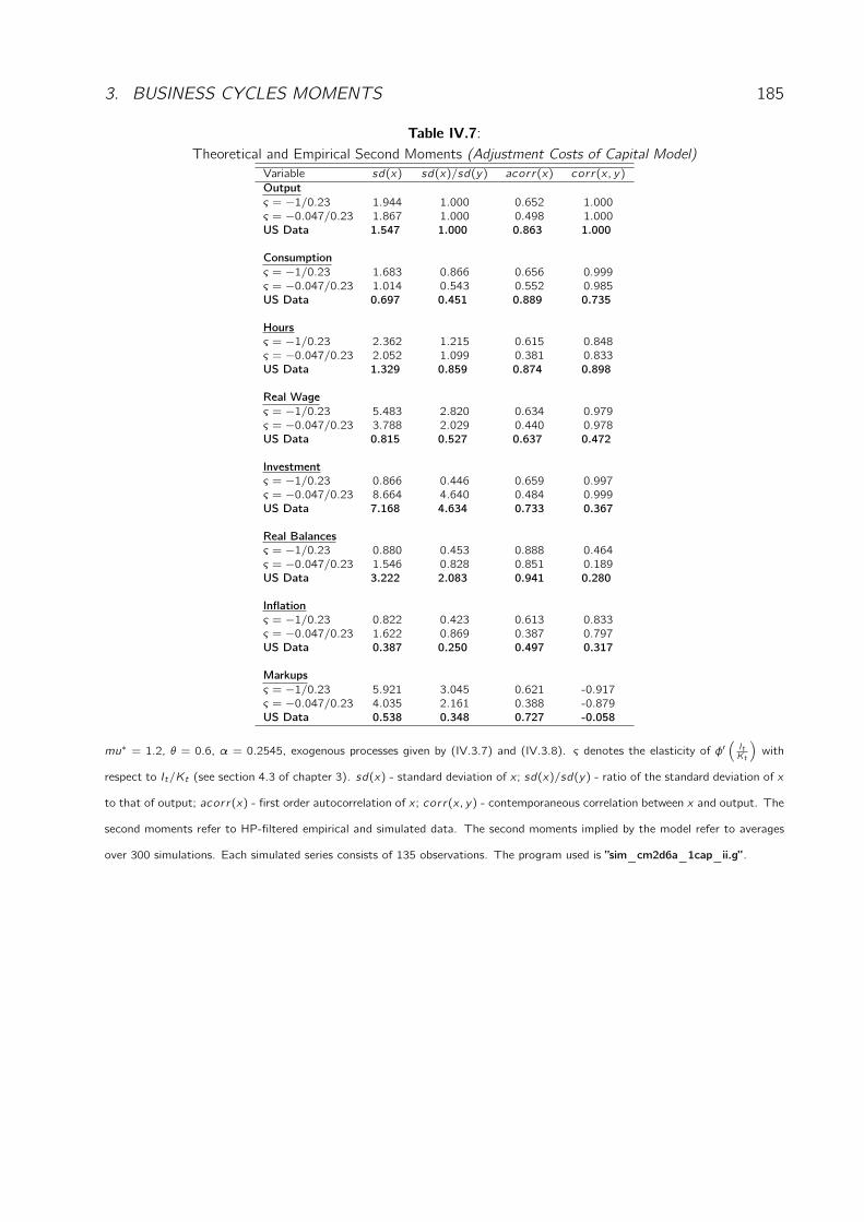
3. BUSINESS CYCLES MOMENTS 185
Table IV.7:Theoretical and Empirical Second Moments (Adjustment Costs of Capital Model)
Variable sd(x) sd(x)/sd(y) acorr(x) corr(x, y)
Outputς = −1/0.23 1.944 1.000 0.652 1.000ς = −0.047/0.23 1.867 1.000 0.498 1.000US Data 1.547 1.000 0.863 1.000
Consumptionς = −1/0.23 1.683 0.866 0.656 0.999ς = −0.047/0.23 1.014 0.543 0.552 0.985US Data 0.697 0.451 0.889 0.735
Hoursς = −1/0.23 2.362 1.215 0.615 0.848ς = −0.047/0.23 2.052 1.099 0.381 0.833US Data 1.329 0.859 0.874 0.898
Real Wageς = −1/0.23 5.483 2.820 0.634 0.979ς = −0.047/0.23 3.788 2.029 0.440 0.978US Data 0.815 0.527 0.637 0.472
Investmentς = −1/0.23 0.866 0.446 0.659 0.997ς = −0.047/0.23 8.664 4.640 0.484 0.999US Data 7.168 4.634 0.733 0.367
Real Balancesς = −1/0.23 0.880 0.453 0.888 0.464ς = −0.047/0.23 1.546 0.828 0.851 0.189US Data 3.222 2.083 0.941 0.280
Inflationς = −1/0.23 0.822 0.423 0.613 0.833ς = −0.047/0.23 1.622 0.869 0.387 0.797US Data 0.387 0.250 0.497 0.317
Markupsς = −1/0.23 5.921 3.045 0.621 -0.917ς = −0.047/0.23 4.035 2.161 0.388 -0.879US Data 0.538 0.348 0.727 -0.058
mu∗ = 1.2, θ = 0.6, α = 0.2545, exogenous processes given by (IV.3.7) and (IV.3.8). ς denotes the elasticity of φ′(ItKt
)with
respect to It/Kt (see section 4.3 of chapter 3). sd(x) - standard deviation of x ; sd(x)/sd(y) - ratio of the standard deviation of x
to that of output; acorr(x) - first order autocorrelation of x ; corr(x, y) - contemporaneous correlation between x and output. The
second moments refer to HP-filtered empirical and simulated data. The second moments implied by the model refer to averages
over 300 simulations. Each simulated series consists of 135 observations. The program used is ”sim_cm2d6a_1cap_ii.g”.
186 CHAPTER 4. GMM ESTIMATION
4 A Comparison with the New Keynesian Model
Based on the suggestion of Christiano et al. (1997) I approximate monetary policy by an
AR(1) process with a coefficient of autocorrelation equal to 0.5. The technology shocks
follows the AR(1) process estimated by Gomme and Rupert (2006). To bias the results
towards a better performance of the New Keynesian model with adjustment costs of capital,
I set the fraction of firms that are not able to adjust their prices at ϕ = 0.75. In both
models the parameter of the adjustment-cost function ς is chosen to approximately match
the observable relative deviation of investment. The second moments implied by the two
models as well as that found in the date are given in figure IV.8. The Inflation Aversion model
accounts better for the standard deviations of output, consumption and hours as well as the
relative standard deviations of the latter two variables. The New Keynesian model is better
able to mach the cyclical properties of inflation. With respect to the remaining variables both
models perform equally well. Nevertheless, recall that setting ϕ at the much more realistic
value 0.3 dramatically worsens the performance of the New Keynesian model. For example,
the correlation between hours and output become negative. The standard deviation of output
drops to 0.84 while inflation becomes more volatile than output. Furthermore, if we leave
ϕ at 0.75 but assume that both exogenous processes are not serially correlated, the New
Keynesian model implies that the standard deviation of output is 0.49, the autocorrelation
of hours, wages and the markup are 0.043, 0.277 and 0.086 respectively and that hours are
more than twice as volatile as output. Combining a low autocorrelation in the shocks with
a low degree of price stickiness ϕ = 0.3 makes the predictions of the New Keynesian model
even worse. More precisely, its predictions become completely at odds with the empirical
observations.
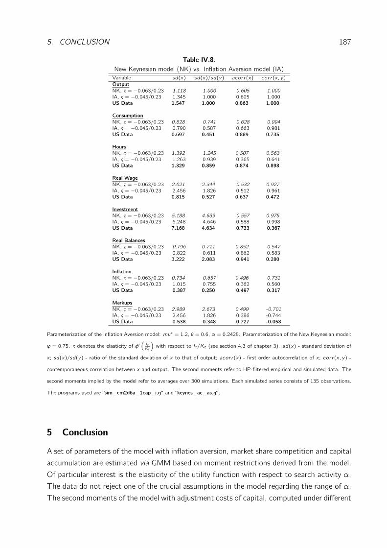
5. CONCLUSION 187
Table IV.8:New Keynesian model (NK) vs. Inflation Aversion model (IA)Variable sd(x) sd(x)/sd(y) acorr(x) corr(x, y)
OutputNK, ς = −0.063/0.23 1.118 1.000 0.605 1.000IA, ς = −0.045/0.23 1.345 1.000 0.605 1.000US Data 1.547 1.000 0.863 1.000
ConsumptionNK, ς = −0.063/0.23 0.828 0.741 0.628 0.994IA, ς = −0.045/0.23 0.790 0.587 0.663 0.981US Data 0.697 0.451 0.889 0.735
HoursNK, ς = −0.063/0.23 1.392 1.245 0.507 0.563IA, ς = −0.045/0.23 1.263 0.939 0.365 0.641US Data 1.329 0.859 0.874 0.898
Real WageNK, ς = −0.063/0.23 2.621 2.344 0.532 0.927IA, ς = −0.045/0.23 2.456 1.826 0.512 0.961US Data 0.815 0.527 0.637 0.472
InvestmentNK, ς = −0.063/0.23 5.188 4.639 0.557 0.975IA, ς = −0.045/0.23 6.248 4.646 0.588 0.998US Data 7.168 4.634 0.733 0.367
Real BalancesNK, ς = −0.063/0.23 0.796 0.711 0.852 0.547IA, ς = −0.045/0.23 0.822 0.611 0.862 0.583US Data 3.222 2.083 0.941 0.280
InflationNK, ς = −0.063/0.23 0.734 0.657 0.496 0.731IA, ς = −0.045/0.23 1.015 0.755 0.362 0.560US Data 0.387 0.250 0.497 0.317
MarkupsNK, ς = −0.063/0.23 2.989 2.673 0.499 -0.701IA, ς = −0.045/0.23 2.456 1.826 0.386 -0.744US Data 0.538 0.348 0.727 -0.058
Parameterization of the Inflation Aversion model: mu∗ = 1.2, θ = 0.6, α = 0.2425. Parameterization of the New Keynesian model:
ϕ = 0.75. ς denotes the elasticity of φ′(ItKt
)with respect to It/Kt (see section 4.3 of chapter 3). sd(x) - standard deviation of
x ; sd(x)/sd(y) - ratio of the standard deviation of x to that of output; acorr(x) - first order autocorrelation of x ; corr(x, y) -
contemporaneous correlation between x and output. The second moments refer to HP-filtered empirical and simulated data. The
second moments implied by the model refer to averages over 300 simulations. Each simulated series consists of 135 observations.
The programs used are ”sim_cm2d6a_1cap_i.g” and ”keynes_ac_as.g”.
5 Conclusion
A set of parameters of the model with inflation aversion, market share competition and capital
accumulation are estimated via GMM based on moment restrictions derived from the model.
Of particular interest is the elasticity of the utility function with respect to search activity α.
The data do not reject one of the crucial assumptions in the model regarding the range of α.
The second moments of the model with adjustment costs of capital, computed under different

188 CHAPTER 4. GMM ESTIMATION
assumptions on the autocorrelation structure of the exogenous processes, are then confronted
with their empirical counterparts. The model is able to account for several important features
of the observable business cycles pattern in the U.S. economy. Furthermore, even without
any serial correlation in the exogenous variables, the model explains a substantial part of
the observed autocorrelation in the main macroeconomic aggregates. Thus, the intrinsic
mechanisms in the model are stronger and explain a larger part of the observable cyclical
behavior of the macroeconomic variables than it is the case in most other business cycle
models, including the New Keynesian one. The quantitative explanatory power of the latter
stems to a large degree from the assumed high serial correlation of the exogenous processes
and the high degree of price stickiness.

Chapter 5
Price Dispersion, Search and MonetaryPolicy
1 Introduction
The purpose of this chapter to develop a monetary model in which search activity in the goods
market is modeled in a more explicit manner than in chapter 3. In particular, the economy
developed here is characterized by price dispersion introduced exogenously via heterogeneity in
productivity across firms. The price dispersion, in turn, generates an incentive for households
to engage in search activity. On the one hand search efforts lead to transaction costs which
reduce the (should be financed by) real balances accumulated in the previous period. On the
other hand, a more intense search increases the probability for becoming a customer of a
supplier charging relatively low prices.
The model provides a further rationale for the positive dependence of search efforts an the
current level of inflation and consumption found in the Inflation Aversion model. A higher in-
flation erodes the value of individual nominal balances. Therefore, it becomes more important
for consumers to find suppliers charging lower prices in order to at least partly compensate
the negative effects of the higher inflation rate. A higher level of desired current consumption
simply increases the marginal benefit of finding a cheaper supplier.
The impulse responses implied by the model have the sign predicted by the bulk of the
SVAR literature. Unfortunately, their persistence is not consistent with the empirical evidence
presented in chapter 1.
189
190 CHAPTER 5. PRICE DISPERSION, SEARCH AND MONETARY POLICY
2 The Model
Goods Market Structure
There are n firms, all producing the same homogeneous good. In each period each household
is randomly assigned to one of the suppliers. However, by engaging in search activity in
the current period the typical household indexed by i can influence the probability xi ,l ,t ,
l = 1, 2, ..., n of becoming a customer of each of the individual firms. As a consequence of
a higher search intensity, the probability to be assigned to a store with above(below) average
price gets smaller(larger) than 1/n. More formally, xi ,l ,t is defined as:
xi ,l ,t =exp
((1− Pl ,t
Pt
)sγi,t
)
∑nj=1 exp
((1− Pj,t
Pt
)sγi,t
) , γ > 0 (V.2.1)
where Pt denotes the overall price level si ,t represents the individual level of search in the
goods market. According to this definition, a higher search activity induces an increase (fall)
in the probability for becoming a customer of a firm that charges an above average (a below
average) current price. Furthermore, xi ,l ,t is bounded between 0 and 1. Note that the actual
(or potential) price dispersion in this framework can be also seen as an approximation of
differences in quality between almost homogeneous products selling at the same nominal
price.
There are two important ideas underlying the definition of xi ,l ,t . First, in spite of the fact that
the household is informed about the average price Pt as well as the distribution of individual
prices, she doesn’t know which supplier offers her the lowest price or the best conditions.
In many cases it is not immediately obvious whether two suppliers charging the same price
offer the same quality. For example many services such es consulting, banking as well as
educational services contain components which are not directly observable. That makes
comparisons between individual products costly, as they usually involve the time and resource
consuming process of analyzing, tasting, testing and trying different products. Often it is
simply not an easy task to find out where the cheapest supplier is located. The service sector
again, provides a vast number of examples. Second, I assume that at the end of each period
firms randomly change their respective positions within the cross-sectional productivity and
thus, the cross-sectional price distribution. As a results, agents are not able to infer from past
information, especially from observed past pricing behavior, which firms charge low enough
prices and which do not. In other words, firm’s movements along the price scala make
any knowledge about the past pricing behavior of particular firms worthless, so that at the
beginning of an arbitrary period t households are as well informed as they were at the beginning
of t−1 and thus, have to play the same game again. The assumption on the intra-distribution
mobility of firms is based on the evidence provided by Lach (2002) and Lach and Tsiddon
2. THE MODEL 191
(1993). After controlling for observed as well as unobserved heterogeneity between almost
identical products they show that there is substantial intra-distribution mobility disabling, as
the authors conclude, consumers to learn which store charges consistently low prices
As explained below, under the assumption of a continuum of ex ante symmetric households
which are able to perfectly pool all idiosyncratic income as well as expenditure risks the mass
of households served by an arbitrary firm l , xl ,t will be equal to the probability to become a
customer at store l faced by a typical household:1
xl ,t = xi ,l ,t .
I refer to xl ,t as the market share of firm l . Since, as assumed below, it is costly to search for
cheaper suppliers, deviations from the average price do not translate into an immediate drop
or increase of the individual market share to zero or hundred percent respectively. Thus, each
firm enjoys a small, short-run monopoly power over the consumers belonging to its customer
base when setting its price. Consequently, the market structure can be characterized as a
form of monopolistic competition. According to (V.2.1), if all firms were to choose the same
price the fraction of aggregate demand each firm faces would be equal to 1/n, irrespective
of the level of search activity. If households do not engage in search at all, si ,t = 0, ∀i thenagain each supplier will serve a fraction of 1/n of the market, irrespective of the degree of
price dispersion.
In contrast to the versions of the Customer Market Model described in chapters 2 and 3 where
the individual firm’s market share follows a random walk process, in the model presented here
the market share xl ,t is modeled as a variable without memory, which is purely statically related
to the level of search efforts and the firm’s relative prices. The assumption that the process
of search, the price adjustments and the reactions of the individual market shares take place
simultaneously can be regarded as reasonable, since one period in the model corresponds to
one quarter in the real world.
Firms
Each profit maximizing monopolistic firm produces according to the linear production function
Yl ,t = (Zt + ιl ,t)Nl ,t ,
where Nl ,t denotes labor input of firm l . Zt denotes the total factor productivity which follows
a stochastic process given by:
ln(Zt) = ρz ln(Zt−1) + εt ,
1That is an implication of the Law of Large Numbers.
192 CHAPTER 5. PRICE DISPERSION, SEARCH AND MONETARY POLICY
where εt follows a White Noise Process with variance σ2ε . ιl ,t is an exogenous firm specific
shift variable which is assumed to evolve according to
ιl ,t = ιl + ειl ,t .
ειl ,t follows a White Noise Process with variance σ2ιl .
Under the assumption that each agent chooses the same level of search activity,2 the demand
function faced by the producer l is given by
Dl ,t = xl ,t ·Dt = exp
((1− Pl ,t
Pt
)sγt
)
∑nj=1 exp
((1− Pj,t
Pt
)sγt
) ·Dt , (V.2.2)
where Dt , st and Pt denote, respectively, aggregate demand, aggregate search efforts and
the aggregate price level. For given marginal costs, µl ,t the profit maximization problem of a
typical firm reads:
maxPl,tPt
exp
((1− Pl ,t
Pt
)sγt
)
∑nj=1 exp
((1− Pj,t
Pt
)sγt
) ·Dt
(Pl ,tPt− µl ,t
) .
It yields the following first order condition for optimal price setting:Pl ,tPt=
1
sγt (1− xl ,t)+ µl ,t , (V.2.3)
where xl ,t also depends on Pl ,tPt. Everything else given, a higher level of search efforts makes
the typical firm more reluctant to set too high a relative price, and leads to a lower markup.
A higher market share xl ,t makes it less likely for a searching customer to meet a supplier
other than l and thus, makes it less likely for him to find a firm charging a price lower than
Pl ,t . Consequently, a higher xl ,t reduces the magnitude of the negative effect of any given
level of search on the relative price Pl ,tPt
and so enables firm l to choose a higher markup.
However, by inspecting equation (V.2.3) one can only gain some very rough intuition about
the mechanisms underlying the price setting behavior of the firms, because (V.2.3) defines
an implicit relationship between the relative price Pl ,tPt, marginal costs µl ,t and search efforts
st . Log-linearizing (V.2.3) around the steady state3 yields:4
ˆ(Pl ,tPt
)=
γ
sγ · PlP
((1− Pl
P
)sγ − (1− xl)1− xl
)st+
+xl
(1− xl) · PlP·
n∑
j=1,j 6=lxjPjP
ˆ(Pj,tPt
)+ (1− xl)µlPl
P
µl ,t ,
(V.2.4)
2See the discussion below.3The properties and the computation of the steady state will be discussed later on.4To arrive at the result one has just to take into account the definition of xl ,t , ∀l , the fact that
n∑
j=1
xj,t = 1
2. THE MODEL 193
where variables without time index denote steady state values, while a ”hat”, ” ˆ ”, over
a variable denotes its percentage deviation from the stationary equilibrium. According to
(V.2.4), if firm l has an above average steady state price, an increase of search activity will
force it pass-through to its price a smaller fraction of any given increase in its marginal costs
and thus, to lower its markup. Only in the case of a sufficiently low Pl/P combined with
a sufficiently large market share, xl will an increase in aggregate search activity enable firm
l to choose a higher pass-through and increase its markup. Putting any general equilibrium
effects aside, if all other firms increase their respective relative prices then firm l will also find
it optimal to do that. Note that in the general equilibrium discussed in the current chapter it
will be possible for all firms to simultaneously increase their respective relative prices, provided
that such a reaction comes along with (is backed by) the ”correct” adjustment of the individual
market shares.
The more conventional representation of the first order condition for optimal price setting is:
Pl ,tPt= mul ,tµl ,t =
(1 +
1
sγt (1− xl ,t)µl ,t
)µl ,t ,
where mul ,t denotes the firm specific markup. As can be easily seen, it will be time varying.
As stressed above, the markup will be only procyclical when Pl/P is sufficiently low and at
the same time xl sufficiently large. Otherwise, mul ,t will tend to be countercyclical.
Since labor is the only factor of production, the real marginal costs of firm l are given by
µl ,t =Wt/PtZt + ιl ,t
. (V.2.5)
Households
The economy is populated by a continuum of ex ante identical agents of total mass equal
to one, organized in m equally large units. Let us refer to these units as families. The
family indexed by j = 1, 2, ..., m consists of the agents with an index i in the interval
i ∈ [j−1m, jm
]. Each family faces a two-stage maximization problem, in which both stages
take place simultaneously. At the ”first” stage, the head of the family, also called planner,
chooses the level as well as the distribution across the family’s members of next-period wealth,
current income, leisure and current expenditure, given the level and the distribution of the
and the definition of the price index:
Pt =
n∑
j=1
xj,tPj,t ,
and then to log-linearize.
194 CHAPTER 5. PRICE DISPERSION, SEARCH AND MONETARY POLICY
family’s current wealth, average prices and the current level of search activity. The j th planner
maximizes the following utility function:
U = Et
∞∑t=0
βt∫ j
m
i= j−1m
(C1−ηi,t1− η + φm
(Mi ,t/Pt)1−χ
1− χ − b2N2i ,t
)di
, φm, b, η, χ > 0, β ∈ (0, 1),
subject to the budget constraint:∫ j
m
i= j−1m
(n∑
l=1
xi ,l ,tPl ,tPtDi ,t +
Mi ,t+1Pt
− Mi ,tπtPt−1
)di =
∫ jm
i= j−1m
(WtPtNi ,t +Πt +
TtPt
)di , ∀t,
where Di ,t , Mi ,t and Ni ,t denote the agent specific total expenditure, nominal balances and
working hours respectively. Wt and Tt denote the nominal wage and nominal net transfers
form the government respectively. Πt is the sum of the firm-specific real profits which are
assumed to flow in a lump-sum manner to family mambers. πt represents the overall inflation
factor. The total expenditure of the i th member of the family, Di ,t , equals the sum of her
consumption expenditure Ci ,t and the transaction costs g(si ,t)Mi ,tπtPt−1
arising when setting
search efforts at si ,t .
At the ”second” stage, given average prices as well as the distribution of the family’s wealth,
income, leisure and consumption expenditure, each member of the family chooses the level
of its search efforts in order to buy the amount of goods chosen by the planner at the lowest
possible cost. The corresponding maximization problem can be written as:
maxsi ,t
−
n∑
l=1
xi ,l ,t(si ,t)Pl ,tPtDi ,t(si ,t)
, (V.2.6)
where xi ,l ,t is defined in (V.2.1).
The two-stage structure can be seen as an approximation of the process of decision-making
in many families, corporations, public and private institutions and other economic units and is
consistent with the approach chosen by a large part of the New Home Economics literature.
The latter views the family as a social unit in which one of the members, usually the husband,
acts as a benevolent planner, endowed with dictatorial power over the other members of the
family, who pools the income streams of the individual members and seeks to maximize a
kind of ”social welfare function” defined as a weighted average of the utility functions of the
family’s members. Each of them then chooses a set of variables (e.g. the production of
particular home goods) to maximize her individual objective function. Examples are Becker
(1973, 1974), Killingsworth (1983), Lundberg and Pollak (1997) as well as the literature
cited there. In most of those models the decision to become (remain) a member of the
family is endogenous and shapes the behavior of the ”dictator” . In the current chapter it is
assumed that for reasons exogenous to the model neither agent has an incentive to leave the
family she belongs to.
2. THE MODEL 195
Many corporations and other public and private institutions are similarly organized: There is a
lot of dictatorship and centralized planning taking place in them, with the managers of such
institutions making almost all important decisions and delegating only the ones of limited
importance to the individual departments of their institution. In a panel study including 300
large U.S. firms Rajan and Wulf (2006) do find support of the widespread view that the
organizational hierarchy of the U.S. firms has become flatter over the last twenty years. The
process has been characterized by the elimination of many intermediate layers of management
and a declining organizational distance between the CEO and the division managers. However,
the authors point out that a naive interpretation of the observed organizational flattering as
a ”decentralization” might be incorrect because on the one hand, decision-making authority
is being delegated down to the individual division heads but on the other hand, the CEO
is getting a more direct control over the lower levels of the organization, which is a form
of centralization. Rajan and Wulf (2006) further conclude that despite the organizational
flattering found in the data, it is still the case that the CEO and the members of the senior
management are the ones ’...who make the resource allocation decisions that ultimately
determine the firm’s performance...’. In an excellent essay Argyris (1998) argues that in spite
of the observable organizational flattering, most companies are still dictatorially governed
without much empowerment of division managers and other employees actually being done.
The reasons are, as both, research and practice, indicate, that on the one hand the ’command-
and-control model’5 is what CEOs know best and on the other, most employees find it
disadvantageous when being held personally accountable. Not surprisingly, the author comes
to the conclusion that decentralization and empowerment in firms are just ’the emperor’s
new clothes’.6 Further examples for theoretical studies discussing recent developments in
the organizational structure of firms and deriving similar conclusions are Kaplan (1996),
Holmstrom and Kaplan (2001), Rajan and Zingales (2000) and many others.
Transaction costs in this model constitute a fraction of nominal money balances accumulated
in the previous period. By this specification I attempt to capture the fact that for performing
different tasks the departments of many public and private institutions as well as the members
of many families are funded in nominal terms in advance. Given that more or less fixed nominal
(monthly, quarterly or annual) budget the departments and family members carry out different
types of transactions. An alternative rationale for the specification chosen, can be found by
assuming that there are autonomous business units (or firms) performing search in the goods
market and selling the information obtained for money to the households.7 Loosely speaking,
5See Argyris (1998), p. 98.6See Argyris (1998), p. 104.7Under this specification the overall price index will be a weighted average of the prices of the consumption
goods and the price charged for performing search activity.
196 CHAPTER 5. PRICE DISPERSION, SEARCH AND MONETARY POLICY
both interpretations can be viewed as a kind of a cash in advance constraint with respect to
search activity.
Assume for now that each member chooses the same level of search activity, si ,t = st , ∀i . Itis then easy to show that the optimal allocation from the point of view of the planner will be
symmetric in any respect across the family members. Given that symmetry and applying the
law of large numbers implies the following relation between the market shares of the individual
firms xl ,t and the agent specific probabilities to become a customer of firm l , xi ,l ,t :
xl ,t = xi ,l ,t , ∀i , l .
Then by using the definition of the overall price index:
n∑
j=1
xj,tPj,tPt= 1
the budget constraint of family j can be written as
∫ jm
i= j−1m
(Ci ,t +
Mi ,t+1Pt
− (1− g(si ,t)) Mi ,tπtPt−1
)di =
∫ jm
i= j−1m
(WtPtNi ,t +Πt +
TtPt
)di , ∀t.
The last equation shows that, as a consequence of the symmetry assumption, the typical
family does not face any idiosyncratic risks although each individual member is exposed to
individual uncertainty with respect to her current expenditure. If in addition initial wealth
is distributed uniformly across families, the latter will be homogeneous. As a result, one
will be able to resort to the representative agent framework. The latter is certainly less
realistic than a similar model with heterogeneous households would be, but since I am only
interested in the cyclical behavior of the most important macroeconomic aggregates and not
in that of family-specific or firm-specific variables, the loss of relevant information caused by
the symmetry assumption will be negligible. Furthermore, the representative agent approach
has the advantage of involving a much lower computational burden than the heterogeneous
agent framework does. The empirical literature dealing with the extent to which there is
income pooling within families provides mixed evidence. Lundberg and Pollak (1997) review
that literature and reject in their own study the hypothesis of income pooling by exploiting a
natural experiment found in the data.
2. THE MODEL 197
First Order Conditions
The first order conditions resulting from the first stage of optimization performed by the
planner, evaluated at the symmetric family specific equilibrium, take the form:
C−ηt = Λt , (V.2.7)
bNt = ΛtWtPt, (V.2.8)
βφmm−χt+1Etπχ−1t+1 = Λt(1− g(st))− βEt
Λt+1(1− g(st+1))
πt+1
, (V.2.9)
Ct +mt+1 − (1− g(st))mtπt=WtPtNt +Πt +
TtPt. (V.2.10)
The family index was dropped from Ct , Nt , mt = MtPt−1
and st because of the homogeneity
across the families in this economy.
The second stage of maximization implies the following first order condition:8
g′(si ,t)s1−γi,t
γ=
(n∑
l=1
xi ,l ,t
(1− Pl ,t
Pt
)2)πtmi ,tDi ,t ,
where i denotes the index of the family member. Note that xi ,l ,t and Di ,t also depend on si ,t .
Evaluating the last equation at the symmetric equilibrium and specifying g(si ,t) as
g(si ,t) =sαi,ta, α, a > 0, α > γ,
yields the condition
α
aγsα−γt =
(n∑
l=1
xl ,t
(1− Pl ,t
Pt
)2)πtmtDt . (V.2.11)
This equation embodies the optimal trade off between the additional increase in transaction
costs and the corresponding additional reduction of the average goods price, both brought
about by a marginal increase in search activity st . Recall that for given relative prices a higher
st implies a lower (higher) probability to become a customer of a relatively expensive (cheap)
supplier. According to (V.2.11), if there is no price dispersion, search activity will be zero. To
avoid the mathematical and computational complications stemming from the possibility of
such a corner solution, the exogenous productivity processes Zt and ιl ,t , l = 1, 2, ..., n are8Details on the derivation of this equation are given in the supplement at the end of this chapter (Section
8).
198 CHAPTER 5. PRICE DISPERSION, SEARCH AND MONETARY POLICY
calibrated so as to ensure that at each point in time and in each state of nature there is a non-
degenerate distribution of goods prices.9 For given total expenditure Dt and market shares
xl ,t a higher inflation πt reduces the transaction costs per unit of st , thus, forcing households
to increase their search efforts. It is not easy to provide a more general intuition about
that dependance, an intuition which is sufficiently close to reality. Perhaps it is plausible to
assume that in times the economic conditions are worsening, and an increase inflation does
represent a worsening since it erodes the value of individual nominal balances, it becomes
more important for consumers to find suppliers charging lower prices in order to at least
partly compensate the negative effects of the higher inflation rate. Perhaps it is plausible to
assume that in such episodes households get more sensitive to differences in prices and are
willing to take a more careful look at the price setting behavior in the goods and other markets.
A similar effect arises in the class of monetary models known as Shopping Time Models.10
The latter motivate the demand for real balances by the desire to reduce the transaction costs
coming about with the purchase of consumption goods. A higher inflation rate in that models
necessitates a higher fraction of time spent in the production of transaction services (or a
higher fraction of time spent carrying out transactions). Put differently, a higher inflation in
the shopping time models reduces the disutility of any given amount of transaction time.
Government
The central bank finances its lump-sum transfers to the public by changes in the nominal
quantity of money:
Mt+1 −Mt = Tt .9Note further that if there is no search activity st = 0, each firm will be able to set its price at infinity since:
Pl ,tPt=
1
sγt (1− xl ,t)+ µl ,t .
Such a reaction would lead to a collapse of the economy. To avoid this, one could replace sγt in the definition
of the market share xl ,t by the function 1 + sγt . This modification, however, reduces the set of parameter
combinations implying an economically meaningful steady state. I performed a large number of numerical
experiments in order to compare the qualitative and quantitative implications of both specifications, the one
with sγt and the one with 1 + sγt . The result was that, provided the parameterization of the model leads to
an economically interpretable steady state, the two specifications imply virtually identical results. Nevertheless,
it should be noted that the model developed here is suitable only for the analysis of economies characterized
by some price dispersion in each period and each state of nature. To understand the evolution of economies
which can switch from an asymmetric to a symmetric equilibrium and vice versa, one should resort to another
theoretical tools.10Examples are Saving (1971), Brock (1974), Croushore (1993), Jovanovich (1982), Romer (1986) and
many others.
2. THE MODEL 199
It is further assumed that in each period transfers constitute a fraction of current money
supply:
Tt = (τt − 1)Mt ,
where the percentage deviation of τt from its steady state τt follows a first order autoregres-
sive process
τt = ρτ τt−1 + ut , ρτ ∈ [0, 1).
ut is assumed to be a White Noise Process with variance σ2u.
Equilibrium
The evolution of the economy is described by the definition of marginal costs (V.2.5), the
first order condition for optimal price setting (V.2.3), the households first order conditions
(V.2.7), (V.2.8), (V.2.9) and (V.2.11), the aggregate consistency conditions
xl ,tDt = (Zt + ιl ,t)Nl ,t , l = 1, 2, ..., n, (V.2.12)
and
n∑
l=1
Nl ,t = Nt (V.2.13)
as well as the definitions of xl ,t for l = 1, 2, ..., n and Dt . Note that if (V.7.4) are satisfied,then the family’s budget constraint implies:11
Dt = Yt =
n∑
l=1
Pl ,tPt(Zt + ιl ,t)Nl ,t .
To close the model, one also needs to specify monetary policy and the exogenous productivity
processes Zt and ιl ,t .
The inclusion of search activity st as an argument of the function describing the evolution of
firm-specific market share introduces an externality from the point of view of the individual
firm, since st depends on overall inflation and consumption.
11Note that the goods market equilibrium together with the definition of the price index imply:
n∑
l=1
Pl ,tPt(Zt + ιl ,t)Nl ,t =
n∑
l=1
Pl ,tPtxl ,tDt = Dt .
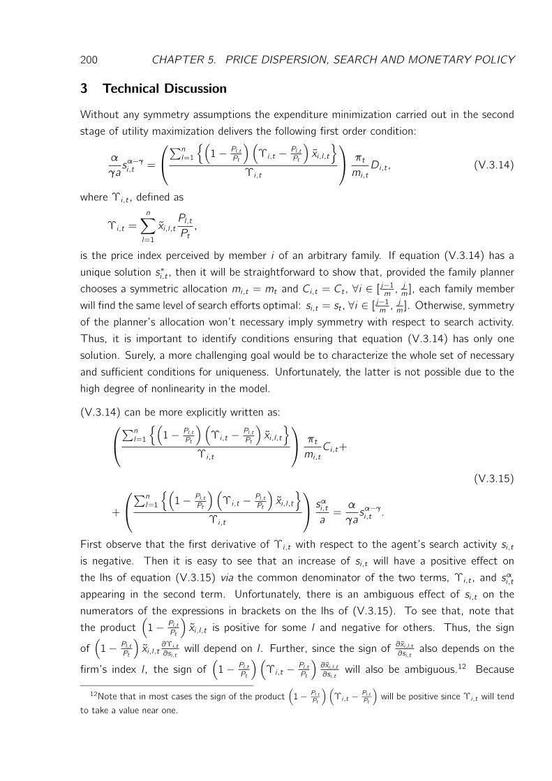
200 CHAPTER 5. PRICE DISPERSION, SEARCH AND MONETARY POLICY
3 Technical Discussion
Without any symmetry assumptions the expenditure minimization carried out in the second
stage of utility maximization delivers the following first order condition:
α
γasα−γi,t =
∑nl=1
(1− Pl ,t
Pt
)(Υi ,t − Pl ,t
Pt
)xi ,l ,t
Υi ,t
πtmi ,tDi ,t , (V.3.14)
where Υi ,t , defined as
Υi ,t =
n∑
l=1
xi ,l ,tPl ,tPt,
is the price index perceived by member i of an arbitrary family. If equation (V.3.14) has a
unique solution s∗i ,t , then it will be straightforward to show that, provided the family planner
chooses a symmetric allocation mi ,t = mt and Ci ,t = Ct , ∀i ∈ [ j−1m , jm ], each family member
will find the same level of search efforts optimal: si ,t = st , ∀i ∈ [ j−1m , jm ]. Otherwise, symmetry
of the planner’s allocation won’t necessary imply symmetry with respect to search activity.
Thus, it is important to identify conditions ensuring that equation (V.3.14) has only one
solution. Surely, a more challenging goal would be to characterize the whole set of necessary
and sufficient conditions for uniqueness. Unfortunately, the latter is not possible due to the
high degree of nonlinearity in the model.
(V.3.14) can be more explicitly written as:
∑nl=1
(1− Pl ,t
Pt
)(Υi ,t − Pl ,t
Pt
)xi ,l ,t
Υi ,t
πtmi ,tCi ,t+
+
∑nl=1
(1− Pl ,t
Pt
) (Υi ,t − Pl ,t
Pt
)xi ,l ,t
Υi ,t
s
αi,t
a=α
γasα−γi,t .
(V.3.15)
First observe that the first derivative of Υi ,t with respect to the agent’s search activity si ,tis negative. Then it is easy to see that an increase of si ,t will have a positive effect on
the lhs of equation (V.3.15) via the common denominator of the two terms, Υi ,t , and sαi,tappearing in the second term. Unfortunately, there is an ambiguous effect of si ,t on the
numerators of the expressions in brackets on the lhs of (V.3.15). To see that, note that
the product(1− Pl ,t
Pt
)xi ,l ,t is positive for some l and negative for others. Thus, the sign
of(1− Pl ,t
Pt
)xi ,l ,t
∂Υi ,t∂si ,t
will depend on l . Further, since the sign of ∂xi ,l ,t∂si ,t
also depends on the
firm’s index l , the sign of(1− Pl ,t
Pt
)(Υi ,t − Pl ,t
Pt
)∂xi ,l ,t∂si ,t
will also be ambiguous.12 Because
12Note that in most cases the sign of the product(1− Pl ,tPt
)(Υi ,t − Pl ,tPt
)will be positive since Υi ,t will tend
to take a value near one.
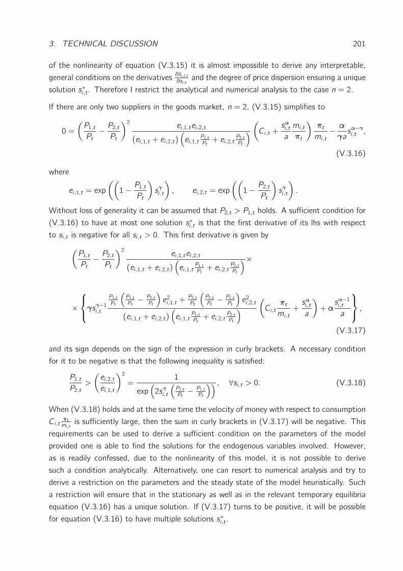
3. TECHNICAL DISCUSSION 201
of the nonlinearity of equation (V.3.15) it is almost impossible to derive any interpretable,
general conditions on the derivatives ∂xi ,l ,t∂si ,t
and the degree of price dispersion ensuring a unique
solution s∗i ,t . Therefore I restrict the analytical and numerical analysis to the case n = 2.
If there are only two suppliers in the goods market, n = 2, (V.3.15) simplifies to
0 =
(P1,tPt− P2,tPt
)2ei ,1,tei ,2,t
(ei ,1,t + ei ,2,t)(ei ,1,t
P1,tPt+ ei ,2,t
P2,tPt
)(Ci ,t +
sαi,ta
mi ,tπt
)πtmi ,t− αγasα−γi,t ,
(V.3.16)
where
ei ,1,t = exp
((1− P1,t
Pt
)sγi,t
), ei ,2,t = exp
((1− P2,t
Pt
)sγi,t
).
Without loss of generality it can be assumed that P2,t > P1,t holds. A sufficient condition for
(V.3.16) to have at most one solution s∗i ,t is that the first derivative of its lhs with respect
to si ,t is negative for all si ,t > 0. This first derivative is given by
(P1,tPt− P2,tPt
)2ei ,1,tei ,2,t
(ei ,1,t + ei ,2,t)(ei ,1,t
P1,tPt+ ei ,2,t
P2,tPt
)×
×γs
γ−1i ,t
P1,tPt
(P1,tPt− P2,tPt
)e2i ,1,t +
P2,tPt
(P2,tPt− P1,tPt
)e2i ,2,t
(ei ,1,t + ei ,2,t)(ei ,1,t
P1,tPt+ ei ,2,t
P2,tPt
)(Ci ,tπtmi ,t+sαi,ta
)+ αsα−1i ,t
a
,
(V.3.17)
and its sign depends on the sign of the expression in curly brackets. A necessary condition
for it to be negative is that the following inequality is satisfied:
P1,tP2,t>
(ei ,2,tei ,1,t
)2=
1
exp(2sγi,t
(P2,tPt− P1,tPt
)) , ∀si ,t > 0. (V.3.18)
When (V.3.18) holds and at the same time the velocity of money with respect to consumption
Ci ,tπtmi ,t
is sufficiently large, then the sum in curly brackets in (V.3.17) will be negative. This
requirements can be used to derive a sufficient condition on the parameters of the model
provided one is able to find the solutions for the endogenous variables involved. However,
as is readily confessed, due to the nonlinearity of this model, it is not possible to derive
such a condition analytically. Alternatively, one can resort to numerical analysis and try to
derive a restriction on the parameters and the steady state of the model heuristically. Such
a restriction will ensure that in the stationary as well as in the relevant temporary equilibria
equation (V.3.16) has a unique solution. If (V.3.17) turns to be positive, it will be possible
for equation (V.3.16) to have multiple solutions s∗i ,t .
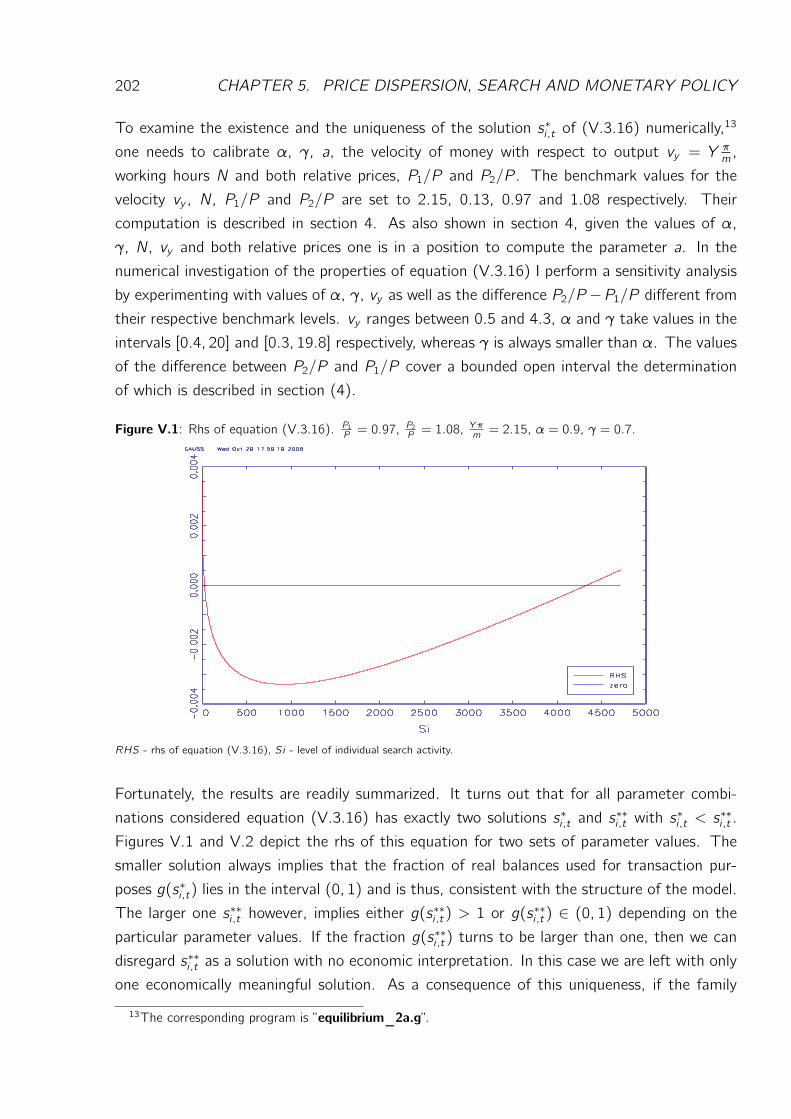
202 CHAPTER 5. PRICE DISPERSION, SEARCH AND MONETARY POLICY
To examine the existence and the uniqueness of the solution s∗i ,t of (V.3.16) numerically,13
one needs to calibrate α, γ, a, the velocity of money with respect to output vy = Y πm ,
working hours N and both relative prices, P1/P and P2/P . The benchmark values for the
velocity vy , N, P1/P and P2/P are set to 2.15, 0.13, 0.97 and 1.08 respectively. Their
computation is described in section 4. As also shown in section 4, given the values of α,
γ, N, vy and both relative prices one is in a position to compute the parameter a. In the
numerical investigation of the properties of equation (V.3.16) I perform a sensitivity analysis
by experimenting with values of α, γ, vy as well as the difference P2/P −P1/P different from
their respective benchmark levels. vy ranges between 0.5 and 4.3, α and γ take values in the
intervals [0.4, 20] and [0.3, 19.8] respectively, whereas γ is always smaller than α. The values
of the difference between P2/P and P1/P cover a bounded open interval the determination
of which is described in section (4).
Figure V.1: Rhs of equation (V.3.16). P1P = 0.97,P2P = 1.08,
Y πm = 2.15, α = 0.9, γ = 0.7.
RHS - rhs of equation (V.3.16), Si - level of individual search activity.
Fortunately, the results are readily summarized. It turns out that for all parameter combi-
nations considered equation (V.3.16) has exactly two solutions s∗i ,t and s∗∗i ,t with s
∗i ,t < s
∗∗i ,t .
Figures V.1 and V.2 depict the rhs of this equation for two sets of parameter values. The
smaller solution always implies that the fraction of real balances used for transaction pur-
poses g(s∗i ,t) lies in the interval (0, 1) and is thus, consistent with the structure of the model.
The larger one s∗∗i ,t however, implies either g(s∗∗i ,t ) > 1 or g(s∗∗i ,t ) ∈ (0, 1) depending on the
particular parameter values. If the fraction g(s∗∗i ,t ) turns to be larger than one, then we can
disregard s∗∗i ,t as a solution with no economic interpretation. In this case we are left with only
one economically meaningful solution. As a consequence of this uniqueness, if the family
13The corresponding program is ”equilibrium_2a.g”.
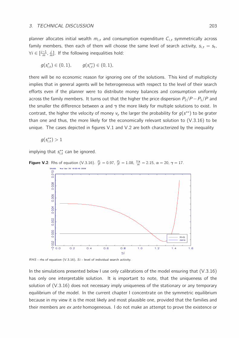
3. TECHNICAL DISCUSSION 203
planner allocates initial wealth mi ,t and consumption expenditure Ci ,t symmetrically across
family members, then each of them will choose the same level of search activity, si ,t = st ,
∀i ∈ [ j−1m, jm]. If the following inequalities hold:
g(s∗i ,t) ∈ (0, 1), g(s∗∗i ,t ) ∈ (0, 1),
there will be no economic reason for ignoring one of the solutions. This kind of multiplicity
implies that in general agents will be heterogeneous with respect to the level of their search
efforts even if the planner were to distribute money balances and consumption uniformly
across the family members. It turns out that the higher the price dispersion P2/P −P1/P and
the smaller the difference between α and γ the more likely for multiple solutions to exist. In
contrast, the higher the velocity of money vy the larger the probability for g(s∗∗) to be grater
than one and thus, the more likely for the economically relevant solution to (V.3.16) to be
unique. The cases depicted in figures V.1 and V.2 are both characterized by the inequality
g(s∗∗i ,t ) > 1
implying that s∗∗i ,t can be ignored.
Figure V.2: Rhs of equation (V.3.16). P1P = 0.97,P2P = 1.08,
Y πm = 2.15, α = 20, γ = 17.
RHS - rhs of equation (V.3.16), Si - level of individual search activity.
In the simulations presented below I use only calibrations of the model ensuring that (V.3.16)
has only one interpretable solution. It is important to note, that the uniqueness of the
solution of (V.3.16) does not necessary imply uniqueness of the stationary or any temporary
equilibrium of the model. In the current chapter I concentrate on the symmetric equilibrium
because in my view it is the most likely and most plausible one, provided that the families and
their members are ex ante homogeneous. I do not make an attempt to prove the existence or
204 CHAPTER 5. PRICE DISPERSION, SEARCH AND MONETARY POLICY
non-existence of further equilibria, characterized by an asymmetric distribution of resources
and heterogeneous levels of search activity, and leave this issue for future research. In this
chapter I am only able to show numerically that for the calibrations chosen the symmetric
equilibrium is locally unique.
4 Calibration
The calibration of this model is more involved than it was the case in the models already
presented.14 First, to reduce the computational burden arising in the approximation, the
calibration and the simulation steps, I consider only the 2-firms case. I assume that the
steady state of the economy is characterized by price dispersion with P1Palways being smaller
than P2P. Alternatively one can assume that the difference between the two relative prices
remains constant over time while in each period firms randomly switch their positions in the
price distribution. The definition of the overall price index
x1P1P+ x2P2P= 1, x1 ∈ (0, 1), x2 = 1− x1
implies that P1P< 1 and P2
P> 1 hold. I start the calibration by setting the difference between
both relative prices ∆ as well as the lower one at particular values. Then the definition of the
price index allows us to determine x1:
x1P1P+ (1− x1)
(P1P+ ∆
)= 1,
⇒
1− x1 = 1− P1/P∆
.
To ensure that the market share of the cheaper supplier is larger then 50 percent, ∆ should
satisfy the following inequality
∆ >1− P1/P0.5
. (V.4.19)
Otherwise the firm charging the higher price will enjoy a larger market share. The level of
search activity in the stationary equilibrium s is identified as the solution of the following
equation:
exp((1− P1
P− ∆)
sγ)
exp((1− P1
P
)sγ
)+ exp
((1− P1
P− ∆)
sγ) = 1− P1/P
∆,
14The corresponding programs are ”equilibrium_2.g” for the general analysis of the sensitivity of the steadystate with respect to the degree of price dispersion ∆ = P2/P − P1/P and ”equilibrium_2a.g” for the deter-
mination of the upper bound for ∆.

4. CALIBRATION 205
which implies
s =
ln
(∆+P1/P−11−P1/P
)
∆
1γ
.
I assume that the sum of the steady state levels of the firm specific productivity variables is
equal to zero:
ι1 = ι, ι2 = −ι.
Further, the steady state value Z of the economy wide productivity shock is set to one.
Hence, the two total factor productivities in the stationary equilibrium are given by 1+ ι and
1− ι for firm 1 and firm 2 respectively. To calibrate ι, I use the conditions for optimal price
setting of the two firms:
P1P=1
sγx2+W/P
1 + ι,
P2P=1
sγx1+W/P
1− ι .
Combining these two equations yields:
1 + ι
1− ι =P2P− 1sγx1
P1P− 1sγx2︸ ︷︷ ︸
:=ϕ
.
Thus ι can be computed as:
ι =ϕ− 1ϕ+ 1
.
Note that both the numerator and the denominator of ϕmust be grater than zero.15 But since
P2/P > P1/P and sγx1 > sγx2 it suffices to ensure that the difference P1P− 1sγx2
is positive.
This requirement imposes an upper bound on ∆ which can be approximated numerically. The
numerical analysis16 also allows us to find a lower bound for P1/P . The lhs and the rhs of
the inequality
P1P>1
sγx2︸︷︷︸:=fl
(V.4.20)
are depicted in figures V.3, V.4 and V.5 for different values of P1/P and ∆. Recall that s as
well as x2 depend on ∆.
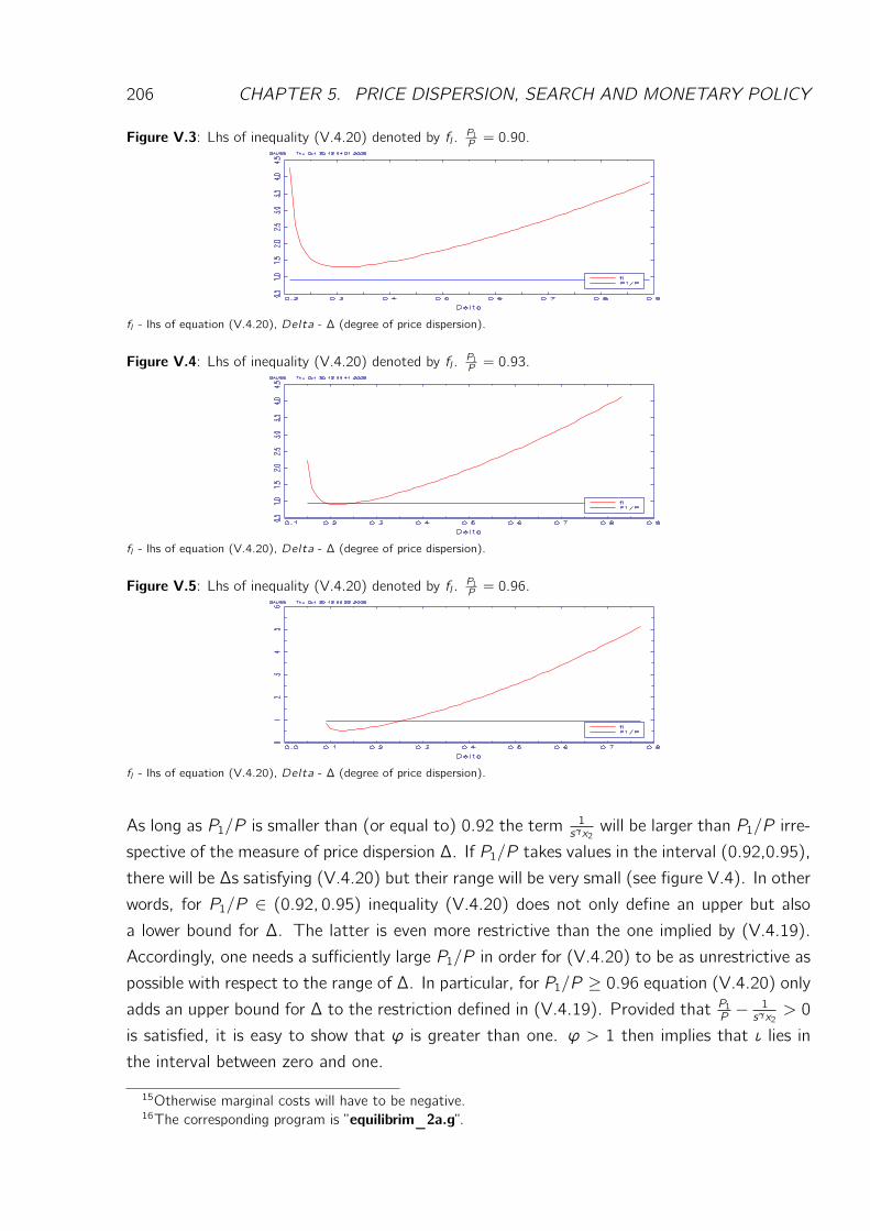
206 CHAPTER 5. PRICE DISPERSION, SEARCH AND MONETARY POLICY
Figure V.3: Lhs of inequality (V.4.20) denoted by fl . P1P = 0.90.
fl - lhs of equation (V.4.20), Delta - ∆ (degree of price dispersion).
Figure V.4: Lhs of inequality (V.4.20) denoted by fl . P1P = 0.93.
fl - lhs of equation (V.4.20), Delta - ∆ (degree of price dispersion).
Figure V.5: Lhs of inequality (V.4.20) denoted by fl . P1P = 0.96.
fl - lhs of equation (V.4.20), Delta - ∆ (degree of price dispersion).
As long as P1/P is smaller than (or equal to) 0.92 the term 1sγx2
will be larger than P1/P irre-
spective of the measure of price dispersion ∆. If P1/P takes values in the interval (0.92,0.95),
there will be ∆s satisfying (V.4.20) but their range will be very small (see figure V.4). In other
words, for P1/P ∈ (0.92, 0.95) inequality (V.4.20) does not only define an upper but also
a lower bound for ∆. The latter is even more restrictive than the one implied by (V.4.19).
Accordingly, one needs a sufficiently large P1/P in order for (V.4.20) to be as unrestrictive as
possible with respect to the range of ∆. In particular, for P1/P ≥ 0.96 equation (V.4.20) onlyadds an upper bound for ∆ to the restriction defined in (V.4.19). Provided that P1
P− 1sγx2> 0
is satisfied, it is easy to show that ϕ is greater than one. ϕ > 1 then implies that ι lies in
the interval between zero and one.
15Otherwise marginal costs will have to be negative.16The corresponding program is ”equilibrim_2a.g”.
4. CALIBRATION 207
An important question regarding the calibration of ∆ is to what extent its range is consistent
with the empirically observable price dispersion among homogeneous nondurable goods. For
example P1/P = 0.97 implies that ∆ should range between 0.06 and 0.25, corresponding to a
percentage difference between the two prices lying between 6 and 23 percent of P1/P . Lach
(2002) provides evidence on price dispersion for virtually homogeneous commodities based
on a panel of stores in the USA. After controlling for observable as well as unobservable
sources of heterogeneity17 between physically homogeneous products he obtains the following
estimates: The difference between the logarithms of the 95% and the 5% quantiles of the
price distribution equals 0.10, 0.23, 0.22 and 0.16 for Refrigerator,18 Chicken, Coffee and
Flour respectively. The differences between the logs of the 75% and the 25% quantiles
of the price distributions of the same commodities are equal to 0.03, 0.09, 0.05 and 0.04
respectively. Thus, choosing ∆ to imply that ln(P2/P ) − ln(P1/P ) lies between 0.10 and
0.20 can be seen as a compromise calibration. For the sake of completeness I also perform
a sensitivity analysis with respect to ∆.
Next, by using the first order condition for optimal price setting of one of the firms one can
compute the steady state value of the real wage:
W
P= (1 + ι)
(P1P− 1
sγx2
).
To calibrate the velocity of money with respect to output vy = Y πm I use national accounts
data provided by the NIPA. Real balances MtPt−1
are measured as the ratio of the monetary
aggregate M1 divided by the value of the nondurables consumption deflator in the previous
period (base year 2000). The same deflator is also used to compute the inflation factor.
Aggregate output is measured by the gross national product at constant prices (base year
2000) adjusted by the imputed product generated by the stock of durable goods and the
government capital stock.19 The mean of the velocity of money for the period from 1973:Q1
through 2003:Q4 equals 2.15. Given vy one is able to compute the parameter a via the
condition governing the optimal level of search efforts (V.2.11) evaluated at the symmetric
steady state:
α
aγsα−γ =
(2∑
l=1
xl ,t
(1− PlP
)2)π
mY
︸︷︷︸:=vy
.
The fraction of time spent working in the stationary equilibrium N is set to 0.1386. The
labor inputs of the two firms, N1 and N2, can be computed as the solution to the following17Lach (2002) controls for the store selling the particular product, the location of the store, the type of the
store as well as for time effects.18Note that refrigerators are durable goods.19The computation procedure is described in Cooley and Prescott (1995).
208 CHAPTER 5. PRICE DISPERSION, SEARCH AND MONETARY POLICY
system of equations:
N1N2=
:=$︷ ︸︸ ︷x1x2
(1− ι)(1 + ι)
N1 + N2 = N.
The result reads:
N1 =$
1 +$N, N2 =
1
1 +$N.
Then the steady state levels of output and consumption are readily computed via:
Y =P1P(1 + ι)N1 +
P2P(1− ι)N2,
m
π=Y
vy,
C = Y − g(s)mπ.
The first of these equations reflects the definition of the economy’s national product: the
latter equals the sum of the two firm-specific products, both measured in units of a common
numeraire. The second equation reflects the definition of the velocity of money with respect
to output. The third equation stems from the requirement that in equilibrium aggregate
supply Y equals aggregate demand D = C + g(s)mπ.
The remaining parameters are set to the so called standard values usually found in the
literature. Table V.1 summarizes the calibration of the model.
Table V.1:Calibration
Households/Preferences Firms/Technology Central Bank
α > 0 sensitivity analysis Z∗ = 1 τ∗ = 1.0138
γ > 0 sensitivity analysis ρz = 0, 0.9641 ρτ = 0
β = 0.991 σε = 0.0082 σu = 0.0092
η = 2 P1/P ∈ (0.95, 0.99] vy = 2.15
χ = 2 ∆ sensitivity analysis
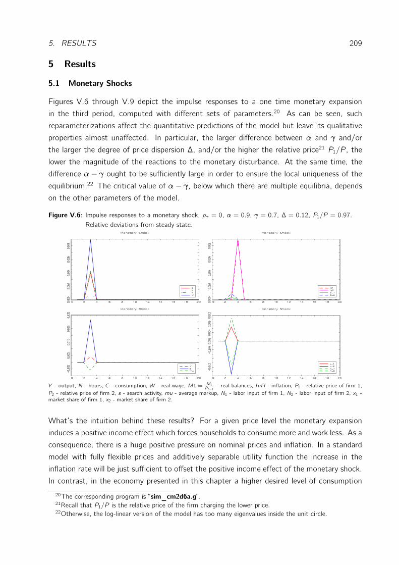
5. RESULTS 209
5 Results
5.1 Monetary Shocks
Figures V.6 through V.9 depict the impulse responses to a one time monetary expansion
in the third period, computed with different sets of parameters.20 As can be seen, such
reparameterizations affect the quantitative predictions of the model but leave its qualitative
properties almost unaffected. In particular, the larger difference between α and γ and/or
the larger the degree of price dispersion ∆, and/or the higher the relative price21 P1/P , the
lower the magnitude of the reactions to the monetary disturbance. At the same time, the
difference α− γ ought to be sufficiently large in order to ensure the local uniqueness of the
equilibrium.22 The critical value of α− γ, below which there are multiple equilibria, depends
on the other parameters of the model.
Figure V.6: Impulse responses to a monetary shock, ρτ = 0, α = 0.9, γ = 0.7, ∆ = 0.12, P1/P = 0.97.Relative deviations from steady state.
Y - output, N - hours, C - consumption, W - real wage, M1 = MtPt−1 - real balances, Inf l - inflation, P1 - relative price of firm 1,
P2 - relative price of firm 2, s - search activity, mu - average markup, N1 - labor input of firm 1, N2 - labor input of firm 2, x1 -market share of firm 1, x2 - market share of firm 2.
What’s the intuition behind these results? For a given price level the monetary expansion
induces a positive income effect which forces households to consume more and work less. As a
consequence, there is a huge positive pressure on nominal prices and inflation. In a standard
model with fully flexible prices and additively separable utility function the increase in the
inflation rate will be just sufficient to offset the positive income effect of the monetary shock.
In contrast, in the economy presented in this chapter a higher desired level of consumption
20The corresponding program is ”sim_cm2d6a.g”.21Recall that P1/P is the relative price of the firm charging the lower price.22Otherwise, the log-linear version of the model has too many eigenvalues inside the unit circle.
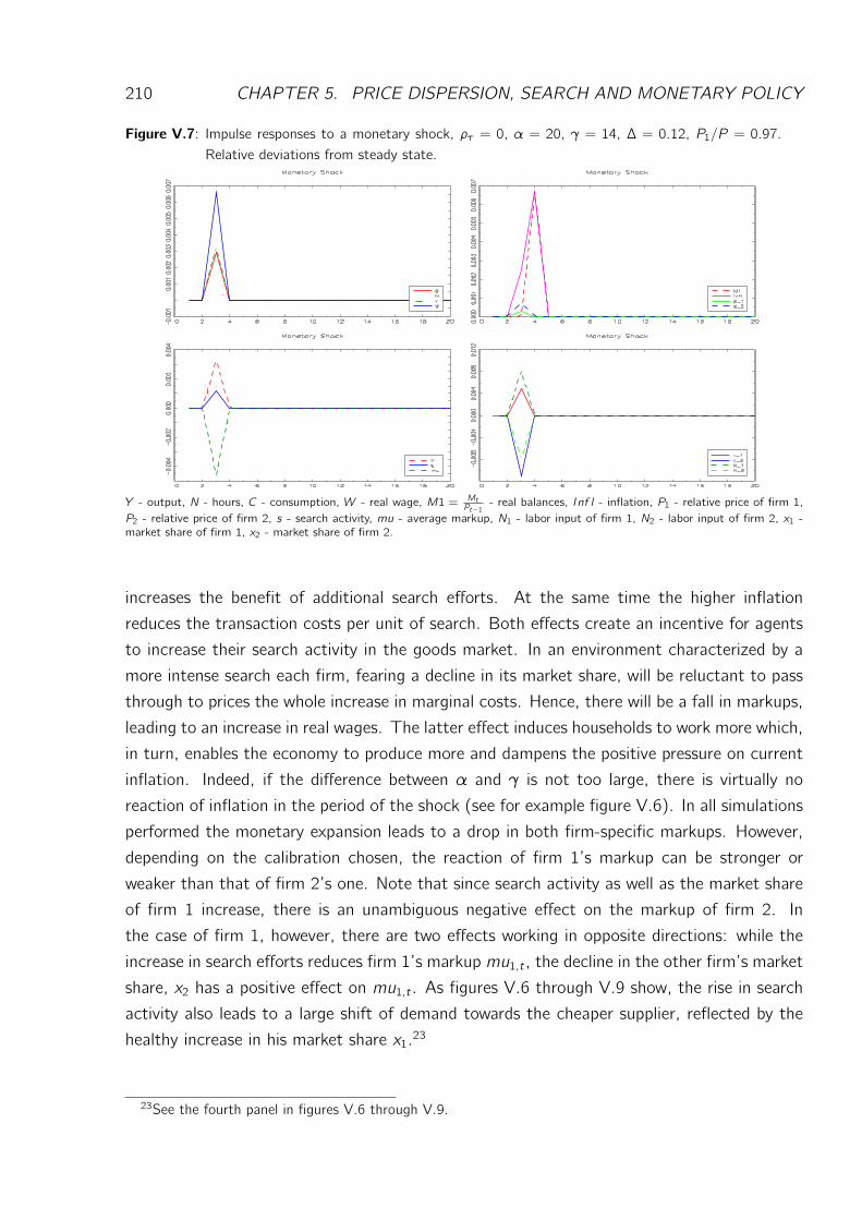
210 CHAPTER 5. PRICE DISPERSION, SEARCH AND MONETARY POLICY
Figure V.7: Impulse responses to a monetary shock, ρτ = 0, α = 20, γ = 14, ∆ = 0.12, P1/P = 0.97.Relative deviations from steady state.
Y - output, N - hours, C - consumption, W - real wage, M1 = MtPt−1 - real balances, Inf l - inflation, P1 - relative price of firm 1,
P2 - relative price of firm 2, s - search activity, mu - average markup, N1 - labor input of firm 1, N2 - labor input of firm 2, x1 -market share of firm 1, x2 - market share of firm 2.
increases the benefit of additional search efforts. At the same time the higher inflation
reduces the transaction costs per unit of search. Both effects create an incentive for agents
to increase their search activity in the goods market. In an environment characterized by a
more intense search each firm, fearing a decline in its market share, will be reluctant to pass
through to prices the whole increase in marginal costs. Hence, there will be a fall in markups,
leading to an increase in real wages. The latter effect induces households to work more which,
in turn, enables the economy to produce more and dampens the positive pressure on current
inflation. Indeed, if the difference between α and γ is not too large, there is virtually no
reaction of inflation in the period of the shock (see for example figure V.6). In all simulations
performed the monetary expansion leads to a drop in both firm-specific markups. However,
depending on the calibration chosen, the reaction of firm 1’s markup can be stronger or
weaker than that of firm 2’s one. Note that since search activity as well as the market share
of firm 1 increase, there is an unambiguous negative effect on the markup of firm 2. In
the case of firm 1, however, there are two effects working in opposite directions: while the
increase in search efforts reduces firm 1’s markup mu1,t , the decline in the other firm’s market
share, x2 has a positive effect on mu1,t . As figures V.6 through V.9 show, the rise in search
activity also leads to a large shift of demand towards the cheaper supplier, reflected by the
healthy increase in his market share x1.23
23See the fourth panel in figures V.6 through V.9.
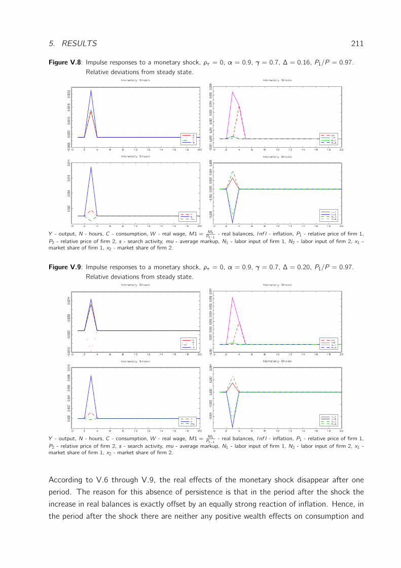
5. RESULTS 211
Figure V.8: Impulse responses to a monetary shock, ρτ = 0, α = 0.9, γ = 0.7, ∆ = 0.16, P1/P = 0.97.Relative deviations from steady state.
Y - output, N - hours, C - consumption, W - real wage, M1 = MtPt−1 - real balances, Inf l - inflation, P1 - relative price of firm 1,
P2 - relative price of firm 2, s - search activity, mu - average markup, N1 - labor input of firm 1, N2 - labor input of firm 2, x1 -market share of firm 1, x2 - market share of firm 2.
Figure V.9: Impulse responses to a monetary shock, ρτ = 0, α = 0.9, γ = 0.7, ∆ = 0.20, P1/P = 0.97.Relative deviations from steady state.
Y - output, N - hours, C - consumption, W - real wage, M1 = MtPt−1 - real balances, Inf l - inflation, P1 - relative price of firm 1,
P2 - relative price of firm 2, s - search activity, mu - average markup, N1 - labor input of firm 1, N2 - labor input of firm 2, x1 -market share of firm 1, x2 - market share of firm 2.
According to V.6 through V.9, the real effects of the monetary shock disappear after one
period. The reason for this absence of persistence is that in the period after the shock the
increase in real balances is exactly offset by an equally strong reaction of inflation. Hence, in
the period after the shock there are neither any positive wealth effects on consumption and
212 CHAPTER 5. PRICE DISPERSION, SEARCH AND MONETARY POLICY
leisure nor any positive (or negative) pressure on search activity via the term mtπt. Thus, there
are no incentives for agents to search more (or less) than in the stationary equilibrium.
A further interesting feature of the model is that as a reaction to a monetary expansion both
relative prices deviate positively from their respective steady state values. However, there is
no violation of the definition of the overall price index since the impulse responses of P1/P
and P2/P are accompanied by suitable reactions of the market shares x1 and x2.
Summarizing the results, I would like to point out that even though the model presented here
does not reproduce the empirically observable shape and persistence of the impulse responses
to monetary shocks, it proposes a simple mechanism which substantially amplifies the real
effects of monetary policy, making their magnitude consistent with the empirical estimates.
Furthermore, as figure V.6 suggests, combining the current model with other theoretical
building blocks could be a fruitful line of research when trying to explain the observable
delayed response of inflation to monetary expansions.
5.2 Technology Shocks
Figures V.10 through V.12 depict the impulse responses to an economy wide technology
shock with no serial correlation. In all cases there is a slight decrease in both relative prices,
with the reaction of P2/P being stronger. There is a large drop in search activity and perhaps
surprisingly, an increase in the market share of the firm charging the higher price. The intuition
behind these results is as follows: The technology shock enables the economy to produce
more even by employing less labor and so puts a downward pressure on inflation. The fall in
inflation has a strong negative effect on search activity. The lower level of search intensity
in the goods market enables both firms to choose higher markups. At the same time, due to
the technological improvement, for any given real wage marginal costs become lower. The
firm with the lower steady state productivity (firm 2) faces a larger marginal cost decrease,
which enables it to reduce its relative price P2/P by a larger percentage amount than firm
1 does.24 The stronger (weaker) decrease in the relative price of firm 2 (firm 1) combined
with a lower search activity in the goods market, in turn, leads to an increase in the market
share of the supplier charging the higher price (firm 2).
What happens to markups? The fall in both, overall search efforts and the market share
of firm 1, unambiguously makes it possible for firm 2 to increase its markup. With regard
to firm 1 there are again two opposing effects: The decline in search intensity allows firm
1 to set a higher markup but the increase in the market share of its competitor does the
24The direct effect of the productivity disturbance on the relative price is measured by the term W/P(P1/P )(1+ι)
Zt
in the case of firm 1 and by W/P(P2/P )(1−ι) Zt for firm 2. In all numerical simulations performed (P1/P )(1 + ι) is
larger than one while (P2/P )(1− ι) takes a value below one.
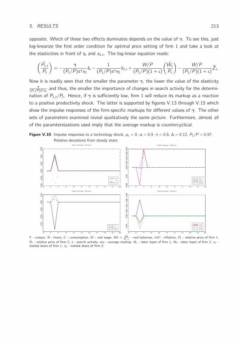
5. RESULTS 213
opposite. Which of these two effects dominates depends on the value of γ. To see this, just
log-linearize the first order condition for optimal price setting of firm 1 and take a look at
the elasticities in front of st and x2,t . The log-linear equation reads:
ˆ(P1,tPt
)= − γ
(P1/P )sγx2st − 1
(P1/P )sγx2x2,t +
W/P
(P1/P )(1 + ι)
ˆ(WtPt
)− W/P
(P1/P )(1 + ι)Zt .
Now it is readily seen that the smaller the parameter γ, the lower the value of the elasticityγ
(P1/P )sγx2and thus, the smaller the importance of changes in search activity for the determi-
nation of P1,t/Pt . Hence, if γ is sufficiently low, firm 1 will reduce its markup as a reaction
to a positive productivity shock. The latter is supported by figures V.13 through V.15 which
show the impulse responses of the firm-specific markups for different values of γ. The other
sets of parameters examined reveal qualitatively the same picture. Furthermore, almost all
of the paramtereizations used imply that the average markup is countercyclical.
Figure V.10: Impulse responses to a technology shock, ρz = 0, α = 0.9, γ = 0.6, ∆ = 0.12, P1/P = 0.97.Relative deviations from steady state.
Y - output, N - hours, C - consumption, W - real wage, M1 = MtPt−1 - real balances, Inf l - inflation, P1 - relative price of firm 1,
P2 - relative price of firm 2, s - search activity, mu - average markup, N1 - labor input of firm 1, N2 - labor input of firm 2, x1 -market share of firm 1, x2 - market share of firm 2.
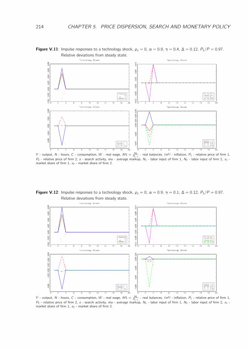
214 CHAPTER 5. PRICE DISPERSION, SEARCH AND MONETARY POLICY
Figure V.11: Impulse responses to a technology shock, ρz = 0, α = 0.9, γ = 0.4, ∆ = 0.12, P1/P = 0.97.Relative deviations from steady state.
Y - output, N - hours, C - consumption, W - real wage, M1 = MtPt−1 - real balances, Inf l - inflation, P1 - relative price of firm 1,
P2 - relative price of firm 2, s - search activity, mu - average markup, N1 - labor input of firm 1, N2 - labor input of firm 2, x1 -market share of firm 1, x2 - market share of firm 2.
Figure V.12: Impulse responses to a technology shock, ρz = 0, α = 0.9, γ = 0.1, ∆ = 0.12, P1/P = 0.97.Relative deviations from steady state.
Y - output, N - hours, C - consumption, W - real wage, M1 = MtPt−1 - real balances, Inf l - inflation, P1 - relative price of firm 1,
P2 - relative price of firm 2, s - search activity, mu - average markup, N1 - labor input of firm 1, N2 - labor input of firm 2, x1 -market share of firm 1, x2 - market share of firm 2.
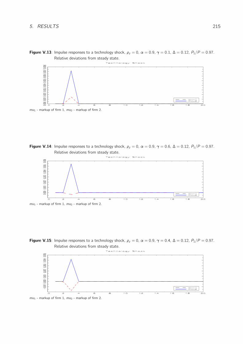
5. RESULTS 215
Figure V.13: Impulse responses to a technology shock, ρz = 0, α = 0.9, γ = 0.1, ∆ = 0.12, P1/P = 0.97.Relative deviations from steady state.
mu1 - markup of firm 1, mu2 - markup of firm 2.
Figure V.14: Impulse responses to a technology shock, ρz = 0, α = 0.9, γ = 0.6, ∆ = 0.12, P1/P = 0.97.Relative deviations from steady state.
mu1 - markup of firm 1, mu2 - markup of firm 2.
Figure V.15: Impulse responses to a technology shock, ρz = 0, α = 0.9, γ = 0.4, ∆ = 0.12, P1/P = 0.97.Relative deviations from steady state.
mu1 - markup of firm 1, mu2 - markup of firm 2.
216 CHAPTER 5. PRICE DISPERSION, SEARCH AND MONETARY POLICY
6 Capital Accumulation
6.1 The Model
Let us extend the model by assuming that there are two production factors - capital and
labor. The production function of firm l exhibits constant returns to scale and is given by
Yl ,t = (Zt + ιl ,t)Nωl,tK
1−ωl,t , ω ∈ (0, 1),
where Kl ,t denotes capital input and Zt+ιl ,t represents total factor productivity following the
same stochastic process as in section 2. The aggregate stock of capital evolves according to
Kt+1 = It + (1− υ)Kt , υ ∈ (0, 1). (V.6.1)
Marginal costs of firm l , µl ,t are now given by
µl ,t =(Wt/Pt)
ωR1−ωtωω(1− ω)1−ω(Zt + ιl ,t) , (V.6.2)
where Rt denotes the rental rate of capital.
Household’s First Order Conditions
Retaining the notation used in section 2 the set of first order conditions describing the
behavior of he typical household have to be extended by the following three equations:
Λt = βEtΛt+1(1 + Rt+1 − υ),
Ct + It + g(st)mtπt︸ ︷︷ ︸
:=Dt
+mt+1 − mtπt=WtPtNt + RtKt +Πt +
TtPt,
Kt+1 = It + (1− υ)Kt .
(V.6.3)
The first condition is the Euler equation governing optimal capital accumulation. The second
one is the modified budget constraint. Note that in this version of the model aggregate
demand Dt equals the sum of consumption, investment and the expenditure on transaction
services. The last equation in (V.6.3) is the low of motion of the capital stock.
Equilibrium
The evolution of the economy is described by the new definition of marginal costs (V.6.2),
the first order condition for optimal price setting (V.2.3), the households first order condi-
tions (V.2.7), (V.2.8), (V.2.9) and (V.2.11) modified by (V.6.3), the aggregate consistency
6. CAPITAL ACCUMULATION 217
conditions
xl ,tDt = (Zt + ιl ,t)Nωl,tK
1−ωl,t l = 1, 2, ..., n, (V.6.4)
andn∑
l=1
Nl ,t = Nt ,
n∑
l=1
Kl ,t = Kt (V.6.5)
as well as the definitions of xl ,t for l = 1, 2, ..., n and Dt . Note that if (V.7.4) are satisfied,then the family’s budget constraint implies:
Dt = Yt =
n∑
l=1
Pl ,tPt(Zt + ιl ,t)N
ωl,tK
1−ωl,t .
To close the model, one again needs to specify monetary policy and the exogenous productivity
processes Zt and ιl ,t .
Calibration
P1/P . α, γ, the measure of price dispersion ∆, the velocity of money with respect to output
vy , ι, N and the parameter a are calibrated in the same way as in the fixed capital case.2526
Then the marginal costs of the two firms can be calibrated by using their price setting
conditions:
µ1 =(W/P )ωR1−ω
ωω(1− ω)1−ω(1 + ι) =(P1P− 1
sγx2
), µ2 =
(W/P )ωR1−ω
ωω(1− ω)1−ω(1− ι) =(P2P− 1
sγx1
)
To calibrate the production elasticity of labor, first observe that the real wage and the two
marginal costs are related as follows:
W
P= µ1(1 + ι)ωN
ω−11 K1−ω1 = µ2(1 + ι)ωN
ω−12 K1−ω2 .
Hence,
W
PN1 = ωµ1 (1 + ι)N
ω1K
1−ω1︸ ︷︷ ︸
=x1Y
,W
PN2 = ωµ2 (1 + ι)N
ω2K
1−ω2︸ ︷︷ ︸
=x2Y
.
Adding the last two equations together and rearranging yields:
ω =(W/P )N
Y︸ ︷︷ ︸:= labor share
· 1
x1µ1 + x2µ2.
25See section 4.26The analysis of the sensitivity of the steady state with respect to ∆ can be found in the program ”equilib-
rium_3.g”.
218 CHAPTER 5. PRICE DISPERSION, SEARCH AND MONETARY POLICY
The labor share is computed on the basis of the national accounts data provided by the NIPA
and transformed in the way suggested by Cooley and Prescott (1995). The value obtained
equals 0.6748. Unfortunately, P1/P < 0.98 implies that the range of values of ∆ consistent
with ω ∈ (0, 1) is extremely small. When the relative price P1/P is larger or equal to 0.98,
∆ should be smaller than 0.09 in order for ω to lie in the range between zero and one.
The consumption-output ratio CYis found by using the economy’s resource constraint:
C
Y=1− g(s)
vy
1− IC
,
where the investment-consumption ratio ICis set at its empirical value 0.1982 obtained with
date from NIPA’s national accounts, transformed as in Cooley and Prescott (1995).
To determine the ratio K1/K2 I use the first order conditions for optimal capital input of
both firms, evaluated at the stationary equilibrium:
R
R= 1 =
µ1µ2
1 + ι
1− ι(N1N2
)ω (K1K2
)−ω. (V.6.6)
Multiplying the rhs of the last equation by K1K2· K2K1
and rearranging yields:
1 =µ1µ2
x1x2
Y
Y
K2K1
which implies:
K1/Y
K2/Y=µ1µ2
x1x2︸ ︷︷ ︸
:=ϕ2
.
Then the aggregate consistency condition for capital input
K1Y+K2Y=K
Y
allows me to determine K1/Y and K2/Y :
K1Y=
ϕ21 + ϕ2
K
Y,
K2Y=
1
1 + ϕ2
K
Y.
The economy wide capital intensity K/Y is estimated with data provided by the NIPA. The
value obtained is 17.44. Having found K1/Y and K2/Y one can use equation (V.6.6) and
the aggregate consistency condition
N1 + N2 = N
to compute N1 and N2. The result is:
N1 =ϕ11 + ϕ1
N, N2 =1
1 + ϕ1N,
6. CAPITAL ACCUMULATION 219
where
ϕ1 =K1K2
(µ1µ2
1− ι1 + ι
) 1ω
.
The depreciation rate υ is calibrated as in the previous sections.
6.2 Results
Monetary Shocks: Figure V.16 depicts the impulse responses to a non-autocorrelated mon-
etary shock.27 Obviously, the model with flexible capital delivers the same qualitative predic-
tions as the one without capital accumulation: The monetary shock is expansionary mainly
due to the fall in markups and triggers off relatively weak reactions of the main economic
aggregates. For example the peak-response of output (investment) is about 10 (3) times
weaker than what is predicted by the SVAR of Chrstiano et al. (2005). The reactions implied
by the current model again have the counterfactual property of being extremely short-lived.
Similar to the no-capital case, the larger the difference between α and γ and/or the higher
the degree of price dispersion measured by ∆, the weaker the real effects of the monetary
shock. In general, in this version of the model the response of consumption is of much smaller
magnitude than it was the case in the economy presented in section 2. The reason is that
capital accumulation allows a more effective consumption smoothing. To take advantage of
this possibility, households sharply increase investment in the period of the shock, absorbing
in this way virtually the whole additional output. The resulting increase in the capital stock
enables the economy to produce and consume more over a relatively long period of time.
However, the deviations of output and consumption from their respective steady state values
in the periods after the shock are very small.
Technology Shocks: The reactions to technology shocks predicted by the model with flex-
ible capital are also similar to their counterparts implied by the model of section 2 (see figure
V.17). For the bulk of the parameterizations examined markups respond negatively to im-
provements in productivity. As a result, in almost all cases markups are countercyclical on
average. The incentive to smooth consumption over time is again strong enough to force
households to substantially accelerate capital accumulation in the period of the shock. As a
consequence, virtually the whole additional production is again absorbed by investment expen-
diture. In the periods after the shock there is a very small positive deviation of consumption
from its steady state value financed by the additionally accumulated capital.
27The corresponding program is ”sim_cm2d7a.g”.
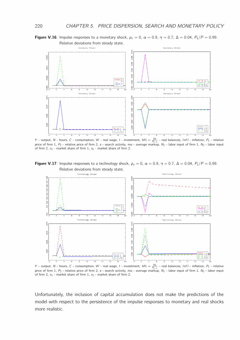
220 CHAPTER 5. PRICE DISPERSION, SEARCH AND MONETARY POLICY
Figure V.16: Impulse responses to a monetary shock, ρτ = 0, α = 0.9, γ = 0.7, ∆ = 0.04, P1/P = 0.99.Relative deviations from steady state.
Y - output, N - hours, C - consumption, W - real wage, I - investment, M1 = MtPt−1 - real balances, Inf l - inflation, P1 - relative
price of firm 1, P2 - relative price of firm 2, s - search activity, mu - average markup, N1 - labor input of firm 1, N2 - labor inputof firm 2, x1 - market share of firm 1, x2 - market share of firm 2.
Figure V.17: Impulse responses to a technology shock, ρz = 0, α = 0.9, γ = 0.7, ∆ = 0.04, P1/P = 0.99.Relative deviations from steady state.
Y - output, N - hours, C - consumption, W - real wage, I - investment, M1 = MtPt−1 - real balances, Inf l - inflation, P1 - relative
price of firm 1, P2 - relative price of firm 2, s - search activity, mu - average markup, N1 - labor input of firm 1, N2 - labor inputof firm 2, x1 - market share of firm 1, x2 - market share of firm 2.
Unfortunately, the inclusion of capital accumulation does not make the predictions of the
model with respect to the persistence of the impulse responses to monetary and real shocks
more realistic.
7. SHOPPING-TIME MODELS 221
7 Shopping-Time Models
7.1 A Standard Shopping-Time Model
Consider an economy with fully flexible prices and perfectly competitive markets. The utility
function of the representative household takes the form
U = Et
∞∑t=0
βt(C1−ηt1− η −
b
2(1− Lt)2
), b, η > 0, β ∈ (0, 1),
where Lt denotes leisure. The corresponding budget constraint is given by
Ct +Mt+1Pt− MtπtPt−1
=WtPtNt +
TtPt, ∀t.
A positive valuation of money arises through the following ”shopping-time” constraint:
sαt1 + sαt
= κCtmt/πt
, (V.7.1)
where κ > 0 and sαt1+sαt
is the time needed to carry out transactions in the goods market.
According to (V.7.1) a higher real value of the money balances accumulated in the previous
period, mtπt
reduces he transaction time associated with a given desired level of consumption
and thus, lowers the transaction costs. The shopping-time technology (V.7.1) originates
from the idea that in a typical barter economy each agent faces extremely large search costs
since she can only achieve the desired consumption bundle if she is able to find enough other
individuals supplying exactly the goods our agent desires and at the same time, demanding
exactly the good(s) she supplies. The search costs, however, can be substantially reduced
by the introduction of money as a common medium of exchange and unit of account. The
transaction cost motive for holding money dates back to Baumol (1952) and Tobin (1956).
In more recent papers Saving (1971), Jovanovich (1982) and Romer (1986) develop general
equilibrium versions of the shopping-time model. The model analysed in this subsection is
very similar to the one presented in Walsh (2003), Ch. 3.
The time constraint of the household reads:
Lt + Nt +sαt1 + sαt
= 1.
The representative firm produces according to the production function:
Yt = ZtNt ,
where Zt evolves according to the same stochastic process as in the previous sections. The
behavior of the central bank, too, is modeled as in section 2.
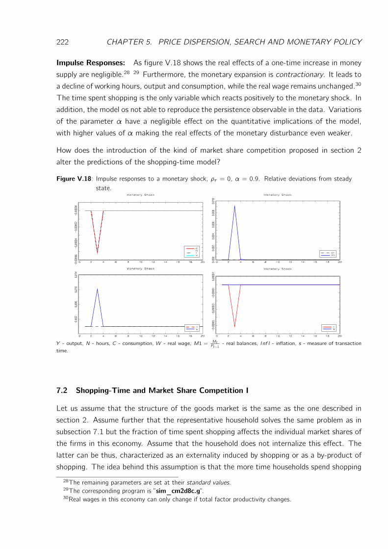
222 CHAPTER 5. PRICE DISPERSION, SEARCH AND MONETARY POLICY
Impulse Responses: As figure V.18 shows the real effects of a one-time increase in money
supply are negligible.28 29 Furthermore, the monetary expansion is contractionary. It leads to
a decline of working hours, output and consumption, while the real wage remains unchanged.30
The time spent shopping is the only variable which reacts positively to the monetary shock. In
addition, the model os not able to reproduce the persistence observable in the data. Variations
of the parameter α have a negligible effect on the quantitative implications of the model,
with higher values of α making the real effects of the monetary disturbance even weaker.
How does the introduction of the kind of market share competition proposed in section 2
alter the predictions of the shopping-time model?
Figure V.18: Impulse responses to a monetary shock, ρτ = 0, α = 0.9. Relative deviations from steadystate.
Y - output, N - hours, C - consumption, W - real wage, M1 = MtPt−1 - real balances, Inf l - inflation, s - measure of transaction
time.
7.2 Shopping-Time and Market Share Competition I
Let us assume that the structure of the goods market is the same as the one described in
section 2. Assume further that the representative household solves the same problem as in
subsection 7.1 but the fraction of time spent shopping affects the individual market shares of
the firms in this economy. Assume that the household does not internalize this effect. The
latter can be thus, characterized as an externality induced by shopping or as a by-product of
shopping. The idea behind this assumption is that the more time households spend shopping
28The remaining parameters are set at their standard values.29The corresponding program is ”sim_cm2d8c.g”.30Real wages in this economy can only change if total factor productivity changes.
7. SHOPPING-TIME MODELS 223
and thus, the more transactions they are involved in, the better informed they are about
the current price distribution as well as the price setting behavior of the individual suppliers.
This information allows households to at least partly shift their demand towards the relatively
cheap suppliers.
The market share of firm l evolves according to:
xl ,t =exp
((1− Pl ,t
Pt
)sγt
)
∑nj=1 exp
((1− Pj,t
Pt
)sγt
) , γ > 0. (V.7.1)
Hence, firms with above average prices suffer larger losses in market share when households
devote more time to transactions in the goods market. Note that in this model aggregate
demand equals aggregate consumption expenditure.
Equilibrium: The evolution of this economy is described by the following set of equations.
The utility maximization problem of the representative household delivers the following first
order conditions:
C−ηt = Λt + κΓtπtmt,
b(1− Lt) = ΛtWtPt,
ΛtWtPt= Γ
αsα−1t
(1 + sαt )2,
sαt1 + sαt
= κCtmt/πt
,
Λt = βEt
κΓt+1m2t+1
Ct+1πt+1 +Λt+1πt+1
,
Ct +mt+1 − mtπt=WtPtNt +Πt +
TtPt,
Nt +sαt1 + sαt
+ Lt = 1,
(V.7.2)
where Λt and Γt are the lagrangean multipliers associated with the budget constraint and the
shopping-time constraint respectively.
224 CHAPTER 5. PRICE DISPERSION, SEARCH AND MONETARY POLICY
The conditions for optimal price setting of the two firms are again given by:
P1,tPt=
1
sγt x2,t+Wt/PtZt + ι1,t
,
P2,tPt=
1
sγt x1,t+Wt/PtZt + ι2,t
.
(V.7.3)
Furthermore, the following aggregate consistency conditions hold:31
xl ,tDt = (Zt + ιl ,t)Nl ,t , l = 1, 2, (V.7.4)
and
2∑
l=1
Nl ,t = Nt . (V.7.5)
Impulse Responses: Unfortunately, it turns out that there is only a relatively small range of
parameter values implying an economically meaningful stationary equilibrium.32 In particular,
to ensure that the steady state value of leisure is positive, the relative price P1/P should be
lower than 0.96 and at the same time, the difference α − γ should be sufficiently low. The
critical value for α − γ depends on the absolute values of the two parameters as well as on
P1/P . Figure V.19 depicts the impulse responses to a monetary disturbance without serial
correlation. The increase in inflation necessitates a higher level of transaction time. As a
result firms are forced to reduce their markups which in turn, leads to a real wage increase.
However, the latter is not sufficient to induce households to work more and thus, the economy
to produce more. The reason is that the jump in inflation generates too strong an incentive
for agents to raise shopping time, so that labor supply and leisure ought to be reduced. As a
consequence, the positive monetary shock again leads to an economic contraction in which
the real wage and the time spent shopping are the only non-nominal aggregates deviating
positively from their respective steady state values.
As can also be seen, the real effects of monetary policy are much more pronounced in this
version of the shopping-time model than in the one described in subsection 7.1. The sensi-
tivity analysis performed revealed that varying the model parameters within the economically
meaningful range has a negligible effect on the quantitative predictions of the model.31The overall price index is defined as:
n∑
l=1
xl ,tPl ,tPt= 1.
32The corresponding programs are ”equilibrium_4.g” for the analysis of the steady state and
”sim_cm2d8b.g” for the computation of the impulse responses provided in this paragraph.
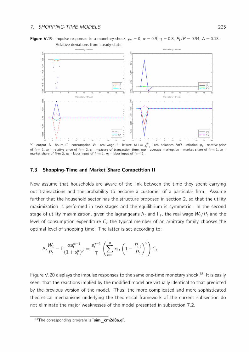
7. SHOPPING-TIME MODELS 225
Figure V.19: Impulse responses to a monetary shock, ρτ = 0, α = 0.9, γ = 0.8, P1/P = 0.94, ∆ = 0.18.Relative deviations from steady state.
Y - output, N - hours, C - consumption, W - real wage, L - leisure, M1 = MtPt−1 - real balances, Inf l - inflation, p1 - relative price
of firm 1, p2 - relative price of firm 2, s - measure of transaction time, mu - average markup, x1 - market share of firm 1, x2 -market share of firm 2, n1 - labor input of firm 1, n2 - labor input of firm 2.
7.3 Shopping-Time and Market Share Competition II
Now assume that households are aware of the link between the time they spent carrying
out transactions and the probability to become a customer of a particular firm. Assume
further that the household sector has the structure proposed in section 2, so that the utility
maximization is performed in two stages and the equilibrium is symmetric. In the second
stage of utility maximization, given the lagrangeans Λt and Γt , the real wage Wt/Pt and the
level of consumption expenditure Ct the typical member of an arbitrary family chooses the
optimal level of shopping time. The latter is set according to:
ΛtWtPt− Γ αs
α−1t
(1 + sαt )2=sγ−1t
γ
(n∑
l=1
xl ,t
(1− Pl ,t
Pt
)2)Ct .
Figure V.20 displays the impulse responses to the same one-time monetary shock.33 It is easily
seen, that the reactions implied by the modified model are virtually identical to that predicted
by the previous version of the model. Thus, the more complicated and more sophisticated
theoretical mechanisms underlying the theoretical framework of the current subsection do
not eliminate the major weaknesses of the model presented in subsection 7.2.
33The corresponding program is ”sim_cm2d8a.g”.
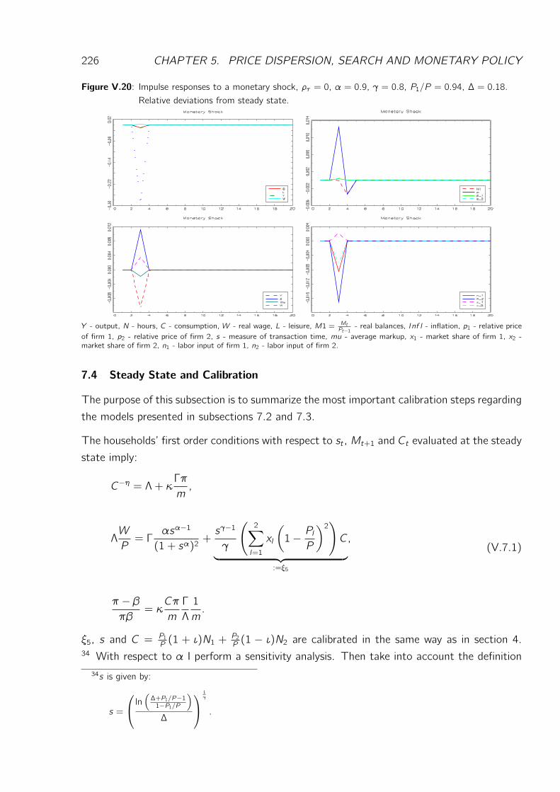
226 CHAPTER 5. PRICE DISPERSION, SEARCH AND MONETARY POLICY
Figure V.20: Impulse responses to a monetary shock, ρτ = 0, α = 0.9, γ = 0.8, P1/P = 0.94, ∆ = 0.18.Relative deviations from steady state.
Y - output, N - hours, C - consumption, W - real wage, L - leisure, M1 = MtPt−1 - real balances, Inf l - inflation, p1 - relative price
of firm 1, p2 - relative price of firm 2, s - measure of transaction time, mu - average markup, x1 - market share of firm 1, x2 -market share of firm 2, n1 - labor input of firm 1, n2 - labor input of firm 2.
7.4 Steady State and Calibration
The purpose of this subsection is to summarize the most important calibration steps regarding
the models presented in subsections 7.2 and 7.3.
The households’ first order conditions with respect to st , Mt+1 and Ct evaluated at the steady
state imply:
C−η = Λ + κΓπ
m,
ΛW
P= Γ
αsα−1
(1 + sα)2+sγ−1
γ
(2∑
l=1
xl
(1− PlP
)2)C
︸ ︷︷ ︸:=ξ5
,
π − βπβ
= κCπ
m
Γ
Λ
1
m.
(V.7.1)
ξ5, s and C = P1P(1 + ι)N1 +
P2P(1 − ι)N2 are calibrated in the same way as in section 4.
34 With respect to α I perform a sensitivity analysis. Then take into account the definition34s is given by:
s =
ln
(∆+P1/P−11−P1/P
)
∆
1γ
.

8. SUPPLEMENT TO CHAPTER V 227
of the shopping-time technology, multiply both sides of the first equation in V.7.1 by C and
solve the resulting system for Λ, Γ and m. The relevant results are:
Λ =ξ5 +
αs(1+sα)
C1−η
WP+ αs(1+sα)
C,
Γ =1 + sα
sα(C1−η − ΛC),
m =sα
1 + sαβπ
π − βΓ
Λ.
(V.7.2)
The steady state value of leisure L is determined by the time constraint with N = 0.1386:
L = 1− N − sα
1 + sα.
The calibration of the model presented in subsection 7.2 is obtained by setting ξ5 equal to
zero.
8 Supplement to Chapter V
The first order condition at the second stage reads:
g′(si ,t)s1−γi,t
γ=
(n∑
l=1
xi ,l ,t
(1− Pl ,t
Pt
)2)πtmi ,tDi ,t ,
where i denotes the index of the family member. To derive this result, the following relation-
ships and results were used: First, recall that
xi ,l ,t =exp
((1− Pl ,t
Pt
)sγi,t
)
∑nj=1 exp
((1− Pj,t
Pt
)sγi,t
) ⇒
⇒ ∂xi ,l ,t∂si ,t
= γsγ−1i ,t xi ,l ,t
(1− Pl ,t
Pt
)− γsγ−1i ,t xi ,l ,t
(n∑
l=1
xi ,l ,t
(1− Pl ,t
Pt
)).
Second, observe that
n∑
l=1
xi ,l ,t
(1− Pl ,t
Pt
)= 0,
228 CHAPTER 5. PRICE DISPERSION, SEARCH AND MONETARY POLICY
so that
∂xi ,l ,t∂si ,t
= γsγ−1i ,t xi ,l ,t
(1− Pl ,t
Pt
).
Hence
n∑
l=1
∂xi ,l ,t∂si ,t
Pl ,tPt= γsγ−1i ,t
n∑
l=1
xi ,l ,t
(Pl ,tPt−
(Pl ,tPt
)2).
Now add to the last equation the following one:
0 = γsγ−1i ,t
n∑
l=1
xi ,l ,t
(Pl ,tPt− 1
)
and rearrange to obtain
n∑
l=1
∂xi ,l ,t∂si ,t
Pl ,tPt= γsγ−1i ,t
n∑
l=1
xi ,l ,t
(−1 + 2Pl ,t
Pt−
(Pl ,tPt
)2)= −γsγ−1i ,t
n∑
l=1
xi ,l ,t
(1− Pl ,t
Pt
)2.
Now insert this result into the second-stage first order condition
−g′(si ,t)mi ,tπt= Di ,t
n∑
l=1
∂xi ,l ,t∂si ,t
Pl ,tPt
to obtain the result given in the main text.
Chapter 6
Conclusion
This monograph describes three different theoretical frameworks that can be used to ad-
dress issues concerning business cycles phenomena or monetary policy. Not surprisingly, each
framework has its advantages and drawbacks. But one of the theories emerges as better
than or, if we want to be more modest, at least as good as the widely used New Keynesian
model. It is the Inflation Aversion model. I conclude that the latter is a useful, or even better,
alternative to the former. And because for a wide range of parameter values both models
deliver similar results, it can not be ruled out that the true foundation of the New Keynesian
framework is not a version of the menu-cost model, but rather the Inflation Aversion model.
The models developed in the current monograph are only baseline versions that can be ex-
tended in various directions. For example consider nominal exchange rate pass-through.
According to the empirical evidence, movements in the nominal exchange rate are not fully
passed through to import prices. Furthermore, the degree of pass-through is time varying.
For example in a world economy characterized by search activity in the goods market and
static market share competition as defined in the last chapter, the optimal pricing decision of
a foreign firm selling part of its output in the home market will be governed by the following
condition:
Pi ,t =
(1 +
1
sγt (1− xi ,t)Z∗i ,tεtP ∗tPt
W ∗tP ∗t
)εtW
∗t
Z∗i ,t,
where εt denotes the nominal exchange rate. W ∗t , P∗t and Z∗i ,t are the foreign nominal wage,
the foreign price level and the productivity of the foreign firm respectively. Pi ,t is the price it
charges in the home goods market. xi ,t is the respective market share. st denotes home search
activity. It is easily seen that, everything else equal, an increase in the nominal exchange rate
will not be completely passed through to the price Pi ,t since a higher εt implies a lower firm-
specific markup. For values of the short run elasticity of demand lower than one the models
with dynamic market share competition also imply incomplete exchange rate pass-through.
229

230 CHAPTER 6. CONCLUSION
Bibliography
[1] Akelrof, G. A. and J. L. Yellen, 1985, Can Small Deviations from Rationality Make Sig-
nificant Differences to Economic Equilibria?, American Economic Review, 75(4), 708:721
[2] Altig, David, Lawrence Christiano, Martin Eichenbaum and Jesper Linde, 2005, Firm-
Specific Capital, Nominal Rigidities and the Business Cycle, NBER Working Paper, w
11034
[3] Ambler, Stephen and Emanuela Cardia, 1996, The Cyclical Behavior of Wages and Profits
under Imperfect Competition, mimeo
[4] Argyris, Chris, 1998, Empowerment: The Emperor’s New Clothes, Harvard Business
Review, 98-105
[5] Atkeson, Andrew and Patrick Kehoe, 2008, On the Need for a New Approach to Analyzing
Monetary Policy, NBER Working Paper, w 14260
[6] Ball Lawrence, N. Gregory Mankiw and Ricardo Reis, 2003, Monetary Policy for Inatten-
tive Economies, NBER Working Paper, w 9491
[7] Ball, L. and D. Romer, 1991, Sticky Prices as Coordination Failure, American Economic
Review, 81(3), 539:552
[8] Basu, Susanto, 1995, Intermediate Inputs and BusinessCycles: Implications for Produc-
tivity and Welfare, American Economic Review, 85, 512:531
[9] Baumol, Williams, 1952, The Transactions Demand for Cash: An Inventory Theoretic
Approach, Quarterly Journal of Economics, 66, 545:556
[10] Becker, Gary, 1973, A Theory of Marriage: Part I, Journal of Political Economy, 81,
813-846
[11] Becker, Gary, 1974, A Theory of Marriage: Part II, Journal of Political Economy, 82,
11-26
231
232 BIBLIOGRAPHY
[12] Benabou, Roland, 1992, Inflation and Markups: Theories and Evidence from the Retail
Trade Sector, European Economic Review, 36, 566:574
[13] Bernanke, Ben and Alan Blinder, 1992, The Federal Funds Rate and the Channels of
Monetary Transmission, American Economic Review, 82 (4), 901:921
[14] Bils, Mark, 1987, The Cyclical Behavior of Marginal Cost and Price, American Economic
Review, 77, 838:857
[15] Bils, Mark and James A. Kahn, 1996, What Inventory Behavior Tells Us about Business
Cycles, Rochester Center for Economic Research, Working Paper 428
[16] Bils, Mark and Peter Klenow, 2004, Some Evidence on the Importance of Sticky Prices,
Journal of Political Economy, 112, 947:985
[17] Biovin, Jean, Marc Giannoni, 2006, DSGE Models in a Data-Rich Environment, NBER
Working Paper, w 12824
[18] Biovin, Jean, Marc Giannoni, 2008, Global Forces and Monetary Policy Effectiveness,
NBER Working Paper, w 13736
[19] Biovin, Jean, Marc Giannoni and Ilian Mihov, 2007, Sticky Prices and Monetary Policy:
Evidence from Disaggregated U.S. Data, NBER Working Paper, w 12824
[20] Blanciforti, Laura A., Richard D. Green and Gordon A. King, 1986, U.S. Consumer
Behavior Over the Postwar Period: An Almost Ideal Demand System Analysis, Giannini
Foundation Monograph Number 40
[21] Boldrin, Michele and Michael Horvath, 1996, Labor Contracts and Business Cycles,
Journal of Political Economy, 103, 972:1004
[22] Boshen, John and Leonard Mills, 1991, The Effects of Countercyclical Monetary Policy
on Money and Interest Rates: An Evaluation of Evidence from FOMC Documents, Federal
Reserve Bank of Philadelphia, Working Paper, 91-20
[23] Brock, W.A., 1974, Money and Growth: The Case of Long Run Perfect Foresight,
International Economic Review, 15(3), 750-770
[24] Bryant, W. Keith and Yan Wang, 1990, American Consumption Patterns and the Price
of Time: A Time Series Analysis, The Journal of Consumer Affairs, 24, 280:306
[25] Burnside, Craig and Martin Eichenbaum, 1994, Factor Hoarding and the Propagation
of Business Cycle Shocks, 1994, NBER Working Paper, w 4675
[26] Burnside, Craig, Martin Eichenbaum and Sergio Rebelo, 1993, Labor Hoarding and the
Business Cycle, Journal of Political Economy, 101, 245-273
BIBLIOGRAPHY 233
[27] Burstein, Ariel and Christian Hellwig, 2007, Prices and Market Shares in a Menu Cost
Model, NBER Working Paper, w 13455
[28] Caplin, Andrew S. and Daniel F. Spulber, 1987, Menu Costs and the Neutrality of
Money, Quarterly Journal of Economics, 102, 703:725
[29] Caplin, Andrew S. and Daniel F. Spulber, 1993, Menu Costs and the Neutrality of
Money, OptimalPricing, Inflation, and the Cost of Price Adjustment, ed. Eytan Sheshinski
and Yoram Weiss, Cambridge, MIT Press, 217:240
[30] Carlton, Dennis, 1979, Contracts, Price Rigidity and Market Equilibrium, Journal of
Political Economy, 87, 1034:1062
[31] Carlton, Dennis, 1986, The Rigidity of Prices, American Economic Review, 76, 637:658
[32] Carrasco, Raquel, Jose M. Labeaga and J. David Lopez-Salido, 2005, Consumption and
Habits: Evidence From Panel Data, The Economic Journal, 115, 144:165
[33] Chari, V., Patrick Kehoe and Ellen McGrattan, 2008, Are Structural Vars with Long-
Run Restrictions Useful in Developing Business Cycle Theory, NBER Working Paper, w
14430
[34] Chari, V., Patrick Kehoe and Ellen McGrattan, 2008b, New Keynesian Models: Not Yet
Useful for Policy Analysis, NBER Working Paper, w 14313
[35] Cecchetti, Stephen, 1986, The Frequency of Price Adjustment: A Study of the News-
stand Prices of Magazines, Journal of Econometrics, 31, 255:274
[36] Chevalier, Judith, Anil Kashyap and Peter Rossi, 2007, Why Don’t Prices Rise during
Periods of Peak Demand? Evidence from Scanner Data, NBER Working Paper w 7981
[37] Christiano, Lawrence and Martin Eichenbaum, 1992, Current Real Business Cycle The-
ories and Aggregate Labor Market Fluctuations, American Economic Review, 82, 430-450
[38] Christiano, Lawrence and Martin Eichenbaum, 1992, Identification and the Liquidity
Effect of a Monetary Policy Shock, in ıPolitical Economy, Growth and Business Cycles,
edited by Alex Cucierman, Zvi Hercowitz and Leonardo Leiderman, Cambridge and London:
MIT Press, 335:370
[39] Christiano, Lawrence J., Martin Eichenbaum and Charles L. Evans, 1996, Sticky Price
and Limited Participation Models of Money: A Comparison, NBER Working Paper, w 5804
[40] Christiano, Lawrence J., Martin Eichenbaum and Charles L. Evans, 1996a, The Effects
of Monetary Policy Shocks: Evidence from the Flow of Funds, Review of Economics and
Stattistics, 78 (1), 16:34
234 BIBLIOGRAPHY
[41] Christiano, Lawrence J., Martin Eichenbaum and Charles L. Evans, 1997, Modeling
Money, NBER Working Paper, w 6371
[42] Christiano, Lawrence J., Martin Eichenbaum and Charles L. Evans, 1999, Monetary Pol-
icy Shocks: What Have We Learned and to What End?, in Handbook of Macroeconomics,
1A, ed. John Taylor and Michael Woodford
[43] Christiano, Lawrence J., Martin Eichenbaum and Charles L. Evans, 2005, Nominal
Rigidities and the Dynamic Effects of a Shock to Monetary Policy Journal of Political
Economy, 113, 1
[44] Cochrane, John, 1994, Shocks, NBER Working Paper, w 4698
[45] Cogley, Timothy and James Nason, 1995, Output Dynamics in Real-Business-Cycle
Models, American Economic Review, 85 (3), 492:511
[46] Correia, Isabel, Joao Neves and Sergio Rebelo, 1995, Business Cycles in a Small Open
Economy, European Economic Review, 39, 1089:1113
[47] Comin, Diego and Mark Gertler, 2003, Medium Term Business Cycles, NBER Working
Paper, w 10003
[48] Cooley T. and G. Hansen, 1989, The Inflation Tax in a Real Business Cycle Model,
American Economic Review, 79 (4), 733:748
[49] Cooley T. and E. C. Prescott, 1995, Economic Growth and Business Cycles, in Cooley,
T., Frontiers of Business Cycles Research, Princeton University Press, Princeton, N.J., pp.
1-38
[50] Croushore, D., 1993, Money in the Utility Function: Functional Equivalence to a
Shopping-Time Model, Journal of Macroeconomics, 15(1), 175-182
[51] Cukierman, Alex, 1983, Relative Price Variability and Inflation - a Survey and Further
Results, in Brunner, K. and A. Meltzer, Variability in Employment Prices and Money,
Carnegie-Rochester Conference Series on Public Policy, 19, North-Holland, Amsterdam,
103:158
[52] Danziger, Leif, 1987, Inflation, Fixed Cost of Price Adjustment, and the Measurement of
Relative Price Variability: Theory and Evidence, American Economic Review, 77, 704:713
[53] Davidson, Russel, James MacKinnon, 1993, Estimation and Inference in Econometrics,
Oxford University Press
[54] Dhyne, Emmanuel, Luis Alvarez, Herve Le Bihan, Giovanni Veronese, Daniel Dias, Jo-
hannes Hoffmann, Nicole Jonker, Patrick Lunnemann, Fabio Rummler and Jouko Vilmunen,
BIBLIOGRAPHY 235
2005, Price Setting in the Euro Area: Some Stylized Facts from Individual Consumer Price
Data, European Central Bank, Working Paper, no. 524
[55] Di Tella, Rafael, Robert J. MacCulloch and Andrew J. Oswald, 2001, Preferences over
Inflation and Unemployment: Evidence from Surveys of Happiness, American Economic
Review, 91, 1, 335:341
[56] Domberger, Simon, 1979, Price Adjustment and Market Structure, Economic Journal,
89, 96:108
[57] Domowitz, Ian R., Glenn Hubbard and Bruce C. Petersen, 1986, Business Cycles and
the Relationship between Concentration and Price Margins, Rand Journal of Economics,
17, 1:17
[58] Dotsey, Michael, Robert King and Alexnder Wolman, 1999, State-Dependent Pricing
and the General Equilibrium Dynamics of Money and Output, Quarterly Journal of Eco-
nomics, 114, 655:690
[59] Edmond, Chris and Laura Veldkamp, 2008, Income Dispersion and Counter-Cyclical
Markups, NBER Working Paper, w 14452
[60] Eichenbaum, Martin and Jonas D. M. Fisher, 2004, Evaluating the Calvo Model of
Sticky Prices, NBER Working Paper, w 10617
[61] Erceg, Christopher, Dale Henderson and Andrew Levin, 2000, Optimal Monetary Policy
with Staggered Wage and Price Contracts, Journal of Monetary Economics, 46, 281:313
[62] Fisher, Jonas, 1997, Monetary Policy and Investment, manuscript, Federal Reserve Bank
of Chicago
[63] , Fisher, Stanley, 1981, Relative Shocks, Relative Price Variability, and Inflation, Brook-
ings Papers on Economic Activity, 2, 381:431
[64] Franses, Philip Hans, 2006, Testing Changes in Consumer Confidence Indicators, Eras-
mus University Rotterdam, Economic Institute, Working Paper
[65] Frey, Bruno S. and Alois Stutzer, 2002, What Can Economists Learn from Happiness
Research?, Journal of Economic Literature, 40, 2, 402:435
[66] Fuhrer, Jeffrey, 2000, Habit Formation in Consumption and Its Implications for
Monetary-Policy Models, American Economic Review, 90, 367:90
[67] Gagnon, Etienne, 2005, Price Setting during Low and High Inflation: Evidence from
Mexico, Manuscript, Northwestern University
236 BIBLIOGRAPHY
[68] Galeotti, Marzio and Fabio Shiantarelli, 1998, The Cyclicity of Markups in a Model with
Adjustment Costs: Econometric Evidence for U.S. Industry, Oxford Bulletin of Economics
and Stattistics, 60 (2), 121:143
[69] Gali Jordi and Mark Gertler, 1999, Inflation Dynamics: A Structural Econometric Anal-
ysis, Journal of Monetary Economics, 44 195:222
[70] Gali, Jordi, Mark Gertler and J.David Lopez-Salido, 2001, European Inflation Dynamics,
European Economic Review, 45, 1237-1270
[71] Gali, Jordi, Mark Gertler and J. David Lopez-Salido, 2002, Markups, Gaps, and the
Welfare Costs of Business Fluctuations, NBER Working Paper, w 8850
[72] Gertler, Mark and Simon Gilchrist, 1994, Monetary Policy, Business Cycles and the
Behavior of Small Manufacturing Firms, Quarterly Journal of Economics, 109 (2), 309:340
[73] Gertler, Mark and John Leahy, 2006, A Phillips Curve with an Ss Foundation, NBER
Working Paper, w 11971
[74] Golosov, Mikhail and Robert Lucas, 2007, Menu Costs and Phillips Curves, Journal of
Political Economy, 115, 171:199
[75] Gomme, Paul and Jeremy Greenwood, 1995, On the Cyclical Allocation of Risk, Journal
of Economic Dynamics and Control, 19, 91:124
[76] Gomme, Paul and Peter Rupert, 2007, Theory, Measurment and Calibration of Macroe-
conomic Models, Journal of Monetary Economics, 54, 460-497
[77] Gordon, David and Eric Leeper, 1994, The Dynamic Impacts of Monetary Policy: An
Exercise in Tentative Identification, Journal of Political Economy, 102 (6), 1228:1247
[78] Gorodnichenko, Yuriy, 2008, Endogenous Information, Menu Costs and Inflation Persis-
tence, NBER Working Paper, w 14184
[79] Hairault, J., F. Portier, 1995, Nominal Rigidities and Monopolistic Competition: A
New-Keynesian View, European Economic Review
[80] Hamilton, James D., 1994, Time Series Analysis, Princeton University Press
[81] Hansen, Lars Peter, 1982, Large Sample Properties of Generalized Method of Moments
Estimators, Econometrica, 50, 1029-1054
[82] Haubrich, J. G. and R. G. King, 1991, Sticky Prices, Money, and Business Fluctuations,
Journal of Money Credit and Banking, 23(2), 243:259
[83] Hayashi, Fumio, 2000, Econometrics, Princeton University Press
BIBLIOGRAPHY 237
[84] Heer, Burkhard and Alfred Maussner, 2007, Inflation and Output Dynamics in a Model
with Labor Market Search and Capital Accumulation, CESIfo Working Paper, No.2036
[85] Holmstrom, Bengt and Steven Kaplan, 2001, Corporate Governance and Merger Ac-
tivity in the United States: Making Sense of the 1980s and 1990s, Journal of Economic
Perspectives, 15(2), 121:145
[86] Hymans, Saul H., 1970, Consumer Durable Spending: Explanation and Prediction,
Brookings papers on Economic Activity, 2, 173:206
[87] Jovanovich, Boyan, 1982, Inflation and Welfare in the Steady-State, Journal of Political
Economy, 90(3), 561:577
[88] Kaplan, Steven, 1996, AreWe All Becoming Henry Kravis Now? The Evolution of US
Corporate Governance, University of Chicago Working Paper
[89] Kashyap, Anil, Sticky Prices: New Evidence from Retail Catalogs, Quarterly Journal of
Economics, 110, 245:274
[90] Kehoe, Patrick, 2006, How to Advance Theory with Structural VARS: Use the Sims-
Cogley-Nason Approach, NBER Working Paper, w 12575
[91] Kehoe, Patrick and Virgiliu Midrigan, 2008, Temporary Price Changes and the Real
Effects of Monetary Policy, NBER Working Paper, w 14392
[92] Killingsworth, Mark, 1983, Labor Supply, Cambridge University Press
[93] Klenow, Peter and Oleksiy Kryvstov, 2005, State-Dependent or Time-Dependent Pric-
ing: Does it Matter for Recent U.S. Inflation?, NBER Working Paper, w 11043
[94] Kollman, Robert, 1996, The Cyclical Behavior of Markups in U.S. Manufacturing and
Trade: New Empirical Evidence Based on a Model of Optimal Storage, mimeo, University
of Montreal
[95] Kydland, Finn and Edward Prescott, 1982, Time to Built and Aggregate Fluctuations,
Econometrica, 50 (6), 1345:1370
[96] Lach, Saul and Daniel Tsiddon, 1993, The Behavior of Prices and Inflation: An Empirical
Analysis of Disaggregated Price Data, in Sheshinski, E. and Yoram Weiss, Optimal Pricing,
Inflation, and the Cost of Price Adjustment, The MIT Press, Cambridge, Massachusetts,
pp. 445-484
[97] Lach, Saul, 2002, Existence and Persistence of Price Dispersion: An Empirical Analysis,
NBER Working Paper, w8737
238 BIBLIOGRAPHY
[98] Lastrapes, William and George Selgin, 1995, The Liquidity Effect: Identifying Short-Run
Interest Rate Dynamics Using Long-Run Restrictions, Journal of Macroeconomics, 17 (3),
387:404
[99] Leamer, Edward, 1985, Vector Autoregressions for Causal Inference?, in Understanding
Monetary Regimes, edited by Karl Brunner and Alan Meltzer, Carnegie-Rochester Confer-
ence Series on Public Policy, 22, 255:304, Amsterdam: North-Holland
[100] Leeper, Eric, 1996, Narrative and VAR Approaches to Monetary Policy: Common
Identification Problems, Indiana University, Working Paper
[101] Leeper, Eric, Christopher Sims and Tao Zha, 1996, What Does Monetary Policy Do?,
Brookings Papers on Economic Activity, 2, 2:63
[102] Leeper, Eric, Todd Walker and Shu-Chun Susan Yang, 2008, Fiscal Foresight: Analytics
and Econometrics, NBER Working Paper, w 14028
[103] Litterman, Robert and Laurence Weiss, 1983, Money, Real Interest Rates and Output:
A Reinterpretation of Postwar U.S. Data, NBER Working Paper 1077
[104] Lovell, Michael C. and Pao Lin Tien, 1999, Economic Discomfort and Consumer Sen-
timent, Wesleyan University, Working Paper
[105] Lucas, Robert and Nancy Stokey, 1987, Money and Interest in a Cash-In-Advance
Economy, Econometrica, 55 (3), 491:513
[106] Lundberg, Shelly and Robert Pollak, 1997, Bargaining and Distribution in Marriage, in
Perrson, Inga and Christina Jonung, Economics of the Family and Family Policies, London,
Routledge, 23-43
[107] Lundberg, Shelly, Robert Pollak and Terence Wales, 1997, Do Husbands and Wives
Pool Their Resources?, Evidence from the United Kingdom Child Benefit, The Journal of
Human Resources, 32, 463-480
[108] Mackowiak, Bartosz and Mirko Wiederholt, 2007, Optimal Sticky Prices Under Rational
Inattention, CEPR Discussion Paper, 6243
[109] Mankiw, N. Gregory and Ricardo Reis, 2001, Sticky Information: A Model of Monetary
Nonneutrality and Structural Slumps, NBER Working Paper, w 8614
[110] Mankiw, N. Gregory and Ricardo Reis, 2006a, Pervasive Stickiness (Extended Version),
NBER Working Paper, w 12024
[111] Mankiw, N. Gregory and Ricardo Reis, 2006b, Sticky Information in General Equilib-
rium, NBER Working Paper, w 12605
BIBLIOGRAPHY 239
[112] Manser, M. and M. Brown, 1980, Marriage and Household Decision Making: A Bar-
gaining Analysis, American Economic Review, 21, 31-44
[113] Maussner, Alfred, 2004, Endogenous Growth with Nominal Frictions, Journal of Eco-
nomics, 83, 1:46
[114] McCallum, Bennett, (1979), Monetarism, Rational Expectations, Oligopolistic Pricing,
and the MPS Econometric Model, Journal of Political Economy, 87 (1), 57:73
[115] McCallum, B. T. and E. Nelson, 1999, An Optimizing IS-LM Specification of Monetary
Policy and Business Cycle Analysis, Journal of Money Credit, and Banking, 31(3), 296:316
[116] Mellin, I. and M. Viren, 1982, An Empirical Analysis of Demand for Houses Durables
and Nondurables, Empirical Economics, 7, 49:61
[117] Nakamura, Emi and Jon Steinsson, 2007, Price Setting in Forward-Looking Customer
Markets, Working Paper, Harvard University
[118] Nakamura, Emi and Jon Steinsson, 2008, Five Facts about Prices: A Reevaluation of
Menu-Cost Models, Quarterly Journal of Economics, 1415:1464
[119] Pagan, Adrian and John Robertson, 1995, Resolving the Liquidity Effect, Federal Re-
serve Bank of St. Louis Review, 77 (3), 33:54
[120] Phelps, Edmund S. and Sidney G. Winter, Jr., 1970, Optimal Price Policy under Atom-
istic Competition, in Edmund S. Phelps, Microeconomic Foundations of Employment and
Inflation Theory, Macmillan
[121] Pollak, Robert, 2002, Gary Becker’s Contribution to Family and Household Economics,
NBER Working Paper, w9232
[122] Rajan, Raghuram and Julie Wulf, 2006, The Flattering Firm: Evidence from Panel Data
on the Changing Nature of Corporate Hierarchies, Review of Economics and Statistics,
88(4), 759-773
[123] Rajan, R., and L. Zingales, 2000, The Governance of the New Enterprise, in Xavier
Vives (Ed.), Corporate Governance, Theoretical and Empirical Perspectives, Cambridge
University Press, 201:227
[124] Ramey, Valerie A., 1991, Non-Convex Costs and the Behavior of Inventories, Journal
of Political Economy, 99, 306:334
[125] Reinsdorf, M., 1994, New Evidence on the Relation between Inflation and Price Dis-
persion, American Economic Review, 84, 3 720:731.
240 BIBLIOGRAPHY
[126] Romer, David, 1986, A Simple General Equilibrium Version of the Baumol-Tobin Model,
Quarterly Journal of Economics, 101(4), 663:685
[127] Romer, Christina and David Romer, 1989, Does Monetary Policy Matter? A New Test
in the Spirit of Firedman and Schwartz, NBER Macroeconomic Annual 1989, Cambridge,
MIT Press, 121:170
[128] Romer, Christina and David Romer, 1994, Monetary Policy Matters, Journal of Mon-
etary Economics, 34, 75:88
[129] Rotemberg, Julio, 1982, Sticky Prices in the United States, Journal of Political Econ-
omy, 90, 1187:1211
[130] Rotemberg, Julio, 2002, Minimally Acceptable Altruism and the Ultimatum Game,
Harvard Business School, Working Paper
[131] Rotemberg, Julio, 2004a, Customer Anger at Price Increases, Time Variation in the
Frequency of Price Changes and Monetary Policy, Harvard Business School, Working Paper
[132] Rotemberg, Julio, 2004b, Fair Pricing, Harvard Business School, Working Paper
[133] Rotemberg, Julio, 2008, Behavioral Aspects of Price Setting, and Their Policy Impli-
cations, NBER Working Paper, w 13754
[134] Rotemberg, Julio and Garth Saloner, 1986, A Supergame-Theoretic Model of Price
Wars During Booms, Journal of Political Economy, 90, 1187:1211
[135] Rotemberg, Julio and Michael Woodford, 1992, Oligopolistic Pricing and the Effects of
Aggregate Demand on Economic Activity, Journal of Political Economy, 100, 1153:1207
[136] Rotemberg, Julio and Michael Woodford, 1995, Dynamic General Equilibrium Models
with Imperfectly Competitive Product Markets, in Thomas F. Cooley, Frontiers of Business
Cycle Reserch, Princeton University Press, Princeton
[137] Rotemberg, Julio and Michael Woodford, 1996, Imperfect Competition and the Effects
of Energy Price Increases on Economic Activity, Journal of Money, Credit and Banking,
28, 549:577
[138] Rotemberg, Julio and Michael Woodford, 1997, An Optimizing-Based Econometric
Model for the Evaluation of Monetary Policy, 1997, NBER Macroeconomics Annual, Cam-
bridge, MIT Press, 297:346
[139] Rotemberg, Julio and Michael Woodford, 1999, The Cyclical Behavior of Prices and
Costs, NBER Working Paper, w 6909
BIBLIOGRAPHY 241
[140] Saving, Thomas R., 1971, Transaction Costs and the Demand for Money, American
Economic Review, 61, 407-420
[141] Sbordone, A. M., 2002, Prices and Unit Labor Costs: A New Test of Price Stickiness,
Journal of Monetary Economics, 49(2), 265:292
[142] Sims, Christopher, 1972, Money, Income, and Causality, American Economic Review,
62, 540:552
[143] Sims, Christopher, 1977, Exogeneity and Causal Ordering in Macroeconomic Models,
in New Methods in Business Cycle Research, Fed. Reserve Bank Minneapolis, 23:44
[144] Sims, Christopher, 1978, Small Econometric Models of the U.S. and Germany, Discus-
sion Paper, Univ. Minnesota
[145] Sims, Christopher, 1980, Comparision of Interwar and Postwar Business Cycles: Mon-
etarism Reconsidered, American Economic Review, 70(2), 250:257
[146] Sims, Christopher, 1986, Are Forecasting Models Usble for Policy Analysis?, Federal
Reserve Bank of Minneapolis, Quarterly Review, 10(1), 2:16
[147] Sims, Christopher, 1989, Models and their Uses, American Journal of Agricultural
Economics, 71 (2), 489:494
[148] Sims, Christopher, 1992, Interpreting the Macroeconomic Time Series Facts: The
Effects of Monetary Policy, European Economic Review, 36 (5), 975:1000
[149] Sims, Christopher and Tao Zha, 1995, Does Monetary Policy Generate Recessions?,
manuscript, Yale University
[150] Sims, Christopher and Tao Zha, 2006, Does Monetary Policy Generate Recessions?,
Macroeconomic Dynamics, 10, 231:272
[151] Smets, Frank and Raf Wouters, 2003, An Estimated Dynamic Stochastic General
Equilibrium Model of the Euro Area, Journal of the European Economic Association 1 (5),
1123:1175
[152] Smets, Frank and Rafael Wouters, 2007, Shocks and Frictions in US Business Cycles:
A Bayesian DSGE Approach, American Economic Review, 97 (3), 586:606
[153] Smyth, David J., Pami Dua and Susan Washburn Taylor, 1994, Voters and Macroe-
conomics: Are They Forward looking or Backward Looking?, Public Choice, 78, 283:293
[154] Strongin, Steven, 1995, The Identification of Monetary Policy Disturbances: Explaining
the Liquidity Puzzle, Journal of Monetary Economics, 34 (3), 463:497
242 BIBLIOGRAPHY
[155] Tellis, Gerard J., 1988, The Price Elasticity of Selected Demand: A Meta-Analysis of
Econometric Models of Sales, Journal of Marketing Research, 25, 331:341
[156] Tobin, James, 1956, The Interest Elasticity of the Transactions Demand for Cash,
Review of Economics and Statistics, 38(3), 241:247
[157] Tommasi, M., 1993, Inflation and Relative Prices: Evidence from Argentina, in Sheshin-
ski, E. and Yoram Weiss, Optimal Pricing, Inflation, and the Cost of Price Adjustment,
The MIT Press, Cambridge, Massachusetts, 485:511
[158] Trigari, A., 2004, Equilibrium Unemployment, Job Flows and Inflation Dynamics, Eu-
ropean Central Bank Working Ppaer Series, No.: 304
[159] Van Hoomissen, T., 1988, Price Dispersion and Inflation: Evidence from Israel, Journal
of Political Economy, 96, 6, 1303:1313
[160] Walsh, Carl E., 2003, Monetary Theory and Policy, Massachusetts Institute of Tech-
nology, 2nd ed.
[161] Walsh, Carl E., 2005, Labor Market Search, Sticky Prices, and Interest Rate Policies,
Review of Economic Dynamics, 8, 829:849
[162] Walton, Clarence C., 1979, Divergent Views of Inflation, Proceedings of the Academy
of Political Science, 33, 3 Inflation and National Survaival, 1:11
[163] Woodford, Michael, 1996, Control of the Public Debt: A Requirement for Price Sta-
bility?, NBER Working Paper, w 5684
[164] Woodford, Michael, 2003, Interest an Prices, Princeton University Press
[165] Yun, T., 1996, Nominal Price Rigidity, Money Supply Endogeneity, and Business Cycles,
Journal of Monetary Economics, 37(2), 345:370

Appendix A
New Keynesian Model
The log-linear equations are given in order of appearance in the program. Variables without
time index denote steady state values.
1 A Model with Fixed Capital
The optimality condition with respect to consumption implies:
C−ηt = Λt ,
⇒−ηCt = Λt .
The optimality condition with respect to working hours implies:
bNt = ΛtWtPt
⇒
ηCt + Nt − WtPt= 0.
The next equation reflects the definition of the production function:
Yt = ZtNt
((1− ϕ)
(P otPt
)−θ+ ϕ
(π
πt
)−θ)−1
⇒Nt − Yt = −Zt ,
243
244 APPENDIX A. NEW KEYNESIAN MODEL
while the expression((1− ϕ)
(P otPt
)−θ+ ϕ
(ππt
)−θ)−1has no first order effects on the equi-
librium dynamics:
((1− ϕ)
(P otPt
)−θ+ ϕ
(π
πt
)−θ)−1= 0.
The equation determining the equilibrium real wage implies:
mut =(Wt/Pt)NtYt
⇒
−Nt + Yt − WtPt= mut .
The aggregate consistency condition reads:
Ct = Yt
⇒Ct − Yt = 0.
The next equation reflects the definition of the markup mut :
1
µt= mut ,
⇒µt + mut = 0,
where µt denotes marginal cost.
The optimality condition with respect to money demand implies:
βφmm−χt+1Etπχ−1t+1 = Λt − βEt
Λt+1πt+1
⇒
χmt+1 +
(β
π − β + 1− χ)Etπt+1 − β
π − βEtΛt+1 +π
π − β Λt = 0
The next equation results from the law of motion of money supply:
mt+1 =τtπtmt
⇒mt+1 − mt + πt = τt .
2. A MODEL WITH ENDOGENOUS CAPITAL 245
The last dynamic equation id the New Keynesian Phillips Curve:
βEtπt+1 − πt = −(1− ϕ)(1− ϕβ)ϕ
µt .
2 A Model with Endogenous Capital
The first two equations read:
−ηCt = Λt ,
and
Nt − WtPt= Λt .
The third equation becomes:
Yt = ZtNωt K
1−ωt
((1− ϕ)
(P otPt
)−θ+ ϕ
(π
πt
)−θ)−1
⇒ωNt − Yt = (ω − 1)Kt − Zt .
The fourth log-linear equation does not change:
−Nt + Yt − WtPt= mut .
The aggregate consistency condition becomes:
Yt = Ct + It ,
⇒C
YCt − Yt + I
YIt = 0.
The first three dynamic equations are the same:
χmt+1 +
(β
π − β + 1− χ)Etπt+1 − β
π − βEt Λt+1 +π
π − β Λt = 0
mt+1 − mt + πt = τt .
246 APPENDIX A. NEW KEYNESIAN MODEL
βEtπt+1 − πt − (1− ϕ)(1− ϕβ)ϕ
mut = 0.
The Euler equation with respect to next-period’s stock of capital implies:
Λt = βEt
Λt+1
(1 +(1− ω)mut+1
Yt+1Kt+1
− υ)
⇒(1− β(1− υ))Kt+1 − EtΛt+1 + (1− β(1− υ))Etmut+1 + Λt = (1− β(1− υ))Et Yt+1,
where υ denotes the rate of depreciation. The last equation reflects the law of motion of
capital:
Kt+1 = It + (1− υ)Kt ,⇒Kt+1 − (1− υ)Kt = υIt .
3 Adjustment Costs of Capital
The first five equations remain unchanged:
−ηCt = Λt ,
Nt − WtPt= Λt .
ωNt − Yt = (ω − 1)Kt − Zt .
−Nt + Yt − WtPt− mut = 0.
Yt − mut = Kt + Rt .
3. ADJUSTMENT COSTS OF CAPITAL 247
The next equation is the optimality condition with respect to investment:
qt =Λt
φ′(ItKt
)
⇒ςIt + qt = ςKt + Λt ,
where ς < 0 is the elasticity of the first derivative of the adjustment-costs function φ′(.) with
respect to its argument I/K, evaluated at the steady state. qt is Tobin’s q. The last static
equation stems from the resource constraint:
C
YCt − Yt + I
YIt = 0.
The first three dynamic equations are the same:
χmt+1 +
(β
π − β + 1− χ)Etπt+1 − β
π − βEt Λt+1 +π
π − β Λt = 0
mt+1 − mt + πt = τt .
βEtπt+1 − πt = (1− ϕ)(1− ϕβ)ϕ
mut .
The log-linear version of the Euler equation with respect to next-period’s stock of capital
becomes:
qt = Et
Λt+1Rt+1 + qt+1
(1− υ + φ
(It+1Kt+1
)− φ′
(It+1Kt+1
)It+1Kt+1
),
⇒−ςυKt+1 − REtRt+1 − REtΛt+1 = −ςEt It+1 + (1− υ)Et qt+1 − qt .
The last equation corresponds to the law of motion of capital:
Kt+1 − (1− υ)Kt = υIt .

248 APPENDIX A. NEW KEYNESIAN MODEL
Appendix B
Chapter 2
The log-linear equations are given in order of appearance in the program. Variables without
time index denote steady state values.
1 A Model with Fixed Capital
aC−bt
(aC1−bt + (1− a)
(mtπt
)1−b) b1−b
= Λt ,
⇒b(ξ1 − 1)Ct − Λt = −bξ2mt + bξ2πt ,
where
ξ1 =
(1 +1− aa
(1− aa
β
π − β) 1−b
b
)−1, ξ2 =
(1 +
a
1− a(a
1− aπ − ββ
) 1−bb
)−1.
φNt = ΛtWtPt
⇒
Nt − WtPt− Λt = 0.
Yt = ZtNt
⇒Nt − Yt = −Zt .
249
250 APPENDIX B. CHAPTER 2
mut =(Wt/Pt)NtYt
⇒
−Nt + Yt − WtPt= mut .
Ct = Yt
⇒Ct − Yt = 0.
Λt = βEt
(1− a)
m−bt+1π1−bt+1
(aC1−bt+1 + (1− a)
(mt+1πt+1
)1−b) b1−b
+Λt+1πt+1
⇒
bπ − βπmt+1 +
π − bπ + bβπ
Etπt+1 = bπ − βπEtCt+1 + EtΛt+1 − Λt .
Note that the last equation, evaluated at the steady state, implies:
Λπ − βπ= (1− a)
(mπ
)−b (aC1−b + (1− a)
(mπ
)1−b) b1−b.
Eliminating Λ by inserting the first optimality condition, also evaluated at the steady state,
yields:
a
1− aπ − ββ=
(m/π
C
)−b.
mt+1 =τtπtmt
⇒mt+1 − mt + πt = τt .
The optimality condition of the representative firm can be written as:
(Pi ,tPt
)−θxi ,tYt − θ
(Pi ,tPt− µt
)(Pi ,tPt
)−θ−1xi ,tYt +
g′(Pi ,tPt
)
g(Pi ,tPt
)Ωt = 0,
2. A MODEL WITH ENDOGENOUS CAPITAL 251
where µt denotes marginal costs and
Ωt = Et
∞∑
j=1
βjΛt+jΛtxi ,t+j
(Pi ,t+jPt+j
− µt+j)(Pi ,t+jPt+j
)−θYt+j
=
= Et
βΛt+1Λtxi ,t+1
(Pi ,t+1Pt+1
− µt+1)(Pi ,t+1Pt+1
)−θYt+1
+ Et
βΛt+1ΛtΩt+1
(II.1.1)
The first equation implies that in the symmetric equilibrium the markup mut is given by:
mut =−θ
1− θ − γΩtYt
(II.1.2)
Log-linearizing the last equation yields:
mut =γΩY
1− θ − γΩY
(Ωt − Yt) = −ξ(Ωt − Yt).
The log-linear version of equation II.1.1 can be written as:
Ωt = EtDF t,t+1 +1− β(mu − 1)Etmut+1 + (1− β)Et Yt+1 + βEtΩt+1,
where DFt,t+1 denotes the stochastic discount factor between t and t + 1. Combining the
last two equations to eliminate Ωt yields:(β
ξ− 1− βmu − 1
)Etmut+1 − 1
ξmut = Et Yt+1 + EtΛt+1 − Yt − Λt .
To obtain the log-linear system for the model without market share competition, just neglect
the last equation and replace the term mut appearing in the fourth underlined equation (the
definition of the real wage) by zero.
To obtain the corresponding New Keynesian model, just replace the optimality conditions for
consumption and next period real balances in the standard New Keynesian model by the ones
given in this section.
2 A Model with Endogenous Capital
The first two equations read:
b(ξ1 − 1)Ct = −bξ2mt + bξ2πt + Λt ,
and
Nt − WtPt= Λt .

252 APPENDIX B. CHAPTER 2
The third equation becomes:
Yt = ZtNωt K
1−ωt
⇒ωNt − Yt = (ω − 1)Kt − Zt .
The fourth log-linear equation does not change:
−Nt + Yt − WtPt= mut .
The definition of the real interest rate Rt implies:
Yt − Rt = Kt + mut .
The first three dynamic equations are the same:
bπ − βπmt+1 +
π − bπ + bβπ
Et πt+1 − EtΛt+1 + Λt = bπ − βπEtCt+1.
mt+1 − mt + πt = τt .
(β
ξ− 1− βmu − 1
)Etmut+1 − EtΛt+1 − 1
ξmut + Λt = Et Yt+1 − Yt .
The log-linear version of the Euler equation with respect to next-period’s stock of capital
reads:
EtΛt+1 − Λt = −(1− β(1− υ))EtRt+1,
where υ denotes the rate of depreciation. The resource constraint becomes:
Kt+1 − (1− υ)Kt = −CKCt +
Y
KYt .
3 Adjustment Costs of Capital
The first five equations remain unchanged:
b(ξ1 − 1)Ct = −bξ2mt + bξ2πt + Λt ,
3. ADJUSTMENT COSTS OF CAPITAL 253
Nt − WtPt= Λt .
ωNt − Yt = (ω − 1)Kt − Zt .
−Nt + Yt − WtPt= mut .
Yt − Rt = Kt + mut .
The next equation is the optimality condition with respect to investment:
qt =Λt
φ′(ItKt
)
⇒ςIt + qt = ςKt + Λt ,
where ς < 0 is the elasticity of the first derivative of the adjustment-costs function φ′(.) with
respect to its argument I/K, evaluated at the steady state. qt is Tobin’s q. The last static
equation stems from the resource constraint:
C
YCt − Yt + I
YIt = 0.
The first three dynamic equations are the same:
bπ − βπmt+1 +
π − bπ + bβπ
Etπt+1 − EtΛt+1 + Λt = bπ − βπEtCt+1.
mt+1 − mt + πt = τt .
(β
ξ− 1− βmu − 1
)Etmut+1 − Et Λt+1 − 1
ξmut + Λt = Et Yt+1 − Yt .
254 APPENDIX B. CHAPTER 2
The log-linear version of the Euler equation with respect to next-period’s stock of capital
becomes:
qt = Et
Λt+1
1− ωmut+1
Yt+1Kt+1
+ qt+1
(1− υ + φ
(It+1Kt+1
)− φ′
(It+1Kt+1
)It+1Kt+1
),
⇒−ςυKt+1 − REtΛt+1 − REtRt+1 = −ςEt It+1 + (1− υ)Et qt+1 − qt .
The last equation corresponds to the law of motion of capital:
Kt+1 − (1− υ)Kt = υIt .
To obtain the corresponding New Keynesian model, just replace the optimality conditions for
consumption and next period real balances in the standard New Keynesian model by the ones
given in this section.

Appendix C
Chapter 3
The log-linear equations are given in order of appearance in the program. Variables without
time index denote steady state values.
1 A Model with Fixed Capital
C−ηt = Λt ,
⇒−ηCt − Λt = 0.
bNt = ΛtWtPt
⇒
ηCt + Nt − WtPt= 0.
Yt = ZtNt
⇒Nt − Yt = −Zt .
mut =(Wt/Pt)NtYt
⇒
−Nt + Yt − WtPt= mut .
255
256 APPENDIX C. CHAPTER 3
The optimality condition with respect to search activity implies:
%st = Cη1+αt π
11+αt ,
⇒
− η
1 + αCt + st =
1
1 + απt .
Ct + st = Yt
⇒C
YCt − Yt + s
Yst = 0.
βφmm−χt+1Etπχ−1t+1 = Λt − βEt
Λt+1πt+1
⇒
χmt+1 +
(β
π − β + 1− χ)Etπt+1 =
β
π − βEtΛt+1 −π
π − β Λt
mt+1 =τtπtmt
⇒mt+1 − mt + πt = τt .
The optimality condition of the representative firm can be written as:
(Pi ,tPt
)−θxi ,tYt − θ
(Pi ,tPt− µt
)(Pi ,tPt
)−θ−1xi ,tYt +
g1
(Pi ,tPt, st
)
g(Pi ,tPt, st
) Ωt = 0,
where µt denotes marginal costs and
Ωt = Et
∞∑
j=1
βjΛt+jΛtxi ,t+j
(Pi ,t+jPt+j
− µt+j)(Pi ,t+jPt+j
)−θYt+j
=
= Et
βΛt+1Λtxi ,t+1
(Pi ,t+1Pt+1
− µt+1)(Pi ,t+1Pt+1
)−θYt+1
+ Et
βΛt+1ΛtΩt+1
(III.1.1)
The first equation implies that in the symmetric equilibrium the markup mut is given by:
mut =−θ
1− θ − st ΩtYt(III.1.2)
2. A MODEL WITH ENDOGENOUS CAPITAL 257
Log-linearizing the last equation yields:
mut =s ΩC
1− θ − s ΩC
(Ωt + st − Yt) = −ξ(Ωt − Yt).
The log-linear version of equation III.1.1 can be written as:
Ωt = EtDF t,t+1 +1− β(mu − 1)Etmut+1 + (1− β)Et Yt+1 + βEtΩt+1,
where DFt,t+1 denotes the stochastic discount factor between t and t + 1. Combining the
last two equations to eliminate Ωt yields:(β
ξ− 1− βmu − 1
)Etmut+1 − 1
ξmut = Et Yt+1 + EtΛt+1 − βEt st+1 − Yt − Λt + st .
2 A Model with Endogenous Capital
The first two equations read:
−ηCt = Λt ,
and
Nt − WtPt= Λt .
The third equation becomes:
Yt = ZtNωt K
1−ωt
⇒ωNt − Yt = (ω − 1)Kt − Zt .
The fourth log-linear equation does not change:
−Nt + Yt − WtPt= mut .
The definition of the real interest rate Rt implies:
Yt − Rt = Kt + mut .
− η
1 + αCt + st =
1
1 + απt .

258 APPENDIX C. CHAPTER 3
The first three dynamic equations are the same:
χmt+1 +
(β
π − β + 1− χ)Etπt+1 − β
π − βEtΛt+1 +π
π − β Λt = 0
mt+1 − mt + πt = τt .
(β
ξ− 1− βmu − 1
)Etmut+1 − EtΛt+1 − 1
ξmut + Λt = Et Yt+1 − βEt st+1 − Yt + st .
The log-linear version of the Euler equation with respect to next-period’s stock of capital
reads:
EtΛt+1 − Λt = −(1− β(1− υ))EtRt+1,
where υ denotes the rate of depreciation. The resource constraint becomes:
Kt+1 − (1− υ)Kt = −CKCt +
Y
KYt − s
Kst .
3 Adjustment Costs of Capital
The first six equations remain unchanged:
−ηCt = Λt ,
Nt − WtPt= Λt .
ωNt − Yt = (ω − 1)Kt − Zt .
−Nt + Yt − WtPt= mut .
Yt − Rt = Kt + mut .
3. ADJUSTMENT COSTS OF CAPITAL 259
− η
1 + αCt + st =
1
1 + απt .
The next equation is the optimality condition with respect to investment:
qt =Λt
φ′(ItKt
)
⇒ςIt + qt = ςKt + Λt ,
where ς < 0 is the elasticity of the first derivative of the adjustment-costs function φ′(.) with
respect to its argument I/K, evaluated at the steady state. qt is Tobin’s q. The last static
equation stems from the resource constraint:
C
YCt − Yt + s
Yst +
I
YIt = 0.
The first three dynamic equations are the same:
χmt+1 +
(β
π − β + 1− χ)Etπt+1 − β
π − βEt Λt+1 +π
π − β Λt = 0
mt+1 − mt + πt = τt .
(β
ξ− 1− βmu − 1
)Etmut+1 − 1
ξmut = Et Yt+1 + EtΛt+1 − Yt − Λt .
The log-linear version of the Euler equation with respect to next-period’s stock of capital
becomes:
qt = Et
Λt+1
1− ωmut+1
Yt+1Kt+1
+ qt+1
(1− υ + φ
(It+1Kt+1
)− φ′
(It+1Kt+1
)It+1Kt+1
),
⇒−ςυKt+1 − REtΛt+1 = REtRt+1 − ςEt It+1 + (1− υ)Et qt+1 − qt .
The last equation corresponds to the law of motion of capital:
Kt+1 − (1− υ)Kt = υIt .

260 APPENDIX C. CHAPTER 3

Appendix D
Chapter 5
The log-linear equations are given in order of appearance in the program. Variables without
time index denote steady state values.
1 A Model with Fixed Capital
C−ηt = Λt ,
⇒−ηCt = Λt .
bNt = ΛtWtPt,
⇒
Nt − WtPt= Λt .
The equations defining the firm-specific marginal costs imply:
µ1,t =Wt/PtZt + ι
, µ2,t =Wt/PtZt − ι ,
⇒WtPt− µ1,t = 1
1 + ιZt ,
WtPt− µ2,t = 1
1− ιZt .
261
262 APPENDIX D. CHAPTER 5
The next equation reflects the first aggregate consistency condition:
x1,tYt = (Zt + ι)N1,t ,
⇒
Yt + x1,t − N1,t = 1
1 + ιZt .
Ct + g(st)mtπt= Yt ,
⇒C
YCt − Yt + m
πY
αsα
ast − m
πY
sα
aπt = − m
πY
sα
amt ,
where mπY
is calibrated by using the empirically observable velocity of money with respect to
output.
P1,tPt=
1
sγt x2,t+Wt/PtZt + ι
,P2,tPt=
1
sγt x1,t+Wt/PtZt − ι ,
⇒W/P
(P1/P )(1 + ι)
WtPt− γ
(P1/P )sγx2st − P1,t
Pt− 1
(P1/P )sγx2x2,t =
W/P
(P1/P )(1 + ι)
1
1 + ιZt ,
W/P
(P2/P )(1− ι)WtPt− γ
(P2/P )sγx1st − P2,t
Pt− 1
(P2/P )sγx2x1,t =
W/P
(P2/P )(1− ι)1
1− ιZt .
The next equation results from the definition of the price index:
x1,tP1,tPt+ x2,t
P2,tPt= 1,
⇒
x1P1P
P1,tPt+ x2P2P
P2,tPt+ x1P1Px1,t + x2
P2Px2,t = 0.
The following two equations are the definition of the variables exp1,t and exp2,t :
exp1,t = exp
((1− P1,t
Pt
)sγt
), exp2,t = exp
((1− P2,t
Pt
)sγt
),
⇒
γ
(1− P1P
)sγ st − sγ P1
P
P1,tPt− exp1,t = 0,
γ
(1− P2P
)sγ st − sγ P2
P
P2,tPt− exp2,t = 0.

1. A MODEL WITH FIXED CAPITAL 263
The definition of the market shares
x1,t =exp1,t
exp1,t + exp2,t, x2,t =
exp2,texp1,t + exp2,t
can be represented as:
x1,t − (1− x1)exp1,t + x2exp2,t = 0, x2,t + x1exp1,t − (1− x2)exp2,t = 0.
The optimality condition with respect to search activity implies:
α
aγsα−γt =
(2∑
l=1
xl ,t
(1− Pl ,t
Pt
)2)πtmtDt ,
⇒
−Yt + (α− γ)st + 2 P1/P
1− (P1/P )ξ3P1,tPt+ 2
P2/P
1− (P2/P )ξ4P2,tPt− ξ3x1,t − ξ4x2,t − πt = −mt ,
where
ξ3 =
(1− P1
P
)2x1(
1− P1P
)2x1 +
(1− P2
P
)2x2, ξ4 =
(1− P2
P
)2x2(
1− P1P
)2x1 +
(1− P2
P
)2x2.
The next equation reflects the second aggregate consistency condition:
x2,tYt = (Zt − ι)N2,t ,⇒
Yt + x2,t − N2,t = 1
1− ιZt .
The last static equation is the consistency condition with respect to working hours:
N1,t + N2,t = Nt ,
⇒
Nt − N1NN1,t − N2
NN2,t = 0.
In contrast, the dynamic block of the model is very simple. From the condition for optimal
money demand we have:
βφmm−χt+1Etπχ−1t+1 = Λt(1− g(st))− βEt
Λt+1(1− g(st+1))
πt+1
,
⇒
χmt+1 − β
π − βEtΛt+1 +π
π − β Λt =
= − β
π − βαsα
a − sαEt st+1 +(χ− 1− β
π − β)Etπt+1 +
π
π − βαsα
a − sα st .

264 APPENDIX D. CHAPTER 5
The law of motion of money supply implies:
mt+1 − mt = −πt + τt .
2 A Model with Endogenous Capital
−ηCt = Λt .
Nt − WtPt= Λt .
The equations defining the firm-specific marginal costs imply:
ωWtPt− µ1,t = −(1− ω)Rt + 1
1 + ιZt , ω
WtPt− µ2,t = −(1− ω)Rt + 1
1− ιZt .
The next equation reflects the first aggregate consistency condition:
x1,tYt = (Zt + ι)Nω1,tK
1−ω1,t ,
⇒
ωN1,t − Yt − x1,t + (1− ω)K1,t = − 1
1 + ιZt .
Ct + g(st)mtπt+ It = Yt ,
⇒C
YCt − Yt + I
YIt +
m
πY
αsα
ast − m
πY
sα
aπt = − m
πY
sα
amt ,
where mπY
is calibrated by using the empirically observable velocity of money with respect to
output.
− γ
(P1/P )sγx2st − P1,t
Pt− 1
(P1/P )sγx2x2,t +
µ1P1/P
µ1,t = 0,
− γ
(P2/P )sγx1st − P2,t
Pt− 1
(P2/P )sγx2x1,t +
µ2P2/P
µ2,t = 0.
2. A MODEL WITH ENDOGENOUS CAPITAL 265
The next six equations are the same as before:
x1P1P
P1,tPt+ x2P2P
P2,tPt+ x1P1Px1,t + x2
P2Px2,t = 0.
γ
(1− P1P
)sγ st − sγ P1
P
P1,tPt− exp1,t = 0,
γ
(1− P2P
)sγ st − sγ P2
P
P2,tPt− exp2,t = 0.
x1,t − (1− x1)exp1,t + x2exp2,t = 0, x2,t + x1exp1,t − (1− x2)exp2,t = 0.
−Yt + (α− γ)st + 2 P1/P
1− (P1/P )ξ3P1,tPt+ 2
P2/P
1− (P2/P )ξ4P2,tPt− ξ3x1,t − ξ4x2,t − πt = −mt ,
where
ξ3 =
(1− P1
P
)2x1(
1− P1P
)2x1 +
(1− P2
P
)2x2, ξ4 =
(1− P2
P
)2x2(
1− P1P
)2x1 +
(1− P2
P
)2x2.
The second aggregate consistency condition becomes:
x2,tYt = (Zt − ι)Nω2,tK1−ω2,t ,⇒
ωN2,t − Yt − x2,t + (1− ω)K2,t = − 1
1− ιZt .
The next equation is the consistency condition with respect to working hours:
N1,t + N2,t = Nt ,
⇒
Nt − N1NN1,t − N2
NN2,t = 0.
The consistency condition with respect to capital implies:
K1,t +K2,t = Kt ,
⇒K1YK1,t − K2
YK2,t =
K
YKt .
266 APPENDIX D. CHAPTER 5
The next two equations result from the firm-specific optimality conditions with respect to
capital input:
µ1,t(Zt + ι)Nω1,tK
−ω1,t = Rt , µ2,t(Zt − ι)Nω2,tK−ω2,t = Rt
⇒
µ1,t + ωN1,t − ωK1,t = Rt − 1
1 + ιZt , µ2,t + ωN2,t − ωK2,t = Rt − 1
1− ιZt .
In contrast, the dynamic block of the model is very simple. From the condition for optimal
money demand we have:
βφmm−χt+1Etπχ−1t+1 = Λt(1− g(st))− βEt
Λt+1(1− g(st+1))
πt+1
,
⇒
χmt+1 − β
π − βEtΛt+1 +π
π − β Λt =
= − β
π − βαsα
a − sαEt st+1 +(χ− 1− β
π − β)Etπt+1 +
π
π − βαsα
a − sα st .
The law of motion of money supply implies:
mt+1 − mt = −πt + τt .
The Euler equation with respect to next-period’s stock of capital implies:
EtΛt+1 + (1− β(1− υ))EtRt+1 − Λt = 0,
where υ denotes the rate of depreciation. Finally, the law of motion of capital reads:
Kt+1 − (1− υ)Kt = υIt .
3 A Shopping-Time Model
C−ηt = Λt + κΓtπtmtCt
,
⇒
−ηCt − κΓπCmCη−1πt − κΓπC
mCη−1Γt = κΓ
πC
mCη−1mt + Cη−1Λt ,
where Γt is the Lagrangean multiplier with respect to the transaction-time constraint.
3. A SHOPPING-TIME MODEL 267
b(1− Lt) = ΛtWtPt,
⇒L
1− LLt +WtPt= −Λt .
The equations defining the firm-specific marginal costs imply:
µ1,t =Wt/PtZt + ι
, µ2,t =Wt/PtZt − ι ,
⇒WtPt− µ1,t = 1
1 + ιZt ,
WtPt− µ2,t = 1
1− ιZt .
The next two equations are the aggregate consistency conditions:
x1,tYt = (Zt + ι)N1,t ,
⇒
Yt + x1,t − N1,t = 1
1 + ιZt .
x2,tYt = (Zt − ι)N2,t ,⇒
Yt + x2,t − N2,t = 1
1− ιZt .
Ct = Yt ,
⇒Ct − Yt = 0,
− γ
(P1/P )sγx2st − P1,t
Pt− 1
(P1/P )sγx2x2,t +
µ1P1/P
µ1,t = 0,
− γ
(P2/P )sγx1st − P2,t
Pt− 1
(P2/P )sγx2x1,t +
µ2P2/P
µ2,t = 0.
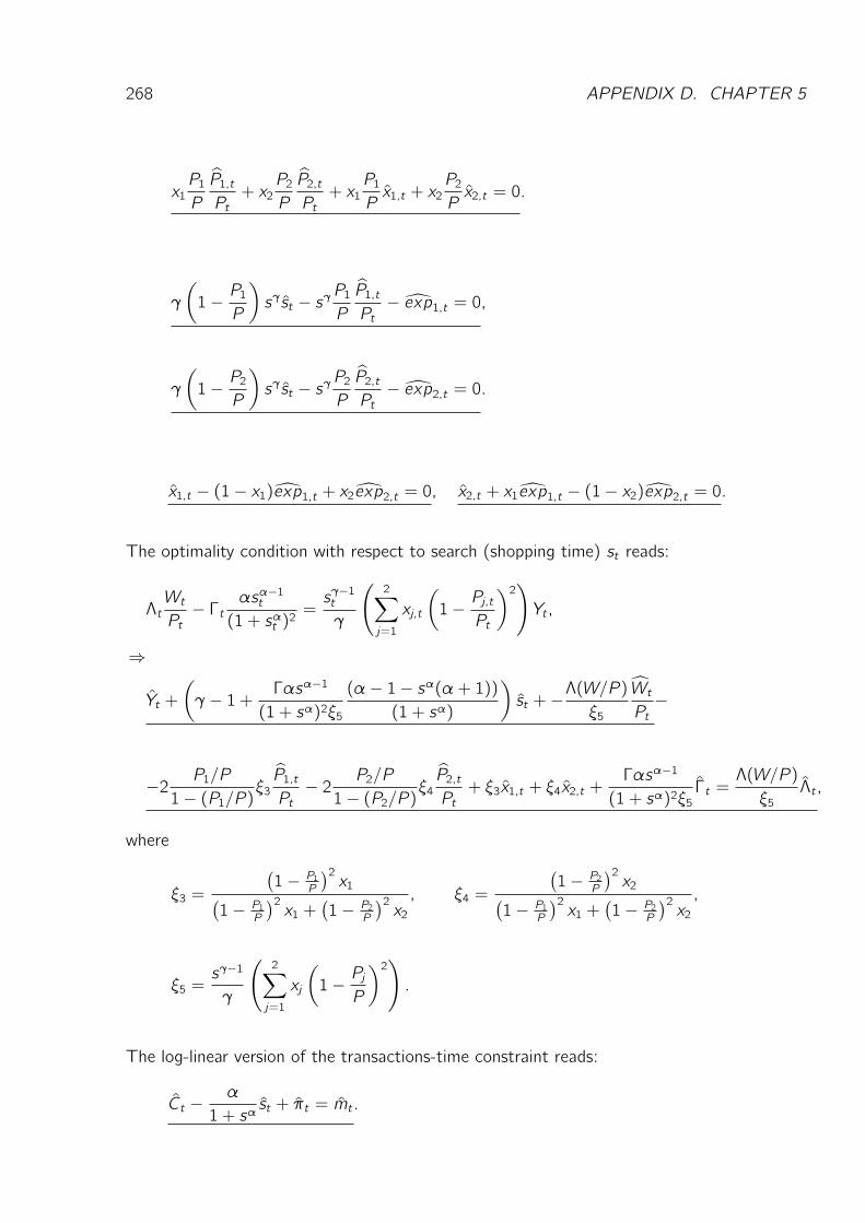
268 APPENDIX D. CHAPTER 5
x1P1P
P1,tPt+ x2P2P
P2,tPt+ x1P1Px1,t + x2
P2Px2,t = 0.
γ
(1− P1P
)sγ st − sγ P1
P
P1,tPt− exp1,t = 0,
γ
(1− P2P
)sγ st − sγ P2
P
P2,tPt− exp2,t = 0.
x1,t − (1− x1)exp1,t + x2exp2,t = 0, x2,t + x1exp1,t − (1− x2)exp2,t = 0.
The optimality condition with respect to search (shopping time) st reads:
ΛtWtPt− Γt αs
α−1t
(1 + sαt )2=sγ−1t
γ
(2∑
j=1
xj,t
(1− Pj,t
Pt
)2)Yt ,
⇒
Yt +
(γ − 1 + Γαsα−1
(1 + sα)2ξ5
(α− 1− sα(α+ 1))(1 + sα)
)st +−Λ(W/P )
ξ5
WtPt−
−2 P1/P
1− (P1/P )ξ3P1,tPt− 2 P2/P
1− (P2/P )ξ4P2,tPt+ ξ3x1,t + ξ4x2,t +
Γαsα−1
(1 + sα)2ξ5Γt =
Λ(W/P )
ξ5Λt ,
where
ξ3 =
(1− P1
P
)2x1(
1− P1P
)2x1 +
(1− P2
P
)2x2, ξ4 =
(1− P2
P
)2x2(
1− P1P
)2x1 +
(1− P2
P
)2x2,
ξ5 =sγ−1
γ
(2∑
j=1
xj
(1− PjP
)2).
The log-linear version of the transactions-time constraint reads:
Ct − α
1 + sαst + πt = mt .
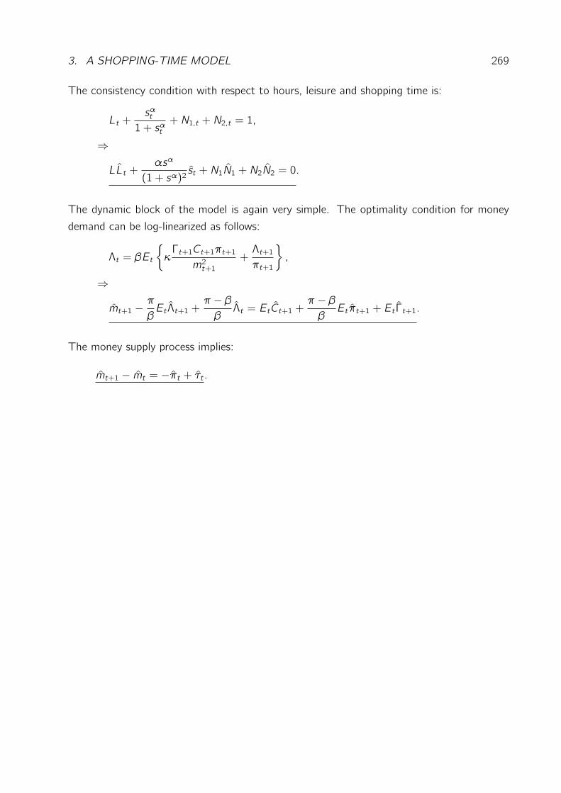
3. A SHOPPING-TIME MODEL 269
The consistency condition with respect to hours, leisure and shopping time is:
Lt +sαt1 + sαt
+ N1,t + N2,t = 1,
⇒
LLt +αsα
(1 + sα)2st + N1N1 + N2N2 = 0.
The dynamic block of the model is again very simple. The optimality condition for money
demand can be log-linearized as follows:
Λt = βEt
κΓt+1Ct+1πt+1m2t+1
+Λt+1πt+1
,
⇒
mt+1 − πβEtΛt+1 +
π − ββΛt = EtCt+1 +
π − ββEtπt+1 + Et Γt+1.
The money supply process implies:
mt+1 − mt = −πt + τt .

270 APPENDIX D. CHAPTER 5

Curriculum Vitae
Education
09/1986 - 05/1993
105th Primary School, Sofia, Bulgaria
09/1993 - 05/1998
91th High School, Sofia, Bulgaria
Areas of Concentration: Mathematics, English, German
10/1998 - 05/2003
University of Augsburg
Diploma in Business Administration (Diplom Kaufmann)
Areas of Concentration: Empirical Macroeconomics; Mathematics and Statistics; Finance and
Banking
10/2000 - 09/2001
Student assistant at the chair of mathematical economics and econometrics (Prof. Dr. Ulrich K.
Schittko)
10/2001 - 05/2003
Student assistant at the chair of empirical macroeconomics (Prof. Dr. Alfred Maussner)
12/2005 - 04/2009
University of Augsburg
Doctoral degree in Economics (Doktor der Wirtschaftswissenschaften (Dr. rer. pol.))
Title of Thesis: ”Customer Markets and the Real Effects of Monetary Policy Shocks”
Employment
06/2003 - 10/2009
University of Augsburg
Research and teaching assistant at the chair of empirical macroeconomics (Prof. Dr. Alfred
Maussner)
10/2009 - Present
ifo Institute for Economic Research (Munich)
Research assistant
Department: Business Cycle Analyses and Surveys (Prof. Dr. Kai Carstensen )
271