p-adic Integration and Birational Calabi–Yau Varieties · projective Calabi–Yau varieties over C.IfX and Y are birationally equivalent, then their Betti numbers coincide, i.e

p-adic Integration and

Birational Calabi–Yau

Varieties

Pablo Magni

Geboren am 31. Januar 1995 in Bonn

11. Juli 2016

Bachelorarbeit Mathematik

Betreuer: Prof. Dr. Daniel Huybrechts

Zweitgutachter: Dr. Wenhao Ou

Mathematisches Institut

Mathematisch-Naturwissenschaftliche Fakult

¨

at der

Rheinischen Friedrich-Wilhelms-Universit

¨

at Bonn

1

Zusammenfassung

Die vorliegende Bachelorarbeit befasst sich mit bestimmten topologischen In-varianten von birationalen Calabi–Yau Varietäten. Zentrales Ziel ist es einen Satzvon Batyrev detailliert zu beweisen. Dieser besagt, dass zwei birationale projektiveCalabi–Yau Varietäten über C dieselben Bettizahlen haben (siehe Theorem 3.1).

Der vorgestellte Beweis basiert auf Methoden der p-adischen Analysis, insbeson-dere auf der p-adischen Integration. Die nötigen Grundlagen aus der Zahlentheorieund p-adischen Analysis sowie analytischen Geometrie werden in Abschnitt 1 einge-führt. Dabei wird die Analytifizierung von glatten Varietäten über einem p-adischenKörper detalliert dargestellt. Anschließend wird in Abschnitt 2 ein zentrales Theoremvon Weil bewiesen, welches analytische Informationen (genauer das Volumen einerK-analytischen Mannigfaltigkeit) und zahlentheoretische Informationen (genauerdie Anzahl der Punkte einer Reduktion einer Varietät) miteinander vergleicht. Diesreduziert den Vergleich von bestimmten lokalen Zeta-Funktionen auf den Vergleichvon Volumina von bestimmten K-analytischen Mannigfaltigkeiten. In Abschnitt 3wird diese Verbindung ausgenutzt, um Batyrevs Theorem zu beweisen, in welchemletztendlich gezeigt wird, dass das Volumen zweier birationaler projektiver Calabi–Yau Varietäten im obigen Sinne gleich ist. Die Gleichheit der Bettizahlen folgt dannaus den Weil-Vermutungen.

Um die oben angedeutete Strategie formal durchzuführen, müssen einige tech-nische Aussagen bewiesen werden. Insbesondere wird in Abschnitt 4 gezeigt, wiedie Situation von birationalen Calabi–Yau Varietäten geeignet “ausgebreitet” und“geliftet” werden kann, so dass die oben erwähnten Methoden der p-adischen Analysisanwendbar sind.

Acknowledgement

I would like to thank Professor Daniel Huybrechts for proposing the topic ofthis bachelor thesis, reading preliminary versions of the text carefully and makingvaluable comments, and being always available for questions. Last but not leastI am indebted to Professor Daniel Huybrechts for giving numerous lectures thataccompanied my entire bachelor studies and enabled me to write this bachelor thesis.

Furthermore I would like to thank Dr. Wenhao Ou for being always availablefor questions and discussions and reading preliminary versions of this text, makinginvaluable suggestions and comments, that improved significantly the clarity andlanguage of the formulations in this text. For example the proof of Lemma 3.17 wassuggested by him and improved a preliminary version substantially.

2 Contents

Contents

Introduction 3

1 Fundamental p-adic analysis 5

1.1 p-adic numbers and p-adic fields . . . . . . . . . . . . . . . . . . . . . . . . 51.1.1 p-adic numbers . . . . . . . . . . . . . . . . . . . . . . . . . . . . . 51.1.2 p-adic local number fields . . . . . . . . . . . . . . . . . . . . . . . 7

1.2 Analytification of smooth schemes over a p-adic field . . . . . . . . . . . . 81.2.1 p-adic analysis . . . . . . . . . . . . . . . . . . . . . . . . . . . . . 81.2.2 K-analytic manifolds . . . . . . . . . . . . . . . . . . . . . . . . . . 101.2.3 Analytification of X/K . . . . . . . . . . . . . . . . . . . . . . . . 14

1.3 Haar measure on p-adic fields . . . . . . . . . . . . . . . . . . . . . . . . . 21

2 p-adic integration on Calabi–Yau varieties 25

2.1 Calabi–Yau varieties . . . . . . . . . . . . . . . . . . . . . . . . . . . . . . 252.2 Weil measure and canonical measure . . . . . . . . . . . . . . . . . . . . . 262.3 Weil’s theorem . . . . . . . . . . . . . . . . . . . . . . . . . . . . . . . . . 29

3 Batyrev’s theorem 31

3.1 Batyrev’s theorem for K-equivalent varieties . . . . . . . . . . . . . . . . . 34

4 Spreading out X/C and lifting to X/OK 37

4.1 Projective systems of schemes . . . . . . . . . . . . . . . . . . . . . . . . . 374.2 Spreading out birationally equivalent Calabi–Yau varieties . . . . . . . . . 394.3 Lift to p-adic fields . . . . . . . . . . . . . . . . . . . . . . . . . . . . . . . 41

5 Conclusion and further work 45

References 46

Introduction 3

Introduction

The bachelor thesis at hand deals with certain topological invariants of birationallyequivalent Calabi–Yau varieties. The central goal is the detailed presentation of thefollowing theorem by Batyrev (Theorem 3.1 in this text).

Theorem (Batyrev’s Theorem, [Bat99, Theorem 1.1]). Let X and Y be two integral,projective Calabi–Yau varieties over C. If X and Y are birationally equivalent, then theirBetti numbers coincide, i.e. for all i � 0 we have

dimCHising(X

an,C) = dimCHising(Y

an,C).

The proof is based on methods of p-adic analysis, especially p-adic integration. Thenecessary fundamental concepts from number theory and p-adic analysis as well as analyticgeometry are introduced in Section 1. In doing so we present the analytification of smoothvarieties over a p-adic field K in detail. Afterwards, in Section 2, we prove a theoremof Weil that plays an important role in the proof of Batyrev’s theorem. It enables usto compare analytic informations (more precisely, the volume of a K-analytic manifoldassociated to the variety under consideration) and arithmetic informations (more precisely,the number of points in a reduction to a finite field of the variety under consideration).This reduces the comparison of local zeta functions to the comparison of volumes ofcertain K-analytic manifolds. In Section 3 this connection is used to give a proof ofBatyrev’s theorem, in which it is shown that the volumes, in the above sense, of twobirationally equivalent projective Calabi–Yau varieties, considered over a p-adic field K,are equal. Then the equality of Betti numbers follows from the Weil conjectures. In orderto realize the indicated strategy formally, we have to prove a few technical propositions.In particular, we show in Section 4 how the situation of two birationally equivalent Calabi–Yau varieties over C can be “spread out” and “lifted” so that the mentioned methods ofp-adic analysis can be applied.

The author always tried to support his arguments by using references to the literatureand by working out basic concepts he tried to make the text accessible to readers thatare not completely familiar with the used theories. The expert may skip some “obvious”explanations and reference to “standard” propositions. For space reasons we have to refersometimes to the literature for proofs and details. In many of these cases the proofs arenot very difficult and the interested reader is advised to look at the referenced literature.Nevertheless the reader should be familiar with the foundations of algebraic geometry, asthey are presented, for example, in the first few chapters of [Liu02].

4


1 Fundamental p-adic analysis

In this section we develop and recall the foundations of p-adic analysis that we will need inthe rest of this text. We present these foundations in a level of generality that highlightsthe developed objects on their own, but still keeps our goals in mind. In this regard weuse, for example, in Section 1.3 the theory explained in Section 1 to classify compactK-analytic manifolds. This result is interesting on its own, but is still connected to ouraims, since it uses p-adic integration in a similar way as applied in the proof of Batyrev’stheorem.

1.1 p-adic numbers and p-adic fields

We introduce the field of p-adic numbers and explain basic results concerning it briefly. Inthis way we want to establish a first understanding of the p-adic setting. Further we recallsome basic results about p-adic local number fields and their rings of integers. These willbe the objects over which our schemes will be defined later.

1.1.1 p-adic numbers

The results of the following subsections and more details may be found in most instancesin [Neu07, Chapter II] or [Ser78]. Let us start by fixing some notation. Notation 1.1 is ineffect in the entire text.

Notation 1.1. We will denote by p a prime number unless otherwise stated. Similarly, qwill denote some power pk of p.

Definition 1.2 (p-adic integers). The ring of p-adic integers Zp is defined as the comple-tion of Z at the maximal ideal (p), i.e. Zp is the projective limit lim �Z/(pn) = { (xn)n 2Q

n�1 Z/(pn) | xn ⌘ xn�1 mod pn�1 }.

Proposition 1.3. Let p 2 Z be a prime number.i) The ring of p-adic integers is an integral domain.ii) The ring of p-adic integers is a compact topological ring with the subspace topology

induced by the one ofQ

n�1 Z/(pn), where each Z/(pn) is endowed with the discretetopology. We call this topology the profinite topology on Zp.

iii) Each element 0 6= x 2 Zp can be written uniquely as x = pnu with n � 0 andu 2 Z⇥

p .

Proof. See [Ser78, Section II.1.1] and [Ser78, Section II.1.2] for a proof.

Definition 1.4 (p-adic numbers). The field of p-adic numbers Qp is the fraction fieldQ(Zp) of the ring of p-adic integers Zp.

Remark 1.5. By the representation in Proposition 1.3.iii) it suffices to invert p 2 Zp toobtain Qp, i.e. Qp = Zp[

1p ]. In particular, every 0 6= x 2 Qp can be written uniquely as

pnu with n 2 Z and u 2 Z⇥p .

Proposition 1.6. Let p 2 Z be a prime number.i) There exists a discrete valuation ⌫p on the field of p-adic numbers Qp such that

the ring of p-adic integers Zp is the discrete valuation ring associated to ⌫p. Thisdiscrete valuation is given by ⌫p(pnu) := n, where u 2 Zp as in Proposition 1.3.iii)and Remark 1.5.

ii) The ring of integers Z is a subring of the ring of p-adic integers via the homomorphismx 7! (x mod pn)n 2 Zp. Furthermore, Z ⇢ Zp is a dense subspace.

6 1.1 p-adic numbers and p-adic fields

Proof. i) This is a short calculation in consideration of Propostion 1.3.iii) and Remark 1.5.ii) We show that the map is injective. Let x 2 Z and assume x maps to 0, then x ⌘ 0

mod pn, i.e. pn | x, for every n � 1. This is only possible for x = 0.To see that Z ⇢ Zp is dense consider an arbitrary element x 2 Zp and write x = (xn)n.

Consider the xn as integers and note that x � xn 2 pnZp, since x � xn ⌘ xn � xn ⌘ 0mod pn. This means limn!1 xn = x.

Definition 1.7. The p-adic absolute value on Qp is defined as |x|p := p�⌫p

(x) for x 6= 0and |0|p := 0.

Remark 1.8. Using the absolute value | · |p, we can view the ring of p-adic integers as theunit disc in the field of p-adic numbers. That is Zp = {x 2 Qp | |x|p 1 }.

Proposition 1.9. Let p 2 Z be a prime number.i) The p-adic absolute value | · |p is a non-Archimedean absolute value on Qp, i.e.

|x+ y|p max{|x|p, |y|p} for all x, y 2 Qp.ii) The topology induced by the absolute value | · |p on Zp, called the metric topology, is

the same as the profinite topology on Zp.iii) The metric topology on Qp is locally compact.

Proof. i) This follows immediately from the definition |x|p = p�⌫p

(x) and the fact that ⌫pis a discrete valuation (cf. Proposition 1.6.i)).

ii) In the metric topology the balls B(0, pk) = (pk) form a neighborhood basis of 0.We show that it is also a neighborhood basis of 0 in the profinite topology. We write(pk) = {(xn)n | xk = 0} = Zp \ {0} ⇥ · · · ⇥ {0} ⇥

Qn�k+1 Z/(pn). Since the profinte

topology is induced from the product topology onQ

n�1 Z/(pn) we have the neighborhoodbasis Zp\U1⇥ · · ·⇥Uk⇥

Qn�k+1 Z/(pn) of 0, where k � 1, Ui ⇢ Z/(pi) open and 0 2 Ui.

This shows that also the (pk) form a neighborhood basis of 0 in the profinite topology asdesired. Since both topologies are compatible with the group structure on Zp we concludethat the two topologies have a common basis and are therefore equal.

iii) Note that, since im(| · |p) ⇢ R is discrete, we see that Zp = B(0, 1) = B(0, p) ⇢ Qp

is open. Now, since Zp is compact and multiplication by p 2 Qp is a homeomorphism, weconclude that B(0, pn), n 2 Z, is a neighborhood basis of 0 consisting of compact andopen sets.

Remark 1.10. The metric induced by the absolute value | · |p is complete and, in fact, Qp

is the completion of Q with respect to the restriction of | · |p on Q. Indeed, this is a shortcalculation using Cauchy sequences and the fact that Zp is compact and Z ⇢ Zp is dense.Alternatively see [Neu07, Satz II.2.2] and [Neu07, Satz II.2.3] for a proof.

The following result illustrates some topological properties in the p-adic setting thatmay be unfamiliar when one is accustomed to the Euclidean or Zariski topology.

Proposition 1.11. Let | · | be a non-Archimedean absolute value on some field K. Thenthe following hold.

i) Every point of a ball is a midpoint of it, i.e. if y 2 B(x, ") then B(x, ") = B(y, ").ii) Tow balls B1 = B(x1, "1) and B2 = B(x2, "2) are either disjoint or one is included

in the other.iii) The topology induced by the absolute value is totally disconnected.

Proof. i) Let y 2 B(x, ") and take z 2 B(x, "). Then |y � z| = |(y � x) + (x � z)| max{|x�y|, |x�z|} < ", i.e. z 2 B(y, "), and we see that B(y, ") ⇢ B(x, "). By exchangingthe roles of x and y we conclude that B(y, ") = B(x, ").


ii) Assume B1\B2 6= ; and take x3 2 B1\B2. Then by i) we can write B1 = B(x3, "1)and B2 = B(x3, "2). Say "1 "2, then B1 ⇢ B2.

iii) Let x 2 K and consider the closed ball B(x, ") = {y 2 K | |x � y| "}. Takey 2 B(x, ") and note B(y, ") ⇢ B(y, ") = B(x, "). This means that B(x, ") is open andwe have found a neighborhood basis consisting of open and closed sets in a Hausdorffspace.

1.1.2 p-adic local number fields

Definition 1.12 (p-adic field). A p-adic (local number) field K is a finite extension ofthe field of p-adic numbers Qp.

Notation 1.13. In the whole text K will denote a p-adic field, unless otherwise stated.

Proposition 1.14. Let K be a p-adic field. Then the following hold.i) The absolute value | · |p on Qp extends uniquely to a non-Archimedean absolute value

| · | on K. Explicitly the extension is given by | · | = |NK/Qp

(·)|1/[K:Qp

]p , where NK/Q

p

denotes the norm of the field extension.ii) This absolute value makes K into a locally compact topological field. Furthermore,

the metric induced by the absolute value is complete.

Proof. i) See [Neu07, Theorem II.4.8] for a proof of a more general result. Note that inour case the uniqueness follows from the fact that all norms on a finite dimensional vectorspace over a locally compact field are equivalent (cf. [Kob77, Theorem 10]).

We want to motivate the definition of the absolute value | · | following the expositionin [Kob77, Page 61]. Consider a 2 K of degree n over Qp and let L be the normal closureof Qp(a). Now L/Qp is a finite Galois extension and for every conjugate ai 2 L of a thereis a �i 2 Gal(L/Qp) with �i(a) = ai. If | · | is an absolute value on L extending | · |p, thenx 7! |�i(x)| is also an absolute value extending | · |p. By the uniqueness of the extension ofthe absolute value we deduce that for every x 2 L we have |x| = |�i(x)| and in particular|a| = |ai|. Now

|NQp

(a)/Qp

(a)|p = |nY

i=1

ai| = |a|n

and hence |a| = |NQp

(a)/Qp

(a)|1/np . To conclude note that we have n = [Qp(a) : Qp] = [K :

Qp]/[K : Qp(a)] and NK/Qp

(a) = (NQp

(a)/Qp

(a))[K:Qp

(a)].ii) Endow Qn

p with the maximum norm k(a1, . . . , an)k := max{|a1|p, . . . , |an|p}. Thismakes Qn

p into a locally compact, complete normed space over Qp. Using as in i) that allnorms on K are equivalent, we deduce that for every basis v1, . . . , vn of K over Qp themap Qn

p ! K, (a1, . . . , an) 7! a1v1 + · · ·+ anvn is an isomorphism of topological vectorspaces. Hence, also K is a locally compact complete normed space over Qp.

Definition 1.15. Let K be a p-adic field. We define its ring of integers as OK := {x 2K | |x| 1}. We also define mK := {x 2 K | |x| < 1}.

Proposition 1.16. Let K be a p-adic field. Then the following hold.i) The ring of integers OK is a discrete valuation ring with maximal ideal mK .ii) The residue field OK/mK is a finite extension of Fp.

Proof. i) Define ⌫(x) := � log(|x|) for 0 6= x 2 K and ⌫(0) := 1. This is a valuation,since the absolute value | · | is non-Archimedean. Furthermore, im(| · |p) = {pn | n 2 Z}implies that im(⌫) ⇢ {n log(p)/[K : Qp] | n 2 Z}, i.e. ⌫ is a discrete valuation.

8 1.2 Analytification of smooth schemes over a p-adic field

Note that for x 2 K we have |x| 1 if and only if log(|x|) log(1) = 0, if and only if⌫(x) � 0. So OK is the discrete valuation ring associated to ⌫ with maximal ideal mK .

ii) Compare to [Neu07, Satz II.5.2]. First note that for x 2 Zp with |x|p < 1 we havex 2 mK , since |x| = |x|p < 1. This means that OK/mK is a Fp vector space.

Now let x1 . . . , xn 2 OK be elements such that x1, . . . , xn 2 OK/mK are linearlyindependent over Fp. Assume ↵1x1 + · · ·+ ↵nxn = 0 is a non-trivial linear combination.By dividing by the ↵i0 with the largest absolute value we can assume that all ↵i 2 OK

and ↵i0 = 1. This means that we get a non-trivial linear combination ↵1x1+ · · ·+↵nxn =0 2 OK/mK . This is a contradiction and hence x1, . . . , xn 2 K are linear independent. Itfollows that dimF

p

(OK/mK) dimQp

(K) <1.

Notation 1.17. We will write Fq for the residue field OK/mK , where it is understoodthat q = pk for some k � 1. The (normalized) discrete valuation associated to OK isdenoted by ⌫K and the (normalized) absolute value is defined as | · |p := q�⌫

K

(·).

Remark 1.18. The normalized absolute value | · |p on K has image im(| · |p) = {qk | k 2Z} [ {0} ⇢ R.

We now recall some technical results that are needed later in the text and are includedfor completeness and ease of reference.

Proposition 1.19. Let K be a p-adic field. Then for every r � 1 there exists an extensionof p-adic fields K(r)/K such that [K(r) : K] = r and [OK(r)/mK(r) : OK/mK ] = r. Thisis called an “unramified” extension of degree r.

Proof. See [Neu07, Satz II.7.12] for a proof.

Proposition 1.20.

i) Let O be a complete discrete valuation ring with fraction field K = Q(O) of charac-teristic zero and finite residue field Fpn . Then K is a p-adic field.

ii) Let O be a discrete valuation ring. Then its completion bO is a complete (in themetric and algebraic sense) discrete valuation ring.

Proof. i) See [Neu07, Satz II.5.2] for a proof.ii) See [Neu07, Satz II.4.3] and [Neu07, Satz II.4.5] for a proof.

1.2 Analytification of smooth schemes over a p-adic field

In this section we recall fundamental concepts from p-adic analysis, develop the notionof K-analytic manifold and show how we can associate such a K-analytic manifold to asmooth scheme over a p-adic field K.

1.2.1 p-adic analysis

The following results serve the purpose to convince the reader that basic concepts fromreal analysis carry over to the p-adic setting. A more detailed exposition of the conceptsof this section may be found in [Sch11, Chapter I]. We restrict ourselves to the caseof p-adic fields K, but the statements we will see in this subsection are also valid forcomplete non-Archimedean valued fields.

Definition 1.21 (Convergent power series).i) A power series f =

P↵ a↵x

↵ 2 K[[x1, . . . , xn]] is called "-convergent if we havelim|↵|!1 "|↵||a↵|p = 0. Here ↵ is a multiindex and " > 0 is a real number.


ii) The set of "-convergent power series is denoted by Tn,"(K) and the set of powerseries that are "-convergent for some " > 0 is denoted by Khhx1, . . . , xnii.

Remark 1.22. Indeed, the definition of "-convergence makes sense, since in the completeNon-Archimedean setting the following holds. Let an 2 K for n � 0. The series

P1n=0 an

converges if and only if limn!1 an = 0 (cf. [Sch11, Lemma I.3.1]).

Proposition 1.23. The set Khhx1, . . . , xnii becomes a K-algebra with algebraic operationsinherited from K[[x1, . . . , xn]]. Furthermore, if f 2 Khhx1, . . . , xnii satisfies f(0) 6= 0,then 1/f 2 Khhx1, . . . , xnii. Also composition in the following sense is well-defined. Letg = (g1, . . . , gn) 2 Tr,�(K)n and write gi =

P↵ a

(i)↵ x↵. If for all i = 1, . . . , n we have

max↵(�|↵||a(i)↵ |p) < ", then there is a K-linear map Tn,"(K)! Tr,�(K), f 7! f � g.Proof. See [Sch11, Page 25], [Sch11, Proposition I.5.3], [Igu00, Corollary 2.1.2] and [Sch11,Proposition I.5.4] for a proof and the definition of the composition map.

Proposition 1.24. We can view a power series f 2 Tn,"(K) as a continuous functionon B(0, ") ⇢ Kn via evaluation, i.e. there is a K-algebra homomorphism Tn,"(K) !C0(B(0, "),K), f 7! (a 7! f(a)). Furthermore, this homomorphism is compatible withcompositions as in Proposition 1.23.

Proof. The map is well-defined by Remark 1.22 and the uniform limit theorem [Que01,Satz 1.23]. See [Sch11, Proposition I.5.3] for a proof that the map is a K-algebrahomomorphism and [Sch11, Proposition I.5.4] for a proof of the compatibility withcompositions.

Remark 1.25. We can define partial derivatives of "-convergent power series via formalpartial derivatives. Indeed, if f 2 Tn,"(K), then also @f

@xi

2 Tn,"(K). To see this useRemark 1.22 and that | · |p is a non-Archimedean absolute value. Let us also remarkthat for f 2 Tn,"(K) and y, a 2 B(0, ") we have @(f(x+y))

@xi

(a) = @f@x

i

(a + y) (cf. [Sch11,Proposition I.5.6]). This will allow us to consider partial derivatives of K-analyticfunctions (cf. Definition 1.29) later.

Proposition 1.26. Let 0 6= f 2 Tn,"(K). Then there exists an a 2 B(0, ") such thatf(a) 6= 0.

Proof. See [Sch11, Corollary I.5.8] for a proof.

The following theorems well-known from real analysis also work in the p-adic setting.This will allow us to introduce a concept of manifold, similar to smooth manifolds, in thenext section.

Theorem 1.27 (Implicit function theorem). Let F1, . . . , Fm 2 Khhx1, . . . , xn, y1, . . . , ymiiwith all Fi(0, 0) = 0. If det((@Fi

@yj

(0, 0))i,j) 6= 0, then there exist power series f1, . . . , fm 2Khhx1, . . . , xnii as well as open neighborhoods 0 2 U ⇢ Kn and 0 2 V ⇢ Km such thatf := (f1, . . . , fm) converges on U , F := (F1, . . . , Fn) converges on U ⇥ V and

{(x, f(x)) | x 2 U} = {(x, y) 2 U ⇥ V | F (x, y) = 0}.

Proof. See [Igu00, Theorem 2.1.1] for a proof.

Corollary 1.28 (Inverse function theorem). Let f1, . . . , fn 2 Khhx1, . . . , xnii with allfi(0) = 0. If det( @fi@x

j

(0))ij 6= 0, then there exist power series g1, . . . , gn 2 Khhx1, . . . , xniiand open neighborhoods 0 2 U, V ⇢ Kn such that the map f = (f1, . . . , fn) : U ! V is ahomeomorphism with inverse g = (g1, . . . , gn).

Proof. Compare to [Igu00, Corollary 2.1.1]. Apply Theorem 1.27 with m = n andFi(x, y) := xi � fi(y). For a direct proof see [Sch11, Proposition I5.9].


1.2.2 K-analytic manifolds

We now define K-analytic manifolds, the analogon of smooth (respectively complex)manifolds, where instead of R (respectively C) we use a p-adic field K. These are theobjects on which we will integrate later. More precisely, we are aiming at taking thevolume of the p-adic manifold X(OK) associated to a Calabi–Yau variety X over OK (cf.Section 1.2.3).

Definition 1.29 (K-analytic functions). Let K be a p-adic field and U ⇢ Kn an opensubset.

i) A function f : U ! K is a K-analytic function if for every a 2 U we can write itlocally around a as a convergent power series, i.e. f 2 Khhx1 � a1, . . . , xn � anii.

ii) A map g : U ! Km is called a K-analytic map if its components are K-analyticfunctions.

Remark 1.30. The operations considered for convergent power series in the last sectionalso make sense for K-analytic functions.

Remark 1.31.i) When we define OKn(U) := { f : U ! K | f is K-analytic }, then OKn becomes a

sheaf on Kn, where for V ⇢ U open the restriction map ⇢UV : OKn(U)! OKn(V )is restriction of functions ⇢UV (f) := f |V .

ii) In this way (Kn,OKn) is a locally ringed space, since for every a 2 Kn we see thatmKn,a := { f 2 OKn,a | f(a) = 0 } is a maximal ideal (cf. Proposition 1.23). Wehave OKn,a/mKn,a ' K via f 7! f(a).

iii) We will always consider (Kn,OKn) as a locally ringed space over (pt,K) via themap K ! OKn(Kn), k 7! constk := (x 7! k). In other words (Kn,OKn) is locallyringed in K-algebras. We refer to such locally ringed spaces also by locally K-ringedspaces.

Definition 1.32 (K-analytic Manifold). Let K be a n-dimensional p-adic field. A K-analytic manifold of dimension n is a locally K-ringed Hausdorff space (X,OX) such thatfor every a 2 X there exist an open neighborhood U ⇢ X of a and an open set V ⇢ Kn

such that (U,OX |U ) ' (V,OKn |V ).

Remark 1.33.i) The morphisms of K-analytic manifolds are the morphisms of locally K-ringed

spaces.ii) Let (X,OX) be a K-analytic manifold, and let U ⇢ X and V ⇢ Kn be open such

that (f, f#) : (U,OX |U )⇠�! (V,OKn |V ). Then we call (U, f) a chart. A collection

{(Ui, fi)}i2I of charts is called an atlas if X =S

i2I Ui.

Notation 1.34.

i) We denote a K-analytic manifold by X instead of (X,OX) when there is noambiguity.

ii) If (U, f) is a chart on X, then we can write f(x) = (f1(x), . . . , fn(x)) for x 2 U .We call the fi local coordinates and usually denote fi(x) by xi.

Example 1.35.

i) The locally ringed space (Kn,OKn) is a K-analytic manifold.ii) If X is a K-analytic manifold and U ⇢ X is an open subset, then (U,OX |U ) is a

K-analytic manifold.


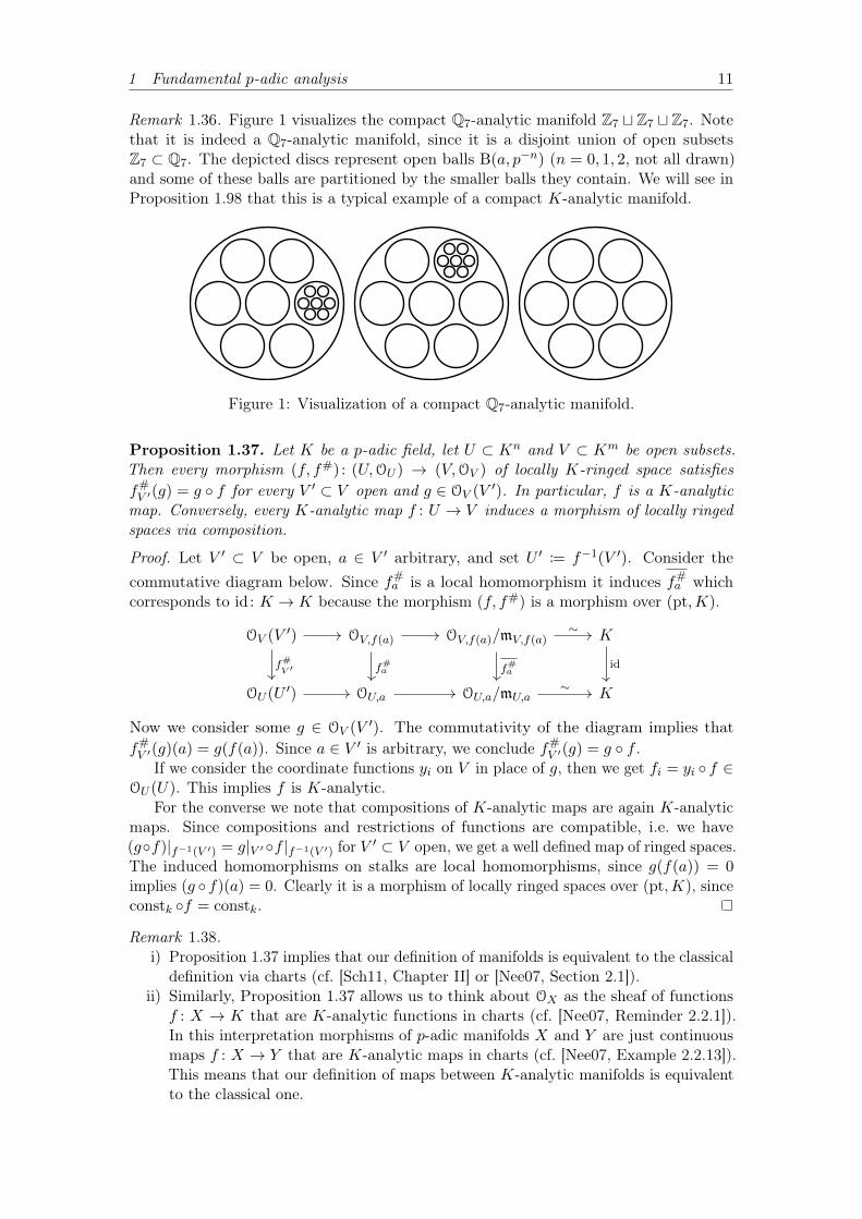
Remark 1.36. Figure 1 visualizes the compact Q7-analytic manifold Z7 t Z7 t Z7. Notethat it is indeed a Q7-analytic manifold, since it is a disjoint union of open subsetsZ7 ⇢ Q7. The depicted discs represent open balls B(a, p�n) (n = 0, 1, 2, not all drawn)and some of these balls are partitioned by the smaller balls they contain. We will see inProposition 1.98 that this is a typical example of a compact K-analytic manifold.

Figure 1: Visualization of a compact Q7-analytic manifold.

Proposition 1.37. Let K be a p-adic field, let U ⇢ Kn and V ⇢ Km be open subsets.Then every morphism (f, f#) : (U,OU ) ! (V,OV ) of locally K-ringed space satisfiesf#V 0(g) = g � f for every V 0 ⇢ V open and g 2 OV (V 0). In particular, f is a K-analytic

map. Conversely, every K-analytic map f : U ! V induces a morphism of locally ringedspaces via composition.

Proof. Let V 0 ⇢ V be open, a 2 V 0 arbitrary, and set U 0 := f�1(V 0). Consider thecommutative diagram below. Since f#

a is a local homomorphism it induces f#a which

corresponds to id : K ! K because the morphism (f, f#) is a morphism over (pt,K).

OV (V 0) OV,f(a) OV,f(a)/mV,f(a) K

OU (U 0) OU,a OU,a/mU,a K

f#V

0 f#a

f#a

⇠

id

⇠

Now we consider some g 2 OV (V 0). The commutativity of the diagram implies thatf#V 0(g)(a) = g(f(a)). Since a 2 V 0 is arbitrary, we conclude f#

V 0(g) = g � f .If we consider the coordinate functions yi on V in place of g, then we get fi = yi � f 2

OU (U). This implies f is K-analytic.For the converse we note that compositions of K-analytic maps are again K-analytic

maps. Since compositions and restrictions of functions are compatible, i.e. we have(g�f)|f�1(V 0) = g|V 0�f |f�1(V 0) for V 0 ⇢ V open, we get a well defined map of ringed spaces.The induced homomorphisms on stalks are local homomorphisms, since g(f(a)) = 0implies (g � f)(a) = 0. Clearly it is a morphism of locally ringed spaces over (pt,K), sinceconstk �f = constk.

Remark 1.38.i) Proposition 1.37 implies that our definition of manifolds is equivalent to the classical

definition via charts (cf. [Sch11, Chapter II] or [Nee07, Section 2.1]).ii) Similarly, Proposition 1.37 allows us to think about OX as the sheaf of functions

f : X ! K that are K-analytic functions in charts (cf. [Nee07, Reminder 2.2.1]).In this interpretation morphisms of p-adic manifolds X and Y are just continuousmaps f : X ! Y that are K-analytic maps in charts (cf. [Nee07, Example 2.2.13]).This means that our definition of maps between K-analytic manifolds is equivalentto the classical one.


As we have seen already for p-adic fields in Proposition 1.11, also K-analytic manifoldsare totally disconnected.

Proposition 1.39. Let (X,OX) be a K-analytic manifold. Then the topological space Xis totally disconnected.

Proof. Since X is Hausdorff it is enough to find for every a 2 X a neighborhood basisconsisting of open and compact sets. Consider a chart (U, f) centered at a, i.e. f(a) = 0.By shrinking U we can assume that f is a homeomorphism onto a ball B(0, qk). SinceB(0, ql) ⇢ B(0, qk) for l k is open and compact, we have found the desired neighborhoodbasis.

Proposition 1.39 suggest that K-analytic manifolds are not very well-behaved. Thiswill lead to the observation that there are not many different compact K-analytic manifolds(cf. Theorem 1.99). In rigid analytic geometry (cf. [Bos14]) one starts by requiring thatthe considered functions converge not only on some open ball but on the whole unit ball(cf. the notion of “Tate algebra”). The resulting theory is deeper than the one of compactK-analytic manifolds.

In the rest of this section we focus our attention on differential forms on K-analyticmanifolds. They will be needed in the construction of the Weil measure in Section 2.2.As we have see so far for K-analytic manifolds, their definition follows the same strategyfamiliar from smooth manifolds. Our presentation is based on the one in [Igu00, Section2.4].

Definition 1.40 (Tangent and cotangent space). Let X be a K-analytic manifold anda 2 X.

i) We call a K-linear map @ : OX,a ! K a derivation at a if it satisfies the Leibnizrule 8f, g 2 OX,a : @(fg) = (@f)g(a) + f(a)(@g).

ii) The space of derivations at a is denoted by TX,a and called the tangent space at a.iii) The cotangent space at a is ⌦X,a := T_

X,a.

Remark 1.41. In a chart x1, . . . , xn around a (recall Notation 1.34) we have a naturalisomorphism OX,a ' Khhx1 � a1, . . . , xn � anii and mX,a ' (x1 � a1, . . . , xn � an) (cf.Proposition 1.26).

Notation 1.42. We use the notation @f@x

i

|a := @(f�'�1)(a)@x

i

, where f 2 OX,a and ' =(x1, . . . , xn) is a chart.

Proposition 1.43. Let X be a K-analytic manifold and x1, . . . , xn a chart around a 2 X.Then { @

@x1|a, . . . , @

@xn

|a} is a basis of the vector space TX,a.

Proof. It is clear that the @@x

i

|a are K-linear and satisfy the Leibniz rule. They are linearindependent, since @

@xn

|a(xj) = �ij . In order to see that they generate TX,a we take anarbitrary f 2 OX,a. Now f can be viewed as a power series around a and we write

f = f(a) +nX

i=1

@f

@xi

��a

xi +X

i<j

xixj f̃ij .

Using the K-linearity of @ 2 TX,a and the Leibniz rule, we see that @f =Pn

i=1@f@x

i

|[email protected], we conclude @ =

Pni=1 @xi

@@x

i

|a.

Definition 1.44. Let X be a K-analytic manifold, let a 2 X and let f 2 OX,a. Wedefine (df)a := f � f(a) 2 mX,a/m2

X,a.


Remark 1.45.i) In a chart x1, . . . , xn around a the (dxi)a form a K-basis of mX,a/m2

X,a. To see thisuse Remark 1.41 and Nakayama’s lemma.

ii) In the situation of i) we have (df)a =Pn

i=1@f@x

i

|a(dxi)a for f 2 OX,a. This followsfrom @

@xi

|a((df)a) = @f@x

i

|a.

Proposition 1.46. Let X be a K-analytic manifold and let a 2 X, then ⌦X,a 'mX,a/m2

X,a.

Proof. Consider the K-linear map mX,a ! ⌦X,a, f 7! (@ 7! @(f)). By the Leibniz rule@(m2

X,a) = 0 and hence we get an induced K-linear map mX,a/m2X,a ! ⌦X,a. Now note

that in a chart x1, . . . , xn centered at a we have (dxi)a 7! (@ 7! @(xi)) = ( @@x

i

|a)_. ByRemark 1.41 the (dxi)a form a basis of mX,a/m2

X,a and by Proposition 1.43 the ( @@x

i

|a)_form a basis of ⌦X,a. This means our map is an isomorphism.

Remark 1.47. Let X be a K-analytic manifold and a 2 X. If (df1)a, . . . , (dfn)a isa basis of mX,a/m2

X,a, then there exists an open neighborhood U around a on which'U := (f1, . . . , fn) defines a chart. To see this note that the change of basis matrix from(df1)a, . . . , (dfn)a to (dx1)a, . . . , (dxn)a is the Jacobian matrix ( @fi@x

j

)ij , and apply theinverse function theorem (Corollary 1.28).

Notation 1.48. Let X be a n-dimensional K-analytic manifold, let a 2 X and let0 r n. We introduce the notation ⌦r

X,a :=Vr ⌦X,a.

Remark 1.49. If x1, . . . , xn is a chart around a, then {(dxi1)a ^ · · · ^ (dxir

)a}i1<···<ir

is abasis of ⌦r

X,a.

Definition 1.50 (Differential form). Let X be a K-analytic manifold of dimension nand let 0 r n. A map ! : X !

Fa2X ⌦r

X,a is called a differential p-form ifi) for all a 2 X one has !(a) 2 ⌦r

X,a, andii) we can write !(a) =

Pi1<···<i

r

fii

,...,ir

(a)(dxi1)a ^ · · · ^ (dxir

)a in every chart(U, x1, . . . , xn), and the fi

i

,...,ir

: U ! K are K-analytic functions.

Definition 1.51. Let X be a K-analytic manifold of dimension n and let 0 r n.The sheaf of differential r-forms ⌦r

X is defined as

⌦rX(U) := {! : X !

G

a2X⌦rX,a | ! is differential r-forms on U}

for U ⇢ X open and the restriction maps ⇢UV : ⌦rX(U) ! ⌦r

X(V ) are restriction offunctions ⇢UV (!) := !|V , where V ⇢ U is open.

Remark 1.52. The sheaf ⌦rX is a sheaf of OX -modules.

Example 1.53. Let X be a K-analytic manifold, let U ⇢ X be open and let f 2 OX(U),then Remark 1.45 shows that df := (x 7! (df)x) is a differential 1-form on U . Thisinduces a morphism d: OK ! ⌦1

X .

Definition 1.54. Let X and Y be K-analytic manifolds, let f : X ! Y be a K-analyticmap and let a 2 X.

i) Define Daf : TX,a ! TY,f(a) as @ 7! (g 7! @(g � f)), andii) denote the dual map by f⇤

a := (Daf)_ : ⌦1Y,f(a) ! ⌦1

X,a.


Remark 1.55. Explicitly f⇤a! = (@ 7! !(Daf(@))) for ! 2 ⌦1

Y,f(a) and under the isomor-phism of Proposition 1.46, where ! b= g 2 mY,f(a)/m

2Y,f(a), this is just g 7! g � f , since we

have !(Daf(@)) = Daf(@)(g) = @(g � f).

Definition 1.56. We denote the mapVr f⇤

a : ⌦rY,f(a) ! ⌦r

X,a again by f⇤a and define

further f⇤ : ⌦1Y (V ) ! ⌦1

X(f�1(V )) by f⇤!(x) := f⇤x(!(f(x))) for V ⇢ Y open and

x 2 f�1(V ).

Remark 1.57. The map f⇤ in Definition 1.56 is well-defined, since in a chart y1, . . . , ymon Y around f(a) we have f⇤

a (dyi)f(a) = f⇤a (yi) = yi � f = (dfi)a, and hence if ! =P

i1<···<ir

gi1...irdyi1^· · ·^dyir we get f⇤!(a) =P

i1<···<ir

gi1...ir(f(a))(dfi1)a^· · ·^(dfir)a.Using (dfi)a =

Pnj=1

@fi

@xj

|a(dxj)a, for a chart x1, . . . , xn around a, we see that f⇤! isagain a differential p-form.

Example 1.58. If X and Y have the same dimension n and r = n, then we can computef⇤! = (g � f)df1 ^ · · · ^ dfn = (g � f) det( @fi@x

j

)ijdx1 ^ · · · ^ dxn.

1.2.3 Analytification of X/K

One can associate to a variety XK over a p-adic field K a topological space XanK in such a

way that if XK is smooth over K the space XanK has the structure of a K-analytic manifold.

This builds a bridge between the algebraic world of varieties and the analytic world ofK-analytic manifolds. We will encounter later Weil’s theorem (Theorem 2.17) whichshows that in the Calabi–Yau case arithmetic data of X over OK , namely the number ofpoints in the reduction X(Fq), and analytic data, namely the volume of X(OK) ⇢ Xan

K

are closely related. We begin this section by recalling the notion of K-rational andOK-integral points as well as the reduction map X(OK)! X(Fq).

Definition 1.59. A variety is a separated scheme of finite type over a field k or over adiscrete valuation ring OK .

Definition 1.60 (Rational and integral points).i) Let X be a scheme over a ring S and R an S-algebra, then we define the set

X(R) := MorSch/S(Spec(R), X).

ii) Let X be a scheme over a field k. We call X(k) the set of k-rational points of X.iii) Let X be a scheme over a discrete valuation ring OK with fraction field K. Then

we call X(OK) the set of OK-integral points of X, and we call X(K) the K-rationalpoints of X.

Remark 1.61. Note that if X is a scheme over OK then X := XK = X⇥OK

K is a schemeover the field K. By the universal property of fiber products the K-rational points of Xand the ones of X coincide.

Remark 1.62. Let X be a scheme over a field k. Then we can view the k-rationalpoints X(k) as the subset of points of X with residue field k via the map X(k) ! X,f 7! f(Spec(k)).

Proposition 1.63 ([Bat99, Remark 2.2]). Let X be a variety over a discrete valuationring OK . Then the following hold.

i) There is a natural inclusion X(OK) ,! X(K).ii) If X is proper, we have X(OK) = X(K) via the inclusion of i).iii) If X is affine, we can identify X(OK) = {a 2 X(K) | 8f 2 �(X,OX) : f(a) 2 OK}.


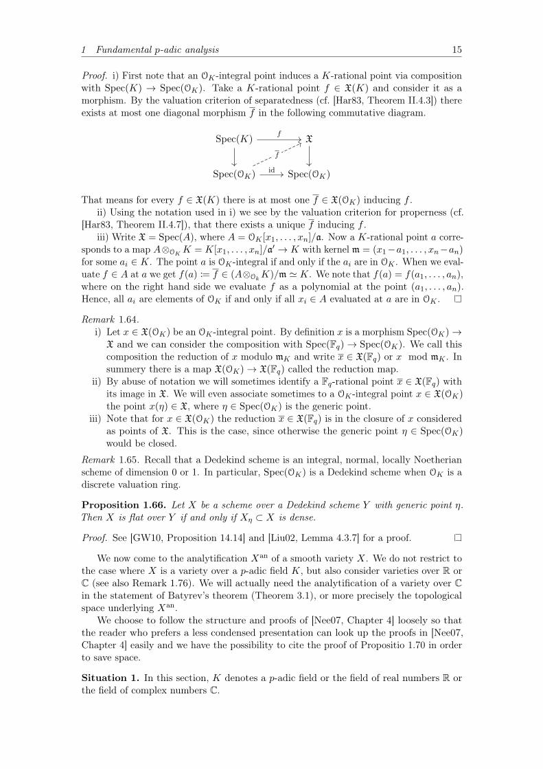
Proof. i) First note that an OK-integral point induces a K-rational point via compositionwith Spec(K) ! Spec(OK). Take a K-rational point f 2 X(K) and consider it as amorphism. By the valuation criterion of separatedness (cf. [Har83, Theorem II.4.3]) thereexists at most one diagonal morphism f in the following commutative diagram.

Spec(K) X

Spec(OK) Spec(OK)

f

f

id

That means for every f 2 X(K) there is at most one f 2 X(OK) inducing f .ii) Using the notation used in i) we see by the valuation criterion for properness (cf.

[Har83, Theorem II.4.7]), that there exists a unique f inducing f .iii) Write X = Spec(A), where A = OK [x1, . . . , xn]/a. Now a K-rational point a corre-

sponds to a map A⌦OK

K = K[x1, . . . , xn]/a0 ! K with kernel m = (x1�a1, . . . , xn�an)for some ai 2 K. The point a is OK-integral if and only if the ai are in OK . When we eval-uate f 2 A at a we get f(a) := f 2 (A⌦O

k

K)/m ' K. We note that f(a) = f(a1, . . . , an),where on the right hand side we evaluate f as a polynomial at the point (a1, . . . , an).Hence, all ai are elements of OK if and only if all xi 2 A evaluated at a are in OK .

Remark 1.64.i) Let x 2 X(OK) be an OK-integral point. By definition x is a morphism Spec(OK)!

X and we can consider the composition with Spec(Fq)! Spec(OK). We call thiscomposition the reduction of x modulo mK and write x 2 X(Fq) or x mod mK . Insummery there is a map X(OK)! X(Fq) called the reduction map.

ii) By abuse of notation we will sometimes identify a Fq-rational point x 2 X(Fq) withits image in X. We will even associate sometimes to a OK-integral point x 2 X(OK)the point x(⌘) 2 X, where ⌘ 2 Spec(OK) is the generic point.

iii) Note that for x 2 X(OK) the reduction x 2 X(Fq) is in the closure of x consideredas points of X. This is the case, since otherwise the generic point ⌘ 2 Spec(OK)would be closed.

Remark 1.65. Recall that a Dedekind scheme is an integral, normal, locally Noetherianscheme of dimension 0 or 1. In particular, Spec(OK) is a Dedekind scheme when OK is adiscrete valuation ring.

Proposition 1.66. Let X be a scheme over a Dedekind scheme Y with generic point ⌘.Then X is flat over Y if and only if X⌘ ⇢ X is dense.

Proof. See [GW10, Proposition 14.14] and [Liu02, Lemma 4.3.7] for a proof.

We now come to the analytification Xan of a smooth variety X. We do not restrict tothe case where X is a variety over a p-adic field K, but also consider varieties over R orC (see also Remark 1.76). We will actually need the analytification of a variety over Cin the statement of Batyrev’s theorem (Theorem 3.1), or more precisely the topologicalspace underlying Xan.

We choose to follow the structure and proofs of [Nee07, Chapter 4] loosely so thatthe reader who prefers a less condensed presentation can look up the proofs in [Nee07,Chapter 4] easily and we have the possibility to cite the proof of Propositio 1.70 in orderto save space.

Situation 1. In this section, K denotes a p-adic field or the field of real numbers R orthe field of complex numbers C.


Definition 1.67 (Strong topology). Let X = V((f1, . . . , fr)) ⇢ AnK . The strong topology

on X(K) is the subspace topology induced by the inclusion X(K) ⇢ AnK(K) = Kn.

Proposition 1.68. Let X be an affine scheme of finite type over K. Then X(K) canbe endowed with a topology such that for every presentation X ' V((f1, . . . , fr)) ⇢ An

K

the topology coincides with the strong topology. We call this topology on X(K) again thestrong topology.

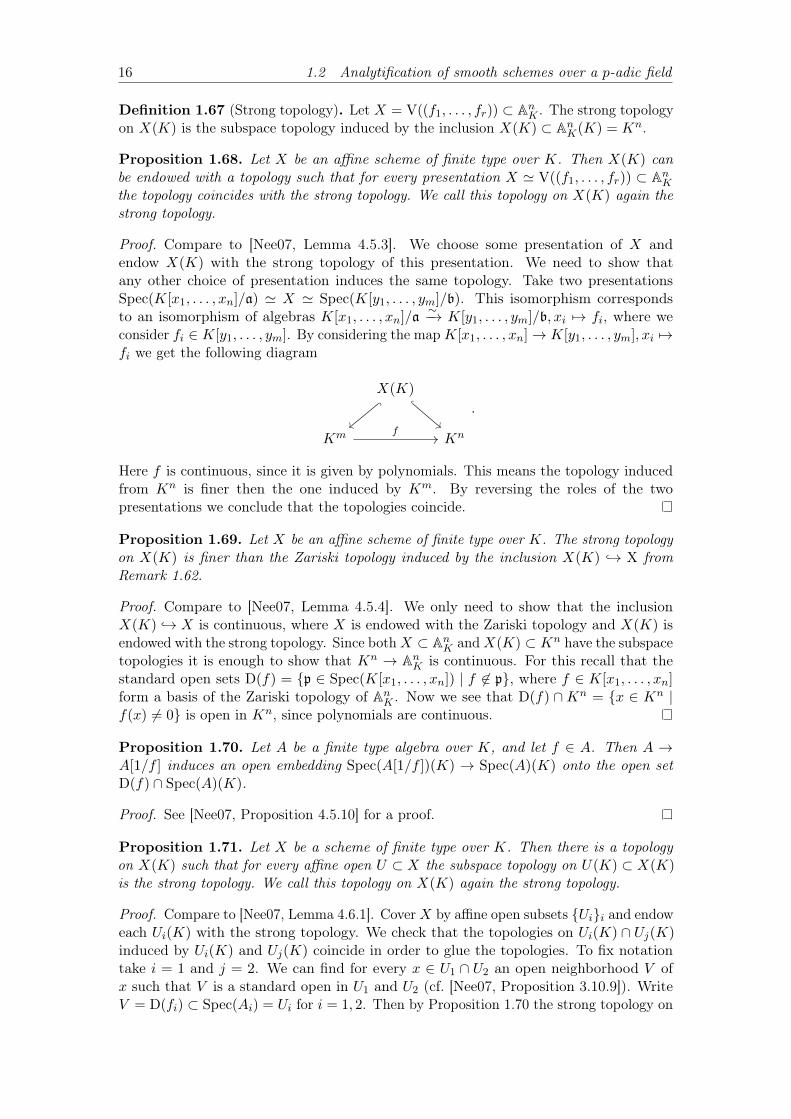
Proof. Compare to [Nee07, Lemma 4.5.3]. We choose some presentation of X andendow X(K) with the strong topology of this presentation. We need to show thatany other choice of presentation induces the same topology. Take two presentationsSpec(K[x1, . . . , xn]/a) ' X ' Spec(K[y1, . . . , ym]/b). This isomorphism correspondsto an isomorphism of algebras K[x1, . . . , xn]/a

⇠�! K[y1, . . . , ym]/b, xi 7! fi, where weconsider fi 2 K[y1, . . . , ym]. By considering the map K[x1, . . . , xn]! K[y1, . . . , ym], xi 7!fi we get the following diagram

X(K)

Km Knf

.

Here f is continuous, since it is given by polynomials. This means the topology inducedfrom Kn is finer then the one induced by Km. By reversing the roles of the twopresentations we conclude that the topologies coincide.

Proposition 1.69. Let X be an affine scheme of finite type over K. The strong topologyon X(K) is finer than the Zariski topology induced by the inclusion X(K) ,! X fromRemark 1.62.

Proof. Compare to [Nee07, Lemma 4.5.4]. We only need to show that the inclusionX(K) ,! X is continuous, where X is endowed with the Zariski topology and X(K) isendowed with the strong topology. Since both X ⇢ An

K and X(K) ⇢ Kn have the subspacetopologies it is enough to show that Kn ! An

K is continuous. For this recall that thestandard open sets D(f) = {p 2 Spec(K[x1, . . . , xn]) | f 62 p}, where f 2 K[x1, . . . , xn]form a basis of the Zariski topology of An

K . Now we see that D(f) \Kn = {x 2 Kn |f(x) 6= 0} is open in Kn, since polynomials are continuous.

Proposition 1.70. Let A be a finite type algebra over K, and let f 2 A. Then A !A[1/f ] induces an open embedding Spec(A[1/f ])(K) ! Spec(A)(K) onto the open setD(f) \ Spec(A)(K).

Proof. See [Nee07, Proposition 4.5.10] for a proof.

Proposition 1.71. Let X be a scheme of finite type over K. Then there is a topologyon X(K) such that for every affine open U ⇢ X the subspace topology on U(K) ⇢ X(K)is the strong topology. We call this topology on X(K) again the strong topology.

Proof. Compare to [Nee07, Lemma 4.6.1]. Cover X by affine open subsets {Ui}i and endoweach Ui(K) with the strong topology. We check that the topologies on Ui(K) \ Uj(K)induced by Ui(K) and Uj(K) coincide in order to glue the topologies. To fix notationtake i = 1 and j = 2. We can find for every x 2 U1 \ U2 an open neighborhood V ofx such that V is a standard open in U1 and U2 (cf. [Nee07, Proposition 3.10.9]). WriteV = D(fi) ⇢ Spec(Ai) = Ui for i = 1, 2. Then by Proposition 1.70 the strong topology on


D(fi)(K) is the subspace topology coming from Spec(Ai) = Ui. Since D(f1) ' V ' D(f2)we see that D(f1)(K) and D(f2)(K) are homeomorphic.

To see that for every U ⇢ X affine open the subspace topology on U(K) ⇢ X(K)is the strong topology we note that we can just extend the above covering by includingU .

Remark 1.72. Proposition 1.71 says that the strong topology on X(K) is the weaktopology with respect to the system {U(K) ,! X(K) | U ⇢ X open affine}, where U(K)is endowed with the strong topology as in Proposition 1.68 (cf. [Nee07, Reminder 4.6.3]).

Notation 1.73. Let X be a variety over K. Then we denote X(K) endowed with thestrong topology by Xan.

Remark 1.74. Consider a morphism f : Spec(A) ! Spec(B) between varieties over K.When we embed Spec(A) ⇢ AN

K and Spec(B) ⇢ AMK for some N,M � 1, then f is specified

by polynomials f1, . . . , fM 2 K[x1, . . . , xN ]. This means that we get a continuous (withrespect to the strong topology) map fan : Spec(A)(K) ! Spec(B)(K). See [Nee07,Lemma 4.5.6] for more details.

As in the affine case a morphism f : X ! Y between schemes of finite type over Kinduces a continuous map fan : Xan ! Y an.

This assignment is functorial, i.e. (f � g)an = fan � gan and idanX = idXan .

Proposition 1.75. Let X and Y be schemes of finite type over K. Then the followinghold.

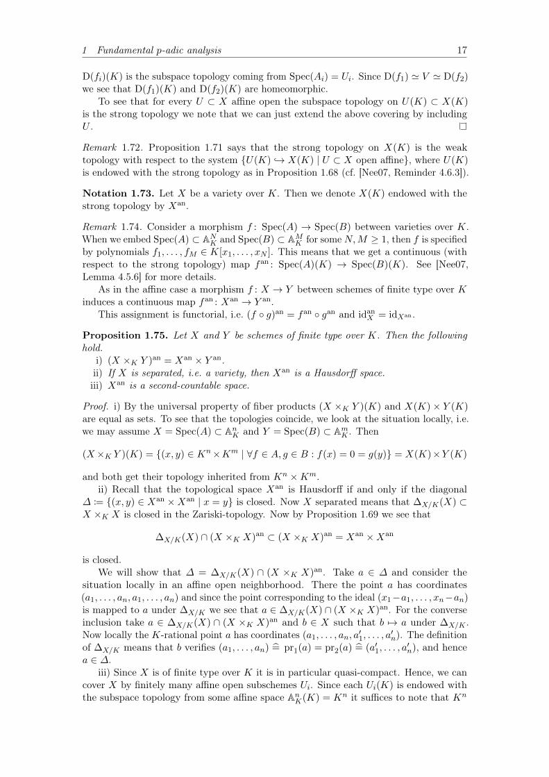
i) (X ⇥K Y )an = Xan ⇥ Y an.ii) If X is separated, i.e. a variety, then Xan is a Hausdorff space.iii) Xan is a second-countable space.

Proof. i) By the universal property of fiber products (X ⇥K Y )(K) and X(K)⇥ Y (K)are equal as sets. To see that the topologies coincide, we look at the situation locally, i.e.we may assume X = Spec(A) ⇢ An

K and Y = Spec(B) ⇢ AmK . Then

(X⇥K Y )(K) = {(x, y) 2 Kn⇥Km | 8f 2 A, g 2 B : f(x) = 0 = g(y)} = X(K)⇥Y (K)

and both get their topology inherited from Kn ⇥Km.ii) Recall that the topological space Xan is Hausdorff if and only if the diagonal

� := {(x, y) 2 Xan ⇥Xan | x = y} is closed. Now X separated means that �X/K(X) ⇢X ⇥K X is closed in the Zariski-topology. Now by Proposition 1.69 we see that

�X/K(X) \ (X ⇥K X)an ⇢ (X ⇥K X)an = Xan ⇥Xan

is closed.We will show that � = �X/K(X) \ (X ⇥K X)an. Take a 2 � and consider the

situation locally in an affine open neighborhood. There the point a has coordinates(a1, . . . , an, a1, . . . , an) and since the point corresponding to the ideal (x1�a1, . . . , xn�an)is mapped to a under �X/K we see that a 2 �X/K(X) \ (X ⇥K X)an. For the converseinclusion take a 2 �X/K(X) \ (X ⇥K X)an and b 2 X such that b 7! a under �X/K .Now locally the K-rational point a has coordinates (a1, . . . , an, a01, . . . , a0n). The definitionof �X/K means that b verifies (a1, . . . , an) b= pr1(a) = pr2(a) b= (a01, . . . , a

0n), and hence

a 2 �.iii) Since X is of finite type over K it is in particular quasi-compact. Hence, we can

cover X by finitely many affine open subschemes Ui. Since each Ui(K) is endowed withthe subspace topology from some affine space An

K(K) = Kn it suffices to note that Kn


is second-countable. Since products of second-countable spaces are second-countableand we can view K as a finite dimensional normed vector space over Qq, we only needto show that Qp is second countable. The latter is satisfied, since Q ⇢ Qp is dense (cf.Proposition 1.6) and hence a separable metric space.

Remark 1.76. If we would consider a topological field K that is not Hausdorff thenProposition 1.75.ii) cannot be true (consider the separated variety A1

K). It is the proof ofProposition 1.69 that fails. There we used that {0} ⇢ K was closed, but this is true ifand only if K is Hausdorff (cf. [Que01, Satz 16.17]). See [Con12] and [LS14] for a moregeneral discussion of endowing the X(R) with a topology, where X is a scheme of finitetype over a topological ring R.

Theorem 1.77 (Jacobian criterion). Let k be a field and X = V((f1, . . . , fr)) ⇢ Ank .

Then X is smooth at x 2 X(k) if and only if rank(( @fi@xj

(x))ij) = n� dimOX,x, where thexi are coordinates on An

k .

Proof. See [Liu02, Theorem 4.2.19] and [Liu02, Exercise 4.3.20] for a proof.

Remark 1.78.i) On a locally Noetherian regular scheme the irreducible components and the con-

nected components coincide, since regular local rings are integral domains (cf. [Liu02,Proposition 4.2.11]).

ii) Let X be an integral scheme of finite type over a field k and x 2 X a closed point.Then dimOX,x = dimX. See [Liu02, Proposition 2.5.23].

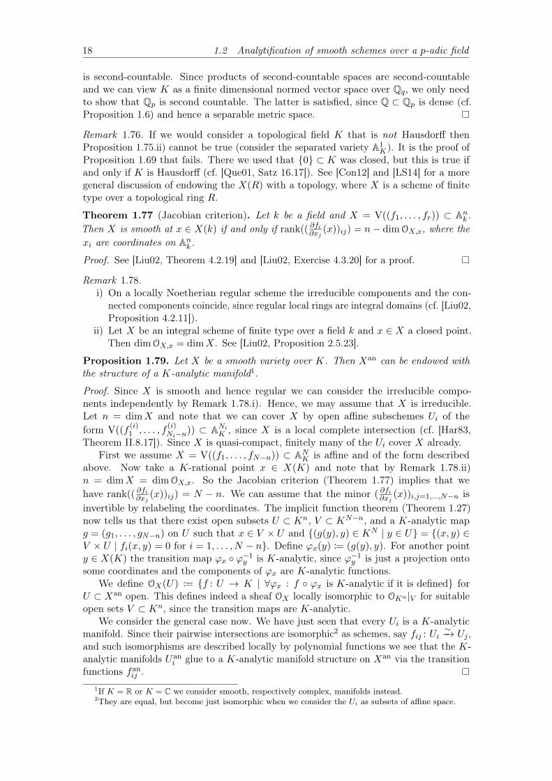
Proposition 1.79. Let X be a smooth variety over K. Then Xan can be endowed withthe structure of a K-analytic manifold1.

Proof. Since X is smooth and hence regular we can consider the irreducible compo-nents independently by Remark 1.78.i). Hence, we may assume that X is irreducible.Let n = dimX and note that we can cover X by open affine subschemes Ui of theform V((f (i)

1 , . . . , f(i)N

i

�n)) ⇢ ANi

K , since X is a local complete intersection (cf. [Har83,Theorem II.8.17]). Since X is quasi-compact, finitely many of the Ui cover X already.

First we assume X = V((f1, . . . , fN�n)) ⇢ ANK is affine and of the form described

above. Now take a K-rational point x 2 X(K) and note that by Remark 1.78.ii)n = dimX = dimOX,x. So the Jacobian criterion (Theorem 1.77) implies that wehave rank(( @fi@x

j

(x))ij) = N � n. We can assume that the minor ( @fi@xj

(x))i,j=1,...,N�n isinvertible by relabeling the coordinates. The implicit function theorem (Theorem 1.27)now tells us that there exist open subsets U ⇢ Kn, V ⇢ KN�n, and a K-analytic mapg = (g1, . . . , gN�n) on U such that x 2 V ⇥ U and {(g(y), y) 2 KN | y 2 U} = {(x, y) 2V ⇥ U | fi(x, y) = 0 for i = 1, . . . , N � n}. Define 'x(y) := (g(y), y). For another pointy 2 X(K) the transition map 'x � '�1

y is K-analytic, since '�1y is just a projection onto

some coordinates and the components of 'x are K-analytic functions.We define OX(U) := {f : U ! K | 8'x : f � 'x is K-analytic if it is defined} for

U ⇢ Xan open. This defines indeed a sheaf OX locally isomorphic to OKn |V for suitableopen sets V ⇢ Kn, since the transition maps are K-analytic.

We consider the general case now. We have just seen that every Ui is a K-analyticmanifold. Since their pairwise intersections are isomorphic2 as schemes, say fij : Ui

⇠�! Uj ,and such isomorphisms are described locally by polynomial functions we see that the K-analytic manifolds Uan

i glue to a K-analytic manifold structure on Xan via the transitionfunctions fan

ij .1If K = R or K = C we consider smooth, respectively complex, manifolds instead.2They are equal, but become just isomorphic when we consider the U

i

as subsets of affine space.


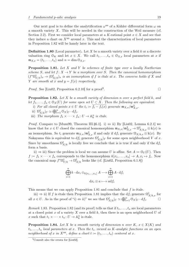
Our next goal is to define the analytification !an of a Kähler differential form ! ona smooth variety X. This will be needed in the construction of the Weil measure (cf.Section 2.2). First we consider local parameters at a K-rational point x 2 X and see thatthey induce a chart on Xan around x. This and the characterization of local parametersin Proposition 1.82 will be handy later in the text.

Definition 1.80 (Local parameter). Let X be a smooth variety over a field k or a discretevaluation ring OK and let x 2 X. We call t1, . . . , tn 2 OX,x local parameters at x ifmX,x = (t1, . . . , tn) and n = dimOX,x.

Proposition 1.81. Let X and Y be schemes of finite type over a locally Noetherianscheme S, and let f : X ! Y be a morphism over S. Then the canonical homomorphism(f⇤⌦1

Y/S)x ! (⌦1X/S)x is an isomorphism if f is étale at x. The converse holds if X and

Y are smooth at x and y = f(x) respectively.

Proof. See [Liu02, Proposition 6.2.10] for a proof3.

Proposition 1.82. Let X be a smooth variety of dimension n over a perfect field k, andlet f1, . . . , fn 2 OX(U) for some open set U ⇢ X. Then the following are equivalent.

i) For all closed points x 2 U the ti := fi � fi(x) generate mX,x/m2X,x.

ii) ⌦1X/k|U '

Lni=1 OX |U · dfi.

iii) The morphism f1 ⇥ · · ·⇥ fn : U ! Ank is étale.

Proof. Compare to [Mum99, Theorem III.§6.1]. i) , ii) By [Liu02, Lemma 6.2.1] weknow that for x 2 U closed the canonical homomorphism mX,x/m2

X,x ! ⌦1X/k,x ⌦ k(x) is

an isomorphism. So ti generate mX,x/m2X,x if and only if dfi generate ⌦X/k,x ⌦ k(x). By

Nakayama this is equivalent to dfi generate ⌦1X/k|V for some open neighborhood V of x.

Since by smoothness ⌦1X/k is locally free we conclude that is is true if and only if the dfi

form a basis.ii) ) iii) Since the problem is local we can assume U is affine. Set A := OU (U). Then

f := f1 ⇥ · · · ⇥ fn corresponds to the homomorphism k[x1, . . . , xn] ! A, xi 7! fi. Nowthe canonical map f⇤⌦1

Y/k ! ⌦1X/k looks like (cf. [Liu02, Proposition 6.1.8])

nM

i=1

k · dxi ⌦k[x1,...,xn

] A �!nM

i=1

A · dfi

dxi ⌦ a 7�! adfi

This means that we can apply Proposition 1.81 and conclude that f is étale.iii) ) ii) If f is étale then Proposition 1.81 implies that the dfi generate ⌦1

X/k,x forall x 2 U . As in the proof of “i) , ii)” we see that ⌦1

X/k|U 'Ln

i=1 OX |U · dfi.

Remark 1.83. Proposition 1.82 (and its proof) tells us that if t1, . . . , tn are local parametersat a closed point x of a variety X over a field k, then there is an open neighborhood U ofx such that t1 ⇥ · · ·⇥ tn : U ! An

k is étale.

Proposition 1.84. Let X be a smooth variety of dimension n over K, x 2 X(K) andt1, . . . , tn local parameters at x. Then the ti, viewed as K-analytic functions on an openneighborhood of x in Xan, define a chart t := (t1, . . . , tn) centered at x.

3Consult also the errata for [Liu02].


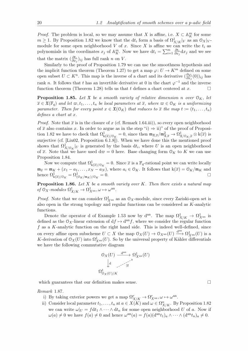
Proof. The problem is local, so we may assume that X is affine, i.e. X ⇢ AmK for some

m � 1. By Proposition 1.82 we know that the dti form a basis of ⌦1X/K |V as an OX |V -

module for some open neighborhood V of x. Since X is affine we can write the ti aspolynomials in the coordinates xj of Am

K . Now we have dti =Pm

i=1@t

i

@xj

dxj and we seethat the matrix ( @t

i

@xj

)ij has full rank n on V .Similarly to the proof of Proposition 1.79 we can use the smoothness hypothesis and

the implicit function theorem (Theorem 1.27) to get a map ' : U ! Km defined on someopen subset U ⇢ Kn. This map is the inverse of a chart and its derivative (@'i

@xj

(0))ij hasrank n. It follows that t has an invertible derivative at 0 in the chart '�1 and the inversefunction theorem (Theorem 1.28) tells us that t defines a chart centered at x.

Proposition 1.85. Let X be a smooth variety of relative dimension n over OK , letx 2 X(Fq) and let $, t1, . . . , tn be local parameters at x, where $ 2 OK is a uniformizingparameter. Then for every point x 2 X(OK) that reduces to x the map t := (t1, . . . , tn)defines a chart at x.

Proof. Note that x is in the closure of x (cf. Remark 1.64.iii)), so every open neighborhoodof x also contains x. In order to argue as in the step “i) ) ii)” of the proof of Proposi-tion 1.82 we have to check that ⌦1

k(x)/OK

= 0, since then mX,x/m2X,x ! ⌦1

X/OK

,x ⌦ k(x) issurjective (cf. [Liu02, Proposition 6.1.8]). When we have done this the mentioned proofshows that ⌦1

X/OK

|U is generated by the basis dti, where U is an open neighborhoodof x. Note that we have used d$ = 0 here. Base changing form OK to K we can useProposition 1.84.

Now we compute that ⌦1k(x)/O

K

= 0. Since x is a Fq-rational point we can write locallymx = mK + (x1 � a1, . . . , xN � aN ), where ai 2 OK . It follows that k(x) = OK/mK andhence ⌦1

k(x)/OK

= ⌦1(O

K

/mK

)/OK

= 0.

Proposition 1.86. Let X be a smooth variety over K. Then there exists a natural mapof OX-modules ⌦1

X/K ! ⌦1Xan ,! 7! !an.

Proof. Note that we can consider ⌦1Xan as an OX -module, since every Zariski-open set is

also open in the strong topology and regular functions can be considered as K-analyticfunctions.

Denote the operator d of Example 1.53 now by dan. The map ⌦1X/K ! ⌦1

Xan isdefined as the OX -linear extension of df 7! danf , where we consider the regular functionf as a K-analytic function on the right hand side. This is indeed well-defined, sinceon every affine open subscheme U ⇢ X the map OX(U) ! OXan(U)

dan��! ⌦1Xan(U) is a

K-derivation of OX(U) into ⌦1Xan(U). So by the universal property of Kähler differentials

we have the following commutative diagram

OX(U) ⌦1Xan(U)

⌦1OX

(U)/K

d

dan

9!

which guarantees that our definition makes sense.

Remark 1.87.i) By taking exterior powers we get a map ⌦r

X/K ! ⌦rXan ,! 7! !an.

ii) Consider local parameter t1, . . . , tn at a 2 X(K) and ! 2 ⌦nX/K . By Proposition 1.82

we can write !|U = fdt1 ^ · · · ^ dtn for some open neighborhood U of a. Now if!(a) 6= 0 we have f(a) 6= 0 and hence !an(a) = f(a)(dant1)a ^ · · · ^ (dantn)a 6= 0.


1.3 Haar measure on p-adic fields

We recall the notion of Haar measure. For a more detailed exposition we refer to [Els11].The general construction of Haar measures provides a measure on a p-adic field K and is afirst step in the definition of the Weil measure, since it endows every chart of a K-analyticmanifold with a ‘good’ measure.

Definition 1.88 (Haar measure). Let G be a locally compact Hausdorff topologicalgroup. Denote by Bo(G) the �-algebra of Borel sets, generated by the open subsets of G.A Haar measure on G is a measure µ : Bo(G)! [0,1] such that

i) it is non-trivial, i.e. µ 6= 0,ii) it is locally finite, i.e. for every g 2 G there exists g 2 U ⇢ G open such that

µ(U) <1,iii) it is inner regular, i.e. for every B 2 Bo(G) we have µ(B) = sup{µ(K) | K ⇢

B compact },iv) it is (left) translation-invariant, i.e. for every g 2 G and B 2 Bo(G) we have

µ(g ·B) = µ(B).

Theorem 1.89 (Existence and uniqueness of Haar measures). Let G be a locally compactHausdorff topological group, then there exists a Haar measure on G. This measure isunique up to a positive factor.

Proof. See [Els11, Theorem VIII.3.12] for a proof.

Notation 1.90. When a locally compact Hausdorff topological group G and a normal-ization (i.e. the positive factor in Theorem 1.89) are fixed we denote the Haar measure onG by µHaar.

Remark 1.91.i) On Rn the Haar measure with normalization µHaar([0, 1]n) = 1 is the Lebesque

measure �n.ii) Let G and H be two locally compact Hausdorff topological groups with Haar

measures µG and µH , respectively. Then the product measure µG ⌦ µH is a Haarmeasure on G⇥H.4 For a finite product G⇥n we denote the product measure alsoby µn

G, or µnHaar if the group G is clear from the context (cf. Notation 1.90).

Proposition 1.92. Let G be a locally compact Hausdorff topological group with Haarmeasure µHaar. Then the following hold.

i) For every compact set K ⇢ G we have µHaar(K) <1.ii) For every open set ; 6= U ⇢ G we have µHaar(U) > 0.

Proof. i) Since µHaar is locally finite we find for every a 2 K an open neighborhoodUa ⇢ G of a with µHaar(Ua) <1. By compactness of K finitely many of those cover K,say {Ua

i

}ni=1, and we conclude µHaar(K) Pn

i=1 µHaar(Uai

) <1.ii) Assume µHaar(U) = 0 and consider an arbitrary compact set K ⇢ G. Then K

can be covered by finitely many ai · U (i = 1, . . . , n) with ai 2 K and hence µHaar(K) Pni=1 µHaar(ai · U) = 0. So all compact subsets of G have measure 0, but by inner

regularity this means µHaar is trivial. This is a contradiction.

Notation 1.93. Recall that every p-adic field K is a locally compact Hausdorff topologicalfield with compact open ring of integers OK (cf. Proposition 1.9.iii) and its proof). In thefollowing we denote by µHaar the Haar measure on K with normalization µHaar(OK) = 1.

4This can be deduced using the Riesz–Markov representation theorem [Els11, Theorem VIII.2.5].

22 1.3 Haar measure on p-adic fields

Proposition 1.94. Let K be a p-adic field, where OK has residue field Fq.i) For all i � 1 we have µHaar(mi

K) = q�i.ii) The measure of a point a 2 K is zero with respect to the Haar measure.

Proof. i) Note that mK ⇢ OK as a subgroup has index (OK : mK) = q, since OK/mK ' Fq.The translation invariance of the Haar measure and the normalization µHaar(OK) = 1imply that µHaar(mK) = 1/q. Similarly, using induction, we see that µHaar(mi

K) = q�i.ii) By translation invariance of the Haar measure we can assume a = 0. Now consider

the balls B(0, q�i) = miK around 0 for i � 0. These have measure q�i as seen in i).

We note that {0} =T1

i=0 B(0, q�i) and hence µHaar({0}) = limi!1 µHaar(B(0, q�i)) =

limi!1 q�i = 0.

Remark 1.95. Note that, since K is non-Archimedean every compact open subset U ⇢ Kn

can be written as a disjoint union of balls B(ai, "i), where ai 2 U and "i > 0 (cf.Proposition 1.11.ii)). Also note that the Borel �-algebra is generated by the compact opensets, in fact the balls B(ai, "i) are compact and open and form a basis of the topology.This means that the calculation in Proposition 1.94 characterized the Haar measure onK (cf. [Els11, Satz II.4.5]).

We have seen already that the implicit function theorem (Theorem 1.27) holds in thep-adic setting. The following theorem tells us that the transformation formula knownfrom the Lebesque integral also works in the p-adic setting. This will allow us to definethe Weil measure in analogy to the definition of measures one associates to volume formson smooth manifolds.

Theorem 1.96 (Transformation formula). Let K be a p-adic field and U, V ⇢ Kn be twoopen subsets. If ' : U ! V is K-bianalytic, then for every integrable function f : V ! Rthe function (f � ') · | det(@'i

@xj

)ij |p is integrable on U and we have

Z

'(U)f dµn

Haar =

Z

U(f � ') · | det

⇣@'

i

@xj

⌘

ij|p dµn

Haar.

Proof. See [Igu00, Proposition 7.4.1] for a proof.

Lemma 1.97. Let K be a p-adic field and let V be a proper linear subspace of Kn. Thenwe have µn

Haar(V ) = 0.

Proof. Since linear maps are K-analytic the transformation formula (Theorem 1.96)allows us to assume Y ⇢ span(e1, . . . , en�1). Here (ei)i is the standard basis of Kn. NowRemark 1.91.ii) tells us that

µnHaar(V ) µHaar(K) · · ·µHaar(K) · µHaar({0}).

Since the measure of a point is zero (cf. Proposition 1.94.ii)), we conclude5 µnHaar(V ) =

0.

The rest of this section is devoted to the classification of compact K-analytic manifolds.An understanding of the following propositions is not necessary for comprehending therest of the text. Nevertheless they demonstrate the usage of p-adic integrals in a simplercontext than considered in Section 2.3. The reader may wish to read Section 2.2, especiallythe construction of Weil’s measure (Construction 2.7), before looking at the proof ofTheorem 1.99.

5Recall that in the context of measures a product is 0 if one factor is 0, even if some factors are 1.


Proposition 1.98 ([Ser65, Théorème 1.a]). Let K be a p-adic field with residue field Fq

and let X be a compact K-analytic manifold of dimension n � 1. Then X is bianalytic toFri=1 O

nK for some 0 < r < q.

Proof. Compare to [Igu00, Lemma 7.5.1]. Take an atlas {(Ui,'i)} such that every Ui

is compact. By compactness of X we can assume that we have only finitely many Ui

and by replacing U1, U2, . . . by U1, U2 \ U1, U3 \ (U1 [ U2), . . . we can assume the Ui tobe pairwise disjoint. Since the Ui are compact, we can write 'i(Ui) =

FNi

j=1 B(xij , qnij )

for certain Ni, xij and nij . Each of these balls is bianalytic to OnK via translation and

rescaling. We conclude that X is bianalytic toFr

i=1 OnK for some r � 1.

Now take a set of representatives a1, . . . , aq 2 OK of Fq and decompose OK =Fqi=1 ai + $KOK , where $K 2 OK is a uniformizing parameter. This means that

OnK ' On�1

K ⇥ OK ' On�1K ⇥

Fqi=1 OK '

Fqi=1 O

nK and we can reduce r until we have

0 < r < q.

Theorem 1.99 ([Ser65, Théorème 1.b, Théorème 2]). Let K be a p-adic field with residuefield Fq and let X be a compact K-analytic manifold of dimension n � 1. Then there isa bianalytic invariant 0 < i(X) < q of X such that X '

Fi(X)i=1 On

K . Moreover, for everyr > 0 we have i(

Fri=1 O

nK) ⌘ r mod q � 1.

Proof. Compare to [Igu00, Theorem 7.5.1]. Consider a nowhere vanishing differentialform ! 2 ⌦n

X(X) and associate to it a measure µ! as in Construction 2.7. We claimthat if !0 2 ⌦n

X(X) is another nowhere vanishing differential form then µ!(X) ⌘ µ!0(X)mod q � 1. By compactness of X and the proof of Proposition 1.39 we may assumethat we have an atlas {(Ui,'i)}i consisting of finitely many pairwise disjoint open setsUi. In a chart (Ui,'i) = (U, x1, . . . , xn) we can write !|U = fUdx1 ^ · · · ^ dxn and!0|U = f 0

Udx1 ^ · · · ^ dxn, where fU and f 0U are K-analytic functions without zeros.

Since im(| · |p) = {qn | n 2 Z} ⇢ R is discrete, we may assume by subdividing U thatfU (x) = qnU and f 0

U (x) = qmU for every x 2 U and fixed nU ,mU 2 Z. Now

µ!(X) =X

i

Z

'i

(Ui

)|fU

i

� '�1i |pdµn

Haar =X

i

qnU

iµnHaar('i(Ui))

and we seeµ!(X)� µ!0(X) =

X

i

(qnU

i � qmU

i )µnHaar('i(Ui)).

Since the Ui are compact (they are closed subsets of a compact space), we deduce that'i(Ui) is a finite union of disjoint balls Bij . Recall that µn

Haar(Bij) 2 {qn | n 2 Z} andhence we see that µn

Haar('i(Ui)) =PN

i

j=1 qkij for suitable Ni and kij . This means that

µ!(X)� µ!0(X) ⌘ 0 mod q � 1.

By Proposition 1.98 we have a bianalytic map f : X⇠�!Fr

i=1 OnK for some 0 < r < q.

We find a nowhere vanishing differential n-form ⇢ onFr

i=1 OnK by defining ⇢|On

K

:=dx1^ · · ·^dxn on each copy of On

K . We can pull back this form to get a nowhere vanishingdifferential n-form ! = f⇤⇢ on X. The transformation formula (Theorem 1.96) andExample 1.58 tell us that µ!(X) = µf⇤⇢(X) = µ⇢(

Fri=1 O

nK). Using the definition of ⇢,

we calculate µ⇢(Fr

i=1 OnK) = rµn

Haar(OnK) = r.

We define 0 < i(X) < q as the number that satisfies i(X) ⌘ µ!(X) mod q � 1 forsome (and hence all) nowhere vanishing differential n-form on X.

Corollary 1.100. Let K be a p-adic field with residue field Fq and let n, r, k � 1 benatural numbers. Then the K-analytic manifolds

Fri=1 O

nK and

Fki=1 O

nK are bianalytic if

and only if r ⌘ k mod q � 1.

24 1.3 Haar measure on p-adic fields

Proof. This follows directly from Theorem 1.99 and the proof of Proposition 1.98.


2 p-adic integration on Calabi–Yau varieties

This section is devoted to the Weil measure on the analytification of a Calabi–Yau varietyand Weil’s theorem. We will finally be able to construct the Weil measure based on thefoundations presented in Section 1.

2.1 Calabi–Yau varieties

Before we denote our attention to the Weil measure, let us define the notion of Calabi–Yauvarieties and consider some examples, in order to get a feeling for the varieties we will beconcerned with in the rest of this text.

Definition 2.1 (Calabi–Yau variety). A Calabi–Yau variety X is a proper, smooth varietyover a field k such that its canonical bundle is trivial, i.e. det⌦1

X/k:= ⌦dim(X)

X/k ' OX . Wecall X a strict Calabi–Yau variety if in addition Hi(X,OX) = 0 for 0 < i < dim(X).

Remark 2.2.i) We will be concerned with not necessarily strict Calabi–Yau varieties.ii) A strict Calabi–Yau variety of dimension two is also called a K3-surface.

Proposition 2.3. Let us give a few examples of Calabi–Yau varieties.i) Non-Example: The projective space Pn

k is not a Calabi–Yau variety, since itscanonical bundle is det⌦1

Pn

k

/k ' OPn

k

(�n� 1).ii) A smooth hypersurface X in Pd�1

k of degree d is a strict Calabi–Yau variety.iii) A smooth complete intersection X of dimension m of k hypersurfaces of degree

d1, . . . , dk in Pm+kk is a Calabi–Yau variety if and only if

Pki=1 di = m+ k + 1.

iv) Abelian varieties are Calabi–Yau varieties. In dimension � 2 they are not strict.v) Integral Calabi–Yau varieties of dimension one with a k-rational point are exactly

elliptic curves.

Proof. i) Using the Euler sequence 0! ⌦1Pn

k

/k ! OPn

k

(�1)�n+1 ! OPn

k

! 0 (cf. [Har83,Theorem II.8.13]) and taking determinants we get det⌦1

Pn

k

/k ' detOPn

k

(�1)�n+1 =

OPn

k

(�(n+ 1)).ii) The short exact sequence

0! O(�d)! OPd�1k

! OX ! 0 (2.1)

induced by 1 7! F , where X = V+(F ) implies #X ' O(�d). Since X is smooth, wealso have the short exact sequence 0 ! #X/#2X ! ⌦1

Pd�1k

/k|X ! ⌦1

X/k ! 0 (cf. [Har83,Theorem II.8.17]). Applying determinants yields

O(�d)|X = det⌦1Pd�1k

/k|X ' det⌦1

X/k ⌦ det#X/#2X ' det⌦1X/k ⌦ detO(�d)|X

and we see det⌦1X/k ' OX .

In order to deduce the strict Calabi–Yau condition, we use the long exact sequence of co-homology (cf. [Har83, Theorem III.1.1A]) associated to the short exact sequence (2.1) andthe fact that Hi(Pd�1

k ,O(l)) = 0 for 0 < i < d� 1 and all l (cf. [Har83, Theorem III.5.1]).iii) See [Har83, Excercise II.8.4] for a proof.iv) In fact the cotangent sheaf ⌦1

X/k is a free OX -module for any group scheme X

over a field k (cf. [Stacks, Tag 047I] or [Mum08, Section II.4]). Since X is smooth asan abelian variety, we know that rank⌦1

X/k = dim(X). This means that the canonicalbundle det⌦1

X/k is trivial.

26 2.2 Weil measure and canonical measure

An abelian variety of dimension n := dim(X) � 2 is not a strict Calabi–Yau variety,since dimk H

r(X,OX) =�nr

�(cf. [Mum08, Corollary III.13.2])6.

v) An elliptic curve X is defined as an integral, proper, smooth curve over a fieldk with geometric genus pg(X) = 1 and a chosen k-rational point. Now every ellipticcurve is an abelian variety (cf. [Liu02, Page 298] or [Har83, Proposition IV.4.8]) andthus by iv) its canonical bundle ⌦1

X/k is trivial. Note that for dimension reasons it is astrict Calabi–Yau variety. Conversely, if ⌦1

X/k ' OX , then pg(X) = dimk H0(X,⌦1

X/k) =

dimk H0(X,OX) = 1. For the last equality apply [Liu02, Corollary 3.3.21] using that X

is proper, reduced and connected and has a k-rational point.

2.2 Weil measure and canonical measure

Now we come to the construction of the Weil measure as promised before. We will alsoencounter the canonical measure, which will be useful for proving a strengthening ofBatyrev’s theorem (cf. Theorem 3.19). We use the following notation in this subsection.

Notation 2.4. Let K be a p-adic field with ring of integers OK . For a smooth variety Xof relative dimension n over OK we denote by ⌦n

X/OK

the n-th exterior power of the sheafof relative differentials ⌦1

X/OK

. We denote X⇥OK

K by X.

Definition 2.5 (Gauge form). Let X be a smooth variety of relative dimension n overOK . A gauge form is a differential form ! 2 H0(X,⌦n

X/OK

) that vanishes nowhere.

Remark 2.6.i) A choice of a gauge ! form is equivalent to a choice of a trivialization OX

⇠�! ⌦nX/O

K

,1 7! !.

ii) Since ⌦nX/O

K

is locally free of rank one, we can always find locally a gauge form.More precisely, for every x 2 X there exists an open neighborhood U ⇢ X aroundx and a section !U 2 H0(U,⌦n

X/OK

) such that 1 7! !U defines an isomorphismOX ' ⌦n

X/OK

.

Construction 2.7. Let X be a smooth variety of relative dimension n over OK . Considera gauge form ! 2 �(X,⌦n

X/OK

) on X. Since X is smooth, Xan and !anX are well-defined.

Here, !X is the pullback of ! to X. Now take an atlas {(Ui,'i)}i. On a chart (U,')write ' = (x1, . . . , xn) and !an|U = fUdx1 ^ · · · ^ dxn, where fU : U ! K is K-analytic.Define µU (A) :=

R'U

(A) |fU � '�1U |pdµn

Haar for A 2 Bo(U).

Proposition 2.8. In the situation of Construction 2.7 let U and V be charts of theatlas. Then µU (A) = µV (A) for every A 2 Bo(U) \ Bo(V ) and the measures glue to aBorel-measure µ on Xan independent of the choice of the atlas.

Proof. We begin by fixing notation. Write 'U = (t1, . . . , tn), 'V = (s1, . . . , sn) anddenote the coordinates on 'U (U \ V ) by x1, . . . , xn, and on 'V (U \ V ) by y1, . . . , yn.Define f̃U := fU �'�1

U , f̃V := fV �'�1V and denote the transition map by 'UV := 'V �'�1

U .In this notation we have 'UV ('U (A)) = 'V (A) and f̃V � 'UV = fV � '�1

U .Now by the transformation formula (Theorem 1.96) we have

µV (A) =

Z

'V

(A)|f̃V |p dµn

Haar(y1, . . . , yn)

=

Z

'U

(A)|(f̃V � 'UV ) det

✓@('UV )i@xj

◆

ij

|p dµnHaar(x1, . . . , xn).

6In characteristic 0 this can be deduced from Hodge symmetry.


By Remark 1.45 we have that dsi =Pn

j=1@s

i

@tj

dtj and it follows that ds1 ^ · · · ^ dsn =

det(@si@tj

)dt1 ^ · · · ^ dtn. Recall that in the notation introduced in Section 1.2.2 we have@s

i

@tj

=@(s

i

�'�1U

)@x

j

� 'U = @('UV

)i

@xj

� 'U . Since fUdt1 ^ · · · ^ dtn = fV ds1 ^ · · · ^ dsn we see

that fU = fV · det(@('UV

)i

@xj

� 'U )ij and hence f̃U = (fV � '�1U ) det(@('UV

)i

@xj

)ij . So we canconclude µV (A) = µU (A).

Now we glue the measures µU to a measure µ on Xan. Since the topological space Xan

is Hausdorff per definition and every point has a neighborhood basis consisting of openand closed sets (cf. the proof of Proposition 1.39), it follows that it is a regular topologicalspace. We have also seen that Xan is second-countable (cf. Proposition 1.75.iii)) andhence paracompact (cf. [Que01, Korollar 10.7]). Thus we may choose a partition of unity{fi}i subordinate to the covering {Ui}i (cf. [Que01, Theorem 10.3]). Now define forA 2 Bo(Xan) the measure

µ(A) :=X

i

Z

Ui

\Afi dµU

i

.

This is indeed a measure, since fi � 0 and hence the involved limits are in fact suprema andwe can change their order freely. We remark that for A 2 Bo(Ui0) we have µ(A) = µU

i0(A),

since we have the following chain of equalities by the pairwise compatibility of the µUj

, themonotone convergence theorem (cf. [Els11, Theorem IV.2.7]) and the fact supp(fj) ⇢ Uj .

µ(A) =X

j

Z

A\Uj

fj dµUj

=X

j

Z

A\Ui0

fj dµUi0

=

Z

A\Ui0

X

j

fj dµUi0=

Z

A\Ui0

1 dµUi0= µU

i0(A)

In order to check the independence of the atlas and the partition of unity we takeanother atlas {(Vj , j)} and a partition of unity gj subordinate to the cover {Vj}j . Wecalculate

X

i

Z

A\Ui

fi dµUi

=X

i

Z

A\Ui

(X

j

gj)fi dµUi

=X

i

X

j

Z

A\Ui

\Vj

gjfi dµUi

=X

i

X

j

Z

A\Ui

\Vj

gjfi dµVj

=X

j

X

i

Z

A\Ui

\Vj

gjfi dµVj

= · · · =X

j

Z

A\Vj

gj dµVj

using monotone convergence, interchangeability of suprema, and pairwise compatibilityof the µU

i

and µVj

.

Definition 2.9 (Weil measure). We call the measure constructed in Proposition 2.8 theWeil measure on Xan and denote it by µWeil when it is clear which variety X we areconsidering. Otherwise we also use the notation µX or µ! when we want to stress thevariety or gauge form.

Proposition 2.10. Let X be a smooth variety of relative dimension n over OK . If!, ⇢ 2 �(X,⌦n

X/OK

) are two gauge forms on X, then the Weil-measures associated to !and ⇢ coincide on X(OK) ⇢ Xan.

Proof. Consider the isomorphisms ! : OX⇠�! ⌦n

X/OK

, 1 7! ! and ⇢ : OX⇠�! ⌦n

X/OK

, 1 7! ⇢.Then the composition ⇢�1 � ! is determined by 1 7! f for some f 2 O⇥

X (X) and wecan write ! = f⇢ 2 �(X,⌦n

X/OK

). Now in a chart (U, x1, . . . , xn) on Xan we can write

28 2.2 Weil measure and canonical measure

!an = gdx1^ · · ·^dxn and ⇢an = hdx1^ · · ·^dxn. We see that g = fh, where we considerf as a K-analytic function, and hence |g(x)|p = |f(x)|p|h(x)|p for every x 2 U .

Since f 2 O⇥X (X) we see that for x 2 X(OK) we have f(x) 2 OK , i.e. |f(x)|p 1.

When we denote by x the reduction modulo mK of x, then we see f(x) = f(x) 6= 0 in Fq,since f vanishes nowhere. This means that |f(x)|p � 1 and hence |f(x)|p = 1.

Construction 2.11. Let X be a smooth variety of relative dimension n over OK . Takea finite cover {Ui}i=1,...,k of X such that on each Ui we have OU

i

' ⌦nX/O

K

|Ui

with 1 7! !i

for some nowhere vanishing differential forms !i. We can associate to each !i a Weilmeasure µ!

i

on (Ui ⇥Ok

K)an. By Proposition 2.10 these measures coincide pairwise on(Ui \ Uj)(OK) = Ui(OK) \ Uj(OK) ⇢ (Ui ⇥O

k

K)an. As in the proof of Proposition 2.8,these measures glue to a measure on X(OK) =

Ski=1 Ui(OK).

Definition 2.12 (Canonical Measure). The measure defined in Construction 2.11 iscalled the canonical measure on X(OK) and is denoted by µcan.

Remark 2.13. If X admits a gauge form, then µcan = µWeil. Indeed, Proposition 2.10allows us to take the trivial cover {X} of X in Construction 2.11. Hence, by definitionµcan = µWeil.

As one would expect sets of codimension greater or equal to one are null sets withrespect to the canonical measure (respectively Weil measure).

Lemma 2.14 ([Bat99, Theorem 2.8]). Let X be a smooth, integral variety over OK

for some p-adic field K and let Y ⇢ X be a closed reduced subscheme of codimensioncodimX(Y) � 1.

i) For the canonical measure µcan on X(OK) we have µcan(Y(OK)) = 0.ii) If X admits a gauge form, then we have µWeil(Y(K)) = 0.

Proof. ii) We base change to K and denote X = X⇥OK

K and Y = Y⇥OK

K. Since Xis flat over OK , we have codimX(Y ) � 1 because otherwise by integrality7 of X we wouldhave X = Y and hence X = Y by Proposition 1.66.

Note that Y is a finite union of its irreducible components, since X is Noetherian asa scheme of finite type over K. By the additivity of measures we can assume that Y isirreducible.

We will now stratify Y into smooth schemes and proof the result by induction onk = dim(Y ). The case k = 0 follows from Proposition 1.94.ii) and the definition of theWeil measure via the Haar measure (cf. Construction 2.7).

Now assume k > 0. The smooth locus Ysm ⇢ Y is open and non-empty (cf. [Liu02,Lemma 4.2.21, Proposition 4.2.24, Remark 4.2.25, Corollary 4.3.33] and [Stacks, Tag 020I]).Since Y is irreducible, we have dim(Y \ Ysm) < k and hence by the induction hypothesiswe get µWeil((Y \Ysm)(K)) = 0. Note that ı : Ysm ,! X is unramified as an immersion (cf.[Liu02, Proposition 4.3.22]) and hence for all y 2 Ysm the canonical map TYsm,z ! TX,z

is injective (cf. [Stacks, Tag 0B2G]). This means that ıan : Y ansm ! Xan is an immersion

(in the sense of manifolds, cf. [Ser92, Section II.III.10.1]), i.e. Xan is covered by charts inwhich ıan looks like the standard embedding Kk ,! Kn. Since Xsm is second-countable,we can assume the cover is countable and using Lemma 1.97 and the countable additivityof measures we conclude µWeil(Ysm(K)) = µWeil(Y an

sm ) = 0.i) We can cover X by open affine subschemes on which µcan is a Weil measure (cf.

Construction 2.11). Since X is of finite type over OK and in particular quasi-compact, wecan take the cover to be finite. This means by additivity of measures that we can assumeX is one of the open affine subschemes, in particular we have µcan = µWeil. Now we canapply statement i).

7X is smooth and in fact connected.


2.3 Weil’s theorem

This section is concerned with Weil’s theorem. It is a central ingredient in the proof ofBatyrev’s theorem, where it will allow us to calculate certain local zeta functions of thereductions module mK of the varieties under consideration, by calculating the volumes ofK-analytic manifolds associated to the varieties. In itself this connection between analysisand arithmetic provided by Weil’s theorem is beautiful and constitutes the first climax ofthis text.

Lemma 2.15 (Hensel). Let K be a p-adic field and f1, . . . , fn 2 OK [T1, . . . , Tn]. Ifx 2 O�n

K satisfies that all fi(x) ⌘ 0 mod mK and the Jacobian det( @fi@Tj

(x)) is a unit inOK , then there exists a unique x0 2 O�n

K with all fi(x0) = 0 and x0 ⌘ x mod mK .

Proof. See [Mum99, Page 177] for a proof.

Lemma 2.16. Let X be a smooth variety of relative dimension n over OK for some p-adicfield K with residue field Fq. Then for every x 2 X(Fq) the fiber Fx := {x 2 X(OK) | x ⌘ xmod mK } is bianalytic to m�n

K via local parameters at x.

Proof. First recall that x (considered as a point of X as in Remark 1.62) is in the closureof each x 2 Fx (cf. Remark 1.64.iii)). So every open neighborhood of x in X will containFx. Take local parameters $K , g1, . . . , gn 2 OX,x at x, where $K 2 OK is a uniformizingparameter, and let U be an affine open neighborhood of x such that all gi are defined on U .Now write U ' V((f1, . . . , fr)) ⇢ Am

OK

= Spec(OK [x1, . . . , xm]) and note that ( @gi@xj

(x))i,jhas rank n, where we view the gi as polynomials (cf. Proposition 1.82). Since X is smoothand hence a local complete intersection, we can assume r = m � n by shrinking U ifnecessary.

The Jacobian criterion tells us that rk( @fi@xj

(x)) = m� n. We consider the matrix

Mx =

0

@@g

i

@xj

(x)

@fi

@xj

(x)

1

A 2 Mat(m⇥m, k(x))

for x 2 Fx. In order that Mx has rank m we have to check that the rows are linearindependent. Assume not, then there is a nontrivial linear combination

nX

i=1

↵i

0

B@

@gi

@x1(x)...

@gi

@xm

(x)

1

CA =m�nX

j=1

�j

0

BB@

@fj

@x1(x)...

@fj

@xm

(x)

1

CCA

for ↵i,�j 2 OK . Since the fj vanish on U , we see that $K , (g1 �Pm�n

j=1 �jfj), g2, . . . , gnare local parameters at x, but their Jacobian matrix evaluated at x does not have rankn. This is a contradiction (cf. Proposition 1.82) and we conclude that det(Mx) 6= 0 2 Fq.Hence, for every x 2 Fx, we have det(Mx) is a unit in OK .

We apply the generalized Hensel Lemma 2.15 and conclude that for arbitrary (↵i)i 2m�n

K there exists a unique x 2 O�nK such that all fi(x) = 0 and gi(x) � ↵i = 0 and

x ⌘ x mod mK . This means that g1, . . . , gn define a bijection Fx⇠�! m�n

K and, since$K , g1, . . . , gn are local parameters, we see that this map is in fact bianalytic (cf. Propo-sition 1.84).

Theorem 2.17 (Weil, [Wei82, Theorem 2.2.5]). Let X be a smooth variety of relativedimension n over OK for some p-adic field K with residue field Fq. Assume that ! 2

30 2.3 Weil’s theorem

H0(X,⌦nX/O

K

) is a gauge form and denote by µWeil the corresponding Weil measure onX(K). Then

µWeil(X(OK)) =#X(Fq)

qn.

Proof. Denote for x 2 X(Fq) the fiber over x by Fx as in Lemma 2.16. Since

µWeil(X(OK)) =X

x2X(Fq

)

µWeil(Fx)

it is enough to see that µWeil(Fx) =1qn .

By Lemma 2.16 we know that Fx ' m�nK via local parameters x1, . . . , xn. Write

! = fdx1 ^ · · · ^ dxn on some open affine neighborhood U around x, where dx1, . . . , dxnform a basis of ⌦1

U/OK

(cf. the proof of Proposition 1.85). Now U ' Spec(OK [x1, . . . , xN ]/a)and we can consider f as a polynomial in the variables x1, . . . , xN . This means thatf(a1, . . . , aN ) 2 OK , i.e. ⌫K(f(a1, . . . , aN )) 1, when all ai 2 OK . Also note thatf(x) 6= 0 implies for every x 2 Fx that f(x) 6= 0 2 Fq, i.e. ⌫K(f(x)) � 1. This meansthat for every x 2 Fx we have |fan(x)|p = 1. Using the definition of Weil’s measure weconclude

µWeil(Fx) =

Z

m�n

K

|f |pdµnHaar = µn

Haar(m�nK ) =

1

qn.

Corollary 2.18. Let X be a smooth variety of relative dimension n over OK for somep-adic field K with residue field Fq. Denote by µcan the canonical measure on X(OK).Then

µcan(X(OK)) =#X(Fq)

qn.

Proof. Compare to [Bat99, Theorem 2.7]. Since X is smooth over OK , the sheaf ⌦nX/O

K

islocally free. Hence we can find an open cover U1, . . . ,Ur ⇢ X on which ⌦n

X/OK

trivializes.Then we have on each Ui the identity µcan = µWeil, where the Weil measure is induced bysome trivializing section !i over Ui (cf. Remark 2.13).

We apply the inclusion-exclusion principle for the canonical measure as well as for thecounting measure and obtain the following equations.

µcan(X(OK)) =X

i1

µcan(Ui1(OK))�X

i1<i2

µcan((Ui1 \ Ui2)(OK)) + . . .

+ (�1)r+1µcan((U1 \ · · · \ Ur)(OK))

#X(Fq) =X

i1

#Ui1(Fq)�X

i1<i2

#(Ui1 \ Ui2)(Fq) + . . .

+ (�1)r+1#(U1 \ · · · \ Ur)(Fq)

Now by Theorem 2.17 the right hand sides are termwise equal up to the factor qn.


3 Batyrev’s theorem

The central theorem presented in this text is Batyrev’s theorem. We will follow Batyrev’sproof using p-adic integration and the Weil conjectures closely. A difference of ourpresentation here is that we separated the passage from the field of complex numbers Cto a p-adic field K from the rest of the proof. Thus we will assume later in this sectionthat our varieties are already defined over OK . The technical step of “spreading out” ourvarieties and “lifting” them to a p-adic field are presented in Section 4.

Theorem 3.1 (Batyrev’s Theorem, [Bat99, Theorem 1.1]). Let X and Y be two integralprojective Calabi–Yau varieties over C. If X and Y are birationally equivalent, then theirBetti numbers coincide, i.e. for all i � 0 we have

dimCHising(X

an,C) = dimCHising(Y

an,C).

Remark 3.2. Recall that singular cohomology only considers the underlying topologicalspaces. This means Theorem 3.1 makes an assertion about a topological invariant.

Remark 3.3. Batyrev’s theorem is in general not true if we drop the assumption thatthe canonical bundles are trivial. For example consider X = P2

C and Y = P1C ⇥C P1

C.Then X and Y are integral, smooth, projective varieties over C that are birationallyequivalent. But ⌦2

Y/C ' det⌦1Y/C ' det(p⇤1⌦

1P1C/C� p⇤2⌦

1P1C/C

) ' p⇤1OP1C(�2)⌦ p⇤2OP1

C(�2)

is not trivial and also ⌦2X/C ' OP2

C(�3) is not trivial. And indeed dimCH2

sing(CP2,C) = 1

and dimCH2sing(CP1 ⇥ CP1,C) = 2.

We recall a few well-known propositions, that will be used in the proof of Lemma 3.8and later in the text.

Proposition 3.4. Let X and Y be projective varieties over a field k. Assume that Xis normal. Then every birational map f : X 99K Y is defined in codimension 1, i.e. f isdefined on an open set U ⇢ X such that codimX(X \ U) � 2.

Proof. See [Har83, Lemma IV.5.1] for a proof.

Proposition 3.5. Let X be a normal, locally Noetherian scheme and let A ⇢ X be a closedsubset of codimension codimX(A) � 2. Then the restriction map OX(X)! OX(X \A)is an isomorphism.

Proof. See [Liu02, Theorem 4.1.14] for a proof.

Theorem 3.6 (Zariski’s Main Theorem). Let f : X ! Y be a separated birationalmorphism of finite type into an integral, normal, locally Noetherian scheme Y . If f isquasi-finite, then f is an open immersion.

Proof. See [Liu02, Corollary 4.4.6] for a proof.

Remark 3.7. We will use Theorem 3.6 only for varieties over a field k. So the conditionsY is Noetherian and f is separated and of finite type are automatically satisfied.

Lemma 3.8 ([Bat99, Proposition 3.1]). Let X and Y be two integral, projective Calabi–Yau varieties of dimension n over C. If X and Y are birationally equivalent then they areisomorphic in codimension one, i.e. there exist open subsets U ⇢ X and V ⇢ Y such thatU ' V and codimX(X \ U) � 2 as well as codimY (Y \ V ) � 2.

32

Proof. Denote by ' : X 99K Y a birational map from X to Y . Since X and Y areprojective and X is normal as a smooth variety, we see by Proposition 3.4 that themaximal open subset U , where ' is regular satisfies codimX(X \ U) � 2.

Now take trivializing sections !X 2 ⌦nX/C(X) and !Y 2 ⌦n

Y/C(Y ). We get8 '|⇤U!Y =

h!X |U for some h 2 OX(U). By Proposition 3.5 we can extend h to a regular functionh 2 OX(X). Since X is integral and projective, we have H0(X,OX) = C (cf. Proposi-tion 4.17.i)). As ' is birational, it is an isomorphism between some open subsets of Xand Y . This implies h 6= 0 2 C.

We want to apply Proposition 1.81. Consider some x 2 U and bases {dx1, . . . , dxn} of⌦1X/C,x and {dy1, . . . , dyn} of ⌦1

Y/C,'(x). Nakayama’s Lemma tells us that it is enough tocheck that the natural map (cf. [Liu02, Proposition 6.1.24]) ↵ : ('⇤⌦1

Y/C)x ⌦OX,x

k(x) ⇣(⌦1

X/C)x ⌦OX,x

k(x) is surjective, since then we get a surjection ('⇤⌦1Y/C)x ⇣ (⌦1

X/C)xbetween free modules of rank n and again by Nakayama’s Lemma this gives us the desiredisomorphism. Now note that ('⇤dyi)(x) := '⇤dyi⌦ 1 2 '⇤⌦1

Y/C⌦OX,x

k(x) considered via↵ as an element of ⌦1

X/C ⌦OX,x

k(x) is just d('#x (yi))(x) := d('#

x (yi))⌦ 1. These latterelements are indeed linearly independent, otherwise d('#

x (y1))(x)^ · · ·^d('#x (yn))(x) = 0,

and hence 0 = '⇤!Y (x) = h!X(x). This is a contradiction, since !X does not vanishanywhere and h 6= 0. Hence, we can apply Proposition 1.81 and get that '|U is étale andin particular quasi-finite.

Zariski’s Main Theorem (Theorem 3.6) tells us that '|U is in fact an open immersioninto the maximal open subset V , where '�1 is regular. Exchanging the roles of X andY we conclude that '|U : U ! V and '�1|V : V ! U are open immersions. Since ' isa birational map, we have ('�1 � ')|U 0 = idU 0 for some open subset U

0 ⇢ U . Now weconclude ('�1 �')|U = idU by using that X is integral and separated and applying [Liu02,Proposition 3.3.11]. This implies that '|U : U ! V is an isomorphism.

We will see in Section 4 how to reduce the situation of Theorem 3.1 to the situationof Lemma 3.9 below, where we can apply Weil’s Theorem (Theorem 2.17). The followingdiagram sketches the connection of the situations.

X/C

X/OK

X0/A0

spreading out

lift

Situation 2. In the diagram A0 ⇢ C is a finitely generated Z-algebra, X0 is projectiveand smooth over A0 and there is a prime ideal p ⇢ A0 such that A0/p = Fq and (X0)pis geometrically connected. Furthermore, there is a p-adic field K and a morphismSpec(OK)! Spec(A0) sending mK to p. We have X0 ⇥A0 C = X and X = X0 ⇥A0 OK .In particular, (X0)p ' Xm

K

.

Lemma 3.9 ([Bat99, Theorem 1.1]). Let X and Y be proper, smooth varieties of relativedimension n over OK such that the generic fibers XK and YK are geometrically connected.Let ; 6= U ⇢ X and ; 6= V ⇢ Y be open subschemes. Assume that there is an isomorphism' : U

⇠�! V and that there exist h 2 O⇥K as well as gauge forms !X 2 ⌦n

X/OK

(X) and!Y 2 ⌦n

Y/OK

(Y) such that '⇤(!Y|V) = h!X|U. Then for every r � 1 we have

#X(Fqr) = #Y(Fqr).8We denote by '|⇤

U

the composition of natural maps ⌦1V/C(V ) ! '|⇤

U

⌦1V/C(U) ! ⌦1

U/C(U).


Proof. In the following we denote the Weil measure associated to a gauge form ! by µ!.We also use the notation !U := !X|U and !V := !Y|V. The assumption '⇤!V = h!U

means that µ'⇤!V = µ!U on U(K), since h satisfies |h|p = 1 as it is a unit in OK .Hence, by the transformation formula (Theorem 1.96, see also the formulation in [Pop11,Theorem 3.3.8])

µ!X(U(K)) = µ!U(U(K)) =

Z

U(K)1 dµ!U =

Z

U(K)1 dµ'⇤!V

=

Z

V(K)1 dµ!V = · · · = µ!Y(V(K)).

Since XK (respectively YK) is connected and smooth it is in particular integral. NowX (respectively Y) is irreducible, since by flatness XK ⇢ X is dense (cf. Proposition 1.66).This means that codimX(X \ U) � 1 and codimY(Y \V) � 1 because U,V 6= ;. So wecan apply Lemma 2.14 to see that9

µ!X(X(K)) = µ!Y(Y(K)).

Note that by properness we have X(K) = X(OK) and Y(K) = Y(OK) (cf. Proposi-tion 1.63.ii)). Now Weil’s theorem (Theorem 2.17) gives us #X(Fq) = #Y(Fq).

For r > 1 consider an unramified extension K(r) as in Proposition 1.19 and basechange our situation to OK(r) . Since OK(r)/mK(r) = Fqr , the above argument yields#X(Fqr) = #Y(Fqr) as desired.

We can now reach the conclusion of Batyrev’s theorem using the Weil Conjectures,proven by Deligne in [Del73]. See [Mus11] for an introduction to the statement of theWeil Conjectures. We recall only the statement of the parts of the Weil Conjectures thatare relevant for Batyrev’s theorem (cf. [Mus11, Section 4.3, Page 39]).

Definition 3.10. Let X 0 be a variety over the finite field Fq. The Hasse–Weil zetafunction, or local zeta function, of X 0 is the power series

Z(X 0, t) := exp

1X

m=1

#X(Fqm)

mtm

!.

Remark 3.11. The conclusion of Lemma 3.9 is that the local zeta functions of the reductionmodulo mK of X and Y are equal, i.e. Z(Xm

K

, t) = Z(YmK

, t).

Theorem 3.12 (Weil Conjectures). Let X 0 be a smooth, projective, geometrically con-nected variety of dimension n over the finite field Fq. Then

i) the local zeta function of X 0 is a rational function of the form

Z(X 0, t) =P1(t)P3(t) . . . P2n�1(t)

P0(t)P2(t) . . . P2n(t)

, where Pi 2 Z[t] and all roots ↵ij of Pi have Euclidean absolute value |↵ij | = q�i/2.ii) Under the assumptions of Situation 2, and X 0 := (X0)p, we have

deg(Pi) = dimCHising((X0 ⇥A0 C)an,C).

9Note that here it is used that we consider K-rational points, in order to have X(K) = U(K)[(X\U)(K).This in turn is the reason, why we want that h is constant, so that our measures µ

'

⇤!V and µ

!U areindeed equal on the set of K-rational points of U and not just on the O

K

-integral points of it.

34 3.1 Batyrev’s theorem for K-equivalent varieties

Remark 3.13. Now if X and Y are varieties over C, spread out to X0 and Y0 as inSituation 2, then Z((X0)p, t) = Z((Y0)p, t) implies

dimCHising((X0 ⇥A0 C)an,C) = dimCHi

sing((Y0 ⇥A0 C)an,C).

Indeed, using the Weil Conjectures (Theorem 3.12) we can write

Z((X0)p, t) =P1(t)P3(t) . . . P2n�1(t)

P0(t)P2(t) . . . P2n(t)Z((Y0)p, t) =

Q1(t)Q3(t) . . . Q2n�1(t)

Q0(t)Q2(t) . . . Q2n(t),

where Pi, Qi 2 Z[t]. The condition on the absolute value of the roots implies Pi = aQi

for some 0 6= a 2 Q. So deg(Pi) = deg(Qi), which implies by the Weil Conjectures thedesired equality Betti numbers10.

Proof of Theorem 3.1 (Batyrev’s theorem). In conclusion this proves Batyrev’s theoremmodulo the spreading out and lifting mentioned in Situation 2. These remaining stepswill be performed in the next section (cf. Lemma 4.14 and Lemma 4.23).

3.1 Batyrev’s theorem for K-equivalent varieties

Using the methods developed so far Batyrev proved a more general version of Theorem 3.1concerning K-equivalent varieties instead of birationally equivalent Calabi–Yau varieties.We want to give a sketch of the proof of this generalization. For space reasons we willrefer to the literature for details.

In this section we will denote the canonical bundle of a smooth variety X over a fieldk by !X . This notation should not be confused with the usage of ! before, where itdenoted a differential form. We also want to remark that the “K” in “K-equivalence”does not refer to a p-adic field.

Definition 3.14 (K-equivalent varieties). Let X and Y be integral, smooth, projectivevarieties over C. Then X and Y are called K-equivalent if there exist a smooth projectivevariety Z over C and proper birational morphisms f : Z ! X, g : Z ! Y such thatf⇤!X ' g⇤!Y , where !X (respectively !Y ) is the canonical bundle on X (respectivelyY ).

The next proposition tells us that the notion of K-equivalence is trivial in the caseof curves or surfaces. In view of Proposition 3.16 this implies that Batyrev’s theorem isclear for curves and surfaces. We refer to the introduction of [Bat99] for a remark on thethree dimensional case.

Proposition 3.15.

i) If X and Y are smooth integral projective birationally equivalent curves over k, thenthey are isomorphic.

ii) If X and Y are K-equivalent surfaces, then they are isomorphic.

Proof. i) The category of smooth projective curves together with dominant morphisms isequivalent to the category of function fields of dimension 1 over k together with k-algebrahomomorphisms (cf. [Har83, Corollary I.6.12]). On the level of objects this equivalenceassociates the function field K(C) to a curve C. Now X and Y are isomorphic, since theyhave the same function field.

ii) See [Pop11, Proposition 4.1.4] for a proof.10Note that for i > 2n the respective singular cohomology groups are zero for dimension reasons.


Proposition 3.16. Let X and Y be projective Calabi–Yau varieties over C. If X and Yare birationally equivalent, then they are K-equivalent.

Proof. Since both canonical bundles !X and !Y are trivial, it suffices to find a smoothprojective variety Z over C and proper birational morphisms f : Z ! X, g : Z ! Y . SinceX and Y are birationally equivalent, there exists an isomorphism ' : U ! V betweenopen subschemes U ⇢ X and V ⇢ Y . Now consider the graph �' ⇢ U ⇥C V . Wedesingularize (cf. [Hir64]) its closure �' ⇢ X ⇥C Y endowed with the reduced inducedscheme structure. That is we get a smooth variety Z over C together with a birationalproper morphism Z ! �'. Postcomposition with the projection prX : X ⇥C Y ! X(respectively prY : X ⇥C Y ! Y ) gives the desired morphism f (respectively g).

Lemma 3.17. Let X and Y be K-equivalent varieties. Then X and Y are isomorphicin codimension one, i.e. there exist open subschemes U ⇢ X and V ⇢ Y such that U ' Vand codimX(X \ U) � 2 as well as codimY (Y \ V ) � 2.

Proof. Compare to [Pop11, Lemma 4.1.6]. Let Z, f and g be as in the definition ofK-equivalence (cf. Definition 3.14). By the ramification formula (cf. [Iit82, Theorem 5.5])there exist effective divisors Rf and Rg on Z such that !Z ' f⇤!X ⌦O

Z

O(Rf ) and !Z 'g⇤!Y ⌦O

Z

O(Rg). Furthermore, Rf (respectively Rg) is supported on the exceptional locusof f (respectively g) (cf. [Pop11, Chapter 3, Page 14]). Now we write Rf =

Pki=1 aiEi and

Rg =Pl

j=1 a0jE

0j with ai, a

0j � 0. The ramification formula together with f⇤!X ' g⇤!Y

implyPk

i=1 aiEi ⇠Pl

j=1 a0jE

0j are linearly equivalent. We can assume in the above linear

equivalence that the Ei, E0j are pairwise distinct by subtracting common terms. Now

there exists a h 2 K(Z) such that div(h) =Pk

i=1 aiEi �Pl

j=1 a0jE

0j . Since Z and Y are

birationally equivalent, we can view h as an element of K(Y ). Now the divisor div(h)on Y cannot have any poles, since codimY (g(E0

j)) � 2 and away from Rg the morphismg is an isomorphism (cf. [Iit82, Proposition 5.8]). This means h 2 H0(Y,OY ) = C andwe conclude div(h) = 0 on Z. In conclusion we see that X and Y are isomorphic incodimension 1.

Remark 3.18. Note that Proposition 3.16 together with Lemma 3.17 provide an alter-native proof of Lemma 3.8. The second proof is conceptually easier but depends ondesingularization.

Theorem 3.19 ([Bat99, Theorem 4.2]). Let X and Y be K-equivalent varieties. Thentheir Betti numbers coincide.

Sketch. See [Ito03, Section 3.3–3.4] or [Pop11, Theorem 4.3.1] for details. First thesituation is spread out and lifted to a p-adic field K similarly as in the proof of Batyrev’stheorem (Theorem 3.1). Now we have f : Z! X and g : Z! Y satisfying f⇤!X ' g⇤!Y.We can ‘pull back’ the canonical measure on X(OK) (respectively Y(OK)) to a measureµZ/X (respectively µZ/Y) on Z(OK) (cf. [Ito03, Section 3.3] for details). The conditionf⇤!X ' g⇤!Y and the equality of ramification divisors, seen in the proof of Proposi-tion 3.17, imply that µZ/X = µZ/Y. Using the transformation formula (Theorem 1.96) andLemma 2.14 we deduce µcan(X(OK)) = µZ/X(Z(OK)). Using a similar argument for Yinstead of X we conclude µcan(Y(OK)) = µZ/Y(Z(OK)) = µZ/X(Z(OK)) = µcan(X(OK)).Now we can apply Corollary 2.18 and get #X(Fq) = #Y(Fq). As in the proof Lemma 3.9and using the Weil Conjectures (Theorem 3.12) we see that the the Betti numbers of Xand Y coincide.

36 3.1 Batyrev’s theorem for K-equivalent varieties


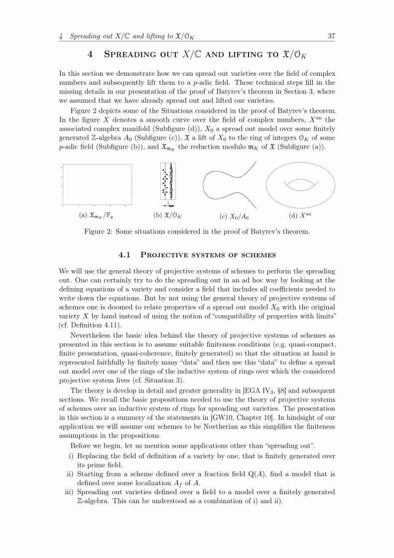
4 Spreading out X/C and lifting to X/OK

In this section we demonstrate how we can spread out varieties over the field of complexnumbers and subsequently lift them to a p-adic field. These technical steps fill in themissing details in our presentation of the proof of Batyrev’s theorem in Section 3, wherewe assumed that we have already spread out and lifted our varieties.

Figure 2 depicts some of the Situations considered in the proof of Batyrev’s theorem.In the figure X denotes a smooth curve over the field of complex numbers, Xan theassociated complex manifold (Subfigure (d)), X0 a spread out model over some finitelygenerated Z-algebra A0 (Subfigure (c)), X a lift of X0 to the ring of integers OK of somep-adic field (Subfigure (b)), and Xm

K

the reduction modulo mK of X (Subfigure (a)).

0

5

10

15

20

0 5 10 15 20

(a) XmK/Fq (b) X/OK (c) X0/A0 (d) Xan

Figure 2: Some situations considered in the proof of Batyrev’s theorem.

4.1 Projective systems of schemes

We will use the general theory of projective systems of schemes to perform the spreadingout. One can certainly try to do the spreading out in an ad hoc way by looking at thedefining equations of a variety and consider a field that includes all coefficients needed towrite down the equations. But by not using the general theory of projective systems ofschemes one is doomed to relate properties of a spread out model X0 with the originalvariety X by hand instead of using the notion of “compatibility of properties with limits”(cf. Definition 4.11).

Nevertheless the basic idea behind the theory of projective systems of schemes aspresented in this section is to assume suitable finiteness conditions (e.g. quasi-compact,finite presentation, quasi-coherence, finitely generated) so that the situation at hand isrepresented faithfully by finitely many “data” and then use this “data” to define a spreadout model over one of the rings of the inductive system of rings over which the consideredprojective system lives (cf. Situation 3).

The theory is develop in detail and greater generality in [EGA IV3

, §8] and subsequentsections. We recall the basic propositions needed to use the theory of projective systemsof schemes over an inductive system of rings for spreading out varieties. The presentationin this section is a summery of the statements in [GW10, Chapter 10]. In hindsight of ourapplication we will assume our schemes to be Noetherian as this simplifies the finitenessassumptions in the propositions.

Before we begin, let us mention some applications other than “spreading out”.i) Replacing the field of definition of a variety by one, that is finitely generated over

its prime field.ii) Starting from a scheme defined over a fraction field Q(A), find a model that is

defined over some localization Af of A.iii) Spreading out varieties defined over a field to a model over a finitely generated

Z-algebra. This can be understood as a combination of i) and ii).

38 4.1 Projective systems of schemes

iv) Eliminating Noetherian hypotheses. This is a variant of iii), where a ring A iswritten as the inductive limit of its finitely generated Z-subalgebras (which areNoetherian by Hilbert’s basis theorem).

v) “Expanding” properties valid at a stalk to an open neighborhood. Here we considerthe stalk Ap as the inductive limit over the open neighborhoods Af with f 62 p.

The presentation in this section is quite formal. The following remark stresses theapplication we have in mind.

Remark 4.1. We can write C as the inductive limit lim�!A�, where A� ⇢ C are finitelygenerated algebras over Z.

Let us fix some notation used in this section.

Situation 3.

i) Denote by ⇤ a filtered partially ordered set with unique minimal element 0.ii) Let (A�)�2⇤ be an inductive system of rings. Denote the transition maps by

��µ : A� ! Aµ, define A := lim�!A� and denote the natural maps A� ! A by ��.iii) Let X0 be a scheme over A0 and set X� := X0 ⇥A0 A�, X := X0 ⇥A0 A. Denote

the morphisms induced by ��µ and �� by x�µ and x�. For Y0 we define Y�, Y , y�µand y� similarly.

iv) If f0 : X0 ! Y0 is a morphism, we denote the morphisms obtained by the basechanges in iii) by f� : X� ! Y� and f : X ! Y .

v) We assume the rings A� and schemes X�, Y� to be Noetherian11.

Definition 4.2. Let X be a Noetherian topological space. A subset C ⇢ X is calledconstructible if it is a finite union of locally closed sets in X.

Notation 4.3. Let T be a topological space. We denote by Open(T ) the family of opensubsets of T , i.e. the topology of T , and by Con(T ) the family of constructible sets in T .

Remark 4.4. Since the morphisms x�µ : Xµ ! X� and x� : X ! X� are continuous,they induce maps Open(X�)! Open(Xµ) and Open(X�)! Open(X) by taking inverseimages of open sets. This gives us a map lim�!Open(X�)! Open(X). Similarly, we get amap lim�!Con(X�)! Con(X).

Proposition 4.5. The maps lim�!Open(X�) ! Open(X) and lim�!Con(X�) ! Con(X)are bijective.

Proof. See [GW10, Theorem 10.57] for a proof.

Proposition 4.6. Assume X is irreducible. Then all X� are irreducible if one of thefollowing conditions is satisfied.

i) The morphisms x�µ : Xµ ! X� are dominant.ii) X0 is flat over A0 and the homomorphisms ��µ : A� ! Aµ are injective.

Proof. i) See [GW10, Exercise 10.26].ii) Locally, on affine open subschemes, the assumptions imply that the ring homo-

morphisms corresponding to the x�µ are injective. This in turn means that the x�µ aredominant and we can apply i).

Remark 4.7. Let F0 and G0 be OX0-modules. Define F� := x⇤0�F0 as well as G� := x⇤0�G0

for each � 2 ⇤, and define F := x⇤�F0, G := x⇤�G0. Since the pull-back x⇤0� is a functor, weget a natural homomorphism lim�!Hom

Mod(X�

)(F�,G�)! HomMod(X)(F,G).

11For a more general situation, without Noetherian hypotheses, see [GW10, Chapter 10]


Proposition 4.8. If F� and G� are quasi-coherent, and F� is finite for some �, then thenatural map lim�!Hom

Mod(X�

)(F�,G�)! HomMod(X)(F,G) is bijective.

Proof. See [GW10, Theorem 10.58] for a proof, recalling that we assume our schemes tobe Noetherian (Situation 3).

Proposition 4.9. Assume that X0 and Y0 are of finite type over A0. Theni) the natural map lim�!Mor

Sch/A�

(X�, Y�)! MorSch/A(X,Y ) is bijective, and

ii) f is an isomorphism if and only if f� is an isomorphism for some �.

Proof. See [GW10, Theorem 10.63] and [GW10, Corollary 10.64] for a proof.

Proposition 4.10. Let Z be a scheme of finite type over A. Then there exists a �, anda scheme Z� of finite type over A� such that Z ' Z� ⇥A

�

A.

Proof. See [GW10, Theorem 10.66] for a proof.

Definition 4.11. Assume that X0 and Y0 are of finite type over A0. We say a property Pof morphisms of schemes is compatible with projective limits if the morphism f : X ! Ysatisfies P if and only if there is a �0 2 ⇤ such that f� : X� ! Y� satisfies P for all � � �0(cf. [GW10, Appendix C]).

Proposition 4.12. The following properties of morphisms of schemes are compatiblewith projective limits.

i) “open immersion”,ii) “closed immersion”,iii) “flat”, andiv) “smooth”.

Proof. See [GW10, Proposition 10.75], [EGA IV3

, Théorème 11.2.6] and [EGA IV4

,Proposition 17.7.8] for a proof.

Remark 4.13. For our applications, we could also use the generic flatness theorem ([EGAIV

2

, Théorème 6.9.1]), and respectively for smoothness [EGA IV3

, Théorème 12.2.4].

4.2 Spreading out birationally equivalent Calabi–Yauvarieties

We now apply the theory of projective systems of schemes recalled in Section 4.1 to thesituation of two birationally equivalent Calabi–Yau varieties. Furthermore, we prove atechnical lemma concerning the generic geometric connectedness of the spread out modelX0 over A0, as required in Situation 2 and Lemma 3.9. In the following we use theinductive system of rings from Remark 4.1.

Lemma 4.14. Let X and Y be projective Calabi–Yau varieties of relative dimension nover C and let U ⇢ X, V ⇢ Y be open subsets such that U ' V and codimX(X \ U) � 2as well as codimY (Y \ V ) � 2. Then there exist a finitely generated Z-algebra A0 ⇢ C,schemes X0, Y0 over A0 and open subschemes U0 ⇢ X0, V0 ⇢ Y0 such that

i) X0 ⇥A0 C ' X and Y0 ⇥A0 C ' Y ,ii) X0 and Y0 are projective and smooth of relative dimension n over A0,iii) ⌦n

X0/A0' OX0 and ⌦n

Y0/A0' OY0 ,

iv) U0 ' V0, andv) codimX0(X0 \ U0) � 2 and codimY0(Y0 \ V0) � 2.

40 4.2 Spreading out birationally equivalent Calabi–Yau varieties

Proof. In the following we will increase � 2 ⇤ several times, i.e. base change to largerZ-algebras. We will suppress this in the notation and will just redefine �. This will notbe a problem, since assertions i)–iv) are stable under base change.

i) We use Remark 4.1 together with Proposition 4.10 to get a finite type Z-algebraA� ⇢ C and schemes X�, Y� of finite type over A� such that X� ⇥A

�

C ' X andY� ⇥A

�

C ' Y .ii) Since closed immersions and smothness is compatible with projective limits (cf.

Proposition 4.12) we deduce that (after increasing � if necessary) X� and Y� are projectiveand smooth over A�. To see that the relative dimension is n we can use that formorphism locally of finite type the relative dimension is stable under base change (cf.[Stacks, Tag 02NK]). Alternatively we can use assertion iii) by noting that if the relativedimension is not n, then ⌦n

X�

/A�

, respectively ⌦nY�

/A�

, cannot have rank one (cf. [Liu02,Proposition 6.2.5]).

iii) Note that ⌦nX

�

/A�

and OX�

pull back to ⌦nX/C and OX under the base change to

C (cf. [Liu02, Proposition 6.1.24]). Since ⌦nX

�

/A�

and OX�

are both coherent sheaves (cf.[Liu02, Proposition 6.1.20]), we can apply Proposition 4.8 and see that (after increasing� if necessary) ⌦n

X�

/A�

' OX�

. Similarly, we have ⌦nY�

/A�

' OY�

.iv) By Propostion 4.5 there exist open subsets U� ⇢ X� and V� ⇢ Y� (after increasing

� if necessary) such that U�⇥A�

C ' U and V�⇥A�

C ' V . Now U� ' V� (after increasing� if necessary) follows from U ' V using Proposition 4.9.

v) We define C := X \ U . The condition codimX(C) � 2 means that there areirreducible closed sets C(0), C(1), C(2) in X such that C ⇢ C(0) ( C(1) ( C(2) ⇢ X.Using Proposition 4.5 we get (after increasing � if necessary) closed sets C� ⇢ C

(0)� (

C(1)� ( C

(2)� ⇢ X� and we can assume C� = X� \ U�. Noting that the C(i) are flat over

the field C, we can use Proposition 4.12.iii) to see that the C(i)� are flat over A� (after

increasing � if necessary). Applying Proposition 4.6 we can assume that the C(i)� are

irreducible (after increasing � if necessary). This shows that codimX�

(X� \ U�) � 2.Similarly, we get codimY

�

(Y� \ V�) � 2.In conclusion, by writing “0 := �”, we have found the desired Z-algebra A0 and schemes

X0, Y0, U0 and V0 over A0.

Remark 4.15. We can assume that A0 in Lemma 4.14 is a regular algebra. Indeed, itsuffices to note that there is an open regular subscheme ; 6= D(f) ⇢ Spec(A0), sincewe can achieve this localization by replacing A0 by a suitable A�. Note that the set ofregular points Reg(A0) ⇢ Spec(A0) is open, since A0 is an algebra of finite type over Zand the latter is an excellent ring (cf. [Liu02, Corollary 8.2.40.(c)]). In fact the proof of[Liu02, Corollary 8.2.40.(c)] also shows that if A0 is integral, then Reg(A0) is non-empty.

We want to remark that we are following the sketch of the spreading out argument inBatyrev’s original proof of his theorem. One can be slightly more efficient by using thecodimension condition and Proposition 3.5 before spreading out. This would mean thatwe don’t have to control the codimension of X0 \U0 (respectively Y0 \ V0) in Lemma 4.14.It would also make Proposition 4.17.ii) in the next section superfluous.

Proposition 4.16. Let X ! S be a projective, flat morphism of Noetherian schemes andassume S is integral. If the generic fiber X⌘ is geometrically connected and geometricallyreduced, then there exists an open subset ; 6= U ⇢ S such that all fibers over U aregeometrically connected.

Proof. Using [Liu02, Corollary 3.3.21] we see that H0(X⌘,OX⌘

) ' K(S). Now we usethe semicontinuity theorem ([Har83, Theorem III.12.8]) to get that the function s 7!


h0(s,OX) := dimk(s)H0(Xs,OX

s

) is upper semi-continuous on S. Hence, we see thatthe set {s 2 S | h0(s,OX) 1} is open and non-empty, since ⌘ lies inside it. Sinceh0(s,OX) � 1, we see that U := {s 2 S | h0(s,OX) = 1} is open and non-empty.

Note that for s 2 U , i.e. H0(Xs,OXs

) ' k(s), we have by the flat base change theorem([Liu02, Corollary 5.2.27]) that

H0(Xs,OXs

) ' H0(Xs,OXs

)⌦k(s) k(s) ' k(s).

This means that Xs is geometrically connected.

4.3 Lift to p-adic fields

The last step we have to perform is to lift our spread out situation to a p-adic field. Thiswill be done in this section.

Proposition 4.17. Let K be a p-adic field.i) Let X be a proper variety over a field k. If X is geometrically reduced and geomet-

rically connected then H0(X,OX) = k.ii) Let X be a proper, flat variety over OK . If H0(XK ,OX

K

) = K then H0(X,OX) = OK .

Proof. i) See [Liu02, Corollary 3.3.21] for a proof.ii) Recall that a module M over a principal ideal domain A is flat if and only if it is

torsion-free over A (cf. [Liu02, Corollary 1.2.5]). Consider M = H0(X,OX) and A = OK .For every f 6= 0 2 H0(X,OX) there exists an open affine subscheme Spec(B) = U ⇢ Xsuch that f |U 6= 0 2 H0(U,OU) = B. Now X flat over OK implies that B is flat over OK

and hence the latter is torsion-free over OK . This means that f cannot be a torsionelement and we conclude that H0(X,OX) is torsion-free and hence flat over OK .

By Serre’s Theorem (cf. [Liu02, Theorem 5.3.2]) we know that H0(X,OX) is a finitelygenerated OK-module. This means that H0(X,OX) is in fact free of finite rank, say r,over the local ring OK (cf. [Liu02, Theorem 1.2.16]).

Now we consider the generic fiber XK , i.e. the base change to Spec(K). Since thisbase change is flat as a localization, we conclude H0(X,OX)⌦O

K

K ' H0(XK ,OXK

) by[Liu02, Corollary 5.2.27]. By assumption dimK H0(XK ,OX

K

) = 1 and hence

1 = dimK(H0(X,OX)⌦OK

K) = dimK(OrK ⌦O

K

K) = r.

This means H0(X,OX) = OK .

Remark 4.18. In particular, Proposition 4.17 says that for a smooth, proper variety Xover OK with XK geometrically connected we have H0(X,OX) = OK .

Proposition 4.19. Let A be a finitely generated algebra over Z of characteristic 0 andlet p 2 Spec(A) be a regular point with k(p) ' Fq. Then there exist a p-adic field K withresidue field Fq and a morphism Spec(OK)! Spec(A) mapping mK to p.

Proof. Compare to [Pop11, Proposition 4.2.3]. Let n = dim(Ap) and write pAp =(s1, . . . , sn). Since the si form a regular sequence, only one si divides p, say s1. Bylocalizing A such that all si 2 A and by dividing out s2, . . . , sn we can assume that n = 1(cf. Krull’s principal ideal theorem).

Now Ap is a discrete valuation ring and hence its completion cAp is a complete discretevaluation ring (cf. Proposition 1.20.ii)). By Proposition 1.20.i) OK := cAp is the ring ofintegers of a p-adic field K. The residue field of K is cAp/pcAp ' Ap/pAp ' Fq and thedesired morphism is the composition A! Ap ! cAp.

42 4.3 Lift to p-adic fields

Remark 4.20. Let A be a finitely generated Z-algebra and let p 2 Spec(A) be a closedpoint, i.e. p ⇢ A is a maximal ideal, then k(p) is a finite field. Indeed, by Hilbert’sNullstellensatz A is a Jacobson ring as a finitely generated Z-algebra and hence A/p is afinite extension of a finite field.

The following theorem by Cassels can also be used to perform the “lift”. It is rathergeneral and can be applied to make methods of p-adic analysis available to questions onfinitely generated fields of characteristic zero.

Theorem 4.21 (Embedding Theorem, Cassels). Let k be a finitely generated field exten-sion of Q and let C ⇢ k⇥ be a finite set. Then there are infinitely many prime numbers pfor which there exists an embedding ◆p : k ,! Qp such that |◆p(c)|p = 1 for all c 2 C.

Proof. See [Cas86, Chapter 5] for a proof.

Remark 4.22. When we apply Cassel’s Embedding Theorem (Theorem 4.21) to the fractionfield K of a finitely generated Z-algebra A and choose C to be the set of generators of Aover Z, we get for infinitely many prime numbers p a morphism Spec(Zp)! Spec(A).

Lemma 4.23. Let A0 be a finitely generated, integral, regular Z-algebra of characteristic0 and X0, Y0 schemes over A0. Then the following hold.

i) There exist a p-adic field K and a homomorphism A0 ! OK . In particular, if mK

contracts to the prime ideal p under this homomorphism, then k(p) is a finite field.Define X := X0 ⇥A0 OK and Y := Y0 ⇥A0 OK .

ii) If X0 (respectively Y0) is projective and smooth of relative dimension n over A0,then X (respectively Y) is a variety over OK that is projective and smooth of relativedimension n.

iii) If in addition to the assumptions in ii) we have that the generic fiber (X0)Q(A0)

(respectively (Y0)Q(A0)) is geometrically connected, then we may assume that ini) the p-adic field K and homomorphism OK ! A0 are chosen such that XK

(respectively YK) and XmK

(respectively YmK

) are geometrically connected.iv) If U0 ⇢ X0 and V0 ⇢ Y0 are isomorphic open subschemes, then there exist isomorphic

open subschemes U ⇢ X and V ⇢ Y, say ' : U ⇠�! Y.v) If in addition to the assumptions in ii), iii) and iv) the open subset U0 in iv)

satisfies codimX0(X0 \ U0) � 2 and there exist nowhere vanishing forms !X0 2⌦n

X0/A0(X0) and !Y0 2 ⌦n

Y0/A0(Y0), then there exist gauge forms !X 2 ⌦n

X/OK

(X),!Y 2 ⌦n

Y/OK

(Y) such that '⇤!Y|V = h!X|U for some h 2 O⇥K

Proof. i) Take some maximal ideal p ⇢ A0. Using Remark 4.20 we can apply Proposi-tion 4.19 to get the desired p-adic field K and homomorphism A0 ! OK .

ii) This is clear, since smoothness and projectiveness are compatible with base change.The proof that the relative dimension is n is similar to the argument in Lemma 4.14.

iii) By Proposition 4.16 there is an open subset D(f) ⇢ Spec(A0) such that all fibersover D(f) are geometrically connected. Now we can just replace A0 by (A0)f in the proofof i).

iv) This is clear, since open immersions and isomorphisms are compatible with basechange.

v) Write '0 : U⇠�! V . Since ⌦n

X0/A0is by assumption trivial we have '⇤

0!Y0 |V =

h0!X0 |U for some h0 2 H0(U,OX0). Note that X0 is Noetherian as a finite type schemeover Z, and it is normal as a smooth scheme. So we can apply Proposition 3.5 to see thath0 2 H0(X0,OX0).

Since isomorphisms of OX0-modules (respectively OY0-modules) are compatible withbase change and ⌦n

X0/A0(respectively ⌦n

Y0/A0) is preserved under base change (cf. [Liu02,


Proposition 6.1.24]), it follows that the base changes !X and !Y of !X0 and !Y0 aregauge forms. Note that the base change of the global section h0 is now a global sectionh 2 H0(X,OX). Hence, by Proposition 4.17 h 2 OK . Since !X and !Y are gauge forms,we conclude h 2 O⇥

K .

At this point we have shown in Lemma 4.14, Remark 4.15 and Lemma 4.23 how toperform the spreading out and lifting needed in the proof of Batyrev’s theorem. Thisconcludes our presentation.

44 4.3 Lift to p-adic fields

5 Conclusion and further work 45

5 Conclusion and further work

To conclude our presentation on K-analytic manifolds, p-adic integration and Batyrev’stheorem, let us reflect on the methods and results encountered in the text.

First let mention some generalizations and strengthenings of Batyrev’s theorem, aswell as further applications of p-adic integration to questions about invariants in birationalsituations.

• In [Wan98] Wang weakens the requirements on the canonical bundle needed toconclude the equality of Betti numbers.

• In [Ito03] Ito and in [Wan02] Wang prove that two K-equivalent varieties X andY have equal Hodge numbers Hr(X,⌦s

X) = Hr(Y,⌦sY ), using methods of p-adic

integration together with p-adic Hodge theory.

• In [Ito04] Ito gives a proof of the well-definedness of Batyrev’s stringy Hodgenumbers using p-adic integration and p-adic Hodge theory.

We want to consider now some positive and some negative aspects of the theory ofp-adic integration as applied in the proof of Batyrev’s theorem. Certainly a positive aspectis the concreteness of p-adic integration and basic p-adic analysis. Many fundamentalresults are familiar from real analysis and one doesn’t have to develop an intuition for thenew objects encountered from scratch. Also p-adic analysis is a very powerful tool andin fact the first of the Weil Conjectures (rationality of local zeta functions) was provedby Dwork using methods from p-adic analysis. In contrast we have seen that compactK-analytic manifolds are not very rich objects. This shows that the naive definition ofmanifold in the p-adic setting may not be the “right” notion. This reflects the fact thatdespite their similarities, the p-adic “world” and the real “world” can be quite different.Another negative aspect of p-adic integration encountered in the text is that one has tofirst translate the problem at hand into the p-adic setting. This technical translationcan be rather tedious and in most cases is difficult to reuse in other arguments. In ourcase the theory of projective systems of schemes mitigates this problem somewhat. Lastbut not least the proof of Batyrev’s theorem presented in this text and the proofs of thegeneralizations and strengthenings referenced above rely heavily on difficult machinery likethe Weil Conjectures, étale cohomology and, as mentioned above, p-adic Hodge theory.

Let us mention an alternative theory that solve some of the problems just observed.Kontsevich introduced in [Kon95] the theory of motivic integration to give a proof ofthe strengthening of Batyrev’s theorem regarding Hodge numbers (Kontsevich’s proofpredates the proofs using p-adic Hodge theory cited above). In this theory the part whereone performs “integration” is separated from the part where one compares invariants likethe Betti or Hodge numbers. This makes the application of the theory easier, since onecan reuse the general theory and doesn’t have to resort to ad hoc methods. Kontsevich’stheory of motivic integration is more geometric in comparison to the arithmetic characterof p-adic integrals and no detour through finite or p-adic fields is needed. We refer to[CNS11, Chapter 6] or [Pop11, Chapter 5–6] for an introduction to motivic integration.After the introduction by Kontsevich the theory of motivic integration was developedfurther and nowadays incorporates ideas from model theory. Some variants of the theoryspecialize to p-adic integrals. See [CNS11, Chapter 1] for an overview of the connectionsbetween the different theories.

In conclusion after studying p-adic integration and Batyrev’s theorem it is also worthto look at motivic integration.

46 References

References

[Bat99] Victor Batyrev. “Birational Calabi–Yau n-folds have equal Betti numbers.”In: New trends in algebraic geometry. Selected papers presented at the Euroconference, Warwick, UK, July 1996. Cambridge: Cambridge UniversityPress, 1999, pp. 1–11.

[Bos14] Siegfried Bosch. Lectures on formal and rigid geometry. Vol. 2105. LectureNotes in Mathematics. Springer, Cham, 2014.

[Cas86] John Cassels. Local fields. London Mathematical Society Student Texts,Cambridge: Cambridge University Press, 1986.

[CNS11] Raf Cluckers, Johannes Nicaise, and Julien Sebag, eds. Motivic integrationand its interactions with model theory and non-archimedean geometry. Vol.I. Cambridge: Cambridge University Press, 2011.

[Con12] Brian Conrad. “Weil and Grothendieck approaches to adelic points.” Enseign.Math. (2) 58.1-2 (2012), pp. 61–97.

[Del73] Pierre Deligne. “La conjecture de Weil. I.” Publ. Math., Inst. Hautes Étud.Sci. 43 (1973), pp. 273–307.

[EGA IV2

] Alexander Grothendieck. “Éléments de géométrie algébrique. IV: Étudelocale des schémas et des morphismes de schémas. (Séconde partie).” Publ.Math., Inst. Hautes Étud. Sci. 24 (1965).

[EGA IV3

] Alexander Grothendieck. “Éléments de géométrie algébrique. IV: Étudelocale des schémas et des morphismes de schémas. (Troisième partie). Rédigéavec la colloboration de Jean Dieudonné.” Publ. Math., Inst. Hautes Étud.Sci. 28 (1966).

[EGA IV4

] Alexander Grothendieck. “Éléments de géométrie algébrique. IV: Étudelocale des schémas et des morphismes de schémas (Quatrième partie). Rédigéavec la colloboration de Jean Dieudonné.” Publ. Math., Inst. Hautes Étud.Sci. 32 (1967).

[Els11] Jürgen Elstrodt. Maß- und Integrationstheorie. 7th revised and updated ed.Berlin: Springer, 2011.

[GW10] Ulrich Görtz and Torsten Wedhorn. Algebraic geometry I. Schemes. Withexamples and exercises. Wiesbaden: Vieweg+Teubner, 2010.

[Har83] Robin Hartshorne. Algebraic geometry. Corr. 3rd printing. Graduate Textsin Mathematics, 52. New York-Heidelberg-Berlin: Springer-Verlag, 1983.

[Hir64] Heisuke Hironaka. “Resolution of singularities of an algebraic variety overa field of characteristic zero. I, II.” Ann. Math. (2) 79 (1964), pp. 109–203,205–326.

[Igu00] Jun-ichi Igusa. An introduction to the theory of local zeta functions. Provi-dence, RI: American Mathematical Society (AMS), 2000.

[Iit82] Shigeru Iitaka. Algebraic geometry. Vol. 76. Graduate Texts in Mathematics.An introduction to birational geometry of algebraic varieties, North-HollandMathematical Library, 24. Springer-Verlag, New York-Berlin, 1982.

References 47

[Ito03] Tetsushi Ito. “Birational smooth minimal models have equal Hodge numbersin all dimensions.” In: Calabi-Yau varieties and mirror symmetry. Proceedingsof the workshop on arithmetic, geometry and physics around Calabi-Yauvarieties and mirror symmetry, Toronto, ON, Canada, July 23–29, 2001.Providence, RI: American Mathematical Society (AMS), 2003, pp. 183–194.

[Ito04] Tetsushi Ito. “Stringy Hodge numbers and p-adic Hodge theory.” Compos.Math. 140.6 (2004), pp. 1499–1517.

[Kob77] Neal Koblitz. p-adic numbers, p-adic analysis, and zeta-functions. GraduateTexts in Mathematics, 58. New York-Heidelberg-Berlin: Springer-Verlag,1977.

[Kon95] Maxim Kontsevich. Lecture at Orsay. Dec. 1995.[Liu02] Qing Liu. Algebraic geometry and arithmetic curves. Oxford: Oxford Univer-

sity Press, 2002.[LS14] Oliver Lorscheid and Cecília Salgado. “Schemes as functors on topological

rings”. ArXiv e-prints (2014). arXiv: 1410.1948.[Mum08] David Mumford. Abelian varieties. Corrected reprint of the 2nd ed. 1974.

New Delhi: Hindustan Book Agency/distrib. by American MathematicalSociety (AMS); Bombay: Tata Institute of Fundamental Research, 2008.

[Mum99] David Mumford. The red book of varieties and schemes. 2nd, expanded ed.with contributions by Enrico Arbarello. Berlin: Springer, 1999.

[Mus11] Mircea Mustață. Zeta functions in algebraic geometry. 2011. url: http://www.math.lsa.umich.edu/~mmustata/zeta_book.pdf (visited on06/28/2016).

[Nee07] Amnon Neeman. Algebraic and analytic geometry. Cambridge: CambridgeUniversity Press, 2007.

[Neu07] Jürgen Neukirch. Algebraische Zahlentheorie. Reprint of the 1992 original.Berlin: Springer, 2007.

[Pop11] Mihnea Popa. Modern aspects of the cohomological study of varieties. 2011.url: %5Csmall % 7B % 5Curl % 7Bhttp : / / www . math . northwestern . edu /

~mpopa/571/index.html%7D%7D (visited on 06/11/2016).[Que01] Boto von Querenburg. Mengentheoretische Topologie. 3., neu bearbeitete

und erweiterte Aufl. Berlin: Springer, 2001.[Sch11] Peter Schneider. p-adic Lie groups. Berlin: Springer, 2011.[Ser65] Jean-Pierre Serre. “Classification des variétés analytiques p-adiques com-

pactes.” Topology 3 (1965), pp. 409–412.[Ser78] Jean-Pierre Serre. A course in arithmetic. Translation of “Cours d’arithmé-

tique”. 2nd corr. print. Graduate Texts in Mathematics, Vol. 7. New York-Heidelberg-Berlin: Springer-Verlag, 1978.

[Ser92] Jean-Pierre Serre. Lie algebras and Lie groups. 1964 lectures, given at HarvardUniversity. 2nd ed. Berlin etc.: Springer-Verlag, 1992.

[Stacks] The Stacks Project Authors. Stacks Project. http://stacks.math.columbia.edu. 2016.

[Wan02] Chin-Lung Wang. “Cohomology theory in birational geometry.” J. Differen-tial Geom. 60.2 (2002), pp. 345–354.

http://arxiv.org/abs/1410.1948

http://www.math.lsa.umich.edu/~mmustata/zeta_book.pdf

http://www.math.lsa.umich.edu/~mmustata/zeta_book.pdf

%5Csmall%7B%5Curl%7Bhttp://www.math.northwestern.edu/~mpopa/571/index.html%7D%7D

%5Csmall%7B%5Curl%7Bhttp://www.math.northwestern.edu/~mpopa/571/index.html%7D%7D

http://stacks.math.columbia.edu

http://stacks.math.columbia.edu

48 References

[Wan98] Chin-Lung Wang. “On the topology of birational minimal models”. J. Dif-ferential Geom. 50.1 (1998), pp. 129–146.

[Wei82] André Weil. Adèles and algebraic groups. Progress in Mathematics, Vol. 23.Boston-Basel-Stuttgart: Birkhäuser. 1982.

Documents

p-adic Integration and Birational Calabi–Yau Varieties · projective Calabi–Yau varieties over C.IfX and Y are birationally equivalent, then their Betti numbers coincide, i.e