Embed Size (px)
Citation preview

Parameter Free Optimization of Shape Adaptive Shell Structures
HelmutzMasching
LehrstuhlzfürzStatikProf.zDr.-Ing.zKai-UwezBletzingerTechnischezUniversitätzMünchen

Schriftenreihe desLehrstuhls für Statik der
Technischen Universität München
Band 31
Helmut Masching
Parameter Free Optimization ofShape Adaptive Shell Structures
München 2016
Veröffentlicht durch
Kai-Uwe BletzingerLehrstuhl für StatikTechnische Universität MünchenArcisstraße 21 80333 München
Tel.: +49(0)89 289 22422Fax: +49(0)89 289 22421E-Mail: [email protected]: www.st.bgu.tum.de
ISBN: 978-3-943683-37-0© Lehrstuhl für Statik, TUM
TECHNISCHE UNIVERSITÄT MÜNCHEN
Ingenieurfakultät Bau Geo Umwelt
Lehrstuhl für Statik
Parameter Free Optimization ofShape Adaptive Shell Structures
Helmut Masching
Vollständiger Abdruck der von der Fakultät für Bau Geo Umwelt derTechnischen Universität München zur Erlangung des akademischen Titelseines
Doktor-Ingenieurs
genehmigten Dissertation.
Vorsitzender:Prof. Dr.-Ing. habil. Fabian Duddeck
Prüfer der Dissertation:1. Prof. Dr.-Ing. Kai-Uwe Bletzinger2. Prof. Dr.-Ing. Axel Schumacher, Bergische Universität Wuppertal3. Prof. Dr.-Ing. Horst Baier
Die Dissertation wurde am 15.09.2015 an der Technischen UniversitätMünchen eingereicht und durch die Ingenieurfakultät Bau Geo Umweltam 05.04.2016 angenommen.
ABSTRACT
Abstract
This thesis combines structural optimization with the field of adaptivestructures. While structural optimization is well established in classicalengineering in the meantime, only few optimization is done concerningadaptive or smart structures. Smart structures are used in order to enablemore efficient and powerful structural designs. This increase in efficiencyusually is achieved by applying control and actuation systems, whichinfluence the structure selectively by additional loading or by modifyingthe structure’s boundary conditions. Goal of this thesis is to combine thesetwo topics, in order to obtain best controllability of structures.For this purpose, mechanisms allowing a most efficient deformation ofthin shell structures are discussed. These mechanisms are generated usingparameter free optimization, whereat the influence of different optimiza-tion setups is discussed. Furthermore, an enlarged design control conceptis presented, meeting the concerns and additional challenges of optimizingan adapted structure. As an example of use, an experimental intelligentairfoil is considered.In the last part, the capabilities of structural optimization in order to gen-erate bistable structures are investigated. In the field of bistable structures,mainly shell structures with constant curvature and uniform material dis-tribution and orientation are considered so far. In this thesis, methods offree shape and material optimization are applied in order to generate novelbistable shell structures.
ii
ZUSAMMENFASSUNG
Zusammenfassung
Diese Arbeit befasst sich mit dem Zusammenführen der Disziplin derStrukturoptimierung mit dem Themenfeld adaptiver Strukturen. Währenddie Strukturoptimierung in den klassischen Bereichen des Ingenieurswe-sens mittlerweile etabliert ist, wird im Themengebiet der adaptiven oderintelligenten Strukturen dagegen wenig Optimierung betrieben. Intelli-gente Strukturen werden eingesetzt, um noch effizientere und leistungs-fähigere Strukturentwürfe zu ermöglichen. Diese Effizienzsteigerungwird in der Regel durch den Einsatz von Regelungs- und Aktua-torsystemen erreicht, welche die Struktur gezielt durch das Einbringenzusätzlicher Belastungen oder Veränderung der Randbedingungen beein-flussen. Ziel dieser Arbeit ist die Kombination dieser beiden Themen-felder, um eine bestmögliche Regelbarkeit von Strukturen zu erreichen.Zu diesem Zweck werden Mechanismen diskutiert, die eine möglichsteffiziente Deformation dünner Schalenstrukturen gewährleisten. Diesewerden durch den Einsatz der parameterfreien Formoptimierung erzeugt,wobei der Einfluss unterschiedlicher Optimierungskonfigurationen disku-tiert wird. Außerdem wird ein erweitertes Konzept zur Design-Kontrollevorgestellt, welches den zusätzlichen Herausforderungen der Optimierungeiner aktuierten Struktur Rechnung trägt. Als Anwendungsbeispiel dientein experimenteller intelligenter Tragflügel.Im letzten Abschnitt werden die Einsatzmöglichkeiten der Strukturopti-mierung zur Generierung bistabiler Strukturen betrachtet. Bisher wer-den im Bereich bistabiler Strukturen hauptsächlich Schalenstrukturen mitkonstanter Krümmung sowie gleichmäßiger Materialisierung betrachtet.
iii

ZUSAMMENFASSUNG
Im Rahmen dieser Arbeit werden die Methoden der Freiform- und Mate-rialoptimierung eingesetzt, um neuartige bistabile Schalenstrukturen zugenerieren.
iv
ACKNOWLEDGMENT
Acknowledgment
This dissertation was written from 2009 to 2015 during my time as aresearch assistant at the Chair of Structural Analysis (Lehrstuhl für Statik)at the Technische Universität München.In the first instance, I want to thank Prof. Kai-Uwe Bletzinger for givingme the opportunity to work in his research group. I want to thank himfor giving me the freedom to follow my own ideas in research, but at thesame time for giving fruitful input and inspiration when ever needed. Ialso want to thank Roland Wüchner for a lot of productive discussions.A special thanks goes to Prof. Axel Schumacher, Prof. Horst Baier andProf. Fabian Duddeck for their interest in my work and their participationin the examination jury.I also want to thank my co-workers at the institute for the good teamworkand the nice work environment. Explicitly I want to mention my officecolleagues Michael Breitenberger, Michael Fischer and Matthias Firl.My research was funded by the Deutsche Forschungsgemeinschaft(DFG). This funding is gratefully acknowledged.Finally, I want to thank my family for their support during my studies andmy PhD.
Munich, September 2015Helmut Masching
v

ACKNOWLEDGMENT
vi
CONTENTS
Contents
1 Introduction 11.1 Structural optimization in product development . . . . . . 11.2 Smart structures . . . . . . . . . . . . . . . . . . . . . . . 1
1.2.1 Definition . . . . . . . . . . . . . . . . . . . . . . 11.2.2 State of the art . . . . . . . . . . . . . . . . . . . 2
1.3 Goal and outline of this thesis . . . . . . . . . . . . . . . 51.4 Introduction to Carat++ . . . . . . . . . . . . . . . . . . . 7
2 Finite Element Method in structural analysis 92.1 Structural analysis in the context of this work . . . . . . . 92.2 Analytical equilibrium . . . . . . . . . . . . . . . . . . . 102.3 The principle of Finite Element formulations . . . . . . . 11
2.3.1 Weak form of equilibrium . . . . . . . . . . . . . 112.3.2 Discretization of geometry and displacement . . . 11
2.4 Finite Element formulations used in this contribution . . . 132.4.1 Multi-layer Reissner-Mindlin shell element . . . . 132.4.2 Three dimensional continuum element . . . . . . . 16
3 Mathematical optimization methods 173.1 Introduction to optimization . . . . . . . . . . . . . . . . 173.2 Optimization methods . . . . . . . . . . . . . . . . . . . . 18
3.2.1 Zero order methods . . . . . . . . . . . . . . . . . 18
vii
CONTENTS
3.2.2 Methods of first order . . . . . . . . . . . . . . . . 203.2.3 Methods of higher order . . . . . . . . . . . . . . 21
3.3 Pros and contras of the different methods . . . . . . . . . 223.4 Conclusion and selection of optimization strategy . . . . . 23
4 Gradient based optimization 254.1 Classification . . . . . . . . . . . . . . . . . . . . . . . . 254.2 Unconstrained optimization . . . . . . . . . . . . . . . . . 25
4.2.1 Optimality criteria . . . . . . . . . . . . . . . . . 254.2.2 Solution methods . . . . . . . . . . . . . . . . . . 26
4.3 Constrained optimization . . . . . . . . . . . . . . . . . . 314.3.1 Definition of constraints . . . . . . . . . . . . . . 314.3.2 Lagrange function . . . . . . . . . . . . . . . . . 314.3.3 Interpretation of Lagrange multipliers . . . . . . . 344.3.4 Karush-Kuhn-Tucker conditions . . . . . . . . . . 364.3.5 Solution methods . . . . . . . . . . . . . . . . . . 37
4.4 Applied algorithms . . . . . . . . . . . . . . . . . . . . . 40
5 Concept of parameter free Shape Optimization 415.1 Branches of Structural Optimization . . . . . . . . . . . . 415.2 Shape modification and design parametrization . . . . . . 435.3 Shape and design control . . . . . . . . . . . . . . . . . . 45
5.3.1 Theory of shape control in node based vertex mor-phing . . . . . . . . . . . . . . . . . . . . . . . . 45
5.3.2 Examples . . . . . . . . . . . . . . . . . . . . . . 505.4 Finite element based sensitivity analysis . . . . . . . . . . 56
5.4.1 Different methods of sensitivity analysis . . . . . . 565.4.2 Semi-analytic sensitivity analysis . . . . . . . . . 58
5.5 Direct and adjoint sensitivity formulation . . . . . . . . . 655.6 Line search procedures . . . . . . . . . . . . . . . . . . . 675.7 Work flow and data management in a object oriented code
environment . . . . . . . . . . . . . . . . . . . . . . . . . 69
viii
CONTENTS
5.8 Summary . . . . . . . . . . . . . . . . . . . . . . . . . . 72
6 Hingelike mechanisms of shell structures 736.1 Classification of kinematic mechanisms . . . . . . . . . . 736.2 Generation of kinematic mechanisms using optimization . 76
6.2.1 Hinge line pattern of a square plate . . . . . . . . 766.2.2 Cylinder roof segment . . . . . . . . . . . . . . . 776.2.3 Spherical cupola . . . . . . . . . . . . . . . . . . 816.2.4 Normal force actuated beam . . . . . . . . . . . . 84
6.3 Conclusions . . . . . . . . . . . . . . . . . . . . . . . . . 89
7 Optimal Actuation 917.1 Introduction . . . . . . . . . . . . . . . . . . . . . . . . . 917.2 An extended sensitivity filtering scheme . . . . . . . . . . 927.3 Numerical examples . . . . . . . . . . . . . . . . . . . . 96
7.3.1 Optimization of an adaptive beam . . . . . . . . . 967.3.2 Generation of complex bead designs . . . . . . . . 1007.3.3 Shape adaptive wing . . . . . . . . . . . . . . . . 111
7.4 Conclusion . . . . . . . . . . . . . . . . . . . . . . . . . 117
8 Bi- and multistable structures 1198.1 Motivation . . . . . . . . . . . . . . . . . . . . . . . . . . 1198.2 Bistable structures in morphing applications . . . . . . . . 1208.3 State of research . . . . . . . . . . . . . . . . . . . . . . . 1218.4 Finite Element based optimization with respect to bistability122
8.4.1 Formulating analysis and optimization problem . . 1228.4.2 Prediction in context of optimization using non-
linear analysis . . . . . . . . . . . . . . . . . . . . 1238.5 Considering of multiple load-path problems and avoiding
of over-critical points . . . . . . . . . . . . . . . . . . . . 1258.6 Response function and sensitivity analysis . . . . . . . . . 1298.7 Example 1: Hinged cylindrical roof . . . . . . . . . . . . 132
ix
CONTENTS
8.7.1 Generation of a bistable configuration using pureshape optimization . . . . . . . . . . . . . . . . . 134
8.7.2 Generation of a bistable structure with predefinedlimit points . . . . . . . . . . . . . . . . . . . . . 136
8.8 Example 2: Hyperbolic paraboloid . . . . . . . . . . . . . 1408.9 Example 3: Three dimensional airfoil . . . . . . . . . . . 1488.10 Conclusion . . . . . . . . . . . . . . . . . . . . . . . . . 157
9 Summary & Outlook 1599.1 Summary . . . . . . . . . . . . . . . . . . . . . . . . . . 1599.2 Outlook . . . . . . . . . . . . . . . . . . . . . . . . . . . 160
A Response functions and their derivatives 163A.1 Geometric linear static computations . . . . . . . . . . . . 163
A.1.1 Derivation of the state equation . . . . . . . . . . 163A.1.2 Strain energy . . . . . . . . . . . . . . . . . . . . 164A.1.3 Nodal displacement . . . . . . . . . . . . . . . . . 165A.1.4 A remark about responses based on linear analysis 166
A.2 Geometric nonlinear static computations . . . . . . . . . . 167A.2.1 Notation and state equation for nonlinear equilib-
rium conditions . . . . . . . . . . . . . . . . . . . 167A.2.2 Derivation of the state equation . . . . . . . . . . 168A.2.3 Strain energy . . . . . . . . . . . . . . . . . . . . 168A.2.4 Nodal displacement . . . . . . . . . . . . . . . . . 171
Bibliography 173
Schriftenreihe 191
x
CHAPTER 1. INTRODUCTION
CHAPTER 1
Introduction
1.1 Structural optimization in product development
Computer based analysis of structures plays an important role in nowa-days process of product development. As product development cyclesbecome shorter, the classical prototype construction is more and morereplaced by numerical simulation. For the designing engineer, it is ofadvantage to have access to optimization software already in an earlyphase of product design, in order to get ideas about possible designimprovements. In this context, usual applications focus on an optimalusage of material, where structures are usually optimized with respect toan optimal weight-to-strength ratio, or structural mass is reduced whilekeeping conditions with respect to maximum deflections or mechanicalstresses.
1.2 Smart structures
1.2.1 Definition
Smart or adaptive structures are actively reacting mechanical systems,being able to respond to changes within their environmental conditions.By this mean, even more efficient and powerful structural designs are
1
CHAPTER 1. INTRODUCTION
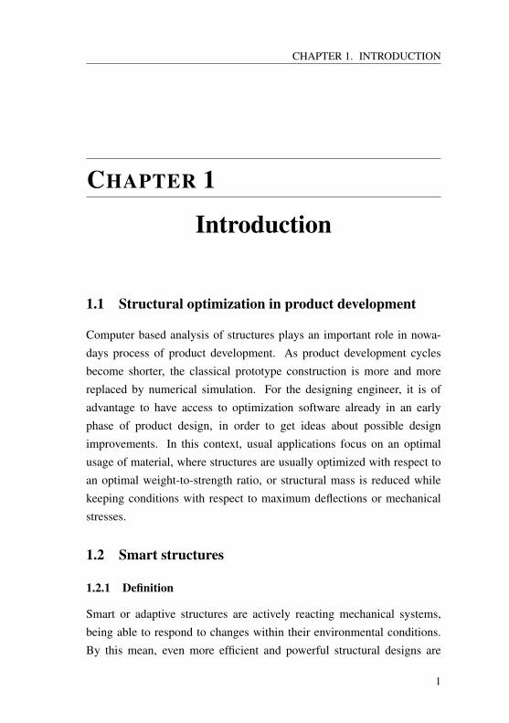
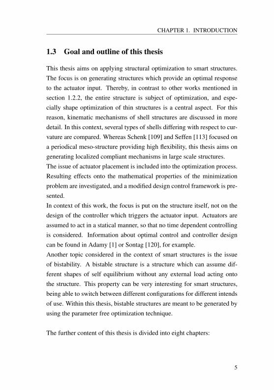
enabled. Typically, smart structures are equipped with sensors, monitor-ing the state of the structure, and with actuators, that provide mechanicalinput and enable the structure to "react" to the actual environmental con-ditions [42]. The actuator reaction usually is linked to the sensor inputdata via a controller, which regulates the structure such that its overallbehaviour, generated by external loading and the actuator influence, isoptimal with respect to a pre-defined criteria [60].Figure 1.1 shows the basic components of a smart structure. Senors, actu-ators and controller can be identified as central blocks, connected viadata streams. These data streams transmit information gathered by thesenors to the controller, and a corresponding actuator instruction is gener-ated. Actuator input and sensor information are linked via the mechanicalbehaviour of the structure.
Controller
Sensor Actuator
data
trans
mission
data instruction
Structure
Figure 1.1: Basis components of a smart structure (according to [2])
1.2.2 State of the art
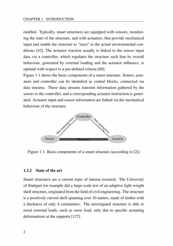
Smart structures are a current topic of intense research. The Universityof Stuttgart for example did a large-scale test of an adaptive light weightshell structure, originated from the field of civil engineering. The structureis a positively curved shell spanning over 10 meters, made of timber witha thickness of only 4 centimeters. The investigated structure is able toresist external loads, such as snow load, only due to specific actuatingdeformations at the supports [127].
2
CHAPTER 1. INTRODUCTION
Figure 1.2: The adaptive "Smart Shell" structure in Stuttgart (source ofpicture: [127])
Another example of smart materials and structures applied in civil engi-neering is the Savannah River Site monitoring project [51], where high-way bridges are monitored using piezoelectric or fiber optic sensors. Ina second stage, the bridges are meant to be upgraded by using fiber rein-forced plastic overlays.Theoretical research regarding compliant shell mechanisms based onorigami folding was done by Mark Schenk [109] and K. Seffen [113].They considered multi-scale shell structures, consisting of repetitive mesocells such as corrugated bellows or "egg-box" segments, folded into sheetmaterial. These meso cells undergo an almost strain free deformation,allowing easy deformability of the global structure.Most applications of smart structures can be grouped into the field ofaerospace applications. In these applications, mainly adaptive wings [23]or rotor blades [99] are considered. These airfoils are able to modify theirshape such that they are optimally suited for the actual flight situationand flow condition of the surrounding air. One quite famous example forsuch an application in serial production is the flutter problem of the Boe-ing 747-8 aircraft. The new wide-bodied aircraft suffered from wing tipfluttering in certain unusual flight states, which endanger the aircraft’s cer-tification by the aviation regulator agency. The problem could be solved
3
CHAPTER 1. INTRODUCTION
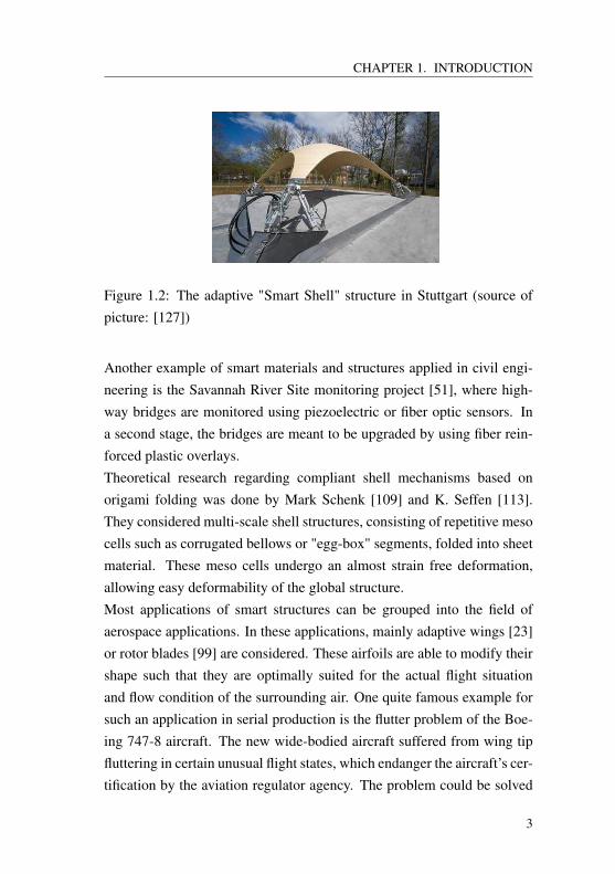
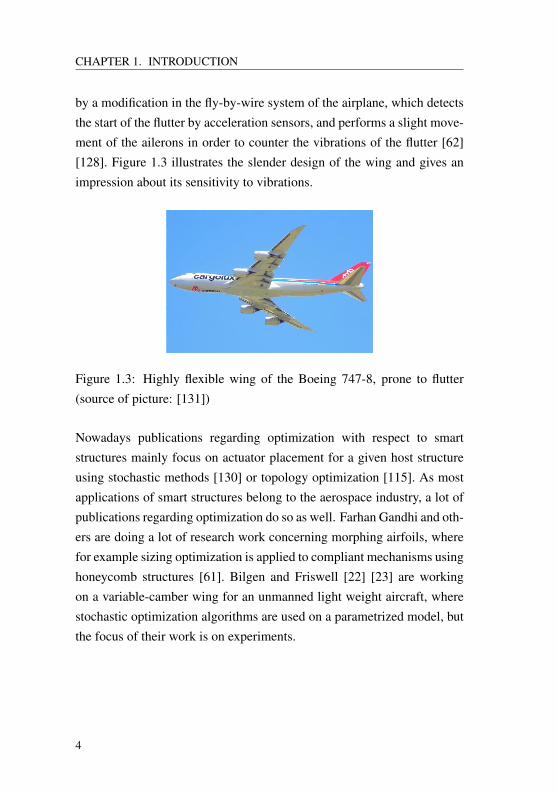
by a modification in the fly-by-wire system of the airplane, which detectsthe start of the flutter by acceleration sensors, and performs a slight move-ment of the ailerons in order to counter the vibrations of the flutter [62][128]. Figure 1.3 illustrates the slender design of the wing and gives animpression about its sensitivity to vibrations.
Figure 1.3: Highly flexible wing of the Boeing 747-8, prone to flutter(source of picture: [131])
Nowadays publications regarding optimization with respect to smartstructures mainly focus on actuator placement for a given host structureusing stochastic methods [130] or topology optimization [115]. As mostapplications of smart structures belong to the aerospace industry, a lot ofpublications regarding optimization do so as well. Farhan Gandhi and oth-ers are doing a lot of research work concerning morphing airfoils, wherefor example sizing optimization is applied to compliant mechanisms usinghoneycomb structures [61]. Bilgen and Friswell [22] [23] are workingon a variable-camber wing for an unmanned light weight aircraft, wherestochastic optimization algorithms are used on a parametrized model, butthe focus of their work is on experiments.
4
CHAPTER 1. INTRODUCTION
1.3 Goal and outline of this thesis
This thesis aims on applying structural optimization to smart structures.The focus is on generating structures which provide an optimal responseto the actuator input. Thereby, in contrast to other works mentioned insection 1.2.2, the entire structure is subject of optimization, and espe-cially shape optimization of thin structures is a central aspect. For thisreason, kinematic mechanisms of shell structures are discussed in moredetail. In this context, several types of shells differing with respect to cur-vature are compared. Whereas Schenk [109] and Seffen [113] focused ona periodical meso-structure providing high flexibility, this thesis aims ongenerating localized compliant mechanisms in large scale structures.The issue of actuator placement is included into the optimization process.Resulting effects onto the mathematical properties of the minimizationproblem are investigated, and a modified design control framework is pre-sented.In context of this work, the focus is put on the structure itself, not on thedesign of the controller which triggers the actuator input. Actuators areassumed to act in a statical manner, so that no time dependent controllingis considered. Information about optimal control and controller designcan be found in Adamy [1] or Sontag [120], for example.Another topic considered in the context of smart structures is the issueof bistability. A bistable structure is a structure which can assume dif-ferent shapes of self equilibrium without any external load acting ontothe structure. This property can be very interesting for smart structures,being able to switch between different configurations for different intendsof use. Within this thesis, bistable structures are meant to be generated byusing the parameter free optimization technique.
The further content of this thesis is divided into eight chapters:
5
CHAPTER 1. INTRODUCTION
Chapter 2 gives a very brief introduction into the fundamentals of theFinite Element Method. Thereby the focus is on introducing the elementformulations used in this thesis.Chapter 3 compares different mathematical methods used for optimiza-tion purpose. Pros and contras of different approaches are discussed, andan appropriate strategy for the intended purpose is chosen.Chapter 4 is a mathematical chapter, giving a brief overview over solu-tion techniques for constrained and unconstrained optimization problemsusing gradient based methods.Chapter 5 introduces the parameter free optimization method, which isused in this thesis. The issue of shape and design control is addressedin detail, and the topic of an efficient and accurate sensitivity analysis isdiscussed. The chapter ends with a description of the data streams insidea modular object oriented analysis and optimization code framework.Chapter 6 discusses optimal kinematic mechanisms for different types ofstructures, focusing on shells. For this purpose, different types of shellsand different stress states are considered.Chapter 7 addresses the issue of optimal actuation of structures. Anextended design control framework is presented, allowing simultaneousshape optimization and actuator placement. The benefits of the parameterfree approach are highlighted by generating complex bead designs, pro-viding high flexibility in large deformation applications. The chapter endswith the consideration of a real world example.Chapter 8 considers the topic of bistability. For this purpose, special char-acteristics of bistable structures and problems arising from the highly non-linear load carrying behaviour are discussed. An appropriate responsefunction is presented and derived, thereupon its fitness for the intendeduse is demonstrated for two curved shell structures.Chapter 9 draws the final conclusions and gives a short outlook aboutpossible future works.
6

CHAPTER 1. INTRODUCTION
1.4 Introduction to Carat++
All optimization and analysis results presented in this thesis are obtainedby the institute’s in-house finite element software Carat++ (ComputerAided Research and Analysis Tool). It is an object oriented research codewritten in C++, containing standard finite element analysis tools, beyondit includes modules for form finding and cutting patterning of membranesas well as a powerful optimization module. The origins of Carat go back tothe late 1980s [84] [30], and a complete re-design in C++ was performedin 2008. Further information about Carat++ can be found in Masching etal [91] or Fischer et al [55].
7

CHAPTER 1. INTRODUCTION
8
CHAPTER 2. FINITE ELEMENT METHOD IN STRUCTURAL ANALYSIS
CHAPTER 2Finite Element Method in
structural analysis
2.1 Structural analysis in the context of this work
In this work, analysis and evaluation of structural behaviour is an essen-tial point. Any structural optimization approach would be useless withoutbeing able to evaluate the structure mechanical properties of the consid-ered component. For this purpose, reliable and efficient numerical meth-ods have to be applied, in order to obtain realistic simulation results of themechanical behaviour of the investigated structure.In the last decades, starting from the 1950s, a multiplicity of text booksfocusing on solving structure mechanical problems using numerical meth-ods have been published. Primarily the Finite Element Method (FEM)was in focus of the authors. Giving a detailed insight about the funda-mentals of these methods would go beyond the scope of this thesis andis also not necessary in this context. For these purposes, this chapter ismeant to give a very brief introduction to state of the art numerical meth-ods of structural analysis, but it is not claimed to be exhaustive. Detailedinformation about the Finite Element Method can be found, among others,
9
CHAPTER 2. FINITE ELEMENT METHOD IN STRUCTURAL ANALYSIS
in the textbooks by Zienkiewicz, Taylor [137] [138], Bathe [14], Argyris[6] [5] or Hughes [73].
2.2 Analytical equilibrium
The governing equation of structural analysis is the equilibrium condition.This equation is directly based on Newton’s second law, which formulatesthe conservation of linear momentum. The equilibrium condition can beformulated as
div(σ (u))+ρ ·b = ρ · dvdt
(2.1)
where σ (u) is the stress state at the considered point of the structure,depending on its displacement u. ρ defines the material density and bdescribes the body force vector. On the right hand side of the equation,v denotes the actual velocity of the point under consideration, so ρ · dv
dt isthe expression of the inertia forces.Considering statical problems only, we can neglect the inertia term on theright hand side, and formulate the static equilibrium condition.
div(σ (u))+ρ ·b = 0 (2.2)
Equation 2.2 formulates the general equilibrium condition of a pointinside an arbitrary continuum. This equation is called the strong form of
equilibrium. In order to define the problem of structural static equilibriumproperly, additional boundary conditions prescribing the deformation u(Dirichlet boundary conditions) or a derivative of the displacement field(Neumann boundary condition) at certain points have to be applied. Theseboundary conditions correspond to supports or local loads influencing thestructure.Unfortunately, equation 2.2 cannot be solved in the general case for arbi-trary boundary conditions in order to determine the displacement u as ananalytical function. In order to obtain an approximated solution for thisproblem nevertheless, numerical methods are applied.
10
CHAPTER 2. FINITE ELEMENT METHOD IN STRUCTURAL ANALYSIS
2.3 The principle of Finite Element formulations
2.3.1 Weak form of equilibrium
A very successful approach to solve the equilibrium condition introducedin equation 2.2 is Galerkin’s Approach [44] [49]. It is a numerical methodsolving operator equations, such as differential equations, approximatelyby applying a method of weighted residuals.As Galerkin’s Approach is an approximation method, equation 2.2 willnot evaluate to zero at every point for the obtained approximated dis-placement field uh. The method weakens the requirements formulatedin equation 2.2, such that it only demands equation 2.2 to be fulfilled inthe integral mean over the complete domain Ω. An additional weightingof the residual is performed, using the so-called test function η.
∫Ω
[div(σ (uh))+ρ ·b] ·η dΩ = 0 (2.3)
Using the variation of displacements δu as test function, the well knownweak form of equilibrium is obtained:
∫Ω
[div(σ (uh))+ρ ·b] ·δu dΩ = 0 (2.4)
2.3.2 Discretization of geometry and displacement
In section 2.3.1, the equilibrium condition from equation 2.2 was trans-ferred to the weak form, using an approximate solution uh of the unknowndisplacement field u. In order to be able to compute this approximate solu-tion, it is necessary to reduce the continuous field u to a finite number ofevaluation points, for which the approximate solution uh is evaluated. Asthe weak form of equilibrium is formulated as an integral over Ω, a dis-cretized description of the domain Ω is needed, too, in order to evaluatethe integral equilibrium equation.
11
CHAPTER 2. FINITE ELEMENT METHOD IN STRUCTURAL ANALYSIS
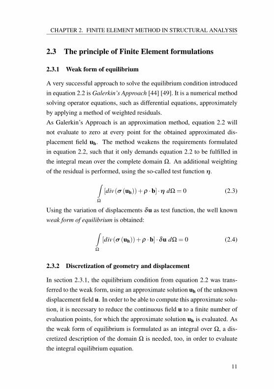
For the discretization of 2D-structures, for example an approximation ofthe surface using triangles or quadrilaterals is used, where the vertices ofthese facets are used as evaluation points for the displacement approxi-mation as well as sampling points for the geometry description. Thesetriangular or quadrangular facets are referred to as finite elements andthe vertices are usually called finite element nodes. Figure 2.1 shows adiscretization of a surface example using a coarse and a fine level of dis-cretization. In this figure, also a template of a four-noded finite elementis presented, showing the node numbering and a local coordinate systemξ1,ξ2 ∈ [−1,1], which allows to address any point inside the element byits local coordinates.
Meshing, coarse mesh
Meshing, fine mesh
1 2
4 3
ξ1
ξ2
ξ1,2 ∈ [−1,1]
Figure 2.1: Discretization: analytical surface description, coarse and finediscretization using finite elements
Having this discretization information, geometry X or displacement u canbe computed within an element by interpolating nodal information usinginterpolation functions, so-called shape functions,
12
CHAPTER 2. FINITE ELEMENT METHOD IN STRUCTURAL ANALYSIS
uh (ξ1,ξ2) =nNodes
∑i=1
Ni (ξ1,ξ2) · ui (2.5)
Xh (ξ1,ξ2) =nNodes
∑i=1
Ni (ξ1,ξ2) · Xi (2.6)
where the index h emphasizes that an approximation is considered. Ni, Xi
and ui denote the shape function, the coordinates and the displacementsbelonging to node i, respectively.
2.4 Finite Element formulations used in this contribu-tion
In this thesis, different kinds of structures are treated. Thin and lightweight structures are considered as well as solid structures. For this rea-son, different types of finite element formulations are used.
2.4.1 Multi-layer Reissner-Mindlin shell element
For analysis and optimization of thin and wide span structures, a Reissner-Mindlin shell formulation is used, based on the thesis of Manfred Bischoff[24]. The element is a multi-layer degenerated solid shell, based onnonlinear, three-dimensional continuum theory. Thus, it is possible touse arbitrary three-dimensional constitutive laws without reduction ormanipulation in nonlinear analysis of moderately thin structures includ-ing large deformations. In context of this thesis, linear elastic isotropic ororthotropic material laws using two or nine independent material param-eters [79] are used.
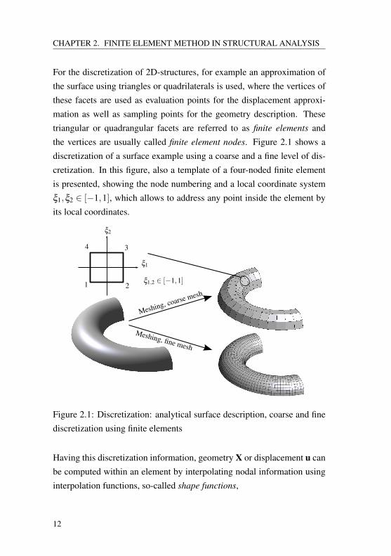
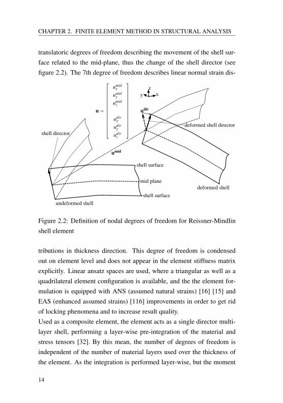
The element uses a 7-parameter concept in order to be able to considerthickness changes as well as non-constant normal stress in thickness direc-tion. Element nodes possess six degrees of freedom, namely three transla-tions evaluated on the mid-plane of the shell structure, and three additional
13
CHAPTER 2. FINITE ELEMENT METHOD IN STRUCTURAL ANALYSIS
translatoric degrees of freedom describing the movement of the shell sur-face related to the mid-plane, thus the change of the shell director (seefigure 2.2). The 7th degree of freedom describes linear normal strain dis-
umid
udir
undeformed shell
deformed shell
u =
umidx
umidy
umidz
udirx
udiry
udirz
shell director
mid plane
shell surface
shell surface
deformed shell director
xz
y
Figure 2.2: Definition of nodal degrees of freedom for Reissner-Mindlinshell element
tributions in thickness direction. This degree of freedom is condensedout on element level and does not appear in the element stiffness matrixexplicitly. Linear ansatz spaces are used, where a triangular as well as aquadrilateral element configuration is available, and the the element for-mulation is equipped with ANS (assumed natural strains) [16] [15] andEAS (enhanced assumed strains) [116] improvements in order to get ridof locking phenomena and to increase result quality.Used as a composite element, the element acts as a single director multi-layer shell, performing a layer-wise pre-integration of the material andstress tensors [32]. By this mean, the number of degrees of freedom isindependent of the number of material layers used over the thickness ofthe element. As the integration is performed layer-wise, but the moment
14
CHAPTER 2. FINITE ELEMENT METHOD IN STRUCTURAL ANALYSIS
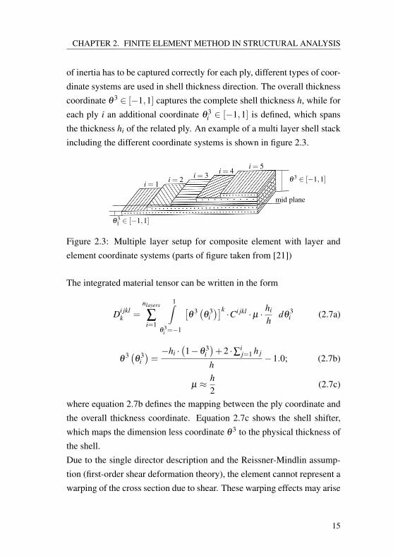
of inertia has to be captured correctly for each ply, different types of coor-dinate systems are used in shell thickness direction. The overall thicknesscoordinate θ 3 ∈ [−1,1] captures the complete shell thickness h, while foreach ply i an additional coordinate θ 3
i ∈ [−1,1] is defined, which spansthe thickness hi of the related ply. An example of a multi layer shell stackincluding the different coordinate systems is shown in figure 2.3.
i = 1i = 2 i = 3 i = 4
i = 5
mid plane
θ 31 ∈ [−1,1]
θ 3 ∈ [−1,1]
Figure 2.3: Multiple layer setup for composite element with layer andelement coordinate systems (parts of figure taken from [21])
The integrated material tensor can be written in the form
Di jklk =
nlayers
∑i=1
1∫θ 3
i =−1
[θ
3 (θ
3i)]k ·Ci jkl ·µ · hi
hdθ
3i (2.7a)
θ3 (
θ3i)=−hi ·
(1−θ 3
i)+2 ·∑i
j=1 h j
h−1.0; (2.7b)
µ ≈ h2
(2.7c)
where equation 2.7b defines the mapping between the ply coordinate andthe overall thickness coordinate. Equation 2.7c shows the shell shifter,which maps the dimension less coordinate θ 3 to the physical thickness ofthe shell.Due to the single director description and the Reissner-Mindlin assump-tion (first-order shear deformation theory), the element cannot represent awarping of the cross section due to shear. These warping effects may arise
15
CHAPTER 2. FINITE ELEMENT METHOD IN STRUCTURAL ANALYSIS
especially for thick layered shell structures with distinct orthotropic mate-rial properties. In order to represent the shear deformation of the crosssection more precisely, multi-layer shell models could be applied [102].These models approximate the deformation of the cross section linearly ineach ply, leading to a zick-zack shaped deformation over the entire thick-ness. Alternatively, higher order shear deformation theories can be used,describing the deformation in shell thickness direction using higher orderpolynomials [88] [108].
2.4.2 Three dimensional continuum element
Continuum elements are usually used in order to analyze structures whichcannot be reduced to one or two dimensions, as their geometrical size issimilar in all three directions in space. In this contribution, a hexahedralelement formulation is used, including geometrical nonlinear kinematics.For the hexahedral element type, eight-noded elements are used applyingtrilinear shape functions. As these elements are known to suffer from geo-metrical locking effects due to parasitic strain [133] [125], the formulationis improved by the EAS (enhanced assumed strain) method as presentedby Simo, Rifai [116] or Andelfinger, Ramm [3]. By this mean, the elementis able to represent a trilinear stress states although the displacement inter-polation itself is just linear. Therefore high computational accuracy can beachieved without increasing the number of element degrees of freedom.
16
CHAPTER 3. MATHEMATICAL OPTIMIZATION METHODS
CHAPTER 3Mathematical optimization
methods
3.1 Introduction to optimization
Optimization is a branch of mathematics which deals with the problem offinding the minimum or maximum value of a function f (x) , f : D→ Rand the related x ∈Ω. Here, x is the vector of design variables, D denotesthe design space of the optimization problem, and Ω is the set of feasibledesigns [11], thus a sub set of the design space. In literature about appliedoptimization, the function f is often referred to as objective function [67].In context of this thesis, design variables are assumed to be real numbers,so the design space D is a higher dimension of R.
D = Rn (3.1)
Accordingly, the feasible set is a sub set of Rn
Ω⊆ Rn (3.2)
The set Ω can be defined either explicitly, or in an implicit way by addingadditional equations or inequalities, so-called constraints, to the optimiza-tion problem, which a feasible design x ∈ Ω has to fulfill. This will be
17
CHAPTER 3. MATHEMATICAL OPTIMIZATION METHODS
discussed in more detail in section 4.3.
Most optimization procedures are designed such that they focus on min-imization problems. Hence the standard optimization task can be formu-lated as the following minimization problem:
f (x) , f : Rn→ R
min f (x)
with x ∈Ω, Ω⊂ Rn
(3.3)
In case the problem to solve is a maximization problem, it can easily betransformed into a minimization problem by applying a standard mini-mization algorithm to the negative function.
max f (x)⇔ min − f (x) (3.4)
As the transformation from maximization to minimization problems (andinverse) can be done in such an easy way, the following part of this chapterwill only focus on the standard case of minimization problems.
3.2 Optimization methods
There are multiple ways to solve an optimization problem as it is definedin equation 3.3. The related methods are usually grouped according to thehighest order of derivative which is used in the algorithm.
3.2.1 Zero order methods
Zero order methods are methods only evaluating the 0th derivative of theobjective function, which is the function value itself. The algorithms eval-uate a multiplicity of candidate solutions and judge for each candidatesolution if it is (a) feasible and (b) a minimum solution. A sub-groupingof zero order algorithms can be done according to the determination ofthe candidate solutions.
18
CHAPTER 3. MATHEMATICAL OPTIMIZATION METHODS
3.2.1.1 Direct search methods
Direct search methods just evaluate a specific set of given candidate solu-tions in order to determine the minimum feasible solution. The set of can-didate solutions can either be generated by random (Monte-Carlo-Search)or by using a defined multi-dimensional grid of evaluation points (grid-search). Drawbacks of this very simple approach are the high numberof response function evaluations and the restriction to discrete evaluationpoints, especially in a continuous design space.
3.2.1.2 Evolutionary Algorithms
The origin of genetic algorithms goes back to the 1950s, when researchersin biology started to simulate genetic processes using computers [59].Soon the optimizing character of these processes became obvious. Thebasic principle of Evolutionary Algorithm can be compared to Darwin’sevolutionary theory, which assumes a natural selection, leading to the sur-vival and reproduction of these individuals which are best adapted to theruling environmental conditions ("survival of the fittest").An Evolutionary Algorithm starts from an arbitrary or randomly cho-sen initial population, which is a set of candidate solutions in the designspace. For these candidate solutions, a fitness assignment according to therelated objective function value is performed, and based on this assign-ment the fittest individuals are chosen for reproduction. Reproduction isbased on two operations, crossover and mutation. Crossover is a pure re-combination procedure and produces a descendant based on the attributesof two parent individuals, while the mutation operator adds some statisti-cal noise to the attributes of the descendant [95] [9]. After reproduction,all descendants are added to the population, and this is how the algorithmapproaches the optimal solution over the generations of descendants.By combining pure re-combination and mutation, the algorithm producesthe best compromise of the initial population’s attributes, but also the rest
19
CHAPTER 3. MATHEMATICAL OPTIMIZATION METHODS
of the design space is investigated by the stochastic component of themutation operator.
3.2.1.3 Particle Swarm Optimization
Particle swarm optimization is a relatively new method of optimization,which was presented in 1995 by Kennedy, Eberhart and Shi [82]. It is amethod trying to mimic the behaviour of birds or fishes inside a swarm inorder to detect the global optimum of an optimization problem [83].Similar to genetic algorithms, particle swarm optimization is also basedon a population, which is usually called "the swarm" in this context. Eachcandidate solution or particle of the swarm is moving through the designspace following a velocity vector vi, which is computed as a linear com-bination of(a) the connection vector from the actual particle position to the "best"position with respect to the objective function which the particle ever hasreached and(b) the connection vector from the actual particle position to the "best"position all particles of the swarm have discovered.Summarizing, the idea of the algorithm is that each particle does not onlyact based on its local knowledge about the design space, but it also profitsfrom information gained by other members of the swarm.
3.2.2 Methods of first order
In contrast to the methods mentioned in section 3.2.1, methods of 1st orderdo not only evaluate the objective function itself, but also the informationprovided by the first derivative of the objective or constraint functions.Compared to zero order function evaluations, which is a pure local infor-mation about the response function, information of 1st order also givesinformation about the actual change of the response function when thedesign is varied.
20
CHAPTER 3. MATHEMATICAL OPTIMIZATION METHODS
Using first order information, directions of steepest ascend or steepestdescend of the response function can be determined, as well as directionswhere the response function can be assumed not to change at all, as longas the investigated region is sufficiently close to the point of evaluation.Making use of this kind of information allows to tremendously reduce thenumber of objective function evaluations compared to zero order methods.The requirements for applying 1st order methods is that the design vari-ables of the optimization problem behave continuously within the designspace, and that the objective function is C1−continuous. When these con-ditions are fulfilled, the information of 1st order can be computed for anydesign x in the design space.
3.2.3 Methods of higher order
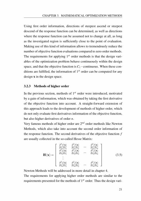
In the previous section, methods of 1st order were introduced, motivatedby a gain of information, which was obtained by taking the first derivativeof the objective function into account. A straight-forward extension ofthis approach leads to the development of methods of higher order, whichdo not only evaluate first derivatives information of the objective function,but also higher derivatives of order n.Very famous methods of higher order are 2nd order methods like NewtonMethods, which also take into account the second order information ofthe response function. The second derivatives of the objective function f
are usually collected in the so-called Hesse Matrix:
H(x) =
∂ 2 f (x)∂x1∂x1
∂ 2 f (x)∂x1∂x2
... ∂ 2 f (x)∂x1∂xn
∂ 2 f (x)∂x2∂x1
∂ 2 f (x)∂x2∂x2
... ∂ 2 f (x)∂x2∂xn
...∂ 2 f (x)∂xn∂x1
∂ 2 f (x)∂xn∂x2
... ∂ 2 f (x)∂xn∂xn
(3.5)
Newton Methods will be addressed in more detail in chapter 4.The requirements for applying higher order methods are similar to therequirements presented for the methods of 1st order. Thus the design vari-
21
CHAPTER 3. MATHEMATICAL OPTIMIZATION METHODS
ables have to be continuous, and the objective function has to be suffi-ciently smooth. It has to satisfy at least Cn−continuity, in order to providethe required data over the complete design space.
3.3 Pros and contras of the different methods
Subsequently, pros and contras of the different approaches are compared.The benefits of methods of zero order are that they are very robust andmay be combined with arbitrary black box software, as the required inputinformation is reduced to the value of the objective function. This makesthese methods also applicable to a non-continuous design space, wheremethods of first or higher order cannot be applied due to the requirementswith respect to continuity mentioned in sections 3.2.2 and 3.2.3. Anotherbenefit of zero order methods is that usually a population or a set of candi-date solutions is used, which automatically leads to a broad exploration ofthe design space. This increases the likelihood of the method to convergeto the global optimum of the problem.On the other hand, methods of zero order require a high number ofresponse function evaluations, especially when a large number of opti-mization variables is used. At this point, gradient based methods are inadvantage towards zero order methods, as usage of information of firstor higher order reduced the number of necessary objective function eval-uations tremendously. At the same time, gradient based methods sufferfrom the previously mentioned drawbacks, that the objective function hasto be smooth enough to provide the desired information, and, in addition,the computation of the gradient information requires detailed knowledgeabout the response function and access to the computational framework,which standard black box computer programs do not provide by default.An efficient computation of the required derivatives is a key feature tofirst or higher order methods. In sections 5.4 and 5.5, important aspects
22
CHAPTER 3. MATHEMATICAL OPTIMIZATION METHODS
considering numerical efficiency of the computation of response functionderivatives are discussed.
3.4 Conclusion and selection of optimization strategy
In the context of this thesis, an optimization approach based on a finiteelement analysis will be used, that supersedes the necessity of a separatemodel in order to define design parameters (detailed information will begiven in chapter 5). While providing a maximum of freedom in design,this approach leads to a large number of optimization variables. Therebythe number of design parameters is equal to the number of finite elementsor finite element nodes, so 10,000 to 100,000 design parameters are eas-ily reached for usual applications. Following the considerations in section3.3, a zero order optimization strategy would not be suitable for thesekinds of problems, due to the large number of required objective func-tion evaluations. The problems of consideration are sufficiently smooth,such that methods of first or second order can be applied. As compu-tations are performed in a self-developed software framework providingfull source-code access, derivatives of objective functions can be com-puted efficiently and with high accuracy. However, computation of higherorder information based on a finite element model would be time consum-ing and numerically disputable, as already first order information requiresspecial treatment, which will be discussed in proceeding chapters.For these reasons, this work will focus on the usage of first order opti-mization strategies.
23

CHAPTER 3. MATHEMATICAL OPTIMIZATION METHODS
24
CHAPTER 4. GRADIENT BASED OPTIMIZATION
CHAPTER 4
Gradient based optimization
4.1 Classification
In context of this thesis, gradient based optimization is used as a collectiveterm for all kind of optimization algorithms where the first or second orderderivatives are taken into account.
4.2 Unconstrained optimization
4.2.1 Optimality criteria
Unconstrained optimization is the most simple case of an optimizationproblem. In this case, there are no restrictions defined which shrink thefeasible set. Consequently the feasible set is equal to the design space.
Ω = D (4.1)
Furthermore, we now assume that f is C1-continuous in D. Based on thisassumption, the necessary condition for f being minimal in x0 is that allfirst partial derivatives at this point arise to be zero.
∂ f∂xi
= 0 ∀ i ∈ 1, ...,n (4.2)
25
CHAPTER 4. GRADIENT BASED OPTIMIZATION
Usually the first partial derivatives of a function are collected in the gra-dient vector. Usage of the gradient vector allows to reformulated the opti-mality condition as
∇ f (x) =[
∂ f∂x1
∂ f∂x2
...∂ f∂xn
]T
= 0 (4.3)
A sufficient condition can be formulated for C2-continuous functions, byadding the additional requirement for the Hesse Matrix to be positive def-inite.
4.2.2 Solution methods
4.2.2.1 Newton Methods
"The Newton Method is a cornerstone of numerics and it can be used forsolving nonlinear systems of equations as well as for minimizing nonlin-ear functions." (from Ulbrich [126], translated by the author) In order todetermine the unconstrained optimum, the nonlinear system of equationspresented in equation 4.3 has to be solved. The Newton Method is a classi-cal and very successful method to solve this kind of problem. It performsan approximation of the original problem using a linear Taylor series.Solving this linear problem provides an improved approximate solutionof the initial problem. By solving these of linearized problems iteratively,the Newton Method approaches the solution of the initial problem [48].Applied to equation 4.3, the corresponding iteration scheme reads
∇ f(xi)+∇
(∇ f(xi))︸ ︷︷ ︸
H(xi)
·∆x = 0 (4.4a)
xi+1 = xi +∆x (4.4b)
where i denotes the current iteration, and xi is the approximated solutionvector in the ith iteration. The approximate solution for the evaluations forthe next iteration step is computed according to equation 4.4b.
26
CHAPTER 4. GRADIENT BASED OPTIMIZATION
Linearization of equation 4.3 leads to second derivatives of the objectivefunction f , collected in the Hesse Matrix H, hence Newton Methods belngto optimization strategies of second order.The necessity to compute the second order information is a drawback ofthe Newton Method. In cases where, for example, the function f is notknown in an analytical form but only can be evaluated numerically, thecomputation of second order derivatives may become very time consum-ing or even impossible. In order to overcome this drawback, so-calledQuasi-Newton-Methods have been developed, which perform an approx-imation of the Hessian matrix or even the inverse Hessian matrix, as infact the inverse matrix is needed in order to compute the incremental vec-tor ∆x. One very popular Quasi-Newton-Method is the so-called BFGS-Method, which was developed in 1970 by the mathematicians Broyden[33], Fletcher [57], Goldfarb [64] and Shanno [114] independently fromeach other.
4.2.2.2 Descent methods
Another method to overcome the problems of the classical NewtonMethod is to completely neglect the second order information and applypure descent methods or algorithms of first order, which only use gradi-ent information only in order to determine the function minimum. Forthis purpose, we do not focus on the multi-dimensional optimality criteriafrom equation 4.3 directly, but the optimization procedure is considereda sequence of one-dimensional optimization problems with respect to achosen search direction. Metaphorically speaking, the algorithm starts ata given point x in D and "moves" through the design space along a cho-sen search direction vector s as long as the function value decreases indirection s. This one-dimensional optimization problem (also called line
search) determines a step-length parameter α such that the total derivativeof f at point x+α · s in direction of s vanishes:
27
CHAPTER 4. GRADIENT BASED OPTIMIZATION
[∇ f (x+α · s)]T · s = 0 (4.5)
Assuming s to be a descent direction such that[si]T ·∇ f
(xi) < 0 [126],
the step length determined in the line search has to be strictly positive.
α > 0 (4.6)
The optimal point found for the current search direction si is used as start-ing point for the next optimization iteration i+1,
xi+1 = xi +α · si (4.7)
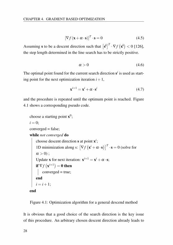
and the procedure is repeated until the optimum point is reached. Figure4.1 shows a corresponding pseudo code.
choose a starting point x0;i = 0;converged = false;while not converged do
choose descent direction s at point xi;1D minimization along s:
[∇ f(xi +α · s
)]T · s = 0 (solve forα > 0) ;Update x for next iteration: xi+1 = xi +α · s;if ∇ f
(xi+1
)= 0 then
converged = true;endi = i+1;
end
Figure 4.1: Optimization algorithm for a general descend method
It is obvious that a good choice of the search direction is the key issueof this procedure. An arbitrary chosen descent direction already leads to
28
CHAPTER 4. GRADIENT BASED OPTIMIZATION
a decrease of the objective function, but of course a more sophisticatedchoice of the search direction has to be made. In order to obtain the mostrapid decrease of f along the search direction, it is appropriate to choosea search direction which is parallel to the gradient vector. This is done inthe steepest descent method, where the search direction is chosen as thenegative gradient [100].
si =−∇ f(xi) (4.8)
A characteristic property of steepest descent is that search directions offollowing iteration steps are orthogonal to each other,(
si+1)T · si = 0 (4.9)
as equation 4.5 holds and the new search direction will be chosen assi+1 = −∇ f
(xi +α i · si
). As a consequence, steepest descent shows a
very good convergence behaviour as long as the eigen values of the Hes-sian are identical. Thus, "optimality" which was reached with respect toone search direction is not destroyed by any further optimization step [8].Otherwise interaction of search directions slows down the convergencerate of the steepest descent algorithm. This can be seen by looking at theorthogonality of search directions with respect to the Hessian matrix of f ,(
si)T ·H · s j 6= 0, i 6= j (4.10)
which is not fulfilled in general for steepest descent search directions.In order to maintain a high rate of convergence also for objective func-tions with badly conditioned Hesse Matrices, Fletcher and Reeves [58]published a method of conjugated gradients (CG), which takes previoussearch directions into account in order to compute a new one. By thismean, search directions are not orthogonal to each other anymore, but sat-isfy equation 4.10. Hence it can be proven that the CG method convergesto the minimum in n steps for quadratic objective functions f : Rn → R.[8]
29
CHAPTER 4. GRADIENT BASED OPTIMIZATION
Equation 4.11 shows the computation of the ith search direction dependingon the previous one according to Fletcher and Reeves [58].
si =−∇ f(xi)+β · si−1
β =∇ f(xi)T ·∇ f
(xi)
∇ f (xi−1)T ·∇ f (xi−1)
(4.11)
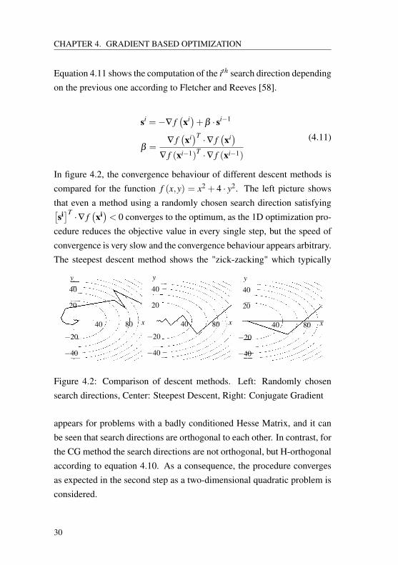
In figure 4.2, the convergence behaviour of different descent methods iscompared for the function f (x,y) = x2 + 4 · y2. The left picture showsthat even a method using a randomly chosen search direction satisfying[si]T ·∇ f
(xi)< 0 converges to the optimum, as the 1D optimization pro-
cedure reduces the objective value in every single step, but the speed ofconvergence is very slow and the convergence behaviour appears arbitrary.The steepest descent method shows the "zick-zacking" which typically
x
y
−20
20
40
−40
40 80x
y
−20
20
40
−40
40 80x
y
−20
20
40
−40
40 80
Figure 4.2: Comparison of descent methods. Left: Randomly chosensearch directions, Center: Steepest Descent, Right: Conjugate Gradient
appears for problems with a badly conditioned Hesse Matrix, and it canbe seen that search directions are orthogonal to each other. In contrast, forthe CG method the search directions are not orthogonal, but H-orthogonalaccording to equation 4.10. As a consequence, the procedure convergesas expected in the second step as a two-dimensional quadratic problem isconsidered.
30
CHAPTER 4. GRADIENT BASED OPTIMIZATION
4.3 Constrained optimization
4.3.1 Definition of constraints
The concept of constraint optimization was already briefly discussed insection 3.1, when the idea of the feasible set was introduced. The feasibleset was defined in a very abstract way, as a sub set of the design space,Ω⊆D. In applied optimization, the definition of the feasible set is usuallydone by adding additional equations or inequalities to the optimizationproblem, so-called equality or inequality constraint functions, which ax ∈Ω has to fulfill. Using the vectors of constraint functions g and h, theabstract formulation of the constrained optimization problem (equation3.3) can be written in the following form:
min f (x)
st
g(x)≤ 0
h(x) = 0
(4.12)
4.3.2 Lagrange function
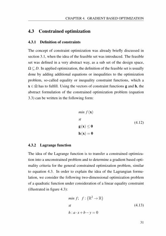
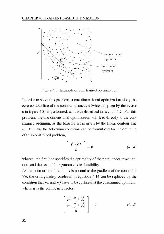
The idea of the Lagrange function is to transfer a constrained optimiza-tion into a unconstrained problem and to determine a gradient based opti-mality criteria for the general constrained optimization problem, similarto equation 4.3. In order to explain the idea of the Lagrangian formu-lation, we consider the following two-dimensional optimization problemof a quadratic function under consideration of a linear equality constraint(illustrated in figure 4.3):
min f ; f :(R2→ R
)st
h : a · x+b− y = 0
(4.13)
31
CHAPTER 4. GRADIENT BASED OPTIMIZATION
x
7
yunconstrainedoptimum
constrainedoptimum
7
s
−∇ f
∇g
h = 0
Figure 4.3: Example of constrained optimization
In order to solve this problem, a one dimensional optimization along thezero contour line of the constraint function (which is given by the vectors in figure 4.3) is performed, as it was described in section 4.2. For thisproblem, the one dimensional optimization will lead directly to the con-strained optimum, as the feasible set is given by the linear contour lineh = 0. Thus the following condition can be formulated for the optimumof this constrained problem,[
sT ·∇ f
h
]= 0 (4.14)
whereat the first line specifies the optimality of the point under investiga-tion, and the second line guarantees its feasibility.As the contour line direction s is normal to the gradient of the constraint∇h, the orthogonality condition in equation 4.14 can be replaced by thecondition that ∇h and ∇ f have to be collinear at the constrained optimum,where µ is the collinearity factor: µ · ∂h
∂x +∂ f∂x
µ · ∂h∂y +
∂ f∂y
h
= 0 (4.15)
32
CHAPTER 4. GRADIENT BASED OPTIMIZATION
A generalized derivation of this optimality condition, based on the ideaof using tangential cones in order to describe the feasible domain, can befound in Ulbrich [126].Computing the potential of equation 4.15 leads to the so-called Lagrangefunction L(x,y,µ) = f + µ · h, and the optimality criteria from equation4.15 can be formulated via the gradient of L with respect to x, y and µ: µ · ∂h
∂x +∂ f∂x
µ · ∂h∂y +
∂ f∂y
h
= ∇x,µ L = 0 (4.16)
Applying this approach to a general constrained optimization prob-lem with arbitrary numbers of equality and inequality constraints, theLagrange function can be formulated in the following form [101]:
L(x,µ,λ,τ ) = f (x)+µ ·h(x)+∑i
λi ·(gi (x)+ τ
2i)
(4.17)
τ2i represents the so-called slack variables, which allow to treat inequality
constraints similar to equality constraints.The values µ and λ represent the so-called Lagrange multipliers, whichrepresent the ratio between the gradients of constraints and the objectivefunction at the optimum point, as it can be seen in equation 4.15 for thesimple example. Alternatively, the design variables x are also called pri-
mal variables, whereas the multipliers µ and λ are referred to as dual
variables.Computing the second derivatives of the Lagrange function, we observethat ∂ 2L
∂µ2 = 0 and ∂ 2L∂λ2 = 0. Accordingly the Hessian matrix of the
Lagrange function will be indefinite, which means that the Lagrangianforms a saddle surface in the space of primal and dual variables.The general first order necessary optimality criteria (FONC) [11] of theconstrained optimization problem now can be formulated, according toequation 4.16, by the requirement of all first partial derivatives of theLagrange function to evaluate to zero (equation 4.18).
33
CHAPTER 4. GRADIENT BASED OPTIMIZATION
∇x,µ,λ,τL =
∂L∂x1...
∂L∂xn∂L
∂ µ1...
∂L∂ µk∂L∂λ1...
∂L∂λl∂L∂τ1...
∂L∂τl
=
∂ f∂x1
+∑kj=1
∂h j∂x1·µ j +∑
lj=1
∂g j∂x1·λ j
...∂ f∂xn
+∑kj=1
∂h j∂xn·µ j +∑
lj=1
∂g j∂xn·λ j
h1...
hk
g1 + τ21
...gl + τ2
l
2 ·λ1 · τ1...
2 ·λl · τl
= 0
(4.18)
4.3.3 Interpretation of Lagrange multipliers
At the beginning of section 4.3.2, we considered an optimization problemwhich was constrained by one equality constraint. In that case, the con-strained optimum was defined by the gradient of the objective ∇ f beingcollinear to the gradient of the constraint ∇h, and the Lagrange multiplierµ turned out to be the collinearity factor of these two vectors. Now, theinteraction of several constraints and the special role of inequality con-straints will be addressed.Equation 4.18 consists of two parts. The first part, which contains thederivatives with respect to the primal variables, enforces a point to beoptimal, while the derivatives with respect to the dual variables in the sec-ond part enforce the constraints to be active. Assuming that all constraintsare active and just considering the first part of equation 4.18, the negativegradient of the response function can be displayed as a linear combination
34
CHAPTER 4. GRADIENT BASED OPTIMIZATION
of the gradients of the active constraints, where the Lagrange multipliersform the linear combination factors. This can be interpreted as a basischange, where −∇ f is transferred to the basis defined by the gradients ofactive constraints ∇g1,∇g2, ...,∇gn, and the Lagrange multipliers formthe new components of −∇ f .
−∇ f =n
∑j=1
∇g j ·λ j (4.19)
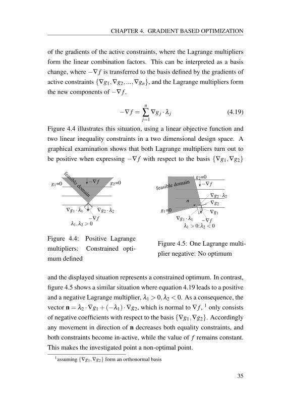
Figure 4.4 illustrates this situation, using a linear objective function andtwo linear inequality constraints in a two dimensional design space. Agraphical examination shows that both Lagrange multipliers turn out tobe positive when expressing −∇ f with respect to the basis ∇g1,∇g2
g1=0 g2=0
∇g2 ·λ2
λ1,λ2 > 0
∇g1 ·λ1
−∇ f
−∇ f
feasible domain
Figure 4.4: Positive Lagrangemultipliers: Constrained opti-mum defined
g2=0−∇ f
∇g2
λ1 > 0;λ2 < 0−∇ f
∇g1
∇g2 ·λ2
∇g1 ·λ1
g1=0
feasible domain
n
Figure 4.5: One Lagrange multi-plier negative: No optimum
and the displayed situation represents a constrained optimum. In contrast,figure 4.5 shows a similar situation where equation 4.19 leads to a positiveand a negative Lagrange multiplier, λ1 > 0,λ2 < 0. As a consequence, thevector n = λ2 ·∇g1 +(−λ1) ·∇g2, which is normal to ∇ f , 1 only consistsof negative coefficients with respect to the basis ∇g1,∇g2. Accordinglyany movement in direction of n decreases both equality constraints, andboth constraints become in-active, while the value of f remains constant.This makes the investigated point a non-optimal point.
1assuming ∇g1,∇g2 form an orthonormal basis
35
CHAPTER 4. GRADIENT BASED OPTIMIZATION
In summary, these examples show that Lagrange multipliers associatedto inequality constraints always have to be non-negative at the optimumpoint [96]. For equality constraints, of course, this condition does nothold, because the constraint equation can be arbitrarily scaled withoutinfluencing the feasible set or the optimum solution.
4.3.4 Karush-Kuhn-Tucker conditions
The awareness gained in the last section is combined with the optimalitycriteria shown in equation 4.18 now. This equation does not yet con-sider any additional conditions regarding inequality constraints, meaningall constraints are assumed to be active at the optimum. As an equalityconstraint can be inactive at the optimum and so it does not effect thesolution, equation 4.18 has to be modified in order to get a general gradi-ent based optimality criteria. For this purpose, inequality constraints areseparated into two groups:
• inactive inequality constraint: gi < 0,λi = 0
• active inequality constraint: gi = 0,λi > 0
As a consequence, it is ensured that the product of inequality constraintvalue times Lagrange multiplier is always equal to zero, no matter if theconstraint is active or not. Using this property, equation 4.18 can be re-formulated to the following form:
∂L∂x
= 0
h j = 0
gi ·λi = 0 with λi ≥ 0, gi ≤ 0
(4.20)
This equation is called Karush-Kuhn-Tucker-condition (KKT), namedafter the mathematicians Harold Kuhn and Albert Tucker, who published
36
CHAPTER 4. GRADIENT BASED OPTIMIZATION
the idea of the necessary condition in 1951 [85]. Later it turned out thatWilliam Karush already worked in this field in 1939 [80].The difference to the previous version in equation 4.18 is, that now inac-tive inequality constraints can be considered in the formulation, too, andthat the non-negativity of Lagrange multipliers associated to inequalityconstraints is part of the formulation.
4.3.5 Solution methods
There are several approaches to solve the constrained optimization prob-lem. A selection of commonly used approaches is briefly presented in thissection.
4.3.5.1 Newton-Lagrange Methods and Sequential Quadratic Program-ming (SQP)
The Newton-Lagrange Method is a quite obvious approach to solve theconstrained optimization problem. Similar to the Newton Method appliedto unconstrained problems (see section 4.2.2.1), it solves the nonlinearequation representing the optimality condition by applying the NewtonMethod. As the straight forward application of the Newton Methodrequires knowledge about the set of active constraints at the optimum, theNewton-Lagrange Method in its basic form usually is applied to equalityconstrained problems [126]. The corresponding linearization reads
[∂L(xi,µi,λi)
∂xh(xi) ]
+
∂ 2L(xi,µi,λi)∂x2
∂h(xi)∂x[
∂h(xi)∂x
]T
0
·[ ∆x∆µ
]= 0 (4.21)
where i again is the iteration counter, and design as well as the Lagrangemultipliers are updated similar to the Newton Method by xi+1 = xi +∆xor µ i+1 = µ i +∆µ .
37
CHAPTER 4. GRADIENT BASED OPTIMIZATION
In case inequality constraints are involved and it is not known which con-straints will become active, usually an auxiliary sequence of quadraticoptimization problems is generated (Sequential Quadratic Programming).For this purpose, response and constraint functions are evaluated at a spe-cific point, and a quadratic approximation of the response function and lin-ear approximations of the active constraints ("active set") are performed.This auxiliary quadratic problem
mind f
(xi)+dT ·
∂ f(xi)
∂x+
12·dT ·
∂L(xi,µi,λi
)∂x
·d
st h(xi)+dT ·
∂h(xi)
∂x= 0; g
(xi)+dT ·
∂g(xi)
∂x≤ 0
(4.22)
is minimized iteratively, and a new active set is chosen for the nextquadratic approximation [31].
4.3.5.2 Penalty methods
Penalty methods solve the constrained optimization problem without con-sideration of a Lagrange function or Karush-Kuhn-Tucker conditions.Instead, it penalizes violations of constraints. By this mean, an auxiliaryobjective function fpen is generated, which can be solved as an uncon-strained problem. A frequently used penalization method is the so-calledquadratic exterior penalization [10], which adds quadratic penalizationterms for violated constraints to the objective function
fpen = f +ρ ·∑i
h2i +ρ ·∑
imax
0gi
2
(4.23)
Here, ρ is a penalty factor, weighting the added penalization terms. Abenefit of this method is that it is very robust, but the drawback is that theconstrained optimum only can be found theoretically by using an infinitelarge penalty factor. Consequently, the approximated solution will alwaysbe located outside the feasible domain for numerically reasonable penaltyfactors. Furthermore, the unconstrained minimization problem min fpen
tends to be ill-conditioned for large penalty factors [11].
38
CHAPTER 4. GRADIENT BASED OPTIMIZATION
4.3.5.3 Dual methods
As it was already described in section 4.3.2, the Lagrange functiondescribes a saddle surface in the space of primal and dual variables, wherethe solution of the constrained problem according to equation 4.18 is givenby the saddle point of this surface. Due to this property, the constrainedoptimum cannot be found by applying a simple descent method like steep-est descent or CG to the Lagrange function, as the solution is defined bya stationary point ∇L = 0, which is not a local minimum.The idea of dual methods is to determine the saddle point using a stag-gered optimization scheme which
• minimizes the Lagrange function with respect to the primal vari-ables x (inner problem) and
• maximizes the Lagrange function with respect to the dual variablesµ and λ (outer problem) [11]
and approaches the saddle point iteratively.The benefit of the dual approach is that, in contrast to the penaltyapproach, the optimum solution can be determined exactly, as it deter-mines the Karush-Kuhn-Tucker point. The drawback is that convergenceof the staggered optimization approach cannot be guaranteed in general.
4.3.5.4 Augmented Lagrangian Method (ALM)
The Augmented Lagrangian Method combines the idea of the dual methodwith a penalty approach in order to overcome the drawbacks of both meth-ods, and so to formulate an optimization method which is guaranteed toconverge and able to find the exact optimum for a finite penalty factor[96]. The ALM was discussed the first time in 1969 by Hestenes [71] andPowell [106].
39
CHAPTER 4. GRADIENT BASED OPTIMIZATION
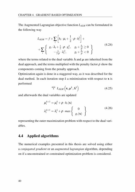
The Augmented Lagrangian objective function LALM can be formulated inthe following way
LALM = f +∑i
[hi ·µi +
12·ρ ·h2
i
]+
+∑i
gi ·λi +
12 ·ρ ·g
2i , gi +
λiρ≥ 0
− 12·ρ ·λ
2i , gi +
λiρ< 0
(4.24)
where the terms related to the dual variable λ and µ are inherited from thedual approach, and the terms multiplied with the penalty factor ρ show thecomponents coming from the penalty approach.Optimization again is done in a staggered way, as it was described for thedual method. In each iteration step k a minimization with respect to x isperformed
minx LALM
(x,µk,λk
)(4.25)
and afterwards the dual variables are updated
µk+1i = µ
ki +ρ ·hi (x)
λk+1i = λ
ki +ρ ·max
0
gi (x)
(4.26)
representing the outer maximization problem with respect to the dual vari-ables.
4.4 Applied algorithms
The numerical examples presented in this thesis are solved using eithera conjugated gradient or an augmented lagrangian algorithm, dependingon if a unconstrained or constrained optimization problem is considered.
40
CHAPTER 5. CONCEPT OF PARAMETER FREE SHAPE OPTIMIZATION
CHAPTER 5Concept of parameter free Shape
Optimization
5.1 Branches of Structural Optimization
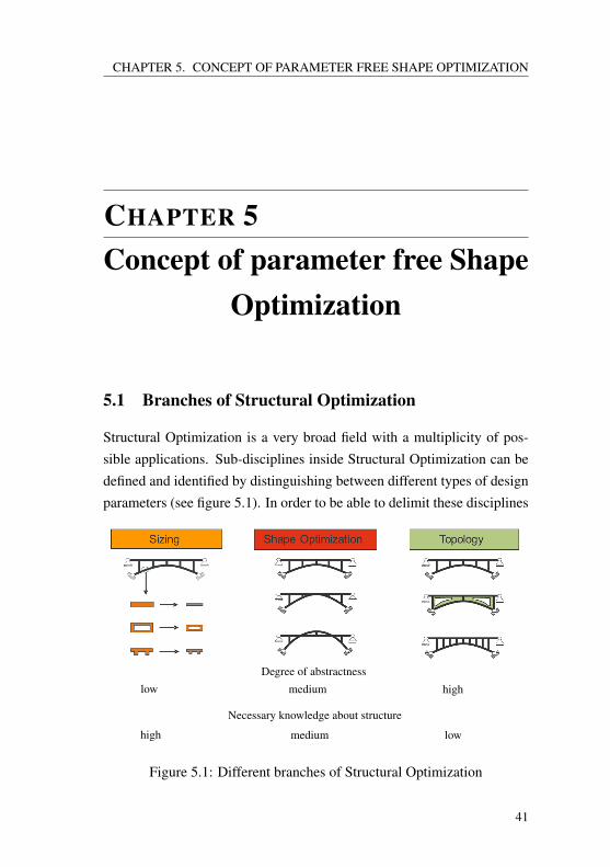
Structural Optimization is a very broad field with a multiplicity of pos-sible applications. Sub-disciplines inside Structural Optimization can bedefined and identified by distinguishing between different types of designparameters (see figure 5.1). In order to be able to delimit these disciplines
Degree of abstractness
low medium high
Necessary knowledge about structure
high medium low
Figure 5.1: Different branches of Structural Optimization
41
CHAPTER 5. CONCEPT OF PARAMETER FREE SHAPE OPTIMIZATION
against each other, two terms have to be defined which are used in orderto describe a structure:The topology of a structure is defined the type and connectivity of thestructural members the structure consists of, such as trusses, beams, orplate components. For discrete or discretized structures, these membersare connected at nodes.The shape of a discrete or discretized structure is defined by the positionof its nodes and the underlying topology.Using these terms, the optimization disciplines illustrated in figure 5.1easily can be delimited:
In Sizing Optimization, the shape of a structure and also the underlyingtopology is determined and remains unchanged. Only non-shape deter-mining parameters are in focus of optimization. These parameters areusually cross section parameters like wall or plate thicknesses, pipe diam-eter or beam heights.In contrast, Topology Optimization does not implicate any restrictingboundary conditions with respect to shape or topology of the structure.The optimization problem is defined by a design space and boundary con-ditions, and the optimizer is completely free in finding a topology and ashape being optimal with respect to the chosen objective function for thegiven boundary conditions.Shape Optimization works on a topologically fixed structure, whose shapeis modified by moving the intersecting nodes of the structural members.Shape optimization includes sizing optimization.
This thesis focuses on shape optimization and its challenges of controllingshape and sizing parameters in a finite element attributed parametrizationscheme.
42
CHAPTER 5. CONCEPT OF PARAMETER FREE SHAPE OPTIMIZATION
5.2 Shape modification and design parametrization1
For the numerical treatment of problems in shape optimization, adequateparametrization of the design space is necessary. A meanwhile classicalway of parameterizing design is to apply an extra CAD-model as a designmodel [97] [86]. This is a self-evident parametrization approach, as theCAD-model used for standard product engineering can be used in orderto derive the parametrized optimization CAD-model [68] [112]. The ideaof using NURBS or Bezier functions based shape descriptions in order toparametrize an optimization model is state of the art [28] [136]. Anotherclassical parametrization approach is the usage of morphing boxes. Mor-phing is a technology which is originated in image manipulation. Therebypixel clusters representing an images are warped using smooth thin platesplines (TPS) of minimum bending [117], whereat the deformation is con-trolled via a set of selected control points [37]. In the optimization context,this spline-based warping is used in order to control the shape of a finiteelement model instead of an image. So, design modifications can be reg-ulated via the movement of the chosen control points [68].In contrast, this thesis uses a node based parametrization approach. Thisapproach defines optimization parameters directly on the finite elementmesh which is used for structural analysis. A separate model for designparametrization is not necessary. Therefore, the name "parameter free" inthe sense of "free of additional design parameters" became conventional.Now, the parameters for shape design are the coordinates of each finiteelement node or vertex in the context of this thesis [56] [72].This finite element attributed parametrization concept is not reduced toshape determining parameters only. In principle, all parameters whichcan be identified in a finite element model can be used as design parame-ters directly, whereby this parametrization approach is also used for sizingoptimization in this thesis. In the following explanations of this chapter,
1Parts of this section have been pre-published in Masching, Bletzinger [90]
43
CHAPTER 5. CONCEPT OF PARAMETER FREE SHAPE OPTIMIZATION
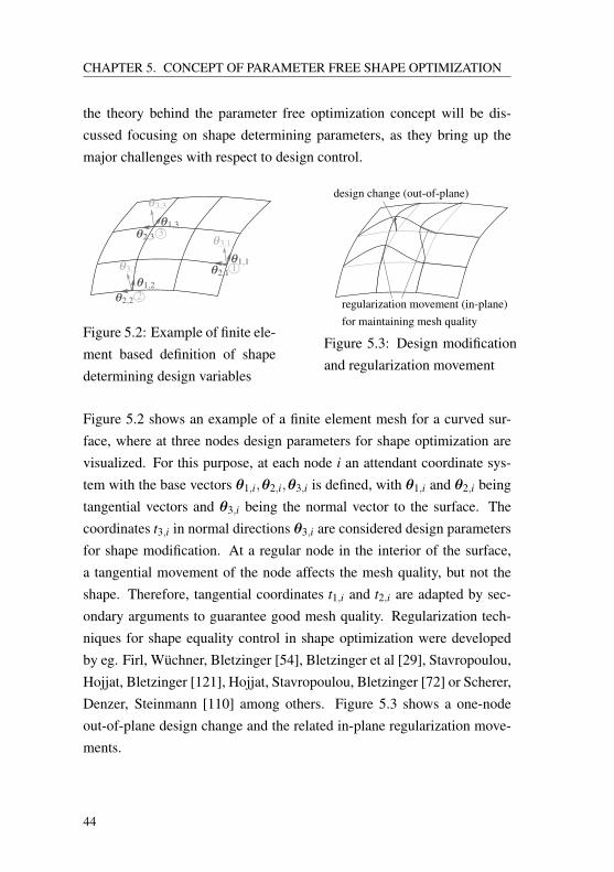
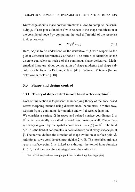
the theory behind the parameter free optimization concept will be dis-cussed focusing on shape determining parameters, as they bring up themajor challenges with respect to design control.
θ2,1θ1,1
θ3,1
θ1,3
θ3,3
θ2,3
θ2,2
θ1,2
θ3,2 1©
3©
2©
Figure 5.2: Example of finite ele-ment based definition of shapedetermining design variables
regularization movement (in-plane)for maintaining mesh quality
design change (out-of-plane)
Figure 5.3: Design modificationand regularization movement
Figure 5.2 shows an example of a finite element mesh for a curved sur-face, where at three nodes design parameters for shape optimization arevisualized. For this purpose, at each node i an attendant coordinate sys-tem with the base vectors θ1,i,θ2,i,θ3,i is defined, with θ1,i and θ2,i beingtangential vectors and θ3,i being the normal vector to the surface. Thecoordinates t3,i in normal directions θ3,i are considered design parametersfor shape modification. At a regular node in the interior of the surface,a tangential movement of the node affects the mesh quality, but not theshape. Therefore, tangential coordinates t1,i and t2,i are adapted by sec-ondary arguments to guarantee good mesh quality. Regularization tech-niques for shape equality control in shape optimization were developedby eg. Firl, Wüchner, Bletzinger [54], Bletzinger et al [29], Stavropoulou,Hojjat, Bletzinger [121], Hojjat, Stavropoulou, Bletzinger [72] or Scherer,Denzer, Steinmann [110] among others. Figure 5.3 shows a one-nodeout-of-plane design change and the related in-plane regularization move-ments.
44
CHAPTER 5. CONCEPT OF PARAMETER FREE SHAPE OPTIMIZATION
Knowledge about surface normal directions allows to compute the sensi-tivity pi of a response function f with respect to the shape modification atthe considered node i by computing the total differential of the responsein direction θ3,i:
pi = (∇ f )T ·θ3,i (5.1)
Here, ∇ f is to be understood as the derivative of f with respect to theglobal Cartesian coordinates x of node i. The term pi is identified as thediscrete equivalent at node i of the continuous shape derivative. Math-ematical literature about computation of shape gradients and shape cal-culus can be found in Delfour, Zolésio [47], Haslinger, Mäkinen [69] orSokolowski, Zolésio [118].
5.3 Shape and design control
5.3.1 Theory of shape control in node based vertex morphing2
Goal of this section is to present the underlying theory of the node basedvertex morphing method using discrete nodal parameters. On this way,we start from a continuous formulation and will discretize later on.We consider a surface Ω in space and related surface coordinates ξ ∈R2 which eventually are called material coordinates as well. The surfacegeometry is given by the spatial coordinates x = x(ξ ) in R3. The fieldt3 ∈R is the field of coordinates in normal direction at every surface pointξ . The normal defines the direction of shape evolution at surface point ξ .Additionally, we consider a control field s(ξ )∈R. The normal coordinatet3 at a surface point ξi is linked to s through the kernel filter functionF (ξ ,ξi) and the convolution integral over the surface Ω:
2Parts of this section have been pre-published in Masching, Bletzinger [90]
45
CHAPTER 5. CONCEPT OF PARAMETER FREE SHAPE OPTIMIZATION
t3 (ξi) =∫Ω
F (ξ ,ξi) · s(ξ )dξ
∫Ω
F (ξ ,ξi)dξ = 1(5.2)
The shape optimization is driven by the manipulation of the control fields. To that end we define the shape optimization problem as:
min f (s,u)
u = u(s) from S (s,u) = 0(5.3)
where f is the objective as a function of the control field s and u whichare the fields of state variables, e.g. the displacement fields in R3, and S
is the state equation. Eventually, the optimization problem is enhancedby further constraints. Regarding the actual goal of explaining the shapecontrol techniques and for the sake of simplicity they do not have to beconsidered.The derivative of the objective f with respect to the design control field s
is determined by following chain rule of differentiation:
d fds
=∫Ω
d fdt3· dt3
dsdξ =
∫Ω
p · dt3ds
dξ (5.4)
where the shape derivative p is the derivative of the objective with respectto the normal coordinates considering shape variations in the surface nor-mal direction. Furthermore, evaluation of d f
ds at position ξi yields
d fds
(ξi) =∫Ω
p(ξ ) ·F (ξi,ξ )dξ (5.5)
We observe that derivatives are treated with the transpose filter operationas compared to the filtering of the normal coordinates t3. Of course, in thecase of symmetric filter functions it holds
F (ξi,ξ ) = F (ξ ,ξi) (5.6)
46
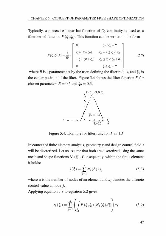
CHAPTER 5. CONCEPT OF PARAMETER FREE SHAPE OPTIMIZATION
Typically, a piecewise linear hat-function of C0-continuity is used as afilter kernel function F (ξ ,ξi). This function can be written in the form
F (ξ ,ξ0,R) =1
R2 ·
0 ξ < ξ0−R
ξ +(R−ξ0) ξ0−R≤ ξ < ξ0
−ξ +(R+ξ0) ξ0 ≤ ξ < ξ0 +R
0 ξ ≥ ξ0 +R
(5.7)
where R is a parameter set by the user, defining the filter radius, and ξ0 isthe center position of the filter. Figure 5.4 shows the filter function F forchosen parameters R = 0.5 and ξ0 = 0.3.
ξ
ξ0 = 0.3
R=0.5
F (ξ ,0.3,0.5)
Figure 5.4: Example for filter function F in 1D
In context of finite element analysis, geometry x and design control field s
will be discretized. Let us assume that both are discretized using the samemesh and shape functions N j (ξ ). Consequently, within the finite elementit holds:
s(ξ ) =n
∑j=1
N j (ξ ) · s j (5.8)
where n is the number of nodes of an element and s j denotes the discretecontrol value at node j.Applying equation 5.8 to equation 5.2 gives
t3 (ξi) =n
∑j=1
∫Ω
F (ξ ,ξi) ·N j (ξ )dξ
s j (5.9)
47
CHAPTER 5. CONCEPT OF PARAMETER FREE SHAPE OPTIMIZATION
from which we can derive the discrete filter operator matrix B whichrelates the discrete nodal control numbers s j and the normal coordinatest3,i at every node:
t3 (ξi) = t3,i =n
∑j=1
Bi j · s j
Bi j =∫Ω
F (ξ ,ξi) ·N j (ξ )dξ
(5.10)
For the derivatives it holds:
d fdsi
=d f
dt3, j·B ji = BT
i j ·d f
dt3, j= BT
i j · p j (5.11)
Collecting all nodal control parameters and normal coordinates in vectorss and t3, respectively, we get
t3 = B · sd fds
= BT ·p(5.12)
As there are as many discrete parameters for p as well as t3, the matrixB is quadratic. For typical filter functions, e.g. the simple hat function,B is positive definite and, additionally, for regular element meshes B issymmetric. Hence matrix B describes a pure parameter transformation,which does not reduce the dimension of the design space. Thus, the orig-inal properties of the optimization problem are maintained, such that anoptimum determined using the transformation is also an optimum of theoriginal minimization problem.For the most practical cases with fine meshes and moderately varyingmesh density B can be approximated to be symmetric.Considering gradient or quasi Newton methods, it appears that the controlparameters s may be substituted. The quadratic approximation of f isgiven by f , where Hα are the matrices of second derivatives with respect
48
CHAPTER 5. CONCEPT OF PARAMETER FREE SHAPE OPTIMIZATION
to α , which is either the control parameters s or the normal coordinatest3:
f = f +d fds
T·∆s+
12·∆sT ·Hs ·∆s =
= f +pT ·B ·∆s+12·∆sT ·B ·Ht3 ·B
T ·∆s(5.13)
From equation 5.13 together with equation 5.12 the update ∆t3 of nodalcoordinates can be derived as
∆s =−(BT ·Ht3 ·B
)−1 ·BT ·p
∆t3 =−B ·(BT ·Ht3 ·B
)−1 ·BT ·p(5.14)
From a practical point of view it appears that the control parameters mustnot be considered when the method is coded. As equation 5.12 holds,considerations can be reduced to the design update ∆t3 and the operator Bfor implementation purpose.Furthermore, on the line of quasi Newton methods, equation 5.14 may bemodified as
∆t3 =−α ·B ·BT ·p
or ∆t3 =−α ·B ·p =−α · p(5.15)
where α is a line search factor. Indeed, the normal coordinates t3 may beupdated by means of applying the filter once or twice to the shape deriva-tive p. Since B is positive definite it is guaranteed that descend directionsare generated. Numerical experience shows that both alternatives of equa-tion 5.15 can be used very efficiently for very large problems together withsteepest descent or conjugate gradient methods for unconstrained and con-strained problems [25] [72]. The second variant of equation 5.15 meets thewell-known sensitivity filtering techniques. The method is most efficienttogether with adjoint methods of sensitivity analysis.The matrix B allows for deeper insight into the method. However, it mustnever be evaluated or stored. Instead, regarding the second variant of
49
CHAPTER 5. CONCEPT OF PARAMETER FREE SHAPE OPTIMIZATION
equation 5.15 the sensitivity filtering is performed node wise by apply-ing an alternative numerical integration scheme considering derivatives ofadjacent nodes within the filter radius R:
pi =∑ j F (ξ j,ξi) · p j
∑ j F (ξ j,ξi)(5.16)
Indeed, the sensitivity filtering (equation 5.16) is equivalent to techniqueswhich are applied in topology optimization by the SIMP method [20].Typically, symmetric hat filters are used.The procedure can be interpreted in different ways. From the mathemat-ical point of view, it is a smoothing operation typically introduced forregularization [103] [77]. In the context of structural shape optimization,this procedure is commonly interpreted and used as a design tool. It givescontrol over the optimization procedure to the user by choice of the filterradius R as an extra problem parameter. Although the filter cancels outin the course of optimization - which can be seen from equation 5.14 - itimproves the numerical properties of the optimization problem by provid-ing smooth geometry updates. On the other hand for non-convex prob-lems, the choice of the filter radius will decide which local minimum willbe reached at convergence. This is the intended effect of the filter, whichsupports the user by exploring the design space, just by simply choosingdifferent filter radii [25] [72].
5.3.2 Examples
5.3.2.1 Convex optimization problem: Generation of catenary curves
The following example applies the presented filtering scheme to a con-vex problem of shape optimization. The system under consideration is aframe structure, subjected to dead load. Objective of the optimization isminimization of strain energy inside the entire structure, which is a global
50
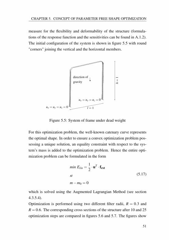
CHAPTER 5. CONCEPT OF PARAMETER FREE SHAPE OPTIMIZATION
measure for the flexibility and deformability of the structure (formula-tions of the response function and the sensitivities can be found in A.1.2).The initial configuration of the system is shown in figure 5.5 with round"corners" joining the vertical and the horizontal members.
l = 1ux = uy = uz = 0
ux = uy = uz = 0
direction of
gravity h=
1Figure 5.5: System of frame under dead weight
For this optimization problem, the well-known catenary curve representsthe optimal shape. In order to ensure a convex optimization problem pos-sessing a unique solution, an equality constraint with respect to the sys-tem’s mass is added to the optimization problem. Hence the entire opti-mization problem can be formulated in the form
min Elin =12·uT · fext
st
m−m0 = 0
(5.17)
which is solved using the Augmented Lagrangian Method (see section4.3.5.4).Optimization is performed using two different filter radii, R = 0.3 andR = 0.6. The corresponding cross sections of the structure after 10 and 25optimization steps are compared in figures 5.6 and 5.7. The figures show
51
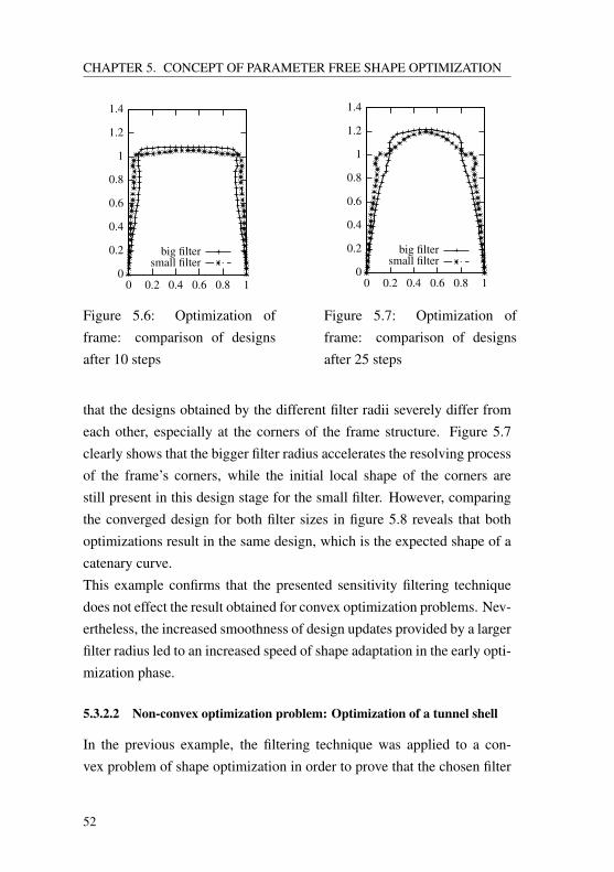
CHAPTER 5. CONCEPT OF PARAMETER FREE SHAPE OPTIMIZATION
0
0.2
0.4
0.6
0.8
1
1.2
1.4
0 0.2 0.4 0.6 0.8 1
big filtersmall filter
Figure 5.6: Optimization offrame: comparison of designsafter 10 steps
0
0.2
0.4
0.6
0.8
1
1.2
1.4
0 0.2 0.4 0.6 0.8 1
big filtersmall filter
Figure 5.7: Optimization offrame: comparison of designsafter 25 steps
that the designs obtained by the different filter radii severely differ fromeach other, especially at the corners of the frame structure. Figure 5.7clearly shows that the bigger filter radius accelerates the resolving processof the frame’s corners, while the initial local shape of the corners arestill present in this design stage for the small filter. However, comparingthe converged design for both filter sizes in figure 5.8 reveals that bothoptimizations result in the same design, which is the expected shape of acatenary curve.This example confirms that the presented sensitivity filtering techniquedoes not effect the result obtained for convex optimization problems. Nev-ertheless, the increased smoothness of design updates provided by a largerfilter radius led to an increased speed of shape adaptation in the early opti-mization phase.
5.3.2.2 Non-convex optimization problem: Optimization of a tunnel shell
In the previous example, the filtering technique was applied to a con-vex problem of shape optimization in order to prove that the chosen filter
52
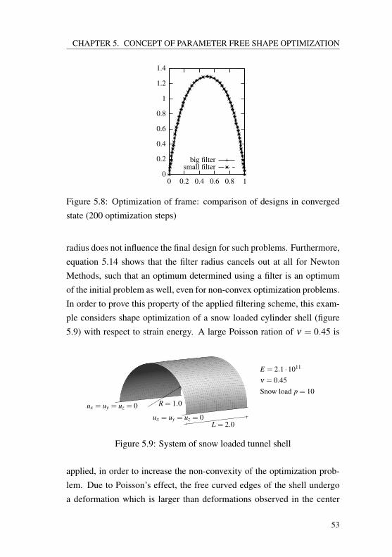
CHAPTER 5. CONCEPT OF PARAMETER FREE SHAPE OPTIMIZATION
0
0.2
0.4
0.6
0.8
1
1.2
1.4
0 0.2 0.4 0.6 0.8 1
big filtersmall filter
Figure 5.8: Optimization of frame: comparison of designs in convergedstate (200 optimization steps)
radius does not influence the final design for such problems. Furthermore,equation 5.14 shows that the filter radius cancels out at all for NewtonMethods, such that an optimum determined using a filter is an optimumof the initial problem as well, even for non-convex optimization problems.In order to prove this property of the applied filtering scheme, this exam-ple considers shape optimization of a snow loaded cylinder shell (figure5.9) with respect to strain energy. A large Poisson ration of ν = 0.45 is
R = 1.0
L = 2.0ux = uy = uz = 0
ux = uy = uz = 0
E = 2.1 ·1011
ν = 0.45Snow load p = 10
Figure 5.9: System of snow loaded tunnel shell
applied, in order to increase the non-convexity of the optimization prob-lem. Due to Poisson’s effect, the free curved edges of the shell undergoa deformation which is larger than deformations observed in the center
53
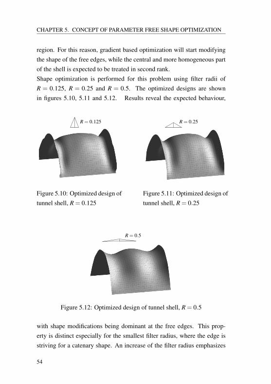
CHAPTER 5. CONCEPT OF PARAMETER FREE SHAPE OPTIMIZATION
region. For this reason, gradient based optimization will start modifyingthe shape of the free edges, while the central and more homogeneous partof the shell is expected to be treated in second rank.Shape optimization is performed for this problem using filter radii ofR = 0.125, R = 0.25 and R = 0.5. The optimized designs are shownin figures 5.10, 5.11 and 5.12. Results reveal the expected behaviour,
R = 0.125
Figure 5.10: Optimized design oftunnel shell, R = 0.125
R = 0.25
Figure 5.11: Optimized design oftunnel shell, R = 0.25
R = 0.5
Figure 5.12: Optimized design of tunnel shell, R = 0.5
with shape modifications being dominant at the free edges. This prop-erty is distinct especially for the smallest filter radius, where the edge isstriving for a catenary shape. An increase of the filter radius emphasizes
54
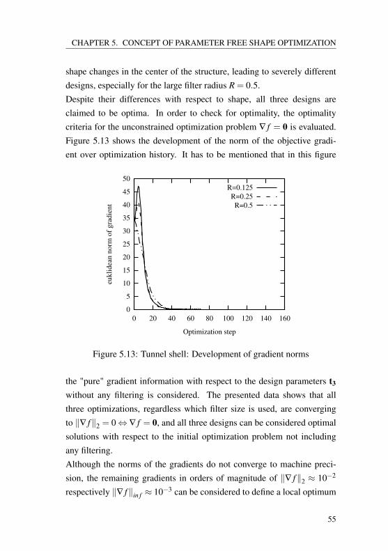
CHAPTER 5. CONCEPT OF PARAMETER FREE SHAPE OPTIMIZATION
shape changes in the center of the structure, leading to severely differentdesigns, especially for the large filter radius R = 0.5.Despite their differences with respect to shape, all three designs areclaimed to be optima. In order to check for optimality, the optimalitycriteria for the unconstrained optimization problem ∇ f = 0 is evaluated.Figure 5.13 shows the development of the norm of the objective gradi-ent over optimization history. It has to be mentioned that in this figure
0
5
10
15
20
25
30
35
40
45
50
0 20 40 60 80 100 120 140 160
eukl
idea
nno
rmof
grad
ient
Optimization step
R=0.125R=0.25
R=0.5
Figure 5.13: Tunnel shell: Development of gradient norms
the "pure" gradient information with respect to the design parameters t3
without any filtering is considered. The presented data shows that allthree optimizations, regardless which filter size is used, are convergingto ‖∇ f‖2 = 0⇔ ∇ f = 0, and all three designs can be considered optimalsolutions with respect to the initial optimization problem not includingany filtering.Although the norms of the gradients do not converge to machine preci-sion, the remaining gradients in orders of magnitude of ‖∇ f‖2 ≈ 10−2
respectively ‖∇ f‖in f ≈ 10−3 can be considered to define a local optimum
55
CHAPTER 5. CONCEPT OF PARAMETER FREE SHAPE OPTIMIZATION
in context of a finite element based sensitivity analysis. The topic of finiteelement based sensitivity analysis will be discussed in the upcoming sec-tion 5.4.In summary, the presented designs can be considered optimal solutions ofthe pure optimization problem, whereat the filter only was used in orderto guide the optimization algorithm into the radius of convergence of thecorresponding optimum.
5.4 Finite element based sensitivity analysis
The field of sensitivity analysis addresses the issue of computing the effectof the variation of an input parameter onto an output parameter. In gra-dient based optimization, sensitivity analysis is used in order to computegradients of response functions with respect to the variations of designparameters. Sensitivity analysis has been an intense field of research formathematicians and engineers over the last decades. While this thesisrepresents an engineer’s point of view onto the topic, more mathematicalliterature can be found under Choi, Kim [39] [40] or Haug, Choi, Komkov[70], for example.
5.4.1 Different methods of sensitivity analysis
Different types of sensitivity analysis can be distinguished. The mostsimple form of sensitivity analysis is the global finite difference method,which approximates the gradient information of the response by a relativedifference of two evaluations of the response function
∂ f∂ si≈ ∆ f
∆si
( f wd)=
f (∆s+ s,u)− f (s,u)ε
(5.18a)
∂ f∂ si≈ ∆ f
∆si
(cent)=
f (∆s+ s,u)− f (−∆s+ s,u)2 · ε
(5.18b)
∆s =
∆s j = 0 j 6= i
∆s j = ε j = i
(5.18c)
56
CHAPTER 5. CONCEPT OF PARAMETER FREE SHAPE OPTIMIZATION
where ∆s is a vector which applies a finite disturbance ε to the designparameter for which the gradient value is evaluated. The equation aboveshows two different types of finite differences. In equation 5.18a, a so-called forward finite difference is used, which uses the evaluation of f atthe point of consideration s, and just one disturbance in forward directionis used. In contrast, in equation 5.18b a central finite difference scheme isapplied, which uses two disturbed evaluations of f , one in forward and onein backward direction. The different methods will be further discussed insection 5.4.2.The advantage of the global finite difference is that it does not contain anyanalytical derivative information, which makes it very easy to implementand quite insusceptible to implementation errors. The drawback is that ahuge number of response function evaluations is necessary, which makesit impracticable for serious applications, but global finite differencing canbe used as a reference solution.For more efficient methods of sensitivity analysis, the derivatives of theresponse functions are determined analytically and implemented as indi-vidual functions of s and u. Depending on how far the analytic approach isfollowed up, one can further distinguish between analytic sensitivity anal-
ysis and semi-analytic sensitivity analysis. In analytic sensitivity anal-ysis, the entire sensitivity analysis is performed analytically, whereat inthe semi-analytic approach the analytic procedure is performed until to acertain extent, and remaining parts of the sensitivity equation are approx-imated by a finite difference scheme. In this thesis, semi-analytic sensi-tivity analysis is used, which will be further explained and discussed insection 5.4.2.Another classification of sensitivity analysis methods can be done bygrouping them in variational sensitivity analysis and discrete sensitivity
analysis. The difference between these groups is the order of the proceed-ing steps. While in discrete sensitivity analysis, the response function isdiscretized in the first step and then the derivatives with respect to discrete
57
CHAPTER 5. CONCEPT OF PARAMETER FREE SHAPE OPTIMIZATION
parameters are evaluated, the variational method proceeds the other wayround. In this case, the derivatives are computed in a continuous formand afterwards a discretization method such as finite elements is appliedto the continuous derivates. Within this thesis, discrete formulations areconsidered only. Further information about variational sensitivity analysiscan be found in Barthold, Stein [13], Ibrahim, Tiwari [76] or Daoud [46].
5.4.2 Semi-analytic sensitivity analysis
5.4.2.1 Computing semi-analytic sensitivities
As already mentioned in the previous section, a semi-analytic approach isused in order to compute sensitivities within this thesis. In this approach,response functions are differentiated analytically until element level. Butinstead of now deriving element entities, such as stiffness or internalforces, analytically, a finite difference scheme is used in order to approxi-mate these derivatives.This approach will be explained considering the sensitivity of the determi-nant of a system stiffness matrix K with respect to the design parameters s.According to Jacobi’s formula [18], the sensitivity with respect to designvariable si can be written as
∂det (K(s))∂ si
= det (K(s)) · trace(
K(s)−1 · ∂K(s)∂ si
)(5.19)
assuming our system to be sufficiently supported such that K−1 exists.The system stiffness matrix K is a global variable, which is generated byassembling over all element matrices ke in the computational domain
K = Aall
ke (5.20)
with A being the assembly operator. At this point, the derived stiffnessmatrix ∂K
∂ s behaves differently. As the modification of a design parameter,such as a nodal position, influences only a small number of neighboringfinite elements, just the stiffness of these elements will be changed, while
58
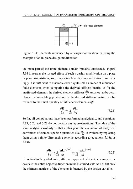
CHAPTER 5. CONCEPT OF PARAMETER FREE SHAPE OPTIMIZATION
ds
∂ke
∂ s = 0
∂ke
∂ s 6= 0, influenced elements
Figure 5.14: Elements influenced by a design modification ds, using theexample of an in-plane design modification
the main part of the finite element domain remains unaffected. Figure5.14 illustrates the located effect of such a design modification on a platein plane stress/strain, so ds is an in-plane design modifcation. Accord-ingly, it is sufficient to assemble over a quite small number of influencedfinite elements when computing the derived stiffness matrix, as for theunaffected elements the derived element stiffness ∂ke
∂ s turns out to be zero.Hence the assembling procedure for the derived stiffness matrix can bereduced to the small quantity of influenced elements infl:
∂K∂ s
= Ainfl
∂ke
∂ s(5.21)
So far, all computations have been performed analytically, and equations5.19, 5.20 and 5.21 do not contain any approximations. The idea of thesemi-analytic sensitivity is, that at this point the evaluation of analyticalderivatives of element specific quantities like ∂ke
∂ s is avoided by replacingthem using a finite differencing scheme according to equations 5.18a or5.18b
∂K∂ s≈ A
infl
∆ke
∆s
( f wd)≈ A
infl
∆ke
∆s
(cent)(5.22)
In contrast to the global finite difference approach, it is not necessary to re-evaluate the entire objective function in the disturbed state ∆s+s, but onlythe stiffness matrices of the elements influenced by the design variable.
59
CHAPTER 5. CONCEPT OF PARAMETER FREE SHAPE OPTIMIZATION
Using equations 5.19, 5.21 and 5.22, the final formulations of the analytic(equation 5.23) and the semi-analytic sensitivities (equation 5.24) can beformulated, whereby (x) denotes the chosen finite differencing scheme.
∂det (K(s))∂ s
= det (K(s)) · trace(
K(s)−1 · Ainfl
∂ke
∂ s
)(5.23)
∂det (K(s))∂ s
≈ det (K(s)) · trace
(K(s)−1 · A
infl
∆ke
∆s
(x))
(5.24)
The usage of the semi-analytic method has several advantages towards thepure analytical approach:
• The implementation of analytic derivatives of element based datacan be omitted. These derivatives may become very tedious, espe-cially when complex element formulations like shell elements withhybrid stress formulation are used.
• Finite differencing schemes according to equation 5.22 can be usedfor any element formulation, whereby any element which is avail-able for simulation directly can be used for optimization purposewithout additional coding.
• Any entity of the finite element formulation, such as shape, thick-ness or material orientation, immediately can be used as a designparameter without specific implementations on element level.
• For most element formulations, the semi-analytic approach turnsout to be faster than the complete analytical sensitivity formulation.This is because evaluating the element stiffness twice and applyinga finite differencing scheme is less costly, from the numerical pointof view, than following the product and chain rules of differentiationin order to determine the analytic sensitivity.
60
CHAPTER 5. CONCEPT OF PARAMETER FREE SHAPE OPTIMIZATION
5.4.2.2 Numerical efficiency
In order to judge about the efficiency of the semi-analytic approach, weconsider a very simple four-noded plain stress element with linear kine-matics. The stiffness matrix of this element can be writen in the well-known form
ke =∫V
BT ·D ·B ·det (J) dV (5.25)
Taking the analytical derivative of the stiffness matrix with respect to adesign variable s, equation 5.25 extends to a three summand expressiondue to the product rule of differentiation:
∂ke
∂ s=∫V
∂B∂ s
T
·D ·B ·det (J)+
BT ·D · ∂B∂ s·det (J)+BT ·D ·B · ∂det (J)
∂ sdV
(5.26)
Due to this extension, the computation of the derived stiffness is approx-imately three times as costly as computing the stiffness itself. As theforward and the central finite differencing scheme only require two evalu-ations of the stiffness matrix, we expect the semi-analytic sensitivity com-putation to save about 33% of the computational time compared to theanalytic approach. In order to get a unaltered comparison of the real cpu-times, a separate C++ implementation of the stiffness matrix, its deriva-tive and the finite differencing schemes is used. The needed cpu-timesin order to compute 100,000 derivatives of element stiffness matrices arepresented in figure 5.15 3. As we can see, the semi-analytic approach isfaster by 25% compared to the analytic approach. This saving of compu-tational time is smaller than the initial expectation of 33%, but this expec-tation neglected the time consumed by evaluating the finite difference aswell as the memory allocation overhead caused by the higher number offunction calls in the semi-analytic procedure.
3Serial computation on an Intel i3 processor
61
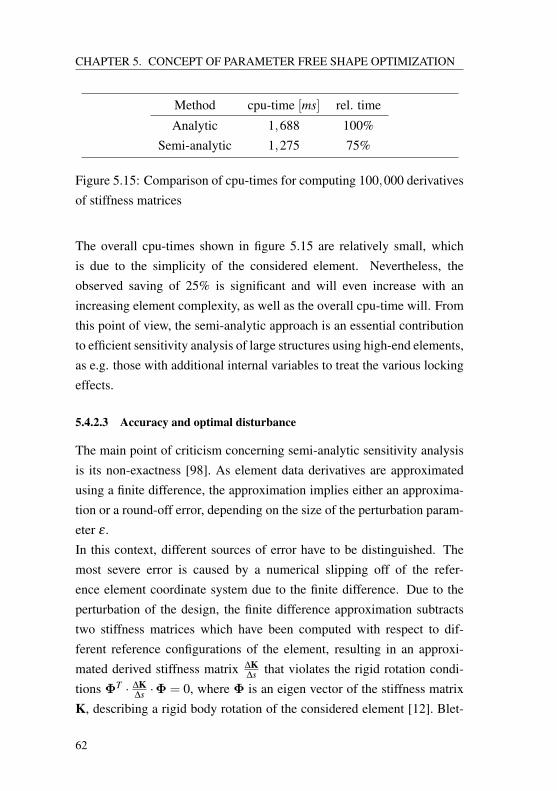
CHAPTER 5. CONCEPT OF PARAMETER FREE SHAPE OPTIMIZATION
Method cpu-time [ms] rel. time
Analytic 1,688 100%Semi-analytic 1,275 75%
Figure 5.15: Comparison of cpu-times for computing 100,000 derivativesof stiffness matrices
The overall cpu-times shown in figure 5.15 are relatively small, whichis due to the simplicity of the considered element. Nevertheless, theobserved saving of 25% is significant and will even increase with anincreasing element complexity, as well as the overall cpu-time will. Fromthis point of view, the semi-analytic approach is an essential contributionto efficient sensitivity analysis of large structures using high-end elements,as e.g. those with additional internal variables to treat the various lockingeffects.
5.4.2.3 Accuracy and optimal disturbance
The main point of criticism concerning semi-analytic sensitivity analysisis its non-exactness [98]. As element data derivatives are approximatedusing a finite difference, the approximation implies either an approxima-tion or a round-off error, depending on the size of the perturbation param-eter ε .In this context, different sources of error have to be distinguished. Themost severe error is caused by a numerical slipping off of the refer-ence element coordinate system due to the finite difference. Due to theperturbation of the design, the finite difference approximation subtractstwo stiffness matrices which have been computed with respect to dif-ferent reference configurations of the element, resulting in an approxi-mated derived stiffness matrix ∆K
∆s that violates the rigid rotation condi-tions ΦT · ∆K
∆s ·Φ = 0, where Φ is an eigen vector of the stiffness matrixK, describing a rigid body rotation of the considered element [12]. Blet-
62
CHAPTER 5. CONCEPT OF PARAMETER FREE SHAPE OPTIMIZATION
zinger et al [26] showed that this effect mainly occurs for elements withcomplex kinematics like Kirchhoff formulations, and presented a methodof exact semi-analytic sensitivities correcting this deficit. For this pur-pose, a modified approximated derived stiffness matrix ∆K∗
∆s is computedby adding correction terms curing the violation of rigid body conditions.Equation 5.27 shows the correction, where Φr is a rigid body rotationvector and nr is the total number of possible rigid body rotations.
[Φk
r
]T·
(∆K∆s
+nr
∑i=1
nr
∑j=1
ai, j ·Φir ·[Φ j
r]T)
︸ ︷︷ ︸∆K∗∆s
·Φlr = 0
∀ k, l ∈ 1, ...,nr
with
ai, j =−[Φi
r]T · ∆K
∆s ·Φjr(
[Φir]
T ·Φir
)·([
Φ jr
]T·Φ j
r
)(5.27)
Applying this corrections, the remaining error in the semi-analytic sen-sitivity reduces to the approximation error contributed by the finite dif-ferencing scheme. This error is directly related to the finite disturbanceε .The following convergence study investigates the error in the approxi-mated sensitivity for a plain stress element formulation, comparing theforward and the central finite difference scheme with and without the rigidbody correction according to equation 5.27. The results are displayed infigure 5.16, where the error is measured by the Frobenius norm of thedifference between the analytical derivative of ke and the finite differenceapproximation. Figure 5.16 presents that for ε > 10−5 both finite differ-ence schemes show a constant decrease of error with the expected ordersof accuracy. The forward finite difference shows an order of accuracy of1 while the central finite difference method possesses an order of accu-
63
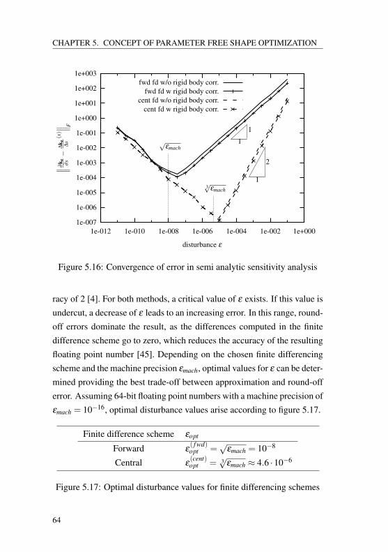
CHAPTER 5. CONCEPT OF PARAMETER FREE SHAPE OPTIMIZATION
1e-007
1e-006
1e-005
1e-004
1e-003
1e-002
1e-001
1e+000
1e+001
1e+002
1e+003
1e-012 1e-010 1e-008 1e-006 1e-004 1e-002 1e+000
disturbance ε
∥ ∥ ∥∂k e ∂s−
∆k e ∆s(x)∥ ∥ ∥ F
√εmach
3√
εmach
fwd fd w/o rigid body corr.fwd fd w rigid body corr.
cent fd w/o rigid body corr.cent fd w rigid body corr.
1
2
1
1
Figure 5.16: Convergence of error in semi analytic sensitivity analysis
racy of 2 [4]. For both methods, a critical value of ε exists. If this value isundercut, a decrease of ε leads to an increasing error. In this range, round-off errors dominate the result, as the differences computed in the finitedifference scheme go to zero, which reduces the accuracy of the resultingfloating point number [45]. Depending on the chosen finite differencingscheme and the machine precision εmach, optimal values for ε can be deter-mined providing the best trade-off between approximation and round-offerror. Assuming 64-bit floating point numbers with a machine precision ofεmach = 10−16, optimal disturbance values arise according to figure 5.17.
Finite difference scheme εopt
Forward ε( f wd)opt =
√εmach = 10−8
Central ε(cent)opt = 3
√εmach ≈ 4.6 ·10−6
Figure 5.17: Optimal disturbance values for finite differencing schemes
64
CHAPTER 5. CONCEPT OF PARAMETER FREE SHAPE OPTIMIZATION
Figure 5.16 also demonstrates that the rigid body correction leads toslightly improved results for both finite difference schemes. For ε > εopt ,the influence of the rigid body correction is constant and comparativelysmall to the approximation error of the finite difference method for thistype of element.
5.5 Direct and adjoint sensitivity formulation
This chapter focuses on formulating the sensitivities of response func-tions typically arising from applications in structural optimization. Theseresponse functions I usually depend on the design s and on the state vari-ables u.
I (u,s) (5.28)
Taking the derivative of I with respect to a design variable si ∈ s underconsideration of the chain rule of differentiation leads to
dIdsi
=∂ I∂ si
+
[∂ I∂u
]T
· ∂u∂ si
(5.29)
where the derivative of the state variables is not known so far.The state variables u are implicitly defined via the state equation S,demanding the structure to be in equilibrium:
S(u) = 0 (5.30)
As the state equation has to be fulfilled for any design s, the derivativeof S with respect to all si ∈ s has to be zero. This allows to solve for theunknown derivatives of the state variables:
dSdsi
=∂S∂ si
+∂S∂u· ∂u
∂ si= 0⇒ ∂u
∂ si=
[∂S∂u
]−1
·[− ∂S
∂ si
](5.31)
Inserting equation 5.31 into equation 5.29 leads to
dIdsi
=∂ I∂ si
+
[∂ I∂u
]T
·[
∂S∂u
]−1
·[− ∂S
∂ si
]︸ ︷︷ ︸
∂u∂ si
(5.32)
65
CHAPTER 5. CONCEPT OF PARAMETER FREE SHAPE OPTIMIZATION
which is called the direct sensitivity formulation of response function I
[39] [40]. It has to be mentioned that the inverse of ∂S∂u usually is not
determined explicitly in large-scale applications. Instead, a factorizationscheme like Gauss or Cholesky is applied in order to transform the matrixto a triangular shape, and the inverse matrix-vector multiplication can beperformed doing a so-called forward-backward substitution [94].In the direct formulation, forward-backward substitution representing thederivatives of the state variable with respect to the design variable si hasto be solved for each design variable, as the right-hand sides of the linearsystems − ∂S
∂ sidepend on si. The intension of adjoint sensitivity formu-
lations is to re-formulate equation 5.32 such that the solution of a linearsystem of equations for each design variables becomes needless. For thispurpose, the rear summand of the equation is transformed switching theorder of execution in the vector-matrix-vector-product exploiting the fol-lowing relation:
vT ·M ·w = wT ·MT ·v (5.33)
The transformed version of equation 5.32 reads
dIdsi
=∂ I∂ si
+
[− ∂S
∂ si
]T
·[
∂S∂u
]−T
· ∂ I∂u
(5.34)
where the Jacobi matrix of the state equation ∂S∂u is identical with the stiff-
ness matrix K in structural mechanics. As the stiffness matrix is symmet-ric for conservative problems [19], the inverse of it is symmetric as well[123]. Therefore the same operator can be used in the adjoint formulationas in the direct formulation,
dIdsi
=∂ I∂ si
+
[− ∂S
∂ si
]T
·[
∂S∂u
]−1
· ∂ I∂u︸ ︷︷ ︸
Λ
(5.35)
where the variable Λ =[
∂S∂u
]−1· ∂ I
∂u is called the adjoint variable. Asthe operator matrix for computing the adjoint variable is the same as for
66
CHAPTER 5. CONCEPT OF PARAMETER FREE SHAPE OPTIMIZATION
determing the derivatives of the state variables ∂u∂ si
in structural mechanics,these problems are called self-adjoint.In contrast to the direct approach, where the derivative of state variableshas to be computed for each single design variable involving the solutionof a linear system of equations, the adjoint approach allows to determinethe derivatives of I with respect to all design variables by only solvingone linear system in order to compute the adjoint variables. From thispoint of few, the adjoint approach is preferable when optimization prob-lems defined by a large number of design variables, but only involving asmall number of response functions, are solved. As soon as the number ofresponse functions approaches the number of design variables, the advan-tage of the adjoint approach vanishes, as the number of linear solutionsbeing necessary to determine the derived state variables is independent ofthe number of responses, but the effort to compute the adjoint variablesincreases linearly with the number of response functions.In parameter free optimization, as it is performed in this thesis, the numberof design variables usually is larger than the number of response functionsby several orders of magnitude for large examples. For this reason, anadjoint formulation of the response functions is a key issue to numericalefficiency in the performed optimizations.More information about adjoint sensitivity formulations can be found inGiles, Pierce [63] or Cao, Li, Petzold [36].
Adjoint sensitivity formulations of frequently used response functions canbe found in appendix A.
5.6 Line search procedures
After the sensitivity information has been computed and filtered for allresponse functions, the final search direction for the actual optimizationstep is determined. Thereby the search direction might be a conjugated
67
CHAPTER 5. CONCEPT OF PARAMETER FREE SHAPE OPTIMIZATION
direction in case of a CG-algorithm or gradient information of a Lagrangefunction in case of a constrained optimization problem, for example. Inthe next step, a line search is performed along the search direction, asit was briefly introduced in section 4.2.2.2. In contrast to an exact linesearch, where the optimal step size α is defined by the gradient of f tovanish [∇ f (x+α · s)] = 0 (see equation 4.5), usually inexact line searchmethods are applied in numerical optimization, as the objective functionis not known analytically. The most simple type of inexact line search isa fixed step method, which prescribes a fixed value for α . The disadvan-tage of this method is that the chosen step length is not optimal, whichincreases the number of necessary optimization iterations or might lead toan "overleaping" of the local minimum. Consequently more sophisticatedinexact line search procedures should fulfill the requirement that "the stepsize should not be too large or too small, and there should be a suffi-cient decrease in the cost function" [8]. Line search methods which tryto meet these criteria using one evaluation of the response function onlyare Armijo’s rule [7] or the Wolfe Condition [134]. These methods use alinear extrapolation of the response function in search direction based onthe actual design, and demand a minimum decrease of the response func-tion within each optimization step. Another method of inexact line searchis the polynomial interpolation method [111]. Thereby the response func-tion is approximated within an interval of acceptable step sizes using apolynomial function, which now can be used as an auxiliary mean foran exact line search. This method requires a larger number of responsefunction evaluations compared to Armijo’s rule or the Wolfe condition, assampling points of the polynomial function need to be determined. Never-theless, as evaluation points are distributed over the interval of acceptablestep sizes, the gained information usually is more precise and reliable thanthe information obtained by methods using only one evaluation point. Sothe line search reflects the real behaviour of the response function moreprecisely.
68
CHAPTER 5. CONCEPT OF PARAMETER FREE SHAPE OPTIMIZATION
5.7 Work flow and data management in a object ori-ented code environment
This section is intended to illustrate the work flow and the data manage-ment of a parameter free optimization, as it is implemented in Carat++(see section 1.4). Figure 5.18 visualizes the connections and the datastreams.The first thing which is conspicuous, is a modular structure of the imple-mentation. The overall optimization framework includes a structural anal-ysis module, which contains the usual finite element tools like classes fornodes, elements, finite element domains or analysis classes managing dif-ferent types of structural analysis. Figure 5.18 shows these standard finiteelement components on the right hand side, separated from the optimiza-tion module by a dot and dash line. The optimization module can beregarded to be a add-on onto the analysis module, which is connected bypointer access in an object oriented manner. The points of connectionare quite limited. The finite element analysis object is controlled by aresponse function object via a pointer connection, as well as the designvariables have pointer access to the underlying finite element object. Thiscould be either a node or an element.Despite this limited number of intersection points, the optimization mod-ule has got the necessary control over the finite element analysis model.Optimization variables are able to modify the design of the finite elementmodel as well as they can query element data, which is essential for thesemi-analytic sensitivity analysis, via the pointer access to a finite ele-ment or a node. State variables and adjoint variables for a given pseudoload vector are provided by the analysis object directly to the responsefunction object, and so all data necessary for sensitivity analysis can begathered inside the response function routines. Once sensitivity informa-tion is computed, there is only a very small amount of further communica-tion necessary between analysis and optimization module in the following
69
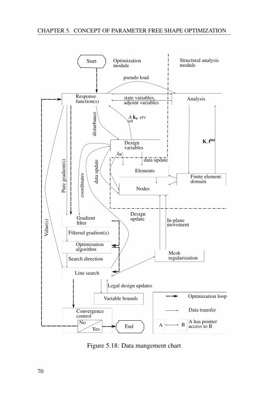
CHAPTER 5. CONCEPT OF PARAMETER FREE SHAPE OPTIMIZATION
Response Analysisfunction(s)
Elements
Nodes
Finite elementdomain
Designvariables
ordata update
K, fint
Ainfl
ke etc
Pure
grad
ient
(s)
data
upda
tedi
stur
banc
e
coor
dina
tes
Optimizationalgorithm
Filtered gradient(s)
Search direction
Line search
Val
ue(s
)
Variable bounds
Legal design updates
Meshregularization
In-planemovement
Designupdate
Data transfer
A BA has pointeraccess to B
Start
Convergencecontrol
EndYesNo
Optimization loop
Structural analysismodule
Optimizationmodule
pseudo load
state variables,adjoint variables
Gradientfilter
Figure 5.18: Data mangement chart
70
CHAPTER 5. CONCEPT OF PARAMETER FREE SHAPE OPTIMIZATION
steps. Pure sensitivity information of the response function, or of severalresponse functions in case of a constrained or multi-objective problem,is passed to the filtering object, which performs the filtering operationdescribed in section 5.3 on the discrete pure sensitivity data. The result-ing filtered gradient data is pushed forward to the mathematical core rou-tine of the optimization algorithm, which determines the search directionfor the actual optimization step, based on the actual gradient informationof all response functions plus some variables coming from optimizationhistory, like Lagrange multipliers or previous search directions. Once thesearch direction is determined, the line search can be applied. Therebyinexact line search methods as presented in section 5.6 are used. Hav-ing computed a step length factor α , the final design update is appliedto the design variables, which, for their part, update the finite elementmodel. The quantity of legal design updates may be restricted by variablebounds, which prevent design variables from assuming arbitrary values.By this mean, unphysical or inpracticable designs can be avoided. Theline search methods take care of these bounds and correct illegal designupdates correspondingly.The thicker dashed line in figure 5.18 shows the optimization loop. Herethe steps
• Gradient computation
• Gradient filtering
• Determination of search direction
• Line search
are repeated until convergence of the optimization is achieved. Therefore,usually convergence criteria based on
• a minimum decrease of the objective function or
• a minimum step length obtained in the line search
71
CHAPTER 5. CONCEPT OF PARAMETER FREE SHAPE OPTIMIZATION
obtained in the last optimization iteration are applied, instead of focusingon a gradient based criterion like equation 4.3 or 4.20.
5.8 Summary
In this chapter, the parameter free optimization approach has been pre-sented as a efficient parametrization method for treatment of structuraloptimization problems. In combination with semi-analytic and adjointsensitivity computation, it is excellently applicable for fine discretizedmodels of industrial relevance. In the upcoming chapter, these methodsand algorithms will be applied in order to generate optimal shapes for effi-ciently deformable shell structures, being a key issue to actuated systems.
72
CHAPTER 6. HINGELIKE MECHANISMS OF SHELL STRUCTURES
CHAPTER 6Hingelike mechanisms of shell
structures
6.1 Classification of kinematic mechanisms
In order to discuss structures which perform a maximum of movement fora limited actuator input, it is important to investigate kinematic mecha-nisms of structures, allowing these structures to undergo large deforma-tions while representing a minimum of mechanical resistance. Figure 6.1presents typical kinematic mechanisms for different types of structures.For beam structures, nodal hinges allowing the connected parts to undergoindependent rotations can be used, which enables the structure to move byproducing a minimum of strain energy or no strain energy at all, whena kinematic system is considered. Considering plates, an entire platecan be divided into sub-plates using line hinge mechanisms, which alloweach sub-plate to perform a rigid body movement. These line hinges aredirectly related to ultimate load analysis of plates using yield line theory[78]. Yield line theory assumes a constant yield moment acting along allyield lines in the ultimate load state, and that elastic deformations canbe neglected. The ultimate load state is characterized by a patch of sub-plates, each deforming in a rigid body state, whereat the entire internal
73
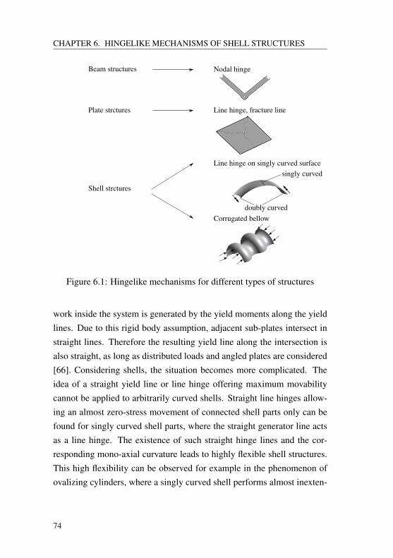
CHAPTER 6. HINGELIKE MECHANISMS OF SHELL STRUCTURES
Beam structures Nodal hinge
Plate strctures Line hinge, fracture line
Shell strctures
Line hinge on singly curved surface
Corrugated bellowdoubly curved
singly curved
Figure 6.1: Hingelike mechanisms for different types of structures
work inside the system is generated by the yield moments along the yieldlines. Due to this rigid body assumption, adjacent sub-plates intersect instraight lines. Therefore the resulting yield line along the intersection isalso straight, as long as distributed loads and angled plates are considered[66]. Considering shells, the situation becomes more complicated. Theidea of a straight yield line or line hinge offering maximum movabilitycannot be applied to arbitrarily curved shells. Straight line hinges allow-ing an almost zero-stress movement of connected shell parts only can befound for singly curved shell parts, where the straight generator line actsas a line hinge. The existence of such straight hinge lines and the cor-responding mono-axial curvature leads to highly flexible shell structures.This high flexibility can be observed for example in the phenomenon ofovalizing cylinders, where a singly curved shell performs almost inexten-
74
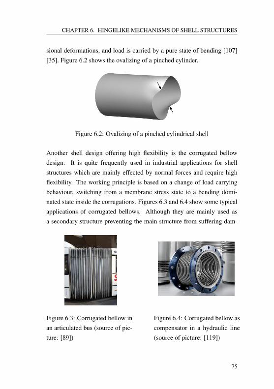
CHAPTER 6. HINGELIKE MECHANISMS OF SHELL STRUCTURES
sional deformations, and load is carried by a pure state of bending [107][35]. Figure 6.2 shows the ovalizing of a pinched cylinder.
Figure 6.2: Ovalizing of a pinched cylindrical shell
Another shell design offering high flexibility is the corrugated bellowdesign. It is quite frequently used in industrial applications for shellstructures which are mainly effected by normal forces and require highflexibility. The working principle is based on a change of load carryingbehaviour, switching from a membrane stress state to a bending domi-nated state inside the corrugations. Figures 6.3 and 6.4 show some typicalapplications of corrugated bellows. Although they are mainly used asa secondary structure preventing the main structure from suffering dam-
Figure 6.3: Corrugated bellow inan articulated bus (source of pic-ture: [89])
Figure 6.4: Corrugated bellow ascompensator in a hydraulic line(source of picture: [119])
75
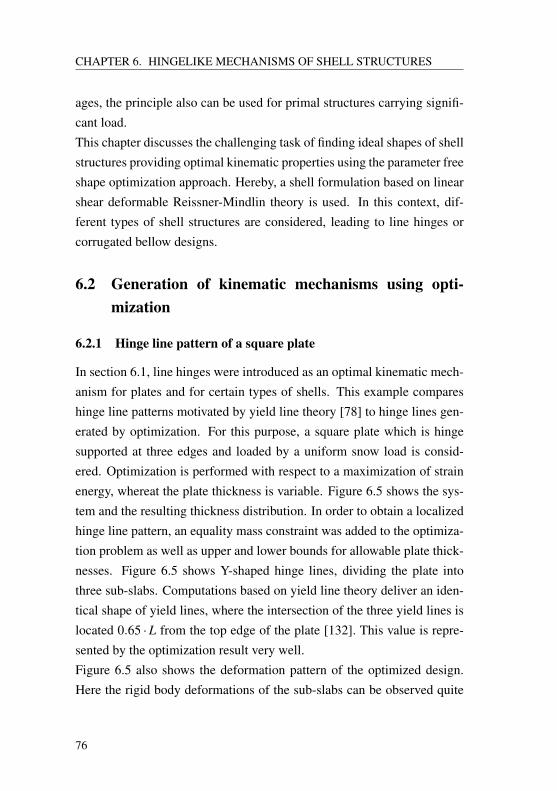
CHAPTER 6. HINGELIKE MECHANISMS OF SHELL STRUCTURES
ages, the principle also can be used for primal structures carrying signifi-cant load.This chapter discusses the challenging task of finding ideal shapes of shellstructures providing optimal kinematic properties using the parameter freeshape optimization approach. Hereby, a shell formulation based on linearshear deformable Reissner-Mindlin theory is used. In this context, dif-ferent types of shell structures are considered, leading to line hinges orcorrugated bellow designs.
6.2 Generation of kinematic mechanisms using opti-mization
6.2.1 Hinge line pattern of a square plate
In section 6.1, line hinges were introduced as an optimal kinematic mech-anism for plates and for certain types of shells. This example compareshinge line patterns motivated by yield line theory [78] to hinge lines gen-erated by optimization. For this purpose, a square plate which is hingesupported at three edges and loaded by a uniform snow load is consid-ered. Optimization is performed with respect to a maximization of strainenergy, whereat the plate thickness is variable. Figure 6.5 shows the sys-tem and the resulting thickness distribution. In order to obtain a localizedhinge line pattern, an equality mass constraint was added to the optimiza-tion problem as well as upper and lower bounds for allowable plate thick-nesses. Figure 6.5 shows Y-shaped hinge lines, dividing the plate intothree sub-slabs. Computations based on yield line theory deliver an iden-tical shape of yield lines, where the intersection of the three yield lines islocated 0.65 ·L from the top edge of the plate [132]. This value is repre-sented by the optimization result very well.Figure 6.5 also shows the deformation pattern of the optimized design.Here the rigid body deformations of the sub-slabs can be observed quite
76
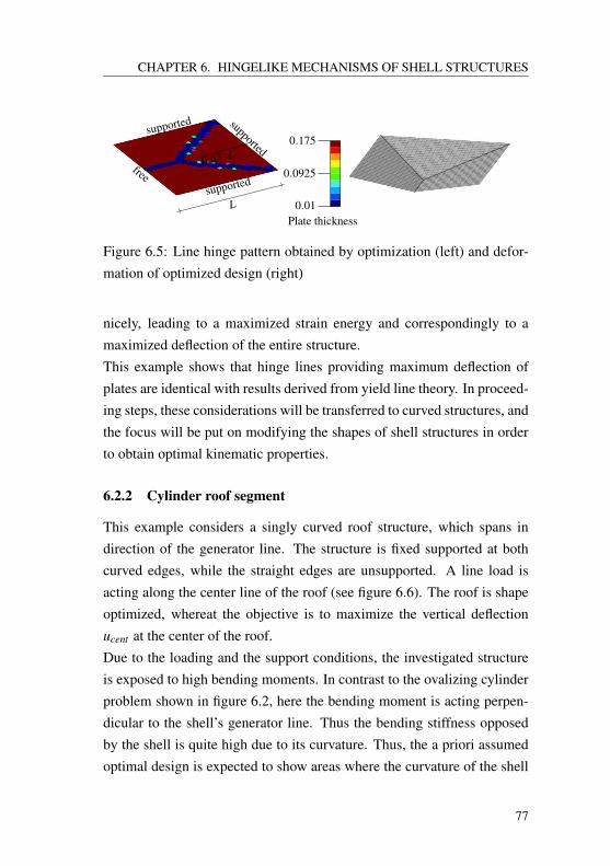
CHAPTER 6. HINGELIKE MECHANISMS OF SHELL STRUCTURES
supported
supported supported
free0.63 ·L
0.175
0.01Plate thickness
0.0925
L
Figure 6.5: Line hinge pattern obtained by optimization (left) and defor-mation of optimized design (right)
nicely, leading to a maximized strain energy and correspondingly to amaximized deflection of the entire structure.This example shows that hinge lines providing maximum deflection ofplates are identical with results derived from yield line theory. In proceed-ing steps, these considerations will be transferred to curved structures, andthe focus will be put on modifying the shapes of shell structures in orderto obtain optimal kinematic properties.
6.2.2 Cylinder roof segment
This example considers a singly curved roof structure, which spans indirection of the generator line. The structure is fixed supported at bothcurved edges, while the straight edges are unsupported. A line load isacting along the center line of the roof (see figure 6.6). The roof is shapeoptimized, whereat the objective is to maximize the vertical deflectionucent at the center of the roof.Due to the loading and the support conditions, the investigated structureis exposed to high bending moments. In contrast to the ovalizing cylinderproblem shown in figure 6.2, here the bending moment is acting perpen-dicular to the shell’s generator line. Thus the bending stiffness opposedby the shell is quite high due to its curvature. Thus, the a priori assumedoptimal design is expected to show areas where the curvature of the shell
77
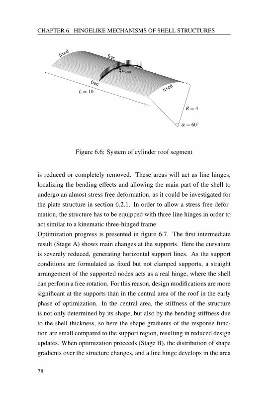
CHAPTER 6. HINGELIKE MECHANISMS OF SHELL STRUCTURES
R = 4
α = 60
L = 10 fixed
fixed
free
free
ucent
Figure 6.6: System of cylinder roof segment
is reduced or completely removed. These areas will act as line hinges,localizing the bending effects and allowing the main part of the shell toundergo an almost stress free deformation, as it could be investigated forthe plate structure in section 6.2.1. In order to allow a stress free defor-mation, the structure has to be equipped with three line hinges in order toact similar to a kinematic three-hinged frame.Optimization progress is presented in figure 6.7. The first intermediateresult (Stage A) shows main changes at the supports. Here the curvatureis severely reduced, generating horizontal support lines. As the supportconditions are formulated as fixed but not clamped supports, a straightarrangement of the supported nodes acts as a real hinge, where the shellcan perform a free rotation. For this reason, design modifications are moresignificant at the supports than in the central area of the roof in the earlyphase of optimization. In the central area, the stiffness of the structureis not only determined by its shape, but also by the bending stiffness dueto the shell thickness, so here the shape gradients of the response func-tion are small compared to the support region, resulting in reduced designupdates. When optimization proceeds (Stage B), the distribution of shapegradients over the structure changes, and a line hinge develops in the area
78
CHAPTER 6. HINGELIKE MECHANISMS OF SHELL STRUCTURES
Stage A
Stage B
Stage C
Figure 6.7: Optimization progress of cylinder roof segment
of load application, while the shape modifications at the supports slowdown. In the converged configuration (Stage C), the central line hingestarts to spread in span direction to a plane plateau, while the line hingesat the supports stay localized. This again can be explained by the bendingeffect inside the structure. As there is no bending moment at the supports,a spread of the flat region would not lead to a significant softening of thestructure. In contrast, the flat plateau in the central area reduced the stiff-
79
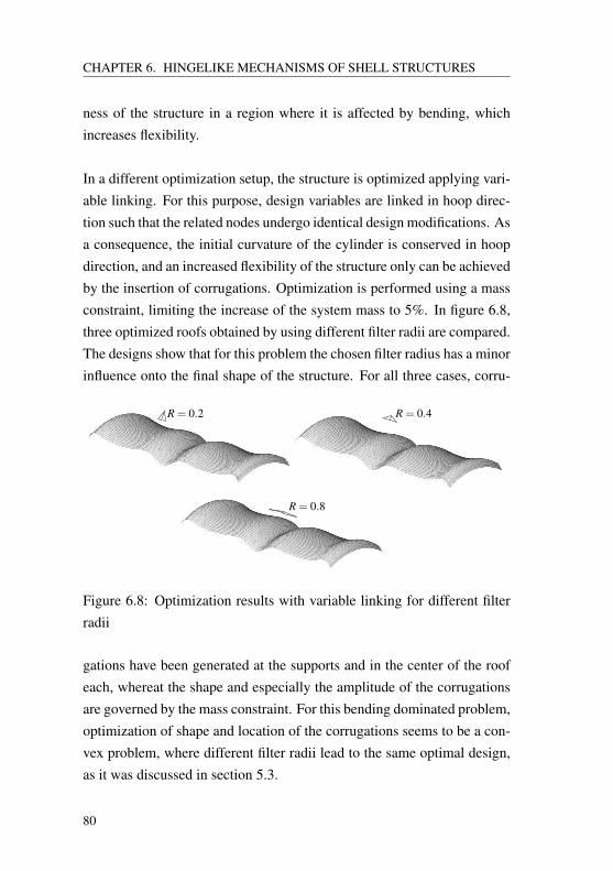
CHAPTER 6. HINGELIKE MECHANISMS OF SHELL STRUCTURES
ness of the structure in a region where it is affected by bending, whichincreases flexibility.
In a different optimization setup, the structure is optimized applying vari-able linking. For this purpose, design variables are linked in hoop direc-tion such that the related nodes undergo identical design modifications. Asa consequence, the initial curvature of the cylinder is conserved in hoopdirection, and an increased flexibility of the structure only can be achievedby the insertion of corrugations. Optimization is performed using a massconstraint, limiting the increase of the system mass to 5%. In figure 6.8,three optimized roofs obtained by using different filter radii are compared.The designs show that for this problem the chosen filter radius has a minorinfluence onto the final shape of the structure. For all three cases, corru-
R = 0.2 R = 0.4
R = 0.8
Figure 6.8: Optimization results with variable linking for different filterradii
gations have been generated at the supports and in the center of the roofeach, whereat the shape and especially the amplitude of the corrugationsare governed by the mass constraint. For this bending dominated problem,optimization of shape and location of the corrugations seems to be a con-vex problem, where different filter radii lead to the same optimal design,as it was discussed in section 5.3.
80
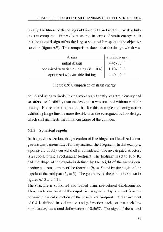
CHAPTER 6. HINGELIKE MECHANISMS OF SHELL STRUCTURES
Finally, the fitness of the designs obtained with and without variable link-ing are compared. Fitness is measured in terms of strain energy, suchthat the fittest design offers the largest value with respect to the objectivefunction (figure 6.9). This comparison shows that the design which was
design strain energy
initial design 4.45 ·10−5
optimized w variable linking (R = 0.4) 1.10 ·10−4
optimized w/o variable linking 4.40 ·10−4
Figure 6.9: Comparison of strain energy
optimized using variable linking stores significantly less strain energy andso offers less flexibility than the design that was obtained without variablelinking. Hence it can be noted, that for this example the configurationexhibiting hinge lines is more flexible than the corrugated bellow design,which still manifests the initial curvature of the cylinder.
6.2.3 Spherical cupola
In the previous section, the generation of line hinges and localized corru-gations was demonstrated for a cylindrical shell segment. In this example,a positively doubly curved shell is considered. The investigated structureis a cupola, fitting a rectangular footprint. The footprint is set to 10×10,and the shape of the cupola is defined by the height of the arches con-necting adjacent corners of the footprint (ha = 3) and by the height of thecupola at the midspan (ha = 5). The geometry of the cupola is shown infigures 6.10 and 6.11.The structure is supported and loaded using pre-defined displacements.Thus, each low point of the cupola is assigned a displacement u in theoutward diagonal direction of the structure’s footprint. A displacementof 0.4 is defined in x-direction and y-direction each, so that each lowpoint undergoes a total deformation of 0.5657. The signs of the x- and
81
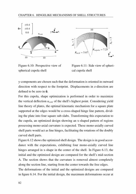
CHAPTER 6. HINGELIKE MECHANISMS OF SHELL STRUCTURES
xz
yu=
±0.4±0.40.0
uu
u
u
ucent
1010
Figure 6.10: Perspective view ofspherical cupola shell
xz
10
Rcupola = 7.25Rarch = 5.67
h a=
3
h b=
5
Figure 6.11: Side view of spheri-cal cupola shell
y-components are chosen such that the deformation is oriented in outwarddirection with respect to the footprint. Displacements in z-direction aredefined to be zero in u.For this cupola, shape optimization is performed in order to maximizethe vertical deflection ucent of the shell’s highest point. Considering yieldline theory of plates, the optimal kinematic mechanism for a square platesupported at the edges would be a cross-shaped hinge line pattern, divid-ing the plate into four square sub-slabs. Transforming this expectation tothe cupola, an optimized design showing an x-shaped pattern of regionspossessing mono-axial curvature is expected. These mono-axially curvedshell parts would act as line hinges, facilitating the rotations of the doublycurved shell parts.Figure 6.12 shows the optimized shell design. The design is in good accor-dance with the expectations, exhibiting four mono-axially curved linehinges arranged in x-shape in the center of the shell. In Figure 6.13, theinitial and the optimized design are compared for the shell’s mid-sectionA. The section shows that the curvature is removed almost completelyalong the section line, starting from the center towards the free edges.The deformations of the initial and the optimized designs are comparedin figure 6.14. For the initial design, the maximum deformations occur at
82
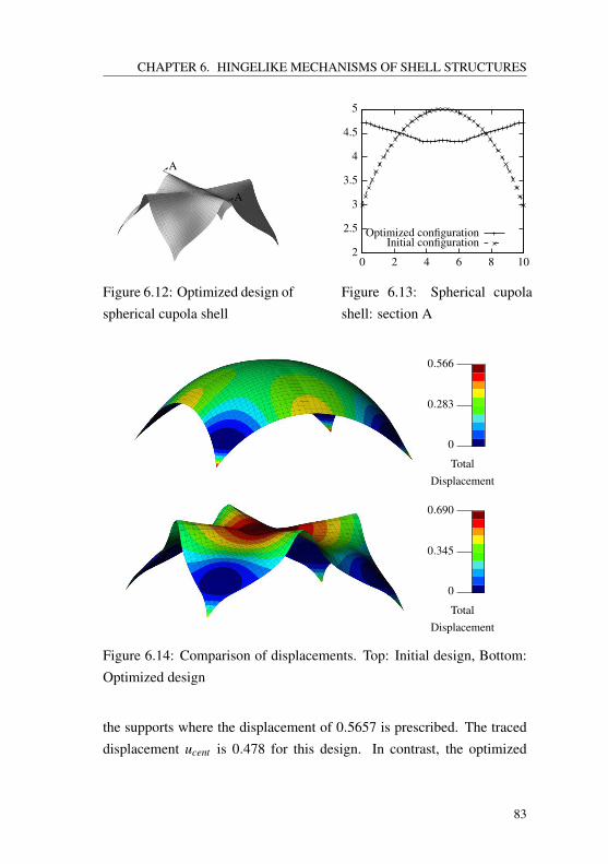
CHAPTER 6. HINGELIKE MECHANISMS OF SHELL STRUCTURES
A
A
Figure 6.12: Optimized design ofspherical cupola shell
2
2.5
3
3.5
4
4.5
5
0 2 4 6 8 10
Optimized configurationInitial configuration
Figure 6.13: Spherical cupolashell: section A
0.690
0
TotalDisplacement
0.345
0.566
0
TotalDisplacement
0.283
Figure 6.14: Comparison of displacements. Top: Initial design, Bottom:Optimized design
the supports where the displacement of 0.5657 is prescribed. The traceddisplacement ucent is 0.478 for this design. In contrast, the optimized
83
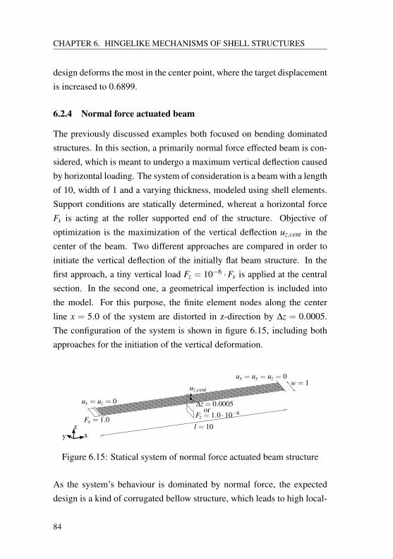
CHAPTER 6. HINGELIKE MECHANISMS OF SHELL STRUCTURES
design deforms the most in the center point, where the target displacementis increased to 0.6899.
6.2.4 Normal force actuated beam
The previously discussed examples both focused on bending dominatedstructures. In this section, a primarily normal force effected beam is con-sidered, which is meant to undergo a maximum vertical deflection causedby horizontal loading. The system of consideration is a beam with a lengthof 10, width of 1 and a varying thickness, modeled using shell elements.Support conditions are statically determined, whereat a horizontal forceFx is acting at the roller supported end of the structure. Objective ofoptimization is the maximization of the vertical deflection uz,cent in thecenter of the beam. Two different approaches are compared in order toinitiate the vertical deflection of the initially flat beam structure. In thefirst approach, a tiny vertical load Fz = 10−6 ·Fx is applied at the centralsection. In the second one, a geometrical imperfection is included intothe model. For this purpose, the finite element nodes along the centerline x = 5.0 of the system are distorted in z-direction by ∆z = 0.0005.The configuration of the system is shown in figure 6.15, including bothapproaches for the initiation of the vertical deformation.
xz
y
uy = uz = 0
ux = uy = uz = 0
Fx = 1.0Fz = 1.0 ·10−6
l = 10
w = 1uz,cent
∆z = 0.0005or
Figure 6.15: Statical system of normal force actuated beam structure
As the system’s behaviour is dominated by normal force, the expecteddesign is a kind of corrugated bellow structure, which leads to high local-
84
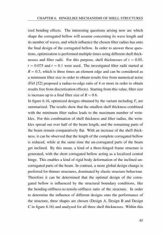
CHAPTER 6. HINGELIKE MECHANISMS OF SHELL STRUCTURES
ized bending effects. The interesting questions arising now are whichshape the corrugated bellow will assume concerning its wave length andits number of waves, and which influence the chosen filter radius has ontothe final design of the corrugated bellow. In order to answer these ques-tions, optimization is performed multiple times using different shell thick-nesses and filter radii. For this purpose, shell thicknesses of t = 0.05,t = 0.075 and t = 0.1 were used. The investigated filter radii started atR = 0.3, which is three times an element edge and can be considered asa minimum filter size in order to obtain results free from numerical noise(Firl [52] proposed a radius-to-edge ratio of 4 or more in order to obtainresults free from discretization effects). Starting from this value, filter sizeis increase up to a final filter size of R = 0.6.In figure 6.16, optimized designs obtained by the variant including Fz aresummarized. The results show that the smallest shell thickness combinedwith the minimum filter radius leads to the maximum number of wrin-kles. For this combination of shell thickness and filter radius, the wrin-kles spread out over half of the beam length, and the remaining parts ofthe beam remain comparatively flat. With an increase of the shell thick-ness, it can be observed that the length of the complete corrugated bellowis reduced, while at the same time the un-corrugated parts of the beamget inclined. By this mean, a kind of a three-hinged frame structure isgenerated, with the short corrugated bellow acting as a localized centralhinge. This enables a kind of rigid body deformation of the inclined un-corrugated parts of the beam. In contrast, a more global design change ispreferred for thinner structures, dominated by elastic structure behaviour.Therefore it can be determined that the optimal design of the corru-gated bellow is influenced by the structural boundary conditions, likethe bending-stiffness-to-tensile-stiffness ratio of the structure. In orderto determine the influence of different designs onto the performance ofthe structure, three shapes are chosen (Design A, Design B and DesignC in figure 6.16) and analyzed for all three shell thicknesses. Within this
85
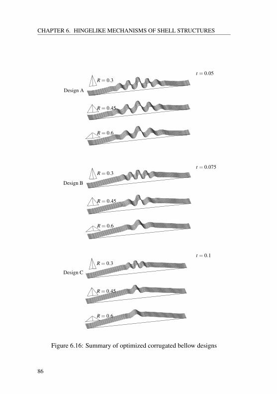
CHAPTER 6. HINGELIKE MECHANISMS OF SHELL STRUCTURES
R = 0.3
R = 0.45
R = 0.6
R = 0.3
R = 0.45
R = 0.6
R = 0.3
R = 0.45
R = 0.6
t = 0.05
t = 0.075
t = 0.1
Design A
Design B
Design C
Figure 6.16: Summary of optimized corrugated bellow designs
86
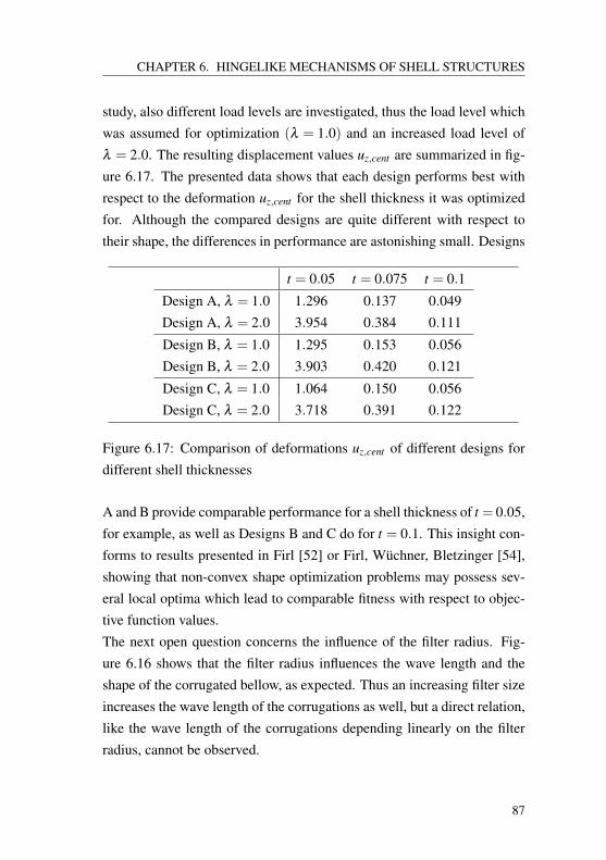
CHAPTER 6. HINGELIKE MECHANISMS OF SHELL STRUCTURES
study, also different load levels are investigated, thus the load level whichwas assumed for optimization (λ = 1.0) and an increased load level ofλ = 2.0. The resulting displacement values uz,cent are summarized in fig-ure 6.17. The presented data shows that each design performs best withrespect to the deformation uz,cent for the shell thickness it was optimizedfor. Although the compared designs are quite different with respect totheir shape, the differences in performance are astonishing small. Designs
t = 0.05 t = 0.075 t = 0.1
Design A, λ = 1.0 1.296 0.137 0.049Design A, λ = 2.0 3.954 0.384 0.111
Design B, λ = 1.0 1.295 0.153 0.056Design B, λ = 2.0 3.903 0.420 0.121
Design C, λ = 1.0 1.064 0.150 0.056Design C, λ = 2.0 3.718 0.391 0.122
Figure 6.17: Comparison of deformations uz,cent of different designs fordifferent shell thicknesses
A and B provide comparable performance for a shell thickness of t = 0.05,for example, as well as Designs B and C do for t = 0.1. This insight con-forms to results presented in Firl [52] or Firl, Wüchner, Bletzinger [54],showing that non-convex shape optimization problems may possess sev-eral local optima which lead to comparable fitness with respect to objec-tive function values.The next open question concerns the influence of the filter radius. Fig-ure 6.16 shows that the filter radius influences the wave length and theshape of the corrugated bellow, as expected. Thus an increasing filter sizeincreases the wave length of the corrugations as well, but a direct relation,like the wave length of the corrugations depending linearly on the filterradius, cannot be observed.
87
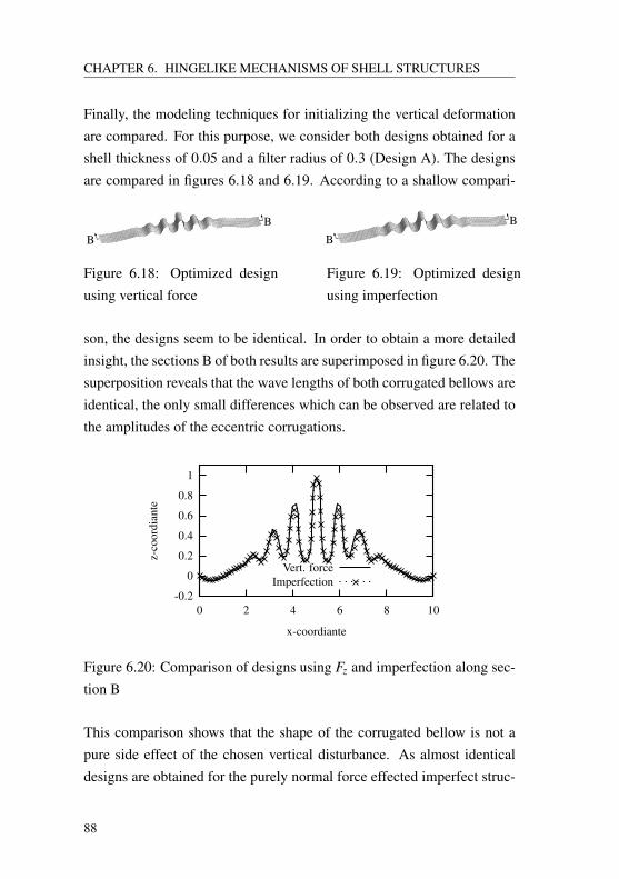
CHAPTER 6. HINGELIKE MECHANISMS OF SHELL STRUCTURES
Finally, the modeling techniques for initializing the vertical deformationare compared. For this purpose, we consider both designs obtained for ashell thickness of 0.05 and a filter radius of 0.3 (Design A). The designsare compared in figures 6.18 and 6.19. According to a shallow compari-
B
B
Figure 6.18: Optimized designusing vertical force
B
B
Figure 6.19: Optimized designusing imperfection
son, the designs seem to be identical. In order to obtain a more detailedinsight, the sections B of both results are superimposed in figure 6.20. Thesuperposition reveals that the wave lengths of both corrugated bellows areidentical, the only small differences which can be observed are related tothe amplitudes of the eccentric corrugations.
-0.2
0
0.2
0.4
0.6
0.8
1
0 2 4 6 8 10
z-co
ordi
ante
x-coordiante
Vert. forceImperfection
Figure 6.20: Comparison of designs using Fz and imperfection along sec-tion B
This comparison shows that the shape of the corrugated bellow is not apure side effect of the chosen vertical disturbance. As almost identicaldesigns are obtained for the purely normal force effected imperfect struc-
88
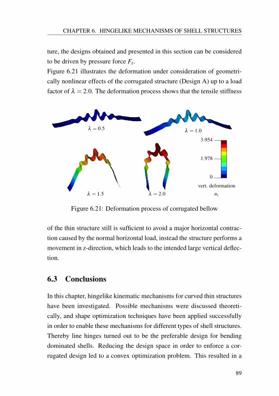
CHAPTER 6. HINGELIKE MECHANISMS OF SHELL STRUCTURES
ture, the designs obtained and presented in this section can be consideredto be driven by pressure force Fx.Figure 6.21 illustrates the deformation under consideration of geometri-cally nonlinear effects of the corrugated structure (Design A) up to a loadfactor of λ = 2.0. The deformation process shows that the tensile stiffness
3.954
0
vert. deformationuz
1.978
λ = 2.0λ = 1.5
λ = 1.0λ = 0.5
Figure 6.21: Deformation process of corrugated bellow
of the thin structure still is sufficient to avoid a major horizontal contrac-tion caused by the normal horizontal load, instead the structure performs amovement in z-direction, which leads to the intended large vertical deflec-tion.
6.3 Conclusions
In this chapter, hingelike kinematic mechanisms for curved thin structureshave been investigated. Possible mechanisms were discussed theoreti-cally, and shape optimization techniques have been applied successfullyin order to enable these mechanisms for different types of shell structures.Thereby line hinges turned out to be the preferable design for bendingdominated shells. Reducing the design space in order to enforce a cor-rugated design led to a convex optimization problem. This resulted in a
89

CHAPTER 6. HINGELIKE MECHANISMS OF SHELL STRUCTURES
unique corrugation pattern for different filter radii, whereat the previousline hinges were removed by single corrugations.The last example applied optimization to a normal force dominated struc-ture. Here multiply corrugated structures could be observed. A centralconclusion which can be drawn from this example is that shape optimiza-tion of a multiply corrugated structure or a corrugated bellow is a highlynon-convex problem. Hence the solution obtained by a gradient basedoptimization scheme corresponds to a local optimum, and the correspond-ing design depends on the chosen set of start parameters with respect tostructure as well as to the optimization algorithm. Nevertheless, optimiza-tion results show that quite different designs may possess comparable fit-ness with respect to the objective function in such a highly non-convexdesign space. This kind of behaviour also was observed by Bletzinger,Firl, Fischer [27] for other applications using the parameter free optimiza-tion approach.
90
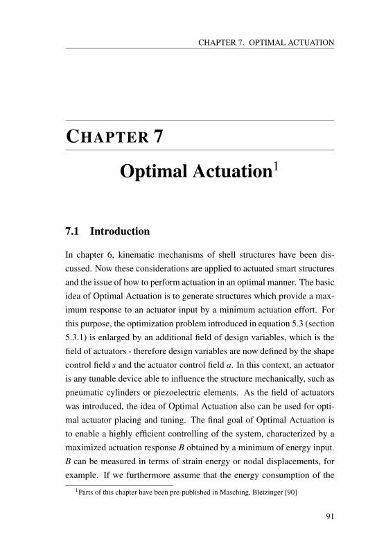
CHAPTER 7. OPTIMAL ACTUATION
CHAPTER 7
Optimal Actuation1
7.1 Introduction
In chapter 6, kinematic mechanisms of shell structures have been dis-cussed. Now these considerations are applied to actuated smart structuresand the issue of how to perform actuation in an optimal manner. The basicidea of Optimal Actuation is to generate structures which provide a max-imum response to an actuator input by a minimum actuation effort. Forthis purpose, the optimization problem introduced in equation 5.3 (section5.3.1) is enlarged by an additional field of design variables, which is thefield of actuators - therefore design variables are now defined by the shapecontrol field s and the actuator control field a. In this context, an actuatoris any tunable device able to influence the structure mechanically, such aspneumatic cylinders or piezoelectric elements. As the field of actuatorswas introduced, the idea of Optimal Actuation also can be used for opti-mal actuator placing and tuning. The final goal of Optimal Actuation isto enable a highly efficient controlling of the system, characterized by amaximized actuation response B obtained by a minimum of energy input.B can be measured in terms of strain energy or nodal displacements, forexample. If we furthermore assume that the energy consumption of the
1Parts of this chapter have been pre-published in Masching, Bletzinger [90]
91
CHAPTER 7. OPTIMAL ACTUATION
actuation process is proportional to the integral p-norm of the actuatorfield over the entire design space, the problem of Optimal Actuation canbe described as a multi-objective optimization problem of the form
min C (a) =∫Ω
|a(ξ )|p dξ (7.1a)
max B(a,s) (7.1b)
where the function C (a) indicates the actuation costs and B(a,s) can beinterpreted as the actuation benefit. Considering the cost-to-benefit ratioas a measure of the efficiency of the actuation, equations 7.1a and 7.1bcan be summarized to the minimization of the inverse efficiency functionE (a,s):
min E (a,s) =C (a)
B(a,s)(7.2)
7.2 An extended sensitivity filtering scheme
As Optimal Actuation introduces a new field of variables into the opti-mization problem, this also has an impact on the procedure of optimiza-tion. While equations 5.3 and 5.2 assumed only one field of design vari-ables controlling the shape and eventually the sizing parameters, we nowhave to consider the enlarged problem of optimizing with respect to twodifferent fields of design variables, s and a. Considering the state equationS and the field of state variables u, the final optimization problem reads
min E (s,a,u)
st.
S (s,a,u) = 0
(7.3)
According to equation 5.14, the new field of design parameters a is alsocontrolled by a gradient field pa. As the response function f probably
92
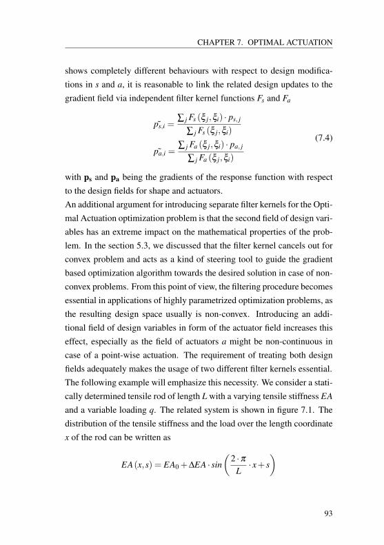
CHAPTER 7. OPTIMAL ACTUATION
shows completely different behaviours with respect to design modifica-tions in s and a, it is reasonable to link the related design updates to thegradient field via independent filter kernel functions Fs and Fa
ps,i =∑ j Fs (ξ j,ξi) · ps, j
∑ j Fs (ξ j,ξi)
˜pa,i =∑ j Fa (ξ j,ξi) · pa, j
∑ j Fa (ξ j,ξi)
(7.4)
with ps and pa being the gradients of the response function with respectto the design fields for shape and actuators.An additional argument for introducing separate filter kernels for the Opti-mal Actuation optimization problem is that the second field of design vari-ables has an extreme impact on the mathematical properties of the prob-lem. In the section 5.3, we discussed that the filter kernel cancels out forconvex problem and acts as a kind of steering tool to guide the gradientbased optimization algorithm towards the desired solution in case of non-convex problems. From this point of view, the filtering procedure becomesessential in applications of highly parametrized optimization problems, asthe resulting design space usually is non-convex. Introducing an addi-tional field of design variables in form of the actuator field increases thiseffect, especially as the field of actuators a might be non-continuous incase of a point-wise actuation. The requirement of treating both designfields adequately makes the usage of two different filter kernels essential.The following example will emphasize this necessity. We consider a stati-cally determined tensile rod of length L with a varying tensile stiffness EA
and a variable loading q. The related system is shown in figure 7.1. Thedistribution of the tensile stiffness and the load over the length coordinatex of the rod can be written as
EA(x,s) = EA0 +∆EA · sin(
2 ·πL· x+ s
)
93
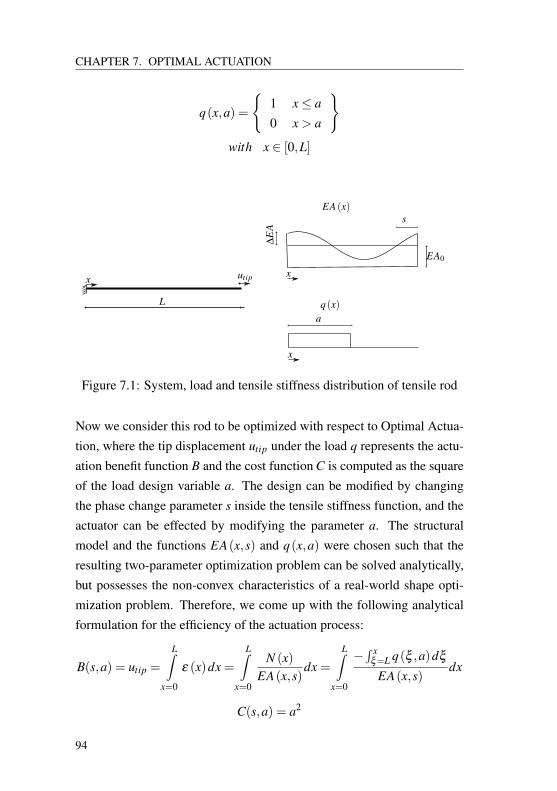
CHAPTER 7. OPTIMAL ACTUATION
q(x,a) =
1 x≤ a
0 x > a
with x ∈ [0,L]
EA0
s
∆E
A
L
EA(x)
q(x)a
x x
x
utip
Figure 7.1: System, load and tensile stiffness distribution of tensile rod
Now we consider this rod to be optimized with respect to Optimal Actua-tion, where the tip displacement utip under the load q represents the actu-ation benefit function B and the cost function C is computed as the squareof the load design variable a. The design can be modified by changingthe phase change parameter s inside the tensile stiffness function, and theactuator can be effected by modifying the parameter a. The structuralmodel and the functions EA(x,s) and q(x,a) were chosen such that theresulting two-parameter optimization problem can be solved analytically,but possesses the non-convex characteristics of a real-world shape opti-mization problem. Therefore, we come up with the following analyticalformulation for the efficiency of the actuation process:
B(s,a) = utip =
L∫x=0
ε (x)dx =L∫
x=0
N (x)EA(x,s)
dx =L∫
x=0
−∫ x
ξ=L q(ξ ,a)dξ
EA(x,s)dx
C(s,a) = a2
94
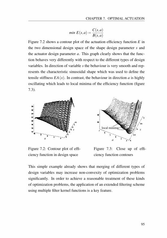
CHAPTER 7. OPTIMAL ACTUATION
min E(s,a) =C(s,a)B(s,a)
Figure 7.2 shows a contour plot of the actuation efficiency function E inthe two dimensional design space of the shape design parameter s andthe actuator design parameter a. This graph clearly shows that the func-tion behaves very differently with respect to the different types of designvariables. In direction of variable s the behaviour is very smooth and rep-resents the characteristic sinusoidal shape which was used to define thetensile stiffness EA(x). In contrast, the behaviour in direction a is highlyoscillating which leads to local minima of the efficiency function (figure7.3).
s
a
Figure 7.2: Contour plot of effi-ciency function in design space
a
slocal minima
Figure 7.3: Close up of effi-ciency function contours
This simple example already shows that merging of different types ofdesign variables may increase non-convexity of optimization problemssignificantly. In order to achieve a reasonable treatment of these kindsof optimization problems, the application of an extended filtering schemeusing multiple filter kernel functions is a key feature.
95
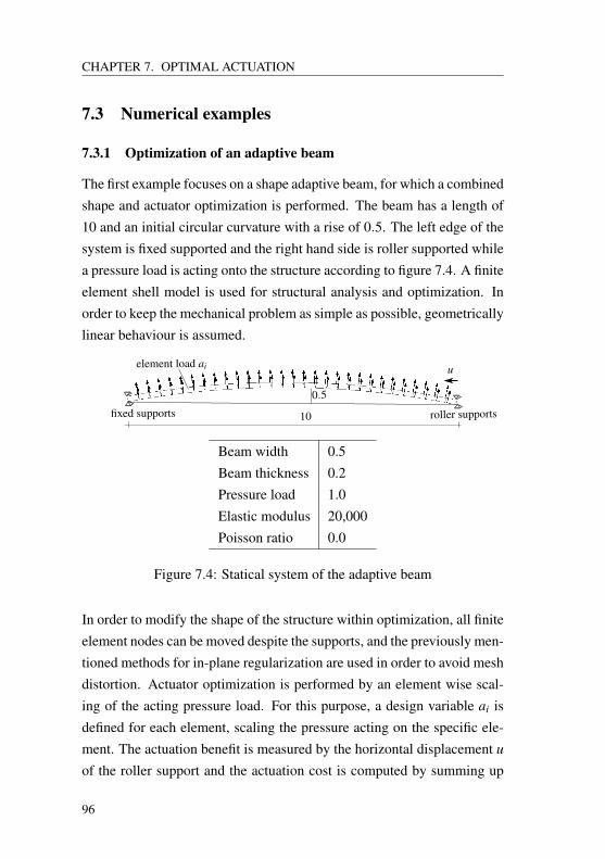
CHAPTER 7. OPTIMAL ACTUATION
7.3 Numerical examples
7.3.1 Optimization of an adaptive beam
The first example focuses on a shape adaptive beam, for which a combinedshape and actuator optimization is performed. The beam has a length of10 and an initial circular curvature with a rise of 0.5. The left edge of thesystem is fixed supported and the right hand side is roller supported whilea pressure load is acting onto the structure according to figure 7.4. A finiteelement shell model is used for structural analysis and optimization. Inorder to keep the mechanical problem as simple as possible, geometricallylinear behaviour is assumed.
fixed supports roller supports10
0.5
uelement load ai
Beam width 0.5Beam thickness 0.2Pressure load 1.0Elastic modulus 20,000Poisson ratio 0.0
Figure 7.4: Statical system of the adaptive beam
In order to modify the shape of the structure within optimization, all finiteelement nodes can be moved despite the supports, and the previously men-tioned methods for in-plane regularization are used in order to avoid meshdistortion. Actuator optimization is performed by an element wise scal-ing of the acting pressure load. For this purpose, a design variable ai isdefined for each element, scaling the pressure acting on the specific ele-ment. The actuation benefit is measured by the horizontal displacement u
of the roller support and the actuation cost is computed by summing up
96
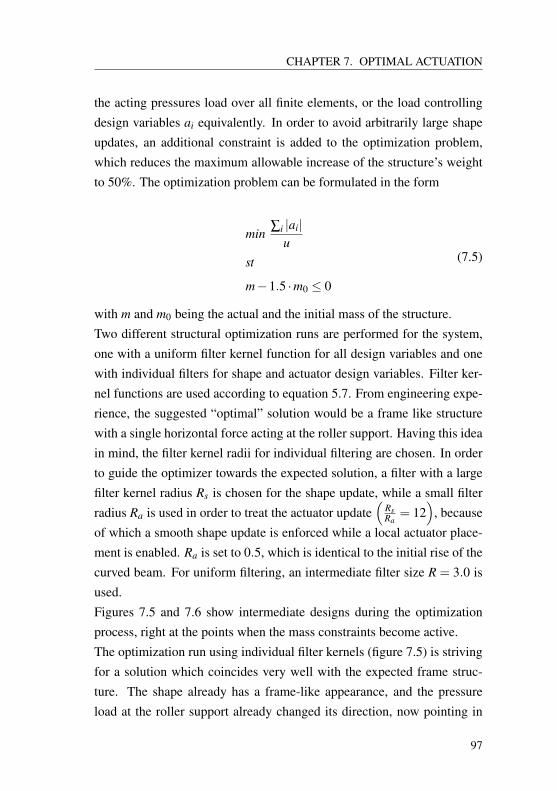
CHAPTER 7. OPTIMAL ACTUATION
the acting pressures load over all finite elements, or the load controllingdesign variables ai equivalently. In order to avoid arbitrarily large shapeupdates, an additional constraint is added to the optimization problem,which reduces the maximum allowable increase of the structure’s weightto 50%. The optimization problem can be formulated in the form
min∑i |ai|
ust
m−1.5 ·m0 ≤ 0
(7.5)
with m and m0 being the actual and the initial mass of the structure.Two different structural optimization runs are performed for the system,one with a uniform filter kernel function for all design variables and onewith individual filters for shape and actuator design variables. Filter ker-nel functions are used according to equation 5.7. From engineering expe-rience, the suggested “optimal” solution would be a frame like structurewith a single horizontal force acting at the roller support. Having this ideain mind, the filter kernel radii for individual filtering are chosen. In orderto guide the optimizer towards the expected solution, a filter with a largefilter kernel radius Rs is chosen for the shape update, while a small filterradius Ra is used in order to treat the actuator update
(RsRa
= 12)
, becauseof which a smooth shape update is enforced while a local actuator place-ment is enabled. Ra is set to 0.5, which is identical to the initial rise of thecurved beam. For uniform filtering, an intermediate filter size R = 3.0 isused.Figures 7.5 and 7.6 show intermediate designs during the optimizationprocess, right at the points when the mass constraints become active.The optimization run using individual filter kernels (figure 7.5) is strivingfor a solution which coincides very well with the expected frame struc-ture. The shape already has a frame-like appearance, and the pressureload at the roller support already changed its direction, now pointing in
97
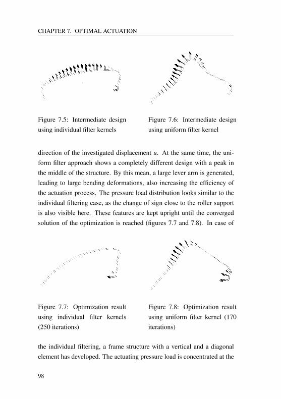
CHAPTER 7. OPTIMAL ACTUATION
Figure 7.5: Intermediate designusing individual filter kernels
Figure 7.6: Intermediate designusing uniform filter kernel
direction of the investigated displacement u. At the same time, the uni-form filter approach shows a completely different design with a peak inthe middle of the structure. By this mean, a large lever arm is generated,leading to large bending deformations, also increasing the efficiency ofthe actuation process. The pressure load distribution looks similar to theindividual filtering case, as the change of sign close to the roller supportis also visible here. These features are kept upright until the convergedsolution of the optimization is reached (figures 7.7 and 7.8). In case of
Figure 7.7: Optimization resultusing individual filter kernels(250 iterations)
Figure 7.8: Optimization resultusing uniform filter kernel (170iterations)
the individual filtering, a frame structure with a vertical and a diagonalelement has developed. The actuating pressure load is concentrated at the
98
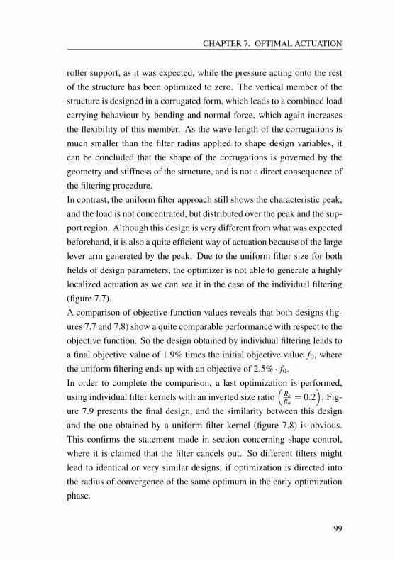
CHAPTER 7. OPTIMAL ACTUATION
roller support, as it was expected, while the pressure acting onto the restof the structure has been optimized to zero. The vertical member of thestructure is designed in a corrugated form, which leads to a combined loadcarrying behaviour by bending and normal force, which again increasesthe flexibility of this member. As the wave length of the corrugations ismuch smaller than the filter radius applied to shape design variables, itcan be concluded that the shape of the corrugations is governed by thegeometry and stiffness of the structure, and is not a direct consequence ofthe filtering procedure.In contrast, the uniform filter approach still shows the characteristic peak,and the load is not concentrated, but distributed over the peak and the sup-port region. Although this design is very different from what was expectedbeforehand, it is also a quite efficient way of actuation because of the largelever arm generated by the peak. Due to the uniform filter size for bothfields of design parameters, the optimizer is not able to generate a highlylocalized actuation as we can see it in the case of the individual filtering(figure 7.7).A comparison of objective function values reveals that both designs (fig-ures 7.7 and 7.8) show a quite comparable performance with respect to theobjective function. So the design obtained by individual filtering leads toa final objective value of 1.9% times the initial objective value f0, wherethe uniform filtering ends up with an objective of 2.5% · f0.In order to complete the comparison, a last optimization is performed,using individual filter kernels with an inverted size ratio
(RsRa
= 0.2)
. Fig-ure 7.9 presents the final design, and the similarity between this designand the one obtained by a uniform filter kernel (figure 7.8) is obvious.This confirms the statement made in section concerning shape control,where it is claimed that the filter cancels out. So different filters mightlead to identical or very similar designs, if optimization is directed intothe radius of convergence of the same optimum in the early optimizationphase.
99
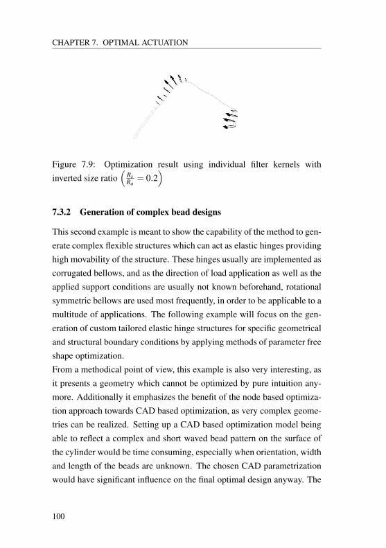
CHAPTER 7. OPTIMAL ACTUATION
Figure 7.9: Optimization result using individual filter kernels withinverted size ratio
(RsRa
= 0.2)
7.3.2 Generation of complex bead designs
This second example is meant to show the capability of the method to gen-erate complex flexible structures which can act as elastic hinges providinghigh movability of the structure. These hinges usually are implemented ascorrugated bellows, and as the direction of load application as well as theapplied support conditions are usually not known beforehand, rotationalsymmetric bellows are used most frequently, in order to be applicable to amultitude of applications. The following example will focus on the gen-eration of custom tailored elastic hinge structures for specific geometricaland structural boundary conditions by applying methods of parameter freeshape optimization.From a methodical point of view, this example is also very interesting, asit presents a geometry which cannot be optimized by pure intuition any-more. Additionally it emphasizes the benefit of the node based optimiza-tion approach towards CAD based optimization, as very complex geome-tries can be realized. Setting up a CAD based optimization model beingable to reflect a complex and short waved bead pattern on the surface ofthe cylinder would be time consuming, especially when orientation, widthand length of the beads are unknown. The chosen CAD parametrizationwould have significant influence on the final optimal design anyway. The
100
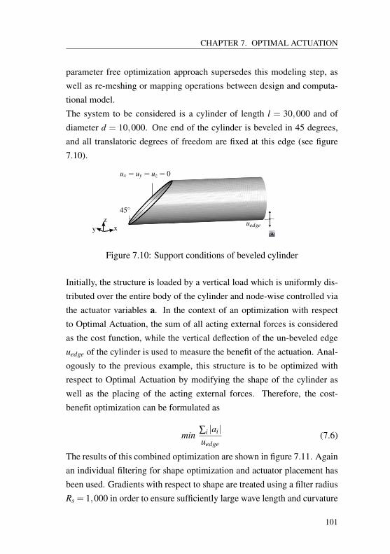
CHAPTER 7. OPTIMAL ACTUATION
parameter free optimization approach supersedes this modeling step, aswell as re-meshing or mapping operations between design and computa-tional model.The system to be considered is a cylinder of length l = 30,000 and ofdiameter d = 10,000. One end of the cylinder is beveled in 45 degrees,and all translatoric degrees of freedom are fixed at this edge (see figure7.10).
ux = uy = uz = 0
45
uedgexz
y
Figure 7.10: Support conditions of beveled cylinder
Initially, the structure is loaded by a vertical load which is uniformly dis-tributed over the entire body of the cylinder and node-wise controlled viathe actuator variables a. In the context of an optimization with respectto Optimal Actuation, the sum of all acting external forces is consideredas the cost function, while the vertical deflection of the un-beveled edgeuedge of the cylinder is used to measure the benefit of the actuation. Anal-ogously to the previous example, this structure is to be optimized withrespect to Optimal Actuation by modifying the shape of the cylinder aswell as the placing of the acting external forces. Therefore, the cost-benefit optimization can be formulated as
min∑i |ai|uedge
(7.6)
The results of this combined optimization are shown in figure 7.11. Againan individual filtering for shape optimization and actuator placement hasbeen used. Gradients with respect to shape are treated using a filter radiusRs = 1,000 in order to ensure sufficiently large wave length and curvature
101
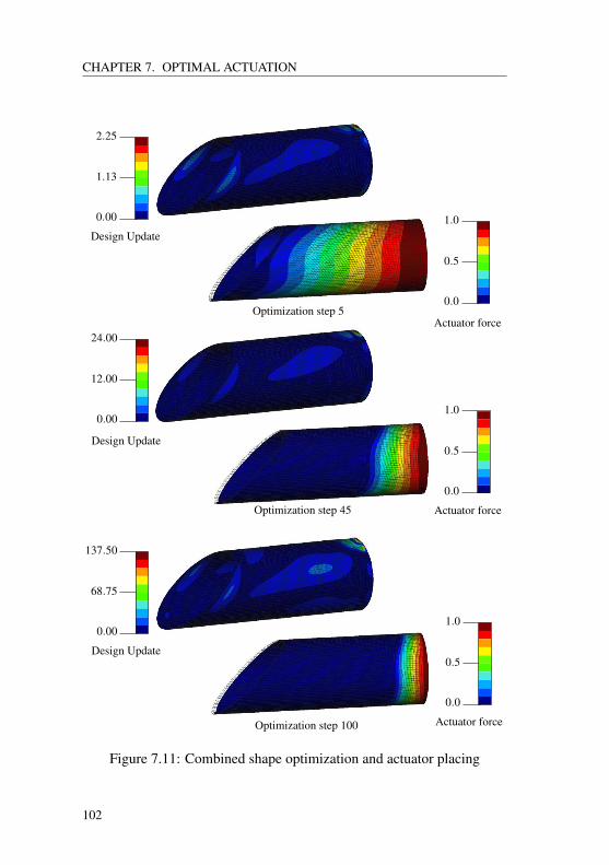
CHAPTER 7. OPTIMAL ACTUATION
Optimization step 5
Optimization step 45
Optimization step 100
1.0
0.0
Actuator force
0.5
2.25
0.00
Design Update
1.13
24.00
0.00
Design Update
12.00
137.50
0.00
Design Update
68.75
1.0
0.0
Actuator force
0.5
1.0
0.0
Actuator force
0.5
Figure 7.11: Combined shape optimization and actuator placing
102
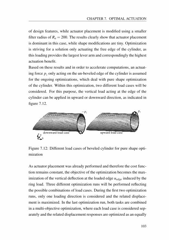
CHAPTER 7. OPTIMAL ACTUATION
of design features, while actuator placement is modified using a smallerfilter radius of Ra = 200. The results clearly show that actuator placementis dominant in this case, while shape modifications are tiny. Optimizationis striving for a solution only actuating the free edge of the cylinder, asthis loading provides the largest lever arm and correspondingly the highestactuation benefit.Based on these results and in order to accelerate computations, an actuat-ing force pz only acting on the un-beveled edge of the cylinder is assumedfor the ongoing optimizations, which deal with pure shape optimizationof the cylinder. Within this optimization, two different load cases will beconsidered. For this purpose, the vertical load acting at the edge of thecylinder can be applied in upward or downward direction, as indicated infigure 7.12.
xz y
downward load case upward load case
pz−pz
Figure 7.12: Different load cases of beveled cylinder for pure shape opti-mization
As actuator placement was already performed and therefore the cost func-tion remains constant, the objective of the optimization becomes the max-imization of the vertical deflection at the loaded edge uedge induced by thering load. Three different optimization runs will be performed reflectingthe possible combinations of load cases. During the first two optimizationruns, only one loading direction is considered and the related displace-ment is maximized. In the last optimization run, both tasks are combinedin a multi-objective optimization, where each load case is considered sep-arately and the related displacement responses are optimized as an equally
103
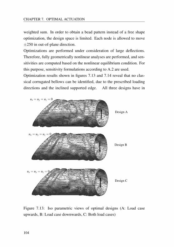
CHAPTER 7. OPTIMAL ACTUATION
weighted sum. In order to obtain a bead pattern instead of a free shapeoptimization, the design space is limited. Each node is allowed to move±250 in out-of-plane direction.Optimizations are performed under consideration of large deflections.Therefore, fully geometrically nonlinear analyses are performed, and sen-sitivities are computed based on the nonlinear equilibrium condition. Forthis purpose, sensitivity formulations according to A.2 are used.Optimization results shown in figures 7.13 and 7.14 reveal that no clas-sical corrugated bellows can be identified, due to the prescribed loadingdirections and the inclined supported edge. All three designs have in
Design A
Design B
Design C
ux = uy = uz = 0
ux = uy = uz = 0
ux = uy = uz = 0
Figure 7.13: Iso parametric views of optimal designs (A: Load caseupwards, B: Load case downwards, C: Both load cases)
104
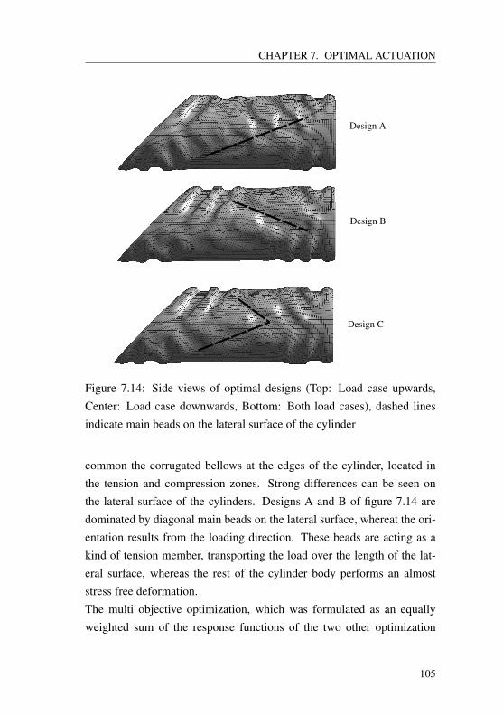
CHAPTER 7. OPTIMAL ACTUATION
Design A
Design B
Design C
Figure 7.14: Side views of optimal designs (Top: Load case upwards,Center: Load case downwards, Bottom: Both load cases), dashed linesindicate main beads on the lateral surface of the cylinder
common the corrugated bellows at the edges of the cylinder, located inthe tension and compression zones. Strong differences can be seen onthe lateral surface of the cylinders. Designs A and B of figure 7.14 aredominated by diagonal main beads on the lateral surface, whereat the ori-entation results from the loading direction. These beads are acting as akind of tension member, transporting the load over the length of the lat-eral surface, whereas the rest of the cylinder body performs an almoststress free deformation.The multi objective optimization, which was formulated as an equallyweighted sum of the response functions of the two other optimization
105
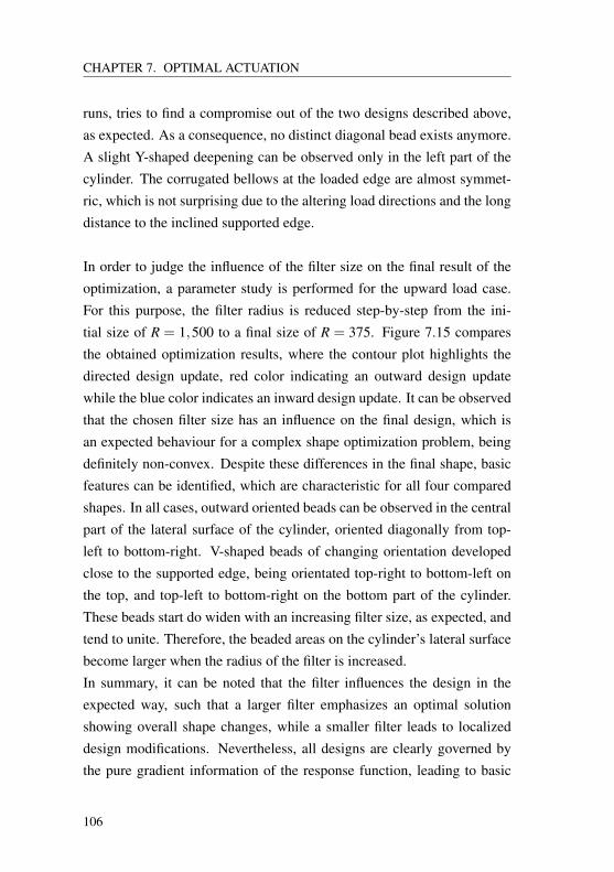
CHAPTER 7. OPTIMAL ACTUATION
runs, tries to find a compromise out of the two designs described above,as expected. As a consequence, no distinct diagonal bead exists anymore.A slight Y-shaped deepening can be observed only in the left part of thecylinder. The corrugated bellows at the loaded edge are almost symmet-ric, which is not surprising due to the altering load directions and the longdistance to the inclined supported edge.
In order to judge the influence of the filter size on the final result of theoptimization, a parameter study is performed for the upward load case.For this purpose, the filter radius is reduced step-by-step from the ini-tial size of R = 1,500 to a final size of R = 375. Figure 7.15 comparesthe obtained optimization results, where the contour plot highlights thedirected design update, red color indicating an outward design updatewhile the blue color indicates an inward design update. It can be observedthat the chosen filter size has an influence on the final design, which isan expected behaviour for a complex shape optimization problem, beingdefinitely non-convex. Despite these differences in the final shape, basicfeatures can be identified, which are characteristic for all four comparedshapes. In all cases, outward oriented beads can be observed in the centralpart of the lateral surface of the cylinder, oriented diagonally from top-left to bottom-right. V-shaped beads of changing orientation developedclose to the supported edge, being orientated top-right to bottom-left onthe top, and top-left to bottom-right on the bottom part of the cylinder.These beads start do widen with an increasing filter size, as expected, andtend to unite. Therefore, the beaded areas on the cylinder’s lateral surfacebecome larger when the radius of the filter is increased.In summary, it can be noted that the filter influences the design in theexpected way, such that a larger filter emphasizes an optimal solutionshowing overall shape changes, while a smaller filter leads to localizeddesign modifications. Nevertheless, all designs are clearly governed bythe pure gradient information of the response function, leading to basic
106
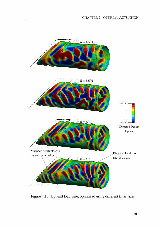
CHAPTER 7. OPTIMAL ACTUATION
R = 1,500
R = 750
R = 375
R = 1,000
+250
−250Directed Design
Update
0
Diagonal beads onlateral surface
V-shaped beads close tothe supported edge
Figure 7.15: Upward load case, optimized using different filter sizes
107
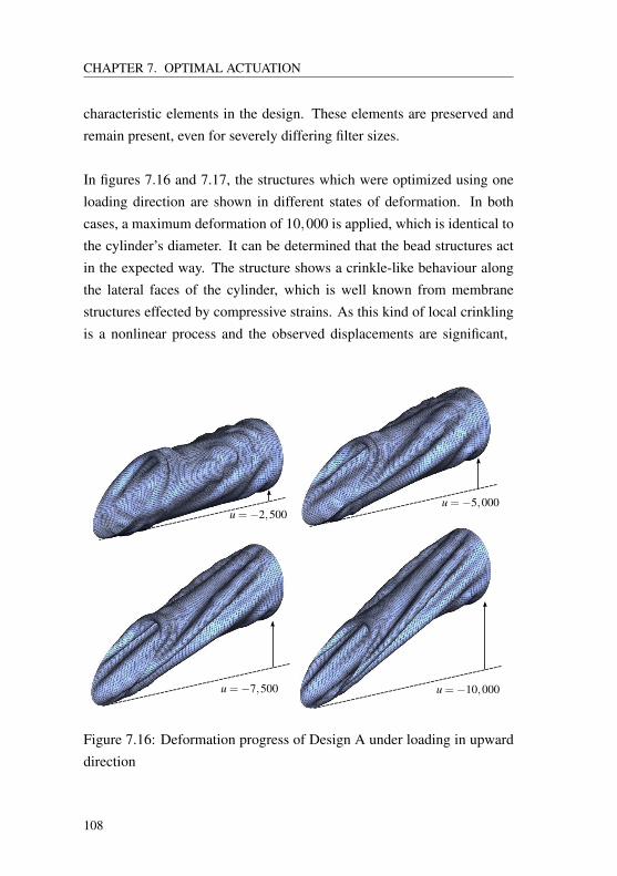
CHAPTER 7. OPTIMAL ACTUATION
characteristic elements in the design. These elements are preserved andremain present, even for severely differing filter sizes.
In figures 7.16 and 7.17, the structures which were optimized using oneloading direction are shown in different states of deformation. In bothcases, a maximum deformation of 10,000 is applied, which is identical tothe cylinder’s diameter. It can be determined that the bead structures actin the expected way. The structure shows a crinkle-like behaviour alongthe lateral faces of the cylinder, which is well known from membranestructures effected by compressive strains. As this kind of local crinklingis a nonlinear process and the observed displacements are significant,
u =−2,500u =−5,000
u =−7,500 u =−10,000
Figure 7.16: Deformation progress of Design A under loading in upwarddirection
108
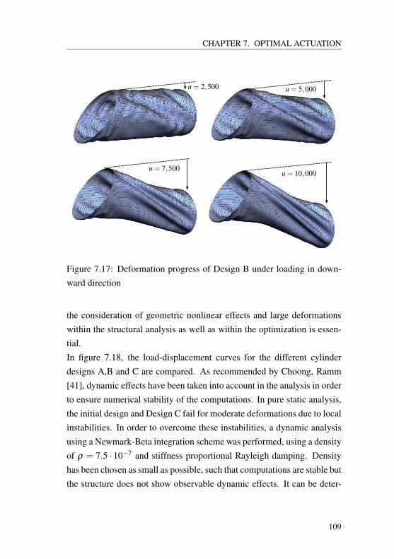
CHAPTER 7. OPTIMAL ACTUATION
u = 2,500 u = 5,000
u = 7,500u = 10,000
Figure 7.17: Deformation progress of Design B under loading in down-ward direction
the consideration of geometric nonlinear effects and large deformationswithin the structural analysis as well as within the optimization is essen-tial.In figure 7.18, the load-displacement curves for the different cylinderdesigns A,B and C are compared. As recommended by Choong, Ramm[41], dynamic effects have been taken into account in the analysis in orderto ensure numerical stability of the computations. In pure static analysis,the initial design and Design C fail for moderate deformations due to localinstabilities. In order to overcome these instabilities, a dynamic analysisusing a Newmark-Beta integration scheme was performed, using a densityof ρ = 7.5 · 10−7 and stiffness proportional Rayleigh damping. Densityhas been chosen as small as possible, such that computations are stable butthe structure does not show observable dynamic effects. It can be deter-
109
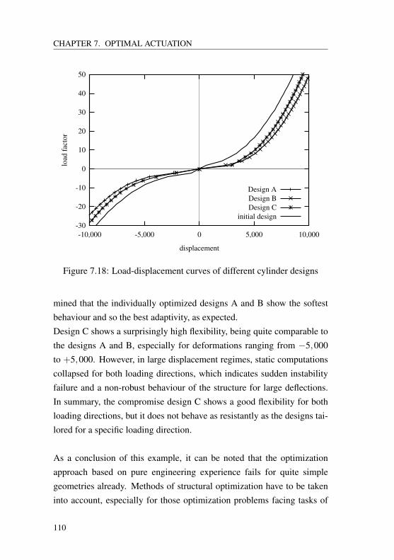
CHAPTER 7. OPTIMAL ACTUATION
-30
-20
-10
0
10
20
30
40
50
-10,000 -5,000 0 5,000 10,000
load
fact
or
displacement
Design ADesign BDesign C
initial design
Figure 7.18: Load-displacement curves of different cylinder designs
mined that the individually optimized designs A and B show the softestbehaviour and so the best adaptivity, as expected.Design C shows a surprisingly high flexibility, being quite comparable tothe designs A and B, especially for deformations ranging from −5,000to +5,000. However, in large displacement regimes, static computationscollapsed for both loading directions, which indicates sudden instabilityfailure and a non-robust behaviour of the structure for large deflections.In summary, the compromise design C shows a good flexibility for bothloading directions, but it does not behave as resistantly as the designs tai-lored for a specific loading direction.
As a conclusion of this example, it can be noted that the optimizationapproach based on pure engineering experience fails for quite simplegeometries already. Methods of structural optimization have to be takeninto account, especially for those optimization problems facing tasks of
110
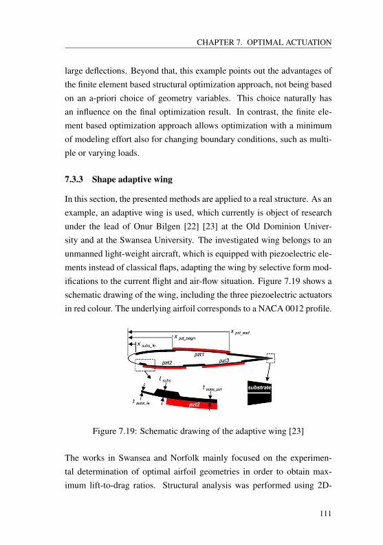
CHAPTER 7. OPTIMAL ACTUATION
large deflections. Beyond that, this example points out the advantages ofthe finite element based structural optimization approach, not being basedon an a-priori choice of geometry variables. This choice naturally hasan influence on the final optimization result. In contrast, the finite ele-ment based optimization approach allows optimization with a minimumof modeling effort also for changing boundary conditions, such as multi-ple or varying loads.
7.3.3 Shape adaptive wing
In this section, the presented methods are applied to a real structure. As anexample, an adaptive wing is used, which currently is object of researchunder the lead of Onur Bilgen [22] [23] at the Old Dominion Univer-sity and at the Swansea University. The investigated wing belongs to anunmanned light-weight aircraft, which is equipped with piezoelectric ele-ments instead of classical flaps, adapting the wing by selective form mod-ifications to the current flight and air-flow situation. Figure 7.19 shows aschematic drawing of the wing, including the three piezoelectric actuatorsin red colour. The underlying airfoil corresponds to a NACA 0012 profile.
Figure 7.19: Schematic drawing of the adaptive wing [23]
The works in Swansea and Norfolk mainly focused on the experimen-tal determination of optimal airfoil geometries in order to obtain max-imum lift-to-drag ratios. Structural analysis was performed using 2D-
111
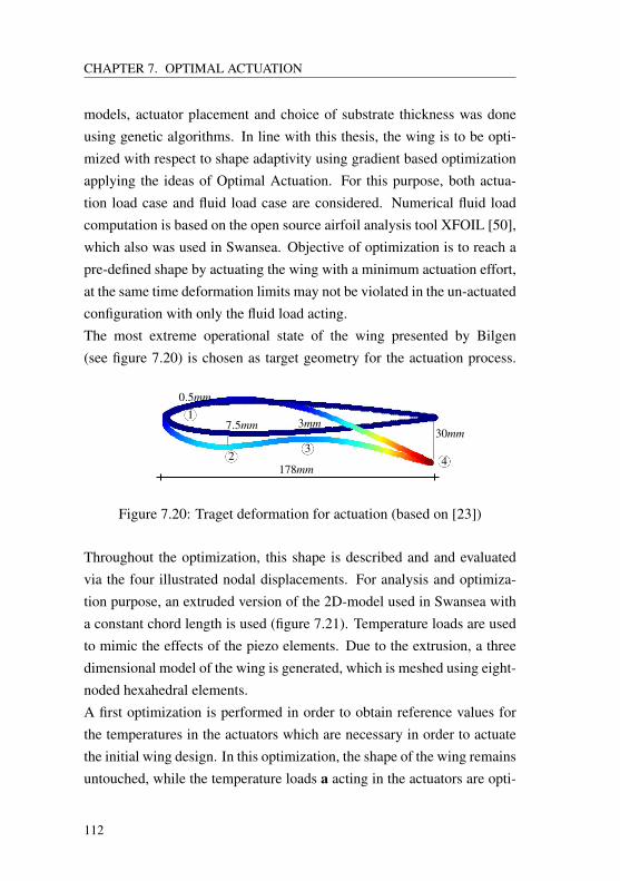
CHAPTER 7. OPTIMAL ACTUATION
models, actuator placement and choice of substrate thickness was doneusing genetic algorithms. In line with this thesis, the wing is to be opti-mized with respect to shape adaptivity using gradient based optimizationapplying the ideas of Optimal Actuation. For this purpose, both actua-tion load case and fluid load case are considered. Numerical fluid loadcomputation is based on the open source airfoil analysis tool XFOIL [50],which also was used in Swansea. Objective of optimization is to reach apre-defined shape by actuating the wing with a minimum actuation effort,at the same time deformation limits may not be violated in the un-actuatedconfiguration with only the fluid load acting.The most extreme operational state of the wing presented by Bilgen(see figure 7.20) is chosen as target geometry for the actuation process.
0.5mm
7.5mm 3mm30mm
1
23
4178mm
Figure 7.20: Traget deformation for actuation (based on [23])
Throughout the optimization, this shape is described and and evaluatedvia the four illustrated nodal displacements. For analysis and optimiza-tion purpose, an extruded version of the 2D-model used in Swansea witha constant chord length is used (figure 7.21). Temperature loads are usedto mimic the effects of the piezo elements. Due to the extrusion, a threedimensional model of the wing is generated, which is meshed using eight-noded hexahedral elements.A first optimization is performed in order to obtain reference values forthe temperatures in the actuators which are necessary in order to actuatethe initial wing design. In this optimization, the shape of the wing remainsuntouched, while the temperature loads a acting in the actuators are opti-
112
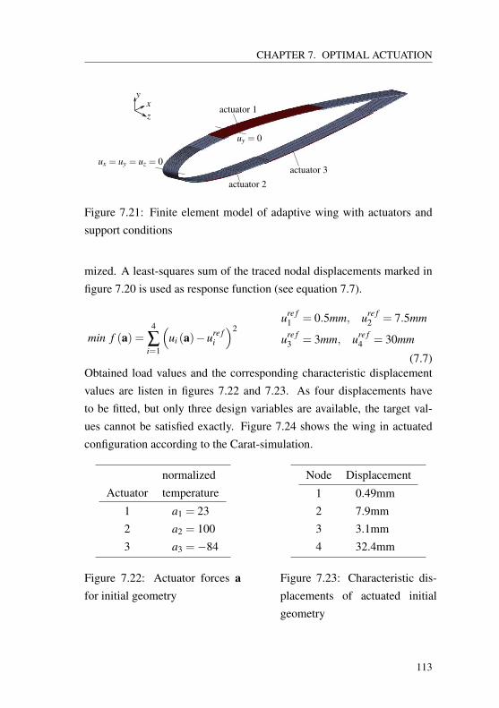
CHAPTER 7. OPTIMAL ACTUATION
actuator 1
actuator 2
actuator 3
uy = 0
ux = uy = uz = 0
xy
z
Figure 7.21: Finite element model of adaptive wing with actuators andsupport conditions
mized. A least-squares sum of the traced nodal displacements marked infigure 7.20 is used as response function (see equation 7.7).
min f (a) =4
∑i=1
(ui (a)−ure f
i
)2ure f
1 = 0.5mm, ure f2 = 7.5mm
ure f3 = 3mm, ure f
4 = 30mm
(7.7)Obtained load values and the corresponding characteristic displacementvalues are listen in figures 7.22 and 7.23. As four displacements haveto be fitted, but only three design variables are available, the target val-ues cannot be satisfied exactly. Figure 7.24 shows the wing in actuatedconfiguration according to the Carat-simulation.
normalizedActuator temperature
1 a1 = 232 a2 = 1003 a3 =−84
Figure 7.22: Actuator forces afor initial geometry
Node Displacement
1 0.49mm2 7.9mm3 3.1mm4 32.4mm
Figure 7.23: Characteristic dis-placements of actuated initialgeometry
113
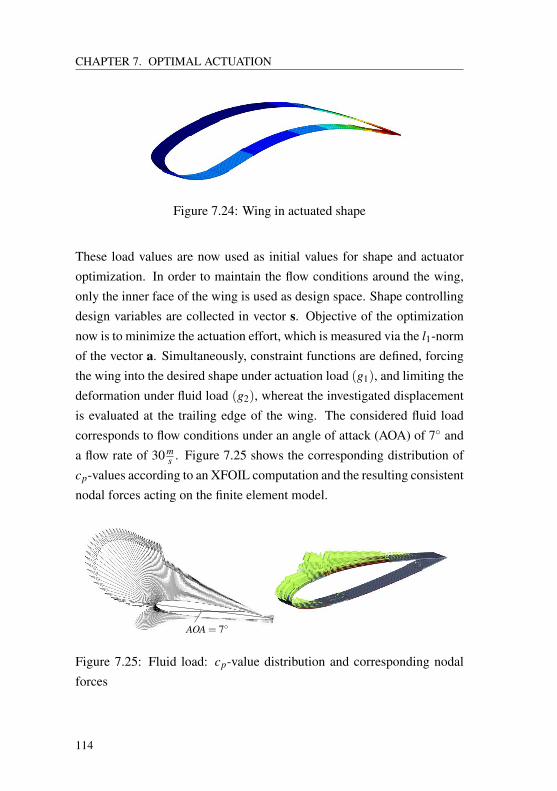
CHAPTER 7. OPTIMAL ACTUATION
Figure 7.24: Wing in actuated shape
These load values are now used as initial values for shape and actuatoroptimization. In order to maintain the flow conditions around the wing,only the inner face of the wing is used as design space. Shape controllingdesign variables are collected in vector s. Objective of the optimizationnow is to minimize the actuation effort, which is measured via the l1-normof the vector a. Simultaneously, constraint functions are defined, forcingthe wing into the desired shape under actuation load (g1), and limiting thedeformation under fluid load (g2), whereat the investigated displacementis evaluated at the trailing edge of the wing. The considered fluid loadcorresponds to flow conditions under an angle of attack (AOA) of 7 anda flow rate of 30 m
s . Figure 7.25 shows the corresponding distribution ofcp-values according to an XFOIL computation and the resulting consistentnodal forces acting on the finite element model.
AOA = 7
Figure 7.25: Fluid load: cp-value distribution and corresponding nodalforces
114
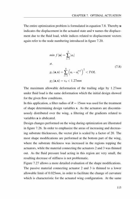
CHAPTER 7. OPTIMAL ACTUATION
The entire optimization problem is formulated in equation 7.8. Thereby uindicates the displacement in the actuated state and v names the displace-ment due to the fluid load, while indices related to displacement vectorsagain refer to the node numbering introduced in figure 7.20.
min f (a) =3
∑i=1|ai|
st.
g1 (a,s) =4
∑i=1
(ui−ure f
i
)2< TOL
g2 (a,s) = v4 < 1.27mm
(7.8)
The maximum allowable deformation of the trailing edge by 1.27mm
under fluid load is the same deformation which the initial design showedfor the given flow conditions.In this application, a filter radius of R = 15mm was used for the treatmentof shape determining design variables s. As the actuators are discontin-uously distributed over the wing, a filtering of the gradients related tovariables a is abdicated.Design changes performed on the wing during optimization are illustratedin figure 7.26. In order to emphasize the areas of increasing and decreas-ing substrate thicknesses, the vector plot is scaled by a factor of 20. Themost shape modifications are performed at the bottom part of the wing,where the substrate thickness was increased in the regions topping theactuators, while the material connecting the actuators 2 and 3 was thinnedout. As the fluid pressure load acting in this region are very small, theresulting decrease of stiffness is not problematic.Figure 7.27 allows a more detailed evaluation of the shape modifications.The passive material connecting actuator 2 and 3 is thinned to a lowerallowable limit of 0.025mm, in order to facilitate the change of curvaturewhich is characteristic for the actuated wing configuration. At the same
115
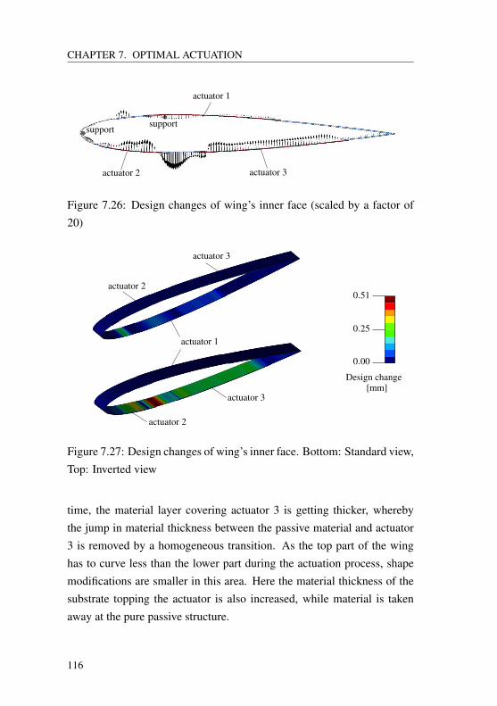
CHAPTER 7. OPTIMAL ACTUATION
actuator 2 actuator 3
actuator 1
supportsupport
Figure 7.26: Design changes of wing’s inner face (scaled by a factor of20)
0.51
0.00
Design change
0.25
[mm]
actuator 2
actuator 3
actuator 1
actuator 2
actuator 3
Figure 7.27: Design changes of wing’s inner face. Bottom: Standard view,Top: Inverted view
time, the material layer covering actuator 3 is getting thicker, wherebythe jump in material thickness between the passive material and actuator3 is removed by a homogeneous transition. As the top part of the winghas to curve less than the lower part during the actuation process, shapemodifications are smaller in this area. Here the material thickness of thesubstrate topping the actuator is also increased, while material is takenaway at the pure passive structure.
116
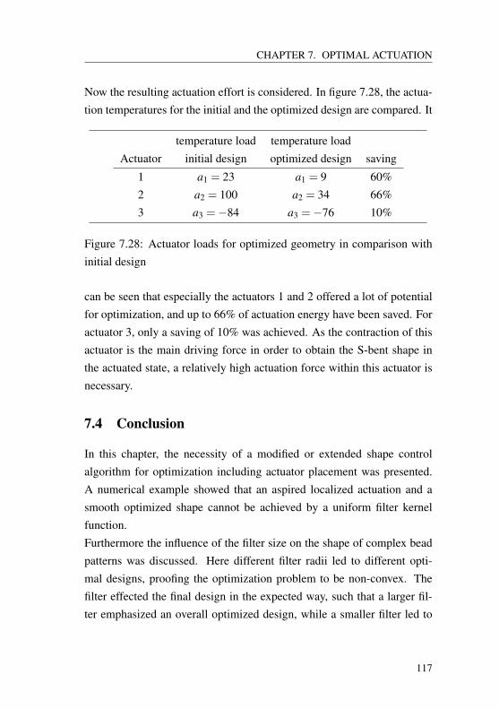
CHAPTER 7. OPTIMAL ACTUATION
Now the resulting actuation effort is considered. In figure 7.28, the actua-tion temperatures for the initial and the optimized design are compared. It
temperature load temperature loadActuator initial design optimized design saving
1 a1 = 23 a1 = 9 60%2 a2 = 100 a2 = 34 66%3 a3 =−84 a3 =−76 10%
Figure 7.28: Actuator loads for optimized geometry in comparison withinitial design
can be seen that especially the actuators 1 and 2 offered a lot of potentialfor optimization, and up to 66% of actuation energy have been saved. Foractuator 3, only a saving of 10% was achieved. As the contraction of thisactuator is the main driving force in order to obtain the S-bent shape inthe actuated state, a relatively high actuation force within this actuator isnecessary.
7.4 Conclusion
In this chapter, the necessity of a modified or extended shape controlalgorithm for optimization including actuator placement was presented.A numerical example showed that an aspired localized actuation and asmooth optimized shape cannot be achieved by a uniform filter kernelfunction.Furthermore the influence of the filter size on the shape of complex beadpatterns was discussed. Here different filter radii led to different opti-mal designs, proofing the optimization problem to be non-convex. Thefilter effected the final design in the expected way, such that a larger fil-ter emphasized an overall optimized design, while a smaller filter led to
117

CHAPTER 7. OPTIMAL ACTUATION
localized design modifications, whereat the characteristic design elementshave been preserved.The example considering the adaptive wing combined a continuous shapedesign field with discretely distributed design variables. Here also a sec-ond load case was considered, subjecting the structure in the un-actuatedstate and so defining a minimum stiffness of the structure. This com-plex optimization problem was solved successfully, leading to a signifi-cant decrease of required actuation force.
118
CHAPTER 8. BI- AND MULTISTABLE STRUCTURES
CHAPTER 8
Bi- and multistable structures
8.1 Motivation
In the chapters 6 and 7, "classical" smart structures have been considered.These structures can be actuated by a permanent actuator input. As soonas the actuator is shut down, the structure returns to its initial configu-ration. This necessity of permanent actuator input brings up the idea ofapplying bistable structures in the field of smart structures, which will bediscussed in this chapter.A bi- or multistable structure is a structure which can assume two or evenmore different shapes of self equilibrium without any load acting onto thestructure. A very simple example of a bistable structure is the two-bar-truss structure, which is discussed quite frequently in introductive lec-tures to nonlinear finite elements, as it shows a distinct nonlinear loadcarrying behaviour despite its simplicity. Figure 8.1 shows the states ofself equilibrium of the two bar truss. The structure even possesses threeconfigurations of self equilibrium, whereof two are stable states and thethird one is a instable state, which means that any disturbance applied tothe position of the center node will cause the structure to a sudden snapthrough towards one of the stable states.
119
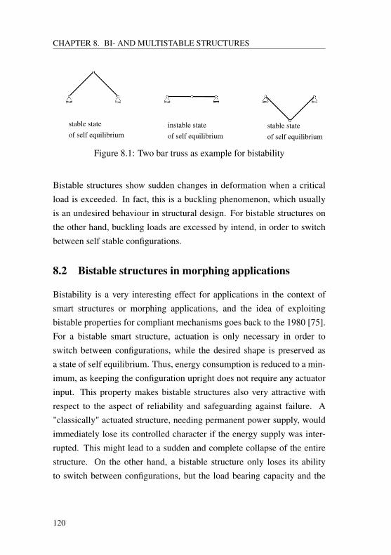
CHAPTER 8. BI- AND MULTISTABLE STRUCTURES
stable stateof self equilibrium
stable stateof self equilibrium
instable stateof self equilibrium
Figure 8.1: Two bar truss as example for bistability
Bistable structures show sudden changes in deformation when a criticalload is exceeded. In fact, this is a buckling phenomenon, which usuallyis an undesired behaviour in structural design. For bistable structures onthe other hand, buckling loads are excessed by intend, in order to switchbetween self stable configurations.
8.2 Bistable structures in morphing applications
Bistability is a very interesting effect for applications in the context ofsmart structures or morphing applications, and the idea of exploitingbistable properties for compliant mechanisms goes back to the 1980 [75].For a bistable smart structure, actuation is only necessary in order toswitch between configurations, while the desired shape is preserved asa state of self equilibrium. Thus, energy consumption is reduced to a min-imum, as keeping the configuration upright does not require any actuatorinput. This property makes bistable structures also very attractive withrespect to the aspect of reliability and safeguarding against failure. A"classically" actuated structure, needing permanent power supply, wouldimmediately lose its controlled character if the energy supply was inter-rupted. This might lead to a sudden and complete collapse of the entirestructure. On the other hand, a bistable structure only loses its abilityto switch between configurations, but the load bearing capacity and the
120
CHAPTER 8. BI- AND MULTISTABLE STRUCTURES
stability of the structure would not be affected immediately by a powerbreakdown.
8.3 State of research
In section 8.1, the effect of bistability was discussed regarding a trussstructure. Generating bistability for curved shell structures is way morechallenging. For this purpose, analytical formulas are used in order toachieve bistable behaviour for shells with constant curvature radii. Cylin-drical shells are known to be monostable if they are made from isotropicmaterial without any prestress [65], thus actual research mainly focuseson the generation of bistable cylindrical shells using orthotropic compos-ite material in combination with prestress [81].In this context, necessary prestress is very often generated by using thedirection dependent thermal expansion of composites materials in theautoclave method in order to obtain prestressed cylindrical shells madefrom staggered composite material [93] [104] [105]. Another approach isto generate prestress by bonding mechanically prestressed rubber mate-rial as top and bottom layers onto elastic core material. By this mean, abistable structure can be generated which switches between a cylindricaland a saddle shape [38].The investigation of bistability for non-prestressed structures is quite anew field of research. In Coburn et al [43], a tristable positively doublycurved shell is presented for which the multistable properties are tailoredby choosing adequate radii of curvature.
121
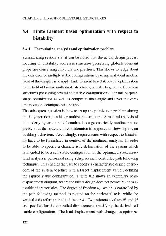
CHAPTER 8. BI- AND MULTISTABLE STRUCTURES
8.4 Finite Element based optimization with respect tobistability
8.4.1 Formulating analysis and optimization problem
Summarizing section 8.3, it can be noted that the actual design processfocusing on bistability addresses structures possessing globally constantproperties concerning curvature and prestress. This allows to judge aboutthe existence of multiple stable configurations by using analytical models.Goal of this chapter is to apply finite element based structural optimizationto the field of bi- and multistable structures, in order to generate free-formstructures possessing several self stable configurations. For this purpose,shape optimization as well as composite fiber angle and layer thicknessoptimization techniques will be used.The subsequent question is, how to set up an optimization problem aimingon the generation of a bi- or multistable structure. Structural analysis ofthe underlying structure is formulated as a geometrically nonlinear staticproblem, as the structure of consideration is supposed to show significantbuckling behaviour. Accordingly, requirements with respect to bistabil-ity have to be formulated in context of the nonlinear analysis. In orderto be able to specify a characteristic deformation of the system whichis intended to be a self stable configuration in the optimized state, struc-tural analysis is performed using a displacement controlled path followingtechnique. This enables the user to specify a characteristic degree of free-dom of the system together with a target displacement values, definingthe aspired stable configuration. Figure 8.2 shows an exemplary load-displacement diagram, where the initial design does not posses bi- or mul-tistable characteristics. The degree of freedom uc, which is controlled bythe path following method, is plotted on the horizontal axis, while thevertical axis refers to the load factor λ . Two reference values u1 and u2
are specified for the controlled displacement, specifying the desired selfstable configurations. The load-displacement path changes as optimiza-
122
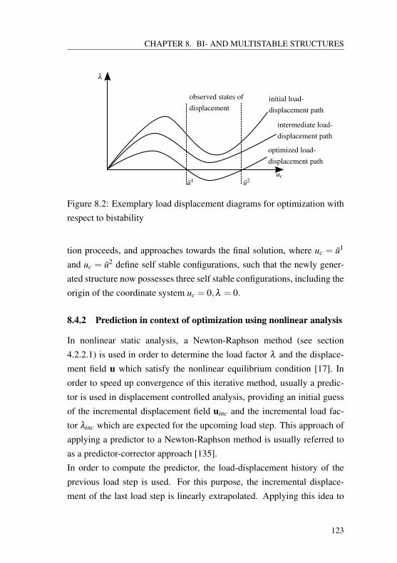
CHAPTER 8. BI- AND MULTISTABLE STRUCTURES
uc
λ
observed states ofdisplacement
initial load-displacement path
optimized load-displacement path
intermediate load-displacement path
u1 u2
Figure 8.2: Exemplary load displacement diagrams for optimization withrespect to bistability
tion proceeds, and approaches towards the final solution, where uc = u1
and uc = u2 define self stable configurations, such that the newly gener-ated structure now possesses three self stable configurations, including theorigin of the coordinate system uc = 0,λ = 0.
8.4.2 Prediction in context of optimization using nonlinear analysis
In nonlinear static analysis, a Newton-Raphson method (see section4.2.2.1) is used in order to determine the load factor λ and the displace-ment field u which satisfy the nonlinear equilibrium condition [17]. Inorder to speed up convergence of this iterative method, usually a predic-tor is used in displacement controlled analysis, providing an initial guessof the incremental displacement field uinc and the incremental load fac-tor λinc which are expected for the upcoming load step. This approach ofapplying a predictor to a Newton-Raphson method is usually referred toas a predictor-corrector approach [135].In order to compute the predictor, the load-displacement history of theprevious load step is used. For this purpose, the incremental displace-ment of the last load step is linearly extrapolated. Applying this idea to
123
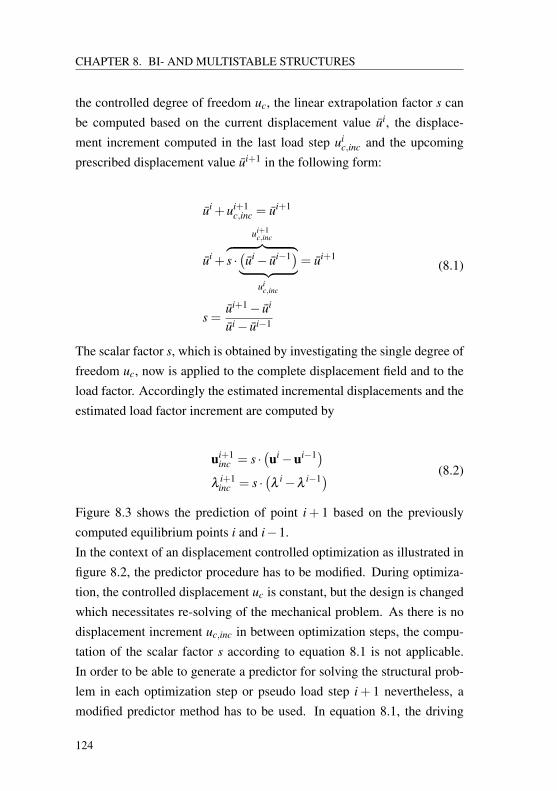
CHAPTER 8. BI- AND MULTISTABLE STRUCTURES
the controlled degree of freedom uc, the linear extrapolation factor s canbe computed based on the current displacement value ui, the displace-ment increment computed in the last load step ui
c,inc and the upcomingprescribed displacement value ui+1 in the following form:
ui +ui+1c,inc = ui+1
ui +
ui+1c,inc︷ ︸︸ ︷
s ·(ui− ui−1)︸ ︷︷ ︸
uic,inc
= ui+1
s =ui+1− ui
ui− ui−1
(8.1)
The scalar factor s, which is obtained by investigating the single degree offreedom uc, now is applied to the complete displacement field and to theload factor. Accordingly the estimated incremental displacements and theestimated load factor increment are computed by
ui+1inc = s ·
(ui−ui−1)
λi+1inc = s ·
(λ
i−λi−1) (8.2)
Figure 8.3 shows the prediction of point i+ 1 based on the previouslycomputed equilibrium points i and i−1.In the context of an displacement controlled optimization as illustrated infigure 8.2, the predictor procedure has to be modified. During optimiza-tion, the controlled displacement uc is constant, but the design is changedwhich necessitates re-solving of the mechanical problem. As there is nodisplacement increment uc,inc in between optimization steps, the compu-tation of the scalar factor s according to equation 8.1 is not applicable.In order to be able to generate a predictor for solving the structural prob-lem in each optimization step or pseudo load step i+ 1 nevertheless, amodified predictor method has to be used. In equation 8.1, the driving
124
CHAPTER 8. BI- AND MULTISTABLE STRUCTURES
uc
λ
ui−1 ui ui+1
λ i−1
λ i
λ i+1
equilibrium points i, i−1
predicted point i+1
ui+1c,inc
λi+1inc
Figure 8.3: Predictor scheme for displacement controlled analysis
force determining the value of s is the ratio of the prescribed displace-ment increments in two subsequent load steps. Accordingly, a predictorused in context of optimization should be driven by the ration of designmodifications for two subsequent optimization iterations. Design modifi-cations can be measured by step length factors α used in the line search(see section 5.6), thus an appropriate predictor can be formulated as
ui+1inc =
α i+1
α i ·(ui−ui−1)
λi+1inc =
α i+1
α i ·(λ
i−λi−1) (8.3)
In case of a fixed step line search, it holds that α i+1
α i = 1. In this case,the predicted changes in displacement and load factor are identical to thechanges observed in the last optimization step.
8.5 Considering of multiple load-path problems andavoiding of over-critical points
As already mentioned in section 8.1, bistable structures show a signif-icant buckling behaviour. Buckling is a very complex mechanical pro-cess, especially when buckling of shell structures is considered, whereat
125
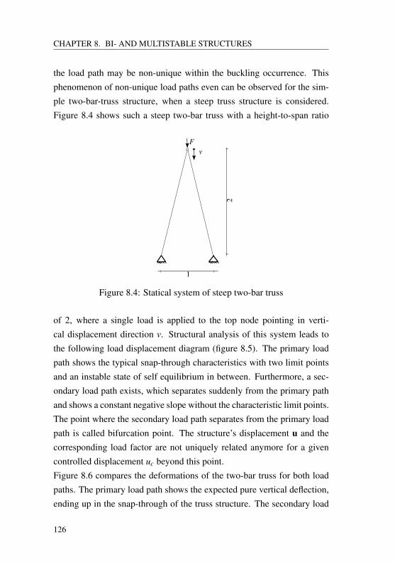
CHAPTER 8. BI- AND MULTISTABLE STRUCTURES
the load path may be non-unique within the buckling occurrence. Thisphenomenon of non-unique load paths even can be observed for the sim-ple two-bar-truss structure, when a steep truss structure is considered.Figure 8.4 shows such a steep two-bar truss with a height-to-span ratio
1
2
Fv
Figure 8.4: Statical system of steep two-bar truss
of 2, where a single load is applied to the top node pointing in verti-cal displacement direction v. Structural analysis of this system leads tothe following load displacement diagram (figure 8.5). The primary loadpath shows the typical snap-through characteristics with two limit pointsand an instable state of self equilibrium in between. Furthermore, a sec-ondary load path exists, which separates suddenly from the primary pathand shows a constant negative slope without the characteristic limit points.The point where the secondary load path separates from the primary loadpath is called bifurcation point. The structure’s displacement u and thecorresponding load factor are not uniquely related anymore for a givencontrolled displacement uc beyond this point.Figure 8.6 compares the deformations of the two-bar truss for both loadpaths. The primary load path shows the expected pure vertical deflection,ending up in the snap-through of the truss structure. The secondary load
126
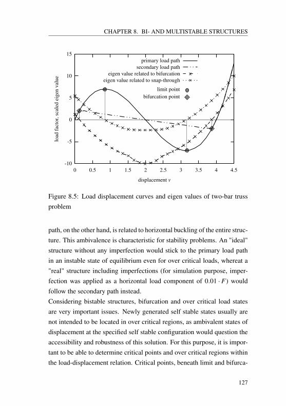
CHAPTER 8. BI- AND MULTISTABLE STRUCTURES
-10
-5
0
5
10
15
0 0.5 1 1.5 2 2.5 3 3.5 4 4.5
load
fact
or,s
cale
dei
gen
valu
e
displacement v
limit pointbifurcation point
primary load pathsecondary load path
eigen value related to bifurcationeigen value related to snap-through
Figure 8.5: Load displacement curves and eigen values of two-bar trussproblem
path, on the other hand, is related to horizontal buckling of the entire struc-ture. This ambivalence is characteristic for stability problems. An "ideal"structure without any imperfection would stick to the primary load pathin an instable state of equilibrium even for over critical loads, whereat a"real" structure including imperfections (for simulation purpose, imper-fection was applied as a horizontal load component of 0.01 · F) wouldfollow the secondary path instead.Considering bistable structures, bifurcation and over critical load statesare very important issues. Newly generated self stable states usually arenot intended to be located in over critical regions, as ambivalent states ofdisplacement at the specified self stable configuration would question theaccessibility and robustness of this solution. For this purpose, it is impor-tant to be able to determine critical points and over critical regions withinthe load-displacement relation. Critical points, beneath limit and bifurca-
127
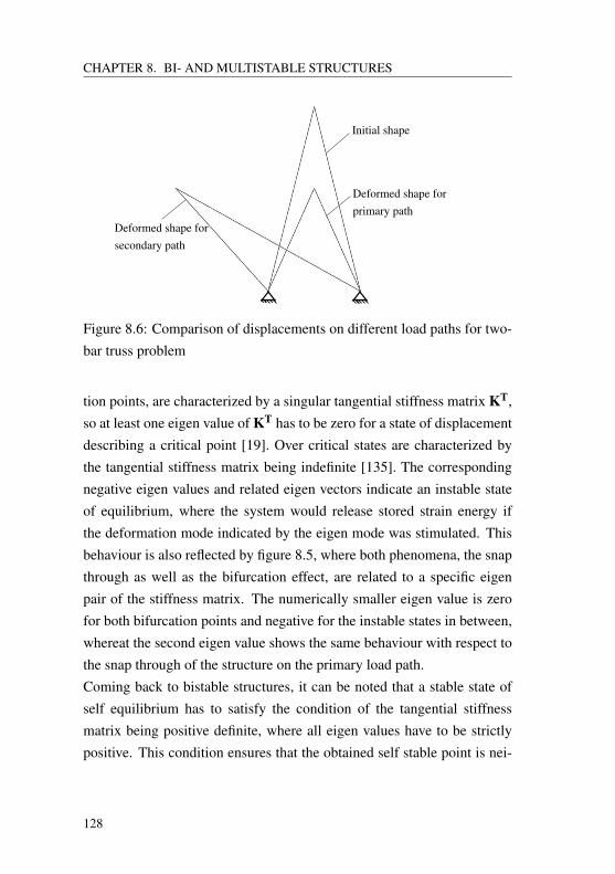
CHAPTER 8. BI- AND MULTISTABLE STRUCTURES
Initial shape
Deformed shape forprimary path
Deformed shape forsecondary path
Figure 8.6: Comparison of displacements on different load paths for two-bar truss problem
tion points, are characterized by a singular tangential stiffness matrix KT,so at least one eigen value of KT has to be zero for a state of displacementdescribing a critical point [19]. Over critical states are characterized bythe tangential stiffness matrix being indefinite [135]. The correspondingnegative eigen values and related eigen vectors indicate an instable stateof equilibrium, where the system would release stored strain energy ifthe deformation mode indicated by the eigen mode was stimulated. Thisbehaviour is also reflected by figure 8.5, where both phenomena, the snapthrough as well as the bifurcation effect, are related to a specific eigenpair of the stiffness matrix. The numerically smaller eigen value is zerofor both bifurcation points and negative for the instable states in between,whereat the second eigen value shows the same behaviour with respect tothe snap through of the structure on the primary load path.Coming back to bistable structures, it can be noted that a stable state ofself equilibrium has to satisfy the condition of the tangential stiffnessmatrix being positive definite, where all eigen values have to be strictlypositive. This condition ensures that the obtained self stable point is nei-
128
CHAPTER 8. BI- AND MULTISTABLE STRUCTURES
ther an instable configuration, nor it is located in a region of ambiguousload paths.
8.6 Response function and sensitivity analysis
As mentioned in sections 8.1 and 8.4, a bistable structure is character-ized by multiple shapes the structure may assume without being subjectto any loading. This property is utilized in order to formulate a responsefunction which can be used for optimizing a structure with respect tobistable nature. The response function is based on a displacement con-trolled nonlinear static analysis. As the structure is meant to become selfstable for specific values of controlled displacement, the absolute amountor the square of the load factor is minimized, such that the optimizationproblem can be written as
min f (s, u) = ‖λ (s, u)‖ ∨ [λ (s, u)]2
st(8.4a)
S(s,λ ,u) = fint (u)−λ · fext = 0 (8.4b)
C (s, u,u) = uc− u = 0 (8.4c)
where equation S is the residual formulation of the equilibrium conditionand C describes the control equation for the displacement controlled pathfollowing algorithm, where uc is the actual displacement at the controlleddegree of freedom, and u is the assigned target value.The sensitivity formulation of the objective function d f
dsiis quite easy in
this case, as the objective only depends on the design s and on the constanttarget displacement u, but not on the state field u. Thus the total derivativeis identical with the partial derivative with respect to si in this case:
d fdsi
=∂ f∂ si
+∂ f∂ u· ∂ u
∂ si︸︷︷︸0
⇒ d fdsi
=∂ ‖λ‖
∂ si∨ ∂λ 2
∂ si(8.5)
129
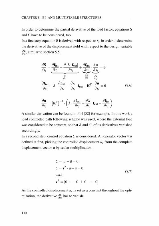
CHAPTER 8. BI- AND MULTISTABLE STRUCTURES
In order to determine the partial derivative of the load factor, equations Sand C have to be considered, too.In a first step, equation S is derived with respect to si, in order to determinethe derivative of the displacement field with respect to the design variable∂u∂ si
, similar to section 5.5.
dSdsi
=∂ fint∂ si− ∂ [λ · fext]
∂ si︸ ︷︷ ︸∂S∂ si
+∂ fint∂u︸ ︷︷ ︸∂S∂u
· ∂u∂ si︸︷︷︸∂u∂ si
= 0
∂ fint∂ si−λ · ∂ fext
∂ si− ∂λ
∂ si· fext +KT · ∂u
∂ si= 0
∂u∂ si
=[KT]−1 ·
(λ · ∂ fext
∂ si+
∂λ
∂ si· fext−
∂ fint∂ si
)(8.6)
A similar derivation can be found in Firl [52] for example. In this work aload controlled path following scheme was used, where the external loadwas considered to be constant, so that λ and all of its derivatives vanishedaccordingly.In a second step, control equation C is considered. An operator vector v isdefined at first, picking the controlled displacement uc from the completedisplacement vector u by scalar multiplication.
C = uc− u = 0
C = vT ·u− u = 0
with
vT = [0 · · · 0 1 0 · · · 0]
(8.7)
As the controlled displacement uc is set as a constant throughout the opti-mization, the derivative dC
dsihas to vanish.
130
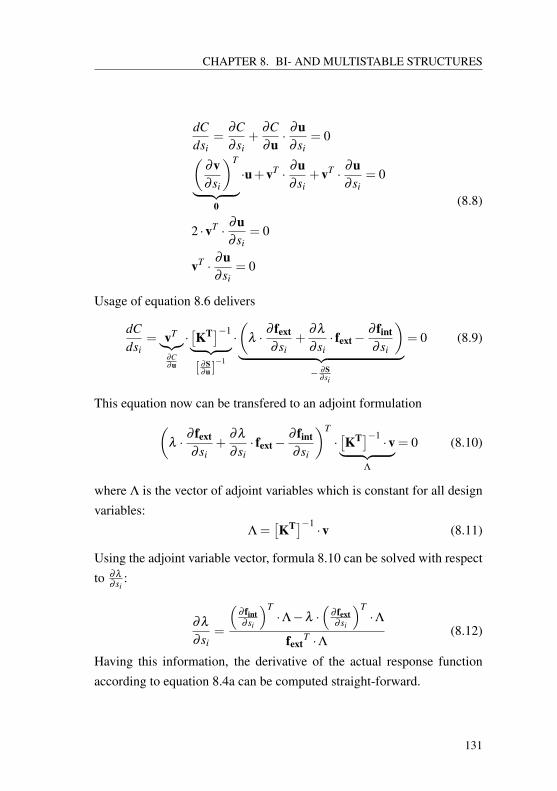
CHAPTER 8. BI- AND MULTISTABLE STRUCTURES
dCdsi
=∂C∂ si
+∂C∂u· ∂u
∂ si= 0(
∂v∂ si
)T
︸ ︷︷ ︸0
·u+vT · ∂u∂ si
+vT · ∂u∂ si
= 0
2 ·vT · ∂u∂ si
= 0
vT · ∂u∂ si
= 0
(8.8)
Usage of equation 8.6 delivers
dCdsi
= vT︸︷︷︸∂C∂u
·[KT]−1︸ ︷︷ ︸[ ∂S
∂u ]−1
·(
λ · ∂ fext
∂ si+
∂λ
∂ si· fext−
∂ fint∂ si
)︸ ︷︷ ︸
− ∂S∂ si
= 0 (8.9)
This equation now can be transfered to an adjoint formulation(λ · ∂ fext
∂ si+
∂λ
∂ si· fext−
∂ fint∂ si
)T
·[KT]−1 ·v︸ ︷︷ ︸
Λ
= 0 (8.10)
where Λ is the vector of adjoint variables which is constant for all designvariables:
Λ =[KT]−1 ·v (8.11)
Using the adjoint variable vector, formula 8.10 can be solved with respectto ∂λ
∂ si:
∂λ
∂ si=
(∂ fint∂ si
)T·Λ−λ ·
(∂ fext∂ si
)T·Λ
fextT ·Λ
(8.12)
Having this information, the derivative of the actual response functionaccording to equation 8.4a can be computed straight-forward.
131
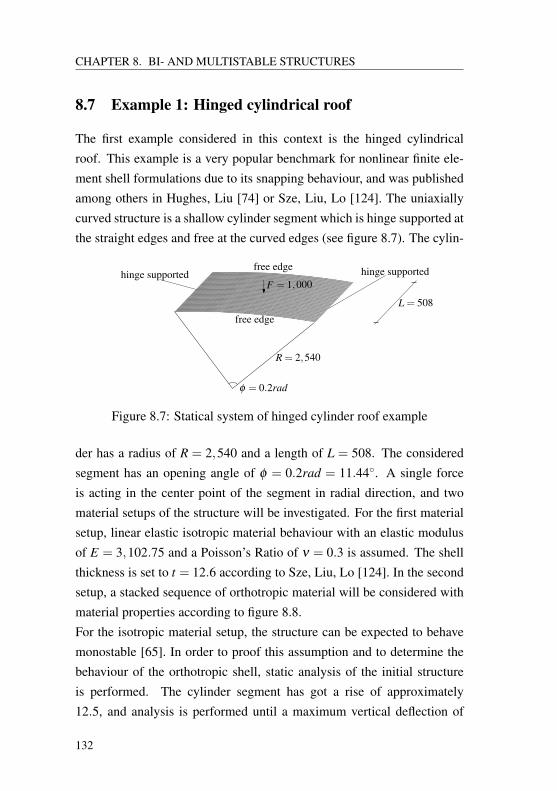
CHAPTER 8. BI- AND MULTISTABLE STRUCTURES
8.7 Example 1: Hinged cylindrical roof
The first example considered in this context is the hinged cylindricalroof. This example is a very popular benchmark for nonlinear finite ele-ment shell formulations due to its snapping behaviour, and was publishedamong others in Hughes, Liu [74] or Sze, Liu, Lo [124]. The uniaxiallycurved structure is a shallow cylinder segment which is hinge supported atthe straight edges and free at the curved edges (see figure 8.7). The cylin-
R = 2,540
φ = 0.2rad
hinge supported
L = 508
hinge supported
free edge
free edge
F = 1,000
Figure 8.7: Statical system of hinged cylinder roof example
der has a radius of R = 2,540 and a length of L = 508. The consideredsegment has an opening angle of φ = 0.2rad = 11.44. A single forceis acting in the center point of the segment in radial direction, and twomaterial setups of the structure will be investigated. For the first materialsetup, linear elastic isotropic material behaviour with an elastic modulusof E = 3,102.75 and a Poisson’s Ratio of ν = 0.3 is assumed. The shellthickness is set to t = 12.6 according to Sze, Liu, Lo [124]. In the secondsetup, a stacked sequence of orthotropic material will be considered withmaterial properties according to figure 8.8.For the isotropic material setup, the structure can be expected to behavemonostable [65]. In order to proof this assumption and to determine thebehaviour of the orthotropic shell, static analysis of the initial structureis performed. The cylinder segment has got a rise of approximately12.5, and analysis is performed until a maximum vertical deflection of
132
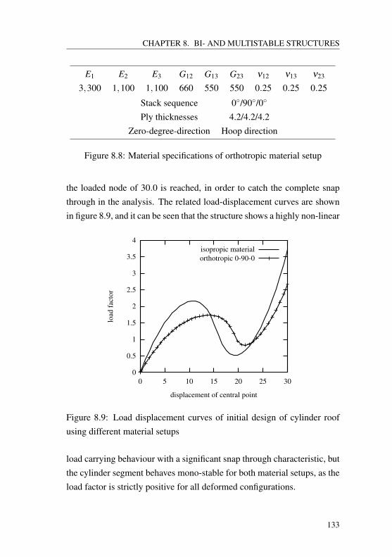
CHAPTER 8. BI- AND MULTISTABLE STRUCTURES
E1 E2 E3 G12 G13 G23 ν12 ν13 ν23
3,300 1,100 1,100 660 550 550 0.25 0.25 0.25
Stack sequence 0/90/0
Ply thicknesses 4.2/4.2/4.2Zero-degree-direction Hoop direction
Figure 8.8: Material specifications of orthotropic material setup
the loaded node of 30.0 is reached, in order to catch the complete snapthrough in the analysis. The related load-displacement curves are shownin figure 8.9, and it can be seen that the structure shows a highly non-linear
0
0.5
1
1.5
2
2.5
3
3.5
4
0 5 10 15 20 25 30
load
fact
or
displacement of central point
isopropic materialorthotropic 0-90-0
Figure 8.9: Load displacement curves of initial design of cylinder roofusing different material setups
load carrying behaviour with a significant snap through characteristic, butthe cylinder segment behaves mono-stable for both material setups, as theload factor is strictly positive for all deformed configurations.
133
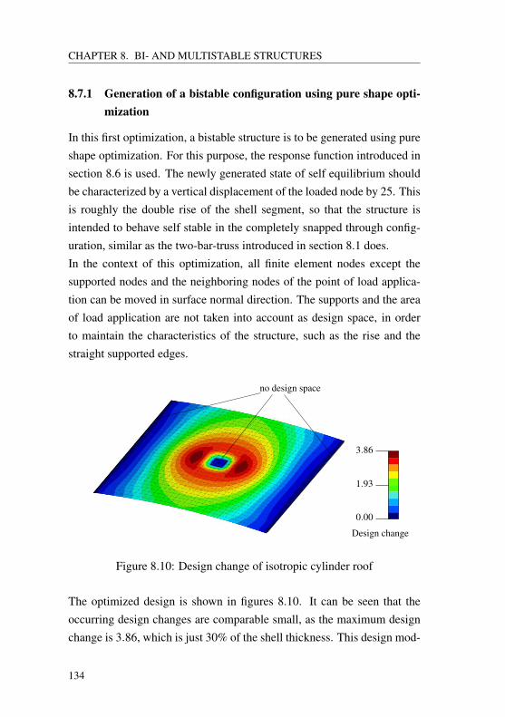
CHAPTER 8. BI- AND MULTISTABLE STRUCTURES
8.7.1 Generation of a bistable configuration using pure shape opti-mization
In this first optimization, a bistable structure is to be generated using pureshape optimization. For this purpose, the response function introduced insection 8.6 is used. The newly generated state of self equilibrium shouldbe characterized by a vertical displacement of the loaded node by 25. Thisis roughly the double rise of the shell segment, so that the structure isintended to behave self stable in the completely snapped through config-uration, similar as the two-bar-truss introduced in section 8.1 does.In the context of this optimization, all finite element nodes except thesupported nodes and the neighboring nodes of the point of load applica-tion can be moved in surface normal direction. The supports and the areaof load application are not taken into account as design space, in orderto maintain the characteristics of the structure, such as the rise and thestraight supported edges.
no design space
3.86
0.00
Design change
1.93
Figure 8.10: Design change of isotropic cylinder roof
The optimized design is shown in figures 8.10. It can be seen that theoccurring design changes are comparable small, as the maximum designchange is 3.86, which is just 30% of the shell thickness. This design mod-
134
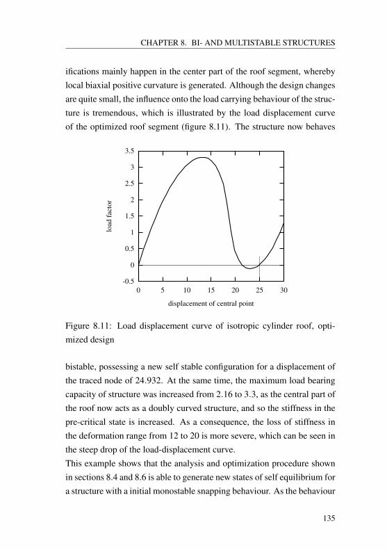
CHAPTER 8. BI- AND MULTISTABLE STRUCTURES
ifications mainly happen in the center part of the roof segment, wherebylocal biaxial positive curvature is generated. Although the design changesare quite small, the influence onto the load carrying behaviour of the struc-ture is tremendous, which is illustrated by the load displacement curveof the optimized roof segment (figure 8.11). The structure now behaves
-0.5
0
0.5
1
1.5
2
2.5
3
3.5
0 5 10 15 20 25 30
load
fact
or
displacement of central point
Figure 8.11: Load displacement curve of isotropic cylinder roof, opti-mized design
bistable, possessing a new self stable configuration for a displacement ofthe traced node of 24.932. At the same time, the maximum load bearingcapacity of structure was increased from 2.16 to 3.3, as the central part ofthe roof now acts as a doubly curved structure, and so the stiffness in thepre-critical state is increased. As a consequence, the loss of stiffness inthe deformation range from 12 to 20 is more severe, which can be seen inthe steep drop of the load-displacement curve.This example shows that the analysis and optimization procedure shownin sections 8.4 and 8.6 is able to generate new states of self equilibrium fora structure with a initial monostable snapping behaviour. As the behaviour
135
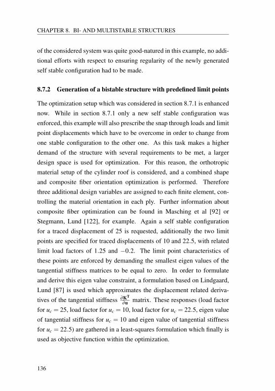
CHAPTER 8. BI- AND MULTISTABLE STRUCTURES
of the considered system was quite good-natured in this example, no addi-tional efforts with respect to ensuring regularity of the newly generatedself stable configuration had to be made.
8.7.2 Generation of a bistable structure with predefined limit points
The optimization setup which was considered in section 8.7.1 is enhancednow. While in section 8.7.1 only a new self stable configuration wasenforced, this example will also prescribe the snap through loads and limitpoint displacements which have to be overcome in order to change fromone stable configuration to the other one. As this task makes a higherdemand of the structure with several requirements to be met, a largerdesign space is used for optimization. For this reason, the orthotropicmaterial setup of the cylinder roof is considered, and a combined shapeand composite fiber orientation optimization is performed. Thereforethree additional design variables are assigned to each finite element, con-trolling the material orientation in each ply. Further information aboutcomposite fiber optimization can be found in Masching et al [92] orStegmann, Lund [122], for example. Again a self stable configurationfor a traced displacement of 25 is requested, additionally the two limitpoints are specified for traced displacements of 10 and 22.5, with relatedlimit load factors of 1.25 and −0.2. The limit point characteristics ofthese points are enforced by demanding the smallest eigen values of thetangential stiffness matrices to be equal to zero. In order to formulateand derive this eigen value constraint, a formulation based on Lindgaard,Lund [87] is used which approximates the displacement related deriva-tives of the tangential stiffness ∂KT
∂u matrix. These responses (load factorfor uc = 25, load factor for uc = 10, load factor for uc = 22.5, eigen valueof tangential stiffness for uc = 10 and eigen value of tangential stiffnessfor uc = 22.5) are gathered in a least-squares formulation which finally isused as objective function within the optimization.
136
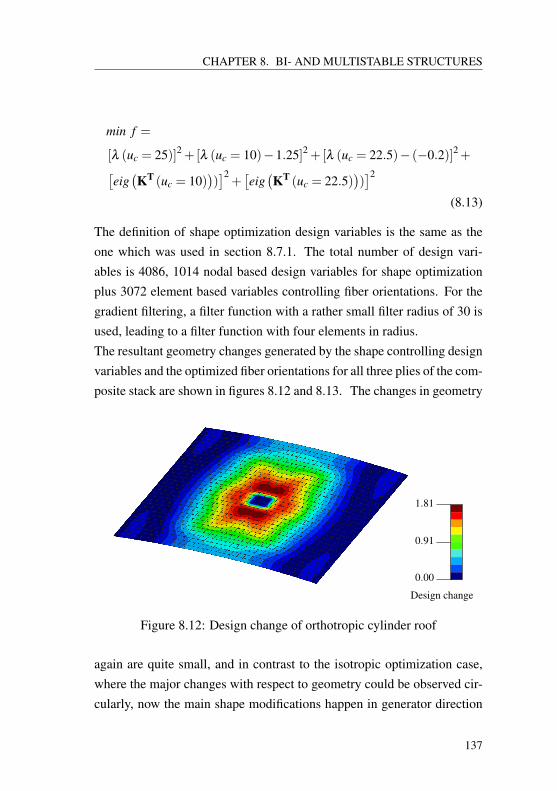
CHAPTER 8. BI- AND MULTISTABLE STRUCTURES
min f =
[λ (uc = 25)]2 +[λ (uc = 10)−1.25]2 +[λ (uc = 22.5)− (−0.2)]2+[eig(KT (uc = 10)
))]2+[eig(KT (uc = 22.5)
))]2
(8.13)
The definition of shape optimization design variables is the same as theone which was used in section 8.7.1. The total number of design vari-ables is 4086, 1014 nodal based design variables for shape optimizationplus 3072 element based variables controlling fiber orientations. For thegradient filtering, a filter function with a rather small filter radius of 30 isused, leading to a filter function with four elements in radius.The resultant geometry changes generated by the shape controlling designvariables and the optimized fiber orientations for all three plies of the com-posite stack are shown in figures 8.12 and 8.13. The changes in geometry
1.81
0.00
Design change
0.91
Figure 8.12: Design change of orthotropic cylinder roof
again are quite small, and in contrast to the isotropic optimization case,where the major changes with respect to geometry could be observed cir-cularly, now the main shape modifications happen in generator direction
137
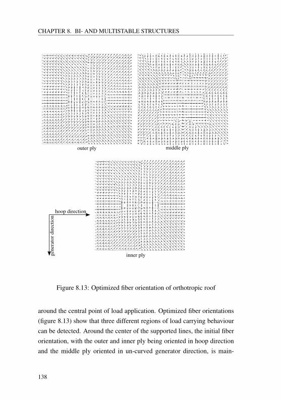
CHAPTER 8. BI- AND MULTISTABLE STRUCTURES
outer ply middle ply
inner ply
hoop direction
gene
rato
rdir
ectio
n
Figure 8.13: Optimized fiber orientation of orthotropic roof
around the central point of load application. Optimized fiber orientations(figure 8.13) show that three different regions of load carrying behaviourcan be detected. Around the center of the supported lines, the initial fiberorientation, with the outer and inner ply being oriented in hoop directionand the middle ply oriented in un-curved generator direction, is main-
138
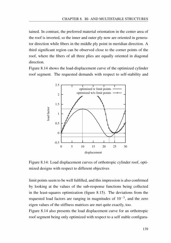
CHAPTER 8. BI- AND MULTISTABLE STRUCTURES
tained. In contrast, the preferred material orientation in the center area ofthe roof is inverted, so the inner and outer ply now are oriented in genera-tor direction while fibers in the middle ply point in meridian direction. Athird significant region can be observed close to the corner points of theroof, where the fibers of all three plies are equally oriented in diagonaldirection.Figure 8.14 shows the load-displacement curve of the optimized cylinderroof segment. The requested demands with respect to self-stability and
-0.5
0
0.5
1
1.5
2
2.5
0 5 10 15 20 25 30
load
fact
or
displacement
optimized w limit pointsoptimized w/o limit points
Figure 8.14: Load displacement curves of orthotropic cylinder roof, opti-mized designs with respect to different objectives
limit points seem to be well fulfilled, and this impression is also confirmedby looking at the values of the sub-response functions being collectedin the least-squares optimization (figure 8.15). The deviations from therequested load factors are ranging in magnitudes of 10−3, and the zeroeigen values of the stiffness matrices are met quite exactly, too.Figure 8.14 also presents the load displacement curve for an orthotropicroof segment being only optimized with respect to a self stable configura-
139
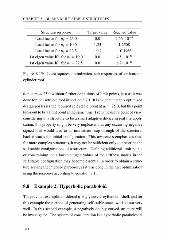
CHAPTER 8. BI- AND MULTISTABLE STRUCTURES
Structure response Target value Reached value
Load factor for uc = 25.0 0.0 2.66 ·10−4
Load factor for uc = 10.0 1.25 1.2508Load factor for uc = 22.5 −0.2 −0.1966
1st eigen value KT for uc = 10.0 0.0 4.5 ·10−6
1st eigen value KT for uc = 22.5 0.0 6.2 ·10−6
Figure 8.15: Least-squares optimization sub-responses of orthotropiccylinder roof
tion at uc = 25.0 without further definitions of limit points, just as it wasdone for the isotropic roof in section 8.7.1. It is evident that this optimizeddesign possesses the required self stable point at uc = 25.0, but this pointturns out to be a limit point at the same time. From the user’s point of view,considering this structure to be a smart adaptive device in real life appli-cation, this property might be very unpleasant, as any occurring negativesigned load would lead to an immediate snap-through of the structure,back towards the initial configuration. This awareness emphasizes that,for more complex structures, it may not be sufficient only to prescribe theself stable configurations of a structure. Defining additional limit pointsor constraining the allowable eigen values of the stiffness matrix in theself stable configuration may become essential in order to obtain a struc-ture serving the intended purposes, as it was done in the first optimizationusing the response according to equation 8.13.
8.8 Example 2: Hyperbolic paraboloid
The previous example considered a singly curved cylindrical shell, and forthis example the method of generating self stable states worked out verywell. In this second example, a negatively doubly curved structure willbe investigated. The system of consideration is a hyperbolic paraboloidal
140
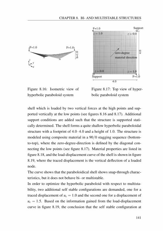
CHAPTER 8. BI- AND MULTISTABLE STRUCTURES
h=1.
0
F=1.0F=1.0
yz
x
Figure 8.16: Isometric view ofhyperbolic paraboloid system
F=1.0
F=1.0
Support
Support
z = 1.0
z = 1.0z = 0.0
z = 0.0
4.0
4.0
zero-degreematerial direction
Figure 8.17: Top view of hyper-bolic paraboloid system
shell which is loaded by two vertical forces at the high points and sup-ported vertically at the low points (see figures 8.16 and 8.17). Additionalsupport conditions are added such that the structure is supported stati-cally determined. The shell forms a quite shallow hyperbolic paraboloidalstructure with a footprint of 4.0 ·4.0 and a height of 1.0. The structure ismodeled using composite material in a 90/0 stagging sequence (bottom-to-top), where the zero-degree-direction is defined by the diagonal con-necting the low points (see figure 8.17). Material properties are listed infigure 8.18, and the load-displacement curve of the shell is shown in figure8.19, where the traced displacement is the vertical deflection of a loadednode.The curve shows that the paraboloidical shell shows snap-through charac-teristics, but it does not behave bi- or multistable.In order to optimize the hyperbolic paraboloid with respect to multista-bility, two additional self stable configurations are demanded, one for atraced displacement of uc = 1.0 and the second one for a displacement ofuc = 1.5. Based on the information gained from the load-displacementcurve in figure 8.19, the conclusion that the self stable configuration at
141
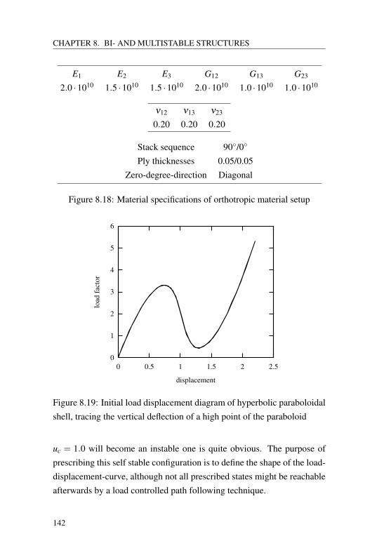
CHAPTER 8. BI- AND MULTISTABLE STRUCTURES
E1 E2 E3 G12 G13 G23
2.0 ·1010 1.5 ·1010 1.5 ·1010 2.0 ·1010 1.0 ·1010 1.0 ·1010
ν12 ν13 ν23
0.20 0.20 0.20
Stack sequence 90/0
Ply thicknesses 0.05/0.05Zero-degree-direction Diagonal
Figure 8.18: Material specifications of orthotropic material setup
0
1
2
3
4
5
6
0 0.5 1 1.5 2 2.5
load
fact
or
displacement
Figure 8.19: Initial load displacement diagram of hyperbolic paraboloidalshell, tracing the vertical deflection of a high point of the paraboloid
uc = 1.0 will become an instable one is quite obvious. The purpose ofprescribing this self stable configuration is to define the shape of the load-displacement-curve, although not all prescribed states might be reachableafterwards by a load controlled path following technique.
142
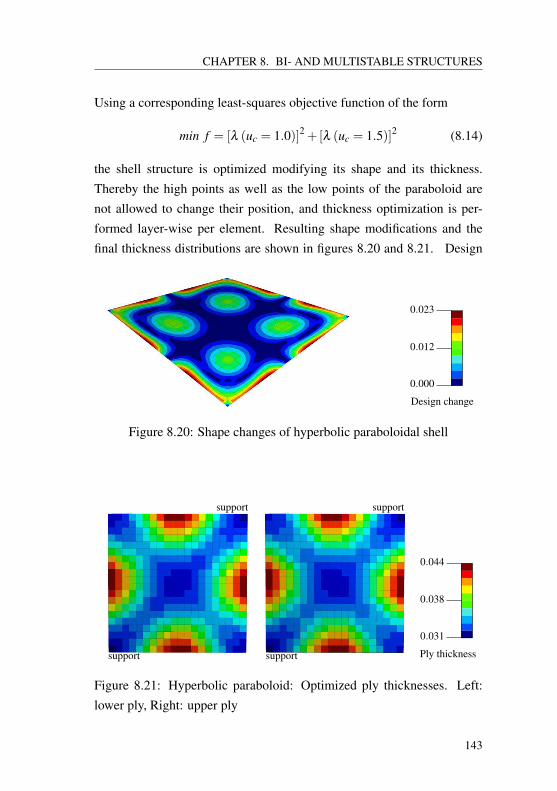
CHAPTER 8. BI- AND MULTISTABLE STRUCTURES
Using a corresponding least-squares objective function of the form
min f = [λ (uc = 1.0)]2 +[λ (uc = 1.5)]2 (8.14)
the shell structure is optimized modifying its shape and its thickness.Thereby the high points as well as the low points of the paraboloid arenot allowed to change their position, and thickness optimization is per-formed layer-wise per element. Resulting shape modifications and thefinal thickness distributions are shown in figures 8.20 and 8.21. Design
0.023
0.000
Design change
0.012
Figure 8.20: Shape changes of hyperbolic paraboloidal shell
supportsupport
0.044
0.031
Ply thickness
0.038
support support
Figure 8.21: Hyperbolic paraboloid: Optimized ply thicknesses. Left:lower ply, Right: upper ply
143
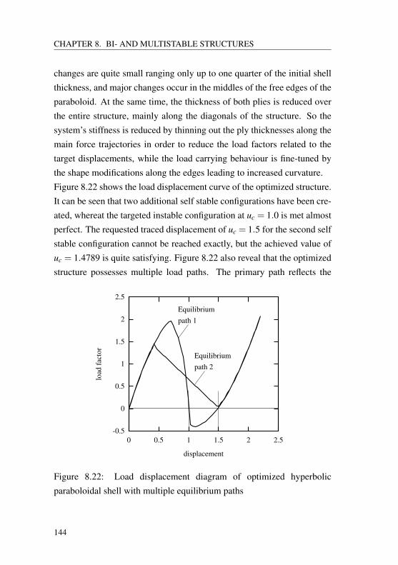
CHAPTER 8. BI- AND MULTISTABLE STRUCTURES
changes are quite small ranging only up to one quarter of the initial shellthickness, and major changes occur in the middles of the free edges of theparaboloid. At the same time, the thickness of both plies is reduced overthe entire structure, mainly along the diagonals of the structure. So thesystem’s stiffness is reduced by thinning out the ply thicknesses along themain force trajectories in order to reduce the load factors related to thetarget displacements, while the load carrying behaviour is fine-tuned bythe shape modifications along the edges leading to increased curvature.Figure 8.22 shows the load displacement curve of the optimized structure.It can be seen that two additional self stable configurations have been cre-ated, whereat the targeted instable configuration at uc = 1.0 is met almostperfect. The requested traced displacement of uc = 1.5 for the second selfstable configuration cannot be reached exactly, but the achieved value ofuc = 1.4789 is quite satisfying. Figure 8.22 also reveal that the optimizedstructure possesses multiple load paths. The primary path reflects the
-0.5
0
0.5
1
1.5
2
2.5
0 0.5 1 1.5 2 2.5
load
fact
or
displacement
Equilibriumpath 1
Equilibriumpath 2
Figure 8.22: Load displacement diagram of optimized hyperbolicparaboloidal shell with multiple equilibrium paths
144
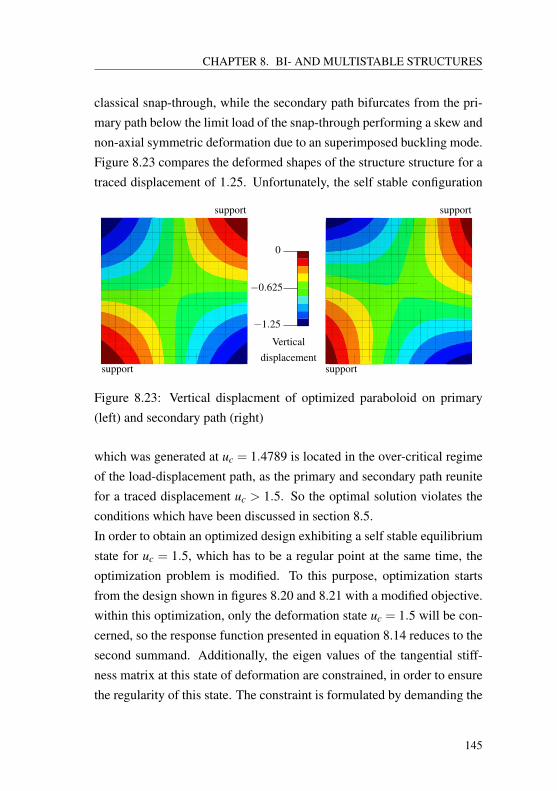
CHAPTER 8. BI- AND MULTISTABLE STRUCTURES
classical snap-through, while the secondary path bifurcates from the pri-mary path below the limit load of the snap-through performing a skew andnon-axial symmetric deformation due to an superimposed buckling mode.Figure 8.23 compares the deformed shapes of the structure structure for atraced displacement of 1.25. Unfortunately, the self stable configuration
0
−1.25
Verticaldisplacement
−0.625
support support
support support
Figure 8.23: Vertical displacment of optimized paraboloid on primary(left) and secondary path (right)
which was generated at uc = 1.4789 is located in the over-critical regimeof the load-displacement path, as the primary and secondary path reunitefor a traced displacement uc > 1.5. So the optimal solution violates theconditions which have been discussed in section 8.5.In order to obtain an optimized design exhibiting a self stable equilibriumstate for uc = 1.5, which has to be a regular point at the same time, theoptimization problem is modified. To this purpose, optimization startsfrom the design shown in figures 8.20 and 8.21 with a modified objective.within this optimization, only the deformation state uc = 1.5 will be con-cerned, so the response function presented in equation 8.14 reduces to thesecond summand. Additionally, the eigen values of the tangential stiff-ness matrix at this state of deformation are constrained, in order to ensurethe regularity of this state. The constraint is formulated by demanding the
145
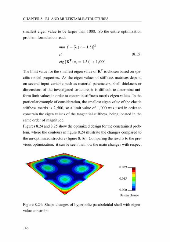
CHAPTER 8. BI- AND MULTISTABLE STRUCTURES
smallest eigen value to be larger than 1000. So the entire optimizationproblem formulation reads
min f = [λ (u = 1.5)]2
st
eig(KT (uc = 1.5)
)> 1,000
(8.15)
The limit value for the smallest eigen value of KT is chosen based on spe-cific model properties. As the eigen values of stiffness matrices dependon several input variable such as material parameters, shell thickness ordimensions of the investigated structure, it is difficult to determine uni-form limit values in order to constrain stiffness matrix eigen values. In theparticular example of consideration, the smallest eigen value of the elasticstiffness matrix is 2,500, so a limit value of 1,000 was used in order toconstrain the eigen values of the tangential stiffness, being located in thesame order of magnitude.Figures 8.24 and 8.25 show the optimized design for the constrained prob-lem, where the contours in figure 8.24 illustrate the changes compared tothe un-optimized structure (figure 8.16). Comparing the results to the pre-vious optimization, it can be seen that now the main changes with respect
0.029
0.000
Design change
0.015
Figure 8.24: Shape changes of hyperbolic paraboloidal shell with eigen-value constraint
146
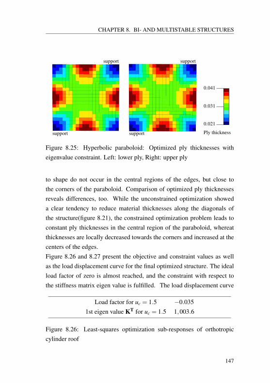
CHAPTER 8. BI- AND MULTISTABLE STRUCTURES
support support
supportsupport
0.041
0.021
Ply thickness
0.031
Figure 8.25: Hyperbolic paraboloid: Optimized ply thicknesses witheigenvalue constraint. Left: lower ply, Right: upper ply
to shape do not occur in the central regions of the edges, but close tothe corners of the paraboloid. Comparison of optimized ply thicknessesreveals differences, too. While the unconstrained optimization showeda clear tendency to reduce material thicknesses along the diagonals ofthe structure(figure 8.21), the constrained optimization problem leads toconstant ply thicknesses in the central region of the paraboloid, whereatthicknesses are locally decreased towards the corners and increased at thecenters of the edges.Figure 8.26 and 8.27 present the objective and constraint values as wellas the load displacement curve for the final optimized structure. The idealload factor of zero is almost reached, and the constraint with respect tothe stiffness matrix eigen value is fulfilled. The load displacement curve
Load factor for uc = 1.5 −0.0351st eigen value KT for uc = 1.5 1,003.6
Figure 8.26: Least-squares optimization sub-responses of orthotropiccylinder roof
147
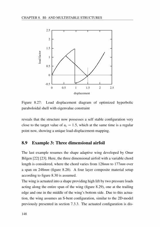
CHAPTER 8. BI- AND MULTISTABLE STRUCTURES
-0.5
0
0.5
1
1.5
2
2.5
0 0.5 1 1.5 2 2.5
load
fact
or
displacement
Figure 8.27: Load displacement diagram of optimized hyperbolicparaboloidal shell with eigenvalue constraint
reveals that the structure now possesses a self stable configuration veryclose to the target value of uc = 1.5, which at the same time is a regularpoint now, showing a unique load-displacement-mapping.
8.9 Example 3: Three dimensional airfoil
The last example resumes the shape adaptive wing developed by OnurBilgen [22] [23]. Here, the three dimensional airfoil with a variable chordlength is considered, where the chord varies from 128mm to 177mm overa span on 248mm (figure 8.28). A four layer composite material setupaccording to figure 8.30 is assumed.The wing is actuated into a shape providing high lift by two pressure loadsacting along the entire span of the wing (figure 8.29), one at the trailingedge and one in the middle of the wing’s bottom side. Due to this actua-tion, the wing assumes an S-bent configuration, similar to the 2D-modelpreviously presented in section 7.3.3. The actuated configuration is dis-
148
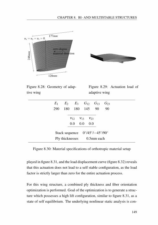
CHAPTER 8. BI- AND MULTISTABLE STRUCTURES
128mm
248m
m
177mmux = uy = uz = 0
zero-degreematerial direction
Figure 8.28: Geometry of adap-tive wing
Figure 8.29: Actuation load ofadaptive wing
E1 E2 E3 G12 G13 G23
290 180 180 145 90 90
ν12 ν13 ν23
0.0 0.0 0.0
Stack sequence 0/45/−45/90
Ply thicknesses 0.5mm each
Figure 8.30: Material specifications of orthotropic material setup
played in figure 8.31, and the load displacement curve (figure 8.32) revealsthat this actuation does not lead to a self stable configuration, as the loadfactor is strictly larger than zero for the entire actuation process.
For this wing structure, a combined ply thickness and fiber orientationoptimization is performed. Goal of the optimization is to generate a struc-ture which possesses a high lift configuration, similar to figure 8.31, as astate of self equilibrium. The underlying nonlinear static analysis is con-
149
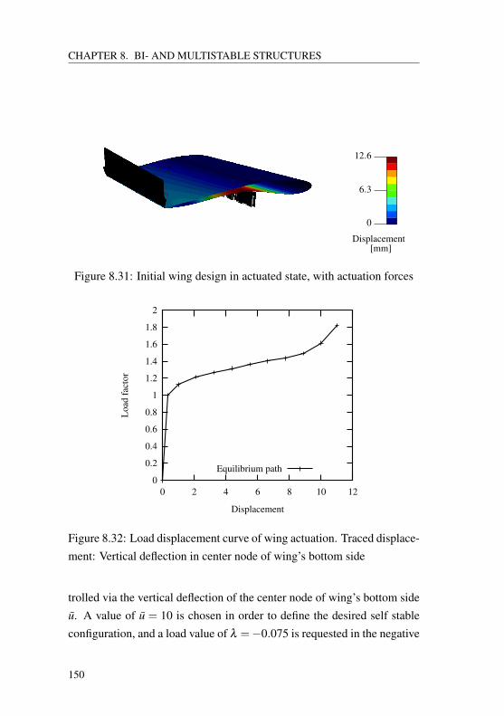
CHAPTER 8. BI- AND MULTISTABLE STRUCTURES
12.6
0
Displacement
6.3
[mm]
Figure 8.31: Initial wing design in actuated state, with actuation forces
0
0.2
0.4
0.6
0.8
1
1.2
1.4
1.6
1.8
2
0 2 4 6 8 10 12
Loa
dfa
ctor
Displacement
Equilibrium path
Figure 8.32: Load displacement curve of wing actuation. Traced displace-ment: Vertical deflection in center node of wing’s bottom side
trolled via the vertical deflection of the center node of wing’s bottom sideu. A value of u = 10 is chosen in order to define the desired self stableconfiguration, and a load value of λ =−0.075 is requested in the negative
150
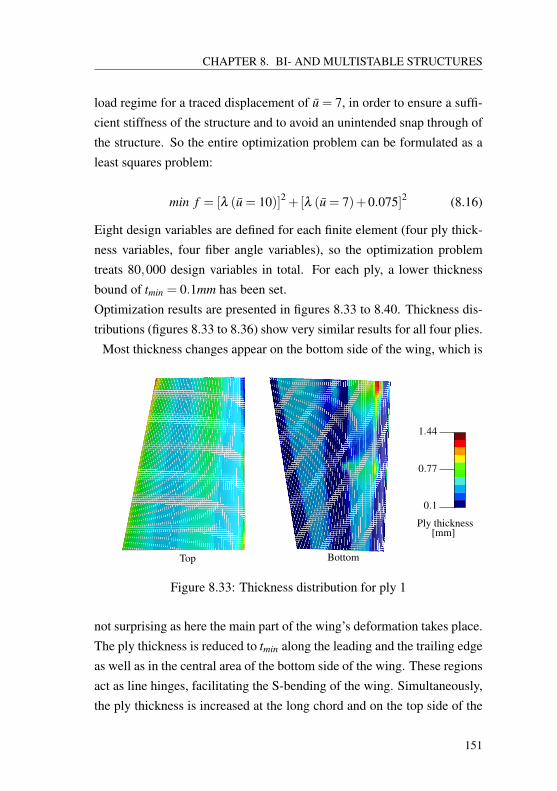
CHAPTER 8. BI- AND MULTISTABLE STRUCTURES
load regime for a traced displacement of u = 7, in order to ensure a suffi-cient stiffness of the structure and to avoid an unintended snap through ofthe structure. So the entire optimization problem can be formulated as aleast squares problem:
min f = [λ (u = 10)]2 +[λ (u = 7)+0.075]2 (8.16)
Eight design variables are defined for each finite element (four ply thick-ness variables, four fiber angle variables), so the optimization problemtreats 80,000 design variables in total. For each ply, a lower thicknessbound of tmin = 0.1mm has been set.Optimization results are presented in figures 8.33 to 8.40. Thickness dis-tributions (figures 8.33 to 8.36) show very similar results for all four plies.
Most thickness changes appear on the bottom side of the wing, which is
1.44
0.1
Ply thickness
0.77
Top Bottom
[mm]
Figure 8.33: Thickness distribution for ply 1
not surprising as here the main part of the wing’s deformation takes place.The ply thickness is reduced to tmin along the leading and the trailing edgeas well as in the central area of the bottom side of the wing. These regionsact as line hinges, facilitating the S-bending of the wing. Simultaneously,the ply thickness is increased at the long chord and on the top side of the
151
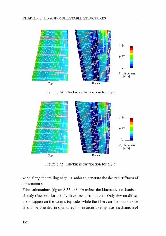
CHAPTER 8. BI- AND MULTISTABLE STRUCTURES
1.44
0.1
0.77
Top Bottom
Figure 8.34: Thickness distribution for ply 2
1.44
0.1
0.77
Top Bottom
Figure 8.35: Thickness distribution for ply 3
wing along the trailing edge, in order to generate the desired stiffness ofthe structure.Fiber orientations (figure 8.37 to 8.40) reflect the kinematic mechanismsalready observed for the ply thickness distributions. Only few modifica-tions happen on the wing’s top side, while the fibers on the bottom sidetend to be oriented in span direction in order to emphasis mechanism of
152
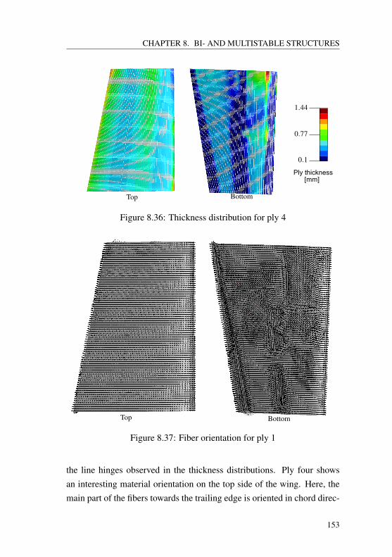
CHAPTER 8. BI- AND MULTISTABLE STRUCTURES
1.44
0.1
0.77
Top Bottom
Figure 8.36: Thickness distribution for ply 4
BottomTop
Figure 8.37: Fiber orientation for ply 1
the line hinges observed in the thickness distributions. Ply four showsan interesting material orientation on the top side of the wing. Here, themain part of the fibers towards the trailing edge is oriented in chord direc-
153
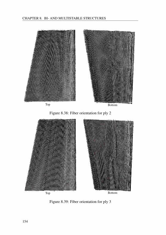
CHAPTER 8. BI- AND MULTISTABLE STRUCTURES
BottomTop
Figure 8.38: Fiber orientation for ply 2
BottomTop
Figure 8.39: Fiber orientation for ply 3
154
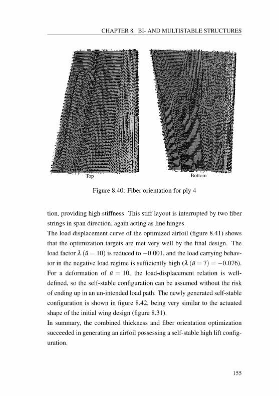
CHAPTER 8. BI- AND MULTISTABLE STRUCTURES
BottomTop
Figure 8.40: Fiber orientation for ply 4
tion, providing high stiffness. This stiff layout is interrupted by two fiberstrings in span direction, again acting as line hinges.The load displacement curve of the optimized airfoil (figure 8.41) showsthat the optimization targets are met very well by the final design. Theload factor λ (u = 10) is reduced to −0.001, and the load carrying behav-ior in the negative load regime is sufficiently high (λ (u = 7) = −0.076).For a deformation of u = 10, the load-displacement relation is well-defined, so the self-stable configuration can be assumed without the riskof ending up in an un-intended load path. The newly generated self-stableconfiguration is shown in figure 8.42, being very similar to the actuatedshape of the initial wing design (figure 8.31).In summary, the combined thickness and fiber orientation optimizationsucceeded in generating an airfoil possessing a self-stable high lift config-uration.
155
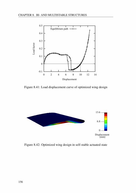
CHAPTER 8. BI- AND MULTISTABLE STRUCTURES
-0.1
0
0.1
0.2
0.3
0.4
0.5
0 2 4 6 8 10 12 14
Loa
dfa
ctor
Displacement
Equilibrium path
Figure 8.41: Load displacement curve of optimized wing design
13.6
0
Displacement
6.8
[mm]
Figure 8.42: Optimized wing design in self-stable actuated state
156
CHAPTER 8. BI- AND MULTISTABLE STRUCTURES
8.10 Conclusion
In summary, it can be noted that the presented formulation of an opti-mization response function based on displacement controlled analysis isapplicable for the generation and development of bistable shell structures.Avoidance of undesired or ambiguous solutions may require an enhancedformulation of the optimization problem, as it can be seen section 8.7.2 orin the last example.The presented examples showed that small changes in shape may alreadyhave a high influence on the load carrying behaviour of a structure. Thussensitivity of bistable structures with respect to imperfections has to beconsidered to be high, which also was observed by Coburn et al [43].
157

CHAPTER 8. BI- AND MULTISTABLE STRUCTURES
158
CHAPTER 9. SUMMARY & OUTLOOK
CHAPTER 9
Summary & Outlook
9.1 Summary
This thesis addressed the issue of generating structures with optimal kine-matic properties, which is a central issue concerning controlled or selec-tively adapted structures. Thereby the main focus was on shell structures,where fundamental kinematic mechanisms of shells have been discussedand successfully generated by means of parameter free shape optimiza-tion. Depending on the loading, the stress state inside the structure and onrestricting boundary conditions, line hinges or corrugated bellows turnedout to be the design elements providing best flexibility. Results showedthat the shapes of these kinematic elements may not be unique, especiallywhen stress states dominated by normal forces are considered. Conse-quently the choice of different optimization setup parameters, such asshell thicknesses or filter radii, might lead to different optimal designs,whereby different designs may perform quite comparably with respect tothe chosen objective function.
The gained awarenesses about kinematic mechanisms were transferred toactuated structures, and the issue of optimal actuation was discussed. Thisbecomes an important aspect when optimal kinematic mechanisms are
159
CHAPTER 9. SUMMARY & OUTLOOK
developed for smart structures, which also includes the problem of actu-ator placement and tuning. It turned out that optimization with respectto optimal actuation implies additional difficulties, as the parallel treat-ment of different types of design variables increases the non-convexity ofthe optimization problem tremendously. A modified filtering and shapecontrol scheme was presented in order to improve orientation of the opti-mization algorithm in this highly non-convex design space.
Finally, the relatively new research field of bistable structures wasaddressed. Bistable structures might be an interesting alternative to "clas-sical" smart structures, needing permanent actuator input. This thesisapplied numerical optimization methods in order to generate structuresexhibiting bistable character. For this purpose, a response function basedon a displacement controlled nonlinear static analysis including an appro-priate predictor scheme was developed. The fitness of this response func-tion has been verified using single and double curved structures. Herebyone can observe that small changes in shape may lead to significantchanges in the load carrying behaviour of shell structures. This especiallyappears when starting from uniaxially curved shells or when modifyingthe edge region of a shell.As the investigated structures are characterized by a significant nonlinearload carrying behaviour, ensuring regularity of the target configuration isa crucial point in generating new self-stable configurations. For this pur-pose, an eigenvalue-based evaluation criteria was used in order to avoidsolutions located on secondary load paths or within a buckling process.
9.2 Outlook
Starting from this thesis, continuative works should be performed in con-text of adaptive structures. Within this work, actuation was considered inan abstract way as a load onto the structure without regarding any con-
160
CHAPTER 9. SUMMARY & OUTLOOK
straints with respect to applicable actuator mechanisms, such as a limitedadjustment travel or maximum allowable curvatures of a laminar actua-tor, for example. Enlarging the optimization process by such constraintswould be a big step towards general applicability.
Another interesting point is verification of the shell designs optimizedwith respect to bistability. For this purpose, prototype construction andtesting of selected shell designs could be performed, in order to verifycomputational results by experimental data.Current research concerning bistable structures only addresses academicexamples. Thus a proceeding step might be the application of bistability toa "real world"-example of a smart structure. As reliability and durabilityof this kind of structures is not tested or verified so far, one possible fieldof application might be unfolding mechanisms for satellites or other spacestructures requiring only a few or even only one transformation cycle intheir entire life time.
161

CHAPTER 9. SUMMARY & OUTLOOK
162
APPENDIX A. RESPONSE FUNCTIONS AND THEIR DERIVATIVES
CHAPTER AResponse functions and their
derivatives
A.1 Geometric linear static computations
A.1.1 Derivation of the state equation
The state equation of static linear problems in structural mechanics can beformulated in the well-known form
S(u) = K ·u− fext = 0 (A.1)
Taking the derivative of S with respect to a design variable si according toequation 5.31 requires the application of the chain rule of differentiation:
dSdsi
= ∂S∂ si
+ ∂S∂u · ∂u
∂ si= 0
dSdsi
= ∂K∂ si·u− ∂ fext
∂ si+ K · ∂u
∂ si= 0
(A.2)
Solving this expression for ∂u∂ si
leads to
∂u∂ si
=[
∂S∂u
]−1·
[− ∂S
∂ si
]∂u∂ si
= K−1 ·[
∂ fext
∂ si− ∂K
∂ si·u]
︸ ︷︷ ︸f
(A.3)
163
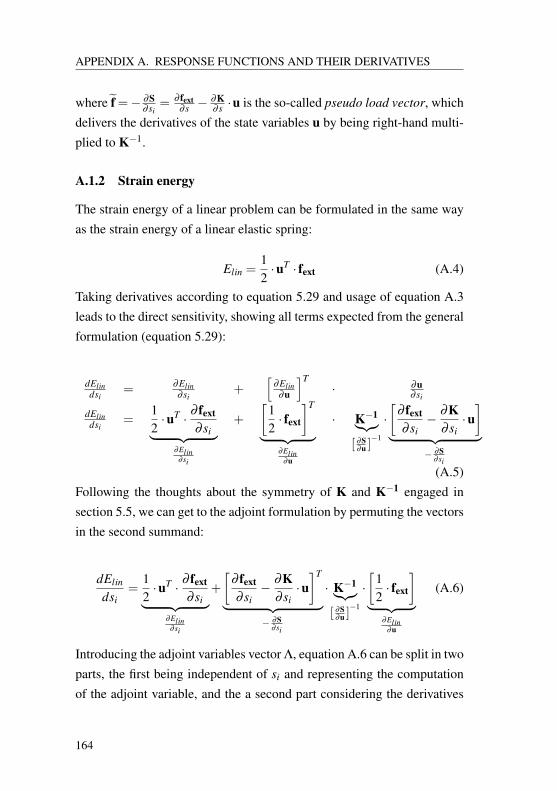
APPENDIX A. RESPONSE FUNCTIONS AND THEIR DERIVATIVES
where f =− ∂S∂ si
= ∂ fext∂ s −
∂K∂ s ·u is the so-called pseudo load vector, which
delivers the derivatives of the state variables u by being right-hand multi-plied to K−1.
A.1.2 Strain energy
The strain energy of a linear problem can be formulated in the same wayas the strain energy of a linear elastic spring:
Elin =12·uT · fext (A.4)
Taking derivatives according to equation 5.29 and usage of equation A.3leads to the direct sensitivity, showing all terms expected from the generalformulation (equation 5.29):
dElindsi
= ∂Elin∂ si
+[
∂Elin∂u
]T· ∂u
∂ si
dElindsi
=12·uT · ∂ fext
∂ si︸ ︷︷ ︸∂Elin
∂ si
+
[12· fext
]T
︸ ︷︷ ︸∂Elin
∂u
· K−1︸︷︷︸[ ∂S
∂u ]−1
·[
∂ fext
∂ si− ∂K
∂ si·u]
︸ ︷︷ ︸− ∂S
∂ si
(A.5)Following the thoughts about the symmetry of K and K−1 engaged insection 5.5, we can get to the adjoint formulation by permuting the vectorsin the second summand:
dElin
dsi=
12·uT · ∂ fext
∂ si︸ ︷︷ ︸∂Elin
∂ si
+
[∂ fext
∂ si− ∂K
∂ si·u]T
︸ ︷︷ ︸− ∂S
∂ si
· K−1︸︷︷︸[ ∂S
∂u ]−1
·[
12· fext
]︸ ︷︷ ︸
∂Elin∂u
(A.6)
Introducing the adjoint variables vector Λ, equation A.6 can be split in twoparts, the first being independent of si and representing the computationof the adjoint variable, and the a second part considering the derivatives
164
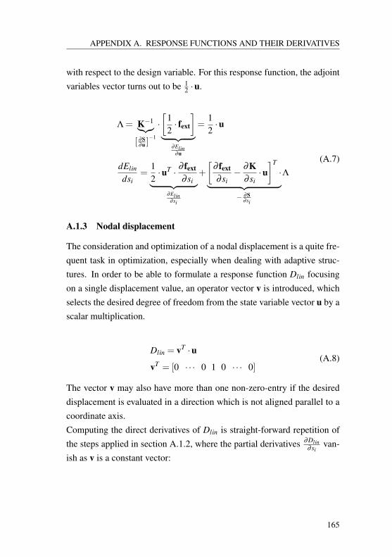
APPENDIX A. RESPONSE FUNCTIONS AND THEIR DERIVATIVES
with respect to the design variable. For this response function, the adjointvariables vector turns out to be 1
2 ·u.
Λ = K−1︸︷︷︸[ ∂S
∂u ]−1
·[
12· fext
]︸ ︷︷ ︸
∂Elin∂u
=12·u
dElin
dsi=
12·uT · ∂ fext
∂ si︸ ︷︷ ︸∂Elin
∂ si
+
[∂ fext
∂ si− ∂K
∂ si·u]T
·︸ ︷︷ ︸− ∂S
∂ si
Λ
(A.7)
A.1.3 Nodal displacement
The consideration and optimization of a nodal displacement is a quite fre-quent task in optimization, especially when dealing with adaptive struc-tures. In order to be able to formulate a response function Dlin focusingon a single displacement value, an operator vector v is introduced, whichselects the desired degree of freedom from the state variable vector u by ascalar multiplication.
Dlin = vT ·u
vT = [0 · · · 0 1 0 · · · 0](A.8)
The vector v may also have more than one non-zero-entry if the desireddisplacement is evaluated in a direction which is not aligned parallel to acoordinate axis.Computing the direct derivatives of Dlin is straight-forward repetition ofthe steps applied in section A.1.2, where the partial derivatives ∂Dlin
∂ sivan-
ish as v is a constant vector:
165
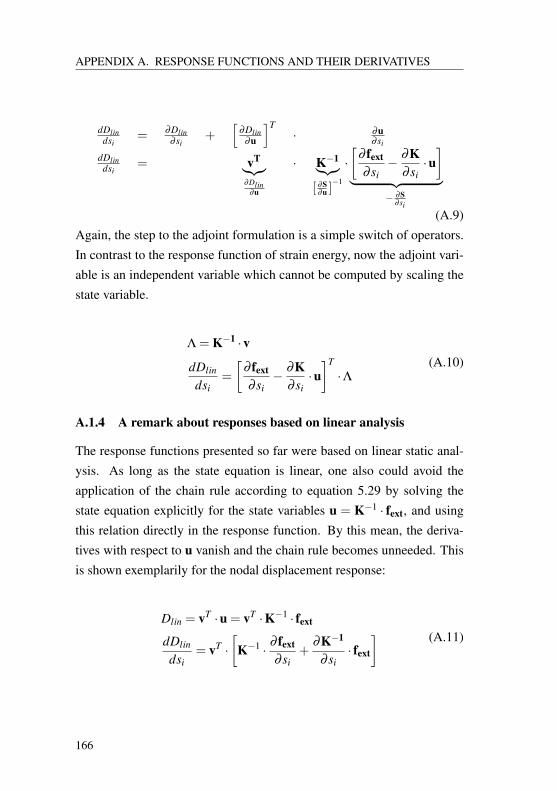
APPENDIX A. RESPONSE FUNCTIONS AND THEIR DERIVATIVES
dDlindsi
= ∂Dlin∂ si
+[
∂Dlin∂u
]T· ∂u
∂ si
dDlindsi
= vT︸︷︷︸∂Dlin
∂u
· K−1︸︷︷︸[ ∂S
∂u ]−1
·[
∂ fext
∂ si− ∂K
∂ si·u]
︸ ︷︷ ︸− ∂S
∂ si(A.9)
Again, the step to the adjoint formulation is a simple switch of operators.In contrast to the response function of strain energy, now the adjoint vari-able is an independent variable which cannot be computed by scaling thestate variable.
Λ = K−1 ·v
dDlin
dsi=
[∂ fext
∂ si− ∂K
∂ si·u]T
·Λ(A.10)
A.1.4 A remark about responses based on linear analysis
The response functions presented so far were based on linear static anal-ysis. As long as the state equation is linear, one also could avoid theapplication of the chain rule according to equation 5.29 by solving thestate equation explicitly for the state variables u = K−1 · fext, and usingthis relation directly in the response function. By this mean, the deriva-tives with respect to u vanish and the chain rule becomes unneeded. Thisis shown exemplarily for the nodal displacement response:
Dlin = vT ·u = vT ·K−1 · fext
dDlin
dsi= vT ·
[K−1 · ∂ fext
∂ si+
∂K−1
∂ si· fext
] (A.11)
166
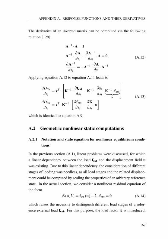
APPENDIX A. RESPONSE FUNCTIONS AND THEIR DERIVATIVES
The derivative of an inverted matrix can be computed via the followingrelation [129]:
A−1 ·A = I
A−1 · ∂A∂ si
+∂A−1
∂ si·A = 0
∂A−1
∂ si=−A−1 · ∂A
∂ si·A−1
(A.12)
Applying equation A.12 to equation A.11 leads to
dDlin
dsi= vT ·
K−1 · ∂ fext
∂ si−K−1 · ∂K
∂ si·K−1 · fext︸ ︷︷ ︸
u
dDlin
dsi= vT ·K−1 ·
[∂ fext
∂ si− ∂K
∂ si·u] (A.13)
which is identical to equation A.9.
A.2 Geometric nonlinear static computations
A.2.1 Notation and state equation for nonlinear equilibrium condi-tions
In the previous section (A.1), linear problems were discussed, for whicha linear dependency between the load fext and the displacement field uwas existing. Due to this linear dependency, the consideration of differentstages of loading was needless, as all load stages and the related displace-ment could be computed by scaling the properties of an arbitrary referencestate. In the actual section, we consider a nonlinear residual equation ofthe form
S(u,λ ) = fint (u)−λ · fext = 0 (A.14)
which raises the necessity to distinguish different load stages of a refer-ence external load fext. For this purpose, the load factor λ is introduced,
167
APPENDIX A. RESPONSE FUNCTIONS AND THEIR DERIVATIVES
which scales the reference load vector.
In the following, it is assumed that λ and u form a pair which satisfiesequation A.14.
A.2.2 Derivation of the state equation
In order to take the derivative of the state equation A.14 with respect toa design parameter si, again the chain rule of differentiation has to beapplied.
dSdsi
= ∂S∂ si
+ ∂S∂u · ∂u
∂ si= 0
dSdsi
= ∂ fint∂ si−λ · ∂ fext
∂ si+ KT · ∂u
∂ si= 0
(A.15)
exploiting that the derivative of the residual force ∂S∂u = fint
∂u is equal to thetangential stiffness matrix KT.Solving this equation for the derivative of state variables again leads to alinear problem with the partial derivatives of the residual equation withrespect to the design parameter acting as a pseudo load f = − ∂S
∂ si= λ ·
∂ fext∂ si− ∂ fint
∂ si:
∂u∂ si
=[
∂S∂u
]−1·
[− ∂S
∂ si
]∂u∂ si
=[KT]−1 ·
[λ · ∂ fext
∂ si− ∂ fint
∂ si
]︸ ︷︷ ︸
f
(A.16)
A.2.3 Strain energy
When computing the strain energy Enonlin of a system under consider-ation of nonlinear behavior, the load stagging and the nonlinear load-displacement relation have to be taken into account. In order to computethe strain energy stored in a system configuration which is defined by the
168
APPENDIX A. RESPONSE FUNCTIONS AND THEIR DERIVATIVES
load factor λ and the displacement field u, energy has to be measured inan integral manner over the load staging parameter λ
E =
λ∫λ=0
fextT ·u
(λ
)dλ (A.17a)
E = λ · fextT ·u− E (A.17b)
where equation A.17a determines the complementary strain energy E, andequation A.17b computes the effective strain energy E. In these formulas,λ and u are still assumed to be conjugated via equation A.14, as well asλ and u
(λ
)are.
As the functional relation u(
λ
)is not known analytically, the integral is
evaluated using an approximation, where the linear relation
u(
λ
)≈ λ
λ·u (A.18)
is assumed. This kind of linear assumption is quite frequently used incontext of geometrically nonlinear optimization and also can be found in[53] or [34]. This simplifies equations A.17a and A.17b to
E ≈ E ≈ 12·λ · fext
T ·u = Enonlin (A.19)
which is similar to equation A.4 in the linear case.In figure A.1, the real strain energy measure according to equation A.17band the approximated strain energy according to equation A.19 are com-pared using an exemplary load-displacement curve.Using the approximated formulation according to equation A.19, thederivative can be computed in a similar way as it was done for the lin-ear case (equation A.5)
169
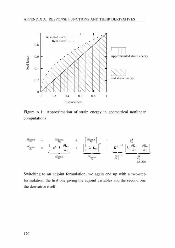
APPENDIX A. RESPONSE FUNCTIONS AND THEIR DERIVATIVES
0
0.2
0.4
0.6
0.8
1
0 0.2 0.4 0.6 0.8 1
load
fact
or
displacement
Assumed curveReal curve
Approxiamted strain energy
real strain energy
Figure A.1: Approximation of strain energy in geometrical nonlinearcomputations
dEnonlindsi
= ∂Enonlin∂ si
+[
∂Enonlin∂u
]T· ∂u
∂ si
dEnonlindsi
=12·uT ·λ · ∂ fext
∂ si︸ ︷︷ ︸∂Enonlin
∂ si
+
[12·λ · fext
]T
︸ ︷︷ ︸∂Enonlin
∂u
·[KT]−1
︸ ︷︷ ︸[∂S∂u
]−1
·[
λ · ∂ fext∂ si− ∂ fint
∂ si
]︸ ︷︷ ︸
− ∂S∂ si
(A.20)
Switching to an adjoint formulation, we again end up with a two-stepformulation, the first one giving the adjoint variables and the second onethe derivative itself.
170
APPENDIX A. RESPONSE FUNCTIONS AND THEIR DERIVATIVES
Λ =[KT]−1︸ ︷︷ ︸[ ∂S
∂u ]−1
·[
12·λ · fext
]︸ ︷︷ ︸
∂Enonlin∂u
dEnonlin
dsi=
12·uT ·λ · ∂ fext
∂ si︸ ︷︷ ︸∂Enonlin
∂ si
+
T[λ · ∂ fext
∂ si− ∂ fint
∂ si
]︸ ︷︷ ︸
− ∂S∂ si
·Λ
(A.21)
A.2.4 Nodal displacement
The objective function focusing on a nodal displacement or rotation isformulated in the same way as it is done in the geometrical linear case.Again the operator vector v is multiplied to the displacement field vectoru in order to define the objective function:
Dnonlin = vT ·u
vT = [0 · · · 0 1 0 · · · 0](A.22)
Computing the derivative, the nonlinear formulation behaves differentlyto the linear one, as the derivative of the state variables ∂u
∂ siis based on a
different state equation (equation A.16).
dDnonlindsi
= ∂Dnonlin∂ si
+[
∂Dnonlin∂u
]T· ∂u
∂ si
dDnonlindsi
= vT︸︷︷︸∂Dnonlin
∂u
·[KT]−1︸ ︷︷ ︸[ ∂S
∂u ]−1
·[
λ · ∂ fext
∂ si− ∂ fint
∂ si
]︸ ︷︷ ︸
− ∂S∂ si
(A.23)Switching to the adjoint formulation, another similarity to the geometricallinear formulated response appears, as in both cases the right hand side inthe adjoint equation system is formed by the operator vector.
171
APPENDIX A. RESPONSE FUNCTIONS AND THEIR DERIVATIVES
Λ =[KT]−1 ·v
dDnonlin
dsi=
[λ · ∂ fext
∂ si− ∂ fint
∂ si
]T
·Λ(A.24)
172
BIBLIOGRAPHY
Bibliography
[1] J. Adamy. Nichtlineare Regelungen. Berlin and Heidelberg:Springer, 2009. ISBN: 978-3642007934.
[2] G. Akhras. “Smart materials and smart systems for the future”. In:Canadian Military Journal 2000.
[3] U. Andelfinger and E. Ramm. “EAS-elements for two-dimensional, three-dimensional, plate and shell structures andtheir equivalence to HR-elements”. In: International Journal for
Numerical Methods in Engineering 36.8 (1993), pp. 1311–1337.ISSN: 0029-5981. DOI: 10.1002/nme.1620360805.
[4] T. Arens et al. Mathematik. 1. Aufl. Heidelberg: SpektrumAkademischer Verlag, 2008. ISBN: 3827417589.
[5] J. H. Argyris. Die Methode der finiten Elemente in der ele-
mentaren Strukturmechanik. Braunschweig: Vieweg, 1986. ISBN:3528089199.
[6] J. H. Argyris and H.-P. Mlejnek. Computerdynamik der Tragw-
erke. [Studienausg.] Vol. Studienbuch für Ingenieure und Natur-wissenschaftler / John Argyris; Hans-Peter Mlejnek ; Bd. 3.Die Methode der finiten Elemente. Braunschweig [u.a.]: Vieweg,1997. ISBN: 3528069163.
[7] L. Armijo. “Minimization of functions having Lipschitz continu-ous first partial derivatives”. In: Pacific J. Math 16 (1966).
173
BIBLIOGRAPHY
[8] J. S. Arora. Introduction to optimum design. 3rd ed. Boston andMA: Academic Press, 2011. ISBN: 978-0123813756.
[9] D. Ashlock. Evolutionary computation for modeling and opti-
mization. New York: Springer, 2006. ISBN: 0387221964.
[10] H. Baier, C. Seesselberg, and B. Specht. Optimierung in der
Strukturmechanik. Braunschweig and Wiesbaden: Vieweg, 1994.ISBN: 3528088990.
[11] R. Baldick. Applied optimization: Formulation and algorithms for
engineering systems. Cambridge, U.K, and New York: CambridgeUniversity Press, 2006. ISBN: 0521100283.
[12] B. Barthelemy, C. T. Chon, and R. T. Haftka. “Accuracy problemsassocited with semi-analytical derivatives of static response”. In:Finite Elements in Analysis and Design 4.3 (1988), pp. 249–265.ISSN: 0168874X. DOI: 10.1016/0168-874X(88)90011-X.
[13] F.-J. Barthold and E. Stein. “A continuum mechanical-based for-mulation of the variational sensitivity analysis in structural opti-mization. Part I: analysis”. In: Structural Optimization 11.1-2(1996), pp. 29–42. ISSN: 0934-4373. DOI: 10.1007/BF01279652.
[14] K.-J. Bathe. Finite-Elemente-Methoden. 2., vollst. neu bearb. underw. Aufl. Berlin [u.a.]: Springer, 2002. ISBN: 978-3540668060.
[15] K.-J. Bathe and E. Dvorkin. “A formulation of general shellelements—the use of mixed interpolation of tensorial compo-nents”. In: Int J Numer Methods Eng 22 (1986), pp. 697–722.
[16] K.-J. Bathe and E. Dvorkin. “A four-node plate bending elementbased on Mindlin/Reissner plate theory and a mixed interpola-tion”. In: Int J Numer Methods Eng 21 (1985), pp. 367–383.
174
BIBLIOGRAPHY
[17] J.-L. Batoz and G. Dhatt. “Incremental displacement algorithmsfor nonlinear problems”. In: International Journal for Numerical
Methods in Engineering 14.8 (1979), pp. 1262–1267. ISSN: 0029-5981. DOI: 10.1002/nme.1620140811.
[18] R. Bellman. Introduction to matrix analysis. 2nd ed. Vol. 19.Classics in applied mathematics. Philadelphia and Pa: Society forIndustrial and Applied Mathematics (SIAM 3600 Market StreetFloor 6 Philadelphia PA 19104), 1997. ISBN: 0898713994. URL:http://epubs.siam.org/ebooks/siam/classics_
in_applied_mathematics/cl19.
[19] T. Belytschko, W. K. Liu, and B. Moran. Nonlinear finite elements
for continua and structures. Chichester and New York: Wiley,2000. ISBN: 0471987743.
[20] M. P. Bendsoe and O. Sigmund. Topology optimization: Theory,
methods, and applications. Berlin and New York: Springer, 2003.ISBN: 3540429921.
[21] J.-M. Berthelot. Composite Materials: Mechanical Behavior and
Structural Analysis. Mechanical Engineering Series. New Yorkand NY: Springer New York, 1999. ISBN: 978-1-4612-0527-2.
[22] O. Bilgen, E. Flores, and M. I. Friswell. “Optimization of Surface-Actuated Piezocomposite Variable-Camber Morphing Wings”. In:ASME 2011 Conference on Smart Materials, Adaptive Structures
and Intelligent Systems (2011), pp. 315–322.
[23] O. Bilgen and M. I. Friswell. “Piezoceramic composite actuatorsfor a solid-state variable-camber wing”. In: Journal of Intelligent
Material Systems and Structures 25 (2014), pp. 806–817.
[24] M. Bischoff. Theorie und Numerik einer dreidimensionalen
Schalenformulierung. Bericht Nr. 30, Institut für Baustatik, Uni-versität Stuttgart, 1999.
175
BIBLIOGRAPHY
[25] K.-U. Bletzinger. “A consistent frame for sensitivity filtering andthe vertex assigned morphing of optimal shape”. In: Structural
and Multidisciplinary Optimization (2014). ISSN: 1615-147X.DOI: 10.1007/s00158-013-1031-5.
[26] K.-U. Bletzinger, M. Firl, and F. Daoud. “Approximation ofderivatives in semi-analytical structural optimization”. In: Com-
puters & Structures 86.13-14 (2008), pp. 1404–1416. ISSN:00457949. DOI: 10.1016/j.compstruc.2007.04.014.
[27] K.-U. Bletzinger, M. Firl, and M. Fischer. “Parameter free shapedesign of thin shells: Efficient and effective, parallel solution tech-niques for very large design problems”. In: 2nd International
Conference on Engineering Optimization, Lisbon (2010).
[28] K.-U. Bletzinger et al. “Computational methods for form findingand optimization of shells and membranes”. In: Computer Meth-
ods in Applied Mechanics and Engineering 194.30-33 (2005),pp. 3438–3452. ISSN: 00457825. DOI: 10.1016/j.cma.2004.12.026.
[29] K.-U. Bletzinger et al. “Optimal shapes of mechanically moti-vated surfaces”. In: Computer Methods in Applied Mechanics and
Engineering 199.5-8 (2010), pp. 324–333. ISSN: 00457825. DOI:10.1016/j.cma.2008.09.009.
[30] K.-U. Bletzinger et al. “Shape Optimization with ProgramCARAT”. In: Software systems for structural optimization. Ed. byHörnlein, H. R. E. M and K. Schittkowski. Vol. vol. 110. ISNM.Basel and Boston: Birkhäuser, 1993, pp. 97–124. ISBN: 978-3-7643-2836-8.
[31] P. T. Boggs and J. W. Tolle. “Sequential quadratic programming”.In: Acta numerica 4 (1995), pp. 1–51.
176
BIBLIOGRAPHY
[32] M. Braun. Nichtlineare Analyse von geschichteten, elastischen
Flächentragwerken. Bericht Nr. 19, Institut für Baustatik, Univer-sität Stuttgart, 1995.
[33] C. G. Broyden. “The Convergence of a Class of Double-rank Min-imization Algorithms 1. General Considerations”. In: IMA Jour-
nal of Applied Mathematics 6.1 (1970), pp. 76–90. ISSN: 0272-4960.
[34] T. Buhl, C. B. Pedersen, and O. Sigmund. “Stiffness design ofgeometrically nonlinear structures using topology optimization”.In: Structural and Multidisciplinary Optimization 19 (2000),pp. 93–104.
[35] C. R. Calladine. Theory of shell structures. Cambridge [Cam-bridgeshire] and New York: Cambridge University Press, 1983.ISBN: 0521369452.
[36] Y. Cao, S. Li, and L. Petzold. “Adjoint sensitivity analysis fordifferential-algebraic equations: algorithms and software”. In:Journal of Computational and Applied Mathematics 149 (2002),pp. 171–191.
[37] E. Carmel and D. Cohen-Or. “Warp-guided object-space morph-ing”. In: The Visual Computer 13.9-10 (1998), pp. 465–478. ISSN:01782789. DOI: 10.1007/s003710050118.
[38] Z. Chen et al. “Nonlinear Geometric Effects in MechanicalBistable Morphing Structures”. In: Physical Review Letters 109(2012), p. 114302.
[39] K. Choi and N. H. Kim. Structural sensitivity analysis and opti-
mization 1: Linear Systems. Mechanical Engineering Series. NewYork: Springer Science+Business Media, 2005. ISBN: 0-387-23336-9.
177
BIBLIOGRAPHY
[40] K. Choi and N. H. Kim. Structural sensitivity analysis and
optimization 2: Nonlinear Systems and Applications. Mechani-cal Engineering Series. New York: Springer Science+BusinessMedia, 2005. ISBN: 978-0-387-27169-9.
[41] K. K. Choong and E. Ramm. “Simulation of buckling pro-cess of shells by using the finite element method”. In: Thin-
Walled Structures 31.1-3 (1998), pp. 39–72. ISSN: 02638231.DOI: 10.1016/S0263-8231(98)00002-0.
[42] R. L. Clark, W. R. Saunders, and G. P. Gibbs. Adaptive struc-
tures: Dynamics and control. New York: Wiley, 1998. ISBN:0471122629.
[43] B. H. Coburn et al. “Tristability of an orthotropic doubly curvedshell”. In: Composite Structures 96 (2013), pp. 446–454. ISSN:02638223. DOI: 10.1016/j.compstruct.2012.08.026.
[44] B. Cockburn, G. Karniadakis, and C.-W. Shu. Discontinu-
ous Galerkin methods: Theory, computation, and applications.Vol. 11. Lecture notes in computational science and engineering.Berlin and New York: Springer, 2000. ISBN: 3540667873.
[45] W. Dahmen and A. Reusken. Numerik für Ingenieure und Natur-
wissenschaftler. 2., korrigierte Aufl. Springer-Lehrbuch. Berlinand Heidelberg: Springer, 2008. ISBN: 978-3-540-76492-2.
[46] F. Daoud. Formoptimierung von Freiformschalen: Mathematis-
che Algorithmen und Filtertechniken. Dissertation at the Chair ofStructural Analysis at the Technical University of Munich, 2005.
[47] M. C. Delfour and J. P. Zolésio. Shapes and geometries: Analysis,
differential calculus, and optimization. Advances in design andcontrol. Philadelphia: Society for Industrial and Applied Mathe-matics, 2001. ISBN: 0898714893.
178
BIBLIOGRAPHY
[48] P. Deuflhard. Newton methods for nonlinear problems: Affine
invariance and adaptive algorithms. Vol. 35. Springer seriesin computational mathematics. Berlin and New York: Springer,2004. ISBN: 3540210997.
[49] D. A. Di Pietro and A. Ern. Mathematical aspects of discontin-
uous galerkin methods. Vol. 69. Mathématiques et Applications.Berlin and New York: Springer, 2012. ISBN: 978-3-642-22979-4.
[50] M. Drela. “XFOIL: An Analysis and Design System for LowReynolds Number Airfoils”. In: Low Reynolds Number Aerody-
namics. Ed. by C. A. Brebbia et al. Vol. 54. Lecture Notes inEngineering. Berlin and Heidelberg: Springer Berlin Heidelberg,1989, pp. 1–12. ISBN: 978-3-540-51884-6. DOI: 10.1007/978-3-642-84010-4_1.
[51] K. A. Dunn et al. “Application of Smart Materials/Technology atthe Savannah River Site”. In: 1999 Symposium on Smart Struc-
tures and Materials. SPIE Proceedings. SPIE, 1999, pp. 64–75.DOI: 10.1117/12.348690.
[52] M. Firl. Optimal Shape Design of Shell Structures. Dissertationat the Chair of Structural Analysis at the Technical University ofMunich, 2010.
[53] M. Firl and K.-U. Bletzinger. “Shape optimization of thin walledstructures governed by geometrically nonlinear mechanics”. In:Computer Methods in Applied Mechanics and Engineering 237-240 (2012), pp. 107–117. ISSN: 00457825. DOI: 10.1016/j.cma.2012.05.016.
[54] M. Firl, R. Wüchner, and K.-U. Bletzinger. “Regularization ofshape optimization problems using FE-based parametrization”.In: Structural and Multidisciplinary Optimization 47.4 (2013),pp. 507–521. ISSN: 1615-147X. DOI: 10.1007/s00158- 012-0843-z.
179
BIBLIOGRAPHY
[55] M. Fischer et al. “Design of Lightweight Composite Structures: AParameter Free Structural Optimization Approach”. In: Key Engi-
neering Materials 504-506 (2012), pp. 1391–1396. ISSN: 1662-9795. DOI: 10.4028/www.scientific.net/KEM.504-506.1391.
[56] M. Fischer et al. “Optimization of Nonlinear Structures basedon Object-Oriented Parallel Programming”. In: The Seventh
International Conference on Engineering Computational Tech-
nology. Civil-Comp Proceedings. Civil-Comp PressStirlingshire,UK, 2010. DOI: 10.4203/ccp.94.67.
[57] R. Fletcher. “A new approach to variable metric algorithms”. In:The Computer Journal 13.3 (1970), pp. 317–322. ISSN: 0010-4620. DOI: 10.1093/comjnl/13.3.317.
[58] R. Fletcher. “Function minimization by conjugate gradients”. In:The Computer Journal 7.2 (1964), pp. 149–154. ISSN: 0010-4620.DOI: 10.1093/comjnl/7.2.149.
[59] A. S. Fraser. “Simulation of genetic systems by automatic digi-tal computers vi. epistasis”. In: Australian Journal of Biological
Sciences 13.2 13.2 (1960), pp. 150–162.
[60] U. Gabbert, T. Nestorovic-Trajkov, and H. Köppe. “Finiteelement-based overall design of controlled smart structures”. In:Structural Control and Health Monitoring 13.6 (2006), pp. 1052–1067. ISSN: 15452255. DOI: 10.1002/stc.93.
[61] F. Gandhi, M. Frecker, and A. Nissly. “Design Optimization ofa Controllable Camber Rotor Airfoil”. In: AIAA Journal 46.1(2008), pp. 142–153. ISSN: 0001-1452. DOI: 10.2514/1.24476.
[62] D. Gates. In Person: Fitzgerald’s fix for Boeing 747-8 earns avia-
tion honors. URL: http://www.seattletimes.com/business/in-person-fitzgeralds-fix-for-boeing-
180
BIBLIOGRAPHY
747 - 8 - earns - aviation - honors/ (visited on03/23/2015).
[63] M. B. Giles and N. A. Pierce. “An Introduction to the AdjointApproach to Design”. In: Flow, Turbulence and Combustion 65(2000), pp. 393–415.
[64] D. Goldfarb. “A family of variable-metric methods derived byvariational means”. In: Mathematics of Computation 24.109(1970), p. 23. ISSN: 0025-5718. DOI: 10.1090/S0025-5718-1970-0258249-6.
[65] S. D. Guest and S. Pellegrino. “Analytical models for bistablecylindrical shells”. In: Proceedings of the Royal Society A: Math-
ematical, Physical and Engineering Sciences 462.2067 (2006),pp. 839–854. ISSN: 1364-5021. DOI: 10.1098/rspa.2005.1598.
[66] H. Haase. Bruchlinientheorie von Platten: Grundlagen und Anwe-
dungen. Düsseldorf: Werner-Verlag, 1962.
[67] R. T. Haftka and Z. Gürdal. Elements of structural optimization.3rd rev. and expanded ed. Vol. v. 11. Solid mechanics and itsapplications. Dordrecht and Boston: Kluwer Academic Publish-ers, 1992. ISBN: 9780792315056.
[68] L. Harzheim. Strukturoptimierung: Grundlagen und Anwendun-
gen. 1. Aufl. Frankfurt am Main: Deutsch, 2008. ISBN: 978 3 81711809 0.
[69] J. Haslinger and R. A. Mäkinen. Introduction to shape opti-
mization: Theory, approximation, and computation. Advances indesign and control. Philadelphia: SIAM, Society for Industrial andApplied Mathematics, 2003. ISBN: 0898715369.
181
BIBLIOGRAPHY
[70] E. J. Haug, K. K. Choi, and V. Komkov. Design sensitivity
analysis of structural systems. Vol. v. 177. Mathematics in sci-ence and engineering. Orlando: Academic Press, 1986. ISBN:9780080960005.
[71] M. R. Hestenes. “Multiplier and gradient methods”. In: Journal of
Optimization Theory and Applications 4.5 (1969), pp. 303–320.ISSN: 0022-3239. DOI: 10.1007/BF00927673.
[72] M. Hojjat, E. Stavropoulou, and K.-U. Bletzinger. “The Ver-tex Morphing method for node-based shape optimization”. In:Computer Methods in Applied Mechanics and Engineering 268(2014), pp. 494–513. ISSN: 00457825. DOI: 10.1016/j.cma.2013.10.015.
[73] T. J. R. Hughes. The finite element method: Linear static and
dynamic finite element analysis. Englewood Cliffs and N.J:Prentice-Hall, ©1987. ISBN: 978-0133170177.
[74] T. J. R. Hughes and W. K. Liu. “Nonlinear finite element analysisof shells: Part I. three-dimensional shells”. In: Computer Methods
in Applied Mechanics and Engineering 26.3 (1981), pp. 331–362.ISSN: 00457825.
[75] M. W. Hyer. “Calculations of the room-temperature shapes ofunsymmetric laminates”. In: Journal of Composite Materials 15(1981), pp. 296–310.
[76] A. H. Ibrahim and S. N. Tiwari. “Variational sensitivity analysisand design optimization”. In: Computers & Fluids 38.10 (2009),pp. 1887–1894. ISSN: 00457930. DOI: 10.1016/j.compfluid.2009.04.008.
[77] A. Jameson. “Optimum aerodynamic design using control the-ory”. In: Computational Fluid Dynamics Review 3 (1995),pp. 495–528.
182
BIBLIOGRAPHY
[78] K. W. Johanses. Brudlinieteorier. Copenhagen: Jul. GjellerupsForlag, 1943.
[79] R. M. Jones. Mechanics of composite materials. 2nd ed. Philadel-phia and PA: Taylor & Francis, 1999. ISBN: 978-1560327127.
[80] W. Karush. Minima of Functions of Several Variables with
Inequalities as Side Constraints. Chicago, 1939.
[81] E. Kebadze, S. D. Guest, and S. Pellegrino. “Bistable prestressedshell structures”. In: International Journal of Solids and Struc-
tures 41.11-12 (2004), pp. 2801–2820. ISSN: 00207683. DOI:10.1016/j.ijsolstr.2004.01.028.
[82] J. Kennedy and R. Eberhart. “Particle swarm optimization”. In:ICNN’95 - International Conference on Neural Networks. 27Nov.-1 Dec. 1995, pp. 1942–1948. DOI: 10.1109/ICNN.1995.488968.
[83] J. F. Kennedy, R. C. Eberhart, and Y. Shi. Swarm intelligence.The Morgan Kaufmann series in evolutionary computation. SanFrancisco: Morgan Kaufmann Publishers, 2001. ISBN: 1-55860-595-9.
[84] S. Kimmich and E. Ramm. “Structural Optimization and Analysiswith Program System CARAT”. In: Discretization Methods and
Structural Optimization — Procedures and Applications. Ed. byC. A. Brebbia et al. Vol. 42. Lecture Notes in Engineering. Berlinand Heidelberg: Springer Berlin Heidelberg, 1989, pp. 186–193.ISBN: 978-3-540-50784-0. DOI: 10.1007/978-3-642-83707-4_24.
[85] H. W. Kuhn and A. W. Tucker. “Nonlinear Programming”. In:Proceedings of the Second Berkeley Symposium on Mathematical
Statistics and Probability (1951), pp. 481–492.
183
BIBLIOGRAPHY
[86] T. Lindby and J. L. T. Santos. “Shape optimization of three-dimensional shell structures with the shape parametrization ofa CAD system”. In: Structural Optimization 18.2-3 (1999),pp. 126–133. ISSN: 0934-4373. DOI: 10.1007/BF01195987.
[87] E. Lindgaard and E. Lund. “Nonlinear buckling optimization ofcomposite structures”. In: Computer Methods in Applied Mechan-
ics and Engineering 199.37-40 (2010), pp. 2319–2330. ISSN:00457825. DOI: 10.1016/j.cma.2010.02.005.
[88] K. H. Lo, R. M. Christensen, and E. M. Wu. “A High-Order The-ory of Plate Deformation—Part 2: Laminated Plates”. In: Journal
of Applied Mechanics 44.4 (1977), p. 669. ISSN: 00218936. DOI:10.1115/1.3424155.
[89] LosHawlos. URL: https://commons.wikimedia.org/w/index.php?curid=369233 (visited on 05/07/2015).
[90] H. Masching and K.-U. Bletzinger. “Parameter free structuraloptimization applied to the shape optimization of smart struc-tures”. In: Finite Elements in Analysis and Design 111 (2016),pp. 33–45. ISSN: 0168874X. DOI: 10.1016/j.finel.2015.12.008.
[91] H. Masching et al. “Finite Element based Structural Optimizationusing Object-Oriented Parallel Programming”. In: Proceedings
of the Second International Conference on Parallel, Distributed,
Grid and Cloud Computing for Engineering. Ed. by P. Iványi andB.H.V. Topping. Stirlingshire: Civil-Comp Press, 2011.
[92] H. Masching et al. “Parameter Free Structural Optimizationof Large Lightweight Composite Structures”. In: Mechanical
response of composites. Ed. by Raimund Rolfes. Hannover: Univ.Hannover Institute of Structural Analysis, 2011. ISBN: 978-3-00-035855-5.
184
BIBLIOGRAPHY
[93] F. Mattioni et al. “Analysis of thermally induced multistablecomposites”. In: International Journal of Solids and Structures
45.2 (2008), pp. 657–675. ISSN: 00207683. DOI: 10 . 101
6/j.ijsolstr.2007.08.031.
[94] A. Meister and C. Vömel. Numerik linearer Gleichungssys-
teme: Eine Einführung in moderne Verfahren; mit MATLAB-
Implementierungen von C. Vömel. 3., überarb. Aufl. Wiesbaden:Vieweg, 2008. ISBN: 978-3-8348-0431-0.
[95] M. Mitchell. An introduction to genetic algorithms. 1st MIT Presspbk. ed. Complex adaptive systems. Cambridge and Mass: MITPress, 1998, c1996. ISBN: 0262631857.
[96] J. Nocedal and S. J. Wright. Numerical optimization. 2nd ed.Springer series in operations research and financial engineering.New York: Springer, 2006. ISBN: 978-0-387-30303-1.
[97] N. Olhoff, M. P. Bendsøe, and J. Rasmussen. “On CAD-integrated structural topology and design optimization”. In: Com-
puter Methods in Applied Mechanics and Engineering 89.1-3(1991), pp. 259–279. ISSN: 00457825. DOI: 10.1016/0045-7825(91)90044-7.
[98] N. Olhoff and J. Rasmussen. “Study of inaccuracy in semi-analytical sensitivity analysis — a model problem”. In: Structural
Optimization 3.4 (1991), pp. 203–213. ISSN: 0934-4373. DOI:10.1007/BF01744055.
[99] S. Opitz, A. D. Gardner, and K. Kaufmann. “Aerodynamic andstructural investigation of an active back-flow flap for dynamicstall control”. In: CEAS Aeronautical Journal 5.3 (2014), pp. 279–291. ISSN: 1869-5582. DOI: 10.1007/s13272-014-0106-3.
185
BIBLIOGRAPHY
[100] J. M. Ortega and W. C. Rheinboldt. Iterative solution of non-
linear equations in several variables. Computer science andapplied mathematics. New York: Academic Press, 1970. ISBN:978-0898714616.
[101] D. A. Pierre. Optimization theory with applications. New York:Dover Publications, 1986. ISBN: 978-0486652054.
[102] P. M. Pinsky and K. O. Kim. “A multi-director formulation forelastic—viscoelastic layered shells”. In: International Journal for
Numerical Methods in Engineering 23.12 (1986), pp. 2213–2244.ISSN: 0029-5981. DOI: 10.1002/nme.1620231206.
[103] O. Pironneau. Optimal Shape Design for Elliptic Systems.Springer Series in Computational Physics. Berlin and Heidelberg:Springer Berlin Heidelberg, 1984. ISBN: 978-3-642-87724-7.
[104] A. Pirrera, D. Avitabile, and P. M. Weaver. “Bistable plates formorphing structures: A refined analytical approach with high-order polynomials”. In: International Journal of Solids and Struc-
tures 47.25-26 (2010), pp. 3412–3425. ISSN: 00207683. DOI:10.1016/j.ijsolstr.2010.08.019.
[105] A. Pirrera, D. Avitabile, and P. M. Weaver. “On the ther-mally induced bistability of composite cylindrical shells formorphing structures”. In: International Journal of Solids and
Structures 49.5 (2012), pp. 685–700. ISSN: 00207683. DOI:10.1016/j.ijsolstr.2011.11.011.
[106] M. Powell. “A method for nonlinear constraints in minimizationproblems”. In: Optimization (1969), pp. 283–298.
[107] E. Ramm. Buckling of shells: Proceedings of a state-of-the-art
colloquium; Stuttgart, May 6-7, 1982. Berlin a.o: Springer, 1982.ISBN: 3540117857.
186
BIBLIOGRAPHY
[108] J. N. Reddy. “A Simple Higher-Order Theory for LaminatedComposite Plates”. In: Journal of Applied Mechanics 51.4 (1984),p. 745. ISSN: 00218936. DOI: 10.1115/1.3167719.
[109] M. Schenk. Folded Shell Structures. Dissertation at the Universityof Cambridge, 2011.
[110] M. Scherer, R. Denzer, and P. Steinmann. “A fictitious energyapproach for shape optimization”. In: International Journal for
Numerical Methods in Engineering (2009), n/a. ISSN: 00295981.DOI: 10.1002/nme.2764.
[111] A. Schumacher. Optimierung mechanischer Strukturen: Grundla-
gen und industrielle Anwendungen. 2., aktual. u. erg. Aufl. 2013.SpringerLink : Bücher. Berlin and Heidelberg: Springer Vieweg,2013. ISBN: 978-3-642-34699-6.
[112] A. Schumacher and R. Hierold. “Parameterized CAD-models formuitidisciplinary optimization processes”. In: 8th AIAA/USAF/-
NASA/ISSMO, Symposium on Multidisciplinary Analysis and
Optimization (2000).
[113] K. A. Seffen. “Compliant shell mechanisms”. In: Philosophical
Transactions of the Royal Society A: Mathematical, Physical and
Engineering Sciences 370.1965 (2012), pp. 2010–2026. ISSN:1364-503X. DOI: 10.1098/rsta.2011.0347.
[114] D. F. Shanno. “Conditioning of quasi-Newton methods for func-tion minimization”. In: Mathematics of Computation 24.111(1970), p. 647. ISSN: 0025-5718. DOI: 10.1090/S0025- 5718-1970-0274029-X.
[115] L. Pereira da Silva, W. Larbi, and J.-F. Deu. “Topology opti-mization of shunted piezoelectric elements for structural vibrationreduction”. In: Journal of Intelligent Material Systems and Struc-
tures 26.10 (2015), pp. 1219–1235. DOI: 10.1177/1045389X14538533.
187
BIBLIOGRAPHY
[116] J. C. Simo and M. S. Rifai. “A class of mixed assumed strainmethods and the method of incompatible modes”. In: Inter-
national Journal for Numerical Methods in Engineering 29.8(1990), pp. 1595–1638. ISSN: 0029-5981. DOI: 10.1002/nme.1620290802.
[117] H. Singh, A. Kumar, and G. Singh. “Image Morphing: A Litera-ture Study”. In: International Journal of Computer Applications
Technology and Research 3.11 (2014), pp. 701–705.
[118] J. Sokolowski and J.-P. Zolesio. Introduction to Shape Optimiza-
tion: Shape Sensitivity Analysis. Vol. 16. Springer series in com-putational mathematics. Berlin and Heidelberg: Springer BerlinHeidelberg, 1992. ISBN: 978-3-642-58106-9.
[119] P. Sonnabend. URL: https://de.wikipedia.org/wiki/Kompensator_(Rohr)#/media/File:Kompensatore
n.jpg (visited on 04/04/2016).
[120] E. D. Sontag. Mathematical control theory: Deterministic finite
dimensional systems. 2nd ed. Vol. 6. Texts in applied mathematics.New York: Springer, 1998. ISBN: 978-0387984896.
[121] E. Stavropoulou, M. Hojjat, and K.-U. Bletzinger. “In-plane meshregularization for node-based shape optimization problems”. In:Computer Methods in Applied Mechanics and Engineering 275(2014), pp. 39–54. ISSN: 00457825. DOI: 10.1016/j.cma.2014.02.013.
[122] J. Stegmann and E. Lund. “Discrete material optimization ofgeneral composite shell structures”. In: International Journal for
Numerical Methods in Engineering 62.14 (2005), pp. 2009–2027.ISSN: 00295981. DOI: 10.1002/nme.1259.
[123] G. Strang. Introduction to linear algebra. 4th ed. Wellesley andMA: Wellesley-Cambridge Press, 2009. ISBN: 978-0-9802327-1-4.
188
BIBLIOGRAPHY
[124] K. Y. Sze, X. H. Liu, and S. H. Lo. “Popular benchmark prob-lems for geometric nonlinear analysis of shells”. In: Finite Ele-
ments in Analysis and Design 40.11 (2004), pp. 1551–1569. ISSN:0168874X. DOI: 10.1016/j.finel.2003.11.001.
[125] R. L. Taylor, P. J. Beresford, and E. L. Wilson. “A non–conforming element for stress analysis”. In: International Journal
for Numerical Methods in Engineering 10 (1976), pp. 1211–1219.
[126] M. Ulbrich and S. Ulbrich. Nichtlineare Optimierung. Math-ematik Kompakt. Basel: Birkhäuser Verlag, 2012. ISBN:3034601425.
[127] Universität Stuttgart. Stuttgart SmartShell. URL: http://www.uni-stuttgart.de/hkom/presseservice/pressem
itteilungen/2012/022_ultraleichtbau?__local
e=en (visited on 03/23/2015).
[128] Unknown. System testing for 747 wingtip flutter problem shows a
major success. URL: http://www.vectorcast.com/news/embedded-software-testing/avionics-aerosp
ace-and-defense-software/system-testing-74
7-wingtip (visited on 03/23/2015).
[129] S. Y. Wang, Y. Sun, and R. H. Gallagher. “Sensitivity analysis inshape optimization of contiuum structures”. In: Computers and
Structures 20 (1985), pp. 855–867.
[130] Z. Wang, Y. Cao, and Y. Zhao. “Modeling and optimal design forstatic shape control of smart reflector using simulated annealingalgorithm”. In: Journal of Intelligent Material Systems and Struc-
tures (2015). DOI: 10.1177/1045389X15577650.
[131] Wikipedia. URL: https://en.wikipedia.org/wiki/File:Cargolux_747-8F_N5573S_over_Fresno.jpg
(visited on 04/04/2016).
189
BIBLIOGRAPHY
[132] N. Will, R. Littwin, and J. Hegger. Berechnung von Stahlbe-
tonplatten nach der Bruchlinientheorie. Fraunhofer IRB Verlag,2003. ISBN: 978-3816778905.
[133] E. L. Wilson et al. “Incompatible displacement models (isopara-metric finite elements in solid and thick shell structural analy-sis)”. In: Numerical and computer methods in structural mechan-
ics (1973), pp. 43–57.
[134] P. Wolfe. “Convergence Conditions for Ascent Methods”. In:SIAM Review 11.2 (1969), pp. 226–235. ISSN: 0036-1445. DOI:10.1137/1011036.
[135] P. Wriggers. Nonlinear finite element methods. Berlin: Springer,2008. ISBN: 3540710000.
[136] G. Yu et al. “CAD-based shape optimisation using adjoint sensi-tivities”. In: Computers & Fluids 46.1 (2011), pp. 512–516. ISSN:00457930. DOI: 10.1016/j.compfluid.2011.01.043.
[137] O. C. Zienkiewicz and R. L. Taylor. Finite Element Method: Vol.
2: Solid and Structural Mechanics. 5th ed. Vol. vol. 2. Finite Ele-ment Method Ser. San Diego: Elsevier Science & TechnologyBooks, Sept. 2000. ISBN: 978-0750650557.
[138] O. C. Zienkiewicz and R. L. Taylor. The finite element method.5th ed. Oxford and Boston: Butterworth-Heinemann, 2000. ISBN:978-0750650496.
190
SCHRIFTENREIHE
Schriftenreihe
In dieser Schriftenreihe sind bisher erschienen
1. F. Koschnik. Geometrische Lockingeffekte bei Finiten Elementen
und ein allgemeines Konzept zu ihrer Vermeidung, 2004
2. N. Camprubi. Design and Analysis in Shape Optimization of Shells,2004
3. B. Thomée. Physikalisch nichtlineare Berechnung von Stahlfaser-
betonkonstruktionen, 2005
4. F. Daoud. Formoptimierung von Freiformschalen - Mathematische
Algorithmen und Filtertechniken, 2005
5. M. Bischoff. Models and Finite Elements for Thin-walled Struc-
tures, 2005
6. A. Hörmann. Ermittlung optimaler Stabwerkmodelle auf Basis des
Kraftflusses als Anwendung plattformunabhängiger Prozesskop-
plung, 2006
7. R. Wüchner. Mechanik und Numerik der Formfindung und Fluid-
Struktur-Interaktion von Membrantragwerken, 2006
8. F. Jurecka. Robust Design Optimization Based on Metamodeling
Techniques, 2007
191
SCHRIFTENREIHE
9. J. Linhard. Numerisch-Mechanische Betrachtung des Entwurf-
sprozesses von Membrantragwerken, 2009
10. A. Kupzok. Modeling the Interaction of Wind and Membrane Struc-
tures by Numerical Simulation, 2009
11. B. Yang. Modified Particle Swarm Optimizers and their Application
to Robust Design and Structural Optimization, 2009
12. M. Fleischer. Absicherung der virtuellen Prozesskette für Folgeop-
erationen in der Umformtechnik, 2009
13. A. Jrusjrungkiat. Nonlinear Analysis of Pneumatic Membranes -
From Subgrid to Interface, 2009
14. A. Michalski. Simulation leichter Flächentragwerke in einer
numerisch generierten atmosphärischen Grenzschicht, 2010
15. M. Firl. Optimal Shape Design of Shell Structures, 2010
16. T. Gallinger. Effiziente Algorithmen zur partitionierten Lösung
stark gekoppelter Probleme der Fluid-Struktur-Wechselwirkung,2011
17. J. Kiendl. Isogeometric Analysis and Shape Optimal Design of
Shell Structures, 2011
18. J. Jordan. Effiziente Simulation großer Mauerwerksstrukturen mit
diskreten Rissmodellen, 2011
19. A. von Boetticher. Flexible Hangmurenbarrieren: Eine numerische
Modellierung des Tragwerks, der Hangmure und der Fluid-
Struktur-Interaktion, 2012
20. R. Schmidt. Trimming, Mapping and Optimization in Isogeometric
Analysis of Shell Structures, 2013
192
SCHRIFTENREIHE
21. M. Fischer. Finite Element Based Simulation, Design and Control
of Piezoelectric and Lightweight Smart Structures, 2013
22. F. Dieringer. Numerical Methods for the Design and Analysis of
Tensile Structures, 2014
23. R. Fisch. Code Verification of Partitioned FSI Environments for
Lightweight Structures, 2014
24. S. Sicklinger. Stabilized Co-Simulation of Coupled Problems
including Fields and Signals, 2014
25. M. Hojjat. Node-based Parameterization for Shape Optimal
Design, 2015
26. U. Israel. Optimierung in der Fluid-Struktur-Interaktion - Sensitiv-
itätsanalyse für die Formoptimierung auf Grundlage des partition-
ierten Verfahrens, 2015
27. E. Stavropoulou. Sensitivity Analysis and Regularization for Shape
Optimization of Coupled Problems, 2015
28. D. Markus. Numerical and Experimental Modeling for Shape Opti-
mization of Offshore Structures, 2015
29. P. Suares. Design Process for the Optimization of Pressurized Bulk-
heads as Components of Aircraft Structures, 2015
30. A. Widhammer. Variation of Reference Strategy - Generation of
Optimized Cutting Patterns for Textile Fabrics, 2015
193

ISBN 978-3-943683-37-0