PERFORMANCE EVALUATION OF SOLAR SHADING SYSTEMS2. Brief introduction to the different types of solar shading systems 6 2.1 Overview 6 2.2 Venetian blinds 8 2.3 Roller blinds 8 2.4

PERFORMANCE EVALUATION OF SOLAR SHADING SYSTEMS

Inês Dionísio Palma Santos

Dissertação para obtenção do Grau de Mestre em

Engenharia Civil

Orientadores estrangeiros Prof. Svend Svendsen

Prof. Jacob Birck Laustsen

Júri Presidente: Prof. Jorge Manuel Caliço Lopes de Brito

Orientador: Prof. António Heleno Domingues Moret Rodrigues

Vogal: Prof.ª Maria Helena Póvoas Corvacho

Outubro de 2007

Acknowledgements

First I would like to thank Professor Svend Svendsen and Research Assistant Jacob Birck

Laustsen, my supervisors at DTU during the months in which I have been carrying out my master

dissertation. Thank you for all your support and great orientation.

I would also like to thank Professor António Moret Rodrigues, my supervisor at IST. Thank you for

supporting my idea of doing the master dissertation at DTU and for the support and comments

when preparing the final version.

Special thanks to the PhD-students Christian A. Hviid and Steffen Petersen. Christian, thank you

for all the support with BuildingCalc/LightCalc and also with IESve/Radiance, thank you for your

permanent availability. Steffen, thank you for helping me also with BuildingCalc/LightCalc and for

the support with the DUBLA worksheet.

Thank you also to Steen Traberg-Borup from SBi. Thank you for the daylight measurements data

and for the visit to the Daylight Laboratory.

I would also like to thank Jan Karolini from the IT group at BYGDTU for the technical support with

IESve software.

Thank you to Sara, Anders, Martin and Anders, my colleagues in my office. Thank you for the great

working atmosphere.

I would also like to thank my “family” here in Denmark, the Erasmus community. You coloured my

time here. Special thanks to Sonia, Maria and Victoria for the great moments spent here. Pedro,

thank you for all the support, especially during the last weeks.

Special thanks to all my friends and family in Portugal. I can not forget names as Inês, Ana,

Helena, João Fung, Guilherme and João Dias. João Ramos, Marcelo and Ricardo thank you for

the great moments in Scandinavia.

Finally I would like to thank my parents, Luis and Cristina, and my sisters, Sara, Joana and Beatriz.

Thank you for the unconditional support and for making possible my Erasmus semester at DTU.

Sara, thank you for the great help with the graphic part of this dissertation.

iii

Abstract

This dissertation is composed of two parts: Part A and Part B. In Part A, a user-friendly method of

how to evaluate the performance of different solar shading systems during an early design phase

of a building is illustrated. The method is based on the use of WIS and BuildingCalc/LightCalc

simulation tools. The solar shading systems integrating a building may be dynamically controlled

and the energy and daylight performances of the building may be evaluated.

A case study of a landscaped office building in which different solar shading systems were tested is

presented. The building was studied for two different climates (Copenhagen and Lisbon). It is clear

the difference when comparing different solar shading systems and different climates.

Nowadays, there is still a lack of information about the thermal/optical properties of solar shading

systems. Some examples and suggestions of how to use the simplified data available are

presented. The results, compared with the use of complete data, show that the difference on the

final performance of the building is not significant. However, more research should be done in this

field as only few cases were studied.

The glass lamellas are a promising type of solar shading system that demands for more precise

daylight evaluation using raytracing tools. In Part B of this dissertation, daylight measurements for

glass lamellas systems performed in the experimental rooms of the Daylight Laboratory at SBi

(Danish Building Research Institute) were compared with IESve/Radiance simulations. Results

show that IESve/Radiance may be used to evaluate the daylight performance of glass lamellas

systems in most situations.

Keywords

Solar shading systems, office buildings, energy, daylight, glass lamellas, WIS,

BuildingCalc/LightCalc, IESve/Radiance

iv

v

Resumo

Esta dissertação é composta por duas partes: Parte A e Parte B. Na Parte A, é apresentado um

método simples de como avaliar o desempenho de diferentes sistemas de sombreamento solar

numa fase inicial de projecto. O método baseia-se na utilização de duas ferramentas: WIS e

BuildingCalc/LightCalc. Os sistemas de sombreamento solar integrados num edifício podem ser

automaticamente controlados e o seu desempenho energético e em termos de trasmissão de luz

natural pode ser avaliado.

Um caso estudo de um edifício de escritórios do tipo open-space no qual diferentes sistemas de

sombreamento solar foram testados é apresentado. Foram estudados dois climas distintos

(Copenhaga e Lisboa). É nítida a diferença entre os dois climas assim como entre tipos distintos

de sistemas de sombreamento solar.

Hoje em dia, existe falta de informação no que diz respeito às propriedades témicas e ópticas de

sistemas de sombreamento solar. São apresentados alguns exemplos e sugestões de como usar

a informação disponível. Os resultados, comparados com o uso de informação completa mostram

que a influência no desempenho global do edifício é mínima. No entanto, poucos casos foram

estudados e mais investigação deve ser feita nesta área.

Os sistemas de sombreamento solar compostos por lamelas de vidro são soluções promissoras e

exigem uma avaliação mais precisa no que diz respeito ao desempenho face à transmissão de luz

natural para o interior dos edifícios. Esta avaliação pode ser feita com recurso a ferramentas de

raytracing. Na Parte B desta dissertação, medições do nível de iluminação natural feitas no

Laboratório de Luz Natural do SBi (Danish Building Research Institute) para avaliar o desempenho

de lamelas de vidro foram comparadas com simulações utilizando o programa IESve/Radiance. Os

resultados mostram que, na mairoria das situações, este programa pode ser utilizado para avaliar

o desempenho de lamelas de vidro no que diz respeito ao comportamento face à luz natural.

Palavras-chave

Sistemas de sombreamento solar, edifícios de escritórios, energia, iluminação natural, lamelas de

vidro, WIS, BuildingCalc/LightCalc, IESve/Radiance

vi

vii

Contents

Acknowledgements 1

Abstract iii

Keywords iii

Resumo v

Palavras-chave v

Contents vii

List of Figures xi

List of Tables xv

List of Symbols xvii

1. Introduction 3 1.1 Background 3 1.2 Goal 5

2. Brief introduction to the different types of solar shading systems 6 2.1 Overview 6 2.2 Venetian blinds 8 2.3 Roller blinds 8 2.4 Glass lamellas 9 2.5 Solar control glass 10

2.5.1 Body-tinted glass 11 2.5.2 Reflective glass 11

2.6 Market search 12

3. Some useful definitions 13 3.1 Electromagnetic spectrum 13 3.2 Reflectance, absorptance and transmittance 13 3.3 Thermal transmittance coefficient 14 3.4 Solar heat gain coefficient 14 3.5 Solar shading coefficient 14 3.6 Visual shading coefficient 14 3.7 General colour rendering index - Ra 15 3.8 Illuminance 15 3.9 Luminance 15

PART A. ENERGY AND DAYLIGHT PERFORMANCE EVALUATION OF SOLAR SHADING SYSTEMS 1

viii

3.10 Daylight Factor 15 3.11 PPD index 15

4. Method to evaluate the performance of different solar shading systems 16 4.1 The Sofware used - Relation between WIS and BuildingCalc/LightCalc 16

4.1.1 WIS 17 4.1.2 BuildingCalc and Light Calc 17

5. Case study - Landscaped office building 19 5.1 Settings for Copenhagen 19

5.1.1 General information and dimensions 19 5.1.2 The window (glazing and frame) 20 5.1.3 Type of construction and furniture 21 5.1.4 Systems 22

5.2 Different settings for Lisbon 23 5.3 Location and weather files 24

6. Energy Performance and indoor comfort evaluation 25 6.1 Requirements and expected results 25

6.1.1 Energy frame 25 6.1.1.1 Denmark 25 6.1.1.2 Portugal 26

6.1.2 Indoor comfort 27 6.2 Characterization of the solar shading systems used 28 6.3 Results 31 6.4 Discussion of the Results 37

6.4.1 Copenhagen 37 6.4.1.1 The reference system 37 6.4.1.2 The different solar shading systems 38

6.4.2 Lisbon 39 6.4.2.1 The reference system 39 6.4.2.2 The different solar shading systems 40

7. Daylight performance evaluation 41 7.1 Criteria and requirements 41

7.1.1 Roller blinds 42 7.1.2 Slat systems (venetian blinds and glass lamellas) 42 7.1.3 Reference glazing and solar control glazings 44

7.2 Results 44 7.3 Discussion of the results 45

8. Some tips on how to overcome the lack of data available for solar shading systems 47

8.1 General Assumptions 47

ix

8.2 Case studies 49 8.2.1 Roller blinds 49

8.2.1.1 Data available from manufacture 49 8.2.1.2 How to use the data available from the manufacture 49

8.2.2 Venetian Blinds 50 8.2.2.1 Data available from manufacture 50 8.2.2.2 How to use the data available from the manufacture 51

8.2.3 Results and Discussion 52

9. Conclusions and further work 55

10. Introduction and goal 59

11. The Daylight Laboratory at SBi 60 11.1 Description of the experimental rooms 60

11.1.1 Geometry 60 11.1.2 Landscape 61 11.1.3 The windows 61 11.1.4 Walls, floor and ceiling 61 11.1.5 The furniture 62 11.1.6 The glass lamellas system 62

11.2 Measuring conditions 63 11.2.1 Case 1 65 11.2.2 Case 2 65 11.2.3 Case 3 66 11.2.4 Case 4 66

12. Modelling in IESve/Radiance 67 12.1 The method 67 12.2 Settings and assumptions 67

12.2.1 The model 67 12.2.2 The surfaces properties 68

12.2.2.1 Plastic Material - All surfaces excluding glazings and glass lamellas 68 12.2.2.2 Glass Material - Glazings 69 12.2.2.3 Trans Material - Glass Lamellas 70

12.2.3 The Sky / Date / Time 71 12.2.4 Image quality 72

13. Results and Comparison with the measurements 73 13.1 Case 1 73

13.1.1 The reference room 73

PART B. GLASS LAMELLA SYSTEMS: COMPARING MEASUREMENTS WITH IESVE/RADIANCE SIMULATIONS 57

x

13.1.1.1 The working plane 73 13.1.1.2 The ceiling 75

13.1.2 The test room 76 13.1.2.1 The working plane 76 13.1.2.2 The ceiling 78

13.2 Case 2 79 13.3 Case 3 80

13.3.1 Comparing 10.07 to 16.07 83 13.4 Case 4 84

14. Conclusions and further work 86

References 87

APPENDICES

Appendix A - Step-by-step example on how to use WIS and BuildingCalc/LightCalc for the purpose of this dissertation A-1

A.1 How to obtain the software A-1

A.1.1 WIS A-1

A.1.2 BuildingCalc/LightCalc A-1

A.2 Step-by-step example A-1

A.2.1 WIS - How to create the text files with the properties of the window A-2

A.2.2 BuildingCalc/LightCalc - How to import the text files with the properties of the

window generated in WIS A-6

Appendix B - How to add a new shading system to WIS B-1 B.1 Inserting data manually B-1

B.2 Importing a text file B-2

Appendix C - Example of how to model glass lamellas from glass pane properties in WIS C-1

Appendix D - Tips on how to import the glass lamellas to BuildingCalc/LightCalc D-1

Appendix E - Detailed drawing of the façade E-1

Appendix F - IESve models of the test room for Cases 1, 2, 3 and 4 F-1

Appendix G - Examples of virtual images of the experimental rooms generated by IESve/Radiance G-1

xi

List of Figures

Figure 2.1- Heating transfer phenomena that occur on external (above) and internal (below)

solar shading systems 7

Figure 2.2 - Schemes of external (A), interpane (B) and internal (C) venetian blinds 8

Figure 2.3 - Schemes of external (A), interpane (B) and internal (C) roller blinds 9

Figure 2.4 - Glass Lamellas - Model CARRIER SYSTEM 1 from COLT manufacturer 9

Figure 2.5 - Glass Lamellas in solar shading position (A and B) and in daylight position (C) 9

Figure 2.6 - Spectral transmittance depending on the angle of incidence, , for the Pilkington:

Suncool Brilliant 66/33 solar control glass 10

Figure 2.7 - Spectral reflectance depending on the angle of incidence, , for the Pilkington:


Figure 2.8 - Spectral absorptance depending on the angle of incidence, , for the Pilkington:


Figure 5.1 - Room drawing 20

Figure 6.1 - Venetian blind geometry 28

Figure 6.2 - Solar shading coefficients for the different solar shading systems 37

Figure 7.1 - LightCalc picture of the room showing point A(x=10m; y=8m; z=0.85m) where

the daylight factor was determined for each solution of solar shading system combined with

the reference glazing. Different colours represent different levels of daylight factor. 41

Figure 7.2 - Cut-off position for a solar shading system composed of slats. Figures (a) and

(b) refer to different positions of the sun. 42

Figure 7.3 - Drawing of a building façade with the representation of the solar altitude angle,

, solar azimuth angle, , and profile angle, . 43

Figure 7.4 - Drawing of a slat system showing the profile angle, , the cut-off angle, c, the

slats width, w and the distance between slats, p. 43

Figure 11.1 - Picture of the Daylight Laboratory at SBi 60

Figure 11.2 - Geometry of the experimental rooms of the Daylight Laboratory at SBi 60

Figure 11.3 - Landscape view from the Reference room of the Daylight Laboratory at SBi 61

Figure 11.4 - Position of the tables inside the experimental rooms 62

Figure 11.5 - Picture of the glass lamellas system mounted on the façade of the Test room 63

Figure 11.6 - Real section of the horizontal metallic profiles in which the glass lamellas are

supported 63

xii

Figure 11.7 - Section of the horizontal metallic profiles in which the glass lamellas are

supported as they were modelled in IESve 63

Figure 11.8 - Plan of the Test room/Reference room with the location of the measuring points 64

Figure 11.9 - Section of the Test room/Reference room with the location of the measuring

points 64

Figure 11.10 - Case studies: sky conditions and position of the glass lamellas for the Test

room 64

Figure 11.11 - Overcast factor for the measurements performed for Case 1 65

Figure 11.12 - Overcast factor for the measurements performed for Case 2. 66

Figure 12.1 - Raytracing method used in Radiance 67

Figure 12.2 - Model of the experimental rooms built in IESve 67

Figure 12.3 - Interior of the experimental rooms modelled in IESve 68

Figure 12.4 - Image of the model in IESve showing the auxiliary cylinders created in the

measuring points positions 68

Figure 12.5 - Diagram of how Radiance simulations handle the encountering of a surface of

a trans material 70

Figure 12.6 - Rendering options set for the IESve/Radiance simulations performed for the

experimental rooms of the Daylight Laboratory at SBi 72

Figure 13.1 - Measured and simulated daylight factors for the working plane in the reference

room for Case1. The standard deviation is visible for each measurement. 74

Figure 13.2 - Components of daylight: (a) direct sun, (b) direct sky, (c) externally reflected,

and (d) internally reflected 75

Figure 13.3 - Measured and simulated daylight factors at the ceiling in the reference room for

Case1. The standard deviation is visible for each measurement 76

Figure 13.4 - Measured and simulated daylight factors for the working plane in the test room

for Case1. The standard deviation is visible for each measurement. 77

Figure 13.5 - Measured and simulated daylight factors for the working plane for Case 1 for

both reference and test room 78

Figure 13.6 - Measured and simulated daylight factors for the ceiling for Case 1 for both

reference and test rooms 79

Figure 13.7 - Measurements and simulations at the working plane for the reference room for

Case 2 79

Figure 13.8 - Measurements at the working plane for both reference and test rooms for

Case2 79

xiii

Figure 13.9 - Measurements and simulations at the working plane for the test room for

Case2 79

Figure 13.10 - Simulations at the working plane for both reference and test rooms for Case 2 79

Figure 13.11 - Measured and simulated “daylight factor for sunny sky” at the working plane

for both reference and test rooms for Case 3. The values refer to May 3rd at 10.07. 81

Figure 13.12 - Relative difference between the measured and simulated “daylight factor for

sunny sky” at the working plane for the reference room for Case 3. The values refer to May

3rd at 10.07. 81

Figure 13.13 - IESve/Radiance image. Test room under sunny sky for Case 3 (May 3rd 2007

at 10.07) - Illuminance 82


for both reference and test rooms for Case3. The values refer to May 3rd at 10.07. 83


for both reference and test rooms for Case3. The values refer to May 3rd at 16.07. 83


for both reference and test rooms for Case4. The values refer to May 18th at 13.07. 84

Figure A.1 - WIS interface - main window. A-2

Figure A.2 - WIS Transparent System window - Settings for the glazing. A-3

Figure A.3 - WIS Calculate window. A-3

Figure A.4 - WIS Transparent System window - Settings for the glazing + internal venetian

blind A-4

Figure A.5 - Scattering layer window - Luxaflex 8%Perforation 2053 record is activated A-5

Figure A.6 - Part of a text file from WIS before being corrected. A-6

Figure A.7 - Part of a text file from WIS after being corrected. A-6

Figure A.8 - BuildingCalc/LightCalc interface A-7

Figure A.9 - Glazings window from Building menu. A-7

Figure A.10 - New entry window A-8

Figure B.1 - Table where the spectral data for the new shading system are defined (valid for

roller blinds and slat shading systems) B-1

Figure B.2 - Table where the integrated data for a new roller blind system are defined (for

different angles of incidence) B-2

Figure B.3 - Table where the integrated data for a new slat shading device are defined (only

normal angle of incidence) B-2

xiv

Figure C.1 - Specular pane window with SGG Antelio Silver pane active C-1

Figure C.2 - Calculate window C-2

Figure C.3 - Text file for the glass lamellas composed of SGG Antelio Silver C-3

Figure C.4 - Geometric properties for the SGG Antelio Silver glass lamellas C-4

Figure D.1 - Shading position > no shading - before correction D-1

Figure D.2 - Shading position > 0 D-2

Figure D.3 - Shading position > no shading - after correction D-2

Figure G.1 - Reference room under overcast sky for Case 2 - Daylight factor values [%] G-1

Figure G.2 - Reference room under sunny sky for Case 4 (May 18th 2007 at 13.07) –

Illuminance values [lux] G-1

Figure G.3 - Test room under overcast sky for G-1

Figure G.4 - Reference room under sunny sky for Case 4 (May 18th 2007 at 13.07) –

Illuminance values [lux] G-1

xv

List of Tables

Table 2.1 - Examples of manufactures for the solar shading systems studied 12

Table 5.1- Composition of the reference glazing for the test room façade 21

Table 5.2 - Properties of the reference glazing for the test room façade 21

Table 5.3 - Properties of the equivalent frame for the test room façade 21

Table 5.4 - Location of Copenhagen and Lisbon 24

Table 6.1 - Maximum values for energy consumption calculated according to the Portuguese

building code 27

Table 6.2 - Properties of the solar shading systems whose performances were evaluated 29

Table 6.3 - Energy and indoor comfort performance of the landscaped office room in

Copenhagen for the reference glazing and for the combination of the reference glazing with

the different solar shading systems 32

Table 6.4 - Energy and indoor comfort performance of the landscaped office room in Lisbon

for the reference glazing and for the combination of the reference glazing with the different

solar shading systems 35

Table 7.1- Cut-off angle, s, for the different slat systems on December 21st at 12.00 o’clock

(the profile angle is 11.2º for Copenhagen and 27.3º for Lisbon) 44

Table 7.2 - Daylight factors calculated in point A(x=10m; y=8m; z=0.85m) with different solar

shading systems applied on the façade of the office building 45

Table 8.1 - Tips on how to use simplified data from manufactures 47

Table 8.2 - Data available from the manufacture 49

Table 8.3 - Data used in WIS based on available data from the manufacture and

assumptions previously suggested. 50

Table 8.4 - Data available from the manufacture 51

Table 8.5 - Data used in WIS based on available data from the manufacture and

assumptions previously suggested 51

Table 8.6 - Comparison of the complete and simplified data of the solar shading systems 54

Table 8.7 - Comparison of results obtained with complete and simplified data. Landscaped

office building in Copenhagen 54

Table 11.1 - Reflectance values for the walls, ceiling and floor of the experimental rooms 61

Table 12.1 - RGB reflectances, specularity and roughness for the surfaces modelled as

plastic material 69

xvi

Table 12.2 - RGB transmissivities of the glazings of the experimental rooms 70

Table 12.3 - IESve/Radiance inputs for Antelio Silver glass lamellas defined as trans material 71

Table 12.4 - Table showing the date/time of the measurements for Case 3 and Case 4 and

the correspondent date/time set for the IESve/Radiance simulations 72

Table 13.1 - Daylight factors at the working plane for the reference room for Case 1:

measurements and IESve/Radiance simulations 73

Table 13.2 - Reflectances defined in the IESve/Radiance model and new reflectances used

to evaluate the influence of the internal surfaces reflectances in the daylight factor in the

back part of the room 75

Table 13.3 - Daylight factors at the working plane in the reference room for Case 1. Results

obtained from IESve/Radiance simulations when increasing 5% the reflectance of the

internal surfaces 75

Table 13.4 - Daylight factors at the ceiling for the reference room for Case 1: measurements

and IESve/Radiance simulations 76

Table 13.5 - Daylight factors at the working plane for the test room for Case 1:

measurements and IESve/Radiance simulations 77

Table 13.6 - Daylight factors at the ceiling for the test room for Case 1: measurements and

IESve/Radiance simulations 78

Table C.1 - Columns needed for the glass lamellas text file C-2

xvii

List of Symbols

A Area [m2]

b. Back surface of the solar shading system

B Blue

B-Refl Blue reflectance [-]

B-tn Blue transmissivity [-]

c Slat crown height [mm]

cw Specific heat capacity of the water [J/kg.ºC]

Cf Heat capacity of furniture [J/K]

Cw Heat capacity [J/K]

DLfactor Daylight factor [%]

DLfactorSS Daylight factor for sunny sky [%]

E Illuminance [lux]

Et Total energy consumption [kWh/m2.year]

Eh Energy consumption for heating [kWh/m2.year]

Ehor Global (horizontal) illuminance [lux]

Ec Energy consumption for cooling [kWh/m2.year]

El Energy consumption for electrical lightning [kWh/m2.year]

Emv Energy consumption for mechanical ventilation [kWh/m2.year]

Ehw Energy consumption for hot water [kWh/m2.year]

Evert Vertical illuminance [lux]

f. Front surface of the solar shading system

FF Shape factor (“factor de forma”) [-]

g-value Solar heat gain coefficient [-]

G Green

G-refl Green reflectance [-]

G-tn Green transmissivity [-]

L Luminance [cd/m2]

n Total number of working hours of the mechanical ventilation system [h]

OF Openness factor [%]

PPD Predicted percent of dissatisfied [%]

IR-radiation Infrared radiation

IR ind Indoor infrared emissivity [-]

IR out Outdoor infrared emissivity [-]

IR trans Infrared transmissivity [-]

R Red

R-refl Red reflectance [-]

xviii

RD Relative difference [%]

RGB-refl Red, green and blue reflectances when they are equal [-]

Ra General colour rendering index [%]

Rough Roughness [-]

R-tn Red transmissivity [-]

SEL Specific electrical power consumption for air transport [kJ/m3]

Spec Specularity [-]

SSC Solar shading coefficient [-]

Stdev Standard deviation [-]

t Thickness [mm]

tn Transmissivity [-]

Tr-spec Transmitted specularity [-]

T Temperature [ºC]

Tn Visual transmittance [-]

U-value Thermal transmittance coefficient [W/m2K] UA-value Sum of thermal transmission losses through the façade excluding windows [W/K]

UV-radiation Ultraviolet radiation

V Volume [m3]

VSC Visual shading coefficient [-]

w Slat width [mm]

p Slat pitch - distance between slats [mm]

Slat angle [º]

c Cut-off angle [º]

Solar altitude angle [º]

s Solar absorptance [-]

v Visual absorptance [-]

uv Ultraviolet absorptance [-]

T Temperature increase needed for the production of hot water [ºC]

Angle of incidence [º]

Solar azimuth angle [º]

Profile angle [º]

Thermal conductivity [W/mK]

s Solar reflectance [-]

v Visual reflectance [-]

uv Ultraviolet reflectance [-]

s Solar transmittance [-]

v Visual transmittance [-]

uv Ultraviolet transmittance [-]

1

PART A. ENERGY AND DAYLIGHT PERFORMANCE EVALUATION OF SOLAR SHADING SYSTEMS

2

3

1. Introduction

1.1 Background

Energy savings are essential for the general long term solution of the problems with use of energy

from fossil fuels.

In buildings, to maintain a good indoor environment, energy is used for heating, cooling and

electrical lighting. This requirement for indoor comfort is especially important in large office

buildings: it is known that the indoor comfort has a large influence on the workers motivation and

efficiency levels. In this way, if the office buildings are not carefully designed the yearly total energy

consumption can reach very high levels.

To assure a high energy performance of buildings not only the insulation of the building

envelopment is important but also other components as the ventilation, heating and cooling

systems are significant.

However, the “weakest” parts of the buildings are the windows. They are incorporated in buildings

to provide indoor daylight and a good view out. In theory, larger the windows are, less the demand

for electrical lightning is.

The drawback of windows is that the heat losses and the solar heat gains occur mainly through

them. If they are not carefully designed they can largely influence the building energy demand for

heating and cooling. To avoid the heat losses, the windows must have a low thermal transmittance

coefficient while solar shading systems must be applied to decrease the unwanted solar gains.

The solar shading systems are the central part of this dissertation. If they are not correctly used

they can have no positive effect or even a negative effect on the overall performance of buildings.

First of all, the solar shading systems must be flexible to different exterior conditions. They need to

be activated especially during warm and sunny days to block the solar gains and, consequently,

avoid the overheating. On the other hand, during cold and sunny days it should be possible to

retract them in order to allow the solar gains to enter the building, reducing in this way the heating

demand.

Another problem is often associated with the use of solar shading systems: when activated to block

the sun rays and avoid the solar heat gains and overheating, the solar shading systems also block

the light. In this way, the need for electrical lightning increases. The critical point is when the

increase on electrical lightning demand is higher than the decrease on cooling demand caused by

the use of the solar shading system. In this situation it is not worthy to have a solar shading

system: besides the higher total energy consumption, the indoor natural light level is lower and the

view out is obstructed (which are the main purposes of having a window).

4

A solution that provides a balance between solar gains and daylight level must be found. It is very

important that the most appropriate solar shading system is chosen for each situation and this

procedure should be simple and done early in the design phase.

The Department of Construction and Architecture from Lund University already developed a tool,

Parasol, for this purpose. Parasol is a user friendly interface which is able to calculate the

properties of windows systems composed of different solutions of glazings and shading devices.

The different window systems can be integrated in a simple model of a room and yearly simulations

can be performed giving as a result the room yearly energy demands for heating and cooling.

In this dissertation the combination of WIS (Window Information System) with

BuildingCalc/LightCalc will be used.

WIS is a tool that calculates the properties of window systems based on the properties of their

components. WIS includes databases with detailed information for some windows components

available in the market as glass panes, shading systems, frames and spacers.

BuildingCalc/LightCalc is a tool that is able to assess the performance of buildings in which

windows from WIS can be integrated and as in Parasol yearly simulations may be performed.

The main advantage of BuildingCalc/LightCalc comparing to Parasol is that also the daylight level

inside the room can be evaluated and if it does not fit the requirement, electrical lightning will be

automatically switched on. Also the yearly energy demand for electrical lightning is calculated. This

is very important when assessing the performance of solar shading systems: when using shading

systems the decrease in the cooling demand should be higher than the consequent increase in

electrical lightning demand.

Using WIS and BuildingCalc/LightCalc it is easy to evaluate the performance of different solar

shading systems and select the best option for each specific building. However, it is not easy for

the designer to find information about the thermal/optical properties of the solar shading systems

available in the market: most of the manufactures do not have the thermal properties of their

products available and regarding optical properties only integrated data is available. Only few

manufactures have the complete data available in databases.

5

1.2 Goal

The goal of the PART A of this dissertation is to illustrate a simple method on how to assess the

performance of different solar shading systems when designing a building.

The method is based on the use of two different softwares: WIS (which is able to calculate

thermal/optical properties of windows systems based on the properties of their components) and

BuildingCalc/LightCalc (a software developed at BYG.DTU that can perform yearly simulations for

a defined building giving as a result the energy demand for heating, cooling and lightning and still

indoor comfort evaluation parameters). The link between both softwares is that the window

systems assessed in WIS can be integrated in the building defined in BuildingCalc/LightCalc.

As a case study, a landscaped office room will be simulated for different solutions of solar shading

systems. The same office room will be studied for two different locations: Copenhagen

(representing a north Europe location) and Lisbon (representing a south Europe location).

The result will be the performance of the building in both climates when using different solutions of

solar shading systems.

Some tips on how to use both softwares for the purpose before referred will be presented

(including some step-by-step examples). Also some suggestions will be given on how to overcome

the lack of information characterizing the solar shading systems available in the market.

6

2. Brief introduction to the different types of solar shading systems

2.1 Overview

There are many different kinds of solar shading systems available in the market. When designing a

building besides the aesthetical component, also the energy performance and indoor comfort

including temperature and daylight must be taken into account.

A solar shading system must be able to control the solar heat gains in order to reduce the risk of

overheating and the energy needs for cooling and at the same time control the indoor daylight and

avoid glare. [1]

The optimum solution is a balance between these factors. According to [21], usually the products

that have low solar transmittance values (g-value) admit almost no daylight into the room and

totally obstruct the view out, which are two of the main purposes of windows. The problem comes

when the energy needed for electrical lightning increases more than the decrease of energy for

cooling originated by the solar shading systems.

The solar shading systems should be as flexible as possible so they can adapt to the outdoor

conditions. In this way, they could be activated in summer sunny days to avoid overheating and

glare and retracted during overcast days to increase the daylight level inside the room. During the

winter they should also allow some solar gains to enter the room as a way of reducing the heating

load.

When completely activated at night some solar shading systems may contribute to decrease the

thermal transmittance coefficient (U-value) of the window. In this way, the heat losses through the

window (from the interior to the exterior of the building) are reduced and, subsequently, also the

heating demand.

The solar shading systems may be characterized depending on their position in the window. Thus,

in accordance with [20] and [21] they can be separated into three groups: external, interpane and

internal. As the group names indicate the external are the ones placed on the external (ambient)

side of the window, the interpane are the ones placed inside the glazing cavity (between panes)

and the internal are the ones placed on the internal (room) side of the window.

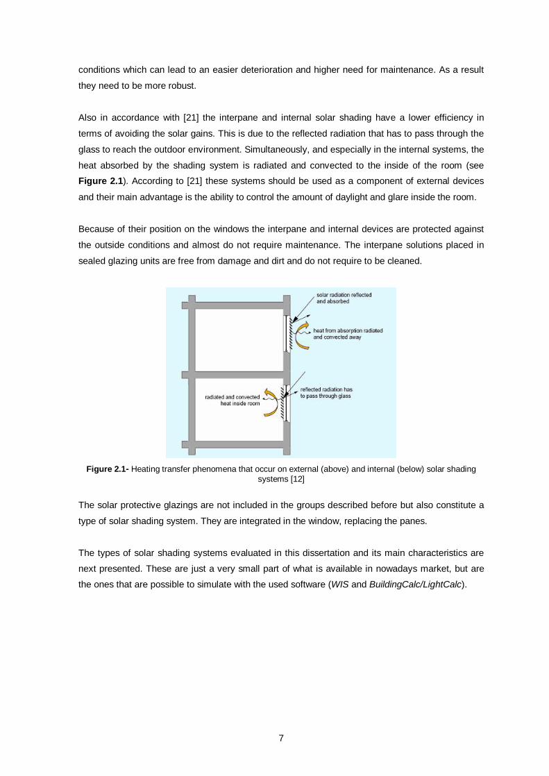
According to [21], the external solar shading systems are the most efficient in reducing the cooling

loads. As they are placed outside they reflect the solar rays before they enter the room. Also the

heat they absorb is dissipated to the outside air by radiation and convection. (Figure 2.1) Their

main drawback is that, as they are placed outside, they are more exposed to the atmosphere

7

conditions which can lead to an easier deterioration and higher need for maintenance. As a result

they need to be more robust.

Also in accordance with [21] the interpane and internal solar shading have a lower efficiency in

terms of avoiding the solar gains. This is due to the reflected radiation that has to pass through the

glass to reach the outdoor environment. Simultaneously, and especially in the internal systems, the

heat absorbed by the shading system is radiated and convected to the inside of the room (see

Figure 2.1). According to [21] these systems should be used as a component of external devices

and their main advantage is the ability to control the amount of daylight and glare inside the room.

Because of their position on the windows the interpane and internal devices are protected against

the outside conditions and almost do not require maintenance. The interpane solutions placed in

sealed glazing units are free from damage and dirt and do not require to be cleaned.

Figure 2.1- Heating transfer phenomena that occur on external (above) and internal (below) solar shading

systems [12]

The solar protective glazings are not included in the groups described before but also constitute a

type of solar shading system. They are integrated in the window, replacing the panes.

The types of solar shading systems evaluated in this dissertation and its main characteristics are

next presented. These are just a very small part of what is available in nowadays market, but are

the ones that are possible to simulate with the used software (WIS and BuildingCalc/LightCalc).

8

2.2 Venetian blinds

A venetian blind is a blind composed of parallel spaced slats that can be tilted in order to control

the amount of solar gains and light entering the room.

The slats are available in different widths and can be made of different materials (usually wood or

aluminium). They are also available with different finishes and colours according to the wanted

esthetical effect.

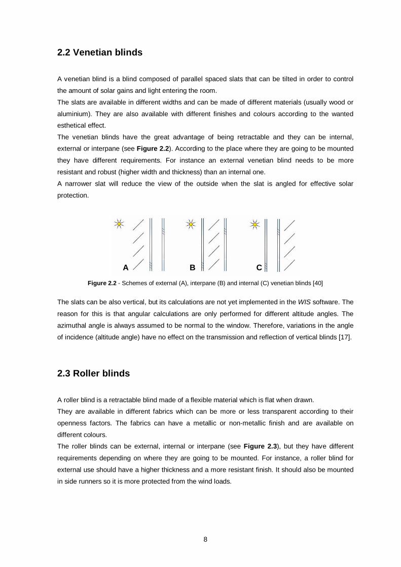
The venetian blinds have the great advantage of being retractable and they can be internal,

external or interpane (see Figure 2.2). According to the place where they are going to be mounted

they have different requirements. For instance an external venetian blind needs to be more

resistant and robust (higher width and thickness) than an internal one.

A narrower slat will reduce the view of the outside when the slat is angled for effective solar

protection.

Figure 2.2 - Schemes of external (A), interpane (B) and internal (C) venetian blinds [40]

The slats can be also vertical, but its calculations are not yet implemented in the WIS software. The

reason for this is that angular calculations are only performed for different altitude angles. The

azimuthal angle is always assumed to be normal to the window. Therefore, variations in the angle

of incidence (altitude angle) have no effect on the transmission and reflection of vertical blinds [17].

2.3 Roller blinds

A roller blind is a retractable blind made of a flexible material which is flat when drawn.

They are available in different fabrics which can be more or less transparent according to their

openness factors. The fabrics can have a metallic or non-metallic finish and are available on

different colours.

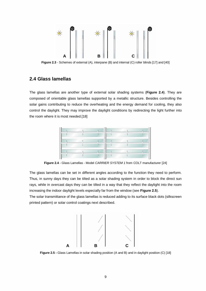
The roller blinds can be external, internal or interpane (see Figure 2.3), but they have different

requirements depending on where they are going to be mounted. For instance, a roller blind for

external use should have a higher thickness and a more resistant finish. It should also be mounted

in side runners so it is more protected from the wind loads.

A B C

9

Figure 2.3 - Schemes of external (A), interpane (B) and internal (C) roller blinds [17] and [40]

2.4 Glass lamellas

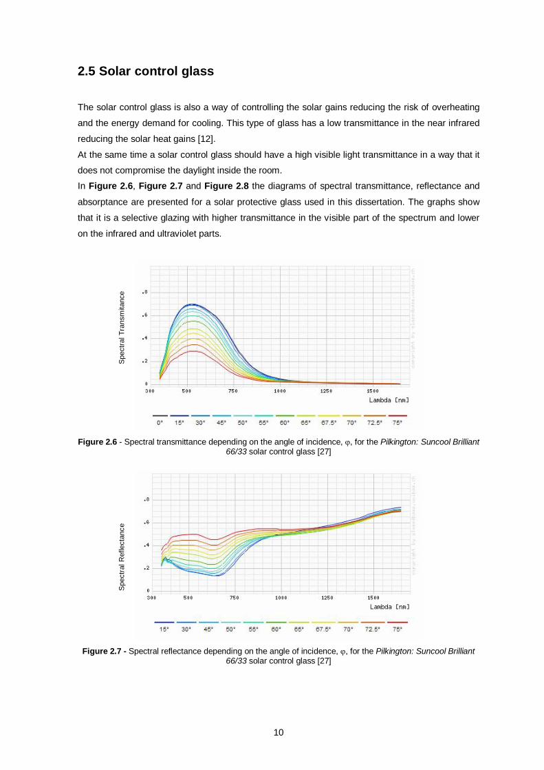
The glass lamellas are another type of external solar shading systems (Figure 2.4). They are

composed of orientable glass lamellas supported by a metallic structure. Besides controlling the

solar gains contributing to reduce the overheating and the energy demand for cooling, they also

control the daylight. They may improve the daylight conditions by redirecting the light further into

the room where it is most needed.[18]

Figure 2.4 - Glass Lamellas - Model CARRIER SYSTEM 1 from COLT manufacturer [24]

The glass lamellas can be set in different angles according to the function they need to perform.

Thus, in sunny days they can be tilted as a solar shading system in order to block the direct sun

rays, while in overcast days they can be tilted in a way that they reflect the daylight into the room

increasing the indoor daylight levels especially far from the window (see Figure 2.5).

The solar transmittance of the glass lamellas is reduced adding to its surface black dots (silkscreen

printed pattern) or solar control coatings next described.

Figure 2.5 - Glass Lamellas in solar shading position (A and B) and in daylight position (C) [18]

A B C

A B C

10

2.5 Solar control glass

The solar control glass is also a way of controlling the solar gains reducing the risk of overheating

and the energy demand for cooling. This type of glass has a low transmittance in the near infrared

reducing the solar heat gains [12].

At the same time a solar control glass should have a high visible light transmittance in a way that it

does not compromise the daylight inside the room.

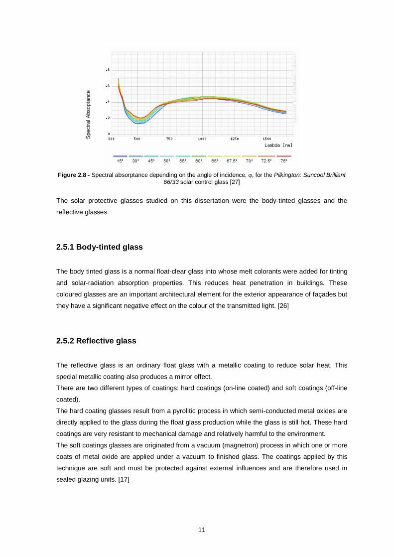
In Figure 2.6, Figure 2.7 and Figure 2.8 the diagrams of spectral transmittance, reflectance and

absorptance are presented for a solar protective glass used in this dissertation. The graphs show

that it is a selective glazing with higher transmittance in the visible part of the spectrum and lower

on the infrared and ultraviolet parts.

Figure 2.6 - Spectral transmittance depending on the angle of incidence, , for the Pilkington: Suncool Brilliant

66/33 solar control glass [27]

Figure 2.7 - Spectral reflectance depending on the angle of incidence, , for the Pilkington: Suncool Brilliant


Spe

ctra

l Tra

nsm

itanc

e S

pect

ral R

efle

ctan

ce

11

Figure 2.8 - Spectral absorptance depending on the angle of incidence, , for the Pilkington: Suncool Brilliant


The solar protective glasses studied on this dissertation were the body-tinted glasses and the

reflective glasses.

2.5.1 Body-tinted glass

The body tinted glass is a normal float-clear glass into whose melt colorants were added for tinting

and solar-radiation absorption properties. This reduces heat penetration in buildings. These

coloured glasses are an important architectural element for the exterior appearance of façades but

they have a significant negative effect on the colour of the transmitted light. [26]

2.5.2 Reflective glass

The reflective glass is an ordinary float glass with a metallic coating to reduce solar heat. This

special metallic coating also produces a mirror effect.

There are two different types of coatings: hard coatings (on-line coated) and soft coatings (off-line

coated).

The hard coating glasses result from a pyrolitic process in which semi-conducted metal oxides are

directly applied to the glass during the float glass production while the glass is still hot. These hard

coatings are very resistant to mechanical damage and relatively harmful to the environment.

The soft coatings glasses are originated from a vacuum (magnetron) process in which one or more

coats of metal oxide are applied under a vacuum to finished glass. The coatings applied by this

technique are soft and must be protected against external influences and are therefore used in

sealed glazing units. [17]

Spe

ctra

l Abs

opta

nce

12

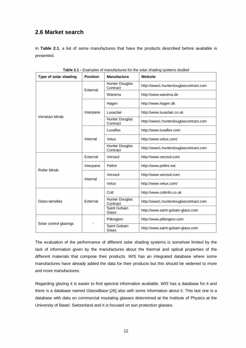
2.6 Market search

In Table 2.1, a list of some manufactures that have the products described before available is

presented.

Table 2.1 - Examples of manufactures for the solar shading systems studied

Type of solar shading Position Manufacture Website

Hunter Douglas Contract http://www1.hunterdouglascontract.com

External Warema http://www.warema.de

Hagen http://www.hagen.dk

Luxaclair http://www.luxaclair.co.uk Interpane


Luxaflex http://www.luxaflex.com

Velux http://www.velux.com/

Venetian blinds

Internal


External Verosol http://www.verosol.com

Interpane Pellini http://www.pellini.net

Verosol http://www.verosol.com Roller blinds

Internal Velux http://www.velux.com/

Colt http://www.coltinfo.co.uk

Hunter Douglas Contract http://www1.hunterdouglascontract.com Glass lamellas External

Saint Gobain Glass http://www.saint-gobain-glass.com

Pilkington http://www.pilkington.com Solar control glazings - Saint Gobain

Glass http://www.saint-gobain-glass.com

The evaluation of the performance of different solar shading systems is somehow limited by the

lack of information given by the manufactures about the thermal and optical properties of the

different materials that compose their products. WIS has an integrated database where some

manufactures have already added the data for their products but this should be widened to more

and more manufactures.

Regarding glazing it is easier to find spectral information available. WIS has a database for it and

there is a database named Glassdbase [26] also with some information about it. This last one is a

database with data on commercial insulating glasses determined at the Institute of Physics at the

University of Basel, Switzerland and it is focused on sun protection glasses.

13

3. Some useful definitions

When characterizing and evaluating the performance of glazings and solar shading systems there

are some standard terms usually referred by manufactures and designers. These terms which will

be used throughout this dissertation are next described.

3.1 Electromagnetic spectrum

The electromagnetic spectrum can be divided into wavelength intervals:

1) <380nm (UV-radiation) - this is the non-visible ultraviolet radiation and it has a little meaning for

the energy balance of buildings. However, this is the part of spectrum responsible for the long term

colours change of buildings furniture. It can be harmful for people

2) 380nm<<780nm (visible radiation) - this wavelength interval represents the visible light and it

contains around 50% of the solar radiation. It is important that windows have a high transmittance

in this wavelength range to allow a high indoor daylight level.

3) 780nm<<2500nm (near-infrared radiation) - this part of the solar radiation is not visible and it

represents approximately 40% of the energy from the sun.

4)>2500nm (IR-radiation) - all the surfaces at room temperatures emit energy in this interval.

Ordinary window glass is not transparent for these wavelengths; however, the radiation is absorbed

and then re-radiated towards indoor and outdoor environments. A major part of the heat loss

through an ordinary window occurs in this way. [1]

3.2 Reflectance, absorptance and transmittance

The glazings and the materials that compose the shading systems can be characterized according

to their solar-optical properties: reflectance, absorptance and transmittance.

The reflectance () is the fraction of the incident flux that is reflected from the glazing or shading

material, the absorptance () is the fraction of incident flux absorbed by the glazing or shading

material and the transmittance () is the fraction that is transmitted through them. The sum of the

reflectance, absorptance and transmittance must be equal to the unit (++=1).

The solar transmittance (S) is the glazing or shading material transmittance over the whole solar

spectrum while the visual transmittance (V) refers to the transmittance only for the visible range of

the solar spectrum. In a similar way also the ultraviolet transmittance (UV) can be defined.

Manufacturers usually give the visual transmittance because it determines how well one can see

through a window and how much natural light can be used in the building to illuminate tasks. [6]

14

3.3 Thermal transmittance coefficient

The thermal transmittance coefficient, U-value, is the amount of heat that passes through an

element per unit area and per unit time when the temperature difference between the environments

separated by the element is 1 Kelvin. This parameter takes into account the surface resistances

and the conduction, convection and radiation phenomena. It is usually defined in W/m2K. [16]

3.4 Solar heat gain coefficient

The solar heat gain coefficient, g-value, is the fraction of incident irradiance (solar radiation incident

on the glazing) that enters the building and becomes heat in the space. It includes both the directly

transmitted portion and the absorbed and re-emitted portion of solar radiation. [6]

3.5 Solar shading coefficient

The solar shading coefficient, SSC, is sometimes defined as the ratio between the g-value of a

window system (glazing + solar shading device) for a particular angle of incidence and the g-value

of a reference clear float glass (3mm thickness) for the same angle of incidence. [6]

However, in this dissertation it was assumed to be the ratio between the g-value of the window

system and the glazing initially selected as the reference. In this way, the reference glazing has a

shading coefficient of 1 and it is easier to compare the performance of the different solutions.

Lower solar shading coefficients indicate higher performances.

3.6 Visual shading coefficient

The visual shading coefficient, VSC, is defined in a similar way as the solar shading coefficient. It is

the ratio between the light transmittance of the window system and the light transmittance of the

glazing initially defined as the reference. In this way, for the reference glazing, the visual shading

coefficient is 1. Higher visual shading coefficient indicates higher visual performance.

15

3.7 General colour rendering index - Ra

This index is used to assess quantitatively the performance of colour rendering through a window

system.

A Ra index of 100% corresponds to perfect colour preservation. [27]

3.8 Illuminance

Illuminance, E, describes the amount of luminous flux arriving at a surface, i.e., the incident flux per

unit area. It is measured in lux. [1]

3.9 Luminance

Luminance, L, describes the light reflected off a surface and it is directly related to the perceived

“brightness” of a surface in a given direction. It depends on the illuminance on an object and its

reflective properties. Luminance is what we see, not illuminance. Luminance is measured in

candelas per square meter (cd/m2). [1]

3.10 Daylight Factor

The daylight factor, DLfactor, is the ratio of the illuminance on a surface in a room to the

illuminance on an external unobstructed horizontal surface, taking only the diffuse radiation into

account. This parameter is usually calculated for evaluating the daylight performance of window

systems under overcast skies when only diffuse light exists. [1]

3.11 PPD index

The PPD index (predicted percent of dissatisfied), defined in %, takes into account the influence of

all 6 thermal parameters (clothing, activity, air- and mean radiant temperature, air velocity and

humidity) and it may be directly used as a indoor comfort criteria [14]

16

4. Method to evaluate the performance of different solar shading systems

4.1 The Sofware used - Relation between WIS and

BuildingCalc/LightCalc To evaluate the performance of different solar shading systems two softwares were used: WIS3.0.1

(developed by TNO Building and Construction Research in Delft) [41] and BuildingCalc/LightCalc

v2.3.1f (developed in Matlab at Technical University of Denmark) [38].

WIS is a European software tool for the calculation of the thermal and solar properties of window

systems.

Knowing previously from the manufactures spectral data for the thermal and optical properties of

the materials that compose the different shading systems and also the properties of the glazing

(panes and gaps), it is possible to calculate the properties of combined systems (glazing+shading

system) for different angles of incidence. Concerning shadings composed of slats that can be tilted

it is also possible to calculate the properties for different positions of the slats. [3]

BuildingCalc/LightCalc is a tool that can be used in three different ways: only BuildingCalc (for

thermal simulations), only LightCalc (for daylight simulations) and BuildingCalc/LightCalc (for

combined simulations).

With BuildingCalc/LightCalc it is possible to create a simple model of a room and import from WIS

the properties of the solution for the window (glazing+shading system). In an hourly basis dynamic

simulation BuildingCalc/LightCalc is able to calculate the needs for heating, cooling and lightning

during one whole year. Also an evaluation of the indoor comfort is made and parameters as total

hours of overheating and PPD index (predicted percent of dissatisfied) are calculated. The indoor

daylight conditions can also be studied for a specific day and hour. [11]

Combining these two softwares it is possible to do some calculations early in the design phase to

evaluate and compare the energy and daylight performances of different solutions of solar shading

systems.

17

4.1.1 WIS

With WIS it is possible to simulate a complete window system including glazing, solar shading

system, frame and spacers. However for posterior use in BuildingCalc/LightCalc only the

transparent system (solar shading + glazing) is necessary to be set. The properties of the frame

and spacers are set separately in BuildingCalc/LightCalc.

Thus, in this dissertation the objective of using WIS is to generate text files that characterize the

transparent systems (glazing + solar shading) in a way that they can be used in

BuildingCalc/LightCalc.

In WIS there are already available databases with commercial solutions for the different

components of a window (solar shading systems, panes of glass, frames and spacers). This

information which includes geometrical, thermal and spectral optical properties of the components

can be added by the manufactures and it is a precious help for the designers. However, still few

manufactures have their information available on WIS databases.

It is also possible for the designer to add products to the database. But due to a lack of information

about the properties of products by the solar shading systems manufactures this process is

sometimes difficult for the designer. The optimum solution would be that the manufactures knew

the properties of their solutions and had them in databases.

This is a problem essentially regarding the solar shading systems manufactures. For the glass this

information is easier to find.

One solution would be to set up a product standard that requires documentation of spectral and

angular optical data and that also requires the manufactures to CE-mark the products sold in the

European Union.

4.1.2 BuildingCalc and Light Calc In this dissertation BuildingCalc/LightCalc was used in two different versions: combined simulations

for determination of the heating, cooling and lightning needs, number of hours of overheating and

PPD index; and light simulations to evaluate the daylight performance of the different solar shading

systems under critical sky conditions.

In this software, the simulation of thermal conditions is based on a simple thermal model of the

room. The building envelope is simply defined by an overall UA-value that takes into account the

sum of the thermal transmission losses through the façade excluding the window. The losses

through the window are characterized separately. The heat capacity of the construction and the

internal surface area are also defined.

18

It is possible to set different systems: heating, cooling, ventilation with air variable volume and heat

recovery, venting and variable solar shading. The solar shading is the main focus of this

dissertation. The systems are controlled by different settings which can be specified for different

periods. This means that different control settings can be defined for summer and winter time and

for working hours and non working hours.

It is possible to plot and export the results from the simulations in an hourly basis.

The location and weather data need also to be set.

The LightCalc component, based on the radiosity method, is able to estimate daylight levels in a

room under different sky conditions. BuildingCalc/LightCalc results from the combination of the features of BuildingCalc with LightCalc.

In this way, the daylight levels will be estimated taking into account the shading control and

consequently this will have an influence on the electrical lightning demand. Also the extra heat gain

from the electrical lightning is taken into account. [11]

In APPENDICES A, B, C and D, some examples of how to use WIS and BuildingCalc/LightCalc

are presented. In APPENDIX A, a step-by-step example of how to use WIS and BuildingCalc/LightCalc for the

purpose of this dissertation is presented. The given example refers to an internal venetian blind

applied on the glass façade of the landscaped office building described on chapter 5. Case Study - Landscaped Office Building.

In APPENDIX B, the way how to add a new shading system to the WIS database is presented.

In APPENDIX C, an example of how to model glass lamellas from glass pane properties (using

WIS) is presented.

In APPENDIX D some tips are given on how to import the glass lamellas to BuildingCalc/LightCalc.

19

5. Case study - Landscaped office building

Office buildings with glass façades are more and more common. The transparent properties of the

glass enable the natural light to come into the buildings allowing high levels of indoor daylight

which is positive: it is known that people prefer working and have higher efficiency under natural

light, and at the same time the cost for electricity and the CO2 emissions decrease.

The drawback is that the glass façade is where the main solar gains and heat losses occur. The

solar gains during winter are useful in decreasing the need for heating. But during summer the

excess of solar gains give raise to many hours of overheating. The indoor comfort could be simple

reached with an air-conditioning system, but this would lead to very high energy consumption for

cooling. A solar shading system main goal is to reduce the need for cooling, avoiding the solar

gains to get into the building.

At the same time the shading systems can control the daylight in buildings avoiding glare problems.

If completely activated outside the working hours they improve the U-value of the window system,

decreasing the heat exchanges between the inside and outside of the building.

5.1 Settings for Copenhagen

The test room will be a storey of a landscaped office building with a rectangular form located in

Copenhagen (North Europe). Also a study of the same building but located in Lisbon (South

Europe) will be done.

Next, the characteristics for the building located in Copenhagen are presented. The building in

Lisbon has almost the same properties apart from some changes later presented.

The main goal is that the building is a relative high performance one according to energy and

indoor comfort points of view. According to energy it should fulfil the energy frame for Denmark and

Portugal. Regarding indoor comfort [14] the building should fulfil Category II, which means “Normal

level of expectation”.

5.1.1 General information and dimensions

The building will have only one façade and it will be facing south. The rest of the boundary walls

will be in contact with heated spaces.

It was assumed that near the front façade there are no other buildings/elements that could in

someway originate shades on the building being studied.

It was also assumed that the building would have three storeys and instead of choosing one of

them for the simulations it was created one that could represent the three at the same time. Thus, it

was assumed that the representative storey would have 1/3 of its ceiling in contact with outside and

20

1/3 of its floor in contact with the ground. The remaining parts of the ceiling and floor were

assumed to be in contact with heated spaces.

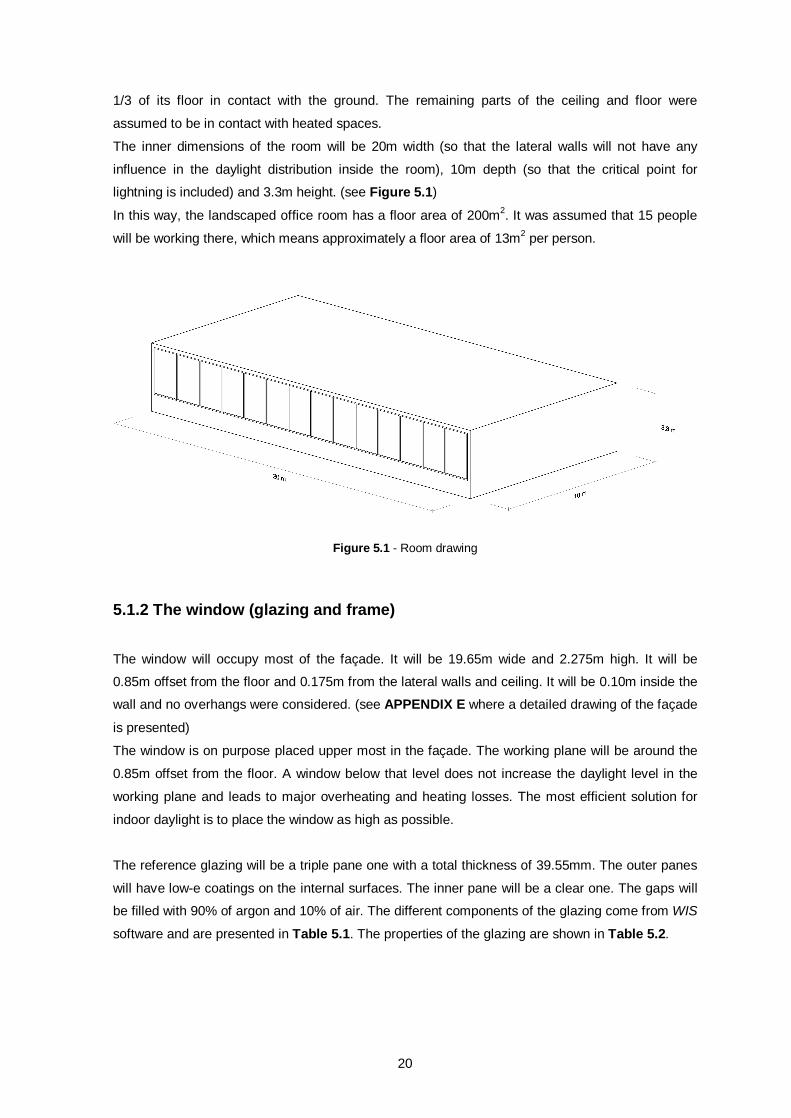
The inner dimensions of the room will be 20m width (so that the lateral walls will not have any

influence in the daylight distribution inside the room), 10m depth (so that the critical point for

lightning is included) and 3.3m height. (see Figure 5.1)

In this way, the landscaped office room has a floor area of 200m2. It was assumed that 15 people

will be working there, which means approximately a floor area of 13m2 per person.

Figure 5.1 - Room drawing

5.1.2 The window (glazing and frame)

The window will occupy most of the façade. It will be 19.65m wide and 2.275m high. It will be

0.85m offset from the floor and 0.175m from the lateral walls and ceiling. It will be 0.10m inside the

wall and no overhangs were considered. (see APPENDIX E where a detailed drawing of the façade

is presented)

The window is on purpose placed upper most in the façade. The working plane will be around the

0.85m offset from the floor. A window below that level does not increase the daylight level in the

working plane and leads to major overheating and heating losses. The most efficient solution for

indoor daylight is to place the window as high as possible.

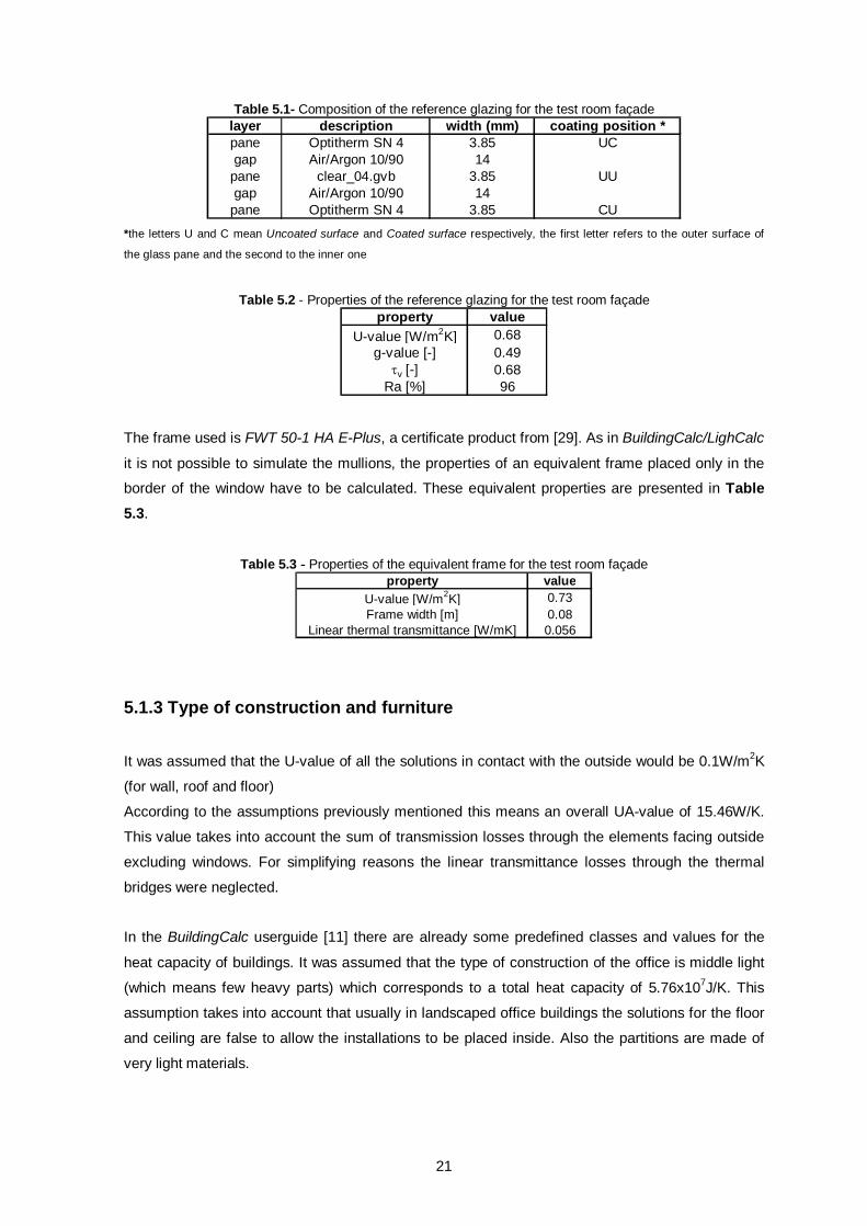
The reference glazing will be a triple pane one with a total thickness of 39.55mm. The outer panes

will have low-e coatings on the internal surfaces. The inner pane will be a clear one. The gaps will

be filled with 90% of argon and 10% of air. The different components of the glazing come from WIS

software and are presented in Table 5.1. The properties of the glazing are shown in Table 5.2.

21

Table 5.1- Composition of the reference glazing for the test room façade layer description width (mm) coating position *pane Optitherm SN 4 3.85 UCgap Air/Argon 10/90 14

pane clear_04.gvb 3.85 UUgap Air/Argon 10/90 14

pane Optitherm SN 4 3.85 CU *the letters U and C mean Uncoated surface and Coated surface respectively, the first letter refers to the outer surface of

the glass pane and the second to the inner one

Table 5.2 - Properties of the reference glazing for the test room façade

property valueU-value [W/m2K] 0.68

g-value [-] 0.49v [-] 0.68

Ra [%] 96

The frame used is FWT 50-1 HA E-Plus, a certificate product from [29]. As in BuildingCalc/LighCalc

it is not possible to simulate the mullions, the properties of an equivalent frame placed only in the

border of the window have to be calculated. These equivalent properties are presented in Table 5.3.

Table 5.3 - Properties of the equivalent frame for the test room façade property value

U-value [W/m2K] 0.73Frame width [m] 0.08

Linear thermal transmittance [W/mK] 0.056

5.1.3 Type of construction and furniture

It was assumed that the U-value of all the solutions in contact with the outside would be 0.1W/m2K

(for wall, roof and floor)

According to the assumptions previously mentioned this means an overall UA-value of 15.46W/K.

This value takes into account the sum of transmission losses through the elements facing outside

excluding windows. For simplifying reasons the linear transmittance losses through the thermal

bridges were neglected.

In the BuildingCalc userguide [11] there are already some predefined classes and values for the

heat capacity of buildings. It was assumed that the type of construction of the office is middle light

(which means few heavy parts) which corresponds to a total heat capacity of 5.76x107J/K. This

assumption takes into account that usually in landscaped office buildings the solutions for the floor

and ceiling are false to allow the installations to be placed inside. Also the partitions are made of

very light materials.

22

Additional heat capacity of the furniture was considered. Taking into account that there are 15

working places, that each one has a weight of 200kg and that the heat capacity of each kg is

1000J/K, the total contribution of the furniture is 3x106J/K.

5.1.4 Systems

Six different systems were defined to simulate different periods of the year and distinct using

conditions. This is one of the great advantages of BuildingCalc/Lightcalc, it allows to define

different settings for different periods according to the correspondent requirements.

Thus, three systems were defined for the coldest months (December, January and February -

weeks 1 to 9 and 10 to 53) and three systems for the other months (March, April, May, June, July,

August, September, October and November – weeks 10 to 48).

The three systems for each season are: one for working hours, other for non-working hours during

working days and another one for weekends.

Two different solutions were studied:

1) no mechanical cooling available (when there is need for cooling the cooling systems are

activated in the following order: shading, venting and increased mechanical ventilation)

2) mechanical cooling available (when the previous solutions are not enough to set the indoor

temperature to the cooling setpoint the mechanical cooling is activated)

The first solution is the more environmental friendly since no energy for cooling is used. However in

most cases this solution is not enough to achieve the indoor comfort level required on [14] specially

regarding south Europe countries like Portugal.

The office is equipped with a heating system with an incorporated heat exchanger (with an

efficiency of 0.85)

The heating system and the mechanical cooling (when available) are only active during working

hours.

According to [14] the heating setpoint will be 20ºC (for a cloth level of 1.0).

In [14] it is required a cooling setpoint of 26ºC (for a cloth level of 0.5) but 22ºC will be set (even if

the cloth level needs to be higher). The objective is that the cooling will start before the indoor

temperature reaches 26ºC. This is a way of decreasing the hours of overheating above 26ºC which

is a measure of discomfort.

Only during working hours mechanical ventilation is active with an airchange rate of 0.9h-1 which

corresponds to 0.8l/s.m2 (requirement for a category II very low-polluted landscaped office [14]).

23

During working hours no venting was set. This is to contemplate the fact that sometimes office

buildings are placed in areas with noise. In this way, venting by opening windows can lead to high

levels of noise inside the office which can interfere with workers concentration and efficiency. Thus

the indoor air quality should be guaranteed without venting.

Outside the coldest months venting with a setpoint of 20ºC was set at night and during weekends.

This is especially important during summer nights to cool down the office when the outdoor

temperature is lower.

The internal loads during the working hours were assumed to be 100W per person and 50W per

equipment which gives a total of 2250W (considering the 15 working places).

The shading system will be dynamically controlled. It will be automatically activated when the

indoor temperature is higher than the cooling setpoint. According to the needs, different positions

can be set for the shading system. For instance the systems with slats are activated in a way that

the orientation of the slats is enough to block the direct sun (cut off position).

For thermal benefits it was assumed that the shading is completely activated during nights and

weekends. The activation of the shading means extra-insulation for the window which is important

during winter in order to reduce the heat losses through the window.

The lightning level is automatically controlled during the working hours. When the general indoor

daylight is lower than 200lux the electrically lightning will be switched on immediately to reach that

level. For working areas in landscaped office buildings, according to [14] the requirement is 500lux.

BuildingCalc/LightCalc will also keep this level with the use of electrical lightning when needed.

For general lightning level the wattage of the system used is 4W/m2, while for specific tasks it is

1W/m2.

5.2 Different settings for Lisbon

The goal is that the building in Lisbon is as much as possible similar to the building in Copenhagen,

so the performance of the different solar shading systems can be compared between North and

South Europe countries.

Only some changes were made. The first one is regarding the U-value of the exterior solutions.

The value assumed for Copenhagen, 0.1W/m2K is extremely low for Lisbon, since the winter is not

so severe in the south Europe countries. According to the Portuguese building code [16], the

reference U-value for exterior solutions is 0.60W/m2K for vertical elements and 0.45W/m2K for

horizontal elements (for Lisbon - climate area I2). Thus 0.4W/m2K was used for whole the exterior

solutions. This means a new UA-value of 61.85W/K.

24

To avoid overheating during the winter months (December, January and February) there was a

need to set venting outside the working hours (night and weekends) also during these months.

However the cooling setpoint is 22ºC instead of 20ºC (which was set for the other months). A

cooling setpoint of 20ºC for venting during night and weekends in winter would lead to an increase

on the heating demand.

5.3 Location and weather files

Also the location and weather data files must be loaded in BuildingCalc/LightCalc.

The location data for Copenhagen and Lisbon are presented on Table 5.4.

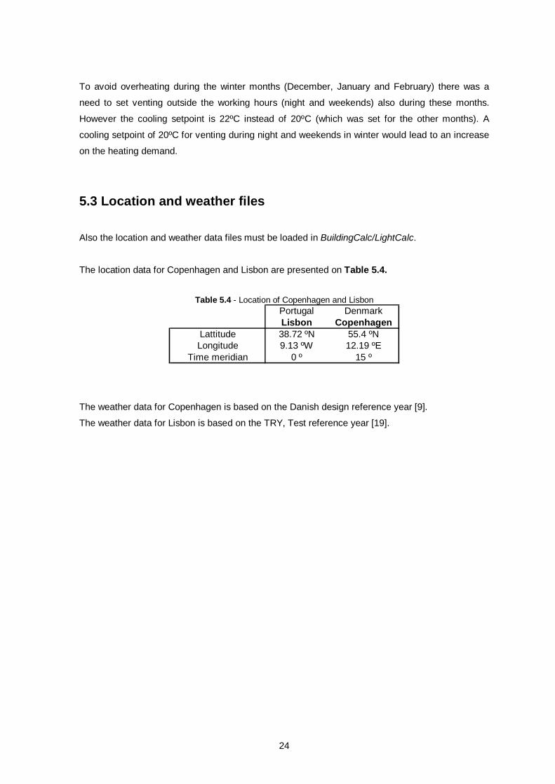
Table 5.4 - Location of Copenhagen and Lisbon Portugal DenmarkLisbon Copenhagen

Lattitude 38.72 ºN 55.4 ºNLongitude 9.13 ºW 12.19 ºE

Time meridian 0 º 15 º

The weather data for Copenhagen is based on the Danish design reference year [9].

The weather data for Lisbon is based on the TRY, Test reference year [19].

25

6. Energy Performance and indoor comfort evaluation

6.1 Requirements and expected results

6.1.1 Energy frame

6.1.1.1 Denmark

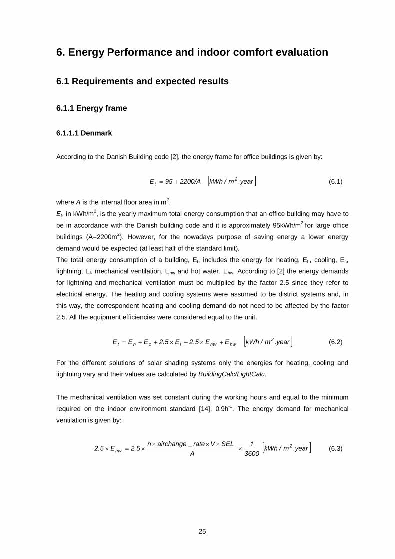
According to the Danish Building code [2], the energy frame for office buildings is given by:

year.m/kWh2200/A95E 2t (6.1)

where A is the internal floor area in m2.

Et, in kWh/m2, is the yearly maximum total energy consumption that an office building may have to

be in accordance with the Danish building code and it is approximately 95kWh/m2 for large office

buildings (A=2200m2). However, for the nowadays purpose of saving energy a lower energy

demand would be expected (at least half of the standard limit).

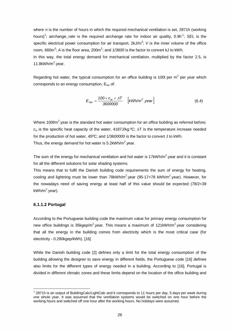
The total energy consumption of a building, Et, includes the energy for heating, Eh, cooling, Ec,

lightning, El, mechanical ventilation, Emv and hot water, Ehw. According to [2] the energy demands

for lightning and mechanical ventilation must be multiplied by the factor 2.5 since they refer to

electrical energy. The heating and cooling systems were assumed to be district systems and, in

this way, the correspondent heating and cooling demand do not need to be affected by the factor

2.5. All the equipment efficiencies were considered equal to the unit.

year.m/kWhEE5.2E5.2EEE 2hwmvlcht (6.2)

For the different solutions of solar shading systems only the energies for heating, cooling and

lightning vary and their values are calculated by BuildingCalc/LightCalc.

The mechanical ventilation was set constant during the working hours and equal to the minimum

required on the indoor environment standard [14], 0.9h-1. The energy demand for mechanical

ventilation is given by:

year.m/kWh3600

1A

SELVrate_airchangen5.2E2.5 2

mv

(6.3)

26

where n is the number of hours in which the required mechanical ventilation is set, 2871h (working

hours)1; airchange_rate is the required airchange rate for indoor air quality, 0.9h-1; SEL is the

specific electrical power consumption for air transport, 2kJ/m3; V is the inner volume of the office

room, 660m3; A is the floor area, 200m2; and 1/3600 is the factor to convert kJ to kWh.

In this way, the total energy demand for mechanical ventilation, multiplied by the factor 2.5, is

11.8kWh/m2.year.

Regarding hot water, the typical consumption for an office building is 100l per m2 per year which

corresponds to an energy consumption, Ehw of:

.yearkWh/m3600000

Tc100E 2w

wh

(6.4)

Where 100l/m2.year is the standard hot water consumption for an office building as referred before;

cw is the specific heat capacity of the water, 4187J/kg.ºC; T is the temperature increase needed

for the production of hot water, 45ºC; and 1/3600000 is the factor to convert J to kWh.

Thus, the energy demand for hot water is 5.2kWh/m2.year.

The sum of the energy for mechanical ventilation and hot water is 17kWh/m2.year and it is constant

for all the different solutions for solar shading systems.

This means that to fulfil the Danish building code requirements the sum of energy for heating,

cooling and lightning must be lower than 78kWh/m2.year (95-17=78 kWh/m2.year). However, for

the nowadays need of saving energy at least half of this value should be expected (78/2=39

kWh/m2.year).

6.1.1.2 Portugal

According to the Portuguese building code the maximum value for primary energy consumption for

new office buildings is 35kgep/m2.year. This means a maximum of 121kWh/m2.year considering

that all the energy in the building comes from electricity which is the most critical case (for

electricity - 0.290kgep/kWh). [16]

While the Danish building code [2] defines only a limit for the total energy consumption of the

building allowing the designer to save energy in different fields, the Portuguese code [16] defines

also limits for the different types of energy needed in a building. According to [16], Portugal is

divided in different climatic zones and these limits depend on the location of the office building and

1 2871h is an output of BuildingCalc/LightCalc and it corresponds to 11 hours per day, 5 days per week during one whole year. It was assumed that the ventilation systems would be switched on one hour before the working hours and switched off one hour after the working hours. No holidays were assumed.

27

on its shape factor, FF (which is the ratio between the exterior envelopment of the building and the

inner volume).

For the studied building (which has a shape form of 0.30) located in Lisbon (which corresponds to

winter climatic zone I1 and summer climatic zone V2 south), the maximum values for the different

energy demands are presented in Table 6.1.

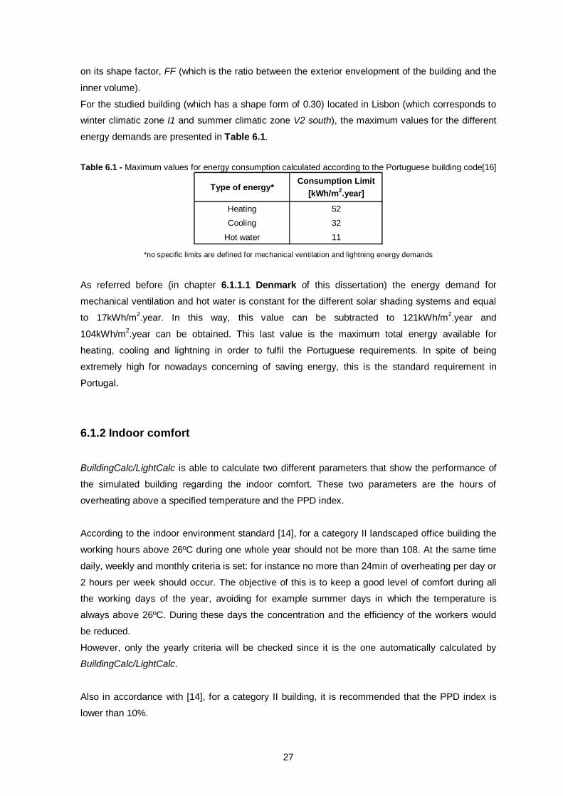
Table 6.1 - Maximum values for energy consumption calculated according to the Portuguese building code[16]

Type of energy*Consumption Limit

[kWh/m2.year]

Heating 52Cooling 32

Hot water 11 *no specific limits are defined for mechanical ventilation and lightning energy demands

As referred before (in chapter 6.1.1.1 Denmark of this dissertation) the energy demand for

mechanical ventilation and hot water is constant for the different solar shading systems and equal

to 17kWh/m2.year. In this way, this value can be subtracted to 121kWh/m2.year and

104kWh/m2.year can be obtained. This last value is the maximum total energy available for

heating, cooling and lightning in order to fulfil the Portuguese requirements. In spite of being

extremely high for nowadays concerning of saving energy, this is the standard requirement in

Portugal.

6.1.2 Indoor comfort

BuildingCalc/LightCalc is able to calculate two different parameters that show the performance of

the simulated building regarding the indoor comfort. These two parameters are the hours of

overheating above a specified temperature and the PPD index.

According to the indoor environment standard [14], for a category II landscaped office building the

working hours above 26ºC during one whole year should not be more than 108. At the same time

daily, weekly and monthly criteria is set: for instance no more than 24min of overheating per day or

2 hours per week should occur. The objective of this is to keep a good level of comfort during all

the working days of the year, avoiding for example summer days in which the temperature is

always above 26ºC. During these days the concentration and the efficiency of the workers would

be reduced.

However, only the yearly criteria will be checked since it is the one automatically calculated by


Also in accordance with [14], for a category II building, it is recommended that the PPD index is

lower than 10%.

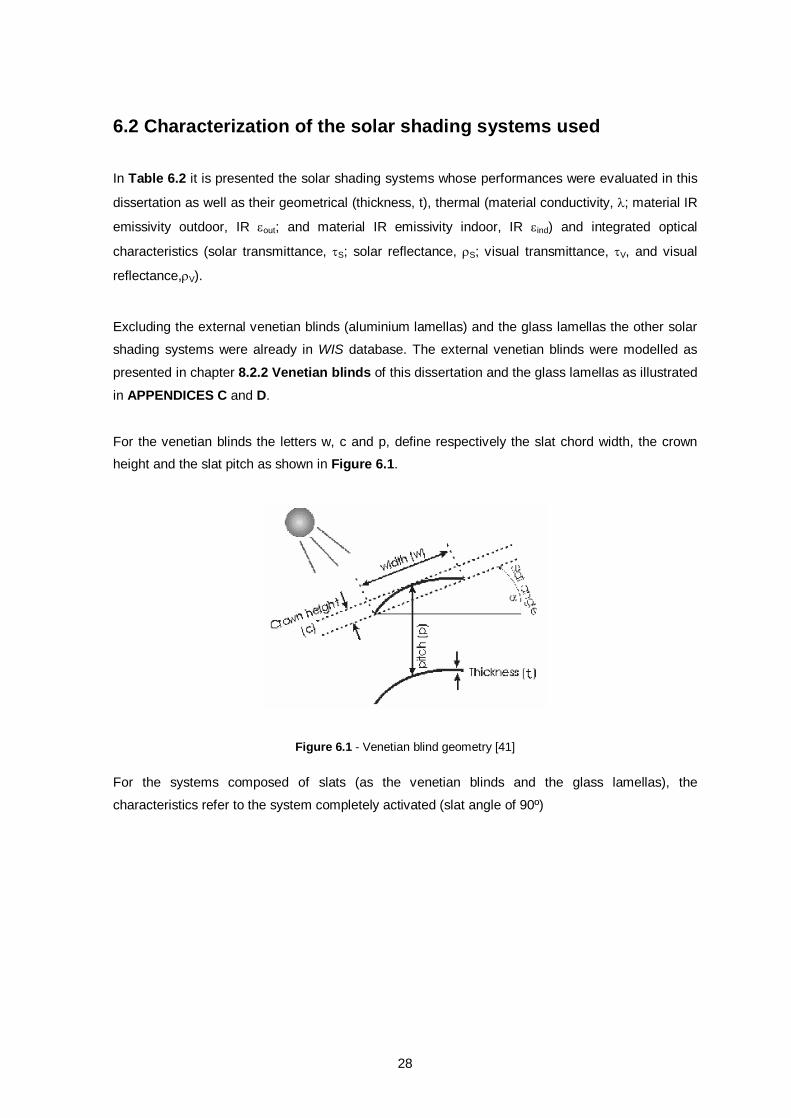
28

6.2 Characterization of the solar shading systems used

In Table 6.2 it is presented the solar shading systems whose performances were evaluated in this

dissertation as well as their geometrical (thickness, t), thermal (material conductivity, ; material IR

emissivity outdoor, IR out; and material IR emissivity indoor, IR ind) and integrated optical

characteristics (solar transmittance, S; solar reflectance, S; visual transmittance, V, and visual

reflectance,V). Excluding the external venetian blinds (aluminium lamellas) and the glass lamellas the other solar

shading systems were already in WIS database. The external venetian blinds were modelled as

presented in chapter 8.2.2 Venetian blinds of this dissertation and the glass lamellas as illustrated

in APPENDICES C and D.

For the venetian blinds the letters w, c and p, define respectively the slat chord width, the crown

height and the slat pitch as shown in Figure 6.1.

Figure 6.1 - Venetian blind geometry [41]

For the systems composed of slats (as the venetian blinds and the glass lamellas), the

characteristics refer to the system completely activated (slat angle of 90º)

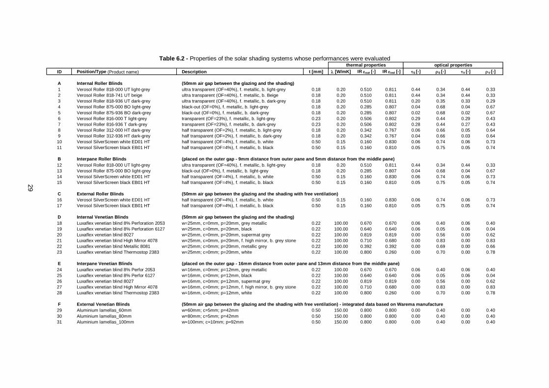
29

Table 6.2 - Properties of the solar shading systems whose performances were evaluated

ID Position/Type (Product name) Description t [mm] [W/mK] IR out [-] IR ind [-] S [-] S [-] V [-] V [-]

A Internal Roller Blinds (50mm air gap between the glazing and the shading)1 Verosol Roller 818-000 UT light-grey ultra transparent (OF=40%), f. metallic, b. light-grey 0.18 0.20 0.510 0.811 0.44 0.34 0.44 0.332 Verosol Roller 818-741 UT beige ultra transparent (OF=40%), f. metallic, b. Beige 0.18 0.20 0.510 0.811 0.44 0.34 0.44 0.333 Verosol Roller 818-936 UT dark-grey ultra transparent (OF=40%), f. metallic, b. dark-grey 0.18 0.20 0.510 0.811 0.20 0.35 0.33 0.294 Verosol Roller 875-000 BO light-grey black-out (OF=0%), f. metallic, b. light-grey 0.18 0.20 0.285 0.807 0.04 0.68 0.04 0.675 Verosol Roller 875-936 BO dark-grey black-out (OF=0%), f. metallic, b. dark-grey 0.18 0.20 0.285 0.807 0.02 0.68 0.02 0.676 Verosol Roller 816-000 T light-grey transparent (OF=23%), f. metallic, b. light-grey 0.23 0.20 0.506 0.802 0.29 0.44 0.29 0.437 Verosol Roller 816-936 T dark-grey transparent (OF=23%), f. metallic, b. dark-grey 0.23 0.20 0.506 0.802 0.28 0.44 0.27 0.438 Verosol Roller 312-000 HT dark-grey half transparent (OF=2%), f. metallic, b. light-grey 0.18 0.20 0.342 0.767 0.06 0.66 0.05 0.649 Verosol Roller 312-936 HT dark-grey half transparent (OF=2%), f. metallic, b. dark-grey 0.18 0.20 0.342 0.767 0.04 0.66 0.03 0.6410 Verosol SilverScreen white ED01 HT half transparent (OF=4%), f. metallic, b. white 0.50 0.15 0.160 0.830 0.06 0.74 0.06 0.7311 Verosol SilverScreen black EB01 HT half transparent (OF=4%), f. metallic, b. black 0.50 0.15 0.160 0.810 0.05 0.75 0.05 0.74

B Interpane Roller Blinds (placed on the outer gap - 9mm distance from outer pane and 5mm distance from the middle pane)12 Verosol Roller 818-000 UT light-grey ultra transparent (OF=40%), f. metallic, b. light-grey 0.18 0.20 0.510 0.811 0.44 0.34 0.44 0.3313 Verosol Roller 875-000 BO light-grey black-out (OF=0%), f. metallic, b. light-grey 0.18 0.20 0.285 0.807 0.04 0.68 0.04 0.6714 Verosol SilverScreen white ED01 HT half transparent (OF=4%), f. metallic, b. white 0.50 0.15 0.160 0.830 0.06 0.74 0.06 0.7315 Verosol SilverScreen black EB01 HT half transparent (OF=4%), f. metallic, b. black 0.50 0.15 0.160 0.810 0.05 0.75 0.05 0.74

C External Roller Blinds (50mm air gap between the glazing and the shading with free ventilation)16 Verosol SilverScreen white ED01 HT half transparent (OF=4%), f. metallic, b. white 0.50 0.15 0.160 0.830 0.06 0.74 0.06 0.7317 Verosol SilverScreen black EB01 HT half transparent (OF=4%), f. metallic, b. black 0.50 0.15 0.160 0.810 0.05 0.75 0.05 0.74

D Internal Venetian Blinds (50mm air gap between the glazing and the shading)18 Luxaflex venetian blind 8% Perforation 2053 w=25mm, c=0mm, p=20mm, grey metallic 0.22 100.00 0.670 0.670 0.06 0.40 0.06 0.4019 Luxaflex venetian blind 8% Perforation 6127 w=25mm, c=0mm, p=20mm, black 0.22 100.00 0.640 0.640 0.06 0.05 0.06 0.0420 Luxaflex venetian blind 8027 w=25mm, c=0mm, p=20mm, supermat grey 0.22 100.00 0.819 0.819 0.00 0.56 0.00 0.6221 Luxaflex venetian blind High Mirror 4078 w=25mm, c=0mm, p=20mm, f. high mirror, b. grey stone 0.22 100.00 0.710 0.680 0.00 0.83 0.00 0.8322 Luxaflex venetian blind Metallic 8081 w=25mm; c=0mm; p=20mm, metallic grey 0.22 100.00 0.392 0.392 0.00 0.69 0.00 0.6623 Luxaflex venetian blind Thermostop 2383 w=25mm; c=0mm; p=20mm, white 0.22 100.00 0.800 0.260 0.00 0.70 0.00 0.78

E Interpane Venetian Blinds (placed on the outer gap - 16mm distance from outer pane and 13mm distance from the middle pane)24 Luxaflex venetian blind 8% Perfor 2053 w=16mm, c=0mm; p=12mm, grey metallic 0.22 100.00 0.670 0.670 0.06 0.40 0.06 0.4025 Luxaflex venetian blind 8% Perfor 6127 w=16mm, c=0mm; p=12mm, black 0.22 100.00 0.640 0.640 0.06 0.05 0.06 0.0426 Luxaflex venetian blind 8027 w=16mm, c=0mm; p=12mm, supermat grey 0.22 100.00 0.819 0.819 0.00 0.56 0.00 0.6227 Luxaflex venetian blind High Mirror 4078 w=16mm, c=0mm; p=12mm, f. high mirror, b. grey stone 0.22 100.00 0.710 0.680 0.00 0.83 0.00 0.8328 Luxaflex venetian blind Thermostop 2383 w=16mm, c=0mm; p=12mm, white 0.22 100.00 0.800 0.260 0.00 0.70 0.00 0.78

F External Venetian Blinds (50mm air gap between the glazing and the shading with free ventilation) - integrated data based on Warema manufacture29 Aluminium lamellas_60mm w=60mm; c=5mm; p=42mm 0.50 150.00 0.800 0.800 0.00 0.40 0.00 0.4030 Aluminium lamellas_80mm w=80mm; c=5mm; p=42mm 0.50 150.00 0.800 0.800 0.00 0.40 0.00 0.4031 Aluminium lamellas_100mm w=100mm; c=10mm; p=92mm 0.50 150.00 0.800 0.800 0.00 0.40 0.00 0.40

thermal properties optical properties

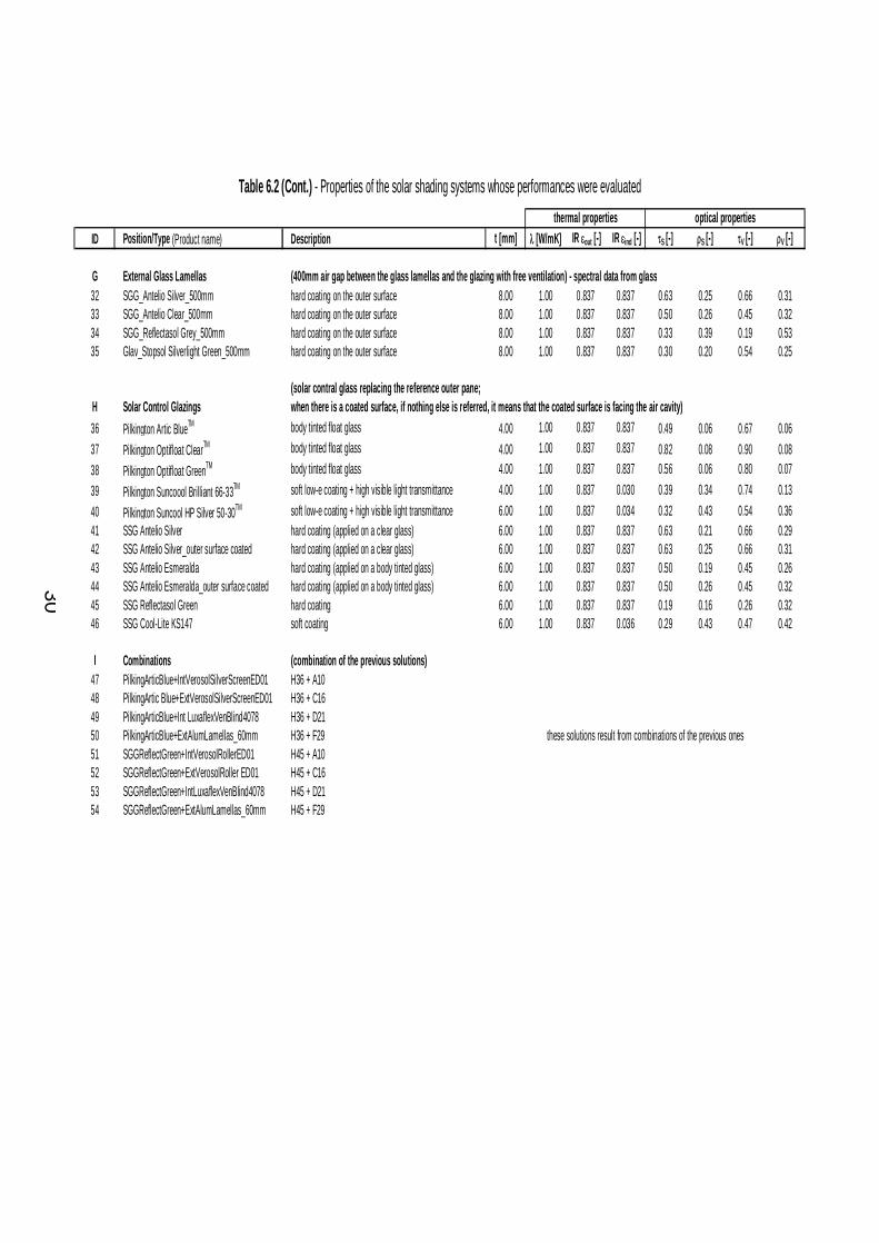
30

Table 6.2 (Cont.) - Properties of the solar shading systems whose performances were evaluated

ID Position/Type (Product name) Description t [mm] [W/mK] IR out [-] IR ind [-] S [-] S [-] V [-] V [-]

G External Glass Lamellas (400mm air gap between the glass lamellas and the glazing with free ventilation) - spectral data from glass32 SGG_Antelio Silver_500mm hard coating on the outer surface 8.00 1.00 0.837 0.837 0.63 0.25 0.66 0.3133 SGG_Antelio Clear_500mm hard coating on the outer surface 8.00 1.00 0.837 0.837 0.50 0.26 0.45 0.3234 SGG_Reflectasol Grey_500mm hard coating on the outer surface 8.00 1.00 0.837 0.837 0.33 0.39 0.19 0.5335 Glav_Stopsol Silverlight Green_500mm hard coating on the outer surface 8.00 1.00 0.837 0.837 0.30 0.20 0.54 0.25

(solar contral glass replacing the reference outer pane; H Solar Control Glazings when there is a coated surface, if nothing else is referred, it means that the coated surface is facing the air cavity)36 Pilkington Artic BlueTM body tinted float glass 4.00 1.00 0.837 0.837 0.49 0.06 0.67 0.0637 Pilkington Optifloat ClearTM body tinted float glass 4.00 1.00 0.837 0.837 0.82 0.08 0.90 0.0838 Pilkington Optifloat GreenTM body tinted float glass 4.00 1.00 0.837 0.837 0.56 0.06 0.80 0.0739 Pilkington Suncoool Brilliant 66-33TM soft low-e coating + high visible light transmittance 4.00 1.00 0.837 0.030 0.39 0.34 0.74 0.1340 Pilkington Suncool HP Silver 50-30TM soft low-e coating + high visible light transmittance 6.00 1.00 0.837 0.034 0.32 0.43 0.54 0.3641 SSG Antelio Silver hard coating (applied on a clear glass) 6.00 1.00 0.837 0.837 0.63 0.21 0.66 0.2942 SSG Antelio Silver_outer surface coated hard coating (applied on a clear glass) 6.00 1.00 0.837 0.837 0.63 0.25 0.66 0.3143 SSG Antelio Esmeralda hard coating (applied on a body tinted glass) 6.00 1.00 0.837 0.837 0.50 0.19 0.45 0.2644 SSG Antelio Esmeralda_outer surface coated hard coating (applied on a body tinted glass) 6.00 1.00 0.837 0.837 0.50 0.26 0.45 0.3245 SSG Reflectasol Green hard coating 6.00 1.00 0.837 0.837 0.19 0.16 0.26 0.3246 SSG Cool-Lite KS147 soft coating 6.00 1.00 0.837 0.036 0.29 0.43 0.47 0.42

I Combinations (combination of the previous solutions)47 PilkingArticBlue+IntVerosolSilverScreenED01 H36 + A1048 PilkingArtic Blue+ExtVerosolSilverScreenED01 H36 + C1649 PilkingArticBlue+Int LuxaflexVenBlind4078 H36 + D2150 PilkingArticBlue+ExtAlumLamellas_60mm H36 + F2951 SGGReflectGreen+IntVerosolRollerED01 H45 + A1052 SGGReflectGreen+ExtVerosolRoller ED01 H45 + C1653 SGGReflectGreen+IntLuxaflexVenBlind4078 H45 + D2154 SGGReflectGreen+ExtAlumLamellas_60mm H45 + F29

these solutions result from combinations of the previous ones

thermal properties optical properties

31

6.3 Results

In Table 6.3 and Table 6.4 the performance of the landscaped office room is presented for the

reference glazing and for the combination of the reference glazing with the different solar shading

systems. Table 6.3 refers to Copenhagen and Table 6.4 to Lisbon. The results painted as grey are

the ones that do not fulfil the standards.

The tables are organized in three distinct groups of columns:

System properties - where the performances of the reference glazing and of the combination of

different solar shading systems with the reference glazing are presented in terms of thermal

transmittance coefficient (U-value), solar heat gain coefficient (g-value), solar shading coefficient

(SSC), visual transmittance (V), visual shading coefficient (VSC) and rendering index (Ra). These

values were obtained in WIS and refer to the solar shading systems completely activated.

Without mechanical cooling - the values presented in these columns were calculated in

BuildingCalc/LightCalc. They show the performance of the landscaped office room (previously

described) for the reference glazing and also for the combination of different solar shading systems

with the reference glazing. No mechanical cooling was set.

The performance of the office building with the different solar shading systems is presented in

terms of energy demand for heating and lightning, total energy demand, hours of overheating and

PPD index.

With mechanical cooling - these columns also refer to the performance of the office room with the

different solutions for the solar shading systems in combination with the reference glazing. In this

case mechanical cooling was applied to eliminate completely the hours of overheating and the

energy demand for it is also presented (as 22ºC is the setpoint defined for cooling, no hours above

this temperature will be registered).

Notes:

The simulations for Denmark were done using a version of BuildingCalc/LightCalc that had an error. Venting during night and weekends was only occurring when the outdoor temperature was lower than the cooling setpoint, even if the indoor temperature was higher than the outdoor temperature. This could lead to more hours of overheating than in a real situation. However the influence of this mistake was tested in the updated version of BuildingCalc/LightCalc and for most cases only a reduction of approximately 10hours above 26ºC was detected. This difference is insignificant and does not have an important influence on the cooling demand for the building when mechanical cooling is activated. For Portugal the updated version of BuildingCalc/LightCalc was used. While for Portugal the hours of overheating above 22ºC, 24ºC and 26ºC are presented, for Denmark only hours above 26ºC are presented. The reason is that the simulations for Denmark were performed using a BuildingCalc/LightCalc runtime version (version that does not need MatLab to run) where the option “export results” is not implemented. In this way to get the hours above 22ºC and 24ºC the simulations would have to be all repeated. Besides being time consuming, this procedure was not find relevant since the indoor standard requirement only refers to overheating as hours above 26ºC.

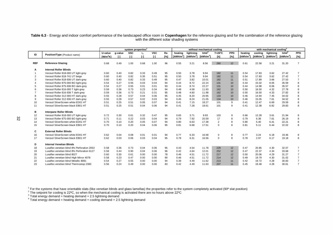
32

Table 6.3 - Energy and indoor comfort performance of the landscaped office room in Copenhagen for the reference glazing and for the combination of the reference glazing with the different solar shading systems

U-value g-value SSC v VSC Ra heating lightning total3 T>26ºC PPD heating cooling lightning total4 PPD[W/m2K] [-] [-] [-] [-] [%] [kWh/m2] [kWh/m2] [kWh/m2] [h] [%] [kWh/m2] [kWh/m2] [kWh/m2] [kWh/m2] [%]

REF Reference Glazing 0.68 0.49 1.00 0.68 1.00 96 0.55 3.21 8.56 260 12 0.61 22.58 3.21 31.20 7

A Internal Roller Blinds1 Verosol Roller 818-000 UT light-grey 0.60 0.40 0.82 0.33 0.49 95 0.50 3.78 9.94 182 11 0.54 17.83 3.62 27.42 72 Verosol Roller 818-741 UT beige 0.60 0.40 0.82 0.35 0.51 95 0.50 3.78 9.94 182 11 0.54 17.83 3.62 27.42 73 Verosol Roller 818-936 UT dark-grey 0.60 0.40 0.82 0.33 0.49 95 0.47 3.82 10.01 182 11 0.51 17.89 3.66 27.53 74 Verosol Roller 875-000 BO light-grey 0.54 0.27 0.55 0.03 0.04 94 0.44 8.72 22.24 131 10 0.44 15.02 8.05 35.59 85 Verosol Roller 875-936 BO dark-grey 0.54 0.27 0.55 0.01 0.01 93 0.44 8.74 22.27 131 10 0.44 14.98 8.06 35.57 86 Verosol Roller 816-000 T light-grey 0.59 0.36 0.73 0.23 0.34 94 0.48 4.58 11.93 162 10 0.50 16.50 4.32 27.78 87 Verosol Roller 816-936 T dark-grey 0.59 0.36 0.73 0.21 0.31 95 0.48 4.60 11.98 162 10 0.50 16.50 4.33 27.82 88 Verosol Roller 312-000 HT dark-grey 0.55 0.28 0.57 0.04 0.06 95 0.45 8.20 20.95 133 10 0.46 14.94 7.45 34.02 89 Verosol Roller 312-936 HT dark-grey 0.55 0.28 0.57 0.02 0.03 94 0.45 8.24 21.05 134 10 0.46 15.05 7.61 34.52 810 Verosol SilverScreen white ED01 HT 0.51 0.25 0.51 0.05 0.07 94 0.41 7.15 18.27 101 9 0.41 12.47 6.69 29.59 811 Verosol SilverScreen black EB01 HT 0.51 0.25 0.51 0.04 0.06 94 0.41 7.28 18.61 101 9 0.41 12.38 6.82 29.83 8

B Interpane Roller Blinds12 Verosol Roller 818-000 UT light-grey 0.72 0.30 0.61 0.32 0.47 95 0.65 3.71 9.93 103 9 0.66 12.28 3.61 21.94 813 Verosol Roller 875-000 BO light-grey 0.71 0.11 0.22 0.03 0.04 94 0.79 7.92 20.59 17 8 0.79 6.38 7.61 26.19 814 Verosol SilverScreen white ED01 HT 0.70 0.10 0.20 0.05 0.07 94 0.80 6.63 17.38 2 8 0.80 5.40 6.41 22.21 815 Verosol SilverScreen black EB01 HT 0.70 0.10 0.20 0.04 0.06 95 0.81 6.68 17.51 0 8 0.81 5.11 6.44 22.02 8

C External Roller Blinds16 Verosol SilverScreen white ED01 HT 0.62 0.04 0.08 0.01 0.01 94 0.77 6.33 16.58 0 8 0.77 3.24 6.18 19.46 817 Verosol SilverScreen black EB01 HT 0.62 0.03 0.06 0.03 0.04 95 0.78 6.31 16.56 0 8 0.78 2.97 6.17 19.18 8

D Internal Venetian Blinds18 Luxaflex venetian blind 8% Perforation 2053 0.58 0.36 0.73 0.04 0.06 95 0.43 4.54 11.78 229 12 0.47 20.85 4.30 32.07 719 Luxaflex venetian blind 8% Perforation 6127 0.58 0.44 0.90 0.04 0.06 96 0.42 4.64 12.01 252 12 0.47 22.37 4.34 33.68 720 Luxaflex venetian blind 8027 0.60 0.30 0.61 0.00 0.00 78 0.46 4.51 11.72 217 12 0.50 20.06 4.29 31.27 721 Luxaflex venetian blind High Mirror 4078 0.58 0.23 0.47 0.00 0.00 90 0.46 4.51 11.72 214 12 0.49 19.79 4.30 31.02 722 Luxaflex venetian blind Metallic 8081 0.54 0.27 0.55 0.00 0.00 94 0.39 4.49 11.62 213 11 0.42 19.72 4.28 30.83 723 Luxaflex venetian blind Thermostop 2383 0.56 0.24 0.49 0.00 0.00 83 0.42 4.49 11.63 207 11 0.45 19.48 4.28 30.61 7

without mechanical cooling with mechanical cooling2

Position/Type (Product name)ID

system properties1

1 For the systems that have orientable slats (like venetian blinds and glass lamellas) the properties refer to the system completely activated (90º slat position) 2 The setpoint for cooling is 22ºC, so when the mechanical cooling is activated there are no hours above 22ºC 3 Total energy demand = heating demand + 2.5 lightning demand 4 Total energy demand = heating demand + cooling demand + 2.5 lightning demand

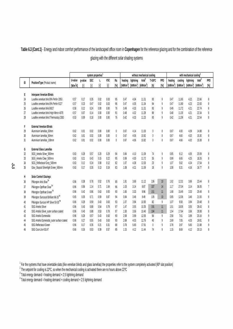
33

Table 6.3 (Cont.1) - Energy and indoor comfort performance of the landscaped office room in Copenhagen for the reference glazing and for the combination of the reference

glazing with the different solar shading systems


E Interpane Venetian Blinds24 Luxaflex venetian blind 8% Perfor 2053 0.57 0.17 0.35 0.02 0.03 95 0.47 4.34 11.31 93 9 0.47 11.65 4.22 22.66 825 Luxaflex venetian blind 8% Perfor 6127 0.57 0.23 0.47 0.02 0.03 96 0.47 4.35 11.34 94 9 0.47 11.80 4.23 22.83 826 Luxaflex venetian blind 8027 0.58 0.12 0.24 0.00 0.00 76 0.49 4.33 11.31 93 9 0.49 11.72 4.21 22.74 827 Luxaflex venetian blind High Mirror 4078 0.57 0.07 0.14 0.00 0.00 91 0.48 4.32 11.28 89 9 0.48 11.35 4.21 22.34 828 Luxaflex venetian blind Thermostop 2383 0.53 0.09 0.18 0.00 0.00 76 0.42 4.33 11.23 93 9 0.42 11.59 4.21 22.54 8

F External Venetian Blinds29 Aluminium lamellas_60mm 0.62 0.01 0.02 0.00 0.00 0 0.67 4.14 11.00 0 8 0.67 4.00 4.09 14.88 830 Aluminium lamellas_80mm 0.62 0.01 0.02 0.00 0.00 0 0.67 4.06 10.82 0 8 0.67 4.60 4.02 15.30 831 Aluminium lamellas_100mm 0.62 0.01 0.02 0.00 0.00 0 0.67 4.06 10.82 0 8 0.67 4.66 4.02 15.38 8

G External Glass Lamellas32 SGG_Antelio Silver_500mm 0.63 0.28 0.57 0.20 0.29 94 0.84 4.10 11.09 74 9 0.85 9.12 4.05 20.09 833 SGG_Antelio Clear_500mm 0.63 0.21 0.43 0.15 0.22 95 0.99 4.30 11.72 35 9 0.99 6.65 4.25 18.26 834 SGG_Reflectasol Grey_500mm 0.63 0.12 0.24 0.08 0.12 82 1.07 4.38 12.00 23 9 1.07 5.62 4.34 17.54 835 Glav_Stopsol Silverlight Green_500mm 0.63 0.17 0.35 0.13 0.19 83 1.08 4.21 11.59 18 9 1.08 5.31 4.16 16.77 8

H Solar Control Glazings 36 Pilkington Artic BlueTM 0.96 0.38 0.78 0.52 0.76 85 1.91 3.69 11.12 106 10 1.92 12.31 3.69 23.44 837 Pilkington Optifloat ClearTM 0.96 0.56 1.14 0.71 1.04 96 1.03 3.14 8.87 337 14 1.17 27.04 3.14 36.05 738 Pilkington Optifloat GreenTM 0.96 0.42 0.86 0.63 0.93 90 1.65 3.33 9.96 151 11 1.68 15.49 3.33 25.48 839 Pilkington Suncoool Brilliant 66-33TM 0.65 0.35 0.71 0.59 0.87 94 0.84 3.46 9.49 105 10 0.85 12.06 3.46 21.55 840 Pilkington Suncool HP Silver 50-30TM 0.66 0.29 0.59 0.43 0.63 93 1.07 3.94 10.90 82 9 1.07 9.58 3.94 20.48 841 SSG Antelio Silver 0.96 0.43 0.88 0.54 0.79 97 1.47 3.55 10.35 191 11 1.51 18.05 3.55 28.43 842 SSG Antelio Silver_outer surface coated 0.96 0.43 0.88 0.53 0.78 97 1.50 3.56 10.40 184 11 1.54 17.64 3.56 28.08 843 SSG Antelio Esmeralda 0.96 0.28 0.57 0.43 0.63 90 2.58 3.99 12.55 56 9 2.58 7.61 3.99 20.16 944 SSG Antelio Esmeralda_outer surface coated 0.96 0.27 0.55 0.43 0.63 90 2.69 4.03 12.76 45 9 2.69 7.05 4.03 19.81 945 SSG Reflectasol Green 0.96 0.17 0.35 0.21 0.31 88 3.78 5.65 17.91 0 9 3.78 3.97 5.65 21.88 946 SSG Cool-Lite KS147 0.66 0.26 0.53 0.39 0.57 95 1.15 4.12 11.44 74 9 1.15 8.69 4.12 20.13 8

with mechanical cooling2without mechanical coolingsystem properties1

ID Position/Type (Product name)


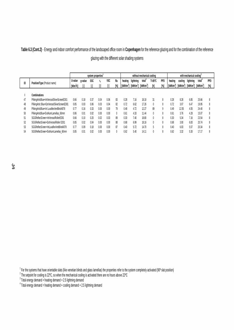
34

Table 6.3 (Cont.2) - Energy and indoor comfort performance of the landscaped office room in Copenhagen for the reference glazing and for the combination of the reference

glazing with the different solar shading systems


I Combinations47 PilkingArticBlue+IntVerosolSilverScreenED01 0.66 0.18 0.37 0.04 0.06 83 0.28 7.16 18.18 31 8 0.28 8.28 6.85 25.66 848 PilkingArtic Blue+ExtVerosolSilverScreenED01 0.85 0.03 0.06 0.03 0.04 82 0.72 6.62 17.26 0 8 0.72 3.07 6.47 19.95 849 PilkingArticBlue+Int LuxaflexVenBlind4078 0.77 0.16 0.33 0.00 0.00 79 0.48 4.72 12.27 89 9 0.49 12.55 4.55 24.40 850 PilkingArticBlue+ExtAlumLamellas_60mm 0.86 0.01 0.02 0.00 0.00 0 0.61 4.33 11.44 0 8 0.61 3.76 4.28 15.07 851 SGGReflectGreen+IntVerosolRollerED01 0.66 0.10 0.20 0.02 0.03 89 0.30 7.40 18.80 0 8 0.30 5.34 7.16 23.54 852 SGGReflectGreen+ExtVerosolRoller ED01 0.85 0.02 0.04 0.00 0.00 88 0.68 6.99 18.16 0 8 0.68 3.00 6.83 20.74 853 SGGReflectGreen+IntLuxaflexVenBlind4078 0.77 0.09 0.18 0.00 0.00 87 0.40 5.72 14.70 5 8 0.40 6.03 5.57 20.34 854 SGGReflectGreen+ExtAlumLamellas_60mm 0.85 0.01 0.02 0.00 0.00 0 0.62 5.40 14.11 0 8 0.62 3.32 5.30 17.17 8

without mechanical cooling with mechanical cooling2system properties1



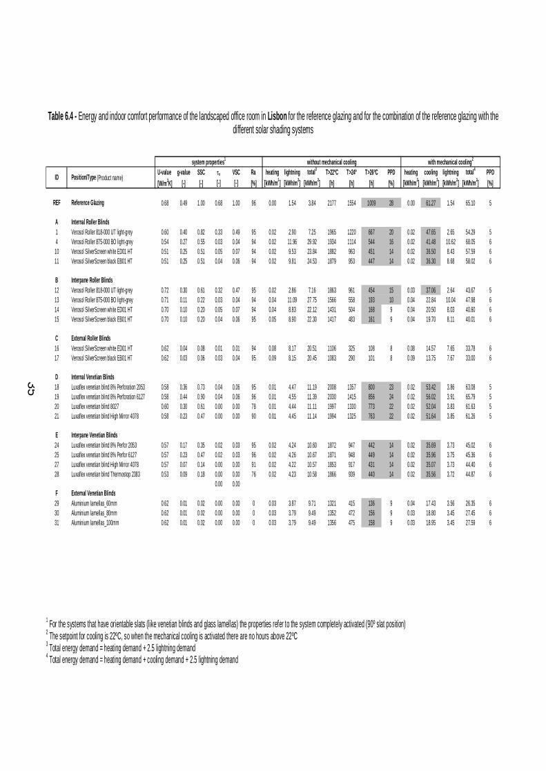
35

Table 6.4 - Energy and indoor comfort performance of the landscaped office room in Lisbon for the reference glazing and for the combination of the reference glazing with the different solar shading systems

U-value g-value SSC v VSC Ra heating lightning total3 T>22ºC T>24º T>26ºC PPD heating cooling lightning total4 PPD[W/m2K] [-] [-] [-] [-] [%] [kWh/m2] [kWh/m2] [kWh/m2] [h] [h] [h] [%] [kWh/m2] [kWh/m2] [kWh/m2] [kWh/m2] [%]

REF Reference Glazing 0.68 0.49 1.00 0.68 1.00 96 0.00 1.54 3.84 2177 1554 1009 28 0.00 61.27 1.54 65.10 5

A Internal Roller Blinds1 Verosol Roller 818-000 UT light-grey 0.60 0.40 0.82 0.33 0.49 95 0.02 2.90 7.25 1965 1220 667 20 0.02 47.65 2.65 54.29 54 Verosol Roller 875-000 BO light-grey 0.54 0.27 0.55 0.03 0.04 94 0.02 11.96 29.92 1934 1114 544 16 0.02 41.48 10.62 68.05 6

10 Verosol SilverScreen white ED01 HT 0.51 0.25 0.51 0.05 0.07 94 0.02 9.53 23.84 1882 963 451 14 0.02 36.50 8.43 57.59 611 Verosol SilverScreen black EB01 HT 0.51 0.25 0.51 0.04 0.06 94 0.02 9.81 24.53 1879 953 447 14 0.02 36.30 8.68 58.02 6

B Interpane Roller Blinds12 Verosol Roller 818-000 UT light-grey 0.72 0.30 0.61 0.32 0.47 95 0.02 2.86 7.16 1863 961 454 15 0.03 37.06 2.64 43.67 513 Verosol Roller 875-000 BO light-grey 0.71 0.11 0.22 0.03 0.04 94 0.04 11.09 27.75 1566 558 193 10 0.04 22.84 10.04 47.98 614 Verosol SilverScreen white ED01 HT 0.70 0.10 0.20 0.05 0.07 94 0.04 8.83 22.12 1431 504 168 9 0.04 20.50 8.03 40.60 615 Verosol SilverScreen black EB01 HT 0.70 0.10 0.20 0.04 0.06 95 0.05 8.90 22.30 1417 483 161 9 0.04 19.70 8.11 40.01 6

C External Roller Blinds16 Verosol SilverScreen white ED01 HT 0.62 0.04 0.08 0.01 0.01 94 0.08 8.17 20.51 1106 325 108 8 0.08 14.57 7.65 33.78 617 Verosol SilverScreen black EB01 HT 0.62 0.03 0.06 0.03 0.04 95 0.09 8.15 20.45 1083 290 101 8 0.09 13.75 7.67 33.00 6

D Internal Venetian Blinds18 Luxaflex venetian blind 8% Perforation 2053 0.58 0.36 0.73 0.04 0.06 95 0.01 4.47 11.19 2008 1357 800 23 0.02 53.42 3.86 63.08 519 Luxaflex venetian blind 8% Perforation 6127 0.58 0.44 0.90 0.04 0.06 96 0.01 4.55 11.39 2030 1415 856 24 0.02 56.02 3.91 65.79 520 Luxaflex venetian blind 8027 0.60 0.30 0.61 0.00 0.00 78 0.01 4.44 11.11 1997 1330 773 22 0.02 52.04 3.83 61.63 521 Luxaflex venetian blind High Mirror 4078 0.58 0.23 0.47 0.00 0.00 90 0.01 4.45 11.14 1994 1325 763 22 0.02 51.64 3.85 61.26 5

E Interpane Venetian Blinds24 Luxaflex venetian blind 8% Perfor 2053 0.57 0.17 0.35 0.02 0.03 95 0.02 4.24 10.60 1872 947 442 14 0.02 35.69 3.73 45.02 625 Luxaflex venetian blind 8% Perfor 6127 0.57 0.23 0.47 0.02 0.03 96 0.02 4.26 10.67 1871 948 449 14 0.02 35.96 3.75 45.36 627 Luxaflex venetian blind High Mirror 4078 0.57 0.07 0.14 0.00 0.00 91 0.02 4.22 10.57 1853 917 431 14 0.02 35.07 3.73 44.40 628 Luxaflex venetian blind Thermostop 2383 0.53 0.09 0.18 0.00 0.00 76 0.02 4.23 10.58 1866 939 440 14 0.02 35.56 3.72 44.87 6

0.00 0.00F External Venetian Blinds29 Aluminium lamellas_60mm 0.62 0.01 0.02 0.00 0.00 0 0.03 3.87 9.71 1321 415 136 9 0.04 17.43 3.56 26.35 630 Aluminium lamellas_80mm 0.62 0.01 0.02 0.00 0.00 0 0.03 3.79 9.49 1352 472 156 9 0.03 18.80 3.45 27.45 631 Aluminium lamellas_100mm 0.62 0.01 0.02 0.00 0.00 0 0.03 3.79 9.49 1356 475 158 9 0.03 18.95 3.45 27.59 6

with mechanical cooling2


system properties1 without mechanical cooling


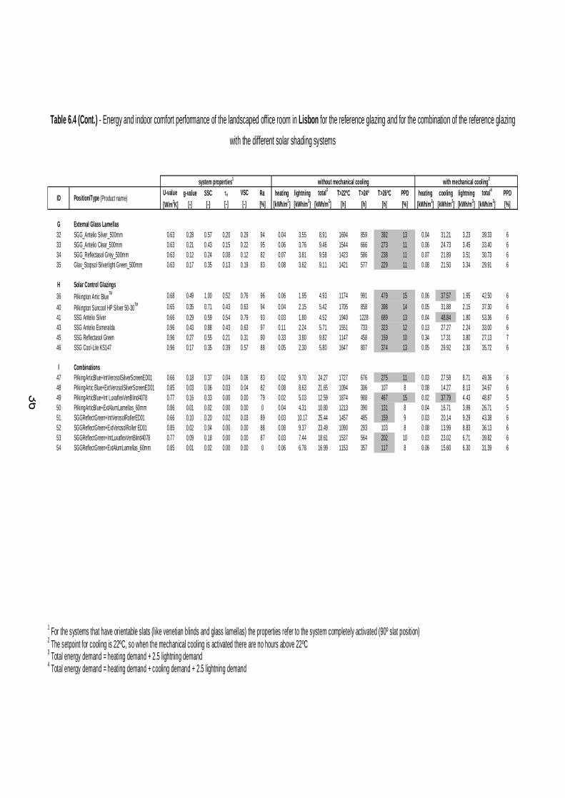
36

Table 6.4 (Cont.) - Energy and indoor comfort performance of the landscaped office room in Lisbon for the reference glazing and for the combination of the reference glazing

with the different solar shading systems

U-value g-value SSC v VSC Ra heating lightning total3 T>22ºC T>24º T>26ºC PPD heating cooling lightning total4 PPD[W/m2K] [-] [-] [-] [-] [%] [kWh/m2] [kWh/m2] [kWh/m2] [h] [h] [h] [%] [kWh/m2] [kWh/m2] [kWh/m2] [kWh/m2] [%]

G External Glass Lamellas32 SGG_Antelio Silver_500mm 0.63 0.28 0.57 0.20 0.29 94 0.04 3.55 8.91 1694 859 392 13 0.04 31.21 3.23 39.33 633 SGG_Antelio Clear_500mm 0.63 0.21 0.43 0.15 0.22 95 0.06 3.76 9.46 1544 666 273 11 0.06 24.73 3.45 33.40 634 SGG_Reflectasol Grey_500mm 0.63 0.12 0.24 0.08 0.12 82 0.07 3.81 9.58 1423 586 238 11 0.07 21.89 3.51 30.73 635 Glav_Stopsol Silverlight Green_500mm 0.63 0.17 0.35 0.13 0.19 83 0.08 3.62 9.11 1421 577 229 11 0.08 21.50 3.34 29.91 6

H Solar Control Glazings 36 Pilkington Artic BlueTM 0.68 0.49 1.00 0.52 0.76 96 0.06 1.95 4.93 1174 991 479 15 0.06 37.57 1.95 42.50 640 Pilkington Suncool HP Silver 50-30TM 0.65 0.35 0.71 0.43 0.63 94 0.04 2.15 5.42 1705 858 398 14 0.05 31.88 2.15 37.30 641 SSG Antelio Silver 0.66 0.29 0.59 0.54 0.79 93 0.03 1.80 4.52 1940 1228 689 13 0.04 48.84 1.80 53.36 643 SSG Antelio Esmeralda 0.96 0.43 0.88 0.43 0.63 97 0.11 2.24 5.71 1551 733 323 12 0.13 27.27 2.24 33.00 645 SSG Reflectasol Green 0.96 0.27 0.55 0.21 0.31 90 0.33 3.80 9.82 1147 458 159 10 0.34 17.31 3.80 27.13 746 SSG Cool-Lite KS147 0.96 0.17 0.35 0.39 0.57 88 0.05 2.30 5.80 1647 807 374 13 0.05 29.92 2.30 35.72 6

I Combinations47 PilkingArticBlue+IntVerosolSilverScreenED01 0.66 0.18 0.37 0.04 0.06 83 0.02 9.70 24.27 1727 676 275 11 0.03 27.58 8.71 49.36 648 PilkingArtic Blue+ExtVerosolSilverScreenED01 0.85 0.03 0.06 0.03 0.04 82 0.08 8.63 21.65 1094 306 107 8 0.08 14.27 8.13 34.67 649 PilkingArticBlue+Int LuxaflexVenBlind4078 0.77 0.16 0.33 0.00 0.00 79 0.02 5.03 12.59 1874 988 467 15 0.02 37.79 4.43 48.87 550 PilkingArticBlue+ExtAlumLamellas_60mm 0.86 0.01 0.02 0.00 0.00 0 0.04 4.31 10.80 1213 390 131 8 0.04 16.71 3.99 26.71 551 SGGReflectGreen+IntVerosolRollerED01 0.66 0.10 0.20 0.02 0.03 89 0.03 10.17 25.44 1457 485 159 9 0.03 20.14 9.29 43.38 652 SGGReflectGreen+ExtVerosolRoller ED01 0.85 0.02 0.04 0.00 0.00 88 0.08 9.37 23.49 1090 293 103 8 0.08 13.99 8.83 36.13 653 SGGReflectGreen+IntLuxaflexVenBlind4078 0.77 0.09 0.18 0.00 0.00 87 0.03 7.44 18.61 1537 564 202 10 0.03 23.02 6.71 39.82 654 SGGReflectGreen+ExtAlumLamellas_60mm 0.85 0.01 0.02 0.00 0.00 0 0.06 6.78 16.99 1153 357 117 8 0.06 15.60 6.30 31.39 6

with mechanical cooling2system properties1 without mechanical cooling



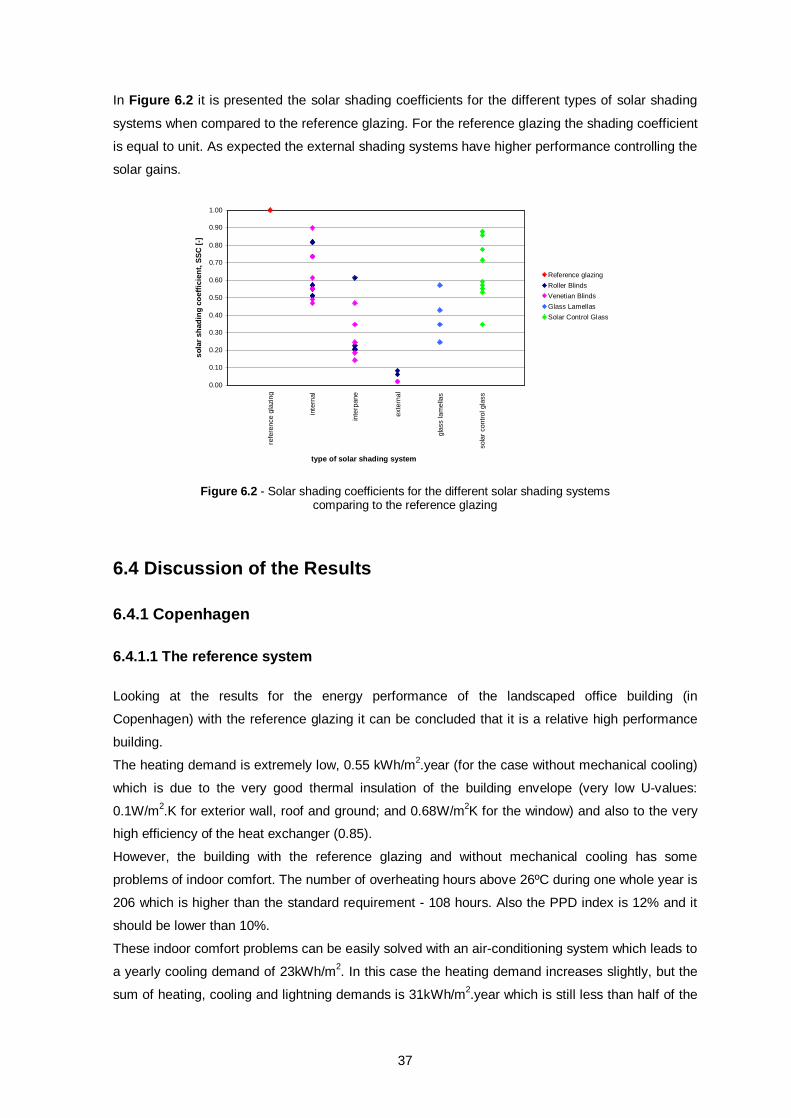
37

In Figure 6.2 it is presented the solar shading coefficients for the different types of solar shading

systems when compared to the reference glazing. For the reference glazing the shading coefficient

is equal to unit. As expected the external shading systems have higher performance controlling the

solar gains.

0.00

0.10

0.20

0.30

0.40

0.50

0.60

0.70

0.80

0.90

1.00

type of solar shading system

sola

r sha

ding

coe

ffici

ent,

SSC

[-]

Reference glazingRoller BlindsVenetian BlindsGlass LamellasSolar Control Glass

inte

rnal

inte

rpan

e

exte

rnal

refe

renc

e gl

azin

g

glas

s la

mel

las

sola

r con

trol g

lass

Figure 6.2 - Solar shading coefficients for the different solar shading systems

comparing to the reference glazing

6.4 Discussion of the Results 6.4.1 Copenhagen 6.4.1.1 The reference system Looking at the results for the energy performance of the landscaped office building (in

Copenhagen) with the reference glazing it can be concluded that it is a relative high performance

building.

The heating demand is extremely low, 0.55 kWh/m2.year (for the case without mechanical cooling)

which is due to the very good thermal insulation of the building envelope (very low U-values:

0.1W/m2.K for exterior wall, roof and ground; and 0.68W/m2K for the window) and also to the very

high efficiency of the heat exchanger (0.85).

However, the building with the reference glazing and without mechanical cooling has some

problems of indoor comfort. The number of overheating hours above 26ºC during one whole year is

206 which is higher than the standard requirement - 108 hours. Also the PPD index is 12% and it

should be lower than 10%.

These indoor comfort problems can be easily solved with an air-conditioning system which leads to

a yearly cooling demand of 23kWh/m2. In this case the heating demand increases slightly, but the

sum of heating, cooling and lightning demands is 31kWh/m2.year which is still less than half of the

38

standard requirement calculated before (78kWh/m2.year). Thus, with air-conditioning system the

building fulfils the energy and indoor comfort requirements.

6.4.1.2 The different solar shading systems In spite of being already in accordance with the standard requirement, different solar shading

systems were added to the reference glazing. With this procedure the goal was to check if when

using a solar shading system it is possible to fulfil the indoor comfort requirements without using

mechanical cooling. And if not how well the shading systems perform reducing the cooling demand.

As presented in the table of results for Copenhagen (Table 6.3) most of the internal solutions for

solar shading systems (roller blinds and venetian blinds) are not enough to accomplish the

standard indoor comfort requirements without the use of an air-conditioning system. However these

shading systems can slightly reduce the cooling demand.

Some special attention should be paid to the lightning demand. While reducing the solar gains and

consequently the cooling demand, some solar shading systems also reduce the indoor daylight

increasing in this way the need for electrical lightning. Sometimes the electrical lightning demand

increases more than the cooling demand decreases, and the total energy demand is higher with

the use of solar shading system than without it (this happens in cases A4, A5, A8, A9).

Regarding the interpane and external solar shading systems (roller blinds and venetian blinds) they

are enough to, without the use of mechanical cooling system, accomplish the standard indoor

comfort requirements.

However if better indoor conditions are desired an air-conditioning system may be used to

completely eliminate the hours in which the temperature is above 22ºC (it is important to remember

that this means a higher total energy consumption). In this case, even with an increase on electrical

lightning demand caused by the shading system, the reduction on the cooling demand is such that

total energy demand decreases: comparing to the reference glazing, a reduction to approximately

2/3 of the total energy demand can be achieved with the use of interpane or external roller blinds.

The interpane venetian blinds can also reduce to 2/3 the total energy demand while the external

venetian blinds can reduced it to 1/2.

With external glass lamellas it is also possible to fulfil the standard indoor requirements without the

use of mechanical cooling. Once again if better levels of indoor environment are desired the

mechanical system may be used. In this case, comparing to the solution with the reference glazing,

the total amount of energy demand can be reduced to between 1/2 and 2/3 depending on the type

of glass that composes the glass lamellas.

As it was expected, the electrical lightning demand is lower when using systems composed of slats

than for instance roller blinds (specially the ones with very low openness factors). When the slat

systems are activated to block the direct sun in order to avoid overheating the daylight can still

39

enter the room through the space between the slats. The same does not happen with the roller

blinds.

It would be expected that the electrical lightning demand of the office room when using glass

lamellas systems was lower than the one when using, for instance, external venetian blinds.

However, when comparing both electrical lightning demands they are very similar. This is mainly

due to the following difference between the two systems: while the external venetian blinds can be

completely retracted during overcast days, the same does not happen with the glass lamellas, they

are permanently in front of the façade and can only be tilted.

Concerning the solar control glasses not all the solutions simulated allow the accomplishment of

the standard indoor requirements without the use of mechanical cooling.

As it was expected,when a solar control glass replaces the reference outer pane which was a low-e

coating glass (Pilkington Optitherm SN4), the heating demand increases slightly.

The need for electrical lightning varies depending on how transparent to light the glass is.

When compared to the reference glazing, the total energy demand for some solar control glasses

combined with mechanical cooling can be reduced approximately to 2/3.

Finally some combinations of solar control glasses with ordinary solar shading systems were

simulated. The best performances were achieved for I50 and I54 which result from the combination

of a solar control glass (body tinted and hard coating respectively) with external venetian lamellas

made of aluminium. In these cases, total energy demands of 11kWh/m2.year and 14kWh/m2.year

were correspondingly obtained without the use of mechanical cooling. To remove completely the

hours of overheating above 22ºC, air-conditioning system may be used and as a result the total

energy demands increase to 15kWh/m2.year and 17kWh/m2.year respectively (this is half of the

energy consumption achieved with the reference glazing).

6.4.2 Lisbon 6.4.2.1 The reference system Regarding the heating demand, the situation for Lisbon is similar to Copenhagen. The envelopment

solutions are very good concerning the Portuguese climate (low U-values: 0.4W/m2.K for exterior

wall, roof and ground; and 0.68W/m2K for the window) and the heat exchanger has a high

efficiency (0.85).

The difference comes with the level of indoor comfort. With the reference glazing and without

mechanical cooling the number of hours of temperature above 26ºC is extremely high, 1009 hours

and the PPD index is 28% which is much higher than the standard maximum, 10%.

When trying to remove the hours of overheating with mechanical cooling, the panorama is different

from Copenhagen. As there are much more hours of overheating the cooling demand to remove

them is very high, 61kWh/m2.year. This value is approximately doubled of 32kWh/m2.year which is

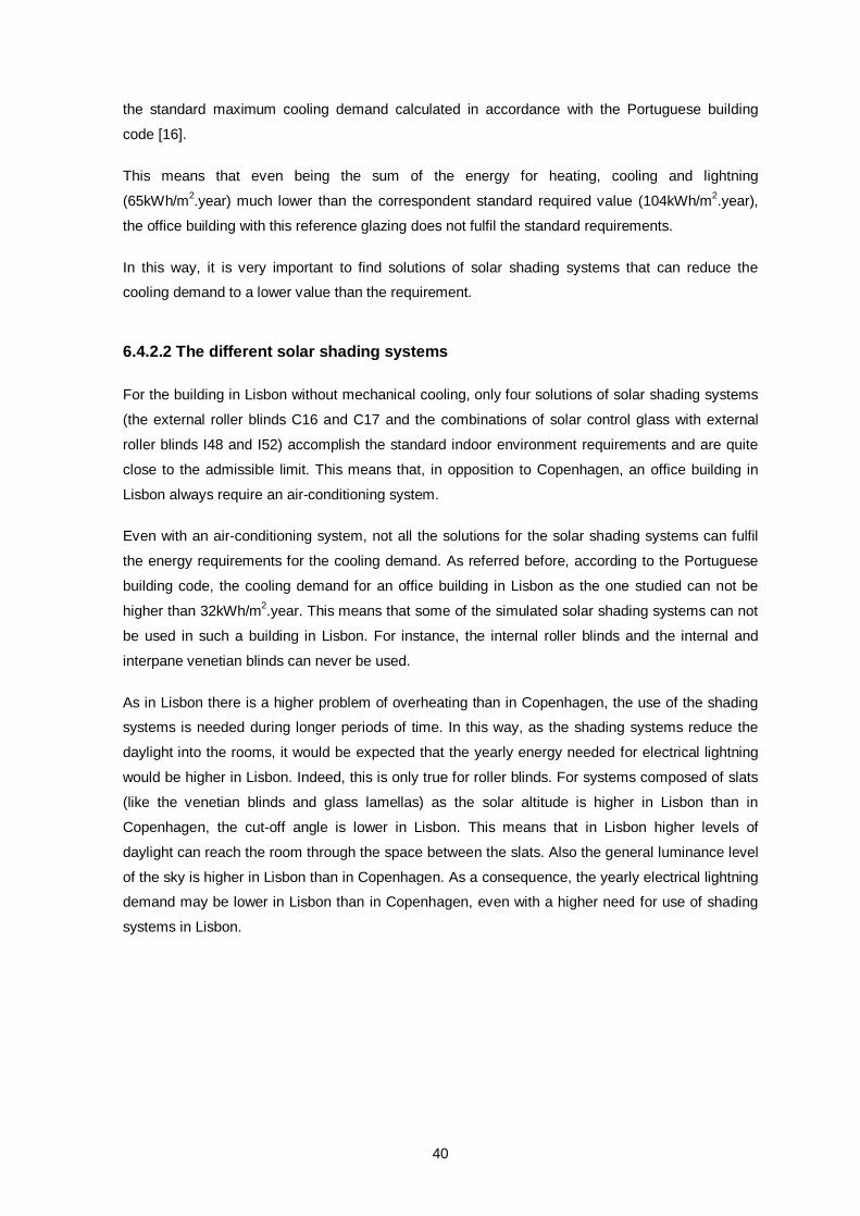
40

the standard maximum cooling demand calculated in accordance with the Portuguese building

code [16].

This means that even being the sum of the energy for heating, cooling and lightning

(65kWh/m2.year) much lower than the correspondent standard required value (104kWh/m2.year),

the office building with this reference glazing does not fulfil the standard requirements.

In this way, it is very important to find solutions of solar shading systems that can reduce the

cooling demand to a lower value than the requirement.

6.4.2.2 The different solar shading systems For the building in Lisbon without mechanical cooling, only four solutions of solar shading systems

(the external roller blinds C16 and C17 and the combinations of solar control glass with external

roller blinds I48 and I52) accomplish the standard indoor environment requirements and are quite

close to the admissible limit. This means that, in opposition to Copenhagen, an office building in

Lisbon always require an air-conditioning system.

Even with an air-conditioning system, not all the solutions for the solar shading systems can fulfil

the energy requirements for the cooling demand. As referred before, according to the Portuguese

building code, the cooling demand for an office building in Lisbon as the one studied can not be

higher than 32kWh/m2.year. This means that some of the simulated solar shading systems can not

be used in such a building in Lisbon. For instance, the internal roller blinds and the internal and

interpane venetian blinds can never be used.

As in Lisbon there is a higher problem of overheating than in Copenhagen, the use of the shading

systems is needed during longer periods of time. In this way, as the shading systems reduce the

daylight into the rooms, it would be expected that the yearly energy needed for electrical lightning

would be higher in Lisbon. Indeed, this is only true for roller blinds. For systems composed of slats

(like the venetian blinds and glass lamellas) as the solar altitude is higher in Lisbon than in

Copenhagen, the cut-off angle is lower in Lisbon. This means that in Lisbon higher levels of

daylight can reach the room through the space between the slats. Also the general luminance level

of the sky is higher in Lisbon than in Copenhagen. As a consequence, the yearly electrical lightning

demand may be lower in Lisbon than in Copenhagen, even with a higher need for use of shading

systems in Lisbon.

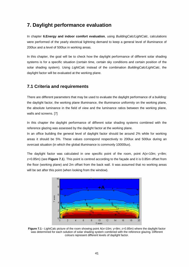
41

7. Daylight performance evaluation In chapter 6.Energy and indoor comfort evaluation, using BuildingCalc/LightCalc, calculations

were performed of the yearly electrical lightning demand to keep a general level of illuminance of

200lux and a level of 500lux in working areas.

In this chapter, the goal will be to check how the daylight performance of different solar shading

systems is for a specific situation (certain time, certain sky conditions and certain position of the

solar shading system). Using LightCalc instead of the combination BuildingCalc/LightCalc, the

daylight factor will be evaluated at the working plane.

7.1 Criteria and requirements There are different parameters that may be used to evaluate the daylight performance of a building:

the daylight factor, the working plane illuminance, the illuminance uniformity on the working plane,

the absolute luminance in the field of view and the luminance ratios between the working plane,

walls and screens. [7]

In this chapter the daylight performance of different solar shading systems combined with the

reference glazing was assessed by the daylight factor at the working plane.

In an office building the general level of daylight factor should be around 2% while for working

areas it should be 5%. These values correspond respectively to 200lux and 500lux during an

overcast situation (in which the global illuminance is commonly 10000lux).

The daylight factor was calculated in one specific point of the room, point A(x=10m; y=8m;

z=0.85m) (see Figure 7.1). This point is centred according to the façade and it is 0.85m offset from

the floor (working plane) and 2m offset from the back wall. It was assumed that no working areas

will be set after this point (when looking from the window).

Figure 7.1 - LightCalc picture of the room showing point A(x=10m; y=8m; z=0.85m) where the daylight factor

was determined for each solution of solar shading system combined with the reference glazing. Different colours represent different levels of daylight factor.

+A

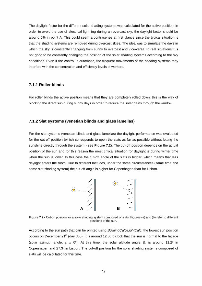
42

The daylight factor for the different solar shading systems was calculated for the active position: in

order to avoid the use of electrical lightning during an overcast sky, the daylight factor should be

around 5% in point A. This could seem a contrasense at first glance since the typical situation is

that the shading systems are removed during overcast skies. The idea was to simulate the days in

which the sky is constantly changing from sunny to overcast and vice-versa. In real situations it is

not good to be constantly changing the position of the solar shading systems according to the sky

conditions. Even if the control is automatic, the frequent movements of the shading systems may

interfere with the concentration and efficiency levels of workers.

7.1.1 Roller blinds

For roller blinds the active position means that they are completely rolled down: this is the way of

blocking the direct sun during sunny days in order to reduce the solar gains through the window.

7.1.2 Slat systems (venetian blinds and glass lamellas)

For the slat systems (venetian blinds and glass lamellas) the daylight performance was evaluated

for the cut-off position (which corresponds to open the slats as far as possible without letting the

sunshine directly through the system - see Figure 7.2). The cut-off position depends on the actual

position of the sun and for this reason the most critical situation for daylight is during winter time

when the sun is lower. In this case the cut-off angle of the slats is higher, which means that less

daylight enters the room. Due to different latitudes, under the same circumstances (same time and

same slat shading system) the cut-off angle is higher for Copenhagen than for Lisbon.

Figure 7.2 - Cut-off position for a solar shading system composed of slats. Figures (a) and (b) refer to different positions of the sun.

According to the sun path that can be printed using BuildingCalc/LightCalc, the lowest sun position

occurs on December 21st (day 355). It is around 12.00 o’clock that the sun is normal to the façade

(solar azimuth angle, , 0º). At this time, the solar altitude angle, , is around 11.2º in

Copenhagen and 27.3º in Lisbon. The cut-off position for the solar shading systems composed of

slats will be calculated for this time.

A B

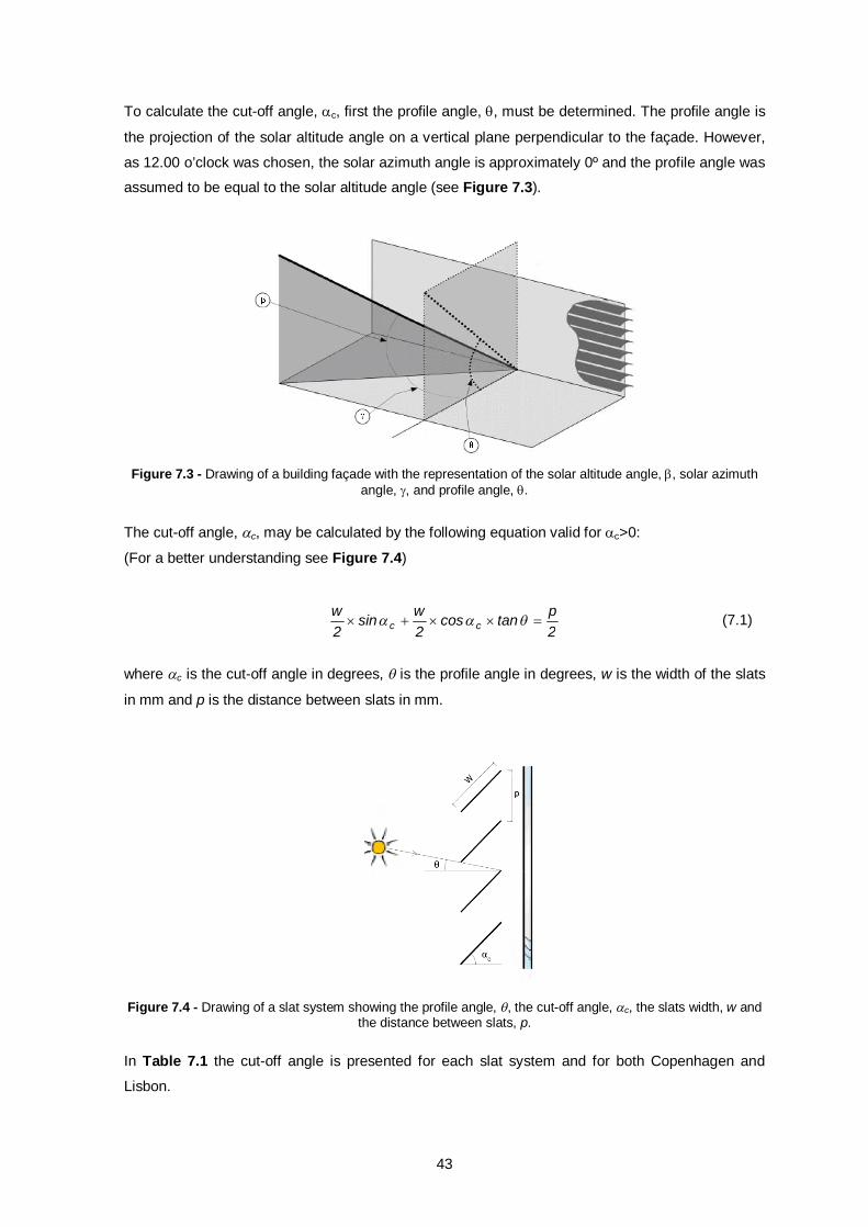
43

To calculate the cut-off angle, c, first the profile angle, , must be determined. The profile angle is

the projection of the solar altitude angle on a vertical plane perpendicular to the façade. However,

as 12.00 o’clock was chosen, the solar azimuth angle is approximately 0º and the profile angle was

assumed to be equal to the solar altitude angle (see Figure 7.3).

Figure 7.3 - Drawing of a building façade with the representation of the solar altitude angle, , solar azimuth

angle, , and profile angle, .

The cut-off angle, c, may be calculated by the following equation valid for c>0:

(For a better understanding see Figure 7.4)

2ptancos

2wsin

2w

cc (7.1)

where c is the cut-off angle in degrees, is the profile angle in degrees, w is the width of the slats

in mm and p is the distance between slats in mm.

Figure 7.4 - Drawing of a slat system showing the profile angle, , the cut-off angle, c, the slats width, w and

the distance between slats, p.

In Table 7.1 the cut-off angle is presented for each slat system and for both Copenhagen and

Lisbon.

44

Table 7.1- Cut-off angle, s, for the different slat systems on December 21st at 12.00 o’clock (the profile angle is 11.2º for Copenhagen and 27.3º for Lisbon)

Copenhagen Lisbontype of solar shading system w [mm] p [mm] s [º] s [º]D. Internal venetian blinds

Valid for all 25 20 41 18D. Interpane venetian blinds

Valid for all 22 16 36 14F. External venetian blinds

29. Aluminium lamellas_60mm 60 52 47 2330. Aluminium lamellas_80mm 80 72 51 2631. Aluminium lamellas_100mm 100 92 53 28

G. Glass lamellasValid for all 500 500 68 35

The relation between the slat width and the distance between two consecutive slats has an

important influence on the cut-off angle. This is the reason for such different cut-off angles when

comparing different slats systems.

7.1.3 Reference glazing and solar control glazings

For the reference glazing and solar control glazings studied there is no active or non active

position. These systems are not flexible to different sky conditions. Thus the daylight factor at point

A should be 5% in order to avoid the use of electrical lightning during the most critical situation for

daylight, the overcast days.

7.2 Results

In Table 7.2 the daylight factor [%] calculated with LightCalc is presented for the reference glazing

and for the different solar shading solutions. The values refer to point A.

As stated before the roller blinds are completely activated while the slats systems (venetian blinds

and glass lamellas) are in the cut-off position.

For the slats systems there are two different values that correspond to distinct cut-off positions for

Copenhagen and Lisbon.

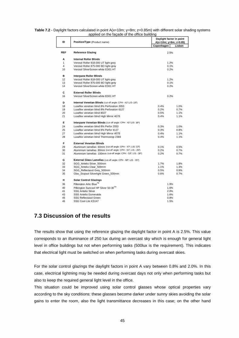
45

Table 7.2 - Daylight factors calculated in point A(x=10m; y=8m; z=0.85m) with different solar shading systems applied on the façade of the office building

Copenhagen Lisbon

REF Reference Glazing

A Internal Roller Blinds1 Verosol Roller 818-000 UT light-grey4 Verosol Roller 875-000 BO light-grey10 Verosol SilverScreen white ED01 HT

B Interpane Roller Blinds12 Verosol Roller 818-000 UT light-grey13 Verosol Roller 875-000 BO light-grey14 Verosol SilverScreen white ED01 HT

C External Roller Blinds16 Verosol SilverScreen white ED01 HT

D Internal Venetian Blinds (cut-off angle: CPH - 41º;LIS- 18º)

18 Luxaflex venetian blind 8% Perforation 2053 0.4% 1.0%19 Luxaflex venetian blind 8% Perforation 6127 0.2% 0.7%20 Luxaflex venetian blind 8027 0.5% 1.1%21 Luxaflex venetian blind High Mirror 4078 0.4% 1.1%

E Interpane Venetian Blinds (cut-off angle: CPH - 41º;LIS- 18º)

24 Luxaflex venetian blind 8% Perfor 2053 0.3% 1.0%25 Luxaflex venetian blind 8% Perfor 6127 0.3% 0.8%27 Luxaflex venetian blind High Mirror 4078 0.4% 1.1%28 Luxaflex venetian blind Thermostop 2383 0.4% 1.1%

F External Venetian Blinds29 Aluminium lamellas_60mm (cut-off angle: CPH - 47º; LIS- 23º) 0.1% 0.5%30 Aluminium lamellas_80mm (cut-off angle: CPH - 51º; LIS - 26º) 0.2% 0.7%31 Aluminium lamellas_100mm (cut-off angle: CPH - 53º; LIS - 28º) 0.2% 0.7%

G External Glass Lamellas (cut-off angle: CPH - 68º; LIS - 35º)32 SGG_Antelio Silver_500mm 1.7% 1.8%33 SGG_Antelio Clear_500mm 1.1% 1.3%34 SGG_Reflectasol Grey_500mm 0.5% 0.9%35 Glav_Stopsol Silverlight Green_500mm 0.6% 0.7%

H Solar Control Glazings 36 Pilkington Artic BlueTM

40 Pilkington Suncool HP Silver 50-30TM

41 SSG Antelio Silver43 SSG Antelio Esmeralda45 SSG Reflectasol Green46 SSG Cool-Lite KS147

1.2%0.1%

1.2%0.1%0.2%

Daylight factor in point A(x=10m; y=8m; z=0.85)

2.5%

ID

1.6%0.8%1.5%

Position/Type (Product name)

0.2%

1.9%1.6%2.0%

0.2%

7.3 Discussion of the results

The results show that using the reference glazing the daylight factor in point A is 2.5%. This value

corresponds to an illuminance of 250 lux during an overcast sky which is enough for general light

level in office buildings but not when performing tasks (500lux is the requirement). This indicates

that electrical light must be switched on when performing tasks during overcast skies.

For the solar control glazings the daylight factors in point A vary between 0.8% and 2.0%. In this

case, electrical lightning may be needed during overcast days not only when performing tasks but

also to keep the required general light level in the office.

This situation could be improved using solar control glasses whose optical properties vary

according to the sky conditions: these glasses become darker under sunny skies avoiding the solar

gains to enter the room, also the light transmittance decreases in this case; on the other hand

46

under overcast skies the glass becomes clear again and the light transmittance increases. These

types of glass could decrease the electrical lightning demand during overcast days. However the

design tools used in this dissertation (WIS and BuildingCalc/LightCalc) are not able to evaluate

their performance.

For the roller blinds the daylight factor in point A is very low (for instance 0.1% and 0.2% for black-

out and half-transparent blinds respectively). This means that if they are activated for a sunny day

and if it turns into overcast and they are not retracted, high electrical lightning demand may be

needed to fulfil the requirements for indoor lightning level. In this way, the roller blind does not

seem the best solution when thinking about avoiding the adjustments of shading systems that may

disturb the workers concentration and efficiency.

For the venetian blinds different daylight performances for Copenhagen and Lisbon can be

achieved because of the different cut-off positions comparing both cities. Because of different

latitudes the solar altitude in Copenhagen is lower than in Lisbon. In this way comparing

Copenhagen with Lisbon for the same venetian blind, for Copenhagen the cut-off position angle is

higher which means that less daylight enters the room. This is the reason for the lower values

obtained for the daylight factor in the office building in Copenhagen when compared to the office in

Lisbon.

The values achieved for the daylight factor (between 0.1% and 0.5% for Copenhagen and 0.5%

and 1.1% for Lisbon) are better than the ones obtained with the roller blinds especially for Lisbon.

This is due to the possibility that the daylight has to enter the room through the space between the

slats. However, the daylight factors obtained show that also the venetian blinds should be retracted

when the sky turns from sunny to overcast in order to decrease the energy consumption for

electrical lightning.

Excluding the reference glazing and the solar control glasses, the glass lamellas are the ones that

have the best performance during overcast sky even if they are activated for the cut-off angle for a

previous sunny sky. This is due to the high visual transmittance of the glass. This system seems to

be a promising solar shading system when trying to reduce the number of adjustments in solar

shading systems due to sky conditions changes.

The results also show that the position (external, interpane and internal) of the shading systems do

not interfere with the indoor daylight performance. External, interpane and internal roller blinds

have equal performance when evaluated under an overcast sky. The same is valid for the venetian

blinds if activated for the same cut-off angle.

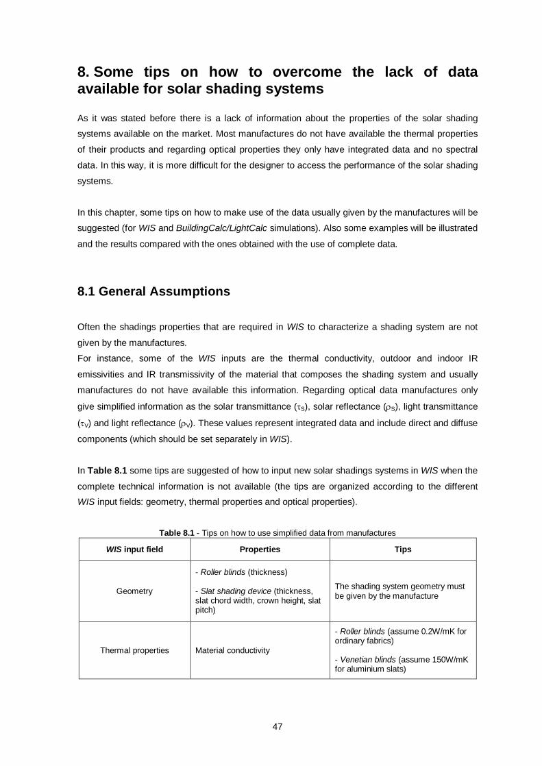
47

8. Some tips on how to overcome the lack of data available for solar shading systems

As it was stated before there is a lack of information about the properties of the solar shading

systems available on the market. Most manufactures do not have available the thermal properties

of their products and regarding optical properties they only have integrated data and no spectral

data. In this way, it is more difficult for the designer to access the performance of the solar shading

systems.

In this chapter, some tips on how to make use of the data usually given by the manufactures will be

suggested (for WIS and BuildingCalc/LightCalc simulations). Also some examples will be illustrated

and the results compared with the ones obtained with the use of complete data.

8.1 General Assumptions

Often the shadings properties that are required in WIS to characterize a shading system are not

given by the manufactures.

For instance, some of the WIS inputs are the thermal conductivity, outdoor and indoor IR

emissivities and IR transmissivity of the material that composes the shading system and usually

manufactures do not have available this information. Regarding optical data manufactures only

give simplified information as the solar transmittance (S), solar reflectance (S), light transmittance

(V) and light reflectance (V). These values represent integrated data and include direct and diffuse

components (which should be set separately in WIS).

In Table 8.1 some tips are suggested of how to input new solar shadings systems in WIS when the

complete technical information is not available (the tips are organized according to the different

WIS input fields: geometry, thermal properties and optical properties).

Table 8.1 - Tips on how to use simplified data from manufactures

WIS input field Properties Tips

Geometry

- Roller blinds (thickness) - Slat shading device (thickness, slat chord width, crown height, slat pitch)

The shading system geometry must be given by the manufacture

Thermal properties Material conductivity

- Roller blinds (assume 0.2W/mK for ordinary fabrics) - Venetian blinds (assume 150W/mK for aluminium slats)

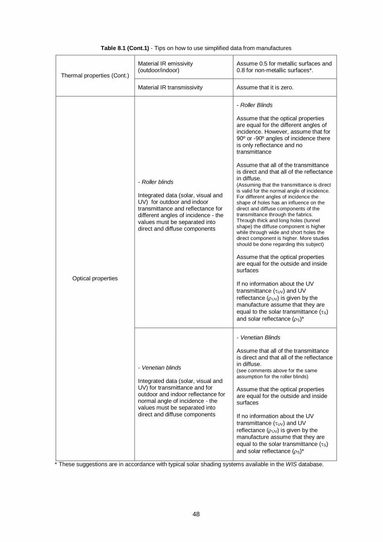
48

Table 8.1 (Cont.1) - Tips on how to use simplified data from manufactures

Material IR emissivity (outdoor/indoor)

Assume 0.5 for metallic surfaces and 0.8 for non-metallic surfaces*.

Thermal properties (Cont.)

Material IR transmissivity Assume that it is zero.

- Roller blinds Integrated data (solar, visual and UV) for outdoor and indoor transmittance and reflectance for different angles of incidence - the values must be separated into direct and diffuse components

- Roller Blinds Assume that the optical properties are equal for the different angles of incidence. However, assume that for 90º or -90º angles of incidence there is only reflectance and no transmittance Assume that all of the transmittance is direct and that all of the reflectance in diffuse. (Assuming that the transmittance is direct is valid for the normal angle of incidence. For different angles of incidence the shape of holes has an influence on the direct and diffuse components of the transmittance through the fabrics. Through thick and long holes (tunnel shape) the diffuse component is higher while through wide and short holes the direct component is higher. More studies should be done regarding this subject) Assume that the optical properties are equal for the outside and inside surfaces If no information about the UV transmittance (UV) and UV reflectance (UV) is given by the manufacture assume that they are equal to the solar transmittance (S) and solar reflectance (S)*

Optical properties

- Venetian blinds Integrated data (solar, visual and UV) for transmittance and for outdoor and indoor reflectance for normal angle of incidence - the values must be separated into direct and diffuse components

- Venetian Blinds Assume that all of the transmittance is direct and that all of the reflectance in diffuse. (see comments above for the same assumption for the roller blinds) Assume that the optical properties are equal for the outside and inside surfaces If no information about the UV transmittance (UV) and UV reflectance (UV) is given by the manufacture assume that they are equal to the solar transmittance (S) and solar reflectance (S)*

* These suggestions are in accordance with typical solar shading systems available in the WIS database.

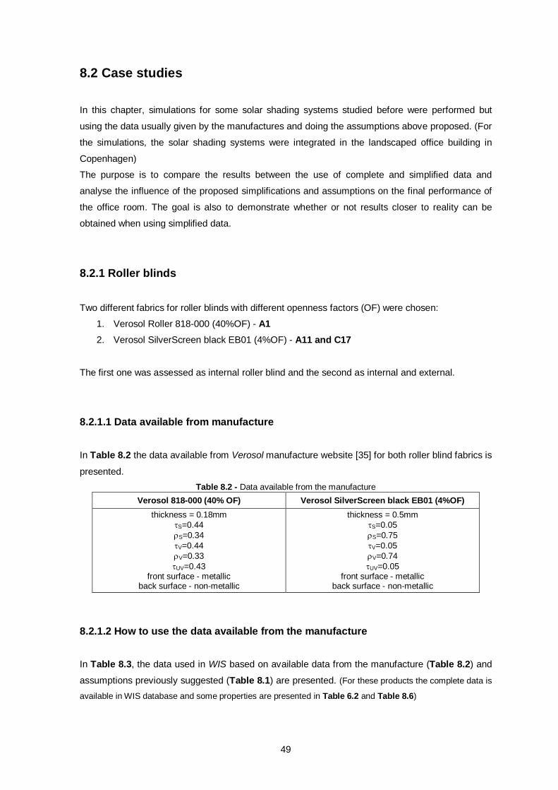
49

8.2 Case studies

In this chapter, simulations for some solar shading systems studied before were performed but

using the data usually given by the manufactures and doing the assumptions above proposed. (For

the simulations, the solar shading systems were integrated in the landscaped office building in

Copenhagen)

The purpose is to compare the results between the use of complete and simplified data and

analyse the influence of the proposed simplifications and assumptions on the final performance of

the office room. The goal is also to demonstrate whether or not results closer to reality can be

obtained when using simplified data.

8.2.1 Roller blinds

Two different fabrics for roller blinds with different openness factors (OF) were chosen:

1. Verosol Roller 818-000 (40%OF) - A1

2. Verosol SilverScreen black EB01 (4%OF) - A11 and C17

The first one was assessed as internal roller blind and the second as internal and external.

8.2.1.1 Data available from manufacture

In Table 8.2 the data available from Verosol manufacture website [35] for both roller blind fabrics is

presented. Table 8.2 - Data available from the manufacture

Verosol 818-000 (40% OF) Verosol SilverScreen black EB01 (4%OF) thickness = 0.18mm

S=0.44 S=0.34 V=0.44 V=0.33 UV=0.43

front surface - metallic back surface - non-metallic

thickness = 0.5mm S=0.05 S=0.75 V=0.05 V=0.74 UV=0.05


8.2.1.2 How to use the data available from the manufacture

In Table 8.3, the data used in WIS based on available data from the manufacture (Table 8.2) and

assumptions previously suggested (Table 8.1) are presented. (For these products the complete data is

available in WIS database and some properties are presented in Table 6.2 and Table 8.6)

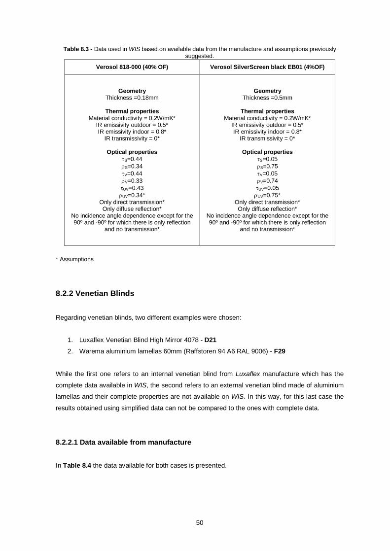
50

Table 8.3 - Data used in WIS based on available data from the manufacture and assumptions previously suggested.

Verosol 818-000 (40% OF) Verosol SilverScreen black EB01 (4%OF)

Geometry Thickness =0.18mm

Thermal properties

Material conductivity = 0.2W/mK* IR emissivity outdoor = 0.5* IR emissivity indoor = 0.8*

IR transmissivity = 0*

Optical properties S=0.44 S=0.34 V=0.44 V=0.33 UV=0.43 UV=0.34*

Only direct transmission* Only diffuse reflection*

No incidence angle dependence except for the 90º and -90º for which there is only reflection

and no transmission*

Geometry Thickness =0.5mm

Thermal properties

Material conductivity = 0.2W/mK* IR emissivity outdoor = 0.5* IR emissivity indoor = 0.8*


Optical properties S=0.05 S=0.75 V=0.05 V=0.74 UV=0.05 UV=0.75*

Only direct transmission* Only diffuse reflection*

No incidence angle dependence except for the 90º and -90º for which there is only reflection

and no transmission*

* Assumptions

8.2.2 Venetian Blinds

Regarding venetian blinds, two different examples were chosen:

1. Luxaflex Venetian Blind High Mirror 4078 - D21

2. Warema aluminium lamellas 60mm (Raffstoren 94 A6 RAL 9006) - F29

While the first one refers to an internal venetian blind from Luxaflex manufacture which has the

complete data available in WIS, the second refers to an external venetian blind made of aluminium

lamellas and their complete properties are not available on WIS. In this way, for this last case the

results obtained using simplified data can not be compared to the ones with complete data.

8.2.2.1 Data available from manufacture

In Table 8.4 the data available for both cases is presented.

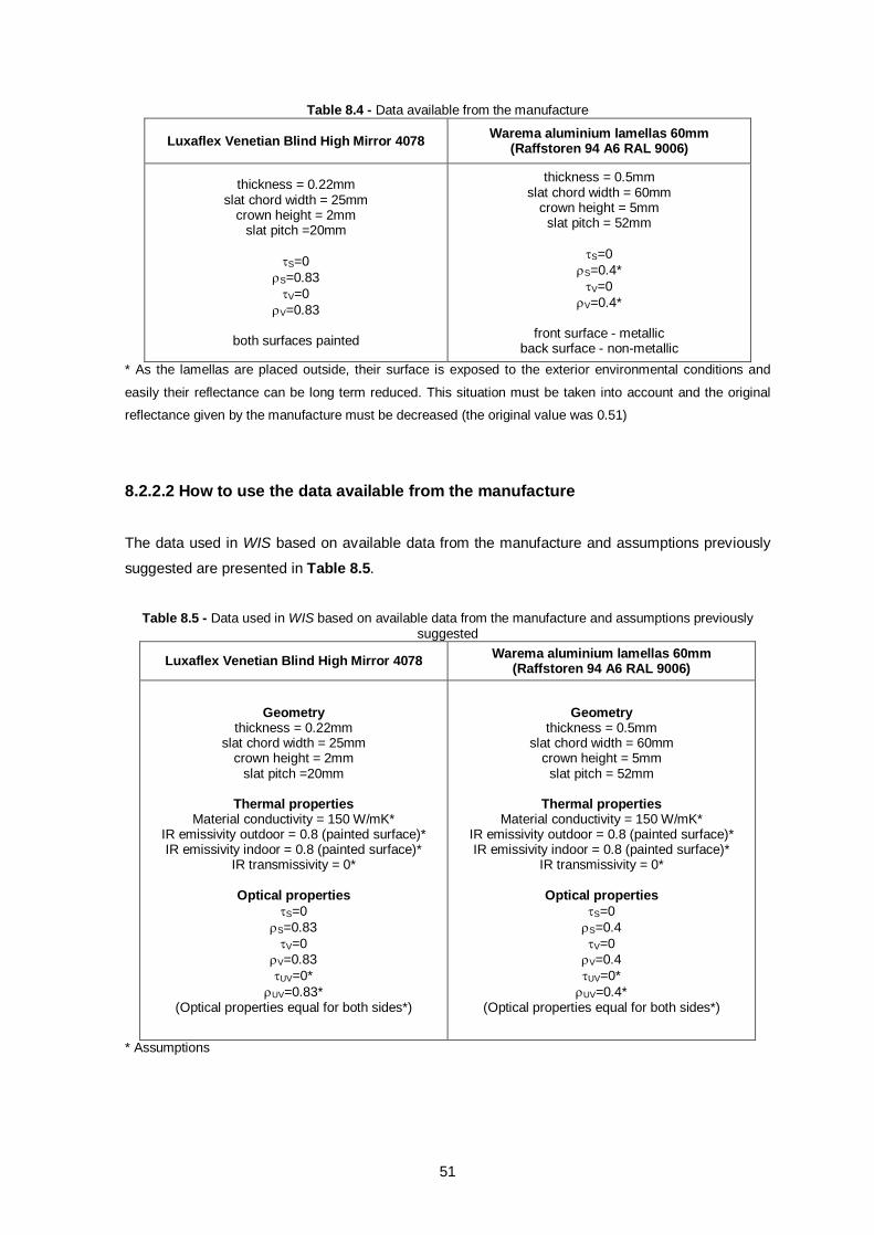
51

Table 8.4 - Data available from the manufacture

Luxaflex Venetian Blind High Mirror 4078 Warema aluminium lamellas 60mm (Raffstoren 94 A6 RAL 9006)

thickness = 0.22mm slat chord width = 25mm

crown height = 2mm slat pitch =20mm

S=0

S=0.83 V=0

V=0.83

both surfaces painted

thickness = 0.5mm slat chord width = 60mm

crown height = 5mm slat pitch = 52mm

S=0

S=0.4* V=0

V=0.4*


* As the lamellas are placed outside, their surface is exposed to the exterior environmental conditions and

easily their reflectance can be long term reduced. This situation must be taken into account and the original

reflectance given by the manufacture must be decreased (the original value was 0.51)

8.2.2.2 How to use the data available from the manufacture

The data used in WIS based on available data from the manufacture and assumptions previously

suggested are presented in Table 8.5.

Table 8.5 - Data used in WIS based on available data from the manufacture and assumptions previously

suggested

Luxaflex Venetian Blind High Mirror 4078 Warema aluminium lamellas 60mm (Raffstoren 94 A6 RAL 9006)

Geometry thickness = 0.22mm

slat chord width = 25mm crown height = 2mm

slat pitch =20mm

Thermal properties Material conductivity = 150 W/mK*

IR emissivity outdoor = 0.8 (painted surface)* IR emissivity indoor = 0.8 (painted surface)*


Optical properties S=0

S=0.83 V=0

V=0.83 UV=0*

UV=0.83* (Optical properties equal for both sides*)

Geometry thickness = 0.5mm

slat chord width = 60mm crown height = 5mm

slat pitch = 52mm

Thermal properties Material conductivity = 150 W/mK*

IR emissivity outdoor = 0.8 (painted surface)* IR emissivity indoor = 0.8 (painted surface)*


Optical properties S=0 S=0.4 V=0 V=0.4 UV=0* UV=0.4*

(Optical properties equal for both sides*)

* Assumptions

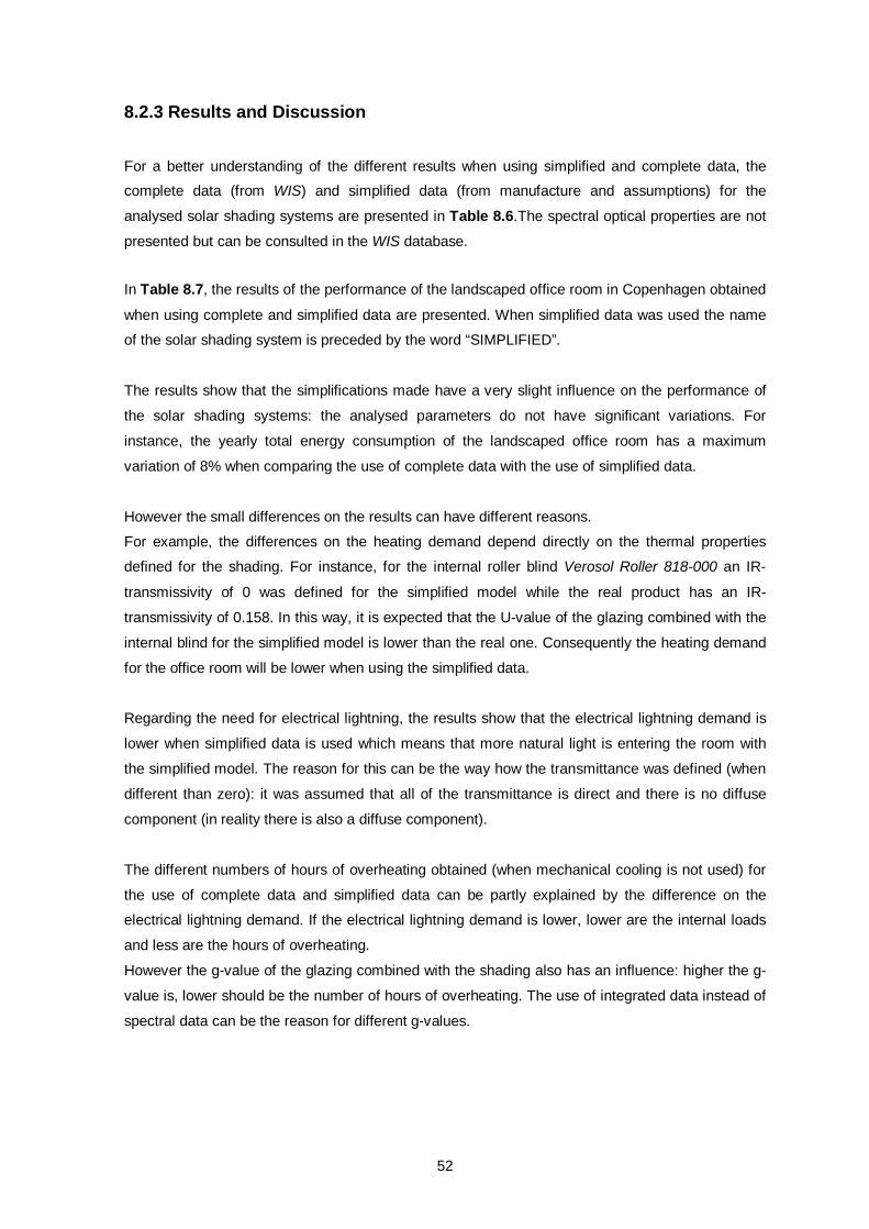
52

8.2.3 Results and Discussion

For a better understanding of the different results when using simplified and complete data, the

complete data (from WIS) and simplified data (from manufacture and assumptions) for the

analysed solar shading systems are presented in Table 8.6.The spectral optical properties are not

presented but can be consulted in the WIS database.

In Table 8.7, the results of the performance of the landscaped office room in Copenhagen obtained

when using complete and simplified data are presented. When simplified data was used the name

of the solar shading system is preceded by the word “SIMPLIFIED”.

The results show that the simplifications made have a very slight influence on the performance of

the solar shading systems: the analysed parameters do not have significant variations. For

instance, the yearly total energy consumption of the landscaped office room has a maximum

variation of 8% when comparing the use of complete data with the use of simplified data.

However the small differences on the results can have different reasons.

For example, the differences on the heating demand depend directly on the thermal properties

defined for the shading. For instance, for the internal roller blind Verosol Roller 818-000 an IR-

transmissivity of 0 was defined for the simplified model while the real product has an IR-

transmissivity of 0.158. In this way, it is expected that the U-value of the glazing combined with the

internal blind for the simplified model is lower than the real one. Consequently the heating demand

for the office room will be lower when using the simplified data.

Regarding the need for electrical lightning, the results show that the electrical lightning demand is

lower when simplified data is used which means that more natural light is entering the room with

the simplified model. The reason for this can be the way how the transmittance was defined (when

different than zero): it was assumed that all of the transmittance is direct and there is no diffuse

component (in reality there is also a diffuse component).

The different numbers of hours of overheating obtained (when mechanical cooling is not used) for

the use of complete data and simplified data can be partly explained by the difference on the

electrical lightning demand. If the electrical lightning demand is lower, lower are the internal loads

and less are the hours of overheating.

However the g-value of the glazing combined with the shading also has an influence: higher the g-

value is, lower should be the number of hours of overheating. The use of integrated data instead of

spectral data can be the reason for different g-values.

53

For the internal venetian blind simulated there was a decrease of 40 hours above 26ºC when using

simplified data. It would be expected the opposite as the g-value is higher for the simplified case.

No reason was found for this.

The results obtained for the last case study, Warema aluminium lamellas 60mm (Raffstoren 94 A6

RAL 9006), can not be compared since there is no available data characterizing this system in

WIS.

Apparently the results show that simplified data can be used when evaluating the energy

performance of solar shading systems: the results obtained for the energy performance of the

building using simplified data are quite close to the ones when using complete data.

However only few cases were studied, more detailed studies should be done in this field and for

different types of solar shading systems to assure that simplified data can be used in any case in

the early design phase to assess the performance of solar shading systems.

The main problem of not using spectral data could be when evaluating the performance of solar

shading systems regarding the influence that they have in the colour of the light that enters the

room. Using integrated data, solar shading systems with different colours can not be distinguished,

the indoor light colour will be the same.

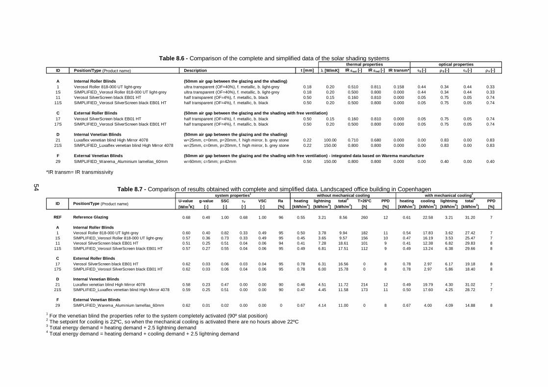
54

Table 8.6 - Comparison of the complete and simplified data of the solar shading systems

ID Position/Type (Product name) Description t [mm] [W/mK] IR out [-] IR ind [-] IR transm* S [-] S [-] V [-] V [-]

A Internal Roller Blinds (50mm air gap between the glazing and the shading)1 Verosol Roller 818-000 UT light-grey ultra transparent (OF=40%), f. metallic, b. light-grey 0.18 0.20 0.510 0.811 0.158 0.44 0.34 0.44 0.33

1S SIMPLIFIED_Verosol Roller 818-000 UT light-grey ultra transparent (OF=40%), f. metallic, b. light-grey 0.18 0.20 0.500 0.800 0.000 0.44 0.34 0.44 0.3311 Verosol SilverScreen black EB01 HT half transparent (OF=4%), f. metallic, b. black 0.50 0.15 0.160 0.810 0.000 0.05 0.75 0.05 0.74

11S SIMPLIFIED_Verosol SilverScreen black EB01 HT half transparent (OF=4%), f. metallic, b. black 0.50 0.20 0.500 0.800 0.000 0.05 0.75 0.05 0.74

C External Roller Blinds (50mm air gap between the glazing and the shading with free ventilation)17 Verosol SilverScreen black EB01 HT half transparent (OF=4%), f. metallic, b. black 0.50 0.15 0.160 0.810 0.000 0.05 0.75 0.05 0.74

17S SIMPLIFIED_Verosol SilverScreen black EB01 HT half transparent (OF=4%), f. metallic, b. black 0.50 0.20 0.500 0.800 0.000 0.05 0.75 0.05 0.74

D Internal Venetian Blinds (50mm air gap between the glazing and the shading)21 Luxaflex venetian blind High Mirror 4078 w=25mm, c=0mm, p=20mm, f. high mirror, b. grey stone 0.22 100.00 0.710 0.680 0.000 0.00 0.83 0.00 0.83

21S SIMPLIFIED_Luxaflex venetian blind High Mirror 4078 w=25mm, c=0mm, p=20mm, f. high mirror, b. grey stone 0.22 150.00 0.800 0.800 0.000 0.00 0.83 0.00 0.83

F External Venetian Blinds (50mm air gap between the glazing and the shading with free ventilation) - integrated data based on Warema manufacture29 SIMPLIFIED_Warema_Aluminium lamellas_60mm w=60mm; c=5mm; p=42mm 0.50 150.00 0.800 0.800 0.000 0.00 0.40 0.00 0.40

optical propertiesthermal properties

*IR transm= IR transmissivity

Table 8.7 - Comparison of results obtained with complete and simplified data. Landscaped office building in Copenhagen

U-value g-value SSC V VSC Ra heating lightning total3 T>26ºC PPD heating cooling lightning total4 PPD[W/m2K] [-] [-] [-] [-] [%] [kWh/m2] [kWh/m2] [kWh/m2] [h] [%] [kWh/m2] [kWh/m2] [kWh/m2] [kWh/m2] [%]

REF Reference Glazing 0.68 0.49 1.00 0.68 1.00 96 0.55 3.21 8.56 260 12 0.61 22.58 3.21 31.20 7

A Internal Roller Blinds1 Verosol Roller 818-000 UT light-grey 0.60 0.40 0.82 0.33 0.49 95 0.50 3.78 9.94 182 11 0.54 17.83 3.62 27.42 7

1S SIMPLIFIED_Verosol Roller 818-000 UT light-grey 0.57 0.36 0.73 0.33 0.49 95 0.45 3.65 9.57 156 10 0.47 16.19 3.53 25.47 711 Verosol SilverScreen black EB01 HT 0.51 0.25 0.51 0.04 0.06 94 0.41 7.28 18.61 101 9 0.41 12.38 6.82 29.83 8

11S SIMPLIFIED_Verosol SilverScreen black EB01 HT 0.57 0.27 0.55 0.04 0.06 95 0.49 6.81 17.51 112 9 0.49 13.24 6.38 29.66 8

C External Roller Blinds17 Verosol SilverScreen black EB01 HT 0.62 0.03 0.06 0.03 0.04 95 0.78 6.31 16.56 0 8 0.78 2.97 6.17 19.18 8

17S SIMPLIFIED_Verosol SilverScreen black EB01 HT 0.62 0.03 0.06 0.04 0.06 95 0.78 6.00 15.78 0 8 0.78 2.97 5.86 18.40 8

D Internal Venetian Blinds21 Luxaflex venetian blind High Mirror 4078 0.58 0.23 0.47 0.00 0.00 90 0.46 4.51 11.72 214 12 0.49 19.79 4.30 31.02 7

21S SIMPLIFIED_Luxaflex venetian blind High Mirror 4078 0.59 0.25 0.51 0.00 0.00 90 0.47 4.45 11.58 173 11 0.50 17.60 4.25 28.72 7

F External Venetian Blinds29 SIMPLIFIED_Warema_Aluminium lamellas_60mm 0.62 0.01 0.02 0.00 0.00 0 0.67 4.14 11.00 0 8 0.67 4.00 4.09 14.88 8

without mechanical cooling with mechanical cooling2


system properties1

1 For the venetian blind the properties refer to the system completely activated (90º slat position) 2 The setpoint for cooling is 22ºC, so when the mechanical cooling is activated there are no hours above 22ºC 3 Total energy demand = heating demand + 2.5 lightning demand 4 Total energy demand = heating demand + cooling demand + 2.5 lightning demand

55

9. Conclusions and further work

The combination of WIS and BuildingCalc/LightCalc is a very promising tool when evaluating and

comparing the performance of buildings with different types of solar shading systems in an early

design phase. From the simple model of the room and the thermal/optical properties of the

shadings systems it is possible to calculate in an hourly basis the yearly energy demand for

heating, cooling and lightning as well as some indoor comfort parameters.

The method on how to evaluate the performance of different solar shading systems using WIS and

BuildingCalc/LightCalc was illustrated for a case study: a landscaped office building located in

Copenhagen and then in Lisbon. Different types of solar shading systems were evaluated for the

façade of the office. Apart from small tricks presented through the dissertation the method is quite

user friendly.

When selecting a solar shading system two main characteristics must be taken into account: the

solar shading performance (assessed by g-value - solar heat gain coefficient) and the daylight

performance (assessed by the V - visual transmittance). Usually good shading devices according

to solar shading performance are poor in daylight performance. It is very important that a solar

shading system is flexible to different sky conditions. In this way it can be activated during warm

and sunny days to avoid the risk of overheating and retracted when solar heat gains and light are

needed in the rooms.

For the case study it was clear the difference between the North Europe (Copenhagen) and South

Europe (Lisbon) climates regarding the solar shading systems. For instance, using the same solar

system for Lisbon and for Copenhagen the cooling demand in Lisbon is in some cases doubled

than in Copenhagen. For some cases this cooling demand for the office room in Lisbon is higher

than the standard requirement which means that some solutions of shading systems should not be

used in Portugal.

One of the main advantages of BuildingCalc/LightCalc is the ability of performing dynamic

simulations. Different setting for distinct periods of the day (working hours and non working hours)

and year (summer and winter) can be defined making simulations closer to reality.

Another benefit is that BuildingCalc/LightCalc works with WIS which is a promising database for

windows components (panes, shading devices, ect). BuildingCalc/LightCalc is able to import the

text files generated by WIS with the thermal/optical properties of glazings and shading systems

combinations. In this way, every shading device existing in WIS can be simulated in a room using


56

Another important profit from BuildingCalc/LightCalc is that it is able to calculate the yearly

electrical lightning demand taking into account the hours in which the shading system is activated

and in which less daylight enters the room. At the same time this electrical lightning demand

contributes to the internal loads of the room.

On the other hand the way the shading system is activated is not yet very close to reality. The

shading system is activated when the indoor temperature is higher than the cooling setpoint. This

means that a shading system can be activated during overcast situations in which the indoor

temperature is higher than the cooling setpoint. In this way the natural light entering the room is

less and the electrical lightning demand may be wrongly increased. In this way the shading

activation should also somehow depend on the luminance of the sky. It would be also interesting to

control the shading systems with respect to indoor daylight and glare.

Nowadays there is still a lack of data about the angular and spectral properties of the solar shading

systems. Manufactures rarely have this information available: often thermal properties are not

available and optical properties are given as integrated values instead of spectral values. Some

suggestions were given on how to make use of the available data from manufactures. It seems that

the use of simplified data for solar shading systems does not have a large influence on the final

performance of buildings. However, only few cases were studied. More research should be done

on this area and for different types of solar shading systems.

57

PART B. GLASS LAMELLA SYSTEMS: COMPARING MEASUREMENTS WITH IESVE/RADIANCE SIMULATIONS

58

59

10. Introduction and goal

As referred in the Part A of this dissertation, the glass lamellas are a promising type of solar

shading system: besides acting as typical solar shading systems reducing the solar gains and

consequently the cooling demand, they may at the same time allow good indoor daylight levels

thanks to the transparent properties of glass. On the other hand during overcast days if they are

correctly tilted they may slightly increase the indoor daylight especially on the back part of the

room.

Some daylight measurements were performed in the Daylight Laboratory at SBi (Danish Building

Research Institute, in Hørsholm, in Denmark) regarding the research project Development of new

solar shading systems based on daylight-directing solar control glass lamellas lead by Steen

Traberg-Borup.

The daylight measurements in the Daylight Laboratory at SBi were performed in two experimental

rooms (reproducing office rooms): one with an ordinary glass façade (reference room) and another

one equal but equipped with a system of glass lamellas on its façade (test room).

Illuminance levels in specific points of both rooms (working plane and ceiling) were measured

under different sky conditions and for different positions of the glass lamellas. The results obtained

for both rooms were compared and the performance of the glass lamellas evaluated.

The goal of Part B of this dissertation is to build the model of the rooms using IESve/Radiance [39]

and assess how close to the measurements can the results from the simulations be.

IESve/Radiance is a simplified and user-friendly version of the original Radiance. The purpose is to

test how accurate is IESve/Radiance assessing the daylight performance of rooms where glass

lamellas are applied.

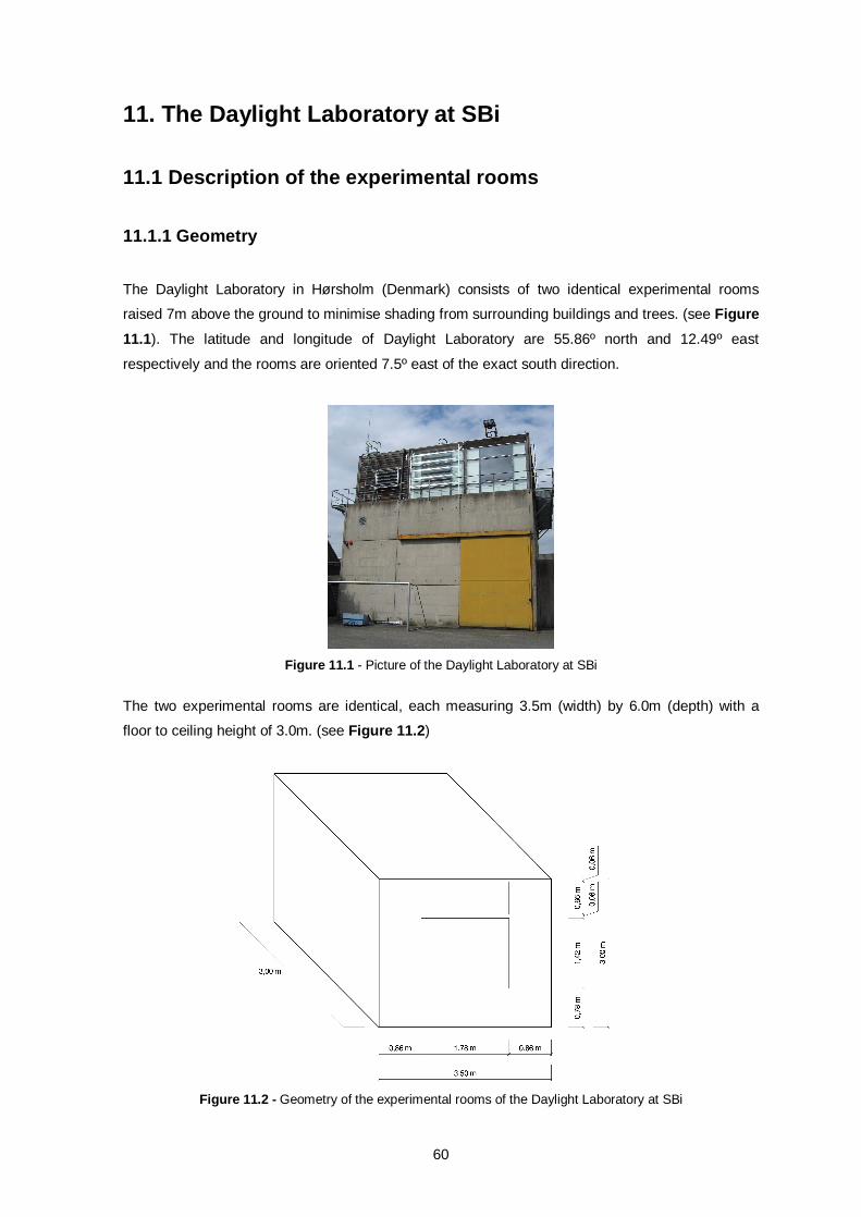
60

11. The Daylight Laboratory at SBi

11.1 Description of the experimental rooms

11.1.1 Geometry

The Daylight Laboratory in Hørsholm (Denmark) consists of two identical experimental rooms

raised 7m above the ground to minimise shading from surrounding buildings and trees. (see Figure 11.1). The latitude and longitude of Daylight Laboratory are 55.86º north and 12.49º east

respectively and the rooms are oriented 7.5º east of the exact south direction.

Figure 11.1 - Picture of the Daylight Laboratory at SBi

The two experimental rooms are identical, each measuring 3.5m (width) by 6.0m (depth) with a

floor to ceiling height of 3.0m. (see Figure 11.2)

Figure 11.2 - Geometry of the experimental rooms of the Daylight Laboratory at SBi

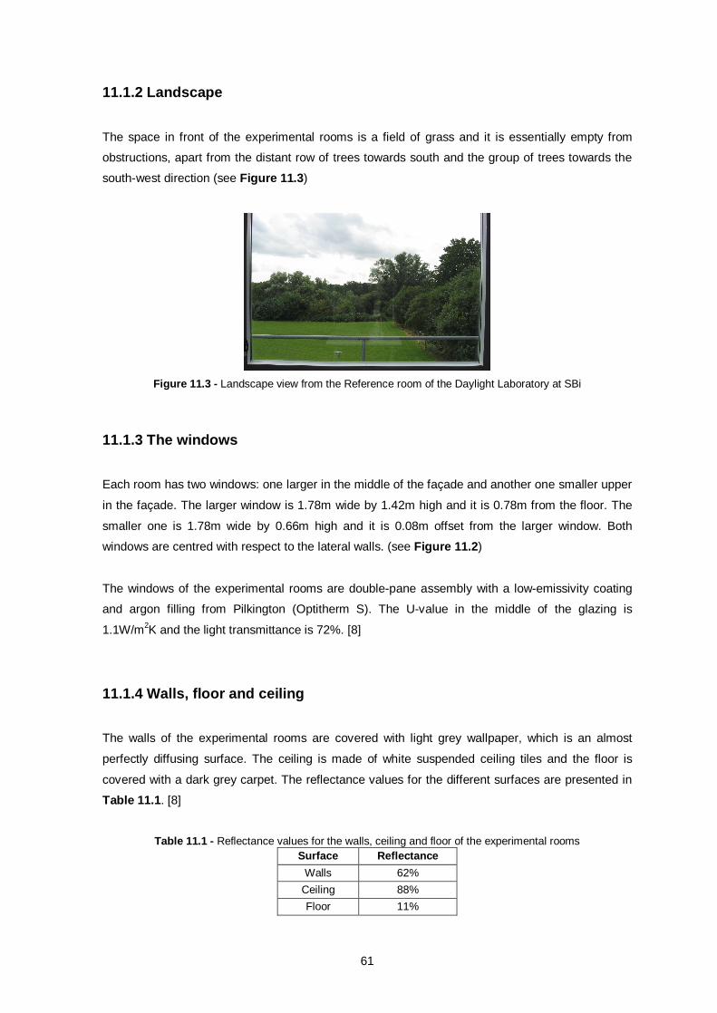
61

11.1.2 Landscape

The space in front of the experimental rooms is a field of grass and it is essentially empty from

obstructions, apart from the distant row of trees towards south and the group of trees towards the

south-west direction (see Figure 11.3)

Figure 11.3 - Landscape view from the Reference room of the Daylight Laboratory at SBi

11.1.3 The windows

Each room has two windows: one larger in the middle of the façade and another one smaller upper

in the façade. The larger window is 1.78m wide by 1.42m high and it is 0.78m from the floor. The

smaller one is 1.78m wide by 0.66m high and it is 0.08m offset from the larger window. Both

windows are centred with respect to the lateral walls. (see Figure 11.2)

The windows of the experimental rooms are double-pane assembly with a low-emissivity coating

and argon filling from Pilkington (Optitherm S). The U-value in the middle of the glazing is

1.1W/m2K and the light transmittance is 72%. [8]

11.1.4 Walls, floor and ceiling

The walls of the experimental rooms are covered with light grey wallpaper, which is an almost

perfectly diffusing surface. The ceiling is made of white suspended ceiling tiles and the floor is

covered with a dark grey carpet. The reflectance values for the different surfaces are presented in

Table 11.1. [8]

Table 11.1 - Reflectance values for the walls, ceiling and floor of the experimental rooms

Surface Reflectance Walls 62%

Ceiling 88% Floor 11%

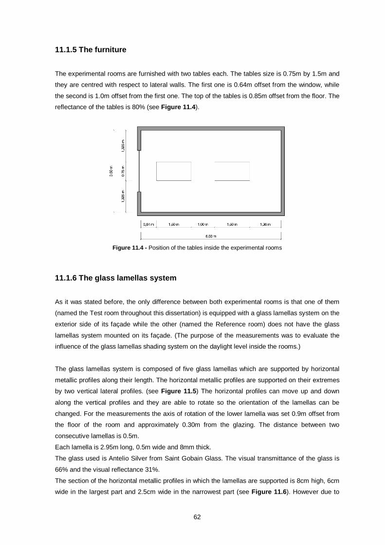
62

11.1.5 The furniture

The experimental rooms are furnished with two tables each. The tables size is 0.75m by 1.5m and

they are centred with respect to lateral walls. The first one is 0.64m offset from the window, while

the second is 1.0m offset from the first one. The top of the tables is 0.85m offset from the floor. The

reflectance of the tables is 80% (see Figure 11.4).

Figure 11.4 - Position of the tables inside the experimental rooms

11.1.6 The glass lamellas system

As it was stated before, the only difference between both experimental rooms is that one of them

(named the Test room throughout this dissertation) is equipped with a glass lamellas system on the

exterior side of its façade while the other (named the Reference room) does not have the glass

lamellas system mounted on its façade. (The purpose of the measurements was to evaluate the

influence of the glass lamellas shading system on the daylight level inside the rooms.)

The glass lamellas system is composed of five glass lamellas which are supported by horizontal

metallic profiles along their length. The horizontal metallic profiles are supported on their extremes

by two vertical lateral profiles. (see Figure 11.5) The horizontal profiles can move up and down

along the vertical profiles and they are able to rotate so the orientation of the lamellas can be

changed. For the measurements the axis of rotation of the lower lamella was set 0.9m offset from

the floor of the room and approximately 0.30m from the glazing. The distance between two

consecutive lamellas is 0.5m.

Each lamella is 2.95m long, 0.5m wide and 8mm thick.

The glass used is Antelio Silver from Saint Gobain Glass. The visual transmittance of the glass is

66% and the visual reflectance 31%.

The section of the horizontal metallic profiles in which the lamellas are supported is 8cm high, 6cm

wide in the largest part and 2.5cm wide in the narrowest part (see Figure 11.6). However due to

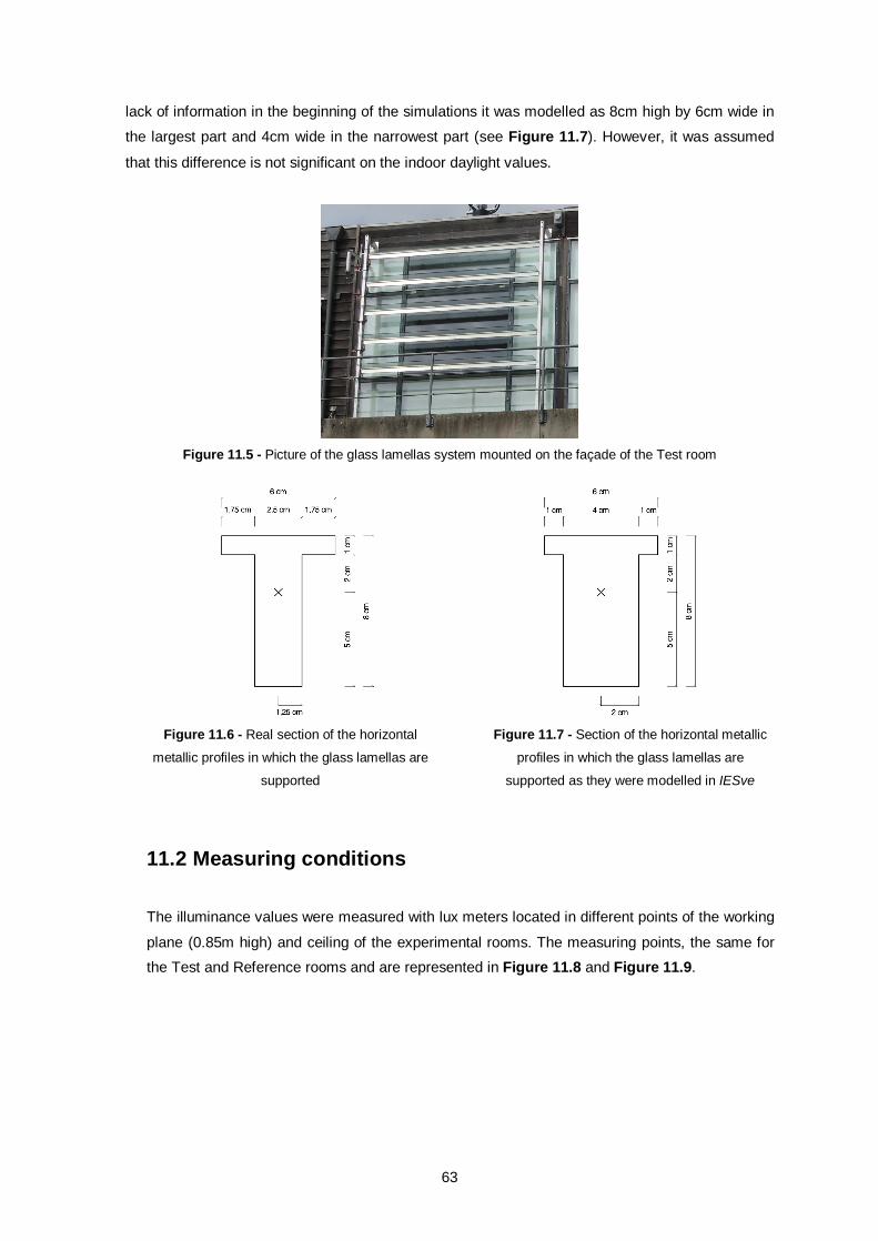
63

lack of information in the beginning of the simulations it was modelled as 8cm high by 6cm wide in

the largest part and 4cm wide in the narrowest part (see Figure 11.7). However, it was assumed

that this difference is not significant on the indoor daylight values.

Figure 11.5 - Picture of the glass lamellas system mounted on the façade of the Test room

Figure 11.6 - Real section of the horizontal

metallic profiles in which the glass lamellas are

supported

Figure 11.7 - Section of the horizontal metallic

profiles in which the glass lamellas are

supported as they were modelled in IESve

11.2 Measuring conditions

The illuminance values were measured with lux meters located in different points of the working

plane (0.85m high) and ceiling of the experimental rooms. The measuring points, the same for

the Test and Reference rooms and are represented in Figure 11.8 and Figure 11.9.

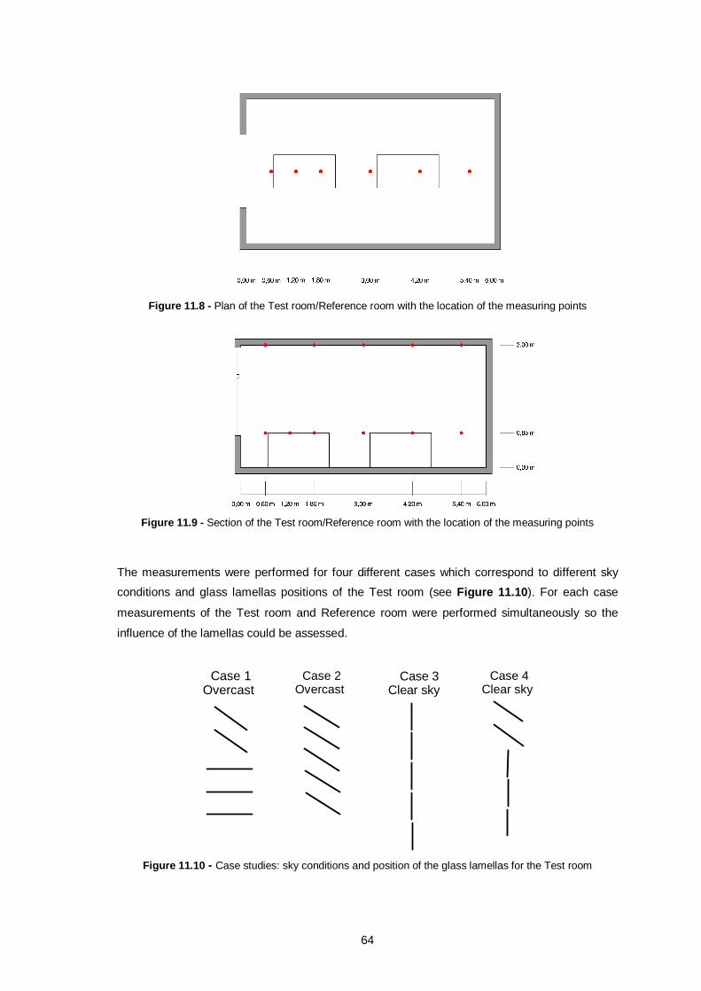
64

Figure 11.8 - Plan of the Test room/Reference room with the location of the measuring points

Figure 11.9 - Section of the Test room/Reference room with the location of the measuring points

The measurements were performed for four different cases which correspond to different sky

conditions and glass lamellas positions of the Test room (see Figure 11.10). For each case

measurements of the Test room and Reference room were performed simultaneously so the

influence of the lamellas could be assessed.

Figure 11.10 - Case studies: sky conditions and position of the glass lamellas for the Test room

Case 1Overcast

Case 2Overcast

Case 3Clear sky

Case 4Clear sky

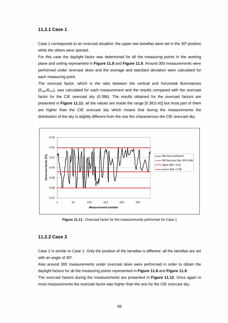
65

11.2.1 Case 1

Case 1 corresponds to an overcast situation: the upper two lamellas were set in the 30º position

while the others were opened.

For this case the daylight factor was determined for all the measuring points in the working

plane and ceiling represented in Figure 11.8 and Figure 11.9. Around 300 measurements were

performed under overcast skies and the average and standard deviation were calculated for

each measuring point.

The overcast factor, which is the ratio between the vertical and horizontal illuminances

(Evert/Ehor), was calculated for each measurement and the results compared with the overcast

factor for the CIE overcast sky (0.396). The results obtained for the overcast factors are

presented in Figure 11.11: all the values are inside the range [0.38;0.42] but most part of them

are higher than the CIE overcast sky which means that during the measurements the

distribution of the sky is slightly different from the one the characterizes the CIE overcast sky.

0.37

0.38

0.39

0.40

0.41

0.42

0.43

1 51 101 151 201 251

Measurement number

Ove

rcas

t fac

tor [

%] SBi OvercastFactor

CIE Overcast Sky OF=0.396

Upper limit = 0.42

Low er limit = 0.38

Figure 11.11 - Overcast factor for the measurements performed for Case 1

11.2.2 Case 2

Case 2 is similar to Case 1. Only the position of the lamellas is different: all the lamellas are set

with an angle of 30º.

Also around 300 measurements under overcast skies were performed in order to obtain the

daylight factors for all the measuring points represented in Figure 11.8 and Figure 11.9.

The overcast factors during the measurements are presented in Figure 11.12. Once again in

most measurements the overcast factor was higher than the one for the CIE overcast sky.

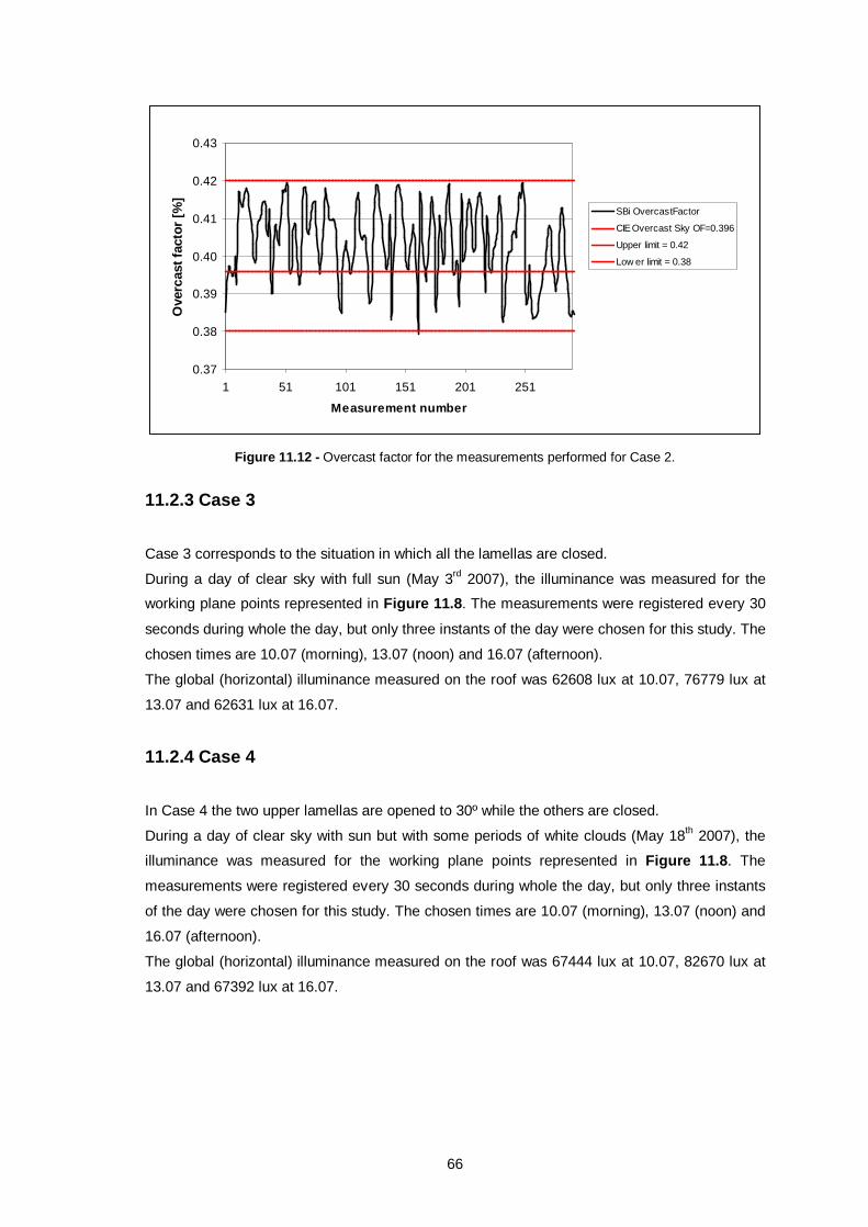
66

0.37

0.38

0.39

0.40

0.41

0.42

0.43

1 51 101 151 201 251

Measurement number

Ove

rcas

t fac

tor [

%]

SBi OvercastFactor

CIE Overcast Sky OF=0.396

Upper limit = 0.42

Low er limit = 0.38

Figure 11.12 - Overcast factor for the measurements performed for Case 2.

11.2.3 Case 3

Case 3 corresponds to the situation in which all the lamellas are closed.

During a day of clear sky with full sun (May 3rd 2007), the illuminance was measured for the

working plane points represented in Figure 11.8. The measurements were registered every 30

seconds during whole the day, but only three instants of the day were chosen for this study. The

chosen times are 10.07 (morning), 13.07 (noon) and 16.07 (afternoon).

The global (horizontal) illuminance measured on the roof was 62608 lux at 10.07, 76779 lux at

13.07 and 62631 lux at 16.07.

11.2.4 Case 4

In Case 4 the two upper lamellas are opened to 30º while the others are closed.

During a day of clear sky with sun but with some periods of white clouds (May 18th 2007), the

illuminance was measured for the working plane points represented in Figure 11.8. The

measurements were registered every 30 seconds during whole the day, but only three instants

of the day were chosen for this study. The chosen times are 10.07 (morning), 13.07 (noon) and

16.07 (afternoon).

The global (horizontal) illuminance measured on the roof was 67444 lux at 10.07, 82670 lux at

13.07 and 67392 lux at 16.07.

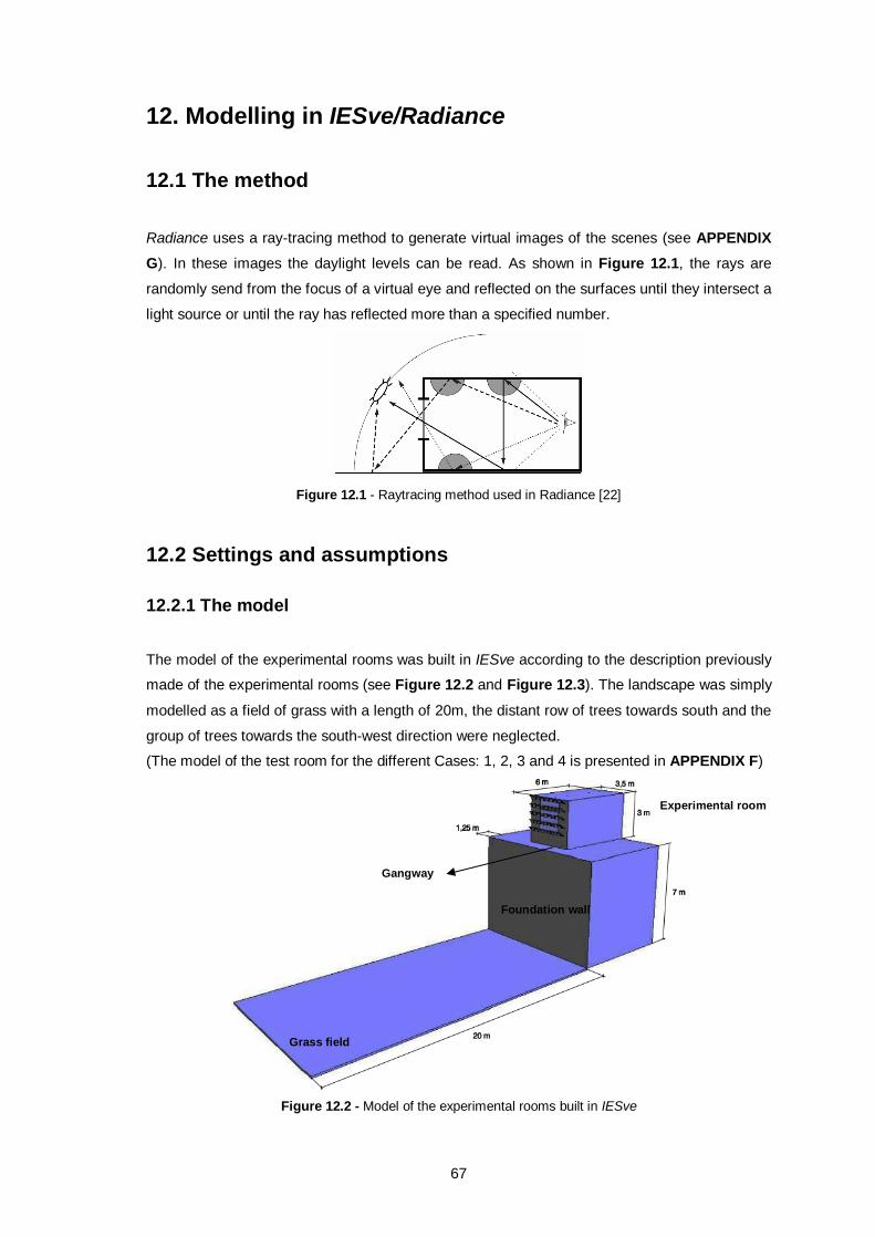
67

12. Modelling in IESve/Radiance

12.1 The method

Radiance uses a ray-tracing method to generate virtual images of the scenes (see APPENDIX G). In these images the daylight levels can be read. As shown in Figure 12.1, the rays are

randomly send from the focus of a virtual eye and reflected on the surfaces until they intersect a

light source or until the ray has reflected more than a specified number.

Figure 12.1 - Raytracing method used in Radiance [22]

12.2 Settings and assumptions 12.2.1 The model

The model of the experimental rooms was built in IESve according to the description previously

made of the experimental rooms (see Figure 12.2 and Figure 12.3). The landscape was simply

modelled as a field of grass with a length of 20m, the distant row of trees towards south and the

group of trees towards the south-west direction were neglected.

(The model of the test room for the different Cases: 1, 2, 3 and 4 is presented in APPENDIX F)

Figure 12.2 - Model of the experimental rooms built in IESve

Grass field

Foundation wall

Experimental room

Gangway

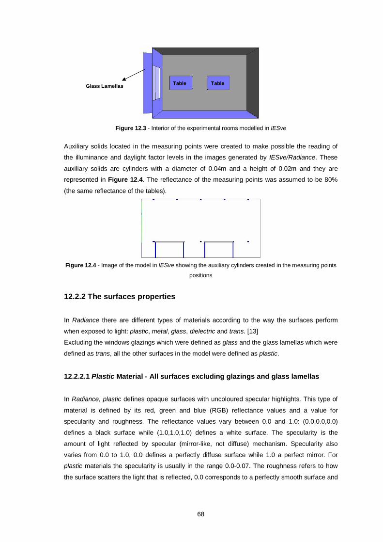
68

Figure 12.3 - Interior of the experimental rooms modelled in IESve

Auxiliary solids located in the measuring points were created to make possible the reading of

the illuminance and daylight factor levels in the images generated by IESve/Radiance. These

auxiliary solids are cylinders with a diameter of 0.04m and a height of 0.02m and they are

represented in Figure 12.4. The reflectance of the measuring points was assumed to be 80%

(the same reflectance of the tables).

Figure 12.4 - Image of the model in IESve showing the auxiliary cylinders created in the measuring points

positions

12.2.2 The surfaces properties

In Radiance there are different types of materials according to the way the surfaces perform

when exposed to light: plastic, metal, glass, dielectric and trans. [13]

Excluding the windows glazings which were defined as glass and the glass lamellas which were

defined as trans, all the other surfaces in the model were defined as plastic.

12.2.2.1 Plastic Material - All surfaces excluding glazings and glass lamellas

In Radiance, plastic defines opaque surfaces with uncoloured specular highlights. This type of

material is defined by its red, green and blue (RGB) reflectance values and a value for

specularity and roughness. The reflectance values vary between 0.0 and 1.0: (0.0,0.0,0.0)

defines a black surface while (1.0,1.0,1.0) defines a white surface. The specularity is the

amount of light reflected by specular (mirror-like, not diffuse) mechanism. Specularity also

varies from 0.0 to 1.0, 0.0 defines a perfectly diffuse surface while 1.0 a perfect mirror. For

plastic materials the specularity is usually in the range 0.0-0.07. The roughness refers to how

the surface scatters the light that is reflected, 0.0 corresponds to a perfectly smooth surface and

Table Table Glass Lamellas

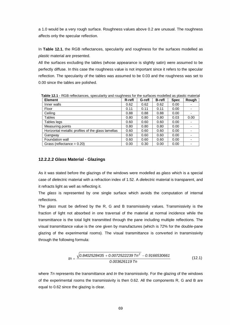
69

a 1.0 would be a very rough surface. Roughness values above 0.2 are unusual. The roughness

affects only the specular reflection.

In Table 12.1, the RGB reflectances, specularity and roughness for the surfaces modelled as

plastic material are presented.

All the surfaces excluding the tables (whose appearance is slightly satin) were assumed to be

perfectly diffuse. In this case the roughness value is not important since it refers to the specular

reflection. The specularity of the tables was assumed to be 0.03 and the roughness was set to

0.00 since the tables are polished.

Table 12.1 - RGB reflectances, specularity and roughness for the surfaces modelled as plastic material

Element R-refl G-refl B-refl Spec Rough Inner walls 0.62 0.62 0.62 0.00 - Floor 0.11 0.11 0.11 0.00 - Ceiling 0.88 0.88 0.88 0.00 - Tables 0.80 0.80 0.80 0.03 0.00 Tables legs 0.60 0.60 0.60 0.00 - Measuring points 0.80 0.80 0.80 0.00 - Horizontal metallic profiles of the glass lamellas 0.60 0.60 0.60 0.00 - Gangway 0.60 0.60 0.60 0.00 - Foundation wall 0.60 0.60 0.60 0.00 - Grass (reflectance = 0.20) 0.00 0.30 0.00 0.00 -

12.2.2.2 Glass Material - Glazings

As it was stated before the glazings of the windows were modelled as glass which is a special

case of dielectric material with a refraction index of 1.52. A dielectric material is transparent, and

it refracts light as well as reflecting it.

The glass is represented by one single surface which avoids the computation of internal

reflections.

The glass must be defined by the R, G and B transmissivity values. Transmissivity is the

fraction of light not absorbed in one traversal of the material at normal incidence while the

transmittance is the total light transmitted through the pane including multiple reflections. The

visual transmittance value is the one given by manufactures (which is 72% for the double-pane

glazing of the experimental rooms). The visual transmittance is converted in transmissivity

through the following formula:

Tn003626119.0

9166530661.0Tn0072522239.08402528435.0tn

2 (12.1)

where Tn represents the transmittance and tn the transmissivity. For the glazing of the windows

of the experimental rooms the transmissivity is then 0.62. All the components R, G and B are

equal to 0.62 since the glazing is clear.

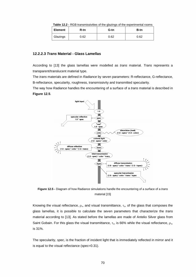
70

Table 12.2 - RGB transmissivities of the glazings of the experimental rooms

Element R-tn G-tn B-tn

Glazings 0.62 0.62 0.62

12.2.2.3 Trans Material - Glass Lamellas

According to [13] the glass lamellas were modelled as trans material. Trans represents a

transparent/translucent material type.

The trans materials are defined in Radiance by seven parameters: R-reflectance, G-reflectance,

B-reflectance, specularity, roughness, transmissivity and transmitted specularity.

The way how Radiance handles the encountering of a surface of a trans material is described in

Figure 12.5.

Figure 12.5 - Diagram of how Radiance simulations handle the encountering of a surface of a trans

material [15]

Knowing the visual reflectance, v, and visual transmittance, v, of the glass that composes the

glass lamellas, it is possible to calculate the seven parameters that characterize the trans

material according to [13]. As stated before the lamellas are made of Antelio Silver glass from

Saint Gobain. For this glass the visual transmittance, v, is 66% while the visual reflectance, v,

is 31%.

The specularity, spec, is the fraction of incident light that is immediately reflected in mirror and it

is equal to the visual reflectance (spec=0.31).

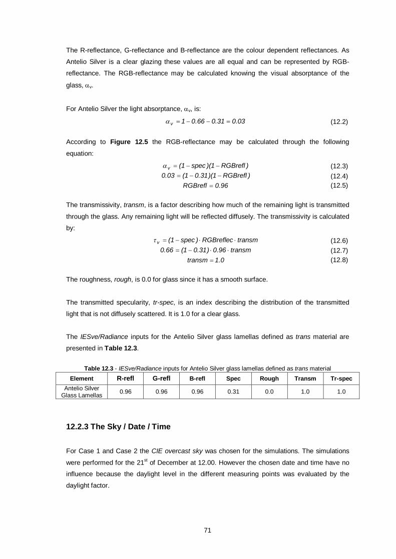
71

The R-reflectance, G-reflectance and B-reflectance are the colour dependent reflectances. As

Antelio Silver is a clear glazing these values are all equal and can be represented by RGB-

reflectance. The RGB-reflectance may be calculated knowing the visual absorptance of the

glass, v.

For Antelio Silver the light absorptance, v, is:

03.031.066.01v (12.2)

According to Figure 12.5 the RGB-reflectance may be calculated through the following

equation:

)RGBrefl1)(spec1(v (12.3) )RGBrefl1)(31.01(03.0 (12.4) 96.0RGBrefl (12.5)

The transmissivity, transm, is a factor describing how much of the remaining light is transmitted

through the glass. Any remaining light will be reflected diffusely. The transmissivity is calculated

by:

transmRGBreflec)spec1(v (12.6) transm96.0)31.01(66.0 (12.7) 0.1transm (12.8)

The roughness, rough, is 0.0 for glass since it has a smooth surface.

The transmitted specularity, tr-spec, is an index describing the distribution of the transmitted

light that is not diffusely scattered. It is 1.0 for a clear glass.

The IESve/Radiance inputs for the Antelio Silver glass lamellas defined as trans material are

presented in Table 12.3.

Table 12.3 - IESve/Radiance inputs for Antelio Silver glass lamellas defined as trans material Element R-refl G-refl B-refl Spec Rough Transm Tr-spec

Antelio Silver Glass Lamellas 0.96 0.96 0.96 0.31 0.0 1.0 1.0

12.2.3 The Sky / Date / Time

For Case 1 and Case 2 the CIE overcast sky was chosen for the simulations. The simulations

were performed for the 21st of December at 12.00. However the chosen date and time have no

influence because the daylight level in the different measuring points was evaluated by the

daylight factor.

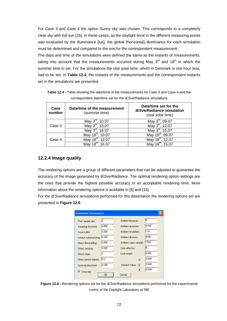
72

For Case 3 and Case 4 the option Sunny sky was chosen. This corresponds to a completely

clear sky with full sun [15]. In these cases, as the daylight level in the different measuring points

was evaluated by the illuminance [lux], the global (horizontal) illuminance for each simulation

must be determined and compared to the one for the correspondent measurement.

The days and time of the simulations were defined the same as the instants of measurements,

taking into account that the measurements occurred during May 3rd and 18th in which the

summer time in set. For the simulations the real solar time, which in Denmark is one hour less,

had to be set. In Table 12.4, the instants of the measurements and the correspondent instants

set in the simulations are presented.

Table 12.4 - Table showing the date/time of the measurements for Case 3 and Case 4 and the

correspondent date/time set for the IESve/Radiance simulations

Case number

Date/time of the measurement (summer time)

Date/time set for the IESve/Radiance simulation

(real solar time) May 3rd, 10.07 May 3rd, 09.07 May 3rd, 13.07 May 3rd, 12.07 Case 3 May 3rd, 16.07 May 3rd, 15.07 May 18th, 10.07 May 18th, 09.07 May 18th, 13.07 May 18th, 12.07 Case 4 May 18th, 16.07 May 18th, 15.07

12.2.4 Image quality The rendering options are a group of different parameters that can be adjusted to guarantee the

accuracy of the image generated by IESve/Radiance. The optimal rendering option settings are

the ones that provide the highest possible accuracy in an acceptable rendering time. More

information about the rendering options is available in [5] and [15].

For the IESve/Radiance simulations performed for this dissertation the rendering options set are

presented in Figure 12.6.

Figure 12.6 - Rendering options set for the IESve/Radiance simulations performed for the experimental

rooms of the Daylight Laboratory at SBi

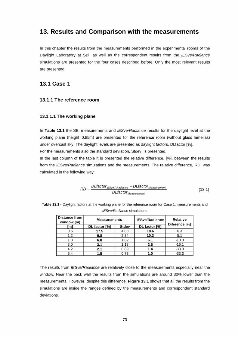
73

13. Results and Comparison with the measurements

In this chapter the results from the measurements performed in the experimental rooms of the

Daylight Laboratory at SBi, as well as the correspondent results from the IESve/Radiance

simulations are presented for the four cases described before. Only the most relevant results

are presented.

13.1 Case 1

13.1.1 The reference room 13.1.1.1 The working plane In Table 13.1 the SBi measurements and IESve/Radiance results for the daylight level at the

working plane (height=0.85m) are presented for the reference room (without glass lamellas)

under overcast sky. The daylight levels are presented as daylight factors, DLfactor [%].

For the measurements also the standard deviation, Stdev, is presented.

In the last column of the table it is presented the relative difference, [%], between the results

from the IESve/Radiance simulations and the measurements. The relative difference, RD, was

calculated in the following way:

tMeasuremen

tMeasuremenRadiance/IESve

DLfactorDLfactorDLfactor

RD

(13.1)

Table 13.1 - Daylight factors at the working plane for the reference room for Case 1: measurements and

IESve/Radiance simulations

Distance from window (m) IESve/Radiance

[m] DL factor [%] Stdev DL factor [%]0.6 17.5 4.03 18.6 6.31.2 9.8 2.34 10.3 5.11.8 6.8 1.82 6.1 -10.33.0 3.1 1.13 2.6 -16.14.2 2.1 0.89 1.4 -33.35.4 1.5 0.73 1.0 -33.3

Measurements Relative Diference [%]

The results from IESve/Radiance are relatively close to the measurements especially near the

window. Near the back wall the results from the simulations are around 30% lower than the

measurements. However, despite this difference, Figure 13.1 shows that all the results from the

simulations are inside the ranges defined by the measurements and correspondent standard

deviations.

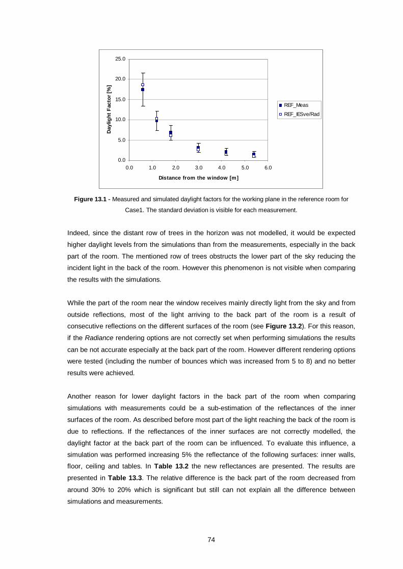
74

0.0

5.0

10.0

15.0

20.0

25.0

0.0 1.0 2.0 3.0 4.0 5.0 6.0

Distance from the window [m]

Day

light

Fac

tor [

%]

REF_Meas

REF_IESve/Rad

Figure 13.1 - Measured and simulated daylight factors for the working plane in the reference room for

Case1. The standard deviation is visible for each measurement.

Indeed, since the distant row of trees in the horizon was not modelled, it would be expected

higher daylight levels from the simulations than from the measurements, especially in the back

part of the room. The mentioned row of trees obstructs the lower part of the sky reducing the

incident light in the back of the room. However this phenomenon is not visible when comparing

the results with the simulations.

While the part of the room near the window receives mainly directly light from the sky and from

outside reflections, most of the light arriving to the back part of the room is a result of

consecutive reflections on the different surfaces of the room (see Figure 13.2). For this reason,

if the Radiance rendering options are not correctly set when performing simulations the results

can be not accurate especially at the back part of the room. However different rendering options

were tested (including the number of bounces which was increased from 5 to 8) and no better

results were achieved.

Another reason for lower daylight factors in the back part of the room when comparing

simulations with measurements could be a sub-estimation of the reflectances of the inner

surfaces of the room. As described before most part of the light reaching the back of the room is

due to reflections. If the reflectances of the inner surfaces are not correctly modelled, the

daylight factor at the back part of the room can be influenced. To evaluate this influence, a

simulation was performed increasing 5% the reflectance of the following surfaces: inner walls,

floor, ceiling and tables. In Table 13.2 the new reflectances are presented. The results are

presented in Table 13.3. The relative difference is the back part of the room decreased from

around 30% to 20% which is significant but still can not explain all the difference between

simulations and measurements.

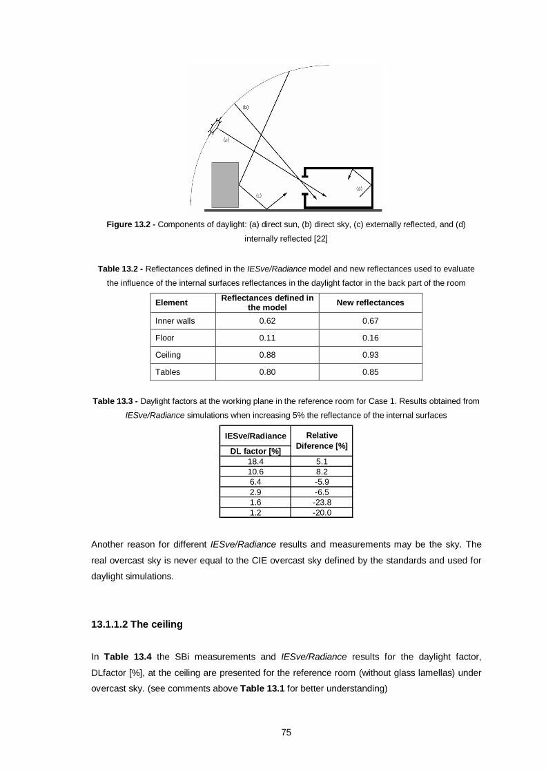
75

Figure 13.2 - Components of daylight: (a) direct sun, (b) direct sky, (c) externally reflected, and (d)

internally reflected [22]

Table 13.2 - Reflectances defined in the IESve/Radiance model and new reflectances used to evaluate

the influence of the internal surfaces reflectances in the daylight factor in the back part of the room

Element Reflectances defined in the model New reflectances

Inner walls 0.62 0.67

Floor 0.11 0.16

Ceiling 0.88 0.93

Tables 0.80 0.85

Table 13.3 - Daylight factors at the working plane in the reference room for Case 1. Results obtained from

IESve/Radiance simulations when increasing 5% the reflectance of the internal surfaces

IESve/Radiance

DL factor [%]18.4 5.110.6 8.26.4 -5.92.9 -6.51.6 -23.81.2 -20.0

Relative Diference [%]

Another reason for different IESve/Radiance results and measurements may be the sky. The

real overcast sky is never equal to the CIE overcast sky defined by the standards and used for

daylight simulations.

13.1.1.2 The ceiling

In Table 13.4 the SBi measurements and IESve/Radiance results for the daylight factor,

DLfactor [%], at the ceiling are presented for the reference room (without glass lamellas) under

overcast sky. (see comments above Table 13.1 for better understanding)

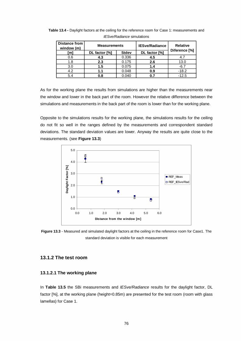
76

Table 13.4 - Daylight factors at the ceiling for the reference room for Case 1: measurements and



[m] DL factor [%] Stdev DL factor [%]0.6 4.3 0.336 4.5 4.71.8 2.3 0.175 2.6 13.03.0 1.5 0.075 1.4 -6.74.2 1.1 0.048 0.9 -18.25.4 0.8 0.040 0.7 -12.5


As for the working plane the results from simulations are higher than the measurements near

the window and lower in the back part of the room. However the relative difference between the

simulations and measurements in the back part of the room is lower than for the working plane.

Opposite to the simulations results for the working plane, the simulations results for the ceiling

do not fit so well in the ranges defined by the measurements and correspondent standard

deviations. The standard deviation values are lower. Anyway the results are quite close to the

measurements. (see Figure 13.3)

0.0

1.0

2.0

3.0

4.0

5.0

0.0 1.0 2.0 3.0 4.0 5.0 6.0


Day

light

Fac

tor [

%]

REF_Meas

REF_IESve/Rad

Figure 13.3 - Measured and simulated daylight factors at the ceiling in the reference room for Case1. The

standard deviation is visible for each measurement

13.1.2 The test room

13.1.2.1 The working plane

In Table 13.5 the SBi measurements and IESve/Radiance results for the daylight factor, DL

factor [%], at the working plane (height=0.85m) are presented for the test room (room with glass

lamellas) for Case 1.

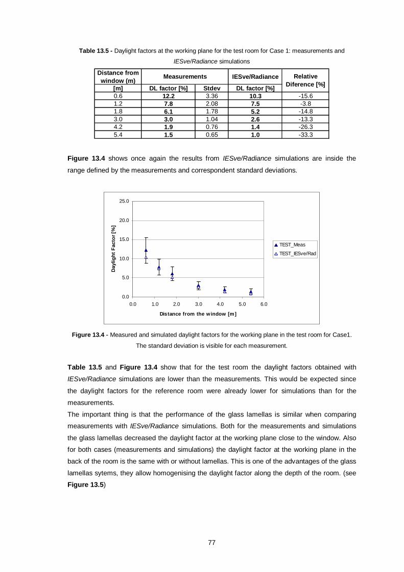
77

Table 13.5 - Daylight factors at the working plane for the test room for Case 1: measurements and



[m] DL factor [%] Stdev DL factor [%]0.6 12.2 3.36 10.3 -15.61.2 7.8 2.08 7.5 -3.81.8 6.1 1.78 5.2 -14.83.0 3.0 1.04 2.6 -13.34.2 1.9 0.76 1.4 -26.35.4 1.5 0.65 1.0 -33.3


Figure 13.4 shows once again the results from IESve/Radiance simulations are inside the

range defined by the measurements and correspondent standard deviations.

0.0

5.0

10.0

15.0

20.0

25.0

0.0 1.0 2.0 3.0 4.0 5.0 6.0


Day

light

Fac

tor [

%]

TEST_Meas

TEST_IESve/Rad

Figure 13.4 - Measured and simulated daylight factors for the working plane in the test room for Case1.

The standard deviation is visible for each measurement.

Table 13.5 and Figure 13.4 show that for the test room the daylight factors obtained with

IESve/Radiance simulations are lower than the measurements. This would be expected since

the daylight factors for the reference room were already lower for simulations than for the

measurements.

The important thing is that the performance of the glass lamellas is similar when comparing

measurements with IESve/Radiance simulations. Both for the measurements and simulations

the glass lamellas decreased the daylight factor at the working plane close to the window. Also

for both cases (measurements and simulations) the daylight factor at the working plane in the

back of the room is the same with or without lamellas. This is one of the advantages of the glass

lamellas sytems, they allow homogenising the daylight factor along the depth of the room. (see

Figure 13.5)

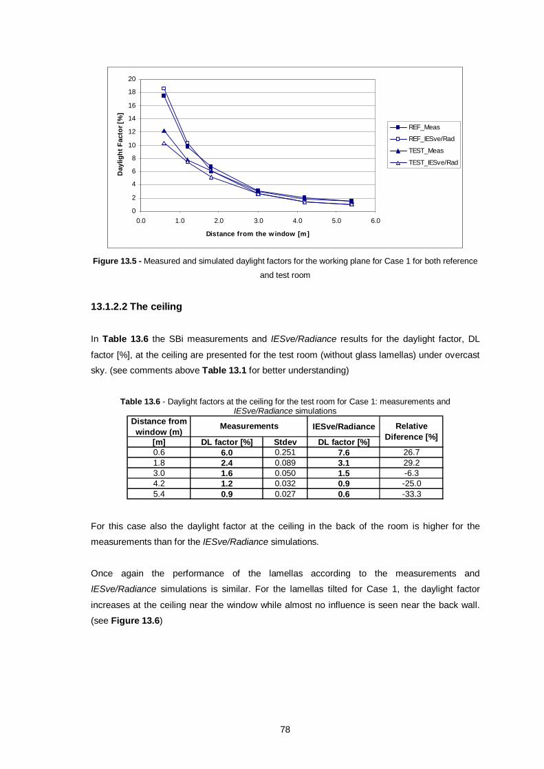
78

0

2

4

6

8

10

12

14

16

18

20

0.0 1.0 2.0 3.0 4.0 5.0 6.0


Day

light

Fac

tor [

%]

REF_Meas

REF_IESve/Rad

TEST_Meas

TEST_IESve/Rad

Figure 13.5 - Measured and simulated daylight factors for the working plane for Case 1 for both reference

and test room

13.1.2.2 The ceiling In Table 13.6 the SBi measurements and IESve/Radiance results for the daylight factor, DL

factor [%], at the ceiling are presented for the test room (without glass lamellas) under overcast

sky. (see comments above Table 13.1 for better understanding)

Table 13.6 - Daylight factors at the ceiling for the test room for Case 1: measurements and

IESve/Radiance simulations Distance from window (m) IESve/Radiance

[m] DL factor [%] Stdev DL factor [%]0.6 6.0 0.251 7.6 26.71.8 2.4 0.089 3.1 29.23.0 1.6 0.050 1.5 -6.34.2 1.2 0.032 0.9 -25.05.4 0.9 0.027 0.6 -33.3


For this case also the daylight factor at the ceiling in the back of the room is higher for the

measurements than for the IESve/Radiance simulations.

Once again the performance of the lamellas according to the measurements and

IESve/Radiance simulations is similar. For the lamellas tilted for Case 1, the daylight factor

increases at the ceiling near the window while almost no influence is seen near the back wall.

(see Figure 13.6)

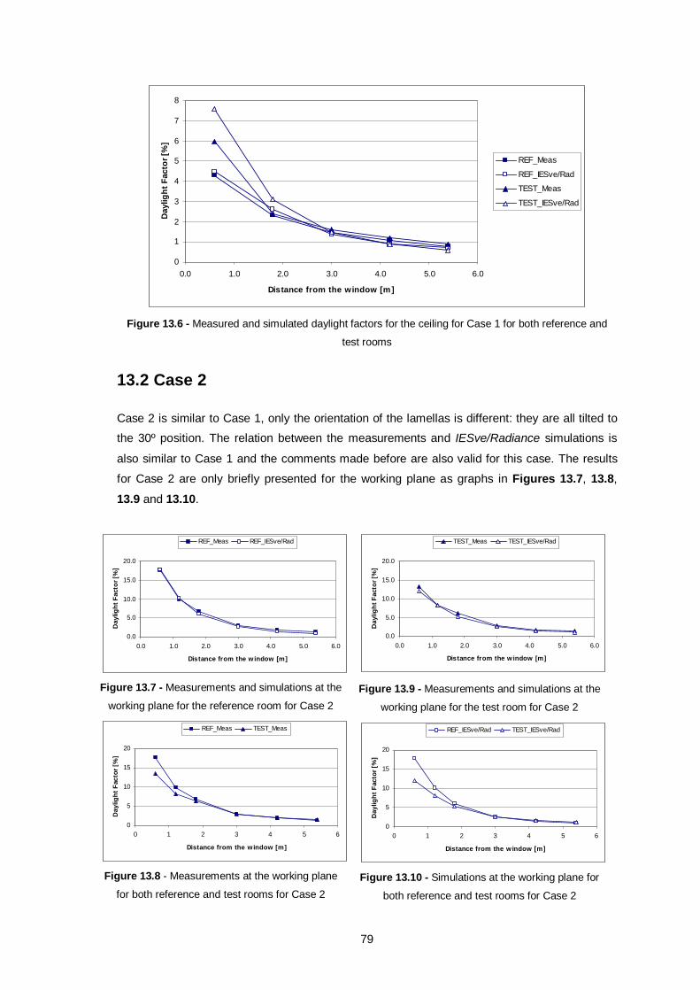
79

0

1

2

3

4

5

6

7

8

0.0 1.0 2.0 3.0 4.0 5.0 6.0


Day

light

Fac

tor [

%]

REF_Meas

REF_IESve/Rad

TEST_Meas

TEST_IESve/Rad

Figure 13.6 - Measured and simulated daylight factors for the ceiling for Case 1 for both reference and

test rooms

13.2 Case 2 Case 2 is similar to Case 1, only the orientation of the lamellas is different: they are all tilted to

the 30º position. The relation between the measurements and IESve/Radiance simulations is

also similar to Case 1 and the comments made before are also valid for this case. The results

for Case 2 are only briefly presented for the working plane as graphs in Figures 13.7, 13.8,

13.9 and 13.10.

0.0

5.0

10.0

15.0

20.0

0.0 1.0 2.0 3.0 4.0 5.0 6.0


Day

light

Fac

tor [

%]

REF_Meas REF_IESve/Rad

Figure 13.7 - Measurements and simulations at the

working plane for the reference room for Case 2

0

5

10

15

20

0 1 2 3 4 5 6


Day

light

Fac

tor [

%]

REF_Meas TEST_Meas

Figure 13.8 - Measurements at the working plane

for both reference and test rooms for Case 2

0.0

5.0

10.0

15.0

20.0

0.0 1.0 2.0 3.0 4.0 5.0 6.0


Day

light

Fac

tor [

%]

TEST_Meas TEST_IESve/Rad

Figure 13.9 - Measurements and simulations at the

working plane for the test room for Case 2

0

5

10

15

20

0 1 2 3 4 5 6


Day

light

Fac

tor [

%]

REF_IESve/Rad TEST_IESve/Rad

Figure 13.10 - Simulations at the working plane for

both reference and test rooms for Case 2

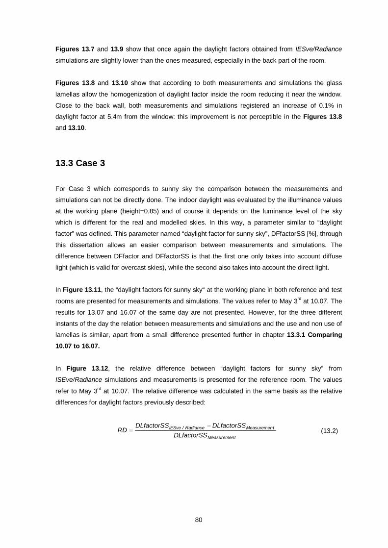
80

Figures 13.7 and 13.9 show that once again the daylight factors obtained from IESve/Radiance

simulations are slightly lower than the ones measured, especially in the back part of the room.

Figures 13.8 and 13.10 show that according to both measurements and simulations the glass

lamellas allow the homogenization of daylight factor inside the room reducing it near the window.

Close to the back wall, both measurements and simulations registered an increase of 0.1% in

daylight factor at 5.4m from the window: this improvement is not perceptible in the Figures 13.8

and 13.10.

13.3 Case 3

For Case 3 which corresponds to sunny sky the comparison between the measurements and

simulations can not be directly done. The indoor daylight was evaluated by the illuminance values

at the working plane (height=0.85) and of course it depends on the luminance level of the sky

which is different for the real and modelled skies. In this way, a parameter similar to “daylight

factor” was defined. This parameter named “daylight factor for sunny sky”, DFfactorSS [%], through

this dissertation allows an easier comparison between measurements and simulations. The

difference between DFfactor and DFfactorSS is that the first one only takes into account diffuse

light (which is valid for overcast skies), while the second also takes into account the direct light.

In Figure 13.11, the “daylight factors for sunny sky“ at the working plane in both reference and test

rooms are presented for measurements and simulations. The values refer to May 3rd at 10.07. The

results for 13.07 and 16.07 of the same day are not presented. However, for the three different

instants of the day the relation between measurements and simulations and the use and non use of

lamellas is similar, apart from a small difference presented further in chapter 13.3.1 Comparing 10.07 to 16.07.

In Figure 13.12, the relative difference between “daylight factors for sunny sky” from

ISEve/Radiance simulations and measurements is presented for the reference room. The values

refer to May 3rd at 10.07. The relative difference was calculated in the same basis as the relative

differences for daylight factors previously described:

tMeasuremen

tMeasuremenRadiance/IESve

DLfactorSSDLfactorSSDLfactorSS

RD

(13.2)

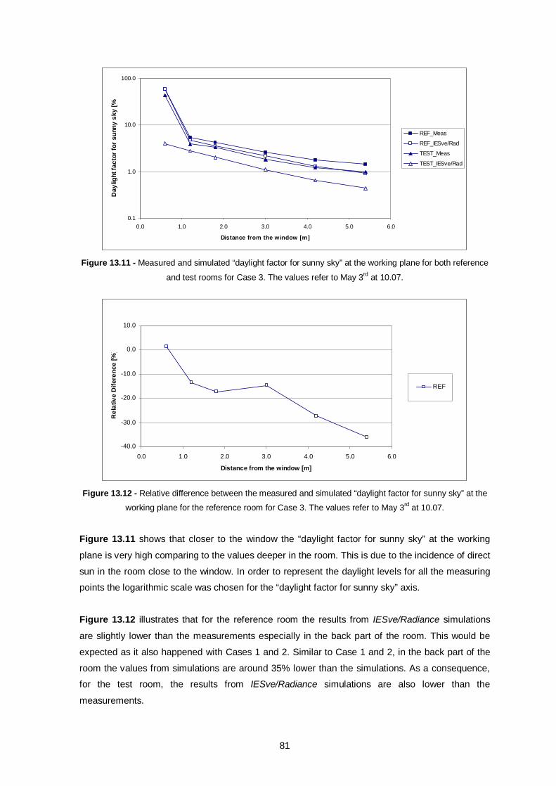
81

0.1

1.0

10.0

100.0

0.0 1.0 2.0 3.0 4.0 5.0 6.0

Distance from the w indow [m]

Day

light

fact

or fo

r su

nny

sky

[%]

REF_Meas

REF_IESve/Rad

TEST_Meas

TEST_IESve/Rad

Figure 13.11 - Measured and simulated “daylight factor for sunny sky” at the working plane for both reference

and test rooms for Case 3. The values refer to May 3rd at 10.07.

-40.0

-30.0

-20.0

-10.0

0.0

10.0

0.0 1.0 2.0 3.0 4.0 5.0 6.0


Rel

ativ

e D

ifere

nce

[%]

REF

Figure 13.12 - Relative difference between the measured and simulated “daylight factor for sunny sky” at the

working plane for the reference room for Case 3. The values refer to May 3rd at 10.07.

Figure 13.11 shows that closer to the window the “daylight factor for sunny sky” at the working

plane is very high comparing to the values deeper in the room. This is due to the incidence of direct

sun in the room close to the window. In order to represent the daylight levels for all the measuring

points the logarithmic scale was chosen for the “daylight factor for sunny sky” axis.

Figure 13.12 illustrates that for the reference room the results from IESve/Radiance simulations

are slightly lower than the measurements especially in the back part of the room. This would be

expected as it also happened with Cases 1 and 2. Similar to Case 1 and 2, in the back part of the

room the values from simulations are around 35% lower than the simulations. As a consequence,

for the test room, the results from IESve/Radiance simulations are also lower than the

measurements.

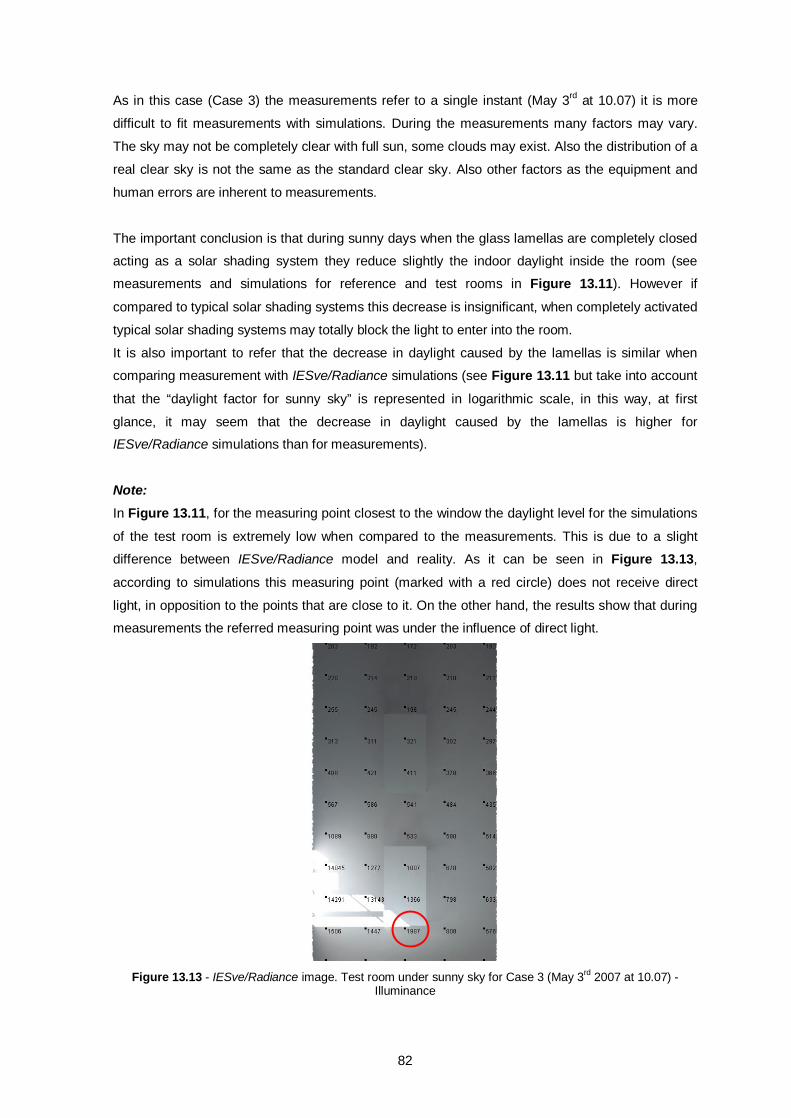
82

As in this case (Case 3) the measurements refer to a single instant (May 3rd at 10.07) it is more

difficult to fit measurements with simulations. During the measurements many factors may vary.

The sky may not be completely clear with full sun, some clouds may exist. Also the distribution of a

real clear sky is not the same as the standard clear sky. Also other factors as the equipment and

human errors are inherent to measurements.

The important conclusion is that during sunny days when the glass lamellas are completely closed

acting as a solar shading system they reduce slightly the indoor daylight inside the room (see

measurements and simulations for reference and test rooms in Figure 13.11). However if

compared to typical solar shading systems this decrease is insignificant, when completely activated

typical solar shading systems may totally block the light to enter into the room.

It is also important to refer that the decrease in daylight caused by the lamellas is similar when

comparing measurement with IESve/Radiance simulations (see Figure 13.11 but take into account

that the “daylight factor for sunny sky” is represented in logarithmic scale, in this way, at first

glance, it may seem that the decrease in daylight caused by the lamellas is higher for

IESve/Radiance simulations than for measurements).

Note: In Figure 13.11, for the measuring point closest to the window the daylight level for the simulations

of the test room is extremely low when compared to the measurements. This is due to a slight

difference between IESve/Radiance model and reality. As it can be seen in Figure 13.13,

according to simulations this measuring point (marked with a red circle) does not receive direct

light, in opposition to the points that are close to it. On the other hand, the results show that during

measurements the referred measuring point was under the influence of direct light.

Figure 13.13 - IESve/Radiance image. Test room under sunny sky for Case 3 (May 3rd 2007 at 10.07) -

Illuminance

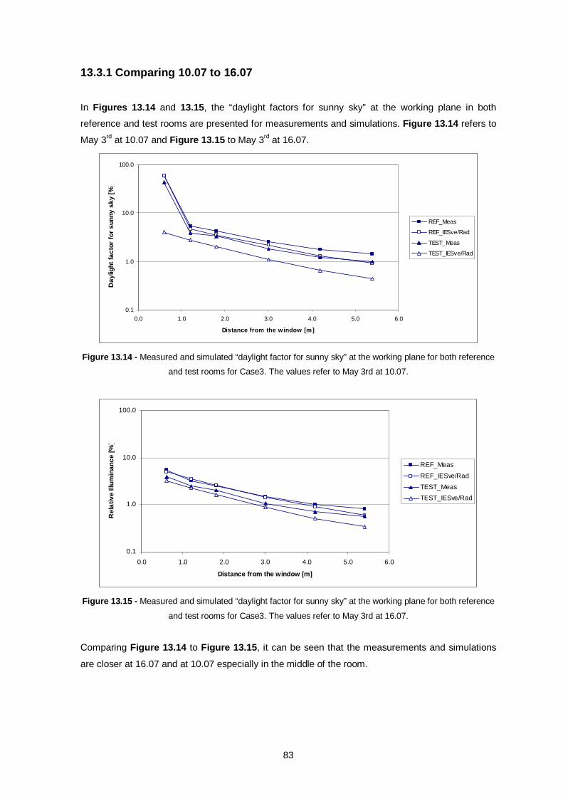
83

13.3.1 Comparing 10.07 to 16.07

In Figures 13.14 and 13.15, the “daylight factors for sunny sky” at the working plane in both

reference and test rooms are presented for measurements and simulations. Figure 13.14 refers to

May 3rd at 10.07 and Figure 13.15 to May 3rd at 16.07.

0.1

1.0

10.0

100.0

0.0 1.0 2.0 3.0 4.0 5.0 6.0


Day

light

fact

or fo

r sun

ny s

ky [%

]

REF_Meas

REF_IESve/Rad

TEST_Meas

TEST_IESve/Rad


and test rooms for Case3. The values refer to May 3rd at 10.07.

0.1

1.0

10.0

100.0

0.0 1.0 2.0 3.0 4.0 5.0 6.0


Rel

ativ

e Ill

umin

ance

[%]

REF_Meas

REF_IESve/Rad

TEST_MeasTEST_IESve/Rad


and test rooms for Case3. The values refer to May 3rd at 16.07.

Comparing Figure 13.14 to Figure 13.15, it can be seen that the measurements and simulations

are closer at 16.07 and at 10.07 especially in the middle of the room.

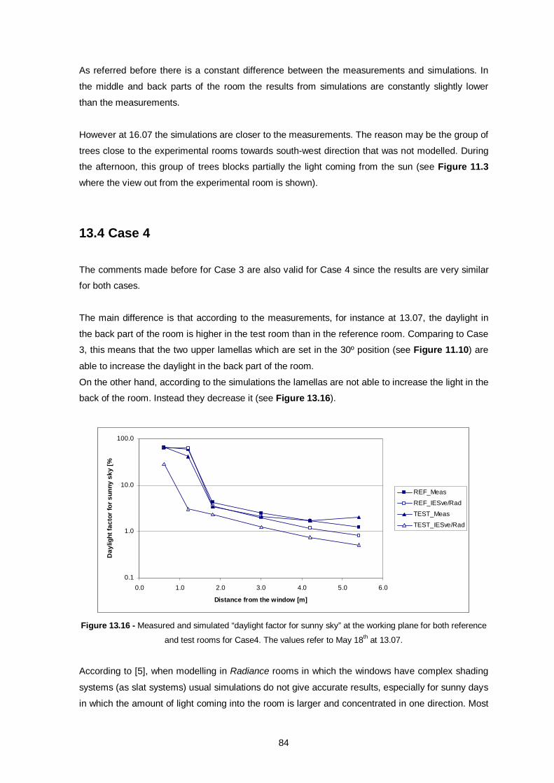
84

As referred before there is a constant difference between the measurements and simulations. In

the middle and back parts of the room the results from simulations are constantly slightly lower

than the measurements.

However at 16.07 the simulations are closer to the measurements. The reason may be the group of

trees close to the experimental rooms towards south-west direction that was not modelled. During

the afternoon, this group of trees blocks partially the light coming from the sun (see Figure 11.3 where the view out from the experimental room is shown).

13.4 Case 4

The comments made before for Case 3 are also valid for Case 4 since the results are very similar

for both cases.

The main difference is that according to the measurements, for instance at 13.07, the daylight in

the back part of the room is higher in the test room than in the reference room. Comparing to Case

3, this means that the two upper lamellas which are set in the 30º position (see Figure 11.10) are

able to increase the daylight in the back part of the room.

On the other hand, according to the simulations the lamellas are not able to increase the light in the

back of the room. Instead they decrease it (see Figure 13.16).

0.1

1.0

10.0

100.0

0.0 1.0 2.0 3.0 4.0 5.0 6.0


Day

light

fact

or fo

r sun

ny s

ky [%

]

REF_Meas

REF_IESve/Rad

TEST_Meas

TEST_IESve/Rad


and test rooms for Case4. The values refer to May 18th at 13.07.

According to [5], when modelling in Radiance rooms in which the windows have complex shading

systems (as slat systems) usual simulations do not give accurate results, especially for sunny days

in which the amount of light coming into the room is larger and concentrated in one direction. Most

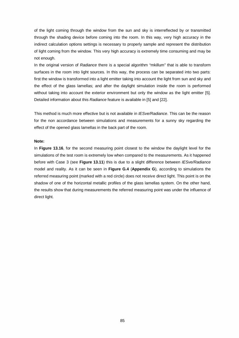
85

of the light coming through the window from the sun and sky is interreflected by or transmitted

through the shading device before coming into the room. In this way, very high accuracy in the

indirect calculation options settings is necessary to properly sample and represent the distribution

of light coming from the window. This very high accuracy is extremely time consuming and may be

not enough.

In the original version of Radiance there is a special algorithm “mkillum” that is able to transform

surfaces in the room into light sources. In this way, the process can be separated into two parts:

first the window is transformed into a light emitter taking into account the light from sun and sky and

the effect of the glass lamellas; and after the daylight simulation inside the room is performed

without taking into account the exterior environment but only the window as the light emitter [5].

Detailed information about this Radiance feature is available in [5] and [22].

This method is much more effective but is not available in IESve/Radiance. This can be the reason

for the non accordance between simulations and measurements for a sunny sky regarding the

effect of the opened glass lamellas in the back part of the room.

Note: In Figure 13.16, for the second measuring point closest to the window the daylight level for the

simulations of the test room is extremely low when compared to the measurements. As it happened

before with Case 3 (see Figure 13.11) this is due to a slight difference between IESve/Radiance

model and reality. As it can be seen in Figure G.4 (Appendix G), according to simulations the

referred measuring point (marked with a red circle) does not receive direct light. This point is on the

shadow of one of the horizontal metallic profiles of the glass lamellas system. On the other hand,

the results show that during measurements the referred measuring point was under the influence of

direct light.

86

14. Conclusions and further work

Comparing measurements with simulations is always a delicate process even with the most highly

developed software. According to [5], Radiance is one of the most advanced daylightning/lightning

simulation tools available but anyway it can not represent perfectly the “nature”. For instance the

distribution of the sky is defined according to standard procedures which are of course not found in

reality. Also during measurements many uncontrolled factors may vary.

Daylight measurements in the experimental rooms of the Daylight Laboratory at SBi were

compared with IESve/Radiance simulations. Four different cases for different sky conditions and

lamellas orientation were studied.

IESve/Radiance is a user-friendly software and according to results it seems that it is valid when

simulating the daylight performance of glass lamellas systems (as a trans material) under overcast

sky and also under sunny sky if the lamellas are closed. For simulations under sunny sky and with

some lamellas opened it is advised to use the original version of Radiance to get more accurate

results.

There are two experimental rooms also at DTU and one of them has already a glass lamellas

system mounted on its façade. The other will be the reference room.

Some daylight measurements and comparison with Radiance simulations are already planned.

IESve/Radiance may be used for this purpose but also a comparison to the original Radiance

should be done especially for sunny days with some lamellas opened (extra features available in

the original Radiance should be used).

It is very important that the characteristics of the room especially the optical properties of the inner

surfaces are well determined so they can be modelled closer to reality.

For a better understanding of the differences between measurements and simulations it is advised

that the person doing the simulations should also be present during the measurements.

It would be also interesting to evaluate the performance of these glass lamellas systems in real

scale buildings located in cities. The evaluation should be done by measurements and software

simulations and it would be also important to perform a survey in order to collect people’s

experience of the visual comfort.

87

References

[1] Bülow-Hube, Helena; Energy Efficient Window Systems - Effects on Energy Use and Daylight

in Buildings, Division of Energy and Building Design, Department of Construction and Architecture,

Lund Institute of Technology, Lund University, 2001

[2] Danish Building Code, http://www.ebst.dk/BR95_13_ID33/0/54/0 (February/August2007)

[3] Dijk, Dick van, WIS version 2.0.1 User Guide – Examples of windows as input for WIS, TNO

Building and Construction Research, Delft, The Netherlands, November 2003

[4] Dubois, Marie-Claude, Impact of Solar Shading Devices on Daylight Quality - Measurements in

Experimental Office Rooms, Report TABK--01/3061, Division of Energy and Building Design,

Department of Construction and Architecture, Lund Institute of Technology, Lund University, 2001

[5] Dubois, Marie-Claude, Impact of Solar Shading Devices on Daylight Quality - Simulations with

Radiance, Report TABK--01/3062, Division of Energy and Building Design, Department of

Construction and Architecture, Lund Institute of Technology, Lund University, 2001

[6] Dubois, Marie-Claude; Solar-Protective Glazing for Cold Climates - A parametric Study of the

Energy Use in Offices, Department of Building Science, Lund Institute of Technology, Lund

University, 1998

[7] Dubois, Marie-Claude, Solar shading for Low Energy Use and Daylight Quality in Offices –

Simulations, Measurements and Design Tools, Report TABK--01/1023, Division of Energy and

Building Design, Department of Construction and Architecture, Lund Institute of Technology, Lund

University, 2001

[8] Information given by Steen Traberg-Borup at Daylight Laboratory at SBi (via e-mail)

[9] Jensen, Jerry Moller; Lund, Hans; Design Reference Year, Dry - Et Nyt Dansk Referencear,

Meddelelse Nr. 281, Laboratoriet for varmeisolering, Danmarks Tekniske Universitet, Oktober 1995

[10] Kuhn, Tilmann E. Kuhn, Summary of the lecture at the Conference on Tall Buildings and

Transparency, 5-7 October 2003

[11] Nielsen, Toke Rammer, Hviid, Christian Anker, BuildingCalc+LightCalc Users guide, BYG,

DTU, 2006

88

[12] Notes from Course 11116 - Sustainable Buildings, Powerpoint Presentation about Solar

Shading Systems, Department of Civil Engineering, Technical University of Denmark, Lyngby,

2006/2007, 2nd semester

[13] Petersen, S., IESVERadiance, Notes from course 11120, 2005

[14] prENrev 15251:2006 (E) - Indoor environment input for design and assessment of energy

performance of buildings - addressing indoor air quality, thermal environment, lightning and

acoustics.

[15] Rayfront User Manual - http://www.schorsch.com/rayfront/manual (August 2007)

[16] Regulamento das Características de Coportamento Térmico dos Edifícios, Colecção

regulamentos - 1, Porto Editora, Porto, 2006

[17] Rosenfeld, J.L.J, WIS DATABASE - Data Submission Procedure for Shading and Diffusing

Components, Version 1.0, Department of Civil Engineering, Technical University of Denmark,

Lyngby, May 2004

[18] Skotte, Tine, Dagslysdirigerende solafskaermende glaslameller; Polyteknisk

Eksamensprojekt, BYG.DTU, 2007

[19] TRY, Test Reference Year, Meteorological National Institute and Civil Engineering National

Laboratory, “Ano Climático de Referência”, Lisbon, December 1989.

[20] Wall, Maria, Bülow-Hübe, Helena, Solar Protection in Buildings, Report TABK--01/3060,

Division of Energy and Building Design, Department of Construction and Architecture, Lund

Institute of Technology, Lund University, 2001

[21] Wall, Maria, Bülow-Hübe, Helena, Solar Protection in Buildings - Part2:2000-2002, Report

TABK--01/3060, Division of Energy and Building Design, Department of Construction and

Architecture, Lund Institute of Technology, Lund University, 2003

[22] Ward Larsson, G., Shakespeare, R, Rendering with Radiance. The Art and Science of

Lighting Vizualization, Morgan Kaufmann Publishers, San Francisco (CA), 1998

89

Sources from the Internet

[23] http://www1.hunterdouglascontract.com (May 2007)

[24] http://www.coltinfo.co.uk (May 2007)

[25] http://www.en.sbi.dk/research (August 2007)

[26] http://www.glassonweb.com (July 2007)

[27] http://www.glassdbase.unibas.ch (May 2007)

[28] http://www.luxaflex.com/uk/ (May 2007)

[29] http://www.passiv.de/ (April 2007)

[30] http://www.pellini.net (August 2007)

[31] http://www.radiance-online.org (June 2007)

[32] http://www.schorsch.com/rayfront/manual/matdef.html (July 2007)

[33] http://www.sciencedirect.com (Renewable Energy, Volume 23, Issues 3-4, July 2001, Pages

497-507)

[34] http://www.velux.com/ (May 2007)

[35] http://www.verosol.com (July 2007)

[36] http://www.warema.de/ (July 2007)

90

Software

[37] BSim 2002, Danish Building and Urban Research, Model of the Daylight Laboratory at SBi

(http://www.bsim.dk)

[38] BuildingCalc/LightCalc, version 2.3.1f, BYG·DTU, Technical University of Denmark, 2007

(contact Christian Anker Hviid, phD student at BYG-DTU, e-mail address: [email protected])

[39] IESve, IES<Virtual Environment>, version 5.8, Integrated Environmental Solution Ltd.,

Glasgow, UK, 2007 (http://www.iesve.com, July 2007)

[40] Parasol v3.0 - Division of Energy and Building Design, Department of Construction and

Architecture, Lund Institute of Technology, Lund University, 2001

(http://www.eere.energy.gov/buildings/tools_directory/software.cfm/ID=443/pagename=alpha_list,

July 2007)

[41] WIS, Windows Information System, version 3.0.1, TNO, Building and Construction Research,

Delft, The Netherlands, 2006 (http://www.windat.org, July 2007)

APPENDICES

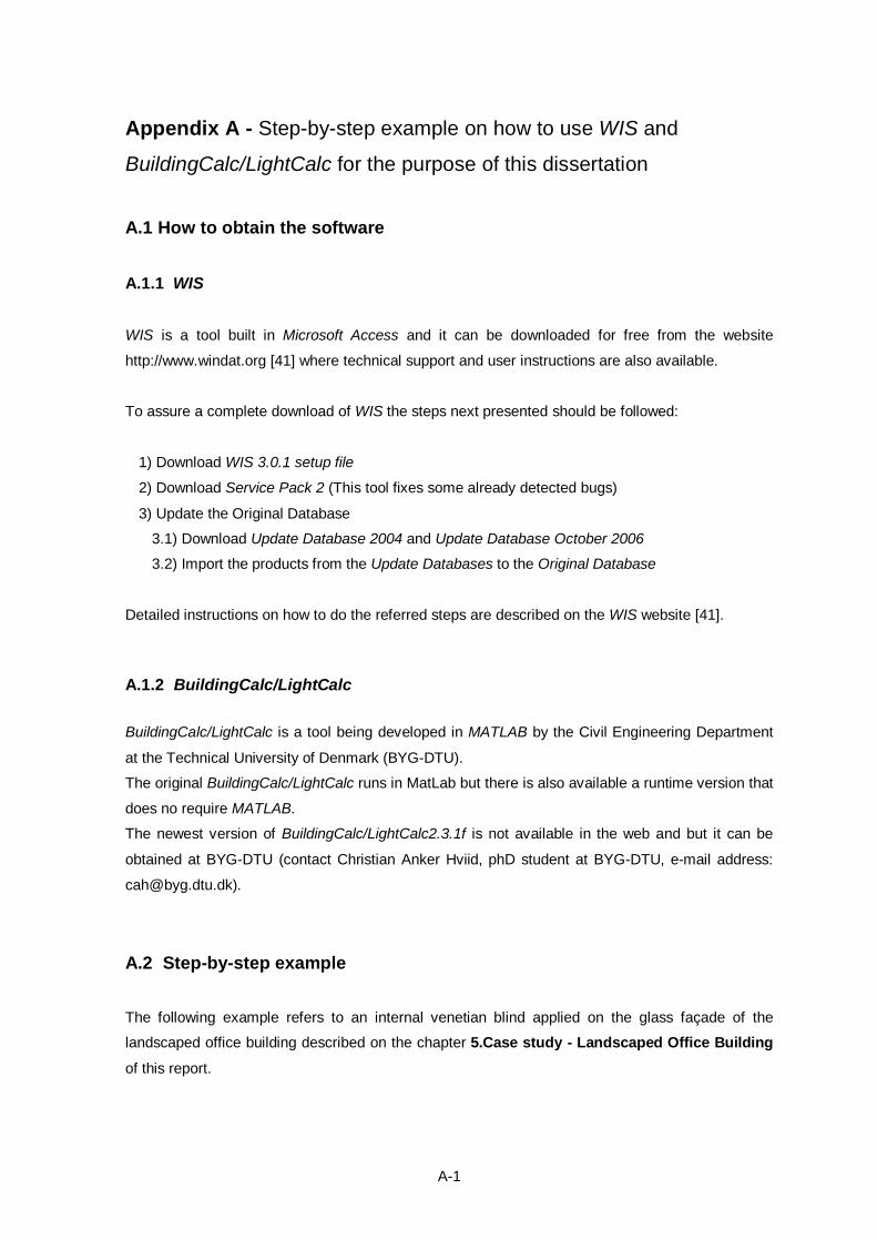
A-1

Appendix A - Step-by-step example on how to use WIS and

BuildingCalc/LightCalc for the purpose of this dissertation

A.1 How to obtain the software

A.1.1 WIS

WIS is a tool built in Microsoft Access and it can be downloaded for free from the website

http://www.windat.org [41] where technical support and user instructions are also available.

To assure a complete download of WIS the steps next presented should be followed:

1) Download WIS 3.0.1 setup file

2) Download Service Pack 2 (This tool fixes some already detected bugs)

3) Update the Original Database

3.1) Download Update Database 2004 and Update Database October 2006

3.2) Import the products from the Update Databases to the Original Database

Detailed instructions on how to do the referred steps are described on the WIS website [41].

A.1.2 BuildingCalc/LightCalc

BuildingCalc/LightCalc is a tool being developed in MATLAB by the Civil Engineering Department

at the Technical University of Denmark (BYG-DTU).

The original BuildingCalc/LightCalc runs in MatLab but there is also available a runtime version that

does no require MATLAB.

The newest version of BuildingCalc/LightCalc2.3.1f is not available in the web and but it can be

obtained at BYG-DTU (contact Christian Anker Hviid, phD student at BYG-DTU, e-mail address:

[email protected]).

A.2 Step-by-step example

The following example refers to an internal venetian blind applied on the glass façade of the

landscaped office building described on the chapter 5.Case study - Landscaped Office Building

of this report.

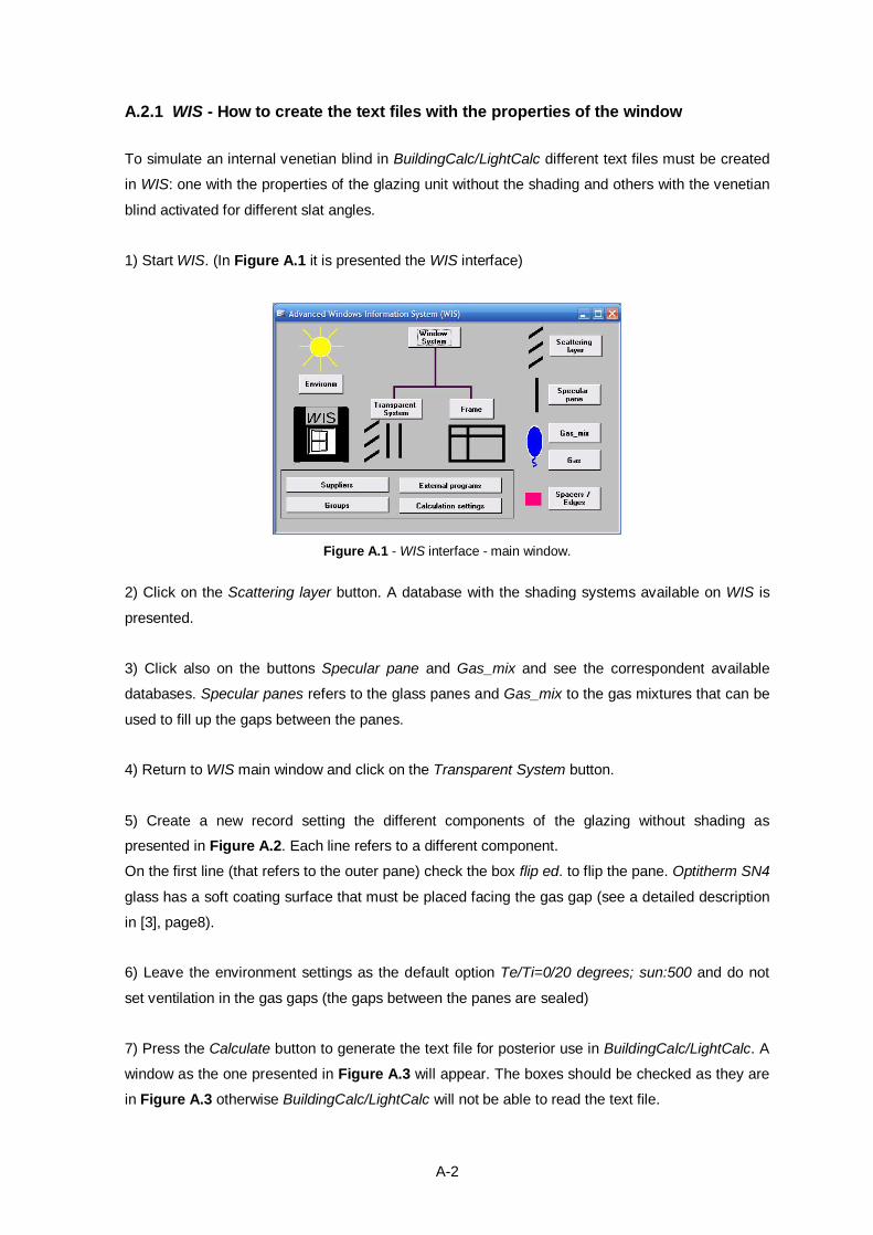
A-2

A.2.1 WIS - How to create the text files with the properties of the window

To simulate an internal venetian blind in BuildingCalc/LightCalc different text files must be created

in WIS: one with the properties of the glazing unit without the shading and others with the venetian

blind activated for different slat angles.

1) Start WIS. (In Figure A.1 it is presented the WIS interface)

Figure A.1 - WIS interface - main window.

2) Click on the Scattering layer button. A database with the shading systems available on WIS is

presented.

3) Click also on the buttons Specular pane and Gas_mix and see the correspondent available

databases. Specular panes refers to the glass panes and Gas_mix to the gas mixtures that can be

used to fill up the gaps between the panes.

4) Return to WIS main window and click on the Transparent System button.

5) Create a new record setting the different components of the glazing without shading as

presented in Figure A.2. Each line refers to a different component.

On the first line (that refers to the outer pane) check the box flip ed. to flip the pane. Optitherm SN4

glass has a soft coating surface that must be placed facing the gas gap (see a detailed description

in [3], page8).

6) Leave the environment settings as the default option Te/Ti=0/20 degrees; sun:500 and do not

set ventilation in the gas gaps (the gaps between the panes are sealed)

7) Press the Calculate button to generate the text file for posterior use in BuildingCalc/LightCalc. A

window as the one presented in Figure A.3 will appear. The boxes should be checked as they are

in Figure A.3 otherwise BuildingCalc/LightCalc will not be able to read the text file.

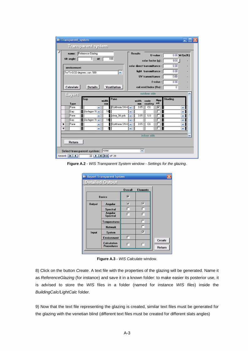
A-3

Figure A.2 - WIS Transparent System window - Settings for the glazing.

Figure A.3 - WIS Calculate window.

8) Click on the button Create. A text file with the properties of the glazing will be generated. Name it

as ReferenceGlazing (for instance) and save it in a known folder: to make easier its posterior use, it

is advised to store the WIS files in a folder (named for instance WIS files) inside the

BuildingCalc/LightCalc folder.

9) Now that the text file representing the glazing is created, similar text files must be generated for

the glazing with the venetian blind (different text files must be created for different slats angles)

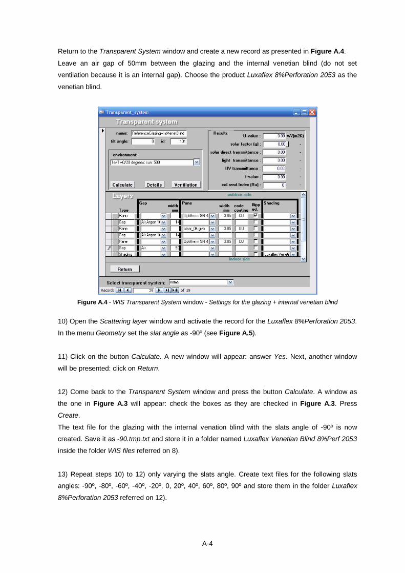
A-4

Return to the Transparent System window and create a new record as presented in Figure A.4.

Leave an air gap of 50mm between the glazing and the internal venetian blind (do not set

ventilation because it is an internal gap). Choose the product Luxaflex 8%Perforation 2053 as the

venetian blind.

Figure A.4 - WIS Transparent System window - Settings for the glazing + internal venetian blind

10) Open the Scattering layer window and activate the record for the Luxaflex 8%Perforation 2053.

In the menu Geometry set the slat angle as -90º (see Figure A.5).

11) Click on the button Calculate. A new window will appear: answer Yes. Next, another window

will be presented: click on Return.

12) Come back to the Transparent System window and press the button Calculate. A window as

the one in Figure A.3 will appear: check the boxes as they are checked in Figure A.3. Press

Create.

The text file for the glazing with the internal venation blind with the slats angle of -90º is now

created. Save it as -90.tmp.txt and store it in a folder named Luxaflex Venetian Blind 8%Perf 2053

inside the folder WIS files referred on 8).

13) Repeat steps 10) to 12) only varying the slats angle. Create text files for the following slats

angles: -90º, -80º, -60º, -40º, -20º, 0, 20º, 40º, 60º, 80º, 90º and store them in the folder Luxaflex

8%Perforation 2053 referred on 12).

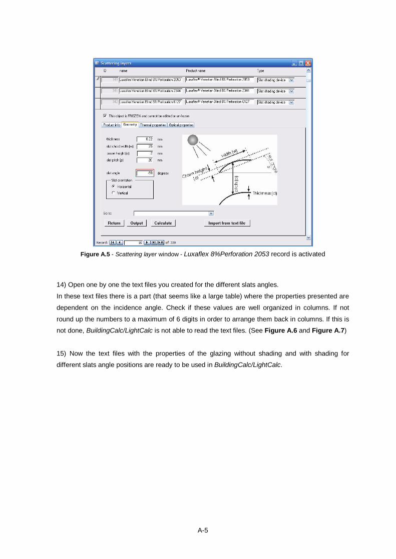
A-5

Figure A.5 - Scattering layer window - Luxaflex 8%Perforation 2053 record is activated

14) Open one by one the text files you created for the different slats angles.

In these text files there is a part (that seems like a large table) where the properties presented are

dependent on the incidence angle. Check if these values are well organized in columns. If not

round up the numbers to a maximum of 6 digits in order to arrange them back in columns. If this is

not done, BuildingCalc/LightCalc is not able to read the text files. (See Figure A.6 and Figure A.7)

15) Now the text files with the properties of the glazing without shading and with shading for

different slats angle positions are ready to be used in BuildingCalc/LightCalc.

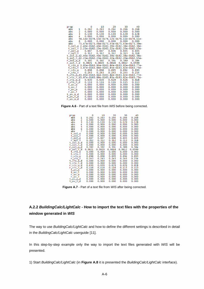
A-6

Figure A.6 - Part of a text file from WIS before being corrected.

Figure A.7 - Part of a text file from WIS after being corrected.

A.2.2 BuildingCalc/LightCalc - How to import the text files with the properties of the window generated in WIS

The way to use BuildingCalc/LightCalc and how to define the different settings is described in detail

in the BuildingCalc/LightCalc userguide [11].

In this step-by-step example only the way to import the text files generated with WIS will be

presented.

1) Start BuildingCalc/LightCalc (in Figure A.8 it is presented the BuildingCalc/LightCalc interface).

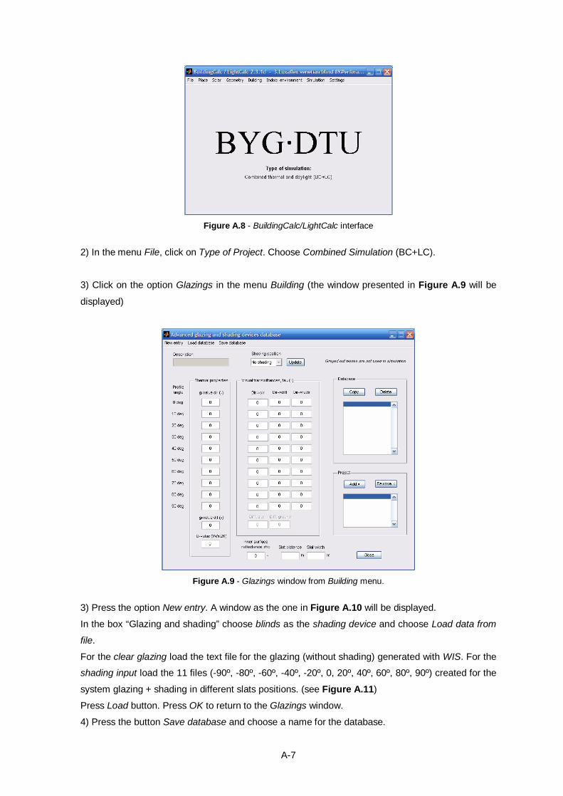
A-7

Figure A.8 - BuildingCalc/LightCalc interface

2) In the menu File, click on Type of Project. Choose Combined Simulation (BC+LC).

3) Click on the option Glazings in the menu Building (the window presented in Figure A.9 will be

displayed)

Figure A.9 - Glazings window from Building menu.

3) Press the option New entry. A window as the one in Figure A.10 will be displayed.

In the box “Glazing and shading” choose blinds as the shading device and choose Load data from

file.

For the clear glazing load the text file for the glazing (without shading) generated with WIS. For the

shading input load the 11 files (-90º, -80º, -60º, -40º, -20º, 0, 20º, 40º, 60º, 80º, 90º) created for the

system glazing + shading in different slats positions. (see Figure A.11)

Press Load button. Press OK to return to the Glazings window.

4) Press the button Save database and choose a name for the database.

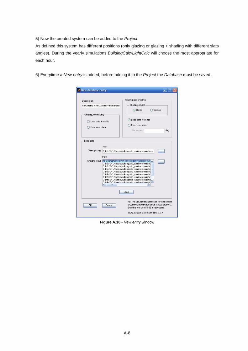
A-8

5) Now the created system can be added to the Project.

As defined this system has different positions (only glazing or glazing + shading with different slats

angles). During the yearly simulations BuildingCalc/LightCalc will choose the most appropriate for

each hour.

6) Everytime a New entry is added, before adding it to the Project the Database must be saved.

Figure A.10 - New entry window

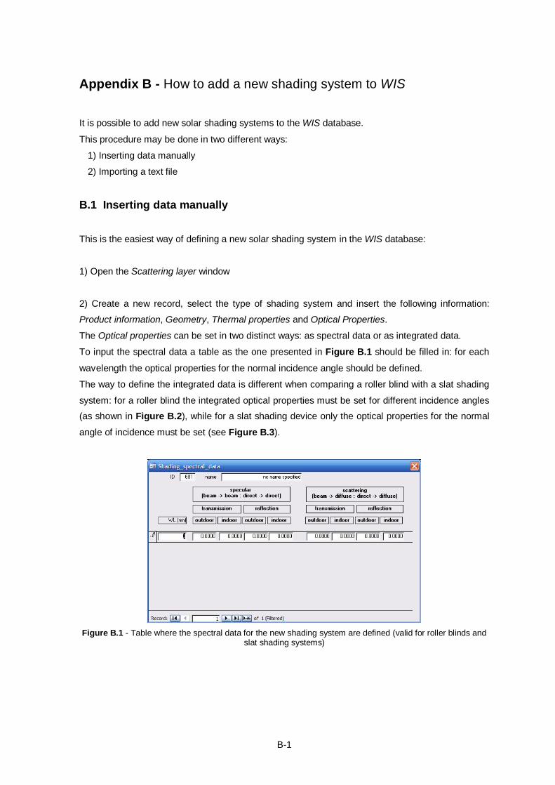
B-1

Appendix B - How to add a new shading system to WIS

It is possible to add new solar shading systems to the WIS database.

This procedure may be done in two different ways:

1) Inserting data manually

2) Importing a text file

B.1 Inserting data manually

This is the easiest way of defining a new solar shading system in the WIS database:

1) Open the Scattering layer window

2) Create a new record, select the type of shading system and insert the following information:

Product information, Geometry, Thermal properties and Optical Properties.

The Optical properties can be set in two distinct ways: as spectral data or as integrated data.

To input the spectral data a table as the one presented in Figure B.1 should be filled in: for each

wavelength the optical properties for the normal incidence angle should be defined.

The way to define the integrated data is different when comparing a roller blind with a slat shading

system: for a roller blind the integrated optical properties must be set for different incidence angles

(as shown in Figure B.2), while for a slat shading device only the optical properties for the normal

angle of incidence must be set (see Figure B.3).

Figure B.1 - Table where the spectral data for the new shading system are defined (valid for roller blinds and

slat shading systems)

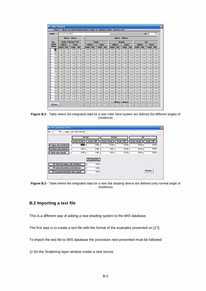
B-2

Figure B.2 - Table where the integrated data for a new roller blind system are defined (for different angles of

incidence)

Figure B.3 - Table where the integrated data for a new slat shading device are defined (only normal angle of

incidence)

B.2 Importing a text file

This is a different way of adding a new shading system to the WIS database.

The first step is to create a text file with the format of the examples presented on [17].

To import the text file to WIS database the procedure next presented must be followed:

1) On the Scattering layer window create a new record.

B-3

2) Click on the button Import from text file. A new window will be displayed: answer Yes. The WIS

database manager will be initialized.

3) On the WIS database manager choose File>Open>WIS database.

Open the database that you are currently using is WIS: by default its name is WISDATA.mdb.

4) Now you need to open the text file you created before. Choose File>Open>Text files.

A new window will be presented. Select Spectral shading data.

Next, select the text file you created and open it. The content of the text file will be presented in the

right window.

5) In the left window go one level up by clicking on the folder where your text file is stored. The

content of the text file will disappear from the right window and only its name will be shown.

6) In the right window select the text file and choose: Menu>Edit>Copy Records.

7) Go to the WISDATA.mdb in the left window and choose shadings. Choose Menu>Edit>Paste

records.

8) The database manager will now request you to type in a groupname (groupname WinDat is not

allowed). The data will be pasted to the shadings database.

9) Now the new shading file is available in the Scattering layers database and ready to be used.

B-4

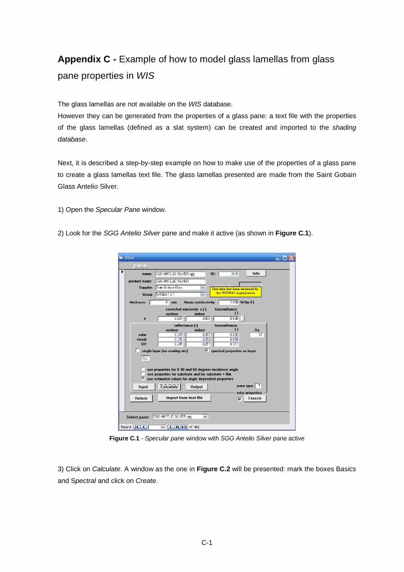
C-1

Appendix C - Example of how to model glass lamellas from glass

pane properties in WIS

The glass lamellas are not available on the WIS database.

However they can be generated from the properties of a glass pane: a text file with the properties

of the glass lamellas (defined as a slat system) can be created and imported to the shading

database.

Next, it is described a step-by-step example on how to make use of the properties of a glass pane

to create a glass lamellas text file. The glass lamellas presented are made from the Saint Gobain

Glass Antelio Silver.

1) Open the Specular Pane window.

2) Look for the SGG Antelio Silver pane and make it active (as shown in Figure C.1).

Figure C.1 - Specular pane window with SGG Antelio Silver pane active

3) Click on Calculate. A window as the one in Figure C.2 will be presented: mark the boxes Basics

and Spectral and click on Create.

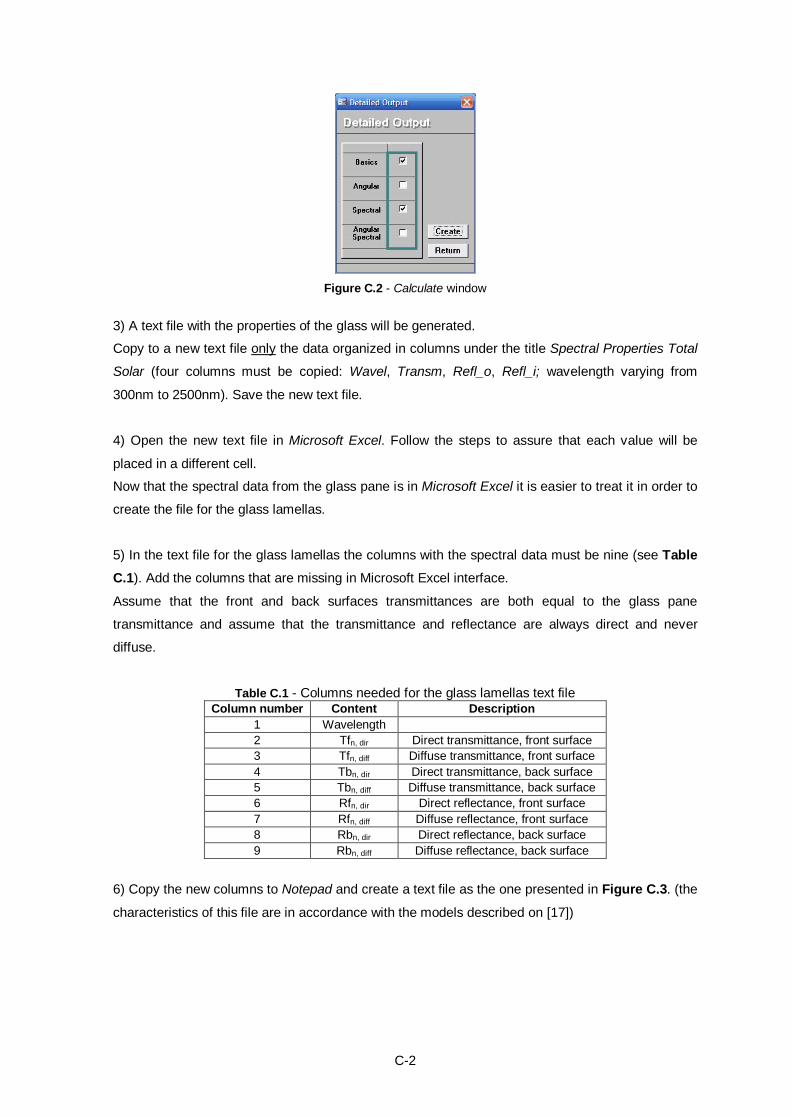
C-2

Figure C.2 - Calculate window

3) A text file with the properties of the glass will be generated.

Copy to a new text file only the data organized in columns under the title Spectral Properties Total

Solar (four columns must be copied: Wavel, Transm, Refl_o, Refl_i; wavelength varying from

300nm to 2500nm). Save the new text file.

4) Open the new text file in Microsoft Excel. Follow the steps to assure that each value will be

placed in a different cell.

Now that the spectral data from the glass pane is in Microsoft Excel it is easier to treat it in order to

create the file for the glass lamellas.

5) In the text file for the glass lamellas the columns with the spectral data must be nine (see Table C.1). Add the columns that are missing in Microsoft Excel interface.

Assume that the front and back surfaces transmittances are both equal to the glass pane

transmittance and assume that the transmittance and reflectance are always direct and never

diffuse.

Table C.1 - Columns needed for the glass lamellas text file Column number Content Description

1 Wavelength 2 Tfn, dir Direct transmittance, front surface 3 Tfn, diff Diffuse transmittance, front surface 4 Tbn, dir Direct transmittance, back surface 5 Tbn, diff Diffuse transmittance, back surface 6 Rfn, dir Direct reflectance, front surface 7 Rfn, diff Diffuse reflectance, front surface 8 Rbn, dir Direct reflectance, back surface 9 Rbn, diff Diffuse reflectance, back surface

6) Copy the new columns to Notepad and create a text file as the one presented in Figure C.3. (the

characteristics of this file are in accordance with the models described on [17])

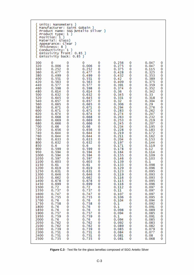
C-3

Figure C.3 - Text file for the glass lamellas composed of SGG Antelio Silver

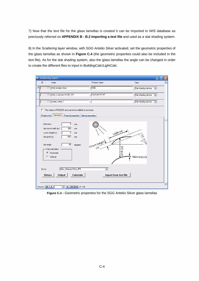
C-4

7) Now that the text file for the glass lamellas is created it can be imported to WIS database as

previously referred on APPENDIX B - B.2 Importing a text file and used as a slat shading system.

8) In the Scattering layer window, with SGG Antelio Silver activated, set the geometric properties of

the glass lamellas as shown in Figure C.4 (the geometric properties could also be included in the

text file). As for the slat shading system, also the glass lamellas the angle can be changed in order

to create the different files to input in BuildingCalc/LightCalc.

Figure C.4 - Geometric properties for the SGG Antelio Silver glass lamellas

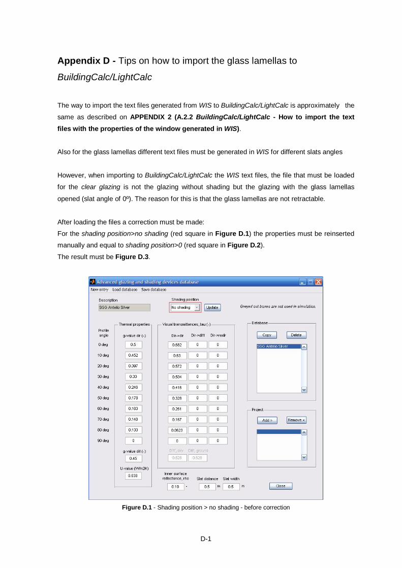
D-1

Appendix D - Tips on how to import the glass lamellas to

BuildingCalc/LightCalc

The way to import the text files generated from WIS to BuildingCalc/LightCalc is approximately the

same as described on APPENDIX 2 (A.2.2 BuildingCalc/LightCalc - How to import the text files with the properties of the window generated in WIS). Also for the glass lamellas different text files must be generated in WIS for different slats angles

However, when importing to BuildingCalc/LightCalc the WIS text files, the file that must be loaded

for the clear glazing is not the glazing without shading but the glazing with the glass lamellas

opened (slat angle of 0º). The reason for this is that the glass lamellas are not retractable.

After loading the files a correction must be made:

For the shading position>no shading (red square in Figure D.1) the properties must be reinserted

manually and equal to shading position>0 (red square in Figure D.2).

The result must be Figure D.3.

Figure D.1 - Shading position > no shading - before correction

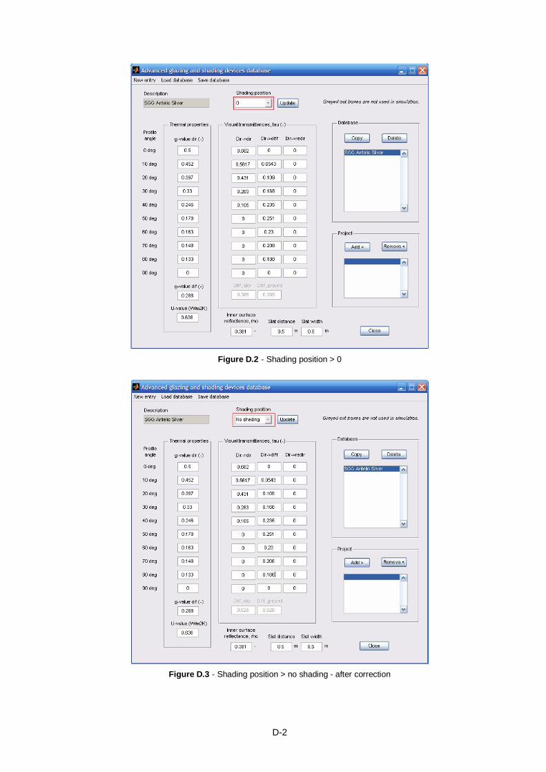
D-2

Figure D.2 - Shading position > 0

Figure D.3 - Shading position > no shading - after correction

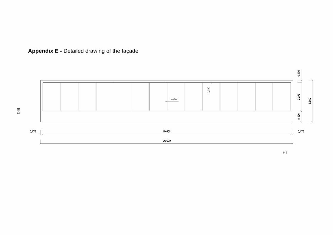
E-1

Appendix E - Detailed drawing of the façade

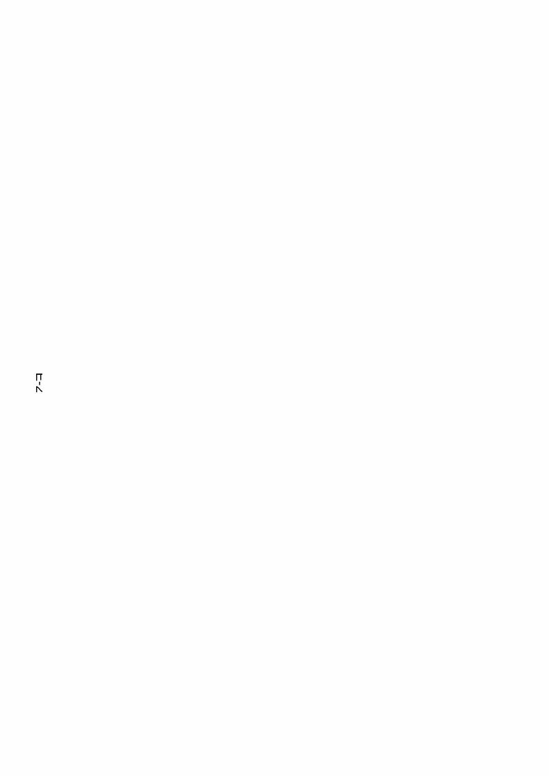
E-2

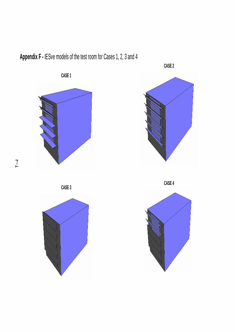
F-1

Appendix F - IESve models of the test room for Cases 1, 2, 3 and 4

CASE 1

CASE 3

CASE 2

CASE 4

F-2

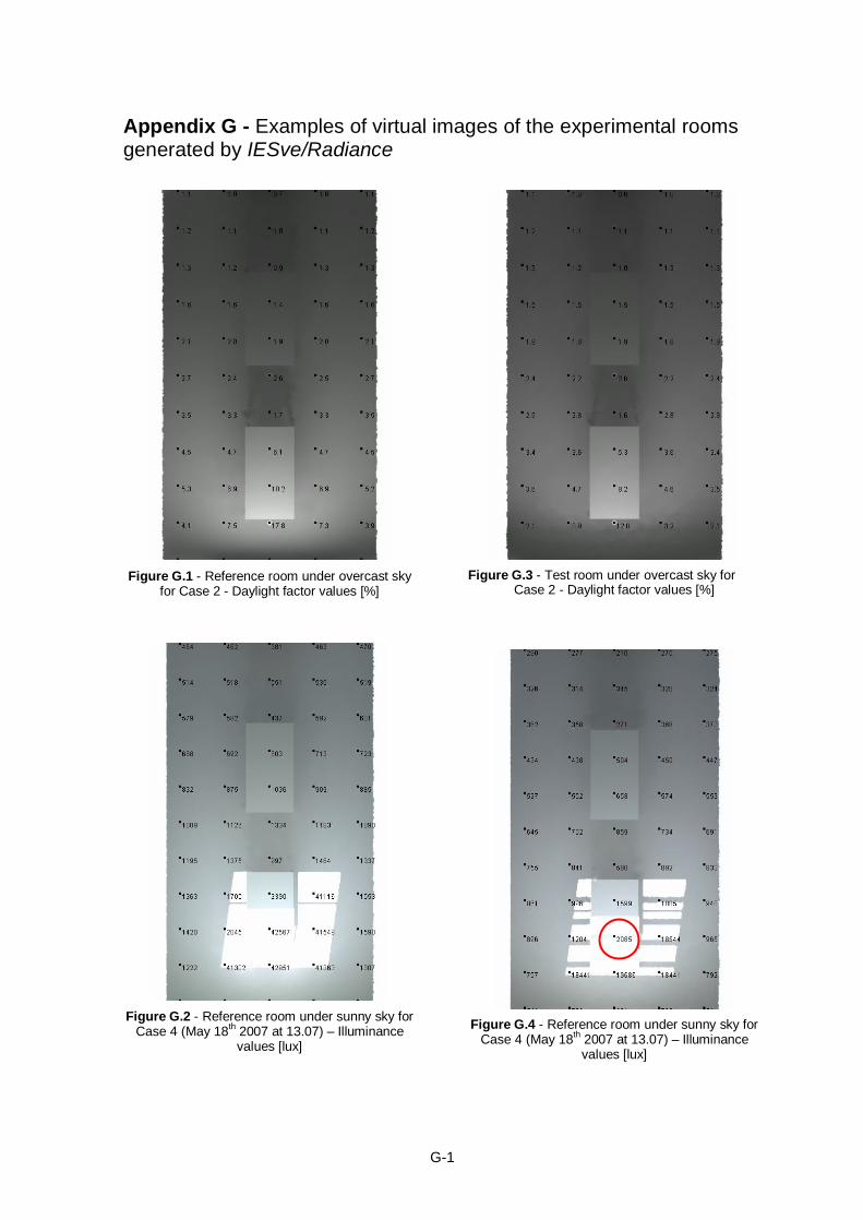
G-1

Appendix G - Examples of virtual images of the experimental rooms generated by IESve/Radiance

Figure G.1 - Reference room under overcast sky

for Case 2 - Daylight factor values [%]

Figure G.2 - Reference room under sunny sky for

Case 4 (May 18th 2007 at 13.07) – Illuminance values [lux]

Figure G.3 - Test room under overcast sky for

Case 2 - Daylight factor values [%]

Figure G.4 - Reference room under sunny sky for

Case 4 (May 18th 2007 at 13.07) – Illuminance values [lux]

Documents

PERFORMANCE EVALUATION OF SOLAR SHADING SYSTEMS2. Brief introduction to the different types of solar shading systems 6 2.1 Overview 6 2.2 Venetian blinds 8 2.3 Roller blinds 8 2.4