T E C H N I S C H E U N I V E R S I TÄT M Ü N C H E NLehrstuhl für Echtzeitsysteme und Robotik

Physics-Based Modeling and Simulationof Musculoskeletal Robots

Steffen Wittmeier

Vollständiger Abdruck der von der Fakultät für Informatik der Technischen UniversitätMünchen zur Erlangung des akademischen Grades eines

Doktors der Naturwissenschaften (Dr. rer. nat.)

genehmigten Dissertation.

Vorsitzender: Univ.-Prof. Dr.-Ing. Alin Albu-Schäffer

Prüfer der Dissertation: 1. Univ.-Prof. Dr.-Ing. habil. Alois Knoll

2. Univ.-Prof. Dr. Rolf Pfeifer (Universität Zürich, Schweiz)

Die Dissertation wurde am 18.12.2013 bei der Technische Universität Müncheneingereicht und durch die Fakultät für Informatik am 21.04.2014 angenommen.

The advantage of the emotions is that they lead us astray, and

the advantage of Science is that it is not emotional.

— Oscar WildeThe Picture of Dorian Gray

A B S T R A C T

In the past decade, a new class of tendon-driven robots has emergedwhich replicates living beings with an unprecedented level of detail.These so-called musculoskeletal robots are characterized by a set ofunique features, such as muscle replicas where the mapping betweenthe muscle forces and the joint torques depends on the robot postureor complex joints with many degrees-of-freedom. On the one hand,these features enable new applications for this class of robots, such asan artificial test-bed for the investigation of biologically inspired con-trol strategies or as service and rehabilitation robots where the com-pliance of the muscular system of these robots increases the safety ofhuman-robot interactions. On the other hand, however, these uniquefeatures also introduce new challenges both in hard- and software.One approach to tackle these challenges is via simulations where eachproblem can be investigated in isolation and in a well-defined envi-ronment. But unfortunately, simulating musculoskeletal robots is achallenge in itself, especially if traditional joint-space simulation ap-proaches are employed as an explicit mapping between the muscleforces and the joint torques is required. Hence, the use of an alterna-tive body-space approach, originally developed for computer gamesand animations and commonly known as physics-based simulations,is proposed.

In this dissertation, the applicability of the physics-based simula-tion approach to the class of musculoskeletal robots is investigated.Therefore, the modeling of skeletons and muscles within the physics-based framework is introduced. Here, particular emphasis is put onextending the rigid-body dynamic algorithms of physics-based simu-lations with joint friction models as well as on the computation of themuscle kinematics, i. e. the muscle path. For the muscle kinematics,models of increasing complexity are considered. These models rangefrom simple straight-line connections to wrapping surfaces that em-ploy geometric primitives, namely spheres and cylinders, or meshesto simulate the wrapping of muscles on the bone surface. Moreover,a calibration routine is presented that employs an Evolution Strat-egy (ES) to minimize the simulation-reality gap of the parametric sim-ulation models for both static robot postures and dynamic trajectories.Finally, the developed modeling and calibration techniques are eval-uated against a physical robot. For this purpose, the musculoskeletalrobot Anthrob is: (i) developed, (ii) modeled and (iii) calibrated. Tofurther assess the accuracy of each of the presented muscle kinemat-ics models, three Anthrob models are derived. While model I is basedsolely on straight-line muscles, model II and model III use cylindrical

v

and mesh wrapping surfaces to model the muscle wrapping on thebones of the robot, respectively.

Prior to calibration, model III clearly out-performs model I and IIfor the tested static robot postures and trajectories. After calibration,these errors are further reduced leading to final errors in the rangeof the robot repeatability for models II and III. Based on these results,it can be concluded that the physics-based simulation approach is asuitable tool for the simulation of musculoskeletal robots and that ithas the potential to promote the development of this particular classof robots in the future.

vi

Z U S A M M E N FA S S U N G

In den vergangenen zehn Jahren hat sich eine neue Klasse von seh-nengetriebenen Robotern herauskristallisiert, welche Lebewesen miteinem noch nie dagewesenen Detailgrad nachbilden. Diese sogenann-ten muskuloskeletalen Roboter zeichnen sich durch eine Reihe von ein-zigartigen Merkmalen aus. Diese sind z. B. Muskelimitate, bei denendie aus den Muskelkräften resultierenden Gelenkdrehmomente vonder Pose des Roboters abhängen, oder komplexe Gelenke mit vie-len Freiheitsgraden. Einerseits ermöglichen diese Merkmale neue An-wendungen für diese Art von Robotern wie z. B. als Testplattformfür biologisch-inspirierte Regelungsalgorithmen oder als Roboter imBereich der Service- und Rehabilitationsrobotik, wo die Nachgiebig-keit des Muskelapparats die Sicherheit von Mensch-Maschine-Inter-aktionen erhöht. Andererseits stellen die einzigartigen Eigenschaftenauch neue Herausforderungen dar—sowohl im Bereich der Hard- alsauch der Software. Ein Ansatz zur Lösung dieser Herausforderun-gen ist dabei der Einsatz von Simulationen, da hier jede Eigenschaftisoliert und unter definierten Rahmenbedingungen untersucht wer-den kann. Leider muss jedoch die Simulation von muskuloskeletalenRobotern selbst bereits als eine Herausforderung betrachtet werden,speziell wenn klassische Drehmoment-basierte Simulationsmethodenzum Einsatz kommen, da hier eine explizite Umrechnung der Mus-kelkräfte auf Gelenkdrehmomente notwendig ist. Aus diesem Grundwird ein alternatives Simulationsverfahren, welches unter dem Na-men physics-based simulation bekannt ist und welches ursprünglichfür Computerspiele und Animationen entwickelt wurde, als mögli-che Lösung des Simulationsproblems vorgeschlagen.

In dieser Dissertation wurde die Eignung von physics-based simula-

tions für die Simulation von muskuloskeletalen Robotern untersucht.Hierzu wurden Skelett sowie Muskelmodelle für physics-based Simu-lationsumgebungen entwickelt. Besonderes Augenmerk wurde dabeiauf die Erweiterung der Festkörperdynamik-Algorithmen von Physik-Engines um Gelenkreibungsmodelle sowie auf die Berechnung derMuskelkinematik, d. h. des Muskelpfades, gelegt. Für die Berechnungder Muskelkinematik werden dabei verschiedene, in ihrer Komplexi-tät variierende Modelle vorgestellt. Diese Modelle reichen von sim-plen Direktverbindungen, bei denen der Muskel als eine Gerade zwi-schen den zwei Ansatzpunkten modelliert wird, bis hin zu Oberflä-chenmodellen basierend auf geometrischen Primitiva oder Polygon-netzen, welche die Simulation des Muskelpfades auf Knochenober-flächen ermöglichen. Darüber hinaus wird eine Kalibrierungsroutine,basierend auf einer Evolutionsstrategie, vorgestellt, welche eingesetzt

vii

werden kann, um den Simulationsfehler der parametrischen Simulati-onsmodelle zu minimieren. Schlussendlich wurden die entwickeltenModellierungs- und Kalibrierungstechniken anhand eines Beispielro-boters getestet. Hierzu wurde der muskuloskeletale Roboter Anthrobentwickelt, modelliert und kalibriert. Um dabei die Genauigkeit derentwickelten Muskelkinematikmodelle bewerten zu können, wurdendrei Anthrob-Modelle abgeleitet. Während in dem ersten Modell dieMuskeln ausschließlich durch Direktverbindungen modelliert wur-den, kommen beim zweiten und dritten Modell Oberflächenmodellebasierend auf Zylindern bzw. Polygonnetzen zum Einsatz, um denMuskelpfad auf dem Knochen zu approximieren.

Betrachtet man zunächst die unkalibrierten Modelle so konnten mitdem dritten Modell, basierend auf Polygonnetzen, die besten Ergeb-nisse erzielt werden. Diese Abweichungen konnten durch die Kali-brierung weiter reduziert werden. So wurden für das zweite und drit-te Modell Abweichungen im Bereich der Wiederholgenauigkeit desRoboters gemessen. Auf Basis der erzielten Ergebnisse kann gefolgertwerden, dass der physics-based Simulationsansatz für die Simulationvon muskuloskeletalen Roboter geeignet ist und daher möglicherwei-se in Zukunft einen wichtigen Beitrag zur Weiterentwicklung dieserRoboterklasse leisten kann.

viii

P U B L I C AT I O N S

Some ideas and figures have appeared previously in the followingpublications:

S. Wittmeier, M. Jäntsch, K. Dalamagkidis, M. Rickert, H. Marques, andA. Knoll. Caliper: A universal robot simulation framework for tendon-drivenrobots. In Intelligent Robots and Systems (IROS), 2011 IEEE/RSJ International

Conference on, pages 1063–1068, 2011

S. Wittmeier, M. Jäntsch, K. Dalamagkidis, and A. Knoll. Physics-based mod-eling of an anthropomimetic robot. In Intelligent Robots and Systems (IROS),

2011 IEEE/RSJ International Conference on, pages 4148–4153, 2011

S. Wittmeier, A. Gaschler, M. Jäntsch, K. Dalamagkidis, and A. Knoll. Calibra-tion of a physics-based model of an anthropomimetic robot using evolutionstrategies. In Intelligent Robots and Systems (IROS), 2012 IEEE/RSJ International

Conference on, pages 445 –450, oct. 2012

S. Wittmeier, C. Alessandro, N. Bascarevic, K. Dalamagkidis, D. Devereux,A. Diamond, M. Jäntsch, K. Jovanovic, R. Knight, H. G. Marques, P. Milosavl-jevic, B. Mitra, B. Svetozarevic, V. Potkonjak, R. Pfeifer, A. Knoll, and O. Hol-land. Toward anthropomimetic robotics: Development, simulation, and con-trol of a musculoskeletal torso. Artificial Life, 19(1):171–193, nov 2012

S. Wittmeier, M. Jäntsch, K. Dalamagkidis, A. Panos, F. Volkart, and A. Knoll.Anthrob – A Printed Anthropomimetic Robot. In Proc. IEEE-RAS International

Conference on Humanoid Robots (Humanoids), pages 342–347, 2013

ix

A C K N O W L E D G M E N T S

First of all, I would like to thank Professor Alois Knoll for giving methe opportunity to work at his chair and, in particular, for being partof two extremely interesting EU projects on musculoskeletal robots,namely ECCEROBOT and Myorobotics. Furthermore, I would like toexpress my gratitude to Professor Rolf Pfeifer for being my externalreviewer.

Many thanks also go to my colleagues Michael Jäntsch and Konstanti-nos Dalamagkidis as well as to Hugo Gravato Marques for their ad-vice and constructive criticism during the past few years as well asfor proofreading this thesis.

Last but not least, many thanks go to everybody at the chair of Robotics

and Embedded Systems as well as to our scientific and industrial projectpartners. I enjoyed working with all of you.

xi

C O N T E N T S

1 introduction 1

1.1 Motivation . . . . . . . . . . . . . . . . . . . . . . . . . . 1

1.2 Contributions . . . . . . . . . . . . . . . . . . . . . . . . 4

1.3 Units and Notation . . . . . . . . . . . . . . . . . . . . . 6

1.4 Readers’ Guide . . . . . . . . . . . . . . . . . . . . . . . 6

2 background 9

2.1 Tendon-Driven and Musculoskeletal Robots . . . . . . 9

2.2 Joint-Space Simulation of Forward Dynamics . . . . . . 16

2.3 Simulation Tools for Musculoskeletal Robots . . . . . . 21

3 skeleton modeling 23

3.1 Bones . . . . . . . . . . . . . . . . . . . . . . . . . . . . . 24

3.2 Joints . . . . . . . . . . . . . . . . . . . . . . . . . . . . . 25

4 muscle modeling 29

4.1 Actuator Dynamics . . . . . . . . . . . . . . . . . . . . . 30

4.1.1 Brushed DC Motor Model . . . . . . . . . . . . . 31

4.2 Muscle Kinematics . . . . . . . . . . . . . . . . . . . . . 34

4.2.1 Straight-Line Muscle . . . . . . . . . . . . . . . . 35

4.2.2 Muscle Via-Points . . . . . . . . . . . . . . . . . 36

4.2.3 Spherical Wrapping Surfaces . . . . . . . . . . . 38

4.2.4 Cylindrical Wrapping Surfaces . . . . . . . . . . 44

4.2.5 Meshes as Wrapping Surfaces . . . . . . . . . . . 47

4.3 Series Elastic Element Modeling . . . . . . . . . . . . . 52

4.3.1 Linear Spring-Damper . . . . . . . . . . . . . . . 52

4.3.2 Models of Linear Viscoelasticity . . . . . . . . . 53

4.4 Muscle Friction . . . . . . . . . . . . . . . . . . . . . . . 56

4.5 Muscle Dynamics Algorithm . . . . . . . . . . . . . . . 60

4.6 Discussion . . . . . . . . . . . . . . . . . . . . . . . . . . 62

5 model calibration 65

5.1 Evolution Strategy . . . . . . . . . . . . . . . . . . . . . 66

5.2 Statics Calibration . . . . . . . . . . . . . . . . . . . . . . 69

5.3 Dynamics Calibration . . . . . . . . . . . . . . . . . . . 73

6 the musculoskeletal robot anthrob 75

6.1 Skeleton . . . . . . . . . . . . . . . . . . . . . . . . . . . 75

6.2 Muscles . . . . . . . . . . . . . . . . . . . . . . . . . . . . 78

6.3 Receptors . . . . . . . . . . . . . . . . . . . . . . . . . . . 81

7 anthrob modeling 85

xiii

xiv contents

7.1 Skeleton Modeling . . . . . . . . . . . . . . . . . . . . . 85

7.2 Muscle Modeling . . . . . . . . . . . . . . . . . . . . . . 86

7.2.1 Actuator Dynamics . . . . . . . . . . . . . . . . . 86

7.2.2 Muscle Kinematics . . . . . . . . . . . . . . . . . 87

7.2.3 Nitrile Butadiene Rubber O-Rings . . . . . . . . 87

7.2.4 Ceramic Eyelets and Muscle Friction . . . . . . 96

7.3 Electronic Control Units . . . . . . . . . . . . . . . . . . 97

7.3.1 Actuator Position Control . . . . . . . . . . . . . 98

7.3.2 Power Circuit Modeling . . . . . . . . . . . . . . 99

7.4 Benchmarks . . . . . . . . . . . . . . . . . . . . . . . . . 100

7.5 Simulation-Reality Gap Analysis . . . . . . . . . . . . . 101

7.5.1 Tier 1: Glenohumeral Joint Models . . . . . . . . 101

7.5.2 Tier 2: Complete Robot Models . . . . . . . . . . 108

8 anthrob model calibration 111

8.1 Calibration . . . . . . . . . . . . . . . . . . . . . . . . . . 111

8.1.1 Tier 1: Glenohumeral Joint Models . . . . . . . . 112

8.1.2 Tier 2: Complete Robot Models . . . . . . . . . . 122

8.2 Validation . . . . . . . . . . . . . . . . . . . . . . . . . . 130

8.3 Discussion . . . . . . . . . . . . . . . . . . . . . . . . . . 133

9 conclusions 137

9.1 Summary . . . . . . . . . . . . . . . . . . . . . . . . . . . 137

9.2 Future Works . . . . . . . . . . . . . . . . . . . . . . . . 140

a real-time motion capture 143

a.1 Hardware Setup . . . . . . . . . . . . . . . . . . . . . . . 143

a.2 Calibration . . . . . . . . . . . . . . . . . . . . . . . . . . 145

a.3 Image Processing Pipeline . . . . . . . . . . . . . . . . . 145

a.3.1 Image Acquisition . . . . . . . . . . . . . . . . . 147

a.3.2 Marker Segmentation . . . . . . . . . . . . . . . 147

a.3.3 Marker Triangulation . . . . . . . . . . . . . . . 148

a.3.4 Marker Target Pose Estimation . . . . . . . . . . 149

a.3.5 Joint Angle Computation . . . . . . . . . . . . . 151

a.4 Performance Benchmarking . . . . . . . . . . . . . . . . 151

a.5 Summary . . . . . . . . . . . . . . . . . . . . . . . . . . . 153

b linear viscoelasticity 155

b.1 Stress and Strain . . . . . . . . . . . . . . . . . . . . . . . 155

b.2 Basic Models . . . . . . . . . . . . . . . . . . . . . . . . . 156

c anthrob models 159

c.1 Skeleton Model . . . . . . . . . . . . . . . . . . . . . . . 159

c.2 Muscle Models . . . . . . . . . . . . . . . . . . . . . . . 161

c.3 Simulation-Reality Gap . . . . . . . . . . . . . . . . . . . 166

d anthrob calibration 167

d.1 Simulation-Reality Gap . . . . . . . . . . . . . . . . . . . 167

contents xv

d.2 Calibration Parameters . . . . . . . . . . . . . . . . . . . 167

e caliper : a robotics development environment 179

e.1 Caliper Core . . . . . . . . . . . . . . . . . . . . . . . . 179

e.2 Caliper Plugins . . . . . . . . . . . . . . . . . . . . . . . 180

f qt pipeline toolkit (qpt) 183

list of figures 187

list of tables 190

list of algorithms 191

list of abbreviations 192

list of symbols 194

bibliography 197

1I N T R O D U C T I O N

1.1 motivation

Motor control and object manipulations are complex tasks that hu- Human motor

control &

neuroroboticsmans execute with remarkable ease, accuracy and repeatability. Thisimmediately poses the question of how the brain is able to solvethe underlying control problem of coordinating the vast number ofmuscles required for a particular movement. Today, this questionis mainly raised by Neuroscientists who employ transection and/orlesioning experiments [138] as well as non-invasive recording tech-niques, such as Functional Magnetic Resonance Imaging (fMRI) [50]or Electromyography (EMG) [7], to elucidate the underlying neuro-physiological processes of human motor control. Even though thesestudies and technologies have significantly contributed to our currentknowledge of human motor control, many questions still remain un-resolved. One possibility of shedding new light on these questions isto employ an interdisciplinary approach uniting robotics and neuro-science in accordance with the synthetic methodology principle “un-derstanding by building” [162].

The study of artificial systems has already significantly contributed Limitations of

traditional robotsto our understanding of human motor control. For instance, indus-trial manipulators have been used to study the problems associatedwith the planning and execution of human limb trajectories [47]. But,robotic manipulators are very different from humans. First, the usageof high precision torque actuators located within joints is an over-simplification of the human muscular system where even single jointmovements require the phased excitation and relaxation of multiplemuscles. Second, robotic manipulators are traditionally composed ofrigid links attached to single Degree of Freedom (DoF) revolute orprismatic joints [16], characteristics which facilitate control and im-prove manipulation performance. But the human body is neither stiffnor made exclusively of revolute joints. These missing properties posesevere limitations for the aspects of motor control that can be inves-tigated by using industrial robots and on the conclusions that can bedrawn from the experimental results. Therefore, more detailed repli-cas of the human motor apparatus are a requisite for the effective

1

2 introduction

investigation of human motor control issues in artificial systems—inaccordance with the concept of embodiment [115].

Some progress towards this goal has been made by the many hu-Anthropomorphic &

musculoskeletal

robotsmanoid robots that have been developed around the world, suchas Asimo [130] or iCub [154], which can deliver impressive perfor-mance on the tasks that they are designed for (e. g. [14]). So far,however, these anthropomorphic robots have failed to generate a sig-nificant stream of new findings in the area of human motor con-trol. Hence, a new class of robots has emerged in the past decadewhich has the potential to unite researchers from the fields of Neuro-sciences and Robotics and to finally reveal the substrates of humanmotor control. This class of robots is called musculoskeletal or an-thropomimetic [46] robots. Musculoskeletal designs differ from an-thropomorphic humanoid robots by not only imitating the morpho-logical appearance of humans, but by capitalizing on the replicationof the inner structures of the human body such as equivalents ofcompliant muscles, tendons, bones, and joints. The resulting robotsare highly complex artifacts that belong to the super-class of tendon-driven robots but exhibit a set of distinct features such as a point-to-point tendon routing (i. e. tendons that can only induce a uni-directional joint rotation) or redundant, antagonistic actuators withposture-dependent lever arms (i. e. lever arms that change with thejoint positions). It is these human-inspired features which make mus-culoskeletal robots both unique and challenging.

Even though musculoskeletal robots now exist for more than a decade,Challenges of

musculoskeletal

robotsthe scientific progress, particularly in the area of control, falls short ofexpectations. The main reason for this is that the unique features ofthese robots introduced new challenges, both in hard- and software.As an example, let us consider a single spherical joint as it is forinstance used in musculoskeletal robots to mimic the glenohumeraljoint of the human shoulder girdle. In contrast to the 1 DoF revolutejoints typically used in industrial robots, spherical joints provide 3rotational DoF. This difference, which might appear to be minor atfirst, has a huge impact. First of all, a spherical joint features no bear-ings and hence the joint ball has to be actively pressed into the socketby the muscular system. This in turn introduces an interdependencebetween the muscle and the joint friction forces as higher muscle ten-sions lead to higher contact forces between the ball and the socketof the joint. Secondly, most control approaches developed for muscu-loskeletal robots are feedback control laws that rely on joint positionerrors to compute the actuator inputs for the next control cycle. But,measuring the joint position of a spherical joint is an inherently diffi-cult task and no intrinsic solutions are available on the market today.This impedes the testing and evaluation of developed controllers onreal artifacts. Furthermore, expressing the joint position by a scalar,

1.1 motivation 3

as for revolute joints, is not possible for spherical joints due the threeDoF. Hence, a singular-free representation, such as unit quaternions,has to be used which further complicates the utilization of standardcontrol laws developed for industrial robots. Even though this exam-ple demonstrates some of the challenges arising from the kinematicdifferences between industrial and musculoskeletal robots, there areeven more significant challenges due to the muscular system of mus-culoskeletal robots. First of all, in industrial robots the actuator torquecan be directly mapped to a joint torque. This is not the case for mus-culoskeletal robots, where the muscular system applies forces to thelinks of the robot. Thus a mapping between muscle forces and jointtorques has to be found to employ joint-space control approachesfrom classical robotics to the class of musculoskeletal robots. But thismapping is not trivial to derive, due to the posture-dependence ofthe lever arms and the redundant actuation (i. e. more than one mus-cle influences a single joint coordinate). Furthermore, similar to thehuman paragon, musculoskeletal robots often feature multi-articularmuscles (i. e. muscles that span more than one joint) or muscles thatwrap around the skeleton surface. These properties further compli-cate the modeling of musculoskeletal robots and the derivation of amapping between the muscle-force and joint-torque space.

One approach to tackle the challenges of musculoskeletal robots is Simulation of

musculoskeletal

robotsvia simulations where each challenge can be investigated in isola-tion and in a well-defined environment. For instance, a spherical jointcould be equipped with a virtual, frictionless bearing or a virtual sen-sor to first analyze other aspects of the musculoskeletal design. Butunfortunately, simulating musculoskeletal robots is a challenge in it-self due to the complexity of the musculo-skeletal interactions. Thus,even though various simulation tools are available for the simulationof mobile or industrial robots, no comparable tools exist for muscu-loskeletal robots. Here, normally tailored solutions are used that havebeen developed to simulate the dynamics of a particular robot (e. g.[33] or [124]). However, due to the close analogy of musculoskeletalrobots with their biological counterpart, the problems associated withthe simulation of this class of robots is very similar to the problemsencountered in biomechanics. Here, simulation models are used toinvestigate the control and the mechanics of biological systems andtwo simulation toolboxes are particularly noteworthy: OpenSim [21]and Anybody. Both tools focus on models of the human body andprovide a variety of muscle models to simulate the dynamics arisingfrom the musculo-skeletal interactions. However, they operate in thejoint-space which means that the dynamics of the skeletons are simu-lated by applying torques to the joints and thus an explicit mappingbetween the muscle forces and the joint torques is required. But thismapping can be tedious to derive for complex musculoskeletal robotsas shown in detail in Chapter 2. Hence, an alternative body-space sim-

4 introduction

ulation approach, known as physics-based simulations, is presentedin this thesis.

Physics-based simulations originate from computer games and ani-Physics-based

simulations mations where so-called physics-engines are used to create the illu-sion of a virtual world that complies with the laws of Newtoniandynamics. A variety of physics-engines has emerged in recent years,such as PhysX, ODE, Bullet Physics or Newton. All these engines of-fer a rich set of functionality such as rigid-body and constrained dy-namics required for the simulation of the skeletons of musculoskele-tal robots (for a detailed comparison see [8]). The major difference be-tween physics-engines and simulation tools from biomechanics is thatphysics-engines operate in the body-space. This means that body po-sitions and orientations are integrated over time rather than joint posi-tions. This fundamental difference simplifies the simulation of muscu-loskeletal robots as an explicit mapping between muscles forces andjoint torques is no longer required and muscle forces can be applieddirectly to rigid bodies at the tendon terminations.

1.2 contributions

Musculoskeletal robots are impressive artifacts that often feature moreSimulation tools for

musculoskeletal

robotsthan 40 skeletal DoF and at least the same number of muscles. But,so far, it is this complexity which has also impeded the applicationof these robots to real-world scenarios. Therefore, the goal of this the-sis is to develop modeling and simulation techniques to provide re-searchers with a tool for the investigation of musculoskeletal robots ina well-defined, virtual environment. These modeling and simulationtechniques are implemented on physics-engines which are originallydeveloped for computer games and which operate in the body-space(see above). It is shown that it is this body-space approach which sim-plifies both the simulation of musculoskeletal robots as well as themodel definition by the researcher—when compared to traditionaljoint-space approaches.

In order to simulate the muscles in the body-space domain, the com-Muscle kinematics

modeling putation of the muscle kinematics is extremely important as theyprovide two substantial quantities: (i) the muscle length and (ii) themuscle lines of action. Therefore, various muscle kinematics mod-els were developed. These range from straight-line connections towrapping surfaces based on geometric primitives and meshes. Eventhough similar muscle kinematics models can be found in the field ofbiomechanics [20, 22, 23, 34, 79, 159], there are still considerable differ-ences to the models presented here. For example, in 2000 Garner andPandy presented the “obstacle-set method for representing muscle

1.2 contributions 5

paths in musculoskeletal models" which included models of spheri-cal and cylindrical wrapping surfaces [34]. However, the presentedmodels were not capable of simulating a change in the wrappingdirection, neither were they able to handle multiple wrapping revolu-tions. Both problems were solved in this work by introducing a statemachine and a revolution counter which contributed to the versatil-ity and applicability of these models to a wider range of use-cases.Another difference between the presented models and the modelsused in biomechanics is that in biomechanics the goal is typically toapproximate the muscle length. This muscle length is subsequentlyused to compute the resulting joint torque by partial differentiationof the muscle length with respect to the joint angles [23] (i. e. themuscle Jacobian, see Section 2.2). However, a similar approach is notfeasible in physics-based simulation engines which operate in thebody-space and hence require the lines of action of the muscle tobe exactly computed. This becomes particularly important in the caseof mesh wrapping surfaces. Here, previous studies suggested to ap-proximate the geodesic path on the convex envelope by the shortestpath on the mesh computed via the algorithm of Dijkstra to reducethe computation time [23]. Even though this approach results in agood approximation of the path length as shown in Section 4.2.5 andconfirmed by other studies [148], large errors in the lines of actionwere observed. Hence, the obtained results show that exact geodesicalgorithms should be favored over approximations if physics-enginesare used.

Furthermore, muscle friction, which plays an important role in the Muscle & joint

friction modelingmuscle dynamics [58], was neglected in previous studies. Therefore,a muscle friction model based on the capstan equation was derivedwhich is capable of modeling the effects of Coulomb friction on spher-ical obstacles within the muscle path. However, while being advan-tageous for the simulation of the muscle dynamics, the body-spaceapproach also has disadvantages. For instance, the modeling of jointfriction is straight-forward in the joint-space domain but difficult inthe body-space. Therefore, a joint friction model is presented thatexploits the error correction term of the constraint solver of physics-engines to model the effects of Coulomb friction.

The simulation-reality gap of musculoskeletal robot models was never Simulation-reality

gap analysis &

minimizationinvestigated by previous studies. Thus, a detailed analysis of the ac-curacy of the developed models and of the physics-based simulationapproach in general was conducted by measuring the model errorsfor static robot postures and dynamic trajectories. For this purposethe musculoskeletal robot Anthrob, which mimics the human upperlimb, was developed and modeled by the presented techniques. Tomeasure the joint position of the spherical glenohumeral joint of therobot, a high-speed motion-capture system was developed which de-

6 introduction

livers joint positions with an update rate of 60 Hz and a latency of4.3 ms.

Furthermore, a calibration procedure was developed to minimize theModel calibration

simulation-reality gap of musculoskeletal robot models. This calibra-tion procedure uses a (µ, λ)-Evolution Strategy and a Gaussian-based,non-isotropic, self-adapting mutation operator to explore the searchspace. In general, the developed procedure can be applied to a largevariety of input data and error measures. However, as an example,two objective functions were developed that can be used to calibratethe statics (i. e. the simulation-reality gap of equilibrium postures)and the dynamics (i. e. the simulation-reality gap of trajectories) ofmusculoskeletal robots that feature compliant, tendon-driven actua-tors.

Finally, real-time simulation performance was neither an issue nor aReal-time

simulations and

online applicationsgoal in previous studies. Here, the presented models perform wellallowing for the real-time simulation of small- and medium-scalerobots. In the future, these real-time capabilities will facilitate newonline applications of musculoskeletal robot simulations, for instanceas an internal model for control.

1.3 units and notation

The mathematical notation in this thesis is based on the guidelinesof the International Organization for Standardization (ISO)1. Hence,scalar variables and functions are set in italic, whereas vectors andmatrices are set in bold lower-case and upper-case letters, respectively.Moreover, an additional hat on vectors is used to indicate unit vectors(e. g. f ) and, if required, the frame of reference of the vector is indi-cated by a preceding superscript (e. g. A f ). In the cases were units arerelevant, SI units are used with one exception: angular positions andposition errors are presented in degrees for the sake of comprehensi-bility.

1.4 readers’ guide

The content of this thesis can be divided into two parts: (i) a theo-retical part presenting physics-based modeling techniques for muscu-loskeletal robots and (ii) a result part in which the models from thefirst part are evaluated.

Chapter 2, which introduces the theoretical part, discusses the majorPart I: Theory

differences between musculoskeletal and the super-class of tendon-driven robots. Furthermore, existing musculoskeletal robots are pre-sented and an overview of joint-space simulation approaches is given.

1 see ISO 80000-2:2009 or ISO 31-11

1.4 readers’ guide 7

In Chapter 3, the physics-based modeling of musculoskeletal robotskeletons is introduced by outlining the analogies of skeletons and ar-ticulated rigid bodies. Subsequently, in Chapter 4 the physics-basedmodeling of the muscular system is described. Finally, Chapter 5

concludes the theoretical part by presenting a calibration procedurethat can be employed to reduce the simulation-reality gap of muscu-loskeletal robot simulation models.

The models and algorithms derived in part I are evaluated in part II Part II: Results

of the thesis. Thus, the musculoskeletal robot Anthrob, presented inChapter 6, was developed. The derivation of three physics-based An-throb models as well as the analysis of their simulation-reality gap ispresented in Chapter 7. Finally, the simulation-reality gap of all threemodels is minimized by means of model calibration in Chapter 8.

The thesis is concluded by a summary and future works prospects inChapter 9.

2B A C K G R O U N D

2.1 tendon-driven and musculoskeletal robots

Today, most industrial robots are actuated via high-precision drives Why use tendons as

transmission

system?that are located within joints to reduce backlash and increase ma-nipulation performance. Despite the popularity and the advantagesof this approach for many applications, such as industrial assemblytasks, there are also disadvantages. For instance, the inclusion of theactuators in the kinematic structure of the robot increases the weightand therefore also the inertia of the manipulator—an aspect that is ofparticular importance in human-centered robot applications, such asmedical or service robotics, where a possible impact can cause severeinjuries or even death due to the high impact loads [177]. One possibil-ity to minimize these effects is to employ additional sensors to antici-

pate impacts or to use more complex control strategies, such as jointtorque control, to reduce the severity of inevitable collisions [44]. An-other promising approach to tackle this problem is to remove the ac-tuators from the moving parts of the robot and to use a transmissionsystem to convey their forces/torques to the required points of ap-plication. This also bears the advantage of higher payload-to-weightratios. One such transmission system that is widely used in roboticssince the early 80’s are tendons. The anatomic term tendon, that inrobotics commonly refers to ropes, cables, belts, wires and other sim-ilar transmission mechanisms [76], has been introduced by the firstrobotic systems that used this class of transmission mechanisms toreplicate human hands (e. g. [54]).

Nowadays, many tendon-driven robots exist that can be categorized A three-tier

classification of

tendon-driven robotsbased on a variety of properties. For instance, Jacobsen et al. classi-fied tendon-driven robots with regard to the number of actuators perskeletal DoF into N, N + 1 and 2N configurations [55, 56]. Anotherclassification has been introduced by Jyh-Jone Lee in 1991 who dis-tinguished two types of tendon routing techniques that he called: (i)open-ended and (ii) endless tendon [76]. Even though both presentedclassifications are still valid today, there are additional properties thatare not captured and that are of particular interest in the contextof this work. Therefore, a more generic, three-tier categorization of

9

10 background

Tendon-Driven

Robots

Point-to-Point

Posture-

Independent

(PILA)

Yes

[54, 129]

Posture-

Dependent

(PDLA)

No Yes

Revolving

Posture-

Independent

(PILA)

No

[128, 173]

Yes

[70, 77]

Tier 1:Tendon Routing

Tier 2:Tendon Lever Arm

Tier 3:Compliant Tendon

Musculoskeletal Robots

(see Table 2.1 on Page 14)

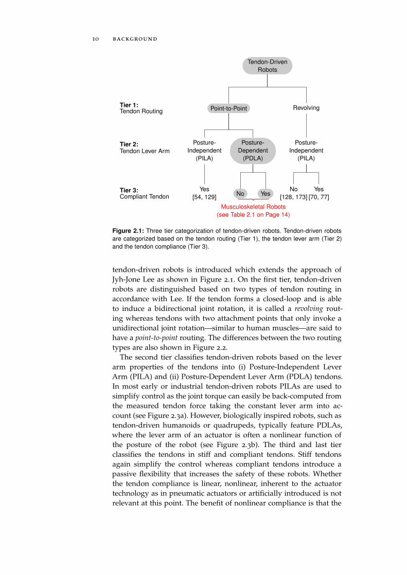
Figure 2.1: Three tier categorization of tendon-driven robots. Tendon-driven robots

are categorized based on the tendon routing (Tier 1), the tendon lever arm (Tier 2)

and the tendon compliance (Tier 3).

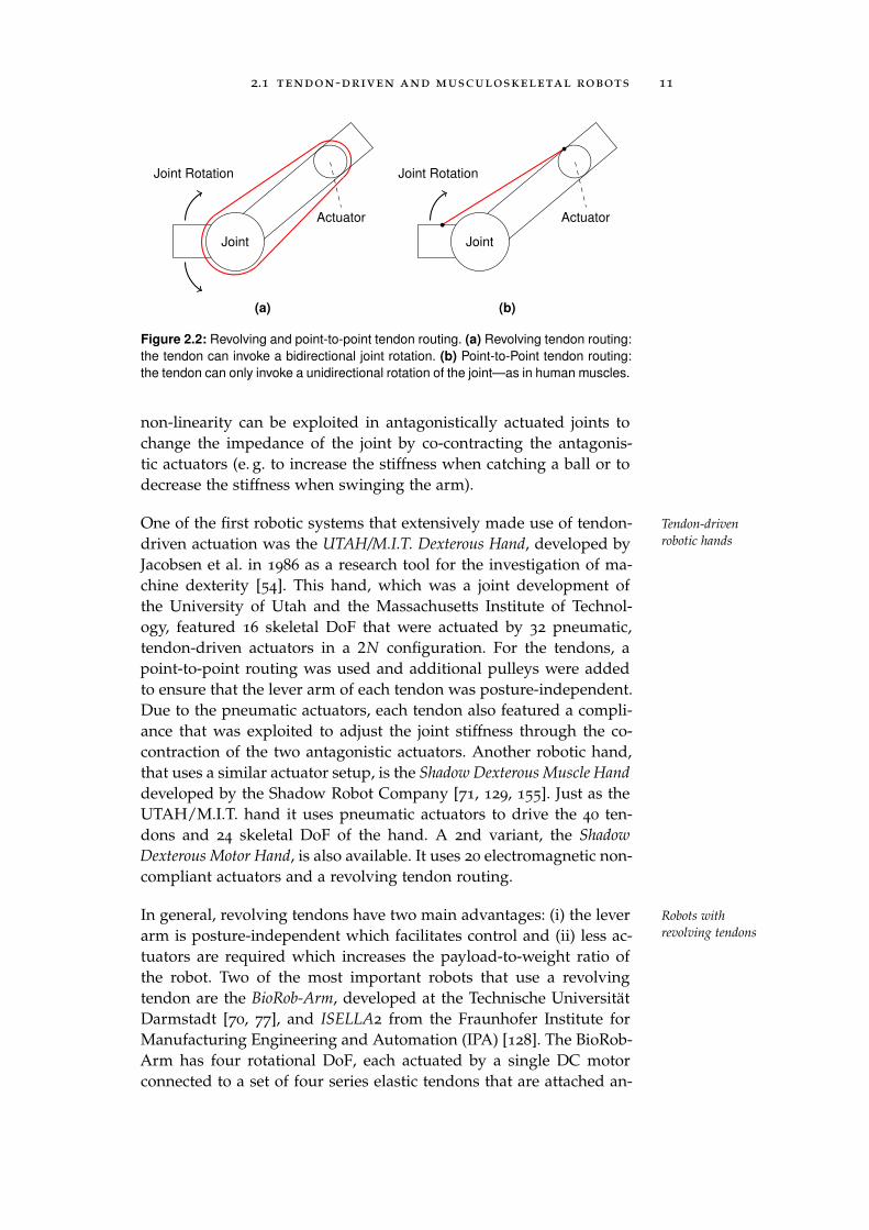
tendon-driven robots is introduced which extends the approach ofJyh-Jone Lee as shown in Figure 2.1. On the first tier, tendon-drivenrobots are distinguished based on two types of tendon routing inaccordance with Lee. If the tendon forms a closed-loop and is ableto induce a bidirectional joint rotation, it is called a revolving rout-ing whereas tendons with two attachment points that only invoke aunidirectional joint rotation—similar to human muscles—are said tohave a point-to-point routing. The differences between the two routingtypes are also shown in Figure 2.2.

The second tier classifies tendon-driven robots based on the leverarm properties of the tendons into (i) Posture-Independent LeverArm (PILA) and (ii) Posture-Dependent Lever Arm (PDLA) tendons.In most early or industrial tendon-driven robots PILAs are used tosimplify control as the joint torque can easily be back-computed fromthe measured tendon force taking the constant lever arm into ac-count (see Figure 2.3a). However, biologically inspired robots, such astendon-driven humanoids or quadrupeds, typically feature PDLAs,where the lever arm of an actuator is often a nonlinear function ofthe posture of the robot (see Figure 2.3b). The third and last tierclassifies the tendons in stiff and compliant tendons. Stiff tendonsagain simplify the control whereas compliant tendons introduce apassive flexibility that increases the safety of these robots. Whetherthe tendon compliance is linear, nonlinear, inherent to the actuatortechnology as in pneumatic actuators or artificially introduced is notrelevant at this point. The benefit of nonlinear compliance is that the

2.1 tendon-driven and musculoskeletal robots 11

Joint

Joint Rotation

Actuator

(a)

Joint

Joint Rotation

Actuator

(b)

Figure 2.2: Revolving and point-to-point tendon routing. (a) Revolving tendon routing:

the tendon can invoke a bidirectional joint rotation. (b) Point-to-Point tendon routing:

the tendon can only invoke a unidirectional rotation of the joint—as in human muscles.

non-linearity can be exploited in antagonistically actuated joints tochange the impedance of the joint by co-contracting the antagonis-tic actuators (e. g. to increase the stiffness when catching a ball or todecrease the stiffness when swinging the arm).

One of the first robotic systems that extensively made use of tendon- Tendon-driven

robotic handsdriven actuation was the UTAH/M.I.T. Dexterous Hand, developed byJacobsen et al. in 1986 as a research tool for the investigation of ma-chine dexterity [54]. This hand, which was a joint development ofthe University of Utah and the Massachusetts Institute of Technol-ogy, featured 16 skeletal DoF that were actuated by 32 pneumatic,tendon-driven actuators in a 2N configuration. For the tendons, apoint-to-point routing was used and additional pulleys were addedto ensure that the lever arm of each tendon was posture-independent.Due to the pneumatic actuators, each tendon also featured a compli-ance that was exploited to adjust the joint stiffness through the co-contraction of the two antagonistic actuators. Another robotic hand,that uses a similar actuator setup, is the Shadow Dexterous Muscle Hand

developed by the Shadow Robot Company [71, 129, 155]. Just as theUTAH/M.I.T. hand it uses pneumatic actuators to drive the 40 ten-dons and 24 skeletal DoF of the hand. A 2nd variant, the Shadow

Dexterous Motor Hand, is also available. It uses 20 electromagnetic non-compliant actuators and a revolving tendon routing.

In general, revolving tendons have two main advantages: (i) the lever Robots with

revolving tendonsarm is posture-independent which facilitates control and (ii) less ac-tuators are required which increases the payload-to-weight ratio ofthe robot. Two of the most important robots that use a revolvingtendon are the BioRob-Arm, developed at the Technische UniversitätDarmstadt [70, 77], and ISELLA2 from the Fraunhofer Institute forManufacturing Engineering and Automation (IPA) [128]. The BioRob-Arm has four rotational DoF, each actuated by a single DC motorconnected to a set of four series elastic tendons that are attached an-

12 background

lA lA

(a)

lA lA

(b)

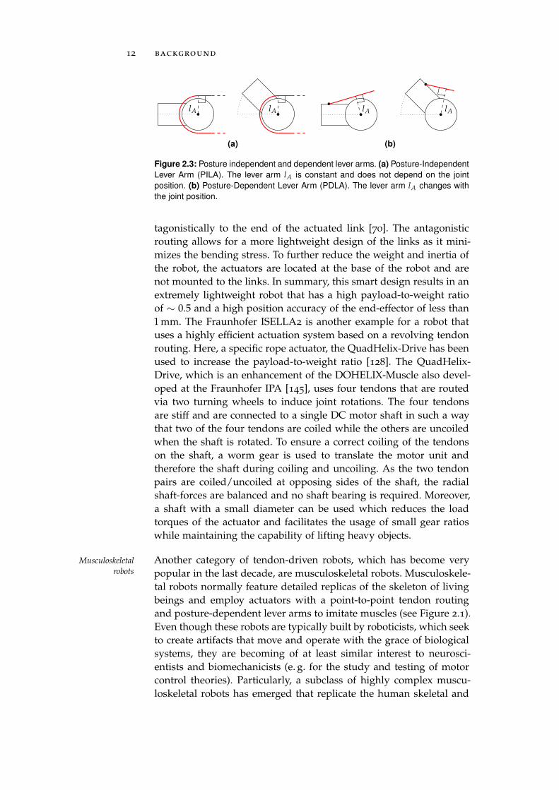
Figure 2.3: Posture independent and dependent lever arms. (a) Posture-Independent

Lever Arm (PILA). The lever arm lA is constant and does not depend on the joint

position. (b) Posture-Dependent Lever Arm (PDLA). The lever arm lA changes with

the joint position.

tagonistically to the end of the actuated link [70]. The antagonisticrouting allows for a more lightweight design of the links as it mini-mizes the bending stress. To further reduce the weight and inertia ofthe robot, the actuators are located at the base of the robot and arenot mounted to the links. In summary, this smart design results in anextremely lightweight robot that has a high payload-to-weight ratioof ∼ 0.5 and a high position accuracy of the end-effector of less than1 mm. The Fraunhofer ISELLA2 is another example for a robot thatuses a highly efficient actuation system based on a revolving tendonrouting. Here, a specific rope actuator, the QuadHelix-Drive has beenused to increase the payload-to-weight ratio [128]. The QuadHelix-Drive, which is an enhancement of the DOHELIX-Muscle also devel-oped at the Fraunhofer IPA [145], uses four tendons that are routedvia two turning wheels to induce joint rotations. The four tendonsare stiff and are connected to a single DC motor shaft in such a waythat two of the four tendons are coiled while the others are uncoiledwhen the shaft is rotated. To ensure a correct coiling of the tendonson the shaft, a worm gear is used to translate the motor unit andtherefore the shaft during coiling and uncoiling. As the two tendonpairs are coiled/uncoiled at opposing sides of the shaft, the radialshaft-forces are balanced and no shaft bearing is required. Moreover,a shaft with a small diameter can be used which reduces the loadtorques of the actuator and facilitates the usage of small gear ratioswhile maintaining the capability of lifting heavy objects.

Another category of tendon-driven robots, which has become veryMusculoskeletal

robots popular in the last decade, are musculoskeletal robots. Musculoskele-tal robots normally feature detailed replicas of the skeleton of livingbeings and employ actuators with a point-to-point tendon routingand posture-dependent lever arms to imitate muscles (see Figure 2.1).Even though these robots are typically built by roboticists, which seekto create artifacts that move and operate with the grace of biologicalsystems, they are becoming of at least similar interest to neurosci-entists and biomechanicists (e. g. for the study and testing of motorcontrol theories). Particularly, a subclass of highly complex muscu-loskeletal robots has emerged that replicate the human skeletal and

2.1 tendon-driven and musculoskeletal robots 13

(a) (b)

(c) (d) (e)

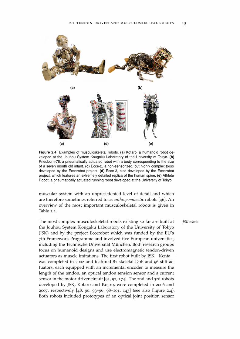
Figure 2.4: Examples of musculoskeletal robots. (a) Kotaro, a humanoid robot de-

veloped at the Jouhou System Kougaku Laboratory of the University of Tokyo. (b)

Pneuborn-7II, a pneumatically actuated robot with a body corresponding to the size

of a seven month old infant. (c) Ecce-2, a non-sensorized, but highly complex torso

developed by the Eccerobot project. (d) Ecce-3, also developed by the Eccerobot

project, which features an extremely detailed replica of the human spine. (e) Athlete

Robot, a pneumatically actuated running robot developed at the University of Tokyo.

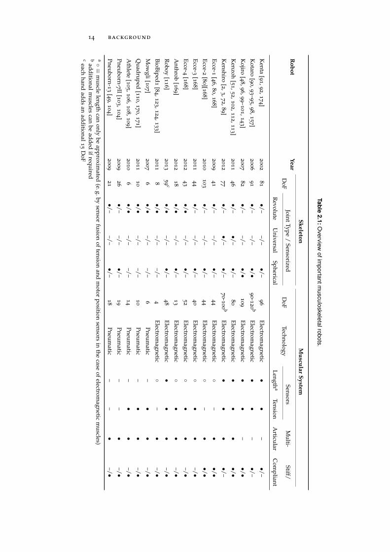
muscular system with an unprecedented level of detail and whichare therefore sometimes referred to as anthropomimetic robots [46]. Anoverview of the most important musculoskeletal robots is given inTable 2.1.

The most complex musculoskeletal robots existing so far are built at JSK robots

the Jouhou System Kougaku Laboratory of the University of Tokyo(JSK) and by the project Eccerobot which was funded by the EU’s7th Framework Programme and involved five European universities,including the Technische Universität München. Both research groupsfocus on humanoid designs and use electromagnetic tendon-drivenactuators as muscle imitations. The first robot built by JSK—Kenta—was completed in 2002 and featured 81 skeletal DoF and 96 stiff ac-tuators, each equipped with an incremental encoder to measure thelength of the tendon, an optical tendon tension sensor and a currentsensor in the motor-driver circuit [91, 92, 174]. The 2nd and 3rd robotsdeveloped by JSK, Kotaro and Kojiro, were completed in 2006 and2007, respectively [48, 90, 93–96, 98–101, 143] (see also Figure 2.4).Both robots included prototypes of an optical joint position sensor

14 background

Ta

ble

2.1

:O

verv

iew

of

imp

orta

nt

mu

scu

loske

leta

lro

bo

ts.

Ro

bo

tY

ea

r

Sk

ele

ton

Mu

scula

rS

yste

m

DoF

Joint

Type

/Sen

sorizedD

oFTech

nology

Sensors

Mu

lti-Stiff/

Revolu

teU

niversal

Sph

ericalL

ength

aTen

sionA

rticular

Com

plian

t

Ken

ta[9

1,9

2,1

74]

20

02

81

•/–

–/–

•/–

96

Electrom

agnetic

••

–•/

–

Kotaro

[90,

93–

95,

98,

15

7]2

00

69

1•/

––/

–•/

•9

0-12

0b

Electrom

agnetic

••

–•/

–

Kojiro

[48,

96,

99–

10

1,1

43]

20

07

82

•/–

–/–

•/•

10

9E

lectromagn

etic•

•–

•/•

Ken

zoh[5

1,5

2,1

02,

11

2,1

13]

20

11

46

•/–

•/–

•/–

80

Electrom

agnetic

••

••/

•

Ken

shiro

[2,3,

72,

89]

20

12

77

•/–

•/–

•/–

70-1

00

bE

lectromagn

etic•

••

•/–

Ecce-1

[46,

80,

16

8]2

00

94

1•/

––/

–•/

–4

4E

lectromagn

etic

–•

•/•

Ecce-2

[80][1

68]

20

10

10

3•/

––/

–•/

–4

4E

lectromagn

etic

–•

•/•

Ecce-3

[16

8]2

01

14

4•/

––/

–•/

–4

0E

lectromagn

etic

••

–/•

Ecce-4

[16

8]2

01

24

3•/

•–/

–•/

–5

2E

lectromagn

etic

••

–/•

An

throb

[16

9]2

01

21

8•/

•–/

–•/

–1

3E

lectromagn

etic

••

–/•

Roboy

[11

6]2

01

35

9c

•/•

–/–

•/–

48

Electrom

agnetic

••

•–/

•

BioB

iped

1[8

4,1

23,

12

4,1

33]

20

11

8•/

•–/

––/

–4

Electrom

agnetic

–

•–/

•

Mow

gli[1

07]

20

07

6•/

•–/

––/

–6

Pn

eum

atic–

••

–/•

Qu

adru

ped

[11

0,1

70,

17

1]2

01

11

0•/

•–/

––/

–1

0P

neu

matic

–•

•–/

•

Ath

lete[1

05,

10

6,1

08,

10

9]2

01

06

•/•

–/–

–/–

14

Pn

eum

atic–

••

–/•

Pn

euborn

-7II[1

03,

10

4]2

00

92

6•/

––/

–•/

–1

9P

neu

matic

––

•–/

•

Pn

euborn

-13

[49,

10

4]2

00

92

1•/

––/

–•/

–1

8P

neu

matic

––

•–/

•

a≡

mu

sclelen

gthcan

only

beap

proxim

ated(e.g.by

sensor

fusion

often

sionan

dm

otorp

ositionsen

sorsin

the

caseof

electromagn

eticm

uscles)

bad

dition

alm

uscles

canbe

add

edif

required

ceach

han

dad

ds

anad

dition

al1

5D

oF

2.1 tendon-driven and musculoskeletal robots 15

for the spherical 3-DoF joints used in the shoulder and hip [157].Moreover, Kojiro was the first robot built by JSK that featured non-linear spring units to provide a passive tendon compliance similarto human muscles [96]. More recently, JSK presented two additionalmusculoskeletal robots. Kenzoh, which was completed in 2011, is atorso with 46 skeletal DoF that included a revised, non-linear springunit as well as bi-articular actuators (actuators with tendons thatspan two joints) [51, 52, 102, 112, 113]. In humans, such bi-articularmuscles are for instance found in the leg and have been reported tocontribute to the coordination of joint synchronization [39, 160]. Themost recent robot developed by JSK—Kenshiro—is still under con-struction [2, 3, 72, 89]. It is the most complex Japanese musculoskele-tal robot so far and it features all improvements that have been madeduring one decade of musculoskeletal robot development.

The only musculoskeletal robots worldwide that can compete with The Eccerobots

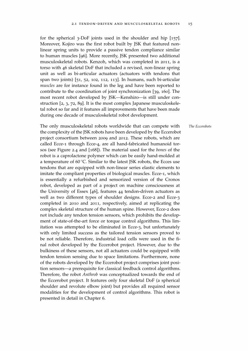
the complexity of the JSK robots have been developed by the Eccerobotproject consortium between 2009 and 2012. These robots, which arecalled Ecce-1 through Ecce-4, are all hand-fabricated humanoid tor-sos (see Figure 2.4 and [168]). The material used for the bones of therobot is a caprolactone polymer which can be easily hand-molded ata temperature of 60 C. Similar to the latest JSK robots, the Ecces usetendons that are equipped with non-linear series elastic elements toimitate the compliant properties of biological muscles. Ecce-1, whichis essentially a refurbished and sensorized version of the Cronosrobot, developed as part of a project on machine consciousness atthe University of Essex [46], features 44 tendon-driven actuators aswell as two different types of shoulder designs. Ecce-2 and Ecce-3completed in 2010 and 2011, respectively, aimed at replicating thecomplex skeletal structure of the human spine. However, Ecce-2 doesnot include any tendon tension sensors, which prohibits the develop-ment of state-of-the-art force or torque control algorithms. This lim-itation was attempted to be eliminated in Ecce-3, but unfortunatelywith only limited success as the tailored tension sensors proved tobe not reliable. Therefore, industrial load cells were used in the fi-nal robot developed by the Eccerobot project. However, due to thebulkiness of these sensors, not all actuators could be equipped withtendon tension sensing due to space limitations. Furthermore, noneof the robots developed by the Eccerobot project comprises joint posi-tion sensors—a prerequisite for classical feedback control algorithms.Therefore, the robot Anthrob was conceptualized towards the end ofthe Eccerobot project. It features only four skeletal DoF (a sphericalshoulder and revolute elbow joint) but provides all required sensormodalities for the development of control algorithms. This robot ispresented in detail in Chapter 6.

16 background

The robots presented so far all featured electromagnetic, tendon-dri-Musculoskeletal

robots with

pneumatic actuatorsven actuators that require an additional series elastic element to im-itate the compliant properties of biological muscles. In contrast, thisis not necessary if pneumatic actuators are used which exhibit a non-linear compliance inherent to the actuation principle. However, pneu-matic actuators require large compressors which make them unsuit-able for mobile robots and are difficult to control. Therefore, theyare only found in few musculoskeletal robots, such as in the bipedalrobots Mowgli [107] and Athlete [105, 106, 108, 109]. Both robots usepneumatic actuators of the McKibben type which provide a similarlength-load curve as biological muscles [107, 152, 153] and demon-strate jumping as well as soft landing due to the intrinsic complianceof the actuation modules.

2.2 joint-space simulation of forward dynamics

The dynamics of robots with open-loop kinematics are commonlyAnalytical modeling

and simulation of

robotsmodeled in joint-space by the following equation:

τ = M(q)q + C(q, q)q + g(q) (2.1)

where q, q and q (all ∈ Rn) are the joint positions, velocities and ac-

celerations, respectively, τ ∈ Rn is a vector of joint torques, M(q) ∈

Rn×n is a symmetric, positive-definite matrix called the mass or iner-

tia matrix, C(q, q) ∈ Rn×n is a matrix that, multiplied with q results

in an n × 1 vector of centrifugal and Coriolis terms, g(q) ∈ Rn is

a vector of gravity terms and n is the number of DoF [16, 141, 142].This equation, which is typically derived by either the Lagrangianor the Newton-Euler formulation, relates the joint accelerations q tojoint torques τ. Therefore, in its presented form, it is typically usedfor robot control where the task is to compute the joint torques re-quired for desired joint accelerations—the inverse dynamics. However,if solved for q, Equation 2.1 is equal to:

q = M−1(q)[τ − C(q, q)q− g(q)] (2.2)

In this form, Equation 2.1 can be used for the simulation of the for-

ward dynamics by employing standard numerical integration methodsto compute the joint velocities and positions from the accelerationsinduced by the applied joint torques [16, 30]. Note that Equation 2.2requires the mass matrix to be invertible which is the case as M is asymmetric, positive-definite matrix [30, 97].

If the task is now to simulate the dynamics of tendon-driven robotsAnalytical modeling

and simulation of

tendon-driven robotswe can still rely on Equation 2.2 but we have to account for the tendon-driven actuation by finding a mapping h between the tendon-forcesf ∈ R

m and the joint-torques τ:

τ = h(q, f ) h : Rn×m → R

n (2.3)

2.2 joint-space simulation of forward dynamics 17

τ = h(q, f )

Lever Arm

L(q)

Trigonometry

[121]

Vector Algebra

[73, 124]

Muscle Jacobian

H(q)

Tendon Length

l(q)

Trigonometry Vector Algebra

[61]

Experiment

[60]

τ = L(q) f τ = −H(q)⊺ f

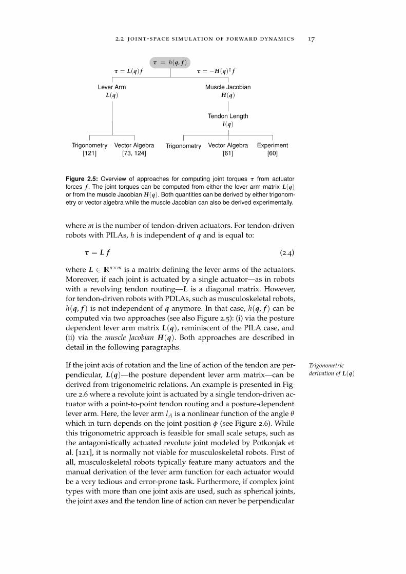
Figure 2.5: Overview of approaches for computing joint torques τ from actuator

forces f . The joint torques can be computed from either the lever arm matrix L(q)or from the muscle Jacobian H(q). Both quantities can be derived by either trigonom-

etry or vector algebra while the muscle Jacobian can also be derived experimentally.

where m is the number of tendon-driven actuators. For tendon-drivenrobots with PILAs, h is independent of q and is equal to:

τ = L f (2.4)

where L ∈ Rn×m is a matrix defining the lever arms of the actuators.

Moreover, if each joint is actuated by a single actuator—as in robotswith a revolving tendon routing—L is a diagonal matrix. However,for tendon-driven robots with PDLAs, such as musculoskeletal robots,h(q, f ) is not independent of q anymore. In that case, h(q, f ) can becomputed via two approaches (see also Figure 2.5): (i) via the posturedependent lever arm matrix L(q), reminiscent of the PILA case, and(ii) via the muscle Jacobian H(q). Both approaches are described indetail in the following paragraphs.

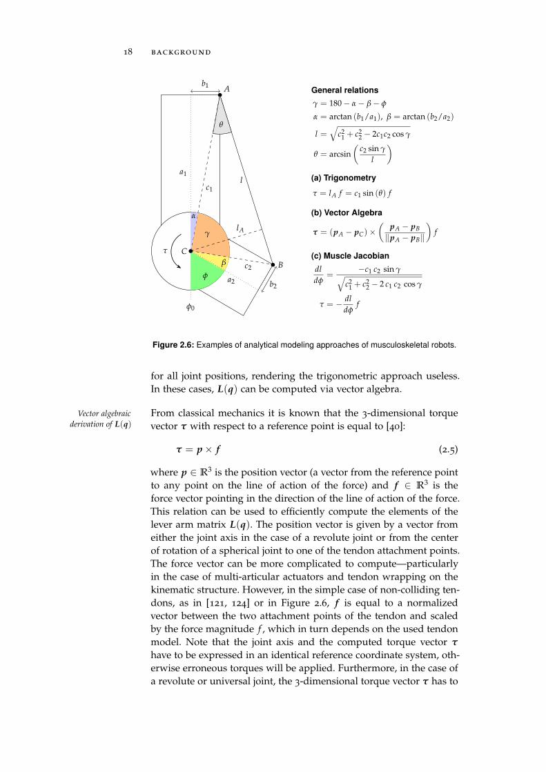
If the joint axis of rotation and the line of action of the tendon are per- Trigonometric

derivation of L(q)pendicular, L(q)—the posture dependent lever arm matrix—can bederived from trigonometric relations. An example is presented in Fig-ure 2.6 where a revolute joint is actuated by a single tendon-driven ac-tuator with a point-to-point tendon routing and a posture-dependentlever arm. Here, the lever arm lA is a nonlinear function of the angle θ

which in turn depends on the joint position φ (see Figure 2.6). Whilethis trigonometric approach is feasible for small scale setups, such asthe antagonistically actuated revolute joint modeled by Potkonjak etal. [121], it is normally not viable for musculoskeletal robots. First ofall, musculoskeletal robots typically feature many actuators and themanual derivation of the lever arm function for each actuator wouldbe a very tedious and error-prone task. Furthermore, if complex jointtypes with more than one joint axis are used, such as spherical joints,the joint axes and the tendon line of action can never be perpendicular

18 background

A

l

γ

τ

φ0

b1

c1

a1

φ

lA

α

β c2

a2 b2

B

θ

C

General relations

γ = 180− α− β− φ

α = arctan (b1/a1), β = arctan (b2/a2)

l =√

c21 + c2

2 − 2c1c2 cos γ

θ = arcsin(

c2 sin γ

l

)

(a) Trigonometry

τ = lA f = c1 sin (θ) f

(b) Vector Algebra

τ = (pA − pC)×(

pA − pB

‖pA − pB‖

)

f

(c) Muscle Jacobian

dl

dφ=

−c1 c2 sin γ√

c21 + c2

2 − 2 c1 c2 cos γ

τ = − dl

dφf

Figure 2.6: Examples of analytical modeling approaches of musculoskeletal robots.

for all joint positions, rendering the trigonometric approach useless.In these cases, L(q) can be computed via vector algebra.

From classical mechanics it is known that the 3-dimensional torqueVector algebraic

derivation of L(q) vector τ with respect to a reference point is equal to [40]:

τ = p× f (2.5)

where p ∈ R3 is the position vector (a vector from the reference point

to any point on the line of action of the force) and f ∈ R3 is the

force vector pointing in the direction of the line of action of the force.This relation can be used to efficiently compute the elements of thelever arm matrix L(q). The position vector is given by a vector fromeither the joint axis in the case of a revolute joint or from the centerof rotation of a spherical joint to one of the tendon attachment points.The force vector can be more complicated to compute—particularlyin the case of multi-articular actuators and tendon wrapping on thekinematic structure. However, in the simple case of non-colliding ten-dons, as in [121, 124] or in Figure 2.6, f is equal to a normalizedvector between the two attachment points of the tendon and scaledby the force magnitude f , which in turn depends on the used tendonmodel. Note that the joint axis and the computed torque vector τ

have to be expressed in an identical reference coordinate system, oth-erwise erroneous torques will be applied. Furthermore, in the case ofa revolute or universal joint, the 3-dimensional torque vector τ has to

2.2 joint-space simulation of forward dynamics 19

be converted into a scalar representing the magnitude of the torquearound a single rotation axis. This conversion can easily be achievedby multiplying τ with a unit vector e in the direction of the jointaxis. In summary, this yields the following equation for computingthe magnitude of the torque τ around the joint axis resulting fromthe tendon force f :

τ =(

p× f)

· e f (2.6)

where the term(

p× f)

· e is the lever arm of the actuator with re-

spect to the joint axis. Therefore, we can use Equation 2.6 to computethe elements of L(q) equal to:

L(q) =

a1,1 a1,2 . . . a1,m

a2,1 a2,2 . . . a2,m...

.... . .

...

an,1 an,2 . . . an,m

with

ai,j =

[

pi,j(q)× f j(q)]

· ei if joint axis i is affected by actuator j

0 otherwise

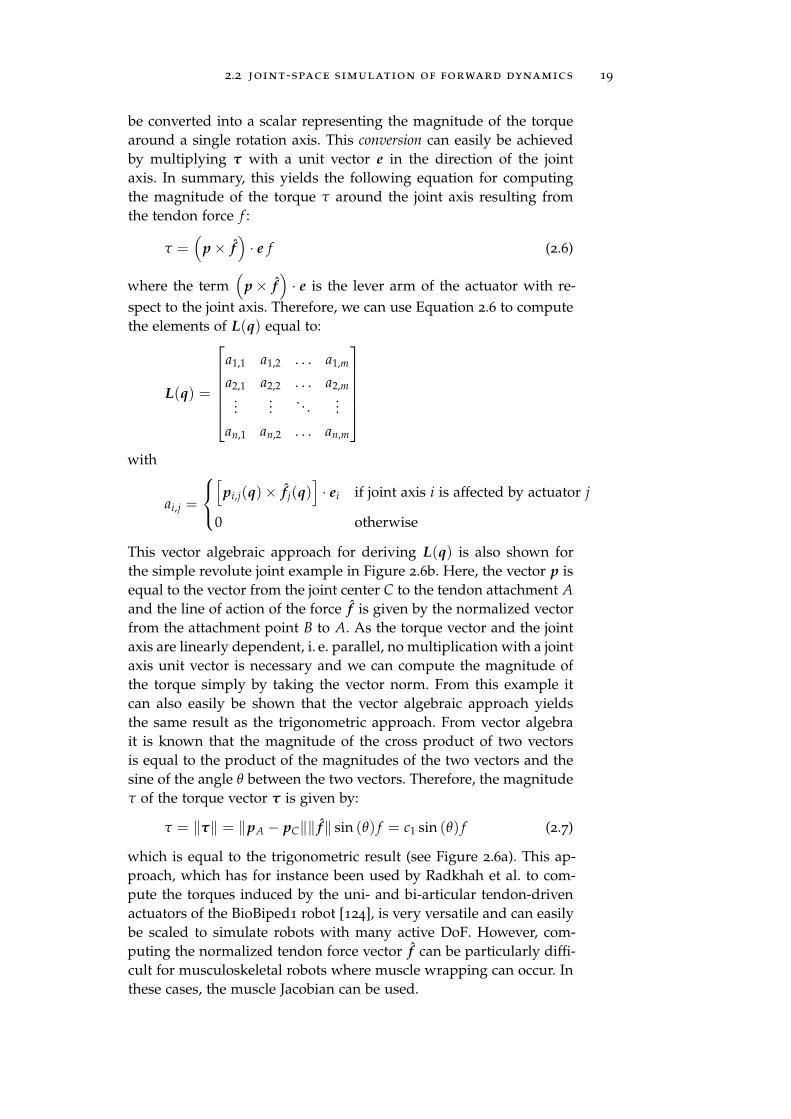
This vector algebraic approach for deriving L(q) is also shown forthe simple revolute joint example in Figure 2.6b. Here, the vector p isequal to the vector from the joint center C to the tendon attachment A

and the line of action of the force f is given by the normalized vectorfrom the attachment point B to A. As the torque vector and the jointaxis are linearly dependent, i. e. parallel, no multiplication with a jointaxis unit vector is necessary and we can compute the magnitude ofthe torque simply by taking the vector norm. From this example itcan also easily be shown that the vector algebraic approach yieldsthe same result as the trigonometric approach. From vector algebrait is known that the magnitude of the cross product of two vectorsis equal to the product of the magnitudes of the two vectors and thesine of the angle θ between the two vectors. Therefore, the magnitudeτ of the torque vector τ is given by:

τ = ‖τ‖ = ‖pA − pC‖‖ f‖ sin (θ) f = c1 sin (θ) f (2.7)

which is equal to the trigonometric result (see Figure 2.6a). This ap-proach, which has for instance been used by Radkhah et al. to com-pute the torques induced by the uni- and bi-articular tendon-drivenactuators of the BioBiped1 robot [124], is very versatile and can easilybe scaled to simulate robots with many active DoF. However, com-puting the normalized tendon force vector f can be particularly diffi-cult for musculoskeletal robots where muscle wrapping can occur. Inthese cases, the muscle Jacobian can be used.

20 background

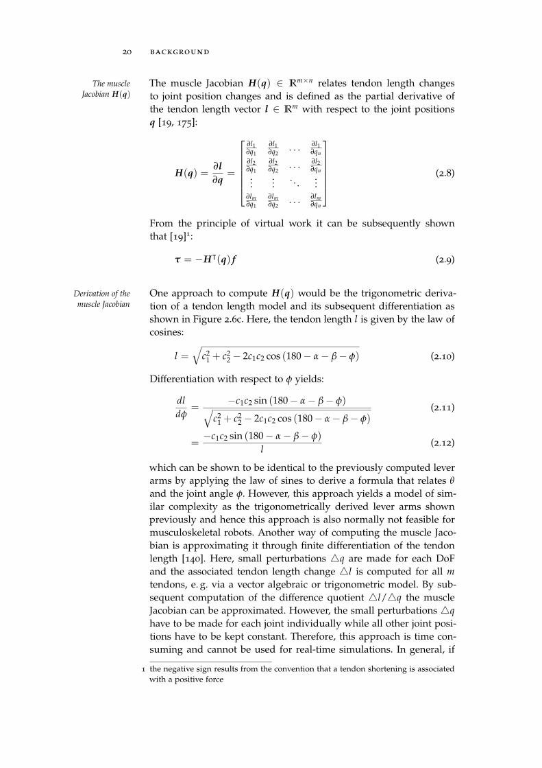
The muscle Jacobian H(q) ∈ Rm×n relates tendon length changesThe muscle

Jacobian H(q) to joint position changes and is defined as the partial derivative ofthe tendon length vector l ∈ R

m with respect to the joint positionsq [19, 175]:

H(q) =∂l

∂q=

∂l1∂q1

∂l1∂q2

. . . ∂l1∂qn

∂l2∂q1

∂l2∂q2

. . . ∂l2∂qn

......

. . ....

∂lm∂q1

∂lm∂q2

. . . ∂lm∂qn

(2.8)

From the principle of virtual work it can be subsequently shownthat [19]1:

τ = −H⊺(q) f (2.9)

One approach to compute H(q) would be the trigonometric deriva-Derivation of the

muscle Jacobian tion of a tendon length model and its subsequent differentiation asshown in Figure 2.6c. Here, the tendon length l is given by the law ofcosines:

l =√

c21 + c2

2 − 2c1c2 cos (180− α− β− φ) (2.10)

Differentiation with respect to φ yields:

dl

dφ=

−c1c2 sin (180− α− β− φ)√

c21 + c2

2 − 2c1c2 cos (180− α− β− φ)(2.11)

=−c1c2 sin (180− α− β− φ)

l(2.12)

which can be shown to be identical to the previously computed leverarms by applying the law of sines to derive a formula that relates θ

and the joint angle φ. However, this approach yields a model of sim-ilar complexity as the trigonometrically derived lever arms shownpreviously and hence this approach is also normally not feasible formusculoskeletal robots. Another way of computing the muscle Jaco-bian is approximating it through finite differentiation of the tendonlength [140]. Here, small perturbations q are made for each DoFand the associated tendon length change l is computed for all m

tendons, e. g. via a vector algebraic or trigonometric model. By sub-sequent computation of the difference quotient l/q the muscleJacobian can be approximated. However, the small perturbations q

have to be made for each joint individually while all other joint posi-tions have to be kept constant. Therefore, this approach is time con-suming and cannot be used for real-time simulations. In general, if

1 the negative sign results from the convention that a tendon shortening is associatedwith a positive force

2.3 simulation tools for musculoskeletal robots 21

real-time constraints are considered, the muscle Jacobian has to becomputed a priori. One approach that has proven to be feasible hasbeen first evaluated in simulations by Schmaler [132] and was lateradapted by Jäntsch et al. for the acquisition of the muscle Jacobian ofthe Anthrob robot [60, 61]. Here, an Artificial Neural Network (ANN)has been used to approximate the tendon length of all actuators andthe difference quotient was used to compute H(q). However, the gen-eration of the training data for the ANN is not trivial, as samples ofthe entire joint space of the robot have to be drawn to preclude theneed for muscle Jacobian extrapolation by the ANN. Furthermore,the question remains how the muscle Jacobian can be learned by thisapproach for arbitrary kinematic setups without supervision. In sum-mary, the usage of the muscle Jacobian for the simulation of the for-ward dynamics of musculoskeletal robots is a promising approach aslong as an efficient algorithm for its computation can be found.

2.3 simulation tools for musculoskeletal robots

Even though many tools exist for the simulation of mobile or indus-trial robots, such as Microsoft’s Robotics Studio [53] or Webots [87],there is no robotic simulation toolbox available that is capable of sim-ulating the forward dynamics of tendon-driven robots. One of themain reasons is the difficulty of automatically deriving the lever armmatrix L(q) or the muscle Jacobian H(q) for an arbitrary robot con-figuration as pointed out in the previous section. However, problemsassociated with the simulation of tendon-driven robots are also en-countered in biomechanics. Here, skeleton and muscle models areused to investigate aspects of motion dynamics. A few tools haveemerged in this field in recent years, such as OpenSim [21] or Any-body. Whereas OpenSim is an academic, free-of-charge project devel-oped at the Center for Biomedical Computation at Stanford, Anybodyis a commercial product. Both tools provide detailed models of thehuman skeleton and include various human-inspired muscle models,such as the Hill model [43]. However, both tools operate in the jointspace which means that the tedious procedure of converting muscleforces into joint torques, as presented in the previous section, has tobe applied. Furthermore, the closed-source character of Anybody im-pedes the inclusion of new muscle models required for the simulationof musculoskeletal robots, such as electromagnetic series elastic actu-ators. Hence, tailored solutions are typically used by roboticists tosimulate the dynamics of a particular musculoskeletal robot [33, 124].To close this gap, a modular and extensible simulation framework fortendon-driven robots, called Caliper, was developed as part of thisthesis. Caliper is based on the physics-based simulation approachand includes all muscle models presented in Chapter 4. An overviewof the functionality of Caliper can be found in Appendix E.

3S K E L E T O N M O D E L I N G

The bones of musculoskeletal robots are typically fabricated either Skeletons &

articulated rigid

bodiesby 3D printing (e. g. Roboy or Anthrob) or by more traditional pro-duction techniques using aluminium or other metals (e. g. BioBiped).In general, these bony structures are optimized for weight, size andshape (the bone should resemble the human model), rather than forsupporting large payloads like the links of industrial robots. Hence,the resulting skeletons are less stiff than an industrial manipulator.But what does this mean for the simulation of the skeletons? Muscu-loskeletal robots are very different from industrial manipulators andtherefore the precision requirements of these two classes cannot becompared. While for industrial robots a repeatability within the sub-millimeter domain is common, musculoskeletal robots exhibit posi-tioning errors in the order of centimeters due to the compliant actua-tors and high joint as well as muscle friction forces [58]. Thus, even ifthe bones would slightly bend under load, the resulting errors wouldstill be negligible in terms of the overall positioning error. Therefore,similar to industrial robots, the skeletons of musculoskeletal robotscan be modeled by a system of articulated rigid bodies.

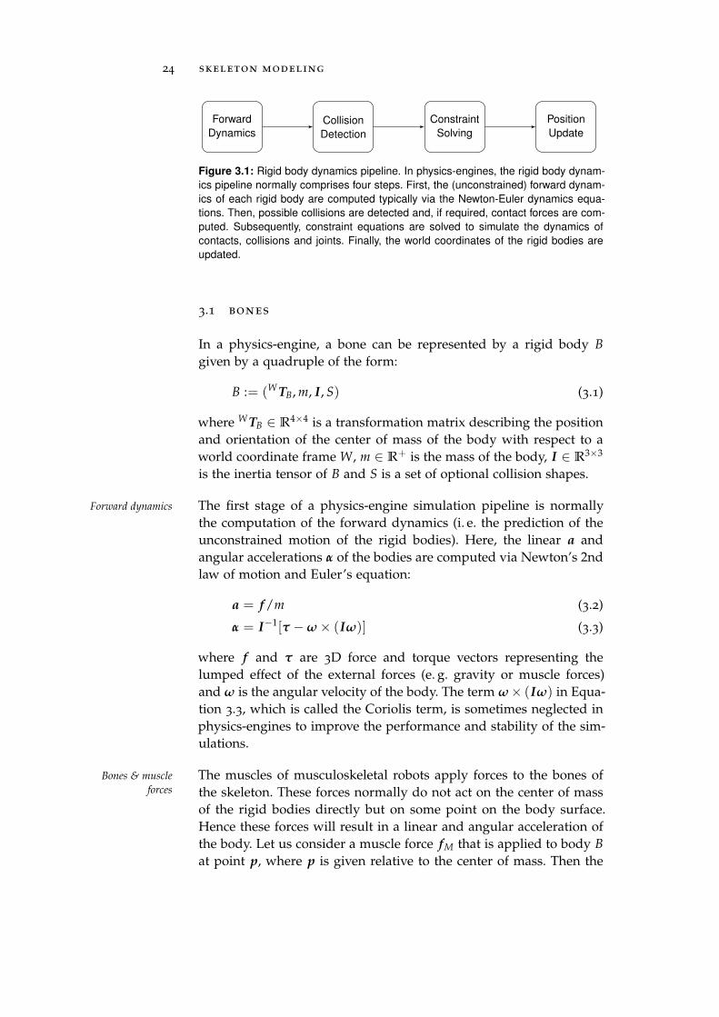
All existing physics-engines support the simulation of articulated rigid Physics-engines &

rigid body dynamicsbody systems by means of rigid body dynamics and Figure 3.1 showsthe four stages typically involved in a single simulation step of arigid body dynamics pipeline: (i) forward dynamics, (ii) collision de-tection, (iii) constraint solving and (iv) position update. Describingeach stage in detail is out of the scope of this dissertation and theinterested reader is referred to the PhD thesis of Kenny Erleben [29],the diploma thesis of Helmut Garstenauer [35] or to the book GamePhysics by David Eberly [27]. In the context of this dissertation, how-ever, it is important to outline the differences between the standardjoint space forward dynamics approach used for the simulation of stan-dard industrial robots as described previously in Section 2.2 and thebody space approach of physics-engines. These differences are summa-rized in Section 3.1. Furthermore, musculoskeletal robots typicallyfeature revolute and spherical joints. The modeling of these jointtypes as well as of joint friction in a physics-engine is summarizedin Section 3.2.

23

24 skeleton modeling

Forward

DynamicsCollision

Detection

Constraint

Solving

Position

Update

Figure 3.1: Rigid body dynamics pipeline. In physics-engines, the rigid body dynam-

ics pipeline normally comprises four steps. First, the (unconstrained) forward dynam-

ics of each rigid body are computed typically via the Newton-Euler dynamics equa-

tions. Then, possible collisions are detected and, if required, contact forces are com-

puted. Subsequently, constraint equations are solved to simulate the dynamics of

contacts, collisions and joints. Finally, the world coordinates of the rigid bodies are

updated.

3.1 bones

In a physics-engine, a bone can be represented by a rigid body B

given by a quadruple of the form:

B := (W TB, m, I, S) (3.1)

where W TB ∈ R4×4 is a transformation matrix describing the position

and orientation of the center of mass of the body with respect to aworld coordinate frame W, m ∈ R

+ is the mass of the body, I ∈ R3×3

is the inertia tensor of B and S is a set of optional collision shapes.

The first stage of a physics-engine simulation pipeline is normallyForward dynamics

the computation of the forward dynamics (i. e. the prediction of theunconstrained motion of the rigid bodies). Here, the linear a andangular accelerations α of the bodies are computed via Newton’s 2ndlaw of motion and Euler’s equation:

a = f /m (3.2)

α = I−1[τ −ω× (Iω)] (3.3)

where f and τ are 3D force and torque vectors representing thelumped effect of the external forces (e. g. gravity or muscle forces)and ω is the angular velocity of the body. The term ω× (Iω) in Equa-tion 3.3, which is called the Coriolis term, is sometimes neglected inphysics-engines to improve the performance and stability of the sim-ulations.

The muscles of musculoskeletal robots apply forces to the bones ofBones & muscle

forces the skeleton. These forces normally do not act on the center of massof the rigid bodies directly but on some point on the body surface.Hence these forces will result in a linear and angular acceleration ofthe body. Let us consider a muscle force fM that is applied to body B

at point p, where p is given relative to the center of mass. Then the

3.2 joints 25

resulting force f and torque τ acting on the body are given by thefollowing two equations:

f = fM (3.4)

τ = p× fM (3.5)

From the previous paragraph and Equation 3.1, the major difference Body space vs.

joint spacebetween the classical robot simulation approach presented in Sec-tion 2.2 and the physics-based approach already becomes apparent.While traditional robot simulations operate in the joint space (i. e. thejoint positions are known and not the body transforms), physics-engines work in the body space with no explicit representation of thejoint positions. This difference, which might appear to be minor atfirst, has a major impact on the simulation of musculoskeletal robots.As shown in detail in Section 2.2, the simulation of musculoskeletalrobots in the joint-space domain requires the muscle forces to be con-verted into joint torques. This intermediate step, which can be tediousfor more complex setups, is not required if a body space approach isemployed. Here, the muscle forces can be applied directly to the rigidbodies of the skeleton, which significantly simplifies the implementa-tion of muscle models as shown in Chapter 4.

Physics-engines normally include algorithms for collision detection Collision detection

and handling. These collision detection algorithms can be used forsimulating skeleton self-collisions as well as for skeleton vs. envi-ronment collisions—as for instance required for the simulation ofhandling or interaction scenarios. Collision detection is performed intwo steps, called broadphase and narrowphase collision detection. Whilein the broadphase, the axis-aligned bounding boxes (AABBs) of thecollision shapes are used to determine whether “bounding volumesoverlap” [158], the exact contact forces are computed in the narrow-phase step. As collision shapes, simple primitives, such as boxes orcylinders, but also arbitrary convex and concave meshes are normallysupported. The details, however, depend on the used physics-engine.

3.2 joints

As physics-engines operate in the body-space, simulating joints ismore complex than in traditional joint-space approaches. But again,a detailed overview of joint modeling in physics-engines is out-of-scope of this dissertation and the interested reader is referred to[27, 29, 35, 158, 164]. Thus, in the following paragraphs, we willlimit ourselves to the basic principles of joint simulations in physics-engines and outline how these algorithms can be used to simulatedry and viscous joint friction.

26 skeleton modeling

In physics-engines, joints are represented by a set of holonomic con-Joints & constraints

straint equations (i. e. equality constraints that only depend on timeand on the position coordinates of the involved body pair) [29, 35].These constraint equations are either solved sequentially or simulta-neously to compute the constraint forces that ensure that the con-straint equations are satisfied. Typically, this is done by finding thebest solution in an iterative loop. As real-time performance is impor-tant for physics-engines, the number of iterations of this loop is nor-mally limited and hence, the solution found might be non-optimalleading to simulation artifacts (i. e. breaking constraints). This can beavoided by either reducing the size of the simulation time-step or byincreasing the number of solver iterations.

Musculoskeletal robots typically feature revolute and spherical joints.Joint types

Whereas the revolute joint removes 5 DoF (3 linear and 2 angular),the spherical joint only constrains the linear motion of the bodiesto be zero, leaving the 3 angular DoF unconstrained. Both of thesejoint types are supported by popular physics-engines (see [8]). Anextensive overview of joint types and joint modeling in general canbe found in the dissertation of Kenny Erleben [29].

Typically the movement range of joints is not infinite. For instance, theJoint limits

movement range of the human elbow joint is approximately 145 [119].These joint limits are simulated in physics-engines similar to contactconstraints [29, 158]. However, instead of assuming a hard limit, softlimits are used to stabilize the simulation in the vicinity of the limitangles [158].

In computer animations and physics-based simulations of traditionalJoint motors &

friction robots with joint-actuators, it is often required to drive a joint to areference position. In physics-engines this can be achieved by theuse of joint motors, which utilize the error reduction term of con-straint equations to invoke a reference joint velocity [29]. In the con-text of musculoskeletal robots, however, joint motors are not relevantto induce motions—this is done by the muscular system—but to re-sist motions by modeling joint friction. If we focus for now on rota-tory joints, then joint motors are typically parametrized by a refer-ence joint velocity ωmotor and by a maximum torque τmax

1. By set-ting ωmotor = 0 and τmax to a non-zero value corresponding to thejoint friction torque, the constraint solver will apply any torque in therange −τmax ≤ τ ≤ τmax in order to reach ωmotor. This principle canbe used to efficiently simulate joint friction.

1 in the case of linear joints, ω and τmax would be substituted by the linear velocityvector v and by a force vector fmax

3.2 joints 27

Three types of friction forces contribute to joint friction: (i) static fric- Joint friction

modelingtion when the norm of the joint velocity ‖ωjoint‖ = 0, (ii) kinetic fric-tion when ‖ωjoint‖ 6= 0 and (iii) viscous friction forces which are pro-portional to ‖ωjoint‖. The lumped effect of all three friction types canbe modeled by a single friction model, called Stribeck friction curve.This friction model, which was developed by the German engineerRichard Stribeck in 1903 [146], models the transition from static to ki-netic friction by a continuous function but exhibits still a discontinu-ity if the relative velocity of the two objects in contact is zero. Hence,to increase the numerical stability of simulations, the friction force isnormally approximated via a linear or sigmoid function in the zerovelocity vicinity [1]. This approach is not required if joint motors areused as the iterative algorithm of the constraint solver already guar-antees that the joint motor applies any torque between 0 and τmax if‖ωjoint‖ = 0 and τmax if ‖ωjoint‖ 6= 0 [29]. Hence, the maximum motortorque of a revolute joint with scalar joint velocity ω is given by theStribeck equation and equal to:

τmax = τStribeck = τk + (τs − τk) e−|ω|/vs + kv ω (3.6)

where τs and τk are static and kinetic friction torques, kv is the viscousfriction coefficient and vs is the Stribeck velocity. In the case of a spher-ical joint, the joint velocity and the joint motor torque are vectors andthe maximum joint motor torque is equal to:

τmax =

ξ

τs

τs

τs

if ‖ω‖ = 0 with 1/√

3 ≤ ξ ≤ 1

ω

‖ω‖τStribeck if ‖ω‖ 6= 0

(3.7)

Thus the motor torque is distributed onto the three joint axis depend-ing on the relative joint velocity if ‖ω‖ 6= 0 and equally distributedotherwise. The factor ξ would be equal to 1 if the joint movementwould be limited to a single axis and 1/

√3 if all three joint axis

would be involved. Hence, assuming ξ = 1/√

3 would apply lessfriction if only one joint axis would be involved and setting ξ = 1would result in too high friction torques if multiple axis are involved.Hence a good compromise is to use the arithmetic mean, equal to:

ξ =1 + 1/

√3

2(3.8)

Due to the velocity dependence of the friction torque, the maximummotor torque has to be recomputed and reset for each joint duringevery simulation step.

28 skeleton modeling

Instead of using joint motors for simulating joint friction, the frictionJoint motors vs.

direct torque

applicationtorque could be applied directly to the rigid bodies of the joint. Thisapproach, however, has two major drawbacks: (i) the static frictionwould need to be approximated by a linear or sigmoid function and(ii) the simulation stability would be affected negatively as the fric-tion torques would not be taken into account by the constraint solver.Hence, when supported by the physics-engine, joint motors shouldbe favored for modeling joint friction.

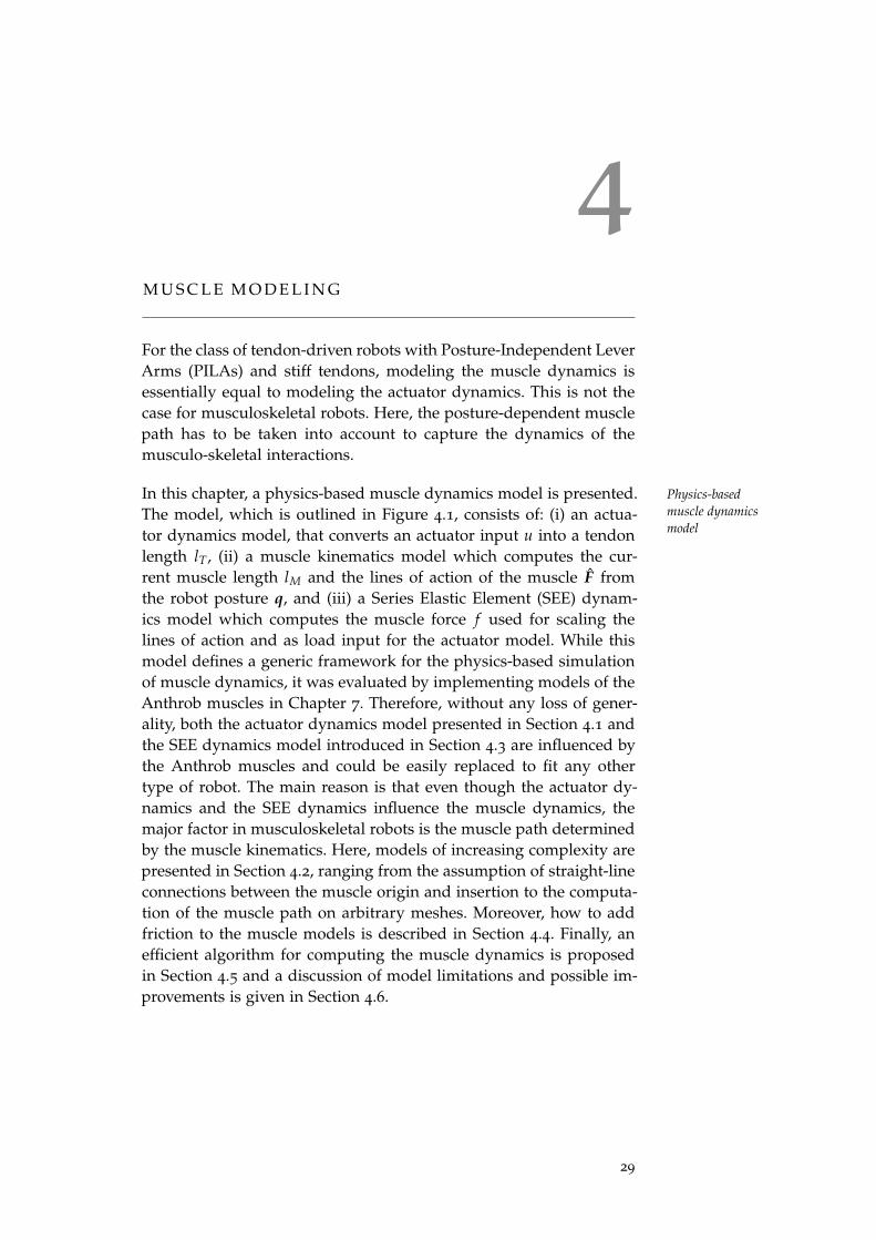
4M U S C L E M O D E L I N G

For the class of tendon-driven robots with Posture-Independent LeverArms (PILAs) and stiff tendons, modeling the muscle dynamics isessentially equal to modeling the actuator dynamics. This is not thecase for musculoskeletal robots. Here, the posture-dependent musclepath has to be taken into account to capture the dynamics of themusculo-skeletal interactions.

In this chapter, a physics-based muscle dynamics model is presented. Physics-based

muscle dynamics

modelThe model, which is outlined in Figure 4.1, consists of: (i) an actua-tor dynamics model, that converts an actuator input u into a tendonlength lT, (ii) a muscle kinematics model which computes the cur-rent muscle length lM and the lines of action of the muscle F fromthe robot posture q, and (iii) a Series Elastic Element (SEE) dynam-ics model which computes the muscle force f used for scaling thelines of action and as load input for the actuator model. While thismodel defines a generic framework for the physics-based simulationof muscle dynamics, it was evaluated by implementing models of theAnthrob muscles in Chapter 7. Therefore, without any loss of gener-ality, both the actuator dynamics model presented in Section 4.1 andthe SEE dynamics model introduced in Section 4.3 are influenced bythe Anthrob muscles and could be easily replaced to fit any othertype of robot. The main reason is that even though the actuator dy-namics and the SEE dynamics influence the muscle dynamics, themajor factor in musculoskeletal robots is the muscle path determinedby the muscle kinematics. Here, models of increasing complexity arepresented in Section 4.2, ranging from the assumption of straight-lineconnections between the muscle origin and insertion to the computa-tion of the muscle path on arbitrary meshes. Moreover, how to addfriction to the muscle models is described in Section 4.4. Finally, anefficient algorithm for computing the muscle dynamics is proposedin Section 4.5 and a discussion of model limitations and possible im-provements is given in Section 4.6.

29

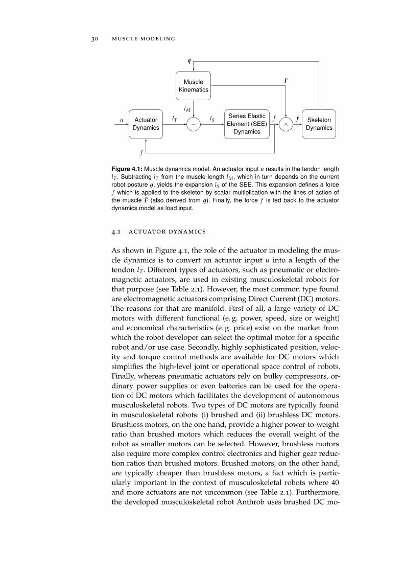
30 muscle modeling

Actuator

Dynamics

Series Elastic

Element (SEE)

Dynamics

Skeleton

Dynamics

Muscle

Kinematics

u −lT

lM

lS ×f

f

q

F

f

Figure 4.1: Muscle dynamics model. An actuator input u results in the tendon length

lT . Subtracting lT from the muscle length lM, which in turn depends on the current

robot posture q, yields the expansion lS of the SEE. This expansion defines a force

f which is applied to the skeleton by scalar multiplication with the lines of action of

the muscle F (also derived from q). Finally, the force f is fed back to the actuator

dynamics model as load input.

4.1 actuator dynamics

As shown in Figure 4.1, the role of the actuator in modeling the mus-cle dynamics is to convert an actuator input u into a length of thetendon lT. Different types of actuators, such as pneumatic or electro-magnetic actuators, are used in existing musculoskeletal robots forthat purpose (see Table 2.1). However, the most common type foundare electromagnetic actuators comprising Direct Current (DC) motors.The reasons for that are manifold. First of all, a large variety of DCmotors with different functional (e. g. power, speed, size or weight)and economical characteristics (e. g. price) exist on the market fromwhich the robot developer can select the optimal motor for a specificrobot and/or use case. Secondly, highly sophisticated position, veloc-ity and torque control methods are available for DC motors whichsimplifies the high-level joint or operational space control of robots.Finally, whereas pneumatic actuators rely on bulky compressors, or-dinary power supplies or even batteries can be used for the opera-tion of DC motors which facilitates the development of autonomousmusculoskeletal robots. Two types of DC motors are typically foundin musculoskeletal robots: (i) brushed and (ii) brushless DC motors.Brushless motors, on the one hand, provide a higher power-to-weightratio than brushed motors which reduces the overall weight of therobot as smaller motors can be selected. However, brushless motorsalso require more complex control electronics and higher gear reduc-tion ratios than brushed motors. Brushed motors, on the other hand,are typically cheaper than brushless motors, a fact which is partic-ularly important in the context of musculoskeletal robots where 40and more actuators are not uncommon (see Table 2.1). Furthermore,the developed musculoskeletal robot Anthrob uses brushed DC mo-

4.1 actuator dynamics 31

τEM = KT i

ωM

τLM

τLG = f rS

ωG

Spindle

Ra

diu

s:

r S

θG

Gear

Efficiency: η

Ratio: N

Motor

JM, JG

iR L

u ue = KE ωM

Figure 4.2: Model of an electromagnetic actuator. The actuator consists of a brushed

DC motor, which converts the input voltage u into an angular velocity and output

torque of the motor shaft (ωM and τEM, respectively), a gear with efficiency η and

ratio N that transforms the applied motor torque and velocity, as well as a spindle

with radius rS that translates the angular velocity of the gear output shaft ωG into a

linear velocity of the tendon vT and the muscle force f into the load torque τLG.

tors. Hence, we focus on the model of a brushed DC motor withinthis chapter as it is required in Chapter 7 for deriving the physics-based Anthrob model. Similar models for brushless DC motors orMcKibben muscles can be found in [83, 117] and [152], respectively.

4.1.1 Brushed DC Motor Model

The electric equations of a brushed DC motor with permanent mag- Electrical subsystem

of the DC motornets can be derived by considering the equivalent circuit diagramshown in Figure 4.2. Applying Kirchhoff’s voltage law yields the fol-lowing first-order linear differential equation [15, 161]:

u = Ri + Ldi

dt+ ue (4.1)

where u is the input voltage, R is the armature resistance, L the arma-ture inductance, i the electric current and ue the Back ElectromotiveForce (BEMF), which opposes the input voltage in normal operation.The BEMF is equal to:

ue = KE ωM (4.2)

where ωM is the angular velocity of the motor output shaft and KE

the BEMF constant. The electromagnetic torque τEM generated by themotor is linearly dependent on the current and given by:

τEM = KT i (4.3)

where KT is the torque constant of the motor1.

1 the BEMF and the torque constant already include the constant magnetic flux

32 muscle modeling

The mechanical equations of a brushed DC motor can be derived byMechanical

subsystem of the DC

motorconsidering the torques acting on the motor shaft and applying New-ton’s second law of motion (see Figure 4.2). This yields the followingequation for the motor shaft acceleration dωM/dt [161]:

JMdωM

dt= τEM − τLM (4.4)

where JM is the moment of inertia of all moving parts of the motor(rotor, shaft, etc.) and τLM is the load torque applied to the motor.

In order to reduce the speed of the motor output shaft and to in-Gear model

crease the generated electromagnetic torque, the DC motor is nor-mally equipped with a gear (see Figure 4.2). The governing equationsof the speed and torque transformations of an ideal gear (no powerlosses) with gear ratio N are equal to:

ωi = N ωo τi =τo

N(4.5)

where τi/τo and ωi/ωo are the input/output torques and angularvelocities of the gear, respectively. Thus, by combining the ideal gearand the mechanical subsystem of the brushed DC motor model, weobtain the equation for the angular acceleration of the gear outputshaft dωG/dt for the motor/gear assembly:

(JM + JG)N2 dωG

dt= NτEM − τLG (4.6)

where JG is the gear moment of inertia given at the input shaft andτLG is the load torque applied to the output shaft.

However, gears are always subject to power losses. Typically, theseGear efficiency

losses are due to bearing and gear teeth friction [114], but depend ona variety of gear parameters, such as the type of gear (e. g. spur orplanetary) or the number of stages. A simple way of modeling thesepower losses is by the gear efficiency η, which is defined as the ratioof the output to the input power of the gear2:

η =τo ωo

τi ωi(4.7)

However, whether the motor torque or the gear load torque τLG takeon the role of the gear input torque and hence are affected by η de-pends on the state of the model. Thus, we have to distinguish betweentwo gear operation modes: (i) the forward (normal) and (ii) the re-verse (generator) mode (see also Table 4.1). If ωG and i have the samesign, the gear is in forward mode. In this case, τEM and the inertia ofthe moving parts are affected by the efficiency, which results in thefollowing equation:

(JM + JG)N2ηdωG

dt= ηNτEM − τLG (4.8)

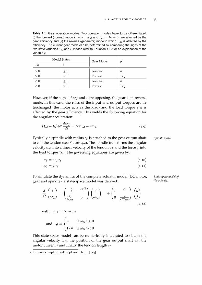
4.1 actuator dynamics 33

Table 4.1: Gear operation modes. Two operation modes have to be differentiated:

(i) the forward (normal) mode in which τEM and Jtot = JM + JG are affected by the

gear efficiency and (ii) the reverse (generator) mode in which τLG is affected by the

efficiency. The current gear mode can be determined by comparing the signs of the

two state variables ωG and i. Please refer to Equation 4.12 for an explanation of the

variable ρ.

Model StatesGear Mode ρ

ωG i

> 0 ≥ 0 Forward η

> 0 < 0 Reverse 1/η

< 0 ≤ 0 Forward η

< 0 > 0 Reverse 1/η

However, if the signs of ωG and i are opposing, the gear is in reversemode. In this case, the roles of the input and output torques are in-terchanged (the motor acts as the load) and the load torque τLG isaffected by the gear efficiency. This yields the following equation forthe angular acceleration:

(JM + JG)N2 dωG

dt= NτEM − ητLG (4.9)

Typically a spindle with radius rS is attached to the gear output shaft Spindle model

to coil the tendon (see Figure 4.2). The spindle transforms the angularvelocity ωG into a linear velocity of the tendon vT and the force f intothe load torque τLG. The governing equations are given by:

vT = ωG rS (4.10)

τLG = f rS (4.11)

To simulate the dynamics of the complete actuator model (DC motor, State-space model of

the actuatorgear and spindle), a state-space model was derived:

d

dt

(

i

ωG

)

=

−RL −KE N

L

KTNJtot

0

(

i

ωG

)

+

1L 0

0 −rS

ρN2 Jtot

(

u

f

)

(4.12)

with Jtot = JM + JG

and ρ =

η if ωG i ≥ 0

1/η if ωG i < 0

This state-space model can be numerically integrated to obtain theangular velocity ωG, the position of the gear output shaft θG, themotor current i and finally the tendon length lT.

2 for more complex models, please refer to [114]

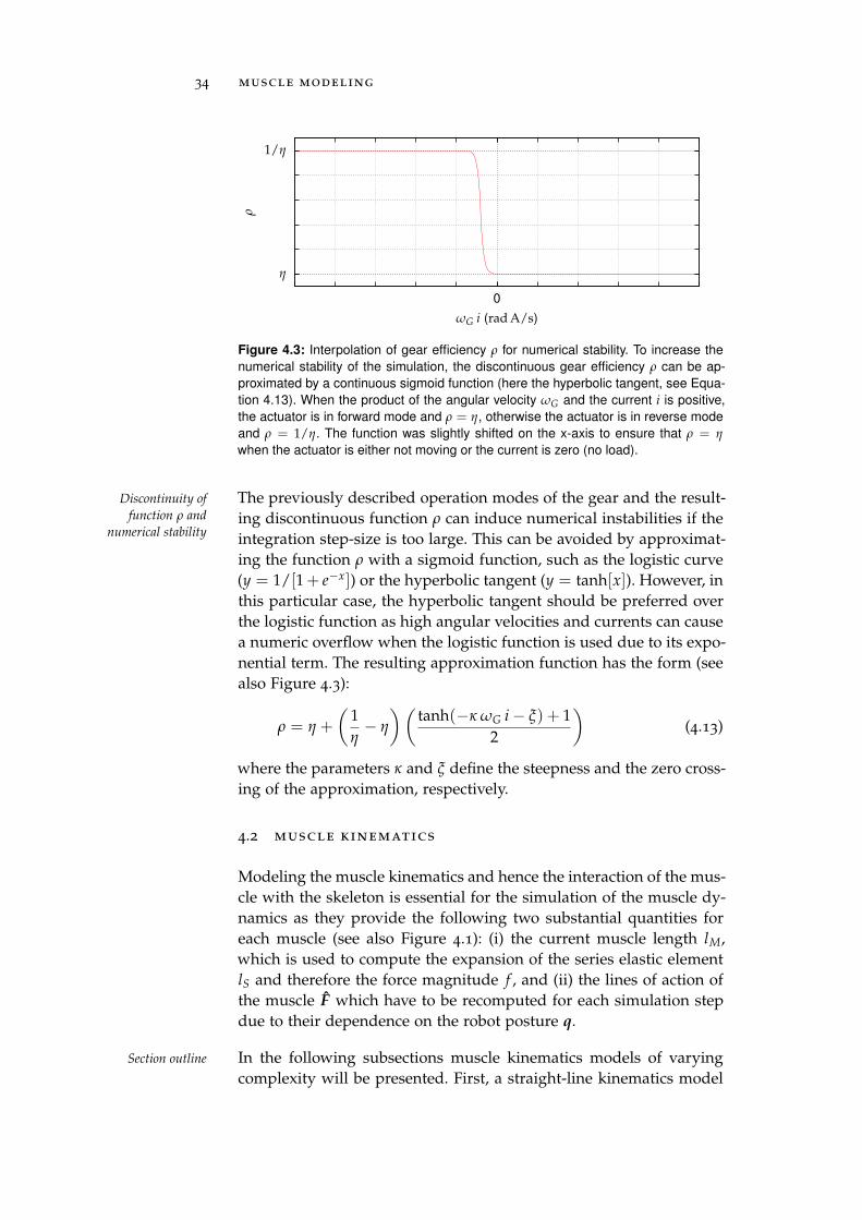
34 muscle modeling

η

1/η

0

ρ

ωG i (rad A/s)

Figure 4.3: Interpolation of gear efficiency ρ for numerical stability. To increase the

numerical stability of the simulation, the discontinuous gear efficiency ρ can be ap-

proximated by a continuous sigmoid function (here the hyperbolic tangent, see Equa-

tion 4.13). When the product of the angular velocity ωG and the current i is positive,

the actuator is in forward mode and ρ = η, otherwise the actuator is in reverse mode

and ρ = 1/η. The function was slightly shifted on the x-axis to ensure that ρ = η

when the actuator is either not moving or the current is zero (no load).

The previously described operation modes of the gear and the result-Discontinuity of

function ρ and

numerical stabilitying discontinuous function ρ can induce numerical instabilities if theintegration step-size is too large. This can be avoided by approximat-ing the function ρ with a sigmoid function, such as the logistic curve(y = 1/[1+ e−x]) or the hyperbolic tangent (y = tanh[x]). However, inthis particular case, the hyperbolic tangent should be preferred overthe logistic function as high angular velocities and currents can causea numeric overflow when the logistic function is used due to its expo-nential term. The resulting approximation function has the form (seealso Figure 4.3):

ρ = η +

(

1η− η

)(

tanh(−κ ωG i− ξ) + 12

)

(4.13)

where the parameters κ and ξ define the steepness and the zero cross-ing of the approximation, respectively.

4.2 muscle kinematics

Modeling the muscle kinematics and hence the interaction of the mus-cle with the skeleton is essential for the simulation of the muscle dy-namics as they provide the following two substantial quantities foreach muscle (see also Figure 4.1): (i) the current muscle length lM,which is used to compute the expansion of the series elastic elementlS and therefore the force magnitude f , and (ii) the lines of action ofthe muscle F which have to be recomputed for each simulation stepdue to their dependence on the robot posture q.

In the following subsections muscle kinematics models of varyingSection outline

complexity will be presented. First, a straight-line kinematics model

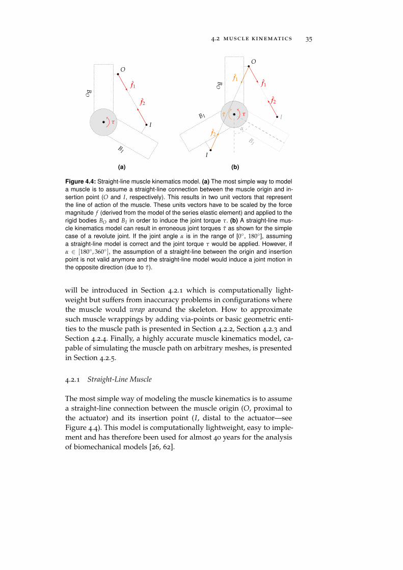
4.2 muscle kinematics 35

O

BO

I

BI

f1

f2

τ

(a)

O

BO

I

BI

I

B I

f1

f2

α

f1

f2

τ τ

(b)

Figure 4.4: Straight-line muscle kinematics model. (a) The most simple way to model

a muscle is to assume a straight-line connection between the muscle origin and in-

sertion point (O and I, respectively). This results in two unit vectors that represent

the line of action of the muscle. These units vectors have to be scaled by the force

magnitude f (derived from the model of the series elastic element) and applied to the

rigid bodies BO and BI in order to induce the joint torque τ. (b) A straight-line mus-

cle kinematics model can result in erroneous joint torques τ as shown for the simple

case of a revolute joint. If the joint angle α is in the range of [0, 180], assuming

a straight-line model is correct and the joint torque τ would be applied. However, if

α ∈ [180, 360], the assumption of a straight-line between the origin and insertion

point is not valid anymore and the straight-line model would induce a joint motion in

the opposite direction (due to τ).

will be introduced in Section 4.2.1 which is computationally light-weight but suffers from inaccuracy problems in configurations wherethe muscle would wrap around the skeleton. How to approximatesuch muscle wrappings by adding via-points or basic geometric enti-ties to the muscle path is presented in Section 4.2.2, Section 4.2.3 andSection 4.2.4. Finally, a highly accurate muscle kinematics model, ca-pable of simulating the muscle path on arbitrary meshes, is presentedin Section 4.2.5.

4.2.1 Straight-Line Muscle

The most simple way of modeling the muscle kinematics is to assumea straight-line connection between the muscle origin (O, proximal tothe actuator) and its insertion point (I, distal to the actuator—seeFigure 4.4). This model is computationally lightweight, easy to imple-ment and has therefore been used for almost 40 years for the analysisof biomechanical models [26, 62].

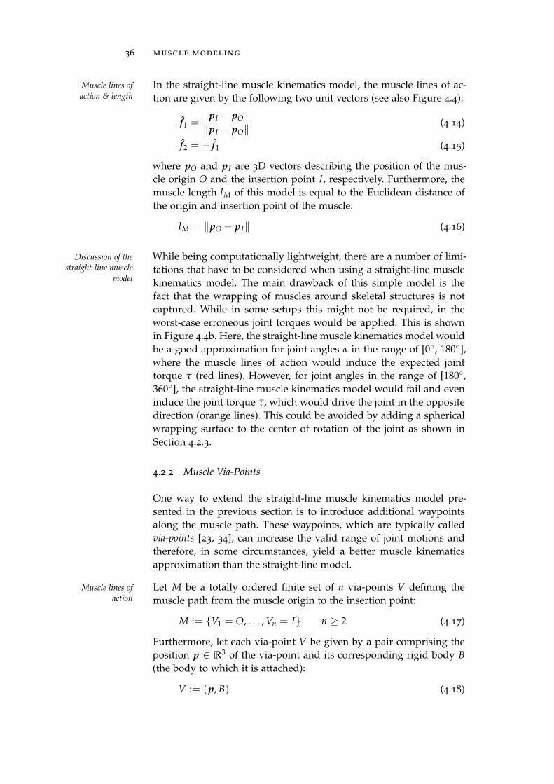
36 muscle modeling

In the straight-line muscle kinematics model, the muscle lines of ac-Muscle lines of

action & length tion are given by the following two unit vectors (see also Figure 4.4):

f1 =pI − pO

‖pI − pO‖(4.14)

f2 = − f1 (4.15)

where pO and pI are 3D vectors describing the position of the mus-cle origin O and the insertion point I, respectively. Furthermore, themuscle length lM of this model is equal to the Euclidean distance ofthe origin and insertion point of the muscle:

lM = ‖pO − pI‖ (4.16)

While being computationally lightweight, there are a number of limi-Discussion of the

straight-line muscle

modeltations that have to be considered when using a straight-line musclekinematics model. The main drawback of this simple model is thefact that the wrapping of muscles around skeletal structures is notcaptured. While in some setups this might not be required, in theworst-case erroneous joint torques would be applied. This is shownin Figure 4.4b. Here, the straight-line muscle kinematics model wouldbe a good approximation for joint angles α in the range of [0, 180],where the muscle lines of action would induce the expected jointtorque τ (red lines). However, for joint angles in the range of [180,360], the straight-line muscle kinematics model would fail and eveninduce the joint torque τ, which would drive the joint in the oppositedirection (orange lines). This could be avoided by adding a sphericalwrapping surface to the center of rotation of the joint as shown inSection 4.2.3.

4.2.2 Muscle Via-Points

One way to extend the straight-line muscle kinematics model pre-sented in the previous section is to introduce additional waypointsalong the muscle path. These waypoints, which are typically calledvia-points [23, 34], can increase the valid range of joint motions andtherefore, in some circumstances, yield a better muscle kinematicsapproximation than the straight-line model.

Let M be a totally ordered finite set of n via-points V defining theMuscle lines of

action muscle path from the muscle origin to the insertion point:

M := V1 = O, . . . , Vn = I n ≥ 2 (4.17)

Furthermore, let each via-point V be given by a pair comprising theposition p ∈ R

3 of the via-point and its corresponding rigid body B

(the body to which it is attached):

V := (p, B) (4.18)

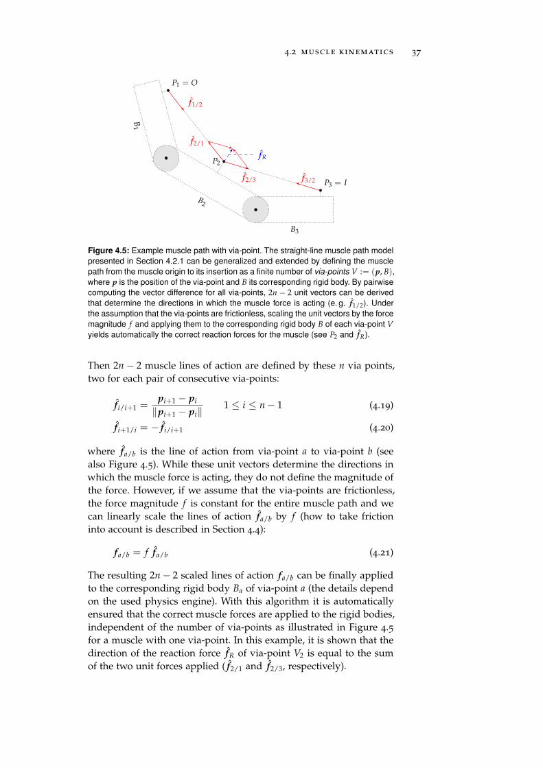
4.2 muscle kinematics 37

P1 = O

B1

P2

B2

B3

P3 = If3/2f2/3

f1/2

f2/1

fR

Figure 4.5: Example muscle path with via-point. The straight-line muscle path model

presented in Section 4.2.1 can be generalized and extended by defining the muscle

path from the muscle origin to its insertion as a finite number of via-points V := (p, B),where p is the position of the via-point and B its corresponding rigid body. By pairwise

computing the vector difference for all via-points, 2n− 2 unit vectors can be derived

that determine the directions in which the muscle force is acting (e. g. f1/2). Under

the assumption that the via-points are frictionless, scaling the unit vectors by the force

magnitude f and applying them to the corresponding rigid body B of each via-point V

yields automatically the correct reaction forces for the muscle (see P2 and fR).

Then 2n− 2 muscle lines of action are defined by these n via points,two for each pair of consecutive via-points:

fi/i+1 =pi+1 − pi

‖pi+1 − pi‖1 ≤ i ≤ n− 1 (4.19)

fi+1/i = − fi/i+1 (4.20)

where fa/b is the line of action from via-point a to via-point b (seealso Figure 4.5). While these unit vectors determine the directions inwhich the muscle force is acting, they do not define the magnitude ofthe force. However, if we assume that the via-points are frictionless,the force magnitude f is constant for the entire muscle path and wecan linearly scale the lines of action fa/b by f (how to take frictioninto account is described in Section 4.4):

fa/b = f fa/b (4.21)

The resulting 2n− 2 scaled lines of action fa/b can be finally appliedto the corresponding rigid body Ba of via-point a (the details dependon the used physics engine). With this algorithm it is automaticallyensured that the correct muscle forces are applied to the rigid bodies,independent of the number of via-points as illustrated in Figure 4.5for a muscle with one via-point. In this example, it is shown that thedirection of the reaction force fR of via-point V2 is equal to the sumof the two unit forces applied ( f2/1 and f2/3, respectively).

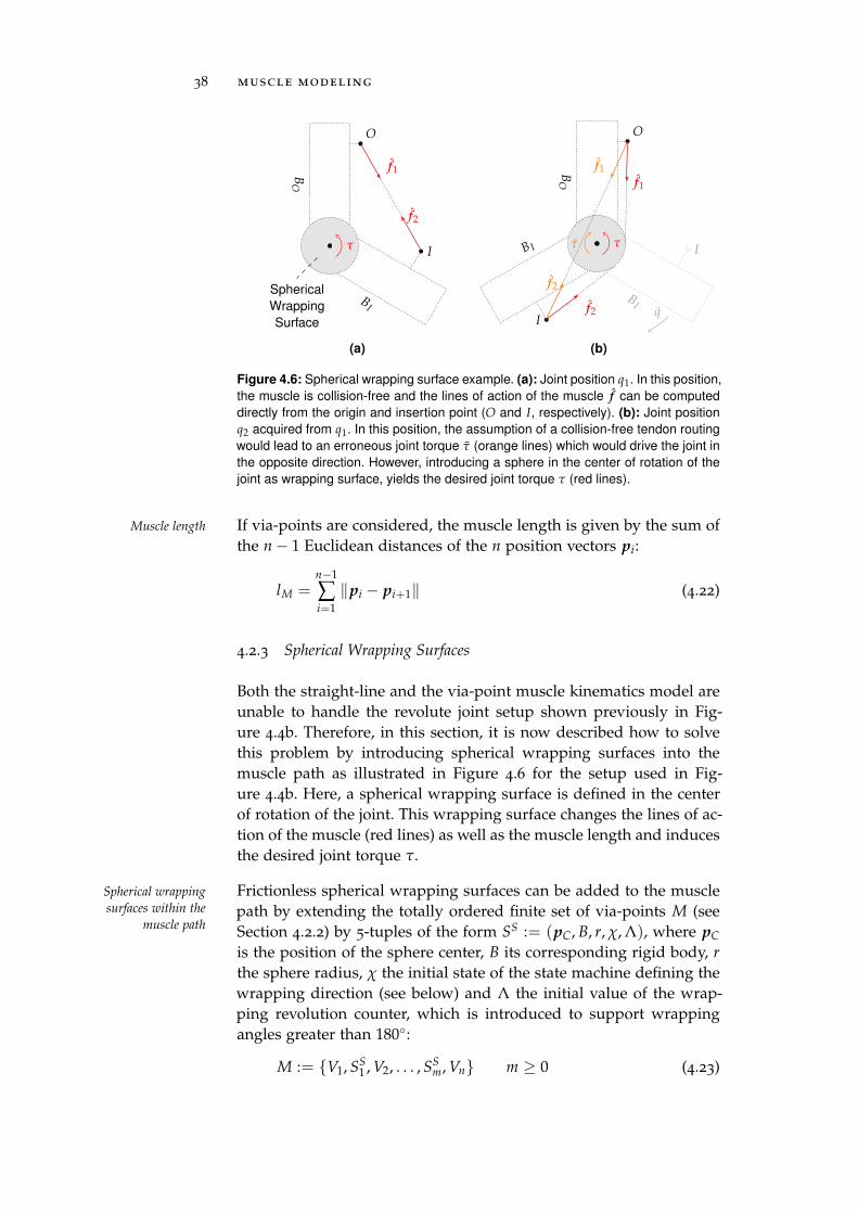
38 muscle modeling

O

BO

I

BI

f1

f2

Spherical

Wrapping

Surface

τ

(a)

O

BO

I

BI

I

B I

q

f1

f2

τ τ

f1

f2

(b)

Figure 4.6: Spherical wrapping surface example. (a): Joint position q1. In this position,

the muscle is collision-free and the lines of action of the muscle f can be computed

directly from the origin and insertion point (O and I, respectively). (b): Joint position

q2 acquired from q1. In this position, the assumption of a collision-free tendon routing

would lead to an erroneous joint torque τ (orange lines) which would drive the joint in

the opposite direction. However, introducing a sphere in the center of rotation of the

joint as wrapping surface, yields the desired joint torque τ (red lines).

If via-points are considered, the muscle length is given by the sum ofMuscle length

the n− 1 Euclidean distances of the n position vectors pi:

lM =n−1

∑i=1

‖pi − pi+1‖ (4.22)

4.2.3 Spherical Wrapping Surfaces

Both the straight-line and the via-point muscle kinematics model areunable to handle the revolute joint setup shown previously in Fig-ure 4.4b. Therefore, in this section, it is now described how to solvethis problem by introducing spherical wrapping surfaces into themuscle path as illustrated in Figure 4.6 for the setup used in Fig-ure 4.4b. Here, a spherical wrapping surface is defined in the centerof rotation of the joint. This wrapping surface changes the lines of ac-tion of the muscle (red lines) as well as the muscle length and inducesthe desired joint torque τ.

Frictionless spherical wrapping surfaces can be added to the muscleSpherical wrapping

surfaces within the

muscle pathpath by extending the totally ordered finite set of via-points M (seeSection 4.2.2) by 5-tuples of the form SS := (pC, B, r, χ, Λ), where pC

is the position of the sphere center, B its corresponding rigid body, r

the sphere radius, χ the initial state of the state machine defining thewrapping direction (see below) and Λ the initial value of the wrap-ping revolution counter, which is introduced to support wrappingangles greater than 180:

M := V1, SS1 , V2, . . . , SS

m, Vn m ≥ 0 (4.23)

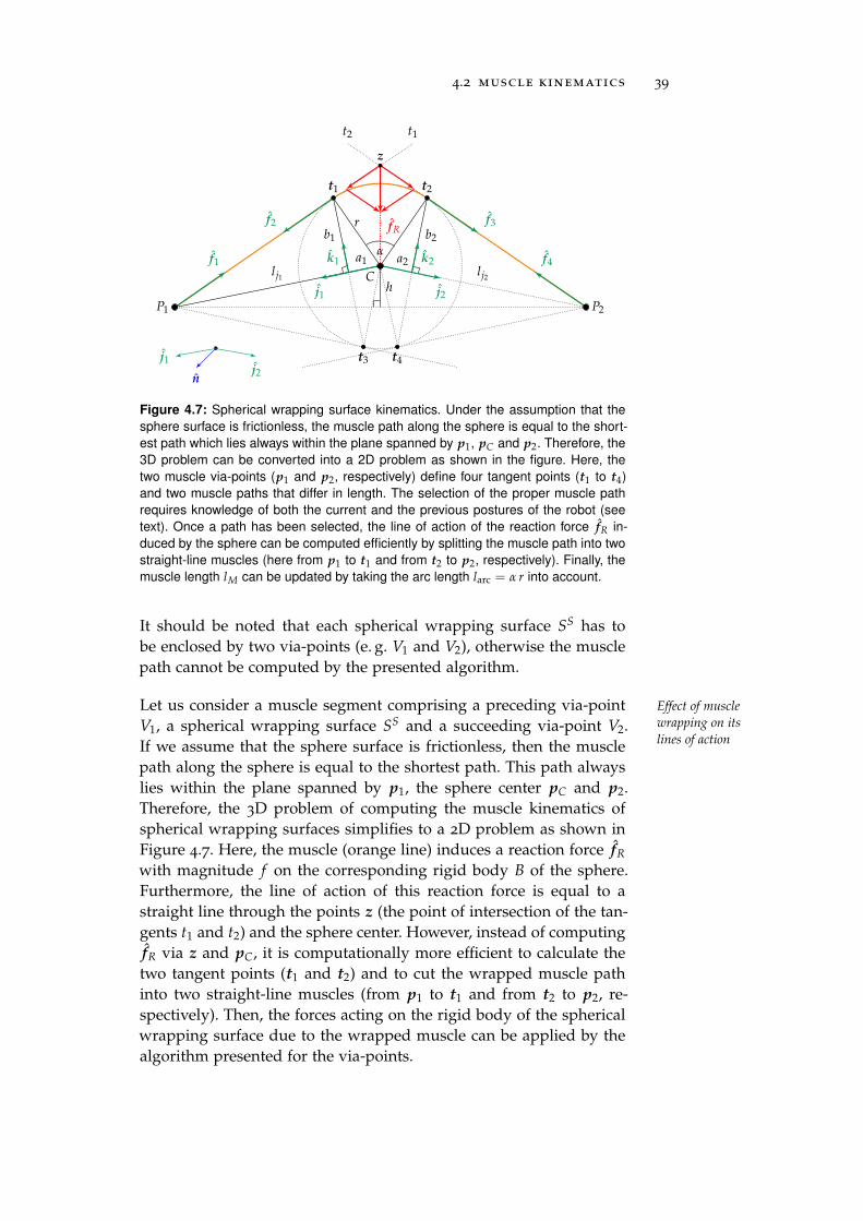
4.2 muscle kinematics 39

n

j1j2

C

P1

t1

P2

t2

lj1 lj2

fR

z

h

α

r

f1

f2

f4

f3

j1 j2

b1

k1

b2

k2a1 a2

t3

t1 t2

t4

Figure 4.7: Spherical wrapping surface kinematics. Under the assumption that the

sphere surface is frictionless, the muscle path along the sphere is equal to the short-

est path which lies always within the plane spanned by p1, pC and p2. Therefore, the

3D problem can be converted into a 2D problem as shown in the figure. Here, the

two muscle via-points (p1 and p2, respectively) define four tangent points (t1 to t4)

and two muscle paths that differ in length. The selection of the proper muscle path

requires knowledge of both the current and the previous postures of the robot (see

text). Once a path has been selected, the line of action of the reaction force fR in-

duced by the sphere can be computed efficiently by splitting the muscle path into two

straight-line muscles (here from p1 to t1 and from t2 to p2, respectively). Finally, the

muscle length lM can be updated by taking the arc length larc = α r into account.

It should be noted that each spherical wrapping surface SS has tobe enclosed by two via-points (e. g. V1 and V2), otherwise the musclepath cannot be computed by the presented algorithm.

Let us consider a muscle segment comprising a preceding via-point Effect of muscle

wrapping on its

lines of actionV1, a spherical wrapping surface SS and a succeeding via-point V2.If we assume that the sphere surface is frictionless, then the musclepath along the sphere is equal to the shortest path. This path alwayslies within the plane spanned by p1, the sphere center pC and p2.Therefore, the 3D problem of computing the muscle kinematics ofspherical wrapping surfaces simplifies to a 2D problem as shown inFigure 4.7. Here, the muscle (orange line) induces a reaction force fR

with magnitude f on the corresponding rigid body B of the sphere.Furthermore, the line of action of this reaction force is equal to astraight line through the points z (the point of intersection of the tan-gents t1 and t2) and the sphere center. However, instead of computingfR via z and pC, it is computationally more efficient to calculate thetwo tangent points (t1 and t2) and to cut the wrapped muscle pathinto two straight-line muscles (from p1 to t1 and from t2 to p2, re-spectively). Then, the forces acting on the rigid body of the sphericalwrapping surface due to the wrapped muscle can be applied by thealgorithm presented for the via-points.

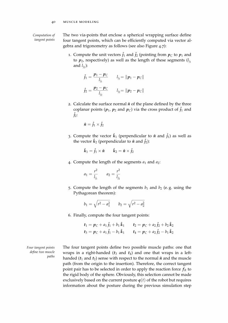
40 muscle modeling

The two via-points that enclose a spherical wrapping surface defineComputation of

tangent points four tangent points, which can be efficiently computed via vector al-gebra and trigonometry as follows (see also Figure 4.7):

1. Compute the unit vectors j1 and j2 (pointing from pC to p1 andto p2, respectively) as well as the length of these segments (lj1

and lj2):

j1 =p1 − pC

lj1

lj1= ‖p1 − pC‖

j2 =p2 − pC

lj2

lj2= ‖p2 − pC‖

2. Calculate the surface normal n of the plane defined by the threecoplanar points (p1, p2 and pC) via the cross product of j1 andj2:

n = j1 × j2

3. Compute the vector k1 (perpendicular to n and j1) as well asthe vector k2 (perpendicular to n and j2):

k1 = j1 × n k2 = n× j2

4. Compute the length of the segments a1 and a2:

a1 =r2

lj1

a2 =r2

lj2

5. Compute the length of the segments b1 and b2 (e. g. using thePythagorean theorem):

b1 =√

r2 − a21 b2 =

√

r2 − a22

6. Finally, compute the four tangent points:

t1 = pC + a1 j1 + b1 k1 t2 = pC + a2 j2 + b2 k2

t3 = pC + a1 j1 − b1 k1 t4 = pC + a2 j2 − b1 k2

The four tangent points define two possible muscle paths: one thatFour tangent points

define two muscle

pathswraps in a right-handed (t3 and t4) and one that wraps in a left-handed (t1 and t2) sense with respect to the normal n and the musclepath (from the origin to the insertion). Therefore, the correct tangentpoint pair has to be selected in order to apply the reaction force fR tothe rigid body of the sphere. Obviously, this selection cannot be madeexclusively based on the current posture q(t) of the robot but requiresinformation about the posture during the previous simulation step

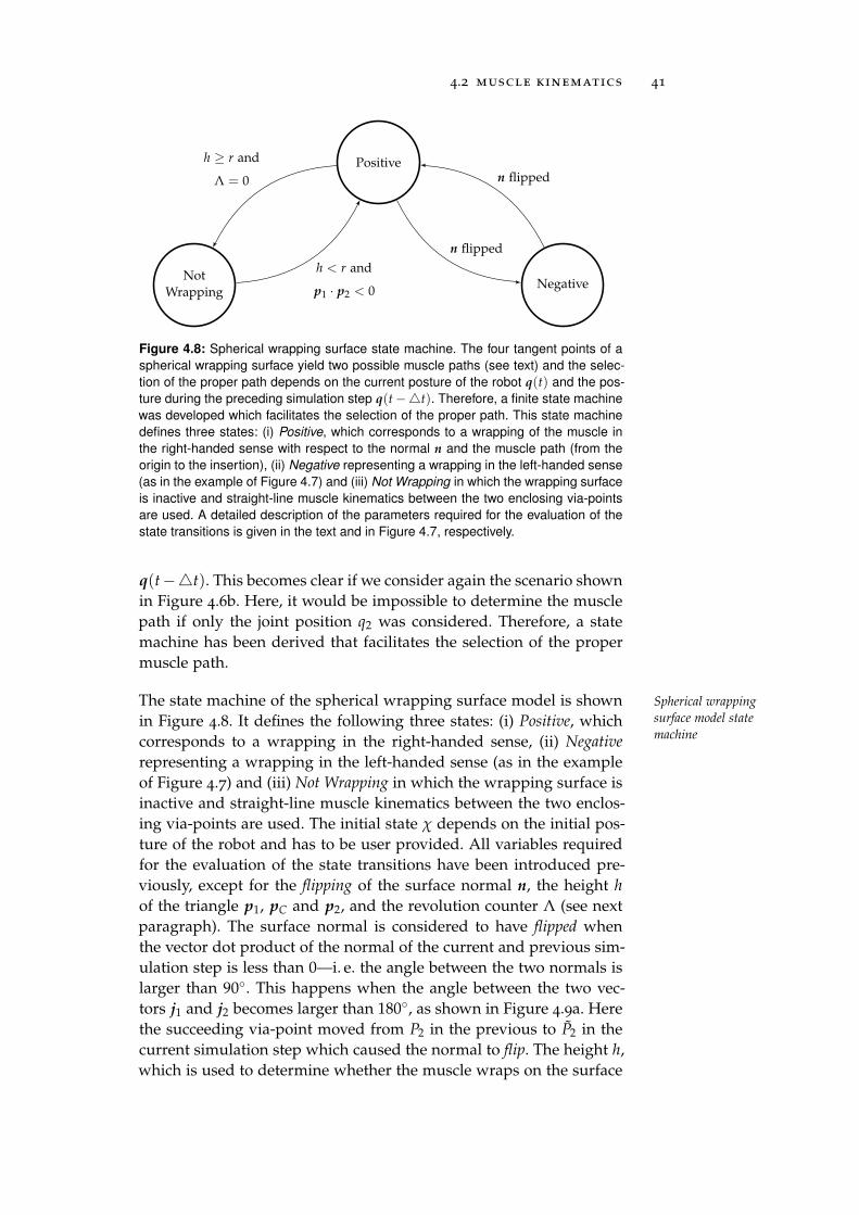
4.2 muscle kinematics 41

NotWrapping

Positive

Negativeh < r and

p1 · p2 < 0

h ≥ r and

Λ = 0

n flipped

n flipped

Figure 4.8: Spherical wrapping surface state machine. The four tangent points of a

spherical wrapping surface yield two possible muscle paths (see text) and the selec-

tion of the proper path depends on the current posture of the robot q(t) and the pos-

ture during the preceding simulation step q(t−t). Therefore, a finite state machine

was developed which facilitates the selection of the proper path. This state machine

defines three states: (i) Positive, which corresponds to a wrapping of the muscle in

the right-handed sense with respect to the normal n and the muscle path (from the

origin to the insertion), (ii) Negative representing a wrapping in the left-handed sense

(as in the example of Figure 4.7) and (iii) Not Wrapping in which the wrapping surface

is inactive and straight-line muscle kinematics between the two enclosing via-points

are used. A detailed description of the parameters required for the evaluation of the

state transitions is given in the text and in Figure 4.7, respectively.

q(t−t). This becomes clear if we consider again the scenario shownin Figure 4.6b. Here, it would be impossible to determine the musclepath if only the joint position q2 was considered. Therefore, a statemachine has been derived that facilitates the selection of the propermuscle path.

The state machine of the spherical wrapping surface model is shown Spherical wrapping

surface model state

machinein Figure 4.8. It defines the following three states: (i) Positive, whichcorresponds to a wrapping in the right-handed sense, (ii) Negative

representing a wrapping in the left-handed sense (as in the exampleof Figure 4.7) and (iii) Not Wrapping in which the wrapping surface isinactive and straight-line muscle kinematics between the two enclos-ing via-points are used. The initial state χ depends on the initial pos-ture of the robot and has to be user provided. All variables requiredfor the evaluation of the state transitions have been introduced pre-viously, except for the flipping of the surface normal n, the height h

of the triangle p1, pC and p2, and the revolution counter Λ (see nextparagraph). The surface normal is considered to have flipped whenthe vector dot product of the normal of the current and previous sim-ulation step is less than 0—i. e. the angle between the two normals islarger than 90. This happens when the angle between the two vec-tors j1 and j2 becomes larger than 180, as shown in Figure 4.9a. Herethe succeeding via-point moved from P2 in the previous to P2 in thecurrent simulation step which caused the normal to flip. The height h,which is used to determine whether the muscle wraps on the surface

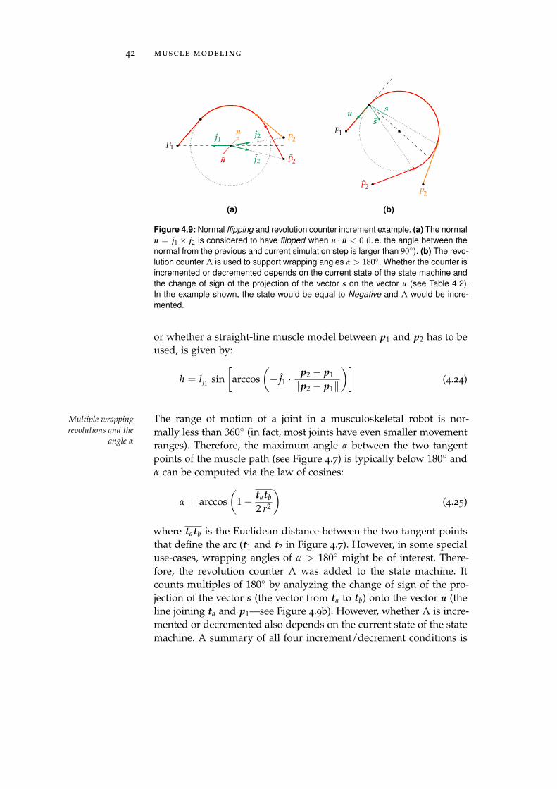
42 muscle modeling

P1

P2

P2

j1j2

j2

n

n

(a)

P1

P2P2

s

su

(b)

Figure 4.9: Normal flipping and revolution counter increment example. (a) The normal

n = j1 × j2 is considered to have flipped when n · n < 0 (i. e. the angle between the

normal from the previous and current simulation step is larger than 90). (b) The revo-

lution counter Λ is used to support wrapping angles α > 180. Whether the counter is

incremented or decremented depends on the current state of the state machine and

the change of sign of the projection of the vector s on the vector u (see Table 4.2).

In the example shown, the state would be equal to Negative and Λ would be incre-

mented.

or whether a straight-line muscle model between p1 and p2 has to beused, is given by:

h = lj1 sin[

arccos(

− j1 ·p2 − p1

‖p2 − p1‖

)]

(4.24)

The range of motion of a joint in a musculoskeletal robot is nor-Multiple wrapping

revolutions and the

angle αmally less than 360 (in fact, most joints have even smaller movementranges). Therefore, the maximum angle α between the two tangentpoints of the muscle path (see Figure 4.7) is typically below 180 andα can be computed via the law of cosines:

α = arccos(

1− tatb

2 r2

)

(4.25)

where tatb is the Euclidean distance between the two tangent pointsthat define the arc (t1 and t2 in Figure 4.7). However, in some specialuse-cases, wrapping angles of α > 180 might be of interest. There-fore, the revolution counter Λ was added to the state machine. Itcounts multiples of 180 by analyzing the change of sign of the pro-jection of the vector s (the vector from ta to tb) onto the vector u (theline joining ta and p1—see Figure 4.9b). However, whether Λ is incre-mented or decremented also depends on the current state of the statemachine. A summary of all four increment/decrement conditions is

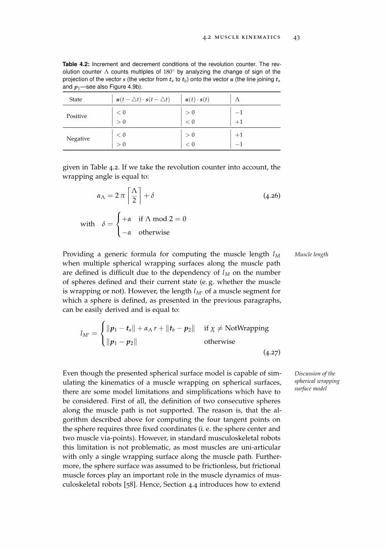
4.2 muscle kinematics 43

Table 4.2: Increment and decrement conditions of the revolution counter. The rev-

olution counter Λ counts multiples of 180 by analyzing the change of sign of the

projection of the vector s (the vector from ta to tb) onto the vector u (the line joining ta

and p1—see also Figure 4.9b).

State u(t−t) · s(t−t) u(t) · s(t) Λ

Positive< 0 > 0 −1

> 0 < 0 +1

Negative< 0 > 0 +1

> 0 < 0 −1

given in Table 4.2. If we take the revolution counter into account, thewrapping angle is equal to:

αΛ = 2 π

⌈

Λ

2

⌉

+ δ (4.26)

with δ =

+α if Λ mod 2 = 0

−α otherwise

Providing a generic formula for computing the muscle length lM Muscle length

when multiple spherical wrapping surfaces along the muscle pathare defined is difficult due to the dependency of lM on the numberof spheres defined and their current state (e. g. whether the muscleis wrapping or not). However, the length lM′ of a muscle segment forwhich a sphere is defined, as presented in the previous paragraphs,can be easily derived and is equal to:

lM′ =

‖p1 − ta‖+ αΛ r + ‖tb − p2‖ if χ 6= NotWrapping

‖p1 − p2‖ otherwise

(4.27)

Even though the presented spherical surface model is capable of sim- Discussion of the

spherical wrapping

surface modelulating the kinematics of a muscle wrapping on spherical surfaces,there are some model limitations and simplifications which have tobe considered. First of all, the definition of two consecutive spheresalong the muscle path is not supported. The reason is, that the al-gorithm described above for computing the four tangent points onthe sphere requires three fixed coordinates (i. e. the sphere center andtwo muscle via-points). However, in standard musculoskeletal robotsthis limitation is not problematic, as most muscles are uni-articularwith only a single wrapping surface along the muscle path. Further-more, the sphere surface was assumed to be frictionless, but frictionalmuscle forces play an important role in the muscle dynamics of mus-culoskeletal robots [58]. Hence, Section 4.4 introduces how to extend

44 muscle modeling

the spherical wrapping surface model with friction forces that actalong the muscle path. Finally, as the presented algorithm computesthe shortest muscle path along the sphere, the muscle can slide side-ways on the surface if the muscle path is not perpendicular to theaxis of rotation of the joint. While this behavior might be desired ifthe sphere is used in a spherical joint setup, it would result in er-roneous force vectors and muscle lengths for a revolute joint. Here,using a cylindrical wrapping surface defined parallel to the joint axiswould yield better results.

4.2.4 Cylindrical Wrapping Surfaces

An algorithm for computing the muscle kinematics when cylindricalwrapping surfaces are considered within the muscle path was devel-oped. This algorithm, which is similar to the one presented by Garnerand Pandy [34], is essentially an extension of the spherical wrappingsurface model presented in the previous section. It assumes a cylin-der of infinite height and, in contrast to [34], is capable of simulatingthe kinematics resulting from multiple muscle wrapping revolutions.

Frictionless cylindrical wrapping surfaces can be added to the muscleCylindrical

wrapping surfaces

within the muscle

path

path by extending the totally ordered finite set of via-points M (seeSection 4.2.2) by 5-tuples of the form SC := (BTC, B, r, χ, Λ), whereBTC is a transformation matrix describing the position and orienta-tion of the cylinder relative to the rigid body B, r the cylinder radius,χ the initial state of the state machine defining the wrapping direc-tion and Λ the initial value of the wrapping revolution counter (seeSection 4.2.3):

M := V1, SC1 , V2, . . . , SC

m, Vn m ≥ 0 (4.28)

Similar to the spherical wrapping surface described in Section 4.2.3,each cylinder SC has to be enclosed by two via-points (e. g. V1 and V2),otherwise the muscle path cannot be computed with the presentedalgorithm. Furthermore, it should be noted that no cylinder heightis included in the model as the cylinder is assumed to have infiniteheight.

As the cylinder surface is assumed to be frictionless, the muscle pathMuscle lines of

action along the cylinder is equal to the shortest Euclidean path from thepreceding to the succeeding via-point (p1 and p2, respectively) acrossthe cylinder surface. But what is the shortest path across a cylinder?For the spherical wrapping surface model it was possible to convertthe 3D into a 2D problem which could be solved using vector algebraand trigonometrical functions. But this was only possible as the short-est path across a sphere always lies within the plane spanned by p1,p2 and the sphere center pC. This is not the case for a cylindrical wrap-ping surface, where the path can cross the surface on any point along

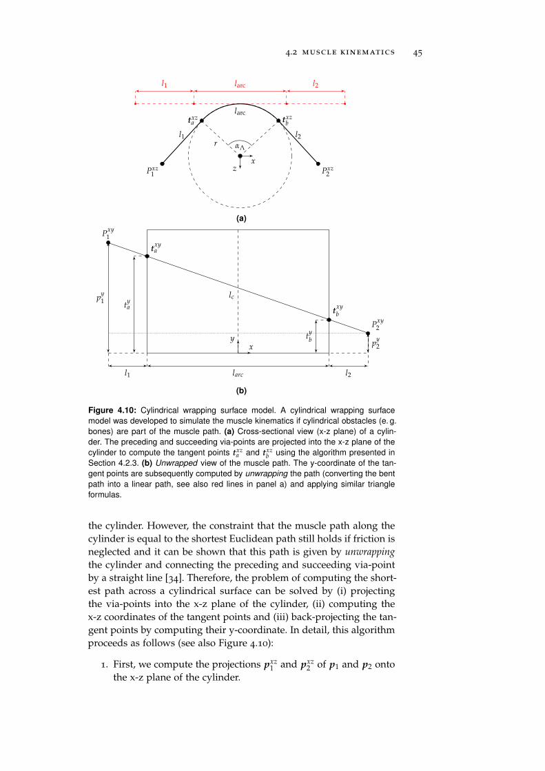
4.2 muscle kinematics 45

l1 larc l2

Pxz1 Pxz

2

αΛr

larc

l1 l2

xz

txza txz

b

(a)

lc

txya

txyb

xy

py1

l1

py2

l2larc

tya

tyb

Pxy1

Pxy2

(b)

Figure 4.10: Cylindrical wrapping surface model. A cylindrical wrapping surface

model was developed to simulate the muscle kinematics if cylindrical obstacles (e. g.

bones) are part of the muscle path. (a) Cross-sectional view (x-z plane) of a cylin-

der. The preceding and succeeding via-points are projected into the x-z plane of the

cylinder to compute the tangent points txza and txz

b using the algorithm presented in

Section 4.2.3. (b) Unwrapped view of the muscle path. The y-coordinate of the tan-

gent points are subsequently computed by unwrapping the path (converting the bent

path into a linear path, see also red lines in panel a) and applying similar triangle

formulas.

the cylinder. However, the constraint that the muscle path along thecylinder is equal to the shortest Euclidean path still holds if friction isneglected and it can be shown that this path is given by unwrapping

the cylinder and connecting the preceding and succeeding via-pointby a straight line [34]. Therefore, the problem of computing the short-est path across a cylindrical surface can be solved by (i) projectingthe via-points into the x-z plane of the cylinder, (ii) computing thex-z coordinates of the tangent points and (iii) back-projecting the tan-gent points by computing their y-coordinate. In detail, this algorithmproceeds as follows (see also Figure 4.10):

1. First, we compute the projections pxz1 and pxz

2 of p1 and p2 ontothe x-z plane of the cylinder.

46 muscle modeling

2. Then we compute the x-z coordinates of the four tangent points(txz

1 – txz4 ) using the algorithm described in Section 4.2.3.

3. These four tangent points define again two muscle paths. Weselect the proper path (txz

a and txzb , respectively) using the previ-

ously introduced state machine (see Section 4.2.3).

4. Once these points are selected, we compute the length of thesegments l1 and l2 (from pxz

1 to txza and from txz

b to pxz2 , respec-

tively) as well as the length of the arc larc in the x-z plane:

l1 = ‖pxz1 − txz

a ‖ l2 = ‖txzb − pxz

2 ‖ larc = αΛ r (4.29)

5. Now we project the tangent points back into R3 by comput-

ing their y-coordinate using similar triangle formulas (see Fig-ure 4.10b):

tya = p

y2 +

(larc + l2)(py1 − p

y2)

l1 + larc + l2(4.30)

tyb = p

y2 +

l2 (py1 − p

y2)

l1 + larc + l2(4.31)

6. Finally, we can compute the lines of action of the muscle byassuming two straight-line connections similar to the sphericalwrapping surface (from p1 to ta and from tb to p2, respectively).

Similar to the spherical wrapping surface, providing a generic for-Muscle length

mula for computing the muscle length lM when cylindrical wrappingsurfaces are part of the muscle path is difficult. Therefore, only theformula for computing the length lM′ of a muscle segment for whicha cylinder is defined is provided:

lM′ =

‖p1 − ta‖+ lc + ‖tb − p2‖ if χ 6= NotWrapping

‖p1 − p2‖ otherwise

(4.32)

with lc =√

(tya − t

yb)

2 + larc2 (4.33)

The presented cylindrical wrapping surface model is ideal for mod-Discussion of the

cylindrical wrapping

surface modeleling the kinematics of muscles that wrap around cylindrical bonesor for revolute joints where the muscle path is not perpendicular tothe joint axis—a setup where the spherical wrapping surfaces wouldperform poorly. Furthermore, in contrast to the implementation of acylindrical wrapping surface described by Garner and Pandy [34], thepresented algorithm is able to handle multiple revolutions by exploit-ing the previously described finite state machine (see Section 4.2.3).

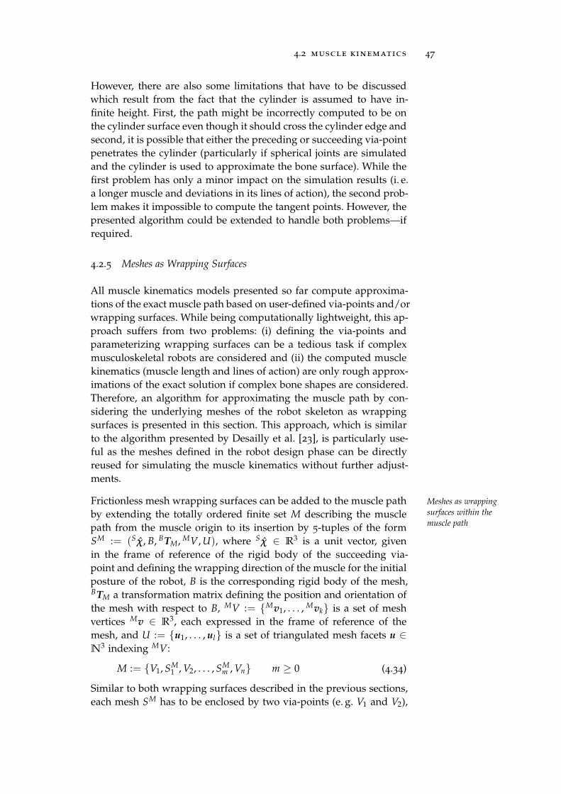
4.2 muscle kinematics 47

However, there are also some limitations that have to be discussedwhich result from the fact that the cylinder is assumed to have in-finite height. First, the path might be incorrectly computed to be onthe cylinder surface even though it should cross the cylinder edge andsecond, it is possible that either the preceding or succeeding via-pointpenetrates the cylinder (particularly if spherical joints are simulatedand the cylinder is used to approximate the bone surface). While thefirst problem has only a minor impact on the simulation results (i. e.a longer muscle and deviations in its lines of action), the second prob-lem makes it impossible to compute the tangent points. However, thepresented algorithm could be extended to handle both problems—ifrequired.

4.2.5 Meshes as Wrapping Surfaces

All muscle kinematics models presented so far compute approxima-tions of the exact muscle path based on user-defined via-points and/orwrapping surfaces. While being computationally lightweight, this ap-proach suffers from two problems: (i) defining the via-points andparameterizing wrapping surfaces can be a tedious task if complexmusculoskeletal robots are considered and (ii) the computed musclekinematics (muscle length and lines of action) are only rough approx-imations of the exact solution if complex bone shapes are considered.Therefore, an algorithm for approximating the muscle path by con-sidering the underlying meshes of the robot skeleton as wrappingsurfaces is presented in this section. This approach, which is similarto the algorithm presented by Desailly et al. [23], is particularly use-ful as the meshes defined in the robot design phase can be directlyreused for simulating the muscle kinematics without further adjust-ments.

Frictionless mesh wrapping surfaces can be added to the muscle path Meshes as wrapping

surfaces within the

muscle pathby extending the totally ordered finite set M describing the musclepath from the muscle origin to its insertion by 5-tuples of the formSM := (Sχ, B, BTM, MV, U), where Sχ ∈ R

3 is a unit vector, givenin the frame of reference of the rigid body of the succeeding via-point and defining the wrapping direction of the muscle for the initialposture of the robot, B is the corresponding rigid body of the mesh,BTM a transformation matrix defining the position and orientation ofthe mesh with respect to B, MV := Mv1, . . . , Mvk is a set of meshvertices Mv ∈ R

3, each expressed in the frame of reference of themesh, and U := u1, . . . , ul is a set of triangulated mesh facets u ∈N

3 indexing MV:

M := V1, SM1 , V2, . . . , SM

m , Vn m ≥ 0 (4.34)

Similar to both wrapping surfaces described in the previous sections,each mesh SM has to be enclosed by two via-points (e. g. V1 and V2),

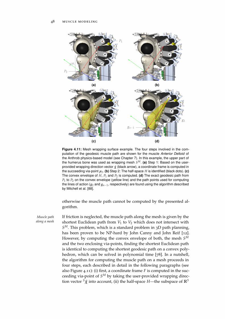
48 muscle modeling

SM

P2

P1

(a) (b)

(c)

gn−1

g2

(d)

Figure 4.11: Mesh wrapping surface example. The four steps involved in the com-

putation of the geodesic muscle path are shown for the muscle Anterior Deltoid of

the Anthrob physics-based model (see Chapter 7). In this example, the upper part of

the humerus bone was used as wrapping mesh SM. (a) Step 1: Based on the user-

provided wrapping direction vector χ (black arrow), a coordinate frame is computed in

the succeeding via-point p2. (b) Step 2: The half-space H is identified (black dots). (c)

The convex envelope of H, P1 and P2 is computed. (d) The exact geodesic path from

P1 to P2 on the convex envelope (yellow line) and the path points used for computing

the lines of action (g2 and gn−1, respectively) are found using the algorithm described

by Mitchell et al. [88].

otherwise the muscle path cannot be computed by the presented al-gorithm.

If friction is neglected, the muscle path along the mesh is given by theMuscle path

along a mesh shortest Euclidean path from V1 to V2 which does not intersect withSM. This problem, which is a standard problem in 3D path planning,has been proven to be NP-hard by John Canny and John Reif [12].However, by computing the convex envelope of both, the mesh SM

and the two enclosing via-points, finding the shortest Euclidean pathis identical to computing the shortest geodesic path on a convex poly-hedron, which can be solved in polynomial time [78]. In a nutshell,the algorithm for computing the muscle path on a mesh proceeds infour steps, each described in detail in the following paragraphs (seealso Figure 4.11): (i) first, a coordinate frame F is computed in the suc-ceeding via-point of SM by taking the user-provided wrapping direc-tion vector Sχ into account, (ii) the half-space H—the subspace of R

3

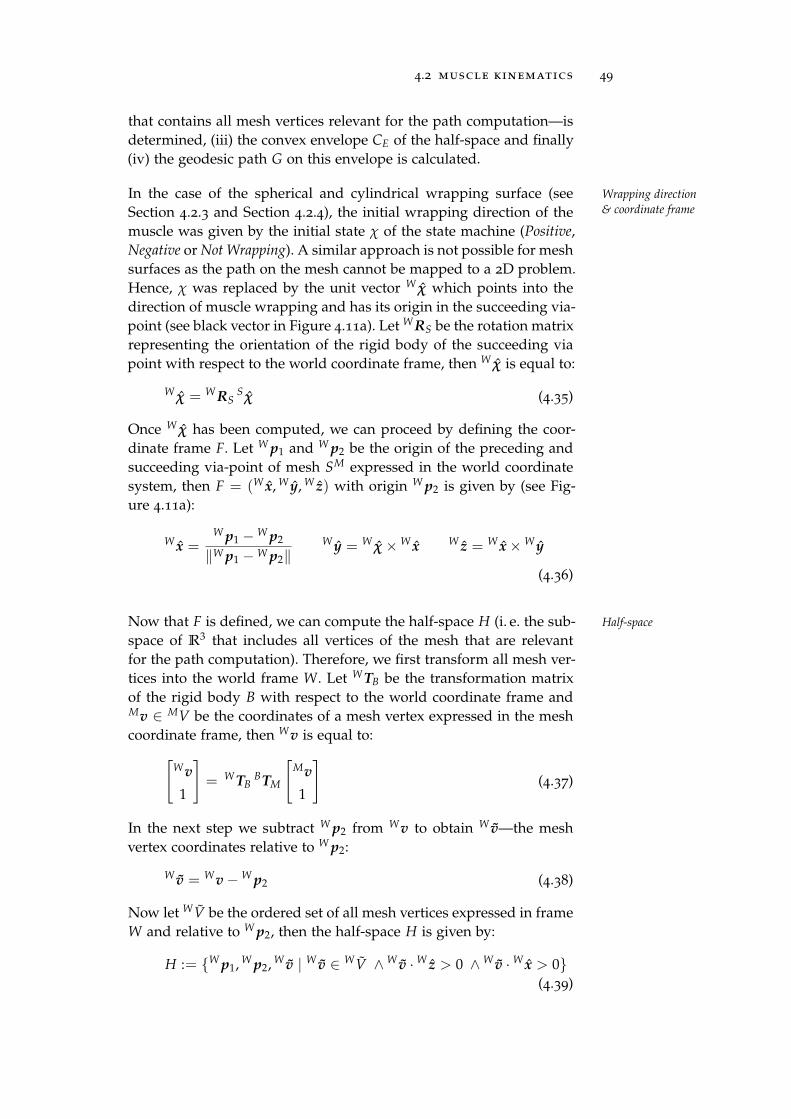
4.2 muscle kinematics 49

that contains all mesh vertices relevant for the path computation—isdetermined, (iii) the convex envelope CE of the half-space and finally(iv) the geodesic path G on this envelope is calculated.

In the case of the spherical and cylindrical wrapping surface (see Wrapping direction

& coordinate frameSection 4.2.3 and Section 4.2.4), the initial wrapping direction of themuscle was given by the initial state χ of the state machine (Positive,Negative or Not Wrapping). A similar approach is not possible for meshsurfaces as the path on the mesh cannot be mapped to a 2D problem.Hence, χ was replaced by the unit vector W χ which points into thedirection of muscle wrapping and has its origin in the succeeding via-point (see black vector in Figure 4.11a). Let W RS be the rotation matrixrepresenting the orientation of the rigid body of the succeeding viapoint with respect to the world coordinate frame, then W χ is equal to:

W χ = W RSSχ (4.35)

Once W χ has been computed, we can proceed by defining the coor-dinate frame F. Let W p1 and W p2 be the origin of the preceding andsucceeding via-point of mesh SM expressed in the world coordinatesystem, then F = (W x, W y, W z) with origin W p2 is given by (see Fig-ure 4.11a):

W x =W p1 −W p2

‖W p1 −W p2‖W y = W χ×W x W z = W x×W y

(4.36)

Now that F is defined, we can compute the half-space H (i. e. the sub- Half-space

space of R3 that includes all vertices of the mesh that are relevant

for the path computation). Therefore, we first transform all mesh ver-tices into the world frame W. Let W TB be the transformation matrixof the rigid body B with respect to the world coordinate frame andMv ∈ MV be the coordinates of a mesh vertex expressed in the meshcoordinate frame, then Wv is equal to:

[

Wv

1

]

= W TBBTM

[

Mv

1

]

(4.37)

In the next step we subtract W p2 from Wv to obtain W v—the meshvertex coordinates relative to W p2:

W v = Wv−W p2 (4.38)

Now let WV be the ordered set of all mesh vertices expressed in frameW and relative to W p2, then the half-space H is given by:

H := W p1, W p2, W v | W v ∈ WV ∧W v ·W z > 0 ∧W v ·W x > 0(4.39)

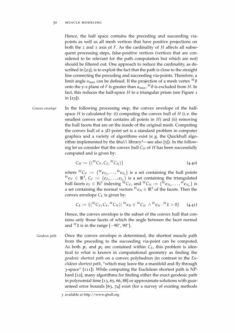
50 muscle modeling

Hence, the half space contains the preceding and succeeding via-points as well as all mesh vertices that have positive projections onboth the z and x axis of F. As the cardinality of H affects all subse-quent processing steps, false-positive vertices (vertices that are con-sidered to be relevant for the path computation but which are not)should be filtered out. One approach to reduce the cardinality, as de-scribed in [23], is to exploit the fact that the path is close to the straightline connecting the preceding and succeeding via-points. Therefore, alimit angle αmax can be defined. If the projection of a mesh vertex W v

onto the y-z plane of F is greater than αmax, W v is excluded from H. Infact, this reduces the half-space H to a triangular prism (see Figure 1

in [23]).

In the following processing step, the convex envelope of the half-Convex envelope

space H is calculated by: (i) computing the convex hull of H (i. e. thesmallest convex set that contains all points in H) and (ii) removingthe hull facets that are on the inside of the original mesh. Computingthe convex hull of a 3D point set is a standard problem in computergraphics and a variety of algorithms exist (e. g. the Quickhull algo-rithm implemented by the Qhull library3—see also [5]). In the follow-ing let us consider that the convex hull CH of H has been successfullycomputed and is given by:

CH := (WCV , CF, WCN) (4.40)

where WCV := WcV1 , . . . , WcVo is a set containing the hull pointsWcV ∈ R

3, CF := cF1 , . . . , cFp is a set containing the triangulatedhull facets cF ∈ N

3 indexing WCV , and WCN := WcN1 , . . . , WcNp isa set containing the normal vectors WcN ∈ R

3 of the facets. Then theconvex envelope CE is given by:

CE := (WCV , CF, WCN)| WcN ∈ WCN ∧WcN ·W z > 0 (4.41)

Hence, the convex envelope is the subset of the convex hull that con-tains only those facets of which the angle between the facet normaland W z is in the range [−90, 90].

Once the convex envelope is determined, the shortest muscle pathGeodesic path

from the preceding to the succeeding via-point can be computed.As both p1 and p2 are contained within CE, this problem is iden-tical to what is known in computational geometry as finding thegeodesic shortest path on a convex polyhedron (in contrast to the Eu-

clidean shortest path, “which may leave the 2-manifold and fly through3-space” [111]). While computing the Euclidean shortest path is NP-hard [12], many algorithms for finding either the exact geodesic pathin polynomial time [13, 65, 66, 88] or approximate solutions with guar-anteed error bounds [63, 74] exist (for a survey of existing methods

3 available at http://www.qhull.org

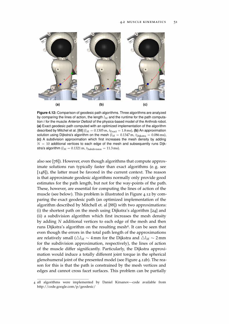
4.2 muscle kinematics 51

(a) (b) (c)

Figure 4.12: Comparison of geodesic path algorithms. Three algorithms are analyzed

by comparing the lines of action, the length lM and the runtime for the path computa-

tion t for the muscle Anterior Deltoid of the physics-based model of the Anthrob robot.

(a) Exact geodesic path computed with an optimized implementation of the algorithm

described by Mitchel et al. [88] (lM = 0.1305 m, tExact = 1.8 ms), (b) An approximation

solution using Dijkstra’s algorithm on the mesh (lM = 0.1347 m, tDijkstra = 0.086 ms),

(c) A subdivision approximation which first increases the mesh density by adding

N = 10 additional vertices to each edge of the mesh and subsequently runs Dijk-

stra’s algorithm (lM = 0.1321 m, tSubdivision = 11.3 ms).

also see [78]). However, even though algorithms that compute approx-imate solutions run typically faster than exact algorithms (e. g. see[148]), the latter must be favored in the current context. The reasonis that approximate geodesic algorithms normally only provide goodestimates for the path length, but not for the way-points of the path.These, however, are essential for computing the lines of action of themuscle (see below). This problem is illustrated in Figure 4.12 by com-paring the exact geodesic path (an optimized implementation of thealgorithm described by Mitchell et. al [88]) with two approximations:(i) the shortest path on the mesh using Dijkstra’s algorithm [24] and(ii) a subdivision algorithm which first increases the mesh densityby adding N additional vertices to each edge of the mesh and thenruns Dijkstra’s algorithm on the resulting mesh4. It can be seen thateven though the errors in the total path length of the approximationsare relatively small (lM ∼ 4 mm for the Dijkstra and lM ∼ 2 mmfor the subdivision approximation, respectively), the lines of actionof the muscle differ significantly. Particularly, the Dijkstra approxi-mation would induce a totally different joint torque in the sphericalglenohumeral joint of the presented model (see Figure 4.12b). The rea-son for this is that the path is constrained by the mesh vertices andedges and cannot cross facet surfaces. This problem can be partially

4 all algorithms were implemented by Daniel Kirsanov—code available fromhttp://code.google.com/p/geodesic/

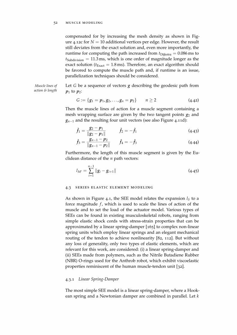
52 muscle modeling

compensated for by increasing the mesh density as shown in Fig-ure 4.12c for N = 10 additional vertices per edge. However, the resultstill deviates from the exact solution and, even more importantly, theruntime for computing the path increased from tDijkstra = 0.086 ms totSubdivision = 11.3 ms, which is one order of magnitude longer as theexact solution (tExact = 1.8 ms). Therefore, an exact algorithm shouldbe favored to compute the muscle path and, if runtime is an issue,parallelization techniques should be considered.

Let G be a sequence of vectors g describing the geodesic path fromMuscle lines of

action & length p1 to p2:

G := g1 = p1, g2, . . . , gn = p2 n ≥ 2 (4.42)

Then the muscle lines of action for a muscle segment containing amesh wrapping surface are given by the two tangent points g2 andgn−1 and the resulting four unit vectors (see also Figure 4.11d):

f1 =g2 − p1

‖g2 − p1‖f2 = − f1 (4.43)

f3 =gn−1 − p2

‖gn−1 − p2‖f4 = − f3 (4.44)

Furthermore, the length of this muscle segment is given by the Eu-clidean distance of the n path vectors:

lM′ =n−1

∑i=1

‖gi − gi+1‖ (4.45)

4.3 series elastic element modeling

As shown in Figure 4.1, the SEE model relates the expansion lS to aforce magnitude f , which is used to scale the lines of action of themuscle and to set the load of the actuator model. Various types ofSEEs can be found in existing musculoskeletal robots, ranging fromsimple elastic shock cords with stress-strain properties that can beapproximated by a linear spring-damper [165] to complex non-linearspring units which employ linear springs and an elegant mechanicalrouting of the tendon to achieve nonlinearity [82, 112]. But withoutany loss of generality, only two types of elastic elements, which arerelevant for this work, are considered: (i) a linear spring-damper and(ii) SEEs made from polymers, such as the Nitrile Butadiene Rubber(NBR) O-rings used for the Anthrob robot, which exhibit viscoelasticproperties reminiscent of the human muscle-tendon unit [32].

4.3.1 Linear Spring-Damper

The most simple SEE model is a linear spring-damper, where a Hook-ean spring and a Newtonian damper are combined in parallel. Let k

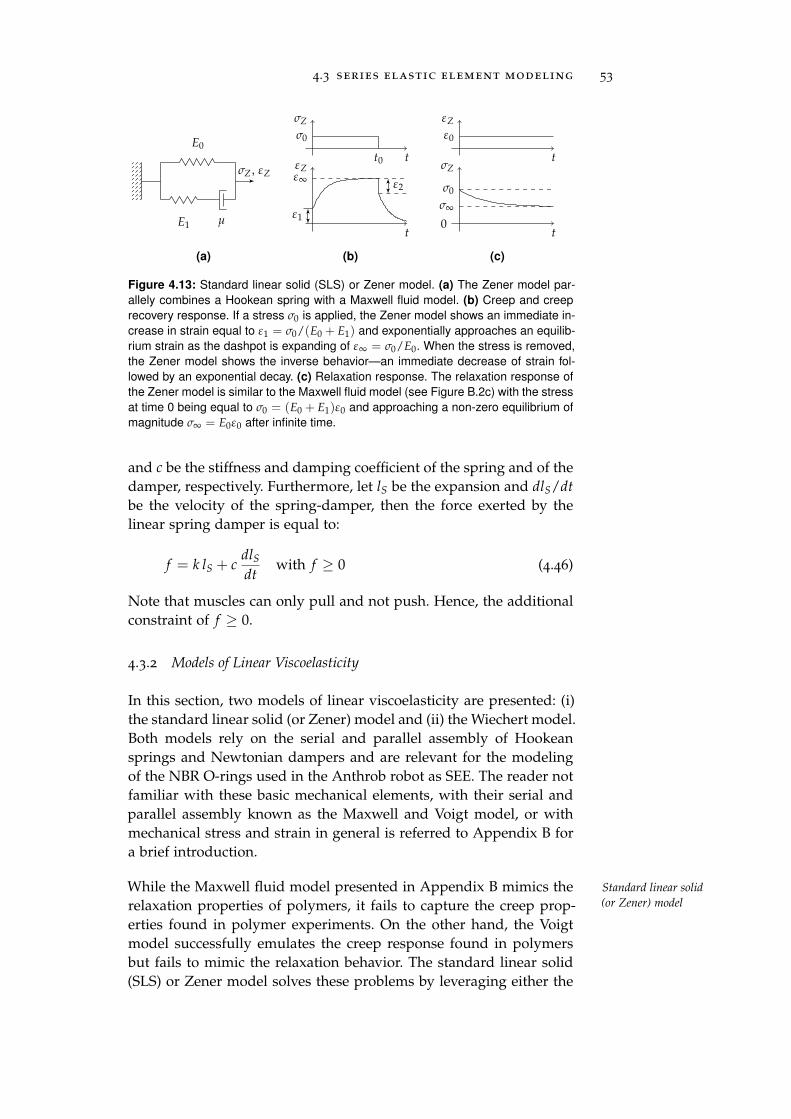
4.3 series elastic element modeling 53

µ

E0

E1

σZ, εZ

(a)

t

σZ

σ0

t0

t

εZ

ε1

ε∞ ε2

(b)

t

εZ

ε0

0t

σZ

σ0

σ∞

(c)

Figure 4.13: Standard linear solid (SLS) or Zener model. (a) The Zener model par-

allely combines a Hookean spring with a Maxwell fluid model. (b) Creep and creep

recovery response. If a stress σ0 is applied, the Zener model shows an immediate in-

crease in strain equal to ε1 = σ0/(E0 + E1) and exponentially approaches an equilib-

rium strain as the dashpot is expanding of ε∞ = σ0/E0. When the stress is removed,

the Zener model shows the inverse behavior—an immediate decrease of strain fol-

lowed by an exponential decay. (c) Relaxation response. The relaxation response of

the Zener model is similar to the Maxwell fluid model (see Figure B.2c) with the stress

at time 0 being equal to σ0 = (E0 + E1)ε0 and approaching a non-zero equilibrium of

magnitude σ∞ = E0ε0 after infinite time.

and c be the stiffness and damping coefficient of the spring and of thedamper, respectively. Furthermore, let lS be the expansion and dlS/dt

be the velocity of the spring-damper, then the force exerted by thelinear spring damper is equal to:

f = k lS + cdlS

dtwith f ≥ 0 (4.46)

Note that muscles can only pull and not push. Hence, the additionalconstraint of f ≥ 0.

4.3.2 Models of Linear Viscoelasticity

In this section, two models of linear viscoelasticity are presented: (i)the standard linear solid (or Zener) model and (ii) the Wiechert model.Both models rely on the serial and parallel assembly of Hookeansprings and Newtonian dampers and are relevant for the modelingof the NBR O-rings used in the Anthrob robot as SEE. The reader notfamiliar with these basic mechanical elements, with their serial andparallel assembly known as the Maxwell and Voigt model, or withmechanical stress and strain in general is referred to Appendix B fora brief introduction.

While the Maxwell fluid model presented in Appendix B mimics the Standard linear solid

(or Zener) modelrelaxation properties of polymers, it fails to capture the creep prop-erties found in polymer experiments. On the other hand, the Voigtmodel successfully emulates the creep response found in polymersbut fails to mimic the relaxation behavior. The standard linear solid(SLS) or Zener model solves these problems by leveraging either the

54 muscle modeling

Voigt solid model with a serial spring—the Voigt form of the SLSmodel [4, 10]—or by extending the Maxwell fluid model with a paral-lel, linear spring as shown in Figure 4.13a. This variant of the SLSmodel, which is typically referred to as the Maxwell form of theSLS [4, 18] or Zener model [131], should be preferred over the Voigtform of the SLS if the stress is to be computed from a strain input.The differential equation of the Zener model is given by [18]:

σZ +E1

µσZ = εZ(E0 + E1) +

E0E1

µεZ (4.47)

where σZ is the stress, εZ the strain, µ the viscosity of the dashpotand E0 as well as E1 are the Young’s moduli of the two springs. Theresponse of the Zener model to creep and relaxation tests is shown inFigure 4.13b and 4.13c, respectively. In the creep test, the Zener modelshows an immediate increase in strain ε1 in response to the appliedstress σ0, equal to:

ε1 =σ0

E0 + E1(4.48)

This step-response is followed by an exponential increase in straindue to the expanding dashpot, similar to the Voigt model (see Fig-ure B.3b). As the strain of the spring in the Maxwell branch decreaseswhen the dashpot strain is increasing, the equilibrium strain of theZener model ε∞ is equal to:

ε∞ =σ0

E0(4.49)

Finally, the creep recovery response of the Zener model shows theinverse behavior of the creep case. Upon stress removal, the strainimmediately decreases by ε2. However, the magnitude of ε2 dependson the current expansion of the spring in the Maxwell branch at thetime when the stress is removed and is bound by:

0 ≤ ε2 ≤σ0

E0 + E1(4.50)

In the relaxation test, the Zener model exhibits a similar response asthe Maxwell fluid model (see Figure B.2c) with two differences. First,the initial stress σ0 at time 0 is equal to the sum of the stresses of thetwo springs:

σ0 = (E0 + E1) ε0 (4.51)

And second, the equilibrium stress σ∞ is non-zero and given by:

σ∞ = E0 ε0 (4.52)

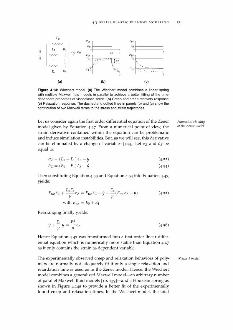
4.3 series elastic element modeling 55

E0

µ1E1

µnEn

σW , εW

(a)

t

σW

σ0

t0

t

εW

ε1

ε∞ ε2

(b)

t

εW

ε0

t

σWσ0

σ∞

(c)

Figure 4.14: Wiechert model. (a) The Wiechert model combines a linear spring

with multiple Maxwell fluid models in parallel to achieve a better fitting of the time-

dependent properties of viscoelastic solids. (b) Creep and creep recovery response.

(c) Relaxation response. The dashed and dotted lines in panels (b) and (c) show the

contribution of two Maxwell terms to the stress and strain trajectories.

Let us consider again the first order differential equation of the Zener Numerical stability

of the Zener modelmodel given by Equation 4.47. From a numerical point of view, thestrain derivative contained within the equation can be problematicand induce simulation instabilities. But, as we will see, this derivativecan be eliminated by a change of variables [144]. Let σZ and σZ beequal to:

σZ = (E0 + E1) εZ − y (4.53)

σZ = (E0 + E1) εZ − y (4.54)

Then substituting Equation 4.53 and Equation 4.54 into Equation 4.47,yields:

Etot εZ +E0E1

µεZ = Etot εZ − y +

E1

µ(Etot εZ − y) (4.55)

with Etot = E0 + E1

Rearranging finally yields:

y +E1

µy =

E21

µεZ (4.56)

Hence Equation 4.47 was transformed into a first order linear differ-ential equation which is numerically more stable than Equation 4.47

as it only contains the strain as dependent variable.

The experimentally observed creep and relaxation behaviors of poly- Wiechert model

mers are normally not adequately fit if only a single relaxation andretardation time is used as in the Zener model. Hence, the Wiechertmodel combines a generalized Maxwell model—an arbitrary numberof parallel Maxwell fluid models [10, 139]—and a Hookean spring asshown in Figure 4.14a to provide a better fit of the experimentallyfound creep and relaxation times. In the Wiechert model, the total

56 muscle modeling

stress σW is equal to the sum of the stress of the spring σs and the n

Maxwell terms:

σW = σs +n

∑i=1

σMi(4.57)

whereas the strain εW is identical for all branches due to the paralleldesign of the model:

εW = εs = εM1 = . . . = εMn (4.58)

Substituting the basic constitutive equations for the spring and theMaxwell fluid model (Equation B.6 and B.10, respectively) into Equa-tion 4.57 and 4.58 and solving for σW yields an inhomogeneous lineardifferential equation of order n. Under the assumption that at t = 0a constant strain ε0 is applied—as in the relaxation test—the solutionof this differential equation is equal to:

σW =

[

n

∑i=1

Ei exp (−t/τi) + E0

]

ε0 (4.59)

which is simply the sum of the stress induced by the free spring andof the n Maxwell terms (the term τi is the relaxation time constant ofthe ith Maxwell term—see Appendix B). It should be noted, that solv-ing this differential equation for the strain, as required for the creeptest, is more complicated and neglected in the context of this work. Inthat case, the Voigt form of the Wiechert model—a Hookean springin series with n Voigt models—should be preferred over the Wiechertmodel [10]. Qualitative responses of the Wiechert model with twoMaxwell terms to creep, creep recovery and relaxation experimentsare shown in Figure 4.14b and 4.14c, respectively.

4.4 muscle friction

In the muscle kinematics models presented so far, friction was ne-glected which allowed for the computation of the muscle path by com-puting the shortest path based on geometrical considerations. How-ever, frictional muscle forces play an important role in the dynam-ics of musculoskeletal robots [58] and two types of muscle frictionforces can be differentiated: (i) forces that alter the muscle path and(ii) forces that do not. While for the latter the muscle path is still equiv-alent to the shortest path, this is not the case for the former. Hence,the friction forces which alter the path cannot be modeled by geomet-ric considerations alone, but require a physical representation of themuscle within the dynamics engine (e. g. using soft-body dynamics).Preliminary tests of such soft-body muscles have revealed two mainproblems [165]: (i) a high computational load, impeding real-time sim-ulations of even simple models, and (ii) simulation instabilities due

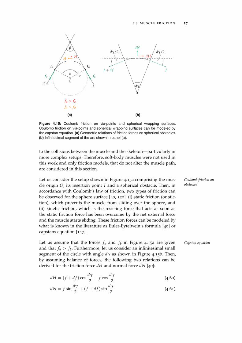
4.4 muscle friction 57

OI

αfa fbr

ta tb

C

β

HH

fa > fb

fa < fb

(a)

ff + d f

dN

dH

dγ

dγ/2 dγ/2

(b)

Figure 4.15: Coulomb friction on via-points and spherical wrapping surfaces.

Coulomb friction on via-points and spherical wrapping surfaces can be modeled by

the capstan equation. (a) Geometric relations of friction forces on spherical obstacles.

(b) Infinitesimal segment of the arc shown in panel (a).

to the collisions between the muscle and the skeleton—particularly inmore complex setups. Therefore, soft-body muscles were not used inthis work and only friction models, that do not alter the muscle path,are considered in this section.

Let us consider the setup shown in Figure 4.15a comprising the mus- Coulomb friction on

obstaclescle origin O, its insertion point I and a spherical obstacle. Then, inaccordance with Coulomb’s law of friction, two types of friction canbe observed for the sphere surface [40, 120]: (i) static friction (or stic-tion), which prevents the muscle from sliding over the sphere, and(ii) kinetic friction, which is the resisting force that acts as soon asthe static friction force has been overcome by the net external forceand the muscle starts sliding. These friction forces can be modeled bywhat is known in the literature as Euler-Eytelwein’s formula [40] orcapstans equation [147].

Let us assume that the forces fa and fb in Figure 4.15a are given Capstan equation

and that fa > fb. Furthermore, let us consider an infinitesimal smallsegment of the circle with angle dγ as shown in Figure 4.15b. Then,by assuming balance of forces, the following two relations can bederived for the friction force dH and normal force dN [40]:

dH = ( f + d f ) cosdγ

2− f cos

dγ

2(4.60)

dN = f sindγ

2+ ( f + d f ) sin

dγ

2(4.61)

58 muscle modeling

As dγ is infinitesimal, cos(dγ/2) ≈ 1, sin(dγ/2) ≈ dγ/2 and theproduct d f dγ can be neglected. This simplifies Equation 4.60 andEquation 4.61 to:

dH = d f (4.62)

dN = f dγ (4.63)

Now, in accordance with Coulomb’s law of friction the friction forceH is proportional to the normal force N with the proportionality con-stant given by the friction coefficient µ:

H = µN (4.64)

Hence, by applying Equation 4.64 to Equation 4.62 and Equation 4.63,we can eliminate the normal force:

d f = µ f dγ (4.65)

Rearranging yields:

d f

f= µdγ (4.66)

Finally, integrating over the complete wrapping angle α provides thecapstan equation which relates the forces on both sides of the spheri-cal obstacle:

∫ fa

fb

1f

d f =∫ α

0µdγ (4.67)

lnfa

fb= µα (4.68)

fa = fb e µα (4.69)

Now let us first consider the static friction case. In accordance withStatic friction on

spherical obstacles Coulomb’s law of friction, the static friction force Hs is equal to:

Hs ≤ µsN with Hs ∈ [0, µsN] (4.70)

where µs is the static friction coefficient. Then the muscle is not slid-ing on the surface (v = 0) as long as the following inequalities aresatisfied:

fa ≤ fb e µsα if fa > fb ∧ v = 0 (4.71)

fa ≥ fb e−µsα if fa < fb ∧ v = 0 (4.72)

As mentioned previously, static friction transforms into kinetic fric-Kinetic friction on

spherical obstacles tion Hk once the static friction is overcome and the muscle starts slid-ing on the sphere with v 6= 0. But, as Hk is opposing the net external

4.4 muscle friction 59

forces, we have to consider again two cases: (i) the muscle is slid-ing on the surface in the direction of the origin (v < 0) and (ii) themuscle is sliding in the direction of the insertion (v > 0). These con-siderations yield the following two equations for relating the muscleforces:

fa = fb e µk α if v < 0 (4.73)

fa = fb e−µk α if v > 0 (4.74)

where µk is the kinetic friction coefficient.

When numerically simulating static and kinetic friction, three prob- Combined static and

kinetic friction

simulation modellems are encountered: (i) Hs is discontinuous at v = 0 as it can takeany value in the range [0, µsN], (ii) the fact that µs is typically higherthan µk [40, 85] introduces a second discontinuity at the transitionfrom static to kinetic friction and (iii) the friction force changes itssign as it always opposes the net external force. These problems canbe solved by using a continuous function for both the sign of the forceand the transition between static and kinetic friction and by approxi-mating the static friction force in the zero velocity vicinity via a linearor sigmoid function [1]. Thus, if the previously introduced Stribeckfriction curve [146] is used to model the static-to-kinetic friction tran-sition and the logistic function for the zero velocity approximation,the resulting continuous friction coefficient µs+k is given by:

µs+k =

[

21 + e−κ v/vs

− 1]

[

µk + (µs − µk)e−|v|/vs

]

(4.75)

where vs is the Stribeck velocity and κ a parameter defining the steep-ness of the approximation around v = 0. This results in the followingfinal equation for the friction on spherical obstacles:

fa = fb e µs+k α (4.76)

Hence, static and kinetic friction as well as the two cases consideredfor each of the friction types previously were combined in a single,continuous equation.

If spherical wrapping surfaces are considered, Equation 4.76 can be Friction on spherical

wrapping surfaces

and via-pointsapplied directly by replacing α with the wrapping angle αΛ (see Equa-tion 4.26). However, if via-points are considered, Equation 4.76 stillholds but α has to be computed from the angle β between the preced-ing and succeeding muscle segments (see also Figure 4.15a):

α = π − β (4.77)

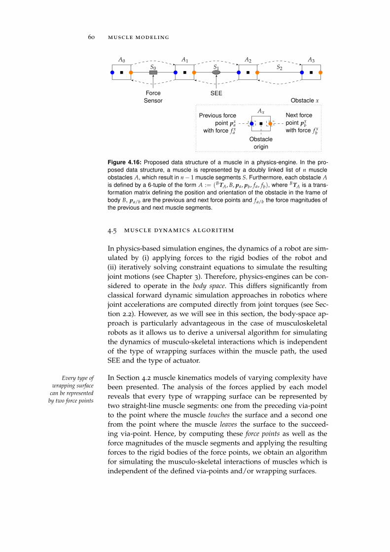
60 muscle modeling

S0 S1 S2

A0 A1 A2 A3

SEEForce

Sensor Obstacle x

AxPrevious force

point pxa

with force f xa

Next force

point pxb

with force f xb

Obstacle

origin

Figure 4.16: Proposed data structure of a muscle in a physics-engine. In the pro-

posed data structure, a muscle is represented by a doubly linked list of n muscle

obstacles A, which result in n− 1 muscle segments S. Furthermore, each obstacle A

is defined by a 6-tuple of the form A := (BTA, B, pa, pb, fa, fb), where BTA is a trans-

formation matrix defining the position and orientation of the obstacle in the frame of

body B, pa/b are the previous and next force points and fa/b the force magnitudes of

the previous and next muscle segments.

4.5 muscle dynamics algorithm

In physics-based simulation engines, the dynamics of a robot are sim-ulated by (i) applying forces to the rigid bodies of the robot and(ii) iteratively solving constraint equations to simulate the resultingjoint motions (see Chapter 3). Therefore, physics-engines can be con-sidered to operate in the body space. This differs significantly fromclassical forward dynamic simulation approaches in robotics wherejoint accelerations are computed directly from joint torques (see Sec-tion 2.2). However, as we will see in this section, the body-space ap-proach is particularly advantageous in the case of musculoskeletalrobots as it allows us to derive a universal algorithm for simulatingthe dynamics of musculo-skeletal interactions which is independentof the type of wrapping surfaces within the muscle path, the usedSEE and the type of actuator.

In Section 4.2 muscle kinematics models of varying complexity haveEvery type of

wrapping surface

can be represented

by two force points

been presented. The analysis of the forces applied by each modelreveals that every type of wrapping surface can be represented bytwo straight-line muscle segments: one from the preceding via-pointto the point where the muscle touches the surface and a second onefrom the point where the muscle leaves the surface to the succeed-ing via-point. Hence, by computing these force points as well as theforce magnitudes of the muscle segments and applying the resultingforces to the rigid bodies of the force points, we obtain an algorithmfor simulating the musculo-skeletal interactions of muscles which isindependent of the defined via-points and/or wrapping surfaces.

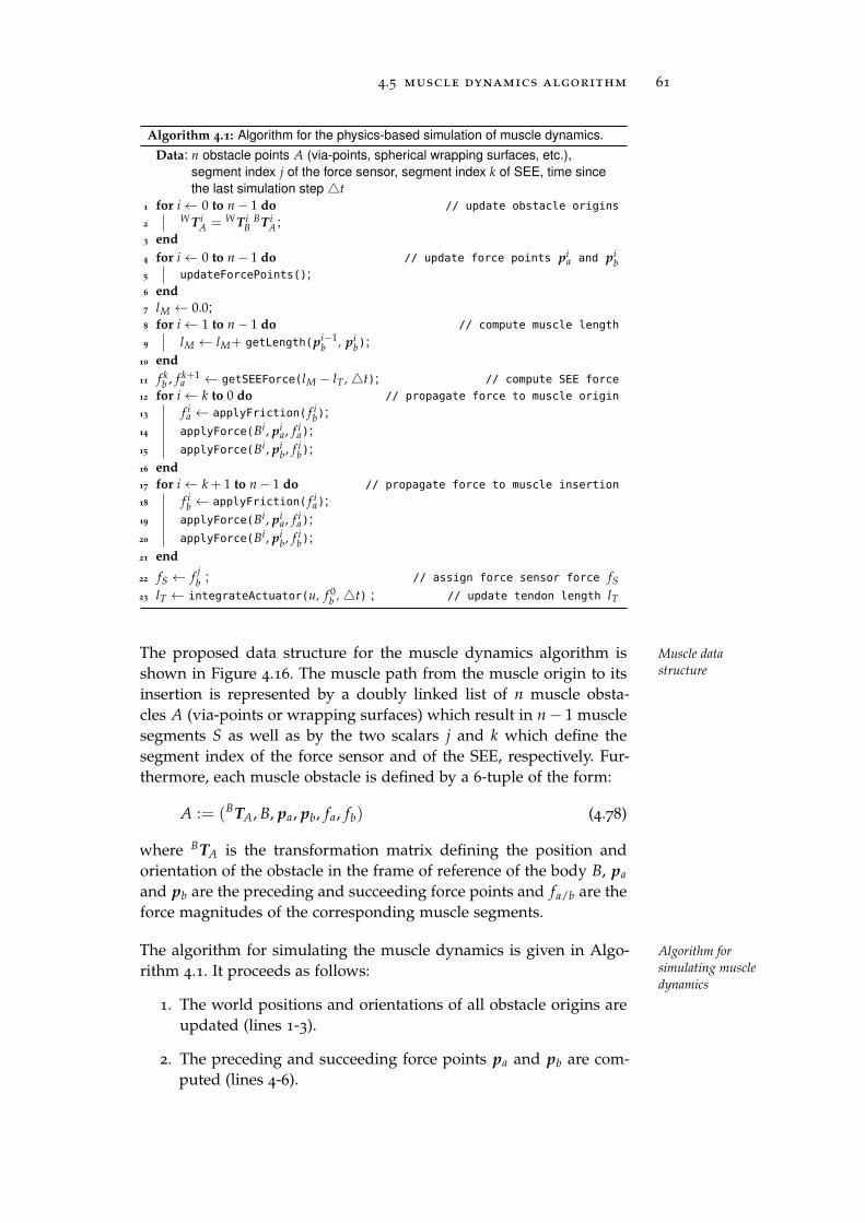
4.5 muscle dynamics algorithm 61

Algorithm 4.1: Algorithm for the physics-based simulation of muscle dynamics.

Data: n obstacle points A (via-points, spherical wrapping surfaces, etc.),

segment index j of the force sensor, segment index k of SEE, time since

the last simulation step t

1 for i← 0 to n− 1 do // update obstacle origins

2W T i

A = W T iB

BT iA;

3 end

4 for i← 0 to n− 1 do // update force points pia and pi

b5 updateForcePoints();

6 end

7 lM ← 0.0;

8 for i← 1 to n− 1 do // compute muscle length

9 lM ← lM+ getLength(pi−1b , pi

b);

10 end

11 f kb , f k+1

a ← getSEEForce(lM − lT , t); // compute SEE force

12 for i← k to 0 do // propagate force to muscle origin

13 f ia ← applyFriction( f i

b);

14 applyForce(Bi, pia, f i

a);

15 applyForce(Bi, pib, f i

b);

16 end

17 for i← k + 1 to n− 1 do // propagate force to muscle insertion

18 f ib ← applyFriction( f i

a);

19 applyForce(Bi, pia, f i

a);

20 applyForce(Bi, pib, f i

b);

21 end

22 fS ← fjb ; // assign force sensor force fS

23 lT ← integrateActuator(u, f 0b , t) ; // update tendon length lT

The proposed data structure for the muscle dynamics algorithm is Muscle data

structureshown in Figure 4.16. The muscle path from the muscle origin to itsinsertion is represented by a doubly linked list of n muscle obsta-cles A (via-points or wrapping surfaces) which result in n− 1 musclesegments S as well as by the two scalars j and k which define thesegment index of the force sensor and of the SEE, respectively. Fur-thermore, each muscle obstacle is defined by a 6-tuple of the form:

A := (BTA, B, pa, pb, fa, fb) (4.78)

where BTA is the transformation matrix defining the position andorientation of the obstacle in the frame of reference of the body B, pa

and pb are the preceding and succeeding force points and fa/b are theforce magnitudes of the corresponding muscle segments.

The algorithm for simulating the muscle dynamics is given in Algo- Algorithm for

simulating muscle

dynamicsrithm 4.1. It proceeds as follows:

1. The world positions and orientations of all obstacle origins areupdated (lines 1-3).

2. The preceding and succeeding force points pa and pb are com-puted (lines 4-6).

62 muscle modeling

3. The length of the muscle lM is calculated (lines 7-10).

4. The expansion of the SEE and hence the force f is computedand set for the muscle segment k of the SEE (line 11).

5. f is applied to the rigid bodies of the obstacles. Possible frictionforces are considered by successively propagating f from k tothe muscle origin and insertion (lines 12-19).

6. The force sensor force is assigned by taking the force sensorsegment index j into account (line 20).

7. Finally, the tendon length lT is updated by integrating the actu-ator model (line 21).

The functions in Algorithm 4.1 (e. g. updateForcePoints) are purevirtual functions which have to be implemented by the concrete typeof obstacle (e. g. spherical wrapping surface), SEE and actuator.

4.6 discussion

In this chapter, the modeling of muscle kinematics within the physics-Role of tendon

radius in muscle

kinematicsbased framework was introduced. But so far, the tendon radius wasnot taken into account by the presented models. This simplificationis reasonable when the tendon radius is small but results in non-negligible errors for thick tendons due to the offset in the force points.In these cases, a readjustment of the force points to match the tendoncenter is required. This can be achieved either online or offline bymanually adjusting the via-point origins and by inflating the wrap-ping surfaces. However, the tendon radius not only affects the musclekinematics but also the actuator dynamics model. Here, the tendonradius increases the spindle radius and therefore the linear velocity ofthe tendon. Hence, when this is a concern, the tendon radius shouldbe added to the spindle radius.

In some musculoskeletal robots stiff muscles, i. e. muscles withoutStiff muscles

SEE are used. These muscles cannot be modeled accurately in thephysics-based framework as the force of the SEE is a prerequisite forthe computation of the actuator load as well as for the forces appliedto the rigid bodies of the skeleton. Hence, if a perfectly stiff muscleis considered, two questions arise: (i) what is the force applied by themuscle and (ii) what is the magnitude of the actuator load? Whilefor the former the output force of the actuator can be used, the lattercannot be determined as it depends on a variety of factors, such asthe number and the mass of the rigid bodies affected by the muscle.Hence, stiff muscles can only be approximated. Typically, an SEE witha high spring stiffness is an adequate substitute.

4.6 discussion 63

In anatomy, a ligament denotes passive fibers attached to two neigh- Ligaments

boring bones that constrain the joint motion [134]. Hence, in the pre-sented framework, a ligament can be simulated as a passive muscle,i. e. a muscle without actuator and with a constant tendon length.

Muscle friction plays an important role in the muscle dynamics as Muscle friction

shown in [58]. Hence, a friction model based on the capstan equationwas introduced. However, this friction model only alters the forcemagnitude but not the muscle path. The reason is that all presentedmuscle kinematics algorithms rely on geometrical considerations ofthe path and do not take physical properties of the muscle, such as themass of the tendon, into account. While, at first glance, this seems tobe a serious limitation of the chosen approach, the simulation-realitygap measured for the physics-based model of the Anthrob proves theopposite (see Chapter 8).

5M O D E L C A L I B R AT I O N

Today, computer simulations are available for many different use-cases in science and engineering. But independent of the use-case andthe model complexity, every simulation exhibits a more or less promi-nent simulation-reality gap. There are two main sources for these dis-crepancies: (i) model errors and (ii) parameter errors. Model errorsresult from the formulation of the used models and are difficult tofix. If, for instance, the muscle kinematics are modeled by a straight-line connection and muscle wrapping occurs in the robot, the modelwill never be able to faithfully reproduce the outputs of the real sys-tem (e. g. muscle force or joint position trajectories). Parameter errors,in contrast, are errors that result from the wrong parametrization ofthe models. These errors can be minimized by adjusting the modelparameters to match the input-output behavior of the real system.This process, which is illustrated in Figure 5.1, is called model cali-

bration [69]. In this chapter, a model calibration method for the opti-mization of the statics (i. e. the simulation-reality gap of equilibriumpostures) and dynamics (i. e. the simulation-reality gap of trajectories)of physics-based, musculoskeletal robot models is presented. The cal-ibration method uses an ES to minimize the joint position and muscleforce error of the model. These output variables have been selectedas they are particularly important for deploying the physics-basedmodel as an offline virtual test-bed for joint or operational space con-trollers or as an online internal model for robot control.

The used ES algorithm is presented in Section 5.1. As we will see,evolution strategies are particularly suited for this use-case as theoptimization algorithm can be applied directly to the physics-basedmodel and no analytical model representation is required. Further-more, the ES procedure is generic in the sense that the algorithm isindependent of the used input and output variables. This is achievedby using a problem-specific objective function that evaluates inputsto the model and computes the model error. Two objective functionshave been developed to calibrate: (i) the statics and (ii) the dynam-ics of musculoskeletal robots. These objective functions are presentedin Section 5.2 and Section 5.3, respectively. The presented calibrationmethod has been evaluated by applying it to the physics-based modelof the Anthrob robot in Chapter 8.

65

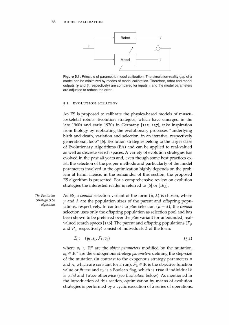
66 model calibration

Robot

Model

y

y

−u

Figure 5.1: Principle of parametric model calibration. The simulation-reality gap of a

model can be minimized by means of model calibration. Therefore, robot and model

outputs (y and y, respectively) are compared for inputs u and the model parameters

are adjusted to reduce the error.

5.1 evolution strategy

An ES is proposed to calibrate the physics-based models of muscu-loskeletal robots. Evolution strategies, which have emerged in thelate 1960s and early 1970s in Germany [125, 137], take inspirationfrom Biology by replicating the evolutionary processes “underlyingbirth and death, variation and selection, in an iterative, respectivelygenerational, loop” [6]. Evolution strategies belong to the larger classof Evolutionary Algorithms (EA) and can be applied to real-valuedas well as discrete search spaces. A variety of evolution strategies hasevolved in the past 40 years and, even though some best practices ex-ist, the selection of the proper methods and particularly of the modelparameters involved in the optimization highly depends on the prob-lem at hand. Hence, in the remainder of this section, the proposedES algorithm is presented. For a comprehensive review on evolutionstrategies the interested reader is referred to [6] or [163].

As ES, a comma selection variant of the form (µ, λ) is chosen, whereThe Evolution

Strategy (ES)

algorithmµ and λ are the population sizes of the parent and offspring popu-lations, respectively. In contrast to plus selection (µ + λ), the comma

selection uses only the offspring population as selection pool and hasbeen shown to be preferred over the plus variant for unbounded, real-valued search spaces [136]. The parent and offspring populations (Pp

and Po, respectively) consist of individuals I of the form:

Ik := (yk, sk,Fk, vk) (5.1)

where yk ∈ Rn are the object parameters modified by the mutation,

sk ∈ Rm are the endogenous strategy parameters defining the step-size

of the mutation (in contrast to the exogenous strategy parameters µ

and λ, which are constant for a run), Fk ∈ R is the objective functionvalue or fitness and vk is a Boolean flag, which is true if individual k

is valid and false otherwise (see Evaluation below). As mentioned inthe introduction of this section, optimization by means of evolutionstrategies is performed by a cyclic execution of a series of operations.

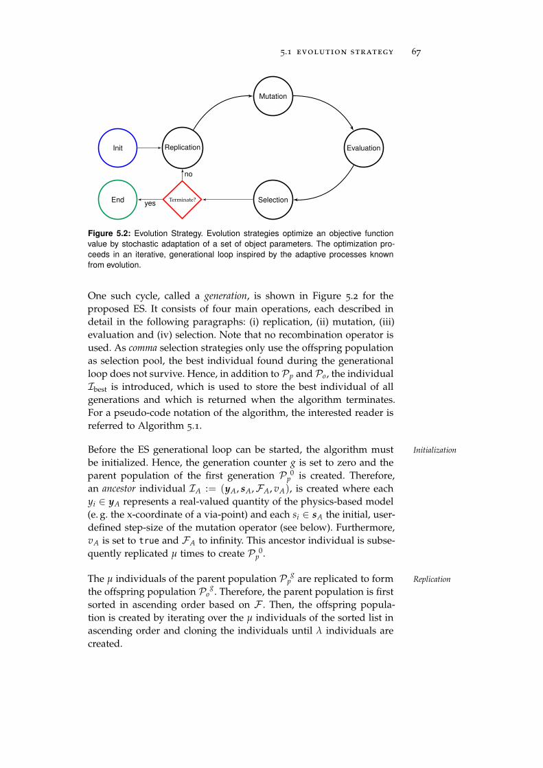
5.1 evolution strategy 67

ReplicationInit

Mutation

Evaluation

Terminate?End Selection

no

yes

Figure 5.2: Evolution Strategy. Evolution strategies optimize an objective function

value by stochastic adaptation of a set of object parameters. The optimization pro-

ceeds in an iterative, generational loop inspired by the adaptive processes known

from evolution.

One such cycle, called a generation, is shown in Figure 5.2 for theproposed ES. It consists of four main operations, each described indetail in the following paragraphs: (i) replication, (ii) mutation, (iii)evaluation and (iv) selection. Note that no recombination operator isused. As comma selection strategies only use the offspring populationas selection pool, the best individual found during the generationalloop does not survive. Hence, in addition to Pp and Po, the individualIbest is introduced, which is used to store the best individual of allgenerations and which is returned when the algorithm terminates.For a pseudo-code notation of the algorithm, the interested reader isreferred to Algorithm 5.1.

Before the ES generational loop can be started, the algorithm must Initialization

be initialized. Hence, the generation counter g is set to zero and theparent population of the first generation P 0

p is created. Therefore,an ancestor individual IA := (yA, sA,FA, vA), is created where eachyi ∈ yA represents a real-valued quantity of the physics-based model(e. g. the x-coordinate of a via-point) and each si ∈ sA the initial, user-defined step-size of the mutation operator (see below). Furthermore,vA is set to true and FA to infinity. This ancestor individual is subse-quently replicated µ times to create P 0

p .

The µ individuals of the parent population P gp are replicated to form Replication

the offspring population P go . Therefore, the parent population is first

sorted in ascending order based on F . Then, the offspring popula-tion is created by iterating over the µ individuals of the sorted list inascending order and cloning the individuals until λ individuals arecreated.

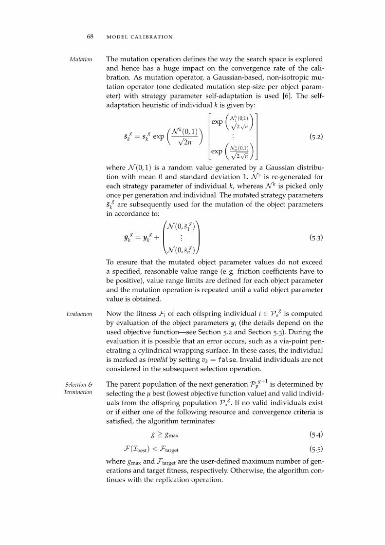
68 model calibration

The mutation operation defines the way the search space is exploredMutation

and hence has a huge impact on the convergence rate of the cali-bration. As mutation operator, a Gaussian-based, non-isotropic mu-tation operator (one dedicated mutation step-size per object param-eter) with strategy parameter self-adaptation is used [6]. The self-adaptation heuristic of individual k is given by:

sg

k = sg

k exp(N k(0, 1)√

2n

)

exp(

N s1 (0,1)√2√

n

)

...

exp(

N sm(0,1)√2√

n

)

(5.2)

where N (0, 1) is a random value generated by a Gaussian distribu-tion with mean 0 and standard deviation 1. N s is re-generated foreach strategy parameter of individual k, whereas N k is picked onlyonce per generation and individual. The mutated strategy parameterss

gk are subsequently used for the mutation of the object parameters

in accordance to:

yg

k = yg

k +

N (0, sg

1 )...

N (0, sg

n )

(5.3)

To ensure that the mutated object parameter values do not exceeda specified, reasonable value range (e. g. friction coefficients have tobe positive), value range limits are defined for each object parameterand the mutation operation is repeated until a valid object parametervalue is obtained.

Now the fitness Fi of each offspring individual i ∈ P go is computedEvaluation

by evaluation of the object parameters yi (the details depend on theused objective function—see Section 5.2 and Section 5.3). During theevaluation it is possible that an error occurs, such as a via-point pen-etrating a cylindrical wrapping surface. In these cases, the individualis marked as invalid by setting vk = false. Invalid individuals are notconsidered in the subsequent selection operation.

The parent population of the next generation P g+1p is determined bySelection &

Termination selecting the µ best (lowest objective function value) and valid individ-uals from the offspring population P g

o . If no valid individuals existor if either one of the following resource and convergence criteria issatisfied, the algorithm terminates:

g ≥ gmax (5.4)

F (Ibest) < Ftarget (5.5)

where gmax and Ftarget are the user-defined maximum number of gen-erations and target fitness, respectively. Otherwise, the algorithm con-tinues with the replication operation.

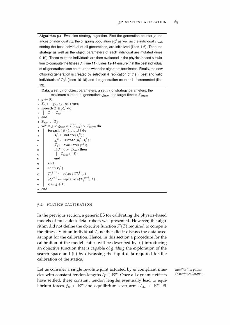
5.2 statics calibration 69

Algorithm 5.1: Evolution strategy algorithm. First the generation counter g, the

ancestor individual IA, the offspring population P 0p as well as the individual Ibest,

storing the best individual of all generations, are initialized (lines 1-6). Then the

strategy as well as the object parameters of each individual are mutated (lines

9-10). These mutated individuals are then evaluated in the physics-based simula-

tion to compute the fitness Fi (line 11). Lines 12-14 ensure that the best individual

of all generations can be returned when the algorithm terminates. Finally, the new

offspring generation is created by selection & replication of the µ best and valid

individuals of P go (lines 16-18) and the generation counter is incremented (line

19).

Data: a set yA of object parameters, a set sA of strategy parameters, the

maximum number of generations gmax, the target fitness Ftarget

1 g← 0;

2 IA ← (yA, sA, ∞, true);

3 foreach I ∈ P 0o do

4 I ← IA;

5 end

6 Ibest ← IA;

7 while g < gmax ∧ F (Ibest) > Ftarget do

8 foreach i ∈ 1, . . . , λ do

9 sg

i ← mutate(sg

i );

10 yg

i ← mutate(yg

i , sg

i );

11 Fi ← evaluate(yg

i );

12 if Fi < F (Ibest) then

13 Ibest ← Ii;

14 end

15 end

16 sort(Pg

o );

17 P g+1p ← select(P g

o , µ);

18 P g+1o ← replicate(P g+1

p , λ);

19 g← g + 1;

20 end

5.2 statics calibration

In the previous section, a generic ES for calibrating the physics-basedmodels of musculoskeletal robots was presented. However, the algo-rithm did not define the objective function F (I) required to computethe fitness F of an individual I , neither did it discuss the data usedas input for the calibration. Hence, in this section a procedure for thecalibration of the model statics will be described by: (i) introducingan objective function that is capable of guiding the exploration of thesearch space and (ii) by discussing the input data required for thecalibration of the statics.

Let us consider a single revolute joint actuated by m compliant mus- Equilibrium points

& statics calibrationcles with constant tendon lengths lT ∈ Rm. Once all dynamic effects

have settled, these constant tendon lengths eventually lead to equi-librium forces f∞ ∈ R

m and equilibrium lever arms lA∞∈ R

m. Fi-

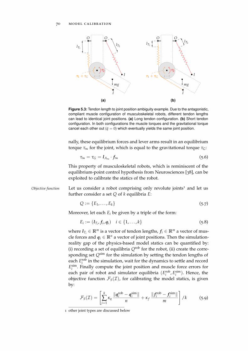
70 model calibration

mg

q = 0

lT1

τ1 + τG

τ2

lT2

O O

I

I

(a)

mg

q = 0

lT1

τ1 + τG

τ2

lT2

O O

I

I

(b)

Figure 5.3: Tendon length to joint position ambiguity example. Due to the antagonistic,

compliant muscle configuration of musculoskeletal robots, different tendon lengths

can lead to identical joint positions. (a) Long tendon configuration. (b) Short tendon

configuration. In both configurations the muscle torques and the gravitational torque

cancel each other out (q = 0) which eventually yields the same joint position.

nally, these equilibrium forces and lever arms result in an equilibriumtorque τ∞ for the joint, which is equal to the gravitational torque τG:

τ∞ = τG = lA∞· f∞ (5.6)

This property of musculoskeletal robots, which is reminiscent of theequilibrium-point control hypothesis from Neurosciences [38], can beexploited to calibrate the statics of the robot.

Let us consider a robot comprising only revolute joints1 and let usObjective function

further consider a set Q of k equilibria E:

Q := E1, . . . , Ek (5.7)

Moreover, let each Ei be given by a triple of the form:

Ei := (lTi, fi, qi) i ∈ 1, . . . , k (5.8)

where lTi∈ R

m is a vector of tendon lengths, fi ∈ Rm a vector of mus-

cle forces and qi ∈ Rn a vector of joint positions. Then the simulation-

reality gap of the physics-based model statics can be quantified by:(i) recording a set of equilibria Qrob for the robot, (ii) create the corre-sponding set Qsim for the simulation by setting the tendon lengths ofeach Erob

i in the simulation, wait for the dynamics to settle and recordEsim

i . Finally compute the joint position and muscle force errors foreach pair of robot and simulator equilibria (Erob

i , Esimi ). Hence, the

objective function FS(I), for calibrating the model statics, is givenby:

FS(I) =[

k

∑i=1

κq‖qrob

i − qsimi ‖

n+ κ f

‖ f robi − f sim

i ‖m

]

/k (5.9)

1 other joint types are discussed below

5.2 statics calibration 71

where κq and κ f are coefficients that can be used to adjust the contri-bution of the joint position and muscle force errors to the fitness ofthe individual.

The question might arise why the forces of the muscles are considered Muscle force error

and the objective

functionfor the objective function and not just the joint positions. The reasonis, that the mapping between tendon lengths lT and joint positions q isnot injective, as different lT can lead to identical joint positions. Thisis illustrated in Figure 5.3 where a revolute joint, actuated by twocompliant muscles, is shown for two tendon length configurations.While the tendon lengths differ, the resulting joint position wouldbe identical. In fact, due to the compliance of the muscles, there isan infinite number of tendon length vectors that would result in theidentical joint position. Hence, neglecting the muscle forces duringcalibration would eventually lead to low joint position errors but tolarge muscle force errors. This, however, is not desirable if the modelis supposed to be used as a test-bed for robot control algorithms thatrely on muscle forces or if the model is used as an internal forwardmodel for control.

So far only revolute joints were considered. This simplified the ob- Other joint types

jective function as the joint positions could be expressed by scalarsand the position error was given by the vector difference of the robotand simulator positions (qrob

i − qsimi ). However, more complex joint

types, such as spherical joints, can be easily added to the objectivefunction as long as the position error can be mapped to a scalar. If,for instance, quaternions are used to represent the joint position ofa spherical joint, then the quaternion distance can be used as errormeasure for the objective function.

Another question that might arise is how many equilibria are re- Required number of

reference equilibriaquired in order to calibrate a musculoskeletal robot. Let us thereforeconsider again a revolute joint setup actuated by m straight-line mus-cles, each equipped with a SEE. The joint is in equilibrium when themuscle and the gravitational torque are equal and the joint velocity iszero:

τG =m

∑i=1

τMi∧ q = 0 (5.10)

From Chapter 2 we recall that the 3-dimensional muscle torque τM

with respect to a reference point is given by:

τM = (p× f ) f (5.11)

where p is a vector from the reference point to any point on the lineof action f and f is the magnitude of the force, which depends on theexpansion lS:

f = g(lS) (5.12)

72 model calibration

Hence, by substituting f with the robot force f rob and solving thefunction g for one of the unknowns from Equation 5.11 yields a sys-tem of 3 + m equations per equilibrium (one for each of the three co-ordinates of the torque vector and one for f and each muscle). There-fore, the number p of required equilibria is given by:

p =

⌈

o−m

3

⌉

(5.13)

where o is the number of unknowns.

As an example let us assume again a revolute joint actuated by mExample

straight-line muscles each equipped with a linear spring as SEE. Thenthe force f of each muscle is given by:

f = k lS = k (lM − lT) (5.14)

where k is the spring stiffness coefficient and lM the muscle length.From Equation 4.16 we know that lM of straight-line muscles is givenby the Euclidean distance of the muscle origin and insertion point:

lM =√

[pxO − px

I (q)]2 + [p

yO − p

yI (q)]

2 + [pzO − pz

I(q)]2 (5.15)

Note that it is assumed that the insertion point pI depends on thejoint position q. In the worst-case, the spring stiffness coefficient aswell as the muscle origin and the insertion point are unknown. Thisyields a total of 7m unknowns (6 coordinates and k for each muscle).Hence, at maximum, 2m equilibria would be required for the calibra-tion of this revolute joint example.

The joints as well as the muscle routing of musculoskeletal robots areStatics calibration

and friction subject to dry friction. These dry friction properties affect the equi-librium and hence the objective function value as the acquired equi-librium becomes dependent on the initial condition (i. e. the startingposture that was used to acquire the equilibrium). To minimize theerror introduced by these frictional properties, it is advisable to useidentical initial conditions during the recording of the robot and thesimulator equilibria. One simple way to achieve such identical initialconditions is to use another equilibrium, i. e. the resting posture ofthe robot, as starting condition.

The physics-based models of musculoskeletal robots comprise a hugeSelection of

calibration

parametersparameter set. For instance, the straight-line muscle model of a singleAnthrob muscle already consists of 32 parameters. Hence, it is impor-tant to select a proper subset of the model parameters as object pa-rameters for the calibration. Normally, parameters that are identifiedexperimentally, that are available in data sheets or that are possibleto extract from Computer-Aided Design (CAD) models should notbe the first choice for the calibration. Furthermore, by analyzing the

5.3 dynamics calibration 73

parameter set of the models we find that there exists a subset whichonly affects the dynamics of the robot, such as joint viscous frictioncoefficients. These parameters have no effect on the equilibrium of therobot and therefore should not be included in the statics calibrationprocedure. However, these parameters can be calibrated in a secondcalibration iteration as described in the following section.

5.3 dynamics calibration

Let us consider the joint position and muscle force trajectories of a sin-gle revolute joint actuated by a single muscle as shown in Figure 5.4.Sampling these continuous trajectories at equidistant intervals resultsin a discrete representation of the trajectories. If we now compute andadd the position and force errors of the model for each of the sam-ples we obtain an objective function which can be used to guide thecalibration of the model dynamics. Formally, this can be expressed asfollows.

Let us consider again a robot comprising only revolute joints and let Objective function

T be a sequence of k trajectory samples S:

T := S1, . . . , Sk (5.16)

Furthermore, let each sample be given by a quadruple of the form:

Si := (ti, lTi, fi, qi) i ∈ 1, . . . , k (5.17)

where ti, lTi, fi and qi are the time, the tendon lengths, the forces

and the joint positions of sample i, respectively. Then the simulation-reality gap of the physics-based model for a single trajectory can bequantified by: (i) recording the trajectory T rob for the robot, (ii) re-playing the trajectory in the simulation by setting the robot tendonlengths l rob

Tiwithin the simulator to record the corresponding simu-

lator trajectory T sim and (iii) compute the joint position and muscleforce error for each pair of robot and simulator samples (S rob

i , S simi )

similar to the objective function of the statics calibration. Hence, thefitness FT(I) of individual I for a single trajectory is given by thearithmetic mean of the fitness of all samples:

FT(I) =[

k

∑i=1

κq‖qrob

i − qsimi ‖

n+ κ f

‖ f robi − f sim

i ‖m

]

/k (5.18)

If we now consider a set of p trajectories for the calibration of themodel dynamics, the objective function FD(I) is given by:

FD(I) =(

p

∑i=1

FT(I))

/p (5.19)

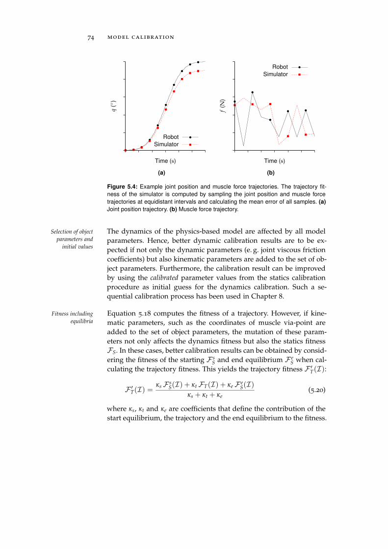
74 model calibration

q(

)

Time (s)

Robot

Simulator

(a)

f(N

)

Time (s)

Robot

Simulator

(b)

Figure 5.4: Example joint position and muscle force trajectories. The trajectory fit-

ness of the simulator is computed by sampling the joint position and muscle force

trajectories at equidistant intervals and calculating the mean error of all samples. (a)

Joint position trajectory. (b) Muscle force trajectory.

The dynamics of the physics-based model are affected by all modelSelection of object

parameters and

initial valuesparameters. Hence, better dynamic calibration results are to be ex-pected if not only the dynamic parameters (e. g. joint viscous frictioncoefficients) but also kinematic parameters are added to the set of ob-ject parameters. Furthermore, the calibration result can be improvedby using the calibrated parameter values from the statics calibrationprocedure as initial guess for the dynamics calibration. Such a se-quential calibration process has been used in Chapter 8.

Equation 5.18 computes the fitness of a trajectory. However, if kine-Fitness including

equilibria matic parameters, such as the coordinates of muscle via-point areadded to the set of object parameters, the mutation of these param-eters not only affects the dynamics fitness but also the statics fitnessFS. In these cases, better calibration results can be obtained by consid-ering the fitness of the starting F s

S and end equilibrium F eS when cal-

culating the trajectory fitness. This yields the trajectory fitness F ′T(I):

F ′T(I) =κs F s

S(I) + κt FT(I) + κe F eS(I)

κs + κt + κe(5.20)

where κs, κt and κe are coefficients that define the contribution of thestart equilibrium, the trajectory and the end equilibrium to the fitness.

6T H E M U S C U L O S K E L E TA L R O B O T A N T H R O B

In order to investigate the suitability of the physics-based simulationapproach for simulating the dynamics of tendon-driven systems, themusculoskeletal robot Anthrob was used (see Figure 6.1). Anthrob,which was conceptualized at the end of the Eccerobot project, wasdeveloped together with Michael Jäntsch and the Swiss companyawtec AG. The robot replicates the human upper limb (sometimesalso referred to as upper extremity), which comprises the bones of thepectoral girdle, the (upper) arm, the forearm and the hand [41, 134].This part of the human skeleton has been chosen as it includes struc-tures that are typical for musculoskeletal robots and challenging forsimulation and control, such as the spherical glenohumeral (shoul-der) joint or biarticular muscles (muscles spanning two joints). Allskeletal parts are designed in CAD tools to provide the required in-put data for the simulation model development and to facilitate the(re)-production of the robot (see Section 6.1). Whenever possible, 3Dprinting technologies based on Selective Laser Sintering (SLS) havebeen used for the production of the robot parts to evaluate cutting-edge technologies, such as tendon canals or solid-state joints, andto minimize the production costs. Furthermore, three types of muscleunits have been developed to match the power requirements of the 13

skeletal muscles of the robot (see Section 6.2). Finally, proprioceptiveand discriminative touch sensors have been included in the muscleunits, in the joints and in the hand to provide sensory feedback forcontrol and for the quantification of the simulation-reality gap (seeSection 6.3).

6.1 skeleton

The shoulder complex can be considered as one of the most compli- Shoulder complex

cated skeletal structures in humans. It consists of the glenohumeraljoint (the shoulder joint) and the pectoral girdle [28]. Whereas thespherical glenohumeral joint enables the movement of the humeruswith respect to the scapula in three mutually perpendicular axes (seeFigure 6.2a), the pectoral girdle has two functions. First, it allows forscapula movements such as scapular elevation or depression [134].

75

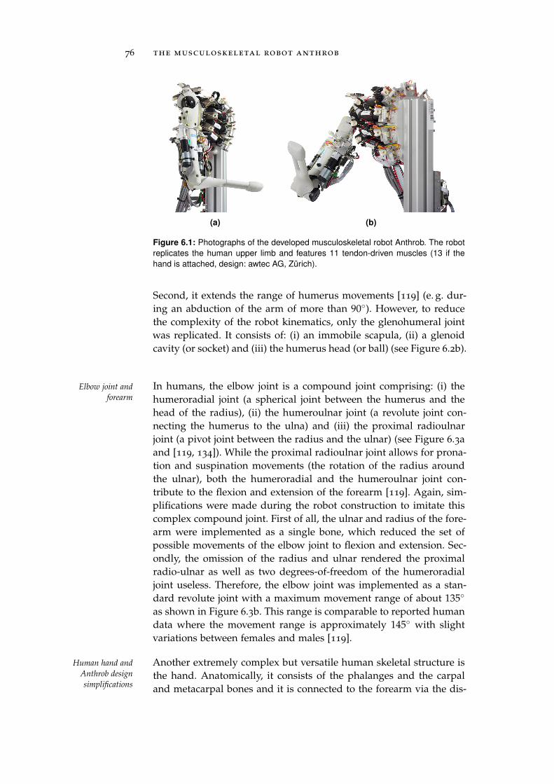
76 the musculoskeletal robot anthrob

(a) (b)

Figure 6.1: Photographs of the developed musculoskeletal robot Anthrob. The robot

replicates the human upper limb and features 11 tendon-driven muscles (13 if the

hand is attached, design: awtec AG, Zürich).

Second, it extends the range of humerus movements [119] (e. g. dur-ing an abduction of the arm of more than 90). However, to reducethe complexity of the robot kinematics, only the glenohumeral jointwas replicated. It consists of: (i) an immobile scapula, (ii) a glenoidcavity (or socket) and (iii) the humerus head (or ball) (see Figure 6.2b).

In humans, the elbow joint is a compound joint comprising: (i) theElbow joint and

forearm humeroradial joint (a spherical joint between the humerus and thehead of the radius), (ii) the humeroulnar joint (a revolute joint con-necting the humerus to the ulna) and (iii) the proximal radioulnarjoint (a pivot joint between the radius and the ulnar) (see Figure 6.3aand [119, 134]). While the proximal radioulnar joint allows for prona-tion and suspination movements (the rotation of the radius aroundthe ulnar), both the humeroradial and the humeroulnar joint con-tribute to the flexion and extension of the forearm [119]. Again, sim-plifications were made during the robot construction to imitate thiscomplex compound joint. First of all, the ulnar and radius of the fore-arm were implemented as a single bone, which reduced the set ofpossible movements of the elbow joint to flexion and extension. Sec-ondly, the omission of the radius and ulnar rendered the proximalradio-ulnar as well as two degrees-of-freedom of the humeroradialjoint useless. Therefore, the elbow joint was implemented as a stan-dard revolute joint with a maximum movement range of about 135

as shown in Figure 6.3b. This range is comparable to reported humandata where the movement range is approximately 145 with slightvariations between females and males [119].

Another extremely complex but versatile human skeletal structure isHuman hand and

Anthrob design

simplificationsthe hand. Anatomically, it consists of the phalanges and the carpaland metacarpal bones and it is connected to the forearm via the dis-

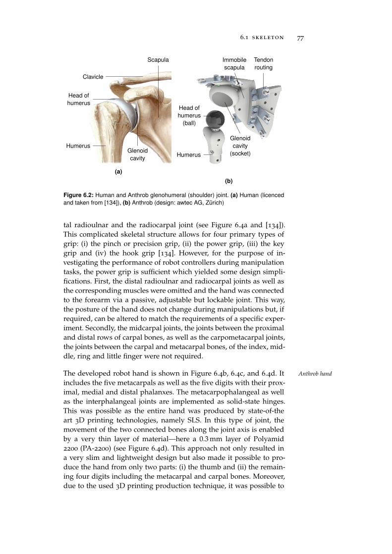
6.1 skeleton 77

Head of

humerus

Glenoid

cavity

Clavicle

Humerus

Scapula

(a)

Immobile

scapula

Tendon

routing

Glenoid

cavity

(socket)Humerus

Head of

humerus

(ball)

(b)

Figure 6.2: Human and Anthrob glenohumeral (shoulder) joint. (a) Human (licenced

and taken from [134]), (b) Anthrob (design: awtec AG, Zürich)

tal radioulnar and the radiocarpal joint (see Figure 6.4a and [134]).This complicated skeletal structure allows for four primary types ofgrip: (i) the pinch or precision grip, (ii) the power grip, (iii) the keygrip and (iv) the hook grip [134]. However, for the purpose of in-vestigating the performance of robot controllers during manipulationtasks, the power grip is sufficient which yielded some design simpli-fications. First, the distal radioulnar and radiocarpal joints as well asthe corresponding muscles were omitted and the hand was connectedto the forearm via a passive, adjustable but lockable joint. This way,the posture of the hand does not change during manipulations but, ifrequired, can be altered to match the requirements of a specific exper-iment. Secondly, the midcarpal joints, the joints between the proximaland distal rows of carpal bones, as well as the carpometacarpal joints,the joints between the carpal and metacarpal bones, of the index, mid-dle, ring and little finger were not required.

The developed robot hand is shown in Figure 6.4b, 6.4c, and 6.4d. It Anthrob hand

includes the five metacarpals as well as the five digits with their prox-imal, medial and distal phalanxes. The metacarpophalangeal as wellas the interphalangeal joints are implemented as solid-state hinges.This was possible as the entire hand was produced by state-of-theart 3D printing technologies, namely SLS. In this type of joint, themovement of the two connected bones along the joint axis is enabledby a very thin layer of material—here a 0.3 mm layer of Polyamid2200 (PA-2200) (see Figure 6.4d). This approach not only resulted ina very slim and lightweight design but also made it possible to pro-duce the hand from only two parts: (i) the thumb and (ii) the remain-ing four digits including the metacarpal and carpal bones. Moreover,due to the used 3D printing production technique, it was possible to

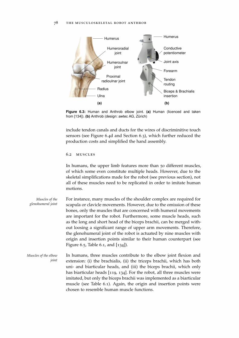
78 the musculoskeletal robot anthrob

Humerus

Radius

Ulna

Humeroradial

joint

Humeroulnar

joint

Proximal

radioulnar joint

(a)

Humerus

Conductive

potentiometer

Joint axis

Forearm

Tendon

routing

Biceps & Brachialis

insertion

(b)

Figure 6.3: Human and Anthrob elbow joint. (a) Human (licenced and taken

from [134]). (b) Anthrob (design: awtec AG, Zürich)

include tendon canals and ducts for the wires of discriminitive touchsensors (see Figure 6.4d and Section 6.3), which further reduced theproduction costs and simplified the hand assembly.

6.2 muscles

In humans, the upper limb features more than 50 different muscles,of which some even constitute multiple heads. However, due to theskeletal simplifications made for the robot (see previous section), notall of these muscles need to be replicated in order to imitate humanmotions.

For instance, many muscles of the shoulder complex are required forMuscles of the

glenohumeral joint scapula or clavicle movements. However, due to the omission of thesebones, only the muscles that are concerned with humeral movementsare important for the robot. Furthermore, some muscle heads, suchas the long and short head of the biceps brachii, can be merged with-out loosing a significant range of upper arm movements. Therefore,the glenohumeral joint of the robot is actuated by nine muscles withorigin and insertion points similar to their human counterpart (seeFigure 6.5, Table 6.1, and [134]).

In humans, three muscles contribute to the elbow joint flexion andMuscles of the elbow

joint extension: (i) the brachialis, (ii) the triceps brachii, which has bothuni- and biarticular heads, and (iii) the biceps brachii, which onlyhas biarticular heads [119, 134]. For the robot, all three muscles wereimitated, but only the biceps brachii was implemented as a biarticularmuscle (see Table 6.1). Again, the origin and insertion points werechosen to resemble human muscle functions.

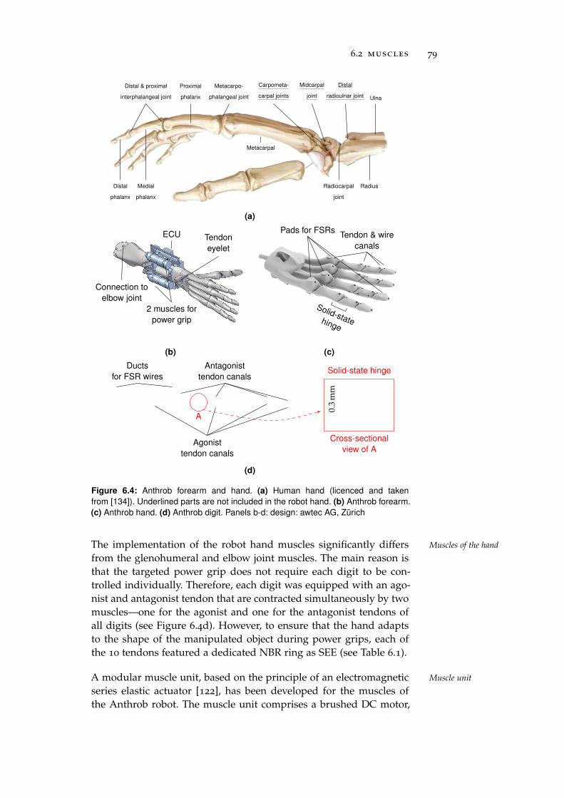
6.2 muscles 79

Distal

phalanx

Distal & proximal

interphalangeal joint

Medial

phalanx

Proximal

phalanx

Metacarpo-

phalangeal joint

Metacarpal

Distal

radioulnar joint

Carpometa-

carpal joints

Midcarpal

joint

Radiocarpal

joint

Ulna

Radius

(a)

Connection to

elbow joint

ECU Tendon

eyelet

2 muscles for

power grip

(b)

Pads for FSRsTendon & wire

canals

Solid-statehinge

(c)

Antagonist

tendon canals

Agonist

tendon canals

Ducts

for FSR wires

A

Cross-sectional

view of A

Solid-state hinge

0.3

mm

(d)

Figure 6.4: Anthrob forearm and hand. (a) Human hand (licenced and taken

from [134]). Underlined parts are not included in the robot hand. (b) Anthrob forearm.

(c) Anthrob hand. (d) Anthrob digit. Panels b-d: design: awtec AG, Zürich

The implementation of the robot hand muscles significantly differs Muscles of the hand

from the glenohumeral and elbow joint muscles. The main reason isthat the targeted power grip does not require each digit to be con-trolled individually. Therefore, each digit was equipped with an ago-nist and antagonist tendon that are contracted simultaneously by twomuscles—one for the agonist and one for the antagonist tendons ofall digits (see Figure 6.4d). However, to ensure that the hand adaptsto the shape of the manipulated object during power grips, each ofthe 10 tendons featured a dedicated NBR ring as SEE (see Table 6.1).

A modular muscle unit, based on the principle of an electromagnetic Muscle unit

series elastic actuator [122], has been developed for the muscles ofthe Anthrob robot. The muscle unit comprises a brushed DC motor,

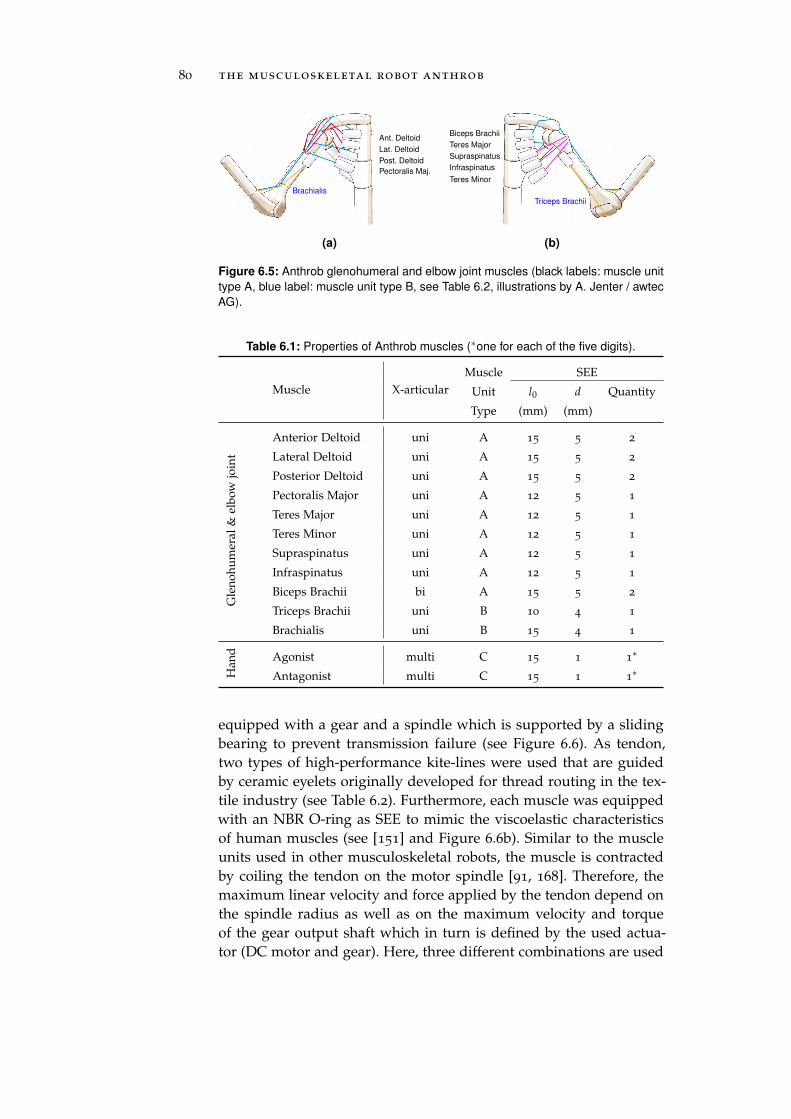
80 the musculoskeletal robot anthrob

Pectoralis Maj.

Post. Deltoid

Lat. Deltoid

Ant. Deltoid

Brachialis

(a)

Teres Minor

Infraspinatus

Supraspinatus

Teres Major

Biceps Brachii

Triceps Brachii

(b)

Figure 6.5: Anthrob glenohumeral and elbow joint muscles (black labels: muscle unit

type A, blue label: muscle unit type B, see Table 6.2, illustrations by A. Jenter / awtec

AG).

Table 6.1: Properties of Anthrob muscles (∗one for each of the five digits).

Muscle X-articular

Muscle SEE

Unit l0 d Quantity

Type (mm) (mm)

Gle

noh

um

eral

&el

bow

join

t

Anterior Deltoid uni A 15 5 2

Lateral Deltoid uni A 15 5 2

Posterior Deltoid uni A 15 5 2

Pectoralis Major uni A 12 5 1

Teres Major uni A 12 5 1

Teres Minor uni A 12 5 1

Supraspinatus uni A 12 5 1

Infraspinatus uni A 12 5 1

Biceps Brachii bi A 15 5 2

Triceps Brachii uni B 10 4 1

Brachialis uni B 15 4 1

Han

d Agonist multi C 15 1 1∗

Antagonist multi C 15 1 1∗

equipped with a gear and a spindle which is supported by a slidingbearing to prevent transmission failure (see Figure 6.6). As tendon,two types of high-performance kite-lines were used that are guidedby ceramic eyelets originally developed for thread routing in the tex-tile industry (see Table 6.2). Furthermore, each muscle was equippedwith an NBR O-ring as SEE to mimic the viscoelastic characteristicsof human muscles (see [151] and Figure 6.6b). Similar to the muscleunits used in other musculoskeletal robots, the muscle is contractedby coiling the tendon on the motor spindle [91, 168]. Therefore, themaximum linear velocity and force applied by the tendon depend onthe spindle radius as well as on the maximum velocity and torqueof the gear output shaft which in turn is defined by the used actua-tor (DC motor and gear). Here, three different combinations are used

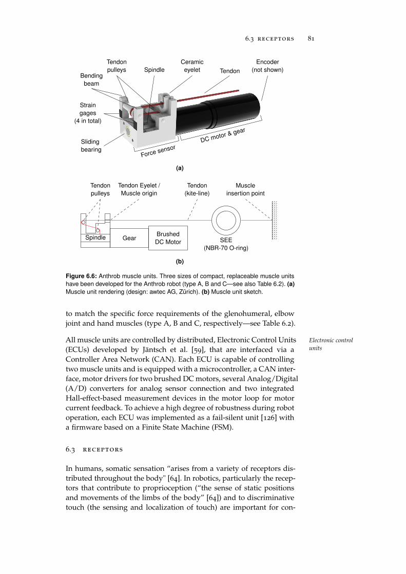
6.3 receptors 81

Sliding

bearing

Tendon

pulleysBending

beam

Ceramic

eyelet Tendon

Strain

gages

(4 in total)

Spindle

Encoder

(not shown)

Force sensorDC motor & gear

(a)

SEE

(NBR-70 O-ring)

Spindle

Muscle

insertion point

Tendon Eyelet /

Muscle origin

Tendon

pulleys

Tendon

(kite-line)

GearBrushed

DC Motor

(b)

Figure 6.6: Anthrob muscle units. Three sizes of compact, replaceable muscle units

have been developed for the Anthrob robot (type A, B and C—see also Table 6.2). (a)

Muscle unit rendering (design: awtec AG, Zürich). (b) Muscle unit sketch.

to match the specific force requirements of the glenohumeral, elbowjoint and hand muscles (type A, B and C, respectively—see Table 6.2).

All muscle units are controlled by distributed, Electronic Control Units Electronic control

units(ECUs) developed by Jäntsch et al. [59], that are interfaced via aController Area Network (CAN). Each ECU is capable of controllingtwo muscle units and is equipped with a microcontroller, a CAN inter-face, motor drivers for two brushed DC motors, several Analog/Digital(A/D) converters for analog sensor connection and two integratedHall-effect-based measurement devices in the motor loop for motorcurrent feedback. To achieve a high degree of robustness during robotoperation, each ECU was implemented as a fail-silent unit [126] witha firmware based on a Finite State Machine (FSM).

6.3 receptors

In humans, somatic sensation “arises from a variety of receptors dis-tributed throughout the body" [64]. In robotics, particularly the recep-tors that contribute to proprioception (“the sense of static positionsand movements of the limbs of the body” [64]) and to discriminativetouch (the sensing and localization of touch) are important for con-

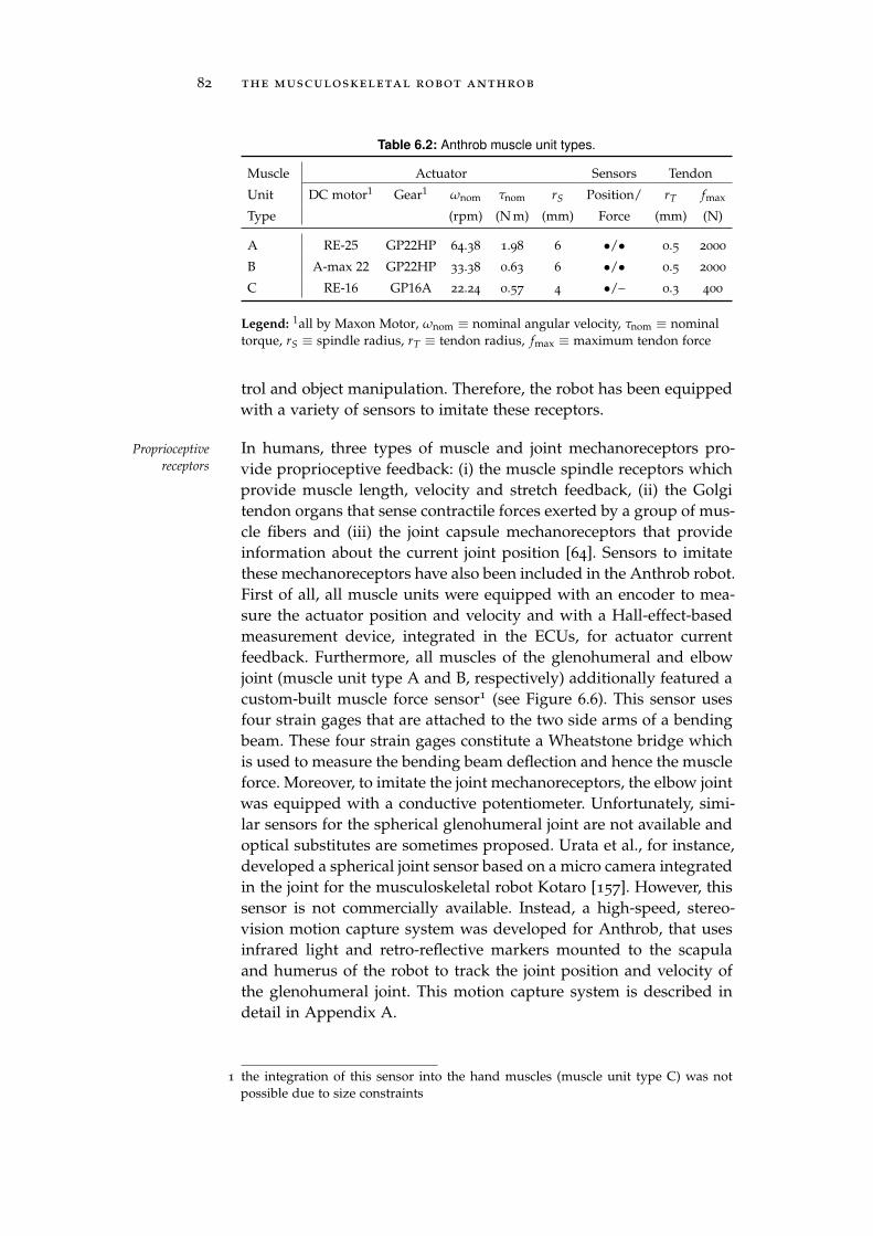
82 the musculoskeletal robot anthrob

Table 6.2: Anthrob muscle unit types.

Muscle Actuator Sensors Tendon

Unit DC motor1 Gear1 ωnom τnom rS Position/ rT fmax

Type (rpm) (N m) (mm) Force (mm) (N)

A RE-25 GP22HP 64.38 1.98 6 •/• 0.5 2000

B A-max 22 GP22HP 33.38 0.63 6 •/• 0.5 2000

C RE-16 GP16A 22.24 0.57 4 •/– 0.3 400

Legend: 1all by Maxon Motor, ωnom ≡ nominal angular velocity, τnom ≡ nominaltorque, rS ≡ spindle radius, rT ≡ tendon radius, fmax ≡ maximum tendon force

trol and object manipulation. Therefore, the robot has been equippedwith a variety of sensors to imitate these receptors.

In humans, three types of muscle and joint mechanoreceptors pro-Proprioceptive

receptors vide proprioceptive feedback: (i) the muscle spindle receptors whichprovide muscle length, velocity and stretch feedback, (ii) the Golgitendon organs that sense contractile forces exerted by a group of mus-cle fibers and (iii) the joint capsule mechanoreceptors that provideinformation about the current joint position [64]. Sensors to imitatethese mechanoreceptors have also been included in the Anthrob robot.First of all, all muscle units were equipped with an encoder to mea-sure the actuator position and velocity and with a Hall-effect-basedmeasurement device, integrated in the ECUs, for actuator currentfeedback. Furthermore, all muscles of the glenohumeral and elbowjoint (muscle unit type A and B, respectively) additionally featured acustom-built muscle force sensor1 (see Figure 6.6). This sensor usesfour strain gages that are attached to the two side arms of a bendingbeam. These four strain gages constitute a Wheatstone bridge whichis used to measure the bending beam deflection and hence the muscleforce. Moreover, to imitate the joint mechanoreceptors, the elbow jointwas equipped with a conductive potentiometer. Unfortunately, simi-lar sensors for the spherical glenohumeral joint are not available andoptical substitutes are sometimes proposed. Urata et al., for instance,developed a spherical joint sensor based on a micro camera integratedin the joint for the musculoskeletal robot Kotaro [157]. However, thissensor is not commercially available. Instead, a high-speed, stereo-vision motion capture system was developed for Anthrob, that usesinfrared light and retro-reflective markers mounted to the scapulaand humerus of the robot to track the joint position and velocity ofthe glenohumeral joint. This motion capture system is described indetail in Appendix A.

1 the integration of this sensor into the hand muscles (muscle unit type C) was notpossible due to size constraints

6.3 receptors 83

In humans, the density of discriminative touch receptors is the “great- Discriminative

touch receptorsest on the hairless (glabrous) skin on the fingers, the palmar surfaceof the hand, the sole of the foot and the lips” [64]. Obviously, forobject manipulation and identification, the finger and palmar surfacereceptors are particularly important. Therefore, the distal phalanx ofthe ring finger as well as three metacarpal heads of the robot handwere equipped with Force-Sensitive Resistors (FSRs) to measure thegrip force during manipulations (see Figure 6.4c).

7A N T H R O B M O D E L I N G

In the previous chapter, the musculoskeletal robot Anthrob was in-troduced. In this chapter, the derivation of three physics-based mod-els of this robot will now be presented. First, the skeleton model ofthese three models is presented in Section 7.1. Then, three differentmuscle as well as an ECU model are presented in Section 7.2 andSection 7.3. Finally, the processing times and the simulation-realitygap of all three models are analyzed in Section 7.4 and Section 7.5,respectively.

7.1 skeleton modeling

The Anthrob skeleton was modeled by three rigid bodies, called base, Rigid bodies

humerus and forearm (see Figure 7.1). While the humerus and the fore-arm were dynamic bodies (i. e. affected by forces), the base was set tobe static. The mass and inertia properties of the bodies were derivedfrom the available CAD data. Therefore, materials were assigned toeach part of the CAD model and the resulting total mass, center ofmass and moments of inertia were computed by SolidWorks. A sum-mary of all parameters is provided in Appendix C. Note that no col-lision shapes were assigned to the rigid bodies as self-collisions arenot relevant in the work-space of the robot and interaction scenarioswere not considered. For the latter reason, the hand of the robot wasalso detached.

Two types of constraints are used within the Anthrob physics-based Constraints

model: a ball-in-socket and a hinge constraint. While the former wasused to model the 3 DoF glenohumeral joint of the robot, the latterwas selected for the 1 DoF elbow joint. The Coulomb friction parame-ters of both joints (µs and µk, respectively) were set to zero to not biasthe equilibrium joint positions, but were included later in the modelcalibration step (see Chapter 8). The viscous friction parameters, how-ever, were non-zero and set to low values to stabilize the simulation.The Anthrob joint position sensors were simulated by ideal sensors(i. e. no noise or offset) and joint position as well as joint velocitieswere provided. A detailed overview of all constraint parameters isprovided in Appendix C.

85

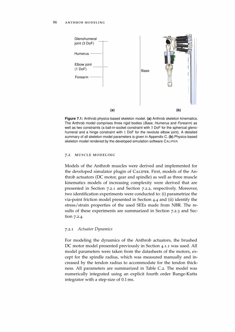
86 anthrob modeling

Base

Forearm

Humerus

Glenohumeral

joint (3 DoF)

Elbow joint

(1 DoF)

(a) (b)

Figure 7.1: Anthrob physics-based skeleton model. (a) Anthrob skeleton kinematics.

The Anthrob model comprises three rigid bodies (Base, Humerus and Forearm) as

well as two constraints (a ball-in-socket constraint with 3 DoF for the spherical gleno-

humeral and a hinge constraint with 1 DoF for the revolute elbow joint). A detailed

summary of all skeleton model parameters is given in Appendix C. (b) Physics-based

skeleton model rendered by the developed simulation software CALIPER.

7.2 muscle modeling

Models of the Anthrob muscles were derived and implemented forthe developed simulator plugin of Caliper. First, models of the An-throb actuators (DC motor, gear and spindle) as well as three musclekinematics models of increasing complexity were derived that arepresented in Section 7.2.1 and Section 7.2.2, respectively. Moreover,two identification experiments were conducted to: (i) parametrize thevia-point friction model presented in Section 4.4 and (ii) identify thestress/strain properties of the used SEEs made from NBR. The re-sults of these experiments are summarized in Section 7.2.3 and Sec-tion 7.2.4.

7.2.1 Actuator Dynamics

For modeling the dynamics of the Anthrob actuators, the brushedDC motor model presented previously in Section 4.1.1 was used. Allmodel parameters were taken from the datasheets of the motors, ex-cept for the spindle radius, which was measured manually and in-creased by the tendon radius to accommodate for the tendon thick-ness. All parameters are summarized in Table C.2. The model wasnumerically integrated using an explicit fourth order Runge-Kuttaintegrator with a step-size of 0.1 ms.

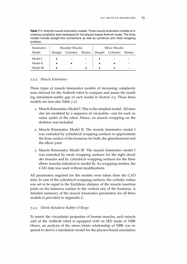
7.2 muscle modeling 87

Table 7.1: Anthrob muscle kinematics models. Three muscle kinematics models of in-

creasing complexity were developed for the physics-based Anthrob model. The three

models include straight-line connections as well as cylindrical and mesh wrapping

surfaces.

Kinematics Shoulder Muscles Elbow Muscles

Model Straight Cylinders Meshes Straight Cylinders Meshes

Model I • – – • – –

Model II • • – • • –

Model III • – • • • –

7.2.2 Muscle Kinematics

Three types of muscle kinematics models of increasing complexitywere derived for the Anthrob robot to compare and assess the result-ing simulation-reality gap of each model in Section 7.5. These threemodels are (see also Table 7.1):

1. Muscle Kinematics Model I: This is the simplest model. All mus-cles are modeled by a sequence of via-points—one for each ce-ramic eyelet of the robot. Hence, no muscle wrapping on theskeleton was included.

2. Muscle Kinematics Model II: The muscle kinematics model Iwas extended by cylindrical wrapping surfaces to approximatethe bone surface of the humerus for both, the glenohumeral andthe elbow joint.

3. Muscle Kinematics Model III: The muscle kinematics model Iwas extended by mesh wrapping surfaces for the eight shoul-der muscles and by cylindrical wrapping surfaces for the threeelbow muscles (identical to model II). As wrapping meshes, theCAD data was used without modifications.

All parameters required for the models were taken from the CADdata. In case of the cylindrical wrapping surfaces, the cylinder radiuswas set to be equal to the Euclidean distance of the muscle insertionpoint on the humerus surface to the vertical axis of the humerus. Adetailed summary of the muscle kinematics parameters for all threemodels is provided in Appendix C.

7.2.3 Nitrile Butadiene Rubber O-Rings

To mimic the viscoelastic properties of human muscles, each muscleunit of the Anthrob robot is equipped with an SEE made of NBR.Hence, an analysis of the stress/strain relationship of NBR was re-quired to derive a simulation model for the physics-based simulation.

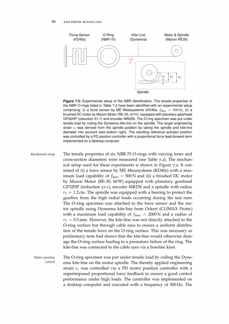
88 anthrob modeling

Force Sensor

(KD40s)

f

Kite-Line

(Dyneema)

Motor & Spindle

(Maxon RE30)

Spindle

rS rCrT

O-Ring

(NBR-70)

Figure 7.2: Experimental setup of the NBR identification. The tensile properties of

the NBR O-rings listed in Table 7.2 have been identified with an experimental setup

comprising: (i) a force sensor by ME Messsysteme (KD40s, fMax = 500 N), (ii) a

brushed DC motor by Maxon Motor (RE-30, 60 W), equipped with planetary gearhead

GP32HP (reduction 51:1) and encoder MR256. The O-ring specimen was put under

tensile load by coiling the Dyneema kite-line on the spindle. The target engineering

strain εt was derived from the spindle position by taking the spindle and kite-line

diameter into account (see bottom right). The resulting reference actuator position

was controlled by a PD position controller with a proportional force feed-forward term

implemented on a desktop computer.

The tensile properties of six NBR-70 O-rings with varying inner andMechanical setup

cross-section diameters were measured (see Table 7.2). The mechan-ical setup used for these experiments is shown in Figure 7.2. It con-sisted of (i) a force sensor by ME Messsysteme (KD40s) with a max-imum load capability of fmax = 500 N and (ii) a brushed DC motorby Maxon Motor (RE-30, 60 W) equipped with planetary gearheadGP32HP (reduction 51:1), encoder MR256 and a spindle with radiusrS = 1.2 cm. The spindle was equipped with a bearing to protect thegearbox from the high radial loads occurring during the test runs.The O-ring specimen was attached to the force sensor and the mo-tor spindle using Dyneema kite-line from Ockert (CLIMAX Protec)with a maximum load capability of fmax = 2000 N and a radius ofrT = 0.5 mm. However, the kite-line was not directly attached to theO-ring surface but through cable eyes to ensure a uniform distribu-tion of the tensile force on the O-ring surface. This was necessary aspreliminary tests had shown that the kite-line would otherwise dam-age the O-ring surface leading to a premature failure of the ring. Thekite-line was connected to the cable eyes via a bowline knot.

The O-ring specimen was put under tensile load by coiling the Dyne-Motor position

control ema kite-line on the motor spindle. The thereby applied engineeringstrain εe was controlled via a PD motor position controller with asuperimposed proportional force feedback to ensure a good controlperformance under high loads. The controller was implemented ona desktop computer and executed with a frequency of 500 Hz. The

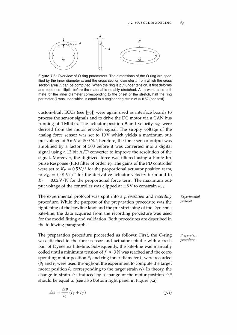
7.2 muscle modeling 89

l0

d

l∗0

d∗d

A

Figure 7.3: Overview of O-ring parameters. The dimensions of the O-ring are spec-

ified by the inner diameter l0 and the cross section diameter d from which the cross

section area A can be computed. When the ring is put under tension, it first deforms

and becomes elliptic before the material is notably stretched. As a worst-case esti-

mate for the inner diameter corresponding to the onset of the stretch, half the ring

perimeter l∗0 was used which is equal to a engineering strain of ≈ 0.57 (see text).

custom-built ECUs (see [59]) were again used as interface boards toprocess the sensor signals and to drive the DC motor via a CAN busrunning at 1 Mbit/s. The actuator position θ and velocity ωG werederived from the motor encoder signal. The supply voltage of theanalog force sensor was set to 10 V which yields a maximum out-put voltage of 5 mV at 500 N. Therefore, the force sensor output wasamplified by a factor of 500 before it was converted into a digitalsignal using a 12 bit A/D converter to improve the resolution of thesignal. Moreover, the digitized force was filtered using a Finite Im-pulse Response (FIR) filter of order 19. The gains of the PD controllerwere set to KP = 0.5 V/ for the proportional actuator position term,to KD = 0.01 V s/ for the derivative actuator velocity term and toKF = 0.02 V/N for the proportional force term. The maximum out-put voltage of the controller was clipped at ±8 V to constrain ωG.

The experimental protocol was split into a preparation and recording Experimental

protocolprocedure. While the purpose of the preparation procedure was thetightening of the bowline knot and the pre-stretching of the Dyneemakite-line, the data acquired from the recording procedure was usedfor the model fitting and validation. Both procedures are described inthe following paragraphs.

The preparation procedure proceeded as follows: First, the O-ring Preparation

procedurewas attached to the force sensor and actuator spindle with a freshpair of Dyneema kite-line. Subsequently, the kite-line was manuallycoiled until a minimum tension of f1 ≈ 3 N was reached and the corre-sponding motor position θ1 and ring inner diameter l1 were recorded(θ1 and l1 were used throughout the experiment to compute the targetmotor position θt corresponding to the target strain εt). In theory, thechange in strain ε induced by a change of the motor position θ

should be equal to (see also bottom right panel in Figure 7.2):

ε =θ

l0(rS + rT) (7.1)

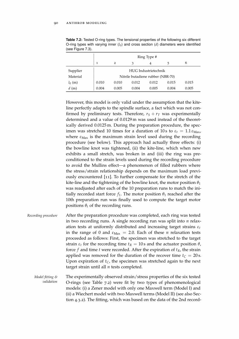
90 anthrob modeling

Table 7.2: Tested O-ring types. The tensional properties of the following six different

O-ring types with varying inner (l0) and cross section (d) diameters were identified

(see Figure 7.3).

Ring Type #

1 2 3 4 5 6

Supplier HUG Industrietechnik

Material Nitrile butadiene rubber (NBR-70)

l0 (m) 0.010 0.010 0.012 0.012 0.015 0.015

d (m) 0.004 0.005 0.004 0.005 0.004 0.005

However, this model is only valid under the assumption that the kite-line perfectly adapts to the spindle surface, a fact which was not con-firmed by preliminary tests. Therefore, rS + rT was experimentallydetermined and a value of 0.0129 m was used instead of the theoret-ically derived 0.0125 m. During the preparation procedure, the spec-imen was stretched 10 times for a duration of 10 s to εt = 1.1 εMax,where εMax is the maximum strain level used during the recordingprocedure (see below). This approach had actually three effects: (i)the bowline knot was tightened, (ii) the kite-line, which when newexhibits a small stretch, was broken in and (iii) the ring was pre-conditioned to the strain levels used during the recording procedureto avoid the Mullins effect—a phenomenon of filled rubbers wherethe stress/strain relationship depends on the maximum load previ-ously encountered [11]. To further compensate for the stretch of thekite-line and the tightening of the bowline knot, the motor position θ1

was readjusted after each of the 10 preparation runs to match the ini-tially recorded start force f1. The motor position θ1 reached after the10th preparation run was finally used to compute the target motorpositions θt of the recording runs.

After the preparation procedure was completed, each ring was testedRecording procedure

in two recording runs. A single recording run was split into n relax-ation tests at uniformly distributed and increasing target strains εt

in the range of 0 and εMax = 2.0. Each of these n relaxation testsproceeded as follows: First, the specimen was stretched to the targetstrain εt for the recording time tR = 10 s and the actuator position θ,force f and time t were recorded. After the expiration of tR, the strainapplied was removed for the duration of the recover time tC = 20 s.Upon expiration of tC, the specimen was stretched again to the nexttarget strain until all n tests completed.

The experimentally observed strain/stress properties of the six testedModel fitting &

validation O-rings (see Table 7.2) were fit by two types of phenomenologicalmodels: (i) a Zener model with only one Maxwell term (Model I) and(ii) a Wiechert model with two Maxwell terms (Model II) (see also Sec-tion 4.3.2). The fitting, which was based on the data of the 2nd record-

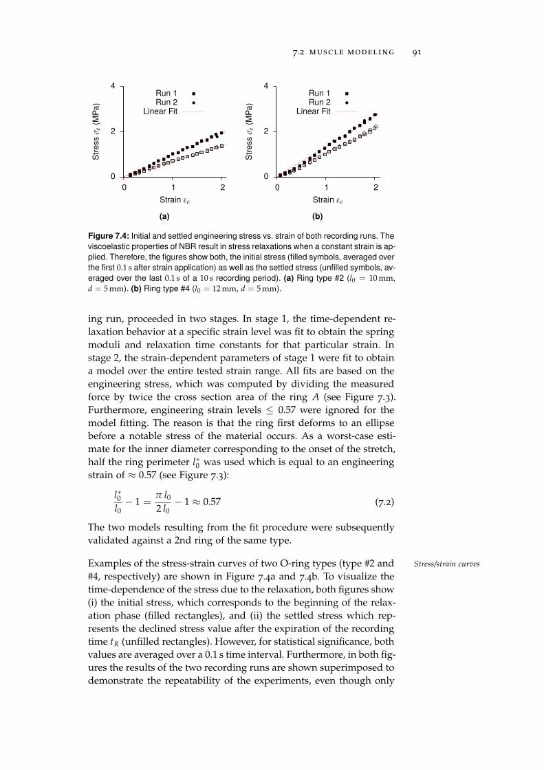
7.2 muscle modeling 91

0

2

4

0 1 2

Str

ess

σe

(MP

a)

Strain εe

Run 1Run 2

Linear Fit

(a)

0

2

4

0 1 2

Str

ess

σe

(MP

a)

Strain εe

Run 1Run 2

Linear Fit

(b)

Figure 7.4: Initial and settled engineering stress vs. strain of both recording runs. The

viscoelastic properties of NBR result in stress relaxations when a constant strain is ap-

plied. Therefore, the figures show both, the initial stress (filled symbols, averaged over

the first 0.1 s after strain application) as well as the settled stress (unfilled symbols, av-

eraged over the last 0.1 s of a 10 s recording period). (a) Ring type #2 (l0 = 10 mm,

d = 5 mm). (b) Ring type #4 (l0 = 12 mm, d = 5 mm).

ing run, proceeded in two stages. In stage 1, the time-dependent re-laxation behavior at a specific strain level was fit to obtain the springmoduli and relaxation time constants for that particular strain. Instage 2, the strain-dependent parameters of stage 1 were fit to obtaina model over the entire tested strain range. All fits are based on theengineering stress, which was computed by dividing the measuredforce by twice the cross section area of the ring A (see Figure 7.3).Furthermore, engineering strain levels ≤ 0.57 were ignored for themodel fitting. The reason is that the ring first deforms to an ellipsebefore a notable stress of the material occurs. As a worst-case esti-mate for the inner diameter corresponding to the onset of the stretch,half the ring perimeter l∗0 was used which is equal to an engineeringstrain of ≈ 0.57 (see Figure 7.3):

l∗0l0− 1 =

π l02 l0− 1 ≈ 0.57 (7.2)

The two models resulting from the fit procedure were subsequentlyvalidated against a 2nd ring of the same type.

Examples of the stress-strain curves of two O-ring types (type #2 and Stress/strain curves

#4, respectively) are shown in Figure 7.4a and 7.4b. To visualize thetime-dependence of the stress due to the relaxation, both figures show(i) the initial stress, which corresponds to the beginning of the relax-ation phase (filled rectangles), and (ii) the settled stress which rep-resents the declined stress value after the expiration of the recordingtime tR (unfilled rectangles). However, for statistical significance, bothvalues are averaged over a 0.1 s time interval. Furthermore, in both fig-ures the results of the two recording runs are shown superimposed todemonstrate the repeatability of the experiments, even though only

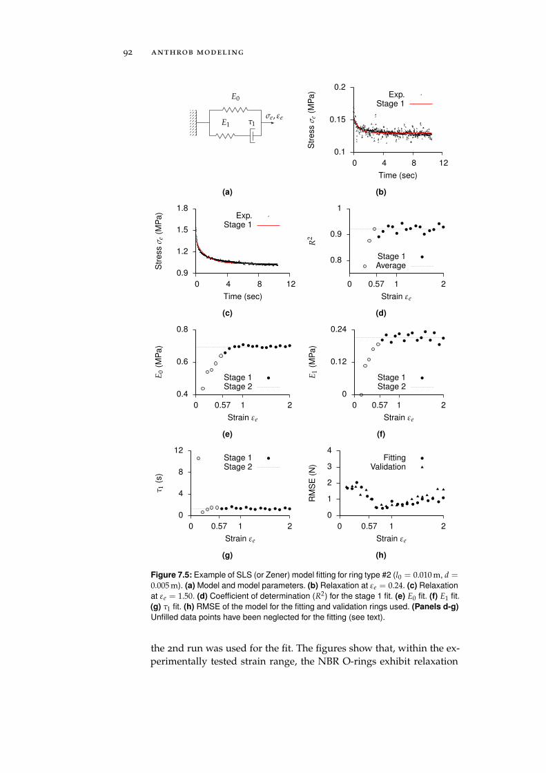
92 anthrob modeling

τ1

E0

E1σe, εe

(a)

0.1

0.15

0.2

0 4 8 12

Str

ess

σe

(MP

a)

Time (sec)

Exp.Stage 1

(b)

0.9

1.2

1.5

1.8

0 4 8 12

Str

ess

σe

(MP

a)

Time (sec)

Exp.Stage 1

(c)

0.8

0.9

1

0 0.57 1 2

R2

Strain εe

Stage 1Average

(d)

0.4

0.6

0.8

0 0.57 1 2

E0

(MP

a)

Strain εe

Stage 1Stage 2

(e)

0

0.12

0.24

0 0.57 1 2

E1

(MP

a)

Strain εe

Stage 1Stage 2

(f)

0

4

8

12

0 0.57 1 2

τ 1(s

)

Strain εe

Stage 1Stage 2

(g)

0

1

2

3

4

0 0.57 1 2

RM

SE

(N)

Strain εe

FittingValidation

(h)

Figure 7.5: Example of SLS (or Zener) model fitting for ring type #2 (l0 = 0.010 m, d =0.005 m). (a) Model and model parameters. (b) Relaxation at εe = 0.24. (c) Relaxation

at εe = 1.50. (d) Coefficient of determination (R2) for the stage 1 fit. (e) E0 fit. (f) E1 fit.

(g) τ1 fit. (h) RMSE of the model for the fitting and validation rings used. (Panels d-g)

Unfilled data points have been neglected for the fitting (see text).

the 2nd run was used for the fit. The figures show that, within the ex-perimentally tested strain range, the NBR O-rings exhibit relaxation

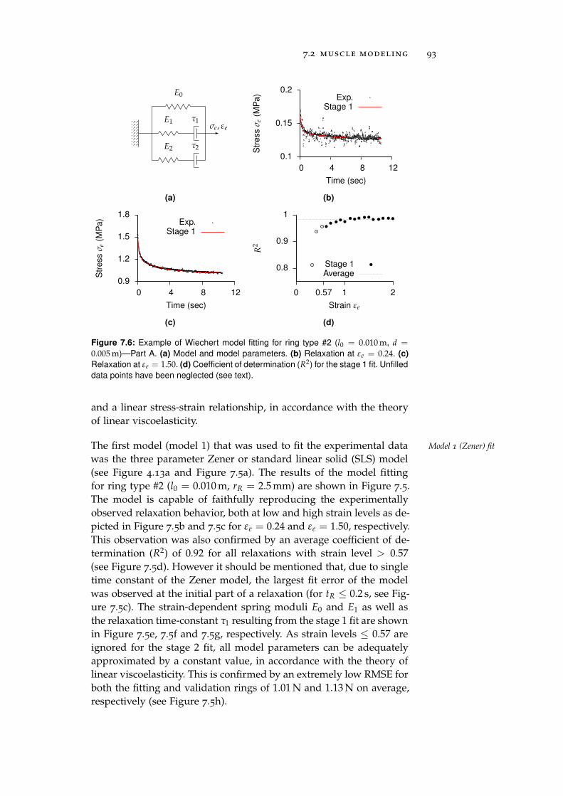
7.2 muscle modeling 93

E0

τ1E1

τ2E2

σe, εe

(a)

0.1

0.15

0.2

0 4 8 12

Str

ess

σe

(MP

a)

Time (sec)

Exp.Stage 1

(b)

0.9

1.2

1.5

1.8

0 4 8 12

Str

ess

σe

(MP

a)

Time (sec)

Exp.Stage 1

(c)

0.8

0.9

1

0 0.57 1 2

R2

Strain εe

Stage 1Average

(d)

Figure 7.6: Example of Wiechert model fitting for ring type #2 (l0 = 0.010 m, d =0.005 m)—Part A. (a) Model and model parameters. (b) Relaxation at εe = 0.24. (c)

Relaxation at εe = 1.50. (d) Coefficient of determination (R2) for the stage 1 fit. Unfilled

data points have been neglected (see text).

and a linear stress-strain relationship, in accordance with the theoryof linear viscoelasticity.

The first model (model 1) that was used to fit the experimental data Model 1 (Zener) fit

was the three parameter Zener or standard linear solid (SLS) model(see Figure 4.13a and Figure 7.5a). The results of the model fittingfor ring type #2 (l0 = 0.010 m, rR = 2.5 mm) are shown in Figure 7.5.The model is capable of faithfully reproducing the experimentallyobserved relaxation behavior, both at low and high strain levels as de-picted in Figure 7.5b and 7.5c for εe = 0.24 and εe = 1.50, respectively.This observation was also confirmed by an average coefficient of de-termination (R2) of 0.92 for all relaxations with strain level > 0.57(see Figure 7.5d). However it should be mentioned that, due to singletime constant of the Zener model, the largest fit error of the modelwas observed at the initial part of a relaxation (for tR ≤ 0.2 s, see Fig-ure 7.5c). The strain-dependent spring moduli E0 and E1 as well asthe relaxation time-constant τ1 resulting from the stage 1 fit are shownin Figure 7.5e, 7.5f and 7.5g, respectively. As strain levels ≤ 0.57 areignored for the stage 2 fit, all model parameters can be adequatelyapproximated by a constant value, in accordance with the theory oflinear viscoelasticity. This is confirmed by an extremely low RMSE forboth the fitting and validation rings of 1.01 N and 1.13 N on average,respectively (see Figure 7.5h).

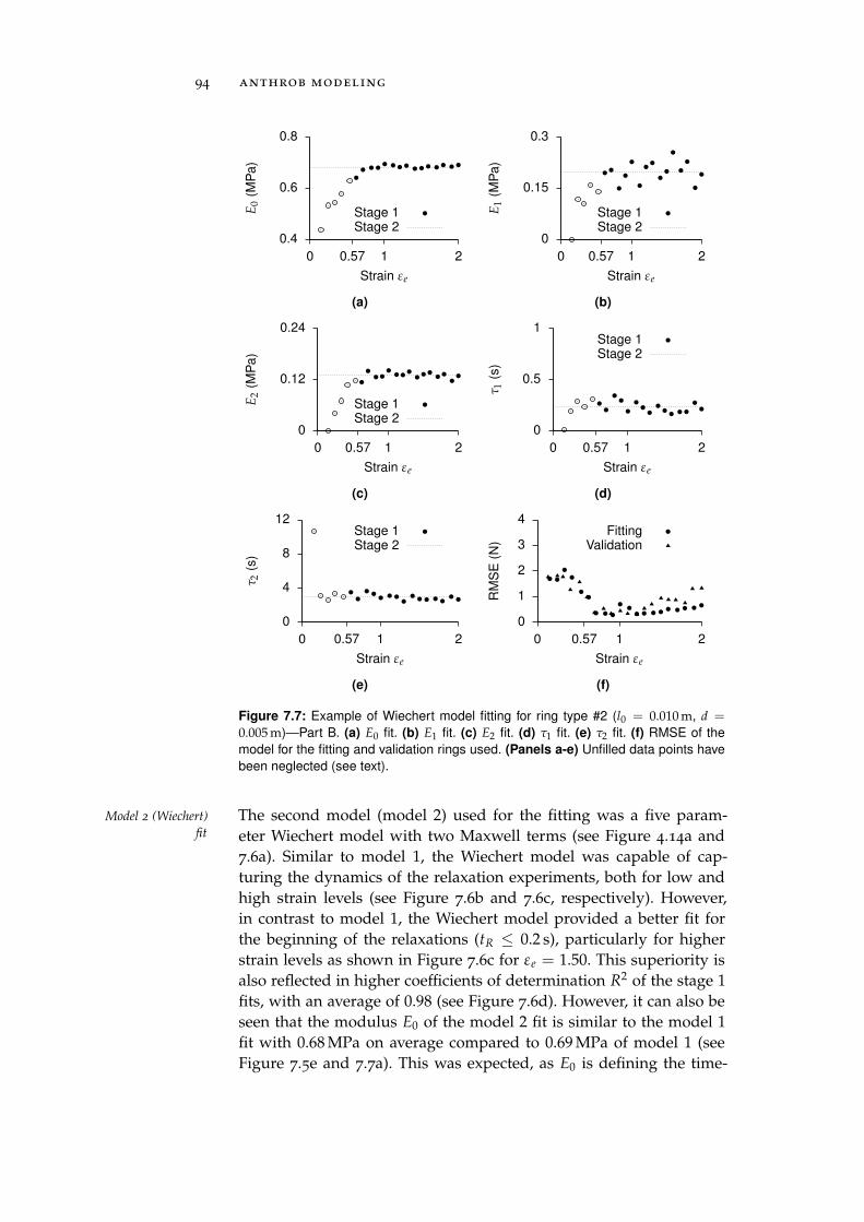
94 anthrob modeling

0.4

0.6

0.8

0 0.57 1 2E

0(M

Pa

)

Strain εe

Stage 1Stage 2

(a)

0

0.15

0.3

0 0.57 1 2

E1

(MP

a)

Strain εe

Stage 1Stage 2

(b)

0

0.12

0.24

0 0.57 1 2

E2

(MP

a)

Strain εe

Stage 1Stage 2

(c)

0

0.5

1

0 0.57 1 2

τ 1(s

)

Strain εe

Stage 1Stage 2

(d)

0

4

8

12

0 0.57 1 2

τ 2(s

)

Strain εe

Stage 1Stage 2

(e)

0

1

2

3

4

0 0.57 1 2

RM

SE

(N)

Strain εe

FittingValidation

(f)

Figure 7.7: Example of Wiechert model fitting for ring type #2 (l0 = 0.010 m, d =0.005 m)—Part B. (a) E0 fit. (b) E1 fit. (c) E2 fit. (d) τ1 fit. (e) τ2 fit. (f) RMSE of the

model for the fitting and validation rings used. (Panels a-e) Unfilled data points have

been neglected (see text).

The second model (model 2) used for the fitting was a five param-Model 2 (Wiechert)

fit eter Wiechert model with two Maxwell terms (see Figure 4.14a and7.6a). Similar to model 1, the Wiechert model was capable of cap-turing the dynamics of the relaxation experiments, both for low andhigh strain levels (see Figure 7.6b and 7.6c, respectively). However,in contrast to model 1, the Wiechert model provided a better fit forthe beginning of the relaxations (tR ≤ 0.2 s), particularly for higherstrain levels as shown in Figure 7.6c for εe = 1.50. This superiority isalso reflected in higher coefficients of determination R2 of the stage 1fits, with an average of 0.98 (see Figure 7.6d). However, it can also beseen that the modulus E0 of the model 2 fit is similar to the model 1fit with 0.68 MPa on average compared to 0.69 MPa of model 1 (seeFigure 7.5e and 7.7a). This was expected, as E0 is defining the time-

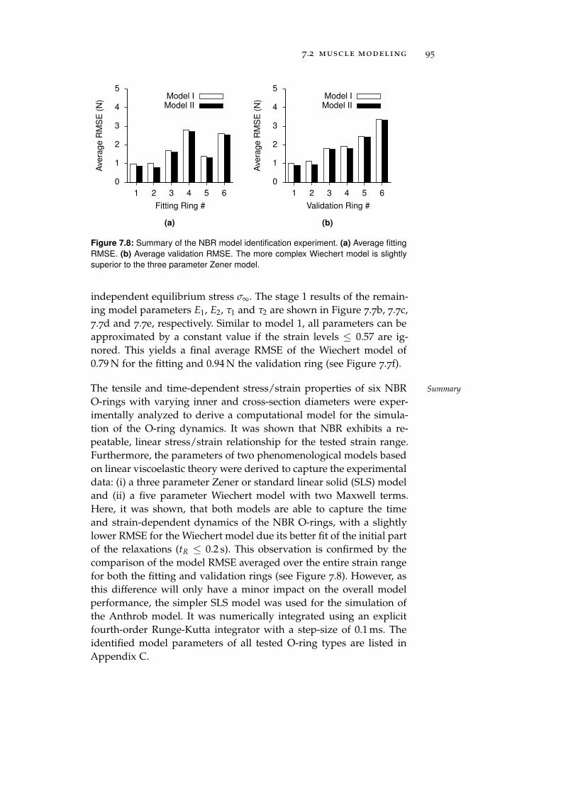
7.2 muscle modeling 95

0

1

2

3

4

5

1 2 3 4 5 6

Ave

rag

eR

MS

E(N

)

Fitting Ring #

Model IModel II

(a)

0

1

2

3

4

5

1 2 3 4 5 6

Ave

rag

eR

MS

E(N

)

Validation Ring #

Model IModel II

(b)

Figure 7.8: Summary of the NBR model identification experiment. (a) Average fitting

RMSE. (b) Average validation RMSE. The more complex Wiechert model is slightly

superior to the three parameter Zener model.

independent equilibrium stress σ∞. The stage 1 results of the remain-ing model parameters E1, E2, τ1 and τ2 are shown in Figure 7.7b, 7.7c,7.7d and 7.7e, respectively. Similar to model 1, all parameters can beapproximated by a constant value if the strain levels ≤ 0.57 are ig-nored. This yields a final average RMSE of the Wiechert model of0.79 N for the fitting and 0.94 N the validation ring (see Figure 7.7f).

The tensile and time-dependent stress/strain properties of six NBR Summary

O-rings with varying inner and cross-section diameters were exper-imentally analyzed to derive a computational model for the simula-tion of the O-ring dynamics. It was shown that NBR exhibits a re-peatable, linear stress/strain relationship for the tested strain range.Furthermore, the parameters of two phenomenological models basedon linear viscoelastic theory were derived to capture the experimentaldata: (i) a three parameter Zener or standard linear solid (SLS) modeland (ii) a five parameter Wiechert model with two Maxwell terms.Here, it was shown, that both models are able to capture the timeand strain-dependent dynamics of the NBR O-rings, with a slightlylower RMSE for the Wiechert model due its better fit of the initial partof the relaxations (tR ≤ 0.2 s). This observation is confirmed by thecomparison of the model RMSE averaged over the entire strain rangefor both the fitting and validation rings (see Figure 7.8). However, asthis difference will only have a minor impact on the overall modelperformance, the simpler SLS model was used for the simulation ofthe Anthrob model. It was numerically integrated using an explicitfourth-order Runge-Kutta integrator with a step-size of 0.1 ms. Theidentified model parameters of all tested O-ring types are listed inAppendix C.

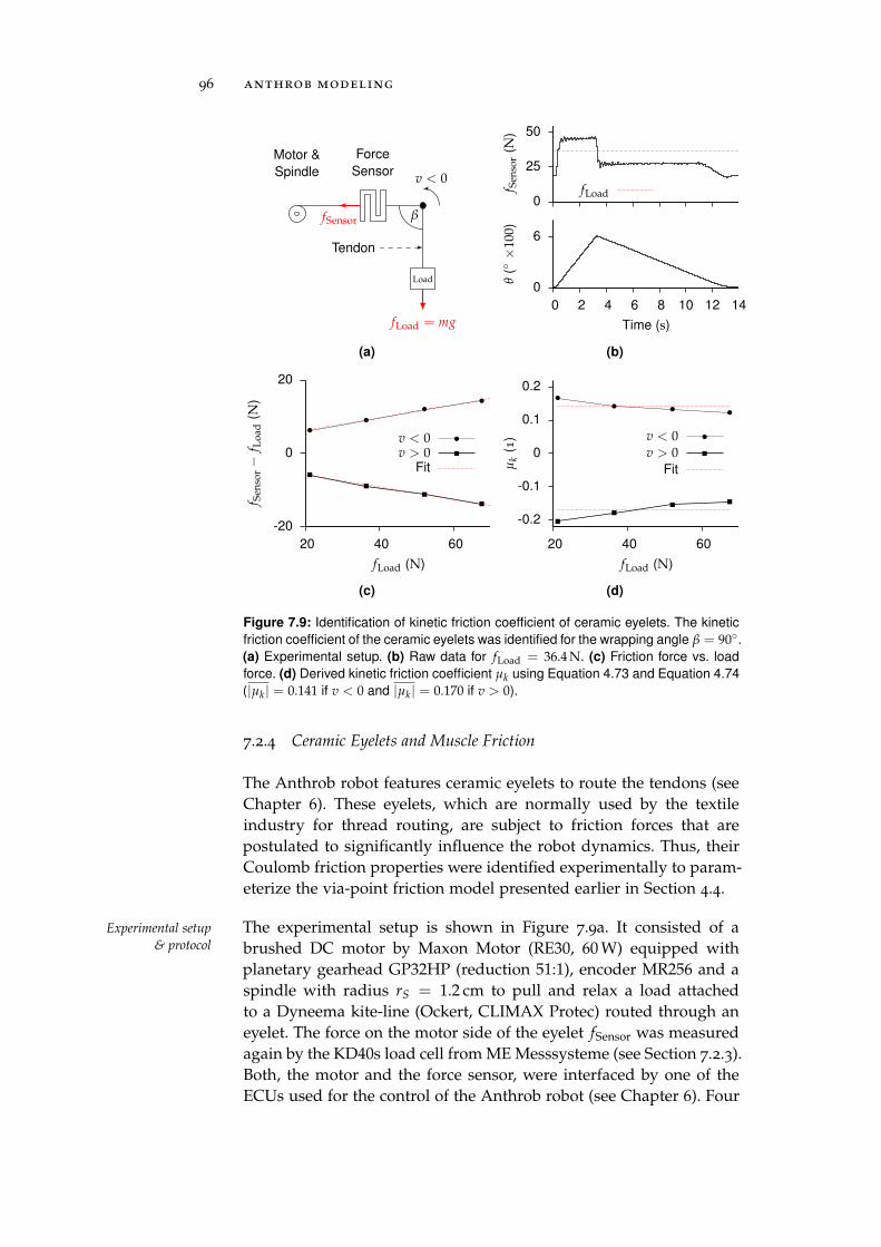
96 anthrob modeling

fSensor

Force

Sensor

Motor &

Spindle

β

v < 0

Load

fLoad = mg

Tendon

(a)

0

25

50

f Sen

sor

(N)

0

6

0 2 4 6 8 10 12 14

θ(×

100)

Time (s)

fLoad

(b)

-20

0

20

20 40 60

f Sen

sor−

f Loa

d(N

)

fLoad (N)

v < 0v > 0

Fit

(c)

-0.2

-0.1

0

0.1

0.2

20 40 60

µk

(1)

fLoad (N)

v < 0v > 0

Fit

(d)

Figure 7.9: Identification of kinetic friction coefficient of ceramic eyelets. The kinetic

friction coefficient of the ceramic eyelets was identified for the wrapping angle β = 90.(a) Experimental setup. (b) Raw data for fLoad = 36.4 N. (c) Friction force vs. load

force. (d) Derived kinetic friction coefficient µk using Equation 4.73 and Equation 4.74

(|µk| = 0.141 if v < 0 and |µk| = 0.170 if v > 0).

7.2.4 Ceramic Eyelets and Muscle Friction

The Anthrob robot features ceramic eyelets to route the tendons (seeChapter 6). These eyelets, which are normally used by the textileindustry for thread routing, are subject to friction forces that arepostulated to significantly influence the robot dynamics. Thus, theirCoulomb friction properties were identified experimentally to param-eterize the via-point friction model presented earlier in Section 4.4.

The experimental setup is shown in Figure 7.9a. It consisted of aExperimental setup

& protocol brushed DC motor by Maxon Motor (RE30, 60 W) equipped withplanetary gearhead GP32HP (reduction 51:1), encoder MR256 and aspindle with radius rS = 1.2 cm to pull and relax a load attachedto a Dyneema kite-line (Ockert, CLIMAX Protec) routed through aneyelet. The force on the motor side of the eyelet fSensor was measuredagain by the KD40s load cell from ME Messsysteme (see Section 7.2.3).Both, the motor and the force sensor, were interfaced by one of theECUs used for the control of the Anthrob robot (see Chapter 6). Four

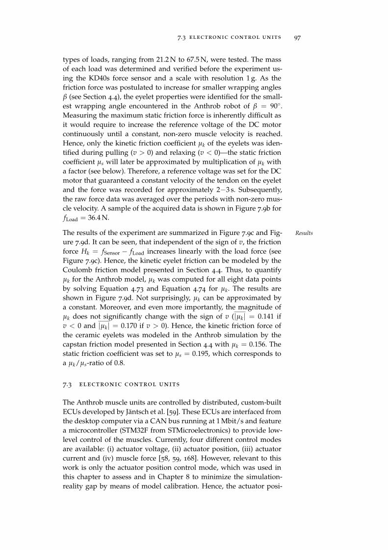
7.3 electronic control units 97

types of loads, ranging from 21.2 N to 67.5 N, were tested. The massof each load was determined and verified before the experiment us-ing the KD40s force sensor and a scale with resolution 1 g. As thefriction force was postulated to increase for smaller wrapping anglesβ (see Section 4.4), the eyelet properties were identified for the small-est wrapping angle encountered in the Anthrob robot of β = 90.Measuring the maximum static friction force is inherently difficult asit would require to increase the reference voltage of the DC motorcontinuously until a constant, non-zero muscle velocity is reached.Hence, only the kinetic friction coefficient µk of the eyelets was iden-tified during pulling (v > 0) and relaxing (v < 0)—the static frictioncoefficient µs will later be approximated by multiplication of µk witha factor (see below). Therefore, a reference voltage was set for the DCmotor that guaranteed a constant velocity of the tendon on the eyeletand the force was recorded for approximately 2−3 s. Subsequently,the raw force data was averaged over the periods with non-zero mus-cle velocity. A sample of the acquired data is shown in Figure 7.9b forfLoad = 36.4 N.

The results of the experiment are summarized in Figure 7.9c and Fig- Results

ure 7.9d. It can be seen, that independent of the sign of v, the frictionforce Hk = fSensor − fLoad increases linearly with the load force (seeFigure 7.9c). Hence, the kinetic eyelet friction can be modeled by theCoulomb friction model presented in Section 4.4. Thus, to quantifyµk for the Anthrob model, µk was computed for all eight data pointsby solving Equation 4.73 and Equation 4.74 for µk. The results areshown in Figure 7.9d. Not surprisingly, µk can be approximated bya constant. Moreover, and even more importantly, the magnitude ofµk does not significantly change with the sign of v (|µk| = 0.141 ifv < 0 and |µk| = 0.170 if v > 0). Hence, the kinetic friction force ofthe ceramic eyelets was modeled in the Anthrob simulation by thecapstan friction model presented in Section 4.4 with µk = 0.156. Thestatic friction coefficient was set to µs = 0.195, which corresponds toa µk/µs-ratio of 0.8.

7.3 electronic control units

The Anthrob muscle units are controlled by distributed, custom-builtECUs developed by Jäntsch et al. [59]. These ECUs are interfaced fromthe desktop computer via a CAN bus running at 1 Mbit/s and featurea microcontroller (STM32F from STMicroelectronics) to provide low-level control of the muscles. Currently, four different control modesare available: (i) actuator voltage, (ii) actuator position, (iii) actuatorcurrent and (iv) muscle force [58, 59, 168]. However, relevant to thiswork is only the actuator position control mode, which was used inthis chapter to assess and in Chapter 8 to minimize the simulation-reality gap by means of model calibration. Hence, the actuator posi-

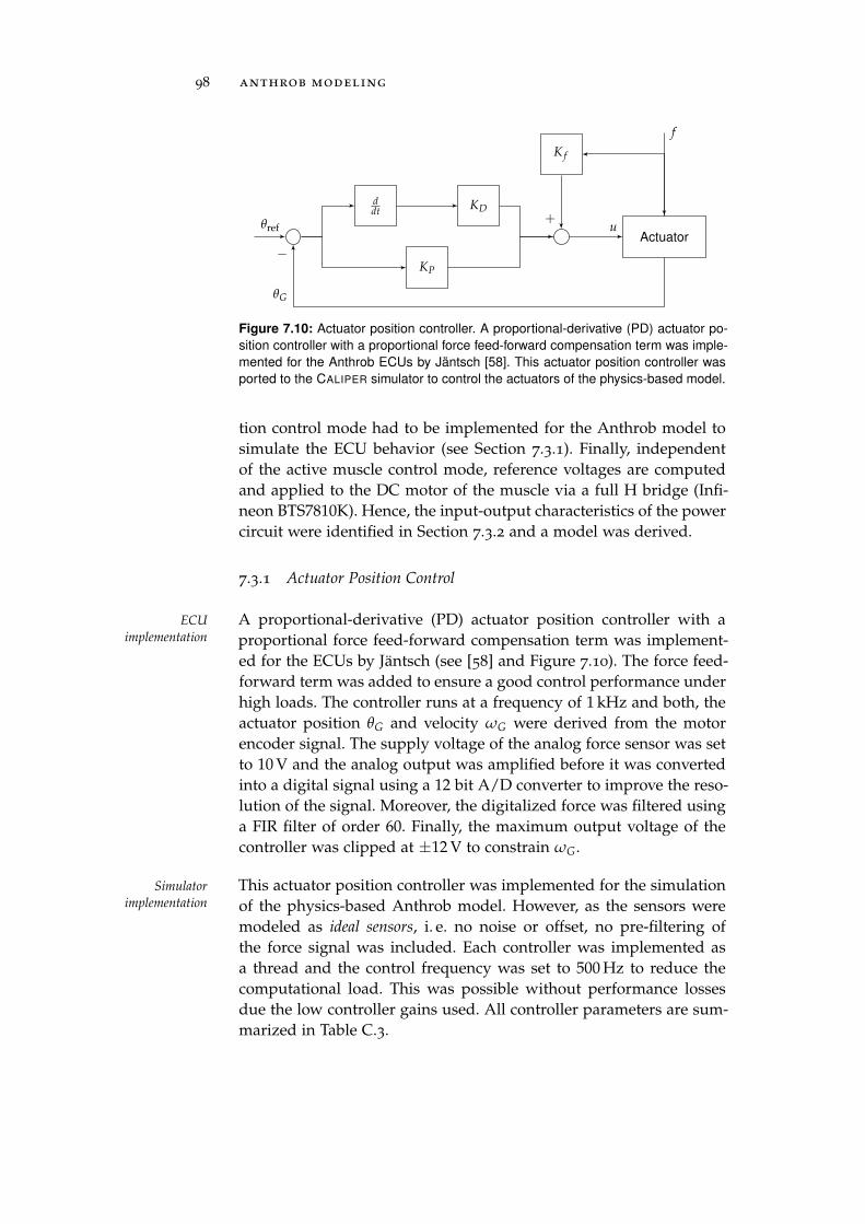
98 anthrob modeling

Actuator

K f

ddt

KD

KP

θG

−

θref u+

f

Figure 7.10: Actuator position controller. A proportional-derivative (PD) actuator po-

sition controller with a proportional force feed-forward compensation term was imple-

mented for the Anthrob ECUs by Jäntsch [58]. This actuator position controller was

ported to the CALIPER simulator to control the actuators of the physics-based model.

tion control mode had to be implemented for the Anthrob model tosimulate the ECU behavior (see Section 7.3.1). Finally, independentof the active muscle control mode, reference voltages are computedand applied to the DC motor of the muscle via a full H bridge (Infi-neon BTS7810K). Hence, the input-output characteristics of the powercircuit were identified in Section 7.3.2 and a model was derived.

7.3.1 Actuator Position Control

A proportional-derivative (PD) actuator position controller with aECU

implementation proportional force feed-forward compensation term was implement-ed for the ECUs by Jäntsch (see [58] and Figure 7.10). The force feed-forward term was added to ensure a good control performance underhigh loads. The controller runs at a frequency of 1 kHz and both, theactuator position θG and velocity ωG were derived from the motorencoder signal. The supply voltage of the analog force sensor was setto 10 V and the analog output was amplified before it was convertedinto a digital signal using a 12 bit A/D converter to improve the reso-lution of the signal. Moreover, the digitalized force was filtered usinga FIR filter of order 60. Finally, the maximum output voltage of thecontroller was clipped at ±12 V to constrain ωG.

This actuator position controller was implemented for the simulationSimulator

implementation of the physics-based Anthrob model. However, as the sensors weremodeled as ideal sensors, i. e. no noise or offset, no pre-filtering ofthe force signal was included. Each controller was implemented asa thread and the control frequency was set to 500 Hz to reduce thecomputational load. This was possible without performance lossesdue the low controller gains used. All controller parameters are sum-marized in Table C.3.

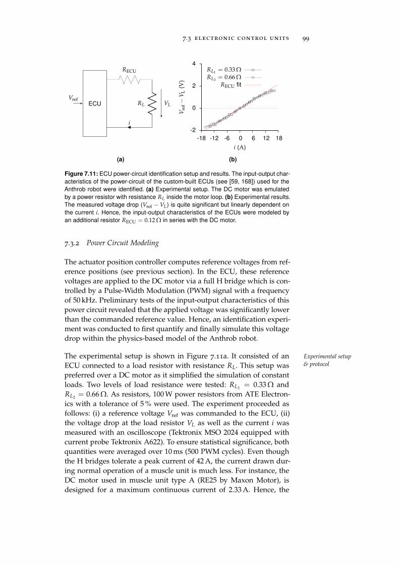
7.3 electronic control units 99

ECUVref

RL

i

VL

RECU

(a)

-2

0

2

4

-18 -12 -6 0 6 12 18

Vre

f−

VL

(V)

i (A)

RL1 = 0.33 Ω

RL2 = 0.66 Ω

RECU fit

(b)

Figure 7.11: ECU power-circuit identification setup and results. The input-output char-

acteristics of the power-circuit of the custom-built ECUs (see [59, 168]) used for the

Anthrob robot were identified. (a) Experimental setup. The DC motor was emulated

by a power resistor with resistance RL inside the motor loop. (b) Experimental results.

The measured voltage drop (Vref − VL) is quite significant but linearly dependent on

the current i. Hence, the input-output characteristics of the ECUs were modeled by

an additional resistor RECU = 0.12 Ω in series with the DC motor.

7.3.2 Power Circuit Modeling

The actuator position controller computes reference voltages from ref-erence positions (see previous section). In the ECU, these referencevoltages are applied to the DC motor via a full H bridge which is con-trolled by a Pulse-Width Modulation (PWM) signal with a frequencyof 50 kHz. Preliminary tests of the input-output characteristics of thispower circuit revealed that the applied voltage was significantly lowerthan the commanded reference value. Hence, an identification experi-ment was conducted to first quantify and finally simulate this voltagedrop within the physics-based model of the Anthrob robot.

The experimental setup is shown in Figure 7.11a. It consisted of an Experimental setup

& protocolECU connected to a load resistor with resistance RL. This setup waspreferred over a DC motor as it simplified the simulation of constantloads. Two levels of load resistance were tested: RL1 = 0.33 Ω andRL2 = 0.66 Ω. As resistors, 100 W power resistors from ATE Electron-ics with a tolerance of 5 % were used. The experiment proceeded asfollows: (i) a reference voltage Vref was commanded to the ECU, (ii)the voltage drop at the load resistor VL as well as the current i wasmeasured with an oscilloscope (Tektronix MSO 2024 equipped withcurrent probe Tektronix A622). To ensure statistical significance, bothquantities were averaged over 10 ms (500 PWM cycles). Even thoughthe H bridges tolerate a peak current of 42 A, the current drawn dur-ing normal operation of a muscle unit is much less. For instance, theDC motor used in muscle unit type A (RE25 by Maxon Motor), isdesigned for a maximum continuous current of 2.33 A. Hence, the

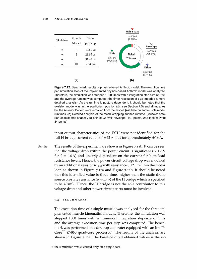
100 anthrob modeling

SkeletonMuscle Time

Model per step

• – 17.89 µs

• I 21.85 µs

• II 31.47 µs

• III 2.94 ms

(a)

Total

2.94 ms

Half-Space

0.07 ms(2.28%)

Envelope

0.99 ms(33.55%)

Other

0.03 ms(0.91%)

Path

1.86 ms(63.25%)

(b)

Figure 7.12: Benchmark results of physics-based Anthrob model. The execution time

per simulation step of the implemented physics-based Anthrob model was analyzed.

Therefore, the simulation was stepped 1000 times with a integration step size of 1 msand the average runtime was computed (the timer resolution of 1 µs impeded a more

detailed analysis). As the runtime is posture dependent, it should be noted that the

skeleton model was in the equilibrium position (E0, see Section 7.5) and all muscles

but the Anterior Deltoid were removed from the model. (a) Skeleton and muscle model

runtimes. (b) Detailed analysis of the mesh wrapping surface runtime. (Muscle: Ante-

rior Deltoid; Half-space: 748 points; Convex envelope: 149 points, 263 facets; Path:

34 points).

input-output characteristics of the ECU were not identified for thefull H bridge current range of ±42 A, but for approximately ±16 A.

The results of the experiment are shown in Figure 7.11b. It can be seenResults

that the voltage drop within the power circuit is significant (∼ 1.6 Vfor i = 16 A) and linearly dependent on the current for both loadresistance levels. Hence, the power circuit voltage drop was modeledby an additional resistor RECU with resistance 0.12 Ω within the motorloop as shown in Figure 7.11a and Figure 7.11b. It should be notedthat this identified value is three times higher than the static drain-source on-state resistance (RDS−ON) of the H bridge which is specifiedto be 40 mΩ. Hence, the H bridge is not the sole contributor to thisvoltage drop and other power circuit parts must be involved.

7.4 benchmarks

The execution time of a single muscle was analyzed for the three im-plemented muscle kinematics models. Therefore, the simulation wasstepped 1000 times with a numerical integration step-size of 1 msand the average execution time per step was computed. The bench-mark was performed on a desktop computer equipped with an Intel R©

CoreTM

i7-860 quad-core processor1. The results of the analysis areshown in Figure 7.12a. The baseline of all obtained values is the ex-

1 the simulation was executed only on a single core

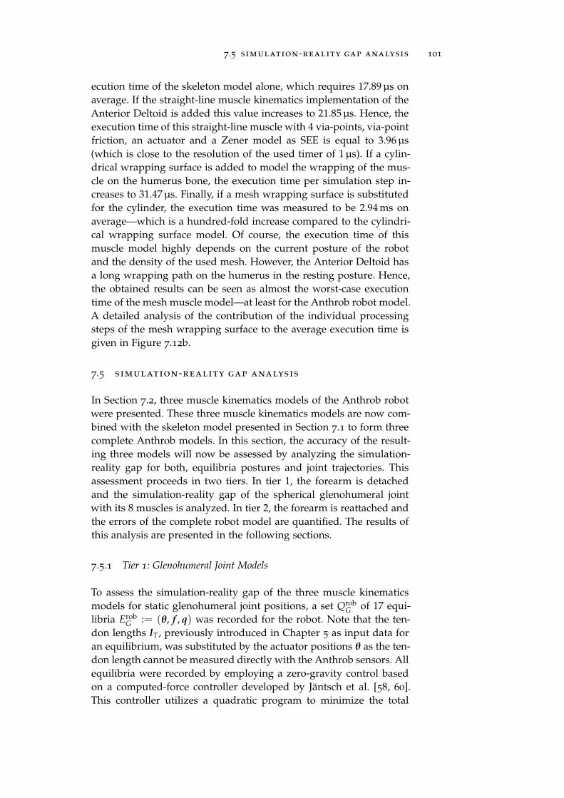
7.5 simulation-reality gap analysis 101

ecution time of the skeleton model alone, which requires 17.89 µs onaverage. If the straight-line muscle kinematics implementation of theAnterior Deltoid is added this value increases to 21.85 µs. Hence, theexecution time of this straight-line muscle with 4 via-points, via-pointfriction, an actuator and a Zener model as SEE is equal to 3.96 µs(which is close to the resolution of the used timer of 1 µs). If a cylin-drical wrapping surface is added to model the wrapping of the mus-cle on the humerus bone, the execution time per simulation step in-creases to 31.47 µs. Finally, if a mesh wrapping surface is substitutedfor the cylinder, the execution time was measured to be 2.94 ms onaverage—which is a hundred-fold increase compared to the cylindri-cal wrapping surface model. Of course, the execution time of thismuscle model highly depends on the current posture of the robotand the density of the used mesh. However, the Anterior Deltoid hasa long wrapping path on the humerus in the resting posture. Hence,the obtained results can be seen as almost the worst-case executiontime of the mesh muscle model—at least for the Anthrob robot model.A detailed analysis of the contribution of the individual processingsteps of the mesh wrapping surface to the average execution time isgiven in Figure 7.12b.

7.5 simulation-reality gap analysis

In Section 7.2, three muscle kinematics models of the Anthrob robotwere presented. These three muscle kinematics models are now com-bined with the skeleton model presented in Section 7.1 to form threecomplete Anthrob models. In this section, the accuracy of the result-ing three models will now be assessed by analyzing the simulation-reality gap for both, equilibria postures and joint trajectories. Thisassessment proceeds in two tiers. In tier 1, the forearm is detachedand the simulation-reality gap of the spherical glenohumeral jointwith its 8 muscles is analyzed. In tier 2, the forearm is reattached andthe errors of the complete robot model are quantified. The results ofthis analysis are presented in the following sections.

7.5.1 Tier 1: Glenohumeral Joint Models

To assess the simulation-reality gap of the three muscle kinematicsmodels for static glenohumeral joint positions, a set Qrob

G of 17 equi-libria Erob

G := (θ, f , q) was recorded for the robot. Note that the ten-don lengths lT, previously introduced in Chapter 5 as input data foran equilibrium, was substituted by the actuator positions θ as the ten-don length cannot be measured directly with the Anthrob sensors. Allequilibria were recorded by employing a zero-gravity control basedon a computed-force controller developed by Jäntsch et al. [58, 60].This controller utilizes a quadratic program to minimize the total

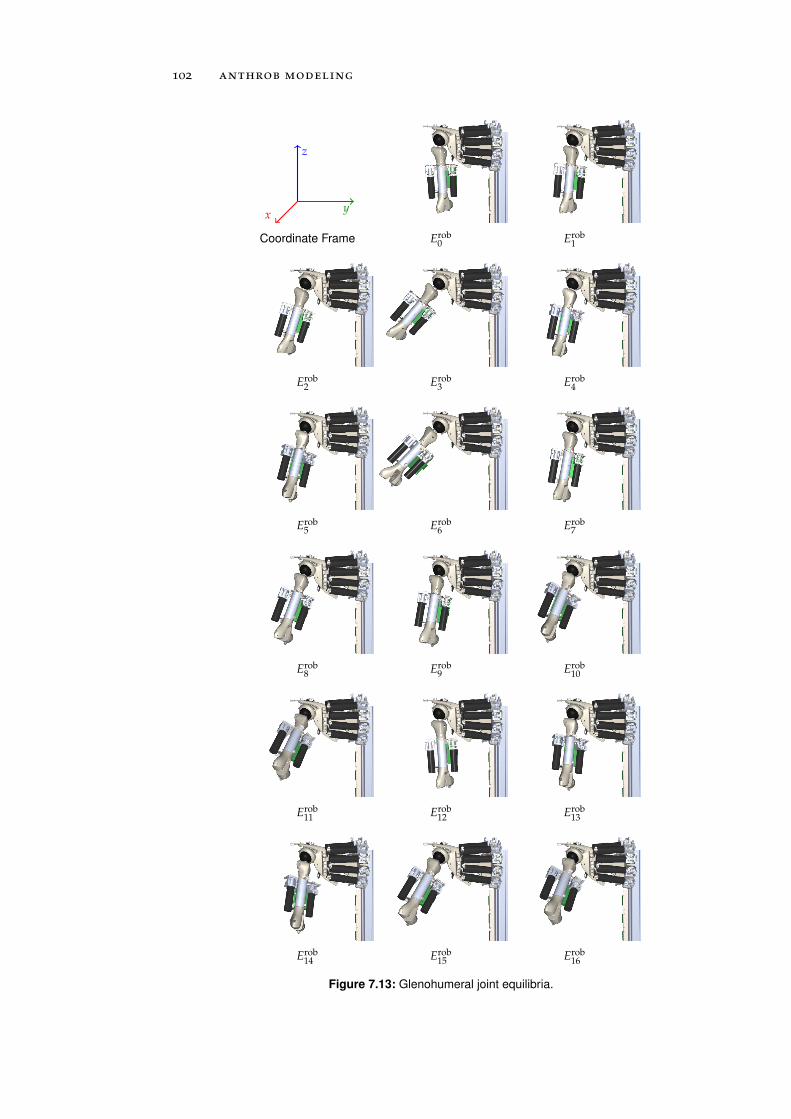
102 anthrob modeling

y

z

x

Coordinate Frame Erob0 Erob

1

Erob2 Erob

3 Erob4

Erob5 Erob

6 Erob7

Erob8 Erob

9 Erob10

Erob11 Erob

12 Erob13

Erob14 Erob

15 Erob16

Figure 7.13: Glenohumeral joint equilibria.

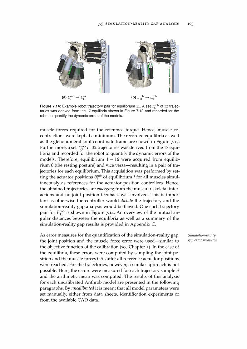
7.5 simulation-reality gap analysis 103

(a) Erob0 → Erob

11 (b) Erob11 → Erob

0

Figure 7.14: Example robot trajectory pair for equilibrium 11. A set TrobG of 32 trajec-

tories was derived from the 17 equilibria shown in Figure 7.13 and recorded for the

robot to quantify the dynamic errors of the models.

muscle forces required for the reference torque. Hence, muscle co-contractions were kept at a minimum. The recorded equilibria as wellas the glenohumeral joint coordinate frame are shown in Figure 7.13.Furthermore, a set Trob

G of 32 trajectories was derived from the 17 equi-libria and recorded for the robot to quantify the dynamic errors of themodels. Therefore, equilibrium 1 − 16 were acquired from equilib-rium 0 (the resting posture) and vice versa—resulting in a pair of tra-jectories for each equilibrium. This acquisition was performed by set-ting the actuator positions θrob

i of equilibrium i for all muscles simul-taneously as references for the actuator position controllers. Hence,the obtained trajectories are emerging from the musculo-skeletal inter-actions and no joint position feedback was involved. This is impor-tant as otherwise the controller would dictate the trajectory and thesimulation-reality gap analysis would be flawed. One such trajectorypair for Erob

11 is shown in Figure 7.14. An overview of the mutual an-gular distances between the equilibria as well as a summary of thesimulation-reality gap results is provided in Appendix C.

As error measures for the quantification of the simulation-reality gap, Simulation-reality

gap error measuresthe joint position and the muscle force error were used—similar tothe objective function of the calibration (see Chapter 5). In the case ofthe equilibria, these errors were computed by sampling the joint po-sition and the muscle forces 0.5 s after all reference actuator positionswere reached. For the trajectories, however, a similar approach is notpossible. Here, the errors were measured for each trajectory sample S

and the arithmetic mean was computed. The results of this analysisfor each uncalibrated Anthrob model are presented in the followingparagraphs. By uncalibrated it is meant that all model parameters wereset manually, either from data sheets, identification experiments orfrom the available CAD data.

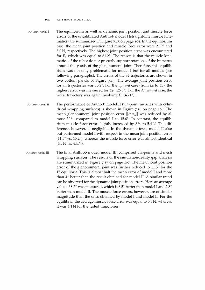
104 anthrob modeling

The equilibrium as well as dynamic joint position and muscle forceAnthrob model I

errors of the uncalibrated Anthrob model I (straight-line muscle kine-matics) are summarized in Figure 7.15 on page 105. In the equilibriumcase, the mean joint position and muscle force error were 21.9 and5.0 N, respectively. The highest joint position error was encounteredfor E9 which was equal to 61.2. The reason is that the muscle kine-matics of the robot do not properly support rotations of the humerusaround the y-axis of the glenohumeral joint. Therefore, this equilib-rium was not only problematic for model I but for all models (seefollowing paragraphs). The errors of the 32 trajectories are shown intwo bottom panels of Figure 7.15. The average joint position errorfor all trajectories was 15.2. For the upward case (from E0 to Ex), thehighest error was measured for E11 (26.8). For the downward case, theworst trajectory was again involving E9 (43.1).

The performance of Anthrob model II (via-point muscles with cylin-Anthrob model II

drical wrapping surfaces) is shown in Figure 7.16 on page 106. Themean glenohumeral joint position error ‖qG‖ was reduced by al-most 30 % compared to model I to 15.6. In contrast, the equilib-rium muscle force error slightly increased by 8 % to 5.4 N. This dif-ference, however, is negligible. In the dynamic tests, model II alsoout-performed model I with respect to the mean joint position error(11.5 vs. 15.2), whereas the muscle force error was almost identical(4.3 N vs. 4.4 N).

The final Anthrob model, model III, comprised via-points and meshAnthrob model III

wrapping surfaces. The results of the simulation-reality gap analysisare summarized in Figure 7.17 on page 107. The mean joint positionerror of the glenohumeral joint was further reduced to 11.3 for the17 equilibria. This is almost half the mean error of model I and morethan 4 better than the result obtained for model II. A similar trendcan be observed for the dynamic joint position errors. Here an averagevalue of 8.7 was measured, which is 6.5 better than model I and 2.8

better than model II. The muscle force errors, however, are of similarmagnitude than the ones obtained by model I and model II. For theequilibria, the average muscle force error was equal to 5.3 N, whereasit was 4.1 N for the tested trajectories.

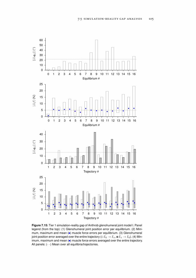
7.5 simulation-reality gap analysis 105

0

10

20

30

40

50

60

0 1 2 3 4 5 6 7 8 9 10 11 12 13 14 15 16

‖q

G‖

()

Equilibrium #

0

5

10

15

20

25

0 1 2 3 4 5 6 7 8 9 10 11 12 13 14 15 16

|f|

(N)

Equilibrium #

0

10

20

30

40

1 2 3 4 5 6 7 8 9 10 11 12 13 14 15 16

‖q

G‖

()

Trajectory #

0

5

10

15

20

25

1 2 3 4 5 6 7 8 9 10 11 12 13 14 15 16

|f|

(N)

Trajectory #

Figure 7.15: Tier 1 simulation-reality gap of Anthrob glenohumeral joint model I. Panel

legend (from the top): (1) Glenohumeral joint position error per equilibrium. (2) Mini-

mum, maximum and mean ( ) muscle force errors per equilibrium. (3) Glenohumeral

joint position error averaged over the entire trajectory ( E0 → Ex, Ex → E0). (4) Min-

imum, maximum and mean ( ) muscle force errors averaged over the entire trajectory.

All panels: ( ) Mean over all equilibria/trajectories.

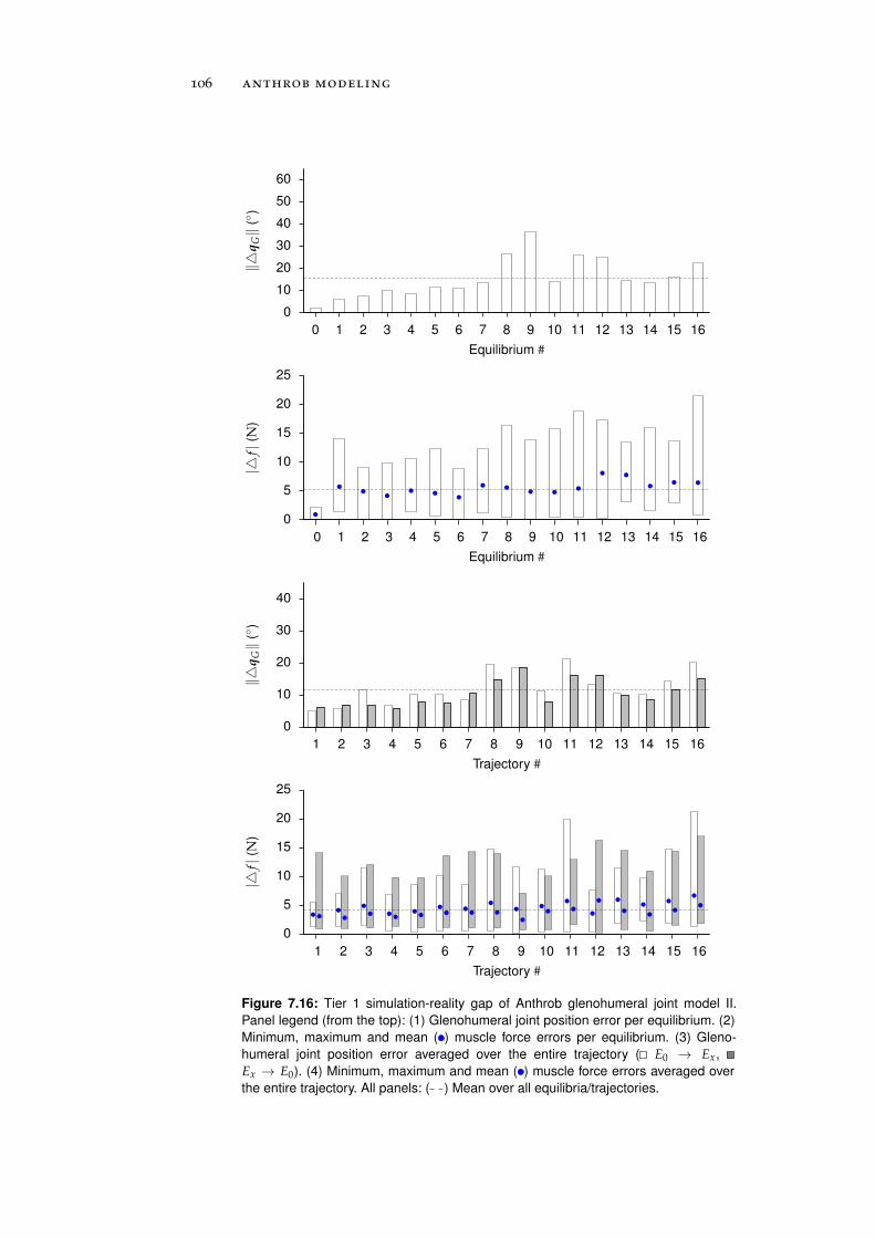
106 anthrob modeling

0

10

20

30

40

50

60

0 1 2 3 4 5 6 7 8 9 10 11 12 13 14 15 16

‖q

G‖

()

Equilibrium #

0

5

10

15

20

25

0 1 2 3 4 5 6 7 8 9 10 11 12 13 14 15 16

|f|

(N)

Equilibrium #

0

10

20

30

40

1 2 3 4 5 6 7 8 9 10 11 12 13 14 15 16

‖q

G‖

()

Trajectory #

0

5

10

15

20

25

1 2 3 4 5 6 7 8 9 10 11 12 13 14 15 16

|f|

(N)

Trajectory #

Figure 7.16: Tier 1 simulation-reality gap of Anthrob glenohumeral joint model II.

Panel legend (from the top): (1) Glenohumeral joint position error per equilibrium. (2)

Minimum, maximum and mean ( ) muscle force errors per equilibrium. (3) Gleno-

humeral joint position error averaged over the entire trajectory ( E0 → Ex,

Ex → E0). (4) Minimum, maximum and mean ( ) muscle force errors averaged over

the entire trajectory. All panels: ( ) Mean over all equilibria/trajectories.

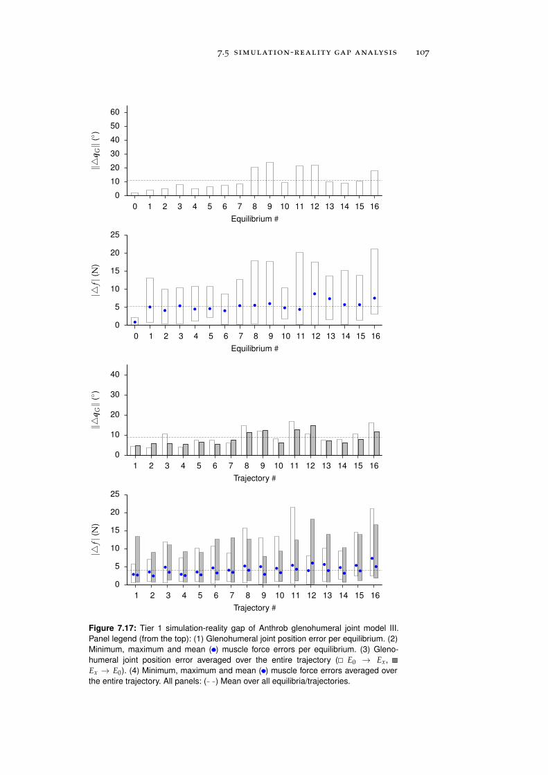
7.5 simulation-reality gap analysis 107

0

10

20

30

40

50

60

0 1 2 3 4 5 6 7 8 9 10 11 12 13 14 15 16

‖q

G‖

()

Equilibrium #

0

5

10

15

20

25

0 1 2 3 4 5 6 7 8 9 10 11 12 13 14 15 16

|f|

(N)

Equilibrium #

0

10

20

30

40

1 2 3 4 5 6 7 8 9 10 11 12 13 14 15 16

‖q

G‖

()

Trajectory #

0

5

10

15

20

25

1 2 3 4 5 6 7 8 9 10 11 12 13 14 15 16

|f|

(N)

Trajectory #

Figure 7.17: Tier 1 simulation-reality gap of Anthrob glenohumeral joint model III.

Panel legend (from the top): (1) Glenohumeral joint position error per equilibrium. (2)

Minimum, maximum and mean ( ) muscle force errors per equilibrium. (3) Gleno-

humeral joint position error averaged over the entire trajectory ( E0 → Ex,

Ex → E0). (4) Minimum, maximum and mean ( ) muscle force errors averaged over

the entire trajectory. All panels: ( ) Mean over all equilibria/trajectories.

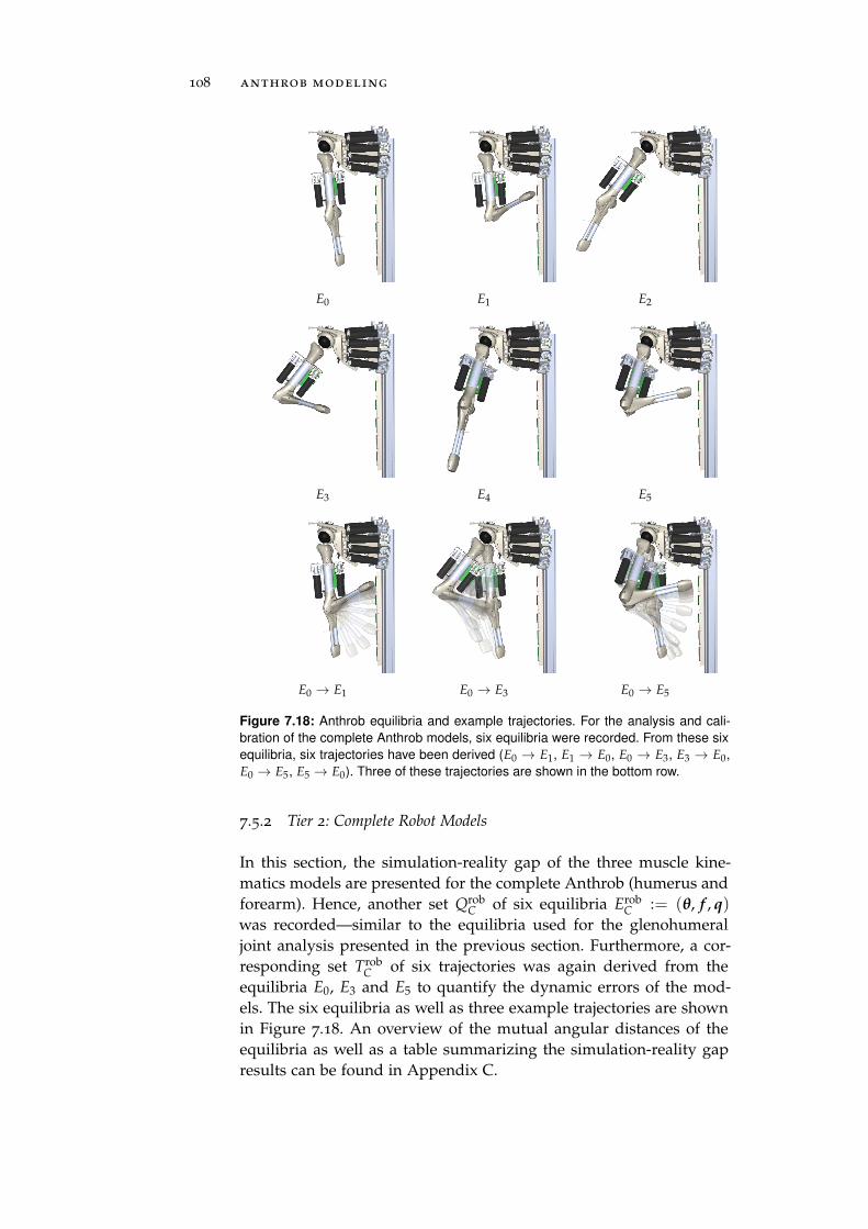
108 anthrob modeling

E0 E1 E2

E3 E4 E5

E0 → E1 E0 → E3 E0 → E5

Figure 7.18: Anthrob equilibria and example trajectories. For the analysis and cali-

bration of the complete Anthrob models, six equilibria were recorded. From these six

equilibria, six trajectories have been derived (E0 → E1, E1 → E0, E0 → E3, E3 → E0,

E0 → E5, E5 → E0). Three of these trajectories are shown in the bottom row.

7.5.2 Tier 2: Complete Robot Models

In this section, the simulation-reality gap of the three muscle kine-matics models are presented for the complete Anthrob (humerus andforearm). Hence, another set Qrob

C of six equilibria ErobC := (θ, f , q)

was recorded—similar to the equilibria used for the glenohumeraljoint analysis presented in the previous section. Furthermore, a cor-responding set Trob

C of six trajectories was again derived from theequilibria E0, E3 and E5 to quantify the dynamic errors of the mod-els. The six equilibria as well as three example trajectories are shownin Figure 7.18. An overview of the mutual angular distances of theequilibria as well as a table summarizing the simulation-reality gapresults can be found in Appendix C.

7.5 simulation-reality gap analysis 109

The results of the simulation-reality gap analysis for Anthrob model I Anthrob model I

are presented in Figure 7.19a on page 110. It can be seen that themean equilibrium and dynamic joint position errors of the elbow jointare significantly lower than those encountered for the glenohumeraljoint previously (4.4 and 5.1, respectively). This was expected fortwo reasons: (i) the elbow joint has only one DoF and hence is lessprone to erroneous muscle routing and (ii) muscle wrapping is notprominent for the elbow joint muscles. Hence, the straight-line mus-cle kinematics can provide a good approximation for the muscle path,particularly for elbow joint positions below 90—above that angle, theTriceps muscle wraps around the robot skeleton. This is also visiblein the results, as E1, E3 and E5 exhibit the largest errors.

The results of the simulation-reality gap analysis for Anthrob model II Anthrob model II

are shown in Figure 7.19b. Here, in accordance with the tier 1 re-sults, the glenohumeral joint position errors are lower than the onesobtained for muscle kinematics model I. However, the elbow jointposition errors are slightly larger (0.7 for both, the statics and the dy-namics analysis). Still, this was not expected as the cylindrical wrap-ping surface introduced for the elbow muscles should be capable ofsimulating the Triceps wrapping for joint positions above 90. As wewill see in Section 8.1, the reason for this is an erroneous manualparametrization of the cylinder radius. If the cylinder radius was cal-ibrated, significantly better results could be obtained for the elbowjoint position errors.

Finally, the results of Anthrob model III are presented in Figure 7.19c. Anthrob model III

Again, in accordance with the tier 1 results, the more complex meshwrapping surface model provided the lowest errors for the gleno-humeral joint positions. However, as model III is identical to model IIfor the elbow joint muscles, no different results were obtained forthis joint. The slight deviations in the elbow joint position error vis-ible between Figure 7.19b and Figure 7.19c are only due to differentglenohumeral joint positions which alter the effect of gravity on theforearm.

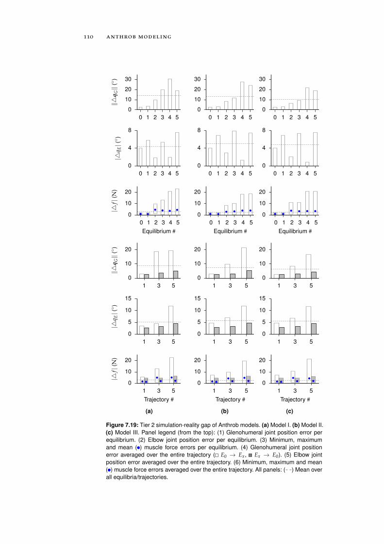
110 anthrob modeling

0

10

20

30

0 1 2 3 4 5‖

qG‖

()

0

4

8

0 1 2 3 4 5

|q E|( )

0

10

20

0 1 2 3 4 5

|f|

(N)

Equilibrium #

0

10

20

1 3 5

‖q

G‖

()

0

5

10

15

1 3 5

|q E|( )

0

10

20

1 3 5

|f|

(N)

Trajectory #

(a)

0

10

20

30

0 1 2 3 4 5

0

4

8

0 1 2 3 4 5

0

10

20

0 1 2 3 4 5

Equilibrium #

0

10

20

1 3 5

0

5

10

15

1 3 5

0

10

20

1 3 5

Trajectory #

(b)

0

10

20

30

0 1 2 3 4 5

0

4

8

0 1 2 3 4 5

0

10

20

0 1 2 3 4 5

Equilibrium #

0

10

20

1 3 5

0

5

10

15

1 3 5

0

10

20

1 3 5

Trajectory #

(c)

Figure 7.19: Tier 2 simulation-reality gap of Anthrob models. (a) Model I. (b) Model II.

(c) Model III. Panel legend (from the top): (1) Glenohumeral joint position error per

equilibrium. (2) Elbow joint position error per equilibrium. (3) Minimum, maximum

and mean ( ) muscle force errors per equilibrium. (4) Glenohumeral joint position

error averaged over the entire trajectory ( E0 → Ex, Ex → E0). (5) Elbow joint

position error averaged over the entire trajectory. (6) Minimum, maximum and mean

( ) muscle force errors averaged over the entire trajectory. All panels: ( ) Mean over

all equilibria/trajectories.

8A N T H R O B M O D E L C A L I B R AT I O N

In Chapter 7, three Anthrob simulation models were presented andthe simulation-reality gap of each model was analyzed. In this chap-ter, this gap is now minimized by applying the ES-based calibrationprocedure previously presented in Chapter 5 in Section 8.1. Once cal-ibrated, the Anthrob models are validated in Section 8.2 to assess thequality of the calibration results. Finally, the chapter concludes by adiscussion of the obtained results in Section 8.3.

8.1 calibration

The calibration proceeded in two tiers (see also Figure 8.1). In tier 1, Calibration

procedurethe forearm of the robot was detached to calibrate the eight musclesof the spherical glenohumeral joint, whereas in tier 2 the forearm wasre-attached and the 2 elbow joint muscles as well as the biarticular Bi-ceps were calibrated for different glenohumeral joint positions. Bothtiers were further subdivided into a statics and dynamics calibrationstage. While in the former a set of equilibria Q was calibrated, thelatter stage employed a set of reference trajectories T to minimize thedynamic errors of the three Anthrob models. Stage 1 was initializedby a manually parametrized ancestor individual IA, whereas the re-maining three calibration stages always used the best individual ofthe preceding stage as initial condition. This results in a single objectparameter set, i. e. the individual IC, for each Anthrob model. Further-more, to reduce the risk that the calibration reached a local minimum,each stage was executed twice and the better run survived. The par-ent and offspring population sizes of all runs were set to µ = 6 andλ = 36 to achieve a µ/λ-ratio of 1/6 which has been shown to pro-vide a maximum rate of convergence [45, 163]. In all runs, the targetfitness was set to zero (i. e. a perfect model with zero joint positionand zero muscle force error). The coefficients κq and κ f , that definethe contribution of the two error measures to the objective functionvalue, were determined in trial runs and set to κq = 1 and κ f = 10−4,respectively. Finally, a distinct set of model parameters was selectedas object parameters for each Anthrob model. However, only modelparameters that were not identified experimentally or that could not

111

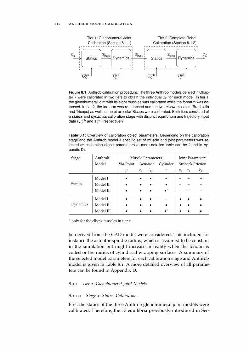
112 anthrob model calibration

Statics Dynamics Statics Dynamics

Tier 1: Glenohumeral Joint

Calibration (Section 8.1.1)

Tier 2: Complete Robot

Calibration (Section 8.1.2)

IA Ibest Ibest Ibest IC

QrobG Trob

G QrobC Trob

C

Figure 8.1: Anthrob calibration procedure. The three Anthrob models derived in Chap-

ter 7 were calibrated in two tiers to obtain the individual IC for each model. In tier 1,

the glenohumeral joint with its eight muscles was calibrated while the forearm was de-

tached. In tier 2, the forearm was re-attached and the two elbow muscles (Brachialis

and Triceps) as well as the bi-articular Biceps were calibrated. Both tiers consisted of

a statics and dynamics calibration stage with disjunct equilibrium and trajectory input

data (Qrobx and Trob

x , respectively).

Table 8.1: Overview of calibration object parameters. Depending on the calibration

stage and the Anthrob model a specific set of muscle and joint parameters was se-

lected as calibration object parameters (a more detailed table can be found in Ap-

pendix D).

Stage Anthrob Muscle Parameters Joint Parameters

Model Via-Point Actuator Cylinder Stribeck Friction

p rs lT0 r τs τk kv

Statics

Model I • • • – – – –

Model II • • • • – – –

Model III • • • •∗ – – –

Dynamics

Model I • • • – • • •

Model II • • • • • • •

Model III • • • •∗

• • •

∗ only for the elbow muscles in tier 2

be derived from the CAD model were considered. This included forinstance the actuator spindle radius, which is assumed to be constantin the simulation but might increase in reality when the tendon iscoiled or the radius of cylindrical wrapping surfaces. A summary ofthe selected model parameters for each calibration stage and Anthrobmodel is given in Table 8.1. A more detailed overview of all parame-ters can be found in Appendix D.

8.1.1 Tier 1: Glenohumeral Joint Models

8.1.1.1 Stage 1: Statics Calibration

First the statics of the three Anthrob glenohumeral joint models werecalibrated. Therefore, the 17 equilibria previously introduced in Sec-

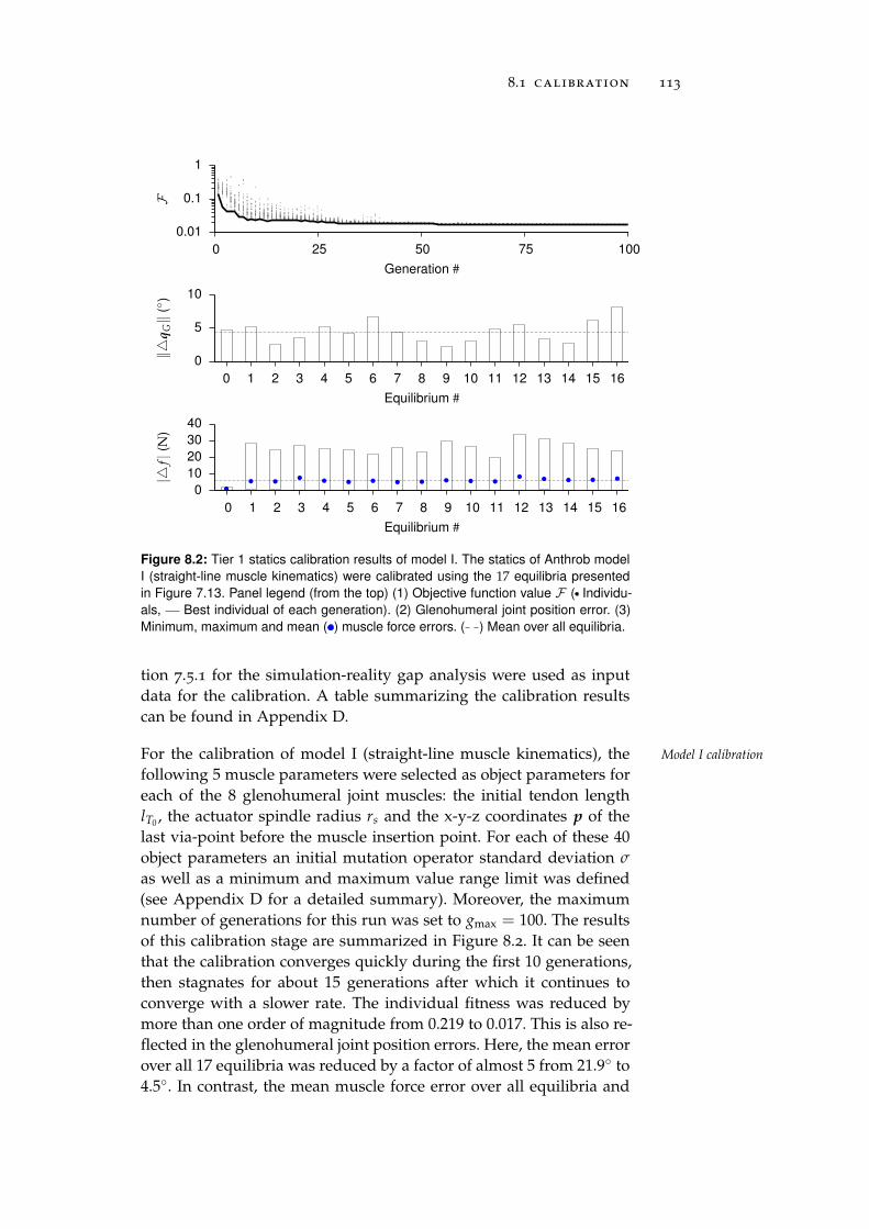
8.1 calibration 113

0.01

0.1

1

0 25 50 75 100

F

Generation #

0

5

10

0 1 2 3 4 5 6 7 8 9 10 11 12 13 14 15 16

‖q

G‖

()

Equilibrium #

0

10

20

30

40

0 1 2 3 4 5 6 7 8 9 10 11 12 13 14 15 16

|f|

(N)

Equilibrium #

Figure 8.2: Tier 1 statics calibration results of model I. The statics of Anthrob model

I (straight-line muscle kinematics) were calibrated using the 17 equilibria presented

in Figure 7.13. Panel legend (from the top) (1) Objective function value F ( Individu-

als, Best individual of each generation). (2) Glenohumeral joint position error. (3)

Minimum, maximum and mean ( ) muscle force errors. ( ) Mean over all equilibria.

tion 7.5.1 for the simulation-reality gap analysis were used as inputdata for the calibration. A table summarizing the calibration resultscan be found in Appendix D.

For the calibration of model I (straight-line muscle kinematics), the Model I calibration

following 5 muscle parameters were selected as object parameters foreach of the 8 glenohumeral joint muscles: the initial tendon lengthlT0 , the actuator spindle radius rs and the x-y-z coordinates p of thelast via-point before the muscle insertion point. For each of these 40object parameters an initial mutation operator standard deviation σ

as well as a minimum and maximum value range limit was defined(see Appendix D for a detailed summary). Moreover, the maximumnumber of generations for this run was set to gmax = 100. The resultsof this calibration stage are summarized in Figure 8.2. It can be seenthat the calibration converges quickly during the first 10 generations,then stagnates for about 15 generations after which it continues toconverge with a slower rate. The individual fitness was reduced bymore than one order of magnitude from 0.219 to 0.017. This is also re-flected in the glenohumeral joint position errors. Here, the mean errorover all 17 equilibria was reduced by a factor of almost 5 from 21.9 to4.5. In contrast, the mean muscle force error over all equilibria and

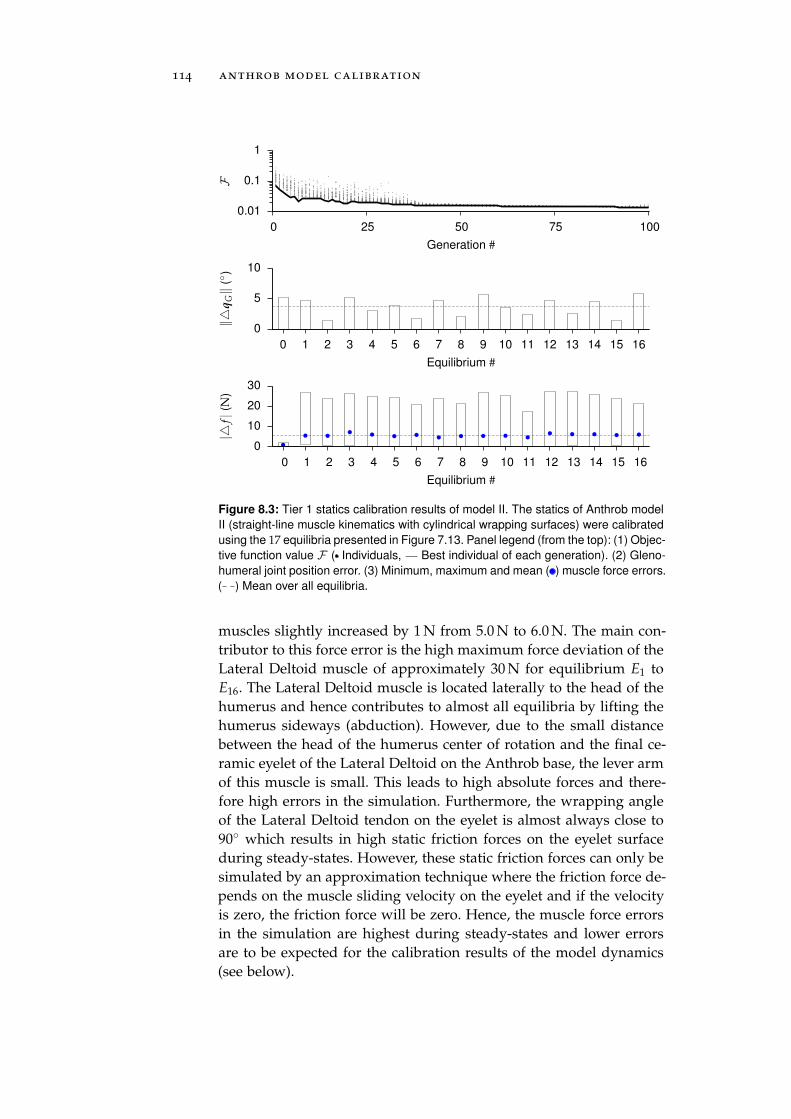
114 anthrob model calibration

0.01

0.1

1

0 25 50 75 100F

Generation #

0

5

10

0 1 2 3 4 5 6 7 8 9 10 11 12 13 14 15 16

‖q

G‖

()

Equilibrium #

0

10

20

30

0 1 2 3 4 5 6 7 8 9 10 11 12 13 14 15 16

|f|

(N)

Equilibrium #

Figure 8.3: Tier 1 statics calibration results of model II. The statics of Anthrob model

II (straight-line muscle kinematics with cylindrical wrapping surfaces) were calibrated

using the 17 equilibria presented in Figure 7.13. Panel legend (from the top): (1) Objec-

tive function value F ( Individuals, Best individual of each generation). (2) Gleno-

humeral joint position error. (3) Minimum, maximum and mean ( ) muscle force errors.

( ) Mean over all equilibria.

muscles slightly increased by 1 N from 5.0 N to 6.0 N. The main con-tributor to this force error is the high maximum force deviation of theLateral Deltoid muscle of approximately 30 N for equilibrium E1 toE16. The Lateral Deltoid muscle is located laterally to the head of thehumerus and hence contributes to almost all equilibria by lifting thehumerus sideways (abduction). However, due to the small distancebetween the head of the humerus center of rotation and the final ce-ramic eyelet of the Lateral Deltoid on the Anthrob base, the lever armof this muscle is small. This leads to high absolute forces and there-fore high errors in the simulation. Furthermore, the wrapping angleof the Lateral Deltoid tendon on the eyelet is almost always close to90 which results in high static friction forces on the eyelet surfaceduring steady-states. However, these static friction forces can only besimulated by an approximation technique where the friction force de-pends on the muscle sliding velocity on the eyelet and if the velocityis zero, the friction force will be zero. Hence, the muscle force errorsin the simulation are highest during steady-states and lower errorsare to be expected for the calibration results of the model dynamics(see below).

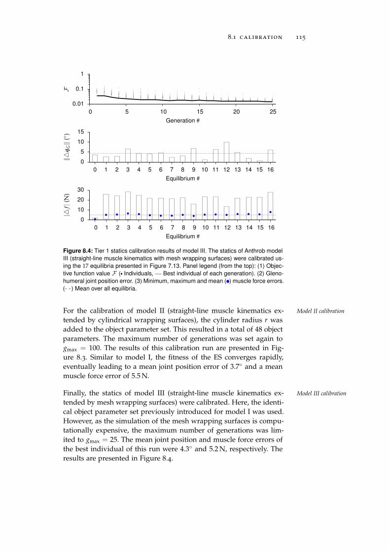
8.1 calibration 115

0.01

0.1

1

0 5 10 15 20 25

F

Generation #

0

5

10

15

0 1 2 3 4 5 6 7 8 9 10 11 12 13 14 15 16

‖q

G‖

()

Equilibrium #

0

10

20

30

0 1 2 3 4 5 6 7 8 9 10 11 12 13 14 15 16

|f|

(N)

Equilibrium #

Figure 8.4: Tier 1 statics calibration results of model III. The statics of Anthrob model

III (straight-line muscle kinematics with mesh wrapping surfaces) were calibrated us-

ing the 17 equilibria presented in Figure 7.13. Panel legend (from the top): (1) Objec-

tive function value F ( Individuals, Best individual of each generation). (2) Gleno-

humeral joint position error. (3) Minimum, maximum and mean ( ) muscle force errors.

( ) Mean over all equilibria.

For the calibration of model II (straight-line muscle kinematics ex- Model II calibration

tended by cylindrical wrapping surfaces), the cylinder radius r wasadded to the object parameter set. This resulted in a total of 48 objectparameters. The maximum number of generations was set again togmax = 100. The results of this calibration run are presented in Fig-ure 8.3. Similar to model I, the fitness of the ES converges rapidly,eventually leading to a mean joint position error of 3.7 and a meanmuscle force error of 5.5 N.

Finally, the statics of model III (straight-line muscle kinematics ex- Model III calibration

tended by mesh wrapping surfaces) were calibrated. Here, the identi-cal object parameter set previously introduced for model I was used.However, as the simulation of the mesh wrapping surfaces is compu-tationally expensive, the maximum number of generations was lim-ited to gmax = 25. The mean joint position and muscle force errors ofthe best individual of this run were 4.3 and 5.2 N, respectively. Theresults are presented in Figure 8.4.

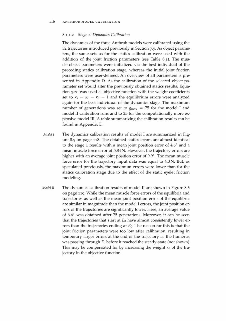
116 anthrob model calibration

8.1.1.2 Stage 2: Dynamics Calibration

The dynamics of the three Anthrob models were calibrated using the32 trajectories introduced previously in Section 7.5. As object parame-ters, the same sets as for the statics calibration were used with theaddition of the joint friction parameters (see Table 8.1). The mus-cle object parameters were initialized via the best individual of thepreceding statics calibration stage, whereas the initial joint frictionparameters were user-defined. An overview of all parameters is pre-sented in Appendix D. As the calibration of the selected object pa-rameter set would alter the previously obtained statics results, Equa-tion 5.20 was used as objective function with the weight coefficientsset to κs = κt = κe = 1 and the equilibrium errors were analyzedagain for the best individual of the dynamics stage. The maximumnumber of generations was set to gmax = 75 for the model I andmodel II calibration runs and to 25 for the computationally more ex-pensive model III. A table summarizing the calibration results can befound in Appendix D.

The dynamics calibration results of model I are summarized in Fig-Model I

ure 8.5 on page 118. The obtained statics errors are almost identicalto the stage 1 results with a mean joint position error of 4.6 and amean muscle force error of 5.84 N. However, the trajectory errors arehigher with an average joint position error of 9.9. The mean muscleforce error for the trajectory input data was equal to 4.0 N. But, asspeculated previously, the maximum errors were lower than for thestatics calibration stage due to the effect of the static eyelet frictionmodeling.

The dynamics calibration results of model II are shown in Figure 8.6Model II

on page 119. While the mean muscle force errors of the equilibria andtrajectories as well as the mean joint position error of the equilibriaare similar in magnitude than the model I errors, the joint position er-rors of the trajectories are significantly lower. Here, an average valueof 6.6 was obtained after 75 generations. Moreover, it can be seenthat the trajectories that start at E0 have almost consistently lower er-rors than the trajectories ending at E0. The reason for this is that thejoint friction parameters were too low after calibration, resulting intemporary larger errors at the end of the trajectory as the humeruswas passing through E0 before it reached the steady-state (not shown).This may be compensated for by increasing the weight κt of the tra-jectory in the objective function.

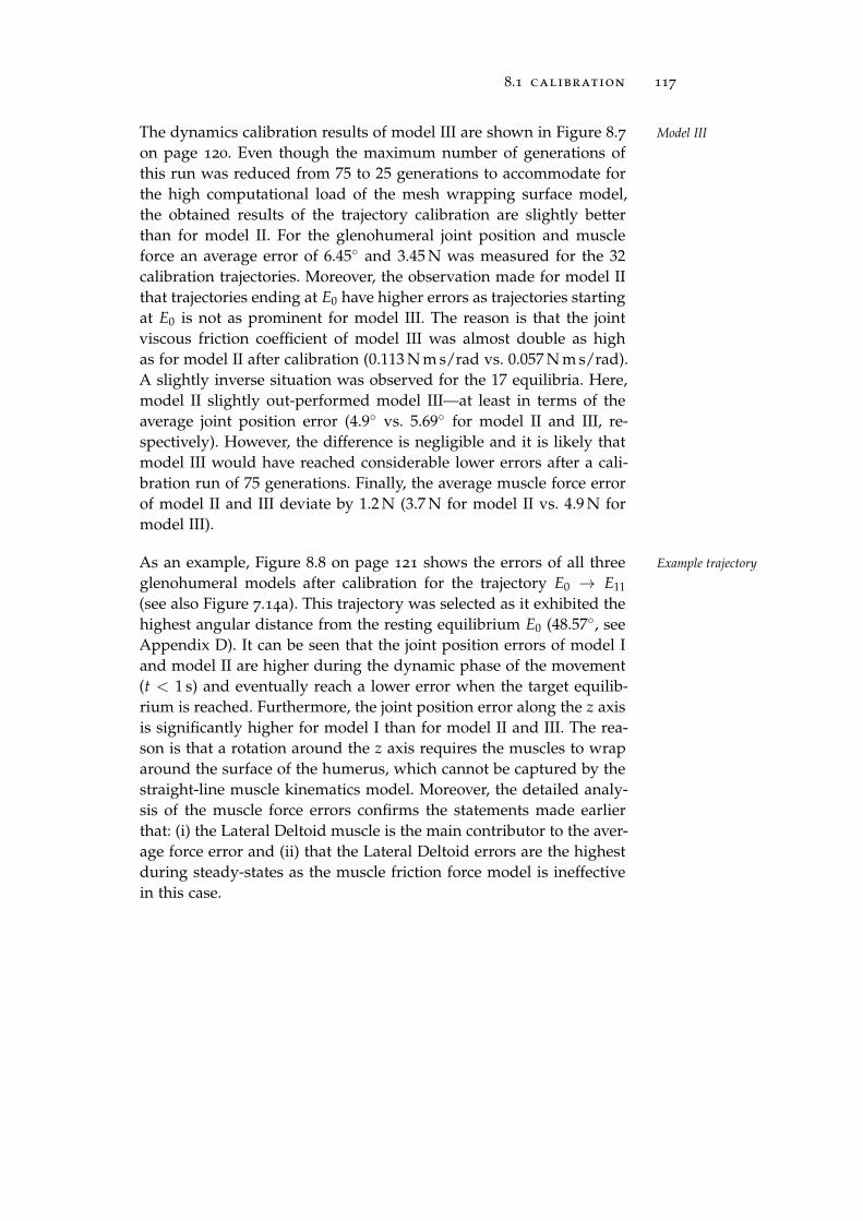
8.1 calibration 117

The dynamics calibration results of model III are shown in Figure 8.7 Model III

on page 120. Even though the maximum number of generations ofthis run was reduced from 75 to 25 generations to accommodate forthe high computational load of the mesh wrapping surface model,the obtained results of the trajectory calibration are slightly betterthan for model II. For the glenohumeral joint position and muscleforce an average error of 6.45 and 3.45 N was measured for the 32calibration trajectories. Moreover, the observation made for model IIthat trajectories ending at E0 have higher errors as trajectories startingat E0 is not as prominent for model III. The reason is that the jointviscous friction coefficient of model III was almost double as highas for model II after calibration (0.113 N m s/rad vs. 0.057 N m s/rad).A slightly inverse situation was observed for the 17 equilibria. Here,model II slightly out-performed model III—at least in terms of theaverage joint position error (4.9 vs. 5.69 for model II and III, re-spectively). However, the difference is negligible and it is likely thatmodel III would have reached considerable lower errors after a cali-bration run of 75 generations. Finally, the average muscle force errorof model II and III deviate by 1.2 N (3.7 N for model II vs. 4.9 N formodel III).

As an example, Figure 8.8 on page 121 shows the errors of all three Example trajectory

glenohumeral models after calibration for the trajectory E0 → E11

(see also Figure 7.14a). This trajectory was selected as it exhibited thehighest angular distance from the resting equilibrium E0 (48.57, seeAppendix D). It can be seen that the joint position errors of model Iand model II are higher during the dynamic phase of the movement(t < 1 s) and eventually reach a lower error when the target equilib-rium is reached. Furthermore, the joint position error along the z axisis significantly higher for model I than for model II and III. The rea-son is that a rotation around the z axis requires the muscles to wraparound the surface of the humerus, which cannot be captured by thestraight-line muscle kinematics model. Moreover, the detailed analy-sis of the muscle force errors confirms the statements made earlierthat: (i) the Lateral Deltoid muscle is the main contributor to the aver-age force error and (ii) that the Lateral Deltoid errors are the highestduring steady-states as the muscle friction force model is ineffectivein this case.

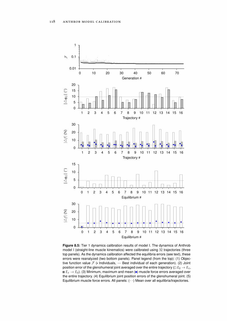
118 anthrob model calibration

0.01

0.1

1

0 10 20 30 40 50 60 70

F

Generation #

0

5

10

15

20

1 2 3 4 5 6 7 8 9 10 11 12 13 14 15 16

‖q

G‖

()

Trajectory #

0

10

20

30

1 2 3 4 5 6 7 8 9 10 11 12 13 14 15 16

|f|

(N)

Trajectory #

0

5

10

15

0 1 2 3 4 5 6 7 8 9 10 11 12 13 14 15 16

‖q

G‖

()

Equilibrium #

0

10

20

30

0 1 2 3 4 5 6 7 8 9 10 11 12 13 14 15 16

|f|

(N)

Equilibrium #

Figure 8.5: Tier 1 dynamics calibration results of model I. The dynamics of Anthrob

model I (straight-line muscle kinematics) were calibrated using 32 trajectories (three

top panels). As the dynamics calibration affected the equilibria errors (see text), these

errors were reanalyzed (two bottom panels). Panel legend (from the top): (1) Objec-

tive function value F ( Individuals, Best individual of each generation). (2) Joint

position error of the glenohumeral joint averaged over the entire trajectory ( E0 → Ex,

Ex → E0). (3) Minimum, maximum and mean ( ) muscle force errors averaged over

the entire trajectory. (4) Equilibrium joint position errors of the glenohumeral joint. (5)

Equilibrium muscle force errors. All panels: ( ) Mean over all equilibria/trajectories.

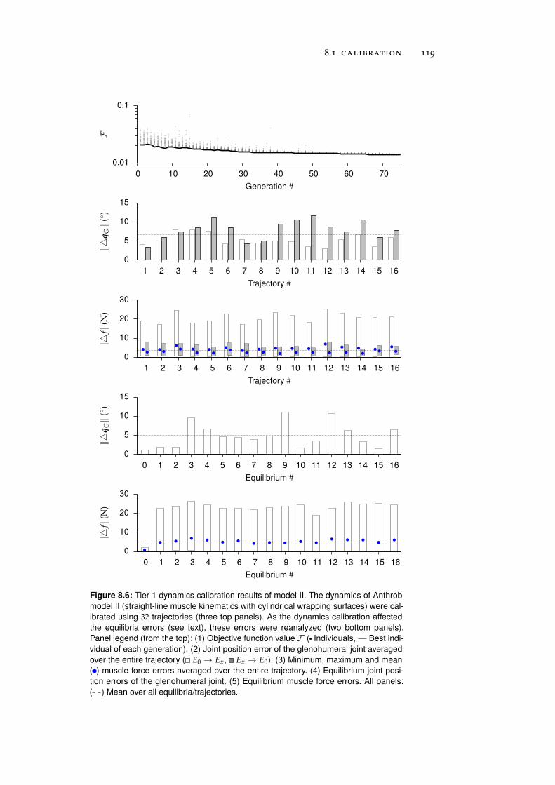
8.1 calibration 119

0.01

0.1

0 10 20 30 40 50 60 70

F

Generation #

0

5

10

15

1 2 3 4 5 6 7 8 9 10 11 12 13 14 15 16

‖q

G‖

()

Trajectory #

0

10

20

30

1 2 3 4 5 6 7 8 9 10 11 12 13 14 15 16

|f|

(N)

Trajectory #

0

5

10

15

0 1 2 3 4 5 6 7 8 9 10 11 12 13 14 15 16

‖q

G‖

()

Equilibrium #

0

10

20

30

0 1 2 3 4 5 6 7 8 9 10 11 12 13 14 15 16

|f|

(N)

Equilibrium #

Figure 8.6: Tier 1 dynamics calibration results of model II. The dynamics of Anthrob

model II (straight-line muscle kinematics with cylindrical wrapping surfaces) were cal-

ibrated using 32 trajectories (three top panels). As the dynamics calibration affected

the equilibria errors (see text), these errors were reanalyzed (two bottom panels).

Panel legend (from the top): (1) Objective function value F ( Individuals, Best indi-

vidual of each generation). (2) Joint position error of the glenohumeral joint averaged

over the entire trajectory ( E0 → Ex, Ex → E0). (3) Minimum, maximum and mean

( ) muscle force errors averaged over the entire trajectory. (4) Equilibrium joint posi-

tion errors of the glenohumeral joint. (5) Equilibrium muscle force errors. All panels:

( ) Mean over all equilibria/trajectories.

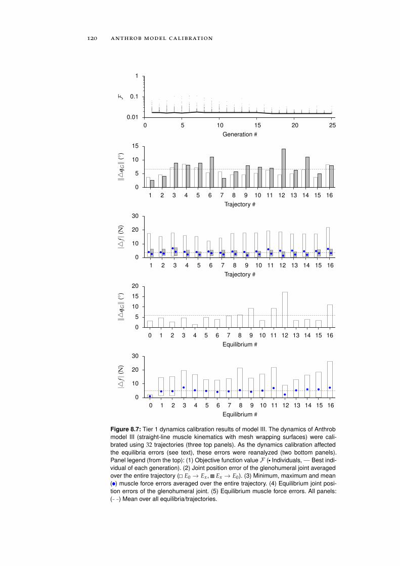
120 anthrob model calibration

0.01

0.1

1

0 5 10 15 20 25F

Generation #

0

5

10

15

1 2 3 4 5 6 7 8 9 10 11 12 13 14 15 16

‖q

G‖

()

Trajectory #

0

10

20

30

1 2 3 4 5 6 7 8 9 10 11 12 13 14 15 16

|f|

(N)

Trajectory #

0

5

10

15

20

0 1 2 3 4 5 6 7 8 9 10 11 12 13 14 15 16

‖q

G‖

()

Equilibrium #

0

10

20

30

0 1 2 3 4 5 6 7 8 9 10 11 12 13 14 15 16

|f|

(N)

Equilibrium #

Figure 8.7: Tier 1 dynamics calibration results of model III. The dynamics of Anthrob

model III (straight-line muscle kinematics with mesh wrapping surfaces) were cali-

brated using 32 trajectories (three top panels). As the dynamics calibration affected

the equilibria errors (see text), these errors were reanalyzed (two bottom panels).

Panel legend (from the top): (1) Objective function value F ( Individuals, Best indi-

vidual of each generation). (2) Joint position error of the glenohumeral joint averaged

over the entire trajectory ( E0 → Ex, Ex → E0). (3) Minimum, maximum and mean

( ) muscle force errors averaged over the entire trajectory. (4) Equilibrium joint posi-

tion errors of the glenohumeral joint. (5) Equilibrium muscle force errors. All panels:

( ) Mean over all equilibria/trajectories.

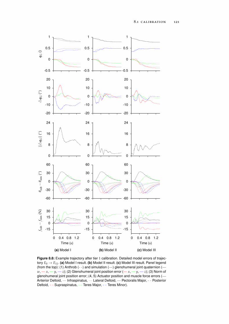
8.1 calibration 121

-0.5

0

0.5

1q

G()

-20

-10

0

10

20

q

G(

)

0

8

16

24

‖q

G‖

()

-60

-30

0

30

60

θ rob−

θ sim

()

-15

0

15

30

0 0.4 0.8 1.2

f rob−

f sim

(N)

Time (s)

(a) Model I

-0.5

0

0.5

1

-20

-10

0

10

20

0

8

16

24

-60

-30

0

30

60

-15

0

15

30

0 0.4 0.8 1.2

Time (s)

(b) Model II

-0.5

0

0.5

1

-20

-10

0

10

20

0

8

16

24

-60

-30

0

30

60

-15

0

15

30

0 0.4 0.8 1.2

Time (s)

(c) Model III

Figure 8.8: Example trajectory after tier 1 calibration. Detailed model errors of trajec-

tory E0 → E11. (a) Model I result. (b) Model II result. (c) Model III result. Panel legend

(from the top): (1) Anthrob ( ) and simulation ( ) glenohumeral joint quaternion (

w, x, y, z); (2) Glenohumeral joint position error ( x, y, z); (3) Norm of

glenohumeral joint position error; (4, 5) Actuator position and muscle force errors (

Anterior Deltoid, Infraspinatus, Lateral Deltoid, Pectoralis Major, Posterior

Deltoid, Supraspinatus, Teres Major, Teres Minor).

122 anthrob model calibration

8.1.2 Tier 2: Complete Robot Models

In tier 2, the forearm of the robot was re-attached and the Biceps, theBrachialis and the Triceps muscle as well as the joint friction parame-ters of the elbow joint were calibrated again in a statics and dynamicscalibration stage, respectively.

8.1.2.1 Stage 1: Statics Calibration

The statics of the complete Anthrob models were calibrated usingthe equilibria set Qrob

C previously introduced for the analysis of thesimulation-reality gap in Section 7.5.2. A table summarizing the cali-bration results can be found in Appendix D.

The results of the model I calibration are summarized in Figure 8.9aModel I calibration

on page 125. Similar to the tier 1 statics calibration, the initial tendonlength lT0 , the actuator spindle radius rs and the x-y-z coordinates ofthe last via-point before the muscle insertion point were used as ob-ject parameters. However, only the newly introduced muscles (Biceps,Brachialis and Triceps) were calibrated and the best individual ob-tained for the dynamics calibration of tier 1 was used to parametrizethe 8 glenohumeral joint muscles. The maximum number of genera-tions was reduced to gmax = 50 due to the smaller set of 15 objectparameters. It can be seen that the mean elbow position error is sig-nificantly lower than the glenohumeral joint error (2.4 vs. 6.7). Thiswas expected and is in accordance with the results obtained for thesimulation-reality gap analysis. Furthermore, by comparison with thestatics results of tier 1 (see Figure 8.5), it becomes clear that the reat-tachment of the forearm had a huge impact on the glenohumeraljoint position errors. While the maximum error was equal to 10.8 af-ter the tier 1 calibration, it increased to 18.2 in tier 2. Moreover, theglenohumeral joint position errors in general exhibited a large jitterdepending on the elbow joint position (see E2 and E3 as well as E4

and E5).

The results of the model II calibration are summarized in Figure 8.9bModel II calibration

on page 125. As this model used a cylindrical wrapping surface tomodel the muscle wrapping on the elbow joint for the Biceps, Brach-ialis and Triceps muscle, these cylinder radii were added to the set ofobject parameters. The maximum number of generations was set togmax = 50. In contrast to the model I calibration results, model II nei-ther did exhibit a jitter in the glenohumeral joint position error dueto the elbow position nor did the glenohumeral joint position errorsdiffer significantly from the tier 1 results. This shows the quality ofthe model which uses cylindrical wrapping surfaces to approximatethe wrapping of the muscles on the humerus bone. Therefore, themodel is able to better capture the muscle kinematics of the gleno-

8.1 calibration 123

humeral joint muscles which finally leads to lower joint position er-rors when the forearm is reattached. Furthermore, in comparison tothe model I results, the average elbow joint error was reduced to 50 %(1.2 vs. 2.4). This shows that the cylindrical wrapping surfaces arecapable of successfully approximating the muscle wrapping on the el-bow joint skeleton. These calibration results also confirm the previousstatement that the large simulation-reality gap of the elbow joint stat-ics of model II were only due to an erroneous manual parametrizationof the cylinder radius (see Section 7.5.2).

The results of the model III calibration are summarized in Figure 8.9c Model III calibration

on page 125. The mean glenohumeral and elbow joint position errorof this run was equal to 5.9 and 1.8, respectively. The muscle forceerror was similar to the model I and model II results with an averagevalue of 3.3 N. The maximum number of generations of this run waslimited to gmax = 10 and it is likely that better results would havebeen obtained if gmax = 50 as for the model I and model II runs.

8.1.2.2 Stage 2: Dynamics Calibration

The dynamics of the complete Anthrob models were calibrated us-ing the trajectory set Trob

C previously introduced for the analysis ofthe simulation-reality gap in Section 7.5. A table summarizing thecalibration results can be found in Appendix D.

In addition to the muscle parameters used for the statics calibration, Model I calibration

the joint friction parameters of the elbow joint were added to the ob-ject parameter set. While the best individual of the previous staticscalibration stage was used to initialize the muscle parameters, the ini-tial joint parameters were manually configured. The maximum num-ber of generations was further reduced to gmax = 25. The results ofthe tier 2 dynamics calibration of model I are summarized in Fig-ure 8.10a and Figure 8.11a on page 126 and 127, respectively. It canbe seen that the glenohumeral joint position errors are significantlylower for trajectories starting at E0 (white boxes) compared to trajec-tories ending at E0 (gray boxes). This phenomenon, which has beenalready encountered for the tier 1 dynamics of model II, is due toerroneous friction parameters after calibration and could be compen-sated for by increasing the weight of the trajectory κt in the objectivefunction. But, in general, the tier 2 dynamics results are in line withthe results of the preceding statics calibration stage.

Similar to the model I calibration, the best individual of the statics cal- Model II calibration

ibration stage was used to initialize the muscle parameters whereasthe initial joint friction parameters were configured manually. More-over, the maximum number of generations was set to gmax = 25. Theresults of the tier 2 dynamics calibration of model II are shown inFigure 8.10b and Figure 8.11b on page 126 and 127, respectively. In

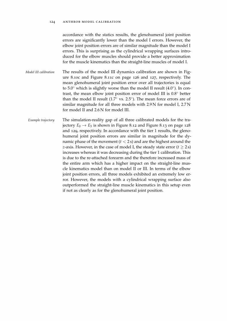
124 anthrob model calibration

accordance with the statics results, the glenohumeral joint positionerrors are significantly lower than the model I errors. However, theelbow joint position errors are of similar magnitude than the model Ierrors. This is surprising as the cylindrical wrapping surfaces intro-duced for the elbow muscles should provide a better approximationfor the muscle kinematics than the straight-line muscles of model I.

The results of the model III dynamics calibration are shown in Fig-Model III calibration

ure 8.10c and Figure 8.11c on page 126 and 127, respectively. Themean glenohumeral joint position error over all trajectories is equalto 5.0 which is slightly worse than the model II result (4.0). In con-trast, the mean elbow joint position error of model III is 0.8 betterthan the model II result (1.7 vs. 2.5). The mean force errors are ofsimilar magnitude for all three models with 2.9 N for model I, 2.7 Nfor model II and 2.6 N for model III.

The simulation-reality gap of all three calibrated models for the tra-Example trajectory

jectory E0 → E5 is shown in Figure 8.12 and Figure 8.13 on page 128

and 129, respectively. In accordance with the tier 1 results, the gleno-humeral joint position errors are similar in magnitude for the dy-namic phase of the movement (t < 2 s) and are the highest around thez-axis. However, in the case of model I, the steady state error (t ≥ 2 s)increases whereas it was decreasing during the tier 1 calibration. Thisis due to the re-attached forearm and the therefore increased mass ofthe entire arm which has a higher impact on the straight-line mus-cle kinematics model than on model II or III. In terms of the elbowjoint position errors, all three models exhibited an extremely low er-ror. However, the models with a cylindrical wrapping surface alsooutperformed the straight-line muscle kinematics in this setup evenif not as clearly as for the glenohumeral joint position.

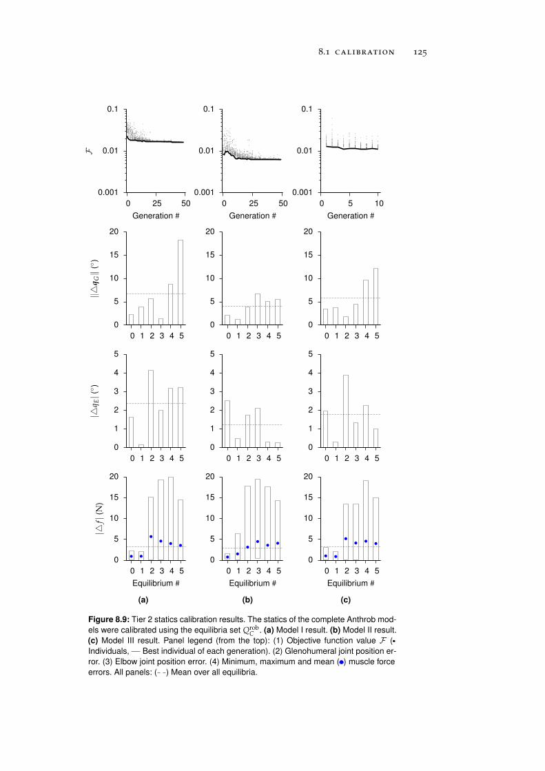
8.1 calibration 125

0.001

0.01

0.1

0 25 50

F

Generation #

0

5

10

15

20

0 1 2 3 4 5

‖q

G‖

()

0

1

2

3

4

5

0 1 2 3 4 5

|q E|( )

0

5

10

15

20

0 1 2 3 4 5

|f|

(N)

Equilibrium #

(a)

0.001

0.01

0.1

0 25 50

Generation #

0

5

10

15

20

0 1 2 3 4 5

0

1

2

3

4

5

0 1 2 3 4 5

0

5

10

15

20

0 1 2 3 4 5

Equilibrium #

(b)

0.001

0.01

0.1

0 5 10

Generation #

0

5

10

15

20

0 1 2 3 4 5

0

1

2

3

4

5

0 1 2 3 4 5

0

5

10

15

20

0 1 2 3 4 5

Equilibrium #

(c)

Figure 8.9: Tier 2 statics calibration results. The statics of the complete Anthrob mod-

els were calibrated using the equilibria set QrobC . (a) Model I result. (b) Model II result.

(c) Model III result. Panel legend (from the top): (1) Objective function value F (

Individuals, Best individual of each generation). (2) Glenohumeral joint position er-

ror. (3) Elbow joint position error. (4) Minimum, maximum and mean ( ) muscle force

errors. All panels: ( ) Mean over all equilibria.

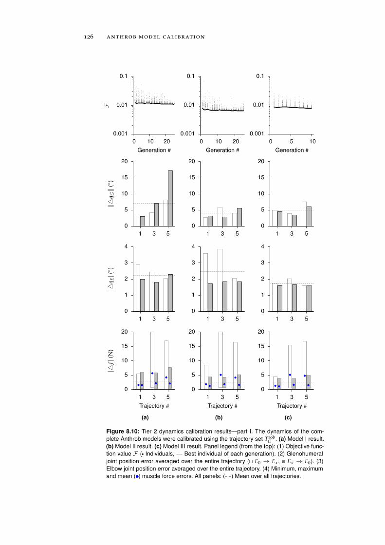
126 anthrob model calibration

0.001

0.01

0.1

0 10 20

F

Generation #

0

5

10

15

20

1 3 5

‖q

G‖

()

0

1

2

3

4

1 3 5

|q E|( )

0

5

10

15

20

1 3 5

|f|

(N)

Trajectory #

(a)

0.001

0.01

0.1

0 10 20

Generation #

0

5

10

15

20

1 3 5

0

1

2

3

4

1 3 5

0

5

10

15

20

1 3 5

Trajectory #

(b)

0.001

0.01

0.1

0 5 10

Generation #

0

5

10

15

20

1 3 5

0

1

2

3

4

1 3 5

0

5

10

15

20

1 3 5

Trajectory #

(c)

Figure 8.10: Tier 2 dynamics calibration results—part I. The dynamics of the com-

plete Anthrob models were calibrated using the trajectory set TrobC . (a) Model I result.

(b) Model II result. (c) Model III result. Panel legend (from the top): (1) Objective func-

tion value F ( Individuals, Best individual of each generation). (2) Glenohumeral

joint position error averaged over the entire trajectory ( E0 → Ex, Ex → E0). (3)

Elbow joint position error averaged over the entire trajectory. (4) Minimum, maximum

and mean ( ) muscle force errors. All panels: ( ) Mean over all trajectories.

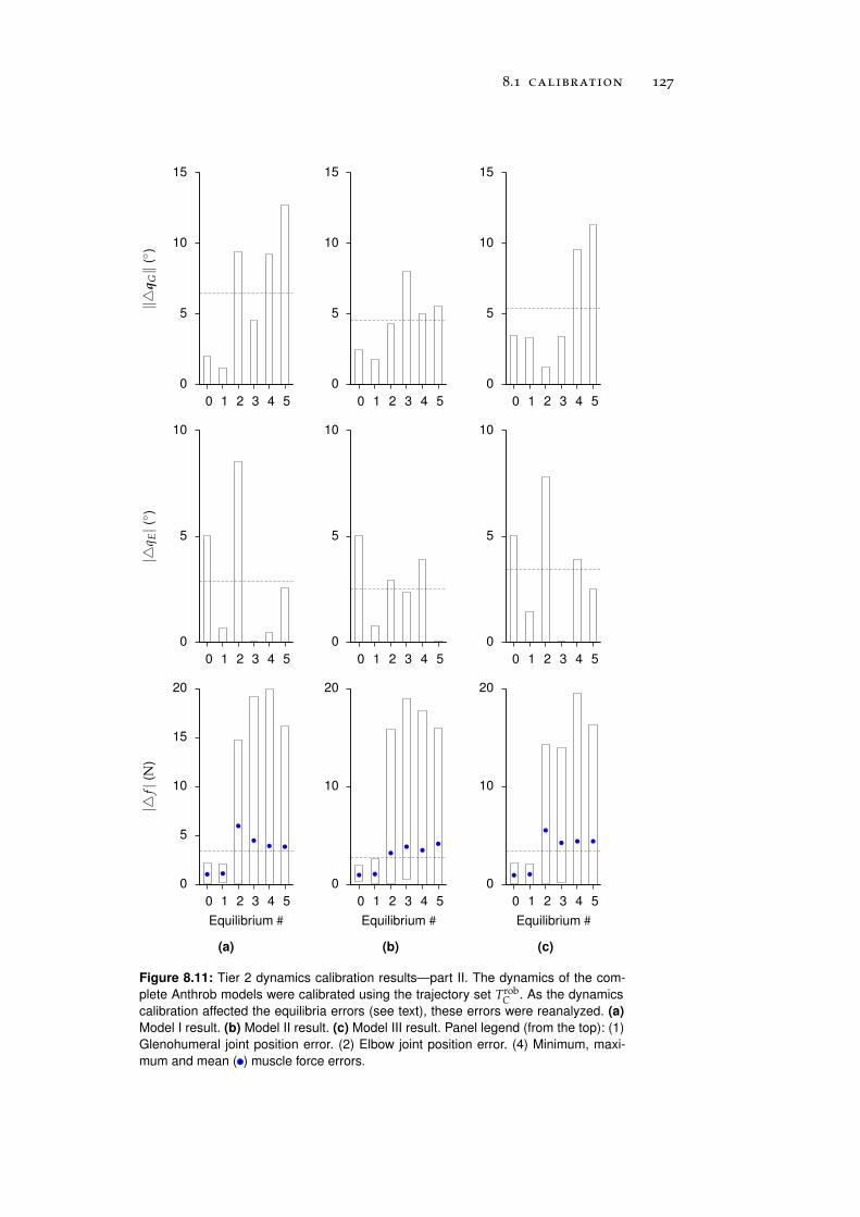
8.1 calibration 127

0

5

10

15

0 1 2 3 4 5

‖q

G‖

()

0

5

10

0 1 2 3 4 5

|q E|( )

0

5

10

15

20

0 1 2 3 4 5

|f|

(N)

Equilibrium #

(a)

0

5

10

15

0 1 2 3 4 5

0

5

10

0 1 2 3 4 5

0

10

20

0 1 2 3 4 5

Equilibrium #

(b)

0

5

10

15

0 1 2 3 4 5

0

5

10

0 1 2 3 4 5

0

10

20

0 1 2 3 4 5

Equilibrium #

(c)

Figure 8.11: Tier 2 dynamics calibration results—part II. The dynamics of the com-

plete Anthrob models were calibrated using the trajectory set TrobC . As the dynamics

calibration affected the equilibria errors (see text), these errors were reanalyzed. (a)

Model I result. (b) Model II result. (c) Model III result. Panel legend (from the top): (1)

Glenohumeral joint position error. (2) Elbow joint position error. (4) Minimum, maxi-

mum and mean ( ) muscle force errors.

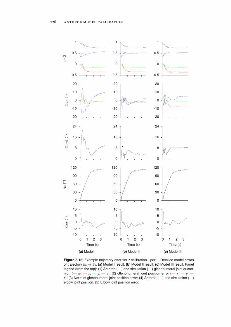
128 anthrob model calibration

-0.5

0

0.5

1

qG

()

-20

-10

0

10

20

q

G(

)

0

8

16

24

‖q

G‖

()

0

30

60

90

120

q E(

)

-10

-5

0

5

10

0 1 2 3

q E

()

Time (s)

(a) Model I

-0.5

0

0.5

1

-20

-10

0

10

20

0

8

16

24

0

30

60

90

120

-10

-5

0

5

10

0 1 2 3

Time (s)

(b) Model II

-0.5

0

0.5

1

-20

-10

0

10

20

0

8

16

24

0

30

60

90

120

-10

-5

0

5

10

0 1 2 3

Time (s)

(c) Model III

Figure 8.12: Example trajectory after tier 2 calibration—part I. Detailed model errors

of trajectory E0 → E5. (a) Model I result. (b) Model II result. (c) Model III result. Panel

legend (from the top): (1) Anthrob ( ) and simulation ( ) glenohumeral joint quater-

nion ( w, x, y, z); (2) Glenohumeral joint position error ( x, y,

z); (3) Norm of glenohumeral joint position error; (4) Anthrob ( ) and simulation ( )

elbow joint position. (5) Elbow joint position error.

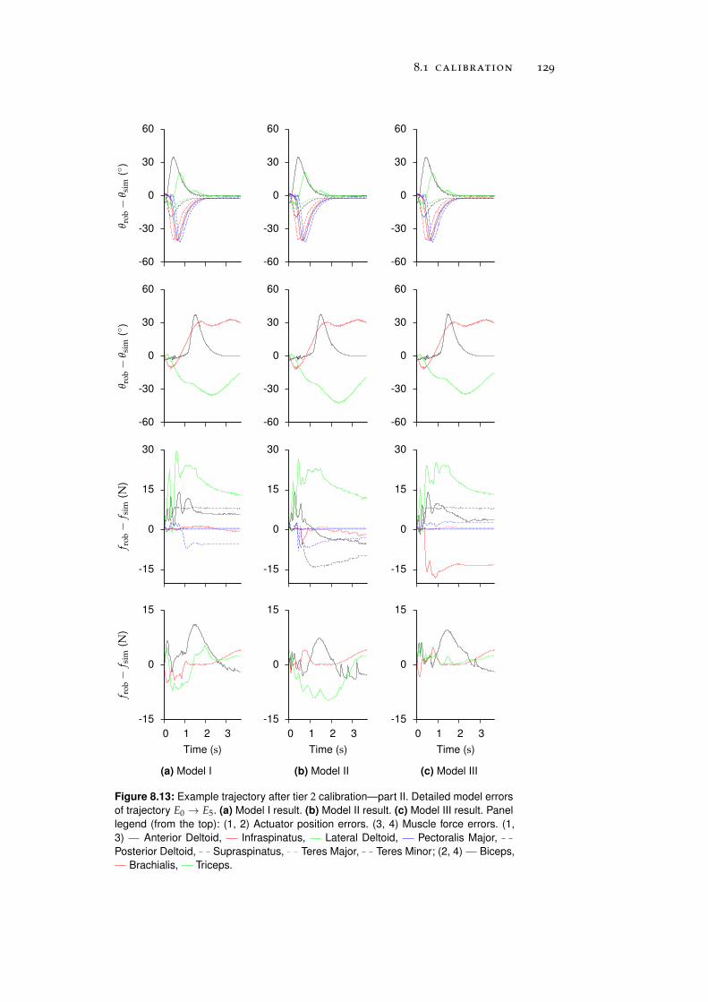
8.1 calibration 129

-60

-30

0

30

60θ r

ob−

θ sim

()

-60

-30

0

30

60

θ rob−

θ sim

()

-15

0

15

30

f rob−

f sim

(N)

-15

0

15

0 1 2 3

f rob−

f sim

(N)

Time (s)

(a) Model I

-60

-30

0

30

60

-60

-30

0

30

60

-15

0

15

30

-15

0

15

0 1 2 3

Time (s)

(b) Model II

-60

-30

0

30

60

-60

-30

0

30

60

-15

0

15

30

-15

0

15

0 1 2 3

Time (s)

(c) Model III

Figure 8.13: Example trajectory after tier 2 calibration—part II. Detailed model errors

of trajectory E0 → E5. (a) Model I result. (b) Model II result. (c) Model III result. Panel

legend (from the top): (1, 2) Actuator position errors. (3, 4) Muscle force errors. (1,

3) Anterior Deltoid, Infraspinatus, Lateral Deltoid, Pectoralis Major,

Posterior Deltoid, Supraspinatus, Teres Major, Teres Minor; (2, 4) Biceps,

Brachialis, Triceps.

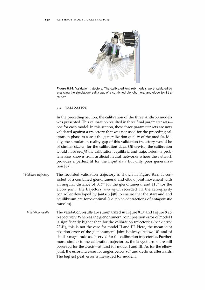
130 anthrob model calibration

Figure 8.14: Validation trajectory. The calibrated Anthrob models were validated by

analyzing the simulation-reality gap of a combined glenohumeral and elbow joint tra-

jectory.

8.2 validation

In the preceding section, the calibration of the three Anthrob modelswas presented. This calibration resulted in three final parameter sets—one for each model. In this section, these three parameter sets are nowvalidated against a trajectory that was not used for the preceding cal-ibration phase to assess the generalization quality of the models. Ide-ally, the simulation-reality gap of this validation trajectory would beof similar size as for the calibration data. Otherwise, the calibrationwould have overfit the calibration equilibria and trajectories—a prob-lem also known from artificial neural networks where the networkprovides a perfect fit for the input data but only poor generaliza-tion [75].

The recorded validation trajectory is shown in Figure 8.14. It con-Validation trajectory

sisted of a combined glenohumeral and elbow joint movement withan angular distance of 50.7 for the glenohumeral and 115 for theelbow joint. The trajectory was again recorded via the zero-gravitycontroller developed by Jäntsch [58] to ensure that the start and endequilibrium are force-optimal (i. e. no co-contractions of antagonisticmuscles).

The validation results are summarized in Figure 8.15 and Figure 8.16,Validation results

respectively. Whereas the glenohumeral joint position error of model Iis significantly higher than for the calibration trajectories (peak error27.4), this is not the case for model II and III. Here, the mean jointposition error of the glenohumeral joint is always below 10 and ofsimilar magnitude as observed for the calibration trajectories. Further-more, similar to the calibration trajectories, the largest errors are stillobserved for the z-axis—at least for model I and III. As for the elbowjoint, the error increases for angles below 90 and declines afterwards.The highest peak error is measured for model I.

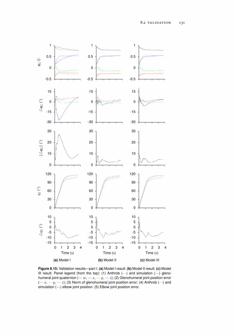
8.2 validation 131

-0.5

0

0.5

1

qG

()

-30

-15

0

15

q

G(

)

0

10

20

30

‖q

G‖

()

0

30

60

90

120

q E(

)

-15

-10

-5

0

5

10

0 1 2 3 4

q E

()

Time (s)

(a) Model I

-0.5

0

0.5

1

-30

-15

0

15

0

10

20

30

0

30

60

90

120

-15

-10

-5

0

5

10

0 1 2 3 4

Time (s)

(b) Model II

-0.5

0

0.5

1

-30

-15

0

15

0

10

20

30

0

30

60

90

120

-15

-10

-5

0

5

10

0 1 2 3 4

Time (s)

(c) Model III

Figure 8.15: Validation results—part I. (a) Model I result. (b) Model II result. (c) Model

III result. Panel legend (from the top): (1) Anthrob ( ) and simulation ( ) gleno-

humeral joint quaternion ( w, x, y, z); (2) Glenohumeral joint position error

( x, y, z); (3) Norm of glenohumeral joint position error; (4) Anthrob ( ) and

simulation ( ) elbow joint position. (5) Elbow joint position error.

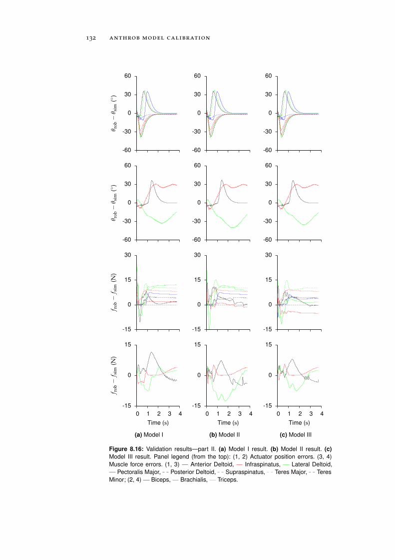
132 anthrob model calibration

-60

-30

0

30

60

θ rob−

θ sim

()

-60

-30

0

30

60

θ rob−

θ sim

()

-15

0

15

30

f rob−

f sim

(N)

-15

0

15

0 1 2 3 4

f rob−

f sim

(N)

Time (s)

(a) Model I

-60

-30

0

30

60

-60

-30

0

30

60

-15

0

15

30

-15

0

15

0 1 2 3 4

Time (s)

(b) Model II

-60

-30

0

30

60

-60

-30

0

30

60

-15

0

15

30

-15

0

15

0 1 2 3 4

Time (s)

(c) Model III

Figure 8.16: Validation results—part II. (a) Model I result. (b) Model II result. (c)

Model III result. Panel legend (from the top): (1, 2) Actuator position errors. (3, 4)

Muscle force errors. (1, 3) Anterior Deltoid, Infraspinatus, Lateral Deltoid,

Pectoralis Major, Posterior Deltoid, Supraspinatus, Teres Major, Teres

Minor; (2, 4) Biceps, Brachialis, Triceps.

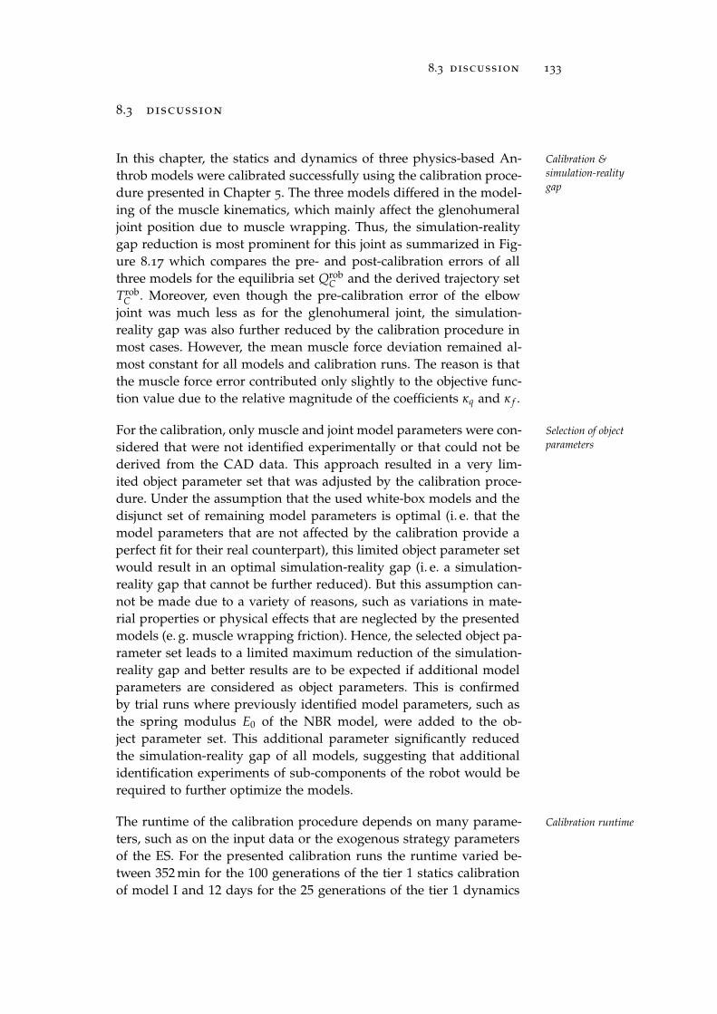
8.3 discussion 133

8.3 discussion

In this chapter, the statics and dynamics of three physics-based An- Calibration &

simulation-reality

gapthrob models were calibrated successfully using the calibration proce-dure presented in Chapter 5. The three models differed in the model-ing of the muscle kinematics, which mainly affect the glenohumeraljoint position due to muscle wrapping. Thus, the simulation-realitygap reduction is most prominent for this joint as summarized in Fig-ure 8.17 which compares the pre- and post-calibration errors of allthree models for the equilibria set Qrob

C and the derived trajectory setTrob

C . Moreover, even though the pre-calibration error of the elbowjoint was much less as for the glenohumeral joint, the simulation-reality gap was also further reduced by the calibration procedure inmost cases. However, the mean muscle force deviation remained al-most constant for all models and calibration runs. The reason is thatthe muscle force error contributed only slightly to the objective func-tion value due to the relative magnitude of the coefficients κq and κ f .

For the calibration, only muscle and joint model parameters were con- Selection of object

parameterssidered that were not identified experimentally or that could not bederived from the CAD data. This approach resulted in a very lim-ited object parameter set that was adjusted by the calibration proce-dure. Under the assumption that the used white-box models and thedisjunct set of remaining model parameters is optimal (i. e. that themodel parameters that are not affected by the calibration provide aperfect fit for their real counterpart), this limited object parameter setwould result in an optimal simulation-reality gap (i. e. a simulation-reality gap that cannot be further reduced). But this assumption can-not be made due to a variety of reasons, such as variations in mate-rial properties or physical effects that are neglected by the presentedmodels (e. g. muscle wrapping friction). Hence, the selected object pa-rameter set leads to a limited maximum reduction of the simulation-reality gap and better results are to be expected if additional modelparameters are considered as object parameters. This is confirmedby trial runs where previously identified model parameters, such asthe spring modulus E0 of the NBR model, were added to the ob-ject parameter set. This additional parameter significantly reducedthe simulation-reality gap of all models, suggesting that additionalidentification experiments of sub-components of the robot would berequired to further optimize the models.

The runtime of the calibration procedure depends on many parame- Calibration runtime

ters, such as on the input data or the exogenous strategy parametersof the ES. For the presented calibration runs the runtime varied be-tween 352 min for the 100 generations of the tier 1 statics calibrationof model I and 12 days for the 25 generations of the tier 1 dynamics

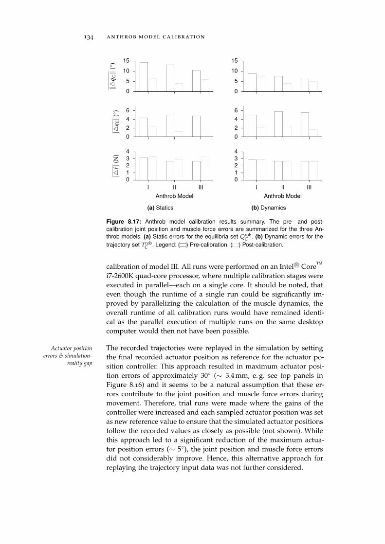
134 anthrob model calibration

0

5

10

15

‖q

G‖

()

0

2

4

6|

q E|( )

0

1

2

3

4

I II III

|f|

(N)

Anthrob Model

(a) Statics

0

5

10

15

0

2

4

6

0

1

2

3

4

I II III

Anthrob Model

(b) Dynamics

Figure 8.17: Anthrob model calibration results summary. The pre- and post-

calibration joint position and muscle force errors are summarized for the three An-

throb models. (a) Static errors for the equilibria set QrobC . (b) Dynamic errors for the

trajectory set TrobC . Legend: ( ) Pre-calibration. ( ) Post-calibration.

calibration of model III. All runs were performed on an Intel R© CoreTM

i7-2600K quad-core processor, where multiple calibration stages wereexecuted in parallel—each on a single core. It should be noted, thateven though the runtime of a single run could be significantly im-proved by parallelizing the calculation of the muscle dynamics, theoverall runtime of all calibration runs would have remained identi-cal as the parallel execution of multiple runs on the same desktopcomputer would then not have been possible.

The recorded trajectories were replayed in the simulation by settingActuator position

errors & simulation-

reality gapthe final recorded actuator position as reference for the actuator po-sition controller. This approach resulted in maximum actuator posi-tion errors of approximately 30 (∼ 3.4 mm, e. g. see top panels inFigure 8.16) and it seems to be a natural assumption that these er-rors contribute to the joint position and muscle force errors duringmovement. Therefore, trial runs were made where the gains of thecontroller were increased and each sampled actuator position was setas new reference value to ensure that the simulated actuator positionsfollow the recorded values as closely as possible (not shown). Whilethis approach led to a significant reduction of the maximum actua-tor position errors (∼ 5), the joint position and muscle force errorsdid not considerably improve. Hence, this alternative approach forreplaying the trajectory input data was not further considered.

8.3 discussion 135

The ECUs used for the Anthrob robot do not feature an encoder in- Anthrob

repeatabilityterface. Therefore, the encoder ticks have to be counted in softwarewhich, due to the limited sampling rate available, leads to drifts inthe actuator position for rapid movements. These drifts result in jointposition errors and thus the Anthrob robot was re-calibrated duringthe recording of the calibration data as soon as the glenohumeraljoint position error of the resting equilibrium E0 was larger than 31.This procedure induced deviations in the calibration input data dueto the jitter resulting from the manual re-calibration. These devia-tions are for instance visible for E5 and trajectory E0 → E5 of QC

and TC, respectively. Here the angular distance between the gleno-humeral joint position of the equilibrium and the final sample of thetrajectory is equal to 3.59. This deviation is also reflected in the cal-ibration results (e. g. the glenohumeral joint position error of E5 inFigure 8.11c is ∼ 11.3 whereas the final trajectory error is ∼ 8 in Fig-ure 8.12c). One option to solve this problem would have been to usethe last sample of the trajectories as target equilibria. But this wouldonly compensate for the deviations between the equilibrium/trajec-tory pairs. Deviations between pairs of equilibria would still persist.These could only be canceled out by the use of a hardware encoderinterface which would allow the recording of all input data withoutthe need of re-calibrations. Fortunately, the presented example can beseen as a worst-case example. Typically, these errors are below 1.5.

For the validation of the calibrated Anthrob models, a single trajec- Validation trajectory

tory was used. Now, one might argue that one trajectory is not suf-ficient to assess the generalization capabilities of the models. This isnot true for two reasons. First, the used validation trajectory has a du-ration of 3.75 s with a total of 372 samples. Hence, not a single robotposture but a sequence involving both robot joints and therefore thecomplete robot dynamics was used. Secondly, poor generalizationnormally is associated with the phenomenon known as over-fittingwhere the model provides a perfect fit for the training data insteadof capturing the essential properties of the input data. This finallyleads to large errors if untrained data sets are presented. Over-fitting,however, is a problem of black-box models, such as ANN, where anetwork structure (number of layers and neurons) is identified by su-pervised learning. In our case, also supervised learning was used butinstead of black-box, white-box models were used. These white-boxmodels were further constrained by value limits for each object pa-rameter during calibration. Thus, it was not possible that the calibra-tion resulted in unrealistic model parameter values and it is thereforeunlikely that the model provides poor generalization—as confirmedby the low errors of the validation trajectory.

1 the elbow joint muscles were not critical due to the lower controller gains whichyield slower movement speeds

9C O N C L U S I O N S

9.1 summary

Musculoskeletal robots, which belong to the super-class of tendon- Problem summary

driven robots, exhibit a set of unique features such as spherical jointsor muscles with Posture-Dependent Lever Arms (PDLAs). These fea-tures enable new applications for this class of robots, such as an ar-tificial test-bed for the investigation of biologically inspired controlstrategies, or as service and rehabilitation robots, where the mus-cle compliance increases the safety of human-robot interactions. But,while being advantageous for many use-cases, these features also in-troduce new challenges for roboticists as outlined in the introduction.For instance, in the field of modeling and simulation the usage ofmuscles instead of torque actuators located within joints complicatesthe application of classical joint-space simulation approaches as anexplicit mapping between the muscle forces and the joint torques isrequired. This mapping, however, is posture-dependent and thereforedifficult to derive. Hence, the application of a different simulation ap-proach for the class of musculoskeletal robots, namely physics-basedsimulations, was proposed.

Physics-based simulations, which originate from computer games and Physics-based

modeling of

musculoskeletal

robots

computer animations, operate in the body-space which means thatbody positions and orientations are integrated over time instead ofthe joint positions as in joint-space approaches. This difference sim-plifies the simulation of musculoskeletal robots as muscle forces canbe applied directly to the rigid bodies of the skeleton without theneed of force-to-torque conversions as in joint-space approaches. Inthis work, the applicability of this alternative simulation approach forthe class of musculoskeletal robots was evaluated. Therefore, the mod-eling of skeletons by means of articulated rigid bodies was presentedand it was shown how to extend the joint models of physics-enginesto simulate joint friction. Subsequently, in order to actuate the passiveskeletons, physics-based muscle models were derived. Here, particu-lar emphasis was put on the muscle kinematics, which determinethe lines of action of a muscle as well as the muscle length—twoquantities that significantly influence the resulting robot dynamics.

137

138 conclusions

Thus, models of varying complexity were presented. These modelsranged from simple straight-line connections to wrapping surfacesthat employ geometric primitives, namely spheres and cylinders, toarbitrary meshes from which the roboticist can select the proper mod-els for a particular robot and/or use-case to simulate the muscle pathalong the skeleton surface. Even though similar models already existin the field of biomechanics, the models were ported to the physics-based framework and were improved when possible. For instance,the sphere and cylinder wrapping surface models presented wereextended to capture the transition from a positive to a negative wrap-ping direction as well as to support multiple wrapping revolutions—two properties not supported by previous models. Furthermore, itwas shown that the approximation of the geodesic path in the caseof mesh wrapping surfaces, as suggested by previous biomechanicalstudies [23], should be avoided for physics-based simulations. Thereason is that these approximations normally only provide good es-timates for the path length but not for the path waypoints. These,however, are particularly important in the physics-based frameworkin order to compute the lines of action of the muscle. Moreover, it wasshown how the presented muscle models can be extended to capturethe effects of muscle friction forces which are postulated to have asignificant impact on the dynamics of musculoskeletal robots [58]. Fi-nally, a universal algorithm for the simulation of muscle dynamicswithin physics-engines was developed. This algorithm exploits thefact that the lumped effect of a wrapped muscle segment on the skele-ton can always be simulated by two straight-line segments (one fromthe preceding via-point to the point where the muscle touches thesurface and one from the point where the muscle leaves the surfaceto the succeeding via-point).

The parametric, physics-based white-box models of musculoskeletalModel calibration

procedure robots exhibit a huge parameter set and even though most of theseparameters can be derived from either data sheets, CAD models orexperiments, there will always be a simulation-reality gap. In order tominimize this gap, a calibration procedure was developed. This pro-cedure uses an Evolution Strategy (ES) with a Gaussian-based, non-isotropic mutation operator to reduce the simulation-reality gap byadjusting the model parameters. It is universal in the sense that itcan be applied to any real-valued model parameter and/or objectivefunction. As examples two objective functions were derived: one forthe calibration of the model statics and one for the model dynamics.Both functions use the joint position and muscle force errors as fitnessmeasure to guide the exploration of the search space by the ES.

9.1 summary 139

Both, the developed physics-based models and the calibration proce- The musculoskeletal

robot Anthrobdure were evaluated on a physical robot. Therefore, the musculoskele-tal robot Anthrob was: (i) developed, (ii) modeled and (iii) calibrated.Anthrob replicates the human upper limb and features four skeletalDoF (one revolute elbow and one spherical glenohumeral joint). Fur-thermore, it is equipped with 11 muscles1 that are implemented byelectromagnetic series-elastic actuators. While 10 out of the 11 mus-cles are uni-articular (i. e. they only affect one joint), Anthrob alsofeatures one bi-articular muscle which spans and actuates the gleno-humeral and elbow joint simultaneously. Anthrob, which was concep-tualized at the end of the Eccerobot project, was developed togetherwith Michael Jäntsch and the Swiss company awtec AG.

To evaluate the physics-based simulation approach, three Anthrob Anthrob modeling

physics-based models were developed. All models used an identi-cal skeleton model but featured different muscle kinematic models.While model I relied exclusively on straight-line muscle kinematics,model II and model III extended model I by cylindrical and meshwrapping surfaces, respectively. Even though most model parame-ters could be deduced from the available data sheets and the CADmodel, three additional identification experiments were required andconducted to derive models of: (i) the stress/strain properties of theNBR O-rings used as Series Elastic Elements (SEEs), (ii) the frictionproperties of the ceramic eyelets used to guide the Dyneema kite-lineand (iii) the input/output properties of the power circuit of the Elec-tronic Control Units (ECUs).

The simulation-reality gap of the three derived Anthrob models was Anthrob model

simulation-reality

gap & calibrationfinally analyzed and minimized using the presented calibration pro-cedure. The gap was quantified by measuring the joint position andmuscle force errors of the models for both, static robot postures anddynamic robot trajectories. To measure the joint position of the spheri-cal glenohumeral joint of the Anthrob robot, an extrinsic stereo-vision,infrared-marker based motion capture system with realtime capabil-ities was developed. In the uncalibrated state, the straight-line mus-cle kinematics model was out-performed by both wrapping surfacemodels with even lower errors for the mesh wrapping surfaces. Aftercalibration, the differences between the three models became smallerwhen steady robot postures are considered. In the dynamics case,the wrapping surface models again out-performed the straight-linemodel significantly, eventually leading to a final average joint positionerror in the order of ∼ 5 and ∼ 2 for the spherical glenohumeraland the revolute elbow joint, respectively. These errors, which arelarge by means of industrial robots, are low for the class of muscu-loskeletal robots where a repeatability of 3-5 is common. Hence, itcan be concluded that the physics-based simulation approach is a

1 13 when the hand is attached

140 conclusions

promising substitute for classical joint-space approaches, which facil-itates the investigation of aspects of the musculoskeletal design in awell-defined environment and finally will hopefully contribute to thepromotion of this class of robots to a greater audience.

9.2 future works

Even though the physics-based simulation approach was successfullyEvaluation of

physics-based

approach on more

complex robot

applied to the Anthrob robot, the question remains how the approachperforms if more complex robots are considered. Here, the main lim-iting factor is the number of skeletal DoF as additional muscles onlyincrease the computational load. However, preliminary simulationsof the Ecce-2 with its 103 DoF conducted by project partners of theEccerobot consortium showed promising results—even though nosimulation-reality gap analysis has been performed so far.

Another aspect, that has to be considered if more complex robotsRealtime

performance of

muscle modelsare targeted, is the execution time of the muscle kinematics mod-els. In Chapter 7 it was shown that a single simulation step of thedeveloped Anthrob skeleton model required 18 µs whereas the sim-ulation of a single straight-line muscle and a muscle with a meshwrapping surface within the muscle path varied between 4 µs and3 ms, respectively. Hence, depending on the used muscle kinemat-ics model, the complete Anthrob robot with 11 muscles can be sim-ulated in realtime if the simulation frequency is lower than 30 Hzfor the mesh wrapping surface kinematics and lower than 16 kHzfor straight-line muscle kinematics. However, particularly the meshwrapping surface frequency is a worst-case estimate. The executiontime of this muscle kinematics model is highly dependent on themesh density and the robot posture which in turn determines thenumber of mesh vertices that have to be considered for the path com-putation. In reality, the complete Anthrob mesh wrapping surfacemodel executed with frequencies between 80 Hz and 120 Hz. The sim-ulation frequency is important as the simple numerical integratorsused in physics-engines induce simulation artifacts if the simulationfrequencies are too low and this lower frequency bound depends onthe complexity of the model. In case of the Anthrob robot, simulationfrequencies below 500 Hz are not advisable. Thus, realtime simula-tions of the mesh wrapping muscle kinematics model are currentlynot possible without compromising the accuracy. However, the com-putation of the muscle dynamics can be perfectly parallelized on mul-tiple Central Processing Units (CPUs). With this technique and fasterCPUs it should be soon possible to run models of similar complex-ity than the Anthrob model in realtime—also when mesh wrappingsurfaces are used.

9.2 future works 141

Jäntsch et al. already successfully employed the developed models as Physics-based model

as internal modela software-in-the-loop tool for the development and testing of novelcontrol strategies [60]. But other use-cases for physics-based simu-lations of musculoskeletal robots are also conceivable. For instance,the simulation model could be used as an internal model for con-trol to predict possible interactions with the robot environment or toderive motor commands required for a desired movement. This ap-proach, which is reminiscent of the internal model control hypothesisknown from Neuroscience [68], is particularly elegant to implementon a physics-engine as the required tools for the simulation of theenvironment, namely rigid body dynamics, are already provided out-of-the-box.

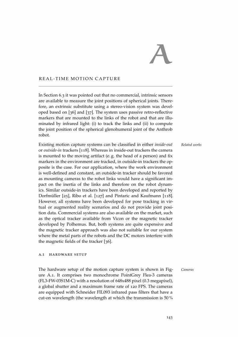
AR E A L - T I M E M O T I O N C A P T U R E

In Section 6.3 it was pointed out that no commercial, intrinsic sensorsare available to measure the joint positions of spherical joints. There-fore, an extrinsic substitute using a stereo-vision system was devel-oped based on [36] and [37]. The system uses passive retro-reflectivemarkers that are mounted to the links of the robot and that are illu-minated by infrared light: (i) to track the links and (ii) to computethe joint position of the spherical glenohumeral joint of the Anthrobrobot.

Existing motion capture systems can be classified in either inside-out Related works

or outside-in trackers [118]. Whereas in inside-out trackers the camerais mounted to the moving artifact (e. g. the head of a person) and fixmarkers in the environment are tracked, in outside-in trackers the op-posite is the case. For our application, where the work environmentis well-defined and constant, an outside-in tracker should be favoredas mounting cameras to the robot links would have a significant im-pact on the inertia of the links and therefore on the robot dynam-ics. Similar outside-in trackers have been developed and reported byDorfmüller [25], Ribo et al. [127] and Pintaric and Kaufmann [118].However, all systems have been developed for pose tracking in vir-tual or augmented reality scenarios and do not provide joint posi-tion data. Commercial systems are also available on the market, suchas the optical tracker available from Vicon or the magnetic trackerdeveloped by Polhemus. But, both systems are quite expensive andthe magnetic tracker approach was also not suitable for our systemwhere the metal parts of the robots and the DC motors interfere withthe magnetic fields of the tracker [36].

a.1 hardware setup

The hardware setup of the motion capture system is shown in Fig- Cameras

ure A.1. It comprises two monochrome PointGrey Flea-3 cameras(FL3-FW-03S1M-C) with a resolution of 648x488 pixel (0.3 megapixel),a global shutter and a maximum frame rate of 120 FPS. The camerasare equipped with Schneider FIL093 infrared pass filters that have acut-on wavelength (the wavelength at which the transmission is 50 %

143

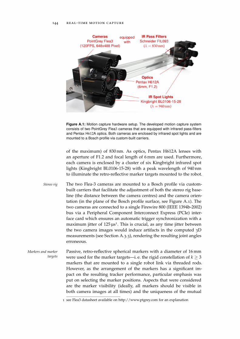
144 real-time motion capture

Cameras

PointGrey Flea3

(120FPS, 648x488 Pixel)

equipped

with

IR Pass Filters

Schneider FIL093

(λ = 830 nm)

Optics

Pentax H612A

(6mm, F1.2)

IR Spot Lights

Kingbright BL0106-15-28

(λ = 940 nm)

Figure A.1: Motion capture hardware setup. The developed motion capture system

consists of two PointGrey Flea3 cameras that are equipped with infrared pass-filters

and Pentax H612A optics. Both cameras are enclosed by infrared spot lights and are

mounted to a Bosch profile via custom-built carriers.

of the maximum) of 830 nm. As optics, Pentax H612A lenses withan aperture of F1.2 and focal length of 6 mm are used. Furthermore,each camera is enclosed by a cluster of six Kingbright infrared spotlights (Kingbright BL0106-15-28) with a peak wavelength of 940 nmto illuminate the retro-reflective marker targets mounted to the robot.

The two Flea-3 cameras are mounted to a Bosch profile via custom-Stereo rig

built carriers that facilitate the adjustment of both the stereo rig base-line (the distance between the camera centres) and the camera orien-tation (in the plane of the Bosch profile surface, see Figure A.1). Thetwo cameras are connected to a single Firewire 800 (IEEE 1394b-2002)bus via a Peripheral Component Interconnect Express (PCIe) inter-face card which ensures an automatic trigger synchronization with amaximum jitter of 125 µs1. This is crucial, as any time jitter betweenthe two camera images would induce artifacts in the computed 3Dmeasurements (see Section A.3.3), rendering the resulting joint angleserroneous.

Passive, retro-reflective spherical markers with a diameter of 16 mmMarkers and marker

targets were used for the marker targets—i. e. the rigid constellation of k ≥ 3markers that are mounted to a single robot link via threaded rods.However, as the arrangement of the markers has a significant im-pact on the resulting tracker performance, particular emphasis wasput on selecting the marker positions. Aspects that were consideredare the marker visibility (ideally, all markers should be visible inboth camera images at all times) and the uniqueness of the mutual

1 see Flea3 datasheet available on http://www.ptgrey.com for an explanation

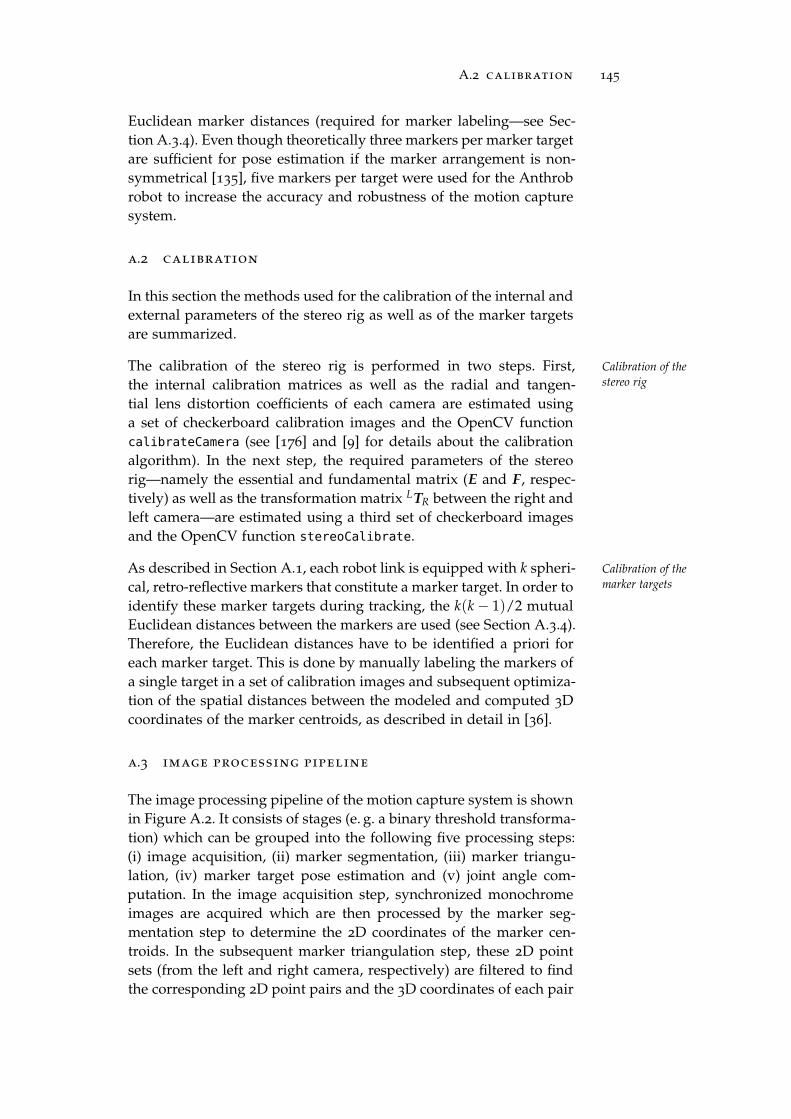
A.2 calibration 145

Euclidean marker distances (required for marker labeling—see Sec-tion A.3.4). Even though theoretically three markers per marker targetare sufficient for pose estimation if the marker arrangement is non-symmetrical [135], five markers per target were used for the Anthrobrobot to increase the accuracy and robustness of the motion capturesystem.

a.2 calibration

In this section the methods used for the calibration of the internal andexternal parameters of the stereo rig as well as of the marker targetsare summarized.

The calibration of the stereo rig is performed in two steps. First, Calibration of the

stereo rigthe internal calibration matrices as well as the radial and tangen-tial lens distortion coefficients of each camera are estimated usinga set of checkerboard calibration images and the OpenCV functioncalibrateCamera (see [176] and [9] for details about the calibrationalgorithm). In the next step, the required parameters of the stereorig—namely the essential and fundamental matrix (E and F, respec-tively) as well as the transformation matrix LTR between the right andleft camera—are estimated using a third set of checkerboard imagesand the OpenCV function stereoCalibrate.

As described in Section A.1, each robot link is equipped with k spheri- Calibration of the

marker targetscal, retro-reflective markers that constitute a marker target. In order toidentify these marker targets during tracking, the k(k− 1)/2 mutualEuclidean distances between the markers are used (see Section A.3.4).Therefore, the Euclidean distances have to be identified a priori foreach marker target. This is done by manually labeling the markers ofa single target in a set of calibration images and subsequent optimiza-tion of the spatial distances between the modeled and computed 3Dcoordinates of the marker centroids, as described in detail in [36].

a.3 image processing pipeline

The image processing pipeline of the motion capture system is shownin Figure A.2. It consists of stages (e. g. a binary threshold transforma-tion) which can be grouped into the following five processing steps:(i) image acquisition, (ii) marker segmentation, (iii) marker triangu-lation, (iv) marker target pose estimation and (v) joint angle com-putation. In the image acquisition step, synchronized monochromeimages are acquired which are then processed by the marker seg-mentation step to determine the 2D coordinates of the marker cen-troids. In the subsequent marker triangulation step, these 2D pointsets (from the left and right camera, respectively) are filtered to findthe corresponding 2D point pairs and the 3D coordinates of each pair

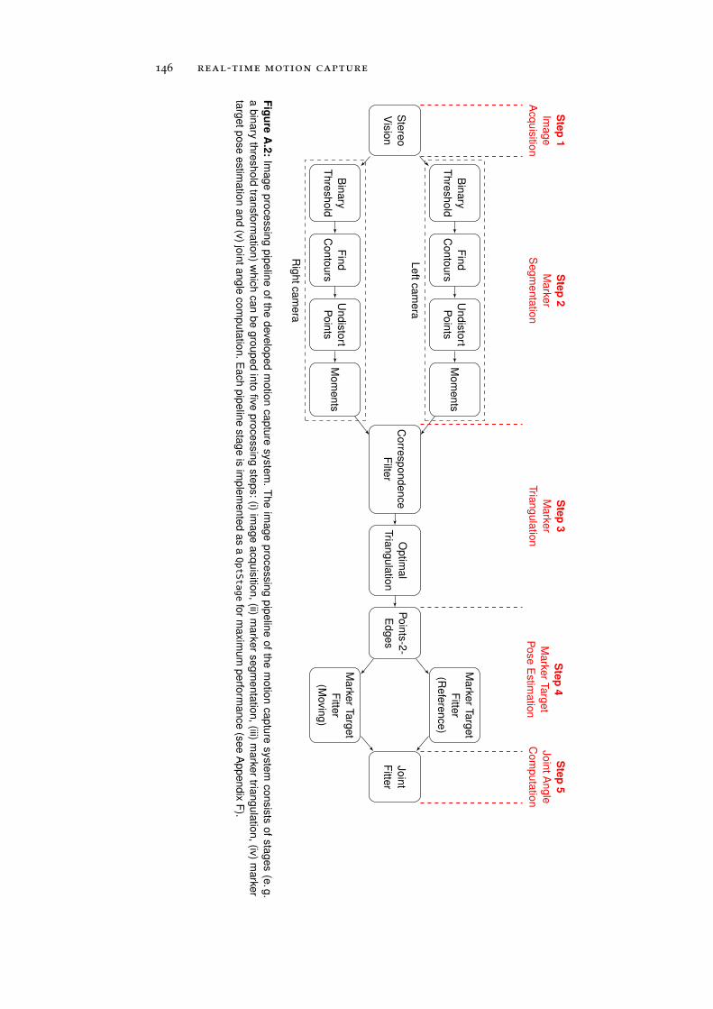
146 real-time motion capture

Ste

reo

Vis

ion

Bin

ary

Th

resh

old

Fin

d

Co

nto

urs

Un

dis

tort

Po

ints

Mo

me

nts

Bin

ary

Th

resh

old

Fin

d

Co

nto

urs

Un

dis

tort

Po

ints

Mo

me

nts

Co

rresp

on

de

nce

Filte

r

Op

tima

l

Tria

ng

ula

tion

Po

ints

-2-

Ed

ge

s

Ma

rke

rTa

rge

t

Fitte

r

(Re

fere

nce

)

Ma

rke

rTa

rge

t

Fitte

r

(Movin

g)

Jo

int

Fitte

r

Le

ftca

me

ra

Rig

ht

ca

me

ra

Ste

p1

Ima

ge

Acq

uis

ition

Ste

p2

Ma

rke

r

Se

gm

en

tatio

n

Ste

p3

Ma

rke

r

Tria

ng

ula

tion

Ste

p4

Ma

rke

rTa

rge

t

Po

se

Estim

atio

n

Ste

p5

Jo

int

An

gle

Co

mp

uta

tion

Fig

ure

A.2

:Im

ag

ep

roce

ssin

gp

ipe

line

of

the

deve

lop

ed

mo

tion

ca

ptu

resyste

m.

Th

eim

ag

ep

roce

ssin

gp

ipe

line

of

the

mo

tion

ca

ptu

resyste

mco

nsis

tso

fsta

ge

s(e

.g.

ab

ina

ryth

resh

old

tran

sfo

rma

tion

)w

hic

hca

nb

egro

up

ed

into

five

pro

ce

ssin

gste

ps:

(i)im

ag

ea

cq

uis

ition

,(ii)

ma

rke

rse

gm

en

tatio

n,

(iii)m

ark

er

trian

gu

latio

n,

(iv)

ma

rke

r

targ

et

po

se

estim

atio

na

nd

(v)

join

ta

ng

leco

mp

uta

tion

.E

ach

pip

elin

esta

ge

isim

ple

me

nte

da

saQptStage

for

ma

xim

um

pe

rform

an

ce

(se

eA

pp

en

dix

F).

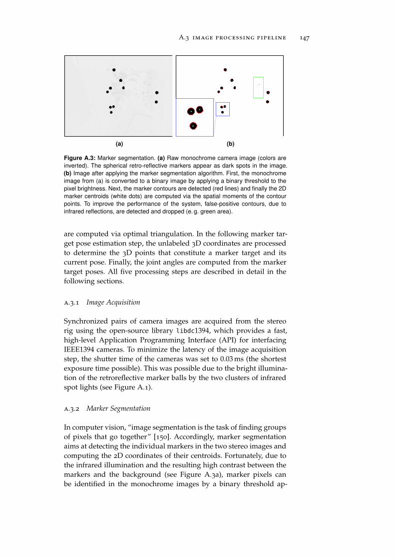
A.3 image processing pipeline 147

(a) (b)

Figure A.3: Marker segmentation. (a) Raw monochrome camera image (colors are

inverted). The spherical retro-reflective markers appear as dark spots in the image.

(b) Image after applying the marker segmentation algorithm. First, the monochrome

image from (a) is converted to a binary image by applying a binary threshold to the

pixel brightness. Next, the marker contours are detected (red lines) and finally the 2D

marker centroids (white dots) are computed via the spatial moments of the contour

points. To improve the performance of the system, false-positive contours, due to

infrared reflections, are detected and dropped (e. g. green area).

are computed via optimal triangulation. In the following marker tar-get pose estimation step, the unlabeled 3D coordinates are processedto determine the 3D points that constitute a marker target and itscurrent pose. Finally, the joint angles are computed from the markertarget poses. All five processing steps are described in detail in thefollowing sections.

a.3.1 Image Acquisition

Synchronized pairs of camera images are acquired from the stereorig using the open-source library libdc1394, which provides a fast,high-level Application Programming Interface (API) for interfacingIEEE1394 cameras. To minimize the latency of the image acquisitionstep, the shutter time of the cameras was set to 0.03 ms (the shortestexposure time possible). This was possible due to the bright illumina-tion of the retroreflective marker balls by the two clusters of infraredspot lights (see Figure A.1).

a.3.2 Marker Segmentation

In computer vision, “image segmentation is the task of finding groupsof pixels that go together” [150]. Accordingly, marker segmentationaims at detecting the individual markers in the two stereo images andcomputing the 2D coordinates of their centroids. Fortunately, due tothe infrared illumination and the resulting high contrast between themarkers and the background (see Figure A.3a), marker pixels canbe identified in the monochrome images by a binary threshold ap-

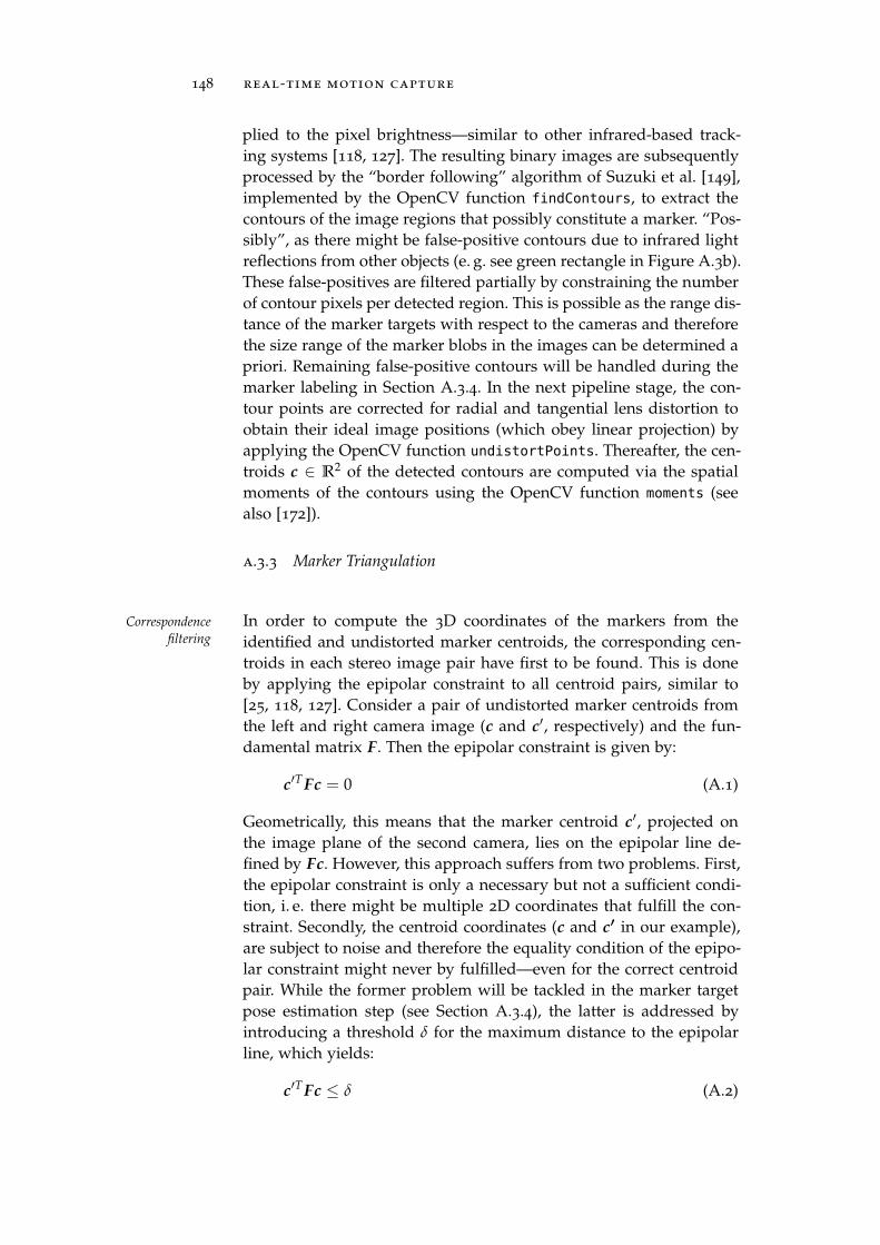
148 real-time motion capture

plied to the pixel brightness—similar to other infrared-based track-ing systems [118, 127]. The resulting binary images are subsequentlyprocessed by the “border following” algorithm of Suzuki et al. [149],implemented by the OpenCV function findContours, to extract thecontours of the image regions that possibly constitute a marker. “Pos-sibly”, as there might be false-positive contours due to infrared lightreflections from other objects (e. g. see green rectangle in Figure A.3b).These false-positives are filtered partially by constraining the numberof contour pixels per detected region. This is possible as the range dis-tance of the marker targets with respect to the cameras and thereforethe size range of the marker blobs in the images can be determined apriori. Remaining false-positive contours will be handled during themarker labeling in Section A.3.4. In the next pipeline stage, the con-tour points are corrected for radial and tangential lens distortion toobtain their ideal image positions (which obey linear projection) byapplying the OpenCV function undistortPoints. Thereafter, the cen-troids c ∈ R

2 of the detected contours are computed via the spatialmoments of the contours using the OpenCV function moments (seealso [172]).

a.3.3 Marker Triangulation

In order to compute the 3D coordinates of the markers from theCorrespondence

filtering identified and undistorted marker centroids, the corresponding cen-troids in each stereo image pair have first to be found. This is doneby applying the epipolar constraint to all centroid pairs, similar to[25, 118, 127]. Consider a pair of undistorted marker centroids fromthe left and right camera image (c and c′, respectively) and the fun-damental matrix F. Then the epipolar constraint is given by:

c′T Fc = 0 (A.1)

Geometrically, this means that the marker centroid c′, projected onthe image plane of the second camera, lies on the epipolar line de-fined by Fc. However, this approach suffers from two problems. First,the epipolar constraint is only a necessary but not a sufficient condi-tion, i. e. there might be multiple 2D coordinates that fulfill the con-straint. Secondly, the centroid coordinates (c and c′ in our example),are subject to noise and therefore the equality condition of the epipo-lar constraint might never by fulfilled—even for the correct centroidpair. While the former problem will be tackled in the marker targetpose estimation step (see Section A.3.4), the latter is addressed byintroducing a threshold δ for the maximum distance to the epipolarline, which yields:

c′T Fc ≤ δ (A.2)

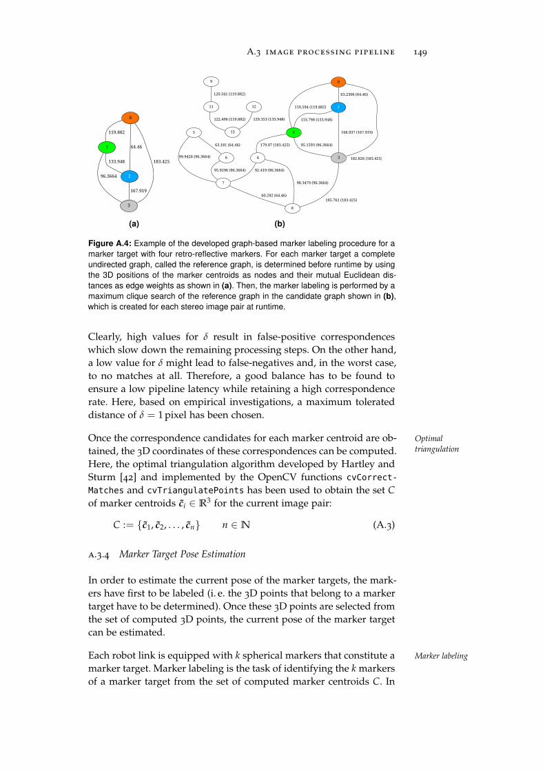
A.3 image processing pipeline 149

0

1

119.882

2

64.46

3

183.425133.948

96.3664

167.919

(a)

0

2

119.594 (119.882) 1

63.2306 (64.46)

3 182.826 (183.425)4

179.07 (183.425) 95.1593 (96.3664)

7

8

60.292 (64.46)

5

99.9426 (96.3664) 6

63.181 (64.46)

95.9296 (96.3664)

133.798 (133.948)

168.937 (167.919)

92.419 (96.3664)

98.3479 (96.3664)

185.761 (183.425)

9

11

120.341 (119.882)

13

122.496 (119.882)

12

129.353 (133.948)

(b)

Figure A.4: Example of the developed graph-based marker labeling procedure for a

marker target with four retro-reflective markers. For each marker target a complete

undirected graph, called the reference graph, is determined before runtime by using

the 3D positions of the marker centroids as nodes and their mutual Euclidean dis-

tances as edge weights as shown in (a). Then, the marker labeling is performed by a

maximum clique search of the reference graph in the candidate graph shown in (b),

which is created for each stereo image pair at runtime.

Clearly, high values for δ result in false-positive correspondenceswhich slow down the remaining processing steps. On the other hand,a low value for δ might lead to false-negatives and, in the worst case,to no matches at all. Therefore, a good balance has to be found toensure a low pipeline latency while retaining a high correspondencerate. Here, based on empirical investigations, a maximum tolerateddistance of δ = 1 pixel has been chosen.

Once the correspondence candidates for each marker centroid are ob- Optimal

triangulationtained, the 3D coordinates of these correspondences can be computed.Here, the optimal triangulation algorithm developed by Hartley andSturm [42] and implemented by the OpenCV functions cvCorrect-

Matches and cvTriangulatePoints has been used to obtain the set C

of marker centroids ci ∈ R3 for the current image pair:

C := c1, c2, . . . , cn n ∈ N (A.3)

a.3.4 Marker Target Pose Estimation

In order to estimate the current pose of the marker targets, the mark-ers have first to be labeled (i. e. the 3D points that belong to a markertarget have to be determined). Once these 3D points are selected fromthe set of computed 3D points, the current pose of the marker targetcan be estimated.

Each robot link is equipped with k spherical markers that constitute a Marker labeling

marker target. Marker labeling is the task of identifying the k markersof a marker target from the set of computed marker centroids C. In

150 real-time motion capture

the literature, different approaches to this problem can be found (seefor instance [25], [127] or [118]). Here, a novel, graph-based approachthat aims at identifying the marker targets in a complete, undirectedand weighted graph generated from the set C of 3D points is pre-sented. From a mathematical point of view, this problem is very sim-ilar to the clique problem in computer science which was proven tobe NP-complete by Richard Karp in 1972 [67].

In detail, the algorithm proceeds as follows. First, each calibratedmarker target (see Section A.2) is converted into an undirected com-plete graph, called the reference graph Gref, by using the k markersas vertices and the mutual Euclidean distances between the markersas edge weights. This has to be done only once per marker targetbefore runtime. An example of such a marker target reference graphis shown in Figure A.4a. Then, the marker centroids ci, which arepossible candidates for the vertices of the reference graph Gref, areidentified. Here, the search space is first pruned by calculating then(n− 1)/2 Euclidean distances between the n marker centroids of C

and selecting only the m centroids ci out of C that have edge corre-spondences in the reference graph Gref. By edge correspondence itis meant that the Euclidean distance between two marker centroids(ca and cb, respectively) is within a threshold ǫ of one of the edgeweights of the reference graph Gref. This way a subset D ⊆ C is ob-tained that contains only the centroids that are possible candidatesfor the vertices of Gref. It should be noted, that the computation ofEuclidean distances between the marker centroids ci is required onlyonce per stereo image pair, independent of the number of trackedmarker targets. Therefore, this computation is performed in a dedi-cated pipeline stage, called Points-2-Edges, before the actual markerlabeling (see Figure A.2). As threshold for the edge length ǫ = 3 mmis used which substantially reduces the search space without affect-ing the marker labeling. In the next step, the m centroids of D areconverted into an undirected, weighted graph, called the candidategraph Gc, using again the centroids as vertices and the mutual Eu-clidean distances between two centroids as edge weights (similar tothe reference graph Gref). However, due to the pruning of the searchspace, Gc is not a complete graph anymore. An example of such acandidate graph generated from a pair of stereo images is shown inFigure A.4b. Once both of these graphs are constructed, the markersare labeled by finding the largest subgraph of the reference graphGref in the candidate graph Gc. Here a recursive implementation of adepth-first search algorithm is used to detect all l cycles in the candi-date graph Gc under the constraint that the edge weights of the cyclematch the corresponding edge weights of the reference graph Gref.

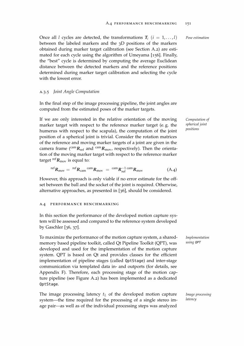
A.4 performance benchmarking 151

Once all l cycles are detected, the transformations Ti (i = 1, . . . , l) Pose estimation

between the labeled markers and the 3D positions of the markersobtained during marker target calibration (see Section A.2) are esti-mated for each cycle using the algorithm of Umeyama [156]. Finally,the “best” cycle is determined by computing the average Euclideandistance between the detected markers and the reference positionsdetermined during marker target calibration and selecting the cyclewith the lowest error.

a.3.5 Joint Angle Computation

In the final step of the image processing pipeline, the joint angles arecomputed from the estimated poses of the marker targets.

If we are only interested in the relative orientation of the moving Computation of

spherical joint

positionsmarker target with respect to the reference marker target (e. g. thehumerus with respect to the scapula), the computation of the jointposition of a spherical joint is trivial. Consider the rotation matricesof the reference and moving marker targets of a joint are given in thecamera frame (camRref and camRmov, respectively). Then the orienta-tion of the moving marker target with respect to the reference markertarget refRmov is equal to:

refRmov = refRcamcamRmov = camR−1

refcamRmov (A.4)

However, this approach is only viable if no error estimate for the off-set between the ball and the socket of the joint is required. Otherwise,alternative approaches, as presented in [36], should be considered.

a.4 performance benchmarking

In this section the performance of the developed motion capture sys-tem will be assessed and compared to the reference system developedby Gaschler [36, 37].

To maximize the performance of the motion capture system, a shared- Implementation

using QPTmemory based pipeline toolkit, called Qt Pipeline Toolkit (QPT), wasdeveloped and used for the implementation of the motion capturesystem. QPT is based on Qt and provides classes for the efficientimplementation of pipeline stages (called QptStage) and inter-stagecommunication via templated data in- and outports (for details, seeAppendix F). Therefore, each processing stage of the motion cap-ture pipeline (see Figure A.2) has been implemented as a dedicatedQptStage.

The image processing latency tL of the developed motion capture Image processing

latencysystem—the time required for the processing of a single stereo im-age pair—as well as of the individual processing steps was analyzed

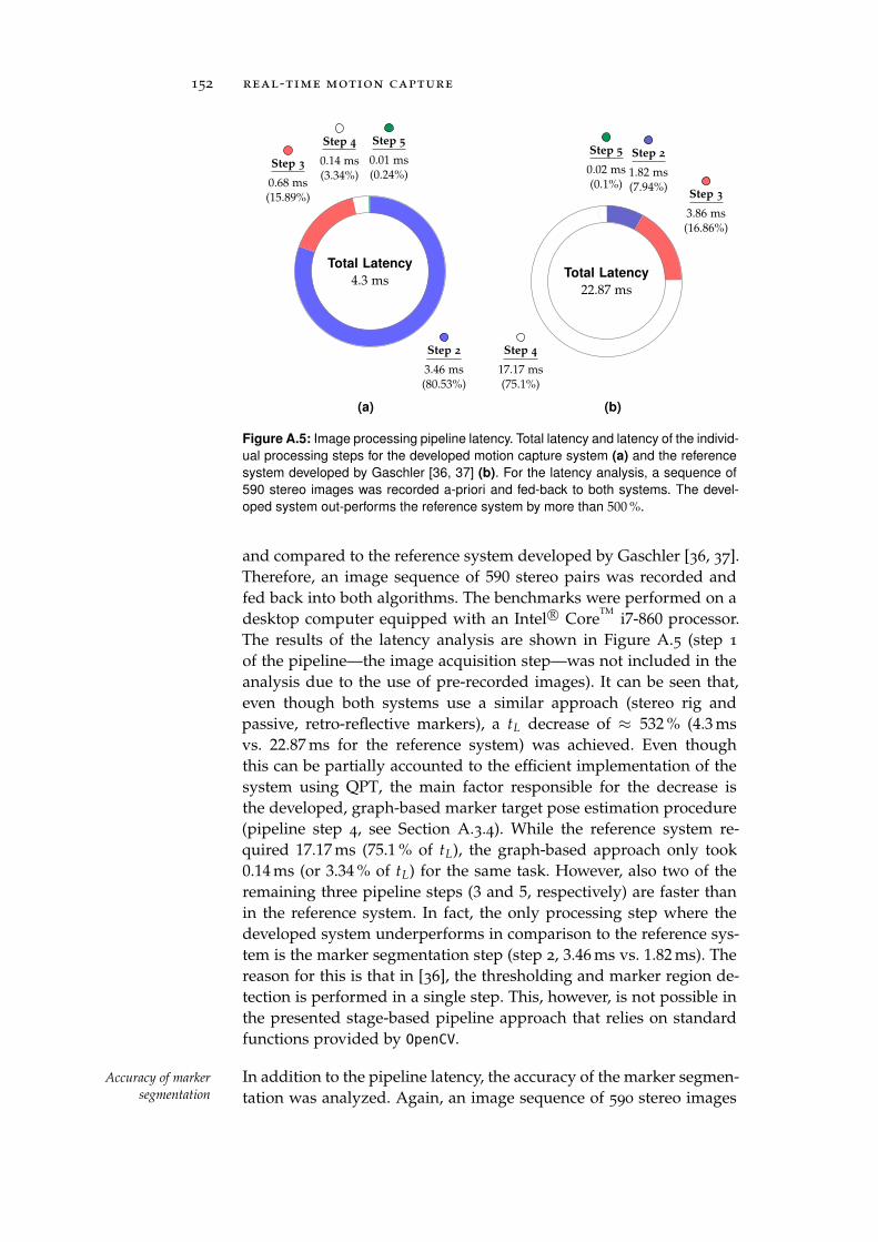
152 real-time motion capture

Total Latency

4.3 ms

Step 2

3.46 ms(80.53%)

Step 3

0.68 ms(15.89%)

Step 4

0.14 ms(3.34%)

Step 5

0.01 ms(0.24%)

(a)

Total Latency

22.87 ms

Step 2

1.82 ms(7.94%)

Step 3

3.86 ms(16.86%)

Step 4

17.17 ms(75.1%)

Step 5

0.02 ms(0.1%)

(b)

Figure A.5: Image processing pipeline latency. Total latency and latency of the individ-

ual processing steps for the developed motion capture system (a) and the reference

system developed by Gaschler [36, 37] (b). For the latency analysis, a sequence of

590 stereo images was recorded a-priori and fed-back to both systems. The devel-

oped system out-performs the reference system by more than 500 %.

and compared to the reference system developed by Gaschler [36, 37].Therefore, an image sequence of 590 stereo pairs was recorded andfed back into both algorithms. The benchmarks were performed on adesktop computer equipped with an Intel R© Core

TMi7-860 processor.

The results of the latency analysis are shown in Figure A.5 (step 1

of the pipeline—the image acquisition step—was not included in theanalysis due to the use of pre-recorded images). It can be seen that,even though both systems use a similar approach (stereo rig andpassive, retro-reflective markers), a tL decrease of ≈ 532 % (4.3 msvs. 22.87 ms for the reference system) was achieved. Even thoughthis can be partially accounted to the efficient implementation of thesystem using QPT, the main factor responsible for the decrease isthe developed, graph-based marker target pose estimation procedure(pipeline step 4, see Section A.3.4). While the reference system re-quired 17.17 ms (75.1 % of tL), the graph-based approach only took0.14 ms (or 3.34 % of tL) for the same task. However, also two of theremaining three pipeline steps (3 and 5, respectively) are faster thanin the reference system. In fact, the only processing step where thedeveloped system underperforms in comparison to the reference sys-tem is the marker segmentation step (step 2, 3.46 ms vs. 1.82 ms). Thereason for this is that in [36], the thresholding and marker region de-tection is performed in a single step. This, however, is not possible inthe presented stage-based pipeline approach that relies on standardfunctions provided by OpenCV.

In addition to the pipeline latency, the accuracy of the marker segmen-Accuracy of marker

segmentation tation was analyzed. Again, an image sequence of 590 stereo images

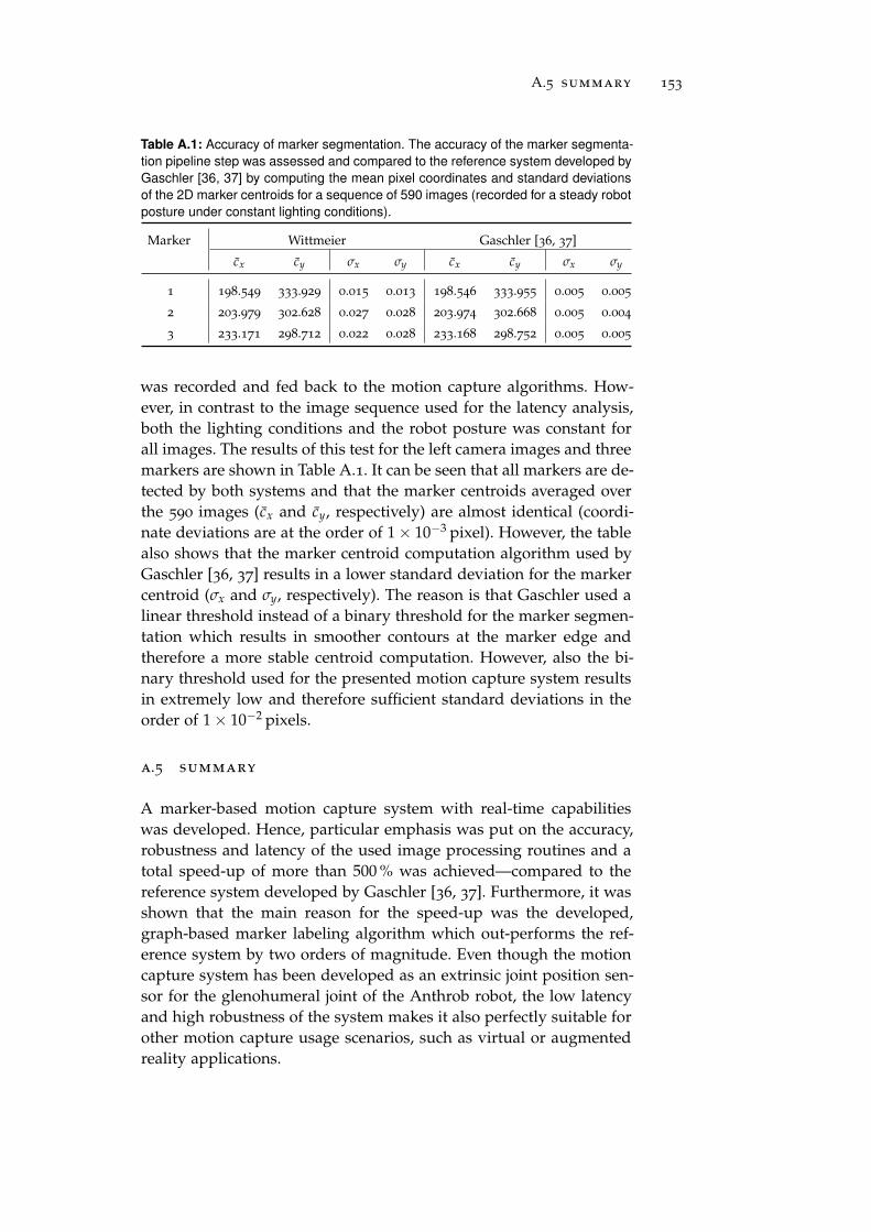
A.5 summary 153

Table A.1: Accuracy of marker segmentation. The accuracy of the marker segmenta-

tion pipeline step was assessed and compared to the reference system developed by

Gaschler [36, 37] by computing the mean pixel coordinates and standard deviations

of the 2D marker centroids for a sequence of 590 images (recorded for a steady robot

posture under constant lighting conditions).

Marker Wittmeier Gaschler [36, 37]

cx cy σx σy cx cy σx σy

1 198.549 333.929 0.015 0.013 198.546 333.955 0.005 0.005

2 203.979 302.628 0.027 0.028 203.974 302.668 0.005 0.004

3 233.171 298.712 0.022 0.028 233.168 298.752 0.005 0.005

was recorded and fed back to the motion capture algorithms. How-ever, in contrast to the image sequence used for the latency analysis,both the lighting conditions and the robot posture was constant forall images. The results of this test for the left camera images and threemarkers are shown in Table A.1. It can be seen that all markers are de-tected by both systems and that the marker centroids averaged overthe 590 images (cx and cy, respectively) are almost identical (coordi-nate deviations are at the order of 1× 10−3 pixel). However, the tablealso shows that the marker centroid computation algorithm used byGaschler [36, 37] results in a lower standard deviation for the markercentroid (σx and σy, respectively). The reason is that Gaschler used alinear threshold instead of a binary threshold for the marker segmen-tation which results in smoother contours at the marker edge andtherefore a more stable centroid computation. However, also the bi-nary threshold used for the presented motion capture system resultsin extremely low and therefore sufficient standard deviations in theorder of 1× 10−2 pixels.

a.5 summary

A marker-based motion capture system with real-time capabilitieswas developed. Hence, particular emphasis was put on the accuracy,robustness and latency of the used image processing routines and atotal speed-up of more than 500 % was achieved—compared to thereference system developed by Gaschler [36, 37]. Furthermore, it wasshown that the main reason for the speed-up was the developed,graph-based marker labeling algorithm which out-performs the ref-erence system by two orders of magnitude. Even though the motioncapture system has been developed as an extrinsic joint position sen-sor for the glenohumeral joint of the Anthrob robot, the low latencyand high robustness of the system makes it also perfectly suitable forother motion capture usage scenarios, such as virtual or augmentedreality applications.

BL I N E A R V I S C O E L A S T I C I T Y

b.1 stress and strain

Consider a specimen that is put under a tensile load f perpendicularto the cross section area of the specimen as shown in Figure B.1. Theload f induces a stretch of the specimen, which is called the strain ε.Furthermore, the load is opposed by the stress σ, which is the reac-tion force of the internal bonds of the material per unit area. Twotypes of stresses and strains are commonly defined: (i) the engineer-ing (or nominal) stress/strain and (ii) the true stress/strain. Both areintroduced in the following paragraphs.

The engineering (or nominal) stress σe is defined as the force per unit Engineering stress

and strainarea A0 of the undeformed specimen (see Figure B.1a) [10, 86, 139]:

σe =f

A0(B.1)

Similar to [86], we use the convention that tensile stresses are positiveand compressive stresses are negative. Stresses are expressed in unitsN/m2 or more commonly in Pa.

Likewise, the engineering (or nominal) strain εe in the direction ofthe tensile load is defined as the integral of the increase in length dl

of the specimen with respect to its initial length l0 [10, 86, 139]:

εe =∫ l1

l0

dl

l0=

l1 − l0l0

=l1l0− 1 (B.2)

If a material exhibits large deformations, such as rubbers or biologicaltissues, the strain is sometimes expressed in terms of the expansionratio λ [86, 139], equal to:

λ = εe + 1 (B.3)

In contrast to the engineering stress and strain, the true stress σt and True stress and

strainstrain εt are calculated with respect to the current cross-section areaA1 and length l of the deformed specimen (see Figure B.1b). There-fore, the true stress σt is defined as [10, 86]:

σt =f

A1(B.4)

155

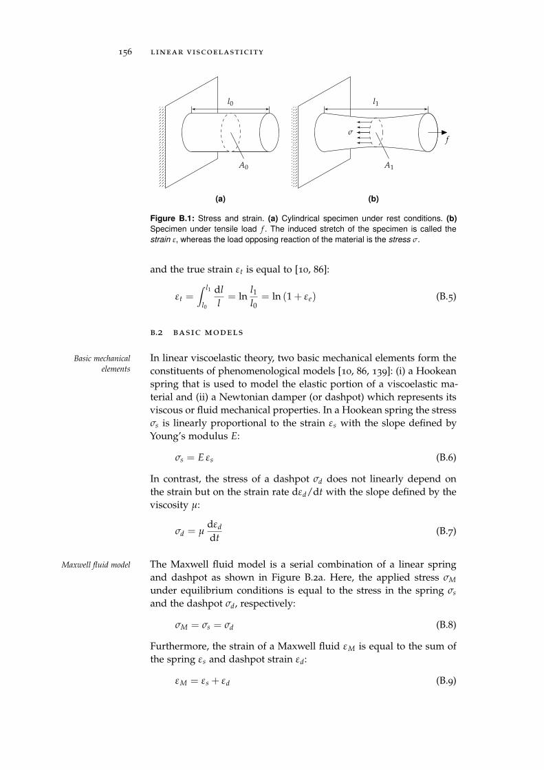
156 linear viscoelasticity

l0

A0

(a)

σ

l1

A1

f

(b)

Figure B.1: Stress and strain. (a) Cylindrical specimen under rest conditions. (b)

Specimen under tensile load f . The induced stretch of the specimen is called the

strain ε, whereas the load opposing reaction of the material is the stress σ.

and the true strain εt is equal to [10, 86]:

εt =∫ l1

l0

dl

l= ln

l1l0

= ln (1 + εe) (B.5)

b.2 basic models

In linear viscoelastic theory, two basic mechanical elements form theBasic mechanical

elements constituents of phenomenological models [10, 86, 139]: (i) a Hookeanspring that is used to model the elastic portion of a viscoelastic ma-terial and (ii) a Newtonian damper (or dashpot) which represents itsviscous or fluid mechanical properties. In a Hookean spring the stressσs is linearly proportional to the strain εs with the slope defined byYoung’s modulus E:

σs = E εs (B.6)

In contrast, the stress of a dashpot σd does not linearly depend onthe strain but on the strain rate dεd/dt with the slope defined by theviscosity µ:

σd = µdεd

dt(B.7)

The Maxwell fluid model is a serial combination of a linear springMaxwell fluid model

and dashpot as shown in Figure B.2a. Here, the applied stress σM

under equilibrium conditions is equal to the stress in the spring σs

and the dashpot σd, respectively:

σM = σs = σd (B.8)

Furthermore, the strain of a Maxwell fluid εM is equal to the sum ofthe spring εs and dashpot strain εd:

εM = εs + εd (B.9)

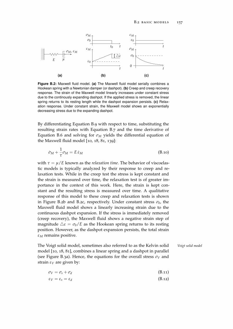
B.2 basic models 157

σM, εM

E µ

(a)

t

σM

σ0

t0

t

εM

ε0

ε

(b)

t

εM

ε0

0t

σM

σ0

(c)

Figure B.2: Maxwell fluid model. (a) The Maxwell fluid model serially combines a

Hookean spring with a Newtonian damper (or dashpot). (b) Creep and creep recovery

response. The strain of the Maxwell model linearly increases under constant stress

due to the continously expanding dashpot. If the applied stress is removed, the linear

spring returns to its resting length while the dashpot expansion persists. (c) Relax-

ation response. Under constant strain, the Maxwell model shows an exponentially

decreasing stress due to the expanding dashpot.

By differentiating Equation B.9 with respect to time, substituting theresulting strain rates with Equation B.7 and the time derivative ofEquation B.6 and solving for σM yields the differential equation ofthe Maxwell fluid model [10, 18, 81, 139]:

σM +1τ

σM = E εM (B.10)

with τ = µ/E known as the relaxation time. The behavior of viscoelas-tic models is typically analyzed by their response to creep and re-laxation tests. While in the creep test the stress is kept constant andthe strain is measured over time, the relaxation test is of greater im-portance in the context of this work. Here, the strain is kept con-stant and the resulting stress is measured over time. A qualitativeresponse of this model to these creep and relaxation tests is shownin Figure B.2b and B.2c, respectively. Under constant stress σ0, theMaxwell fluid model shows a linearly increasing strain due to thecontinuous dashpot expansion. If the stress is immediately removed(creep recovery), the Maxwell fluid shows a negative strain step ofmagnitude ε = σ0/E as the Hookean spring returns to its restingposition. However, as the dashpot expansion persists, the total strainεM remains positive.

The Voigt solid model, sometimes also referred to as the Kelvin solid Voigt solid model

model [10, 18, 81], combines a linear spring and a dashpot in parallel(see Figure B.3a). Hence, the equations for the overall stress σV andstrain εV are given by:

σV = σs + σd (B.11)

εV = εs = εd (B.12)

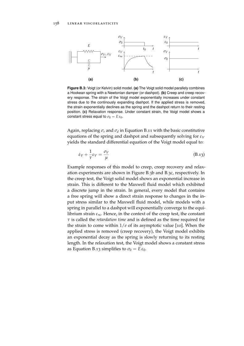
158 linear viscoelasticity

µ

E

σV , εV

(a)

t

σV

σ0

t0

t

εV

ε∞

(b)

t

εV

ε0

t

σV

σ0

(c)

Figure B.3: Voigt (or Kelvin) solid model. (a) The Voigt solid model parallely combines

a Hookean spring with a Newtonian damper (or dashpot). (b) Creep and creep recov-

ery response. The strain of the Voigt model exponentially increases under constant

stress due to the continously expanding dashpot. If the applied stress is removed,

the strain exponentially declines as the spring and the dashpot return to their resting

position. (c) Relaxation response. Under constant strain, the Voigt model shows a

constant stress equal to σ0 = E ε0.

Again, replacing σs and σd in Equation B.11 with the basic constitutiveequations of the spring and dashpot and subsequently solving for εV

yields the standard differential equation of the Voigt model equal to:

εV +1τ

εV =σV

µ(B.13)

Example responses of this model to creep, creep recovery and relax-ation experiments are shown in Figure B.3b and B.3c, respectively. Inthe creep test, the Voigt solid model shows an exponential increase instrain. This is different to the Maxwell fluid model which exhibiteda discrete jump in the strain. In general, every model that containsa free spring will show a direct strain response to changes in the in-put stress similar to the Maxwell fluid model, while models with aspring in parallel to a dashpot will exponentially converge to the equi-librium strain ε∞. Hence, in the context of the creep test, the constantτ is called the retardation time and is defined as the time required forthe strain to come within 1/e of its asymptotic value [10]. When theapplied stress is removed (creep recovery), the Voigt model exhibitsan exponential decay as the spring is slowly returning to its restinglength. In the relaxation test, the Voigt model shows a constant stressas Equation B.13 simplifies to σ0 = E ε0.

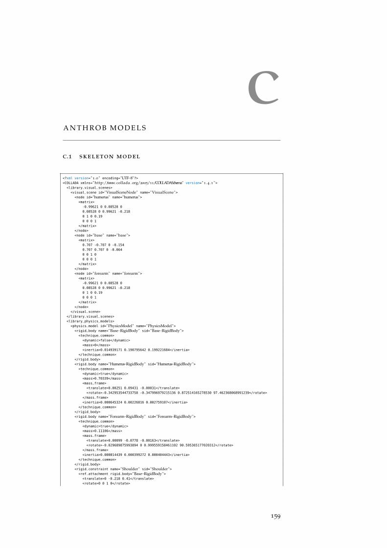
CA N T H R O B M O D E L S

c.1 skeleton model

<?xml version=" 1.0 " encoding="UTF−8"?><COLLADA xmlns=" http://www. collada . org/2005/11/COLLADASchema" version=" 1 .4 .1 "><library_visual_scenes>

<visual_scene id="VisualSceneNode" name="VisualScene"><node id="humerus" name="humerus"><matrix>

-0.99621 0 0.08528 0

0.08528 0 0.99621 -0.218

0 1 0 0.19

0 0 0 1

</matrix>

</node>

<node id="base" name="base"><matrix>

0.707 -0.707 0 -0.154

0.707 0.707 0 -0.064

0 0 1 0

0 0 0 1

</matrix>

</node>

<node id="forearm" name="forearm"><matrix>

-0.99621 0 0.08528 0

0.08528 0 0.99621 -0.218

0 1 0 0.19

0 0 0 1

</matrix>

</node>

</visual_scene>

</library_visual_scenes>

<library_physics_models>

<physics_model id="PhysicsModel" name="PhysicsModel"><rigid_body name="Base−RigidBody" sid="Base−RigidBody"><technique_common>

<dynamic>false</dynamic>

<mass>0</mass>

<inertia>0.014939171 0.190795642 0.199221684</inertia>

</technique_common>

</rigid_body>

<rigid_body name="Humerus−RigidBody" sid="Humerus−RigidBody"><technique_common>

<dynamic>true</dynamic>

<mass>0.70339</mass>

<mass_frame>

<translate>0.00251 0.09431 -0.00031</translate>

<rotate>-0.342953544733758 -0.347996979215136 0.872514165278530 97.462368068991239</rotate>

</mass_frame>

<inertia>0.000645324 0.00226816 0.002759107</inertia>

</technique_common>

</rigid_body>

<rigid_body name="Forearm−RigidBody" sid="Forearm−RigidBody"><technique_common>

<dynamic>true</dynamic>

<mass>0.11106</mass>

<mass_frame>

<translate>0.00099 -0.0778 -0.00163</translate>

<rotate>-0.029689875993894 0 0.999559158461102 90.595365177020312</rotate>

</mass_frame>

<inertia>0.000014439 0.000399272 0.000404443</inertia>

</technique_common>

</rigid_body>

<rigid_constraint name="Shoulder" sid="Shoulder"><ref_attachment rigid_body="Base−RigidBody"><translate>0 -0.218 0.41</translate>

<rotate>0 0 1 0</rotate>

159

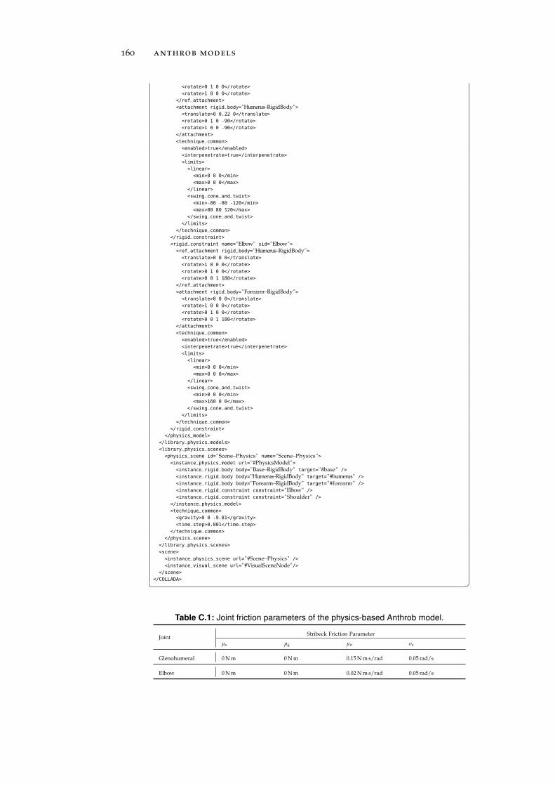
160 anthrob models

<rotate>0 1 0 0</rotate>

<rotate>1 0 0 0</rotate>

</ref_attachment>

<attachment rigid_body="Humerus−RigidBody"><translate>0 0.22 0</translate>

<rotate>0 1 0 -90</rotate>

<rotate>1 0 0 -90</rotate>

</attachment>

<technique_common>

<enabled>true</enabled>

<interpenetrate>true</interpenetrate>

<limits>

<linear>

<min>0 0 0</min>

<max>0 0 0</max>

</linear>

<swing_cone_and_twist>

<min>-80 -80 -120</min>

<max>80 80 120</max>

</swing_cone_and_twist>

</limits>

</technique_common>

</rigid_constraint>

<rigid_constraint name="Elbow" sid="Elbow"><ref_attachment rigid_body="Humerus−RigidBody"><translate>0 0 0</translate>

<rotate>1 0 0 0</rotate>

<rotate>0 1 0 0</rotate>

<rotate>0 0 1 180</rotate>

</ref_attachment>

<attachment rigid_body="Forearm−RigidBody"><translate>0 0 0</translate>

<rotate>1 0 0 0</rotate>

<rotate>0 1 0 0</rotate>

<rotate>0 0 1 180</rotate>

</attachment>

<technique_common>

<enabled>true</enabled>

<interpenetrate>true</interpenetrate>

<limits>

<linear>

<min>0 0 0</min>

<max>0 0 0</max>

</linear>

<swing_cone_and_twist>

<min>0 0 0</min>

<max>160 0 0</max>

</swing_cone_and_twist>

</limits>

</technique_common>

</rigid_constraint>

</physics_model>

</library_physics_models>

<library_physics_scenes>

<physics_scene id="Scene−Physics" name="Scene−Physics"><instance_physics_model url="#PhysicsModel"><instance_rigid_body body="Base−RigidBody" target="#base" />

<instance_rigid_body body="Humerus−RigidBody" target="#humerus" />

<instance_rigid_body body="Forearm−RigidBody" target="#forearm" />

<instance_rigid_constraint constraint="Elbow" />

<instance_rigid_constraint constraint="Shoulder" />

</instance_physics_model>

<technique_common>

<gravity>0 0 -9.81</gravity>

<time_step>0.001</time_step>

</technique_common>

</physics_scene>

</library_physics_scenes>

<scene>

<instance_physics_scene url="#Scene−Physics" />

<instance_visual_scene url="#VisualSceneNode"/></scene>

</COLLADA>

Table C.1: Joint friction parameters of the physics-based Anthrob model.

JointStribeck Friction Parameter

µs µk µv vs

Glenohumeral 0 N m 0 N m 0.15 N m s/rad 0.05 rad/s

Elbow 0 N m 0 N m 0.02 N m s/rad 0.05 rad/s

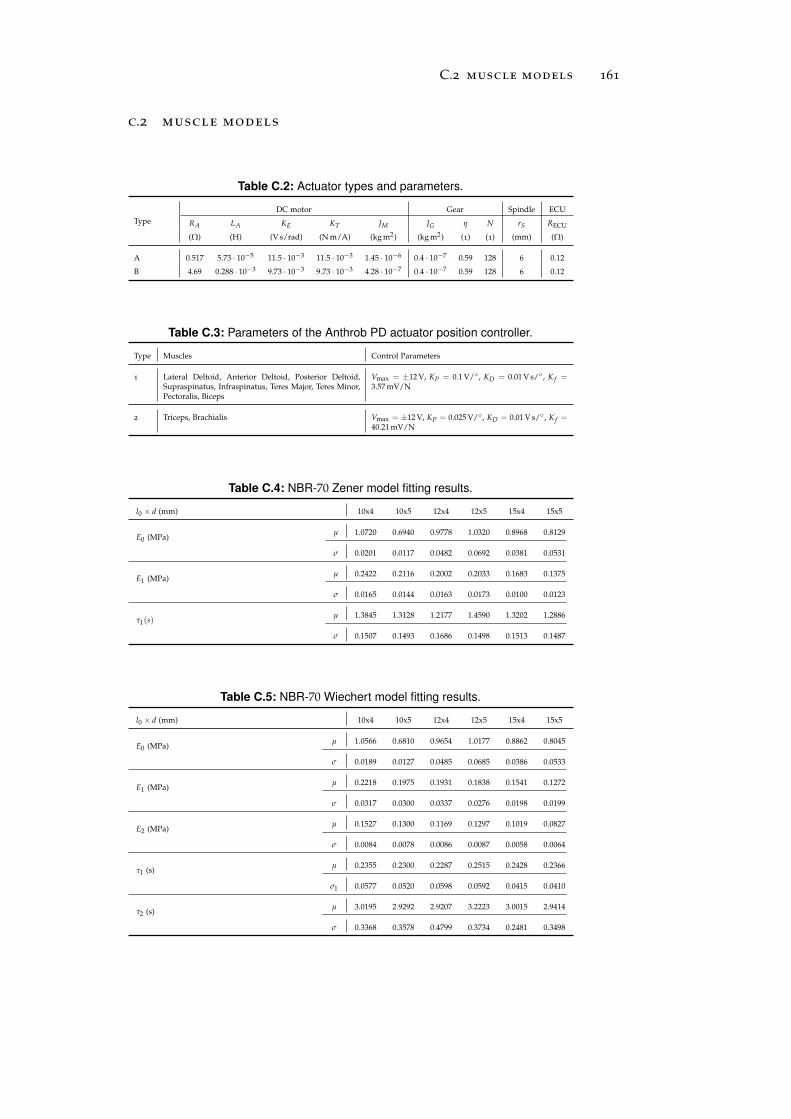
C.2 muscle models 161

c.2 muscle models

Table C.2: Actuator types and parameters.

Type

DC motor Gear Spindle ECU

RA LA KE KT JM JG η N rS RECU

(Ω) (H) (V s/rad) (N m/A) (kg m2) (kg m2) (1) (1) (mm) (Ω)

A 0.517 5.73 · 10−5 11.5 · 10−3 11.5 · 10−3 1.45 · 10−6 0.4 · 10−7 0.59 128 6 0.12

B 4.69 0.288 · 10−3 9.73 · 10−3 9.73 · 10−3 4.28 · 10−7 0.4 · 10−7 0.59 128 6 0.12

Table C.3: Parameters of the Anthrob PD actuator position controller.

Type Muscles Control Parameters

1 Lateral Deltoid, Anterior Deltoid, Posterior Deltoid,Supraspinatus, Infraspinatus, Teres Major, Teres Minor,Pectoralis, Biceps

Vmax = ±12 V, KP = 0.1 V/ , KD = 0.01 V s/ , K f =3.57 mV/N

2 Triceps, Brachialis Vmax = ±12 V, KP = 0.025 V/ , KD = 0.01 V s/ , K f =40.21 mV/N

Table C.4: NBR-70 Zener model fitting results.

l0 × d (mm) 10x4 10x5 12x4 12x5 15x4 15x5

E0 (MPa)µ 1.0720 0.6940 0.9778 1.0320 0.8968 0.8129

σ 0.0201 0.0117 0.0482 0.0692 0.0381 0.0531

E1 (MPa)µ 0.2422 0.2116 0.2002 0.2033 0.1683 0.1375

σ 0.0165 0.0144 0.0163 0.0173 0.0100 0.0123

τ1(s)µ 1.3845 1.3128 1.2177 1.4590 1.3202 1.2886

σ 0.1507 0.1493 0.1686 0.1498 0.1513 0.1487

Table C.5: NBR-70 Wiechert model fitting results.

l0 × d (mm) 10x4 10x5 12x4 12x5 15x4 15x5

E0 (MPa)µ 1.0566 0.6810 0.9654 1.0177 0.8862 0.8045

σ 0.0189 0.0127 0.0485 0.0685 0.0386 0.0533

E1 (MPa)µ 0.2218 0.1975 0.1931 0.1838 0.1541 0.1272

σ 0.0317 0.0300 0.0337 0.0276 0.0198 0.0199

E2 (MPa)µ 0.1527 0.1300 0.1169 0.1297 0.1019 0.0827

σ 0.0084 0.0078 0.0086 0.0087 0.0058 0.0064

τ1 (s)µ 0.2355 0.2300 0.2287 0.2515 0.2428 0.2366

σ1 0.0577 0.0520 0.0598 0.0592 0.0415 0.0410

τ2 (s)µ 3.0195 2.9292 2.9207 3.2223 3.0015 2.9414

σ 0.3368 0.3578 0.4799 0.3734 0.2481 0.3498

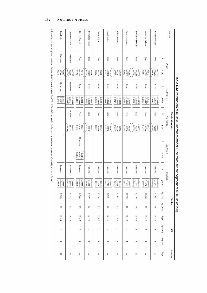
162 anthrob models

Ta

ble

C.6

:P

ara

me

ters

of

mu

scle

kin

em

atic

sm

od

elI

(the

forc

ese

nso

rse

gm

en

to

fa

llm

uscle

sis

0).

Mu

scleM

uscle

Kin

em

atics

Ten

do

nS

EE

Actu

ato

r

Origin

Via-P

oint

1V

ia-Poin

t2

Via-P

oint

3In

sertion

Bp

(m)

Bp

(m)

Bp

(m)

Bp

(m)

Bp

(m)

lT0(m

)r

T(m

m)

Type

Qu

antity

Segmen

tTyp

e

Lateral

Deltoid

Base

−0.0060−

0.02870.4656

Base

−0.0060−

0.05570.4643

Base

0.0000−

0.25700.4500

Hu

meru

s

−0.0090

0.1475−

0.0090

0.32950.5

15×5

21

A

An

teriorD

eltoidB

ase

0.0643−

0.02880.4084

Base

0.0626−

0.05570.4088

Base

0.0430−

0.15400.4308

Hu

meru

s

−0.0090

0.1475−

0.0090

0.24300.5

15×5

21

A

Posterior

Deltoid

Base

−0.0532−

0.02880.4398

Base

−0.0520−

0.05580.4389

Base

−0.0351−

0.22460.4270

Hu

meru

s

−0.0090

0.1475−

0.0090

0.27800.5

15×5

21

A

Sup

raspin

atus

Base

−0.0657−

0.02900.3963

Base

−0.0638−

0.05600.3967

Base

−0.0485−

0.17200.4189

Hu

meru

s

−0.0098

0.1922−

0.0171

0.21900.3

12×5

11

A

Infrasp

inatu

sB

ase

−0.0611−

0.02870.3525

Base

−0.0595−

0.05560.3548

Base

−0.0528−

0.17200.3837

Hu

meru

s

−0.0106

0.1820−

0.0202

0.21610.3

12×5

11

A

TeresM

inor

Base

−0.0439−

0.02970.3112

Base

−0.0431−

0.05640.3154

Base

−0.0402−

0.17100.3485

Hu

meru

s

−0.0091

0.1702−

0.0147

0.20750.3

12×5

11

A

TeresM

ajorB

ase

0.0638−

0.02790.3636

Base

0.0622−

0.05480.3659

Base

0.0528−

0.15400.3837

Hu

meru

s

−0.0202

0.1820−

0.0106

0.21540.3

12×5

11

A

Pectoralis

Major

Base

0.0486−

0.02830.3214

Base

0.0477−

0.05500.3256

Base

0.0402−

0.15400.3485

Hu

meru

s

−0.0108

0.15200.0108

0.18700.3

12×5

11

A

Bicep

sB

rachii

Base

0.0446−

0.02880.4496

Base

0.0434−

0.05580.4486

Base

0.0271−

0.20520.4503

Hu

meru

s

−0.0170

0.13900.0170

Forearm

0.0000−

0.04600.0050

0.47080.5

15×5

21

A

Triceps

Brach

iiH

um

erus

−0.0097

0.1360−

0.0345

Hu

meru

s

−0.0089

0.1090−

0.0357

Hu

meru

s

0.00000.0470−

0.0300

Forearm

0.0000−

0.0008−

0.0220

0.12840.3

10×4

12

B

Brach

ialisH

um

erus

0.00970.13600.0345

Hu

meru

s

0.00890.10900.0357

Forearm

0.0000−

0.04600.0050

0.17030.3

15×4

11

B

All

position

vectorsare

givenrelative

toth

evisu

aln

ode

transform

sof

the

CO

LL

AD

Askeleton

mod

el(before

the

correctionof

the

center

ofm

assby

the

mass

frame).

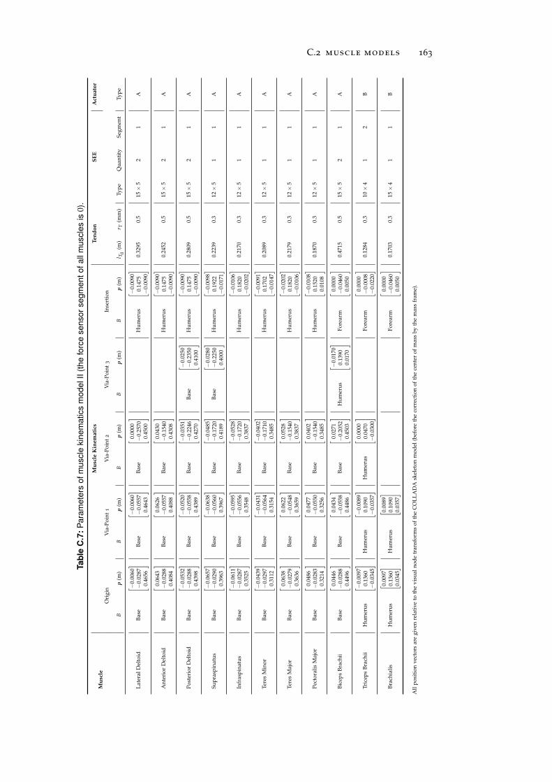
C.2 muscle models 163

Ta

ble

C.7

:P

ara

me

ters

of

mu

scle

kin

em

atics

mo

de

lII

(th

efo

rce

se

nso

rse

gm

en

to

fa

llm

uscle

sis

0).

Mu

scle

Mu

scle

Kin

em

ati

csT

en

do

nS

EE

Act

uato

r

Ori

gin

Via

-Poi

nt

1V

ia-P

oin

t2

Via

-Poi

nt

3In

sert

ion

Bp

(m)

Bp

(m)

Bp

(m)

Bp

(m)

Bp

(m)

l T0

(m)

r T(m

m)

Typ

eQ

uan

tity

Segm

ent

Typ

e

Lat

eral

Del

toid

Bas

e

−0.

0060

−0.

0287

0.46

56

Bas

e

−0.

0060

−0.

0557

0.46

43

Bas

e

0.00

00−

0.25

700.

4500

Hu

mer

us

−0.

0090

0.14

75−

0.00

90

0.32

950.

515×

52

1A

An

teri

orD

elto

idB

ase

0.06

43−

0.02

880.

4084

Bas

e

0.06

26−

0.05

570.

4088

Bas

e

0.04

30−

0.15

400.

4308

Hu

mer

us

−0.

0090

0.14

75−

0.00

90

0.24

520.

515×

52

1A

Pos

teri

orD

elto

idB

ase

−0.

0532

−0.

0288

0.43

98

Bas

e

−0.

0520

−0.

0558

0.43

89

Bas

e

−0.

0351

−0.

2246

0.42

70

Bas

e

−0.

0250

−0.

2350

0.41

00

Hu

mer

us

−0.

0090

0.14

75−

0.00

90

0.28

090.

515×

52

1A

Sup

rasp

inat

us

Bas

e

−0.

0657

−0.

0290

0.39

63

Bas

e

−0.

0638

−0.

0560

0.39

67

Bas

e

−0.

0485

−0.

1720

0.41

89

Bas

e

−0.

0280

−0.

2250

0.40

00

Hu

mer

us

−0.

0098

0.19

22−

0.01

71

0.22

390.

312×

51

1A

Infr

asp

inat

us

Bas

e

−0.

0611

−0.

0287

0.35

25

Bas

e

−0.

0595

−0.

0556

0.35

48

Bas

e

−0.

0528

−0.

1720

0.38

37

Hu

mer

us

−0.

0106

0.18

20−

0.02

02

0.21

700.

312×

51

1A

Tere

sM

inor

Bas

e

−0.

0439

−0.

0297

0.31

12

Bas

e

−0.

0431

−0.

0564

0.31

54

Bas

e

−0.

0402

−0.

1710

0.34

85

Hu

mer

us

−0.

0091

0.17

02−

0.01

47

0.20

890.

312×

51

1A

Tere

sM

ajor

Bas

e

0.06

38−

0.02

790.

3636

Bas

e

0.06

22−

0.05

480.

3659

Bas

e

0.05

28−

0.15

400.

3837

Hu

mer

us

−0.

0202

0.18

20−

0.01

06

0.21

790.

312×

51

1A

Pec

tora

lis

Maj

orB

ase

0.04

86−

0.02

830.

3214

Bas

e

0.04

77−

0.05

500.

3256

Bas

e

0.04

02−

0.15

400.

3485

Hu

mer

us

−0.

0108

0.15

200.

0108

0.18

700.

312×

51

1A

Bic

eps

Bra

chii

Bas

e

0.04

46−

0.02

880.

4496

Bas

e

0.04

34−

0.05

580.

4486

Bas

e

0.02

71−

0.20

520.

4503

Hu

mer

us

−0.

0170

0.13

900.

0170

Fore

arm

0.00

00−

0.04

600.

0050

0.47

150.

515×

52

1A

Tric

eps

Bra

chii

Hu

mer

us

−0.

0097

0.13

60−

0.03

45

Hu

mer

us

−0.

0089

0.10

90−

0.03

57

Hu

mer

us

0.00

000.

0470

−0.

0300

Fore

arm

0.00

00−

0.00

08−

0.02

20

0.12

840.

310×

41

2B

Bra

chia

lis

Hu

mer

us

0.00

970.

1360

0.03

45

Hu

mer

us

0.00

890.

1090

0.03

57

Fore

arm

0.00

00−

0.04

600.

0050

0.17

030.

315×

41

1B

All

pos

itio

nve

ctor

sar

egi

ven

rela

tive

toth

evi

sual

nod

etr

ansf

orm

sof

the

CO

LL

AD

Ask

elet

onm

odel

(bef

ore

the

corr

ecti

onof

the

cen

ter

ofm

ass

byth

em

ass

fram

e).

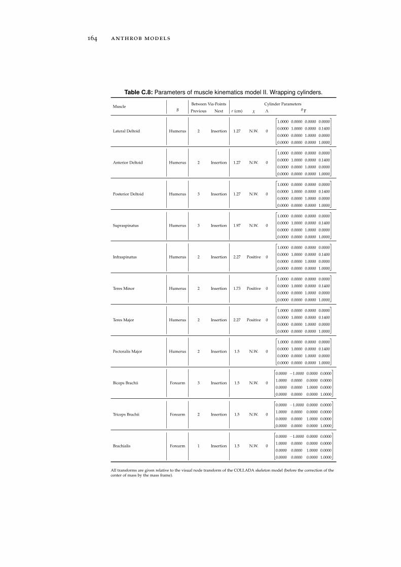
164 anthrob models

Table C.8: Parameters of muscle kinematics model II. Wrapping cylinders.

MuscleB

Between Via-Points Cylinder Parameters

Previous Next r (cm) χ Λ B T

Lateral Deltoid Humerus 2 Insertion 1.27 N.W. 0

1.0000 0.0000 0.0000 0.0000

0.0000 1.0000 0.0000 0.1400

0.0000 0.0000 1.0000 0.0000

0.0000 0.0000 0.0000 1.0000

Anterior Deltoid Humerus 2 Insertion 1.27 N.W. 0

1.0000 0.0000 0.0000 0.0000

0.0000 1.0000 0.0000 0.1400

0.0000 0.0000 1.0000 0.0000

0.0000 0.0000 0.0000 1.0000

Posterior Deltoid Humerus 3 Insertion 1.27 N.W. 0

1.0000 0.0000 0.0000 0.0000

0.0000 1.0000 0.0000 0.1400

0.0000 0.0000 1.0000 0.0000

0.0000 0.0000 0.0000 1.0000

Supraspinatus Humerus 3 Insertion 1.97 N.W. 0

1.0000 0.0000 0.0000 0.0000

0.0000 1.0000 0.0000 0.1400

0.0000 0.0000 1.0000 0.0000

0.0000 0.0000 0.0000 1.0000

Infraspinatus Humerus 2 Insertion 2.27 Positive 0

1.0000 0.0000 0.0000 0.0000

0.0000 1.0000 0.0000 0.1400

0.0000 0.0000 1.0000 0.0000

0.0000 0.0000 0.0000 1.0000

Teres Minor Humerus 2 Insertion 1.73 Positive 0

1.0000 0.0000 0.0000 0.0000

0.0000 1.0000 0.0000 0.1400

0.0000 0.0000 1.0000 0.0000

0.0000 0.0000 0.0000 1.0000

Teres Major Humerus 2 Insertion 2.27 Positive 0

1.0000 0.0000 0.0000 0.0000

0.0000 1.0000 0.0000 0.1400

0.0000 0.0000 1.0000 0.0000

0.0000 0.0000 0.0000 1.0000

Pectoralis Major Humerus 2 Insertion 1.5 N.W. 0

1.0000 0.0000 0.0000 0.0000

0.0000 1.0000 0.0000 0.1400

0.0000 0.0000 1.0000 0.0000

0.0000 0.0000 0.0000 1.0000

Biceps Brachii Forearm 3 Insertion 1.5 N.W. 0

0.0000 −1.0000 0.0000 0.0000

1.0000 0.0000 0.0000 0.0000

0.0000 0.0000 1.0000 0.0000

0.0000 0.0000 0.0000 1.0000

Triceps Brachii Forearm 2 Insertion 1.5 N.W. 0

0.0000 −1.0000 0.0000 0.0000

1.0000 0.0000 0.0000 0.0000

0.0000 0.0000 1.0000 0.0000

0.0000 0.0000 0.0000 1.0000

Brachialis Forearm 1 Insertion 1.5 N.W. 0

0.0000 −1.0000 0.0000 0.0000

1.0000 0.0000 0.0000 0.0000

0.0000 0.0000 1.0000 0.0000

0.0000 0.0000 0.0000 1.0000

All transforms are given relative to the visual node transform of the COLLADA skeleton model (before the correction of thecenter of mass by the mass frame).

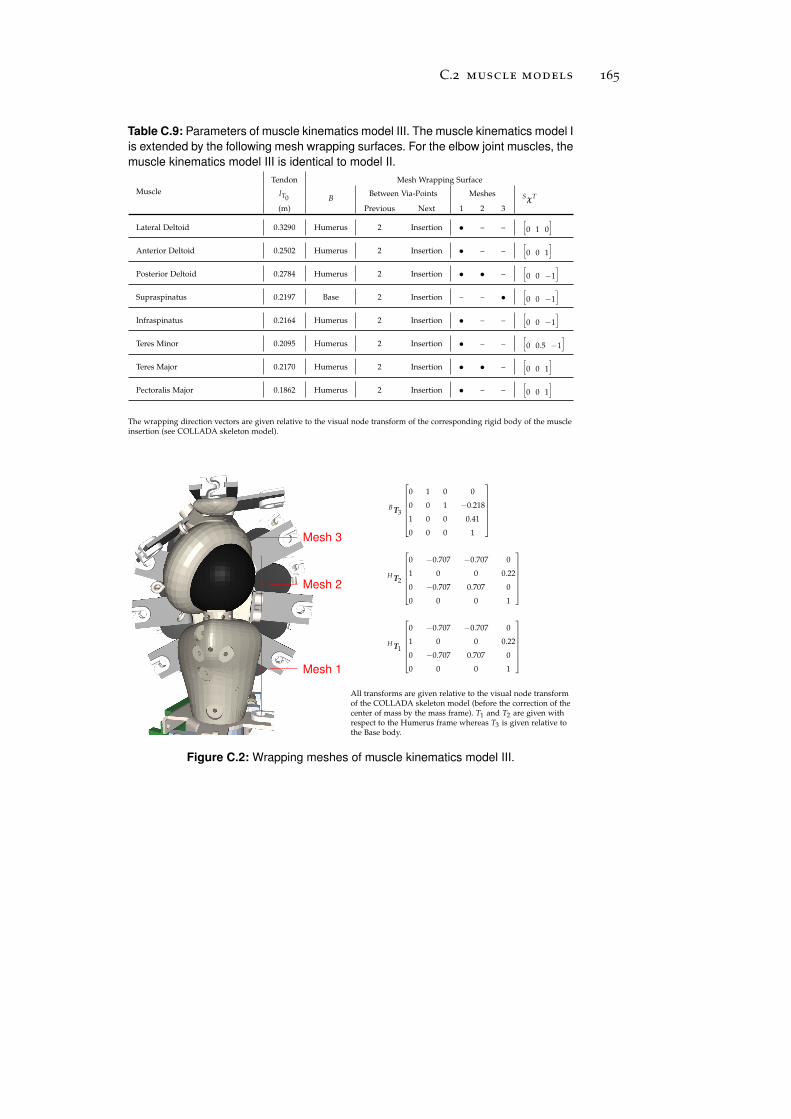
C.2 muscle models 165

Table C.9: Parameters of muscle kinematics model III. The muscle kinematics model I

is extended by the following mesh wrapping surfaces. For the elbow joint muscles, the

muscle kinematics model III is identical to model II.

Muscle

Tendon Mesh Wrapping Surface

lT0 BBetween Via-Points Meshes SχT

(m) Previous Next 1 2 3

Lateral Deltoid 0.3290 Humerus 2 Insertion • – –[

0 1 0]

Anterior Deltoid 0.2502 Humerus 2 Insertion • – –[

0 0 1]

Posterior Deltoid 0.2784 Humerus 2 Insertion • • –[

0 0 −1]

Supraspinatus 0.2197 Base 2 Insertion – – •

[

0 0 −1]

Infraspinatus 0.2164 Humerus 2 Insertion • – –[

0 0 −1]

Teres Minor 0.2095 Humerus 2 Insertion • – –[

0 0.5 −1]

Teres Major 0.2170 Humerus 2 Insertion • • –[

0 0 1]

Pectoralis Major 0.1862 Humerus 2 Insertion • – –[

0 0 1]

The wrapping direction vectors are given relative to the visual node transform of the corresponding rigid body of the muscleinsertion (see COLLADA skeleton model).

Mesh 1

Mesh 2

Mesh 3

B T3

0 1 0 0

0 0 1 −0.218

1 0 0 0.41

0 0 0 1

H T2

0 −0.707 −0.707 0

1 0 0 0.22

0 −0.707 0.707 0

0 0 0 1

H T1

0 −0.707 −0.707 0

1 0 0 0.22

0 −0.707 0.707 0

0 0 0 1

All transforms are given relative to the visual node transformof the COLLADA skeleton model (before the correction of thecenter of mass by the mass frame). T1 and T2 are given withrespect to the Humerus frame whereas T3 is given relative tothe Base body.

Figure C.2: Wrapping meshes of muscle kinematics model III.

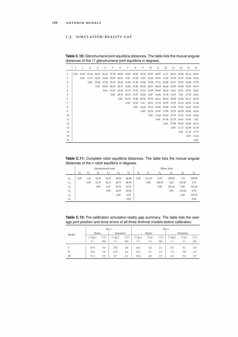
166 anthrob models

c.3 simulation-reality gap

Table C.10: Glenohumeral joint equilibria distances. The table lists the mutual angular

distances of the 17 glenohumeral joint equilibria in degrees.

0 1 2 3 4 5 6 7 8 9 10 11 12 13 14 15 16

0 0.00 10.35 21.24 42.07 26.19 37.38 49.09 18.69 30.82 16.10 45.57 48.57 6.33 28.53 38.56 45.16 48.07

1 0.00 11.77 34.23 18.48 29.05 40.63 8.92 21.08 9.05 36.64 39.91 11.84 21.59 31.57 35.46 39.64

2 0.00 23.00 17.92 27.27 30.20 10.58 17.45 15.64 33.00 37.31 22.88 24.31 32.32 30.28 37.59

3 0.00 34.05 40.62 20.71 32.84 33.29 38.34 42.51 48.54 44.64 43.58 47.84 39.04 49.76

4 0.00 14.10 43.69 15.10 17.02 19.23 22.09 29.60 28.43 14.61 18.31 27.01 30.81

5 0.00 45.70 22.12 15.27 25.45 8.87 16.56 37.76 12.33 7.66 17.25 18.41

6 0.00 36.74 33.86 40.90 45.53 46.61 48.93 46.98 52.06 36.11 46.78

7 0.00 12.23 6.21 28.91 31.35 18.29 15.25 25.14 26.63 31.06

8 0.00 16.06 19.12 20.26 29.85 13.38 19.51 14.41 20.20

9 0.00 32.52 33.47 13.95 15.79 26.78 30.02 32.64

10 0.00 11.64 45.62 19.73 12.78 13.36 14.66

11 0.00 47.04 21.35 16.61 10.55 3.42

12 0.00 27.58 38.30 43.96 46.10

13 0.00 11.17 22.09 21.18

14 0.00 21.12 17.77

15 0.00 11.42

16 0.00

Table C.11: Complete robot equilibria distances. The table lists the mutual angular

distances of the 6 robot equilibria in degrees.

Glenohumeral Joint Elbow Joint

E0 E1 E2 E3 E4 E5 E0 E1 E2 E3 E4 E5

E0 0.00 1.16 42.42 43.01 49.04 48.88 0.00 111.33 6.93 109.09 1.15 108.58

E1 0.00 41.53 42.11 48.71 48.54 0.00 104.39 2.23 112.47 2.75

E2 0.00 0.67 43.56 43.31 0.00 102.16 8.08 101.64

E3 0.00 44.07 43.82 0.00 110.24 0.52

E4 0.00 0.25 0.00 109.72

E5 0.00 0.00

Table C.12: Pre-calibration simulation-reality gap summary. The table lists the aver-

age joint position and force errors of all three Anthrob models before calibration.

Model

Tier 1 Tier 2

Statics Dynamics Statics Dynamics

‖qG‖ | f | ‖qG‖ | f | ‖qG‖ |qE | | f | ‖qG‖ |qE | | f |() (N) () (N) () () (N) () () (N)

I 21.9 5.0 15.2 4.4 14.3 4.4 3.1 8.7 5.1 2.9

II 15.6 5.4 11.5 4.3 13.0 5.1 2.7 7.5 5.8 2.7

III 11.3 5.3 8.7 4.1 10.4 4.8 2.7 6.3 5.6 2.7

DA N T H R O B C A L I B R AT I O N

d.1 simulation-reality gap

Table D.1: Post-calibration simulation-reality gap summary. The table lists the average

joint position and force errors of all three Anthrob models after calibration.

Model

Tier 1 Tier 2

Statics Dynamics Statics Dynamics

‖qG‖ | f | ‖qG‖ | f | ‖qG‖ |qE | | f | ‖qG‖ |qE | | f |() (N) () (N) () () (N) () () (N)

I 4.5 6.0 9.9 4.0 6.7 2.4 3.3 7.1 2.2 2.9

II 3.7 5.5 6.6 3.7 4.1 1.2 3.0 4.0 2.5 2.7

III 4.3 5.2 6.6 3.6 5.9 1.8 3.3 5.0 1.7 2.6

d.2 calibration parameters

The tables on the following pages list the object and strategy parame-ter sets used for the calibration of the three Anthrob models.

167

168 anthrob calibration

Ta

ble

D.2

:O

bje

ct

pa

ram

ete

rso

fA

nth

rob

mo

de

lI

(tier

1,

sta

tics).

TierStage

Mu

scleM

uscle

Kin

ematics

Actu

ator

Via-P

oint

pSp

ind

lerad

ius

rSTen

don

length

lT0

Idx

Ran

geσ

Initial

Final

Min

.M

ax.σ

Initial

Final

Min

.M

ax.σ

Initial

Final

(1)(m

m)

(mm

)(m

)(m

)(m

m)

(mm

)(m

m)

(mm

)(m

m)

(mm

)(m

m)

(mm

)(m

m)

(mm

)

1Statics

Lateral

Deltoid

2

±2.5

±2.5

±2.5

111

0.0000

−0.2570

0.4500

0.0015

−0.258

0.450

6.58.5

0.56.5

7.670

10002

329.5348.5

An

teriorD

eltoid2

±2.5

±2.5

±2.5

111

0.0430

−0.1540

0.4308

0.045

−0.153

0.431

6.58.5

0.56.5

6.510

10002

243.0249.9

Posterior

Deltoid

2

±2.5

±2.5

±2.5

111

−0.0351

−0.2246

0.4270

−0.0355

−0.2229

0.4249

6.58.5

0.56.5

7.080

10002

278.0281.6

Sup

raspin

atus

2

±2.5

±2.5

±2.5

111

−0.0485

−0.1720

0.4189

−0.0492

−0.1698

0.4190

6.37.5

0.256.3

7.090

10002

219.0225.8

Infrasp

inatu

s2

±2.5

±2.5

±2.5

111

−0.0528

−0.1720

0.3837

−0.0541

−0.1723

0.3838

6.37.5

0.256.3

6.930

10002

216.1218.8

TeresM

inor

2

±2.5

±2.5

±2.5

111

−0.0402

−0.1710

0.3485

−0.0418

−0.1686

0.3465

6.37.5

0.256.3

6.760

10002

207.5202.7

TeresM

ajor2

±2.5

±2.5

±2.5

111

0.0528

−0.1540

0.3837

0.0517

−0.1549

0.3840

6.37.5

0.256.3

6.430

10002

215.4220.4

Pectoralis

Major

2

±2.5

±2.5

±2.5

111

0.0402

−0.1540

0.3485

0.0390

−0.1539

0.3501

6.37.5

0.256.3

6.730

10002

187.0184.8

∗ifan

yfi

nal

value

exceeds

the

defi

ned

value

boun

ds

than

this

isd

ue

torou

nd

-oferrors

D.2 calibration parameters 169

Ta

ble

D.3

:O

bje

ct

pa

ram

ete

rso

fA

nth

rob

mo

de

lI

(tie

r1

,d

yn

am

ics).

Tier

Stag

eM

usc

leM

usc

leK

inem

atic

sA

ctu

ator

Via

-Poi

nt

pSp

ind

lera

diu

sr S

Ten

don

len

gth

l T0

Idx

Ran

geσ

Init

ial

Fin

alM

in.

Max

.σ

Init

ial

Fin

alM

in.

Max

.σ

Init

ial

Fin

al

(1)

(mm

)(m

m)

(m)

(m)

(mm

)(m

m)

(mm

)(m

m)

(mm

)(m

m)

(mm

)(m

m)

(mm

)(m

m)

1D

ynam

ics

Lat

eral

Del

toid

2

±2.

5

±2.

5

±2.

5

0.5

0.5

0.5

0.00

15

−0.

258

0.45

0

0.00

06

−0.

2606

0.44

99

6.5

8.5

0.25

7.67

7.64

010

001

348.

535

0.2

An

teri

orD

elto

id2

±2.

5

±2.

5

±2.

5

0.5

0.5

0.5

0.04

5

−0.

153

0.43

1

0.04

77

−0.

1532

0.43

26

6.5

8.5

0.25

6.51

6.52

010

001

249.

925

1.8

Pos

teri

orD

elto

id2

±2.

5

±2.

5

±2.

5

0.5

0.5

0.5

−0.

0355

−0.

2229

0.42

49

−0.

0339

−0.

2223

0.42

56

6.5

8.5

0.25

7.08

6.64

010

001

281.

628

2.5

Sup

rasp

inat

us

2

±2.

5

±2.

5

±2.

5

0.5

0.5

0.5

−0.

0492

−0.

1698

0.41

90

−0.

0479

−0.

1674

0.41

91

6.3

7.5

0.12

57.

096.

350

1000

122

5.8

226.

5

Infr

asp

inat

us

2

±2.

5

±2.

5

±2.

5

0.5

0.5

0.5

−0.

0541

−0.

1723

0.38

38

−0.

0553

−0.

1727

0.38

13

6.3

7.5

0.12

56.

936.

410

1000

121

8.8

216.

9

Tere

sM

inor

2

±2.

5

±2.

5

±2.

5

0.5

0.5

0.5

−0.

0418

−0.

1686

0.34

65

−0.

0427

−0.

1677

0.34

66

6.3

7.5

0.12

56.

766.

340

1000

120

2.7

206.

7

Tere

sM

ajor

2

±2.

5

±2.

5

±2.

5

0.5

0.5

0.5

0.05

17

−0.

1549

0.38

40

0.05

27

−0.

1528

0.38

59

6.3

7.5

0.12

56.

436.

320

1000

122

0.4

222.

4

Pec

tora

lis

Maj

or2

±2.

5

±2.

5

±2.

5

0.5

0.5

0.5

0.03

90

−0.

1539

0.35

01

0.03

92

−0.

1552

0.35

11

6.3

7.5

0.12

56.

737.

140

1000

118

4.8

184.

9

∗ if

any

fin

alva

lue

exce

eds

the

defi

ned

valu

ebo

un

ds

than

this

isd

ue

toro

un

d-o

fer

rors

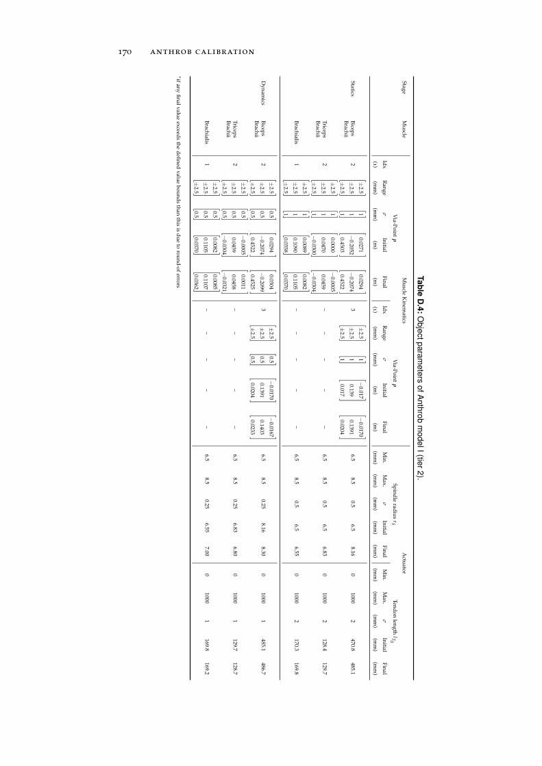
170 anthrob calibration

Ta

ble

D.4

:O

bje

ct

pa

ram

ete

rso

fA

nth

rob

mo

de

lI

(tier

2).

StageM

uscle

Mu

scleK

inem

aticsA

ctuator

Via-P

oint

pV

ia-Poin

tp

Spin

dle

radiu

srS

Tend

onlen

gthlT0

Idx

Ran

geσ

Initial

Final

Idx

Ran

geσ

Initial

Final

Min

.M

ax.σ

Initial

Final

Min

.M

ax.σ

Initial

Final

(1)(m

m)

(mm

)(m

)(m

)(1)

(mm

)(m

m)

(m)

(m)

(mm

)(m

m)

(mm

)(m

m)

(mm

)(m

m)

(mm

)(m

m)

(mm

)(m

m)

StaticsB

iceps

Brach

ii2

±2.5

±2.5

±2.5

111

0.0271

−0.2052

0.4503

0.0294

−0.2074

0.4522

3

±2.5

±2.5

±2.5

111

−0.017

0.139

0.017

−0.0170

0.1391

0.0204

6.58.5

0.56.5

8.160

10002

470.8485.1

Triceps

Brach

ii2

±2.5

±2.5

±2.5

111

0.0000

0.0470

−0.0300

−0.0005

0.0459

−0.0304

––

––

–6.5

8.50.5

6.56.83

01000

2128.4

129.7

Brach

ialis1

±2.5

±2.5

±2.5

111

0.0089

0.1090

0.0358

0.0082

0.1105

0.0370

––

––

–6.5

8.50.5

6.56.55

01000

2170.3

169.8

Dyn

amics

Bicep

sB

rachii

2

±2.5

±2.5

±2.5

0.5

0.5

0.5

0.0294

−0.2074

0.4522

0.0304

−0.2099

0.4525

3

±2.5

±2.5

±2.5

0.5

0.5

0.5

−0.0170

0.1391

0.0204

−0.0167

0.1403

0.0233

6.58.5

0.258.16

8.300

10001

485.1486.7

Triceps

Brach

ii2

±2.5

±2.5

±2.5

0.5

0.5

0.5

−0.0005

0.0459

−0.0304

0.0011

0.0458

−0.0321

––

––

–6.5

8.50.25

6.836.80

01000

1129.7

128.7

Brach

ialis1

±2.5

±2.5

±2.5

0.5

0.5

0.5

0.0082

0.1105

0.0370

0.0085

0.1107

0.0362

––

––

–6.5

8.50.25

6.557.00

01000

1169.8

169.2

∗ifan

yfi

nal

value

exceeds

the

defi

ned

value

boun

ds

than

this

isd

ue

torou

nd

-oferrors

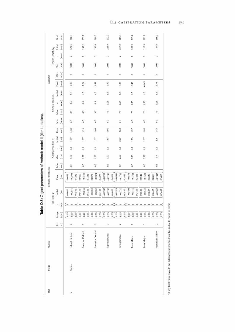
D.2 calibration parameters 171

Ta

ble

D.5

:O

bje

ct

pa

ram

ete

rso

fA

nth

rob

mo

de

lII

(tie

r1

,sta

tics).

Tier

Stag

eM

usc

leM

usc

leK

inem

atic

sA

ctu

ator

Via

-Poi

nt

pC

ylin

der

rad

ius

r CSp

ind

lera

diu

sr S

Ten

don

len

gth

l T0

Idx

Ran

geσ

Init

ial

Fin

alM

in.

Max

.σ

Init

ial

Fin

alM

in.

Max

.σ

Init

ial

Fin

alM

in.

Max

.σ

Init

ial

Fin

al

(1)

(mm

)(m

m)

(m)

(m)

(cm

)(c

m)

(cm

)(c

m)

(cm

)(m

m)

(mm

)(m

m)

(mm

)(m

m)

(mm

)(m

m)

(mm

)(m

m)

(mm

)

1St

atic

sL

ater

alD

elto

id2

±2.

5

±2.

5

±2.

5

1 1 1

0.00

00

−0.

2570

0.45

00

0.00

23

−0.

2554

0.44

82

0.5

1.27

0.1

1.27

0.52

76.

58.

50.

56.

57.

050

1000

232

9.5

340.

0

An

teri

orD

elto

id2

±2.

5

±2.

5

±2.

5

1 1 1

0.04

30

−0.

1540

0.43

08

0.04

10

−0.

1553

0.43

31

0.5

1.27

0.1

1.27

1.26

6.5

8.5

0.5

6.5

7.29

010

002

245.

225

3.7

Pos

teri

orD

elto

id3

±2.

5

±2.

5

±2.

5

1 1 1

−0.

0250

−0.

2350

0.41

00

0.02

74

−0.

2374

0.40

75

0.5

1.27

0.1

1.27

1.03

6.5

8.5

0.5

6.5

6.53

010

002

280.

928

0.5

Sup

rasp

inat

us

3

±2.

5

±2.

5

±2.

5

1 1 1

−0.

0280

−0.

2250

0.40

00

−0.

0291

−0.

2248

0.40

14

0.5

1.97

0.1

1.97

1.96

6.3

7.5

0.25

6.3

6.90

010

002

223.

923

2.2

Infr

asp

inat

us

2

±2.

5

±2.

5

±2.

5

1 1 1

−0.

0528

−0.

1720

0.38

37

−0.

0549

−0.

1742

0.38

23

0.5

2.27

0.1

2.27

2.22

6.3

7.5

0.25

6.3

6.33

010

002

217.

021

9.3

Tere

sM

inor

2

±2.

5

±2.

5

±2.

5

1 1 1

−0.

0403

−0.

1710

0.34

85

−0.

0396

−0.

1724

0.34

84

0.5

1.73

0.1

1.73

1.27

6.3

7.5

0.25

6.3

6.45

010

002

208.

920

3.4

Tere

sM

ajor

2

±2.

5

±2.

5

±2.

5

1 1 1

0.05

28

−0.

1540

0.38

37

0.05

41

−0.

1521

0.38

29

0.5

2.27

0.1

2.27

1.80

6.3

7.5

0.25

6.3

6.64

50

1000

221

7.9

221.

2

Pec

tora

lis

Maj

or2

±2.

5

±2.

5

±2.

5

1 1 1

0.04

02

−0.

1540

0.34

85

0.04

15

−0.

1543

0.34

63

0.5

1.5

0.1

1.5

1.43

6.3

7.5

0.25

6.3

6.75

010

002

187.

018

6.2

∗ if

any

fin

alva

lue

exce

eds

the

defi

ned

valu

ebo

un

ds

than

this

isd

ue

toro

un

d-o

fer

rors

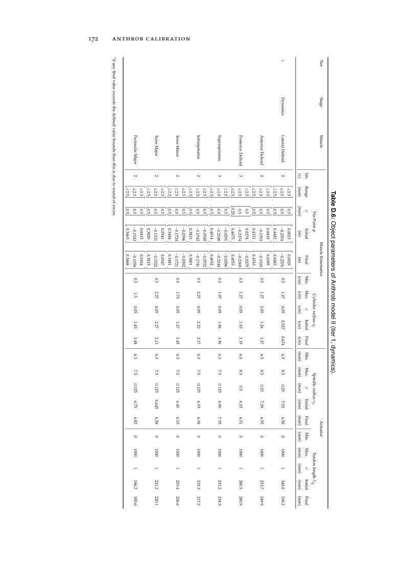
172 anthrob calibration

Ta

ble

D.6

:O

bje

ct

pa

ram

ete

rso

fA

nth

rob

mo

de

lII

(tier

1,

dyn

am

ics).

TierStage

Mu

scleM

uscle

Kin

ematics

Actu

ator

Via-P

oint

pC

ylind

errad

ius

rCSp

ind

lerad

ius

rSTen

don

length

lT0

Idx

Ran

geσ

Initial

Final

Min

.M

ax.σ

Initial

Final

Min

.M

ax.σ

Initial

Final

Min

.M

ax.σ

Initial

Final

(1)(m

m)

(mm

)(m

)(m

)(cm

)(cm

)(cm

)(cm

)(cm

)(m

m)

(mm

)(m

m)

(mm

)(m

m)

(mm

)(m

m)

(mm

)(m

m)

(mm

)

1D

ynam

icsL

ateralD

eltoid2

±2.5

±2.5

±2.5

0.5

0.5

0.5

0.0023

−0.2554

0.4482

0.0029

−0.2570

0.4483

0.51.27

0.050.527

0.6746.5

8.50.25

7.056.50

01000

1340.0

338.2

An

teriorD

eltoid2

±2.5

±2.5

±2.5

0.5

0.5

0.5

0.0410

−0.1553

0.4331

0.0395

−0.1529

0.4310

0.51.27

0.051.26

1.276.5

8.50.25

7.296.55

01000

1253.7

249.9

Posterior

Deltoid

3

±2.5

±2.5

±2.5

0.5

0.5

0.25

0.0274

−0.2374

0.4075

−0.0275

−0.2369

0.4053

0.51.27

0.051.03

1.196.5

8.50.5

6.536.51

01000

1280.5

280.9

Sup

raspin

atus

3

±2.5

±2.5

±2.5

0.5

0.5

0.5

−0.0291

−0.2248

0.4014

−0.0296

−0.2244

0.4032

0.51.97

0.051.96

1.566.3

7.50.125

6.907.35

01000

1232.2

234.5

Infrasp

inatu

s2

±2.5

±2.5

±2.5

0.5

0.5

0.5

−0.0549

−0.1742

0.3823

−0.0532

−0.1741

0.3801

0.52.27

0.052.22

2.176.3

7.50.125

6.336.30

01000

1219.3

217.2

TeresM

inor

2

±2.5

±2.5

±2.5

0.5

0.5

0.5

−0.0396

−0.1724

0.3484

−0.0392

−0.1721

0.3481

0.51.73

0.051.27

1.456.3

7.50.125

6.456.33

01000

1203.4

206.6

TeresM

ajor2

±2.5

±2.5

±2.5

0.5

0.5

0.5

0.0541

−0.1521

0.3829

0.0547

−0.1522

0.3815

0.52.27

0.052.27

2.136.3

7.50.125

6.6456.58

01000

1221.2

220.1

Pectoralis

Major

2

±2.5

±2.5

±2.5

0.5

0.5

0.5

0.0415

−0.1543

0.3463

0.0424

−0.1559

0.3468

0.51.5

0.051.43

1.486.3

7.50.125

6.756.82

01000

1186.2

185.6

∗ifan

yfi

nal

value

exceeds

the

defi

ned

value

boun

ds

than

this

isd

ue

torou

nd

-oferrors

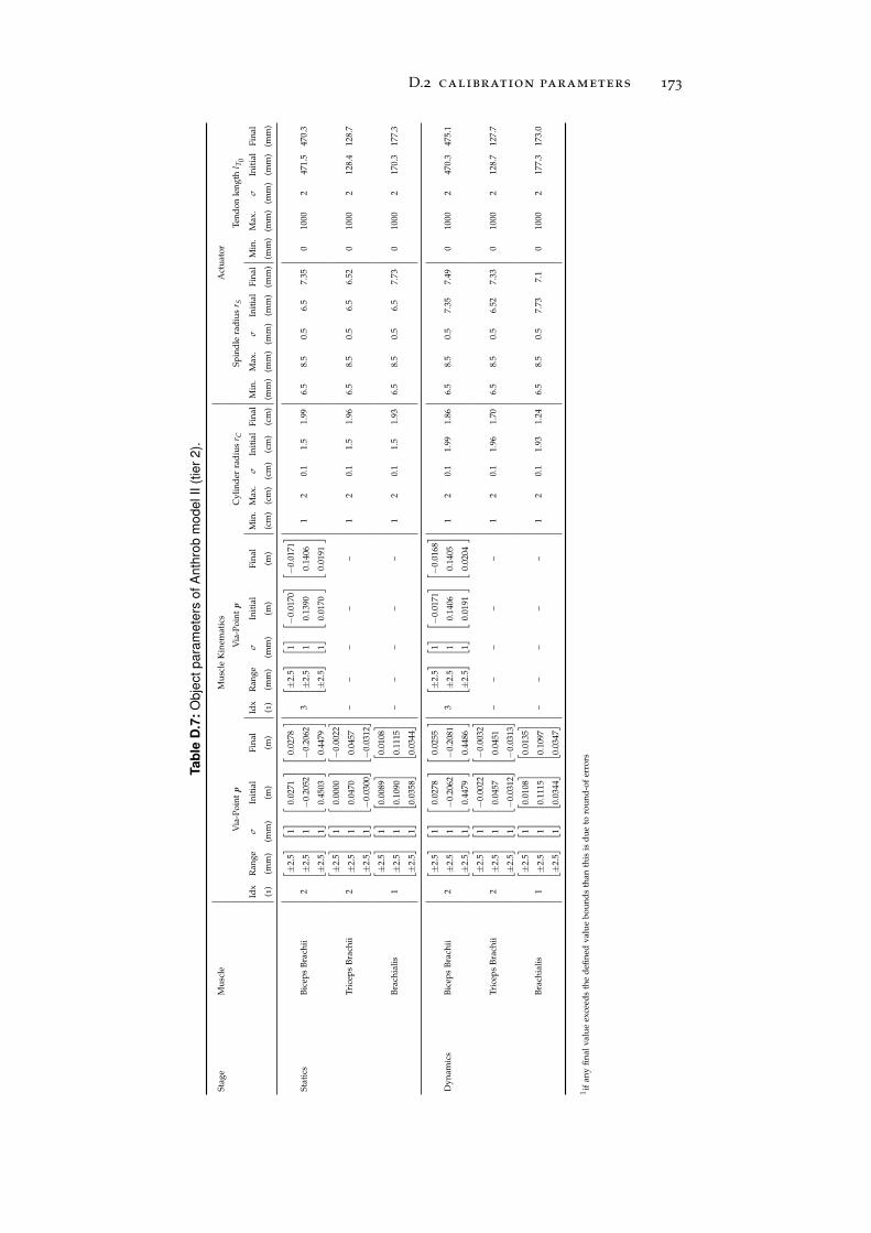
D.2 calibration parameters 173

Ta

ble

D.7

:O

bje

ct

pa

ram

ete

rso

fA

nth

rob

mo

de

lII

(tie

r2

).

Stag

eM

usc

leM

usc

leK

inem

atic

sA

ctu

ator

Via

-Poi

nt

pV

ia-P

oin

tp

Cyl

ind

erra

diu

sr C

Spin

dle

rad

ius

r STe

nd

onle

ngt

hl T

0

Idx

Ran

geσ

Init

ial

Fin

alId

xR

ange

σIn

itia

lFi

nal

Min

.M

ax.

σIn

itia

lFi

nal

Min

.M

ax.

σIn

itia

lFi

nal

Min

.M

ax.

σIn

itia

lFi

nal

(1)

(mm

)(m

m)

(m)

(m)

(1)

(mm

)(m

m)

(m)

(m)

(cm

)(c

m)

(cm

)(c

m)

(cm

)(m

m)

(mm

)(m

m)

(mm

)(m

m)

(mm

)(m

m)

(mm

)(m

m)

(mm

)

Stat

ics

Bic

eps

Bra

chii

2

±2.

5

±2.

5

±2.

5

1 1 1

0.02

71

−0.

2052

0.45

03

0.02

78

−0.

2062

0.44

79

3

±2.

5

±2.

5

±2.

5

1 1 1

−0.

0170

0.13

90

0.01

70

−0.

0171

0.14

06

0.01

91

12

0.1

1.5

1.99

6.5

8.5

0.5

6.5

7.35

010

002

471.

547

0.3

Tric

eps

Bra

chii

2

±2.

5

±2.

5

±2.

5

1 1 1

0.00

00

0.04

70

−0.

0300

−0.

0022

0.04

57

−0.

0312

––

––

–1

20.

11.

51.

966.

58.

50.

56.

56.

520

1000

212

8.4

128.

7

Bra

chia

lis

1

±2.

5

±2.

5

±2.

5

1 1 1

0.00

89

0.10

90

0.03

58

0.01

08

0.11

15

0.03

44

––

––

–1

20.

11.

51.

936.

58.

50.

56.

57.

730

1000

217

0.3

177.

3

Dyn

amic

sB

icep

sB

rach

ii2

±2.

5

±2.

5

±2.

5

1 1 1

0.02

78

−0.

2062

0.44

79

0.02

55

−0.

2081

0.44

86

3

±2.

5

±2.

5

±2.

5

1 1 1

−0.

0171

0.14

06

0.01

91

−0.

0168

0.14

05

0.02

04

12

0.1

1.99

1.86

6.5

8.5

0.5

7.35

7.49

010

002

470.

347

5.1

Tric

eps

Bra

chii

2

±2.

5

±2.

5

±2.

5

1 1 1

−0.

0022

0.04

57

−0.

0312

−0.

0032

0.04

51

−0.

0313

––

––

–1

20.

11.

961.

706.

58.

50.

56.

527.

330

1000

212

8.7

127.

7

Bra

chia

lis

1

±2.

5

±2.

5

±2.

5

1 1 1

0.01

08

0.11

15

0.03

44

0.01

35

0.10

97

0.03

47

––

––

–1

20.

11.

931.

246.

58.

50.

57.

737.

10

1000

217

7.3

173.

0

1if

any

fin

alva

lue

exce

eds

the

defi

ned

valu

ebo

un

ds

than

this

isd

ue

toro

un

d-o

fer

rors

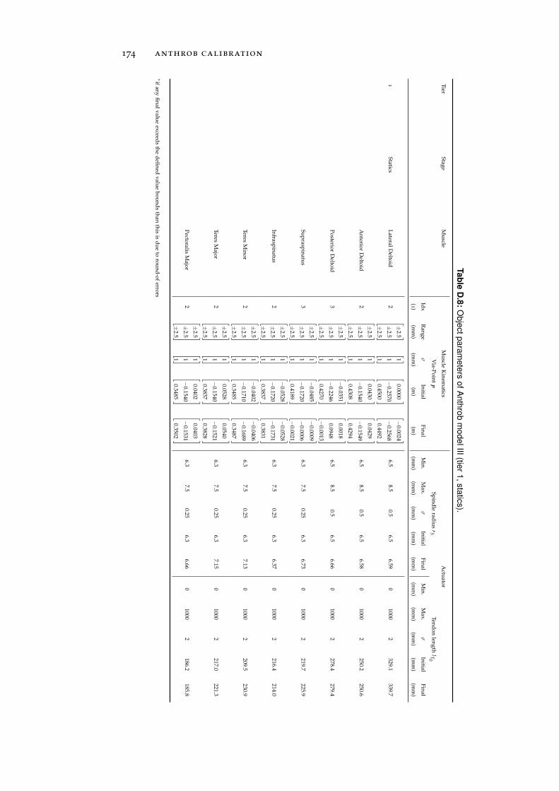
174 anthrob calibration

Ta

ble

D.8

:O

bje

ct

pa

ram

ete

rso

fA

nth

rob

mo

de

lIII

(tier

1,

sta

tics).

TierStage

Mu

scleM

uscle

Kin

ematics

Actu

ator

Via-P

oint

pSp

ind

lerad

ius

rSTen

don

length

lT0

Idx

Ran

geσ

Initial

Final

Min

.M

ax.σ

Initial

Final

Min

.M

ax.σ

Initial

Final

(1)(m

m)

(mm

)(m

)(m

)(m

m)

(mm

)(m

m)

(mm

)(m

m)

(mm

)(m

m)

(mm

)(m

m)

(mm

)

1Statics

Lateral

Deltoid

2

±2.5

±2.5

±2.5

111

0.0000

−0.2570

0.4500

−0.0024

−0.2568

0.4492

6.58.5

0.56.5

6.590

10002

329.1339.7

An

teriorD

eltoid2

±2.5

±2.5

±2.5

111

0.0430

−0.1540

0.4308

0.0429

−0.1549

0.4294

6.58.5

0.56.5

6.580

10002

250.2250.6

Posterior

Deltoid

3

±2.5

±2.5

±2.5

111

−0.0351

−0.2246

0.4270

0.0018

0.0948

−0.0013

6.58.5

0.56.5

6.660

10002

278.4279.4

Sup

raspin

atus

3

±2.5

±2.5

±2.5

111

−0.0485

−0.1720

0.4189

−0.0009

−0.0006

−0.0021

6.37.5

0.256.3

6.730

10002

219.7225.9

Infrasp

inatu

s2

±2.5

±2.5

±2.5

111

−0.0528

−0.1720

0.3837

−0.0528

−0.1731

0.3831

6.37.5

0.256.3

6.370

10002

216.4214.0

TeresM

inor

2

±2.5

±2.5

±2.5

111

−0.0402

−0.1710

0.3485

−0.0406

−0.1689

0.3487

6.37.5

0.256.3

7.130

10002

209.5230.9

TeresM

ajor2

±2.5

±2.5

±2.5

111

0.0528

−0.1540

0.3837

0.0540

−0.1521

0.3828

6.37.5

0.256.3

7.150

10002

217.0221.3

Pectoralis

Major

2

±2.5

±2.5

±2.5

111

0.0402

−0.1540

0.3485

0.0403

−0.1531

0.3502

6.37.5

0.256.3

6.660

10002

186.2185.8

∗ifan

yfi

nal

value

exceeds

the

defi

ned

value

boun

ds

than

this

isd

ue

torou

nd

-oferrors

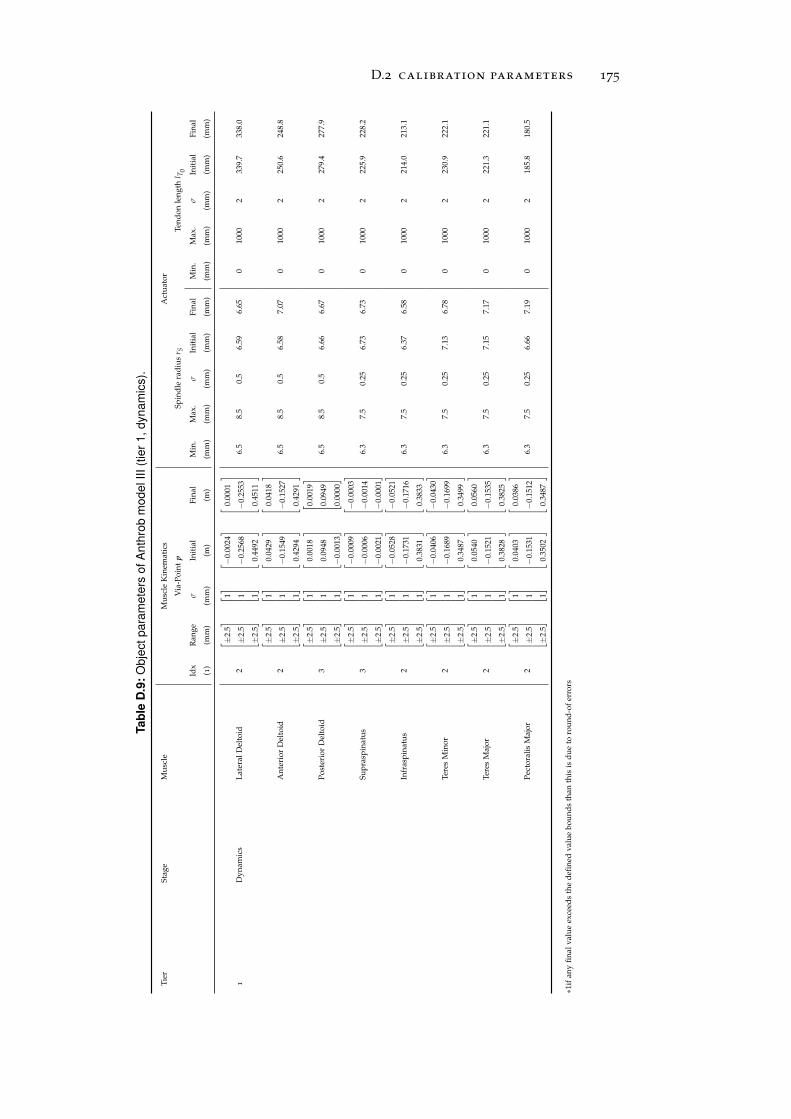
D.2 calibration parameters 175

Ta

ble

D.9

:O

bje

ct

pa

ram

ete

rso

fA

nth

rob

mo

de

lII

I(t

ier

1,

dyn

am

ics).

Tier

Stag

eM

usc

leM

usc

leK

inem

atic

sA

ctu

ator

Via

-Poi

nt

pSp

ind

lera

diu

sr S

Ten

don

len

gth

l T0

Idx

Ran

geσ

Init

ial

Fin

alM

in.

Max

.σ

Init

ial

Fin

alM

in.

Max

.σ

Init

ial

Fin

al

(1)

(mm

)(m

m)

(m)

(m)

(mm

)(m

m)

(mm

)(m

m)

(mm

)(m

m)

(mm

)(m

m)

(mm

)(m

m)

1D

ynam

ics

Lat

eral

Del

toid

2

±2.

5

±2.

5

±2.

5

1 1 1

−0.

0024

−0.

2568

0.44

92

0.00

01

−0.

2553

0.45

11

6.5

8.5

0.5

6.59

6.65

010

002

339.

733

8.0

An

teri

orD

elto

id2

±2.

5

±2.

5

±2.

5

1 1 1

0.04

29

−0.

1549

0.42

94

0.04

18

−0.

1527

0.42

91

6.5

8.5

0.5

6.58

7.07

010

002

250.

624

8.8

Pos

teri

orD

elto

id3

±2.

5

±2.

5

±2.

5

1 1 1

0.00

18

0.09

48

−0.

0013

0.00

19

0.09

49

0.00

00

6.5

8.5

0.5

6.66

6.67

010

002

279.

427

7.9

Sup

rasp

inat

us

3

±2.

5

±2.

5

±2.

5

1 1 1

−0.

0009

−0.

0006

−0.

0021

−0.

0003

−0.

0014

−0.

0001

6.3

7.5

0.25

6.73

6.73

010

002

225.

922

8.2

Infr

asp

inat

us

2

±2.

5

±2.

5

±2.

5

1 1 1

−0.

0528

−0.

1731

0.38

31

−0.

0521

−0.

1716

0.38

33

6.3

7.5

0.25

6.37

6.58

010

002

214.

021

3.1

Tere

sM

inor

2

±2.

5

±2.

5

±2.

5

1 1 1

−0.

0406

−0.

1689

0.34

87

−0.

0430

−0.

1699

0.34

99

6.3

7.5

0.25

7.13

6.78

010

002

230.

922

2.1

Tere

sM

ajor

2

±2.

5

±2.

5

±2.

5

1 1 1

0.05

40

−0.

1521

0.38

28

0.05

60

−0.

1535

0.38

25

6.3

7.5

0.25

7.15

7.17

010

002

221.

322

1.1

Pec

tora

lis

Maj

or2

±2.

5

±2.

5

±2.

5

1 1 1

0.04

03

−0.

1531

0.35

02

0.03

86

−0.

1512

0.34

87

6.3

7.5

0.25

6.66

7.19

010

002

185.

818

0.5

∗1if

any

fin

alva

lue

exce

eds

the

defi

ned

valu

ebo

un

ds

than

this

isd

ue

toro

un

d-o

fer

rors

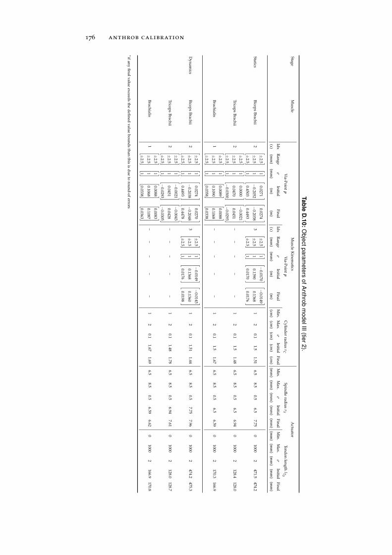
176 anthrob calibration

Ta

ble

D.1

0:

Ob

ject

pa

ram

ete

rso

fA

nth

rob

mo

de

lIII

(tier

2).

StageM

uscle

Mu

scleK

inem

aticsA

ctuator

Via-P

oint

pV

ia-Poin

tp

Cylin

der

radiu

srC

Spin

dle

radiu

srS

Tend

onlen

gthlT0

Idx

Ran

geσ

Initial

Final

Idx

Ran

geσ

Initial

Final

Min

.M

ax.σ

Initial

Final

Min

.M

ax.σ

Initial

Final

Min

.M

ax.σ

Initial

Final

(1)(m

m)

(mm

)(m

)(m

)(1)

(mm

)(m

m)

(m)

(m)

(cm)

(cm)

(cm)

(cm)

(cm)

(mm

)(m

m)

(mm

)(m

m)

(mm

)(m

m)

(mm

)(m

m)

(mm

)(m

m)

StaticsB

iceps

Brach

ii2

±2.5

±2.5

±2.5

111

0.0271

−0.2052

0.4503

0.0274

−0.2038

0.4493

3

±2.5

±2.5

±2.5

111

−0.0170

0.1390

0.0170

−0.0149

0.1368

0.0176

12

0.11.5

1.516.5

8.50.5

6.57.75

01000

2471.5

474.2

Triceps

Brach

ii2

±2.5

±2.5

±2.5

111

0.0000

0.0470

−0.0300

−0.0021

0.0451

−0.0293

––

––

–1

20.1

1.51.48

6.58.5

0.56.5

6.940

10002

128.4128.0

Brach

ialis1

±2.5

±2.5

±2.5

111

0.0089

0.1090

0.0358

0.0088

0.1068

0.0338

––

––

–1

20.1

1.51.67

6.58.5

0.56.5

6.590

10002

170.3166.9

Dyn

amics

Bicep

sB

rachii

2

±2.5

±2.5

±2.5

111

0.0274

−0.2038

0.4493

0.0270

−0.2048

0.4478

3

±2.5

±2.5

±2.5

111

−0.0149

0.1368

0.0176

−0.0143

0.1360

0.0198

12

0.11.51

1.446.5

8.50.5

7.757.96

01000

2474.2

475.3

Triceps

Brach

ii2

±2.5

±2.5

±2.5

111

−0.0021

0.0451

−0.0293

−0.0043

0.0428

−0.0305

––

––

–1

20.1

1.481.78

6.58.5

0.56.94

7.610

10002

128.0128.7

Brach

ialis1

±2.5

±2.5

±2.5

111

0.0088

0.1068

0.0338

0.0083

0.1087

0.0363

––

––

–1

20.1

1.671.69

6.58.5

0.56.59

6.620

10002

166.9170.8

∗ifan

yfi

nal

value

exceeds

the

defi

ned

value

boun

ds

than

this

isd

ue

torou

nd

-oferrors

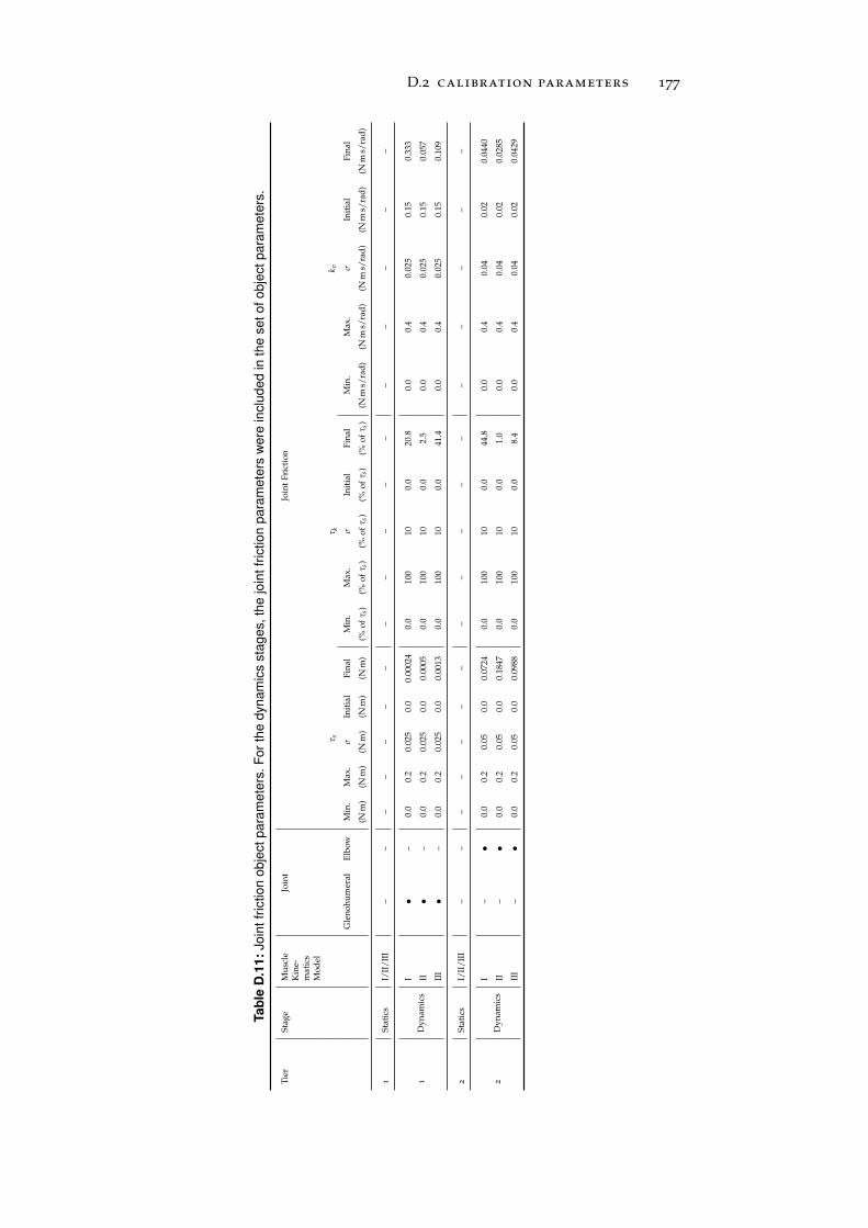
D.2 calibration parameters 177

Ta

ble

D.1

1:

Jo

int

fric

tio

no

bje

ct

pa

ram

ete

rs.

Fo

rth

ed

yn

am

ics

sta

ge

s,

the

join

tfr

ictio

np

ara

me

ters

we

rein

clu

de

din

the

se

to

fo

bje

ct

pa

ram

ete

rs.

Tier

Stag

eM

usc

leK

ine-

mat

ics

Mod

el

Join

tJo

int

Fric

tion

τ sτ k

k v

Gle

noh

um

eral

Elb

owM

in.

Max

.σ

Init

ial

Fin

alM

in.

Max

.σ

Init

ial

Fin

alM

in.

Max

.σ

Init

ial

Fin

al

(Nm

)(N

m)

(Nm

)(N

m)

(Nm

)(%

ofτ s

)(%

ofτ s

)(%

ofτ s

)(%

ofτ s

)(%

ofτ s

)(N

ms/

rad

)(N

ms/

rad

)(N

ms/

rad

)(N

ms/

rad

)(N

ms/

rad

)

1St

atic

sI/

II/

III

––

––

––

––

––

––

––

––

–

1D

ynam

ics

I•

–0.

00.

20.

025

0.0

0.00

024

0.0

100

100.

020

.80.

00.

40.

025

0.15

0.33

3

II•

–0.

00.

20.

025

0.0

0.00

050.

010

010

0.0

2.5

0.0

0.4

0.02

50.

150.

057

III

•–

0.0

0.2

0.02

50.

00.

0013

0.0

100

100.

041

.40.

00.

40.

025

0.15

0.10

9

2St

atic

sI/

II/

III

––

––

––

––

––

––

––

––

–

2D

ynam

ics

I–

•0.

00.

20.

050.

00.

0724

0.0

100

100.

044

.80.

00.

40.

040.

020.

0440

II–

•0.

00.

20.

050.

00.

1847

0.0

100

100.

01.

00.

00.

40.

040.

020.

0285

III

–•

0.0

0.2

0.05

0.0

0.09

880.

010

010

0.0

8.4

0.0

0.4

0.04

0.02

0.04

29

EC A L I P E R : A R O B O T I C S D E V E L O P M E N TE N V I R O N M E N T

A robotics software framework, called Caliper, has been developedwhich is particularly tailored for the simulation of tendon-drivenrobots. The framework is implemented in C++ and relies on Qt as wellas on CMake as build system for platform independence. In itself,Caliper provides only some very basic built-in functionality, such asa logging system or a container for Graphical User Interfaces (GUIs).However, it can be extended at runtime by plugins which makes it ahighly versatile and easy-to-use framework (see Figure E.1). Caliper

is already in use by leading research institutions in Europe.

e.1 caliper core

The Caliper core consists of three components (see Figure E.1): (i) a Overview

GUI, derived from QMainWindow, which provides a basic user-interfacefor changing application settings and which serves as a container forthe GUIs of the plugins (see below), (ii) a logging system based on theC++ logging library log4cpp and, most importantly, a plugin manage-ment system which provides a GUI for activating and deactivatingplugins at runtime as well as for configuring plugin search folders.

The Caliper GUI exploits Qt’s dock widget concept (see QDockWid- Graphical User

Interface (GUI)get) to provide a flexible user-interface that can be adjusted to theparticular needs of an experiment and/or user. In this concept, theapplication window is divided into five “dock areas” and a plugincan be either docked to one of these areas or be floating as top-levelwindow on the desktop. The current arrangement of the GUI (size, po-sition and used docking area of each plugin) is stored at applicationexit and restored at restart using the platform independent helperclass QSettings. Furthermore, a settings dialog is provided which canbe extended by plugins at runtime to include plugin-specific settings.

Log files are inevitable to debug application problems, particular in Logging system

an extensible framework in which plugins from different develop-ers are interacting. Therefore, a logging facility was integrated intoCaliper based on the log4cpp library. The logger can be configured

179

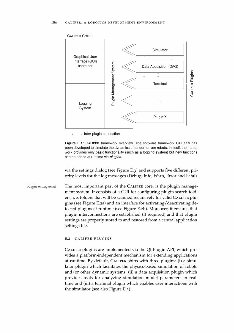
180 caliper : a robotics development environment

Inter-plugin connection

Plu

gin

Ma

na

ge

me

nt

Syste

m

Logging

System

Graphical User

Interface (GUI)

container

CALIPER CORE

CA

LIP

ER

Plu

gin

s

Simulator

Data Acquisition (DAQ)

Terminal

...

Plugin X

Figure E.1: CALIPER framework overview. The software framework CALIPER has

been developed to simulate the dynamics of tendon-driven robots. In itself, the frame-

work provides only basic functionality (such as a logging system) but new functions

can be added at runtime via plugins.

via the settings dialog (see Figure E.3) and supports five different pri-ority levels for the log messages (Debug, Info, Warn, Error and Fatal).

The most important part of the Caliper core, is the plugin manage-Plugin management

ment system. It consists of a GUI for configuring plugin search fold-ers, i. e. folders that will be scanned recursively for valid Caliper plu-gins (see Figure E.2a) and an interface for activating/deactivating de-tected plugins at runtime (see Figure E.2b). Moreover, it ensures thatplugin interconnections are established (if required) and that pluginsettings are properly stored to and restored from a central applicationsettings file.

e.2 caliper plugins

Caliper plugins are implemented via the Qt Plugin API, which pro-vides a platform-independent mechanism for extending applicationsat runtime. By default, Caliper ships with three plugins: (i) a simu-lator plugin which facilitates the physics-based simulation of robotsand/or other dynamic systems, (ii) a data acquisition plugin whichprovides tools for analyzing simulation model parameters in real-time and (iii) a terminal plugin which enables user interactions withthe simulator (see also Figure E.3).

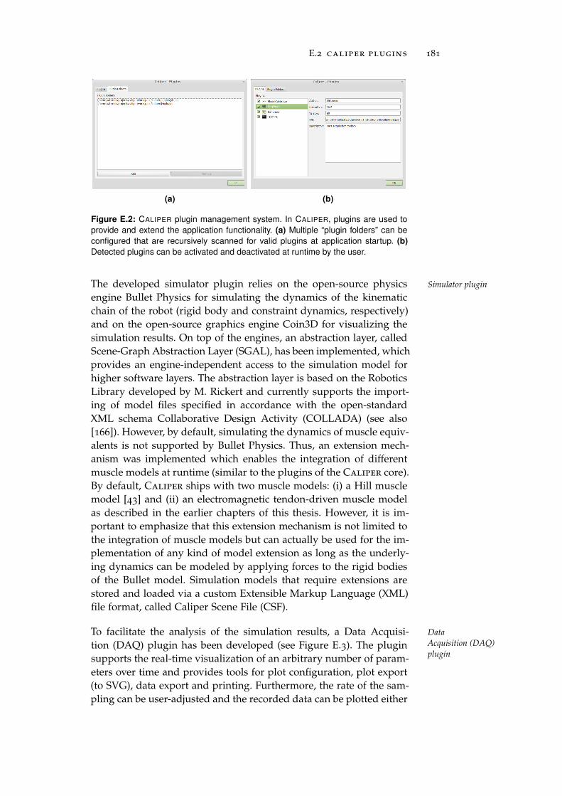
E.2 caliper plugins 181

(a) (b)

Figure E.2: CALIPER plugin management system. In CALIPER, plugins are used to

provide and extend the application functionality. (a) Multiple “plugin folders” can be

configured that are recursively scanned for valid plugins at application startup. (b)

Detected plugins can be activated and deactivated at runtime by the user.

The developed simulator plugin relies on the open-source physics Simulator plugin

engine Bullet Physics for simulating the dynamics of the kinematicchain of the robot (rigid body and constraint dynamics, respectively)and on the open-source graphics engine Coin3D for visualizing thesimulation results. On top of the engines, an abstraction layer, calledScene-Graph Abstraction Layer (SGAL), has been implemented, whichprovides an engine-independent access to the simulation model forhigher software layers. The abstraction layer is based on the RoboticsLibrary developed by M. Rickert and currently supports the import-ing of model files specified in accordance with the open-standardXML schema Collaborative Design Activity (COLLADA) (see also[166]). However, by default, simulating the dynamics of muscle equiv-alents is not supported by Bullet Physics. Thus, an extension mech-anism was implemented which enables the integration of differentmuscle models at runtime (similar to the plugins of the Caliper core).By default, Caliper ships with two muscle models: (i) a Hill musclemodel [43] and (ii) an electromagnetic tendon-driven muscle modelas described in the earlier chapters of this thesis. However, it is im-portant to emphasize that this extension mechanism is not limited tothe integration of muscle models but can actually be used for the im-plementation of any kind of model extension as long as the underly-ing dynamics can be modeled by applying forces to the rigid bodiesof the Bullet model. Simulation models that require extensions arestored and loaded via a custom Extensible Markup Language (XML)file format, called Caliper Scene File (CSF).

To facilitate the analysis of the simulation results, a Data Acquisi- Data

Acquisition (DAQ)

plugintion (DAQ) plugin has been developed (see Figure E.3). The pluginsupports the real-time visualization of an arbitrary number of param-eters over time and provides tools for plot configuration, plot export(to SVG), data export and printing. Furthermore, the rate of the sam-pling can be user-adjusted and the recorded data can be plotted either

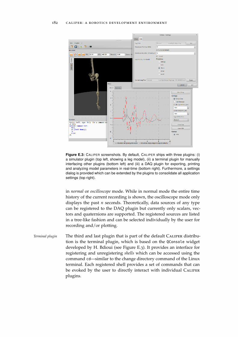
182 caliper : a robotics development environment

Figure E.3: CALIPER screenshots. By default, CALIPER ships with three plugins: (i)

a simulator plugin (top left, showing a leg model), (ii) a terminal plugin for manually

interfacing other plugins (bottom left) and (iii) a DAQ plugin for exporting, printing

and analyzing model parameters in real-time (bottom right). Furthermore, a settings

dialog is provided which can be extended by the plugins to consolidate all application

settings (top right).

in normal or oscilloscope mode. While in normal mode the entire timehistory of the current recording is shown, the oscilloscope mode onlydisplays the past n seconds. Theoretically, data sources of any typecan be registered to the DAQ plugin but currently only scalars, vec-tors and quaternions are supported. The registered sources are listedin a tree-like fashion and can be selected individually by the user forrecording and/or plotting.

The third and last plugin that is part of the default Caliper distribu-Terminal plugin

tion is the terminal plugin, which is based on the QConsole widgetdeveloped by H. Bdioui (see Figure E.3). It provides an interface forregistering and unregistering shells which can be accessed using thecommand cd—similar to the change directory command of the Linuxterminal. Each registered shell provides a set of commands that canbe evoked by the user to directly interact with individual Caliper

plugins.

FQ T P I P E L I N E T O O L K I T ( Q P T )

In computer science, two techniques are common to increase the per- Overview

formance of a task: (i) pipelining and (ii) parallelization [31]. Whilein pipelining a task is partitioned in a sequence of stages that areexecuted sequentially (either synchronously using a clock signal, orasynchronously using a hand-shake mechanism [57]), in paralleliza-tion multiple tasks or subtasks are executed simultaneously (e. g. ondifferent CPUs). Here we present an open-source software frameworkthat was developed for the efficient implementation and execution ofasynchronous software pipelines. The framework, which is called QtPipeline Toolkit (QPT), is implemented in C++ and based on Qt. Ituses a shared memory approach for inter-stage communication andCMake as build system. It is available for download at Sourceforge.

In QPT, a software pipeline is represented by an object of the class The class

QptPipelineQptPipeline, which is derived from QThread and provides methodsfor adding and removing pipeline stages as well as for executing thepipeline stages in either the (i) non-threaded or (ii) threaded mode.In the non-threaded mode, a thread is started only for the pipelineobject and each pipeline stage is executed in this thread in the order inwhich it was added to the pipeline. This is identical to the sequentialexecution of the pipeline stages and hence no performance increasedue to pipelining occurs. In contrast, in threaded mode, a thread isstarted for each stage of the pipeline and not for the pipeline object.In this case, the pipeline execution is identical to an asynchronouspipeline (pipeline stages are not executed with respect to a centralclock but the stages synchronize with each other via the data ports—see below).

In QPT, a pipeline stage is created by instantiating objects of the The class

QptStageclass QptStage. Each QptStage is derived from QThread and can havean arbitrary number of data in- and outports that are registered tothe stage for inter-stage communication (implemented by the classesQptInport and QptOutport, see below). The execution of each stageproceeds as follows. First, it checks whether all registered and con-nected QptInports have data. If this is not the case, the execution ofthe stage blocks, otherwise it proceeds with the execution by calling

183

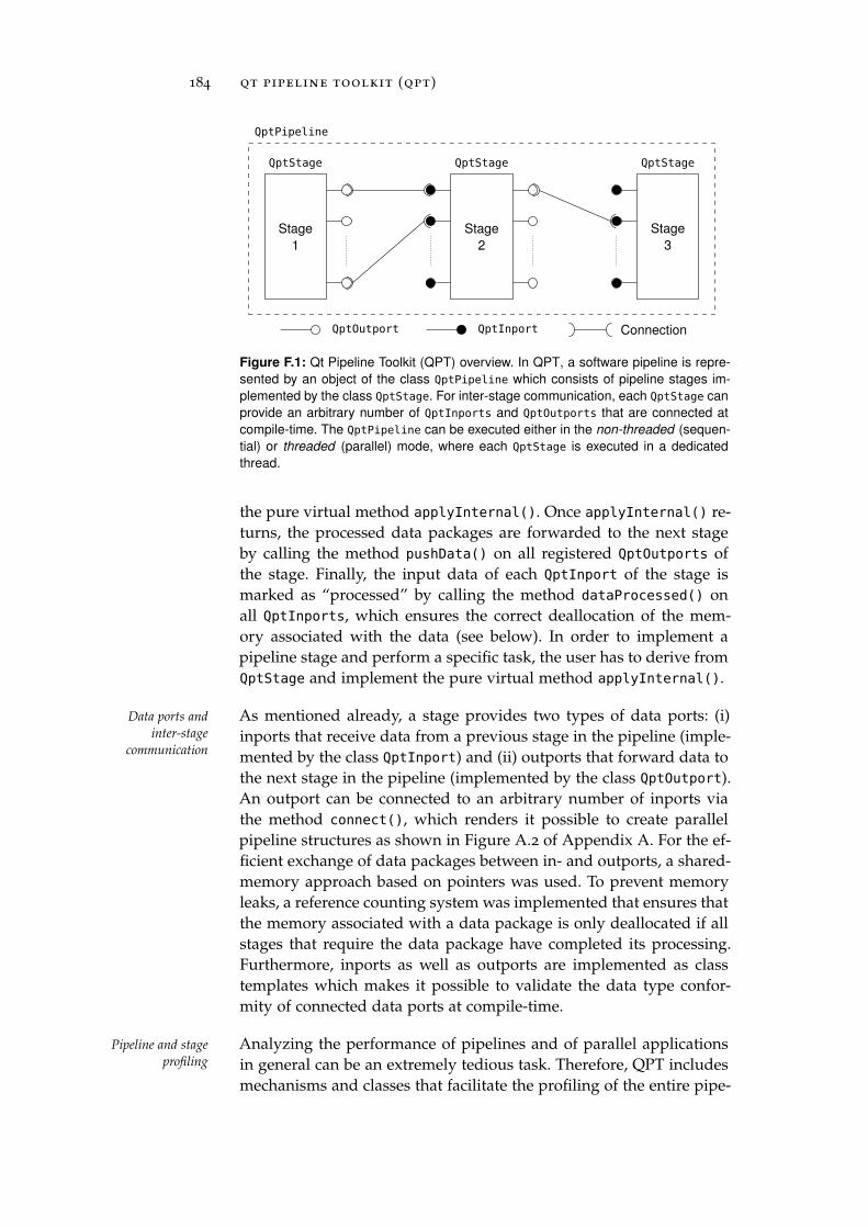
184 qt pipeline toolkit (qpt)

QptStage

Stage

1

QptStage

Stage

2

QptStage

Stage

3

QptOutport QptInport Connection

QptPipeline

Figure F.1: Qt Pipeline Toolkit (QPT) overview. In QPT, a software pipeline is repre-

sented by an object of the class QptPipeline which consists of pipeline stages im-

plemented by the class QptStage. For inter-stage communication, each QptStage can

provide an arbitrary number of QptInports and QptOutports that are connected at

compile-time. The QptPipeline can be executed either in the non-threaded (sequen-

tial) or threaded (parallel) mode, where each QptStage is executed in a dedicated

thread.

the pure virtual method applyInternal(). Once applyInternal() re-turns, the processed data packages are forwarded to the next stageby calling the method pushData() on all registered QptOutports ofthe stage. Finally, the input data of each QptInport of the stage ismarked as “processed” by calling the method dataProcessed() onall QptInports, which ensures the correct deallocation of the mem-ory associated with the data (see below). In order to implement apipeline stage and perform a specific task, the user has to derive fromQptStage and implement the pure virtual method applyInternal().

As mentioned already, a stage provides two types of data ports: (i)Data ports and

inter-stage

communicationinports that receive data from a previous stage in the pipeline (imple-mented by the class QptInport) and (ii) outports that forward data tothe next stage in the pipeline (implemented by the class QptOutport).An outport can be connected to an arbitrary number of inports viathe method connect(), which renders it possible to create parallelpipeline structures as shown in Figure A.2 of Appendix A. For the ef-ficient exchange of data packages between in- and outports, a shared-memory approach based on pointers was used. To prevent memoryleaks, a reference counting system was implemented that ensures thatthe memory associated with a data package is only deallocated if allstages that require the data package have completed its processing.Furthermore, inports as well as outports are implemented as classtemplates which makes it possible to validate the data type confor-mity of connected data ports at compile-time.

Analyzing the performance of pipelines and of parallel applicationsPipeline and stage

profiling in general can be an extremely tedious task. Therefore, QPT includesmechanisms and classes that facilitate the profiling of the entire pipe-

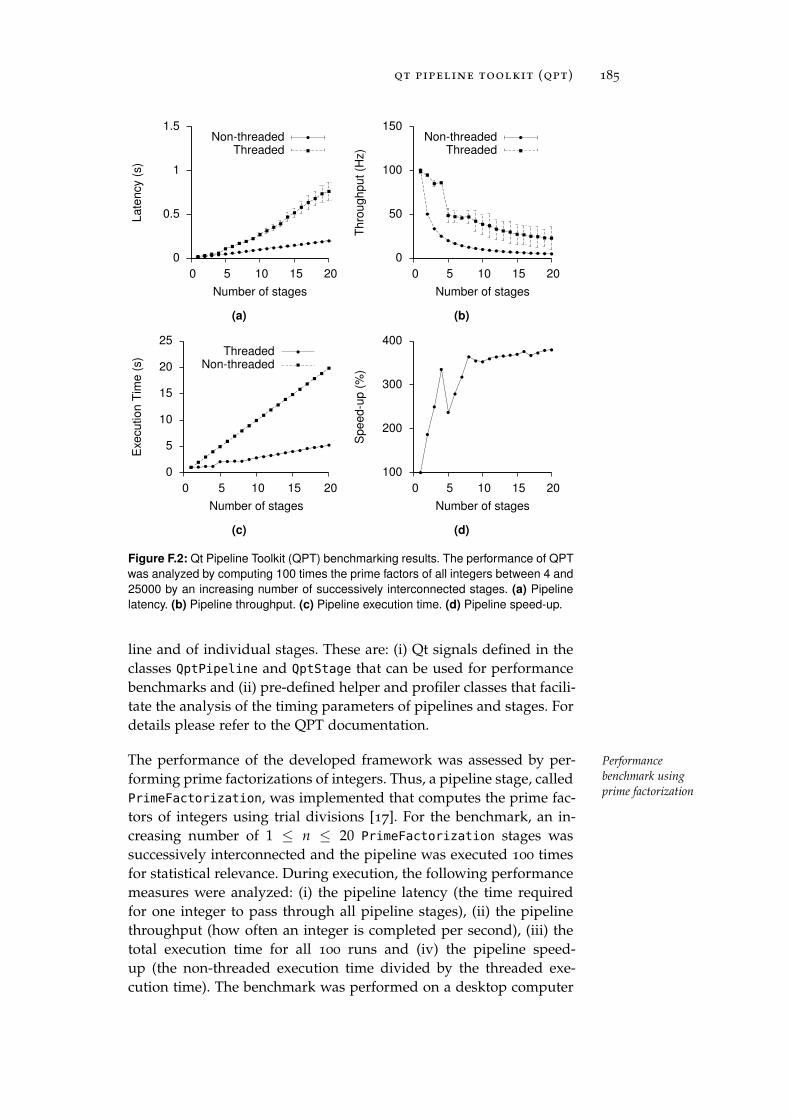
qt pipeline toolkit (qpt) 185

0

0.5

1

1.5

0 5 10 15 20

La

ten

cy

(s)

Number of stages

Non-threadedThreaded

(a)

0

50

100

150

0 5 10 15 20

Th

rou

gh

pu

t(H

z)

Number of stages

Non-threadedThreaded

(b)

0

5

10

15

20

25

0 5 10 15 20

Exe

cu

tio

nT

ime

(s)

Number of stages

ThreadedNon-threaded

(c)

100

200

300

400

0 5 10 15 20

Sp

ee

d-u

p(%

)

Number of stages

(d)

Figure F.2: Qt Pipeline Toolkit (QPT) benchmarking results. The performance of QPT

was analyzed by computing 100 times the prime factors of all integers between 4 and

25000 by an increasing number of successively interconnected stages. (a) Pipeline

latency. (b) Pipeline throughput. (c) Pipeline execution time. (d) Pipeline speed-up.

line and of individual stages. These are: (i) Qt signals defined in theclasses QptPipeline and QptStage that can be used for performancebenchmarks and (ii) pre-defined helper and profiler classes that facili-tate the analysis of the timing parameters of pipelines and stages. Fordetails please refer to the QPT documentation.

The performance of the developed framework was assessed by per- Performance

benchmark using

prime factorizationforming prime factorizations of integers. Thus, a pipeline stage, calledPrimeFactorization, was implemented that computes the prime fac-tors of integers using trial divisions [17]. For the benchmark, an in-creasing number of 1 ≤ n ≤ 20 PrimeFactorization stages wassuccessively interconnected and the pipeline was executed 100 timesfor statistical relevance. During execution, the following performancemeasures were analyzed: (i) the pipeline latency (the time requiredfor one integer to pass through all pipeline stages), (ii) the pipelinethroughput (how often an integer is completed per second), (iii) thetotal execution time for all 100 runs and (iv) the pipeline speed-up (the non-threaded execution time divided by the threaded exe-cution time). The benchmark was performed on a desktop computer

186 qt pipeline toolkit (qpt)

equipped with an Intel R© CoreTM

i7-860 quad-core processor and theresults are shown in Figure F.2. As expected, it can be seen that thepipeline latency increases linearly with the number of stages if thepipeline is executed in non-threaded mode (see Figure F.2a). An iden-tical linear increase could be expected for the threaded mode if adedicated CPU would be available for each of the n stages. However,in our test setup, this is only the case for n ≤ 4. For higher numbersof stages, the latency progressively increases as more stages contendfor CPU time. A similar behavior can be observed for the pipelinethroughput. Theoretically, the throughput should decrease inverselyproportional to the number of stages for the non-threaded executionmode and remain constant for the threaded mode. The predicted be-havior of the non-threaded mode can be well observed in Figure F.2b,whereas the throughput of the threaded mode does not remain con-stant and substantially drops once the number of stages exceeds thenumber of physical CPUs. However, a remaining increase in through-put of more than 400 % was observed for n = 20. The last measurethat was analyzed is the total execution time for the 100 runs whichwas also used to compute the overall speed-up. The results of thisanalysis are shown in Figure F.2c and Figure F.2d, respectively. Asexpected, the execution time observed for the non-threaded modeis linearly increasing with the number of stages. However, for thethreaded mode an about 4 times lower execution time was measuredwhich results in a speed-up close to the theoretical limit of 400 % ofthe used quad-core CPU.

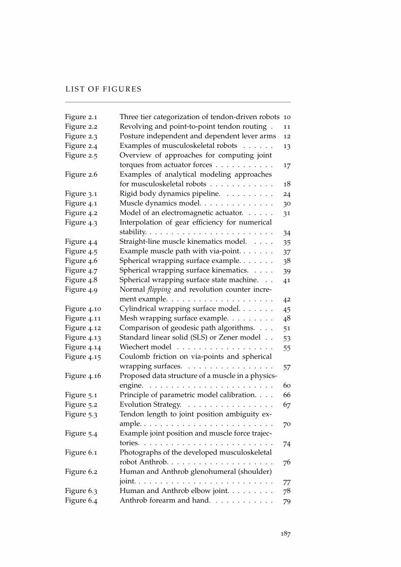
L I S T O F F I G U R E S

Figure 2.1 Three tier categorization of tendon-driven robots 10

Figure 2.2 Revolving and point-to-point tendon routing . 11

Figure 2.3 Posture independent and dependent lever arms 12

Figure 2.4 Examples of musculoskeletal robots . . . . . . 13

Figure 2.5 Overview of approaches for computing jointtorques from actuator forces . . . . . . . . . . . 17

Figure 2.6 Examples of analytical modeling approachesfor musculoskeletal robots . . . . . . . . . . . . 18

Figure 3.1 Rigid body dynamics pipeline. . . . . . . . . . 24

Figure 4.1 Muscle dynamics model. . . . . . . . . . . . . . 30

Figure 4.2 Model of an electromagnetic actuator. . . . . . 31

Figure 4.3 Interpolation of gear efficiency for numericalstability. . . . . . . . . . . . . . . . . . . . . . . . 34

Figure 4.4 Straight-line muscle kinematics model. . . . . 35

Figure 4.5 Example muscle path with via-point. . . . . . . 37

Figure 4.6 Spherical wrapping surface example. . . . . . . 38

Figure 4.7 Spherical wrapping surface kinematics. . . . . 39

Figure 4.8 Spherical wrapping surface state machine. . . 41

Figure 4.9 Normal flipping and revolution counter incre-ment example. . . . . . . . . . . . . . . . . . . . 42

Figure 4.10 Cylindrical wrapping surface model. . . . . . . 45

Figure 4.11 Mesh wrapping surface example. . . . . . . . . 48

Figure 4.12 Comparison of geodesic path algorithms. . . . 51

Figure 4.13 Standard linear solid (SLS) or Zener model . . 53

Figure 4.14 Wiechert model . . . . . . . . . . . . . . . . . . 55

Figure 4.15 Coulomb friction on via-points and sphericalwrapping surfaces. . . . . . . . . . . . . . . . . 57

Figure 4.16 Proposed data structure of a muscle in a physics-engine. . . . . . . . . . . . . . . . . . . . . . . . 60

Figure 5.1 Principle of parametric model calibration. . . . 66

Figure 5.2 Evolution Strategy. . . . . . . . . . . . . . . . . 67

Figure 5.3 Tendon length to joint position ambiguity ex-ample. . . . . . . . . . . . . . . . . . . . . . . . . 70

Figure 5.4 Example joint position and muscle force trajec-tories. . . . . . . . . . . . . . . . . . . . . . . . . 74

Figure 6.1 Photographs of the developed musculoskeletalrobot Anthrob. . . . . . . . . . . . . . . . . . . . 76

Figure 6.2 Human and Anthrob glenohumeral (shoulder)joint. . . . . . . . . . . . . . . . . . . . . . . . . . 77

Figure 6.3 Human and Anthrob elbow joint. . . . . . . . . 78

Figure 6.4 Anthrob forearm and hand. . . . . . . . . . . . 79

187

188 List of Figures

Figure 6.5 Anthrob glenohumeral and elbow joint muscles. 80

Figure 6.6 Anthrob muscle units. . . . . . . . . . . . . . . 81

Figure 7.1 Anthrob physics-based skeleton model. . . . . 86

Figure 7.2 Experimental setup of the NBR identification. 88

Figure 7.3 Overview of O-Ring parameters. . . . . . . . . 89

Figure 7.4 Initial and settled engineering stress vs. strainof both recording runs for two NBR O-ring types. 91

Figure 7.5 Example of SLS (or Zener) model fitting forring type #2. . . . . . . . . . . . . . . . . . . . . 92

Figure 7.6 Example of Wiechert model fitting for ring type#2—Part A. . . . . . . . . . . . . . . . . . . . . . 93

Figure 7.7 Example of Wiechert model fitting for ring type#2—Part B. . . . . . . . . . . . . . . . . . . . . . 94

Figure 7.8 Summary of the NBR model identification ex-periment. . . . . . . . . . . . . . . . . . . . . . . 95

Figure 7.9 Identification of kinetic friction coefficient ofceramic eyelets. . . . . . . . . . . . . . . . . . . 96

Figure 7.10 Actuator position controller. . . . . . . . . . . . 98

Figure 7.11 ECU power-circuit identification setup and re-sults. . . . . . . . . . . . . . . . . . . . . . . . . 99

Figure 7.12 Benchmark results of physics-based Anthrobmodel. . . . . . . . . . . . . . . . . . . . . . . . 100

Figure 7.13 Glenohumeral joint equilibria. . . . . . . . . . . 102

Figure 7.14 Example robot trajectory pair. . . . . . . . . . . 103

Figure 7.15 Tier 1 simulation-reality gap of Anthrob gleno-humeral joint model I. . . . . . . . . . . . . . . 105

Figure 7.16 Tier 1 simulation-reality gap of Anthrob gleno-humeral joint model II. . . . . . . . . . . . . . . 106

Figure 7.17 Tier 1 simulation-reality gap of Anthrob gleno-humeral joint model III. . . . . . . . . . . . . . 107

Figure 7.18 Anthrob equilibria and example trajectories. . 108

Figure 7.19 Tier 2 simulation-reality gap of Anthrob models.110

Figure 8.1 Anthrob calibration procedure. . . . . . . . . . 112

Figure 8.2 Tier 1 statics calibration results of model I. . . 113

Figure 8.3 Tier 1 statics calibration results of model II. . . 114

Figure 8.4 Tier 1 statics calibration results of model III. . 115

Figure 8.5 Tier 1 dynamics calibration results of model I. 118

Figure 8.6 Tier 1 dynamics calibration results of model II. 119

Figure 8.7 Tier 1 dynamics calibration results of model III. 120

Figure 8.8 Example trajectory after tier 1 calibration. . . . 121

Figure 8.9 Tier 2 statics calibration results. . . . . . . . . . 125

Figure 8.10 Tier 2 dynamics calibration results—part I. . . 126

Figure 8.11 Tier 2 dynamics calibration results—part II. . . 127

Figure 8.12 Example trajectory after tier 2 calibration—part I.128

Figure 8.13 Example trajectory after tier 2 calibration—part II.129

Figure 8.14 Validation trajectory. . . . . . . . . . . . . . . . 130

List of Figures 189

Figure 8.15 Validation results—part I. . . . . . . . . . . . . 131

Figure 8.16 Validation results—part II. . . . . . . . . . . . . 132

Figure 8.17 Anthrob model calibration results summary. . 134

Figure A.1 Motion capture hardware setup . . . . . . . . . 144

Figure A.2 Image processing pipeline of the developed mo-tion capture system. . . . . . . . . . . . . . . . . 146

Figure A.3 Marker segmentation. . . . . . . . . . . . . . . . 147

Figure A.4 Example of the developed graph-based markerlabeling procedure. . . . . . . . . . . . . . . . . 149

Figure A.5 Image processing pipeline latency. . . . . . . . 152

Figure B.1 Stress and strain . . . . . . . . . . . . . . . . . . 156

Figure B.2 Maxwell fluid model . . . . . . . . . . . . . . . 157

Figure B.3 Voigt (or Kelvin) solid model . . . . . . . . . . 158

Figure C.2 Wrapping meshes of muscle kinematics model III.165

Figure E.1 Caliper framework overview. . . . . . . . . . . 180

Figure E.2 Caliper plugin management system. . . . . . 181

Figure E.3 Caliper screenshots. . . . . . . . . . . . . . . . 182

Figure F.1 Qt Pipeline Toolkit (QPT) overview. . . . . . . 184

Figure F.2 Qt Pipeline Toolkit (QPT) benchmarking results. 185

L I S T O F TA B L E S

Table 2.1 Overview of important musculoskeletal robots 14

Table 4.1 Gear operation modes. . . . . . . . . . . . . . . 33

Table 4.2 Increment and decrement conditions of the rev-olution counter. . . . . . . . . . . . . . . . . . . 43

Table 6.1 Properties of Anthrob muscles. . . . . . . . . . 80

Table 6.2 Anthrob muscle unit types. . . . . . . . . . . . 82

Table 7.1 Anthrob muscle kinematics models. . . . . . . 87

Table 7.2 Tested O-ring types. . . . . . . . . . . . . . . . . 90

Table 8.1 Overview of calibration object parameters. . . 112

Table A.1 Accuracy of marker segmentation. . . . . . . . 153

Table C.1 Joint friction parameters of the physics-basedAnthrob model. . . . . . . . . . . . . . . . . . . 160

Table C.2 Actuator types and parameters. . . . . . . . . . 161

Table C.3 Parameters of the Anthrob PD actuator posi-tion controller. . . . . . . . . . . . . . . . . . . . 161

Table C.4 NBR-70 Zener model fitting results. . . . . . . 161

Table C.5 NBR-70 Wiechert model fitting results. . . . . . 161

Table C.6 Parameters of muscle kinematics model I. . . . 162

Table C.7 Parameters of muscle kinematics model II. . . 163

Table C.8 Parameters of muscle kinematics model II. . . 164

Table C.9 Parameters of muscle kinematics model III. . . 165

Table C.10 Glenohumeral joint equilibria distances. . . . . 166

Table C.11 Complete robot equilibria distances. . . . . . . 166

Table C.12 Pre-calibration simulation-reality gap summary. 166

Table D.1 Post-calibration simulation-reality gap summary.167

Table D.2 Object parameters of Anthrob model I (tier 1,statics). . . . . . . . . . . . . . . . . . . . . . . . 168

Table D.3 Object parameters of Anthrob model I (tier 1,dynamics) . . . . . . . . . . . . . . . . . . . . . 169

Table D.4 Object parameters of Anthrob model I (tier 2). 170

Table D.5 Object parameters of Anthrob model II (tier 1,statics). . . . . . . . . . . . . . . . . . . . . . . . 171

Table D.6 Object parameters of Anthrob model II (tier 1,dynamics). . . . . . . . . . . . . . . . . . . . . . 172

Table D.7 Object parameters of Anthrob model II (tier 2). 173

Table D.8 Object parameters of Anthrob model III (tier 1,statics). . . . . . . . . . . . . . . . . . . . . . . . 174

Table D.9 Object parameters of Anthrob model III (tier 1,dynamics). . . . . . . . . . . . . . . . . . . . . . 175

Table D.10 Object parameters of Anthrob model III (tier 2). 176

Table D.11 Joint friction object parameters. . . . . . . . . . 177

190

L I S T O F A L G O R I T H M S

4.1 Algorithm for the physics-based simulation of muscles. 61

5.1 Evolution strategy algorithm. . . . . . . . . . . . . . . . . 69

191

L I S T O F A B B R E V I AT I O N S

A/D Analog/Digital

ANN Artificial Neural Network

API Application Programming Interface

BEMF Back Electromotive Force

CAD Computer-Aided Design

CAN Controller Area Network

COLLADA Collaborative Design Activity

CPU Central Processing Unit

CSF Caliper Scene File

DAQ Data Acquisition

DC Direct Current

DoF Degree of Freedom

EA Evolutionary Algorithms

Eccerobot Embodied Cognition in a Compliantly EngineeredRobot

ECU Electronic Control Unit

EMG Electromyography

ES Evolution Strategy

FIR Finite Impulse Response

fMRI Functional Magnetic Resonance Imaging

FPS Frames Per Second

FSM Finite State Machine

FSR Force-Sensitive Resistor

EU European Union

GUI Graphical User Interface

IPA Fraunhofer Institute for Manufacturing Engineeringand Automation

192

list of abbreviations 193

ISO International Organization for Standardization

JSK Jouhou System Kougaku Laboratory of theUniversity of Tokyo

NBR Nitrile Butadiene Rubber

PA-2200 Polyamid 2200

PCIe Peripheral Component Interconnect Express

PILA Posture-Independent Lever Arm

PDLA Posture-Dependent Lever Arm

PWM Pulse-Width Modulation

QPT Qt Pipeline Toolkit

RMSE Root Mean Square Error

SEE Series Elastic Element

SGAL Scene-Graph Abstraction Layer

SLS Selective Laser Sintering

SVG Scalable Vector Graphics

XML Extensible Markup Language

L I S T O F S Y M B O L S

Λ Revolution counter of the spherical and cylindrical wrap-ping surface

η, ρ Gear forward-mode efficiency, gear-mode dependent effi-ciency

κ, ξ Scalar coefficients

λ Offspring population size or expansion ratio

µ Viscosity of a Newtonian damper or friction coefficient orpopulation size

σ Stress

ε Strain

A Obstacle or area

B Rigid body

C Set of marker centroids

CH, CE Convex hull and convex envelope

D Set of candidate centroids

E Robot equilibrium or Young’s modulus of Hookean spring

F Coordinate frame

G Geodesic path or graph

H Friction force or half-space

J Moment of inertia

K Controller gain

KE BEMF constant

KT Torque constant

L Inductance

N Gear ratio or normal force

O, I Muscle origin and insertion

P, p Point in 3D space and its position vector

194

List of Symbols 195

Q Set of equilibria E

R Resistance

Sx Wrapping surface

T Trajectory

V Via-point or set of mesh vertices

F Individual objective function value (fitness)

I Individual

N (µ, σ) Gaussian distribution with mean µ and standard deviation σ

P Population

t Simulation time-step

c Spring damping coefficient

d Diameter

h Height

i Electric current

k Spring stiffness or viscous friction coefficient

l Length

m Mass

r Radius

t Time

u Input or voltage

C Matrix of Coriolis terms

E Essential matrix

F Fundamental matrix or matrix of triangulated mesh facets

H Muscle Jacobian

I Inertia tensor

L Matrix of lever arms

M Mass (or inertia) matrix

α, a Vector of angular and linear accelerations

χ, χ State of the mesh wrapping surface and of the sphere/cylin-der wrapping surface state machine

196 List of Symbols

ω, ω Angular velocity vector, angular velocity

τ, τ Vector of torques (∈ Rn), torque (or relaxation/retardation

time)

c, c Marker centroid (∈ R2 and ∈ R

3, respectively)

f , f Force vector (∈ Rn), force (∈ R)

g, g Vector of gravity terms, gravity or generation counter

n Normal vector

q, q, q Vector of joint positions, velocities and accelerations

s Vector of strategy parameters

t Tangent point

v, v Linear velocity vector, linear velocity

y Vector of object parameters

F Matrix of muscle lines of action

f Vector of force errors

q Vector of angular distances

ARB Rotation matrix of frame B relative to frame A

ATB Transformation matrix of frame B relative to frame A

B I B L I O G R A P H Y

[1] S. Andersson, A. Söderberg, and S. Björklund. Friction models for sliding dry,boundary and mixed lubricated contacts. Tribology International, 40(4):580 –587, 2007.

[2] Y. Asano, H. Mizoguchi, M. Osada, T. Kozuki, J. Urata, T. Izawa, Y. Nakanishi,K. Okada, and M. Inaba. Biomimetic design of musculoskeletal humanoidknee joint with patella and screw-home mechanism. In Robotics and Biomimetics

(ROBIO), 2011 IEEE International Conference on, pages 1813 –1818, 2011.

[3] Y. Asano, H. Mizoguchi, T. K. Y. Motegi, M. Osada, J. Urata, Y. Nakanishi,K. Okada, and M. Inaba. Lower Thigh Design of Detailed MusculoskeletalHumanoid “Kenshiro”. In IEEE/RSJ International Conference on Intelligent Robots

and Systems, 2012.

[4] K. Athanasiou and R. Natoli. Introduction to Continuum Biomechanics. SynthesisLectures on Biomedical Engineering Series. Morgan & Claypool, 2008.

[5] C. B. Barber, D. P. Dobkin, and H. Huhdanpaa. The quickhull algorithm forconvex hulls. ACM Trans. Math. Softw., 22(4):469–483, Dec. 1996.

[6] H.-G. Beyer and H.-P. Schwefel. Evolution strategies – a comprehensive intro-duction. Natural Computing, 1:3–52, May 2002.

[7] E. Bizzi, N. Accornero, W. Chapple, and N. Hogan. Arm trajectory formationin monkeys. Exp Brain Res, 46(1):139–143, 1982.

[8] A. Boeing and T. Bräunl. Evaluation of real-time physics simulation systems.In GRAPHITE ’07: Proceedings of the 5th international conference on Computer

graphics and interactive techniques in Australia and Southeast Asia, pages 281–288,New York, NY, USA, 2007. ACM.

[9] J. Bouguet. Matlab calibration tool. URL http://www.vision.caltech.edu/

bouguetj/calib_doc/.

[10] H. F. Brinson and L. C. Brinson. Polymer Engineering Science and Viscoelasticity:

An Introduction. Springer, 2008.

[11] F. Bueche. Molecular basis for the mullins effect. Journal of Applied Polymer

Science, 4(10):107–114, 1960.

[12] J. Canny and J. Reif. New lower bound techniques for robot motion plan-ning problems. In Proceedings of the 28th Annual Symposium on Foundations of

Computer Science, SFCS ’87, pages 49–60, Washington, DC, USA, 1987. IEEEComputer Society.

[13] J. Chen and Y. Han. Shortest paths on a polyhedron, part i: Computing short-est paths. International Journal of Computational Geometry & Applications, 6:127–144, 1990.

[14] J. Chestnutt, P. Michel, J. Kuffner, and T. Kanade. Locomotion among dynamicobstacles for the Honda ASIMO. In Proc. IEEE/RSJ International Conference on

Intelligent Robots and Systems IROS, pages 2572–2573, Nov 2007.

197

198 bibliography

[15] J. Chiasson. Modeling and High Performance Control of Electric Machines. Wiley-IEEE Press, 2005.

[16] J. J. Craig. Introduction to Robotics: Mechanics and Control. Prentice Hall Interna-tional, 3rd ed. edition, Sept. 2003.

[17] R. Crandall and C. Pomerance. Prime Numbers: A Computational Perspective.Lecture notes in statistics. Springer, 2005.

[18] R. Crawford. Plastics Engineering. Elsevier Science, 3rd edition, 1998.

[19] V. De Sapio, J. Warren, O. Khatib, and S. Delp. Simulating the task-level controlof human motion: a methodology and framework for implementation. The

Visual Computer, 21:289–302, 2005.

[20] S. Delp, J. Loan, M. Hoy, F. E. Zajac, E. Topp, and J. Rosen. An interactivegraphics-based model of the lower extremity to study orthopaedic surgicalprocedures. Biomedical Engineering, IEEE Transactions on, 37(8):757–767, 1990.

[21] S. Delp, F. Anderson, A. Arnold, P. Loan, A. Habib, C. John, E. Guendelman,and D. Thelen. Opensim: Open-source software to create and analyze dynamicsimulations of movement. Biomedical Engineering, IEEE Transactions on, 54(11):1940 –1950, Nov. 2007.

[22] S. L. Delp and J. P. Loan. A computational framework for simulating andanalyzing human and animal movement. Computing in Science & Engineering,2(5):46–55, Oct. 2000.

[23] E. Desailly, P. Sardain, N. Khouri, D. Yepremian, and P. Lacouture. The convexwrapping algorithm: a method for identifying muscle paths using the under-lying bone mesh. J Biomech, 43(13):2601–2607, Sep 2010.

[24] E. Dijkstra. A note on two problems in connexion with graphs. Numerische

Mathematik, 1(1):269–271, 1959.

[25] K. Dorfmüller. Robust tracking for augmented reality using retroreflectivemarkers. Computers & Graphics, 23(6):795 – 800, 1999.

[26] W. F. Dostal and J. G. Andrews. A three-dimensional biomechanical model ofhip musculature. Journal of Biomechanics, 14(11):803 – 812, 1981.

[27] D. Eberly. Game Physics. Interactive 3D technology series. Taylor & Francis,2003.

[28] A. Engín. On the biomechanics of the shoulder complex. Journal of Biomechan-

ics, 13(7):575 – 590, 1980.

[29] K. Erleben. Stable, Robust, and Versatile Multibody Dynamics Animation. PhDthesis, University of Copenhagen, Denmark, November 2004.

[30] R. Featherstone. Rigid Body Dynamics Algorithms. Kluwer international series inengineering and computer science: Robotics. Springer London, Limited, 2008.

[31] J. Foley. Computer Graphics: Principles and Practice, Second Edition in C. Addison-Wesley systems programming series. Addison-Wesley Pub, 1996.

[32] R. L. Gajdosik. Passive extensibility of skeletal muscle: review of the literaturewith clinical implications. Clinical Biomechanics, 16(2):87 – 101, 2001.

[33] D. Gamez, R. Newcombe, O. Holland, and R. Knight. Two simulation toolsfor biologically inspired virtual robotics. In Proceedings of the IEEE 5th Chapter

Conference on Advances in Cybernetic Systems, pages 85–90, 2006.

bibliography 199

[34] B. A. Garner and M. G. Pandy. The obstacle-set method for representingmuscle paths in musculoskeletal models. Computer Methods in Biomechanics

and Biomedical Engineering, 3(1):1–30, 2000.

[35] H. Garstenauer. A Unified Framework for Rigid Body Dynamics. Master’sthesis, Johannes Kepler Universität Linz, 2006.

[36] A. Gaschler. Real-Time Marker-Based Motion Tracking: Application to Kine-matic Model Estimation of a Humanoid Robot. Master’s thesis, TechnischeUniversität München, Germany, 2011.

[37] A. Gaschler. Visual motion capturing for kinematic model estimation of ahumanoid robot. In Proceedings of the 33rd international conference on Pattern

recognition, pages 438–443. Springer, 2011.

[38] H. Gomi and Kawato. Equilibrium-point control hypothesis examined by mea-sured arm stiffness during multijoint movement. Science, 272(5258):117–120,Apr 1996.

[39] L. Gregoire, H. E. Veeger, P. A. Huijing, and G. J. van Ingen Schenau. Role ofmono-and biarticular muscles in explosive movements. Int J Sports Med, 5(6):301–305, 1984.

[40] D. Gross, W. Hauger, J. Schrader, J. Schröder, and W. Wall. Technische Mechanik

1: Statik. Springer-Lehrbuch. Springer, 2008.

[41] A. Halim. Human Anatomy: Upper Limb and Thorax. I.K. International Publish-ing House Pvt., Limited, 2008.

[42] R. I. Hartley and P. Sturm. Triangulation. Computer Vision and Image Under-

standing, 68(2):146 – 157, 1997.

[43] A. V. Hill. The heat of shortening and the dynamic constants of muscle. Pro-

ceedings of the Royal Society of London. Series B, Biological Sciences, 126(843):pp.136–195, 1938.

[44] G. Hirzinger, N. Sporer, A. Albu-Schaffer, M. Hahnle, R. Krenn, A. Pascucci,and M. Schedl. DLR’s torque-controlled light weight robot III-are we reachingthe technological limits now? In Robotics and Automation, 2002. Proceedings.

ICRA ’02. IEEE International Conference on, volume 2, pages 1710 – 1716 vol.2,2002.

[45] F. Hoffmeister and T. Bäck. Genetic algorithms and evolution strategies - sim-ilarities and differences. In Proceedings of the 1st Workshop on Parallel Prob-

lem Solving from Nature, PPSN I, pages 455–469, London, UK, 1991. Springer-Verlag.

[46] O. Holland and R. Knight. The anthropomimetic principle. In Proceedings of

the AISB06 Symposium on Biologically Inspired Robotics, 2006.

[47] J. M. Hollerbach. Computers, brains and the control of movement. Trends

Neurosci, 5:189–192, Jan. 1982.

[48] K. Hongo, Y. Nakanishi, Y. Namiki, I. Mizuuchi, and M. Inaba. Automaticparameter adjustment of reflexive walking of a musculo-skeletal humanoid. InHumanoid Robots, 2008. Humanoids 2008. 8th IEEE-RAS International Conference

on, pages 16 –21, dec. 2008.

[49] K. Hosoda and Y. Ishii. External rotation as morphological bootstrapping foremergence of biped walking. In Development and Learning (ICDL), 2010 IEEE

9th International Conference on, pages 317 –322, aug. 2010.

200 bibliography

[50] H. Imamizu, S. Miyauchi, T. Tamada, Y. Sasaki, R. Takino, B. Pütz, T. Yoshioka,and M. Kawato. Human cerebellar activity reflecting an acquired internalmodel of a new tool. Nature, 403(6766):192–195, Jan 2000.

[51] N. Ito, J. Urata, Y. Nakanishi, K. Okada, and M. Inaba. Development ofvery small high output motor driver for realizing forceful musculoskeletal hu-manoids. In Humanoid Robots (Humanoids), 2010 10th IEEE-RAS International

Conference on, pages 385 –390, dec. 2010.

[52] T. Izawa, Y. Nakanishi, N. Ito, M. Osada, K. Hongo, S. Ohta, T. Yoshikai,K. Okada, and M. Inaba. Development of stiffness changeable multijointcervical structure with soft sensor flesh for musculo-skeletal humanoids. InHumanoid Robots (Humanoids), 2010 10th IEEE-RAS International Conference on,pages 665 –670, dec. 2010.

[53] J. Jackson. Microsoft robotics studio: A technical introduction. Robotics Au-

tomation Magazine, IEEE, 14(4):82–87, dec. 2007.

[54] S. Jacobsen, E. Iversen, D. Knutti, R. Johnson, and K. Biggers. Design of theUtah/M.I.T. dextrous hand. In Robotics and Automation. Proceedings. 1986 IEEE

International Conference on, volume 3, pages 1520– 1532, Apr. 1986.

[55] S. C. Jacobsen, H. Ko, E. K. Iversen, and C. C. Davis. Antagonistic control ofa tendon driven manipulator. In Proc. Conf. IEEE Int Robotics and Automation,pages 1334–1339, 1989.

[56] S. C. Jacobsen, H. Ko, E. K. Iversen, and C. C. Davis. Control strategies fortendon-driven manipulators. Control Systems Magazine, IEEE, 10(2):23–28, Feb.1990.

[57] S. Jadhav. Advanced Computer Architecture & Computing. Technical Publications,2009.

[58] M. Jäntsch. Non-Linear Control Strategies for Musculoskeletal Robots. PhD thesis,Technische Universität München, 2013.

[59] M. Jäntsch, S. Wittmeier, and A. Knoll. Distributed Control for an Anthro-pomimetic Robot. In Intelligent Robots and Systems (IROS), 2010 IEEE/RSJ Inter-

national Conference on, pages 5466 –5471, Oct 2010.

[60] M. Jäntsch, C. Schmaler, S. Wittmeier, K. Dalamagkidis, and A. Knoll. A scal-able Joint-Space Controller for Musculoskeletal Robots with Spherical Joints.In Proc. IEEE International Conference on Robotics and Biomimetics ROBIO 2011,2011.

[61] M. Jäntsch, S. Wittmeier, K. Dalamagkidis, and A. Knoll. Computed musclecontrol for an anthropomimetic elbow joint. In Intelligent Robots and Systems

(IROS), 2012 IEEE/RSJ International Conference on, pages 2192 –2197, oct. 2012.

[62] R. Jensen and D. Davy. An investigation of muscle lines of action about the hip:A centroid line approach vs the straight line approach. Journal of Biomechanics,8(2):103 – 110, 1975.

[63] T. Kanai. Approximate shortest path on a polyhedral surface and its applica-tions. In Computer-Aided Design, pages 241–250, 2000.

[64] E. R. Kandel, J. Schwartz, and T. M. Jessell. Principles of Neural Science.McGraw-Hill, 4th edition, 2000.

[65] B. Kaneva and J. O’Rourke. An Implementation of Chen & Han’s ShortestPaths Algorithm. In Proc. of the 12th Canadian Conference on Computational Ge-

ometry, pages 139–146, New Brunswick, August 2000.

bibliography 201

[66] S. Kapoor. Efficient computation of geodesic shortest paths. In In Proc. 32nd

Annu. ACM Sympos. Theory Comput, pages 770–779, 1999.

[67] R. M. Karp. Reducibility Among Combinatorial Problems. In R. E. Millerand J. W. Thatcher, editors, Complexity of Computer Computations, pages 85–103.Plenum Press, 1972.

[68] M. Kawato. Internal models for motor control and trajectory planning. Current

Opinion in Neurobiology, 9(6):718–727, 1999.

[69] M. C. Kennedy and A. O’Hagan. Bayesian calibration of computer models.Journal of the Royal Statistical Society: Series B (Statistical Methodology), 63(3):425–464, 2001.

[70] S. Klug, T. Lens, O. von Stryk, B. Möhl, and A. Karguth. Biologically inspiredrobot manipulator for new applications in automation engineering. In Proc. of

Robotik Congress 2008. VDI Wissensforum GmbH, 2008.

[71] A. Kochan. Shadow delivers first hand. Industrial Robot: An International Jour-

nal, 32(1):15–16, 2005.

[72] T. Kozuki, H. Mizoguchi, Y. Asano, M. Osada, T. Shirai, U. Junichi, Y. Nakan-ishi, K. Osada, and M. Inaba. Design Methodology for the Thorax andShoulder of Human MImetic Musculoskeletal Humanoid Kenshiro—A Tho-rax structure with Rib like Surface—. In IEEE/RSJ International Conference on

Intelligent Robots and Systems, 2012.

[73] M. Kumamoto, T. Oshima, and T. Yamamoto. Control properties induced bythe existence of antagonistic pairs of bi-articular muscles – mechanical engi-neering model analyses. Human Movement Science, 13(5):611–634, Oct. 1994.

[74] M. Lanthier, A. Maheshwari, and J.-R. Sack. Approximating weighted shortestpaths on polyhedral surfaces. In Proceedings of the thirteenth annual symposium

on Computational geometry, SCG ’97, pages 485–486, New York, NY, USA, 1997.ACM.

[75] S. Lawrence, C. L. Giles, and A. C. Tsoi. Lessons in neural network training:Overfitting may be harder than expected. In In Proceedings of the Fourteenth Na-

tional Conference on Artificial Intelligence, AAAI-97, pages 540–545. AAAI Press,1997.

[76] J. J. Lee. Tendon-driven manipulators: analysis, synthesis, and control. PhD thesis,University of Maryland, 1991.

[77] T. Lens, J. Kunz, O. v. Stryk, C. Trommer, and A. Karguth. Biorob-arm: Aquickly deployable and intrinsically safe, light- weight robot arm for servicerobotics applications. Robotics (ISR), 2010 41st International Symposium on and

2010 6th German Conference on Robotics (ROBOTIK), pages 1 –6, june 2010.

[78] A. Maheshwari and S. Wuhrer. Geodesic paths on 3d surfaces: Survey andopen problems. CoRR, abs/0904.2550, 2009.

[79] G. Marai, D. Laidlaw, C. Demiralp, S. Andrews, C. Grimm, and J. Crisco. Es-timating joint contact areas and ligament lengths from bone kinematics andsurfaces. Biomedical Engineering, IEEE Transactions on, 51(5):790–799, 2004.

[80] H. Marques, M. Jäntsch, S. Wittmeier, O. Holland, C. Alessandro, A. Diamond,M. Lungarella, and R. Knight. ECCE1: The first of a series of anthropomimeticmusculoskeletal upper torsos. In 10th IEEE-RAS International Conference on

Humanoid Robots (Humanoids), pages 391 –396, Dec 2010.

202 bibliography

[81] S. P. Marques and G. J. Creus. Computational Viscoelasticity. Springer, 2012.

[82] O. Masahiko, I. Nobuyuki, N. Yuto, and I. Masayuki. Stiffness readout inmusculo-skeletal humanoid robot by using rotary potentiometer. In Sensors,

2010 IEEE, pages 2329–2333, 2010.

[83] N. Matsui and M. Shigyo. Brushless dc motor control without position andspeed sensors. Industry Applications, IEEE Transactions on, 28(1):120–127, 1992.

[84] C. Maufroy, H.-M. Maus, K. Radkhah, D. Scholz, O. von Stryk, and A. Sey-farth. Dynamic leg function of the BioBiped humanoid robot. In Proc. 5th Int.

Symposium on Adaptive Motion of Animals and Machines (AMAM), Osaka, Japan,Oct. 11-14 2011.

[85] J. Meriam and L. Kraige. Engineering Mechanics: Statics. Engineering Mechan-ics: SI Version. Wiley, 2008.

[86] M. A. Meyers and K. K. Chawla. Mechanical Behavior of Materials. CambridgeUniversity Press, 2nd edition, 2009.

[87] O. Michel. Cyberbotics Ltd. Webots TM : Professional Mobile Robot Simula-tion. Int. Journal of Advanced Robotic Systems, 1:39–42, 2004.

[88] J. S. B. Mitchell, D. M. Mount, and C. H. Papadimitriou. The discrete geodesicproblem. SIAM J. Comput., 16(4):647–668, Aug. 1987.

[89] H. Mizoguchi, Y. Asano, T. Izawa, M. Osada, J. Urata, Y. Nakanishi, K. Okada,and M. Inaba. Biomimetic design and implementation of muscle arrangementaround hip joint for musculoskeletal humanoid. In Robotics and Biomimetics

(ROBIO), 2011 IEEE International Conference on, pages 1819 –1824, dec. 2011.

[90] I. Mizuuchi. A musculoskeletal flexible-spine humanoid Kotaro aiming at thefuture in 15 years’ time. Mobile Robots-Towards New Applications, pages 45–56,2006.

[91] I. Mizuuchi, R. Tajima, T. Yoshikai, D. Sato, K. Nagashima, M. Inaba, Y. Ku-niyoshi, and H. Inoue. The design and control of the flexible spine of a fullytendon-driven humanoid “Kenta”. In Proc. IEEE/RSJ Int Intelligent Robots and

Systems Conf, volume 3, pages 2527–2532, 2002.

[92] I. Mizuuchi, S. Yoshida, T. Yoshikai, M. Inaba, D. Sato, and H. Inoue. Behaviordeveloping environment for the large-dof muscle-driven humanoid equippedwith numerous sensors. In Robotics and Automation, 2003. Proceedings. ICRA ’03.

IEEE International Conference on, volume 2, pages 1940 – 1945 vol.2, sept. 2003.

[93] I. Mizuuchi, T. Yoshikai, Y. Nakanishi, Y. Sodeyama, T. Yamamoto,A. Miyadera, T. Niemela, M. Hayashi, J. Urata, and M. Inaba. Development ofmuscle-driven flexible-spine humanoids. In Humanoid Robots, 2005 5th IEEE-

RAS International Conference on, pages 339 –344, dec. 2005.

[94] I. Mizuuchi, Y. Nakanishi, Y. Namiki, T. Nishino, J. Urata, M. Inaba, T. Yoshikai,and Y. Sodeyama. Realization of Standing of the Musculoskeletal HumanoidKotaro by Reinforcing Muscles. In Humanoid Robots, 2006 6th IEEE-RAS Inter-

national Conference on, pages 176–181, 2006.

[95] I. Mizuuchi, T. Yoshikai, Y. Sodeyama, Y. Nakanishi, A. Miyadera, T. Ya-mamoto, T. Niemela, M. Hayashi, J. Urata, Y. Namiki, T. Nishino, and M. Inaba.Development of musculoskeletal humanoid Kotaro. In Robotics and Automation,

2006. ICRA 2006. Proceedings 2006 IEEE International Conference on, pages 82 –87,May 2006.

bibliography 203

[96] I. Mizuuchi, Y. Nakanishi, Y. Sodeyama, Y. Namiki, T. Nishino, N. Muramatsu,J. Urata, K. Hongo, T. Yoshikai, and M. Inaba. An advanced musculoskeletalhumanoid Kojiro. In Humanoid Robots, 2007 7th IEEE-RAS International Confer-

ence on, pages 294 –299, 292007-dec.1 2007.

[97] R. Murray, Z. Li, S. Sastry, and S. Sastry. A Mathematical Introduction to Robotic

Manipulation. CRC PressINC, 1994.

[98] Y. Nakanishi, I. Mizuuchi, T. Yoshikai, T. Inamura, and M. Inaba. Pedaling bya redundant musculo-skeletal humanoid robot. In Humanoid Robots, 2005 5th

IEEE-RAS International Conference on, pages 68–73, 2005.

[99] Y. Nakanishi, Y. Namiki, K. Hongo, J. Urata, I. Mizuuchi, and M. Inaba. Designof the musculoskeletal trunk and realization of powerful motions using spines.In Humanoid Robots, 2007 7th IEEE-RAS International Conference on, pages 96–101, 29 2007-dec. 1 2007.

[100] Y. Nakanishi, Y. Namiki, K. Hongo, J. Urata, I. Mizuuchi, and M. Inaba. Re-alization of large joint movement while standing by a musculoskeletal hu-manoid using its spine and legs coordinately. In Intelligent Robots and Sys-

tems, 2008. IROS 2008. IEEE/RSJ International Conference on, pages 205–210, sept.2008.

[101] Y. Nakanishi, K. Hongo, I. Mizuuchi, and M. Inaba. Joint proprioception acqui-sition strategy based on joints-muscles topological maps for musculoskeletalhumanoids. In Robotics and Automation (ICRA), 2010 IEEE International Confer-

ence on, pages 1727 –1732, may 2010.

[102] Y. Nakanishi, T. Izawa, M. Osada, N. Ito, S. Ohta, J. Urata, and M. Inaba. De-velopment of musculoskeletal humanoid kenzoh with mechanical compliancechangeable tendons by nonlinear spring unit. In Robotics and Biomimetics (RO-

BIO), 2011 IEEE International Conference on, pages 2384 –2389, dec. 2011.

[103] K. Narioka and K. Hosoda. Motor development of an pneumatic muscu-loskeletal infant robot. In Robotics and Automation (ICRA), 2011 IEEE Inter-

national Conference on, pages 963 –968, may 2011.

[104] K. Narioka, R. Niiyama, Y. Ishii, and K. Hosoda. Pneumatic musculoskele-tal infant robots. In Workshop of the 2009 IEEE/RSJ International Conference on

Intelligent Robots and Systems, 2009.

[105] R. Niiyama and Y. Kuniyoshi. A pneumatic biped with an artificial muscu-loskeletal system. In 4th international symposium on adaptive motion of animals

and machines (AMAM2008), pages 80–81, 2008.

[106] R. Niiyama and Y. Kuniyoshi. Design principle based on maximum outputforce profile for a musculoskeletal robot. Industrial Robot: An International Jour-

nal, 37(3):250–255, 2010.

[107] R. Niiyama, A. Nagakubo, and Y. Kuniyoshi. Mowgli: A bipedal jumpingand landing robot with an artificial musculoskeletal system. In Robotics and

Automation, 2007 IEEE International Conference on, pages 2546–2551, 2007.

[108] R. Niiyama, S. Nishikawa, and Y. Kuniyoshi. Athlete robot with applied hu-man muscle activation patterns for bipedal running. In Humanoid Robots (Hu-

manoids), 2010 10th IEEE-RAS International Conference on, pages 498 –503, dec.2010.

[109] S. Nishikawa, R. Niiyama, and Y. Kuniyoshi. Running motion in a muscu-loskeletal bipedal robot using muscle activation pattern control based on ahuman electromyogram. In The 5th International Symposium on Adaptive Motion

of Animals and Machines (AMAM 2011), pages 15–16, 2011.

204 bibliography

[110] S. Nishikawa, Y. Yamada, K. Shida, and Y. Kuniyoshi. Dynamic motions bya quadruped musculoskeletal robot with angle-dependent moment arms. InInternational Workshop on Bio-Inspired Robots, 2011.

[111] J. O’Rourke. Computational geometry column 35. Internat. J. Comput. Geom.

Appl., 4–5:513–515, 1999. Also in SIGACT News, 30(2):31-32 (1999), Issue 111.

[112] M. Osada, N. Ito, Y. Nakanishi, and M. Inaba. Stiffness readout in musculo-skeletal humanoid robot by using rotary potentiometer. In Sensors, 2010 IEEE,pages 2329 –2333, nov 2010.

[113] M. Osada, T. Izawa, J. Urata, Y. Nakanishi, K. Okada, and M. Inaba. Approachof planar muscle suitable for musculoskeletal humanoids, especially for theirbody trunk with spine having multiple vertebral. In Humanoid Robots (Hu-

manoids), 2011 11th IEEE-RAS International Conference on, pages 358 –363, oct.2011.

[114] C. Pelchen, C. Schweiger, and M. Otter. Modeling and simulating the efficiencyof gearboxes and of planetary gearboxes. In Proceedings of the 2nd International

Modelica Conference, pages 257–266, Oberpfaffenhofen, March 18-19 2002.

[115] R. Pfeifer, M. Lungarella, and F. Iida. Self-Organization, embodiment, andbiologically inspired robotics. Science, 318(5853):1088 –1093, Nov. 2007.

[116] R. Pfeifer, H. G. Marques, and F. Iida. Soft robotics: The next generation ofintelligent machines. In F. Rossi, editor, IJCAI. IJCAI/AAAI, 2013.

[117] P. Pillay and R. Krishnan. Modeling, simulation, and analysis of permanent-magnet motor drives. ii. the brushless dc motor drive. Industry Applications,

IEEE Transactions on, 25(2):274–279, 1989.

[118] T. Pintaric and H. Kaufmann. Affordable infrared-optical pose-tracking forvirtual and augmented reality. In Proc. of Trends and Issues in Tracking for Virtual

Environments Workshop, IEEE VR, 2007.

[119] W. Platzer and G. Spitzer. Color Atlas of Human Anatomy: Locomotor System.Basic Sciences Series. Thieme Medical Publishers, Incorporated, 2009.

[120] V. Popov. Coulomb’s Law of Friction. In Contact Mechanics and Friction, pages133–154. Springer Berlin Heidelberg, 2010.

[121] V. Potkonjak, B. Svetozarevic, and O. Holland. Control of Compliant Anthro-pomimetic Robot Joint. In Symposium on Computational Geometric Methods in

Multibody System Dynamics, 2010.

[122] G. Pratt and M. Williamson. Series elastic actuators. In Intelligent Robots and

Systems 95. ’Human Robot Interaction and Cooperative Robots’, Proceedings. 1995

IEEE/RSJ International Conference on, volume 1, pages 399–406 vol.1, 1995.

[123] K. Radkhah, C. Maufroy, M. Maus, D. Scholz, A. Seyfarth, and O. von Stryk.Concept and design of the BioBiped1 robot for human-like walking and run-ning. International Journal of Humanoid Robotics, 8(3):439–458, 2011.

[124] K. Radkhah, T. Lens, and O. von Stryk. Detailed Dynamics Modeling of Bio-Biped’s Monoarticular and Biarticular Tendon-Driven Actuation System. InIEEE/RSJ Int. Conf. on Intelligent Robots and Systems (IROS), pages 4243–4250,2012.

[125] I. Rechenberg. Evolutionsstrategie - Optimierung technischer Systeme nach Prinzip-

ien der biologischen Evolution. PhD thesis, Technische Universität Berlin, 1971.

bibliography 205

[126] J. Reisinger and A. Steininger. The design of a fail-silent processing node forthe predictable hard real-time system mars. Distributed Systems Engineering, 1

(2):104–111, 1993.

[127] M. Ribo, A. Pinz, and A. Fuhrmann. A new optical tracking system for vir-tual and augmented reality applications. In Instrumentation and Measurement

Technology Conference, 2001. IMTC 2001. Proceedings of the 18th IEEE, volume 3,pages 1932–1936 vol.3, 2001.

[128] A. Rost and A. Verl. The quadhelix-drive - an improved rope actuator forrobotic applications. In Robotics and Automation (ICRA), 2010 IEEE International

Conference on, pages 3254 –3259, may 2010.

[129] F. Rothling, R. Haschke, J. Steil, and H. Ritter. Platform portable anthropo-morphic grasping with the bielefeld 20-dof shadow and 9-dof tum hand. InIntelligent Robots and Systems, 2007. IROS 2007. IEEE/RSJ International Confer-

ence on, pages 2951 –2956, nov 2007.

[130] Y. Sakagami, R. Watanabe, C. Aoyama, S. Matsunaga, N. Higaki, and K. Fu-jimura. The intelligent ASIMO: system overview and integration. In Intelligent

Robots and Systems, 2002. IEEE/RSJ International Conference on, volume 3, pages2478 – 2483 vol.3, 2002.

[131] H. Schiessel, R. Metzler, A. Blumen, and T. F. Nonnenmacher. Generalizedviscoelastic models: their fractional equations with solutions. Journal of Physics

A: Mathematical and General, 28(23):6567, 1995.

[132] C. Schmaler. Extracting the Muscle Jacobian for Anthropomimetic RobotControl using Machine Learning. Master’s thesis, Technische UniversitätMünchen, 2011.

[133] D. Scholz, S. Kurowski, K. Radkhah, and O. von Stryk. Bio-inspired motioncontrol of the musculoskeletal BioBiped1 robot based on a learned inversedynamics model. In Humanoid Robots (Humanoids), 2011 11th IEEE-RAS Inter-

national Conference on, pages 395 –400, oct. 2011.

[134] M. Schünke, E. Schulte, L. Ross, U. Schumacher, and E. Lamperti. Thieme

Atlas of Anatomy: General Anatomy and Musculoskeletal System. Number Bd. 433

in Thieme Atlas of Anatomy Series. Thieme Medical Publishers, Incorporated,2006.

[135] B. Schwald. Punktbasiertes 3D-Tracking starrer und dynamischer Modelle mit einem

Stereokamerasystem für mixed reality. PhD thesis, Technische Universiät Darm-stadt, 2006.

[136] H. Schwefel. Collective Phenomena in Evolutionary Systems. In Preprints of

the 31st Annual Meeting of the International Society for General System Research,pages 1025–1033, 1987.

[137] H.-P. Schwefel. Kybernetische Evolution als Strategie der experimentellenForschung in der Strömungstechnik. Diplomarbeit, Technische UniversitätBerlin, 1965.

[138] N. Schweighofer, M. A. Arbib, and M. Kawato. Role of the cerebellum inreaching movements in humans. i. distributed inverse dynamics control. Eur

J Neurosci, 10(1):86–94, Jan 1998.

[139] M. T. Shaw and W. J. MacKnight. Introduction to Polymer Viscoelasticity. Wiley,3rd edition, 2005.

206 bibliography

[140] M. Sherman, A. Seth, and S. Delp. How to compute muscle moment armusing generalized coordinates. Technical report, Stanford University, 2010.

[141] B. Siciliano and O. Khatib, editors. Handbook of Robotics. Springer, 2008.

[142] B. Siciliano, L. Sciavicco, L. Villani, and G. Oriolo. Robotics: Modelling, Planning

and Control. Springer, 2009.

[143] Y. Sodeyama, T. Nishino, Y. Namiki, Y. Nakanishi, I. Mizuuchi, and M. In-aba. The designs and motions of a shoulder structure with a spherical thorax,scapulas and collarbones for humanoid Kojiro. In Intelligent Robots and Sys-

tems, 2008. IROS 2008. IEEE/RSJ International Conference on, pages 1465 –1470,sept. 2008.

[144] J. Sorvari and J. Hämäläinen. Time integration in linear viscoelasticity—acomparative study. Mechanics of Time-Dependent Materials, 14(3):307–328, 2010.

[145] H. Staab, A. Sonnenburg, and C. Hieger. The dohelix-muscle: A novel tech-nical muscle for bionic robots and actuating drive applications. In Automa-

tion Science and Engineering, 2007. CASE 2007. IEEE International Conference on,pages 306 –311, sept. 2007.

[146] R. Stribeck. Die wesentlichen Eigenschaften der Gleit- und Rollenlager. Mitteilun-gen über Forschungsarbeiten auf dem Gebiete des Ingenieurwesens. Heft 7.Julius Springer, 1903.

[147] I. M. Stuart. Capstan equation for strings with rigidity. British Journal of Applied

Physics, 12(10):559, 1961.

[148] V. Surazhsky, T. Surazhsky, D. Kirsanov, S. J. Gortler, and H. Hoppe. Fast exactand approximate geodesics on meshes. ACM Trans. Graph., 24(3):553–560, July2005.

[149] S. Suzuki and K. be. Topological structural analysis of digitized binary imagesby border following. Computer Vision, Graphics, and Image Processing, 30(1):32 –46, 1985.

[150] R. Szeliski. Computer Vision: Algorithms and Applications. Springer-Verlag NewYork, Inc., New York, NY, USA, 1st edition, 2010.

[151] D. C. Taylor, D. E. Brooks, and J. B. Ryan. Viscoelastic characteristics of muscle:passive stretching versus muscular contractions. Med Sci Sports Exerc, 29(12):1619–1624, Dec 1997.

[152] B. Tondu and P. Lopez. Modeling and control of McKibben artificial musclerobot actuators. Control Systems, IEEE, 20(2):15 –38, apr 2000.

[153] B. Tondu, V. Boitier, and P. Lopez. Naturally compliant robot-arms actuated byMcKibben artificial muscles. In Systems, Man, and Cybernetics, 1994. Humans, In-

formation and Technology., 1994 IEEE International Conference on, volume 3, pages2635 –2640 vol. 3, oct 1994.

[154] N. Tsagarakis, M. Sinclair, F. Becchi, G. Metta, G. Sandini, and D. Caldwell.Lower body design of the ‘iCub’ a human-baby like crawling robot. In Proc.

IEEE/RAS International Conference on humanoid robots, pages 450–455, dec. 2006.

[155] P. Tuffield and H. Elias. The shadow robot mimics human actions. Industrial

Robot: An International Journal, 30(1):56–60, 2003.

[156] S. Umeyama. Least-squares estimation of transformation parameters betweentwo point patterns. Pattern Analysis and Machine Intelligence, IEEE Transactions

on, 13(4):376–380, 1991.

bibliography 207

[157] J. Urata, Y. Nakanishi, A. Miyadera, I. Mizuuchi, T. Yoshikai, and M. Inaba. AThree-Dimensional Angle Sensor for a Spherical Joint Using a Micro Camera.In Proc. of the IEEE International Conference on Robotics and Automation, pages4428–4430, 2006.

[158] G. van den Bergen and D. Gregorius. Game Physics Pearls. A.K. Peters, 2010.

[159] F. C. T. Van der Helm, H. E. J. Veeger, G. M. Pronk, L. H. V. Van der Woude,and R. H. Rozendal. Geometry parameters for musculoskeletal modelling ofthe shoulder system. Journal of Biomechanics, 25(2):129–144, Feb. 1992.

[160] G. J. van Ingen Schenau, M. F. Bobbert, and R. H. Rozendal. The unique actionof bi-articular muscles in complex movements. Journal of Anatomy, 155:1, 1987.

[161] S. N. Vukosavic. Electrical Machines. Springer, 2013.

[162] B. Webb. Animals versus animats: Or why not model the real iguana? Adaptive

Behavior, 17(4):269–286, 2009.

[163] K. Weicker. Evolutionäre Algorithmen. Teubner, 2007.

[164] A. Witkin. Physically based modeling: Principles and practice – constraineddynamics. In Computer Graphics, 2001.

[165] S. Wittmeier, M. Jäntsch, K. Dalamagkidis, and A. Knoll. Physics-based model-ing of an anthropomimetic robot. In Intelligent Robots and Systems (IROS), 2011

IEEE/RSJ International Conference on, pages 4148–4153, 2011.

[166] S. Wittmeier, M. Jäntsch, K. Dalamagkidis, M. Rickert, H. Marques, andA. Knoll. Caliper: A universal robot simulation framework for tendon-drivenrobots. In Intelligent Robots and Systems (IROS), 2011 IEEE/RSJ International

Conference on, pages 1063–1068, 2011.

[167] S. Wittmeier, C. Alessandro, N. Bascarevic, K. Dalamagkidis, D. Devereux,A. Diamond, M. Jäntsch, K. Jovanovic, R. Knight, H. G. Marques, P. Milosavlje-vic, B. Mitra, B. Svetozarevic, V. Potkonjak, R. Pfeifer, A. Knoll, and O. Holland.Toward anthropomimetic robotics: Development, simulation, and control of amusculoskeletal torso. Artificial Life, 19(1):171–193, nov 2012.

[168] S. Wittmeier, A. Gaschler, M. Jäntsch, K. Dalamagkidis, and A. Knoll. Calibra-tion of a physics-based model of an anthropomimetic robot using evolutionstrategies. In Intelligent Robots and Systems (IROS), 2012 IEEE/RSJ International

Conference on, pages 445 –450, oct. 2012.

[169] S. Wittmeier, M. Jäntsch, K. Dalamagkidis, A. Panos, F. Volkart, and A. Knoll.Anthrob – A Printed Anthropomimetic Robot. In Proc. IEEE-RAS International

Conference on Humanoid Robots (Humanoids), pages 342–347, 2013.

[170] Y. Yamada, S. Nishikawa, K. Shida, and Y. Kuniyoshi. Emergent locomotionpatterns from a quadruped pneumatic musculoskeletal robot with spinobulbarmodel. In International Workshop on Bio-Inspired Robots, 2011.

[171] Y. Yamada, S. Nishikawa, K. Shida, R. Niiyama, and Y. Kuniyoshi. Neural-body coupling for emergent locomotion: A musculoskeletal quadruped robotwith spinobulbar model. In Intelligent Robots and Systems (IROS), 2011

IEEE/RSJ International Conference on, pages 1499 –1506, sept. 2011.

[172] L. Yang and F. Albregtsen. Fast and exact computation of cartesian geometricmoments using discrete green’s theorem. Pattern Recognition, 29(7):1061 – 1073,1996.

208 bibliography

[173] K. Yoshida, N. Hata, T. Uchida, and Y. Hori. A novel design and realization ofrobot arm based on the principle of bi-articular muscles. In Industrial Technol-

ogy, 2006. ICIT 2006. IEEE International Conference on, pages 882–886, 2006.

[174] T. Yoshikai, S. Yoshida, I. Mizuuchi, D. Sato, M. Inaba, and H. Inoue. Multi-sensor guided behaviors in whole body tendon-driven humanoid kenta. InMultisensor Fusion and Integration for Intelligent Systems, MFI2003. Proceedings of

IEEE International Conference on, pages 9 – 14, july-1 aug. 2003.

[175] V. Zatsiorsky. Kinetics of human motion. Human Kinetics Publishers, 2002.

[176] Z. Zhang. A flexible new technique for camera calibration. Pattern Analysis

and Machine Intelligence, IEEE Transactions on, 22(11):1330–1334, 2000.

[177] M. Zinn, O. Khatib, B. Roth, and J. K. Salisbury. Playing it safe: Human-friendly robots. Robotics & Automation Magazine, IEEE, 11(2):12– 21, June 2004.