Embed Size (px)
Citation preview
Pit Pattern Classification inColonoscopy using Wavelets
Diplomarbeitzur Erlangung des akademischen Grades
eines Diplom-Ingenieursan der Naturwissenschaftlichen Fakultat
der Universitat Salzburg
Betreut von Ao.Univ.-Prof. Dr. Andreas Uhl, Universitat Salzburg
Eingereicht von Michael LiedlgruberSalzburg, Mai 2006

ii
Abstract
Computer assisted analysis of medical imaging data is a very important field of research.One topic of interest in this research area is colon cancer detection. A new classificationmethod, namely the pit pattern classification scheme, developed some years ago deliversvery promising results already. Although this method is not yet used in practical medicine,it is a hot topic of research since it is based on a fairly simple classification scheme.
In this work we present algorithms and methods with which we try to classify medicalimages taken during colonoscopy. The classification is based on the pit pattern classifica-tion method and all methods are highly focused on different wavelet methods. The methodsproposed should help a physician to make a pre-diagnosis already during colonoscopy, al-though a final histological finding will be needed to decide whether a lesion is malignant ornot.
iii

iv

PrefaceTime is the school in which we learn, time isthe fire in which we burn.
- Delmore Schwartz
Writing this thesis sometimes was a very challenging task, but in the end time passed byvery quickly. Now, that the journey is over, it’s time to say thanks to those people withoutwhom this thesis would not have been possible.
I want to thank Andreas Uhl for supervising my thesis, keeping me always on track andinspiring me with new ideas.
Furthermore I want to thank my family which always believed in me and supported meduring my study.
I also want to thank Michael Hafner from the Medical University of Vienna and ThomasSchickmair from the Elisabethinen Hospital in Linz for their support during this thesis.
Finally I want to thank Naoki Saito from the University of California for helping meto understand the concept of Local Discriminant Bases, Dominik Engel for helping metackling my first steps in the realm of Wavelets, Manfred Eckschlager and Clemens Bauerfor listening to me patiently when I was again talking about my thesis only, Martin Tammefor having very inspiring discussions with him about this thesis and image processing ingeneral and, last but not least, I want to thank the people from RIST++ for providing mewith enough computing power on their cluster to perform the tests the final results are basedon.
Michael LiedlgruberSalzburg, May 2006
v

vi
Contents
1 Introduction 11.1 Colonoscopy . . . . . . . . . . . . . . . . . . . . . . . . . . . . . . . . . 11.2 Pit patterns . . . . . . . . . . . . . . . . . . . . . . . . . . . . . . . . . . 21.3 Computer based pit pattern classification . . . . . . . . . . . . . . . . . . . 5
2 Wavelets 72.1 Introduction . . . . . . . . . . . . . . . . . . . . . . . . . . . . . . . . . . 72.2 Continuous wavelet transform . . . . . . . . . . . . . . . . . . . . . . . . 82.3 Discrete wavelet transform . . . . . . . . . . . . . . . . . . . . . . . . . . 92.4 Filter based wavelet transform . . . . . . . . . . . . . . . . . . . . . . . . 122.5 Pyramidal wavelet transform . . . . . . . . . . . . . . . . . . . . . . . . . 142.6 Wavelet packets . . . . . . . . . . . . . . . . . . . . . . . . . . . . . . . . 14
2.6.1 Basis selection . . . . . . . . . . . . . . . . . . . . . . . . . . . . 142.6.1.1 Best-basis algorithm . . . . . . . . . . . . . . . . . . . . 152.6.1.2 Tree-structured wavelet transform . . . . . . . . . . . . . 172.6.1.3 Local discriminant bases . . . . . . . . . . . . . . . . . 18
3 Texture classification 233.1 Introduction . . . . . . . . . . . . . . . . . . . . . . . . . . . . . . . . . . 233.2 Feature extraction . . . . . . . . . . . . . . . . . . . . . . . . . . . . . . . 23
3.2.1 Wavelet based features . . . . . . . . . . . . . . . . . . . . . . . . 233.2.2 Other possible features for endoscopic classification . . . . . . . . 27
3.3 Classification . . . . . . . . . . . . . . . . . . . . . . . . . . . . . . . . . 283.3.1 k-NN . . . . . . . . . . . . . . . . . . . . . . . . . . . . . . . . . 283.3.2 ANN . . . . . . . . . . . . . . . . . . . . . . . . . . . . . . . . . 293.3.3 SVM . . . . . . . . . . . . . . . . . . . . . . . . . . . . . . . . . 30
4 Automated pit pattern classification 354.1 Introduction . . . . . . . . . . . . . . . . . . . . . . . . . . . . . . . . . . 354.2 Classification based on features . . . . . . . . . . . . . . . . . . . . . . . . 35
4.2.1 Feature extraction . . . . . . . . . . . . . . . . . . . . . . . . . . . 354.2.1.1 Best-basis method (BB) . . . . . . . . . . . . . . . . . . 354.2.1.2 Best-basis centroids (BBCB) . . . . . . . . . . . . . . . 424.2.1.3 Pyramidal wavelet transform (WT) . . . . . . . . . . . . 424.2.1.4 Local discriminant bases (LDB) . . . . . . . . . . . . . . 43
4.3 Structure-based classification . . . . . . . . . . . . . . . . . . . . . . . . . 44
vii
Contents
4.3.1 A quick quadtree introduction . . . . . . . . . . . . . . . . . . . . 444.3.2 Distance by unique nodes . . . . . . . . . . . . . . . . . . . . . . 44
4.3.2.1 Unique node values . . . . . . . . . . . . . . . . . . . . 444.3.2.2 Renumbering the nodes . . . . . . . . . . . . . . . . . . 454.3.2.3 Unique number generation . . . . . . . . . . . . . . . . 454.3.2.4 The mapping function . . . . . . . . . . . . . . . . . . . 464.3.2.5 The metric . . . . . . . . . . . . . . . . . . . . . . . . . 464.3.2.6 The distance function . . . . . . . . . . . . . . . . . . . 47
4.3.3 Distance by decomposition strings . . . . . . . . . . . . . . . . . . 484.3.3.1 Creating the decomposition string . . . . . . . . . . . . . 494.3.3.2 The distance function . . . . . . . . . . . . . . . . . . . 504.3.3.3 Best basis method using structural features (BBS) . . . . 51
4.3.4 Centroid classification (CC) . . . . . . . . . . . . . . . . . . . . . 544.3.5 Centroid classification based on BB and LDB (CCLDB) . . . . . . 56
4.4 Classification . . . . . . . . . . . . . . . . . . . . . . . . . . . . . . . . . 574.4.1 K-nearest neighbours (k-NN) . . . . . . . . . . . . . . . . . . . . 574.4.2 Support vector machines (SVM) . . . . . . . . . . . . . . . . . . . 58
5 Results 615.1 Test setup . . . . . . . . . . . . . . . . . . . . . . . . . . . . . . . . . . . 61
5.1.1 Test images . . . . . . . . . . . . . . . . . . . . . . . . . . . . . . 615.1.2 Test scenarios . . . . . . . . . . . . . . . . . . . . . . . . . . . . . 63
5.2 Results . . . . . . . . . . . . . . . . . . . . . . . . . . . . . . . . . . . . . 655.2.1 Best-basis method (BB) . . . . . . . . . . . . . . . . . . . . . . . 655.2.2 Best-basis method based on structural features (BBS) . . . . . . . . 725.2.3 Best-basis centroids (BBCB) . . . . . . . . . . . . . . . . . . . . . 735.2.4 Pyramidal decomposition (WT) . . . . . . . . . . . . . . . . . . . 775.2.5 Local discriminant bases (LDB) . . . . . . . . . . . . . . . . . . . 825.2.6 Centroid classification (CC) . . . . . . . . . . . . . . . . . . . . . 845.2.7 CC based on BB and LDB (CCLDB) . . . . . . . . . . . . . . . . 895.2.8 Summary . . . . . . . . . . . . . . . . . . . . . . . . . . . . . . . 91
5.2.8.1 Pit pattern images . . . . . . . . . . . . . . . . . . . . . 915.2.8.2 Outex images . . . . . . . . . . . . . . . . . . . . . . . 91
6 Conclusion 936.1 Future research . . . . . . . . . . . . . . . . . . . . . . . . . . . . . . . . 94
List of Figures 95
List of Tables 97
Bibliography 99
viii
1 IntroductionImagination is more important thanknowledge. Knowledge is limited.Imagination encircles the globe.
- Albert Einstein
The incidence of colorectal cancer is highest in developed countries and lowest in countrieslike Africa and Asia. According to the American cancer society colon cancer is the thirdmost common type of cancer in males and fourth in females in western countries. This isperhaps mainly due to lifestyle factors such as obesity, eating fat-high, smoking and drinkingalcohol for example, which drastically increase the risk of colon cancer. But there are alsoother factors such as the medical history of the family and genetic inheritance, which alsoincrease the risk of colon cancer.Therefore a regular colon examination is recommended especially for people at an age of50 years and older. Such a diagnosis can be done for example by colonoscopy, which is thebest test available to detect abnormalities within the colon.
1.1 Colonoscopy
Colonoscopy is a medical procedure which makes it possible for a physician to evaluate theappearance of the inside of the colon. This is done by using a colonoscope - hence the namecolonoscopy.A colonoscope is a flexible, lighted instrument which enables physicians to view the colonfrom inside without any surgery involved. If the physician detects suspicious tissue he mightalso obtain a biopsy, which is a sample of suspicious tissue used for further examinationunder a microscope.Some colonoscopes are also able to take pictures and video sequences from inside the colonduring the colonoscopy. This allows a physician to review the results from a colonoscopyto document the growth and spreading of an eventual tumorous lesion.
Another possibility arising from the ability of taking pictures from inside the colon isanalysis of the images or video sequences with the assistance of computers. This allowscomputer assisted detection of tumorous lesions by analyzing video sequences or imageswhere the latter one is the main focus of this thesis.
To get images which are as detailed as possible a special endoscope - a magnifying en-doscope - was used to create the set of images used throughout this thesis. A magnifying
1
1 Introduction
endoscope represents a significant advance in colonoscopic diagnosis as it provides imageswhich are up to 150-fold magnified. This magnification is possible through an individuallyadjustable lens. Images taken with this type of endoscope are very detailed as they uncoverthe fine surface structure of the mucosa as well as small lesions.To visually enhance the structure of the mucosa and therefore the structure of an eventualtumorous lesion, a common procedure is to spray indigo carmine or methylen blue ontothe mucosa. While dyeing with indigo carmine causes a plastic appearance of the mucosa,dyeing with methylen blue helps to highlight the boundary of a lesion. Cresyl violet, whichactually stains the margins of the pit structures, is also often sprayed over a lesion. Thismethod is also referred to as staining.
1.2 Pit patterns
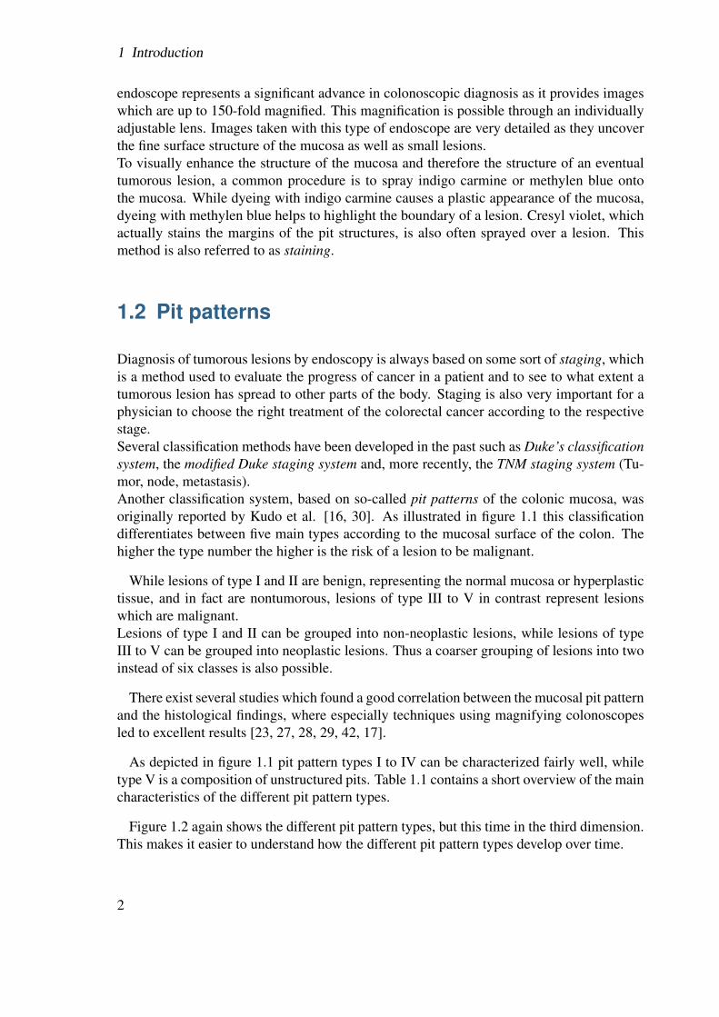
Diagnosis of tumorous lesions by endoscopy is always based on some sort of staging, whichis a method used to evaluate the progress of cancer in a patient and to see to what extent atumorous lesion has spread to other parts of the body. Staging is also very important for aphysician to choose the right treatment of the colorectal cancer according to the respectivestage.Several classification methods have been developed in the past such as Duke’s classificationsystem, the modified Duke staging system and, more recently, the TNM staging system (Tu-mor, node, metastasis).Another classification system, based on so-called pit patterns of the colonic mucosa, wasoriginally reported by Kudo et al. [16, 30]. As illustrated in figure 1.1 this classificationdifferentiates between five main types according to the mucosal surface of the colon. Thehigher the type number the higher is the risk of a lesion to be malignant.
While lesions of type I and II are benign, representing the normal mucosa or hyperplastictissue, and in fact are nontumorous, lesions of type III to V in contrast represent lesionswhich are malignant.Lesions of type I and II can be grouped into non-neoplastic lesions, while lesions of typeIII to V can be grouped into neoplastic lesions. Thus a coarser grouping of lesions into twoinstead of six classes is also possible.
There exist several studies which found a good correlation between the mucosal pit patternand the histological findings, where especially techniques using magnifying colonoscopesled to excellent results [23, 27, 28, 29, 42, 17].
As depicted in figure 1.1 pit pattern types I to IV can be characterized fairly well, whiletype V is a composition of unstructured pits. Table 1.1 contains a short overview of the maincharacteristics of the different pit pattern types.
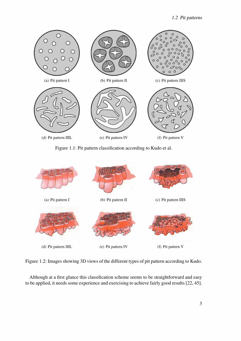
Figure 1.2 again shows the different pit pattern types, but this time in the third dimension.This makes it easier to understand how the different pit pattern types develop over time.
2
1.2 Pit patterns
(a) Pit pattern I (b) Pit pattern II (c) Pit pattern IIIS
(d) Pit pattern IIIL (e) Pit pattern IV (f) Pit pattern V
Figure 1.1: Pit pattern classification according to Kudo et al.
(a) Pit pattern I (b) Pit pattern II (c) Pit pattern IIIS
(d) Pit pattern IIIL (e) Pit pattern IV (f) Pit pattern V
Figure 1.2: Images showing 3D views of the different types of pit pattern according to Kudo.
Although at a first glance this classification scheme seems to be straightforward and easyto be applied, it needs some experience and exercising to achieve fairly good results [22, 45].
3
1 Introduction
Pit pattern type CharacteristicsI roundish pits which designate a normal mucosaII stellar or papillary pits
III S small roundish or tubular pits, which are smallerthan the pits of type I
III L roundish or tubular pits, which are larger thanthe pits of type I
IV branch-like or gyrus-like pitsV non-structured pits
Table 1.1: The characteristics of the different pit pattern types.
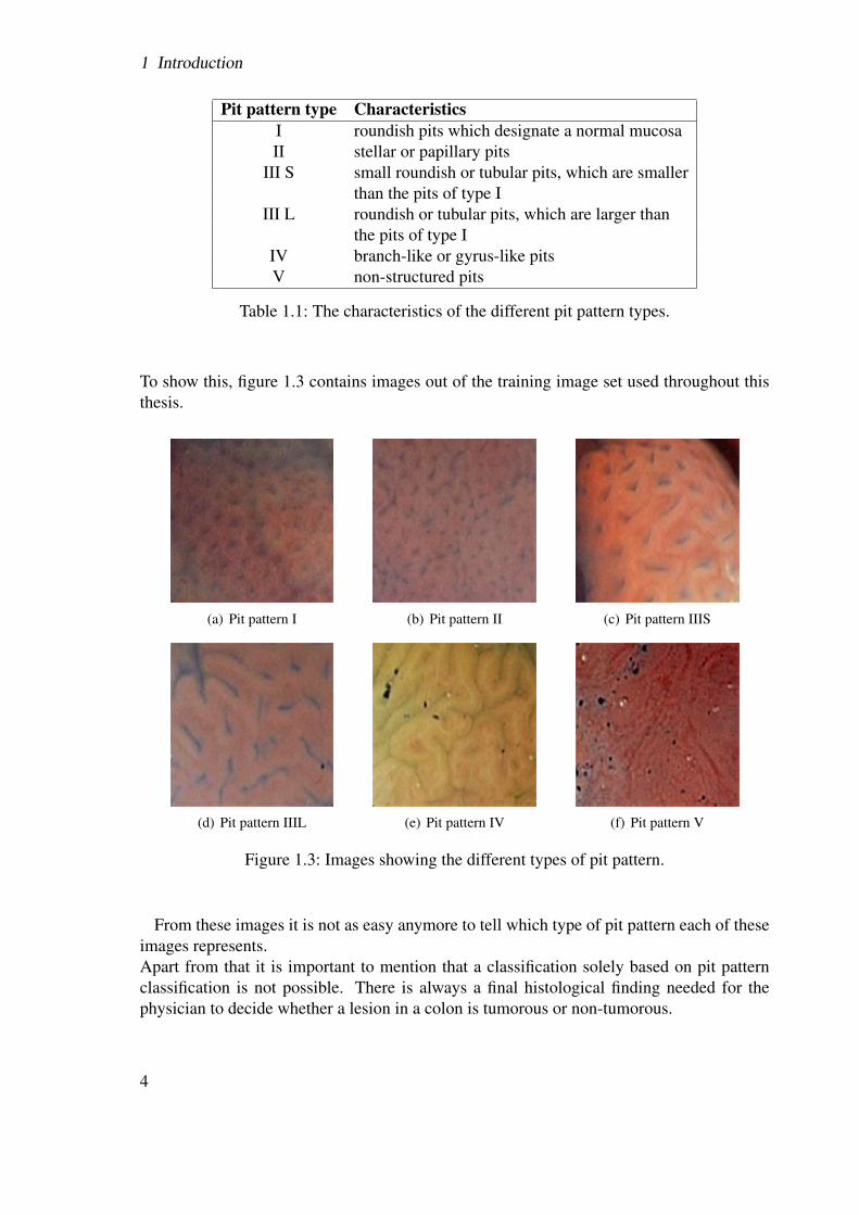
To show this, figure 1.3 contains images out of the training image set used throughout thisthesis.
(a) Pit pattern I (b) Pit pattern II (c) Pit pattern IIIS
(d) Pit pattern IIIL (e) Pit pattern IV (f) Pit pattern V
Figure 1.3: Images showing the different types of pit pattern.
From these images it is not as easy anymore to tell which type of pit pattern each of theseimages represents.Apart from that it is important to mention that a classification solely based on pit patternclassification is not possible. There is always a final histological finding needed for thephysician to decide whether a lesion in a colon is tumorous or non-tumorous.
4
1.3 Computer based pit pattern classification
1.3 Computer based pit pattern classification
The motivation behind computer based pit pattern classification is to assist the physicianin analyzing the colon images taken with a colonoscope just in time. Thus a classificationcan already be done during the colonoscopy and therefore this makes a fast classificationpossible. But as already mentioned above, a final histological finding is needed here too toconfirm the classification made by the computer.
The process of the computer based pit pattern classification can be divided into the fol-lowing steps:
1. First of all as many images as possible have to be acquired. These images serve fortraining as well as for testing a trained classification algorithm.
2. The images are analyzed for some specific features such as textural features, colorfeatures, frequency domain features or any other type of features.
3. A classification algorithm of choice is trained with the features gathered in the laststep.
4. The classification algorithm is presented some unknown image to classify. The un-known image in this context is an image which has not been used during the trainingstep.
From these steps the very important question which features to extract from the imagesarises. Since there are many possibilities for image features, chapter 3 will give a shortoverview of some possible features for texture classification.
However, as the title of this thesis already suggests, the features we intend to use are solelybased on the wavelet transform. Hence, before we start thinking about possible featuresto extract from endoscopic images, the next chapter tries to give a short introduction towavelets and the wavelet transform.
5

1 Introduction
6
2 WaveletsEvery great advance in science has issuedfrom a new audacity of imagination.
- John Dewey, The Quest for Certainty
2.1 Introduction
In the history of mathematics wavelet analysis shows many origins. It was Joseph Fourierwho did the first step towards wavelet analysis by doing research in the field of frequencyanalysis. He asserted that any 2π-periodic function can be expressed as a sum of sines andcosines with different amplitudes and frequencies.The first wavelet function developed was the Haar wavelet developed by A. Haar in 1909.This wavelet has compact support but unfortunately is not continuously differentiable, afact, which limits its applications.
The wavelet theory adopts the idea to express a function as a sum of other so-called basisfunctions. But the key difference between a fourier series and a wavelet is the choice ofthe basis functions. A fourier series expresses a function, as already mentioned, in terms ofsines and cosines which are periodic functions whereas the discrete wavelet transform forexample only uses basis functions with compact support. This means that wavelet functionsvanish outside of a finite interval.This choice of the basis functions eliminates a disadvantage of the fourier analysis. Waveletfunctions are localized in space, the sine and cosine functions of the fourier series are not.
The name “wavelet” originates from the important requirement of wavelets that theyshould integrate to zero, “waving” above and below the x-axis. This requirement can beexpressed more mathematically as∫ ∞
−∞ψ(t)dt = 0 (2.1)
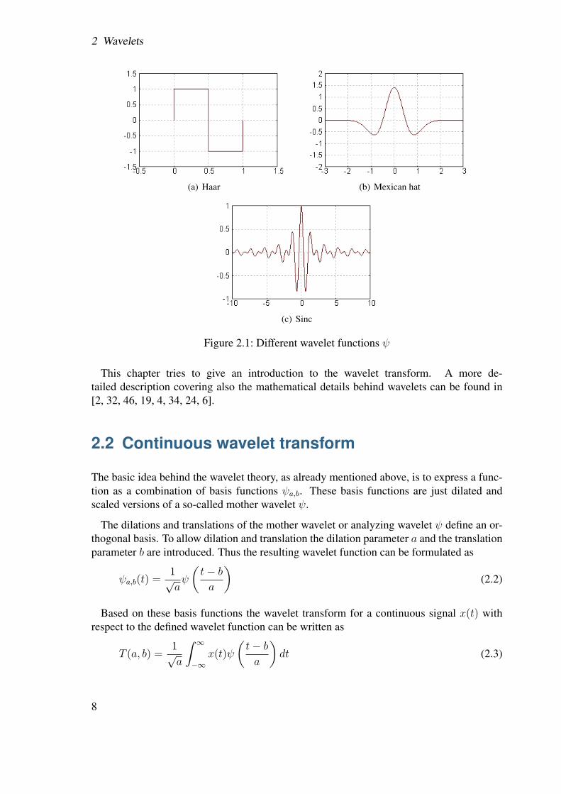
where ψ is the wavelet function used. Figure 2.1 shows some different choices for ψ.
An important fact is that wavelet transforms do not have a single set of basis functionslike the Fourier transform. Instead, the number of possible basis functions for the wavelettransforms is infinite.
The range of applications where wavelets are used nowadays is wide. It includes signalcompression, pattern recognition, speech recognition, computer graphics, signal processing,just to mention a few.
7
2 Wavelets
(a) Haar (b) Mexican hat
(c) Sinc
Figure 2.1: Different wavelet functions ψ
This chapter tries to give an introduction to the wavelet transform. A more de-tailed description covering also the mathematical details behind wavelets can be found in[2, 32, 46, 19, 4, 34, 24, 6].
2.2 Continuous wavelet transform
The basic idea behind the wavelet theory, as already mentioned above, is to express a func-tion as a combination of basis functions ψa,b. These basis functions are just dilated andscaled versions of a so-called mother wavelet ψ.
The dilations and translations of the mother wavelet or analyzing wavelet ψ define an or-thogonal basis. To allow dilation and translation the dilation parameter a and the translationparameter b are introduced. Thus the resulting wavelet function can be formulated as
ψa,b(t) =1√aψ
(t− b
a
)(2.2)
Based on these basis functions the wavelet transform for a continuous signal x(t) withrespect to the defined wavelet function can be written as
T (a, b) =1√a
∫ ∞
−∞x(t)ψ
(t− b
a
)dt (2.3)
8
2.3 Discrete wavelet transform
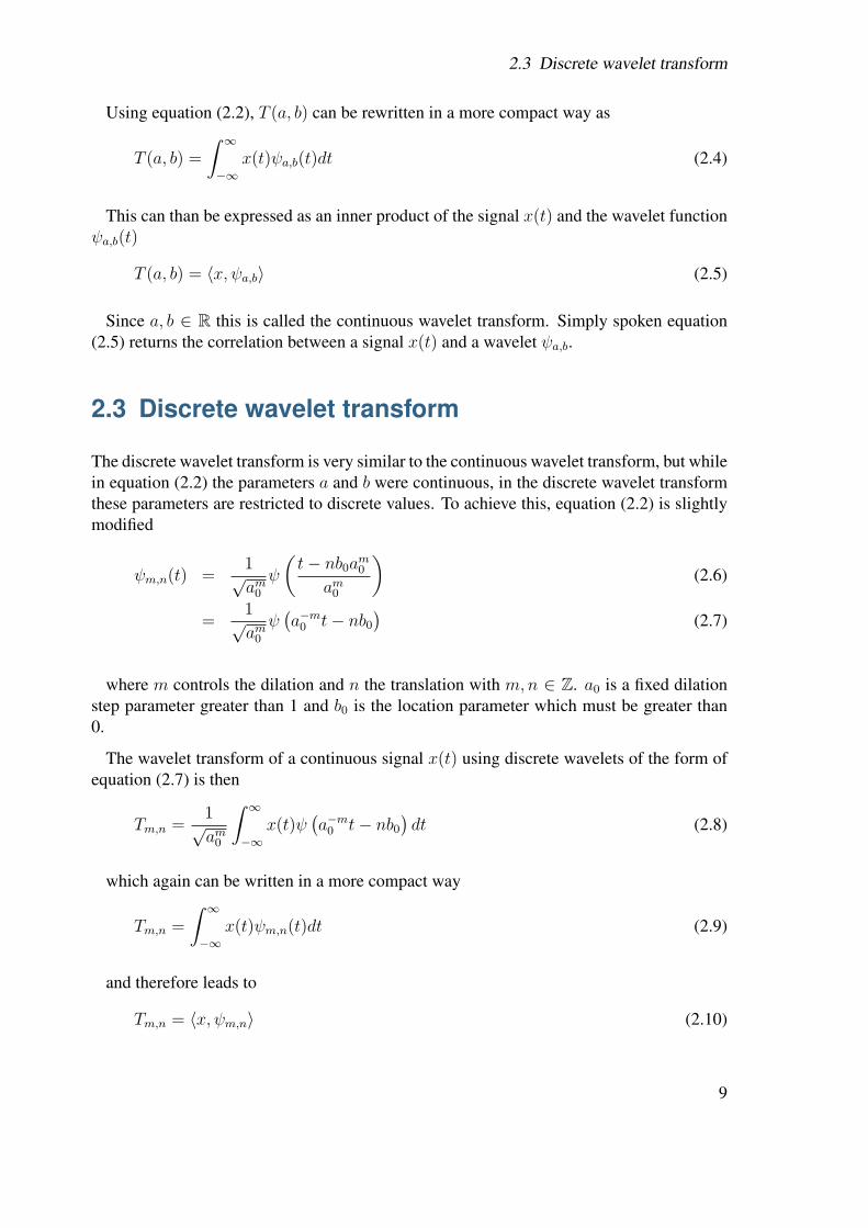
Using equation (2.2), T (a, b) can be rewritten in a more compact way as
T (a, b) =
∫ ∞
−∞x(t)ψa,b(t)dt (2.4)
This can than be expressed as an inner product of the signal x(t) and the wavelet functionψa,b(t)
T (a, b) = 〈x, ψa,b〉 (2.5)
Since a, b ∈ R this is called the continuous wavelet transform. Simply spoken equation(2.5) returns the correlation between a signal x(t) and a wavelet ψa,b.
2.3 Discrete wavelet transform
The discrete wavelet transform is very similar to the continuous wavelet transform, but whilein equation (2.2) the parameters a and b were continuous, in the discrete wavelet transformthese parameters are restricted to discrete values. To achieve this, equation (2.2) is slightlymodified
ψm,n(t) =1√am
0
ψ
(t− nb0a
m0
am0
)(2.6)
=1√am
0
ψ(a−m
0 t− nb0)
(2.7)
where m controls the dilation and n the translation with m,n ∈ Z. a0 is a fixed dilationstep parameter greater than 1 and b0 is the location parameter which must be greater than0.
The wavelet transform of a continuous signal x(t) using discrete wavelets of the form ofequation (2.7) is then
Tm,n =1√am
0
∫ ∞
−∞x(t)ψ
(a−m
0 t− nb0)dt (2.8)
which again can be written in a more compact way
Tm,n =
∫ ∞
−∞x(t)ψm,n(t)dt (2.9)
and therefore leads to
Tm,n = 〈x, ψm,n〉 (2.10)
9
2 Wavelets
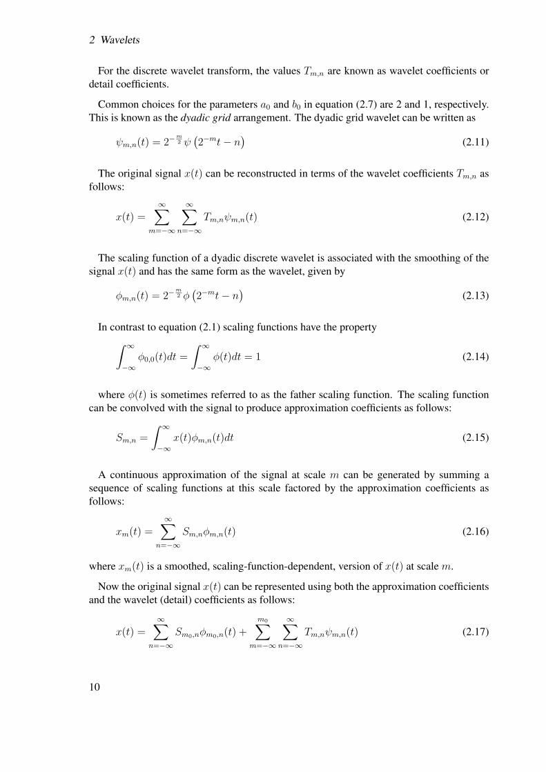
For the discrete wavelet transform, the values Tm,n are known as wavelet coefficients ordetail coefficients.
Common choices for the parameters a0 and b0 in equation (2.7) are 2 and 1, respectively.This is known as the dyadic grid arrangement. The dyadic grid wavelet can be written as
ψm,n(t) = 2−m2 ψ
(2−mt− n
)(2.11)
The original signal x(t) can be reconstructed in terms of the wavelet coefficients Tm,n asfollows:
x(t) =∞∑
m=−∞
∞∑n=−∞
Tm,nψm,n(t) (2.12)
The scaling function of a dyadic discrete wavelet is associated with the smoothing of thesignal x(t) and has the same form as the wavelet, given by
φm,n(t) = 2−m2 φ
(2−mt− n
)(2.13)
In contrast to equation (2.1) scaling functions have the property∫ ∞
−∞φ0,0(t)dt =
∫ ∞
−∞φ(t)dt = 1 (2.14)
where φ(t) is sometimes referred to as the father scaling function. The scaling functioncan be convolved with the signal to produce approximation coefficients as follows:
Sm,n =
∫ ∞
−∞x(t)φm,n(t)dt (2.15)
A continuous approximation of the signal at scale m can be generated by summing asequence of scaling functions at this scale factored by the approximation coefficients asfollows:
xm(t) =∞∑
n=−∞
Sm,nφm,n(t) (2.16)
where xm(t) is a smoothed, scaling-function-dependent, version of x(t) at scale m.
Now the original signal x(t) can be represented using both the approximation coefficientsand the wavelet (detail) coefficients as follows:
x(t) =∞∑
n=−∞
Sm0,nφm0,n(t) +
m0∑m=−∞
∞∑n=−∞
Tm,nψm,n(t) (2.17)
10
2.3 Discrete wavelet transform
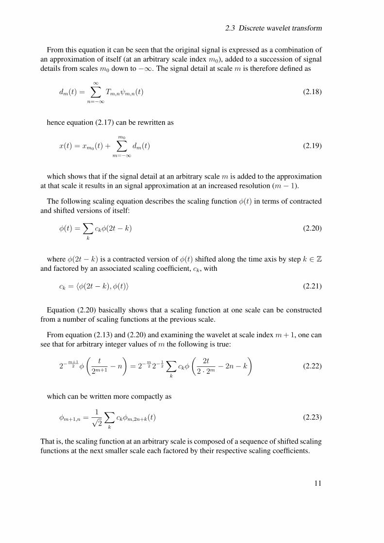
From this equation it can be seen that the original signal is expressed as a combination ofan approximation of itself (at an arbitrary scale index m0), added to a succession of signaldetails from scales m0 down to −∞. The signal detail at scale m is therefore defined as
dm(t) =∞∑
n=−∞
Tm,nψm,n(t) (2.18)
hence equation (2.17) can be rewritten as
x(t) = xm0(t) +
m0∑m=−∞
dm(t) (2.19)
which shows that if the signal detail at an arbitrary scale m is added to the approximationat that scale it results in an signal approximation at an increased resolution (m− 1).
The following scaling equation describes the scaling function φ(t) in terms of contractedand shifted versions of itself:
φ(t) =∑
k
ckφ(2t− k) (2.20)
where φ(2t− k) is a contracted version of φ(t) shifted along the time axis by step k ∈ Zand factored by an associated scaling coefficient, ck, with
ck = 〈φ(2t− k), φ(t)〉 (2.21)
Equation (2.20) basically shows that a scaling function at one scale can be constructedfrom a number of scaling functions at the previous scale.
From equation (2.13) and (2.20) and examining the wavelet at scale index m+ 1, one cansee that for arbitrary integer values of m the following is true:
2−m+1
2 φ
(t
2m+1− n
)= 2−
m2 2−
12
∑k
ckφ
(2t
2 · 2m− 2n− k
)(2.22)
which can be written more compactly as
φm+1,n =1√2
∑k
ckφm,2n+k(t) (2.23)
That is, the scaling function at an arbitrary scale is composed of a sequence of shifted scalingfunctions at the next smaller scale each factored by their respective scaling coefficients.
11
2 Wavelets
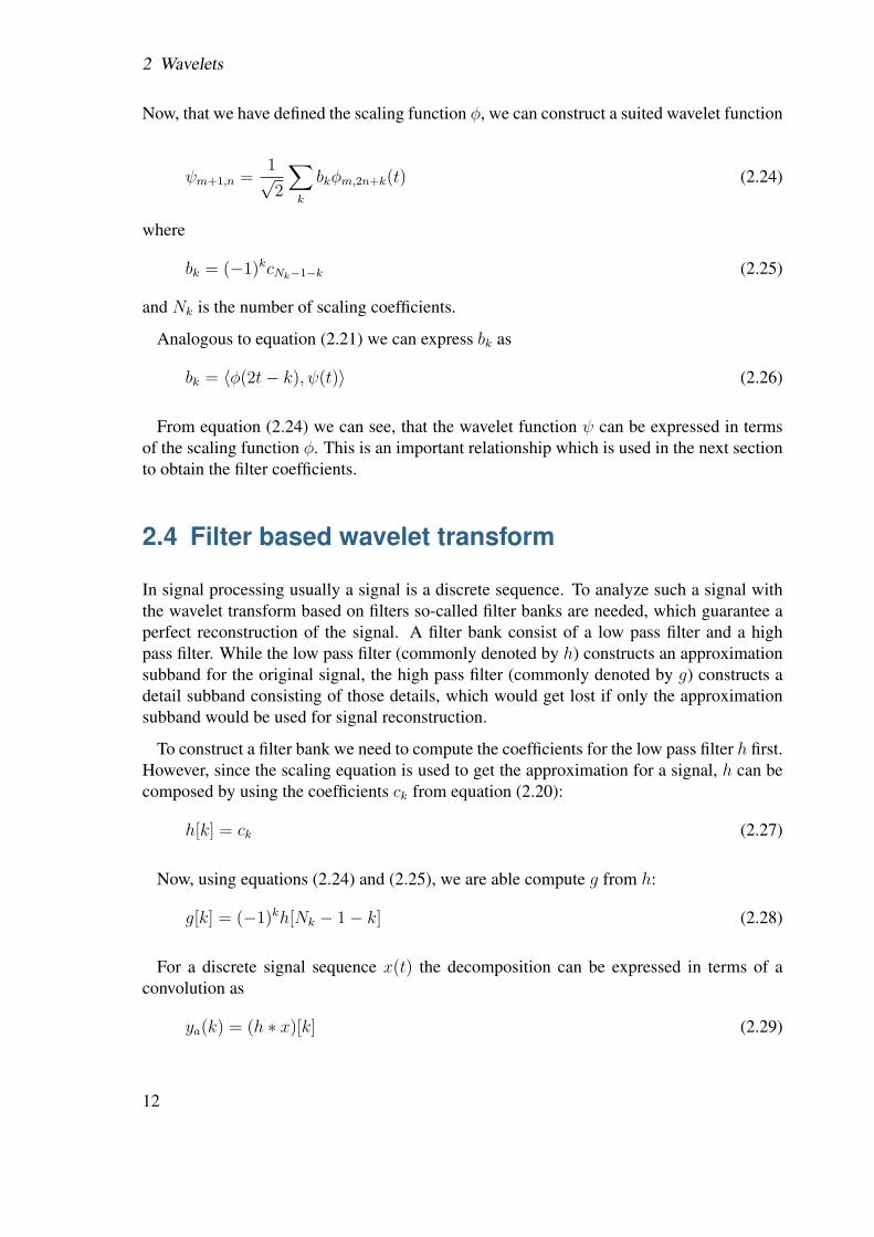
Now, that we have defined the scaling function φ, we can construct a suited wavelet function
ψm+1,n =1√2
∑k
bkφm,2n+k(t) (2.24)
where
bk = (−1)kcNk−1−k (2.25)
and Nk is the number of scaling coefficients.
Analogous to equation (2.21) we can express bk as
bk = 〈φ(2t− k), ψ(t)〉 (2.26)
From equation (2.24) we can see, that the wavelet function ψ can be expressed in termsof the scaling function φ. This is an important relationship which is used in the next sectionto obtain the filter coefficients.
2.4 Filter based wavelet transform
In signal processing usually a signal is a discrete sequence. To analyze such a signal withthe wavelet transform based on filters so-called filter banks are needed, which guarantee aperfect reconstruction of the signal. A filter bank consist of a low pass filter and a highpass filter. While the low pass filter (commonly denoted by h) constructs an approximationsubband for the original signal, the high pass filter (commonly denoted by g) constructs adetail subband consisting of those details, which would get lost if only the approximationsubband would be used for signal reconstruction.
To construct a filter bank we need to compute the coefficients for the low pass filter h first.However, since the scaling equation is used to get the approximation for a signal, h can becomposed by using the coefficients ck from equation (2.20):
h[k] = ck (2.27)
Now, using equations (2.24) and (2.25), we are able compute g from h:
g[k] = (−1)kh[Nk − 1− k] (2.28)
For a discrete signal sequence x(t) the decomposition can be expressed in terms of aconvolution as
ya(k) = (h ∗ x)[k] (2.29)
12
2.4 Filter based wavelet transform
and
yd(k) = (g ∗ x)[k] (2.30)
where ya and yd denote the approximation and the detail subband.The discrete convolution between a discrete signal x(t) and a filter f(t) is defined as
(f ∗ x)(k) =l∑
i=0
f(i)x(k − i) (2.31)
where l is the length of the respective filter f .
To avoid redundant data in the decomposed subbands, the signal of length N is down-sampled to length N/2. Therefore the result of equation (2.29) and (2.30) are sequences oflength N/2 and the decomposed signal has a length of N .
To reconstruct the original signal x from ya and yd a reconstruction filter bank consistingof the filters h and g, which are the low pass and high pass reconstruction filters, is used.Since during the decomposition the signal was downsampled, the detail and the approxima-tion subband have to be upsampled from size N/2 to size N . Then the following formula isused to reconstruct the original signal x.
x(t) = (h ∗ ya)(t) + (g ∗ yd)(t) (2.32)
The reconstruction filters h and g can be computed from the previously computed decom-position filters h and g using the following equations
h[k] = (−1)k+1g[k] (2.33)
and
g[k] = (−1)kh[k] (2.34)
A special wavelet decomposition method without any downsampling and upsampling in-volved is the algorithme a trous. This algorithm provides approximate shift-invariance withan acceptable level of redundancy. Since in the discrete wavelet transform at each decom-position level every second coefficient is discarded, this can result in considerably largeshift-variances.
When using the algorithme a trous however the subbands are not downsampled duringdecomposition and the same amount of coefficients is stored for each subband - no mat-ter at which level of decomposition a subband is located in the decomposition tree. As aconsequence no upsampling is needed at all when reconstructing a signal.
13
2 Wavelets
2.5 Pyramidal wavelet transform
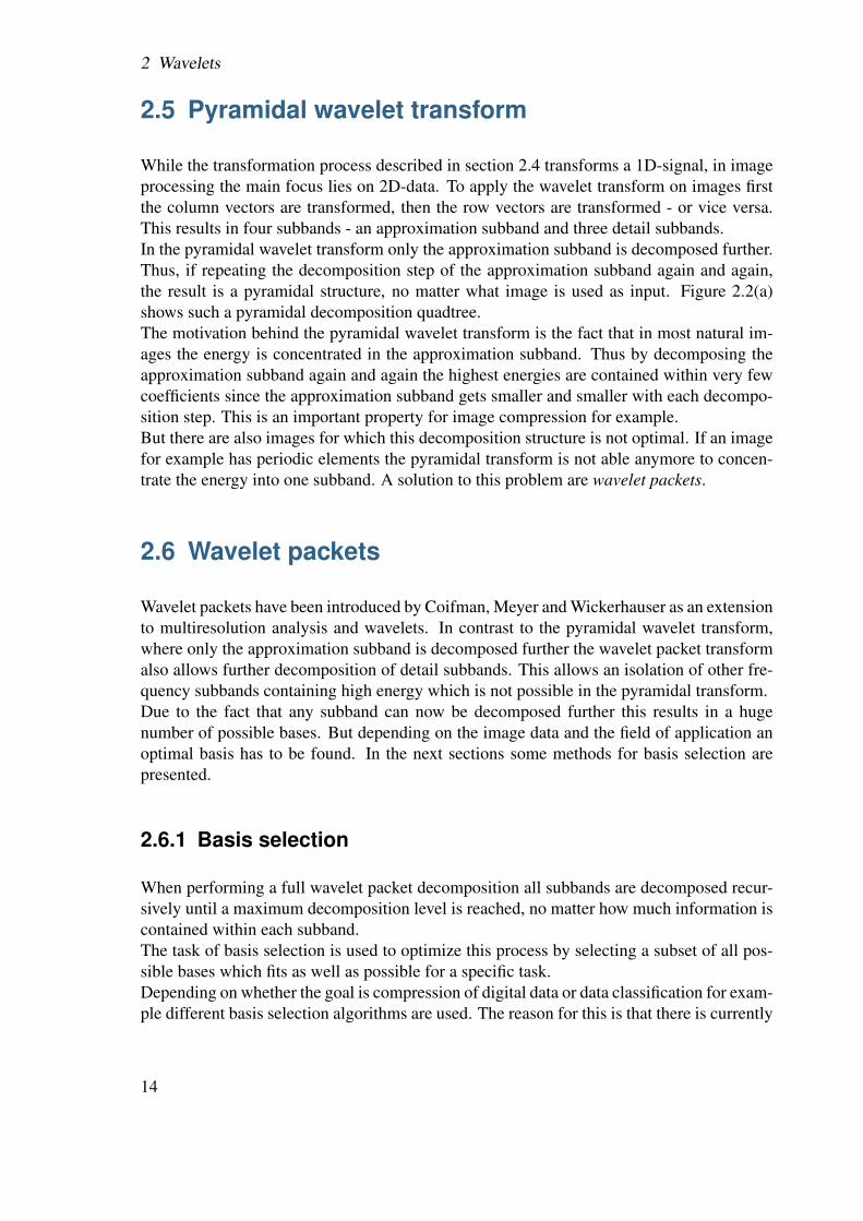
While the transformation process described in section 2.4 transforms a 1D-signal, in imageprocessing the main focus lies on 2D-data. To apply the wavelet transform on images firstthe column vectors are transformed, then the row vectors are transformed - or vice versa.This results in four subbands - an approximation subband and three detail subbands.In the pyramidal wavelet transform only the approximation subband is decomposed further.Thus, if repeating the decomposition step of the approximation subband again and again,the result is a pyramidal structure, no matter what image is used as input. Figure 2.2(a)shows such a pyramidal decomposition quadtree.The motivation behind the pyramidal wavelet transform is the fact that in most natural im-ages the energy is concentrated in the approximation subband. Thus by decomposing theapproximation subband again and again the highest energies are contained within very fewcoefficients since the approximation subband gets smaller and smaller with each decompo-sition step. This is an important property for image compression for example.But there are also images for which this decomposition structure is not optimal. If an imagefor example has periodic elements the pyramidal transform is not able anymore to concen-trate the energy into one subband. A solution to this problem are wavelet packets.
2.6 Wavelet packets
Wavelet packets have been introduced by Coifman, Meyer and Wickerhauser as an extensionto multiresolution analysis and wavelets. In contrast to the pyramidal wavelet transform,where only the approximation subband is decomposed further the wavelet packet transformalso allows further decomposition of detail subbands. This allows an isolation of other fre-quency subbands containing high energy which is not possible in the pyramidal transform.Due to the fact that any subband can now be decomposed further this results in a hugenumber of possible bases. But depending on the image data and the field of application anoptimal basis has to be found. In the next sections some methods for basis selection arepresented.
2.6.1 Basis selection
When performing a full wavelet packet decomposition all subbands are decomposed recur-sively until a maximum decomposition level is reached, no matter how much information iscontained within each subband.The task of basis selection is used to optimize this process by selecting a subset of all pos-sible bases which fits as well as possible for a specific task.Depending on whether the goal is compression of digital data or data classification for exam-ple different basis selection algorithms are used. The reason for this is that there is currently
14
2.6 Wavelet packets
(a) (b)
Figure 2.2: Pyramidal decomposition (a) and one possible best-basis wavelet packet decom-position (b)
no known basis selection algorithm with has to be proven to perform well in classificationtasks as well as in compression tasks. This is mainly due to the fact that the underlyingprinciples of compression and classification are quite different. While in compression themain goal is to reduce the size of some data with as few loss as possible, the main goal inclassification is to find a set of features which is similar among inputs of the same class andwhich differ among inputs from different classes.
2.6.1.1 Best-basis algorithm
The best-basis algorithm, which was developed by Coifman and Wickerhauser [11] mainlyfor signal compression, tries to minimize the decomposition tree by focusing on subbandsonly which contain enough information to be regarded as being interesting. To achieve this,an additive cost function is used to decide whether a subband should be further decomposedor not. The algorithm can be outlined by the following steps:
1. A full wavelet packet decomposition is calculated for the input data which results ina decomposition tree.
2. The resulting decomposition tree is traversed from the leafs upwards to the tree rootcomparing the additive cost of the children nodes and the according parent node foreach node in the tree having children nodes.
3. If the summed cost of the children nodes exceeds the cost of the according parentnode the tree gets pruned at that parent node, which means that the children nodes areremoved.
The resulting decomposition is optimal in respect to the cost function used. The most com-mon additive cost functions used are
15
2 Wavelets
Logarithm of energy (LogEnergy)
cost(I) =N∑
i=1
log∗(s) with s = I(i)2
Entropy
cost(I) = −N∑
i=1
s log∗(s) with s = I(i)2
Lp-Norm
cost(I) =N∑
i=1
|I(i)|p
Threshold
cost(I) =N∑
i=1
a with a =
{1 if I(i) > t0 else
where I is the input sequence (the subband), N is the length of the input, log∗ is the log-function with the convention log(0) = 0 and t is some threshold value.
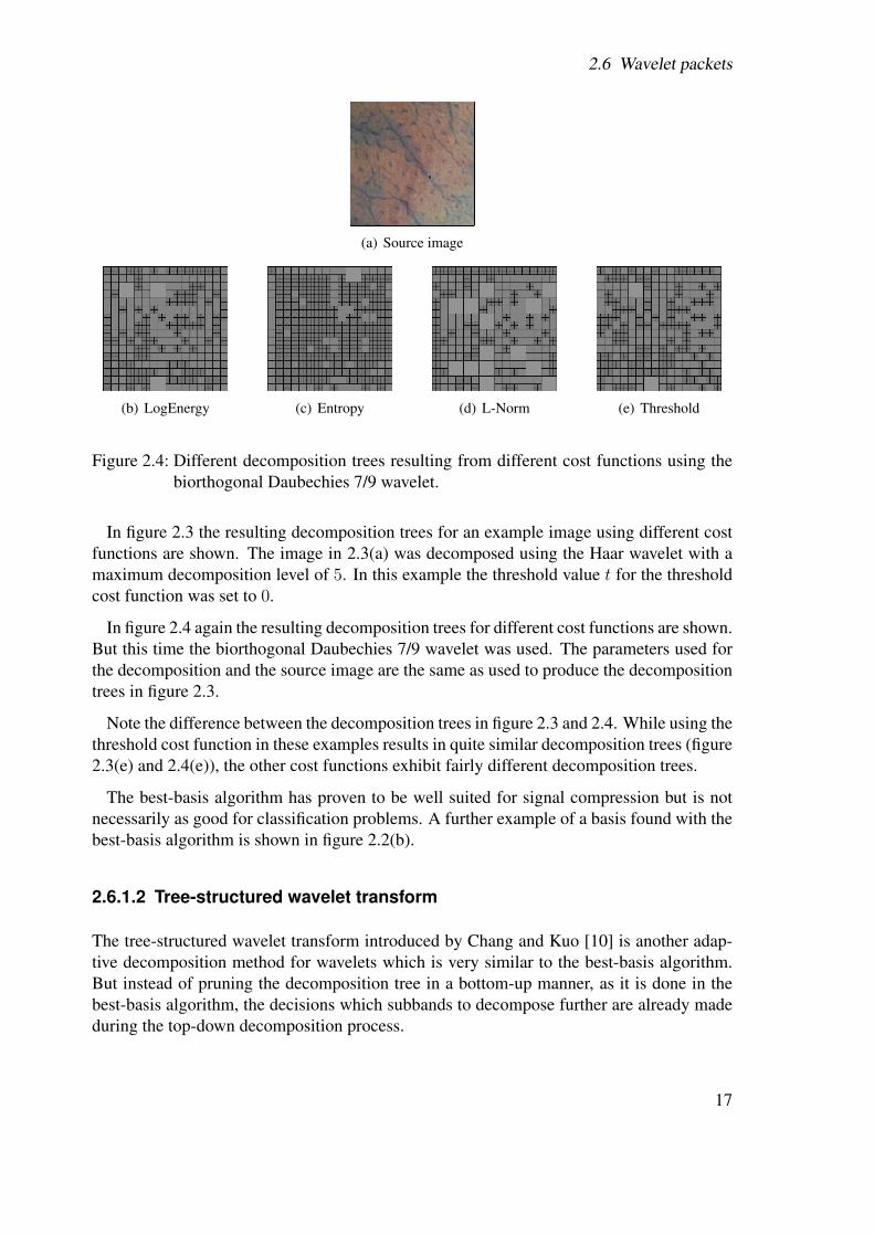
(a) Source image
(b) LogEnergy (c) Entropy (d) L-Norm (e) Threshold
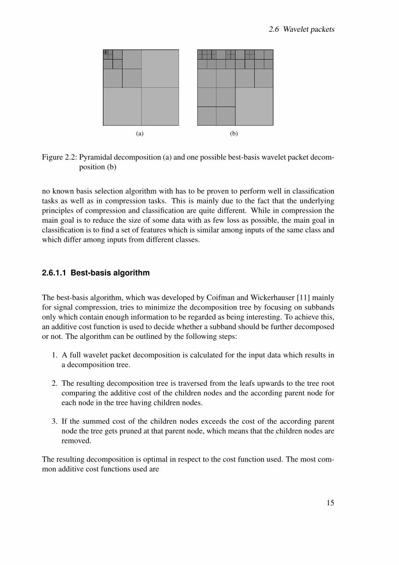
Figure 2.3: Different decomposition trees resulting from different cost functions using theHaar wavelet.
16
2.6 Wavelet packets
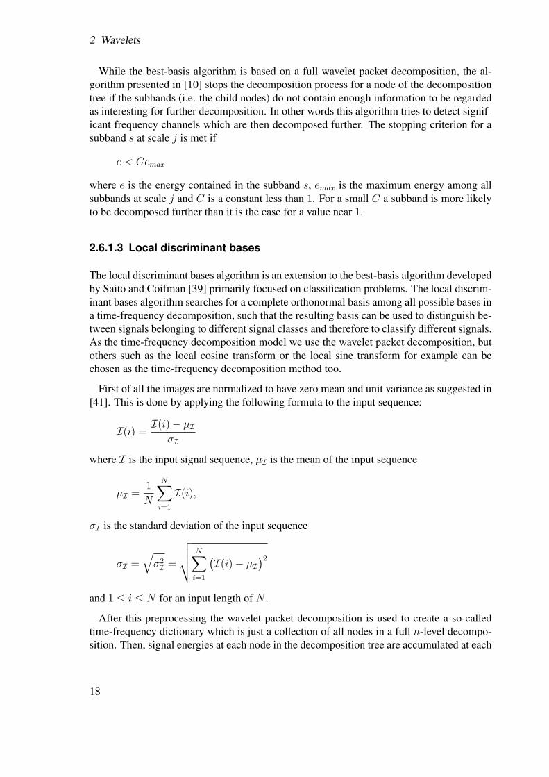
(a) Source image
(b) LogEnergy (c) Entropy (d) L-Norm (e) Threshold
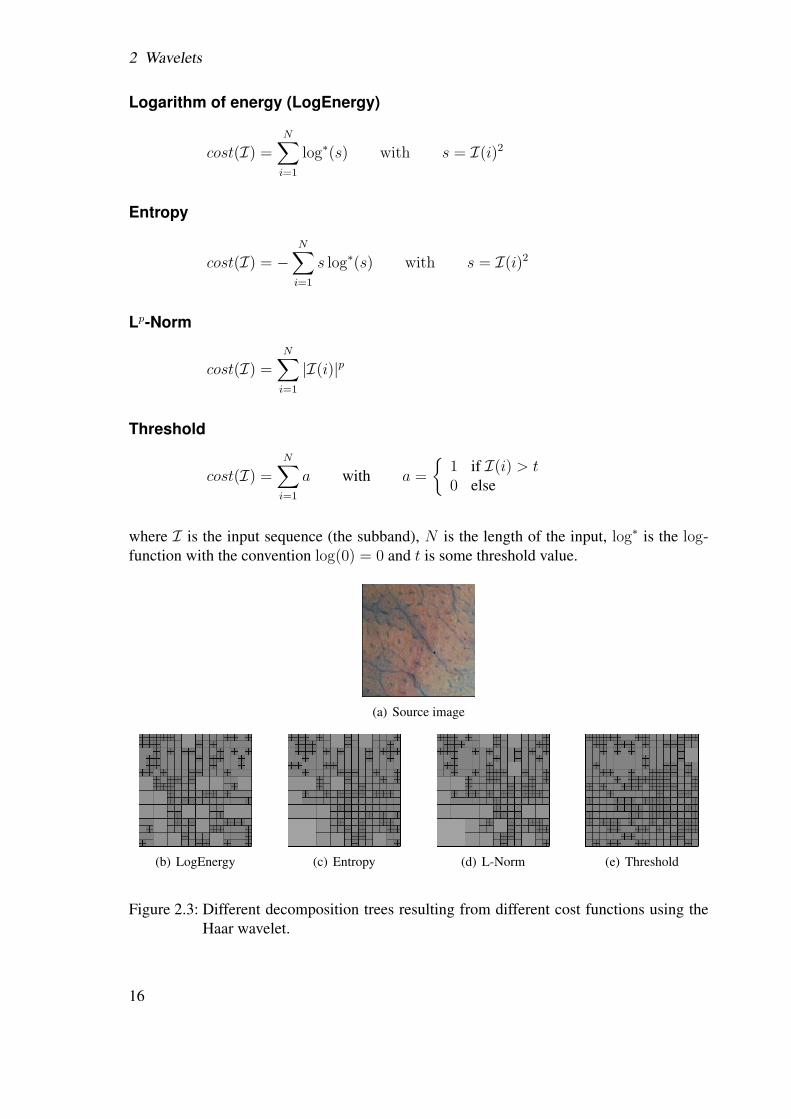
Figure 2.4: Different decomposition trees resulting from different cost functions using thebiorthogonal Daubechies 7/9 wavelet.
In figure 2.3 the resulting decomposition trees for an example image using different costfunctions are shown. The image in 2.3(a) was decomposed using the Haar wavelet with amaximum decomposition level of 5. In this example the threshold value t for the thresholdcost function was set to 0.
In figure 2.4 again the resulting decomposition trees for different cost functions are shown.But this time the biorthogonal Daubechies 7/9 wavelet was used. The parameters used forthe decomposition and the source image are the same as used to produce the decompositiontrees in figure 2.3.
Note the difference between the decomposition trees in figure 2.3 and 2.4. While using thethreshold cost function in these examples results in quite similar decomposition trees (figure2.3(e) and 2.4(e)), the other cost functions exhibit fairly different decomposition trees.
The best-basis algorithm has proven to be well suited for signal compression but is notnecessarily as good for classification problems. A further example of a basis found with thebest-basis algorithm is shown in figure 2.2(b).
2.6.1.2 Tree-structured wavelet transform
The tree-structured wavelet transform introduced by Chang and Kuo [10] is another adap-tive decomposition method for wavelets which is very similar to the best-basis algorithm.But instead of pruning the decomposition tree in a bottom-up manner, as it is done in thebest-basis algorithm, the decisions which subbands to decompose further are already madeduring the top-down decomposition process.
17
2 Wavelets
While the best-basis algorithm is based on a full wavelet packet decomposition, the al-gorithm presented in [10] stops the decomposition process for a node of the decompositiontree if the subbands (i.e. the child nodes) do not contain enough information to be regardedas interesting for further decomposition. In other words this algorithm tries to detect signif-icant frequency channels which are then decomposed further. The stopping criterion for asubband s at scale j is met if
e < Cemax
where e is the energy contained in the subband s, emax is the maximum energy among allsubbands at scale j and C is a constant less than 1. For a small C a subband is more likelyto be decomposed further than it is the case for a value near 1.
2.6.1.3 Local discriminant bases
The local discriminant bases algorithm is an extension to the best-basis algorithm developedby Saito and Coifman [39] primarily focused on classification problems. The local discrim-inant bases algorithm searches for a complete orthonormal basis among all possible bases ina time-frequency decomposition, such that the resulting basis can be used to distinguish be-tween signals belonging to different signal classes and therefore to classify different signals.As the time-frequency decomposition model we use the wavelet packet decomposition, butothers such as the local cosine transform or the local sine transform for example can bechosen as the time-frequency decomposition method too.
First of all the images are normalized to have zero mean and unit variance as suggested in[41]. This is done by applying the following formula to the input sequence:
I(i) =I(i)− µI
σI
where I is the input signal sequence, µI is the mean of the input sequence
µI =1
N
N∑i=1
I(i),
σI is the standard deviation of the input sequence
σI =√σ2I =
√√√√ N∑i=1
(I(i)− µI
)2
and 1 ≤ i ≤ N for an input length of N .
After this preprocessing the wavelet packet decomposition is used to create a so-calledtime-frequency dictionary which is just a collection of all nodes in a full n-level decompo-sition. Then, signal energies at each node in the decomposition tree are accumulated at each
18
2.6 Wavelet packets
coefficient for each signal class l separately to get a so-called time-frequency energy map Γl
for each signal class l, which is then normalized by the total energy of the signals belongingto class l. This can be formulated as
Γl(j, k) =
Nl∑i=1
(s(l)i,k)
2/
Nl∑i=1
‖x(l)i ‖2 (2.35)
where j denotes the j-th node of the decomposition tree, Nl is the number of samples(images) in class l, s(l)
i,j,k is the k-th wavelet coefficient of the j-th subband (node) of the i-thimage of class l and x(l)
i is the i-th signal of class l.
This time-frequency energy map is then used by the algorithm to determine the discrim-ination between signals belonging to different classes l = 1, . . . , L where L is the numberof total different signal classes. The discriminant power of a node is calculated using adiscriminant measure D, which measures statistical distances among classes.
There are many choices for the discriminant measure such as the relative entropy which isalso known as the cross-entropy, Kullback-Leibler distance or I-divergence. Other possiblemeasures include the J-divergence, which is a symmetric version of the I-divergence, theHellinger distance, the Jenson-Shannon divergence and the euclidean distance.
I-divergence
D(pa, pb) =n∑
i=1
pailog
pai
pbi
J-divergence
D(pa, pb) =n∑
i=1
pailog
pai
pbi
+n∑
i=1
pbilog
pbi
pai
Hellinger-distance
D(pa, pb) =n∑
i=1
(√pai
−√pbi
)2
Jenson-Shannon divergence
D(pa, pb) =
( n∑i=1
pailog
pai
qi+
n∑i=1
pbilog
pbi
qi
)/2
with
qi =pai
+ pbi
2
19
2 Wavelets
Euclidean distance
D(pa, pb) = ‖pa − pb‖2
where pa and pb are two nonnegative sequences representing probability distributions ofsignals belonging to classes a and b respectively and n is number of elements in pa and pb.Thus, the discriminant measures listed above are distance measures for probability distribu-tions and are used to calculate the discriminant power between pa and pb.
To use these measures to calculate the discriminant power over L classes we use thefollowing equation:
D({pl}Ll=1) =
L−1∑i=1
L∑j=i+1
D(pi, pj) (2.36)
In terms of the time frequency energy map equation (2.36) can be written as
D({Γl(n)}Ll=1) =
L−1∑i=1
L∑j=i+1
D(Γi(n),Γj(n)) (2.37)
where n denotes the n-th subband (node) in the decomposition tree.
The algorithm to find the optimal basis can be outlined as follows:
1. A full wavelet packet decomposition is calculated for the input data which results ina decomposition tree.
2. The resulting decomposition tree is traversed from the leafs upwards to the tree rootcomparing the additive discriminant power of the children nodes and the accordingparent node for each node in the tree having children nodes. To calculate the discrimi-nant power the discriminant measureD is used to evaluate the power of discriminationof the nodes in the decomposition tree between different signal classes.
3. If the discriminant power of the parent node exceeds the summed discriminant powerof the children nodes the tree gets pruned at that parent node, which means that thechildren nodes are removed.
To obtain a fast computational algorithm to find the optimal basis, D has to be additive justas the cost function used in the best-basis algorithm.
After the pruning process we have a complete orthonormal basis and all wavelet expansioncoefficients of signals in this basis could be used as features already. But due to the fact thatthe dimension of such a feature vector would be rather high it is necessary to reduce thedimensionality of the problem such that k � n where n is the number of all basis vectorsof the orthonormal basis and k is the dimension of the feature vector after dimensionalityreduction.
20
2.6 Wavelet packets
To reduce the dimension of the feature vector the first step is to sort the basis functionsby their power of discrimination. There are several choices as a measure of discriminantpower of one of the basis functions such as using the discriminant measure D on the time-frequency distribution among different classes of a single decomposition tree node, whichis just the power of discrimination of one node and therefore a measure of usefulness of thisnode for the classification process.Another measure would be the Fisher’s class separability of wavelet coefficients of a singlenode in the decomposition tree, which expresses the ratio of the between-class variance tothe in-class variance of a specific subband s(c)
i,j and can be formulated as∑Ll=1 πl
(meani(s
(l)i,j)−meanl(meani(s
(l)i,j))
)2∑Ll=1 πlvariancei(s
(l)i,j)
(2.38)
where L is the number of classes, πl is the empirical proportion of class l, s(l)i,j is the j-th
subband for the i-th image of class l containing the wavelet coefficients and meanl(·) is themean over class l, meani(·) and variancei(·) are operations to take mean and variance forthe wavelet coefficients of s(l)
i,j , respectively.The following equation is similar to equation (2.38), but it uses the median instead of themean, and the median absolute deviation instead of the variance:∑L
l=1 πl|(medi(s
(l)i,j)−medl(medi(s
(l)i,j))
)|∑L
l=1 πlmadi(s(l)i,j)
(2.39)
An advantage of using this more robust method instead of the version in equation (2.38) isthat it is more resistant to outliers.
Having the list of basis functions (nodes of the decomposition tree) which is sorted now,the k most discriminant basis function can be chosen for constructing a classifier by feedingthe features of the remaining k subbands into a classifier such as linear discriminant analysis(LDA) [39, 3], classification and regression trees (CART) [35], k-nearest neighbours (k-NN) [18] or artificial neural networks (ANN) [38]. This process can then be regarded as atraining process for a given classifier, which labels each given feature vector with a classname.The classification of a given signal is then done by expanding the signal into the LDB andfeeding the classifier already trained with the respective feature vector of the signal sequenceto classify. The classifier then tries to classify the signal and returns the according class.
After this introduction to wavelets and showing some important preliminaries regardingwavelets, we are now prepared to start thinking about possible features which might be usedfor the classification of pit pattern images. Hence the next chapter will present some alreadyexisting techniques regarding texture feature extraction with a focus on wavelet based meth-ods. Chapter 4 then gives a more thorough overview regarding possible features, when thedifferent technique are presented, which are used to test the pit pattern classification.
21

2 Wavelets
22
3 Texture classificationIt is not enough to do your best; you mustknow what to do, and then do your best.
- W. Edwards Deming
3.1 Introduction
If a computer program has to discriminate between different classes of images some sort ofclassification algorithm has to be applied to the training data during the training phase. Dur-ing the classification of some unknown image the formerly trained classification algorithmis presented the new, unknown image and tries to classify it correctly.Thus the classification process mainly consist of two parts: the extraction of relevant fea-tures from images and the classification based on these features.
This chapter will give a literature review, presenting approaches which mainly employfeatures based on wavelets presented in chapter 2. But we will also see some examples ofendoscopic classification which do not use any wavelet based features.Apart from the feature extraction this chapter gives an introduction to some well-knownclassification algorithms.
3.2 Feature extraction
3.2.1 Wavelet based features
To use wavelet based features, the image to be analyzed has to be decomposed using awavelet decomposition method such as the pyramidal wavelet transform or wavelet packets(see chapter 2). Then, having the resulting subbands, different types of features can beextracted from the coefficients contained within the according subbands. These includethe mean and standard deviation of coefficients in a subband, features based on waveletcoefficient histograms, features based on wavelet coefficient co-occurrence matrices (seesection 4.2.1.1) and modeling parameters for wavelet coefficient histograms, just to mentiona few.
The method presented in [5], for example, uses features based on the mean and standarddeviation of coefficients inside of wavelet subbands. Bhagavathy presents a wavelet-based
23
3 Texture classification
image retrieval system based on a wavelet-based texture descriptor which is based upon aweighted standard deviation (WSD) descriptor. To extract the WSD texture feature vectorfrom a gray scale image the first step is a L-level wavelet decomposition using the Haarwavelet.Then the standard deviation is calculated for the three resulting detail images of each level(HL, LH and HH) and the approximation image at level L. Additionally the mean of theapproximation image is calculated.The WSD texture feature vector is then built up from these values as follows:
f = {σLH1 , σHL
1 , σHH1 , ν2σ
LH2 , ν2σ
HL2 , ν2σ
HH2 , . . . , νLσ
LHL , νLσ
HLL , νLσ
HHL , νLσ
A, µA}(3.1)
with
νk = 2−k+1 (3.2)
where σLHi , σHL
i and σHHi are the standard deviations of the according detail subbands of
level i and µA is the mean of the approximation image. The weighting factor at each levelis motivated by the expectation that higher frequency subbands contain more texture infor-mation and should therefore contribute more to the WSD feature vector. The mean of theapproximation image gives information about the intensity in the image.The resulting feature vector for a L-level wavelet decomposition then has a magnitude of3L+ 2.For the image retrieval process the images are first mapped from RGB space to YCrCb spaceto separate textural information and color information of the image. Then the WSD featurevector is calculated for each image component (Y, Cr and Cb) which results in a final fea-ture vector containing 33 elements. This content descriptor now compactly describes bothtexture and color in images. One major advantage of this descriptor is the possibility to beable to give weights to the texture and color components.
The approach presented in [37] is also based on the discrete wavelet transform, but itutilizes the local discriminant bases (see 2.6.1.3) to extract the optimal features for classifi-cation.Rajpoot presents a basis selection algorithm which extends the concept of “Local Discrimi-nant Basis” to two dimensions. The feature selection is addressed by the features accordingto their relevance, which has a significant advantage over other feature selection methodssince the basis selection and reduction of dimensionality can be done simultaneously.Since in contrast to the wavelet decomposition in a wavelet packet decomposition highfrequency subbands can be further decomposed as well, this results in a huge number ofpossible bases. From these bases the most suitable basis for texture classification, a basiswith a maximum discriminating power among all possible bases, needs to be chosen.For this purpose Rajpoot employed the concept of Local Discriminant Bases and used fourdifferent cost functions in his experiments. Namely, Kullback-Leibler divergence, Jensen-Shannon divergence, Euclidean distance and Hellinger distance.Feature selection is done by selecting a subset out of all subbands of the wavelet packet
24
3.2 Feature extraction
decomposition. This subset is composed of subbands which show a high discriminationbetween different classes of textures such that it highlights the frequency characteristics ofone class but not the other. Once it has been ensured that the optimal basis for texture clas-sification is chosen, the selection of most discriminant subbands can proceed by using thecost function as a measure of relevance to classification.The feature used for classification in this approach is the discriminant power of a subband(see section 2.6.1.3).
Another approach based on the wavelet transform is presented by Wouver et al. in [14].The authors describe a method which uses first order statistics as well as second order statis-tics to describe the characteristics of texture.The first step of the feature extraction process is a four-level wavelet frame decomposition,which is an overcomplete representation since the detail images are not subsampled at all.The resulting wavelet detail coefficients are then used for the calculation of the waveletcoefficient histograms, which capture all first order statistics and the wavelet coefficientco-occurrence matrices (see section 4.2.1.1), which reflect the second order statistics. Theauthors propose that a combination of these two feature sets outperforms the use of thetraditionally used energy signature in terms of classification accuracy.
In another paper, Wouver et al. [15] investigate the characterization of textures by takinga possible asymmetry of wavelet detail coefficient histograms into account.In this approach the image is transformed to a normalized gray level image which is thendecomposed using a four-level wavelet decomposition. For the resulting detail subbands themultiscale asymmetry signatures (MAS) are calculated as follows:
Ani=
∫ ∞
0
|hni(u)− hni
(−u)|u du (3.3)
where hniis the wavelet coefficient histogram for the i-th detail subband of the n-th decom-
position level. For perfectly symmetric textures this value equals 0, whereas for asymmetrictextures this value represents the degree of asymmetry.These MAS are calculated for each detail subband which results in a feature vector E con-taining the energy signatures. Additionally a second feature vector A+E containing theenergy signatures and the asymmetry signatures is computed. These two feature vectors arethen compared in terms of the classification error rate during the tests performed.This approach shows that texture classification can indeed be improved by also using asym-metry signatures, which however are very data-dependent since they are only of value fortextures which exhibit asymmetry on a particular decomposition scale.
A method using the extraction of histogram model parameters is presented in [12]. Cossudescribes a method to discriminate different texture classes by searching for subbands withmultimodal histograms. These histograms are then modeled using a model which is param-eterized by the following data: a dyadic partition of one quadrant of the Fourier domain,T , which, given a mother wavelet, defines a wavelet packet basis; a map from T to the setof the three different models used; a map from T to the space of model parameters of eachsubband.
25
3 Texture classification
By approximating the used model to a subband histogram, the respective parameters of themodel are evaluated and can be used as features for a classification process.
Another approach by Karkanis et al. [25], which is already focused on the classificationof colonoscopic images, is based on a feature extraction scheme which uses second orderstatistics of the wavelet transformation of each frame of the endoscopic video. These fea-tures are then used as input to a Multilayer Feed Forward Neural Network (MFNN).As already proposed in other publications a major characteristic to differentiate between nor-mal tissue and possible malignant lesions is the texture of the region to examine. Thereforethe classification of regions in endoscopic images can be treated as a texture classificationproblem.For this texture classification process this approach uses the discrete wavelet transform(DWT) with Daubechies wavelet bases to extract textural feature vectors. Using the DWT aone-level wavelet decomposition is performed resulting in four wavelet subbands which arethen used to obtain statistical descriptors for the texture in the region being examined.The statistical descriptors are estimated over the co-occurrence matrix (see section 4.2.1.1)for each region. These co-occurrence matrices are calculated for various angles (0◦, 45◦,90◦ and 135◦) with a predefined distance of one pixel in the formation of the co-occurrencematrices.Based on these matrices four statistical measures are calculated which provide high discrim-ination accuracy. Namely angular second moment, correlation, inverse difference momentand the entropy. Calculating these four measures for each subband of the one-level waveletdecomposition, results in a feature vector containing 16 features for each region which isthen used as input for the MFNN. An implementation of this approach along with classifi-cation results is documented in [33].
The methods in [31] and [43] are very similar to this method but slightly differ in the wayfeatures are extracted. While the approach by Karkanis et al. is based on co-occurrencematrix features of all subbands resulting from the wavelet decomposition, in [43] only thesubband whose histogram presents the maximum variance is chosen for further feature ex-traction.
The last method presented here using wavelet based features can be found in [26]. Karka-nis et al. describe a method which first decomposes the image into the three color bandsaccording to the RGB color model. Each of the resulting color bands is then scanned usinga fixed size sliding squared window. The windows of this process are then transformed us-ing a discrete three-level wavelet transform. Since the texture features are best representedin the middle wavelet detail channels only the detail subbands of the second level of thedecomposition are considered for further examination.Since this sliding window wavelet decomposition is done for each color channel this stepresults in a set of nine subimages for each sliding window position. For all nine subimagesthe co-occurrence matrices in four directions (0◦, 45◦, 90◦ and 135◦) are calculated to obtainstatistical measures which results in a set of 36 matrices. The four statistical measures usedare the same as in [25], namely, angular second moment, correlation, inverse difference mo-ment and entropy. This results in a feature vector containing 144 components.
26
3.2 Feature extraction
Finally the covariances between pairs of values out of these 144 elements are calculatedwhich results in a 72-component vector which is called the color wavelet covariance (CWC)feature vector. This CWC feature vector is then used for the classification of the image re-gions.
3.2.2 Other possible features for endoscopic classification
The method presented by Huang et al. in [13], describes a computerized diagnosis methodto analyze and classify endoscopic images of the stomach. In this paper the first step isthe selection of regions of interest (ROIs) by a physician. This is done for three images,one each from the antrum, body and cardia of the stomach. These ROIs are then used forfurther examination for which the authors developed image parameters based on two majorcharacteristics, color and texture.The image parameters compromising the color criterion were further defined for gray-scaleintensity and the components of red, green and blue color channels of an image. For eachsub-image three statistical parameters were derived: the maximum, the average and exten-sion, indicating the maximum value, mean value and distribution extent of the histogram inthe sub-image. Thus the result was a total of 12 (4× 3) color features.To obtain the texture parameters, the same features as used in the color feature computationwere introduced for the texture. Additionally three texture descriptors were generated basedon sum and difference histograms in the horizontal and vertical direction. These descriptorsare contrast, entropy and energy. This further refinement of texture features results in a totalnumber of 72 (4× 3× 3× 2) texture features and therefore in a total number of 84 features(color and texture).
Another method also focused on the computer based examination of the colon is presentedin [44]. Instead of examining an image in total texture units (TU’s) are introduced. A TUcharacterizes the local texture information for a given pixel. Statistics of all TUs over thewhole image can then be used to gather information about the global texture aspects.Each entry of a TU can hold one of the following three values:
0 if the value of the center pixel is less than the neighbouring pixel value
1 if the value of the center pixel is equal to the neighbouring pixel value
2 if the value of the center pixel is greater than the neighbouring pixel value
Having three possible values for each entry of a TU, the neighbourhood of a pixel coveringeight pixels can represent one out of 38 (6561) possible TU’s. The texture unit number isthen calculated from the elements of a texture unit by using the formula
NTU =
(δ×δ)−1∑i=1
Ei × δi−1 (3.4)
27
3 Texture classification
where Ei is the i-th element of the TU and δ is the length and width of the neighbourhoodmeasured in pixels (3 in this approach).Using this texture unit numbers a texture spectrum histogram for an image can be calculatedrevealing the frequency distribution of the various texture units. Such a texture spectrum iscalculated for the image components Intensity, Red, Green, Blue, Hue and Saturation. Thesespectra are then used to obtain statistical measures such as energy, mean, standard-deviation,skew, kurtosis and entropy.Apart from the textural descriptors color-based features are extracted too. This is motivatedby the fact that malignant tumors tend to be reddish and more severe in color than thesurrounding tissue. Benign tumors on the other hand exhibit less intense hues. Based onthese properties color features for various image components (Intensity, Red, Green, Blue,Hue and Saturation) are extracted. This is done by specifying threshold values L1 andL2. Then all histogram values for the intensities from 0 to L1 are summed up to form S1.Similarly all histogram values for the intensities between L1 and L2 are summed up to formS2. The color feature for the according image component is then S2 divided by S1.
3.3 Classification
In the previous section some methods used to extract features from images were presented.Without any classification process however these features would be meaningless. In thefollowing we present the methods used for classification in the approaches presented in theprevious section which are the k-NN classifier (k-NN), artificial neural networks (ANNs)and support vector machines (SVMs).
3.3.1 k-NN
The k-NN classifier is one of the simplest classifiers but already delivers promising results.This classifier has been used for example in [14] for evaluation of the features’ discrimina-tive power.
To apply the k-NN classifier first of all feature vectors for each sample to classify mustbe calculated. Then the k-NN algorithm searches for the k training samples for which therespective feature vectors have the smallest distances to the feature vector to be classifiedaccording to some distance function such as the euclidean distance. The euclidean distanceD between two feature vectors f and g is defined as follows:
D(f, g) =smax∑i=1
(fi − gi)2 (3.5)
The class label which is represented most among these k images is then assigned to unclas-sified data sample.
28
3.3 Classification
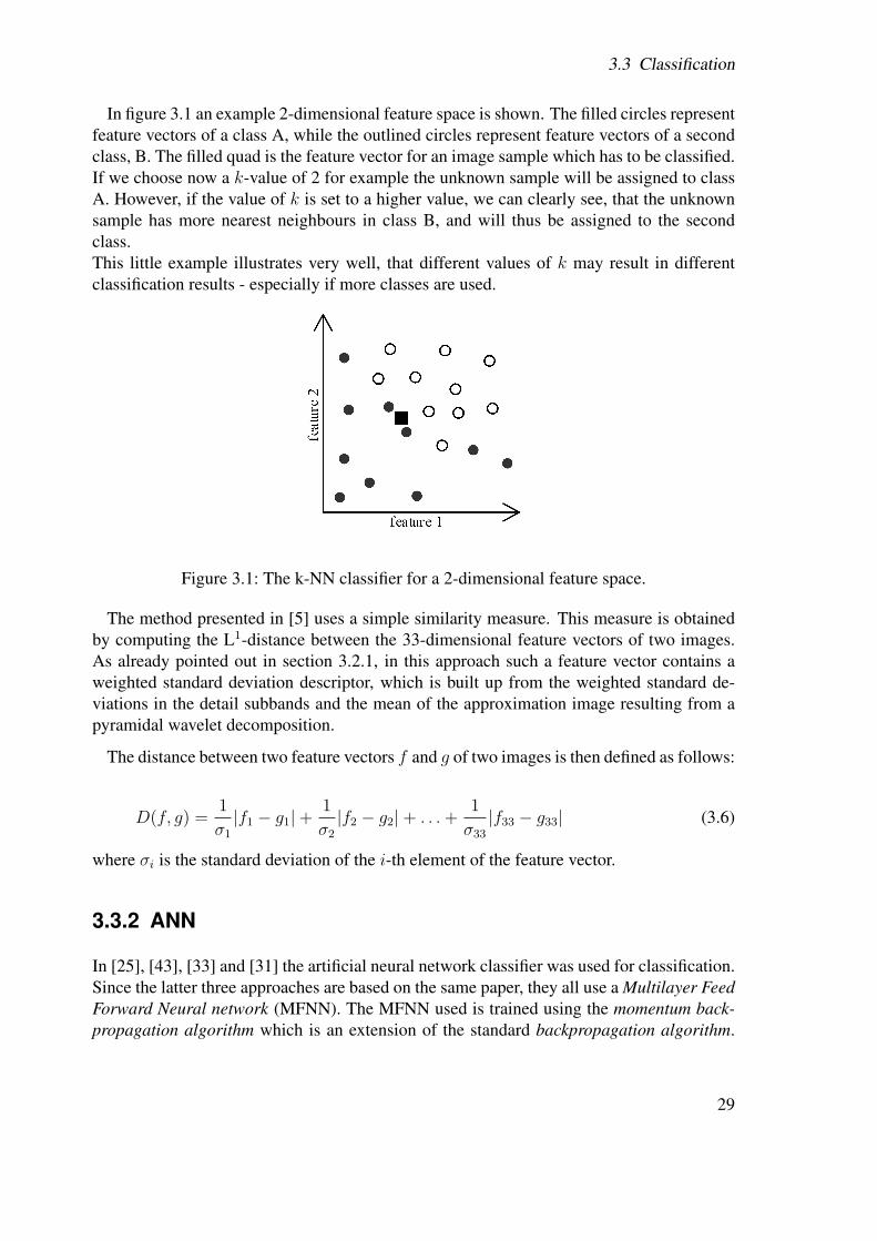
In figure 3.1 an example 2-dimensional feature space is shown. The filled circles representfeature vectors of a class A, while the outlined circles represent feature vectors of a secondclass, B. The filled quad is the feature vector for an image sample which has to be classified.If we choose now a k-value of 2 for example the unknown sample will be assigned to classA. However, if the value of k is set to a higher value, we can clearly see, that the unknownsample has more nearest neighbours in class B, and will thus be assigned to the secondclass.This little example illustrates very well, that different values of k may result in differentclassification results - especially if more classes are used.
Figure 3.1: The k-NN classifier for a 2-dimensional feature space.
The method presented in [5] uses a simple similarity measure. This measure is obtainedby computing the L1-distance between the 33-dimensional feature vectors of two images.As already pointed out in section 3.2.1, in this approach such a feature vector contains aweighted standard deviation descriptor, which is built up from the weighted standard de-viations in the detail subbands and the mean of the approximation image resulting from apyramidal wavelet decomposition.
The distance between two feature vectors f and g of two images is then defined as follows:
D(f, g) =1
σ1
|f1 − g1|+1
σ2
|f2 − g2|+ . . .+1
σ33
|f33 − g33| (3.6)
where σi is the standard deviation of the i-th element of the feature vector.
3.3.2 ANN
In [25], [43], [33] and [31] the artificial neural network classifier was used for classification.Since the latter three approaches are based on the same paper, they all use a Multilayer FeedForward Neural network (MFNN). The MFNN used is trained using the momentum back-propagation algorithm which is an extension of the standard backpropagation algorithm.
29
3 Texture classification
After the MFNN has been trained successfully it is able to discriminate between normal andabnormal texture regions by forming hyperplane decision boundaries in the pattern space.In [43], [33] and [31] the ANN is fed with feature vectors, which contain wavelet coefficientco-occurrence matrix based features based on the subbands resulting from a 1-level DWT.Karkanis et al. use in [25] a very similar approach, but consider only the subband exhibitingthe maximum variance for feature vector creation.
According to the results in the publications the classification results are promising sincethe system used has been proven capable to classify and locate regions of lesions with asuccess rate of 94 up to 99%.
The approach in [44] uses an artificial neural network for classification too. The colorfeatures extracted in this approach are used as input for a Backpropagation Neural Network(BPNN) which is trained using various training algorithms such as resilient propagation,scaled conjugate gradient algorithm and the Marquardt algorithm.Depending on the training algorithm used for the BPNN and the combination of featureswhich is used as input for the BPNN this approach reaches an average classification accuracybetween 89 and 98%.
The last of the presented methods also using artificial neural networks is presented in [13].The 84 features extracted with this method are used as input for a multilayer backpropaga-tion neural network. This results in a classification accuracy between 85 and 90%.
3.3.3 SVM
The SVM classifier, further described in [7, 20], is another, more recent technique for dataclassification, which has already been used for example by Rajpoot in [36] to classify textureusing wavelet features.
The basic idea behind support vector machines is to construct classifying hyperplaneswhich are optimal for separation of given data. Apart from that the hyperplanes constructedfrom some training data should have the ability to classify any unknown data presented tothe classifier as well as possible.
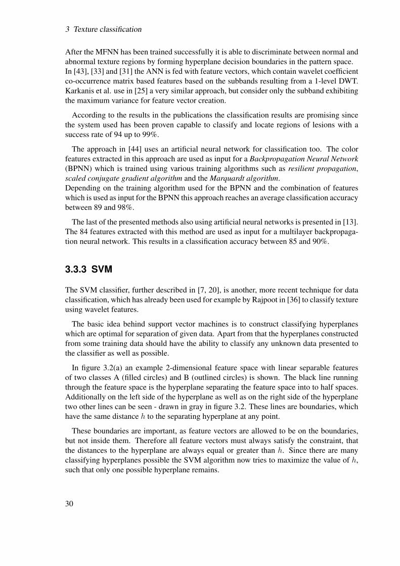
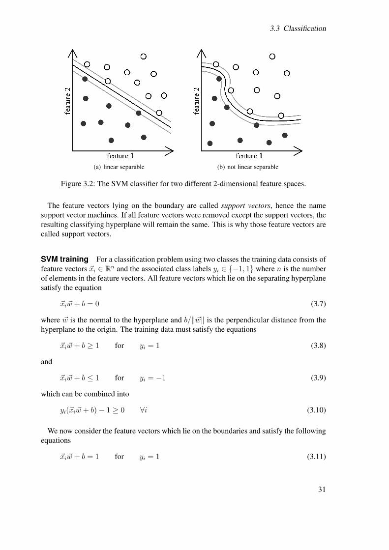
In figure 3.2(a) an example 2-dimensional feature space with linear separable featuresof two classes A (filled circles) and B (outlined circles) is shown. The black line runningthrough the feature space is the hyperplane separating the feature space into to half spaces.Additionally on the left side of the hyperplane as well as on the right side of the hyperplanetwo other lines can be seen - drawn in gray in figure 3.2. These lines are boundaries, whichhave the same distance h to the separating hyperplane at any point.
These boundaries are important, as feature vectors are allowed to be on the boundaries,but not inside them. Therefore all feature vectors must always satisfy the constraint, thatthe distances to the hyperplane are always equal or greater than h. Since there are manyclassifying hyperplanes possible the SVM algorithm now tries to maximize the value of h,such that only one possible hyperplane remains.
30
3.3 Classification
(a) linear separable (b) not linear separable
Figure 3.2: The SVM classifier for two different 2-dimensional feature spaces.
The feature vectors lying on the boundary are called support vectors, hence the namesupport vector machines. If all feature vectors were removed except the support vectors, theresulting classifying hyperplane will remain the same. This is why those feature vectors arecalled support vectors.
SVM training For a classification problem using two classes the training data consists offeature vectors ~xi ∈ Rn and the associated class labels yi ∈ {−1, 1} where n is the numberof elements in the feature vectors. All feature vectors which lie on the separating hyperplanesatisfy the equation
~xi ~w + b = 0 (3.7)
where ~w is the normal to the hyperplane and b/‖~w‖ is the perpendicular distance from thehyperplane to the origin. The training data must satisfy the equations
~xi ~w + b ≥ 1 for yi = 1 (3.8)
and
~xi ~w + b ≤ 1 for yi = −1 (3.9)
which can be combined into
yi(~xi ~w + b)− 1 ≥ 0 ∀i (3.10)
We now consider the feature vectors which lie on the boundaries and satisfy the followingequations
~xi ~w + b = 1 for yi = 1 (3.11)
31
3 Texture classification
and
~xi ~w + b = −1 for yi = −1 (3.12)
Using the euclidean distance between a vector ~x and the hyperplane (~w, b)
d(~w, b; ~x) =|~x~w + b|‖~w‖
(3.13)
and the constraints imposed by equations (3.11) and (3.12), the distance between the featurevectors which are closest to the separating hyperplane is defined by
h =1
‖~w‖(3.14)
Thus, the optimal hyperplane can be found by maximizing h, which is equal to minimizing‖~w‖2 and satisfying the constraint defined by equation (3.10).
Nonlinear problems The method described above works well for problems which arelinear separable. But as depicted in figure 3.2(b), many problems are not linear separable.The boundaries are no longer lines, like in figure 3.2(a), but curves. In the nonlinear casethe main problem is that the separating hyperplane is no longer linear which imposes com-putational complexity to the problem. To overcome this problem the SVM classifier usesthe Kernel trick.The basic idea is to map the input data to some higher dimensional (maybe infinite) eu-clidean space H using a mapping function Φ.
Φ : Rn → H (3.15)
Then the SVM finds a linear separating hyperplane in this higher dimensional space. Sincethe mapping can be very costly a kernel function K is used.
K(~xi, ~xi) = Φ(~xi) · Φ(~xj) (3.16)
Using K we need never to know explicitly what Φ looks like, but only use K. Somecommonly used choices for the kernel function K are
Linear
K(xj, xj) = xTi xj (3.17)
Polynomial
K(xj, xj) = (γxTi xj + r)d with γ > 0 (3.18)
32
3.3 Classification
Radial basis function (RBF)
K(xj, xj) = e−γ‖xi−xj‖2 with γ > 0 (3.19)
Sigmoid
K(xj, xj) = tanh(γxTi xj + r) with γ > 0 (3.20)
where γ, r and d are kernel parameters.
Multi-class case So far we only focused on the two-class case. To handle the multi-class case as well the classification has to be extended in some way. An overview of possiblemethods to handle more classes with the SVM can be found in [21]. Here we present theone-against-one approach only, since this is the method used in libSVM [8].This method creates k(k− 1)/2 classifiers, where k is the number of different classes. Eachof these classifiers can then be used to make a binary classification between some classes caand cb where a, b ∈ {1, . . . , k} and a 6= b.
Now, each binary classification is regarded as voting. An input vector ~xi, which has tobe classified, is classified using each of the binary classifiers. This results in a class label,whose according voting is incremented by one. After ~xi has been classified with all of thek(k − 1)/2 binary classifiers, the class with the maximum number of votes is assigned to~xi.
33

3 Texture classification
34
4 Automated pit patternclassification
In order to succeed, your desire for successshould be greater than your fear of failure.
- Bill Cosby
4.1 Introduction
Based on the preliminaries introduced in the last two chapters this chapter now presentsmethods we developed for an automated classification of pit pattern images. We describea few techniques and algorithms to extract features from image data and how to perform aclassification based on these features. Additionally this chapter introduces two classificationschemes without any wavelet subband feature extraction involved.
4.2 Classification based on features
The methods presented in this section first extract feature vectors from the images used,which are then used to train classifiers. The used classifiers and the process of classifiertraining and classification is then further described in section 4.4.
4.2.1 Feature extraction
4.2.1.1 Best-basis method (BB)
In section 2.6.1 two different methods for basis selection have been presented. The clas-sification scheme presented in this section is based on the best-basis algorithm, which, asalready stated before, is primarily used for compression of image data. This approach how-ever uses the best basis algorithm to try to classify image data.
During the training process all images in IT are decomposed to obtain the wavelet packetcoefficients for each image. Additionally during the decomposition some cost informationis stored along with each node of the respective quadtree. This cost information is basedon the chosen cost function and is used to determine the importance of a subband for the
35
4 Automated pit pattern classification
feature extraction. This is important since during the feature extraction process the questionarises, which subbands to choose to build the feature vector from.
If the number of subbands for an image I is denoted by sI the maximum number of sub-bands which can be used to extract features smax from each of the images is
smax = min1<i≤n
sIi(4.1)
where n is the total number of images and sIiis the number of subbands of image Ii resulting
from the wavelet packet decomposition. The calculation of smax is important since it can notbe guaranteed that all images result in a decomposition tree with the same number of leafs(subbands respectively) - in fact the higher the number of images is the more improbablethis would be. But since the feature vectors must all be of the same length it is important toextract the same number of features from each image.
Now that it is clear how many subbands can be used to extract features there must be madesome choice on which subbands to use. This is the moment where the cost informationstored along with the tree nodes is used.
If Si denotes the list of all subbands of an image indexed by i and Si denotes an arbitrarysubband of the same image, Si can be written as
Si = {S1, S2, . . . , SsIi} (4.2)
Since the cost information of the nodes and therefore of the subbands expresses the impor-tance of a subband for the feature extraction process, the subbands are first sorted by theircost information with the subbands with the highest cost at the beginning of the list. Aftersorting Si by the cost information the result is a new list Oi which is ordered now.
Oi = {Sα1 , Sα2 , . . . , SαsIi} (4.3)
with
cα1 ≥ cα2 ≥ . . . ≥ cαsIi(4.4)
where cαjis the cost information stored along with the αj-th subband. Then the first smax
subbands of the sorted list are marked as feature nodes. A feature node in this contextis nothing more than a subband which is to be used for the feature extraction process. Asubband Sαi
is marked as a feature node if i ≤ smax.
The subset of Oi consisting of feature nodes only now is taken for the creation of thefeature vector:
Fi = {Sα1 , Sα2 , . . . , Sαsmax} (4.5)
The construction of the feature vector Fi is then
Fi = F(Fi) F : Fi 7→ Rsmax (4.6)
36

4.2 Classification based on features
with
Fi = {f1, f2, . . . , fsmax} (4.7)
where F is the feature extractor chosen and fi is the feature for a subband Si.
But the feature vectors just created can not yet be fed into any classifier, since we stillhave a major problem. Due to the fact that the best-basis algorithm most times will producedifferent decomposition structures and therefore different lists of subbands for different im-ages, it can not be assured that later, during the classification process, the features of thesame subbands among the images are compared. It is even possible, that a feature for asubband, which is present in the subband list for one image is not present in the subband listfor another image.Therefore, when the feature vectors for all images have been created we have to perform thefollowing steps to post-process the feature vectors:
1. We create a dominance tree TD, which is a full wavelet packet tree with a decompo-sition depth lmax (the maximum decomposition depth among all decomposition treesfor all images).
2. This dominance tree is now updated using the decomposition tree Ti for a trainingimage indexed by i.This updating process is done by comparing the tree Ti and Td node by node. For eachnode Td,j present in Td we try to find the according node Ti,j at the same position j inthe tree Ti.Such a node in the dominance tree holds the following two values:
• A counter cd,j , which is incremented by one if the tree Ti has a node at the treeposition j too, which additionally is marked as being a feature node.Thus, after the dominance tree has been updated with all trees for all trainingimages, this counter stores the number of times that specific node at tree positionj was present and selected as a feature node among all trees of the trainingimages.
This counter is used later as a measure of relevance for a specific subband andto decide whether that specific subband should be included in the process offeature vector creation. In other words, the higher the counter for a specificnode (subband) is, the higher is the chance that the according subband will bechosen to construct a part of the feature vector from its coefficients.
• A flag fd,j , indicating whether at least one of the trees of the training images hasa node located at tree position j. This flag is set the first time a tree Ti has a nodelocated at position j. This flag is used during the pruning process following inthe next step.
3. When TD has been updated for all Ti, TD gets pruned. This is done by traversingthe tree from the leafs upwards to the root and deleting any child nodes not present
37
4 Automated pit pattern classification
in any of the Ti. This is the moment the flag fd,j stored along with the nodes of thedominance tree is used.After the pruning process the dominance tree contains only nodes which are presentat least once among all Ti.
4. Now a list D of all nodes in TD is created, which is then sorted by the counter cd,j
stored along with the nodes of the dominance tree. The first entries of this sorted listare regarded as more relevant for feature extraction than those at the end of the list.This, as mentioned above, is due to the fact that a higher counter value means, thatthe according node was marked as a feature node more often than nodes at the end ofthe sorted node list having lower counter values.
5. Finally all feature vectors are recreated based on this list of dominance tree nodes.But instead of using the cost information stored along with the nodes in Ti to choosefrom which subbands to create the feature vectors, the subbands and the order of thesubbands to extract the feature vectors from are now derived from the informationstored in the dominance tree nodes.If we remember that smax subbands are to be used to create the feature vector, we usethe first smax entries of the ordered list of the dominance tree nodes D to constructthe new feature vector from. This means, that the new feature vector Fi for an imageindexed by i is created using a slightly modified version of equation (4.7)
Fi = {fβ1 , fβ2 , . . . , fβsmax} (4.8)
where βk denotes the tree position for the k-th dominance tree node in D.
With this extension it can be assured that all feature vectors are created from the samesubbands with the same subband ordering. But there is still the problem that the dominancetree may contain leaf nodes (subbands) which are simply not present in the decompositiontree of an image indexed by i. This may happen if the decomposition tree of that image gotpruned at the parent node of such a node during the best-basis pruning. Although it is nottotally correct, for the sake of simplicity we insert a feature value of 0 for such a subband.Now the feature vectors Fi are ready to be fed into a classifier of choice.
There are a variety of functions to choose for the feature extractor such as energy, loga-rithm of energy, variance, entropy and l-norm - just to name a few.If S is a subband of size w × w, the formulas for this feature functions, which extract onlyone feature value fi from a subband Si, are as follows:
Energy
fi =w2−1∑j=0
Si(j)2 (4.9)
38
4.2 Classification based on features
Logarithm of energy
fi =w2−1∑j=0
log∗(Si(j)2) (4.10)
Variance
fi =w2−1∑j=0
(µSi(j))2 with µ =
∑w2−1z=0 Si(j)
w2(4.11)
Entropy
fi = −w2−1∑j=0
Si(j)2 log∗(Si(j)
2) (4.12)
l-Norm
fi =w2−1∑j=0
|Si(j)| (4.13)
These feature extractors are based on the coefficients of the subbands directly. But thereare also other possibilities for features such as co-occurrence matrix based features for ex-ample.
In image processing a co-occurrence matrix C is a matrix of size n × n representing anestimate of probability that two pixels P1 and P2 of an image have the gray levels g1 and g2
respectively, where n is the number of different gray levels in the image and C(i, j) = 0 forall i, j ∈ [1, n] .Based on a spatial relation R for each pixel P1 in the image the pixel P2 satisfying relationR is determined. Then, taking the gray levels g1 and g2 at P1 and P2 respectively, theco-occurrence matrix is incremented by one at column g1 and row g2.
An example for a spatial relation R would be that a pixel P2 is d pixel right of a pixelP1. d can be any arbitrary number and R is not limited to a specific direction - any possibledirection can be used to construct a co-occurrence matrix. But it is important to mention thatR is not a symmetric relation. This means that, using the notation from above, P1 can beregarded as starting point and R expresses the direction and distance to some end point P2.Therefore P2 denotes the only possible resulting pixel position for some given P1 andR andthe resulting co-occurrence matrix represents only one specific relation R, that is directionand distance.It is clear that in general as a logical consequence the resulting co-occurrence matrix is notsymmetric either.
39
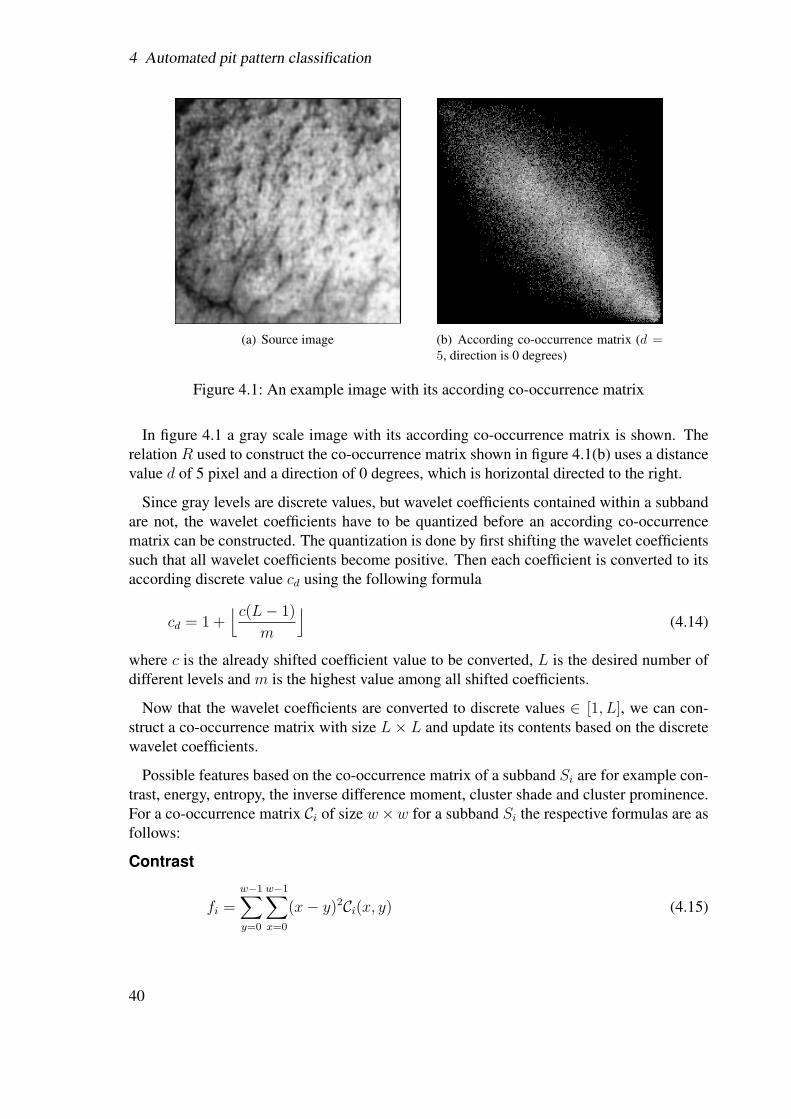
4 Automated pit pattern classification
(a) Source image (b) According co-occurrence matrix (d =5, direction is 0 degrees)
Figure 4.1: An example image with its according co-occurrence matrix
In figure 4.1 a gray scale image with its according co-occurrence matrix is shown. Therelation R used to construct the co-occurrence matrix shown in figure 4.1(b) uses a distancevalue d of 5 pixel and a direction of 0 degrees, which is horizontal directed to the right.
Since gray levels are discrete values, but wavelet coefficients contained within a subbandare not, the wavelet coefficients have to be quantized before an according co-occurrencematrix can be constructed. The quantization is done by first shifting the wavelet coefficientssuch that all wavelet coefficients become positive. Then each coefficient is converted to itsaccording discrete value cd using the following formula
cd = 1 +⌊c(L− 1)
m
⌋(4.14)
where c is the already shifted coefficient value to be converted, L is the desired number ofdifferent levels and m is the highest value among all shifted coefficients.
Now that the wavelet coefficients are converted to discrete values ∈ [1, L], we can con-struct a co-occurrence matrix with size L× L and update its contents based on the discretewavelet coefficients.
Possible features based on the co-occurrence matrix of a subband Si are for example con-trast, energy, entropy, the inverse difference moment, cluster shade and cluster prominence.For a co-occurrence matrix Ci of size w×w for a subband Si the respective formulas are asfollows:
Contrast
fi =w−1∑y=0
w−1∑x=0
(x− y)2Ci(x, y) (4.15)
40
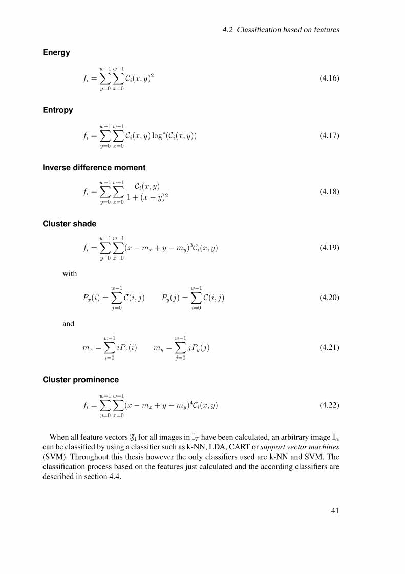
4.2 Classification based on features
Energy
fi =w−1∑y=0
w−1∑x=0
Ci(x, y)2 (4.16)
Entropy
fi =w−1∑y=0
w−1∑x=0
Ci(x, y) log∗(Ci(x, y)) (4.17)
Inverse difference moment
fi =w−1∑y=0
w−1∑x=0
Ci(x, y)
1 + (x− y)2(4.18)
Cluster shade
fi =w−1∑y=0
w−1∑x=0
(x−mx + y −my)3Ci(x, y) (4.19)
with
Px(i) =w−1∑j=0
C(i, j) Py(j) =w−1∑i=0
C(i, j) (4.20)
and
mx =w−1∑i=0
iPx(i) my =w−1∑j=0
jPy(j) (4.21)
Cluster prominence
fi =w−1∑y=0
w−1∑x=0
(x−mx + y −my)4Ci(x, y) (4.22)
When all feature vectors Fi for all images in IT have been calculated, an arbitrary image Iα
can be classified by using a classifier such as k-NN, LDA, CART or support vector machines(SVM). Throughout this thesis however the only classifiers used are k-NN and SVM. Theclassification process based on the features just calculated and the according classifiers aredescribed in section 4.4.
41
4 Automated pit pattern classification
4.2.1.2 Best-basis centroids (BBCB)
Just like the best-basis method described in section 4.2.1.1 this method is based on thebest-basis algorithm too. But there is a key difference between the method from section4.2.1.1 and the method from this section. While the best-basis method resulted in differentdecomposition structures due to the underlying best-basis algorithm this method alwaysexhibits the same decomposition structure.
Just like in section 4.2.1.1 first of all the training images are decomposed using the best-basis algorithm. But instead of using the resulting decomposition structures and subbandsfor feature extraction, a centroid (see section 4.3.4) based on the decomposition structuresof all classes is calculated. This results in one centroid for all images. Then all images aredecomposed again, but this time into the structure of the centroid.
Although all images are transformed into the same subband structure, it is not guaranteedthat the subbands are extracted in the same order for different images. This is due to thefact that, as explained in section 4.2.1.1, we use the first smax subbands from the orderedlist of subbands in equation (4.3) which is ordered by cost information. But since the costinformation for some specific subband sometimes will not be the same for all images, theordered lists of subbands among all images may differ.
Therefore this method uses the dominance tree extension too, to guarantee that all createdfeature vectors contain the same subbands in the same order.
4.2.1.3 Pyramidal wavelet transform (WT)
This method is very similar to the method described in section 4.2.1.2. The are only smalldifferences such as the usage of the pyramidal wavelet transform instead of the waveletpackets transform in conjunction with a centroid base. This again yields the same decom-position tree for all images in IT and for all testing images Iα to be classified. Hence thenumber of subbands is equal among all images and the calculation of smax can be written as
smax = 3l + 1 (4.23)
since a wavelet transform of an image to l levels always results in 3l + 1 subbands.Another important difference is the lack of cost information in the pyramidal wavelet trans-form, since no pruning takes place. Therefore it is necessary to slightly extend the wavelettransform to store some cost information along with the decomposition tree nodes. This canbe done by simply evaluating the cost of a node just as in the best-basis method.
The remaining parts of the feature vector calculations and the classification process arejust the same as in the previous method. Although the pyramidal decomposition always pro-duces the same list of subbands for each image, the same problem as described in section4.2.1.2 arises and it is not assured that for a smax the same subbands are used for the feature
42
4.2 Classification based on features
vector creation process for all images. Therefore the dominance tree extension is used inthis method too.Since the dominance tree extension is based on cost information stored along with the sub-bands but the pyramidal decomposition does not rely on any cost information, throughoutthis thesis the pyramidal decomposition additionaly stores the cost for each subband. Tocalculate the cost information the L2-norm is used.
4.2.1.4 Local discriminant bases (LDB)
In contrast to the previous methods this method is already based on a feature extractionscheme which is highly focused on discrimination between classes. Since in the past theLDB algorithm has already been successfully applied to classification problems [37, 40, 41]it is an excellent candidate to be used for this thesis.
While in all previous methods the training images are analyzed regardless of the classesthe images belong to, this method, as already described in section 2.6.1, constructs a waveletpacket basis which is optimal for differentiating between images of different classes.Once this basis has been calculated all training images are decomposed into this basis, whichyields the same number of subbands Smax for all images in IT . And since this method isbased already on discriminant power, the discriminant power for each subband is storedalong with the respective node of the decomposition tree. This information is then usedlike in section 2.6.1.1 to construct the feature vector extracted from the most discriminantsubbands. Again, if Si denotes the list of all subbands of an image i and Si denotes anarbitrary subband of the same image, Si can be written as
Si = {S1, S2, . . . , SsIi} (4.24)
After sorting this list by the discriminant power, a new list Oi is created which is orderednow.
Oi = {Sα1 , Sα2 , . . . , SαsIi} (4.25)
with
pα1 ≥ pα2 ≥ . . . ≥ pαsIi(4.26)
where pαjis the discriminant power for the αj-th subband.
Now the feature vector is created like in the best-basis method, using the same set of possiblefeature functions F and using the first k most discriminant subbands.
The remaining part of the classification process is the same as in the previous two methods.Since the nature of the LDB already defines the list of subbands to extract the features fromand the ordering of the subbands, the dominance tree is not needed here.
43
4 Automated pit pattern classification
4.3 Structure-based classification
While the classification methods presented in the previous sections were based on featuresbased on wavelet coefficients and therefore needed some classifier to be trained, the nextsections introduce a classification method, which does not involve any feature extractionin terms of image features. Instead the “centroid classification” tries to assign pit patternclasses to unknown images by decomposing the image and compare the resulting decompo-sition structure to the centroids of the respective classes.But first of all a quick introduction into quadtrees and a description of the used quadtreedistance metrics are given.
4.3.1 A quick quadtree introduction
A quadtree is a tree with the important property, that every node in a quadtree having childnodes has exactly four child nodes. As all trees in mathematics a quadtree can be definedlike a graph by a vertex set V an edge set E. For a tree with n ∈ N+ nodes this can bewritten formally as
V = {v1, . . . , vn} with |V | = n (4.27)
E = {(vi, vj)|i 6= j, vi, vj ∈ V } (4.28)
where the elements vi ∈ V are called vertices and the elements ej ∈ E are called edges.Vertices which do not have any child nodes are called leaf nodes.
4.3.2 Distance by unique nodes
This distance metric tries to measure a distance between two quadtrees by first assigningeach node of the quadtrees an unique node value, which is unique among all possiblequadtrees. Then for each quadtree a list of quadtree node values is generated which arethen compared against each other to identify nodes which appear in one of the two treesonly.
4.3.2.1 Unique node values
To be able to compare different quadtrees, we must be able to uniquely identify a nodeaccording to its position in the quadtree. To accomplish this we assign a unique number toeach node according to its position in the tree.
44

4.3 Structure-based classification
4.3.2.2 Renumbering the nodes
As already mentioned above renumbering is necessary since we want a unique number foreach node in the tree depending only on the path to the node. Normally the nodes in a treewould be numbered arbitrarily. By renumbering the vertices of the quadtree we get a list ofvertices which is defined very similar to equation (4.27):
V = {vu1 , . . . , vun} with |V | = n (4.29)
where the numbers u1, . . . , un are the unique numbers of the respective nodes.
These numbers can be mapped through a function U
U : V −→ N (4.30)
where U must have the properties
U(vi) = U(vj) ⇔ i = j (4.31)
and
U(vi) 6= U(vj) ⇔ i 6= j (4.32)
4.3.2.3 Unique number generation
A node in a quadtree can also be described by the path in the tree leading to the specificnode. As we saw in section 4.3.1, if a node in a quadtree has child nodes there are alwaysexactly four children. This means that for each node in the tree having child nodes we havethe choice between four possible child nodes to traverse down the tree.
By defining the simple function s
s(vl) =
1, if vl is the lower left child node of the parent node2, if vl is the lower right child node of the parent node3, if vl is the upper left child node of the parent node4, if vl is the upper right child node of the parent node
, (4.33)
we can express the path to a node vi as sequence Pviwhich is defined as
Pvi= (p1, . . . , pM) (4.34)
where M is the length of the path and for 1 ≤ j ≤M the values pj are given by
pj = s(vm) (4.35)
where m is the index of the j-th node of the path into the vertex set V .
45
4 Automated pit pattern classification
4.3.2.4 The mapping function
To construct the mapping function U from section 4.3.2.2, which maps a vertex vi to aunique number ui, we use the formula
ui =M∑
j=1
5jpj where pj ∈ Pvi(4.36)
where M is the number of nodes along the path to the node vi. j is nothing more than thedepth level in the tree of the j-th node in the path to node vi. Hence equation (4.36) is justa p-adic number with p = 5 which is a unique representation of a number with base 5.Base 5 is required since at each node there are four possible ways to traverse down the tree.If we used base 4 we would only have the digits 0 to 3, which is not useful since this wouldresult in a tree with multiple nodes having a unique id of 0.
To ensure that every ui is unique for all vi ∈ V the requirement that a path sequencePvi
for a node vi must be unique among the quadtree must be met. And since a quadtreecontains no cycles and every node in a tree has only one parent node, this requirement ismet.
4.3.2.5 The metric
We are now able to express the similarity between to quadtrees by measuring the distancebetween them. Distance, in this context, is a function d(T1, T2) which returns the real valueddistance between two quadtrees T1 and T2, which are elements of the so-called metric set T.More formally this can be written as
d : T× T −→ R (4.37)
Now the following properties for metrics hold for all T1, T2 ∈ T:
d(T1, T2) > 0 ⇔ T1 6= T2 (4.38)
d(T1, T2) = 0 ⇔ T1 = T2 (4.39)
d(T1, T2) = d(T2, T1) (4.40)
Therefore this distance between two quadtrees can be used to express the similarity be-tween two quadtrees.
46
4.3 Structure-based classification
4.3.2.6 The distance function
We can now represent each node vi in the quadtree by its unique value ui which is a uniquenumber for the path to the node too as shown in section 4.3.2.4.
Thus we now create the unordered sets of unique values for the trees T1 and T2 which aredenoted by LT1 and LT2 defined as
LT1 = {u1j |1 ≤ j ≤ n1} (4.41)
where n1 is the number of nodes in T1 and u1j is the unique number for the j-th node of T1
subtracted from 5ml+1. The definition of LT2 is similar
LT2 = {u2j |1 ≤ j ≤ n2} (4.42)
where n2 is the number of nodes in T2 and u2j is the unique number for the j-th node of T2
subtracted from 5ml+1. ml is the maximum quadtree depth level among the two quadtreesto compare.
Having this set we now can compare them for similarity and calculate a distance.
To compare the quadtrees T1 and T2 we compare the lists LT1 and LT2 for equal nodes. Todo this for each element u1
j we look into LT2 for a u2k such that
u1j = u2
k with 1 ≤ j ≤ n1 and 1 ≤ k ≤ n2 (4.43)
Apart from that we introduce the value t1 and t2 which are just the sum over all uniquevalues of the nodes of T1 and T2 respectively. Additionally the value tmax is introduced asthe maximum of t1 and t2. This can be written as:
t1 =
n1∑j=1
u1j (4.44)
t2 =
n2∑j=1
u2j (4.45)
tmax = max(t1, t2) (4.46)
If we do not find a u1j and a u2
k satisfying equation (4.43) we calculate a similarity value svusing the following formula
sv1 =S∑
z=1
u1z (4.47)
47
4 Automated pit pattern classification
where S is the number of different nodes in the two trees and u1z is the z-th node value which
is only contained in the first quadtree subtracted from 5ml+1. The same procedure is donefor all nodes in the second tree. We sum up all unique node values of the second tree whichare not contained within the first quadtree.
sv2 =S∑
z=1
u2z (4.48)
The final similarity value is then
sv = sv1 + sv2 (4.49)
Finally this similarity value is normalized to always be between 0 and 1. This is done bydividing sv by the maximum difference which can occur in terms of the unique node values.This results in the final formula for sv:
sv =sv1 + sv2
t1 + t2(4.50)
It is obvious that sv is 0 for equal trees since then the expression sv1 + sv2 equals zero.And it is also obvious that sv can never exceed 1, since if all nodes are different sv1 + sv2
becomes t1 + t2 which results in a similarity value of 1.This function already satisfies the requirement of the distance function from equation (4.40)for equal trees to be 0, thus the final distance can be formulated as
d(T1, T2) = sv (4.51)
This distance in now in the range between 0 (for equal trees) and 1 for completely differenttrees. Apart from that the distance has the property that differences in the first levels of thequadtree contribute more to the distance than differences in the deeper levels. This is dueto the fact that the unique numbers contained within LT1 and LT2 get smaller down the tree.The biggest value is therefore assigned to the root node of the trees.
Figures 4.2(b)-(e) show some example quadtrees for which the distances to the tree infigure 4.2(a) have been measured. The resulting distances listed in table 4.1 clearly show,that, as intended, differences in the upper levels of a quadtree contribute more to the distancethan differences in the lower levels.
4.3.3 Distance by decomposition strings
This approach measures the distance between two quadtrees by creating a decompositionstring for each tree and comparing these strings for equal string sequences.
48
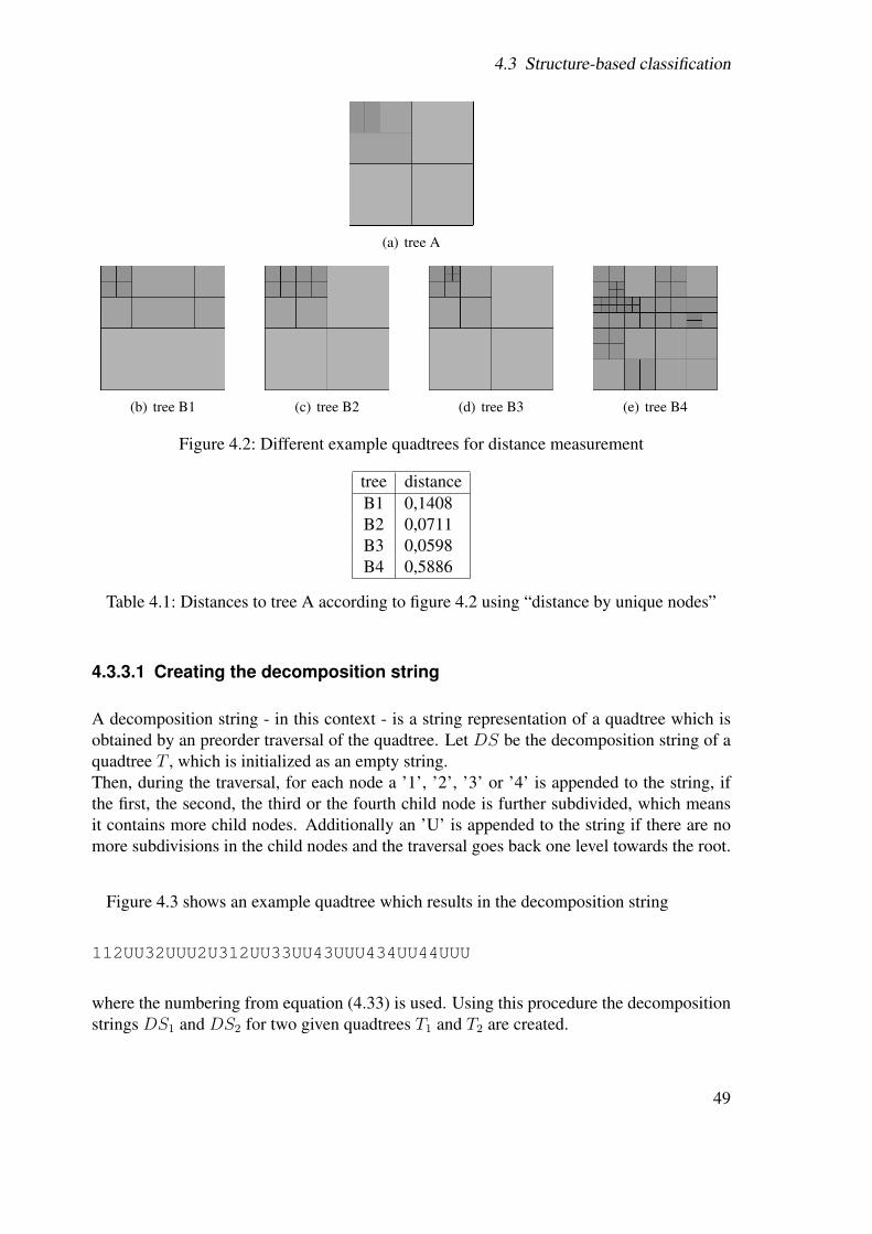
4.3 Structure-based classification
(a) tree A
(b) tree B1 (c) tree B2 (d) tree B3 (e) tree B4
Figure 4.2: Different example quadtrees for distance measurement
tree distanceB1 0,1408B2 0,0711B3 0,0598B4 0,5886
Table 4.1: Distances to tree A according to figure 4.2 using “distance by unique nodes”
4.3.3.1 Creating the decomposition string
A decomposition string - in this context - is a string representation of a quadtree which isobtained by an preorder traversal of the quadtree. Let DS be the decomposition string of aquadtree T , which is initialized as an empty string.Then, during the traversal, for each node a ’1’, ’2’, ’3’ or ’4’ is appended to the string, ifthe first, the second, the third or the fourth child node is further subdivided, which meansit contains more child nodes. Additionally an ’U’ is appended to the string if there are nomore subdivisions in the child nodes and the traversal goes back one level towards the root.
Figure 4.3 shows an example quadtree which results in the decomposition string
112UU32UUU2U312UU33UU43UUU434UU44UUU
where the numbering from equation (4.33) is used. Using this procedure the decompositionstrings DS1 and DS2 for two given quadtrees T1 and T2 are created.
49
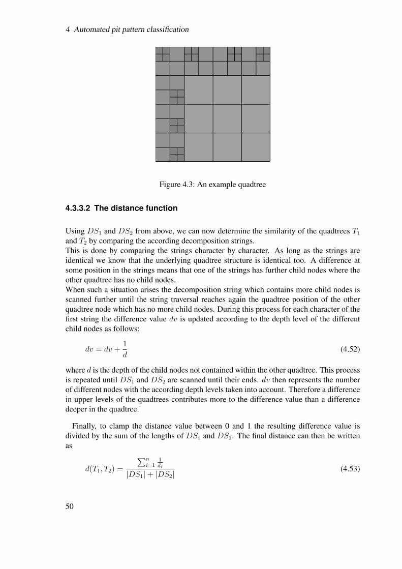
4 Automated pit pattern classification
Figure 4.3: An example quadtree
4.3.3.2 The distance function
Using DS1 and DS2 from above, we can now determine the similarity of the quadtrees T1
and T2 by comparing the according decomposition strings.This is done by comparing the strings character by character. As long as the strings areidentical we know that the underlying quadtree structure is identical too. A difference atsome position in the strings means that one of the strings has further child nodes where theother quadtree has no child nodes.When such a situation arises the decomposition string which contains more child nodes isscanned further until the string traversal reaches again the quadtree position of the otherquadtree node which has no more child nodes. During this process for each character of thefirst string the difference value dv is updated according to the depth level of the differentchild nodes as follows:
dv = dv +1
d(4.52)
where d is the depth of the child nodes not contained within the other quadtree. This processis repeated until DS1 and DS2 are scanned until their ends. dv then represents the numberof different nodes with the according depth levels taken into account. Therefore a differencein upper levels of the quadtrees contributes more to the difference value than a differencedeeper in the quadtree.
Finally, to clamp the distance value between 0 and 1 the resulting difference value isdivided by the sum of the lengths of DS1 and DS2. The final distance can then be writtenas
d(T1, T2) =
∑ni=1
1di
|DS1|+ |DS2|(4.53)
50
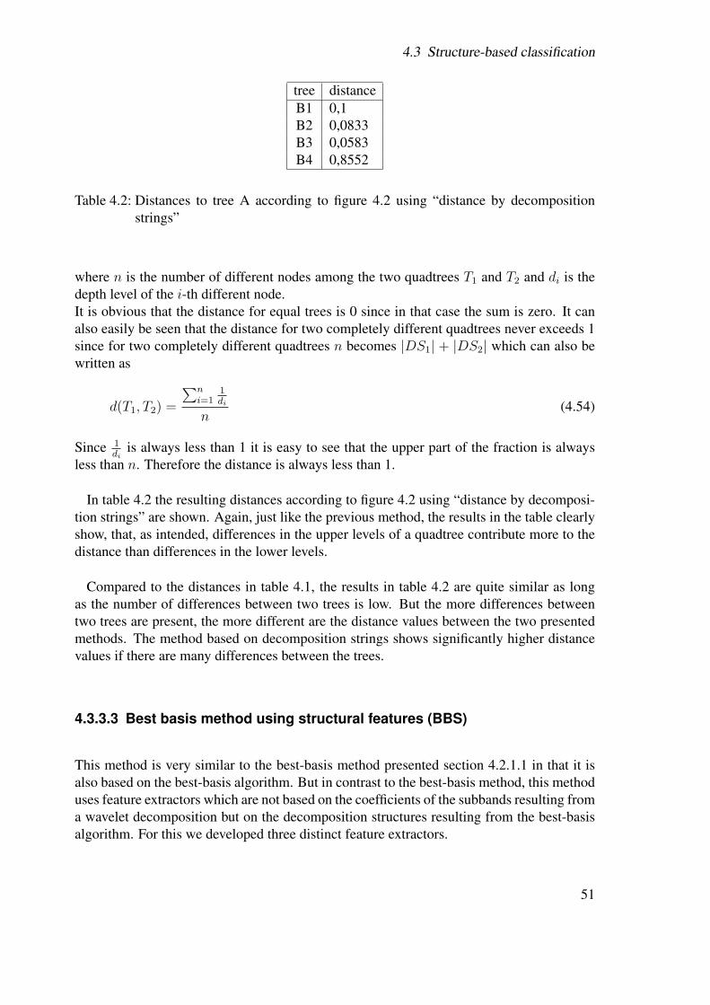
4.3 Structure-based classification
tree distanceB1 0,1B2 0,0833B3 0,0583B4 0,8552
Table 4.2: Distances to tree A according to figure 4.2 using “distance by decompositionstrings”
where n is the number of different nodes among the two quadtrees T1 and T2 and di is thedepth level of the i-th different node.It is obvious that the distance for equal trees is 0 since in that case the sum is zero. It canalso easily be seen that the distance for two completely different quadtrees never exceeds 1since for two completely different quadtrees n becomes |DS1| + |DS2| which can also bewritten as
d(T1, T2) =
∑ni=1
1di
n(4.54)
Since 1di
is always less than 1 it is easy to see that the upper part of the fraction is alwaysless than n. Therefore the distance is always less than 1.
In table 4.2 the resulting distances according to figure 4.2 using “distance by decomposi-tion strings” are shown. Again, just like the previous method, the results in the table clearlyshow, that, as intended, differences in the upper levels of a quadtree contribute more to thedistance than differences in the lower levels.
Compared to the distances in table 4.1, the results in table 4.2 are quite similar as longas the number of differences between two trees is low. But the more differences betweentwo trees are present, the more different are the distance values between the two presentedmethods. The method based on decomposition strings shows significantly higher distancevalues if there are many differences between the trees.
4.3.3.3 Best basis method using structural features (BBS)
This method is very similar to the best-basis method presented section 4.2.1.1 in that it isalso based on the best-basis algorithm. But in contrast to the best-basis method, this methoduses feature extractors which are not based on the coefficients of the subbands resulting froma wavelet decomposition but on the decomposition structures resulting from the best-basisalgorithm. For this we developed three distinct feature extractors.
51
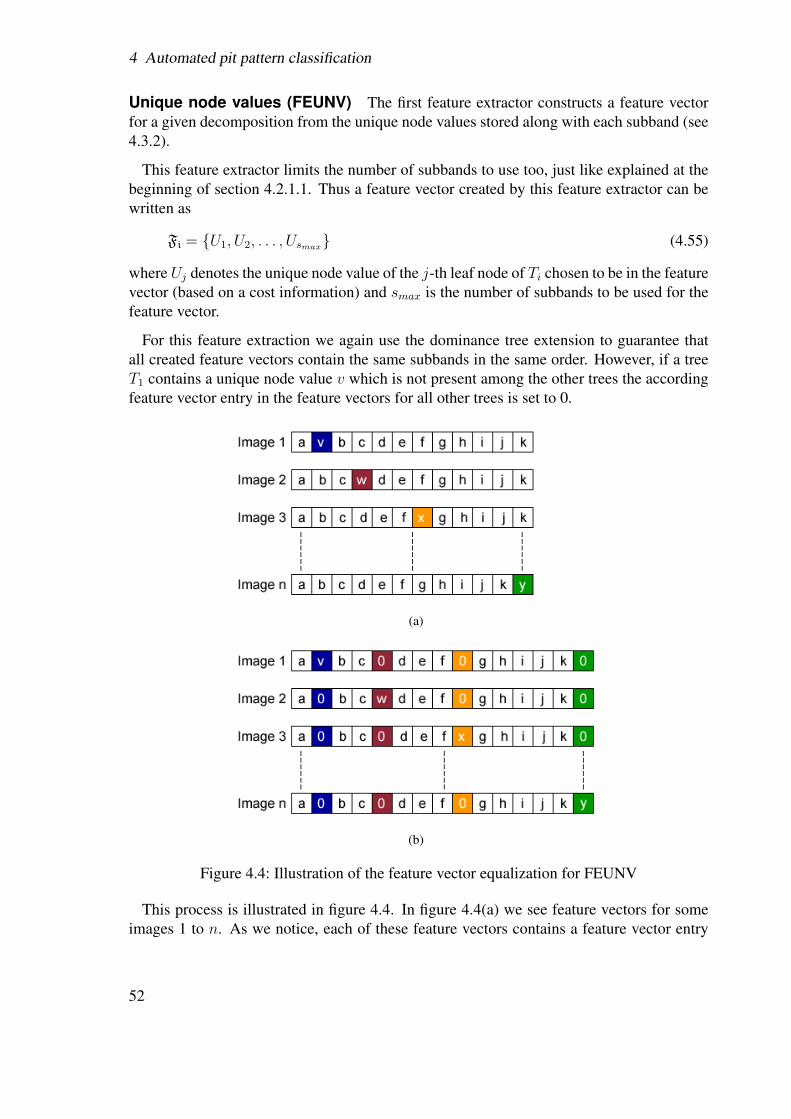
4 Automated pit pattern classification
Unique node values (FEUNV) The first feature extractor constructs a feature vectorfor a given decomposition from the unique node values stored along with each subband (see4.3.2).
This feature extractor limits the number of subbands to use too, just like explained at thebeginning of section 4.2.1.1. Thus a feature vector created by this feature extractor can bewritten as
Fi = {U1, U2, . . . , Usmax} (4.55)
where Uj denotes the unique node value of the j-th leaf node of Ti chosen to be in the featurevector (based on a cost information) and smax is the number of subbands to be used for thefeature vector.
For this feature extraction we again use the dominance tree extension to guarantee thatall created feature vectors contain the same subbands in the same order. However, if a treeT1 contains a unique node value v which is not present among the other trees the accordingfeature vector entry in the feature vectors for all other trees is set to 0.
(a)
(b)
Figure 4.4: Illustration of the feature vector equalization for FEUNV
This process is illustrated in figure 4.4. In figure 4.4(a) we see feature vectors for someimages 1 to n. As we notice, each of these feature vectors contains a feature vector entry
52
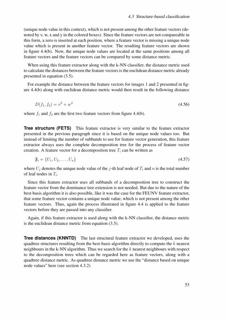
4.3 Structure-based classification
(unique node value in this context), which is not present among the other feature vectors (de-noted by v, w, x and y in the colored boxes). Since the feature vectors are not compareable inthis form, a zero is inserted at each position, where a feature vector is missing a unique nodevalue which is present in another feature vector. The resulting feature vectors are shownin figure 4.4(b). Now, the unique node values are located at the same positions among allfeature vectors and the feature vectors can be compared by some distance metric.
When using this feature extractor along with the k-NN classifier, the distance metric usedto calculate the distances between the feature vectors is the euclidean distance metric alreadypresented in equation (3.5).
For example the distance between the feature vectors for images 1 and 2 presented in fig-ure 4.4(b) along with euclidean distance metric would then result in the following distance
D(f1, f2) = v2 + w2 (4.56)
where f1 and f2 are the first two feature vectors from figure 4.4(b).
Tree structure (FETS) This feature extractor is very similar to the feature extractorpresented in the previous paragraph since it is based on the unique node values too. Butinstead of limiting the number of subbands to use for feature vector generation, this featureextractor always uses the complete decomposition tree for the process of feature vectorcreation. A feature vector for a decomposition tree Ti can be written as
Fi = {U1, U2, . . . , Un} (4.57)
where Uj denotes the unique node value of the j-th leaf node of Ti and n is the total numberof leaf nodes in Ti.
Since this feature extractor uses all subbands of a decomposition tree to construct thefeature vector from the dominance tree extension is not needed. But due to the nature of thebest-basis algorithm it is also possible, like it was the case for the FEUNV feature extractor,that some feature vector contains a unique node value, which is not present among the otherfeature vectors. Thus, again the process illustrated in figure 4.4 is applied to the featurevectors before they are passed into any classifier.
Again, if this feature extractor is used along with the k-NN classifier, the distance metricis the euclidean distance metric from equation (3.5).
Tree distances (KNNTD) The last structural feature extractor we developed, uses thequadtree structures resulting from the best-basis algorithm directly to compute the k nearestneighbours in the k-NN algorithm. Thus we search for the k nearest neighbours with respectto the decomposition trees which can be regarded here as feature vectors, along with aquadtree distance metric. As quadtree distance metric we use the “distance based on uniquenode values” here (see section 4.3.2)
53
4 Automated pit pattern classification
4.3.4 Centroid classification (CC)
Similar to the best-basis method presented in section 4.2.1.1 this method is based on thecalculation of the best wavelet packet basis too. But in contrast to the best-basis methodthis method is not based on features extracted from the subbands resulting from the waveletpacket decomposition but on the quadtrees resulting from the wavelet packet decomposi-tion.
The idea behind this method is the question whether images decomposed using thewavelet packets algorithm in conjunction with the best-basis algorithm result in decom-position trees which can be further used for classification. A perfect classification wouldthen be possible if trees of one image class are more similar than trees resulting from im-ages of different classes. In other words, the similarity between trees of the same class mustbe much higher than the similarity of trees of different classes to be able to perform someuseful classification.The similarity of two quadtrees can be expressed by the distance between them as explainedin section 4.3.1.
It is worthwhile to mention that having a method to express the distances between twoquadtrees we could easily use that distance measure for a k-NN classification. This is exactlywhat the feature extractor KNNTD (see section 4.3.3.3 above) does. Since we know theclasses for all training images, for an unknown test image we create the respective best-basis decomposition tree and calculate the quadtree distances to all trees of the trainingimages. The class, which dominates over the k nearest training images is then assigned tothe unknown training image.
Now, having a method to express the distance between two quadtrees and a set of imagesIT used for training, first of all the distances between all possible pairs of quadtrees ofimages out of this set are calculated as follows
di,j = d(Ti, Tj) i, j ∈ {1, . . . , n} (4.58)
where Ti and Tj are the decomposition trees of the i-th and the j-th image respectively, n isthe number of images in IT and d is the quadtree distance metric used. ITc is the subset ofIT which contains all images of class c.
IT = IT1 ∪ IT2 ∪ · · · ∪ ITC(4.59)
where C is the total number of classes of images.
The trees Ti and Tj , as stated above, are the result of the best-basis algorithm and are theoptimal basis for the respective images in respect to a certain cost function such as the oneslisted in section 4.2.1.1.The distances di,j obtained above are now used to construct a distance matrix D of sizen× n with
dTi,Ti= 0 ∀i = 1, . . . , n (4.60)
54
4.3 Structure-based classification
since dTi,Tiis just the distance of a quadtree of an image to itself, which must by definition
of a metric always be 0. Therefore D is
D =
0 dT1,T2 . . . dT1,Tn
dT2,T1 0 . . . dT2,Tn
...... . . . ...
dTn,T1 dTn,T2 . . . 0
This matrix then contains the quadtree distances (similarities) between all possible pairs
of images out of the training image set.For each class c the matrix contains a submatrix Dc which contains the distances betweenall images belonging to class c. Therefore D can also be written as
D =
0 dT11 ,T12. . . dT11 ,T1n
. . . dT11 ,TC1. . . dT11 ,TCn
dT12 ,T110 . . . dT12 ,T1n
. . . dT12 ,TC1. . . dT12 ,TCn
...... . . . ...
......
......
dT1n ,T11dT1n ,T12
. . . 0 . . . dT1n ,TC1. . . dT1n ,TCn
......
...... . . . ...
......
dTC1,T11
dTC1,T12
. . . dTC1,T1n
. . . 0 . . . dTC1,TCn
......
......
...... . . . ...
dTCn ,T11dTCn ,T12
. . . dTCn ,T1n. . . dTCn ,TC1
. . . 0
where dTij
,Tklis the distance between the j-th image (quadtree) of class i and the l-th image
(quadtree) of class k.
Figure 4.5(a) shows an example distance matrix for the two-class case. This exampleshows a perfect distance matrix with very small intra-class distances (black boxes) and veryhigh inter-class distances (white boxes). In reality however, a distance matrix is more likelyto look like the one illustrated in figure 4.5(b), since the trees for different images from aspecific class hardly will be totally identical in real-world applications.As can been seen in figure 4.5 and following from equation (4.40) the distance matrices areall symmetric.
Having calculated the matrix D the next task is to find the centroid of each class. Acentroid of a class c in this context is the training image out of ITc which has the smallestaverage distance to all other images of class c. In other words, it is now necessary to find theimage of class c to which all other images of class c have the smallest distance in respect tothe chosen quadtree distance metric. After the centroids of all classes have been found theclassification process can now take place.
To classify an arbitrary image first of all the image is decomposed using the waveletpackets transform to get the respective decomposition tree. It is important to note that forclassification the same cost function has to be used for pruning the decomposition tree aswas used during the training phase for all training images. Then the distances of the result-ing decomposition tree to the decomposition trees of the centroids of all possible classes are
55
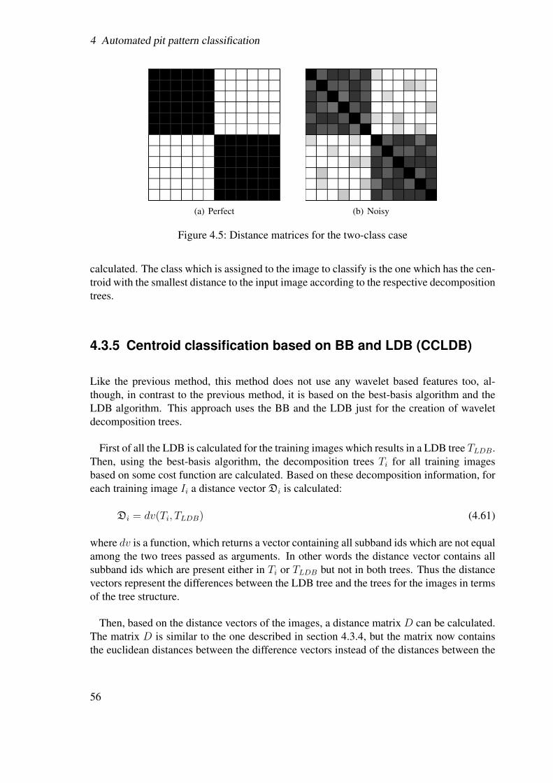
4 Automated pit pattern classification
(a) Perfect (b) Noisy
Figure 4.5: Distance matrices for the two-class case
calculated. The class which is assigned to the image to classify is the one which has the cen-troid with the smallest distance to the input image according to the respective decompositiontrees.
4.3.5 Centroid classification based on BB and LDB (CCLDB)
Like the previous method, this method does not use any wavelet based features too, al-though, in contrast to the previous method, it is based on the best-basis algorithm and theLDB algorithm. This approach uses the BB and the LDB just for the creation of waveletdecomposition trees.
First of all the LDB is calculated for the training images which results in a LDB tree TLDB.Then, using the best-basis algorithm, the decomposition trees Ti for all training imagesbased on some cost function are calculated. Based on these decomposition information, foreach training image Ii a distance vector Di is calculated:
Di = dv(Ti, TLDB) (4.61)
where dv is a function, which returns a vector containing all subband ids which are not equalamong the two trees passed as arguments. In other words the distance vector contains allsubband ids which are present either in Ti or TLDB but not in both trees. Thus the distancevectors represent the differences between the LDB tree and the trees for the images in termsof the tree structure.
Then, based on the distance vectors of the images, a distance matrix D can be calculated.The matrix D is similar to the one described in section 4.3.4, but the matrix now containsthe euclidean distances between the difference vectors instead of the distances between the
56
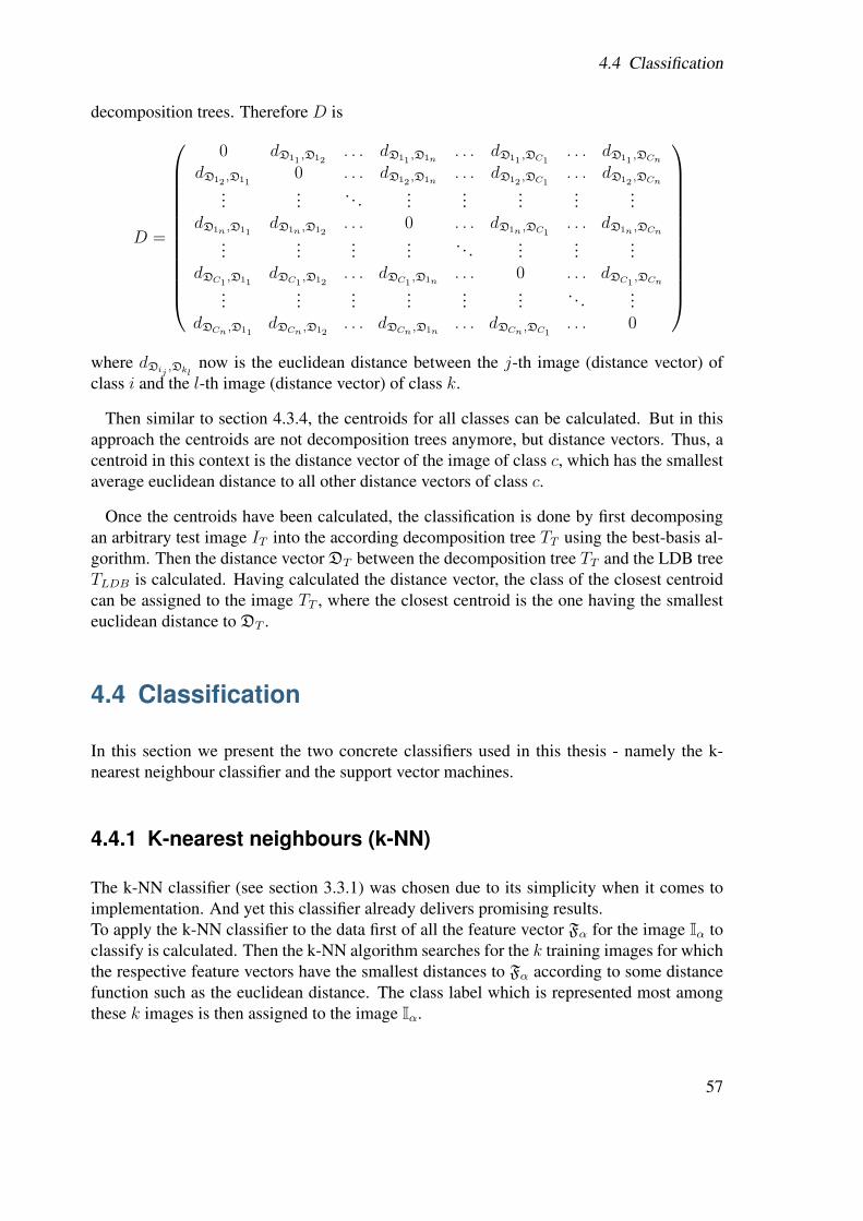
4.4 Classification
decomposition trees. Therefore D is
D =
0 dD11 ,D12. . . dD11 ,D1n
. . . dD11 ,DC1. . . dD11 ,DCn
dD12 ,D110 . . . dD12 ,D1n
. . . dD12 ,DC1. . . dD12 ,DCn
...... . . . ...
......
......
dD1n ,D11dD1n ,D12
. . . 0 . . . dD1n ,DC1. . . dD1n ,DCn
......
...... . . . ...
......
dDC1,D11
dDC1,D12
. . . dDC1,D1n
. . . 0 . . . dDC1,DCn
......
......
...... . . . ...
dDCn ,D11dDCn ,D12
. . . dDCn ,D1n. . . dDCn ,DC1
. . . 0
where dDij
,Dklnow is the euclidean distance between the j-th image (distance vector) of
class i and the l-th image (distance vector) of class k.
Then similar to section 4.3.4, the centroids for all classes can be calculated. But in thisapproach the centroids are not decomposition trees anymore, but distance vectors. Thus, acentroid in this context is the distance vector of the image of class c, which has the smallestaverage euclidean distance to all other distance vectors of class c.
Once the centroids have been calculated, the classification is done by first decomposingan arbitrary test image IT into the according decomposition tree TT using the best-basis al-gorithm. Then the distance vector DT between the decomposition tree TT and the LDB treeTLDB is calculated. Having calculated the distance vector, the class of the closest centroidcan be assigned to the image TT , where the closest centroid is the one having the smallesteuclidean distance to DT .
4.4 Classification
In this section we present the two concrete classifiers used in this thesis - namely the k-nearest neighbour classifier and the support vector machines.
4.4.1 K-nearest neighbours (k-NN)
The k-NN classifier (see section 3.3.1) was chosen due to its simplicity when it comes toimplementation. And yet this classifier already delivers promising results.To apply the k-NN classifier to the data first of all the feature vector Fα for the image Iα toclassify is calculated. Then the k-NN algorithm searches for the k training images for whichthe respective feature vectors have the smallest distances to Fα according to some distancefunction such as the euclidean distance. The class label which is represented most amongthese k images is then assigned to the image Iα.
57
4 Automated pit pattern classification
Throughout this thesis an extended version of the euclidean distance metric from equation(3.5) is used:
d(Fa,Wa,Fb,Wb) =smax∑i=1
(Fa(i)Wa(i)− Fb(i)Wa(i))2 (4.62)
where Wa and Wb are weighting vectors for the according feature vectors. The weights inthese vectors are derived from the cost information obtained by a wavelet decomposition.
The motivation behind using a weighted version of the euclidean distance is that featurevector entries associated with large weights (features from subbands with high energy forexample) should contribute more to the distance the more these entries differ among differ-ent feature vectors.
However, regarding our test results presented in chapter 5 it does not make much of adifference whether we use the common version of the euclidean distance from equation(3.5) or the weighted version from equation (4.62).
4.4.2 Support vector machines (SVM)
The other classifier chosen for this thesis is the SVM classifier (see section3.3.3). For ourimplementation we use the libSVM [8].
For the training process of this classifier the training data for all images in I is calculatedand provided to the classifier.
The classification is similar to the k-NN classifier - for a given image Iα, which should beclassified, the according feature vector Fα is calculated and presented to the SVM classifier.The SVM classifier then returns a class prediction which is used to assign the given testimage to a specific pit pattern class.
To improve classification accuracy the feature vectors extracted from the subbands arescaled down to the range between−1 and +1 before they are used to train the SVM classifieras suggested in [20]. As a consequence the feature vectors used to test the classifier must bescaled down by the same factor before they can be used for classification.Additionally to scaling down the feature space we use a naive grid search for the SVMparameters γ and ν [20]. γ is a parameter used in the gaussian radial basis function kerneltype. The parameter ν is used to control the number of support vectors and errors [9].
Since optimal values for γ and ν are not known beforehand we employ a naive grid searchto find the best choices for these parameters for a single test run. The goal is to identify suchγ and ν that the classifier is able to classify unknown data as accurate as possible. The gridsearch is done by iterating two values a and b which are then used as follows to calculate γand ν:
γ = 2a with al ≤ a ≤ au and a, al, au ∈ Z (4.63)
58

4.4 Classification
ν = 2b with bl ≤ b ≤ bu and b, bl, bu ∈ Z (4.64)
where al and au are the lower and the upper bound for parameter a and bl and bu are thelower and the upper bound for parameter b. In our implementation the parameter ν is limitedby 1 [9], thus we set bu = 0.
From equations (4.63) and (4.64) it is clear that in our implementation the grid search isnot optimal at all since it suffers from a high granularity because a ∈ Z and b ∈ Z. It istherefore quite possible that the best choices for γ and ν are not in Z but in R. For the sakeof speed and simplicity however we use the naive and faster approach and simply iterateover values out of Z regardless of the possibility to miss the best possible choices for γ andν.
59

4 Automated pit pattern classification
60
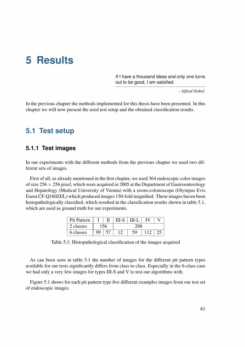
5 ResultsIf I have a thousand ideas and only one turnsout to be good, I am satisfied.
- Alfred Nobel
In the previous chapter the methods implemented for this thesis have been presented. In thischapter we will now present the used test setup and the obtained classification results.
5.1 Test setup
5.1.1 Test images
In our experiments with the different methods from the previous chapter we used two dif-ferent sets of images.
First of all, as already mentioned in the first chapter, we used 364 endoscopic color imagesof size 256× 256 pixel, which were acquired in 2005 at the Department of Gastroenterologyand Hepatology (Medical University of Vienna) with a zoom-colonoscope (Olympus EvisExera CF-Q160ZI/L) which produced images 150-fold magnified. These images haven beenhistopathologically classified, which resulted in the classification results shown in table 5.1,which are used as ground truth for our experiments.
Pit Pattern I II III-S III-L IV V2 classes 156 2086 classes 99 57 12 59 112 25
Table 5.1: Histopathological classification of the images acquired
As can been seen in table 5.1 the number of images for the different pit pattern typesavailable for our tests significantly differs from class to class. Especially in the 6-class casewe had only a very few images for types III-S and V to test our algorithms with.
Figure 5.1 shows for each pit pattern type five different examples images from our test setof endoscopic images.
61
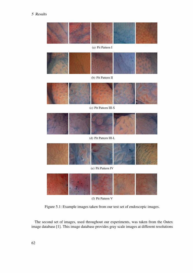
5 Results
(a) Pit Pattern I
(b) Pit Pattern II
(c) Pit Pattern III-S
(d) Pit Pattern III-L
(e) Pit Pattern IV
(f) Pit Pattern V
Figure 5.1: Example images taken from our test set of endoscopic images.
The second set of images, used throughout our experiments, was taken from the Outeximage database [1]. This image database provides gray scale images at different resolutions
62
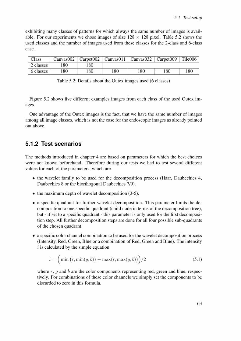
5.1 Test setup
exhibiting many classes of patterns for which always the same number of images is avail-able. For our experiments we chose images of size 128 × 128 pixel. Table 5.2 shows theused classes and the number of images used from these classes for the 2-class and 6-classcase.
Class Canvas002 Carpet002 Canvas011 Canvas032 Carpet009 Tile0062 classes 180 1806 classes 180 180 180 180 180 180
Table 5.2: Details about the Outex images used (6 classes)
Figure 5.2 shows five different examples images from each class of the used Outex im-ages.
One advantage of the Outex images is the fact, that we have the same number of imagesamong all image classes, which is not the case for the endoscopic images as already pointedout above.
5.1.2 Test scenarios
The methods introduced in chapter 4 are based on parameters for which the best choiceswere not known beforehand. Therefore during our tests we had to test several differentvalues for each of the parameters, which are
• the wavelet family to be used for the decomposition process (Haar, Daubechies 4,Daubechies 8 or the biorthogonal Daubechies 7/9).
• the maximum depth of wavelet decomposition (3-5).
• a specific quadrant for further wavelet decomposition. This parameter limits the de-composition to one specific quadrant (child node in terms of the decomposition tree),but - if set to a specific quadrant - this parameter is only used for the first decomposi-tion step. All further decomposition steps are done for all four possible sub-quadrantsof the chosen quadrant.
• a specific color channel combination to be used for the wavelet decomposition process(Intensity, Red, Green, Blue or a combination of Red, Green and Blue). The intensityi is calculated by the simple equation
i =(
min(r,min(g, b)
)+ max(r,max(g, b)
))/2 (5.1)
where r, g and b are the color components representing red, green and blue, respec-tively. For combinations of these color channels we simply set the components to bediscarded to zero in this formula.
63
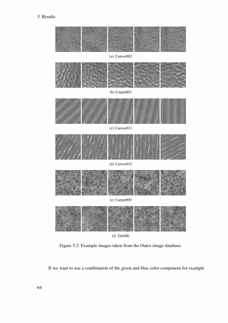
5 Results
(a) Canvas002
(b) Carpet002
(c) Canvas011
(d) Canvas032
(e) Carpet009
(f) Tile006
Figure 5.2: Example images taken from the Outex image database.
If we want to use a combination of the green and blue color component for example
64
5.2 Results
for the decomposition process, the intensity would be calculated by the equation
i =(
min(0,min(g, b)
)+ max(0,max(g, b)
))/2 = max(g, b)/2 (5.2)
This parameter affected tests only which are based on the endoscopic images, sincethe Outex images do not contain any color information.
• a cost function for best basis based methods (see section 2.6.1.1).
• a quadtree distance metric (see section 4.3).
• the number of subbands to use for feature extraction (1-50).
• the number of neighbours for the k-NN classifier (1-100) (see section 3.3.1).
• the type of feature to extract from a given subband (see section 4.2.1).
• the type of discriminant measure for the LDB algorithm (see section 2.6.1.3).
• the SVM gridsearch parameters ν and γ (see section 3.3.3).
Looking at this list of parameters it is obvious that testing our algorithms with the differentchoices resulted in a huge number of different tests.
5.2 Results
In this section we will present the best results from our experiments for each of our im-plemented methods. Since, as mentioned above, the number of test performed during ourexperiments, we select the feature extraction and classification configuration based on themaximal value of correctly classified images, applied to the 2 or 6 classes case.
Tables 5.3, 5.4 and 5.5 show the final results of our experiments. The values throughoutthese tables are the number of true positives divided by the overall number of images in theaccording class. It is also important to mention that the results are rounded throughout alltables presented in this chapter.
In the following sections we well investigate the results in more detail.
5.2.1 Best-basis method (BB)
The best results with this method have been obtained using the gray scale versions of theimages (i.e. the color information contained within the original pit pattern images has beendiscarded).
As we can see in table 5.3, in the two classes case the best result achieved was 70% usingthe SVM classifier. The best result achieved with the k-NN classifier was clearly lower with
65
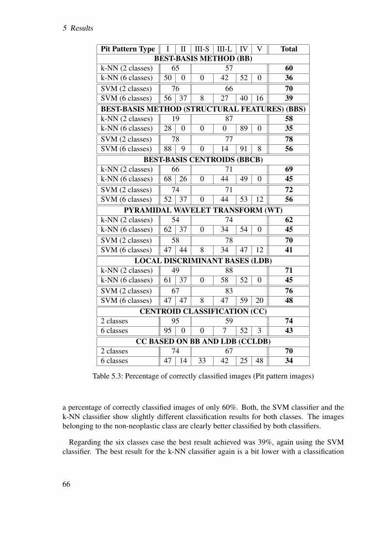
5 Results
Pit Pattern Type I II III-S III-L IV V TotalBEST-BASIS METHOD (BB)
k-NN (2 classes) 65 57 60k-NN (6 classes) 50 0 0 42 52 0 36SVM (2 classes) 76 66 70SVM (6 classes) 56 37 8 27 40 16 39BEST-BASIS METHOD (STRUCTURAL FEATURES) (BBS)k-NN (2 classes) 19 87 58k-NN (6 classes) 28 0 0 0 89 0 35SVM (2 classes) 78 77 78SVM (6 classes) 88 9 0 14 91 8 56
BEST-BASIS CENTROIDS (BBCB)k-NN (2 classes) 66 71 69k-NN (6 classes) 68 26 0 44 49 0 45SVM (2 classes) 74 71 72SVM (6 classes) 52 37 0 44 53 12 56
PYRAMIDAL WAVELET TRANSFORM (WT)k-NN (2 classes) 54 74 62k-NN (6 classes) 62 37 0 34 54 0 45SVM (2 classes) 58 78 70SVM (6 classes) 47 44 8 34 47 12 41
LOCAL DISCRIMINANT BASES (LDB)k-NN (2 classes) 49 88 71k-NN (6 classes) 61 37 0 58 52 0 45SVM (2 classes) 67 83 76SVM (6 classes) 47 47 8 47 59 20 48
CENTROID CLASSIFICATION (CC)2 classes 95 59 746 classes 95 0 0 7 52 3 43
CC BASED ON BB AND LDB (CCLDB)2 classes 74 67 706 classes 47 14 33 42 25 48 34
Table 5.3: Percentage of correctly classified images (Pit pattern images)
a percentage of correctly classified images of only 60%. Both, the SVM classifier and thek-NN classifier show slightly different classification results for both classes. The imagesbelonging to the non-neoplastic class are clearly better classified by both classifiers.
Regarding the six classes case the best result achieved was 39%, again using the SVMclassifier. The best result for the k-NN classifier again is a bit lower with a classification
66
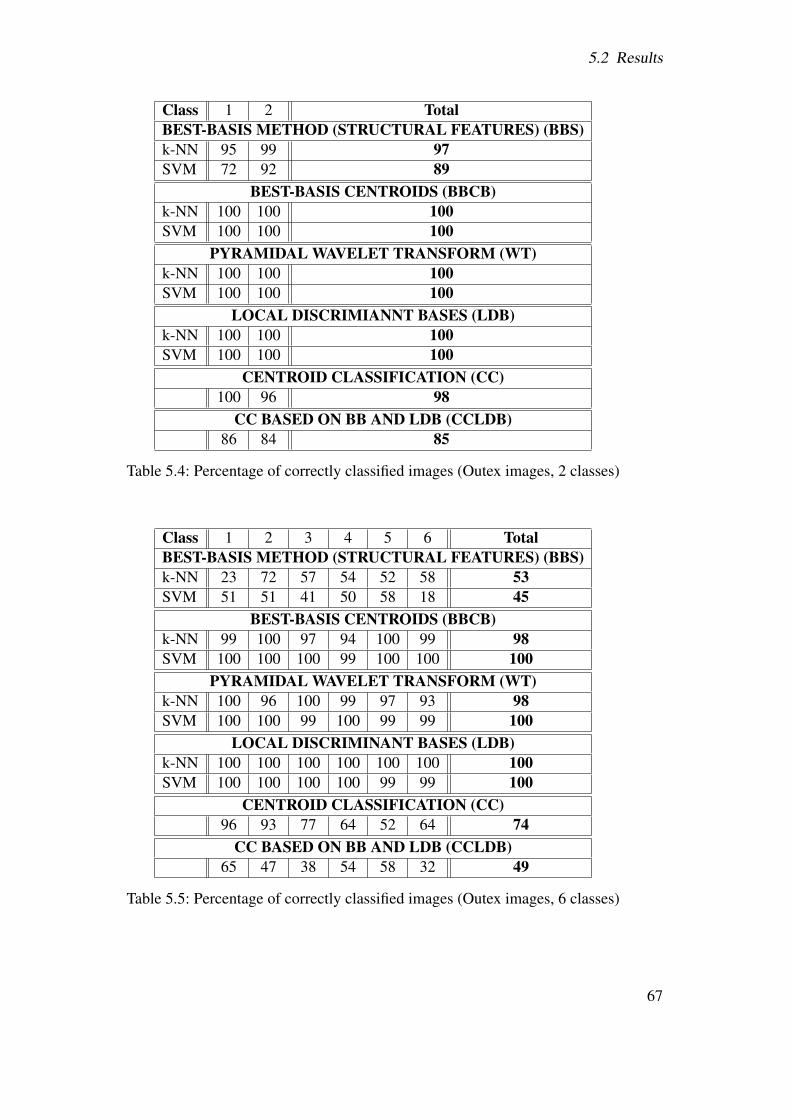
5.2 Results
Class 1 2 TotalBEST-BASIS METHOD (STRUCTURAL FEATURES) (BBS)k-NN 95 99 97SVM 72 92 89
BEST-BASIS CENTROIDS (BBCB)k-NN 100 100 100SVM 100 100 100
PYRAMIDAL WAVELET TRANSFORM (WT)k-NN 100 100 100SVM 100 100 100
LOCAL DISCRIMIANNT BASES (LDB)k-NN 100 100 100SVM 100 100 100
CENTROID CLASSIFICATION (CC)100 96 98
CC BASED ON BB AND LDB (CCLDB)86 84 85
Table 5.4: Percentage of correctly classified images (Outex images, 2 classes)
Class 1 2 3 4 5 6 TotalBEST-BASIS METHOD (STRUCTURAL FEATURES) (BBS)k-NN 23 72 57 54 52 58 53SVM 51 51 41 50 58 18 45
BEST-BASIS CENTROIDS (BBCB)k-NN 99 100 97 94 100 99 98SVM 100 100 100 99 100 100 100
PYRAMIDAL WAVELET TRANSFORM (WT)k-NN 100 96 100 99 97 93 98SVM 100 100 99 100 99 99 100
LOCAL DISCRIMINANT BASES (LDB)k-NN 100 100 100 100 100 100 100SVM 100 100 100 100 99 99 100
CENTROID CLASSIFICATION (CC)96 93 77 64 52 64 74
CC BASED ON BB AND LDB (CCLDB)65 47 38 54 58 32 49
Table 5.5: Percentage of correctly classified images (Outex images, 6 classes)
67
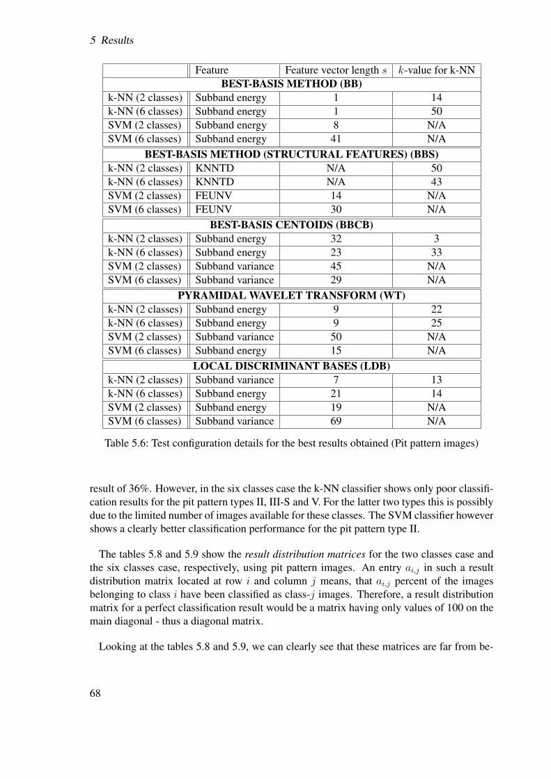
5 Results
Feature Feature vector length s k-value for k-NNBEST-BASIS METHOD (BB)
k-NN (2 classes) Subband energy 1 14k-NN (6 classes) Subband energy 1 50SVM (2 classes) Subband energy 8 N/ASVM (6 classes) Subband energy 41 N/A
BEST-BASIS METHOD (STRUCTURAL FEATURES) (BBS)k-NN (2 classes) KNNTD N/A 50k-NN (6 classes) KNNTD N/A 43SVM (2 classes) FEUNV 14 N/ASVM (6 classes) FEUNV 30 N/A
BEST-BASIS CENTOIDS (BBCB)k-NN (2 classes) Subband energy 32 3k-NN (6 classes) Subband energy 23 33SVM (2 classes) Subband variance 45 N/ASVM (6 classes) Subband variance 29 N/A
PYRAMIDAL WAVELET TRANSFORM (WT)k-NN (2 classes) Subband energy 9 22k-NN (6 classes) Subband energy 9 25SVM (2 classes) Subband variance 50 N/ASVM (6 classes) Subband energy 15 N/A
LOCAL DISCRIMINANT BASES (LDB)k-NN (2 classes) Subband variance 7 13k-NN (6 classes) Subband energy 21 14SVM (2 classes) Subband energy 19 N/ASVM (6 classes) Subband variance 69 N/A
Table 5.6: Test configuration details for the best results obtained (Pit pattern images)
result of 36%. However, in the six classes case the k-NN classifier shows only poor classifi-cation results for the pit pattern types II, III-S and V. For the latter two types this is possiblydue to the limited number of images available for these classes. The SVM classifier howevershows a clearly better classification performance for the pit pattern type II.
The tables 5.8 and 5.9 show the result distribution matrices for the two classes case andthe six classes case, respectively, using pit pattern images. An entry ai,j in such a resultdistribution matrix located at row i and column j means, that ai,j percent of the imagesbelonging to class i have been classified as class-j images. Therefore, a result distributionmatrix for a perfect classification result would be a matrix having only values of 100 on themain diagonal - thus a diagonal matrix.
Looking at the tables 5.8 and 5.9, we can clearly see that these matrices are far from be-
68
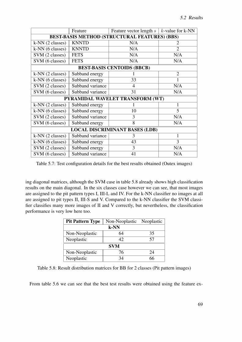
5.2 Results
Feature Feature vector length s k-value for k-NNBEST-BASIS METHOD (STRUCTURAL FEATURES) (BBS)
k-NN (2 classes) KNNTD N/A 2k-NN (6 classes) KNNTD N/A 2SVM (2 classes) FETS N/A N/ASVM (6 classes) FETS N/A N/A
BEST-BASIS CENTOIDS (BBCB)k-NN (2 classes) Subband energy 1 2k-NN (6 classes) Subband energy 33 1SVM (2 classes) Subband variance 4 N/ASVM (6 classes) Subband variance 31 N/A
PYRAMIDAL WAVELET TRANSFORM (WT)k-NN (2 classes) Subband energy 1 1k-NN (6 classes) Subband energy 10 5SVM (2 classes) Subband variance 3 N/ASVM (6 classes) Subband energy 8 N/A
LOCAL DISCRIMINANT BASES (LDB)k-NN (2 classes) Subband variance 3 1k-NN (6 classes) Subband energy 43 3SVM (2 classes) Subband energy 3 N/ASVM (6 classes) Subband variance 41 N/A
Table 5.7: Test configuration details for the best results obtained (Outex images)
ing diagonal matrices, although the SVM case in table 5.8 already shows high classificationresults on the main diagonal. In the six classes case however we can see, that most imagesare assigned to the pit pattern types I, III-L and IV. For the k-NN classifier no images at allare assigned to pit types II, III-S and V. Compared to the k-NN classifier the SVM classi-fier classifies many more images of II and V correctly, but nevertheless, the classificationperformance is very low here too.
Pit Pattern Type Non-Neoplastic Neoplastick-NN
Non-Neoplastic 64 35Neoplastic 42 57
SVMNon-Neoplastic 76 24Neoplastic 34 66
Table 5.8: Result distribution matrices for BB for 2 classes (Pit pattern images)
From table 5.6 we can see that the best test results were obtained using the feature ex-
69
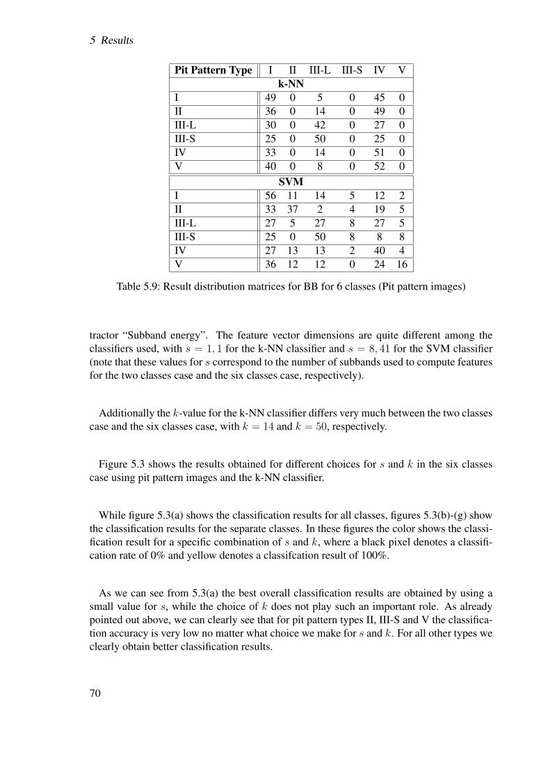
5 Results
Pit Pattern Type I II III-L III-S IV Vk-NN
I 49 0 5 0 45 0II 36 0 14 0 49 0III-L 30 0 42 0 27 0III-S 25 0 50 0 25 0IV 33 0 14 0 51 0V 40 0 8 0 52 0
SVMI 56 11 14 5 12 2II 33 37 2 4 19 5III-L 27 5 27 8 27 5III-S 25 0 50 8 8 8IV 27 13 13 2 40 4V 36 12 12 0 24 16
Table 5.9: Result distribution matrices for BB for 6 classes (Pit pattern images)
tractor “Subband energy”. The feature vector dimensions are quite different among theclassifiers used, with s = 1, 1 for the k-NN classifier and s = 8, 41 for the SVM classifier(note that these values for s correspond to the number of subbands used to compute featuresfor the two classes case and the six classes case, respectively).
Additionally the k-value for the k-NN classifier differs very much between the two classescase and the six classes case, with k = 14 and k = 50, respectively.
Figure 5.3 shows the results obtained for different choices for s and k in the six classescase using pit pattern images and the k-NN classifier.
While figure 5.3(a) shows the classification results for all classes, figures 5.3(b)-(g) showthe classification results for the separate classes. In these figures the color shows the classi-fication result for a specific combination of s and k, where a black pixel denotes a classifi-cation rate of 0% and yellow denotes a classifcation result of 100%.
As we can see from 5.3(a) the best overall classification results are obtained by using asmall value for s, while the choice of k does not play such an important role. As alreadypointed out above, we can clearly see that for pit pattern types II, III-S and V the classifica-tion accuracy is very low no matter what choice we make for s and k. For all other types weclearly obtain better classification results.
70
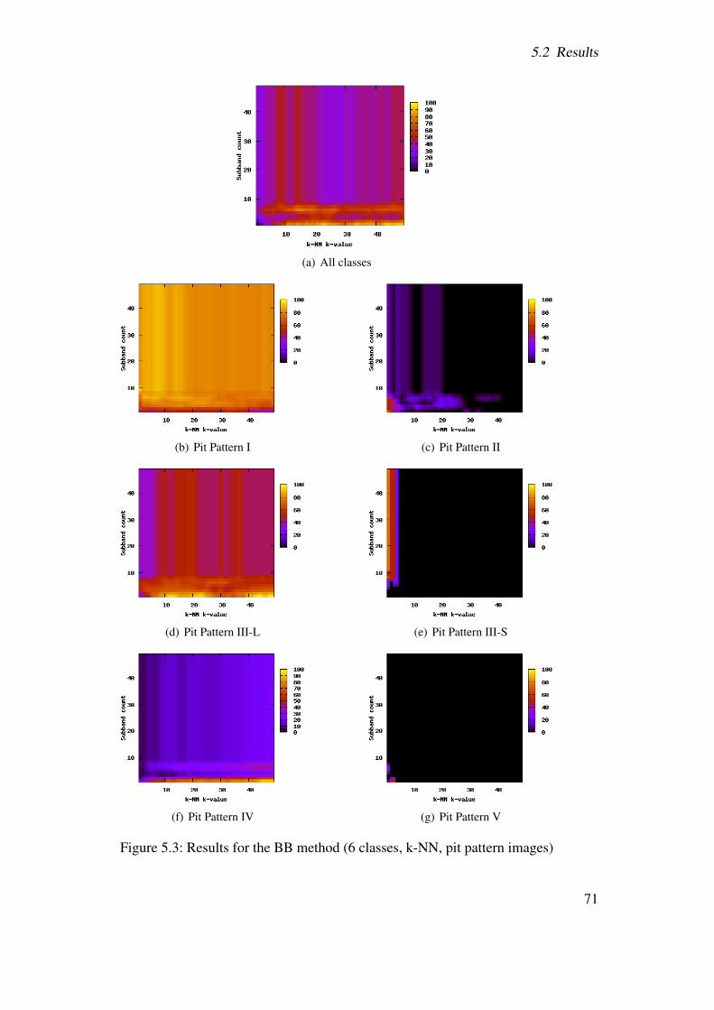
5.2 Results
(a) All classes
(b) Pit Pattern I (c) Pit Pattern II
(d) Pit Pattern III-L (e) Pit Pattern III-S
(f) Pit Pattern IV (g) Pit Pattern V
Figure 5.3: Results for the BB method (6 classes, k-NN, pit pattern images)
71
5 Results
5.2.2 Best-basis method based on structural features (BBS)
As we saw in section 4.3.3.3 this method is similar to the method in the previous section. Butfor the tests with this method we used the structural feature extractors FEUNV (based on theunique node values) and FETS (based on the complete tree structure) already presented insection 4.3.3.3. Apart from that we used KNNTD (distances based on trees and a quadtreedistance metric instead of feature vectors and a vector distance metric) in conjunction withthe k-NN classifier.
Just like in the previous method, the best results have been obtained using the gray scaleversions of the pit pattern images.
As we can see in table 5.3, in the two classes case the best result obtained for the pitpattern images was 78% using the SVM classifier. The best result achieved with the k-NNclassifier was clearly lower with a percentage of correctly classified images of 58%.
In the six classes case again the SVM classifier clearly outperforms the k-NN classifierwith a classification result of 56% compared to 35% and the misclassification rates for pitpattern types III-S and V again are extremely high, just like in the previous method.
Additionally we can see in table 5.3 that the classification performance seems to be supe-rior for the second class in the two classes case for the k-NN classifier. In the six classescase the results are similar - while pit pattern type I gets classified clearly worse than typeIV, the classification fails completely for all other types.
Compared to the tests with the pit pattern images, the tests performed using the Outeximages resulted in very high classification results, as can been seen in the tables 5.4 and5.5. In the two classes case the total classification result was 97% for the k-NN classifierand 89% for the SVM classifier. In the six classes case the classification result was 53% forthe k-NN classifier. The top result achieved with the SVM classifier is a bit lower with anoverall classification result of 45%.
At this point it is worthwhile to mention that during the first test runs the SVM resultsfor the Outex images were conspicuously worse with a top result of 0%. After limiting thenumber of SVM training samples however, we were able to get clearly higher results. Toachieve these results we trained the SVM classsifier with only 10% out of all images.
From table 5.6 we see, that regarding the pit pattern images in conjunction with the k-NNclassifier the structural feature extractor KNNTD always delivered the best results. Whilein the two classes case the best result has been achieved with a value for k of 50, the bestresults in the six classes case has been obtained using a smaller k-value of 43. When usingthe SVM classifier however, the best results have been achieved using the FEUNV featureextractor.
For the Outex images in connection with the k-NN classifier the values for k leading tothe best overall classification results are clearly much lower than for the pit pattern images
72
5.2 Results
as we can see in figure 5.7. For the two classes case as well as for the six classes case thebest results have been obtained with a k-value of 2.
In figure 5.4 we see the results obtained for different choices for s in the six classes caseusing pit pattern images and the SVM classifier.
As we can see from figure 5.4(a) the overall classification results seem to get higher withincreasing values for s until a value of 33. Then the classification rate drops and remainsconstant for higher values for s.From the figures for the separate classes we again see, that pit pattern type III-S deliversvery low results only, while all other classes definitely show better classification results.
5.2.3 Best-basis centroids (BBCB)
Just like with the previous method, the best results have been achieved using the gray scaleversions of the pit pattern images.
As we can see in table 5.3, in the two classes case the best result obtained for the pit patternimages was 72% using the SVM classifier. The best result achieved with the k-NN classifierwas only insignificantly lower with a percentage of correctly classified images of 69%.In contrast to the BB method, both classifiers show approximately the same classificationresults for each separate class.
In the six classes case again the SVM classifier outperforms the k-NN classifier with aclassification result of 56% compared to 45% and the misclassification rates for pit patterntypes III-S and V again are extremely high, just like in the previous method.
The tables 5.10 and 5.11 show the result distribution matrices for the two classes caseand the six classes case, respectively, using pit pattern images. For the two classes case theclassification results are very similar to the BB method and also for the six classes case weagain observe a poor classification performance for pit pattern types III-S and V, just like inthe BB method.
Pit Pattern Type Non-Neoplastic Neoplastick-NN
Non-Neoplastic 66 33Neoplastic 28 71
SVMNon-Neoplastic 73 26Neoplastic 28 71
Table 5.10: Result distribution matrices for BBCB for 2 classes (Pit pattern images)
The BBCB method has also been tested with the Outex images, which resulted in excellentclassification results, as can been seen in the tables 5.4 and 5.5. In the two classes case the
73
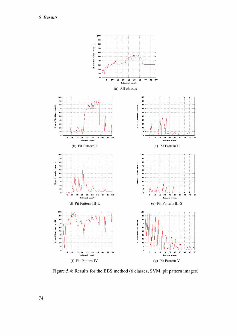
5 Results
(a) All classes
(b) Pit Pattern I (c) Pit Pattern II
(d) Pit Pattern III-L (e) Pit Pattern III-S
(f) Pit Pattern IV (g) Pit Pattern V
Figure 5.4: Results for the BBS method (6 classes, SVM, pit pattern images)
74
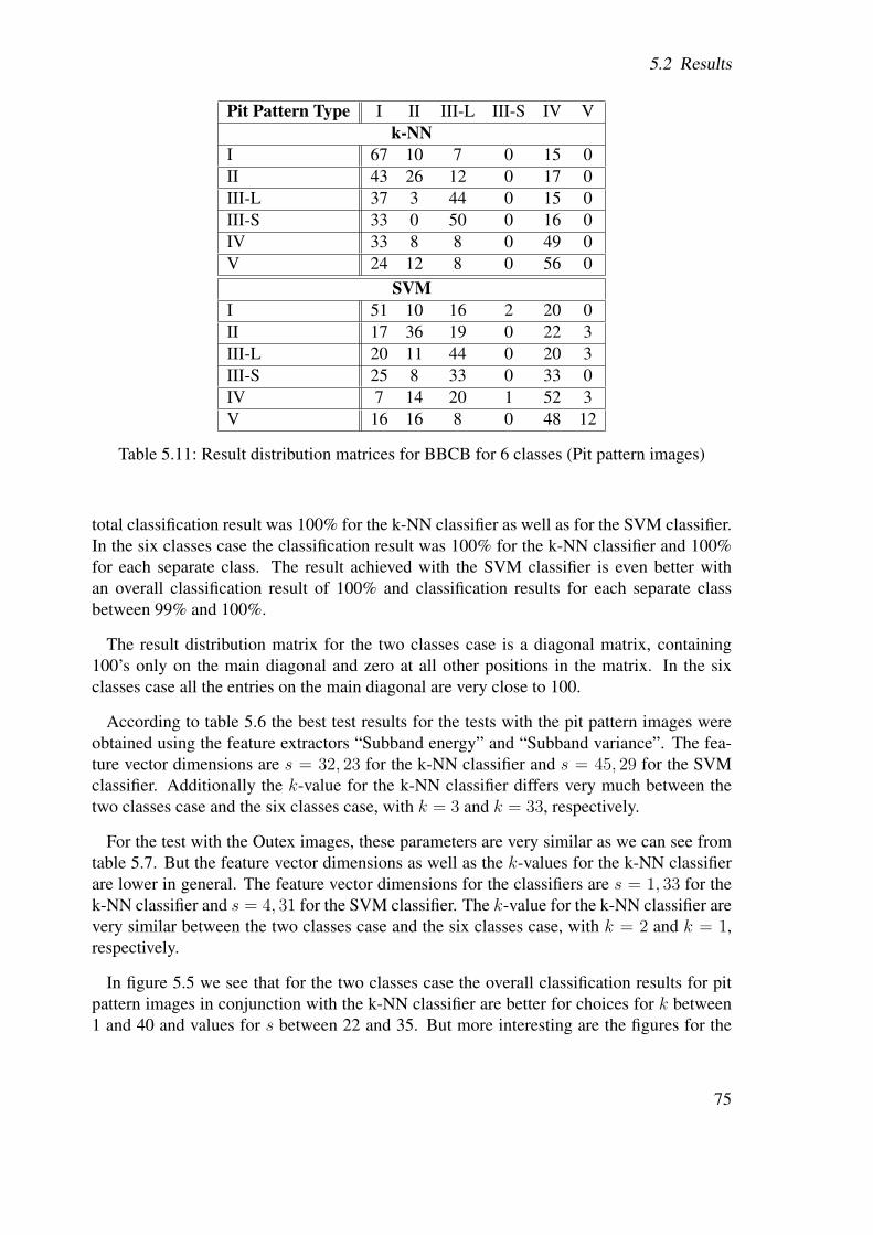
5.2 Results
Pit Pattern Type I II III-L III-S IV Vk-NN
I 67 10 7 0 15 0II 43 26 12 0 17 0III-L 37 3 44 0 15 0III-S 33 0 50 0 16 0IV 33 8 8 0 49 0V 24 12 8 0 56 0
SVMI 51 10 16 2 20 0II 17 36 19 0 22 3III-L 20 11 44 0 20 3III-S 25 8 33 0 33 0IV 7 14 20 1 52 3V 16 16 8 0 48 12
Table 5.11: Result distribution matrices for BBCB for 6 classes (Pit pattern images)
total classification result was 100% for the k-NN classifier as well as for the SVM classifier.In the six classes case the classification result was 100% for the k-NN classifier and 100%for each separate class. The result achieved with the SVM classifier is even better withan overall classification result of 100% and classification results for each separate classbetween 99% and 100%.
The result distribution matrix for the two classes case is a diagonal matrix, containing100’s only on the main diagonal and zero at all other positions in the matrix. In the sixclasses case all the entries on the main diagonal are very close to 100.
According to table 5.6 the best test results for the tests with the pit pattern images wereobtained using the feature extractors “Subband energy” and “Subband variance”. The fea-ture vector dimensions are s = 32, 23 for the k-NN classifier and s = 45, 29 for the SVMclassifier. Additionally the k-value for the k-NN classifier differs very much between thetwo classes case and the six classes case, with k = 3 and k = 33, respectively.
For the test with the Outex images, these parameters are very similar as we can see fromtable 5.7. But the feature vector dimensions as well as the k-values for the k-NN classifierare lower in general. The feature vector dimensions for the classifiers are s = 1, 33 for thek-NN classifier and s = 4, 31 for the SVM classifier. The k-value for the k-NN classifier arevery similar between the two classes case and the six classes case, with k = 2 and k = 1,respectively.
In figure 5.5 we see that for the two classes case the overall classification results for pitpattern images in conjunction with the k-NN classifier are better for choices for k between1 and 40 and values for s between 22 and 35. But more interesting are the figures for the
75
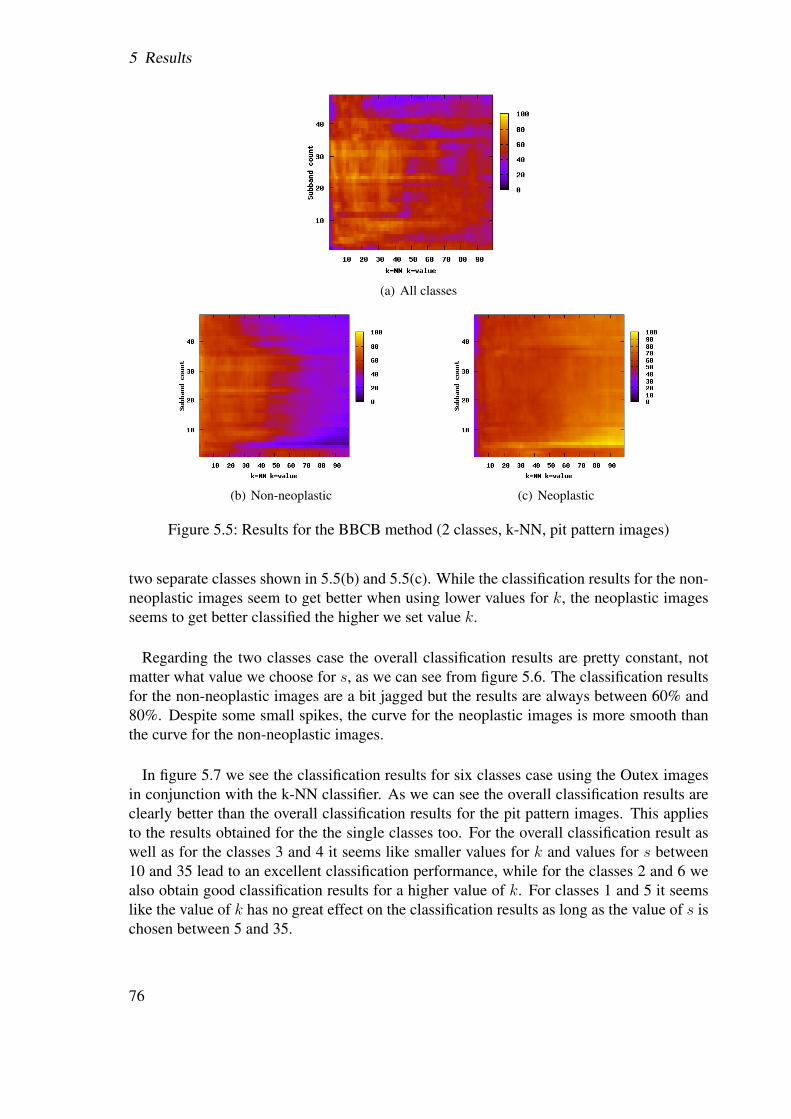
5 Results
(a) All classes
(b) Non-neoplastic (c) Neoplastic
Figure 5.5: Results for the BBCB method (2 classes, k-NN, pit pattern images)
two separate classes shown in 5.5(b) and 5.5(c). While the classification results for the non-neoplastic images seem to get better when using lower values for k, the neoplastic imagesseems to get better classified the higher we set value k.
Regarding the two classes case the overall classification results are pretty constant, notmatter what value we choose for s, as we can see from figure 5.6. The classification resultsfor the non-neoplastic images are a bit jagged but the results are always between 60% and80%. Despite some small spikes, the curve for the neoplastic images is more smooth thanthe curve for the non-neoplastic images.
In figure 5.7 we see the classification results for six classes case using the Outex imagesin conjunction with the k-NN classifier. As we can see the overall classification results areclearly better than the overall classification results for the pit pattern images. This appliesto the results obtained for the the single classes too. For the overall classification result aswell as for the classes 3 and 4 it seems like smaller values for k and values for s between10 and 35 lead to an excellent classification performance, while for the classes 2 and 6 wealso obtain good classification results for a higher value of k. For classes 1 and 5 it seemslike the value of k has no great effect on the classification results as long as the value of s ischosen between 5 and 35.
76
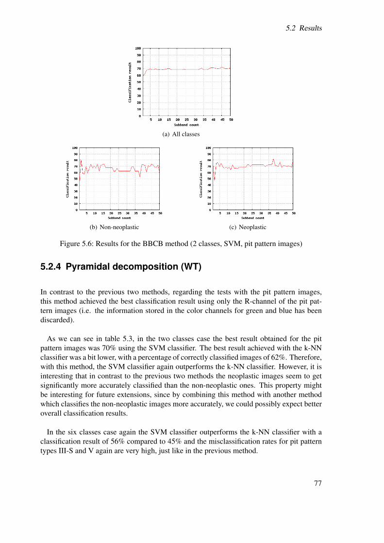
5.2 Results
(a) All classes
(b) Non-neoplastic (c) Neoplastic
Figure 5.6: Results for the BBCB method (2 classes, SVM, pit pattern images)
5.2.4 Pyramidal decomposition (WT)
In contrast to the previous two methods, regarding the tests with the pit pattern images,this method achieved the best classification result using only the R-channel of the pit pat-tern images (i.e. the information stored in the color channels for green and blue has beendiscarded).
As we can see in table 5.3, in the two classes case the best result obtained for the pitpattern images was 70% using the SVM classifier. The best result achieved with the k-NNclassifier was a bit lower, with a percentage of correctly classified images of 62%. Therefore,with this method, the SVM classifier again outperforms the k-NN classifier. However, it isinteresting that in contrast to the previous two methods the neoplastic images seem to getsignificantly more accurately classified than the non-neoplastic ones. This property mightbe interesting for future extensions, since by combining this method with another methodwhich classifies the non-neoplastic images more accurately, we could possibly expect betteroverall classification results.
In the six classes case again the SVM classifier outperforms the k-NN classifier with aclassification result of 56% compared to 45% and the misclassification rates for pit patterntypes III-S and V again are very high, just like in the previous method.
77
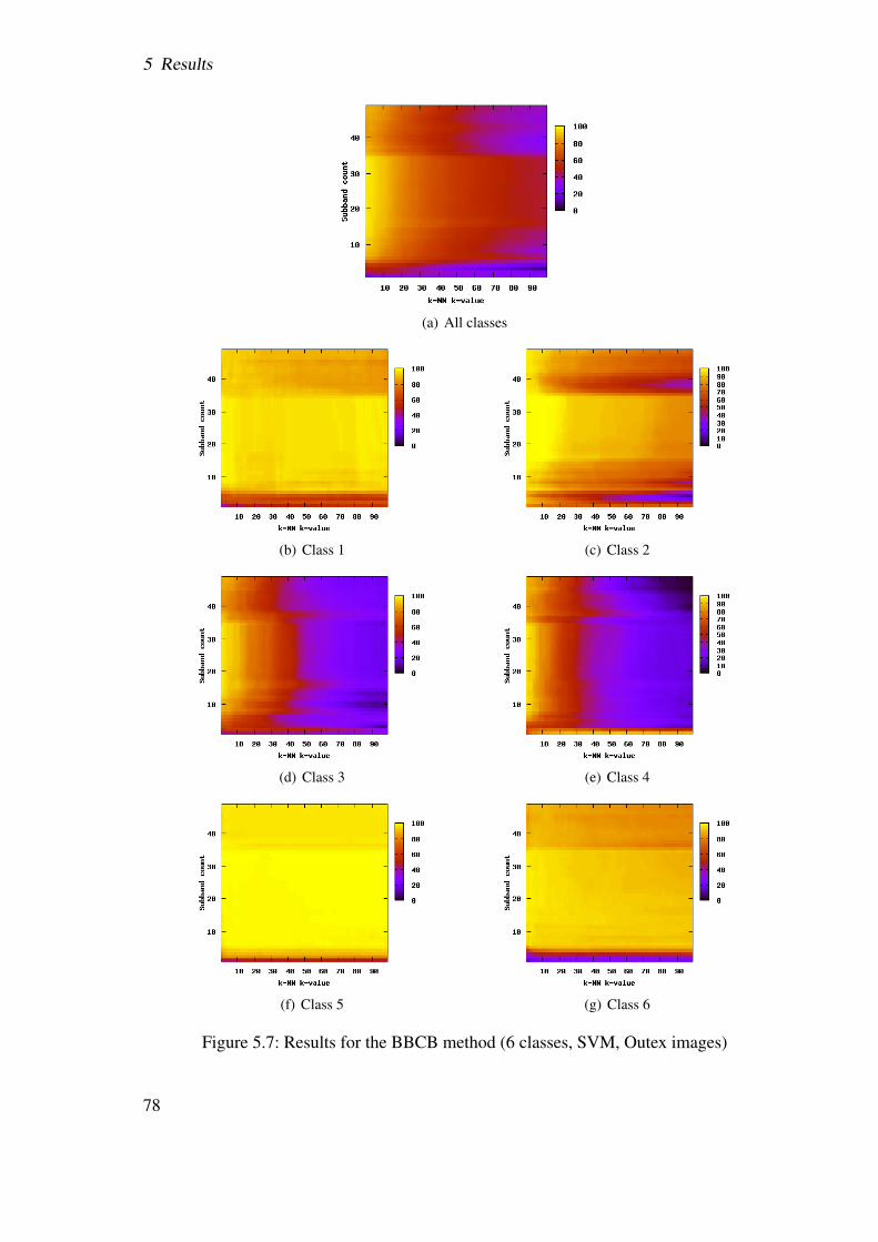
5 Results
(a) All classes
(b) Class 1 (c) Class 2
(d) Class 3 (e) Class 4
(f) Class 5 (g) Class 6
Figure 5.7: Results for the BBCB method (6 classes, SVM, Outex images)
78
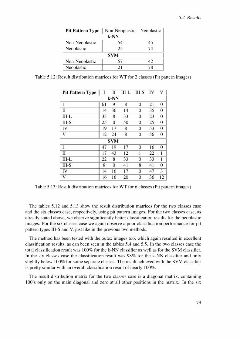
5.2 Results
Pit Pattern Type Non-Neoplastic Neoplastick-NN
Non-Neoplastic 54 45Neoplastic 25 74
SVMNon-Neoplastic 57 42Neoplastic 21 78
Table 5.12: Result distribution matrices for WT for 2 classes (Pit pattern images)
Pit Pattern Type I II III-L III-S IV Vk-NN
I 61 9 8 0 21 0II 14 36 14 0 35 0III-L 33 8 33 0 23 0III-S 25 0 50 0 25 0IV 19 17 8 0 53 0V 12 24 8 0 56 0
SVMI 47 19 17 0 16 0II 17 43 12 1 22 1III-L 22 8 33 0 33 1III-S 8 0 41 8 41 0IV 14 16 17 0 47 3V 16 16 20 0 36 12
Table 5.13: Result distribution matrices for WT for 6 classes (Pit pattern images)
The tables 5.12 and 5.13 show the result distribution matrices for the two classes caseand the six classes case, respectively, using pit pattern images. For the two classes case, asalready stated above, we observe significantly better classification results for the neoplasticimages. For the six classes case we again observe a poor classification performance for pitpattern types III-S and V, just like in the previous two methods.
The method has been tested with the outex images too, which again resulted in excellentclassification results, as can been seen in the tables 5.4 and 5.5. In the two classes case thetotal classification result was 100% for the k-NN classifier as well as for the SVM classifier.In the six classes case the classification result was 98% for the k-NN classifier and onlyslightly below 100% for some separate classes. The result achieved with the SVM classifieris pretty similar with an overall classification result of nearly 100%.
The result distribution matrix for the two classes case is a diagonal matrix, containing100’s only on the main diagonal and zero at all other positions in the matrix. In the six
79
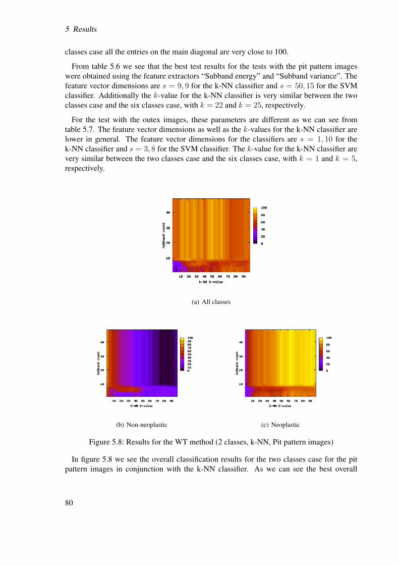
5 Results
classes case all the entries on the main diagonal are very close to 100.
From table 5.6 we see that the best test results for the tests with the pit pattern imageswere obtained using the feature extractors “Subband energy” and “Subband variance”. Thefeature vector dimensions are s = 9, 9 for the k-NN classifier and s = 50, 15 for the SVMclassifier. Additionally the k-value for the k-NN classifier is very similar between the twoclasses case and the six classes case, with k = 22 and k = 25, respectively.
For the test with the outex images, these parameters are different as we can see fromtable 5.7. The feature vector dimensions as well as the k-values for the k-NN classifier arelower in general. The feature vector dimensions for the classifiers are s = 1, 10 for thek-NN classifier and s = 3, 8 for the SVM classifier. The k-value for the k-NN classifier arevery similar between the two classes case and the six classes case, with k = 1 and k = 5,respectively.
(a) All classes
(b) Non-neoplastic (c) Neoplastic
Figure 5.8: Results for the WT method (2 classes, k-NN, Pit pattern images)
In figure 5.8 we see the overall classification results for the two classes case for the pitpattern images in conjunction with the k-NN classifier. As we can see the best overall
80
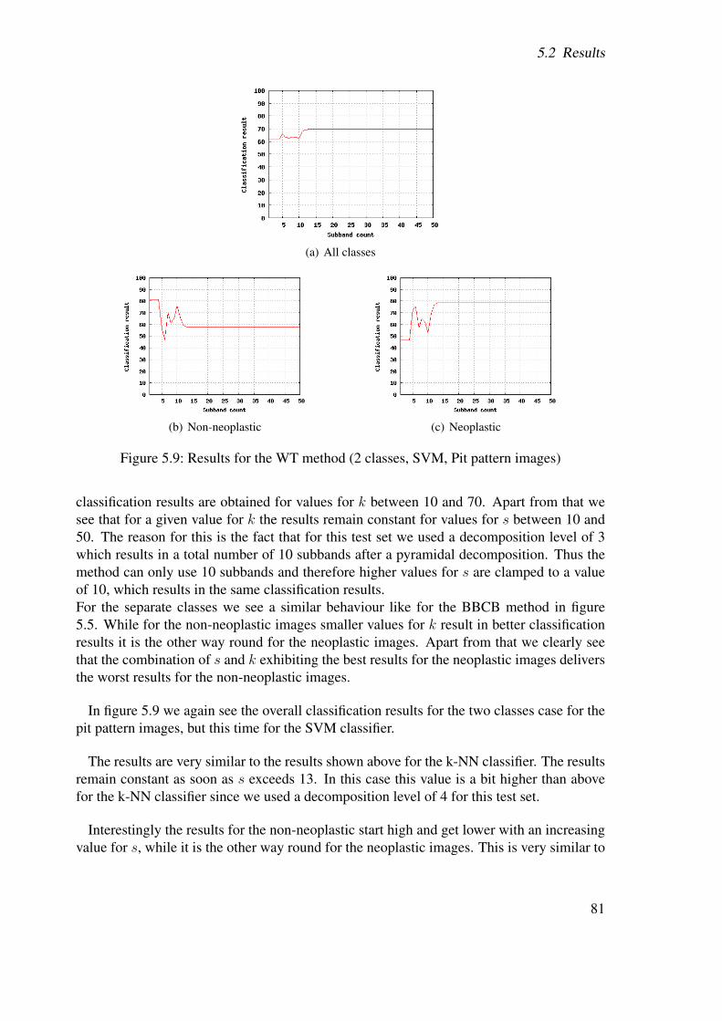
5.2 Results
(a) All classes
(b) Non-neoplastic (c) Neoplastic
Figure 5.9: Results for the WT method (2 classes, SVM, Pit pattern images)
classification results are obtained for values for k between 10 and 70. Apart from that wesee that for a given value for k the results remain constant for values for s between 10 and50. The reason for this is the fact that for this test set we used a decomposition level of 3which results in a total number of 10 subbands after a pyramidal decomposition. Thus themethod can only use 10 subbands and therefore higher values for s are clamped to a valueof 10, which results in the same classification results.For the separate classes we see a similar behaviour like for the BBCB method in figure5.5. While for the non-neoplastic images smaller values for k result in better classificationresults it is the other way round for the neoplastic images. Apart from that we clearly seethat the combination of s and k exhibiting the best results for the neoplastic images deliversthe worst results for the non-neoplastic images.
In figure 5.9 we again see the overall classification results for the two classes case for thepit pattern images, but this time for the SVM classifier.
The results are very similar to the results shown above for the k-NN classifier. The resultsremain constant as soon as s exceeds 13. In this case this value is a bit higher than abovefor the k-NN classifier since we used a decomposition level of 4 for this test set.
Interestingly the results for the non-neoplastic start high and get lower with an increasingvalue for s, while it is the other way round for the neoplastic images. This is very similar to
81
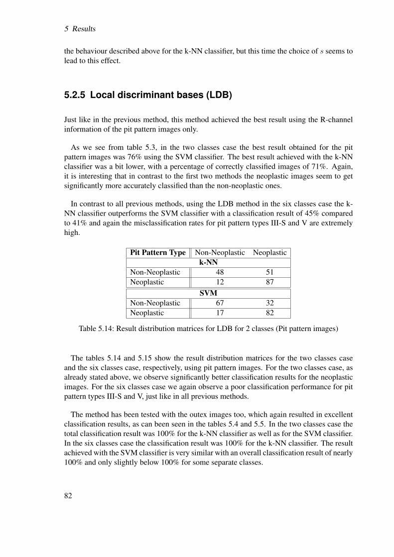
5 Results
the behaviour described above for the k-NN classifier, but this time the choice of s seems tolead to this effect.
5.2.5 Local discriminant bases (LDB)
Just like in the previous method, this method achieved the best result using the R-channelinformation of the pit pattern images only.
As we see from table 5.3, in the two classes case the best result obtained for the pitpattern images was 76% using the SVM classifier. The best result achieved with the k-NNclassifier was a bit lower, with a percentage of correctly classified images of 71%. Again,it is interesting that in contrast to the first two methods the neoplastic images seem to getsignificantly more accurately classified than the non-neoplastic ones.
In contrast to all previous methods, using the LDB method in the six classes case the k-NN classifier outperforms the SVM classifier with a classification result of 45% comparedto 41% and again the misclassification rates for pit pattern types III-S and V are extremelyhigh.
Pit Pattern Type Non-Neoplastic Neoplastick-NN
Non-Neoplastic 48 51Neoplastic 12 87
SVMNon-Neoplastic 67 32Neoplastic 17 82
Table 5.14: Result distribution matrices for LDB for 2 classes (Pit pattern images)
The tables 5.14 and 5.15 show the result distribution matrices for the two classes caseand the six classes case, respectively, using pit pattern images. For the two classes case, asalready stated above, we observe significantly better classification results for the neoplasticimages. For the six classes case we again observe a poor classification performance for pitpattern types III-S and V, just like in all previous methods.
The method has been tested with the outex images too, which again resulted in excellentclassification results, as can been seen in the tables 5.4 and 5.5. In the two classes case thetotal classification result was 100% for the k-NN classifier as well as for the SVM classifier.In the six classes case the classification result was 100% for the k-NN classifier. The resultachieved with the SVM classifier is very similar with an overall classification result of nearly100% and only slightly below 100% for some separate classes.
82
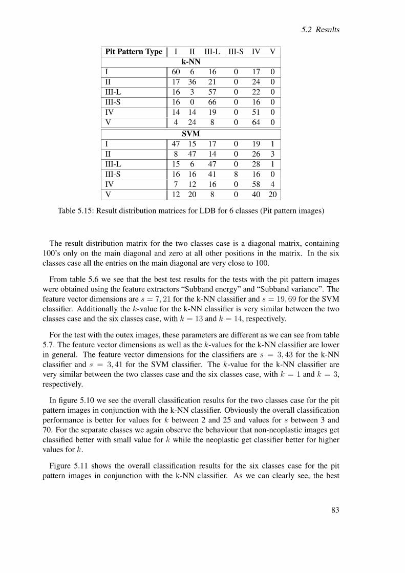
5.2 Results
Pit Pattern Type I II III-L III-S IV Vk-NN
I 60 6 16 0 17 0II 17 36 21 0 24 0III-L 16 3 57 0 22 0III-S 16 0 66 0 16 0IV 14 14 19 0 51 0V 4 24 8 0 64 0
SVMI 47 15 17 0 19 1II 8 47 14 0 26 3III-L 15 6 47 0 28 1III-S 16 16 41 8 16 0IV 7 12 16 0 58 4V 12 20 8 0 40 20
Table 5.15: Result distribution matrices for LDB for 6 classes (Pit pattern images)
The result distribution matrix for the two classes case is a diagonal matrix, containing100’s only on the main diagonal and zero at all other positions in the matrix. In the sixclasses case all the entries on the main diagonal are very close to 100.
From table 5.6 we see that the best test results for the tests with the pit pattern imageswere obtained using the feature extractors “Subband energy” and “Subband variance”. Thefeature vector dimensions are s = 7, 21 for the k-NN classifier and s = 19, 69 for the SVMclassifier. Additionally the k-value for the k-NN classifier is very similar between the twoclasses case and the six classes case, with k = 13 and k = 14, respectively.
For the test with the outex images, these parameters are different as we can see from table5.7. The feature vector dimensions as well as the k-values for the k-NN classifier are lowerin general. The feature vector dimensions for the classifiers are s = 3, 43 for the k-NNclassifier and s = 3, 41 for the SVM classifier. The k-value for the k-NN classifier arevery similar between the two classes case and the six classes case, with k = 1 and k = 3,respectively.
In figure 5.10 we see the overall classification results for the two classes case for the pitpattern images in conjunction with the k-NN classifier. Obviously the overall classificationperformance is better for values for k between 2 and 25 and values for s between 3 and70. For the separate classes we again observe the behaviour that non-neoplastic images getclassified better with small value for k while the neoplastic get classifier better for highervalues for k.
Figure 5.11 shows the overall classification results for the six classes case for the pitpattern images in conjunction with the k-NN classifier. As we can clearly see, the best
83
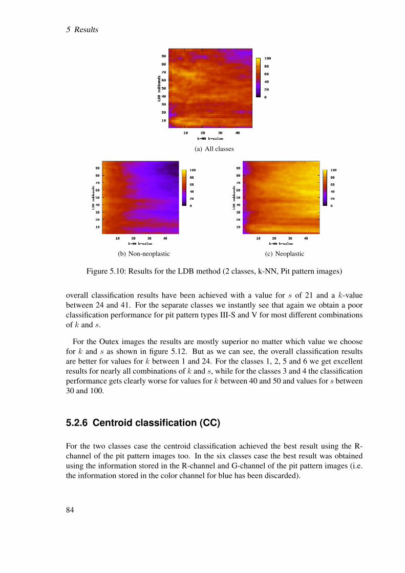
5 Results
(a) All classes
(b) Non-neoplastic (c) Neoplastic
Figure 5.10: Results for the LDB method (2 classes, k-NN, Pit pattern images)
overall classification results have been achieved with a value for s of 21 and a k-valuebetween 24 and 41. For the separate classes we instantly see that again we obtain a poorclassification performance for pit pattern types III-S and V for most different combinationsof k and s.
For the Outex images the results are mostly superior no matter which value we choosefor k and s as shown in figure 5.12. But as we can see, the overall classification resultsare better for values for k between 1 and 24. For the classes 1, 2, 5 and 6 we get excellentresults for nearly all combinations of k and s, while for the classes 3 and 4 the classificationperformance gets clearly worse for values for k between 40 and 50 and values for s between30 and 100.
5.2.6 Centroid classification (CC)
For the two classes case the centroid classification achieved the best result using the R-channel of the pit pattern images too. In the six classes case the best result was obtainedusing the information stored in the R-channel and G-channel of the pit pattern images (i.e.the information stored in the color channel for blue has been discarded).
84
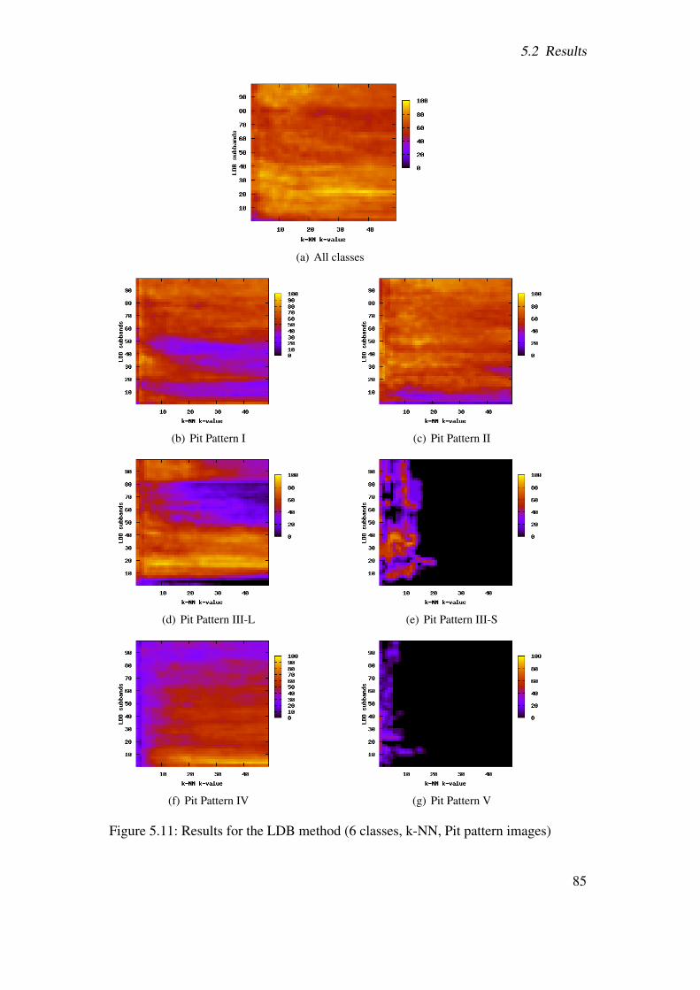
5.2 Results
(a) All classes
(b) Pit Pattern I (c) Pit Pattern II
(d) Pit Pattern III-L (e) Pit Pattern III-S
(f) Pit Pattern IV (g) Pit Pattern V
Figure 5.11: Results for the LDB method (6 classes, k-NN, Pit pattern images)
85
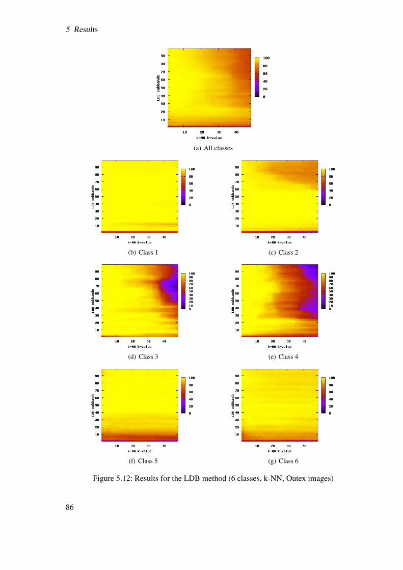
5 Results
(a) All classes
(b) Class 1 (c) Class 2
(d) Class 3 (e) Class 4
(f) Class 5 (g) Class 6
Figure 5.12: Results for the LDB method (6 classes, k-NN, Outex images)
86
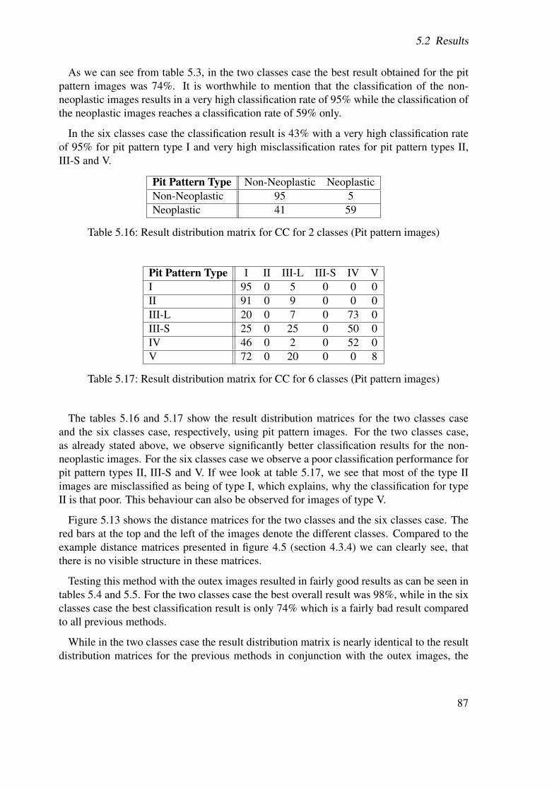
5.2 Results
As we can see from table 5.3, in the two classes case the best result obtained for the pitpattern images was 74%. It is worthwhile to mention that the classification of the non-neoplastic images results in a very high classification rate of 95% while the classification ofthe neoplastic images reaches a classification rate of 59% only.
In the six classes case the classification result is 43% with a very high classification rateof 95% for pit pattern type I and very high misclassification rates for pit pattern types II,III-S and V.
Pit Pattern Type Non-Neoplastic NeoplasticNon-Neoplastic 95 5Neoplastic 41 59
Table 5.16: Result distribution matrix for CC for 2 classes (Pit pattern images)
Pit Pattern Type I II III-L III-S IV VI 95 0 5 0 0 0II 91 0 9 0 0 0III-L 20 0 7 0 73 0III-S 25 0 25 0 50 0IV 46 0 2 0 52 0V 72 0 20 0 0 8
Table 5.17: Result distribution matrix for CC for 6 classes (Pit pattern images)
The tables 5.16 and 5.17 show the result distribution matrices for the two classes caseand the six classes case, respectively, using pit pattern images. For the two classes case,as already stated above, we observe significantly better classification results for the non-neoplastic images. For the six classes case we observe a poor classification performance forpit pattern types II, III-S and V. If wee look at table 5.17, we see that most of the type IIimages are misclassified as being of type I, which explains, why the classification for typeII is that poor. This behaviour can also be observed for images of type V.
Figure 5.13 shows the distance matrices for the two classes and the six classes case. Thered bars at the top and the left of the images denote the different classes. Compared to theexample distance matrices presented in figure 4.5 (section 4.3.4) we can clearly see, thatthere is no visible structure in these matrices.
Testing this method with the outex images resulted in fairly good results as can be seen intables 5.4 and 5.5. For the two classes case the best overall result was 98%, while in the sixclasses case the best classification result is only 74% which is a fairly bad result comparedto all previous methods.
While in the two classes case the result distribution matrix is nearly identical to the resultdistribution matrices for the previous methods in conjunction with the outex images, the
87
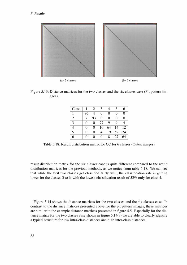
5 Results
(a) 2 classes (b) 6 classes
Figure 5.13: Distance matrices for the two classes and the six classes case (Pit pattern im-ages)
Class 1 2 3 4 5 61 96 4 0 0 0 02 7 93 0 0 0 03 0 0 77 9 9 44 0 0 10 64 14 125 0 0 4 19 52 246 0 0 0 8 27 64
Table 5.18: Result distribution matrix for CC for 6 classes (Outex images)
result distribution matrix for the six classes case is quite different compared to the resultdistribution matrices for the previous methods, as we notice from table 5.18. We can seethat while the first two classes get classified fairly well, the classification rate is gettinglower for the classes 3 to 6, with the lowest classification result of 52% only for class 4.
Figure 5.14 shows the distance matrices for the two classes and the six classes case. Incontrast to the distance matrices presented above for the pit pattern images, these matricesare similar to the example distance matrices presented in figure 4.5. Especially for the dis-tance matrix for the two classes case shown in figure 5.14(a) we are able to clearly identifya typical structure for low intra-class distances and high inter-class distances.
88
5.2 Results
(a) 2 classes (b) 6 classes
Figure 5.14: Distance matrices for the two classes and the six classes case (Outex images)
5.2.7 CC based on BB and LDB (CCLDB)
The last of the used methods achieved the best result for the two classes case using the B-channel of the pit pattern images (i.e. discarding the red and green color components). In thesix classes case the best result was obtained using the information stored in the G-channelof the pit pattern images (i.e. the information stored in the color channels for red and bluehas been discarded).
As we can see from table 5.3, in the two classes case the best result obtained for the pitpattern images was 70%. The classification results for the separate classes are fairly equalwith 74% and 67% for non-neoplastic and neoplastic images, respectively.
In the six classes case the classification result is 34%, which is the lowest classificationresult for pit pattern images using six classes throughout all methods. But interestingly thismethod does not suffer from such low classification rates for pit pattern types II, III-S andV, like all other previous methods did. This might be an interesting property for combiningthis method with other method to obtain better, more stable classification results.
Pit Pattern Type Non-Neoplastic NeoplasticNon-Neoplastic 74 26Neoplastic 33 67
Table 5.19: Result distribution matrix for CCLDB for 2 classes (Pit pattern images)
The tables 5.19 and 5.20 show the result distribution matrices for the two classes caseand the six classes case, respectively, using pit pattern images. As already stated above,we observe fairly equal classification rates over the two classes. For the six classes casewe observe a poor classification performance for all pit pattern types, which means, that no
89
5 Results
Pit Pattern Type I II III-L III-S IV VI 47 21 7 4 17 3II 45 14 12 5 19 4III-L 14 5 42 10 24 5III-S 0 8 17 33 33 8IV 21 10 15 13 25 15V 8 12 4 4 24 48
Table 5.20: Result distribution matrix for CCLDB for 6 classes (Pit pattern images)
pit pattern type has a classification rate exceeding 48%. But as already mentioned above,this method does not suffer from low classification rates for pit pattern types II, III-S and Vcompared to the other pit pattern types, as shown in table 5.20.
Using this method with the outex images resulted in good results, at least for the twoclasses case, as shown in table 5.4. For the two classes case the best overall result was 85%,which is the worst result for outex tests compared to all other methods. In the six classescase the results are even worse. The best result obtained here is only 49% which is a fairlybad result compared to all previous methods as shown in table 5.5.
Pit Pattern Type Non-Neoplastic NeoplasticNon-Neoplastic 86 14Neoplastic 16 84
Table 5.21: Result distribution matrix for CCLDB for 2 classes (Outex images)
Class 1 2 3 4 5 61 65 0 13 5 3 132 12 47 10 5 22 43 19 4 38 6 22 114 6 0 8 54 15 175 1 11 6 7 58 176 3 3 9 8 45 32
Table 5.22: Result distribution matrix for CCLDB for 6 classes (Outex images)
From table 5.21 we see that the classification rates and therefore the misclassification ratesfor the two classes in the two classes case are nearly identical. In the six classes case, asdepicted in table 5.22, we see that although the highest classification rates for the classesare located on the main diagonal, almost any other entry in the table contains a value greaterthan 0, which results in a bad classification result for each single class, and thus in a fairlybad total classification result.
90
5.2 Results
5.2.8 Summary
5.2.8.1 Pit pattern images
Regarding our experiments with pit pattern images and two classes of images the results dif-fer from method to method, using the feature extractors “Subband energy”, “Subband vari-ance”, FETS, FEUNV and KNNTD only. When looking at table 5.3, we see that all meth-ods achieve overall classification results between 43% and 78%, where the BBS method incombination with the SVM classifier returns the best result (78%) using the FEUNV featureextractor. The worst result (58%) was obtained again using the BBS method, but this timein conjunction with the k-NN classifier using the KNNTD feature extractor.
Regarding our experiments with pit pattern images and six classes of images the resultsagain are quite different between the methods. Looking at table 5.3, we see that the overallclassification results are between 34% and 56%, where the BBS method (using the FEUNVfeature extractor) and the BBCB method - both in combination with the SVM classifier -return the best overall classification result (both 56%). The worst result (34%) has beenobtained using the CCLDB method.
Apart from that, we obviously have the problem that all methods tested except for theCCLDB method and the BB method in conjunction with the SVM classifier have significantproblems with classifying some specific pit pattern types. This can be observed especiallyfor the pit pattern types III-S and V. But as already mentioned earlier, this is most likely dueto the low number of images available for these classes.However, the CCLDB method, although delivering quite bad classification results for thesix classes case, does not seem to suffer from this problem.
In general, from the results obtained, we can say that the SVM classifier seems to outper-form the k-NN classifier, except for the six classes case of the WT method, where the k-NNclassifier returns a slightly better overall classification result of 45 % compared to the SVMclassifier achieving only 41%. But from table 5.3 we see, that for most methods the resultsbetween the SVM classifier and the k-NN classifier are very much alike.
Interestingly, as we can see from table 5.6, it seems that the SVM classifier needs a muchhigher feature vector dimension (ranging from 8 to 69) than the k-NN classifier (rangingfrom 1 to 32) to perform well. The k-value mostly is rather high with values between 13and 50. Only the BBCB method seems to achieve higher results with a rather low k-valueof 3.
5.2.8.2 Outex images
The results we obtained from our experiments with the outex images are superior comparedto the results we got for the pit pattern images. From table 5.4 we see that all methodsbut BBS, CC and CCLDB are able to classify all outex images correctly in the two classescase. The CC method and the CCLDB method reach overall classification results of 98%
91
5 Results
and 85%, respectively. The BBS method achieved overall classification results of 97% and89% for the k-NN classifier and the SVM classifier, respectively.
As we can see from table 5.5, the results for the six classes tests return very similar clas-sification rates. Again, the CC method and the CCLDB method return lower classificationresults of 74% and 49%, respectively, The BBS method delivers 53% and 45% for the k-NN classifier and the SVM classifier, respectively. All other methods return overall resultsbetween 97% and 100%.
For the outex images we cannot say that a particular classifier performs better, since bothclassifiers used return only slightly different results, if at all. Only for the BBS method itseems that k-NN classifier outperforms the SVM classifier.
The classification rates for the separate classes are all very much alike, in contrast to thetest with the pit pattern images.
As we already saw above, the feature vector dimensions as well as the k-values are ratherlow compared to the pit pattern tests. In the two classes cases the feature vectors havedimensions between 1 and 4 only, while in the six classes cases the dimensions are quitehigher with values between 7 and 43. The k-values are equally low among all tests withvalues between 1 and 5.
92
6 ConclusionIt is good to have an end to journey toward,but it is the journey that matters in the end.
- Ursula K. LeGuin
The main aim of this work was to investigate whether computer assisted pit pattern classi-fication is feasible. For this purpose we first shortly introduced the concept of wavelets andsome possible classification methods. Based on these preliminaries we then implementedvarious wavelet based methods such as Local discriminant bases, Pyramidal decomposition,Best-basis based methods, Centroid classification and combinations of these methods.
When it came to the choice of a classifier we restricted our tests to k-NN and SVM, sincethe first one is easy to implement, while the latter one has strong capabilities in adapting tomore complex classification problems.
To have comparable results we did not limit our tests to the pit pattern images only. Wealso used the Outex image library to test the classification abilities of our methods in gen-eral.
From the previous chapter we see that the results already obtained by our methods areencouraging. Especially the classification of pit pattern images in the two classes casedelivers promising results for some methods. On the other hand, we also see that especiallythe classification of neoplastic lesions in the six classes case is a serious problem. Examiningthe results it is obvious that for a clinical usage there is still a physician needed who stillprovides significantly higher recognition rates.
One possible explanation of the results for the pit pattern images, as already mentionedrepeatedly in the previous chapters, is that the image set we were provided for our experi-ments was rather limited. Especially for the pit pattern types III-S and V we only had veryfew images, due to the fact that these types of lesions are rare compared to the other types.Thus the bad classification results may stem from this fact.
Apart from the partly limited image set we mainly focused on standard wavelet basedtextural features known from texture classification. But pit patterns have not yet been provento exhibit specific textural properties. Additionally the ground truth classification does notrely on visual properties, therefore it is not even clear yet whether visual properties existwhich could theoretically be used to correctly classify.
Regarding the tests carried out with the Outex images we obtained excellent classifica-tion results, especially for the two classes case, where most methods classified all images
93
6 Conclusion
correctly. But also in the six classes case we obtained very promising results for the Outeximages.
The results we gained from our experiments showed that for nearly all methods the SVMclassifier outperformed the k-NN classifier, although the differences are not that huge. Re-garding our results and the much higher computational complexity of the SVM classifierfor most of our methods implemented the k-NN would be the better choice. When look-ing at our results for the Outex images, the differences between the two classifiers get evensmaller and for one method the classification accuracy of the k-NN classifier is even a bithigher than for the SVM classifier.
Comparing the results obtained for the pyramidal wavelet transform and the adaptivemethods, we see that in most cases the adaptive methods perform better. This is the case forthe pit pattern images as well as for the Outex images, although the differences are not verybig. In the six classes case with the Outex images the results are even equally well.
6.1 Future research
Regarding our methods and the resulting classification accuracy for each method the maingoal of future research must be to get better results, also across the different image classes.To accomplish this there are several possibilities, which may lead to better results.
As already mentioned above, it is not proven yet whether pit patterns exhibit specifictextural properties. Thus one possibility is trying to find features which describe a pit patternmore appropriately. Therefore what we need are features which are more focused on thestructure of pit patterns.
Another possibility is to combine several different features for the classification process.This could possibly stabilize the results and eventually produce even better classificationresults than we obtained until now.
Also artificial neural networks have been widely used successfully for classification prob-lems. Perhaps this classifier could deliver more accurate classification results than the clas-sifiers we used throughout this thesis.
94
List of Figures
1.1 Pit pattern classification according to Kudo et al. . . . . . . . . . . . . . . 31.2 Images showing 3D views of the different types of pit pattern according to
Kudo. . . . . . . . . . . . . . . . . . . . . . . . . . . . . . . . . . . . . . 31.3 Images showing the different types of pit pattern. . . . . . . . . . . . . . . 4
2.1 Different wavelet functions ψ . . . . . . . . . . . . . . . . . . . . . . . . . 82.2 Pyramidal decomposition (a) and one possible best-basis wavelet packet de-
composition (b) . . . . . . . . . . . . . . . . . . . . . . . . . . . . . . . . 152.3 Different decomposition trees resulting from different cost functions using
the Haar wavelet. . . . . . . . . . . . . . . . . . . . . . . . . . . . . . . . 162.4 Different decomposition trees resulting from different cost functions using
the biorthogonal Daubechies 7/9 wavelet. . . . . . . . . . . . . . . . . . . 17
3.1 The k-NN classifier for a 2-dimensional feature space. . . . . . . . . . . . 293.2 The SVM classifier for two different 2-dimensional feature spaces. . . . . . 31
4.1 An example image with its according co-occurrence matrix . . . . . . . . . 404.2 Different example quadtrees for distance measurement . . . . . . . . . . . 494.3 An example quadtree . . . . . . . . . . . . . . . . . . . . . . . . . . . . . 504.4 Illustration of the feature vector equalization for FEUNV . . . . . . . . . . 524.5 Distance matrices for the two-class case . . . . . . . . . . . . . . . . . . . 56
5.1 Example images taken from our test set of endoscopic images. . . . . . . . 625.2 Example images taken from the Outex image database. . . . . . . . . . . . 645.3 Results for the BB method (6 classes, k-NN, pit pattern images) . . . . . . 715.4 Results for the BBS method (6 classes, SVM, pit pattern images) . . . . . . 745.5 Results for the BBCB method (2 classes, k-NN, pit pattern images) . . . . . 765.6 Results for the BBCB method (2 classes, SVM, pit pattern images) . . . . . 775.7 Results for the BBCB method (6 classes, SVM, Outex images) . . . . . . . 785.8 Results for the WT method (2 classes, k-NN, Pit pattern images) . . . . . . 805.9 Results for the WT method (2 classes, SVM, Pit pattern images) . . . . . . 815.10 Results for the LDB method (2 classes, k-NN, Pit pattern images) . . . . . 845.11 Results for the LDB method (6 classes, k-NN, Pit pattern images) . . . . . 855.12 Results for the LDB method (6 classes, k-NN, Outex images) . . . . . . . . 865.13 Distance matrices for the two classes and the six classes case (Pit pattern
images) . . . . . . . . . . . . . . . . . . . . . . . . . . . . . . . . . . . . 885.14 Distance matrices for the two classes and the six classes case (Outex images) 89
95

List of Figures
96
List of Tables
1.1 The characteristics of the different pit pattern types. . . . . . . . . . . . . . 4
4.1 Distances to tree A according to figure 4.2 using “distance by unique nodes” 494.2 Distances to tree A according to figure 4.2 using “distance by decomposition
strings” . . . . . . . . . . . . . . . . . . . . . . . . . . . . . . . . . . . . 51
5.1 Histopathological classification of the images acquired . . . . . . . . . . . 615.2 Details about the Outex images used (6 classes) . . . . . . . . . . . . . . . 635.3 Percentage of correctly classified images (Pit pattern images) . . . . . . . . 665.4 Percentage of correctly classified images (Outex images, 2 classes) . . . . . 675.5 Percentage of correctly classified images (Outex images, 6 classes) . . . . . 675.6 Test configuration details for the best results obtained (Pit pattern images) . 685.7 Test configuration details for the best results obtained (Outex images) . . . 695.8 Result distribution matrices for BB for 2 classes (Pit pattern images) . . . . 695.9 Result distribution matrices for BB for 6 classes (Pit pattern images) . . . . 705.10 Result distribution matrices for BBCB for 2 classes (Pit pattern images) . . 735.11 Result distribution matrices for BBCB for 6 classes (Pit pattern images) . . 755.12 Result distribution matrices for WT for 2 classes (Pit pattern images) . . . . 795.13 Result distribution matrices for WT for 6 classes (Pit pattern images) . . . . 795.14 Result distribution matrices for LDB for 2 classes (Pit pattern images) . . . 825.15 Result distribution matrices for LDB for 6 classes (Pit pattern images) . . . 835.16 Result distribution matrix for CC for 2 classes (Pit pattern images) . . . . . 875.17 Result distribution matrix for CC for 6 classes (Pit pattern images) . . . . . 875.18 Result distribution matrix for CC for 6 classes (Outex images) . . . . . . . 885.19 Result distribution matrix for CCLDB for 2 classes (Pit pattern images) . . 895.20 Result distribution matrix for CCLDB for 6 classes (Pit pattern images) . . 905.21 Result distribution matrix for CCLDB for 2 classes (Outex images) . . . . . 905.22 Result distribution matrix for CCLDB for 6 classes (Outex images) . . . . . 90
97

List of Tables
98
Bibliography
[1] University of oulu texture database. Available online at http://www.outex.oulu.fi/temp/ (28.11.2005).
[2] Paul S. Addison. The Illustrated Wavelet Transform Handbook. Institute of PhysicsPublishing, 2002.
[3] S. Balakrishnama and A. Ganapathiraju. Linear Discriminant Analysis - A Brief Tu-torial. Institute for Signal and Information Processing, Mississippi State University,1998.
[4] Werner Bani. Wavelets - Eine Einfuhrung fur Ingenieure. Oldenbourg, 2002.
[5] Sitaram Bhagavathy and Kapil Chhabra. A wavelet-based image retrieval system.Technical report, Vision Research Laboratory, Department of Electrical and ComputerEngineering, University Of California, Santa Barbara, 2004.
[6] Christian Blatter. Wavelets - Eine Einfuhrung. Vieweg, 1998.
[7] Christopher J. C. Burges. A tutorial on support vector machines for pattern recognition.Data Mining and Knowledge Discovery, 2(2):121–167, 1998.
[8] Chih-Chung Chang and Chih-Jen Lin. LIBSVM: A Library for Support Vec-tor Machines, 2001. Software available at http://www.csie.ntu.edu.tw/˜cjlin/libsvm (01.04.2005).
[9] Chih-Chung Chang and Chih-Jen Lin. LIBSVM: A Library for Support Vector Ma-chines, 2001. Implementation details, available at http://www.csie.ntu.edu.tw/˜cjlin/papers/libsvm.pdf (01.04.2005).
[10] T. Chang and C.C.J. Kuo. Texture analysis and classification with tree-structuredwavelet transform. IEEE Transactions on Image Processing, 2(4):429–441, October1993.
[11] R. R. Coifman and M. V. Wickerhauser. Entropy-based algorithms for best basis se-lection. IEEE Transactions on Information Theory, 38(2):713–719, 1992.
[12] R. Cossu, I. H. Jermyn, and J. Zerubia. Texture discrimination using multimodalwavelet packet subbands. IEEE International Conference on Image Processing(ICIP’04), 3:1493–1496, October 2004.
99
Bibliography
[13] Huang C.R., Sheu B.S., Chung P.C., and Yang H.B. Computerized diagnosis of heli-cobacter pylori infection and associated gastric inflammation from endoscopic imagesby refined feature selection using a neural network. Endoscopy, 36(7):601–608, July2004.
[14] G. Van de Wouwer, P. Scheunders, and D. Van Dyck. Statistical texture characteriza-tion from discrete wavelet representations. IEEE Transactions on Image Processing,8(4):592–598, April 1999.
[15] G. Van de Wouwer, B. Weyn, and D. Van Dyck. Multiscale asymmetry signaturesfor texture analysis. IEEE International Conference on Image Processing (ICIP ’04),3:1517–1520, 2004.
[16] Shin-Ei Kudo et al. Diagnosis of colorectal tumorous lesions by magnifying en-doscopy. Gastrointestinal Endoscopy, 44(1):8–14, July 1996.
[17] K.-I. Fu et al. Chromoendoscopy using indigo carmine dye spraying with mag-nifying observation is the most reliable method for differential diagnosis betweennon-neoplastic and neoplastic colorectal lesions: a prospective study. Endoscopy,36(12):1089–1093, 2004.
[18] Keinosuke Fukunaga. Statistical Pattern Recognition. Morgan Kaufmann, 2nd edition,1990.
[19] Rafael C. Gonzalez and Richard E. Woods. Digital Image Processing. Prentice Hall,2nd edition, 2002.
[20] Chih-Wei Hsu, Chih-Chung Chang, and Chih-Jen Lin. A practical guide to supportvector classification. http://www.csie.ntu.edu.tw/˜cjlin/papers/guide/guide.pdf (23.11.2005).
[21] Chih-Wei Hsu and Chih-Jen Lin. A comparison of methods for multi-class supportvector machines. IEEE Transactions on Neural Networks, 13(2):415–425, 2002.
[22] D.P. Hurlstone. High-resolution magnification chromoendoscopy: Common problemsencountered in “pit pattern” interpretation and correct classification of flat colorectallesions. American Journal of Gastroenterology, 97:1069–1070, 2002.
[23] D.P. Hurlstone et al. Efficacy of high magnification chromoscopic colonoscopy for thediagnosis of neoplasia in flat and depressed lesions of the colorectum: a prospectiveanalysis. Gut, 53:284–290, 2004.
[24] Gerald Kaiser. A Friendly Guide To Wavelets. Birkhauser, 1995.
[25] S. Karkanis, D. Iakovidis, D. Karras, and D. Maroulis. Detection of lesions in en-doscopic video using textural descriptors on wavelet domain supported by artificialneural network architectures. In Proceedings of the IEEE International Conference inImage Processing (ICIP’01), pages 833–836, 2001.
100
Bibliography
[26] Stavros A. Karkanis. Computer-aided tumor detection in endoscopic video usingcolor wavelet features. IEEE Transactions on Information Technology in Biomedicine,7(3):141–152, September 2003.
[27] S. Kato et al. Assessment of colorectal lesions using magnifying colonoscopy andmucosal dye spraying: Can significant lesions be distinguished? Endoscopy, 33:306–310, 2001.
[28] R. Kiesslich et al. Methylene blue-aided chromoendoscopy for the detection of intraep-ithelial neoplasia and colon cancer in ulcerative colitis. Gastroenterology, 124:880–888, 2003.
[29] K. Konishi et al. A comparison of magnifying and nonmagnifying colonoscopy fordiagnosis of colorectal polyps: a prospective. Gastrointestinal Endoscopy, 57:48–53,2003.
[30] Shin-Ei Kudo et al. Colorectal tumorous and pit pattern. Journal of Clinical Pathology,47:880–885, 1994.
[31] G. D. Magoulas, M. Grigoriadou, M. Schurr, and S. A. Karkanis. Detecting abnormal-ities in colonoscopic images by textural description and neural networks. In ACAI99,Workshop on Machine Learning in Medical Applications, pages 59–62, July 1999.
[32] Stephane Mallat. A Wavelet Tour Of Signal Processing (2nd Ed.). Academic Press,1999.
[33] D.E. Maroulis, D.K. Iakovidis, S.A. Karkanis, and D.A. Karras. CoLD: a versatile de-tection system for colorectal lesions in endoscopy video-frames. In Computer MethodsPrograms Biomed., volume 70, pages 151–166, February 2003.
[34] Peter Maß. Wavelets. Teubner, 1998.
[35] Michael Nashvili. Decision Tree Learning, 2004. Resources and information availableonline at http://decisiontrees.net (30.01.2006).
[36] Kashif Mahmood Rajpoot and Nasir Mahmood Rajpoot. Wavelets and support vec-tor machines for texture classification. In Proceedings of the 8th IEEE InternationalMultioptic Conference (INMIC’04), pages 328–333, 2004.
[37] Nasir Rajpoot. Local discriminant wavelet packet basis for texture classification. InProceedings of the International Society for Optical Engineering SPIE Wavelets: Ap-plications in Signal and Image Processing X, pages 774–783, San Diego, California(USA), August 2003.
[38] Raul Rojas. Theorie der Neuronalen Netze. Springer, 1996.
[39] N. Saito and R. R. Coifman. Local discriminant bases. In Proceedings of the Inter-national Society for Optical Engineering SPIE Wavelets: Applications in Signal andImage Processing II, volume 2303, pages 2–14, 1994.
101
Bibliography
[40] Naoki Saito. Classification of geophysical acoustic waveforms and extraction of geo-logical information using time-frequency atoms. In 1996 Proceedings of the Comput-ing Section of the American Statistical Association, pages 322–327, 1997.
[41] Naoki Saito and Ronald R. Coifman. Local discriminant bases and their applications.J. Mathematical Imaging and Vision, 5(4):337–358, 1995.
[42] N. Stergiou et al. Reduction of miss rates of colonic adenomas by zoom chromoen-doscopy. International Journal of Colorectal Diseases, 2006. To appear.
[43] N. G. Theofanous, D. E. Maroulis, D. K. Iakovidis, G. D. Magoulas, and S. A. Karka-nis. Tumor recognition in endoscopic video images using artificial neural networkarchitectures. In 26th EUROMICRO Conference, pages 423–429, September 2000.
[44] Marta P. Tjoa and Shankar M. Krishman. Feature extraction for the analysisof colon status from the endoscopic images. BioMedical Engineering OnLine,April 2003. Online available at http://www.pubmedcentral.nih.gov/articlerender.fcgi?artid=155673 (07.10.2004).
[45] S.-Y. Tung, C.-S. Wu, and M.-Y. Su. Magnifying colonoscopy in differentiating neo-plastic from nonneoplastic colorectal lesions. American Journal of Gastroenterology,96:2628–2632, 2001.
[46] Mladen Victor Wickerhauser. Adapted Wavelet Analysis from Theory to Software. AK Peters, 1994.
102