Polymer Analysis by Compact NMR

Polymer Analysis by Compact NMR

Der Fakultät für Mathematik, Informatik und Naturwissenschaften der RWTH Aachen

University vorgelegte Dissertation zur Erlangung des akademischen Grades eines

Doktors der Naturwissenschaften

vorgelegt von

M.Sc. Yadollah Teymouri

aus dem Iran

Berichter: Prof. Dr. Bernhard Blümich

Prof. Dr. Sonja Herres-Pawlis

Tag der mündlichen Prüfung: 15.05.2017

Diese Dissertation ist auf den Internetseiten der Universitätsbibliothek online verfügbar.

ii

This dissertation is lovingly dedicated to my wife, Noushin Teymouri. Her supports,

persuasion, unlimited love and endless enthusiasm have encouraged me to promote my

life among the sever difficulties which we have experienced.

iii

„Es ist nicht genug zu wissen; man muss auch anwenden. Es ist nicht genug zu wollen;

man muss auch tun.“

Johann Wolfgang Goethe

iv

Abstract

Magnetic resonance is well known in the fields of chemical analysis and medical

imaging, where typical instruments use superconducting magnets that generate high

magnetic fields. However, the development of high-field NMR is limited by the cost and

complexity of the equipment. During the last years considerable progress has been

achieved with compact NMR machines employing permanent magnets, which provide

sufficient sensitivity and robustness for nondestructive characterization in applications

outdoors and on the factory floor. The aim of this work is to understand the polymer

morphology and its chain dynamics upon conditions relevant to industry. This is

followed by creating new NMR methodologies with compact low-field NMR. First,

compact NMR is used to investigate the thermal aging and degradation of polyethylene

in combination with standard test methods. The interaction of polyethylene with different

solvents is analyzed at various swelling conditions by compact NMR to study solvent-

induced crystallization in semi-crystalline polymers. Employing compact NMR

spectroscopy coupled with the standard addition method, the wax content in

polyethylene grades is differentiated with impressed accuracy. Furthermore, for a

PET/PBT gradient polymer, the NMR crystallinity and the PET/PBT ratio are estimated

in different depths using the profile NMR-MOUSE and 13C CPMAS spectroscopy.

Lastly, by making use of stray-field NMR for non-destructive testing, the rubber fraction

in rubber-modified asphalts is determined in both laboratory and field tests.

v

Content

List of Figures ..................................................................................................................ix

1 Introduction .................................................................................................................. 1

2 Fundamentals of compact low-field NMR and solid- and liquid-state NMR .................. 6

2.1 Low-field NMR ....................................................................................................... 6

2.1.1 Single-sided magnet ........................................................................................ 6

2.1.2 Halbach Magnet ............................................................................................... 8

2.1.3 Relaxation measurements and pulse sequences ............................................ 9

2.2 Liquid-state NMR spectroscopy of polymers ........................................................ 10

2.3 Solid-state NMR spectroscopy of polymers ......................................................... 12

2.4 Spin diffusion measurements ............................................................................... 14

3 Thermal aging and degradation of LDPE ................................................................... 17

3.1 Introduction and motivation .................................................................................. 17

3.2 Experimental ........................................................................................................ 19

3.2.1 Sample description and preparation .............................................................. 19

3.2.2 Measurements .............................................................................................. 19

3.3 Results and discussions ....................................................................................... 21

3.3.1 Segmental mobility by transverse relaxation times ........................................ 21

3.3.2 Phase composition in different regions from NMR relaxation ........................ 24

3.3.3 Studies with FTIR, SEC and of sample color: Correlation with NMR results.. 27

3.4 Conclusions ......................................................................................................... 31

4 Solvent-induced crystallization in PE ........................................................................ 33

4.1 Introduction .......................................................................................................... 33

4.2 Experimental ........................................................................................................ 35

4.2.1 Sample description and preparation .............................................................. 35

4.2.2 Exposure procedure ...................................................................................... 36

4.2.3 Measurements .............................................................................................. 37

4.3 Results and discussion ......................................................................................... 39

4.3.1 NMR results .................................................................................................. 39

vi

4.3.2 Thermal properties ......................................................................................... 46

4.4 Conclusions ......................................................................................................... 48

5 Wax content in polyethylene ...................................................................................... 50


5.2 Experimental section ............................................................................................ 52

5.2.1 Materials........................................................................................................ 52

5.2.2 Swelling and wax extraction procedure ......................................................... 52

5.2.3 NMR experiments and data processing ......................................................... 52

5.3 Results and discussion ........................................................................................ 54

5.3.1 Wax content by NMR spectroscopy ............................................................... 55

5.3.2 Comparison of wax content determined by relaxometry and spectroscopy ... 57

5.4 Conclusions ......................................................................................................... 60

6 Morphology of a PET/PBT gradient polymer .............................................................. 61


6.2 Experimental Section ........................................................................................... 63

6.2.1 Materials ........................................................................................................ 63

6.2.2 NMR experiments and data processing ......................................................... 63


6.3.1 Low-field NMR results .................................................................................... 66

6.3.2 13C CPMAS NMR results ............................................................................... 69

6.3.3 Spin diffusion results ...................................................................................... 72

6.4 Conclusions ......................................................................................................... 75

7 Non-destructive determination of rubber content in rubber-modified asphalt ............. 77


7.2 Experimental section ............................................................................................ 80


7.3.1 1H relaxation measurements at elevated temperature .................................. 83

7.3.2 Calibration curve for the field measurements ................................................ 85

7.3.3 Field test and the subsequent estimation of rubber fraction .......................... 87

7.4 Conclusions ......................................................................................................... 91

8 Summary .................................................................................................................... 92

vii

References .................................................................................................................... 96

Acknowledgments ....................................................................................................... 108

Curriculum Vitae .......................................................................................................... 109

viii

ix

List of Figures

2.1 Schematic illustration of the NMR-MOUSE. …………………………………… 7

2.2 Schematic illustration of the profile NMR-MOUSE. The sample is simply placed

on the top of the device. …………………………………………………………. 8

2.3 Schematic illustration of the Halbach magnet. It consists of two identical arrays,

each separated by a gap distance of x. ………………………………………… 8

2.4 Pulse sequence for 1H-13C CPMAS. T1pH is the spin temperature of 1H and TCH

of cross polarized 13C. ………………………………………………………….. 13

2.5 Spin-diffusion pulse sequence with a double-quantum dipolar filter [40]. Here

e/r is the excitation/reconversion time and DQ the double-quantum coherence

period. ………………………………………………………………………….. 15

3.1 Change in relaxation time T2eff with aging time for a) LDPE with wax annealed

at 80° C, b) LDPE with wax samples annealed at 90° C, c) LDPE with and

without wax annealed at 100 °C. ……………………………………………… 21

3.2 Initial parts of the relaxation decays acquired at room temperature from

thermally aged LDPE. a) 80° C aging temperature and different durations. b) 28

days aging at 80° C, 90° C and 100° C. ……………………………………… 22

3.3 The contributions of rigid, semi-rigid and soft domains of aged LDPE as a

function of aging time. a) From low-field NMR at 100° C. b) From high-field

NMR at 100° C. c) From low-field NMR at 80° C. d) From high-field NMR at 80°

C. ………………………………………………………………………………….. 24

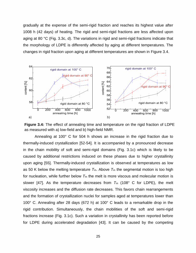
3.4 The effect of annealing time and temperature on the rigid fraction of LDPE as

measured with a) low-field and b) high-field NMR. ………………………….. 25

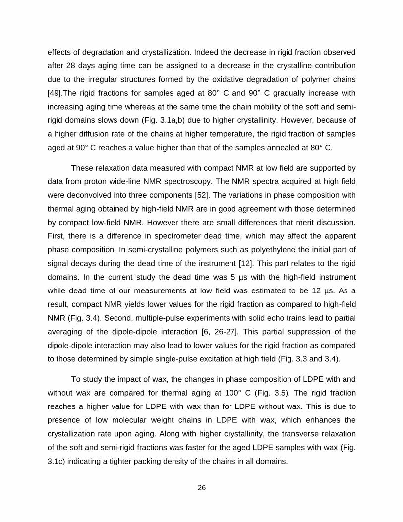
3.5 The contributions of rigid, semi-rigid and soft domains of LDPE with and without

wax aged at 100 °C as a function of aging time. ……………………………. 27

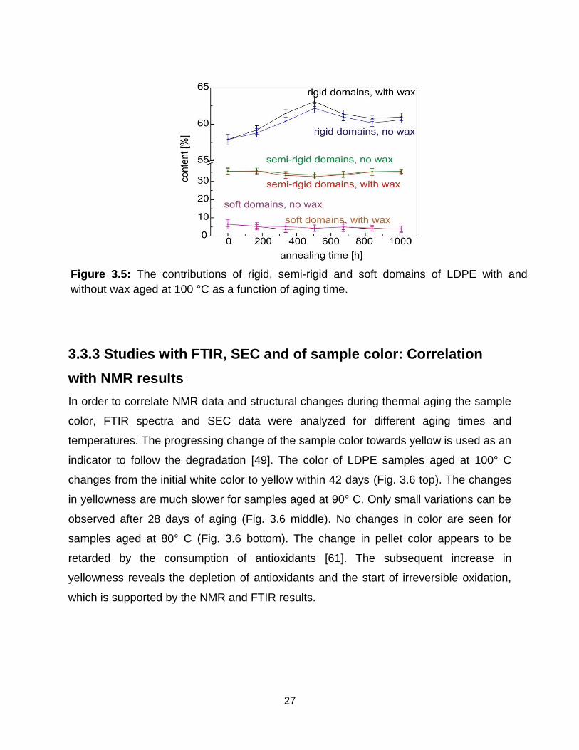
3.6 Changes in yellowness of LDPE samples. The yellowness increases

significantly after aging at 100° C for 28 days (top). There are only slight

x

changes in color when annealing at 90° C for 28 days (middle), and no

changes are observed for annealing at 80° C (bottom). ……………………. 28

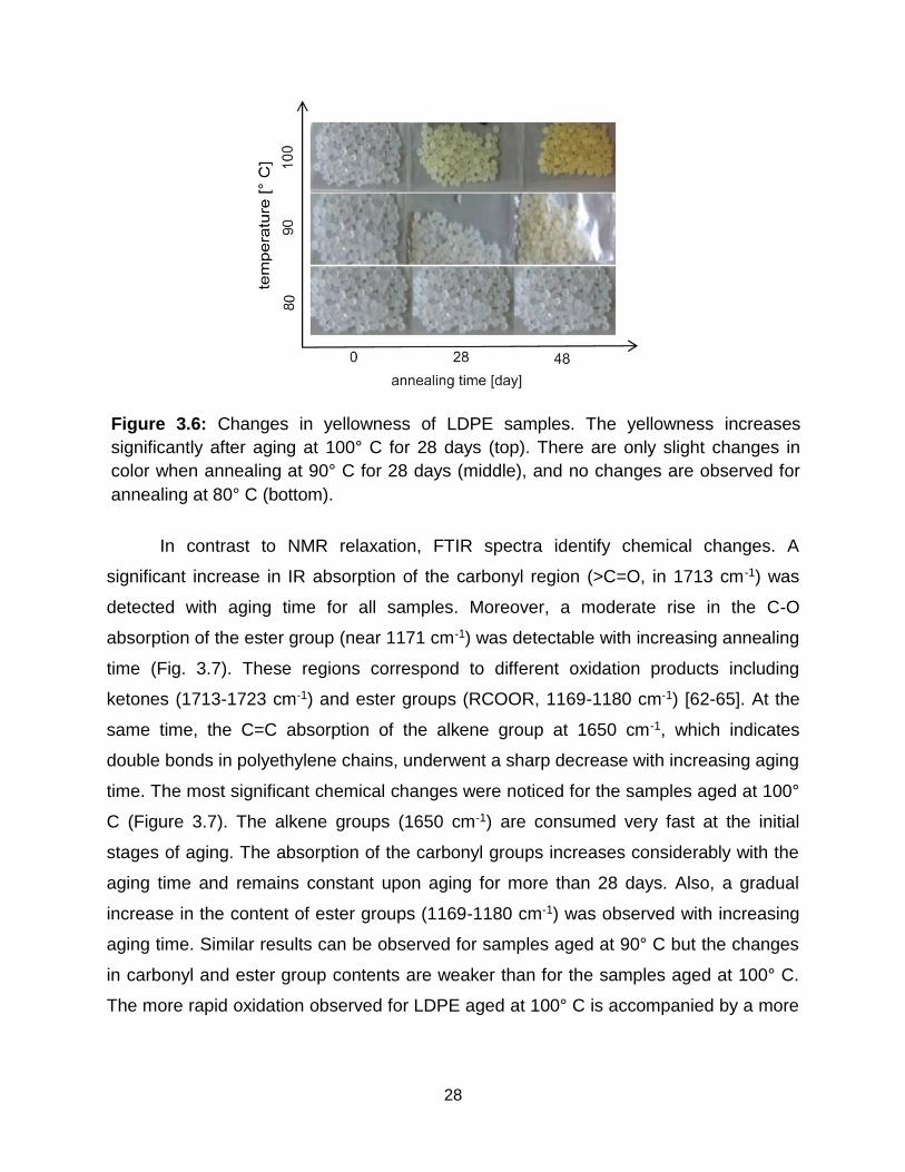
3.7 FTIR spectra for LDPE aged samples at 100° C. b) Variations of the carbonyl

index (Ico) for different temperatures as a function of aging time. ………….. 29

3.8 Molecular weight distributions obtained by SEC for samples aged at 80° C. b)

Number of chain scissions n and crosslinks x per mass unit as a function of

aging time at 80° C. …………………………………………………………….. 29

3.9 Changes in weight-average molecular weight Mw of LDPE samples at different

temperatures as a function of aging time. ……………………………………. 31

4.1 a) Mass changes of the swollen polyethylene sample upon drying. b) 13C solid-

state cross-polarization magic angle spinning NMR spectra of an LDPE sample

before and after swelling in n-hexane and subsequent drying. The 13C direct-

polarization NMR spectrum of the pure n-hexane is shown for comparison

raisons. ………………………………………………………………………….. 36

4.2 Experimental set-up for measuring PE pellets inside a Halbach magnet. ... 37

4.3 NMR data and analysis. a) 1H NMR relaxation decay of LDPE pellets measured

at room temperature using a Halbach magnet and bi-exponential fit to the

signal decay. The correlation coefficient R of the fit was higher than 0.99. b)

Proton wide-line NMR spectrum of LDPE measured at 70° C using a 500 MHz

NMR spectrometer and its analysis in terms of three components. The fit error

of this frequency-domain analysis is less than 0.6%. ………………………. 38

4.4 Changes in relaxation times T2eff (a) and in fraction (b) of LDPE domains as a

function of the swelling time in n-hexane at room temperature. ………….. 40

4.5 Changes in the inverse linewidths (a) and in the fractions (b) of LDPE domains

as a function of the swelling time in n-hexane at room temperature. ……... 41

4.6 Change in relaxation time T2eff of LDPE domains as a function of the swelling

time in different solvents at room temperature. ……………………………… 42

4.7 Variation of the relaxation times T2eff of the LDPE domains with the swelling

time in n-hexane at different temperatures. ………………………………….. 44

xi

4.8 13C NMR spectra of different polyethylene grades measured by magic angle

spinning with cross polarization (CPMAS) at room temperature. ………….. 45

4.9 Change in relaxation time T2eff of HDPE domains (a) and LLDPE domains (b)

as a function of the swelling time in different solvents at room temperature. 46

4.10 Differential scanning calorimetry scans of the swollen LDPE in n-hexane at

room temperature and subsequent drying. The DSC scan of the non-exposed

LDPE sample is shown for comparison reasons. …………………………… 47

5.1 Molecular weight distributions of the wax extracted from LDPE pellets with

leaching times of 1 day and 6 days. ………………………………………….. 54

5.2 Wax concentration in LDPE pellets determined by 1 T 1H NMR spectroscopy.

a) Spectrum of n-hexane with wax extracted from factory-grade LDPE pellets.

b) Calibration curve for the standard addition method. ……………………... 54

5.3 Wax content of LDPE leached into solvents versus leaching time by NMR

spectroscopy. a) n-Hexane. b) Xylene. ………………………………………. 56

5.4 Wax content in n-hexane by NMR spectroscopy as a function of the swelling

time. a) HDPE. b) LLDPE. ……………………………………………………... 57

5.5 Evaluation of NMR relaxometry data. a) 1H NMR relaxation decay of wax in n-

hexane extracted from extracted from LDPE pellets. b) Calibration curve

obtained with the standard addition method using a bi-exponential fit function to

extrapolate the NMR relaxation decay to zero time. ………………………... 58

5.6 Wax content of LDPE in n-hexane determined from fits of NMR relaxation

decays. a) Mono-exponential fits. b) Bio-exponential fits. ………………….. 59

5.7 Residuals of the concentrations determined experimentally and the linear fits of

the calibration curves for the standard addition method. a) Mono-exponential

fits of relaxometry data. b) Bi-exponential fits of relaxometry data. c)

Spectroscopy data. ……………………………………………………………... 59

6.1 Schematic transesterification reaction between two different polyesters forming

new cross links between the polymer strains. ……………………………….. 62

xii

6.2 Representative proton relaxation decay for the PET-PBT blend sample. ….. 64

6.3 Proton DQ build-up curves for PBT/PET blends and pure PBT samples with

and without glass-fibers at 140°C. The maximum e/r is marked with dashed

lines at about 14 µs for blends and 20 µs for the PBT samples. ………….. 66

6.4 Depth-profiles of PBT/PET blend sample at room temperature. a) different

phase fractions, b) transverse relaxation times of different phase domains. The

error in the phase fractions and T2eff are respectively less than 1 % and 7 s. 67

6.5 Depth-profiles of PBT/PET blend sample with GF at room temperature. a)

Different phase fractions, b) transverse relaxation times of different phase

domains. ………………………………………………………………………….. 67

6.6 Relative amplitude of blend samples (left) and amplitude difference reflecting

the glass fiber distribution in PBT/PET Blend + GF sample (right). ……….. 68

6.7 1H-13C CPMAS spectra of PBT (blue) sample and PBT/PET blend (red).

Spinning sidebands are marked with asterisks. PAR: protonated aromatics,

NPAR: non-protonated aromatics. The spectra are recorded at room

temperature. …………………………………………………………………….. 69

6.8 13C line-shape deconvolution for PBT/PET blend sample. The green and the

light blue line represent the amorphous and crystalline domains of PBT

respectively, while the purple line shows the PET amorphous fraction and the

orange curve represents the crystalline domains of PET. ………………….. 70

6.9 Depth-dependent analysis of the PBT/PET blend samples a) Extracted

deconvolution results b) PBT/PET ratio. ……………………………………... 70

6.10 Depth-dependent analysis of the PBT/PET blend samples with GF a) Extracted

deconvolution results b) PBT/PET ratio ……………………………………… 71

6.11 Depth-dependent proton spin-diffusion decays and build-up curves for the rigid

(crystalline) and soft (amorphous) fractions from PBT/PET blend without GF: 1)

Surface layer, 2) layer in the middle of the sample, 3) layer on the other surface

area. ……………………………………………………………………………… 72

6.12 Depth-dependent proton spin-diffusion decays and build-up curves for the rigid

(crystalline) and soft (amorphous) fractions from PBT/PET blend with GF: 1)

xiii

Surface layer 2) layer in the middle of the sample 3) layer on the other surface

area. ……………………………………………………………………………... 73

6.13 Depth-dependent spin-diffusion coefficients for the PBT/PET blends with and

without glass-fiber (GF). ……………………………………………………….. 73

6.14 Depth-dependent domains size distribution for the PBT/PET samples with and

without GF. ………………………………………………………………………. 74

7.1 Rubber-modified asphalt produced by wet process (left) and dry process (right)

[141]. ……………………………………………………………………………... 78

7.2 Experimental set-up for measuring the asphalt samples with a PM5 NMR-

MOUSE. The NMR-MOUSE is the black block underneath the black plate on

which the rubber cylinder rests. Its sensitive slice is located inside the asphalt

cylinder. To acquire depth profiles, the NMR-MOUSE is lowered from

measurement to measurement in a step-wise fashion, so that the distance

between NMR-MOUSE and test object decreases and the sensitive slice move

outward towards the bottom of the object. ………………………………….. 81

7.3 Representative relaxation decay for asphalt sample at 40° C. …………….. 82

7.4 NMR-Mouse field set-up for measuring the asphalt. ………………………... 82

7.5 T2eff (a) and fractions (b) of the rigid and soft components of asphalt sample 1

at 40° C. ………………………………………………………………………….. 83

7.6 Depth profiles of asphalt sample 1, at 40° C calculated as the sums of the first

8, 32 and 64 data points (top to bottom). …………………………………….. 84

7.7 Comparison of NMR relaxation data for the 5 asphalt samples in terms of depth

averages. a) T2eff of the soft domains from a component analysis if the

relaxation signals measured at 40° C. b) Rubber fractions of soft domains

estimated from a component analysis of the relaxation signals measured at 40°

C. c) Sum of the first 8 data points measured at 40° C. d) Sum of the first 8 data

points measured at room temperature. ………………………………………. 85

7.8 Correlation of actual rubber fraction with the NMR data sum measured at room

temperature. …………………………………………………………………….. 86

xiv

7.9 Master curve for the determination of the field rubber fractions at different

temperatures for rubber-modified asphalt projects prepared by dry process. 86

7.10 Comparison of signal decay measured at N1 a pure asphalt field and S13

rubber-modified asphalt filed. The significant difference in the initial part of the

decays results from the contribution of the 20 % rubber fraction in the S13

rubber-modified asphalt field. ………………………………………………….. 88

1

Chapter 1

1 Introduction

The context of modern Nuclear Magnetic Resonance (NMR) was contemporaneously

established by F. Bloch and E.M. Purcell in 1946 for which they were honored by the

Nobel Prize in physics in 1952. Since that time the importance of NMR has permanently

increased and in 1991 the Swiss physical chemist Richard R. Ernst succeeded to attain

the Nobel Prize in chemistry for his prominent contributions to the development of

experimental NMR methods. Nowadays NMR is well known in the fields of chemical

analysis and medical imaging for the quantitative and qualitative studies [1-2].

Particularly in the polymer industry, it is considered as a powerful analytical technique to

probe the structural heterogeneity and molecular mobility in polymers by directly

detecting differences in chemical shift and relaxation behavior [3-4]. Conventionally,

NMR experiments in polymer science are applied on the high-field instruments with high

sensitivity by employing high magnetic fields, where the signal-to-noise ratio is

proportional to the square of the static magnetic field [5]. NMR measurement on solid

samples such as polymers with strong dipole-dipole interactions results in significant

line broadening in collected spectra, which generally affects the structural information

[6]. While simple static proton broad-line and spin-diffusion measurements can deliver

morphological information when performing at a temperature much higher than the

glass transition temperature of the investigated polymer, CPMAS (Cross Polarization

Magic Angle Spinning) coupled with dipolar decoupling (DD) provides unique

information about the material structure at room temperature [6-7].

The development of high-field NMR is limited by the cost and complexity of the

equipment which prevents the use of such a device for outdoor applications. However,

during the last years considerable progress has been achieved with compact NMR

machines employing permanent magnets, which provide sufficient sensitivity and

2

robustness for nondestructive characterization in applications outdoors and on the

factory floor [8]. Compact NMR sensors have different geometries which depend on the

area of the applications and position of the samples with respect to the magnet. The

NMR-MOUSE® (MObile Universal Surface Explorer) [9] is a low-cost open sensor

device based on stray field NMR which shows great applications in non-destructive

material testing also by being portable as hand luggage. Due to a flat and thin sensitive

slice, which is located in an area a few millimeters away from the surface, the NMR-

MOUSE can also be employed to measure high-resolution depth profiles corresponding

to 1D images for studying a variety of polymer materials such as semicrystalline

polymers [3] and rubbers [10-11]. While the development of compact NMR was started

with singled-sided or insight-out NMR, the concept of mobile NMR was also applied to

the conventional outside-in NMR, where the object is placed into a magnet, for example

with the use of tube-shaped Halbach magnets [12-14]. They particularly promise novel

applications for polymer industries where the quality of raw and intermediate needs to

be monitored during production in the chemical plants and after production during use of

the product in the field.

Polymers are materials made from macromolecules composed of many small

repeat units, which drive from monomers. They show a broad range of properties which

make them a suitable alternative for traditional materials in everyday life. Polyethylene

(PE) has garnered the largest share of the worldwide polymer market with end products

ranging from trash bags to automotive parts. While PE shows excellent mechanical and

thermal properties strongly associated to its morphology [3], the morphology of PE end

products, in turn, is dictated by their thermal and mechanical history. This history

includes the processing parameters as well as temperature, pressure, deformation, and

solvent treatments. Therefore, the study of thermal aging and swelling is highly relevant

from an economic as well as a scientific perspective in order to understand how the

properties of polyethylene change over time. Furthermore, in the most technical

polyreaction processes of PE a considerable fraction of low-molecular weight polymers,

known as wax is generated. The separation of wax from the polymer and the

quantification of the wax content are of extreme importance in the polyolefin industry

where, for example, the Ziegler-Natta polymerization of ethylene can produce significant

3

amounts of wax as a by-product depending on the catalyst used and the operating

conditions of the plant. Therefore, the accurate determination of the polyethylene wax

content is of great practical and economical interest. On the other hand, over many

years a lot of efforts have been done on improving the materials properties in order to

increase the life time and performance efficiency. PET and PBT are well-known

engineering thermoplastic polyester with very valuable commercial applications. While

PET and PBT show their own individual properties, melt blending of those polyesters

leads to a compound with improved properties including the characteristics of both

polymers. Last but not least, impact modifiers are added to a specific matrix in order to

improve the impact properties. The final compound is supposed to show the improved

properties while retaining the cost and performance balance. Nowadays, compounds

including the rubber-modified asphalts have become of significant interest to the paving

industry where, they show a lot of improvements in fatigue cracking resistance, aging

and oxidation resistance and reduction of maintenance costs.

This dissertation focuses on the investigation of polymers by nuclear magnetic

resonance (NMR) combined with other analytical methods for implementing in polymer

industry. The main aim of such work is to develop and design novel analytical chemistry

methods and NMR methodologies for use on the factory floor. The related fundamental

concepts on low-field NMR, liquid- and solid-state NMR performed on the investigated

subjects will be discussed in chapter 2. This includes a brief review on the different

geometries of compact NMR where the appropriate pulse sequences for the relaxation

measurements are introduced. This is followed by an overview of liquid- and solid-state

NMR spectroscopy of polymers where industrial samples are investigated in order to

develop a test method based on practical and industrial requirements.

In chapter 3, the thermal degradation of polyethylene pellets directly out of the

factory is monitored with compact low-field NMR to accurately evaluate aging effects. It

is shown that simple NMR relaxation measurements can be employed to follow

thermally-induced crystallization and chemical degradation of polyethylene in a

quantitative manner. This is demonstrated by measuring the variations in chain

dynamics of crystalline, interphase and amorphous domains of LDPE samples annealed

4

at different temperatures for different times. The findings from compact NMR are

supported with data from high-field 1H solid-state NMR spectroscopy, FTIR and SEC.

The interaction between the solvent and the polymer matrix is a complex

phenomenon that triggers changes of different material properties. Chapter 4

investigates to what extent compact low-field NMR is a viable method for evaluating

swelling-induced morphological changes in PE. Here, factory-made PE-pellets were

exposed to various solvents at different times, and the morphological changes resulting

from solvent ingress were monitored. The findings from compact NMR are compared

with data from high-field 1H solid-state NMR spectroscopy and DSC. Moreover, when a

semicrystalline polymer such as PE is exposed to the solvent, it loses it’s low molecular

weight fraction or wax content. The presence of wax in polymers affects the processing

and application properties of the final product. In chapter 5, a novel way to determine

the wax content of PE pellets is introduced. The wax content is quantified with the

standard addition method employing compact NMR instruments for 1H NMR

spectroscopy and 1H NMR relaxometry. The findings from both NMR methods are

compared with data from gravimetric measurements.

Blending of polymers is considered as solution to establish a new polymer with

the tailored properties. Since PBT and PET are miscible in the amorphous phase, they

are suitable for melt blending process. However, it is essential to find an efficient

analytical method in order to understand the miscibility, melting, and crystallization

behavior of polyester blends. Chapter 6 analyzes PBT/PET blends with and without

glass fibers (GF) in comparison with pure PBT samples where the morphological

changes and the crystallinity are studied using NMR methods. The NMR-MOUSE is

applied to investigate the molecular mobility, morphological changes and the effect of

GF. Furthermore, an approach for estimating the glass-fiber distribution is introduced

using low-field measurements. In addition to these, 1H-13C-CPMAS (Cross Polarization

Magic Angle Spinning) in high-field is applied to study the rigid fraction in the blend

samples. The CPMAS spectra reveal differences between the blend and the pure PBT

sample and enable to gain information about the fractions of different polymer

components. In order to determine the domain sizes of different morphological domains,

5

Double-quantum (DQ) and spin-diffusion measurements are performed on the blend

samples.

In the last recent decades, many efforts have been generated in order to improve

the long-term performance and cost effectiveness of asphalt pavements. Rubber-

modified asphalt is one the most prevalent approached where the waste rubber is used

to modify the asphalt binder and mixture. The quantification of the rubber fraction along

with the control of the rubber distribution in the asphalt mixture is a key factor in the

quality control of rubber-modified asphalt. Chapter 7 reports on the determination of the

rubber fraction in rubber modified asphalt using the NMR-MOUSE, where the

transverse NMR relaxation signal is used to analyze the relative amplitudes. Here a new

NMR methodology has been developed in the laboratory based on calibration curves

obtained from reference samples. Furthermore, for actual field tests a modified version

of portable NMR-MOUSE set-up is used. The raw data from the field measurements

need to be further inserted into the calibration model to estimate the rubber fraction in

the field and to study the field variations in terms of the rubber distribution.

6

Chapter 2

2 Fundamentals of compact low-field

NMR and solid- and liquid-state NMR

This chapter reviews the fundamental concepts of the NMR methods which have been

used in this dissertation. This includes an introduction to the hardware of low-field NMR,

relaxation measurements and related pulse sequences, and the concepts of liquid- and

solid-state NMR concerning polymer investigations.

2.1 Low-field NMR

2.1.1 Single-sided magnet

The common high-field magnets are mainly in use for high-resolution liquid- and solid-

state NMR spectroscopy and MRI. They are expensive to operate due to the need for

cryogenic cooling and operator expertise. Furthermore with high-fields magnet, the

investigated samples should be inserted into the limited space of the magnet bore which

restricts non-destructive analysis of arbitrarily large samples. NMR measurements of

moisture in the soil and fluids properties confined to rock pores opened up a new

avenue into the inside-out NMR concepts, where in contrast to the conventional magnet

the instrument is placed inside the objects [15-17]. These efforts introduced mobile

NMR instruments as a successful tool for non-destructive analysis. Well-login tools were

the first prototype of mobile NMR which were established for use in the field in particular

for the oil industry more than 3 decades ago [16-17]. The difference in various NMR

properties such as relaxation times T1 and T2 and diffusivity D of various fluids makes it

possible to distinguish various components such as bound water, movable water, gas,

7

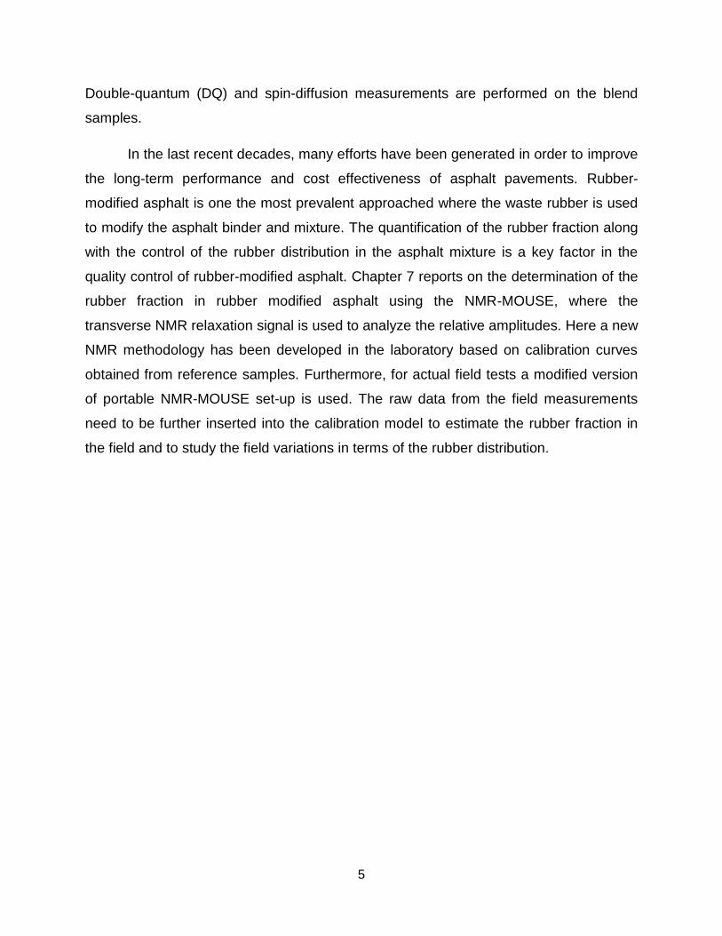
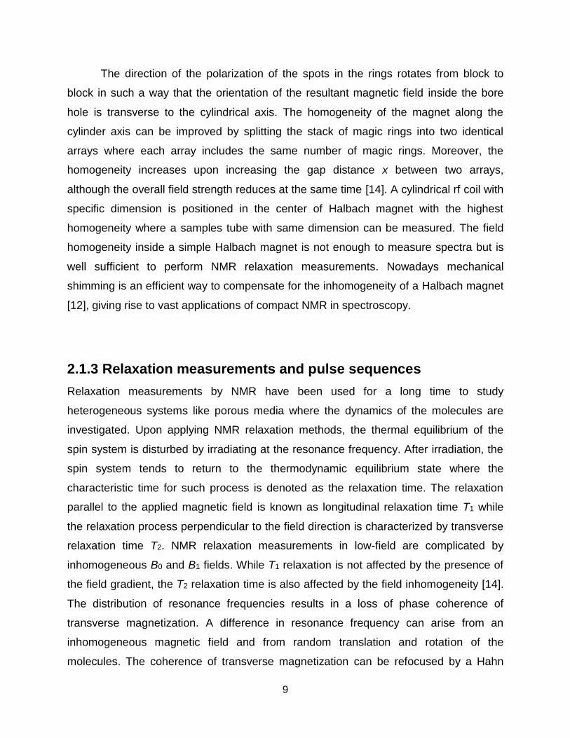
Figure 2.1: Schematic illustration of the NMR-MOUSE.

light oil, and heavy oil [18]. While developing well-logging NMR, the similar single-sided

sensors were developed to use in different applications such as in medicine, material

science and process control [19]. The NMR-MOUSE (MObile Universal Surface

Explorer) is a prominent output of systematic investigations of single-sided NMR,

introduced in the mid 1990’s [20]. The NMR-MOUSE (Fig. 2.1) is drived from a classical

C-shaped magnet that produces a comparatively homogeneous magnetic field B0 above

the gap between two poles and parallel to the surface by opening up the C [12].

Such a small unilateral NMR sensor can generate the static magnetic field up to

0.5 T with an adjustable gradient up to 45 T/m. [9]. The rf coil is placed in the gap

between the poles which produces a B1 rf field perpendicular to the B0 field within a

sensitive volume above the surface [21]. The sensitive volume achieved in the vicinity of

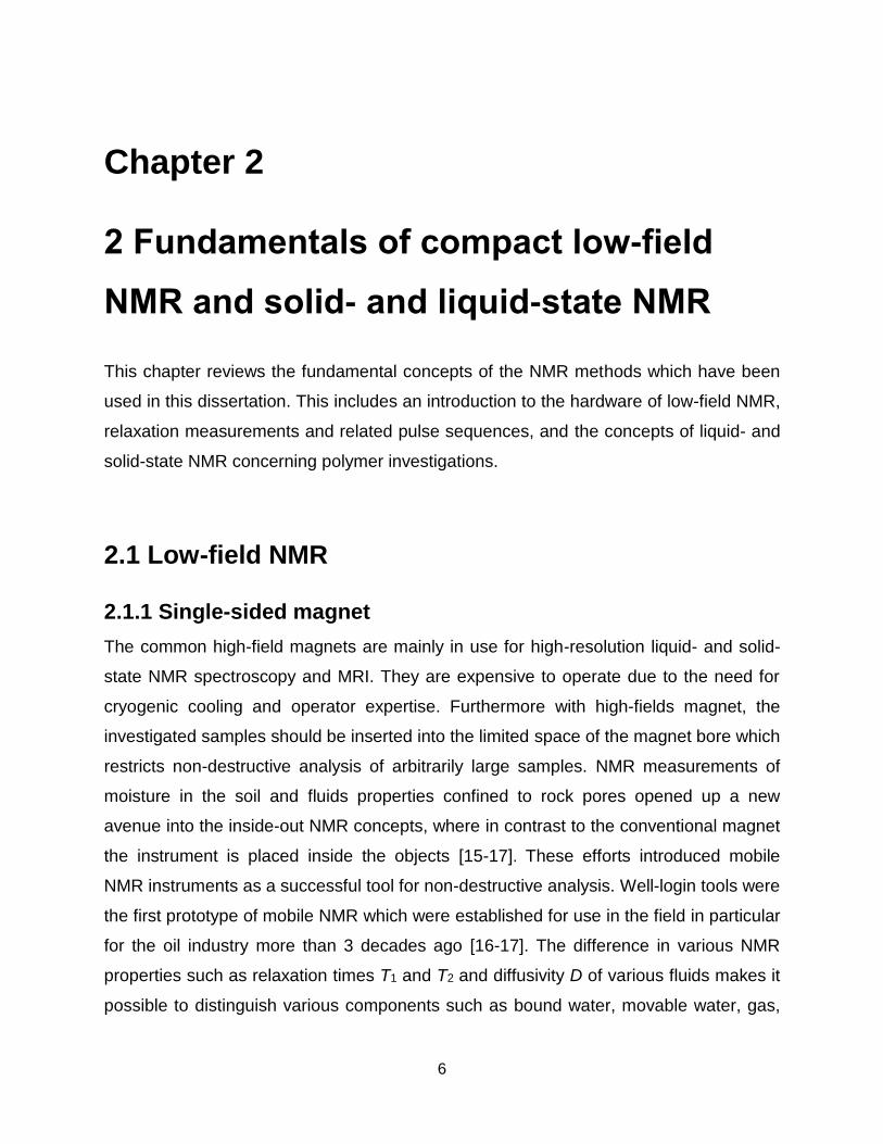
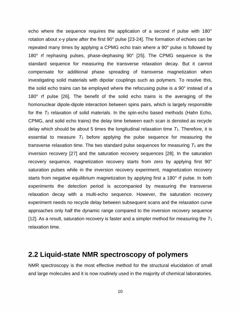
the coil is a function of field gradient and rf pulse length. Furthermore, to acquire depth

profiles, the NMR-MOUSE is lowered from measurement to measurement in a step-

wise fashion, so that the distance between NMR-MOUSE and test object increases and

the sensitive slice moves outward towards the bottom of the object (Fig. 2.2). The

optimum depth resolution can be achieved when the position of the sensitive slide is in

the order of the gap, and the magnet is well suited for profiling in a penetration depth

ranging from 0.5 to 1.5 times the gap [9].

8

Figure 2.2: Schematic illustration of the profile NMR-MOUSE. The sample is simply

placed on the top of the device [22].

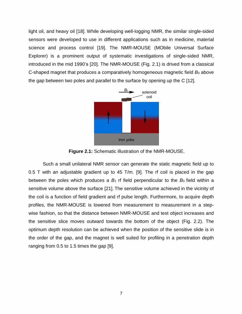
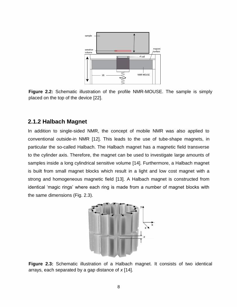
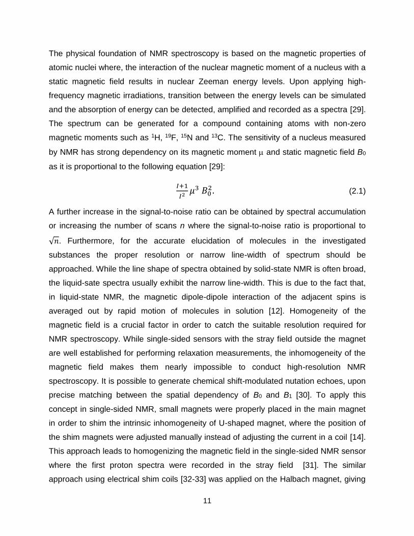
Figure 2.3: Schematic illustration of a Halbach magnet. It consists of two identical

arrays, each separated by a gap distance of x [14].

2.1.2 Halbach Magnet

In addition to single-sided NMR, the concept of mobile NMR was also applied to

conventional outside-in NMR [12]. This leads to the use of tube-shape magnets, in

particular the so-called Halbach. The Halbach magnet has a magnetic field transverse

to the cylinder axis. Therefore, the magnet can be used to investigate large amounts of

samples inside a long cylindrical sensitive volume [14]. Furthermore, a Halbach magnet

is built from small magnet blocks which result in a light and low cost magnet with a

strong and homogeneous magnetic field [13]. A Halbach magnet is constructed from

identical ‘magic rings’ where each ring is made from a number of magnet blocks with

the same dimensions (Fig. 2.3).

9

The direction of the polarization of the spots in the rings rotates from block to

block in such a way that the orientation of the resultant magnetic field inside the bore

hole is transverse to the cylindrical axis. The homogeneity of the magnet along the

cylinder axis can be improved by splitting the stack of magic rings into two identical

arrays where each array includes the same number of magic rings. Moreover, the

homogeneity increases upon increasing the gap distance x between two arrays,

although the overall field strength reduces at the same time [14]. A cylindrical rf coil with

specific dimension is positioned in the center of Halbach magnet with the highest

homogeneity where a samples tube with same dimension can be measured. The field

homogeneity inside a simple Halbach magnet is not enough to measure spectra but is

well sufficient to perform NMR relaxation measurements. Nowadays mechanical

shimming is an efficient way to compensate for the inhomogeneity of a Halbach magnet

[12], giving rise to vast applications of compact NMR in spectroscopy.

2.1.3 Relaxation measurements and pulse sequences

Relaxation measurements by NMR have been used for a long time to study

heterogeneous systems like porous media where the dynamics of the molecules are

investigated. Upon applying NMR relaxation methods, the thermal equilibrium of the

spin system is disturbed by irradiating at the resonance frequency. After irradiation, the

spin system tends to return to the thermodynamic equilibrium state where the

characteristic time for such process is denoted as the relaxation time. The relaxation

parallel to the applied magnetic field is known as longitudinal relaxation time T1 while

the relaxation process perpendicular to the field direction is characterized by transverse

relaxation time T2. NMR relaxation measurements in low-field are complicated by

inhomogeneous B0 and B1 fields. While T1 relaxation is not affected by the presence of

the field gradient, the T2 relaxation time is also affected by the field inhomogeneity [14].

The distribution of resonance frequencies results in a loss of phase coherence of

transverse magnetization. A difference in resonance frequency can arise from an

inhomogeneous magnetic field and from random translation and rotation of the

molecules. The coherence of transverse magnetization can be refocused by a Hahn

10

echo where the sequence requires the application of a second rf pulse with 180°

rotation about x-y plane after the first 90° pulse [23-24]. The formation of echoes can be

repeated many times by applying a CPMG echo train where a 90° pulse is followed by

180° rf rephasing pulses, phase-dephasing 90° [25]. The CPMG sequence is the

standard sequence for measuring the transverse relaxation decay. But it cannot

compensate for additional phase spreading of transverse magnetization when

investigating solid materials with dipolar couplings such as polymers. To resolve this,

the solid echo trains can be employed where the refocusing pulse is a 90° instead of a

180° rf pulse [26]. The benefit of the solid echo trains is the averaging of the

homonuclear dipole-dipole interaction between spins pairs, which is largely responsible

for the T2 relaxation of solid materials. In the spin-echo based methods (Hahn Echo,

CPMG, and solid echo trains) the delay time between each scan is denoted as recycle

delay which should be about 5 times the longitudinal relaxation time T1. Therefore, it is

essential to measure T1 before applying the pulse sequence for measuring the

transverse relaxation time. The two standard pulse sequences for measuring T1 are the

inversion recovery [27] and the saturation recovery sequences [28]. In the saturation

recovery sequence, magnetization recovery starts from zero by applying first 90°

saturation pulses while in the inversion recovery experiment, magnetization recovery

starts from negative equilibrium magnetization by applying first a 180° rf pulse. In both

experiments the detection period is accompanied by measuring the transverse

relaxation decay with a multi-echo sequence. However, the saturation recovery

experiment needs no recycle delay between subsequent scans and the relaxation curve

approaches only half the dynamic range compared to the inversion recovery sequence

[12]. As a result, saturation recovery is faster and a simpler method for measuring the T1

relaxation time.

2.2 Liquid-state NMR spectroscopy of polymers

NMR spectroscopy is the most effective method for the structural elucidation of small

and large molecules and it is now routinely used in the majority of chemical laboratories.

11

The physical foundation of NMR spectroscopy is based on the magnetic properties of

atomic nuclei where, the interaction of the nuclear magnetic moment of a nucleus with a

static magnetic field results in nuclear Zeeman energy levels. Upon applying high-

frequency magnetic irradiations, transition between the energy levels can be simulated

and the absorption of energy can be detected, amplified and recorded as a spectra [29].

The spectrum can be generated for a compound containing atoms with non-zero

magnetic moments such as 1H, 19F, 15N and 13C. The sensitivity of a nucleus measured

by NMR has strong dependency on its magnetic moment and static magnetic field B0

as it is proportional to the following equation [29]:

𝐼+1

𝐼2𝜇3 𝐵0

2. (2.1)

A further increase in the signal-to-noise ratio can be obtained by spectral accumulation

or increasing the number of scans n where the signal-to-noise ratio is proportional to

√𝑛. Furthermore, for the accurate elucidation of molecules in the investigated

substances the proper resolution or narrow line-width of spectrum should be

approached. While the line shape of spectra obtained by solid-state NMR is often broad,

the liquid-sate spectra usually exhibit the narrow line-width. This is due to the fact that,

in liquid-state NMR, the magnetic dipole-dipole interaction of the adjacent spins is

averaged out by rapid motion of molecules in solution [12]. Homogeneity of the

magnetic field is a crucial factor in order to catch the suitable resolution required for

NMR spectroscopy. While single-sided sensors with the stray field outside the magnet

are well established for performing relaxation measurements, the inhomogeneity of the

magnetic field makes them nearly impossible to conduct high-resolution NMR

spectroscopy. It is possible to generate chemical shift-modulated nutation echoes, upon

precise matching between the spatial dependency of B0 and B1 [30]. To apply this

concept in single-sided NMR, small magnets were properly placed in the main magnet

in order to shim the intrinsic inhomogeneity of U-shaped magnet, where the position of

the shim magnets were adjusted manually instead of adjusting the current in a coil [14].

This approach leads to homogenizing the magnetic field in the single-sided NMR sensor

where the first proton spectra were recorded in the stray field [31]. The similar

approach using electrical shim coils [32-33] was applied on the Halbach magnet, giving

12

rise to a sufficient homogeneity for NMR spectroscopy. Nowadays, the compact NMR

spectroscopy employing a highly homogeneous Halbach magnet provides new

applications on the chemical workbench for the determination of chemical structures

and reaction monitoring [34-35]. In addition to the common 1D NMR spectra such as 1H

and 13C, there are a variety of two-dimensional NMR methods which can be performed

by compact NMR spectroscopy. Such 2D NMR methods are useful even at low-field

where more often the chemical shifts cannot be clearly extracted from 1D spectrum due

to the complex structure of investigated molecules [12, 36].

2.3 Solid-state NMR spectroscopy of polymers

In the liquid samples thanks to the rapid and random motion of the molecules, the

dipole-dipole interaction has no effect in NMR experiments while in solid samples the

effect of the dipole-dipole interaction does not average to zero due to the restricted

motion of the molecules. The resonance frequency of the nucleus depends on the local

magnetic field which is a function of neighboring spins. In solid samples, variation in the

orientation of neighboring spins leads to a significant spread in the resonant frequency

which consequently increases the spectra line-width by several order of magnitude

compared to the line-width of liquid samples [37-38]. Another reason for the line

broadening in the solid-state NMR is the chemical shift anisotropy where a local field

produced by a variation in the electron orbits in the strong static magnetic field leads to

the spread of the resonance frequency. The NMR active nuclei can be mainly divided to

two categories: high natural abundance such as 1H and low natural abundance like 13C.

The most difficult experiment in solid-state NMR belongs to the nuclei of the first group

where due to high natural abundance, homonuclear dipolar interactions are strong and

homonuclear decoupling is hardly impossible [2]. A low abundant nucleus such as 13C,

on the other hand, is diluted and typically far away from other 13C. So that 13C nuclei are

isolated relative to each other while interacting with the neighboring protons. However, a

variety of techniques can be used to solve this problem and decrease the line

broadening.

13

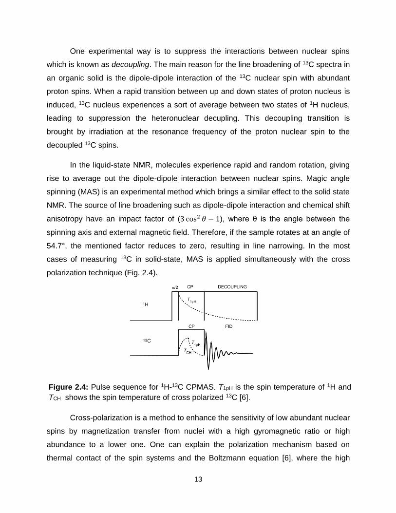
Figure 2.4: Pulse sequence for 1H-13C CPMAS. T1pH is the spin temperature of 1H and

TCH shows the spin temperature of cross polarized 13C [6].

period.

One experimental way is to suppress the interactions between nuclear spins

which is known as decoupling. The main reason for the line broadening of 13C spectra in

an organic solid is the dipole-dipole interaction of the 13C nuclear spin with abundant

proton spins. When a rapid transition between up and down states of proton nucleus is

induced, 13C nucleus experiences a sort of average between two states of 1H nucleus,

leading to suppression the heteronuclear decupling. This decoupling transition is

brought by irradiation at the resonance frequency of the proton nuclear spin to the

decoupled 13C spins.

In the liquid-state NMR, molecules experience rapid and random rotation, giving

rise to average out the dipole-dipole interaction between nuclear spins. Magic angle

spinning (MAS) is an experimental method which brings a similar effect to the solid state

NMR. The source of line broadening such as dipole-dipole interaction and chemical shift

anisotropy have an impact factor of (3 cos2 𝜃 − 1), where θ is the angle between the

spinning axis and external magnetic field. Therefore, if the sample rotates at an angle of

54.7°, the mentioned factor reduces to zero, resulting in line narrowing. In the most

cases of measuring 13C in solid-state, MAS is applied simultaneously with the cross

polarization technique (Fig. 2.4).

Cross-polarization is a method to enhance the sensitivity of low abundant nuclear

spins by magnetization transfer from nuclei with a high gyromagnetic ratio or high

abundance to a lower one. One can explain the polarization mechanism based on

thermal contact of the spin systems and the Boltzmann equation [6], where the high

14

abundant spin system is supposed to be in a low temperature state compared to the low

abundant nuclear spins. Upon thermal contact, heat transfers from low abundant

system to the cold system with high abundant nuclear spins. Due to this, the spin

temperature of low abundant system is decreased, indicating the higher population

difference between the upper and lower energy levels equivalent to the increased

sensitivity of the NMR experiment. However, here employing the proper contact time

between the high and low abundant spin systems is an essential factor. Upon selecting

the good contact time, the low abundant nuclear spins needs the less time to recover its

equilibrium polarization which shortens the experimental time. Magnetic dipole-dipole

interactions are responsible for providing the thermal contact in solids. From a classical

standpoint, resonance energy can be exchanged between two oscillating systems if the

initial frequencies of the systems are close. From the quantum mechanical standpoint,

the Hartmann-Hahn condition has to be fulfilled for the proper thermal contact and the

magnetization transfer:

𝛾H𝐵1H = 𝛾C𝐵1C , (2.2)

where represents the gyromagnetic factor and B1 shows the rf field denoted for the

proton and carbon nuclei [6]. Upon the contact time, the spin temperature of the low

abundant system can be lowered by a factor of 𝛾𝑙𝑜𝑤 𝑎𝑏𝑢𝑛𝑑𝑎𝑛𝑡

𝛾ℎ𝑖𝑔ℎ 𝑎𝑏𝑢𝑛𝑑𝑎𝑛𝑡. For the protons and 13C

nuclei, this factor reaches to ¼ which gives rise to 4 times enhancement in the

sensitivity of the 13C nuclear spins upon applying the cross polarization.

2.4 Spin diffusion measurements

Most semicrystalline polymers and blends are heterogeneous materials which arise

from the various domains characterized by different chain dynamics. Among other

methods, such as transmission electron microscopy (TEM) and small-angle X-ray

scattering (SAXS), solid state NMR emerged as a useful approach to explore and

understand heterogeneous materials. Based on the magnetization exchange after

15

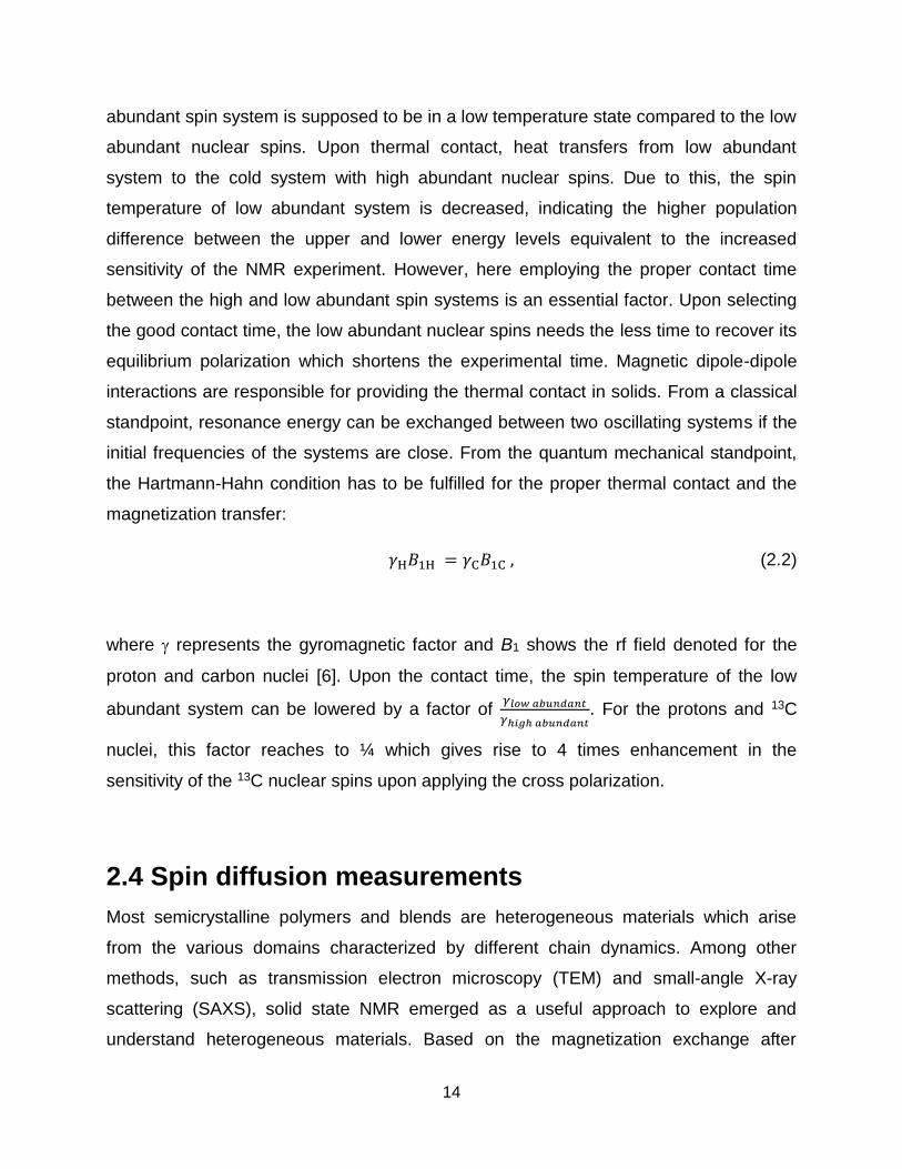
Figure 2.5: Spin-diffusion pulse sequence with a double-quantum dipolar filter [40].

Here e/r is the excitation/reconversion time and DQ is the double-quantum coherence

period.

inducing a z magnetization gradient by a dipolar filter, the 1H spin-diffusion technique is

capable of quantifying the domain size in heterogeneous polymers well above their

glass transition temperature [39].

Figure 2.5 shows a typical spin-diffusion pulse sequence with a double-quantum

dipolar filter. It consists of an excitation and matched reconversion period followed by a

spin-diffusion period. For semi-crystalline polymers, the magnetization of the rigid phase

of polymer is selected by applying appropriate excitation and reconversion times. The

approach to equilibrium of the magnetization within the polymer is then monitored

during the mixing time m. The applied mixing times m should be shorter than T1 to

avoid the effect of this relaxation process on the spin-diffusion process. Further details

about the methodology can be founded in literature [40-41].

The spectra recorded for each mixing time are then analyzed in order to extract

information about the phase fractions of each phase and to generate the spin-diffusion

build-up and decay curves. In order to extract reliable information about domain sizes,

the type of morphology and the spin-diffusion coefficients need to be known. The spin-

diffusion coefficients for the crystalline (Dc), amorphous (Da) and interface (Di) regions

can be calculated using following equations [41]:

𝐷C ≈1

12√

π

2ln2⟨𝑟2⟩Δ𝜈1

2

, (2.3)

16

𝐷a ≈1

6⟨𝑟2⟩[𝛼Δ𝜈1 2⁄ ]

1 2⁄, (2.4)

𝐷𝑖 ≈ (𝐷𝑐 + 𝐷𝑎) 2 ⁄ , (2.5)

where ⟨𝑟²⟩ is the mean square distance between the nearest spins. Δν1 2⁄ is the line

width at the half height of the spectrum of each different phase and α is known as the

cut-off parameter for the Lorentzian line shape. The domain size itself can be

determined with the initial-rate approximation which estimates tm*. Having this value it is

possible to determine the ratio Vtot/Stot, which is set as the volume per interface area for

a given mixture of A and B:

Vtot

Stot= (

ρHAϕA+ρHBϕB

ϕAϕB)

2

√π

√DADB

√DAρHA+√DBρHB√tm

* , (2.6)

here Vtot is the total volume and Stot the total interface volume. ϕ represents the volume

fractions and ρ is the proton density of a certain fraction. After the introduction of the

dimensionality ε and the relation between the long period 𝑑 ≡ 𝑑dis + 𝑑mat (dispersed

phase and matrix) and the volume fractions for dispersed phase and for the matrix, one

can get the ratio of Vtot

Stot based on the following equation:

𝑉tot

𝑆tot=

𝑑dis

2 𝜀 𝜙dis, (2.7)

As a result, the domain size of the dispersed phase can be determined after

transformation, using the following equation:

𝑑dis = (𝜌HA𝜙A+𝜌HB𝜙B

𝜙A𝜙B)

4𝜀𝜙dis

√π

√𝐷A𝐷B

√𝐷A𝜌HA+√𝐷B𝜌HB√𝑡m

∗ , (2.8)

Here one can calculate the different domain sizes by taking the different volume

fractions for ϕ𝑑𝑖𝑠, which is the dispersed volume fraction. Furthermore, it is possible to

consider the dimensionality by setting ε = 1 for lamellar, ε = 2 for cylindrical or ε = 3 for

spherical morphologies [42].

17

Chapter 3

3 Thermal aging and degradation of

LDPE

This chapter is derived from my publication, reference 4, which was published in the

Journal of Macromolecular and Material Engineering. The second and third authors of

this publication are respectively Rance Kwamen and Bernhard Blümich. Dr. Kwamen

has contributed in the conduction of experiments and correcting the publication and

Prof. Blümich has formulated and supervised the project and edited the manuscript.

3.1 Introduction and motivation

Polyethylene (PE) is one of the most popular polymer materials. Its product range

extends from water and gas pipes to medical implants and plastic wraps. PE has

excellent mechanical and thermal properties which are strongly related to its

morphology [43]. The morphology of PE end products typically changes when the

sample is exposed to temperatures above the glass transition temperature due to

physical and chemical aging. This causes changes in different material properties such

as the density, the modulus, the dynamic mechanical response and optical clarity [44-

46]. Therefore the study of physical and chemical changes is of great practical and

fundamental interest.

Various thermodynamic and kinetic factors influence the morphology of semi-

crystalline polymers [47]. Most importantly, temperature affects the segmental chain

mobility and thus the formation of crystallites. Thermally-induced crystallization is

observed as low as 50 K below the melting temperature Tm. In the range between Tm-50

K < T < Tm the thermal motion of polymer chains can lead to stable and ordered regions

18

[47-48]. Moreover, in the presence of oxygen polymers degrade reactively [43], which

subsequently impacts the crystallization mechanism during physical aging.

Consequently, it is important to investigate the changes in phase composition and chain

mobility of different domains induced by thermal and oxidative aging in order to

understand the properties of polyethylene as they change over time.

The phase composition of semi-crystalline polymers during aging has been

determined with various experimental methods. The changes in crystallinity and melting

point of polyethylene upon annealing were determined with differential scanning

calorimetry (DSC) [49-50]. These results showed that crystallinity Xc and melting

temperature Tm of PE increase upon aging. The relative phase fractions of

semicrystalline polymers were estimated with X-ray diffraction (XRD) [51]. XRD

patterns were deconvolved into amorphous and crystalline fractions based on a two-

phase model. The results showed a gradual increase in the amount of the crystalline

phase upon annealing. While DSC and X-ray provide valuable information about

crystalline domains, the primary changes induced by thermal aging arise in the

amorphous and interphase domains [52], which are not directly probed by these

methods.

The existence of a rigid amorphous interface separating the crystalline and

amorphous phases of semi-crystalline polymers has been shown in NMR studies [3, 53-

54]. This interface plays a determining role for the morphology and thus mechanical

properties [51]. The aging of semicrystalline polymers at elevated temperatures has

been investigated with NMR at high field [55]. An alternative to high-field NMR is low-

field NMR, in particular, unilateral stray-field NMR. The latter combines sufficient

sensitivity and robustness for outdoor applications and nondestructive characterization.

[3, 51-52] To our knowledge no NMR investigation of the thermal degradation of low

density polyethylene (LDPE) under accelerated aging conditions has been reported so

far. Moreover, in previous low-field NMR studies of PE aging, the thermal history was ill

defined [51]. In particular, the thermo-mechanical history of untreated samples before

applying a well-defined aging protocol was unknown. In this study the thermal

degradation of polyethylene pellets directly out of the factory is monitored with compact

19

low-field NMR to accurately evaluate the aging effects. It is shown that simple NMR

relaxation measurements can be employed to follow thermally-induced crystallization

and chemical degradation of polyethylene in a quantitative manner. This is

demonstrated by measuring the variations in chain dynamics of crystalline, interphase

and amorphous domains of LDPE samples annealed at different temperatures for

different times. The findings from compact NMR are supported with data from high-field

1H solid-state NMR spectroscopy, FTIR and SEC.

3.2 Experimental

3.2.1 Sample description and preparation

The LDPE type studied was Lupolen 1806H from LyondelBasell. Its melt flow index

(MFI) is 1.6 dg/min (190/2.16) and its density and melting point are 0.919 g/cm3 and

108° C, respectively. LDPE pellets were aged in an air circulating oven at 100° C, 90° C

and 80° C up to 42 days (1008 h). The NMR experiments on aged samples were

conducted at room temperature. To investigate the effect of low molecular weight chains

(wax content) on the aging process, ‘LDPE without wax’ was prepared by swelling

untreated LDPE in n-hexane for 4 weeks at room temperature. This LDPE without wax

was aged at 100° C and compared to untreated LDPE aged at the same temperature.

3.2.2 Measurements

NMR measurements and data analysis

Two different NMR methods, wide-line NMR spectroscopy and transverse

magnetization relaxation were employed to study the phase composition and molecular

mobility in LDPE. All measurements were performed at room temperature. The wide-

line NMR spectra were measured at high magnetic field with a Bruker DSX-200

spectrometer operating at a proton resonance frequency of 200 MHz. The relaxation

was measured with a home-built Halbach magnet connected to a Bruker Minispec

20

spectrometer operating at a proton resonance frequency of 34.2 MHz. The region with

the highest magnetic field homogeneity was found in the center of the magnet with a

cylindrical volume of 8-mm diameter and 8-mm length, where a radio-frequency coil of

similar dimensions was positioned.

The transverse magnetization decays of the samples were measured with a multi

solid echo pulse sequence, i.e., 90°x-(tE/2)-90°y-(tE/2)-[acquisition] using an echo time of

tE = 30 µs. The decays were analyzed by fitting the experimental data to a triple

exponential function,

A(t) =Arigid exp(-t/T2eff rigid)+ Asemi-rigid exp(-t/T2eff

semi-rigid)+Asoft exp(-t/T2eff soft). (3.1)

The relaxation times T2eff are related to the chain mobilities in each fraction. The relative

fractions of the relaxation components Ai/(Arigid+Asemi-rigid+Asoft) represent the relative

numbers of hydrogen atoms (molar fractions) of the LDPE phases with different

molecular mobilities.

Fourier transform infrared spectroscopy (FTIR)

FTIR spectra were acquired at room temperature with a Perkin Elmer UATR TWO

spectrometer in the range of 450-4000 cm-1. The resolution was set to 2 cm-1, and 16

scans were measured per spectrum. The carbonyl index ICO was determined using the

amplitude ratio of the carbonyl band at 1713 cm-1 and of the C-H band at 720 cm-1[43].

Size-exclusion chromatography (SEC)

Molecular weights (Mn and Mw) and molecular weight distributions (Mw/Mn) were

determined by size-exclusion chromatography (SEC). SEC with 1,2,4-Trichlorobenzene

(for GPC, AppliChem) as eluent was employed using an Polymer-Char-system

equipped with an IR-4 (for CH and CH3 groups) and a Visco detector. The eluent

contained 200 mg/ml 3,5-di-tert-4-butylhydroxytoluene (BHT, ≥99%, Fluka) as internal

standard. One pre-column (8 mm x 50 mm) and four Polefin gel columns (8 mm x 300

mm, Polymer Standards Service) were utilized at a flow rate of 1.0 ml/min at 150° C.

21

The diameter of the gel particles measured 10 µm, the nominal pore widths were 102,

103, 105, and 106 °A. The apparatus calibrated with narrowly distributed polyethylene

standards (Polymer Standards Service). The injection volume and sample concentration

were 200 l and 3 mg/ml, respectively. Results were evaluated using the PSS WinGPC

UniChrom software (Version 8.1.1).

The number of chain scissions (n) and crosslinks (x) per mass unit of aged

samples can be determined from equations (3.2) and (3.3) [56]:

∆𝑛=1

𝑀𝑛−

1

𝑀𝑛,0 ∆𝑤=

1

𝑀𝑤−

1

𝑀𝑤,0 , (3.2)

𝑛 =2

3 (2∆n − ∇w) 𝑎𝑛𝑑 𝑥 =

1

3(∆𝑛 − 2∆𝑤), (3.3)

Where Mn,0 and Mw,0 are the initial number-average and weight-average molecular

weights.

3.3 Results and discussions

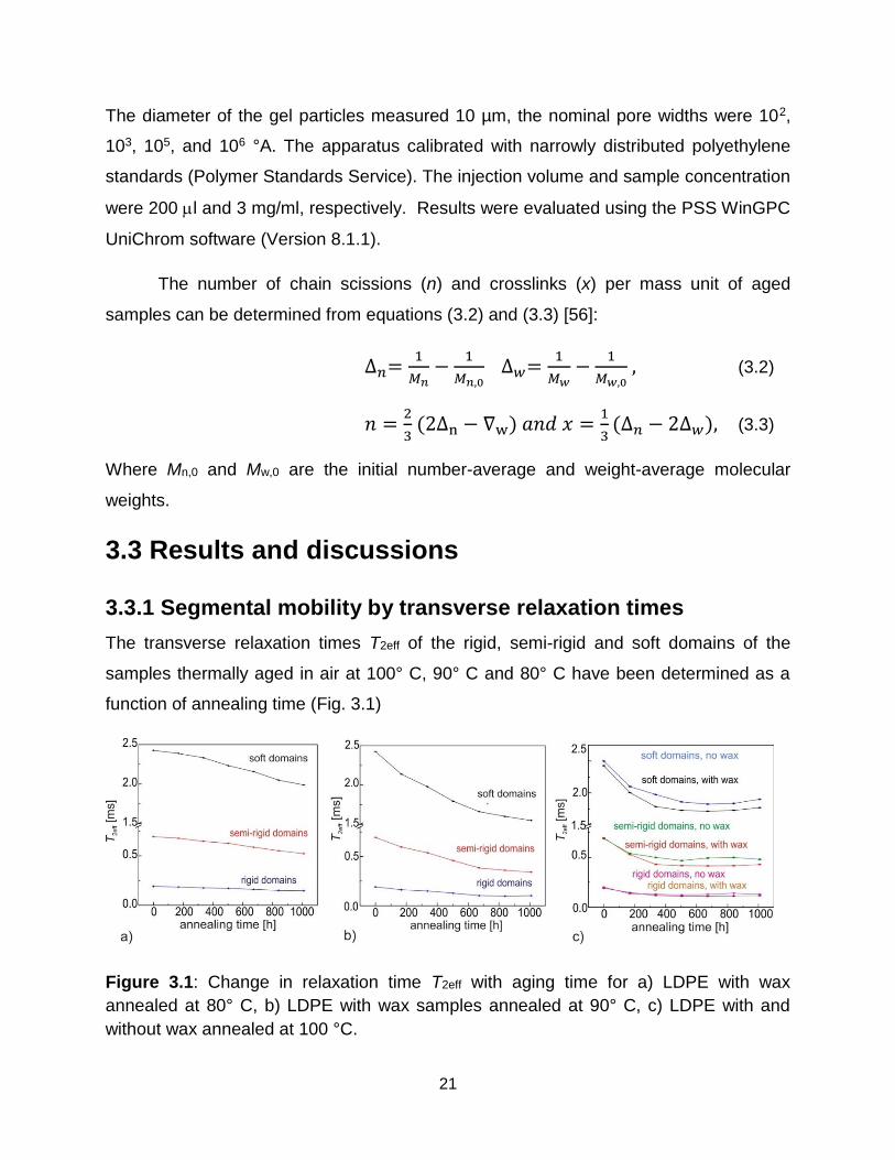
3.3.1 Segmental mobility by transverse relaxation times

The transverse relaxation times T2eff of the rigid, semi-rigid and soft domains of the

samples thermally aged in air at 100° C, 90° C and 80° C have been determined as a

function of annealing time (Fig. 3.1)

Figure 3.1: Change in relaxation time T2eff with aging time for a) LDPE with wax

annealed at 80° C, b) LDPE with wax samples annealed at 90° C, c) LDPE with and

without wax annealed at 100 °C.

22

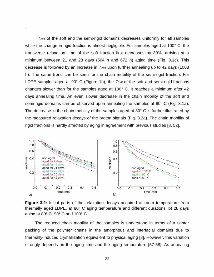
Figure 3.2: Initial parts of the relaxation decays acquired at room temperature from

thermally aged LDPE. a) 80° C aging temperature and different durations. b) 28 days

aging at 80° C, 90° C and 100° C.

.

T2eff of the soft and the semi-rigid domains decreases uniformly for all samples

while the change in rigid fraction is almost negligible. For samples aged at 100° C, the

transverse relaxation time of the soft fraction first decreases by 30%, arriving at a

minimum between 21 and 28 days (504 h and 672 h) aging time (Fig. 3.1c). This

decrease is followed by an increase in T2eff upon further annealing up to 42 days (1008

h). The same trend can be seen for the chain mobility of the semi-rigid fraction. For

LDPE samples aged at 90° C (Figure 1b), the T2eff of the soft and semi-rigid fractions

changes slower than for the samples aged at 100° C. It reaches a minimum after 42

days annealing time. An even slower decrease in the chain mobility of the soft and

semi-rigid domains can be observed upon annealing the samples at 80° C (Fig. 3.1a).

The decrease in the chain mobility of the samples aged at 80° C is further illustrated by

the measured relaxation decays of the proton signals (Fig. 3.2a). The chain mobility of

rigid fractions is hardly affected by aging in agreement with previous studies [8, 52].

The reduced chain mobility of the samples is understood in terms of a tighter

packing of the polymer chains in the amorphous and interfacial domains due to

thermally-induced crystallization equivalent to physical aging [8]. However, this variation

strongly depends on the aging time and the aging temperature [57-58]. As annealing

23

time and temperature increase, thermal-oxidative aging gives rise to chain scission

which enhances the chain mobility while also accelerating crystallization. Thus physical

crystallization, and chemical degradation need to be considered together [43]. A slight

increase in T2eff of the soft and semi-rigid domains upon annealing for more than 672

hours (28 days) at 100° C indicates that chemical degradation is becoming the

dominant process at long annealing times. This competition between the two processes

is also illustrated by the signal decays of samples aged for 28 days at different

temperatures (Fig. 3.2b). With the aging temperature increasing from 80° C to 100° C,

the molecular mobility increases, which leads to faster structural rearrangements and

higher crystallization rates [55]. The signal decays of the samples aged at 90° C and

100° C become similar after 28 days (Fig. 3.2b). This is attributed to more efficient

averaging of the magnetic dipole-dipole interaction due to increased chain mobility

following chain scission of LDPE aged at 100° C. This interpretation of ageing in terms

of a competition between physical crystallization and chemical degradation is also

supported by changes in the sample color (Fig. 3.6) and a gradual decrease in the rigid

fraction (Fig. 3.3a,b) when the samples are aged at 100° C for more than 28 days.

In industrial polymers, a further parameter needs to be considered in aging

studies. This concerns the polydispersity of the polymer chains. A considerable fraction

of oligomers and low-molecular weight polymers is generated in most technical

polyreaction processes [59]. Upon swelling in a solvent a semi-crystalline polymer loses

some of its low molecular weight fraction. This fraction is refereed to as the wax content

and is less than 1 wt. % for LDPE. We show here how the wax content affects the aging

process when the sample is exposed to elevated temperatures. Figure 3.1c compares

the variations in T2eff of standard LDPE with wax and LDPE without wax upon aging at

100° C. The lower chain mobilities of the soft and semi-rigid fractions of LDPE with wax

suggest that the wax content can accelerate the physical aging process and increase

the crystallinity during thermal aging. Short chains can diffuse faster giving rise to a

higher rigid fraction for LDPE samples with wax as compared to LDPE without wax (Fig.

3.1c). Moreover, FTIR results show higher chain scission for LDPE with wax (Fig. 3.7),

so that the presence of wax enhances not only the physical aging by crystallization but

also the chemical aging with the formation of unsaturated groups (>C=O groups) [60].

24

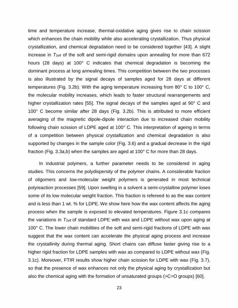
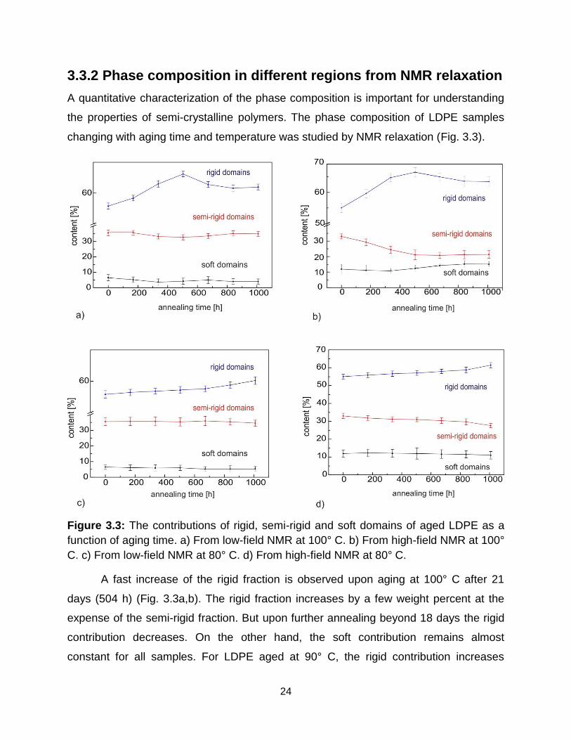
3.3.2 Phase composition in different regions from NMR relaxation

A quantitative characterization of the phase composition is important for understanding

the properties of semi-crystalline polymers. The phase composition of LDPE samples

changing with aging time and temperature was studied by NMR relaxation (Fig. 3.3).

Figure 3.3: The contributions of rigid, semi-rigid and soft domains of aged LDPE as a

function of aging time. a) From low-field NMR at 100° C. b) From high-field NMR at 100°

C. c) From low-field NMR at 80° C. d) From high-field NMR at 80° C.

A fast increase of the rigid fraction is observed upon aging at 100° C after 21

days (504 h) (Fig. 3.3a,b). The rigid fraction increases by a few weight percent at the

expense of the semi-rigid fraction. But upon further annealing beyond 18 days the rigid

contribution decreases. On the other hand, the soft contribution remains almost

constant for all samples. For LDPE aged at 90° C, the rigid contribution increases

25

Figure 3.4: The effect of annealing time and temperature on the rigid fraction of LDPE

as measured with a) low-field and b) high-field NMR.

gradually at the expense of the semi-rigid fraction and reaches its highest value after

1008 h (42 days) of heating. The rigid and semi-rigid fractions are less affected upon

aging at 80 °C (Fig. 3.3c, d). The variations in rigid and semi-rigid fractions indicate that

the morphology of LDPE is differently affected by aging at different temperatures. The

changes in rigid fraction upon aging at different temperatures are shown in Figure 3.4.

Annealing at 100° C for 504 h shows an increase in the rigid fraction due to

thermally-induced crystallization [52-54]. It is accompanied by a pronounced decrease

in the chain mobility of soft and semi-rigid domains (Fig. 3.1c) which is likely to be

caused by additional restrictions induced on these phases due to higher crystallinity

upon aging [55]. Thermally-induced crystallization is observed at temperatures as low

as 50 K below the melting temperature Tm. Above Tm the segmental motion is too high

for nucleation, while further below Tm the melt is more viscous and molecular motion is

slower [47]. As the temperature decreases from Tm (108° C for LDPE), the melt

viscosity increases and the diffusion rate decreases. This favors chain rearrangements

and the formation of crystallization nuclei for samples aged at temperatures lower than

100° C. Annealing after 28 days (672 h) at 100° C leads to a remarkable drop in the

rigid contribution. Simultaneously, the chain mobilities of the soft and semi-rigid

fractions increase (Fig. 3.1c). Such a variation in crystallinity has been reported before

for LDPE during accelerated degradation [43]. It can be caused by the competing

26

effects of degradation and crystallization. Indeed the decrease in rigid fraction observed

after 28 days aging time can be assigned to a decrease in the crystalline contribution

due to the irregular structures formed by the oxidative degradation of polymer chains

[49].The rigid fractions for samples aged at 80° C and 90° C gradually increase with

increasing aging time whereas at the same time the chain mobility of the soft and semi-

rigid domains slows down (Fig. 3.1a,b) due to higher crystallinity. However, because of

a higher diffusion rate of the chains at higher temperature, the rigid fraction of samples

aged at 90° C reaches a value higher than that of the samples annealed at 80° C.

These relaxation data measured with compact NMR at low field are supported by

data from proton wide-line NMR spectroscopy. The NMR spectra acquired at high field

were deconvolved into three components [52]. The variations in phase composition with

thermal aging obtained by high-field NMR are in good agreement with those determined

by compact low-field NMR. However there are small differences that merit discussion.

First, there is a difference in spectrometer dead time, which may affect the apparent

phase composition. In semi-crystalline polymers such as polyethylene the initial part of

signal decays during the dead time of the instrument [12]. This part relates to the rigid

domains. In the current study the dead time was 5 µs with the high-field instrument

while dead time of our measurements at low field was estimated to be 12 µs. As a

result, compact NMR yields lower values for the rigid fraction as compared to high-field

NMR (Fig. 3.4). Second, multiple-pulse experiments with solid echo trains lead to partial

averaging of the dipole-dipole interaction [6, 26-27]. This partial suppression of the

dipole-dipole interaction may also lead to lower values for the rigid fraction as compared

to those determined by simple single-pulse excitation at high field (Fig. 3.3 and 3.4).

To study the impact of wax, the changes in phase composition of LDPE with and

without wax are compared for thermal aging at 100° C (Fig. 3.5). The rigid fraction

reaches a higher value for LDPE with wax than for LDPE without wax. This is due to

presence of low molecular weight chains in LDPE with wax, which enhances the

crystallization rate upon aging. Along with higher crystallinity, the transverse relaxation

of the soft and semi-rigid fractions was faster for the aged LDPE samples with wax (Fig.

3.1c) indicating a tighter packing density of the chains in all domains.

27

Figure 3.5: The contributions of rigid, semi-rigid and soft domains of LDPE with and

without wax aged at 100 °C as a function of aging time.

3.3.3 Studies with FTIR, SEC and of sample color: Correlation

with NMR results

In order to correlate NMR data and structural changes during thermal aging the sample

color, FTIR spectra and SEC data were analyzed for different aging times and

temperatures. The progressing change of the sample color towards yellow is used as an

indicator to follow the degradation [49]. The color of LDPE samples aged at 100° C

changes from the initial white color to yellow within 42 days (Fig. 3.6 top). The changes

in yellowness are much slower for samples aged at 90° C. Only small variations can be

observed after 28 days of aging (Fig. 3.6 middle). No changes in color are seen for

samples aged at 80° C (Fig. 3.6 bottom). The change in pellet color appears to be

retarded by the consumption of antioxidants [61]. The subsequent increase in

yellowness reveals the depletion of antioxidants and the start of irreversible oxidation,

which is supported by the NMR and FTIR results.

28

Figure 3.6: Changes in yellowness of LDPE samples. The yellowness increases

significantly after aging at 100° C for 28 days (top). There are only slight changes in

color when annealing at 90° C for 28 days (middle), and no changes are observed for

annealing at 80° C (bottom).

In contrast to NMR relaxation, FTIR spectra identify chemical changes. A

significant increase in IR absorption of the carbonyl region (>C=O, in 1713 cm-1) was

detected with aging time for all samples. Moreover, a moderate rise in the C-O

absorption of the ester group (near 1171 cm-1) was detectable with increasing annealing

time (Fig. 3.7). These regions correspond to different oxidation products including

ketones (1713-1723 cm-1) and ester groups (RCOOR, 1169-1180 cm-1) [62-65]. At the

same time, the C=C absorption of the alkene group at 1650 cm-1, which indicates

double bonds in polyethylene chains, underwent a sharp decrease with increasing aging

time. The most significant chemical changes were noticed for the samples aged at 100°

C (Figure 3.7). The alkene groups (1650 cm-1) are consumed very fast at the initial

stages of aging. The absorption of the carbonyl groups increases considerably with the

aging time and remains constant upon aging for more than 28 days. Also, a gradual

increase in the content of ester groups (1169-1180 cm-1) was observed with increasing

aging time. Similar results can be observed for samples aged at 90° C but the changes

in carbonyl and ester group contents are weaker than for the samples aged at 100° C.

The more rapid oxidation observed for LDPE aged at 100° C is accompanied by a more

29

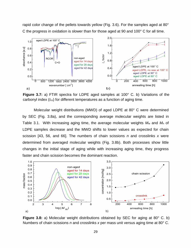
Figure 3.7: a) FTIR spectra for LDPE aged samples at 100° C. b) Variations of the

carbonyl index (Ico) for different temperatures as a function of aging time.

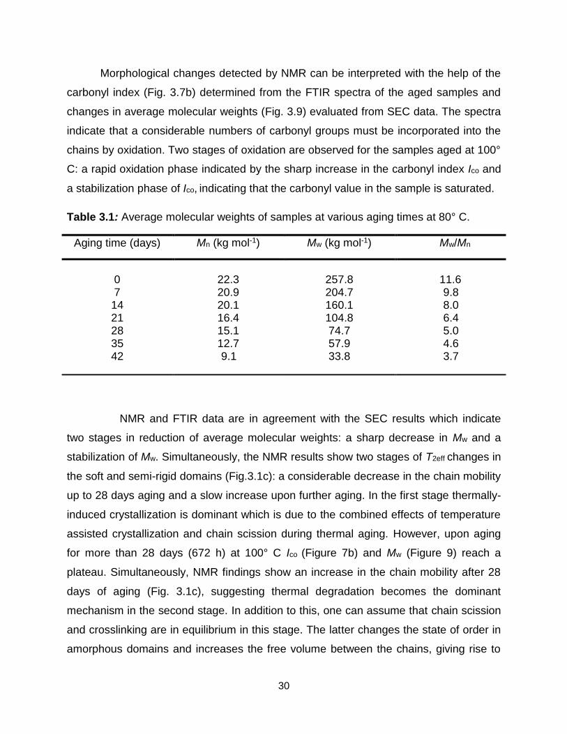
Figure 3.8: a) Molecular weight distributions obtained by SEC for aging at 80° C. b)

Numbers of chain scissions n and crosslinks x per mass unit versus aging time at 80° C.

rapid color change of the pellets towards yellow (Fig. 3.6). For the samples aged at 80°

C the progress in oxidation is slower than for those aged at 90 and 100° C for all time.

Molecular weight distributions (MWD) of aged LDPE at 80° C were determined

by SEC (Fig. 3.8a), and the corresponding average molecular weights are listed in

Table 3.1. With increasing aging time, the average molecular weights Mw and Mn of

LDPE samples decrease and the MWD shifts to lower values as expected for chain

scission [43, 56, and 66]. The numbers of chain scissions n and crosslinks x were

determined from averaged molecular weights (Fig. 3.8b). Both processes show little

changes in the initial stage of aging while with increasing aging time, they progress

faster and chain scission becomes the dominant reaction.

30

Morphological changes detected by NMR can be interpreted with the help of the

carbonyl index (Fig. 3.7b) determined from the FTIR spectra of the aged samples and

changes in average molecular weights (Fig. 3.9) evaluated from SEC data. The spectra

indicate that a considerable numbers of carbonyl groups must be incorporated into the

chains by oxidation. Two stages of oxidation are observed for the samples aged at 100°

C: a rapid oxidation phase indicated by the sharp increase in the carbonyl index Ico and

a stabilization phase of Ico, indicating that the carbonyl value in the sample is saturated.

Table 3.1: Average molecular weights of samples at various aging times at 80° C.

Aging time (days) Mn (kg mol-1) Mw (kg mol-1) Mw/Mn

0 22.3 257.8 11.6 7 20.9 204.7 9.8 14 20.1 160.1 8.0 21 16.4 104.8 6.4 28 15.1 74.7 5.0 35 12.7 57.9 4.6 42 9.1 33.8 3.7

NMR and FTIR data are in agreement with the SEC results which indicate

two stages in reduction of average molecular weights: a sharp decrease in Mw and a

stabilization of Mw. Simultaneously, the NMR results show two stages of T2eff changes in

the soft and semi-rigid domains (Fig.3.1c): a considerable decrease in the chain mobility

up to 28 days aging and a slow increase upon further aging. In the first stage thermally-

induced crystallization is dominant which is due to the combined effects of temperature

assisted crystallization and chain scission during thermal aging. However, upon aging

for more than 28 days (672 h) at 100° C Ico (Figure 7b) and Mw (Figure 9) reach a

plateau. Simultaneously, NMR findings show an increase in the chain mobility after 28

days of aging (Fig. 3.1c), suggesting thermal degradation becomes the dominant

mechanism in the second stage. In addition to this, one can assume that chain scission

and crosslinking are in equilibrium in this stage. The latter changes the state of order in

amorphous domains and increases the free volume between the chains, giving rise to

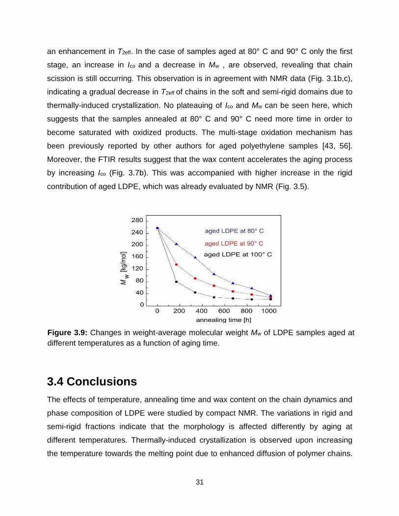
31

Figure 3.9: Changes in weight-average molecular weight Mw of LDPE samples aged at

different temperatures as a function of aging time.

time at 80° C.

an enhancement in T2eff. In the case of samples aged at 80° C and 90° C only the first

stage, an increase in Ico and a decrease in Mw , are observed, revealing that chain

scission is still occurring. This observation is in agreement with NMR data (Fig. 3.1b,c),

indicating a gradual decrease in T2eff of chains in the soft and semi-rigid domains due to

thermally-induced crystallization. No plateauing of Ico and Mw can be seen here, which

suggests that the samples annealed at 80° C and 90° C need more time in order to

become saturated with oxidized products. The multi-stage oxidation mechanism has

been previously reported by other authors for aged polyethylene samples [43, 56].

Moreover, the FTIR results suggest that the wax content accelerates the aging process

by increasing Ico (Fig. 3.7b). This was accompanied with higher increase in the rigid

contribution of aged LDPE, which was already evaluated by NMR (Fig. 3.5).

3.4 Conclusions

The effects of temperature, annealing time and wax content on the chain dynamics and

phase composition of LDPE were studied by compact NMR. The variations in rigid and

semi-rigid fractions indicate that the morphology is affected differently by aging at

different temperatures. Thermally-induced crystallization is observed upon increasing

the temperature towards the melting point due to enhanced diffusion of polymer chains.

32

Moreover, in the presence of oxygen polymers degrade reactively [43], which

subsequently impacts the crystallization mechanism during physical aging. The changes

in phase composition and relaxation time suggest that thermally-induced crystallization

is predominant during aging and oxidation of LDPE (at 80° C, 90° C, and 100° C) due to

enhanced chain scission while, after 28 days aging at 100° C, chemical degradation is

predominant where here chain scission and crosslinking are in equilibrium.

The particular material changes upon thermal aging depend on the wax content.

Investigations with compact NMR showed that the wax content can increase the

crystallinity during thermal aging. This is due to the presence of low molecular weight

chains in LDPE, which enhance the mobility of the macromolecular chains.

The morphological changes observed by NMR correlate with chemical

changes derived from FTIR spectra in terms of the carbonyl index and molecular weight

variations determined by SEC. FTIR shows two stages of oxidation for samples aged at

100° C: rapid oxidation indicated by a sharp increase in the carbonyl index Ico and a

stabilization of the Ico, indicating that the carbonyl content in the sample is saturated.

This is in agreement with the SEC results which indicate two stages in reduction of

average molecular weight: a sharp decrease in Mw and a stabilization of Mw.

Simultaneously, the NMR mobility shows two stages of T2eff changes in soft and semi-

rigid domains: a considerable decrease in mobility of the chains up to 28 days and a

slow increase after annealing for more than 28 days. In the first stage thermally-

induced crystallization dominates while with longer annealing at 100° C for more than

28 days (672 h) thermal degradation is the dominant mechanism. In the case of

samples aged at 80° C and 90° C, NMR, FTIR and SEC yield only the first aging stage,

revealing that chain scission is occurring but thermally-induced crystallization is

predominant.

33

Chapter 4

4 Solvent-induced crystallization in PE

This chapter is derived from my publication, reference 122, which was published in the

European Polymer Journal. The second and third authors of this publication are

respectively Alina Adams and Bernhard Blümich. Dr. Adams has contributed in the

conduction of experiments and correcting the publication and Prof. Blümich has

formulated and supervised the project and edited the manuscript.

4.1 Introduction

Polyethylene (PE) has garnered the largest share of the worldwide polymer market with

end products ranging from trash bags to automotive parts. While PE shows excellent

mechanical and thermal properties strongly associated to its morphology [3], the

morphology of PE end products, in turn, is dictated by their thermal and mechanical

history. This history includes the processing parameters as well as temperature,

pressure, deformation, and solvent treatments [4, 67]. With respect to these treatments,

the interaction between the solvent and the polymer matrix is a complex phenomenon

that triggers changes in different material properties such as density, permeability and

yield stress [59, 68-71]. Yet polymer-solvent compatibility is a fundamental issue in

industry where, for example, the wrong selection of a polymer to be used for making

pipes or gaskets that come into contact with highly compatible fluids may cause severe

swelling and impair the operation of the whole system [47]. Therefore, the study of

solvent-polymer interaction is highly relevant from an economic as well as a scientific

perspective.

34

The solvent transport in semi-crystalline polymers significantly depends on the

initial degree of crystallinity as well as on temperature [72-76] as was shown by

gravimetry [77-82] and NMR studies [76, 82-83]. Most solvents do not ingress into the

crystalline regions of a polymer, and mass transfer or diffusion occurs only in the

continuous amorphous phase between the crystallites [73, 84-85]. There, the solvent

affects the segmental chain mobility [86-87] and can trigger changes in the morphology

of semi-crystalline polymers. In particular, semi-crystalline polymers such as poly(aryl

ether ether ketone) (PEEK) [88] and crystalline block copolymers such as polystyrene-

b-poly(ethylene oxide)-b-polystyrene (PS-b-PEO-b-PS) [89] have shown solvent-

induced crystallization (SINC) and anisotropic swelling in the presence of various

solvents. Moreover, SINC was observed for cross-linked polyethylene exposed to

various solvents in the presence of sour gases [90]. A similar observation was reported

for isotactic polypropylene (iPP) upon swelling in solvents such as n-hexane,

cyclohexane, toluene, chloroform and dichloromethane, thereby indicating a complex

structure rearrangement that results in SINC [68-70]. Consequently, it is important to

investigate the changes in phase composition and chain mobility of different domains

induced by swelling in order to understand how the properties of semi-crystalline

polymer change over time. Gaining such information is relevant for better understanding

the transport process of different solvents in various semi-crystalline polymers and for

improving material models.

Various experimental methods such as differential scanning calorimetry (DSC)

and X-ray diffraction (XRD) have been used to determine the phase composition of

semi-crystalline polymers and to evaluate their morphological changes under the impact

of different parameters [8, 49, 52, 69, 87]. Whereas DSC and XRD can lend valuable

information about the crystalline domains, these methods cannot directly detect

swelling-induced changes that arise primarily in the amorphous phase [52]. Thus,

implementing analytical methods that enable researchers to directly probe this phase

and quantify its changes upon solvent ingress is crucial for unmasking and elucidating

the associated morphological changes. Among various existing analytical tools, 1H

solid-state NMR is a powerful technique to probe the structural heterogeneity and

molecular mobility in semi-crystalline polymers by directly detecting each phase [3-4, 8,

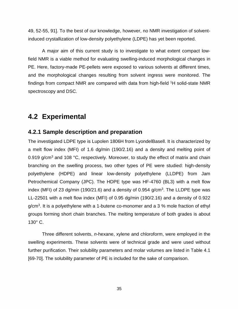
35

49, 52-55, 91]. To the best of our knowledge, however, no NMR investigation of solvent-

induced crystallization of low-density polyethylene (LDPE) has yet been reported.

A major aim of this current study is to investigate to what extent compact low-

field NMR is a viable method for evaluating swelling-induced morphological changes in

PE. Here, factory-made PE-pellets were exposed to various solvents at different times,

and the morphological changes resulting from solvent ingress were monitored. The

findings from compact NMR are compared with data from high-field 1H solid-state NMR

spectroscopy and DSC.

4.2 Experimental

4.2.1 Sample description and preparation

The investigated LDPE type is Lupolen 1806H from LyondelBasell. It is characterized by

a melt flow index (MFI) of 1.6 dg/min (190/2.16) and a density and melting point of

0.919 g/cm3 and 108 °C, respectively. Moreover, to study the effect of matrix and chain

branching on the swelling process, two other types of PE were studied: high-density

polyethylene (HDPE) and linear low-density polyethylene (LLDPE) from Jam

Petrochemical Company (JPC). The HDPE type was HF-4760 (BL3) with a melt flow

index (MFI) of 23 dg/min (190/21.6) and a density of 0.954 g/cm3. The LLDPE type was

LL-22501 with a melt flow index (MFI) of 0.95 dg/min (190/2.16) and a density of 0.922

g/cm3. It is a polyethylene with a 1-butene co-monomer and a 3 % mole fraction of ethyl

groups forming short chain branches. The melting temperature of both grades is about

130° C.

Three different solvents, n-hexane, xylene and chloroform, were employed in the

swelling experiments. These solvents were of technical grade and were used without

further purification. Their solubility parameters and molar volumes are listed in Table 4.1

[69-70]. The solubility parameter of PE is included for the sake of comparison.

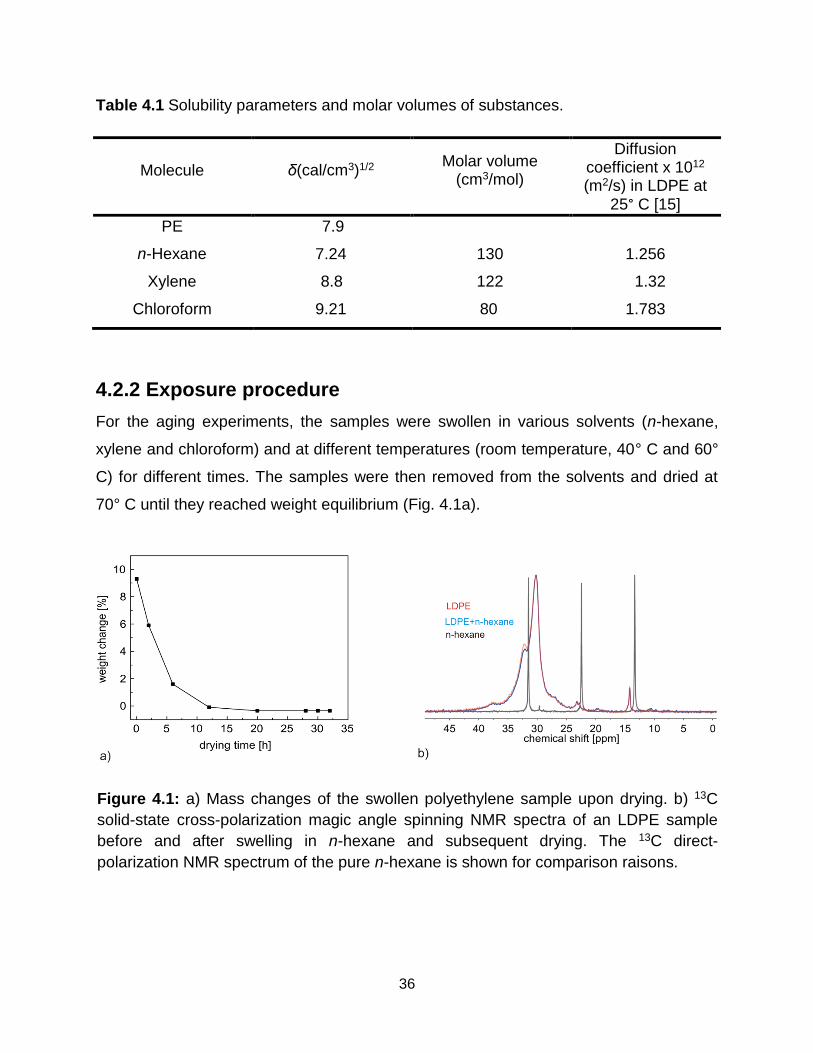
36

Table 4.1 Solubility parameters and molar volumes of substances.

Molecule δ(cal/cm3)1/2 Molar volume (cm3/mol)

Diffusion coefficient x 1012 (m2/s) in LDPE at

25° C [15]

PE 7.9

n-Hexane 7.24 130 1.256

Xylene 8.8 122 1.32

Chloroform 9.21 80 1.783

4.2.2 Exposure procedure

For the aging experiments, the samples were swollen in various solvents (n-hexane,

xylene and chloroform) and at different temperatures (room temperature, 40° C and 60°

C) for different times. The samples were then removed from the solvents and dried at

70° C until they reached weight equilibrium (Fig. 4.1a).

Figure 4.1: a) Mass changes of the swollen polyethylene sample upon drying. b) 13C

solid-state cross-polarization magic angle spinning NMR spectra of an LDPE sample

before and after swelling in n-hexane and subsequent drying. The 13C direct-

polarization NMR spectrum of the pure n-hexane is shown for comparison raisons.

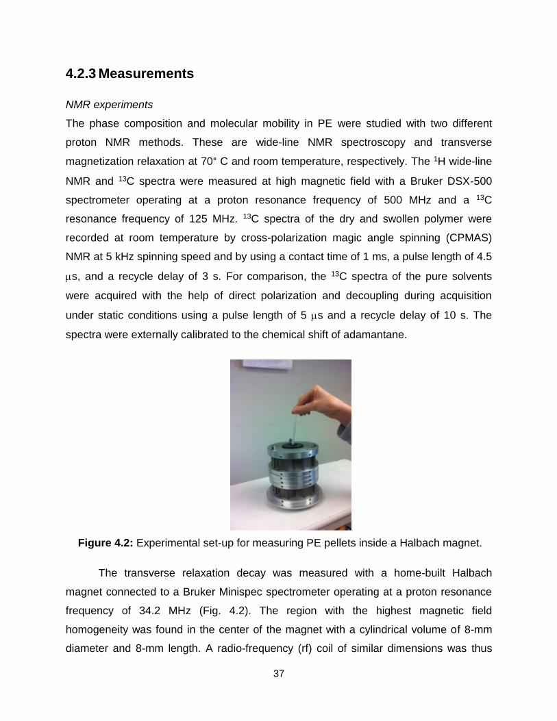
37

4.2.3 Measurements

NMR experiments

The phase composition and molecular mobility in PE were studied with two different

proton NMR methods. These are wide-line NMR spectroscopy and transverse

magnetization relaxation at 70° C and room temperature, respectively. The 1H wide-line

NMR and 13C spectra were measured at high magnetic field with a Bruker DSX-500

spectrometer operating at a proton resonance frequency of 500 MHz and a 13C

resonance frequency of 125 MHz. 13C spectra of the dry and swollen polymer were

recorded at room temperature by cross-polarization magic angle spinning (CPMAS)

NMR at 5 kHz spinning speed and by using a contact time of 1 ms, a pulse length of 4.5

s, and a recycle delay of 3 s. For comparison, the 13C spectra of the pure solvents

were acquired with the help of direct polarization and decoupling during acquisition

under static conditions using a pulse length of 5 s and a recycle delay of 10 s. The

spectra were externally calibrated to the chemical shift of adamantane.

The transverse relaxation decay was measured with a home-built Halbach

magnet connected to a Bruker Minispec spectrometer operating at a proton resonance

frequency of 34.2 MHz (Fig. 4.2). The region with the highest magnetic field

homogeneity was found in the center of the magnet with a cylindrical volume of 8-mm

diameter and 8-mm length. A radio-frequency (rf) coil of similar dimensions was thus

Figure 4.2: Experimental set-up for measuring PE pellets inside a Halbach magnet.

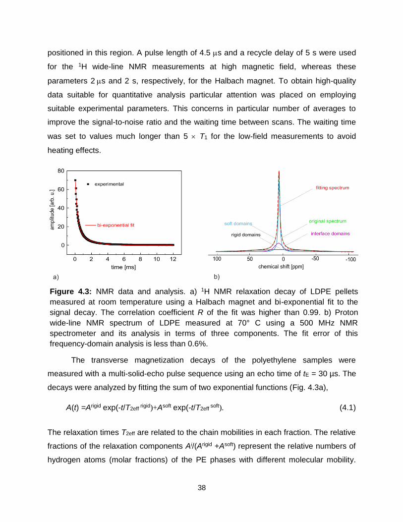
38

positioned in this region. A pulse length of 4.5 s and a recycle delay of 5 s were used

for the 1H wide-line NMR measurements at high magnetic field, whereas these

parameters 2s and 2 s, respectively, for the Halbach magnet. To obtain high-quality

data suitable for quantitative analysis particular attention was placed on employing

suitable experimental parameters. This concerns in particular number of averages to

improve the signal-to-noise ratio and the waiting time between scans. The waiting time

was set to values much longer than 5 T1 for the low-field measurements to avoid

heating effects.

The transverse magnetization decays of the polyethylene samples were

measured with a multi-solid-echo pulse sequence using an echo time of tE = 30 µs. The

decays were analyzed by fitting the sum of two exponential functions (Fig. 4.3a),

A(t) =Arigid exp(-t/T2eff rigid)+Asoft exp(-t/T2eff

soft). (4.1)

The relaxation times T2eff are related to the chain mobilities in each fraction. The relative

fractions of the relaxation components Ai/(Arigid +Asoft) represent the relative numbers of

hydrogen atoms (molar fractions) of the PE phases with different molecular mobility.

Figure 4.3: NMR data and analysis. a) 1H NMR relaxation decay of LDPE pellets

measured at room temperature using a Halbach magnet and bi-exponential fit to the

signal decay. The correlation coefficient R of the fit was higher than 0.99. b) Proton

wide-line NMR spectrum of LDPE measured at 70° C using a 500 MHz NMR

spectrometer and its analysis in terms of three components. The fit error of this

frequency-domain analysis is less than 0.6%.

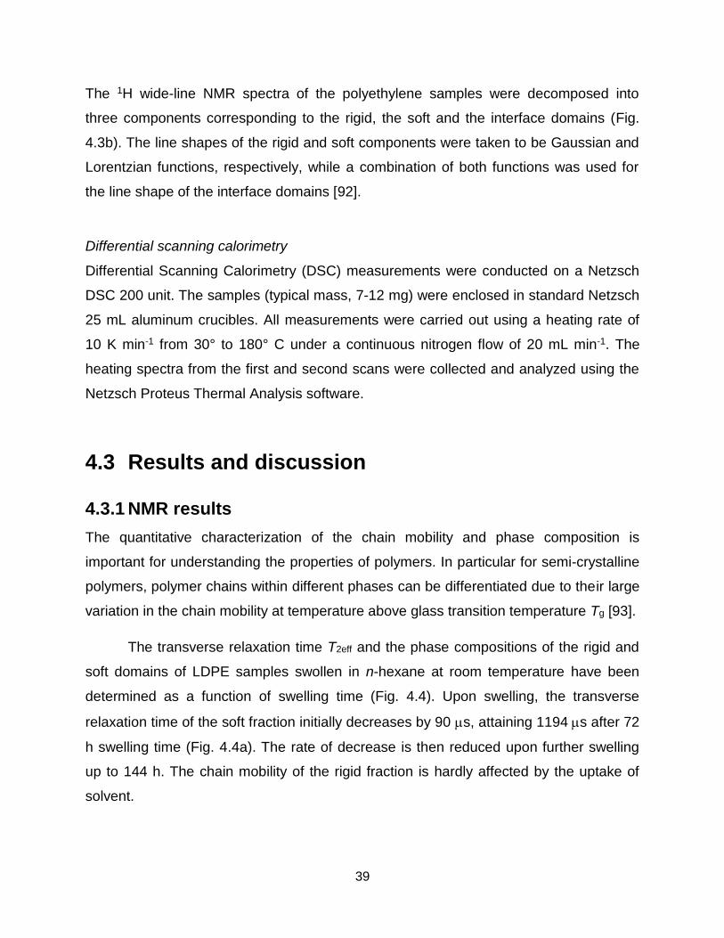
39

The 1H wide-line NMR spectra of the polyethylene samples were decomposed into

three components corresponding to the rigid, the soft and the interface domains (Fig.

4.3b). The line shapes of the rigid and soft components were taken to be Gaussian and

Lorentzian functions, respectively, while a combination of both functions was used for

the line shape of the interface domains [92].

Differential scanning calorimetry

Differential Scanning Calorimetry (DSC) measurements were conducted on a Netzsch

DSC 200 unit. The samples (typical mass, 7-12 mg) were enclosed in standard Netzsch

25 mL aluminum crucibles. All measurements were carried out using a heating rate of

10 K min-1 from 30° to 180° C under a continuous nitrogen flow of 20 mL min-1. The

heating spectra from the first and second scans were collected and analyzed using the

Netzsch Proteus Thermal Analysis software.

4.3 Results and discussion

4.3.1 NMR results

The quantitative characterization of the chain mobility and phase composition is

important for understanding the properties of polymers. In particular for semi-crystalline

polymers, polymer chains within different phases can be differentiated due to their large

variation in the chain mobility at temperature above glass transition temperature Tg [93].

The transverse relaxation time T2eff and the phase compositions of the rigid and

soft domains of LDPE samples swollen in n-hexane at room temperature have been

determined as a function of swelling time (Fig. 4.4). Upon swelling, the transverse

relaxation time of the soft fraction initially decreases by 90 s, attaining 1194s after 72

h swelling time (Fig. 4.4a). The rate of decrease is then reduced upon further swelling

up to 144 h. The chain mobility of the rigid fraction is hardly affected by the uptake of

solvent.

40

Figure 4.4: Changes in relaxation times T2eff (a) and in fraction (b) of LDPE domains as

a function of the swelling time in n-hexane at room temperature.

On the other hand, the phase composition of LDPE shows a slighter variation

upon swelling as compared to changes in the transverse relaxation time (Fig. 4.4b). The

rigid fraction increases by almost one weight percent at the expense of the soft fraction.

Upon further swelling beyond 48 h, the rigid contribution reaches a plateau. The

variations in the chain mobility and contributions of rigid and soft fractions indicate that

the changes in the morphology of LDPE induced by swelling depend on the time of

exposure to the solvent. The lower chain mobility of the samples after solvent exposure

can be understood in terms of a tighter packing of the polymer chains in the amorphous

domain due to solvent-induced crystallization [67-69]. When a semi-crystalline polymer

such as polyethylene is exposed to a solvent, the amorphous regions swell to

accommodate the solvent and may also undergo structural changes. The reversibility of

such changes is relevant to polymer-solvent interactions [59]. The molecular

interactions between the penetrating solvent molecules and the polymer chain

segments reduce the glass transition temperature (Tg) of the polymer and significantly

enhance the chain mobility and the chain rearrangement. In addition to this, the solvent

may dissolve small crystallites with their melting points close to the swelling

temperature, and this may further enhance the chain mobility in the amorphous

domains. Hence, crystallization becomes kinetically more favorable [88-90]. However,

for the experimental conditions and samples used in this study, the thermodynamic

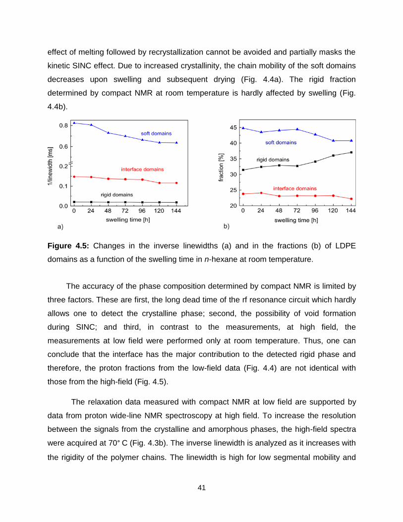
41

effect of melting followed by recrystallization cannot be avoided and partially masks the

kinetic SINC effect. Due to increased crystallinity, the chain mobility of the soft domains

decreases upon swelling and subsequent drying (Fig. 4.4a). The rigid fraction

determined by compact NMR at room temperature is hardly affected by swelling (Fig.

4.4b).

Figure 4.5: Changes in the inverse linewidths (a) and in the fractions (b) of LDPE

domains as a function of the swelling time in n-hexane at room temperature.

The accuracy of the phase composition determined by compact NMR is limited by

three factors. These are first, the long dead time of the rf resonance circuit which hardly

allows one to detect the crystalline phase; second, the possibility of void formation

during SINC; and third, in contrast to the measurements, at high field, the

measurements at low field were performed only at room temperature. Thus, one can

conclude that the interface has the major contribution to the detected rigid phase and

therefore, the proton fractions from the low-field data (Fig. 4.4) are not identical with

those from the high-field (Fig. 4.5).

The relaxation data measured with compact NMR at low field are supported by

data from proton wide-line NMR spectroscopy at high field. To increase the resolution

between the signals from the crystalline and amorphous phases, the high-field spectra

were acquired at 70° C (Fig. 4.3b). The inverse linewidth is analyzed as it increases with

the rigidity of the polymer chains. The linewidth is high for low segmental mobility and

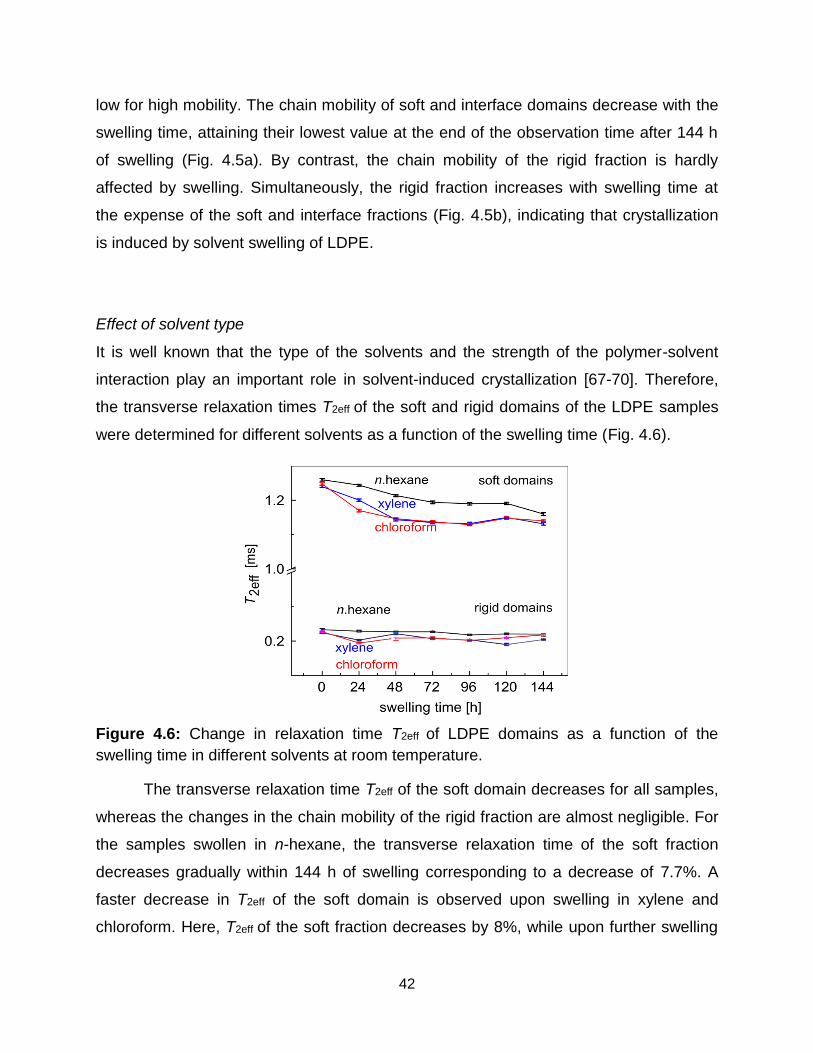
42

low for high mobility. The chain mobility of soft and interface domains decrease with the

swelling time, attaining their lowest value at the end of the observation time after 144 h

of swelling (Fig. 4.5a). By contrast, the chain mobility of the rigid fraction is hardly

affected by swelling. Simultaneously, the rigid fraction increases with swelling time at

the expense of the soft and interface fractions (Fig. 4.5b), indicating that crystallization

is induced by solvent swelling of LDPE.

Effect of solvent type

It is well known that the type of the solvents and the strength of the polymer-solvent

interaction play an important role in solvent-induced crystallization [67-70]. Therefore,

the transverse relaxation times T2eff of the soft and rigid domains of the LDPE samples

were determined for different solvents as a function of the swelling time (Fig. 4.6).

Figure 4.6: Change in relaxation time T2eff of LDPE domains as a function of the

swelling time in different solvents at room temperature.

The transverse relaxation time T2eff of the soft domain decreases for all samples,

whereas the changes in the chain mobility of the rigid fraction are almost negligible. For

the samples swollen in n-hexane, the transverse relaxation time of the soft fraction

decreases gradually within 144 h of swelling corresponding to a decrease of 7.7%. A

faster decrease in T2eff of the soft domain is observed upon swelling in xylene and

chloroform. Here, T2eff of the soft fraction decreases by 8%, while upon further swelling

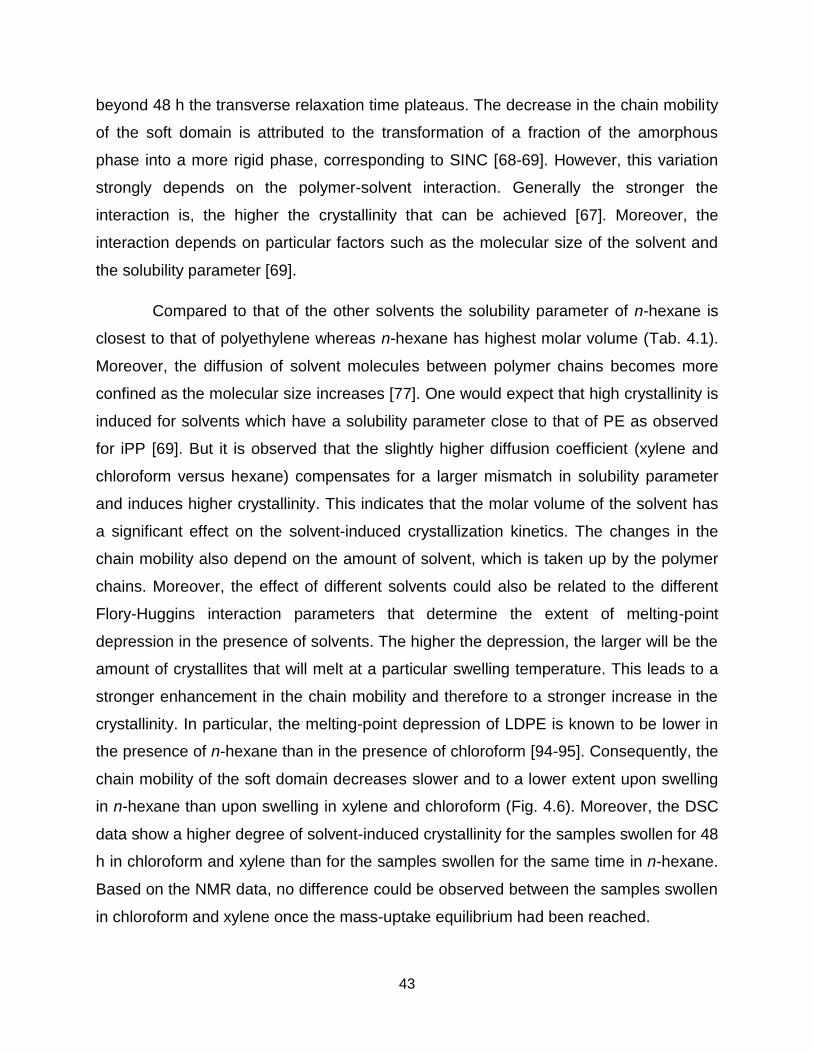
43

beyond 48 h the transverse relaxation time plateaus. The decrease in the chain mobility

of the soft domain is attributed to the transformation of a fraction of the amorphous

phase into a more rigid phase, corresponding to SINC [68-69]. However, this variation

strongly depends on the polymer-solvent interaction. Generally the stronger the

interaction is, the higher the crystallinity that can be achieved [67]. Moreover, the

interaction depends on particular factors such as the molecular size of the solvent and

the solubility parameter [69].

Compared to that of the other solvents the solubility parameter of n-hexane is

closest to that of polyethylene whereas n-hexane has highest molar volume (Tab. 4.1).

Moreover, the diffusion of solvent molecules between polymer chains becomes more

confined as the molecular size increases [77]. One would expect that high crystallinity is

induced for solvents which have a solubility parameter close to that of PE as observed

for iPP [69]. But it is observed that the slightly higher diffusion coefficient (xylene and

chloroform versus hexane) compensates for a larger mismatch in solubility parameter

and induces higher crystallinity. This indicates that the molar volume of the solvent has

a significant effect on the solvent-induced crystallization kinetics. The changes in the

chain mobility also depend on the amount of solvent, which is taken up by the polymer

chains. Moreover, the effect of different solvents could also be related to the different

Flory-Huggins interaction parameters that determine the extent of melting-point

depression in the presence of solvents. The higher the depression, the larger will be the

amount of crystallites that will melt at a particular swelling temperature. This leads to a

stronger enhancement in the chain mobility and therefore to a stronger increase in the

crystallinity. In particular, the melting-point depression of LDPE is known to be lower in

the presence of n-hexane than in the presence of chloroform [94-95]. Consequently, the

chain mobility of the soft domain decreases slower and to a lower extent upon swelling

in n-hexane than upon swelling in xylene and chloroform (Fig. 4.6). Moreover, the DSC

data show a higher degree of solvent-induced crystallinity for the samples swollen for 48

h in chloroform and xylene than for the samples swollen for the same time in n-hexane.

Based on the NMR data, no difference could be observed between the samples swollen

in chloroform and xylene once the mass-uptake equilibrium had been reached.

44

Effect of temperature

The diffusion coefficient and, thus, polymer-solvent interaction vary with the swelling

temperature [81]. Hence, the transverse relaxation times T2eff of the soft and rigid

domains of the LDPE samples are presented in Figure 4.7 as a function of swelling time

at different temperatures. For the samples swollen in n-hexane at room temperature,

the transverse relaxation time of the soft fraction decreases gradually with the swelling

time (Fig. 4.7). By contrast, the T2eff of the soft domain decreases faster upon swelling

at 40° C and 60° C. Here, the T2eff of the soft fraction decreases by 9%. Upon further

swelling beyond 24 h, the transverse relaxation time remains almost constant. The

solvent-induced crystallization occurs faster by increasing the swelling temperature from

room temperature to 40° C and 60° C, which is in agreement with previous studies [67-

68]. In particular, at room temperature, the diffusion rate is lower, thereby leading to a

slower solvent-induced crystal growth and, thus, to a slower decrease of the transverse

relaxation time of the soft fraction with swelling time (Fig. 4.7).

Figure 4.7: Variation of the relaxation times T2eff of the LDPE domains with the swelling

time in n-hexane at different temperatures.

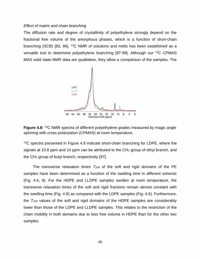
45

Figure 4.8: 13C NMR spectra of different polyethylene grades measured by magic angle

spinning with cross polarization (CPMAS) at room temperature.

Effect of matrix and chain branching

The diffusion rate and degree of crystallinity of polyethylene strongly depend on the

fractional free volume of the amorphous phases, which is a function of short-chain

branching (SCB) [83, 96]. 13C NMR of solutions and melts has been established as a

versatile tool to determine polyethylene branching [97-99]. Although our 13C CPMAS

MAS solid state-NMR data are qualitative, they allow a comparison of the samples. The

13C spectra presented in Figure 4.8 indicate short-chain branching for LDPE, where the

signals at 10.8 ppm and 14 ppm can be attributed to the CH3 group of ethyl branch, and

the CH3 group of butyl branch, respectively [97].

The transverse relaxation times T2eff of the soft and rigid domains of the PE

samples have been determined as a function of the swelling time in different solvents

(Fig. 4.6, 9). For the HDPE and LLDPE samples swollen at room temperature, the

transverse relaxation times of the soft and rigid fractions remain almost constant with

the swelling time (Fig. 4.9) as compared with the LDPE samples (Fig. 4.6). Furthermore,

the T2eff values of the soft and rigid domains of the HDPE samples are considerably

lower than those of the LDPE and LLDPE samples. This relates to the restriction of the

chain mobility in both domains due to less free volume in HDPE than for the other two

samples.

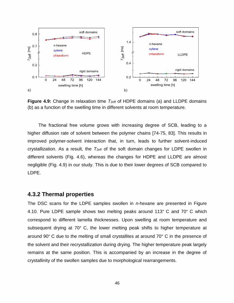
46

Figure 4.9: Change in relaxation time T2eff of HDPE domains (a) and LLDPE domains

(b) as a function of the swelling time in different solvents at room temperature.

The fractional free volume grows with increasing degree of SCB, leading to a

higher diffusion rate of solvent between the polymer chains [74-75, 83]. This results in

improved polymer-solvent interaction that, in turn, leads to further solvent-induced

crystallization. As a result, the T2eff of the soft domain changes for LDPE swollen in

different solvents (Fig. 4.6), whereas the changes for HDPE and LLDPE are almost

negligible (Fig. 4.9) in our study. This is due to their lower degrees of SCB compared to

LDPE.

4.3.2 Thermal properties

The DSC scans for the LDPE samples swollen in n-hexane are presented in Figure

4.10. Pure LDPE sample shows two melting peaks around 113° C and 70° C which

correspond to different lamella thicknesses. Upon swelling at room temperature and

subsequent drying at 70° C, the lower melting peak shifts to higher temperature at

around 90° C due to the melting of small crystallites at around 70° C in the presence of

the solvent and their recrystallization during drying. The higher temperature peak largely

remains at the same position. This is accompanied by an increase in the degree of

crystallinity of the swollen samples due to morphological rearrangements.

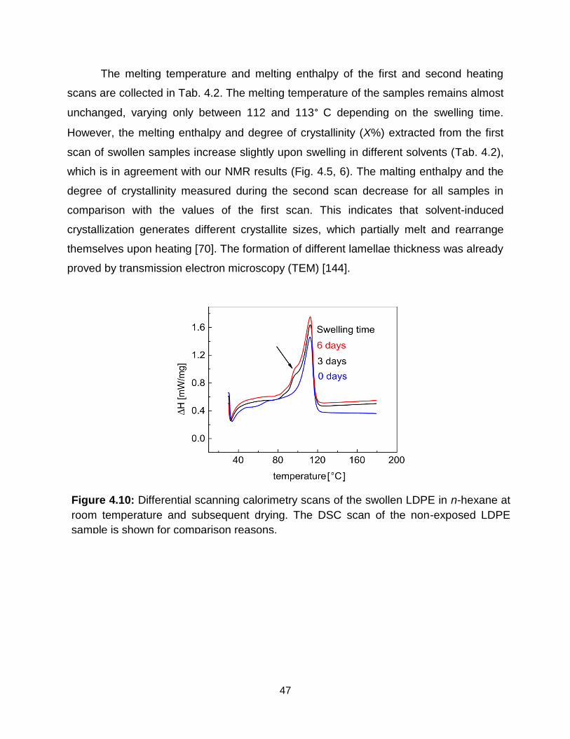
47

Figure 4.10: Differential scanning calorimetry scans of the swollen LDPE in n-hexane at

room temperature and subsequent drying. The DSC scan of the non-exposed LDPE

sample is shown for comparison reasons.

The melting temperature and melting enthalpy of the first and second heating

scans are collected in Tab. 4.2. The melting temperature of the samples remains almost

unchanged, varying only between 112 and 113° C depending on the swelling time.

However, the melting enthalpy and degree of crystallinity (X%) extracted from the first

scan of swollen samples increase slightly upon swelling in different solvents (Tab. 4.2),

which is in agreement with our NMR results (Fig. 4.5, 6). The malting enthalpy and the

degree of crystallinity measured during the second scan decrease for all samples in

comparison with the values of the first scan. This indicates that solvent-induced

crystallization generates different crystallite sizes, which partially melt and rearrange

themselves upon heating [70]. The formation of different lamellae thickness was already

proved by transmission electron microscopy (TEM) [144].

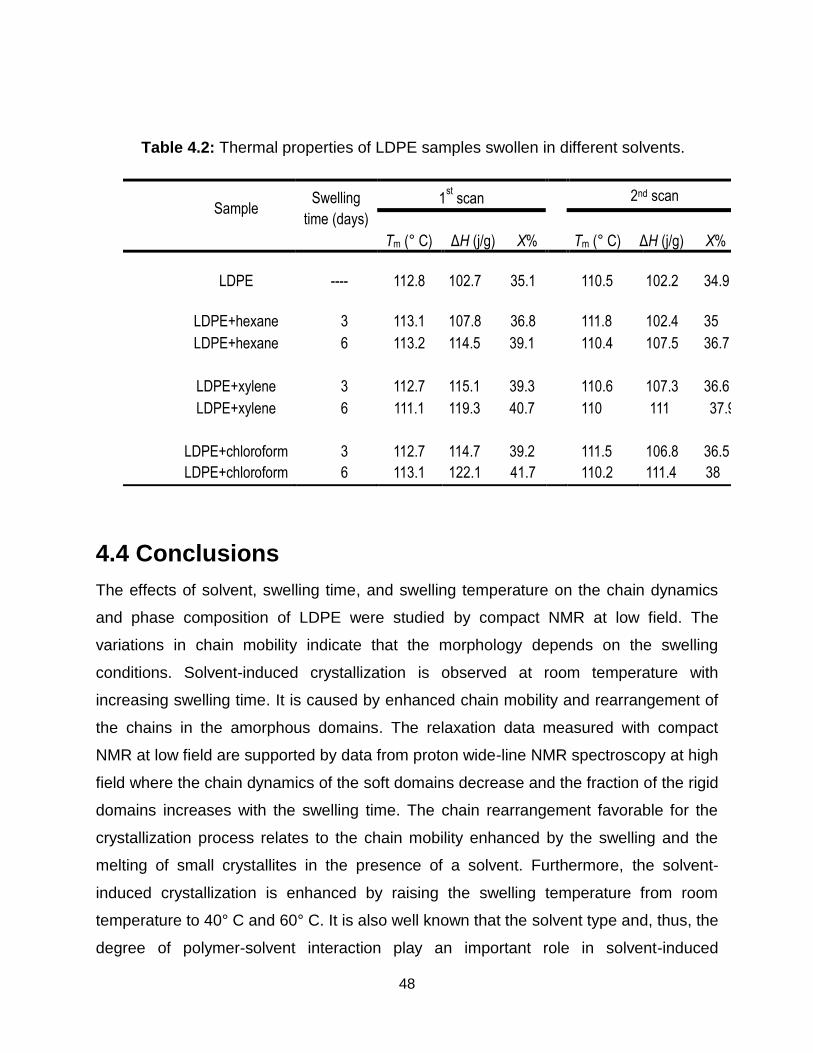
48

4.4 Conclusions

The effects of solvent, swelling time, and swelling temperature on the chain dynamics

and phase composition of LDPE were studied by compact NMR at low field. The

variations in chain mobility indicate that the morphology depends on the swelling

conditions. Solvent-induced crystallization is observed at room temperature with

increasing swelling time. It is caused by enhanced chain mobility and rearrangement of

the chains in the amorphous domains. The relaxation data measured with compact

NMR at low field are supported by data from proton wide-line NMR spectroscopy at high

field where the chain dynamics of the soft domains decrease and the fraction of the rigid

domains increases with the swelling time. The chain rearrangement favorable for the

crystallization process relates to the chain mobility enhanced by the swelling and the

melting of small crystallites in the presence of a solvent. Furthermore, the solvent-

induced crystallization is enhanced by raising the swelling temperature from room

temperature to 40° C and 60° C. It is also well known that the solvent type and, thus, the

degree of polymer-solvent interaction play an important role in solvent-induced

Table 4.2: Thermal properties of LDPE samples swollen in different solvents.

Sample Swelling

time (days)

1st scan

2nd scan

Tm (° C) ΔH (j/g) X%

Tm (° C) ΔH (j/g) X%

LDPE ---- 112.8 102.7 35.1

110.5 102.2 34.9

LDPE+hexane 3 113.1 107.8 36.8

111.8 102.4 35

LDPE+hexane 6 113.2 114.5 39.1

110.4 107.5 36.7

LDPE+xylene

3

112.7

115.1 39.3

110.6

107.3 36.6

LDPE+xylene 6 111.1 119.3 40.7

110 111 37.9

LDPE+chloroform

LDPE+chloroform

3

6

112.7

113.1

114.7 39.2

122.1 41.7

111.5

110.2

106.8 36.5

111.4 38

49

crystallization [67-69]. We have observed that the higher the diffusion coefficient is, the

faster the solvent-induced crystallinity occurs, while the mismatch in solubility parameter

seemed to have less of an impact. This implies that the molar volume of the solvent is

an important factor in determining the speed of solvent-induced crystallization. The

investigations with compact low-field NMR have also shown that short-chain branching

can accelerate the solvent-induced crystallization due to the higher fractional free

volume, which enhances the diffusion rate of the solvent between the polymer chains

[83]. The NMR results agree with those from DSC measurements which show that

solvent-induced crystallization generates different crystallite sizes that partially

rearrange themselves upon heating [70]. In this study, compact low-field NMR has

proven itself as a viable technique for detecting morphological changes invoked by

solvent-induced crystallization in polyethylene.

50

Chapter 5

5 Wax content in polyethylene


Polyethylene (PE) grades are used in variety of applications as engineering plastics for

packaging, pipes, containers, automotive parts, and medical applications [100].

Depending on the application, the molecular weight of PE varies between a few

thousands and a few million g/mol [101-102]. PE waxes are low molecular weight

ethylene-based polymers and oligomers with molecular weights of less than 10000

g/mol [101, 103]. The separation of wax from the polymer and the quantification of the

wax content are of extreme importance in the polyolefin industry where, for example,

the Ziegler-Natta polymerization of ethylene can produce significant amounts of wax as

a by-product depending on the catalyst used and the operating conditions of the plant

[101, 103]. Therefore, the accurate determination of the polyethylene wax content is of

great practical and economical interest.

Chromatography is a standard method for determining the wax content of PE.

With gas chromatography (GC) the gas mixture is separated in the column into

individual components making use of differences in physical properties like boiling point,

molecular size, and polarity [104-105]. However, GC has an upper molecular weight

limit and the resolution decreases when separating alkanes with more than 90 carbons

[106-107]. Also size exclusion chromatography (SEC) has been extensively used to

identify alkanes in polyethylene wax. While stationary phases with small pores make it

possible to separate alkanes from C50 to C150, SEC-based methods require extraction or

preconcentration before separation and identification, which is a time consuming and

assiduous process [108-110]. In high-performance liquid chromatography (HPLC) the

separation quality is affected by the interactions of the wax with the stationary and the

mobile solute phases [111]. When operating HPLC gradient-mode, successively eluted

substances experience stronger solute-mobile phase interactions and emerge from a

51

column more rapidly than in the isocratic mode, resulting in faster and superior

separation [112]. However, quantitative analysis may be limited unless HPLC is coupled

with mass spectroscopy [113]. Furthermore the detection of alkanes below C50 is

difficult due to operation of the evaporating light scattering detector (ELSD) [114].

On the other hand, Nuclear magnetic resonance (NMR) spectroscopy is a well-

known analytical technique for structure elucidation of small and large molecules [1,12,

115], where typical instruments use super-conducting magnets that generate high

magnetic fields. However, widespread use of high-field NMR is limited by the cost and



sufficient sensitivity and robustness for nondestructive characterization in applications

outdoors and on the factory floor [4, 116-117]. Among the different applications in

material science and chemical engineering, compact NMR spectrometers enable novel

applications with online reaction monitoring for process analysis [34] and for coupling

with other methods such as SEC with a more comprehensive description of material

properties [118].

The presence of wax in polymers affects the processing and application

properties of the final product. The amount present is usually used to evaluate the

catalyst performance in polyethylene plants [119-120]. Therefore, the quantification of

polyethylene wax is of pivotal interest in the polyolefin industry. Moreover, it is essential

to quantify and study the wax in polymers for the food and packaging industries where,

oligomers may migrate to the film surface and thus get in touch with the packaged

contents [114]. To our knowledge, no investigation of polyethylene wax content by NMR

spectroscopy has been reported so far.

In this study, the wax content of PE pellets as received from the factory and

leached into solvents is quantified with the standard addition method employing

compact NMR instruments for 1H NMR spectroscopy and 1H NMR relaxometry. The

findings from both NMR methods are compared with data from gravimetric

measurements.

52

5.2 Experimental section

5.2.1 Materials

Factory-grade pellets from low-density PE (LDPE), high-density PE (HDPE), and linear

low-density PE (LLDPE) were studied. The LDPE type was Lupolen 1806H from

LyondelBasell. It is characterized by a melt flow index (MFI) of 1.6 dg/min (190/2.16) a

density of 0.919 g/cm3 and a melting point of 108° C. The LDPE pellets were swollen in

n-hexane and xylene at room temperature. The LDPE data are compared with data

from HDPE and LLDPE pellets obtained from Jam Petrochemical Company (JPC). The

HDPE type was HF-4760 (BL3) with a melt flow index (MFI) of 23 dg/min (190/21.6) and

a density of 0.954 g/cm3. The LLDPE type was LL-22501 with a melt flow index (MFI) of

0.95 dg/min (190/2.16) and a density of 0.922 g/cm3. The melting temperature of both

grades is about 130° C.

5.2.2 Swelling and wax extraction procedure

To extract the wax, 3 g of PE pellets were swollen in 6 ml n-hexane at room

temperature for different times. The pellets were then removed from the solvent, and the

resultant solution was subsequently filled into a standard 5 mm NMR sample tube in

order to determine the wax content by NMR. The difference in the weight of the PE bulk

before and after the swelling process is referred as the gravimetric wax content.

5.2.3 NMR experiments and data processing

Two different NMR methods, 1H NMR spectroscopy and transverse magnetization

relaxation were employed to detect the wax content in solutions. Single-scan 1H NMR

spectra of the solutions were acquired with a 1 T Spinsolve NMR spectrometer by

Magritek, having a deadtime of 20 s. The data were processed with MestreNova 8.1.1

software for phase and baseline corrections. Transverse 1H NMR relaxation decays of

the solutions were measured with a home-built Halbach magnet connected to a Bruker

53

Minispec spectrometer with a deadtime of 30 s and operating at a proton resonance

frequency of 34.2 MHz. The region with the highest magnetic field homogeneity was

found in the center of the magnet with a cylindrical volume of 8-mm diameter and 8-mm

length, where a radio-frequency coil of similar dimensions was positioned.

The relaxation signal decays were measured with the Carr-Purcell-Meiboom-Gill

(CMPG) pulse sequence using an echo time of tE = 2.5 ms and including 4000 echoes

to acquire whole the relaxation decay. The decays were analyzed by fitting the

experimental data in two ways, with a double and a single exponential function,

A(t) =Awax exp(-t/T2eff wax) + Asolvent exp(-t/T2eff

solvent), (5.1)

A(t) =A exp(-t/T2eff). (5.2)

The relaxation times T2eff are related to the molecular mobility. The amplitudes A

represent the spin concentration.

Quantitative analysis by NMR requires a reference compound for calculating the

absolute concentration of an analyte [115]. In our study the standard addition method,

also called the method of ‘variable total volume with continuous variation of standard’ is

used to determine the wax content [115, 121]. For each sample, the same volume of

wax solution (Vx = 0.4 ml) is prepared. Serial volume increments Vs = 0.02 ml of pure

solvent (Cs = 1) are added in steps numbered n = 0, 1, 2, … to the solution with

unknown wax concentration Cx. Formally the total integral of a solution spectrum in the

frequency domain is the same as the and total initial amplitude of the relaxation signal

measured in the time domain, so that the total amount Rn = A(0) of 1H in eqns. (5.1) and

(5.2) depends upon the concentrations Cx of the unknown and Cs of the standard

solvent, which is given by expression (5.3) [121]. In practice differences in precision

result from the spectrometer dead time and signal processing steps.

𝑅𝑛 = 𝑘 [𝑉𝑥𝐶𝑥

𝑉𝑥+𝑛𝑉𝑠+

𝑁𝑉𝑠𝐶𝑠

𝑉𝑥+𝑛𝑉𝑠], (5.3)

Or

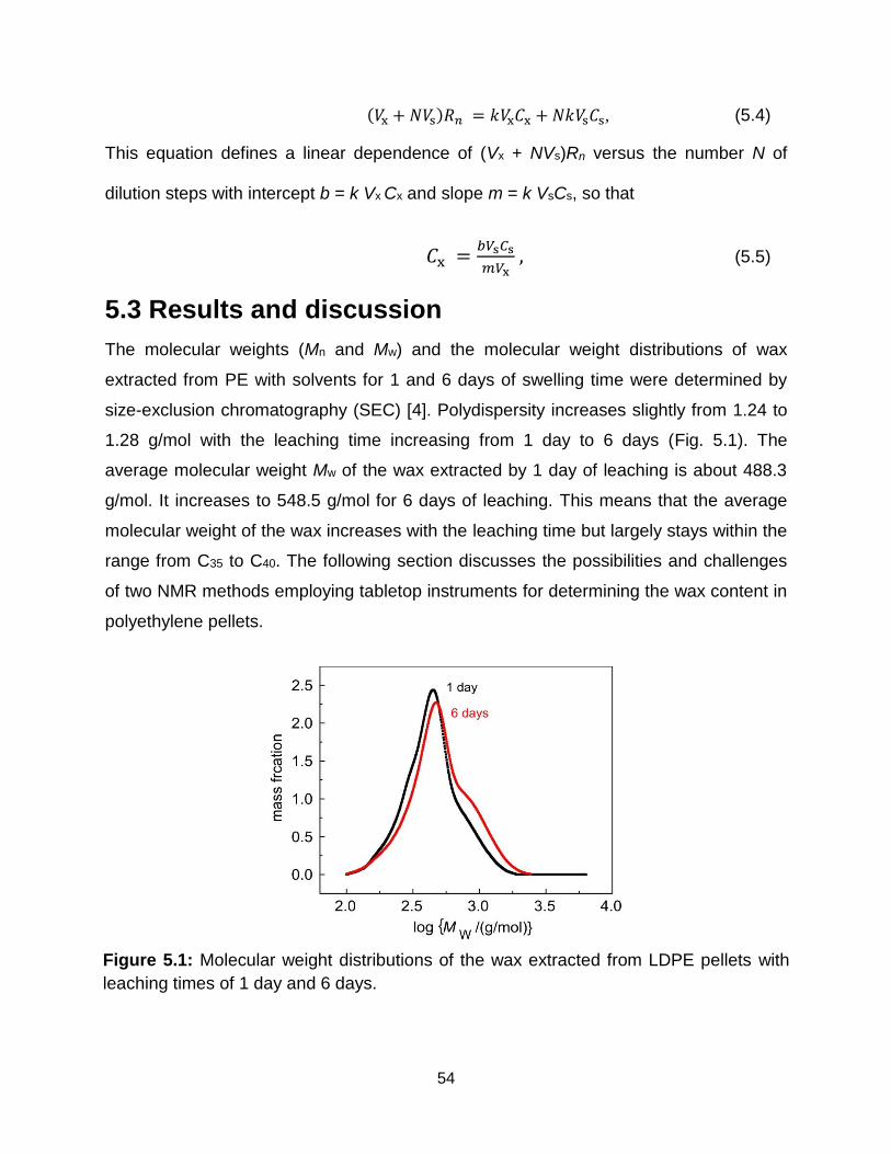
54

Figure 5.1: Molecular weight distributions of the wax extracted from LDPE pellets with

leaching times of 1 day and 6 days.

(𝑉x + 𝑁𝑉s)𝑅𝑛 = 𝑘𝑉x𝐶x + 𝑁𝑘𝑉s𝐶s, (5.4)

This equation defines a linear dependence of (Vx + NVs)Rn versus the number N of

dilution steps with intercept b = k Vx Cx and slope m = k VsCs, so that

𝐶x =𝑏𝑉s𝐶s

𝑚𝑉x , (5.5)


The molecular weights (Mn and Mw) and the molecular weight distributions of wax

extracted from PE with solvents for 1 and 6 days of swelling time were determined by

size-exclusion chromatography (SEC) [4]. Polydispersity increases slightly from 1.24 to

1.28 g/mol with the leaching time increasing from 1 day to 6 days (Fig. 5.1). The

average molecular weight Mw of the wax extracted by 1 day of leaching is about 488.3

g/mol. It increases to 548.5 g/mol for 6 days of leaching. This means that the average

molecular weight of the wax increases with the leaching time but largely stays within the

range from C35 to C40. The following section discusses the possibilities and challenges

of two NMR methods employing tabletop instruments for determining the wax content in

polyethylene pellets.

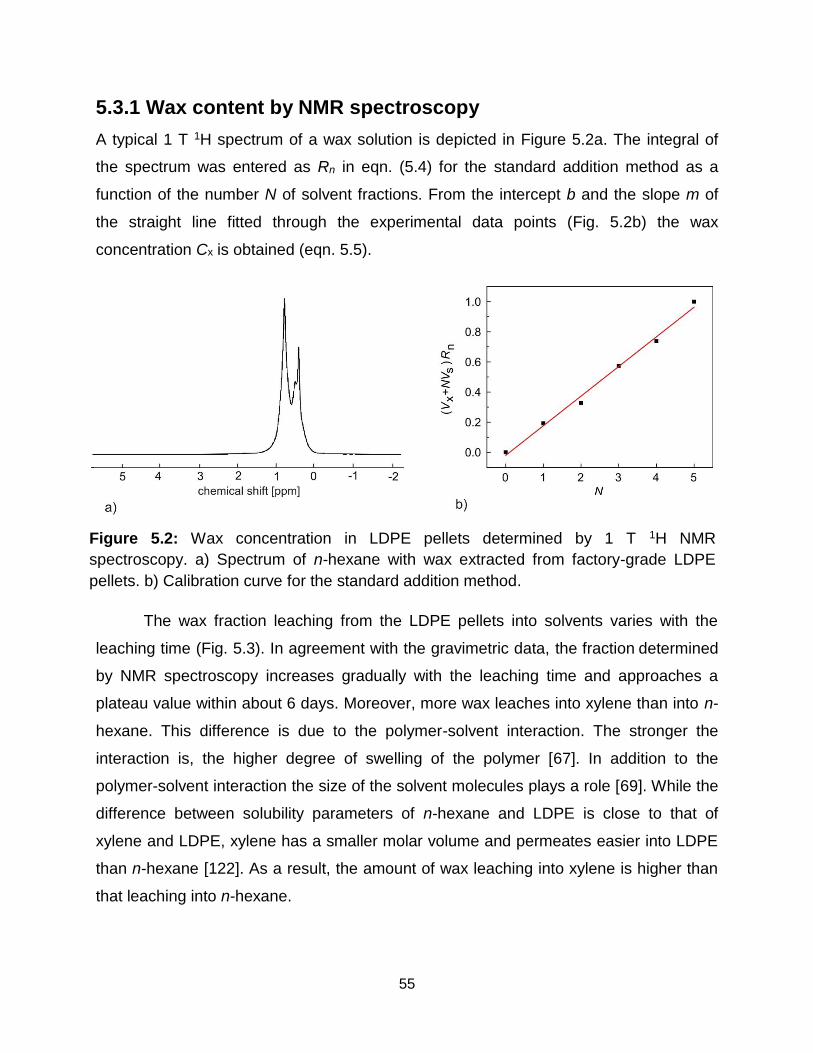
55

Figure 5.2: Wax concentration in LDPE pellets determined by 1 T 1H NMR

spectroscopy. a) Spectrum of n-hexane with wax extracted from factory-grade LDPE

pellets. b) Calibration curve for the standard addition method.

5.3.1 Wax content by NMR spectroscopy

A typical 1 T 1H spectrum of a wax solution is depicted in Figure 5.2a. The integral of

the spectrum was entered as Rn in eqn. (5.4) for the standard addition method as a

function of the number N of solvent fractions. From the intercept b and the slope m of

the straight line fitted through the experimental data points (Fig. 5.2b) the wax

concentration Cx is obtained (eqn. 5.5).

The wax fraction leaching from the LDPE pellets into solvents varies with the

leaching time (Fig. 5.3). In agreement with the gravimetric data, the fraction determined

by NMR spectroscopy increases gradually with the leaching time and approaches a

plateau value within about 6 days. Moreover, more wax leaches into xylene than into n-

hexane. This difference is due to the polymer-solvent interaction. The stronger the

interaction is, the higher degree of swelling of the polymer [67]. In addition to the

polymer-solvent interaction the size of the solvent molecules plays a role [69]. While the

difference between solubility parameters of n-hexane and LDPE is close to that of

xylene and LDPE, xylene has a smaller molar volume and permeates easier into LDPE

than n-hexane [122]. As a result, the amount of wax leaching into xylene is higher than

that leaching into n-hexane.

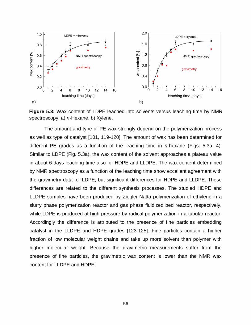
56

Figure 5.3: Wax content of LDPE leached into solvents versus leaching time by NMR

spectroscopy. a) n-Hexane. b) Xylene.

The amount and type of PE wax strongly depend on the polymerization process

as well as type of catalyst [101, 119-120]. The amount of wax has been determined for

different PE grades as a function of the leaching time in n-hexane (Figs. 5.3a, 4).

Similar to LDPE (Fig. 5.3a), the wax content of the solvent approaches a plateau value

in about 6 days leaching time also for HDPE and LLDPE. The wax content determined

by NMR spectroscopy as a function of the leaching time show excellent agreement with

the gravimetry data for LDPE, but significant differences for HDPE and LLDPE. These

differences are related to the different synthesis processes. The studied HDPE and

LLDPE samples have been produced by Ziegler-Natta polymerization of ethylene in a

slurry phase polymerization reactor and gas phase fluidized bed reactor, respectively,

while LDPE is produced at high pressure by radical polymerization in a tubular reactor.

Accordingly the difference is attributed to the presence of fine particles embedding

catalyst in the LLDPE and HDPE grades [123-125]. Fine particles contain a higher

fraction of low molecular weight chains and take up more solvent than polymer with

higher molecular weight. Because the gravimetric measurements suffer from the

presence of fine particles, the gravimetric wax content is lower than the NMR wax

content for LLDPE and HDPE.

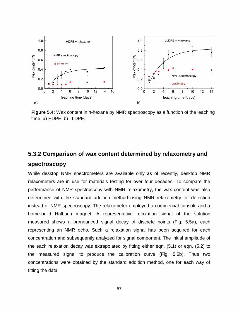
57

Figure 5.4: Wax content in n-hexane by NMR spectroscopy as a function of the leaching

time. a) HDPE. b) LLDPE.

5.3.2 Comparison of wax content determined by relaxometry and

spectroscopy

While desktop NMR spectrometers are available only as of recently, desktop NMR

relaxometers are in use for materials testing for over four decades. To compare the

performance of NMR spectroscopy with NMR relaxometry, the wax content was also

determined with the standard addition method using NMR relaxometry for detection

instead of NMR spectroscopy. The relaxometer employed a commercial console and a

home-build Halbach magnet. A representative relaxation signal of the solution

measured shows a pronounced signal decay of discrete points (Fig. 5.5a), each

representing an NMR echo. Such a relaxation signal has been acquired for each

concentration and subsequently analyzed for signal component. The initial amplitude of

the each relaxation decay was extrapolated by fitting either eqn. (5.1) or eqn. (5.2) to

the measured signal to produce the calibration curve (Fig. 5.5b). Thus two

concentrations were obtained by the standard addition method, one for each way of

fitting the data.

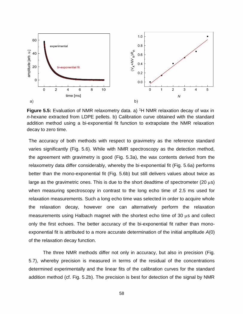
58

Figure 5.5: Evaluation of NMR relaxometry data. a) 1H NMR relaxation decay of wax in

n-hexane extracted from LDPE pellets. b) Calibration curve obtained with the standard

addition method using a bi-exponential fit function to extrapolate the NMR relaxation

decay to zero time.

The accuracy of both methods with respect to gravimetry as the reference standard

varies significantly (Fig. 5.6). While with NMR spectroscopy as the detection method,

the agreement with gravimetry is good (Fig. 5.3a), the wax contents derived from the

relaxometry data differ considerably, whereby the bi-exponential fit (Fig. 5.6a) performs

better than the mono-exponential fit (Fig. 5.6b) but still delivers values about twice as

large as the gravimetric ones. This is due to the short deadtime of spectrometer (20 s)

when measuring spectroscopy in contrast to the long echo time of 2.5 ms used for

relaxation measurements. Such a long echo time was selected in order to acquire whole

the relaxation decay, however one can alternatively perform the relaxation

measurements using Halbach magnet with the shortest echo time of 30 s and collect

only the first echoes. The better accuracy of the bi-exponential fit rather than mono-

exponential fit is attributed to a more accurate determination of the initial amplitude A(0)

of the relaxation decay function.

The three NMR methods differ not only in accuracy, but also in precision (Fig.

5.7), whereby precision is measured in terms of the residual of the concentrations

determined experimentally and the linear fits of the calibration curves for the standard

addition method (cf. Fig. 5.2b). The precision is best for detection of the signal by NMR

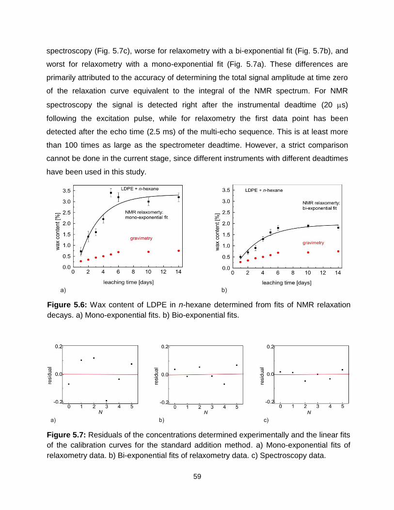
59

Figure 5.6: Wax content of LDPE in n-hexane determined from fits of NMR relaxation

decays. a) Mono-exponential fits. b) Bio-exponential fits.

Figure 5.7: Residuals of the concentrations determined experimentally and the linear fits

of the calibration curves for the standard addition method. a) Mono-exponential fits of

relaxometry data. b) Bi-exponential fits of relaxometry data. c) Spectroscopy data.

spectroscopy (Fig. 5.7c), worse for relaxometry with a bi-exponential fit (Fig. 5.7b), and

worst for relaxometry with a mono-exponential fit (Fig. 5.7a). These differences are

primarily attributed to the accuracy of determining the total signal amplitude at time zero

of the relaxation curve equivalent to the integral of the NMR spectrum. For NMR

spectroscopy the signal is detected right after the instrumental deadtime (20 s)

following the excitation pulse, while for relaxometry the first data point has been

detected after the echo time (2.5 ms) of the multi-echo sequence. This is at least more

than 100 times as large as the spectrometer deadtime. However, a strict comparison

cannot be done in the current stage, since different instruments with different deadtimes

have been used in this study.

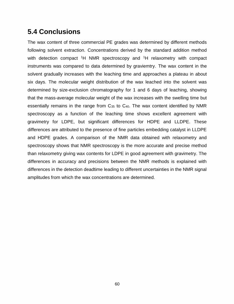
60

5.4 Conclusions

The wax content of three commercial PE grades was determined by different methods

following solvent extraction. Concentrations derived by the standard addition method

with detection compact 1H NMR spectroscopy and 1H relaxometry with compact

instruments was compared to data determined by graviemtry. The wax content in the

solvent gradually increases with the leaching time and approaches a plateau in about

six days. The molecular weight distribution of the wax leached into the solvent was

determined by size-exclusion chromatography for 1 and 6 days of leaching, showing

that the mass-average molecular weight of the wax increases with the swelling time but

essentially remains in the range from C35 to C40. The wax content identified by NMR

spectroscopy as a function of the leaching time shows excellent agreement with

gravimetry for LDPE, but significant differences for HDPE and LLDPE. These

differences are attributed to the presence of fine particles embedding catalyst in LLDPE

and HDPE grades. A comparison of the NMR data obtained with relaxometry and

spectroscopy shows that NMR spectroscopy is the more accurate and precise method

than relaxometry giving wax contents for LDPE in good agreement with gravimetry. The

differences in accuracy and precisions between the NMR methods is explained with

differences in the detection deadtime leading to different uncertainties in the NMR signal

amplitudes from which the wax concentrations are determined.

61

Chapter 6

6 Morphology of a PET/PBT gradient

polymer

This chapter reports part of the work performed in an industrial collaboration under my

supervision by the master student Alexander Görges. I supervised his experiments,

guided the writing of his report and substantially edited his thesis. (A. Görges, NMR

Investigation on Gradient Polymer Material, Master thesis, RWTH Aachen, 2016)


Over many years, considerable effort has been placed on improving the physical and

mechanical properties of polymers. This includes a variety of applications, where for

example people deal with human’s safety in automotive engineering or with high cost of

products in the daily markets. PET and PBT are the most well-known thermoplastic

polyesters used widely in engineering applications. In contrast to PET, which is largely

used for the fabrication of molten products, fibers and films, PBT is mainly used for

injection molded products. PET resins are utilized for those applications requiring higher

heat-deflection temperature, greater rigidity and economy. However, the processing of

PET is difficult because of its slow rate of crystallization and high melting point [128],

while PBT resins show the better moldability and a rapid crystallization rate. On the

other hand, blending of polymers is considered as a solution to establish new polymers

with tailored properties [126-128]. Furthermore, gradient polymers have been

established as a commercial solution to enhance, for example, mechanical, thermal and

optical properties [129].

Since PBT and PET are miscible in the amorphous phase, they are suitable for

melt blending. Furthermore, at the same time the blend does not cocrystallize but rather

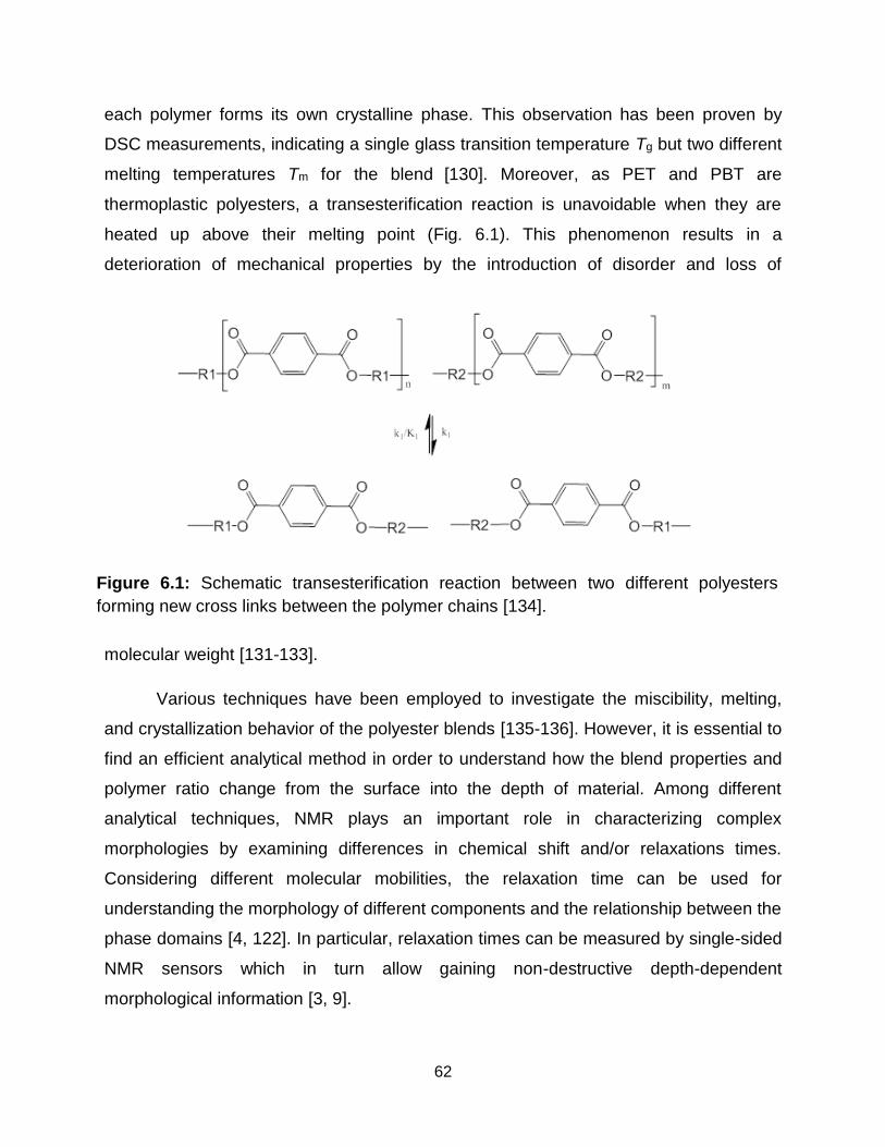
62

Figure 6.1: Schematic transesterification reaction between two different polyesters

forming new cross links between the polymer chains [134].

each polymer forms its own crystalline phase. This observation has been proven by

DSC measurements, indicating a single glass transition temperature Tg but two different

melting temperatures Tm for the blend [130]. Moreover, as PET and PBT are

thermoplastic polyesters, a transesterification reaction is unavoidable when they are

heated up above their melting point (Fig. 6.1). This phenomenon results in a

deterioration of mechanical properties by the introduction of disorder and loss of

molecular weight [131-133].

Various techniques have been employed to investigate the miscibility, melting,

and crystallization behavior of the polyester blends [135-136]. However, it is essential to

find an efficient analytical method in order to understand how the blend properties and

polymer ratio change from the surface into the depth of material. Among different

analytical techniques, NMR plays an important role in characterizing complex

morphologies by examining differences in chemical shift and/or relaxations times.

Considering different molecular mobilities, the relaxation time can be used for

understanding the morphology of different components and the relationship between the

phase domains [4, 122]. In particular, relaxation times can be measured by single-sided

NMR sensors which in turn allow gaining non-destructive depth-dependent

morphological information [3, 9].

63

The aim of this study is to investigate PBT/PET blends with and without glass

fibers (GF) in comparison with pure PBT samples. The NMR-MOUSE is applied to

investigate the molecular mobility, the morphological changes, and the glass fiber

distribution in blend samples. In addition to these, 1H-13C-CPMAS (Cross Polarization

Magic Angle Spinning) NMR is applied in high-field to study the rigid fraction in the

blend samples. The CPMAS spectra reveal differences between the blend and the pure

PBT samples and provide information about the fractions of the different polymer

components. Furthermore, in order to determine the sizes of the different morphological

domains, spin-diffusion is measured in the blend samples.

6.2 Experimental Section

6.2.1 Materials

Polymer plates with the dimension of 40 mm x 40 mm x 2 mm were used in the current

study. The samples were employed as received for acquiring the depth profiles non-

destructively using the NMR-MOUSE. After the low-field measurements, all samples

have been shaved slice by slice with a CNC (computerized numerical control) milling

machine into layers with a thickness of 400 µm. Thereby, for the 2 mm thick sample one

gets 5 different shavings. These shavings were then used to get depth-dependent

information by high-field NMR in a destructive way.

6.2.2 NMR experiments and data processing

Low-field NMR measurements

Proton transverse relaxation measurements were conducted with an NMR-MOUSE to

obtain depth-dependent profiles and morphological variations. The low-field NMR

measurements were carried out at room temperature with a PM2 NMR-MOUSE working

at a proton frequency of 29.3 MHz, which has a penetration depth of 2 mm. All low-field

measurements were performed with a CPMG sequence using a 2 seconds recycle

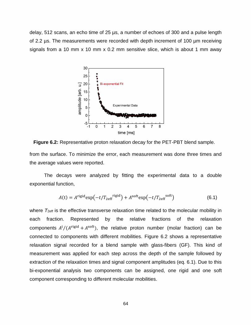
64

Figure 6.2: Representative proton relaxation decay for the PET-PBT blend sample.

delay, 512 scans, an echo time of 25 µs, a number of echoes of 300 and a pulse length

of 2.2 µs. The measurements were recorded with depth increment of 100 µm receiving

signals from a 10 mm x 10 mm x 0.2 mm sensitive slice, which is about 1 mm away

from the surface. To minimize the error, each measurement was done three times and

the average values were reported.

The decays were analyzed by fitting the experimental data to a double

exponential function,

𝐴(t) = 𝐴rigidexp(−𝑡/𝑇2effrigid) + 𝐴softexp(−𝑡/𝑇2eff

soft) (6.1)

where T2eff is the effective transverse relaxation time related to the molecular mobility in

each fraction. Represented by the relative fractions of the relaxation

components 𝐴i (𝐴rigid +⁄ 𝐴soft), the relative proton number (molar fraction) can be

connected to components with different mobilities. Figure 6.2 shows a representative

relaxation signal recorded for a blend sample with glass-fibers (GF). This kind of

measurement was applied for each step across the depth of the sample followed by

extraction of the relaxation times and signal component amplitudes (eq. 6.1). Due to this

bi-exponential analysis two components can be assigned, one rigid and one soft

component corresponding to different molecular mobilities.

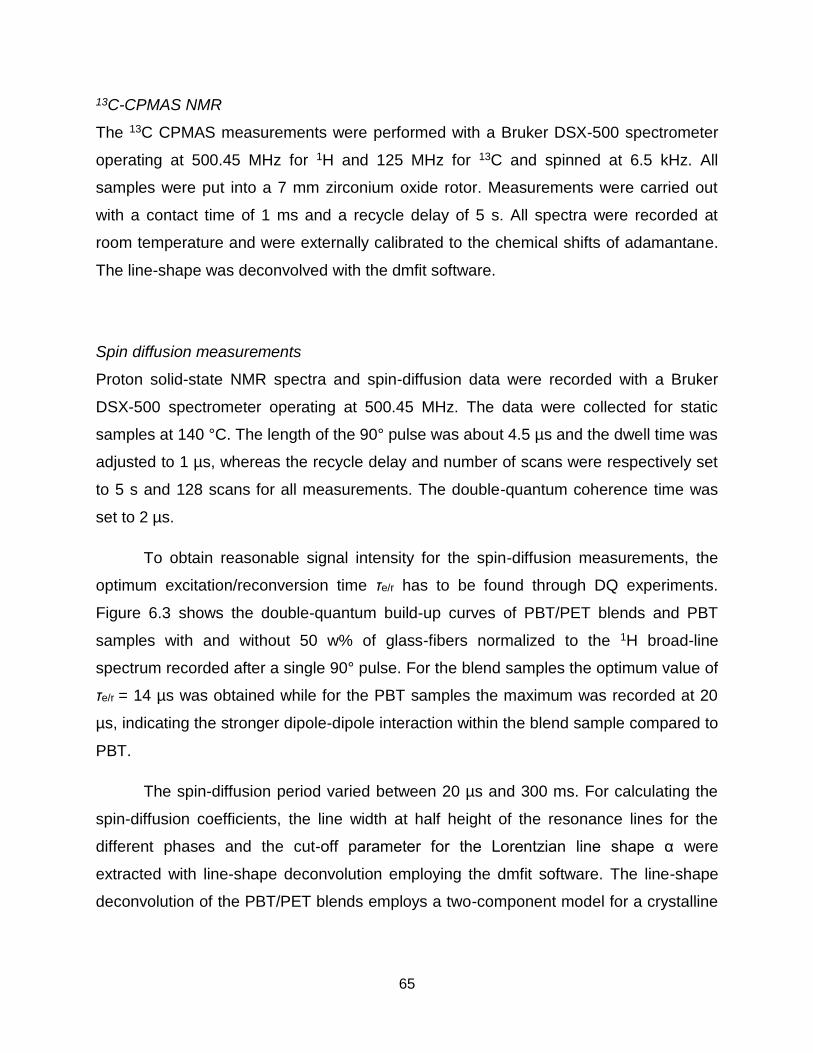
65

13C-CPMAS NMR

The 13C CPMAS measurements were performed with a Bruker DSX-500 spectrometer

operating at 500.45 MHz for 1H and 125 MHz for 13C and spinned at 6.5 kHz. All

samples were put into a 7 mm zirconium oxide rotor. Measurements were carried out

with a contact time of 1 ms and a recycle delay of 5 s. All spectra were recorded at

room temperature and were externally calibrated to the chemical shifts of adamantane.

The line-shape was deconvolved with the dmfit software.

Spin diffusion measurements

Proton solid-state NMR spectra and spin-diffusion data were recorded with a Bruker

DSX-500 spectrometer operating at 500.45 MHz. The data were collected for static

samples at 140 °C. The length of the 90° pulse was about 4.5 µs and the dwell time was

adjusted to 1 µs, whereas the recycle delay and number of scans were respectively set

to 5 s and 128 scans for all measurements. The double-quantum coherence time was

set to 2 µs.

To obtain reasonable signal intensity for the spin-diffusion measurements, the

optimum excitation/reconversion time τe/r has to be found through DQ experiments.

Figure 6.3 shows the double-quantum build-up curves of PBT/PET blends and PBT

samples with and without 50 w% of glass-fibers normalized to the 1H broad-line

spectrum recorded after a single 90° pulse. For the blend samples the optimum value of

τe/r = 14 µs was obtained while for the PBT samples the maximum was recorded at 20

µs, indicating the stronger dipole-dipole interaction within the blend sample compared to

PBT.

The spin-diffusion period varied between 20 µs and 300 ms. For calculating the

spin-diffusion coefficients, the line width at half height of the resonance lines for the

different phases and the cut-off parameter for the Lorentzian line shape α were

extracted with line-shape deconvolution employing the dmfit software. The line-shape

deconvolution of the PBT/PET blends employs a two-component model for a crystalline

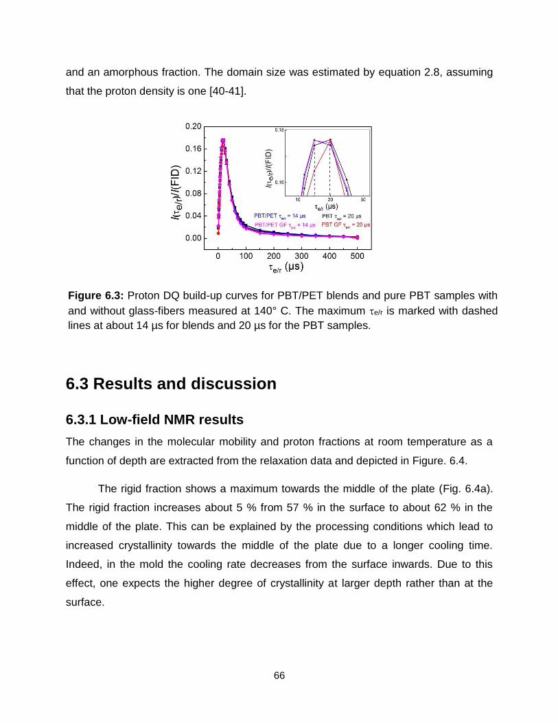
66

Figure 6.3: Proton DQ build-up curves for PBT/PET blends and pure PBT samples with

and without glass-fibers measured at 140° C. The maximum e/r is marked with dashed

lines at about 14 µs for blends and 20 µs for the PBT samples.

and an amorphous fraction. The domain size was estimated by equation 2.8, assuming

that the proton density is one [40-41].


6.3.1 Low-field NMR results

The changes in the molecular mobility and proton fractions at room temperature as a

function of depth are extracted from the relaxation data and depicted in Figure. 6.4.

The rigid fraction shows a maximum towards the middle of the plate (Fig. 6.4a).

The rigid fraction increases about 5 % from 57 % in the surface to about 62 % in the

middle of the plate. This can be explained by the processing conditions which lead to

increased crystallinity towards the middle of the plate due to a longer cooling time.

Indeed, in the mold the cooling rate decreases from the surface inwards. Due to this

effect, one expects the higher degree of crystallinity at larger depth rather than at the

surface.

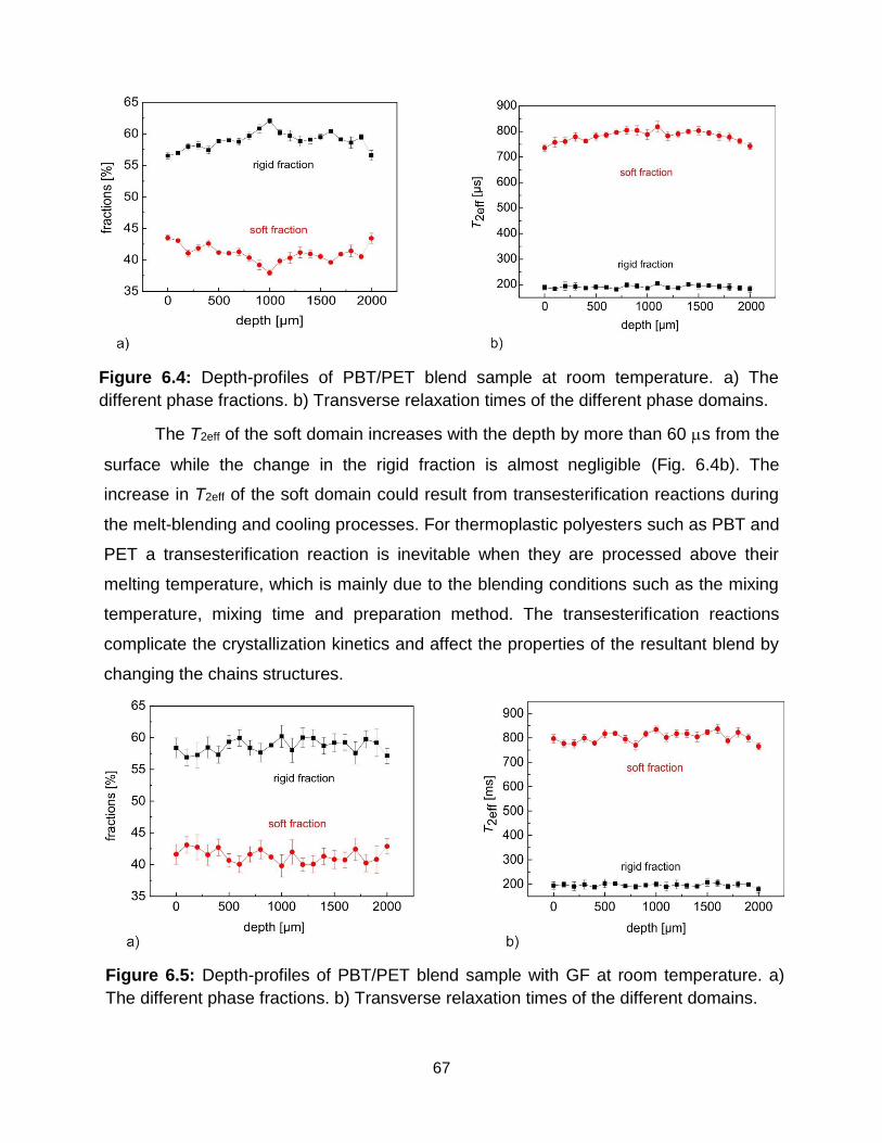
67

Figure 6.4: Depth-profiles of PBT/PET blend sample at room temperature. a) The

different phase fractions. b) Transverse relaxation times of the different phase domains.

Figure 6.5: Depth-profiles of PBT/PET blend sample with GF at room temperature. a)

The different phase fractions. b) Transverse relaxation times of the different domains.

The T2eff of the soft domain increases with the depth by more than 60 s from the

surface while the change in the rigid fraction is almost negligible (Fig. 6.4b). The

increase in T2eff of the soft domain could result from transesterification reactions during

the melt-blending and cooling processes. For thermoplastic polyesters such as PBT and

PET a transesterification reaction is inevitable when they are processed above their

melting temperature, which is mainly due to the blending conditions such as the mixing

temperature, mixing time and preparation method. The transesterification reactions

complicate the crystallization kinetics and affect the properties of the resultant blend by

changing the chains structures.

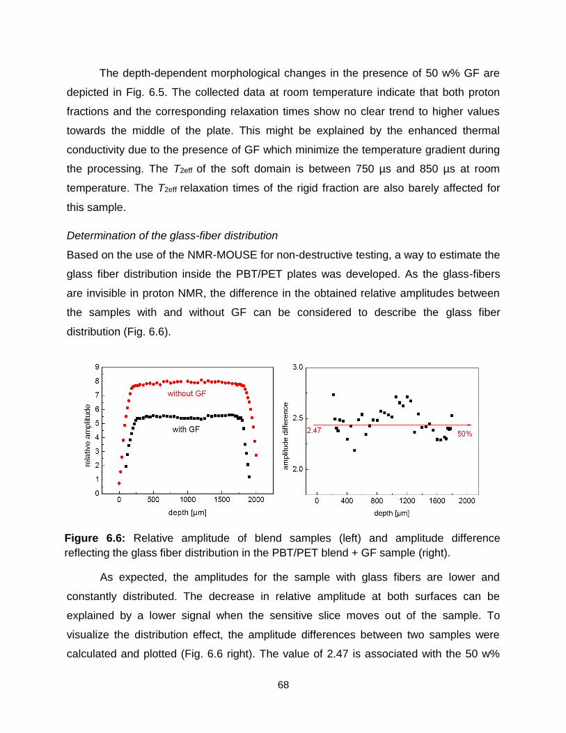
68

Figure 6.6: Relative amplitude of blend samples (left) and amplitude difference

reflecting the glass fiber distribution in the PBT/PET blend + GF sample (right).

The depth-dependent morphological changes in the presence of 50 w% GF are

depicted in Fig. 6.5. The collected data at room temperature indicate that both proton

fractions and the corresponding relaxation times show no clear trend to higher values

towards the middle of the plate. This might be explained by the enhanced thermal

conductivity due to the presence of GF which minimize the temperature gradient during

the processing. The T2eff of the soft domain is between 750 µs and 850 µs at room

temperature. The T2eff relaxation times of the rigid fraction are also barely affected for

this sample.

Determination of the glass-fiber distribution

Based on the use of the NMR-MOUSE for non-destructive testing, a way to estimate the

glass fiber distribution inside the PBT/PET plates was developed. As the glass-fibers

are invisible in proton NMR, the difference in the obtained relative amplitudes between

the samples with and without GF can be considered to describe the glass fiber

distribution (Fig. 6.6).

As expected, the amplitudes for the sample with glass fibers are lower and

constantly distributed. The decrease in relative amplitude at both surfaces can be

explained by a lower signal when the sensitive slice moves out of the sample. To

visualize the distribution effect, the amplitude differences between two samples were

calculated and plotted (Fig. 6.6 right). The value of 2.47 is associated with the 50 w%

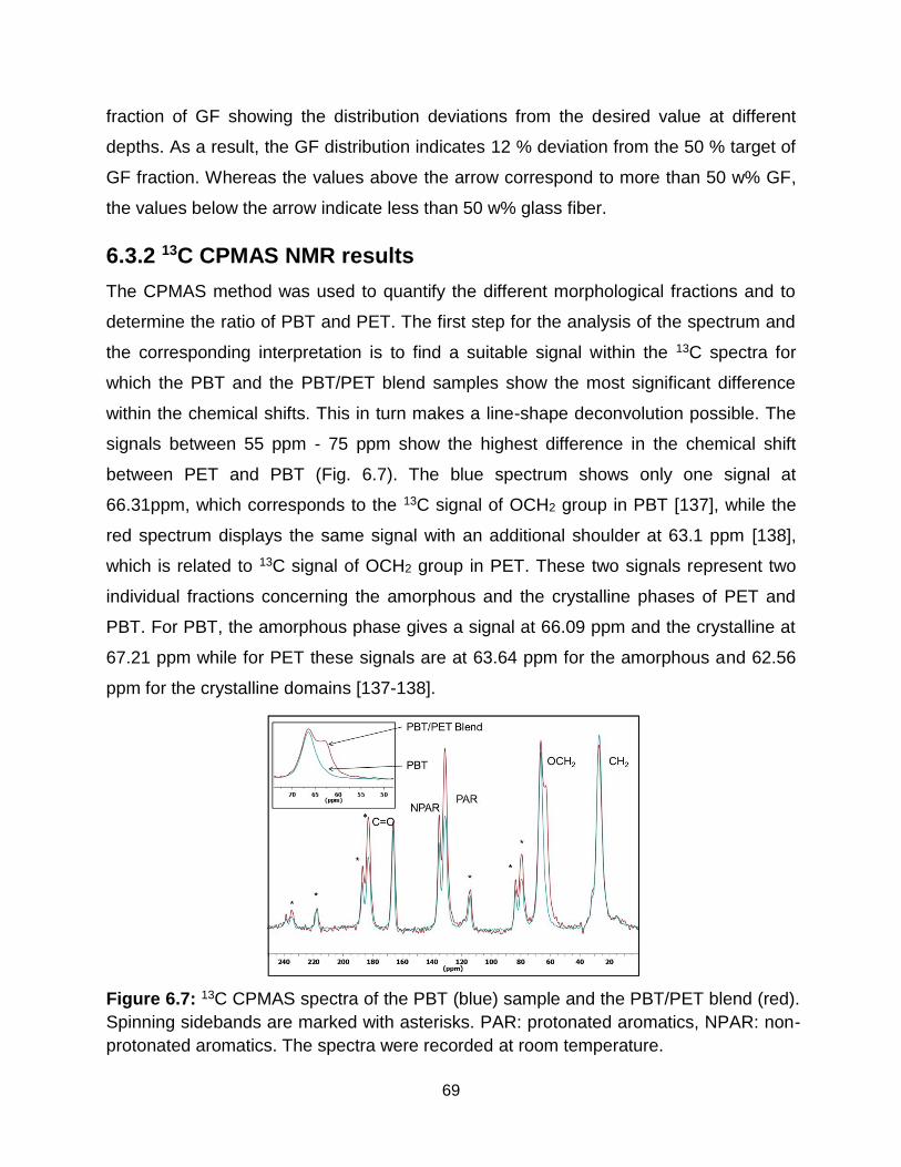
69

Figure 6.7: 13C CPMAS spectra of the PBT (blue) sample and the PBT/PET blend (red).

Spinning sidebands are marked with asterisks. PAR: protonated aromatics, NPAR: non-

protonated aromatics. The spectra were recorded at room temperature.

fraction of GF showing the distribution deviations from the desired value at different

depths. As a result, the GF distribution indicates 12 % deviation from the 50 % target of

GF fraction. Whereas the values above the arrow correspond to more than 50 w% GF,

the values below the arrow indicate less than 50 w% glass fiber.

6.3.2 13C CPMAS NMR results

The CPMAS method was used to quantify the different morphological fractions and to

determine the ratio of PBT and PET. The first step for the analysis of the spectrum and

the corresponding interpretation is to find a suitable signal within the 13C spectra for

which the PBT and the PBT/PET blend samples show the most significant difference

within the chemical shifts. This in turn makes a line-shape deconvolution possible. The

signals between 55 ppm - 75 ppm show the highest difference in the chemical shift

between PET and PBT (Fig. 6.7). The blue spectrum shows only one signal at

66.31ppm, which corresponds to the 13C signal of OCH2 group in PBT [137], while the

red spectrum displays the same signal with an additional shoulder at 63.1 ppm [138],

which is related to 13C signal of OCH2 group in PET. These two signals represent two

individual fractions concerning the amorphous and the crystalline phases of PET and

PBT. For PBT, the amorphous phase gives a signal at 66.09 ppm and the crystalline at

67.21 ppm while for PET these signals are at 63.64 ppm for the amorphous and 62.56

ppm for the crystalline domains [137-138].

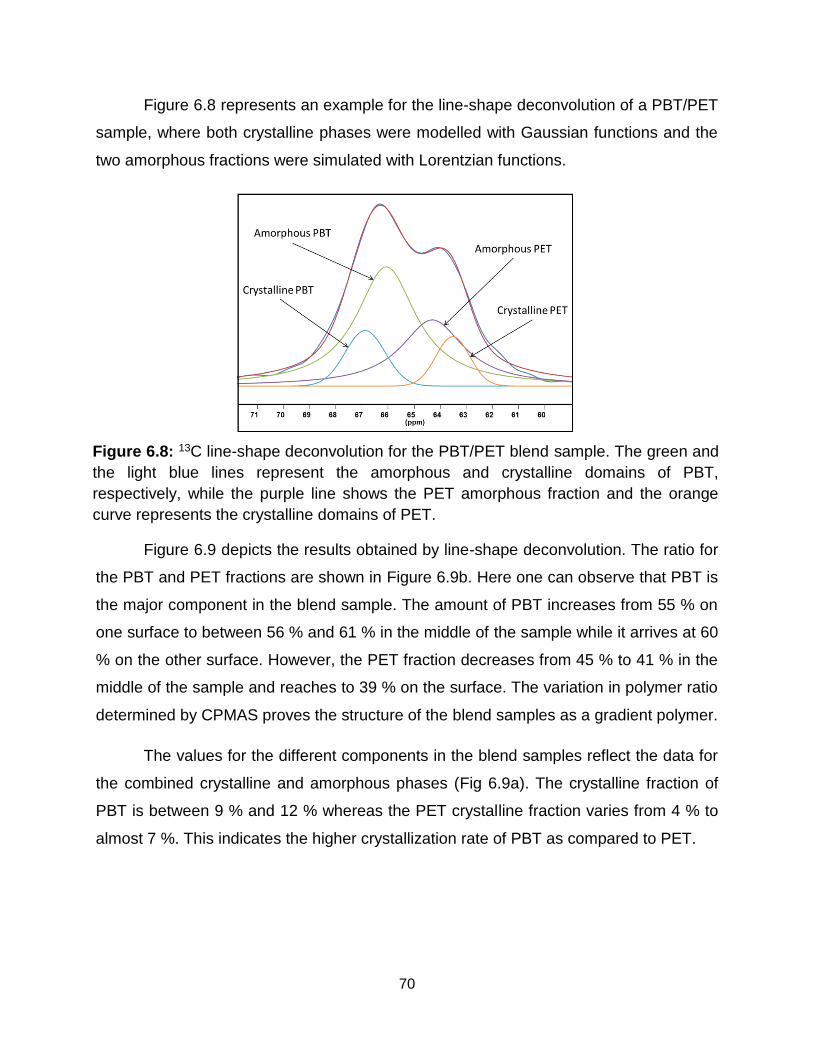
70

Figure 6.8: 13C line-shape deconvolution for the PBT/PET blend sample. The green and

the light blue lines represent the amorphous and crystalline domains of PBT,

respectively, while the purple line shows the PET amorphous fraction and the orange

curve represents the crystalline domains of PET.

.

Figure 6.8 represents an example for the line-shape deconvolution of a PBT/PET

sample, where both crystalline phases were modelled with Gaussian functions and the

two amorphous fractions were simulated with Lorentzian functions.

Figure 6.9 depicts the results obtained by line-shape deconvolution. The ratio for

the PBT and PET fractions are shown in Figure 6.9b. Here one can observe that PBT is

the major component in the blend sample. The amount of PBT increases from 55 % on

one surface to between 56 % and 61 % in the middle of the sample while it arrives at 60

% on the other surface. However, the PET fraction decreases from 45 % to 41 % in the

middle of the sample and reaches to 39 % on the surface. The variation in polymer ratio

determined by CPMAS proves the structure of the blend samples as a gradient polymer.

The values for the different components in the blend samples reflect the data for

the combined crystalline and amorphous phases (Fig 6.9a). The crystalline fraction of

PBT is between 9 % and 12 % whereas the PET crystalline fraction varies from 4 % to

almost 7 %. This indicates the higher crystallization rate of PBT as compared to PET.

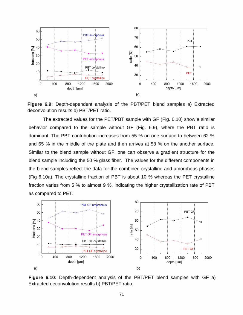
71

Figure 6.9: Depth-dependent analysis of the PBT/PET blend samples a) Extracted

deconvolution results b) PBT/PET ratio.

Figure 6.10: Depth-dependent analysis of the PBT/PET blend samples with GF a)

Extracted deconvolution results b) PBT/PET ratio.

The extracted values for the PET/PBT sample with GF (Fig. 6.10) show a similar

behavior compared to the sample without GF (Fig. 6.9), where the PBT ratio is

dominant. The PBT contribution increases from 55 % on one surface to between 62 %

and 65 % in the middle of the plate and then arrives at 58 % on the another surface.

Similar to the blend sample without GF, one can observe a gradient structure for the

blend sample including the 50 % glass fiber. The values for the different components in

the blend samples reflect the data for the combined crystalline and amorphous phases

(Fig 6.10a). The crystalline fraction of PBT is about 10 % whereas the PET crystalline

fraction varies from 5 % to almost 9 %, indicating the higher crystallization rate of PBT

as compared to PET.

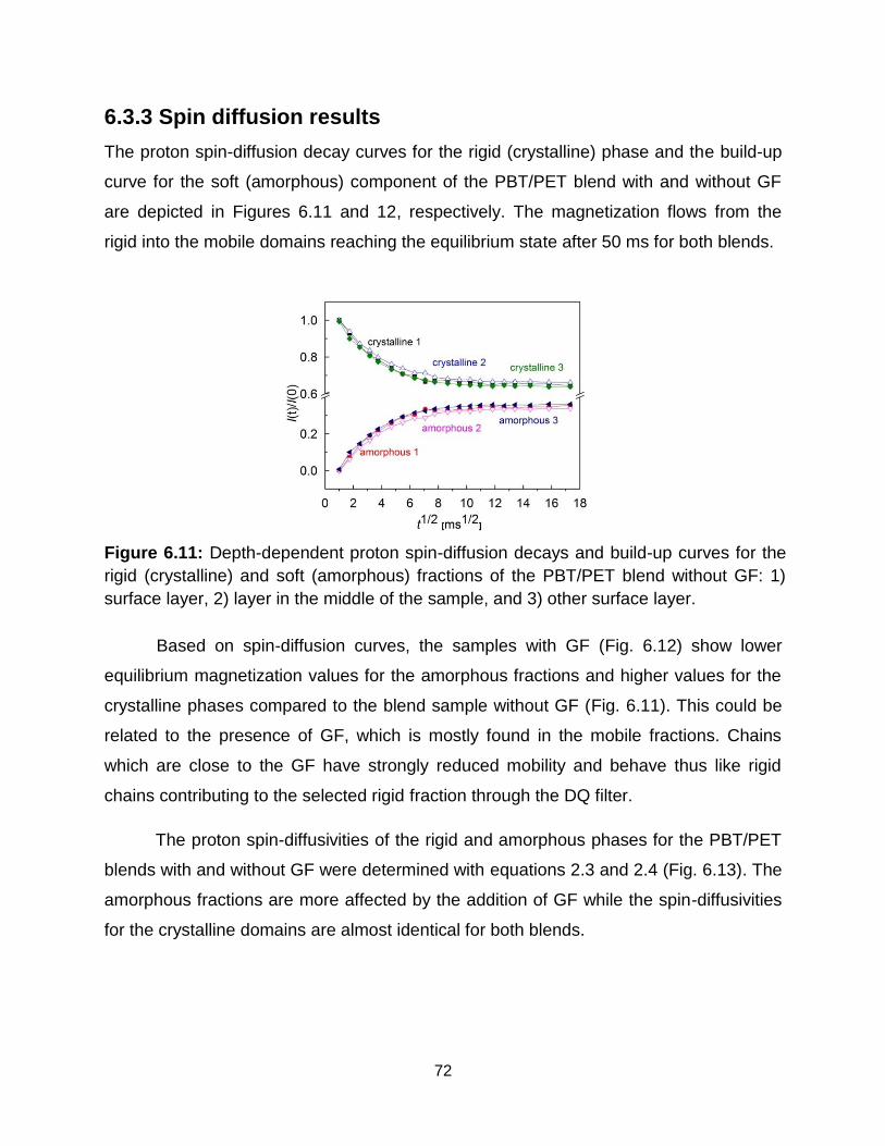
72

Figure 6.11: Depth-dependent proton spin-diffusion decays and build-up curves for the

rigid (crystalline) and soft (amorphous) fractions of the PBT/PET blend without GF: 1)

surface layer, 2) layer in the middle of the sample, and 3) other surface layer.

6.3.3 Spin diffusion results

The proton spin-diffusion decay curves for the rigid (crystalline) phase and the build-up

curve for the soft (amorphous) component of the PBT/PET blend with and without GF

are depicted in Figures 6.11 and 12, respectively. The magnetization flows from the

rigid into the mobile domains reaching the equilibrium state after 50 ms for both blends.

Based on spin-diffusion curves, the samples with GF (Fig. 6.12) show lower

equilibrium magnetization values for the amorphous fractions and higher values for the

crystalline phases compared to the blend sample without GF (Fig. 6.11). This could be

related to the presence of GF, which is mostly found in the mobile fractions. Chains

which are close to the GF have strongly reduced mobility and behave thus like rigid

chains contributing to the selected rigid fraction through the DQ filter.

The proton spin-diffusivities of the rigid and amorphous phases for the PBT/PET

blends with and without GF were determined with equations 2.3 and 2.4 (Fig. 6.13). The

amorphous fractions are more affected by the addition of GF while the spin-diffusivities

for the crystalline domains are almost identical for both blends.

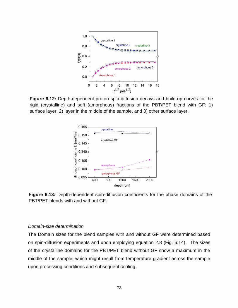
73

Figure 6.12: Depth-dependent proton spin-diffusion decays and build-up curves for the

rigid (crystalline) and soft (amorphous) fractions of the PBT/PET blend with GF: 1)

surface layer, 2) layer in the middle of the sample, and 3) other surface layer.

Figure 6.13: Depth-dependent spin-diffusion coefficients for the phase domains of the

PBT/PET blends with and without GF.

Domain-size determination

The Domain sizes for the blend samples with and without GF were determined based

on spin-diffusion experiments and upon employing equation 2.8 (Fig. 6.14). The sizes

of the crystalline domains for the PBT/PET blend without GF show a maximum in the

middle of the sample, which might result from temperature gradient across the sample

upon processing conditions and subsequent cooling.

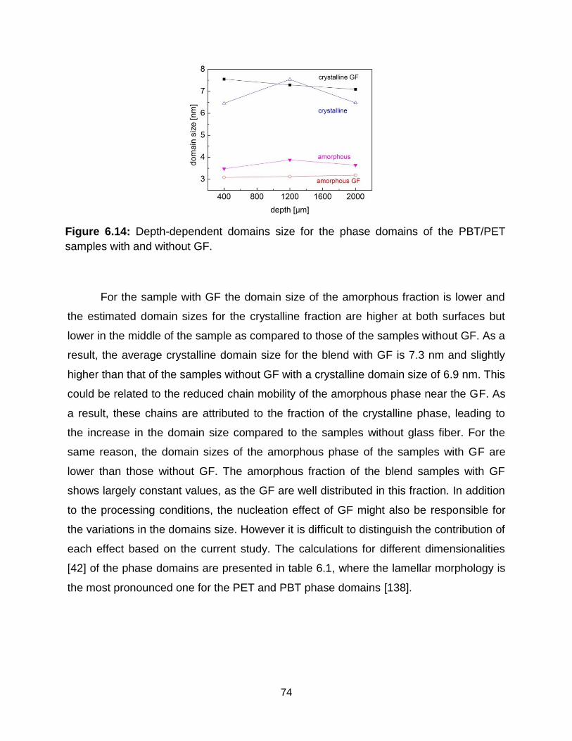
74

Figure 6.14: Depth-dependent domains size for the phase domains of the PBT/PET

samples with and without GF.

For the sample with GF the domain size of the amorphous fraction is lower and

the estimated domain sizes for the crystalline fraction are higher at both surfaces but

lower in the middle of the sample as compared to those of the samples without GF. As a

result, the average crystalline domain size for the blend with GF is 7.3 nm and slightly

higher than that of the samples without GF with a crystalline domain size of 6.9 nm. This

could be related to the reduced chain mobility of the amorphous phase near the GF. As

a result, these chains are attributed to the fraction of the crystalline phase, leading to

the increase in the domain size compared to the samples without glass fiber. For the

same reason, the domain sizes of the amorphous phase of the samples with GF are

lower than those without GF. The amorphous fraction of the blend samples with GF

shows largely constant values, as the GF are well distributed in this fraction. In addition

to the processing conditions, the nucleation effect of GF might also be responsible for

the variations in the domains size. However it is difficult to distinguish the contribution of

each effect based on the current study. The calculations for different dimensionalities

[42] of the phase domains are presented in table 6.1, where the lamellar morphology is

the most pronounced one for the PET and PBT phase domains [138].

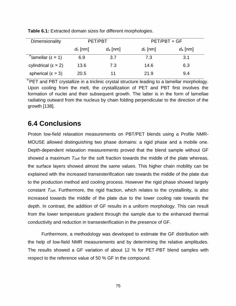
75

Table 6.1: Extracted domain sizes for different morphologies.

Dimensionality PET/PBT PET/PBT + GF

dc [nm] da [nm] dc [nm] da [nm]

lamellar (ε = 1) 6.9 3.7 7.3 3.1

cylindrical (ε = 2) 13.6 7.3 14.6 6.3

spherical (ε = 3) 20.5 11 21.9 9.4

PET and PBT crystallize in a triclinic crystal structure leading to a lamellar morphology.

Upon cooling from the melt, the crystallization of PET and PBT first involves the

formation of nuclei and their subsequent growth. The latter is in the form of lamellae

radiating outward from the nucleus by chain folding perpendicular to the direction of the

growth [138].

6.4 Conclusions

Proton low-field relaxation measurements on PBT/PET blends using a Profile NMR-

MOUSE allowed distinguishing two phase domains: a rigid phase and a mobile one.

Depth-dependent relaxation measurements proved that the blend sample without GF

showed a maximum T2eff for the soft fraction towards the middle of the plate whereas,

the surface layers showed almost the same values. This higher chain mobility can be

explained with the increased transesterification rate towards the middle of the plate due

to the production method and cooling process. However the rigid phase showed largely

constant T2eff. Furthermore, the rigid fraction, which relates to the crystallinity, is also

increased towards the middle of the plate due to the lower cooling rate towards the

depth. In contrast, the addition of GF results in a uniform morphology. This can result

from the lower temperature gradient through the sample due to the enhanced thermal

conductivity and reduction in transesterification in the presence of GF.

Furthermore, a methodology was developed to estimate the GF distribution with

the help of low-field NMR measurements and by determining the relative amplitudes.

The results showed a GF variation of about 12 % for PET-PBT blend samples with

respect to the reference value of 50 % GF in the compound.

76

Line-shape deconvolution of 13C CPMAS spectra allowed the quantification of the

crystalline and amorphous fractions as well as the PET/PBT ratio. Upon estimating the

PBT/PET ratio, it was observed that the investigated blend samples behave as a

gradient polymer, whereby the PBT content is dominant across the sample with around

a 60 % contribution.

A spin-diffusion analysis recorded that the blend samples form a two-component

system consisting of the crystalline and amorphous fractions. By a line-shape analysis

of the obtained 1H spectra, the spin-diffusivities of the different morphological fractions

were determined. The spin-diffusivities of the amorphous domains were lower for

samples with GF, which might be related to a reduction in the chain mobilities due to the

presence of GF. Furthermore, the domains size was estimated for the different

morphological phases and various dimensionalities. The domain sizes for the crystalline

fractions of the samples without GF showed a maximum in the middle of the sample,

which might be related to the processing conditions. However, for the blend sample with

GF, the average domain size was higher for the crystalline fraction and lower for the

amorphous domains as compared to the samples without GF. This could be related to

the reduced chain mobility of the amorphous phase in the vicinity of the GF.

77

Chapter 7

7 Non-destructive determination of

rubber content in rubber-modified

asphalt


In the last recent decades, many efforts have been generated in order to improve the

long-term performance and cost effectiveness of asphalt pavements. Polymer

modification of bitumen (PMB) is one well-established procedure for improving the

performance of asphalt pavements [139-140]. In particular, modification of bitumen with

thermoplastic polymers and elastomers such as polyethylene (PE), polypropylene (PP),

ethylene-vinyl acetate (EVA), ethylene-butyl acrylate (EBA), styrene-butadiene-styrene

(SBS), styrene-isoprene-styrene (SIS), and styrene-ethylene/butylene-styrene (SEBS)

have been reported [140]. Although all of these polymers improve bitumen properties to

different degrees, their drawbacks limiting the future development of bitumen polymer

modification can include high cost, low ageing resistance, and poor storage stability of

polymer modified bitumen (PMB) [139-140].

Another approach to asphalt modification is the use of recycled tire rubber or

vulcanized crumb rubber to modify asphalt binder and mixtures. The tendency towards

using this approach is now increasing in the paving industry due to the prominent

benefits and improvements such as improved resistance to fatigue cracking, improved

aging and oxidation resistance, and lower pavement maintenance costs [141-142].

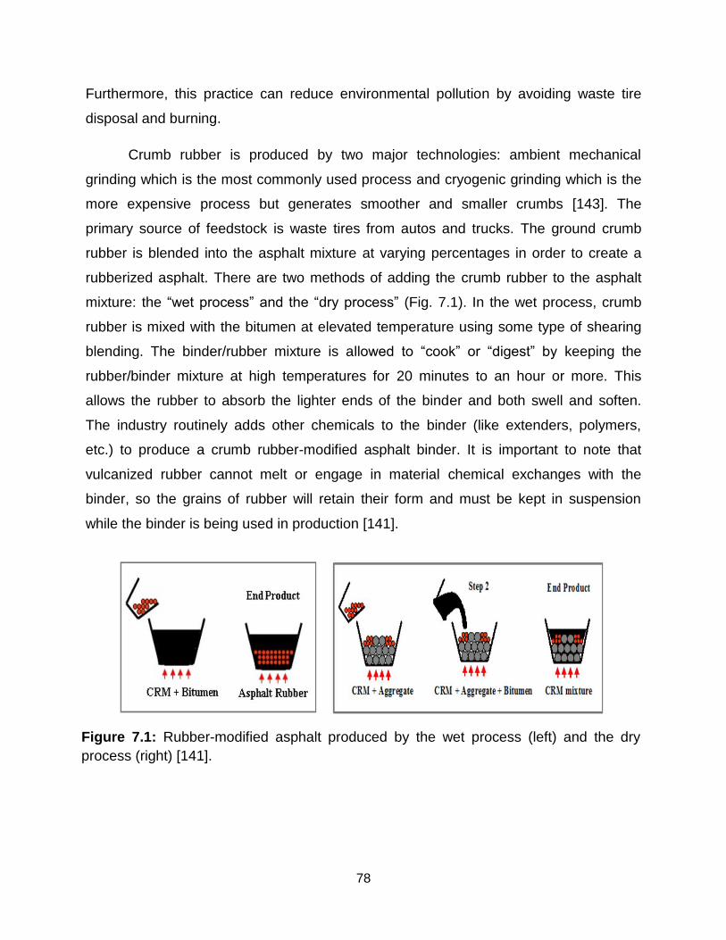
78

Figure 7.1: Rubber-modified asphalt produced by the wet process (left) and the dry

process (right) [141].

Furthermore, this practice can reduce environmental pollution by avoiding waste tire

disposal and burning.

Crumb rubber is produced by two major technologies: ambient mechanical

grinding which is the most commonly used process and cryogenic grinding which is the

more expensive process but generates smoother and smaller crumbs [143]. The

primary source of feedstock is waste tires from autos and trucks. The ground crumb

rubber is blended into the asphalt mixture at varying percentages in order to create a

rubberized asphalt. There are two methods of adding the crumb rubber to the asphalt

mixture: the “wet process” and the “dry process” (Fig. 7.1). In the wet process, crumb

rubber is mixed with the bitumen at elevated temperature using some type of shearing

blending. The binder/rubber mixture is allowed to “cook” or “digest” by keeping the

rubber/binder mixture at high temperatures for 20 minutes to an hour or more. This

allows the rubber to absorb the lighter ends of the binder and both swell and soften.

The industry routinely adds other chemicals to the binder (like extenders, polymers,

etc.) to produce a crumb rubber-modified asphalt binder. It is important to note that

vulcanized rubber cannot melt or engage in material chemical exchanges with the

binder, so the grains of rubber will retain their form and must be kept in suspension

while the binder is being used in production [141].

79

In the dry process, recycled tire crumb rubber is blended with heated stone

aggregate before mixing with bitumen. This process produces rubber/binder/aggregate

amalgam where the rubber is randomly distributed throughout the mix and cannot

separate. During and immediately after production, the crumb rubber absorbs the lighter

ends of the binder, swells and softens. The dry process also produces a crumb rubber-

modified asphalt mix that performs comparably with wet process rubber in the field [141-

142].

A broad range of physical, mechanical and rheological techniques are used to

investigate the properties of asphalt mixtures and binders. Among these, mechanical

testing is a common method used to evaluate the mixture performance in the terms of

the stiffness modulus, permanent deformation and fatigue resistance [141].

Furthermore, the quantification of the rubber fraction along with the control of the rubber

distribution in the asphalt mixture are key factors in the quality control of rubber-

modified asphalt. While various investigations have been reported on the mixing

processes, characterization and properties of crumb rubber-modified asphalt mixtures,

there is no analytical study for investigating and monitoring the rubber fraction in the

finished asphalt mixtures in a non-destructive fashion.

Nuclear Magnetic Resonance (NMR) is a well-known analytical tool in chemistry for

molecular analysis and in medicine for diagnostic imaging. NMR machines are fitted

with proper magnets, which typically are super-conducting to provide high field strength

for high sensitivity. During the last years considerable progress has been achieved with

the development of compact NMR machines employing permanent magnets, which

provide sufficient sensitivity and robustness for nondestructive characterization in

applications outdoors and on the factory floor [4]. In most cases, samples are drawn

and placed inside the magnet where the field is strongest and most homogeneous. But

there are also stray-field NMR sensors, like the NMR-MOUSE (MObile Universal

Surface Explorer), which can be placed on an object to measure the NMR signal from a

region of the object covered by the sensor. Such measurements are truly non-

destructive and are applicable to electrically insulating and non-magnetic objects of any

size as long as they are rich in hydrogen. The measurement signal is collected from a

80

sensitive slice a few millimeters away from the surface outside the sensor. Different

surface regions of the object as well as depth profiles can be recorded by simply shifting

the position of this sensitive slice through the sample [22].

This study reports the first use of the NMR-MOUSE to quantify the rubber fraction in

rubber-modified asphalt. A new NMR methodology has been developed in the

laboratory based on calibration curves obtained from reference samples. This is

accomplished by measuring the transverse NMR relaxation signal and analyzing the

relative amplitudes and variations in the molecular dynamics of the soft and rigid

domains of asphalt samples. Furthermore, for actual field test a modified version of

potable NMR-MOUSE set-up was used. The raw data from the field measurements

need to be further inserted in the calibration model to estimate the rubber fraction in the

field and study the field variations in the terms of the rubber distribution.

7.2 Experimental section

Five different asphalt samples with known rubber fractions were prepared under

controlled laboratory conditions and were used as reference samples for NMR-MOUSE

measurement (Table 7.1). The NMR experiments were performed with the Profile NMR-

MOUSE PM5 by Magritek GmbH, Germany, with a proton resonance frequency of 17.1

MHz. The transverse magnetization decays of the samples were measured with a Carr–

Purcell–Meiboom–Gill (CPMG) sequence from a 10 × 10 × 0.1 mm3 sensitive slice at 5

mm depth into each sample using an echo time of 50 µs and depth interval of 200 µm.

The decays were analyzed by fitting the experimental data to a double exponential

function,

A(t) =Arigid exp(-t/T2eff rigid)+ Asoft exp(-t/T2eff

soft). (7.1)

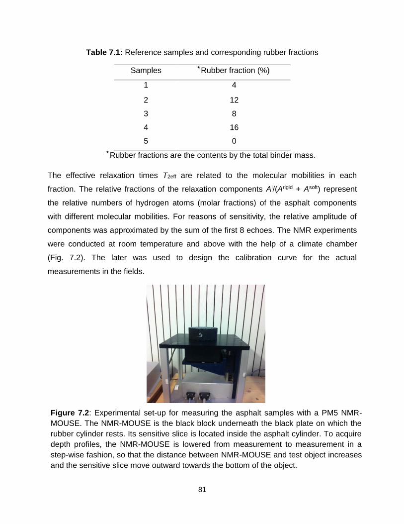
81

Figure 7.2: Experimental set-up for measuring the asphalt samples with a PM5 NMR-

MOUSE. The NMR-MOUSE is the black block underneath the black plate on which the

rubber cylinder rests. Its sensitive slice is located inside the asphalt cylinder. To acquire

depth profiles, the NMR-MOUSE is lowered from measurement to measurement in a

step-wise fashion, so that the distance between NMR-MOUSE and test object increases

and the sensitive slice move outward towards the bottom of the object.

Table 7.1: Reference samples and corresponding rubber fractions

Samples Rubber fraction (%)

1 4

2 12

3 8

4 16

5 0

Rubber fractions are the contents by the total binder mass.

The effective relaxation times T2eff are related to the molecular mobilities in each

fraction. The relative fractions of the relaxation components Ai/(Arigid + Asoft) represent

the relative numbers of hydrogen atoms (molar fractions) of the asphalt components

with different molecular mobilities. For reasons of sensitivity, the relative amplitude of

components was approximated by the sum of the first 8 echoes. The NMR experiments

were conducted at room temperature and above with the help of a climate chamber

(Fig. 7.2). The later was used to design the calibration curve for the actual

measurements in the fields.

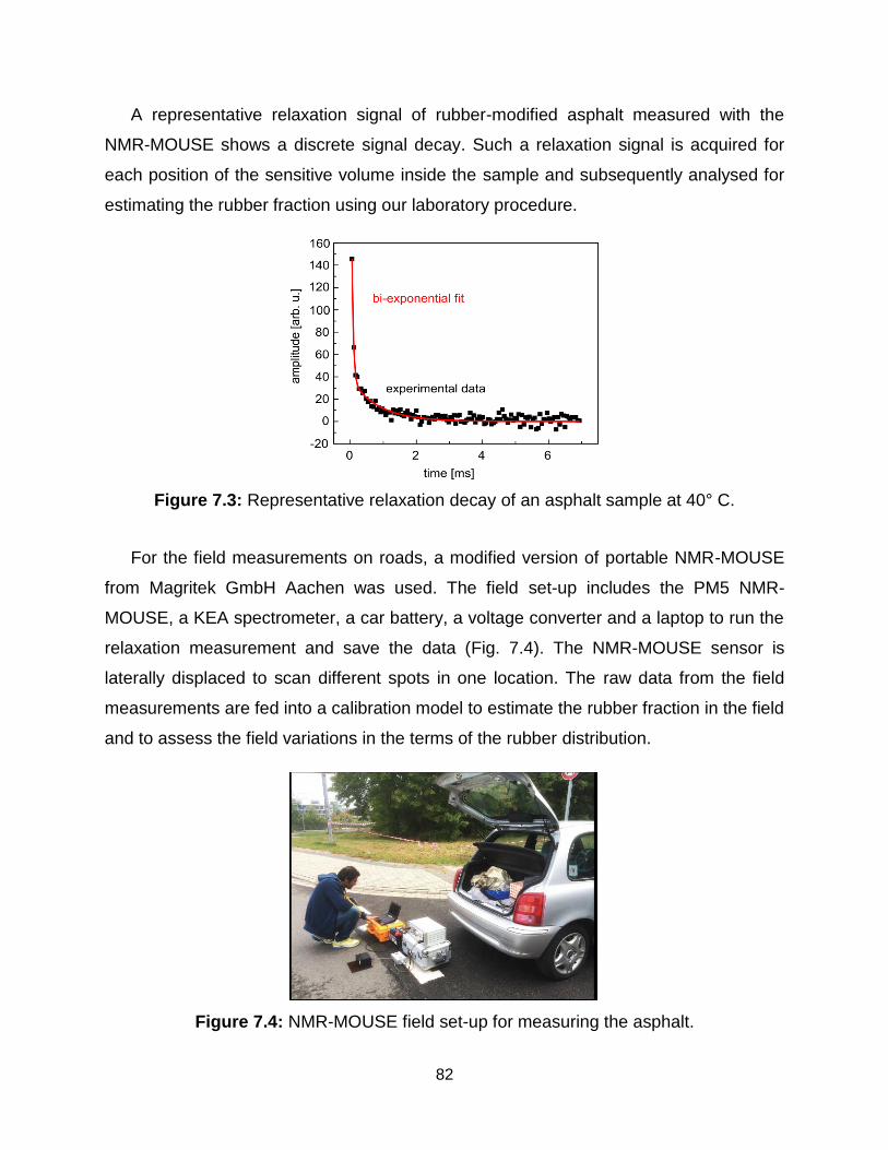
82

A representative relaxation signal of rubber-modified asphalt measured with the

NMR-MOUSE shows a discrete signal decay. Such a relaxation signal is acquired for

each position of the sensitive volume inside the sample and subsequently analysed for

estimating the rubber fraction using our laboratory procedure.

Figure 7.3: Representative relaxation decay of an asphalt sample at 40° C.

For the field measurements on roads, a modified version of portable NMR-MOUSE

from Magritek GmbH Aachen was used. The field set-up includes the PM5 NMR-

MOUSE, a KEA spectrometer, a car battery, a voltage converter and a laptop to run the

relaxation measurement and save the data (Fig. 7.4). The NMR-MOUSE sensor is

laterally displaced to scan different spots in one location. The raw data from the field

measurements are fed into a calibration model to estimate the rubber fraction in the field

and to assess the field variations in the terms of the rubber distribution.

Figure 7.4: NMR-MOUSE field set-up for measuring the asphalt.

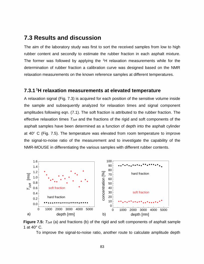
83

Figure 7.5: T2eff (a) and fractions (b) of the rigid and soft components of asphalt sample

1 at 40° C.

0 1000 2000 3000 4000 5000

0

10

20

30

40

50

60

70

80

90

100

co

nce

ntr

atio

n [

%]

depth [mm]

soft fraction

hard fraction

0 1000 2000 3000 4000 5000

0.0

0.2

0.4

0.6

0.8

1.0

1.2

1.4

1.6

T2

eff

[m

s]

depth [mm]

soft fraction

hard fraction

a) b)


The aim of the laboratory study was first to sort the received samples from low to high

rubber content and secondly to estimate the rubber fraction in each asphalt mixture.

The former was followed by applying the 1H relaxation measurements while for the

determination of rubber fraction a calibration curve was designed based on the NMR

relaxation measurements on the known reference samples at different temperatures.

7.3.1 1H relaxation measurements at elevated temperature

A relaxation signal (Fig. 7.3) is acquired for each position of the sensitive volume inside

the sample and subsequently analyzed for relaxation times and signal component

amplitudes following eqn. (7.1). The soft fraction is attributed to the rubber fraction. The

effective relaxation times T2eff and the fractions of the rigid and soft components of the

asphalt samples have been determined as a function of depth into the asphalt cylinder

at 40 C (Fig. 7.5). The temperature was elevated from room temperature to improve

the signal-to-noise ratio of the measurement and to investigate the capability of the

NMR-MOUSE in differentiating the various samples with different rubber contents.

To improve the signal-to-noise ratio, another route to calculate amplitude depth

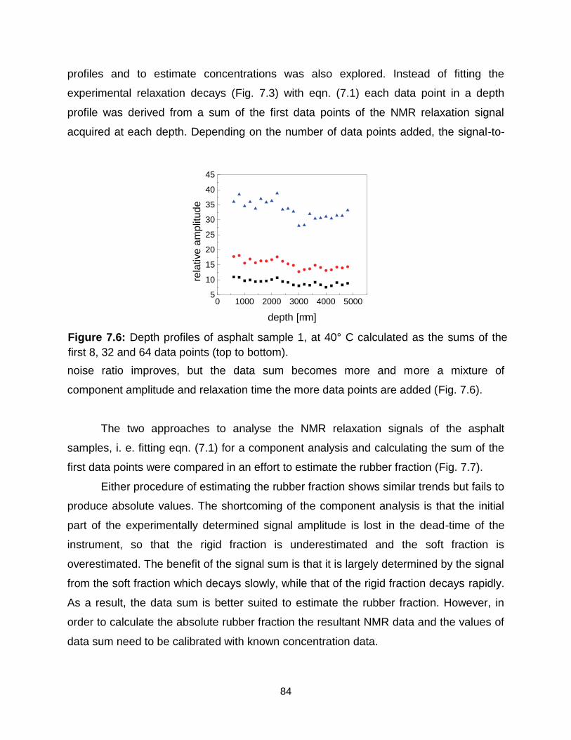
84

Figure 7.6: Depth profiles of asphalt sample 1, at 40° C calculated as the sums of the

first 8, 32 and 64 data points (top to bottom).

0 1000 2000 3000 4000 50005

10

15

20

25

30

35

40

45

rela

tive

am

plit

ud

e

depth [mm]

profiles and to estimate concentrations was also explored. Instead of fitting the

experimental relaxation decays (Fig. 7.3) with eqn. (7.1) each data point in a depth

profile was derived from a sum of the first data points of the NMR relaxation signal

acquired at each depth. Depending on the number of data points added, the signal-to-

noise ratio improves, but the data sum becomes more and more a mixture of

component amplitude and relaxation time the more data points are added (Fig. 7.6).

The two approaches to analyse the NMR relaxation signals of the asphalt

samples, i. e. fitting eqn. (7.1) for a component analysis and calculating the sum of the

first data points were compared in an effort to estimate the rubber fraction (Fig. 7.7).

Either procedure of estimating the rubber fraction shows similar trends but fails to

produce absolute values. The shortcoming of the component analysis is that the initial

part of the experimentally determined signal amplitude is lost in the dead-time of the

instrument, so that the rigid fraction is underestimated and the soft fraction is

overestimated. The benefit of the signal sum is that it is largely determined by the signal

from the soft fraction which decays slowly, while that of the rigid fraction decays rapidly.

As a result, the data sum is better suited to estimate the rubber fraction. However, in

order to calculate the absolute rubber fraction the resultant NMR data and the values of

data sum need to be calibrated with known concentration data.

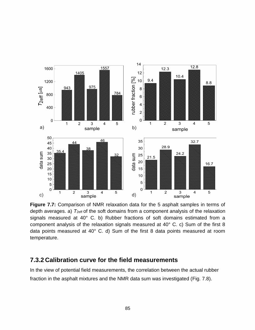
85

Figure 7.7: Comparison of NMR relaxation data for the 5 asphalt samples in terms of

depth averages. a) T2eff of the soft domains from a component analysis of the relaxation

signals measured at 40° C. b) Rubber fractions of soft domains estimated from a

component analysis of the relaxation signals measured at 40° C. c) Sum of the first 8

data points measured at 40° C. d) Sum of the first 8 data points measured at room

temperature.

7.3.2 Calibration curve for the field measurements

In the view of potential field measurements, the correlation between the actual rubber

fraction in the asphalt mixtures and the NMR data sum was investigated (Fig. 7.8).

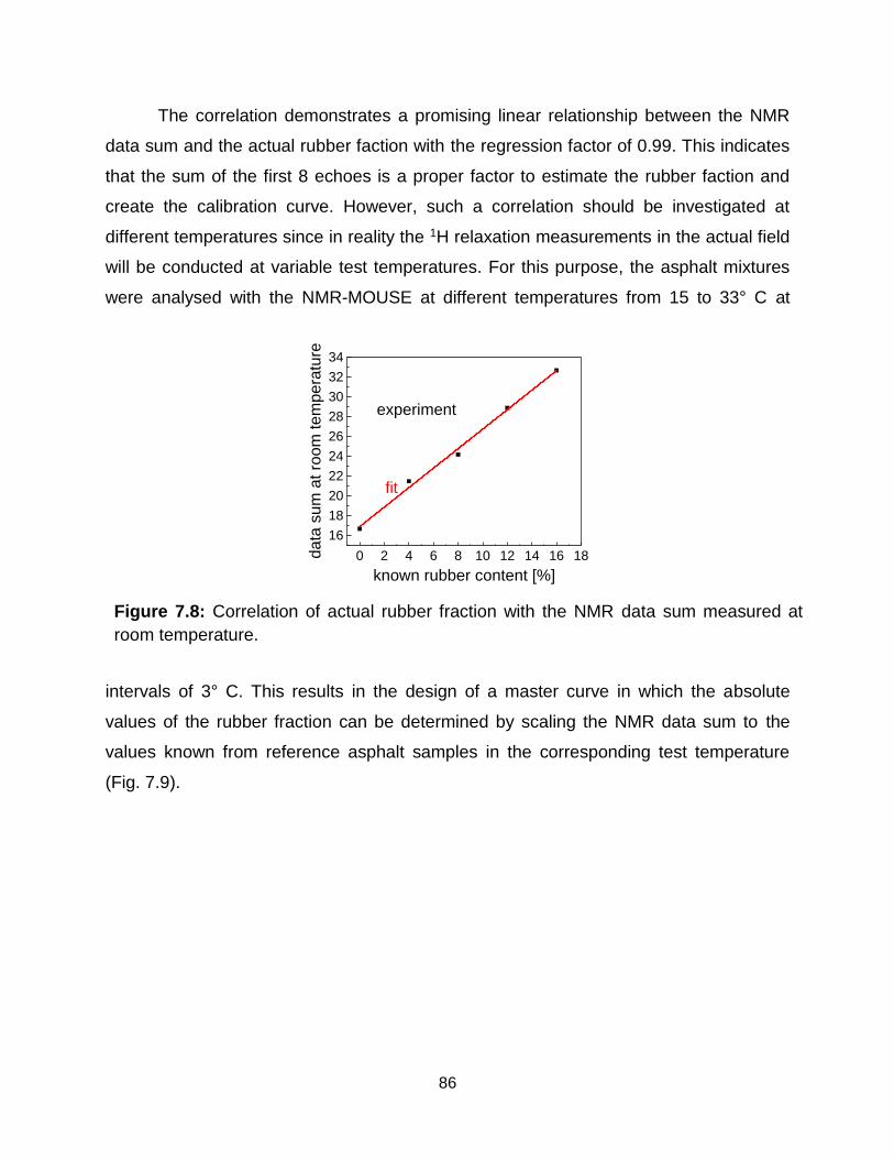
86

Figure 7.8: Correlation of actual rubber fraction with the NMR data sum measured at

room temperature.

0 2 4 6 8 10 12 14 16 18

16

18

20

22

24

26

28

30

32

34

data

sum

at ro

om

tem

pera

ture

known rubber content [%]

fit

experiment

The correlation demonstrates a promising linear relationship between the NMR

data sum and the actual rubber faction with the regression factor of 0.99. This indicates

that the sum of the first 8 echoes is a proper factor to estimate the rubber faction and

create the calibration curve. However, such a correlation should be investigated at

different temperatures since in reality the 1H relaxation measurements in the actual field

will be conducted at variable test temperatures. For this purpose, the asphalt mixtures

were analysed with the NMR-MOUSE at different temperatures from 15 to 33° C at

intervals of 3° C. This results in the design of a master curve in which the absolute

values of the rubber fraction can be determined by scaling the NMR data sum to the

values known from reference asphalt samples in the corresponding test temperature

(Fig. 7.9).

87

Figure 7.9: Master curve for the determination of the field rubber fractions at different

temperatures for rubber-modified asphalt projects prepared by the dry process.

7.3.3 Field test and the subsequent estimation of rubber fraction

For field measurements in the USA, a modified KEA spectrometer was fitted for use

with the NMR-MOUSE PM5. In particular a suitable duplexer and pre-amplifier were

built for this purpose. We planned to power the NMR set-up from a 12 V rechargeable

car battery (Fig. 7.4). As a result, a 250 W power converter was built to convert the 12 V

from the car battery to 24 Volt for operation of the NMR equipment on the road. The

measuring time for one spot on the road is 20 min. Based on the our calibration study in

the lab, we needed to scan 5 laterally displaced spots in one location at the given depth

of 5 mm of our NMR sensor (NMR-MOUSE PM5). Following this approach with 2048

scans, an NMR measurement takes 2 hours for each location and a total of 8 hours for

4 different locations on each project. Furthermore, to quantify the rubber content from

road measurements and determine the NMR signal at a reference temperature, it is

necessary to know the average test temperature. For this purpose, the test temperature

in each spot was measured using an infrared thermometer before and after the NMR

measurement. The average value was then used as the spot temperature and its

corresponding NMR signal was converted to the signal at the reference temperature

using the temperature coefficient determined from the laboratory temperature calibration

study of the known samples (Fig. 7.9). The signals at different locations were then

averaged and a single value was reported as a data sum for each field at the reference

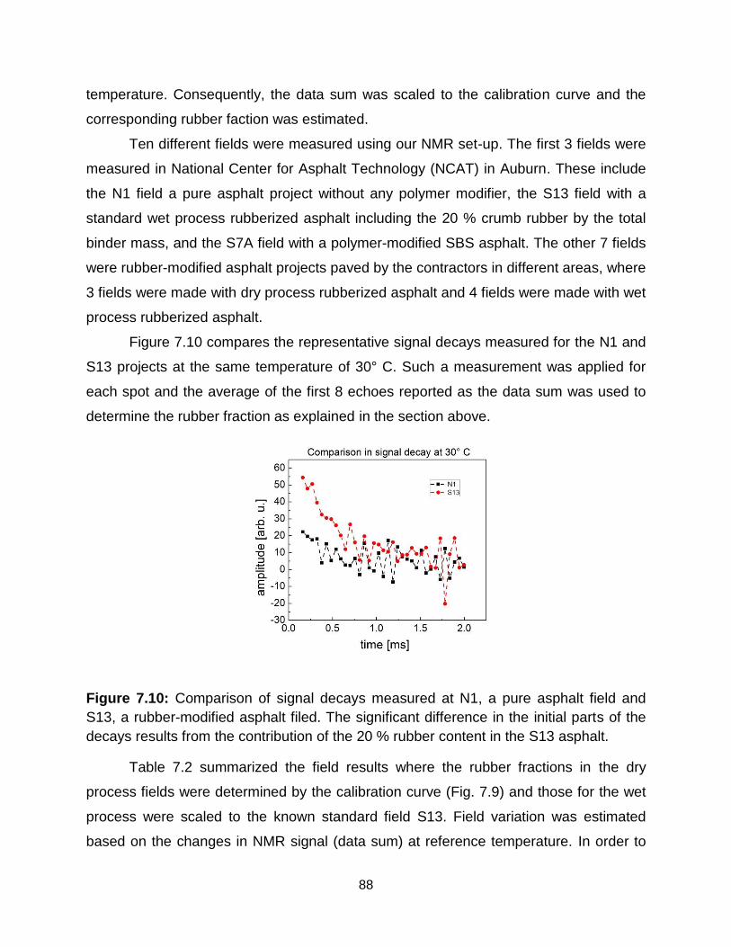
88

temperature. Consequently, the data sum was scaled to the calibration curve and the

corresponding rubber faction was estimated.

Ten different fields were measured using our NMR set-up. The first 3 fields were

measured in National Center for Asphalt Technology (NCAT) in Auburn. These include

the N1 field a pure asphalt project without any polymer modifier, the S13 field with a

standard wet process rubberized asphalt including the 20 % crumb rubber by the total

binder mass, and the S7A field with a polymer-modified SBS asphalt. The other 7 fields

were rubber-modified asphalt projects paved by the contractors in different areas, where

3 fields were made with dry process rubberized asphalt and 4 fields were made with wet

process rubberized asphalt.

Figure 7.10 compares the representative signal decays measured for the N1 and

S13 projects at the same temperature of 30° C. Such a measurement was applied for

each spot and the average of the first 8 echoes reported as the data sum was used to

determine the rubber fraction as explained in the section above.

Figure 7.10: Comparison of signal decays measured at N1, a pure asphalt field and

S13, a rubber-modified asphalt filed. The significant difference in the initial parts of the

decays results from the contribution of the 20 % rubber content in the S13 asphalt.

Table 7.2 summarized the field results where the rubber fractions in the dry

process fields were determined by the calibration curve (Fig. 7.9) and those for the wet

process were scaled to the known standard field S13. Field variation was estimated

based on the changes in NMR signal (data sum) at reference temperature. In order to

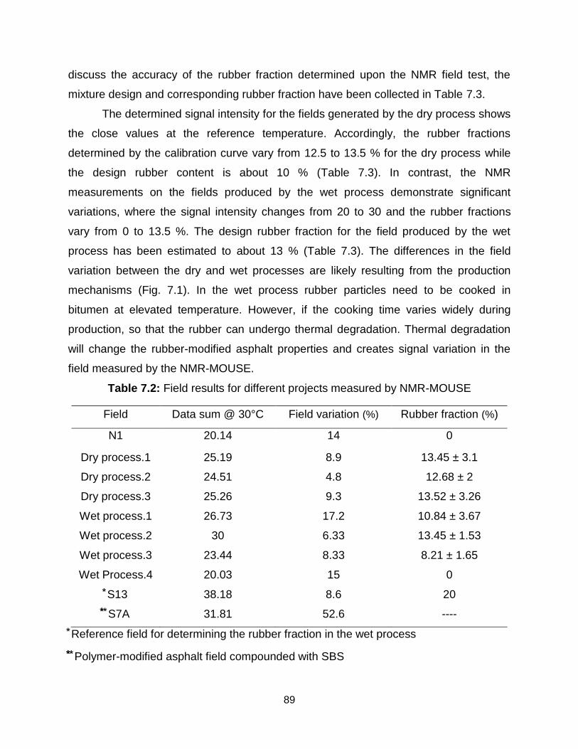
89

discuss the accuracy of the rubber fraction determined upon the NMR field test, the

mixture design and corresponding rubber fraction have been collected in Table 7.3.

The determined signal intensity for the fields generated by the dry process shows

the close values at the reference temperature. Accordingly, the rubber fractions

determined by the calibration curve vary from 12.5 to 13.5 % for the dry process while

the design rubber content is about 10 % (Table 7.3). In contrast, the NMR

measurements on the fields produced by the wet process demonstrate significant

variations, where the signal intensity changes from 20 to 30 and the rubber fractions

vary from 0 to 13.5 %. The design rubber fraction for the field produced by the wet

process has been estimated to about 13 % (Table 7.3). The differences in the field

variation between the dry and wet processes are likely resulting from the production

mechanisms (Fig. 7.1). In the wet process rubber particles need to be cooked in

bitumen at elevated temperature. However, if the cooking time varies widely during

production, so that the rubber can undergo thermal degradation. Thermal degradation

will change the rubber-modified asphalt properties and creates signal variation in the

field measured by the NMR-MOUSE.

Table 7.2: Field results for different projects measured by NMR-MOUSE

Field Data sum @ 30°C Field variation (%) Rubber fraction (%)

N1 20.14 14 0

Dry process.1 25.19 8.9 13.45 ± 3.1

Dry process.2 24.51 4.8 12.68 ± 2

Dry process.3 25.26 9.3 13.52 ± 3.26

Wet process.1 26.73 17.2 10.84 ± 3.67

Wet process.2 30 6.33 13.45 ± 1.53

Wet process.3 23.44 8.33 8.21 ± 1.65

Wet Process.4 20.03 15 0

S13 38.18 8.6 20

S7A 31.81 52.6 ----

Reference field for determining the rubber fraction in the wet process

Polymer-modified asphalt field compounded with SBS

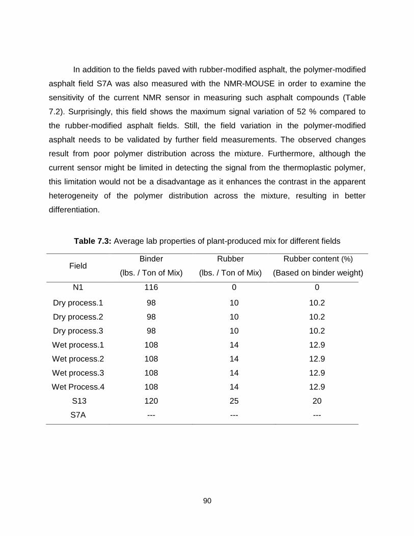
90

In addition to the fields paved with rubber-modified asphalt, the polymer-modified

asphalt field S7A was also measured with the NMR-MOUSE in order to examine the

sensitivity of the current NMR sensor in measuring such asphalt compounds (Table

7.2). Surprisingly, this field shows the maximum signal variation of 52 % compared to

the rubber-modified asphalt fields. Still, the field variation in the polymer-modified

asphalt needs to be validated by further field measurements. The observed changes

result from poor polymer distribution across the mixture. Furthermore, although the

current sensor might be limited in detecting the signal from the thermoplastic polymer,

this limitation would not be a disadvantage as it enhances the contrast in the apparent

heterogeneity of the polymer distribution across the mixture, resulting in better

differentiation.

Table 7.3: Average lab properties of plant-produced mix for different fields

Field Binder

(lbs. / Ton of Mix)

Rubber

(lbs. / Ton of Mix)

Rubber content (%)

(Based on binder weight)

N1 116 0 0

Dry process.1 98 10 10.2



Wet process.1 108 14 12.9



Wet Process.4 108 14 12.9

S13 120 25 20

S7A --- --- ---

91

7.4 Conclusions

The sensitivity of the NMR-MOUSE PM5 was shown to be good enough to determine

the relative amplitude of the soft fraction of asphalt samples at room temperature. It

demonstrated that the sum of the first 8 data points is a valid measure of the soft

fraction in rubber-modified asphalt. However, a laboratory calibration procedure needs

to be done in order to estimate the rubber fraction at room temperature. A calibration

curve was investigated at room temperature, which expresses the correlation between

the rubber fraction of known reference samples and the sum of the first data points of

the NMR relaxation signal from the asphalt samples. However, such a calibration curve

needs to be investigated at different temperature since in reality the 1H relaxation

measurements in the field will be conducted at variable test temperatures. This results

in the design of a master curve in which the absolute values of the rubber fraction can

be determined by scaling the NMR data sum to the values known from reference

asphalt samples at the corresponding test temperature. For the actual field test in the

USA a modified version of NMR-MOUSE was used (Fig. 7.4). The different asphalt

fields paved with different formulations were measured using our NMR set-up. In

general, the rubber-modified asphalt produced by the dry process showed less variation

in the NMR signal intensity and the subsequent rubber fractions as compared to those

produced by the wet process. However, in order to validate the current methodology

also for polymer-modified asphalt more proper fields need to be studied.

92

Chapter 8

8 Summary

Magnetic resonance is well known in the fields of chemical analysis and medical

imaging, where typical instruments use superconducting magnets that generate high

magnetic fields. However, the development of high-field NMR is limited by the cost and



sufficient sensitivity and robustness for non-destructive characterization in applications

outdoors and on the factory floor. Among the different applications in material science

and chemical engineering, compact NMR machines promise novel applications for

polymer industries where the quality of raw and intermediate product needs to be

monitored during production in the chemical plants and after production during use of

the product in the field. While other experimental methods such as DSC, XRD, FTIR,

and SEC have been extensively used to study semi-crystalline polymers, the

implementation of compact NMR approved by standard methods can give rise to non-

destructive investigations of polyethylene in the term of thermal and swelling-induced

aging, studies of the PE wax content, and analysis of gradient polyesters. Furthermore,

the NMR-MOUSE showed a promising application in rubber-modified asphalt fields

where the rubber fraction and field variation in term of the rubber distribution can be

non-destructively studied.

In Chapter three, thermal aging of PE was investigated and the morphological

changes observed by NMR were correlated with FTIR and SEC results. It was

confirmed that aging temperature, annealing time and wax content will affect the aging

process to different extend. Thermally-induced crystallization is observed upon

increasing the temperature towards the melting point due to enhanced diffusion of

polymer chains. Moreover, in the presence of oxygen polymers degrade reactively,

which subsequently impacts the crystallization mechanism during physical aging.

Chemical aging is a dominant process upon aging samples at higher temperature for

93

longer time. Furthermore, our study proved that the wax content can accelerate the

aging process due to the higher chain mobility induced by low molecular weight chains.

NMR data have proven the multi-stage degradation mechanism of polyethylene upon

thermal aging. This was in good agreement with FTIR and SEC results which

respectively investigated the changes in the carbonyl index and molecular weight of the

aged samples.

In the fourth and fifth chapters, solvent-induced crystallization and wax content in

polyethylene were investigated. Compact NMR in combination with high-field NMR

spectroscopy and DSC were used to study the effects of the solvent, swelling time, and

swelling temperature on the chain dynamics and phase composition of LDPE. Upon

increasing the swelling time, the chain dynamics of the soft domains decreased and the

fraction of rigid domains increased, equivalent to solvent-induced crystallization. The

chain rearrangement favorable for the crystallization process concerns to the polymer

chain mobility enhanced by the swelling and the melting of small crystallites in the

presence of a solvent. Furthermore, it is well-known that the solvent type and the

degree of polymer-solvent interaction have an important role in solvent-induced

crystallization. Our study showed that the higher the diffusion coefficient is, the faster

the solvent-induced crystallization, while the mismatch in solubility parameter seemed to

have little impact. In addition to this, short chain branching can accelerate the solvent-

induced crystallization which is due to higher diffusion rate of the solvent between the

polymer chains induced by a higher fractional free volume. Chapter 5 addressed the

determination of the wax content in different PE grades. The wax content was derived

by the standard addition method coupled with detection by compact NMR spectroscopy

and relaxometry. The wax content identified by NMR spectroscopy showed good

agreement with gravimetry for LDPE, but considerable differences for HDPE and

LLDPE. This was hypothesized to be due to the presence of fine particles embedding

catalyst in HDPE and LLDPE. In addition to this, compact NMR data showed that NMR

spectroscopy is a more precise method than relaxometry. The later appears to result

from differences in the detection deadtime applied in both techniques.

Using the profile NMR-MOUSE and 13C CPMAS spectroscopy, the NMR

crystallinity fraction and PET/PBT ratio in different depths were estimated for polyester

94

blend sheets. For samples without glass fiber, the rigid fraction increased towards the

middle of the plate which is due to a lower cooling rate towards the interior. However,

the addition of the GF resulted to a uniform morphology due to the lower temperature

gradient through the samples upon increasing the compound’s thermal conductivity.

Furthermore, the chain mobility of the soft domain for the blend sample without GF

showed a maximum in the middle of the samples. This can be explained with an

accelerated transesterification mechanism towards the middle of the plate induced by

the production and cooling processes. A particular NMR methodology employing the

profile NMR-MOUSE was used to estimate the GF distribution across the sample. The

results showed a better distribution of glass fiber in the middle rather than the surfaces

of the sample. Applying the line-shape deconvolution of the 13C spectra, PET/PBT ratio

was investigated. It was confirmed that the blend samples behaved as a gradient

polymer where the PBT content was dominant across the sample. Besides these, the

spin diffusivities and domain size of the different morphological fractions were

determined by spin-diffusion measurements. The spin-diffusivities of the amorphous

domains were lower for samples with GF, which might be related to a significant

reduction in the chain mobilities due to the presence of GF. Moreover, the average

domain size was higher for the crystalline domains and lower for the amorphous

domains of the sample with glass fiber which might result from the reduced chain

mobility of the amorphous phase in the vicinity of the GF.

The determination of the rubber fraction in rubber-modified asphalt (RMA) in a

non-destructive fashion is of great interest for asphalt industries. Thus in chapter 7, the

rubber content in RMA was investigated using the NMR-MOUSE. It was proved that the

sum of the first data points in the relaxation signal decay and its correlation with the

rubber fractions of the known reference samples is a valid procedure to estimate the

absolute value of the rubber content. For estimating the rubber fraction in actual field

measurements a comprehensive master curve was created in the laboratory. The raw

data from the field measurements were fed into a calibration model to estimate the

rubber fraction and to assess the field variations in the terms of the rubber distribution.

Different types of rubber-modified asphalts were measured using our NMR field set-up.

As a result, our NMR field set-up was shown to be a valuable analytical device for

95

quality control of rubber-modified asphalt pavements, whereby the fields produced by

the dry process showed less variation in the NMR signal intensity and the associated

rubber fractions than those produced by the wet process.

Throughout this thesis, a deeper understanding of the polymer morphology and

its chain dynamic were obtained in a non-destructive way when semi-crystalline

polymers are analyzed at conditions relevant to industry. This acclaims a brighter future

for NMR in polymer science where in the close future, the new NMR methodology

employing compact devices can be used to explore solutions to current issues and to

approach novel analytical methods on the factory floor.

96

References

[1] H. Friebolin, J. K. Becconsall, Basic one-and two-dimensional NMR

spectroscopy, VCH Weinheim, 1993.

[2] H. Günther, NMR spectroscopy: basic principles, concepts and applications in

chemistry, 2nd ed., John Wiley & Sons, Chichester, 2013.

[3] A. Adams, B. Blümich, Single-sided NMR of semicrystalline polymers, Macromol.

Symp. 327 (2013) 29-38.

[4] Y. Teymouri, R. Kwamen, B. Blümich, Aging and degradation of LDPE by

compact NMR, Macromol. Mater. Eng. 300 (2015) 1063-1070.

[5] D. I. Hoult, R. Richards, The signal-to-noise ratio of the nuclear magnetic

resonance experiment, J. Magn. Reson. 24 (1976) 71-85.

[6] E. O. Stejskal, J. D. Memory, High Resolution NMR in the Solid State, Oxford

University Press, New York, 1994.

[7] J. W. Hennel, J. Klinowski, Kinetics of Cross-Polarization in Solid-State NMR: A

Guide for Chemists, Chem. Rev. 102 (2002) 613-628.

[8] C. Hedesiu, D. E. Demco, R. Kleppinger, G. V. Poel, K. Remerie, V. M. Litvinov,

B. Blümich, R. Steenbakkers, Aging effects on the phase composition and chain

mobility of isotactic Poly(propylene), Macromol. Mater. Eng. 293 (2008) 847-858.

[9] F. Casanova, J. Perlo, B. Blümich, Single-sided NMR, Springer, Heidelberg,

2011.

[10] J. Kolz, N. Goga, F. Casanova, T. Mang, B. Blümich, Spatial localization with

single-sided NMR sensors, appl. Magn. Reson. 32 (2007) 171-184.

[11] G. Zimmer, A. Guthausen, B. Blümich, Characterization of technical elastomers

by the NMR-mouse, Solid State Nucl. Magn. Reson. 12 (1998)183–190.

[12] B. Blümich, S. H. Pohlmeier, W. Zia, Compact NMR, De Gruyter, Berlin, 2014.

[13] H. Raich, P. Blümer, Design and construction of a dipolar Halbach array with a

homogeneous field from identical bar-magnets: NMR mandhalas, Magn. Reson.

Eng. 23B (2004) 16-25.

97

[14] S. Anferova, V. Anferova, J. Arnold, E. Talnishnikh, M. A. Voda, K.

Kupferschläger, P. Blümler, C. Clauser, B. Blümich, Improved Halbach sensor for

NMR scanning of drill cores, Magn. Reson. Imaging. 25 (2007) 474-480.

[15] A. Nordon, C. A. McGill, D. Littlejohn, Process NMR spectrometry, Analyst 126

(2001) 260–272.

[16] W. L. Rollwitz, G. A. Persyn, On-stream NMR measurements and control, J. Am.

Oil. Chem. Soc. 48 (1971) 59–66.

[17] R. K. J. Sandor, W. J. Looyestijn, NMR logging-the new measurement, Shell

International Petroleum Maatschappij 1995, The Hague, The Netherlands, 8 p.

[18] G. R. Coates, L. Xiao, and M. G. Prammer, NMR Logging Principles and

Applications, Halliburton Energy Services, Houston, 1999.

[19] J. A. Jackson, L. J. Burnett, J. F. Harmon, Remote (Inside-Out) NMR. III.

Detection of nuclear magnetic-resonance in a remotely produced region of

homogeneous magnetic-field. J. Magn. Reson. 41(1980) 411–421.

[20] G. Eidmann, R. Savelsberg, P. Blümler, B. Blümich, The NMR-MOUSE, a mobile

universal surface explorer, J. Magn. Reson. 122 (1996) 104–109.

[21] B. Blümich B, P. Blümler, G. Eidmann, A. Guthausen, R. Haken, U. Schmitz, K.

Saito, G. Zimmer, The NMR-mouse: construction, excitation, and applications,

Magn. Reson. Imaging. 16 (1998) 479–484.

[22] J. Perlo, F. Casanova, B. Blümich, Profiles with microscopic resolution by single-

sided NMR, J. Magn. Reson. 176 (2005) 64-70.

[23] E. L. Hahn, Spin echoes, Phys. Rev. 80 (1950) 580–594.

[24] E. L. Hahn, Free nuclear induction, Phys. Today. 6 (1953) 65–70.

[25] S. Meiboom, D. Gill, Modified spin-echo method for measuring nuclear relaxation

times, Rev. Sci. Instrum. 29 (1958) 688–691.

[26] C. H. Wang, J. D. Ramshaw, Decay of multiple spin echoes in dipolar solids

Phys. Rev. B. 6 (1972) 3253-3262.

[27] R. V. Vold,J. S. Waugh, M. P. Klein, D. E. Phelps, Measurement of spin

relaxation in complex systems, J. Chem. Phys. 48 (1968) 3831–3832.

[28] J. L. Markley, W. j. Horsley, M. P. Klein, Spin-lattice relaxation measurements in

slowly relaxing complex spectra, J. Chem. Phys. 55 (1971) 3604–3605.

http://www.sciencedirect.com/science/article/pii/S0730725X06004176?np=y











98

[29] Günther, H., NMR spectroscopy: basic principles, concepts and applications in

chemistry, 2nd ed., John Wiley & Sons, Chichester, 1998.

[30] C. A. Meriles, D. Sakellariou, H. Heise, A. J. Moule, A. Pines, Approach to high

resolution ex situ NMR spectroscopy, Science 293 (2001) 82–85.

[31] J. Perlo, F. Casanova, B. Blümich, Ex situ NMR in highly homogeneous fields: 1H

spectroscopy, Science 315 (2007) 1110–1112.

[32] Y. Terada, S. Kono, K. Ishizawa, S. Inamura, T. Uchiumi, D. Tamada, K. Kose,

Magnetic field shimming of a permanent magnet using a combination of pieces of

permanent magnets and a single-channel shim coil for skeletal age assessment

of children, J. Magn. Reosn. 230 (2013) 125-133.

[33] Y. Xu, Q. Chen, G. Zhang, X. Yang, Shim coils design for Halbach magnet based

on target field method, App. Magn. Reson. 46 (2015) 823–836.

[34] K. Singh, E. Danieli, B. Blümich, Real time reaction monitoring for acetalization

of p-nitrobenzaldehyde using compact nuclear magnetic resonance

spectroscopy, Anal. Bioanal. Chem. in press.

[35] K. Singh, B. Blümich, Trends. Anal. Chem. 83 (2016) 12-26. [36] K. Singh, B. Blümich, Structure elucidation and counter-ion effect in strychnine

using 1D and 2D compact NMR spectroscopy, J. Magn. Reson. In press.

[37] E. D. Becker, High Resolution NMR: Theory and Chemical Applications,

Academic Press, New York, 1980.

[38] A. H. Fawcett, Polymer spectroscopy, John Wily and Sons, Chichester, 1996.

[39] M. Goldman, L. Shen, Spin-spin relaxation in LaF3. Phys. Rev. 144 (1966) 321.

[40] A. R. Buda, Solid-state NMR for advanced materials characterization, Bibliothek

der RWTH Aachen, (2004).

[41] J. Clauss, K. Schmidt‐Rohr, H. W. Spiess, Determination of domain sizes in

heterogeneous polymers by solid‐state NMR, Acta. Polym. 44 (1993) 1-17.

[42] M. Mehring, K. Schmidt‐Rohr, H. W. Spiess, Multidimensional solid‐state NMR

and polymers, Phys. Chem. 100 (1996) 1091-1091.

[43] A. Benitez, J. J. Sanchez, M. L. Arnal, A. J. Müller, O. Rodriguez, G. Morales,

Abiotic degradation of LDPE and LLDPE formulated with a pro-oxidant additive

Polym. Degrad. Stabil. 98 (2013) 490-501.

99

[44] M. Iijima, G. Strobl, Isothermal crystallization and melting of isotactic

polypropylene analyzed by time- and temperature-dependent small-angle X-ray

scattering experiments, Macromolecules 33 (2000) 5204-5214.

[45] P. Maiti, M. Hikosaka, K. Yamada, A. Toda, F. Gu, Lamellar thickening in

isotactic polypropylene with high tacticity crystallized at high temperature,

Macromolecules 33 (2000) 9069-9075.

[46] A. Alizahedh, S. Sohn, J. Quinn, H. Marand, L. C. Shank, H. D. Iler, Influence of

structural and topological constraints on the crystallization and melting behavior

of polymers: 3. Bisphenol A Polycarbonate, Macromolecules 34 (2001) 4066-

4078.

[47] J. M. G. Cowie, Polymers: chemistry and physics of modern materials, 2nd ed.,

Blackie Academic and Professional, Glasgow, 1991.

[48] E. Zhmayev, D. Cho and Y.L. Joo, Modeling of melt electrospinning for semi-

crystalline polymers, Polymer 51 (2010) 274-290.

[49] J. Paul, E. W. Hansen, J. Roots, Probing the molecular dynamics in XLPE aged

at different temperatures by 1H NMR relaxation time measurements, Polym.

Degrad. Stabil. 97 (2012) 2403-2411.

[50] A. V. Liuch, L. C. Rodrigo, A. R. Greus, Differential Scanning Calorimetry studies

on High- and Low-Density annealed and irradiated Polyethylenes: influence of

aging, J. Appl. Polym. Sci. 89 (2003) 3260-3271.

[51] C. Hedesiu, D. E. Demco, R. Kleppinger, G. V. Poel, K. Remerie, V. M. Litvinov,

B. Blümich, R. Steenbakkers, Aging effects on the phase composition and chain

mobility of isotactic poly(propylene), Macromol. Mater. Eng. 293 (2008) 847-858.

[52] C. Hedesiu, D. E. Demco, R. Kleppinger, G. V. Poel, W. Gijsbers, B. Blümich, K.

Remerie, V. M. Litvinov, Effect of temperature and annealing on the phase

composition, molecular mobility, and the thickness of domains in isotactic

polypropylene studied by proton solid-state NMR, SAXS, and DSC,


[53] A. Maus, C. Hertlein, K. Saalwächter, A robust proton NMR method to investigate

Hard/Soft ratios, crystallinity, and component mobility in polymers, Macromol.

Chem. Phys. 207 (2006) 1150-1158.

100

[54] C. Hertlein, K. Saalwächter, G. Strobl, Low-field NMR studies of polymer

crystallization kinetics: Changes in the melt dynamics, Polymer 47 (2006) 7216-

7221.

[55] C. Hedesiu, D. E. Demco, R. Kleppinger, A. Adams, B. Blümich, K. Remerie, V.

M. Litvinov, The effect of temperature and annealing on the phase composition,

molecular mobility and the thickness of domains in high-density polyethylene,

Polymer 48 (2007) 763-777.

[56] X. Shi, J. Wang, S. Stapf, C. Mattea, W. Li, Y. Yang, Effects of thermo-oxidative

aging on chain mobility, phase composition, and mechanical behavior of high-

density polyethylene, Polym. Eng. Sci. 51 (2011) 2171-2177.

[57] A. Corti, S. Muniyasamy, M. Vitali, S. H. Imam, E. Chiellini, Oxidation and

biodegradation of polyethylene films containing pro-oxidant additives: Synergistic

effects of sunlight exposure, thermal aging and fungal biodegradation, Polym.

Degrad. Stabil. 95 (2010) 1106-1114.

[58] A. Corti, S. Muniyasamy, E. Chiellini, Assessment of the whole environmental

degradation of oxo-biodegradable linear low density polyethylene (LLDPE) films

designed for mulching applications, J. Polym. Environ. 20 (2012) 1007-1018.

[59] D. A. Blackadder, J. S. Keniry, The morphological consequences of annealing

high-density polyethylene in solvents, J. App. Polym. Sci. 16 (1972) 1261-1280.

[60] E. Chiellini, A. Corti, S. D. Antone, Oxo-biodegradable carbon backbone

polymers–Oxidative degradation of polyethylene under accelerated test

conditions, Polym. Degrad. Stabil. 91 (2006) 2739-2747.

[61] J. Pospisil, W. D. Habicher, J. Pilar, S. Nespurek, J. Kuthan, G. O. Piringer,

Discoloration of polymers by phenolic antioxidants, Polym. Degrad. Stabil. 77

(2002) 531-538.

[62] S. Balasubramaniam, S. Maruthamuthu, A. Khare, N. Palanisamy, V. S.

Muralidharan, R. Ragunathan, Influence of thermal oxidation on surface and

thermo-mechanical properties of polyethylene, J. Polym. Res. 18 (2011) 2175-

2185.

[63] E. Chiellini, A. Corti, G. Swift, Biodegradation of thermally-oxidized, fragmented

low-density polyethylenes, Polym. Degrad. Stabil. 81 (2003) 341-351.

101

[64] L. Guadagno, C. Naddeo, V. Vittoria, G. Camino, C. Cagnani, Chemical and

morphologial modifications of irradiated linear low density polyethylene (LLDPE),

Polym. Degrad. Stabil. 72 (2001) 175-183.

[65] P. K. Roy, P. Surekha, C. Rajagopal, S. N. Chatterjee, V. Choudhary, Studies on

the photo-oxidative degradation of LDPE films in the presence of oxidized

polyethylene, Polym. Degrad. Stabil. 92 (2007) 1151-1160.

[66] T. Ojeda, A. Freitas, K. Birck, E. Dalmolin, R. Jacques, F. Bento, F. Camargo,

Degradability of linear polyolefins under natural weathering, Polym. Degrad.

Stabil. 96 (2011) 703-707.

[67] J. Gao, L. Duan, G. Yang, Q. Zhang, M. Yang, Q. Fu, Manipulating poly(lactic

acid) surface morphology by solvent-induced crystallization, Appl. Surf. Sci. 261

(2012) 528-535.

[68] V. Vittoria, Solvent-induced crystallization of isotactic polypropylene in

cyclohexane at different temperatures, Polymer 32 (1991) 856-859.

[69] V. Vittoria, F. Riva, Solvent-induced crystallization of quenched isotactic

polypropylene in different liquids, Macromolecules 19 (1986) 1975-1979.

[70] V. Vittoria, R. H. Olley, D. C. Bassett, Structural changes in solvent-induced

crystallization of quenched isotactic polypropylene, Colloid. Polym. Sci. 267

(1989) 661-667.

[71] A. Rozanski, A. Galeski, Plastic yielding of semicrystalline polymers affected by

amorphous phase, Intern. J. Plast. 41 (2013) 14–29.

[72] C. J. Wolf, M. A. Grayson, Solubility, diffusion and swelling of fluids in

thermoplastic resin systems, Polymer 34 (1993) 746-751.

[73] M. Hedenqvist, A. Angelstok, L. Edsberg, P. T. Larsson, U. V. Gedde, Diffusion

of small-molecule penetrants in polyethylene: free volume and morphology,

Polymer 37 (1996) 2887-2902.

[74] A. Mattozzi, B. Neway, M. S. Hedenqvist, U. W. Gedde, Morphological

interpretation of n-hexane diffusion in polyethylene, Polymer 46 (2005) 929-938.

[75] G. Fleischer, P. Holstein, Selbstdiffusion von Alkanen in Polyethylen niederer

Dichte–Einfluß des Polyethylentyps und der Diffusantgröße, Acta. polymerica. 35

(1984) 738-744.

102

[76] G. Hunter, D. M. Lane, S. N. Scrimgeour, P. J. McDonald, C. H. Lloyd,

Measurement of the diffusion of liquids into dental restorative resins by stray-field

nuclear magnetic resonance imaging (STRAFI), Dent. Mater. 19 (2003) 632-638.

[77] M. Saleem, A. F. A. Asfour, D. D. Kee, Diffusion of organic penetrants through

low density polyethylene (LDPE) films: effect of size and shape of the penetrant

molecules, J. App. Polym. Sci. 37 (1989) 617-625.

[78] P. Dole, A. E. Feigenbaum, C. D. L. Cruz, S. Pastorelli, P. Paseiro, T.

Hankemeier, Y. Voulzatis, S. Aucejo, P. Saillard, C. Papaspyrides, Typical

diffusion behaviour in packaging polymers–application to functional barriers,

Food. Addit. Contam. 23 (2006) 202-211.

[79] J. S. Qi, C. Krishnan, J. A. Incavo, V. Jain, W. L. Rueter, Investigation of hexane

diffusion in HDPE particulates for drying applications, Ind. Eng. Chem. Res. 35

(1996) 3422-3430.

[80] G. Karlsson, M. S. Hedenqvist, U. W. Gedde, A new method for determining

solute diffusivity in polymers from data obtained by non-isothermal

thermogravimetry, Thermochim. Acta. 356 (2000) 133-138.

[81] B. Kogarkoa, M. Markelov, Diffusion of n-Hexane in Polyethylenes, Intern. J.

Polymeric. Mater. 41 (1998) 249-262.

[82] R. Kwamen, B. Blümich, A. Adams, Estimation of self-diffusion coefficients of

small penetrants in semicrystalline polymers using single-sided NMR, Macromol.

Rapid. Commun. 33 (2012) 943-947.

[83] G. Fleischer, A pulsed field gradient NMR study of diffusion in semicrystalline

polymers: self-diffusion of alkanes in polyethylenes, Colloid. Polym. Sci. 262

(1984) 919-928.

[84] N. Lützow, A. Tihminlioglu, R. P. Danner, J. L. Duda, A. D. Haan, G. Warnier, J.

M. Zeilinkski, Diffusion of toluene and n-heptane in polyethylenes of different

crystallinity, Polymer 40 (1999) 2797-2803.

[85] R. Makitra, Y. Pyrih, E. Sagladko, A. Turovskiy, G. Ziakov, Generalization of

polymer/organic solvent interaction process by means of linear polyparameter

equations. i. swelling of polyethylene, J. App. Polym. Sci. 81 (2001) 3133-3140.

103

[86] Y. Ye, B. Kim, J. Seog, K. Y. Choi, Transitions of morphological patterns of

crystallizing polycarbonate in thin films, J. App. Polym. Sci. 124 (2012) 560-567.

[87] E. B. Gowd, K. Tashiro, Effect of chain-length of n-alkane on solvent-induced

crystallization and solvent exchange phenomenon in syndiotactic polystyrene,

Polymer 52 (2011) 822-829.

[88] C. I. Wolf, J. A. Bornmann, M. A. Grayson, Absorption of toluene in Poly(aryl-

ether-ether-ketone), J. Polym. Sci. Part B. 30 (1992) 113-126.

[89] C. Luo, X. Han, Y. Gao, H. Liu, Solvent-induced crystallization of PS-b-PEO-b-

PS block copolymer films, J. Macromol. Sci. Part B. 49 (2010) 440-453.

[90] A. Adams, A. Piechatzek, G. Schmitt, G. Siegmund, Single-sided Nuclear

Magnetic Resonance for condition monitoring of cross-linked polyethylene

exposed to aggressive media, Anal. Chim. Acta. 887 (2015) 163-171.

[91] N. Sun, M. Wenzel, A. Adams, Morphology of high-density polyethylene pipes

stored under hydrostatic pressure at elevated temperature, Polymer 55 (2014)

3792-3800.

[92] D. Massiot, F. Fyon, M. Capron, I. King, S. L. Calve, B. Alonso, J. O. Durand, B.

Bujoli, Z. Gan, G. Hoatson, Modelling one- and two-dimensional solid-state NMR

spectra, Magn. Reson. Chem. 40 (2002) 70-76.

[93] V. J. McBrierty, K. J. Packer, Nuclear magnetic resonance in solid polymers,

Cambridge University Press, Cambridge, 2006.

[94] E. A. Cernia, C. Mancini, A. Saini, Thermodynamic interactions of branched

polyethylene in polar and nonpolar systems, J. App. Polym. Sci. 12 (1968) 789-

803

[95] U. W. Gedde, Polymer physics, Chapman & Hall, London, 1995.

[96] N. Fazeli, H. Arabi, S. Bolandi, Effect of branching characteristics of ethylene/1-

butene copolymers on melt flow index, Polym. Test. 25 (2006) 28-33.

[97] J. C. Randall, A review of high resolution liquid 13carbon nuclear magnetic

resonance characterizations of ethylene-based polymers, Macromol. Chem.

Phys. 29 (1989) 201-317.

104

[98] K. Klimke, M. Parkinson, C. Piel, W. Kaminsky, H. W. Spiess, M. Wilhelm,

Optimisation and application of polyolefin branch quantification by melt-state 13C

NMR spectroscopy, Macromol. Chem. Phys. 207 (2006) 382-395.

[99] M. Pollard, k. Klimke, R. Graf, H. W. Spiess, M. Wilhelm, O. Sperber, C. Piel, W.

Kaminsky, Observation of chain branching in polyethylene in the solid state and

melt via 13C NMR spectroscopy and melt NMR relaxation time measurements,


[100] J. B. P. Soares, T. F. L. McKenna, Polyolefin reaction engineering, first edition,

Wiley-VCH Verlag, Weinheim, 2012.

[101] D. Munteanu, F. Toma, Studies of controlled oxidation of low molecular weight

polyethylens, Angew. Makromol. Chem. 216 (1994) 67-85.

[102] A. Alizadeh, T. F. L. McKenna, Condensed mode cooling for ethylene

polymerization: The influence of the heat of sorption, Macromol. Symp. 333

(2013) 233-241.

[103] D. Munteanu, Metal-containing polyethylene waxes, J. Macromol. Sci. Chem. 27

(1990) 1395-1404.

[104] H. M. McNair, Basic gas chromatography, Wiley, New York, 1998.

[105] http://www2.emersonprocess.com/siteadmincenter/PM%20Danalyzer%20Docum

ents/DAN_AN_42-NGC-AN-OG-FUNDAMENTALS.pdf.

[106] F. R. Neto, J. N. Cardoso, A. Pereira, M. C. Z. Fernandes, C. A. Caetano, A. L.

Machado, Application of high temperature high resolution gas chromatography to

paraffinic deposits in petroleum production pipelines, J. High Resolut.

Chromatogr. 17 (1994) 259-263.

[107] J. C. Delrio, R. P. Philip, Nature and geochemistry of high molecular weight

hydrocarbons (above C40) in oils and solid bitumens, J. Org. Geochem. 18 (1992)

541-553.

[108] E. Ozaki, K. Saitoh, N. Suzuki, Gel chomatography of n-alkanes on a

polylstyrene gel with various organic solvents, J. Chromatogr. A 177 (1979) 122-

126.

[109] D. H. Freeman, I. C. Poinescu, Particle porosimetry by inverse gel permeation

chromatography, Anal. Chem. 49 (1977) 1183-1188.

105

[110] D. E. Hillman, Characterization and analysis of waxes by gel permeation

chromatography, Anal. Chem. 43 (1971) 1007-1013.

[111] L. R. Snyder, J. J. Kirkland, Introduction to modern liquid chromatography, 2nd

ed, Wiley-Interscience, New York, 1979.

[112] H. Sunderam, N. Nijayalakshmi, K.P. Srilatha, High performance liquid

chromatography and its role in identification of mycobacteria, NTI Bulletin 45

(2009) 1-4.

[113] F. Settle, Handbook of Instrumental Techniques for Analytical Chemistry,

Prentice Hall, New Jersey, 1997.

[114] D. Mekap, T. Macko, R. Brüll, R. Cong, A. W. deGroot, A. Parrott and W. Yau,

One-step method for separation and identification of n‑alkanes/oligomers in

HDPE using high-temperature high-performance liquid chromatography,


[115] S. K. Bharti, R. Roy, Quantitative 1H NMR spectroscopy, Trends. Analyt. Chem.

35 (2012) 5-26.

[116] K. Singh, B. Blümich, Desktop NMR spectroscopy for quality control of raw

rubber, J. Macromol. Symp. 365 (2016) 191-193.

[117] A. Nordon, C. Meunier, R. H. Carr, P. J. Gemperline, D. Littlejohn, Determination

of the ethylene oxide content of polyether polyols by low-field 1H nuclear magnetic

resonance spectroscopy, Anal. Chimica. Acta. 472 (2002) 133-140.

[118] V. Räntzsch, M. Wilhelm, G. Guthausen, Hyphenated low-field NMR techniques:

combining NMR with NIR, GPC/SEC and rheometry, Magn. Reson. Chem. (2015)

DOI: 10.1002/mrc.4219.

[119] A. Mehta, G. Tembe, P. Parikh, G. Metha, A study of ethylene polymerization

catalyzed by homogenous and silsesquioxane supported titanium (IV) complex,

Polimery 58 (2013) 875-882.

[120] H. Mahdavi, A. Badiei, G. H. Zohuri, A. Rezaee, R. Jamjah, S. Ahmadjo,

Homogeneous polymerization of ethylene using an iron-based metal catalyst

system, J. App. Polym. Sci. 103 (2007) 1517-1522.

[121] M. Bader, A systematic approach to standard addition methods in instrumental

analysis, J. Chem. Educ. 57 (1980) 703-706.

106

[122] Y. Teymouri, A. Adams, B. Blümich, Compact low-field NMR: unmasking

morphological changes from solvent-induced crystallization in polyethylene, Eur.

Polym. J. 80 (2016) 48-57.

[123] T. Xie, K. McAuley, J. C. C. Hsu, D. W. Bacon, Gas phase ethylene

polymerization: production processes, polymer properties, and reactor modeling,

Ind. Eng. Chem. Res. 33 (1994) 449-479.

[124] M. Alizadeh, N. Mostoufi, S. Pourmahdian, R. S. Gharebagh, Modelling of

fluidized bed reactor of ethylene polymerization, Chem. Eng. J. 97 (2004) 27-35.

[125] V. D. Makwana, G. Sivalingam, S. M. Vakil, Catalyst evaluation and scale-up

studies for polyethylene production, Int. J. Chem. Eng. App. 5 (2014) 6-12.

[126] G. Aravinthan, D. Kale, Blends of poly (ethylene terephthalate) and poly

(butylene terephthalate), J. Appl. Polym. Sci. 98 (2005) 75-82.

[127] S. Mishra, B. Deopura, Theoretical predictions of compatibility of poly (ethylene

terephtalate) and poly (butylene terephthalate) blends, Polym. Commun. 26

(1985) 5-7.

[128] F. Wang, X. Meng, X. Xu, B. Wen, Z. Qian, X. Gao, Y. Ding, S. Zhang, M. Yang,

Inhibited transesterification of PET/PBT blends filled with silica nanoparticles

during melt processing, Polym. Degrad. Stabil. 93 (2008) 1397-1404.

[129] M. Kryszewski, Gradient polymers and copolymers, Polym. Advan. Technol. 9

(1998) 244-259.

[130] M. D. Lechner, K. Gehrke, E. H. Nordmeier, U. Guhr, Macromolecular chemistry,

Birkhäuser, Basel, 2009.

[131] S. S. Lee, J. Kim, M. Park, S. Lim, C. R. Choe, Transesterification reaction of the

BaSO4‐filled PBT/poly (ethylene terephthalate) blend, J. Polym. Sci. Pol. Phys. 39

(2001) 2589-2597.

[132] H. Matsuda, T. Asakura, B. Nagasaka, K. Sato, Relationship between sequence

distribution and thermal properties of the transesterification product between poly

(ethylene terephthalate) and poly (butylene terephthalate), Macromolecule 37

(2004) 4651-4657.

[133] A. Kotliar, Interchange reactions involving condensation polymers, J. Polym. Sci.

Macromol. Rev. 16 (1981) 367-395.

107

[134] K. P. C. Vollhardt, N. E. Schore, K. Peter, Organische chemie, John Wiley &

Sons, Weinheim, 2011.

[135] B. Wunderlich, Thermal analysis of polymeric materials, Springer Science &

Business Media, Heidelberg, 2005.

[136] R. Blaine, Thermal applications note polymer heats of fusion, Texas Instruments,

New Castle, 2002.

[137] M. Gomez, M. Cozine, A. Tonelli, High-resolution solid-state carbon-13 NMR

study of the alpha and. beta. crystalline forms of poly (butylene terephthalate).

Macromolecule 21 (1988) 388-392.

[138] W. Gabrielse, H. A. Gaur, F. Feyen, W. Veeman, 13C Solid-state NMR study of

differently processed poly (ethylene terephthalate) yarns, Macromolecule 27

(1994) 5811-5820.

[139] J. Zhu, B. Birgisson, N. Kringos, Polymer modification of bitumen: Advances and

challenges, Eur. Polym. J. 54 (2014) 18-38.

[140] D. H. Timm, R. Powell, J. R. Willis, R. Q. Kluttz, Pavement rehabilitation using

high polymer asphalt mix, 5th Eurasphalt & Eurobitume Congress. 2012, Istanbul.

[141] N. A. Hassan, G. D. Airey, R. P. Jaya, N. Mashros, M. A. Aziz, A review of crumb

rubber modification in dry mixed rubberized asphalt mixtures, Jurnal Teknologi 70

(2014) 127-134.

[142] D. L. Presti, Recycled tire Rubber modified bitumen for road asphalt mixtures: a

literature review, Constr. Build. Mater. 49 (2013) 863-881.

[143] Scarp Tire news, crumb rubber overview, http://scraptirenews.com/crumb.php.

[144] D. Campbell, R. A. Pethrick, J. R. White, Polymer Characterization, 2nd Ed.,

Taylor & Francis, Boca Raton, 2000.

http://scraptirenews.com/crumb.php

108

Acknowledgments

I am deeply grateful to my supervisor, Prof. Bernhard Blümich, who gave me this

opportunity to be a part of his prestigious group. It was a great honor to be a member of

Macromolecular Chemistry group and to work under the guidance of Prof. Blümich. I

was beneficiary from his exclusive supports and have learned how to do scientific

research from the elementary to the advanced level while following industrial

collaborations from the laboratory to the industrial scales.

I sincerely thank to Dr. Alina Adams for the valuable advice, suggestions, and

careful work on the research subjects related to polymer science and solid-state NMR.

I would like to thank Dr. Markus Küppers for all the technical and administrative

support.

I wish to express my warmest thanks to my colleagues and friends, Dr. Rance

Kwamen, Dr. Antonio Marchi Netto, Dr. Ernesto Danieli, Dr. Dirk Oligschläger, Dr.

Markus Raue, Kawarpal Sing, Alexander Görges, and, former and current members of

the Blümich group for the nice working atmosphere. Meanwhile, I need to thank Gerlind

Breuer, Klaus Kupferschläger and Michael Adams for their kind help in technical and

practical matters related to the work.

Last but not least, I would like to thank my wife Noushin for her endless and

constant support and my entire family who encouraged me throughout the years of my

study abroad as well as their support and encouragement during my whole life.

109

Curriculum Vitae

Personal Details Surname: Teymouri

First name: Yadollah

Birth date: 10. 01. 1981

Birth place: Shiraz, Iran

Education 09/2003 Bachelor of Science in Polymer engineering

Amirkabir University of Technology, Tehran, Iran

09/2007 Master of Science in Polymer engineering

Amirkabir University of Technology, Tehran, Iran

15.05.2017 Defense for the Doctoral Degree in Natural Sciences

RWTH Aachen, Germany

Career positions 01/2013 – 04/2017 Research Assistant at the Department of Macromolecular

Chemistry (Prof. B. Blümich), RWTH Aachen

10/2010 – 01/2013 Polymer Scientist at R&D Department of Jam Petrochemical

Company, Assaluyeh, Iran

10/2006 – 10/2010 Senior Process Engineer for production plant (Plant

Supervisor), Jam Petrochemical Company, Assaluyeh, Iran

Selected publication

Y. Teymouri, A. Adams, and B. Blümich, "Compact Low-field NMR: Unmasking Morphological Changes from Solvent-Induced Crystallization in Polyethylene", European Polymer Journal 2016, 80, 48-57.

Y. Teymouri, R. Kwamen, and B. Blümich, "Aging and degradation of LDPE by Compact NMR", Journal of Macromolecular Material and Engineering 2015, 300, 1063-1070.

Y. Teymouri, H. Nazockdast, "The Effect of Process Parameters on Physical and Mechanical Properties of Commercial Low Density Polyethylene/ORG-MMT Nanocomposites", Journal of Material Science 2011, 46, 6642-6647.

Documents

Polymer Analysis by Compact NMR