Embed Size (px)
Citation preview
Predictive Modeling of Organic Pollutant Leaching and
Transport Behavior at the Lysimeter and Field Scales.
Dissertation
zur Erlangung des akademischen Grades Doctor rerum naturalium
vorgelegt der Fakultät Forst-, Geo- und Hydrowissenschaften der Technischen Universität Dresden
von Edward Akwasi Amankwah MSc.
Gutachter:
Prof. Dr. Rudolf Liedl, TU Dresden Prof. Dr. Peter Grathwohl, Eberhard-Karls-Universität Tübingen
Prof. Dr.-Ing. Peter-Wolfgang Gräber, TU Dresden.
Dresden, Mai 2007
Abstract
Soil and groundwater pollution has become a global issue since the advent of
industrialization and mechanized agriculture. Some contaminants such as PAHs may
persist in the subsurface for decades and centuries. In a bid to address these issues,
protection of groundwater must be based on the quantification of potential threats to
pollution at the subsurface which is often inaccessible. Risk assessment of
groundwater pollution may however be strongly supported by applying process-
based simulation models, which turn out to be particularly helpful with regard to long-
term predictions, which cannot be undertaken by experiments. Such reliable
predictions, however, can only be achieved if the used modeling tool is known to be
applicable.
The aim of this work was threefold. First, a source strength function was developed to
describe the leaching behavior of point source organic contaminants and thereby
acting as a time-dependent upper boundary condition for transport models. For
general application of these functions dimensionless numbers known as Damköhler
numbers were used to characterize the reaction of the pollutants with the solid matrix.
Two functions were derived and have been incorporated into an Excel worksheet to
act as a practical aid in the quantification of leaching behavior of organic contaminant
in seepage water prognoses. Second, the process based model tool SMART, which
is well validated for laboratory scale data, was applied to lysimeter scale data from
two research centres, FZJ (Jülich) and GSF (München) for long term predictions.
Results from pure forward model runs show a fairly good correlation with the
measured data. Finally, the derived source term functions in combination with the
SMART model were used to assess groundwater vulnerability beneath a typical
landfill at Kwabenya in Ghana. The predicted breakthrough time after leaking from
the landfill was more than 200 years considering the operational time of the facility
(30 years). Considering contaminant degradation, the landfill would therefore not
cause groundwater pollution under the simulated scenarios and the SMART model
can be used to establish waste acceptance criteria for organic contaminants in the
landfill at Kwabenya.
ii
Zusammenfassung
Seit dem Beginn der Industrialisierung und der mechanisierten Landwirtschaft wurde
die Boden- und Grundwasserverschmutzung zu einem weltweiten Problem. Einige
Schadstoffe wie z. B. PAK können für Jahrzehnte oder Jahrhunderte im Untergrund
bestehen. Um diese Probleme behandeln zu können, muss der Schutz des
Grundwassers basierend auf der Quantifizierung potentieller Gefährdungen des
zumeist unzugänglichen Untergrundes erfolgen. Risikoabschätzungen von
Grundwasserverschmutzungen können jedoch durch die Anwendung prozess-
basierter Simulationsmodelle erheblich unterstützt werden, die sich besonders im
Hinblick auf Langzeitvorhersagen als hilfreich erweisen und nicht experimentell
ermittelbar sind. Derart zuverlässige Vorhersagen können jedoch nur erhalten
werden, wenn das verwendete Modellierwerkzeug als anwendbar bekannt ist.
Das Ziel dieser Arbeit bestand aus drei Teilen. Erstens wurde eine Quellstärke-
funktion entwickelt, die das Ausbreitungsverhalten organischer Schadstoffe aus einer
Punktquelle beschreibt und dadurch als zeitabhängige obere Randbedingung bei
Transportmodellen dienen kann. Im Hinblick auf die allgemeine Anwendbarkeit
dieser Funktion werden als Damköhler-Zahlen bekannte, dimensionslose Zahlen
verwendet, um die Reaktion von Schadstoffen mit Feststoffen zu charakterisieren.
Zwei Funktionen wurden abgeleitet und in ein Excel-Arbeitsblatt eingefügt, das ein
praktisches Hilfsmittel bei der Quantifizierung des Freisetzungsverhaltens
organischer Schadstoffe im Rahmen der Sickerwasserprognose darstellt. Der zweite
Teil dieser Arbeit beinhaltet die Anwendung des prozessbasierten und mittels
Laborexperimenten validierten Modellwerkzeugs SMART für Langzeitprognosen auf
der Lysimeterskala anhand von Daten zweier Forschungszentren, FZJ (Jülich) und
GSF (München). Ergebnisse reiner Vorwärtsmodellierungsläufe zeigten gute
Übereinstimmungen mit den gemessenen Daten. Im dritten Teil wurden die
erhaltenen Quellstärkefunktionen in Kombination mit dem SMART-Modell eingesetzt,
um das Grundwassergefährdungspotential unter einer typischen Deponie in
Kwabenya, Ghana, einzuschätzen. Die vorhergesagten Durchbruchszeiten nach
einer Leckage in der Deponie betragen über 200 Jahre bei einer Betriebszeit von 30
Jahren. Unter Berücksichtigung des Schadstoffabbaus verursacht die Deponie somit
keine Grundwasserverunreinigung im Rahmen der simulierten Szenarien und das
SMART-Modell kann verwendet werden, um Schadstoffgrenzwerte für organische
Schadstoffe in der Deponie in Kwabenya festzulegen.

Acknowledgements
Work for this study has been partly financed by the Bundesministerium für Bildung
und Forschung (BMBF, grant 02WP0198 and IPS04/4P2) and published with the
support of the Institute for Groundwater Management, Technische Universität
Dresden.
I will like to express my profound gratitude to Professor Rudolf Liedl, my supervisor
who has supported this study since the beginning of the journey and has
demonstrated this by his constructive discussions. Many thanks to Professor Peter
Grathwohl and Professor Peter-Wolfgang Gräber for their co-supervisory and review
roles in the research work. Working under my Professors’ supervision has brought
my knowledge of Groundwater Management to levels of understanding far beyond
my expectations. The remarkable leadership of my supervisors has inculcated in me
a sense of professionalism, discipline in team work and friendship.
I am also grateful to the special assistance given to me by Professor Eberle in co-
ordinating and providing data for the “Sickerwasserprognose” project. Special thank
to all other Professors and Friends whom I have worked with in the Institute and who
in various ways have contributed to my evolution as a professional. They contributed
by providing a congenial atmosphere which made this scientific work much
interesting than I anticipated.
Furthermore I am grateful to Mr. Dietze, Mr. De Aguinaga and Mr. Hope for their
assistance in formatting and reading through this manuscript. Finally I am indebted to
all my family members and all well wishers whose timely words of encouragement
have always been a footstool.
iv
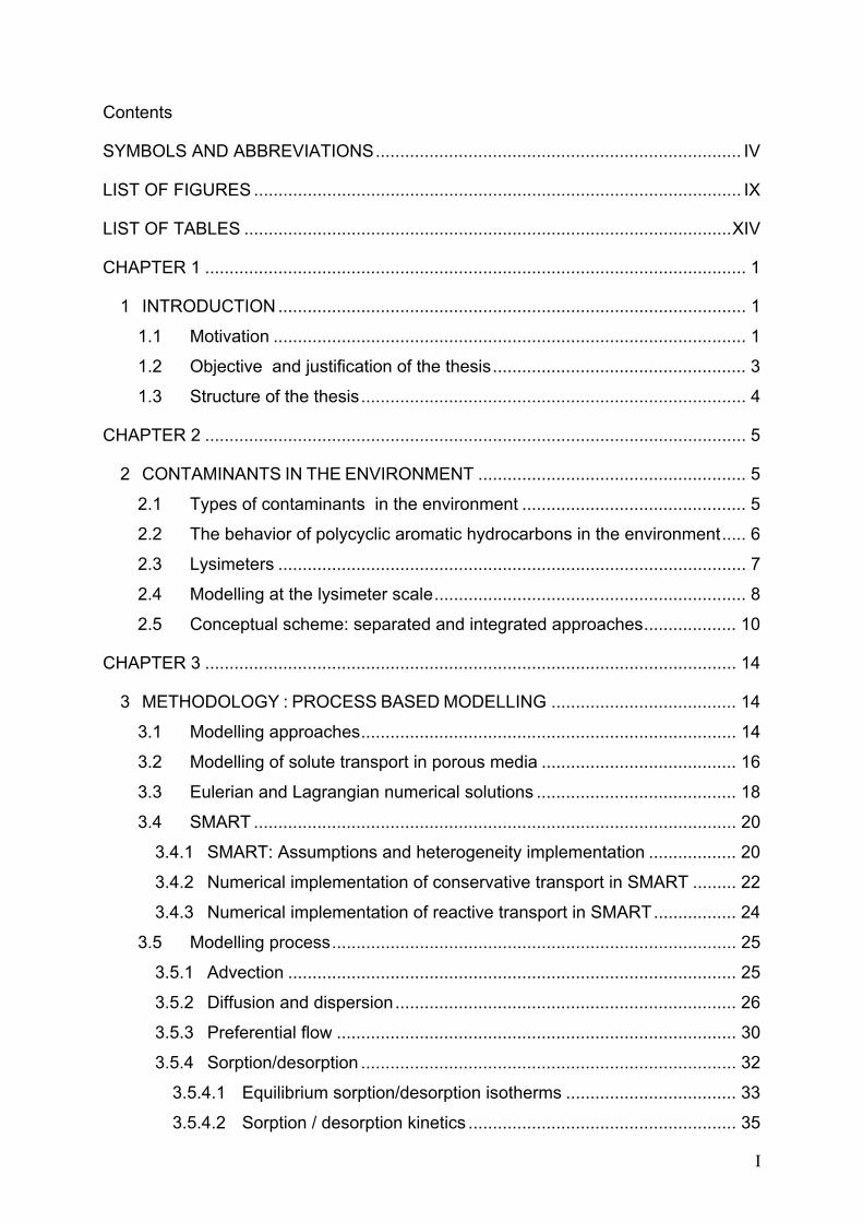
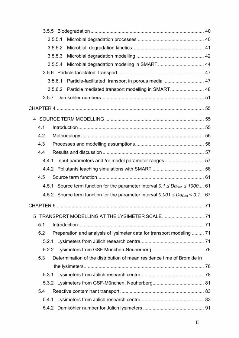
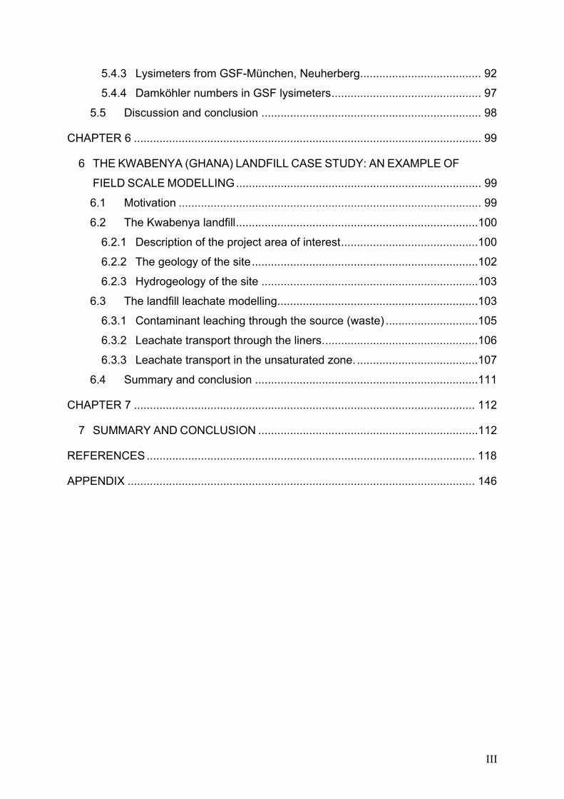
Contents
SYMBOLS AND ABBREVIATIONS........................................................................... IV
LIST OF FIGURES .................................................................................................... IX
LIST OF TABLES ....................................................................................................XIV
CHAPTER 1 ............................................................................................................... 1
1 INTRODUCTION................................................................................................ 1
1.1 Motivation ................................................................................................. 1
1.2 Objective and justification of the thesis.................................................... 3
1.3 Structure of the thesis............................................................................... 4
CHAPTER 2 ............................................................................................................... 5
2 CONTAMINANTS IN THE ENVIRONMENT ....................................................... 5
2.1 Types of contaminants in the environment .............................................. 5
2.2 The behavior of polycyclic aromatic hydrocarbons in the environment..... 6
2.3 Lysimeters ................................................................................................ 7
2.4 Modelling at the lysimeter scale................................................................ 8
2.5 Conceptual scheme: separated and integrated approaches................... 10
CHAPTER 3 ............................................................................................................. 14
3 METHODOLOGY : PROCESS BASED MODELLING ...................................... 14
3.1 Modelling approaches............................................................................. 14
3.2 Modelling of solute transport in porous media ........................................ 16
3.3 Eulerian and Lagrangian numerical solutions ......................................... 18
3.4 SMART ................................................................................................... 20
3.4.1 SMART: Assumptions and heterogeneity implementation .................. 20
3.4.2 Numerical implementation of conservative transport in SMART ......... 22
3.4.3 Numerical implementation of reactive transport in SMART................. 24
3.5 Modelling process................................................................................... 25
3.5.1 Advection ............................................................................................ 25
3.5.2 Diffusion and dispersion...................................................................... 26
3.5.3 Preferential flow .................................................................................. 30
3.5.4 Sorption/desorption ............................................................................. 32
3.5.4.1 Equilibrium sorption/desorption isotherms ................................... 33
3.5.4.2 Sorption / desorption kinetics ....................................................... 35
I
3.5.5 Biodegradation .................................................................................... 40
3.5.5.1 Microbial degradation processes ................................................. 40
3.5.5.2 Microbial degradation kinetics..................................................... 41
3.5.5.3 Microbial degradation modelling .................................................. 42
3.5.5.4 Microbial degradation modeling in SMART.................................. 44
3.5.6 Particle-facilitated transport................................................................ 47
3.5.6.1 Particle-facilitated transport in porous media .............................. 47
3.5.6.2 Particle mediated transport modelling in SMART......................... 48
3.5.7 Damköhler numbers............................................................................ 51
CHAPTER 4 ............................................................................................................. 55
4 SOURCE TERM MODELLING ......................................................................... 55
4.1 Introduction............................................................................................. 55
4.2 Methodology ........................................................................................... 55
4.3 Processes and modelling assumptions................................................... 56
4.4 Results and discussion ........................................................................... 57
4.4.1 Input parameters and /or model parameter ranges ............................. 57
4.4.2 Pollutants leaching simulations with SMART ...................................... 58
4.5 Source term function............................................................................... 61
4.5.1 Source term function for the parameter interval 0.1 ≤ DaDes ≤ 1000.... 61
4.5.2 Source term function for the parameter interval 0.001 ≤ DaDes < 0.1 .. 67
CHAPTER 5 ............................................................................................................. 71
5 TRANSPORT MODELLING AT THE LYSIMETER SCALE............................... 71
5.1 Introduction............................................................................................. 71
5.2 Preparation and analysis of lysimeter data for transport modeling ......... 71
5.2.1 Lysimeters from Jülich research centre............................................... 71
5.2.2 Lysimeters from GSF München-Neuherberg....................................... 76
5.3 Determination of the distribution of mean residence time of Bromide in
the lysimeters......................................................................................... 78
5.3.1 Lysimeters from Jülich research centre............................................... 78
5.3.2 Lysimeters from GSF-München, Neuherberg...................................... 81
5.4 Reactive contaminant transport .............................................................. 83
5.4.1 Lysimeters from Jülich research centre............................................... 83
5.4.2 Damköhler number for Jülich lysimeters ............................................. 91
II
5.4.3 Lysimeters from GSF-München, Neuherberg...................................... 92
5.4.4 Damköhler numbers in GSF lysimeters............................................... 97
5.5 Discussion and conclusion ..................................................................... 98
CHAPTER 6 ............................................................................................................. 99
6 THE KWABENYA (GHANA) LANDFILL CASE STUDY: AN EXAMPLE OF
FIELD SCALE MODELLING............................................................................. 99
6.1 Motivation ............................................................................................... 99
6.2 The Kwabenya landfill............................................................................100
6.2.1 Description of the project area of interest...........................................100
6.2.2 The geology of the site.......................................................................102
6.2.3 Hydrogeology of the site ....................................................................103
6.3 The landfill leachate modelling...............................................................103
6.3.1 Contaminant leaching through the source (waste) .............................105
6.3.2 Leachate transport through the liners.................................................106
6.3.3 Leachate transport in the unsaturated zone. ......................................107
6.4 Summary and conclusion ......................................................................111
CHAPTER 7 ........................................................................................................... 112
7 SUMMARY AND CONCLUSION .....................................................................112
REFERENCES ....................................................................................................... 118
APPENDIX ............................................................................................................. 146
III
SYMBOLS AND ABBREVIATIONS
Symbols
1/nFr Freundlich exponent [-]
A grain size [L]
A cross-sectional area [L2]
B(C) degradation kinetics [ML-3T-1]
c dissolved solute concentration in intraparticle pores...[ML-3 ]
cmax maximum dissolved solute concentration in intraparticle pores [ML-3 ]
C total mobile solute concentration [ML-3]
C0 initial solute concentration [ML-3]
CC mobil particle concentration [ML-3]
CC, o particle input concentration [ML-3]
CD dissolved solute concentration [ML-3]
CD dissolved solute input concentration [ML-3]
CINP tracer in flow concentration [ML-3]
Cl observed tracer concentration [ML-3]
Ceqm equilibrium solute concentration [ML-3]
Csat saturated vapour phase concentration [ML-3]
C∞ total mobile long-term concentration [ML-3]
D dispersion coefficient [L2T-1]
Dp coefficient of molecular diffusion [L2T-1]
D* hydrodynamic dispersion coefficient [L2T-1]
Dmec coefficient of molecular diffusion [L2T-1]
Da Damköhler number [-]
Da,bio Damköhler number for biodegradation [-]
Da1 the ratio of mass transfer rate to advection [-]
Da2 the ratio of biodegradation rate to advection [-]
Da3 the ratio of biodegradation to mass transfer rate [-]
Da,des Damköhler number for desorption [-]
De effective diffusion coefficient [L2T-1]
Dapp apparent diffusion coefficient [L2T-1]
Deff effective diffusion coefficient [L2T-1]
IV
F mass flux into soil grain [ML-2T-1]
Fmax maximum mass flux into soil grain [ML-2T-1]
foc fraction of organic carbon [-]
g(τ) PDF of travel times [T-1]
gmatrix(τ) PDF of travel times in matrix region [T-1]
gpref(τ) PDF of travel times in preferential flow region [T-1]
j diffusive flux [ML2T-1]
kj particle j deposition rate coefficient [T-1]
kLH Langmuir-Hinshelwood parameter [-]
Kf unsaturated hydraulic conductivity [LT-1]
K maximum substrates concentration [T-1]
Ks half saturation constant [ML-3]
Ko kinetic reaction rates [T-1]
koc distribution coefficent standardised on the content of organic carbon
[L3M-1]
Kd partitioning coefficient between contaminant and soil matrix [L3M-1]
Kd,c partitioning coefficient between contaminant and particles [L3M-1]
KFr Freundlich coefficient [(MM-1)(ML-3)-1/nFr]
KL Langmuir sorption coefficient [L3M-1]
KT affinity parameter [-]
l diffusion length [L]
Mdiff contaminant mass within soil grain [M]
Mp mass of particle [M]
Ms solid mass [M]
n degradation order [-]
ne effective porosity [-]
nip intraparticle porosity [-]
p number of particles [-]
Pc particle dry solid density [-]
PV pore volume [-]
r radial coordinate [L]
R retardation factor [-]
RT residence time [T]
Smatrix ratio of sorbed solute mass per unit mass of soil matrix [-]
V
Scm ratio of sorbed solute mass per unit mass of mobile particle [-]
Scim ratio of sorbed solute mass per unit mass of immobile particle [-]
s substrate concentration [ML-3]
Sw degree of saturation [-]
t time [T]
tl observed tracer travel time [T]
T1/2 half life [T]
v pore water velocity [LT-1]
Q Darcy flow [L3T-1]
q specific flux [LT-1]
qs solid phase concentration [ML-3]
M/A solid mass per unit cross sectional area [ML2]
W/F water – solid ratio [L3M-1]
vmatrix flow velocity in matrix region [LT-1]
vpref flow velocity in preferential flow region [LT-1]
x vertical coordinate [L]
Xb biomass concentration [ML-3]
Greek symbols
α volume fraction of preferential flow [-]
α* characteristic mixing length [-]
β contaminant mass ratio not subject to particle-facilitated transport [-]
βT heterogeneity parameter [-]
ε porosity [-]
θ water content [-]
λ degradation rate [T-1]
λ’ modified degradation rate [T-1]
ρ solid density of soil matrix grain [ML-3]
ρb bulk density of soil matrix [ML-3]
ρc solid density of particle [ML-3]
ψ matrix potential [L]
τ travel time of a conservative tracer [T]
τa travel time of a conservative tracer in homogeneous soils [T]
VI
τ mean travel time of a conservative tracer [T]
ζ tortuosity factor [-]
σc volume of the immobile particle per unit volume [-]
Γ(τ,t) reaction function [-]
Abbreviations
AMA Accra Metropolitan Authority
2,4-D 2,4-Dichlorphenoxyacetic
BBA Richtlinie fur die Priifung von Nagetierbekampfungsmitteln gegen
Wanderratten
BBodSchV Bundes-Bodenschutz- und Altlastenverordnung
BESSY Batch Experiment Simulation System
BMBF Bundesministerium für Bildung und Forschung
BMU Federal Ministry for Environment, Nature Conservation and Nuclear
Safety
BTC Breakthrough Curve
DCE Dichlorethylene
CDE Convection-Dispersion Equation
CDE Convection-Dispersion Equation
CLT Convective Lognormal Transfer function model
DDT Dichloro-Diphenyl-Trichloroethane
NAPL Non Aqueous Phase Liquid
DNAPL Dense Non Aqueous Phase Liquid
DND Damköhler number distribution
ETFM Extended Transfer Function Model
FAO Food and Agricultural Organization
FD Finite Difference
GRACOS Groundwater Risk Assessment at Contaminated Sites
GLEAMS Groundwater Loading Effects of Agricultural Management System
GTFM Generalised Transfer Function Model
GWN Groundwater flow rates
IPD Intraparticle diffusion
LEA Local Equilibrium Assumption
VII
MOC Method of Characteristics
PAH Polycyclic Aromatic Hydrocarbons
PCE Perchloroethylene
PDF Probability Density Function
PERMO Pesticide Leaching Model
PFM Piston Flow Model
PRZM Pesticide Root Zone Model
P4 Point of Compliance
PV Pore Volume
RIZA Rijksinstituut voor Integraal Zoetwaterbeheer en Afvalwaterbehandeling
(Institute for Inland Water Management and Waste Water Treatment)
RTD resident time distribution
SMART Streamtube Model for Advective and Reactive Transport
SOM Soil organic matter
TCE Trichloroethylene
TDR Time Domain Reflectometry
TOC Total Organic Carbon
TVD Total Variation Diminishing
VARLEACH Variable Leaching
VOC Volatile Organic Compounds
SVOC Semi Volatile Organic Compounds
VIII
LIST OF FIGURES Fig. 2.1: Scheme of work.......................................................................................... 10
Fig. 2.2: Left, a cross section of a test lysimeter...................................................... 12
Fig. 2.3. A concentration profile showing the source and transport zones of a
landfill ................................................................................................................ 13
Fig. 3.1 modelling approaches.................................................................................. 15
Fig. 3.2: Conceptual illustration of the streamtube model SMART ........................... 21
Fig. 3.3. Equilibrium sorption isotherms.................................................................... 35
Fig. 3.4: Modelling of intraparticle diffusion.............................................................. 37
Fig. 3.5: Microbial growth phases adopted from Adriaens (2003)............................. 42
Fig. 3.6: Plots of microbial growth kinetics adopted from Meckenstock (2002)......... 43
Fig. 4.1: Leaching behaviour of organic pollutants for Damköhler numbers from
the intervals 0.001 ≤ DaDes ≤ 1000 and/or. 0.001 ≤ DaBio ≤ 1000....................... 58
Fig. 4.2: S-shaped curve group type of the leaching behaviour for the case 0.1 ≤
DaDes ≤ 1000. The relative leaching concentration is represented as a
function of dimensionless pore volume time t’ after equation 3.62..................... 59
Fig. 4.3: Left bent curve group type of the leaching behaviour for the case 0.001 ≤
DaDes < 0.1. The relative leaching concentration is represented as a function
of dimensionless pore volume time t’ after equation 3.62. ................................. 60
Fig. 4.4 : Flattened curves of the leaching behaviour for cases 100 ≤ DaBio and
independent of the value of DaDes. The relative leaching concentration is
represented as a function of dimensionless pore volume time t’ after equation
3.62. .................................................................................................................. 61
Fig. 4.5: Comparison of long term source strength functions of equation (4.1)
(broken curves) with the SMART results ( solid curves) for the case DaDes =
1000 with a retardation factor of R = 340. ......................................................... 63
Fig. 4.6: Comparison of long term source strength functions of equation (4.1)
(broken curves) with the SMART results ( solid curves) for the case DaDes =
1000 with a retardation factor of R = 105 .......................................................... 63
Fig. 4.7: Comparison of long term source strength functions of equation (4.1)
(broken curves) with the SMART results ( solid curves) for the case DaDes =
1000 with a retardation factor of R = 32. ........................................................... 64
IX
Fig. 4.8: Comparison of long term source strength functions of equation (4.1)
(broken curves) with the SMART results ( solid curves) for the case DaDes =
1000 with a retardation factor of R = 10. ........................................................... 64
Fig. 4.9: Comparison of long term source strength functions of equation (4.1)
(broken curves) with the SMART results ( solid curves) for the case DaDes = 1
with a retardation factor of R = 340. .................................................................. 65
Fig. 4.10: Comparison of long term source strength functions of equation (4.1)
(broken curves) with the SMART results ( solid curves) for the case DaDes = 1
with a retardation factor of R = 105. .................................................................. 65
Fig. 4.11: Comparison of long term source strength functions of equation (4.1)
(broken curves) with the SMART results ( solid curves) for the case DaDes = 1
with a retardation factor of R = 32. .................................................................... 66
Fig. 4.12: Comparison of long term source strength functions of equation (4.1)
(broken curves) with the SMART results ( solid curves) for the case DaDes = 1
with a retardation factor of R = 10. .................................................................... 66
Fig. 4.13: Comparison of long term source strength functions of equation (4.2)
(broken curves) with the SMART results (coloured solid curves) for the case
DaDes = 0.01 with a retardation factor of R = 340............................................... 68
Fig. 4.14: Comparison of long term source strength functions of equation (4.2)
(broken curves) with the SMART results (coloured solid curves) for the case
DaDes = 0.01 with a retardation factor of R = 150............................................... 69
Fig. 4.15: Comparison of long term source strength functions of equation (4.2)
(broken curves) with the SMART results (coloured solid curves) for the case
DaDes = 0.01 with a retardation factor of R = 32................................................. 69
Fig. 4.16: Comparison of long term source strength functions of equation (4.2)
(broken curves) with the SMART results (coloured solid curves) for the case
DaDes = 0.01 with a retardation factor of R = 10................................................. 70
Fig. 5.1: Schematic longitudinal cross section of lysimeter (adopted and modified
from Pütz et al., 2002). ...................................................................................... 72
Fig. 5.2: Bromide breakthrough at a transport distance of 35 cm from the lysimeter
station Merzenhausen (data from Pütz et al., 2002). ......................................... 78
Fig. 5.3: Comparison of the retention time distribution at a transport distance of 35
cm...................................................................................................................... 79
X
Fig. 5.4: Plausibility check of the SMART results for bromide transport at the
plane of measurement of 35 cm. ....................................................................... 80
Fig. 5.5: Lysimeter at the research centre, Jülich: Retention time distribution
evaluation by bromide transport at the discharge outlet. ................................... 81
Fig. 5.6: Plausibility check of the SMART results for bromide transport at the
Jülich lysimeter discharge outlet........................................................................ 81
Fig. 5.7: Lysimeter from GSF-München Neuherberg: Retention time distribution
evaluation of bromide transport at the discharge outlet. .................................... 82
Fig. 5.8: Lysimeter from GSF-München Neuherberg: Plausibility check of the
SMART results for bromide transport at the lysimeter discharge outlet............. 83
Fig. 5.9: Measured and simulated Phenanthrene breakthrough of the Jülich
lysimeter with contaminated soil as source layer material at a transport
distance of 35 cm under equilibrium (eqm) and non equilibrium conditions
(ipd-small: grain radius 0.0001 cm; ipd-medium: grain radius 0.0013 cm; ipd-
big: grain radius 0.0415 cm). ............................................................................. 84
Fig. 5.10: Measured and simulated Anthracene breakthrough of the Jülich
lysimeter with contaminated soil as source layer material at a transport
distance of 35 cm under equilibrium (eqm) and non equilibrium conditions
(ipd-small: grain radius 0.0001 cm; ipd-medium: grain radius 0.0013 cm; ipd-
big: grain radius 0.0415 cm). ............................................................................. 85
Fig. 5.11: Long term prediction of PAH-breakthrough for Jülich lysimeter with
contaminated soil as source layer material at a transport distance of 35 cm
under non equilibrium conditions (grain radius 0.0013 cm). .............................. 86
Fig. 5.12: Measured and simulated Phenanthrene breakthrough forJülich
lysimeters with demolition waste as source layer material at a transport
distance of 35 cm under equilibrium (eqm) and non equilibrium conditions
(ipd-small: grain radius 0.0001 cm; ipd-medium: grain radius 0.0013 cm; ipd-
big: grain radius 0.0415 cm). ............................................................................. 87
Fig. 5.13: Measured and simulated Anthracene breakthrough for Jülich lysimeter
with demolition waste as source layer material at a transport distance of 35
cm under equilibrium (eqm) and non equilibrium conditions (ipd-small: grain
radius 0.0001 cm; ipd-medium: grain radius 0.0013 cm; ipd-big: grain radius
0.0415 cm). ....................................................................................................... 87
XI
Fig. 5.14: Long term prediction of PAH breakthrough for Jülich lysimeter with
demolition waste as source layer material at a transport distance of 35 cm
under non equilibrium conditions (grain radius 0.0013 cm). .............................. 88
Fig. 5.15: Measured and simulated Phenanthrene breakthrough for Jülich
lysimeters with demolition waste as source layer material at a transport
distance of 100 cm under equilibrium (eqm) and non equilibrium conditions
(ipd-small: grain radius 0.0001 cm; ipd-medium: grain radius 0.0013 cm; ipd-
big: grain radius 0.0415 cm). ............................................................................. 89
Fig. 5.16: Measured and simulated Anthracene breakthrough for Jülich lysimeters
with demolition waste as source layer material at a transport distance of 100
cm under equilibrium (eqm) and non equilibrium conditions (ipd-small: grain
radius 0.0001 cm; ipd-medium: grain radius 0.0013 cm; ipd-big: grain radius
0.0415 cm) ........................................................................................................ 89
Fig. 5.17: Long term prediction of PAH-breakthrough for Jülich lysimeters with
demolition waste as source layer material at a transport distance of 100 cm
under non equilibrium conditions (grain radius 0.0013 cm). .............................. 90
Fig. 5.18: Measured and simulated Naphthalene breakthrough of GSF lysimeters
with contaminated soil as source layer material at a transport distance of 125
cm under equilibrium and non equilibrium conditions (ipd-small: grain radius
0.00315 cm; ipd-medium: grain radius 0.027 cm; ipd-big: grain radius 0.1 cm) 93
Fig. 5.19: Measured and simulated Phenanthene breakthrough of GSF lysimeters
with contaminated soil as source layer material at a transport distance of 125
cm under equilibrium and non equilibrium conditions (ipd-small: grain radius
0.00315 cm; ipd-medium: grain radius 0.027 cm; ipd-big: grain radius 0.1 cm) 93
Fig. 5.20: Measured and simulated Anthracene breakthrough of GSF lysimeters
with contaminated soil as source layer material at a transport distance of 125
cm under equilibrium and non equilibrium conditions (ipd-small: grain radius
0.00315 cm; ipd-medium: grain radius 0.027 cm; ipd-big: grain radius 0.1 cm) 94
Fig. 5.21: Measured and simulated Fluoranthene breakthrough of GSF lysimeters
with contaminated soil as source layer material at a transport distance of 125
cm under equilibrium and non equilibrium conditions (ipd-small: grain radius
0.00315 cm; ipd-medium: grain radius 0.027 cm; ipd-big: grain radius 0.1 cm) 94
Fig. 5.22: Measured and simulated Anthraquinone breakthrough of GSF
lysimeters with contaminated soil as source layer material at a transport
XII
distance of 125 cm under equilibrium and non equilibrium conditions (ipd-
small: grain radius 0.00315 cm; ipd-medium: grain radius 0.027 cm; ipd-big:
grain radius 0.1 cm)........................................................................................... 95
Fig. 5.23: Measured and simulated Pyrene breakthrough of GSF lysimeters with
contaminated soil as source layer material at a transport distance of 125 cm
under equilibrium and non equilibrium conditions (ipd-small: grain radius
0.00315 cm; ipd-medium: grain radius 0.027 cm; ipd-big: grain radius 0.1 cm) 95
Fig. 5.24: Long term prediction of PAH breakthrough for GSF-lysimeters with
contaminated soil as source layer material at a transport distance of 125 cm
under non equilibrium conditions (grain radius 0.027 cm). ................................ 96
Fig. 6.1: The map of Ghana showing the landfill site at Kwabenya. ....................... 101
Fig. 6.2: Schematic diagram of the solid waste landfill scenario at Kwabenya ....... 101
Fig. 6.3: Predicted contaminant concentrations at p1 for a waste layer of 15 m
thickness. ........................................................................................................ 106
Fig. 6.4: Contaminant breakthroughs at the transport distance 1 m (p3 - p4) of the
Kwabenya landfill scenario S1......................................................................... 109
Fig. 6.5: Contaminant breakthroughs at the transport distance 3 m (p2 - p4) of the
Kwabenya landfill scenario S2......................................................................... 110
XIII
LIST OF TABLES Table 4.1: Selection of parameter ranges for the SMART process simulations with
phenanthrene as model pollutant and HMVA BAM as solid material................ 57
Table 4.2: Scenario parameters for very fast desorption leaching behaviour of
phenanthrene. .................................................................................................. 62
Table 4.3: Scenario parameters for slow desorption leaching behaviour of
phenanthrene. .................................................................................................. 67
Table 5.1: Physico-chemical soil parameters for the test site Merzenhausen. Soil
types after AGBoden (1994). All units based on mass of dry matter except
field capacity, (fc), based on saturated soil (adopted from Weihermüller, 2005). 73
Table 5.2: Soil parameters of the test site Merzenhausen: the saturated moisture
content θs as well as van Genuchten parameters n and α were fitted with the
retention curve fit program RETC (van Genuchten et al., 1991). The
saturated hydraulic conductivity Ks was taken from Pütz et al. (2002). The
residual moisture content θr was set to 0 for all fits. ......................................... 73
Table 5.3: Model input parameters for the lysimeters operated at the Jülich
research centre................................................................................................. 75
Table 5.4: Model input parameters for the lysimeters operated at the GSF
München-Neuherberg research centre. ............................................................ 77
Table 5.5: Comparison of the 50 % breakthrough time for the GSF lysimeter with
demolishing waste as source layer material at a transport distance of 100 cm
(grain radius 0.0013 cm)................................................................................... 91
Table 5.6: Sorption Damköhler numbers for FZJ lysimeters at a transport distance
of 100 cm under non equilibrium conditions ..................................................... 91
Table 5.7: Comparison of the 50 % breakthrough time for the GSF lysimeter with
contaminated soil as source layer material at a transport distance of 125 cm
(outlet). ............................................................................................................. 97
Table 5.8: Sorption Damköhler numbers for GSF lysimeters at a transport
distance of 125 cm (outlet) under non equilibrium conditions (grain radius
0.027 cm).......................................................................................................... 97
Table 6.1: Input parameter for the Excel spread sheet evaluation of the source
concentration released at the Kwabenya landfill............................................. 105
Table 6.2: Input parameters of leachate leakage through the landfill liners............ 107
Table 6.3: Transport parameters for the Kwabenya landfill scenarios .................... 108
XIV
Chapter 1 1 INTRODUCTION
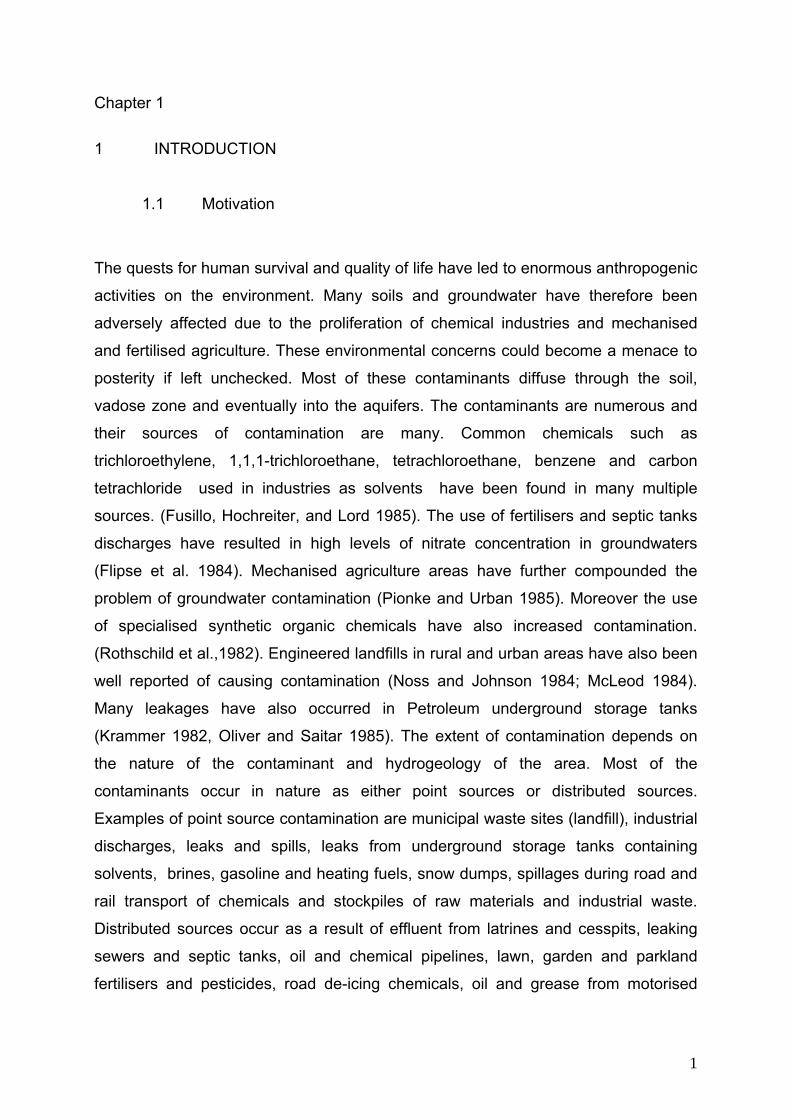
1.1 Motivation
The quests for human survival and quality of life have led to enormous anthropogenic
activities on the environment. Many soils and groundwater have therefore been
adversely affected due to the proliferation of chemical industries and mechanised
and fertilised agriculture. These environmental concerns could become a menace to
posterity if left unchecked. Most of these contaminants diffuse through the soil,
vadose zone and eventually into the aquifers. The contaminants are numerous and
their sources of contamination are many. Common chemicals such as
trichloroethylene, 1,1,1-trichloroethane, tetrachloroethane, benzene and carbon
tetrachloride used in industries as solvents have been found in many multiple
sources. (Fusillo, Hochreiter, and Lord 1985). The use of fertilisers and septic tanks
discharges have resulted in high levels of nitrate concentration in groundwaters
(Flipse et al. 1984). Mechanised agriculture areas have further compounded the
problem of groundwater contamination (Pionke and Urban 1985). Moreover the use
of specialised synthetic organic chemicals have also increased contamination.
(Rothschild et al.,1982). Engineered landfills in rural and urban areas have also been
well reported of causing contamination (Noss and Johnson 1984; McLeod 1984).
Many leakages have also occurred in Petroleum underground storage tanks
(Krammer 1982, Oliver and Saitar 1985). The extent of contamination depends on
the nature of the contaminant and hydrogeology of the area. Most of the
contaminants occur in nature as either point sources or distributed sources.
Examples of point source contamination are municipal waste sites (landfill), industrial
discharges, leaks and spills, leaks from underground storage tanks containing
solvents, brines, gasoline and heating fuels, snow dumps, spillages during road and
rail transport of chemicals and stockpiles of raw materials and industrial waste.
Distributed sources occur as a result of effluent from latrines and cesspits, leaking
sewers and septic tanks, oil and chemical pipelines, lawn, garden and parkland
fertilisers and pesticides, road de-icing chemicals, oil and grease from motorised
1
vehicles, wet and dry deposition from smoke stacks and fill material containing
construction waste.
In a bid to address these concerns, the problem of groundwater contamination must
be addressed holistically. The United Nations in its report for sustainable
development pointed out the accelerated degradation of groundwater systems
through pollution of aquifers, the economic implications of not balancing groundwater
demand and supply management and the lack of public awareness about the
importance of groundwater resource management (International Water and
Sanitation Center, 2003). The European community fifth framework program, Energy,
Environment and Sustainable development called for guidelines for groundwater risk
assessment at contaminated sites (GRACOS research project). The European
Landfill Directive (Council Directive 1999/31EC, 1999) also called for the provision
and protection of the environment, soil and groundwater from the adverse effects of
toxic pollutants. In Germany about 74 % of the source of drinking water is from
groundwater (Federal Ministry for Environment, Nature conservation and Nuclear
safety (BMU) report, January 2006), hence the sustainable use and protection of
groundwater is crucial. The German BMBF issued a research initiative
”Sickerwasserprognose” which involved an extensive research work. The main
objective of this research activity is to propose a method that can reliably predict the
concentration and mass of pollutants at the point of compliance, i.e. at the
groundwater table, in accordance with the German Soil Protection Act (BBodSchV,
1998). One major item of “Sickerwasserprognose” is the model-based prediction of
groundwater pollution. Corresponding tools have to account for all relevant
processes, which are responsible for a decrease (sorption, biodegradation) or an
increase of groundwater pollution risk (particle-facilitated transport, preferential flow).
For organic contaminants, recent studies on these processes and process
interactions have been done, e.g., by (Rahman 2002), (Cata 2003), (Schmidt 2003),
(Bold 2004), (Cai 2004), (Christ 2004), (Henzler 2004), (Madlener 2004), and (Susset
2004). Most of these authors used the modeling software SMART (Streamtube Model
for Advective and Reactive Transport). So far, all SMART applications were limited to
laboratory scale problems, i.e. relying on data which have been obtained under fully
controlled conditions. In this thesis quantification and predictions at the lysimeter
scale are studied for conservative and reactive transport under unsaturated
conditions.
2
1.2 Objective and justification of the thesis
Among the persistent contaminants in the environment are organic pollutants such as
polycyclic hydrocarbon compounds. Quantifying and predicting contamination at the
groundwater table is therefore necessary to assess the potential threats to pollution.
The objectives of the thesis are:
(1) to determine a source strength function for the quantification of the possible
temporally variable discharge behaviour of organic pollutants from point
sources of pollutant,
(2) to quantity the discharge behaviour for proper control and management of
polluted sites, and its associated effects on underground waters,
(3) to simulate the ageing of the source by time dependent modelling which would
eventually aid in developing remediation strategies for the control of the
pollutants,
(4) to determine the temporal change of the pollutant concentration in the
seepage water at the transition from the pollutant source to the transport zone,
(5) to simulate transport and reactive processes by using the source strength
function as a time-dependent upper boundary condition for pollutants
migrating to the ground-water level (point of the compliance),
(6) to quantify the fate of organic pollutants such as Polycyclic Aromatic
Hydrocarbons (PAHs) at the lysimeter scale,
(7) to demonstrate the predictive capabilities of the reactive transport model,
SMART at the lysimeter and field scales,
(8) to predict the longterm contaminant breakthroughs at the outlet (an index of
groundwater table) of lysimeter data from Jülich and GSF-München research
centers,
(9) to predict the fate of PAHs at a field scale landfill at Kwabenya in Ghana.
3
1.3 Structure of the thesis
The primary topic of this thesis is long term process based modelling of organic non-
volatile compounds at the lysimeter scale and the scenario based modelling of the
Kwabenya landfill in Ghana. Chapter 1 gives the problem statement, aims and
justification of the thesis. In chapter 2 the general overview of non-volatile organic
compounds, especially PAHs, is discussed. The application of lysimeters in the
environment and solute transport are also reviewed. Chapter 3 presents the
methodology, description of the important processes triggering the migration of
contaminants in the vadose zone. Some of the existing analytical and numerical
methods are given. Moreover, Damköhler numbers, which are used to quantify the
relative importance of the major source and transport processes, are also discussed.
In addition, the main model SMART, which was used throughout this work is
discussed in detail. Chapters 4 deals with the derivation and identification of source
term functions to describe the leaching behaviour of organic pollutants. Again
Chapter 4 discusses how the contaminant is modelled at the source zone, the use of
regression analysis for the derivation of a source term function which could be used
as a time-dependent upper boundary condition for ensuing pollutants migrating to the
transport zone. Rosen’s analytical solutions which show the proximity of the
numerical solutions are also introduced. Chapter 5 is dedicated to the longterm
modelling of lysimeter data. Chapter 5 also discussed the preparation and analysis of
the input data needed for the transport modelling of the Jülich and München
lysimeters. Uncalibrated forward model results are compared with the observed
lysimeter data in the short term. Based on the relevant processes in the transport
zone, the long term fate of the contaminants at the lysimeter outlets (a representation
of the point of compliance between the saturated and unsaturated zone) is predicted.
Chapter 6 presents the application of the derived source term functions and SMART
to a proposed field scale landfill at Kwabenya, a sub urban town in Ghana. Again
Damkökler numbers are exploited to elucidate the major driven processes. Summary
and conclusions of this thesis are given in Chapter 7.
4
Chapter 2 2 CONTAMINANTS IN THE ENVIRONMENT
2.1 Types of contaminants in the environment
Different types of contaminants occur in groundwater depending on the type of site
and the site activities. The following groups of contaminants may be identified:
1. Halogenated and non halogenated VOCs: They are hydrocarbon compounds
that evaporate readily at room temperature and are usually found at locations
including burn pits, chemical manufacturing plants and disposal areas such as
marine sediments, disposal wells and leach fields, landfills and burial pits,
leaking storage tanks, dry cleaning shops, pesticide and herbicide mixing
areas, solvent degreasing areas, surface impoundments, and vehicle
maintenance areas. Halogenated VOCs have a halogen (fluorine, chlorine,
bromide, iodine) attached to it while non halogenated VOCs are without a
halogen. Examples of such compounds include 1-Chloro-2-propene Carbon
tetrachloride, Hexachlorobutadiene, 1,1-Dichloroethane, Vinyl chloride,
Chloroform, ethanol and vinyl acetate.
2. Halogenated and non halogenated SVOCs: They are semi volatile organic
compound that have boiling points above 200 oC. They are usually found in
sites such as wood preservation sites in addition to the sites stated above.
Examples of these compounds are Benzedrine, benzoic acid, isoprophorone,
anthracene, naphthalene, pyrene and phenanthrene. Pesticides such as
andrin, chlordane, Malathion and DDT form a subgroup of halogenated
SVOCs.
3. Fuels: They are a group of chemicals produced by refining and manufacturing
of petroleum or natural gas to generate heat and energy in combustion
processes. Sites where fuel contamination may be found include aircraft,
storage and service areas, and solvent degreasing areas and in addition to
those locations mentioned above. Most of the non halogenated VOCs and / or
SVOCs are also fuels. Typical fuel contaminants encountered at many sites
5
include creosol, phenol, toluene, fluorine, fluoranthene, naphthalene, propane
and benzene.
4. Metals and metalloids: Metals are usually hard, with high melting point and
electrical conductivity. They heat well while metalloids are usually semi
conductors whose properties are between metals and non metals. They are
usually found at electroplating and metal finishing shops, landfills and burial
pits, paint striping and sand blasting areas. Metals and metalloids
contaminants include mercury, lead, chromium, cadmium, nickel, zinc and
arsenic.
5. Explosives: They are usually chemicals produced as explosive and repellents.
They are usually located in contaminant sites such as marine sediments,
disposal wells, leach fields, landfills and burial pits. Examples are
nitroaromatics, trinitrobenzenes, picrates, nitrocellulose TNT and 2, 4-DNT (2,
4-Dinitrotoluene) Nitroglycerine (EPA Roadmap, 2005).
2.2 The behavior of polycyclic aromatic hydrocarbons in the environment
PAHs in the environment are a large group of compounds with a similar structure
comprising two or more benzene or other aromatic hydrocarbon rings with carbon
and hydrogen atoms only. They are formed through incomplete combustion of carbon
compounds. The unmeticulious use of petroleum and charcoal products leads to the
input of aromatic hydrocarbons into the environment. PAHs vary with respect to
sources, chemical and physical characteristics and are predominantly found in
particulate phase under ambient conditions (UBA, 1998). Concern over PAH
emissions relates to their health effects. With a view to the amount and the size of the
contaminated sites the largest potential risk for groundwater contamination emerges
from coking plants and gas industry. PAH containing tar oils can be DNAPL which
can sink to the bottom of the aquifer. Laboratory experiments have shown that the
desorption of PAH from soils occurs very slowly. At times the adsorption of PAH on
coal particles is very strong. They can form a long term contamination source with
contaminations which could persist for centuries.
6
Aromatic hydrocarbons belong to the most important ground water contaminants with
very slow degradation tendencies leading to the formation of long contaminant
plumes and pollutant transport over long distances. Such processes endanger the
drinking water supply in many areas. Diffuse emissions through combustion of coal or
gasoline cause a widespread pollution of air and soil, especially close to main traffic
roads, and massive punctual contaminations due to spills during transport and at
sites of storage and refinement of petroleum and coal products. When large amounts
of aromatic hydrocarbons enter environments with limited oxygen supply such as
aquifers. This slows down the degradation of aromatic compounds so that long
pollutant plumes are transported in aquifers endangering drinking water supply in
many areas. Other natural sources also exist in the environment. Anaerobic bacteria
produce benzene and toluene during fermentation of aromatic aminoacids (Jüttner
and Henatsch, 1986; Jüttner, 1988; Fischer-Romero et al., 1996). Certain termite
species use naphthalene to fumigate their nests (Chen et al., 1998). Moreover
incomplete combustion of organic materials also produces polynuclear aromatic
hydrocarbons, for instance when forest fires occur (Hirner et al., 2000). However, it
has also been shown that degradation of petroleum products in the subsurface can
lead to alteration of oils which may have ecologic implications (Aitken et al., 2004).
Modelling PAHs could therefore help in formulating risk assessment principles which
can lead to management practices that would ensure the safety of drinking water.
2.3 Lysimeters Lysimeters are field devices containing a soil column and vegetation, used for
measuring actual evapotranspiration. (Fetter, 2005). They may also be defined as
containers with a given soil volume and depth. They are either filled undisturbed or
disturbed, installed plane to the surface and are used to collect seepage water
(drainage/leachate) which is gained by means of different methods at the lysimeter
bottom (Lanthaler, 2004). Depending on functions and characteristics such as the soil
size and fractions, weighability, the soil filling techniques and the vegetation cover,
lysimeters may be grouped according to the following types: weighable and non
weighable lysimeters, monolithic lysimeters, groundwater lysimeters and large
lysimeters. According to (Muller, 1996) the term lysimeter originated from the Greek
words “lusis” meaning solution and “metron” meaning measure. Originally it was
designed to measure soil leaching (Kutilek and Neilsen, 1994) but due to the
7
increase of pollution and groundwater contamination (BAL, 1993) in the last decades,
it has been applied in the field of research studies such as soil hydrology,
hydrogeology, water economy, agriculture and forest economies, ecology and
environmental protection. The FAO applied it to study crop water balance and
evapotranspiration (FAO, 1982). In many European currents lysimeters have been
used for registration of plant protection products and research purposes (Hance and
Führ, 1992). For instance the German pesticide testing guidelines (BBA, 1990) were
established for the registration and regulation of lysimeters in Germany. This has
provided many local authorities and decision makers with a tool for the idenfication of
vulnerable areas where specific monitoring actions and preventive measures for the
protection of water could be studied. Though an ideal lysimeter may not exist (Seeger
et al. in Böhm et al. 2002), lysimeter contribution to the risk assessment of
groundwater is enormous. The concentration measured at the bottom of lysimeters,
filled with one or more soils representative of the local territorial could be used as an
index of risk for groundwater even though contaminant transport may vary between
the field and the lysimeters (Bergström and Jarvis, 1994). Moreover they enable a
close mass balance of contaminants in soils.
2.4 Modelling at the lysimeter scale
Modelling has become an integral part of water management and research in the
field of water science and agric economy. Many models have been developed for
different purposes and scales. In this section the application of models to
contaminant leaching is discussed. Tracer investigation and numerical modelling in
lysimeters on the movement of water and solids from the surface of the soil through
the un-saturated and saturated zones of an aquifer enable to quantitatively predict
the impact of different measures on to the whole subsurface system. Many single
component and multicomponent analytical and numerical models have been
developed to simulate and predict water and leaching behaviour of solutes in the
unsaturated zone and the water table through lysimeters.
The following models though not used in this work are discussed briefly due to their
comparative usage to the model SMART 2200 (Finkel, 1999) that was used:
GLEAMS (Leonard et al., 1987 and Rekolainen et al., 2000b), PELMO 2.02 (Klein et
8
al., 2000), PRZM-2 (Trevisan et al., 2000), VARLEACH (Trevisan et al., 2000),
SIMULAT 2.3 (Aden and Diekkrüger, 2000), MACRO 3.1 and 4.0 (Jarvies et al.,
2000), WAVE (Vanclooster et al., 2000a) and LEACHP (Dust et al., 2000). Details of
the models may be seen in the attached references. All the models were applied as
1-D flow with no horizontal components to lysimeter data sets. They are deterministic
and process based and have the potential to predict without calibration. The main
medium by which contaminants flow is by waterflow hence a proper description is
necessary. Two main approaches were identified. In the first four models, a simple
capacity approach was used in which drainage only occurs above a user specified
soil water content without considering hydraulic gradients. This makes those models
weak to circumvent upward fluxes and groundwater tables. In the last four models
(SIMULAT, MACRO, WAVE and LEACHP), water flow is described by the Richards
equation in which hydraulic gradients and hydraulic conductivity function describe the
water flow. Contaminant transport is evaluated by convection, i.e. taking the product
of the soil water flux and chemical concentrations for the first four models. The rest
which are more physically based, involve the hydrodynamic dispersion and molecular
diffusion coefficients and solve the convection-dispersion equation (CDE). Such
description usually encounters numerical dispersion due to the choice of correct
combination of layer thickness (spatial discretization) and time steps. All the models
considered reversible and equilibrium sorption processes. The models GLEAMS,
PRZM2, VARLEACH, MACRO and WAVE considered linear sorption which requires
a combination of fraction of organic content (foc) and distribution coefficient between
organic matter or organic carbon and soil matrix (Koc) or linear distribution coefficient
(Kd), while the models PELMO, SIMULAT and LEACHP took into account non linear
Freundlich sorption which requires an extra parameter, the Freundlich exponent, n, to
describe the nonlinearity of the isotherm. All the models took into account first order
degradation. Parameters such as degradation rate or degradation half life to depends
on depth of soil profile, soil water content and temperature were described. With the
exception of the model SIMULAT, all the models considered contaminant (in this
case pesticides) passive uptake by plants which calls for the inclusion of a
concentration stream factor to cater for selective uptake. Only the LEACHP model
considered gas phase and surface volatilization based on Henry’s law. The model
HYDRUS-1D 3.0 (Simunek et al., 2005) has recently also been used by Concalves et
al. (2006) to analyse water flow and multicomponent solute transport in three soil
9
lysimeters irrigated with different water quality to evaluate salinization and alkalinity
risk. The model solves the Richards equation by taking into account variably
saturated water flow and different forms of the convection-dispersion equation that
takes into account solutes, carbon dioxide and heat transport. Additionally the flow
equation includes a sink term that deals with water uptake by plant roots. Models
such as HYDRUS-2D, 3D (Sansoulet, 2006) and SiWaPro-1D, 2D (Kemmesies,
1999) perform similar functions of flow and transport as described above.
SMART is the Streamtube Model for Advective and Reactive Transport that takes
into account most of the major processes that lead to the contamination or leaching
of solutes from the soil to the groundwater table. Processes considered in SMART
are advection, sorption/desorption (equilibrium and kinetic), biodegradation, particle
facilitated transport and preferential flow. Details of model conceptualization and
numerical implementation are given in section three.
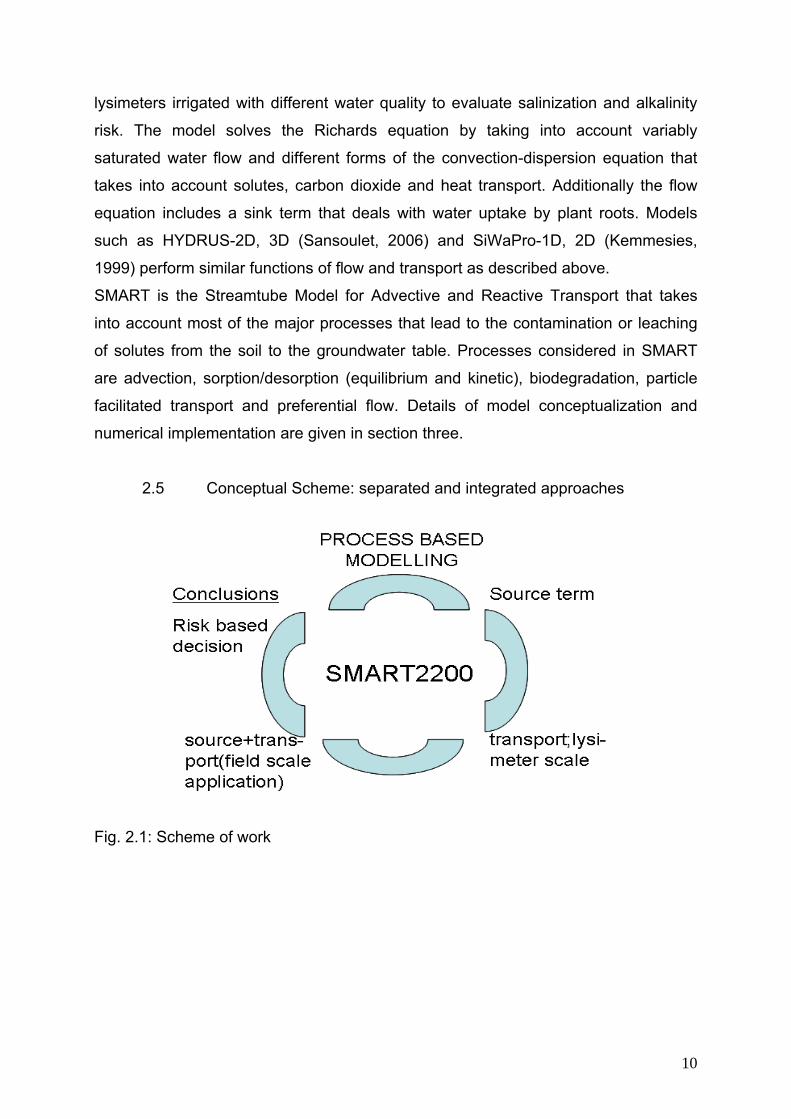
2.5 Conceptual Scheme: separated and integrated approaches
Fig. 2.1: Scheme of work
10
The figure 2.1 above puts the process based modelling of this study in three perspec-
tives.
1. The development of a source strength function which could predict the
behaviour of non volatile organic pollutant leaching at the basement of a
source zone.
2. The quantification and prediction of contaminants at the outlet of a lysimeter
over a long period. The outlet of the lysimeters could serve as good index of
risk for groundwater providing the local authorities and the decision makers
with a tool for the identification of the areas at risk of pollution, where specific
monitoring actions and prevention measures for the protection of waters can
be studied (Francaveglia et al., 2000).
3. A scenario based modelling of a typical landfill in Ghana which extends the
model tool SMART into field scale applications.
After applying SMART through this cycle, the model tool which has been tested and
validated at the laboratory scale (Bold, 2004) would have been employed as well up
to the field scale, the ultimate aim of groundwater risk assessment.
The source strength function was achieved through scenario based modelling
considering major processes such as advection, desorption kinetics and
biodegradation and the use of Damköhler numbers to quantify the relative
importance of each of the processes. Usually laboratory experiments are performed
to quantify the contaminant release at the base of a source zone. For instance,
Susset (2004) described the assessment of groundwater risk due to pollutant
emission from contaminated soils through leaching column tests. But laboratory
experiments may not last long enough to establish equilibrium between the solutes
and the soil matrix. This may lead to lower concentration measurements. However
the expected maximum concentration released could be achieved through longterm
modelling. For this purpose the model assumes steady state release with no ageing
of the pollutant source.
The second objective is achieved through transport modelling.
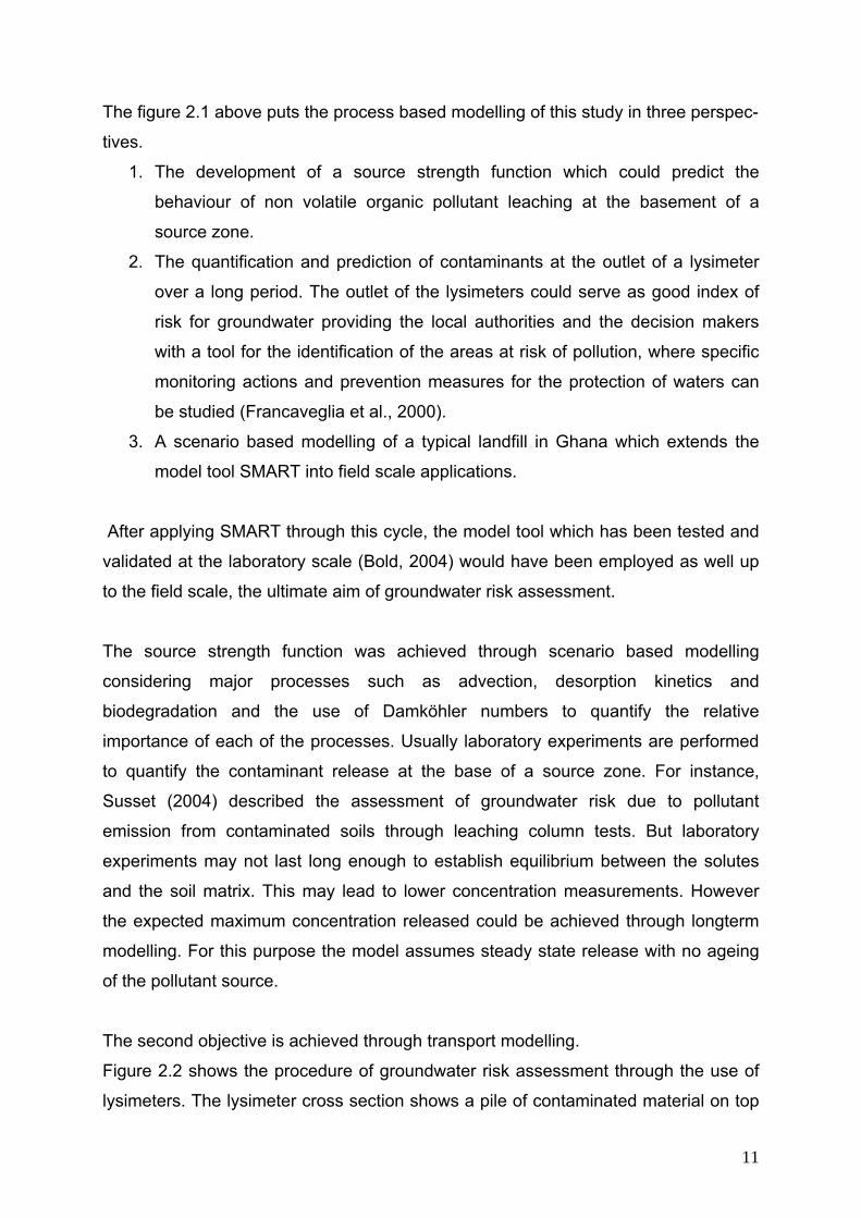
Figure 2.2 shows the procedure of groundwater risk assessment through the use of
lysimeters. The lysimeter cross section shows a pile of contaminated material on top
11
of an undisturbed transport layer of porous medium with measuring instruments such
as tensiometers, temperature sensors and TDR probes. The plot on the right of figure
2.2 depicts the increase of contaminant concentration in seepage water at maximum
mass flux, Fmax (non equilibrium) until a maximum concentration Cmax is reached.
Maximum concentration is established when equilibrium occurs during desorption
and dissolution from residual phase. A decrease in concentration in the seepage
water further down the transport distance occurs due to biodegradation. Mean
contaminant concentrations rather than total compositions of the contaminants are
quantified at the base of the lysimeter through forward modelling involving all the
relevant processes. Not only is the inaccessibility of the point of compliance a
problem but also the contaminant compositions are highly variable and depend on
local conditions. Hence the uses of mean breakthrough concentrations give a better
estimate than extreme values of concentration (Grathwohl and Susset, 2001).
Fig. 2.2: Left, a cross section of a test lysimeter. The figure in the middle shows
contaminant quantification procedure of the lysimeter which is separated
into source term and transport term material and measurements. The
diagram shows maximum concentration build up during desorption and a
decrease in the seepage water after a long transport distance due to
biodegradation.
12
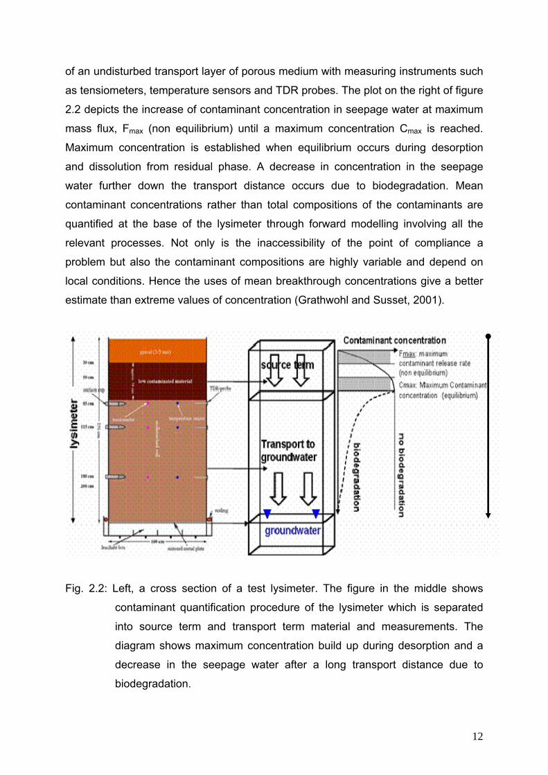
Figure 2.3 below shows a typical concentration profile of a scenario based modellling
of a typical landfill in which the source zone contamination is depleting into the
unsaturated transport zone. In the integral approach, the source zone and the
transport zone are modelled together as a single unit. In the separated approach,
the concentration at the bottom of the source zone is taken as the upper boundary
condition of the transport zone. The concentration profile in Fig. 2.3 shows the extent
of kinetic interactions within the system but not due to dispersion. For this thesis the
integral approach was not used but rather the application of the source strength
function as upper boundary condition for solute spreading in the transport zone
modelled with SMART.
Fig 2:
.
Fig. 2.3: A concentration profile showing the source and transport zones of a landfill.
13
Chapter 3
3 METHODOLOGY : PROCESS BASED MODELLING
A model may be defined as a selected simplified version of a real system, which
approximately simulates the latter's excitation-response relations that are of interest.
A system includes the domain and phenomena that take place within the domain
(Bear, 2001). In modeling the reality is simplified but not reproduced. In recent times
models are increasingly applied in water management and research to predict the
responses of systems.
3.1 Modelling approaches
Model approaches differ depending on the nature of problem being addressed, data
needs and other complexities involve. According to (Addiscott and Wagenet, 1985)
models may be classified as deterministic or stochastic, mechanistic or functional,
and numerical or analytical. Also other approaches could be based on spatial scale
(pore scale or global scale), temporal scale considerations (instantaneous or
decades), level of complexity (scientific or decision making) and level of integrity
(holistic or reductionistic)
Indeed the scope of modelling could be very wide. According to Figure 3.1 below,
which was adopted from the STOWA/RIZA (1999) report, the approaches could be
seen from two extremes with different degrees of combinations in between. Firstly,
models can be fully data oriented (based on measurements from the field). An
example is the Archydro data model by Maidment (2003) which provides a
standardized framework for storing information. And secondly, fully process oriented
models follow a deterministic approach based on physical processes. Here the
physical processes are assumed to be known and stored in the model in a form of
equations. The ensuing parameters in the equations are supplied in the form of time
series. For instance, the SMART (Finkel, 1999) model used in this thesis contains
routines to simulate hydrologic solute transport processes. Usually many models
consist of a combination of these two extremes.
14
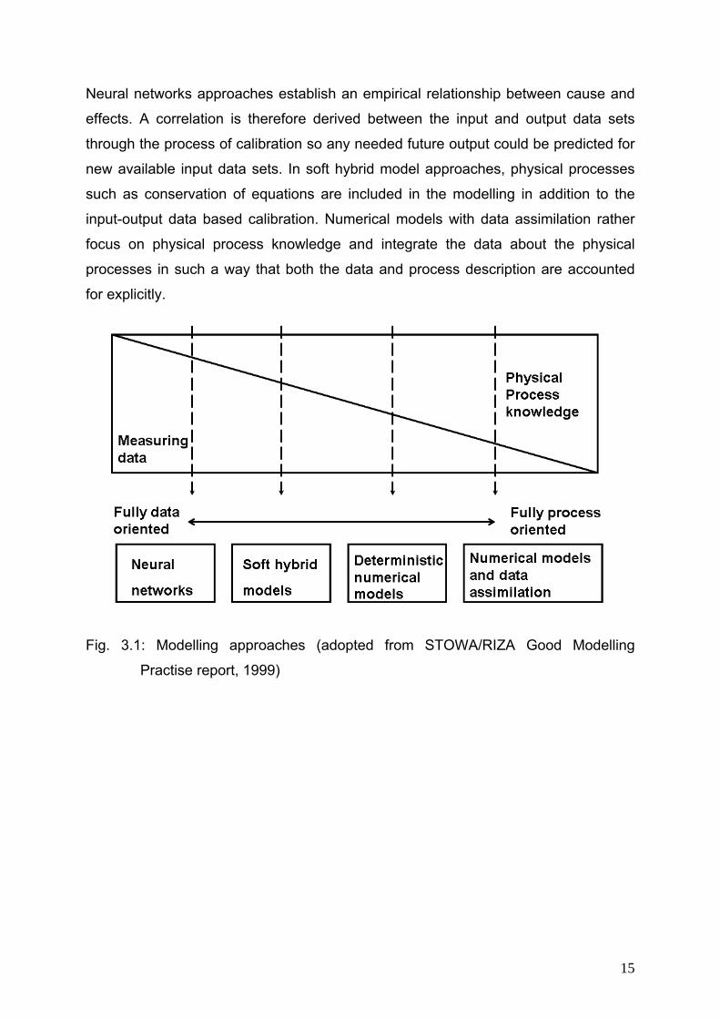
Neural networks approaches establish an empirical relationship between cause and
effects. A correlation is therefore derived between the input and output data sets
through the process of calibration so any needed future output could be predicted for
new available input data sets. In soft hybrid model approaches, physical processes
such as conservation of equations are included in the modelling in addition to the
input-output data based calibration. Numerical models with data assimilation rather
focus on physical process knowledge and integrate the data about the physical
processes in such a way that both the data and process description are accounted
for explicitly.
Fig. 3.1: Modelling approaches (adopted from STOWA/RIZA Good Modelling
Practise report, 1999)
15
3.2 Modelling of Solute Transport in Porous Media
Figure 3.1 above shows clearly the extent of modelling approaches applied in water
and solute transport through porous media. Most of the models differ in the
underlying model concept and partial differential equations describing the system.
Flow and solute transport in the vadose zone have been simulated with models such
as FEFLOW (Diersch, 2002), HYDRUS (Simunek et al., 1998) and MACRO (Jarvis et
al., 2000). Water flow in the vadose zone is usually described by the Richards
equation (Richards, 1931). Neglecting the flow of air for simplification purposes the
Richards equation is given in 1-D form as:
⎥⎦
⎤⎢⎣
⎡⎟⎠⎞
⎜⎝⎛∂∂
∂∂
=∂∂
xK
xt fφψθ )( 3.1
where θ is the water content [-], t is the time [T], ψ is the matrix potential [L], Kf(ψ) is
the unsaturated hydraulic conductivity [LT-1] at given ψ, φ is the total soil-moisture
potential [L] and x [L] is the spatial coordinate corresponding to the vertical direction
and oriented positively downward. The unsaturated hydraulic conductivity Kf(ψ)
could be estimated by Van Genuchten (1980) parameters based on the soil
properties.
Depending on the assumption of solute movement, many approaches exist as
mentioned in section 2.4. Four of such solute transport approaches are further briefly
described.
1. The conversion dispersion equation (CDE) (van Genuchten and Wierenga,
1976) : Solute transport in 1-D steady flow field may be described by
2
2
∂ ∂= −
∂ ∂D D
DC CD vt x
C 3.2
where CD is the dissolved solute flux concentration [ML-3], v is the flow velocity [LT-1]
and D is the hydrodynamic dispersion coefficient [L2T-1]. The CDE assumes perfect
mixing of solute in the lateral direction. The solute movement is driven by pore water
velocity variations. Various representation of the velocity variations in the 1-D CDE
16
have been developed by Parker and van Genuchten (1984) and Bresler and Dagan,
(1981).
2. Convective Lognormal Transfer function model (CLT) : Solute transport is
represented by the use of transfer functions in which system output flux are
described as a function of the input function. Using the idea of probability density
functions to describe the distribution of transport times from the inlet to the outlet and
the concept of stochastic convection transport, transfer functions are generated to
characterise the solute transport processes (Jury, 1982; White et al., 1986; Jury and
Scotter 1994). CLT assumes that the travel time of solute molecules is a linear
function of transport distance without lateral mixing. This assumption may however
be insufficient in complex soil settings to describe the movement to solute through
the porous media. The CLT which is based on stochastic convective transport has
been shown by field experiments to predict solute transport well at the first 3 m of the
top soil. The predictions were however poor at deeper depth where layering occurred
(Butters et al. 1989; Roth et al. 1991). Nonetheless Zhang (1995) and Jacques et al.
(1998) compared solute transport results of CLT and CDE using column data and
field experiments respectively and came to a conclusion that the CLT gives better
predictions than CDE.
3. Extended Transfer Function Model (ETFM) (Lui and Dane, 1996): The model
described the concept of partial mixing with a changeable constant which represents
the level of horizontal mixing and an extension of the transfer function models. Its
range of applicability is between the CDE and CLT as described in points 1 and 2.
The model is however restricted to characterizing solute transport described by either
a quadratic or linear increase in the solute travel time in a steady state flow field with
depth.
4. Generalised Transfer Function Model (GTFM) (Zhang, 2000): In heterogeneous
media, effective transport parameters such as dispersive coefficient, D, and average
linear water velocity, v, can be applied to the macroscopic mean transport equations
to describe the solute movement (Gelhar and Axness, 1983). The CDE in this case
assumes a Fickian mixing (high degree) within flow paths. The PDF of travel time by
an impulse input follows the so called Fickian PDF (Jury and Roth, 1990). The GTFM
17
describes solute transport processes in heterogeneous media similar to the CLT but
with two additional parameters which characterise the depth dependency of the
mean and standard deviation of the logarithmic travel time. The GTFM can describe
or predict not only the models described in points 1, 2 and 3 above but can also
characterise solute transport in heterogeneous media in which changes in the soil
moisture content and pore water velocity causes the mean travel time to increase
with depth non-linearly. Moreover it is applicable to heterogeneous systems in which
the scale dependency of the dispersivity to the travel distance results in a power law
(Zhang et al., 2000).
3.3 Eulerian and Lagrangian numerical solutions
Many solutions have been developed to solve solute transport equations such as
3.2. Several analytical solutions exist that can solve the equations with different level
of simplified boundary conditions. For instance (Ogata and Banks, 1961; Ogata,
1964; Thomann and Mueller,1987; O’Loughlin and Bowmer, 1975; Rose, 1977;
Runkel, 1996) solve the CDE equation under steady state and spatially constant
model parameters with simplified boundary conditions. The transport equation could
therefore be solved numerically when other arbitrary boundary and transient
conditions with distributed model parameters are considered. Solution methods
normally employed in solving the CDE are Finite Difference (FD), Finite Element
(FE), Total Variation Diminishing (TVD), Random Walk (RW) and Method of
Characteristics (MOC). Two of such numerical model approaches are discussed.
1. Eulerian Approach: This approach considers changes in fluid properties or the
rate of change of the fluid motion such as the orientation of non spherical distribution
at a fixed point in the fluid mesh. The mesh therefore presents a fixed reference
frame. It is therefore applied when fixed sampling or predictions are made in space
and time. The set of concentration distributions can be described by the Fokker-
Planck ordinary differential equation which reduces to the convective diffusion
equation under conditions of dilute suspensions (Adamczyk et al., 1983; Jia and
Williams, 1990; Peters and Ying, 1991). Examples of application are flow and
diffusion equations.
The Eulerian approach is more responsive to analytical approximations and
numerical solutions than the Lagrangian approach. The FD, FE and TVD solution
18
techniques are all based on the Eulerian approach. The model tool MT3D (Zheng
1990; Zheng and Wang, 1999) includes Eulerian approaches to predict concentration
of conservative solutes at any time in space. Its FD scheme is efficient, convenient
and produces good mass balances but may lead to either over prediction in source
concentration or prediction of negative concentrations in contaminant flow processes
in which advection dominates. It also has the disadvantage of introducing
computational errors in algorithms which leads to numerical dispersion that cannot be
separated from physical dispersion. Results from the FD approach can be improved
by using smaller time steps and grid size. However the required computational effort
may restrict the fine discretization.
2. Lagrangian Approaches: They describe the trajectories of single particles
encroaching a collector surface. This approach considers changes in the fluid
properties as the fluid moves along a trajectory. The mesh is therefore deformed or
moves with the fluid in a fixed grid. It is mostly applied when the evolvement of a
solute in space is predicted. It is governed by the Newton’s second law and leads to
the Langevin-type equation when combined with Brownian motion (thermal random
force), the solution of which produces stochastic trajectories (Gupta and Peters,
1985; Russel et al., 1989; Ramaro et al., 1991). An example is the pure advection
(without dispersion) equation. The model tool SMART (Finkel et al., 1999; Finkel,
1999) uses the Lagrangian approach to track the trajectory motion of conservative
parcels of solute in an Eulerian steady state flow field. The heterogeneous model
domain was discretised along flow paths by the travel time of the conservative solute.
It is perfectly applied in pure advective processes but becomes complex when other
processes such as dispersion, sources are involved in a heterogeneous medium.
In order to reduce numerical problems, overshooting and/or undershooting of source
concentrations, a mixture of the Eulerian and Lagrangians approaches may be used.
Examples of such solution options are Method of Characteristics, Modified Method of
Characteristics and Hybrid Method of Characteristics (Zheng 1990; Zheng, 1996).
19
3.4 SMART The numerical code SMART (Streamtube Model for Advective and Reactive
Transport) was developed by Finkel (1999) a the Centre for Applied Geosciences,
Universität Tübingen. It is based on the Lagrangian approach of describing flow
paths by the use of probability density functions (PDF) of travel time of inert tracers
(Dagan and Cvetkovic, 1996). The PDF is used as an input for the reactive transport
modelling. This allows the decoupling of conservative transport from physicochemical
processes. The approach ensures a good mass balance, is almost free from
numerical dispersion and consumes less time during numerical computations (Thiele
et al., 1995a, b; Batycky et al., 1996). It is designed for use as a pure forward model
involving input parameters which can be derived from independent laboratory or field
scale experiments. Solute transport through heterogeneous media is represented by
an ensemble of 1-D streamtubes with infinitesimal cross-sectional area and time
dependent concentrations.
3.4.1 SMART: Assumptions and heterogeneity implementation
The SMART model assumes:
(1) The flow field is at steady state.
(2) The variability of the velocity field completely describes the hydraulic
heterogeneities within the porous medium. The travel time approach does not allow
heterogeneity of the hydrogeochemical parameters.
(3) Dispersion of solute plumes is solely attributed to macroscopic hydraulic
heterogeneities, i.e pore scale dispersion and molecular diffusion is neglected.
The third assumption which neglects diffusion is unrealistic in general but is a
reasonably valid approximation in application scenarios where advection becomes
dominant (Finkel et al., 1999). In this approach solute in the form of parcels moves
and spreads out in the streamtube from an injection plane (i.e. source zone of the
lysimeter) to a control plane (outlet of the lysimeter) normal to the mean flow direction
(Fig 3.2). The parcel flow shows how non-uniformity in the hydraulic properties
causes the spatial spreading of the fluid parcels along the streamtubes. The
spreading is similar to macro scale solute dispersion.
20
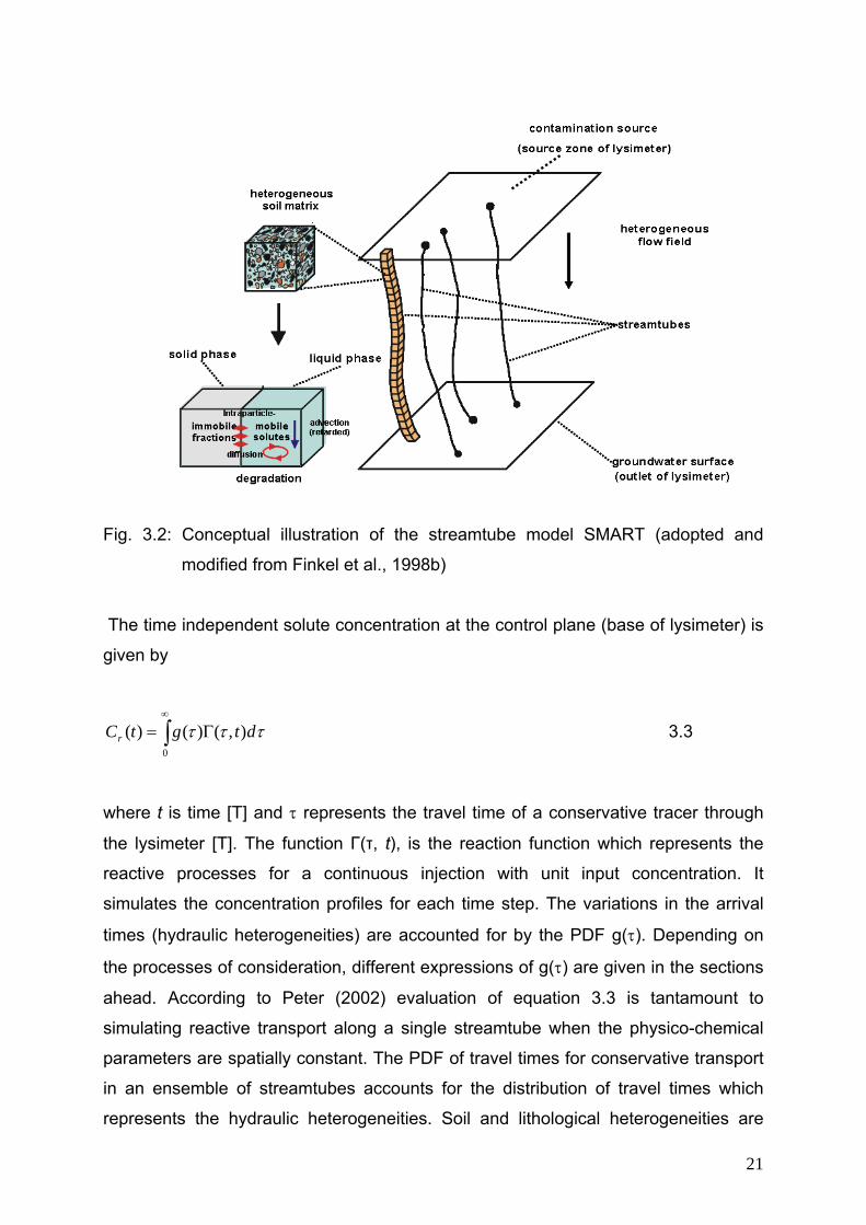
Fig. 3.2: Conceptual illustration of the streamtube model SMART (adopted and
modified from Finkel et al., 1998b)
The time independent solute concentration at the control plane (base of lysimeter) is
given by
∫∞
Γ=0
),()()( τττ dtgtCr 3.3
where t is time [T] and τ represents the travel time of a conservative tracer through
the lysimeter [T]. The function Γ(τ, t), is the reaction function which represents the
reactive processes for a continuous injection with unit input concentration. It
simulates the concentration profiles for each time step. The variations in the arrival
times (hydraulic heterogeneities) are accounted for by the PDF g(τ). Depending on
the processes of consideration, different expressions of g(τ) are given in the sections
ahead. According to Peter (2002) evaluation of equation 3.3 is tantamount to
simulating reactive transport along a single streamtube when the physico-chemical
parameters are spatially constant. The PDF of travel times for conservative transport
in an ensemble of streamtubes accounts for the distribution of travel times which
represents the hydraulic heterogeneities. Soil and lithological heterogeneities are
21
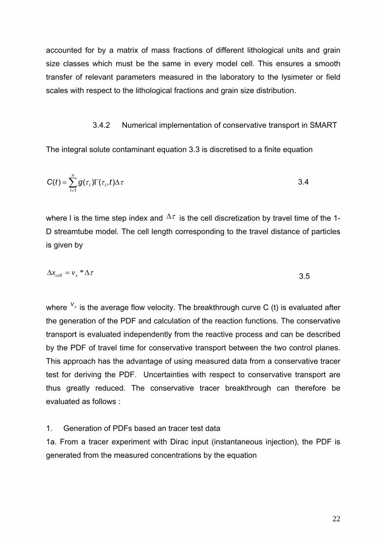
accounted for by a matrix of mass fractions of different lithological units and grain
size classes which must be the same in every model cell. This ensures a smooth
transfer of relevant parameters measured in the laboratory to the lysimeter or field
scales with respect to the lithological fractions and grain size distribution.
3.4.2 Numerical implementation of conservative transport in SMART
The integral solute contaminant equation 3.3 is discretised to a finite equation
1( ) ( ) ( , )
n
l ll
C t g tτ τ=
= Γ∑ τΔ 3.4
where l is the time step index and τΔ is the cell discretization by travel time of the 1-
D streamtube model. The cell length corresponding to the travel distance of particles
is given by
τΔ=Δ *xcell vx 3.5
where is the average flow velocity. The breakthrough curve C (t) is evaluated after
the generation of the PDF and calculation of the reaction functions. The conservative
transport is evaluated independently from the reactive process and can be described
by the PDF of travel time for conservative transport between the two control planes.
This approach has the advantage of using measured data from a conservative tracer
test for deriving the PDF. Uncertainties with respect to conservative transport are
thus greatly reduced. The conservative tracer breakthrough can therefore be
evaluated as follows :
xv
1. Generation of PDFs based an tracer test data
1a. From a tracer experiment with Dirac input (instantaneous injection), the PDF is
generated from the measured concentrations by the equation
22
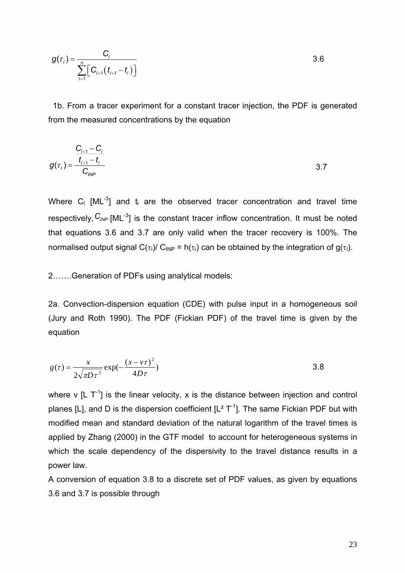
( )1 1
1
( ) ll n
l l ll
CgC t t
τ+ +
=
=⎡ ⎤−⎣ ⎦∑
3.6
1b. From a tracer experiment for a constant tracer injection, the PDF is generated
from the measured concentrations by the equation
1
1( )
l l
l ll
INP
C Ct tgC
τ
+
+
−−
= 3.7
Where Cl [ML-3] and tl are the observed tracer concentration and travel time
respectively, [ML-3] is the constant tracer inflow concentration. It must be noted
that equations 3.6 and 3.7 are only valid when the tracer recovery is 100%. The
normalised output signal C(τl)/ CINP = h(τl) can be obtained by the integration of g(τl).
INPC
2…….Generation of PDFs using analytical models:
2a. Convection-dispersion equation (CDE) with pulse input in a homogeneous soil
(Jury and Roth 1990). The PDF (Fickian PDF) of the travel time is given by the
equation
)4
)(exp(2
)(2
3 ττ
τπτ
Dvx
Dxg −
−= 3.8
where v [L T-1] is the linear velocity, x is the distance between injection and control
planes [L], and D is the dispersion coefficient [L² T-1]. The same Fickian PDF but with
modified mean and standard deviation of the natural logarithm of the travel times is
applied by Zhang (2000) in the GTF model to account for heterogeneous systems in
which the scale dependency of the dispersivity to the travel distance results in a
power law.
A conversion of equation 3.8 to a discrete set of PDF values, as given by equations
3.6 and 3.7 is possible through
23
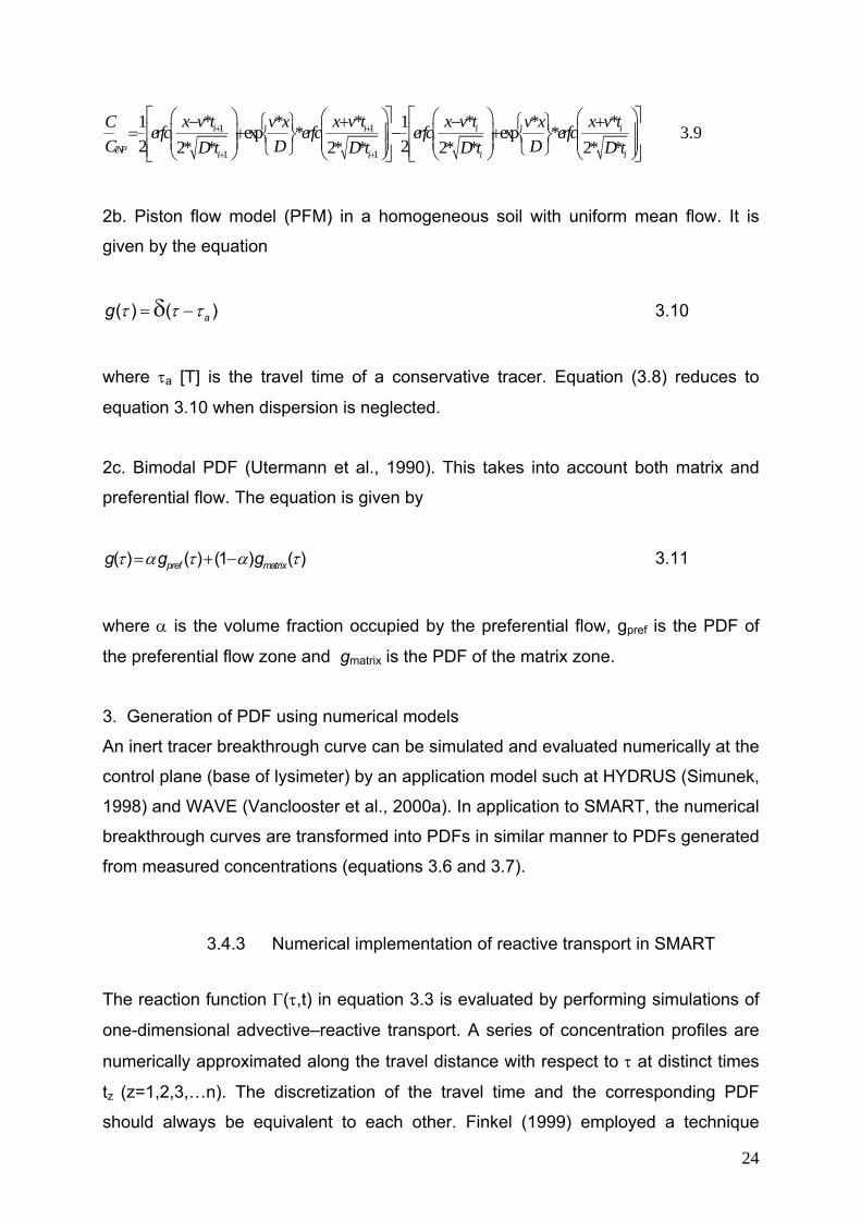
1 1
1 1
* * *1 * 1 *exp * exp *2 22* * 2* * 2* * 2* *
i i i
INP i i i
x v t x v t x v t x v tC v x v xerfc erfc erfc erfcC D DD t D t D t D t
+ +
+ +
⎡ ⎤ ⎡⎛ ⎞ ⎛ ⎞ ⎛ ⎞ ⎛− + −⎧ ⎫ ⎧ ⎫= + − +⎢ ⎥ ⎢⎜ ⎟ ⎜ ⎟ ⎜ ⎟ ⎜⎨ ⎬ ⎨ ⎬⎜ ⎟ ⎜ ⎟ ⎜ ⎟ ⎜⎩ ⎭ ⎩ ⎭⎢ ⎥ ⎢⎝ ⎠ ⎝ ⎠ ⎝ ⎠ ⎝⎣ ⎦ ⎣
* i
i
⎤⎞+⎥⎟⎟⎥⎠⎦ 3.9
2b. Piston flow model (PFM) in a homogeneous soil with uniform mean flow. It is
given by the equation
( ) ( )ag τ τ τ= −δ 3.10
where τa [T] is the travel time of a conservative tracer. Equation (3.8) reduces to
equation 3.10 when dispersion is neglected.
2c. Bimodal PDF (Utermann et al., 1990). This takes into account both matrix and
preferential flow. The equation is given by
τ α τ α= + −( ) ( ) (1 ) ( )pref matrixg g g τ 3.11
where α is the volume fraction occupied by the preferential flow, gpref is the PDF of
the preferential flow zone and gmatrix is the PDF of the matrix zone.
3. Generation of PDF using numerical models
An inert tracer breakthrough curve can be simulated and evaluated numerically at the
control plane (base of lysimeter) by an application model such at HYDRUS (Simunek,
1998) and WAVE (Vanclooster et al., 2000a). In application to SMART, the numerical
breakthrough curves are transformed into PDFs in similar manner to PDFs generated
from measured concentrations (equations 3.6 and 3.7).
3.4.3 Numerical implementation of reactive transport in SMART
The reaction function Γ(τ,t) in equation 3.3 is evaluated by performing simulations of
one-dimensional advective–reactive transport. A series of concentration profiles are
numerically approximated along the travel distance with respect to τ at distinct times
tz (z=1,2,3,…n). The discretization of the travel time and the corresponding PDF
should always be equivalent to each other. Finkel (1999) employed a technique
24
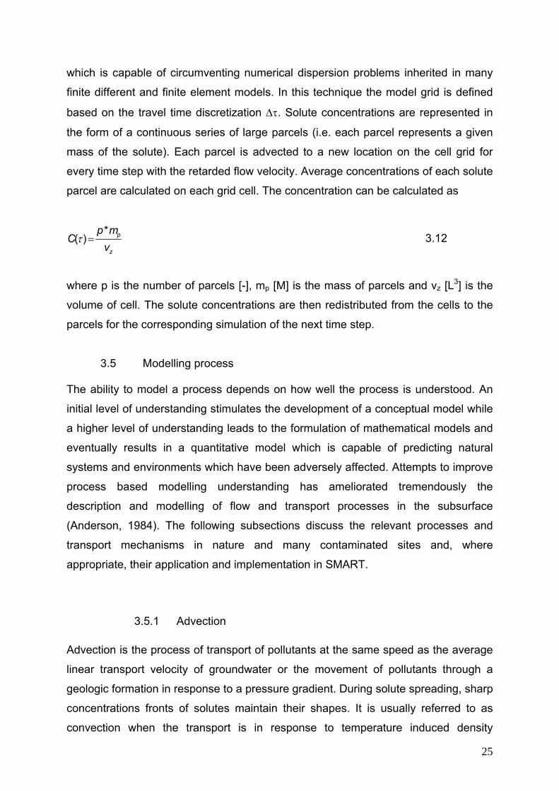
which is capable of circumventing numerical dispersion problems inherited in many
finite different and finite element models. In this technique the model grid is defined
based on the travel time discretization Δτ. Solute concentrations are represented in
the form of a continuous series of large parcels (i.e. each parcel represents a given
mass of the solute). Each parcel is advected to a new location on the cell grid for
every time step with the retarded flow velocity. Average concentrations of each solute
parcel are calculated on each grid cell. The concentration can be calculated as
*( ) p
z
p mC
vτ = 3.12
where p is the number of parcels [-], mp [M] is the mass of parcels and vz [L3] is the
volume of cell. The solute concentrations are then redistributed from the cells to the
parcels for the corresponding simulation of the next time step.
3.5 Modelling process The ability to model a process depends on how well the process is understood. An
initial level of understanding stimulates the development of a conceptual model while
a higher level of understanding leads to the formulation of mathematical models and
eventually results in a quantitative model which is capable of predicting natural
systems and environments which have been adversely affected. Attempts to improve
process based modelling understanding has ameliorated tremendously the
description and modelling of flow and transport processes in the subsurface
(Anderson, 1984). The following subsections discuss the relevant processes and
transport mechanisms in nature and many contaminated sites and, where
appropriate, their application and implementation in SMART.
3.5.1 Advection Advection is the process of transport of pollutants at the same speed as the average
linear transport velocity of groundwater or the movement of pollutants through a
geologic formation in response to a pressure gradient. During solute spreading, sharp
concentrations fronts of solutes maintain their shapes. It is usually referred to as
convection when the transport is in response to temperature induced density
25
gradients (Anderson, 1984). Advection does not take into account microscopic
processes but follows the bulk Darcian flow vectors. Moreover it is also described as
the transport along pathlines. Pure advective transport can be evaluated from the
results of the flow model with path line models (e.g. particle tracking and Method of
Characteristics). Known specific fluxes within cells can be used to calculate advective
fluxes.
QqA
= 3.13
where Q [L3 T-1] is the discharge of flow, q [L T-1] is specific flux or Darcy velocity, and
A [L2] is cross-sectional area for water flux. The pore velocity which determines the
advective flux is given by
e
qun
= 3.14
where u [L T-1] is pore velocity and ne [-] is the effective porosity.
In pure advection transport problems the Lagrangian approach is employed to
eliminate numerical dispersion. In the SMART code pure advection is represented as
a flug-flow or piston-flow model (equation 3.10).
3.5.2 Diffusion and dispersion Diffusion is the spreading of compounds through the effects of random molecular
motion. The compounds passively move and transfer mass from an area of higher
concentration to area of lower concentration causing mixing in the direction of their
concentration gradient. It primarily starts from movement of molecules and results in
variation of concentrations. Solute emanating from a point source by diffusion in the
absence of hindrance or advection to movement will lead to a Gaussian distribution
of the concentration, with the width of the plume growing with the square root of time.
The higher molecular activity in gases causes spreading due to diffusion about 100
times faster than in the liquid phase (Selker et al., 1999). Diffusion rate changes with
the square root of temperature (measured in Kelvin) and since temperatures vary
26
little in typical groundwater, variation of diffusion tends to be very low in groundwaters
(Selker et al., 1999). The diffusive mass flux is determined through the concentration
gradient and the effective coefficient of diffusion of the porous media. The diffusive
flux is described by Fick’s first law
i icJ Dx∂
=−∂ 3.15
where Ji [M L-2 T-1] is the diffusive flux of chemical i. Di [L2 T-1] is the coefficient of
molecular diffusion and icx∂∂ [M L-3 L-1] is the concentration gradient. The molecular
diffusion coefficient depends on solvent temperature, solvent viscosity, molecular
size and shape. According to (Neretnieks, 2002), the magnitude of diffusive distance
can be approximated by the equation
2.2 *il D= t
iD
3.16
where l [L] is the distance of diffusive transport for which the mean concentration
equals 50% of the maximum concentration and t [T] is typical time. The effective
molecular diffusion coefficient De [L2 T-1] is given by the relation
*eD =ζ 3.17
where ζ [-] is the tortuosity factor.
Dispersion is the mixing that occurs as a result of differences in velocities of
neighbouring parcels of fluid at different scales. At pore scale dispersion leads to the
separation of intergranular particles and mixing of solutes (Selker et al., 1999).
Natural sediments are heterogeneous and lead to a non uniform velocity distribution
which causes the smearing of fronts above the pore scale. This additional mixing
process is termed macro-dispersion. The presence of macro dispersion has been
confirmed by field studies (Skibitzkie and Robinson, 1963; Anderson, 1979). Groundwater moves at rates that are both greater than and less than the average
linear velocity. This is due to hydrodynamic dispersion, a phenomenon caused by
27
mechanical dispersion and molecular diffusion. Mechanical dispersion is basically
caused by three phenomena:
1) As fluid moves through the pores, it will move faster in the center of the pores than
along the edges. This causes an accelerated arrival of contaminant at a point of
discharge.
2) Some of the particles will travel along longer flow paths in porous media than other
particles to go the same linear distance. This caused the smearing of concentration
fronts.
3) And some pores are larger than others, which allow the fluid flowing through these
pores to move faster (Fetter, 1993). Dispersion is a mechanism of dilution which
causes mixing with unpolluted groundwater and the spread of contaminants into
greater volumes in aquifers than normal groundwater velocity vectors would predict.
It is more important in predicting transport away from point sources than diffused
sources. Slichter (1905) predicted an s-shape breakthrough curve owing to
dispersion from his laboratory experiment of flow through porous media.
Along the direction of flow the velocity variations within and between pores as well as
the variation in the flow path length causes the dispersive effect know as longitudinal
dispersion. Similar dispersive effects which are mainly due to the splitting of flow
paths but normal to the mean flow path is know as transverse dispersion. The
longitudinal dispersion is usually greater than the transverse dispersion. The
combined effect of these two mechanisms is known as mechanical dispersion.
Studies have found the mechanisms to be scale dependent (Anderson, 1984 , Gelhar
et al., 1992).
Usually the process of molecular diffusion cannot be separated from mechanical
dispersion in flowing groundwater. The two are therefore combined to define a new
parameter called the hydrodynamic dispersion coefficient, D* (Fetter, 1993)
*
mec pD D D= + 3.18
28
where Dp [L2T-1] is the pore diffusion coefficient and Dmec [L2T-1] is the coefficient of
mechanical dispersion. The coefficient of mechanical dispersion is given by the
relation
*mecD α ν= 3.19
where α [L] is the characteristic mixing length usually known as dispersivity and v is
the average linear pore velocity [LT-1].
Most field studies and flow and transport modelling are conducted at the
macroscopic level. This may be due to measurement problems (Fried, 1975) and the
use of the fundamental macroscopic Darcy (the use of unresolved velocity
distribution and single average values in a representative elementary volume)
equation in models. Taylor (1921, 1953) therefore suggested that dispersion could be
represented by Fick’s 1st law of diffusion. The mass flux due to dispersion is given by
∂=−
∂* cJ D
x 3.20
where D* is the hydrodynamic dispersion coefficient as given in equation 3.18.
Further studies from many researchers have found out that the Fickian
representation of dispersion is only valid after some distance and certain length of
time have elapsed in porous media and in rivers (Fisher, 1973; Matheron and
DeMarsily, 1980; Gelhar and Axness, 1981; Dagan, 1982; Beltaos and Day, 1978).
Only for long times or travel distances under special geologic conditions can the
Fickian process accurately represent dispersion. Moreover other studies show that
dispersion is non Fickian near the source of a contamination (Molinari et al., 1977;
Lee et al., 1980; Pickens and Grisak, 1981b). Other approaches which are not
discussed in detail in this thesis (Schwartz, 1977 and Smith and Schwartz, 1980,
1981a, 1981b) described dispersion by defining the hydraulic conductivities
statistically. Dispersion close to a source therefore requires other terms of higher
order. Therefore detailed characterisation of heterogeneities, hydraulic conductivity
units, heads and gradient is needed for accurate prediction of contaminant transport
(Anderson, 1984). In SMART, the Langrangian approach in which solutes moving
along non interacting streamtubes are tracked do not account for dispersion. Hence
29
unsuitable in heterogeneous systems or geologic settings where dispersion is
dominating the over all advective-dispersive transport process.
3.5.3 Preferential flow The quests for management of land and chemical inputs on soil have increased
recently as more and more chemicals and fertilizers are applied on land to ensure
optimised crop yield. Unexpected chemicals have been found in drinking wells as
well as ground waters Compounds which are highly degradable or highly sorbed
have been found at higher concentrations and much more rapidly than would have
been predicted in groundwaters. This would constitute a longterm hazard that
posterity would have to deal with. This fast movement of solute endangers
groundwater quality with an associated adverse effect on humans and aquatic
systems. Recent studies have shown this phenomenon to be a process known as
preferential flow which occurs in many natural geological and soil settings (Flury,
1996; Traub-Eberhard et al., 1995; Kladivko et al., 1991; Parlange et al., 1998).
Again preferential flow has been observed in many laboratory and field studies
(Pyrak et al., 1985; Abelin, 1986; Bourke, 1987; Haldeman et al., 1991). The process
had actually been described earlier on by Lawes et al. (1882) who distinguished
between preferential flow and matrix flow in field drain experiments. Preferential flow
is the unequal and fast movement of water and solutes through porous media which
is characterised by structural and textural inhomogeneous. Three mechanisms have
been reported to be responsible for preferential flow processes: (i) macropore flow
(bypass flow) is due to several soil forming factors such as soil fauna, tubes left from
rotten roots, flow through non capillary cracks, subsurface erosion, aggregate, gabs
and exclusion due to parts of pore area. High macropore routes form and persist in
structured soils with flow fairly uniform near the upper horizons and becomes sparse
as it drains down the unsaturated zone. (ii) Finger flow is due to the instability in
wetting front which causes water to flow in channel or fingers. Fingers results from
infiltration through dry sands, water flow from fine into coarse material (Akthar et al.,
2003) and local variations in wetting characteristics of porous media. Hill and
Parlange (1972) observed this mechanism in homogeneous media at low rate of
infiltration. The higher the flow rate the higher the number of fingers formed and vice
versa (Selker et al., 1996). This unstable wetting fronts results in preferred finger flow
30
paths which end up in fast transport to ground waters (Ritsema et al., 1998). (iii)
Funnel flow is caused by the sloping geological layers which also cause water flow
laterally or diagonally. Stones and lenses of different texture in sandy matrix result in
preferred flow of the funnel nature. This diverging of flow due to layering or sloping
(Welter et al., 2000) is important because monitoring wells emplaced to capture
contaminants may miss entirely if the wells are located away from places where
layering of the geological setting and funnelling are known to occur. Preferential flow
is again known to affect other processes such as biodegradation and particle
transport. Biodegradation rates were found to be initially less in macro pores than
rates in matrix pores but later increased and exceeded matrix pore rates as a result
of greater mass of substrate passing through and increase of microbial pollution with
time in the macrospores (Pivetz and Steenhuis (1995), Pevetz et al., 1996; Utermann
et al., 1990). Again Ryan and Elimelech (1996) demonstrated that particle transport is
enhanced in macrospores due to their higher travel velocities.
Many analytical and numerical models have also been conducted to characterise
preferential flow. (Van Dam et al., 1990; De Rooij, 1995) modelled flow and transport
in water repellent soils with analytical approaches. Ritsema (2001) modelled 2-D flow
and transport using finite element techniques described by Nieber (1996) and
Ritsema et al. (1998) including preferential flow and hysteresis which affects water
retention characteristics in repellent soils. He also used SWAP (Van Dam et al.,
1997) in that same study which again incorporated preferential flow and hysteresis.
Two-region stage models based on Coats and Smith (1964) in which chemical
exchange is rate limited between soil matrix and preferential flow paths have been
applied earlier. Multi layer models which encompass many flow paths have also been
used (Ma et al., 1995; Jarvis et al., 1991a, b; Hutson and Wagenet, 1995; Steenhuis
et al., 1990). Additionally (Skopp et al., 1981) considered a preferential flow model in
which water is mobile in both matrix and macro pores while (Wallach et al., 1998)
looked at other cases in which water in the matrix pores is considered stagnant (MIM
models). The mobile-immobile (MIM) models (Skopp and Warrick, 1974; van
Genuchten and Wierenga, 1976; van Genuchten and Dalton, 1986) are reported to
provide good predictions for measured breakthrough curves since their
concentrations are averaged and distributed uniformly across the lateral dimensions
throughout the model domain.
31
In SMART, preferential flow is modelled as a conservative process by using the
bimodal PDF approach after Utermann et al. (1990). Accounting for both matrix and
preferential flow in porous media their formulation is given as
( ) ( ) (1 ) ( )pref matrixg g gτ α τ α= + − τ . 3.21
as shown in equation 3.11. Bold (2003) in his thesis demonstrated that the expected
long term concentration at the control plane (outlet of lysimeter) taking into account
sorption, biodegradation, particle-facilitated transport and preferential flow and
assuming physico-chemical equilibrium between contaminants and particles is given
by:
' '
2 2
4 4exp 1 1 (1 )exp 1 12 2
pref pref matrix matrixINP
pref pref matrix matrix
v x D v x DC CD v D v
λ λα α∞
⎧ ⎡ ⎤ ⎫⎛ ⎞ ⎡ ⎤⎛ ⎞⎪ ⎪⎢ ⎥⎜ ⎟ ⎢ ⎥⎜ ⎟= − + + − − +⎨ ⎬⎜ ⎟⎜ ⎟⎢ ⎥ ⎢ ⎥⎪ ⎪⎝ ⎠⎣ ⎦⎝ ⎠ ⎭⎣ ⎦⎩ 3.22
where C∞[ ML-3 ] is total mobile long-term concentration, CINP[ ML-3 ] is total mobile
solute input concentration, α[-] is volume fraction of preferential flow, vpref [LT-1] and
Vmatrix [LT-1] are flow velocities in preferential flow and matrix flow regions
respectively, Dpref [L2T-1 ] and Dmatrix [L2T-1 ] are the dispersion coefficients in
preferential flow and matrix regions respectively, λ’ [T-1] is modified effective
degradation rate accounting for all particles involved and x is the vertical coordinate.
Bold (2003) successfully applied equation 3.21 to data from a lysimeter tracer (2H)
experiment conducted under steady state in an unsaturated medium by Seiler (2000).
In this thesis preferential flow is not accounted for since the expected lysimeter
breakthroughs to be modelled showed no signs of macropore flow.
3.5.4 Sorption/desorption The rate at which solutes pass through the zone of aeration (vadose zone) and break
through at the groundwater table partly depends on the interaction between the
moving mass in the aqueous phase and the solid matrix in the immobile phase.
Depending on the interfacial conditions, solute can either be sorbed into or desorbed
from soil matrices. Two of such major fundamental phenomena that take place in
soils and sediments are adsorption and absorption. Adsorption is the process in
32
which the solute accumulation is generally restricted to a surface or interface, for
instance solid/liquid, solid/gas and liquid/gas. Absorption describes a process in
which the solute penetrates the sorbent similar to solution in a solvent. Both
processes may take place simultaneously due to the heterogeneous nature of soils
and sediments. The term sorption is used to describe both absorptive and adsorptive
processes. The solute in solution not yet sorbed is also referred to as sorptive
(Grathwohl, 1997). In addition sorption processes also include chemisorption and ion
exchange. Chemisorption occurs when the solute is incorporated on a sediment or
soil surface by a chemical reaction (Fetter, 1991). Sorption is extremely important
because of its ability to effectively affect the fate and impact of chemicals in the
environment (Schwarzenbach et al., 1992).
3.5.4.1 Equilibrium sorption/desorption isotherms
Sorption isotherms relate the aqueous concentration to the sorbed concentration at a
constant temperature. The aqueous concentration is assumed to be in equilibrium
with the sorbed concentration if the sorptive uptake of the solvent by the sorbent is
instantaneous or occurs in a time that can be neglected when compared to the
advective time. The simplest case is when the concentration in the solid (qs) is
directly proportional to the corresponding equilibrium solute concentration (Ceq) in
aqueous or vapour phase:
s dq K C= eq 3.23
where Kd [L3M] denotes distribution coefficient, which defines the ratio between the
solute concentrations in aqueous and solids phases. qs is frequently termed sorbate
concentration but actually represents the ratio of sorbed mass to solid mass. Kd
describes the partitioning and is equal to the slope of the sorption isotherm when
sorption is linear. Kd becomes solute concentration dependent when sorption
isotherms are nonlinear. Four models often used to describe nonlinear sorption
isotherms in soils and sediments are described below.
(i) Freundlich model (Freundlich, 1909):
33
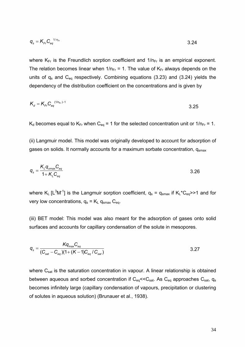
1/ Frn
s Fr eqq K C= 3.24
where KFr is the Freundlich sorption coefficient and 1/nFr is an empirical exponent.
The relation becomes linear when 1/nFr = 1. The value of KFr always depends on the
units of qs and Ceq respectively. Combining equations (3.23) and (3.24) yields the
dependency of the distribution coefficient on the concentrations and is given by
Fr(1/n ) 1
d Fr eqK K C −= 3.25
Kd becomes equal to KFr when Ceq = 1 for the selected concentration unit or 1/nFr = 1.
(ii) Langmuir model. This model was originally developed to account for adsorption of
gases on solids. It normally accounts for a maximum sorbate concentration, qsmax
max
1L s eq
sL eq
K q Cq
K C=
+ 3.26
where KL [L3M-1] is the Langmuir sorption coefficient, qs = qsmax if KL*Ceq>>1 and for
very low concentrations, qs = KL qsmax Ceq.
(iii) BET model: This model was also meant for the adsorption of gases onto solid
surfaces and accounts for capillary condensation of the solute in mesopores.
max
( )(1 ( 1) /eq
ssat eq eq sat
Kq Cq
C C K C C=
− + − ) 3.27
where Csat is the saturation concentration in vapour. A linear relationship is obtained
between aqueous and sorbed concentration if Ceq<<Csat. As Ceq approaches Csat, qs
becomes infinitely large (capillary condensation of vapours, precipitation or clustering
of solutes in aqueous solution) (Brunauer et al., 1938).
34
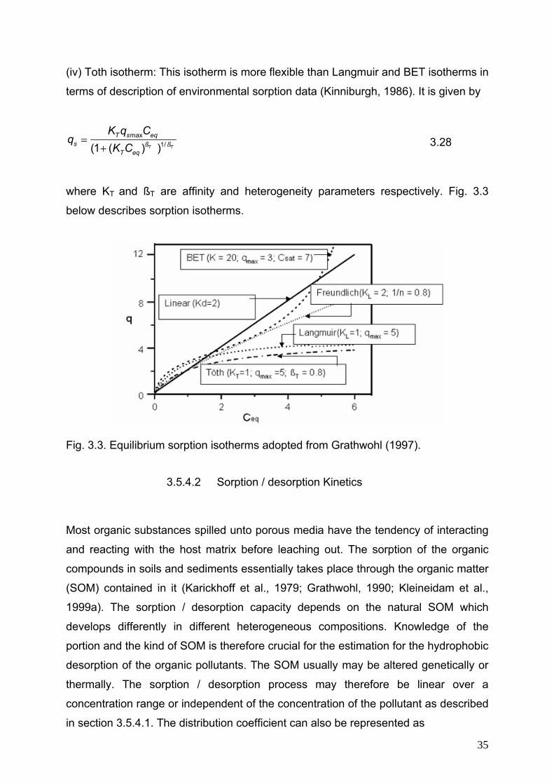
(iv) Toth isotherm: This isotherm is more flexible than Langmuir and BET isotherms in
terms of description of environmental sorption data (Kinniburgh, 1986). It is given by
=+
max1/(1 ( ) )T
T s eqs ß ß
T eq
K q Cq
K C T 3.28
where KT and ßT are affinity and heterogeneity parameters respectively. Fig. 3.3
below describes sorption isotherms.
Fig. 3.3. Equilibrium sorption isotherms adopted from Grathwohl (1997).
3.5.4.2 Sorption / desorption Kinetics
Most organic substances spilled unto porous media have the tendency of interacting
and reacting with the host matrix before leaching out. The sorption of the organic
compounds in soils and sediments essentially takes place through the organic matter
(SOM) contained in it (Karickhoff et al., 1979; Grathwohl, 1990; Kleineidam et al.,
1999a). The sorption / desorption capacity depends on the natural SOM which
develops differently in different heterogeneous compositions. Knowledge of the
portion and the kind of SOM is therefore crucial for the estimation for the hydrophobic
desorption of the organic pollutants. The SOM usually may be altered genetically or
thermally. The sorption / desorption process may therefore be linear over a
concentration range or independent of the concentration of the pollutant as described
in section 3.5.4.1. The distribution coefficient can also be represented as
35
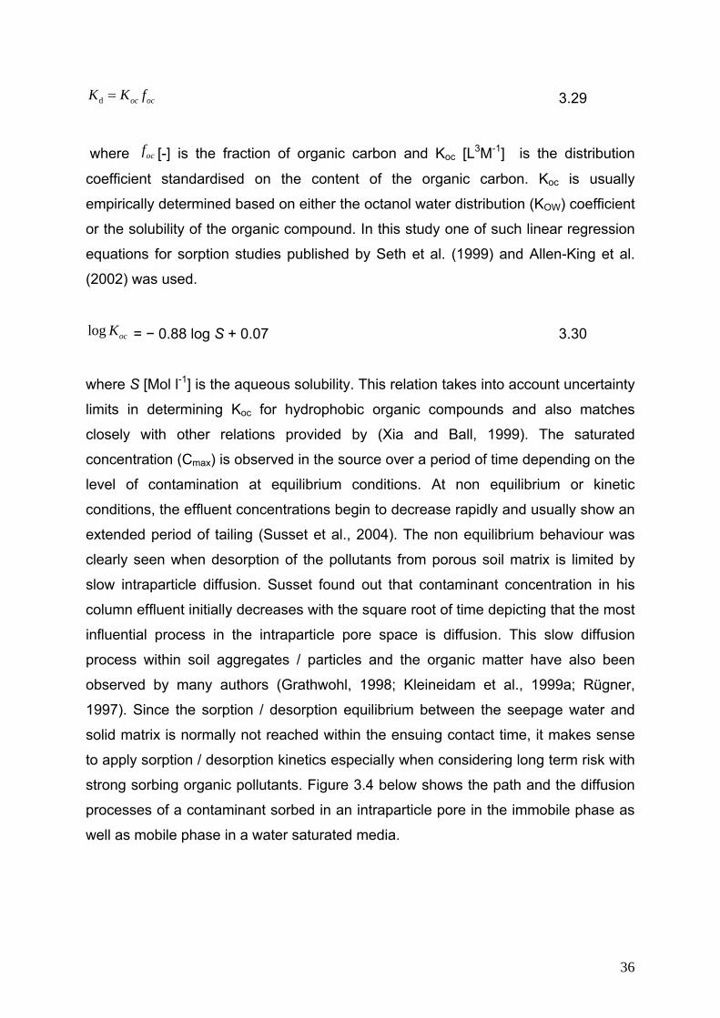
d = oc ocK K f 3.29
where ocf [-] is the fraction of organic carbon and Koc [L3M-1] is the distribution
coefficient standardised on the content of the organic carbon. Koc is usually
empirically determined based on either the octanol water distribution (KOW) coefficient
or the solubility of the organic compound. In this study one of such linear regression
equations for sorption studies published by Seth et al. (1999) and Allen-King et al.
(2002) was used.
log ocK = − 0.88 log S + 0.07 3.30
where S [Mol l-1] is the aqueous solubility. This relation takes into account uncertainty
limits in determining Koc for hydrophobic organic compounds and also matches
closely with other relations provided by (Xia and Ball, 1999). The saturated
concentration (Cmax) is observed in the source over a period of time depending on the
level of contamination at equilibrium conditions. At non equilibrium or kinetic
conditions, the effluent concentrations begin to decrease rapidly and usually show an
extended period of tailing (Susset et al., 2004). The non equilibrium behaviour was
clearly seen when desorption of the pollutants from porous soil matrix is limited by
slow intraparticle diffusion. Susset found out that contaminant concentration in his
column effluent initially decreases with the square root of time depicting that the most
influential process in the intraparticle pore space is diffusion. This slow diffusion
process within soil aggregates / particles and the organic matter have also been
observed by many authors (Grathwohl, 1998; Kleineidam et al., 1999a; Rügner,
1997). Since the sorption / desorption equilibrium between the seepage water and
solid matrix is normally not reached within the ensuing contact time, it makes sense
to apply sorption / desorption kinetics especially when considering long term risk with
strong sorbing organic pollutants. Figure 3.4 below shows the path and the diffusion
processes of a contaminant sorbed in an intraparticle pore in the immobile phase as
well as mobile phase in a water saturated media.
36
immobile phase
tortuosity =
sorbed
contaminant,
diffusion
(sorbent)
dissolved in water
mobile phase
Intraparticle pore
Fig. 3.4: Modelling of intraparticle diffusion (Grathwohl 1998)
The release rate depends on the pollutant properties such as diffusion coefficients,
solubilities, mass and partitioning of the pollutant in the particles. Assuming a
spherical nature of the particles, the sorption / desorption processes in water
saturated media can be described by Fick`s second law in spherical coordinates
given as:
2
2
2=⎡ ⎤∂ ∂ ∂
+⎢∂ ∂⎣ ⎦app
C CDt r r ⎥∂
Cr 3.31
where C [ML-3] is the aqueous concentration, t [T] is time , r [L] is the radial distance
from the centre of the spherical particle and Dapp [L2T-1] is the apparent diffusion
coefficient. According to equation 3.32 below the apparent diffusion coefficient
assumes a linear isotherm between the sorbate and the aqueous concentrations and
that the intraparticle tortuosity is inversely proportional to the intraparticle porosity.
The apparent diffusion coefficient (Dapp) takes into account the geometry of the pores
and relates the aqueous diffusion coefficient (Daq), intraparticle porosity ( ), the
sorption / desorption distribution coefficient (Kd), and the material density of the
particle (ρ) as
ipn
3.32
2
(1 ) ρ⋅
=+ − ⋅ ⋅pp
aq ipa
ip ip d
D nDn n K
37
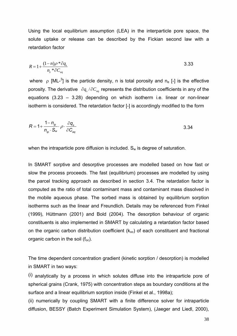
Using the local equilibrium assumption (LEA) in the interparticle pore space, the
solute uptake or release can be described by the Fickian second law with a
retardation factor
3.33
(1 ) *1*ρ− ∂
= +∂
s
e aq
n qRn C
where ρ [ML-3] is the particle density, n is total porosity and ne [-] is the effective
porosity. The derivative represents the distribution coefficients in any of the
equations (3.23 – 3.28) depending on which isotherm i.e. linear or non-linear
isotherm is considered. The retardation factor [-] is accordingly modified to the form
/∂ ∂s aqq C
11 ip s
wip aq
n qRn S C
ρ− ∂
= + ⋅ ⋅⋅ ∂ 3.34
when the intraparticle pore diffusion is included. Sw is degree of saturation.
In SMART sorptive and desorptive processes are modelled based on how fast or
slow the process proceeds. The fast (equilibrium) processes are modelled by using
the parcel tracking approach as described in section 3.4. The retardation factor is
computed as the ratio of total contaminant mass and contaminant mass dissolved in
the mobile aqueous phase. The sorbed mass is obtained by equilibrium sorption
isotherms such as the linear and Freundlich. Details may be referenced from Finkel
(1999), Hüttmann (2001) and Bold (2004). The desorption behaviour of organic
constituents is also implemented in SMART by calculating a retardation factor based
on the organic carbon distribution coefficient (koc) of each constituent and fractional
organic carbon in the soil (foc).
The time dependent concentration gradient (kinetic sorption / desorption) is modelled
in SMART in two ways:
(i) analytically by a process in which solutes diffuse into the intraparticle pore of
spherical grains (Crank, 1975) with concentration steps as boundary conditions at the
surface and a linear equilibrium sorption inside (Finkel et al., 1998a);
(ii) numerically by coupling SMART with a finite difference solver for intraparticle
diffusion, BESSY (Batch Experiment Simulation System), (Jaeger and Liedl, 2000),
38
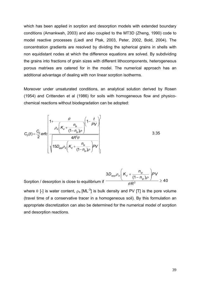
which has been applied in sorption and desorption models with extended boundary
conditions (Amankwah, 2003) and also coupled to the MT3D (Zheng, 1990) code to
model reactive processes (Liedl and Ptak, 2003, Peter, 2002, Bold, 2004). The
concentration gradients are resolved by dividing the spherical grains in shells with
non equidistant nodes at which the difference equations are solved. By subdividing
the grains into fractions of grain sizes with different lithocomponents, heterogeneous
porous matrixes are catered for in the model. The numerical approach has an
additional advantage of dealing with non linear sorption isotherms.
Moreover under unsaturated conditions, an analytical solution derived by Rosen
(1954) and Crittenden et al (1986) for soils with homogeneous flow and physico-
chemical reactions without biodegradation can be adopted:
θ
ρρ
θ
ρρ
⎡ ⎤⎛ ⎞⎢ ⎥+ −⎜ ⎟⎛ ⎞ ⎝ ⎠⎢ ⎥+⎜ ⎟⎢ ⎥⎜ ⎟−⎝ ⎠⎢=
⎢⎢ ⎥
⎛ ⎞⎢ ⎥+⎜ ⎟⎢ ⎥⎜ ⎟−⎢ ⎥⎝ ⎠⎣ ⎦
02
1 1
(1 )( )
2 4
15(1 )
ipb d
ipD
ipapp b d
ip
tPVn
KnCC t erfc
Rn
D K PVn
⎥⎥ 3.35
Sorption / desorption is close to equilibrium if ρ
ρ
θ
⎛ ⎞+⎜ ⎟⎜ ⎟−⎝ ⎠ ≥2
3(1 )
40
ipapp b d
ip
nD K PV
nR
where θ [-] is water content, ρb [ML-3] is bulk density and PV [T] is the pore volume
(travel time of a conservative tracer in a homogeneous soil). By this formulation an
appropriate discretization can also be determined for the numerical model of sorption
and desorption reactions.
39
3.5.5 Biodegradation
Petroleum and charcoal products are used for a large range of chemical synthesis
and fuel in the industry. Some of these chemicals are carcinogenic and can find their
way into the environment through point and diffuse emissions. They persist due to
their inert and hydrophobic nature endangering humans and the ecosystem.
Biodegradation is the only natural attenuation mechanism that has the potential to
destroy the contaminants in-situ with nontoxic inorganic end products even though
adsorption may contribute to the reduction of concentrations to some extent (Peter,
2002). Depending on the type of organic contaminant, bioavailability of the
compound (usually accessible in the aqueous phase), environmental conditions (e.g.
pH, temperature, EC and nutrients) and properties of the microorganisms
(Wiedemeier et al., 1999; Alexander, 1999; Salanitro et al., 1997), the pollution risk
expected at the groundwater table could be greatly reduced. With the exception of
some metabolites which would be toxic biodegradation therefore becomes a reaction
sink by which solute concentrations are reduced (Seagren et al., 1993). Since human
activities though managed continue to pose a threat to the environment, many
laboratory and field studies (Luthy et al., 1994) have been conducted to improve the
understanding of the degradation process and see how the process could be
augmented and enhanced during remediation (Franck, 1963; Nakahara et al., 1977;
Jüttner and Henatsch, 1986; Nielsen and Christensen, 1994; Fischer et al., 1996;
Guha et al., 1999).
3.5.5.1 Microbial degradation processes
The biodegradation process may involve (i) the conversion of contaminants to
mineralized end-products through biological mechanisms (e.g. CO2, H2O, and salts).
(ii) the biological process in which the contaminant is biotransformed into end-
products which are not minerals (e.g. dehalogenation of PCE to TCE, DCE) and (iii)
the process of extracting energy from organic chemicals through oxidation of the
organic chemicals. These biotic processes may take place under aerobic or
anaerobic conditions. The degradation process is aerobic when oxygen becomes the
terminal electron acceptor. Oxygen atoms are incorporated into the organic
40
contaminant resulting in products with hydroxyl groups (Gibson and Subramanian,
1984; Cerniglia, 1984, 1992). The degradation capacity of oxygen related
degradation has been found to be low due to the low solubility of oxygen in water and
the slow diffusion process of oxygen into plumes (Wiedemeier et al., 1999). Based on
the studies of Coover and Sims (1987), Groenewegen and Stolp (1976), and Sims
(1990), Howard et al. (1991) predicted that the half-lifes of PAHs in soils could vary
between 1-2 orders of magnitude and estimated an average value of 570 days. Other
effects such as cometabolism and inhibition have also been observed (Bouchez et
al., 1995; Wackett and Ellis, 1999). The degradation process is anaerobic when all
available oxygen is depleted. Many studies have substantiated the biodegradation of
organic compounds in the absence of oxygen (Kuhn et al., 1985; Zeyer et al., 1986;
Grbic-Galic and Vogel, 1987; Meckenstock, 1999; Wiedemeier et al., 1999). The
degradation is found to proceed in the following order of electron acceptor processes:
denitrification (Evans et al., 1991; Song et al., 1999), manganese reduction, iron
reduction (Lovely and Lonergan, 1990), sulfate reduction (Rabus et al., 1993; Beller
et al., 1996), and methanogenesis (Beller and Edwards, 2000, Lovley et al., 1994b).
According to Wiedemeier et al. (1999) the degradation capacity of the combined
anaerobic processes is 97 % as against 3 % of aerobic process. Some laboratory
studies have shown the anaerobic biodegradation of PAHs (Zhang and Young, 1997;
Galushko et al., 1999; Meckenstock et al., 2000; Rockne et al., 2000; Annweiler et
al., 2000). However field scale biodegradation of PAHs is still debatable.
3.5.5.2 Microbial degradation kinetics
Degradation kinetics studies the rate at which microbial / enzyme reactions occur.
This offers insight into biodegradation mechanics of biomass growth and substrate
depletion. Many biodegradation studies focus on the rate of biodegradation or
biotransformation of pollutants to predict the kinetics of microbial uptake and growth.
In single pure cultures, growth linked processes are often described by Monod
kinetics (Monod, 1940) whilst nongrowth (enzymes) linked biodegradation is
described by Michaelis-Menten kinetics. In other studies mixtures of bacterial cultures
and substrates have been studied to determine the interaction, inhibition parameters,
and effects caused by the substituents of the mixture in such environment (Meyer et
41
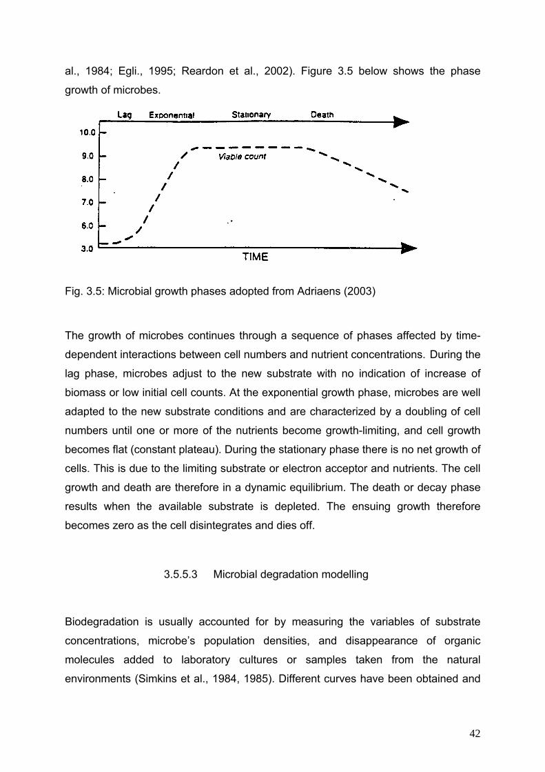
al., 1984; Egli., 1995; Reardon et al., 2002). Figure 3.5 below shows the phase
growth of microbes.
Fig. 3.5: Microbial growth phases adopted from Adriaens (2003)
The growth of microbes continues through a sequence of phases affected by time-
dependent interactions between cell numbers and nutrient concentrations. During the
lag phase, microbes adjust to the new substrate with no indication of increase of
biomass or low initial cell counts. At the exponential growth phase, microbes are well
adapted to the new substrate conditions and are characterized by a doubling of cell
numbers until one or more of the nutrients become growth-limiting, and cell growth
becomes flat (constant plateau). During the stationary phase there is no net growth of
cells. This is due to the limiting substrate or electron acceptor and nutrients. The cell
growth and death are therefore in a dynamic equilibrium. The death or decay phase
results when the available substrate is depleted. The ensuing growth therefore
becomes zero as the cell disintegrates and dies off.
3.5.5.3 Microbial degradation modelling
Biodegradation is usually accounted for by measuring the variables of substrate
concentrations, microbe’s population densities, and disappearance of organic
molecules added to laboratory cultures or samples taken from the natural
environments (Simkins et al., 1984, 1985). Different curves have been obtained and
42
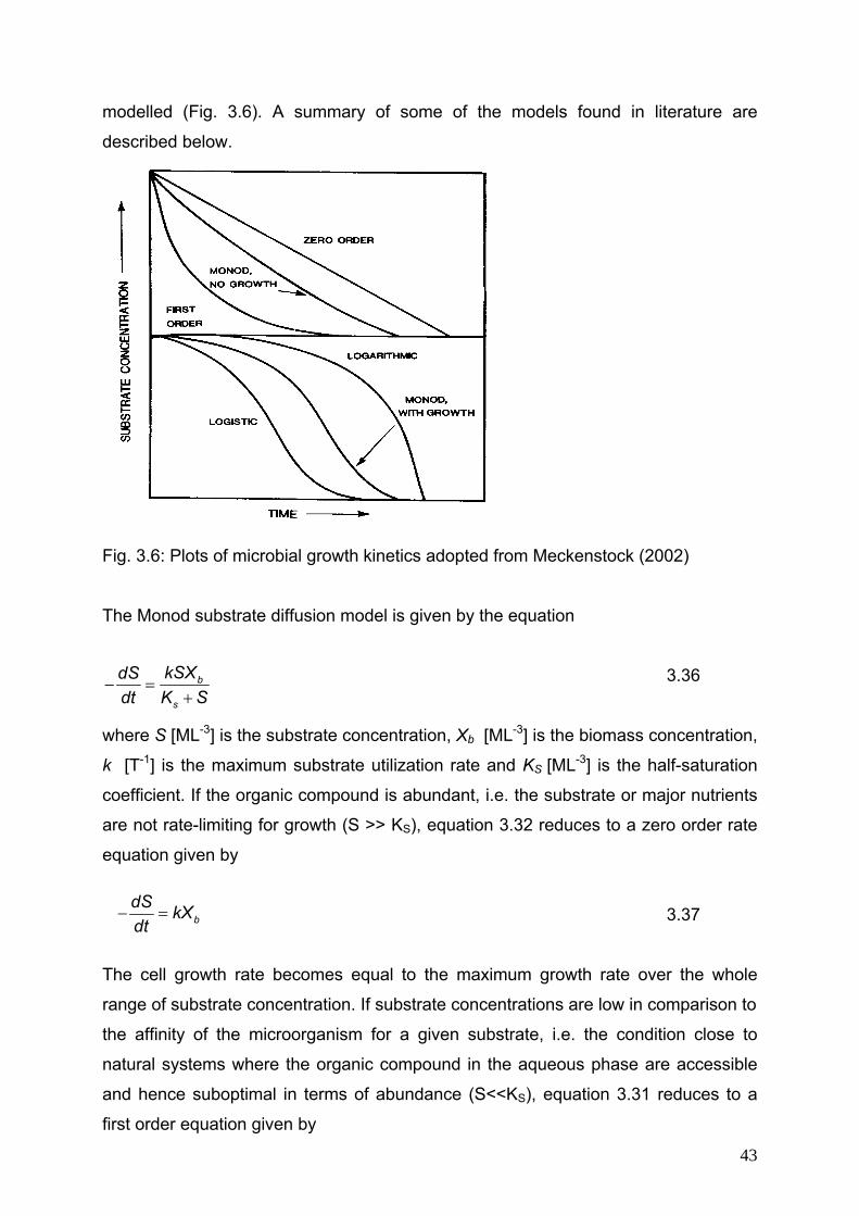
modelled (Fig. 3.6). A summary of some of the models found in literature are
described below.
Fig. 3.6: Plots of microbial growth kinetics adopted from Meckenstock (2002)
The Monod substrate diffusion model is given by the equation
3.36 b
s
kSXdSdt K S
− =+
where S [ML-3] is the substrate concentration, Xb [ML-3] is the biomass concentration,
k [T-1] is the maximum substrate utilization rate and KS [ML-3] is the half-saturation
coefficient. If the organic compound is abundant, i.e. the substrate or major nutrients
are not rate-limiting for growth (S >> KS), equation 3.32 reduces to a zero order rate
equation given by
3.37 bdS kXdt
− =
The cell growth rate becomes equal to the maximum growth rate over the whole
range of substrate concentration. If substrate concentrations are low in comparison to
the affinity of the microorganism for a given substrate, i.e. the condition close to
natural systems where the organic compound in the aqueous phase are accessible
and hence suboptimal in terms of abundance (S<<KS), equation 3.31 reduces to a
first order equation given by
43
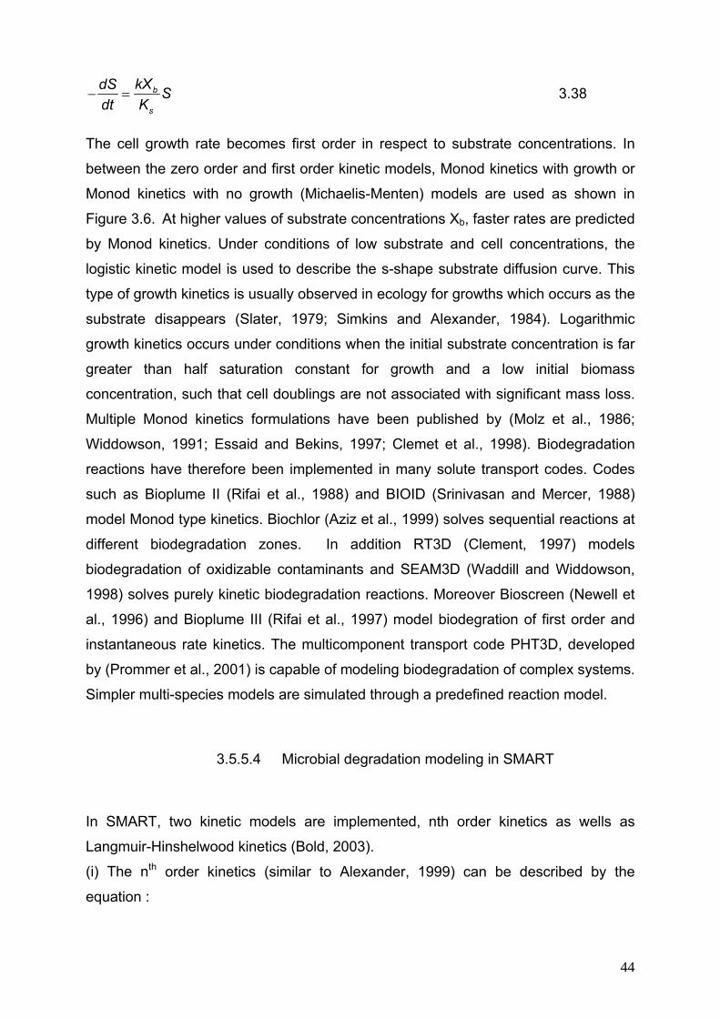
3.38
b
s
kXdS Sdt K
− =
The cell growth rate becomes first order in respect to substrate concentrations. In
between the zero order and first order kinetic models, Monod kinetics with growth or
Monod kinetics with no growth (Michaelis-Menten) models are used as shown in
Figure 3.6. At higher values of substrate concentrations Xb, faster rates are predicted
by Monod kinetics. Under conditions of low substrate and cell concentrations, the
logistic kinetic model is used to describe the s-shape substrate diffusion curve. This
type of growth kinetics is usually observed in ecology for growths which occurs as the
substrate disappears (Slater, 1979; Simkins and Alexander, 1984). Logarithmic
growth kinetics occurs under conditions when the initial substrate concentration is far
greater than half saturation constant for growth and a low initial biomass
concentration, such that cell doublings are not associated with significant mass loss.
Multiple Monod kinetics formulations have been published by (Molz et al., 1986;
Widdowson, 1991; Essaid and Bekins, 1997; Clemet et al., 1998). Biodegradation
reactions have therefore been implemented in many solute transport codes. Codes
such as Bioplume II (Rifai et al., 1988) and BIOID (Srinivasan and Mercer, 1988)
model Monod type kinetics. Biochlor (Aziz et al., 1999) solves sequential reactions at
different biodegradation zones. In addition RT3D (Clement, 1997) models
biodegradation of oxidizable contaminants and SEAM3D (Waddill and Widdowson,
1998) solves purely kinetic biodegradation reactions. Moreover Bioscreen (Newell et
al., 1996) and Bioplume III (Rifai et al., 1997) model biodegration of first order and
instantaneous rate kinetics. The multicomponent transport code PHT3D, developed
by (Prommer et al., 2001) is capable of modeling biodegradation of complex systems.
Simpler multi-species models are simulated through a predefined reaction model.
3.5.5.4 Microbial degradation modeling in SMART
In SMART, two kinetic models are implemented, nth order kinetics as wells as
Langmuir-Hinshelwood kinetics (Bold, 2003).
(i) The nth order kinetics (similar to Alexander, 1999) can be described by the
equation :
44
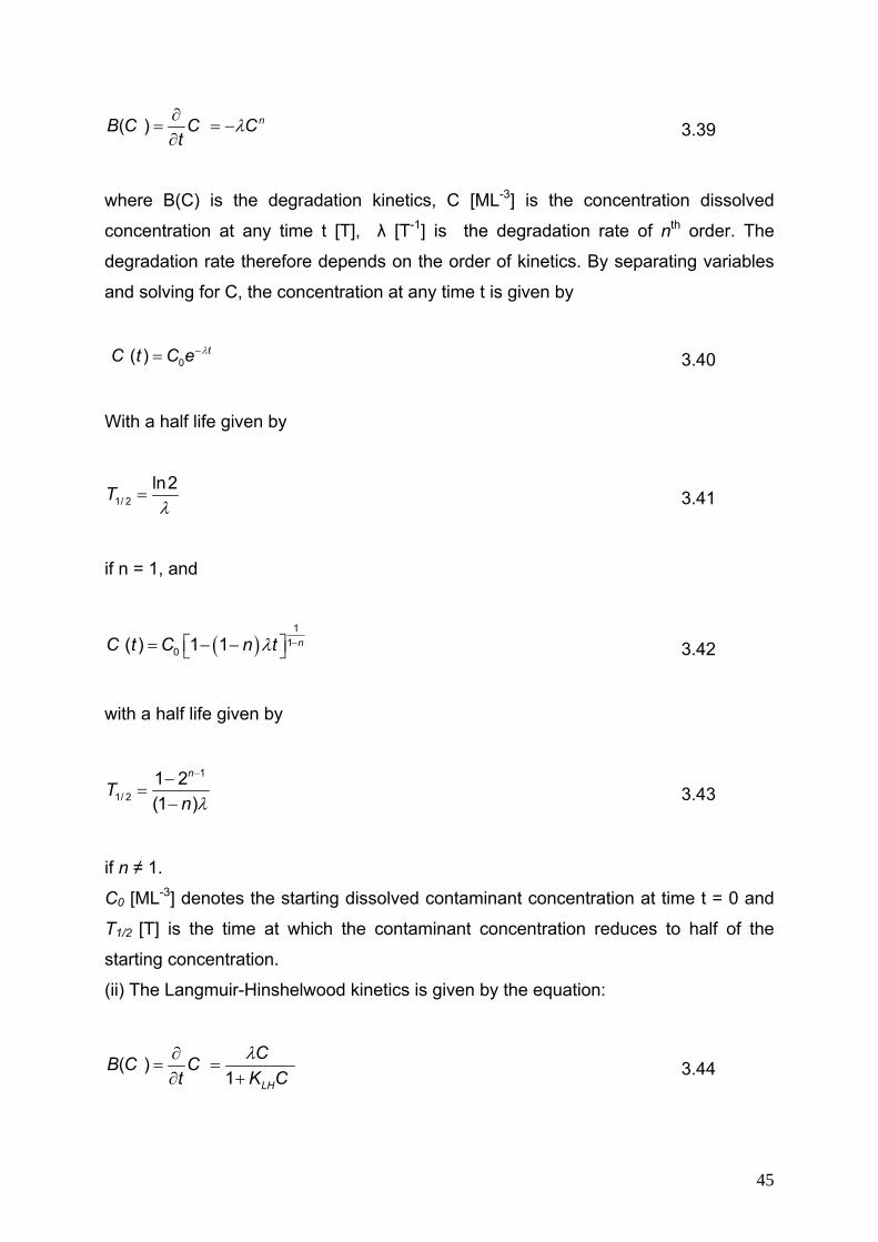
( ) nB C C Ct
λ∂= = −∂ 3.39
where B(C) is the degradation kinetics, C [ML-3] is the concentration dissolved
concentration at any time t [T], λ [T-1] is the degradation rate of nth order. The
degradation rate therefore depends on the order of kinetics. By separating variables
and solving for C, the concentration at any time t is given by
0( ) tC t C e λ−= 3.40
With a half life given by
1/ 2ln2Tλ
= 3.41
if n = 1, and
( )1
10( ) 1 1 nC t C n tλ −⎡= − −⎣ ⎤⎦ 3.42
with a half life given by
1
1/ 21 2(1 )
n
Tn λ
−−=
− 3.43
if n ≠ 1.
C0 [ML-3] denotes the starting dissolved contaminant concentration at time t = 0 and
T1/2 [T] is the time at which the contaminant concentration reduces to half of the
starting concentration.
(ii) The Langmuir-Hinshelwood kinetics is given by the equation:
( )1 LH
CB C Ct K
λ∂= =∂ + C 3.44
45
where λ [T-1] and KLH [-] represent the two kinetic parameters. It is only valid for
biodegradation scenarios in which the decay starts from a zero order kinetics and
moves to a first order kinetics. An implicit solution to equation 3.39 is given by
ln LH LHo o
C CK KC C
tλ+ = − 3.45
With a half life of
21/ 2
ln2LHK
Tλ+
= 3.46
The parameter KLH determines the order of the degradation kinetics. For KLH = 0, the
kinetics reduces to first order but tends to zero order as KLH increases.
Biodegradation is implemented in SMART by considering each model cell as
independent batch system. Biodegradation with equilibrium sorption is coupled and
solved iteratively while biodegradation with sorption kinetics is coupled with the
integration of the intraparticle diffusion model BESSY with batch boundary conditions.
The expected long term concentration with first order decay and reaction function that
follows the CDE formulation is given by
2
4exp 1 12ovx DC CD v
λ∞
⎡ ⎤⎛ ⎞= − +⎢ ⎜⎜⎢ ⎥⎝ ⎠⎣ ⎦
⎥⎟⎟ 3.47
where Co [ML-3] is the input concentration and C∞ [ML-3] is the expected long term
concentration at the point of compliance (Bold, 2003).
46
3.5.6 Particle-facilitated transport
3.5.6.1 Particle-facilitated transport in porous media
Particle facilitated or particle mediated transport, though not modeled in this thesis, is
reviewed as part of the reactive code SMART. The terms particles and colloids are
used interchangeably. Particles movement in porous media is well reported in
literature (Avogadro et al., 1984; Marchy and Zachara., 1989; Moulin and Ouzounian,
1992; Ryan and Elimelech, 1995). Some of the particles or colloids though
imperceptible can enhance the transport of solute which can endanger subsurface
waters. According to (McCarthy et al., 2004) the impact of mobile colloid transport in
terms of human risk from infiltrating pathogens and environmental and geological
hazards from contaminant transport to groundwater can be significant. For instance
colloid transport becomes increasingly important in high level nuclear waste
repositories where the only form of transport is through fractures that may be
developed in low permeability geological formations (Chryskopoulos and Abdel-
Salam, 1995; Ryan and Elimelech, 1996). Also the effects of aqueous chemical
conditions of colloid dispersion and permeability of geological settings have been
carried out to improve the recovery of oil and gas (Khilar and Fogler, 1984; Cerda,
1987; Kia et al., 1987). Pathogens found in drinking wells are reported to have
originated from sources such as sewage sludge, animal waste and septic fields and
transported by microbial particles. Bacteria transport also has a dual role as a
pathogen risk and a remedial option to degrade and or immobilize contaminants in
groundwater (McCarthy and McKay, 2004). In several laboratory and field studies,
particles have been found to enhance transport (McDowell-Boyer et al., 1986;
Penrose et al., 1990) of contaminants such as radionuclides (Airey, 1986; Haldeman
et al., 1991; McCarthy et al., 1998; Flurry et al., 2002), metals (McCarthy and
Zachara, 1989; Grolimund et al., 1996; Karathanasis, 1999), organics (Vinten et al.,
1983; Jonson-Logan et al., 1992), pesticides (de Jonge et al., 1998; Sprague et al.,
2000; Williams et al., 2000), and inorganics in porous media (Gounaris et al., 1993).
The enhancement has been attributed to the translocation of particle-reactive
contaminant effects in soils (Steenhuis et al., 2005). PAH contaminants have also
been reported sorbing to colloids thereby reducing their bioavailability (McCarthy and
Jimenez, 1985) and consequently their uptake by microbes (Dohse and Lion, 1994).
47
However these PAHs could be partly available for microbes in the presence of some
surfactants (Guha and Jaffe, 1996a, b; Guha et al., 1998). The particles may be in
the form of clay minerals, oxides, carbonates, humic substances, microbial
elucidates, bacteria, polystyrene microspheres and viruses (Higgo et al., 1993). They
are mostly generated and become mobilized through processes such as chemical
and physical perturbations (Lallay et al., 1987; Wood and Ehrlich, 1978; Gschwend
and Reynolds, 1987), rapid infiltration of rainfall (Kaplan et al., 1993; Ryan et al.,
1995), an increase in pH, decrease in ionic strength due to infiltration of dilute
precipitation water (Frenkel, 1978; Abu-Sharar et al., 1987) and hydrodynamic
detachment of their solutions (Abdel-Salam and Chrysikopoulos, 1995). Also
increasing concentration of surfactants and dissolved organic matter and soil
macropores can mobilize colloids or particles.
In groundwaters, the deposition of particles primarily controls the transport of colloids.
Filtration theories are used to calculate and analyse the deposition rate in porous
media. Details of the filtration theories based on the Langrangian and Eulerian
approaches (section 3.3) applied to particles deposition may be referenced from
(Adamczyk et al., 1983; Tien, 1989; Ryan and Elimelech, 1995).
In the unsaturated zone mechanisms such as advection and dispersion (Abdel-Salam
and Chrysikopoulos, 1995; Lenhart and Saiers, 2002), preferential flow (Bourke,
1987; Steenhuis et al., 2001), diffusion (Yao et al., 1971; Schelde et al., 2002)
sorption (Sposito, 1984; Toran and Palumbo, 1992; Schäfer at al., 1998a; Chu et al.,
2001), film straining (Wan and Tokunaga, 1997), microbial contamination in aquifers
(McCarthy and McKay, 2004) and other pore scale and air-water-solid interfaces
(Lanhart and Saiers, 2002; Steenhuis et al., 2005) affect transport and distribution of
particles.
3.5.6.2 Particle mediated transport modelling in SMART
In the subsurface several interactions between particles, contaminants and the host
matrix can take place. According to Bold (2004) the significant interactions are
between particle and matrix, contaminant and matrix, and contaminant and particle.
48
Biodegradation in the aqueous phase affects these interactions. In SMART the
interaction process between particles and contaminant can be considered as (i)
equilibrium (sorption rate of solute is significantly larger than its mass flow rate) (ii)
kinetic (sorption rate of solute is comparable to its mass flow rate) and (iii) decoupled
(no interaction). Assuming that immobilised particles have no effect on the effective
porosity of the porous medium, the equation describing the transport of particles
along a streamtube is given by
, ,c j c j j c jC C K Ct τ∂ ∂
+ = −∂ ∂
3.48 ,
where Cc,j [ML-3] is the mobile particle concentration, j is an index characterising
particle size and material [-] and K [T-1] is the particle deposition rate coefficient.
According to the right-hand side of equation (3.48) deposition is modelled by a first
order rate law. If the interaction between particle and matrix can be described as an
equilibrium process, then equation (3.48) is replaced by
3.49 ,
, ,
( )0b matrix c j
c j c j
s CC C
t tρ
θ⎛ ⎞∂ ∂
+ +⎜ ⎟∂ ∂⎝ ⎠=
where ρb [ML-3] is the bulk density of the porous medium, s,matrix, can be any type of
equilibrium isotherm between particles and solid matrix, and θ [-] is the water content.
Taking into account the sorption of contaminants by matrix, mobile and immobile
particles and assuming a first order decay of the dissolved contaminants in the
aqueous phase the contaminant transport for a single type of particle is described by
the equation
[ ]( ) ( )( ) ( )b matrix D cim D c cDD cm D c D cm D c
e e
S C S CC S C C C S C Ct n n
ρ ρ σ Cλτ
⎡ ⎤∂ ∂+ + + + + =⎢ ⎥∂ ∂⎣ ⎦
−
3.50
where CD [ML-3] is the dissolved contaminant concentration, ρb [ML-3] is the bulk
density of the porous medium, ρc is the particle dry solid density, σc [-] is the volume
of immobile particles per unit volume and λ [T-1] is the first-order degradation rate
constant. Smatrix(CD), Scm(CD), Scim(CD) are the ratios of sorbed solute mass per unit
mass of solid matrix, mobile and immobile particles, respectively. The mechanisms
49
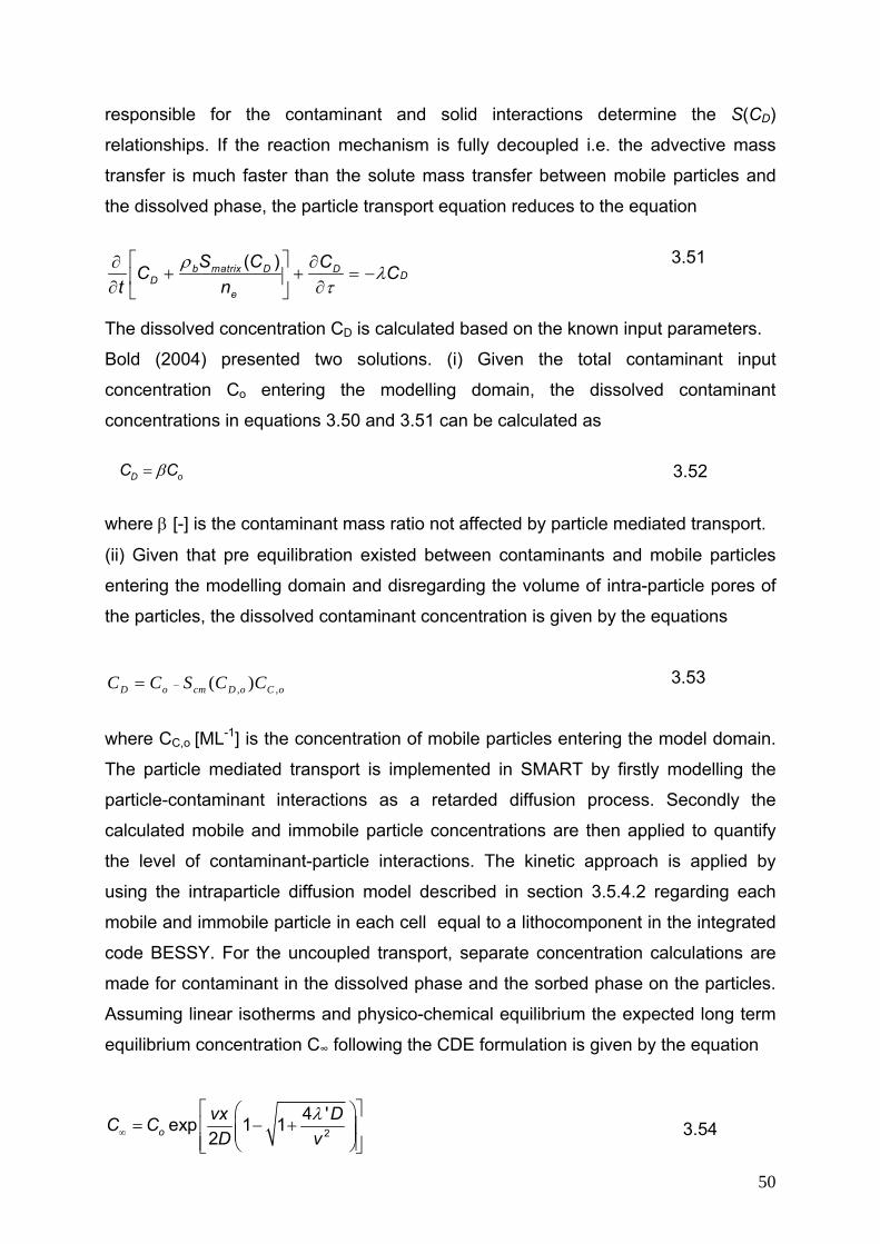
responsible for the contaminant and solid interactions determine the S(CD)
relationships. If the reaction mechanism is fully decoupled i.e. the advective mass
transfer is much faster than the solute mass transfer between mobile particles and
the dissolved phase, the particle transport equation reduces to the equation
3.51
( )b matrix D D DDe
S C CC Ct n
ρλ
τ⎡ ⎤ ∂∂
+ + =⎢ ⎥∂ ∂⎣ ⎦−
The dissolved concentration CD is calculated based on the known input parameters.
Bold (2004) presented two solutions. (i) Given the total contaminant input
concentration Co entering the modelling domain, the dissolved contaminant
concentrations in equations 3.50 and 3.51 can be calculated as
3.52 D oC Cβ=
where β [-] is the contaminant mass ratio not affected by particle mediated transport.
(ii) Given that pre equilibration existed between contaminants and mobile particles
entering the modelling domain and disregarding the volume of intra-particle pores of
the particles, the dissolved contaminant concentration is given by the equations
3.53 , ,( )−=D o cm D o CC C S C C o
where CC,o [ML-1] is the concentration of mobile particles entering the model domain.
The particle mediated transport is implemented in SMART by firstly modelling the
particle-contaminant interactions as a retarded diffusion process. Secondly the
calculated mobile and immobile particle concentrations are then applied to quantify
the level of contaminant-particle interactions. The kinetic approach is applied by
using the intraparticle diffusion model described in section 3.5.4.2 regarding each
mobile and immobile particle in each cell equal to a lithocomponent in the integrated
code BESSY. For the uncoupled transport, separate concentration calculations are
made for contaminant in the dissolved phase and the sorbed phase on the particles.
Assuming linear isotherms and physico-chemical equilibrium the expected long term
equilibrium concentration C∞ following the CDE formulation is given by the equation
2
4 'exp 1 12ovx DC CD v
λ∞
⎡ ⎤⎛ ⎞= − +⎢ ⎜⎜⎢ ⎥⎝ ⎠⎣ ⎦
⎥⎟⎟ 3.54
50
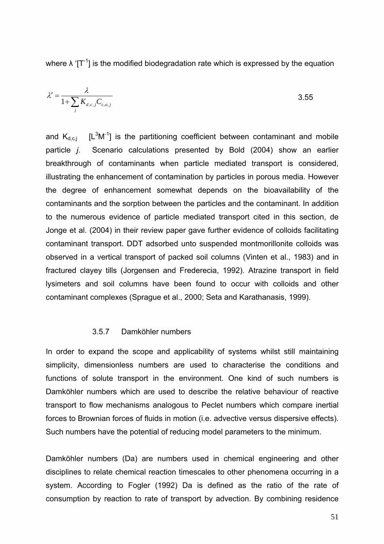
where λ ‘[T-1] is the modified biodegradation rate which is expressed by the equation
, , , ,1λλ′ =
+∑ d c j c o jj
K C 3.55
and Kd,c,j [L3M-1] is the partitioning coefficient between contaminant and mobile
particle j. Scenario calculations presented by Bold (2004) show an earlier
breakthrough of contaminants when particle mediated transport is considered,
illustrating the enhancement of contamination by particles in porous media. However
the degree of enhancement somewhat depends on the bioavailability of the
contaminants and the sorption between the particles and the contaminant. In addition
to the numerous evidence of particle mediated transport cited in this section, de
Jonge et al. (2004) in their review paper gave further evidence of colloids facilitating
contaminant transport. DDT adsorbed unto suspended montmorillonite colloids was
observed in a vertical transport of packed soil columns (Vinten et al., 1983) and in
fractured clayey tills (Jorgensen and Frederecia, 1992). Atrazine transport in field
lysimeters and soil columns have been found to occur with colloids and other
contaminant complexes (Sprague et al., 2000; Seta and Karathanasis, 1999).
3.5.7 Damköhler numbers In order to expand the scope and applicability of systems whilst still maintaining
simplicity, dimensionless numbers are used to characterise the conditions and
functions of solute transport in the environment. One kind of such numbers is
Damköhler numbers which are used to describe the relative behaviour of reactive
transport to flow mechanisms analogous to Peclet numbers which compare inertial
forces to Brownian forces of fluids in motion (i.e. advective versus dispersive effects).
Such numbers have the potential of reducing model parameters to the minimum.
Damköhler numbers (Da) are numbers used in chemical engineering and other
disciplines to relate chemical reaction timescales to other phenomena occurring in a
system. According to Fogler (1992) Da is defined as the ratio of the rate of
consumption by reaction to rate of transport by advection. By combining residence
51
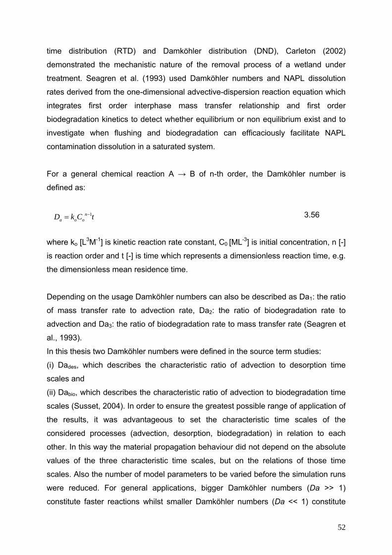
time distribution (RTD) and Damköhler distribution (DND), Carleton (2002)
demonstrated the mechanistic nature of the removal process of a wetland under
treatment. Seagren et al. (1993) used Damköhler numbers and NAPL dissolution
rates derived from the one-dimensional advective-dispersion reaction equation which
integrates first order interphase mass transfer relationship and first order
biodegradation kinetics to detect whether equilibrium or non equilibrium exist and to
investigate when flushing and biodegradation can efficaciously facilitate NAPL
contamination dissolution in a saturated system.
For a general chemical reaction A → B of n-th order, the Damköhler number is
defined as:
3.56 1−= na o oD k C t
where ko [L3M-1] is kinetic reaction rate constant, C0 [ML-3] is initial concentration, n [-]
is reaction order and t [-] is time which represents a dimensionless reaction time, e.g.
the dimensionless mean residence time.
Depending on the usage Damköhler numbers can also be described as Da1: the ratio
of mass transfer rate to advection rate, Da2: the ratio of biodegradation rate to
advection and Da3: the ratio of biodegradation rate to mass transfer rate (Seagren et
al., 1993).
In this thesis two Damköhler numbers were defined in the source term studies:
(i) Dades, which describes the characteristic ratio of advection to desorption time
scales and
(ii) Dabio, which describes the characteristic ratio of advection to biodegradation time
scales (Susset, 2004). In order to ensure the greatest possible range of application of
the results, it was advantageous to set the characteristic time scales of the
considered processes (advection, desorption, biodegradation) in relation to each
other. In this way the material propagation behaviour did not depend on the absolute
values of the three characteristic time scales, but on the relations of those time
scales. Also the number of model parameters to be varied before the simulation runs
were reduced. For general applications, bigger Damköhler numbers (Da >> 1)
constitute faster reactions whilst smaller Damköhler numbers (Da << 1) constitute
52
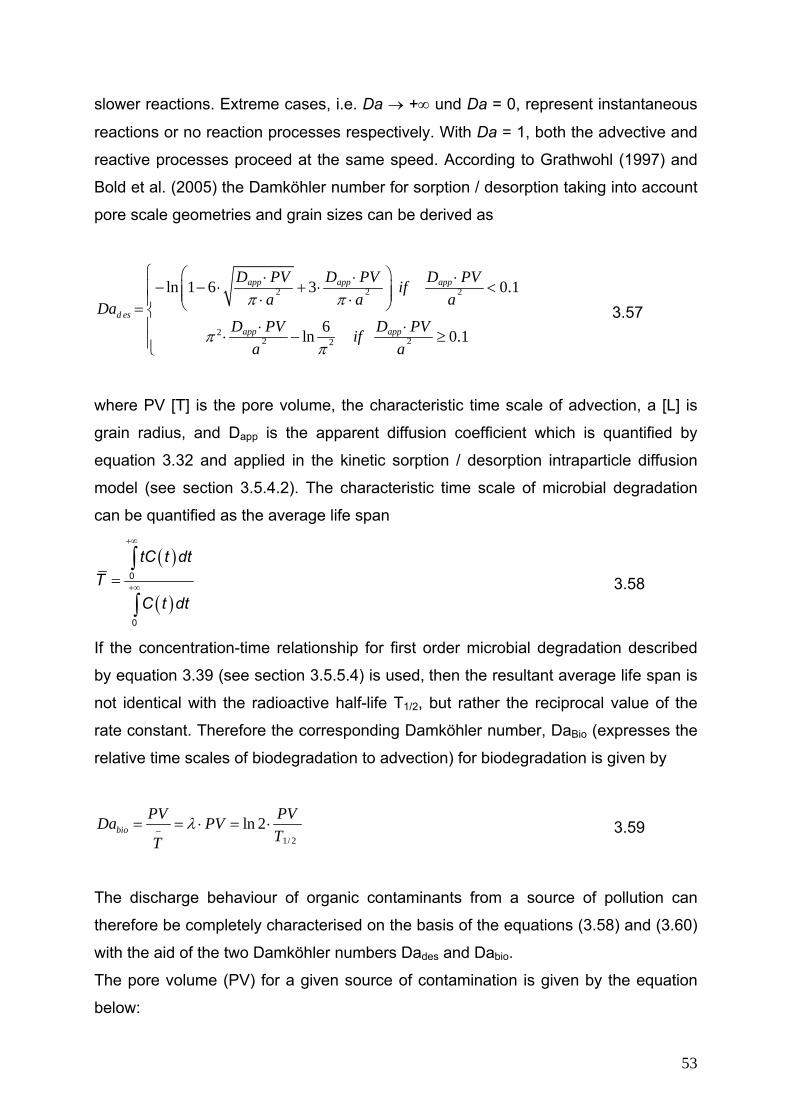
slower reactions. Extreme cases, i.e. Da → +∞ und Da = 0, represent instantaneous
reactions or no reaction processes respectively. With Da = 1, both the advective and
reactive processes proceed at the same speed. According to Grathwohl (1997) and
Bold et al. (2005) the Damköhler number for sorption / desorption taking into account
pore scale geometries and grain sizes can be derived as
2 2 2
22 22
ln 1 6 3 0.1
6ln 0.1
π π
ππ
⎧ ⎛ ⎞⋅ ⋅ ⋅− − ⋅ + ⋅ <⎪ ⎜ ⎟⎜ ⎟⎪ ⋅ ⋅⎝ ⎠= ⎨
⋅ ⋅⎪⋅ − ≥⎪⎩
app app app
esd
app app
D PV D PV D PVifa a aDa
D PV D PVifa a
3.57
where PV [T] is the pore volume, the characteristic time scale of advection, a [L] is
grain radius, and Dapp is the apparent diffusion coefficient which is quantified by
equation 3.32 and applied in the kinetic sorption / desorption intraparticle diffusion
model (see section 3.5.4.2). The characteristic time scale of microbial degradation
can be quantified as the average life span
( )
( )0
0
tC t dtT
C t dt
+∞
+∞=∫
∫ 3.58
If the concentration-time relationship for first order microbial degradation described
by equation 3.39 (see section 3.5.5.4) is used, then the resultant average life span is
not identical with the radioactive half-life T1/2, but rather the reciprocal value of the
rate constant. Therefore the corresponding Damköhler number, DaBio (expresses the
relative time scales of biodegradation to advection) for biodegradation is given by
1/ 2ln 2λ−= = ⋅ = ⋅bio
PV PVDa PVTT
3.59
The discharge behaviour of organic contaminants from a source of pollution can
therefore be completely characterised on the basis of the equations (3.58) and (3.60)
with the aid of the two Damköhler numbers Dades and Dabio.
The pore volume (PV) for a given source of contamination is given by the equation
below:
53
wn S LPVQ⋅ ⋅
= 3.60
where n [-] is porosity, Sw [-] is degree of water saturation, L [L] is the thickness of the
source and Q [LT-1] groundwater flux. In contaminant and seepage water
(“Sickerwasserprognose”) studies, breakthrough plots are sometimes expressed in
units of concentrations versus water to solid mass ratios (W/F). W and F represent
the time-independent volume of water passing through the source zone and the
mass of solids in the source zone, respectively. A conversion between dimensionless
time and water-solid mass ratio is given by the relations:
/' /e
M At Wn L
= ⋅⋅
F 3.61
where t’ [-] is time normalised by pore volume, M/A [ML2] is solid mass per unit cross-
sectional area, and W/F [L3M-1] is the water-solid mass ratio. The normalised pore
volume time is given by the equation:
t ' = t/PV 3.62
This conversion assumes that groundwater flow is at steady state. The use of the
normalised pore volume time t’ offers a crucial advantage in the context of setting of
tasks, because the retention time of the pollutant in the mobile phase is thereby
included. This enters directly in the determination of the Damköhler numbers (Dades
and Dabio) with which the relative contributions of desorption kinetics and the
microbial degradation in the discharge behaviour are quantified.
54
Chapter 4 4 SOURCE TERM MODELLING
4.1 Introduction
4.2 Methodology
One goal of this study was the development of a source term function for organic
pollutants (in particular non volatile PAHs). This function was to quantify the time–
dependent leaching behaviour of materials from sources of contaminants and serve
as a practical tool in seepage water prognosis. The source term function included
primarily measured variables (for example source term thickness, pollutant-solid
distribution coefficients, seepage water flow rates and contents of typical pollutants).
Initially, selections of realistic representative values and or ranges of values of
measured variables for the leaching behaviour were made (thickness of source zone,
pollutant solid interaction parameters such as foc, porosity and bulk density, flow
rate, pollutant type etc.) to cover the relevant spectrum of leaching curves.
Laboratory results (Henzler, 2004; Susset, 2004) mainly focusing on seepage water
prognoses were also included. Series of linear forward simulations were run with the
modelling tool SMART (Streamtube Model for Advective and Reactive Transport) for
each combination of variables. Breakthrough curves of each simulated scenario were
evaluated. Depending on the type and properties of the organic pollutant under
consideration, different types of effluent leaching curves were obtained. Appropriate
mathematical functions were then used to characterise these numerical curves. In
general two groups of curves were obtained with coefficients which were obtained by
fitting the analytical curves to the numerical curves while ensuring minimum
discrepancies. The optimization of the curves and minimisation of the discrepancies
were accomplished by the method of least squares. As a result of this step, the
source strength function for the leaching behaviour of organic pollutants was
obtained. This function does not only serve as seepage water management tool but
also as a close-to-reality boundary condition for the transport modelling of organic
contaminants in the subsurface.
55
4.3 Processes and modelling assumptions
In order to determine the source strength function, the major and relevant processes
must be taken into consideration. Advection, desorption kinetics and microbial
degradation were considered as relevant discharge processes. Advection accounted
for the bulk movement of the fluid or liquid phase as polluted solutes deplete down to
the transport zone. The depletion or release of the solutes from the solid grain matrix
with time is accounted for by the desorption kinetics as described by the intraparticle
diffusion model (section 3.5.4.2). Microbial degradation which accounts for the
transformation of the solutes as they encounter microorganisms in the dissolved
phased was modelled with a first order rate kinetics (see section 3.5.5). The following
modelling assumptions were made:
• The flow in the unsaturated zone was at steady state with time invariant flow.
This is acceptable for longterm investigations in which average concentrations
are more representative rather than variations or extreme values.
• The model parameters that quantify the reactive processes such as desorption
(nip,ρ, Kd, Daq und grain radius) and microbial degradation (λ and/or T1/2 ) were
spatially constant.
• The soil materials were homogeneous with respect to grain size and lithology.
• Desorption kinetics was simulated with the aid of the intraparticle diffusion
model.
• Solute transport in the interparticle pores is purely advective i.e. there is no
mass transfer between streamtubes (no dispersion).
• A concentration equilibrium existed between mobile and immobile phase at the
beginning of simulation (t=0). This concentration equilibrium is determined by
the distribution coefficient Kd.
• Microbial degradation is represented in the model by a first order rate law.
Degradation occurred solely in the interparticle pore area.
56
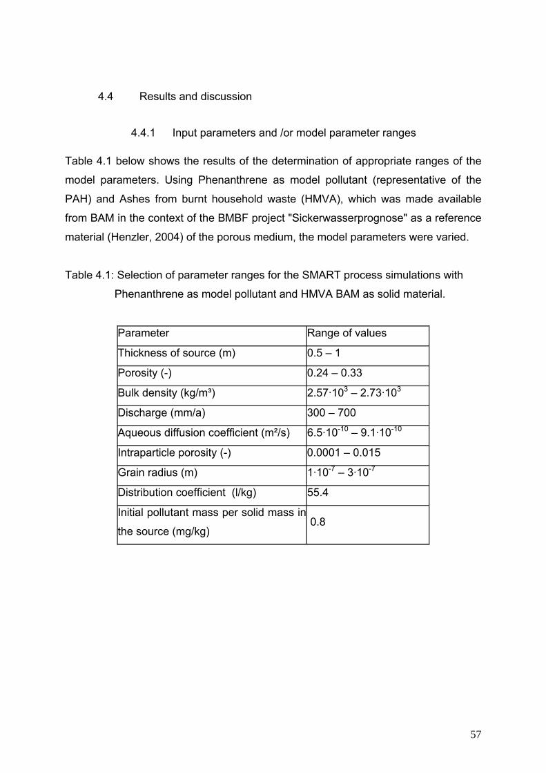
4.4 Results and discussion
4.4.1 Input parameters and /or model parameter ranges Table 4.1 below shows the results of the determination of appropriate ranges of the
model parameters. Using Phenanthrene as model pollutant (representative of the
PAH) and Ashes from burnt household waste (HMVA), which was made available
from BAM in the context of the BMBF project "Sickerwasserprognose" as a reference
material (Henzler, 2004) of the porous medium, the model parameters were varied.
Table 4.1: Selection of parameter ranges for the SMART process simulations with
Phenanthrene as model pollutant and HMVA BAM as solid material.
Parameter Range of values
Thickness of source (m) 0.5 – 1
Porosity (-) 0.24 – 0.33
Bulk density (kg/m³) 2.57·103 – 2.73·103
Discharge (mm/a) 300 – 700
Aqueous diffusion coefficient (m²/s) 6.5·10-10 – 9.1·10-10
Intraparticle porosity (-) 0.0001 – 0.015
Grain radius (m) 1·10-7 – 3·10-7
Distribution coefficient (l/kg) 55.4
Initial pollutant mass per solid mass in
the source (mg/kg) 0.8
57
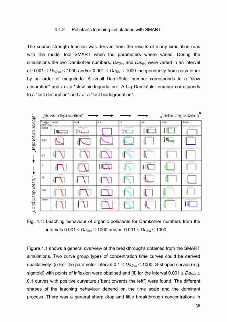
4.4.2 Pollutants leaching simulations with SMART
The source strength function was derived from the results of many simulation runs
with the model tool SMART when the parameters where varied. During the
simulations the two Damköhler numbers, DaDes and DaAbb were varied in an interval
of 0.001 ≤ DaDes ≤ 1000 and/or 0.001 ≤ DaBio ≤ 1000 independently from each other
by an order of magnitude. A small Damköhler number corresponds to a “slow
desorption“ and / or a “slow biodegradation“. A big Damköhler number corresponds
to a “fast desorption“ and / or a “fast biodegradation“.
Fig. 4.1: Leaching behaviour of organic pollutants for Damköhler numbers from the
intervals 0.001 ≤ DaDes ≤ 1000 and/or. 0.001 ≤ DaBio ≤ 1000.
Figure 4.1 shows a general overview of the breakthroughs obtained from the SMART
simulations. Two curve group types of concentration time curves could be derived
qualitatively: (i) For the parameter interval 0.1 ≤ DaDes ≤ 1000, S-shaped curves (e.g.
sigmoid) with points of inflexion were obtained and (ii) for the interval 0.001 ≤ DaDes ≤
0.1 curves with positive curvature (“bent towards the left”) were found. The different
shapes of the leaching behaviour depend on the time scale and the dominant
process. There was a general sharp drop and little breakthrough concentrations in
58
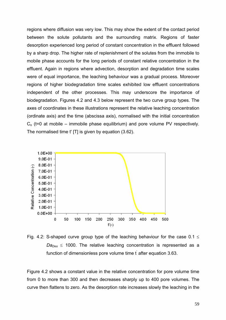
regions where diffusion was very low. This may show the extent of the contact period
between the solute pollutants and the surrounding matrix. Regions of faster
desorption experienced long period of constant concentration in the effluent followed
by a sharp drop. The higher rate of replenishment of the solutes from the immobile to
mobile phase accounts for the long periods of constant relative concentration in the
effluent. Again in regions where advection, desorption and degradation time scales
were of equal importance, the leaching behaviour was a gradual process. Moreover
regions of higher biodegradation time scales exhibited low effluent concentrations
independent of the other processes. This may underscore the importance of
biodegradation. Figures 4.2 and 4.3 below represent the two curve group types. The
axes of coordinates in these illustrations represent the relative leaching concentration
(ordinate axis) and the time (abscissa axis), normalised with the initial concentration
Co (t=0 at mobile – immobile phase equilibrium) and pore volume PV respectively.
The normalised time t' [T] is given by equation (3.62).
Fig. 4.2: S-shaped curve group type of the leaching behaviour for the case 0.1 ≤
DaDes ≤ 1000. The relative leaching concentration is represented as a
function of dimensionless pore volume time t’ after equation 3.63.
Figure 4.2 shows a constant value in the relative concentration for pore volume time
from 0 to more than 300 and then decreases sharply up to 400 pore volumes. The
curve then flattens to zero. As the desorption rate increases slowly the leaching in the
59
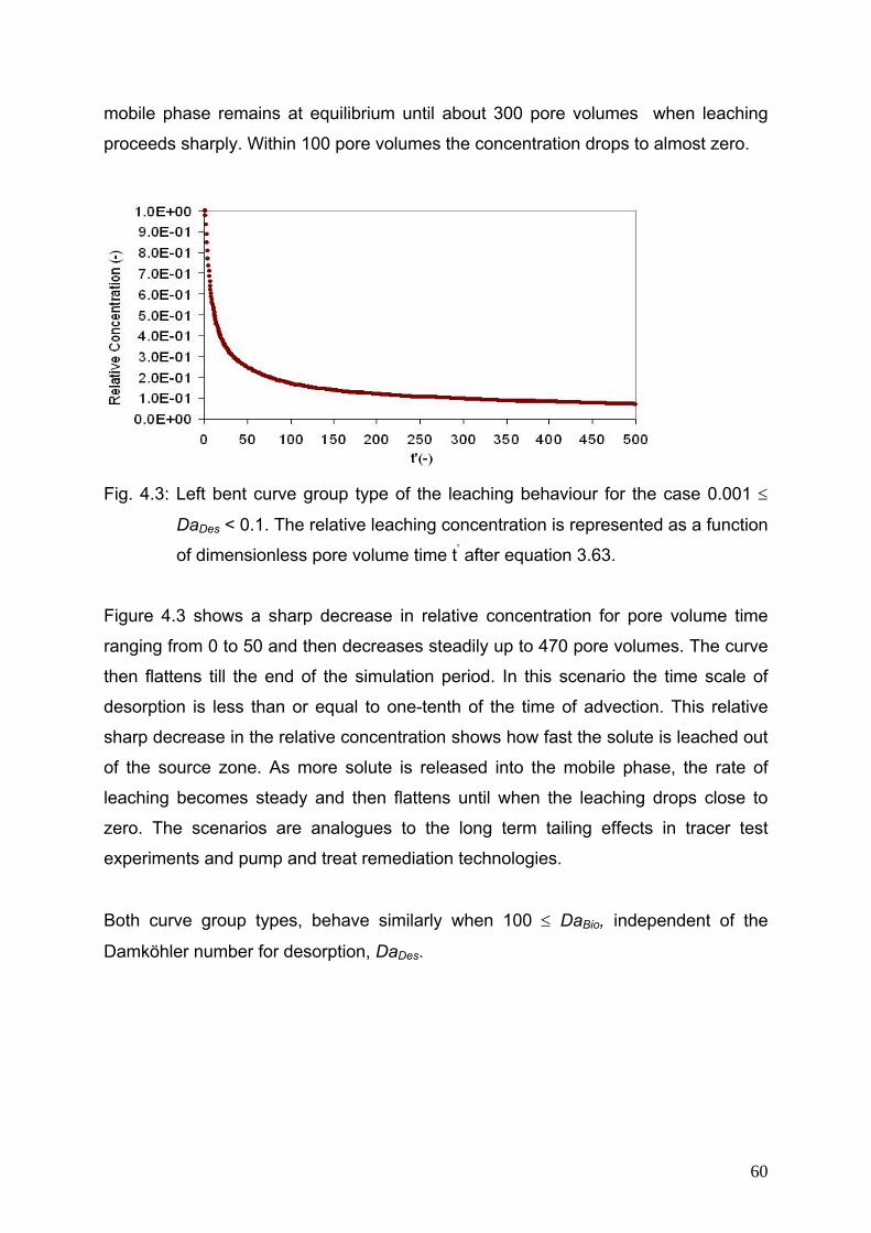
mobile phase remains at equilibrium until about 300 pore volumes when leaching
proceeds sharply. Within 100 pore volumes the concentration drops to almost zero.
Fig. 4.3: Left bent curve group type of the leaching behaviour for the case 0.001 ≤
DaDes < 0.1. The relative leaching concentration is represented as a function
of dimensionless pore volume time t’ after equation 3.63.
Figure 4.3 shows a sharp decrease in relative concentration for pore volume time
ranging from 0 to 50 and then decreases steadily up to 470 pore volumes. The curve
then flattens till the end of the simulation period. In this scenario the time scale of
desorption is less than or equal to one-tenth of the time of advection. This relative
sharp decrease in the relative concentration shows how fast the solute is leached out
of the source zone. As more solute is released into the mobile phase, the rate of
leaching becomes steady and then flattens until when the leaching drops close to
zero. The scenarios are analogues to the long term tailing effects in tracer test
experiments and pump and treat remediation technologies.
Both curve group types, behave similarly when 100 ≤ DaBio, independent of the
Damköhler number for desorption, DaDes.
60
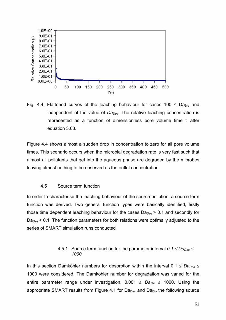
Fig. 4.4: Flattened curves of the leaching behaviour for cases 100 ≤ DaBio and
independent of the value of DaDes. The relative leaching concentration is
represented as a function of dimensionless pore volume time t’ after
equation 3.63.
Figure 4.4 shows almost a sudden drop in concentration to zero for all pore volume
times. This scenario occurs when the microbial degradation rate is very fast such that
almost all pollutants that get into the aqueous phase are degraded by the microbes
leaving almost nothing to be observed as the outlet concentration.
4.5 Source term function In order to characterise the leaching behaviour of the source pollution, a source term
function was derived. Two general function types were basically identified, firstly
those time dependent leaching behaviour for the cases DaDes > 0.1 and secondly for
DaDes < 0.1. The function parameters for both relations were optimally adjusted to the
series of SMART simulation runs conducted
4.5.1 Source term function for the parameter interval 0.1 ≤ DaDes ≤ 1000
In this section Damköhler numbers for desorption within the interval 0.1 ≤ DaDes ≤
1000 were considered. The Damköhler number for degradation was varied for the
entire parameter range under investigation, 0.001 ≤ DaBio ≤ 1000. Using the
appropriate SMART results from Figure 4.1 for DaDes and DaBio the following source
61
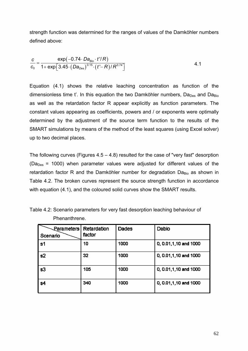
strength function was determined for the ranges of values of the Damköhler numbers
defined above:
( )( ) ( )0.15 0.74
0
exp 0.74 '/1 exp 3.45 ' /
Bio
Des
Da t Rcc Da t R R
− ⋅ ⋅=
⎡+ ⋅ ⋅ −⎣ ⎦⎤ 4.1
Equation (4.1) shows the relative leaching concentration as function of the
dimensionless time t’. In this equation the two Damköhler numbers, DaDes and DaBio
as well as the retardation factor R appear explicitly as function parameters. The
constant values appearing as coefficients, powers and / or exponents were optimally
determined by the adjustment of the source term function to the results of the
SMART simulations by means of the method of the least squares (using Excel solver)
up to two decimal places.
The following curves (Figures 4.5 – 4.8) resulted for the case of "very fast" desorption
(DaDes = 1000) when parameter values were adjusted for different values of the
retardation factor R and the Damköhler number for degradation DaBio as shown in
Table 4.2. The broken curves represent the source strength function in accordance
with equation (4.1), and the coloured solid curves show the SMART results.
Table 4.2: Scenario parameters for very fast desorption leaching behaviour of
Phenanthrene.
62
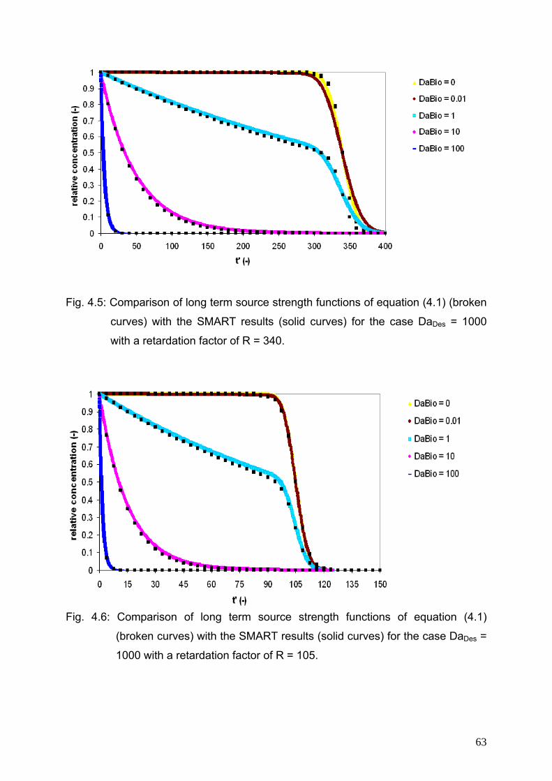
Fig. 4.5: Comparison of long term source strength functions of equation (4.1) (broken
curves) with the SMART results (solid curves) for the case DaDes = 1000
with a retardation factor of R = 340.
Fig. 4.6: Comparison of long term source strength functions of equation (4.1)
(broken curves) with the SMART results (solid curves) for the case DaDes =
1000 with a retardation factor of R = 105.
63
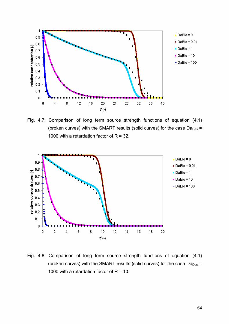
Fig. 4.7: Comparison of long term source strength functions of equation (4.1)
(broken curves) with the SMART results (solid curves) for the case DaDes =
1000 with a retardation factor of R = 32.
Fig. 4.8: Comparison of long term source strength functions of equation (4.1)
(broken curves) with the SMART results (solid curves) for the case DaDes =
1000 with a retardation factor of R = 10.
64
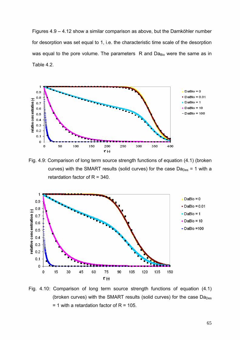
Figures 4.9 – 4.12 show a similar comparison as above, but the Damköhler number
for desorption was set equal to 1, i.e. the characteristic time scale of the desorption
was equal to the pore volume. The parameters R and DaBio were the same as in
Table 4.2.
Fig. 4.9: Comparison of long term source strength functions of equation (4.1) (broken
curves) with the SMART results (solid curves) for the case DaDes = 1 with a
retardation factor of R = 340.
Fig. 4.10: Comparison of long term source strength functions of equation (4.1)
(broken curves) with the SMART results (solid curves) for the case DaDes
= 1 with a retardation factor of R = 105.
65
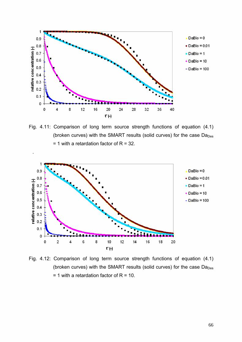
Fig. 4.11: Comparison of long term source strength functions of equation (4.1)
(broken curves) with the SMART results (solid curves) for the case DaDes
= 1 with a retardation factor of R = 32.
.
Fig. 4.12: Comparison of long term source strength functions of equation (4.1)
(broken curves) with the SMART results (solid curves) for the case DaDes
= 1 with a retardation factor of R = 10.
66
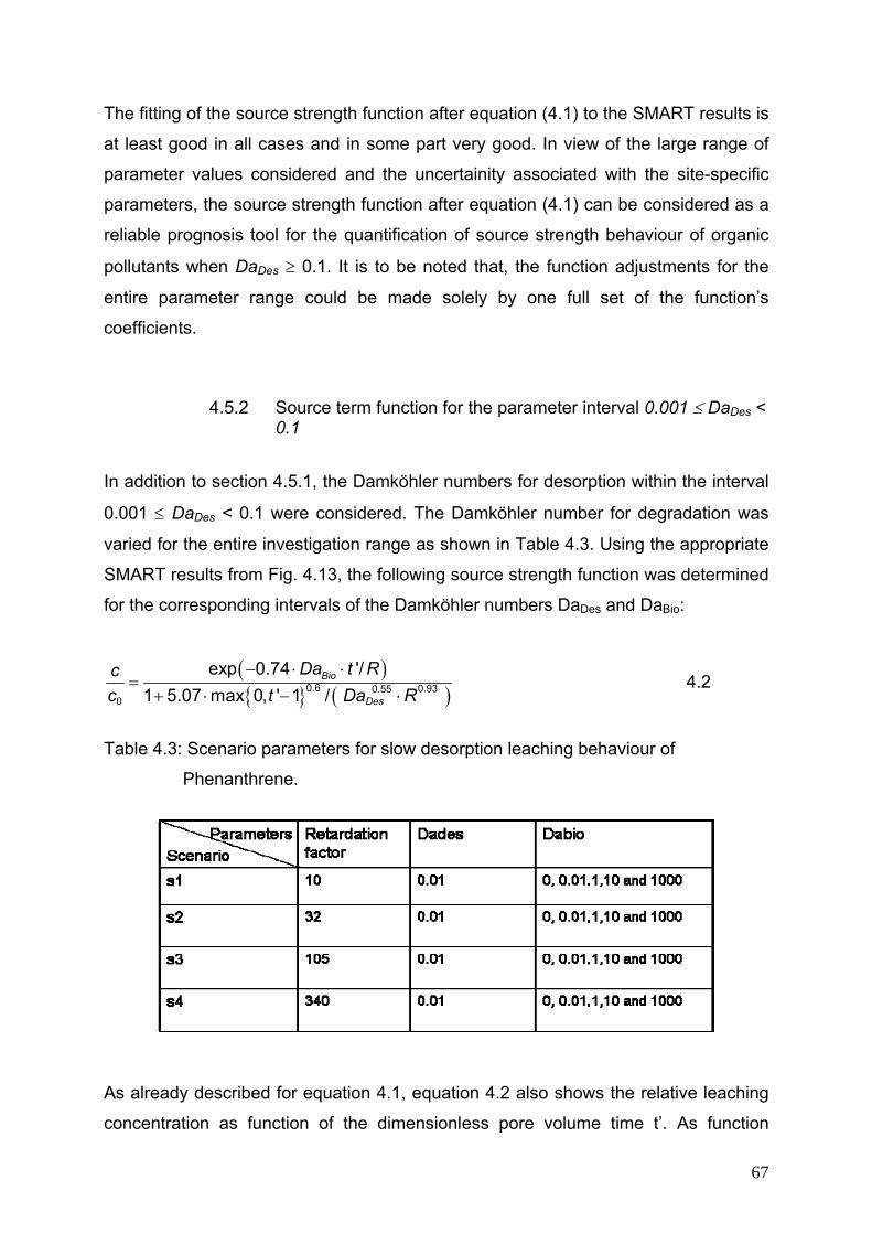
The fitting of the source strength function after equation (4.1) to the SMART results is
at least good in all cases and in some part very good. In view of the large range of
parameter values considered and the uncertainity associated with the site-specific
parameters, the source strength function after equation (4.1) can be considered as a
reliable prognosis tool for the quantification of source strength behaviour of organic
pollutants when DaDes ≥ 0.1. It is to be noted that, the function adjustments for the
entire parameter range could be made solely by one full set of the function’s
coefficients.
4.5.2 Source term function for the parameter interval 0.001 ≤ DaDes < 0.1
In addition to section 4.5.1, the Damköhler numbers for desorption within the interval
0.001 ≤ DaDes < 0.1 were considered. The Damköhler number for degradation was
varied for the entire investigation range as shown in Table 4.3. Using the appropriate
SMART results from Fig. 4.13, the following source strength function was determined
for the corresponding intervals of the Damköhler numbers DaDes and DaBio:
( ){ } ( )0.6 0.930.55
0
exp 0.74 '/1 5.07 max 0, ' 1 /
Bio
Des
Da t Rcc t Da
− ⋅ ⋅=
+ ⋅ − ⋅R 4.2
Table 4.3: Scenario parameters for slow desorption leaching behaviour of
Phenanthrene.
As already described for equation 4.1, equation 4.2 also shows the relative leaching
concentration as function of the dimensionless pore volume time t’. As function
67
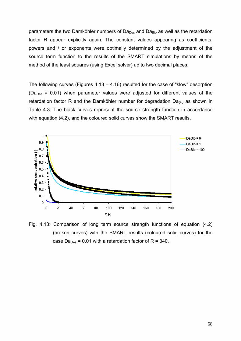
parameters the two Damköhler numbers of DaDes and DaBio as well as the retardation
factor R appear explicitly again. The constant values appearing as coefficients,
powers and / or exponents were optimally determined by the adjustment of the
source term function to the results of the SMART simulations by means of the
method of the least squares (using Excel solver) up to two decimal places.
The following curves (Figures 4.13 – 4.16) resulted for the case of "slow" desorption
(DaDes = 0.01) when parameter values were adjusted for different values of the
retardation factor R and the Damköhler number for degradation DaBio as shown in
Table 4.3. The black curves represent the source strength function in accordance
with equation (4.2), and the coloured solid curves show the SMART results.
Fig. 4.13: Comparison of long term source strength functions of equation (4.2)
(broken curves) with the SMART results (coloured solid curves) for the
case DaDes = 0.01 with a retardation factor of R = 340.
68
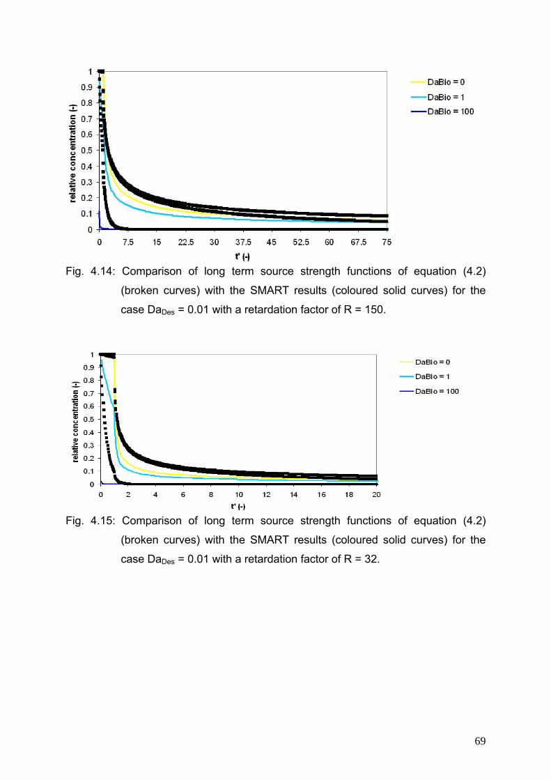
Fig. 4.14: Comparison of long term source strength functions of equation (4.2)
(broken curves) with the SMART results (coloured solid curves) for the
case DaDes = 0.01 with a retardation factor of R = 150.
Fig. 4.15: Comparison of long term source strength functions of equation (4.2)
(broken curves) with the SMART results (coloured solid curves) for the
case DaDes = 0.01 with a retardation factor of R = 32.
69
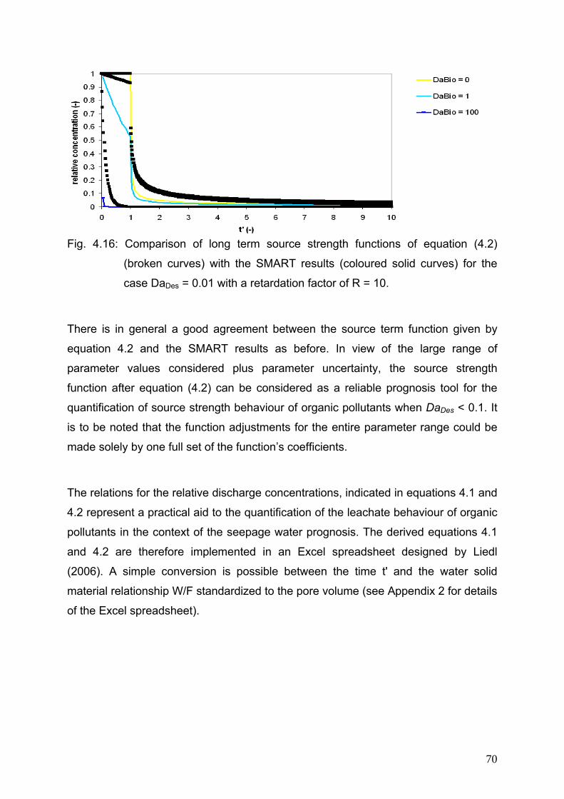
Fig. 4.16: Comparison of long term source strength functions of equation (4.2)
(broken curves) with the SMART results (coloured solid curves) for the
case DaDes = 0.01 with a retardation factor of R = 10.
There is in general a good agreement between the source term function given by
equation 4.2 and the SMART results as before. In view of the large range of
parameter values considered plus parameter uncertainty, the source strength
function after equation (4.2) can be considered as a reliable prognosis tool for the
quantification of source strength behaviour of organic pollutants when DaDes < 0.1. It
is to be noted that the function adjustments for the entire parameter range could be
made solely by one full set of the function’s coefficients.
The relations for the relative discharge concentrations, indicated in equations 4.1 and
4.2 represent a practical aid to the quantification of the leachate behaviour of organic
pollutants in the context of the seepage water prognosis. The derived equations 4.1
and 4.2 are therefore implemented in an Excel spreadsheet designed by Liedl
(2006). A simple conversion is possible between the time t' and the water solid
material relationship W/F standardized to the pore volume (see Appendix 2 for details
of the Excel spreadsheet).
70
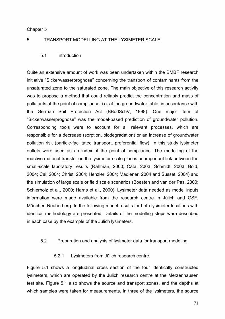
Chapter 5 5 TRANSPORT MODELLING AT THE LYSIMETER SCALE
5.1 Introduction
5.2
Quite an extensive amount of work was been undertaken within the BMBF research
initiative ”Sickerwasserprognose” concerning the transport of contaminants from the
unsaturated zone to the saturated zone. The main objective of this research activity
was to propose a method that could reliably predict the concentration and mass of
pollutants at the point of compliance, i.e. at the groundwater table, in accordance with
the German Soil Protection Act (BBodSchV, 1998). One major item of
“Sickerwasserprognose” was the model-based prediction of groundwater pollution.
Corresponding tools were to account for all relevant processes, which are
responsible for a decrease (sorption, biodegradation) or an increase of groundwater
pollution risk (particle-facilitated transport, preferential flow). In this study lysimeter
outlets were used as an index of the point of compliance. The modelling of the
reactive material transfer on the lysimeter scale places an important link between the
small-scale laboratory results (Rahman, 2000; Cata, 2003; Schmidt, 2003; Bold,
2004; Cai, 2004; Christ, 2004; Henzler, 2004; Madlener, 2004 and Susset, 2004) and
the simulation of large scale or field scale scenarios (Boesten and van der Pas, 2000;
Schierholz et al., 2000; Harris et al., 2000). Lysimeter data needed as model inputs
information were made available from the research centre in Jülich and GSF,
München-Neuherberg. In the following model results for both lysimeter locations with
identical methodology are presented. Details of the modelling steps were described
in each case by the example of the Jülich lysimeters.
Preparation and analysis of lysimeter data for transport modeling
5.2.1 Lysimeters from Jülich research centre. Figure 5.1 shows a longitudinal cross section of the four identically constructed
lysimeters, which are operated by the Jülich research centre at the Merzenhausen
test site. Figure 5.1 also shows the source and transport zones, and the depths at
which samples were taken for measurements. In three of the lysimeters, the source
71
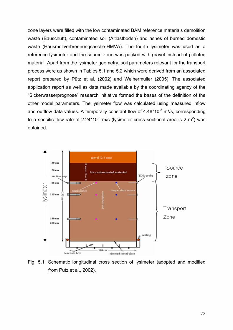
zone layers were filled with the low contaminated BAM reference materials demolition
waste (Bauschutt), contaminated soil (Altlastboden) and ashes of burned domestic
waste (Hausmüllverbrennungsasche-HMVA). The fourth lysimeter was used as a
reference lysimeter and the source zone was packed with gravel instead of polluted
material. Apart from the lysimeter geometry, soil parameters relevant for the transport
process were as shown in Tables 5.1 and 5.2 which were derived from an associated
report prepared by Pütz et al. (2002) and Weihermüller (2005). The associated
application report as well as data made available by the coordinating agency of the
“Sickerwasserprognose” research initiative formed the bases of the definition of the
other model parameters. The lysimeter flow was calculated using measured inflow
and outflow data values. A temporally constant flow of 4.48*10-8 m³/s, corresponding
to a specific flow rate of 2.24*10-8 m/s (lysimeter cross sectional area is 2 m2) was
obtained.
Fig. 5.1: Schematic longitudinal cross section of lysimeter (adopted and modified
from Pütz et al., 2002).
72
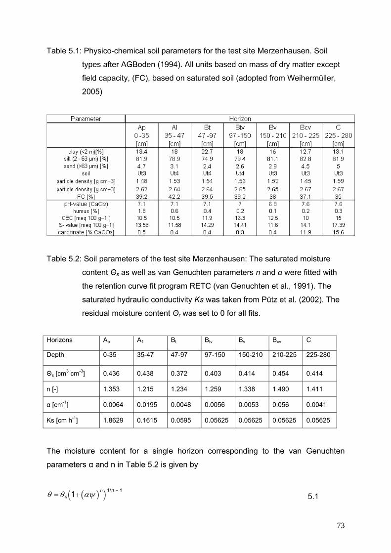
Table 5.1: Physico-chemical soil parameters for the test site Merzenhausen. Soil
types after AGBoden (1994). All units based on mass of dry matter except
field capacity, (FC), based on saturated soil (adopted from Weihermüller,
2005)
Table 5.2: Soil parameters of the test site Merzenhausen: The saturated moisture
content Θs as well as van Genuchten parameters n and α were fitted with
the retention curve fit program RETC (van Genuchten et al., 1991). The
saturated hydraulic conductivity Ks was taken from Pütz et al. (2002). The
residual moisture content Θr was set to 0 for all fits.
Horizons Ap A1 Bt Btv Bv Bcv C
Depth 0-35 35-47 47-97 97-150 150-210 210-225 225-280
Θs [cm3 cm-3] 0.436 0.438 0.372 0.403 0.414 0.454 0.414
n [-] 1.353 1.215 1.234 1.259 1.338 1.490 1.411
α [cm-1] 0.0064 0.0195 0.0048 0.0056 0.0053 0.056 0.0041
Ks [cm h-1] 1.8629 0.1615 0.0595 0.05625 0.05625 0.05625 0.05625
The moisture content for a single horizon corresponding to the van Genuchten
parameters α and n in Table 5.2 is given by
( )( ) 1/ 11 nnsθ θ αψ
−= + 5.1
73
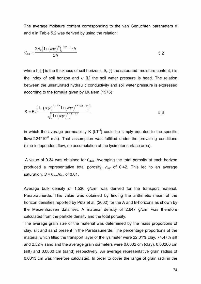
The average moisture content corresponding to the van Genuchten parameters α
and n in Table 5.2 was derived by using the relation:
( )( ) 1/ 1*1 nn
s iiave
i
hh
θ αψθ
−Σ +
=Σ 5.2
where hi [-] is the thickness of soil horizons, θs [-] the saturated moisture content, i is
the index of soil horizon and ψ [L] the soil water pressure is head. The relation
between the unsaturated hydraulic conductivity and soil water pressure is expressed
according to the formula given by Mualem (1976)
( ) ( ){ }( )
1 21/ 1
1 1/
1 1
1
n n n
s n nK Kαψ αψ
αψ
− −
−
⎡ ⎤− +⎣ ⎦=⎡ ⎤+⎣ ⎦
5.3
in which the average permeability K [LT-1] could be simply equated to the specific
flow(2.24*10-8 m/s). That assumption was fulfilled under the prevailing conditions
(time-independent flow, no accumulation at the lysimeter surface area).
A value of 0.34 was obtained for θave. Averaging the total porosity at each horizon
produced a representative total porosity, ntot of 0.42. This led to an average
saturation, S = θave/ntot of 0.81.
Average bulk density of 1.536 g/cm³ was derived for the transport material,
Parabraunerde. This value was obtained by finding the arithmetic mean of the
horizon densities reported by Pütz et al. (2002) for the A and B-horizons as shown by
the Merzenhausen data set. A material density of 2.647 g/cm³ was therefore
calculated from the particle density and the total porosity.
The average grain size of the material was determined by the mass proportions of
clay, silt and sand present in the Parabraunerde. The percentage proportions of the
material which filled the transport layer of the lysimeter were 22.01% clay, 74.47% silt
and 2.52% sand and the average grain diameters were 0.0002 cm (clay), 0.00266 cm
(silt) and 0.0830 cm (sand) respectively. An average representative grain radius of
0.0013 cm was therefore calculated. In order to cover the range of grain radii in the
74
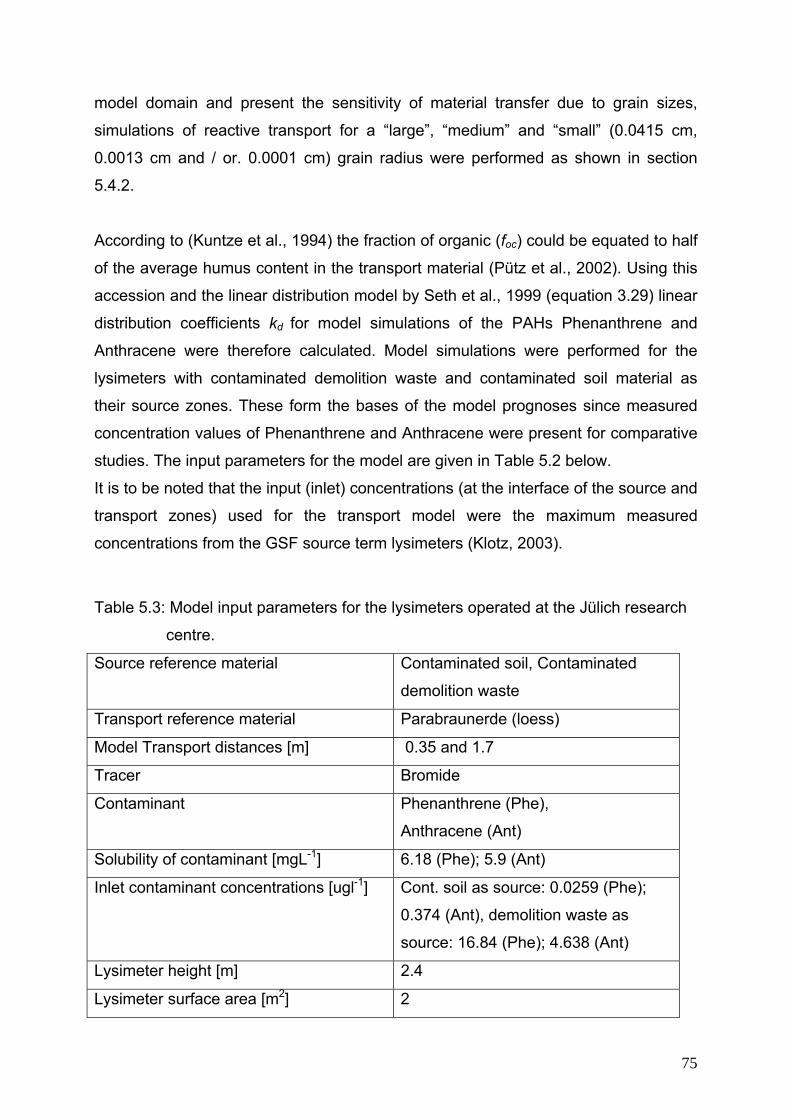
model domain and present the sensitivity of material transfer due to grain sizes,
simulations of reactive transport for a “large”, “medium” and “small” (0.0415 cm,
0.0013 cm and / or. 0.0001 cm) grain radius were performed as shown in section
5.4.2.
According to (Kuntze et al., 1994) the fraction of organic (foc) could be equated to half
of the average humus content in the transport material (Pütz et al., 2002). Using this
accession and the linear distribution model by Seth et al., 1999 (equation 3.29) linear
distribution coefficients kd for model simulations of the PAHs Phenanthrene and
Anthracene were therefore calculated. Model simulations were performed for the
lysimeters with contaminated demolition waste and contaminated soil material as
their source zones. These form the bases of the model prognoses since measured
concentration values of Phenanthrene and Anthracene were present for comparative
studies. The input parameters for the model are given in Table 5.2 below.
It is to be noted that the input (inlet) concentrations (at the interface of the source and
transport zones) used for the transport model were the maximum measured
concentrations from the GSF source term lysimeters (Klotz, 2003).
Table 5.3: Model input parameters for the lysimeters operated at the Jülich research
centre.
Source reference material
Contaminated soil, Contaminated
demolition waste
Transport reference material Parabraunerde (loess)
Model Transport distances [m] 0.35 and 1.7
Tracer Bromide
Contaminant Phenanthrene (Phe),
Anthracene (Ant)
Solubility of contaminant [mgL-1] 6.18 (Phe); 5.9 (Ant)
Inlet contaminant concentrations [ugl-1] Cont. soil as source: 0.0259 (Phe);
0.374 (Ant), demolition waste as
source: 16.84 (Phe); 4.638 (Ant)
Lysimeter height [m] 2.4
Lysimeter surface area [m2] 2
75
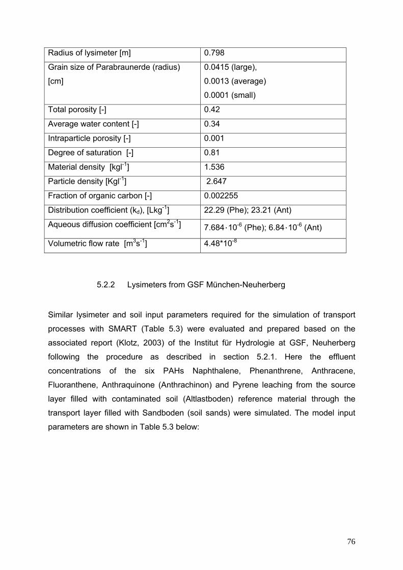
Radius of lysimeter [m] 0.798
Grain size of Parabraunerde (radius)
[cm]
0.0415 (large),
0.0013 (average)
0.0001 (small)
Total porosity [-] 0.42
Average water content [-] 0.34
Intraparticle porosity [-] 0.001
Degree of saturation [-] 0.81
Material density [kgl-1] 1.536
Particle density [Kgl-1] 2.647
Fraction of organic carbon [-] 0.002255
Distribution coefficient (kd), [Lkg-1] 22.29 (Phe); 23.21 (Ant)
Aqueous diffusion coefficient [cm2s-1] 7.684·10-6 (Phe); 6.84·10-6 (Ant)
Volumetric flow rate [m3s-1] 4.48*10-8
5.2.2 Lysimeters from GSF München-Neuherberg
Similar lysimeter and soil input parameters required for the simulation of transport
processes with SMART (Table 5.3) were evaluated and prepared based on the
associated report (Klotz, 2003) of the Institut für Hydrologie at GSF, Neuherberg
following the procedure as described in section 5.2.1. Here the effluent
concentrations of the six PAHs Naphthalene, Phenanthrene, Anthracene,
Fluoranthene, Anthraquinone (Anthrachinon) and Pyrene leaching from the source
layer filled with contaminated soil (Altlastboden) reference material through the
transport layer filled with Sandboden (soil sands) were simulated. The model input
parameters are shown in Table 5.3 below:
76
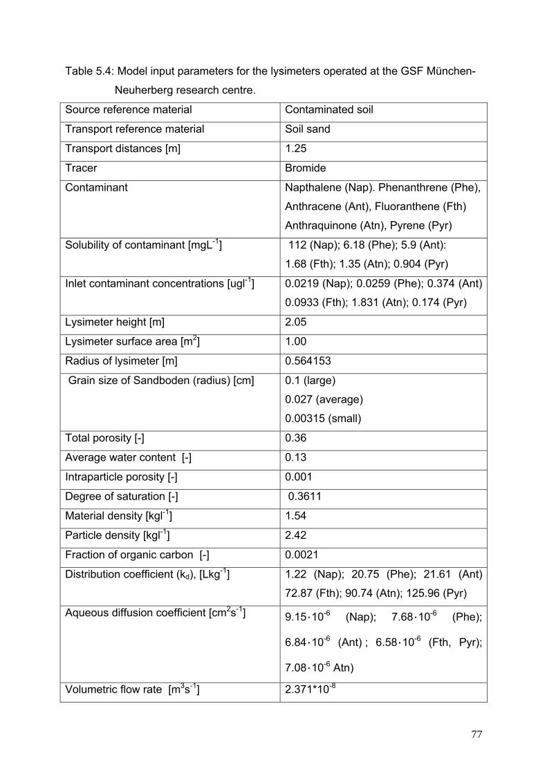
Table 5.4: Model input parameters for the lysimeters operated at the GSF München-
Neuherberg research centre.
Source reference material Contaminated soil
Transport reference material Soil sand
Transport distances [m] 1.25
Tracer Bromide
Contaminant Napthalene (Nap). Phenanthrene (Phe),
Anthracene (Ant), Fluoranthene (Fth)
Anthraquinone (Atn), Pyrene (Pyr)
Solubility of contaminant [mgL-1] 112 (Nap); 6.18 (Phe); 5.9 (Ant):
1.68 (Fth); 1.35 (Atn); 0.904 (Pyr)
Inlet contaminant concentrations [ugl-1] 0.0219 (Nap); 0.0259 (Phe); 0.374 (Ant)
0.0933 (Fth); 1.831 (Atn); 0.174 (Pyr)
Lysimeter height [m] 2.05
Lysimeter surface area [m2] 1.00
Radius of lysimeter [m] 0.564153
Grain size of Sandboden (radius) [cm] 0.1 (large)
0.027 (average)
0.00315 (small)
Total porosity [-] 0.36
Average water content [-] 0.13
Intraparticle porosity [-] 0.001
Degree of saturation [-] 0.3611
Material density [kgl-1] 1.54
Particle density [kgl-1] 2.42
Fraction of organic carbon [-] 0.0021
Distribution coefficient (kd), [Lkg-1] 1.22 (Nap); 20.75 (Phe); 21.61 (Ant)
72.87 (Fth); 90.74 (Atn); 125.96 (Pyr)
Aqueous diffusion coefficient [cm2s-1] 9.15·10-6 (Nap); 7.68·10-6 (Phe);
6.84·10-6 (Ant) ; 6.58·10-6 (Fth, Pyr);
7.08·10-6 Atn)
Volumetric flow rate [m3s-1] 2.371*10-8
77
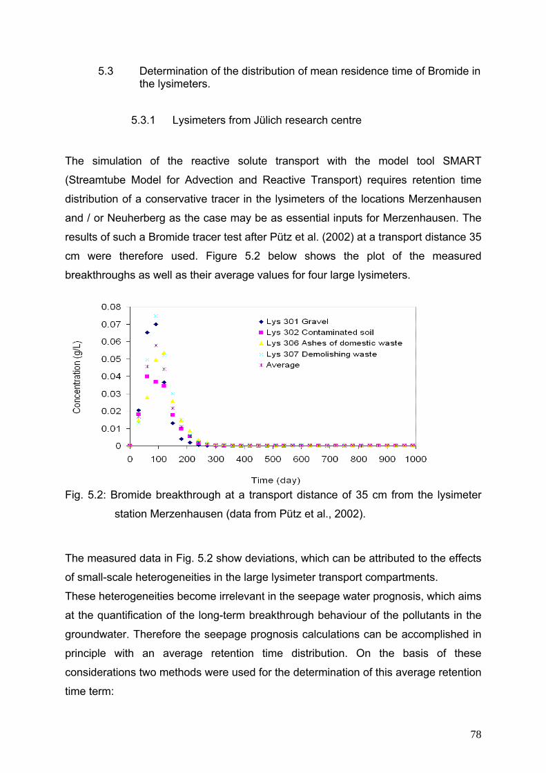
5.3 Determination of the distribution of mean residence time of Bromide in the lysimeters.
5.3.1 Lysimeters from Jülich research centre
The simulation of the reactive solute transport with the model tool SMART
(Streamtube Model for Advection and Reactive Transport) requires retention time
distribution of a conservative tracer in the lysimeters of the locations Merzenhausen
and / or Neuherberg as the case may be as essential inputs for Merzenhausen. The
results of such a Bromide tracer test after Pütz et al. (2002) at a transport distance 35
cm were therefore used. Figure 5.2 below shows the plot of the measured
breakthroughs as well as their average values for four large lysimeters.
Fig. 5.2: Bromide breakthrough at a transport distance of 35 cm from the lysimeter
station Merzenhausen (data from Pütz et al., 2002).
The measured data in Fig. 5.2 show deviations, which can be attributed to the effects
of small-scale heterogeneities in the large lysimeter transport compartments.
These heterogeneities become irrelevant in the seepage water prognosis, which aims
at the quantification of the long-term breakthrough behaviour of the pollutants in the
groundwater. Therefore the seepage prognosis calculations can be accomplished in
principle with an average retention time distribution. On the basis of these
considerations two methods were used for the determination of this average retention
time term:
78
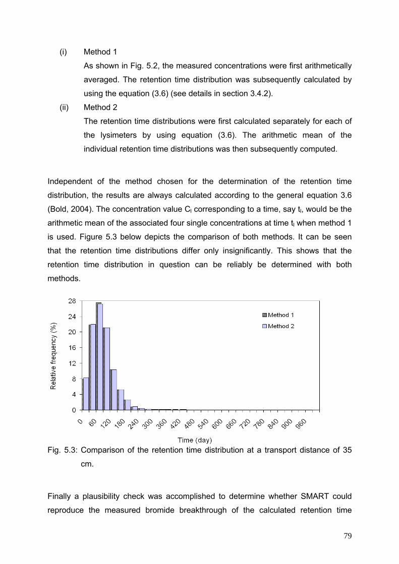
(i) Method 1
As shown in Fig. 5.2, the measured concentrations were first arithmetically
averaged. The retention time distribution was subsequently calculated by
using the equation (3.6) (see details in section 3.4.2).
(ii) Method 2
The retention time distributions were first calculated separately for each of
the lysimeters by using equation (3.6). The arithmetic mean of the
individual retention time distributions was then subsequently computed.
Independent of the method chosen for the determination of the retention time
distribution, the results are always calculated according to the general equation 3.6
(Bold, 2004). The concentration value Cl corresponding to a time, say tl, would be the
arithmetic mean of the associated four single concentrations at time tl when method 1
is used. Figure 5.3 below depicts the comparison of both methods. It can be seen
that the retention time distributions differ only insignificantly. This shows that the
retention time distribution in question can be reliably be determined with both
methods.
Fig. 5.3: Comparison of the retention time distribution at a transport distance of 35
cm.
Finally a plausibility check was accomplished to determine whether SMART could
reproduce the measured bromide breakthrough of the calculated retention time
79
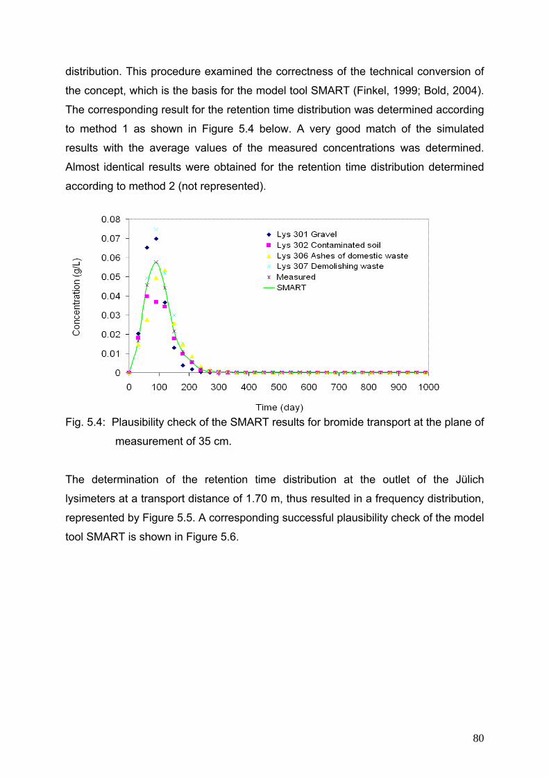
distribution. This procedure examined the correctness of the technical conversion of
the concept, which is the basis for the model tool SMART (Finkel, 1999; Bold, 2004).
The corresponding result for the retention time distribution was determined according
to method 1 as shown in Figure 5.4 below. A very good match of the simulated
results with the average values of the measured concentrations was determined.
Almost identical results were obtained for the retention time distribution determined
according to method 2 (not represented).
Fig. 5.4: Plausibility check of the SMART results for bromide transport at the plane of
measurement of 35 cm.
The determination of the retention time distribution at the outlet of the Jülich
lysimeters at a transport distance of 1.70 m, thus resulted in a frequency distribution,
represented by Figure 5.5. A corresponding successful plausibility check of the model
tool SMART is shown in Figure 5.6.
80
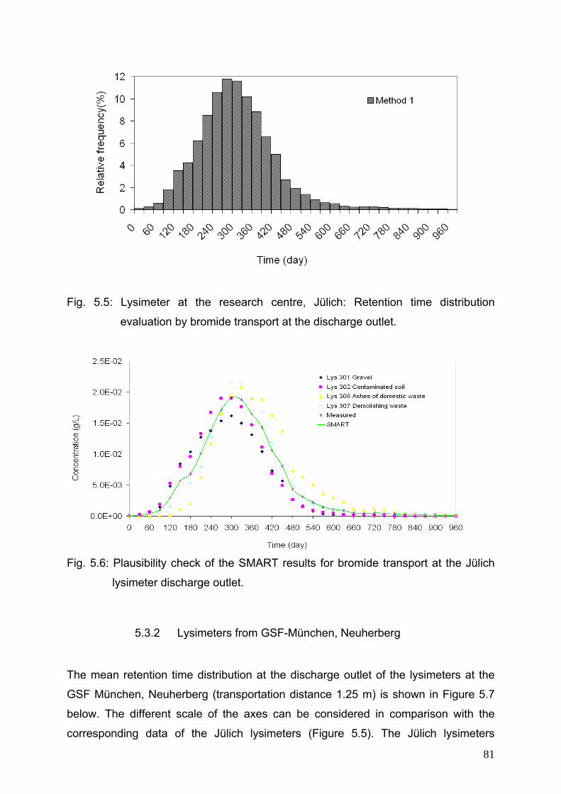
Fig. 5.5: Lysimeter at the research centre, Jülich: Retention time distribution
evaluation by bromide transport at the discharge outlet.
Fig. 5.6: Plausibility check of the SMART results for bromide transport at the Jülich
lysimeter discharge outlet.
5.3.2 Lysimeters from GSF-München, Neuherberg
The mean retention time distribution at the discharge outlet of the lysimeters at the
GSF München, Neuherberg (transportation distance 1.25 m) is shown in Figure 5.7
below. The different scale of the axes can be considered in comparison with the
corresponding data of the Jülich lysimeters (Figure 5.5). The Jülich lysimeters
81
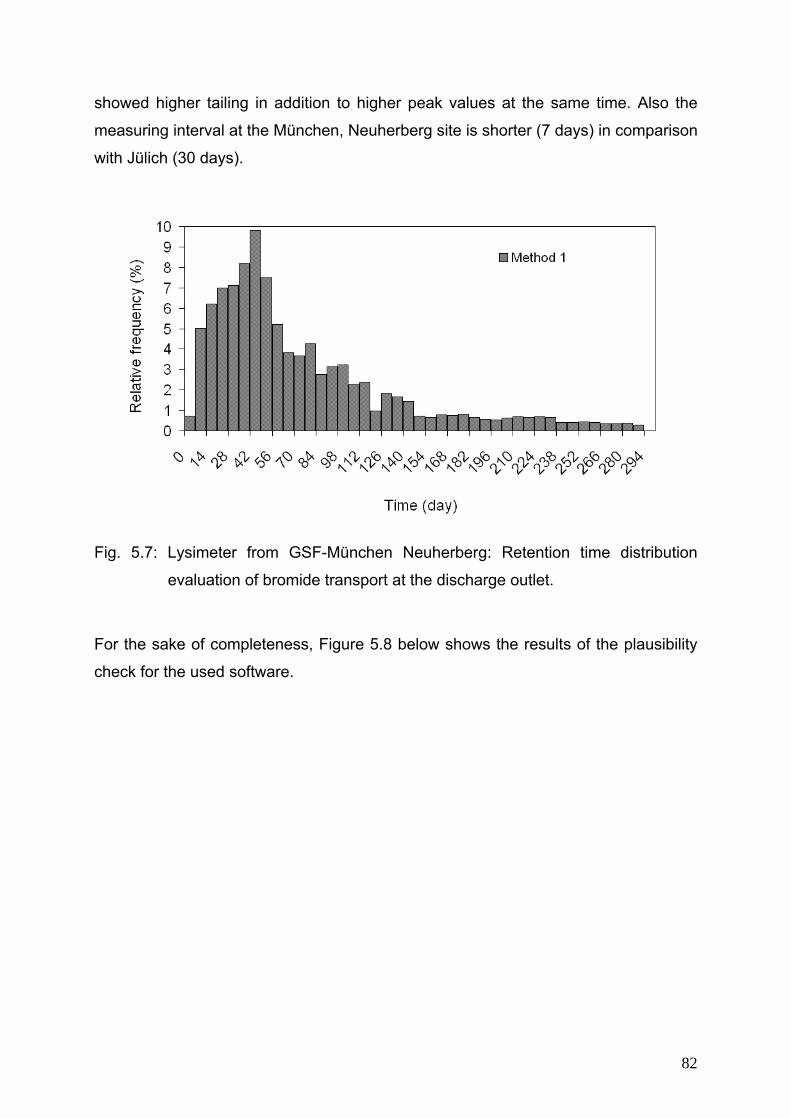
showed higher tailing in addition to higher peak values at the same time. Also the
measuring interval at the München, Neuherberg site is shorter (7 days) in comparison
with Jülich (30 days).
Fig. 5.7: Lysimeter from GSF-München Neuherberg: Retention time distribution
evaluation of bromide transport at the discharge outlet.
For the sake of completeness, Figure 5.8 below shows the results of the plausibility
check for the used software.
82
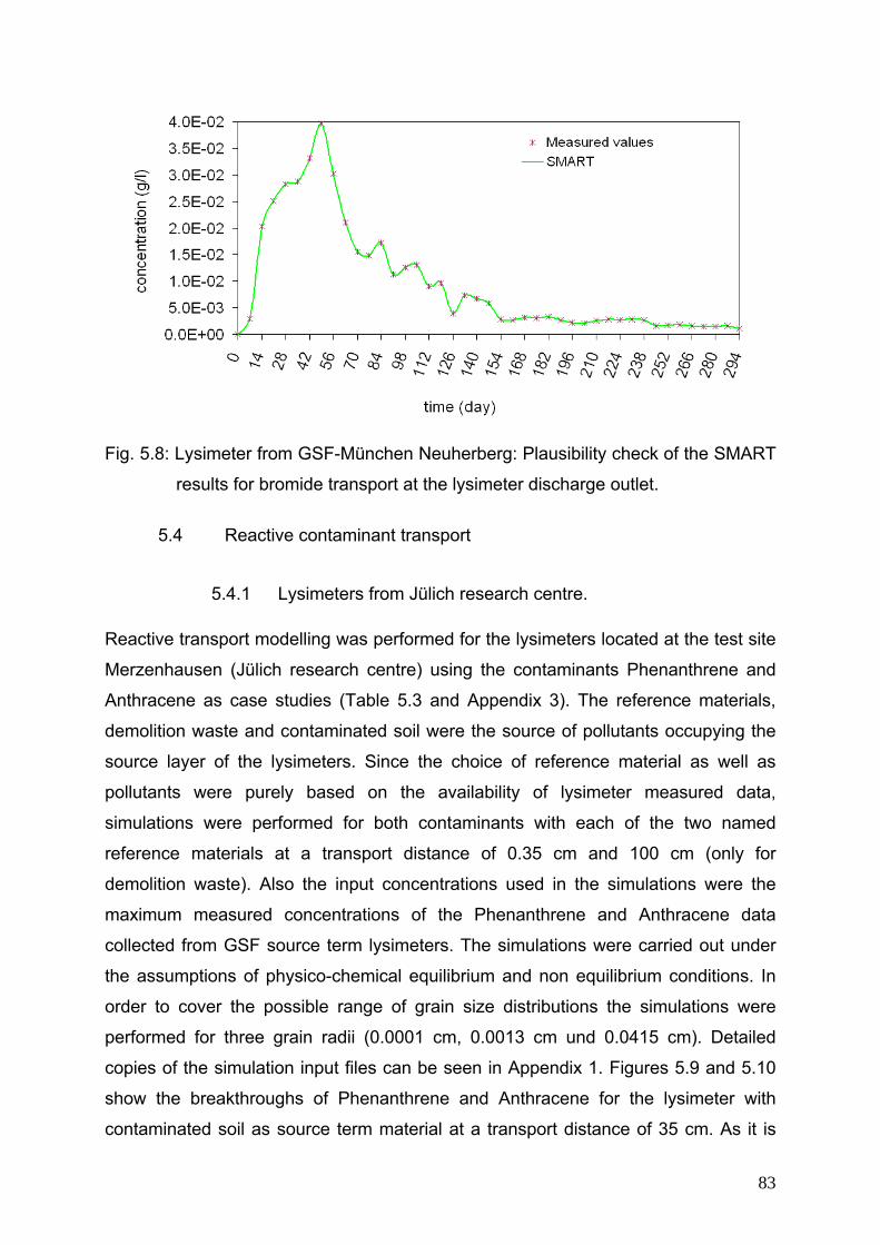
Fig. 5.8: Lysimeter from GSF-München Neuherberg: Plausibility check of the SMART
results for bromide transport at the lysimeter discharge outlet.
5.4 Reactive contaminant transport
5.4.1 Lysimeters from Jülich research centre. Reactive transport modelling was performed for the lysimeters located at the test site
Merzenhausen (Jülich research centre) using the contaminants Phenanthrene and
Anthracene as case studies (Table 5.3 and Appendix 3). The reference materials,
demolition waste and contaminated soil were the source of pollutants occupying the
source layer of the lysimeters. Since the choice of reference material as well as
pollutants were purely based on the availability of lysimeter measured data,
simulations were performed for both contaminants with each of the two named
reference materials at a transport distance of 0.35 cm and 100 cm (only for
demolition waste). Also the input concentrations used in the simulations were the
maximum measured concentrations of the Phenanthrene and Anthracene data
collected from GSF source term lysimeters. The simulations were carried out under
the assumptions of physico-chemical equilibrium and non equilibrium conditions. In
order to cover the possible range of grain size distributions the simulations were
performed for three grain radii (0.0001 cm, 0.0013 cm und 0.0415 cm). Detailed
copies of the simulation input files can be seen in Appendix 1. Figures 5.9 and 5.10
show the breakthroughs of Phenanthrene and Anthracene for the lysimeter with
contaminated soil as source term material at a transport distance of 35 cm. As it is
83
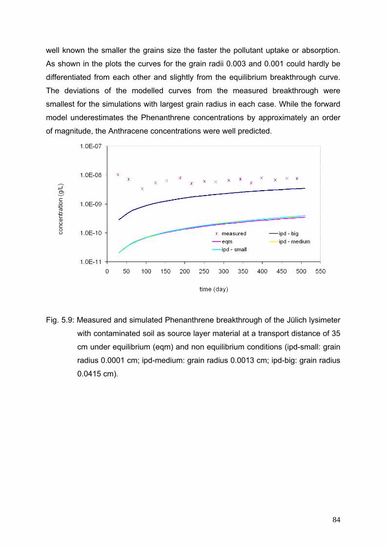
well known the smaller the grains size the faster the pollutant uptake or absorption.
As shown in the plots the curves for the grain radii 0.003 and 0.001 could hardly be
differentiated from each other and slightly from the equilibrium breakthrough curve.
The deviations of the modelled curves from the measured breakthrough were
smallest for the simulations with largest grain radius in each case. While the forward
model underestimates the Phenanthrene concentrations by approximately an order
of magnitude, the Anthracene concentrations were well predicted.
Fig. 5.9: Measured and simulated Phenanthrene breakthrough of the Jülich lysimeter
with contaminated soil as source layer material at a transport distance of 35
cm under equilibrium (eqm) and non equilibrium conditions (ipd-small: grain
radius 0.0001 cm; ipd-medium: grain radius 0.0013 cm; ipd-big: grain radius
0.0415 cm).
84
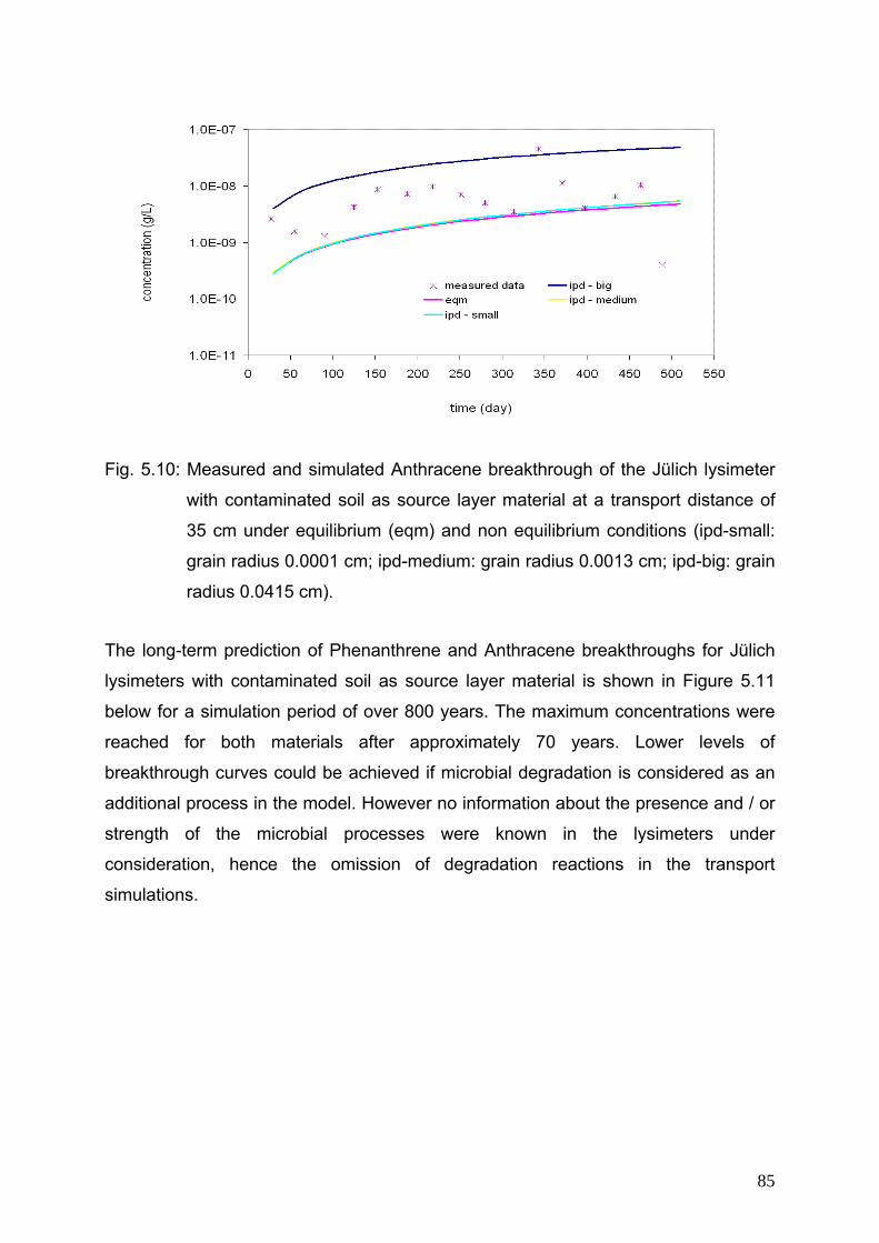
Fig. 5.10: Measured and simulated Anthracene breakthrough of the Jülich lysimeter
with contaminated soil as source layer material at a transport distance of
35 cm under equilibrium (eqm) and non equilibrium conditions (ipd-small:
grain radius 0.0001 cm; ipd-medium: grain radius 0.0013 cm; ipd-big: grain
radius 0.0415 cm).
The long-term prediction of Phenanthrene and Anthracene breakthroughs for Jülich
lysimeters with contaminated soil as source layer material is shown in Figure 5.11
below for a simulation period of over 800 years. The maximum concentrations were
reached for both materials after approximately 70 years. Lower levels of
breakthrough curves could be achieved if microbial degradation is considered as an
additional process in the model. However no information about the presence and / or
strength of the microbial processes were known in the lysimeters under
consideration, hence the omission of degradation reactions in the transport
simulations.
85
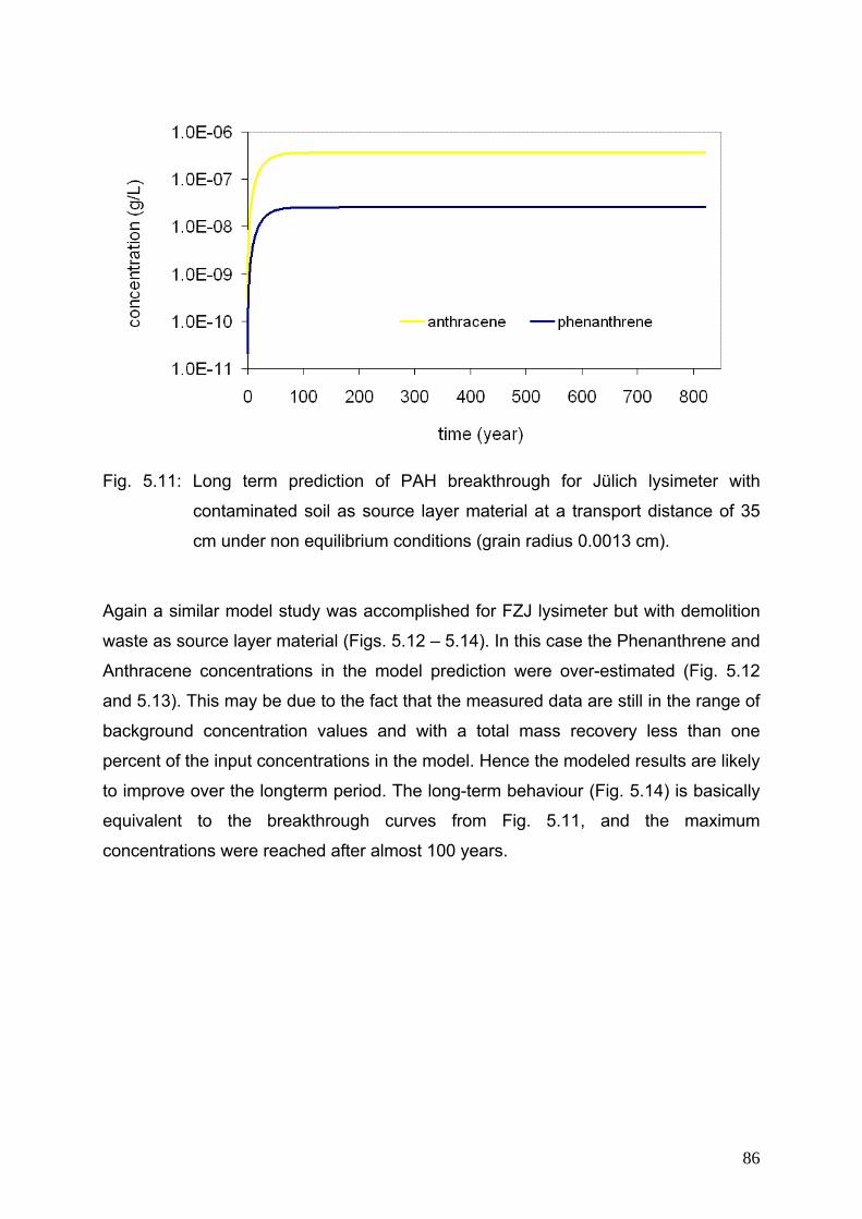
Fig. 5.11: Long term prediction of PAH breakthrough for Jülich lysimeter with
contaminated soil as source layer material at a transport distance of 35
cm under non equilibrium conditions (grain radius 0.0013 cm).
Again a similar model study was accomplished for FZJ lysimeter but with demolition
waste as source layer material (Figs. 5.12 – 5.14). In this case the Phenanthrene and
Anthracene concentrations in the model prediction were over-estimated (Fig. 5.12
and 5.13). This may be due to the fact that the measured data are still in the range of
background concentration values and with a total mass recovery less than one
percent of the input concentrations in the model. Hence the modeled results are likely
to improve over the longterm period. The long-term behaviour (Fig. 5.14) is basically
equivalent to the breakthrough curves from Fig. 5.11, and the maximum
concentrations were reached after almost 100 years.
86
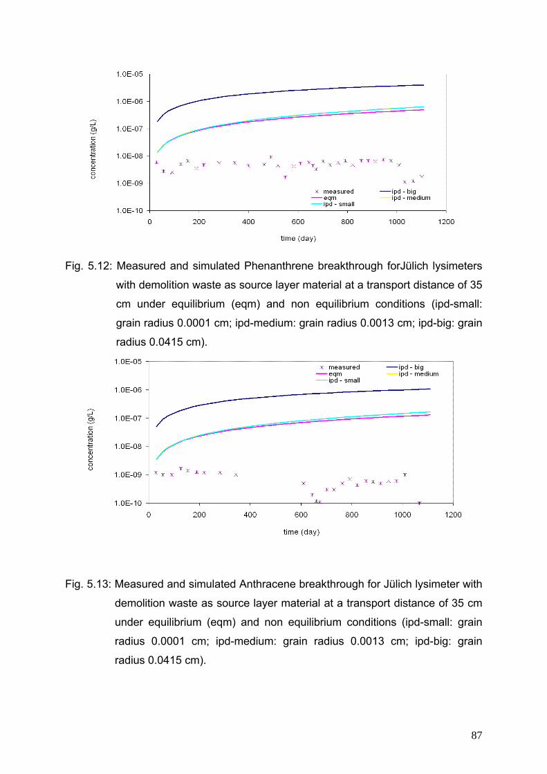
Fig. 5.12: Measured and simulated Phenanthrene breakthrough forJülich lysimeters
with demolition waste as source layer material at a transport distance of 35
cm under equilibrium (eqm) and non equilibrium conditions (ipd-small:
grain radius 0.0001 cm; ipd-medium: grain radius 0.0013 cm; ipd-big: grain
radius 0.0415 cm).
Fig. 5.13: Measured and simulated Anthracene breakthrough for Jülich lysimeter with
demolition waste as source layer material at a transport distance of 35 cm
under equilibrium (eqm) and non equilibrium conditions (ipd-small: grain
radius 0.0001 cm; ipd-medium: grain radius 0.0013 cm; ipd-big: grain
radius 0.0415 cm).
87
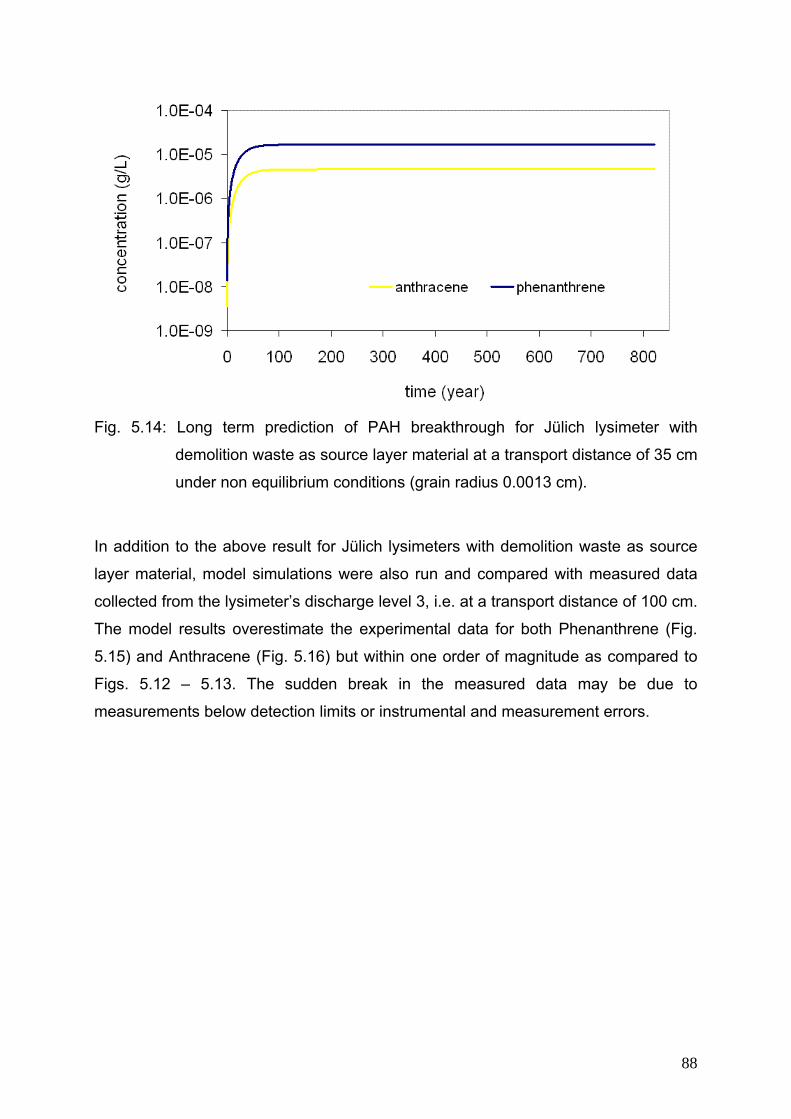
Fig. 5.14: Long term prediction of PAH breakthrough for Jülich lysimeter with
demolition waste as source layer material at a transport distance of 35 cm
under non equilibrium conditions (grain radius 0.0013 cm).
In addition to the above result for Jülich lysimeters with demolition waste as source
layer material, model simulations were also run and compared with measured data
collected from the lysimeter’s discharge level 3, i.e. at a transport distance of 100 cm.
The model results overestimate the experimental data for both Phenanthrene (Fig.
5.15) and Anthracene (Fig. 5.16) but within one order of magnitude as compared to
Figs. 5.12 – 5.13. The sudden break in the measured data may be due to
measurements below detection limits or instrumental and measurement errors.
88
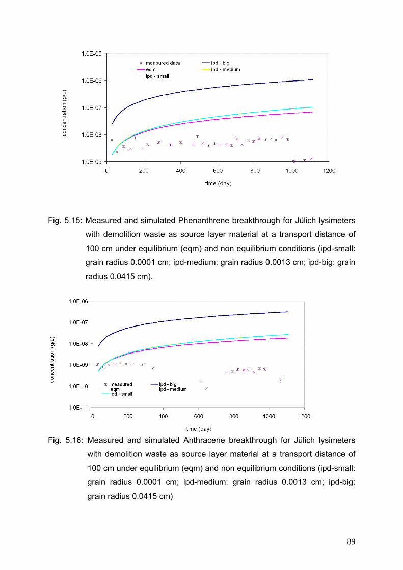
Fig. 5.15: Measured and simulated Phenanthrene breakthrough for Jülich lysimeters
with demolition waste as source layer material at a transport distance of
100 cm under equilibrium (eqm) and non equilibrium conditions (ipd-small:
grain radius 0.0001 cm; ipd-medium: grain radius 0.0013 cm; ipd-big: grain
radius 0.0415 cm).
Fig. 5.16: Measured and simulated Anthracene breakthrough for Jülich lysimeters
with demolition waste as source layer material at a transport distance of
100 cm under equilibrium (eqm) and non equilibrium conditions (ipd-small:
grain radius 0.0001 cm; ipd-medium: grain radius 0.0013 cm; ipd-big:
grain radius 0.0415 cm)
89
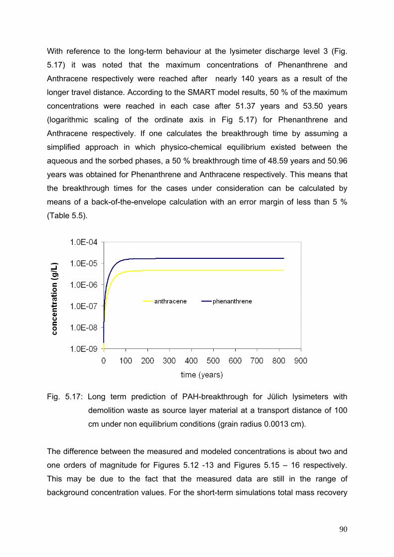
With reference to the long-term behaviour at the lysimeter discharge level 3 (Fig.
5.17) it was noted that the maximum concentrations of Phenanthrene and
Anthracene respectively were reached after nearly 140 years as a result of the
longer travel distance. According to the SMART model results, 50 % of the maximum
concentrations were reached in each case after 51.37 years and 53.50 years
(logarithmic scaling of the ordinate axis in Fig 5.17) for Phenanthrene and
Anthracene respectively. If one calculates the breakthrough time by assuming a
simplified approach in which physico-chemical equilibrium existed between the
aqueous and the sorbed phases, a 50 % breakthrough time of 48.59 years and 50.96
years was obtained for Phenanthrene and Anthracene respectively. This means that
the breakthrough times for the cases under consideration can be calculated by
means of a back-of-the-envelope calculation with an error margin of less than 5 %
(Table 5.5).
Fig. 5.17: Long term prediction of PAH-breakthrough for Jülich lysimeters with
demolition waste as source layer material at a transport distance of 100
cm under non equilibrium conditions (grain radius 0.0013 cm).
The difference between the measured and modeled concentrations is about two and
one orders of magnitude for Figures 5.12 -13 and Figures 5.15 – 16 respectively.
This may be due to the fact that the measured data are still in the range of
background concentration values. For the short-term simulations total mass recovery
90
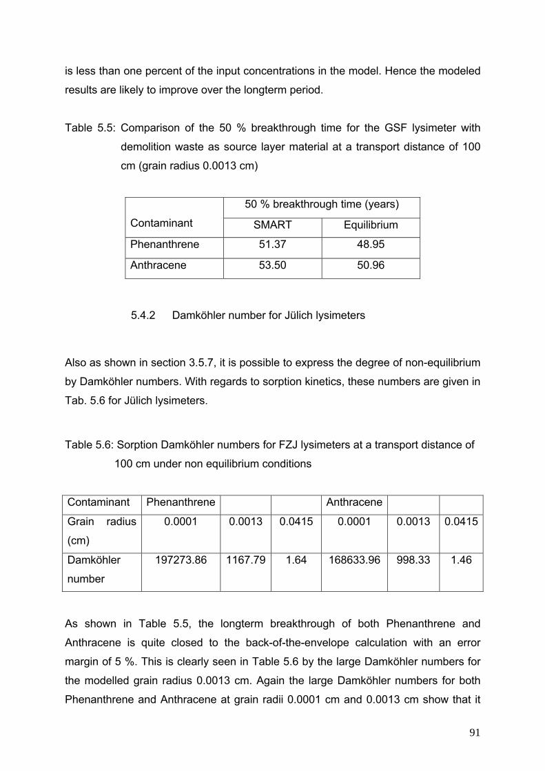
is less than one percent of the input concentrations in the model. Hence the modeled
results are likely to improve over the longterm period.
Table 5.5: Comparison of the 50 % breakthrough time for the GSF lysimeter with
demolition waste as source layer material at a transport distance of 100
cm (grain radius 0.0013 cm)
50 % breakthrough time (years)
Contaminant SMART Equilibrium
Phenanthrene 51.37 48.95
Anthracene 53.50 50.96
5.4.2 Damköhler number for Jülich lysimeters
Also as shown in section 3.5.7, it is possible to express the degree of non-equilibrium
by Damköhler numbers. With regards to sorption kinetics, these numbers are given in
Tab. 5.6 for Jülich lysimeters.
Table 5.6: Sorption Damköhler numbers for FZJ lysimeters at a transport distance of
100 cm under non equilibrium conditions
Contaminant Phenanthrene Anthracene
Grain radius
(cm)
0.0001 0.0013 0.0415 0.0001 0.0013 0.0415
Damköhler
number
197273.86 1167.79 1.64 168633.96 998.33 1.46
As shown in Table 5.5, the longterm breakthrough of both Phenanthrene and
Anthracene is quite closed to the back-of-the-envelope calculation with an error
margin of 5 %. This is clearly seen in Table 5.6 by the large Damköhler numbers for
the modelled grain radius 0.0013 cm. Again the large Damköhler numbers for both
Phenanthrene and Anthracene at grain radii 0.0001 cm and 0.0013 cm show that it
91
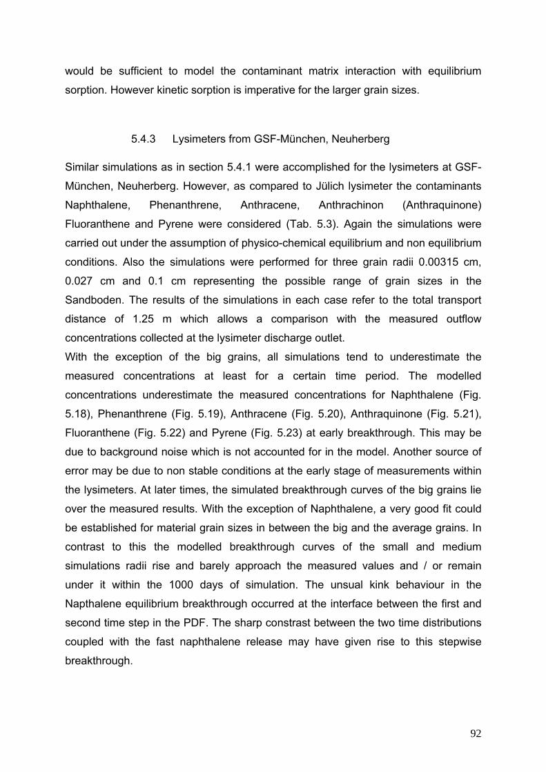
would be sufficient to model the contaminant matrix interaction with equilibrium
sorption. However kinetic sorption is imperative for the larger grain sizes.
5.4.3 Lysimeters from GSF-München, Neuherberg Similar simulations as in section 5.4.1 were accomplished for the lysimeters at GSF-
München, Neuherberg. However, as compared to Jülich lysimeter the contaminants
Naphthalene, Phenanthrene, Anthracene, Anthrachinon (Anthraquinone)
Fluoranthene and Pyrene were considered (Tab. 5.3). Again the simulations were
carried out under the assumption of physico-chemical equilibrium and non equilibrium
conditions. Also the simulations were performed for three grain radii 0.00315 cm,
0.027 cm and 0.1 cm representing the possible range of grain sizes in the
Sandboden. The results of the simulations in each case refer to the total transport
distance of 1.25 m which allows a comparison with the measured outflow
concentrations collected at the lysimeter discharge outlet.
With the exception of the big grains, all simulations tend to underestimate the
measured concentrations at least for a certain time period. The modelled
concentrations underestimate the measured concentrations for Naphthalene (Fig.
5.18), Phenanthrene (Fig. 5.19), Anthracene (Fig. 5.20), Anthraquinone (Fig. 5.21),
Fluoranthene (Fig. 5.22) and Pyrene (Fig. 5.23) at early breakthrough. This may be
due to background noise which is not accounted for in the model. Another source of
error may be due to non stable conditions at the early stage of measurements within
the lysimeters. At later times, the simulated breakthrough curves of the big grains lie
over the measured results. With the exception of Naphthalene, a very good fit could
be established for material grain sizes in between the big and the average grains. In
contrast to this the modelled breakthrough curves of the small and medium
simulations radii rise and barely approach the measured values and / or remain
under it within the 1000 days of simulation. The unsual kink behaviour in the
Napthalene equilibrium breakthrough occurred at the interface between the first and
second time step in the PDF. The sharp constrast between the two time distributions
coupled with the fast naphthalene release may have given rise to this stepwise
breakthrough.
92
Fig. 5.18: Measured and simulated Naphthalene breakthrough of GSF lysimeters with
contaminated soil as source layer material at a transport distance of 125
cm under equilibrium and non equilibrium conditions (ipd-small: grain
radius 0.00315 cm; ipd-medium: grain radius 0.027 cm; ipd-big: grain
radius 0.1 cm)
Fig. 5.19: Measured and simulated Phenanthene breakthrough of GSF lysimeters
with contaminated soil as source layer material at a transport distance of
25 cm under equilibrium and non equilibrium conditions (ipd-small: grain
radius 0.00315 cm; ipd-medium: grain radius 0.027 cm; ipd-big: grain
radius 0.1 cm)
93
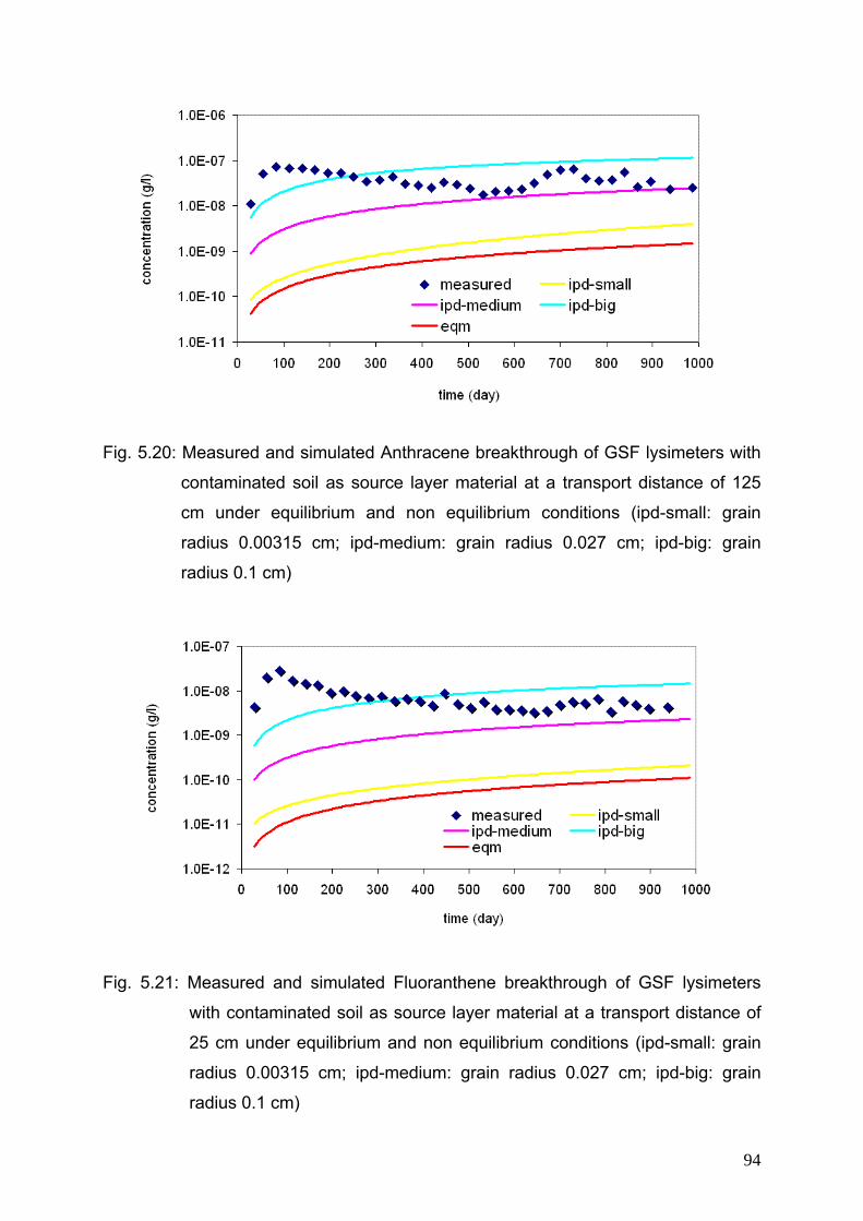
Fig. 5.20: Measured and simulated Anthracene breakthrough of GSF lysimeters with
contaminated soil as source layer material at a transport distance of 125
cm under equilibrium and non equilibrium conditions (ipd-small: grain
radius 0.00315 cm; ipd-medium: grain radius 0.027 cm; ipd-big: grain
radius 0.1 cm)
Fig. 5.21: Measured and simulated Fluoranthene breakthrough of GSF lysimeters
with contaminated soil as source layer material at a transport distance of
25 cm under equilibrium and non equilibrium conditions (ipd-small: grain
radius 0.00315 cm; ipd-medium: grain radius 0.027 cm; ipd-big: grain
radius 0.1 cm)
94
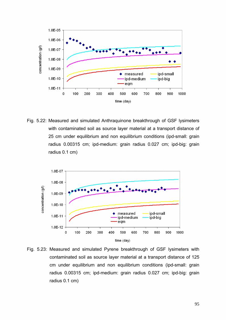
Fig. 5.22: Measured and simulated Anthraquinone breakthrough of GSF lysimeters
with contaminated soil as source layer material at a transport distance of
25 cm under equilibrium and non equilibrium conditions (ipd-small: grain
radius 0.00315 cm; ipd-medium: grain radius 0.027 cm; ipd-big: grain
radius 0.1 cm)
Fig. 5.23: Measured and simulated Pyrene breakthrough of GSF lysimeters with
contaminated soil as source layer material at a transport distance of 125
cm under equilibrium and non equilibrium conditions (ipd-small: grain
radius 0.00315 cm; ipd-medium: grain radius 0.027 cm; ipd-big: grain
radius 0.1 cm)
95

Fig. 5.24: Long term prediction of PAH breakthrough for GSF-lysimeters with
contaminated soil as source layer material at a transport distance of 125
cm under non equilibrium conditions (grain radius 0.027 cm).
Figure 5.24 above shows the long-term predictions for the six PAHs, which were
analysed at the GSF lysimeter filled with contaminated soil as the source layer
material for the transport modelling. The time at which the maximum concentration is
reached is strongly contaminant-dependent and increases with hydrophobicity.
Finally the 50 % breakthrough times which were determined based on SMART
simulations for the pollutants Naphthalene, Phenanthrene, Anthracene, Fluoranthene
Anthrachinon and Pyrene are given in Table 5.7 below. These values were compared
to the results of the estimations of the back-of-the-envelope calculations, which were
based on the assumption that physico-chemical (sorption) interactions proceeded
under equilibrium conditions. The SMART results are overestimated by about 43 - 51
%.
In comparison with FZJ lysimeters, the reactive processes are less close to
physicochemical equilibrium. The kinetic processes are therefore of more importance
in the GSF lysimeters. In the long run, this is due to the larger grain sizes of the
sandy materials in the GSF lysimeters. The associated longer diffusion length in the
grains therefore represents a crucial factor of influence for sorption kinetics.
Moreover the smaller Damköhler numbers (see Table 5.8 below) calculated for the
GSF lysimeters further confirmed the importance of kinetic sorption.
96
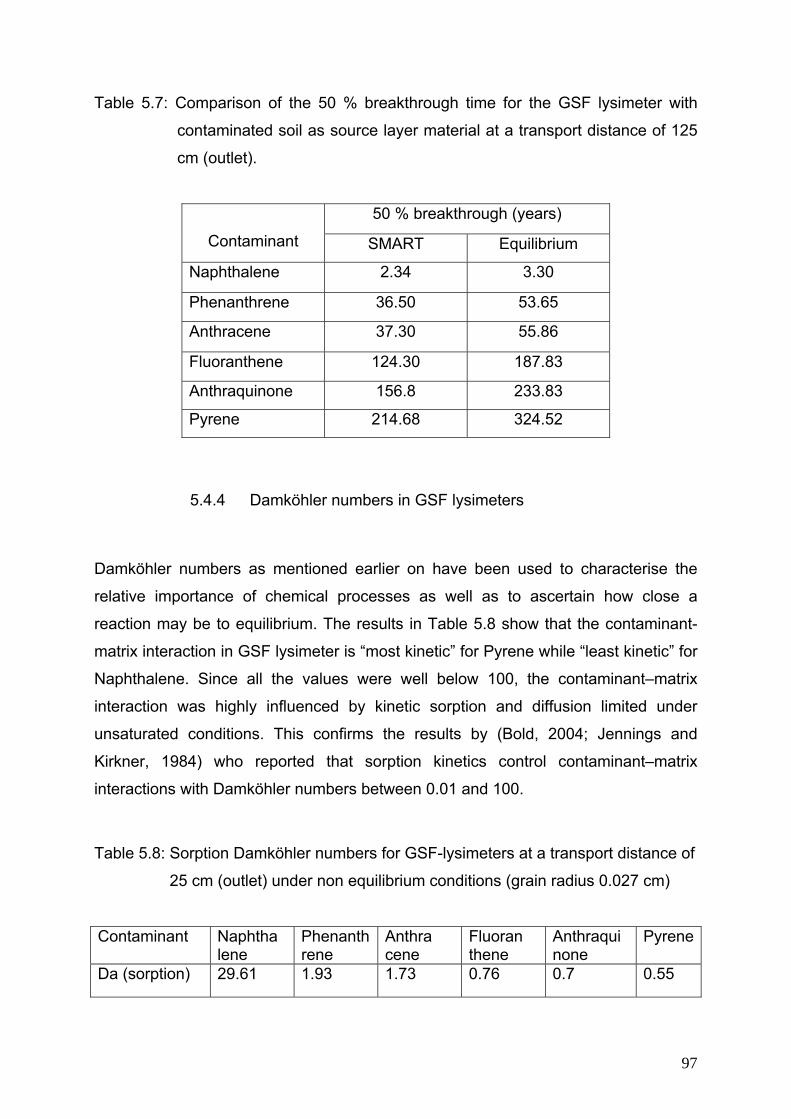
Table 5.7: Comparison of the 50 % breakthrough time for the GSF lysimeter with
contaminated soil as source layer material at a transport distance of 125
cm (outlet).
50 % breakthrough (years)
Contaminant SMART Equilibrium
Naphthalene 2.34 3.30
Phenanthrene 36.50 53.65
Anthracene 37.30 55.86
Fluoranthene 124.30 187.83
Anthraquinone 156.8 233.83
Pyrene 214.68 324.52
5.4.4 Damköhler numbers in GSF lysimeters
Damköhler numbers as mentioned earlier on have been used to characterise the
relative importance of chemical processes as well as to ascertain how close a
reaction may be to equilibrium. The results in Table 5.8 show that the contaminant-
matrix interaction in GSF lysimeter is “most kinetic” for Pyrene while “least kinetic” for
Naphthalene. Since all the values were well below 100, the contaminant–matrix
interaction was highly influenced by kinetic sorption and diffusion limited under
unsaturated conditions. This confirms the results by (Bold, 2004; Jennings and
Kirkner, 1984) who reported that sorption kinetics control contaminant–matrix
interactions with Damköhler numbers between 0.01 and 100.
Table 5.8: Sorption Damköhler numbers for GSF-lysimeters at a transport distance of
25 cm (outlet) under non equilibrium conditions (grain radius 0.027 cm)
Contaminant Naphtha lene
Phenanthrene
Anthra cene
Fluoran thene
Anthraqui none
Pyrene
Da (sorption) 29.61 1.93 1.73 0.76 0.7 0.55
97
5.5 Discussion and Conclusion The simulations of the reactive material transfer predict long residence times of the
respective pollutants in the lysimeters for both sites. This could be attributed to the
high sorption of the pollutants in the solid materials present in the transport layers.
The small grain size in particular and its associated short diffusion length in the solid
particles are regarded responsible for the fast contaminant sorption. It was also a fact
that the equilibrium model in all Jülich cases predicted the 50 % breakthrough at the
same time as the kinetic model. From the data in Tables 5.3 and 5.4 the respective
retardation factors can be easily calculated. The retardation factors are between 101
- 107 and 15 - 1493 for Jülich and München respectively, indicating that sorption
capacity is high. The overall results could be improved if background concentration
and biodegradation data are included. In summary the applicability of the model tool
SMART for the reactive material transfer at the lysimeter scale could be shown. This
encompasses the consideration of different solid materials and pollutant
characteristics.
98
Chapter 6
6 THE KWABENYA (GHANA) LANDFILL CASE STUDY: AN EXAMPLE OF
FIELD SCALE MODELLING
6.1 Motivation
Environmental sanitation issues resulting from inadequate water supply, drainage,
solid waste management as well as sanitation facilities have been a major bone of
contention in Ghana for more than decades. The Ghana strategy for reducing poverty
document for the years 2003 – 2005 emphasises the urgent need of environmental
sanitation and capacity to deal with solid and liquid waste. The problems have
adversely affected the urban poor. According to Mensah and Larbi (2005) the
problem of solid waste disposal in Ghana is not only engineering but of multi-
dimensional difficulties such as indiscriminate dumping of refuse, increasing
difficulties of acquiring suitable disposal sites, lack of effective road network which
aids in the conveyance of solid waste, rapid urbanization and poor financial and
technical capacities of local authorities. The problems are further aggravated by
effective planning and management lapses. Almost all landfills in Ghana are actually
open dumps without leachate and gas collection facilities and hence operated not
according to recommended standards and practices of sanitation. Recently the waste
disposal situation was further worsened by creation and uncontrolled dumping of
plastic bags. In 2002, the problem assumed a political dimension that led to the
dismissal of the Accra City’s mayor. A controlled dumping site which was in use at
Oblogo, a site in the Accra metropolis, was usually compacted to ensure proper
dumping. The dumping of waste at Oblogo began in January 2002. Since then
Oblogo received an average daily waste load of about 1200 metric tons. The capacity
of the facility was stressed up in July 2004. Other dumping sites were also available
in or around the city but they were all temporary in nature. These sites were used or
are being used partly because of limited capacity for collection of waste and partly
because of the lack of suitable disposal sites. These temporary or ad hoc tips were
unsightly and represent a risk to public health (Mensah and Larbi, 2005). Wastes
deposited at these sites were picked over by scavengers and dispersed by animals.
99
In the absence of a new landfill site, solid wastes would be collected in similar
uncontrolled dumps in numerous locations within the city. The number and size of
such dumps would escalate. These waste dumps therefore obviously constitute a risk
to public health and significantly cause environmental nuisance to the City.
There was therefore an urgent need for the development of a new site which could
accept solid waste and retain the waste in such a manner as to protect public health
and minimize damage to the environment. Foreign loads were therefore secured to
help in tackle environmental sanitation especially engineered mediated landfills. One
of the landfill that was sited in the Accra metropolis is the Kwabenya landfill.
Environmental impact assessment (EIA) was conducted as a first phase of the overall
landfill contraction. The modelling work done in the EIA report was exclusively for
inorganic pollutants that may emanate from the landfill as a leachate. The objective of
this chapter is therefore to model the spreading of organic contaminants, which is
PAHs in this case. This is significant because the waste types are likely to change in
the future as a result of industrialization and increased effluence (EIA report, 2000)
towards organic contaminants.
6.2 The Kwabenya landfill
6.2.1 Description of the project area of interest The growth of the cities of Accra and Tema has extended to neighbouring districts
such as the district Ga in which the proposed landfill Kwabenya is located (Fig. 6.1).
The principal objective of the landfill construction was to improve the surroundings,
living conditions and quality of life of the entire citizenry of present and future
generations. The Oblogo site is situated in the western part of Accra and was
formerly a hard-rock quarry. The Accra Metropolitan Assembly (AMA) and other key
stake holders in the region identified the urgent need for a landfill. Subsequently to
site selection studies carried out by Accra Metropolitan Authority (AMA) and local
consultants several years ago, the advisory committees of the AMA Waste
Management Department advocated a site at Kwabenya for the proposed landfill
after which the EIA had been conducted.
100
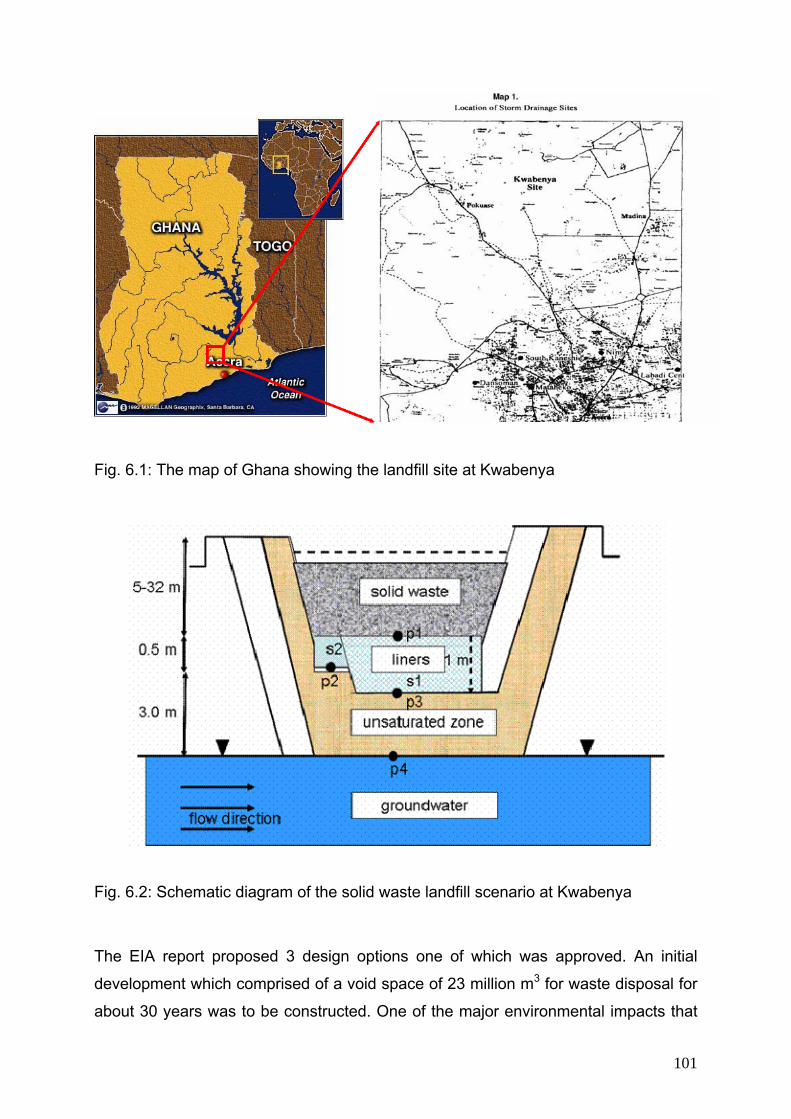
101
An Environmental Impact Study on the landfill was carried out by Taywood
Environmental Consultancy. Most of the literature review and modelling carried out in
this thesis is based on the Proposed Landfill at kwabenya (the–Environmental
Sanitation Project, 1999 Southhall, UK report was obtained by permission from the
AMA.)
Fig. 6.1: The map of Ghana showing the landfill site at Kwabenya
Fig. 6.2: Schematic diagram of the solid waste landfill scenario at Kwabenya
The EIA report proposed 3 design options one of which was approved. An initial
development which comprised of a void space of 23 million m3 for waste disposal for
about 30 years was to be constructed. One of the major environmental impacts that
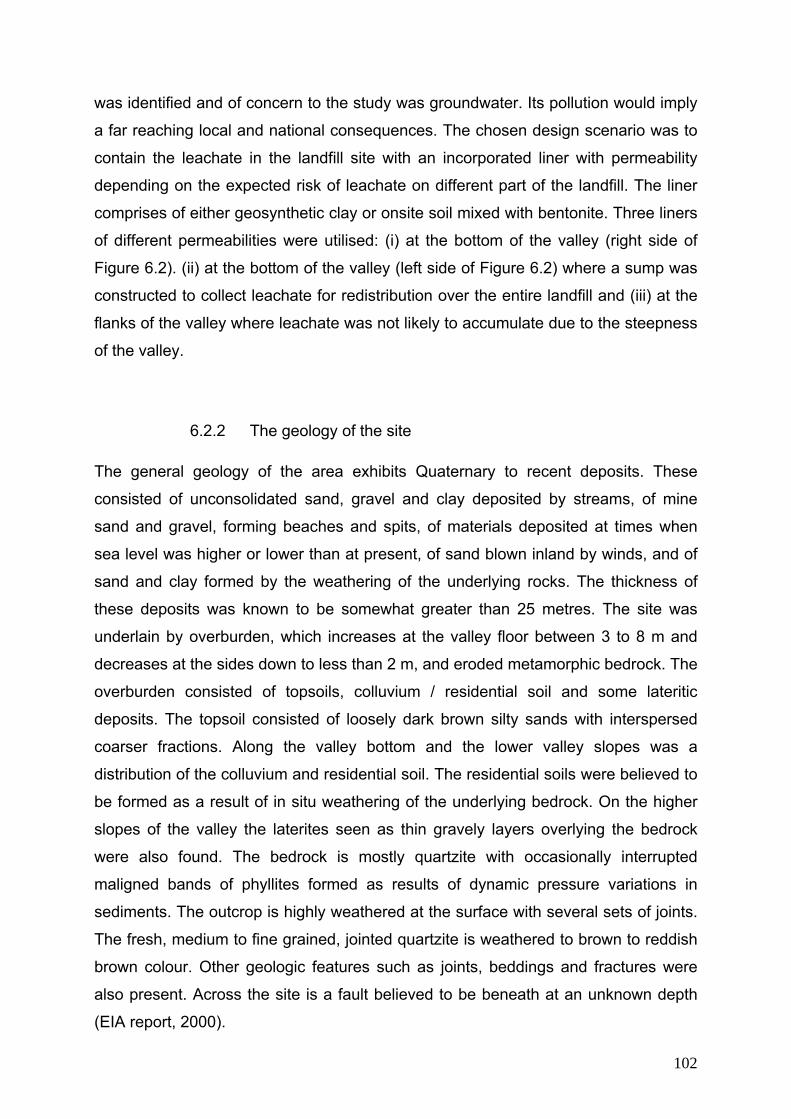
was identified and of concern to the study was groundwater. Its pollution would imply
a far reaching local and national consequences. The chosen design scenario was to
contain the leachate in the landfill site with an incorporated liner with permeability
depending on the expected risk of leachate on different part of the landfill. The liner
comprises of either geosynthetic clay or onsite soil mixed with bentonite. Three liners
of different permeabilities were utilised: (i) at the bottom of the valley (right side of
Figure 6.2). (ii) at the bottom of the valley (left side of Figure 6.2) where a sump was
constructed to collect leachate for redistribution over the entire landfill and (iii) at the
flanks of the valley where leachate was not likely to accumulate due to the steepness
of the valley.
6.2.2 The geology of the site The general geology of the area exhibits Quaternary to recent deposits. These
consisted of unconsolidated sand, gravel and clay deposited by streams, of mine
sand and gravel, forming beaches and spits, of materials deposited at times when
sea level was higher or lower than at present, of sand blown inland by winds, and of
sand and clay formed by the weathering of the underlying rocks. The thickness of
these deposits was known to be somewhat greater than 25 metres. The site was
underlain by overburden, which increases at the valley floor between 3 to 8 m and
decreases at the sides down to less than 2 m, and eroded metamorphic bedrock. The
overburden consisted of topsoils, colluvium / residential soil and some lateritic
deposits. The topsoil consisted of loosely dark brown silty sands with interspersed
coarser fractions. Along the valley bottom and the lower valley slopes was a
distribution of the colluvium and residential soil. The residential soils were believed to
be formed as a result of in situ weathering of the underlying bedrock. On the higher
slopes of the valley the laterites seen as thin gravely layers overlying the bedrock
were also found. The bedrock is mostly quartzite with occasionally interrupted
maligned bands of phyllites formed as results of dynamic pressure variations in
sediments. The outcrop is highly weathered at the surface with several sets of joints.
The fresh, medium to fine grained, jointed quartzite is weathered to brown to reddish
brown colour. Other geologic features such as joints, beddings and fractures were
also present. Across the site is a fault believed to be beneath at an unknown depth
(EIA report, 2000).
102
6.2.3 Hydrogeology of the site
The hydrogeology is influenced by the topology and geology of the site.
Investigations conducted in situ on the silty sand soils showed a hydraulic
conductivity varying from 10-7 m/s to 10-5 m/s. However laboratory tests with
compacted samples recorded conductivity values of 1.4*10-8 m/s to 1.8*10-4 m/s.
The conductivity results of the soils showed the existence of hydraulic continuity with
the underlying bedrock. According to tests conducted in trial pits groundwater levels
were shallow at the valley flanks due to the thin dry overburden present. This
suggested a lateral flow towards the center of the valley or vertically to the underlying
rocks which could occur at different seasons in different rates. The original (primary)
porosity of the quartzite and phyllite was low due to their metamorphic origins. The
presents of joints, beddings and fractures in the rocks resulted in secondary
porosities and hence increased conductivities. Most of the in situ tests in these rocks
showed a conductivity range of 10-6 m/s to 10-5 m/s which corresponded to moderate
permeabilities normally encountered in fractured rocks. These values were further
confirmed by borehole logs and drilling records. Effective porosities and storativities
of the quartzites were assumed to be quite low since most of the water was believed
to be stored in fissures. However storativity in the colluvium could be 10% or higher
as compared to the 1 % that was guessed in the absence of pumping data. A
groundwater level of 2 m was observed below the valley bottom which could rise to
feed surface streams in time of rainfall event. The hydraulic gradients were 1/40 and
1/20 for the valley bottom and valley flanks respectively. Conceptually a nominal
water flow through the active zone on the flanks of the valley and beneath the
colluvium extended to a depth of 10 m. According to the EIA report a ground water
flow of 0.75 L/sec and 0.19 L/sec was calculated for the rock and colluvium
respectively by using the one dimensional Darcy method (EIA report, 2000).
6.3 The landfill leachate modelling
Emerging dilute and disperse leachate management was the main driving force of the
landfill design. The target was to reduce and control ensuing leachate emerging from
the landfill. As waste mass builds up at the landfill site, leachate would be generated.
The input liquid component, changes in the soil moisture retentions and transmission
characteristics of the waste as well as the infiltration through the successive layers
103
and ground surface would determine the volume of leachate generation. Potential
leachate may migrate to contaminant surface water and ground water in and around
the landfill hence the proposition of the lining system to minimise the risk. Drains are
normally provided to take care of the leachates that are generated in the waste.
However the lining may leak as the leachate heads build up in the landfill to
contaminate the underlying groundwater (EIA report, 2000).
The conceptual model is described in terms of source (waste), pathway through the
geosynthetic clay liner and receptor (the point of compliance between the
unsaturated and saturated zone). The landfill is shown schematically in the Figure
6.2. In order to quantify the contaminant concentrations needed to assess the
vulnerability of the underground water, breakthrough curves were calculated at the
following levels of the landfill:
(i) p1, the level directly below the base of the waste
(ii) p2, the level directly below the liner at the left side of the landfill
(iii) p3, the level directly below the liner at the right side of the landfill
(iv) p4, the level of point of transition between the saturated and unsaturated
zones.
Two pathway scenarios were considered in the model:
(1) s1: Leachate from the solid waste leaking through the liner (1 m thickness at
the base of the valley) and through the unsaturated zone to the point of
compliance, p4. The total vulnerability breakthrough is the time lag between
p1, p3 and p4.
(2) s2: Leachate from the solid waste leaking through the liner (0.5 m thickness at
the left side of the base of the valley) and through the unsaturated zone to the
point of compliance, p4. The total vulnerability breakthrough is the time lag
between p1, p2 and p4.
As a worst case scenario, the following assumptions were made similar to that of the
inorganic contaminant model (EIA report, 2000):
(1) Groundwater and leachate migration are uniform through isotropic materials.
(2) There is no retardation or attenuation of the leachate in the lining system.
104
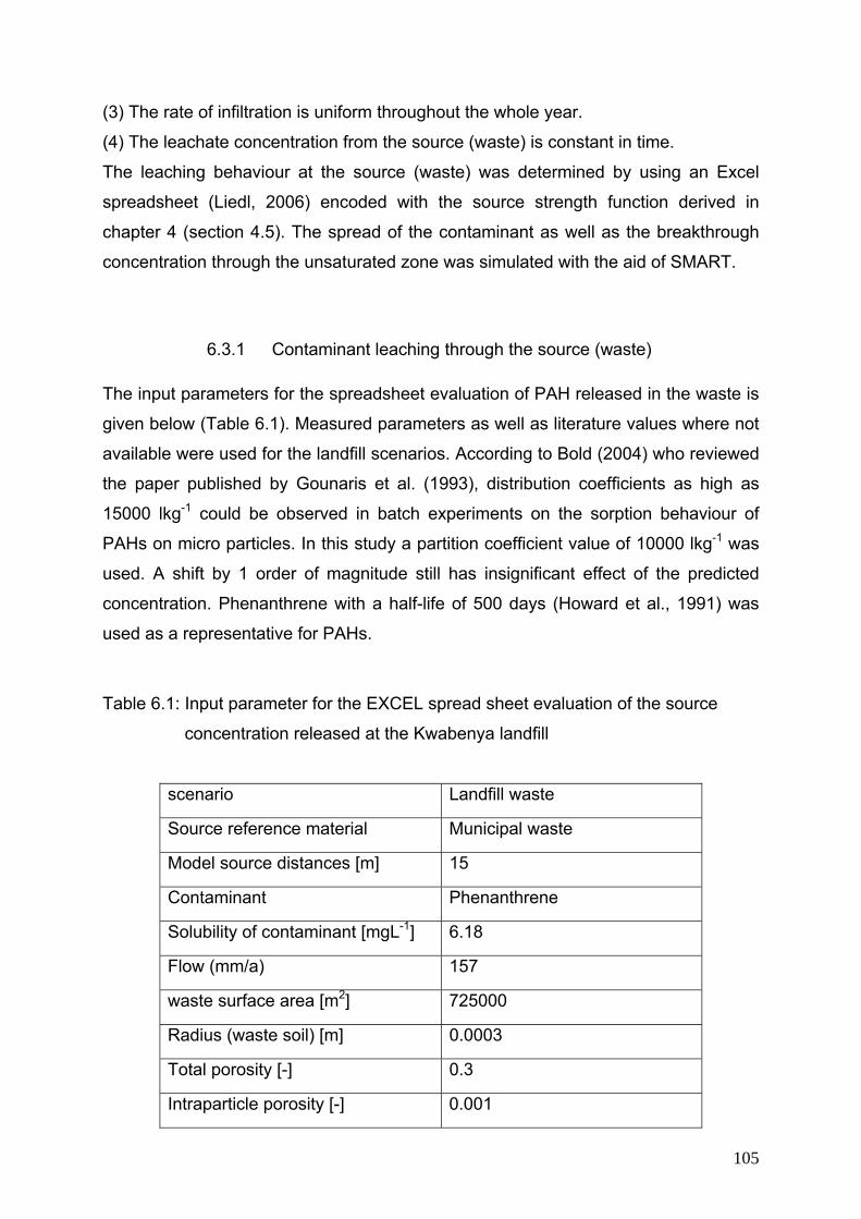
(3) The rate of infiltration is uniform throughout the whole year.
(4) The leachate concentration from the source (waste) is constant in time.
The leaching behaviour at the source (waste) was determined by using an Excel
spreadsheet (Liedl, 2006) encoded with the source strength function derived in
chapter 4 (section 4.5). The spread of the contaminant as well as the breakthrough
concentration through the unsaturated zone was simulated with the aid of SMART.
6.3.1 Contaminant leaching through the source (waste) The input parameters for the spreadsheet evaluation of PAH released in the waste is
given below (Table 6.1). Measured parameters as well as literature values where not
available were used for the landfill scenarios. According to Bold (2004) who reviewed
the paper published by Gounaris et al. (1993), distribution coefficients as high as
15000 lkg-1 could be observed in batch experiments on the sorption behaviour of
PAHs on micro particles. In this study a partition coefficient value of 10000 lkg-1 was
used. A shift by 1 order of magnitude still has insignificant effect of the predicted
concentration. Phenanthrene with a half-life of 500 days (Howard et al., 1991) was
used as a representative for PAHs.
Table 6.1: Input parameter for the EXCEL spread sheet evaluation of the source
concentration released at the Kwabenya landfill
scenario Landfill waste
Source reference material Municipal waste
Model source distances [m] 15
Contaminant Phenanthrene
Solubility of contaminant [mgL-1] 6.18
Flow (mm/a) 157
waste surface area [m2] 725000
Radius (waste soil) [m] 0.0003
Total porosity [-] 0.3
Intraparticle porosity [-] 0.001
105
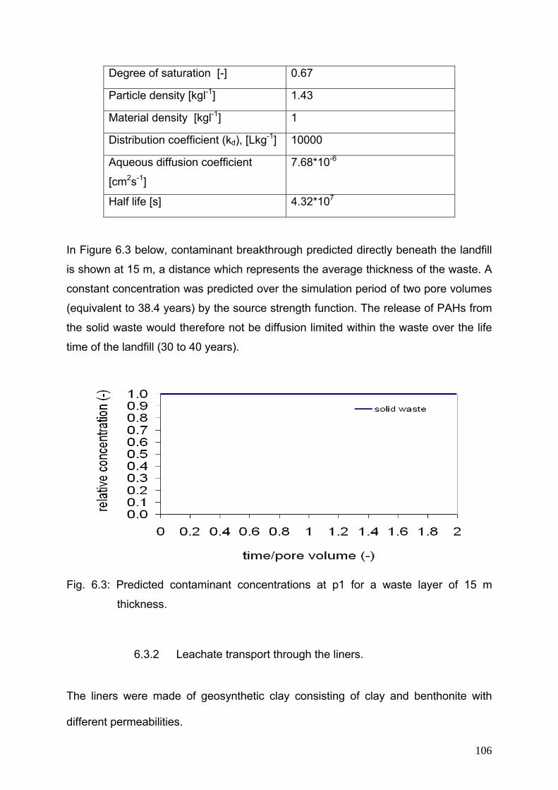
Degree of saturation [-] 0.67
Particle density [kgl-1] 1.43
Material density [kgl-1] 1
Distribution coefficient (kd), [Lkg-1] 10000
Aqueous diffusion coefficient
[cm2s-1]
7.68*10-6
Half life [s] 4.32*107
In Figure 6.3 below, contaminant breakthrough predicted directly beneath the landfill
is shown at 15 m, a distance which represents the average thickness of the waste. A
constant concentration was predicted over the simulation period of two pore volumes
(equivalent to 38.4 years) by the source strength function. The release of PAHs from
the solid waste would therefore not be diffusion limited within the waste over the life
time of the landfill (30 to 40 years).
Fig. 6.3: Predicted contaminant concentrations at p1 for a waste layer of 15 m
thickness.
6.3.2 Leachate transport through the liners.
The liners were made of geosynthetic clay consisting of clay and benthonite with
different permeabilities.
106
Table 6.2: Input parameters of leachate leakage through the landfill liners
scenario Base of valley (right
side)
Base of valley (left
side)
Thickness of liner [m] 1 0.5
Head gradient [-] 0.3 0.3
Conductivity of liner [ms-1] 1*10-9 8*10-10
effective porosity [-] 0.1 0.1
Considering a worse case scenario, advective and diffusive time scales were
computed and compared with the aid of the equations 3.12 – 3.15 (chapter 3). A time
scale ratio of advection in relation to diffusion of 8:1 and 6.5:1 was obtained for the
liners at the right side and left side of the base of the valley (waste) respectively. This
means it would take a potential leachate at the bottom of the waste 3.3 years and
10.57 years to transverse through the left and right liners respectively, to the upper
part of the unsaturated zone if diffusion is neglected. The overall leachate travel time
would therefore be extended in favour of groundwater protection if retardation is
considered in the liners.
6.3.3 Leachate transport in the unsaturated zone. Considering a constant leaching concentration source (solid waste), contaminant
breakthroughs at the point of compliance (p4) were simulated with SMART for two
pathways, p3 – p4 (1 m) and p2 – p4 (3 m). The input parameters for the transport
models are given in Table 6.3.
107
Table 6.3: Transport parameters for the Kwabenya landfill scenarios.
scenario Unsaturated zone (s1 and
s2)
Transport reference material Colluvium (silty sand)
Model Transport distances [m] 1 (s1) and 3 (s2)
Inlet contaminant concentrations
[mgl-1]
10-3
Grain size of colluvium [cm] 0.014
Total porosity [-] 0.35
Intraparticle porosity [-] 0.01
Degree of saturation [-] 50
Material density [kgl-1] 1.58
Particle density [kgl-1] 2.43
Distribution coefficient (kd), [Lkg-1] 10
Aqueous diffusion coefficient
[cm2s-1]
7.68*10-6
Volume flow rate [m3s-1] 2.4*10-9 (s1); 2.0*10-9 (s2)
The flow rates in table Table 6.3 are vertical flow seeping from the base of the liners
in the unsaturated zone.
In Figures 6.4 and 6.5 contaminant breakthroughs at 1 m and 3 m are shown for the
pathways p3 - p4 and p2 - p4 respectively by taking into account sorption and
biodegradation. The dotted line shows the drinking water standard of the World
Health Organisation (WHO, 2003).
108
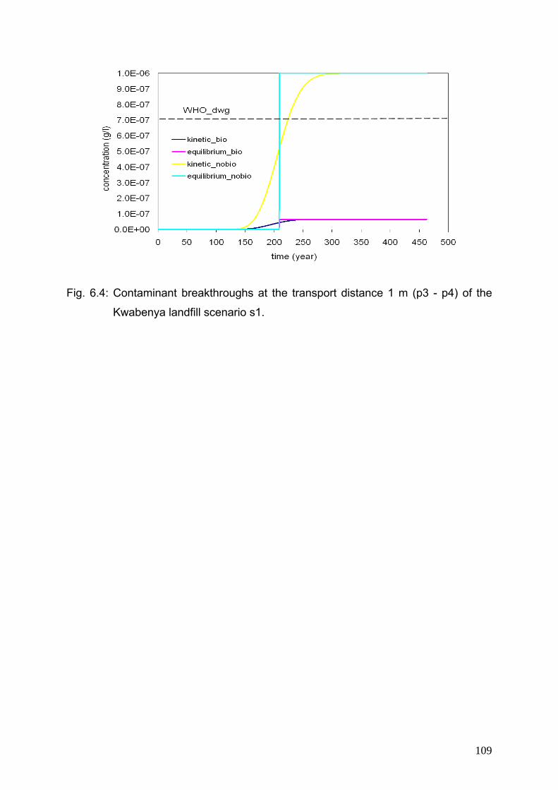
Fig. 6.4: Contaminant breakthroughs at the transport distance 1 m (p3 - p4) of the
Kwabenya landfill scenario s1.
109
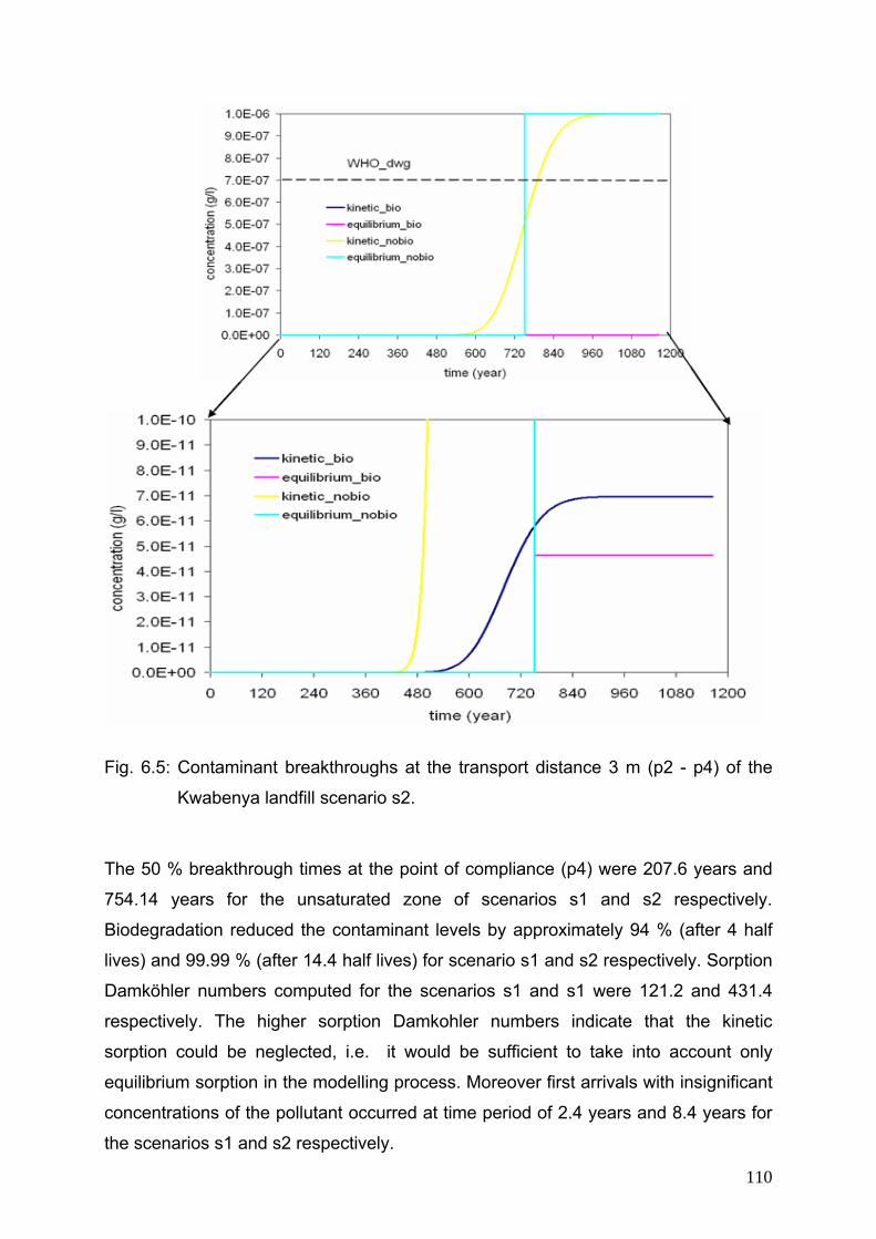
Fig. 6.5: Contaminant breakthroughs at the transport distance 3 m (p2 - p4) of the
Kwabenya landfill scenario s2.
The 50 % breakthrough times at the point of compliance (p4) were 207.6 years and
754.14 years for the unsaturated zone of scenarios s1 and s2 respectively.
Biodegradation reduced the contaminant levels by approximately 94 % (after 4 half
lives) and 99.99 % (after 14.4 half lives) for scenario s1 and s2 respectively. Sorption
Damköhler numbers computed for the scenarios s1 and s1 were 121.2 and 431.4
respectively. The higher sorption Damkohler numbers indicate that the kinetic
sorption could be neglected, i.e. it would be sufficient to take into account only
equilibrium sorption in the modelling process. Moreover first arrivals with insignificant
concentrations of the pollutant occurred at time period of 2.4 years and 8.4 years for
the scenarios s1 and s2 respectively.
110
6.4 Summary and conclusion
Two worse case scenarios (s1 and s2) were modelled for the Kwabenya, Ghana
landfill. It was shown that the leachate concentration inside the source (waste) would
stay constant during the 30 to 40 years life time of the landfill. However at any time
the PAH leachates starts to leach through the liner and the unsaturated zone towards
the receptor (groundwater table), the leachate would take 218.17 years and 434.70
years for the pathway scenarios s1 and s2 respectively. The World Health
Organization (WHO) drinking water standards (dwg) of 0.7 ugl-1 (WHO, 2003) would
therefore only be exceeded after a long period of 234.17 years and 973.4 years for
scenarios S1 and S2 respectively. The large Damköhler numbers show that the
kinetic behaviour of contaminant–matrix interaction could be neglected if the time
evolution of the contaminant is to be monitored. The model shows that within the 30
year of landfill operation, the predicted concentrations would still be about 14 orders
of magnitude lower than the WHO drinking standards. Biodegradation reduces the
overall concentration levels thereby making the subsurface waters more secured.
(Figures 6.4 and 6.5). The model therefore shows that the receptor, i.e. groundwater,
is secured as far as leachate of the non volatile organic compounds such as PAHs
through the geosynthetic liners and the underneath unsaturated zone of the landfill is
concerned.
111
Chapter 7
7 SUMMARY AND CONCLUSION
Organic chemicals such as PAHs, though helpful domestically and industrially, can
still be devastating and recalcitrant when entering the environmental media.
Research in the behaviour, toxicity, carcinogenicity and modelling of PAH fate and
transport is still ongoing. One of the objectives of this thesis was the development of
a source strength function which could be used to predict the behaviour of organic
leachate that could form the upper boundary condition for transport modelling. Also a
process based prediction of long term PAH concentrations at the lysimeter outlets, an
index of groundwater risk assessment, was conducted with the modelling tool
SMART. In addition the application of SMART was to be extended to a field scale
study of a landfill site in Ghana (Kwabenya). The major identifiable processes
involved in groundwater risk assessment were reviewed. Sorption and
biodegradation are known to cause a decrease of groundwater pollution risk while
particle facilitated transport and preferential flow mostly increase groundwater
pollution risk. Other tools such as GLEAMSS, PELMO, PRZM, VARLEACH,
SIMULAT, MACRO, WAVE, LEACHP used in lysimeter studies were summarily
described in terms of their flow and transport characteristics and equations.
Most of the aforementioned models solve the Richards equation for flow in the
unsaturated zone and use the convection-dispersion equation to model solute
transport. The SMART model is based on the Lagrangian streamtube approach
which allows the separation of conservative transport and reactive processes under
steady state flow conditions, thereby reducing numerical errors to the minimum. This
software was validated successfully by authors Rahman (2002), Cata (2003),
Schmidt (2003), Bold (2004), Cai (2004), Christ (2004), Henzler (2004), Madlener
(2004), and Susset (2004) at the laboratory scale. The following conclusions are
drawn for the source term, lysimeter and landfill modelling.
112
(1) Source term modeling
A source strength function was determined for the quantification of the possibly
temporally variable discharge behaviour of organic pollutants from small-scale (point-
like) sources of pollutant. With the aid of the source strength function, the temporal
change of the pollutant concentration is determined in the seepage water at the
transition from the pollutant source to the transport distance. In order to simulate
transport and the reactive processes, the source strength function can be used as a
time-dependent upper boundary condition for those pollutants migrating to the
groundwater level (= point of compliance). In determining the source strength
function, advection, desorption kinetics and microbial degradation were considered
as relevant discharge processes. It was assumed that
- desorption kinetics can be simulated with an intraparticle diffusion model,
- seepage water flow is steady state,
- a concentration equilibrium exists between mobile and immobile phases at
the beginning of the simulations,
- microbial degradation only occurs in the mobile phase.
In order to ensure the general applicability of the source strength function,
dimensionless numbers and / or conditions were used throughout: The time t was
standardized in terms of pore volumes, PV = neL/GWN (ne = effective porosity, L =
thickness of the source, GWN = seepage-water flow rate). The relative meaning of
desorption in comparison to advection was expressed by means of the Damköhler
number Dades. The relative meaning of microbial degradation in comparison to the
advection was expressed by means of the Damköhler number Dabio. The pollutant
source concentration C at the outlet of the source was normalised with the initial
concentration Co in the mobile phase. This value corresponds to the concentration
under equilibrium conditions. In the seepage water prognosis, a conversion between
the dimensionless time and water-solid mass ratio W/F is given by the relations:
FWLnAMt
e//' ⋅
⋅=
and '
// t
AMLnFW e⋅
⋅=
where t’ = normalised pore volume time (t ' = t/PV), M/A = solid mass per unit cross
sectional area. This conversion presupposes that flow can be accepted as steady
113
state (if necessary after suitable averaging). The use of the normalised pore volume
time t’ offers a crucial advantage in the context of setting of tasks, because the
retention time of the pollutant in the mobile phase is thereby included. This enters
directly in the determination of the Damköhler numbers Dades and Dabio, with which
the relative contributions of desorption kinetics and the microbial degradation in the
discharge behaviour are quantified.
(1) The Damköhler number Dades is given by
2 2 2
22 22
ln 1 6 3 0.1
6ln 0.1
app app app
esd
app app
D PV D PV D PVifa a aDa
D PV D PVifa a
π π
ππ
⎧ ⎛ ⎞⋅ ⋅ ⋅− − ⋅ + ⋅ <⎪ ⎜ ⎟⎜ ⎟⎪ ⋅ ⋅⎝ ⎠= ⎨⎪ ⋅ ⋅
⋅ − ≥⎪⎩
with apparent diffusion coefficient: dipip
ipaqapp Knn
nDD⋅⋅−+
⋅=
ρ)1(
2
where a is grain radius, nip = intraparticle porosity, ρ is solid density und Kd is
distribution coefficient.
(2) The Damköhler number Dabio is given as 1/2
ln2bioPVDa PVT
λ= ⋅ = ⋅
where λ is biodegradation rate constant and T1/2 = half life.
The source strength function was derived from the results of many simulation runs
with the model tool SMART. Within the SMART simulations both Damköhler numbers
were varied independently from each other in the interval from 0.001 to 1000, in order
to cover as large a range of the discharge behaviour as possible. Large values of the
Damköhler numbers mean very fast, small values correspond to very slow reactions,
where pore volume specification forms the comparison yardstick of typical advection
time scales. With the help of the simulation results two function types were identified,
which could be distinguished for the cases Dades ≥ 0.1 and Dades ≤ 0.1. Function
parameters were obtained for both types by an optimum adjustment to the results of
the SMART simulations.
(i) For case 1 (Dades ≥ 0.1) the relative discharge concentration is in the form
114
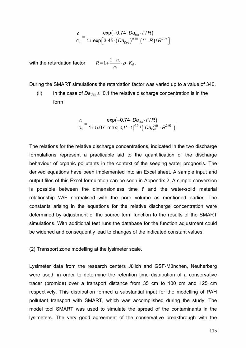
( )( ) ( )0.15 0.74
0
exp 0.74 '/1 exp 3.45 ' /
Bio
Des
Da t Rcc Da t R R
− ⋅ ⋅=
⎡ ⎤+ ⋅ ⋅ −⎣ ⎦
with the retardation factor de
e Kn
nR ⋅⋅−
+= ρ11 .
During the SMART simulations the retardation factor was varied up to a value of 340.
(ii) In the case of Dades ≤ 0.1 the relative discharge concentration is in the
form
( ){ } ( )0.6 0.930.55
0
exp 0.74 '/1 5.07 max 0, ' 1 /
Bio
Des
Da t Rcc t Da
− ⋅ ⋅=
+ ⋅ − ⋅R
The relations for the relative discharge concentrations, indicated in the two discharge
formulations represent a practicable aid to the quantification of the discharge
behaviour of organic pollutants in the context of the seeping water prognosis. The
derived equations have been implemented into an Excel sheet. A sample input and
output files of this Excel formulation can be seen in Appendix 2. A simple conversion
is possible between the dimensionless time t' and the water-solid material
relationship W/F normalised with the pore volume as mentioned earlier. The
constants arising in the equations for the relative discharge concentration were
determined by adjustment of the source term function to the results of the SMART
simulations. With additional test runs the database for the function adjustment could
be widened and consequently lead to changes of the indicated constant values.
(2) Transport zone modelling at the lysimeter scale.
Lysimeter data from the research centers Jülich and GSF-München, Neuherberg
were used, in order to determine the retention time distribution of a conservative
tracer (bromide) over a transport distance from 35 cm to 100 cm and 125 cm
respectively. This distribution formed a substantial input for the modelling of PAH
pollutant transport with SMART, which was accomplished during the study. The
model tool SMART was used to simulate the spread of the contaminants in the
lysimeters. The very good agreement of the conservative breakthrough with the
115
observed tracer data in the Jülich and München lysimeters were a good technical
basis for the modelling of the reactive transport with sufficient accuracy. During the
model simulations, the initial model input parameters were defined independently
from the PAH concentrations, which were recorded along the transport distance and /
or at the lysimeter discharge outlet. This proceeding corresponds to a pure forward
modelling of the reactive material transfer, i.e. there was no model calibration with
regards to reactive processes as is the case in many modelling projects, in order to
be able to examine the predictive capability of the model tool SMART. The 50 %
breakthrough of the source term concentrations at the lysimeter measuring points
were predicted to occur at 52 years for Jülich and between 2 to 215 years for
München lysimeters. Large breakthrough times are due to the high PAH sorption
capacity and rapid solute uptake of the predominantly fine-grained material and the
associated, pronounced pollutant retardation along the travel distance. This was
consistent with the very low recovery rate and low concentrations (Klotz and
Schramm, 2006) detected in the lysimeter research facilities for more than 2.5 years
of monitoring. However the appropriate breakthrough times could also be determined
for many of the studied settings with simple calculation based on the measured data
on the assumption of equilibrium conditions. The consistent good agreement
between the observed data and the model predictions shows the usefulness of the
model tool SMART as a prognosis instrument for pollutant risk assessment. Other
lysimeter specific modelling with SMART, not presented in this study showed much
improved agreement between the observed and the model results within the limit of
experimental errors but limited in application.
(3) Landfill modelling
In addition to the Environmental Impact Assessment and inorganic leachate
modelling with the Landsim model tool (Environmental Agency / Golder Associate,
1996) performed by (Taywood Environmental Consultancy) (Environmental Impact
Assessment report, 2000) the process based reactive transport model SMART has
been used to predict organic (PAH) contamination at a landfill site in Ghana
(Kwabenya), a country whose solid waste is increasingly becoming organic in nature
due to industrialisation with low waste recycling and minimisation programs.
116
Leachate released from the source (waste) was modelled with the source term
functions encoded in the Excel spreadsheet introduced in chapter 3. The source term
modelling of the organic leachate from the waste predicted a straight line horizontal
breakthrough. This shows that the release of the leachate will be time independent at
least for the 30 - 40 year operational period of the landfill i.e. the organic leachates
were not affected by age within this period. Advective and diffusive time lags of
leachate leaking through two liners with different permeabilities emplaced at the base
of the landfill directly in contact with the waste were also determined. With the
activation of sorption (equilibrium and kinetics) and biodegradation processes, two
pathway scenarios were modelled with SMART for the unsaturated zone. Due to the
relative longer half-life of PAHs, the effect of biodegradation is estimated to be
minimal during the landfill operational period. The prediction of longer breakthrough
times implies that the receptor (groundwater) would not be impaired if leachate
leakage starts at any time within the operational period of the landfill. Even though
there was no observed data for validation of the model as is often the case in field
scale studies, SMART was found to be useful to a reasonable level of accuracy.
SMART can therefore be used to establish waste acceptance criteria for organic
contaminants in the landfill at Kwabenya.
117
REFERENCES Abdel-Salam., A. and Chrysikopoulos, C. V. (1995): Modeling of Colloid and Colloid-
Facilitated Contaminant Transport in a Two-Dimensional Fracture with
patially Variable Aperture. Kluwer Academic Publishers. 20, 197-221.
Abelin, H. (1986): Migration in a single fracture: An in situ experiment in a natural
fracture, Ph.D. dissertation, Dep. of Chem. Eng., R. Inst. of Tech.,
Stockholm, 170 pp.
Abu-Sharar, T.M., F.T. (1987): Bingham and J.D. Rhoades, Stability of soil
aggregates as affected by electrolyte concentration and composition. Soil
Sci. Soc. Am. J., 51, 309.
Adamczyk, Z., T. Dabros, J. Czarnecki and T.G.M. van de Ven (1983): Physical
Chemistry of Colloid and Interfaces: Biotechnologies and Drug Research
Adv. Colloid Interface Sci., 19 183.
Aden, K., Diekkrueger, B (2000): Modeling pesticide dynamics of four different sites
using the model system SIMULAT. Agric. Water Mgmt. 44, 337±355.
Adriaens, P. (2003): Applied Environmental Geoscience lecture notes: Microbiology
II. Sec 5.2p. Eberhard-Karls-Universität Tuebingen.
AGBoden (1994): Bodenkundliche Kartieranleitung, 4. Auflage, E. Schweizbart’sche
Verlagsbuchhandlung, Stuttgart,.
Aitken, C.M., Jones, D.M., and Larter, S.R. (2004): Anaerobic hydrocarbon
biodegradation in deep subsurface oil reservoirs. Nature 431: 291-294.
Akthar, M.S., B.K.Richards, P.A.Medrano, M. deGroot, and T.S.Steenhuis. (2003):
Dissolved Phosphorus Losses from Undisturbed Soil Cores: Related to
Adsorption Strenth, Flow Rate, or Soil Structure? Soil Science of America
Journal 67:458-470
118
Alexander, M., (1999): Biodegradation and Bioremediation, 2. ed., Academic Press,
San Diego,. an unsaturated field soil. Water Resour. Res. 27:2533–2541.
Amankwah, E.(2003). Modeling of Sorption and Desorption Hysteresis phenomena.
Master Thesis. Eberhard Karls Universität, Tuebingen.
Anderson, M.P. (1979): Using models to simulate the movement of contaminant
through groundwater flow system. Crit. Rev. Environ. Controls 9(2), 97-156.
Anderson, M.P., (1984): Movement of Contaminants in Groundwater: Groundwater
Transport-Advection and Dispersion: in Groundwater Contamination, Studies
in Geophysics. National Academy Press, Washington D.C., pp. 429-437.
Avogadro, A. and G. de Marsily, (1984): The Role of Colloids in Nuclear Waste
Disposal, Mat. Res. Symp. Proc.,26 495.
BAL/Bundesanstalt für alpenländische Landwirtschaft Gumpenstein (ed.), 1991,
1992, 1993, 1994, 1995, 1996, 1997, 1999, 2001, 2003: Berichte über die
Lysimetertagungen. – BAL Gumpenstein/Bundesministerium für Land- und
Forstwirtschaft bzw. Bundesministerium für Land- und Forstwirtschaft,
Umwelt und Wasserwirtschaft, Irdning.
Batycky, R.P., Thiele, M. and M.J. Blunt, (1996): A streamline simulator to model field
scale three-dimensional flow, Proceedings of the 5th European conference on
the mathematics of oil recovery, Leoben, Austria,.
BBA, (1990): Lysimeter investigations for the displacement of pesticides into the
subsoil. In: Guidelines for the testing of agricultural pesticides with
registration procedure, Part IV 4-3, Braunschweig, Germany, Biological
Bundesanstalt.
BBodSchG, (1998): Gesetz zum Schutz des Bodens vom 17. März 1998. -
Bundesgesetzblatt, 16, 505-510,.
119
BBodSchV (1999): Bundes-Bodenschutz- und Altlastenverordnung vom 16. Juli
1999. Bundesgesetzblatt, 36, 1554-1682.
Bear, J., (2001): Modelling groundwater flow and contaminant transport,
http://www.cmdlet.com/demo/mgfc-course/mgfcmod.html
Beltaos, S., T.J. Day (1978): A field study of longitudinal dispersion, Can, J.Civil
Eng.5, 572-585.
Böhm, K. E. et al. (2002): Lysimeter – Anforderungen, Erfahrungen, technische
Konzepte/ Lysimeter – Demands, Experiences, Technical Concepts. –
Beiträge zur Hydrogeologie 53, Graz, pp 115-232
Bold, S. (2004): Process-based prediction of the long-term risk of groundwater
pollution by organic non-volatile contaminants. Zentrum für Angwandte
Geowissenschaften. Tuebingen, Eberhard Karls Universität,Tuebingen.
Boesten, J.J.T.I., van der Pas, L.J.T., (2000): Movement of water bromide ion and the
pesticides ethoprophos and bentazone in a sandy soil.: description of the
Vredepeel dataset. Agric. Water Manage. 44, 21-42.
Bourke, P. J. (1987): Channeling of flow through fractures in rock, Proceedings,
GEOVAL87 Symposium, Swed. Nucl. Power Inst., Stockholm, pp. 167-177.
Bresler, E; Dagan, G. (1981): Convective and Pore Scale Dispersive Solute
Transport in Unsaturated Heterogeneous Fields. WATER RESOURCES
RES. Vol. 17, no. 6, pp. 1683 -1693.
Brunauer, S., Emmett P.H., Teller E. (1938): Adsorption of gases in multimolecular
layers. - J. Amer. Chem. Soc. 60 (2): 309-319, Washington.
Buddemeier, R.W. and J.R. Hunt, (1988): Appl. Geochem., 3: 535.
Bundesgesetzblatt, 36, 1554-1682, 1999.
120
Butters, G.L., W.A. Jury, and F.F. Ernst. (1989): Field scale transport of bromide in
an unsaturated soil. 2. Dispersion modeling. Water Resour. Res. 25:1583–
1589. by EU-Commission: 66.
Cai, W. (2004): Effects of enhanced solute spreading in the unsaturated zone on the
bioavailability of contaminants. Zentrum für Angewandte Geowissenschaften.
Tuebingen, Eberhard Karls Universität of Tuebingen.
Cata, C. (2003): Prediction of contaminant transport in unsaturated layered porous
media. Zentrum für Angewandte Geowissenschaften. Tuebingen, Eberhard
Karls Universität of Tuebingen.
Cerda, C.M. (1987): Mobilization of kaolinite fines in porous media. Colloids Surf.
27:219–241.
Cerniglia, C.E. (1984): Microbial metabolism of polycyclic aromatic hydrocarbons.
Adv. Appl. Microbiol. 30: 31-71.
Cerniglia, C.E. (1992): Biodegradation of polycyclic aromatic hydrocarbons.
Biodegradation 3: 351-368
Champ, D.R., Young, J.L., Robertson, D.E., and Abel, K.H. (1984): Chemical
speciation of long-lived radionuclides in a shallow groundwater flow system.
Water Poll. Res. J. Canada, 19, 35-54.
Chen, J., Henderson, G., Grimm, C.C., Lloyd, S.W., and Laine, R.A. (1998): Termites
fumigate their nests with naphthalene. Nature 392: 558-559.
Christ, A. (2004): Zum Transport von partikelgebundenen Schadstoffen in der
ungesättigten Zone. Inst. f. Geowiss. der Johannes-Gutenberg-Universität
Mainz.
Chu, J., Y. Jin, M. Flury, and M.V. Yates. (2001): Mechanisms of virus removal during
transport in unsaturated porous media. Water Resour. Res. 37:253–263.
121
Clement, T.P. (1998): RT3D - A Modular Computer Code for Simulating Reactive
Multi-Species Transport in 3-Dimensional Groundwater Aquifers Version 1.0.
Comanys, R., Gaganis, P., Gorostiza, I., Höhener, P., Kjeldsen, P. and Van (1999):
Compounds in a New Jersey Coastal Plain Aquifer System. Groundwater
Contaminated Sites (GRACOS). Tübingen, GRACOSConsortium, funded .
Council directive 1999/31/EC of 26 April 1999 on the landfill of waste, (1999):.Official
Journal of the European Communities, L 182, 1-19,
Crank, J., (1975):.Mathematics of diffusion, 2nd ed., Oxford University Press, London,
Crittenden, J.C., Hutzler, N.J., Geyer, D.G., Oravitz, J.L. and G. (1986): Friedman,
Transport of organic compounds with saturated groundwater flow: Model
development and parameter sensitivity, Water Resour. Res., 22(3), 271-284.
Dagan, G. and V. Cvetkovic, Reactive transport and immiscible flow in geological
media, I. General theory. Proc. R. Soc. London, A, 452, 285-301, 1996.
Dagan., G (1982). Stochastic modelling of groundwater by unconditional and
conditional probilities.2. The solute transport, Water Resour. Res. 18, 835-
848.
de Jonge, L.-W., C. Kjaergaard, and P. Moldrup. (2004): Colloids and Colloid-
Facilitated Transport of Contaminants in Soils: An Introduction. Vadose Zone
Journal 3:321–325
De Rooij, G.H., (1995): A three-region analytical model of solute leaching in a soil
with a water repellent top layer. der Sloot, H. (2003). Guideline for
Groundwater Risk Assessment.
Diersch, H.-J.G., (2002): FEFLOW – Reference manual, WASY Ltd., Berlin.
122
Dohse, D.M. and L.W. Lion, (1994): Effect of microbial polymers on the sorption and
transport of phenanthrene in a low-carbon sand, Environ. Sci. Technol.,
28(4), 541-548,.
Dust, M., Baran, N., Errera, G., Hutson, J.L., Mouvet, C., Schaefer, H., Vereecken,
H., Walker, A., (2000): Simulation of water and solute transport in ®eld soils
with the LEACHP model. Agric. Water Manage., 44, 225-245
Egli T. (1995): The ecological and physiological significance of the growth of
heterotrophic microorganisms with mixtures of substrates. In: Advances in
Microbial Ecology, Vol 14 (Jones JG, ed). New York: Plenum Press, 305–
386.
Environmental Agency / Golder Associate (1996). LandSim: Landfill Performance
Simulation by Monte Carlo. Release 1.0.
Environmental Impact Assessment report (2000): Proposed landfill at Kwabenya –
Environmental sanitation project. Taywood Environmental Consultancy,
investigation and cleanup, fourth edition. EPA-542-B-05.
Estrella, M.R., Brusseau, M.L., Maier, R.S., Pepper, I.L., Wierenga, P.J. and R.M.
Miller (1993): Biodegradation, sorption, and transport of 2,4-
dichlorophenoxyacetic acid in saturated and unsaturated soils. Appl. Environ.
Microbiol., 59(12), 4266-44273.
Evans, P.J., Mang, D.T. and Young, L.Y., (1991): Degradation of toluene and m-
xylene and transformation of oxylene by denitrifying enrichment cultures.
Applied and Environmental Microbiology, 57: 450-454.
Federal Ministry for Environment, Nature Conservation and Nuclear safety (BMU)
(2006): Water Resource Management in Germany.
Fetter, C.W., (2004): Applied hydrogeology, fourth edition.
123
Finkel, M., Liedl, R. and G. Teutsch, (1998b): A modelling study on the efficiency of
groundwater treatment walls in heterogeneous aquifers, In: Groundwater
quality: Remediation and protection, IAHS Publ., 250.
Finkel, M., Liedl, R. and G. Teutsch, (1998a): Modelling Surfactant Influenced PAH
Migration, Phys. Chem. Earth, 23(2), 245-250.
Finkel, M., Liedl, R. and G. Teutsch, (1999): Modelling surfactant-enhanced
remediation of polycyclic aromatic hydrocarbons, Environmental Modelling &
Software, 14, 203-211.
Fischer, H.B. (1973): Longitudinal dispersion and turbulent mixing in open channel
flow. Ann. Rev. Fluid Mech.5,59-78.
Fischer-Romero, C., Tindall, B.J., and Jüttner, F. (1996): Tolumonas auensis gen.
nov., sp. nov., a toluene-producing bacterium from anoxic sediments of a
freshwater lake. Int. J. Sys. Biol. 46: 183-188.
Flipse, W. J., Jr., B. G. Katz, J. B. Linder, and R. Markel. (1984): Sources of Nitrate in
Ground Water in a Sewered Housing Development, Central Long Island,
New York. Ground Water. 32:418-426.
Flury, M. (1996): Experimental evidence of transport of pesticides through fields. A
review. J. Environ. Qual. 25:35-45.
Flury, M., (1996): Experimental evidence of transport of pesticides through field soils.
A review, J. Environ. Qual., 25(1), 25-45.
Food and Agriculture Organization of the United Nations, (1982): Lysimeters. FAO
Irrigation and Drainage Paper, 39, 67 pp.
Francaviglia, R., Capri, E., (2000): Lysimeter experiments in Tor Mancina (Italy).
Agric.Water Manage. 44, 63±74.
124
Francaviglia, R., Capri, E., Klein, M., Hosang, J., Aden, K., Trevisan, M., Errera, G.,
2000. Comparing and evaluating pesticide leaching models: results for the
Tor Mancina data set (Italy). Agric. Water Manage. 44, 135±151.
Franck, H.G. (1963): The challenge in coal tar chemicals. Ind. eng. chem. 55: 38 - 44.
Frenkel, H., J.O. Goertzen and J.D. Rhoades, Soil Sci. Soc. Am. J., 42 (1978) 32.
1233.
Freundlich, H. (1909): Kapillarchemie, Leipzig (Akademische Verlagsgesellschaft
m.b.H), 51.
Fried, J.J. (1975): Groundwater Pollution, Elsevier, Amsterdam, 330 pp.
Fusillo, T.V., J.J. Hochreiter and D.G. Lord. (1985): Distribution of Volatile Organics.
Galushko, A., Minz, D., Schink, B., and Widdel, F. (1999): Anaerobic degradation of
naphthalene by a pure culture of a novel type of marine sulphate-reducing
bacterium Environ. Microbiol. 1: 415-420.
Gelhar, L.W., and C. Axness. (1983): Three Dimensional Stochastic Analysis of
Macrodispersion in Aquifers. Water Resour. Res. 19:161–180.
Gelhar, L.W., and C.L. Axness (1981): Stochastic Analysis of Macro-Dispersion in
Three Dimensionally Heterogeneous Aquifer, Geophysical Research Centre,
Hydrology Research Program, Rep. No. H8, New Mexico Inst. of Mining and
Technology, Socorro, New Mexico, 140 pp. Golden, Colorado, p. 202.
Gelhar, L.W., Welty, C. and Rehfeldt, K.R., (1992): A critical review of data on field
scale dispersion in aquifers. Water Resour. Res., 28(7): 1955-1974.
Gibson D.T, Subramanian V. (1984):. Microbial degradation of aromatic
hydrocarbons. In: Gibson DT, editor. Microbial degradation of organic
compounds. New York: Marcel Dekker.pp 181-252.
125
Gonçalves, M. C., J. Šimůnek, T. B. Ramos, J. C. Martins, M. J. Neves, and F. P.
Pires (2006): Multicomponent solute transport in soil lysimeters irrigated with
waters of different quality, Water Resour. Res., 42, W08401, doi:
10.1029/2005WR004802.
Good Modeling Practices handbook,: STOWA/RIZA, (1999): Smooth modeling in
water management. STOWA report 99-05, Dutch depts. Public works,
institute for inland water management and waste water treatment report
99.036.
Gounaris, V., Anderson, P.R. and T.M. Holsen, (1993): Characteristics and
environmental significance of colloids in landfill leachate, Environ. Sci.
Technol., 27(7), 1381-1387.
Grathwohl, P. and B. Susset, (2001): Sickerwasserprognose für organische
Schadstoffe: Grundlagen und Stand der Forschung, Altlastenspektrum, 6,
285-293.
Grathwohl, P., (1990): Influence of Organic Matter from Soils and Sediments from
Various Origins on the Sorption of Some Chlorinated Aliphatic Hydrocarbons:
Implications on Koc Correlations. Environmental Science and Technology,
24: 1687-1693.
Grathwohl, P., (1998): Diffusion in natural porous media, Kluwer Academic Publisher,
Boston,.
Grathwohl., P. (1997): Diffusion in natural porous media – Contaminant transport,
sorption/desorption and dissolution kinetics, Kluwer, Dordrecht.
Grathwohl., P., (1998): Diffusion in Natural Porous Media: Contaminant Transport,
Boston, 224.
126
Grbic-Galic, D. and T.M. Vogel, (1987): Transformation of Toluene and Benzene by
mixed methanogenic cultures, Appl. Environ. Microbiol., 53(2), 254-260.
Grolimund, D., Borkovec, M., Barmettler, K. and H. Sticher., (1996): Colloid-facilitated
transport of strongly sorbing contaminants in natural porous media: A
laboratory column study, Environ. Sci. Technol., 30(10), 3118-3123.
Gschwend, P,M. and M.D. Reynolds (1987): Monodisperse ferrous phosphate
colloids in an anoxic groundwater plume J. Contam. Hydrol., 1, 309.
Gschwend, P.M. and J.N. Ryan., (1994): Effects of ionic strength and flow rate on
colloid release: Relating kinetics to intersurface potential energy. J. Colloid
Interface Sci. 164:21–34 J. Colloid Interface Sci., 164, 21.
Guha, S. and P.R. Jaffé., (1996a): Biodegradation kinetics of phenanthrene
partitioned into the micellar phase of nonionic surfactants Environ, Sci.
Technol., 30(2), 605-611,.
Guha, S., and P.R. Jaffé., (1996b): The Bioavailability of Hydrophobic Compounds
Partitioned into the Micellar Phase of Nonionic Surfactants, Environmental
Science and Technology, Vol. 30, No. 4,. 1382-1391.
Guha, S., Jaffé, P.R. and C.A. Peters., (1998):.Bioavailability of mixtures of PAHs
partitioned into the micellar phase of a nonionic surfactant, Environ. Sci.
Technol., 32(15), 2317-2324.
Guha, S., Peters C., Jaffé P., (1999): Multisubstrate biodegradation kinetics of
naphthalene, phenanthrene, and pyrene mixtures. Biotechnol Bioeng
65:491–499.
Gupta, D. and M.H. Peters, J., (1985): Colloid Interface Sci., 104 375.
127
Haldeman, W. R., Chuang, Y., Rasmussen, T. C. and Evans, D. D, (1991):
Laboratory analysis of fluid flow and solute transport through a fracture
embedded in porous tuff, Water Resour. Res. 27(1), 53-65.
Hance, R.J. and Führ F., (1992): Methods to study fate and behaviour of pesticides in
the soil. In: Lysimeter studies of the fate of pesticides in the soil (eds. Führ F.
and Hance R.J.), British Crop Protection Council Monograph, 53: 9-21.
Harris, G.L., Catt, J.A., Bromilow, R.H., Armstrong, A.C., (2000): Evaluating
pesticides leaching models: the Brimstone farm dataset. Agric. Water
Manage. 44, 75-83.
Henzler, R., (2004): Quantifizierung und Modellierung der PAK-Elution aus
verfestigten und unverfestigten Abfallmaterialien. Zentrum für Angewandte
Geowissenschaften. Tuebingen, Eberhard Karls Universät Tuebingen.
Hirner, A. V., Rehage, H., Sulkowski, M., (2000): Polyzyklische aromatische
Kohlenwasserstoffe. In Umweltgeochemie. Darmstadt: Steinkopf, pp 308-
317.
Howard, P.H., Boethling, R.S., Jarvis, W.F., Meylan, W.M. and E.M. Michalenko.,
(1991) Handbook of environmental degradation rates, Lewis Publisher,
Chelsea,.
Hutson, J.L. and R.J. Wagenet., (1995): A multiple-region model describing flow and
solute transport in heterogeneous soils, Soil Sci. Soc. Am. J., 59, 743-751.
Hüttmann, A., (2001): Jump-displacement: Eine Methode zur Modellierung des
Transports von Stoffen mit nichtlinearen Sorptionsisothermen, Diplomarbeit,
University of Tübingen, Tübingen.
IRC (2000): International water and sanitation center, Netherlands.
128
Jacques, D., D. Kim, J. Diels, J. Vanderborght, H. Vereeken, and J. Feyen., (1998):
Analysis of steady state chloride transport through two heterogeneous field
soils. Water Resour. Res. 34:2539–2550.
Jaeger, R. and R. Liedl., (2000): Prognose der Sorptionskinetik organischer
Schadstoffe in heterogenem Aquifermaterial, Grundwasser, 5(2), 57-66,.
Jarvis, N., Brown, C., Granitza, E., (2000). Sources of error in model predictions of
pesticide leaching: a case study using the MACRO model. Agric. Water
Manage. 44, 247±262.
Jia, X. and R.A. Williams., (1990): The effect of ionic migration and diffusion on the
roughness development of growing electrodeposits. Chem. Eng. Commun.,
91 127.
Jia, X.; Williams, R.A., (1990): Particle deposition at a charged solid-liquid interface
Chemical Engineering Communications, 91, pp.127-198.
Jia, X.; Williams, R.A.; Green M., (1990): The feasibility of selective separation of
colloidal particles at a solid-liquid interface Chemical Engineering
Communications, 91, pp.199-223.
Jørgensen, P.R., and J. Frederecia., (1992): Migration of nutrients, pesticides and
heavy metals in fractured clayey till.Geotechnique 42:67–77.
Jury, W.A., (1982): Simulation of solute transport using a transfer function model
parameters. Water Resour. Res. 18:363 – 368.
Jury, W.A. and K. Roth., (1990): Transfer functions and solute movement through
soils, Birkhäuser, Basel.
Jury, W.A., and D. Scotter., (1994): A unified approach to stochastic–convective
transport problems. Soil Sci. Soc. Am. J. 58:1327–1336.
129
Jüttner, F., (1988): Benzene in the anoxic hypolimnion of a freshwater lake.
Naturwissenschaften 75: 151-153.
Jüttner, F., and Henatsch, J.J., (1986): Anoxic hypolymnion is a significant source of
biogenic toluene. Nature 323: 797-798.
Kallay, N., E. Barouch and E. Matijevid., (1987): Diffusional detachment of colloidal
particles from solid/solution interfaces. Adv. Colloid Interface Sci., 27.
Karathanasis, A.D., (1999): Subsurface migration of copper and zinc mediated by soil
colloids, Soil Sci. Soc. Am. J. 63, 830-838.
Karickhoff, S.W., D.S. and Scott, T.A., (1997): Sorption of hydrophobic pollutants on
natural sediments. Water Research, 13(3):241-248.
Kemmesies, O., (1999): Darstellung des Sachstandes. Umsetzung im Programm
SIWAPRO/HYDRUS. BWK-AG 6.2, Instrumente zur
Sickerwasserprognose.
Kinniburgh, D.G., (1986): General purpose adsorption isotherms. Environ. Sci.
Technol. 20, 895-904.
Kladivko, E. J., G.E van Scoyoc, E. J. Monke, K.M. Oates, and W.J. Pask., (1991):
Pesticide and nutrient movement into subsurface tile drains on a silt loam in
Indiana. J. Environ. Qual. 20:264-272.
Klein, M., Hosang, J., Schaefer, H., Erzgraeber, B., Resseler, H., (2000): Comparing
and evaluating pesticide leaching models. Results of simulations with
PELMO. Agric. Water Mgmt. 44, 263±281.
Kleineidam S., Rügner H., Grathwohl P., (1999): Impact of grain scale heterogeneity
on slow sorption kinetics, Environ. Toxic. Chem. 18 (8), 1673-1678.
130
Kleineidam, S., Rügner, H. and P. Grathwohl., (1999): Impact of grain scale
heterogeneity on slow sorption kinetics, Environ. Tox. Chem., 18(8), 1673-
1678.
Kuhn, E.P., Colberg, P.J., Schnoor, J.L., Wanner, O., Zehnder, A.J.B., and
Schwarzenbach, R.P., (1985): Microbial transformation of substituted
benzenes during infiltration of river water to groundwater: laboratory column
studies. Environ. Sci. Technol. 19: 961-968.
KUTÍLEK, M. and D. R. NIELSEN., (1994): Soil Hydrology. – GeoEcology textbook,
Catena Verlag, Cremlingen-Destedt, 370 p.
Lanthaler, C., (2004): Lysimeter Stations and Soil Hydrology Measuring Sites in
Europe. Purpose, Equipment, Research Results, Future Developments.
Diploma Thesis, Karl-Franzens-University Graz.
Lawes, J.B. Gilbert, and R.Warington., (1882):. On the amount and composition of
the rain and drainage water collected at Rothamstead. Williams Clowes and
Sons, Ltd., London
Lee, D. R., J.A. Cherry, and J.F Pickens., (1980):. Groundwater transport of a salt
tracer through a sandy lakebed, Limnol.Oceanogr. 25, 45-61.
Lenhart, J.J., and J.E. Saiers., (2002): Transport of silica colloids through
unsaturated porous media: Experimental results and model comparisons.
Environ. Sci. Technol. 36:769–777.
Leonard, R.A., Knisel, W.G., Still, D.A., (1987): GLEAMS: groundwater loading
effects of agricultural management systems. Trans. Am. Soc. Agric. Eng.
30(5), 1403±1418.
Liedl, R. and T. Ptak., (2003): Modelling of diffusion-limited retardation of
contaminants in hydraulically and lithologically non-uniform media, J.
Contam. Hydrol., 66(3-4), 239-259,.
131
Lui, H.H. and J.H. Dane., (1996): An extended transfer function model of field-scales
solute transport: Model development. Soil Science Society of America
Journal [Soil Sci. Soc. AM. J.]. Vol. 60, no. 4, pp. 986-991.
Madlener, I., (2004): Quantifizierung und Modellierung der PAK- esorptionsverhaltens
aus feinkörnigem Material mittels Säulenversuchen (DIN V 19736) und
Hochdruck - Temperatur-Elution (ASE). Zentrum für Angewandte
Geowissenschaften. Tuebingen, Eberhard Karls Universität Tuebingen.
Madlener, I., Henzler, R. and P. Grathwoh.l, (2003): Material investigations to
determine the leaching behaviour of PAHs at elevated temperatures, In: D.
Halm and P. Grathwohl (Eds.), Proceedings of the 2st international workshop
on groundwater risk assessment at contaminated sites (GRACOS), TGA,
C68, Tübingen.
Maidment D.R., (2003): GIS for water resources, ESRI Press, Redlands.
Matheron, C., and G. DeMarsily.,(1980): Is transport in porous media always
diffusive? Water Resour. Res. 16, 901-917.
McCarthy, J.F. and B.D. Jimenez., (1985): Interactions between polycyclic aromatic
hydrocarbons and dissolved humic material: Binding and dissociation,
Environ. Sci. Technol., 19(11), 1072-1076,.
McCarthy, J.F., and L.D. McKay. (2004): Colloid transport in the subsurface: Past,
present, and future challenges. Available at www.2004. – vadose zone
journal.org. Vadose Zone J. 3:326–337 (this issue).
McCarthy., F.J and J.M. Zachara., (1989): Environ. Sci. Technol.,23, 496.
McCarthy., J.F., and J.M. Zachara., (1989): Subsurface transport of contaminants.
Environ. Sci. Technol. 23:496–502.
132
McDowell-Boyer, L.M., Hunt, J.R. and N. Sitar., (1986): Particle transport through
porous media, Water Resour. Res., 22(13), 1901-1921.
McDowell-Boyer, L.M., (1992): Chemical mobilization of micro-sized particles in
saturated porous media under steady flow conditions. Environ, Sci. Technol.,
26, 586.
Meckenstock, R.U., Annweiler, E., Michaelis, W., Richnow, H.H., and Schink, B.,
(2000): Anaerobic naphthalene degradation by a sulfate-reducing enrichment
culture. Appl. Environ. Microbiol. 66: 2743-2747.
Meckenstock, R.U., (2002): Applied Environmental Geoscience lecture notes:
Microbiology I. 78p. Eberhard Karls Universität Tuebingen.
Mensah, A., and E. Larbi., (2006): Fact sheet: Solid waste disposal in Ghana 1-6.
Meyer J.S, Marcus M.D, (1984): Bergman HL. Inhibitory interactions of aromatic
organics during microbial degradation. Environ Toxicol Chem 3:583-587.
Molinari J.P., B.G. Plaudecerf, and M. Launay., (1977) : Essais conjoints en
laboratoire et sur le terrain en vue d`une approche simplifie de la prevision
des propogations des substances miscibles dans les aquiferes reels, in Prac.
of the Symp. on Hydrodynamic Diffusion and Dispersion in Porous Media, Int.
Assoc. for Hydraulic Research, Pavia, Italy, pp, 89-102.
Moulin,V and G. Ouzounian., (1992): Role of colloids and humic substances in the
transport of radio-elements through the geosphere Appl. Geochem., Suppl.
Issue No. 1 179.
Muller, J.-C. (ed.), 1996: Un point sur trente ans de lysimétrie en France. Une
technique, un outil pour l’etude de l’evironnement. – INRA, editions, comifer,
Paris, 390p.
133
Neretnieks, I., (2002): A stochastic multi-channel model for solute transport - analysis
of tracer tests in fractured rock. J. Contaminant Hydrol., 55(3-4): 175-211.
Neuman, S.P., (1990): Universal scaling of hydraulic conductivities and dispersivities
in geologic media. Water Resourc. Res. 26:1749–1758.
Nieber, J.L., (1996): Modeling finger development and persistence in initially dry
porous media. Geoderma 70, 207-230.
Nielsen, P.H. and T.H. Christensen., (1994): Variability of biological degradation of
aromatic hydrocarbons in an arobic aquifer determined by laboratory batch
experiments. J. Contam. Hydrol., 15, 305-320.
Nießner, R., Zajic, A., Schäfer, O. and M. Kühnhardt, (1994): Einfluß der
Wechselwirkung organischer Luftschadstoffe (PAH’s, PCB’s) in
athmosphärischen Aerosol und Niederschlag auf die Qualität
oberflächennaher Grundwässer, Abschlussbericht, Lehrstuhl für
Hydrogeologie, Hydrogeochemie und Umweltanalytik, Technische Universität
München, München,.
Noss, RR; Johnson, ET., (1984): The Fourth National Symposium and Exposition on
Aquifer Restoration and Ground Water Monitoring May 23-25,. The Fawcett
Center, Columbus, Ohio. p 356-362, 9 fig, 1 tab, 8 ref. Massachusetts
Division of Water Pollution Control, Contract No. 80-32.
O`Loughlin, E.M., and Bowmer, K.H., (1975): Dilution and decay of aquatic
herbicides in flowing channel. J. Hydrol., 26. 217-235
Ogata, A., (1964): Mathematics of dispersion with linear adsorption isotherm. U.S.
Geol. Surv.Prof. Pap.No.411-H.
Ogata, A., and Banks, R.B (1961): Solution of the differential equation of longitudinal
dispersion in porous media. US. Geol. Surv. Prof. Pap.No.411-A.
134
Parker, J.C. and van Genuchten, M.Th., (1984): Flux-averaged and volume-averaged
concentrations in continuum approaches to solute transport. Water Resour.
Res., 20: 866-872.
Parlange, J- Y., T.S. Steenhuis, R.J. Glass, T.L. Richard, N.B. Pickering, W.J
Waltman, N.O. Bailey, M.S. Andreine, and J.A. Throop., (1988): The flow of
pesticides through preferential paths in soils . N.Y. Food Life Sci. Quart. 8:20-
23.
Penrose., W.R., W.L. Polzer, E.H. Essington, D.M. Nelson and K.A. Orlandini.,
(1990): Environ. Sci. Technol., 24 228.
Peter, A., (2002): Assessing natural attenuation at field scale by stochastic reactive
transport modeling, Tübinger Geowissenschaftliche Arbeiten, C64, Tübingen.
Peter, A., Liedl, R., Ptak, T. and Teutsch, G., (2002): Comparing two approaches for
modelling natural attenuation of organic compounds in heterogeneous
porous media. In: H. Schulz and G. Teutsch (Editors), Geochemical
Processes - Concepts for Modelling Reactive Transport in Soils and
Groundwater. VCH Wiley.
Pickens, J.F., and G.E. Grisak., (1981b): Modeling of scale-dependent dispersion in
hydrogeologic systems, Water Resour. Res. 17. 1701-1711.
Pivetz, B.E. and T.S. Steenhuis., (1995): Soil matrix and macropore biodegradation
of 2,4-D, J. Environ. Qual., 24, 564-570,
Pivetz, B.E., Kelsey, J.W., Steenhuis, T.S. and M. Alexander., (1996): A procedure to
calculate biodegradation during preferential flow through heterogeneous soil
columns, Soil Sci. Soc. Am. J. 60, 381-388,.
Prommer, H., D.A Barry, W.H. Chiang and C. Zheng., (2003): PHT3D-A
MODFLOW/MT3DS-based reactive multi-component transport model.
Groundwater. 41(2).
135
Pütz T., Rützel H., Vereecken H., (2002): Erfassung von realitätsnahen
Verlagerungsszenarien im Großlysimeterversuch und begleitende
Simulationen Rahmen des BMBF-Projekts: Prognose des Stoffeintrages in
das Grundwasser mit dem Sickerwasser (Sickerwasserprognose) –
Applikationsbericht, Forschungszentrum Jülich GmbH, 25 S.
Pyrak, L. R., Myer, L. R. and Cook, N. G. W., (1985): Determination of fracture void
geometry and contact area at different effective stress, Eos Trans. AGU
Abstract, 66(46), 903.
Quirk, J.P., and R.K. Schofield. (1955): The effect of electrolyte concentration on soil
permeability. J. Soil Sci. 6: 163–178.
Rahman, M.M., (2002): Sorption and transport behaviour of hydrophobic organic
compounds in soils and sediments of Bangladesh and their impact on
groundwater pollution - Laboratory investigations and model simulations.
TGA, C63, Eberhard-Karls-Universität Tübingen.
Ramaro, B.V. and C. Tien, in R.P. Chabra and D. DeKey., (Eds.) (1991): Transport
Processes in Bubbles, Drops and Particles, Hemisphere, New York, , p. 191.
Reardon, KF, D.C. Mosteller and J.D. Rogers., (2000): Biodegradation kinetics of
benzene, toluene, and phenol as single and mixed substrates for
Pseudomonas putida F1. Biotechnol Bioeng 69:385–400.
Rekolainen, S., Gouy, V., Francaviglia, R., Eklo, O.M., BaÈrlund, I., (2000):
Simulation of soil water, bromide and pesticide behaviour in soil with the
GLEAMS model. Agric. Water Mgmt. 44, 201±224.
Richards, L.A., (1931): Capillary conduction of liquids through porous mediums,
Physics, 1, 318-333.
Ritsema, C.J., J.C. van Dam, J.L. Nieber, L.W. Dekker, K. Oostindie, and T.
Steenhuis., (2001): Preferential Flow in Water Repellent Sandy Soils:
136
Principles and Modeling Approaches. In Proceeding of the 2nd ASAE
International Symposium on Preferential Flow: Water movement and
chemical transport in the environment. Honolulu, HI. January 3-5.
Ritsema, J.C., L.W.Dekker, J.L.Nieber, and T.S.Steenhuis., (1998): Modelling and
field evidence of finger formation and finger recurrence in a water repellent
sandy soil. Water Resources Research 34(4):555-567.
Road map to understanding innovative technology options for brownfields (2005).
Rose, D.A., (1977): Dilution and decay of aquatic herbicides in flowing channels. J.
Hydro., 32, 399-400.
Rosen, J.B., (1954): General numerical solutions for solid diffusion in fixed beds, Ind.
Eng. Chem., 46(8), 1590-1594.
Roth, K., W.A. Jury, H. Fluhler, and W. Attinger., (1991): Transport of chloride
through an unsaturated fied soil Water Resour. Res. 27:2533–2541.
Rothschild, E.R. Manser, R.J. and M.P Anderson., (1982): Ground Water Vol. 20, No.
4, p 437-445, Fig, 1 Tab, 26 Ref
Rügner, H., Kleineidam, S. and P.Grathwohl., (1997): Sorptionsverhalten organisher
Schadstoffe in heterogenem Aquifermaterial am Beispiel des Phenanthrens.
Grundwasser, 3: 133-138.
Runkel., R.L., (1996): Solution of the Advective–Dispersion Equation: Continous
Load of Finite Duration. U.S. Geol. Surv. Water Resource Division.
Russel., W.B., D.A. Saville and W.R. Schowalter., (1989): Colloidal Dispersions,
Cambridge University Press, Cambridge,.
137
Ryan, J.N. and M. Elimelech., (1996): Colloid mobilization and transport in
groundwater, Colloids and Surfaces A: Physiochem. and Eng. Aspects, 107,
1-56,.
Ryan, J. N. and M. Elimelech., (1995): Colloid mobilization and transport in
groundwater .Colloids Surfaces A: Physicochem. Eng. Aspects 107.
Salanitro, J. P., Dorn, P. B., Huesemann, M. H., Moore, K. O., Rhodes, I. A.,
Jackson, L. M. R., Vipond, T. E., Western, M. M. and Wisniewski, H. L.,
(1997): Crude Oil Hydrocarbon Bioremediation and Soil Ecotoxicity
Assessment. Environmental Sciences and Technology, 31(6): 1769-1776.
Sansoulet, J., (2007): Water flow and transport of potassium and nitrate ions in a
variable charge soil under rainfall redistributed by crop. Experimental and
modeling study in a banana plantation fertilized on an andosol, PhD thesis,
Institut National Agronomique, Paris, Grignon, 136 pp.
Schäfer, A., P. Ustohal, H. Harms, F. Stauffer, T. Dracos, and A.J.B. Zehnder.,
(1998a): Transport of bacteria in unsaturated porous media.J. Contam.
Hydrol. 33:149–169.
Schelde, K., P. Moldrup, O.H. Jacobsen, H. de Jonge, L.W. de Jonge, and T.
Komatsu., (2002). Diffusion-limited mobilization and transport of natural
colloids in macroporous soil.Available at www.vadosezonejournal.org.
Vadose Zone J. 1:125–136.
Schierholz, I., Shäfer, H., Kolle, K., (2000). The Weiherbach dataset: an experimental
data set for pesticide model testing on the field scale. Agric. Water Manage.
44, 43-61.
Schmidt, M., (2002): Validation of SMART for the transport of Phenanthrene through
the unsaturated zone, Master thesis, University of Tübingen, Tübingen,
Germany,
138
Schwartz, F. W. (1977): Macroscopic dispersion in porous media:The controlling
factors, Water Resourc. Res. 13, 743-752.
Schwarzenbach R.P., Gschwend P.M., Imboden D.M., (1992): Environmental
Organic Chemistry.255.
Seagren, E.A., B.E. Rittmann and Valocchi. A.J., (1993): Quantitative evaluation of
flushing and biodegradation for enhancing in situ dissolution of non equeous-
phase liquids. J. Contam. Hydrol., 12: 103-132.
Seiler, K.-P., (2000): Markierungen in der wasserungesättigten Zone, in Methoden
der Sickerwassermodellierung – Theorie und Praxis, K.-P. Seiler and D. Klotz
(Eds.), GSF-Bericht 18/00, 42-49.
Selker, J.S., T.S. Steenhuis, and J.-Y. Parlange., (1996): An Engineering Approach
to Fingered Vadose Pollutant Transport. In: Fingered Flow in Unsaturated
Soil: From Nature to Model, T.S. Steenhuis, C.J. Ritsema, and L.W. Dekker,
Eds. Special Issue of Geoderma 70:197-206.
Seth R, Mackay D, Muncke J., (1999): Estimating the organic carbon partition
coefficient and its variability for hydrophobic chemicals. Environ Sci Technol;
33:2390-4.
Simkins, S. and Alexander, M., (1984): Models for Mineralization Kinetics with the
Variables of Substrate Concentration and Population Density. Applied and
Environmental Microbiology, 47(6): 1299-1306.
Simkins, S and M., Alexander., (1984): Models for Mineralization Kinetics with the
Variables of Substrate Concentration and Population Density.Applied
Environmental Microbiology, p. 1299-1306.
Simůnek, J., M. Šejna and M, Th van Genuchten., (1998): The HYDRUS-1D software
package for simulating the one-dimensional movement of water, heat, and
multiple solutes in variably saturated media. Version 2.0, IGWMC-TPS-70,
International Ground Water Modeling Center, Colorado School of Mines.
139
Simůnek, J., M, Th. van Genuchten, and M. Šejna., (2005): The HYDRUS-1D
software. Version 3.0, HYDRUS.
Skibitzkie, H.E., and G.M. Robinson., (1963): Dispersion in groundwater flowing
through heterogeneous materials. U.S. Geol. Survey.Prof. Pap.386-B, 5 pp.
Slater, J. H., (1979): Microbial population and community dynamics, p. 45-63. In J. M.
Lynch and N. J. Poole (ed.), Microbial ecology: a conceptual approach.
Blackwell Scientific Publications, Ltd., Oxford.
Slichter, C.S. (1905): Field measurement of the rate of underground water, U.S.
Geol. Surv. Water supply Pap.140, pp. 9-85.
Smith, L., and F. W. Schwartz., (1980): Mass transport, 1, A stochastic analysis of
macroscopic dispersion, Water Resour. Res. 16, 303-313.
Smith, L., and F. W. Schwartz., (1981a): Mass transport, 2 Analysis of uncertainty in
prediction. Water Resour. Res. 17. 351-369.
Smith, L., and F. W. Schwartz (1981a): Mass transport, 3, Role of hydraulic
conductivity data in prediction. Water Resour. Res. 17.,1463-1479. Software
Series 1, Department of Environmental Sciences, University of California
Riverside, Riverside, CA, 270pp., 2005.
Sposito, G., (1984): The Surface Chemistry of Soils, Oxford University Press, New
York.
Sprague, L.A., Herman, J.S., Hornberger, G.M. and A.L. Mills, (2000): Atrazine
adsorption and colloid-facilitated transport through the unsaturated zone, J.
Environ. Qual., 29, 1632-1641,.
Steenhuis, T.S., J.-Y. Parlange, and M.S. Andreini., (1990): A Numerical Model for
Preferential Solute Movement in Structured Soils. Geoderma 46:193-208.
140
Steenhuis, T.S., Y.-J. Kim, J.-Y. Parlange, M.S. Akhtar, B.K. Richards, K.-J.S. Kung,
T.J. Gish, L.W. Dekker, C.J. Ritsema, and S.A.Abur- ime., (2001): An
equation for describing solute transport in field soils with preferential flow
paths. p. 137–140. In D.D. Bosch and K.W. King (ed.) Preferential flow, water
movement and chemical transport in the environment. ASAE, St. Joseph, MI.
Steenhuis, T.S., J.-T. Christ, Y.,Zeve, J.-F. McCarthy,J.-A. Throop., (2005): Transport
and Retention Mechanisms of Colliods in Partially Saturated Porous Media.
Vadose Zone Journal 4:184-195.
Susset, B., T. Delschen, and Leuchs, W., (2004): Stoffaustrag aus mineralischen
Abfällen: Untersuchung der zeitlichen Quellstärkeentwicklung in
Großlysimetern des LUA NRW.- Beitrag in Tagungsband zur 37. Essener
Tagung für wasser-und-Abfallwirtschaft vom 24.bis.26. März.
Susset, B., (2004): Materialuntersuchungen und Modellierungen zur Quantifizierung
des Quellterms im Rahmen des „Sickerwasserprognoseverfahrens“, Ph.D.
Thesis, TGA, C74, Eberhard-Karls-Universität Tübingen.
Taylor, G.I., (1921): Diffusion by continuous movements, Math.Soc.Ser.2.20, 196-
212.
Taylor, G.I., (1953): The dispersion of matter in solvent flowing slowly through a tube,
Prac. R. Soc. London. Ser. A 219, 189-203.
Thiele, M., Blunt, M.J: and F.M. Orr, Jr., (1995a): Modeling flow in heterogeneous
media using streamtubes. 1. Misible and immisible displacements, IN SITU,
19(3), 299-339.
Thomann, R.V., and Mueller, J.A., (1987): Principles of Surface Water Quality
Modeling and Control, Harper and Row, New York.
141
Tien, C., (1989): Granular Filtration of Aerosols and Hydrosols, Butterworth,
Stoneham, MA.
Toran, L. and Palumbo, A. V. (1992): Colloid transport through fractured and
unfractured laboratory sand columns, J. Contam. HydroL 9, 289-303.
Traub-Eberhard, U., K.-P. Henschel, W.Kördel and W. Klein. (1995): Influence of
different field sites on pesticide movement into subsurface drains. Pestic. Sci.
43:121-129.
Trevisan, M., Errera, G., Goerlitz, G., Remy, B., Sweeney, P., (2000): PRZM-2
evaluation using Vredepeel dataset. Agric. Water Manage. 44, 317±335.
Trevisan, M., Errera, G., Vischetti, A., Walker, A., (2000): Varleach evaluation. Agric.
Water Manage., this issue.
UBA (1998): IC-07 Leather Processing Industry. Assessment of the environmental
release of chemicals from the leather processing industry. Draft.
Umweltbundesamt, Berlin.
Utermann, J., Kladivko, E.J. and W.A. Jury, (1990): Evaluating pesticide migration in
tile-drained soils with a transfer function model, J. Environ. Qual., 19, 707-
714.
Van Dam, J.C., J. Huygen, J.G. Wesseling, R.A. Feddes, P. Kabat, P.E.V. van
Walsum, P. Groenendijk, C.A. van Diepen., (1997): Theory of SWAP version
2.0. – Simulation of water flow, solute transport and plant growth in the Soil-
Water-Atmosphere-Plant environment. Tech. Doc. 45, DLO Winand Staring
Centre, Wageningen, Netherlands. pp. 167.
Van Dam, J.C., J.M.H. Hendrickx, H.C. van Ommen, M.H. Bannink, M.Th. van
Genuchten, L.W. Dekker, 1990.
142
Van Genuchten, M.T., (1980): A closed-form equation for predicting the hydraulic
conductivity of unsaturated soils, Soil Sci. Soc. Am. J., 44, 892 –898.
Van Genuchten, M.Th. and Wierenga, P.J., (1976): Mass transfer studies in sorbing
porous media. I. Analytical solutions. Soil Sci. Soc. Am. J., 40: 473-481.
Vanclooster, M., Boesten, J.J.T.I., Trevisan, M., Brown, C., Capri, E., Eklo, O.M.,
GottesbuÈren, B., Gouy, V., Van der Linden, A.M.A., (2000): A European test
of pesticide leaching models. Methodology and major recommendations.
Agric. Water Mgmt. 44, 1±19.
Vinten, A.J.A., B. Yaron, and P.H. Nye., (1983): Vertical transport of pesticides into
soil when adsorbed on suspended particles. J. Agric. Food Chem. 31:662–
664.
Wackett, L.P., and Ellis, L .M., (1999): Predicting biodegradation. Environ. Microbiol.
1: 119-124.
Walter, M.T., J.-S. Kim, T.S. Steenhuis, J.-Y. Parlange, A.Heiilig, R.D. Braddock, J.S.
Selker, and J.Boll., (2000): Funneled flow mechanisms in a sloping layered
soil: Laboratory investigation, 2000. Wat. Resources Res. 36(4):841-849.
Wan, J., and T.K. Tokunaga., (1997): Film straining of colloids in unsaturated porous
media: Conceptual model and experimental testing. Environ. Sci. Technol.
31:2413–2420.
Water and solute movement in a coarse-textured water-repellent field soil. J. Hydr.
120, 359-379. Water Resour. Res. 31, 2701-2707.
Weihermüller G. L., (2005): Comparison of different soil water extraction systems for
the prognoses of solute transport at the field scale using numerical
simulations, field and lysimeter experiments. Rheinischen Friedrich-
Wilhelms-Universit¨at zu Bonn.
143
White, R.E., J.S. Dyson, R.A. Haigh, W.A. Jury, and G. Sposito., (1986): A transfer
function model of solute transport through soil. - 2. Illustrative applications.
Water Resour. Res. 22:248–254.
WHO, (2003): Polynuclear aromatic hydrocarbons in drinking water.Background
document for preparation of WHO Guidelines for drinking-water quality.
Geneva, World Health Organisation (WHO/SDE/WSH/03.04/59).
Wiedemeier, T.H., Rifai, H.S., Newell, C.J. and Wilson, J.T., (1999): Natural
Attenuation of Fuels and Chlorinated Solvents in the Subsurface. John Wiley
and Sons, New York, 617 pp.
Williams, C.F., M. Agassi, J. Letey, W.J. Farmer, S.D. Nelson, and M.Ben-Hur.
(2000): Facilitated transport of napropamide by dissolved organic matter
through soil columns. Soil Sci. Soc. Am. J. 64:. 590–594.
Wood, W.W. and G.G. Ehrlich. (1978): Use of baker's yeast to trace microbial
movement in groundwater Ground Water. 16, 398.
Xia G, Ball W.P., (1999): Adsorption-partitioning uptake of nine low-polarity organic
chemicals on a natural sorbent. Environ Sci and Technol, 33:262-9.
Yao, K.-M., M.T. Habibian, and C.R. O’Melia. (1971): Water and waste water
filtration: Concepts and applications. Environ. Sci. Tech nol. 5:1105–1106.
Ying, R., Peters, M.H., (1991): Brownian dynamics simulation of rotational correlation
functions for a three-body macromolecular model.The Journal of Chemical
Physics . July 15, .Volume 95, Issue 2, pp. 1234-1241.
Zhang, R., (1995): Prediction of solute transport using a transfer function model and
the convection–dispersion equation. Soil Sci. 160:18–27.
Zhang, R., A.J. Krzyszowska-Waitkus, G.F. Vance, and J. Qi. (2000): Pesticide
transport in field soils. Adv. Environ. Res.
144
Zhang, X., and Young, L.Y.,(1997): Carboxylation as an initial reaction in the
anaerobic metabolism of naphthalene and phenanthrene by sulfidogenic
consortia. Appl. Environ. Microbiol. 63: 4759-4764.
Zheng, C., (1990): MT3D – A modular three-dimensional transport model for
simulation of advection, dispersion and chemical reactions of contaminants in
groundwater systems, S.S. Papadopoulos and associates, Inc.
Zheng, C., Wang, P.P., (1999): MT3DMS: A modular three-dimensional multispecies
model for simulation of advection, dispersion and chemical reactions of
contaminants in groundwater systems; Documentation and User’s Guide,
Contract Report SERDP-99-1, U.S. Army Engineer Research and
Development Center, Vicksburg, MS.
145
APPENDIX Appendix 1: Example of SMART input data set The input data set for a simulation run with SMART essentially consists of one main
input file as well as two catalog files with solid and / or pollutant characteristics. An
example of a input data set, how it was used for the investigations of this subproject,
is arranged in the following Tables A.1 - A.3.
Table A-1: Main input data set
__TITEL
7 ! no. of titel lines,
SIWA-TASKFORCE-sourceterm-modelling
Desorption (IPD), only advection, saturated sat=100%
ne= 30%, GWR=300mm/a, saturated, l=1m, Kd= 55.4 L/kg
iitial conc: 10 mg/Kg (PAH(PHE))
1 Lithocomponent
1 grain size class (1 mm)
units: Meter, kg, seconds
------------------------------------------------------------------------
__SIMULATION_MODE
1 ! sim_mode: simulation mode
1 ! sat_mode ! saturated
__DIMENSIONS
250 ! # of cells (nix)
125000 ! # of time steps (nit)
1 ! # of lithocomponents (nj)
1 ! # of grain size classes (nk)
1 ! # of contaminants (ni)
0 ! # of surfactants (nm)
__FILE_DATA
8
12 source.out
13 source.dat
146
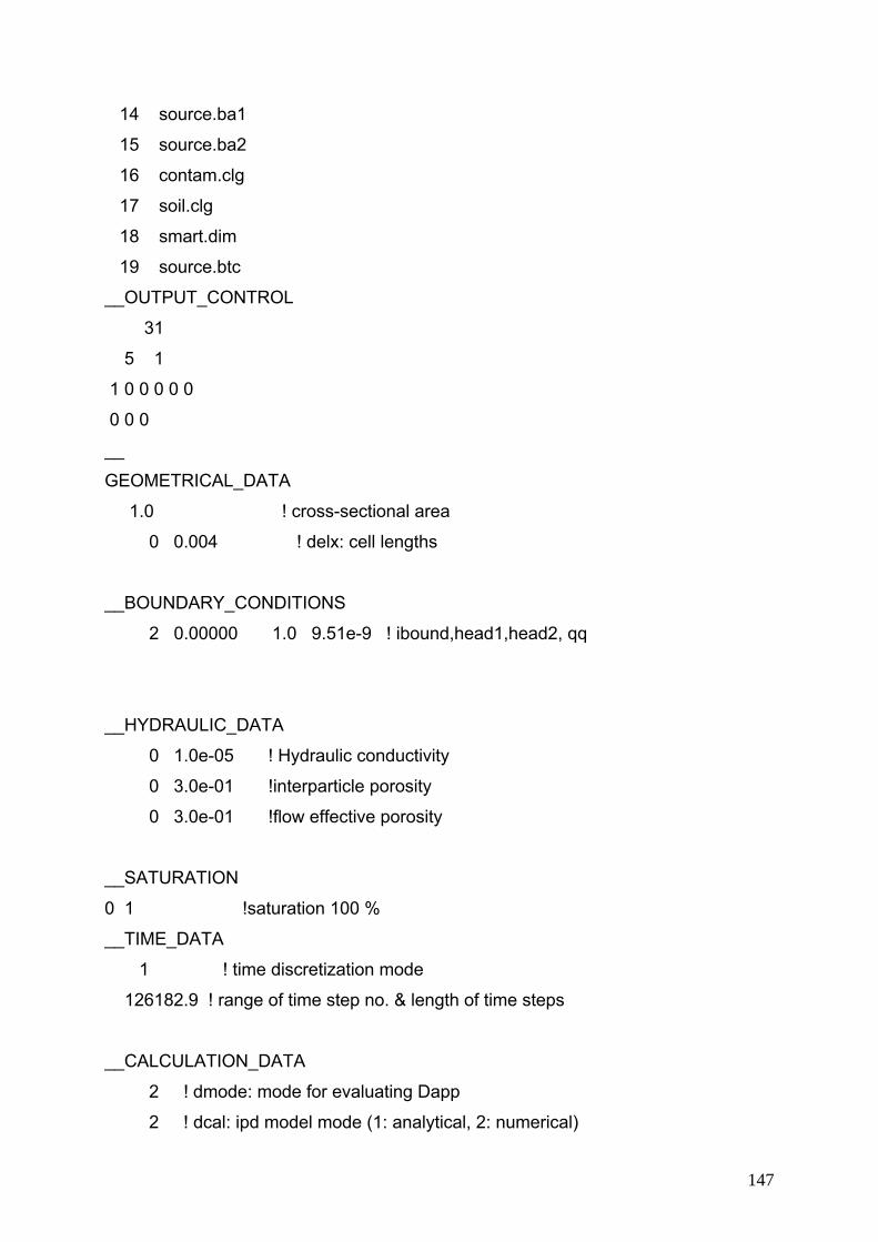
14 source.ba1
15 source.ba2
16 contam.clg
17 soil.clg
18 smart.dim
19 source.btc
__OUTPUT_CONTROL
31
5 1
1 0 0 0 0 0
0 0 0
__
GEOMETRICAL_DATA
1.0 ! cross-sectional area
0 0.004 ! delx: cell lengths
__BOUNDARY_CONDITIONS
2 0.00000 1.0 9.51e-9 ! ibound,head1,head2, qq
__HYDRAULIC_DATA
0 1.0e-05 ! Hydraulic conductivity
0 3.0e-01 !interparticle porosity
0 3.0e-01 !flow effective porosity
__SATURATION
0 1 !saturation 100 %
__TIME_DATA
1 ! time discretization mode
126182.9 ! range of time step no. & length of time steps
__CALCULATION_DATA
2 ! dmode: mode for evaluating Dapp
2 ! dcal: ipd model mode (1: analytical, 2: numerical)
147
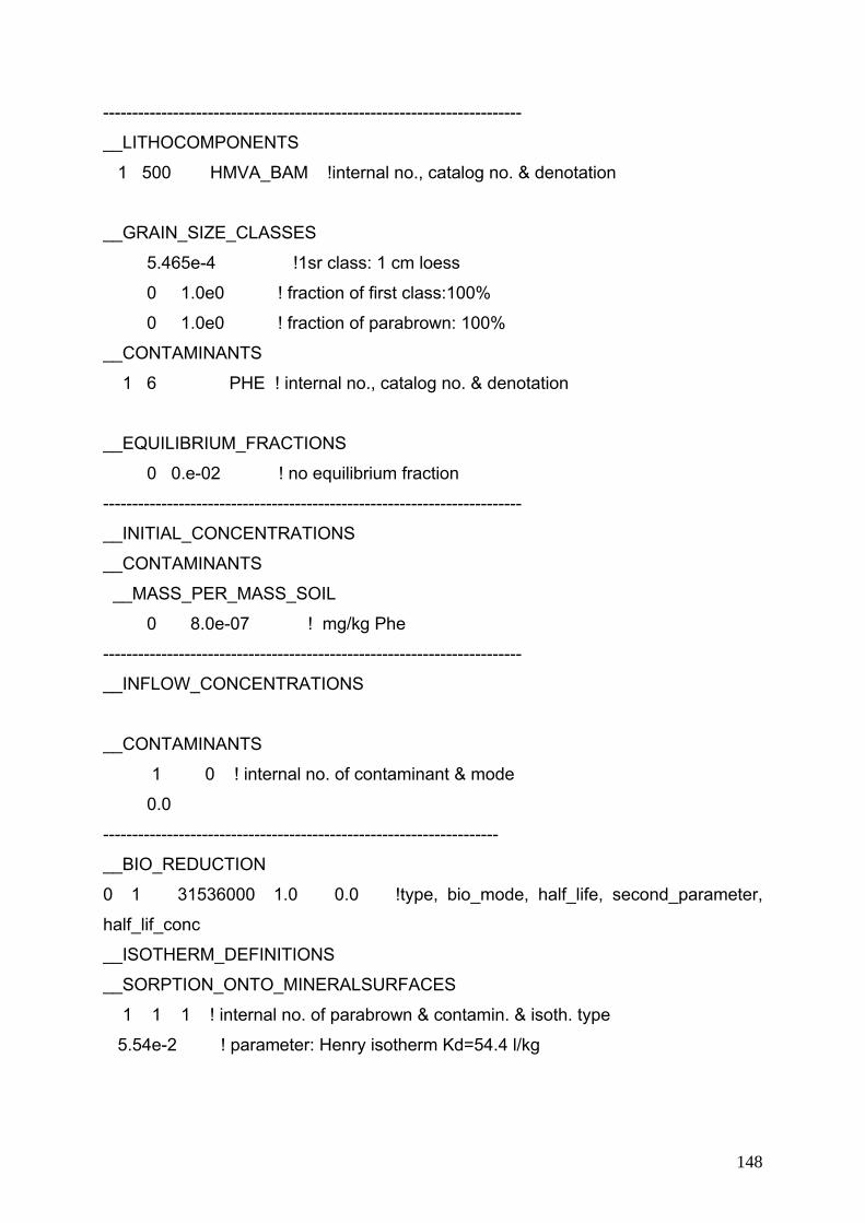
148
------------------------------------------------------------------------
__LITHOCOMPONENTS
1 500 HMVA_BAM !internal no., catalog no. & denotation
__GRAIN_SIZE_CLASSES
5.465e-4 !1sr class: 1 cm loess
0 1.0e0 ! fraction of first class:100%
0 1.0e0 ! fraction of parabrown: 100%
__CONTAMINANTS
1 6 PHE ! internal no., catalog no. & denotation
__EQUILIBRIUM_FRACTIONS
0 0.e-02 ! no equilibrium fraction
------------------------------------------------------------------------
__INITIAL_CONCENTRATIONS
__CONTAMINANTS
__MASS_PER_MASS_SOIL
0 8.0e-07 ! mg/kg Phe
------------------------------------------------------------------------
__INFLOW_CONCENTRATIONS
__CONTAMINANTS
1 0 ! internal no. of contaminant & mode
0.0
--------------------------------------------------------------------
__BIO_REDUCTION
0 1 31536000 1.0 0.0 !type, bio_mode, half_life, second_parameter,
half_lif_conc
__ISOTHERM_DEFINITIONS
__SORPTION_ONTO_MINERALSURFACES
1 1 1 ! internal no. of parabrown & contamin. & isoth. type
5.54e-2 ! parameter: Henry isotherm Kd=54.4 l/kg
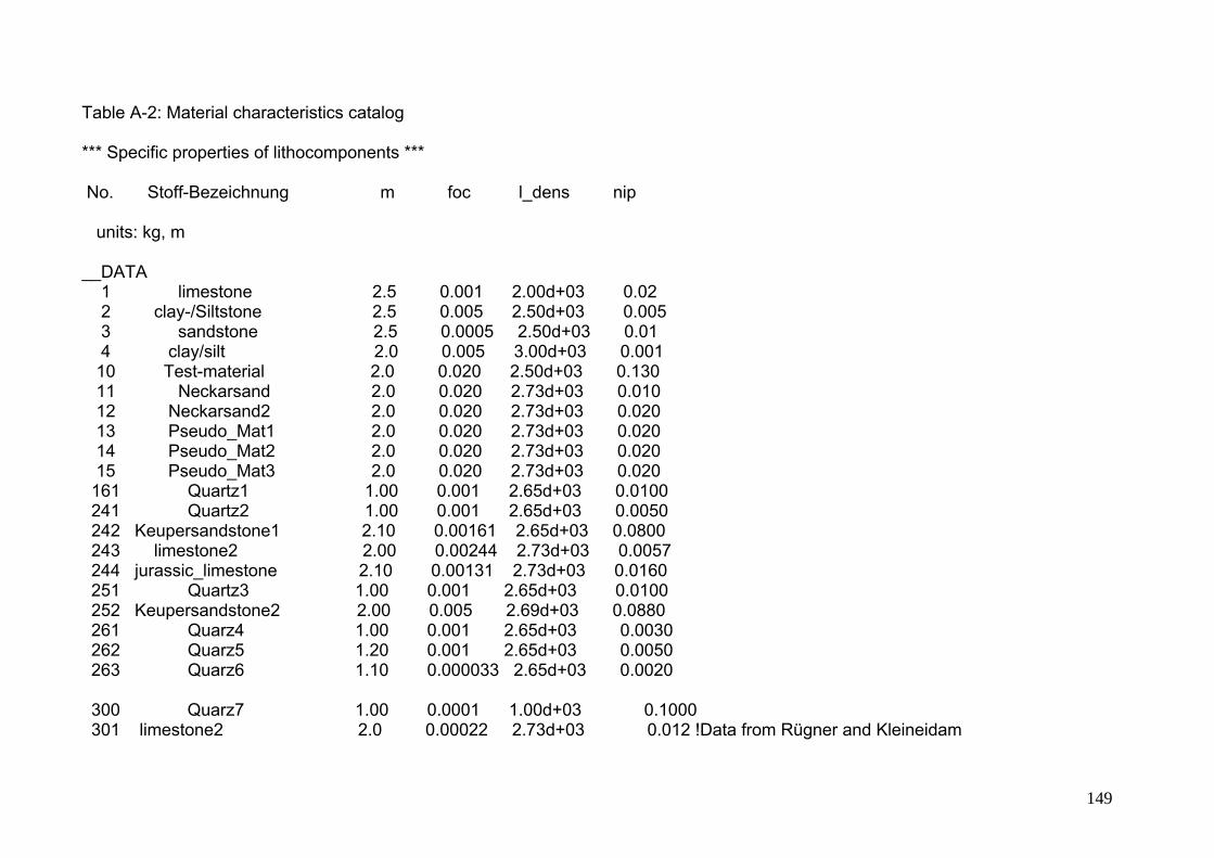
Table A-2: Material characteristics catalog
*** Specific properties of lithocomponents *** No. Stoff-Bezeichnung m foc l_dens nip units: kg, m __DATA 1 limestone 2.5 0.001 2.00d+03 0.02 2 clay-/Siltstone 2.5 0.005 2.50d+03 0.005 3 sandstone 2.5 0.0005 2.50d+03 0.01 4 clay/silt 2.0 0.005 3.00d+03 0.001 10 Test-material 2.0 0.020 2.50d+03 0.130 11 Neckarsand 2.0 0.020 2.73d+03 0.010 12 Neckarsand2 2.0 0.020 2.73d+03 0.020 13 Pseudo_Mat1 2.0 0.020 2.73d+03 0.020 14 Pseudo_Mat2 2.0 0.020 2.73d+03 0.020 15 Pseudo_Mat3 2.0 0.020 2.73d+03 0.020 161 Quartz1 1.00 0.001 2.65d+03 0.0100 241 Quartz2 1.00 0.001 2.65d+03 0.0050 242 Keupersandstone1 2.10 0.00161 2.65d+03 0.0800 243 limestone2 2.00 0.00244 2.73d+03 0.0057 244 jurassic_limestone 2.10 0.00131 2.73d+03 0.0160 251 Quartz3 1.00 0.001 2.65d+03 0.0100 252 Keupersandstone2 2.00 0.005 2.69d+03 0.0880 261 Quarz4 1.00 0.001 2.65d+03 0.0030 262 Quarz5 1.20 0.001 2.65d+03 0.0050 263 Quarz6 1.10 0.000033 2.65d+03 0.0020 300 Quarz7 1.00 0.0001 1.00d+03 0.1000 301 limestone2 2.0 0.00022 2.73d+03 0.012 !Data from Rügner and Kleineidam
149
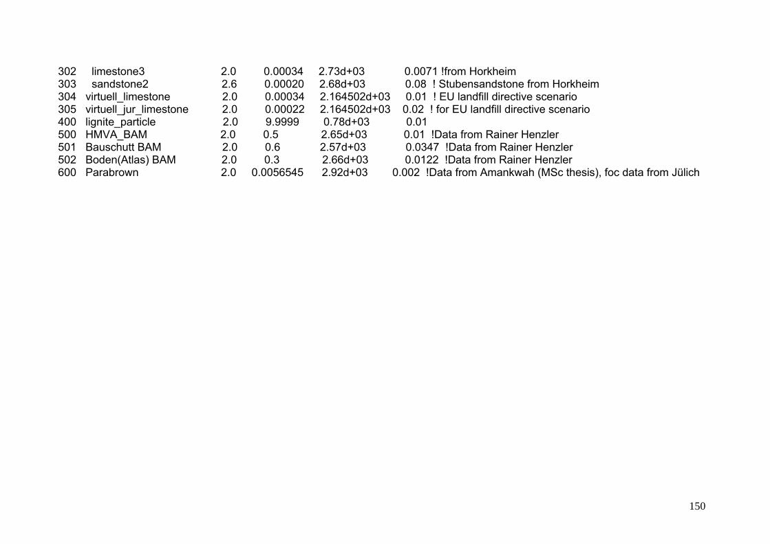
150
302 limestone3 2.0 0.00034 2.73d+03 0.0071 !from Horkheim 303 sandstone2 2.6 0.00020 2.68d+03 0.08 ! Stubensandstone from Horkheim 304 virtuell_limestone 2.0 0.00034 2.164502d+03 0.01 ! EU landfill directive scenario 305 virtuell_jur_limestone 2.0 0.00022 2.164502d+03 0.02 ! for EU landfill directive scenario 400 lignite_particle 2.0 9.9999 0.78d+03 0.01 500 HMVA_BAM 2.0 0.5 2.65d+03 0.01 !Data from Rainer Henzler 501 Bauschutt BAM 2.0 0.6 2.57d+03 0.0347 !Data from Rainer Henzler 502 Boden(Atlas) BAM 2.0 0.3 2.66d+03 0.0122 !Data from Rainer Henzler 600 Parabrown 2.0 0.0056545 2.92d+03 0.002 !Data from Amankwah (MSc thesis), foc data from Jülich
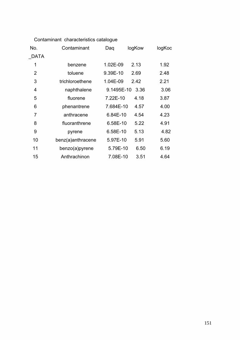
Contaminant characteristics catalogue
No. Contaminant Daq logKow logKoc
_DATA
1 benzene 1.02E-09 2.13 1.92
2 toluene 9.39E-10 2.69 2.48
3 trichloroethene 1.04E-09 2.42 2.21
4 naphthalene 9.1495E-10 3.36 3.06
5 fluorene 7.22E-10 4.18 3.87
6 phenantrene 7.684E-10 4.57 4.00
7 anthracene 6.84E-10 4.54 4.23
8 fluoranthrene 6.58E-10 5.22 4.91
9 pyrene 6.58E-10 5.13 4.82
10 benz(a)anthracene 5.97E-10 5.91 5.60
11 benzo(a)pyrene 5.79E-10 6.50 6.19
15 Anthrachinon 7.08E-10 3.51 4.64
151
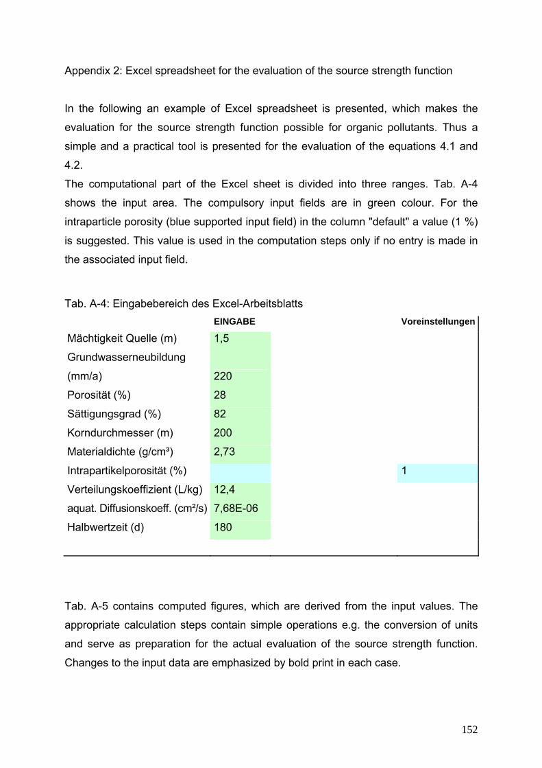
Appendix 2: Excel spreadsheet for the evaluation of the source strength function
In the following an example of Excel spreadsheet is presented, which makes the
evaluation for the source strength function possible for organic pollutants. Thus a
simple and a practical tool is presented for the evaluation of the equations 4.1 and
4.2.
The computational part of the Excel sheet is divided into three ranges. Tab. A-4
shows the input area. The compulsory input fields are in green colour. For the
intraparticle porosity (blue supported input field) in the column "default" a value (1 %)
is suggested. This value is used in the computation steps only if no entry is made in
the associated input field.
Tab. A-4: Eingabebereich des Excel-Arbeitsblatts EINGABE Voreinstellungen
Mächtigkeit Quelle (m) 1,5
Grundwasserneubildung
(mm/a) 220
Porosität (%) 28
Sättigungsgrad (%) 82
Korndurchmesser (m) 200
Materialdichte (g/cm³) 2,73
Intrapartikelporosität (%) 1
Verteilungskoeffizient (L/kg) 12,4
aquat. Diffusionskoeff. (cm²/s) 7,68E-06
Halbwertzeit (d) 180
Tab. A-5 contains computed figures, which are derived from the input values. The
appropriate calculation steps contain simple operations e.g. the conversion of units
and serve as preparation for the actual evaluation of the source strength function.
Changes to the input data are emphasized by bold print in each case.
152
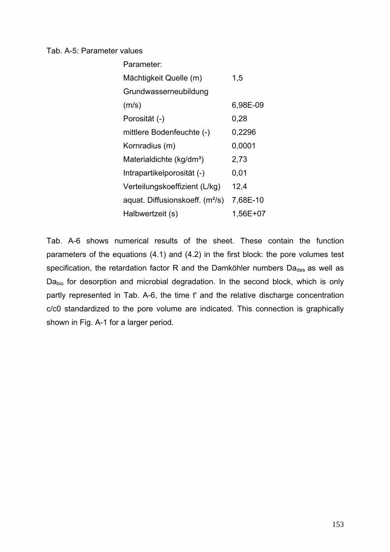
Tab. A-5: Parameter values
Parameter:
Mächtigkeit Quelle (m) 1,5
Grundwasserneubildung
(m/s) 6,98E-09
Porosität (-) 0,28
mittlere Bodenfeuchte (-) 0,2296
Kornradius (m) 0,0001
Materialdichte (kg/dm³) 2,73
Intrapartikelporosität (-) 0,01
Verteilungskoeffizient (L/kg) 12,4
aquat. Diffusionskoeff. (m²/s) 7,68E-10
Halbwertzeit (s) 1,56E+07
Tab. A-6 shows numerical results of the sheet. These contain the function
parameters of the equations (4.1) and (4.2) in the first block: the pore volumes test
specification, the retardation factor R and the Damköhler numbers Dades as well as
Dabio for desorption and microbial degradation. In the second block, which is only
partly represented in Tab. A-6, the time t' and the relative discharge concentration
c/c0 standardized to the pore volume are indicated. This connection is graphically
shown in Fig. A-1 for a larger period.
153
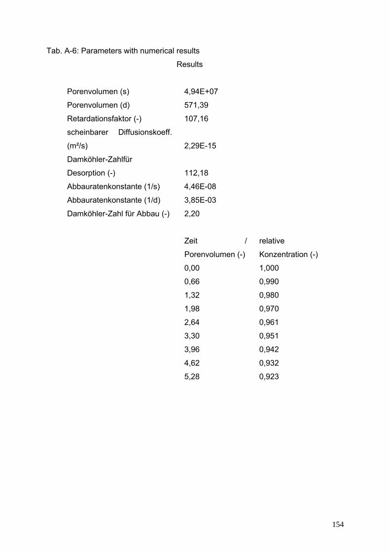
Tab. A-6: Parameters with numerical results
Results
Porenvolumen (s) 4,94E+07
Porenvolumen (d) 571,39
Retardationsfaktor (-) 107,16
scheinbarer Diffusionskoeff.
(m²/s) 2,29E-15
Damköhler-Zahlfür
Desorption (-) 112,18
Abbauratenkonstante (1/s) 4,46E-08
Abbauratenkonstante (1/d) 3,85E-03
Damköhler-Zahl für Abbau (-) 2,20
Zeit /
Porenvolumen (-)
relative
Konzentration (-)
0,00 1,000
0,66 0,990
1,32 0,980
1,98 0,970
2,64 0,961
3,30 0,951
3,96 0,942
4,62 0,932
5,28 0,923
154
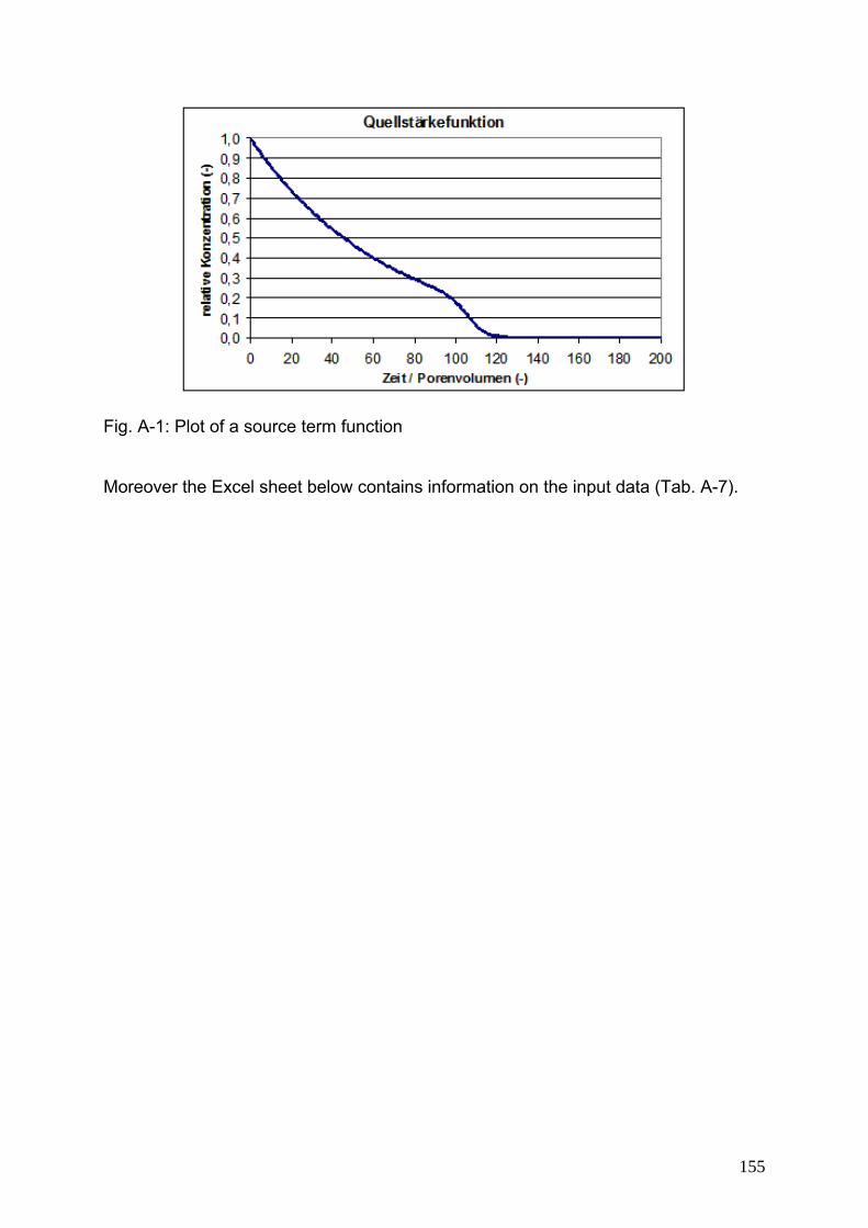
155
Moreover the Excel sheet below contains information on the input data (Tab. A-7).
Fig. A-1: Plot of a source term function
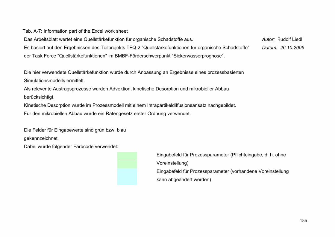
Tab. A-7: Information part of the Excel work sheet
Das Arbeitsblatt wertet eine Quellstärkefunktion für organische Schadstoffe aus. Autor: Rudolf Liedl
Es basiert auf den Ergebnissen des Teilprojekts TFQ-2 "Quellstärkefunktionen für organische Schadstoffe" Datum: 26.10.2006
der Task Force "Quellstärkefunktionen" im BMBF-Förderschwerpunkt "Sickerwasserprognose".
Die hier verwendete Quellstärkefunktion wurde durch Anpassung an Ergebnisse eines prozessbasierten
Simulationsmodells ermittelt.
Als relevente Austragsprozesse wurden Advektion, kinetische Desorption und mikrobieller Abbau
berücksichtigt.
Kinetische Desorption wurde im Prozessmodell mit einem Intrapartikeldiffusionsansatz nachgebildet.
Für den mikrobiellen Abbau wurde ein Ratengesetz erster Ordnung verwendet.
Die Felder für Eingabewerte sind grün bzw. blau
gekennzeichnet.
Dabei wurde folgender Farbcode verwendet:
Eingabefeld für Prozessparameter (Pflichteingabe, d. h. ohne
Voreinstellung)
Eingabefeld für Prozessparameter (vorhandene Voreinstellung
kann abgeändert werden)
156
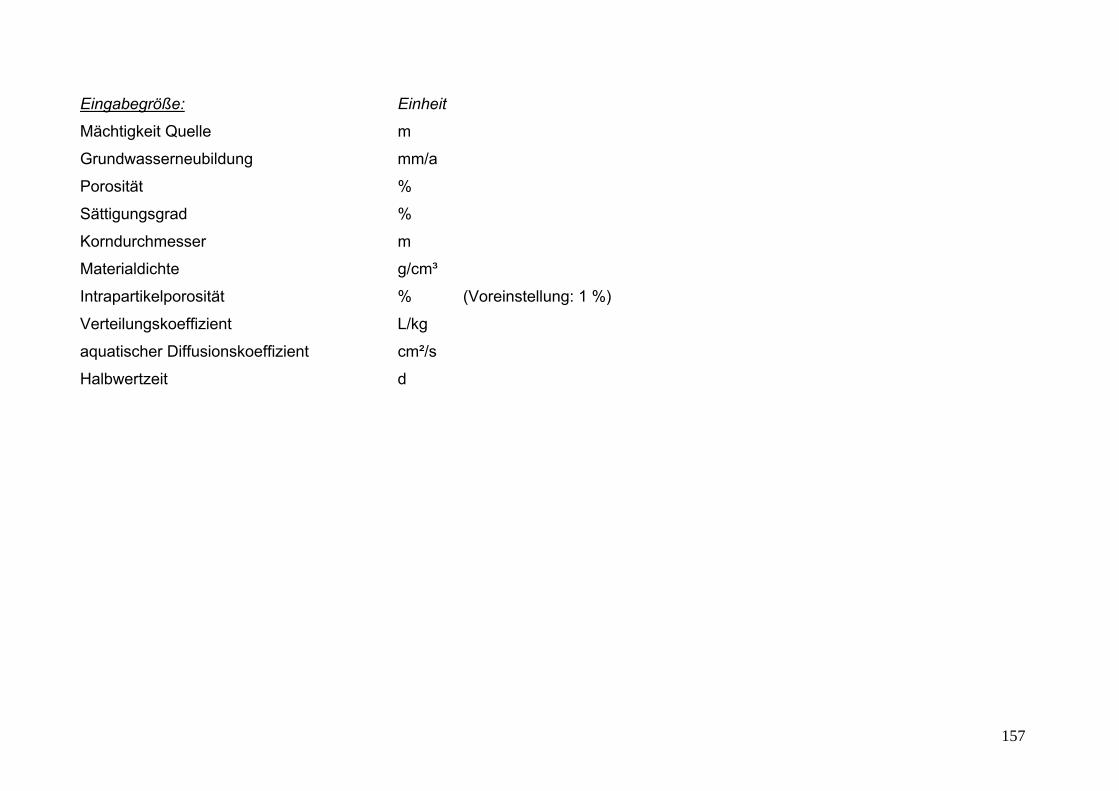
Eingabegröße: Einheit
Mächtigkeit Quelle m
Grundwasserneubildung mm/a
Porosität %
Sättigungsgrad %
Korndurchmesser m
Materialdichte g/cm³
Intrapartikelporosität % (Voreinstellung: 1 %)
Verteilungskoeffizient L/kg
aquatischer Diffusionskoeffizient cm²/s
Halbwertzeit d
157
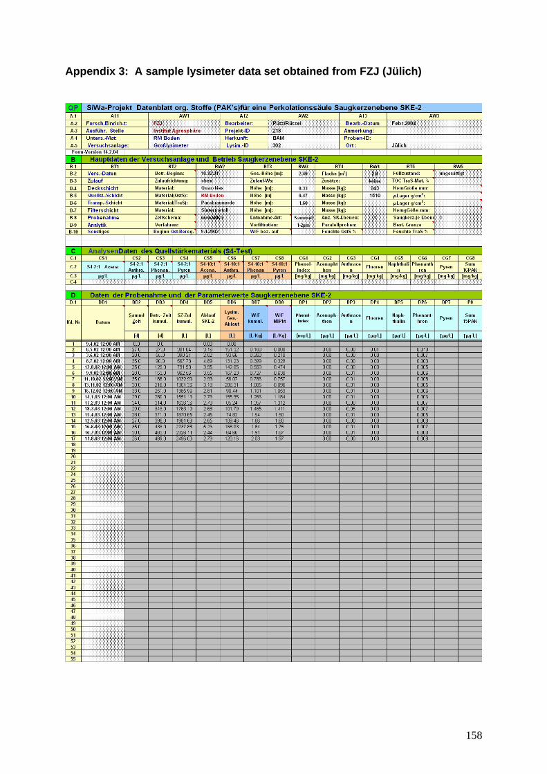
Appendix 3: A sample lysimeter data set obtained from FZJ (Jülich)
158