Embed Size (px)
Citation preview
Prof. Dr.-Ing. K. Brandenburg, [email protected] Prof. Dr.-Ing. G. Schuller, [email protected] Page ‹Nr.›
Psychoacoustics
lecturer:
Prof. Dr.-Ing. K. Brandenburg, [email protected] Prof. Dr.-Ing. G. Schuller, [email protected] Page ‹Nr.›
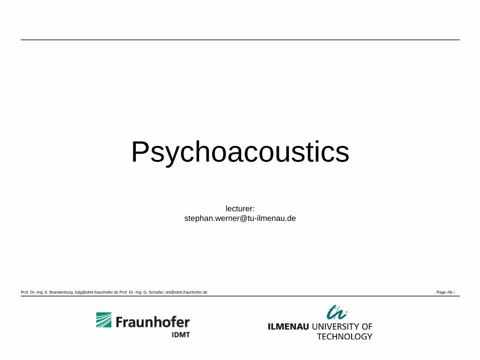
Block Diagram of a Perceptual Audio Encoder
Source: Brandenburg, “Vorlesung: Dig. Audiosignalverarbeitung”
• loudness
• critical bands
• masking:
• frequency domain
• time domain
• binaural cues (overview)
Prof. Dr.-Ing. K. Brandenburg, [email protected] Prof. Dr.-Ing. G. Schuller, [email protected] Page ‹Nr.›
Structure of the Human Ear
Prof. Dr.-Ing. K. Brandenburg, [email protected] Prof. Dr.-Ing. G. Schuller, [email protected] Page ‹Nr.›
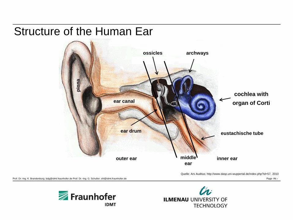
Structure of the Human Ear
Quelle: Ars Auditus; http://www.dasp.uni-wuppertal.de/index.php?id=57, 2010
outer ear middle
ear inner ear
ear canal
pin
na
cochlea with
organ of Corti
archways ossicles
eustachische tube ear drum
Prof. Dr.-Ing. K. Brandenburg, [email protected] Prof. Dr.-Ing. G. Schuller, [email protected] Page ‹Nr.›
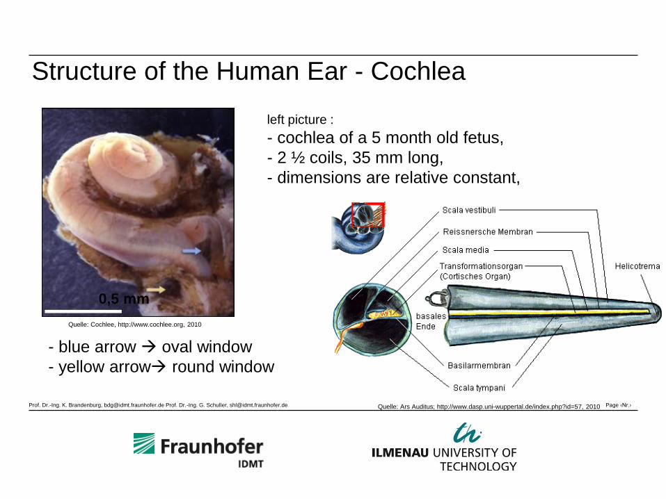
Structure of the Human Ear - Cochlea
Quelle: Ars Auditus; http://www.dasp.uni-wuppertal.de/index.php?id=57, 2010
left picture :
- cochlea of a 5 month old fetus,
- 2 ½ coils, 35 mm long,
- dimensions are relative constant,
Quelle: Cochlee, http://www.cochlee.org, 2010
- blue arrow oval window
- yellow arrow round window
0,5 mm
Prof. Dr.-Ing. K. Brandenburg, [email protected] Prof. Dr.-Ing. G. Schuller, [email protected] Page ‹Nr.›
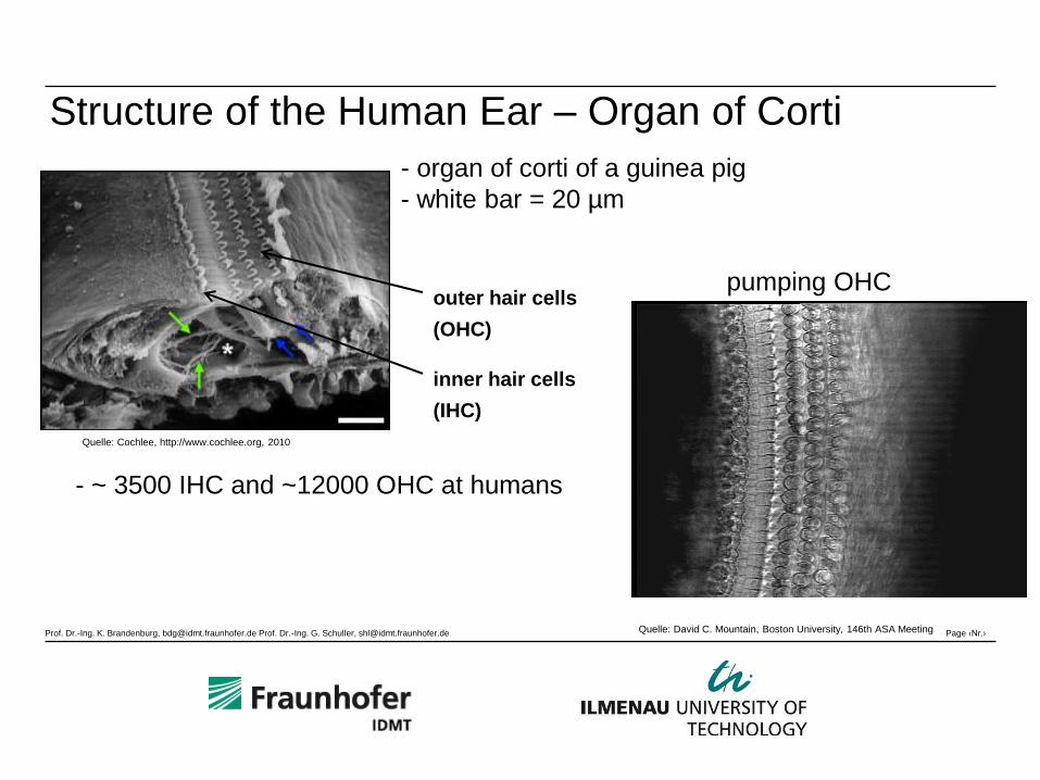
Structure of the Human Ear – Organ of Corti
- organ of corti of a guinea pig
- white bar = 20 µm
outer hair cells
(OHC)
inner hair cells
(IHC)
Quelle: Cochlee, http://www.cochlee.org, 2010
Quelle: David C. Mountain, Boston University, 146th ASA Meeting
- ~ 3500 IHC and ~12000 OHC at humans
pumping OHC
Prof. Dr.-Ing. K. Brandenburg, [email protected] Prof. Dr.-Ing. G. Schuller, [email protected] Page ‹Nr.›
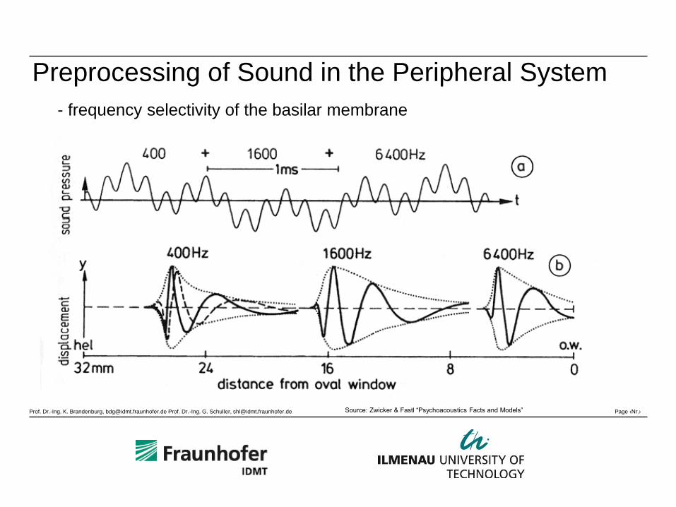
Preprocessing of Sound in the Peripheral System
Source: Zwicker & Fastl “Psychoacoustics Facts and Models”
- frequency selectivity of the basilar membrane
Prof. Dr.-Ing. K. Brandenburg, [email protected] Prof. Dr.-Ing. G. Schuller, [email protected] Page ‹Nr.›
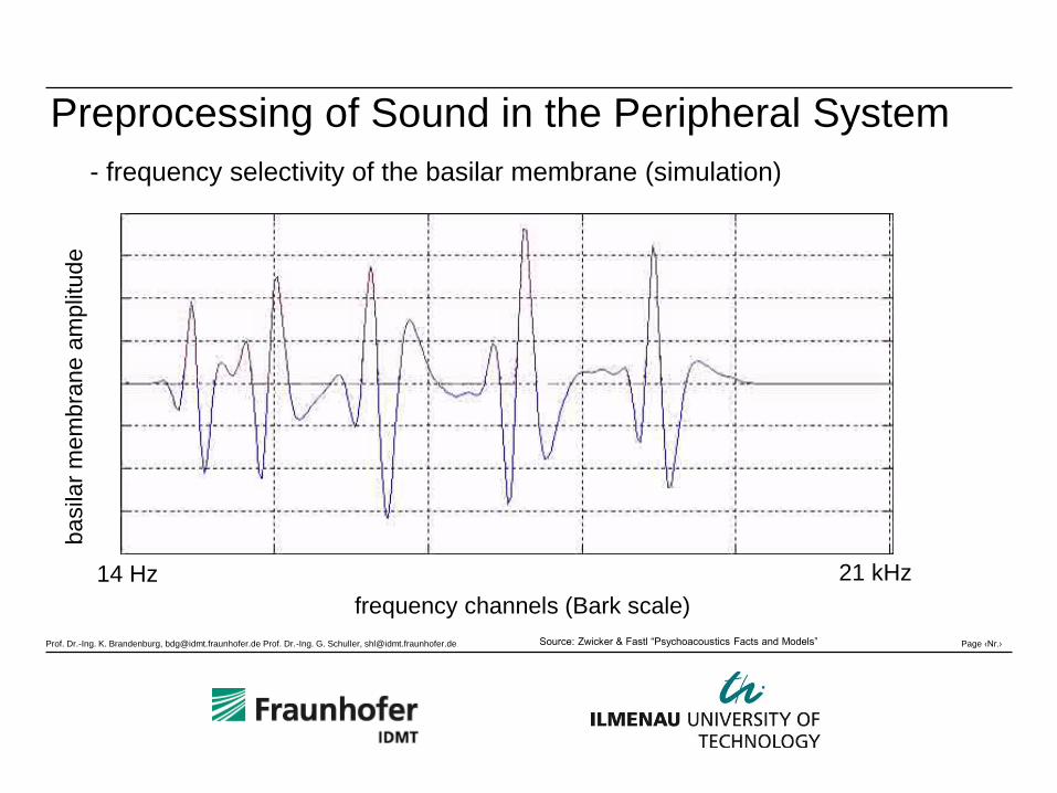
Preprocessing of Sound in the Peripheral System
Source: Zwicker & Fastl “Psychoacoustics Facts and Models”
- frequency selectivity of the basilar membrane (simulation)
21 kHz
frequency channels (Bark scale)
ba
sila
r m
em
bra
ne
am
plit
ud
e
14 Hz
Prof. Dr.-Ing. K. Brandenburg, [email protected] Prof. Dr.-Ing. G. Schuller, [email protected] Page ‹Nr.›
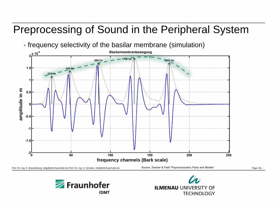
Preprocessing of Sound in the Peripheral System
Source: Zwicker & Fastl “Psychoacoustics Facts and Models”
- frequency selectivity of the basilar membrane (simulation)
frequency channels (Bark scale)
am
pli
tud
e i
n m
Prof. Dr.-Ing. K. Brandenburg, [email protected] Prof. Dr.-Ing. G. Schuller, [email protected] Page ‹Nr.›
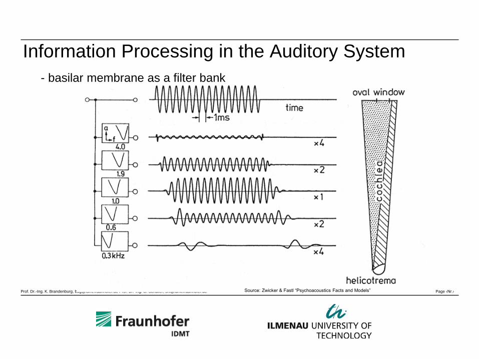
Information Processing in the Auditory System
Source: Zwicker & Fastl “Psychoacoustics Facts and Models”
- basilar membrane as a filter bank
Prof. Dr.-Ing. K. Brandenburg, [email protected] Prof. Dr.-Ing. G. Schuller, [email protected] Page ‹Nr.›
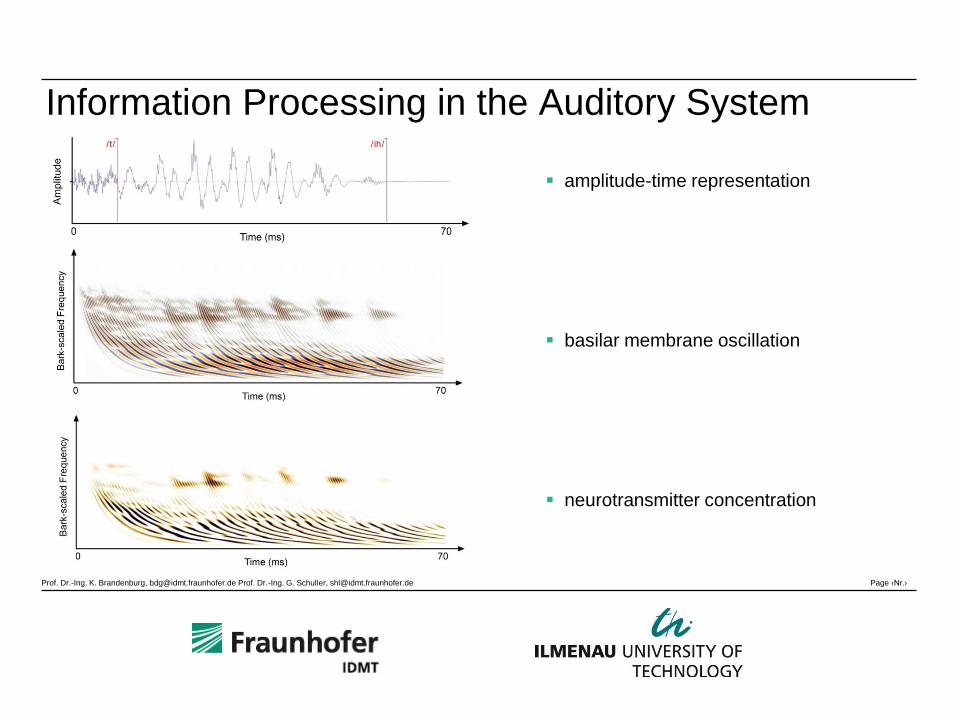
Information Processing in the Auditory System
amplitude-time representation
basilar membrane oscillation
neurotransmitter concentration
Prof. Dr.-Ing. K. Brandenburg, [email protected] Prof. Dr.-Ing. G. Schuller, [email protected] Page ‹Nr.›
Sound Perception
Prof. Dr.-Ing. K. Brandenburg, [email protected] Prof. Dr.-Ing. G. Schuller, [email protected] Page ‹Nr.›
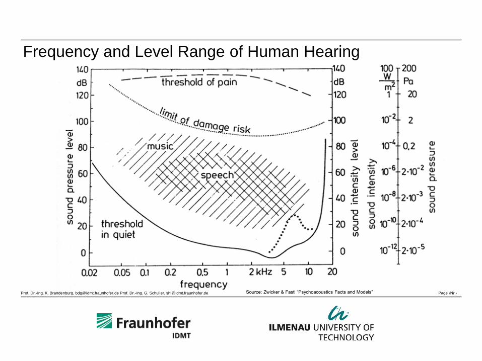
Frequency and Level Range of Human Hearing
Source: Zwicker & Fastl “Psychoacoustics Facts and Models”
Prof. Dr.-Ing. K. Brandenburg, [email protected] Prof. Dr.-Ing. G. Schuller, [email protected] Page ‹Nr.›
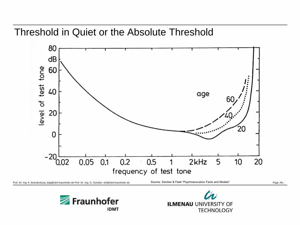
Threshold in Quiet or the Absolute Threshold
Source: Zwicker & Fastl “Psychoacoustics Facts and Models”
Prof. Dr.-Ing. K. Brandenburg, [email protected] Prof. Dr.-Ing. G. Schuller, [email protected] Page ‹Nr.›
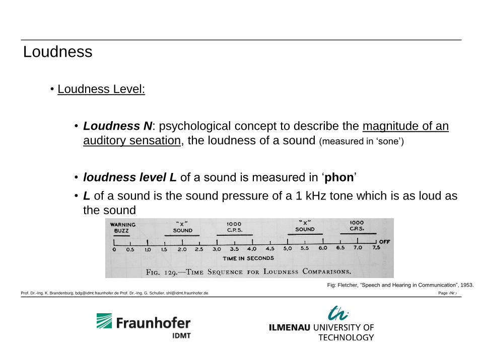
Loudness
• Loudness Level:
• Loudness N: psychological concept to describe the magnitude of an
auditory sensation, the loudness of a sound (measured in ‘sone’)
• loudness level L of a sound is measured in ‘phon’
• L of a sound is the sound pressure of a 1 kHz tone which is as loud as
the sound
Fig: Fletcher, “Speech and Hearing in Communication”, 1953.
Prof. Dr.-Ing. K. Brandenburg, [email protected] Prof. Dr.-Ing. G. Schuller, [email protected] Page ‹Nr.›
Loudness
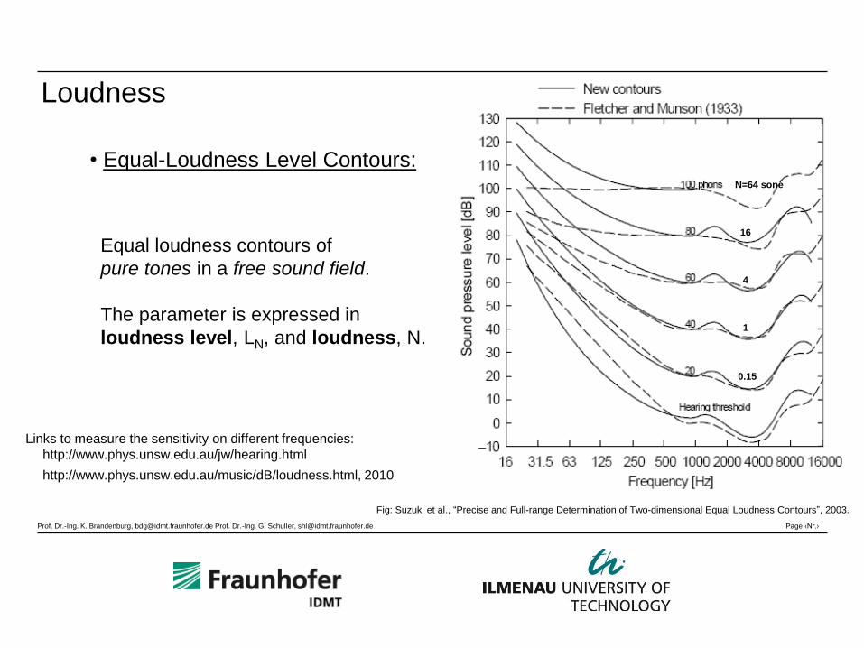
• Equal-Loudness Level Contours:
Links to measure the sensitivity on different frequencies:
http://www.phys.unsw.edu.au/jw/hearing.html
http://www.phys.unsw.edu.au/music/dB/loudness.html, 2010
Fig: Suzuki et al., “Precise and Full-range Determination of Two-dimensional Equal Loudness Contours”, 2003.
0.15
1
4
16
N=64 sone
Equal loudness contours of
pure tones in a free sound field.
The parameter is expressed in
loudness level, LN, and loudness, N.
Prof. Dr.-Ing. K. Brandenburg, [email protected] Prof. Dr.-Ing. G. Schuller, [email protected] Page ‹Nr.›
Loudness
• Loudness Scale:
• aim: double the number of units on this scale means magnitude of
sensation is doubled
• relation G(L) between loudness level L and the loudness N on the
new scale
• one potential experiment:
• listen to sound with L1 and than adjust same sound until L2=2xL1
Prof. Dr.-Ing. K. Brandenburg, [email protected] Prof. Dr.-Ing. G. Schuller, [email protected] Page ‹Nr.›
Loudness
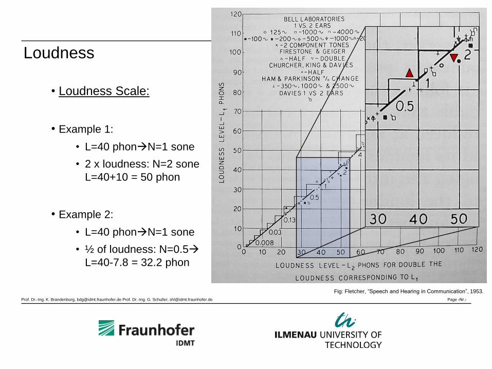
• Loudness Scale:
• Example 1:
• L=40 phonN=1 sone
• 2 x loudness: N=2 sone
L=40+10 = 50 phon
• Example 2:
• L=40 phonN=1 sone
• ½ of loudness: N=0.5
L=40-7.8 = 32.2 phon
Fig: Fletcher, “Speech and Hearing in Communication”, 1953.
Prof. Dr.-Ing. K. Brandenburg, [email protected] Prof. Dr.-Ing. G. Schuller, [email protected] Page ‹Nr.›
Loudness
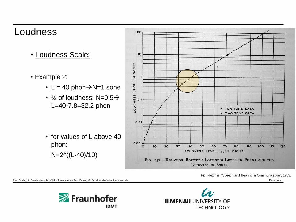
• Loudness Scale:
• Example 2:
• L = 40 phonN=1 sone
• ½ of loudness: N=0.5
L=40-7.8=32.2 phon
• for values of L above 40
phon:
N=2^((L-40)/10)
Fig: Fletcher, “Speech and Hearing in Communication”, 1953.
Prof. Dr.-Ing. K. Brandenburg, [email protected] Prof. Dr.-Ing. G. Schuller, [email protected] Page ‹Nr.›
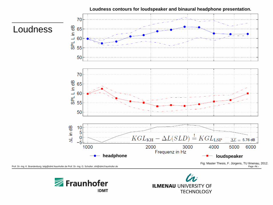
Loudness
Loudness contours for loudspeaker and binaural headphone presentation.
headphone loudspeaker
Fig: Master Thesis, F. Jürgens, TU Ilmenau, 2012.
Prof. Dr.-Ing. K. Brandenburg, [email protected] Prof. Dr.-Ing. G. Schuller, [email protected] Page ‹Nr.›
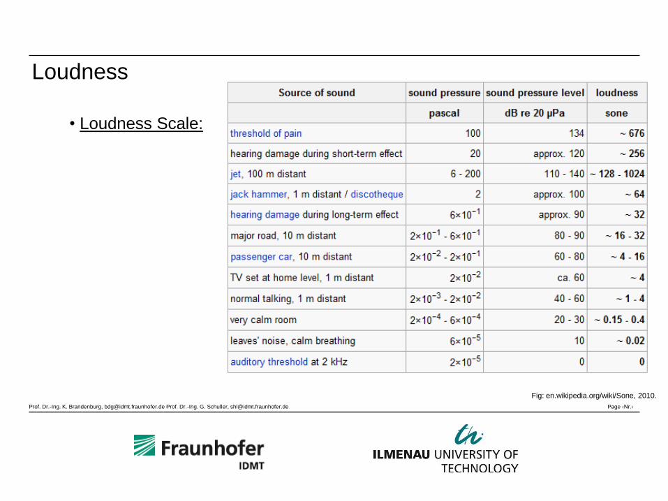
Loudness
• Loudness Scale:
Fig: en.wikipedia.org/wiki/Sone, 2010.
Prof. Dr.-Ing. K. Brandenburg, [email protected] Prof. Dr.-Ing. G. Schuller, [email protected] Page ‹Nr.›
Sound Example
• Example 1: Equal amplitude
– tones of frequencies 40Hz, 100Hz, 4000Hz, and 12000Hz
• Example 2: Equal amplitude
– Sweep from 0-16000 Hz
Prof. Dr.-Ing. K. Brandenburg, [email protected] Prof. Dr.-Ing. G. Schuller, [email protected] Page ‹Nr.›
Critical Bands
Prof. Dr.-Ing. K. Brandenburg, [email protected] Prof. Dr.-Ing. G. Schuller, [email protected] Page ‹Nr.›
Frequency Grouping in Human Hearing
Source: Brandenburg, “Vorlesung: Dig. Audiosignalverarbeitung
• Different interpretations that produce the same
segmentation
– Constant distance in the Cochlea
– By using tones under the threshold in quiet,
their intensity add up in a critical band and are
now audible
– Tones in a critical band above the threshold in
quiet: their energy adds up
• Formula for the width of the critical bands
– for frequencies < 500 Hz: Constant 100Hz
width
– for frequencies > 500 Hz: 0.2*frequency
Prof. Dr.-Ing. K. Brandenburg, [email protected] Prof. Dr.-Ing. G. Schuller, [email protected] Page ‹Nr.›
Frequency Grouping Bandwidth The Critical Bands
Source: Zwicker & Fastl “Psychoacoustics Facts and Models”
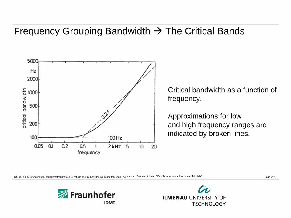
Critical bandwidth as a function of
frequency.
Approximations for low
and high frequency ranges are
indicated by broken lines.
Prof. Dr.-Ing. K. Brandenburg, [email protected] Prof. Dr.-Ing. G. Schuller, [email protected] Page ‹Nr.›
Excursus - Critical Bands and Loudness
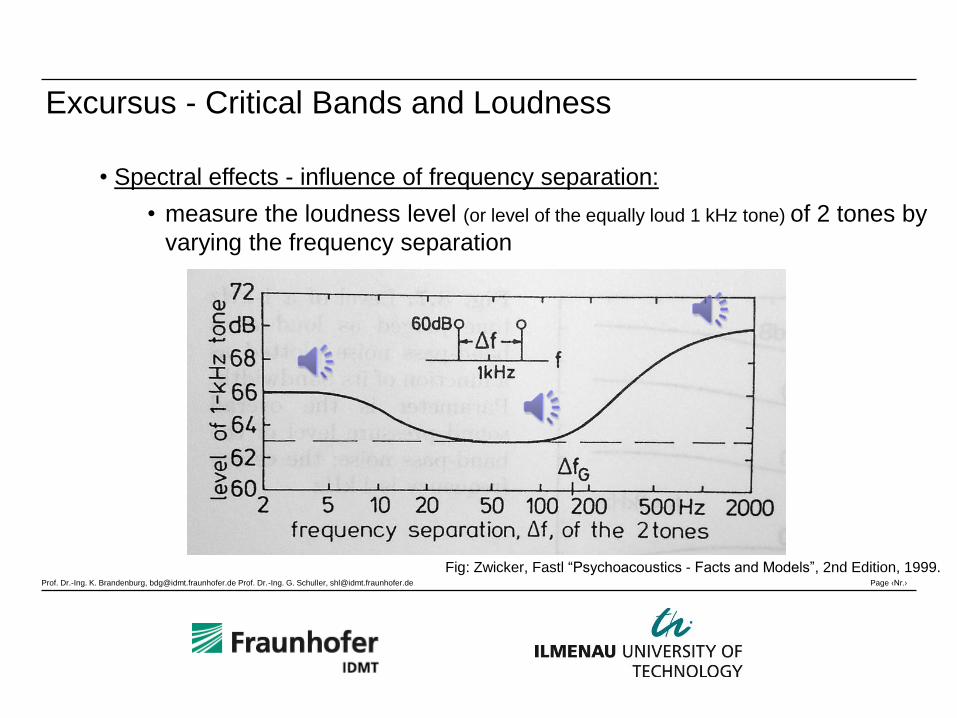
• Spectral effects - influence of frequency separation:
• measure the loudness level (or level of the equally loud 1 kHz tone) of 2 tones by
varying the frequency separation
Fig: Zwicker, Fastl “Psychoacoustics - Facts and Models”, 2nd Edition, 1999.
Prof. Dr.-Ing. K. Brandenburg, [email protected] Prof. Dr.-Ing. G. Schuller, [email protected] Page ‹Nr.›
Excursus - Critical Bands and Loudness
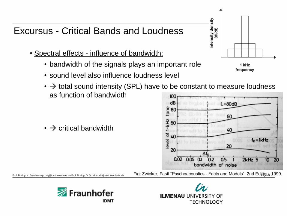
• Spectral effects - influence of bandwidth:
• bandwidth of the signals plays an important role
• sound level also influence loudness level
• total sound intensity (SPL) have to be constant to measure loudness
as function of bandwidth
• critical bandwidth
Fig: Zwicker, Fastl “Psychoacoustics - Facts and Models”, 2nd Edition, 1999.
Prof. Dr.-Ing. K. Brandenburg, [email protected] Prof. Dr.-Ing. G. Schuller, [email protected] Page ‹Nr.›
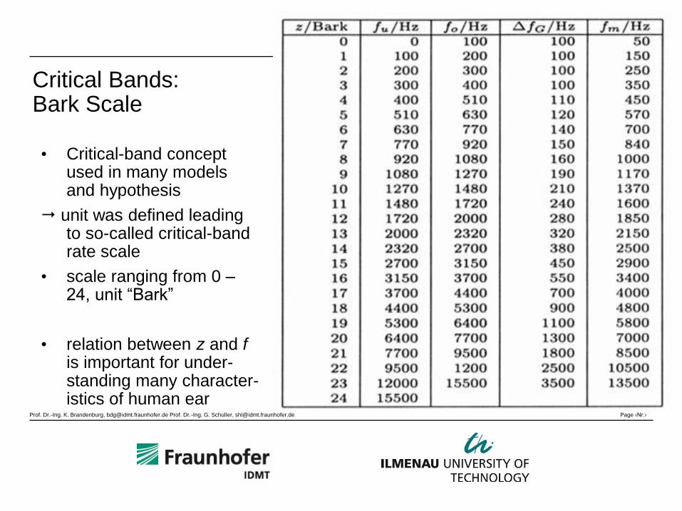
Critical Bands: Bark Scale
• Critical-band concept used in many models and hypothesis
unit was defined leading to so-called critical-band rate scale
• scale ranging from 0 – 24, unit “Bark”
• relation between z and f is important for under-standing many character-istics of human ear
Prof. Dr.-Ing. K. Brandenburg, [email protected] Prof. Dr.-Ing. G. Schuller, [email protected] Page ‹Nr.›
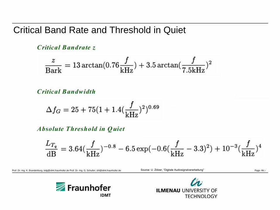
Critical Band Rate and Threshold in Quiet
Source: U. Zölzer, “Digitale Audiosignalverarbeitung”
Prof. Dr.-Ing. K. Brandenburg, [email protected] Prof. Dr.-Ing. G. Schuller, [email protected] Page ‹Nr.›
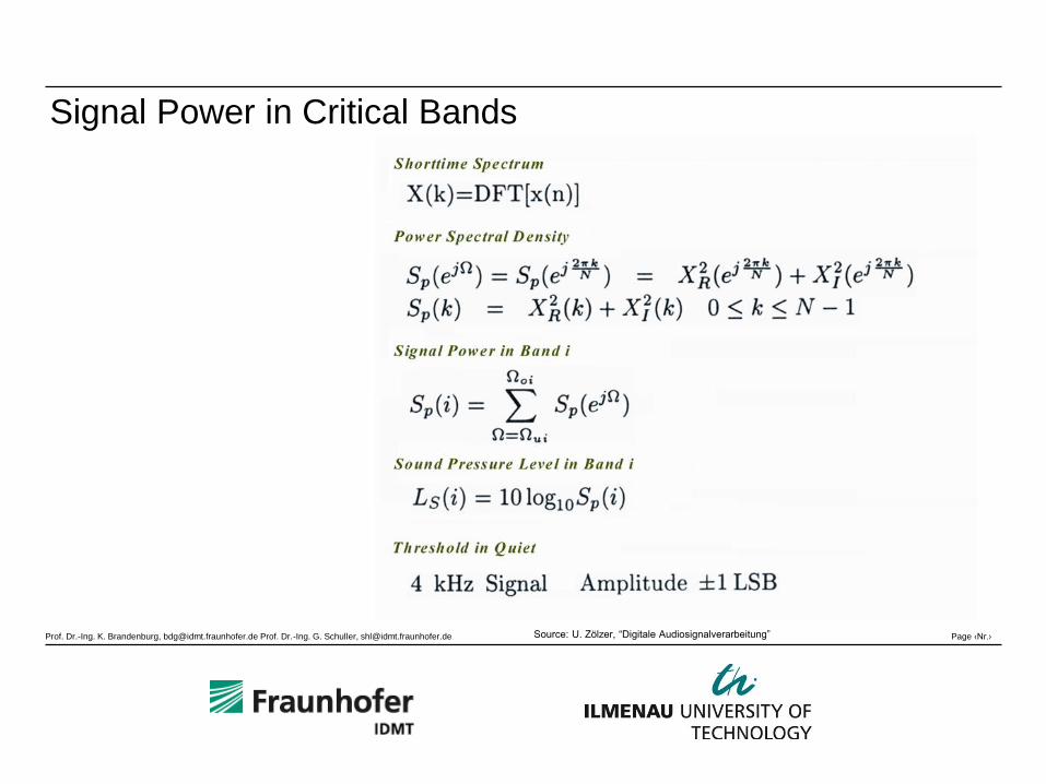
Signal Power in Critical Bands
Source: U. Zölzer, “Digitale Audiosignalverarbeitung”
Prof. Dr.-Ing. K. Brandenburg, [email protected] Prof. Dr.-Ing. G. Schuller, [email protected] Page ‹Nr.›
Masking
Prof. Dr.-Ing. K. Brandenburg, [email protected] Prof. Dr.-Ing. G. Schuller, [email protected] Page ‹Nr.›
Masking
• data compression
– exploitation of perception in critical bands with
reference to the threshold in quiet is not
enough
• Basis for further compression are masking effects as
described by Zwicker, Fletcher, Fastl, Feldtkeller and others.
Prof. Dr.-Ing. K. Brandenburg, [email protected] Prof. Dr.-Ing. G. Schuller, [email protected] Page ‹Nr.›
Masking of Pure Tones by Noise - Broad-Band Noise
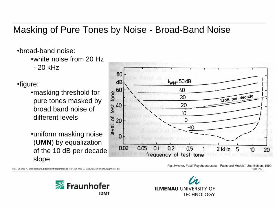
Fig: Zwicker, Fastl “Psychoacoustics - Facts and Models”, 2nd Edition, 1999.
•broad-band noise:
•white noise from 20 Hz
- 20 kHz
•figure:
•masking threshold for
pure tones masked by
broad band noise of
different levels
•uniform masking noise
(UMN) by equalization
of the 10 dB per decade
slope
Prof. Dr.-Ing. K. Brandenburg, [email protected] Prof. Dr.-Ing. G. Schuller, [email protected] Page ‹Nr.›
Masking of Pure Tones by Noise - Narrow-Band Noise
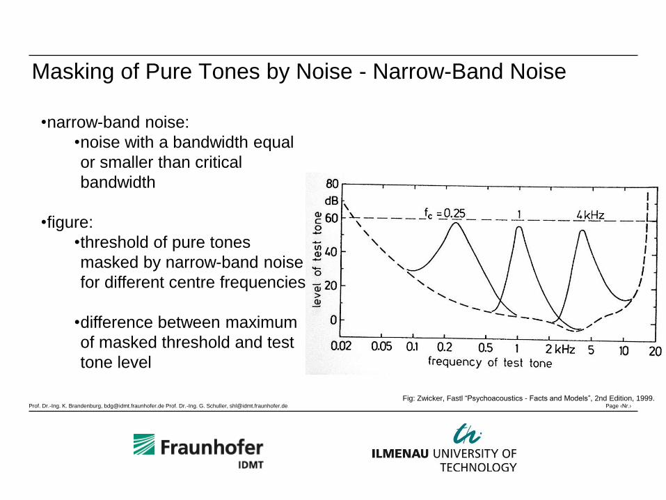
Fig: Zwicker, Fastl “Psychoacoustics - Facts and Models”, 2nd Edition, 1999.
•narrow-band noise:
•noise with a bandwidth equal
or smaller than critical
bandwidth
•figure:
•threshold of pure tones
masked by narrow-band noise
for different centre frequencies
•difference between maximum
of masked threshold and test
tone level
Prof. Dr.-Ing. K. Brandenburg, [email protected] Prof. Dr.-Ing. G. Schuller, [email protected] Page ‹Nr.›
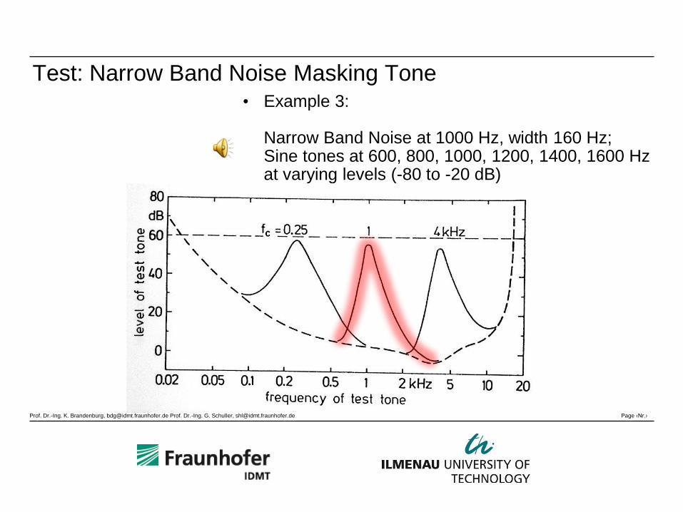
Masking of Pure Tones by Noise - Narrow-Band Noise
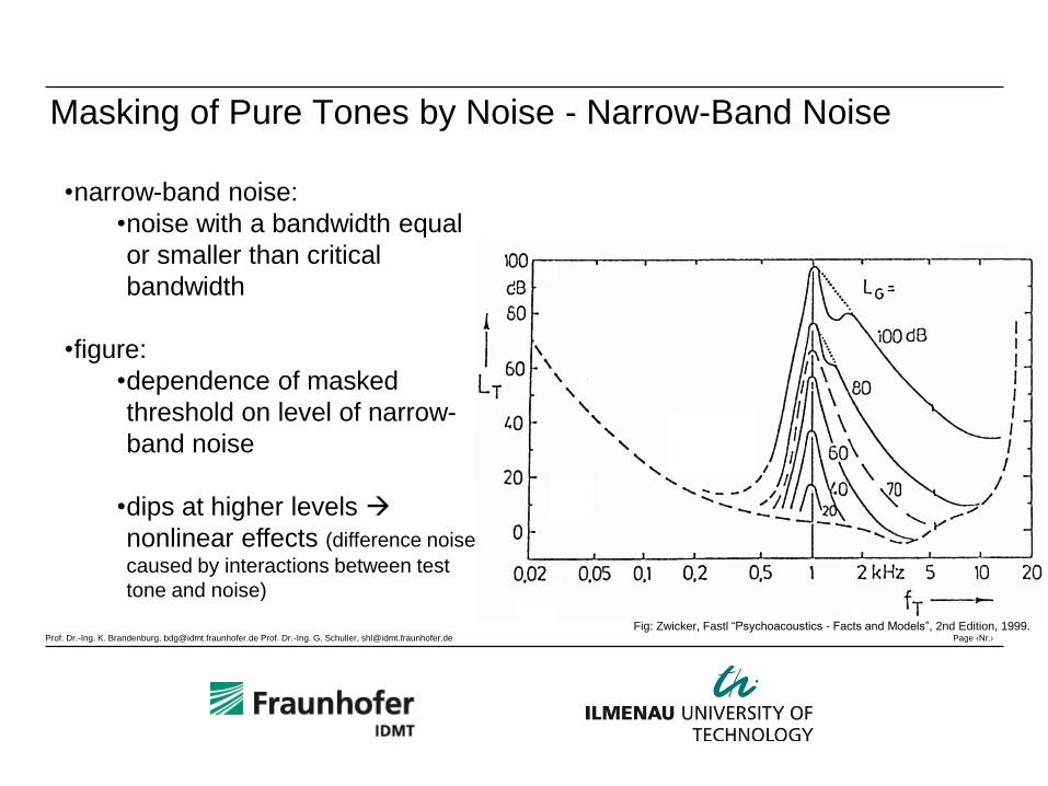
Fig: Zwicker, Fastl “Psychoacoustics - Facts and Models”, 2nd Edition, 1999.
•narrow-band noise:
•noise with a bandwidth equal
or smaller than critical
bandwidth
•figure:
•dependence of masked
threshold on level of narrow-
band noise
•dips at higher levels
nonlinear effects (difference noise
caused by interactions between test
tone and noise)
Prof. Dr.-Ing. K. Brandenburg, [email protected] Prof. Dr.-Ing. G. Schuller, [email protected] Page ‹Nr.›
Test: Narrow Band Noise Masking Tone • Example 3:
Narrow Band Noise at 1000 Hz, width 160 Hz; Sine tones at 600, 800, 1000, 1200, 1400, 1600 Hz at varying levels (-80 to -20 dB)

Prof. Dr.-Ing. K. Brandenburg, [email protected] Prof. Dr.-Ing. G. Schuller, [email protected] Page ‹Nr.›
Sound Examples: Masking with White Noise
• Example 4: Masking with white noise
– 500 Hz sinusoid tone at varying amplitude ALONE
– Level: -40,-35,-30,-25,-20,-15,-10 dB
• Example 5: Masking with white noise
– 500 Hz tone at varying amplitude with White
Noise
– Level: -40,-35,-30,-25,-20,-15,-10 dB
– Noise Level: -50 db
• Example 6: Masking with white noise
– 5000 Hz tone at varying amplitude with White
Noise
– Levels: same as Example 5
Prof. Dr.-Ing. K. Brandenburg, [email protected] Prof. Dr.-Ing. G. Schuller, [email protected] Page ‹Nr.›
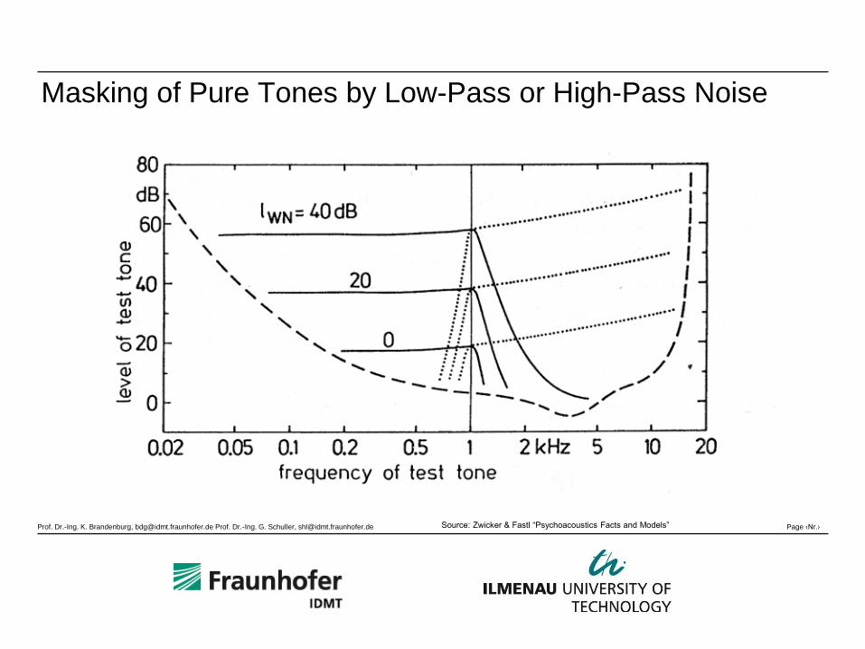
Masking of Pure Tones by Low-Pass or High-Pass Noise
Source: Zwicker & Fastl “Psychoacoustics Facts and Models”
Prof. Dr.-Ing. K. Brandenburg, [email protected] Prof. Dr.-Ing. G. Schuller, [email protected] Page ‹Nr.›
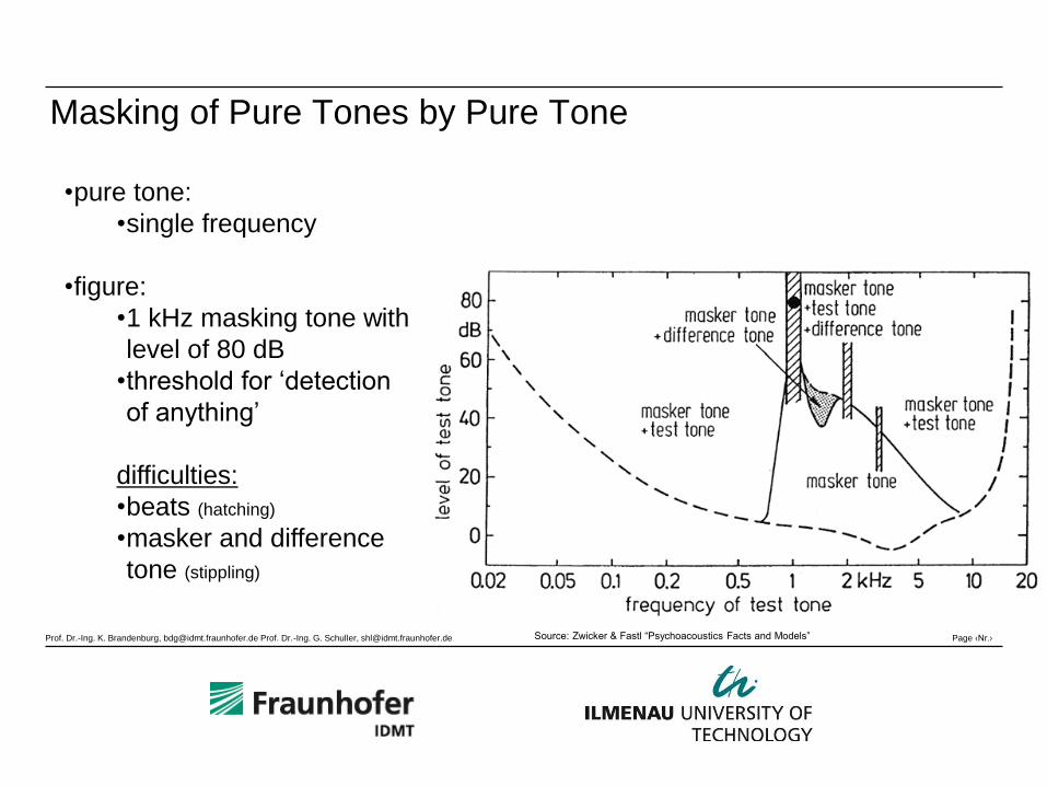
Masking of Pure Tones by Pure Tone
Source: Zwicker & Fastl “Psychoacoustics Facts and Models”
•pure tone:
•single frequency
•figure:
•1 kHz masking tone with
level of 80 dB
•threshold for ‘detection
of anything’
difficulties:
•beats (hatching)
•masker and difference
tone (stippling)
Prof. Dr.-Ing. K. Brandenburg, [email protected] Prof. Dr.-Ing. G. Schuller, [email protected] Page ‹Nr.›
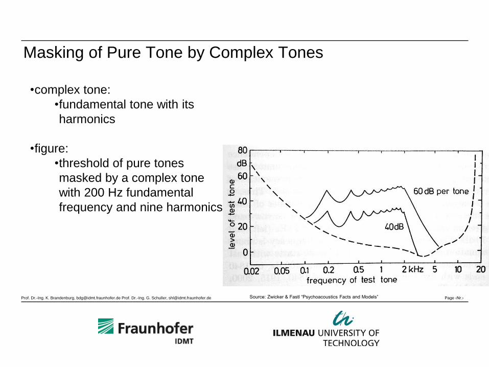
Masking of Pure Tone by Complex Tones
Source: Zwicker & Fastl “Psychoacoustics Facts and Models”
•complex tone:
•fundamental tone with its
harmonics
•figure:
•threshold of pure tones
masked by a complex tone
with 200 Hz fundamental
frequency and nine harmonics
Prof. Dr.-Ing. K. Brandenburg, [email protected] Prof. Dr.-Ing. G. Schuller, [email protected] Page ‹Nr.›
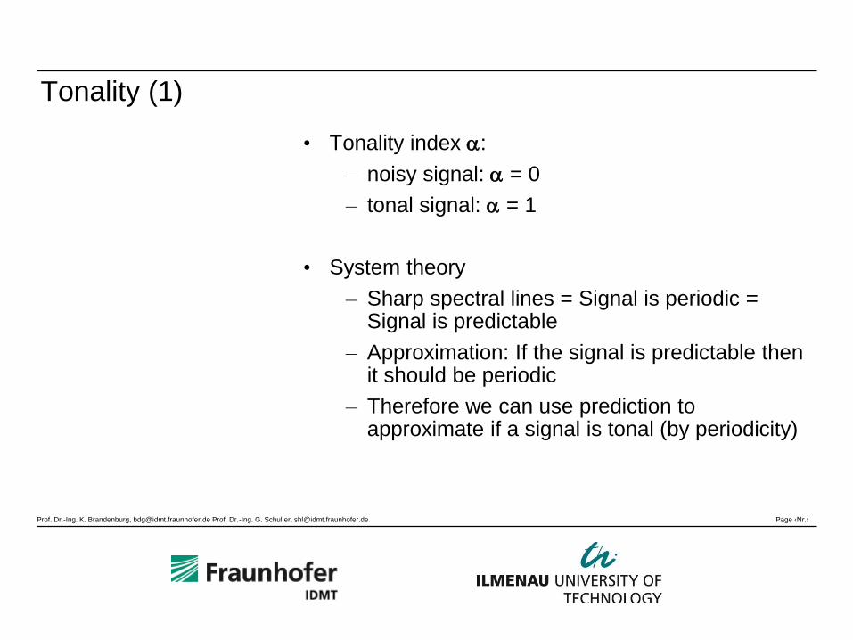
Tonality (1)
• Tonality index :
– noisy signal: = 0
– tonal signal: = 1
• System theory
– Sharp spectral lines = Signal is periodic = Signal is predictable
– Approximation: If the signal is predictable then it should be periodic
– Therefore we can use prediction to approximate if a signal is tonal (by periodicity)
Prof. Dr.-Ing. K. Brandenburg, [email protected] Prof. Dr.-Ing. G. Schuller, [email protected] Page ‹Nr.›
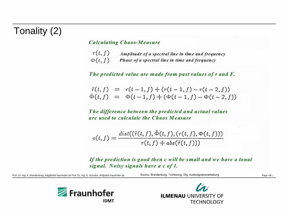
Tonality (2)
Source: Brandenburg, “Vorlesung: Dig. Audiosignalverarbeitung
Prof. Dr.-Ing. K. Brandenburg, [email protected] Prof. Dr.-Ing. G. Schuller, [email protected] Page ‹Nr.›
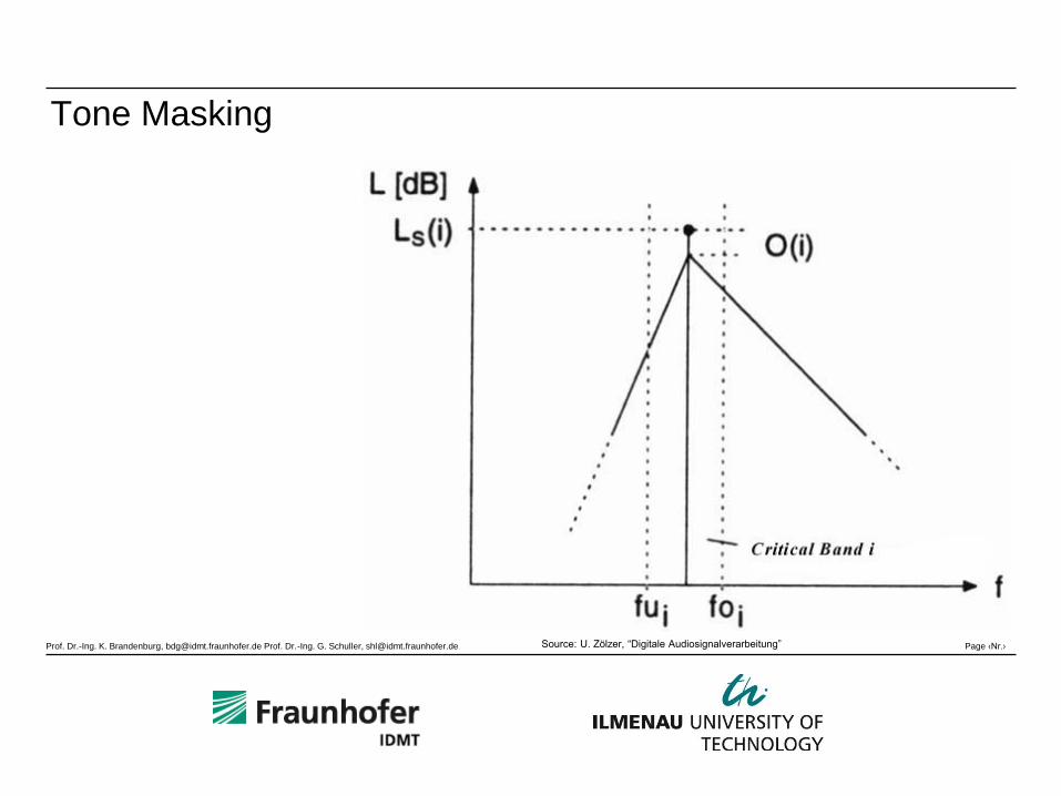
Tone Masking
Source: U. Zölzer, “Digitale Audiosignalverarbeitung”
Prof. Dr.-Ing. K. Brandenburg, [email protected] Prof. Dr.-Ing. G. Schuller, [email protected] Page ‹Nr.›
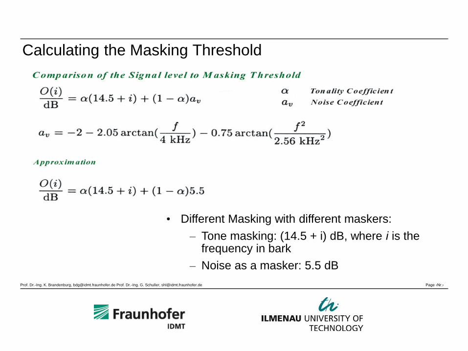
Calculating the Masking Threshold
• Different Masking with different maskers:
– Tone masking: (14.5 + i) dB, where i is the frequency in bark
– Noise as a masker: 5.5 dB
Prof. Dr.-Ing. K. Brandenburg, [email protected] Prof. Dr.-Ing. G. Schuller, [email protected] Page ‹Nr.›
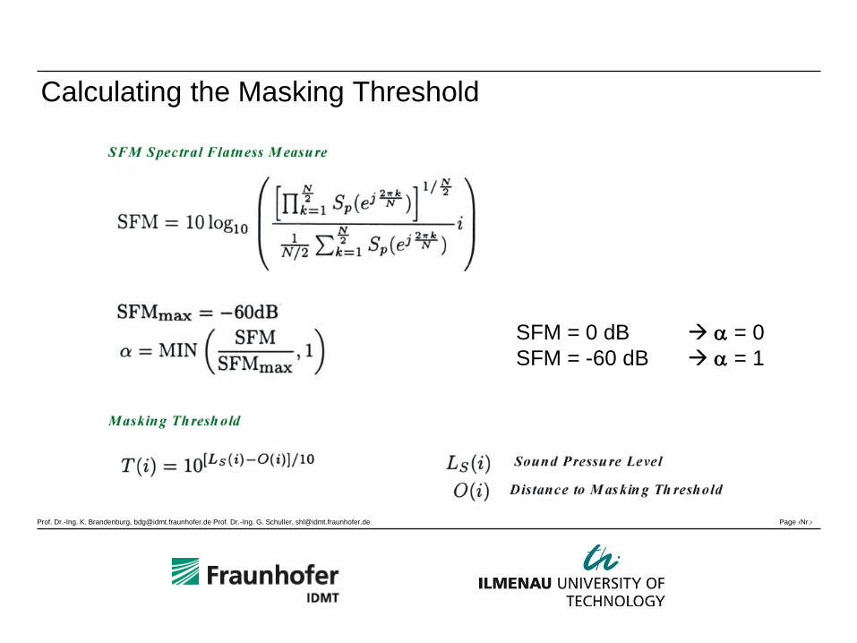
Calculating the Masking Threshold
SFM = 0 dB = 0
SFM = -60 dB = 1
Prof. Dr.-Ing. K. Brandenburg, [email protected] Prof. Dr.-Ing. G. Schuller, [email protected] Page ‹Nr.›
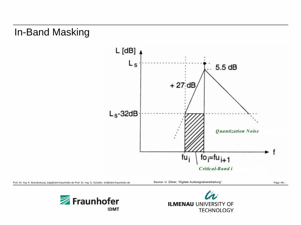
In-Band Masking
Source: U. Zölzer, “Digitale Audiosignalverarbeitung”
Prof. Dr.-Ing. K. Brandenburg, [email protected] Prof. Dr.-Ing. G. Schuller, [email protected] Page ‹Nr.›
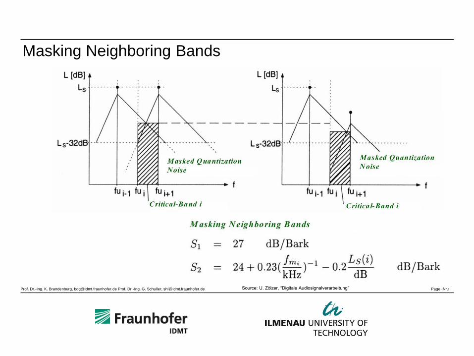
Masking Neighboring Bands
Source: U. Zölzer, “Digitale Audiosignalverarbeitung”
Prof. Dr.-Ing. K. Brandenburg, [email protected] Prof. Dr.-Ing. G. Schuller, [email protected] Page ‹Nr.›
• Example 7: Dynamic range
– Bach organ music with 16 bits per sample
• Example 8: Dynamic range
– Bach organ music with 11 bits per sample
• Example 9: Dynamic range
– Bach organ music with 6 bits per sample
Sound Examples
Prof. Dr.-Ing. K. Brandenburg, [email protected] Prof. Dr.-Ing. G. Schuller, [email protected] Page ‹Nr.›
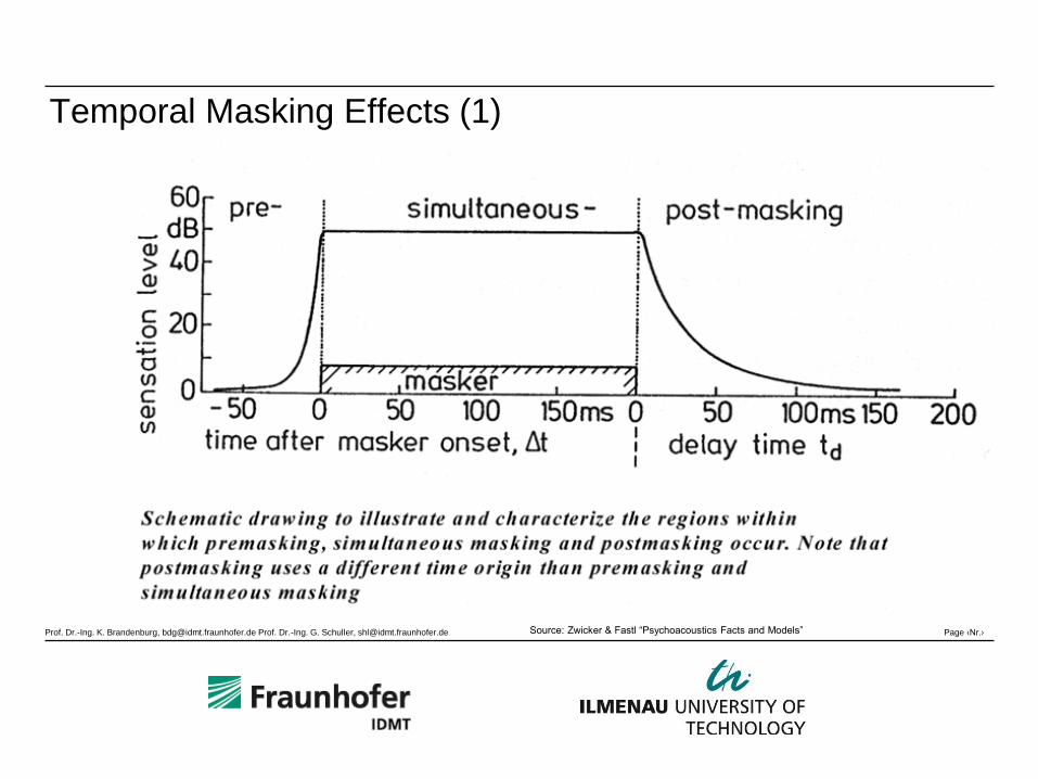
Temporal Masking Effects (1)
Source: Zwicker & Fastl “Psychoacoustics Facts and Models”
Prof. Dr.-Ing. K. Brandenburg, [email protected] Prof. Dr.-Ing. G. Schuller, [email protected] Page ‹Nr.›
Temporal Masking Effects (2)
• Post-Masking: corresponds to decay in the effect of
the masker expected
• Pre-Masking: appears during time before masker is
switched on
– Quick build-up time for loud maskers
– Slower build-up time for faint test sounds
• Frequency resolution Blurring in time
• Frequency resolution in the ear Masking in time
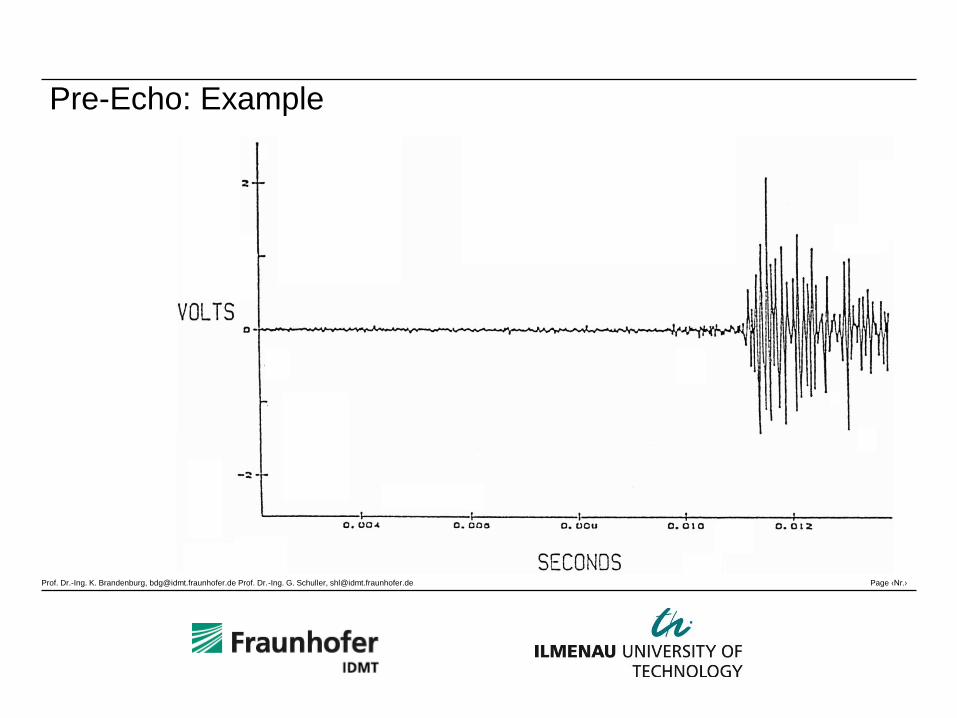
• Because of in-ear fast processing between quiet to
loud signals, we get Pre-Echoes
– Pre-Masking: 1-5 ms
– Post-Masking: ~100ms
Prof. Dr.-Ing. K. Brandenburg, [email protected] Prof. Dr.-Ing. G. Schuller, [email protected] Page ‹Nr.›
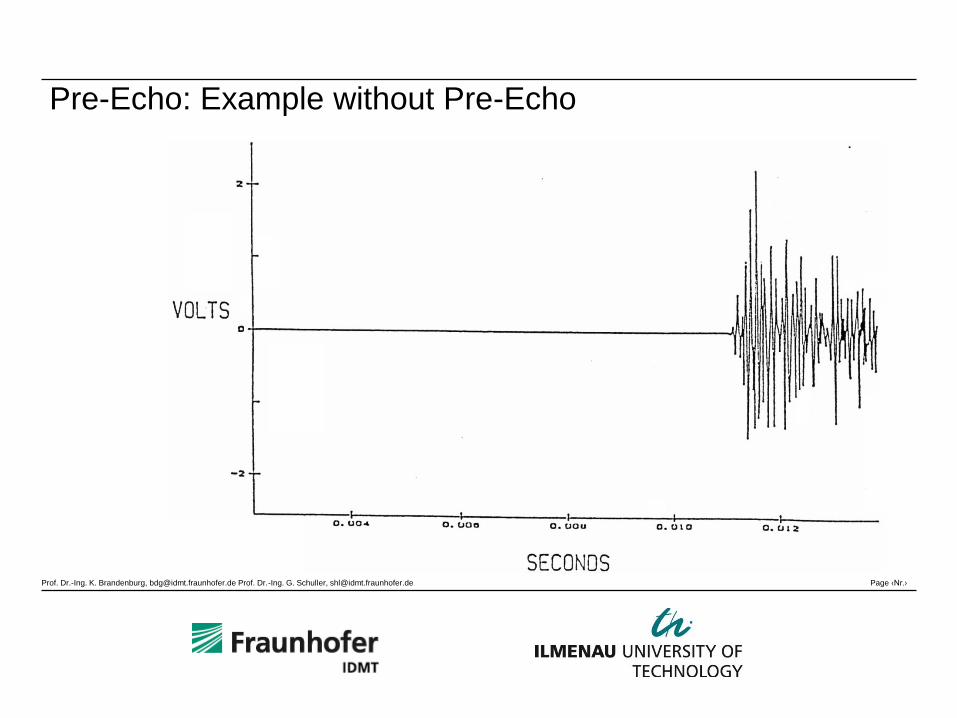
Pre-Echo: Example without Pre-Echo
Prof. Dr.-Ing. K. Brandenburg, [email protected] Prof. Dr.-Ing. G. Schuller, [email protected] Page ‹Nr.›
Pre-Echo: Example
Prof. Dr.-Ing. K. Brandenburg, [email protected] Prof. Dr.-Ing. G. Schuller, [email protected] Page ‹Nr.›
Sound Examples
• Example 10:
- Castanets original
• Example 11:
- Castanets coded with a block size of
2048 samples
Prof. Dr.-Ing. K. Brandenburg, [email protected] Prof. Dr.-Ing. G. Schuller, [email protected] Page ‹Nr.›
next lecture:
?? Quantization and Coding ??