Prof. Dr. G. M. PastorInstitut fur Theoretische PhysikFachbereich NaturwissenschaftenUniversitat Kassel

Quantum Mechanics I (SS 2009)

Das Skript, das Sie in der Hand haben, ist ein Lernhilfsmittel zur Vorlesung ,,Quanten-mechanik I”, wie sie an der Universitat Kassel im SS 09 gehalten wurde. Es handelt sichkeineswegs um ein vollstandiges Werk oder um einen richtigen Beitrag zur der zahlrei-chen auf dem Gebiet vorhandenen Literatur, deren Bearbeitung den Studenten dringendanempfohlen wird. Daruber hinaus soll die jetzige Fassung nur als ein erster Entwurfbetrachtet werden. Dies wird der Leser nicht nur an den ,,geschickt” verstreuten Druck-fehlern und knappen Formulierungen, sondern auch am Fehlen von erlauternden Abbil-dungen erkennen. Dies ist eine Schwache, die wir in spateren Fassungen beheben werden.

Kassel, Dezember 2009

1 Fundamental concepts of classical mechanics

In this chapter we briefly recall the fundamental concepts of classical mechanics startingfrom Newton’s second law and introducing basic notions like linear momentum, energy,Hamiltonian and conservation laws.

1.1 Dynamics of a single particle: Newton’s second law

Given a physical system as defined by its constituent particles, their interactions andpossible external fields, the purpose of a mechanical theory (either classical, quantum orstatistical) is to be able to predict the state of the system at any future time t > t0 on thebasis of the sole knowledge of the state of the system at a previous, so-called initial timet0. The mathematical definition of the state will of course depend on the type of theoryone is considering (e.g., classical, quantum or statistical mechanics), but in all cases itshould be such that it contains the minimum amount of information needed to predictthe outcome of any experiment performed in the system.

In the case of a single particle the state in classical mechanics is defined by the positionvector ~r and the linear momentum ~p (~r, ~p ∈ R3). Let ~r(t) be the curve traced by theparticle as a function of t, then the linear momentum is defined in terms of the velocity

~v =d~r

dt= lim

∆t→0

~r(t+∆t)− ~r(t)

∆t

by

~p = m~v = m~r, (1.1)

1

where m is the mass of the particle. Notice that we have implicitly assumed that the posi-tion is a continuous (actually differentiable) function of time, i.e., as ∆t → [~r(t+∆t)− ~r(t)]' ~v ∆t, where ~v is a constant vector. Do you think this is a reasonable assumption?

The fundamental physics involved in the dynamics of a particle is contained in Newton’ssecond law of motion, which in terms of ~r and ~p is given by

~F(~r(t)

)=

d~p

dt= ~p, (1.2)

where ~F is the force acting on the particle when it is at the position ~r. One says that~F (~r) is a force vector field (~F : R3 → R3). Once more, differentiability of ~p as a functionof t is assumed.

If the mass of the particle is independent of time, from (1.1) and (1.2) we obtain the morefamiliar but less general form

~F = md~v

dt= m~r,

where ~r = ~a is the acceleration.

1.2 Constants of motion

In classical mechanics, as well as in quantum mechanics, there are special physical quan-tities whose value remains constant throughout the time evolution of the system. Thesequantities have a special physical meaning and provide a fundamental insight on thesymmetries underlying the laws of motion.

1.2.1 Linear momentum

The first and most fundamental conservation theorem is the law of conservation of linearmomentum:

If the force ~F (~r) (or sum of forces) acting on a particle is zero then the momentum ~p isconserved.

This statement (also known as Newton’s first law 1) is an immediate consequence of Eq.(1.2) since

~F = 0 ⇒ ~p = 0 ⇒ ~p = constant.

The linear momentum conservation law is intimately related with translational symmetry.It appears whenever the system is invariant under translations, i.e., when all points inspace are equivalent, in the absence of external forces, or when the energy at all points inspace is the same. We shall come back to this point in Sec. 1.4.

1 Actually, the first law is not just a special case of the second one, since it defines the notionof inertial systems, where the second law applies.

2

1.2.2 Angular momentum

The angular momentum ~L of a particle with respect to a given point O (typically theorigin of the coordinate system) is defined as

~L = ~r × ~p,

where ~r is the position vector going from O to the particle. Clearly, the value of ~L dependson the choice of O. This can be illustrated by considering, for example, a free particlewith constant ~p and a point O at a distance d from the trajectory, in which case L = pd.

The time dependence of ~L is given by

d~L

dt=

d~r

dt× ~p+ ~r × d~p

dt.

Since ~p = md~r

dtwe have

d~L

dt= ~r × ~F = ~N, (1.3)

where ~F is the force acting on the particle and ~N = ~r × ~F the torque of the force.Equation (1.3) is a relation between vectors (pseudovectors) which holds irrespectively of

the coordinate system, although both ~L and ~N depend on the choice of the origin O.

From Eq. (1.3) the law of conservation of angular momentum follows:

If the total torque ~N is zero, the angular momentum ~L is conserved (~L = 0).

This conservation law is useful in problems involving central forces, i.e., force fields point-ing to a common origin O, which is taken as the origin of the coordinate system. Forinstance the gravitation field of the sun in the solar system or the electric field of thenucleus ~E = −Ze~r/r3 in the atom.

The conservation of angular momentum is intimately related with the rotational symme-try of the force field. Since Eq. (1.3) is a vector equation it holds for each componentindependently, i.e., if Nz = 0 then Lz is conserved.

1.2.3 Energy conservation: Kinetic and potential energy

Let us consider a particle of constant mass m under the action of an external force ~Fand determine the work done by ~F when the particle moves between two points ~r1 and~r2 along the trajectory. This work is given by the circulation

W12 =∫ ~r2

~r1

~F · d~r.

The integral can be calculated by using the parametrization of the trajectory ~r = ~r(t) as

a function of time [~r1 = ~r(t1) and ~r2 = ~r(t2)]. Knowing that ~F =d~p

dtand ~p = m

d~r

dt, or

3

equivalently d~r =~p

mdt, we have

W12 =∫ t2

t1

d~p

dt· ~p

mdt.

Assuming that the mass of the particle is independent of time and observing thatd

dt(p2) =

d

dt(~p · ~p) = 2 ~p · d~p

dtwe obtain

W12 =1

2m

∫ t2

t1

d

dt(p2) dt =

1

2m(p22 − p21), (1.4)

where ~p1 = ~p(t1) and ~p2 = ~p(t2) are the linear momenta at the initial and final points ofthe integration path.

The scalar quantity

T =p2

2m=

p2x + p2y + p2z2m

(1.5)

is known as the kinetic energy of the particle. Eq. (1.4) states that the work of the externalforce is equal to the change in kinetic energy:

W12 = T2 − T1.

It should be noted that the non-relativistic expression (1.5) for T is the simplest one thatsatisfies the conditions imposed by symmetry: i) Since time is homogeneous, T cannotdepend explicitly on t; ii) since space is homogeneous, it cannot depend on ~r ; iii) sincespace is isotropic, it must be invariant under rotations, i.e., all directions of the motionmust be equivalent; and iv) T must be positive definite and vanish only when the particleis at rest (~p = 0). In relativistic classical mechanics T has the form

T =√(mc2)2 + p2c2 −mc2,

which of course satisfies all these general symmetry conditions.

All fundamental forces in nature (gravitational, electrical, etc.) have the property that

the circulation of the force field ~F (~r) around any closed path C is zero, i.e.,

∮

C~F (~r) · d~r = 0 ∀ C closed.

Force fields having this property are said to be conservative. Mathematically this is equiv-alent to requiring

~∇× ~F = 0 ∀ ~r

or

~F (~r) = −~∇V (~r) = −(∂V

∂x,∂V

∂y,∂V

∂z

),

4

where V (~r) is a scalar differentiable function called potential energy (V: R3 → R). Well-known examples of potential energy functions are the potential energy of the gravitationat the surface of the earth:

V (~r) = mgz ⇒ ~F = −~∇V = (0, 0,−mg),

or the Coulomb interaction between an electron and the nucleus carrying a charge Ze:

V (~r) = −Ze2

r⇒ ~F (~r) = −Ze2

~r

r3.

In the presence of conservative force fields the time dependence of the kinetic energy takesa particularly simple and insightful form. Consider T = p2/2m along a trajectory of theparticle. Differentiating with respect to time one obtains

dT

dt=

1

2m

d

dt(~p · ~p) = 1

m~p · d~p

dt= −~∇V · d~r

dt=

−dV

dt,

where we have used that m is independent of time, ~F = −~∇V and ~p = md~r

dt. Moreover,

we know that for any scalar field V: R3 → R, the differential dV is given by

dV = V (~r + d~r)− V (~r) =∂V

∂xdx+

∂V

∂ydy +

∂V

∂zdz = ~∇V · d~r.

ThereforedT

dt=

−dV

dt,

or equivalently,d

dt(T + V ) = 0.

In other words the total energy

E = T + V =p2

2m+ V (~r) (1.6)

is a constant of motion. This explains why the force fields obtained as the gradient of apotential are called conservative fields.

1.3 Hamiltonian and Hamilton equations for a single particle

The total energy E regarded as a function of the dynamical variables ~r and ~p and even-tually time t is known as Hamilton’s function or Hamiltonian H = T + V . This is thecentral mathematical object in the powerful Hamiltonian formulation of classical me-chanics. Moreover, the corresponding operator in quantum mechanics defines the timeevolution of the quantum mechanical state or wave function. It is therefore important togain some insight into the physical significance of H.

5

For a single particle and in Cartesian coordinates H is given by

H =p2

2m+ V (~r) =

p2x + p2y + p2z2m

+ V (x, y, z).

In order to compact the notation, and to allow for more general sets of coordinates (e.g.,spherical or cylindrical) and constraints it is customary to denote the coordinates by qand the conjugated or corresponding momenta by p. Thus, in Cartesian coordinates wehave

~q = (q1, q2, q3) = (x, y, z)

and the conjugated momenta

~p = (p1, p2, p3) = (px, py, pz),

which are the usual components of the linear momentum.

Newton’s second law and the relation between velocity and momentum can be replacedby a set of first order differential equations known as Hamiltonian’s equations or, owingto their simple and symmetric form, canonical equations. In terms of qi and pi they takethe form

qi =∂H

∂pi(1.7)

and

pi = −∂H

∂qi. (1.8)

It is easy to verify that Eq. (1.7) is equivalent to the definition of linear momentum. Forinstance for i = 1 we have

x = q1 =∂H

∂p1=

∂(p2/2m)

∂px=

pxm.

The second set of n equations (n is the dimension of space) are equivalent to Newton’ssecond law. For example for i = 2

py = p2 = −∂H

∂q2= −∂V

∂y= Fy.

The canonical equations are valid in general, including interacting many-particle systems,other curvilinear coordinate systems or in the presence of constraints. Therefore, theHamiltonian

H = H(q1, . . . qn, p1, . . . pn, t) = T + V +W

as a function of qi, pi and eventually t (or in Cartesian coordinates as a function of ~pi and~ri) univocally defines the time evolution of the system starting from the initial conditionsp0i = pi(t0) and q0i = qi(t0). In particular H contains all the information on possibleconservation laws.

6

For the sake of completeness let us mention that in relativistic mechanics the kinetic plusrest energy of a free particle is related to the momentum ~p by the requirement that themagnitude of the momentum four vector is constant:

pµ pµ = p2 − T 2

c2= −m2c2

or equivalentlyT 2 = c2p2 +m2c4.

Consequently, the Hamiltonian of a relativistic particle under the action of a velocityindependent potential V is given by

H = T + V =√c2p2 +m2c4 + V.

1.4 Symmetry and conservation laws

Let us consider a particle or a set of particles moving along their classical trajectory qi(t)and pi(t). The total time derivative of the Hamiltonian along the trajectory is given by

dH

dt=

∂H

∂t+

∑

i

(∂H

∂qiqi +

∂H

∂pipi

).

Substituting the canonical equations −∂H

∂qi= pi and

∂H

∂pi= qi we obtain

dH

dt=

∂H

∂t∀ t.

This implies that if the system is isolated (i.e., no external potential), or if the externalpotential is independent of time, H does not depend explicitly on t and the energy isconserved (∂H/∂t = 0). From the point of view of symmetry, one would say that ifall times are equivalent or, in other words, if a translation in time does not change theHamiltonian, then the energy is conserved:

Time invariance ↔ Energy conservation

Let us now consider a system whose energy is unchanged upon a translation δx along agiven direction x. For example, a rigid body in the gravitational field at the earth surface,which energy remains constant under translations in the x or y horizontal directions. Theinvariance of H implies

0 = δH =∂H

∂xδx ⇒ ∂H

∂x= 0 ⇒ px = −∂H

∂x= 0 ⇒ px is conserved.

The invariance of the Hamiltonian with respect to translations along a given directionimplies, actually is equivalent to, the conservation of the corresponding component of thelinear momentum:

Invariance upon translation ↔ Linear momentum conservation

7

Let us now discuss what happens if the system is invariant upon rotations around a givenaxis n. For simplicity we consider a single particle with coordinates ~r = (x, y, z) andmomentum ~p = (px, py, pz). The changes in ~r and ~p after an infinitesimal rotation withangle δφ around n are given by

δ~r = n× ~r δφ

andδ~p = n× ~p δφ.

If H is invariant upon rotations around n we have

0 = δH =3∑

i=1

(∂H

∂riδri +

∂H

∂piδpi

)

= −~p · (n× ~r) δφ+ ~ri · (n× ~p) δφ

= −δφ[n · (~r × ~p) + n · (~r × ~p)

]

= −δφd

dt[n · (~r × ~p)]

= −δφd

dt(n · ~L).

This implies that n · ~L is conserved:

Invariance upon rotationaround n

↔ Conservation of angularmomentum ~L along n

The fundamental relations between the symmetries of the system or of the Hamiltonianand the conservation laws also hold in quantum mechanics. In fact, the constants ofmotion are the generators of the infinitesimal transformations which leave the Hamiltonianinvariant.

1.5 Many-particle systems

When we consider a system of particles we must distinguish between external forces ~F(e)i ,

due to the action of external fields applied on each particle i, and internal forces ~Fji dueto the interactions between the particles i and j. Newton’s second law then takes the form

~pi = ~F(e)i +

∑

j 6=i

~Fji,

where ~Fji is the force acting on particle i due to particle j. The forces of interest for thefollowing satisfy Newton’s third law of action and reaction:

~Fij = −~Fji

and, moreover, the interparticle forces lie along the line joining the particles:

~Fij = (~ri − ~rj) f(rij) where rij = ‖~ri − ~rj‖.

The latter condition is rather strong and does not apply to the electromagnetic forcesbetween moving charges.

8

1.5.1 Linear momentum

The action-reaction principle (which is of course obeyed by the important electron-electronand electron-nucleus interactions) implies that the time dependence of the total momen-tum

~P =∑

i

~pi

is unaffected by the interparticle interactions since

~P =∑

i

~pi =∑

i

~F(e)i = ~F (e). (1.9)

The conservation law of the total linear momentum follows: If the total external force iszero the total linear momentum is conserved.

The universal validity of this conservation law can be easily verified over all ranges oflength and energy (supernova, firework, nuclear decay, etc.).

We may also use Eq. (1.9) to derive the equation of motion for the center of mass ~R ofthe many-particle system. Using that

~R =

∑imi ~ri∑imi

, M =∑

i

mi

we have~P =

∑

i

mi ~ri = M ~R =∑

i

~F(e)i = ~F (e).

Notice that this equation is not easy to solve when the external force field is inhomoge-neous, i.e., ~Fi = ~F (~ri).

1.5.2 Angular momentum

The angular momentum of the system is obtained by summing the individual angularmomenta of all the particles with respect to the given origin O:

~L =∑

i

~li =∑

i

~ri × ~pi.

Its time dependence is given by

~L =∑

i

(~ri × ~pi + ~ri × ~pi

)=

∑

i

~ri × ~pi =∑

i

~ri × ~Fi.

It is meaningful to split the force ~Fi acting on particle i in external and internal contri-butions:

~L =∑

i

~ri × ~F(e)i +

∑

i

~ri ×∑

j 6=i

~Fji.

9

Putting together the terms for each pair i and j the second term reads

∑

i<j

(~ri × ~Fji + ~rj × ~Fij

),

and using the action-reaction condition on the internal forces ~Fij = −~Fji we have

∑

i<j

(~ri − ~rj)× ~Fji.

Finally, for internal forces acting along the line connecting the particles, ~Fji is parallel

to ~rij = ~ri − ~rj and thus each term of the sum vanishes ( ~Fij × ~rij = 0). Hence the timedependence of the total angular momentum is determined by the total external torque

~N (e) =∑

i

~ri × ~F(e)i ,

which results exclusively from the external forces:

~L = ~N (e).

The conservation theorem for the angular momentum follows: The total angular momen-tum of a many-particle system is conserved if the total external torque is zero.

Note that the conservation of angular momentum relies on ~Fji being parallel to ~rij = ~ri−~rj,which does not hold for moving charges. In this case, transfer of angular momentumbetween the mechanical degrees of freedom and the electromagnetic field is possible, andonly the sum of both is conserved.

1.5.3 Energy conservation

In order to introduce the concept of total kinetic energy we consider the work done byall the forces acting on the particles along a path between any two given points in ann-particle trajectory [e.g., ~r1(t1), . . . ~rn(t1) and ~r1(t2), . . . ~rn(t2)]:

W12 =∑

i

∫ 2

1

~Fi · d~si =∑

i

∫ 2

1~pi · ~pi

mi

dt

=∑

i

∫ 2

1

d

dt

(p2i2mi

)dt =

∫ 2

1

d

dt

(∑

i

p2i2mi

)dt

= T2 − T1,

where

T =∑

i

p2i2mi

.

We turn now to the most interesting case of conservative forces. Concerning the externalforces the situation is the same as for a single particle, since the force field acts on eachparticle independently:

~F(e)i (~ri) = −~∇ vext(~ri).

10

Consequently, the total potential energy due to the external field is

V =∑

i

vext(~ri).

For the interparticle forces we must require ~Fij = −~Fji and ~Fij = (~ri − ~rj) f(rij), wheref(rij) depends only on the distance rij = |~ri − ~rj| between the particles i and j. In orderto obtain a scalar function W (~r1, . . . ~rn) such that

−~∇iW = ~F(int)i =

∑

j

~Fji ,

we consider first the interaction between two particles i and j and seek for a functionwij(~ri, ~rj) such that

−~∇iwij = ~Fji = −~Fij = ~∇jwij.

This can be solved by recalling the calculation of the gradient of a function of the distancew = w(r)

∂w

∂x=

dw

dr

∂r

∂x= w′(r)

2x

2√x2 + y2 + z2

= w′(r)~r

r.

Consequently, if we choosewij(~ri, ~rj) = wij(rij)

with rij = |~ri − ~rj| we have

−~Fji = ∇iwij(rij) = w′ij(rij)

(~ri − ~rj)

rij

and

−~Fij = ∇jwij(rij) = w′(rij)(~rj − ~ri)

rij= ~Fji.

In order to obtain the interaction potential we simply sum over all pairs (i, j):

W =1

2

∑

i6=j

wij(rij) =∑

i<j

wij(rij).

Example: wij =qi qjrij

or simply w(rij) =e2

rijand W =

1

2

∑

i6=j

e2

|~ri − ~rj| .

Note the factor1

2if the double sum over i and j is used, which results from the fact that

each pair of variables ij appears twice, once in∑

i and once in∑

j. We may explicitlyverify that

−∂W

∂xk

= −1

2

∑

j

∂wkj

∂xk

+∑

i

∂wik

∂xk

=1

2

∑

j

~Fjk +∑

i

~Fik

=

∑

j

~Fjk.

11

Summarizing, the total potential energy

V +W =∑

i

vext(~ri) +1

2

∑

i6=j

wij(|~ri − ~rj|)

satisfies

−~∇i(V +W ) = ~F(e)i +

∑

j

~Fji. (1.10)

With the help of Eq. (1.10) we can easily determine the time dependence of the totalkinetic energy

T =∑

i

p2i2mi

as

dT

dt=

∑

i

~pim

· ~pi =∑

i

−~∇i(V +W ) · d~ridt

= −d(V +W )

dt.

Therefore,d

dt(T + V +W ) = 0,

which implies that the total energy, namely, kinetic, plus external potential, plus interac-tion energy, is a constant of motion. For example, the total energy of a system of n chargedparticles (e.g., electrons) around the point charge of a nucleus with atomic number Z isgiven by

E =n∑

i=1

p2i2m

+∑

i

(−Ze2)

|~ri| +1

2

∑

i6=j

e2

|~ri − ~rj| .

12

2 Basic concepts of quantum mechanics

Whenever one attempts to apply classical mechanics to explain atomic or subatomicphenomena, one inevitably comes to very profound contradictions. For instance, in thecase of the atom, one would have to conclude that the electrons should fall into the nucleus,since classical charge systems are unstable, and since moving charges in closed trajectorieswould radiate electromagnetic waves, thereby losing progressively their kinetic energy.

The contradictions are so profound that the formulation of a theory capable of describingmicroscopic phenomena (i.e., those occuring at very small distances and for particles ofvery small mass) requires a complete modification of the basic physical concepts and laws.The examples to be discussed below will show that some of the most basic notions of classi-cal mechanics and of our experience with macroscopic phenomena are simply unapplicableto the atomic world. The limitations of classical mechanics are not simple quantitative dis-agreements but much more fundamental. The main problem is that classical physics doesnot even provide an appropriate language for describing certain microscopic phenomena,just in qualitative terms.

We will start by discussing a number of experiments that illustrate the concept of wave-particle duality, the complementary principle, the superposition principle, the measure-ment process in quantum mechanics, and the stochastic nature of the observed events.While the conclusions of these experiments are for the most part negative, in the sensethat they show how the classical concepts fail or why they should be abandoned, they alsoprovide some extremely useful insights on the problems that quantum mechanics needsto (and actually does) solve. Moreover, the examples will unravel important clues on howthe theory should look like.

2.1 Electromagnetic waves

The equations governing the classical dynamics of electrical and magnetic fields in vacuumare the Maxwell equations

~∇ · ~B = 0 ~∇× ~E +1

c

∂B

∂t= 0

~∇ · ~E = 0 ~∇× ~B − 1

c

∂E

∂t= 0.

With a few simple manipulations one can easily derive the equation for classical electro-magnetic waves. Starting from

~∇× ~E +1

c

∂ ~B

∂t= 0,

take ~∇× to obtain

~∇× (~∇× ~E) +1

c

∂

∂t(~∇× ~B) = 0.

13

Using a known relation from vector calculus this is written as

~∇ (~∇ · ~E)−∇2 ~E +1

c

∂

∂t

1

c

∂ ~E

∂t

= 0,

which implies

∇2 ~E − 1

c2∂2 ~E

∂t= 0.

If we focus for simplicity on one component of ~E, a scalar electromagnetic field which wedenote by φ, we have

∇2φ− 1

c2∂2φ

∂t= 0. (2.1)

Let us solve this linear homogeneous differential equation with the usual exponentialansatz

φ~k(~x, t) = ei(~k·~x−ωt),

where ~x = (x1, x2, x3) refers to the position vector, ~k to the wave vector, and ω to theangular frequency. Let us see under which conditions φ(~x, t) = ei(kx−ωt) satisfies the waveequation:

~∇φ~k =~∇

[ei(k~x−ωt)

]= i~k ei(k~x−ωt)

and thus

~∇ · (~∇φ~k) = i~k ~∇(ei(

~k·~x−ωt))= −k2 ei(kx−ωt).

Since∂2

∂t2φ~k = −ω2ei(

~k~x−ωt) we have

∇2φ~k −1

c2∂2φ~k

∂t2=

(ω2

c2− k2

)ei(

~k~x−ωt) = 0,

which can only hold if

ω = c k with k = |~k|.

This is known as the dispersion relation of electromagnetic waves. A dispersion relationgives the energy or frequency of a wave state as a function of the wave vector ~k. In thepresent case the isotropy of space (vacuum) implies that ω depends only on k. Using therelation ω = c k we can write the monochromatic plane wave as

φk(x, t) = ei k(x−c t),

which explicitly shows that the point of stationary phase propagates with the light velocity

c =∂ω

∂k.

14

The wave equation is a linear homogeneous equation. This means that if φ1 and φ2 aresolutions, then αφ1 + β φ2 is also a solution for any α, β ∈ C. We may then write themost general solution φ(~x, t) of the wave equation (2.1) as a linear combination of plane

waves φ~k = ei(~k·~x−ωt). If φ(~x, t) is periodic in space [φ(~x+~ai, t) = φ(~x, t) for i = 1−3] only

discrete values of ~k are allowed. For instance, in one dimension kn = (2π n)/a with n ∈ Zso that ei knx = ei kn(x+a). However, in the most general case all values of ~k are allowedand the linear combination takes the form of a Fourier integral

φ(x, t) =1

(√2π)3

∫d3k A(~k) ei(

~k·~x−ωt). (2.2)

The coefficient A(~k) ∈ C represents the weight in amplitude and phase of the plane wave

φ~k in the electromagnetic wave φ(~x, t). Notice that, since A(~k) = eiϕ~k |A(~k)| ∈ C, anyphase shifts ϕ~k between the plane waves can be taken into account.

The intensity of the radiation at the point ~x and time t is given by the square of the fields(E2+B2)/8π, which in the present scalar-field approximation corresponds to |φ(x, t)|2. Itis important to notice that, given two waves φ1 and φ2, the superposed solution φ1 + φ2

leads to interference effects since the intensity of the superposed waves is not equal to thesum of the intensities:

|φ1 + φ2|2 6= |φ1|2 + |φ2|2.We may profit from the general expansion (2.2) to analyze under which conditions a wavepacket or light pulse can be localized in some reduced region in space. To this aim weconsider a Gaussian wave packet in one dimension:

φ(x, t) =1√

2π∆k2

∫ +∞

−∞dk e−

(k−k0)2

2∆k2︸ ︷︷ ︸A(k) ∈ R⇒ all planewaves in phase

ei k(x−c t).

We replace for a moment x− c t by x and obtain

φ(x, t) =ei k0 x√2π∆k2

∫ +∞

−∞dk e−

(k−k0)2

2∆k2 ei (k−k0)x

and shifting the origin of k to k − k0

φ(x, t) =ei k0 x√2π∆k2

∫ +∞

−∞dk e−

k2

2∆k2 ei k x.

Taking into account that

k2

2∆k2− i k x =

(k√2∆k

− i∆k x√

2

)2

+∆k2x2

2

we can write

φ(x, t) =ei k0 x√2π∆k2

e−∆k2x2

2

∫ +∞

−∞e−

(k−i∆k2x)2

2∆k2 dk.

15

This integral can be solved by changing to the complex variable z = k − i∆k2x. Notingthat dz = dk we obtain

φ(x, t) = ei k0 x e−∆k2x2

21√

2π∆k2

∫e−

z2

2∆k2 dz = ei k0 x e−x2 (∆k)2

2 .

Finally

φ(x, t) = ei k0 x e−x2

2∆x2 ,

where ∆x = 1/∆k. The uncertainty or dispersion ∆x in the wave-packet’s position isinversely proportional to the uncertainty ∆k in the wave vector.

Since the Gaussian packet is an optimal packet in the sense that it reaches the largestlocalization (smallest ∆x) for a given ∆k, we conclude that the uncertainty ∆k in thevalue of the wave vector k and in the position of the light pulse (i.e., the photons) arerelated by

∆x∆k ≥ 1.

For 3 dimensions we can generalize the relation to

∆xi∆kj ≥ δij,

since the dispersion of k in the direction i has no influence in the localization of φ(~x) inthe directions j with j 6= i.

Replacing now x by x− c t we obtain

φ(x, t) = ei k0 (x−c t) e−(x−c t)2

2∆x2 .

One observes that the Gaussian wave packet propagates undistorted with the speed c,since the dispersion relation is strictly linear in vacuum: ω = c k.

It is interesting to relate the uncertainty or width ∆x of the wave packet with the duration∆t of the pulse at a given fixed point in space. For a wave packet with the dispersion ∆kthe dispersion in frequency is ∆ω = c∆k. Moreover, the spatial extension of the packetis

∆x ≥ 1

∆k=

c

∆ω

∆x∆ω

c≥ 1

∆x

c∆ω ≥ 1.

The time of passage of such a packet at any given point is

∆t =∆x

c≥ 1

c

c

∆ω=

1

∆ω.

Consequently,∆t∆ω ≥ 1.

16

One concludes that it is impossible to ascribe a well-defined position (∆x = 0) and awell-defined wave vector (∆k = 0) or frequency (∆ω = 0) to a photon. Moreover, it is notpossible to define the frequency (∆ω = 0) and the time of passage of a pulse (∆x = 0) atany given point. To be strict one should replace “photon” by “electromagnetic wave” or“ensemble of photons” in the previous statement. These uncertainty relations ∆k∆x ≥ 1are a typical manifestation of wave properties. They are inherited by quantum mechanicalparticles with a finite rest mass (e.g., electrons) due to wave–particle duality.

2.2 Non-classical aspects of the electromagnetic field: Photons

2.2.1 The photoelectric effect

The interactions between light and electrons have provided many important clues in thedevelopment of quantum theory. The first manifestation of the quantized, particle-likenature of light is the photoelectric effect. The main experimental observations are thefollowing:

i) The rate of electron emission is proportional to the intensity of radiation, i.e., to |φ|2.

ii) For each metal there is a threshold frequency ωc such that for ω < ωc no emission atall is observed despite intensity increase (within reasonable limits).

iii) For ω > ωc, the largest kinetic energy Emaxkin of the emitted electrons depends linearly

on ω, but not on the intensity of the radiation |φ|2.iv) The time delay between the start of the incident radiation and electron emission is

very short (< 10−9 s).

These results are incompatible with the classical theory of electromagnetic radiation. Allthe observations indicate that the energy is not transferred by the field |φ2| but ratherthat the process occurs in a quantized way.

Einstein’s explanation proposes that the emitted electron is scattered by a quantum oflight known as photon thereby receiving momentum and energy. The energy E of thephoton is related to its frequency by

E = ~ω

and its momentum ~p is given by~p = ~~k,

where ~ = 1.054 × 10−34 Joule · s = 0.66 eV · fs is Planck’s constant (~ = h/2π). ~ hasthe units of action or of angular momentum.

The intensity of the light corresponds to the number of emitted photons per unit time.The energy of each photon is independent of intensity, it depends only on the frequencyω or the wave length λ = 2π/k = 2πc/ω.

Since ω = c k ⇒ E = ~ω = c ~ k = c p. Recalling the relativistic energy-momentumrelation E2 = p2c2 +m2c4 one concludes that photons have vanishing rest mass m. Theexplanation is as follows:

17

i) Emaxkin = ~ω−W , where W is the metal’s work function. If Emax

kin < 0 ⇒ no emissionwhatever the intensity, since the electrons cannot escape from the metal.

ii) Emaxkin = ~ω − W is independent of the number of photons, i.e., of the radiation

intensity.

iii) The intensity of the radiation defines the number of photons, which controls thenumber of emitted electrons.

iv) A single photon can emit an electron. Therefore, no delay in accumulating absorbedenergy is involved. According to the classical picture one would have to integrate |φ|2during some time before emission can occur, and this time delay would be inverselyproportional to the intensity |φ|2.

2.2.2 The Compton effect

The Compton effect provides a number of additional important clues. Consider a wavepacket with small ∆k (large spatial extension), i.e., essentially monochromatic. Classically

one expects that the electron would gain momentum in the direction ~k of the incidentradiation and that the light would be scattered in the form of spherical waves. However,Compton X-ray scattering experiments show the following:

i) The scattered electron often acquires a momentum ~p transversal to the incident ~k.

ii) There is no sign of a spherical outgoing wave.

iii) The scattered light is concentrated in a spatially confined packet.

iv) The propagation direction of the scattered light is correlated with the momentumvector ~p of the scattered electron.

v) The wave length and consequently the energy of the scattered light depends on thelight’s scattering angle θ as

ω′ = ω

(1 +

2~ωmc2

sin2 θ

2

)−1

or equivalently

λ′ − λ = 2λc sin2 θ

2,

where λc =2π ~mc

is the Compton wave length.

This experiment can be explained by assuming that photons scatter with electrons asindividual particles like billard balls, i.e., following energy and momentum conservationaccording to Einstein’s relations ~p = ~~k and E = ~ω = c p for photons, and E2 =c2p2 +m2c4 for electrons.

In the photoelectronic effect, the need for the quantization of the energy

E = ~ω

18

of the electromagnetic radiation became clear. This established the relation between en-ergy and frequency of electromagnetic oscillations given by

ei ω t = eiE~ t.

For the explanation of the Compton effect we need to assume the relation

~p = ~~k

between the wave vector ~k and momentum ~p of a quantum of radiation. This establishesthe relation between momentum and the oscillations of the electromagnetic wave in spacegiven by

ei~k·~x = e

i~ ~p·~x.

Consequently there is a relation between momentum and wave length:

λ =2π

k=

2π ~p

.

Since ω = c k, we also have E = c p.

The correlations between the light-scattering direction and its frequency, as well as be-tween the directions of the scattered particles, can be explained by assuming that theinteraction occurs between a single photon and an electron, and that the total energy andmomentum are conserved in the process. Let us assume that the direction of the wavevector of the incident (scattered) photon is along ~k (~k ′), and that the electron is initiallyat rest (~p = 0). Energy and momentum conservation imply

~ω +mc2 = ~ω ′ +√m2c4 + c2p′ 2 (2.3)

and

~~k = ~~k ′ + ~p ′, (2.4)

where ~p ′ refers to the momentum of the scattered electron. From Eq. (2.4) we have

~p ′ = ~ (~k − ~k ′) and therefore

p′ 2 = ~2 (~k − ~k ′)2 = ~2 (k2 + k′ 2 − 2~k · ~k ′)

= ~2[(k − k′)2 + 2 k k′ (1− cos θ)

]

= ~2[(k − k′)2 + 4 k k′ sin2

(θ

2

)]. (2.5)

Moreover, Eq. (2.3) can be written as

~ c (k − k′) +mc2 =√m2c4 + c2p′ 2. (2.6)

Taking the square on both sides of Eq. (2.6) and replacing p′ 2 by Eq. (2.5) one obtains

mc (k − k′) = 2~ k k′ sin2 θ

2.

19

Finally, introducing the Compton wavelength λc =2π ~mc

we have

2π(1

k′ −1

k

)= 2λc sin

2 θ

2

or

λ′ − λ = 2λc sin2 θ

2.

A number of nontrivial conclusions can be inferred from the previous partial explanationof the effect:

1) The concept of particles or photons and waves ei (~k·~x−ωt) are linked by Einstein’s

relationsE = ~ω and ~p = ~~k.

In other words, we attach an energy quantum to the electromagnetic field and amomentum ~p to a wave vector. This wave-particle duality is a concept that does notexist at all in classical physics. In terms of Bohr’s complementary principle one wouldsay that a single classical concept (in this case wave- or particle-like aspects) is notenough to describe atomic phenomena.

2) Another most remarkable feature of the experiment is the stochastic nature of theoutcome. It seems that there is no way one could control the momentum of the scat-tered electron or the wave length of scattered light. Compton incorporates part of thestatistical aspect in the interpretation by establishing a relation between the scat-tered angle and the frequency of the light. But this first analysis is clearly incomplete,since it cannot predict the probability for each scattering angle.

3) Classical theory, in contrast, is completely useless, since it would conclude that theinitial conditions (which are all the same for all photons) completely define the out-come of the scattering process. The concepts of classical theory are inappropriatesince they do not incorporate the statistical aspects of the observed phenomena.

4) Already at this point one may ask oneself a kind of philosophical question: What isthe origin of the statistical nature of the experimental outcome? Is it the quantummechanical state (whatever this is) that has a statistical, somehow non-deterministicnature? Or are the statistical results of the experiment only a consequence of themeasurement process, i.e., of the interaction between the quantum mechanical stateand the macroscopic world or apparatus that detects scattering angle and wavelength,so that a human can read it? To put it in Einstein’s terms, is God playing dices withnature?

2.2.3 Young interference experiment

One of the most remarkable features of quantum physics is the so-called wave-particleduality which states that particle and wave aspects of quantum phenomena (in the presentcase light) are indivisible. In other words, if one attempts to interpret quantum phenomenawith classical concepts corresponding to the notions of particles and waves, one realizesthat both concepts are needed at the same time. Since these are classically incompatible,it is clear that the classical interpretation and language are inappropriate.

20

Young’s interference experiment for light, and the similar phenomenon of electron diffrac-tion observed for particles having a nonvanishing rest mass, illustrate the problem veryclearly. We consider the following arrangement:

(Bild)

The main qualitative observations are the following:

1) If S2 is closed, one observes a diffraction spot I1(x).

2) If S1 is closed and S2 open, one sees I2(x).

3) If both sides are open, one sees an interference pattern I(x) 6= I1(x) + I2(x).

How to explain this with the particle picture put forward by the explanation of photo-electric effect and Compton’s experiment?

1) One could attempt to interpret the single-slit diffraction spot I1(x) or I2(x) classicallyin terms of collisions of the particles (photons) during the passage through the slit.This is actually not quite satisfactory in detail, but anyway this is not so crucial.

2) Let us focus on the interference effect that appears when both slits are open. Howcan one explain that a particle, which in a classical picture follows a trajectory going,for example, through S1, knows whether S2 is open or not?

One could try to argue that the interference is due to interactions of the photons goingthrough S1 with photons going through S2. However, if one reduces the intensity, sothat only one or a few photons pass at a time and there is no possible interaction,and one increases proportionally the exposure time, the interference pattern remains.Consequently, interference is not a result of photon-photon interactions.

The observed effect is therefore incompatible with the idea that particles go through oneslit or the other. The interference phenomenon is thus incompatible with the classicalnotion of path.

However, we all know that the interference pattern can be easily interpreted by using thenotion of waves and the superposition principle, which holds for any linear homogeneousdifferential equation such as the wave equation

∇2φ− 1

c2∂2φ

∂t2= 0.

The wave picture of light implies that the intensity of the photon beam is proportionalto the square of the electric and magnetic fields

|E|2 or |φ|2.

The intensity at any point in the screen is given by the square of the sum or superpositionof the fields generated by each slit S1 and S2 which act as secondary sources:

E(x) = E1(x) + E2(x) with Ei = ei~k·(~ri−~Ri),

21

and

I(x) = |E(x)| = |E1(x) + E2(x)|2= |E1(x)|2 + |E2(x)|2 + 2ReE1(x)E

∗2(x)︸ ︷︷ ︸

interference term

6= |E1|2 + |E2|2.

There is no interaction at all between the fields E1 and E2, just linear superposition.

You could pragmatically say: “Here the wave explanation works, so maybe we can forgetabout the particle picture for this experiment (despite Compton’s experiment). Maybesomething different happened there.”

But then you decide to look in more detail at the one-photon-at-a-time version of Young’sexperiment and you see what’s really going on.

If you reduce the intensity to the limit of one or a few photons at a time and keep theexposure time relatively short, so that only one or a few photons are emitted, you seeno interference pattern in the photographic plate, but isolated single-photon dots. Thisis completely incompatible with the wave picture which predicts an interference for allintensities, i.e.,

I ∝ |E(x)|2.

The individual dots follow a random distribution with no correlation between the po-sitions corresponding to successive photons. We recover here Compton’s randomness ofsuccessively scattered photons.

Only when we increase the exposure time, so that many photons have arrived per unit areaand one can no longer distinguish or resolve individual dots, we recover the interferencepattern as predicted by the classical wave theory

I = |E(x)|2 = |E1(x) + E2(x)|2.

We must conclude that the wave theory, which follows superposition, only predicts theprobability density for a light quantum or photon to hit the screen at a given point x.In fact |E(x)|2, which is the result of the superposition of E1(x) and E2(x), gives theprobability density.

While the idea that the classical field gives the probability amplitude is attractive, itdoesn’t solve the problem that a photon going through S1 behaves differently if S2 is openor closed. So we may want to check if the photon does get through one slit or the other.To this aim we put detectors just after the slits. One then observes 50% of the counts onS1, 50% on S2, and never a count on both. In other words, if we measure the position ofthe photon we get a well-defined value.

What happens if we put a detector only behind S2 (that absorbs of course all the photonsgoing through S2), so that we know that the rest of the photons go certainly through S1.In this case, as expected, we recover the single-slit result I1(x) with no interference at all.

At this point we can draw a few important conclusions:

1) If the photons are allowed to traverse different paths, we either remain ignorantabout which path the quantum particles have traversed and observe an interference

22

pattern, or we experimentally determine (i.e., “measure”) which was the path thathas actually been taken and then lose the interference pattern.

One often summarizes this by the complementarity principle which states that ameasurement designed to manifest one classical attribute (e.g., a wave or particleaspect) precludes the possibility of observing the other or at least part of the otherclassical attribute. A measurement affects the quantum state of a microscopic particlein an essential way.

This is not what happens in classical physics. In classical mechanics the particleshave their own dynamical variables (position, momentum, etc.), irrespectively of themeasurement, which can in principle be as soft as wished.(Example: Photons ¿ Train.)

2) We must conclude that a photon follows no trajectory. It has no intrinsic dynamicalvariables like position or momentum. These variables appear only as a result of ameasurement.

3) The photons make random individual spots on the screen, so that there is no possi-bility of predicting the outcome of a single measurement. The experiment can onlyattempt to determine the probabilities for individual events. This implies recordinga large number of quantum events.

2.3 Non-classical properties of particles having finite rest mass:The uncertainty principle

While the properties of photons and the interaction of light with matter are both interest-ing and clarifying, a detailed development of the quantum theory of radiation cannot bediscussed without a previous background on non-relativistic quantum mechanics. Fromnow on we focus therefore on the properties of electrons, which we will loosely take as asynonym of a quantum object with a non-vanishing rest mass.

We have already pointed out the impossibility of understanding the stability of atoms ina classical framework. For the formulation of quantum mechanics it is also important torealize that electrons show (like photons) a number of features belonging to wave physics.In particular electrons diffract displaying interference patterns when they pass throughcrystals, in a completely analogous way as electromagnetic waves.

Let us consider an idealized version of the electron diffraction experiment. In the two-slitexperiment

(Bild)

one observes the same phenomena found for electromagnetic waves. As already discussedfor photons, this result is incompatible with the idea that electrons follow a path. Thelack of path or trajectory in quantum dynamics is one of the manifestations of Heisen-berg’s uncertainty principle, which is probably the most fundamental concept in quantummechanics.

The fact that electrons lack of a path also implies that they have no intrinsic dynamicalvariables in a classical sense. In particular it means that an electron has no intrinsic valueof the position, velocity or momentum. These dynamical variables can only appear as the

23

result of a measurement. A measurement is the result of the interaction of an electron witha classical object (typically, but not necessarily a macroscopic object like a photomultiplierdetector). These classical objects are called apparatus. As a result of a measurement, i.e.,as a result of the interaction of the electron and the classical object, the state of theapparatus and the state of the electron change. These changes depend on the initial stateof the electron and can thus be used to characterize its state quantitatively. For example,a detector set behind the slits S1 or S2 allows one to define the position of the electron.

Notice that the notion of measurement as interaction is completely independent of thepresence of a human observer. Moreover, the apparatus need not be macroscopic. It shouldsimply follow classical mechanics to a sufficiently high accuracy. For instance the vapormolecules in a Wilson chamber, which condense to a thin but macroscopic cloud uponthe passage of an electron, allow one to determine the electron’s path to a low degreeof accuracy. As we shall see, momentum or velocity and position can be simultaneouslydetermined provided that both measurements are done with a limited accuracy. Precisesimultaneous measurements of both position and momentum are of course not possible,since this would imply that the electron follows a trajectory.

We see that classical mechanics is not only a limiting case of quantum mechanics. Itis also needed to formulate the connection between the quantum and the macroscopicworlds, i.e., the relation between the quantum state and the results of measurements. Atypical problem in quantum mechanics is to predict the result of a measurement on thebasis of the result of a previous measurement. The first measurement (i.e., the interactionwith a macroscopic classical object) is often referred to as a “preparation” of the system.An example would be an electron going through a slit with a given kinetic energy. Thepresence of a slit defines the position of the electron, even if no human is looking atit. Moreover, quantum mechanics must be able to predict the possible values of a givenmeasurement which, as we shall see, are often restricted. For example, part of the energylevels of an atom are discrete.

The measurement is an interaction and therefore affects the state of the electron. Thiseffect becomes increasingly important with increasing precision of the measurement. Thismight remind you of the analysis of the electromagnetic wave packet, for which a welldefined wave length ∆k → 0 implies an undefined position ∆x → ∞, and vice versa.For a given accuracy of the measurement the effect of the measurement cannot be madearbitrarily small. If this would be possible, it would mean that this property is an intrinsicproperty of the electron (e.g., its mass or charge) and not a dynamical variable. Thesituation is conceptually completely different from what one is used to in classical physics.

Among the different physical observables, the measurement of the coordinates of theparticle (position) plays a fundamental role. Successive measurements of the position ofan electron do not lie on a straight line. However, as the delay ∆t between consecutivemeasurements is reduced (∆t → 0), the distance between the recorded positions tendsto vanish. This implies that a position measurement is reproducible. No velocity can beinferred as the limit of ~xi+1 − ~xi for ∆t → 0. It is not possible to measure positionand velocity at the same time, since otherwise the electron would have a trajectory. Oneconcludes that position and velocity cannot be measured simultaneously. However, inexactmeasurements of both ~x and ~p (or velocity) are possible.

Our previous analysis of a wave packet in the context of classical electromagnetic waveshas shown that the uncertainty ∆k in the wave vector and the uncertainty ∆x in the

24

position of a Gaussian wave packet are related by

∆k∆x = 1.

Using the de Broglie-Einstein relation between wave vector (or wave length λ = 2π/k)and momentum

~p = ~~k

we have for an hypothetical Gaussian electronic wave packet

∆x∆p = ~.

This provides a mathematically more precise statement of Heisenberg’s uncertainty prin-ciple. It quantifies to what extent simultaneous measurements of position and momentumwith a limited degree of accuracy are possible. Notice in particular that ∆x → 0 implies∆p → +∞ and vice versa.

Later on, as soon as the mathematical formulation of quantum mechanics is available, weshall define

∆x =√〈 (x− 〈 x 〉)2 〉

and∆p =

√〈 (p− 〈 p 〉)2 〉,

and we shall prove that

∆p∆x ≥ ~2

for any quantum mechanical state.

The uncertainty principle is in my views the most important single fundamental conceptin quantum mechanics. The reader may wish to stop here and think for himself aboutthe numerous physical implications of the simple relation ∆p∆x ∼ ~. Why do electronsdiffract through a small opening? Why do electrons not fall to the nucleus, whatever largethe nuclear charge is, as a meteorite would fall into the sun? Why do fast electrons lookas if they would follow a path in a Wilson chamber? Why is the uncertainty principleirrelevant in the classical macroscopic world, e.g., for cannon shots or for the motion ofthe moon around the earth? Why is it possible to use electrons to create a moving imagein a television set? Is it in principle possible to record a film of a chemical reaction or of avibrating molecule? If yes, under which conditions? And finally, are two identical quantummechanical particles (e.g., two electrons) distinguishable or not? Could one devise anexperiment to attach a label to an electron to distinguish it from another electron, as onecan do with any classical object?

A measurement on a quantum object changes its state. It is therefore not possible ingeneral to predict with certainty the result of a subsequent measurement on the basis of aprevious one. We have discussed the example of subsequent measurements of the position.One can only predict the probability for a given result of a measurement, for instance,the probability for an electron to hit the screen at a given point. There are two kinds ofmeasurements in quantum mechanics: those which do not lead with certainty to a givenresult and those for which the result can be predicted precisely. In the latter case we saythat the associated physical quantity has a definite value. The measurement of a set of

25

physical quantities, also called observables, which have simultaneously definite values andthat are such that no other observable can have a definite value at the same time arecalled complete set of observables. A measurement of a complete set of observables definesthe quantum state completely, irrespectively of the history of the electron prior to themeasurement.

In the following we will focus on complete defined states. Moreover, we consider an ele-mentary particle, i.e., a particle with no internal structure, for which the measurementof the position (x, y, z) in R3 constitutes a complete set of observables. For all practicalpurpose this will be an electron ignoring for the moment its intrinsic spin.

26

3 Fundamental mathematical formalism

The experiments discussed in the previous chapter have illustrated the problems facedby quantum mechanics, the inadequacy of classical concepts such as trajectory and in-trinsic dynamical variables, and the concept of measurement in quantum mechanics asan interaction between quantum objects and a classical apparatus. They also provideda number of hints on the probabilistic nature of the outcome of experiments, as well ason the mathematical structure of the theory. For instance, the experiments suggest thenotion of interference and superposition, and the relation between momentum and wavelength (or wave vector) even for particles having a non-vanishing rest mass (e.g., elec-trons). We are thus ready to present the mathematical formalism of quantum mechanics.Clearly, a new theory requires new assumptions that cannot be derived from a less generaltheory. We intend to present these basic assumptions or “postulates” clearly as such. Atthe same time we shall attempt to provide plausibility arguments based on intuition andthe previous experimental discussion.

3.1 The wave function

In the following we shall denote by q the coordinates of the system and by dq the volumeelement in the coordinate space. Thus, for an electron in one dimension (1D) q = x anddq = dx, while in 3D we have q = ~x (or q = ~r) and dq = d3x (or dq = d3r). For amany-particle system q = (~x1, ~x2, . . . ~xn) and dq = d3x1, . . . d

3xn.

The fundamental mathematical formulation of the theory relies on the fact that the stateof a quantum mechanical system at a given time t is completely described by a definite ingeneral complex function

Ψ (q, t) ∈ Cof the coordinates. The wave function contains the complete information of the physicalstate. The answer to any question we may ask about the system is contained in Ψ(q).This means that the knowledge of Ψ(q) allows one to predict the probability for each ofthe various results of the measurement of any other observable (e.g., the momentum ~p ofthe particle).

The state of the system and thus the wave function Ψ(q) vary in general with time [i.e.,Ψ(q) = Ψ(q, t)]. According to our first postulate Ψ(q, t0) describes the quantum state com-pletely at time t0. Therefore, the knowledge of Ψ(q, t0) at t0 must suffice to predict thestate of the system and thus Ψ(q, t) at any future time t > t0. Mathematically, this impliesthat the equations governing the time evolution of Ψ(q, t) must contain at most first-orderderivatives with respect to time. If higher derivatives would be involved (like in Newton’sequations) one would also need to know Ψ(q, t0) to predict Ψ(q, t) for t > t0. Conversely,if the time-evolution equation involves only first-order time derivatives, the knowledgeof Ψ(q, t0) implies that Ψ(q, t) is univocally defined for all future times. Therefore, oncethe actual state of the system is defined by Ψ(q), quantum mechanics is absolutely de-terministic in the sense that the state Ψ(q, t) is perfectly known to every possible detailat any future time t. As already discussed, it is the outcome of a measurement that isstochastic in nature, but this has nothing to do with time evolution. It is a consequence ofthe nature of the measurement process and the interaction between the quantum objectand a classical apparatus.

27

3.2 The superposition principle

Once the notion of wave function and quantum state has been introduced we may turnto the chief principle of quantum mechanics: The superposition principle.

Suppose that at time t the system can be in a state 1 described by the wave functionΨ1(q) and suppose there is another possible state 2 described by Ψ2(q), we postulate thatevery function of the form

Ψ(q) = c1Ψ1(q) + c2 Ψ2(q) (3.1)

with c1 and c2 arbitrary constants in C describes a possible state of the system. Ψ(q) issaid to be a linear combination of Ψ1 and Ψ2. Note that c1 and c2 are independent of qand t. Moreover, if we know the time dependence of the state of the system when it is inthe states 1 and 2 [i.e., Ψ1(q, t) and Ψ2(q, t)], then the time dependence of the combinedstate is

Ψ(q, t) = c1Ψ1(q, t) + c2 Ψ2(q, t). (3.2)

In other words the linear relation (3.1) holds for all times. Remember that c1 and c2 areindependent of t. An immediate consequence of the principle of superposition is that allthe equations satisfied by any wave function Ψ(q, t) must be linear in Ψ and homogeneous.

Conversely, if the time-evolution equation of the wave function is linear and homogeneous,then the superposition principle holds.

The previous statement can be immediately generalized to n wave functions. Given thepossible states Ψ1(q), . . .Ψn(q) of a system, then

Ψ(q) =∑n

anΨn(q) (3.3)

is a possible state for arbitrary an ∈ C. If the set of functions Ψ1, . . .Ψn is such that anystate of the system can be written in the form (3.3) we say that the set of functions iscomplete or closed.

From a mathematical perspective the first part of the superposition principle is equivalentto asserting that the wave functions describing the states of a quantum system form alinear vector space over the field of complex numbers C. The physical principle assertsmerely closure, while the other axioms of the definition of vector space follow immediatelyfrom the properties of C. In mathematical language the postulate concerning the super-position of time dependences is equivalent to requiring that the time-evolution operatorU(t, t0) is linear. The definition of U(t, t0) is

Ψ(q, t) = U(t, t0)Ψ(q, t0), (3.4)

which simply expresses that U(t, t0) connects or propagates the wave function at twodifferent times t0 and t. The linearity of U(t, t0) means precisely

U(c1Ψ1 + c2Ψ2) = c1 U Ψ1 + c2 U Ψ2. (3.5)

Replacing Eq. (3.1) in (3.4) and using (3.5) one obtains indeed (3.2).

28

At this point it is useful to clarify the abstract notion of quantum mechanical state and toprovide an appropriate notation for it. From vector algebra we are used to the idea thata vector ~v (for instance the position vector ~r), although it can be represented in differentorthonormal bases (coordinate systems), always has a well-defined physical meaning as apoint in space, which is independent of the basis choice. This imposes precise relationsbetween the coordinates in different bases:

~r =∑

i

xi ei =∑

i

x′i e

′i,

where xi (x′i) are the coordinates in the basis ei (e′i). Using the properties of the

scalar product: ei · ej = e′i · e′j = δij we obtain the coordinates as

xi = ~r · ei and x′i = ~r · e′i.

In quantum mechanics the physical states of the system, which vector properties areguaranteed by the superposition principle, are also independent of the basis, i.e., of thecomplete set of observables used for defining them. The different choices of complete setsof observables are called representations. Besides the coordinate representation based onthe coordinate wave function Ψ(~x) one may consider, for example, the momentum repre-sentation based on the momentum wave function Φ(~p). It is therefore useful to introducethe notion of quantum mechanical state in a representation-independent form which, fol-lowing Dirac, we denote by the ket

|Ψ 〉.The superposition principle can be stated as

|Ψ 〉 = ∑n

an |n 〉,

where |n 〉 = |Ψn 〉 stands for the ket or vector state associated to the wave function Ψn(q).In this framework the wave function is denoted by

〈 q |Ψ 〉 = Ψ(q).

As a result of the superposition principle it is easy to see that the application

〈 q | : vector space |Ψ 〉 → C

that associates the wave function Ψ(q) to the vector state |Ψ 〉, namely |Ψ 〉 → 〈 q |Ψ 〉 =Ψ(q), is linear in |Ψ 〉:

Ψ(q) = 〈 q |Ψ 〉 = 〈 q |∑n

an |n 〉 = ∑n

an Ψn(q) =∑n

an 〈 q |n 〉.

Later on we shall show that 〈 q |Ψ 〉 has the properties of an inner product in the complexvector space of quantum mechanical states |Ψ 〉.Analogously the momentum-space wave function associated with the state |Ψ 〉 is givenby

〈 ~p |Ψ 〉 = Φ(~p).

Of course, 〈 ~p |n 〉 = Φn(~p) is the momentum-space wave function associated to the state|n 〉 and

Φ(~p) =∑n

anΦn(~p)

29

is the momentum-space wave function associated to |Ψ 〉 = ∑n an |n 〉.

3.3 The wave function and the measurements of the coordinates

The connection between the wave function Ψ(q) and the measurement of the coordinates qof the system is given by the third and last fundamental postulate of quantum mechanics:The probability P that a measurement of the coordinates of the system yields values q′

in the volume element dq around q is

Pq′ ∈ dq@q = |Ψ(q)|2 dq.

One says that |Ψ(q)|2 represents the probability density that a measurement of the coor-dinates yields the value q.

The definition of probability requires that the sum of the probabilities of all possibleevents be equal to one. This means

∫|Ψ(q)|2 dq = 1,

where the integration runs over all space. This is known as the normalization conditionfor the wave function. If the integral

∫ |Ψ|2 dq converges, one can always normalize thewave function by multiplying it by an appropriate constant. However, there are situationswhere

∫ |Ψ|2 dq diverges (e.g., for plane waves or for eigenfunctions of continuous spectra).In these cases |Ψ|2 does not represent the probability density, but nevertheless the ratio|Ψ(q)|2/|Ψ(q′)|2 always gives the relative probability for a measurement at any two pointsq and q′.

We can now use the probability distribution |Ψ(q)|2 in order to compute mean values, alsoknown as expectation values, of any function of the coordinates. Assuming that the wavefunction is properly normalized (

∫ |Ψ(~x)|2 d3x = 1) the expectation value of the positionis given by

〈 ~x 〉 =∫

|Ψ(x)|2 ~x d3x

and the uncertainty in the position by

∆x2 = 〈 (~x− 〈 ~x 〉)2 〉 = 〈x2 〉 − 〈 ~x 〉2,

where〈x2 〉 =

∫|Ψ(~x)|2 x2 d3x.

As usual ~x = (x1, x2, x3) and x2 =∑

i x2i . One can also calculate the average interaction

energy between an electron and the nucleus as

〈V (r) 〉 =⟨− Ze2

r

⟩= −

∫ Ze2

r|Ψ(~r)|2 d3r

= −4π Ze2∫ +∞

0r |Ψ(r)|2 dr

where we have assumed for simplicity that |Ψ(~r)|2 is spherically symmetric (i.e., |Ψ(~r)|2 =|Ψ(r)|2). In this case the normalization condition reads 4π

∫+∞0 r2 |Ψ(r)|2 dr = 1.

30

3.4 Observables

We now turn to the question of the probability of measuring an arbitrary physical propertywhich in quantum mechanics are known as observables.

Let us consider a physical quantity f . The values that a physical quantity or observablecan take are called eigenvalues and the set of possible values is called the spectrum ofeigenvalues of f . The spectrum of eigenvalues can be continuous (e.g., position or mo-mentum eigenvalues) or discrete (angular momentum, energy of bound atomic levels, etc.).We consider here for simplicity an observable with a discrete spectrum.

Let fn denote the n-th eigenvalue (n = 1, 2, . . .) and let Ψn(q) be the wave functioncorresponding to the state where a measurement of the observable f yields with certaintythe value fn. The wave function Ψn(q) is said to be an eigenfunction or eigenstate of theobservable f with eigenvalue fn. We assume that the wave functions Ψn are normalizedfor all n: ∫

|Ψn(q)|2 dq = 1.

If one considers just one observable, one finds that there are in general several differenteigenstates Ψn(q) which have the same eigenvalue. For instance, if f is the kinetic energyp2/2m there are different states with momentum along the x, y or z direction whichhave the same energy. This would complicate the following discussion, since eigenstateswith the same or different fn need to be treated separately. We therefore assume that fnrefers to a complete set of observables. This implies that they characterize the state |Ψ 〉and wave function Ψn(q) completely and that no other observable can be measured withcertainty at the same time. Since the set of values fn with n = 1, 2, . . . covers all possiblevalues of fn, a measurement of the observable f on an arbitrary state |Ψ 〉 must yield oneof the eigenvalues fn. In accordance with the superposition principle the wave function Ψmust be a linear combination of the eigenstates Ψn. We can therefore write

Ψ(q) =∑n

anΨn(q) (3.6)

or, in a representation-independent form,

|Ψ 〉 = ∑n

an |n 〉

with some coefficients an. This is a consequence of the fact that fn characterizes the statecompletely and that all possible values of fn are taken into account in the sum. In fact, ifthere would be a state that cannot be written in this form, one would be able to constructa state which is orthogonal to the subspace spanned by Ψ1,Ψ2, . . . and for which ameasurement of the observable f yields either a known value fn, which would contradictthe assumption that f is a complete set, or a new value, which would contradict theassumption that all possible values of the observable f were included in the expansion(3.6).

We therefore conclude that an arbitrary wave function can always be represented bya linear combination (usually an infinite series) of the eigenstates of a complete set ofobservables.

Once the state is written in the form (3.6), we postulate that |an|2 (i.e., the square modulusof the coefficient of Ψ in the eigenstate Ψn) gives the probability Pn that the value fn is

31

obtained as a result of the measurement of the observable f in the state Ψ(q) . This holdsprovided that

∫ |Ψ(q)|2 dq = 1, otherwise one would divide |an|2 by∫ |Ψ(q)|2 dq.

One may now analyze why this is a reasonable assumption. We know that Ψ(q) definesthe state, and since the Ψn(q) are fixed, the probability Pn for fn can only depend onthe expansion coefficients an. Moreover, we must have Pn ≥ 0, so that Pn cannot bea linear function of an. Pn has to be bilinear (i.e., quadratic) in an and the sum ofall probabilities

∑n Pn must be invariant under any unitary transformation among the

eigenstates |n 〉. Moreover, if Ψ = Ψn for some n, then Pm = δmn ∀ m. The only possiblechoice is then Pn = |an|2, which tends to 1 whenever Ψ → Ψn.

A few important remarks are due:

i) Notice that if one multiplies the wave function Ψ(q) or the vector state |Ψ 〉 by anarbitrary complex number eiϕ of modulus 1 (ϕ ∈ R), none of the results of anypossible experiment would change. In other words Ψ(q), −Ψ(q) or eiϕΨ(q) representthe same physical state.

This indeterminacy is irremovable. It has, hovewer, no physical significance since ithas no effect on any physical result.

Some authors say that quantum mechanics is a theory of rays since only the directionof the vector |Ψ 〉 matters. The ray associated to a vector |Ψ 〉 is given by the setc |Ψ 〉 with c ∈ C and |c| = 1. In fact the restriction |c| = 1 is not very importantsince one can always normalize the probabilities Pn a posteriori.

Notice that eiϕ is a constant independent of q and t. Phase factors that depend onposition or time do matter [e.g., ei (kx−ωt)].

ii) The second important consequence concerns the change in the quantum mechanicalstate |Ψ 〉 that is caused by the measurement process. If the result of the measurementof the complete set of observables f is fn, then the system can only be in the stateΨn after the measurement. The measurement acts therefore as a projector

Ψ =∑n

an Ψnf measurement−−−−−−−−→ |Ψn 〉

with probability |an|2. This can be understood as follows. If the result of a measure-ment is fn, then a subsequent measurement of f at an instant ∆t later must yield thesame result as the previous measurement when ∆t → 0. Taking into account that fndefines the state completely, then |Ψ 〉 = |Ψn 〉 after the measurement (besides anirrelevant phase factor). Note that the change in state |Ψ 〉 → |Ψn 〉 upon measuringf (and obtaining fn) occurs even if no human records the result. The change of stateoccurs because of the interaction with the apparatus and has nothing to do with thepresence or not of a human observer.

It is clear that the previous history of the quantum state |Ψ 〉 system is irrelevantjust after the measurement. For t > t0 (t0 time of the measurement) we do not careabout the values of all the other am with m 6= n if the result of the measurementwas fn.

32

A measurement in quantum mechanics acts as a filter. It prepares the state in a giveneigenstate |Ψn 〉 of the system corresponding to the measured observable fn.

(Bild)

This would be a selective measurement with only one state filtered. But one canof course filter two or more states |Ψn 〉 and let them interfere, as in our idealizedelectron diffraction experiment.

(Bild)

iii) If we remove the assumption that fn is a complete set (which defines |Ψn 〉 univocallybesides a phase factor) the probability Pn of measuring a particular eigenvalue fnwould be

Pn =∑

n′|an′|2,

where the sum runs over all the eigenstates n′ having the eigenvalue fn(〈Ψl |Ψm 〉 = δlm ∀ l,m). Concerning the change of state resulting from a mea-surement we have

|Ψ 〉 f measurement−−−−−−−−−→ A∑

n′an′ |Ψn′ 〉,

where n′ runs over all the eigenstates |Ψn′ 〉 having the eigenvalue fn, which is theresult of the measurement, and A−1 =

∑n′ |an′|2 is the normalization constant.

We see that the weaker the filtering is, i.e., the larger the number of acceptableresults of the measurement, the weaker the change in the quantum state after themeasurement, i.e., the weaker the projection.

In this context one often introduces the projection operator

Λn = |Ψn 〉 〈Ψn |

which describes the result of the measurement of the complete set of eigenvalues fnon any state |Ψ 〉:

Λn |Ψ 〉 = Λn

∑m

am |Ψm 〉 = ∑m

am Λn |Ψm 〉 = ∑m

am |Ψn 〉 〈Ψn |Ψm 〉︸ ︷︷ ︸δnm

= an |Ψn 〉.

For a simple eigenvalue fn, which does not define |Ψn 〉 completely, or when themeasurement does not discern between different completely defined states |Ψn′ 〉, themeasurement process is described by the operator

Λ′n =

∑

n′|Ψn′ 〉 〈Ψn′ |,

where the sum runs over the eigenstates having the eigenvalue fn.

The operator Λn = |Ψn 〉 〈Ψn |, which we can simply write Λn = |n 〉 〈n |, is alsoknown as outer product in contrast to the inner product 〈Ψ |Φ 〉 which is a complexnumber. Notice that Λ2

n = Λn and Λ′ 2n = Λ′

n, as for any projector.

iv) We return now to the general case where fn is a complete set of observables in orderto infer some properties about the states |n 〉 and the corresponding wave functions

33

Ψn(q). We know that |an|2 is the probability for measuring fn (provided∫ |Ψ|2 dq = 1)

and consequently

∑n

|an|2 = 1. (3.7)

If Ψ(q) is not normalized we would have to divide |an|2 by∫ |Ψ|2 dq, so that in general

we can write

∑n

|an|2 =∫

|Ψ|2 dq (3.8)

and ignore the constraint on the expansion coefficients an concerning the normaliza-tion of Ψ. From Eq. (3.6) we have

Ψ∗(q) =∑n

a∗n Ψ∗n(q),

so that Eq. (3.8) implies

∑n

a∗n an =∫ [∑

n

a∗nΨ∗n(q)

]Ψ(q) dq

=∑n

a∗n

∫Ψ∗

n(q) Ψ(q) dq. (3.9)

Since this holds for any values of the complex coefficients an, one can derive Eq. (3.9)with respect to a∗n by considering an and a∗n as independent variables. This yields

an =∫

Ψ∗n(q) Ψ(q) dq, (3.10)

which is the expression for determining the coefficients an in terms of the wave func-tion Ψ(q) and the eigenfunction Ψn(q). This is a very important relation between thewave function Ψ(q), which characterizes the state of the system, and the eigenfunc-tion or eigenstate Ψn(q) having the definite value fn of the observable in question.We realize that finding the eigenstates of physical observables will be a central taskin solving problems in quantum mechanics.

v) Replacing Eq. (3.6) in Eq. (3.10) we further obtain

an =∫

Ψ∗n(q)

(∑m

amΨm(q)

)dq

=∑m

am

∫Ψ∗

n(q) Ψm(q) dq

which implies∫

Ψ∗n(q) Ψm(q) dq = δmn, (3.11)

where δmn is the Kronecker delta defined by δmn = 1 for m = n and δmn = 0 form 6= n. This is known as the orthogonality condition between the eigenfunctions Ψn.We have demonstrated that the eigenfunctions corresponding to different eigenvaluesfn are orthogonal to each other. Therefore, the set of Ψn forms complete orthonormalbasis of the vector space of all the wave functions of the system.

34

Notice that Eq. (3.11) is a particular case of Eq. (3.10), in which one sets Ψ(q) equalto Ψm(q), since Ψ(q) is equal to Ψm(q) precisely when the expansion coefficientsan = δmn.

The orthogonality relation (3.11) has been derived assuming that fn is a complete setof observables which defines Ψn univocally. This means that for any two eigenstatesΨn and Ψm there is some observable whose value in the lists fn and fm is different.For simple observables (e.g., the momentum px or the kinetic energy p2/2m) thereare many states corresponding to the same eigenvalue. However, even in this case theeigenstates are either orthogonal (e.g., because they differ in the eigenvalue of someother observable) or they can be reorthogonalized among the eigenstates having thesame eigenvalue. In conclusion one can always assume that all the eigenstates of aphysical observable can be written in the form of an orthonormal basis.

3.5 Inner product

In the previous section we have repeatedly found expressions of the form∫Ψ∗(q) Φ(q) dq,

where Ψ and Φ are wave functions. It is therefore useful to analyze the properties ofthis application V ×V → C from a more mathematical perspective and in particular toidentify it as the inner product in the vector space V of all quantum mechanical states.

Given two vector states |Ψ 〉 and |Φ 〉 corresponding to the wave functions Ψ(q) and Φ(q)we define

〈Ψ |Φ 〉 =∫

Ψ∗(q) Φ(q) dq. (3.12)

Denoting the vector space of quantum mechanical states |Ψ 〉 by V, we may say that〈Ψ |Φ 〉 is an application from V×V to C. It is easy to see that this application satisfiesall the properties of an inner product in V:

i) Positive definiteness:

〈Ψ |Ψ 〉 =∫

|Ψ|2 dq ≥ 0 ∀ |Ψ 〉and

〈Ψ |Ψ 〉 = 0 ⇒∫

|Ψ|2 dq = 0 ⇒ |Ψ|2 = 0 ∀ q ⇒ |Ψ 〉 = 0.

ii) Linearity at right:

〈Ψ |αΦ1 + β Φ2 〉 =∫

Ψ∗ (αΦ1 + β Φ2) dq

= α∫

Ψ∗ Φ1 dq + β∫

Ψ Φ2 dq

= α 〈Ψ |Φ1 〉+ β 〈Ψ |Φ2 〉.

35

iii) Antisymmetry:

〈Φ |Ψ 〉 =∫

Φ∗(q) Ψ(q) dq =[∫

Ψ∗(q) Φ(q) dq]∗

= 〈Ψ |Φ 〉∗.

iv) Combining ii) and iii) the so-called antilinearity at left follows:

〈αΨ1 + βΨ2 |Φ 〉 = 〈Φ |αΨ1 + βΨ2 〉∗ == [α 〈Φ |Ψ1 〉+ β 〈Φ |Ψ2 〉]∗= α∗〈Φ |Ψ2 〉∗ + β∗〈Φ |Ψ2 〉∗= α∗〈Ψ1 |Φ 〉+ β∗〈Ψ2 |Φ 〉.

The coefficients get conjugated when extracted from the left hand side of the innerproducts.

3.6 Kets and Bras

P. M. Dirac denoted the quantum mechanical vector state |Ψ 〉 of the system a ket andattached to each ket |Ψ 〉 a bra 〈Ψ | so that 〈Φ |Ψ 〉 is a “bra-ket”. Though this maysound trivial or almost silly at the beginning, the notation in ket and bra form is ex-tremely useful in practice, since it allows to write most relations in quantum mechanicsin a representation-independent form. It applies throughout quantum mechanics from thepresent elementary level all over to relativistic quantum mechanics and complex many-body problems.

For the algebraic manipulations one just needs to know that the bra 〈Ψ | and the ket |Ψ 〉are related one-to-one by

ket

|Ψ 〉 = α |Ψ1 〉+ β |Ψ2 〉←→ bra

〈Ψ | = α∗〈Ψ1 |+ β∗〈Ψ2 |.

This follows from ii)–iv).

We may now profit from Dirac’s notation to summarize the previous results obtainedusing the wave function notation in the more compact and representation-independentket-bra form. Let |Ψ 〉 be the ket associated to the wave function Ψ(q), |Φ 〉 the one asso-ciated to Φ(q), and |n 〉 the eigenket corresponding to the eigenvalue fn of the observablef . Expanding the wave functions Ψ(q) =

∑n an Ψn(q) and Φ(q) =

∑n bnΨn(q) in the

eigenfunctions Ψn(q) = 〈 q |n 〉 we have

〈Φ |Ψ 〉 = ∑n,m

b∗m an

∫Ψ∗

m(q) Ψn(q) dq︸ ︷︷ ︸

δmn

=∑n

b∗n an,

which corresponds to the usual inner product in Cn. In particular for the eigenstates |n 〉and |m 〉 we have

〈n |m 〉 = δnm.

36

We can now write

|Ψ 〉 = ∑n

an |n 〉,

where

〈n |Ψ 〉 = 〈n | ∑m

am |m 〉 = ∑m

am 〈n |m 〉 = ∑m

am δmn = an =∫

Ψ∗n(q) Ψ(q) dq.

The operator Λn = |n 〉 〈n |, also known as outer product, acts like a projector onto theket |n 〉 since for any

|Ψ 〉 = ∑m

am |m 〉

it holds

Λn |Ψ 〉 = |n 〉 〈n | ∑m

am |m 〉 = ∑m

am |n 〉 〈n |m 〉︸ ︷︷ ︸δnm

= an |n 〉.

In other words Λn projects |Ψ 〉 along the state vector |n 〉. Notice that Λ2n = Λn, as

expected for any projector operator.

The completeness of the orthonormal set of eigenstates |n 〉 is equivalent to stating thatany state |Ψ 〉 can be expressed as a linear combination of them

|Ψ 〉 = ∑n

an |n 〉.

Taking into account that an = 〈n |Ψ 〉 we can write

|Ψ 〉 = ∑n

〈n |Ψ 〉 |n 〉 = ∑n

|n 〉 〈n |Ψ 〉.

Since this holds for any |Ψ 〉 we must have

∑n

|n 〉 〈n | = 1. (3.13)

We conclude that an orthonormal basis of kets is complete if and only if Eq. (3.13) holds.This equation is therefore known as the completeness relation for the basis of eigenstates.This is an operator identity that expresses a relation between the ensemble of projectoroperators Λn = |n 〉 〈n |.The completeness relation (3.13) is the most important contribution or innovation ofDirac’s ket-bra notation. It is a very powerful tool for deriving algebraic relations betweendifferent representations as well as operator relations.

In Dirac’s notation one recovers the wave function Ψ(q) by projecting |Ψ 〉 onto a ket ofdefined position:

Ψ(q) = 〈 q |Ψ 〉. (3.14)

37

At this point one may consider Eq. (3.14) as a definition of the bra 〈 q |. The definition

〈Ψ |Φ 〉 =∫

Ψ∗(q) Φ(q) dq

can then be written as

〈Ψ |Φ 〉 =∫〈 q |Ψ 〉∗ 〈 q |Φ 〉 dq

=∫〈Ψ | q 〉 〈 q |Φ 〉 dq

=⟨Ψ

∣∣∣( ∫

| q 〉 〈 q | dq)∣∣∣Φ

⟩. (3.15)

Noting that Eq. (3.15) holds for any states |Ψ 〉 and |Φ 〉 one concludes that

∫| q 〉 〈 q | dq = 1. (3.16)

This relation is known as completeness relation for the coordinate representation.

3.7 Operators

So far we have introduced the wave function Ψ(q) and the more abstract notion of vectorstate or ket |Ψ 〉 as the fundamental mathematical objects describing the state of a quan-tum system and we have established the general relation between Ψ(q) or |Ψ 〉 and theoutcome of any experiment (i.e., the possible values of physical observables or eigenvaluesfn and the probabilities |an|2 for observing each eigenvalue). To this aim we have intro-duced the concepts of eigenvalues and eigenstates, the latter being the quantum statesin which a measurement of the observable f yields with certainty the value fn. It is thepurpose of this section to derive the general form of the mathematical equations fromwhich both fn and Ψn are obtained.

Our starting point is the concept of mean value or expectation value of the observable fin a given state Ψ(q) =

∑n an Ψn(q) which is given by

〈 f 〉 = ∑n

|an|2 fn. (3.17)

This is the usual expression of a mean value known from probability theory (i.e., sumof the possible values of a random variable times the corresponding probabilities). It isequivalent to the result one would obtain by averaging the outcomes of a large number ofmeasurements performed on the same state |Ψ 〉 or wave function Ψ(q).

It is clear that for each observable f with a spectrum fn, n = 1, 2, . . . the expectationvalue depends only on Ψ(q) since an =

∫Ψ∗

n(q)Ψ(q) dq. We therefore seek for an expressionfor 〈 f 〉 that involves Ψ(q) explicitly and not the expansion coefficients an. Eq. (3.17) isbilinear in an and a∗n and must therefore be bilinear in Ψ and Ψ∗, since we have thecorrespondence αΨ + βΨ′ ↔ α an + β a′n. The most general form of such a bilinearexpression is

〈 f 〉 =∫

Ψ∗(q)(f Ψ(q)

)dq, (3.18)

38

where f is some linear operator 2 acting on Ψ(q). This operator is simply a linear appli-cation f : V → V, where V is the vector space of wave functions of the system. Thelinearity of f means that f (αΨ + βΨ′) = α (f Ψ) + β (f Ψ′) for any wave functions Ψand Ψ′ and complex coefficients α and β. f Ψ(q) is the function obtained by applying theoperator f to the wave function Ψ(q).

From Eq. (3.17) we have

〈 f 〉 = ∑n

a∗n an fn

and since

an =∫

Ψ∗n Ψ dq ⇔ a∗n =

∫Ψ∗ Ψn dq

we obtain

〈 f 〉 = ∑n

(∫Ψ∗ Ψn dq

)an fn

=∫

Ψ∗(∑

n

an fn Ψn

)dq. (3.19)

Since Eqs. (3.18) and (3.19) hold for any quantum state Ψ we conclude that

f Ψ(q) =∑n

an fnΨn(q). (3.20)

In Dirac’s notation one would write |Ψ 〉 = ∑n an |n 〉 and f |Ψ 〉 = ∑

n an fn |n 〉.One concludes that for any physical quantity or observable f there is a definite linearoperator f given by Eq. (3.20). The linearity of f can be easily verified by noting thelinear correspondence between Ψ and the expansion coefficients an (i.e., αΨ + βΨ′ ↔α an + β a′n).

A very important consequence of Eq. (3.20) is the so-called eigenvalue equation fromwhich both fn and Ψn(q) are derived. Consider Eq. (3.20) for Ψ(q) = Ψn(q) for some n,i.e., when Ψ(q) is one of the eigenfunctions of the observable f . In this case an = 1 andam = 0 ∀ m 6= n so that

f Ψn(q) = fn Ψn(q). (3.21)

In Dirac’s notation Eq. (3.21) reads f |n 〉 = fn |n 〉. The result of applying f to Ψn(q) isjust the multiplication by the eigenvalue fn. Since this holds for all n, we conclude thatthe eigenfunctions of the observable f are the solutions of the equation

f Ψ(q) = f Ψ(q), (3.22)

where f is a constant. The eigenvalues fn are the values of f for which Eq. (3.22) has anon-trivial solution (Ψ(q) 6= 0).

2 Throughout these notes we use a circumflex or hat ˆ to distinguish operators from numbers.

39

In following sections we shall derive the form of the operators associated to the mostimportant observables based on general physical considerations. A few examples, namelyposition, momentum and kinetic energy, are given below.

3.7.1 Position, momentum and kinetic energy operators

The operator x associated with a measurement of the x coordinate of an electron is simplythe multiplication by the x coordinate:

xΨ(~r) = xΨ(~r),

where ~r = (x, y, z). This follows from the fact that |Ψ(~r)|2 represents the probabilitydensity for a measurement of the position ~r and from the definition of average value

〈x 〉 =∫

Ψ∗(~r)xΨ(~r) d3r,

which holds for all Ψ(~r). Of course, analogous relations hold for the y and z coordinates,i.e., y = y and z = z.

The momentum operator px along the x direction is related to the changes in the wavefunction upon translation along this direction and is therefore proportional to the deriva-tive of the wave function along the x direction. The precise form is

px = −i ~∂

∂x, (3.23)

which means that

px Ψ(~r) = −i ~∂Ψ

∂x.

The corresponding expressions for py and pz follow from symmetry considerations so that

~p = −i ~ ~∇ = −i ~(

∂

∂x,∂

∂y,∂

∂z

).

In order to justify the form (3.23) of the operator px we recall that according to the de

Broglie relation a plane-wave state ei~k·~r carries a momentum ~p = ~~k. Thus,

px ei~k·~r = px ei

~k·~r = ~ kx ei~k·~r = −i ~

∂

∂xei

~k·~r.

Consider now an arbitrary wave function Ψ(~r) which can be expanded in terms of planewaves as a Fourier transform

Ψ(~r) =∫

d3k A(~k) ei~k·~r =

∫d3k A(~k) ei

~p~ ·~r.

40

Applying px to Ψ(~r) one obtains

px Ψ(~r) =∫

d3k A(~k) px ei~k·~r

=∫

d3k A(~k)

(−i ~

∂

∂x

)ei

~k·~r

= −i ~∂

∂xΨ(~r).

Therefore px = −i ~∂

∂xfor any wave function Ψ(~r).

The form of the kinetic energy operator can be derived by using the relation betweenkinetic energy and momentum known from classical mechanics, which applies to wavepackets for which the de Broglie wave length is much shorter than the system’s dimensions.In the classical limit we have

T =p2

2m.

Consequently, for a classical wave packet we must have

〈T 〉 =∫

Ψ∗(T Ψ) dq =∫

Ψ∗(p2

2m

)Ψ dq,

which implies

T =p2

2m.

Noting that px = −i ~∂

∂xand therefore p2x = −~2 ∂2

∂x2we obtain

T =p2

2m= − ~

2

2m∇2 = − ~

2

2m

(∂2

∂x2+

∂2

∂y2+

∂2

∂z2

).

The previous derivations of the momentum and kinetic energy operators are admittedlynot quite rigorous mathematically. Nevertheless, they do provide serious plausibility ar-guments. Achieving mathematical rigor would imply a too long digression that we cannotafford in this lecture.

3.8 Properties of physical operators

The expectation values

〈 f 〉 = ∑n

fn |an|2 =∫

Ψ(q)(f Ψ(q)

)dq (3.24)

and the eigenvalues fn of the operators associated to physical observables must be real.Note that fn is a particular case of Eq. (3.24) when Ψ = Ψn. This important physicalcondition imposes precise restrictions on the form of the operator f . Before discussingthis problem it is useful to introduce a few mathematical definitions.

41

For any orthonormal basis Ψn(q) (not necessarily a basis of eigenstates) we define thematrix elements fmn of an operator f in the basis Ψn, n = 1, 2, . . . as

fmn =∫

Ψ∗m(q)

[f Ψn(q)

]dq = 〈m | f n 〉 = 〈m | f | n 〉. (3.25)

For the calculation of the matrix elements fmn only the form of the operator f in somerepresentation is needed, since knowing how f modifies any function we can determinef Ψn(q) or f |n 〉 for any basis state Ψn(q) or |n 〉 and compute the inner product withΨ∗

m(q) or 〈m |.Conversely, if we know fmn in a complete basis we also know f |Ψ 〉 for any |Ψ 〉, since wecan always write

f |Ψ 〉 =(∑

m

|m 〉 〈m |)f |Ψ 〉 = ∑

m

|m 〉 〈m | f |Ψ 〉 =

=∑m

|m 〉 〈m | f(∑

n

|n 〉 〈n |)|Ψ 〉

=∑m,n

|m 〉 〈m | f |n 〉 〈n |Ψ 〉

=∑m,n

|m 〉 fmn 〈n |Ψ 〉.

Notice the repeated use of the completeness relation∑

n |n 〉 〈n | = 1. In other words,if we write |Ψ 〉 =

∑an |n 〉 or Ψ(q) =

∑n anΨn(q) we obtain f |Ψ 〉 =

∑m bm |m 〉 or

f Ψ(q) =∑

m bmΨm(q) withbm =

∑n

fmn an.

The siutation is analogous to the description of a vector state |Ψ 〉, which is definedwhenever we give its components on a basis

|Ψ 〉 = ∑n

an |n 〉.

In the case of operators, giving the value of the matrix elements in a complete basisdefines the operator completely. One can actually say that fmn are the components of theoperator f in the basis |n 〉 with n = 1, 2, . . ..Notice that the definition (3.25) holds for any orthonormal set Ψn, which are not ne-cessarily eigenstates of f . However, if f Ψn = fn Ψn ∀ n, Eq. (3.25) takes the particularlysimple form

fmn = fn 〈m |n 〉 = fn δmn. (3.26)

In this case, one says that the matrix fmn is diagonal. Of course, the converse is alsotrue. If Eq. (3.26) holds for all m and n in a complete orthonormal basis, then the statesΨn, n = 1, 2, . . . are the eigenstates of f .

Given an operator f we define the conjugate operator f ∗ by the relation

(f Ψ)∗ = f ∗ Ψ∗.

42

In other words, if f Ψ = Φ ⇒ f ∗Ψ∗ = Φ∗. It is easy to show that f ∗ is linear, since f islinear. Note that (f ∗)∗ = f .

For an arbitrary operator f we define the transpose operator f t by the relation

∫Φ (f Ψ) dq =

∫Ψ(f t Φ) dq.

Notice that we simply interchange the functions Φ and Ψ. In addition we have (f t)t = f .The adjoint or complex-conjugate-transpose operator f † of an operator f is defined by

f † = (f ∗)t = (f t)∗.

It is easy to see that the order of the transposition and conjugation does not matter since

∫Φ∗ (f ∗)t Ψ dq =

∫Ψ f ∗Φ∗ dq =

(∫Ψ∗ f Φ dq

)∗=

(∫Φ f t Ψ∗ dq

)∗=

∫Φ∗ (f t)∗ Ψ dq

for all Φ(q) and Ψ(q).

An operator f and its adjoint f † satisfy the following important relation

〈Φ | f Ψ 〉 = 〈 f † Φ |Ψ 〉 (3.27)

or equivalently

∫Φ∗(q)

(f Ψ(q)

)dq =

∫ [f † Φ(q)

]∗Ψ(q) dq. (3.28)

Notice that in the left-hand side f acts on Ψ(q) while in the right-hand side f † acts onΦ(q). This can be proven straightforwardly:

∫Φ∗ (f Ψ) dq =

∫Ψ(f t Φ∗) dq =

∫Ψ(f † Φ)∗ dq.

The matrix elements of f and f † are related to each other by

(f †)mn = (fnm)∗. (3.29)

As in the usual adjoint of matrices in Cn×n, the indices are transposed and the resultconjugated. Eq. (3.29) can be demonstrated by using Eq. (3.28) since

(f †)mn = 〈m | f † n 〉 = 〈 f m |n 〉 = 〈n | f m 〉∗ = (fnm)∗. (3.30)

Using this relation one can show that (f ∗)mn = [(f t)nm]∗. To this aim one replaces f by

f t in Eq. (3.30) and uses that (f t)† = [(f t)t]∗ = f ∗.

Conversely, let us assume that f † is defined by means of its matrix elements on a completebasis as (f †)mn = (fnm)

∗. This is equivalent to

〈m | f † n 〉 = 〈n | f m 〉∗ = 〈 f m |n 〉.

43

For arbitrary states |Ψ 〉 = ∑n an |n 〉 and |Φ 〉 = ∑

n bn |n 〉 we have

〈Φ | f †Ψ 〉 = ∑m,n

b∗m an 〈m | f † n 〉 = ∑m,n

b∗m an 〈 f m |n 〉

= 〈 f Φ |Ψ 〉,

which means that the matrix-element relation (3.30) is equivalent to the definition ofadjoint operator as given by Eq. (3.27) or (3.28).

After this mathematical digression we may return to the properties of operators associatedto physical observables. Since 〈 f 〉 is real for all quantum states Ψ, all its eigenvalues fnare real. Let Ψn be a complete set of eigenstates then

fmn = δmn fn ∈ R ⇒ fmn = (fnm)∗ ⇒ fmn = (f †)mn ∀ m,n.

This impliesf = f †.

One concludes that all operators f of real physical quantities are equal to their adjoint.These operators are called self-adjoint or hermitian.

It is easy to see that the converse is also true. If an operator is hermitian, i.e., f † = f ,then all its eigenvalues f are real. In fact

f |Ψ 〉 = f |Ψ 〉 ⇒ f = 〈Ψ | f |Ψ 〉 = 〈 f Ψ |Ψ 〉∗ = 〈Ψ | f † |Ψ 〉∗ = 〈Ψ | f |Ψ 〉∗ = f ∗.

This does not imply, of course, that any hermitian operator corresponds to a meaningfulphysical quantity.

Knowing that all operators of physical observables are hermitian (i.e., f † = f) we canprove the orthogonality of eigenstates corresponding to different eigenvalues directly. Letus consider two eigenstates

f |n 〉 = fn |n 〉 and f |m 〉 = fm |m 〉.

It follows that〈m | f n 〉 = 〈m | fn n 〉 = fn 〈m |n 〉

and at the same time

〈m | f n 〉 = 〈 f †m |n 〉 = 〈 f m |n 〉 (f † = f)

= 〈 fmm |n 〉 = f ∗m 〈m |n 〉 = fm 〈m |n 〉 (fm ∈ R).

Subtracting the two identities one obtains

0 = (fm − fn) 〈m |n 〉,

which implies that 〈m |n 〉 = 0, whenever fm 6= fn.

In general f refers to a complete system of physical quantities f , g, h, etc. In this case wehave operators f , g, h, etc. and eigenvalues fn, gn, hn with n = 1, 2, . . .. The eigenstatesΨn must therefore be the solutions of a system of equations f Ψ = f Ψ, gΨ = gΨ, etc.

44

Operators can be added and multiplied by constants. Since

〈α f + β g 〉 = α 〈 f 〉+ β 〈 g 〉

we must have(α f + β g)Ψ = α f Ψ+ β gΨ.

If the quantities f and g have a common complete set of eigenvalues fn and gn, i.e., if

f Ψn = fn Ψn and gΨn = gnΨn

for the same set of quantum states Ψn, we have

(α f + β g)Ψn = (α fn + β gn)Ψn.

However, in the general case where f and g cannot be determined simultaneously withcertainty, the eigenvalues of f + g bear no relation to the eigenvalues of f and g.

For any α and β ∈ R and hermitic operators f = f † and g = g† it is clear that

(α f + β g)† = α∗ f † + β∗ g†

= α f + β g.

This implies that a linear combination of hermitic operators α f+β g with real coefficientsα and β is also hermitic.

The multiplication of operators is defined like the composition of functions

Ψf−→ f Ψ = Φ

g−→ χ = gΦ = g (f Ψ).

3.9 Sums, products and commutators of operators

In general two operators f and g corresponding to two observables need not commute. Inorder to quantify this difference one actually defines the commutator

[f , g] = f g − g f ,

which is in general a new operator. It is easy to see that

[f , g] = −[g, f ]

and that[f g, h] = f [g, h] + [f , h] g.

Notice that if [f , h] = 0 and [g, h] = 0, i.e., if f and g commute with h, then f g alsocommutes with h. However, this does not imply that f and g commute.

The commutator of two operators corresponding to the observables f and g is very im-portant, since it determines whether these two quantities can be measured simultaneouslywith certainty, i.e., whether they can take simultaneously definite values.

45

In order to show this, let us first consider the case where two observables f and g havedefinite values in the complete set of eigenfunctions Ψn, i.e.,

f Ψn = fnΨn and gΨn = gn Ψn.

It then follows that

(f g)Ψn = f (gΨn) = gn (f Ψn) = gn fn Ψn (3.31)

and analogously

(g f)Ψn = g (f Ψn) = fn (gΨn) = fn gn Ψn. (3.32)

Comparing Eqs. (3.31) and (3.32) we conclude that

(g f)Ψn = (f g)Ψn

for all states of a complete basis. Thus,

g f = f g

and the operators commute.

The proof of the converse is more subtle. Let us assume that [f , g] = f g − g f = 0 andconsider the matrix elements

〈m | f g |n 〉 = 〈m | g f |n 〉, (3.33)

where |m 〉 and |n 〉 are eigenstates of f . Using that f † = f and that fn ∈ R we have

〈m | f g |n 〉 = 〈 f † m | g |n 〉 = 〈 f m | g |n 〉 = 〈 fmm | g |n 〉 = f ∗m〈m | g |n 〉 = fm 〈m | g |n 〉

and

〈m | g f |n 〉 = 〈m | g fn |n 〉 = fn 〈m | g |n 〉.

Using Eq. (3.33) we obtain

(fm − fn) 〈m | g |n 〉 = 0.

Consequently, 〈m | g |n 〉 = gmn vanishes for every pair of eigenstates of f with differenteigenvalues fm 6= fn. Moreover, since g† = g, linear combinations of the eigenstates of fwith the same eigenvalues fn allow one to diagonalize g within these subspaces so thatone can achieve gmn = 0 ∀ m 6= n. This implies that g and f have a common completeset of eigenstates.

Examples:

Consider the different components (x, y, z) of the position operator ~r. It is clear that

x yΨ(~r) = x yΨ(~r) = y xΨ(~r) = y xΨ(~r).

46

Therefore, all the components xi of the position of the electron, or even of a systemof many electrons, can be determined simultaneously with arbitrary accuracy. Thesame holds for all the components of the momentum since

px py Ψ(~r) =

(−i ~

∂

∂x

)(−i ~

∂Ψ

∂y

)=

= −~2 ∂2Ψ

∂x ∂y= −~2 ∂2Ψ

∂y ∂x= py pxΨ(~r).

However, the same components of the position and momentum operators x and pxdo not commute:

[x, px] Ψ = (x px − px x)Ψ = x

(−i ~

∂Ψ

∂x

)−

(−i ~

∂(xΨ)

∂x

)

= −i ~x∂Ψ

∂x+ i ~Ψ+ i ~x

∂Ψ

∂x= i ~Ψ.

Consequently,

[x, px] = i ~.One concludes that position and momentum cannot be determined simultaneouslywith arbitrary accuracy, in agreement with the Heisenberg principle. Of course, dif-ferent components of position and momentum commute (e.g, [x, py] = 0), so that ingeneral we have

[xk, pl] = i ~ δkl.

Summarizing, we have achieved the following important result: Two observables f and gcan be measured simultaneously to an arbitrary accuracy, i.e., they can have simultaneouslydefinite values, if and only if the corresponding operators f and g commute. Therefore, ifthe operators commute one says that the observables are compatible.

The simplest example of a product of operators is an operator raised to some integerpower f ν (ν ∈ N). It is clear that the eigenvalues of f ν are the ν-th power of the eigen-values fn of f . For any function Φ(f) admitting a Taylor expansion Φ(f) =

∑ν αν f

ν theoperator Φ(f) has the same eigenstates Ψn as f and the eigenvalues Φ(fn). It is easy tosee that if f is hermitic (f † = f) then [Φ(f)]† = Φ(f). To show this it is enough to provethe hermiticity of f ν by induction: 〈m | f ν+1 |n 〉 = 〈m | f f ν |n 〉 = 〈 f †m | f ν |n 〉 =〈 f m | f ν n 〉 = 〈 (f ν)† f m |n 〉 = 〈 f ν+1m |n 〉 = 〈n | f ν+1 |m 〉∗, where we have used theinduction hypothesis (f ν)† = f ν .

It is important to note that the product f g of two hermitian operators f = f † and g = g†

is not necessarily hermitian, unless the two operators commute. In the latter case theeigenstate basis of the product operator is the eigenstate basis common to f and g andhas fn gn as eigenvalues. This is due to the particular form of the transpose of a productof operators

∫Φ (f gΨ) dq =

∫Φ

[f (gΨ)

]dq =

∫(gΨ) (f t Φ) dq

=∫(f t Φ) (gΨ) dq =

∫Ψ

[gt (f t Φ)

]dq

=∫

Ψ gt f t Φ dq.

47

This implies that (f g)t = gt f t. Since (f gΨ)∗ = [f (gΨ)]∗ = f ∗ (gΨ)∗ = f ∗ g∗Ψ we have

(f g)† = g† f †.

For hermitic operators f = f † and g = g† this implies

(f g)† = g f .

It is easy to verify that for any f and g, (f g + g f) and i[f , g] = i(f g − g f) are alwayshermitian.

3.10 Dirac’s delta function δ(x)

Before discussing the properties of eigenfunctions having a continuous spectrum of eigen-values it is useful to recall the main properties and some important representations ofDirac’s delta function.

Dirac’s delta function δ(x) is defined by the following conditions:

δ(x) = 0 ∀ x 6= 0 (3.34)

and∫ +∞

−∞δ(x) dx = 1. (3.35)

Clearly, δ(x) is not well defined as a function since (3.34) and (3.35) imply δ(x)x→0−−→ +∞.

Moreover, from (3.34) and (3.35) we have

∫ ε

−εδ(x) dx = 1 ∀ ε > 0. (3.36)

It follows that the integral

∫ x

−∞δ(x′) dx′ = θ(x) =

0 x < 0

1/2 x = 0

1 x > 0

is the Heaviside step function. The value for x = 0 follows from the fact that δ(x) is even,

i.e., δ(x) = δ(−x) ∀ x, and thus∫ 0

−∞δ(x′) dx′ =

∫ +∞

0δ(x′) dx′ = 1/2.

From the fundamental theorem of analysis follows the differential representation of thedelta function:

δ(x) =d θ

dx(x).

The delta function is not a function in the usual sense, but a generalized function ordistribution function which are defined as the regular sequence of particularly well-behavedfunctions. To be more explicit mathematically, a particularly well-behaved function hasderivatives of all orders at all points and falls at least as fast as |x|−n for x → ∞ for all

48

n. A sequence of particularly well-behaved functions fτ (x) with respect to a parameter

τ (τ > 0) is said to be a regular sequence when limτ→0

∫ +∞

−∞fτ (x) g(x) dx exists for any

particularly well-behaved function g(x).

The central property of the delta function is that for any function that is continuous atx = 0 it holds

∫ +∞

−∞f(x) δ(x) dx = f(0). (3.37)

This follows from δ(x) = 0 for x 6= 0, or equivalently∫ ε

−εδ(x) dx = 1 ∀ ε > 0, and the

continuity of f(x). One can immediately generalize Eq. (3.37) as

∫f(x) δ(x− a) dx = f(a) (3.38)

provided that f(x) is continuous at x = a and that the integration range includes thepoint x = a.

There are many useful representations of δ(x), as a derivative, regular sequence of func-tions, integral or series:

i) δ(x) =d θ

dx, where θ(x) is the Heaviside step function.

ii) δ(3)(~r) = δ(x) δ(y) δ(z) = − 1

4π∇2

(1

r

).

This can be easily proved by applying Gauss theorem to the vector field

~E = −~∇(1

r

)=

~r

r3.

iii) δ(x) = limε→0

δε(x), where δε(x) =

1/ε for |x| < ε/2

0 otherwiseis a square function.

iv) δ(x) = limσ→0

δσ(ε), where δσ(ε) =1√2πσ2

e−x2

2σ2 is a Gaussian function.

v) δ(x) = limλ→0

δλ(ε), where δλ(ε) =1

π

λ

λ2 + x2is a Lorentzian function.

vi) δ(x) = limK→+∞

δK(ε), where δK(ε) =1

2π

∫ K

−Kei k xdk =

1

π

sin(Kx)

x.

Of course, these limits do not exist in the sense of the usual definition. They have to beinterpreted in the sense of a regular sequence, i.e., inside an integral. In fact, the limit

limε→0

∫δε(x) f(x) dx always exists. It is in this sense that the integral

∫δ(x) f(x) dx = lim

ε→0

∫δε(x) f(x) dx

is to be interpreted.

49

Among other useful properties of the δ-function we have

δ(ax) =δ(x)

|a|

or the more general expression

δ(f(x)) =∑

i

δ(x− xi)

|f ′(xi)| ,

where xi are the roots of f(xi) = 0 and f ′(xi) 6= 0. These relations can be provedstraightforwardly:

∫ +∞

−∞δ(ax) f(x) dx =

1

|a|∫ +∞

−∞δ(x′) f

(x′

|a|

)dx′ =

1

af(0).

3.10.1 Fourier integral representation of δ(x)

The Fourier integral theorem states that we can express any function f(x) in the form

f(x) =1√2π

∫ +∞

−∞F (k) ei k x dk, (3.39)

where the Fourier transform is

F (k) =1√2π

∫ +∞

−∞f(x) e−i k x dx. (3.40)

Replacing (3.40) in (3.39) we obtain

f(x) =1

2π

∫ +∞

−∞

(∫ +∞

−∞f(x′) e−i k x′

dx′)ei k x dk

=∫ +∞

−∞

(1

2π

∫ +∞

−∞ei k (x−x′) dk

)f(x′) dx′.

Consequently,

δ(x− x′) =1

2π

∫ +∞

−∞ei k (x−x′) dk (3.41)

is an integral representation of the δ-function. As in any representation Eq. (3.41) is usedin connection with an integral of the form

∫δ(x) f(x) dx.

3.10.2 Representation of δ(x) by a complete basis of orthonormal functions

Consider a complete orthonormal basis in a Hilbert space Ψn(x), n = 1, 2, . . .. Com-pleteness means that an arbitrary function can be written in the form

Ψ(x) =∑n

an Ψn(x). (3.42)

50

Using the orthonormality of the basis we have

an =∫

Ψ∗n(x)Ψ(x) dx, (3.43)

and substituting (3.43) in (3.42) we obtain

Ψ(x) =∑n

(∫Ψ∗

n(x′)Ψ(x′) dx′

)Ψn(x)

or

Ψ(x) =∫

dx′[∑

n

Ψ∗n(x

′)Ψn(x)

]Ψ(x′).

Therefore

δ(x′ − x) =∑n

Ψ∗n(x

′)Ψn(x). (3.44)

In general Ψn(x) is either real or Ψ∗n(x) is another element of the basis for a different

n so that δ(x − x′) as given by Eq. (3.44) can be shown to be real and symmetric [i.e.,δ(x− x′) = δ(x′ − x)].

3.11 The continuum spectrum

The properties of eigenvalues and eigenvectors discussed so far for observables having adiscrete spectrum can be generalized with a few but significant changes to observableshaving a continuous spectrum. Let f be an observable (actually a complete set of observ-ables) having a continuous spectrum. Assuming that all possible values of f are takeninto account we can expand any wave function in the form of an integral

Ψ(q) =∫

af Ψf (q) df, (3.45)

where af are complex coefficients that depend on the continuous variable f . In the caseof a continuous spectrum the normalization of the eigenstates Ψf (q) is more complex andwe cannot require that the norm is equal to 1. We look however for a normalization inwhich the probability P that a measurement of the physical quantity f in a system withwave function Ψ(q) yields a value f ′ in the range (f, f + df) satisfies the proportionalityrelation

P [f ′ ∈ (f, f + df)] ∝ |af |2 df. (3.46)

If the wave function is normalized (∫ |Ψ|2 dq = 1) we must have

∫|af |2 df = 1.

Otherwise we must divide |af |2 by∫ |Ψ|2 dq. In general we have

∫|af |2 df =

∫|Ψ(q)|2 dq. (3.47)

51

From Eq. (3.45) we have

Ψ∗(q) =∫

a∗f Ψ∗f (q) dq

and thus∫

a∗f af df =∫ (∫

a∗f Ψ∗f (q) df

)Ψ(q) dq

=∫

a∗f

(∫Ψ∗

f (q)Ψ(q) dq)df. (3.48)

Since af is an arbitrary complex function of f , we may consider af and a∗f as independentvariables. Taking ∂/∂a∗f in Eq. (3.48), keeping af and thus Ψ(q) constant, we obtain

af =∫

Ψ∗f (q)Ψ(q) dq. (3.49)

This expression gives expansion coefficients of Ψ(q) in terms of the eigenstates Ψf (q) ofthe continuum spectrum. It is analogous to the corresponding expression an =

∫Ψ∗

nΨ dqfor the discrete spectrum.

Replacing Eq. (3.45) in Eq. (3.49) we obtain

af =∫

Ψ∗f (q)

(∫af ′ Ψf ′(q) df ′

)dq

=∫

af ′

(∫Ψ∗

f (q)Ψf ′(q) dq)df ′.

Since this holds for any function af of f we must have∫

Ψ∗f (q)Ψf ′(q) dq = δ(f ′ − f). (3.50)

This is the orthonormalization condition for the eigenfunctions of the continuum spectrum.Notice that this follows simply from Eq. (3.47) and the expansion (3.45). It replaces theorthonormalization rule

∫Ψ∗

m(q)Ψn(q) dq = δmn

for a discrete spectrum, basically by replacing Kronecker’s delta by Dirac’s delta function.

We may now derive the completeness relation in the continuum spectrum. For this wereplace Eq. (3.49) in Eq. (3.45), which gives

Ψ(q) =∫ (∫

Ψ∗f (q

′)Ψ(q′) dq′)Ψf (q) df

=∫ (∫

Ψ∗f (q

′)Ψf (q) df)Ψ(q′) dq′.

This implies∫

Ψ∗f (q

′)Ψf (q) df = δ(q′ − q). (3.51)

The analogous relation for a discrete spectrum is

∑n

Ψ∗n(q

′)Ψn(q) = δ(q′ − q), (3.52)

52

which was demonstrated in section 3.10.2 [Eq. (3.44)].

Using Dirac’s notation we can write

|Ψ 〉 =∫

af | f 〉 df (3.53)

and

〈 f | f ′ 〉 =∫

Ψ∗f (q)Ψf ′(q) dq = δ(f ′ − f), (3.54)

while in the discrete spectrum we have

|Ψ 〉 = ∑n

an |n 〉

and

〈m |n 〉 =∫

Ψ∗m(q)Ψn(q) dq = δmn.

From Eqs. (3.53) and (3.54) we obtain

〈 f |Ψ 〉 =∫

af ′ 〈 f | f ′ 〉 df ′ =∫

af ′ δ(f ′ − f) df ′ = af (3.55)

which coincides with Eq. (3.49) noting that

〈 f |Ψ 〉 =∫

Ψ∗f (q)Ψ(q) dq. (3.56)

Finally, replacing Eq. (3.55) in Eq. (3.53) we have

|Ψ 〉 =∫

| f 〉 〈 f |Ψ 〉 df

which implies

∫df | f 〉 〈 f | = 1. (3.57)

This is the completeness relation for the continuum spectrum in analogy with the knownexpression

∑n

|n 〉 〈n | = 1

for a discrete spectrum.

In particular the position is a complete set of eigenvalues. Therefore,

∫dq | q 〉 〈 q | = 1 or

∫d3r |~r 〉 〈~r | = 1.

We look now for the eigenstates of the position operator q = q, which we know is simplythe multiplication by q (q = x, y, z). Let Ψq′(q) be the eigenfunction with defined positionq′. Then we must have

qΨq′(q) = qΨq′(q) (3.58)

53

and

qΨq′(q) = q′ Ψq′(q) (3.59)

for all q. Notice that Eq. (3.58) follows from the definition of the position operator q whichholds for any Ψ(q), while Eq. (3.59) is the condition for Ψq′(q) to be an eigenfunction ofq with eigenvalues q′. This implies

(q − q′)Ψq′(q) = 0 ∀ q.

Consequently,

Ψq′(q) = 0 ∀ q 6= q′.

The normalization condition (3.50) reads

∫Ψ∗

q′(q)Ψq′′(q) dq = δ(q′′ − q′),

which is satisfied if we set

Ψq′(q) = δ(q − q′).

The expansion coefficient aq′ of the wave function Ψ(q) is then given by

aq′ =∫

Ψ∗q′(q)Ψ(q) dq =

∫δ(q − q′)Ψ(q) dq = Ψ(q′).

The probability of measuring a position q′ ∈ (q, q + dq) is |aq|2 dq = |Ψ(q)|2 dq, as itshould.

In Dirac’s ket-bra form we denote the ket with defined position q′ by | q′ 〉. A generalvector state |Ψ 〉 would be expanded like

|Ψ 〉 =∫

aq′ | q′ 〉 dq′ =∫

Ψ(q′) | q′ 〉 dq′.

Thus

〈 q |Ψ 〉 = aq = Ψ(q).

The wave function is the projection of the state |Ψ 〉 in the eigenstate with defined positionq. Moreover, if we want to change the representation, i.e., the complete set of observablesused to describe the state of the system, we can write

Ψ(q) = 〈 q |Ψ 〉 = 〈 q |(∫

| f 〉 〈 f | df)|Ψ 〉

=∫

〈 q | f 〉︸ ︷︷ ︸Ψf (q)

〈 f |Ψ 〉︸ ︷︷ ︸af

df

=∫

af Ψf (q) df.

All relations and transformations between the various representations can be obtained byusing Dirac’s ket-bra notation, together with the orthonormalization and completenessrelations.

54

The projection of the ket |Ψ 〉 in the eigenstates of f , namely

〈 f |Ψ 〉 = af ,

is analogous to the wave function Ψ(q) = aq with the only difference that in the case ofaf the observable f has been considered to represent the state and not the position q.Actually af = 〈 f |Ψ 〉 defines the state |Ψ 〉 as much as aq = 〈 q |Ψ 〉 = Ψ(q) defines it.Therefore af = 〈 f |Ψ 〉 is known as the wave function in the f representation.

A particularly relevant example of a representation in the continuum is the momentumrepresentation

Φ(~p) = 〈 ~p |Ψ 〉.

Let us consider the eigenstates

px | p′x 〉 = p′x | p′x 〉.

Knowing that in coordinate representation px = −i ~∂

∂xwe have

〈x | px | p′x 〉 = −i ~∂

∂x〈x | p′x 〉 = p′x 〈x | p′x 〉.

The solution to this differential equation with respect to the variable x has the form

〈x | p′x 〉 = A ei~ p′x x,

where A is a constant to be determined from the normalization condition

〈 p′′x | p′x 〉 =∫〈 p′′x |x 〉 〈 x | p′x 〉 dx = |A|2

∫e

i~ (p′x−p′′x) dx

= |A|2 ~∫ dx

~e

i~ (p′x−p′′x)x = 2 π ~ |A|2 = δ(p′x − p′′x).

Consequently |A|2 = (2 π ~)−1 and

〈x | px 〉 = 1√2 π ~

ei~ px x.

Finally, let us mention that there are observables with partly discrete and continuousspectra (e.g., the energy of atoms). In this case we have

|Ψ 〉 = ∑n

an |n 〉+∫

af | f 〉 df,

where |n 〉 and | f 〉 refer, respectively, to the eigenstates of the discrete and continuousspectra.

55

4 Quantum dynamics

In this section we focus on the time dependence of the wave function, the correspondingkets, and observable quantities.

4.1 The Hamilton operator

From the superposition principle we know that the equations governing the time depen-dence of the wave function must be linear and that they must involve only first-orderderivatives with respect to time. In the most general form we can write

i ~∂Ψ

∂t= H Ψ, (4.1)

where H is a linear operator known as the Hamiltonian or Hamilton operator. The factori ~ is introduced for convenience. We would like to demonstrate some general propertiesof H.

If a wave function is normalized at a given time

∫|Ψ(q, t0)|2 dq = 1,

then |Ψ(q, t)|2 dq represents the probability for an electron to have a coordinate q′ ∈(q, q + dq) and must remain normalized at any future time. We must therefore have

0 =∂

∂t

∫|Ψ(q, t)|2 dq =

∫ ∂Ψ∗

∂t(q)Ψ(q) dq +

∫Ψ∗(q)

∂Ψ

∂t(q) dq

for all t. Replacing Eq. (4.1) and its complex conjugate −i ~∂Ψ∗

∂t= (H Ψ)∗ = H∗ Ψ∗ we

have

0 =∫ [

−(H∗ Ψ∗)Ψ dq +Ψ∗(H Ψ)]dq

=∫(Ψ∗ H Ψ−Ψ∗H† Ψ) dq

=∫

Ψ∗(H −H†)Ψ dq.

Since this holds for any state Ψ, we must have

H = H†.

The Hamiltonian is therefore hermitian.

As in classical mechanics the Hamiltonian defines the dynamics of the system. If a systemis isolated, i.e., it is not subject to any varying external fields, the Hamiltonian cannotdepend on time. In fact, in the absence of varying external field all times are equivalentfor the system and therefore the laws for the time evolution must be the same at all times.

56

4.2 Stationary states

Since the Hamiltonian is hermitic and time-independent (isolated system), its eigenstatesand eigenvalues given by

H Ψn = En Ψn

are also time-independent. As in classical mechanics the quantity associated to the Hamil-tonian and which is conserved in isolated systems is the energy of the system. The eigen-values En of H are known as eigenenergies.

The time dependence of the eigenstates of H is very easy to solve. It is given simply bya phase factor, since

i ~∂Ψn

∂t= H Ψn = En Ψn

implies

Ψn(q, t) = e−i~ En(t−t0) Ψ(q, t0). (4.2)

The probability amplitude af for any time-independent observable f (∂f/∂t = 0) in thestate Ψn(q, t) is given by

af (t) =∫

Ψ∗f (q)Ψn(q, t) dq = e−

i~ En(t−t0)

∫Ψ∗

f (q)Ψn(q, t0) dq.

Consequently, the probability |af |2 of measuring the value f and the expectation value

〈Ψn | f |Ψn 〉 are independent of t. Notice that we have used that the operator f andthus its eigenstates Ψf (q) do not depend on time. In particular the probability density

|Ψn(q, t)|2 for any value of the position is time-independent in an eigenstate of H [see alsoEq. (4.2)]. For these reasons the eigenstates of H are called stationary states.

The stationary state with the lowest energy is called the ground-state or normal stateof the system and the associated energy eigenvalue E0 is the ground-state energy. Thestationary states with higher energy eigenvalues En > E0 are called excited states.

An arbitrary wave function at a given time t0 can be expanded in terms of the wavefunctions Ψn(q) of stationary states as

Ψ(q, t0) =∑n

an Ψn(q),

where the Ψn(q) are the solutions of the eigenvalue equation H Ψn = EnΨn. As usual thesquare modulus |an|2 represents the probability of finding the system in the state Ψn. Thetime dependence of Ψ is then given by

Ψ(q, t) =∑n

an Ψn(q) e− i~ En(t−t0).

This is the result of the superposition of the time dependences of the different stationarystates composing Ψ(q, t0). Notice that as soon as more than one value of En is involvedin the expansion of Ψ(q), the probablity density |Ψ(q)|2 oscillates in time and is thereforenot stationary.

57

4.3 Conserved quantities

We have seen that two physical observables f and g can be measured simultaneously if andonly if the corresponding operators commute ([f , g] = 0). A quantity or observable f thatcan be measured simultaneously with the energy, and which operator f is independent oftime, is called a conserved quantity. The reason for this name is that under these conditionsthe average value

〈 f 〉 = 〈Ψ | f |Ψ 〉

in any state |Ψ 〉 is independent of time. The proof of this important property is actuallyvery simple. Since f and E can be measured simultaneously, one can find a complete setof eigenstates of H that are also eigenstates of f :

H |n 〉 = En |n 〉

and

f |n 〉 = fn |n 〉,

where En, fn and |n 〉 are independent of time. For any state

|Ψ(t) 〉 = ∑n

an e−i~ En t |n 〉

we have

〈 f 〉 = 〈Ψ | f |Ψ 〉 = ∑nm

a∗m an ei~ (Em−En) t 〈m | f |n 〉︸ ︷︷ ︸

δmn fn

=∑n

|an|2 fn.

One concludes that in quantum mechanics a conserved property is characterized by thecondition [f , H] = 0 and ∂f/∂t = 0.

4.4 Degenerate energy levels

One often finds that there are various different eigenstates that correspond to the sameenergy. In these cases one says that the corresponding energy level is degenerate. Physicallythis means that the energy alone does not form a complete set of observables.

An example of a system having a degenerate energy spectrum is the free particle whoseenergy is given by E = p2/2m. Except for ~p = 0 there are infinitely many eigenstates(two eigenstates in 1D) having the same energy.

It is interesting to see that if [f , H] = 0 and |n 〉 is an eigenstate of H with energy En,then |n′ 〉 = f |n 〉 is also a stationary state with the same energy:

H |n′ 〉 = H f |n 〉 = f H |n 〉 = En f |n 〉 = En |n′ 〉.

In fact, f can be time-dependent (∂f/∂t 6= 0) provided it commutes with H at all times.Notice that |n 〉 need not be an eigenstate of f . Consequently, as soon as |n 〉 is not an

58

eigenstate of f , there are degenerate levels. This situation is found when there are twooperators f and g that commute with H, but not between themselves. Consider

[f , H] = 0 and [g, H] = 0, but [f , g] 6= 0

and let |n 〉 with n = 1, 2, . . . be a set of eigenstates of f and H with energy En. Thenthere is at least one state |n 〉 for which

g |n 〉 6= g |n 〉,

i.e., |n 〉 is not an eigenstate of g, since otherwise f and g would commute. Taking intoaccount that g |n 〉 has the same energy En as |n 〉 and that g |n 〉 6= |n 〉 it is clear thatthe energy level En is degenerate. An important example of non-commuting conservedquantities are the components Lx, Ly and Lz of the angular momentum in a centralsymmetric field.

Excercise: Consider a system composed of two non-interacting parts whose Hamiltoniancan be written as H = H1(q1)+H2(q2). Let Ψ1(q1) and Ψ2(q2) denote the eigenstates of H1

and H2 respectively (i.e., H1 Ψ1 = E1Ψ1 and H2Ψ2 = E2Ψ2). Show that the compositestate Ψ(q1, q2) = Ψ1(q1)Ψ2(q2) is an eigenstate of H with energy E = E1 + E2.

4.5 Finite vs. infinite motion

As we shall see the stationary states can have a discrete or continuous energy spectrum.One can show that stationary states of the discrete spectrum necessarily correspond to afinite motion, which means that neither the system nor any part of it moves to infinity atany time. This can be easily understood since the eigenfunctions of the discrete spectrumare square integrable, i.e.,

∫|Ψn|2 dq = 1.

Therefore, |Ψn|2 → 0 for q → ∞ faster than q−D, where D refers to the dimensions of thecoordinate space.

In contrast the stationary states of a continuous energy spectrum have non-square-integrablewave functions satisfying the orthonormality condition

∫Ψ∗

E(q)ΨE′(q) dq = δ(E − E ′).

In particular the norm of ΨE(q) diverges. The stationary states of a continuum spectrumcorrespond therefore to an infinite motion. Even if at t = 0 the wave function Ψ(q, t0) islocalized, one can show that the probability of finding the particle at q → ∞ becomesfinite for sufficiently long t. In fact the probability

∫V |ΨE(q, t)|2 dq of finding the particle

in any finite volume V vanishes for sufficiently long time t.

4.6 The Schrodinger equation

We know that the momentum ~p of a particle defines its state completely, very much likethe position ~r does. Moreover, for a free particle, ~p is conserved and well defined. Therefore

59

~p and the energy can be measured simultaneously. The Hamiltonian of a free particle canthus be expressed in terms of the operators px, py and pz, since one can find a complete set

of eigenstates with defined values of ~p and E. The isotropy of space requires that H canonly depend on p2 = p2x + p2y + p2z. Moreover, the homogenity of space and time requires

that for a free particle H cannot depend on t or ~r = (x, y, z). The precise form of H mustsatisfy the correspondence principle, i.e., the limit of classical mechanics. Therefore for afree particle we have

H =p2

2m, (4.3)

where m is the particle’s mass. It should be noted that Eq. (4.3) can be derived withoutany reference to classical mechanics by requiring simply the Galileo invariance of theequations of motion for Ψ(q, t).

In the presence of an external potential U(x, y, z) the Hamiltonian is given as in classicalmechanics by

H =p2

2m+ U(x, y, z)

= − ~2

2m∇2 + U(x, y, z).

The stationary states are therefore given by the time-independent Schrodinger equation

H Ψ = EΨ

which takes the form

− ~2

2m∇2Ψ+ U(x, y, z)Ψ = EΨ.

For a free particle the equation reads

− ~2

2m∇2 Ψ = EΨ.

This is solved by the eigenstates

Ψ(~r) =1

(2π~)3/2e

i~ ~p·~r

of the momentum operator ~p, where ~p = (px, py, pz) is an arbitrary vector in R3. Here wehave chosen the normalization condition 〈 ~p | ~p ′ 〉 = δ(~p − ~p ′). The corresponding energyis

E =p2

2m=

p2x + p2y + p2z2m

.

Therefore the energy spectrum E ≥ 0 is continuous, unbound and infinitely degenerateexcept for E = 0 (twofold degenerate in 1D). The complete time-dependent stationarystates are given by

Ψ(~r, t) =1

(2π~)3/2e−

i~ E t+i ~p·~r.

60

4.7 The variational principle

Mathematically it is always possible to reformulate a differential equation in a variationalform by finding an appropriate functional 3 such that its minimization with respect to thefunction yields the original differential equation. In the case of the Schrodinger equationthe variational principle takes a very simple and physically transparent form. One canin fact show that the stationary states are the extremes of the expectation value of theenergy subject to the normalization constraint. Let

E[Ψ] = 〈Ψ | H |Ψ 〉 =∫

Ψ∗(q) H Ψ(q) dq (4.4)

be the average energy in the wave function Ψ(q). E[Ψ] is a functional of Ψ(q). Thenormalization condition reads

∫Ψ∗(q)Ψ(q) = 1. (4.5)

Actually the precise value of the norm∫ |Ψ|2 dq is not important, provided that it remains

constant when Ψ is varied. Therefore the following also applies to states of the continuumspectrum. The extrema of Eq. (4.4) subject to Eq. (4.5) are obtained by introducing aLagrange multiplier E, so that we actually seek for the extrema of the auxiliary functional

F [Ψ] =∫

Ψ∗(q) H Ψ(q) dq − E∫

Ψ∗(q)Ψ(q) dq. (4.6)

Since Ψ(q) ∈ C we may consider the variations δΨ(q) and δΨ∗(q) as independent variables,instead of taking the variations of the real and imaginary parts. At the extrema thevariation δF of F with respect to Ψ∗(q) and Ψ(q) must vanish. Varying Ψ∗ keeping Ψconstant, we have

0 = δF =∫

δΨ∗(q)[H Ψ(q)− EΨ(q)

]dq.

Since this holds for any function δΨ∗(q) we must have

H Ψ(q) = EΨ(q) (4.7)

at all q, which is the Schrodinger equation. Taking the variations of F given by Eq. (4.6)with respect to Ψ(q) keeping Ψ∗(q) constant yields the same result:

0 = δF =∫ [

Ψ∗(q) H − EΨ∗(q)]δΨ(q) dq =

∫ [H Ψ(q)]∗ − EΨ∗(q)

δΨ(q) dq,

which also implies Eq. (4.7).

The absolute minimum of E[Ψ] [subject to Eq. (4.5)] is the lowest eigenvalue of H, i.e.,the ground state energy E0. We may therefore write

E0 = minΨ

〈Ψ | H |Ψ 〉〈Ψ |Ψ 〉 . (4.8)

3 A functional is an application that assigns to each function a number in R or C.

61

This result can be obtained more directly by computing E[Ψ] in the form

E[Ψ] =∑n

|an|2En, (4.9)

where |Ψ 〉 = ∑n an |n 〉 is expanded in the stationary states |n 〉 of H (H |n 〉 = En |n 〉).

Here we assume for simplicity that∑

n |an|2 = 1. From Eq. (4.9) it is clear that theabsolute minimum of E[Ψ] is the lowest eigenvalue of H, i.e., the ground-state energy E0.

Eq. (4.9) also gives a useful hint for obtaining the excited states from a variational pro-cedure. Suppose that one has determined the ground state |Ψ0 〉 or that one knows itssymmetry. One can then minimize E[Ψ] = 〈Ψ | H |Ψ 〉 by requiring not only 〈Ψ |Ψ 〉 = 1but also 〈Ψ0 |Ψ 〉 = 0. This means minimizing E[Ψ] keeping a0 = 0 and

∑n |an|2 = 1,

which corresponds to a1 = 1 and am = 0 ∀ m 6= 1. In this way the first excited state Ψ1

and its energy E1 are obtained. The procedure can be iterated in principle at will. Then-th excited state is the minimum of E[Ψ] = 〈Ψ | H |Ψ 〉 with the additional conditions

〈Ψ |Ψ 〉 = 1 and 〈Ψm |Ψ 〉 = 0 ∀ m < n.

Using the variational principle one can show that the ground-state wave function fora single-particle system has no nodes. Consequently the excited states necessarily havenodes, since otherwise

∫Ψ∗

n Ψ0 dq 6= 0. Moreover, this implies that the ground state isnondegenerate, since otherwise nodes could be introduced by forming linear combinationsof two or more states having the ground-state energy.

If the motion occurs in a restricted region, Ψ0 vanishes at the boundaries and has nonodes inside. If the size of the restricted region increases (e.g., if the size of a nanoparticleincreases), the energy of all levels decreases since the number of accessible functions for theminimization of E[Ψ] increases. We recover Heisenberg’s uncertainty principle implying

lower ∆p2 and⟨ p2

2m

⟩for larger ∆x2.

4.8 Properties of the Schrodinger equation and stationary wave functions

The single-particle Schrodinger equation reads

H Ψ = EΨ

with

H =p2

2m+ U(x, y, z) = − ~

2

2m∇2 + U(x, y, z)

and can be written as

− ~2

2m∇2Ψ+ (U(x, y, z)− E)Ψ = 0. (4.10)

For simplicity we often focus on the one-dimensional case for which Eq. (4.10) reads

− ~2

2m

d2Ψ

dx2+ [U(x)− E] Ψ = 0. (4.11)

62

Continuity boundary conditions

In order to identify the conditions that physical solutions of Eqs. (4.10) and (4.11) mustsatisfy, several cases should be considered:

i) If U(~r) is continuous at ~r, then Ψ(~r) has continuous second-order (partial) derivatives

at this point. Obviously, the first-order derivates ~∇Ψ ordΨ

dxand the wave function

Ψ(~r) are also continuous at ~r.

ii) If ~r belongs to a surface of finite discontinuities of U(~r), or if U(x) is discontinuous

at x in 1D, the second-order derivatived2Ψ

dx2=

2m

~[U(x) − E] also shows a finite

discontinuity at this point. However, the integral ofd2Ψ

dx2, i.e.,

dΨ

dx, remains continuous

at this point:

dΨ

dx(x+ η)− dΨ

dx(x) =

∫ x+η

x

d2Ψ

dx2(x′) dx′ η→0−−→ 0,

where we have used thatd2Ψ

dx2=

2m

~(U − E) is everywhere finite. Since

dΨ

dxis

continuous the wave function itself is also continuous even in the presence of finitediscontinuities of the potential U(~r).

iii) Finally, we consider a potential that becomes infinitely repulsive in a region of fi-nite measure (i.e., a finite volume in 3D or a segment of finite length in 1D). IfU(~r) → ∞ in a finite (non-infinitesimal) region the wave function must strictly van-ish throughout this region, since otherwise the energy E would diverge: Ψ(~r) → 0 forU(~r) → +∞. At the boundary of the domain where U(~r) → +∞, Ψ(x) is continuous,

and thus vanishes, butdΨ

dxhas a finite discontinuity. To show this we can write

dΨ

dx(x+ η)− dΨ

dx(x− η) =

∫ η

−η

2m

~(U − E) dx′ =

2m

~〈 (U − E) 〉 2η,

where x refers to a point at the boundary of the infinitely repulsive domain and〈 . . . 〉 indicates the average in the interval [x− η, x+ η]. We may now take the limit

U → +∞ keeping 〈 (U −E) 〉 η constant. Therefore the discontinuity ofdΨ

dxremains

finite even at points where the discontinuity in U(~r) diverges. A finite discontinuity

indΨ

dximplies of course that Ψ(x) is continuous.

The previous arguments also apply to the limit of arbitrarily small width of the di-vergent region. If the potential has a divergency only at one point and the divergencyis integrable of the form U(x) = α δ(x), then Ψ(x) remains finite and continuous butdΨ

dxis discontinuous. To illustrate the origin of the discontinuity of

dΨ

dxwe can write

63

dΨ

dx(x− η)− dΨ

dx(x+ η) =

∫ η

−η

d2Ψ

dx2(x′) dx′

=2m

~

∫ η

−η(U(x′)− E) dx′ =

2m

~

∫ η

−η[α δ(x′)− E] dx′

=2m

~(α− 2ηE)

η→0−−→ 2m

~α.

Since the discontinuity ofdΨ

dxis finite, Ψ(x) remains continuous even in the presence

of locally divergent potentials.

Eigenenergy lower bound

Concerning the eigenenergies E it is easy to see that they are necessarily larger than theminimum value Umin of the potential. In fact U(~r) ≥ Umin ∀ ~r implies 〈U 〉 ≥ Umin.

Moreover, the kinetic energy T =⟨ p2

2m

⟩is always positive. Consequently,

E = 〈Ψ | T + U |Ψ 〉 ≥ 〈Ψ | U |Ψ 〉 ≥ Umin.

The nature of the energy spectrum, either discrete or continuous, is conditioned by thelong-distance behavior of the potential energy. Let us consider a potential U(~r) thatvanishes at infinite or, more precisely, such that limr→+∞ U(r, θ, ϕ) = 0 ∀ θ, ϕ. In this caseall possible negative-energy eigenstates have a wave function that vanishes for r → ∞.The motion is thus localized and the spectrum is discrete. Conversely, if the energy ispositive, the motion is not bounded and the spectrum is continuous. In the case whereU > 0 ∀ ~r and U(~r)

r→∞−−−→ 0 there is no discrete spectrum, since E ≥ Umin = 0 and E > 0implies unbounded motion.

Let us finally recall that the time-independent Schrodinger equation in the absence ofmagnetic fields

− ~2

2m∇2 Ψ+ UΨ = EΨ

is real. The same holds for the above-mentioned continuity boundary conditions on Ψ(~r)

and ~∇Ψ. Therefore, in the absence of magnetic field the time-independent stationarystates Ψn(~r) can be chosen to be real. If the level is nondegenerate Ψn(x) is necessarilyreal. In any case Ψ∗(x) is always an eigenstate of energy E, whenever Ψ(x) is an eigenstatewith energy E. Consequently, it is always possible to choose Ψ(x) to be real by consideringΨ + Ψ∗ and i (Ψ−Ψ∗).

4.9 Motion in one dimension: The square potential well

If U(~r) depends only on one coordinate or, more generally, if U(~r) = U1(x)+U2(y)+U3(z),the Hamiltonian can be splitted in the sum of three terms each of which involves thevariables x, y and z separately. The stationary states are then given by the product

64

Ψ(~r) = Ψ1(x)Ψ2(y)Ψ3(z), where Ψi are the solutions of one-dimensional equations of theform

− ~2

2m

d2Ψ

dx2+ U(x)Ψ = EΨ.

In order to illustrate some of the properties of Ψ(x) we consider a square potential wellgiven by

U(x) =

U0 > 0 for |x| > a/2

0 for |x| ≤ a/2.

In the region I, where |x| < a/2, the Schrodinger equation reads

− ~2

2m

d2Ψ

dx2= EΨ

with E > 0. The solutions have therefore the form

Ψ(x) = Aei k x +B e−i k x

with

E =~2k2

2m

and k > 0 (k ∈ R). For x outside the well, in regions II (x < −a/2) and III (x > a/2),we have

− ~2

2m

d2Ψ

dx2= (E − U0)Ψ with (E − U0) < 0.

The solutions for E < U0 have the form

Ψ±(x) = e±κx

with

U0 − E =~2κ2

2mor κ =

√2m

~2(U0 − E) > 0.

The spectrum for E < U0 is discrete and therefore the eigenfunctions must be integrable.Thus we have

Ψ(x) = C eκx for x < −a/2 (Region I)

and

Ψ(x) = D e−κx for x > a/2 (Region III),

where C and D are constants (κ > 0).

Notice that the particle has a finite probability to be found outside the well (U0 finite).However, the penetration length 1/κ vanishes for U0 → +∞, as already discussed in

65

the previous section. The discrete eigenvalues E < U0 and the constants A, B, C andD are determined by imposing the continuity of Ψ(x) and Ψ′(x) at the well boundariesx = ± a/2. This is discussed in some detail below.

For E > U0 the motion is infinite and the spectrum is therefore continuum. In the regionsI and III the solutions have the general plane-wave form

Ψ(x) = A′ ei k′ x +B′ e−i k′ x

with k =

√2m

~2(E − U0) ≥ 0 (|x| > a/2). However, notice that the constants A′ and B′

may be different in regions I and III.

As a first example of a system having a completely discrete energy spectrum we considerthe case U0 → +∞, for which the motion is confined to region II. Ψ(x) vanishes in regionsI and III and the continuity of Ψ(x) imposes the constraints Ψ(± a/2) = 0 at the wellboundaries. We thus have

Ψ(a/2) = Aei k a/2 +B e−i k a/2 = 0 (4.12)

and

Ψ(−a/2) = Ae−i k a/2 +B ei k a/2 = 0. (4.13)

Multiplying Eq. (4.12) by e−i k a/2 (ei k a/2) and Eq. (4.13) by ei k a/2 (e−i k a/2) and subtract-ing one obtains

B(e−i k a − ei k a

)= 0 ⇒ B sin k a = 0

and

A(ei k a − e−i k a

)= 0 ⇒ A sin k a = 0.

Since A and B cannot be simultaneously zero, we have sin k a = 0, which implies k =nπ

awith n = 1, 2, . . . . Note that n = 0 is excluded since it yields a constant Ψ(x) ≡ 0. Thecorresponding eigenenergies take thus the values

En =π2 ~2

2ma2n2 with n = 1, 2, . . . .

The condition Ψ(−a/2) = 0 implies

A+B ei k a = A+B ei n π = A+ (−1)nB = 0,

which is equivalent to the relation

A+B e−i k a = A+B e−i n π = A+ (−1)nB = 0

derived from the constraint Ψ(a/2) = 0. Consequently, A = B =

√2

aand

Ψn(x) =

√2

acos

(nπ x

a

)for n odd.

66

Similarly A = −B =

√2

aand

Ψn(x) =

√2

asin

(nπ x

a

)for n even.

Notice that Ψn(x) is either even or odd [Ψn(−x) = (−1)n+1Ψn(x)] and that the groundstate Ψ1(x) is even and nodeless. These are general properties of even potentials [U(−x) =U(x)].

4.10 Summary of quantum dynamics

4.10.1 The time-dependent Schrodinger equation

The superposition principle implies that the dynamics (time evolution) of the wave func-tion Ψ(q, t) is given by a first-order linear differential equation of the general form

i ~∂Ψ

∂t= H Ψ,

where H is the Hamilton operator or Hamiltonian of the system. For a single particle inan external potential U(~r) it is given by

H =p2

2m+ U(~r).

In general we know that the dynamics must preserve the normalization of the wave func-tion, i.e.,

∫|Ψ(q, t)|2 dq is independent of t.

This requires that H† = H is an hermitic operator, which means just that for all Ψ1(~r)and Ψ2(~r)

∫Ψ∗

1(q) [H Ψ2(q)] dq =∫[H Ψ1(q)]

∗ Ψ2(q) dq.

4.10.2 Stationary states

Since H† = H we can find a complete set of eigenstates Ψn(q), i.e.,

H Ψn(q) = En Ψn(q),

where En ∈ R are the eigenenergies. Ψn(q) are independent of time since H does notdepend explicitly on time. The eigenstates of H have a very simple time dependence:

Ψn(q, t) = Ψn(q) e− i~ En(t−t0),

67

where we have set Ψn(q, t0) = Ψn(q). The eigenstates Ψn(q) of H are called stationarystates since for any observable f that does not depend explicitly on time we have that

|af |2 =∣∣∣∫

Ψ∗f (q) Ψn(q, t) dq

∣∣∣2

is independent of time (f Ψf = f Ψf ).

The time dependence of an arbitrary state is obtained straightforwardly if the completeset of stationary states Ψn(q) is known. One then expands

Ψ(q, t0) =∑n

anΨn(q)

in terms of Ψn, and the superposition implies

Ψ(q, t) =∑n

anΨn(q) e− i~ En(t−t0)

for all t ≥ t0.

4.10.3 The energy spectrum

The spectrum of eigenenergies can be discrete or continuous. A discrete spectrum, ac-tually a stationary state Ψn belonging to a discrete energy spectrum, corresponds to afinite motion that is restricted in space, since the corresponding wave function is square-integrable:

∫dq |Ψn(q)|2 = 1.

In contrast an energy eigenstate ΨE of the continuous spectrum corresponds to an infinitemotion that is unbounded. These are known as scattering states. Even if localized statescan be constructed with stationary states of the continuous spectrum, one can show thatthe particle always moves to infinity for large enough time. In this case

∫

V|ΨE(q, t)|2 dq t→∞−−−→ 0 for any finite volume V.

A given eigenvalue En of H can correspond to a single stationary state, to several states,or to infinitely many states. In the first case we say that the energy level is nondegenerate,otherwise it is said to be degenerate. In most cases the energy levels are degenerate, whichmeans that the energy alone does not suffice to define the quantum state univocally. Asexamples one can mention the p, d, and f orbitals in atoms, or a free particle with ~p 6= 0.

4.10.4 The variational principle

The stationary state with the lowest energy is known as the ground state, while the otherstates are called excited states. The ground state energy E0 and the corresponding wavefunction can be derived from a variational procedure

E0 = minΨ

〈Ψ | H |Ψ 〉〈Ψ |Ψ 〉 .

68

The excited states Ψn(q) can be derived by minimizing

E[Ψ] = 〈Ψ | H |Ψ 〉

under the constraints 〈Ψ |Ψ 〉 = 1 and 〈Ψ |Ψm 〉 = 0 ∀ m < n. For the ground state Ψ0

only the constraint 〈Ψ0 |Ψ0 〉 = 1 applies.

4.10.5 Properties of the stationary Schrodinger equation

We consider the time-independent Schrodinger equation

H Ψ = EΨ (4.14)

or, making the form of H explicit,

− ~2

2m∇2 Ψ+ U(x, y, z)Ψ = EΨ (4.15)

in 3D and

− ~2

2m

d2Ψ

dx2+ U(x)Ψ = EΨ (4.16)

in 1D. Since the Schrodinger equation is a second-order differential equation, it is thesecond derivative of Ψ(~r) that shows discontinuities at the points where the potential isdiscontinuous. Consequently,

i) Ψ(x) and−−→∇Ψ are continuous provided that U(~r) has only finite discontinuities.

ii) If U(~r) → +∞ in a finite volume in space (or in a finite segment in 1D), thenΨ(~r) = 0 in this volume. Otherwise E would diverge.

iii) At the boundary of regions excluded to the particles [Ψ(~x) = 0] the wave function

remains continuous but−−→∇Ψ is discontinuous.

If the potential has a lower bound Umin = min U(~r) for ~r ∈ R3, the ground stateenergy E0 satisfies E0 ≥ Umin. If U → −∞ for a finite number of points (e.g., at thenuclei of atoms), the ground state remains finite and the particle does not fall into thecenter of attraction provided that the potential does not decrease (diverge) very rapidlywith distance, actually as long as

U(~r) ∼ 1

rαwith α < 2.

The reason is the positive kinetic energy contribution which diverges as ∆r−2 when thewave function is localized in a region ∆r.

In the absence of magnetic field H is real. Moreover, the boundary conditions on Ψ(~r)are also real. Therefore, if Ψ(~r) is a solution of Eq. (4.14), then Ψ∗(~r) is also a solutionwith the same eigenenergy E. Thus, the stationary state wave functions can be taken tobe real [ proportional to Ψ + Ψ∗ and (Ψ−Ψ∗)/i ]. Nondegenerate states have necessarilyreal Ψ(~r). Otherwise one can search the energy eigenstates assuming a real Ψ(~r).

69

4.11 The square potential well

In this section we consider the problem of a one-dimensional potential of the form

U(x) =

U0 > 0 for x < 0 I

0 for 0 < x < a II

U0 for x > a III.

The potential being piecewise constant, we determine the energy eigenfunctions by solvingEq. (4.16) in the three regions I–III and by matching the solutions at the boundaries.

In regions I and III the Schrodinger equation reads

− ~2

2m

d2Ψ

dx2+ U0Ψ = EΨ ⇔ 2m

~2(U0 − E)Ψ =

d2Ψ

dx2.

For the discrete spectrum of bound states having 0 ≤ E ≤ U0 we obtain

Ψ(x) = e±κx

with κ2 =2m

~2(U0 − E) > 0 ⇒ κ =

√2m(U0 − E)

~2. Since Ψ(x) → 0 for |x| → +∞

(bound state), we must have

Ψ1(x) = A1 eκx for x < 0 (region I)

and

Ψ3(x) = A3 e−κx for x > a (region III)

with κ > 0 and A1, A3 ∈ R. Let us recall that the discrete spectrum is non-degenerateand therefore the eigenfunctions are real.

In region II we have

d2Ψ

dx2= −2mE

~2Ψ

with E > 0. This implies

Ψ(x) = e±i k x

with k2 =2mE

~2> 0 ⇒ k =

√2mE

~. The most general solution in region II has the

form

Ψ2(x) = A ei k x +B e−i k x

with A and B ∈ C (k > 0). Since we are looking for real solutions we consider

Ψ2 ±Ψ∗2 = (A±B∗) ei k x + (B ± A∗) e−i k x.

70

Without loss of generality we can write

Ψ2(x) = A2 sin(k x+ ϕ) for 0 < x < a

with k > 0, A2 and ϕ ∈ R.

The continuity constraints on Ψ(x) and Ψ′ =dΨ

dxcan be replaced by the requirement

that Ψ(x) and Ψ′(x)/Ψ(x) are continuous. Considering the logarithmic derivative Ψ′/Ψis more practical since the continuity conditions define Ψ up to a multiplicative constant.

At x = 0 we must have Ψ1 = Ψ2, i.e.,

A1 = A2 sin δ.

Noting that Ψ′1(x) = A1 κ e

κx and Ψ′2(x) = A2 k cos(k x+ δ), Ψ′

1/Ψ1 = Ψ′2/Ψ2 implies

κA1

A1

=k A2 cos δ

A2 sin δ

k = tan δ κ = tan δ

√2m

~2(U0 − E)

k = tan δ

√√√√2m

~2

(U0 − ~2 k2

2m

)

k = tan δ

√2mU0

~2− k2 (k > 0). (4.17)

Note that tan δ > 0. At x = a we must have

A2 sin(k a+ δ) = A3

and

Ψ′

Ψ=

−κ e−κ a

e−κa=

k cos(k a+ δ)

sin(k a+ δ)

k = − tan(k a+ δ)κ = − tan(k a+ δ)

√2mU0

~2− k2. (4.18)

Note that tan(k a+ δ) < 0. We can obtain k and δ from Eqs. (4.17) and (4.18) as follows.From Eq. (4.17) we have

k2 =sin2δ

cos2 δ

(2mU0

~2− k2

)

k2(1− sin2 δ) = sin2 δ(2mU0

~2− k2

)

k2 = sin2 δ2mU0

~2

sin δ = ± ~ k√2mU0

.

71

In this way we obtain

δ = sin−1 ~ k√2mU0

+ nπ (4.19)

with k > 0, tan δ > 0 and n ∈ Z. In the following we choose 0 ≤ sin−1 x ≤ π/2 to ensurethat tan δ > 0. Analogously from Eq. (4.18) we have

sin(k a+ δ) = ∓ ~ k√2mU0

(4.20)

with k > 0, tan(k a + δ) < 0 and n ∈ Z. Notice that the signs in Eqs. (4.19) and (4.20)

are opposite sincetan δ

tan(k a+ δ)= −1. Thus we obtain

k a+ δ = − sin−1 ~ k√2mU0

+ n′ π

with 0 ≤ sin−1 x ≤ π/2. The minus sign ensures that tan(k a + δ) < 0. Finally, k isobtained from the transcendental equation

n′ π − sin−1

(~ k√2mU0

)= k a+ sin−1

(~ k√2mU0

)+ nπ

with n and n′ ∈ Z. We can then write m = n′ − n

k a = mπ − 2 sin−1

(~ k√2mU0

)

1

2(mπ − k a) = sin−1

(~ k√2mU0

)

sin[1

2(mπ − k a)

]=

~√2mU0

k,

where 0 ≤ (mπ − k a)/2 ≤ π/2. It follows that

sin(mπ

2

)cos

(k a

2

)+ cos

(mπ

2

)sin

(k a

2

)=

~√2mU0

k (4.21)

and

0 ≤ mπ

2− k a

2≤ π

2⇔ (m− 1) π

2≤ k a

2≤ mπ

2

⇔tan

(k a2

)> 0 for m odd

tan(k a2

)< 0 for m even.

For m odd we have sin (mπ/2) = (−1)(m−1)/2. Thus, Eq. (4.21) implies

(−1)(m−1)/2 cos

(k a

2

)=

~√2

a√mU0

k a

2and tan

(k a

2

)> 0. (4.22)

72

For m even we have cos (mπ/2) = (−1)m/2. Thus, Eq. (4.21) implies

(−1)m/2 sin

(k a

2

)=~a

√2√

mU0

k a

2and tan

(k a

2

)< 0. (4.23)

Once k is known from Eq. (4.22) or (4.23) the eigenenergies are given by

En =~2 k2

2m=

2 ~2

ma2

(k a

2

)2

.

4.12 General properties of one-dimensional systems

A system is said to be one-dimensional when it is governed by the one-dimensionalSchrodinger equation

− ~2

2m

d2Ψ(x)

dx2+ U(x)Ψ(x) = EΨ(x). (4.24)

This is the case when U(~r) depends only on x, but also when U(~r) = U1(x)+U2(y)+U3(z)so that the eigenfunctions can be written in the form Ψ(~r) = φ1(x)φ2(y)φ3(z). Somegeneral properties of the motion in one dimension are summarized below.

Degeneracy of the energy spectrum: The energy levels of the discrete spectrum, i.e., whenthe motion is finite, are nondegenerate. The same holds when the particle cannot move in

one direction, i.e., when the spectrum is continuous but Ψ(x)x→+∞−−−−→ 0 or Ψ(x)

x→−∞−−−−→ 0.

To prove this assertion consider that there were two solutions Ψ1 and Ψ2 of Eq. (4.24).In this case we would have

Ψ′′1

Ψ1

=2m (U − E)

~=

Ψ′′2

Ψ2

∀ x,

which implies

Ψ′′1 Ψ2 −Ψ′′

2 Ψ1 = 0 or Ψ′1Ψ2 −Ψ′

2Ψ1 = constant.

Taking the limit of x → ±∞ in the direction for which Ψ1,2(x) → 0, we find that theconstant is zero:

Ψ′1Ψ2 −Ψ′

2 Ψ1 = 0.

IntegratingΨ′

1

Ψ1

=Ψ′

2

Ψ2

we obtain

lnΨ1 = lnΨ2 + constant ∀ x

or

Ψ1 = cΨ2 ∀ x.

The two functions can only differ in an irrelevant constant (phase) factor.

73

Nodes of the wave function: The eigenfunction of the discrete spectrum corresponding tothe n-th eigenvalue has n nodes, i.e., it vanishes n times. The ground state is nodeless andthe n-th excited state has n nodes. This is known as oscillation theorem. If the motion isrestricted to a finite region (e.g., |Ψ(x)| = 0 for |x| > a due to U(x) = +∞ for |x| > a),then the oscillation theorem applies to the finite region where Ψ(x) 6= 0.

Symmetric potentials: Let us consider a potential that is even, i.e., U(x) = U(−x), and

let Ψ(x) be a stationary state of energy E. Taking into account thatd2Ψ(−x)

dx2=

d2Ψ(x)

dx2

it is clear that the function Ψ(−x) is also an eigenstate with the same energy E. In fact,starting from Eq. (4.24) and replacing x by −x we have

d2Ψ(−x)

dx2+ U(x)Ψ(−x) = EΨ(−x),

where we have used that U(x) = U(−x). There are then two possibilities. If the energylevel is nondegenerate (e.g., discrete spectrum), then Ψ(x) and Ψ(−x) can only differ bya constant:

Ψ(x) = cΨ(−x).

Repeating the change of sign again we obtain

Ψ(x) = cΨ(−x) = c2Ψ(x),

which implies c = ±1. Consequently,

Ψ(x) = ±Ψ(−x)

is either even or odd. In this case one says that Ψ has defined parity. Taking into accountthat the n-th eigenstate has n nodes we conclude that the ground state Ψ0 is necessarilyeven, that the first excited state is odd, and that in general the n-th eigenstate Ψn hasthe same parity as n.

If the stationary is doubly degenerate, the parity of the wave function is not univocallydefined by its energy. However we can always construct the states

Ψ+(x) = Ψ(x) + Ψ(−x)

and

Ψ−(x) = Ψ(x)−Ψ(−x)

which are, respectively, even and odd. For instance, if we have

Ψ(x) = ei k x,

the corresponding even and odd states are

Ψ+ = ei k x + e−i k x = 2 cos kx

and

Ψ− = ei k x − e−i k x = 2 i sin kx.

74

In conclusion, for even potentials U(x) = U(−x) one can always assume that the station-ary states have defined parity, i.e., that they are even or odd.

Scattering states:We consider now a potential U(x) which tends to finite limiting values for

large distances. Let U(x)x→−∞−−−−→ 0 and U(x)

x→+∞−−−−→ U0 > 0. Since the discrete spectrumcorresponds to a finite motion we can only find discrete energy levels for Umin ≤ E < 0. Inthis case the wave function decreases exponentially in both directions as soon as E < U(x).

For 0 < E < U0 the motion is infinite in the direction x → −∞ and therefore the spectrumis continuous. As already discussed the eigenvalues are nondegenerate since Ψ(x) → 0 forx → +∞ (E < U0). For x → −∞, U(x) → 0 and we can neglect the potential in order toinfer the limiting value of the wave function. For x → −∞ we therefore have a stationaryplane way of the form

Ψ(x) = A sin(k x+ δ),

where k =√2mE/~. In the other limit (x → +∞) we can approximate U(x) ' U0 and

the wave function takes the limiting form

Ψ(x) = B e−κx,

where κ =√2m (U0 − E)/~. This follows from

d2Ψ(x)

dx2∼= 2m

~(U0 − E) for x → +∞. As

expected Ψ(x) decreases exponentially in the classically forbidden region where E < U(x).

Finally for E > U0 the spectrum is continuous and doubly degenerate. In this case bothsolutions of the second order differential equation are physically acceptable (no divergentbehavior). The asymptotic forms of the stationary state are

Ψ(x) = A1 ei k1 x +B1 e

−i k1 x

with k1 =√2m (E − U0)/~ for x → +∞, and

Ψ(x) = A2 ei k2 x +B2 e

−i k2 x

with k2 =√2mE/~ for x → −∞. Notice that the form of Ψ(x) is similar for both limits

but that wave vectors or momenta p = ±~ k are different. As we will discuss in moredetail below the term ei k x (k > 0) corresponds to a particle having a positive velocityand current density, i.e., moving to the right, while e−i k x corresponds to a particle movingto the left.

4.13 Transmission and reflection coefficients

We consider a potential as in the previous section such that U(x) → 0 for x → −∞and U(x) → U0 > 0 for x → +∞. For simplicity we can assume that U(x) increasesmonotonously with x, but this is not really necessary. Suppose we are dealing with classicalparticles that are moving from left to right under the action of such a force field ~F = −~∇U .If the energy of the incident particles is E < U0, a classical particle would move from leftto right with a velocity v that decreases with increasing x until it reaches the return pointxc given by U(xc) = E. After that, the particle is always reflected by the potential wall

75

and continues its motion back towards x → −∞ with reversed v. If the incident energy isE > U0 the classical particle overcomes the barrier and continues its motion to x → +∞,

albeit with a reduced velocity v =√2 (E − U0)/m. In quantum mechanics, however, two

new phenomena appear. First, there is a finite probability of finding the particle beyondthe classical return point xc (i.e., |Ψ(x)|2 > 0 for x > xc). And second, there is a finite(non-vanishing) probability that the particle is reflected even for an incident kinetic energyE > U0.

We consider an incident particle from the left with E > U0, which can eventually bereflected in the direction x → −∞, or transmitted to x → +∞. The wave function hasthus the form

Ψ(x) = A2 ei k2 x where k2 =

√2m (E − U0)/~

for x → +∞, and

Ψ(x) = A1 ei k1 x +B1 e

−i k1 x where k1 =√2mE/~

for x → −∞. In order to introduce the notions of transmission and reflection coefficientswe consider the probability current density j, which measures the flux of probability acrossa surface (or a given point in 1D). For the transmitted wave (x → +∞), j is given by

jt =~ k2m

|A2|2 = p2m

|A2|2, while for the incident wave it is given by ji =~ k1m

|A1|2. Theconcept of probability current density is discussed in detail in Sec. 4.16.

We define the transmission coefficient T as the ratio between the transmitted and theincident probability current densities:

T =jtji

=k2 |A2|2k1 |A1|2 .

Analogously, the probability current density of the reflected wave is jr = −~ k1m

|B1|2 (i.e.,pointing to the negative x direction). The reflection coefficient R is then defined by theratio

R =|jr||ji| =

|B1|2|A1|2

between the reflected and the incident probability current densities.

In any stationary state the probability of finding an electron in any finite volume isindependent of time. Therefore the total flux of the probability current density over thesurface of any volume must vanish. This means that the incident probability flux must beequal to the sum of the reflected and transmitted flux:

~ k1m

|A1|2 = ~ k2m

|A2|2 + ~ k1m

|B1|2.

Consequently, we have

T +R = 1.

It is interesting to point out that the reflection and transmission coefficients are the samefor positive and negative directions of the incoming particle. To show this we write the

76

asymptotic values of a general solution of the Schrodinger equation for a given energy E:

Ψ(x) =

A1 e

i k1 x +B1 e−i k1 x for x → −∞

A2 ei k2 x +B2 e

−i k2 x for x → +∞.(4.25)

We consider first the particular case A1 = 1 and B1 = 0 and denote the correspondingcomplex coefficients of the asymptotic values for x → +∞ as α and α′:

Ψ1(x) =

ei k1 x for x → −∞α ei k2 x + α′ e−i k2 x for x → +∞.

Second, we consider the case A1 = 0 and B1 = 1 and we write

Ψ2(x) =

e−i k1 x for x → −∞β ei k2 x + β′ e−i k2 x for x → +∞.

Since the Schrodinger equation is linear we can construct the general solution Ψ(x) givenby Eq. (4.25) as a linear combination Ψ(x) = A1Ψ1 + B1Ψ2. Comparing the asymptoticbehaviors for x → +∞ we infer

A2 = αA1 + β B1 (4.26)

and

B2 = α′A1 + β′B1 (4.27)

for all A1 and B1 ∈ C. Since the Hamiltonian is real, Ψ∗ is a stationary state wheneverΨ(x) is a stationary state. We can therefore construct the function Ψ(x) given by Eq. (4.25)by combining Ψ∗

1(x) and Ψ∗2(x) with the coefficients B1 and A1, respectively. Indeed

Ψ(x) = B1Ψ∗1(x) + A1 Ψ

∗2(x)

=

A1 e

i k1 x +B1 e−i k1 x for x → −∞

(α′∗B1 + β′∗A1) ei k2 x + (α∗B1 + β∗A1) e

−i k2 x for x → +∞

has the same asymptotic behavior for x → −∞ as the stationary state given by Eq. (4.25)and must therefore coincide with it for all x. Comparing with Eq. (4.25) we conclude that

B2 = α∗B1 + β∗A1. (4.28)

The reflection coefficient for a particle coming from left to right [B2 = 0 in Eq. (4.25)] isgiven by

Rl =

∣∣∣∣∣B1

A1

∣∣∣∣∣2

.

Since B2 = 0 we have, using Eq. (4.28), that α∗B1 + β∗A1 = 0. This implies

Rl =

∣∣∣∣∣β∗

α∗

∣∣∣∣∣2

.

77

The reflection coefficient for a particle coming from the right [A1 = 0 in Eq. (4.25)] isgiven by

Rr =

∣∣∣∣∣A2

B2

∣∣∣∣∣2

.

Since A1 = 0 we have, using Eq. (4.28), B2 = α∗B1 and, using Eq. (4.26), A2 = β B1.Thus,

Rr =

∣∣∣∣∣β

α∗

∣∣∣∣∣2

= Rl.

Since T + R = 1, the transmission coefficients Tl and Tr for left and right incidence arealso the same. Notice that in classical mechanics we have Rr = Rl = 0 and Tr = Tl = 1(E > U0). Therefore, the left-right symmetry also holds in the classical case.

If E < U0, then E − U(x) < 0 for x → −∞ and k2 becomes purely imaginary. The wavefunction Ψ2(x) → 0 for x → +∞ and the transmitted current density vanishes. In thiscase T = 0 and R = 1. However, notice that there is a finite probability of finding theparticle beyond the classical turning point xc. This probability decreases exponentiallyfor x → +∞.

A few simple examples can be worked out analytically, for instance, the square potentialstep. For E < E0, R = 1 and T = 0. For E ≥ U0 we have R → 1 for E → U0 and R → 0for E → +∞.

Another interesting example is the rectangular potential barrier. In this case we see thatthe transmission coefficient does not vanish even for E < U0. Since there is always areflected wave, we must have R ≥ 0 and T ≤ 1. The possibility that the particles traversea potential energy barrier is known as tunnel effect. It is a well-known specific feature ofquantum mechanics. The phenomenon appears in a number of experiments in nanophysics,condensed matter, atomic physics, chemistry, etc.

4.14 Time dependence of observables and operators

In quantum mechanics the derivative of observables with respect to time cannot be definedas in classical physics. Consider for example the position of the particle as observable andits derivative, the velocity. In classical mechanics the position is an intrinsic dynamicalvariable of the particle and one can measure it with arbitrary accuracy at any time. Thevelocity v(t) is then defined as

v(t) = lim∆t→0

x(t+∆t)− x(t)

∆t,

where x(t) refers to the position at time t. However, in quantum mechanics the particlesdo not have an intrinsic value of the position. The position appears only as the result ofa measurement, and the measurement alters the quantum state in an essential way.4 Aparticle having a definite position at time t will not have a definite position at a subsequent

4 As already discussed, the measurement of an observable f projects the quantum state in aneigenstate Ψf ′ of the observable, where f ′ is the result of the measurement.

78

time t +∆t. Therefore, the result of the differences ∆x = x(t +∆t) − x(t) can never bepredicted with certainty. Only the probability distribution of the position |Ψ(x, t)|2 iswell-defined at all times. Therefore, only the average value of the position 〈x 〉 and anyother higher moments 〈xn 〉 of |Ψ(x, t)|2 have well-defined values at all times.

The previous arguments apply to any observable. Except for the conserved quantities of aspecific physical situation (i.e., for a specific Hamiltonian), an observable having a definitevalue at an instant t will not have a definite value at time t + ∆t. Only the probabilitydistribution |af |2 is well-defined. It is therefore natural to define time derivatives of ob-

servables in terms of mean values. We introduce the derivative of the physical quantity f

by means of the operator˙f = df/dt, which is defined by the relation

⟨Ψ

∣∣∣ dfdt

∣∣∣Ψ⟩=

d

dt〈Ψ | f |Ψ 〉. (4.29)

In other words, the average value of the quantity˙f is equal to the time derivative of the

average value of f for any state |Ψ 〉. Notice that in this way˙f is univocally defined, since

two operators having the same average on any state |Ψ 〉 are necessarily equal. Moreover,

f † = f implies˙f † = ˙

f . Consequently, if f is a physical observable,˙f also corresponds to

an observable.

An explicit expression for˙f can be readily obtained from Eq. (4.29) by calculating

the derivative of 〈Ψ | f |Ψ 〉 =∫Ψ∗f Ψ dq taking into account the time dependence of

Ψ = Ψ(q, t), as well as a possible time dependence of f = f(t). A straightforward differ-entiation yields

d

dt〈Ψ | f |Ψ 〉 =

∫ (∂Ψ∗

∂tf Ψ+Ψ∗ ∂f

∂tΨ+Ψ∗f

∂Ψ

∂t

)dq.

From the Schrodinger equation i ~∂Ψ

∂t= H Ψ we have −i ~

∂Ψ∗

∂t= (H Ψ)∗, and therefore

∫ ∂Ψ∗

∂tf Ψ dq =

i

~

∫(H Ψ)∗f Ψ dq =

∫Ψ∗ H f Ψ dq,

where we have used the hermiticity of H (H† = H). It follows that

d

dt〈 f 〉 =

∫ (Ψ∗ ∂f

∂tΨ+

i

~Ψ∗ H f Ψ− i

~Ψ∗ f H Ψ

)dq.

Applying the definition (4.29) of˙f we have

∫Ψ∗ ˙

f Ψ dq =∫

Ψ∗[∂f

∂t+

i

~(Hf − f H

)]Ψ dq.

Since this holds for all Ψ, we conclude that

˙f =

∂f

∂t+

i

~[H, f ]. (4.30)

At the present stage Eq. (4.30) should be regarded as the definition of the operator˙f

associated to a new observable, namely, the derivative of the observable f .

79

In most cases of interest the operator f does not depend explicitly on time (∂f/∂t = 0),so that

˙f =

i

~[H, f

]. (4.31)

Assuming that H does not depend on time (isolated system) we conclude that˙f does not

depend explicitly on time, either. From this perspective only the wave functions Ψ(q, t) orthe representation-independent kets |Ψ(t) 〉 depend on time. The operators associated tothe observables are time-independent. This is the so-called Schrodinger picture in whichthe quantum dynamics is governed by the Schrodinger equation. An alternative approachto quantum dynamics is to consider Eq. (4.30) or (4.31) as a differential equation forthe operator f , which is now regarded as being time-dependent. This is the so-calledHeisenberg picture. In the present section and in the following sections (4.15–4.17) westick to the Schrodinger picture in which the operators are independent of time (exceptfor an eventual explicit dependence) and the wave functions depend on t following theSchrodinger equation. The Heisenberg picture will be discussed in Sec. 4.18.

An important class of observables are the conserved quantities which mean value doesnot depend on time for any state Ψ(q, t). In previous sections we have shown that theoperators f of conserved quantities do not depend explicitly on time and commute with

H. Eq. (4.30) shows that this is equivalent to requiring˙f = 0. In other words, the operator

˙f corresponding to the time derivative of the observable f (in short, the time derivative˙f of the observable f) vanishes if and only if the observable is conserved. Let us recallthat if the particle is in a state Ψf ′ with a defined value f ′ of a conserved observable f

at a time t (f Ψf ′ = f ′ Ψf ′), it preserves the same defined value f ′ of f at all subsequenttimes.

Finally, one may notice that Eq. (4.30) implies

( ˙f)†

=∂f †

∂t− i

~[f †, H

]=

∂f †

∂t+

i

~[H, f †] .

In particular for hermitic operators we have( ˙f)†

=˙f . In other words, the time derivative

of a physical observable is also a physical observable.

4.15 Velocity and acceleration: Ehrenfest theorem

As a first application of the derivative of an operator we determine the velocity operator

~v =d

dt~r.

The x component of the velocity is given by

vx =i

~[H, x],

since x does not depend explicitly on time. Using that H = p 2/2m+ U(~r) we have

[H, x] =1

2m[p2x, x] =

1

2m(px [px, x] + [px, x] px) = −i ~

mpx.

80

Consequently,

vx =pxm.

Proceeding analogously for the other components we obtain

~v =~p

m.

This relation is formally the same as in classical mechanics. It implies that in the classicallimit, when the de Broglie wavelength is much smaller than the system dimensions, werecover the classical value of the velocity.

The eigenstates of the velocity and momentum are the same. A state having a definedvelocity (or momentum) cannot have a defined position and vice versa ([xi, pj] = i ~ δij).This means that after a measurement of the position at time t, the velocity is undefinedand therefore the position at an infinitesimally close time t + ∆t is undefined. The the-ory reproduces the experimental observations which demonstrate the breakdown of theconcept of trajectory in the microscopic world.

Let us determine the derivative of the momentumd~p

dtwhich is related to the acceleration

operator ~a =d~v

dtby

d~p

dt= m~a. From Eq. (4.30) we have

d~p

dt=

i

~[H, ~p ],

since ~p does not depend explicitly on time (∂p/∂t = 0). Using that H = p 2/2m + U(~r)we have, for the x component,

˙px =i

~[U(~r), px] =

i

~(Upx − px U)

= U∂

∂x− ∂

∂xU = U

∂

∂x− ∂U

∂x− U

∂

∂x

= −∂U

∂x.

Analogous expressions hold for the other components and therefore

d~p

dt= −~∇U(~r) = ~F (~r).

This relation, also known as Ehrenfest theorem, is formally the same as Newton’s equationin classical mechanics. As before it ensures that the classical limit is properly obtained.Moreover, for any quantum state Ψ(~r, t) the time derivative of the average momentum

d

dt〈 ~p 〉 = d

dt〈Ψ | ~p |Ψ 〉 =

⟨Ψ

∣∣∣∣d~p

dt

∣∣∣∣Ψ⟩= 〈 ~F 〉

follows the average force 〈 ~F 〉. In other words 〈 ~p 〉 follows a classical equation of motion.While this relation is seldom used for electrons, it is often applied to compute the dy-namics of nuclei in molecules and clusters in the framework of the Born-Oppenheimer

81

approximation or other semiclassical approximations. Here the nuclear motion is treatedclassically under the action of the average force derived from the electronic ground-statewave function corresponding to the given nuclear coordinates.

4.16 The probability current density

The probability density |Ψ(q, t)|2 gives the probability per unit volume of finding theelectron in a small volume dq around point q at time t. It is therefore very interesting toinvestigate the time dependence of |Ψ|2 and to relate it to the flux of probability densityacross the surface of the small volume dq:

∂|Ψ|2∂t

=∂Ψ∗

∂tΨ+Ψ∗ ∂Ψ

∂t=

i

~(H Ψ)∗ Ψ− i

~Ψ∗ (H Ψ).

Using that

H = H∗ = − ~2

2m∇2 + U(~r)

we have

∂|Ψ|2∂t

= − ~2

2m

(Ψ ∇2Ψ∗ −Ψ∗ ∇2Ψ

). (4.32)

We can now rewrite the right-hand side with the help of known identities from vectorcalculus:

~∇ · (ϕ ~A) = ~∇ϕ · ~A+ ϕ ~∇ · ~Aimplies

~∇ · (Ψ ~∇Ψ∗) = ~∇Ψ · ~∇Ψ∗ +Ψ ∇2Ψ∗ (4.33)

and

~∇ · (Ψ∗ ~∇Ψ) = ~∇Ψ∗ · ~∇Ψ+Ψ∗∇2Ψ. (4.34)

Subtracting Eqs. (4.33) and (4.34) we obtain the identity

~∇ · (Ψ ~∇Ψ∗ −Ψ∗ ~∇Ψ) = Ψ ∇2Ψ∗ −Ψ∗∇2Ψ, (4.35)

which can be substituted in Eq. (4.32) to yield

∂|Ψ|2∂t

= − i ~2m

~∇ · (Ψ ~∇Ψ∗ −Ψ∗ ~∇Ψ).

This has the form of a continuity equation

∂%

∂t+ ~∇ · ~ = 0

provided that we identify the density % = |Ψ|2 with the probability density and

~ =i ~2m

(Ψ ~∇Ψ∗ −Ψ∗ ~∇Ψ) (4.36)

82

with the probability current density. Eq. (4.36) can also be written in the form

~ =1

2m

[Ψ(~p Ψ)∗ +Ψ∗(~p Ψ)

]=

1

mRe Ψ∗(~p Ψ)

or

~ =1

2

[Ψ(~v Ψ)∗ +Ψ∗(~v Ψ)

]= Re Ψ∗(~v Ψ).

Notice that ~ vanishes for real Ψ(x) since ~p = −i ~ ~∇ and ~v = ~p/m are purely imaginary.Therefore in the absence of magnetic field (real H) ~ vanishes for all nondegeneratestationary states.

In order to clarify the physical interpretation of ~ we can integrate∂|Ψ|2∂t

over a finite

volume V . The rate of change in the probability∫V |Ψ|2 dq of finding the particle in the

volume V is given by

d

dt

∫

V|Ψ|2 dV =

∫

V

∂|Ψ|2∂t

dV = −∫

V

~∇ · ~ dV.

Using Gauss theorem we can write the last integral as the flux of ~ through the closedsurface S surrounding the volume V , and obtain

d

dt

∫

V|Ψ|2 dV = −

∫

S~ · d~s.

Let us recall that the surface-element vector d~s = ds n is given by the surface differentialds multiplied by the outwards pointing normal to the surface n. If ~ · d~s > 0 the flux ofprobability current density across ds goes outside the volume V , and the contribution tothe change in the probability of finding the particle inside V is negative. The total fluxof ~ across the surface S enclosing V gives the probability that the particle abandons thevolume V per unit time.

As an example consider Ψ(~r) = Aei~k·~r. In this case ~pΨ = −i ~ ~∇Ψ = A ~~k ei k·~r and

Ψ∗ ~pΨ = |A|2 ~~k so that

~ = |A|2 ~~k

m= |A|2 ~p

m.

The current density ~ is equal to the probability |A|2 of finding the particle at ~r times the

velocity ~v =~p

m. The analogy with a classical fluid is clear. Notice that for real Ψ(x), for

instance, Ψ(x) = sin(~k·~r), we have ~pΨ = −i ~~k cos(~k·~r), Ψ∗ ~pΨ = −i ~~k sin(~k·~r) cos(~k·~r)and ~ = 0 ∀ ~r.

4.17 The time-evolution operator

So far we have implicitly worked in the so-called Schrodinger picture in which the quantumdynamics is derived exclusively from the time dependence of the wave function Ψ(q, t) orof the corresponding ket |Ψ(t) 〉. In this case the operators associated to the variousobservables are independent of time, except for a possible explicit time dependence found

83

in particular cases. As we shall see this is not the only possibility of describing the quantumdynamics. In order to discuss these alternative approaches it is useful to introduce theconcept of time-evolution operator.

Our starting point is the time evolution of an arbitrary ket

|Ψ(t) 〉 = ∑n

an e− i~ En t |Ψn(0) 〉, (4.37)

where |Ψ(0) 〉 = ∑n an |Ψn(0) 〉 and |Ψn(0) 〉 are the stationary states given by H |Ψn(0) 〉 =

En |Ψn(0) 〉. Using that

e−i~ En t |Ψn(0) 〉 = e−

i~ H t |Ψn(0) 〉

we can rewrite Eq. (4.37) as

|Ψ(t) 〉 = ∑n

an e− i~ H t |Ψn(0) 〉 = e−

i~ H t |Ψ(0) 〉. (4.38)

Note that if A is a linear operator, An is also linear ∀ n ∈ Z and therefore F (A) is alsolinear for any function F . Eq. (4.38) can be written in a more general form

|Ψ(t) 〉 = U(t, t0) |Ψ(t0) 〉, (4.39)

where U(t, t0) is the time-evolution operator. For closed systems, for which H is indepen-dent of time, we have

U(t, t0) = e−i~ H (t−t0). (4.40)

U(t, t0) propagates the state |Ψ 〉 from time t0 to time t. The superposition principleimplies that Eq. (4.39) is valid in general with U(t, t0) being a linear operator (even incases where H depends on time). The conservation of the norm, i.e.,

〈Ψ(t) |Ψ(t) 〉 = 〈Ψ(t0) |Ψ(t0) 〉

for all |Ψ 〉, t and t0, requires that

U(t, t0)† U(t, t0) = 1

or

U(t, t0)−1 = U(t, t0)

† = U(t0, t), (4.41)

since

〈Ψ(t) |Ψ(t) 〉 = 〈Ψ(t0) | U †(t, t0) U(t, t0) |Ψ(t0) 〉.

In other words, U is a unitary operator. Note that Eq. (4.41) holds if and only if H ishermitic (H = H†). One can easily verify Eq. (4.41) in the case of a closed system, whereH is independent of time and U is given by Eq. (4.40).

Notice that Eqs. (4.39) and (4.40) contain the same physical information as Eq. (4.37)or as the Schrodinger equation. They have, however, the advantage of being written in arepresentation-independent form.

84

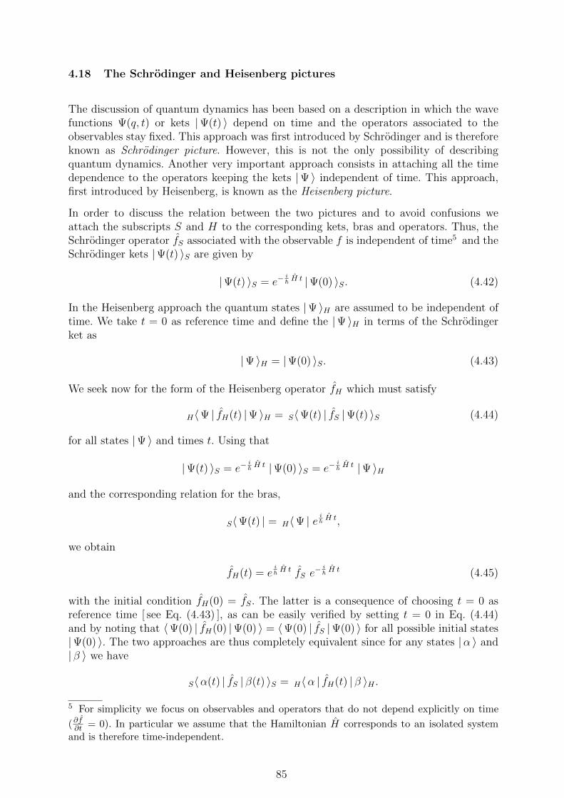
4.18 The Schrodinger and Heisenberg pictures

The discussion of quantum dynamics has been based on a description in which the wavefunctions Ψ(q, t) or kets |Ψ(t) 〉 depend on time and the operators associated to theobservables stay fixed. This approach was first introduced by Schrodinger and is thereforeknown as Schrodinger picture. However, this is not the only possibility of describingquantum dynamics. Another very important approach consists in attaching all the timedependence to the operators keeping the kets |Ψ 〉 independent of time. This approach,first introduced by Heisenberg, is known as the Heisenberg picture.

In order to discuss the relation between the two pictures and to avoid confusions weattach the subscripts S and H to the corresponding kets, bras and operators. Thus, theSchrodinger operator fS associated with the observable f is independent of time5 and theSchrodinger kets |Ψ(t) 〉S are given by

|Ψ(t) 〉S = e−i~ H t |Ψ(0) 〉S. (4.42)

In the Heisenberg approach the quantum states |Ψ 〉H are assumed to be independent oftime. We take t = 0 as reference time and define the |Ψ 〉H in terms of the Schrodingerket as

|Ψ 〉H = |Ψ(0) 〉S. (4.43)

We seek now for the form of the Heisenberg operator fH which must satisfy

H〈Ψ | fH(t) |Ψ 〉H = S〈Ψ(t) | fS |Ψ(t) 〉S (4.44)

for all states |Ψ 〉 and times t. Using that

|Ψ(t) 〉S = e−i~ H t |Ψ(0) 〉S = e−

i~ H t |Ψ 〉H

and the corresponding relation for the bras,

S〈Ψ(t) | = H〈Ψ | e i~ H t,

we obtain

fH(t) = ei~ H t fS e−

i~ H t (4.45)

with the initial condition fH(0) = fS. The latter is a consequence of choosing t = 0 asreference time [ see Eq. (4.43) ], as can be easily verified by setting t = 0 in Eq. (4.44)and by noting that 〈Ψ(0) | fH(0) |Ψ(0) 〉 = 〈Ψ(0) | fS |Ψ(0) 〉 for all possible initial states|Ψ(0) 〉. The two approaches are thus completely equivalent since for any states |α 〉 and| β 〉 we have

S〈α(t) | fS | β(t) 〉S = H〈α | fH(t) | β 〉H .5 For simplicity we focus on observables and operators that do not depend explicitly on time

(∂f∂t = 0). In particular we assume that the Hamiltonian H corresponds to an isolated systemand is therefore time-independent.

85

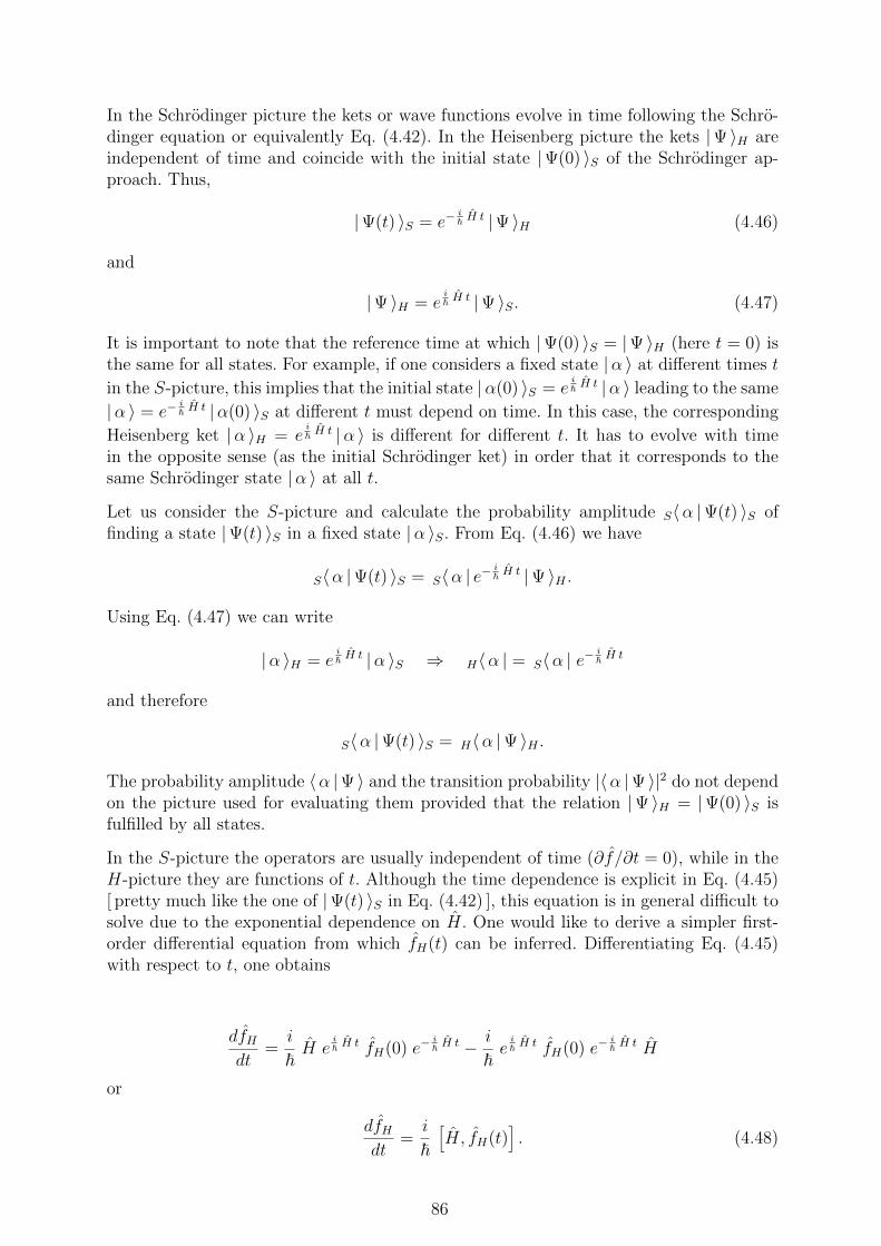
In the Schrodinger picture the kets or wave functions evolve in time following the Schro-dinger equation or equivalently Eq. (4.42). In the Heisenberg picture the kets |Ψ 〉H areindependent of time and coincide with the initial state |Ψ(0) 〉S of the Schrodinger ap-proach. Thus,

|Ψ(t) 〉S = e−i~ H t |Ψ 〉H (4.46)

and

|Ψ 〉H = ei~ H t |Ψ 〉S. (4.47)

It is important to note that the reference time at which |Ψ(0) 〉S = |Ψ 〉H (here t = 0) isthe same for all states. For example, if one considers a fixed state |α 〉 at different times t

in the S-picture, this implies that the initial state |α(0) 〉S = ei~ H t |α 〉 leading to the same

|α 〉 = e−i~ H t |α(0) 〉S at different t must depend on time. In this case, the corresponding

Heisenberg ket |α 〉H = ei~ H t |α 〉 is different for different t. It has to evolve with time

in the opposite sense (as the initial Schrodinger ket) in order that it corresponds to thesame Schrodinger state |α 〉 at all t.Let us consider the S-picture and calculate the probability amplitude S〈α |Ψ(t) 〉S offinding a state |Ψ(t) 〉S in a fixed state |α 〉S. From Eq. (4.46) we have

S〈α |Ψ(t) 〉S = S〈α | e− i~ H t |Ψ 〉H .

Using Eq. (4.47) we can write

|α 〉H = ei~ H t |α 〉S ⇒ H〈α | = S〈α | e− i

~ H t

and therefore

S〈α |Ψ(t) 〉S = H〈α |Ψ 〉H .

The probability amplitude 〈α |Ψ 〉 and the transition probability |〈α |Ψ 〉|2 do not dependon the picture used for evaluating them provided that the relation |Ψ 〉H = |Ψ(0) 〉S isfulfilled by all states.

In the S-picture the operators are usually independent of time (∂f/∂t = 0), while in theH-picture they are functions of t. Although the time dependence is explicit in Eq. (4.45)[ pretty much like the one of |Ψ(t) 〉S in Eq. (4.42) ], this equation is in general difficult tosolve due to the exponential dependence on H. One would like to derive a simpler first-order differential equation from which fH(t) can be inferred. Differentiating Eq. (4.45)with respect to t, one obtains

dfHdt

=i

~H e

i~ H t fH(0) e

− i~ H t − i

~e

i~ H t fH(0) e

− i~ H t H

or

dfHdt

=i

~[H, fH(t)

]. (4.48)

86

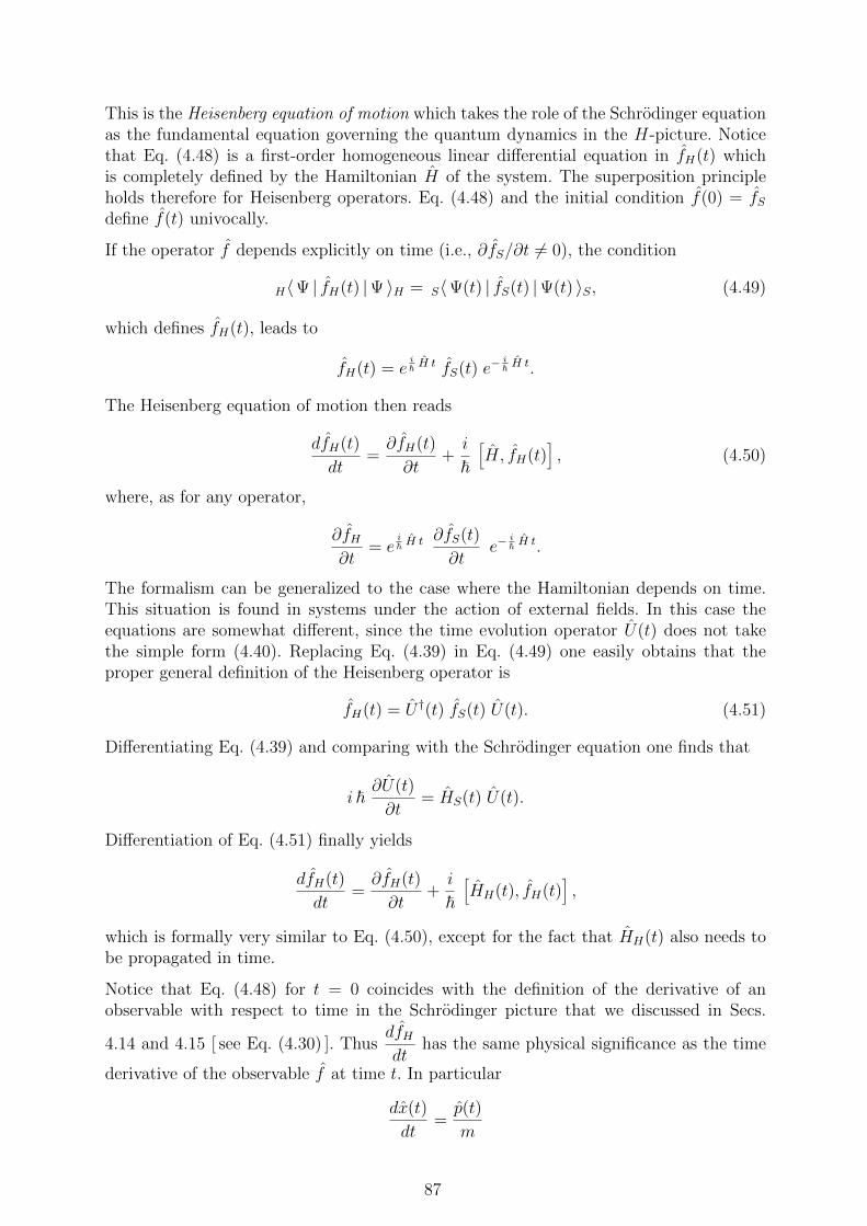
This is the Heisenberg equation of motion which takes the role of the Schrodinger equationas the fundamental equation governing the quantum dynamics in the H-picture. Noticethat Eq. (4.48) is a first-order homogeneous linear differential equation in fH(t) whichis completely defined by the Hamiltonian H of the system. The superposition principleholds therefore for Heisenberg operators. Eq. (4.48) and the initial condition f(0) = fSdefine f(t) univocally.

If the operator f depends explicitly on time (i.e., ∂fS/∂t 6= 0), the condition

H〈Ψ | fH(t) |Ψ 〉H = S〈Ψ(t) | fS(t) |Ψ(t) 〉S, (4.49)

which defines fH(t), leads to

fH(t) = ei~ H t fS(t) e

− i~ H t.

The Heisenberg equation of motion then reads

dfH(t)

dt=

∂fH(t)

∂t+

i

~[H, fH(t)

], (4.50)

where, as for any operator,

∂fH∂t

= ei~ H t ∂fS(t)

∂te−

i~ H t.

The formalism can be generalized to the case where the Hamiltonian depends on time.This situation is found in systems under the action of external fields. In this case theequations are somewhat different, since the time evolution operator U(t) does not takethe simple form (4.40). Replacing Eq. (4.39) in Eq. (4.49) one easily obtains that theproper general definition of the Heisenberg operator is

fH(t) = U †(t) fS(t) U(t). (4.51)

Differentiating Eq. (4.39) and comparing with the Schrodinger equation one finds that

i ~∂U(t)

∂t= HS(t) U(t).

Differentiation of Eq. (4.51) finally yields

dfH(t)

dt=

∂fH(t)

∂t+

i

~[HH(t), fH(t)

],

which is formally very similar to Eq. (4.50), except for the fact that HH(t) also needs tobe propagated in time.

Notice that Eq. (4.48) for t = 0 coincides with the definition of the derivative of anobservable with respect to time in the Schrodinger picture that we discussed in Secs.

4.14 and 4.15 [ see Eq. (4.30) ]. ThusdfHdt

has the same physical significance as the time

derivative of the observable f at time t. In particular

dx(t)

dt=

p(t)

m

87

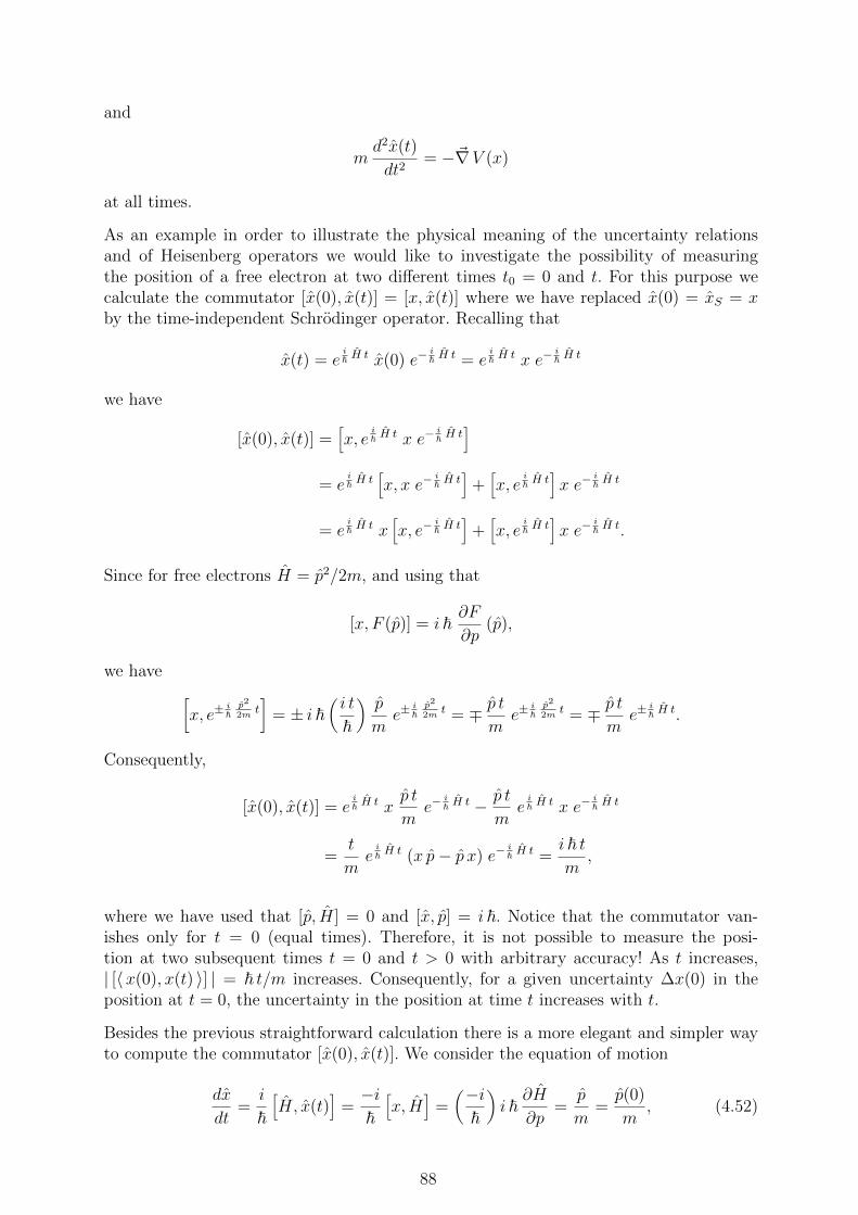
and

md2x(t)

dt2= −~∇V (x)

at all times.

As an example in order to illustrate the physical meaning of the uncertainty relationsand of Heisenberg operators we would like to investigate the possibility of measuringthe position of a free electron at two different times t0 = 0 and t. For this purpose wecalculate the commutator [x(0), x(t)] = [x, x(t)] where we have replaced x(0) = xS = xby the time-independent Schrodinger operator. Recalling that

x(t) = ei~ H t x(0) e−

i~ H t = e

i~ H t x e−

i~ H t

we have

[x(0), x(t)] =[x, e

i~ H t x e−

i~ H t

]

= ei~ H t

[x, x e−

i~ H t

]+

[x, e

i~ H t

]x e−

i~ H t

= ei~ H t x

[x, e−

i~ H t

]+

[x, e

i~ H t

]x e−

i~ H t.

Since for free electrons H = p2/2m, and using that

[x, F (p)] = i ~∂F

∂p(p),

we have

[x, e±

i~

p2

2mt]= ± i ~

(i t

~

)p

me±

i~

p2

2mt = ∓ p t

me±

i~

p2

2mt = ∓ p t

me±

i~ H t.

Consequently,

[x(0), x(t)] = ei~ H t x

p t

me−

i~ H t − p t

me

i~ H t x e−

i~ H t

=t

me

i~ H t (x p− p x) e−

i~ H t =

i ~ tm

,

where we have used that [p, H] = 0 and [x, p] = i ~. Notice that the commutator van-ishes only for t = 0 (equal times). Therefore, it is not possible to measure the posi-tion at two subsequent times t = 0 and t > 0 with arbitrary accuracy! As t increases,| [〈x(0), x(t) 〉] | = ~ t/m increases. Consequently, for a given uncertainty ∆x(0) in theposition at t = 0, the uncertainty in the position at time t increases with t.

Besides the previous straightforward calculation there is a more elegant and simpler wayto compute the commutator [x(0), x(t)]. We consider the equation of motion

dx

dt=

i

~[H, x(t)

]=

−i

~[x, H

]=

(−i

~

)i ~

∂H

∂p=

p

m=

p(0)

m, (4.52)

88

where we have used that

[x, F (p)] = i ~∂F

∂p

and that [p, H] = 0 for free particles, which implies that p(t) = p(0) is independent of t.

Eq. (4.52) fordx

dtcan be integrated straightforwardly to give

x(t) = x(0) +p(0)

mt.

Consequently,

[x(0), x(t)] =t

m[x, p] =

i ~ tm

. (4.53)

In order to analyze the physical meaning of Eq. (4.53) we consider the uncertainty in-equality

〈 (∆A)2 〉 〈 (∆B)2 〉 ≥ 1

4

∣∣∣∣[A, B

] ∣∣∣∣2

,

where ∆A = A − 〈 A 〉 and ∆B = B − 〈 B 〉. Applying this relation to the dispersion oruncertainty 〈 (∆x)2 〉t = 〈 [ x(t) − 〈 x(t) 〉 ]2 〉 of the position at time t and 〈 (∆x)2 〉0 =〈 [ x(0)− 〈 x(0) 〉 ]2 〉 at time t = 0, one obtains

√〈 (∆x)2 〉t

√〈 (∆x)2 〉0 ≥ ~ t

2m

for t ≥ 0. As physically expected, the product of uncertainties increases with t and

vanishes only for t = 0. For any given t > 0 (whatever small)√〈 (∆x)2 〉t diverges as the

measurement of the position at t = 0 becomes arbitrarily sharp[〈 (∆x)2 〉0 → 0

].

The Heisenberg formulation allows us to characterize conserved quantities in a very simpleand transparent way. In the H-picture a quantity is conserved if the time derivative ofthe corresponding operator vanishes. From Eq. (4.50) we conclude that this is the casewhen the operator does not depend explicitly on time (i.e., ∂fS/∂t = 0) and [H, fH ] = 0.

This is equivalent to ∂fS/∂t = 0 and [H, fS] = 0, since [H, ei~ H t] = 0. The condition

characterizing conserved quantities is of course the same as the one derived in previoussections within the S-picture.

4.19 The uncertainty relation for arbitrary observables

The uncertainty relation between position and momentum has been discussed in differentcontexts. The impossibility of measuring the position and momentum of a particle at thesame time demonstrates most clearly that quantum particles do not follow a classicaltrajectory. This fact has changed profoundly our views of the physical world and thus ledto the new concepts inherent to quantum theory. Furthermore, we have shown that twophysical observables A and B can be measured simultaneously with arbitrary accuracyin all states |Ψ 〉, if and only if the corresponding operators commute (i.e., [A, B] = 0).

89

It is the purpose of this section to quantify the relation between the commutator [A, B]and the minimum possible value of the mean square deviations of the outcomes of themeasurement of A and B in an arbitrary state |Ψ 〉.Let us recall that, given the operator A and a complete set of eigenstates

A | a 〉 = a | a 〉,the probability of measuring the value a of A in the state |Ψ 〉 is

PΨ(a) = |〈 a |Ψ 〉|2.The average value of A according to the probability distribution PΨ(a) is therefore

〈A 〉 = ∑a

aPΨ(a) = 〈Ψ | A |Ψ 〉.

The variance ∆A2 of the probability distribution PΨ(a) is given by

∆A2 =∑a

(a− 〈A 〉)2 PΨ(a) = 〈Ψ | (A− 〈A 〉)2 |Ψ 〉. (4.54)

Developing (A− 〈A 〉)2 in Eq. (4.54) we recover the usual relation

∆A2 = 〈Ψ | (A− 〈A 〉)2 |Ψ 〉 = 〈Ψ | A2 |Ψ 〉 − 〈Ψ | A |Ψ 〉2 (4.55)

known from statistics. ∆A2 gives a measure of the dispersion of the outcome of a mea-surement of A in the state |Ψ 〉. The uncertainty of the observable A in the state |Ψ 〉 isdefined as the mean square deviation

∆A =√〈Ψ | (A− 〈A 〉)2 |Ψ 〉. (4.56)

Consider for example an eigenstate | a′ 〉 of A. In this case one says that the observable Ais sharp since A | a′ 〉 = a′ | a′ 〉 implies 〈 a′ | A | a′ 〉 = a′ and ∆A2 = 〈 a′ | (A− a′)2 | a′ 〉 = 0.

In this context it is important to recall that for any two observables A and B, the prob-ability distribution of the measured values PΨ(a) = |〈 a |Ψ 〉|2 and PΨ(b) = |〈 b |Ψ 〉|2 arenot independent of each other, since they both derive from the same state |Ψ 〉. Our goalhere is to quantify this relation in terms of the uncertainties ∆A and ∆B.

Using the Schwarz inequality

|〈Ψ |ϕ 〉|2 ≤ 〈Ψ |Ψ 〉 〈ϕ |ϕ 〉,which is valid for any state vectors |Ψ 〉 and |ϕ 〉, and a few algebraic manipulations thefollowing important generalization of Heisenberg’s uncertainty principle can be shown.

For any hermitic operators A = A† and B = B† and any arbitrary state |Ψ 〉 it holds that√〈Ψ | (A− 〈A 〉)2 |Ψ 〉

√〈Ψ | (B − 〈B 〉)2 |Ψ 〉 ≥ 1

2

∣∣∣〈Ψ | [A, B] |Ψ 〉∣∣∣. (4.57)

Taking advantage of the definition of uncertainty or mean square deviation ∆A [see Eqs.(4.54)–(4.56)] we can write the inequality (4.57) in a more compact form as

∆A∆B ≥ 1

2

∣∣∣〈 [A, B] 〉∣∣∣. (4.58)

90

The average of the commutator [A, B] gives a measure of the degree of incompatibilityof a simultaneous measurement of A and B in the quantum state |Ψ 〉. In other words,|〈 [A, B] 〉| measures the minimum degree of uncertainty ∆B to be expected in a mea-surement of B if the observable A is measured at the same time with an accuracy ∆A.Moreover, the uncertainty relation (4.58) provides a means of quantifying to what extenta measurement of A alters the outcome of a measurement of B. In fact we see that unless[A, B] = 0, the more accurate the measurement of A is (∆A → 0), the more unpredictablethe outcome of a measurement of B becomes (∆B → ∞).

For incompatible observables ([A, B] 6= 0) having an unbounded eigenvalue spectrum (e.g.,x and p) one usually finds ∆B → ∞ when ∆A → 0 since for most states |Ψ 〉 the average〈Ψ | [A, B] |Ψ 〉 6= 0. This is of course always the case when [A, B] is a constant like for xand p. However, for operators with bounded eigenvalues (e.g., the components Lx, Ly and

Lz of the angular momentum ~L), the uncertainty or mean square deviation cannot diverge.Thus, ∆B remains finite even if ∆A = 0. This is possible because 〈Ψ | [A, B] |Ψ 〉 = 0when |Ψ 〉 is an eigenstate of A. For example, for the angular momentum operators we

have [Lx, Ly] = i ~ Lz ⇒ ∆L2x ∆L2

y ≥~2

4|〈Lz 〉|2. If we consider an eigenstate of Lx, i.e.,

Lx |Ψ 〉 = lx |Ψ 〉, we have ∆Lx = 0 and ∆Ly finite, since 〈Ψ | Lz |Ψ 〉 = 0 when |Ψ 〉 is

an eigenstate of Lx or Ly.

A few examples are worth mentioning in order to assess the implications of the uncertaintyrelation. In the case of compatible observables (i.e., [A, B] = 0) the lower bound is zeroand there is no limitation for measuring A and B with arbitrary accuracy at the sametime. The states satisfying ∆A = 0 and ∆B = 0 are the simultaneous eigenstates of Aand B. Of course nothing precludes considering states |Ψ 〉 where either A, B or bothare not sharp (i.e., ∆A > 0 and ∆B > 0). We can apply Eqs. (4.57) and (4.58) to thefundamental commutation relation

[x, p] = i ~

in order to obtain

∆x∆p ≥ ~2, (4.59)

which physical consequences have already been discussed in length.

Motivated by the inequality (4.59), we may investigate the mathematical conditions forhaving optimal-uncertainty kets |Ψ 〉, such that the equality sign in (4.58) holds, anddetermine the corresponding wave functions Ψ(x) = 〈x |Ψ 〉. One can show that

∆A∆B =1

2〈 [A, B] 〉

when ∆A |Ψ 〉 and ∆B |Ψ 〉 are collinear, i.e.,

∆A |Ψ 〉 = λ ∆B |Ψ 〉 (4.60)

with λ ∈ C, where ∆A = A−〈A 〉 and ∆B = B−〈B 〉 are the zero-average deviation op-erators. This follows from the Schwarz inequality in which the equal sign holds only whenthe corresponding kets are a multiple of each other (|α 〉 = λ | β 〉). A further condition

91

needs to be imposed to |Ψ 〉, namely

〈Ψ | ∆A, ∆B |Ψ 〉 = 〈Ψ | (∆A ∆B + ∆B ∆A) |Ψ 〉 = 0.

Using Eq. (4.60) one can show that this implies that λ must be purely imaginary (λ∗ =−λ).

To illustrate these optimal-uncertainty kets let us consider x and p. The condition (4.60)reads

xΨ(x) = λ

[−i ~

∂

∂xΨ(x)

], (4.61)

where we have assumed for simplicity 〈Ψ | xΨ 〉 = 0 and 〈Ψ | p |Ψ 〉 = 0. Note that 〈x 〉can be shifted at will by redefining the origin of the coordinates. Moreover, the averagemomentum can be shifted by considering Ψ′(x) = Ψ(x) e

i~ p′ x since

p(Ψ(x) ei

p′~ x

)= ei

p′~ x p Ψ(x) + p′ ei

p′~ x Ψ(x) ⇒ 〈Ψ′ | p |Ψ′ 〉 = 〈Ψ | p |Ψ 〉+ p′.

Eq. (4.61) can be written as

i

λ ~x dx =

dΨ

Ψ

and integrated to give

i

2λ ~x2 = lnΨ + c ⇒ Ψ(x) = a e

i2λ ~ x2

= a e−x2

2 ~ |λ| ,

where in the last step we have set λ = −i |λ| in order that Ψ(x) is normalizable (i/λ < 0).This shows that the Gaussians are the optimal wave packets in the sense that they corre-spond to the best possible compromise between uncertainty in position and momentum.

This example should also help to emphasize that1

2|〈 [A, B] 〉| should always be regarded

as a lower bound of ∆A∆B and that only very special kets actually show this lowestvalue for a given pair of observables. Furthermore, we can also use |〈 [A, B] 〉| as a lessrigorous order-of-magnitude estimate of ∆A∆B, since the lower bound can be attained.

A particularly interesting case of the uncertainty relation is found when one of the ob-servables is the energy, i.e., B = H and ∆B = ∆E. In this case we have

∆A∆E ≥ |〈 [H, A] 〉|2

=~2

∣∣∣∣∣

⟨d A

dt

⟩∣∣∣∣∣ =~2

∣∣∣∣∣d〈A 〉dt

∣∣∣∣∣, (4.62)

sincedA

dt=

i

~[H, A]. This implies that conserved quantities can be measured with arbi-

trary accuracy at the same time as the energy (∆E∆A ≥ 0 for dA/dt = 0). In the caseof non-conserved quantities, Eq. (4.62) allows us to estimate the time ∆t after which thequantity A (more precisely, the probability distribution for A) has changed significantlyin the given state |Ψ 〉. As we shall see in the following section, this characteristic timeis essentially independent of the particular property considered and simply given by theuncertainty in the energy ∆E of the state |Ψ 〉.

92

4.20 The energy-time uncertainty relation

We consider a state |Ψ 〉 at t = 0 and an observable A and would like to estimate the time∆t required for the ket |Ψ 〉 to change significantly from the perspective of this observable.At time t the quantity A has a given probability distribution PΨ(a) = |〈 a |Ψ 〉|2 with anaverage 〈A 〉 and an uncertainty or mean-square deviation ∆A. The time ∆t required forobserving a significant change in the probability distribution PΨ(a) can be estimated byrequiring that after this time the change in the average of 〈A 〉 should be comparablewith the width ∆A of the original probability distribution PΨ(a). Mathematically this isexpressed by the condition

|∆〈A 〉| =∣∣∣∣∣d 〈A 〉dt

∣∣∣∣∣∆t ' ∆A.

Using the uncertainty relation

∆E∆A ≥ ~2

∣∣∣∣∣d〈A 〉dt

∣∣∣∣∣

we obtain

∆E∆t ≥ ~2. (4.63)

This inequality is usually referred to as the energy-time uncertainty relation. It should behowever noted that the inequality (4.63) is conceptually very different from the uncertaintyrelation (4.58) between two incompatible observables. In the latter case we compare theuncertainty of two quantities that are measured simultaneously in a given state |Ψ 〉. Incontrast in the relation (4.63) we compare the uncertainty in the energy ∆E with the time∆t after which the quantum state |Ψ 〉 changes significantly. Only the energy is a physicalmagnitude, the time being simply a parameter in quantum mechanics. In particular thereis no operator associated to time.

Physically, the energy-time uncertainty relation states that the time evolution of a stateoccurs faster when the energy of the system is known less precisely. In particular an energyeigenstate has ∆E = 0. It is therefore a stationary state and the time required for anyphysical property to change is infinite. More precisely, the probability distribution PΨ(a)for any physical property remains unchanged at all times.

Notice that the relation (4.63) is the same for all observables. Its universal validity allowsus to illustrate it in a variety of physical situations. Let us consider for example a wavepacket with a given spatial extension ∆x. The uncertainty in the momentum can beestimated by

∆p ' ~∆x

and the corresponding uncertainty in the energy is given by

∆E =dE

dp∆p =

p

m∆p = vG∆p, (4.64)

93

where vG is known as the group velocity of the wave packet. The time required for thewave packet to move a distance comparable with its spatial extension is

∆t =∆x

vG. (4.65)

Combining (4.64) and (4.65) we have

∆E ·∆t = vG ∆p · ∆x

vG= ∆p∆x ≥ ~

2.

The broader the energy uncertainty of the wave packet is, the shorter is the time ∆t forit to pass, i.e., the faster the time evolution.

As a further example let us consider a state given by the superposition of two stationarystates |Ψ1 〉 and |Ψ2 〉 with energies E1 and E2. At time t we have

|Ψ(t) 〉 = a1 e− i~ E1 t |Ψ1 〉+ a2 e

− i~ E2 t |Ψ2 〉,

where a1 and a2 are complex numbers defining the initial state |Ψ(0) 〉. A measure ofthe change in |Ψ(t) 〉 as a function of time is given by the modulus of the correlationamplitude

c(t) = 〈Ψ(0) |Ψ(t) 〉 = |a1|2 e− i~ E1 t + |a2|2 e− i

~ E2 t,

where we have used that 〈Ψ1 |Ψ2 〉 = 0. Thus,

|c(t)|2 =∣∣∣|a1|2 + |a2|2 e− i

~ ∆E t∣∣∣2,

where ∆E = E2 − E1. We see that |c(t)|2 oscillates with a period

T =2π ~∆E

.

Therefore, the characteristic time of the dynamics of the system satisfies

∆t∆E ' 2 π ~.

The energy-time uncertainty also applies to quasi-stationary states |Ψ 〉 having a finitelifetime τ . In this context τ represents the typical time required for the system to de-cay into other states, i.e., for |Ψ 〉 to change significantly. The relation (4.63) impliesthat quasi-stationary states have a finite energy width ∆E = Γ of the order of ~/τ . Inspectroscopy Γ is often referred to as the line width of the corresponding excited energylevel.

94

5 The harmonic oscillator

The harmonic oscillator is a very important problem in quantum mechanics. On the oneside it is simple enough to be solvable analytically using the fundamental concepts ofquantum theory. Therefore it constitutes a very useful example of quantum mechanicalmethodology. On the other side the harmonic oscillator appears in a number of differentphysical situations including the vibrations of the atoms in molecules and solids, as wellas the quantum theory of radiation. Understanding its properties in detail is of the utmostimportance.

The basic assumption or formulation of the problem is that the potential energy takes theform

U(x) =1

2k x2,

where k is a constant. It is important to remark that any potential can be approximatedby this form close to minimum. This actually holds in n dimensions once the coordinatesystem is taken along the normal modes. Close to an n-dimensional minimum one can

always write U =1

2

∑ni=1 ki q

2i , where qi refers to the normal coordinates. Since U is

the sum of potentials of the form U =∑n

i=1 Ui (qi), the n-dimensional problem can beseparated in n one-dimensional ones, each of them corresponding to an harmonic oscillator.In the following we will therefore focus on the 1D case.

5.1 The classical oscillator

Let us recall the main properties of the classical solution. Since U(x) =1

2k x2, the force

is given by Fx = −∂U

∂x= −k x. The equation of motion reads

mdx2

dt2= −k x. (5.1)

The restoring force is proportional to the displacement from the equilibrium positionx = 0. We can easily solve Eq. (5.1) with an exponential ansatz of the form

x(t) = ei ω t.

Substituting in Eq. (5.1) we obtain

−mω2 ei ω t = −k ei ω t,

which implies

mω2 = k. (5.2)

Taking ω =√k/m, the most general solution has the form

x(t) = Aei ω t +B e−i ω t, (5.3)

95

or equivalently

x(t) = xM cos(ω t+ ϕ),

where xM is the largest possible displacement [ | cos(ω t+ ϕ)| ≤ 1]. The velocity

v(t) =dx

dt= −xM ω sin(ω t+ ϕ)

vanishes at the turning points ±xM . The total energy

E =p2

2m+

1

2k x2

is of course conserved. Since p = mv = 0 at the turning points ±xM we have

E =1

2k x2

M

or xM =√2E/k. The classical motion is thus constrained to a finite region given by

|x| ≤ xM =√2E/k.

In order to make the dependence on the vibrational frequency apparent it is customaryto replace k by using Eq. (5.2) and to write the Hamiltonian in the form

H =p2

2m+

mω2

2x2.

For the sake of future comparison it is useful to express the classical solution (5.3) interms of the initial position x(0) and momentum p(0). From (5.3) we have

x(t) = Aei ω t +B e−i ω t = (A+B) cosω t+ i (A−B) sinω t

and

p(t) = mx(t) = imω Aei ω t − imω B e−i ω t

= imω (A−B) cosω t−mω (A+B) sinω t

with x(0) = A+B and p(0) = imω (A−B). Thus we can write

p(t) = p(0) cosω t−mω x(0) sinω t (5.4)

and

x(t) = x(0) cosω t+p(0)

mωsinω t. (5.5)

5.2 The quantum oscillator

In order to solve the quantum mechanical problem we consider first the Heisenberg pictureand determine the time dependence of the operators x(t) and p(t). The equations of motion

96

are

i ~dp

dt=

[p, H

]=

[p,

mω2 x2

2

]= −i ~

∂

∂x

(mω2 x2

2

)= −i ~mω2 x

⇒ dp

dt= −mω2 x (5.6)

and

i ~dx

dt=

[x, H

]=

[x,

p2

2m

]= i ~

∂

∂p

(p2

2m

)= i ~

p

m

⇒ dx

dt=

p

m. (5.7)

Multiplying Eq. (5.7) by imω and subtracting to Eq. (5.6) we obtain

d

dt(p− imω x) = −imω

p

m−mω2 x

= −i ω (p− imω x) .

The non-hermitian operator6

a =p− imω x√

2m ~ω(5.8)

satisfies the simple equation

da

dt+ i ω a = 0.

This implies

a(t) = a(0) e−i ω t,

where a(0) =p(0)− imω x(0)√

2m ~ωrefers to the Schrodinger operator. Let us recall that at

t = 0 the operators for the H- and S-pictures are identical. Introducing the hermiticconjugate operator

a† =p+ imω x√

2m ~ω, (5.9)

which time dependence is given by a†(t) = a†(0) ei ω t, we can solve for p and x as

p(t) =

(m ~ω2

)1/2 [a(t) + a†(t)

](5.10)

= p(0) cosω t−mω x(0) sinω t

6 At this point the normalizing factor (2m ~ω)−1/2 is not relevant. However, it will provevery useful later on in order to simplify the commutation rules for a and a†. Note that a isdimensionless and that mω x has the units of momentum.

97

and

x(t) = i

(~

2mω

)1/2 [a(t)− a†(t)

](5.11)

= x(0) cosω t+p(0)

mωsinω t. (5.12)

These equations are formally the same as the classical solution (5.4) and (5.5). In partic-ular the average values of the position and momentum follow the classical trajectory aspredicted by the Ehrenfest theorem.

From Eq. (5.12) it is interesting to calculate the commutator

[x(0), x(t)] =sinω t

mω[x(0), p(0)] =

i ~mω

sinω t

between the position operator at times t = 0 and t. This shows that the observables x(t)and x(0) are incompatible except at the same time t = 0 and at integer multiples of thehalf period T/2 = π/ω. The uncertainty relation implies

∆x(0)∆x(t) ≥ ~2mω

| sinω t|

and in the limit of short times t ¿ 1/ω

∆x(0)∆x(t) ≥ ~2m

t.

For small t, ∆x(0)∆x(t) increases as expected with increasing t. Moreover, for all finitet 6= 2 π n/ω with n ∈ N, ∆x(t) → +∞ for ∆x(0) → 0. Notice that for short times thedetails of the potential play no role since [x(0), x(t)] is independent of ω for ω t ¿ 1.

Since a(t) and a†(t) have a simple oscillatory time dependence, it is interesting to expressH in terms of them by replacing p and x using Eqs. (5.10) and (5.11). From Eq. (5.10)we have

p2

2m=

1

2m

m ~ω2

(a2 + a† 2 + a a† + a† a

)

and from Eq. (5.11)

mω2

2x2 =

mω2

2

(− ~2mω

) (a2 + a† 2 − a a† − a† a

).

Summing the kinetic and potential energy contributions we obtain

H =~ω2

(a a† + a† a

). (5.13)

Notice that, since H is hermitic and time-independent, we could have already expectedthat a and a† appear in bilinear expressions of the form a a† + a† a.

98

In order to determine the eigenenergies of H it is useful to compute the commutator

[a, a†

]=

1

2m ~ω[p− imω x, p+ imω x]

=1

2m ~ω[imω (−i ~)− imω (i ~)]

=1

2m ~ω2mω ~ = 1.

The commutation rule

[a, a†

]= 1 (5.14)

is of central importance to the problem. Using it we can write H in the form

H = ~ω(a† a+

1

2

).

The hermitian operator

n = a† a

is positive definite since for all |Ψ 〉

〈Ψ | a† a |Ψ 〉 = 〈 aΨ | aΨ 〉 ≥ 0. (5.15)

Therefore the eigenenergies have ~ω/2 as a lower bound. The presence of a finite (non-zero) lower bound for the ground state energy, that is proportional to ~, is clearly a con-sequence of Heisenberg’s uncertainty principle. The phenomenon is sometimes referred toas the zero point motion of the oscillator.

The stationary states are clearly the eigenstates of n. Let |n 〉 denote the normalizedeigenstate with eigenvalue n:

n |n 〉 = n |n 〉 with 〈n |m 〉 = δnm.

Notice that Eq. (5.15) implies that n ≥ 0. In other words, the eigenvalues n have zero asa lower bound. In terms of |n 〉 we have

H |n 〉 = En |n 〉 with En =(n+

1

2

)~ω.

It is easy to see that a |n 〉 is either zero or an eigenstate of n with eigenvalue n − 1. Toshow this we calculate the effect of n on the state a |n 〉:

n a |n 〉 = a† a a |n 〉 = (a a† − 1) a |n 〉 = a a† a |n 〉 − a |n 〉= (n− 1) a |n 〉.

Thus a |n 〉 is either zero or it is proportional to an eigenstate |n′ 〉 of n which eigenvalueis reduced by one (n′ = n− 1). Let us compute the square norm of this state:

〈 a n | a n 〉 = 〈n | a† a |n 〉 = n ≥ 0.

99

This implies that n must be a positive integer or zero, since for any non-integer value of none would obtain an eigenstate of n with a negative eigenvalue by successive applicationof a. Notice that 〈 a n | a n 〉 vanishes only for n = 0. Thus we must have that for all n > 0,a positive integer exists such that n− k = 0. Otherwise we would violate the lower boundexisting on the eigenvalues of n.

Moreover, it is easy to see that all non-negative integers are actually eigenvalues of n,since for any |n 〉 (n |n 〉 = n |n 〉), a† |n 〉 is also an eigenstate of n with eigenvalue n+1:

n a† |n 〉 = a† a a† |n 〉 = a† (a† a+ 1) |n 〉 = (n+ 1) a† |n 〉.

The square norm of a† |n 〉 is given by

〈 a† n | a† n 〉 = 〈n | a a† |n 〉 = 〈n | (1 + n) |n 〉 = n+ 1.

Finally, choosing the relative phases between |n 〉, a |n 〉 and a† |n 〉 to be zero, we have

a |n 〉 = √n |n− 1 〉

and

a† |n 〉 = √n+ 1 |n+ 1 〉.

The eigenenergies are then given by

En =(n+

1

2

)~ω

with n a non-negative integer. The operator a† (a) increases (decreases) the level of exci-tation by one and is therefore known as the creation (annihilation) operator. The operatorn = a† a counts the level of excitation and is therefore known as the number operator.Starting from an eigenstate of n, applying a causes a quantum of energy ~ω to disappear(En−1 = En − ~ω), while a† adds a quantum of energy to the system (En+1 = En + ~ω).

5.3 Some properties of the stationary kets

Before we determine the wave functions 〈x |n 〉 = Ψn(x) of the harmonic oscillator it isinteresting to derive some average properties of the stationary eigenkets |n 〉 in the so-called occupation number representation. For this purpose we use the commutation rulesfor the creation, annihilation and number operators and the properties of |n 〉. Startingfrom

x = i

(~

2mω

)1/2

(a− a†)

and

p =

(m ~ω2

)1/2

(a+ a†)

we have 〈n | x |n 〉 = 0 and 〈n | p |n 〉 = 0, since both a and a† change the occupationnumber n by one and since 〈n |m 〉 = δnm. The average position and momentum of all

100

stationary states is zero. This is consistent with the fact that the eigenfunctions of aneven potential have defined parity (even or odd).

In order to compute the uncertainty in position and momentum we calculate

〈n | p2 |n 〉 =(m ~ω2

)〈n | (a+ a†)2 |n 〉

=

(m ~ω2

)〈n | (a2 + a a† + a† a+ a† 2) |n 〉

=

(m ~ω2

)〈n | (1 + 2 a† a) |n 〉 = m ~ω

(n+

1

2

)= mEn

and

〈n | x2 |n 〉 = −(

~2mω

)〈n | (a− a†)2 |n 〉

=~

2mω〈n | a a† + a† a |n 〉 = ~

mω

(n+

1

2

)=

En

mω2.

As expected, both 〈 x2 〉 and 〈 p2 〉 increase with increasing excitation level. For the uncer-tainty product one obtains

∆x∆p =(n+

1

2

)~.

Thus the ground state corresponds to the lowest possible value allowed by the uncertaintyrelation (4.58). From our previous discussion of uncertainty-optimal wave functions in 1Dwe may already conclude that the ground-state wave function 〈x | 0 〉 is a Gaussian.

5.4 The eigenfunctions

In order to determine the wave functions Ψn(x) = 〈x |n 〉 we start with the condition

defining the ground state | 0 〉, namely, a | 0 〉 = 0. Using that a =p− imω x√

2m ~ωwe can

write

〈x | (p− imω x) | 0 〉 = 0

or equivalently

−i ~∂

∂x〈x | 0 〉 − imω x 〈x | 0 〉 = 0, (5.16)

where we have used that 〈x | p |α 〉 = −i ~∂

∂x〈x |α 〉 for any ket |α 〉. Let us recall

that 〈x | p |α 〉 represents the wave function obtained by applying the operator p to thestate |α 〉. In wave-function language (position representation) 〈x | p α 〉 corresponds to

pΨα(x) = −i ~∂Ψα(x)

∂x= −i ~

∂ 〈x |α 〉∂x

, since by definition Ψα(x) = 〈x |α 〉.

101

Once the connection between the stationary kets |n 〉 and the wave function Ψn(x) hasbeen established it is helpful to change to the more familiar notation

Ψn(x) = 〈x |n 〉.

The equation (5.16) defining the ground-state wave function then reads

∂

∂xΨ0(x) +

mω

~x Ψ0(x) = 0. (5.17)

At this point it is useful to introduce the characteristic length

λ =

(~

mω

)1/2

of the quantum oscillator. Physically, λ represents the distance at which the potentialenergy equals the ground-state energy ~ω/2 or, in other words, the return point of aclassical oscillator with energy E = ~ω/2 (i.e., mω2 λ2/2 = ~ω/2). From Eq. (5.17) weobtain

dΨ0 = − x

λ2Ψ0 dx

1

Ψ0

dΨ0 = − x

λ2dx

lnΨ0 = − x2

2λ2+ c

Ψ0(x) = A e−x2

2λ2 ,

where c and A = ec are constants. The normalization condition implies

Ψ0(x) =(

1

π λ2

)1/4e−

x2

2λ2 =(mω

π ~

)1/4e−

x2

2λ2 .

The wave function of the excited states can be generated by applying the creation operator:

a† | 0 〉 = | 1 〉

(a†)2 | 0 〉 = a† | 1 〉 =√2 | 2 〉

(a†)3 | 0 〉 =√2 a† | 2 〉 =

√6 | 3 〉

(a†)n | 0 〉 =√(n− 1)! a† |n− 1 〉 =

√n! |n 〉.

Consequently,

|n 〉 = 1√n!

(a†)n | 0 〉,

Ψn(x) =1√n!

〈x | (a†)n | 0 〉 = 1√n!

⟨x

∣∣∣∣(p+ imω x)√

2m ~ω

∣∣∣∣ 0⟩

102

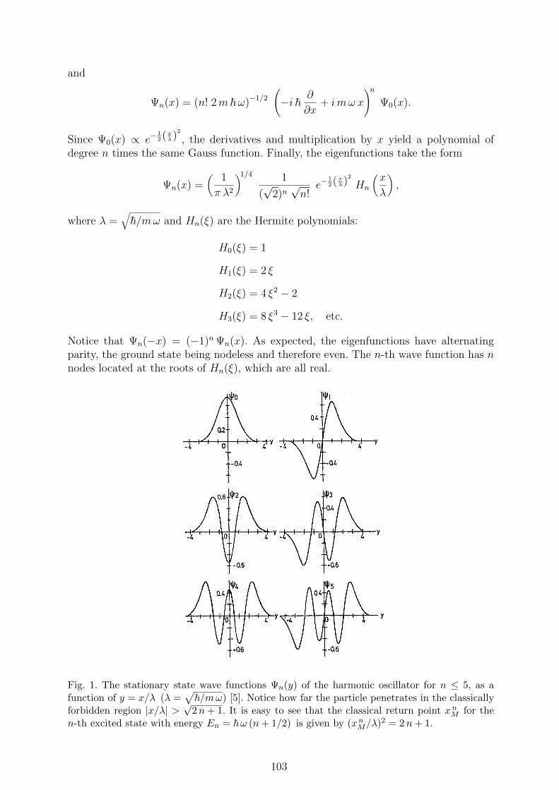
and

Ψn(x) = (n! 2m ~ω)−1/2

(−i ~

∂

∂x+ imω x

)n

Ψ0(x).

Since Ψ0(x) ∝ e−12(

xλ)

2

, the derivatives and multiplication by x yield a polynomial ofdegree n times the same Gauss function. Finally, the eigenfunctions take the form

Ψn(x) =(

1

π λ2

)1/4 1

(√2)n

√n!

e−12(

xλ)

2

Hn

(x

λ

),

where λ =√~/mω and Hn(ξ) are the Hermite polynomials:

H0(ξ) = 1

H1(ξ) = 2 ξ

H2(ξ) = 4 ξ2 − 2

H3(ξ) = 8 ξ3 − 12 ξ, etc.

Notice that Ψn(−x) = (−1)n Ψn(x). As expected, the eigenfunctions have alternatingparity, the ground state being nodeless and therefore even. The n-th wave function has nnodes located at the roots of Hn(ξ), which are all real.

Fig. 1. The stationary state wave functions Ψn(y) of the harmonic oscillator for n ≤ 5, as afunction of y = x/λ (λ =

√~/mω) [5]. Notice how far the particle penetrates in the classically

forbidden region |x/λ| > √2n+ 1. It is easy to see that the classical return point xn

M for then-th excited state with energy En = ~ω (n+ 1/2) is given by (xn

M/λ)2 = 2n+ 1.

103

6 Angular momentum

In the absence of external fields or external potential V (x) the space is homogeneous and

the linear momentum p = −i ~ ~∇ is a conserved quantity. The correlation between homo-geneity of space (i.e., all points in space are equivalent or ∂H/∂x = ∂H/∂y = ∂H/∂z = 0)

and momentum conservation is well known from classical mechanics (~p = −~∇H). In addi-tion we know that in the absence of external fields the space is also isotropic, i.e., invariantwith respect to rotations. This implies that all directions in space are equivalent, and wehave actually used this fact in order to infer that the free-particle Hamiltonian H ∝ p2. Inclassical mechanics the isotropy of space implies the conservation of angular momentum,which is an important observable even in the presence of an external field, particularlywhen it is centrally symmetric. The purpose of this chapter is to introduce the conceptof angular momentum in quantum mechanics and to investigate its most fundamentalproperties such as its eigenvalues and eigenfunctions.

6.1 Definition and commutation rules

Following the correspondence principle the angular momentum operator ~l is defined as inclassical mechanics by the vector relation

~ ~l = ~r × ~p, (6.1)

where ~r = (x, y, z) = (x1, x2, x3) and ~p = −i ~ ~∇. The factor ~ is introduced in order to

simplify the equations. Thus, ~l is measured in units of ~ and is therefore dimensionless.For the individual components we have

~ lx = y pz − z py, (6.2)

~ ly = z px − x pz, (6.3)

~ lz = x py − y px. (6.4)

Notice that a cyclic permutation of the coordinates (i.e., x → y, y → z and z → x) allowsone to obtain (6.3) from (6.2), (6.4) from (6.3) and (6.2) from (6.4). This symmetry will beused to avoid repeating calculations which results can be inferred by cyclic permutations.Moreover, one observes that the order of xi and pj in Eqs. (6.2)–(6.4) is irrelevant, sincethe same components are never multiplied together and [xi, pj] = 0 for i 6= j.

The fundamental commutation rule between the components of~l can be calculated straight-forwardly:

~[lx, ly

]= [y pz − z py, z px − x pz]

= [y pz, z px] + [z py, x pz]

= y [pz, z] px + x [z, pz] py

= −i ~ y px + i ~ x py

= i ~ lz.

104

Thus,

[lx, ly

]= i lz.

Cyclic permutation of the variables implies

[lm, lj

]= i lk, (6.5)

where (m, j, k) is a cyclic permutation of (1, 2, 3). This is often written in the compactform

[lm, lj

]= i εmjk lk with m, j, k = 1–3, (6.6)

where εmjk is the Levy-Civita symbol (or antisymmetric unit tensor of rank 3) satisfyingεmjk = 1 for (m, j, k) a cyclic permutation of (1, 2, 3), εmjk = −1 for (m, j, k) a cyclicpermutation of (2, 1, 3) and εmjk = 0 in all other cases, i.e., when two indices are equal.

In Eq. (6.6) a sum over repeated indices is implied(∑3

k=1

)in which only one term is

non-vanishing.

Eq. (6.6) is the fundamental angular momentum commutation rule. Notice that thedifferent components do not commute with each other. Therefore, any pair of themcannot have definite values simultaneously, except when all the components are zero(∆lx∆ly ≥ |〈 [lx, ly] 〉|/2 = |〈 lz 〉|/2). The angular momentum (a pseudovector) is in thisrespect fundamentally different from other vectors like position ~r or linear momentum ~p,which components can all be measured simultaneously with arbitrary accuracy.

The commutation rules between ~l, ~r and ~p can be easily found. It is straightforward toshow that

[lx, x

]=

[ly, y

]=

[lz, z

]= 0

and

[lx, y

]=

1

~[y pz − z py, y] =

−z

~[py, y] = i z.

Cyclic permutation implies

[lm, xj

]= i εmjk xk. (6.7)

Analogously for the linear momentum we have

[lx, px

]=

[ly, py

]=

[lz, pz

]= 0

and

[lx, py

]=

1

~[y pz − z py, py] =

1

~[y, py] pz = i pz,

which can be written in a more compact form as

[lm, pj

]= i εmjk pk. (6.8)

105

A set of three operators ~v = (v1, v2, v3) satisfying the commutation rule [lm, vj] = i εmjk vk(like ~p and ~r) are known as vector operators. Their components transform like usual vectorsunder rotations.7

With the components of ~l we can construct, as for any vector, the operator of the square

modulus of ~l given by

l 2 = l 2x + l 2y + l 2z .

It is easy to see that l 2 commutes with all the components of ~l:

[l 2, lx

]=

[l 2y , lx

]+

[l 2z , lx

]

= ly[ly, lx

]+

[ly, lx

]ly + lz

[lz, lx

]+

[lz, lx

]lz

= −ly lz − lz ly + lz ly + ly lz = 0.

Since the same holds for ly and lz (cyclic permutation leaves l 2 unchanged), we have

[l 2, lk

]= 0 ∀ k = 1, 2, 3. (6.9)

One concludes that the square modulus l 2 and any one of the components (e.g., lz) can

have definite values at the same time, although the different components of ~l cannot havedefinite values simultaneously. Notice that Eq. (6.9) has been derived using exclusivelythe fundamental angular momentum commutation rule (6.6). Therefore, it also holds for

the intrinsic angular momentum ~S of elementary particles (e.g., the spin of the electron)which fulfills Eq. (6.6) but which can not be written in terms of position and momentumoperators, as the orbital angular momentum in Eq. (6.1).

6.2 Translations and rotations

The purpose of this section is to provide with a physical or geometrical interpretation

of the vector operators ~p and ~l of the linear and angular momentum. We would like tocalculate how a wave function Ψ(~r) changes when we translate it by an infinitesimaldisplacement δ~a. Let Ψ be the translated wave function which is given by

Ψ(~r) = Ψ(~r − δ~a) = Ψ(~r)− δ~a · ~∇Ψ(~r) +O(δa2).

Using the definition of the momentum operator ~p = −i ~ ~∇ we can write

Ψ(~r) =[1− i

~(−i ~ δ~a · ~∇)

]Ψ(~r) +O(δa2) =

(1− i

~δ~a · ~p

)Ψ(~r) +O(δa2).

7 The commutation rules (6.7) and (6.8) can be derived more elegantly by using the knownexpression (~x× ~p)k = εkmn xm pn for the components of the vector product (sum over repeatedindices is implied). Noting that ~ lk = εkmn xm pn we have ~ [lk, xj ] = εkmn [xm pn, xj ] =

εkmn xm [pn, xj ] = −i ~ εkmn xm δnj = −i ~ εkmj xm = i ~ εkjm xm and ~ [lk, pj ] =εkmn [xm pn, pj ] = εkmn pn δmj (i ~) = i ~ εkjn pn.

106

We conclude that ~p is the operator describing an infinitesimal translation of the wave func-tion. We actually say that ~p is the generator of infinitesimal translations. The translatedwave function Ψ is usually written in terms of the linear operator δU(δ~a) for infinitesimaltranslations as

Ψ(~r) = δU Ψ(~r)

with

δU(δ~a) = 1− i

~δ~a · ~p.

Notice that δU is unitary to first order in δ~a, since δU δU † = 1 + O(δa2), where we have

used that ~p = ~p † is hermitic. The fact that δU is unitary was of course expected, since atranslation (infinitesimal or finite) does not change the norm of Ψ(~r).

We say that an observable A is invariant under a given transformation, in the present casea translation, if the result of applying the operator to the translated function, A Ψ, is thesame as the translation of the function AΨ. Mathematically, invariance upon translationmeans

A Ψ = A δU Ψ = δU AΨ

for all Ψ, which is equivalent to

A δU = δU A

or

A ~p = ~p A ⇔[~p, A

]= 0. (6.10)

We conclude that the linear momentum operator commutes with translational invariantobservables and vice versa. Moreover, in the case where the Hamiltonian H is translationalinvariant

d~p

dt=

i

~[H, ~p

]= 0 (6.11)

and the linear momentum is a conserved quantity.

An alternative, maybe more explicit proof of the previous statements is obtained bycalculating the change in an operator, for example the Hamiltonian H, resulting from atranslation δ~a of the coordinates:

δH = H (~r + δ~a, ~p )− H (~r, ~p ) = δ~a · ~∇~r H =3∑

i=1

δai∂H

∂xi

=i

~

3∑

i=1

δai[pi, H

]

=i

~δ~a ·

[~p, H

], (6.12)

where we have used that

[pi, F

]= −i ~

∂F

∂xi

(6.13)

for any function F (~r) of the position operator ~r[~r = (x1, x2, x3) and ~p = (p1, p2, p3)

].

107

Let us recall that a similar relation

[xi, G

]= i ~

∂G

∂pi(6.14)

holds for the commutator of the position operator ~r = (x1, x2, x3) and any function G(~p)of the linear momentum.8

We now turn to the somewhat more complicated case of rotations. We would like tocalculate how the wave function Ψ(~r) changes when we rotate the system by a smallangle δϕ around an arbitrary axis n. We know that the change δ~r in the position vector~r is given by

δ~r = δ~ϕ× ~r,

where δ~ϕ = δϕ n. The rotated wave function Ψ is given by

Ψ(~r) = Ψ(~r − δ~r) = Ψ(~r)− δ~r · ~∇Ψ(~r) +O (δr2)

=[1− i

~(δ~ϕ× ~r) · ~p

]Ψ(~r) +O (δr2).

Using the relation (~a×~b) · ~c = ~a · (~b× ~c), which holds also for non-commuting operators,we have

Ψ(~r) =[1− i

~δ~ϕ · (~r × ~p )

]Ψ(~r) + δ (δϕ2)

=(1− i δ~ϕ ·~l

)Ψ(~r) +O (δϕ2).

We conclude that ~ ~l = ~r × ~p is the operator describing an infinitesimal rotation of the

wave function. One therefore says that ~l is the generator of infinitesimal rotations. As inthe case of translations it is useful to write

Ψ(~r) = δU Ψ(r),

where the operator of an infinitesimal rotation δU(δ~ϕ) is given by

δU(δ~ϕ) = 1− i δ~ϕ · ~l.

As in the case of translations, δU is unitary up to first order in δϕ[δU δU † = 1 +O (δϕ2)

]

since ~l = ~l † is hermitic.

The arguments used to derive Eqs. (6.10) and (6.11) apply to any symmetry transforma-

tion δU . We can therefore conclude that the orbital angular momentum ~l commutes withany rotational invariant observable. Moreover, if the Hamiltonian is rotational invariant

d~l

dt=

i

~

[H,~l

]= 0

8 The proof of Eqs. (6.13) and (6.14) is straightforward by induction once F (~r) are expanded ina Taylor series. In the case of Eq. (6.13) we have [p, xn] = x

[p, xn−1

]+ [p, x]xn−1 = −i ~x (n−

1)xn−2 − i ~xn−1 = −i ~nxn−1. The proof of Eq. (6.14) is analogous.

108

and the angular momentum is conserved.

The calculation of the change in the Hamiltonian (or any other operator) under an in-finitesimal rotation is somewhat more complicated, since a rotation implies a change in theposition δ~r = δ~ϕ×~r as well as in the momentum δ~p = δ~ϕ×~p. We consider a single-particleHamiltonian H = H(~r, ~p) given by the sum of the kinetic energy operator T (~p) = p2/2mand the potential energy V (~r).9 The change in the Hamiltonian following an infinitesimalrotation is

δH = H(~r + δ~ϕ× ~r, ~p+ δ~ϕ× ~p)− H(~r, ~p)

= (δ~ϕ× ~r) · ~∇~r H + (δ~ϕ× ~p) · ~∇~p H

= δ~ϕ · (~r × ~∇~r H) + δ~ϕ · (~p× ~∇~p H)

= δ~ϕ · (~r × ~∇~r V ) + δ~ϕ · (~p× ~∇~p T ).

Using the relations

i[~l, F (~r)

]= ~r × ~∇r F

and

i[~l, G(~p)

]= ~p× ~∇~p G

we can write

δH = i δ~ϕ ·[~l, V

]+ i δ~ϕ ·

[~l, T

]

= i δ~ϕ ·[~l, H

].

Consequently, the angular momentum operator ~l commutes with rotational invariant ob-servables. Moreover, if the Hamiltonian is invariant under rotations, the angular momen-tum is conserved. The most important and fundamental examples of rotational invariantHamiltonians are the atoms.

6.3 Angular momentum operator in spherical coordinates

Taking into account that ~l is conserved when the external potential V = V (r) is spherically

symmetric, it is important to know how to express ~l and l2 in spherical coordinates.Let us recall the usual relation between spherical coordinates (r, ϕ, θ) and the Cartesiancoordinates (x, y, z):

x = r sin θ cosϕ

y = r sin θ sinϕ (6.15)

z = r cos θ.

9 The extension to a many-particle Hamiltonian H(~r1, . . . ~rN , ~p1, . . . ~pN ) including interactionsis rather straightforward.

109

For any function Ψ(~r) we have

∂Ψ

∂ϕ=

∂Ψ

∂x

∂x

∂ϕ+

∂Ψ

∂y

∂y

∂ϕ,

since z is independent of ϕ. Using Eqs. (6.15) we have

∂Ψ

∂ϕ= −r sin θ sinϕ

∂Ψ

∂x+ r sin θ cosϕ

∂Ψ

∂y

= −y∂Ψ

∂x+ x

∂Ψ

∂y

=i

~

(y i ~

∂Ψ

∂x− x i ~

∂Ψ

∂y

)=

i

~(x py − y px)Ψ.

Recalling that ~~l = ~r × ~p, this implies

lz = −i∂

∂ϕ.

As expected the z component of the angular momentum operator represents the effect ofan infinitesimal rotation of the wave function around the z axis. It is actually analogous

to a Cartesian component of the linear momentum operator, for example, px = −i ~∂

∂x.

The eigenfunctions of lz satisfy the equation

−i∂Ψ(r, θ, ϕ)

∂ϕ= mΨ(r, θ, ϕ),

where m ∈ R denotes the eigenvalue. This can be easily integrated to yield

Ψm(r, ϕ, θ) = f(r, θ) eimϕ. (6.16)

If we focus on single-valued functions, Ψm must be periodic in ϕ with a period 2 π, whichimplies that the eigenvalues of lz must be integers m = 0,±1,±2, . . . .

For the orbital angular momentum ~~l = ~r×~p, integer values of m and single-valued wavefunctions Ψm(r, ϕ, θ) are the only possibility. However, from a more general perspectiveone could also expect m to be a half integer m = ±1/2,±3/2, . . . . To see this, one shouldrecall that the wave function Ψ cannot be directly measured in experiment. Instead, theexperimentally accessible quantity is the probability distribution given by |Ψ|2. Therefore,it is actually |Ψ|2 that always has to be single-valued, i.e., periodic in ϕ with period 2 π.Of course, applying this condition to the eigenfunctions of lz given by Eq. (6.16) gives noinformation on the possible values of m, since |eimϕ|2 = 1 for all m ∈ R. The point isthat the single-valued condition on |Ψ|2 must hold for any physical state and thereforefor any linear combination of eigenstates of lz. Let

Ψ = α eimϕ + β eim′ ϕ,

then

|Ψ|2 = |α|2 + |β|2 + αβ∗ ei (m−m′)ϕ + α∗β e−i (m−m′)ϕ

= |α|2 + |β|2 + 2 Re αβ∗ ei (m−m′)ϕ.

110

The 2 π periodicity of |Ψ|2 implies that m−m′ must be an integer. Taking m′ = −m oneconcludes that 2m must be an integer, and thus the eigenvalues of angular momentumoperators must be integer or half-integer. The physical consequences of half-integer valuesof the angular momentum, as found for instance in the case of the electron spin (S = 1/2),will be discussed later on.

6.4 Eigenvalues and eigenstates of ~l

We have shown that[lz, l

2]= 0 and therefore it is possible to find a complete basis of

simultaneous eigenstates of l 2 and lz. We denote these eigenstates by |λ,m 〉 so that

l 2 |λ,m 〉 = λ |λ,m 〉

with λ ≥ 0 and

lz |λ,m 〉 = m |λ,m 〉.

The derivation of the eigenvalues of l 2 and lz will be done on the sole basis of the com-mutation rule

[lx, lz

]= i lz

and its cyclic permutations. It is therefore valid for any type of angular momentum: orbitalor intrinsic, integer or half-integer. We have already shown that

[l 2, lz

]= 0.

Since

l 2 = l 2x + l 2y + l 2z

it is clear that

〈α | l 2 − l 2z |α 〉 = 〈α | l 2x + l 2y |α 〉 ≥ 0

for all states |α 〉. In particular for the eigenstates |λ,m 〉 we have

λ ≥ m2

or

√λ ≥ |m|.

This means that for any given eigenvalue of l 2 the eigenvalues of lz are bounded. We shalldenote by l = lmax

z the largest possible value of m for the given λ. Note that l can besmaller than

√λ.

The eigenstates having different m but the same λ of l 2 can be related to each other withthe help of the so-called ladder operators

l+ = lx + i ly

111

and

l− = lx − i ly,

in a similar way as the creation and annihilation operators relate different eigenstates ofthe number operator in the harmonic oscillator. One first notices the important commu-tation relations

[lz, l±

]=

[lz, lx

]± i

[lz, ly

]= i ly ± lx = ±l±.

This implies

lz l+ − l+ lz = l+ ⇔ lz l+ = l+(lz + 1

).

Consider now an eigenstate |λ,m 〉, then we have

lz(l+ |λ,m 〉

)= l+

(lz + 1

)|λ,m 〉 = (m+ 1) l+ |λ,m 〉.

Therefore, l+ |λ,m 〉 is either zero or it is an eigenstate of lz with the eigenvalue lz increasedby one. We can then write

l+ |λ,m 〉 = c+ |λ,m+ 1 〉,

where c+ = c+(m) is a constant (eventually equal to zero) that depends on m. Moreover,we know that the eigenvalues of lz for a given λ are bounded by the relation lz ≤ l = lmax

z ,where l ≤ λ. We must therefore have c+(l) = 0 or equivalently

l+ |λ, l 〉 = 0, (6.17)

since otherwise, by applying l+, one would obtain an eigenstate of lz with eigenvalue largerthan l.

The equation derived in the following is important in order to relate λ and l:

l− l+ = (lx − i ly) (lx + i ly)

= l 2x + l 2y + i (lx ly − ly lx)

= l 2x + l 2y − lz

= l 2 − l 2z − lz. (6.18)

Applying l− l+ to |λ, l 〉 and using Eqs. (6.17) and (6.18) we have

0 = l− l+ |λ, l 〉 =(l 2 − l 2z − lz

)|λ, l 〉 =

(λ− l2 − l

)|λ, l 〉.

One concludes that

λ = l (l + 1).

Since λ is a simple function of l = lmaxz , it is meaningful to label the eigenstates of l 2 in

terms of l as | l,m 〉 instead of using the actual eigenvalue λ of l 2 [λ = l (l + 1)]. Thus,

112

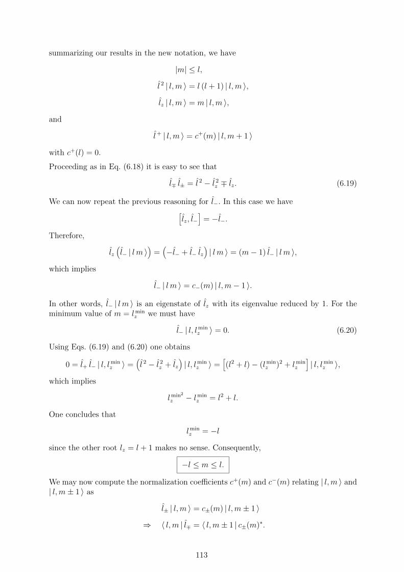
summarizing our results in the new notation, we have

|m| ≤ l,

l 2 | l,m 〉 = l (l + 1) | l,m 〉,lz | l,m 〉 = m | l,m 〉,

and

l+ | l,m 〉 = c+(m) | l,m+ 1 〉with c+(l) = 0.

Proceeding as in Eq. (6.18) it is easy to see that

l∓ l± = l 2 − l 2z ∓ lz. (6.19)

We can now repeat the previous reasoning for l−. In this case we have[lz, l−

]= −l−.

Therefore,

lz(l− | l m 〉

)=

(−l− + l− lz

)| l m 〉 = (m− 1) l− | l m 〉,

which implies

l− | l m 〉 = c−(m) | l,m− 1 〉.

In other words, l− | l m 〉 is an eigenstate of lz with its eigenvalue reduced by 1. For theminimum value of m = lmin

z we must have

l− | l, lminz 〉 = 0. (6.20)

Using Eqs. (6.19) and (6.20) one obtains

0 = l+ l− | l, lminz 〉 =

(l 2 − l 2z + lz

)| l, lmin

z 〉 =[(l2 + l)− (lmin

z )2 + lminz

]| l, lmin

z 〉,which implies

lmin2

z − lminz = l2 + l.

One concludes that

lminz = −l

since the other root lz = l + 1 makes no sense. Consequently,

−l ≤ m ≤ l.

We may now compute the normalization coefficients c+(m) and c−(m) relating | l,m 〉 and| l,m± 1 〉 as

l± | l,m 〉 = c±(m) | l,m± 1 〉⇒ 〈 l,m | l∓ = 〈 l,m± 1 | c±(m)∗.

113

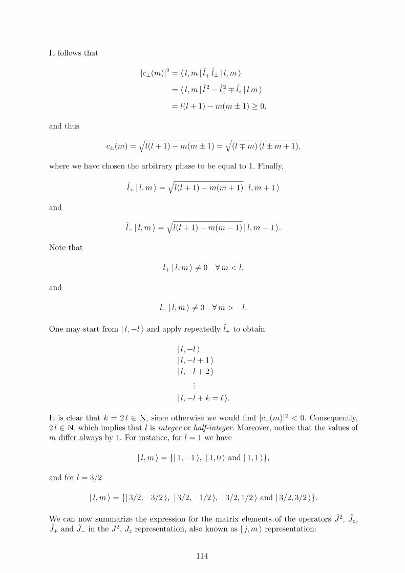
It follows that

|c±(m)|2 = 〈 l,m | l∓ l± | l,m 〉= 〈 l,m | l 2 − l 2z ∓ lz | l m 〉= l(l + 1)−m(m± 1) ≥ 0,

and thus

c±(m) =√l(l + 1)−m(m± 1) =

√(l ∓m) (l ±m+ 1),

where we have chosen the arbitrary phase to be equal to 1. Finally,

l+ | l,m 〉 =√l(l + 1)−m(m+ 1) | l,m+ 1 〉

and

l− | l,m 〉 =√l(l + 1)−m(m− 1) | l,m− 1 〉.

Note that

l+ | l,m 〉 6= 0 ∀m < l,

and

l− | l,m 〉 6= 0 ∀m > −l.

One may start from | l,−l 〉 and apply repeatedly l+ to obtain

| l,−l 〉| l,−l + 1 〉| l,−l + 2 〉

...

| l,−l + k = l 〉.

It is clear that k = 2 l ∈ N, since otherwise we would find |c+(m)|2 < 0. Consequently,2 l ∈ N, which implies that l is integer or half-integer. Moreover, notice that the values ofm differ always by 1. For instance, for l = 1 we have

| l,m 〉 = | 1,−1 〉, | 1, 0 〉 and | 1, 1 〉,

and for l = 3/2

| l,m 〉 = | 3/2,−3/2 〉, | 3/2,−1/2 〉, | 3/2, 1/2 〉 and | 3/2, 3/2 〉.

We can now summarize the expression for the matrix elements of the operators J2, Jz,J+ and J− in the J2, Jz representation, also known as | j,m 〉 representation:

114

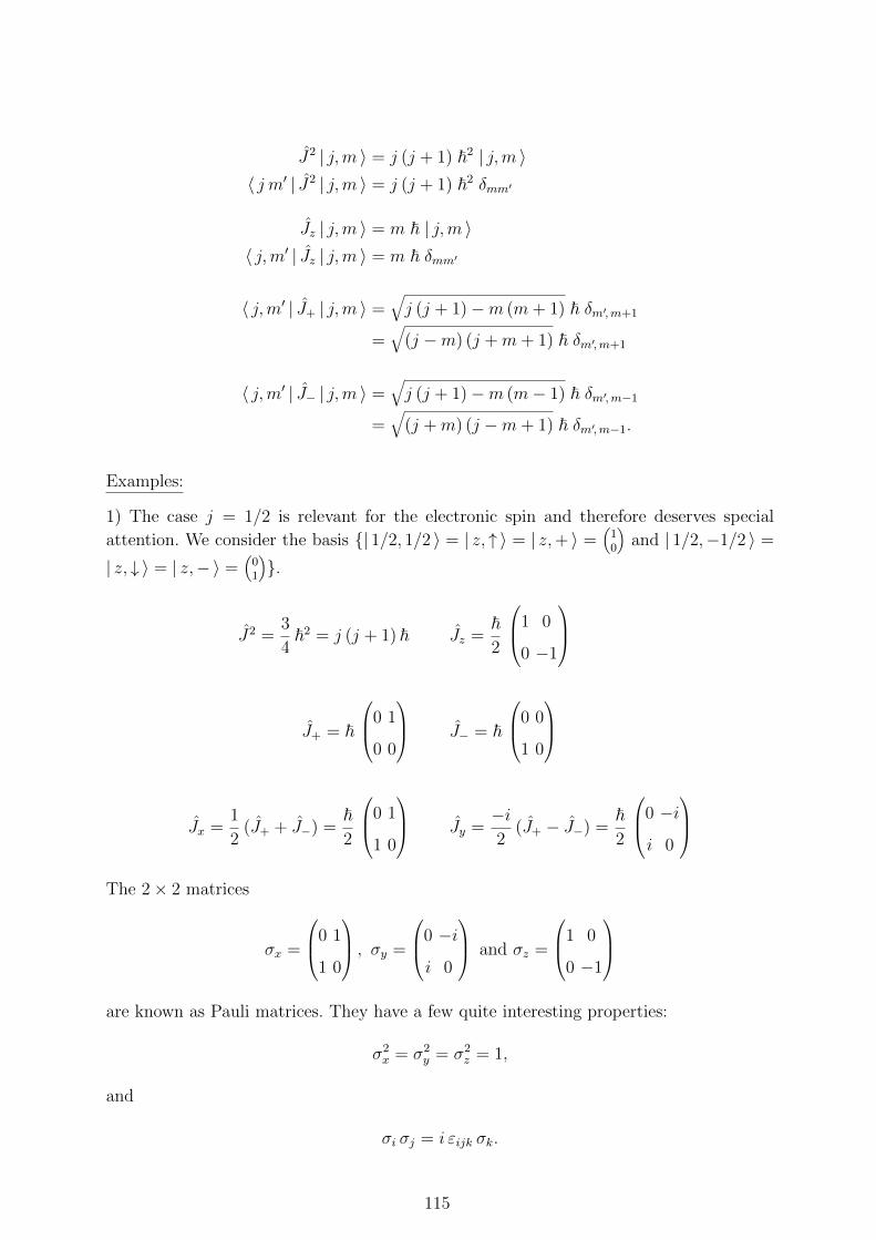
J2 | j,m 〉 = j (j + 1) ~2 | j,m 〉〈 j m′ | J2 | j,m 〉 = j (j + 1) ~2 δmm′

Jz | j,m 〉 = m ~ | j,m 〉〈 j,m′ | Jz | j,m 〉 = m ~ δmm′

〈 j,m′ | J+ | j,m 〉 =√j (j + 1)−m (m+ 1) ~ δm′,m+1

=√(j −m) (j +m+ 1) ~ δm′,m+1

〈 j,m′ | J− | j,m 〉 =√j (j + 1)−m (m− 1) ~ δm′,m−1

=√(j +m) (j −m+ 1) ~ δm′,m−1.

Examples:

1) The case j = 1/2 is relevant for the electronic spin and therefore deserves special

attention. We consider the basis | 1/2, 1/2 〉 = | z, ↑ 〉 = | z,+ 〉 =(10

)and | 1/2,−1/2 〉 =

| z, ↓ 〉 = | z,−〉 =(01

).

J2 =3

4~2 = j (j + 1) ~ Jz =

~2

1 0

0 −1

J+ = ~

0 1

0 0

J− = ~

0 0

1 0

Jx =1

2(J+ + J−) =

~2

0 1

1 0

Jy =

−i

2(J+ − J−) =

~2

0 −i

i 0

The 2× 2 matrices

σx =

0 1

1 0

, σy =

0 −i

i 0

and σz =

1 0

0 −1

are known as Pauli matrices. They have a few quite interesting properties:

σ2x = σ2

y = σ2z = 1,

and

σi σj = i εijk σk.

115

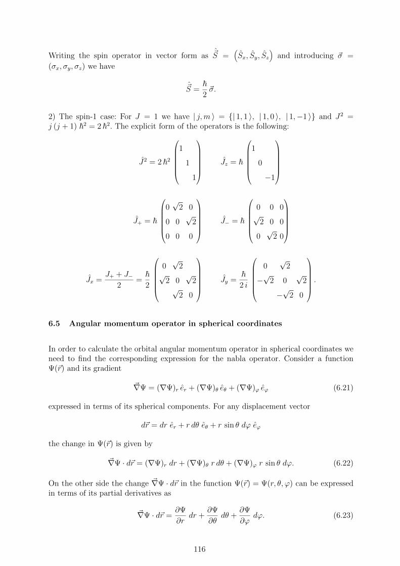
Writing the spin operator in vector form as ~S =(Sx, Sy, Sz

)and introducing ~σ =

(σx, σy, σz) we have

~S =~2~σ.

2) The spin-1 case: For J = 1 we have | j,m 〉 = | 1, 1 〉, | 1, 0 〉, | 1,−1 〉 and J2 =j (j + 1) ~2 = 2 ~2. The explicit form of the operators is the following:

J2 = 2 ~2

1

1

1

Jz = ~

1

0

−1

J+ = ~

0√2 0

0 0√2

0 0 0

J− = ~

0 0 0√2 0 0

0√2 0

Jx =J+ + J−

2=~2

0√2

√2 0

√2

√2 0

Jy =~2 i

0√2

−√2 0

√2

−√2 0

.

6.5 Angular momentum operator in spherical coordinates

In order to calculate the orbital angular momentum operator in spherical coordinates weneed to find the corresponding expression for the nabla operator. Consider a functionΨ(~r) and its gradient

~∇Ψ = (∇Ψ)r er + (∇Ψ)θ eθ + (∇Ψ)ϕ eϕ (6.21)

expressed in terms of its spherical components. For any displacement vector

d~r = dr er + r dθ eθ + r sin θ dϕ eϕ

the change in Ψ(~r) is given by

~∇Ψ · d~r = (∇Ψ)r dr + (∇Ψ)θ r dθ + (∇Ψ)ϕ r sin θ dϕ. (6.22)

On the other side the change ~∇Ψ · d~r in the function Ψ(~r) = Ψ(r, θ, ϕ) can be expressedin terms of its partial derivatives as

~∇Ψ · d~r = ∂Ψ

∂rdr +

∂Ψ

∂θdθ +

∂Ψ

∂ϕdϕ. (6.23)

116

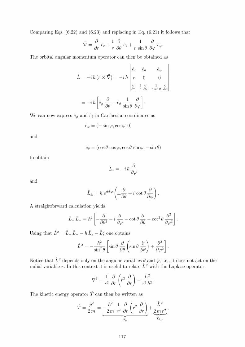
Comparing Eqs. (6.22) and (6.23) and replacing in Eq. (6.21) it follows that

~∇ =∂

∂rer +

1

r

∂

∂θeθ +

1

r sin θ

∂

∂ϕeϕ.

The orbital angular momentum operator can then be obtained as

L = −i ~ (~r × ~∇) = −i ~

∣∣∣∣∣∣∣∣∣∣∣

er eθ eϕ

r 0 0

∂∂r

1r

∂∂θ

1r sin θ

∂∂ϕ

∣∣∣∣∣∣∣∣∣∣∣

= −i ~[eϕ

∂

∂θ− eθ

1

sin θ

∂

∂ϕ

].

We can now express eϕ and eθ in Carthesian coordinates as

eϕ = (− sinϕ, cosϕ, 0)

and

eθ = (cos θ cosϕ, cos θ sinϕ,− sin θ)

to obtain

Lz = −i ~∂

∂ϕ

and

L± = ~ e±i ϕ

(± ∂

∂θ+ i cot θ

∂

∂ϕ

).

A straightforward calculation yields

L+ L− = ~2[− ∂

∂θ2− i

∂

∂ϕ− cot θ

∂

∂θ− cot2 θ

∂2

∂ϕ2

].

Using that L2 = L+ L− − ~ Lz − L2z one obtains

L 2 = − ~2

sin2 θ

[sin θ

∂

∂θ

(sin θ

∂

∂θ

)+

∂2

∂ϕ2

].

Notice that L 2 depends only on the angular variables θ and ϕ, i.e., it does not act on theradial variable r. In this context it is useful to relate L 2 with the Laplace operator:

∇2 =1

r2∂

∂r

(r2

∂

∂r

)− L 2

r2 ~2.

The kinetic energy operator T can then be written as

T =p2

2m= − ~2

2m

1

r2∂

∂r

(r2

∂

∂r

)

︸ ︷︷ ︸Tr

+L 2

2mr2︸ ︷︷ ︸Tθ,ϕ

,

117

where Tr depends only on r and Tθ,ϕ depends only on θ and ϕ. Taking into account that

L 2 and Tθ,ϕ act only on θ and ϕ, and that the radial part of the kinetic energy Tr acts only

on r, we can seek for the eigenfunction of T , and even of the Hamiltonian H = T+V (r) inthe presence of a spherically symmetric potential V (r), by separating radial and angularvariables as

Ψlm(~r) = R(r) Ylm(θ, ϕ),

where Ylm(θ, ϕ) is an eigenfunction of L 2 and Lz.

The angular dependent functions Ylm(θ, ϕ) are known as spherical harmonics. They areeigenfunctions of Lz, and therefore

−i ~∂

∂ϕYlm(θ, ϕ) = m ~ Ylm(θ, ϕ) ⇒ Ylm(θ, ϕ) = f(θ) eimϕ,

where f(θ) is a function of θ alone. Replacing Ylm(θ, ϕ) in the equation

L 2 Ylm(θ, ϕ) = l (l + 1) ~ Ylm(θ, ϕ)

one obtains a differential equation for f of the form[d

dz(1− z2)

d

dz+

(l (l + 1)− m2

1− z2

)]f(z) = 0,

where z = cos θ. The spherical harmonics thus take the form

Ylm(θ, ϕ) =

√√√√2 l + 1

4 π

(l −m)!

(l +m)!Pml (cos θ) eimϕ

form ≥ 0, where Pml (cos θ) are the associated Legendre polynomials. Besides an arbitrary

choice of phase factor, we have used the normalization condition

∫ 2π

0

∫ 1

−1dΩ Y ∗

l′m′(θ, ϕ) Ylm(θ, ϕ) = δll′ δmm′ .

For m = 0, Pml (cos θ) reduces to the usual Legendre polynomials Pl(cos θ). Thus,

Yl 0(θ, ϕ) =

√2 l + 1

4πPl(cos θ).

For m < 0 we have

Yl,−|m|(θ, ϕ) = (−1)m Y ∗l, |m|(θ, ϕ).

The spherical harmonics satisfy the following important completeness relation:

+∞∑

l=0

l∑

m=−l

Y ∗lm(θ

′, ϕ′) Ylm(θ, ϕ) = δ(ϕ− ϕ′) δ(cos θ − cos θ′).

Consequently, an arbitrary function Ψ(r, θ, ϕ) can be written in the form

Ψ(r, θ, ϕ) =+∞∑

l=0

l∑

m=−l

Rlm(r) Ylm(θ, ϕ).

118

Examples:

i) l = 0

Y00(θ, ϕ) =1√4π

← independent of θ and ϕ.

ii) l = 1

Y10(θ, ϕ) =

√3

4πcos θ ← independent of ϕ.

Y1;±1(θ, ϕ) = ∓√

3

8πsin θ e±i ϕ

= ∓√

3

8πsin θ (cosϕ± i sinϕ)

Notice that Y10 ∝ cos θ ∝ z corresponds to the atomic orbital pz and that Y1;±1 ∝ (x± i y)

corresponds to the atomic orbital px ± i py. The eigenfunctions of L2 and Lz are classified

according to the value of l as

l 0 1 2 3

s p d f orbitals.

The spherical harmonics have well-defined inversion symmetry, i.e., symmetry with respectto the transformation ~r → −~r, or equivalently (r, θ, ϕ) → (r, π − θ, ϕ + π). In fact, uponinversion we have

Ylm(π − θ, ϕ+ π) = (−1)l Ylm(θ, ϕ).

This implies even (odd) parity for l even (odd).

An alternative derivation of the eigenfunctions of L2 and Lz would be to apply our know-ledge of the operator algebra. Starting from

L+ | l l 〉 = 0,

and using that

L+ = ~ ei ϕ(

∂

∂θ+ i cot θ

∂

∂ϕ

)

as well as

〈~r | l l 〉 = Yl l(θ, ϕ) = ei l ϕ f(θ),

we have

0 = ei l ϕ∂f

∂θ+ i

cos θ

sin θ(i l) ei l ϕ f(θ),

which implies

∂f

∂θ− l

cos θ

sin θf(θ) = 0.

119

This equation is satisfied by f(θ) = c sinl(θ) so that

Yl l(θ, ϕ) = cl sinl(θ) ei l ϕ.

Repeated application of L− allows one to obtain all the other Ylm(θ, ϕ) with m < l. Thenormalization constant is determined by the condition

∫dΩ |Yl l(θ, ϕ)|2 = 1.

With an appropriate choice of the phase factor, so that (L−)l Yl l(θ, ϕ) has the same signas Pl(cos θ), one obtains

cl =(−1)l

2l l!

√(2 l + 1) (2l)!

4π.

Taking into account that

L− = ~ e−i ϕ

(− ∂

∂θ+ i cot θ

∂

∂ϕ

)

and

L− | l,m 〉 = ~√(l +m) (l −m+ 1) | l,m− 1 〉

we finally arrive to the recursive relation

Ylm−1(θ, ϕ) =1√

(l +m) (l −m+ 1)e−i ϕ

(− ∂

∂θ+ i cot θ

∂

∂ϕ

)Ylm(θ, ϕ).

120

7 Spin

Consider a system consisting of several parts such as a nucleus. We would like to describethe quantum mechanical state of the nucleus as a whole for a given fixed internal energyE. It is clear that the position (or momentum) of the nucleus is not enough to describeits QM state, since we must take into account that the nucleus can have different internalstates. Taking into account the rotational invariance of isolated systems we can attempt todescribe the state of the nucleus by its total angular momentum L. It often happens thatall the states of a given energy E have the same total angular momentum L. However,even in this case, we must also take into account the possible orientations of ~L in space(unless L = 0). These have all the same E and are characterized by the 2L + 1 possible

projections of ~L along a given axis, say, the z axis. Therefore, in order to describe thestate of the nucleus, we need to consider not only its coordinates ~r (or momentum ~p),but also an additional discrete variable, namely the projection of the angular momentumalong a given direction in space. The state of a composite particle can then be describedby the wave function

ΨnL = ΨnL(~r, Lz).

There is no reason why elementary particles, that is, particles that appear to be structure-less in the considered energy range of the interactions,10 should not have such an internaldegree of freedom. In fact there are many examples in nature where a particle “at rest”or in a state bearing no orbital angular momentum (e.g., a spherically symmetric stateΨ(~r) = Ψ(r) or in a plane wave state Ψ(~r) = 1√

Vei ~p~r) shows a finite (non-vanishing)

intrinsic angular momentum j0 6= 0. Moreover, the value of j0 is very often half-integer.

The intrinsic angular momentum of an elementary particle is called spin and the vectoroperator associated to this observable is denoted by ~s = (sx, sy, sz). The commutationrules for sx, sy and sz follow from the commutation rules of the rotations (matrices) in

R3 and are the same as those of the orbital angular momentum ~l = ~r× ~p, since sx, sy andsz are the generators of infinitesimal rotations (around the axis x, y and z) acting on thespin variables. Therefore

[sx, sy] = i ~ sz, [sy, sz] = i ~ sx, and [sz, sx] = i ~ sy.

All the properties derived for the angular momentum ~ hold of course for ~s. In particulars2 and sz form a complete set of compatible observables. The corresponding eigenvaluesare s(s+1) and ms = −s,−s+1, . . . , s− 1, s. Since the length of the spin is fixed by thenature of the particle considered (e.g., s = 1/2 for an electron), the angular momentum~~s vanishes in the limit ~→ 0. Thus, the spin has no classical equivalent.

For the description of the state of a particle we not only need to consider the usual classicalvariables such as position ~r or momentum ~p, but also the spin variable ms, also denotedby σ, which characterizes the intrinsic state. The length s of the spin is fixed, like themass or the charge of the given particle, and therefore does not depend on the particlestate. In three dimensions four compatible observables are needed to describe the state ofa particle having s 6= 0. These can be written as |~r,ms 〉 or | ~p,ms 〉, for example. One may

also define the state by the observables H, l 2, lz and sz or H, l 2, 2 and z, where ~ = ~l+~s

10 The fact that the notion of elementary particle is energy dependent shall be discussed below.

121

is the total angular momentum. In this case one denotes the states as |E, l,ml,ms 〉 and|E, l, j, jz 〉, respectively. The wave function

〈~r, σ |Ψ 〉 = Ψ(~r, σ) = Ψσ(~r)

is thus a function of four variables (3 continuous and 1 discrete). One often attaches anindex to the wave function corresponding to the different values of ms = σ. These areknown as the spin components of the wave function. Notice that the spin variables arecompletely independent of the usual classical variables ~r or ~p. One can therefore regard thekets of a particle with spin as the elements of a Hilbert space, which is the direct productof the usual Hilbert space associated to the classical variables and (2 s + 1)-dimensionalspace associated to the spin variable. For example,

| ~p,ms 〉 = | ~p 〉 · |ms 〉

or

|E, l,ml,ms 〉 = |E, l,ml 〉 |ms 〉.

The spin operators act on the spin variable only and therefore commute with the operatorsacting on the coordinates such as ~r, ~p, ~l, etc. If one rotates a particle with spin, one musttake into account the effect of the rotation on both the coordinates and the spin variable.The operator describing an infinitesimal rotation of the orbital part of the ket is given by

Uorb(δφ) = 1− i

~n · ~l δφ+O(δφ2),

where δφ denotes the angle and n the axis of rotation. The rotation of the spin variablesis realized by the operator

Uspin(δφ) = 1− i

~n · ~s δφ+O(δφ2),

where ~s is the spin operator. The operator corresponding to the rotation of the completeket is therefore given by the product

U = Uspin Uorb = Uorb Uspin

= 1− i

~n · (~l + ~s ) δφ+O(δφ2).

Consequently, the total angular momentum

~ = ~l + ~s

is the generator of infinitesimal rotations. It is easy to verify that

[i, k] = i εikl l,

from which it follows that 2 and z form a complete set of observables with eigenvaluesj(j+1) and m = −j,−j+1, . . . , j−1, j. It is therefore important to determine which arethe eigenvalues of 2, i.e., the possible values of j, that can be obtained for given valuesof l and s.

122

For a system of particles the total angular momentum is given by the sum of the operatorsacting on each variable:

~J =∑

i

~i with ~i = ~li + ~si,

which we can put in the form

~J = ~L+ ~S

with ~L =∑

i~li and ~S =

∑i ~si.

Example: The electron spin and spinor states

Electrons are particles having s = 1/2. The dimension of the spin space is therefore2 s + 1 = 2. We can write the wave function as Ψσ(~r) with σ = 1/2 and −1/2 or as atwo-component or spin-1/2 spinor :

|Ψ 〉 =

Ψ1/2(~r)

Ψ−1/2(~r)

=

Ψ↑(~r)

Ψ↓(~r)

=

Ψ+(~r)

Ψ−(~r)

.

For the discussion of the spin dependence one can drop the dependence on the classicalvariables ~r or ~p (e.g., one may consider a given position ~r or imagine that the electronhas a defined momentum ~p) and simply write

|Ψ 〉 =c+

c−

with |c+|2 + |c−|2 = 1.

The eigenstates of

sx =~2

0 1

1 0

are given by

|x,+ 〉 = 1√2

1

1

and |x,−〉 = 1√

2

1

−1

,

which correspond to the eigenvalues sx = ± ~/2. The ket | x,+ 〉 (|x,−〉) represents astate in which the spin of the electron points along the positive (negative) x direction. Interms of the eigenstates of sz, namely

| z,+ 〉 =1

0

and | z,−〉 =

0

1

,

we can write

|x,±〉 = 1√2(| z,+ 〉 ± | z,−〉) .

123

And the corresponding components of the wave functions are

Ψx±(~r) = 〈~r |x,±〉 = 1√

2(〈~r | z,+ 〉 ± 〈~r | z,−〉) = 1√

2

[Ψz

1/2(~r)±Ψz−1/2(~r)

].

Let us finally notice that if one prepares an electron in a state |x,+ 〉 having its spinpointing along the positive x direction (e.g., as a result of a Stern-Gerlach filtering ex-periment with the magnetic field gradient along the x direction) and one measures theprojection of the spin along a perpendicular direction (e.g., by means of a second Stern-Gerlach experiment with the magnetic field gradient along the z direction) the probabilityof measuring the value sz = + ~/2 or sz = − ~/2 is |〈 z,± | x,+ 〉|2 = 1/2.

The addition of spin and orbital angular momenta is discussed in the following section.

7.1 Addition of angular momentum

We consider two commuting angular momentum operators ~J1 and ~J2 acting on different

subspaces S1 and S2. These can be the spin ~S and orbital momentum ~L of an electron,for which we have

[~L, ~S ] = 0,

since they act on different variables, or the total angular momenta ~1 and ~2 of twoelectrons, which satisfy

[~1, ~2] = 0

for the same reason. The usual commutation relations in component form read

[J1 k, J1 l] = i ~ εklm J1m

and

[J2 k, J2 l] = i ~ εklm J2m

with

[J1 k, J2 l] = 0

for all k, l,m = 1–3. Since ~J1 and ~J2 are angular momentum operators, and choosing asusual z as the quantization direction, we have

[J1 z, J21 ] = 0

and

[J2 z, J22 ] = 0.

124

Recalling that [ ~J1, ~J2] = 0, it is clear that J1 z, J21 , J2 z and J2

2 are compatible observables.Therefore, we can characterize our kets by the corresponding quantum numbers as

| j1, j2; m1,m2 〉 ≡ | j1m1 〉︸ ︷︷ ︸φ orbital

| j2m2 〉︸ ︷︷ ︸χ spin

.

As usual Jαz | jα mα 〉 = mα | jα mα 〉 and J2α | jα mα 〉 = jα (jα + 1) | jα mα 〉 for α = 1

and 2. If we now perform a rotation R on the system we must rotate or transform theorbital ket and the spin ket, or the coordinates of both electrons, if we are dealing with atwo-electron system. The corresponding operators are given by

D1(R) = e−i~

~J1·n φ

and

D2(R) = e−i~

~J2·n φ.

The operator transforming the complete ket is

D(R) = D1(R) D2(R) = D2(R) D1(R),

where it is understood thatD1 acts on the variables of subspace S1 andD2 on the variables

of S2. In terms of ~J1 and ~J2 we have

D(R) = e−i~

~J1·n φ e−i~

~J2·n φ = e−i~ ( ~J1+ ~J2)·n φ.

The generator of rotations of the composite system S1 ⊕ S2 is therefore

~J = ~J1 + ~J2,

i.e., the vector sum of the individual operators. The fundamental property of ~J = ~J1 + ~J2reads

[Jk, Jl] = i ~ εklm Jm, (7.1)

i.e., ~J is an angular momentum operator. The usual properties of angular momenta follow:

i) [J2, Jz] = [J2, Jy] = [J2, Jx] = 0.

ii) [Jz, J±] = ± ~ J±.

iii) One finds the same kind of eigenstates | j m 〉 with −j ≤ m ≤ j.

iv) The values of j are either integer or half-integer, and the values of m arem = −j,−j + 1, . . . , j − 1, j.

v) The ladder operators J± = Jx ± i Jy satisfy

J± | j m 〉 =√j (j + 1)−m (m± 1) | j,m± 1 〉.

125

It is therefore important to construct the states | j m 〉 with defined J2 | j m 〉 = j(j + 1)| j m 〉 and Jz | j m 〉 = m | j m 〉 in terms of the states | j1, j2; m1,m2 〉 = | j1,m1 〉 | j2,m2 〉of S1 ⊕ S2.

The proof of Eq. (7.1) is straightforward:

[Jk, Jl] = [J1k + J2k, J1l + J2l]

= [J1k, J1l] + [J2k, J2l]

= i ~ εklm J1m + i ~ εklm J2m

= i ~ εklm Jm.

In addition we have

[Jk, J1l] = [J1k, J2l] = i ~ εklm J1m.

This implies that ~J1 and ~J2 are vector operators. Therefore [J21 ,

~J ] = [J 22 ,

~J ] = 0. We canprove this statement for vector operators in general:

[V 2, Jz] = [V 2x + V 2

y + V 2z , Jz]

= Vx [Vx, Jz] + [Vx, Jz] Vx + Vy [Vy, Jz] + [Vy, Jz] Vy

= Vx (−i ~ Vy) + (−i ~ Vy) Vx + Vy (i ~ Vx) + (i ~ Vx) Vy

= 0.

In conclusion, besides J1z, J21 , J2z and J2

2 , we also have the following set of compatible op-erators J 2

1 , J22 , J

2 and Jz. The states of the composite system S1⊕S2 can be characterizedby the corresponding quantum numbers as | j1, j2; j,m 〉, where

J 21 | j1, j2; j,m 〉 = j1 (j1 + 1) | j1, j2; j,m 〉

J 22 | j1, j2; j,m 〉 = j2 (j2 + 1) | j1, j2; j,m 〉J2 | j1, j2; j,m 〉 = j (j + 1) | j1, j2; j,m 〉Jz | j1, j2; j,m 〉 = m | j1, j2; j,m 〉.

What are the possible values of j in terms of j1 and j2? How are the states | j1, j2; j,m 〉,which are eigenstates of J 2

1 , J22 , J

2 and Jz, written in terms of the states | j1, j2; m1,m2 〉,which are eigenstates of J 2

1 , J 22 , J1z and J2z? In general we can have

| j1, j2; j,m 〉 =j1∑

m1=−j1

j2∑

m2=−j2

| j1, j2; m1,m2 〉 〈 j1, j2; m1,m2 | j1, j2; j,m 〉.

〈 j1, j2; m1,m2 | j1, j2; j,m 〉 are the so-called Clebsch-Gordan or vector addition coeffi-cients. An important property is the conservation of the total z component of the angularmomentum:

〈 j1, j2; m1,m2 | j1, j2; j,m 〉 = 0

126

unless

m1 +m2 = m. (7.2)

To prove Eq. (7.2) we compute

〈 j1, j2 |m1,m2 | Jz − J1z − J2z | j1, j2; j,m 〉 = 0

(since Jz = J1z + J2z) by acting with Jz on the ket and with J1z and J2z on the bra. Thisimplies

(m−m1 −m2) 〈 j1, j2; m1,m2 | j1, j2; j,m 〉 = 0,

which proves the statement.

The second important property is

〈 j1, j2; m1,m2 | j1, j2; j,m 〉 = 0

unless

|j1 − j2| ≤ j ≤ j1 + j2. (7.3)

This can be demonstrated as follows: Since Jz | j1, j2; m1,m2 〉 = (m1+m2) | j1, j2; m1,m2 〉,the largest possible value of Jz is j1+j2. There is only one state with Jz = j1+j2, namely,

| j1, j2, j = j1 + j2, m = j1 + j2 〉 = | j1, j2; m1 = j1,m2 = j2 〉.

Applying J+ = J1+ + J2+ we obtain

J+ | j1, j2; m1 = j1,m2 = j2 〉 = 0

⇒ | j1, j2; m1 = j1,m2 = j2 〉 = | j1, j2; j = j1 + j2, m = j1 + j2 〉.

There are 2 kets for m = j1+ j2− 1. One is proportional to J− | j = j1+ j2, m = j1+ j2 〉,and the other has j = j1 + j2 − 1. There are 3 kets for m = j1 + j2 − 2, etc. In general,one finds k + 1 kets with m = j1 + j2 − k until j2 − k = minj1, j2 = j2, where we havechosen j2 ≤ j1 by convention. This proves the inequality (7.3).

One can easily verify that the sum of the numbers 2j+1 of orthogonal states | j1, j2; j,m 〉corresponding to each value of j gives (2j1 + 1) (2j2 + 1), which is the number of states| j1, j2; m1,m2 〉 = | j1,m1 〉 | j2,m2 〉 that can be formed by combining the two angularmomenta (direct product):

j1+j2∑

j=|j1−j2|(2j + 1) = (2j1 + 1) (2j2 + 1).

This means that the dimension of the subspace is not modified by the change of repre-sentation (unitary transformation).

The spectrum of J2 is then given by

j = j1 + j2, j1 + j2 − 1, . . . |j1 − j2|.

127

Notice that the difference between successive values of j is always 1, even if j can be halfinteger (e.g., j = 5/2, 3/2 and 1/2 for j1 = 3/2 and j2 = 1). Moreover, there is only onesequence of 2j+1 states having m = −j, −j+1, . . . j for each value of j. This is usuallysummarized by the triangular relation

|j1 − j2| ≤ j ≤ j1 + j2.

Let us finally recall that the actual eigenvalues of J2 are as usual j(j + 1), since

J2 | j,m 〉 = j(j + 1) | j,m 〉.

Example: L = 2 and S = 1/2

In order to ilustrate how the different eigenstates of J2 are constructed we would like todetermine the states with defined total angular momentum ~J = ~L + ~S for an electron(S = 1/2) in an atomic orbital (L = 2). We denote the eigenstates with definedmL andmS

by |L, S; mL,mS 〉 (Lz |L, S; mL,mS 〉 = mL |L, S; mL,mS 〉 with mL = ±2, ±1 and 0,and Sz |L, S; mL,mS 〉 = mS |L, S; mL,mS 〉 with mS = ±1/2) and the eigenstates of J2

and Jz by |L, S; J,mJ 〉. There is only one possible state with maximal mJ = L+S = 5/2.It is given by

| 2, 1/2; J = 5/2, mJ = 5/2 〉 = | 2, 1/2; mL = 2, mS = 1/2 〉.

There are two states with mJ = 3/2, one with mL = 1 and mS = 1/2 and the other withmL = 2 and mS = −1/2. Appropriate linear combinations of these two states yield thefollowing eigenstates of J2 and Jz:

| 2, 1/2; J = 5/2, mJ = 3/2 〉

and

| 2, 1/2; J = 3/2, mJ = 3/2 〉.

How many states can we find with defined mL and mS and mL +mS = mJ = 1/2? Theseare

| 2, 1/2; mL = 0, mS = 1/2 〉

and

| 2, 1/2; mL = −1, mS = 1/2 〉.

Since application of J− on the eigenstates having J = 5/2 and J = 3/2 with mJ = 3/2yields two orthogonal states withmJ = 1/2, it is clear that no new values of J are obtainedfor mJ = 1/2. The states | 2, 1/2; J = 5/2, mJ = 1/2 〉 and | 2, 1/2; J = 3/2, mJ = 1/2 〉are obtained by appropriate linear combination of the states | 2, 1/2; mL = 0, mS =−1/2 〉 and | 2, 1/2; mL = −1, mS = 1/2 〉. The same reasoning applies to negative valuesof mJ = −1/2, −3/2 and −5/2. Therefore, the values of J resulting from the sum ofL = 2 and S = 1/2 are simply J = 5/2 and 3/2, in agreement with the inequality (7.3).

128

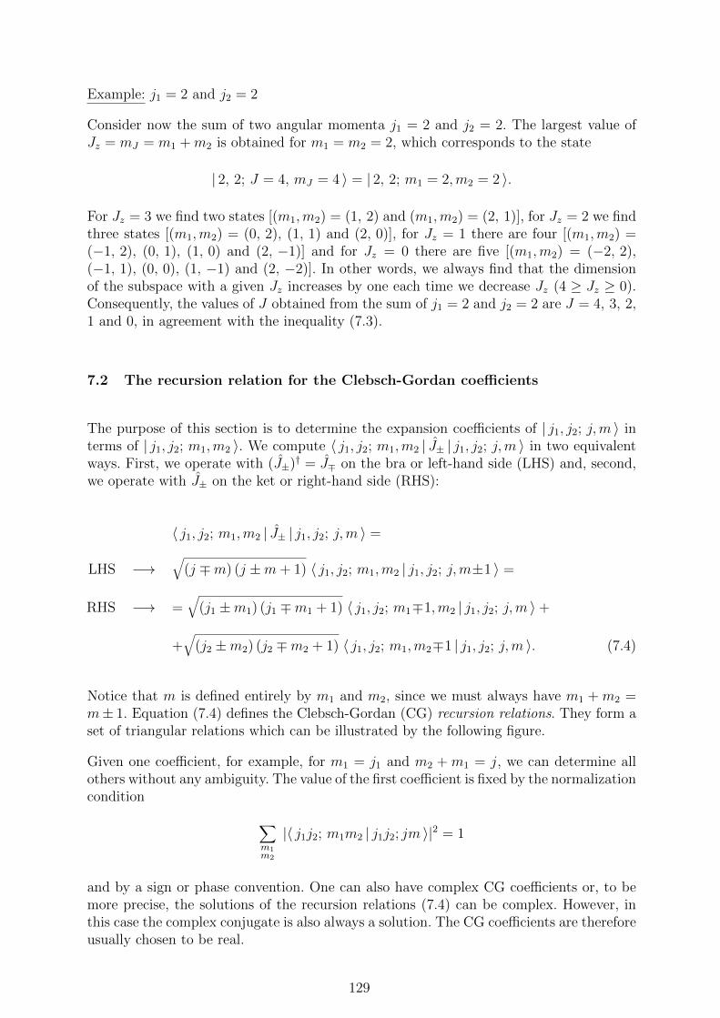
Example: j1 = 2 and j2 = 2

Consider now the sum of two angular momenta j1 = 2 and j2 = 2. The largest value ofJz = mJ = m1 +m2 is obtained for m1 = m2 = 2, which corresponds to the state

| 2, 2; J = 4, mJ = 4 〉 = | 2, 2; m1 = 2,m2 = 2 〉.

For Jz = 3 we find two states [(m1,m2) = (1, 2) and (m1,m2) = (2, 1)], for Jz = 2 we findthree states [(m1,m2) = (0, 2), (1, 1) and (2, 0)], for Jz = 1 there are four [(m1,m2) =(−1, 2), (0, 1), (1, 0) and (2, −1)] and for Jz = 0 there are five [(m1,m2) = (−2, 2),(−1, 1), (0, 0), (1, −1) and (2, −2)]. In other words, we always find that the dimensionof the subspace with a given Jz increases by one each time we decrease Jz (4 ≥ Jz ≥ 0).Consequently, the values of J obtained from the sum of j1 = 2 and j2 = 2 are J = 4, 3, 2,1 and 0, in agreement with the inequality (7.3).

7.2 The recursion relation for the Clebsch-Gordan coefficients

The purpose of this section is to determine the expansion coefficients of | j1, j2; j,m 〉 interms of | j1, j2; m1,m2 〉. We compute 〈 j1, j2; m1,m2 | J± | j1, j2; j,m 〉 in two equivalentways. First, we operate with (J±)† = J∓ on the bra or left-hand side (LHS) and, second,we operate with J± on the ket or right-hand side (RHS):

〈 j1, j2; m1,m2 | J± | j1, j2; j,m 〉 =

LHS −→√(j ∓m) (j ±m+ 1) 〈 j1, j2; m1,m2 | j1, j2; j,m±1 〉 =

RHS −→ =√(j1 ±m1) (j1 ∓m1 + 1) 〈 j1, j2; m1∓1,m2 | j1, j2; j,m 〉+

+√(j2 ±m2) (j2 ∓m2 + 1) 〈 j1, j2; m1,m2∓1 | j1, j2; j,m 〉. (7.4)

Notice that m is defined entirely by m1 and m2, since we must always have m1 +m2 =m± 1. Equation (7.4) defines the Clebsch-Gordan (CG) recursion relations. They form aset of triangular relations which can be illustrated by the following figure.

Given one coefficient, for example, for m1 = j1 and m2 + m1 = j, we can determine allothers without any ambiguity. The value of the first coefficient is fixed by the normalizationcondition

∑m1m2

|〈 j1j2; m1m2 | j1j2; jm 〉|2 = 1

and by a sign or phase convention. One can also have complex CG coefficients or, to bemore precise, the solutions of the recursion relations (7.4) can be complex. However, inthis case the complex conjugate is also always a solution. The CG coefficients are thereforeusually chosen to be real.

129

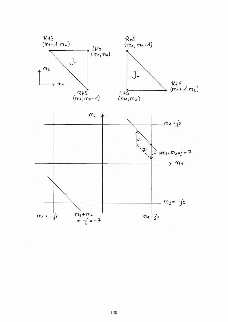
130

8 The central symmetric field

8.1 General formulation

We consider the motion of two different interacting particles, for example, an electronmoving around a nucleus or an electron-positron pair. Taking into account the isotropy ofspace, the interaction energy U(r) between the particles can only depend on the distancer = |~r2 − ~r1| between the particles. Denoting by m1 and m2 the particle masses, theHamilton operator of the two-particle system is given by

H = − ~2

2m1

∇21 −

~2

2m2

∇22 + U(r).

As in classical mechanics it is convenient to change the coordinates by using the relativecoordinate

~r = ~r2 − ~r1

and the center of mass coordinate

~R =m1 ~r1 +m2 ~r2

m1 +m2

⇔ M ~R = m1 ~r1 +m2 ~r2,

where M = m1 +m2 is the total mass. Since

~r1 = ~R− m2

M~r

and

~r2 = ~R +m1

M~r,

and denoting the vector components as ~r = (x, y, z), ~R = (X,Y, Z), ~r1 = (x1, y1, z1) and~r2 = (x2, y2, z2) we have

∂Ψ

∂x1,2

=∂Ψ

∂x· ∂x

∂x1,2

+∂Ψ

∂X· ∂X

∂x1,2

= ∓∂Ψ

∂x+

m1

M

∂Ψ

∂X,

where − (+) corresponds to 1 (2). From this it follows that

∂2Ψ

∂x1,2

= ∓(∓∂2Ψ

∂x2+

∂2Ψ

∂X ∂x

m1,2

M

)+

m1,2

M

(∓ ∂2Ψ

∂x ∂X+

∂2Ψ

∂X2

m1,2

M

)

and therefore

1

m1

∂2Ψ

∂x21

+1

m2

∂2Ψ

∂x22

=(

1

m1

+1

m2

)∂Ψ

∂x2+

m1 +m2

M2

∂2Ψ

∂X2+

2

M

∂2Ψ

∂X ∂x− 2

M

∂2Ψ

∂x ∂X.

The Hamilton operator can then be written in the form

H = − ~2

2M∇2

R − ~2

2µ∇2

r + U(r),

131

where ∇2R refers to the Laplacian with respect to the center of mass coordinate ~R, ∇2

r to

the Laplacian with respect to the relative coordinate ~r, and µ =m1m2

m1 +m2

to the reduced

mass.

The separation of variables ~r and ~R in H allows us to write the wave function Ψ(~r1, ~r2)of the system in the form of a product

Ψ(~r, ~R) = φ(~R)Ψ(~r),

where φ(~R) describes the free-particle motion of the center of mass and Ψ(~r) the relativemotion of the particles under the action of the interparticle potential U(r).

We focus on the relative motion and write the Schrodinger equation as

− ~2

2µ∇2 Ψ+ U(r)Ψ = EΨ.

Using the expression for the Laplace operator in spherical coordinates

∇2 =1

r2∂

∂r

(r2

∂

∂r

)+

1

r21

sin2 θ

[sin θ

∂

∂θ

(sin θ

∂

∂θ

)+

∂2

∂φ2

]

and the expression for the square of the angular momentum (in units of ~)

l 2 = − 1

sin2 θ

[sin θ

∂

∂θ

(sin θ

∂

∂θ+

∂2

∂φ2

)]

we can write the Hamiltonian as

H = − ~2

2µ

1

r2∂

∂r

(r2

∂

∂r

)+~2

2µ

l 2

r2+ U(r). (8.1)

If one introduces the radial component of the linear momentum

pr Ψ = −i ~1

r

∂

∂r(rΨ) = −i ~

(∂Ψ

∂r+

Ψ

r

),

one can bring H in the form known from classical mechanics:

H =p2r2µ

+1

2µ

L2

r2+ U(r), (8.2)

where ~L = ~~l = ~r × p.

Recalling that ~r and ~p are vector operators and that the corresponding squares r2 and

p2 are invariant upon rotation(i.e.,

[r2, ~l

]=

[p2, ~l

]= 0

), it is easy to see that the

Hamiltonian given by Eq. (8.1) or (8.2) commutes with ~l, since the interparticle potentialU depends only on r. We may therefore search for the common eigenstates of H, l 2 andlz. The eigenfunctions of l 2 and lz have the form

Ψ = R(r) Ylm(θ, ϕ), (8.3)

132

where R(r) is the radial wave function and Ylm(θ, ϕ) are spherical harmonics satisfying

l 2 Ylm = l(l + 1) Ylm

and

lz Ylm = m Ylm.

Replacing Eq. (8.3) in Eq. (8.1) and using that ~l acts only on the angular variables θ andϕ we obtain that the radial part of the stationary states is given by

− ~2

2µ

1

r2d

dr

(r2

dR

dr

)+~2

2µ

l(l + 1)

r2R + U(r)R = E R.

This is the Schrodinger equation for the radial wave function. Notice that R depends onE and l but not on the z component of the angular momentum lz = m. Consequently,all stationary states are 2l + 1 degenerate. This is of course an expected consequence of[H,~l

]= 0 and in particular

[H, l±

]= 0. In the case of a discrete spectrum one usually

denotes the radial part by Rνl(r), where ν ≥ 0 is an integer known as radial quantumnumber.

In order to investigate the properties of R(r) it is useful to make the substitution

R(r) =χ(r)

r.

Using that

1

r2d

dr

(r2

dR

dr

)=

1

r2d

dr

[r2

(1

r

dχ

dr− 1

r2χ

)]=

1

r2d

dr

(rdχ

dr− χ

)

=1

r2dχ

dr+

1

r

d2χ

dr2− 1

r2dχ

dr

=1

r

d2χ

dr2

one obtains that the equation for χ reads

− ~2

2µ

d2χ

dr2+~2

2µ

l(l + 1)

r2χ+ U χ = E χ. (8.4)

Since R(r) must be finite everywhere, it follows that

χ(0) = 0.

This condition, which is rather obvious if U(r) is finite everywhere, also holds when U(r)diverges at the origin (r → 0) as U(r) ∼ rs with s < 0 [2]. The normalization conditionfor R requires

1 =∫ +∞

0|R(r)|2 r2 dr =

∫ +∞

0|χ(r)|2 dr.

Equation (8.4) is equivalent to a one-dimensional (1D) Schrodinger equation for χ(r) withthe boundary condition r ≥ 0 and χ(0) = 0.

133

8.2 Properties of the motion in a spherical potential

Based on our knowledge of the motion in one dimension (see Sec. 4.12) a few generalconclusions can be derived concerning the motion in a spherically symmetric field:

i) Since the motion is bounded on one side [χ(0) = 0], there is only one eigenstate ofEq. (8.4) for each energy E. This implies that for a given l there is only one radialsolution χEl for each value of E. This does not preclude, however, that differentvalues of l might lead to different χlE having the same eigenenergy. This is actuallythe case in the Coulomb field U(r) = −α/r (α > 0). Such degeneracies are said tobe accidental, since they are not a consequence of symmetry.

ii) Taking into account that the angular part is completely defined by the values of land m, we conclude that E, l and m form a complete set of compatible observablesaccording to which the eigenstates

ΨElm(~r) = REl(r) Ylm(θ, ϕ)

can be classified.

iii) Further insight in the structure of the energy spectrum can be obtained by applyingthe oscillator theorem, which states that the eigenfunction corresponding to the n-theigenvalue of a discrete spectrum in 1D has n− 1 nodes (i.e., the lowest-energy statehas no nodes, the following 1 node, etc.). Notice that the effective potential

Ul(r) = U(r) +~2

2m

l(l + 1)

r2

of the 1D Schrodinger equation for χνl(r) depends on l. We therefore fix the valueof l and conclude that the lowest-energy eigenstate χ0l for each l has no nodes. Thenumber of nodes in χνl increases by one as we increase the level of excitation νfor any given l. Assigning ν = 0 to the lowest-energy state and ordering the statesby increasing energy, it follows that ν defines the number of nodes in χ(r) and inR(r) = χ/r for all finite values of r [excluding r = 0 where χ(0) = 0]. The numberν is known as radial quantum number, l as azimuthal quantum number and m asmagnetic quantum number.

iv) Since the centrifugal potential~2

2m

l(l + 1)

r2is strictly positive, it is clear that the

ground state of a central symmetric problem always has l = 0. This is easily seen byapplying the variational principle. In fact, using the radial part χ of a hypotheticalground state for l ≥ 1 as a variational ansatz for the l = 0 equation, would alwaysyield a strictly lower energy. Consequently, the ground state is non-degenerate (2l+1 = 1 for l = 0).

v) The previous variational argument also implies that the lowest possible energy fora given l increases monotonously with l. While E increases with increasing l for agiven ν, and also E increases with ν for a given l, there is no simple rule concerningdifferent ν and l. For instance, in the Coulomb field U(r) = −α/r, the eigenstatehaving l = 0 and ν = 1 (i.e., the 2s-orbital) is degenerate with the eigenstate havingl = 1 and ν = 0 (i.e., the 2p-orbital).

134

vi) Finally, we can determine the behavior of R(r) near the origin. We restrict ourselvesto potentials that do not diverge very rapidly at the origin, satisfying

limr→0

r2 U(r) = 0, (8.5)

which includes all cases of interest including the unscreened Coulomb field. TheSchrodinger equation reads

− ~2

2µ

1

r2d

dr

(r2

dR

dr

)+~2

2µ

l(l + 1)

r2R + UR = ER. (8.6)

Multiplying Eq. (8.6) by r2 and taking the limit r → 0 we conclude by using (8.5)that for small r the radial wave function satisfies the equation

d

dr

(r2

dR

dr

)= l(l + 1)R.

We seek R(r) for r → 0 in the form of a power law

R(r) = Ars +O(rs+1)

and focus on the leading term. Since

d

dr

[r2

d

dr(rs)

]= s

d

dr

(rs+1

)= s(s+ 1) rs,

the condition on s reads

s(s+ 1) = l(l + 1),

whose solutions are s = l ≥ 0 and s = −(l + 1) ≤ −1. The latter is of courseunphysical, since R would diverge at the origin. Thus,

Rnl(r) ∼ rl.

The larger l is, the stronger is the centrifugal potential. Therefore, the probability offinding the particle close to the origin decreases faster as l increases.

8.3 The Coulomb field

A particularly important example of central potential is the Coulomb field of the form

U(r) = −α

r

with α > 0, which applies to Hydrogen-like atoms (α = Z e2). In this potential theeigenenergies take the form

En = −µα2

2 ~21

n2,

135

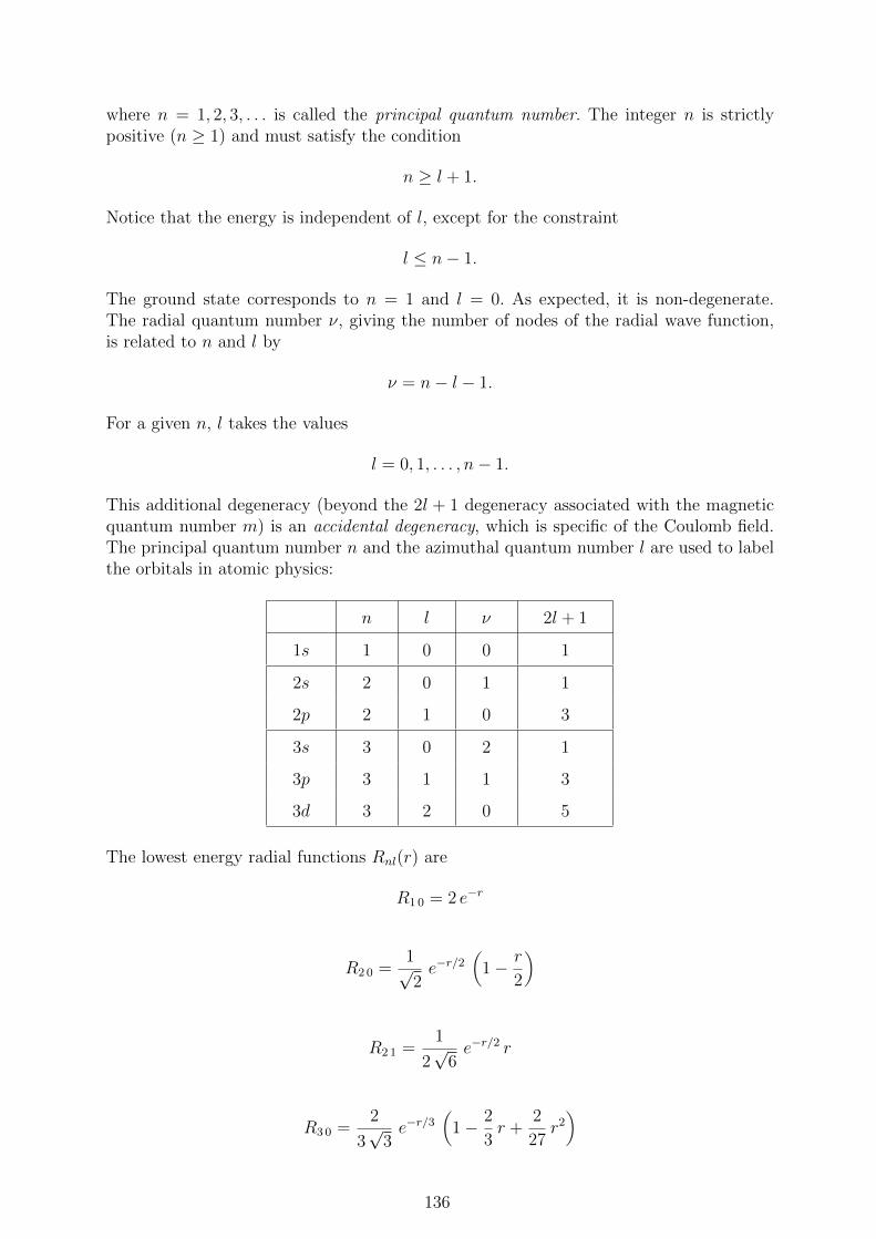
where n = 1, 2, 3, . . . is called the principal quantum number. The integer n is strictlypositive (n ≥ 1) and must satisfy the condition

n ≥ l + 1.

Notice that the energy is independent of l, except for the constraint

l ≤ n− 1.

The ground state corresponds to n = 1 and l = 0. As expected, it is non-degenerate.The radial quantum number ν, giving the number of nodes of the radial wave function,is related to n and l by

ν = n− l − 1.

For a given n, l takes the values

l = 0, 1, . . . , n− 1.

This additional degeneracy (beyond the 2l + 1 degeneracy associated with the magneticquantum number m) is an accidental degeneracy, which is specific of the Coulomb field.The principal quantum number n and the azimuthal quantum number l are used to labelthe orbitals in atomic physics:

n l ν 2l + 1

1s 1 0 0 1

2s 2 0 1 1

2p 2 1 0 3

3s 3 0 2 1

3p 3 1 1 3

3d 3 2 0 5

The lowest energy radial functions Rnl(r) are

R1 0 = 2 e−r

R2 0 =1√2e−r/2

(1− r

2

)

R2 1 =1

2√6e−r/2 r

R3 0 =2

3√3e−r/3

(1− 2

3r +

2

27r2

)

136

R3 1 =8

27√6e−r/3 r

(1− 1

6r)

R3 2 =4

81√30

e−r/3 r2.

The reader may wish to verify that the general properties discussed in the previous sectionare fulfilled.

9 Identity of particles

The physical world and in particular atoms, molecules and solids are made of many inter-acting particles. In principle the N body wave function Ψ(x1 . . . xN) and the Schrodingerequation i~∂Ψ

∂t= HΨ contain all the information for describing the physical states of

a given system of N identical particles and their time evolution. However, neither theSchrodinger equation is easy to solve in general nor the wave function Ψ(x1 . . . xN) ap-pears to be the most practical representation of many-particle states. The representationin terms of occupation numbers usually known as second quantization provides a muchmore appropriate framework. Most of the theoretical developments on the many-bodyproperties of matter rely on this approach.

Second quantization is a formalism in which the occupation numbers of an arbitrarycomplete set of single-particle states play the role of independent variables, instead ofthe coordinates xi of the individual particles, as in the usual wave function Ψ(x1 . . . xN).The transitions between different many-particle states can be visualized as changes inthe occupations of simpler single-particle orbitals. This is particularly useful in order toformulate, visualize and understand the fundamental physical processes defining the elec-tronic and magnetic properties of matter. For instance, the relevant orbitals responsiblefor chemical bonding, optical transitions, conductivity, magnetism etc. can be focused byan appropriate choice of the single-particle basis. The most important interactions andenergy scales can then be readily identified. In the following we discuss the principle ofindistinguishability of identical particles and its consequences on the symmetry of many-body wave functions. A detailed discussion of second quantization may be found in thebooks by Landau & Lifshitz or Fetter & Wallecka [2,6] or in the lecture notes on QuantumMechanics II (http://www.physik.uni-kassel.de/pastor).

9.1 The principle of indistinguishability of identical particles

In classical physics the particles preserve their individuality despite having the same phys-ical properties. A “numbering” of the particles is possible with which one can follow thetrajectory of each particle individually along its path. This applies, whatever the numberof particles is, and in particular for particles that are exactly identical in all respects. Inquantum mechanics the situation is entirely different, since the notion of deterministicpath ceases to have any meaning as a consequence of Heisenberg’s uncertainty principle.Even if a numbering of the particles were possible at some time, for example if we measurethe position of each particle in the system at time t, there is no possibility of tracking thepositions of the particles at any future (or past) time t′ > t (t′ < t), since the coordinates

137

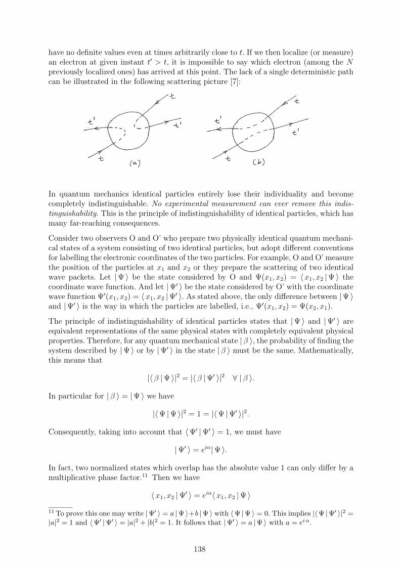
have no definite values even at times arbitrarily close to t. If we then localize (or measure)an electron at given instant t′ > t, it is impossible to say which electron (among the Npreviously localized ones) has arrived at this point. The lack of a single deterministic pathcan be illustrated in the following scattering picture [7]:

In quantum mechanics identical particles entirely lose their individuality and becomecompletely indistinguishable. No experimental measurement can ever remove this indis-tinguishability. This is the principle of indistinguishability of identical particles, which hasmany far-reaching consequences.

Consider two observers O and O’ who prepare two physically identical quantum mechani-cal states of a system consisting of two identical particles, but adopt different conventionsfor labelling the electronic coordinates of the two particles. For example, O and O’ measurethe position of the particles at x1 and x2 or they prepare the scattering of two identicalwave packets. Let |Ψ 〉 be the state considered by O and Ψ(x1, x2) = 〈x1, x2 |Ψ 〉 thecoordinate wave function. And let |Ψ′ 〉 be the state considered by O’ with the coordinatewave function Ψ′(x1, x2) = 〈x1, x2 |Ψ′ 〉. As stated above, the only difference between |Ψ 〉and |Ψ′ 〉 is the way in which the particles are labelled, i.e., Ψ′(x1, x2) = Ψ(x2, x1).

The principle of indistinguishability of identical particles states that |Ψ 〉 and |Ψ′ 〉 areequivalent representations of the same physical states with completely equivalent physicalproperties. Therefore, for any quantum mechanical state | β 〉, the probability of finding thesystem described by |Ψ 〉 or by |Ψ′ 〉 in the state | β 〉 must be the same. Mathematically,this means that

|〈 β |Ψ 〉|2 = |〈 β |Ψ′ 〉|2 ∀ | β 〉.

In particular for | β 〉 = |Ψ 〉 we have

|〈Ψ |Ψ 〉|2 = 1 = |〈Ψ |Ψ′ 〉|2.

Consequently, taking into account that 〈Ψ′ |Ψ′ 〉 = 1, we must have

|Ψ′ 〉 = eiα|Ψ 〉.

In fact, two normalized states which overlap has the absolute value 1 can only differ by amultiplicative phase factor.11 Then we have

〈x1, x2 |Ψ′ 〉 = eiα〈x1, x2 |Ψ 〉11 To prove this one may write |Ψ′ 〉 = a |Ψ 〉+b |Ψ 〉 with 〈Ψ |Ψ 〉 = 0. This implies |〈Ψ |Ψ′ 〉|2 =|a|2 = 1 and 〈Ψ′ |Ψ′ 〉 = |a|2 + |b|2 = 1. It follows that |Ψ′ 〉 = a |Ψ 〉 with a = ei α.

138

or

Ψ′(x1, x2) = eiαΨ(x1, x2),

and thus

Ψ(x2, x1) = eiαΨ(x1, x2).

By repeating the interchange we obtain

Ψ(x1, x2) = eiαΨ(x2, x1) = e2iαΨ(x1, x2),

which implies that e2iα = 1 or eiα = ±1. One concludes that

Ψ(x1, x2) = ±Ψ(x2, x1).

In other words, the wave function of two identical particles is either symmetric or anti-symmetric with respect to the interchange of the two coordinates.

The previous arguments can immediately be generalized to any two particles xi, xj in anN -particle system. Therefore,

Ψ(x1, . . . xi, . . . xj, . . . xN) = ±Ψ(x1, . . . xj, . . . xi, . . . xN)

for all i and j. Since the particles are indistinguishable, the same sign holds for any twoparticles in the system. The wave function Ψ(x1, . . . xN) is either fully symmetrical orfully antisymmetrical with respect to the interchange of variables. The superposition ofstates with different symmetry is not possible, since the resulting wave function wouldneither be symmetrical nor antisymmetrical.

The particles in nature are thus divided in two disjoint groups. The particles havingsymmetrical wave functions are called bosons and are said to obey Bose-Einstein statistics.The particles with antisymmetrical wave functions are called fermions and are said toobey Fermi-Dirac statistics. The property of being a boson or a fermion is of course afundamental property that depends on the nature of the particle. Experiment shows thatthere is a one-to-one correspondance between the fermionic or bosonic character and theintrinsic spin of the particles: Bosons are particles with integer spin, while Fermions areparticles with half-integer spin. Most elementary particles are fermions (e−, e+, p, n).However, photons and a number of elementary excitations in condensed matter (phonons,magnons, etc.) are bosons.

In the case of complex particles (e.g., an α particle) the interchange of two particles canbe regarded as the simultaneous interchange of its constituents. Therefore, the statisticsof complex particles is fermionic if the number of elementary fermions in the particle isodd, or bosonic if the number of fermions is even. Thus, an α particle composed by twoprotons and two neutrons is a boson. 3He atoms are fermions while 4He atoms are bosons.This has crucial consequences on the low-temperature properties of these two isotopes.Notice that the integer/half-integer rule holds also for complex particles, since an even(odd) number of half-integer elementary particles corresponds to a total spin which isinteger (half-integer).

To conclude this section, let us consider the effect of an arbitrary permutation on thecoordinates. Let P : [1, N ] → [1, N ] be a permutation in the natural interval [1, N ] which

139

we denote by

P =

1 2 . . . N

P (1) P (2) . . . P (N)

or simply P = [P (1), P (2), . . . P (N)]. The order of the permutation O(P ) = p is definedas the number of transpositions required to bring the sequence [P (1), P (2), . . . P (N)] intothe normal ordering [1, 2, . . . N ]. For example,

P =

1 2 3

1 3 2

has p = 1, while P =

1 2 3

3 1 2

has p = 2.

It is then easy to see that for bosons

Ψ(xP (1), xP (2), . . . xP (N)

)= Ψ(x1, x2, . . . xN), (9.1)

while for fermions

Ψ(xP (1), xP (2), . . . xP (N)

)= (−1)p Ψ(x1, x2, . . . xN). (9.2)

This fundamental property of the many-particle wave function [Eq. (9.1) or (9.2)] hasmany far-reaching consequences for the properties of matter. In the case of Fermions itleads to the Pauli exclusion principle with which the structure of Mendeleev’s periodictable of the elements can be explained.

References

[1] K. Gottfried, Quantum Mechanics Volume I: Fundamentals(W. A. Benjamin Inc., New York, Amsterdam, 1966)

[2] L.D. Landau and E.M. Lifshitz, Quantum Mechanics (Non-relativistic Theory)(Butterworth-Heinemann, Oxford, 1958)

[3] C. Cohen-Tannoudji, B. Diu and F. Laloe, Quantenmechanik, Band 1(De Gruyter, Berlin, 2008)

[4] G. B. Arfken and H. J. Weber, Mathematical Methods for Physicists (Elsevier, 2005)

[5] F. Schwabl, Quantenmechanik (QM I), (Springer, Berlin/Heidelberg/New York, 2005)

[6] A. L. Fetter and J. D. Wallecka, Quantum Theory of Many-particle systems(Mc Graw Hill, San Farncisco, 1971); Reprinted by Dover, Mineola, 2003.

[7] J.J. Sakurai, Modern Quantum Mechanics (Addison Wesley, 1985)

Acknowledgement

Die Vorbereitung dieses Skriptes ist nur durch die sorgfaltige und interessierte Mitarbeit vonFrau Andrea Wecker moglich gewesen, wofur der Autor und hoffentlich auch der Leser sehrdankbar sind.

140

Appendix: Systems of units

The cgs Gaussian system

Throughout this lecture and the associated exercises we will try to stick to the cgs (centimeter-gram-second) system in the Gaussian version for electromagnetic units. The Maxwell equationsthus take the form

~∇ · ~D = 4πρ

~∇× ~H =4π

c~J +

1

c

∂ ~D

∂t

~∇ · ~B = 0

~∇× ~E +1

c

∂ ~B

∂t= 0.

The Lorentz force per unit charge is given by~F

q= ~E +

~v

c× ~B.

The following are the units corresponding to some important physical magnitudes:

[Energy] = ergs = erg

[Charge] = electrostatic unit = esu = statcoulomb = statC

1 Coulomb = 1 C = 3 × 109 statC

[Potential] = statV = 1 erg/esu

[Current] = statA = esu/s

[Current density] = statA/cm2

Some physical constants in Gaussian units:

Bohr radius a0 =~2

me2= 0.529 A = 5.29× 10−9 cm

Electron mass = me = 9.109× 10−28 g

Electron charge = e = 4.803× 10−10 esu

Planck constant ~ =h

2π= 1.054× 10−27 erg × s

c = 2.998× 1010 cm/s

The dimensionless fine structure constant is α =e2

~ c∼= 1

137.

Atomic units

A very practical unit system for the calculations, particularly if one focuses on the properties ofelectrons, is the system of atomic units denoted by au. In this system the following fundamentalphysical constants are set equal to 1:

Electron charge e = 1 au

Electron mass me = 1 au

Planck’s constant ~ =h

2π= 1 au

The Bohr radius a0 =~2

me2= 1 au = 5.29× 10−9 cm = 0.529 A becomes the

unit of length.

141

The Hartree, i.e., twice the ionization energy of the H atom, is given by

Eh =me4

~2=

e2

a0=

~2

ma02= 1 au = 27, 2 eV = 4.36× 10−11 erg = 2 Ry

Finally, 1 eV = 1.6× 10−19 J = 1.6× 10−12 erg.

142

Table of Contents

1 Fundamental concepts of classical mechanics 1

1.1 Dynamics of a single particle: Newton’s second law . . . . . . . . . . . . . . . 1

1.2 Constants of motion . . . . . . . . . . . . . . . . . . . . . . . . . . . . . . . . 2

1.2.1 Linear momentum . . . . . . . . . . . . . . . . . . . . . . . . . . . . 2

1.2.2 Angular momentum . . . . . . . . . . . . . . . . . . . . . . . . . . . . 3

1.2.3 Energy conservation: Kinetic and potential energy . . . . . . . . . . . 3

1.3 Hamiltonian and Hamilton equations for a single particle . . . . . . . . . . . 5

1.4 Symmetry and conservation laws . . . . . . . . . . . . . . . . . . . . . . . . . 7

1.5 Many-particle systems . . . . . . . . . . . . . . . . . . . . . . . . . . . . . . . 8

1.5.1 Linear momentum . . . . . . . . . . . . . . . . . . . . . . . . . . . . 9

1.5.2 Angular momentum . . . . . . . . . . . . . . . . . . . . . . . . . . . . 9

1.5.3 Energy conservation . . . . . . . . . . . . . . . . . . . . . . . . . . . 10

2 Basic concepts of quantum mechanics 13

2.1 Electromagnetic waves . . . . . . . . . . . . . . . . . . . . . . . . . . . . . . . 13

2.2 Non-classical aspects of the electromagnetic field: Photons . . . . . . . . . . 17

2.2.1 The photoelectric effect . . . . . . . . . . . . . . . . . . . . . . . . . . 17

2.2.2 The Compton effect . . . . . . . . . . . . . . . . . . . . . . . . . . . . 18

2.2.3 Young interference experiment . . . . . . . . . . . . . . . . . . . . . . 20

2.3 Non-classical properties of particles having finite rest mass:The uncertainty principle . . . . . . . . . . . . . . . . . . . . . . . . . . . . . 23

3 Fundamental mathematical formalism 27

3.1 The wave function . . . . . . . . . . . . . . . . . . . . . . . . . . . . . . . . . 27

3.2 The superposition principle . . . . . . . . . . . . . . . . . . . . . . . . . . . . 28

3.3 The wave function and the measurements of the coordinates . . . . . . . . . 30

3.4 Observables . . . . . . . . . . . . . . . . . . . . . . . . . . . . . . . . . . . . . 31

3.5 Inner product . . . . . . . . . . . . . . . . . . . . . . . . . . . . . . . . . . . 35

3.6 Kets and Bras . . . . . . . . . . . . . . . . . . . . . . . . . . . . . . . . . . . 36

3.7 Operators . . . . . . . . . . . . . . . . . . . . . . . . . . . . . . . . . . . . . . 38

3.7.1 Position, momentum and kinetic energy operators . . . . . . . . . . . 40

3.8 Properties of physical operators . . . . . . . . . . . . . . . . . . . . . . . . . 41

3.9 Sums, products and commutators of operators . . . . . . . . . . . . . . . . . 45

3.10 Dirac’s delta function δ(x) . . . . . . . . . . . . . . . . . . . . . . . . . . . . 48

3.10.1 Fourier integral representation of δ(x) . . . . . . . . . . . . . . . . . 50

3.10.2 Representation of δ(x) by a complete basis of orthonormal functions 50

3.11 The continuum spectrum . . . . . . . . . . . . . . . . . . . . . . . . . . . . . 51

4 Quantum dynamics 56

4.1 The Hamilton operator . . . . . . . . . . . . . . . . . . . . . . . . . . . . . . 56

4.2 Stationary states . . . . . . . . . . . . . . . . . . . . . . . . . . . . . . . . . . 57

4.3 Conserved quantities . . . . . . . . . . . . . . . . . . . . . . . . . . . . . . . . 58

4.4 Degenerate energy levels . . . . . . . . . . . . . . . . . . . . . . . . . . . . . 58

4.5 Finite vs. infinite motion . . . . . . . . . . . . . . . . . . . . . . . . . . . . . 59

4.6 The Schrodinger equation . . . . . . . . . . . . . . . . . . . . . . . . . . . . . 59

4.7 The variational principle . . . . . . . . . . . . . . . . . . . . . . . . . . . . . 61

4.8 Properties of the Schrodinger equation and stationary wave functions . . . . 62

4.9 Motion in one dimension: The square potential well . . . . . . . . . . . . . . 64

143

4.10 Summary of quantum dynamics . . . . . . . . . . . . . . . . . . . . . . . . . 674.10.1 The time-dependent Schrodinger equation . . . . . . . . . . . . . . . 674.10.2 Stationary states . . . . . . . . . . . . . . . . . . . . . . . . . . . . . 674.10.3 The energy spectrum . . . . . . . . . . . . . . . . . . . . . . . . . . . 684.10.4 The variational principle . . . . . . . . . . . . . . . . . . . . . . . . . 684.10.5 Properties of the stationary Schrodinger equation . . . . . . . . . . . 69

4.11 The square potential well . . . . . . . . . . . . . . . . . . . . . . . . . . . . . 704.12 General properties of one-dimensional systems . . . . . . . . . . . . . . . . . 734.13 Transmission and reflection coefficients . . . . . . . . . . . . . . . . . . . . . 754.14 Time dependence of observables and operators . . . . . . . . . . . . . . . . . 784.15 Velocity and acceleration: Ehrenfest theorem . . . . . . . . . . . . . . . . . . 804.16 The probability current density . . . . . . . . . . . . . . . . . . . . . . . . . . 824.17 The time-evolution operator . . . . . . . . . . . . . . . . . . . . . . . . . . . 834.18 The Schrodinger and Heisenberg pictures . . . . . . . . . . . . . . . . . . . . 854.19 The uncertainty relation for arbitrary observables . . . . . . . . . . . . . . . 894.20 The energy-time uncertainty relation . . . . . . . . . . . . . . . . . . . . . . 93

5 The harmonic oscillator 955.1 The classical oscillator . . . . . . . . . . . . . . . . . . . . . . . . . . . . . . . 955.2 The quantum oscillator . . . . . . . . . . . . . . . . . . . . . . . . . . . . . . 965.3 Some properties of the stationary kets . . . . . . . . . . . . . . . . . . . . . . 1005.4 The eigenfunctions . . . . . . . . . . . . . . . . . . . . . . . . . . . . . . . . . 101

6 Angular momentum 1046.1 Definition and commutation rules . . . . . . . . . . . . . . . . . . . . . . . . 1046.2 Translations and rotations . . . . . . . . . . . . . . . . . . . . . . . . . . . . 1066.3 Angular momentum operator in spherical coordinates . . . . . . . . . . . . . 109

6.4 Eigenvalues and eigenstates of ~l . . . . . . . . . . . . . . . . . . . . . . . . . 1116.5 Angular momentum operator in spherical coordinates . . . . . . . . . . . . . 116

7 Spin 1217.1 Addition of angular momentum . . . . . . . . . . . . . . . . . . . . . . . . . 1247.2 The recursion relation for the Clebsch-Gordan coefficients . . . . . . . . . . . 129

8 The central symmetric field 1318.1 General formulation . . . . . . . . . . . . . . . . . . . . . . . . . . . . . . . . 1318.2 Properties of the motion in a spherical potential . . . . . . . . . . . . . . . . 1348.3 The Coulomb field . . . . . . . . . . . . . . . . . . . . . . . . . . . . . . . . . 135

9 Identity of particles 1379.1 The principle of indistinguishability of identical particles . . . . . . . . . . . 137

References 140

144