UNIVERSITÄT LINZJOHANNES KEPLER

JKU

Technisch-Naturwissenschaftliche

Fakultät

Relations between Gröbner bases,differential Gröbner bases, and differential

characteristic sets

MASTERARBEIT

zur Erlangung des akademischen Grades

Diplomingenieur

im Masterstudium

Computermathematik

Eingereicht von:

Christian Aistleitner

Angefertigt am:

Institut für Symbolisches Rechnen

Beurteilung:

Univ.-Prof. DI. Dr. Franz Winkler

Linz, Dezember 2010

Cover sheet template taken from [36].

This thesis was typeset using the Emacs [13], Inkscape [26], graphviz [20], xfig [46], andTeX Live [41] software packages on a Gentoo [17] GNU [18] / Linux [29] system.

This work was partially supported by the Austrian Science Foundation (FWF) under theproject DIFFOP (P20336-N18) and Doctoral Program “Computational Mathematics”(W1214), project DK11.

Abstract

While Gröbner bases classically focus on purely algebraic settings, Gröbner basis lit-erature followed the general trend of the last decades to also incorporate differentialsettings, which resulted in the notion of differential Gröbner bases. In the differentialsetting, there is also the much older, but different notion of differential characteristicsets. Although those three methods of elimination theory are closely related, literaturedoes not provide a comparison of those methods.

The main contribution of this thesis is such a comparison.

Additionally, we give a presentation of Gröbner bases, differential Gröbner bases, anddifferential characteristic sets using a unified notation system that allows to easily iden-tify and exhibit differences and matches between the different methods.

5

To the Studien- und Prüfungsabteilung’s(now Prüfungs- und Anerkennungsservice)

support during my studies.

Contents

Abstract 5

Notation 11

Conventions 17

1 Introduction 19

2 Setting 21

2.1 Algebraic notions . . . . . . . . . . . . . . . . . . . . . . . . . . . . . . . 21

2.2 Differential notions . . . . . . . . . . . . . . . . . . . . . . . . . . . . . 22

2.3 Saturation ideals . . . . . . . . . . . . . . . . . . . . . . . . . . . . . . 24

3 Simplifying systems of algebraic equations using elimination theory 27

3.1 Resultants . . . . . . . . . . . . . . . . . . . . . . . . . . . . . . . . . . 28

3.2 Gröbner bases . . . . . . . . . . . . . . . . . . . . . . . . . . . . . . . . 29

3.3 Characteristic sets . . . . . . . . . . . . . . . . . . . . . . . . . . . . . . 31

3.4 Comparison of different methods . . . . . . . . . . . . . . . . . . . . . 32

4 Gröbner bases in algebraic polynomial rings 35

4.1 Algebraic reduction . . . . . . . . . . . . . . . . . . . . . . . . . . . . . 35

4.2 Gröbner bases and their properties . . . . . . . . . . . . . . . . . . . . 38

5 Differential characteristic sets 43

5.1 Definition via being differentially pseudo-reduced . . . . . . . . . . . . 43

5.2 Pseudo-remainders and differential characteristic sets . . . . . . . . . . 46

5.3 Coherence . . . . . . . . . . . . . . . . . . . . . . . . . . . . . . . . . . 49

5.4 Characteristic decomposition . . . . . . . . . . . . . . . . . . . . . . . . 52

6 Differential Gröbner bases 55

6.1 Differential Gröbner bases following Carrà Ferro and Ollivier . . . . . . 55

6.2 Differential Gröbner bases following Mansfield . . . . . . . . . . . . . . 60

9

7 Comparing Gröbner bases and characteristic set methodology 65

7.1 Classification of different approaches . . . . . . . . . . . . . . . . . . . 65

7.2 Comparison of equivalences . . . . . . . . . . . . . . . . . . . . . . . . 66

7.3 Integration into computer algebra systems . . . . . . . . . . . . . . . . 69

8 Conclusion 71

A Differential pseudo-reduction 73

B Refinements of rankings 79

List of Definitions 85

List of Theorems 87

List of Examples 89

List of Figures 91

List of Tables 93

References 95

10

Notation

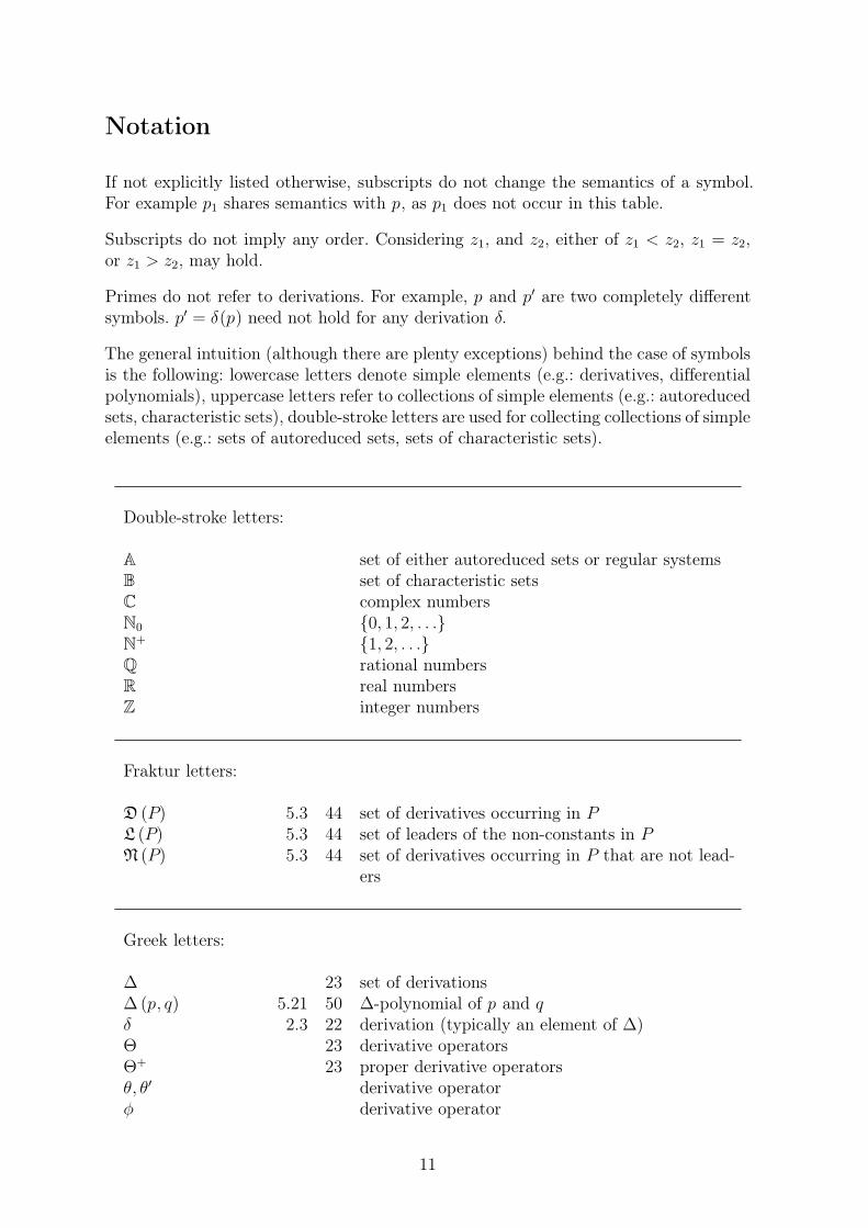
If not explicitly listed otherwise, subscripts do not change the semantics of a symbol.For example p1 shares semantics with p, as p1 does not occur in this table.

Subscripts do not imply any order. Considering z1, and z2, either of z1 < z2, z1 = z2,or z1 > z2, may hold.

Primes do not refer to derivations. For example, p and p′ are two completely differentsymbols. p′ = δ(p) need not hold for any derivation δ.

The general intuition (although there are plenty exceptions) behind the case of symbolsis the following: lowercase letters denote simple elements (e.g.: derivatives, differentialpolynomials), uppercase letters refer to collections of simple elements (e.g.: autoreducedsets, characteristic sets), double-stroke letters are used for collecting collections of simpleelements (e.g.: sets of autoreduced sets, sets of characteristic sets).

Double-stroke letters:

A set of either autoreduced sets or regular systemsB set of characteristic setsC complex numbersN0 {0, 1, 2, . . .}N+ {1, 2, . . .}Q rational numbersR real numbersZ integer numbers

Fraktur letters:

D (P) 5.3 44 set of derivatives occurring in PL (P) 5.3 44 set of leaders of the non-constants in PN (P) 5.3 44 set of derivatives occurring in P that are not lead-

ers

Greek letters:

∆ 23 set of derivations∆(p, q) 5.21 50 ∆-polynomial of p and qδ 2.3 22 derivation (typically an element of ∆)Θ 23 derivative operatorsΘ+ 23 proper derivative operatorsθ, θ′ derivative operatorφ derivative operator

11

Latin letters:

A 5.7 45 autoreduced seta, a′ elements of Aapredp(p, q) 5.5 44 p is algebraically pseudo-reduced with respect to qaredp (p, q) 4.3 36 p is algebraically reduced with respect to pareds (p, P) 4.3 36 p is algebraically reduced with respect to Paredt (p, t, q) 4.3 36 p is algebraically reduced with respect to t and paremstepp (p, p′, q) 4.4 37 q is the result of a single algebraical remainder step

of p with respect to p′

aremsteps (p, P, q) 4.4 37 q is the result of a single algebraical remainder stepof p with respect to P

aremstept (p, t, p′, q) 4.4 37 q is the result of a single algebraical remainder stepof p with respect to t and p′

aremsws (p, P, q) 4.5 37 q is an algebraic stepwise remainder of p with re-spect to P

C 5.9 45 autoreduced set (typically a characteristic set)ComMonoid (X) 21 commutative monoid generated by Xc constant, or coefficientcoeffI(p, z, d) 17 coefficient of p (as univariate polynomial in z) with

respect to zd

coeffT(p, t) 17 coefficient of p with respect to t via evaluation ofp (as function from indeterminates to ground field)at t

d element of N0 ∪{−∞} to denote the degree ofsome polynomial in an indeterminate

degz(p) 17 degree of the polynomial p in the indeterminate zdpredas(p, P) 5.8 45 p is differentially pseudo-reduced with respect to

Adpredp(p, q) 5.6 44 p is differentially pseudo-reduced with respect to qdpreds(p, P) 5.8 45 p is differentially pseudo-reduced with respect to

Pdpremas(p,A, q) 5.14 48 q is a differential pseudo-remainder of p with re-

spect to Adpremras(p,A, q) 5.13 48 q is a respectful differential pseudo-remainder of p

with respect to AdpremMstepd (p, p′, θ′, q)

6.12 62 q is the result of a single differential pseudo-remainder Mansfield step of p with respect to θ′,and p′

dpremMstepp (p, p′, q)6.12 62 q is the result of a single differential pseudo-

remainder Mansfield step of p with respect to p′

dpremMsteps (p, P, q)6.12 62 q is the result of a single differential pseudo-

remainder Mansfield step of p with respect to P

12

dpremMsws (p, P, q)6.13 63 q is differential stepwise pseudo-remainder of p

with respect to Mansfield steps and Pdredp (p, q) 6.3 57 p is differentially reduced with respect to qdreds (p, P) 6.3 57 p is differentially reduced with respect to Pdremdis (p, P, q) 6.4 57 q is a differential remainder of p with respect to

the differential ideal generated by Pdremsws (p, P, q) 6.5 58 q is a differential stepwise remainder of p with re-

spect to PF 21 field having characteristic zeroF [X] polynomial ring over F in the indeterminates XF{Y } 23 differential polynomial ring over F in the differen-

tial indeterminates Y and the derivations ∆g, g′ element of G, or G′

G, G′ set of polynomials that are a Gröbner basis (inAppendix A the set to generate the ideal for thecongruence equation)

gcd (p, q) greatest common divisor of p and qHP 5.12 47 set of initials and separants of PH∞

P smallest multiplicatively closed set containing 1and the initials and separants of P. To be readas (HP)

∞. Compare HP and H∞.H∞ 2.13 24 smallest multiplicatively closed set containing 1

and the elements of HHo o 26 set of factors of H∞

h element of H or H ′

I 23 index set for YIP 5.12 47 set of initials of Pi, i′ element of Iinit(p) 5.11 47 initial of pJ idealj element of Jk index (typically ranging over a subset of N0)lc (p) 4.2 36 leading coefficient of plcdD

(

yi,θ , yi,θ′)

5.19 50 least common derivative of yi,θ and yi,θ′lcdP (p, q) 5.20 50 least common derivative of p and qlcm (t, s) least common multiple of t and slead(p) 5.2 43 highest ranking indeterminate occurring in pltp (p) 4.2 36 leading term of plts (P) 4.2 36 set of leading terms in PM set of polynomials, whose separants and initials are

used for premultiplication when pseudo-reducingm 23 number of elements in ∆n 23 number of elements in I, respectively Yord(θ) B.1 79 total order of the derivative operator θordδ(θ) B.1 79 order of the derivative operator θ with respect to

the derivation δp, p′ polynomial

13

pdpredas(p,A) 5.8 45 p is partially differentially pseudo-reduced with re-spect to A

pdpredp(p, q) 5.4 44 p is partially differentially pseudo-reduced with re-spect to q

pdpreds(p, P) 5.8 45 p is partially differentially pseudo-reduced with re-spect to P

pseudoS (p, q) 5.18 50 pseudo-S-polynomial of p and qq polynomialR 17 ringResz(p, q) 28 resultant of p and q with respect to zr, r′ element of RSP 5.12 47 set of separants of PS (p, q) 4.6 38 S-polynomial of p and qs termsep(p) 5.11 47 separant of pT 4.2 36 set of termsTerms (p) 4.2 36 set of terms occurring in pt termu termX 21 set of indeterminatesY 23 family (yi)i∈Iyi either an element of Y or a short-hand notation

for yi,1yi,θ derivativeZ subset of (yi,θ)i∈I,θ∈Θz, z′ indeterminate (typically an element of X, or

(yi,θ)i∈I,θ∈Θ)

Lines along symbols:

PΘ

2.6 23 differential closure of P

PΘ,<z

5.22 51 PΘ

with derivatives bounded by z|P| number of elements in P

Punctuation:

J : H∞ 2.14 25 saturation of J by H

Parentheses:

R (X) algebraic extension of the ring R by the elementsof X

〈P〉 21 algebraic ideal generated by P in F{Y }〈P〉R 21 algebraic ideal generated by P in R

14

〈〈P〉〉 21 radical algebraic ideal generated by P in F{Y }〈〈P〉〉R 21 radical algebraic ideal generated by P in R[P] 2.8 23 differential ideal generated by P in F{Y }R [X] algebraic polynomial ring over R in X[[P]] 2.10 24 radical differential generated by P in F{Y }F{Y } 23 differential polynomial ring over F with differen-

tial indeterminates Y and the derivations ∆|P| number of elements in P

15

Conventions

Besides the conventions for symbols listed on page 11, we use the following conventionson basic mathematics, and layout.

• We use “ring” to refer to a commutative ring with identity.

• For polynomial rings we use “term” to denote a finite product of the polynomialring’s indeterminates (an indeterminate may occur more than once in such aproduct). We use “monomial” for the product of a term with an element of theground field.

• We consider the result of empty operations as the neutral element with respectto this operation in the structure of interest. So for example,

2∑

k=3

r = 02∏

k=3

r = 1⋂

h∈∅

hp = F{Y }, (1)

for some r ∈ Z, and p ∈ F{Y }.

• We use degz(p) to denote the degree of p in z, where p is a not necessary univariatepolynomial and z a indeterminate of p’s polynomial ring. We set the degree of 0to −∞, and ∀k ∈ N0 : −∞ < k. For example, considering 0, 3, and y43y

21 + 4 in

Q [y1, y2, y3], then

degy1(

y43y21 + 4

)

= 2 degy2(

y43y21 + 4

)

= 0 (2)

degy1(3) = 0 degy1(0) = −∞. (3)

• In this thesis, we are in the unfortunate situation to combine two different branchesof literature each using a different concept of coefficients. Hence, we introducethem both. The first variant (coeffT) interprets polynomials as functions from theterms to the ground field and evaluates such a function at a term. For examplein Q [y1, y2, y3] with p := 2 + 11y21 + y2 + 3y21y2y3 + 7y21y3, we obtain

coeffT

(

p, y21y3)

:= 7 coeffT

(

p, y21)

:= 11 (4)

coeffT(p, y3) := 0 coeffT(p, 1) := 2. (5)

coeffT computes the coefficient with respect to a (possibly multivariate) term.

The second variant (coeffI) reinterprets a polynomial ring F [X] as univariatepolynomial ring for a given indeterminate z (i.e.: F [X\ {z}] [z]) and computes thecoefficient of zd in this domain, for a given degree d. Reconsidering the previousexample we obtain

coeffI(p, y1, 2) := 11 + 3y2y3 + 7y3 (6)

coeffI(p, y3, 1) := 3y21y2 + 7y21 coeffI(p, y1, 0) := 2 + y2. (7)

coeffI computes the coefficient with respect to an indeterminate and a correspond-ing degree.

17

• We did not only attach numbers to formulas, which we reference, but we attachednumbers to any formula, when space allowed it. Thereby, we make it easier toreference equations in discussions about this thesis.

• For most definitions, and theorems we provide references to literature (the “com-pare” part). The term “compare” in those references really means “compare” anddoes not automatically imply, we took the result unmodified from there. Instead,the given references are in the spirit of our definitions, and theorems.

18

1 Introduction

In this thesis, we relate three important concepts of computer algebra: Gröbner bases,differential Gröbner bases, and differential characteristic sets. All three concepts are partof elimination theory and allow to simplify systems of equations. These simplificationsmay for example lower the degree of certain indeterminates or decouple equations. Suchsimplifications typically aid when trying to solve a system of equations.

As of writing this thesis, Gröbner basis is not only the most prominent among the threeconcepts, but also undoubtedly constitutes an integral part of computer algebra, asfor example the Gröbner basis bibliography [7] documents over 1000 scientific articles,books, etc. on the topic of Gröbner bases.

While Gröbner basis are typically applied to systems of equations in algebraic polyno-mial rings, Gröbner basis literature provides generalizations in various directions rang-ing for example from non-commutative settings (e.g.: [33]) to differential polynomialrings (e.g.: [8]).

As current research in computer algebra seems to progress towards treating not onlyalgebraic equations (as in typical Gröbner basis settings), but also differential equa-tions, especially the abstractions of Gröbner bases towards differential polynomial ringsmay be expected to gain relevance. While some researchers work in this direction (e.g.:Aleksey Zobnin), it seems that the theory of differential characteristic sets (which is aconcept predating Gröbner bases, operating in differential polynomial rings, having sim-ilar applications as Gröbner bases) gained more momentum over the last two decades.Nevertheless, we do not know of any research trying to explicitly relating those threemethods: Gröbner bases, differential Gröbner bases, and differential characteristic sets.In this thesis we give such a comparison.

In Section 2, we present the basic setting of this thesis and introduce notation foralgebraic and differential polynomial rings. Using this notation, we motivate the useand importance of Gröbner bases in Section 3, where we show how elimination theorymay help to solve systems of algebraic equations using resultants, Gröbner bases, andcharacteristic sets.

After those precursory parts, we present Gröbner bases in Section 4, followed by differ-ential characteristic sets in Section 5. Finally, we introduce differential Gröbner bases inSection 6. Section 7 compares Gröbner bases, differential Gröbner bases, and differentialcharacteristic sets.

While the individual sections are meant to be read sequentially, readers already familiarwith Gröbner bases, differential Gröbner bases, and differential characteristic sets mayskip directly to Section 7—the used notation is given in tabular form on page 11.

19

2 Setting

In this section, we present the mathematical setting of this thesis. While we presentthe notations ordered by their semantics, a condensed presentation of the used notationordered by the symbols can be found on page 11 in tabular form.

We begin by presenting the algebraic notions, followed by the notions for differentialaspects of polynomial rings. The third and last part of this section discusses saturationideals.

2.1 Algebraic notions

Throughout this thesis, let F refer to a field having characteristic zero. F typically actsas coefficient domain for the used polynomial rings.

For any set P, we use ComMonoid (P) to denote the commutative monoid generated byP1. We use 1 as neutral element of this monoid.

By R [X] we refer to the polynomial ring over R in X, where R is a ring, and X is a(not necessarily finite) set that is algebraically independent over R.

From now on, let X be an algebraically independent set over F . X may be finite, butit need not be finite.

To denote the ideal generated in a ring R by a set P ⊆ R2, we use 〈P〉R . If R = F{Y }3,we may omit the subscript and denote 〈P〉R by 〈P〉.

For the radical ideal generated in a ring R by a set P ⊆ R, we use 〈〈P〉〉R 4. If R = F{Y },we may again omit the subscript and denote 〈〈P〉〉R by 〈〈P〉〉.

The two main theorems for algebraic polynomial rings used in this thesis are Hilbert’s ba-sis theorem (Theorem 2.1) and Hilbert’s Nullstellensatz (Theorem 2.2). While Hilbert’s

1We later also introduce P∞ for the commutative monoid generated by P. While bothComMonoid (P) , and P∞ result in the same mathematical object, there is a slight but crucial se-mantic difference between them, as we argue in Section 2.3.

2Although the observation also holds for the rest of this thesis, we want to emphasize here that by“⊆” we mean any subset. Hence, P can be empty, finite, infinite and even the whole ring R itself.

3Although, we define F{Y } only later in Section 2.2, we already present 〈P〉 already here, to havethe notions for algebraic ideals in one place.

4The approach to denote generated radical ideals by doubling the ideal generating brackets withalmost no space in between comes from [22] for differential radical ideals as approach to avoid theclassical notation {P}, which leads to confusion between the set containing P and the radical differentialideal generated by P.

The alternative would be to use the√

sign, which however distorts the rendered text when encoun-tered in running text (“

√

[P]”).Hence, we adopted the approach of doubling the brackets and reducing the space between them and

thereby obtain a nicer looking representation in running text—while still not introducing ambiguity,as 〈〈P〉〉 (the ideal generated by the elements of the ideal generated by P; we never use this constructin this thesis, as the outer layer of angle brackets are redundant) differs from 〈〈P〉〉 (the radical idealgenerated by P) by its spacing and 〈〈P〉R〉R additionally differs from 〈〈P〉〉R in the subscript R betweenthe two closing brackets.

21

basis theorem asserts finite bases for ideals in polynomial rings in finitely many in-determinates, Hilbert’s Nullstellensatz bridges between radical ideals and solutions ofsystems of equations.

Theorem 2.1 (Hilbert’s basis theorem). [compare 45, Theorem 8.2.2, page 180] If Xis finite, then every ideal in F [X] has a finite basis.

Theorem 2.2 (Hilbert’s Nullstellensatz). [compare 45, Theorem 8.4.2, page 190] LetF be an algebraically closed field and J be an ideal in the polynomial ring F [X] suchthat J 6= F [X]. Then the radical of J contains exactly those polynomials vanishing onall the common roots of J .

After this presentation of the basic notions that we use in purely algebraic polynomialrings, we introduce the required notions of differential polynomial rings.

2.2 Differential notions

In this part we introduce differential polynomial rings along with ideals in them andfinally establish a basis theorem and a Nullstellensatz.

To define a differential polynomial ring it is essential to model the differential structure.Therefore, we start by a definition of derivation followed by a restriction to commutativederivations, before actually defining differential polynomial rings in Definition 2.5.

Definition 2.3 (Derivation). [compare 28, I, 1, page 58] Let R be a ring. A functionδ : R → R is called a derivation on R if and only if

∀r, r′ ∈ R : δ(r + r′) = δ(r) + δ(r′) (8)

and∀r, r′ ∈ R : δ(rr′) = δ(r) r′ + r δ(r′) . (9)

Definition 2.4 (Commuting derivations). Let R be a ring and ∆ a set of derivationson R. We refer to the derivations as being commutative if and only if

∀ δ1, δ2 ∈ ∆ ∀r ∈ R : δ1(δ2(r)) = δ2(δ1(r)) . (10)

While there exists elimination theory literature considering non-commuting derivations(e.g.: [24]), elimination theory literature typically only deals with commuting derivations.Hence, we also restrict ourselves to commuting derivations in this thesis.

Whenever, we use a set of derivations on some ring, we silently assume that thosederivations commute for the given ring.

Definition 2.5 (Differential polynomial ring). [compare 28, I, 6, page 70] Let I be afinite set, (yi,θ)i∈I,θ∈Θ be algebraically independent over the field F of characteristic zero,and let ∆ be a finite set of commuting derivations on F [(yi,θ)i∈I,θ∈Θ], using Θ as ab-breviation for ComMonoid (∆) . We call F [(yi,θ)i∈I,θ∈Θ] together with ∆ the differentialpolynomial ring over F in (yi)i∈I and ∆, if and only if

∀δ ∈ ∆ : δ|F is a derivation on F , (11)

22

and additionally

∀δ ∈ ∆ ∀i ∈ I ∀θ ∈ Θ : δ(yi,θ) = yi,δθ . (12)

For the rest of this thesis, let I denote a finite set, such that (yi,θ)i∈I,θ∈Θ is algebraicallyindependent over F . We use n to refer to |I| , and Y as abbreviation for (yi)i∈I .

Furthermore, let ∆ be a finite set of commuting derivations on F [(yi,θ)i∈I,θ∈Θ], such that(11), and (12) hold. We use m to refer to |∆| , Θ as abbreviation for ComMonoid (∆) ,and Θ+ to denote Θ\{1} . Finally, we denote the differential polynomial ring over F inY and ∆ by F{Y }.

From its definition, we see that F{Y } can be interpreted as polynomial ring F [X] whenignoring the differential structure of F{Y }, and choosing X = (yi,θ)i∈I,θ∈Θ. Typically,such an X is infinite. Nevertheless, this correspondence allows to carry notions we laterdevelop for purely algebraic polynomial rings (e.g.: the Terms operator of Definition 4.2)to differential polynomial rings. Wherever necessary, we silently take advantage of thiscorrespondence.

On the same note, we may use notions defined solely on F{Y } also on F [X] with finiteX, as for ∆ = ∅, F{Y } can be identified with F [X].

The elements of (algebraic) ideals in differential polynomial rings are closed under ad-dition and multiplications. However, they are not necessarily closed under derivations.We call ideals having this additional closure property differential ideals.

Definition 2.6 (Differential closure). Let P ⊆ F{Y }. We refer to the set

{p ∈ F{Y } | ∃q ∈ P ∧ ∃θ ∈ Θ : p = θ(q)} (13)

by the differential closure of P (or PΘ

5).

Definition 2.7 (Differential ideal). An ideal J in F{Y } is called differential ideal ifand only if

J = JΘ. (14)

Similarly, to how we generate (algebraic) ideals from a set, we can generate differentialideals from a set.

Definition 2.8 (Generated differential ideals). Let P be a subset of F{Y }. By [P] ,we denote the smallest subset of F{Y } containing P while being closed under applyingderivations, multiplication by elements of F{Y }, and addition.

Accordingly, radical differential ideals are differential ideals that are radical.

5While the notation PΘ

may seem cumbersome when viewed on its own, it is part of a moreexpressive, clear notation approach allowing differential closure along selection of only some elements[1, § 11.4, Definition 11.5, page 202]. From this general notation approach, we only introduce the those

two parts that are relevant in this thesis (PΘ

from Definition 2.6, and AΘ,<z

as used in Definition 5.22).

23

Definition 2.9 (Radical differential ideal). A differential ideal J in F{Y } is calledradical differential ideal if and only if J is a radical ideal (i.e.:

∀j ∈ F{Y } ∀k ∈ N+ :((

jk ∈ J)

=⇒ j ∈ J))

. (15)

Definition 2.10 (Generated, radical differential ideals). Let P be a subset of F{Y }.By [[P]], we denote the smallest subset of F{Y } containing P while being closed undertaking roots (i.e.: (15) holds), applying derivations, multiplication by elements of F{Y },and addition.

Before closing the introduction to basic notions around differential polynomial rings, weestablish a basis theorem and a Nullstellensatz, just as we did in Section 2.1. While thedifferential Nullstellensatz directly corresponds to the Hilbert’s Nullstellensatz (Theo-rem 2.2), there is no differential equivalent of Hilbert’s basis theorem (Theorem 2.1).Finite bases need not exist for arbitrary differential ideals. However, they exist forradical differential ideals, as stated by the Ritt Raudenbush basis theorem.

Theorem 2.11 (Ritt Raudenbush basis theorem). [compare 27, VII, § 27, Theorem7.1, page 45]6 For every radical ideal in F{Y }, there is a finite P ⊆ F{Y }, such thatJ = [[P]].

Theorem 2.12 (Differential Nullstellensatz). [compare 22, Theorem 2.7, page 8] LetF be an algebraically closed differential field and J be a differential ideal in F{Y } suchthat J 6= F{Y }. Then the radical of J contains exactly those polynomials vanishing onall the common roots of J .

The final part of Section 2 presents saturation ideals, which form an essential ingredientof differential characteristic set computations (Section 5).

2.3 Saturation ideals

In characteristic set literature, ideals are often encountered as saturation ideals, whichare denoted by an ideal followed by a colon (“:”) and another expression. In this section,we present the notion of saturation ideals, relate it to quotients and additionally presentan abstraction used in some modern differential characteristic set literature.

Before defining saturation ideals, we define a second variant of the commutative monoidgenerated by a set.

Definition 2.13 (Multiplicatively closed set with 1). Let H be a subset of F{Y }. ByH∞we denote the smallest multiplicatively closed subset of F{Y } such that 1 ∈ H∞ andH ⊆ H∞.

6While it might appear close to heresy to not give an reference to Raudenbush or probably themost influential use through [38, IX, § 7, last sentence on page 165] for the Ritt Raudenbush basistheorem, we are nevertheless convinced that the elaboration of [27, VII, § 27, Theorem 7.1, page 45]is very practical and also favor the immediate relation to the important decomposition theorem in [27,VII, § 29, page 48].

24

We previously introduced ComMonoid on page 21 to construct the commutative monoidgenerated by a set, and we see that H∞ = ComMonoid (H) for any H ⊆ F{Y }.However, the use and semantics of ComMonoid (H) and H∞ are different. While weuse ComMonoid (H) to construct general products of elements of H, H∞ carries theadditional semantic of being used to saturate ideals.

It is tempting to merge those two different notations and ignore the semantic difference.However, in differential characteristic set literature (the main application of saturatedideals in our thesis) some advances towards extending H∞ can be found, as we show lateron page 26. Those generalizations only make sense when saturating ideals, and do nottranslate to the settings where we use ComMonoid (H) . Hence, the semantic differencebetween ComMonoid (H) and H∞ is crucial, when relating our notation to differentialcharacteristic set literature, and we therefore separate between ComMonoid (H) andH∞ based on the required semantic.

With the help of Definition 2.13, we can now define saturation ideals.

Definition 2.14 (Saturation ideals). [compare 22, § 2.1, paragraph before Proposition2.2, page 6] Let J be an ideal in F{Y } and H be a subset of F{Y }. By the saturationof J by H (or J : H∞), we refer to

J : H∞ := {p ∈ F{Y } | ∃h ∈ H∞ : hp ∈ J } . (16)

It is important to notice that the two ∞ within (16) are not related. The ∞ on theleft hand side of (16) is part of the colon notation—(16) defines the saturation of Jby H, not the saturation of J by H∞. The ∞ on the right hand side of (16) refers toDefinition 2.13. This two different uses of ∞ are certainly bewildering. However, thisdual use is ubiquitous in modern differential characteristic set literature (e.g.: [19, § 2,last but one paragraph, page 585]) and we therefore adopted it. Besides, this distinctionis crucial to not misinterpret J : H∞ as J : (H∞)7, which is the quotient of J withrespect to H∞, and is defined as

J : (H∞) := {p ∈ F{Y } | ∀h ∈ H∞ : hp ∈ J } (17)

for example in [28, Chapter 0, last paragraph of § 1, page 2]8. In (17), both ∞ refer toDefinition 2.13.

The difference between (16), and (17) is the quantifier within the set. Although, thereis a strong connection between (16), and (17)9, we nevertheless do not go into detailsto avoid unnecessary, further notational confusion.

The quotient interpretation (17) is only used in above separation between (16), and(17). Everywhere else in this thesis, only the saturation interpretation (16) is used.

A crucial observation for saturation ideals is that they actually are ideals.

7The additional parenthesis around H∞ are only used to disambiguate and not necessary for thequotient of J with respect to H∞.

8Analogous, modern definitions can be found if H∞ were an ideal, as for example in [45, Definition8.4.2, page 199], or [12, 4, § 4, Definition 5, page 194].

9For example, (16) has classically been formulated via unions of quotients. Also some results forsaturations carry over to quotient settings. For example, Theorem 2.15 for purely algebraic ideals alsoholds for the quotient interpretation. However, for differential ideals the quotient interpretation doesnot allow to formulate such a result.

25

Theorem 2.15 (Saturated differential ideal is differential ideal). [compare 28, I, 3,page 62] Let J be a (differential) ideal in F{Y } and H ⊆ F{Y }. Then J : H∞ is againa (differential) ideal.

Some pieces of differential characteristic set literature work towards generalizing Defini-tion 2.13 by adding closure under factorization10—sometimes using the ∞ notation (e.g.:[24, § 5.3, last but one paragraph of page 181]), sometimes using new notation (e.g.: [31,§ 2.5, Definition 2, page 38]). Since this factorization chops individual polynomials intosmaller parts, we suggest using a notation that reflects this chopping up. For exampleby using Ho o, where the ∞ is chopped into o o. Then we may incorporate factorizationby

Ho o := {p ∈ F{Y } | ∃q ∈ F{Y } : pq ∈ H∞} , (18)

and accordingly introduce factored saturation of J by H via

J : Ho o := {p ∈ F{Y } | ∃h ∈ Ho o : hp ∈ J } . (19)

However, it turns out that (19) on its own is futile, as J : H∞ = J : Ho o. Nevertheless,(18) proves useful, as it allows to specify more general congruence equations for pseudo-reductions. For example from dpremMsws (p, P, q) (see Definition 6.13), we obtain thecongruence relation11

∃h ∈ Ho oP : hp ≡ q (mod [P]) , (20)

while∃h ∈ H∞

P : hp ≡ q (mod [P]) , (21)

would not hold. Hence, o o provides an important step towards generalizing pseudo-reduction even further than [1] did. Such a further generalization is however beyond thescope of this thesis and left to further research.

Having discussed the basic notions of polynomials and ideals, we continue by relatingdifferent elimination methods in the purely algebraic setting in Section 3, followed bya more detailed presentation of the relevant algebraic and differential approaches toelimination in Sections 4–6.

10A collection of the different formulations of generalizing ∞ can be found in [1, § 4.3, Footnote 33,page 72].

11HP denotes the set of separants and initials, which we define in Definition 5.12.

26

3 Simplifying systems of algebraic equations using elim-

ination theory

In elimination theory, there are three main approaches to simplifying (and therebyaiding to solve) algebraic equations: resultants, Gröbner basis computations, and char-acteristic set methods.

In this section, we bring these three approaches in context and briefly exhibit theirpeculiarities with the help of two simple exemplary systems of algebraic equations. Af-terwards, we relate our observations to the title of this thesis, where only Gröbner basisbut neither resultants nor characteristic sets (for the algebraic setting) are mentioned.

There, we identify that Gröbner basis is the relevant core concept for our treatment, andhence only Gröbner bases receive a formal presentation (see Section 4) in addition tothe intuitive presentation of the methods given in this section. A formal introduction ofresultants, and algebraic characteristic sets is left to literature (e.g.: [16] for resultants,and [21], [23], and [42] for algebraic characteristic sets). Nevertheless we want to pointout that a formal presentation of characteristic sets can also be obtained by restrictingour presentation of differential characteristic sets in Section 5 to ∆ = ∅.

We now present the two exemplary systems of equations, which are then treated usingresultants (Section 3.1), Gröbner bases computations (Section 3.2), and characteristicset methods (Section 3.3).

The first problem we consider is to find solutions of

p1 = 0 p2 = 0, (22)

in C [y1, y2], using

p1 := y21 + 2y1y2 − 6y1 + y22 − 6y2 + 9 (23)

p2 := y21 + 2y1y2 − 6y1 + 2y22 − 9y2 + 11. (24)

The second problem is to find solutions to

q1 = 0 q2 = 0 q3 = 0, (25)

in C [y1, y2, y3], using

q1 := y1y2y3 + y1y2 − y2 + 1 (26)

q2 := −y1y22 + y1y2 + y22 + y2y

23 − y2 + y3 (27)

q3 := −y1y22 − y1y2y3 + y22 + y2y

23 + y2y3 + y3. (28)

Using resultants, Gröbner basis computations and characteristic set methods, we nowsolve each of those problems and finally collect the relevant differences.

27

3.1 Resultants

A resultant12 of two univariate polynomials is an element of the coefficient ring, equatingto zero if and only if the original two polynomials have a common zero. For multivariatepolynomials, the resultant effectively allows to eliminate indeterminates when trying tosolve a system of equations.

Considering (22), we see that we cannot compute the resultant directly, as p1 and p2are not univariate polynomials. Formally translating the polynomials from C [y1, y2] toC [y1] [y2], we can compute the resultant of p1 and p2 (with respect to y2)

13

Resy2(p1, p2) := y41 − 6y31 + 13y21 − 12y1 + 4 = (y1 − 1)2 (y1 − 2)2 . (29)

Hence, p1 and p2 have a common zero if and only if (29) equates to 0. For this to happen,either y1 = 1, or y1 = 2 has to hold.

Computing the resultant of p1 and p2 with respect to y1 we obtain

Resy1(p1, p2) := y42 − 6y32 + 13y22 − 12y2 + 4 = (y2 − 1)2 (y2 − 2)2 . (30)

Again, p1 and p2 have a common zero if and only if (30) equates to 0. For this to happen,either y2 = 1, or y2 = 2 has to hold.

Plugging the four possible choices for (y1, y2) into (22), we obtain the solution set

{(1, 2) , (2, 1)} . (31)

We now switch to the second problem described in the beginning of this section, andtry to find solutions to (22).

Eliminating y2 from q1, and q2, and also from q1, and q3, we arrive at

Resy2(q1, q2) := y21y33 + 2y21y

23 − y21 − y1y

33 − 3y1y

23 − y1y3 + y1 + y23 + y3 (32)

Resy2(q1, q3) := y21y33 + 3y21y

23 + 2y21y3 − y1y

33 − 4y1y

23 − 4y1y3 − y1 + y23 + 2y3 + 1. (33)

Hence, for a common zero of the polynomials in (25), also both (32), and (33) have toequate to 0. Rewriting these considerations, we arrive at the system

Resy2(q1, q2) = 0 Resy2(q1, q3) = 0 (34)

and look for solutions to this system in C [y1, y3]. Hence, we compute the resultant of(32), and (33) with respect to y1. However, we obtain

Resy1(Resy2(q1, q2),Resy2(q1, q3)) = 0, (35)

12Throughout this thesis, we use the term resultant to refer to the determinant of the Sylvester matrixof two univariate polynomials univariate polynomials. Other and more general notions of resultantsare presented for example in [16].

13This translation of a multivariate polynomial into a univariate polynomial ring and moving theresult back to the multivariate polynomial ring is cumbersome and only formal. Hence, we adopt theconvention of denoting the relevant indeterminate besides the symbol Res and tacitly perform therequired translation between the multivariate and the appropriate univariate polynomial rings.

28

as Resy2(q1, q2) and Resy2(q1, q3) are not relatively prime,

gcd (Resy2(q1, q2),Resy2(q1, q3)) = (y1 − 1) (y3 + 1) . (36)

As furthermore

Resy1

(

Resy2(q1, q2)

gcd (Resy2(q1, q2),Resy2(q1, q3)),

Resy2(q1, q3)

gcd (Resy2(q1, q2),Resy2(q1, q3))

)

= 1, (37)

we see that either y1 = 1, or y3 = −1 has to hold, for solutions of (25).

Assuming y1 = 1, (25) simplifies to

y2y3 + 1 = 0 (38)

y2y23 + y3 = 0 (39)

y2y23 + y3 = 0. (40)

If y2 = 0 held, (38) would not hold. However, any non-zero y2 forces y3 = − 1y2, which

is a solution to (25).

Assuming y3 = −1, (25) simplifies to

−y2 + 1 = 0 (41)

−y1y22 + y1y2 + y22 − 1 = 0 (42)

−y1y22 + y1y2 + y22 − 1 = 0 (43)

From (41), we see y2 = 1. For arbitrary y1, this choice solves (25).

Combining those two branches, we arrive at{

(1, c2, c3) ∈ C3

∣

∣

∣

∣

c2 6= 0 ∧ c3 = − 1

c2

}

∪{

(c1, 1,−1) ∈ C3}

(44)

as solution set for (25).

In Section 3.2, we continue to exhibit elimination methods by again trying find thesolution sets of the above two examples, but this time using Gröbner bases techniquesinstead of resultants.

3.2 Gröbner bases

A Gröbner basis is a special kind of basis of an ideal. Once a Gröbner basis has beencomputed with respect to an admissible order (Definition 4.1) on the polynomial ring’sindeterminates, membership can be decided algebraically. For certain orders (Theo-rem 4.11), Gröbner bases carry a triangular shape, easing equation solving.

Trying to solve (22) using Gröbner basis computations, the first step is to choosean admissible order on the terms of C [y1, y2]. For this order, a Gröbner basis for〈{p1, p2}〉C[y1,y2] is computed. Using

g1 := y22 − 3y2 + 2 = (y2 − 1) (y2 − 2) , (45)

g2 := y21 + 2y1y2 − 6y1 − 3y2 + 7, (46)

29

G := {g1, g2} is such a Gröbner basis for a lexicographic order with y1 > y2.

From the definition of Gröbner bases, we see that G is a basis for 〈{p1, p2}〉C[y1,y2] .Therefore,

〈{p1, p2}〉C[y1,y2,y3] = 〈G〉C[y1,y2,y3] , (47)

and additionally〈〈{p1, p2}〉〉C[y1,y2,y3] = 〈〈G〉〉C[y1,y2,y3] . (48)

Using Hilbert’s Nullstellensatz (Theorem 2.2), we see that the systems (22), and

g1 = 0 g2 = 0, (49)

have the same solutions.

We now try to find solutions to the system (49) instead of the system (22). This switchdoes not obviously simplify the problem as we trade a system of two equations foranother system of (in this case also) two equations. However, (49) has to carry somestructure (for being a Gröbner basis with respect to a lexicographic order), which neednot be the case for (22).

In this example we see (from g1 = 0) that either y2 = 1, or y2 = 2 has to hold.

For y2 = 1, g2 simplifies to

y21 − 4y1 + 4 = (y1 − 2)2 . (50)

We obtain the solution (2, 1) for (y1, y2) .

For y2 = 2, g2 simplifies to

y21 − 2y1 + 1 = (y1 − 1)2 , (51)

and we arrive at the solution (1, 2) .

Combining the two branches we obtain (31) as solution set for (49) and therefore againas solution set for (22).

Moving on to the second problem from the beginning of this section, we try to solve (25)using Gröbner basis computations. The first step is again to choose an admissible orderon the terms of C [y1, y2, y3] and compute a Gröbner basis for 〈{q1, q2, q3}〉C[y1,y2,y3] .Using

g′1 := y2y3 + 1, (52)

g′2 := y1y3 + y1 − y3 − 1, (53)

g′3 := y1y2 − y1 − y2 + 1, (54)

G′ := {g′1, g′2, g′3} is such a Gröbner basis for a lexicographic order with y1 > y2 > y3.

Again using Hilbert’s Nullstellensatz, we see that the systems (25), and

g′1 = 0 g′2 = 0 g′3 = 0, (55)

30

have the same solutions.

In this example we see (from g′1 = 0) that y2 needs to be non-zero and forces y3 = − 1y2,

analogous to the discussion of (38). Using this choice, (55) simplifies to

0 = 0 (56)

y1y2 − y1 − y2 + 1 = 0 (57)

y1y2 − y1 − y2 + 1 = 0. (58)

As y1y2 − y1 − y2 + 1 = (y1 − 1) (y2 − 1) , we see that y1 = 1 or y2 = 1 has to hold.

Assuming y1 = 1, we obtain a solution, regardless of the non-zero choice of y2.

Assuming y2 = 1, we see that y3 = − 1y2

= −1, and obtain a solution, regardless of thechoice of y1.

We again obtain (44) as solution set for (55) and therefore as solution set for (25).

In Section 3.3 we finally use characteristic set methods to attack the same two systemsone last time, before comparing the different approaches in Section 3.4.

3.3 Characteristic sets

Characteristic set methods decompose a radical ideal into a finite number of radical ide-als, each having a “nice” representation—a characteristic set. Although a characteristicset is may be a basis for the ideal, it need not be one. Still, characteristic sets allow todecide the membership problem and provide a triangular structure, hence ease equationsolving.

Trying to solve (22) using characteristic set methods, the first step is to choose a ranking(Definition 5.1) on the indeterminates of C [y1, y2]. With this ranking, a characteristicdecomposition of 〈〈{q1, q2}〉〉C[y1,y2] is computed. Using y1 > y2,

〈〈{p1, p2}〉〉C[y1,y2] = 〈{(y2 − 1) (y2 − 2) , y1 + y2 − 3}〉C[y1,y2] : {2y2 − 3}∞ (59)

is such a suitable decomposition14. Using Hilbert’s Nullstellensatz, we see that thesolutions of (22) and the solutions of

(y2 − 1) (y2 − 2) = 0 (60)

y1 + y2 − 3 = 0 (61)

2y2 − 3 6= 0 (62)

coincide.

From (60), we see that either y2 = 1, or y2 = 2 has to hold. Exploiting (61), we canread off (31) as solution set to (60)–(62) and therefore again as solution set to (22).

14The right hand side of (59) is a “decomposition” of the left hand side of (59) into only one compo-nent. Hence, it is not plainly visible, that the right hand side of (59) actually constitutes a decomposi-tion. The treatment of the second example from the beginning of this section shows a decompositioninto two different components in (63). There, the decomposition is better visible.

31

Again, we switch to the second problem presented in the beginning of this section. Tryingto solve (25) using characteristic set methods, we choose the ranking y1 > y2 > y3 toobtain the characteristic decomposition

〈〈{q1, q2, q3}〉〉C[y1,y2,y3] = 〈{y1 − 1, y2y3 + 1}〉C[y1,y2,y3] : {y3}∞ ∩

∩ 〈{y2 − 1, y3 + 1}〉C[y1,y2,y3](63)

From characteristic set theory, we see that both ideals on the right hand side of (63)are radical. Hence, using Hilbert’s Nullstellensatz on them, we see that each solution of(25) is either a solution of the system

y1 − 1 = 0 (64)

y2y3 + 1 = 0 (65)

y3 6= 0 (66)

or the system

y2 − 1 = 0 (67)

y3 + 1 = 0 (68)

and vice versa.

For the system (64)–(66), we see y1 = 1 from (64). Furthermore, y2 needs to be non-zeroand forces y3 = − 1

y2, analogous to the discussion of (38). Hence, the system (64)–(66)

has the solution set{

(1, c2, c3) ∈ C3

∣

∣

∣

∣

c2 6= 0 ∧ c3 = − 1

c2

}

. (69)

For the system (67)–(68), we see y2 = 1 from (67), and y3 = −1, from (68). We arriveat the solution set

{

(c1, 1,−1) ∈ C3}

. (70)

Joining the two solution sets, we again arrive at (44) as solution set for (25).

Having treated the same two systems of equations with resultants, Gröbner bases com-putations, and characteristic set methods, we relate those methods in Section 3.4.

3.4 Comparison of different methods

Unsurprisingly, we arrived at (31) as solution set for (22) and at (44) as solution set for(25), regardless of whether using resultants, Gröbner basis computations, or characteris-tic set methods. Nevertheless, each of the approaches has advantages and disadvantages.

Resultant based methods attack the problem of finding common factors of polynomials.From the perspective of trying to find solutions of systems of equations, the output ofresultant based methods typically yield projections of the solution set along different

32

directions15. From those projections, it is tried to reclaim the solution set. If all com-puted resultants are non-zero16, the method is straight forward. However, if a resultantvanishes17, extra effort is needed to be able to proceed using resultants.

Gröbner basis have seen much research over the last decades and allow to simplify a sys-tem of equations automatically by a program. While solutions to systems of equationsclosely relate to the radical ideal generated by the system, Gröbner basis computationsput focus on arbitrary ideals instead of radical ideals. Although this approach has advan-tages (e.g.: deciding the ideal membership problem also for non-radical ideals), it doesnot attack systems of equations at their heart (radical ideals generated by the equations)but rather at an intermediate stage (ideals generated by the equations)18. Nevertheless,they are today’s typical tool of choice, when attacking systems of equations.

Although characteristic sets predate Gröbner bases and while they have seen researchever since, they lack the wide range of implementations that Gröbner bases come upwith. However, especially in the last two decades, characteristic set methods beganto again receive broad attention and new implementations arose. Characteristic setmethods naturally attack radical ideals and therefore ease exhibiting properties of thesystems of equations. However, due to this focus, it is harder to use characteristic setsto treat non-radical ideals. Furthermore, characteristic sets methods typically do notyield a basis of an ideal, but decompose an ideal into different, finitely many radicalideals, for which a characteristic set can be obtained more easily.

When finally trying to relate purely algebraic and differential elimination methods,resultants do not fit nicely into the picture. Although some research works towardstranslating resultant concepts to differential settings (e.g.: [11] for differential operators,or [9] for ordinary differential polynomial rings), already in the purely algebraic settingcomplications may arise and make detours necessary, as illustrated by the previousexamples. In a differential setting those obstacles do not vanish but increase. Finally, theinner workings of computing resultants (both purely algebraically and also differentially)is inherently different from Gröbner bases and characteristic set methods. The effortsnecessary to nicely, and concisely describe above obstacles and work around them arebeyond the scope of this thesis. We leave the inclusion of such a comparison of purelyalgebraic and differential resultants to further research.

In the comparison of purely algebraic and differential elimination methods, Gröbnerbases are a natural candidate: In the algebraic setting they enjoy great popularityin both applications and research and are at the heart of computer algebra. As theresearch interest of the community broadened from algebraic settings to differential

15For example, the solutions of equating (29) to 0 is a projection of the solution set (31) onto its firstcoordinate. The solutions of equating (30) to 0 is a projection of the solution set (31) onto its secondcoordinate.

16For example systems with finite solution sets over a field having characteristic zero, as in the firstof the two problems from the beginning of this section.

17This happens for example if the solution sets are infinite, as in the second of the two problemsfrom the beginning of this section.

18Hence, trying to read off solutions from Gröbner bases is typically harder than using methodsattacking the radical ideal directly. For example when fixing y2 the relevant factor occurs to the power2 in both (50) and (51), while corresponding equation (61) in the treatment using characteristic setmethods is linear.

33

settings, Gröbner bases techniques saw generalizations to the differential setting. Dueto the pervasive use of Gröbner bases, those relations are essential. We present Gröbnerbases in Section 4 and its generalization to differential polynomial rings in Section 6.

The generalization of Gröbner basis to differential settings described in Section 6.2borrows ideas from differential characteristic sets as for example the use of differentialpseudo-reduction instead of differential reduction. Hence, describing the generalizationof Gröbner basis to differential settings and ignoring characteristic set methods wouldhide relevant relations. However, the history of characteristic set methods is quite theopposite of Gröbner bases. Initially, characteristic set methods have been described fordifferential settings and have later been specialized to algebraic polynomial rings withthe rise of mechanical theorem proving. By treating characteristic set methods just asGröbner basis and presenting the concept algebraically and afterwards lifting it to thedifferential setting, we would artificially reverse history. Therefore, we directly presentcharacteristic set methods in the differential setting in Section 5.

A presentation of purely algebraic characteristic set methods does not allow to gain fur-ther insight, as algebraic characteristic sets can be obtained by restricting the treatmentof Section 5 to ∆ = ∅. Hence, we omit purely algebraic characteristic set methods fromour treatment. Further information on characteristic sets in purely algebraic polynomialrings can be found for example in [23], or [42].

In the following sections we present above concepts (Section 4 introduces Gröbner basesin a purely algebraic setting, Section 5 covers differential characteristic sets, and Sec-tion 6 presents Gröbner bases for differential polynomial rings) and finally comparethem in Section 7.

34

4 Gröbner bases in algebraic polynomial rings

In this section, we introduce Gröbner bases in algebraic polynomial rings along withtheir key properties. This section forms (together with Section 5) the foundation forthe discussion of differential Gröbner basis in Section 6

Our treatment is split into two parts. The first part introduces notions leading to alge-braic reduction, while the latter part uses algebraic reduction to define and characterizeGröbner bases.

We want to remind ourselves that in Section 2.1 we chose F to be a field having charac-teristic zero, and X to be a not necessarily finite set that is algebraically independentover F .

4.1 Algebraic reduction

For the computation of Gröbner bases, typically a set of polynomials is reduced againand again until a representation as Gröbner basis is reached. In this part we give adescription of the reduction of a polynomial. Section 4.2 uses this reduction to obtainGröbner bases.

When reducing a polynomial, other polynomials are again and again subtracted there-from to eliminate “cumbersome” monomials occurring in the original polynomial. Typ-ically, this elimination requires to introduce other monomials, which are however less“cumbersome.” For describing how “cumbersome” each of the monomials is, we use anorder on their corresponding terms. This order has to respect multiplication. We callsuch orders admissible. Reduction for Gröbner bases tries to arrive at polynomials withmonomials having low terms with respect to a given admissible order.

Definition 4.1 (Admissible order for terms). [compare 45, Definition 8.2.1, page 180]We call a total order < on ComMonoid (X) admissible order on X if and only if

∀t ∈ ComMonoid (X) \ {1} : 1< t, and additionally (71)

∀t, s, u ∈ ComMonoid (X) : t < s =⇒ ut <us. (72)

Intuitively, an admissible order is a total order on the terms respecting the multiplicativestructure of the terms—multiplying terms leads to higher ranking terms.

In literature, admissible orders are also called “term order” (e.g.: [2, Definition 5.3, page189]) or (due to a different notion of “term” and “monomial”) also “monomial order”(e.g.: [12, 2.2, Definition 1, page 55]).

For the rest of this section, let < denote an arbitrary but fixed admissible order on X.With this order, we can identify the leading (i.e.: maximal with respect to <) term andits corresponding coefficient in a polynomial.

35

Definition 4.2 (Coefficients and leading terms). [compare 45, Definition 8.2.2, page181] For any p ∈ F [X] there is a minimal set T ⊆ ComMonoid (X) and for all t in Tthere are unique ct ∈ F\ {0} such that

p =∑

t∈T

ctt. (73)

For t ∈ ComMonoid (X) \T , we set ct = 0.

We use Terms (p) to denote the terms occurring in p:

Terms (p) := T . (74)

For t ∈ ComMonoid (X) , we use coeffT(p, t) to refer to the coefficient of p in the termt:

coeffT(p, t) := ct . (75)

If p 6= 0, we use ltp (p) to denote the leading term of the polynomial p:

ltp (p) := max<(T ) . (76)

We lift the notion of leading terms to sets P ⊆ F [X]:

lts (P) := {t ∈ ComMonoid (X) | ∃p ∈ P\ {0} : ltp (p) = t} . (77)

Finally, we use lc (p) to denote the leading coefficient of p:

lc (p) :=

{

coeffT(p, ltp (p)) if p 6= 0

0 otherwise.(78)

The leading term of a polynomial is the crucial ingredient to reduction. For a polynomialp, reduction with respect to a polynomial q tries to get rid of those terms in p thatcontain ltp (q) as factor. If no such term occurs in p, we consider p algebraically reduced.

Definition 4.3 (Algebraically reduced polynomials). [compare 45, Definition 8.1.2,page 174] Let P ⊆ F [X], p, q ∈ F [X], and t ∈ ComMonoid (X) . We say that p isalgebraically reduced with respect to the term t and the polynomial q (or aredt (p, t, q))if and only if

q = 0 ∨ tltp (q) 6∈ Terms (p). (79)

p is algebraically reduced with respect to the polynomial q (or aredp (p, q)) if and onlyif

∀s ∈ ComMonoid (X) : aredt (p, s, q). (80)

Finally, we use p is algebraically reduced with respect to the set P (or areds (p, P)) todenote

∀p′ ∈ P : aredp (p, p′). (81)

36

Our presentation of algebraic reduction is split into two parts. First, we introduce asingle step in the reduction process. Afterwards, we introduce reduction as successiveapplication of those single reduction steps.

Definition 4.4 (Algebraic reduction step). [compare 45, Definition 8.2.4, page 182]Let P ⊆ F [X], and p, q ∈ F [X]. If furthermore, p′ ∈ F [X] and t ∈ ComMonoid (X) ,we use q is the result of a single algebraical remainder step of p with respect to the termt and the polynomial p′ (or aremstept (p, t, p′, q)) to denote

¬aredt (p, t, p′) ∧ q = p − coeffT(p, t ltp (p′))

lc (p′)tp′. (82)

For p′ ∈ F [X], we say q is the result of a single algebraic remainder step of p withrespect to the polynomial p′ (or aremstepp (p, p′, q)) to denote

∃ t ∈ ComMonoid (X) : aremstept (p, t, p′, q). (83)

Finally, we say q is the result of a single algebraic remainder step of p with respect tothe set P (or aremsteps (p, P, q)) if and only if

∃ p′ ∈ P : aremstepp (p, p′, q). (84)

After defining a single reduction step, we can finally give a definition of reduction.

Definition 4.5 (Algebraic stepwise reduction). [compare 45, Theorem 8.3.1, page 183]Let P ⊆ F [X], and p, q ∈ F [X]. We say that q is an algebraic stepwise remainder of pwith respect to the set P (or aremsws (p, P, q)) if and only if

areds (q, P), and (85)

∃k ∈ N0 : aremswc (p, P, q, k), (86)

where

aremswc (p, P, q, 0) :⇐⇒ p = q, (87)

aremswc (p, P, q, 1) :⇐⇒ aremsteps (p, P, q), and (88)

aremswc (p, P, q, k) :⇐⇒ ∃p′ ∈ F [X] : aremswc (p, P, p′, 1) ∧ aremswc (p′, P, q, k − 1).(89)

The relation between p and q is overly strict in above reduction specification and canbe loosened. Nevertheless, the formulation of Definition 4.5 represents the formulationstypically found in literature. Additionally, the presented approach translates nicely intodifferential reduction (Section 6.1).

With the help of Definition 4.5, we are now in the position to introduce Gröbner basisin Section 4.2.

37

4.2 Gröbner bases and their properties

As we see later in Theorem 4.12, Gröbner bases for an ideal allow to reduce everyelement of the ideal to zero. This important property is the difference between a basisand a Gröbner basis for an ideal.

This powerful property leads to a huge number of applications, if we are given a Gröbnerbasis. Nevertheless, we cannot easily use this criterion to check for or arrive at Gröbnerbases, as ideals typically contain infinitely many elements. It turns out that it is notnecessary to try to reduce all elements of an ideal, when trying to obtain a Gröbnerbases: it is sufficient to check for the S-polynomials.

Definition 4.6 (S-polynomial). [compare 45, Definition 8.3.1, page 183] Let p, q ∈F [X]. If p 6= 0 and also q 6= 0, we define the S-polynomial of p and q (or S (p, q)) as

1

lc (p)tp − 1

lc (q)sq, (90)

where t, s ∈ ComMonoid (X) , such that

lcm (ltp (p), ltp (q)) = tltp (p) = sltp (q). (91)

Otherwise, we set S (p, q) := 0.

If some set of polynomials allows to algebraically reduce all its S-polynomials to 0, theset is a Gröbner basis.

Definition 4.7 (Gröbner basis). [compare 45, Theorem 8.3.1, page 183] Let G ⊆ F [X].G is a Gröbner basis if and only if 0 6∈ G and

∀g, g′ ∈ G : aremsws (S (g, g′) , G, 0). (92)

Some definitions of Gröbner bases allow 0 to be part of a Gröbner basis (e.g.: [45,Theorem 8.3.1, page 183]), while other definitions forbid 0 in Gröbner bases (e.g.: [2,Definition 5.37, page 207]). For reduction with respect to a Gröbner basis, it is notimportant, whether or not 0 is part of the Gröbner basis, as both variants reduce inexactly the same way. Also for the ideal generated by a Gröbner basis, an additional 0would not have any impact. Despite the fact that most pieces of literature referencedin this thesis do not forbid 0 in Gröbner bases, we nevertheless choose to forbid 0 inGröbner bases. On the one hand, this approach brings Gröbner bases and autoreducedsets (Definition 5.7) closer together. On the other hand, it seems that even most worksallowing 0 in Gröbner bases intended to forbid it. In those works, Gröbner bases con-taining 0 typically allow to arrive at undefined situations when reducing with respect tosuch Gröbner bases, they cause problems in definitions, or they allow to build counterexamples to proofs.

Forbidding 0 in Gröbner bases, we spare trouble in corner cases, without impeding onapplicability or versatility of Gröbner basis.

Definition 4.7 does not coin an “admissible order” as we fixed an admissible order before.Note however that whether or not a subset P ⊆ F [X] is a Gröbner basis depends on

38

the chosen ordering. While for some admissible orderings P might be a Gröbner basis,it need not be a Gröbner basis for a different admissible ordering.

Typically, interest is not so much in Gröbner bases per se, but rather on Gröbner basesfor a given ideal.

Definition 4.8 (Gröbner basis for an ideal). [compare 2, Definition 5.37, page 207]Let J be an ideal in F [X]. A Gröbner basis G in F [X] is called Gröbner basis for J ifand only if 〈G〉F [X] = J.

Definition 4.8 describes a crucial motivation for computing Gröbner bases. Given somebasis of an ideal, computing a Gröbner basis of this ideal, we arrive at a nice basis forthe same ideal. Gröbner bases allow for example to decide the (radical) membershipproblem, or effectively perform operations on ideals. And a Gröbner basis does not onlyexist for some special ideals, Gröbner basis exist for every ideal.

Theorem 4.9 (Every ideal has a Gröbner basis). [compare 45, Theorem 8.3.3, page186] Let J be an ideal in F [X]. There exists a Gröbner basis for J .

There are many possible approaches to arriving at Gröbner bases from a given basis of anideal. The simplest and most straight-forward approach is to start with a candidate for aGröbner basis, compute all possible S-polynomials, reduce those S-polynomials, adjointhe non-zero remainders to the candidate set, and iterate, until no new elements areadjoined. This approach is typically called “Buchberger’s algorithm” (e.g.: [2, Theorem5.53, page 213]) and in practice not the most efficient formulation. Much research hasbeen devoted on speeding up Gröbner basis computations, among which the F4 ([14]),F5 ([15]), and SlimGB ([6]) formulations are prominent examples.

We continue presenting the relevant properties of Gröbner bases. Starting with theelimination property (Theorem 4.11, we continue with the relation between reductionand Gröbner bases (Theorem 4.12). Finally, we work towards a unique representativefor the Gröbner bases of an ideal (Theorem 4.15).

In the Gröbner basis part of Section 3, we saw that the computed Gröbner bases typ-ically contain equations involving only a small number of indeterminates; the higherranking indeterminates have been eliminated. Such a basis eases equation solving, butcannot be expected in general. However, for admissible orders being block orders, we getthe elimination property (Theorem 4.11), which leads to Gröbner bases, where higherranking indeterminates are eliminated if possible.

Definition 4.10 (Block order). [compare 2, Examples 5.8.(iv), page 191] Let X1 ⊆ X.We say that admissible order < on X is a block order for X1 on X if and only if

∀t, s ∈ ComMonoid (X) : t < s ⇐⇒ t1 <X1 s1 ∨ (t1 = s1 ∧ t2 <X2 s2) , (93)

where

X2 := X\X1, (94)

<X1 := < |ComMonoid(X1)×ComMonoid(X1), (95)

<X2 := < |ComMonoid(X2)×ComMonoid(X2), (96)

39

and for each t and s we choose

t1 ∈ ComMonoid (X1) , t2 ∈ ComMonoid (X2) , such that t = t1t2, and (97)

s1 ∈ ComMonoid (X1) , s2 ∈ ComMonoid (X2) , such that s = s1s2. (98)

In literature, block orders are also called “product orders” (e.g.: [45, Sentence afterTheorem 8.4.5, page 192]).

Any lexicographic order is a block order, and they form an important group among theblock orders.

Theorem 4.11 (Elimination property of Gröbner bases). [compare 45, Theorem 8.4.5,page 192] Let X1 ⊆ X, J be an ideal in F [X], and G be a Gröbner basis of J withrespect to a block order for X1 on X. Then

J ∩F [X1] = 〈G∩F [X1]〉F [X1]. (99)

Using a block order on X for some X1 ⊆ X, we see that for describing the F [X1]aspects of an ideal, those polynomials of a corresponding Gröbner basis that are inF [X1] suffice.

For lexicographic orders Theorem 4.11 states that the Gröbner basis has a certain tri-angular shape. Hence, Gröbner basis with respect to lexicographic orders ease equationsolving.

Besides aiding equation solving, Gröbner bases (regardless of the chosen admissibleorder) also allow to decide the ideal membership problem.

Theorem 4.12 (Gröbner bases equivalences). [compare 45, Theorem 8.3.4, page 187]Let J be an ideal in F [X], and P ⊆ J\ {0} . Then the following statements are equiva-lent:

• P is a Gröbner basis for J .

• 〈P〉F [X] ⊇ J ∧ ∀p, q ∈ P : aremsws (S (p, q) , P, 0). (100)

• 〈lts (J)〉F [X] = 〈lts (P)〉F [X] . (101)

• ∄ j ∈ J : j 6= 0 ∧ areds (j, P). (102)

• ∀j ∈ J ∀p ∈ F [X] : aremsws (j, P, p) =⇒ p = 0. (103)

• ∀j ∈ J : aremsws (j, P, 0). (104)

• ∀p ∈ F [X] : p ∈ J ⇐⇒ aremsws (p, P, 0). (105)

By listing (100) in Theorem 4.12, we reproduced (92) (after adding the first conjunctivepart to assure that P is a Gröbner basis for J) from the definition of Gröbner bases(Definition 4.7) to collect all relevant equivalent formulations in a single place.

By (101), we give a characterization of Gröbner bases completely agnostic of reduction.Using this item, we could have presented Gröbner bases without ever mentioning reduc-tion. However, it does not allow to specify Gröbner bases, but only Gröbner bases for

40

an ideal—which however is the typical use-case for Gröbner bases. Furthermore, (101)does not directly lead to a method for computing Gröbner bases.

The formulations (102)–(105) are used later in Section 7.2 when comparing Gröbnerbases to differential elimination methods. For this comparison it is advantageous tocollect the relevant reduction properties of Gröbner bases in a single theorem. Amongthe above equations, (105) is especially noteworthy for stating that Gröbner bases allowto solve the ideal membership problem.

Among all possible Gröbner bases some carry additional properties, as for example beingmutually algebraically reduced or having each element having 1 as leading coefficient.As those properties allow finding good representatives among the Gröbner bases fora certain ideal, we introduce descriptive names for those properties in the followingdefinition.

Definition 4.13 (Algebraically reduced and normed sets). [compare 45, Definition8.3.2, pages 187–188] Let P ⊆ F [X]. Then P is called algebraically reduced if and onlyif

∀p, q ∈ P : p 6= q =⇒ aredp (p, q). (106)

P is called normed if and only if

∀p ∈ P : lc (p) = 1. (107)

Using above notions, we can refine Theorem 4.9 to Theorem 4.14.

Theorem 4.14 (Every ideal has a unique normed, algebraically reduced Gröbner basis).[compare 25, Theorem 1.11, pages 3429] Let J be an ideal in F [X]. There exists a uniquenormed algebraically reduced Gröbner basis for J .

As most computer algebra systems cannot deal (sufficiently well) with infinite sets, finiteGröbner bases are desirable. In the general setting, with an arbitrary set X, Gröbnerbases need not be finite. However, when restricting to finite X19, finite Gröbner basesalways exist due to Hilbert’s basis theorem (Theorem 2.1).

Theorem 4.15 (Finite normed algebraically reduced Gröbner bases). [compare 45,Theorem 8.3.6, pages 188] If X is finite, then every ideal in F [X] has a unique finitenormed algebraically reduced Gröbner basis.

After this treatment of Gröbner basis in algebraic polynomial rings, it would be naturalto present differential Gröbner bases in the following chapter. However, one of thedifferent formulations of differential Gröbner bases is built upon ideas from differentialcharacteristic set methods, which have not yet been discussed. We therefore continueto present differential characteristic sets in Section 5 and postpone the introduction ofdifferential Gröbner bases to Section 6.

19A finite X is the typical setting anyways for purely algebraic problems. Only, when switching todifferential problems, polynomial rings are typically built from infinitely many indeterminates.

41

5 Differential characteristic sets

In this section we present differential characteristic sets and pseudo-reduction. We baseour treatment heavily on [1].

The first part presents differential characteristic sets via being partially differentiallypseudo-reduced. In the second part, we introduce specifications to compute partialdifferential pseudo-remainders and relate them to differential characteristic sets. Finally,we discuss coherence in the third part, which constitutes an important step in differentialcharacteristic set computation, as explained in the fourth and last part.

5.1 Definition via being differentially pseudo-reduced

Just as Gröbner basis are typically computed by reducing a set of polynomials againand again, characteristic sets are computed by reducing a set of polynomials againand again. However, characteristic sets base themselves on a different reduction notion.Instead of the reduction used for Gröbner bases, characteristic sets use pseudo-reduction.Pseudo-reduction does not focus on terms, but on indeterminates themselves. This shiftin focus is reflected by no longer requiring an admissible order, but a ranking on theindeterminates.

Definition 5.1 (Ranking of derivatives). [compare 28, I, 8, page 75] A total order <on (yi,θ)i∈I,θ∈Θ for which the additional properties

∀i ∈ I ∀θ ∈ Θ ∀φ ∈ Θ+ : yi,θ <yi,φθ (108)

and∀i, i′ ∈ I ∀θ, θ′ ∈ Θ ∀φ ∈ Θ+ : yi,θ <yi′,θ′ =⇒ yi,φθ <yi′,φθ′ (109)

hold is called ranking on (yi,θ)i∈I,θ∈Θ.

Intuitively, a ranking is a total order respecting the differential structure of the deriva-tives—applying derivations to indeterminates leads to higher ranking derivatives.

For the rest of this section, let < denote an arbitrary but fixed ranking on (yi,θ)i∈I,θ∈Θ.

Similarly to the introduction of leading terms for reduction, we now introduce methodsto extract information from polynomials that is relevant for pseudo-reduction. Themost crucial ingredient is the leader of a polynomial, which is the highest rankingindeterminate occurring in a polynomial.

Definition 5.2 (Leader). [compare 28, I, 1, page 75] Let p ∈ F{Y }\F . We use theterm leader of p (or lead(p)) for the highest ranking derivative occurring in p withrespect to the ranking <:

lead(p) := max{

z ∈ (yi,θ)i∈I,θ∈Θ∣

∣ degz(p) > 0}

. (110)

In order to get a more versatile notation, we lift the notation of the leader of a singledifferential polynomial to sets of differential polynomials along with non-leaders.

43

Definition 5.3 (Sets of derivatives, leaders, and non-leaders). [compare 22, § 2.3, firstparagraph, page 4] Let P ⊆ F{Y }. We use the following notation

D (P) :={

z ∈ (yi,θ)i∈I,θ∈Θ∣

∣ ∃p ∈ P : degz(p) > 0}

, (111)

L (P) := {z ∈ D (P) | ∃p ∈ P\F : lead(p) = z} , (112)

N (P) := D (P) \L (P) , (113)

where D (P) holds the derivatives of P, L (P) contains the leaders of P, and N (P)gathers the non-leaders of P,

Using the notion of a leader, we introduce (partial) differential pseudo-reducedness,autoreduced sets and finally characteristic sets.

Definition 5.4 (Partially differentially pseudo-reduced polynomials). [compare 1, Def-inition 3.15, page 53] Let p, q ∈ F{Y }. If q is zero, p is partially differentially pseudo-reduced with respect to q. If p is zero and q is non-zero, p is partially differentiallypseudo-reduced with respect to q. If p is a non-zero constant and q is not a constant,p is partially differentially pseudo-reduced with respect to q. If both p and q are notconstants, p is partially differentially pseudo-reduced with respect to q if and only if

∀θ ∈ Θ+ : θ(lead(q)) 6∈ D ({p}) (114)

Otherwise, p is not reduced with respect to q.

We use pdpredp(p, q) to denote “p is partially differentially pseudo-reduced with respectto the polynomial q”.

The final ingredient for defining differentially pseudo-reduced polynomials in Defini-tion 5.6, is the upcoming notion of being algebraically pseudo-reduced.

Definition 5.5 (Algebraically pseudo-reduced polynomials). [compare 1, Definition3.16, page 53]20 Let p, q ∈ F{Y }. If q is zero, p is algebraically pseudo-reduced withrespect to q. If p is zero and q is non-zero, p is algebraically pseudo-reduced withrespect to q. If p is a non-zero constant and q is not a constant, p is algebraicallypseudo-reduced with respect to q. If both p and q are not constants, p is algebraicallypseudo-reduced with respect to q if and only if

deglead(q)(p) < deglead(q)(q) . (115)

Otherwise, p is not reduced with respect to q.

We use apredp(p, q) to denote “p is algebraically pseudo-reduced with respect to thepolynomial q”.

Definition 5.6 (Differentially pseudo-reduced polynomials). [compare 1, Definition3.16, page 53] Let p, q ∈ F{Y }. Then, p is said to be differentially pseudo-reducedwith respect to the polynomial q (or dpredp(p, q)) if and only if

pdpredp(p, q) ∧ apredp(p, q) . (116)

20The first part of Definition 5.5 coincides with Definition 5.4 (after substituting “algebraically” for“partially differentially”). The important difference is between (114) and (115). While (114) focus onfinding proper derivatives of lead(q) , (115) only considers lead(q) itself.

44

Characteristic sets require their elements to be mutually differentially pseudo-reduced.We call such sets of mutually differentially pseudo-reduced elements autoreduced sets.

Definition 5.7 (Autoreduced sets). [compare 28, I, 9, third paragraph on page 77] LetP ⊆ F{Y } and A ⊆ P. A is called autoreduced set of P if and only if 0 /∈ A, andadditionally

∀a, a′ ∈ A : a 6= a′ =⇒ dpredp(a, a′) . (117)

Excluding 0 from autoreduced sets has rather practical than essential reasons. 0 doesnot contribute to the ideal generated by an autoreduced set, yet 0 causes lots of casedistinctions and complications in proofs. Hence, we exclude it. Differential characteristicset literature typically either excludes all constants (not only 0) from autoreduced sets ordoes not specify whether or not constants are allowed. Works excluding all constants areunnecessary restrictive, while those not specifying whether or not constants are allowedtypically allow to derive contradictions in their presentation. In [1], we improve onliterature’s treatment of constants and give a presentation of autoreduced set allowingnon-zero constants. Additionally, [1, Section 12, pages 213–238] relate the conceptsrelated to autoreduced sets to literature.

Any autoreduced set is finite, as can be seen by applying a variant of Dickson’s Lemma(e.g.: [1, Lemma 3.24, page 58]).

After lifting “being differentially pseudo-reduced” to (autoreduced) sets in Definition 5.8,we are finally in the position to define differential characteristic sets in Definition 5.9.

Definition 5.8 ((Partially) differentially pseudo-reduced with respect to sets). [compare1, Definition 5.8, page 87] Let q ∈ F{Y } and P ⊆ F{Y }. We say that q is partiallydifferentially pseudo-reduced with respect to the set P (or pdpreds(q, P)) if and only if

∀p ∈ P : pdpredp(q, p). (118)

Accordingly, we use q differentially pseudo-reduced with respect to to the set P (ordpreds(q, P)) to denote

∀p ∈ P : dpredp(q, p). (119)

If P is an autoreduced set, we also use pdpredas(q, P) to denote pdpreds(q, P) , anddpredas(q, P) to denote dpreds(q, P) .

Definition 5.9 (Differential characteristic set). [compare 1, Theorem 6.2, page 100]Let P ⊆ F{Y }. An autoreduced subset A of P is called a differential characteristic setof P if and only if

∄ p ∈ P : p 6= 0 ∧ dpredas(p,A) . (120)

An equivalent (e.g.: [1, Theorem 6.2, page 100]), alternative definition of a differentialcharacteristic set bases itself on a ranking of autoreduced sets (e.g.: [1, Definition 3.25,page 58]). The lowest ranking autoreduced set among all possible autoreduced sets ofsome set P is a differential characteristic set of P (e.g.: [1, Definition 3.26, page 59]). Inthis thesis, we however spare introducing a ranking on autoreduced sets, and thereforealso spare the definition of differential characteristic sets basing on such a ranking.Nevertheless, this equivalent definition of differential characteristic sets provides aneasy proof for the existence of differential characteristic sets.

45

Theorem 5.10 (Existence of characteristic sets). [compare 1, Theorem 3.28, page 60]Let P ⊆ F{Y }. P has a differential characteristic set.

When simply trying to check whether some autoreduced set A of a finite set P ⊆F{Y } is a differential characteristic set of P, Definition 5.9 suffices. However, whentrying to actually compute a differential characteristic set, Definition 5.9 serves onlyas motivation, and does not actually contribute to the computation. Instead of onlychecking for being differentially pseudo-reduced, it is more advantageous to actuallycompute differential pseudo-remainders. Therefore, we now relate differential pseudo-remainders and differential characteristic sets in Section 5.2.

5.2 Pseudo-remainders and differential characteristic sets

In relation to Gröbner bases, which are typically computed for a specific ideal, alsodifferential characteristic sets are typically computed for a specific differential ideal.Hence, an interesting special case of Definition 5.9 is, when P is a differential ideal.Then several equivalences between differential characteristic sets and differential pseudo-reduction can be established. First, we work towards presenting differential pseudo-remainders and finally relate them to differential characteristic sets in Theorem 5.15and Theorem 5.17.

Differential characteristic set literature presents differential pseudo-remainders in sev-eral different variants. While those approaches are all in the same spirit, they bearconsiderable differences, which are described for example in [1, Chapter 11.5, pages206–212]. We adapt the notions of differential pseudo-remainders presented in [1, Chap-ter 5, pages 77–98], which is a first step to unifying those different formulations. How-ever, we replace the drem in the kernel of the specification names of [1] by dprem21.Hence for example, we would use dpremraikras in this thesis to denote the specificationdremraikras of [1]. Furthermore, if the differential pseudo-remainder is with respect toa polynomial instead of an autoreduced set, we add a trailing p to the name of thespecification. For example dpremdip in this thesis refers to the specification dremdi of[1].

While [1] presents 64 different specifications of differential pseudo-reduction, we do notattempt to reproduce all of those specifications and explain their differences. Due to therenaming, we give the defining properties of all 64 specifications in Appendix A, but

21While this renaming is certainly cumbersome and confusing, the naming scheme for the speci-fications of [1] has been devised having solely differentially characteristic sets and therefore solelydifferential pseudo-reduction in mind, and in differential characteristic set literature, it is not commonto add the “p” for differential pseudo-reduction to the name of a program or specification. Indeed, fromthe 26 differential pseudo-reduction presentations compared in [1, Chapter 11.5, pages 206–212], onlythree carry the “p”.

Nevertheless, by the need to also consider reduction besides pseudo-reduction in this thesis, the nam-ing convention of [1] seems unfortunate, as drem seems more appropriate for a “differential remainder”than for a “differential pseudo-remainder.”

The most convincing solution to naming different approaches to reduction is to replace drem in thenames of the specifications of [1] by dprem.

46

for now resort to only presenting the properties of the classes dpremas, and dpremras,which we need to relate differential pseudo-remainders to differential characteristic sets.

After introducing initials and separants and sets thereof, we present the classes dpre-mas, and dpremras of specifications of differential pseudo-reduction and relate themto characteristic sets. Finally, we present characterizable ideals and refine the relationbetween differential pseudo-reduction and characteristic sets in this context.

When reducing a polynomial p with respect to another polynomial (or set thereof), pis considered and terms of it are eliminated. For pseudo-reduction, not p, but hp isconsidered and again terms of it are eliminated. h is a premultiplication polynomialarising from the polynomial(s) to pseudo-reduce by. Typically, h is product of initialsand/or separants of the the polynomial(s) to pseudo-reduce by. Hence, before the firstvariant of a specification of pseudo-reduction in Definition 5.13, we introduce notionstowards separants and initials.

Definition 5.11 (Initial and separant of a differential polynomial). [compare 22, § 3.1,page 11] Let p ∈ F{Y }. If p 6∈ F , we choose d = deglead(p)(p) and for all k ∈ {0, 1, . . . , d}we choose ck ∈ F

[

(yi,θ)i∈I,θ∈Θ,yi,θ 6=lead(p)

]

such that

p =d

∑

k=0

ck(

lead(p))k. (121)

Using this notation, we define the initial of p (denoted by init(p)) as22

init(p) :=

{

0 if p is a constant,

cd otherwise,(122)

and the separant of p (denoted by sep(p)) as

sep(p) :=

{

0 if p is a constant,∑d

k=1 kck(

lead(p))k−1

otherwise.(123)

Definition 5.12 (Sets of initials and separants). [compare 22, § 3.2, page 13] LetP ⊆ F{Y }. We use,

IP := {q ∈ F{Y } | ∃p ∈ P : q = init(p)} , (124)

SP := {q ∈ F{Y } | ∃p ∈ P : q = sep(p)} , and (125)

HP := IP ∪SP . (126)

Using the notation around separants and initials, we introduce dpremras and dpremas.

22The term “initial” is not without problems in elimination theory. Besides the presented notion fromcharacteristic set theory, “initial” is sometimes used in Gröbner bases theory to denote lc (p)ltp (p) fora non-zero p (e.g.: [45, Definition 8.2.2, page 181]).

We base our presentation of Gröbner bases solely on leading terms instead of “initial”s and thereforeuse “initial” exclusively in the characteristic set theory meaning of (122).

47

Definition 5.13 (Respectful differential pseudo-reduction with respect to an autore-duced set). We use dpremras to denote any predicate for triples (p,A, q) with p, q ∈F{Y } and A be an autoreduced set in F{Y } implying

dpredas(q, A) , (127)

dpredas(p,A) ∧ p 6= 0 =⇒ q 6= 0, (128)

and

∃h ∈ H∞A : hp ≡ q (mod [A]) . (129)

If dpremras(p,A, q) holds, we call q a respectful differential pseudo-remainder of p withrespect to A.

Dropping (128) from Definition 5.13, we still obtain a variant of pseudo-reduction, how-ever no longer a respectful pseudo-reduction.

Definition 5.14 (Differential pseudo-reduction with respect to an autoreduced set).We use dpremas to denote any predicate for triples (p,A, q) with p, q ∈ F{Y } and Abe an an autoreduced set in F{Y } implying

dpredas(q, A) , (130)

and

∃h ∈ H∞A : hp ≡ q (mod [A]) . (131)

If dpremas(p,A, q) holds, we call q a differential pseudo-remainder of p with respect toA.

If differential pseudo-reduction (respectful or not) with respect to an autoreduced setof an ideal forces all elements of the ideal to 0, the autoreduced set is a characteristicset. Similarly, if respectful pseudo-reduction with respect to an autoreduced set of anideal allows to take the ideal’s elements to 0, the autoreduced set is a characteristic set.These implications are actually equivalences.

Theorem 5.15 (Differential characteristic sets and differential pseudo-reduction). [compare1, Chapter 6.1, pages 99–105] Let J be a differential ideal in F{Y }, and let A be anautoreduced set of J . Then the following statements are equivalent:

• A is a differential characteristic set of J .

• ∄ j ∈ J : j 6= 0 ∧ dpredas(j, A) . (132)

• ∀j ∈ J ∀p ∈ F{Y } : dpremas(j, A, p) =⇒ p = 0. (133)

• ∀j ∈ J : dpremras(j, A, 0) . (134)

48

Just as for Gröbner basis in Theorem 4.12, we reproduced the defining equation ofdifferential characteristic sets (i.e.: (120)) in Theorem 5.15 as (132) to have all relevantproperties of differential characteristic sets next to each other.

For a further, final relation, we need to specialize to characterizable ideals.

Definition 5.16 (Characterizable differential ideal). [compare 22, Definition 5.1, page24] Let J be a differential ideal in F{Y }. J is characterizable if and only if there is adifferential characteristic set C of J such that

J = [C] : H∞C . (135)

Such a differential characteristic set C is said to characterize J .

Theorem 5.17 (Characterizable differential ideals and differential pseudo-reduction).[compare 22, § 5.1, pages 24–25] Let J be a characterizable differential ideal in F{Y }and C be an autoreduced set of J characterizing J . Choosing such a differential charac-teristic set C, we obtain

∀p ∈ F{Y } : p ∈ J ⇐⇒ dpremas(p, C, 0) . (136)

Hence for characterizable differential ideals, differential characteristic sets actually solvethe membership problem.

For Gröbner bases, we saw on page 39 that their definitions allow to come up with sim-ple methods to obtain them. Trying to translate those methods to differential pseudo-reduction and a differential setting, we do not arrive at differential characteristic sets.We only arrive at coherent sets, which we present in Section 5.3. Nevertheless, coherentsets constitute an important intermediate goal in the computation of differential char-acteristic sets, as we illustrate in Section 5.4, where we briefly exhibit computation ofdifferential characteristic sets.

5.3 Coherence

When computing Gröbner bases, reduction of S-polynomials to zero plays an importantrole. The S-polynomials model cancellation of leading terms of two polynomials bymultiplying monomials to the polynomials. ∆-polynomials23 are a similar concept fordifferential characteristic set computations modelling cancellation of leaders by applyingderivations. However, while being able to reduce all S-polynomials to zero leads to aGröbner basis, being able to pseudo-reduce all ∆-polynomials to zero only leads tocoherence (Definition 5.22), which however is a prerequisite for a being differentialcharacteristic set. Additionally, coherence is a crucial property of a set of differentialpolynomials, as it allows to defer further computations from differential rings to purelyalgebraic rings.

23Some papers (e.g.: [32]) use ∆ within text as an abbreviation for “differential”, which would turn“∆-polynomial” into “differential polynomial”. We do not use such an abbreviation and follow thenotation of [22].

49

We introduce ∆-polynomials via the intermediate notion of pseudo-S-polynomials, whichhelps to relate S-polynomials and ∆-polynomials. Afterwards, we define coherence andrelate it to differential characteristic sets.

Definition 5.18 (Pseudo-S-polynomial). [compare 34, Definition 3.5] Let p, q ∈ F{Y }.If p and q are both not constants, then we define the pseudo-S-polynomial of p and q(or pseudoS (p, q)) to be

init(q) zdegz(q)−dp − init(p) zdegz(p)−dq, (137)

where z = max {lead(p) , lead(q)} , and d := min{

degz(p) , degz(q)}

. Otherwise, wechoose pseudoS (p, q) := 0.

The pseudo-S-polynomial of two non-constant polynomials p and q within F{Y } dif-fers from the the S-polynomial of p and q within the univariate algebraic polynomialring F [(yi,θ)i∈I,θ∈Θ\ {z}] [z], where z = max {lead(p) , lead(q)} only by a constant fac-tor. This constant factor is due to the fact that S-polynomial divides by the leadingcoefficients, while the pseudo-S-polynomial multiplies with the initials.

Before defining ∆-polynomials in Definition 5.21, we introduce “least common deriva-tives” which are to derivatives what “least common multiples” are to terms.

Definition 5.19 (Least common derivative). [compare 22, § 4.1, paragraph before Def-inition 4.1, page 18] Let z1, z2 ∈ (yi,θ)i∈I,θ∈Θ. Using

Z :=(

{z1}Θ ∩ {z2}

Θ)

, (138)

we use the least common derivative of z1 and z2 (or lcdD(z1, z2)) to denote minZ24, ifZ is not empty. Otherwise, the least common derivative of z1, and z2 does not exist.

Definition 5.20 (Least common derivative for differential polynomials). Let p, q ∈F{Y }. The least common derivative of p and q (or lcdP (p, q)) is

lcdD(lead(p) , lead(q)) , (139)

if neither p nor q is constant and (139) exists. Otherwise, the least common derivativeof p and q does not exist.

Definition 5.21 (∆-polynomial). [compare 34, Definition 4.2] Let p, q ∈ F{Y }. IflcdP (p, q) exists, choose θ, θ′ ∈ Θ such that

lcdP (p, q) = θ(lead(p)) = θ′(lead(q)) . (140)

Then the ∆-polynomial of p and q (or ∆(p, q)) is

pseudoS (θ(p) , θ′(q)) (141)

Otherwise, ∆(p, q) := 0.

24Note that Z ⊆ (yi,θ)i∈I,θ∈Θ, hence min refers to the minimum with respect to the chosen ranking.

50

With the notion of ∆-polynomials, we can introduce coherence. While coherence is typ-ically established by trying to pseudo-reduce all ∆-polynomials to zero, its formulationis free of pseudo-reduction.

Definition 5.22 (Coherent autoreduced set). [compare 39, page 397] An autoreducedset A in F{Y } is called coherent if and only if for all non-constant a, a′ ∈ A, for whichlcdP (a, a

′) exists and a 6= a′ holds, also

∆(a, a′) ∈⟨

AΘ,<z

⟩

: HA∞ (142)

holds, where we use z to denote lcdP (a, a′) , and A

Θ,<zto denote

{p ∈ AΘ | ∀z′ ∈ D ({p}) : z′ < z}. (143)

The motivation for computing coherent autoreduced sets is three-fold. Firstly, coherenceis a prerequisite for a characteristic set.

Theorem 5.23 (Characteristic sets of ideals are coherent). [compare 21, Lemma 6.1,page 14] Let J be a differential ideal in F{Y }. Furthermore, let C ⊆ J be a differentialcharacteristic set of J25. Then C is coherent.

The second motivation to compute coherent autoreduced sets is the Rosenfeld lemma,which asserts the Rosenfeld property to coherent autoreduced sets.

Definition 5.24 (Rosenfeld property). [compare 1, Definition 7.11, page 129] Let Abe an autoreduced set in F{Y }. A has the Rosenfeld property if and only if

∀p ∈ F{Y } : pdpredas(p,A) =⇒(

p ∈ [A] : H∞A ⇐⇒ p ∈ 〈A〉 : H∞

A

)

. (144)

Theorem 5.25 (Rosenfeld lemma). [compare 1, Theorem 7.13, page 129] Let A be acoherent autoreduced set in F{Y }. Then A has the Rosenfeld property.

By the Rosenfeld property, the membership problem of a differential polynomial in[A] : H∞

A can be decided purely algebraic after partial differential pseudo-reduction ofthe differential polynomial.

Finally, coherent autoreduced sets (again via the Rosenfeld property) yield radical ideals,which is crucial for the decomposition described in Section 5.4.

Theorem 5.26 (Ideals having Rosenfeld property are radical). [compare 1, Theorem7.16, page 136]) Let A be an autoreduced set in F{Y } having the Rosenfeld property.Then [A] : H∞

A is a radical differential ideal.

We continue to present an overview of how to compute differential characteristic sets inSection 5.4. There, we identify two separate stages within the computation. The firstof those two stages covers obtaining coherent autoreduced sets and is motivated byTheorem 5.23, Theorem 5.25, and Theorem 5.26.

25Note that J = [C] : H∞

C need not hold. We do not require J to be characterizable.

51

5.4 Characteristic decomposition

On page 39, we paraphrased Buchberger’s algorithm of computing Gröbner bases, bytrying to reduce all S-polynomials to zero again and again, while collecting the non-zero remainders. Although differential characteristic sets and Gröbner bases share someaspects, applying Buchberger’s algorithm using differential pseudo-reduction insteadof algebraic reduction does not lead to differential characteristic sets in general—evenwhen additionally considering the ∆-polynomials. Due to the pseudo-reduction, theresulting autoreduced sets relate to saturated ideals and not to the original ideals.

Although each differential ideal has a differential characteristic set (Theorem 5.10),differential characteristic set methods typically do not attempt to compute such a dif-ferential characteristic set. Instead, starting with a finitely generated, radical differentialideal, characteristic set methods arrive at differential characteristic sets for other char-acterizable differential ideals, whose intersection yields the original ideal. Starting withsome finite P ⊆ F{Y }, differential characteristic set methods obtain a finite set B ofautoreduced sets, such that

[[P]] =⋂

C∈B

[C] : H∞C , (145)

and each C ∈ B is a characteristic set of the characterizable ideal [C] : H∞C . Using such a

characteristic decomposition, we can solve for example the membership problem of [[P]],by delegating it to the membership problem in the ideals [C] : H∞

C . The membershipproblem in each [C] : H∞

C is easily solved via Theorem 5.17.

Obtaining a decomposition in spirit of (145) is typically a two step process. A differentialstep is followed by a purely algebraic step. The inner workings of each of these two stepsare rather involved, while not contributing to the understanding of the relations between(differential) Gröbner bases and differential characteristic sets. Hence, we only presentthe essential aspects of the two steps in the following paragraphs and leave a discussionof the details to literature (e.g.: [1] for the differential stage, and [21], and [23] for thealgebraic stage).

The differential step operates in the differential ring F{Y } and decomposes [[P]] intofinitely many ideals generated by regular systems (see Definition 5.27):

[[P]] =⋂

(A,H)∈A

[A] : H∞, (146)

where A is a finite set of regular systems depending on P. As each of the A in (146)is coherent, the differential ideals [A] : H∞ are radical. A detailed treatment of thedifferential stage can be found for example in [1, Sections 8–10, pages 137–195].

Definition 5.27 (Regular system). [compare 3, Définition 14, page 36] Let A,H ⊆F{Y }, such that A is a coherent autoreduced set,

HA ⊆ H∞, and (147)

∀h ∈ H : pdpredas(h,A) . (148)

Then (A,H) is a called regular system

52

The second, purely algebraic step completes the decomposition by turning each [A] : H∞

of (146) into an intersection of finitely many characterizable ideals [C] : H∞C such that

[A] : H∞ =⋂

C∈B(A,H)

[C] : H∞C , (149)

where B(A,H) depends on A and H. Each C ∈ B(A,H) of (149) denotes a differentialcharacteristic set of [C] : H∞

C . This second stage of the decomposition is typicallycarried out in purely algebraic rings26. For details about this algebraic stage, we againrefer to literature (e.g.: [21], or [23]).

Combining the differential stage (146) and the algebraic stage (149), we arrive at thedesired decomposition (145).

After this exposure of differential characteristic sets, we present formulations of differ-ential Gröbner basis in Section 6, followed by a comparison of the presented conceptsin Section 7.

26Assuming A does not contain constants (otherwise [A] : H∞ = F{Y } and the decomposition istrivial), this algebraic decomposition is typically computed in F [D (A ∪H) \L (A)] [L (A)].

53

6 Differential Gröbner bases

When trying to translating Gröbner basis theory to differential polynomial rings, thereare basically two hurdles. The first problem is that the differential structure has to beconsidered. This differential structure requires revisiting the notion of admissible order-ings, reduction and also considering S-polynomials arising from applying derivations.The second problem is more fundamental: The precondition to Hilbert’s basis theorem(Theorem 2.1) does not hold in typical differential rings (m ≥ 1∧ n ≥ 1), only the RittRaudenbush basis theorem (Theorem 2.11) holds. Hence, the differential analogues ofways to compute Gröbner bases need not terminate; the resulting bases need not befinite.

Literature provides two ways of addressing those problems. The first approach is due toCarrà Ferro [8] and Ollivier [37]. This approach incorporates the differential structureinto the admissible ordering, into reduction, and also adapts the use of S-polynomials.However, applicability depends on the termination of the used methods and the finite-ness of the computed bases. We present this approach in Section 6.1. The secondapproach to addressing the problems of the switch to a differential setting is due toMansfield [31]. This approach trades reduction for differential pseudo-reduction and ingeneral connects ideas from Gröbner bases and differential characteristic sets. Due tothe change in the used reduction paradigm, termination can be shown. However, someidentities of usual Gröbner bases get lost. This approach is discussed in Section 6.2.

Although the given original references for both approaches are already roughly 20 yearsold, we nevertheless tried to refer to those papers as much as possible, while of courseincorporating recent results.

6.1 Differential Gröbner bases following Carrà Ferro and Ol-

livier

In this part we present the approach to differential Gröbner bases taken in [8], and [37],which received a exhaustive round up in [10]. While in our treatment we sometimeshave to criticize [10], we are well aware of the fact, that the author died before beingable to revise the paper. We want to point out that our intention is not to lessenthe contribution of [10]. On the contrary. We think that the contribution of [10] is animportant step for differential Gröbner bases, even though the printed version comeswith some problems.

When trying to lift the concept of Gröbner bases to the differential setting accordingto [8], and [37], the first difference to the purely algebraic formulation is a refinementof an admissible order to an differentially admissible order.

Definition 6.1 (Differentially admissible ordering). [compare 49, § 2.2, O1–O3, page2] We call a total order < on ComMonoid ((yi,θ)i∈I,θ∈Θ) differentially admissible orderon (yi,θ)i∈I,θ∈Θ if and only if both

55

• < is an admissible order on (yi,θ)i∈I,θ∈Θ, and

• <|((yi,θ)i∈I,θ∈Θ×(yi,θ)i∈I,θ∈Θ) is a ranking on (yi,θ)i∈I,θ∈Θ.

Literature presents several different variants in spirit of Definition 6.1. All those variantsrefine an admissible order on (yi,θ)i∈I,θ∈Θ. However, the nature of those refinements isquite diverse. In the original paper by Carrà Ferro an orderly ranking on (yi,θ)i∈I,θ∈Θ(Definition B.6) is required ([8, Section 4, second definition on page 135]). The originalpaper by Ollivier refines admissible orders by the requirements

t 6= 1 =⇒ t < fδ (t) (150)

t < s =⇒ fδ (t)<fδ (s) (151)

for all t, s ∈ ComMonoid ((yi,θ)i∈I,θ∈Θ) , and δ ∈ ∆, where

fδ : ComMonoid ((yi,θ)i∈I,θ∈Θ) → ComMonoid ((yi,θ)i∈I,θ∈Θ)

u 7→{

ltp (δ(u)) if u 6= 1,

1 otherwise.

In [44, Section 2, Definition 2.1, page 247], we find an even more complicated refinementof admissible orders.

[10, Section 4, pages 85–92] relates the different refinements among each other27, andit turns out that each such set of refinements of admissible orders is a special case ofan differentially admissible order, as also noted for example in [47, Section 3, pages210–212]. Hence, we base our presentation of differential Gröbner bases on differentiallyadmissible orders.

For Section 6.1, let < denote an arbitrary but fixed differentially admissible order.

As < is an admissible order, the notion of “leading terms” can be used, and we obtaina first characterization of differential Gröbner bases in spirit of (101).

Definition 6.2 (Differential Gröbner basis). [compare 10, Definition 5.2, page 92]28

Let J be a differential ideal in F{Y }, and G ⊆ F{Y }. G is called differential Gröbnerbasis of J if and only if 0 6∈ G, G ⊆ J29, and

〈lts (J)〉 =⟨

lts(

GΘ)⟩

. (152)

27Sadly enough, this part of [10] contains a considerable amount of formal (e.g.: not quantifyingθ′ in [10, Equation (4.22), page 90] and additionally dropping the condition θ 6= θ′) or minor errors(e.g.: not excluding θ = 1 in [10, Equation (4.21), page 89]), and hence requires great alertness whenreading it and constant comparison with the cited literature. Nevertheless, we refer to this part as itselaboration on the relations of the refinements is excellent and invaluable.

28While the original reference for this definition is [8, Section 4, second definition on page 135] andwhile this formulation is the same as in our presentation, we nevertheless refer to the more recent work[10], as the original work [8] uses a very restrictive order on the terms.

29While the cited definition does not require [G] ⊆ J, requirements in this spirit can be found inthe original papers in this field ([8, Section 4, second definition on page 135] requires [G] = J, whichseems stronger. However, as [G] ⊇ J follows from (152) with G ⊆ J , it is equivalent to our setting. [37,Section 1.3, Definition 3, page 8] explicitly requires G ⊆ J). Finally, a differential Gröbner basis neednot be a basis of J without the requirement G ⊆ J.

56

For the same arguments as made after Definition 4.7, we forbid 0 within differentialGröbner bases. However, this restriction is not crucial for the concept of a differentialGröbner basis.

Besides the more theoretic characterization of differential Gröbner bases in Defini-tion 6.2, reduction again allows to establish many equivalences. We begin by introducingthe concept of “differentially reduced” and afterwards present literature’s two most com-mon approaches to differential reduction. Finally, we elaborate on equivalences betweendifferential Gröbner bases and properties using differential reduction.

The concept of differentially reduced polynomials naturally lifts itself from the notionof (algebraically) reduced polynomials via introducing θ within (155)

Definition 6.3 (Differentially reduced polynomials). [compare 10, Definition 5.6, page93] Let P ⊆ F{Y }, and p, q ∈ F{Y }. We say that p is differentially reduced with respectto the polynomial q (or dredp (p, q)) if and only if30

∀θ ∈ Θ : aredp (p, θ(q)). (155)

We use p is differentially reduced with respect to the set P (or dreds (p, P)) to denote

∀p′ ∈ P : dredp (p, p′). (156)

Using the notion of differentially reduced polynomials, we introduce differential re-duction. We present two different approaches. The first approach (Definition 6.4) ismore general and holds the differential reduction equivalent to the differential pseudo-reduction specification dpremdias. The second approach (Definition 6.5) lifts algebraicstepwise reduction to the differential setting. Both approaches are found in literatureand allow to obtain differential Gröbner bases. However, the second variant seems tobe the variant typically intended, as can be seen from the difference in equivalences todifferential Gröbner bases (Theorem 6.6, and Theorem 6.7).

Definition 6.4 (Differential pseudo-reduction with respect to generated differentialideal). [compare 10, Remark 5.8, page 93] Let p, q ∈ F{Y }, and P ⊆ F{Y }. We saythat q is a differential remainder of p with respect to the differential ideal generated bythe set P (or dremdis (p, P, q)) if and only if

dreds (q, P), and (157)

p ≡ q (mod [P]) . (158)

30Using the notation of Definition 2.6, we may rephrase (155) as

areds(

p, {q}Θ)

, (153)

and (156) as

areds(

p, PΘ)

. (154)

While this notation is certainly more compact, and takes better advantage of the notation alreadydeveloped for purely algebraic reduction, such a formulation does not highlight Θ as much as (155)does and it does not put as much focus on bottom-up construction of predicates as (155), and (156)do. Furthermore, (155) and (156) are closer to the formulation used in [10, Definition 5.6, page 93].Therefore, we decided to use the more verbose formulations within Definition 6.3.

57

Definition 6.5 (Differential stepwise reduction). [compare 37, Section 1.2, Definition7, page 6] Let P ⊆ F{Y }, and p, q ∈ F{Y }. We say that q is a differential stepwiseremainder of p with respect to the set P (or dremsws (p, P, q)) if and only if

dreds (q, P), and (159)

aremsws(

p, PΘ, q)

. (160)

While (157) and (159) agree, the difference between dremdis and dremsws is between(158), and (160).

We now present the equivalent formulations to being a differential Gröbner bases usingabove notions of differential reduction. Again, we incorporate the defining condition(i.e.: (152)) into the list of equivalent conditions (see (161)), to collect all equivalentformulations in one place.

Theorem 6.6 (Differential Gröbner bases equivalences). [compare 37, Section 1.3, The-orem 4, page 8] Let J be a differential ideal in F{Y }, and P ⊆ J\ {0} . Then thefollowing statements are equivalent:

• P is a Gröbner basis for J .

• 〈lts (J)〉 =⟨

lts(

PΘ)⟩

. (161)

• ∄ j ∈ J : j 6= 0 ∧ dreds (j, P). (162)

• ∀j ∈ J ∀p ∈ F{Y } : dremsws (j, P, p) =⇒ p = 0. (163)

• ∀j ∈ J : dremsws (j, P, 0). (164)

• ∀p ∈ F{Y } : p ∈ J ⇐⇒ dremsws (p, P, 0). (165)

• [P] ⊇ J ∧ ∀p, q ∈ PΘ: dremsws (S (p, q) , P, 0). (166)

• ∀j ∈ J ∀p ∈ F{Y } : dremdis (j, P, p) =⇒ p = 0. (167)

Theorem 6.7 (Properties using dremdis). Let J be a differential ideal in F{Y }, andP ⊆ F{Y } with [P] = J. Then the following statements hold:

• ∀j ∈ J : dremdis (j, P, 0). (168)

• ∀p ∈ F{Y } : p ∈ J ⇐⇒ dremdis (p, P, 0). (169)

• ∀p, q ∈ PΘ: dremdis (S (p, q) , P, 0). (170)

We want to point out, that in Theorem 6.7, P is an arbitrary subset of F{Y } with[P] = J. P need not be a or relate to a differential Gröbner basis in any way. Thechosen setting alone already implies (168), (169), and (170).

In fact, Theorem 6.7 is a contradiction to some formulations in literature. For examplein [10, Section 5.1, Proposition 5.9, page 93] claims that (170) is equivalent to P beinga differential Gröbner basis of J31. In Example 6.8, we give a counter-example to thisclaim.

31When closely scrutinizing the settings of Theorem 6.7 and [10, Section 5.1, Proposition 5.9, page

58

Example 6.8 (S-polynomial reduction by dremdis does not yield differential Gröbnerbases). Let F = R, I = {1, 2} , and ∆ = {δ} . We choose a differentially admissibleorder that is an elimination ranking on (yi,θ)i∈I,θ∈Θ (Definition B.8) with y1 < y2. Wechoose

p1 := y2, p2 := y2,δ + y1. (171)

Using P := {p1, p2} , and J := [P] , we see that P is not a differential Gröbner basis forJ , due to (152) of Definition 6.2. For example, y1 ∈ 〈lts (J)〉 , as y1 = ltp (p2 − δ(p1)),

but y1 6∈⟨

lts(

PΘ)⟩

, as

⟨

lts(

PΘ)⟩

=⟨

{y2}Θ⟩

= [y2] . (172)

On the other hand, we see (170). Let p, q ∈ PΘ. We use pS to denote S (p, q) . To

establish dremdis (pS, P, 0), we have to show

dreds (0, P), and (173)

pS ≡ 0 (mod [P]) . (174)

(173) holds as 0 is reduced with respect to any polynomial. As we obtain pS ∈ [P] fromthe construction of pS, (174) follows. Hence, dremdis (pS, P, 0), and we see (170).

Although P is not a differential Gröbner basis for J , (170) holds. Hence, [10, Section5.1, Proposition 5.9, page 93] does not hold.

We devote the rest of Section 6.1 to establish a theorem similar to Theorem 4.14 in thedifferential setting.

Definition 6.9 (Differentially reduced sets). [compare 8, Section 4, definition on page134] Let P ⊆ F{Y }. Then P is called differentially reduced if and only if

∀p, q ∈ P : p 6= q =⇒ dredp (p, q). (175)

Some variants of differential Gröbner bases require the basis to be differentially reduced(e.g.: [8, Section 4, Second definition on page 135]). We find this requirement too limiting,and follow definitions not employing such a restriction.

Combining “differentially reduced” and “normed” of Definition 4.13, we can bring The-orem 4.14 to the differential setting.

93], we see that there is a slight mismatch. Theorem 6.7 requires [P] = J, while this requirement isabsent from [10, Section 5.1, Proposition 5.9, page 93].

Interpreting [10, Section 5.1, Proposition 5.9, page 93] literally (without [P] = J), we would imme-diately obtain that {1} is a differential Gröbner bases for any differential ideal in F{Y }, as it allowsto reduce any element to 0 and therefore can also take any S-polynomial to 0. However, 1 being adifferential Gröbner bases would contradict [10, Section 5.1, Definition 5.2, page 92].

This counter-example renders [10] inconsistent, when interpreting [10, Section 5.1, Proposition 5.9,page 93] literally (without [P] = J). The requirement [P] = J is natural and it is a typical requirementit Gröbner basis theory. Hence, we implicitly and silently add [P] = J whenever referring to [10, Section5.1, Proposition 5.9, page 93].

59

Theorem 6.10 (Every ideal has a unique normed, differentially reduced differentialGröbner basis). Let J be an ideal in F{Y }. There exists a unique normed differentiallyreduced differential Gröbner basis for J .

Unfortunately, there is no equivalent of Theorem 4.15 in the differential setting, as theprecondition to Hilbert’s basis theorem (Theorem 2.1) is violated, and hence such afinite basis need not exist. Nevertheless, there are formulations of differential Gröbnerbases requiring finiteness (e.g.: [8, Section 4, Second definition on page 135]). Usingsuch an alternative formulation, there are ideals without differential Gröbner bases.Using our formulation, every ideal has a differential Gröbner basis. Some papers usethe finiteness of the basis as distinguishing property between differential Gröbner basesand differential standard bases (e.g.: [10, Definition 5.2, page 92]).

In Section 6.2 we continue, by presenting a second approach to bringing Gröbner basesto differential polynomial rings. This second approach does not replace the algebraicreduction of purely algebraic Gröbner bases by differential reduction, but by differentialpseudo-reduction.

6.2 Differential Gröbner bases following Mansfield

While the approach to differential Gröbner bases presented in Section 6.2 may yield infi-nite sets, the approach to differential Gröbner bases of [31, Section 2, pages 25–68] triesto circumvent this issue by shifting from differential reduction to differential pseudo-reduction. Although the setting of [31] does not exactly agree with the setting of ourthesis, we nevertheless choose to present it in our setting (after discussing the differ-ences), as the theory also works in our setting and this rebasing improves comparabilityto our presentation of (differential) Gröbner basis and differential characteristic sets.

The main mismatch in setting is the notion of differential polynomial rings given in [31,Section 2.1, pages 27]. Besides obvious minor issues (e.g.: the indeterminates are alge-braically dependent in [31]), the main differences are the restriction to partial derivationsand the requirement of the partial derivations’ coordinates to act as indeterminates ofthe polynomial ring. Our setting does not restrict itself to partial derivations, but allowsany derivation. However, our setting does not allow coordinates of partial derivationsto occur as indeterminates of the final polynomial ring structure. Instead, our settingforces those coordinates into the ground field, which can typically be modelled by analgebraic extension of the ground field by the coordinates of the partial derivations32.

32For example using the field R, R1,1 = R[x1, u1, p1(0), p

1(1), p

1(2), . . .] in the notation of [31] corresponds

to R (x1) {Y } in our notation. Although we can of course clear denominators for x1 in our differentialring, the same set of polynomials may give rise to different ideals in the two notations. For example,the ideal generated by x1 does not contain 1 in the formulation of [31], while it does contain 1 usingour notation, as x1 is in the coefficient domain (which is the field R (x1)) of our interpretation ofdifferential polynomial rings. Such ideals however do not seem to be considered in [31], as [31, Section2.1, last paragraph, page 27] restricts itself to “ideals whose elements contain derivative terms [Ann:i.e.: some pjα, which corresponds to (yi,θ)i∈I,θ∈Θ in our notation].” Nevertheless, we are not completelysure how to interpret this restriction, as in several places, elements of R occur in ideals of [31] (e.g.: 0in [31, Section 2.7, Definition 9, page 46], or 1 in [31, Section 2.7, Property two, pages 46–47]).

As the approach to differential Gröbner bases of [31] however also works in our interpretation ofdifferential polynomial rings and ideals, we chose to present the concepts of [31] in our setting.

60

A second issue is the chosen approach to orders in [31]. [31, Section 2.2, pages 27–32]begins by giving the defining property of the orders, followed by four examples fororders on derivatives and finally the cited section closes by a procedure to lift theorders on derivatives to orders on differential polynomials. However, lifting any of thosefour exemplary orders on derivatives to orders on differential polynomials, the requireddefining property does not hold33. As an order on the derivatives is sufficient for pseudo-reduction, and definitions of [31] only rely on pseudo-reduction, it is tempting, to ignorethe defining property for orders on polynomials and build the theory with just thefour exemplary definitions of orders on derivatives—trying to extract a sound definingproperty from those four presented examples. However, the last of the four variantsdoes not allow to build meaningful pseudo-reduction without further restrictions on theused weights34. Hence, we chose to rebase the differential Gröbner bases approach of[31] not only in terms of the differential ring as illustrated above, but also in terms ofthe used order. Our presentation relies on a ranking on the derivatives. This approachcovers the first three of the four presented orders35 of [31] completely and additionallycovers the fourth variant for meaningful weights.

Hence, for Section 6.2, let < denote a ranking.

Having clarified the basic setting, we present a further coefficient notation, the basicpseudo-reduction step, followed by stepwise differential pseudo-reduction, and finallyMansfield differential Gröbner bases.

33To observe the contradiction, we begin by discussing the defining property. In [31, Section 2.2, lastparagraph of page 27], we find that “[a] compatible ordering is desired, that is

f1 > f2 =⇒ Di(f1) > Di(f2) and f.f1 > f.f2 (176)

for all i and all [differential polynomials] f.”Sadly enough, this definition leaves f1, and f2 unquantified. Assuming the order > within (176)

should be an order on (yi,θ)i∈I,θ∈Θ, f.f1 and f.f2 need not be comparable, as neither of them needsto be in (yi,θ)i∈I,θ∈Θ. Assuming the order > within (176) should be an order on terms built from(yi,θ)i∈I,θ∈Θ, Di(f1) and Di(f2) need not be comparable, as neither of them needs to be a term builtfrom (yi,θ)i∈I,θ∈Θ. Finally, assuming the order > within (176) should be an order on the differentialpolynomial ring, seems most plausible from the context and the used notation. However, when usingthis assumption, (176) does not hold for the orders given in [31, Section 2.2, pages 27–32], which weshow with the help of the following example.

Using the notation of [31], we choose R0,3 over R with any order on (yi,θ)i∈I,θ∈Θ such that u3 >

u2 > u1. We lift this order using the description of [31, Section 2.2, last two paragraphs, page 32], andconsider

f1 := u3 + u2 f2 := u3 + u1 (177)

We observe f1 > f2, as HDT(f1) = u3 = HDT(f2), Hp(f1) = 1 = Hp(f2), Hcoeff(f1) = 1 =Hcoeff(f2) (By a very rigorous interpretation, the Hcoeffs would not be comparable at all, as they haveno HDTs), and finally HDT(f1−Head(f1)) = u2 > u1 = HDT(f2−Head(f2)). Hence, the preconditionof (176) is met.

However, for f := u3 − u2, we obtain ff1 < ff2 as HDT(ff1) = u3 = HDT(ff2), Hp(f1) = 2 =Hp(f2), Hcoeff(ff1) = 1 = Hcoeff(ff2), and finally HDT(ff1 − Head(ff1)) = u2 < u3 = HDT(ff2 −Head(ff2)). Hence, (176) does not hold.

34Consider negative wh(xi) in relevant rules, which thereby do not honor the differential structure.Or in R1,2 over R, for s = 1, consider w1(u

1) = w1(u2) = w1(x1) = 1 , which does not allow to resolve

ties between p11, and p20.35Those three orders satisfy the even stronger requirements of an elimination ranking (Defini-

tion B.8).

61

Definition 6.11 (Coefficients with respect to an indeterminate). Let p ∈ F [X], z ∈X, and d ∈ N0. We may then (unambiguously) choose ck ∈ F [X]\ {z} for all k ∈{

0, 1, . . . , degz(p)}

, such that

p =

degz(p)∑

k=0

ckzk . (178)

We use coeffI(p, z, d) to refer to the coefficient of p in the indeterminate z to the powerd:

coeffI(p, z, d) :=

{

cd if d ≤ degz(p)

0 otherwise.(179)

Note that coeffI(p, z, d) is different from coeffT

(

p, zd)

. On page 17, we provide examplesillustrating the difference.

Definition 6.12 (Differential pseudo-reduction Mansfield step). [compare 31, Section2.5, page 36] Let p, q ∈ F{Y }.

For p′ ∈ F{Y } and θ′ ∈ Θ, we say q is the result of a single differential pseudo-remainder Mansfield step of p with respect to the derivative operator θ′ and the polyno-mial p′ (or dpremMstepd (p, p′, θ′, q)) to denote

¬ apredp(p, θ′(p′)) ∧ q =

{

init(θ′(p′))c

p − coeffI(p,z,d)c

zdegz(p)−dθ′(p′) if θ′(p′) 6∈ F ,

0 otherwise,(180)

where we use z := lead(θ′(p′)) , d := degz(θ′(p′)) , and c := gcd (init(θ′(p′)) , coeffI(p, z, d)) .

For p′ ∈ F{Y }, we say q is the result of a single differential pseudo-remainder Mansfieldstep of p with respect to the polynomial p′ (or dpremMstepp (p, p′, q)) to denote

∃ θ′ ∈ Θ : dpremMstepd (p, p′, θ′, q). (181)

Finally, for P ⊆ F{Y }, we say q is the result of a single differential pseudo-remainderMansfield step of p with respect to the set P (or dpremMsteps (p, P, q)) if and only if

∃ p′ ∈ P : dpremMstepp (p, p′, q). (182)

Note that the fractions within (180) are purely formal due to the construction of c.Those fractions do not require to translate the setting to a localization of F{Y } at c.

Furthermore, it is noteworthy that in the “otherwise” branch of (180), not only θ′(p′) ∈F , but even θ′(p′) ∈ F\ {0} holds. To observe this, first assume θ′(p′) ∈ F . As¬ apredp(p, θ′(p′)) has to hold, we see that θ′(p′) cannot be zero. From θ′(p′) ∈ F\ {0} ,we observe 〈θ′(p′)〉 = F{Y }, which motivates requiring q = 0 for the “otherwise” branch.

Taking differential pseudo-remainder Mansfield steps again and again, we eventuallyarrive at a differentially pseudo-reduced polynomial.

62

Definition 6.13 (Stepwise differential pseudo-reduction by Mansfield steps). [compare31, Section 2.5, second paragraph on page 37] Let P ⊆ F{Y }, and p, q ∈ F{Y }. We saythat q is a differential stepwise pseudo-remainder of p with respect to Mansfield stepsand the set P (or dpremMsws (p, P, q)) if and only if

dpreds(q, P) , and (183)

∃k ∈ N0 : dpremMc (p, P, q, k), (184)

where

dpremMc (p, P, q, 0) :⇐⇒ p = q, (185)

dpremMc (p, P, q, 1) :⇐⇒ dpremMsteps (p, P, q), and (186)

dpremMc (p, P, q, k) :⇐⇒ ∃p′ ∈ F{Y } : dpremMc (p, P, p′, 1) ∧∧ dpremMc (p′, P, q, k − 1). (187)

A Mansfield differential Gröbner bases for a differential ideal is a set generating thisideal, while allowing to pseudo-reduce the ideal’s elements to zero.

Definition 6.14 (Mansfield differential Gröbner basis). [compare 31, Definition 9, page49] Let J be a differential ideal in F{Y }, and G ⊆ F{Y }. G is called Mansfield differ-ential Gröbner basis of J if and only if 0 6∈ G, [G] = J, and

∀j ∈ J ∀p ∈ F{Y } : dpremMsws (j, G, p) =⇒ p = 0. (188)

The given reference for Definition 6.14 does not forbid 0 in Mansfield differential Gröbnerbases. We nevertheless forbid it for the same arguments as made after Definition 4.7.

In the upcoming list of equivalent formulations towards Mansfield differential Gröbnerbasis, we again adjoin the defining condition (i.e.: (188)) to collect all conditions in asingle theorem.

Theorem 6.15 (Mansfield differential Gröbner bases equivalences). Let J be a differ-ential ideal in F{Y }, and P ⊆ F{Y }\ {0} with [P] = J. Then the following statementsare equivalent:

• P is a Mansfield differential Gröbner basis for J .

• ∀j ∈ J ∀p ∈ F{Y } : dpremMsws (j, P, p) =⇒ p = 0. (189)

• ∄ j ∈ J : j 6= 0 ∧ dpreds(j, P) . (190)

• ∀j ∈ J : dpremMsws (j, P, 0). (191)

Having introduced Gröbner bases, differential characteristic sets, differential Gröbnerbases, and Mansfield differential Gröbner bases, we now compare those notions in Sec-tion 7

63

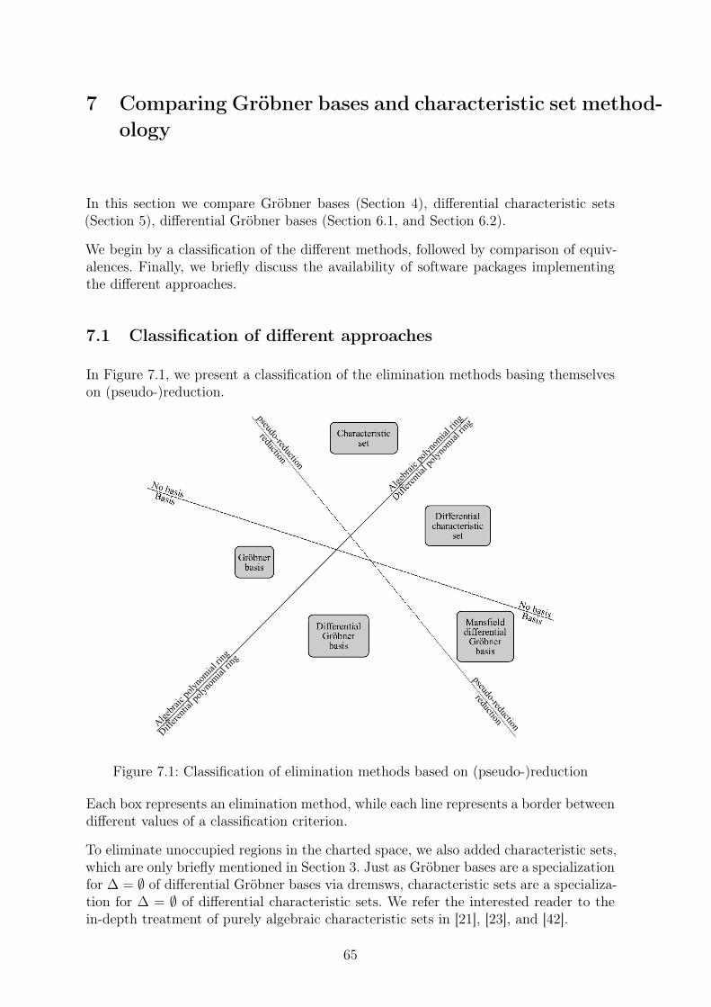
7 Comparing Gröbner bases and characteristic set method-

ology

In this section we compare Gröbner bases (Section 4), differential characteristic sets(Section 5), differential Gröbner bases (Section 6.1, and Section 6.2).

We begin by a classification of the different methods, followed by comparison of equiv-alences. Finally, we briefly discuss the availability of software packages implementingthe different approaches.

7.1 Classification of different approaches

In Figure 7.1, we present a classification of the elimination methods basing themselveson (pseudo-)reduction.

Alg

ebra

ic p

olyn

omia

l rin

g

Diff

eren

tial p

olyn

omia

l rin

g

No basis

pseudo-reduction

reductionCharacteristic

set

Mansfielddifferential

Gröbnerbasis

pseudo-reduction

reduction

Alg

ebra

ic p

olyn

omia

l rin

g

Diff

eren

tial p

olyn

omia

l rin

g

Basis

Figure 7.1: Classification of elimination methods based on (pseudo-)reduction

Each box represents an elimination method, while each line represents a border betweendifferent values of a classification criterion.

To eliminate unoccupied regions in the charted space, we also added characteristic sets,which are only briefly mentioned in Section 3. Just as Gröbner bases are a specializationfor ∆ = ∅ of differential Gröbner bases via dremsws, characteristic sets are a specializa-tion for ∆ = ∅ of differential characteristic sets. We refer the interested reader to thein-depth treatment of purely algebraic characteristic sets in [21], [23], and [42].

65

Methods below the solid line in Figure 7.1 (differential Gröbner bases, Mansfield differ-ential Gröbner bases, differential characteristic sets) operate in differential polynomialrings, while those above the solid line (Gröbner bases, characteristic sets) operate inalgebraic polynomial rings. Methods below the dashed line (Gröbner bases, differentialGröbner bases, Mansfield differential Gröbner bases) provide a basis for the ideal, whilethose above the dashed line (characteristic sets, differential characteristic sets) need notyield a basis. Methods above the dotted line (characteristic sets, differential characteris-tic sets, Mansfield differential Gröbner bases) take advantage of pseudo-reduction, whilethose below the dotted line (Gröbner bases, differential Gröbner bases) base themselveson reduction.

We observe that the center and the top-left regions are unoccupied: There is no elim-ination method based on reduction that does not also yield a basis of the relevantideal.

While the three classification criteria give rise to eight distinct regions, the projectionpresented in Figure 7.1 can only show seven of those regions. The missing region corre-sponds to “pseudo-reduction” in “algebraic polynomial rings” yielding a “basis” for theideal. No method is known to us that occupies this region. However, when restrictingMansfield differential Gröbner bases to the algebraic setting, we would obtain a methodin this region.

Figure 7.1 nicely shows that Mansfield differential Gröbner bases act as connector be-tween classical Gröbner bases notions and characteristic sets. And indeed Mansfielddifferential Gröbner bases blur the distinction between those two approaches. Mans-field differential Gröbner bases base themselves on pseudo-reduction, while yielding abasis and calling themselves Gröbner bases. This approach mixes the crucial aspects ofboth characteristic sets and Gröbner bases. In discussions often the impression arisesthat the distinction between characteristic sets and Gröbner bases is whether reduc-tion or pseudo-reduction is used. Using Figure 7.1, we see that the distinction is ratherwhether or not the resulting set is a basis for the ideal.

After this comparison of the methodological differences, Section 7.2 tries to identify re-lations between the formulated equivalences for the different approaches to elimination.

7.2 Comparison of equivalences

In Table 7.1 we compare the equivalences for the different approaches to eliminationpresented in this thesis.

The table is divided into nine columns. The first column presents the name of the elim-ination method. The second and third column give the requirements on <, and further,general requirements. On top of columns four to nine we find expressions depending onSet, Pred, or both.

The table cells relate the names of elimination methods on the left to the expressionson top. If an expression is equivalent to P being a Gröbner basis, ... for J , we findappropriate values in for Set, Pred, or (if applicable) both in the corresponding table

66

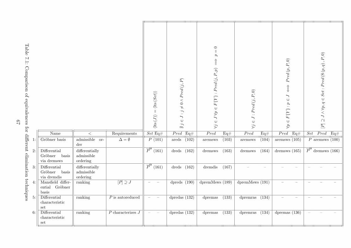
〈lts(J

)〉=

〈lts(S

et)〉

∄j∈J:j6=

0∧Pred(j,P

)

∀j∈J∀p

∈F{Y

}:Pred(j,P

,p)=⇒

p=

0

∀j∈J:Pred(j,P

,0)

∀p∈F{Y

}:p∈J

⇐⇒

Pred(p,P

,0)

[P]⊇

J∧∀p

,q∈Set:Pred(S

(p,q),P

,0)

Name < Requirements Set Eq# Pred Eq# Pred Eq# Pred Eq# Pred Eq# Set Pred Eq#

1: Gröbner basis admissible or-der

∆ = ∅ P (101) areds (102) aremsws (103) aremsws (104) aremsws (105) P aremsws (100)

2: DifferentialGröbner basisvia dremsws

differentiallyadmissibleordering

PΘ

(161) dreds (162) dremsws (163) dremsws (164) dremsws (165) PΘdremsws (166)

3: DifferentialGröbner basisvia dremdis

differentiallyadmissibleordering

PΘ

(161) dreds (162) dremdis (167) – – – – – – –

4: Mansfield differ-ential Gröbnerbasis

ranking [P] ⊇ J – – dpreds (190) dpremMsws (189) dpremMsws (191) – – – – –

5: Differentialcharacteristicset

ranking P is autoreduced – – dpredas (132) dpremas (133) dpremras (134) – – – – –

6: Differentialcharacteristicset

ranking P characterizes J – – dpredas (132) dpremas (133) dpremras (134) dpremas (136) – – –

Tab

le7.1:

Com

parison

ofeq

uivalen

cesfor

diff

erent

elimin

ationtech

niq

ues

67

cell and additionally the equation number (Eq#), where this equivalence occurs ina theorem. If there is no such equivalence between the elimination method and theexpression on top, the table cell lists “–”.

In Table 7.1, J denotes an arbitrary differential ideal in F{Y }, and P denotes anarbitrary subset of J\ {0} .

To clarify the information contained in Table 7.1, consider the fifth cell in row 4 (i.e.:the cell containing (190) in the “Eq#” field). This cell states that if [P] = J36 holds,then P being a Mansfield differential Gröbner basis of J is equivalent to J containingno non-zero differentially pseudo-reduced polynomial with respect to P.

The last cell of row 5 serves as second example. The “–” in this cell indicate that thereis no equivalence between an autoreduced set P being a differential characteristic set ofJ and reduction of S-polynomials.

For row 1, we restrict ourselves to ∆ = ∅. In this setting we may identify F{Y } andF [X] for a finite X and thereby describe the properties of Gröbner basis using thedifferential formulations in the expressions on top Table 7.1. This approach also showsnicely that Gröbner bases are the algebraic counterpart to differential Gröbner bases

via dremsws (row 2). PΘ

becomes P and dremsws becomes aremsws when switchingfrom the differential to the algebraic setting.

The difference between Gröbner basis via dremsws (row 2) and Gröbner basis viadremdis (row 3) is already apparent when looking at Theorem 6.6 and Theorem 6.7.However, in the direct comparison within Table 7.1, we clearly see that Gröbner basisvia dremdis is not an appropriate differential counterpart to purely algebraic Gröbnerbasis, as for example the S-polynomial criterion (last column) gets lost.

Similarly, the relation between Gröbner basis and Mansfield differential Gröbner basisis exposed when comparing row 1 to row 4. We see that the equivalences of the leadingterm ideal (first column with expression on top), ideal membership problem (last butone column), and the S-polynomial criterion (last column) do not carry over. The rea-son is the switch from reduction to pseudo-reduction. Keeping this switch in mind andcomparing row 4 with differential characteristic sets (row 5) suggests a stronger relationbetween Mansfield differential Gröbner bases and differential characteristic sets than be-tween Mansfield differential Gröbner bases and Gröbner bases. Nevertheless, the crucialdistinction between Mansfield differential Gröbner bases and differential characteristicsets is that Mansfield differential Gröbner bases need to be a basis for J , while this is notthe case for differential characteristic sets. This observation warrants the term “basis”within “Mansfield differential Gröbner basis ”. Furthermore, differential characteristicsets need to be autoreduced sets, while neither Gröbner bases nor Mansfield differentialGröbner bases need to be autoreduced sets.

The only difference between the last two rows of Table 7.1 is the additional requirementfor P to characterize J (and thereby requiring P to be a differential characteristic set ofJ), which allows to solve the ideal membership problem (last but one column). While

36P ⊆ J\ {0} is the general assumption on P as presented in the paragraph above. [P] ⊇ J is comingfrom the “Requirements” column. Hence, combining those two, we obtain the requirement [P] = J.

68

the requirement of P to characterize J is a strong requirement, we nevertheless presentrow 6, as the ideal membership problem is crucial to elimination theory.

Finally, we want to point out that in row 5, and row 6 the last but two column containsdremras, while the other reduction specifications in those rows contain dremas—withoutthe “r”.

Inspecting the overall patterns of Table 7.1, the correlation between the loss of theleading term ideal equivalence (first column with expression on top) and the switchfrom admissible orders to a ranking may appear relevant. However, this loss is inherent,as for rankings there is no meaning for leading terms37. More intriguing is the factthat all formulations of elimination methods provide the criterion that J contains nonon-zero reduced (either with respect to reduction or with respect to pseudo-reduction)polynomials (second column with expression on top), and also the criterion which forcesreduction (again either with respect to reduction or pseudo-reduction) to zero (thirdcolumn with expression on top). Finally, the table seems to demote the importance ofthe S-polynomial criterion (last column). However, this criterion is obviously crucial toGröbner bases as it allows a simple (although typically not especially efficient) methodto compute Gröbner bases. Furthermore—although this aspect is not and cannot bevisible in the table—reducing (a special variant of) S-polynomials to zero is crucial whentrying to obtain differential characteristic sets and leads to the concept of coherence(Section 5.3), which asserts that the generated ideals are radical and allows to conductfurther computations in purely algebraic polynomial rings.

We close Section 7 by a brief survey of implementations of the various eliminationmethods in computer algebra systems.

7.3 Integration into computer algebra systems

One important aspect of methods in elimination theory is certainly their applicabilityin modern computer algebra systems. In general, the purely algebraic methods foundtheir way into computer algebra systems, while differential methods are still on theverge of being implemented and included in computer algebra systems. While someof the methods provide native implementations that can be used without a computeralgebra system, we only focus on implementations usable from within computer algebrasystem, as those implementations typically are easier accessible. We only provide linksfor packages not shipped with the respective computer algebra systems.

Most computer algebra systems naturally provide means to obtain Gröbner bases givena finite basis of an ideal. Computer algebra systems do not distinguish them for provid-ing a Gröbner basis, but for providing especially efficient Gröbner basis implementationsfor various benchmarks.

For differential Gröbner bases the situation is fundamentally different. The main prob-lem is that the resulting sets need not be finite and are therefore not well suited for

37Trying to base a notion of leading terms on recursively collecting leaders to their respective powersdoes not allow to reclaim equivalences.

69

today’s computer algebra systems. We do not know implementations computing dif-ferential Gröbner bases in the general case. Nevertheless, there are several packagesavailable in this direction (e.g.: the Rif package of Maple) or research trying to obtaindifferential Gröbner bases, if they are finite (e.g.: [48]).

Methods to obtain Mansfield differential Gröbner bases for certain classes of systemshave been implemented in the diffgrob2 package for Maple. This package has notbeen shipped with Maple and is no longer publicly available. We do not know anyother implementation of Mansfield differential Gröbner bases.

Characteristic set methods found their way into Maple in various packages (e.g.: theRegularChains and the epsilon package [43]). For Mathematica, the WuRitt-

Solva package [30] is available. However, most computer algebra systems do not shipwith methods to explicitly compute characteristic sets.

Among the major computer algebra systems, only Maple allows to compute differentialcharacteristic sets. Besides the shipped DifferentialAlgebra package (which is aconnector between Maple and the BLAD library [4]), there is the diffalg package[5] for general settings, and the epsilon package [43] for the case ∆ = 1.

When trying to apply the presented elimination methods using computer algebra sys-tems, there is not a broad choice. While Gröbner bases are ubiquitously available, othermethods typically require the use of Maple. However, Maple provides an extensivetoolbox of mature implementations of different elimination methods.

We close this thesis, be summing up its contributions in Section 8

70

8 Conclusion

While especially Gröbner bases but also differential characteristic sets, and to someextend differential Gröbner bases received a considerable amount of research on theirown, there is not much research comparing those related approaches. We presented sucha comparison in this thesis.

After introducing the significant concepts for each of the approaches, we gave the rel-evant definitions and equivalences. For this presentation we used a common notationsystem and thereby ease comparability.

Finally, we presented relations among the methods both from a methodological, and alsofrom a property oriented perspective. Thereby, we not only explored the connectionsand distinctions between the presented approaches, but also provide a basis to tie infurther research in terms of additional elimination methods and also in terms of furthercriteria.

Purely algebraic characteristic sets serve as example for further elimination methodsthat can be integrated into the comparison.

Examples for further criteria are the commutativity of F{Y } (e.g.: non-commutativerings, or commutative rings with non-commuting derivations) or the characteristic of F(e.g.: characteristic two, or positive characteristic in general). For both Gröbner basisand differential characteristic sets, there is research in both of the mentioned directions.

Additionally, it might be intriguing, to also add both algebraic and differential resultantbased methods into the comparison, although their approach to elimination is a bitdifferent.

Finally, further elaborating on the notions towards saturation will certainly allow tomerge the pseudo-reduction notions used for differential characteristic set, and Mansfielddifferential Gröbner basis computations and find common generalizations.

71

A Differential pseudo-reduction

For describing different approaches to differential pseudo-reduction, [1] presents an ex-pressive notation framework, which bases its names on drem. As [1] only discussesdifferential pseudo-remainders, this naming seems adequate. In our thesis, we howeverpresent differential remainders (Section 6.1) besides differential pseudo-remainders (Sec-tion 5), hence this naming convention may lead to confusion.

It turned out to be more appropriate to base names for differential pseudo-remaindersaround dprem and use drem solely for differential remainders.

This necessary difference in notation between [1] and our thesis renders [1, AppendixA, pages 281–287], which explicitly presents required properties for different formula-tions of differential pseudo-reduction, unusable and confusing even for simple look ups.Hence, we now reproduce [1, Appendix A, pages 281–287] with our improved namingconvention.

In Table A.1, we present the requirements of differential pseudo-reduction specificationswith respect to autoreduced sets. The “Requirements” columns explicitly show whichspecification of differential pseudo-reduction with respect to an autoreduced set carrieswhat requirements on the triple (p,A, q) . Additionally, Table A.1 illustrates in the“Classes of reductions” columns, which specification of differential pseudo-reduction isallowed or forbidden in which class of specifications of differential pseudo-reduction. Fora given specification and class of specification, “∗” denotes that the specification can beused for the corresponding class of specifications. The absence of “∗” denotes that thespecification must not be used for the corresponding class.

For example, dpremraikas may be used for dpremas but must not be used for dpremras.

In Table A.2, we present the requirements of reduction specifications with respect to adifferential polynomial. The “Requirements” columns explicitly show which specificationof differential pseudo-reduction with respect to a differential polynomial carries whatrequirements on the triple (p, p′, q) .

Table A.2 is essentially Table A.1, when setting A to {p′} , and replacing “as” from thespecification names by “p”. Nevertheless, we give both tables to avoid vagueness andallow easier reference.

In the formulas referenced in both Table A.1 and Table A.2, sometimes curly relationoperators occur. As those relation operators are not relevant for the results of this thesis,we did not introduce them. For the use of the curly relation operator as superscript tosets with an overline (e.g.: M, and G below (195)) [1, Definition 11.5, page 202] providesa definition, while the use as binary relation of two differential polynomials (e.g.: (202))is defined for example in [1, Definition 3.17, page 54].

73

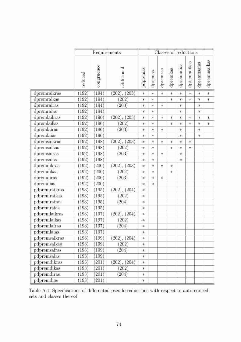
Requirements Classes of reductions

reduce

d

congr

uen

ce

addit

ional

pdpre

mas

dpre

mas

dpre

mra

s

dpre

mka

s

dpre

mndia

s

dpre

mndik

as

dpre

mnsa

ias

dpre

mnsa

ikas

dpremraikras (192) (194) (202), (203) ∗ ∗ ∗ ∗ ∗ ∗ ∗ ∗dpremraikas (192) (194) (202) ∗ ∗ ∗ ∗ ∗ ∗ ∗dpremrairas (192) (194) (203) ∗ ∗ ∗ ∗ ∗dpremraias (192) (194) ∗ ∗ ∗ ∗dpremlaikras (192) (196) (202), (203) ∗ ∗ ∗ ∗ ∗ ∗ ∗ ∗dpremlaikas (192) (196) (202) ∗ ∗ ∗ ∗ ∗ ∗ ∗dpremlairas (192) (196) (203) ∗ ∗ ∗ ∗ ∗dpremlaias (192) (196) ∗ ∗ ∗ ∗dpremsaikras (192) (198) (202), (203) ∗ ∗ ∗ ∗ ∗ ∗dpremsaikas (192) (198) (202) ∗ ∗ ∗ ∗ ∗dpremsairas (192) (198) (203) ∗ ∗ ∗ ∗dpremsaias (192) (198) ∗ ∗ ∗dpremdikras (192) (200) (202), (203) ∗ ∗ ∗ ∗dpremdikas (192) (200) (202) ∗ ∗ ∗dpremdiras (192) (200) (203) ∗ ∗ ∗dpremdias (192) (200) ∗ ∗pdpremraikras (193) (195) (202), (204) ∗pdpremraikas (193) (195) (202) ∗pdpremrairas (193) (195) (204) ∗pdpremraias (193) (195) ∗pdpremlaikras (193) (197) (202), (204) ∗pdpremlaikas (193) (197) (202) ∗pdpremlairas (193) (197) (204) ∗pdpremlaias (193) (197) ∗pdpremsaikras (193) (199) (202), (204) ∗pdpremsaikas (193) (199) (202) ∗pdpremsairas (193) (199) (204) ∗pdpremsaias (193) (199) ∗pdpremdikras (193) (201) (202), (204) ∗pdpremdikas (193) (201) (202) ∗pdpremdiras (193) (201) (204) ∗pdpremdias (193) (201) ∗

Table A.1: Specifications of differential pseudo-reductions with respect to autoreducedsets and classes thereof

74

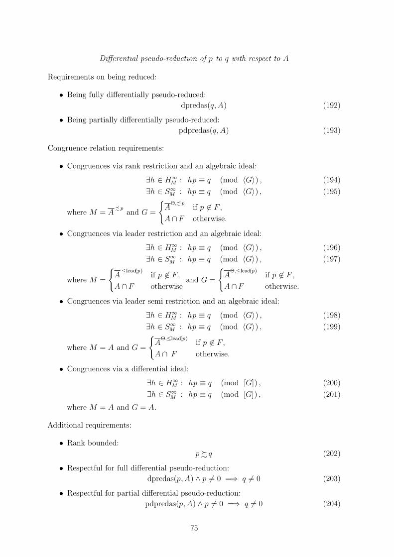
Differential pseudo-reduction of p to q with respect to A

Requirements on being reduced:

• Being fully differentially pseudo-reduced:

dpredas(q, A) (192)

• Being partially differentially pseudo-reduced:

pdpredas(q, A) (193)

Congruence relation requirements:

• Congruences via rank restriction and an algebraic ideal:

∃h ∈ H∞M : hp ≡ q (mod 〈G〉) , (194)

∃h ∈ S∞M : hp ≡ q (mod 〈G〉) , (195)

where M = A- p

and G =

{

AΘ,- p

if p 6∈ F ,

A ∩F otherwise.

• Congruences via leader restriction and an algebraic ideal:

∃h ∈ H∞M : hp ≡ q (mod 〈G〉) , (196)

∃h ∈ S∞M : hp ≡ q (mod 〈G〉) , (197)

where M =

{

A≤lead(p)

if p 6∈ F ,

A ∩F otherwiseand G =

{

AΘ,≤lead(p)

if p 6∈ F ,

A ∩F otherwise.

• Congruences via leader semi restriction and an algebraic ideal:

∃h ∈ H∞M : hp ≡ q (mod 〈G〉) , (198)

∃h ∈ S∞M : hp ≡ q (mod 〈G〉) , (199)

where M = A and G =

{

AΘ,≤lead(p)

if p 6∈ F ,

A ∩ F otherwise.

• Congruences via a differential ideal:

∃h ∈ H∞M : hp ≡ q (mod [G]) , (200)

∃h ∈ S∞M : hp ≡ q (mod [G]) , (201)

where M = A and G = A.

Additional requirements:

• Rank bounded:

p% q (202)

• Respectful for full differential pseudo-reduction:

dpredas(p,A) ∧ p 6= 0 =⇒ q 6= 0 (203)

• Respectful for partial differential pseudo-reduction:

pdpredas(p,A) ∧ p 6= 0 =⇒ q 6= 0 (204)

75

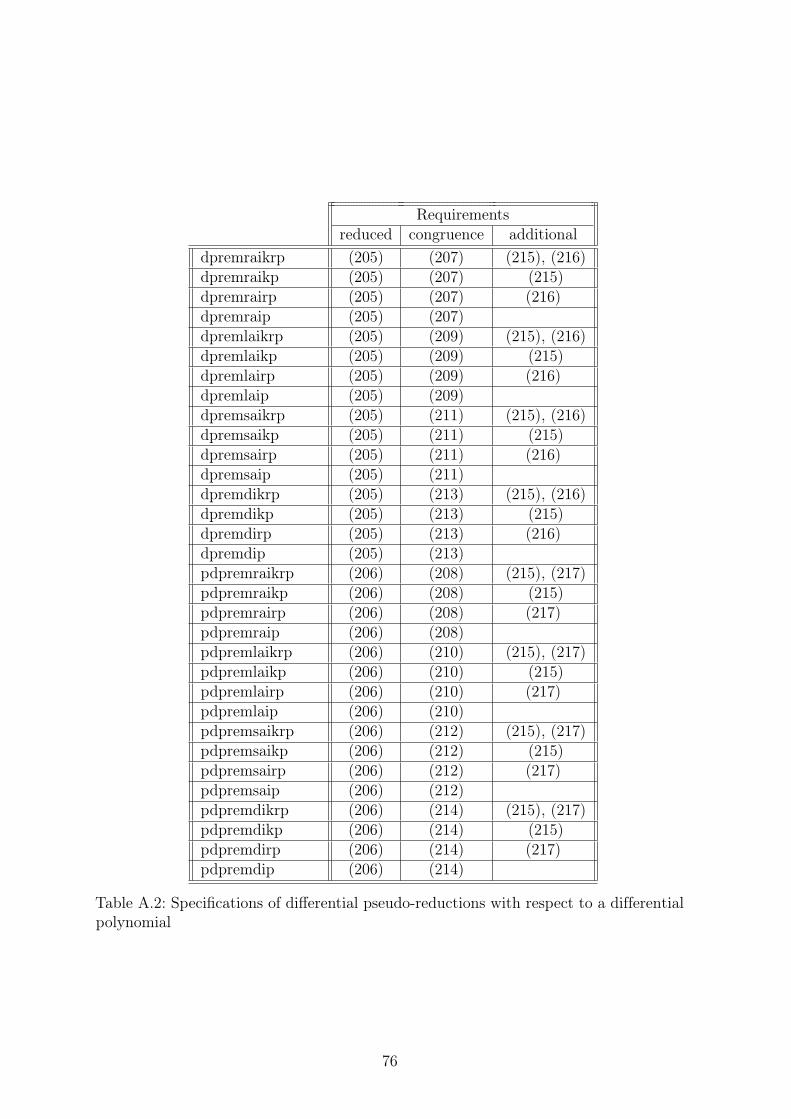
Requirementsreduced congruence additional

dpremraikrp (205) (207) (215), (216)dpremraikp (205) (207) (215)dpremrairp (205) (207) (216)dpremraip (205) (207)dpremlaikrp (205) (209) (215), (216)dpremlaikp (205) (209) (215)dpremlairp (205) (209) (216)dpremlaip (205) (209)dpremsaikrp (205) (211) (215), (216)dpremsaikp (205) (211) (215)dpremsairp (205) (211) (216)dpremsaip (205) (211)dpremdikrp (205) (213) (215), (216)dpremdikp (205) (213) (215)dpremdirp (205) (213) (216)dpremdip (205) (213)pdpremraikrp (206) (208) (215), (217)pdpremraikp (206) (208) (215)pdpremrairp (206) (208) (217)pdpremraip (206) (208)pdpremlaikrp (206) (210) (215), (217)pdpremlaikp (206) (210) (215)pdpremlairp (206) (210) (217)pdpremlaip (206) (210)pdpremsaikrp (206) (212) (215), (217)pdpremsaikp (206) (212) (215)pdpremsairp (206) (212) (217)pdpremsaip (206) (212)pdpremdikrp (206) (214) (215), (217)pdpremdikp (206) (214) (215)pdpremdirp (206) (214) (217)pdpremdip (206) (214)

Table A.2: Specifications of differential pseudo-reductions with respect to a differentialpolynomial

76

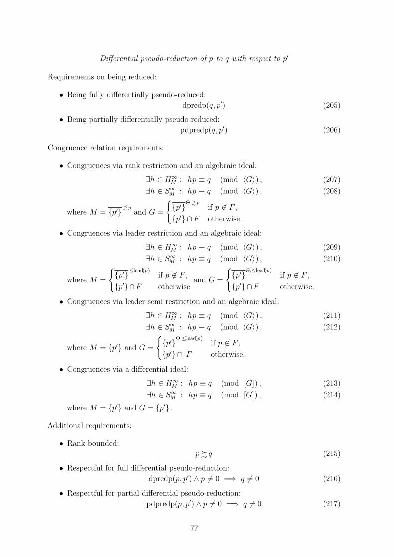
Differential pseudo-reduction of p to q with respect to p′

Requirements on being reduced:

• Being fully differentially pseudo-reduced:

dpredp(q, p′) (205)

• Being partially differentially pseudo-reduced:

pdpredp(q, p′) (206)

Congruence relation requirements:

• Congruences via rank restriction and an algebraic ideal:

∃h ∈ H∞M : hp ≡ q (mod 〈G〉) , (207)

∃h ∈ S∞M : hp ≡ q (mod 〈G〉) , (208)

where M = {p′} - pand G =

{

{p′}Θ,- pif p 6∈ F ,

{p′}∩F otherwise.

• Congruences via leader restriction and an algebraic ideal:

∃h ∈ H∞M : hp ≡ q (mod 〈G〉) , (209)

∃h ∈ S∞M : hp ≡ q (mod 〈G〉) , (210)

where M =

{

{p′}≤lead(p)if p 6∈ F ,

{p′}∩F otherwiseand G =

{

{p′}Θ,≤lead(p)if p 6∈ F ,

{p′}∩F otherwise.

• Congruences via leader semi restriction and an algebraic ideal:

∃h ∈ H∞M : hp ≡ q (mod 〈G〉) , (211)

∃h ∈ S∞M : hp ≡ q (mod 〈G〉) , (212)

where M = {p′} and G =

{

{p′}Θ,≤lead(p)if p 6∈ F ,

{p′}∩ F otherwise.

• Congruences via a differential ideal:

∃h ∈ H∞M : hp ≡ q (mod [G]) , (213)

∃h ∈ S∞M : hp ≡ q (mod [G]) , (214)

where M = {p′} and G = {p′} .

Additional requirements:

• Rank bounded:

p% q (215)

• Respectful for full differential pseudo-reduction:

dpredp(p, p′) ∧ p 6= 0 =⇒ q 6= 0 (216)

• Respectful for partial differential pseudo-reduction:

pdpredp(p, p′) ∧ p 6= 0 =⇒ q 6= 0 (217)

77

B Refinements of rankings

In this section we present the refinements of rankings found in literature.

Several parts of this thesis refer to this section, when requiring special kinds of rankings,although giving their definition directly there would distract too much from the mainarguments (e.g.: orderly ranking in the first paragraph after Definition 6.1).

After some introductory remarks and definitions, we define each of the five refinementsof rankings along with examples. At the end of this section, we relate the differentrefinements graphically.

For the examples (and only for the examples) of this section, we choose I as some subsetof N0. Therefore, the addition of elements of I and N0 is well-defined. With the help ofthe usual total order on N0, we may additionally compare the elements of I.

Before actually giving the definitions of the refinements, we introduce the concept oforders for derivative operators.

Definition B.1 (Order of derivative operators). [compare 28, I, 1, third paragraph onpage 59] Let θ ∈ Θ. We may then (unambiguously) choose dδ ∈ N0 for each δ ∈ ∆, suchthat

θ =∏

δ∈∆

δdδ . (218)

By the order of θ (or ord(θ)), we refer to∑

δ∈∆ dδ.

For any δ ∈ ∆, we use order of θ with respect to δ (or ordδ(θ)) to denote dδ.

The notion of orders on derivative operators leads to the orderly rankings, which weintroduce by specializing integrated rankings to sequential rankings, which we in turnspecialize to orderly rankings.

Definition B.2 (Integrated ranking). [compare 28, I, 8, page 75] A ranking < on(yi,θ)i∈I,θ∈Θ is called integrated ranking if and only if

∀θ, θ′ ∈ Θ ∀i, i′ ∈ I : yi,θ <yi′,θ′ =⇒ ∃φ ∈ Θ : yi′,θ′ <yi,θφ . (219)

Integrated rankings are rankings where derivatives stemming from different elements ofI are interwoven.

In most algebraic settings (i.e.: m = 0 ∧ n > 1), no ranking can be integrated, asthere are i, i′, θ, θ′ such that the precondition of the implication in (219) holds, whileconclusion cannot hold as Θ = {1} .

79

Example B.3 (Integrated ranking). Let I = {1, 2} , and ∆ = {δ1, δ2, δ3} . By choosing< such that38

∀θ, θ′ ∈ Θ ∀i, i′ ∈ I : yi,θ <yi′,θ′ : ⇐⇒(i+ ordδ3(θ) , i, ordδ3−i

(θ) , ord(θ)) <lex (i′ + ordδ3(θ′) , i′, ordδ3−i

(θ′) , ord(θ′)), (220)

we see that < is an integrated ranking on (yi,θ)i∈I,θ∈Θ.

Writing down the derivatives increasingly, we obtain

y1 < y1,δ1 < y1,δ21 < · · · < y1,δ2 < y1,δ1δ2 < y1,δ21δ2 < · · · < y1,δ3 < y1,δ1δ3 < · · ·· · · < y1,δ2δ3 < y1,δ1δ2δ3 < · · · < y2 < y2,δ2 < y2,δ22 < · · · < y2,δ1 < y2,δ1δ2 < · · ·

· · · < y1,δ23 < · · · < y2,δ3 < · · · < y1,δ33 < · · · < y2,δ23 < · · · . (221)

As can be seen in Example B.3, there are integrated rankings where derivatives mayhave infinitely many derivatives below them (e.g.: y2, as can be seen in (221)). Refiningintegrated rankings to avoid such cases, we arrive at sequential rankings.

Definition B.4 (Sequential ranking). [compare 28, I, 8, page 75] A ranking < on(yi,θ)i∈I,θ∈Θ is called sequential ranking if and only if

∀z ∈ (yi,θ)i∈I,θ∈Θ :∣

∣ {z′ ∈ (yi,θ)i∈I,θ∈Θ | z′ <z}∣

∣ ∈ N0. (222)

For sequential rankings, any derivative has only finitely many lower ranking derivatives.If the setting allows an integrated ranking (i.e.: m > 0 ∨ (m = 0 ∧ n ≤ 1)), then anysequential ranking is integrated. The converse does not hold as Example B.3 gives aranking that is integrated, but is not sequential.

Example B.5 (Sequential ranking). Let I = {1, 2} , and ∆ = {δ1, δ2} . By choosing <such that

∀θ, θ′ ∈ Θ ∀i, i′ ∈ I : yi,θ <yi′,θ′ : ⇐⇒(i+ ord(θ) , i, ordδ3−i

(θ)) <lex (i′ + ord(θ′) , i′, ordδ3−i(θ′)), (223)

we see that < is a sequential ranking on (yi,θ)i∈I,θ∈Θ.

Writing down the derivatives increasingly, we obtain

y1 < y1,δ1 < y1,δ2 < y2 < y1,δ21 < y1,δ1δ2 < y1,δ22 < y2,δ2 < y2,δ1 < · · · . (224)

For applications some sequential rankings are especially interesting: rankings, wheresequences of increasing derivatives provide non-decreasing orders, allow to simplify (e.g.:using differential characteristic set computations) systems of differential equations byreducing their order. Therefore, such rankings are called orderly.

38The δ3−i in the third slot of the tuples in (220) is used to select δ2, if i = 1, and δ1, if i = 2.Thereby, the chosen order switches with different i. This cumbersome formulation allows to arrive ata ranking that is not a Riquier ranking (Definition B.10).

Note that slots three and four are only relevant for the comparison if the first two slots agree. Hencei = i′. Therefore, our use of δ3−i does not hurt the ranking properties.

80

Definition B.6 (Orderly ranking). [compare 28, I, 8, page 75] A ranking < on (yi,θ)i∈I,θ∈Θis called orderly ranking if and only if

∀θ, θ′ ∈ Θ ∀i, i′ ∈ I : ord(θ) < ord(θ′) =⇒ yi,θ <yi′,θ′ . (225)

Although any orderly ranking is sequential, the converse cannot hold, as the ranking ofExample B.5 is sequential but not orderly..

Example B.7 (Orderly ranking). Let I = {1, 2} , and ∆ = {δ1, δ2} . By choosing <such that

∀θ, θ′ ∈ Θ ∀i, i′ ∈ I : yi,θ <yi′,θ′ : ⇐⇒(ord(θ) , i, ordδ3−i

(θ)) <lex (ord(θ′) , i′, ordδ3−i(θ′)), (226)

we see that < is an orderly ranking on (yi,θ)i∈I,θ∈Θ.

Writing down the derivatives increasingly, we obtain

y1 < y2 < y1,δ1 < y1,δ2 < y2,δ2 < y2,δ1 <

< y1,δ21 < y1,δ1δ2 < y1,δ22 < y2,δ22 < y2,δ1δ2 < y2,δ21 < · · · . (227)

The remaining two refinements of rankings are not directly connected to the first three.We begin by presenting elimination rankings, which in contrast to orderly rankings donot focus on lowering the order, but on grouping derivatives by the element of I theyare built from. In differential characteristic set computations, elimination rankings areused to decouple differential equations.

Definition B.8 (Elimination ranking). [compare 22, § 3.1, last but one paragraph onpage 10] A ranking < on (yi,θ)i∈I,θ∈Θ is called elimination ranking if and only if

∀θ ∈ Θ ∀i, i′ ∈ I : yi <yi′ =⇒ yi,θ <yi′ . (228)

When writing down all the derivatives increasingly, an elimination ranking results inn blocks, where each block only contains derivatives stemming from the same elementof I.

Example B.9 (Eliminiation ranking). Let I = {1, 2} , and ∆ = {δ1, δ2} . By choosing< such that

∀θ, θ′ ∈ Θ ∀i, i′ ∈ I : yi,θ <yi′,θ′ : ⇐⇒(i, ordδ3−i

(θ) , ord(θ)) <lex (i′, ordδ3−i(θ′) , ord(θ′)), (229)

we see that < is an elimination ranking on (yi,θ)i∈I,θ∈Θ.

Writing down the derivatives increasingly, we obtain

y1 < y1,δ1 < y1,δ21 < · · · < y1,δ2 < y1,δ1δ2 < y1,δ21δ2 < · · · < y1,δ22 < · · ·· · · < y2 < y2,δ2 < y2,δ22 < · · · < y2,δ1 < y2,δ1δ2 < y2,δ1δ22 < · · · < y2,δ21 < · · · . (230)

81

The final refinement of rankings are Riquier rankings, which state that structure ofderivatives coming from the same element of I corresponds the structure of derivativescoming from any other element of I.

Definition B.10 (Riquier ranking). [compare 40, § 3, Theorem 7, page 5] A ranking< on (yi,θ)i∈I,θ∈Θ is called Riquier ranking if and only if

∀θ, θ′ ∈ Θ ∀i, i′ ∈ I : yi,θ <yi,θ′ ⇐⇒ yi′,θ <yi′,θ′ . (231)

Whether or not a ranking is a Riquier ranking is independent from whether or not theranking meets the requirements of any of the previous four refinements.

Example B.11 (Riquier ranking). Let I = {1, 2, 3} , and ∆ = {δ1, δ2} . By choosing <such that

∀θ, θ′ ∈ Θ ∀i, i′ ∈ I : yi,θ <yi′,θ′ : ⇐⇒

(ord(θ) , ordδ2(θ) , i) <lex (ord(θ′) , ordδ2(θ′) , i′) if i ∈ {1, 2} ∧ i′ ∈ {1, 2}

(ord(θ) , ordδ2(θ)) <lex (ord(θ′) , ordδ2(θ′)) if i = i′ = 3

i < i′ otherwise,

(232)

we see that < is a Riquier ranking on (yi,θ)i∈I,θ∈Θ.

Writing down the derivatives increasingly, we obtain

y1 < y2 < y1,δ1 < y2,δ1 < y1,δ2 < y2,δ2 < y1,δ21 < y2,δ21 < y1,δ1δ2 < y2,δ1δ2 <

< y1,δ22 < y2,δ22 < · · · < y3 < y3,δ1 < y3,δ2 < y3,δ21 < y3,δ1δ2 < y3,δ22 . (233)

While the ranking in Example B.11 does not meet the requirements of any of the firstfour refinements of rankings, we see that it is an orderly ranking on (yi,θ)i∈{1,2},θ∈Θ, andan elimination ranking on both (yi,θ)i∈{1,3},θ∈Θ, and also on (yi,θ)i∈{2,3},θ∈Θ.

Note however, that the given examples do not represent all possible constellations ofrefinements for the non-degenerate case (i.e.: m > 0 ∧ n > 1). The rankings given inany of the first four examples can be modified to additionally meet the Riquier rank-ing requirements by substituting δ1 for δ3−i. Finally, there are of course also rankingsmeeting none of the presented refinements, as illustrated by the following example.

Example B.12 (General ranking). Let I = {1, 2, 3} , and ∆ = {δ1, δ2, δ3} . By choosing< such that

∀θ, θ′ ∈ Θ ∀i, i′ ∈ I : yi,θ <yi′,θ′ : ⇐⇒

(i+ ordδ3(θ) , i, ordδ3−i(θ) , ord(θ)) <lex

<lex (i′ + ordδ3(θ′) , i′, ordδ3−i

(θ′) , ord(θ′)) if i ∈ {1, 2} ∧ i′ ∈ {1, 2}(ord(θ) , ordδ3(θ) , ordδ2(θ)) <lex

<lex (ord(θ′) , ordδ3(θ′) , ordδ2(θ

′)) if i = i′ = 3

i < i′ otherwise,

(234)

82

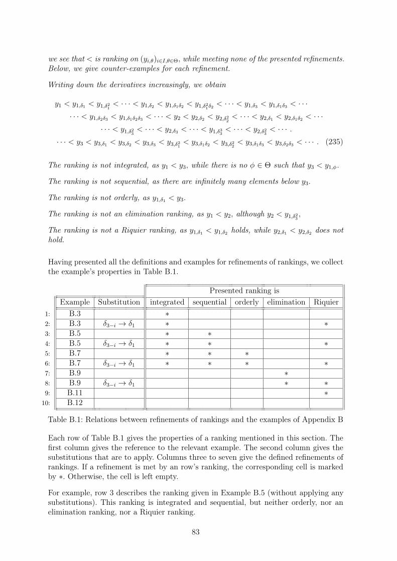
we see that < is ranking on (yi,θ)i∈I,θ∈Θ, while meeting none of the presented refinements.Below, we give counter-examples for each refinement.

Writing down the derivatives increasingly, we obtain

y1 < y1,δ1 < y1,δ21 < · · · < y1,δ2 < y1,δ1δ2 < y1,δ21δ2 < · · · < y1,δ3 < y1,δ1δ3 < · · ·· · · < y1,δ2δ3 < y1,δ1δ2δ3 < · · · < y2 < y2,δ2 < y2,δ22 < · · · < y2,δ1 < y2,δ1δ2 < · · ·

· · · < y1,δ23 < · · · < y2,δ3 < · · · < y1,δ33 < · · · < y2,δ23 < · · · .· · · < y3 < y3,δ1 < y3,δ2 < y3,δ3 < y3,δ21 < y3,δ1δ2 < y3,δ22 < y3,δ1δ3 < y3,δ2δ3 < · · · . (235)

The ranking is not integrated, as y1 < y3, while there is no φ ∈ Θ such that y3 < y1,φ .

The ranking is not sequential, as there are infinitely many elements below y3.

The ranking is not orderly, as y1,δ1 < y3.

The ranking is not an elimination ranking, as y1 < y2, although y2 < y1,δ23 ,

The ranking is not a Riquier ranking, as y1,δ1 < y1,δ2 holds, while y2,δ1 < y2,δ2 does nothold.

Having presented all the definitions and examples for refinements of rankings, we collectthe example’s properties in Table B.1.

Presented ranking is

Example Substitution integrated sequential orderly elimination Riquier

1: B.3 ∗2: B.3 δ3−i → δ1 ∗ ∗3: B.5 ∗ ∗4: B.5 δ3−i → δ1 ∗ ∗ ∗5: B.7 ∗ ∗ ∗6: B.7 δ3−i → δ1 ∗ ∗ ∗ ∗7: B.9 ∗8: B.9 δ3−i → δ1 ∗ ∗9: B.11 ∗

10: B.12

Table B.1: Relations between refinements of rankings and the examples of Appendix B

Each row of Table B.1 gives the properties of a ranking mentioned in this section. Thefirst column gives the reference to the relevant example. The second column gives thesubstitutions that are to apply. Columns three to seven give the defined refinements ofrankings. If a refinement is met by an row’s ranking, the corresponding cell is markedby ∗. Otherwise, the cell is left empty.

For example, row 3 describes the ranking given in Example B.5 (without applying anysubstitutions). This ranking is integrated and sequential, but neither orderly, nor anelimination ranking, nor a Riquier ranking.

83

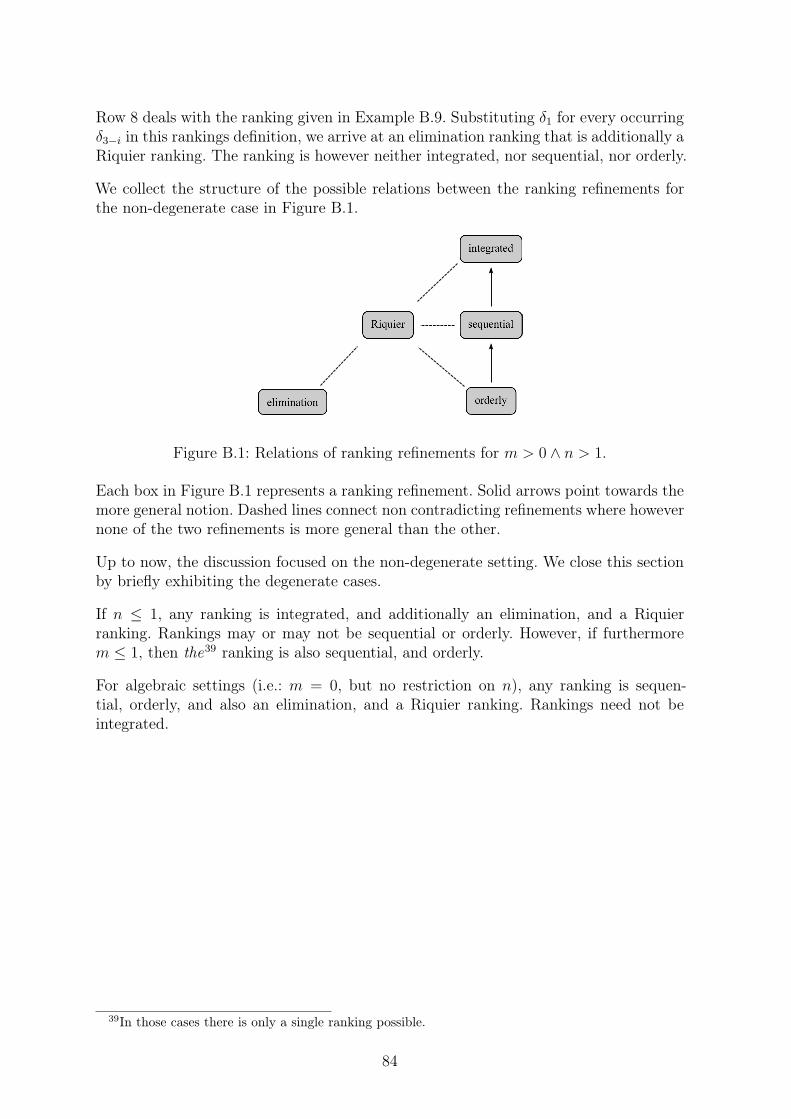
Row 8 deals with the ranking given in Example B.9. Substituting δ1 for every occurringδ3−i in this rankings definition, we arrive at an elimination ranking that is additionally aRiquier ranking. The ranking is however neither integrated, nor sequential, nor orderly.

We collect the structure of the possible relations between the ranking refinements forthe non-degenerate case in Figure B.1.

elimination

Riquier

integrated

sequential

orderly

Figure B.1: Relations of ranking refinements for m > 0 ∧ n > 1.

Each box in Figure B.1 represents a ranking refinement. Solid arrows point towards themore general notion. Dashed lines connect non contradicting refinements where howevernone of the two refinements is more general than the other.

Up to now, the discussion focused on the non-degenerate setting. We close this sectionby briefly exhibiting the degenerate cases.

If n ≤ 1, any ranking is integrated, and additionally an elimination, and a Riquierranking. Rankings may or may not be sequential or orderly. However, if furthermorem ≤ 1, then the39 ranking is also sequential, and orderly.

For algebraic settings (i.e.: m = 0, but no restriction on n), any ranking is sequen-tial, orderly, and also an elimination, and a Riquier ranking. Rankings need not beintegrated.

39In those cases there is only a single ranking possible.

84

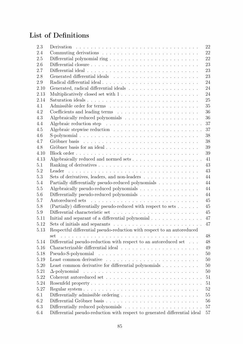
List of Definitions

2.3 Derivation . . . . . . . . . . . . . . . . . . . . . . . . . . . . . . . . . 222.4 Commuting derivations . . . . . . . . . . . . . . . . . . . . . . . . . . 222.5 Differential polynomial ring . . . . . . . . . . . . . . . . . . . . . . . . 222.6 Differential closure . . . . . . . . . . . . . . . . . . . . . . . . . . . . . 232.7 Differential ideal . . . . . . . . . . . . . . . . . . . . . . . . . . . . . . 232.8 Generated differential ideals . . . . . . . . . . . . . . . . . . . . . . . 232.9 Radical differential ideal . . . . . . . . . . . . . . . . . . . . . . . . . . 242.10 Generated, radical differential ideals . . . . . . . . . . . . . . . . . . . 242.13 Multiplicatively closed set with 1 . . . . . . . . . . . . . . . . . . . . . 242.14 Saturation ideals . . . . . . . . . . . . . . . . . . . . . . . . . . . . . . 254.1 Admissible order for terms . . . . . . . . . . . . . . . . . . . . . . . . 354.2 Coefficients and leading terms . . . . . . . . . . . . . . . . . . . . . . 364.3 Algebraically reduced polynomials . . . . . . . . . . . . . . . . . . . . 364.4 Algebraic reduction step . . . . . . . . . . . . . . . . . . . . . . . . . . 374.5 Algebraic stepwise reduction . . . . . . . . . . . . . . . . . . . . . . . . 374.6 S-polynomial . . . . . . . . . . . . . . . . . . . . . . . . . . . . . . . . 384.7 Gröbner basis . . . . . . . . . . . . . . . . . . . . . . . . . . . . . . . 384.8 Gröbner basis for an ideal . . . . . . . . . . . . . . . . . . . . . . . . . 394.10 Block order . . . . . . . . . . . . . . . . . . . . . . . . . . . . . . . . . 394.13 Algebraically reduced and normed sets . . . . . . . . . . . . . . . . . . . 415.1 Ranking of derivatives . . . . . . . . . . . . . . . . . . . . . . . . . . . 435.2 Leader . . . . . . . . . . . . . . . . . . . . . . . . . . . . . . . . . . . 435.3 Sets of derivatives, leaders, and non-leaders . . . . . . . . . . . . . . . 445.4 Partially differentially pseudo-reduced polynomials . . . . . . . . . . . 445.5 Algebraically pseudo-reduced polynomials . . . . . . . . . . . . . . . . 445.6 Differentially pseudo-reduced polynomials . . . . . . . . . . . . . . . . 445.7 Autoreduced sets . . . . . . . . . . . . . . . . . . . . . . . . . . . . . 455.8 (Partially) differentially pseudo-reduced with respect to sets . . . . . . 455.9 Differential characteristic set . . . . . . . . . . . . . . . . . . . . . . . 455.11 Initial and separant of a differential polynomial . . . . . . . . . . . . . . 475.12 Sets of initials and separants . . . . . . . . . . . . . . . . . . . . . . . . 475.13 Respectful differential pseudo-reduction with respect to an autoreduced

set . . . . . . . . . . . . . . . . . . . . . . . . . . . . . . . . . . . . . 485.14 Differential pseudo-reduction with respect to an autoreduced set . . . 485.16 Characterizable differential ideal . . . . . . . . . . . . . . . . . . . . . 495.18 Pseudo-S-polynomial . . . . . . . . . . . . . . . . . . . . . . . . . . . 505.19 Least common derivative . . . . . . . . . . . . . . . . . . . . . . . . . 505.20 Least common derivative for differential polynomials . . . . . . . . . . 505.21 ∆-polynomial . . . . . . . . . . . . . . . . . . . . . . . . . . . . . . . 505.22 Coherent autoreduced set . . . . . . . . . . . . . . . . . . . . . . . . . . 515.24 Rosenfeld property . . . . . . . . . . . . . . . . . . . . . . . . . . . . . . 515.27 Regular system . . . . . . . . . . . . . . . . . . . . . . . . . . . . . . . 526.1 Differentially admissible ordering . . . . . . . . . . . . . . . . . . . . . 556.2 Differential Gröbner basis . . . . . . . . . . . . . . . . . . . . . . . . . 566.3 Differentially reduced polynomials . . . . . . . . . . . . . . . . . . . . . 576.4 Differential pseudo-reduction with respect to generated differential ideal 57

85

6.5 Differential stepwise reduction . . . . . . . . . . . . . . . . . . . . . . 586.9 Differentially reduced sets . . . . . . . . . . . . . . . . . . . . . . . . . 596.11 Coefficients with respect to an indeterminate . . . . . . . . . . . . . . 626.12 Differential pseudo-reduction Mansfield step . . . . . . . . . . . . . . . 626.13 Stepwise differential pseudo-reduction by Mansfield steps . . . . . . . 636.14 Mansfield differential Gröbner basis . . . . . . . . . . . . . . . . . . . 63B.1 Order of derivative operators . . . . . . . . . . . . . . . . . . . . . . . 79B.2 Integrated ranking . . . . . . . . . . . . . . . . . . . . . . . . . . . . . 79B.4 Sequential ranking . . . . . . . . . . . . . . . . . . . . . . . . . . . . . 80B.6 Orderly ranking . . . . . . . . . . . . . . . . . . . . . . . . . . . . . . . 81B.8 Elimination ranking . . . . . . . . . . . . . . . . . . . . . . . . . . . . . 81B.10 Riquier ranking . . . . . . . . . . . . . . . . . . . . . . . . . . . . . . 82

86

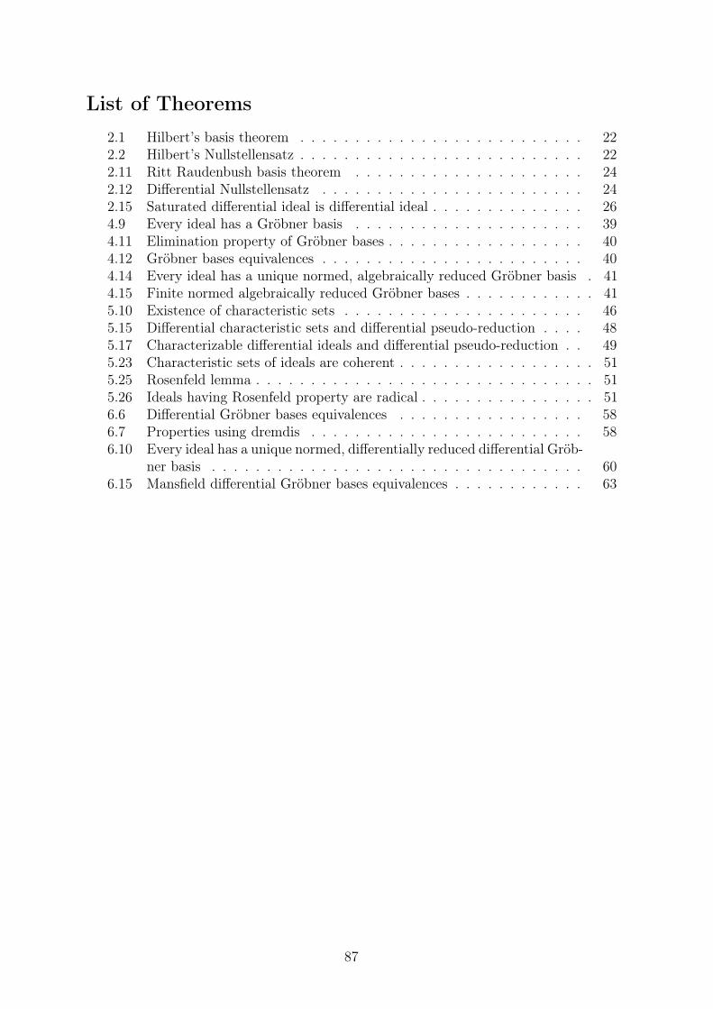
List of Theorems

2.1 Hilbert’s basis theorem . . . . . . . . . . . . . . . . . . . . . . . . . . 222.2 Hilbert’s Nullstellensatz . . . . . . . . . . . . . . . . . . . . . . . . . . 222.11 Ritt Raudenbush basis theorem . . . . . . . . . . . . . . . . . . . . . 242.12 Differential Nullstellensatz . . . . . . . . . . . . . . . . . . . . . . . . 242.15 Saturated differential ideal is differential ideal . . . . . . . . . . . . . . 264.9 Every ideal has a Gröbner basis . . . . . . . . . . . . . . . . . . . . . 394.11 Elimination property of Gröbner bases . . . . . . . . . . . . . . . . . . 404.12 Gröbner bases equivalences . . . . . . . . . . . . . . . . . . . . . . . . 404.14 Every ideal has a unique normed, algebraically reduced Gröbner basis . 414.15 Finite normed algebraically reduced Gröbner bases . . . . . . . . . . . . 415.10 Existence of characteristic sets . . . . . . . . . . . . . . . . . . . . . . 465.15 Differential characteristic sets and differential pseudo-reduction . . . . 485.17 Characterizable differential ideals and differential pseudo-reduction . . 495.23 Characteristic sets of ideals are coherent . . . . . . . . . . . . . . . . . . 515.25 Rosenfeld lemma . . . . . . . . . . . . . . . . . . . . . . . . . . . . . . . 515.26 Ideals having Rosenfeld property are radical . . . . . . . . . . . . . . . . 516.6 Differential Gröbner bases equivalences . . . . . . . . . . . . . . . . . 586.7 Properties using dremdis . . . . . . . . . . . . . . . . . . . . . . . . . 586.10 Every ideal has a unique normed, differentially reduced differential Gröb-

ner basis . . . . . . . . . . . . . . . . . . . . . . . . . . . . . . . . . . 606.15 Mansfield differential Gröbner bases equivalences . . . . . . . . . . . . 63

87

List of Examples

6.8 S-polynomial reduction by dremdis does not yield differential Gröbnerbases . . . . . . . . . . . . . . . . . . . . . . . . . . . . . . . . . . . . 59

B.3 Integrated ranking . . . . . . . . . . . . . . . . . . . . . . . . . . . . . 80B.5 Sequential ranking . . . . . . . . . . . . . . . . . . . . . . . . . . . . . 80B.7 Orderly ranking . . . . . . . . . . . . . . . . . . . . . . . . . . . . . . . 81B.9 Eliminiation ranking . . . . . . . . . . . . . . . . . . . . . . . . . . . . . 81B.11 Riquier ranking . . . . . . . . . . . . . . . . . . . . . . . . . . . . . . 82B.12 General ranking . . . . . . . . . . . . . . . . . . . . . . . . . . . . . . 82

89

List of Figures

7.1 Classification of elimination methods based on (pseudo-)reduction . . . 65B.1 Relations of ranking refinements for m > 0 ∧ n > 1. . . . . . . . . . . . 84

91

List of Tables

7.1 Comparison of equivalences for different elimination techniques . . . . . . 67A.1 Specifications of differential pseudo-reductions with respect to autore-

duced sets and classes thereof . . . . . . . . . . . . . . . . . . . . . . . 74A.2 Specifications of differential pseudo-reductions with respect to a differen-

tial polynomial . . . . . . . . . . . . . . . . . . . . . . . . . . . . . . . 76B.1 Relations between refinements of rankings and the examples of Appendix B 83

93

References

[1] C. Aistleitner. Differential aspects of differential characteristic set computations.PhD thesis, Johannes Kepler Universität, Linz, 2010.

[2] T. Becker and V. Weispfenning. Gröbner Bases — A computational approachto commutative algebra. Springer Verlag, Wien, 1993. ISBN 0-387-97971-9. Incooperation with Heinz Kredel.

[3] F. Boulier. Étude et implantation de quelques algorithmes en algèbre différentielle.PhD thesis, Université Lille I, June 1994. URL http://tel.archives-ouvertes.

fr/docs/00/13/78/66/PDF/these.pdf (last seen on 2010-03-03).

[4] F. Boulier. BLAD. Internet. URL http://www2.lifl.fr/~boulier/BLAD/index.

html (last seen on 2010-04-07).

[5] F. Boulier and E. Hubert. diffalg. Internet. URL http://www-sop.inria.fr/

cafe/Evelyne.Hubert/diffalg/ (last seen on 2005-12-06).

[6] M. Brickenstein. Slimgb: Gröbner Bases with Slim Polynomials. In ReportsOn Computer Algebra, number 35. Centre for Computer Algebra, Universityof Kaiserslautern, September 2005. URL http://www.mathematik.uni-kl.de/

~zca/Reports_on_ca/35/paper_35_full.ps.gz (last seen on 2010-08-24).

[7] B. Buchberger and A. Zapletal. Gröbner bases bibliography. Internet. URLhttp://www.ricam.oeaw.ac.at/Groebner-Bases-Bibliography/ (last seen on2010-11-30).

[8] G. Carrà Ferro. Gröbner bases and differential algebra. In L. Huguet and A. Poli,editors, Proceedings of the 5th International Symposium on Applied Algebra, Al-gebraic Algorithms and Error-Correcting Codes, volume 356 of Lecture Notes inComputer Science, pages 131–140. Springer, 1987. ISBN 3-540-51082-6.

[9] G. Carrà Ferro. A resultant theory for ordinary algebraic differential equations. InT. Mora and H. F. Mattson, editors, Proceedings of the 12th International Sym-posium on Applied Algebra, Algebraic Algorithms and Error-Correcting Codes, vol-ume 1255 of Lecture Notes in Computer Science, pages 55–65. Springer, 1997. ISBN3-540-63163-1.

[10] G. Carrà Ferro. A survey on differential Gröbner bases, pages 77–108. Number 2in Radon Series on Computational and Applied Mathematics. Walter de Gruyter,2007. ISBN 978-3-11-019323-7.

[11] M. Chardin. Differential resultants and subresultants. In L. Budach, editor, Pro-ceedings of the 1991 Fundamentals of Computation Theory, volume 529 of LectureNotes in Computer Science, pages 180–189. Springer, 1993. ISBN 3-540-54458-5.

[12] D. A. Cox, J. B. Little, and D. O’Shea. Ideals, varieties, and algorithms. Springer,3. edition, 2007. ISBN 978-0-387-35650-1.

[13] Emacs. Internet. URL http://www.gnu.org/software/emacs/emacs.html (lastseen on 2010-05-27).

95

[14] J.-C. Faugère. A new efficient algorithm for computing gröbner bases (F4). Journalof Pure and Applied Algebra, 139(1–3):61–88, 1999. doi: 10.1016/S0022-4049(99)00005-5. URL http://www-calfor.lip6.fr/~jcf/Papers/F99a.pdf (last seenon 2010-08-24).

[15] J.-C. Faugère. A new efficient algorithm for computing gröbner bases withoutreduction to zero (F5). In T. Mora, editor, Proceedings of the 2002 InternationalSymposium on Symbolic and Algebraic Computation, pages 55–62. ACM Press,2001. ISBN 1-58113-484-3. URL http://www-calfor.lip6.fr/~jcf/Papers/

F02a.pdf (last seen on 2010-08-24).

[16] I. M. Gelfand, M. M. Kapranov, and A. V. Zelevinsky. Discriminants, resul-tants and multidimensional determinants. Mathematics: theory & applications.Birkhäuser GmbH, 1994. ISBN 0-8176-3660-9.

[17] Gentoo linux. Internet. URL http://www.gentoo.org/ (last seen on 2010-05-27).

[18] The GNU operating system. Internet. URL http://www.gnu.org/ (last seen on2010-05-27).

[19] O. Golubitsky, M. Kondratieva, M. Moreno Maza, and A. Ovchinnikov. A boundfor the Rosenfeld Groebner algorithm. Journal of Symbolic Computation, 43(8):582–610, August 2008. doi: 10.1016/j.jsc.2007.12.002.

[20] Graphviz. Internet. URL http://www.graphviz.org/ (last seen on 2010-05-27).

[21] E. Hubert. Factorization free decomposition algorithms in differential algebra.Journal of Symbolic Computation, 29(4–5):641–662, 2000. doi: 10.1006/jsco.1999.0344.

[22] E. Hubert. Notes on triangular sets and triangulation-decomposition algorithmsII: Differential systems. In F. Winkler and U. Langer, editors, SNSC, volume2630 of Lecture Notes in Computer Science. Springer, 2003. ISBN 3-540-40554-2. URL http://www-sop.inria.fr/members/Evelyne.Hubert/publications/

sncsd.pdf (last seen on 2010-03-03).

[23] E. Hubert. Notes on triangular sets and triangulation-decomposition algorithmsI: Polynomial systems. In F. Winkler and U. Langer, editors, SNSC, volume2630 of Lecture Notes in Computer Science. Springer, 2003. ISBN 3-540-40554-2. URL http://www-sop.inria.fr/members/Evelyne.Hubert/publications/

sncsp.pdf (last seen on 2010-03-03).

[24] E. Hubert. Differential algebra for derivations with nontrivial commutation rules.Journal of Pure and Applied Algebra, 200:163–190, 2005. doi: 10.1016/j.jpaa.2004.12.034.

[25] K. Iima and Y. Yoshino. Gröbner bases for the polynomial ring with infinite vari-ables and their applications. Communications in Algebra, 37(10):3424–3437, 2009.URL http://www.math.okayama-u.ac.jp/~yoshino/pdffiles/Groebner7.pdf

(last seen on 2010-08-26).

[26] Inkscape. Internet. URL http://inkscape.org/ (last seen on 2010-12-02).

96

[27] I. Kaplansky. An introduction to differential algebra. Hermann, Paris, 1957.

[28] E. R. Kolchin. Differential Algebra and Algebraic Groups, volume 54 of Pure andApplied Mathematics. Academic Press, 1973.

[29] Linux. Internet. URL http://kernel.org/ (last seen on 2010-05-27).

[30] H.-S. Liu. WuRittSolva: Implementation of Wu-Ritt Characteristic Set Method.Internet. URL http://library.wolfram.com/infocenter/MathSource/5716/

(last seen on 2005-12-06).

[31] E. Mansfield. Differential Gröbner bases. PhD thesis, University of Sydney,1991. URL http://www.kent.ac.uk/ims/personal/elm2/liz/papers/thesis.

pdf.gz (last seen on 2010-03-31).

[32] M. Minzlaff and J. Calmet. A new definition for passivity and its relation to coher-ence. In 8th International Conference on Artificial Intelligence and Symbolic Com-putation, 2006. doi: 10.1007/11856290_10. URL http://www.math.tu-berlin.

de/~minzlaff/publications/mc-06-ndp.pdf (last seen on 2010-01-07).

[33] F. Mora. Gröbner bases for non-commutative polynomial rings. In J. Calmet,editor, Proceedings of the 3rd International Symposium on Algebraic Algorithmsand Error-Correcting Codes, volume 229 of Lecture Notes in Computer Science,pages 353–362. Springer, 1986. ISBN 3-540-16776-5. doi: 10.1007/3-540-16776-5_740.

[34] S. Morrison. The differential ideal [P ] : M∞. Journal of Symbolic Computation,28(4–5):631–656, Oct./Nov. 1999. ISSN 0747-7171. doi: 10.1006/jsco.1999.0318.

[35] n. n. JKU Linz. URL http://www.jku.at/zv/stpa/tndok.htm (last seen on2007-07-18).

[36] A. Neubauer. Deckblatt für Dissertationen an der TNF der JKU Linz,2009. URL http://www.jku.at/STA/content/e4426/e4269/e3904/e3903/

e3902/e49235/coversheet-tnf_ger.zip (last seen on 2010-05-24).

[37] F. Ollivier. Standard bases of differential ideals. In S. Sakata, editor, Proceedingsof the 8th International Symposium on Applied Algebra, Algebraic Algorithms andError-Correcting Codes, volume 508 of Lecture Notes in Computer Science, pages304–321. Springer, 1991. ISBN 3-540-54195-0. doi: 10.1007/3-540-54195-0_60.

[38] J. F. Ritt. Differential Algebra, volume 33 of American Mathematical SocietyColloquium Publications. American Mathematical Society, 1950. URL http://

www.ams.org/online_bks/coll33/ (last seen on 2004-09-03).

[39] A. Rosenfeld. Specializations in differential algebra. Transactions of the Mathe-matical Society, 90(3):394–407, March 1959.

[40] C. J. Rust and G. J. Reid. Rankings of partial derivatives. In W. Küchlin, editor,Proceedings of the 1997 International Symposium on Symbolic and Algebraic Com-putation, pages 9–16. ACM Press, 1997. ISBN 0-89791-875-4. URL http://oldweb.

cecm.sfu.ca/~reid/Rust/RustReidIssac97.dvi.gz (last seen on 2006-08-04).

97

[41] TeX Live. Internet. URL http://tug.org/texlive/ (last seen on 2010-05-27).

[42] D. Wang. Elimination Methods. Springer, 2001. ISBN 3-211-83241-6.

[43] D. Wang. Epsilon. Internet. URL http://www-calfor.lip6.fr/~wang/epsilon/

(last seen on 2005-12-06).

[44] V. Weispfenning. Differential term-orders. In M. Bronstein, editor, Proceedings ofthe 1993 International Symposium on Symbolic and Algebraic Computation, page245–253. ACM Press, 1993. ISBN 0-89791-604-2.

[45] F. Winkler. Polynomial algorithms in computer algebra. Springer, 1996. ISBN3-211-82759-5.

[46] Xfig. Internet. URL http://www.xfig.org/ (last seen on 2010-05-27).

[47] A. I. Zobnin. Essential properties of admissible orderings and rankings. In I. Cha-jda, K. Denecke, G. Eigenthaler, M. Goldstern, W. B. Müller, and R. Pöschl, ed-itors, Contributions to General Algebra 14, page 205–221. Verlag Johannes Heyn,Klagenfurt, 2004. ISBN 3-7084-0116-6. Proceedings of the Olomouc Workshop2002 on General Algebra, Potsdam Workshop 2003 on General Algebra.

[48] A. I. Zobnin. Admissible orderings and finiteness criteria for differential standardbases. In M. Kauers, editor, Proceedings of the 2005 International Symposiumon Symbolic and Algebraic Computation, pages 365–372. ACM Press, 2005. ISBN1-59593-095-7.

[49] A. I. Zobnin. On standard bases in rings of differential polynomials. Journal ofMathematical Sciences, 135(5):3327–3335, 2006. doi: 10.1007/s10958-006-161-3.

98

Ich erkläre an Eides statt, dass ich die vorliegende Arbeit selbstständig und ohne fremdeHilfe verfasst, andere als die angegebenen Quellen und Hilfsmittel nicht benutzt bzw.die wörtlich oder sinngemäß entnommenen Stellen als solche kenntlich gemacht habe.[35]

Linz, Dezember 2010

99