Embed Size (px)
Citation preview

Rotational spectroscopyof acetone and its
mono-13C isotopologues
I n a u g u r a l - D i s s e r t a t i o nzur Erlangung des Doktorgrades der
Mathematisch-Naturwissenschaftlichen Fakultätder Universität zu Köln
vorgelegt von
Matthias Hakan Orduaus Köln
Köln, 2017


1. Gutachter: Prof. Dr. Stephan Schlemmer2. Gutachter: Prof. Dr. Joachim Hemberger
Tag der mündlichen Prüfung: 22. April 2016

Für Alyssa Bunyola
HinweisDiese Dissertation berichtet über eines von zwei größeren Projekten,die ich während meines Promotionsstudiums am I. Physikalischen In-stitut der Universität zu Köln bearbeitet habe. Das zweite, nicht wei-ter dargestellte Projekt war die Entwicklung und der Aufbau einesEinseitenband-Heterodynempfängers um 345 GHz mit einem flüssig-heliumgekühlten Supraleiter-Isolator-Supraleiter-Übergang als ers-ter Mischerstufe. Diese Technologie, die normalerweise in astrono-mischen Observatorien eingesetzt wird, sollte in diesem Gerät imLabormaßstab zur Detektion der extrem schwachen Linienemissi-on von Probengasen in einem neuartigen Emissionsspektrometer ge-nutzt werden. Die Fortschritte dieses Laborinstrumentierungspro-jekts werden hier nicht weiter ausgeführt, da sich gezeigt hatte, dassbeide Projekte für eine gemeinsame Darstellung in derselben Disser-tation zu umfangreich sind. Mehrere Arbeitsgruppen des Institutssind an diesem kollaborativen Projekt beteiligt und es wurden bisjetzt keine Ergebnisse daraus veröffentlicht.
NoteThis thesis reports on one out of two larger projects which I pur-sued during my PhD studies at the I. Institute of Physics in Co-logne. The second project, not reported here, was the develop-ment and construction of a single-side-band heterodyne receiver op-erating around 345 GHz, with its first mixer stage built as a li-quid helium cooled superconductor–insulator–superconductor junc-tion. This technology is normally deployed in astronomical obser-vatories but was intended to be applied in a laboratory-scale deviceto enable the detection of extremely weak line emission from samplesof molecular gases in a novel emission spectrometer. The proceed-ings of this laboratory instrumentation project are not reported herebecause it turned out that both projects were too extensive to bepresented in one thesis. The collaborative effort involving severalworkgroups of the Institute is still ongoing and none of its resultshave been published elsewhere to date.
Kurzzusammenfassung
Aceton, (CH3)2CO, gehört zu den größten der fast 200 bis heuteim interstellaren Medium oder in zirkumstellaren Hüllen entdecktenMoleküle. Die Ursprünge dieser chemischen Vielfalt sind Gegenstandder aktuellen astrochemischen Forschung. Der Vergleich interstella-rer Häufigkeiten komplexer Moleküle (wie Aceton) und ihrer isoto-pensubstituierten Analoga (wie Aceton-13C) wird entscheidend sein,um die Reaktionswege zu identifizieren, die dieses Phänomen hervor-gebracht haben, welches Berührungspunkte zu unserem Verständnisder Entstehung von Sternen und des Ursprungs des Lebens aufweist.
Der Nachweis eines Moleküls und die Vermessung seiner Häufig-keit kann nur gelingen, wenn eine präzise Vorhersage seines Rotati-onsspektrums aus Laborbeobachtungen gewonnen wurde. Eine her-ausfordernde Aufgabe für jedes komplexe Molekül, doch umso mehr,wenn Gegebenheiten wie funktionelle Gruppen existieren, die sich ineiner Oszillationsbewegung mit großer Amplitude befinden und sodie Komplexität des Spektrums weiter erhöhen. Aceton, ein Molekülmit zwei Methylgruppen in oszillierender Torsionsbewegung, gehörtzu den anspruchsvollsten bekannten Fällen in dieser Hinsicht, da dieKopplung zwischen diesen zwei Eigenbewegungen und der Rotationdes Gesamtmoleküls hier besonders stark ist.
Erst im Jahr 2005 waren sowohl das Auflösungsvermögen unddie Empfindlichkeit astronomischer Millimeterwellen-Observatorienals auch die Zuverlässigkeit der Vorhersage des Acetonspektrumsso weit fortgeschritten, dass der Nachweis von Aceton im interstel-laren Medium über ein provisorisches Niveau hinausgehen konnte.Damit war die Entwicklung jedoch nicht beendet: Die interstella-ren Spektren der ALMA-Ära enthalten zahlreiche neue Linien, die
vi
zu bereits entdeckten Molekülen gehören, ihnen aber nicht zuge-ordnet werden können, weil die vormals erfolgreichen Vorhersagenin manchen Quantenzahlenbereichen, die früheren Beobachtungennicht zugänglich waren, zu ungenau sind.
Im Verlauf der Versuche, das Laborspektrum von Aceton-2-13Czumodellieren, wurde deutlich, dass die für den Bedarf der heutigenAstronomie nötige Vorhersagepräzision nicht erreicht werden kann,ohne Ergänzungen am Modell vorzunehmen. Im Anschluss darankonnte dieses erweiterte Modell ebenfalls erfolgreich auf das Spek-trum von Aceton-12C angewendet werden.
In dieser Dissertation werden nach einer detaillierten Diskussiondes erweiterten Modells die resultierenden Modellparameter vorge-stellt, welche neue Vorhersagen für Aceton-12C, Aceton-1-13C undAceton-2-13C erlauben. Ein erstes Beispiel, in dem Spektralliniender korrigierten Vorhersage für Aceton-12C in einem Spektrum ausdem Sternentstehungsgebiet Sagittarius B2 erfolgreich identifiziertwerden konnten, wird ebenfalls gezeigt.
Abstract
Acetone, (CH3)2CO, is among the largest of the almost 200 mo-lecules so far detected in the interstellar medium or circumstellarshells. The origins of this chemical richness in space are a matter ofcurrent astrochemical research. Comparing the interstellar abund-ances of complex molecules (like acetone) to their isotopically sub-stituted analogues (like acetone-13C) will be pivotal to identify thereaction pathways that have brought about this phenomenon whichis touching our understanding of star formation and the origin oflife.
Detecting an interstellar molecular species and measuring itsabundance can only succeed if a precise prediction of its rotationalspectrum has been derived from laboratory observations. This taskis challenging for every complex molecule, but even more so if furthercomplications like functional groups undergoing large-amplitude mo-tions exist. Acetone, a molecule with two torsionally oscillatingmethyl groups, belongs to the most difficult cases known in thisregard, as the coupling between these two large-amplitude motionsand the overall rotation is especially strong.
It was not before 2005 that the resolution and sensitivity of as-tronomical millimetre-wave observatories and the reliability of thespectral prediction for acetone had proceeded so far that acetonecould be detected in the interstellar medium in a way that was nottentative. However, the development did not end there: Interstellarspectra of the ALMA era contain plenty of new lines from already de-tected molecules which are not assignable to them because the oncesuccessful predictions are too imprecise in some quantum numberranges which were not detectable in the past.
viii
During the attempts to model the laboratory spectrum of acetone-2-13C it became clear that the necessary precision for a predictionwhich will match the needs of modern astrophysics cannot be gainedwithout amendments to the model. Afterwards, this enhanced modelcould be successfully applied to the spectrum of acetone-12C as well.
In this thesis, the resulting model parameters which enable newpredictions for the rotational spectra of acetone-12C, acetone-1-13C,and acetone-2-13C are presented after a detailed discussion of the en-hanced model. Furthermore, a first example is shown where spectrallines from the corrected prediction for acetone-12C were successfullyidentified in a spectrum from the star-forming region Sagittarius B2.
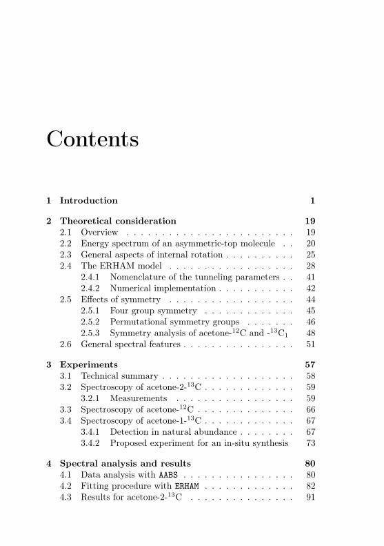
Contents
1 Introduction 1
2 Theoretical consideration 192.1 Overview . . . . . . . . . . . . . . . . . . . . . . . . 192.2 Energy spectrum of an asymmetric-top molecule . . 202.3 General aspects of internal rotation . . . . . . . . . . 252.4 The ERHAM model . . . . . . . . . . . . . . . . . . 28
2.4.1 Nomenclature of the tunneling parameters . . 412.4.2 Numerical implementation . . . . . . . . . . . 42
2.5 Effects of symmetry . . . . . . . . . . . . . . . . . . 442.5.1 Four group symmetry . . . . . . . . . . . . . 452.5.2 Permutational symmetry groups . . . . . . . 462.5.3 Symmetry analysis of acetone-12C and -13C1 48
2.6 General spectral features . . . . . . . . . . . . . . . . 51
3 Experiments 573.1 Technical summary . . . . . . . . . . . . . . . . . . . 583.2 Spectroscopy of acetone-2-13C . . . . . . . . . . . . . 59
3.2.1 Measurements . . . . . . . . . . . . . . . . . 593.3 Spectroscopy of acetone-12C . . . . . . . . . . . . . . 663.4 Spectroscopy of acetone-1-13C . . . . . . . . . . . . . 67
3.4.1 Detection in natural abundance . . . . . . . . 673.4.2 Proposed experiment for an in-situ synthesis 73
4 Spectral analysis and results 804.1 Data analysis with AABS . . . . . . . . . . . . . . . . 804.2 Fitting procedure with ERHAM . . . . . . . . . . . . . 824.3 Results for acetone-2-13C . . . . . . . . . . . . . . . 91
x CONTENTS
4.3.1 Torsional ground state . . . . . . . . . . . . . 914.3.2 First excited torsional state (v12 = 1) . . . . 110
4.4 Results for acetone-12C . . . . . . . . . . . . . . . . 1174.5 Results for acetone-1-13C . . . . . . . . . . . . . . . 118
5 Implications, summary and outlook 1255.1 Related results . . . . . . . . . . . . . . . . . . . . . 125
5.1.1 Acetone lines in an ALMA Sgr B2 spectrum . 1255.1.2 Dipole moment of acetone . . . . . . . . . . . 127
5.2 Summary and Outlook . . . . . . . . . . . . . . . . . 127
A Tables from the theoretical formalism 130A.1 Representations of molecular coordinates . . . . . . . 130A.2 Character and product tables . . . . . . . . . . . . . 131A.3 Correlation tables . . . . . . . . . . . . . . . . . . . . 137
B Manufacturers and models 139

List of Figures
1.1 Structure of acetone and its mono-13C isotopologues 31.2 Subsequent improvement of a predicted acetone spec-
trum . . . . . . . . . . . . . . . . . . . . . . . . . . . 16
2.1 Influence of rotational asymmetry on the general en-ergy level scheme of a rigid, non-distorted molecule . 24
2.2 Lowest-order torsional potential of a threefold internalrotor . . . . . . . . . . . . . . . . . . . . . . . . . . . 26
2.3 Influence of the barrier height on the torsional energylevels . . . . . . . . . . . . . . . . . . . . . . . . . . . 29
2.4 ERHAM: Origin of seemingly forbidden transitions . . 542.5 Internal axes, atom positions and internal rotational
directions in acetone . . . . . . . . . . . . . . . . . . 552.6 Acetone-2-13C: Observed relative intensities in the labor-
atory spectrum . . . . . . . . . . . . . . . . . . . . . 552.7 Acetone-2-13C: Overview spectrum up to 1.5 THz . . 56
3.1 General setup of a source-modulated absorption spec-trometer . . . . . . . . . . . . . . . . . . . . . . . . . 58
3.2 MIDAS-COINS: Optical and vacuum setup . . . . . 623.3 MIDAS-COINS: Absorption cells . . . . . . . . . . . 633.4 MIDAS-COINS: Beam splitter system . . . . . . . . 643.5 Acetone-13C: Isotopic abundances . . . . . . . . . . . 673.6 Acetone-1-13C: Predictive uncertainty, J dependence 693.7 Acetone-12C: Distribution of line spacings in the pre-
dicted spectrum . . . . . . . . . . . . . . . . . . . . . 703.8 Acetone-1-13C: Feasibility of acetone-12C high-sensit-
ivity measurements . . . . . . . . . . . . . . . . . . . 72
xii LIST OF FIGURES
3.9 Reaction scheme for the dry destillation of calciumacetate . . . . . . . . . . . . . . . . . . . . . . . . . . 73
3.10 DT-TG measurement of calcium acetate . . . . . . . 743.11 Acetone-1-13C: Yield optimisation by acetic acid-2-
13C content . . . . . . . . . . . . . . . . . . . . . . . 763.12 Acetone-1-13C: Proposed experiment for an in-situ
synthesis . . . . . . . . . . . . . . . . . . . . . . . . . 78
4.1 AABS screenshot . . . . . . . . . . . . . . . . . . . . . 814.2 AABS–ERHAM work sequence . . . . . . . . . . . . . . 824.3 ERHAM: Time complexity . . . . . . . . . . . . . . . . 844.4 Acetone-2-13C: Canonical fit statistics for J , N , f . 1024.5 Acetone-2-13C: Canonical fit statistics for (q, q′), obs.–
calc., (Ka −Kc)/(J + 1) . . . . . . . . . . . . . . . . 1034.6 Acetone-2-13C: J dependence of torsional and asym-
metry splittings for K ′′a = 3 . . . . . . . . . . . . . . 1044.7 Acetone-2-13C: Canonical fit, frequencies, K dep. . . 1064.8 Acetone-2-13C: Canonical fit, splittings, K dep. . . . 1074.9 Acetone-2-13C: Canonical fit, errors, K dependence . 1084.10 Acetone-2-13C: Evidence for a v12 torsional satellite 1124.11 Acetone-1-13C: Line confusion in natural abundance 1184.12 Acetone-1-13C: Line splittings at 264 GHz . . . . . . 119
5.1 Acetone-12C: New lines in ALMA Sgr B2 spectrum . 126
List of Tables
2.1 Acetone-12C and -2-13C: Spin weights . . . . . . . . 492.2 Acetone-12C and -2-13C: Relative intensities and se-
lection rules . . . . . . . . . . . . . . . . . . . . . . . 502.3 Acetone-1-13C: Spin weights . . . . . . . . . . . . . . 522.4 Acetone-1-13C: Relative intensities and selection rules 52
3.1 Acetone-2-13C: Measurement setups . . . . . . . . . 60
4.1 Evaluation of non-canonical tunneling parameters . . 924.2 Acetone-2-13C ground state fit . . . . . . . . . . . . 964.3 Acetone-2-13C, v12 = 1 fit . . . . . . . . . . . . . . . 1134.4 Acetone-12C: Fit results . . . . . . . . . . . . . . . . 1144.5 Acetone-1-13C: Fit results . . . . . . . . . . . . . . . 122
A.1 Coordinate representations . . . . . . . . . . . . . . 130A.2 Cs character table . . . . . . . . . . . . . . . . . . . 131A.3 C3 character table . . . . . . . . . . . . . . . . . . . 131A.4 C2v / V (a, b, c) character table with e/o assignments 132A.5 G18 character table . . . . . . . . . . . . . . . . . . . 133A.6 G18 product table . . . . . . . . . . . . . . . . . . . 134A.7 G36 character table . . . . . . . . . . . . . . . . . . . 135A.8 G36 product table . . . . . . . . . . . . . . . . . . . 136A.9 G18–σ correlation . . . . . . . . . . . . . . . . . . . . 137A.10 G36–σ correlation . . . . . . . . . . . . . . . . . . . . 138

Technology has never been a surrogate for a good idea –but even a good idea can never replace instinct.
Michael Cretu
Chapter 1
Introduction
Acetone, (CH3)2CO, is among the simplest asymmetric rotors fea-turing two methyl groups which undergo a large-amplitude torsionalvibration [Fig. 1.1 a)]. This motion is subject to a potential barrierof a specific height, which defines the strength of coupling to themolecule’s overall rotation and between the two rotors. Torsional-rotational coupling generally takes place within all molecules withtwo internal rotors, a fact which made it very difficult to obtain a cor-rect model of the rotational energy spectrum for such molecules forseveral decades. Its especially low barrier, or equivalently its strongcoupling, made acetone a touchstone molecule of rotational-torsionalspectroscopy. The exploration of its spectrum and molecular proper-ties was therefore pursued at the forefront of technical possibilities inspectroscopy and calculational performance. The detection of acet-one in the interstellar medium raised new astrochemical questions,with changing perspectives but no definitive answers each time anew step of technology or predictive accuracy was reached. Thisthesis continues this development, which is outlined in the follow-ing, towards an unprecedented predictional quality of its rotationalspectrum, and paves the way for future investigations of acetoneformation in interstellar environments by presenting new predictionsfor the rotational spectra of its singly 13C-substituted isotopologues.
2 Introduction
Timeline of acetone spectroscopy
Before the announcement of ERHAM1 in 1997, there were somesophisticated, but no comprehensive solutions to the problem of mo-lecules with two internal rotors. Fits to the spectrum based on per-turbative Hamiltonians, which were computationally very demand-ing and allowed for approximative predictions for lower quantumnumbers only. On the experimental side, there was a continuousdevelopment towards increased sensitivity, frequency coverage upto the sub-millimetre range, resolution and data acquisition speed.Moreover, the correct torsional excitation frequencies and the barrierheight could not be uniquely determined for a long time. Altogether,there was always a basis for a steadily recurrent interest in acetonespectroscopy.
Acetone belongs to the first organic molecules investigated [2]when microwave spectroscopy evolved after World War II [101]. In1959, following two mostly unsuccessful attempts by other groups,Swalen and Costain published the first assignment of 16 microwavetransitions of acetone [89] together with extensive further results(mentioned in the following), notwithstanding their small data set.This started a series of works to add more rotational transitions inline with the technical progress. Swalen and Costain’s assignmentswere made possible by a new algebraic group they introduced tocorrectly handle the symmetry of wavefunctions for the special caseof non-rigid molecules with C2v symmetry; an approach which wasconsolidated by Myers and Wilson [72] only one year later. The sym-metry calculations presented in Section 2.5 follow a slightly refinedmethodology [9, 10], which has grown over the years after, and usedifferent groups which are, though, still isomorphic to those presen-ted in these pioneering works.
The first broadband measurement of the infrared spectrum from300 cm−1 was reported by Cossee and Schachtschneider in 1966 [14],who tried to assign the observed wavenumbers to vibrational andtorsional modes using two different calculations. They also citedone wavenumber out of their measuring range from a publicationwhich had recently assigned this line to the co-rotating torsionalmode, but none of the works which appeared soon after could repro-duce this value nor any other values ascribed to the higher energy
1A phenomenological model based on an effective rotational Hamiltonian;see [32,35]
3
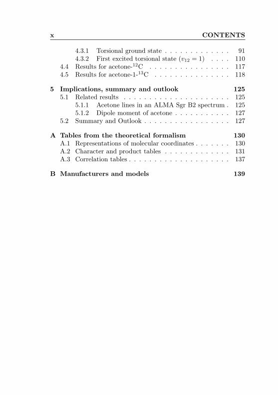
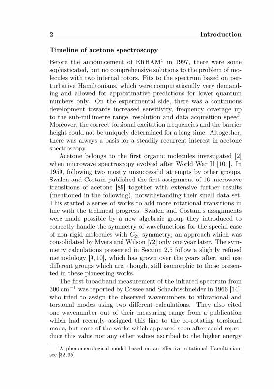
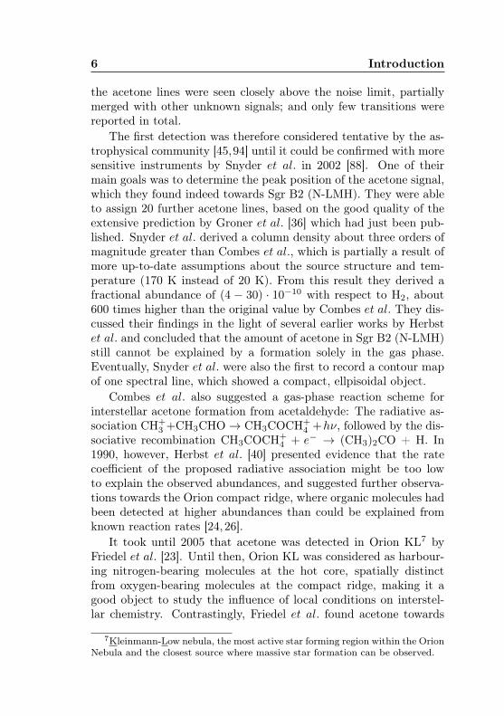
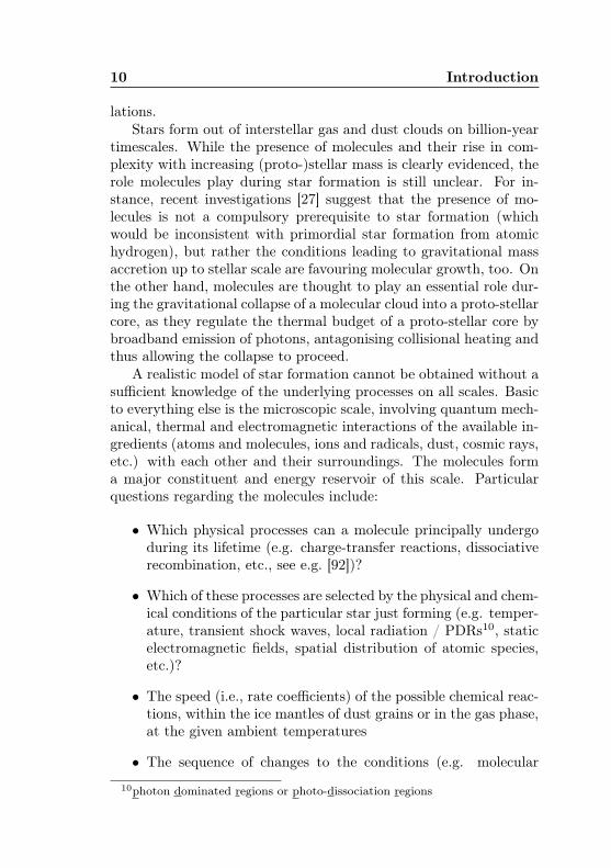
Figure 1.1: a) Equilibrium structure of acetone, (CH3)2CO, andits two mono-13C isotopologues acetone-1-13C [b)] and acetone-2-13C [c)], which were also spectroscopically analysed in thisthesis. All molecular structures depicted herein were calculated withArgusLab [91] using an AM1 Hamiltonian [18].
counter-rotating mode. Nonetheless, in 1972 a more comprehensiveassignment of the strongest transitions was published by Mann andDixon [61], and the order of transitions defined by their list has beenused to number the vibrational modes of acetone since. It was notuntil 1986 that Groner et al. [37] were able to find an unambiguousvalue for the second torsional mode (v17, 124.5 cm−1) in a Fouriertransform infrared (FTIR) spectrum, and finally Kundu et al. [53]detected the first mode (v12, 77.8 cm−1) in a Rydberg spectrum [63]in 1992.
By comparison of the torsional splittings with a Mathieu func-tion table (cf. Section 2.3), Swalen and Costain were able to derivea value for the height of the barrier to internal rotation. Severalcontradictory values were published with later reports on rotationaland vibrational spectroscopy works. Only a deeper analysis of thetorsional potential function by Groner, performed with his new ER-HAM method, brought clarity in 2000 [33]. He determined a valueof 251.4 ± 2.6 cm−1, which is quite low compared to more typicalvalues such as approx. 950 cm−1 for dimethyl ether [34].
A significant step forward for molecules with two internal rotorswas made when ERHAM was introduced in 1997 (see Section 2.4 orthe original publications [32, 35]). While good results could alreadybe achieved for single-rotor molecules with a perturbative treatmentunder the principle axis method (PAM) or the internal axis method(IAM) [59], this model could not be straightforwardly extended tomolecules with two internal rotors because the indispensable coup-
4 Introduction
ling terms could hardly be handled within a resonable calculationalframework to reproduce experimental accuracy. The ERHAMmodelis the logical extension of the concept of phenomenological Hamilto-nians, which had been successfully used for single-rotor, quasi-rigid2
molecules since the 1970s, to molecules with two symmetric internalrotors. Its advantages – mainly a complete handling of all couplingterms with merely one minor approximation of which no exceptionsare known to date; adaptability to double-rotor molecules of arbit-rary symmetry; and a substantial reduction of calculation time underfull retention of all asymmetric rotor parameters – are counterbal-anced by the loss of information about the torsional potential, whichcan only be inferred from additional, not purely rotational measure-ments. A FORTRAN implementation of a least-squares algorithmfor the ERHAMmodel (called ERHAM), which, being the current stateof the art [36], had since been used for the acetone predictions, waslikewise used for the calculations in this thesis (Chapter 4).
With the great improvements of the ERHAM model at hand, itwas obvious to try and fit spectra from the excited torsional states,too. This was accomplished for v12 = 1 in 2006 [38], and for v17 = 1in 2008 [38].
The latest publication on the acetone spectrum reports an at-tempt to fit the given acetone data with a dedicated PAM programfor molecules with two methyl rotors and C2v symmetry [44]. In-deed, this non-phenomenological approach achieves an overall im-provement of the fit by fitting parts of the data set better, yet otherparts are fit worse. To date, the introduced programme does not yetallow for predictions and lacks the general applicability and compu-tational efficiency of ERHAM.
The first, and still the most recent, spectroscopic work on acetone-13C1 was published by Lovas and Groner [60] in 2006. They used aBalle-Flygare-type spectrometer (a resonator-based FTMW3 spec-trometer, where the sample molecules are expanded into a cold jet),leading to sufficiently high sensitivity at low quantum numbers tosee both mono-13C isomers of acetone in natural abundance. Theyreported observations of 11 rotational transitions, where the fourtorsional components (five for acetone-1-13C) could be assigned inall cases, giving a total of 44 (55) transitions. This thesis ties in with
2i.e., featuring only small-amplitude internal motions3FTMW = Fourier-transform microwave
5
the predictions they made by extrapolation from measurements be-low 25 GHz.
Acetone in the interstellar medium
A new series of open questions was added to the acetone case whenit was first detected by spectral observations of the extended starforming region Sagittarius (Sgr) B2 close to the Galactic centre byCombes et al. in 1986 [13]. This introduction shall give but a briefsummary of the extensive literature in this field to outline the sci-entific context of this thesis within the research on interstellar acet-one.
Interstellar molecules are detected by observations of their uniquespectra4, which are usually seen in emission due to their internal ex-citation in dense molecular clouds (Tkin ≈ 10−300 K) in front of thecold cosmic microwave background (2.725 K). These spectra must becompared to spectral predictions for the gas under interstellar con-ditions, which must be derived from laboratory observations underterrestrial conditions (i.e., higher pressure and room temperature).The accuracy of the predicted spectrum should exceed that of theobservatories, which is usually the case if the respective molecularmodel can be fit to the assigned transition with experimental uncer-tainty (peak detection typically of the order ∆f/f ∼ 10−7). At thetime of its interstellar discovery, laboratory spectroscopy of acetonehad proceeded up to ∼ 300 GHz [95], and a prediction of sufficientprecision for observations around 3 mm was available.
Combes et al. found lines of four rotational transitions (J = 8and 9) in the source Sgr B2 (OH)5, at a time when it was not knownthat the nearby hot-core source Sgr B2 (N-LMH) is hosting a muchlarger number of complex6 organic molecules (COMs). Accordingly,
4The term “spectral fingerprint” alludes to the extremely strong dependenceof line frequencies in rotational spectra on the molecular structure.
5Notable sources within the large Sgr B2 cloud include (OH), a region ofstrong OH maser emission, (N) about 1’19” to the north, and (M) in the middlebetween these regions. Sgr B2(N) contains the hot-core region (N-LMH), “LargeMolecule Heimat”, where an unusually large number of complex molecules hasbeen found.
6The complexity ascribed to a molecular species strongly depends on the re-searcher’s point of view. While the complexity of enzymes or DNA is accepted asstandard in organic chemistry or molecular biology, current astrochemical mod-els are dealing with molecules consisting of not much more than 10 atoms [24].
6 Introduction
the acetone lines were seen closely above the noise limit, partiallymerged with other unknown signals; and only few transitions werereported in total.
The first detection was therefore considered tentative by the as-trophysical community [45,94] until it could be confirmed with moresensitive instruments by Snyder et al. in 2002 [88]. One of theirmain goals was to determine the peak position of the acetone signal,which they found indeed towards Sgr B2 (N-LMH). They were ableto assign 20 further acetone lines, based on the good quality of theextensive prediction by Groner et al. [36] which had just been pub-lished. Snyder et al. derived a column density about three orders ofmagnitude greater than Combes et al., which is partially a result ofmore up-to-date assumptions about the source structure and tem-perature (170 K instead of 20 K). From this result they derived afractional abundance of (4 − 30) · 10−10 with respect to H2, about600 times higher than the original value by Combes et al. They dis-cussed their findings in the light of several earlier works by Herbstet al. and concluded that the amount of acetone in Sgr B2 (N-LMH)still cannot be explained by a formation solely in the gas phase.Eventually, Snyder et al. were also the first to record a contour mapof one spectral line, which showed a compact, ellpisoidal object.
Combes et al. also suggested a gas-phase reaction scheme forinterstellar acetone formation from acetaldehyde: The radiative as-sociation CH+
3 +CH3CHO→ CH3COCH+4 +hν, followed by the dis-
sociative recombination CH3COCH+4 + e− → (CH3)2CO + H. In
1990, however, Herbst et al. [40] presented evidence that the ratecoefficient of the proposed radiative association might be too lowto explain the observed abundances, and suggested further observa-tions towards the Orion compact ridge, where organic molecules hadbeen detected at higher abundances than could be explained fromknown reaction rates [24,26].
It took until 2005 that acetone was detected in Orion KL7 byFriedel et al. [23]. Until then, Orion KL was considered as harbour-ing nitrogen-bearing molecules at the hot core, spatially distinctfrom oxygen-bearing molecules at the compact ridge, making it agood object to study the influence of local conditions on interstel-lar chemistry. Contrastingly, Friedel et al. found acetone towards
7Kleinmann-Low nebula, the most active star forming region within the OrionNebula and the closest source where massive star formation can be observed.
7
the hot core, but not above 3σ towards the compact ridge, suggest-ing an influence of nitrogen chemistry on acetone formation. Thisidea was not too unrealistic, as the picture of interstellar chemistryhad changed from pure gas-phase reactions to gas-grain chemistryin the meantime, where catalytic reactions within the ice mantles ofinterstellar dust grains take place at lower cloud temperatures andthe onset of star formation triggers a sublimation of the productsthrough heating.
Since then, research on interstellar acetone strongly accelerated.After one confirmation by Goddi et al. in 2009 [28], two later pa-pers by Friedel and Widicus Weaver [22,100] were the first to lowerthe confusion about interstellar acetone a little. They reported thefirst study of Orion KL at high angular resolution and substantiallyimproved sensitivity, involving the spectra of eight molecular spe-cies. They found that the model of chemical differentiation betweennitrogenic and oxygenic species, which had arisen from the lowersensitivity of former astronomical equipment, had to be given up, asall complex molecules considered within their study showed a muchgreater spatial overlap at lower abundances. Acetone was foundmainly in parts of the cloud where the overlap between ethyl cyanide(C2H5CN) and acetic acid (CH3COOH) was greatest. Interpretingthis result as showing a link between the formation of these two spe-cies and acetone would be too early, as Orion KL hosts many otherspecies which had not been considered in this study. Friedel andWidicus Weaver also analysed the dynamics of the same species andfound that acetone seems to be robuster against changing physicalor chemical conditions than other complex molecules. It is seen closeto the hottest structures of the region (rotational temperatures ofmethanol, CH3OH, up to ∼ 400 K), but not actually tracing them.
The latest publication on acetone in Orion KL by Peng et al. 2013[77] is an independent PdBI8 survey of Orion-KL focusing purely onthe problem of acetone formation. While their observations (includ-ing lines around 225 GHz for the first time) are similar to thosereported by Widicus Weaver and Friedel, they conclude that an al-ternative formation path involving N-bearing molecules should ex-ist which is missing in all previous models on acetone formation inOrion-KL.
Only two months earlier, a third interstellar source containing
8Plateau de Bure Interferometer, operated near Grenoble, France
8 Introduction
acetone was found by Codella et al. with the high-mass young stel-lar object G24.78+0.08 [12]. The detection is only tentative becauseonly one acetone transition (184,14 ← 175,13), with all four com-ponents overlapping, matches a particular pattern observed in oneof the 2 GHz SMA9 sidebands, but it is still reasonable becauseacetone is expected to trace star forming regions. The most re-cent publication on interstellar acetone by Rong et al. 2015 reportsa detection (by thirteen lines) in one further high-mass star form-ing region, W51 North [84]. Among investigations concerning otherspecies, they found hints that grain-surface reactions may be moresuitable to explain acetone formation, while the structurally similardimethyl ether [(CH3)2O] should rather have a gas-phase formationroute similar to that of methyl formate (CH3OCHO). A rotationaltemperature of 140 K could be derived.
The greater picture: Star formation and interstellar chem-istry
The development of interstellar acetone detections is exemplary forthe changes observational (sub-)millimetre astronomy is currentlyundergoing, and the challenges still to be mastered to gain a coherentpicture of interstellar chemistry. See [98] for an excellent reviewarticle by W. D. Watson (1976) where the basic, and still valid,foundations of modern astrochemistry are collected.
Interpreting interstellar molecular spectra is highly demandingfor a number of reasons. To detect an interstellar molecule, onemust know the frequencies and intensities of all of its spectral lineswithin the observed frequency range with a precision that matchesor exceeds that of the telescopes. The observed intensities depend onthe molecules’ rotational temperature; if candidate lines are found,the absolute intensity of the predicted spectrum can be scaled tomatch the observed spectrum. The frequencies are Doppler shiftedby a usually inhomogeneous velocity distribution of the source. Theconnections between observed spectra and physical conditions makeinterstellar spectroscopy a highly sensitive tool, often even the onlyone, to explore these conditions and thus gain an understanding ofthe complex processes underlying interstellar chemistry.
Interstellar spectra are composed from the emission of all species
9Submillimeter Array, operated at the Mauna Kea Observatory, Hawai‘i, USA
9
present in the observed source. With increasing molecular complex-ity, the total emitted power spreads over a growing spectral density,which leads to a decreasing specific line intensity. As a result, oneobserves a superposition of some very strong, usually well-separatedlines from smaller species, and a background of increasingly mergedweak lines originating from the more complex species. For thisreason, the correct absolute intensities for newly investigated spe-cies – especially for the complex ones, dubbed “molecular weeds”by astronomers –, which are needed to derive their relative abund-ances, can be correctly determined only if one knows the intensitiesof all other species participating in blended lines. Superposition alsolowers the number of lines which can be uniquely assigned to a cer-tain species, which is hampering the detection of complex species inparticular.
Deriving the abundance of an interstellar molecular species fromcolumn densities, which in turn are calculated from the flux densitiesreceived from unique emission lines of such species, is crucial to gaina correct quantitative understanding of interstellar chemistry. Thereare several technical problems relating to column density determin-ations, see e.g. the discussion in [100]. An additional source of errorarises from the predicted intensities: The molecular model basedon laboratory work must provide a correct estimate of the partitionfunction Q, where all energy levels populated at a given temperat-ure have to be taken into account. This is especially important formolecules like acetone, which exhibit low-lying vibrational or tor-sional states (e.g. acetone’s v12 = 77.8 cm−1, corresponding to anexcitational temperature of 112 K) that are significantly populatedeven in cooler interstellar sources.
Interstellar molecules are observed in a multiplicity of sourceswith distinct chemistries. The largest, fully hydrogenated organicmolecules are found in hot molecular cores [8]. These dense, compactclouds show temperatures above 100 K and are typically found inactive star-forming regions. The research interest in rotational spec-tra of complex organic molecules (COMs) is therefore also drivenby the astrophysical research on star formation [41, 86]. Progressin understanding this highly complex, turbulent, feedback-driven,multi-scale process is currently fostered by an international inter-disciplinary effort, combining approaches like magnetohydrodynam-ics, quantum thermodynamics, astrochemistry and numerical simu-
10 Introduction
lations.Stars form out of interstellar gas and dust clouds on billion-year
timescales. While the presence of molecules and their rise in com-plexity with increasing (proto-)stellar mass is clearly evidenced, therole molecules play during star formation is still unclear. For in-stance, recent investigations [27] suggest that the presence of mo-lecules is not a compulsory prerequisite to star formation (whichwould be inconsistent with primordial star formation from atomichydrogen), but rather the conditions leading to gravitational massaccretion up to stellar scale are favouring molecular growth, too. Onthe other hand, molecules are thought to play an essential role dur-ing the gravitational collapse of a molecular cloud into a proto-stellarcore, as they regulate the thermal budget of a proto-stellar core bybroadband emission of photons, antagonising collisional heating andthus allowing the collapse to proceed.
A realistic model of star formation cannot be obtained without asufficient knowledge of the underlying processes on all scales. Basicto everything else is the microscopic scale, involving quantum mech-anical, thermal and electromagnetic interactions of the available in-gredients (atoms and molecules, ions and radicals, dust, cosmic rays,etc.) with each other and their surroundings. The molecules forma major constituent and energy reservoir of this scale. Particularquestions regarding the molecules include:
• Which physical processes can a molecule principally undergoduring its lifetime (e.g. charge-transfer reactions, dissociativerecombination, etc., see e.g. [92])?
• Which of these processes are selected by the physical and chem-ical conditions of the particular star just forming (e.g. temper-ature, transient shock waves, local radiation / PDRs10, staticelectromagnetic fields, spatial distribution of atomic species,etc.)?
• The speed (i.e., rate coefficients) of the possible chemical reac-tions, within the ice mantles of dust grains or in the gas phase,at the given ambient temperatures
• The sequence of changes to the conditions (e.g. molecular
10photon dominated regions or photo-dissociation regions
11
evaporation from grain surfaces in response to increased tem-perature) and their timing
• The degree of molecular complexity reached by this sequenceof processes before star formation is completed
• The complex process of incorporation of these molecules intothe circumstellar proto-planetary disk.
The prevailing picture of molecule formation in interstellar con-ditions – a fact deemed impossible not a hundered years ago – isthat atoms, ions, radicals and small molecules condense onto colddust grains, coating them into an ice mantle. Their mobility in ice islow, but not zero, just enough to migrate the ice and occasionally, ifactivation energy is present, undergo chemical reactions with otherice-mantle species. This way, they outlast captured until the dust isheated up during the onset of star formation. In the gas phase, withincreased mobility and direct exposure to radiation, further reactionsbecome possible, increasing molecular complexity if destructive pro-cesses are not dominating. A review article representing the state ofthe art in gas-grain chemistry modeling as of 2008 is [24].
One open question in astrochemistry is the role of carbon monox-ide. It is the most abundant molecule containing carbon and, dueto its sole composition of carbon and oxygen, of high influence onboth carbon and oxygen chemistry in the ISM. While its high abund-ance is a hint that the formation of organic molecules should usuallystart from CO, observations of highly unsaturated carbon species incold environments, in conjunction with the overabundant elementhydrogen, suggest that COMs could also be formed from these bysubsequent hydrogenation reactions during cloud collapse and heat-ing.
Further interesting questions exist regarding the molecular com-plexity created by interstellar chemistry. For instance, one may askwhether molecules like n-propyl cyanide (C3H7CN), which base on acarbon chain, are the product of a pure carbon chain undergoing hy-drogenation, or built from smaller precursors like e.g. methyl cyan-ide and ethanol in a more modular way; whether molecules like acet-one ((CH3)2CO) containing a C=O double bond were formed fromcarbon monoxide by methyl addition or from a pure hydrocarbon byoxygen addition; or whether the formation of branched isomers [4] orconformers, like tert-butyl cyanide or gauche-anti n-butyl cyanide,
12 Introduction
is disadvantaged from linear configurations like anti-anti n-butyl cy-anide, as is known from chemistry on earth [75]. As interstellar mo-lecules form under conditions far from thermal equilibrium, futuredetections of exotic conformational isomers (conformers) of knownmolecules in the ISM can be expected. Observations and analyses ofinterstellar conformational abundances in comparison to their equi-librium distribution, based on their differing formation energies, areexpected to give new insights into interstellar chemistry.
The interest in interstellar COMs does not end with star form-ation and astrochemistry per se. Besides their suitability as highlysensitive probes for the local physical conditions within a source, itis peculiar that all species with more than five atoms identified so farare organic [41]. They are therefore capable of forming species (notyet detected) which could have been the molecular precursors of lifeon Earth. It is an important conceptual difference whether moleculesenabling the formation of life were formed in the ISM and have onlybeen transported to Earth, meaning that this process may happenin any other planetary system as well, or if conditions on Earth areso “special” that life has accidentally formed here from minor pre-cursors. While more than 80 different amino acids of most probablyextraterrestrial origin11 have been found in meteorite cores and evenin a sample of cometary outflow to date [6,19,54], only one presumedprecursor of glycine, the smallest proteinogenic amino acid, could beidentified in the ISM [3,87].
Isotopic abundances in the ISM
Isotopically substituted molecules, which are also called isotopo-logues, and their respective isomers called isotopomers, are espe-cially interesting for interstellar astronomy. Lighter or heavier atomsintroduce slight changes to the adjacent bond lengths, thereby shift-ing the frequencies of all spectral lines, and sometimes even changingmolecular symmetry, which usually strongly impacts the appearanceof the whole spectrum. If, for instance, one methyl carbon atom inacetone ((CH3)2CO) is replaced by 13C, the symmetry of the mainisotopologue is broken (see Section 2.5) and each rotational trans-ition splits into five components, with a different intensity pattern,instead of the four components known from the main isotopologue.
11As suggested by their isotopic signatures and racemic mixture.
13
Isotopologues also behave different chemically, which becomes es-pecially apparent at cold cloud temperatures (some 10 K) which aresmall compared to the energy released during exothermal reactionslike H+
3 +HD→ H2D+ +H2 (230 K) or CH+3 +HD→ CH2D+ +H2
(370 K) [45]. In the past decades, many interstellar objects werefound to host molecules with isotopic signatures exceeding the cos-mic values, sometimes by many orders of magnitude [64]. Isotopesare often inherited to more complex species along preferred reactionpaths, leading to a strong enhancement for one species and depletionfor the others. For more than four decades [99], the fractionationreactions leading to interstellar isotopic enhancement or depletionhave been subject to ongoing observations [102], calculations [65],theoretical works [85], and experiments [43].
As regards carbon-13, it has been calculated to get stronglyenriched in carbon monoxide by cold gas-phase ion-neutral reac-tions [20, 55]. For this reason, astronomical observations with theaim to obtain reliable values for the abundances of interstellar singly13C-substituted species can give strong hints on the role CO playsin the formation of a molecule or its constituents. Furthermore,it is possible that many of the still unknown interstellar spectrallines (“U lines”) belong to signals from enriched isotopologues whoselaboratory spectra simply have not yet been analysed. In their re-view article on complex organic interstellar molecules [41], Herbstand van Dishoeck mention a millimetre-wave survey [90] where thenumber of U lines was reduced from roughly 8000 to 6000 after somespectral data from isotopologues and excited states of known specieshad been added to the catalogue.
Observations of interstellar isotopic signatures thus are a prom-ising tool to gain insight into the complex phenomena of interstellarchemistry. Signatures may be compared between different interstel-lar regions, different conformational or other isomers of the samespecies, or molecules of high structural similarity but possibly a dif-ferent formation path, such as dimethyl ether, (CH3)2O, and acet-one, (CH3)2CO. For instance, acetone has to date been found onlyin two high-mass star forming regions, whereas dimethyl ether is alsofound in the low-mass star forming region IRAS 16293 – 2422 [11].It is questionable whether this non-detection originates from a lackof sensitivity or differences in the chemistry of these particular re-gions. Isotopic signatures, being a sensitive and versatile probe for
14 Introduction
the conditions and history of a given site, can also help solve theever-returning question whether a species is formed in the gas phaseor on grain surfaces [52], and they increasingly come into play as sev-eral new astronomical observatories for the (sub-)millimetre regionhave recently been launched or are getting finished these days.
Ongoing technical developments in observational and labor-atory astronomy
The interpretation of astronomical spectra has widely evolved sinceFraunhofer’s first observations of the visible solar spectrum with itsfamous absorption lines from atoms in the solar atmosphere. Besidesrecording the position, intensity, polarisation and time dependenceof astronomical sources, spectral analysis is still the most import-ant means to gain insight into their physical and chemical condi-tions. To date, nearly all spectral regions are covered by a numberof observatories, one of the technically most demanding being theTHz regime [16]. Together with the microwave / millimetre-waveregion, this part of the electromagnetic spectrum reflects the char-acteristic energy scale for the excitation of molecular rotation. Asthe spectral transition frequencies of a molecule are characteristicfor its structure and the intensities depend sensitively on its phys-ical state, (sub)millimetre spectroscopy is the method of choice toinvestigate the chemical composition and the physical conditions ofcold to warm inter-, circum-, and protostellar gases.
However, a clear identification of an interstellar molecular speciesis difficult because the beam arriving at a telescope usually containssignals from a large number of species within the same source, pro-ducing a dense spectrum with many spectral lines superposed. Asufficiently large number of spectral lines can be identified only ifprecise predictions of spectral line frequencies and intensities existfor each of the known species at the model temperature of the source.With increasing molecular complexity (i.e., large weight and asym-metric structure), the spectra become denser and weaker at the sametime. For these reasons, collaborations of the most sensitive spec-troscopic laboratories and astronomical observatories are essentialto expand our understanding of the mechanisms which have formedthis variety of molecules under interstellar conditions [86]. More
15
than 180 molecular species12 have been found by spectral analysisof interstellar molecular clouds and circumstellar envelopes to thecurrent date.
The previous paragraphs already hinted at the current situationof missing spectral predictions derived from laboratory spectroscopy.The astronomical (sub-)millimetre observatories of the latest gener-ation, above all the Stratospheric Observatory for Infrared Astro-nomy (SOFIA, [42]), the Atacama Large Millimetre / submillimetreArray (ALMA), the already exhausted Herschel satellite [15] or theupcoming Northern Extended Millimetre Array (NOEMA), are un-precedented in sensitivity and angular and frequency resolution. In-terstellar maps and spectra are about to be unveiled in ever moredetail, and signals from isotopologues and excited torsional statesof many known species will become visible for the first time. Ob-taining reliable and precise spectral predictions for the prospectivespecies in this vein is among laboratory astrophysics’ major jobs forthe next decades [71].
Another consequence of this technical progress, which is espe-cially relevant for COMs, is that earlier spectral predictions, whichmay have sufficed for past astrophysical detections, have grown tooinaccurate to serve as a data source for spectral analysis of the datagenerated by the new-generation observatories. Any imprecision inpredicted spectra can become influential if one wants to model thecorrect intensities of stronger superposition lines or detect an un-known species with lines of similar intensity. The complex interstel-lar species are therefore sometimes dubbed “weed molecules”, whichare to be separated from the species of interest. Past works on astro-physical spectra relied on calculated line frequencies which used toreside within an acceptable range around the true frequencies. Thewidth of this range was a direct consequence of larger line widthsor other experimental uncertainties encountered in earlier laborat-ory spectra. With their new spectrometric equipment, showing en-hanced sensitivity and frequency resolution, modern observatorieshave stricter acceptability limits for predictive deviations. Moreover,transitions with quantum numbers beyond the boundaries of formerfits (meaning weaker branches and higher quantum numbers, espe-cially in K) are now observed in astronomical data for the first time,but cannot be correctly identified because the old predictions for
12Source: Cologne Database for Molecular Spectroscopy, CDMS [68–70]
16 Introduction
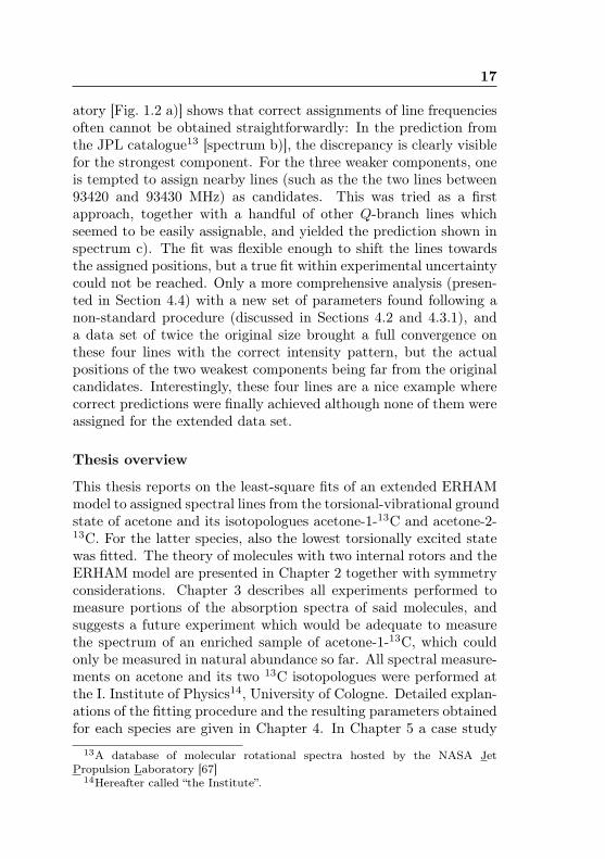
such branches are systematically shifted from the true frequencies.An example involving recent ALMA 3-mm data is presented in
Chapter 5 to show that the latter effect can be striking for chal-lenging molecules like acetone. Improved spectral predictions foracetone may also be of use for atmospheric research, where acetonewas found to be an atmospheric pollutant [1, 17] intervening withozone chemistry.
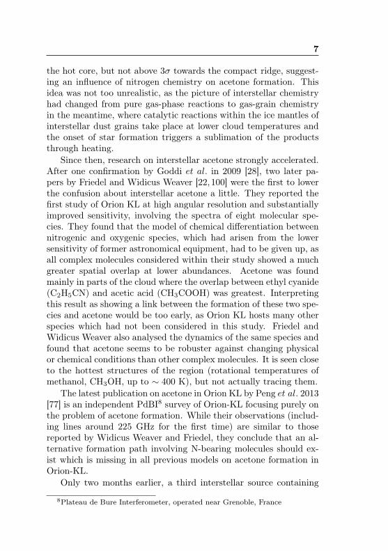
A closer inspection of an acetone spectrum measured in the labor-
Figure 1.2: The four component lines of the acetone-12C transition2715,12 ← 2714,13 as seen in a spectrum measured in the laboratory[a); see Section 3.3] and predicted from three different fits [b) tod)]. Starting with the prediction by Groner et al. [b)], the fit wasrepeated after four lines, which would seemingly match the predictedintensity pattern in the depicted frequency range, and a handful ofothers had been added to the data set. The resulting prediction[c)] showed significant shifts towards the assigned frequencies, butno satisfactory agreement. Spectrum d) shows the final predictionaccording to a revised fit (see Section 4.4) after about 1000 newassigments in the range 38 – 130 GHz. Frequencies are given inMHz.
17
atory [Fig. 1.2 a)] shows that correct assignments of line frequenciesoften cannot be obtained straightforwardly: In the prediction fromthe JPL catalogue13 [spectrum b)], the discrepancy is clearly visiblefor the strongest component. For the three weaker components, oneis tempted to assign nearby lines (such as the the two lines between93420 and 93430 MHz) as candidates. This was tried as a firstapproach, together with a handful of other Q-branch lines whichseemed to be easily assignable, and yielded the prediction shown inspectrum c). The fit was flexible enough to shift the lines towardsthe assigned positions, but a true fit within experimental uncertaintycould not be reached. Only a more comprehensive analysis (presen-ted in Section 4.4) with a new set of parameters found following anon-standard procedure (discussed in Sections 4.2 and 4.3.1), anda data set of twice the original size brought a full convergence onthese four lines with the correct intensity pattern, but the actualpositions of the two weakest components being far from the originalcandidates. Interestingly, these four lines are a nice example wherecorrect predictions were finally achieved although none of them wereassigned for the extended data set.
Thesis overview
This thesis reports on the least-square fits of an extended ERHAMmodel to assigned spectral lines from the torsional-vibrational groundstate of acetone and its isotopologues acetone-1-13C and acetone-2-13C. For the latter species, also the lowest torsionally excited statewas fitted. The theory of molecules with two internal rotors and theERHAM model are presented in Chapter 2 together with symmetryconsiderations. Chapter 3 describes all experiments performed tomeasure portions of the absorption spectra of said molecules, andsuggests a future experiment which would be adequate to measurethe spectrum of an enriched sample of acetone-1-13C, which couldonly be measured in natural abundance so far. All spectral measure-ments on acetone and its two 13C isotopologues were performed atthe I. Institute of Physics14, University of Cologne. Detailed explan-ations of the fitting procedure and the resulting parameters obtainedfor each species are given in Chapter 4. In Chapter 5 a case study
13A database of molecular rotational spectra hosted by the NASA JetPropulsion Laboratory [67]
14Hereafter called “the Institute”.

18 Introduction
is shown where the new predictions for the main isotopologue havebeen used to find interstellar spectral lines which were predictedwrongly before. The chapter continues with a short comment onthe prevalent literature values of the dipole moment of acetone andcloses with a summary of the results and an outlook on future worksneeded to accomplish what was started here. Tables from the the-ory chapter and additional information on the laboratory equipmentused during the measurements have been collected in the Appendix(page 130).
Chapter 2
Theoretical consideration
2.1 Overview
The appearance of the rotational spectrum of a large class of mo-lecules, including acetone, derives from the fact that their respect-ive equilibrium structure constitutes an asymmetric top. The termasymmetry is meant here purely in terms of the mass distributionwhich becomes effective during a molecule’s overall rotation. Inmathematical terms, the geometrical arrangement of its nuclei res-ults in three different non-zero components in the diagonalised mo-ment of inertia tensor. This rotational asymmetry is independent ofthe symmetry operations existing for the point group formed bythe equilibrium structure of its nuclei. The spectrum of a gen-eral asymmetric-top molecule is described in the standard literat-ure [30,93] and summarised in Section 2.2.
A major effect in the spectrum of acetone arises from the collect-ive torsional motion of the hydrogen atoms located in each of the twomethyl groups with respect to the rotating frame (Section 2.3). Thisinternal large-amplitude motion (LAM) couples to the molecule’soverall rotation, causing a splitting of each asymmetric rotor lineinto four components (five for acetone-1-13C). While spacing andorder of these torsional components can vary strongly with the ro-tational state, their intensity distribution always follows one outof two patterns, depending on the rotational quantum numbers in-volved in the transition. Intensity patterns and selection rules for
20 Theoretical consideration
acetone-13C1 are explained in Section 2.5 within the group theoret-ical framework described in the literature [9, 10].
Reconstructing the full torsional-rotational Hamiltonian from as-signments of recorded spectra is calculationally too demanding to es-tablish a resonable workflow which allows for iterative assigning andfitting. A practical, time-saving procedure to calculate an effectiverotational Hamiltonian (ERHAM) has therefore been established,together with a homonymous FORTRAN program, by P. Groner in1997 [32]. It builds upon the insight that the Hamiltonian dependsperiodically on the rotational quantum numbers and symmetry la-bels, and applies several approaches, including molecular symmetry,to simplify the calculation as much as possible. The theory behindthis effective model and its software implementation ERHAM [47] isoutlined in Section 2.4. The program ERHAM cannot be used to de-termine the potential energy surface (PES) of a molecule only fromits rotational spectrum, but it has proven its practical use to fit andpredict rotational spectra of molecules with two or more internalperiodic large-amplitude motions, see e.g. [52].
The general appearance of the rotational spectra of acetone-12C and -13C1, as derived from the theory presented, is explained inSection 2.6.
2.2 Energy spectrum of an asymmetric-top molecule
The general theory of a rotating asymmetric molecule has been ex-tensively described in the literature [30, 93]. It starts with the clas-sical Hamilton function of a freely rotating rigid body,
H =~2
2
(P 2a
Ia+P 2b
Ib+P 2b
Ib
)(2.1)
=AP 2a +BP 2
b + CP 2c (2.2)
which is formally identical to the quantum mechanical Hamiltonoperator by straightforward application of the principle of corres-pondence. The labels a, b and c of the principle axes of inertia arechosen such that the principal moments of inertia fulfill the rela-tion Ia ≤ Ib ≤ Ic. A rearranged form of eq. (2.2) more useful for
2.2 Energy spectrum of an asymmetric-top molecule 21
spectroscopy is
H = 12 (A+ C)P 2 + 1
2 (A− C)H(ξ) (2.3)
with P 2 = P 2a+P 2
b +P 2c , the reduced HamiltonianH(ξ) = P 2
a+ξP 2b −
P 2c and the asymmetry parameter ξ = 2B − A − C/(A − C)1. The
two limiting cases which can generally be discerned for a rotatingasymmetric body are the prolate top (Ia = Ib < Ic ⇒ ξ = −1) andthe oblate top (Ia < Ib = Ic ⇒ ξ = +1). Although the theory of theasymmetric top deals with all other non-spherical2 configurations,i.e., −1 < ξ < +1, its quantum mechanical treatment is based onthe symmetric-top solutions of the Schrödinger equation, which aretherefore displayed in the following.
The symmetric rotor
Two further axes systems are important for a proper descriptionof a rotating molecule: The space-fixed or laboratory axes systemX,Y, Z and the body-fixed or molecular axes system x, y, z, whichis usually chosen according to symmetry considerations. In manycases it is advantegeous to have the x, y, z system coinciding withthe a, b, c system, and one out of six assignment possibilities calledrepresentations is chosen (See Table A.1). The representations ofchoice for near-prolate and near-oblate tops are Ir and IIIl, respect-ively, where the z axis coincides with the symmetry axis a or c toyield a Hamiltonian of most simplified structure.
In a force-free environment, which can be assumed for all experi-ments described here, the total angular momentum and its directionin the laboratory frame are conserved:
dP
dt= X
(dPXdt
)+ Y
(dPYdt
)+ Z
(dPZdt
)= 0 (2.4)
This is still true in the rotating frame, but in the corresponding equa-tions (Euler’s equations of motion) an additional fictitious torqueω×P called Euler force occurs as a compensation for the change of
1The asymmetry parameter is called κ in the literature. This would cre-ate confusion here, however, because κ is also an important parameter in theERHAM model.
2Bodies with Ia = Ib = Ic are called spherical rotors.
22 Theoretical consideration
coordinates:
X
(dPxdt
)+ Y
(dPydt
)+ Z
(dPzdt
)+ ω ×P = 0 (2.5)
For an appropriate representation, the equality of the moments ofinertia typical for symmetric tops is inherited to x and y, and itfollows from Euler’s equation of motion for the z component,
dPzdt
+
(1
Ix− 1
Iy
)PxPy = 0 (2.6)
that Pz is conserved, too. The operators PZ , Pz, and P 2 = P 2X +
P 2Y + P 2
Z = P 2x + P 2
y + P 2z therefore have common eigenfunctions
|JKM〉 with the Hamiltonian, with quantum nubers defined by thealgebraic properties
〈JKM |P 2|JKM〉 = ~2J(J + 1), J ∈ N0 (2.7a)〈JKM |Pz|JKM〉 = ~K,−J ≤ K ∈ Z ≤ J (2.7b)〈JKM |PZ |JKM〉 = ~M,−J ≤M ∈ Z ≤ J (2.7c)
The energy levels of the two symmetric-top cases are thus found tobe3
〈J,K|H(P )R |J,K〉 = h[BJ(J + 1) + (A−B)K2] (2.8)
for the prolate case, and
〈J,K|H(O)R |J,K〉 = h[BJ(J + 1) + (C −B)K2] (2.9)
for the oblate case. Note that K measures the projection of angularmomentum on the respective symmetry axis a or c, and that theenergy depends quadratically on both J and K. As a consequence,except for K = 0, the energy levels do not depend on the sign of Kand are therefore doubly degenerate. A prolate top features a seriesof energies increasing with K for a given J , whereas the same seriesis decreasing for an oblate top.
3Eigenfunctions and -values are independent of M due to momentum conser-vation.
2.2 Energy spectrum of an asymmetric-top molecule 23
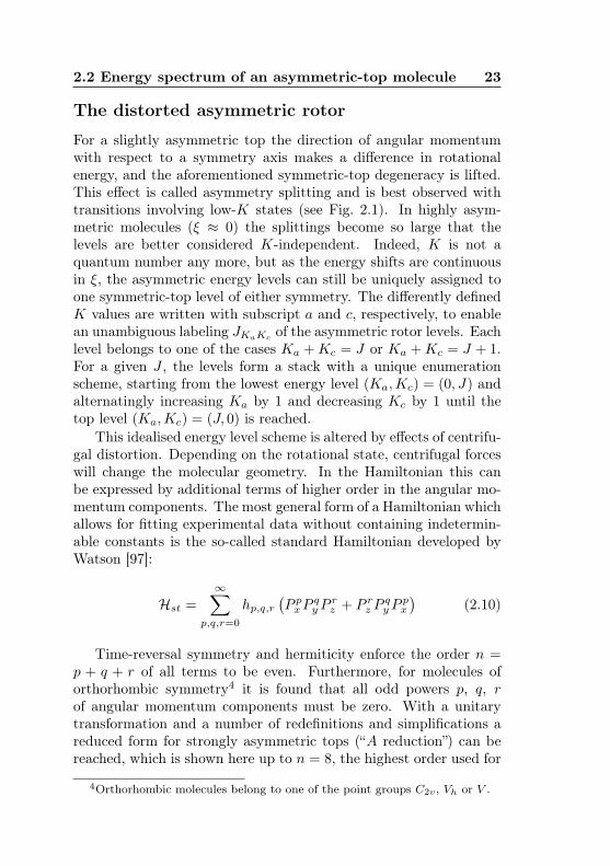
The distorted asymmetric rotor
For a slightly asymmetric top the direction of angular momentumwith respect to a symmetry axis makes a difference in rotationalenergy, and the aforementioned symmetric-top degeneracy is lifted.This effect is called asymmetry splitting and is best observed withtransitions involving low-K states (see Fig. 2.1). In highly asym-metric molecules (ξ ≈ 0) the splittings become so large that thelevels are better considered K-independent. Indeed, K is not aquantum number any more, but as the energy shifts are continuousin ξ, the asymmetric energy levels can still be uniquely assigned toone symmetric-top level of either symmetry. The differently definedK values are written with subscript a and c, respectively, to enablean unambiguous labeling JKaKc of the asymmetric rotor levels. Eachlevel belongs to one of the cases Ka +Kc = J or Ka +Kc = J + 1.For a given J , the levels form a stack with a unique enumerationscheme, starting from the lowest energy level (Ka,Kc) = (0, J) andalternatingly increasing Ka by 1 and decreasing Kc by 1 until thetop level (Ka,Kc) = (J, 0) is reached.
This idealised energy level scheme is altered by effects of centrifu-gal distortion. Depending on the rotational state, centrifugal forceswill change the molecular geometry. In the Hamiltonian this canbe expressed by additional terms of higher order in the angular mo-mentum components. The most general form of a Hamiltonian whichallows for fitting experimental data without containing indetermin-able constants is the so-called standard Hamiltonian developed byWatson [97]:
Hst =
∞∑p,q,r=0
hp,q,r(P pxP
qyP
rz + P rz P
qyP
px
)(2.10)
Time-reversal symmetry and hermiticity enforce the order n =p + q + r of all terms to be even. Furthermore, for molecules oforthorhombic symmetry4 it is found that all odd powers p, q, rof angular momentum components must be zero. With a unitarytransformation and a number of redefinitions and simplifications areduced form for strongly asymmetric tops (“A reduction”) can bereached, which is shown here up to n = 8, the highest order used for
4Orthorhombic molecules belong to one of the point groups C2v , Vh or V .
24 Theoretical consideration
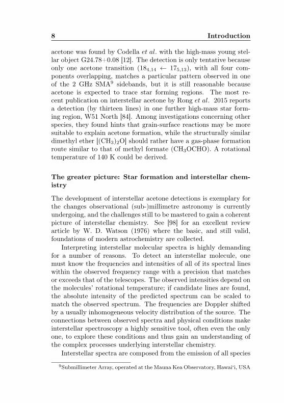
Figure 2.1: Influence of rotational asymmetry on the general energylevel scheme of a rigid, non-distorted molecule. For ξ 6= ±1, the de-generacies of the prolate and oblate limiting cases are lifted and K isnot a good quantum number any more. Because the asymmetric-topenergy levels interconnect the limiting-case levels seamlessly, theirrespective K values can be used as labels in the JKaKc notation.Image adapted from [30].
2.3 General aspects of internal rotation 25
the fit of the torsional ground state of acetone-2-13C:
H(A)red = Hr +
10∑n=4n even
H(n)d (2.11)
Hr =1
2(A+B)P 2 +[C− 1
2(A+B)]P 2
z +1
2(A−B)(P 2
x −P 2y ) (2.12)
H(4)d = ∆JP
4 −∆JKP2P 2
z −∆KP4z − 2δJP
2(P 2x − P 2
y )
− δK [P 2z (P 2
x − P 2y ) + (P 2
x − P 2y )P 2
z ] (2.13)
H(6)d = ΦJP
6 + ΦJKP4P 2
z + ΦKJP2P 4
z + ΦKP6z
+ 2φJP4(P 2
x − P 2y ) + φJKP
2[P 2z (P 2
x − P 2y ) + (P 2
x − P 2y )P 2
z ]
+ φK [P 4z (P 2
x − P 2y ) + (P 2
x − P 2y )P 4
z ]
(2.14)
H(8)d = LJP
8 + LJJKP6P 2
z + LJKP4P 4
z + LKKJP2P 6
z + LKP8z
+ 2lJP6(P 2
x − P 2y ) + lJKP
4[P 2z (P 2
x − P 2y ) + (P 2
x − P 2y )P 2
z ]
+ lKJP2[P 4
z (P 2x − P 2
y ) + (P 2x − P 2
y )P 4z ]
+ lK [P 6z (P 2
x − P 2y ) + (P 2
x − P 2y )P 6
z ]
(2.15)
Note that A, B and C now are effective coefficients contain-ing the respective rotational constant and further coefficients fromtransformed distortion terms of the same order. For nearly sym-metric tops a different reduction of similar form (“S reduction”) isfound, where terms involving Px or Py are combined in the lowering /raising operators P+ = Px + iPy and P− = Px − iPy.
2.3 General aspects of internal rotationThis section summarises the key points of Lin and Swalen’s fun-damental review on internal rotation [59] as applicable for acetone.Besides its overall rotational and vibrational modes, each of the twomethyl groups (to be more precisely, the hydrogens) of acetone mayoscillate in a common movement. Said hydrogen atoms are lightcompared to the “backbone” carbon and oxygen atoms involved inthe overall vibrational modes. Two consequences arise from this
26 Theoretical consideration
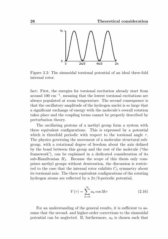
Figure 2.2: The sinusoidal torsional potential of an ideal three-foldinternal rotor.
fact: First, the energies for torsional excitation already start fromaround 100 cm−1, meaning that the lowest torsional excitations arealways populated at room temperature. The second consequence isthat the oscillatory amplitude of the hydrogen nuclei is so large thata significant exchange of energy with the molecule’s overall rotationtakes place and the coupling terms cannot be properly described byperturbation theory.
The oscillating protons of a methyl group form a system withthree equivalent configurations. This is expressed by a potentialwhich is threefold periodic with respect to the torsional angle τ .The physics governing the movement of a molecular structural sub-group, with a rotational degree of freedom about the axis definedby the bond between this group and the rest of the molecule (“theframework”), can be explained in a dedicated consideration of itssub-Hamiltonian HI . Because the scope of this thesis only com-prises methyl groups without deuteration, the discussion is restric-ted to the case that the internal rotor exhibits C3 symmetry aboutits torsional axis. The three equivalent configurations of the rotatinghydrogen atoms are reflected by a 2π/3-periodic potential,
V (τ) =
∞∑k=0
ak cos 3kτ (2.16)
For an understanding of the general results, it is sufficient to as-sume that the second- and higher-order corrections to the sinusoidalpotential can be neglected. If, furthermore, a0 is chosen such that
2.3 General aspects of internal rotation 27
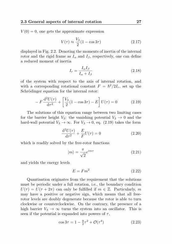
V (0) = 0, one gets the approximate expression
V (τ) ≈ V3
2(1− cos 3τ) (2.17)
displayed in Fig. 2.2. Denoting the moments of inertia of the internalrotor and the rigid frame as Iα and Iβ , respectively, one can definea reduced moment of inertia
Ir =IαIβIα + Iβ
(2.18)
of the system with respect to the axis of internal rotation, andwith a corresponding rotational constant F = ~2/2Ir, set up theSchrödinger equation for the internal rotor:
− F d2U(τ)
dτ2+
[V3
2(1− cos 3τ)− E
]U(τ) = 0 (2.19)
The solutions of this equation range between two limiting casesfor the barrier height V3: the vanishing potential V3 → 0 and thehard-wall potential V3 →∞. For V3 → 0, eq. (2.19) takes the form
d2U(τ)
dτ2+E
FU(τ) = 0 (2.20)
which is readily solved by the free-rotor functions
|m〉 =π√2eimτ (2.21)
and yields the energy levels
E = Fm2 (2.22)
Quantisation originates from the requirement that the solutionsmust be periodic under a full rotation, i.e., the boundary conditionU(τ) = U(τ + 2π) can only be fulfilled if m ∈ Z. Particularly, mmay have a positive or negative sign, which means that all free-rotor levels are doubly degenerate because the rotor is able to turnclockwise or counterclockwise. On the contrary, the presence of ahigh barrier V3 → ∞ turns the system into an oscillator. This isseen if the potential is expanded into powers of τ ,
cos 3τ = 1− 92τ
2 +O(τ4) (2.23)
28 Theoretical consideration
giving a harmonic oscillator for small values of τ ,
d2U(τ)
dτ2+
1
F(E − 9
4V3τ2)U(τ) = 0 (2.24)
with the energies
E = 3√V3F (v + 1
2 ), v ∈ N0 (2.25)
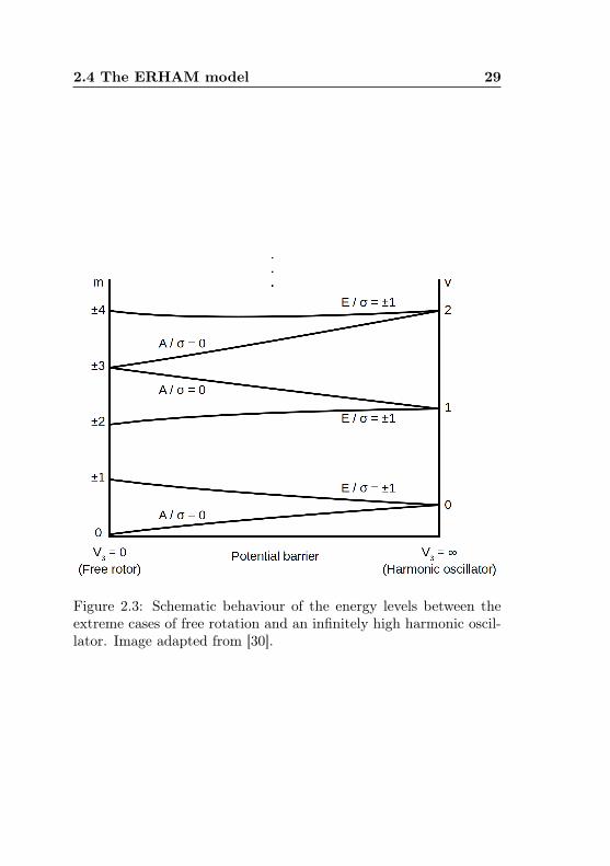
The equidistant levels are now threefold degenerate because theoscillation may likewise take place in each of the three potentialwells. Now the dynamics of the real internal rotor with a finitebarrier height become obvious: while, especially for the lowest states,a free rotation is hindered by the barrier, the system may still tunnelbetween the potential wells. For a mathematical description thetorsional equation (2.19) is rescaled into Mathieu’s equation:
d2M(x)
dx2+ (b− s cos2 x)M(x) = 0 (2.26)
where 3τ+π = 2x, V3 = 94Fs, and E = 9
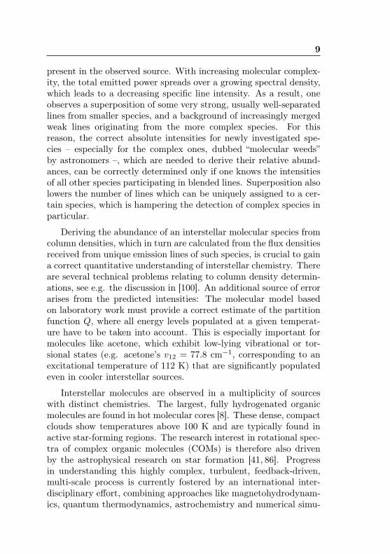
4Fb have been inserted. Theboundary condition for the Mathieu functions is nowM(x) = M(x+3π), and it is fulfilled by two different types of solutions: A set offunctions with period π belonging to nondegenerate eigenvalues bv0,and another one with period 3π whose eigenvalues bv,±1 are doublydegenerate. The second label, the symmetry number σ = 0,±1, isused to differ between the three solutions pertaining to one harmonicoscillator label v, which is the same for two subsequent degenerateand nondegenerate eigenvalues (see Fig. 2.3). The symmetry labelsshown in the Figure correspond to the symmetry species under therotations of the C3 group (see Table A.3). It is seen that the finite-barrier case can be regarded as a splitting of the harmonic oscillatorlevels, which increases as the barrier height is decreased. The doubledegeneracy of the free-rotor levels is maintained from a convergenceof two A levels if m is a multiple of three, and from one of the Elevels otherwise.
2.4 The ERHAM modelFor a molecule like acetone with two internal rotors, the periodic po-tential shown in Fig. 2.2 is superposed with itself in a second dimen-sion, resulting in an “egg-crate”-like potential energy surface. Due to
2.4 The ERHAM model 29
Figure 2.3: Schematic behaviour of the energy levels between theextreme cases of free rotation and an infinitely high harmonic oscil-lator. Image adapted from [30].
30 Theoretical consideration
the strong coupling of internal and overall rotation, actually solvingthe full rotational-torsional Hamiltonian with all internal coordin-ates and the potential would be computationally too demanding toperform a realistic workflow of subsequent assigning and fitting. In-stead, the periodicity of the potential can be inherited to all basisfunctions, matrix elements and energy levels by Fourier expansion.A skilful choice of basis is necessary to simplify the terms as far aspossible, and the remaining free parameters split into four groups:
• Those of the reduced Watson Hamiltonian for a rigid5 asym-metric rotor with centrifugal distortion,
• the coefficients of the Fourier expansion of the internal energylevels (i.e., the eigenfunctions of the Hamiltonian HI describ-ing the internal rotation),
• the so-called tunneling parameters describing integrals overtwo functions of the basis functions in Fourier space,
• and a few geometrical parameters describing the length ρk andrelative orientation of the vectors (ρ0)k (defined below), whichare needed for a simplification in addition to the mentionedchoice of basis.
The following sections give a detailed summary of this theory asit is published in [32,35].
Structure of a Hamiltonian involving internal ro-tation
The general Hamiltonian of a molecule with internal rotation can berepresented in two different ways:
H = HR +HRI +HI (2.27a)
=∑l
RlTl (2.27b)
5“Rigid” here denotes a molecule without internal rotation, whereas centri-fugal distortion is permissible with no restriction. In contrast, an imaginarymolecule without centrifugal distortion is said to be in its equilibrium configur-ation.
2.4 The ERHAM model 31
The sub-Hamiltonians in eqn. (2.27a) describe (from left to right)the pure terms for overall rotation, the interaction products betweenoverall and internal rotation, and the terms involving only the mo-menta of internal motion. On the other hand, eq. (2.27b) statesthat every term whatsoever must be a product of operators contain-ing some power of overall (Rl) and internal (Tl) momenta, whichwill be useful for more detailed examinations. The generalised in-dex l denotes an expansion in an appropriate representation; see theexamples given in Section 2.4.1. One may notice further that in afield-free experiment there is no potential in addition to the internalpotential V (τ1, τ2) described above.
Apart from that, H is identical to the kinetic energy, which ismost easily expressed in terms of the overall angular velocity ω =(ωx, ωy, ωz) and the internal angular velocity τ = (τ1, τ2):
T = 12 (ωt, τ t)
(Iω IωτItωτ Iτ
)(ω
τ
)(2.28)
It is yet more worthwile for a quantum mechanical treatmentto convert T into an expression in terms of the conjugate momentaP = − i
~∇ω and p = − i~∇τ :
T = (Pt,pt)
(A + ρFρt −ρF−Fρt F
)(P
p
)(2.29)
with the matrices
A =~2
2 I−1ω , (2.30a)
ρ =I−1ω Iωτ , (2.30b)
F =~2
2 (Iτ − ρtIωρ)−1 (2.30c)
ρ is a matrix which can be subdivided into a constant part ρ0 anda variable part ∆ρ. It depends only on the molecule’s momentsof inertia, thus on its geometry, and the column vectors of ρ0 =[(ρ0)1, (ρ0)2] define two axes which are each physically meaningfulfor either of the two internal rotors and play a major role duringthe remaining discussion. With said definitions one obtains the finalform of the three partial Hamiltonians:
HR =Pt(A + ∆ρF∆ρt + ∆ρFρt0 + ρ0F∆ρt)P, (2.31a)
HRI =− (Pt∆ρFp + ptF∆ρtP), (2.31b)
HI =(pt −Ptρ0)F(p− ρt0P) + V. (2.31c)
32 Theoretical consideration
The internal Hamiltonian HI
A straightforward approach to obtain a usable model without theneed to actually solve the Schrödinger equation is to assume theexistence of solutions which are products of free rigid-top wavefunc-tions |JKM〉 describing the states of overall rotation and the un-known solutions of HI describing those of internal rotation. Thesolutions of HI can be constructed from free-rotor functions in thetorsional coordinates of the k-th internal rotor:
|j1σ1j2σ2〉 = |j1σ1〉|j2σ2〉, with (2.32)
|jkσk〉 = 1√2πei(nkjk+σk)τk (2.33)
Note that the free-rotor functions contain a phase shift in form ofthe so-called symmetry numbers σk. Before constructing the eigen-functions of HI , it is highly useful to simplify its matrix elements inthis basis in order to remove their explicit dependency on the overallangular momentum P. Starting from the basis
|JKMj1σ1j2σ2〉 = |JKM〉|j1σ1j2σ2〉 (2.34)
the functions |JKM〉 can be rotated into a basis |JKkM〉, whereKk denotes the projection of K on the new zk axis defined by (ρ0)k.The matrix elements are then rewritten as
〈JK ′Mj′1σ1j′2σ2|HI |JKMj1σ1j2σ2〉
=∑K1K2
YK′K(K1,K2)〈j′1σ1j′2σ2|HI(K1,K2)|j1σ1j2σ2〉 (2.35)
with a projection term
YK′K(K1,K2) = 12 (〈JK ′M |JK1M〉〈JK1M |JK2M〉〈JK2M |JKM〉+〈JK ′M |JK2M〉〈JK2M |JK1M〉〈JK1M |JKM〉)
(2.36)
tracking the effect of the basis rotation, and the matrix elements
〈j′1σ1j′2σ2|HI(K1,K2)|j1σ1j2σ2〉
=
2∑k=1
2∑l=1
(nkj′k + σk − ρkKk)F
(kl)j′1−j1,j′2−j2
(nljl + σl − ρlKl)
+ Vj′1−j1,j′2−j2(2.37)
2.4 The ERHAM model 33
in the desired form containing no further differential operators andvector products. Note that only those matrix elements with identicalσk/l are displayed because the symmetry numbers are conserved.This becomes obvious by noting that, just like the potential, theF (kl) are periodic functions,
F (kl)(τ1, τ2) =∑j1j2
F(kl)j1,j2
ei(n1j1τ1+n2j2τ2) (2.38)
and hence all matrix elements off-diagonal in the symmetry numbersvanish due to orthogonality of the free-rotor functions.
The eigenvectors U (K1,K2)j1j2νσ1σ2
of HI in a complex standard spaceare obtained by diagonalisation,
HI(K1,K2)U(K1,K2)j1j2νσ1σ2
= E(K1,K2)νσ1σ2
U(K1,K2)j1j2νσ1σ2
(2.39)
and can be used to construct the assumed solutions to the Schrödingerequation for an internal excitation ν,
|νσ1(K1)σ2(K2)〉 =∑j1j2
U(K1,K2)j1j2νσ1σ2
|j1σ1j2σ2〉 (2.40)
which in turn are vectors in a Hilbert space. Inserting this an-satz into the Schrödinger equation and multiplying both sides by〈j′1σ1j
′2σ2| yields∑
j1j2
〈j′1σ1j′2σ2|HI(K1,K2)|j1σ1j2σ2〉U (K1,K2)
j1j2νσ1σ2= E(K1,K2)
νσ1σ2U
(K1,K2)j′1j
′2νσ1σ2
(2.41)This equation can be used together with eq. (2.37), as well as period-icity and other basic arguments not shown here in detail, to deducefurther relationships which enable Fourier expansion of the eigen-quantities, which is the central step towards the effective Hamilto-nian, and provide deeper insights into the nature of the results.
Fourier transformationThe eigenvalues, -vectors and -functions of HI are periodic functionsof the torsional angles. For example, the corresponding relationshipfor the eigenvalues is
E(K1,K2)νσ1σ2
= E(K1,K2)ν,σ1+λ1n1,σ2+λ2n2
, λ1,2 ∈ Z (2.42)
34 Theoretical consideration
It is therefore possible to write the internal rotor energies and eigen-functions as Fourier series:
E(K1,K2)νσ1σ2
=
N1−1∑q1=0
N2−1∑q2=0
e2πi(q1σ1/n1+q2σ2/n2)ε(K1,K2)νq1q2 (2.43)
These expressions introduce various new symbols. While realnumbers can be used as coefficients in the energy series, the expan-sion of the eigenfunctions results in a new set of complex functionsϑ
(K1,K2)νq1q2 (τ1, τ2) which are called localised functions. Their name was
coined from the observation that, if the torsional energies E(K1,K2)νσ1σ2
for the considered state ν lie sufficiently deep below the potentialbarrier, their probability density is centered in one of the minima ofthe potential function V 6. The conjugate indices of the symmetrynumbers, qk, can be regarded as a numbering scheme for the poten-tial wells as they determine the well where the respective function islocalised. The finite upper bounds of summation needed for numer-ical evaluation are defined by Nk = mknk, with mk being a largeinteger chosen such that the occurrence of the real numbers ρk in theFourier terms (cf. the extended formulas below) does not (at leastup to a good approximation) affect the periodicity of the expandedquantity.
It has been found in accordance with earlier results reported forphenomenological Hamiltonians of molecules with a single internalrotor [31] that the quantities given above also depend periodicallyon the projections Kk of the overall angular momentum on the ρaxes. With the abbreviations ενq1q2 ≡ ε
(0,0)νq1q2 and ϑνq1q2 ≡ ϑ
(0,0)νq1q2 the
full periodicity relations can be written as
E(K1,K2)νσ1σ2
=
N1−1∑q1=0
N2−1∑q2=0
e2πi(q1(σ1−ρ1K1)/n1+q2(σ2−ρ2K2)/n2)ενq1q2
(2.44a)
ϑ(K1,K2)νq1q2 (τ1, τ2) = ϑν00
(τ1 −
2πq1
n1, τ2 −
2πq1
n1
)· ei(ρ1K1(τ1−2πq1/n1)+ρ2K2(τ2−2πq2/n2)) (2.44b)
These expressions show that the K dependence appears onlyin the exponential factors and that the energy Fourier coefficients
6For an appropriate choice of a complex phase factor ϕσ1σ2 defined in [32].
2.4 The ERHAM model 35
and localised functions can be traced back to quantities which areindependent of K. Furthermore, any imaginary part of the localisedfunctions must come from the exponential factors, as ϑ(0,0)
νq1q2 is real.The role of q enabling to select a particular potential well is seenfrom eq. (2.44b), too.
The matrix elements of an operator t(τ1, τ2), which shall be in-dependent of the internal angular momenta p1 and p2, in the basisof eigenfunctions of HI in Fourier representation is therefore:
〈ν′σ1(K ′1)σ2(K ′2)|t(τ1, τ2)|νσ1(K1)σ2(K2)〉
=1
m1m2
N1−1∑q1=0
N2−1∑q2=0
e2πi(q1σ1/n1+q2σ2/n2)
·m1π∫−m1π
m2π∫−m2π
ϑ(K′
1,K′2)
ν′00
∗(τ1, τ2)t(τ1, τ2)ϑ(K1,K2)
νq1q2 (τ1, τ2) dτ1 dτ2
=∑q1q2
eπi(q1(2σ1−ρ1(K1+K′1))/n1+q2(2σ2−ρ2(K2+K′
2))/n2)T(κ1,κ2)ν′νq1q2
(2.45)
where, in (2.45), the explicitK dependence of the localised functionswas inserted and κi = Ki −K ′i was used. The Fourier coefficients
T(κ1,κ2)ν′νq1q2
=1
m1m2e−πi(ρ1q1κ1/n1+ρ2q2κ2/n2)
·m1π∫−m1π
m2π∫−m2π
ei(ρ1κ1τ1+ρ2κ2τ2)ϑν′00(τ1, τ2)t(τ1, τ2)ϑνq1q2(τ1, τ2) dτ1 dτ2
(2.46)
can be interpreted as descriptions of t during a tunneling motionbetween the potential wells (0,0) of torsional state ν′ and (q1, q2) ofstate ν. For t = 1 one can further define
i(κ1,κ2)ν′νq1q2
:= eπi(ρ1q1κ1/n1+ρ2q2κ2/n2)T(κ1,κ2)ν′νq1q2
[t(τ1, τ2) = 1] (2.47)
which is useful for the Fourier transformations of scalar productsshown below. If K1 = K2, they obey the orthogonality relation
i(0,0)ν′νq1q2
= δν′νδ0q1δ0q2 (2.48)
36 Theoretical consideration
which derives from the general orthogonality relation
1
m1m2
m1π∫−m1π
m2π∫−m2π
ϑ(K1,K2)ν′q′1q
′2
∗(τ1, τ2)ϑ(K1,K2)
νq1q2 (τ1, τ2) dτ1 dτ2
= δν′νδq′1q1δq′2q2
q′1=0
q′2=0=⇒ 1
m1m2
∫∫e−2πi
(ρ1K1q1n1
+ρ2K2q2n2
)ϑν′00(τ1, τ2)ϑνq1q2(τ1, τ2) dτ1,2
= δν′νδ0q1δ0q2(2.49)
It has been found that the integrals i(κ1,κ2)ν′νq1q2
are still approxim-ately orthogonal for tunneling states with different K:
i(κ1,κ2)ν′νq1q2
≈ δν′νδ0q1δ0q2 , κ1,2 6= 0. (2.50)
A comparison of i(κ1,κ2)ν′νq1q2
with the orthogonality relation for thelocalised functions for q′1 = 0 and q′2 = 0 shows that, in the latter, theconstant phase factor in (2.49) is replaced by a variable one, givingdifferent weights and signs to the functions in certain regions of theintegration domain. The approximate orthogonality thus being notself-evident, Groner states that it is usually fulfilled in a very goodapproximation [32,35]. A possible interpretation of these usual con-ditions is that, for a given system, disadvantageous combinations ofν, ν′, ρk,Kk,mk, and qk may exist where the integrals do not vanishas expected, and further contributions to torsional energy may bemistakenly neglected by an algorithm which assumes orthogonality.
Transformed matrix elements of the rotational-tor-sional HamiltonianAll sub-Hamiltonians can now be written in the basis
|JKMνσ1σ2〉 = |JKM〉|νσ1(K)σ2(sK)〉 (2.51)
which is an orthonormal subset of solutions for HI(K, sK) of thecomplete set which one would obtain with eq. (2.40). The signs = sign(ρz1ρz2) indicates whether the two ρ vectors are pointing
2.4 The ERHAM model 37
into the same half space with respect to the xy plane. In compar-ison to the projection K of the total angular momentum on themolecule-fixed z axis, the rho-axis projections Kk used so far arenot feasible to serve as quantum numbers for the whole Hamilto-nian. The eigenvalues of HI , however, are essential to turn theHamiltonian into a phenomenological one by removing the expressoccurrence of the potential. As they can only be included from thegeneral solutions for HI(K1,K2), two more rotations are needed toarrive at a satisfactory expression for HI :
〈ν′σ1(K ′)σ2(sK ′)|HI(K1,K2)|νσ1(K)σ2(sK)〉
=∑ν′′
∑ν′′′
〈ν′σ1(K ′)σ2(sK ′)|ν′′σ1(K ′′1 )σ2(K ′′2 )〉
· 〈ν′′σ1(K ′′1 )σ2(K ′′2 )|HI(K1,K2)|ν′′′σ1(K ′′′1 )σ2(K ′′′2 )〉· 〈ν′′′σ1(K ′′′1 )σ2(K ′′′2 )|νσ1(K)σ2(sK)〉 (2.52)
By identifying the arbitrary constantsK ′′′k = K ′′k = Kk, the cent-ral bracket takes the value δν′′ν′′′E
(K1,K2)ν′′σ1σ2
, and the matrix elementsof HI can be rewritten in a form which (apart from YK′K(K1,K2),where it is not necessary) fully supports Fourier expansion:
〈JK ′Mν′σ1σ2|HI |JKMνσ1σ2〉 =∑K1K2
YK′K(K1,K2)
·∑ν′′
〈ν′σ1(K ′)σ2(sK ′)|ν′′σ1(K1)σ2(K2)〉E(K1,K2)ν′′σ1σ2
· 〈ν′′σ1(K1)σ2(K2)|νσ1(K)σ2(sK)〉 (2.53)
The scalar products can be transformed with eq. (2.47):
〈ν′′σ1(K1)σ2(K2)|νσ1(K)σ2(sK)〉
=
N1−1∑q1=0
N2−1∑q2=0
e2πi(q1(σ1−ρ1K1)/n1+q2(σ2−ρ2K2)/n2)i(K−K1,sK−K2)νν′′,−q1,−q2 ,
(2.54)
38 Theoretical consideration
〈ν′σ1(K ′)σ2(sK ′)|νσ1(K)σ2(sK)〉
=
N1−1∑q1=0
N2−1∑q2=0
e2πi(q1(σ1−ρ1K1)/n1+q2(σ2−ρ2K2)/n2)i(K1−K′,K2−sK′)ν′ν′′,q1,q2
,
(2.55)
and, with the Fourier expansion of E(K1,K2)νσ1σ2 from eq. (2.44a) and
the orthogonality relations discussed above, one obtains the fullytransformed matrix elements
〈JK ′Mν′σ1σ2|HI |JKMνσ1σ2〉 ≈∑K1K2
YK′K(K1,K2)
·N1−1∑q1=0
N2−1∑q2=0
e2πi(q1(σ1−ρ1K1)/n1+q2(σ2−ρ2K2)/n2)ενq1q2 . (2.56)
Fourier expansion is straightforwardly applied to HR =∑lRlTl:
〈JK ′Mν′σ1σ2|HR|JKMνσ1σ2〉
=∑l
〈JK ′M |Rl|JKM〉〈ν′σ1(K ′)σ2(sK ′)|Tl|νσ1(K)σ2(sK)〉
=∑l
〈JK ′M |Rl|JKM〉
·∑q1,q2
eπi(q1(2σ1−ρ1(K+K′))/n1+q2(2σ2−sρ2(K+K′))/n2)T(κ,sκ)l ν′νq1q2
(2.57)
For HRI the Fourier expansion is done analogously, but slightlymore complex nonetheless. The matrix elements of
HRI = −∑α
PαTα = −∑α
Pα∑k
[tαk(τ1, τ2)pk + pktαk(τ1, τ2)],
(2.58)
2.4 The ERHAM model 39
in the basis as above, are finally written as:
〈JK ′Mν′σ1σ2|HRI |JKMνσ1σ2〉
=
N1−1∑q1=0
N2−1∑q2=0
eπi(q1(2σ1−ρ1(K+K′))/n1+q2(2σ2−sρ2(K+K′))/n2)
·∑α
[−〈JK ′M |Pα|JKM〉T(κ,sκ)
α ν′νq1q2
+ 〈JK ′M |PzPα + PαPz|JKM〉T (κ,sκ)α ν′νq1q2 ]
(2.59)
Here, T (κ,sκ)α ν′νq1q2 is inferred from eq. (2.46) with t(τ1, τ2) =
ρ1tα1(τ1, τ2)+sρ2tα2(τ1, τ2), and T(κ,sκ)
α ν′νq1q2 are similar tunnelingparameters involving, and being the only such case in this treatment,odd orders of internal angular momentum:
T(κ,sκ)
α ν′νq1q2 =1
m1m2e−πi(q1ρ1κ1/n1+q2ρ2κ2/n2)
·m1π∫−m1π
m2π∫−m2π
ei(ρ1κ1τ1−ρ2κ2τ2)
·∑k
tαk(τ1, τ2)[(pkϑν′00(τ1, τ2)
)ϑνq1q2(τ1, τ2)
− ϑν′00(τ1, τ2)(pkϑνq1q2(τ1, τ2)
)]dτ1 dτ2 (2.60)
As tunneling parameters with even or odd order in p transformslightly differently under sign reversal of κ and q, a further sign ω =+1 or −1 for even- or odd-order rotational operators, respectively,is introduced by writing
T(κ1,κ2)ν′νq1q2
= ωT(−κ1,−κ2)∗ν′νq1q2
= ωT(κ1,κ2)νν′,−q1,−q2 = T
(−κ1,−κ2)∗νν′,−q1,−q2 (2.61)
to avoid having to distinguish two classes of tunneling parameters.All sub-Hamiltonians can now be combined in the generalised
Fourier transformed matrix element of the full rotational-torsional
40 Theoretical consideration
Hamiltonian:
〈JK ′Mν′σ1σ2|H|JKMνσ1σ2〉 =∑l
〈JK ′M |Rl|JKM〉
·N1−1∑q1=0
N2−1∑q2=0
eπi
(q1n1
(2σ1−ρ1(K+K′))+q2n2
(2σ2−sρ2(K+K′)))T
(κ,sκ)l ν′νq1q2
+ δν′ν
∑K1,K2
YK′K(K1,K2)
·N1−1∑q1=0
N2−1∑q2=0
e2πi(q1(σ1−ρ1K1)/n1+q2(σ2−ρ2K2)/n2)ενq1q2
(2.62)
The effective rotational HamiltonianThe general matrix elements (2.62) include the energies for trans-itions between two different internal states ν and ν′. However, thelowest energies necessary to excite internal vibrations are large (typ-ically some 100 cm−1) compared to those of the rotational trans-itions of a single state ν. In a (sub-)millimetre spectrum (about1 − 30 cm−1), no transitions are thus observed between two tor-sional states, and the rotational spectrum can be calculated as acomposition of separate spectra for each state. It is therefore ad-equate to use an effective rotational Hamiltonian where all elementsoff-diagonal in ν are neglected. Removing all “ν” subscripts and re-placing (κ, sκ) by (κ), the matrix elements of the effective rotationalHamiltonian become
〈JK ′Mν′σ1σ2|H|JKMνσ1σ2〉
=∑l
〈JK ′M |Rl|JKM〉
·N1−1∑q1=0
N2−1∑q2=0
eπi
(q1n1
(2σ1−ρ1(K+K′))+q2n2
(2σ2−sρ2(K+K′)))T
(κ)l q1q2
+∑K1,K2
YK′K(K1,K2)∑q1,q2
e2πi
(q1n1
(σ1−ρ1K1)+q2n2
(σ2−ρ2K2))εq1q2
(2.63)
Note that in this notation, which is used for consistency with the
2.4 The ERHAM model 41
literature, the symbols T and ε are still state-specific, although thesubscripts ν and νν have been omitted. The most compressed formof these matrix elements is
〈JK ′Mν′σ1σ2|H|JKMνσ1σ2〉
=∑K1,K2
YK′K(K1,K2)Σ0 +∑l
〈JK ′M |Rl|JKM〉Σl. (2.64)
Expressions for the Fourier series Σ0 and Σl depend on the equi-valence of the internal rotors and the molecular symmetry and canbe looked up from tables in [32]. Since they contain only equivalentmethyl rotors, an identical expression for Σ0 can be given for allacetone isotopologues treated here:
Σ0 = ε00 + 2∑q>0
C ′qqεqq + C ′q−qεq−q +
q−1∑q′=−(q−1)
(C ′qq′ + C ′q′q)εqq′
,(2.65)
where q = q1 and q′ = q2 have been introduced for shortness. Σ0 isa pure cosine expansion, which is seen from the definition
C ′qq′ = cos(2π(q(σ1 − ρK1) + q′(σ2 − ρK2))/n). (2.66)
Σl, on the other hand, exhibits a more complex structure. It is aFourier series structurally similar to Σ0, with the εqq′ coefficients re-placed by the tunneling parameters T (κ)
l qq′ and structurally refinedsine and cosine expressions instead of the C ′qq′ above, but differentsubseries being enabled depending on details of point group sym-metry, the orientation of the reference axes (s value, eq. (2.51)) andthe ω values pertaining to the particular operators within T
(κ)l qq′ .
Furthermore, the real and imaginary parts of the tunneling para-meters must be treated separately. The interested reader is referredto the original publication [32] if full comprehension is needed.
2.4.1 Nomenclature of the tunneling parametersThere are two equivalent ways to label the tunneling parameters:
• Watson-type parameter labeling: [t]qq′ , where the product op-erator t is represented by the label for its respective coefficient.The pair ∆JK (from eq. (2.13)) and [∆JK ]10 is an example.
42 Theoretical consideration
• Cylindrical tensor form: [Bkpr]qq′ , from the definition givenin [32]:
HR =∑kpr
1
2(1 + δ0r)[JkJpz , J
r+ + Jr−]+Bkpr (2.67)
While the usage of Watson-type labels is more convenient for tun-neling parameters of centrifugal terms, the cylindrical tensor formis more general, because it is also defined for all product operatorswhich are not included in one of the Watson reductions. It will beused here whenever no other label could be found for operators ofa particular combination of powers. The r power used in the cyl-indrical tensor notation is identical to the absolute K difference,r = |κ|, from eq. (2.57). Furthermore, the order of a tunnelingparameter η := k + p+ r will be used.
In the numerical fit, the right choice of tunneling parametersto describe the J or K dependence of the torsional splittings canbe narrowed down to enabling parameters which are adjacent (asdefined in Section 4.2) to a given parameter set with respect to theirindices k and p.
2.4.2 Numerical implementation
A FORTRAN programme “ERHAM” capable of fitting the EffectiveRotational Hamiltonian to a set of assigned transitions and pre-dicting the spectrum based on the determined parameters has beendeveloped by P. Groner and is publicly available [47]. It can beinitialised with appropriate settings to reflect given molecular prop-erties like point group symmetry, which affects the appearance of Σ0
and Σl in (2.64).ERHAM uses parameter start values and assigned transition fre-
quencies from a user generated input file to set up the Hamilto-nian in form of (2J + 1) × (2J + 1) block matrices for each tor-sional state ν and each combination of symmetry numbers σ1σ2
such that all states |JKMνσ1σ2〉 are represented. Eigenvalues and -vectors of these are determined with standard algebra algorithms (in-cluding Householder transformation to upper triangular form, rootfinding by bisection, and singular value decomposition). This per-state mathematics is embedded in a non-linear weighted least-square
2.4 The ERHAM model 43
routine, which fits the parameters to the data and is iterated a pre-determined number of times. Every cycle ends with an output of thedetermined singular values and associated right singular vectors, thestandard deviation of the least-square fit, a list of the current para-meter values, their uncertainties and changes, and, importantly, acorrelation matrix of the parameters. The correlation score may takevalues between −100 000 and 100 000, with these extreme values de-noting fully linearly dependent parameters of opposite or same sign,respectively, and a value of 0 indicating two fully decoupled paramet-ers. After the last cycle, several geometrical and physical parametersof the molecule (including torsional energy differences) are derivedand, optionally, a prediction of the spectrum is generated from theobtained parameters.
A major validation of the model is the rapid convergence of theFourier series in q and q′ for states well below the barrier, as it hasbeen expected by Groner and proven by numerous earlier spectralfits performed with ERHAM. The analyses presented in Chapter 4confirm this once more as they require no Fourier terms beyond theorder ζ := |q|+ |q′| = 2. Besides v, q and q′, each parameter in theERHAM user input takes four further identifiers to be fully defined:ω = ±1 as defined in eq. (2.61) to denote angular momenta of evenor odd order, and the powers k, p and r of angular momentumdefined in Section 2.4.1.
By counting the unsplit distorted rotor energy levels in ascendingorder, ERHAM circumvents the problem of having to select a par-ticular coordinate representation (Section 2.2), at the price thatthe pseudo-quantum numbers Ka and Kc need to be derived forphysical interpretation. This leads to a common counting mistakewhich becomes apparent if the observed spectrum contains trans-itions between crossing energy levels (Fig. 2.4). Consequentially,transitions between rotational energy levels thus mislabeled in Kappear to have wrong transition types. As the dipole moment ofacetone coincides with the b axis, apparently forbidden a- and c-typetransitions appear in the assignments and predictions (Fig. 2.7).
An enhanced version ERHAMZ developed and published by Z. Kisiel[47] was used at the beginning of the works described in Chapter 4.ERHAMZ generates additional output, most importantly a list of thefifty lines that were fit worst in the current cycle and two root-mean-square errors (weighted and unweighted) for the least-square
44 Theoretical consideration
fit. When it turned out that the array dimensions originally providedby ERHAM were insufficient for the acetone-2-13C data set and theparameters needed to obtain a satisfactory fit, a new fork calledERHAMO with larger arrays was compiled by the author in order tocontinue the analysis.
2.5 Effects of symmetry
In many physical systems the number of possible solutions to theSchrödinger equation is restricted by the presence of symmetry.Mathematical transformations which do not change the Hamilto-nian, the so-called symmetry operations, may yet impose a changeon the symmetry of some wavefunctions which would violate phys-ical laws like the spin-statistics theorem. Consequently, not all apriori possible states are realised by the system, and selection rulesbetween states of certain symmetry arise. The states and / or en-ergy levels are given symmetry labels accordingly. In spectroscopy,another consequence of symmetry is the distribution of intensities,which originates from differences in the number of spin states per-taining to a particular state and its symmetry labels.
Considerations of physical symmetry are inherently connected togroup theory, as symmetry operations form a group by construction.The behaviour of the total wavefunction7
ψtot = ψrveψns (2.68)
under the transformations of a symmetry group applicable to themolecule can strongly depend on the molecular state described bythe rovibrational wavefunction ψrve and the nuclear spin state ψns.The transformational behaviour of these functions, determined byfinding the irreducible components of the reducible representationformed by the symmetry behaviour of the molecule’s nuclear spins,is the starting point for an assessment of selection rules and thedistribution of intensity between the torsional components of a ro-tational transition.
7The wavefunction describing the translational motion of the centre of massis omitted here because translational symmetry / momentum conservation istaken as given.
2.5 Effects of symmetry 45
2.5.1 Four group symmetry
There is a general symmetry of the rotational Hamiltonian leadingto selection rules for the asymmetric-top states [30]. It is a directconsequence of energy and angular momentum conservation: Theconstance of angular momentum means that the points in angularmomentum space reached by the P vector form a sphere:
P 2 = P 2x + P 2
y + P 2z = constant (2.69)
On the other hand, the kinetic energy is constant if no external forcesare applied:
Er =1
2
(P 2x
Ix+P 2y
Iy+P 2z
Iz
)= constant (2.70)
which further restricts the angular momentum components onto anellipsoid. As a consequence, the angular momentum vector may onlypoint to one of the curves along the intersections of the angular mo-mentum sphere and the energy ellipsoid. Regardless of the detailedshape of these surfaces, they are always symmetric under a C2 ro-tation about the x, y, and z axes each. These operations form theFour group V (a, b, c), which is isomorphic to the group C2v
8. Underthe rotations of the Four group, the angular momentum compon-ents transform according to one of the symmetry species (see thecharacter table in Appendix A):
E :Pa → Pa, Pb → Pb, Pc → Pc
C2(a) :Pa → Pa, Pb → −Pb, Pc → −PcC2(b) :Pa → −Pa, Pb → Pb, Pc → −PcC2(c) :Pa → −Pa, Pb → −Pb, Pc → Pc
The effect of the Four group rotations on the asymmetric-topwavefunctions is expressed by the projection labels Ka and Kc. Thisis most easily seen by comparison to a symmetric-top wavefunction:A prolate molecule rotated by π about its symmetry axis a willchange the angle φ to φ+ π, but will not change the other Eulerian
8The C2v symmetry of the rotational Hamiltonian is of a general nature andnot related to the C2v symmetry of the equilibrium structure of acetone.
46 Theoretical consideration
angles. The rotational wavefunction |JKM〉 depends on φ like eiKφ,so one gets the K dependence
C2(a) : |JKM〉 → eiKπ|JKM〉 = (−1)K |JKM〉. (2.71)
For an asymmetric top the effect on the angles is more complic-ated, but because a change in moments of inertia (i.e., ξ) cannotaffect the symmetry of a rotational state, the transformational be-haviour of the limiting prolate and oblate cases, expressed by therespective quantum number K, is inherited to the asymmetric-topwavefunctions with respect to the labels Ka and Kc. The symmetryof any state JKaKc is thus found to depend on Ka and Kc being even(e) or odd (o), and the corresponding symmetry classes according tothe character table (see Table A.4) are A for (KaKc) = (ee), Ba for(eo), Bb for (oo), and Bc for (oe). Table A.4 also contains the sep-arate e/o selection rules between these labels existing for the threeasymmetric-top transition types (see [30] for a detailed explanation),and the equivalent symmetry classes of the isomorphic C2v group aswell.
2.5.2 Permutational symmetry groupsThe formalism on permutational symmetry presented here goes backto the detailed treatment in the books by Bunker and Jensen [9,10].Symmetry operations of a molecule – regardless of being a rotation,reflection or inversion – can be represented by isomorphic permuta-tions of identical nuclei. To handle the individual case, one mustuse the group containing the set of operations which correctly de-scribes the physical aspect under consideration as well as the degreeof experimental detail. Besides the Four group mentioned in Sec-tion 2.5.1, the following symmetry groups are used in rotationalspectroscopy:
The point group. In their equilibrium configuration, the nucleiof many molecules are arranged in a symmetric manner. Theoperations transforming this structure into itself form the pointgroup of a molecule.
The CNPI group. The largest permutation group of a molecule,containing all possible exchanges of identical nuclei even ifthey are not realised in the experiment (e.g. bond breaking of
2.5 Effects of symmetry 47
stable molecules), is called the Complete Nuclear PermutationInversion group.
The MS group. The set of feasible operations9 forms the MolecularSymmetry group, a subgroup of the CNPI group.
A symmetry analysis of the rotational states is composed of twomajor steps: First, the spin-statistical weight gns is determined foreach rovibrational symmetry species Γrve of the MS group. For thispurpose, the characters of the reducible representation Γredns formedby the spins under the symmetry transformations of the MS groupare calculated by
χtotns [P ] =∏a
(2Ia + 1). (2.72)
The index a denotes sets of identical nuclei permuted by the opera-tion P , where each nucleus not permuted by P is counted as a set ofits own containing one element. Said reducible representation canbe decomposed into irreducible representations Γins according to thegeneral rule
Γred =⊕i
aiΓi (2.73)
with the coefficients
ai =1
h
∑R
χΓred [R]χΓi [R]∗ (2.74)
This sum is taken over all symmetry transformations R and h is thenumber of elements in the group (e.g. h = 36 for G36). Furthermore,the total wavefunction is required to obey the Pauli principle (e.g.ψtot must be symmetric under an even permutation of H nuclei).The allowed rovibrational symmetry species can then be concludedfrom the direct product table, using
Γtot!⊂ Γrve ⊗ Γns. (2.75)
Finally, the nuclear spin weights of the rovibrational symmetry spe-cies are obtained by adding the coefficients ai for all allowed com-binations.
9Observable operations actually taking place during the measurement.
48 Theoretical consideration
In the second step, these spin weights must be assigned to thetorsional components of the rotational transitions. First, selectionrules for the rovibrational species are established by exploiting thevanishing-integral rule: The matrix element describing the dipolemoment transition between two rovibrational states,
∫ψ
(f)rve
∗µψ
(i)rve dτ ,
will vanish unless the integrand contains the totally symmetric spe-cies:
Γ(f)rve ⊗ Γ[µ]⊗ Γ(i)
rve
!⊃ A1 (2.76)
The symmetry species Γ[µ] is found by testing its transformationalbehaviour with the character table. Once more, the product tableshows the complementary rovibrational species needed to fulfill therequirement (2.76).
The rovibrational selection rules thus obtained can be connec-ted to the torsional symmetry labels σ1,2 with a correlation tablewhich interprets internal rotation as an MS group operation. Thesetables could be found in the literature for the cases applying here.If the MS group contains overall C2 rotations of the molecule, thee/o selection rules shown in Table A.4 apply in addition, and a cor-relation table between the MS group and the Four group must becreated to connect the rovibrational selection rules to those of theFour group. This way, the weights gns can be distributed to all pos-sible transitions, delivering the relative intensities of the torsionalcomponents.
2.5.3 Symmetry analysis of acetone-12C and -13C1
Acetone-12C
Acetone’s equilibrium structure has a C2 axis coinciding with theCO bond and the intersection line of two perpendicular reflectionplanes. Its symmetry is therefore described by the group C2v. TheCNPI group contains 6! = 720 permutations of hydrogen, 3! = 6 per-mutations of carbon-12, and a factor of 2 to account for inversion,giving a total of 8640 elements. Out of these operations, however,only those describing an internal or overall rotation (or a combin-ation of both) are feasible. They form the MS group G36 and areshown in its character table A.8.
The nuclear spins in acetone are I = 12 for the six hydrogens, and
I = 0 for the three carbons and the oxygen. Inserting into (2.72)
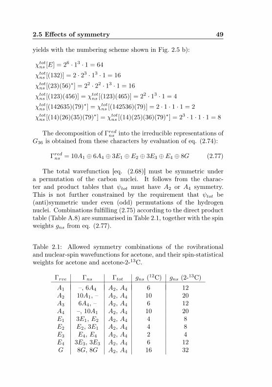
2.5 Effects of symmetry 49
yields with the numbering scheme shown in Fig. 2.5 b):
χtotns [E] = 26 · 13 · 1 = 64
χtotns [(132)] = 2 · 23 · 13 · 1 = 16
χtotns [(23)(56)∗] = 22 · 22 · 13 · 1 = 16
χtotns [(123)(456)] = χtotns [(123)(465)] = 22 · 13 · 1 = 4
χtotns [(142635)(79)∗] = χtotns [(142536)(79)] = 2 · 1 · 1 · 1 = 2
χtotns [(14)(26)(35)(79)∗] = χtotns [(14)(25)(36)(79)∗] = 23 · 1 · 1 · 1 = 8
The decomposition of Γredns into the irreducible representations ofG36 is obtained from these characters by evaluation of eq. (2.74):
Γredns = 10A1 ⊕ 6A4 ⊕ 3E1 ⊕ E2 ⊕ 3E3 ⊕ E4 ⊕ 8G (2.77)
The total wavefunction [eq. (2.68)] must be symmetric undera permutation of the carbon nuclei. It follows from the charac-ter and product tables that ψtot must have A2 or A4 symmetry.This is not further constrained by the requirement that ψtot be(anti)symmetric under even (odd) permutations of the hydrogennuclei. Combinations fulfilling (2.75) according to the direct producttable (Table A.8) are summarised in Table 2.1, together with the spinweights gns from eq. (2.77).
Table 2.1: Allowed symmetry combinations of the rovibrationaland nuclear-spin wavefunctions for acetone, and their spin-statisticalweights for acetone and acetone-2-13C.
Γrve Γns Γtot gns (12C) gns (2-13C)
A1 –, 6A4 A2, A4 6 12A2 10A1, – A2, A4 10 20A3 6A4, – A2, A4 6 12A4 –, 10A1 A2, A4 10 20E1 3E1, E2 A2, A4 4 8E2 E2, 3E1 A2, A4 4 8E3 E4, E4 A2, A4 2 4E4 3E3, 3E3 A2, A4 6 12G 8G, 8G A2, A4 16 32
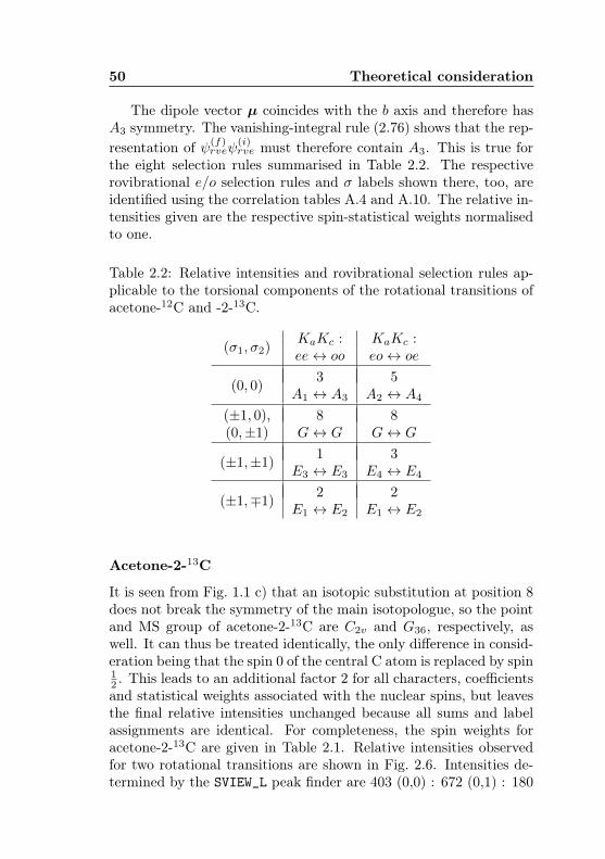
50 Theoretical consideration
The dipole vector µ coincides with the b axis and therefore hasA3 symmetry. The vanishing-integral rule (2.76) shows that the rep-resentation of ψ(f)
rveψ(i)rve must therefore contain A3. This is true for
the eight selection rules summarised in Table 2.2. The respectiverovibrational e/o selection rules and σ labels shown there, too, areidentified using the correlation tables A.4 and A.10. The relative in-tensities given are the respective spin-statistical weights normalisedto one.
Table 2.2: Relative intensities and rovibrational selection rules ap-plicable to the torsional components of the rotational transitions ofacetone-12C and -2-13C.
(σ1, σ2)KaKc : KaKc :ee↔ oo eo↔ oe
(0, 0)3 5
A1 ↔ A3 A2 ↔ A4
(±1, 0), 8 8(0,±1) G↔ G G↔ G
(±1,±1)1 3
E3 ↔ E3 E4 ↔ E4
(±1,∓1)2 2
E1 ↔ E2 E1 ↔ E2
Acetone-2-13C
It is seen from Fig. 1.1 c) that an isotopic substitution at position 8does not break the symmetry of the main isotopologue, so the pointand MS group of acetone-2-13C are C2v and G36, respectively, aswell. It can thus be treated identically, the only difference in consid-eration being that the spin 0 of the central C atom is replaced by spin12 . This leads to an additional factor 2 for all characters, coefficientsand statistical weights associated with the nuclear spins, but leavesthe final relative intensities unchanged because all sums and labelassignments are identical. For completeness, the spin weights foracetone-2-13C are given in Table 2.1. Relative intensities observedfor two rotational transitions are shown in Fig. 2.6. Intensities de-termined by the SVIEW_L peak finder are 403 (0,0) : 672 (0,1) : 180
2.6 General spectral features 51
(1,2) : 252 (1,1) for the eo ← oe case and 1052 (0,0) : 2642 (0,1) :341 (1,1) : 774 (1,2) for the oo← ee case, confirming the calculationwithin experimental uncertainty.
Acetone-1-13C
The asymmetric 13C1 isotopologue of acetone is substituted at oneof the equivalent positions 7 or 9 indicated in Fig. 2.5 b). As therotational-reflectional symmetry of the other two isotopologues isbroken, the remaining reflectional symmetry with respect to the C-C-C plane is described by the point group Cs (see Table A.2). Thisalso impacts the MS group, which becomes G18 and is obtained fromG36 by eliminating all classes containing C2 rotation, represented bythe permutation (79). Using the character table A.5 and the producttable A.6, the procedure outlined above gives the following results:
χtotns [E] = 26 · 2 · 12 · 1 = 128
χtotns [(123)] = χtotns [(456)] = 2 · 23 · 2 · 12 · 1 = 32
χtotns [(123)(456)] = χtotns [(123)(465)] = 2 · 2 · 2 · 12 · 1 = 8
χtotns [(23)(56)∗] = 22 · 22 · 2 · 12 · 1 = 32
Γredns = 32A1 ⊕ 16E1 ⊕ 16E2 ⊕ 8E3 ⊕ 8E4 (2.78)
ψtot must be (anti-)symmetric under an even (odd) permutationof the H nuclei. While the odd permutations pose no restrictionson ψtot, the product table reveals that ψtot must have A1 or A2
symmetry due to the even permutations. Table 2.3 states the allowedcombinations of symmetry species and their spin weights.
The vanishing-integral rule allows for all rovibrational trans-itions whose product representation contains the species Γ[µ] = A2.Table 2.4 gives an overview of the resulting selection rules and rel-ative intensities. Note that, unlike for the other two isotopologues,there is no distinction between ee↔ oo and eo↔ oe, because C2 isnot a symmetry operation any more. Label assignments were takenfrom correlation table A.9.
2.6 General spectral featuresA short explanation of the composition of the acetone spectrum shallbe given here as a reference. The dipole moment of acetone has been
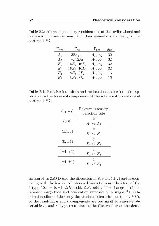
52 Theoretical consideration
Table 2.3: Allowed symmetry combinations of the rovibrational andnuclear-spin wavefunctions, and their spin-statistical weights, foracetone-1-13C.
Γrve Γns Γtot gns
A1 32A1, – A1, A2 32A2 –, 32A1 A1, A2 32E1 16E1, 16E1 A1, A2 32E2 16E2, 16E2 A1, A2 32E3 8E3, 8E3 A1, A2 16E4 8E4, 8E4 A1, A2 16
Table 2.4: Relative intensities and rovibrational selection rules ap-plicable to the torsional components of the rotational transitions ofacetone-1-13C.
(σ1, σ2)Relative intensity,Selection rule
(0, 0)2
A1 ↔ A2
(±1, 0)2
E1 ↔ E1
(0,±1)2
E2 ↔ E2
(±1,∓1)1
E3 ↔ E3
(±1,±1)1
E4 ↔ E4
measured as 2.89 D (see the discussion in Section 5.1.2) and is coin-ciding with the b axis. All observed transitions are therefore of theb type (∆J = 0,±1; ∆Ka odd, ∆Kc odd). The change in dipolemoment magnitude and orientation imposed by a single 13C sub-stitution affects either only the absolute intensities (acetone-2-13C),or the resulting a and c components are too small to generate ob-servable a- and c- type transitions to be discerned from the dense
2.6 General spectral features 53
background of low-intensity lines (acetone-1-13C). However, the pre-dicted spectra contain mock a- and c-type transitions caused by themislabeling effect explained in Section 2.4.2.
While the magnitude of the dipole moment directly influencesthe absolute intensities (I ∝ |µ|2), the relative intensities of therotational transitions of a particular transition type and torsionalstate follow the population differences introduced by the Boltzmanndistribution.
The rotational spectra in this work have been recorded at roomtemperature, corresponding to a characteristic energy kT ∼ 204 cm−1.This is well above the lowest torsional excitational energies (v12 =77.8 cm−1, v17 = 124.5 cm−1). Thus, rotational spectra of torsion-ally excited states are visible besides the ground state spectrum. Asthe excitation energies are low enough to reach a significant pop-ulation also in hot-core regions 10, which are the only interstellarplaces where acetone has been found so far, a useful prediction ofthe spectrum for astronomical observations should contain at leastthe ground state and the first excited state.
As can be seen from Fig. 4.9 a), a remarkable feature in asymmet-ric-rotor spectra is the grouping of R-branch transitions of growingKa in a rather small frequency range. The first line of a Ka seriesof a particular J + 1 ← J transition is always the strong pair ofdegenerate transitions Ka = 0 ↔ 1. From one J to the next, thesetransitions lie about 10 GHz apart, establishing a convenient struc-ture for the assignments. They are always predicted with a low un-certainty and have a characteristic intensity pattern (see Fig. 4.10),which facilitates the collection of lines from a Ka series because onecan keep track of the shifts between the predicted and measuredspectra from the start.
10e.g. in Orion-KL, where a peak temperature of 415 K / 289 cm−1 wasreported in [22]
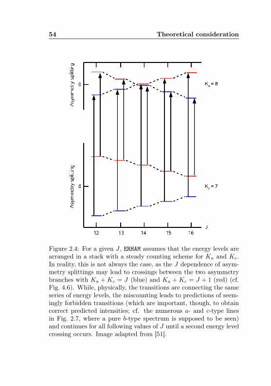
54 Theoretical consideration
Figure 2.4: For a given J , ERHAM assumes that the energy levels arearranged in a stack with a steady counting scheme for Ka and Kc.In reality, this is not always the case, as the J dependence of asym-metry splittings may lead to crossings between the two asymmetrybranches with Ka +Kc = J (blue) and Ka +Kc = J + 1 (red) (cf.Fig. 4.6). While, physically, the transitions are connecting the sameseries of energy levels, the miscounting leads to predictions of seem-ingly forbidden transitions (which are important, though, to obtaincorrect predicted intensities; cf. the numerous a- and c-type linesin Fig. 2.7, where a pure b-type spectrum is supposed to be seen)and continues for all following values of J until a second energy levelcrossing occurs. Image adapted from [51].
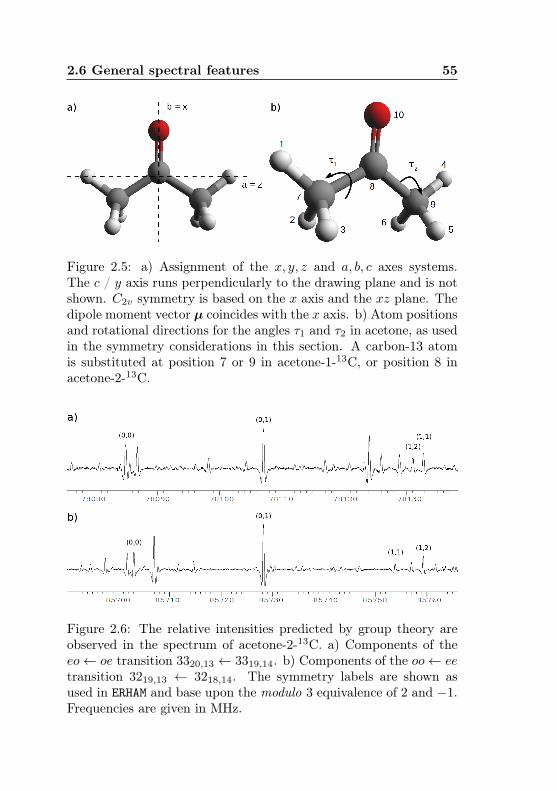
2.6 General spectral features 55
Figure 2.5: a) Assignment of the x, y, z and a, b, c axes systems.The c / y axis runs perpendicularly to the drawing plane and is notshown. C2v symmetry is based on the x axis and the xz plane. Thedipole moment vector µ coincides with the x axis. b) Atom positionsand rotational directions for the angles τ1 and τ2 in acetone, as usedin the symmetry considerations in this section. A carbon-13 atomis substituted at position 7 or 9 in acetone-1-13C, or position 8 inacetone-2-13C.
Figure 2.6: The relative intensities predicted by group theory areobserved in the spectrum of acetone-2-13C. a) Components of theeo← oe transition 3320,13 ← 3319,14. b) Components of the oo← eetransition 3219,13 ← 3218,14. The symmetry labels are shown asused in ERHAM and base upon the modulo 3 equivalence of 2 and −1.Frequencies are given in MHz.
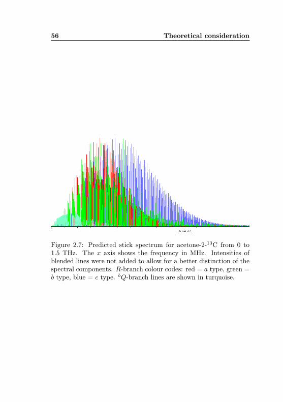
56 Theoretical consideration
Figure 2.7: Predicted stick spectrum for acetone-2-13C from 0 to1.5 THz. The x axis shows the frequency in MHz. Intensities ofblended lines were not added to allow for a better distinction of thespectral components. R-branch colour codes: red = a type, green =b type, blue = c type. bQ-branch lines are shown in turquoise.
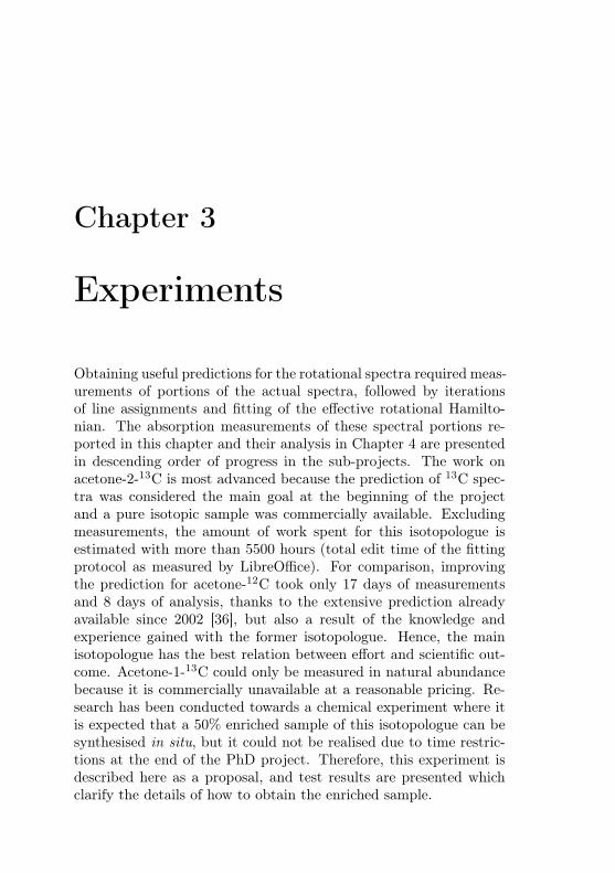
Chapter 3
Experiments
Obtaining useful predictions for the rotational spectra required meas-urements of portions of the actual spectra, followed by iterationsof line assignments and fitting of the effective rotational Hamilto-nian. The absorption measurements of these spectral portions re-ported in this chapter and their analysis in Chapter 4 are presentedin descending order of progress in the sub-projects. The work onacetone-2-13C is most advanced because the prediction of 13C spec-tra was considered the main goal at the beginning of the projectand a pure isotopic sample was commercially available. Excludingmeasurements, the amount of work spent for this isotopologue isestimated with more than 5500 hours (total edit time of the fittingprotocol as measured by LibreOffice). For comparison, improvingthe prediction for acetone-12C took only 17 days of measurementsand 8 days of analysis, thanks to the extensive prediction alreadyavailable since 2002 [36], but also a result of the knowledge andexperience gained with the former isotopologue. Hence, the mainisotopologue has the best relation between effort and scientific out-come. Acetone-1-13C could only be measured in natural abundancebecause it is commercially unavailable at a reasonable pricing. Re-search has been conducted towards a chemical experiment where itis expected that a 50% enriched sample of this isotopologue can besynthesised in situ, but it could not be realised due to time restric-tions at the end of the PhD project. Therefore, this experiment isdescribed here as a proposal, and test results are presented whichclarify the details of how to obtain the enriched sample.
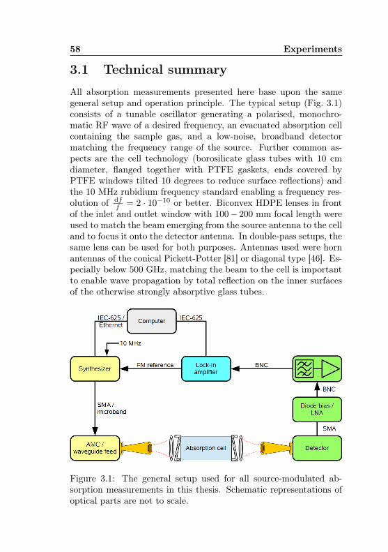
58 Experiments
3.1 Technical summary
All absorption measurements presented here base upon the samegeneral setup and operation principle. The typical setup (Fig. 3.1)consists of a tunable oscillator generating a polarised, monochro-matic RF wave of a desired frequency, an evacuated absorption cellcontaining the sample gas, and a low-noise, broadband detectormatching the frequency range of the source. Further common as-pects are the cell technology (borosilicate glass tubes with 10 cmdiameter, flanged together with PTFE gaskets, ends covered byPTFE windows tilted 10 degrees to reduce surface reflections) andthe 10 MHz rubidium frequency standard enabling a frequency res-olution of df
f = 2 · 10−10 or better. Biconvex HDPE lenses in frontof the inlet and outlet window with 100− 200 mm focal length wereused to match the beam emerging from the source antenna to the celland to focus it onto the detector antenna. In double-pass setups, thesame lens can be used for both purposes. Antennas used were hornantennas of the conical Pickett-Potter [81] or diagonal type [46]. Es-pecially below 500 GHz, matching the beam to the cell is importantto enable wave propagation by total reflection on the inner surfacesof the otherwise strongly absorptive glass tubes.
Figure 3.1: The general setup used for all source-modulated ab-sorption measurements in this thesis. Schematic representations ofoptical parts are not to scale.
3.2 Spectroscopy of acetone-2-13C 59
Absorption line detection was performed through frequency mod-ulation of the source. To this end, a sine signal (≤ 50 kHz) from thebuilt-in oscillator of the lock-in amplifier was used to modulate thesource frequency. The detector output signal was transferred back tothe lock-in amplifier, where it was demodulated at the double mod-ulation frequency (2F mode), generating the second derivative ofthe absorption characteristics thus measured. A frequency-selectiveamplifier between the detector output and the lock-in amplifier wasused to filter and amplify the 2F signal to obtain a monochromaticsignal in the mV range. A LabView program was used to controldata acquisition from the lock-in via an IEC-625 bus system and todisplay, process and store the data.
3.2 Spectroscopy of acetone-2-13C
3.2.1 MeasurementsSeven separate portions of the rotational spectrum of acetone-2-13C were measured in the Cologne spectroscopy laboratories at theInstitute with several different setups summarised in Table 3.1.
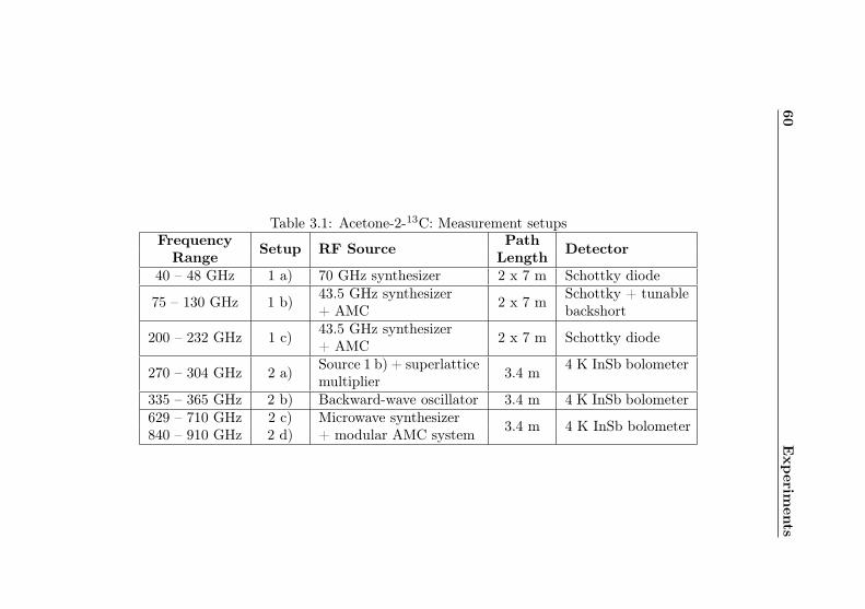
60Exp
eriments
Table 3.1: Acetone-2-13C: Measurement setupsFrequency Setup RF Source Path DetectorRange Length40 – 48 GHz 1 a) 70 GHz synthesizer 2 x 7 m Schottky diode
75 – 130 GHz 1 b) 43.5 GHz synthesizer+ AMC 2 x 7 m Schottky + tunable
backshort
200 – 232 GHz 1 c) 43.5 GHz synthesizer+ AMC 2 x 7 m Schottky diode
270 – 304 GHz 2 a) Source 1 b) + superlatticemultiplier 3.4 m 4 K InSb bolometer
335 – 365 GHz 2 b) Backward-wave oscillator 3.4 m 4 K InSb bolometer629 – 710 GHz 2 c) Microwave synthesizer 3.4 m 4 K InSb bolometer840 – 910 GHz 2 d) + modular AMC system
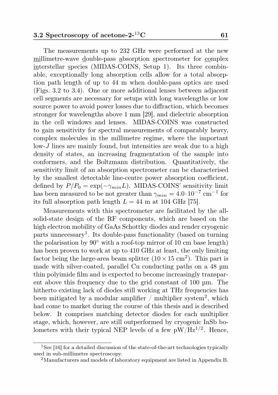
3.2 Spectroscopy of acetone-2-13C 61
The measurements up to 232 GHz were performed at the newmillimetre-wave double-pass absorption spectrometer for complexinterstellar species (MIDAS-COINS, Setup 1). Its three combin-able, exceptionally long absorption cells allow for a total absorp-tion path length of up to 44 m when double-pass optics are used(Figs. 3.2 to 3.4). One or more additional lenses between adjacentcell segments are necessary for setups with long wavelengths or lowsource power to avoid power losses due to diffraction, which becomesstronger for wavelengths above 1 mm [29], and dielectric absorptionin the cell windows and lenses. MIDAS-COINS was constructedto gain sensitivity for spectral measurements of comparably heavy,complex molecules in the millimetre regime, where the importantlow-J lines are mainly found, but intensities are weak due to a highdensity of states, an increasing fragmentation of the sample intoconformers, and the Boltzmann distribution. Quantitatively, thesensitivity limit of an absorption spectrometer can be characterisedby the smallest detectable line-centre power absorption coefficient,defined by P/P0 = exp(−γminL). MIDAS-COINS’ sensitivity limithas been measured to be not greater than γmin = 4.0 ·10−7 cm−1 forits full absorption path length L = 44 m at 104 GHz [75].
Measurements with this spectrometer are facilitated by the all-solid-state design of the RF components, which are based on thehigh electron mobility of GaAs Schottky diodes and render cryogenicparts unnecessary1. Its double-pass functionality (based on turningthe polarisation by 90◦ with a roof-top mirror of 10 cm base length)has been proven to work at up to 410 GHz at least, the only limitingfactor being the large-area beam splitter (10× 15 cm2). This part ismade with silver-coated, parallel Cu conducting paths on a 48 µmthin polyimide film and is expected to become increasingly transpar-ent above this frequency due to the grid constant of 100 µm. Thehitherto existing lack of diodes still working at THz frequencies hasbeen mitigated by a modular amplifier / multiplier system2, whichhad come to market during the course of this thesis and is describedbelow. It comprises matching detector diodes for each multiplierstage, which, however, are still outperformed by cryogenic InSb bo-lometers with their typical NEP levels of a few pW/Hz1/2. Hence,
1See [16] for a detailed discussion of the state-of-the-art technologies typicallyused in sub-millimetre spectroscopy.
2Manufacturers and models of laboratory equipment are listed in Appendix B.
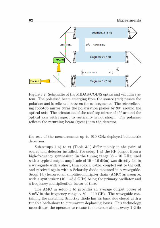
62 Experiments
Figure 3.2: Schematic of the MIDAS-COINS optics and vacuum sys-tem. The polarised beam emerging from the source (red) passes thepolariser and is reflected between the cell segments. The retroreflect-ing roof-top mirror turns the polarisation planes by 90◦ around theoptical axis. The orientation of the roof-top mirror of 45◦ around theoptical axis with respect to verticality is not shown. The polariserreflects the returning beam (green) into the detector.
the rest of the measurements up to 910 GHz deployed bolometricdetection.
Sub-setups 1 a) to c) (Table 3.1) differ mainly in the pairs ofsource and detector installed. For setup 1 a) the RF output from ahigh-frequency synthesizer (in the tuning range 38 − 70 GHz; usedwith a typical output amplitude of 10− 16 dBm) was directly fed toa waveguide with a short, thin coaxial cable, coupled out to the cell,and received again with a Schottky diode mounted in a waveguide.Setup 1 b) featured an amplifier-multiplier chain (AMC) as a source,with a synthesizer (10− 43.5 GHz) being the primary oscillator anda frequency multiplication factor of three.
The AMC in setup 1 b) provides an average output power of8 mW in the frequency range ∼ 80− 110 GHz. The waveguide con-taining the matching Schottky diode has its back side closed with atunable back-short to circumvent dephasing losses. This technologynecessitates the operator to retune the detector about every 1 GHz
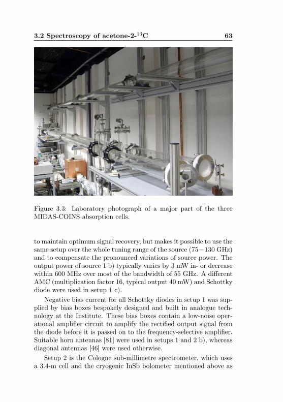
3.2 Spectroscopy of acetone-2-13C 63
Figure 3.3: Laboratory photograph of a major part of the threeMIDAS-COINS absorption cells.
to maintain optimum signal recovery, but makes it possible to use thesame setup over the whole tuning range of the source (75−130 GHz)and to compensate the pronounced variations of source power. Theoutput power of source 1 b) typically varies by 3 mW in- or decreasewithin 600 MHz over most of the bandwidth of 55 GHz. A differentAMC (multiplication factor 16, typical output 40 mW) and Schottkydiode were used in setup 1 c).
Negative bias current for all Schottky diodes in setup 1 was sup-plied by bias boxes bespokely designed and built in analogue tech-nology at the Institute. These bias boxes contain a low-noise oper-ational amplifier circuit to amplify the rectified output signal fromthe diode before it is passed on to the frequency-selective amplifier.Suitable horn antennas [81] were used in setups 1 and 2 b), whereasdiagonal antennas [46] were used otherwise.
Setup 2 is the Cologne sub-millimetre spectrometer, which usesa 3.4-m cell and the cryogenic InSb bolometer mentioned above as
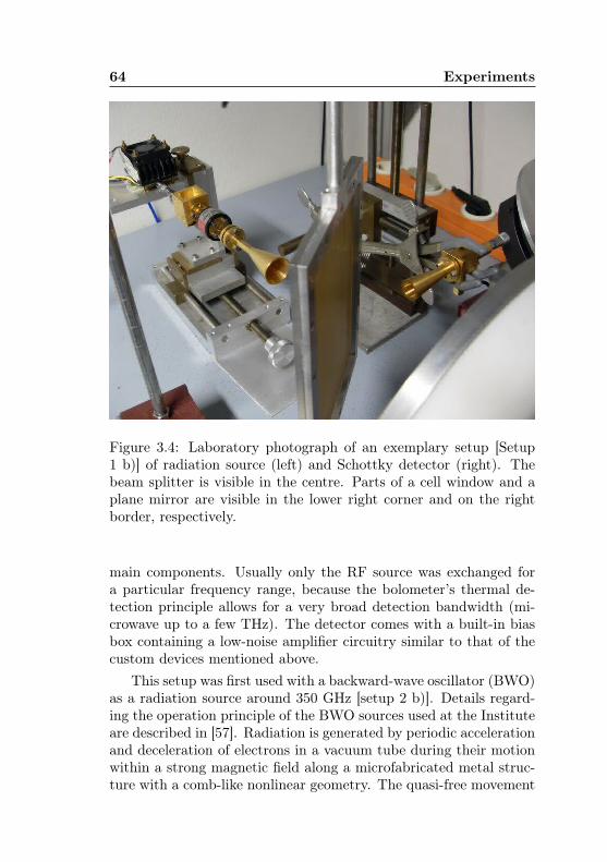
64 Experiments
Figure 3.4: Laboratory photograph of an exemplary setup [Setup1 b)] of radiation source (left) and Schottky detector (right). Thebeam splitter is visible in the centre. Parts of a cell window and aplane mirror are visible in the lower right corner and on the rightborder, respectively.
main components. Usually only the RF source was exchanged fora particular frequency range, because the bolometer’s thermal de-tection principle allows for a very broad detection bandwidth (mi-crowave up to a few THz). The detector comes with a built-in biasbox containing a low-noise amplifier circuitry similar to that of thecustom devices mentioned above.
This setup was first used with a backward-wave oscillator (BWO)as a radiation source around 350 GHz [setup 2 b)]. Details regard-ing the operation principle of the BWO sources used at the Instituteare described in [57]. Radiation is generated by periodic accelerationand deceleration of electrons in a vacuum tube during their motionwithin a strong magnetic field along a microfabricated metal struc-ture with a comb-like nonlinear geometry. The quasi-free movement
3.2 Spectroscopy of acetone-2-13C 65
of electrons guarantees a high output power over the whole tuningrange of the tube (> 30 mW on a tuning range of > 100 GHz forthe 300-GHz tube “OB-30” used here). The BWO is operated asa sideband spectrometer: A harmonic mixer fed by part of the ra-diation from the beam and a local oscillator tuned to a frequencyfLO = (fBWO ± 350 MHz)/m, m being an odd integer, generatesa sideband signal of 350 MHz, which is used to lock the BWO fre-quency by an automatically tuning phase-locked loop device (PLL).The local oscillator used for this work was an identical AMC as insetup 1 b). A redraw of this setup was that the PLL used here wasa replacement for the one originally described in [57], which had al-lowed for broadband measurements of 1 GHz or more once the BWOfrequency was locked. Contrastingly, the acetone-2-13C spectrum of30 GHz was acquired in 612 single scans as the spare PLL lost lockif a range of a few ten MHz was exceeded.
After the BWO measurements, setup 2 a) was intended as a testwith the same cell and detector to find out if the 100-GHz sourcefrom setup 1 b) delivers enough power to reach multiplication factorsof 5 or more with a superlattice multiplier [21,76] in order to accessfrequencies above 400 GHz. This test failed, yet a sufficiently strongsignal identified as the pure third harmonic enabled broadband spec-troscopy of acetone-2-13C around 300 GHz. The superlattice mul-tiplier belongs to a series of similar devices which had been givento the Cologne spectroscopy workgroup (at the Institute) during along-lasting collaboration with Dmitry Pavelyev3.
The goal of determining all relevant spectroscopic parameterssufficiently well for a precise prediction at least down to λ ≈ 2 mmcould not be met with the data collected from the experiments de-scribed so far. An inspection of the predicted spectrum as a whole(Fig. 2.7) showed that measurements up to about 1 THz were worth-wile to obtain a diversification in quantum numbers which could beexpected to be adequate as a remedy. Laboratory work on this isoto-pologue was hence continued when a new solid-state radiation sourcewith a frequency coverage up to 1.1 THz became available in 2014[Setups 2 c) and d)]. Dubbed “THz Starter Kit” by the manufacturer(see Appendix B), it is a modular system consisting of a microwave-driven basis system, which is essentially an AMC with multiplicationfactor 9 enhanced by external modulation and power control capabil-
3Lobachevsky State University of Nizhny Novgorod, Russia
66 Experiments
ity, and five waveguide-mounted multipliers (three doublers and twotriplers) externally connectable to its output flange. The frequencyrange of 82–125 GHz accessible by the basis system can thus be mul-tiplied by 2, 3, 4, 6 [Setup 2 c)], and 9 [Setup 2 d)] to cover the entirerange mentioned, with only one gap between 125 and 170 GHz. Thestandard single-pass setup with the InSb bolometer, which providessufficiently high sensitivity to compensate the power losses at highmultiplication factors due to photonic energy conservation, was usedagain for broadband measurements in two atmospheric transmissionwindows up to 710 and 910 GHz.
3.3 Spectroscopy of acetone-12C
Spectral measurements of acetone’s main isotopologue were origin-ally done to search for the strongest lines of acetone-1-13C in naturalabundance. This first approach was a response to the poor commer-cial availability of this isotopologue. The predictions by Lovas andGroner [60] were good up to the millimetre-wave region, so the ideaformed to use the liquid helium-cooled InSb bolometer described inSection 3.2, being the most sensitive detector available for absorp-tion experiments in this range at the Institute, in combination withSource 1 a), to search for the strongest lines, which were expectedto be 2–3 orders of magnitude less intense than those of the mainisotopologue (see Section 3.4).
Besides the single-line scans described there, too, preparatorybroadband measurements were performed with the THz Starter Kit(Section 3.2) in frequency regions originally selected for future meas-urements of an enriched sample of acetone-1-13C (Section 3.4.2).The 12C spectra acquired this way were intended to be subtractedfrom the spectra of the enriched sample to filter out the lines fromthe main isotopologue, allowing for increased intensities relative tothe by-product acetone-1,3-13C2 by intentionally shifting the educts’stoichiometry (see the detailed explanations in Section 3.4.2). Fourfrequency regions (83–125 GHz, 200–250 GHz, 400-475 GHz and800–908 GHz) could be covered in only one week thanks to the highmultiplication factors of 9 to 81, allowing to exploit the synthes-izer’s high switching speed at microwave frequencies. Yet the firstof these measurements, together with the 70-GHz measurements de-scribed above, would prove later to be sufficient for a substantial
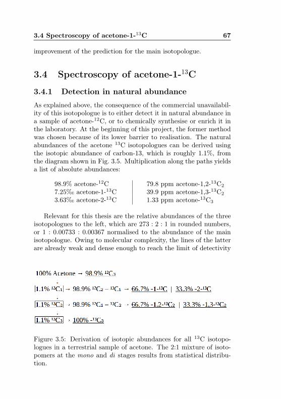
3.4 Spectroscopy of acetone-1-13C 67
improvement of the prediction for the main isotopologue.
3.4 Spectroscopy of acetone-1-13C
3.4.1 Detection in natural abundance
As explained above, the consequence of the commercial unavailabil-ity of this isotopologue is to either detect it in natural abundance ina sample of acetone-12C, or to chemically synthesise or enrich it inthe laboratory. At the beginning of this project, the former methodwas chosen because of its lower barrier to realisation. The naturalabundances of the acetone 13C isotopologues can be derived usingthe isotopic abundance of carbon-13, which is roughly 1.1%, fromthe diagram shown in Fig. 3.5. Multiplication along the paths yieldsa list of absolute abundances:
98.9% acetone-12C 79.8 ppm acetone-1,2-13C2
7.25‰ acetone-1-13C 39.9 ppm acetone-1,3-13C2
3.63‰ acetone-2-13C 1.33 ppm acetone-13C3
Relevant for this thesis are the relative abundances of the threeisotopologues to the left, which are 273 : 2 : 1 in rounded numbers,or 1 : 0.00733 : 0.00367 normalised to the abundance of the mainisotopologue. Owing to molecular complexity, the lines of the latterare already weak and dense enough to reach the limit of detectivity
Figure 3.5: Derivation of isotopic abundances for all 13C isotopo-logues in a terrestrial sample of acetone. The 2:1 mixture of isoto-pomers at the mono and di stages results from statistical distribu-tion.
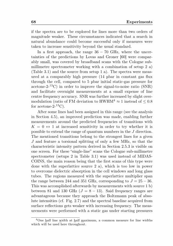
68 Experiments
if the spectra are to be explored for lines more than two orders ofmagnitude weaker. These circumstances indicated that a search innatural abundance could become successful only if measures weretaken to increase sensitivity beyond the usual standard.
In a first approach, the range 36 − 70 GHz, where the uncer-tainties of the predictions by Lovas and Groner [60] were compar-ably small, was covered by broadband scans with the Cologne sub-millimetre spectrometer working with a combination of setup 2 a)(Table 3.1) and the source from setup 1 a). The spectra were meas-ured at a comparably high pressure (14 µbar in constant gas fluxthrough the cell, compared to 5 µbar initial static-gas pressure foracetone-2-13C) in order to improve the signal-to-noise ratio (SNR)and facilitate overnight measurements at a small expense of linecentre frequency accuracy. SNR was further increased by slight over-modulation (ratio of FM deviation to HWHM4 ≈ 1 instead of ≤ 0.8for acetone-2-13C).
After some lines had been assigned in this range (see the analysisin Section 4.5), an improved prediction was made, enabling furthermeasurements around the predicted frequencies of transitions withK = 0 ↔ 1 at increased sensitivity in order to try whether it ispossible to extend the range of quantum numbers in the J direction.The mentioned transitions belong to the strongest lines for a givenJ and feature a torsional splitting of only a few MHz, so that thecharacteristic intensity pattern derived in Section 2.5.3 is visible onone screen. For these “single-line” scans the Cologne sub-millimetrespectrometer (setups 2 in Table 3.1) was used instead of MIDAS-COINS, the main reason being that the first scans of this type weredone with the superlattice source 2 a), which is too low in powerto overcome dielectric absorption in the cell windows and long glasstubes. The regions measured with the superlattice multiplier spanthe range between 244 and 351 GHz, corresponding to J = 25− 36.This was accomplished afterwards by measurements with source 1 b)between 81 and 130 GHz (J = 8 − 13). Said frequency ranges areadvantageous because they approach the Boltzmann peak of abso-lute intensities (cf. Fig. 2.7) and the spectral baseline acquired fromsurface reflections gets weaker with increasing frequency. The meas-urements were performed with a static gas under starting pressures
4One half line width at half maximum, a common measure for line widthswhich will be used here throughout.
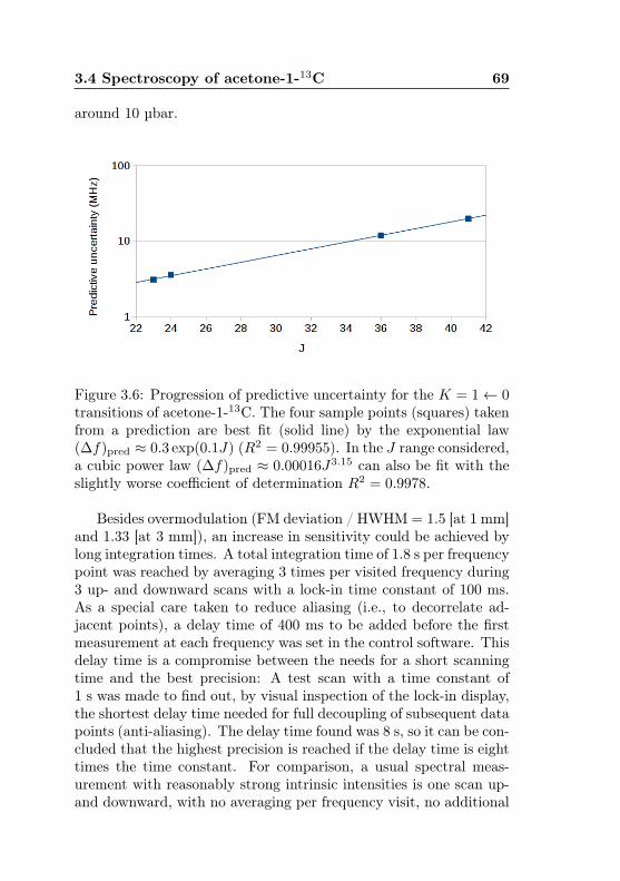
3.4 Spectroscopy of acetone-1-13C 69
around 10 µbar.
Figure 3.6: Progression of predictive uncertainty for the K = 1← 0transitions of acetone-1-13C. The four sample points (squares) takenfrom a prediction are best fit (solid line) by the exponential law(∆f)pred ≈ 0.3 exp(0.1J) (R2 = 0.99955). In the J range considered,a cubic power law (∆f)pred ≈ 0.00016J3.15 can also be fit with theslightly worse coefficient of determination R2 = 0.9978.
Besides overmodulation (FM deviation / HWHM = 1.5 [at 1 mm]and 1.33 [at 3 mm]), an increase in sensitivity could be achieved bylong integration times. A total integration time of 1.8 s per frequencypoint was reached by averaging 3 times per visited frequency during3 up- and downward scans with a lock-in time constant of 100 ms.As a special care taken to reduce aliasing (i.e., to decorrelate ad-jacent points), a delay time of 400 ms to be added before the firstmeasurement at each frequency was set in the control software. Thisdelay time is a compromise between the needs for a short scanningtime and the best precision: A test scan with a time constant of1 s was made to find out, by visual inspection of the lock-in display,the shortest delay time needed for full decoupling of subsequent datapoints (anti-aliasing). The delay time found was 8 s, so it can be con-cluded that the highest precision is reached if the delay time is eighttimes the time constant. For comparison, a usual spectral meas-urement with reasonably strong intrinsic intensities is one scan up-and downward, with no averaging per frequency visit, no additional
70 Experiments
Figure 3.7: a) Distribution of line spacings in the spectrum of acet-one between 75 and 130 GHz, as predicted by Groner et al. [36]and available in the Cologne Database for Molecular Spectroscopy(CDMS) [68–70]. b) Percentile curve of the spacings.
delay time and a time constant of 20 ms.
3.4 Spectroscopy of acetone-1-13C 71
During the test, it was also found that the balance between anti-aliasing and lock-in relaxation speed can be controlled with a previ-ously unknown setting of the lock-in detector: The model used for allmeasurements in this thesis comes with a digital filter for the X (out-put) channel, the steepness of which can be chosen between 6, 12,18, and 24 decibel per octave (dB/oct.) [66]. A steeper slope corres-ponds to better hardware anti-aliasing. The first setting corrsepondsto a first-order filter (filter gain antiproportional to frequency in thehigh-f limit), the second to second-order filtering etc. The choice ofsteepness for this filter (implemented by the envelope of a frequencyresponse function) directly influences the sampling process in thelock-in’s main ADC. For the high-precision measurements presen-ted here, second-order filtering was used, whereas a higher settingwould have enforced even higher delay times. Particularly, the “eighttimes the time constant” rule found for the delay time holds onlyfor this setting. Otherwise, for measurements with standard sensit-ivity as described before, first-order filtering is acceptable in mostcases, though leading to slightly broader lines due to frequency shiftsbetween the up- and downward scans.
The increase in integration and delay time resulted in a long dur-ation of measurements (up to 6:32 hours for one prediction with scanwidths calculated as explained below), especially for the measure-ments around 3 mm, where the switching speed of the synthesizerwas significantly lower owing to the frequency multiplication factorof 3. This required an analysis to determine the minimum widthto be scanned around each predicted line frequency. As superpos-ition often prevents an identification of candidates for all torsionalcomponents of a rotational transition, candidates must be measuredagainst known, unperturbed lines of the main isotopologue (calibra-tion lines). The minimum width to be scanned is thus determined bythe number of lines from the main isotopologue available for intens-ity calibration rather than the progression of predictive uncertainty,which follows an exponential law (Fig. 3.6), but increases still tooslowly within the range of J values covered by the measurementsto get a high probability of including at least one sufficiently strongcalibration line.
The number of available calibration lines was taken into accountindirectly by deriving a rule-of-thumb formula from a statistical ana-lysis of the line spacings encountered in the main isotopologue pre-
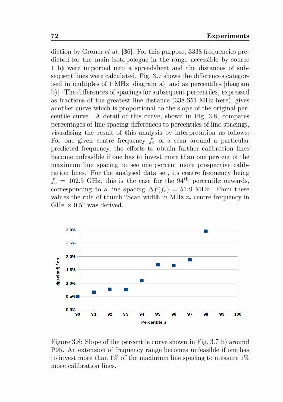
72 Experiments
diction by Groner et al. [36]. For this purpose, 3338 frequencies pre-dicted for the main isotopologue in the range accessible by source1 b) were imported into a spreadsheet and the distances of sub-sequent lines were calculated. Fig. 3.7 shows the differences categor-ised in multiples of 1 MHz [diagram a)] and as percentiles [diagramb)]. The differences of spacings for subsequent percentiles, expressedas fractions of the greatest line distance (338.651 MHz here), givesanother curve which is proportional to the slope of the original per-centile curve. A detail of this curve, shown in Fig. 3.8, comparespercentages of line spacing differences to percentiles of line spacings,visualising the result of this analysis by interpretation as follows:For one given centre frequency fc of a scan around a particularpredicted frequency, the efforts to obtain further calibration linesbecome unfeasible if one has to invest more than one percent of themaximum line spacing to see one percent more prospective calib-ration lines. For the analysed data set, its centre frequency beingfc = 102.5 GHz, this is the case for the 94th percentile onwards,corresponding to a line spacing ∆f(fc) = 51.9 MHz. From thesevalues the rule of thumb “Scan width in MHz ≈ centre frequency inGHz × 0.5” was derived.
Figure 3.8: Slope of the percentile curve shown in Fig. 3.7 b) aroundP95. An extension of frequency range becomes unfeasible if one hasto invest more than 1% of the maximum line spacing to measure 1%more calibration lines.
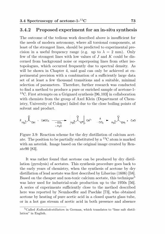
3.4 Spectroscopy of acetone-1-13C 73
3.4.2 Proposed experiment for an in-situ synthesis
The outcome of the tedious work described above is insufficient forthe needs of modern astronomy, where all torsional components, atleast of the strongest lines, should be predicted to experimental pre-cision in a useful frequency range (e.g. up to λ = 2 mm). Onlyfew of the strongest lines with low values of J and K could be dis-cerned from background noise or superposing lines from other iso-topologues, which occurred frequently due to spectral density. Aswill be shown in Chapter 4, said goal can only be achieved at ex-perimental precision with a combination of a sufficiently large dataset of at least a few thousand transitions and a suitable, minimalselection of parameters. Therefore, further research was conductedto find a method to produce a pure or enriched sample of acetone-1-13C. First attempts on a Grignard synthesis [96,103] in collaborationwith chemists from the group of Axel Klein (Department of Chem-istry, University of Cologne) failed due to the close boiling points ofsolvent and product.
Figure 3.9: Reaction scheme for the dry distillation of calcium acet-ate. The position to be partially substituted by a 13C atom is markedwith an asterisk. Image based on the original image created by Ren-ate90 [83].
It was rather found that acetone can be produced by dry distil-lation (pyrolysis) of acetates. This synthesis procedure goes back tothe early years of chemistry, when the synthesis of acetone by drydistillation of lead acetate was first described by Libavius (1606) [58].Based on the cheaper and non-toxic calcium acetate, this technique5was later used for industrial-scale production up to the 1950s [56].A series of experiments sufficiently close to the method describedhere was reported by Neunhoeffer and Paschke [73], who obtainedacetone by heating of pure acetic acid in a closed quartz glass tube,or in a hot gas stream of acetic acid in both presence and absence
5Called Kalksalzdestillation in German, which translates to “lime salt distil-lation” in English.
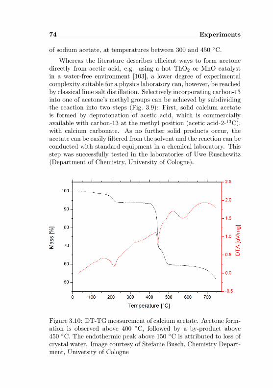
74 Experiments
of sodium acetate, at temperatures between 300 and 450 ◦C.
Whereas the literature describes efficient ways to form acetonedirectly from acetic acid, e.g. using a hot ThO2 or MnO catalystin a water-free environment [103], a lower degree of experimentalcomplexity suitable for a physics laboratory can, however, be reachedby classical lime salt distillation. Selectively incorporating carbon-13into one of acetone’s methyl groups can be achieved by subdividingthe reaction into two steps (Fig. 3.9): First, solid calcium acetateis formed by deprotonation of acetic acid, which is commerciallyavailable with carbon-13 at the methyl position (acetic acid-2-13C),with calcium carbonate. As no further solid products occur, theacetate can be easily filtered from the solvent and the reaction can beconducted with standard equipment in a chemical laboratory. Thisstep was successfully tested in the laboratories of Uwe Ruschewitz(Department of Chemistry, University of Cologne).
Figure 3.10: DT-TGmeasurement of calcium acetate. Acetone form-ation is observed above 400 ◦C, followed by a by-product above450 ◦C. The endothermic peak above 150 ◦C is attributed to loss ofcrystal water. Image courtesy of Stefanie Busch, Chemistry Depart-ment, University of Cologne
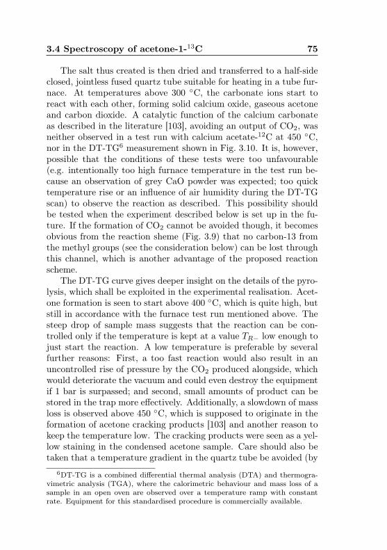
3.4 Spectroscopy of acetone-1-13C 75
The salt thus created is then dried and transferred to a half-sideclosed, jointless fused quartz tube suitable for heating in a tube fur-nace. At temperatures above 300 ◦C, the carbonate ions start toreact with each other, forming solid calcium oxide, gaseous acetoneand carbon dioxide. A catalytic function of the calcium carbonateas described in the literature [103], avoiding an output of CO2, wasneither observed in a test run with calcium acetate-12C at 450 ◦C,nor in the DT-TG6 measurement shown in Fig. 3.10. It is, however,possible that the conditions of these tests were too unfavourable(e.g. intentionally too high furnace temperature in the test run be-cause an observation of grey CaO powder was expected; too quicktemperature rise or an influence of air humidity during the DT-TGscan) to observe the reaction as described. This possibility shouldbe tested when the experiment described below is set up in the fu-ture. If the formation of CO2 cannot be avoided though, it becomesobvious from the reaction sheme (Fig. 3.9) that no carbon-13 fromthe methyl groups (see the consideration below) can be lost throughthis channel, which is another advantage of the proposed reactionscheme.
The DT-TG curve gives deeper insight on the details of the pyro-lysis, which shall be exploited in the experimental realisation. Acet-one formation is seen to start above 400 ◦C, which is quite high, butstill in accordance with the furnace test run mentioned above. Thesteep drop of sample mass suggests that the reaction can be con-trolled only if the temperature is kept at a value TR− low enough tojust start the reaction. A low temperature is preferable by severalfurther reasons: First, a too fast reaction would also result in anuncontrolled rise of pressure by the CO2 produced alongside, whichwould deteriorate the vacuum and could even destroy the equipmentif 1 bar is surpassed; and second, small amounts of product can bestored in the trap more effectively. Additionally, a slowdown of massloss is observed above 450 ◦C, which is supposed to originate in theformation of acetone cracking products [103] and another reason tokeep the temperature low. The cracking products were seen as a yel-low staining in the condensed acetone sample. Care should also betaken that a temperature gradient in the quartz tube be avoided (by
6DT-TG is a combined differential thermal analysis (DTA) and thermogra-vimetric analysis (TGA), where the calorimetric behaviour and mass loss of asample in an open oven are observed over a temperature ramp with constantrate. Equipment for this standardised procedure is commercially available.
76 Experiments
heating up slowly) to suppress acetone cracking on the walls. An-other endothermic reaction with a mass loss of some 5% seen above150 ◦C is ascribed to the evaporation of crystal water, which has tobe removed from the sample before acetone formation is started.
Figure 3.11: Theoretical yield of acetone-1-13C as a function ofthe content of isotopically enriched acetic acid at the beginning ofsynthesis. Products: blue = 12–12; yellow = 13–13; red = 12–13. The curves have been calculated from the molar fraction xof isotopic acetic acid by x12−12 = (1 − x)2, x13−13 = x2, andx12−13 = 1− x12−12 − x13−13.
The proposed reaction supports a selective 13C enrichment of themethyl groups. The isotope must be introduced by mixing naturalacetic acid with a pure isotopic sample at the beginning of the firstreaction. Fig. 3.11 shows the amount of the respective acetone iso-topologues which will be produced from an acetic acid mixture of agiven isotopic content. The highest yield of 50% acetone-1-13C isachieved with a 1:1 mixture of acetic acid-12C and acetic acid-2-13C.The reaction tolerates ±16% inaccuracy of mixture within 5% lossof desired product. A shift towards a lower portion of acetic acid-13C is justifiable to increase the ratio of acetone-1-13C to acetone-1,3-13C2, as the spectrum of acetone-12C has been measured andcan be subtracted from the spectrum of the mixed sample. For in-
3.4 Spectroscopy of acetone-1-13C 77
stance, as a good compromise between preferences regarding a highabsolute abundance of acetone-1-13C and a high abundance ratioto acetone-13C2, an enrichment of only 33% would yield a 1:1 mix-ture of acetone-1-13C with the main isotopologue, while the ratioto doubly substituted acetone were 4:1. Using an enrichment below33% is not recommended because of the low production efficiency,leading to a low signal-to-noise ratio for the desired product due toa low absolute abundenace, and because this would mean a too highreliance on the quality of the acetone-12C spectrum to be subtracted.
A last obstacle to be overcome by the experiment is the captureand storage of the product. A separation of acetone from the vapourphase in a simple condenser tube is not advisable because of itsvolatility (vapour pressure7 roughly 200 mbar at 15 ◦C): it wouldevaporate during the CO2 removal. On the other hand, removingthe CO2 is essential because its partial pressure would rise aboveany practical limit otherwise (vapour pressure ∼ 57 bar at roomtemperature). A better approach is to remove the carbon dioxide bysublimation, which can normally be done in a cold trap, e.g. at liquidnitrogen temperature. However, as no reliable data for the boilingpoints of acetone and carbon dioxide under vacuum conditions couldbe found, it had to be verified experimentally whether a separationof the products could be performed as imagined.
In a preliminary experiment, a small amount of liquid acetonewas filled into a glass bulb with an inlet valve for the sample andan outlet valve connected to a turbomolecular pump, and cooleddown to 77 K with liquid nitrogen. Only the bottom of the bulbwas immersed, so that the air in the bulb could be pumped outafter the acetone had frozen. It was observed that the sample hadnot frozen out completely; instead, its central region remained in ajellylike condition. This is in accordance with the observed residualpressure, which could not be reduced below 500 µbar even when thebulb was immersed as a whole. The most successful freeze-out ofacetone with a final background pressure of 1.5 µbar was realisedby opening and closing the outlet valve several times with the bulbcompletely immersed.
The experiment was repeated with carbon dioxide, which was letinto the bulb after having been evacuated and cooled to 77 K. The
7The vapour pressures given in this section were extrapolated from datapoints available in the GESTIS database [25].
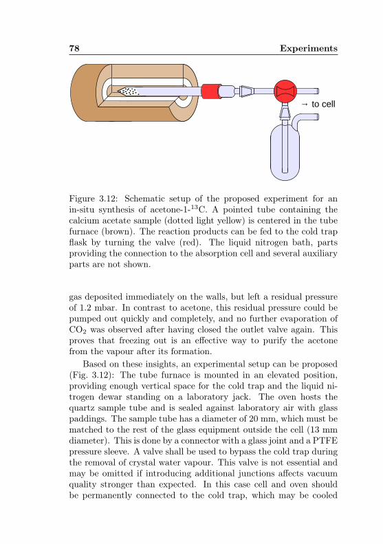
78 Experiments
→ to cell
Figure 3.12: Schematic setup of the proposed experiment for anin-situ synthesis of acetone-1-13C. A pointed tube containing thecalcium acetate sample (dotted light yellow) is centered in the tubefurnace (brown). The reaction products can be fed to the cold trapflask by turning the valve (red). The liquid nitrogen bath, partsproviding the connection to the absorption cell and several auxiliaryparts are not shown.
gas deposited immediately on the walls, but left a residual pressureof 1.2 mbar. In contrast to acetone, this residual pressure could bepumped out quickly and completely, and no further evaporation ofCO2 was observed after having closed the outlet valve again. Thisproves that freezing out is an effective way to purify the acetonefrom the vapour after its formation.
Based on these insights, an experimental setup can be proposed(Fig. 3.12): The tube furnace is mounted in an elevated position,providing enough vertical space for the cold trap and the liquid ni-trogen dewar standing on a laboratory jack. The oven hosts thequartz sample tube and is sealed against laboratory air with glasspaddings. The sample tube has a diameter of 20 mm, which must bematched to the rest of the glass equipment outside the cell (13 mmdiameter). This is done by a connector with a glass joint and a PTFEpressure sleeve. A valve shall be used to bypass the cold trap duringthe removal of crystal water vapour. This valve is not essential andmay be omitted if introducing additional junctions affects vacuumquality stronger than expected. In this case cell and oven shouldbe permanently connected to the cold trap, which may be cooled
3.4 Spectroscopy of acetone-1-13C 79
down after removing the crystal water. The cold trap consists of atwo-necked cylindrical flask with a glass tube fed through its upperneck and reaching its bottom. The glass setup may be connectedto the cell inlet valve by a rubber hose with matching joints. Suffi-cient vacuum tightness has been verified for a for a setup where thequartz tube fittings were directly connected to the cell, i.e. withoutvalve and cold trap. Trap and valve should not be omitted if a wayis found to perform a catalytic reaction without CO2 generation, asthe trap allows for efficient collection and controlled release of thesample.
To the current state of knowledge, the best practice to conductthe experiment with this setup is as follows: Removal of crystal wa-ter is done first by heating up the sample to 250 ◦C with the valvein bypass position and the cell inlet open. When the pressure hasrelaxed, the glass valve is turned into trap position or, respectively,the cold trap is cooled down. The heat is then carefully increased toTR− and the pressure rise is observed while some acetone is formed.If the amount of educt is too small, the reaction can alternatively beperformed with the cell inlet valve closed to increase freeze-out effi-ciency. Oven temperature is to be decreased early enough to avoidoverproduction, as any excess acetone will be removed with the CO2
background pressure when the cold trap heats up again. The liquidnitrogen reservoir must be refilled manually. Unattended overnightscans are impossible for the same reasons. However, a thermallyinsulated, pressureless liquid nitrogen reservoir with a small outletthrough a hose (dubbed “chicken feeder” by practical analogy) isavailable at the Institute and could be tried for continuous nitro-gen refilling to avoid these problems if the reaction cannot be runcatalytically. In this case, preserving the sample in the glass tubesat room temperature to continue measuring on the next day wouldbe possible. A preliminary experiment with regular calcium acetateis suggested to find a way to run the reaction without CO2 gener-ation, to identify the reaction temperature TR−, and to clarify theneed for manual pressure control and the allowable reaction dura-tion for creating the right amount of sample needed for one spectralmeasurement.
Chapter 4
Spectral analysis andresults
4.1 Data analysis with AABS
The software package AABS1 developed by Z. Kisiel [48,49] was usedto visualise the experimental data and assign line frequencies to pre-dicted transitions for all species and torsional excitations treatedhere. A screenshot of a typical working session is shown in Fig. 4.1.AABS has been designed for keyboard-only operation to process largeamounts of spectral data in a short time.
The display of experimental and calculated data is implementedin the two independent programs SVIEW_L and ASCP_L, respectively,which can be operated synchronously by providing a predeterminedsettings file in the working directory. Functions of SVIEW_L includezooming and shifting, background subtraction [50], smoothing, peakfinding, distance measurements and gle output. ASCP_L can displaysimulated stick and / or contour spectra of multiple catalogues witha diversified colour map, quickly navigate and filter transitions ofa specified type, flip through transitions within a blended line, andindicate frequencies where an assignment was already made. An as-signment is made by placing a marker on a candidate transition fromthe catalogue and shifting an independent cursor to the frequency
1Assignment and Analysis of Broadband Spectra
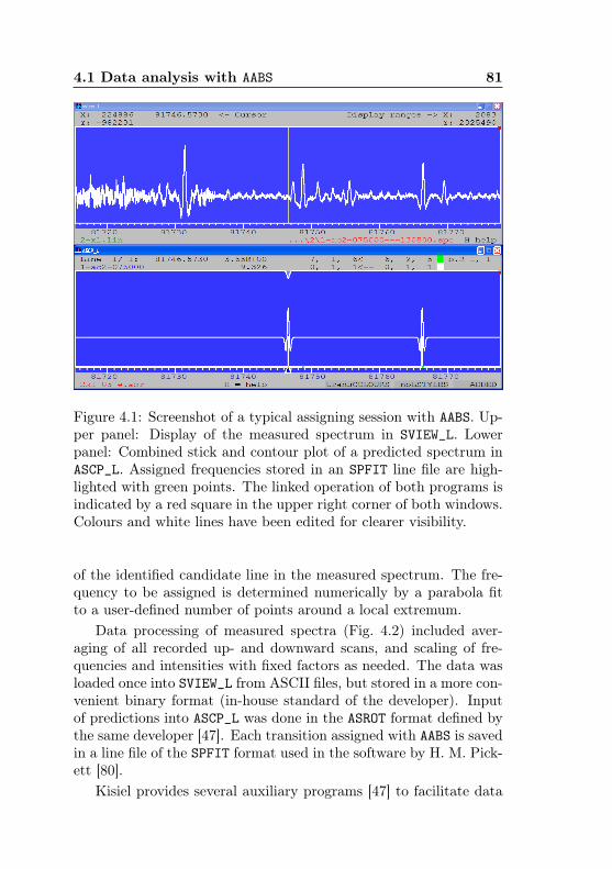
4.1 Data analysis with AABS 81
Figure 4.1: Screenshot of a typical assigning session with AABS. Up-per panel: Display of the measured spectrum in SVIEW_L. Lowerpanel: Combined stick and contour plot of a predicted spectrum inASCP_L. Assigned frequencies stored in an SPFIT line file are high-lighted with green points. The linked operation of both programs isindicated by a red square in the upper right corner of both windows.Colours and white lines have been edited for clearer visibility.
of the identified candidate line in the measured spectrum. The fre-quency to be assigned is determined numerically by a parabola fitto a user-defined number of points around a local extremum.
Data processing of measured spectra (Fig. 4.2) included aver-aging of all recorded up- and downward scans, and scaling of fre-quencies and intensities with fixed factors as needed. The data wasloaded once into SVIEW_L from ASCII files, but stored in a more con-venient binary format (in-house standard of the developer). Inputof predictions into ASCP_L was done in the ASROT format defined bythe same developer [47]. Each transition assigned with AABS is savedin a line file of the SPFIT format used in the software by H. M. Pick-ett [80].
Kisiel provides several auxiliary programs [47] to facilitate data
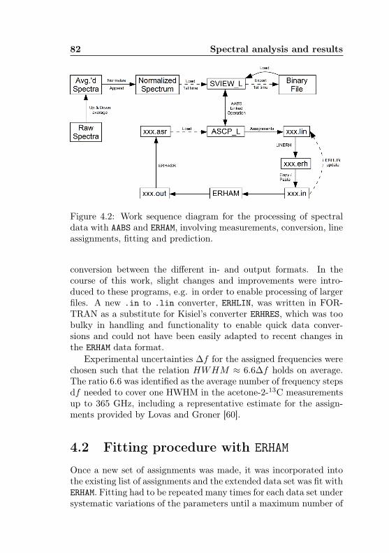
82 Spectral analysis and results
Figure 4.2: Work sequence diagram for the processing of spectraldata with AABS and ERHAM, involving measurements, conversion, lineassignments, fitting and prediction.
conversion between the different in- and output formats. In thecourse of this work, slight changes and improvements were intro-duced to these programs, e.g. in order to enable processing of largerfiles. A new .in to .lin converter, ERHLIN, was written in FOR-TRAN as a substitute for Kisiel’s converter ERHRES, which was toobulky in handling and functionality to enable quick data conver-sions and could not have been easily adapted to recent changes inthe ERHAM data format.
Experimental uncertainties ∆f for the assigned frequencies werechosen such that the relation HWHM ≈ 6.6∆f holds on average.The ratio 6.6 was identified as the average number of frequency stepsdf needed to cover one HWHM in the acetone-2-13C measurementsup to 365 GHz, including a representative estimate for the assign-ments provided by Lovas and Groner [60].
4.2 Fitting procedure with ERHAM
Once a new set of assignments was made, it was incorporated intothe existing list of assignments and the extended data set was fit withERHAM. Fitting had to be repeated many times for each data set undersystematic variations of the parameters until a maximum number of
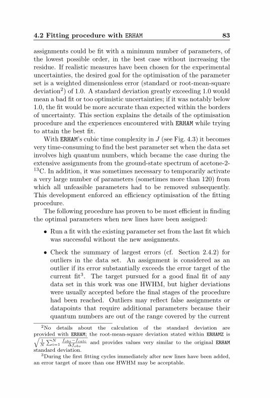
4.2 Fitting procedure with ERHAM 83
assignments could be fit with a minimum number of parameters, ofthe lowest possible order, in the best case without increasing theresidue. If realistic measures have been chosen for the experimentaluncertainties, the desired goal for the optimisation of the parameterset is a weighted dimensionless error (standard or root-mean-squaredeviation2) of 1.0. A standard deviation greatly exceeding 1.0 wouldmean a bad fit or too optimistic uncertainties; if it was notably below1.0, the fit would be more accurate than expected within the bordersof uncertainty. This section explains the details of the optimisationprocedure and the experiences encountered with ERHAM while tryingto attain the best fit.
With ERHAM’s cubic time complexity in J (see Fig. 4.3) it becomesvery time-consuming to find the best parameter set when the data setinvolves high quantum numbers, which became the case during theextensive assignments from the ground-state spectrum of acetone-2-13C. In addition, it was sometimes necessary to temporarily activatea very large number of parameters (sometimes more than 120) fromwhich all unfeasible parameters had to be removed subsequently.This development enforced an efficiency optimisation of the fittingprocedure.
The following procedure has proven to be most efficient in findingthe optimal parameters when new lines have been assigned:
• Run a fit with the existing parameter set from the last fit whichwas successful without the new assignments.
• Check the summary of largest errors (cf. Section 2.4.2) foroutliers in the data set. An assignment is considered as anoutlier if its error substantially exceeds the error target of thecurrent fit3. The target pursued for a good final fit of anydata set in this work was one HWHM, but higher deviationswere usually accepted before the final stages of the procedurehad been reached. Outliers may reflect false assignments ordatapoints that require additional parameters because theirquantum numbers are out of the range covered by the current
2No details about the calculation of the standard deviation areprovided with ERHAM; the root-mean-square deviation stated within ERHAMZ is√
1N
∑Ni=1
fobs−fcalc∆fobs
and provides values very similar to the original ERHAMstandard deviation.
3During the first fitting cycles immediately after new lines have been added,an error target of more than one HWHM may be acceptable.
84 Spectral analysis and results
Figure 4.3: Time complexity of ERHAM in J as measured by manuallystopping the execution time of each cycle in a three-cycle fit of thefull data set for acetone-2-13C (J ≤ 92) or identical fits of the samedata set truncated to the indicated values. The size difference of thedata sets (7627 transitions for J ≤ 50; 9758 for J ≤ 92) is supposedto have an effect not stronger than linear. To improve reproducibil-ity, the fits were repeated until both the standard deviation and thedifference between least and greatest cycle duration did not exceed1 second. The values were determined by parallel execution on an8-core 2.5 GHz machine. The data are fit equally well (R2 = 0.994)by a cubic or exponential law.
parameter set. Said definition is partly subjective as it dependson the “normal” size of deviations between assigned and cal-culated frequencies encountered in the current fit and impliesthat reasonable convergence is achieved for most assignments.
Outliers are taken out of the fit for the time being by settingtheir frequency uncertainties to zero. Later steps aim to rein-corporate as many assignments as possible4 by identifying theparameter set with the best performance for this data set. Aslong as the ERHAM model is correct, it can be expected thatall outliers remaining after completion of this fitting proced-ure are false assignments which can be removed and assignedcorrectly at a later point when the frequency range where thenew assignments have been made is revisited with a better pre-diction. Removal of outliers is repeated until all outliers have
4This is greatly facilitated by the usage of standard uncertainties per spectralrange rather then individual uncertainties for every assigned line.
4.2 Fitting procedure with ERHAM 85
been ruled out.
As this frequently recurrent task is time-consuming and proneto mistakes, a dedicated FORTRAN application was written toset the experimental uncertainties of all assignments with anerror above a user-specified threshold to zero automatically.The figure of merit for decisions on the outlier status of anassignment is the error divided by experimental uncertainty.These values are a frequency independent error measure be-cause the uncertainties have been chosen as fixed fractions ofthe linewidth (see Section 4.1), which in turn scales with thefrequency. Once an improved parameter set was established,ruled-out transitions could be restored easily because standarduncertainties had been used for each frequency region.
• Use a spreadsheet to copy and paste the parameter outputinto a comparator table and calculate the relative errors. Inthe comparator, the output is arranged in three columns (onefor label, value and error). The relative errors are calculatedin a fourth column and the columns containing the values anderrors are hidden such that only the parameter identifiers, theirnumbers within the last fit, and their relative errors remainvisible. Results from later fits are imported likewise into thecolumns to the right. This table allows to track the completehistory of parameter responses to any changes introduced tothe fit and is the basis for most decisions on further changesto the fit.
• The following steps are to be repeated for each applicable com-bination (q, q′) in ascending Fourier order ζ = (|q|+|q′|). Cent-rifugal parameters can be considered as tunneling parameterswith (q, q′) = (0, 0) and should be treated first.
• For the current pair (q, q′), add new parameters in groups ofthe same order (cf. Section 2.4.1) and repeat the fit. Repeatadding higher orders until no significant improvement is ob-served any more. At this stage, a given order is considered asan improvement of the fit if the standard deviation drops by10% or more.
• Repeat the previous step for all other (q, q′) until the standarddeviation is minimised with a maximum of parameters. The
86 Spectral analysis and results
next steps are intended to filter out the smallest subset ofbeneficial parameters from this parameter set.
• Strongly underdetermined parameters (uncertainty > 100%)can be removed immediately. If the relative uncertainties ofthis parameter class span more than one order of magnitude,one should however perform the removal in subclasses, startingwith the greatest order of relative uncertainty, rerun the fitand proceed with the next subclass until no parameters above100% are left before continuing with the next class. This wayit is less probable that parameters will be removed accidentallybecause they are coupled to a bad parameter (see explanationsbelow). When the worst parameters are removed, such coupledparameters may become well-determined rapidly.
• From now on the fit should be rerun after every major changeto the parameters, which usually means an addition or removalof one or two parameters.
• Remove all remaining parameters with an uncertainty exceed-ing 30%. This is the threshold above which a parameter willhave no significant effect on the fit any more. In rare cases,more or less well-determined parameters may exist which areacting only on the second decimal place of the standard de-viation. If such a parameter is discovered (normally due toan unpredictable behaviour of its uncertainty or having in-dex numbers which are not adjacent to those of other well-determined parameters), it can be removed likewise. The con-cept of adjacent parameters is explained below. A divisioninto substeps is also advisable here if the relative uncertaintiesbetween 30% and 100% are distributed unequally.
• Some parameters are correlated to others so strongly that theywill become underdetermined if one of their correlation part-ners is removed. During this work, parameters were regardedas coupled if their correlation index in the ERHAM output ex-ceeded ±80000 (cf. Section 2.4.2). Coupled parameters areknown to occur in least-square algorithms if the numericalstructure of the data set is pronounced too weakly to be fit-ted if one of the coupled parameters is removed. In algebraic
4.2 Fitting procedure with ERHAM 87
terms, coupled parameters are a weaker form of linearly de-pendent parameters because they still have a slight freedom ofindeterminacy.
This effect is called (multi-)collinearity and has been describedin the literature [7]. Collinearity should be avoided becauseit diminishes the integrity of the model, as an independentvariation of supposedly independent parameters is no longerpossible. This becomes noticeable in ERHAM primarily througha slower convergence of the least-square algorithm and dispro-portionate predictive uncertainties (e.g. some MHz even forassigned transitions). Proven ways to eliminate collinearity inERHAM are comparable to what is known from systems of linearequations with linearly dependent coefficients:
– Try to identify one of the coupled parameters which fitsthe data set similarly well as the set of coupled parametersdoes. This is sufficient in the majority of cases when(mostly) parameters of high order are affected and theincrease of residue due to the parameter removal is small.
– Alternatively, the coupled parameters can be kept in theparameter set until the data set is extended further. Thisapproach is especially promising if none of the paramet-ers in the coupled subset appears to be dispensable andfurther assignments are planned.
– Some cases of coupled parameters arise from other para-meters having been removed from the fit too early. Thiscase can be solved by close inspection of the comparatortable to find hints when the coupling occurred for the firsttime.
– If persistent coupling is observed in coincidence with othergeneral problems of the fit, this could be a hint that animportant parameter might not yet have been introducedin the parameter set. This option has been used for thefit of the acetone-2-13C ground state successfully and willbe discussed further in Section 4.3.
Decoupled parameters show an additive effect on the residue(standard deviation, see the introduction of this Section), which
88 Spectral analysis and results
can be used to obtain an indirect hint on coupling. If, for in-stance, the decrease in residue is known for either of two para-meters if enabled alone, the residue should decrease by the sumof both effects if both parameters are enabled together. If thisbehaviour is not observed, an immediate localisation of the re-sponsible parameters is possible with no further inspection ofthe correlation table.
• Parameters may be removed from unequal (q, q′) at the sametime if they are decoupled.
• In the final stages of this procedure, it is worthwhile to test ifsome parameters with relative uncertainties between 20% and30% can be removed as well.
• Sometimes the situation occurs that, following this procedure,parameters of an intermediate order are removed while adja-cent parameters of higher order remain in the fit and are well-determined. Two parameters pertaining to the same subset(q, q′) are called adjacent if their index (κ, p, r) differs by 2 inone of the three powers κ, p, or r (see Section 2.4.1). Adjacentparameters differ mainly in their order while having a compar-able effect on the fit. Such “cheese holes” in the parameter setshould be avoided because they destroy the monotonic con-vergence of the Hamiltonian. In this situation one can try tosubstitute the stand-alone parameter of higher order by one ofits adjacent parameters of lower order. However, this is notalways possible and there is no better option than acceptingthe “cheese hole” for the time being and continuing the proced-ure. Some cases have been observed where low-order tunnelingparameters are not eligible because they would couple to anadjacent parameter in a different parameter subset (q, q′).The concept of adjacent parameters is also helpful if two ormore parameters seem equally eligible for being enabled, orwhen decoupling parameters.
• If most of the possibilities for parameter removal have beengone through, parameters may be added or removed morefreely until the residue cannot be lowered further.
• After the outlier removal at the beginning of this procedure,all operations up to this point concerned only the parameters.
4.2 Fitting procedure with ERHAM 89
When the smallest possible parameter set has been determ-ined, check the deviation summary once more for lines whichhave been wrongly assigned or which cannot be fit better withthe current data and parameter set. These lines should be re-visited with the assignment software and given zero weight ifthe assignment is still apparently correct.
• Go through the output of transitions and check whether lineswith zero weight can be reinvoked. This is usually the casewhen their deviation is below one HWHM. If the procedureto minimise the parameter set was carried out correctly, thereshould be a substantial amount of assignments which had beenweighted out from the data set at the beginning and are nowdescribed well by the revised parameter set. Cases may existwhen one torsional component of a rotational transition fitswell, while other assigned components still deviate strongly.In these cases it is optional to keep the well-fitting compon-ent at zero weight until a better prediction is available for allcomponents.
• When removing a parameter from the fit, care must be takendeciding whether a parameter should be fixed to its non-zerostart value or to zero. As a rule of thumb, larger parametersshould be kept at their start values more likely than small ones.
• If assignments of similar transitions (i.e., transitions of one par-ticular branch covering a small range or sequence of quantumnumbers) are deviating systematically, this is a hint that thereis still potential for improvements of the fit. In this case, someor all of the deviating transitions should also be incorporatedto the revised data set, and parts or all of the fitting procedureshould be repeated.
• If no further groups of assignments can be reinvoked and theparameters work satisfactorily, a fine tuning towards an evenlower residue is often possible by revisiting some lines with theassignment software and adding and removing single paramet-ers and transitions as required.
ERHAM does not check for convergence of the least-square loop.Especially if new data or parameters are introduced, it is advisable
90 Spectral analysis and results
to set the number of cycles (usually 2− 3) to a high value (e.g. 30)in order to find out if the fit is really diverging or only convergingslower than usual. The comparator table is useful even if the fitdiverges, because it enables a quick overview of all parameters withdiverging uncertainties.
As mentioned before, an important observation was made duringthe fit of the acetone-2-13C data: For the high-resolution data recor-ded in this work, experimental precision could only be reached whentunneling parameters were used which are not mentioned or statedas inappropriate in the literature [35]. Details about the natureof these parameters are given in Section 4.3; a verification of theirirreplaceability was performed with the extended data set for themain isotopologue (Section 4.4). The use of tunneling parameterscorresponding to non-tunneling operators with odd powers of angu-lar momentum (Section 2.2), or which are forbidden in the chosenWatson-type reduction, is nonetheless justified if they improve thefit significantly because of the phenomenological nature of the ER-HAM model. Tunneling parameters from one of these groups willbe called non-canonical tunneling parameters or shortly NCTPs inthe following. The use of NCTPs is considered to be in accordancewith Groner’s vague statement that tunneling parameters repres-enting unsuitable operators may be allowed in a ρ or principal axissystem [35]. Choices whether to incorporate a parameter into themodel were made by systematic testing and rigorous application ofthe following suitability criteria:
• The standard deviation drops notably, i.e., at least in the orderof a few percents.
• At least the rotational and centrifugal parameters become bet-ter determined.
• One “good” parameter can play the role of several other para-meters, which become ill-determined when the new parameteris introduced and can be removed from the fit. An example isseen by comparison of the first and second column of Table 4.4.
• Corrections in the choice of parameters lead to better fit resultsfor previously poorly fit groups of lines with similar quantumnumbers and selection rules.
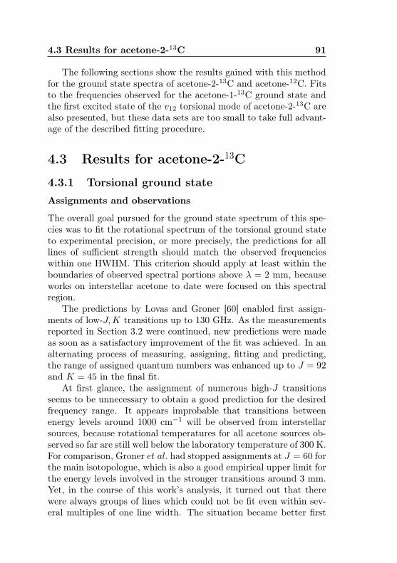
4.3 Results for acetone-2-13C 91
The following sections show the results gained with this methodfor the ground state spectra of acetone-2-13C and acetone-12C. Fitsto the frequencies observed for the acetone-1-13C ground state andthe first excited state of the v12 torsional mode of acetone-2-13C arealso presented, but these data sets are too small to take full advant-age of the described fitting procedure.
4.3 Results for acetone-2-13C
4.3.1 Torsional ground stateAssignments and observations
The overall goal pursued for the ground state spectrum of this spe-cies was to fit the rotational spectrum of the torsional ground stateto experimental precision, or more precisely, the predictions for alllines of sufficient strength should match the observed frequencieswithin one HWHM. This criterion should apply at least within theboundaries of observed spectral portions above λ = 2 mm, becauseworks on interstellar acetone to date were focused on this spectralregion.
The predictions by Lovas and Groner [60] enabled first assign-ments of low-J,K transitions up to 130 GHz. As the measurementsreported in Section 3.2 were continued, new predictions were madeas soon as a satisfactory improvement of the fit was achieved. In analternating process of measuring, assigning, fitting and predicting,the range of assigned quantum numbers was enhanced up to J = 92and K = 45 in the final fit.
At first glance, the assignment of numerous high-J transitionsseems to be unnecessary to obtain a good prediction for the desiredfrequency range. It appears improbable that transitions betweenenergy levels around 1000 cm−1 will be observed from interstellarsources, because rotational temperatures for all acetone sources ob-served so far are still well below the laboratory temperature of 300 K.For comparison, Groner et al. had stopped assignments at J = 60 forthe main isotopologue, which is also a good empirical upper limit forthe energy levels involved in the stronger transitions around 3 mm.Yet, in the course of this work’s analysis, it turned out that therewere always groups of lines which could not be fit even within sev-eral multiples of one line width. The situation became better first
92 Spectral analysis and results
Table 4.1: Results of a systematic assessment of non-canonical tun-neling parameters for usability in the fit for acetone-2-13C. SeeTable 4.2 for examples.
Parameterdescription
Observation
Purely odd κ, p, r Allowed with the restrictions mentioned here.
Mixed even andodd κ, p, r
Allowed with the restrictions mentioned here.
[Bκpr]qq′ , κ < 0 Automatically converted to −[B−κpr]qq′ .
ω = −1 Can be tried for all parameters allowed oth-erwise.
κ, p, r = 3, 5, . . . Higher odd-order parameters can be tried if alow-order adjacent parameter is well determ-ined (uncertainty < 1%).
[Bκ1r]qq′ =−[Bκ0r]qq′
These parameters are linearly dependentand cannot be enabled together.
Pure S-reductionparameters(κ = 4, 6, . . .)
Tested up to κ = 8 with no restrictionsfound.
4.3 Results for acetone-2-13C 93
when lines exceeding J = 60 were assigned above 600 GHz andthe sextic centrifugal parameters became determined better. Aboveall, a satisfactory modeling of all reasonably strong lines and obvi-ously correct assignments became increasingly difficult with growingdiversity of assigned branches and quantum number ranges. Prob-lems, which had gradually emerged during the data set extensionsup to 365 GHz and turned out to be enduring, mainly concernedthe residue, which could not be reduced below former levels aftereach assignment of new lines, and an inconsistency with some of theassignments by Lovas and Groner, which were not fit within severalline widths any more when the parameters had been optimised fora low residue.
The working scheme pursued up to this point was to extend theparameter set by systematically exploring the effect of all allowedparameters of a given order according to the lists available fromGroner [35] and Kisiel [47] after every new set of assignments. How-ever, both lists also included examples for the declaration of NCTPs(see Section 4.2) which had not been used in earlier works for themain isotopologue [36] or the ground states of isotopologues of thestructurally similar dimethyl ether [(CH3)2O] [21,51,52]. In view ofthe problems described – knowing that the SPFIT [80] fit for dimethylether’s main isotopologue indeed contains a few odd-order tunnelingand non-tunneling parameters for its (10) and (01) torsionally ex-cited states, and expecting that torsional tunneling in acetone showsenhanced coupling effects due to its lower barrier height (Chapter 1)–, it was considered worthwhile to try out some of the NCTPs.
The ∆K = 1 Coriolis tunneling parameters [ga]10 (= [B−010]10)and [gb]10 (= [B−001]10) were added first, and it was found that theyimproved the fit by lowering the residue about 17% and removed theinconsistency regarding the microwave assignments. Both of themhad uncertainties below 15% from the start and exceeded all othertunneling parameters in magnitude (> 0.1 MHz). This improve-ment encouraged a systematic evaluation of all possible definitionsfor NCTPs, the results of which are summarised in Table 4.1. Itwas found that some parameters were rejected by ERHAM or led to adiverging fit; most had no noticeable effect; but gradually a handfulof useful NCTPs emerged, mainly for (q, q′) = (1, 0). Eventually,an accurate fit of 9760 transitions at 5922 frequencies was possiblewith 74 parameters and a dimensionless standard deviation of 1.20.
94 Spectral analysis and results
Found parameters are shown in Table 4.2 (“Stand-alone fit”), withthe results given by Lovas and Groner shown to the left for compar-ison.
In his 2012 review paper [35], Groner discourages the use of tun-neling parameters if their non-tunneling counterpart is not used inthe fit. It was therefore tried at several stages of this work to followhis advice and fit the given data set with the restriction to enabletunneling and non-tunneling parameters only synchronously. Dur-ing all of these attempts it became clear quickly that this restrictionprevented a successful modeling, as the standard deviation couldnot be reduced below 3.0 in the best case (cf. Section 4.2). It maythus be concluded that it is advisable to make full use of the phe-nomenological nature of the ERHAM model, i.e., try out NCTPs,whenever canonical parameters alone are not successful to achieve asatisfactory reproduction of observed frequencies.
The successful use of NCTPs and the independent treatment oftunneling and non-tunneling parameters raises the question abouttheir interpretation. As no non-canonical non-tunneling paramet-ers were used, it can be concluded that the Watson-type reducedHamiltonian describing the feedback between overall rotation andcentrifugal deformation is still valid and the effects described bythe additional tunneling parameters concern the torsional splittingonly. With growing torsional excitation, the tunneling methyl pro-tons encounter increasing forces, amplitudes and coupling strengthbefore they approach free torsional rotation (cf. Section 2.3). Thenecessity of one Coriolis-type tunneling parameter to fit an excited-state spectrum of dimethyl ether, but not its ground-state spectrum,may reflect this circumstance. Following up on this argument, thelower torsional barrier height in acetone (251 cm−1 [33], comparedto 950 cm−1 [34] for dimethyl ether) accounts for the larger numberof NCTPs, and also for the larger number of tunneling parametersin total, even for the torsional ground state.
Fictitious or inertial forces in a rotating frame (the centrifugal,Coriolis, and Euler forces, see Section 2.2 for the latter) occur assoon as there is a body co-rotating or undergoing relative motion oracceleration with respect to the frame. While the (peak) centrifugalforce on the internal rotors is specific to their state of torsional excit-ation, time-dependent Coriolis and Euler forces encountered duringtorsional oscillation will have an effect on the coupling of overall
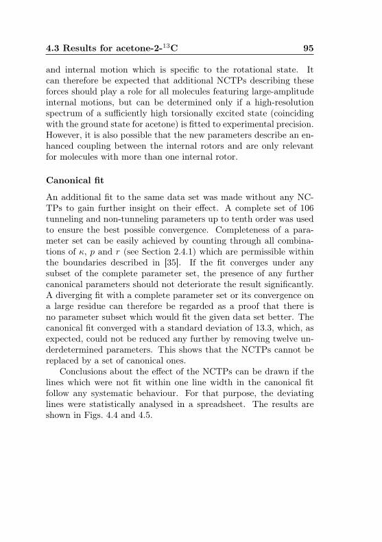
4.3 Results for acetone-2-13C 95
and internal motion which is specific to the rotational state. Itcan therefore be expected that additional NCTPs describing theseforces should play a role for all molecules featuring large-amplitudeinternal motions, but can be determined only if a high-resolutionspectrum of a sufficiently high torsionally excited state (coincidingwith the ground state for acetone) is fitted to experimental precision.However, it is also possible that the new parameters describe an en-hanced coupling between the internal rotors and are only relevantfor molecules with more than one internal rotor.
Canonical fit
An additional fit to the same data set was made without any NC-TPs to gain further insight on their effect. A complete set of 106tunneling and non-tunneling parameters up to tenth order was usedto ensure the best possible convergence. Completeness of a para-meter set can be easily achieved by counting through all combina-tions of κ, p and r (see Section 2.4.1) which are permissible withinthe boundaries described in [35]. If the fit converges under anysubset of the complete parameter set, the presence of any furthercanonical parameters should not deteriorate the result significantly.A diverging fit with a complete parameter set or its convergence ona large residue can therefore be regarded as a proof that there isno parameter subset which would fit the given data set better. Thecanonical fit converged with a standard deviation of 13.3, which, asexpected, could not be reduced any further by removing twelve un-derdetermined parameters. This shows that the NCTPs cannot bereplaced by a set of canonical ones.
Conclusions about the effect of the NCTPs can be drawn if thelines which were not fit within one line width in the canonical fitfollow any systematic behaviour. For that purpose, the deviatinglines were statistically analysed in a spreadsheet. The results areshown in Figs. 4.4 and 4.5.
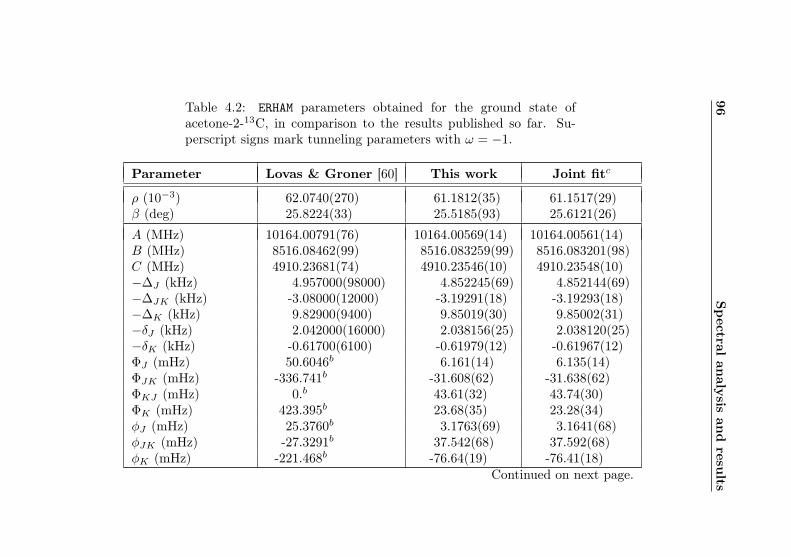
96Spectral
analysis
andresu
lts
Table 4.2: ERHAM parameters obtained for the ground state ofacetone-2-13C, in comparison to the results published so far. Su-perscript signs mark tunneling parameters with ω = −1.
Parameter Lovas & Groner [60] This work Joint fitc
ρ (10−3) 62.0740(270) 61.1812(35) 61.1517(29)β (deg) 25.8224(33) 25.5185(93) 25.6121(26)
A (MHz) 10164.00791(76) 10164.00569(14) 10164.00561(14)B (MHz) 8516.08462(99) 8516.083259(99) 8516.083201(98)C (MHz) 4910.23681(74) 4910.23546(10) 4910.23548(10)−∆J (kHz) 4.957000(98000) 4.852245(69) 4.852144(69)−∆JK (kHz) -3.08000(12000) -3.19291(18) -3.19293(18)−∆K (kHz) 9.82900(9400) 9.85019(30) 9.85002(31)−δJ (kHz) 2.042000(16000) 2.038156(25) 2.038120(25)−δK (kHz) -0.61700(6100) -0.61979(12) -0.61967(12)ΦJ (mHz) 50.6046b 6.161(14) 6.135(14)ΦJK (mHz) -336.741b -31.608(62) -31.638(62)ΦKJ (mHz) 0.b 43.61(32) 43.74(30)ΦK (mHz) 423.395b 23.68(35) 23.28(34)φJ (mHz) 25.3760b 3.1763(69) 3.1641(68)φJK (mHz) -27.3291b 37.542(68) 37.592(68)φK (mHz) -221.468b -76.64(19) -76.41(18)
Continued on next page.
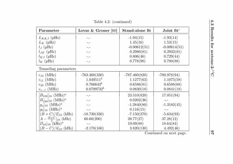
4.3Resu
ltsfor
acetone-2-
13C
97Table 4.2: (continued)
Parameter Lovas & Groner [60] Stand-alone fit Joint fitc
LKKJ (µHz) -.- -1.94(15) -1.93(14)LK (µHz) -.- 1.45(16) 1.53(15)lJ (µHz) -.- -0.00612(51) -0.00614(51)lJK (µHz) -.- 0.2980(81) 0.2932(81)lKJ (µHz) -.- 0.806(46) 0.729(44)lK (µHz) -.- 0.778(90) 0.780(88)
Tunneling parameters
ε10 (MHz) -763.360(330) -787.460(820) -780.978(94)ε11 (MHz) 1.049511b 1.1277(63) 1.1075(58)ε20 (MHz) 0.766643b 0.6586(81) 0.6588(68)ε1−1 (MHz) 0.0799732b 0.0830(18) 0.0841(18)
[B100]10 (MHz)a -.- 23.510(820) 17.051(94)[B−100]10 (MHz)a -.- 0.0202(36) -.-[ga]10 (MHz)a -.- -1.2840(80) -1.3182(45)[gb]10 (MHz)a -.- 0.116(15) -.-[(B + C)/2]10 (kHz) -18.730(330) -7.150(270) -5.634(93)[A− B+C
2 ]10 (kHz) 60.60(200) 39.77(27) 37.28(12)[Dab]10 (kHz)a -.- 19.09(88) 18.64(84)[(B − C)/4]10 (kHz) -2.170(160) 3.820(130) 4.492(46)
Continued on next page.
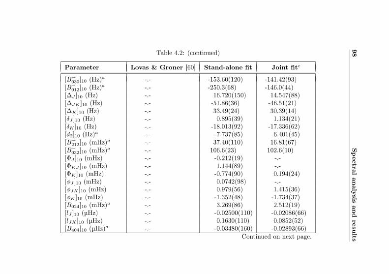
98Spectral
analysis
andresu
lts
Table 4.2: (continued)
Parameter Lovas & Groner [60] Stand-alone fit Joint fitc
[B−030]10 (Hz)a -.- -153.60(120) -141.42(93)[B−012]10 (Hz)a -.- -250.3(68) -146.0(44)[∆J ]10 (Hz) -.- 16.720(150) 14.547(88)[∆JK ]10 (Hz) -.- -51.86(36) -46.51(21)[∆K ]10 (Hz) -.- 33.49(24) 30.39(14)[δJ ]10 (Hz) -.- 0.895(39) 1.134(21)[δK ]10 (Hz) -.- -18.013(92) -17.336(62)[d2]10 (Hz)a -.- -7.737(85) -6.401(45)[B−212]10 (mHz)a -.- 37.40(110) 16.81(67)[B−032]10 (mHz)a -.- 106.6(23) 102.6(10)[ΦJ ]10 (mHz) -.- -0.212(19) -.-[ΦKJ ]10 (mHz) -.- 1.144(89) -.-[ΦK ]10 (mHz) -.- -0.774(90) 0.194(24)[φJ ]10 (mHz) -.- 0.0742(98) -.-[φJK ]10 (mHz) -.- 0.979(56) 1.415(36)[φK ]10 (mHz) -.- -1.352(48) -1.734(37)[B024]10 (mHz)a -.- 3.269(86) 2.512(19)[lJ ]10 (µHz) -.- -0.02500(110) -0.02086(66)[lJK ]10 (µHz) -.- 0.1630(110) 0.0852(52)[B404]10 (µHz)a -.- -0.03480(160) -0.02893(66)
Continued on next page.
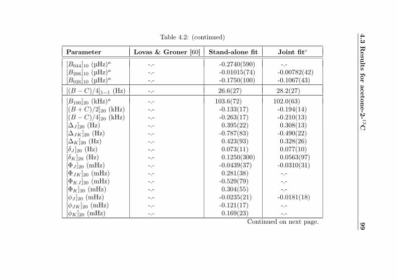
4.3Resu
ltsfor
acetone-2-
13C
99Table 4.2: (continued)
Parameter Lovas & Groner [60] Stand-alone fit Joint fitc
[B044]10 (µHz)a -.- -0.2740(590) -.-[B206]10 (µHz)a -.- -0.01015(74) -0.00782(42)[B026]10 (µHz)a -.- -0.1750(100) -0.1067(43)
[(B − C)/4]1−1 (Hz) -.- 26.6(27) 28.2(27)
[B100]20 (kHz)a -.- 103.6(72) 102.0(63)[(B + C)/2]20 (kHz) -.- -0.133(17) -0.194(14)[(B − C)/4]20 (kHz) -.- -0.263(17) -0.210(13)[∆J ]20 (Hz) -.- 0.395(22) 0.308(13)[∆JK ]20 (Hz) -.- -0.787(83) -0.490(22)[∆K ]20 (Hz) -.- 0.423(93) 0.328(26)[δJ ]20 (Hz) -.- 0.073(11) 0.077(10)[δK ]20 (Hz) -.- 0.1250(300) 0.0563(97)[ΦJ ]20 (mHz) -.- -0.0439(37) -0.0310(31)[ΦJK ]20 (mHz) -.- 0.281(38) -.-[ΦKJ ]20 (mHz) -.- -0.529(79) -.-[ΦK ]20 (mHz) -.- 0.304(55) -.-[φJ ]20 (mHz) -.- -0.0235(21) -0.0181(18)[φJK ]20 (mHz) -.- -0.121(17) -.-[φK ]20 (mHz) -.- 0.169(23) -.-
Continued on next page.
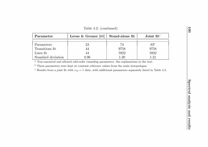
100Spectral
analysis
andresu
lts
Table 4.2: (continued)
Parameter Lovas & Groner [60] Stand-alone fit Joint fitc
Parameters 23 74 63cTransitions fit 44 9758 9758Lines fit 44 5922 5922Standard deviation 0.96 1.20 1.21a Non-canonical and allowed odd-order tunneling parameters. See explanations in the text.b These parameters were kept at constant reference values from the main isotopologue.c Results from a joint fit with v12 = 1 data, with additional parameters separately listed in Table 4.3.
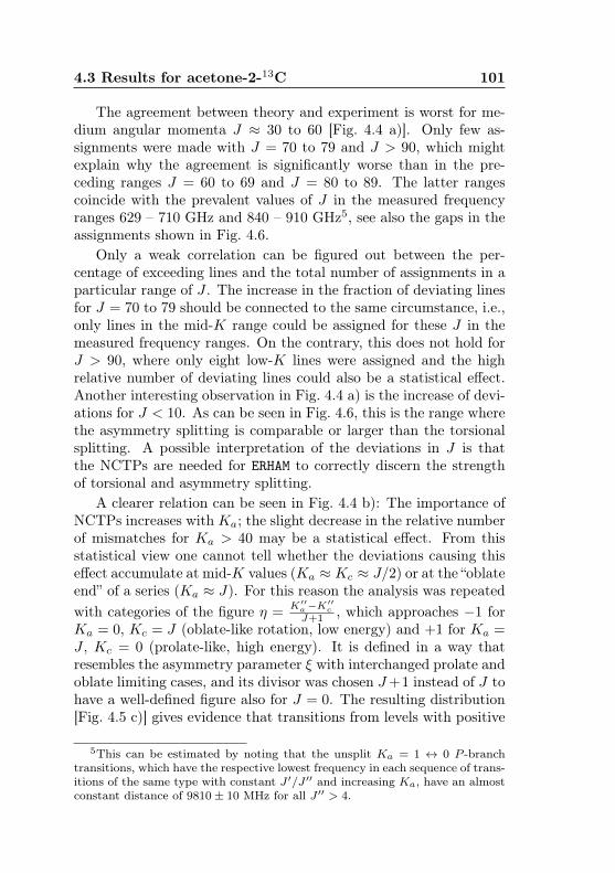
4.3 Results for acetone-2-13C 101
The agreement between theory and experiment is worst for me-dium angular momenta J ≈ 30 to 60 [Fig. 4.4 a)]. Only few as-signments were made with J = 70 to 79 and J > 90, which mightexplain why the agreement is significantly worse than in the pre-ceding ranges J = 60 to 69 and J = 80 to 89. The latter rangescoincide with the prevalent values of J in the measured frequencyranges 629 – 710 GHz and 840 – 910 GHz5, see also the gaps in theassignments shown in Fig. 4.6.
Only a weak correlation can be figured out between the per-centage of exceeding lines and the total number of assignments in aparticular range of J . The increase in the fraction of deviating linesfor J = 70 to 79 should be connected to the same circumstance, i.e.,only lines in the mid-K range could be assigned for these J in themeasured frequency ranges. On the contrary, this does not hold forJ > 90, where only eight low-K lines were assigned and the highrelative number of deviating lines could also be a statistical effect.Another interesting observation in Fig. 4.4 a) is the increase of devi-ations for J < 10. As can be seen in Fig. 4.6, this is the range wherethe asymmetry splitting is comparable or larger than the torsionalsplitting. A possible interpretation of the deviations in J is thatthe NCTPs are needed for ERHAM to correctly discern the strengthof torsional and asymmetry splitting.
A clearer relation can be seen in Fig. 4.4 b): The importance ofNCTPs increases with Ka; the slight decrease in the relative numberof mismatches for Ka > 40 may be a statistical effect. From thisstatistical view one cannot tell whether the deviations causing thiseffect accumulate at mid-K values (Ka ≈ Kc ≈ J/2) or at the “oblateend” of a series (Ka ≈ J). For this reason the analysis was repeatedwith categories of the figure η =
K′′a−K
′′c
J+1 , which approaches −1 forKa = 0, Kc = J (oblate-like rotation, low energy) and +1 for Ka =J , Kc = 0 (prolate-like, high energy). It is defined in a way thatresembles the asymmetry parameter ξ with interchanged prolate andoblate limiting cases, and its divisor was chosen J+1 instead of J tohave a well-defined figure also for J = 0. The resulting distribution[Fig. 4.5 c)] gives evidence that transitions from levels with positive
5This can be estimated by noting that the unsplit Ka = 1 ↔ 0 P -branchtransitions, which have the respective lowest frequency in each sequence of trans-itions of the same type with constant J ′/J ′′ and increasing Ka, have an almostconstant distance of 9810± 10 MHz for all J ′′ > 4.
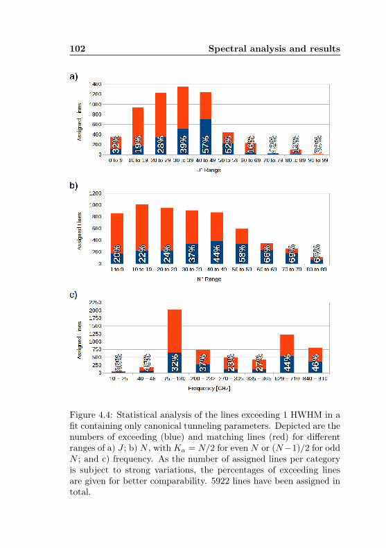
102 Spectral analysis and results
Figure 4.4: Statistical analysis of the lines exceeding 1 HWHM in afit containing only canonical tunneling parameters. Depicted are thenumbers of exceeding (blue) and matching lines (red) for differentranges of a) J ; b) N , with Ka = N/2 for even N or (N−1)/2 for oddN ; and c) frequency. As the number of assigned lines per categoryis subject to strong variations, the percentages of exceeding linesare given for better comparability. 5922 lines have been assigned intotal.
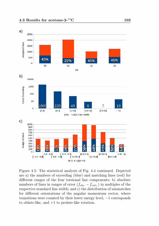
4.3 Results for acetone-2-13C 103
Figure 4.5: The statistical analysis of Fig. 4.4 continued. Depictedare a) the numbers of exceeding (blue) and matching lines (red) fordifferent ranges of the four torsional line components; b) absolutenumbers of lines in ranges of error (fobs. − fcalc.) in multiples of therespective standard line width; and c) the distribution of mismatchesfor different orientations of the angular momentum vector, wheretransitions were counted by their lower energy level, −1 correspondsto oblate-like, and +1 to prolate-like rotation.
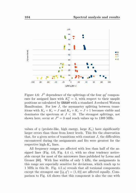
104 Spectral analysis and results
Figure 4.6: J ′′ dependence of the splittings of the four qq′ compon-ents for assigned lines with K ′′a = 3, with respect to their unsplitpositions as calculated by ERHAM with a standard A-reduced WatsonHamiltonian. For low J , the asymmetry splitting between trans-itions with Ka +Kc = J and Ka +Kc = J + 1 becomes visible anddominates the spectrum at J < 10. The strongest splittings, notshown here, occur at J ′′ = 3 and reach values up to 1389 MHz.
values of η (prolate-like, high energy, large Ka) have significantlylarger errors than those from lower levels. This fits the observationthat, for a given series of transitions with constant J , the difficultiesencountered during the assignments and fits were greatest for therespective high-Ka lines.
All frequency ranges are affected with less than half of the as-signed lines (Fig. 4.6, Fig. 4.4 c), with no clear tendency notice-able except for most of the microwave lines published by Lovas andGroner [60]. With line widths of only 5 kHz, the assignments inthis range are especially sensitive for deviations, which reach up to1 MHz in this fit. Fig. 4.5 a) reveals that all torsional componentsexcept the strongest one [(q, q′) = (1, 0)] are affected equally. Com-parison to Fig. 4.6 shows that this component is also the one with
4.3 Results for acetone-2-13C 105
the smallest splitting. Finally, Fig. 4.5 b) shows the number of lineswithin a certain distance from the calculated position, in multiplesof one line width. While most lines miss the one line width criteriononly closely, the number of lines deviating four line widths or moreis still substantial. Especially aforementioned microwave lines reachdeviations of dozens or hundereds of line widths and are predomin-antly included in the last column.
The statistical analysis shows no clear evidence which could yielda rationale of use for the NCTPs, which might have been the case ife.g. only one small quantum number range had been affected by aperturbation. There are, however, tendencies to be found: NCTPsimprove convergence best for lines with a large splitting, regardlessof its physical reason, and for transitions involving large values ofKa with respect to J , i.e., Ka > J/2.
Further insight into these findings may be gained with a casestudy of K dependences for a given J like the one for J ′ = 18 shownin Figs. 4.7 to 4.9. This set of R-branch transitions was selectedbecause it had been showing persistent deviations, especially in thehigh-Ka lines, before the NCTPs were introduced. Fig. 4.7 showsthe change of transition frequencies between oblate and prolate ro-tation. High- and low-K regions with their characteristic pairingsare connected by a transition region around Ka = (ξ+ 1)J ≈ 11. Inthis region, the splittings of each shown transition type can changedramatically (Fig. 4.8) in an intricate, high-frequency manner whichstrongly differs between the transition types. The errors made bythe canonical fit (Fig. 4.9) are seen to follow reasonably periodicpatterns with a periodicity of ∆Ka ≈ 8 and larger errors coincidingwith larger splittings.
Hence, the NCTPs help reproduce the observed splittings byadding K-periodic corrections to energy levels, which becomes obvi-ous because the (q, q′) = (0, 0) transitions are supposed to be non-periodic in K (see eq. (2.63)). Evaluating the K-periodic part ofthis formula with K = K ′ = Ka, q1 = q, q2 = q′, n1 = n2 = n andρ1 = ρ2 = ρ yields the condition (q + sq′)Corr
!= n
ρ∆K for an effect-ive Fourier index pair (q, q′)Corr which would be needed to describethe periodic correction in the canonical ERHAM formalism. Withs = −1 (the direction cosines of the methyl rotors have different signsfor all acetone isotopologues), n = 3 and ρ ≈ 0.0612 in acetone-2-13C this condition reads (q−q′)Corr = 6.127 . . . ≈ 6. The corrections
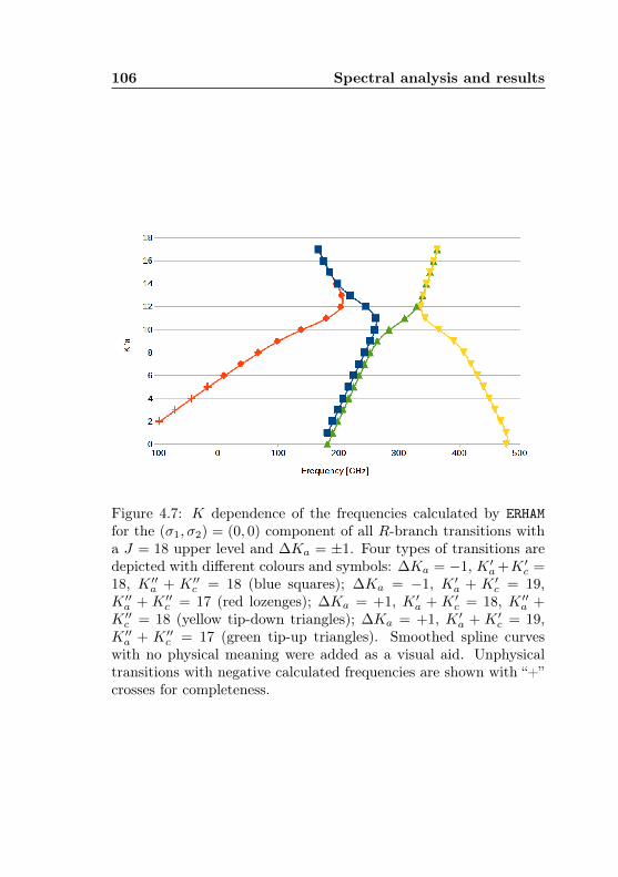
106 Spectral analysis and results
Figure 4.7: K dependence of the frequencies calculated by ERHAMfor the (σ1, σ2) = (0, 0) component of all R-branch transitions witha J = 18 upper level and ∆Ka = ±1. Four types of transitions aredepicted with different colours and symbols: ∆Ka = −1, K ′a+K ′c =18, K ′′a + K ′′c = 18 (blue squares); ∆Ka = −1, K ′a + K ′c = 19,K ′′a + K ′′c = 17 (red lozenges); ∆Ka = +1, K ′a + K ′c = 18, K ′′a +K ′′c = 18 (yellow tip-down triangles); ∆Ka = +1, K ′a + K ′c = 19,K ′′a + K ′′c = 17 (green tip-up triangles). Smoothed spline curveswith no physical meaning were added as a visual aid. Unphysicaltransitions with negative calculated frequencies are shown with “+”crosses for completeness.
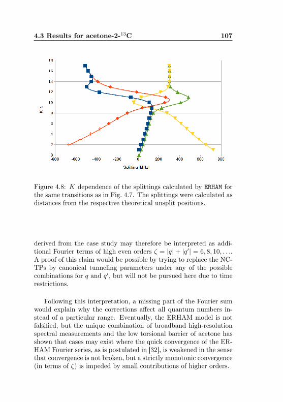
4.3 Results for acetone-2-13C 107
Figure 4.8: K dependence of the splittings calculated by ERHAM forthe same transitions as in Fig. 4.7. The splittings were calculated asdistances from the respective theoretical unsplit positions.
derived from the case study may therefore be interpreted as addi-tional Fourier terms of high even orders ζ = |q|+ |q′| = 6, 8, 10, . . ..A proof of this claim would be possible by trying to replace the NC-TPs by canonical tunneling parameters under any of the possiblecombinations for q and q′, but will not be pursued here due to timerestrictions.
Following this interpretation, a missing part of the Fourier sumwould explain why the corrections affect all quantum numbers in-stead of a particular range. Eventually, the ERHAM model is notfalsified, but the unique combination of broadband high-resolutionspectral measurements and the low torsional barrier of acetone hasshown that cases may exist where the quick convergence of the ER-HAM Fourier series, as is postulated in [32], is weakened in the sensethat convergence is not broken, but a strictly monotonic convergence(in terms of ζ) is impeded by small contributions of higher orders.
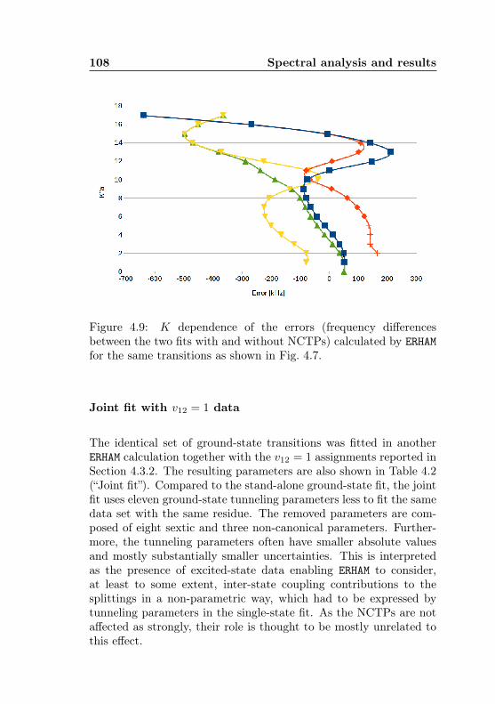
108 Spectral analysis and results
Figure 4.9: K dependence of the errors (frequency differencesbetween the two fits with and without NCTPs) calculated by ERHAMfor the same transitions as shown in Fig. 4.7.
Joint fit with v12 = 1 data
The identical set of ground-state transitions was fitted in anotherERHAM calculation together with the v12 = 1 assignments reported inSection 4.3.2. The resulting parameters are also shown in Table 4.2(“Joint fit”). Compared to the stand-alone ground-state fit, the jointfit uses eleven ground-state tunneling parameters less to fit the samedata set with the same residue. The removed parameters are com-posed of eight sextic and three non-canonical parameters. Further-more, the tunneling parameters often have smaller absolute valuesand mostly substantially smaller uncertainties. This is interpretedas the presence of excited-state data enabling ERHAM to consider,at least to some extent, inter-state coupling contributions to thesplittings in a non-parametric way, which had to be expressed bytunneling parameters in the single-state fit. As the NCTPs are notaffected as strongly, their role is thought to be mostly unrelated tothis effect.
4.3 Results for acetone-2-13C 109
Continuative discussion
A rationale of use for the NCTPs used herein can be derived fromtheir respective index classes:
• Tunneling parameters of odd order η (Section 2.4.1) or con-taining odd or mixed powers κ, p, r are permissible becausethey describe enhanced effects of inertial forces encounteredby the internal rotors.
• Parameters with κ > 2 are also admissible because the A-type Watson-reduced Hamiltonian, where no equivalent non-tunneling parameters are defined, describes the centrifugal dis-tortion of the rigid molecule rather than its internal rotors.
• Parameters with ω = −1 are generally permissible, but notessential for many molecules.
An open question is to which extent NCTPs have been usedearlier to fit spectra of other two-rotor molecules. The fact thatGroner mentions some odd-order parameters, but at the same timeexpresses reservation regarding a too permissive use of obviouslynon-canonical parameters [35], reads like a response to earlier works,but no references are cited explicitly.
In the PhD thesis by Christian Endres [21], 9535 transitions upto J = 59,Ka = 21 from the two excited torsional states of dimethylether (DME) have been fit with 21 asymmetric-top rotational andcentrifugal parameters up to octic order, ρ, β, and only 12 canonicaltunneling parameters up to the order η = 6 for (q, q′) = (1, 0). In ad-dition, a global fit made with SPFIT [80] involving the ground stateand both excited states is presented where, besides a larger numberof tunneling parameters up to (q, q′) = (2, 0), the Coriolis interactionparameters Gc and Fab have been used with their respective tunnel-ing parameters. As the torsional barrier of DME (950 cm−1, [34])is high compared to that of acetone (251 cm−1, [33]), the multitudeof tunneling parameters and the presence of interaction (tunneling)parameters may serve as an indicator for the torsional-rotationalcoupling strength. From a formal point of view, acetone, in its tor-sional ground state, may therefore be considered equivalent to atwo-rotor molecule with a more usual barrier height, like DME, in acomparably highly excited torsional state. It may thus be predictedthat presumable future ERHAM fits of such highly excited states in
110 Spectral analysis and results
other molecules must be treated in a similar way, i.e., using a largenumber of tunneling parameters including NCTPs.
The lacking necessity to use NCTPs for acetone in earlier workscan be traced back to the fact that Groner’s 12C data set (1002 fittransitions) was much smaller than this work’s data set for acetone-2-13C, and mostly recorded at substantially lower resolution6. Undersuch conditions, the effects accounted for by the NCTPs are possiblytoo small to be seen (cf. Fig. 4.9), or could just be caught up bythe canonical parameters. They become fully apparent only whena data set, which is sufficiently large and diversified in quantumnumbers to get useful predictions even for high-K lines, can be builtup from high-resolution, high-sensitivity, broadband measurements.If the data set is smaller, other tunneling parameters like those with(q, q′) = (1,−1) and (1, 1) used by Lovas and Groner (Table 4.2),but which are not useful here any more, can play their role withoutnotice.
Further inspection of Table 4.2 shows that the NCTPs consist-ently blend in with canonical ones of the same order η in terms oftheir magnitude. This work’s effort of unbiasedly testing the eli-gibility of tunneling independently from non-tunneling parameters,non-canonical independently from canonical parameters etc. is ob-served here to help unfold the full use of the phenomenological natureof the ERHAM model for the benefit of preciser predictions. In par-ticular, an application of NCTPs is suggested for all species wherethe spectrum cannot be easily fit with canonical parameters only,and of course in all cases where odd-order non-tunneling paramet-ers like Coriolis interactions play a role. Retrospectively, the goodagreement with observations might also have been reached with asmaller data set if non-canonical parameters had been used from thebeginning.
4.3.2 First excited torsional state (v12 = 1)
During the ground state assignments reported above it was noticedthat the characteristic triplet of the strong K = 0 ↔ 1 transitions
6For example, the FASSST spectrometer [79] allows for rapid BWO scanningof a spectrum around 300 GHz at the cost of a low frequency accuracy of ≈100 kHz. The high-resolution measurements of the same region used for thisthesis had an accuracy of the order 10 Hz and were rather limited by Dopplerbroadening, with a typical peak-finder accuracy of less than 10 kHz.
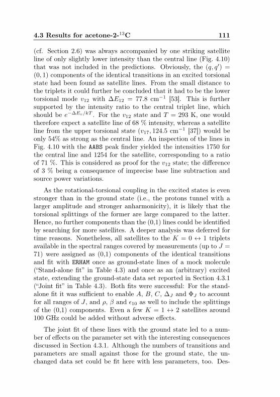
4.3 Results for acetone-2-13C 111
(cf. Section 2.6) was always accompanied by one striking satelliteline of only slightly lower intensity than the central line (Fig. 4.10)that was not included in the predictions. Obviously, the (q, q′) =(0, 1) components of the identical transitions in an excited torsionalstate had been found as satellite lines. From the small distance tothe triplets it could further be concluded that it had to be the lowertorsional mode v12 with ∆E12 = 77.8 cm−1 [53]. This is furthersupported by the intensity ratio to the central triplet line, whichshould be e−∆Ev/kT . For the v12 state and T = 293 K, one wouldtherefore expect a satellite line of 68 % intensity, whereas a satelliteline from the upper torsional state (v17, 124.5 cm−1 [37]) would beonly 54% as strong as the central line. An inspection of the lines inFig. 4.10 with the AABS peak finder yielded the intensities 1750 forthe central line and 1254 for the satellite, corresponding to a ratioof 71 %. This is considered as proof for the v12 state; the differenceof 3 % being a consequence of imprecise base line subtraction andsource power variations.
As the rotational-torsional coupling in the excited states is evenstronger than in the ground state (i.e., the protons tunnel with alarger amplitude and stronger anharmonicity), it is likely that thetorsional splittings of the former are large compared to the latter.Hence, no further components than the (0,1) lines could be identifiedby searching for more satellites. A deeper analysis was deferred fortime reasons. Nonetheless, all satellites to the K = 0 ↔ 1 tripletsavailable in the spectral ranges covered by measurements (up to J =71) were assigned as (0,1) components of the identical transitionsand fit with ERHAM once as ground-state lines of a mock molecule(“Stand-alone fit” in Table 4.3) and once as an (arbitrary) excitedstate, extending the ground-state data set reported in Section 4.3.1(“Joint fit” in Table 4.3). Both fits were successful: For the stand-alone fit it was sufficient to enable A, B, C, ∆J and ΦJ to accountfor all ranges of J , and ρ, β and ε10 as well to include the splittingsof the (0,1) components. Even a few K = 1 ↔ 2 satellites around100 GHz could be added without adverse effects.
The joint fit of these lines with the ground state led to a num-ber of effects on the parameter set with the interesting consequencesdiscussed in Section 4.3.1. Although the numbers of transitions andparameters are small against those for the ground state, the un-changed data set could be fit here with less parameters, too. Des-
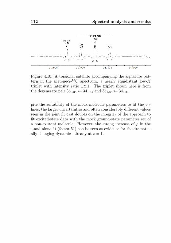
112 Spectral analysis and results
Figure 4.10: A torsional satellite accompanying the signature pat-tern in the acetone-2-13C spectrum, a nearly equidistant low-Ktriplet with intensity ratio 1:2:1. The triplet shown here is fromthe degenerate pair 350,35 ← 341,34 and 351,35 ← 340,34.
pite the suitability of the mock molecule parameters to fit the v12
lines, the larger uncertainties and often considerably different valuesseen in the joint fit cast doubts on the integrity of the approach tofit excited-state data with the mock ground-state parameter set ofa non-existent molecule. However, the strong increase of ρ in thestand-alone fit (factor 51) can be seen as evidence for the dramatic-ally changing dynamics already at v = 1.
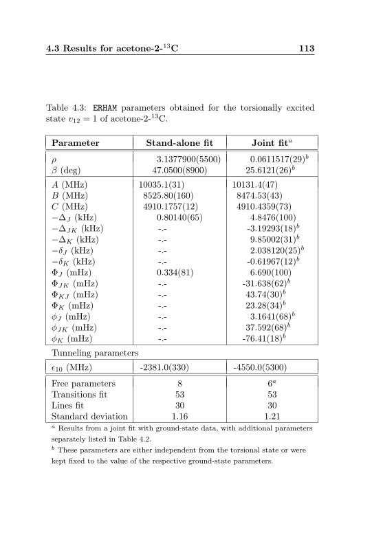
4.3 Results for acetone-2-13C 113
Table 4.3: ERHAM parameters obtained for the torsionally excitedstate v12 = 1 of acetone-2-13C.
Parameter Stand-alone fit Joint fita
ρ 3.1377900(5500) 0.0611517(29)bβ (deg) 47.0500(8900) 25.6121(26)b
A (MHz) 10035.1(31) 10131.4(47)B (MHz) 8525.80(160) 8474.53(43)C (MHz) 4910.1757(12) 4910.4359(73)−∆J (kHz) 0.80140(65) 4.8476(100)−∆JK (kHz) -.- -3.19293(18)b−∆K (kHz) -.- 9.85002(31)b−δJ (kHz) -.- 2.038120(25)b−δK (kHz) -.- -0.61967(12)bΦJ (mHz) 0.334(81) 6.690(100)ΦJK (mHz) -.- -31.638(62)bΦKJ (mHz) -.- 43.74(30)bΦK (mHz) -.- 23.28(34)bφJ (mHz) -.- 3.1641(68)bφJK (mHz) -.- 37.592(68)bφK (mHz) -.- -76.41(18)b
Tunneling parameters
ε10 (MHz) -2381.0(330) -4550.0(5300)
Free parameters 8 6aTransitions fit 53 53Lines fit 30 30Standard deviation 1.16 1.21a Results from a joint fit with ground-state data, with additional parametersseparately listed in Table 4.2.b These parameters are either independent from the torsional state or werekept fixed to the value of the respective ground-state parameters.
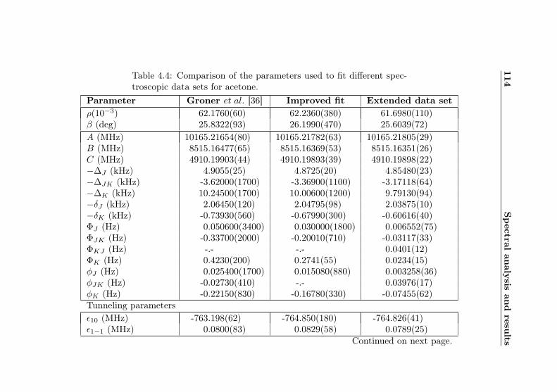
114Spectral
analysis
andresu
lts
Table 4.4: Comparison of the parameters used to fit different spec-troscopic data sets for acetone.
Parameter Groner et al. [36] Improved fit Extended data setρ(10−3) 62.1760(60) 62.2360(380) 61.6980(110)β (deg) 25.8322(93) 26.1990(470) 25.6039(72)A (MHz) 10165.21654(80) 10165.21782(63) 10165.21805(29)B (MHz) 8515.16477(65) 8515.16369(53) 8515.16351(26)C (MHz) 4910.19903(44) 4910.19893(39) 4910.19898(22)−∆J (kHz) 4.9055(25) 4.8725(20) 4.85480(23)−∆JK (kHz) -3.62000(1700) -3.36900(1100) -3.17118(64)−∆K (kHz) 10.24500(1700) 10.00600(1200) 9.79130(94)−δJ (kHz) 2.06450(120) 2.04795(98) 2.03875(10)−δK (kHz) -0.73930(560) -0.67990(300) -0.60616(40)ΦJ (Hz) 0.050600(3400) 0.030000(1800) 0.006552(75)ΦJK (Hz) -0.33700(2000) -0.20010(710) -0.03117(33)ΦKJ (Hz) -.- -.- 0.0401(12)ΦK (Hz) 0.4230(200) 0.2741(55) 0.0234(15)φJ (Hz) 0.025400(1700) 0.015080(880) 0.003258(36)φJK (Hz) -0.02730(410) -.- 0.03976(17)φK (Hz) -0.22150(830) -0.16780(330) -0.07455(62)Tunneling parametersε10 (MHz) -763.198(62) -764.850(180) -764.826(41)ε1−1 (MHz) 0.0800(83) 0.0829(58) 0.0789(25)
Continued on next page.
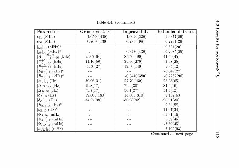
4.3Resu
ltsfor
acetone-2-
13C
115Table 4.4: (continued)
Parameter Groner et al. [36] Improved fit Extended data setε11 (MHz) 1.0500(430) 1.0690(320) 1.0877(89)ε20 (MHz) 0.7670(130) 0.7805(98) 0.7791(29)[ga]10 (MHz)a -.- -.- -0.327(20)[gb]10 (MHz)a -.- 0.3430(430) -0.2985(25)[A− B+C
2 ]10 (kHz) 55.07(64) 85.40(190) 44.49(45)[B+C
2 ]10 (kHz) -21.16(56) -39.60(270) -3.08(25)[B−C4 ]10 (kHz) -3.40(27) -12.50(140) 5.84(12)[B012]10 (kHz)a -.- -.- -0.842(27)[B210]10 (kHz)a -.- -0.3440(380) -0.2252(96)[∆J ]10 (Hz) 39.06(34) 27.70(160) 28.98(65)[∆JK ]10 (Hz) -99.8(17) -79.9(30) -84.4(16)[∆K ]10 (Hz) 73.7(17) 50.1(27) 54.4(12)[δJ ]10 (Hz) 19.600(180) 14.000(810) 2.152(63)[δK ]10 (Hz) -34.27(98) -30.93(92) -20.51(30)[B211]10 (Hz)a -.- -.- 9.62(98)[d2]10 (Hz)a -.- -.- -12.37(34)[ΦJ ]10 (mHz) -.- -.- -1.91(16)[ΦJK ]10 (mHz) -.- -.- 5.59(45)[ΦKJ ]10 (mHz) -.- -.- -3.69(45)[φJK ]10 (mHz) -.- -.- 2.165(93)
Continued on next page.
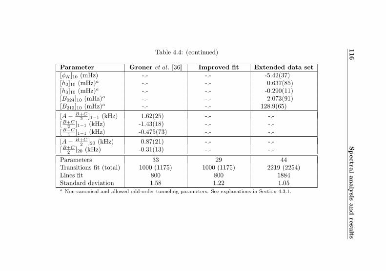
116Spectral
analysis
andresu
lts
Table 4.4: (continued)
Parameter Groner et al. [36] Improved fit Extended data set[φK ]10 (mHz) -.- -.- -5.42(37)[h2]10 (mHz)a -.- -.- 0.637(85)[h3]10 (mHz)a -.- -.- -0.290(11)[B024]10 (mHz)a -.- -.- 2.073(91)[B212]10 (mHz)a -.- -.- 128.9(65)[A− B+C
2 ]1−1 (kHz) 1.62(25) -.- -.-[B+C
2 ]1−1 (kHz) -1.43(18) -.- -.-[B−C4 ]1−1 (kHz) -0.475(73) -.- -.-[A− B+C
2 ]20 (kHz) 0.87(21) -.- -.-[B+C
2 ]20 (kHz) -0.31(13) -.- -.-
Parameters 33 29 44Transitions fit (total) 1000 (1175) 1000 (1175) 2219 (2254)Lines fit 800 800 1884Standard deviation 1.58 1.22 1.05a Non-canonical and allowed odd-order tunneling parameters. See explanations in Section 4.3.1.

4.4 Results for acetone-12C 117
4.4 Results for acetone-12C
Thanks to the work of Groner et al. [36], a good prediction for thelow to medium Ka ranges already existed. However, a number ofmid-Ka examples where the prediction was too far off to make evententative assignments were known from high-resolution astronomy(see the figures and discussion in Chapter 5). With the new NCTPconcept found for acetone-2-13C, it seemed likely that an improve-ment of the prediction is possible with merely a small effort.
The first approach was to fit the existing data set with an im-proved parameter set. Within one afternoon, all reasonable com-binations with and without NCTPs were tried. The best fit, whichshowed a clearly reduced standard deviation (column “Improved fit”in Table 4.4) upon replacement of one centrifugal and five tunnelingparameters by two NCTPs, was used for a new prediction. Duringanother afternoon, the data set could be extended by more than1200 transitions assigned in the spectra between 36 and 125 GHz(standard uncertainties 35 and 40 kHz). Assignments were possibleat such a high speed because most of the already correctly predictedlines were skipped. Eventually, about one day was spent to fit thisextended data set, with the results shown in the fourth column ofTable 4.4. A very good agreement (dimensionless standard devi-ation close to 1.0) was reached for the whole data set, including allbut one of the new assignments in the important 3 mm range (cf.Chapter 1). Except for ρ, the uncertainties of all former parameterscould be lowered. Additionally, many lines which were assigned butnot fitted by Groner et al. could be reassigned with a better uncer-tainty or reinvoked in the final fit. While the J range of assignmentswas not extended, the new assignments reach a maximum Ka of 34instead of 30 before.
The extended set of transitions assigned for the main isotopo-logue was used to verify once more that the NCTPs introducedfor acetone-2-13C for the first time cannot be replaced by canonicaltunneling parameters. Despite its size has more than doubled, the12C data set is more favourable for this task as it is faster to fit dueto its smaller size (2254 transitions compared to 9758) and quantumnumber coverage. After removing the ten NCTPs and adding allcentrifugal parameters up to eighth order; all canonical tunnelingparameters for (q, q′) = (1, 0) up to tenth, (1,−1) and (1, 1) up to
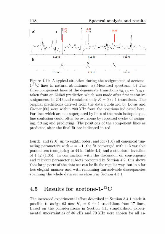
118 Spectral analysis and results
Figure 4.11: A typical situation during the assignments of acetone-1-13C lines in natural abundance. a) Measured spectrum, b) Thethree component lines of the degenerate transitions 80/1,8 ← 71/0,7,taken from an ERHAM prediction which was made after first tentativeassignments in 2013 and contained only K = 0↔ 1 transitions. Theoriginal predictions derived from the data published by Lovas andGroner [60] were within 200 kHz from the positions indicated here.For lines which are not superposed by lines of the main isotopologue,line confusion could often be overcome by repeated cycles of assign-ing, fitting and predicting. The positions of the component lines aspredicted after the final fit are indicated in red.
fourth, and (2, 0) up to eighth order; and for (1, 0) all canonical tun-neling parameters with ω = −1, the fit converged with 113 variableparameters (comparing to 44 in Table 4.4) and a standard deviationof 1.42 (1.05). In conjunction with the discussion on convergenceand relevant parameter subsets presented in Section 4.2, this showsthat large parts of the data set can be fit the regular way, but in a farless elegant manner and with remaining unresolvable discrepanciesspanning the whole data set as shown in Section 4.3.1.
4.5 Results for acetone-1-13C
The increased experimental effort described in Section 3.4.1 made itpossible to assign 63 new Ka = 0 ↔ 1 transitions from 17 lines.Based on the considerations in Section 4.1, standardised experi-mental uncertainties of 36 kHz and 70 kHz were chosen for all as-
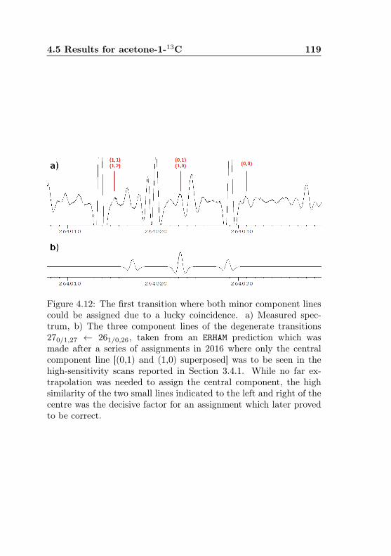
4.5 Results for acetone-1-13C 119
Figure 4.12: The first transition where both minor component linescould be assigned due to a lucky coincidence. a) Measured spec-trum, b) The three component lines of the degenerate transitions270/1,27 ← 261/0,26, taken from an ERHAM prediction which wasmade after a series of assignments in 2016 where only the centralcomponent line [(0,1) and (1,0) superposed] was to be seen in thehigh-sensitivity scans reported in Section 3.4.1. While no far ex-trapolation was needed to assign the central component, the highsimilarity of the two small lines indicated to the left and right of thecentre was the decisive factor for an assignment which later provedto be correct.
120 Spectral analysis and results
signments in the ranges 80–130 GHz and 240–350 GHz, respectively.Two further lines below 70 GHz (36 kHz uncertainty) could be addedfrom the broadband scans mentioned in Section 3.3. The J rangehas been extended up to 36.
An example which explains the difficulty of assignments in nat-ural abundance is shown in Fig. 4.11. Strong superpositions and con-fusion with other lines in the dense spectrum prevented many assign-ments, and if possible at all, only the central superposed (σ1, σ2) =(0, 1) and (1, 0) components could be identified. However, in a hand-ful of cases the disturbances were accidentally located in a lucky wayso that also the two weaker components could be found by lookingfor weak lines with the same intensity and at identical shifts (withdifferent signs) from the predicted positions (Fig. 4.12). The lattercriterion could be applied only because many central lines had beenassigned in an coherent series before. Sometimes a new fit had to berun after each new assignment.
As no lines were assigned with higher K, the new transitionscould be fit with only few K-type parameters to account for theassignments made by Lovas and Groner. In contrast to their ap-proach, no parameters were copied from the ground state of themain isotopologue here because their effect, if any, was not foundto be beneficial. The only parameter presented as a fixed non-zerovalue here, δK , showed an adverse effect on A,B, and C at relat-ive uncertainties between 40% and 50% when tested as a releasedparameter, but caused significant unresolvable deviations if fixed tozero. It was therefore fixed to the value obtained when it had beenreleased.
As was to be expected according to the discussion in Section 4.3.1,canonical tunneling parameters up to k = 4 and p, κ = 2 were suf-ficient to fit all splittings. Three tunneling parameters for (q, q′) =(0, 1) were fixed to the value of the respective second-rotor parameterwith (q, q′) = (1, 0) to prevent ERHAM from generating large artifac-tual splittings of opposite signs between the superposed (σ1, σ2) =(0, 1) and (1, 0) components (typically some 10 MHz) which sum upto a small combined error for the superposed line. Dimensionlessstandard deviations below 1.0 were achieved regularly, with the bestfit for the final data set shown in column “Best fit” in Table 4.5. Thisresult, however, was achieved with some parameters which had a rel-ative uncertainty in excess of 30% (see the discussion in Section 4.2).
4.5 Results for acetone-1-13C 121
Furthermore, a too low residue may be a sign of too careless assign-ments, because in a dense spectrum of lines with similar intensitiesit is always possible to find a line matching any prediction.
Because this issue cannot be cleared with more spectroscopy innatural abundance, a second fit (“Regular fit” in Table 4.5) was gen-erated where the 30-percent rule was strictly applied. Its resultingstandard deviation of 1.01 and the fact that all microwave assign-ments were fitted with high precision [maximum (obs.−calc.)/unc. <1.5] may be interpreted as a hint that the data set does not con-tain too many wrong assignments; on the other hand, two lineswith a previously seemingly clear assignment (one of which from the(0, 1)/(1, 0) component series) could not be fit and were weightedout for the time being. Eventually, the predictions generated fromthe regular fit will come with more trustworthy uncertainties thanthose from the best fit, which might prove helpful for future assign-ments from the spectra to be recorded with the proposed pyrolysisexperiment (Section 3.4.2).
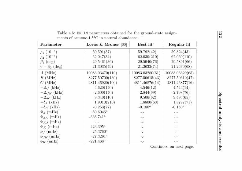
122Spectral
analysis
andresu
lts
Table 4.5: ERHAM parameters obtained for the ground-state assign-ments of acetone-1-13C in natural abundance.
Parameter Lovas & Groner [60] Best fita Regular fit
ρ1 (10−3) 60.591(37) 59.792(42) 59.824(43)ρ2 (10−3) 62.047(34) 62.030(210) 62.060(110)β1 (deg) 29.5461(36) 29.5940(76) 29.5891(66)π − β2 (deg) 21.3035(49) 21.2632(74) 21.2630(68)
A (MHz) 10083.03470(110) 10083.03280(61) 10083.03329(65)B (MHz) 8277.50700(130) 8277.50615(43) 8277.50610(47)C (MHz) 4811.46920(100) 4811.46876(14) 4811.46877(16)−∆J (kHz) 4.620(140) 4.546(12) 4.544(14)−∆JK (kHz) -2.600(140) -2.844(69) -2.798(76)−∆K (kHz) 9.340(110) 9.506(62) 9.493(65)−δJ (kHz) 1.9010(210) 1.8800(63) 1.8797(71)−δK (kHz) -0.253(77) -0.180a -0.180aΦJ (mHz) 50.6046a -.- -.-ΦJK (mHz) -336.741a -.- -.-ΦKJ (mHz) -.- -.- -.-ΦK (mHz) 423.395a -.- -.-φJ (mHz) 25.3760a -.- -.-φJK (mHz) -27.3291a -.- -.-φK (mHz) -221.468a -.- -.-
Continued on next page.
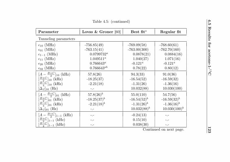
4.5Resu
ltsfor
acetone-1-
13C
123Table 4.5: (continued)
Parameter Lovas & Groner [60] Best fita Regular fit
Tunneling parameters
ε10 (MHz) -756.85(49) -769.09(58) -768.60(61)ε01 (MHz) -763.15(41) -763.00(300) -762.70(160)ε1−1 (MHz) 0.0799732a 0.0878(21) 0.0884(16)ε11 (MHz) 1.049511a 1.040(27) 1.071(16)ε20 (MHz) 0.766643a -0.121a -0.121aε02 (MHz) 0.766643ab 0.78(22) 0.80(12)
[A− B+C2 ]10 (kHz) 57.8(26) 94.3(33) 91.0(36)
[B+C2 ]10 (kHz) -18.25(37) -16.54(52) -16.59(32)
[B−C4 ]10 (kHz) -2.21(18) -1.31(26) -1.36(16)[∆J ]10 (Hz) -.- 10.032(88) 10.030(100)
[A− B+C2 ]01 (kHz) 57.8(26)b 55.0(110) 54.7(56)
[B+C2 ]01 (kHz) -18.25(37)b -16.54(52)b -16.59(32)b
[B−C4 ]01 (kHz) -2.21(18)b -1.31(26)b -1.36(16)b[∆J ]01 (Hz) -.- 10.032(88)b 10.030(100)b
[A− B+C2 ]1−1 (kHz) -.- -0.24(13) -.-
[B+C2 ]1−1 (kHz) -.- 0.15(10) -.-
[B−C4 ]1−1 (kHz) -.- 0.038(30) -.-Continued on next page.
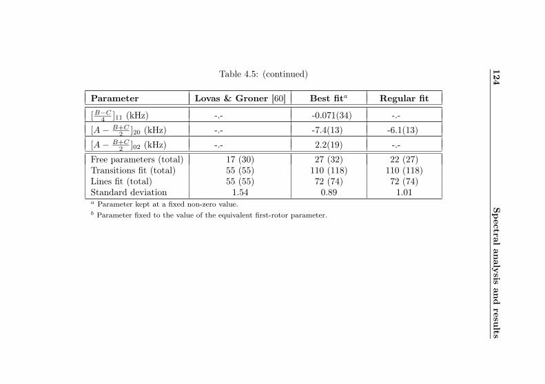
124Spectral
analysis
andresu
lts
Table 4.5: (continued)
Parameter Lovas & Groner [60] Best fita Regular fit
[B−C4 ]11 (kHz) -.- -0.071(34) -.-
[A− B+C2 ]20 (kHz) -.- -7.4(13) -6.1(13)
[A− B+C2 ]02 (kHz) -.- 2.2(19) -.-
Free parameters (total) 17 (30) 27 (32) 22 (27)Transitions fit (total) 55 (55) 110 (118) 110 (118)Lines fit (total) 55 (55) 72 (74) 72 (74)Standard deviation 1.54 0.89 1.01a Parameter kept at a fixed non-zero value.b Parameter fixed to the value of the equivalent first-rotor parameter.
Chapter 5
Implications, summaryand outlook
5.1 Related results
5.1.1 Acetone lines in an ALMA spectrum of Sagit-tarius B2
An early success of this work has already been achieved with the cor-rected spectral prediction for acetone-12C. In data from EMoCA1, arecently published ALMA 3-mm survey of the hot-core star-formingregion Sagittarius B2(N) [4,5], several lines from the former acetoneprediction by Groner et al. [36] with moderately high quantum num-bers could not be found in the observed spectrum, although acetonewas confirmed for this source from other transitions.
Fig. 5.1 shows excerpts from the spectrum of a source slightlywest of Sgr B2 (N1) (positions defined in [3]), with the old (up-per panel) and new (lower panel) predictions in comparison. Thediagrams in this figure are a selection of those spectral portions inthe observed frequency range where the differences between old andnew prediction were greatest. Some lines were predicted correctly,whereas others are shifted by up to 22 MHz (left spectrum) in theimproved prediction. Obviously, at the fitted overall intensity, the
1Exploring Molecular Complexity with ALMA
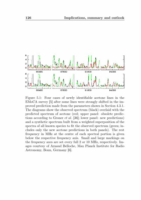
126 Implications, summary and outlook
Figure 5.1: Four cases of newly identifiable acetone lines in theEMoCA survey [5] after some lines were strongly shifted in the im-proved prediction made from the parameters shown in Section 4.3.1.The diagrams show the observed spectrum (black) overlaid with thepredicted spectrum of acetone (red; upper panel: obsolete predic-tions according to Groner et al. [36]; lower panel: new predictions)and a synthetic spectrum built from a weighted superposition of thespectra of all known species to fit the observed spectrum (green; in-cludes only the new acetone predictions in both panels). The restfrequency in MHz at the centre of each spectral portion is givenbelow the respective frequency axis. Small and large markings onthe frequency axes are set every full 2 or 10 MHz, respectively. Im-ages courtesy of Arnaud Belloche, Max Planck Institute for RadioAstronomy, Bonn, Germany [6].
5.2 Summary and Outlook 127
new predictions are reproducing interstellar spectral features in allcases.
5.1.2 Dipole moment of acetone
During this thesis’ works it was noticed that the value of 2.93±0.03 Dderived from the latest of three independent measurements [62, 78,89] has silently grown to be accepted as the experimental value forthe dipole moment. However, it should be remarked that this valuehas a larger experimental uncertainty than the oldest value, and thatthe oldest and the latest value are at the limit of mutual consistency.It is thus recommended to use the weighted average of the threeindependent values (2.89± 0.01 D) in the future.
5.2 Summary and Outlook
The greatest progress in this work was achieved for acetone-2-13C.Thanks to its commercial availability, large portions of its rotationalspectrum could be recorded with high resolution and sensitivity, al-lowing for assignments of more than 9000 transitions. In order toobtain a precise prediction of the spectrum, at least for the frequencyrange up to 130 GHz, an Effective Rotational Hamiltonian was fitto its spectrum. It was shown that the fit reaches experimentalprecision only if the full power of the ERHAM algorithm is harnessedby allowing for non-standard configurations of the tunneling para-meters. Besides allowed interaction-type tunneling parameters likega, which represent odd-power angular momentum dependencies ofthe torsional splittings, new non-canonical parameters of mixed evenand odd powers or originally defined for the S reduction were foundto be essential to obtain a satisfactory fit. These parameters accountfor an enhanced periodicity of the energy levels in Ka, which is aspecialty of acetone due to its exceptionally low barrier to torsionalrotation of the methyl groups and cannot be fit with canonical tun-neling parameters of the usual low Fourier orders. The successfulreproduction of transitions in large ranges of quantum numbers toexperimental precision will allow for a detection of acetone-2-13C inthe interstellar medium with the most sensitive astronomical (sub-)millimetre wave observatories.
The flexible, but accurate new concept takes the idea behind
128 Implications, summary and outlook
the established ERHAM model one step further to fit the spectraof even those molecules where the coupling between large-amplitudeinternal torsional motion and overall rotation is especially strong.It is expected to be applicable also to molecules with a higher tor-sional barrier in their excited torsional states. Further evidence wasgained here through its successful application to the main isotopo-logue, acetone-12C, whose spectrum was also measured at the Insti-tute with the same resolution and sensitivity. Its spectrum was fitto this high experimental precision for the first time, where about1200 transitions have been added to the data set and the parameterset was also set up with some non-canonical tunneling parameters,which cannot be omitted without gaining large errors.
The transferability of the non-canonical concept, with substantialimprovements regarding fitting accuracy and work load, underlinesthe efficacy of the new fitting procedure presented in this thesis andthe improvements which are possible if it is applied to other speciesin the future. The data set for acetone-1-13C was extended by as-signments in natural abundance, but is still too small for the newconcept to be applicable. An enhancement of the previous predic-tions for this molecule [60] was achieved nonetheless. An experimentenabling an exploration of its spectrum in the near future has beenpresented. Similarly, some 100 assignments have been made for thefirst excited state v12 = 1 of acetone-2-13C, which could be fit to-gether with the large set of ground-state assingnments successfully.
Values for the asymmetry parameter ξ derived from the currentA,B,C values are ξ = 0.372 for acetone-12C, ξ = 0.315 for acetone-1-13C, and ξ = 0.373 for acetone-2-13C.
The following list gives an overview of suggested future spec-troscopy projects which are necessary to gain fully comprehensivepredictions for all three isotopologues treated here.
• The acetone-12C spectrum was measured up to 908 GHz, butnew assignments were made only up to 125 GHz. The remain-ing frequency ranges (see Section 3.3) should be screened forfurther erroneous predictions in the ground state.
• Based on the existing predictions made by Groner et al. [38,39], it is expected that similar enhancements and improve-ments can be achieved for the two lowest torsionally excitedstates of acetone-12C.
5.2 Summary and Outlook 129
• It is deemed possible that more lines from the v12 = 1 stateof acetone-2-13C be identified by guessing positions for theother components. This may be done by generating a predic-tion from the parameters determined herein with additionaltunneling parameters copied from the main isotopologue oracetone-2-13C.
• Vibrational satellites from the v17 = 1 state of acetone-2-13C should be apparent in the spectrum with a relative in-tensity of 54% and a larger splitting from the ground-statepositions than those from the v12 = 1 state. It appears worth-while to search for such satellites and repeat what was donefor v12 = 1.
• The availability of spectral predictions for acetone-1-13C ata similar accuracy as that reached for acetone-2-13C wouldfoster the astrochemical dialogue on the formation of acetoneand similar complex carbon- and oxygen-bearing species. Con-structing and conducting the pyrolysis experiment proposed inSection 3.4.2 to record acetone-1-13C spectra from a sample ofup to 50% purity would be the first major step towards thisgoal. It should also be tried to use the measured 12C spectrato improve the signal content from the desired isotopologueby decorrelation. Assignments, fitting and predictions shouldbe accomplished according to the standards and proceduresdescribed here.
As a closing remark, it would be nice if a functionality was addedto ERHAM where groups of strongly correlated parameters (with acorrelation index above a threshold value to be set by the user) areautomatically listed in a separate table.
Lists of assigned and predicted transitions for all isotopologuesand torsional states treated herein will be published in peer-reviewedjournals and the Cologne Database for Molecular Spectroscopy (CDMS)[68] in electronic data files.
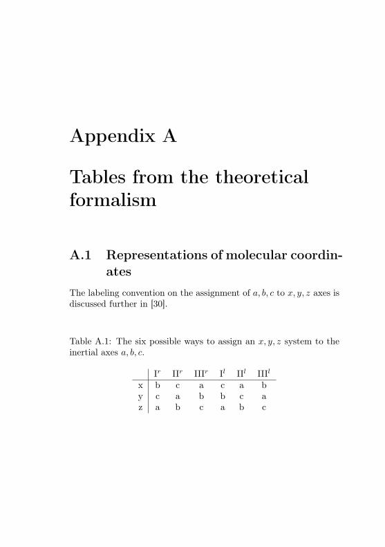
Appendix A
Tables from the theoreticalformalism
A.1 Representations of molecular coordin-ates
The labeling convention on the assignment of a, b, c to x, y, z axes isdiscussed further in [30].
Table A.1: The six possible ways to assign an x, y, z system to theinertial axes a, b, c.
Ir IIr IIIr Il IIl IIIl
x b c a c a by c a b b c az a b c a b c
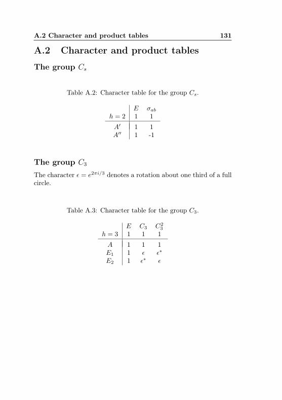
A.2 Character and product tables 131
A.2 Character and product tables
The group Cs
Table A.2: Character table for the group Cs.
E σabh = 2 1 1
A′ 1 1A′′ 1 -1
The group C3
The character ε = e2πi/3 denotes a rotation about one third of a fullcircle.
Table A.3: Character table for the group C3.
E C3 C23
h = 3 1 1 1
A 1 1 1E1 1 ε ε∗
E2 1 ε∗ ε
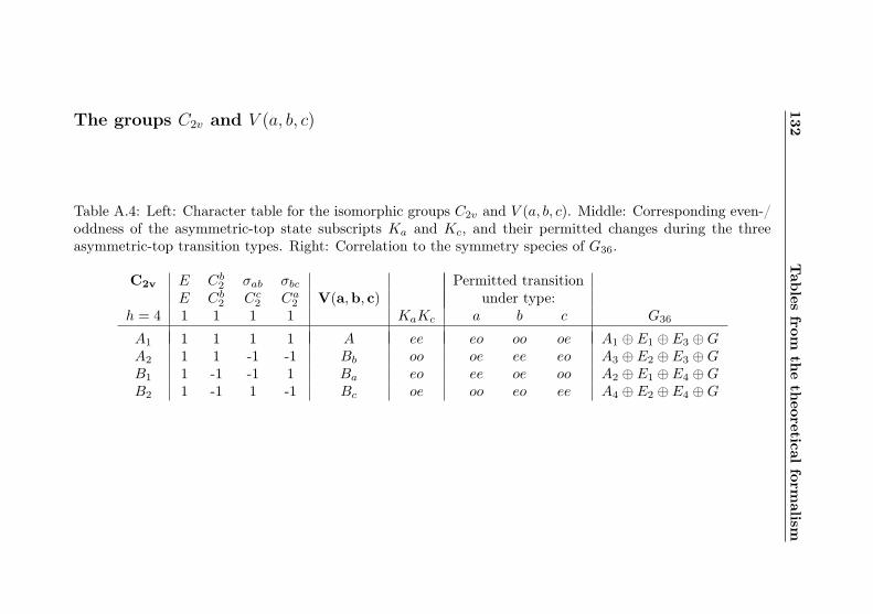
132Tab
lesfrom
thetheoretical
formalism
The groups C2v and V (a, b, c)
Table A.4: Left: Character table for the isomorphic groups C2v and V (a, b, c). Middle: Corresponding even-/oddness of the asymmetric-top state subscripts Ka and Kc, and their permitted changes during the threeasymmetric-top transition types. Right: Correlation to the symmetry species of G36.
C2v E Cb2 σab σbc Permitted transitionE Cb2 Cc2 Ca2 V(a,b, c) under type:
h = 4 1 1 1 1 KaKc a b c G36
A1 1 1 1 1 A ee eo oo oe A1 ⊕ E1 ⊕ E3 ⊕GA2 1 1 -1 -1 Bb oo oe ee eo A3 ⊕ E2 ⊕ E3 ⊕GB1 1 -1 -1 1 Ba eo ee oe oo A2 ⊕ E1 ⊕ E4 ⊕GB2 1 -1 1 -1 Bc oe oo eo ee A4 ⊕ E2 ⊕ E4 ⊕G
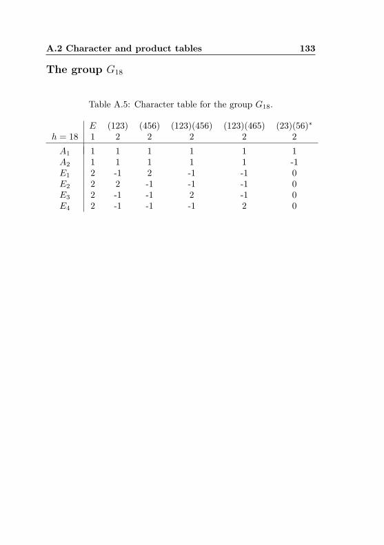
A.2 Character and product tables 133
The group G18
Table A.5: Character table for the group G18.
E (123) (456) (123)(456) (123)(465) (23)(56)∗h = 18 1 2 2 2 2 2
A1 1 1 1 1 1 1A2 1 1 1 1 1 -1E1 2 -1 2 -1 -1 0E2 2 2 -1 -1 -1 0E3 2 -1 -1 2 -1 0E4 2 -1 -1 -1 2 0
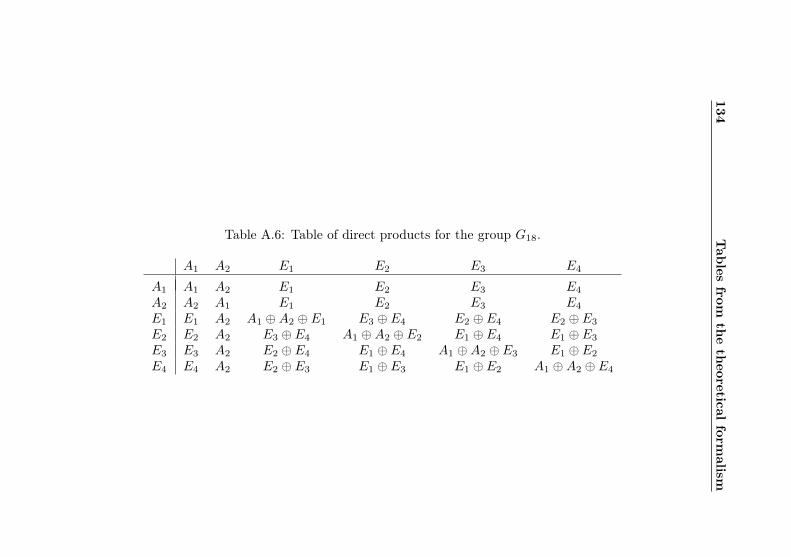
134Tab
lesfrom
thetheoretical
formalism
Table A.6: Table of direct products for the group G18.
A1 A2 E1 E2 E3 E4
A1 A1 A2 E1 E2 E3 E4
A2 A2 A1 E1 E2 E3 E4
E1 E1 A2 A1 ⊕A2 ⊕ E1 E3 ⊕ E4 E2 ⊕ E4 E2 ⊕ E3
E2 E2 A2 E3 ⊕ E4 A1 ⊕A2 ⊕ E2 E1 ⊕ E4 E1 ⊕ E3
E3 E3 A2 E2 ⊕ E4 E1 ⊕ E4 A1 ⊕A2 ⊕ E3 E1 ⊕ E2
E4 E4 A2 E2 ⊕ E3 E1 ⊕ E3 E1 ⊕ E2 A1 ⊕A2 ⊕ E4
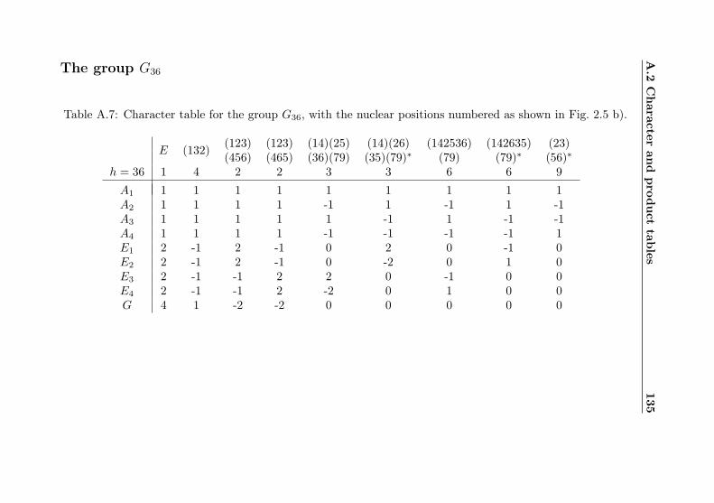
A.2
Character
andprod
uct
tables
135The group G36
Table A.7: Character table for the group G36, with the nuclear positions numbered as shown in Fig. 2.5 b).
E (132) (123) (123) (14)(25) (14)(26) (142536) (142635) (23)(456) (465) (36)(79) (35)(79)∗ (79) (79)∗ (56)∗
h = 36 1 4 2 2 3 3 6 6 9A1 1 1 1 1 1 1 1 1 1A2 1 1 1 1 -1 1 -1 1 -1A3 1 1 1 1 1 -1 1 -1 -1A4 1 1 1 1 -1 -1 -1 -1 1E1 2 -1 2 -1 0 2 0 -1 0E2 2 -1 2 -1 0 -2 0 1 0E3 2 -1 -1 2 2 0 -1 0 0E4 2 -1 -1 2 -2 0 1 0 0G 4 1 -2 -2 0 0 0 0 0
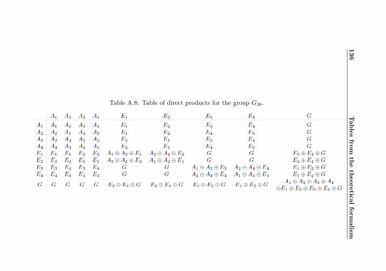
136Tab
lesfrom
thetheoretical
formalism
Table A.8: Table of direct products for the group G36.
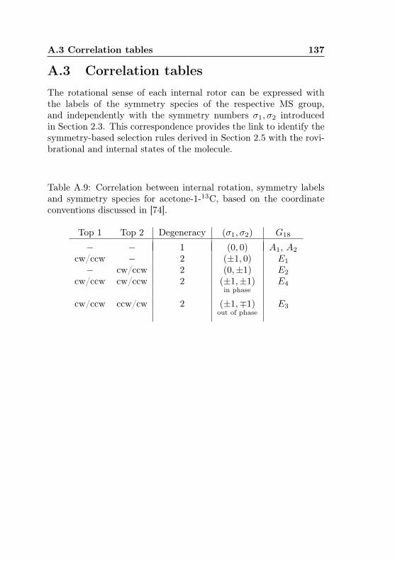
A.3 Correlation tables 137
A.3 Correlation tablesThe rotational sense of each internal rotor can be expressed withthe labels of the symmetry species of the respective MS group,and independently with the symmetry numbers σ1, σ2 introducedin Section 2.3. This correspondence provides the link to identify thesymmetry-based selection rules derived in Section 2.5 with the rovi-brational and internal states of the molecule.
Table A.9: Correlation between internal rotation, symmetry labelsand symmetry species for acetone-1-13C, based on the coordinateconventions discussed in [74].
Top 1 Top 2 Degeneracy (σ1, σ2) G18
− − 1 (0, 0) A1, A2
cw/ccw − 2 (±1, 0) E1
− cw/ccw 2 (0,±1) E2
cw/ccw cw/ccw 2 (±1,±1) E4in phase
cw/ccw ccw/cw 2 (±1,∓1) E3out of phase
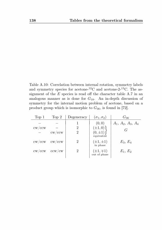
138 Tables from the theoretical formalism
Table A.10: Correlation between internal rotation, symmetry labelsand symmetry species for acetone-12C and acetone-2-13C. The as-signment of the E species is read off the character table A.7 in ananalogous manner as is done for G18. An in-depth discussion ofsymmetry for the internal motion problem of acetone, based on aproduct group which is isomorphic to G36, is found in [72].
Top 1 Top 2 Degeneracy (σ1, σ2) G36
− − 1 (0, 0) A1, A2, A3, A4
cw/ccw − 2 (±1, 0)(0,±1)
}G− cw/ccw 2
equivalent
cw/ccw cw/ccw 2 (±1,±1) E3, E4in phase
cw/ccw ccw/cw 2 (±1,∓1) E1, E2out of phase

Appendix B
Manufacturers and models ofmajor laboratory devices andequipment
• Synthesizers:
– Agilent E8257D, f ≤ 70 GHz– Rohde & Schwarz SMF 100A, f ≤ 43.5 GHz
• AMETEK Signal Recovery / EG&G Instruments 7260 DSPlock-in amplifiers
• Virginia Diodes amplifier-multiplier chains (AMCs):
– AMC-S179 (75–130 GHz)– AMC-S206 (200–232 GHz)– AMC-405 “Starter Kit” (exchangeable modules, coverage
82.5–1,100 GHz)
• Liquid helium cooled InSb bolometers with dedicated low-noiseamplifiers made by the manufaturer QMC
• “Model 109” frequency selective amplifiers
• Waveguide-mounted superlattice multipliers. These deviceswere developed and kindly provided to the Institute by Dr.Dmitriy Paveliev (Electronics Department, Lobachevsky State

140 Manufacturers and models
University of Nizhny Novgorod, Russia). Their design and op-erating principle is described in [76], and their use in a sub-mmabsorption spectrometer is demonstrated in [21].
• Bespoken parts and equipment designed and built at the In-stitute
– Low-noise analogue amplifier–bias boxes (see Fig. 3.1)
– Schottky diodes (see Fig. 3.1)
– 345-GHz diagonal antennas [46] designed and assembledfrom half parts by the author
– PTFE absorption cell windows (see Fig. 3.3)
– HDPE lenses (diameter ≤ 100 mm)
– Large-area millimetre-wave beam splitters (see Fig. 3.4)

Bibliography
[1] F. Arnold et al., Observation of upper tropospheric sulfur dioxide- andacetone pollution: Potential implications for hydroxyl radical and aerosolformation, Geophys. Res. Lett. 24 (1997), no. 1, 57–60.
[2] B. Bak et al., Microwave Absorption of Some Organic Vapors, Phys. Rev.75 (1949), 1622–1623.
[3] A. Belloche et al., Detection of amino acetonitrile in Sgr B2(N), Astron.Astrophys. 482 (2008), no. 1.
[4] , Detection of a branched alkyl molecule in the interstellar medium:iso-propyl cyanide, Science 345 (2014), no. 6204, 1584–1587.
[5] , EMoCA: Exploring Molecular Complexity with ALMA, Revolu-tion in Astronomy with ALMA: The Third Year. Proceedings of a Confer-ence held at the Tokyo International Forum, Tokyo, Japan 8-11 December2014, ASP Conference Series, vol. 499, Astronomical Society of the Pacific,San Francisco, 2015.
[6] A. Belloche. Private communication.
[7] D. A. Belsley, E. Kuh, and R. E. Welsch, Regression Diagnostics: Identify-ing Influential Data and Sources of Collinearity, Wiley, New York, 1980.
[8] P. D. Brown et al., A model of the chemistry in hot molecular cores, Mon.Not. R. Astron. Soc. 231 (1988), 409–417.
[9] P. R. Bunker and P. Jensen, Molecular Symmetry and Spectroscopy, NRCResearch Press, Ottawa, 1998.
[10] , Fundamentals of Molecular Symmetry, Institute of Physics Pub-lishing, Bristol, 2005.
[11] S. Cazaux et al., The Hot Core around the Low-mass Protostar IRAS16293-2422: Scoundrels Rule!, Astrophys. J. 593 (2002), L51–L55.
[12] C. Codella et al., SiO collimated outflows driven by high-mass YSOs inG24.78+0.08, Astron. Astrophys. 550 (2013), A81.
[13] F. Combes et al., Acetone in interstellar space, Astron. Astrophys. 180(1987), L13–L16.
[14] P. Cossee and J. H. Schachtschneider, Vibrational Analysis of Acetone,Acetaldehyde, and Formaldehyde, J. Chem. Phys. 44 (1944), 97–111.
142 BIBLIOGRAPHY
[15] T. de Graauw et al., The Herschel-Heterodyne Instrument for the Far-Infrared (HIFI): instrument and pre-launch testing, Space Telescopes andInstrumentation 2008: Optical, Infrared, and Millimeter (Marseille, France,2008).
[16] F. C. de Lucia, The submillimeter: A spectroscopist’s view, J. Mol. Spec-trosc. 261 (2010), 1–17.
[17] M. de Reus et al., On the relationship between acetone and carbon monox-ide in different air masses, Atmos. Chem. Phys. 3 (2003), 1709–1723.
[18] M. J. S. Dewar et al., AM1: A General Purpose Quantum MechanicalMolecular Model, J. Am. Chem. Soc. 44 (1985), no. 107, 3902–3909.
[19] J. E. Elsila et al., Cometary glycine detected in samples returned by Star-dust, Meteor. Planet. Sci. 44 (2009), no. 9, 1323–1330.
[20] , Compound-specific carbon, nitrogen, and hydrogen isotopic ratiosfor amino acids in CM and CR chondrites and their use in evaluatingpotential formation pathways, Meteor. Planet. Sci. 47 (2012), no. 9, 1517–1536.
[21] C. P. Endres, Terahertz Spectroscopy of Dimethyl Ether, PhD thesis, Uni-versity of Cologne, 2009.
[22] D. N. Friedel and S. L. Widicus Weaver, Complex organic molecules athigh spatial resolution toward Orion-KL: II. Kinematics, Astrophys. J.Suppl. Ser. 201 (2012), no. 17.
[23] D. N. Friedel et al., Detection of interstellar acetone toward the Orion-KLhot core, Astrophys. J. 632 (2005), L95–L98.
[24] R. T. Garrod et al., Complex chemistry in star-forming regions: An expan-ded gas-grain warm-up chemical model, Astrophys. J. 682 (2008), 283–302.
[25] GESTIS database of hazardous substances. Information system on haz-ardous substances of the German Social Accident Insurance, http://www.dguv.de/ifa/gestis-database.
[26] E. L. Gibb et al., Interstellar Ice: The Infrared Space Observatory Legacy,Astrophys. J. Suppl. Ser. 151 (2004), 35.
[27] S. C. O. Glover and P. C. Clark, Is molecular gas necessary for star form-ation?, Mon. Not. R. Astron. Soc. 421 (2012), 9–19.
[28] C. Goddi et al., A 42.3–43.6 GHz spectral survey of Orion BN/KL: Firstdetection of the v = 0J = 1 − −0 line from the isotopologues 29SiO and30SiO, Astrophys. J. 691 (2009), 1254–1264.
[29] P. F. Goldsmith, Quasioptical systems: Gaussian beam quasiopticalpropagation and applications, IEEE Press, New York, 1998.
[30] W. Gordy and R. L. Cook, Microwave Molecular Spectra, John Wiley &Sons, New York, 1984.
[31] P. Groner, Large-amplitude motion tunneling parameters in effective rota-tional Hamiltonians from rotation-internal rotation theory, J. Mol. Spec-trosc. 156 (1992), 164-189.
[32] , Effective rotational Hamiltonian for molecules with two periodiclarge-amplitude motions, J. Chem. Phys. 107 (1997), 4483–4498.
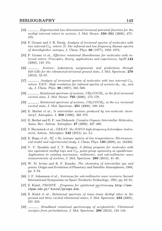
BIBLIOGRAPHY 143
[33] , Experimental two-dimensional torsional potential function for themethyl internal rotors in acetone, J. Mol. Struct. 550–551 (2000), 473–479.
[34] P. Groner and J. R. Durig, Analysis of torsional spectra of molecules withtwo internal C3v rotors: II. Far infrared and low frequency Raman spectraof dimethylether isotopes, J. Chem. Phys. 66 (1977), 1856–1874.
[35] P. Groner et al., Effective rotational Hamiltonian for molecules with in-ternal rotors: Principles, theory, applications and experiences, ApJS 142(2002), 145–151.
[36] , Acetone: Laboratory assignments and predictions through620 GHz for the vibrational-torsional ground state, J. Mol. Spectrosc. 278(2012), 52–67.
[37] , Analysis of torsional spectra of molecules with two internal C3v
rotors: XXIV. High resolution far infrared spectra of acetone-d0, -d3, and-d6, J. Chem. Phys. 86 (1987), 565–568.
[38] , Rotational spectrum of acetone, CH3COCH3, in the first torsionalexcited state, J. Mol. Struct. 795 (2006), 173–178.
[39] , Rotational spectrum of acetone, CH3COCH3, in the ν17 torsionalexcited state, J. Mol. Spectrosc. 251 (2008), 180–184.
[40] E. Herbst et al., Is interstellar acetone produced by ion-molecule chem-istry?, Astrophys. J. 358 (1990), 468–472.
[41] E. Herbst and E. F. van Dishoeck, Complex Organic Interstellar Molecules,Annu. Rev. Astron. Astrophys. 47 (2009), 427–480.
[42] S. Heyminck et al., GREAT: the SOFIA high-frequency heterodyne instru-ment, Astron. Astrophys. 542 (2012), no. L1.
[43] E. Hugo et al., H+3 +H2 isotopic system at low temperatures: Microcanon-
ical model and experimental study, J. Chem. Phys. 130 (2009), no. 164302.
[44] V. V. Ilyushin and J. T. Hougen, A fitting program for molecules withtwo equivalent methyl tops and C2v point-group symmetry at equilibrium:Application to existing microwave, millimeter, and sub-millimeter wavemeasurements of acetone, J. Mol. Spectrosc. 289 (2013), 41–49.
[45] W. M. Irvine and R. F. Knacke, The chemistry of interstellar gas andgrains, Origin and Evolution of Planetary and Satellite Atmospheres, 1989,pp. 3–34.
[46] J. F. Johansson et al., Antennas for sub-millimetre wave receivers, SecondInternational Symposium on Space Terahertz Technology, 1991, pp. 63–81.
[47] Z. Kisiel, PROSPE – Programs for rotational spectroscopy, http://www.ifpan.edu.pl/~kisiel/prospe.htm.
[48] Z. Kisiel et al., Rotational spectrum of trans–trans diethyl ether in theground and three excited vibrational states, J. Mol. Spectrosc. 233 (2005),231–243.
[49] , Broadband rotational spectroscopy of acrylonitrile: Vibrationalenergies from perturbations, J. Mol. Spectrosc. 280 (2012), 134–144.
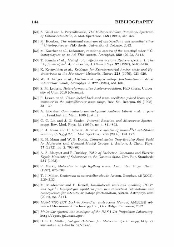
144 BIBLIOGRAPHY
[50] Z. Kisiel and L. Pszczółkowski, The Millimeter-Wave Rotational Spectrumof Chloroacetonitrile, J. Mol. Spectrosc. 158 (1993), 318–327.
[51] M. Koerber, The rotational spectrum of oxatrisulfane and dimethyl ether13C isotopologues, PhD thesis, University of Cologne, 2012.
[52] M. Koerber et al., Laboratory rotational spectra of the dimethyl ether 13C-isotopologues up to 1.5 THz, Astron. Astrophys. 558 (2013), A112.
[53] T. Kundu et al., Methyl rotor effects on acetone Rydberg spectra: I. The1A2(3p← n)←1 A1 transition, J. Chem. Phys. 97 (1992), 5410–5416.
[54] K. Kvenvolden et al., Evidence for Extraterrestrial Amino-acids and Hy-drocarbons in the Murchison Meteorite, Nature 228 (1970), 923–926.
[55] W. D. Langer et al., Carbon and oxygen isotope fractionation in denseinterstellar clouds, Astrophys. J. 277 (1984), 581–604.
[56] S. M. Lederle, Heterofermentative Acetonproduktion, PhD thesis, Univer-sity of Ulm, 2010 (German).
[57] F. Lewen et al., Phase locked backward wave oscillator pulsed beam spec-trometer in the submillimeter wave range, Rev. Sci. Instrum. 69 (1998),32 – 39.
[58] A. Libavius, Commentariorum alchymiae Andreae Libavii med. d. pars. . ., Frankfurt am Main, 1606 (Latin).
[59] C. C. Lin and J. D. Swalen, Internal Rotation and Microwave Spectro-scopy, Rev. Mod. Phys. 31 (1959), no. 4, 841–892.
[60] F. J. Lovas and P. Groner, Microwave spectra of mono-13C substitutedacetone, (CH3)2CO, J. Mol. Spectrosc. 236 (2006), 173–177.
[61] R. H. Mann and W. B. Dixon, Comprehensive Urey-Bradley Force Fieldfor Molecules with Geminal Methyl Groups: I. Acetone, J. Chem. Phys.57 (1972), no. 2, 792–802.
[62] A. A. Maryott and F. Buckley, Table of Dielectric Constants and ElectricDipole Moments of Substances in the Gaseous State, Circ. Bur. Standards537 (1953).
[63] F. Merkt, Molecules in high Rydberg states, Annu. Rev. Phys. Chem.(1997), 675–709.
[64] T. J. Millar, Deuterium in interstellar clouds, Astron. Geophys. 46 (2005),2.29–2.32.
[65] M. Mladenović and E. Roueff, Ion-molecule reactions involving HCO+
and N2H+: Isotopologue equilibria from new theoretical calculations andconsequences for interstellar isotope fractionation, Astron. Astrophys. 566(2014), no. A144.
[66] Model 7265 DSP Lock-in Amplifier: Instruction Manual, AMETEK Ad-vanced Measurement Technology Inc., Oak Ridge, Tennessee, 2002.
[67] Molecular spectral line catalogue of the NASA Jet Propulsion Laboratory,http://spec.jpl.nasa.gov.
[68] H. S. P. Müller, Cologne Database for Molecular Spectroscopy, http://www.astro.uni-koeln.de/cdms/.
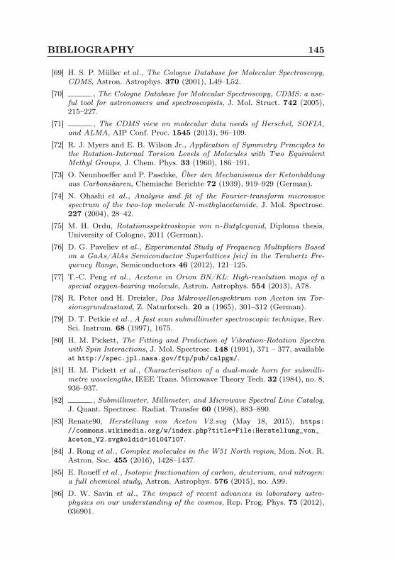
BIBLIOGRAPHY 145
[69] H. S. P. Müller et al., The Cologne Database for Molecular Spectroscopy,CDMS, Astron. Astrophys. 370 (2001), L49–L52.
[70] , The Cologne Database for Molecular Spectroscopy, CDMS: a use-ful tool for astronomers and spectroscopists, J. Mol. Struct. 742 (2005),215–227.
[71] , The CDMS view on molecular data needs of Herschel, SOFIA,and ALMA, AIP Conf. Proc. 1545 (2013), 96–109.
[72] R. J. Myers and E. B. Wilson Jr., Application of Symmetry Principles tothe Rotation-Internal Torsion Levels of Molecules with Two EquivalentMethyl Groups, J. Chem. Phys. 33 (1960), 186–191.
[73] O. Neunhoeffer and P. Paschke, Über den Mechanismus der Ketonbildungaus Carbonsäuren, Chemische Berichte 72 (1939), 919–929 (German).
[74] N. Ohashi et al., Analysis and fit of the Fourier-transform microwavespectrum of the two-top molecule N-methylacetamide, J. Mol. Spectrosc.227 (2004), 28–42.
[75] M. H. Ordu, Rotationsspektroskopie von n-Butylcyanid, Diploma thesis,University of Cologne, 2011 (German).
[76] D. G. Paveliev et al., Experimental Study of Frequency Multipliers Basedon a GaAs/AlAs Semiconductor Superlattices [sic] in the Terahertz Fre-quency Range, Semiconductors 46 (2012), 121–125.
[77] T.-C. Peng et al., Acetone in Orion BN/KL: High-resolution maps of aspecial oxygen-bearing molecule, Astron. Astrophys. 554 (2013), A78.
[78] R. Peter and H. Dreizler, Das Mikrowellenspektrum von Aceton im Tor-sionsgrundzustand, Z. Naturforsch. 20 a (1965), 301–312 (German).
[79] D. T. Petkie et al., A fast scan submillimeter spectroscopic technique, Rev.Sci. Instrum. 68 (1997), 1675.
[80] H. M. Pickett, The Fitting and Prediction of Vibration-Rotation Spectrawith Spin Interactions, J. Mol. Spectrosc. 148 (1991), 371 – 377, availableat http://spec.jpl.nasa.gov/ftp/pub/calpgm/.
[81] H. M. Pickett et al., Characterisation of a dual-mode horn for submilli-metre wavelengths, IEEE Trans. Microwave Theory Tech. 32 (1984), no. 8,936–937.
[82] , Submillimeter, Millimeter, and Microwave Spectral Line Catalog,J. Quant. Spectrosc. Radiat. Transfer 60 (1998), 883–890.
[83] Renate90, Herstellung von Aceton V2.svg (May 18, 2015), https://commons.wikimedia.org/w/index.php?title=File:Herstellung_von_Aceton_V2.svg&oldid=161047107.
[84] J. Rong et al., Complex molecules in the W51 North region, Mon. Not. R.Astron. Soc. 455 (2016), 1428–1437.
[85] E. Roueff et al., Isotopic fractionation of carbon, deuterium, and nitrogen:a full chemical study, Astron. Astrophys. 576 (2015), no. A99.
[86] D. W. Savin et al., The impact of recent advances in laboratory astro-physics on our understanding of the cosmos, Rep. Prog. Phys. 75 (2012),036901.
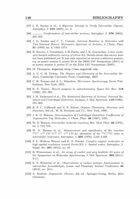
146 BIBLIOGRAPHY
[87] L. E. Snyder et al., A Rigorous Attempt to Verify Interstellar Glycine,Astrophys. J. 619 (2005), no. 2.
[88] , Confirmation of interstellar acetone, Astrophys. J. 578 (2002),245–255.
[89] J. D. Swalen and C. C. Costain, Internal Rotation in Molecules withTwo Internal Rotors: Microwave Spectrum of Acetone, J. Chem. Phys.31 (1959), no. 6, 1562–1574.
[90] B. Tercero, J. Cernicharo, J. R. Pardo, and J. R. Goicoechea, A line confu-sion limited millimeter survey of Orion KL. Details about this survey havenot been published yet. It was only reported on several conference posters,e.g. as poster session 2: poster 93 at the 280th IAU Symposium (2011) oras poster session 2: poster 57 at the 231st IAU Symposium (2005).
[91] M. Thompson, ArgusLab, http://www.arguslab.com.
[92] A. G. G. M. Tielens, The Physics and Chemistry of the Interstellar Me-dium, Cambridge University Press, Cambridge, 2005.
[93] C. H. Townes and A. L. Schawlow, Microwave Spectroscopy, Dover Pub-lications, New York, 1975.
[94] B. E. Turner, Recent progress in astrochemistry, Space Sci. Rev. 118(1986), 355–362.
[95] J. M. Vacherand et al., The Rotational Spectrum of Acetone: Internal Ro-tation and Centrifugal Distortion Analysis, J. Mol. Spectrosc. 118 (1986),355–362.
[96] K. P. C. Vollhardt and N. E. Schore, Organic Chemistry, Structure andFunction, 3rd ed., W. H. Freeman and Co., New York, 1999.
[97] J. K. G. Watson, Determination of Centrifugal Distortion Coefficients ofAsymmetric-Top Molecules, J. Chem. Phys. 46 (1967), 1935.
[98] W. D. Watson, Interstellar molecule reactions, Rev. Mod. Phys. 48 (1976),no. 4, 513–553.
[99] W. D. Watson et al., Measurement and significance of the reaction13C+ +12 CO �12 C+ +13 CO for alteration of the 13C/12C ratio ininterstellar molecules, Astrophys. J. 205 (1976), L165–L168.
[100] S. L. Widicus Weaver and D. N. Friedel, Complex organic molecules athigh spatial resolution toward Orion-KL: I. Spatial scales, Astrophys. J.Suppl. Ser. 201 (2012), no. 16.
[101] B. Winnewisser et al., An array of scarlet and grey booklets: 65 years ofthe Symposium on Molecular Spectroscopy, J. Mol. Spectrosc. 269 (2011),2–11.
[102] E. S. Wirström et al., Observations of carbon isotopic fractionation ininterstellar formaldehyde, Lunar and Planetary Science Conference 43(2012), no. 1611.
[103] A. Wollrab, Organische Chemie, 4th ed., Springer-Verlag, Berlin, 2014(German).

Danksagung
So lange ich für diese Arbeit am Rechner gesessen habe, so warich doch niemals allein. Daher möchte ich an dieser Stelle all jenendanken, die mich die ganzen Jahre über begleitet haben und ohnedie diese Doktorarbeit nie möglich gewesen wäre.
• Mein Dank gebührt an erster Stelle meinem Betreuer Prof.Dr. Stephan Schlemmer für das reizvolle Forschungsthemaund die Gelegenheit, im Umfeld eines herausragenden Spek-troskopielabors und eines wunderbaren Teams mein Könnenan einem der „großen“ Moleküle unter Beweis zu stellen.
• Dr. Frank Lewen – der Mann, ohne den es einfach nichtgeht. Der Beduine, der im trockensten Staub der Nüchtern-heit nicht untergeht! Ein großes Dankeschön für die unzähligenStunden des Wissenstransfers, der tatkräftigen Unterstützungim Labor, bei der Auswertung und der Niederschrift, für dasKorrekturlesen des Experimental- und Analyseteils sowie dasgrößte Repertoire an Lach- und Sachgeschichten, das mir inden letzten zehn Jahren begegnet ist!
• Ich danke ebenso Dr. Holger Müller, für sein jederzeit offe-nes Ohr zu allen Fragen, Sorgen und Nöten aus dem Bereichder numerischen Anpassung, allerlei hilf- und lehrreiche Kom-mentare aus der Welt der Spektroskopie und wissenschaftlichenPublizistik und sein gleich bleibendes Interesse an meiner Ar-beit.
• Allen anderen aktuellen und ehemaligen Mitgliedern der Köl-ner Spektroskopiegruppe, die mit ihrer guten Laune und einer
gehörigen Portion „Geht nicht gibt’s nicht“ immer wieder da-für gesorgt haben, dass die Arbeit Spaß macht und der Ladenläuft. Es sind besonders hervorzuheben:
– Dr. Monika Koerber und Dr. Christian Endres fürihre einführende Unterstützung bei der Arbeit mit ERHAMund AABS. Danke, Monika, für die vielen freundschaftli-chen Gespräche zwischendurch.
– Dr. Sandra Brünken,Dr. Nadine Wehres undHan-no Schmiedt für blitzschnelles Korrekturlesen.
• Prof. Dr. Joachim Hemberger danke ich für die unkompli-zierte Übernahme des Zweitgutachtens, Prof. Dr. StefanieWalch-Gassner für den Vorsitz der Prüfungskommission so-wie abermals Dr. Frank Lewen für den Beisitz.
• Einigen Kolleginnen und Kollegen aus dem Kölner Departmentfür Chemie gebührt Dank für ihre Unterstützung und Bera-tung auf dem Weg zum perfekten Experiment zur Synthesevon Aceton-1-13C:
– Prof. Dr. Uwe Ruschewitz, der mir freundlicherweiseseinen Rohrofen zur Verfügung gestellt hat, und seinenStudierenden Stefanie Busch, Verena Gramm undChristian Tobeck für die Realisierung der ersten 12C-Acetatprobe und das umfangreiche zur Verfügung gestell-te Material.
– Priv.-Doz. Mathias Schäfer für seine kritische Prü-fung meines Vorhabens und die freundliche Vermittlung.
– Prof. Dr. Axel Klein und einigen seiner Doktorandenfür den Syntheseversuch per Grignard-Reaktion.
• Ein herzliches Dankeschön geht ebenfalls an Dr. ArnaudBelloche vom Bonner Max-Planck-Institut für Radioastrono-mie für die vielen zur Verfügung gestellten ALMA-Diagram-me, die Präsentation seines SFB-Talks 2014 und die gute undfreundliche Zusammenarbeit.
• Dr. Peter Groner danke ich für die zugesendeten ERHAM-Input-Dateien.

• Mirko Schäfer sei für die Übernahme der 40-GHz-Messungenwährend meiner Elternzeit 2012 gedankt.
Es gibt sogar einige Leute, die mir durch ihre Arbeit indirektsehr weitergeholfen haben, ohne dass ich sie wirklich kenne.
• Zbigniew Kisiel, whose web site “PROSPE” [47] was a help-ful data and information portal through all the years.
• A big thank you goes to the community of Wikipedia au-thors for providing me hundreds of insights from myriads ofsearchable details in the same place. The critical hint to analternative synthesis path for acetone came from the GermanWikipedia article!
• Likewise, large parts of the software that was used as a basefor most of the texts, tables, diagrams and graphics seen inthis thesis were free software packages which are supported bylarge communities of mostly unpaid volunteers. Thank youto all who helped create LibreOffice, GIMP, TEXLive, andLinux Mint Debian.
Zu guter Letzt, doch nicht am geringsten, sei den Menschen ausmeinem privaten Umfeld gedankt, die mich unterstützt und an michgeglaubt haben. Eure Hilfe war stets unsichtbar, doch stets unver-zichtbar.
• Rebecca – du hast für mich die Stellung gehalten, damit ichmeine Aufmerksamkeit diesem Werk widmen konnte. Hier istes nun, auf deinem Rücken geschrieben. Auch wenn dir derlange Weg manchmal hoffnungslos erschien: Es war für etwasgut. Danke!
• Meinen Eltern Monika und Ercan Ordu, meinen verstor-benen Großeltern Karl und Irmgard Leukel und meinerTaufpatin Ute Täfler danke ich einmal mehr für die lang-jährige Förderung meiner Bildung, ohne die ich es niemals bishierher geschafft hätte!
• Meinem ehemaligen Schullehrer Dr. Ralf Mehlmann dankeich herzlich für die Förderung meines Interesses an der Physik.Hier sieht man, wozu das alles führen kann!

Sollte jemand in dieser Liste fehlen, bitte ich um Nachsicht undempfehle die Lektüre ebendieser Dissertation, um zu verstehen, wo-mit ich gerade den Kopf voll hatte.

ErklärungIch versichere, dass ich die von mir vorgelegte Dissertation selbstän-dig angefertigt, die benutzten Quellen und Hilfsmittel vollständig an-gegeben und die Stellen der Arbeit – einschließlich Tabellen, Kartenund Abbildungen –, die anderen Werken im Wortlaut oder dem Sinnnach entnommen sind, in jedem Einzelfall als Entlehnung kenntlichgemacht habe; dass diese Dissertation noch keiner anderen Fakultätoder Universität zur Prüfung vorgelegen hat; dass sie – abgesehenvon unten angegebenen Teilpublikationen – noch nicht veröffentlichtworden ist, sowie, dass ich eine solche Veröffentlichung vor Abschlussdes Promotionsverfahrens nicht vornehmen werde. Die Bestimmun-gen der Promotionsordnung sind mir bekannt. Die von mir vorgelegteDissertation ist von Prof. Dr. Stephan Schlemmer betreut worden.
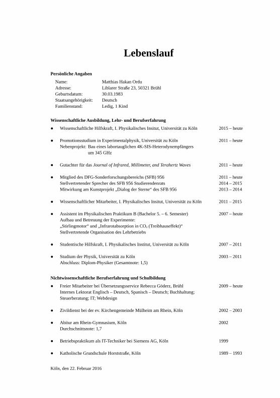
Lebenslauf
Persönliche Angaben
Name: Matthias Hakan OrduAdresse: Liblarer Straße 23, 50321 BrühlGeburtsdatum: 30.03.1983Staatsangehörigkeit: DeutschFamilienstand: Ledig, 1 Kind
Wissenschaftliche Ausbildung, Lehr- und Berufserfahrung
● Wissenschaftliche Hilfskraft, I. Physikalisches Insitut, Universität zu Köln 2015 – heute
● Promotionsstudium in Experimentalphysik, Universität zu Köln 2011 – heuteNebenprojekt: Bau eines labortauglichen 4K-SIS-Heterodynempfängers
um 345 GHz
● Gutachter für das Journal of Infrared, Millimeter, and Terahertz Waves 2011 – heute
● Mitglied des DFG-Sonderforschungsbereichs (SFB) 956 2011 – heuteStellvertretender Sprecher des SFB 956 Studierendenrats 2014 – 2015Mitwirkung am Kunstprojekt „Dialog der Sterne“ des SFB 956 2013 – 2014
● Wissenschaftlicher Mitarbeiter, I. Physikalisches Insitut, Universität zu Köln 2011 – 2015
● Assistent im Physikalischen Praktikum B (Bachelor 5. – 6. Semester) 2007 – heuteAufbau und Betreuung der Experimente:„Stirlingmotor“ und „Infrarotabsorption in CO2 (Treibhauseffekt)“Stellvertretende Organisation des Lehrbetriebs
● Studentische Hilfskraft, I. Physikalisches Institut, Universität zu Köln 2007 – 2011
● Studium der Physik, Universität zu Köln 2003 – 2011Abschluss: Diplom-Physiker (Gesamtnote: 1,5)
Nichtwissenschaftliche Berufserfahrung und Schulbildung
● Freier Mitarbeiter bei Übersetzungsservice Rebecca Göderz, Brühl 2009 – heuteInternes Lektorat Englisch – Deutsch, Spanisch – Deutsch; Buchhaltung;Steuerberatung; IT; Webdesign
● Zivildienst bei der ev. Kirchengemeinde Mülheim am Rhein, Köln 2002 – 2003
● Abitur am Rhein-Gymnasium, Köln 2002Durchschnittsnote: 1,7
● Betriebspraktikum als IT-Techniker bei Siemens AG, Köln 1999
● Katholische Grundschule Horststraße, Köln 1989 – 1993
Köln, den 22. Februar 2016


![Rotational Depolarization of Fluorescence of Prolate ...zfn.mpdl.mpg.de/data/Reihe_A/45/ZNA-1990-45a-1357.pdf · ized Langevin equation is taken into account in the theory [8], the](https://img.pdfslide.org/doc/110x75/5ebdc7a387ea1526d967c77a/rotational-depolarization-of-fluorescence-of-prolate-zfnmpdlmpgdedatareihea45zna-1990-45a-1357pdf.jpg)