Embed Size (px)
Citation preview

SAT and CP - Parallelisationand Applications
Thorsten Ehlers
Dissertationzur Erlangung des akademischen Grades
Doktor der Ingenieurwissenschaften(Dr.-Ing.)
der Technischen Fakultätder Christian-Albrechts-Universität zu Kiel
eingereicht im Jahr 2017
Kiel Computer Science Series (KCSS) 2017/3 dated 2017-05-30
URN:NBN urn:nbn:de:gbv:8:1-zs-00000333-a0ISSN 2193-6781 (print version)ISSN 2194-6639 (electronic version)
Electronic version, updates, errata available via https://www.informatik.uni-kiel.de/kcss
The author can be contacted via [email protected]
Published by the Department of Computer Science, Kiel University
Dependable Systems Group
Please cite as:
Ź Thorsten Ehlers. SAT and CP - Parallelisation and Applications Number 2017/3 in Kiel Com-puter Science Series. Department of Computer Science, 2017. Dissertation, Faculty of Engi-neering, Kiel University.
@bookDissThorstenEhlers2017,
author = Thorsten Ehlers,
title = SAT and CP - Parallelisation and Applications,
publisher = Department of Computer Science, CAU Kiel,
year = 2017,
number = 2017/3,
series = Kiel Computer Science Series,
note = Dissertation, Faculty of Engineering,
Kiel University.
© 2017 by Thorsten Ehlers
ii
About this Series
The Kiel Computer Science Series (KCSS) covers dissertations, habilitationtheses, lecture notes, textbooks, surveys, collections, handbooks, etc. writtenat the Department of Computer Science at Kiel University. It was initiated in2011 to support authors in the dissemination of their work in electronic andprinted form, without restricting their rights to their work. The series providesa unified appearance and aims at high-quality typography. The KCSS is an openaccess series; all series titles are electronically available free of charge at thedepartment’s website. In addition, authors are encouraged to make printedcopies available at a reasonable price, typically with a print-on-demand service.
Please visit http://www.informatik.uni-kiel.de/kcss for more information, forinstructions how to publish in the KCSS, and for access to all existing publica-tions.
iii

1. Gutachter: Prof. Dr. Dirk NowotkaChristian-Albrechts-UniversitätKiel
2. Gutachter: Prof. Dr. Mike CodishBen Gurion University of the Negev
Datum der mündlichen Prüfung: 22.05.2017
iv

Acknowledgements
I’m rolling thunder pouring rainI’m coming on like a hurricaneMy lightning’s flashing across thesky
AC/DC
This work would not have been possible without the help, encouragement,support and advise of many people whom I would like to thank at this place.
First of all I would like to thank my family, especially my parents Manfredand Susanne, for growing me, making me the person I am now, and supportingme through all decisions, especially the hard ones.
Next, I thank my supervisor, Dirk Nowotka, for his guidance, patience, andsupport, and for providing me the freedom and funding to do research indifferent directions.
Thanks to my current and former colleagues from the Dependable SystemsGroup in Kiel, who supported, questioned me. Namely, this is Gesa Walsdorf,Philipp Sieweck, Tim Grebien, Mike Müller, Florin Manea, Robert Mercas, MaikeBradler, Kamellia Reshadi, Mitja Kulczynski, Danny Poulsen, Joel Day, PamelaFleischmann, Max Friese, Yvonne Küstermann, Anneke Twardzik and KaroliinaLehtinen.
Furthermore, I would like the members of my examining committee, MikeCodish, Steffen Börm and Manfred Schimmler for their efforts.
I had a great time in Melbourne, Australia, when spending six month at theMelbourne University in 2015. Here, I owe thanks especially to Peter Stuckey forhosting me, the many fruitful discussions we had, and the advise he gave me.This stay surely changed my understanding of constraint programming andSAT solving. A big thanks also to my colleagues there, Graeme Gange, Diego deUña, Ignasi Abio, Valentin Mayer-Eichberger and Geoffrey Chu. Furthermore,I would like to thank Mark, Sigrid, Oliver, Kylie, Linda, all the guys from theGraduate House and my football gang for the pleasant time.
Science is collaboration; I would like to thank my co-authors that were notmentioned so far, Peter Schneider-Kamp, Luís Cruz-Filipe, Miro Spönemann,Reinhard von Hanxleden, Ulf Rüegg and Johannes Traub.
v

I also had some fun debugging the software I worked on with Max Bannachand Sebastian Berndt in the field of tree decompositions, hopefully we willmanage to publish some results shortly!
I would also like to thank my friends and flatmates, for their support andpatience, for example when I was writing a paper while we were renovating theflat.
Last but not least I want to thank Maria for her patience and advice when Ifelt overstrained by this work, and for just having a good time with me.
vi
Zusammenfassung
Diese Dissertation befasst sich mit der Parallelisierung von Programmen welcheeine beliebige, oder eine optimale Lösung zu Problemen suchen, die auf be-stimmte, formale Arten spezifiziert werden. Wir beschreiben Parallelisierungs-ansätze für zwei verschiedene Arten von Lösern, sowie einen Anwendungsfall.
In dem ersten Kapitel beschäftigen wir uns mit SAT, dem Erfüllbarkeitsproblemder Aussagenlogik, und Algorithmen, welche die Erfüllbarkeit oder Unerfüll-barkeit aussagenlogischer Formeln entscheiden. Wir beginnen mit einer kur-zen Einführung in Grundlagen der Beweistheorie, welche dann in Bezug zuder Stärke verschiedener algorithmischer Ansätze gesetzt wird. Desweiterendiskutieren wir Implementierungsdetails aktueller SAT Löser, und zeigen Ver-besserungen. Zuletzt wird eine Parallelisierung dieser Löser diskutiert, wobeiein Schwerpunkt auf der Kommunikation von Zwischenergebnissen innerhalbeines parallelen Lösers, dem Austausch gelernter Klauseln, liegt.
In dem zweiten Kapitel betrachten wir Constraint Programing (CP) mit Lern-mechanismen. Im Gegensatz zu klassische Techniken werden hier Lernme-chanismen, wie sie bei SAT Lösern zum Einsatz kommen, übernommen. Wirpräsentieren Ergebnisse einer Parallelisierung von CHUFFED, einem lernendenCP Löser. Da dieser sowohl Charakteristiken eines klassischen CP-Lösers alsauch eines SAT-Lösers aufweist, ist es nicht klar, welche Parallelisierungsansätzehier am besten funktionieren.
Im letzten Kapitel diskutieren wir Sortiernetzwerke, Sortieralgorithmen derenVergleichsoperationen a priori, also unabhängig von der Eingabe, festgelegt wer-den. Aufgrund dieser Datenunabhängigkeit können Sortiernetzwerke effizientparallel implementiert werden. Wir betrachten die Frage nach der minimalenAnzahl von parallelen Sortierschritten, welche für die Sortierung von bestimm-ten Eingabegrößen benötigt werden, und zeigen untere und obere Schrankenfür mehrere Fälle.
vii

Abstract
This thesis is considered with the parallelisation of solvers which search foreither an arbitrary, or an optimum, solution to a problem stated in some formalway. We discuss the parallelisation of two solvers, and their application in threechapters.
In the first chapter, we consider SAT, the decision problem of propositionallogic, and algorithms for showing the satisfiability or unsatisfiability of proposi-tional formulas. We sketch some proof-theoretic foundations which are relatedto the strength of different algorithmic approaches. Furthermore, we discussdetails of the implementations of SAT solvers, and show how to improve uponexisting sequential solvers. Lastly, we discuss the parallelisation of these solverswith a focus on clause exchange, the communication of intermediate resultswithin a parallel solver.
The second chapter is concerned with Contraint Programing (CP) with learning.Contrary to classical Constraint Programming techniques, this incorporateslearning mechanisms as they are used in the field of SAT solving. We presentresults from parallelising CHUFFED, a learning CP solver. As this is both a kindof CP and SAT solver, it is not clear which parallelisation approaches work besthere.
In the final chapter, we will discuss Sorting networks, which are data oblivi-ous sorting algorithms, i. e., the comparisons they perform do not depend onthe input data. Their independence of the input data lends them to parallelimplementation. We consider the question how many parallel sorting stepsare needed to sort some inputs, and present both lower and upper bounds forseveral cases.
ix

Contents
1 Introduction 1
2 SAT 32.1 Preliminaries . . . . . . . . . . . . . . . . . . . . . . . . . . . . . . . 5
2.1.1 Propositional Formulas . . . . . . . . . . . . . . . . . . . . . 52.1.2 Satisfiability of Propositional Formulas . . . . . . . . . . . . 72.1.3 Conjunctive Normal Form . . . . . . . . . . . . . . . . . . . 8
2.2 Proofs and Complexity . . . . . . . . . . . . . . . . . . . . . . . . . . 102.2.1 Resolution . . . . . . . . . . . . . . . . . . . . . . . . . . . . . 112.2.2 The DP Algorithm . . . . . . . . . . . . . . . . . . . . . . . . 122.2.3 The DPLL Algorithm . . . . . . . . . . . . . . . . . . . . . . . 132.2.4 CDCL . . . . . . . . . . . . . . . . . . . . . . . . . . . . . . . . 152.2.5 Underlying Proof Systems . . . . . . . . . . . . . . . . . . . . 20
2.3 Techniques & Implementations . . . . . . . . . . . . . . . . . . . . 262.3.1 Preprocessing via Bounded Variable Elimination . . . . . . 262.3.2 Watched Literal Scheme . . . . . . . . . . . . . . . . . . . . . 272.3.3 Branching . . . . . . . . . . . . . . . . . . . . . . . . . . . . . 302.3.4 Conflict Driven Clause Learning . . . . . . . . . . . . . . . . 312.3.5 Restarts . . . . . . . . . . . . . . . . . . . . . . . . . . . . . . . 34
2.4 SAT Competition 2016 . . . . . . . . . . . . . . . . . . . . . . . . . . 362.4.1 Refining the Restart Strategy . . . . . . . . . . . . . . . . . . 362.4.2 Re-considering LBD . . . . . . . . . . . . . . . . . . . . . . . 38
2.5 Parallel SAT . . . . . . . . . . . . . . . . . . . . . . . . . . . . . . . . 422.5.1 Portfolio-based Parallel SAT Solving . . . . . . . . . . . . . . 442.5.2 Subsequent Implementations . . . . . . . . . . . . . . . . . 65
2.6 Conclusion and Open Questions . . . . . . . . . . . . . . . . . . . . 66
3 Parallelising Constraint Programming with Learning 693.1 Introduction . . . . . . . . . . . . . . . . . . . . . . . . . . . . . . . . 693.2 Constraint Programming . . . . . . . . . . . . . . . . . . . . . . . . 70
xi

Contents
3.2.1 Constraint Satisfaction Problems . . . . . . . . . . . . . . . 703.2.2 Applications . . . . . . . . . . . . . . . . . . . . . . . . . . . . 713.2.3 Consistency and Propagators . . . . . . . . . . . . . . . . . . 733.2.4 Backtracking . . . . . . . . . . . . . . . . . . . . . . . . . . . . 763.2.5 Backtracking and Branch&Bound . . . . . . . . . . . . . . . 77
3.3 Constraint Programming with Learning . . . . . . . . . . . . . . . 803.4 Parallel Constraint Programming . . . . . . . . . . . . . . . . . . . . 843.5 Parallel Constraint Programming with Learning . . . . . . . . . . . 86
3.5.1 Portfolio-based Parallel LCG . . . . . . . . . . . . . . . . . . 873.5.2 Splitting the Search Space . . . . . . . . . . . . . . . . . . . . 893.5.3 Objective Probing . . . . . . . . . . . . . . . . . . . . . . . . . 933.5.4 Further Diversification . . . . . . . . . . . . . . . . . . . . . . 96
3.6 Conclusion and Open Questions . . . . . . . . . . . . . . . . . . . . 97
4 Sorting Networks 1014.1 Introduction . . . . . . . . . . . . . . . . . . . . . . . . . . . . . . . . 101
4.1.1 Construction of Sorting Networks . . . . . . . . . . . . . . . 1064.1.2 Bounds on Depth and Size of Sorting Networks . . . . . . . 110
4.2 Properties of Sorting Networks . . . . . . . . . . . . . . . . . . . . . 1124.2.1 Notation and Definitions . . . . . . . . . . . . . . . . . . . . 1124.2.2 Permutations of Sorting Networks . . . . . . . . . . . . . . . 1154.2.3 Prefixes of Sorting Networks . . . . . . . . . . . . . . . . . . 1174.2.4 Suffixes of Sorting Networks . . . . . . . . . . . . . . . . . . 120
4.3 SAT-based Search for Improved Bounds . . . . . . . . . . . . . . . 1204.3.1 Prefix-Optimisation . . . . . . . . . . . . . . . . . . . . . . . 1254.3.2 Preprocessing . . . . . . . . . . . . . . . . . . . . . . . . . . . 130
4.4 Improved Upper Bounds . . . . . . . . . . . . . . . . . . . . . . . . 1314.5 Improved Lower Bounds . . . . . . . . . . . . . . . . . . . . . . . . . 1384.6 Conclusion and Open Questions . . . . . . . . . . . . . . . . . . . . 143
5 Further Publications 147
A Appendix 149A.1 List of Benchmarks Used in the Paper “Communication in Massively-
Parallel SAT Solving" . . . . . . . . . . . . . . . . . . . . . . . . . . . 149A.2 Algorithms for the Optimisation of Prefixes . . . . . . . . . . . . . 151A.3 Comparison of Results from SAT Competition 2016 . . . . . . . . 160
xii

Contents
Bibliography 161
xiii

List of Figures
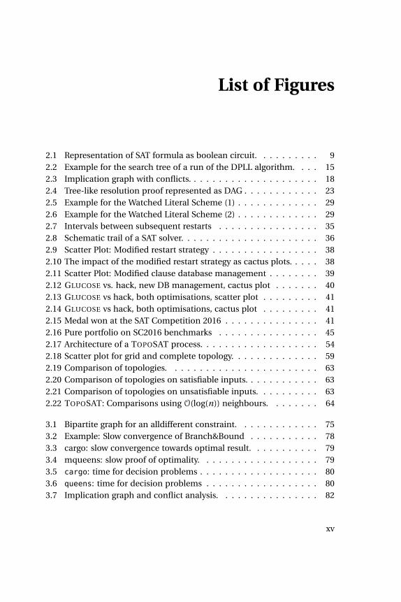
2.1 Representation of SAT formula as boolean circuit. . . . . . . . . . 92.2 Example for the search tree of a run of the DPLL algorithm. . . . 152.3 Implication graph with conflicts. . . . . . . . . . . . . . . . . . . . . 182.4 Tree-like resolution proof represented as DAG . . . . . . . . . . . . 232.5 Example for the Watched Literal Scheme (1) . . . . . . . . . . . . . 292.6 Example for the Watched Literal Scheme (2) . . . . . . . . . . . . . 292.7 Intervals between subsequent restarts . . . . . . . . . . . . . . . . 352.8 Schematic trail of a SAT solver. . . . . . . . . . . . . . . . . . . . . . 362.9 Scatter Plot: Modified restart strategy . . . . . . . . . . . . . . . . . 382.10 The impact of the modified restart strategy as cactus plots. . . . . 382.11 Scatter Plot: Modified clause database management . . . . . . . . 392.12 GLUCOSE vs. hack, new DB management, cactus plot . . . . . . . 402.13 GLUCOSE vs hack, both optimisations, scatter plot . . . . . . . . . 412.14 GLUCOSE vs hack, both optimisations, cactus plot . . . . . . . . . 412.15 Medal won at the SAT Competition 2016 . . . . . . . . . . . . . . . 412.16 Pure portfolio on SC2016 benchmarks . . . . . . . . . . . . . . . . 452.17 Architecture of a TOPOSAT process. . . . . . . . . . . . . . . . . . . 542.18 Scatter plot for grid and complete topology. . . . . . . . . . . . . . 592.19 Comparison of topologies. . . . . . . . . . . . . . . . . . . . . . . . 632.20 Comparison of topologies on satisfiable inputs. . . . . . . . . . . . 632.21 Comparison of topologies on unsatisfiable inputs. . . . . . . . . . 632.22 TOPOSAT: Comparisons using O(log(n)) neighbours. . . . . . . . 64
3.1 Bipartite graph for an alldifferent constraint. . . . . . . . . . . . . 753.2 Example: Slow convergence of Branch&Bound . . . . . . . . . . . 783.3 cargo: slow convergence towards optimal result. . . . . . . . . . . 793.4 mqueens: slow proof of optimality. . . . . . . . . . . . . . . . . . . 793.5 cargo: time for decision problems . . . . . . . . . . . . . . . . . . . 803.6 queens: time for decision problems . . . . . . . . . . . . . . . . . . 803.7 Implication graph and conflict analysis. . . . . . . . . . . . . . . . 82
xv

List of Figures
3.8 Search driven by SAT engine. . . . . . . . . . . . . . . . . . . . . . . 833.9 Search driven by FD engine. . . . . . . . . . . . . . . . . . . . . . . 833.10 mqueens: scaling behavior of Gecode. . . . . . . . . . . . . . . . . 853.11 suite: comparison between sequential and port. . . . . . . . . . 873.12 suite: scaling of port with number of cores. . . . . . . . . . . . . 873.13 suite: impact of clause sharing on port with 64 cores. . . . . . . 903.14 Work stealing in CHUFFED . . . . . . . . . . . . . . . . . . . . . . . . 903.15 suite: comparison between sequential and SSS with 64 cores. . . 913.16 suite: scaling of SSS with number of cores. . . . . . . . . . . . . . 913.17 suite: comparison of SSS and port, 64 cores. . . . . . . . . . . . . 923.18 queens: Number of conflicts in SSS . . . . . . . . . . . . . . . . . . 933.19 suite: impact of bounds sharing in SSS with 64 cores. . . . . . . 933.20 cargo: incumbent bounds, portfolio . . . . . . . . . . . . . . . . . 943.21 cargo: incumbent bounds, search space splitting . . . . . . . . . . 943.22 cargo: bounds, objective probing . . . . . . . . . . . . . . . . . . . 963.23 suite: finding good solutions, SSSP . . . . . . . . . . . . . . . . . . 963.24 suite: comparison between SSS and SSSP. . . . . . . . . . . . . . 973.25 suite: comparison between port and portP. . . . . . . . . . . . . 973.26 suite: comparison between SSS and port, 64 cores. . . . . . . . . 983.27 suite: comparison between SSS and port, 8 cores. . . . . . . . . 983.28 suite: comparison between hybrid and SSS solver, 64 cores. . . 98
4.1 A comparator. . . . . . . . . . . . . . . . . . . . . . . . . . . . . . . . 1034.2 A sorting network on 5 channels, operating on the input (5,4,3,2,1).1034.3 A Sorting Network performing an Insertion Sort. . . . . . . . . . . 1044.4 A Sorting Network performing an Insertion Sort in parallel steps. 1044.5 A Bubble Sort implemented as sorting network. . . . . . . . . . . . 1064.6 Odd-even-transposition sort. . . . . . . . . . . . . . . . . . . . . . . 1074.7 odd-even merge sort . . . . . . . . . . . . . . . . . . . . . . . . . . . 1084.8 An odd-even Merge Sort network on 8 channels. . . . . . . . . . . 1094.9 A Bitonic MergeSort on 8 channels. . . . . . . . . . . . . . . . . . . 1144.10 A bitonic Merge Sort and the result of untangling it. . . . . . . . . 1164.11 First layer in BZ-style . . . . . . . . . . . . . . . . . . . . . . . . . . . 1194.12 Example: propagations of the first layer . . . . . . . . . . . . . . . 1244.13 Difference between three permutations of a prefix . . . . . . . . . 1264.14 Generating partially ordered sets for n P 2,4,8,16 inputs. . . . . 131
xvi
List of Figures
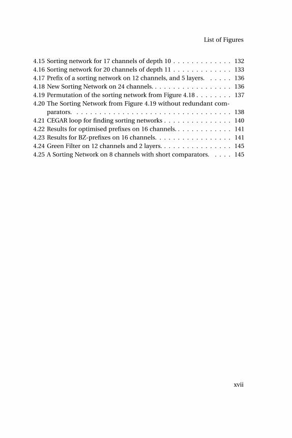
4.15 Sorting network for 17 channels of depth 10 . . . . . . . . . . . . . 1324.16 Sorting network for 20 channels of depth 11 . . . . . . . . . . . . . 1334.17 Prefix of a sorting network on 12 channels, and 5 layers. . . . . . 1364.18 New Sorting Network on 24 channels. . . . . . . . . . . . . . . . . . 1364.19 Permutation of the sorting network from Figure 4.18 . . . . . . . . 1374.20 The Sorting Network from Figure 4.19 without redundant com-
parators. . . . . . . . . . . . . . . . . . . . . . . . . . . . . . . . . . . 1384.21 CEGAR loop for finding sorting networks . . . . . . . . . . . . . . . 1404.22 Results for optimised prefixes on 16 channels. . . . . . . . . . . . . 1414.23 Results for BZ-prefixes on 16 channels. . . . . . . . . . . . . . . . . 1414.24 Green Filter on 12 channels and 2 layers. . . . . . . . . . . . . . . . 1454.25 A Sorting Network on 8 channels with short comparators. . . . . 145
xvii

List of Tables
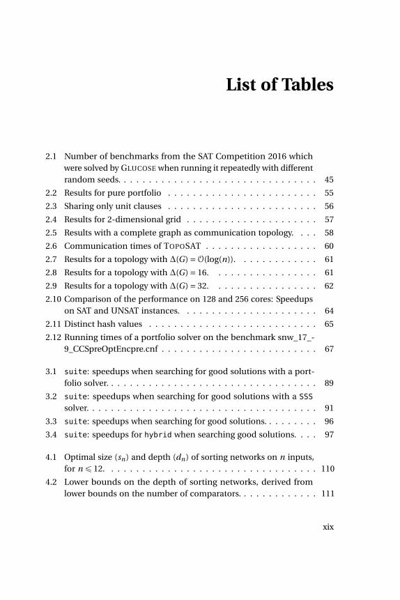
2.1 Number of benchmarks from the SAT Competition 2016 whichwere solved by GLUCOSE when running it repeatedly with differentrandom seeds. . . . . . . . . . . . . . . . . . . . . . . . . . . . . . . . 45
2.2 Results for pure portfolio . . . . . . . . . . . . . . . . . . . . . . . . 55
2.3 Sharing only unit clauses . . . . . . . . . . . . . . . . . . . . . . . . 56
2.4 Results for 2-dimensional grid . . . . . . . . . . . . . . . . . . . . . 57
2.5 Results with a complete graph as communication topology. . . . 58
2.6 Communication times of TOPOSAT . . . . . . . . . . . . . . . . . . 60
2.7 Results for a topology with ∆(G) =O(log(n)). . . . . . . . . . . . . 61
2.8 Results for a topology with ∆(G) = 16. . . . . . . . . . . . . . . . . 61
2.9 Results for a topology with ∆(G) = 32. . . . . . . . . . . . . . . . . 62
2.10 Comparison of the performance on 128 and 256 cores: Speedupson SAT and UNSAT instances. . . . . . . . . . . . . . . . . . . . . . 64
2.11 Distinct hash values . . . . . . . . . . . . . . . . . . . . . . . . . . . 65
2.12 Running times of a portfolio solver on the benchmark snw_17_-9_CCSpreOptEncpre.cnf . . . . . . . . . . . . . . . . . . . . . . . . . 67
3.1 suite: speedups when searching for good solutions with a port-folio solver. . . . . . . . . . . . . . . . . . . . . . . . . . . . . . . . . . 89
3.2 suite: speedups when searching for good solutions with a SSS
solver. . . . . . . . . . . . . . . . . . . . . . . . . . . . . . . . . . . . . 91
3.3 suite: speedups when searching for good solutions. . . . . . . . . 96
3.4 suite: speedups for hybrid when searching good solutions. . . . 97
4.1 Optimal size (sn) and depth (dn) of sorting networks on n inputs,for nď 12. . . . . . . . . . . . . . . . . . . . . . . . . . . . . . . . . . 110
4.2 Lower bounds on the depth of sorting networks, derived fromlower bounds on the number of comparators. . . . . . . . . . . . . 111
xix
List of Tables
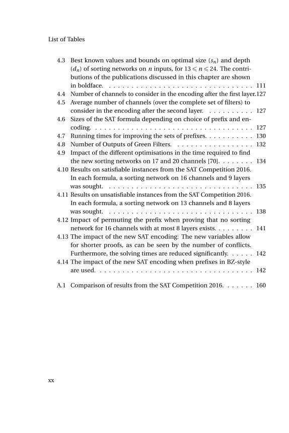
4.3 Best known values and bounds on optimal size (sn) and depth(dn) of sorting networks on n inputs, for 13ď nď 24. The contri-butions of the publications discussed in this chapter are shownin boldface. . . . . . . . . . . . . . . . . . . . . . . . . . . . . . . . . 111
4.4 Number of channels to consider in the encoding after the first layer.1274.5 Average number of channels (over the complete set of filters) to
consider in the encoding after the second layer. . . . . . . . . . . 1274.6 Sizes of the SAT formula depending on choice of prefix and en-
coding. . . . . . . . . . . . . . . . . . . . . . . . . . . . . . . . . . . . 1274.7 Running times for improving the sets of prefixes. . . . . . . . . . . 1304.8 Number of Outputs of Green Filters. . . . . . . . . . . . . . . . . . 1324.9 Impact of the different optimisations in the time required to find
the new sorting networks on 17 and 20 channels [70]. . . . . . . . 1344.10 Results on satisfiable instances from the SAT Competition 2016.
In each formula, a sorting network on 16 channels and 9 layerswas sought. . . . . . . . . . . . . . . . . . . . . . . . . . . . . . . . . 135
4.11 Results on unsatisfiable instances from the SAT Competition 2016.In each formula, a sorting network on 13 channels and 8 layerswas sought. . . . . . . . . . . . . . . . . . . . . . . . . . . . . . . . . 138
4.12 Impact of permuting the prefix when proving that no sortingnetwork for 16 channels with at most 8 layers exists. . . . . . . . . 141
4.13 The impact of the new SAT encoding: The new variables allowfor shorter proofs, as can be seen by the number of conflicts.Furthermore, the solving times are reduced significantly. . . . . . 142
4.14 The impact of the new SAT encoding when prefixes in BZ-styleare used. . . . . . . . . . . . . . . . . . . . . . . . . . . . . . . . . . . 142
A.1 Comparison of results from the SAT Competition 2016. . . . . . . 160
xx

List of Algorithms
1 Enumeration of all assignments . . . . . . . . . . . . . . . . . . . . . 112 The DP algorithm . . . . . . . . . . . . . . . . . . . . . . . . . . . . . 133 The DPLL algorithm . . . . . . . . . . . . . . . . . . . . . . . . . . . . 144 Conflict clause generation . . . . . . . . . . . . . . . . . . . . . . . . 165 The CDCL algorithm . . . . . . . . . . . . . . . . . . . . . . . . . . . . 196 Bounded Variable Elimination . . . . . . . . . . . . . . . . . . . . . . 277 Naïve BCP . . . . . . . . . . . . . . . . . . . . . . . . . . . . . . . . . . 28
8 Solving a CSP by Backtracking . . . . . . . . . . . . . . . . . . . . . . 769 Solving a CSP by Branch&Bound . . . . . . . . . . . . . . . . . . . . 77
10 Insertion Sort . . . . . . . . . . . . . . . . . . . . . . . . . . . . . . . . 10211 Sorting algorithm for 4 elements . . . . . . . . . . . . . . . . . . . . 10212 Bubble Sort . . . . . . . . . . . . . . . . . . . . . . . . . . . . . . . . . 10613 Odd-Even- Merge Sort . . . . . . . . . . . . . . . . . . . . . . . . . . . 10814 OddEvenMerge . . . . . . . . . . . . . . . . . . . . . . . . . . . . . . . 10915 untangle . . . . . . . . . . . . . . . . . . . . . . . . . . . . . . . . . . . 11616 Evolutionary Algorithm for the Permutation of Prefixes . . . . . . . 12917 Gradient Descent Algorithm . . . . . . . . . . . . . . . . . . . . . . . 130
xxi


Chapter 1
Introduction
“It’s a dangerous business, Frodo,going out your door. You step ontothe road, and if you don’t keep yourfeet, there’s no knowing where youmight be swept off to.”
BILBO BAGGINS
This thesis presents results from three different fields. Still, they are connectedto each other. In the first two chapters, we will discuss procedures which auto-matically create proofs for the satisfiability or unsatisfiability of propositionsgiven in a certain form, propositional formulas in Chapter 2, and constraintsatisfaction problems in Chapter 3. In both cases, we will especially considerthe parallelisation of these procedures.
Modern algorithms for these satisfiability problems perform a sophisticatedversion of a backtracking algorithm. Whenever a backtrack has to be done, alearning mechanism is invoked which learns a reason for this backtrack. Thisno-good is stored and used to prune the search space in subsequent search.Moreover, if the solver proves the formula unsatisfiable, this proof is made ofthese no-goods. These learning techniques are the foundation of the impressiveperformance of state-of-the-art solvers, computer programs which decide thesatisfiability of such formulas. Besides experimental results, this can also beseen by an analysis of proof systems that these learning techniques can berelated to. However, they are also a burden on the parallelisability of theseprocedures.
In Chapter 2, we will give an overview over techniques used in nowadaysSAT solvers, and relate them to proof systems. Understanding these proofsystems is beneficial both for understanding the challenges in parallelising
1
1. Introduction
these solvers, and the SAT encoding of some specific problem we discuss inChapter 4.
Next, we present and discuss the changes we made to the SAT solver GLU-COSE for the SAT Competition 2016. With these changes, our solver won a goldmedal in this competition.
Finally, we discuss the parallelisation of SAT solvers. Here, we especiallyconsider the exchange of no-goods recorded during search between SAT solversrunning in parallel. On the one hand, it is crucial for the performance of parallelSAT solvers to avoid redundant work, which can be achieved by communicatinginformation about failed search among the parallel solvers. On the other hand,one has to consider the amount of information exchange, especially whenscaling to larger numbers of parallel processing units used.
Next, we consider the parallelisation of CHUFFED, a CP solver with learning,in Chapter 3. As this solver is both kind of a SAT solver and a CP solver, itis not clear how to parallelise it. After giving an overview of some ideas andtechniques from the field of constraint programming, we compare approachesfrom the fields of SAT and CP, respectively. When considering optimisationproblems, the parallel solver achieves a super-linear speed-up.
Chapter 4 is concerned with sorting networks, a model of data-oblivioussorting algorithms. We will consider sorting networks which are restricted in thesense that the number of sorting steps they perform is bounded. The existenceof such networks can be encoded in formulas in propositional logic. We presenta technique which takes advantage of symmetries in sorting networks, andderive an optimisation problem which allows for minimising the size of thesepropositional formulas. Furthermore, we extend encodings used in previousresearch on this topic by some predicates, which allow for smaller formulas,and reduce the size of proofs created by a SAT solver.
2
Chapter 2
SAT
“Romanes eunt domus.”
BRIAN
The satisfiability problem of propositional logic, SAT, was the first problemproven to be NP-complete [77]. On the one hand, this implies that it is com-putationally challenging, and intractable unless P = N P . On the other hand,many problems from NP can be encoded as propositional formulas, whichmakes SAT an interesting foundation.
In the past two decades, SAT solvers, i. e., procedures which decide thesatisfiability of a formula in propositional logic, have become extremely fast fora broad range of formulas, which in turn has attracted interest in this field.
One of the first applications was the verification of hardware. In BoundedModel Checking [46], LTL formulas describing some execution steps of thehardware under consideration are encoded as a SAT formula. Contrary to pre-vious approaches based on BDDs, this allows for using state-of-the-art SATsolvers [47]. This technique has proven extremely useful, and won the prize forbeing the “most influential paper in the first 20 years of TACAS” 2014. Anothertechnique for verifying properties of transition systems like hardware is IC3 (“In-cremental Construction of Inductive Clauses for Indubitable Correctness") [54],based on SAT encodings.
Analogously, SAT solvers are used as core technology in software verification.The tool Blast [42] searches for execution paths which lead to some errorlocation, a part of the code that should be unreachable. The feasibility of thesepaths is encoded in SAT: if the formula is satisfiable, the location is reachable,and the SAT-certificate contains input values that lead to this error. A similarapproach is chosen in KLEE [60], which uses a SAT solver to generate inputsfor a program which make the program execute along some path. These inputs
3
2. SAT
are then used as test cases, yielding good code coverages. These techniques areused both in academia and in software companies [26]. Furthermore, SAT isused for the analysis of termination of programs [146].
In cryptanalysis, SAT solvers were used to check the security of crypto-graphic procedures. While they cannot prove the security, successful attacks ona cryptographic procedure would imply that it is unsafe. In [158], SAT solversare used to do the “laborious” work in attacks on MD4 and MD5. Cryptomin-iSAT, developed by Mate Soos [201], is a SAT solver which is tuned towards cryp-tographic problems, and extends normal SAT encodings to XOR constraints.
Lately, SAT solvers have been used to compute lower bounds for somecombinatorial problems, among them Ramsey numbers [75], the pythagoreantriples problem [120], and bounds on some properties of sorting networks [56,70]. The last case will be handled in more detail in Chapter 4.
Lastly, SAT solvers are used as foundation of solvers for more complex logic.In “SAT modulo theories” (SMT), boolean variables are connected with a mean-ing with respect to some background theory. The DPLL(T)-framework uses SATsolvers as core technology, and checks consistency with the background theorylazily [167]. This framework is used in state-of-the-art SMT solvers like Z3 [163],BARCELOGIC [48] or CVC4 [31]. Additionally, clause learning CP solvers likeCHUFFED [62] use an architecture which is similar to DPLL(T). We will discussthe parallelisation of such solvers in Chapter 3.
In this chapter, we will discuss the satisfiability problem of propositionallogic and algorithms to decide it. As some concepts are also relevant for thesubsequent chapters, the foundations explained here are more complete thanactually required for this chapter. We present some formalisms first, and thendiscuss proof systems for deciding the unsatisfiability of a propositional for-mula, especially with a focus on the size of the proofs they produce. This isrelevant as SAT solvers — software programs, which create proofs accordingto some proof system — are limited by lower bounds of the respective proofsystem: A solver implementing a weak proof systems cannot yield short proofs.
In this context, we also show changes made to GLUCOSE [19] in the SAT com-petition 2016, with which we won the gold medal as best GLUCOSE hack [96].
We then discuss the parallelisation of SAT solvers, especially with a focuson the exchange of information inside a parallelised SAT solver. These resultswere published in [97].
4
2.1. Preliminaries
2.1 Preliminaries
SAT is the common abbreviation for the satisfiability problem of propositionallogic. It is also called Boolean Logic, after George Boole, who formalised itsmain concepts in 1847 [52]. Propositional logic deals with boolean propositions— they are either true (1), or false (0). Boolean variables are such that maytake exactly one of these values. Propositional formulas are built from booleanvariables and constants, and connections between them [59]. It is sufficient toconsider the logical “OR” and negation, as we will see shortly. The “OR”, writtenas _, is defined as
0_0 = 0
0_1 = 1
1_0 = 1
1_1 = 1
As can be seen by this definition, the logical “OR” is commutative. Thenegation is represented by the symbol , and defined as
1 = 0
0 = 1
A literal is either a variable or its negation.
2.1.1 Propositional Formulas
Definition 2.1 (Propositional formula). The set of formulas in propositionallogic, FPL , can be defined recursively as
1 P FPL
x P FPL If x is a boolean variable
( f ) P FPL f P FPL
f P FPL f P FPL
f _ g P FPL f , g P FPL
It is common to use further connectives for “AND” ^, implications ñ,
5

2. SAT
equivalences ô or “XOR” ‘. These can be defined by the above definitions as
0 = 1
f ^ g = ( f _ g )
f ñ g = f _ g
f ô g = ( f ñ g )^ (g ñ f )
f ‘ g = ( f ô g )
A conjunction of propositional formulas is their connection by ^, and theirdisjunction is the connection by _. The definition of ^ by _ and is one ofDe Morgan’s laws [85].
As an example for propositional encodings, consider the node colouringproblem on graphs.
Problem 2.2 (Node colouring). Let G = (V ,E) denote a graph, and c PN. Thenode colouring problem asks for a mapping ξ : V ÞÑ [1,c]XN such that eachpair of adjacent nodes is coloured with different colours, i. e.,
ξ(u)‰ ξ(v) @u, v P E
Node colouring is one of Karp’s 21 NP-complete problems [131], but ithas also practical applications. For example, consider the problem of assigningfrequencies to radio stations such that stations which are close to each other donot interfere [161], which can be modeled as a node colouring problem: Radiostations are represented by nodes in the graph. For every pair of radio stationsthat must not use the same frequency, the respective nodes are connected byan edge. Then, the colours represent the frequencies used.
Node colouring can be encoded as a SAT problem as follows.
Example 2.3. We may encode the proposition ξ(v) = i by a boolean variable xvi .
In this encoding, we encode the implicit constraint from the problem definitionthat ξ is a function: Each node has to be coloured with exactly one colour, whichhas to be encoded explicitly. Furthermore, we add the colouring-constraint thateach two adjacent nodes must be coloured with different colours, and yield thefollowing encoding.
xvi _ xv
j @1ď i ď j ď c, v PV
xui _ xv
i @1ď i ď c, u, v P E
6
2.1. Preliminaries
c∨i=1
xvi @v PV
The first set of clauses forbids that a node v is coloured both with differentcolours i and j . The second set forbids colouring adjacent nodes u and v withthe same colour, whereas the last clauses encode that each node has to becoloured with at least one colour. ä
2.1.2 Satisfiability of Propositional Formulas
Given a propositional formula φ and an assignment of its variables to true orfalse, we may ask for the evaluation of the formula under this assignment. Thevariables of a formula can be defined as follows.
Definition 2.4 (Variables of a formula). The variables of a formula are
vars(1) =
vars(x) = x
vars(( f )) = vars( f )
vars( f ) = vars( f )
vars( f _ g ) = vars( f )Yvars(g )
Let β : vars(φ) ÞÑ 1,0 denote a mapping of the variables of some formulaφ to true and false values. With this, we evaluate the truth value of φ.
Definition 2.5 (Evaluation of a propositional formula). Let f denote a functionwhich evaluates a formula φ and an assignment to the variables of φ to either1 or 0. It can be defined as follows.
f (1,β) = 1
f (x,β) =β(x)
f ((φ),β) = f (φ,β)
f ( φ,β) = f (φ,β)
f (φ_φ1,β) = f (φ,β)_ f (φ1,β)
Definition 2.6 (Satisfiability of a propositional formula). A propositional for-mula φ is satisfiable if and only if there exists an assignment β such thatf (φ,β) = 1.
7
2. SAT
A formula is called unsatisfiable if it is not satisfiable, i.e. there is no satisfy-ing assignment. The negation of an unsatisfiable formula, which is satisfied byall variable assignments, is denoted a tautology.
Let φ and ψ denote propositional formulas, β : vars(φ)Y vars(ψ) ÞÑ 1,0and f an evaluation function. φ entails ψ, written φ |ùψ, iff for every β it holdsthat if β satisfies φ, it also satisfies ψ, i. e., f (φ,β)ñ f (ψ,β). The formulas areequivalent, denoted φ” ψ, iff φ |ù ψ and ψ |ù φ. They are equisatisfiable ifeither both, or none are satisfiable [155].
2.1.3 Conjunctive Normal Form
There are different normal forms for SAT formulas, as NNF, DNF [141] orDDNF[82]. Most SAT solvers expect the input formula to be in conjunctivenormal form (CNF).
Definition 2.7 (CNF). A propositional formula φ in conjunctive normal form isa conjunction over disjunctions of (possibly negated) boolean variables. Thesedisjunctions are denoted as clauses, and |ci | denotes the number of literals ina clause ci . Furthermore, |φ| denotes the number of clauses in φ.
φ=n∧
i=1ci
=n∧
i=1
|ci |∨j=1
li , j |li , j P x, x, x P vars(φ)
This restriction does not restrict the power of these solvers, as every propo-sitional formula can be transformed into a formula in CNF [205]. The so-calledTseitin Transformation considers the input formula as a boolean circuit, andintroduces auxiliary variables for the outputs of each gate. These are bound tothe correct value by a constant number of clauses for each gate — thus, the sizeof the resulting formula is linear in the size of the input formula. We exemplifythis procedure in the following example.
Example 2.8. Consider the formula
φ= ((A^B)_C )^ ( A_ ( B^D))
We represent the formula as a boolean circuit, and introduce new variablesx1, . . . , x5 for the gate outputs, as shown in Figure 2.1. Note that a satisfying
8

2.1. Preliminaries
x1
x2
x5
x4
x3
A
B
C
A
B
D
Figure 2.1. The formula ((A^B)_C )^( A_( B^D)), represented as boolean circuit.
assignment for φ must satisfy the newly introduced variable x5.
The output variables x1, . . . , x5 are defined by the following equivalences.
x1Ø (A^B)
x2Ø (x1_C )
x3Ø ( B^D)
x4Ø ( A_x3)
x5Ø (x2^x4)
These equivalences can easily be transformed into CNF by replacing eachbi-implication by two implications, and representing these by disjunctions. Theresulting CNF consists of 16 clauses.
( x1_ A) ( x1_B)
(x1_ A_ B) (x2_ x1)
(x2_ C ) ( x2_x1_C )
( x3_ B) ( x3_D)
(x3_B_ D) ( x4_ A_x3)
(x4_ A) (x4_ x3)
( x5_x2) ( x5_x4)
9
2. SAT
(x5_ x2_ x4) (x5)
äSubsumption of clauses is a useful notion when dealing with formulas
in CNF. Consider a formula φ containing clauses c1 and c2. The clause c1
subsumes clause c2 if all its literals are contained in c2. Abusing notation wemay write c1Ď c2. Every satisfying assignment for φ must assign at least oneliteral in c1 to 1, which also satisfies c2. Thus, c2 may be removed from φ
without changing the satisfiability.
2.2 Proofs and Complexity
In this section, we consider procedures to prove the satisfiability, or unsatisfia-bility, of a given propositional formula. Furthermore, we discuss the structureof proofs especially for the unsatisfiability of SAT formulas. Determining the sat-isfiability of a propositional formula, or SAT in short, is obviously in NP: Givenan assignment of its variables to 1 or 0, it is easily verifiable in polynomialtime if it satisfies the formula, or not. Conversely, proving the unsatisfiabilityof a SAT formula is more involved. We will discuss different proof systems inSection 2.2.5 and relate them to the algorithms we discuss before.
We first introduce some notation, and then discuss algorithms and proofsystems for SAT. We will restrict ourselves to formulas in CNF for this. It iscommon to handle such formulas as a set of sets of literals. Thus, given aclause c , we simply write c Pφ to denote that c is a conjunct of φ. As common,we define the empty conjunction as true, and the empty disjunction as false.
∧∨H= 1∧∨
H, . . . = 0
In the following algorithms, we will often need the set of clauses that con-tain some literal `. As as shorthand, we will denote this set by
φ` = c Pφ : ` P c
If a literal is assigned to true, it satisfies all clauses containing it. All clauseswhich contain its negation must be satisfied by other literals. The residual
10
2.2. Proofs and Complexity
Algorithm 1: Enumeration of all assignments
Data: Propositional formula φ in CNFResult: 1 if φ is satisfiable, and 0 otherwise
1 for β : vars(φ) ÞÑ 0,1n do2 if f (φ,β) = 1 then3 return 1;
4 return 0;
formula with respect to some partial assignment can be defined as follows.
Definition 2.9 (Formulas under partial assignment). For a formula φ, x Pvars(φ),` P x, x, let φ|` denote the residual formula with ` set to true.
φ|` =(φz(φ`Yφ `)
)Y c : cY ` Pφ
This is, all clauses containing ` are removed, as they are satisfied, and ` isremoved from all clauses containing it as they cannot be satisfied by it.
The naïve approach to determining the satisfiability of a formula on nvariables is the enumeration of all 2n possible assignments, as depicted inAlgorithm 1.
This algorithm can be seen as the deterministic version of the behaviour ofa non-deterministic Turing Machine which guesses assignments, and checksif they satisfy the formula. It can easily be implemented to run in O(2n |φ|)time. Next, we will discuss some algorithms that cannot be proven to be fasteron all formulas, but perform better in practice. Afterwards, we consider theunderlying proof systems.
2.2.1 Resolution
Resolution [84, 187] is the underlying principle of most SAT solving algorithms.It is an inference system which only knows the rule
(C_x) (D_ x)(C_D)
11
2. SAT
The intuition behind this rule is that in a satisfying assignment, x is eitherset to true, and hence D must be satisfied, or x is set to false, and C must besatisfied.
A SAT formula is unsatisfiable if and only if the empty clause can be derivedby repeated applications of this rule. This is, there is a sequence of clausesc0, . . . ,ck such that every clause is derived from clauses either from the originalformula, or a clause derived before, ending with the empty clause.
We will first consider its application in SAT solving algorithms. Afterwards,we discuss the strength of different restrictions of resolution, and relate theserestricted versions to different algorithms.
2.2.2 The DP Algorithm
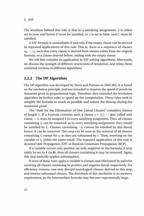
The DP algorithm was developed by Davis and Putnam in 1960 [84]. It is basedon the resolution principle, and was intended to improve the speed of proofs fortheorems given in propositional logic. Therefore, they extended the resolutionalgorithm by further rules to speed up the computation. These rules seek tosimplify the formula as much as possible and reduce the blowup during theresolution proof.
The “Rule for the Elimination of One-Literal Clauses” considers clausesof length 1. If a formula contains such a clause c = (li ) — also called unitclause — li must be assigned 1 in every satisfying assignment. Thus, all clausescontaining li can be removed, as in every satisfying assignment, they wouldbe satisfied by li . Clauses containing li cannot be satisfied by this literal,hence, it can be removed. This step can be seen as the removal of all clausescontaining li except for c, as they are subsumed by c. Then, resolving on thevariable of li yields the same result. The repeated application of this rule isdenoted Unit Propagation (UP) or Boolean Constraint Propagation (BCP).
If a variable occurs only positive (or only negative) in the formula, it maysafely be set to 1 (to 0), thus all clauses containing it may be removed. Again,this step basically applies subsumption.
If none of these rules apply, a variable is chosen, and eliminated by pairwiseresolving all clauses containing its positive and negative literal, respectively. Forefficiency reasons, one may discard tautological clauses derived in this step,and remove subsumed clauses. The drawback of this resolution is its memoryrequirement, as the intermediate formula may become exponentially large.
12
2.2. Proofs and Complexity
Algorithm 2: The DP algorithm
Data: Propositional formula φ in CNFResult: 1 if φ is satisfiable, and 0 otherwise
1 if φ=H then2 return 1;
3 if HPφ then4 return 0;
/* Unit Propagation */
5 if ` Pφ then6 return DP(φ|`);
/* Pure Literal */
7 if D`.φ ` =H then8 return DP(φ|`);
9 Choose Variable x P vars(φ);10 φ1 :=φY (c1Y c2)zx, x,c1 Pφx ,c2 Pφ x z(φxYφ x );11 return DP(φ1);
2.2.3 The DPLL Algorithm
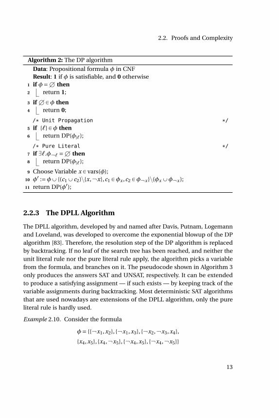
The DPLL algorithm, developed by and named after Davis, Putnam, Logemannand Loveland, was developed to overcome the exponential blowup of the DPalgorithm [83]. Therefore, the resolution step of the DP algorithm is replacedby backtracking. If no leaf of the search tree has been reached, and neither theunit literal rule nor the pure literal rule apply, the algorithm picks a variablefrom the formula, and branches on it. The pseudocode shown in Algorithm 3only produces the answers SAT and UNSAT, respectively. It can be extendedto produce a satisfying assignment — if such exists — by keeping track of thevariable assignments during backtracking. Most deterministic SAT algorithmsthat are used nowadays are extensions of the DPLL algorithm, only the pureliteral rule is hardly used.
Example 2.10. Consider the formula
φ= x1, x2, x1, x3, x2, x3, x4,
x4, x5, x4, x5, x4, x5, x4, x5
13
2. SAT
Algorithm 3: The DPLL algorithm
Data: Propositional formula φ in CNFResult: 1 if φ is satisfiable, and 0 otherwise
1 if φ=H then2 return 1;
3 if HPφ then4 return 0;
/* Unit Propagation */
5 if ` Pφ then6 return DPLL(φ|`=1);
/* Pure Literal */
7 if D`.φ ` =H then8 return DPLL(φ|`);
9 Choose Variable x P vars(φ);10 if DPLL(|φx=1) = 1 then11 return 1;12 else13 return DPLL(|φx=0);
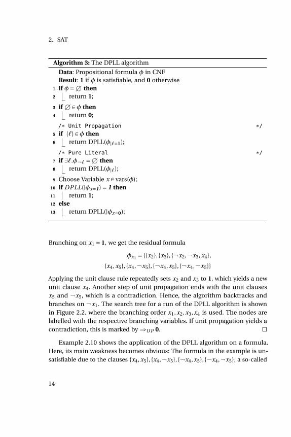
Branching on x1 = 1, we get the residual formula
φx1 = x2, x3, x2, x3, x4,
x4, x5, x4, x5, x4, x5, x4, x5
Applying the unit clause rule repeatedly sets x2 and x3 to 1, which yields a newunit clause x4. Another step of unit propagation ends with the unit clausesx5 and x5, which is a contradiction. Hence, the algorithm backtracks andbranches on x1. The search tree for a run of the DPLL algorithm is shownin Figure 2.2, where the branching order x1, x2, x3, x4 is used. The nodes arelabelled with the respective branching variables. If unit propagation yields acontradiction, this is marked by ñU P 0. ä
Example 2.10 shows the application of the DPLL algorithm on a formula.Here, its main weakness becomes obvious: The formula in the example is un-satisfiable due to the clauses x4, x5, x4, x5, x4, x5, x4, x5, a so-called
14

2.2. Proofs and Complexity
x1ñU P 0 x1
x2
x3ñU P 0 x3
x4ñU P 0 x4ñU P 0
x2
x3
x4ñU P 0 x4ñU P 0
x3
x4ñU P 0 x4ñU P 0
Figure 2.2. Example for the search tree of a run of the DPLL algorithm.
unsatisfiable core. With the chosen variable ordering, the DPLL algorithm isnot capable of taking advantage of this fact. Instead, the search visits similarparts of the search space several times.
2.2.4 CDCL
In 1999, Marques-Silva and Sakallah published GRASP (Generic seaRch Algo-rithm for the Satisfiability Problem) [196]. It seeks to overcome the weaknessesof the DPLL algorithm. Assume that the DPLL algorithm derives the emptyclause after branching and unit propagating. It will then backtrack and tryanother variable assignment, but it will not re-use any information about thefailed search. The idea of conflict driven clause learning (CDCL) is to derive ano-good which explains why the search failed. This no-good can then be usedto prune the search space, and prevent the solver from running into similarconflicts in other parts of the search space.
In case the search algorithm finds a leaf of the search tree which yields anempty clause, the reason for this conflict is analysed. To do this, the algorithmkeeps track of all unit propagations that occurred during search, and the clausescausing them. In case a conflict occurs, i.e. all literals of one clause — the
15
2. SAT
Algorithm 4: Conflict clause generation
Data: Propositional formula φ in CNF, implication graph, clause inconflict c
Result: backjump level `, learned clause cl/* Initialisation */
1 cl := c;2 ` := 0;3 while cl contains more than one literal assigned at current decision level
do4 ` := literal from cl that was assigned last;5 reason := clause that propagated `;6 v := var(`);7 cl := resolve(cl, reason, v);
8 ` := second highest decision level in cl ;
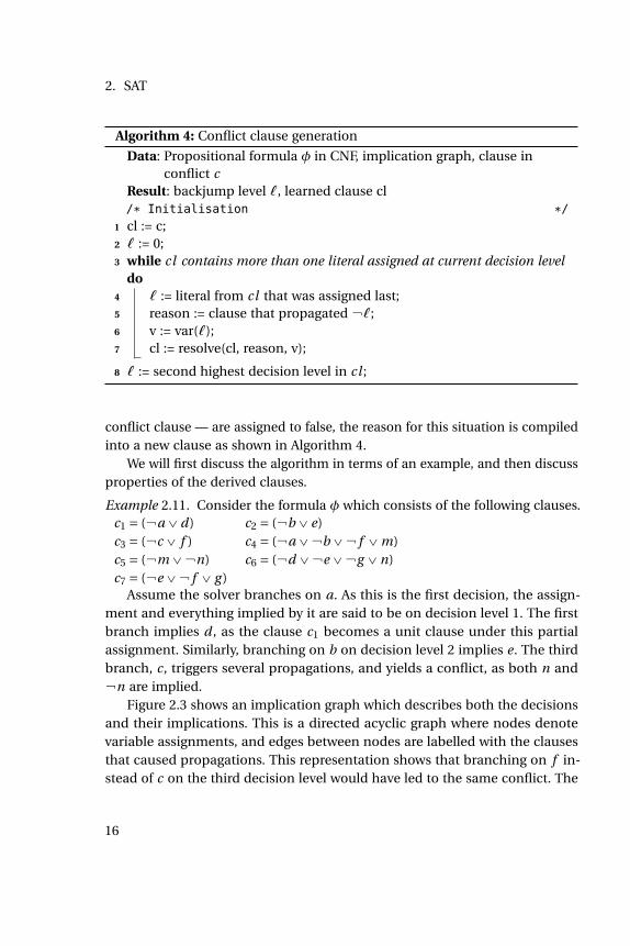
conflict clause — are assigned to false, the reason for this situation is compiledinto a new clause as shown in Algorithm 4.
We will first discuss the algorithm in terms of an example, and then discussproperties of the derived clauses.
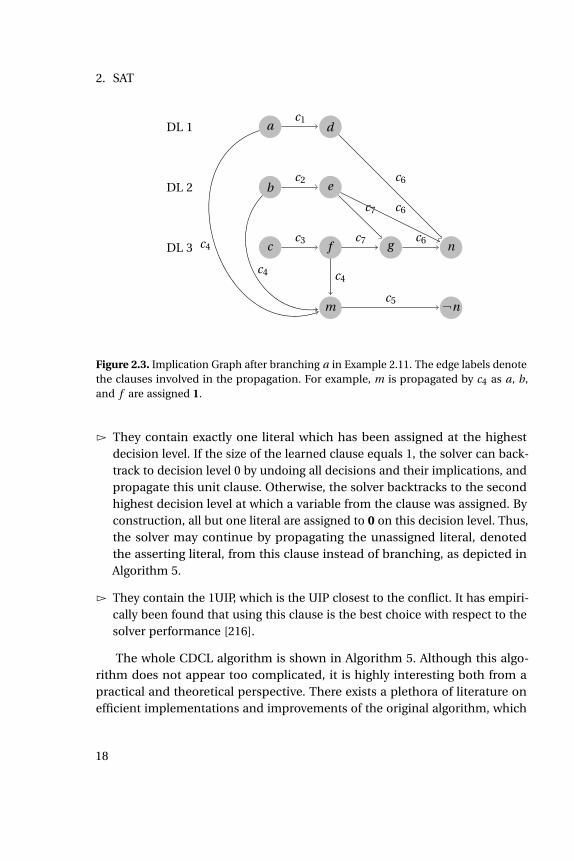
Example 2.11. Consider the formula φ which consists of the following clauses.c1 = ( a_d) c2 = ( b_e)c3 = ( c_ f ) c4 = ( a_ b_ f _m)c5 = ( m_ n) c6 = ( d_ e_ g _n)c7 = ( e_ f _ g )
Assume the solver branches on a. As this is the first decision, the assign-ment and everything implied by it are said to be on decision level 1. The firstbranch implies d , as the clause c1 becomes a unit clause under this partialassignment. Similarly, branching on b on decision level 2 implies e. The thirdbranch, c, triggers several propagations, and yields a conflict, as both n and n are implied.
Figure 2.3 shows an implication graph which describes both the decisionsand their implications. This is a directed acyclic graph where nodes denotevariable assignments, and edges between nodes are labelled with the clausesthat caused propagations. This representation shows that branching on f in-stead of c on the third decision level would have led to the same conflict. The
16
2.2. Proofs and Complexity
node labelled with f is called a unique implication point (UIP) [196], as it ison all paths from the decision on the last decision level, c, to the conflictingassignments.
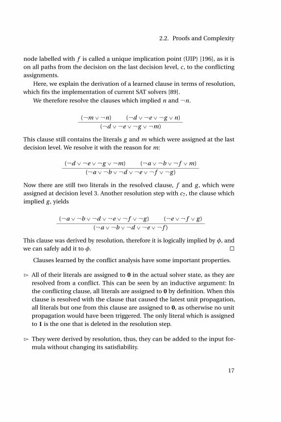
Here, we explain the derivation of a learned clause in terms of resolution,which fits the implementation of current SAT solvers [89].
We therefore resolve the clauses which implied n and n.
( m_ n) ( d_ e_ g _n)
( d_ e_ g _ m)
This clause still contains the literals g and m which were assigned at the lastdecision level. We resolve it with the reason for m:
( d_ e_ g _ m) ( a_ b_ f _m)
( a_ b_ d_ e_ f _ g )
Now there are still two literals in the resolved clause, f and g , which wereassigned at decision level 3. Another resolution step with c7, the clause whichimplied g , yields
( a_ b_ d_ e_ f _ g ) ( e_ f _ g )
( a_ b_ d_ e_ f )
This clause was derived by resolution, therefore it is logically implied by φ, andwe can safely add it to φ. ä
Clauses learned by the conflict analysis have some important properties.
Ź All of their literals are assigned to 0 in the actual solver state, as they areresolved from a conflict. This can be seen by an inductive argument: Inthe conflicting clause, all literals are assigned to 0 by definition. When thisclause is resolved with the clause that caused the latest unit propagation,all literals but one from this clause are assigned to 0, as otherwise no unitpropagation would have been triggered. The only literal which is assignedto 1 is the one that is deleted in the resolution step.
Ź They were derived by resolution, thus, they can be added to the input for-mula without changing its satisfiability.
17
2. SAT
DL 1
DL 2
DL 3
a d
b e
c f g
m
n
n
c1
c2
c3c4
c4 c4
c7
c7
c6
c6
c6
c5
Figure 2.3. Implication Graph after branching a in Example 2.11. The edge labels denotethe clauses involved in the propagation. For example, m is propagated by c4 as a, b,and f are assigned 1.
Ź They contain exactly one literal which has been assigned at the highestdecision level. If the size of the learned clause equals 1, the solver can back-track to decision level 0 by undoing all decisions and their implications, andpropagate this unit clause. Otherwise, the solver backtracks to the secondhighest decision level at which a variable from the clause was assigned. Byconstruction, all but one literal are assigned to 0 on this decision level. Thus,the solver may continue by propagating the unassigned literal, denotedthe asserting literal, from this clause instead of branching, as depicted inAlgorithm 5.
Ź They contain the 1UIP, which is the UIP closest to the conflict. It has empiri-cally been found that using this clause is the best choice with respect to thesolver performance [216].
The whole CDCL algorithm is shown in Algorithm 5. Although this algo-rithm does not appear too complicated, it is highly interesting both from apractical and theoretical perspective. There exists a plethora of literature onefficient implementations and improvements of the original algorithm, which
18

2.2. Proofs and Complexity
Algorithm 5: The CDCL algorithm
Data: Propositional formula φ in CNFResult: 1 if φ is satisfiable, and 0 otherwise/* Initialisation */
1 DL=0;2 while true do3 if propagate() = Conflict then4 if D L =0 then5 return 0;6 else7 (newDL, learned clause) := analyse_conflict();8 Add learned clause;9 backtrack(newDL);
10 DL := newDL;
11 else12 if Free variables remaining then13 ` := find_branching_literal();14 DL := DL+1;15 assign `= 1;16 else
/* All variables are assigned without a conflict */
17 return 1;
will be discussed in Section 2.3. When run on unsatisfiable formulas, CDCL-based SAT solvers create a proof of unsatisfiability based on the clauses theylearn during search, i. e., a resolution proof. This clause learning process is notdirected, as in the DP algorithm, it is rather guided by the search. The next sec-tion will present some foundations for the structure of proofs generated in thisway. Afterwards, details concerning the implementation of propagation andbranching are explained, which were only sketched in the above presentation.
19

2. SAT
2.2.5 Underlying Proof Systems
In this section, we will consider proof systems for propositional logic. This is ofinterest for several reasons. Firstly, analysing the behaviour of an actual solverimplementation is hard due to the heuristics used in it. Therefore, it is usefulto relate the proofs generated by a solver to some proof system S: If it can beshown that proofs generated by the solver on some formula φ correspond toproofs in S, then the proof generated by the solver cannot be smaller than thesmallest proofs derivable in S.
Secondly, analysing the weaknesses of such a proof system may yield in-sights in weaknesses of solver implementations. This topic will also be relevantin Chapter 3.
Fourthly, it is a fundamental problem in computer science. If there was asystem that generates proofs for the unsatisfiability of a formula such that thesize of these proofs is polynomially bounded by the size of the input formula,and they could be verified by a deterministic Turing machine in polynomialtime, this would imply that NP is closed under complementation, and thereforethat N P = coN P [78].
Formally [34], a proof system is a polynomial-time computable predicate S
such that
F P T AU T ØDp.S(F, p),
i. e., F is tautological if and only if there is a proof p that is recognised by S. Inthe literature, the notion of proof systems is sometimes used interchangeablywith inference systems that can be used to create a proof [33, 34, 50].
This section will be concerned with the proofs of unsatisfiability for a propo-sitional formula, which implies that its negation is tautological; thus, the abovenotation is also applicable.
We will discuss only proof systems based on resolution, as these form thefoundation of the proofs generated by DP, DPLL or CDCL SAT solvers.
Comparison of proof systems
When discussing the relative strength of proof systems, it is crucial to have a no-tion of whether one proof system is stronger than another. The first definitiongives a notion that one proof system is at least as strong as another one.
20

2.2. Proofs and Complexity
Definition 2.12 (p-simulation [209]). Given two proof systems S1 and S2, S1
p-simulates S2 if there exists a polynomial-time computable function f suchthat for every unsatisfiable formula φ and proof p,
S1(φ, f (p))Ø S2(φ, p).
Given a resolution refutation, there are different metrics to estimate itscomplexity like the number of symbols required to encode it into a string [79],or its width which is defined as the maximum size of a clause in it [38]. Here,we will consider the complexity in terms of resolution steps performed.
Definition 2.13 (Complexity of a resolution refutation [113]). Let Γ= c0, . . . ,ck
denote a resolution refutation of a formula φ=∧ni=0 ci . Then, the complexity
of Γ is the number of clauses generated for the refutation i. e., k´n.
With this notion of the complexity of a proof, proof systems can be com-pared to each other. A common tool is to consider families of formulas whichare easy to prove for one, but hard to prove for another proof system.
Definition 2.14 (Separation of proof systems [6]). Let F denote a family ofunsatisfiable SAT formulas, and S1, S2 be two proof systems such that S1
p-simulates S2. Furthermore, let p1(φ) (p2(φ)) denote a shortest proof forsome formula φ P F accepted by S1 (S2). If there exists a function f suchthat |p1(φ)|ď f (|p2(φ)|) for all φ PF, then f separates S1 from S2. If f is expo-nential, then there is an exponential separation between S1 and S2.
Given this notion, we discuss the relative strength of different restrictedversions of resolution, and relate them to algorithms which yield proofs in therespective proof system.
In order to characterise these different resolution refinements, it is helpfulto describe the resolution proof as a directed, acyclic graph [58]. The nodes arelabelled with clauses derived in the proof and clauses from the input formula.For each clause derived by resolution, there are two edges pointing to theclauses that it was derived from. These edges are labeled with the variable thatwas removed in the respective resolution step.
General Resolution
General resolution proofs are sometimes also called unrestricted [109]: Here,the proof is just a sequence of clauses, beginning with the original formula,
21
2. SAT
such that every clause generated for this proof is the resolvent of two clauseswhich either belong to the original formula, or have been derived before. Hakenproved in 1985 that there is a family of formulas for which the shortest generalresolution proof has exponential size [113]. These formulas are often referredto as “pigeonhole principle”, as they seek for an one-to-one mapping of n +1pigeons to n holes. Alternatively, this can be seen as the question for a n-colouring of a complete graph Kn+1. It has been shown that clause learningSAT solver are as strong as general resolution [181].
Accordingly, every SAT solver based on the CDCL algorithm requires anexponential running time on the pigeon hole formulas.
Next, we will consider restricted forms of resolution refutations, discusstheir respective strengths, and relate them to the DPLL and DP algorithm,respectively.
Tree Resolution
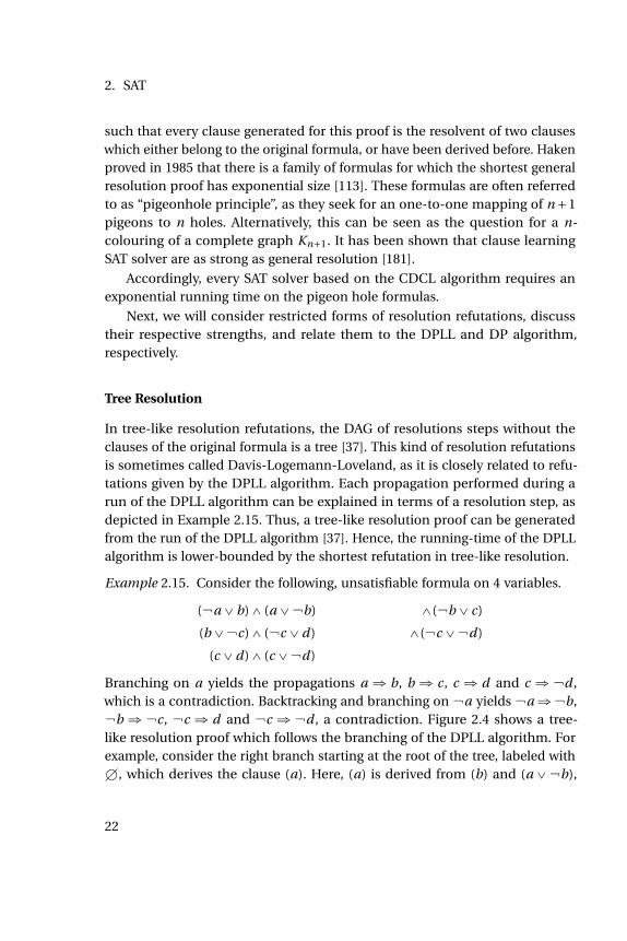
In tree-like resolution refutations, the DAG of resolutions steps without theclauses of the original formula is a tree [37]. This kind of resolution refutationsis sometimes called Davis-Logemann-Loveland, as it is closely related to refu-tations given by the DPLL algorithm. Each propagation performed during arun of the DPLL algorithm can be explained in terms of a resolution step, asdepicted in Example 2.15. Thus, a tree-like resolution proof can be generatedfrom the run of the DPLL algorithm [37]. Hence, the running-time of the DPLLalgorithm is lower-bounded by the shortest refutation in tree-like resolution.
Example 2.15. Consider the following, unsatisfiable formula on 4 variables.
( a_b)^ (a_ b) ^( b_ c)
(b_ c)^ ( c_d) ^( c_ d)
(c_d)^ (c_ d)
Branching on a yields the propagations a ñ b, b ñ c, c ñ d and c ñ d ,which is a contradiction. Backtracking and branching on a yields añ b, b ñ c, c ñ d and c ñ d , a contradiction. Figure 2.4 shows a tree-like resolution proof which follows the branching of the DPLL algorithm. Forexample, consider the right branch starting at the root of the tree, labeled withH, which derives the clause (a). Here, (a) is derived from (b) and (a_ b),
22

2.2. Proofs and Complexity
H
( a)
( b)
( c)
( c_ d) ( c_d)
( b_ c)
( a_b)
(a)
(b)
(c)
(c_ d) (c_d)
(b_ c)
(a_ b)
Figure 2.4. Tree-like resolution proof represented as DAG
which can be related to the unit propagation a ñ b in the run of the DPLLalgorithm. ä
The weakness of tree-like resolution refutations can be seen analogously tothe weakness of the DPLL algorithm, which cannot learn from failed search inone part of the search space, and therefore repeatedly performs similar work.Tree-like resolutions may not re-use clauses from one part of the derivationtree in another part.
There are families of formulas for which tree-like resolution proofs have size
2Ω
(n
logn
), where n denotes the size of the input formula. On the contrary, there
exist general resolution proofs of size O(n) for these formulas [37]. As everytree-like resolution proof is also a general resolution proof, general resolutionp-simulates tree-like resolution, hence general resolution is strictly strongerthan tree-like resolution.
We will reconsider this gap between the respective proof systems in Chap-ter 3, as backtracking algorithms for CP solving have the same weakness as theDPLL algorithm, and are thus outperformed by clause learning solvers.
23
2. SAT
Regular Resolution
Regular resolution proofs (REG) are a subset of general resolution proofs. Here,on every path in the respective DAG which starts from the empty clause, everyvariable may appear at most once as label of an arc.
This can be further restricted to ordered resolution proofs [108], wherethe variables occurring on paths starting from the empty clause are orderedaccording to the same ordering. These proofs are also called Davis-Putnam,as they correspond to proofs generated by the DP algorithm. There exists afamily of formulas for which proofs in ordered resolution have size nO(log(logn)),whereas general resolution proofs of size O(n4) exist [108]. This result was im-proved by Bonet et al., and later Urquhart, who gave an exponential separationbetween regular and general resolution [50, 208]. As ordered resolution proofsare also regular, this implies an exponential separation between ordered andgeneral resolution, which may be seen as a theoretical explanation for thebetter performance of CDCL based SAT solvers, compared to the DP algorithm.
Extended Resolution
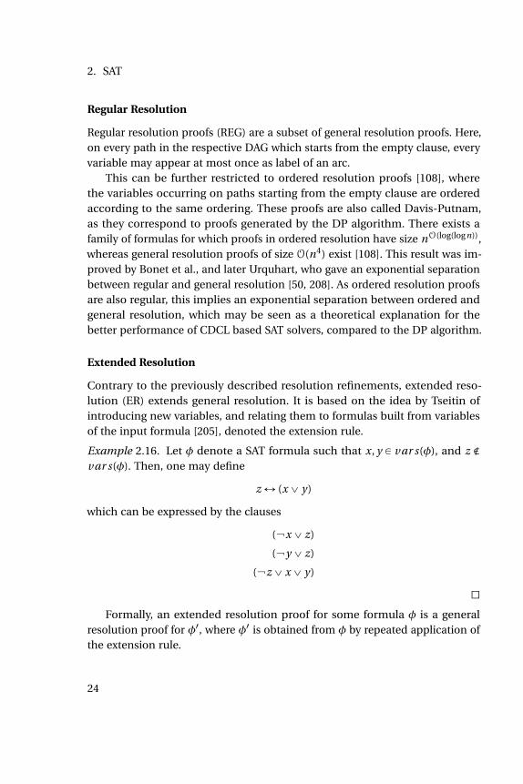
Contrary to the previously described resolution refinements, extended reso-lution (ER) extends general resolution. It is based on the idea by Tseitin ofintroducing new variables, and relating them to formulas built from variablesof the input formula [205], denoted the extension rule.
Example 2.16. Let φ denote a SAT formula such that x, y P var s(φ), and z ∉var s(φ). Then, one may define
zØ (x_ y)
which can be expressed by the clauses
( x_ z)
( y_ z)
( z_x_ y)
äFormally, an extended resolution proof for some formula φ is a general
resolution proof for φ1, where φ1 is obtained from φ by repeated application ofthe extension rule.
24

2.2. Proofs and Complexity
Interestingly, this yields a stronger proof system. Intuitively, this corre-sponds to the size of SAT encodings: By the Tseitin encoding, every propo-sitional formula can be encoded in conjunctive normal form without asymptot-ically increasing its size by introducing new variables, whereas the encoding ofsimple formulas may become exponentially large if no new variables are used.In resolution proofs without the extension rule, only clauses are derived, butno addition of new variables is allowed.
Cook proved that there exist polynomial size proofs for the pigeon holeprinciple using extended resolution [76]. However, if there were polynomialsize extended resolution refutations for every unsatisfiable SAT formula, thiswould imply N P = coN P [50]. Thus, there has been work both in deepening theunderstanding of extended resolution [142] and in proving super-polynomiallower bounds on the proof size [206].
The strength of ER has attracted interest in using it in SAT solvers. Au-demard et al. modified their SAT solver GLUCOSE, allowing it to apply theextension rule [14]. While successful on some formulas, it appears hard todecide when to apply the extension rule in general. Furthermore, the solverhas to be forced to preferably use the newly introduced literals in propagationsand conflict analysis.
Example 2.17. Consider a formula φ which contains the constraint (a_b)ñ(c^d) represented by the clauses ( a_ c), ( a_d), ( b_d) and ( b_d).One may seek to introduce a new variable x which indicates that independentlyof whether a or b are set to true, this implies c and d . x can be defined byterms of the extension rule ( x_a_b), ( a_x) and ( b_x). Then, resolutionyields
( b_x)( a_ c) ( x_a_b)
( x_b_ c)( x_ c)
Equivalently, x ñ d can be derived. Once a clause learning solver detects aconflict during its search, it may use x in the newly learned clause rather thana or b, which is a more general no-good. However, propagation is typically im-plemented as a breadth-first search [89], thus, setting a or b to 1 will propagatec and d without considering x, a problem that was encountered in [14]. ä
Chu et al. used problem-specific knowledge to find good definitions forwhich they applied extended resolution in [65].
25
2. SAT
Furthermore, it has been suggested to use the extension rule as inspirationof a preprocessing step, denoted by Bounded Variable Addition (BVA) [154].
2.3 Techniques & Implementations
We will now consider techniques which were presented in seminal papers,and are used in practically all modern SAT solvers. These techniques considerlearning clauses, efficient data structure for propagations, branching, restartingand the deletion of learned clauses.
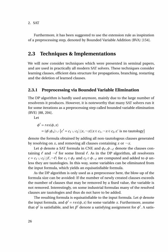
2.3.1 Preprocessing via Bounded Variable Elimination
The DP algorithm is hardly used anymore, mainly due to the large number ofresolvents it produces. However, it is noteworthy that many SAT solvers run itfor some iterations as a preprocessing step called bounded variable elimination(BVE) [88, 204].
Let
φ1 = r es(φ, x)
= (φzφx )Yc 1 = c1Y c2zx, x|x P c1, x P c2,c’ is no tautology
denote the formula obtained by adding all non-tautologous clauses generatedby resolving on x, and removing all clauses containing x or x.
Let φ denote a SAT formula in CNF, and φ`,φ ` denote the clauses con-taining ` and ` for some literal `. As in the DP algorithm, all resolventsc = c1Y c2z`, ` for c1 Pφ` and c2 Pφ ` are computed and added to φ un-less they are tautologies. In this way, some variables can be eliminated fromthe input formula, which yields an equisatisfiable formula.
As the DP algorithm is only used as a preprocessor here, the blow-up of theformula size can be avoided: If the number of newly created clauses exceedsthe number of clauses that may be removed by a fixed value, the variable isnot removed. Interestingly, on some industrial formulas many of the resolvedclauses are tautologies and thus do not have to be added.
The resulting formula is equisatisfiable to the input formula. Let φ denotethe input formula, and φ1 = r es(φ, x) for some variable x. Furthermore, assumethat φ1 is satisfiable, and let β1 denote a satisfying assignment for φ1. A satis-
26
2.3. Techniques & Implementations
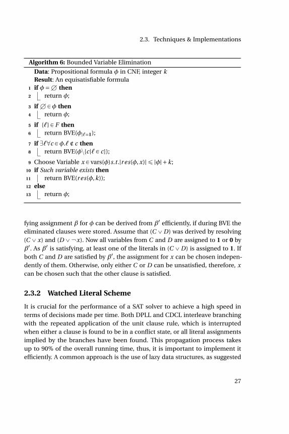
Algorithm 6: Bounded Variable Elimination
Data: Propositional formula φ in CNF, integer kResult: An equisatisfiable formula
1 if φ=H then2 return φ;
3 if HPφ then4 return φ;
5 if ` P F then6 return BVE(φ|`=1);
7 if D`@c Pφ.` ∉ c then8 return BVE(φzc|` P c);
9 Choose Variable x P vars(φ)s.t .|r es(φ, x)|ď |φ|+k;10 if Such variable exists then11 return BVE(r es(φ,k));12 else13 return φ;
fying assignment β for φ can be derived from β1 efficiently, if during BVE theeliminated clauses were stored. Assume that (C_D) was derived by resolving(C_x) and (D_ x). Now all variables from C and D are assigned to 1 or 0 byβ1. As β1 is satisfying, at least one of the literals in (C_D) is assigned to 1. Ifboth C and D are satisfied by β1, the assignment for x can be chosen indepen-dently of them. Otherwise, only either C or D can be unsatisfied, therefore, xcan be chosen such that the other clause is satisfied.
2.3.2 Watched Literal Scheme
It is crucial for the performance of a SAT solver to achieve a high speed interms of decisions made per time. Both DPLL and CDCL interleave branchingwith the repeated application of the unit clause rule, which is interruptedwhen either a clause is found to be in a conflict state, or all literal assignmentsimplied by the branches have been found. This propagation process takesup to 90% of the overall running time, thus, it is important to implement itefficiently. A common approach is the use of lazy data structures, as suggested
27

2. SAT
Algorithm 7: Naïve BCP
Data: Propositional formula φ in CNF, literal ` to propagateResult: Conflicting clause c if conflict occurred, and null otherwise
1 prop_queue := `;2 while prop_queue is not empty do
/* Take next literal from queue */
3 Take ` P prop_queue;4 prop_queue := prop_queuez`;5 val(`) := 1;
/* Check all clauses containing ` */
6 for c Pφ ` do7 if D`1 P c.val (`1) = 1 then
/* Clause is already satisfied */
8 continue;
/* Count number of literals assigned to false */
9 falseLits := |`1 P c|val (`1) = 0|;10 if falseLits = |c| then
/* Clause is in conflict */
11 return c;12 else if falseLits = |c|´1 then
/* Unit propagate */
13 Choose `1 as unassigned literal from c;14 prop_queue := prop_queue Y`1;15 val(`1) := 1;
16 return null;
in [162]. A naïve implementation may keep a list for each literal, containingthe clauses in which the negation of this literal is contained. Once the literalis set, either by branching or implication, each of the clauses in this list ischecked: If all but one literals in it are set to 0, the remaining literal is impliedand propagated, unless it is set to true already. If all literals are assigned tofalse, a conflict is detected. The pseudocode for the propagation of one literalis given in Algorithm 7.
Here, we assume a function val which returns the current valuation of a
28
2.3. Techniques & Implementations
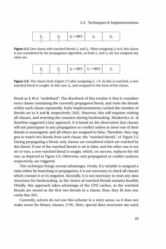
l1 l2 l3 = 0@1 l4 l5
Figure 2.5. One clause with watched literals l1 and l2. When assigning l3 to 0, this clauseis not considered by the propagation algorithm, as both l1 and l2 are not assigned anyvalue yet.
l4 l2 l3 = 0@1 l1 = 0@2 l5
Figure 2.6. The clause from Figure 2.5 after assigning l1 = 0. As this is watched, a newwatched literal is sought, in this case l4, and swapped to the front of the clause.
literal as 1, 0 or “undefined”. The drawback of this routine is that it considersevery clause containing the currently propagated literal, and visits the literalswithin each clause repeatedly. Early implementations cached the number ofliterals set to 1 and 0, respectively [162]. However, this still requires visitingall clauses, and resetting the counters during backtracking. Moskewicz et. altherefore suggested a lazy approach. It is based on the observation that clauseswill not participate in any propagation or conflict unless at most one of theirliterals is unassigned, and all others are assigned to false. Therefore, they sug-gest to watch two literals from each clause, the “watched literals”, cf. Figure 2.5.During propagating a literal, only clauses are considered which are watched bythis literal. If one of the watched literals is set to false, and the other one is notset to true, a new watched literal is sought, which, on success, replaces the oldone, as depicted in Figure 2.6. Otherwise, unit propagation or conflict analysis,respectively, are triggered.
This technique brings several advantages. Firstly, if a variable is assigned avalue either by branching or propagation, it is not necessary to check all clauseswhich contain it or its negation. Secondly, it is not necessary to reset any datastructures for backtracking, as the choice of watched literals remains feasible.Thirdly, this approach takes advantage of the CPU caches, as the watchedliterals are stored as the first two literals in a clause, thus, they fit into onecache line [62].
Currently, solvers do not use this scheme in a strict sense, as it does notmake sense for binary clauses [179]. Here, special data structures are used,
29

2. SAT
where the watch lists contain the other literals in the respective clause ratherthan a pointer to the clause.
2.3.3 Branching
The DPLL algorithm described in Section 2.2.3 contains the line “Choose vari-able x. . .” in which the decision is made how to branch next. There is no expla-nation here how to make this choice. A deterministic polynomial-time algo-rithm that, when given a propositional formula φ, returns a literal ` such thatφ|` is equisatisfiable to φ would imply P = N P .
Thus, several heuristics have been suggested to find good literals for branch-ing. Jeroslaw and Wang suggested in [129] to choose a literal ` which maximises∑
cPφ:`Pc 2´|c|, where φ is the input formula. The idea behind this choice is thatpicking a literal which occurs often on short clauses will satisfy them, andleave some other literals in long clauses such that it is likely that these can besatisfied as well. One may either compute these values statically, or dynamicallybefore every branching decision [196]. The latter heuristic, dynamic largestindividual sum (DLIS) considers the fact that branching and subsequent unitpropagations may significantly change the importance of different literals. Forexample, occurrences in a clause should only be counted if the clause is notalready satisfied under the current partial assignment.
These heuristics come with some drawback: Either it is computationallyexpensive to compute the ranking of each literal before every decision, or it isstatic and does not consider learned clauses.
The solver ZChaff [162] introduced a new technique, called variable stateindependent decaying sum (VSIDS). Here, there is a counter for every literal.Whenever a (learned) clause is added to the database, the counter for eachliteral in it is incremented. When branching, the literal with the highest countervalue is chosen. To emphasise on conflict clauses learned recently, these coun-ters are divided by some constant c > 1 periodically. As the counter values canbe stored in a priority queue, implemented as a heap, it is significantly faster tofind a new branching literal. Furthermore, it proved beneficial for SAT solversto focus on recent conflicts. Most current SAT solvers use variations of this tech-nique [17, 44, 89]. Here, the counter is often called activity of a variable. Thesevariations include the choice of literals for which the activity is increased [17],the amount of increase, or the frequency of decrease [89]. Interestingly, VSIDS
30
2.3. Techniques & Implementations
seems to be able to identify important variables in the formula, and lead thesolver to consider these preferably [134, 149].
Another important extension is phase saving. Assume a formula φ=φ1^φ2with vars(φ1)Xvars(φ2) =H. Furthermore assume that a solver has found apartial assignment β1 satisfying φ1. Then, a bad branching decision which is notcompatible with β1 may force the solver to perform unnecessary work to finda satisfying assignment for φ1 again. Therefore, Pipatsrisawat and Darwichesuggested to store the last polarity that a variable was assigned to, and re-use itin the next branching decision [180].
2.3.4 Conflict Driven Clause Learning
The concept of CDCL was briefly introduced in Section 2.2.4. In theory, a SATsolver may resolve any two fitting clauses, and add them to its database, whichwould yield an algorithm similar to DP, except for the order in which clausesare learned. However, CDCL solvers run a search to find a solution for theinput formula, and learn clauses during this process. Thus, when the result isUNSAT, this is proven by a resolution proof which was led by the search for aSAT result. This works surprisingly well, and current SAT solvers implementseveral techniques to increase their efficiency. In this section, we will reviewsome techniques related to the learning process.
Clause Minimisation
The minimisation of learned clauses was introduced in [202]. Consider againthe learned clause from Example 2.11. It contains all literals set at the decisionlevels 1 and 2, which in fact is not necessary. The literal d was set due to thebinary clause ( a_d). Now a is also contained in the learned clause, thus,we may remove d from it. The reason for this is just a resolution step
( a_ b_ d_ e_ f ) ( a_d)
( a_ b_ e_ f )
This is called self-subsuming resolution, as the result subsumes the learnedclause. Thus, the subsuming clause can be added instead of the firstly learnedclause. Furthermore, this step can be repeated for e, gaining
31

2. SAT
( a_ b_ e_ f ) ( b_e)
( a_ b_ f )
In this example, only binary clauses were used, but this technique can alsohandle non-binary clauses.
Literal Block Distance
The literal block distance (LBD) was introduced in [19] to estimate the valueof learned clauses. Consider a learned clause in the moment when it waslearned, i. e., before a backjump was performed. Then, all literals in this clauseare assigned to 0 at different decision levels. The LBD value is defined as thenumber of different decision levels on which literals from this clause wereassigned.
The idea is that literals which were assigned at the same decision level,called a block, are likely to be linked together directly. Thus, a learned clausecreates some connection between the blocks in it, which is considered helpful.The authors call learned clauses with a LBD of 2 “glue clauses”, as in theseclauses there is exactly one literal from the decision level on which the conflictoccurred; all other literals were assigned at the same decision level. Therefore,this creates a strong link between the asserting literal and the remaining literals.These so-called “glue clauses” inspired the name of the solver GLUCOSE.
The LBD value of learned clauses is used for determining which clauses areworth being kept in the clause database of a CDCL solver, as we will discussin the next section. Furthermore, it is used to trigger solver restarts (cf. Sec-tion 2.3.5) and to control communication in parallel solvers (cf. Section 2.5.1).
Clause Deletion Strategies
CDCL based SAT solvers learn many clauses during a solver run. On the onehand, this is beneficial as these learned clauses allow for more propagationsduring search, and they are the foundation of UNSAT proofs, as shown in theprevious section. On the other hand, keeping a lot of learned clauses slowsdown the propagation process, and may even cause the solver to run out ofmemory. Therefore, solvers clean their learned clause database regularly anddelete some of the learned clauses [19, 111, 126, 169].
MINISAT uses an activity value for each clause, similar to the activitiesused for variables in the VSIDS heuristic. The activity of clauses seen in the
32

2.3. Techniques & Implementations
analysis of conflicts is increased by some value, and this value is multipliedby a constant c > 1 after every conflict analysis, which emphasises on recentlylearned clauses. If the size of the learned clause database reaches some thresh-old, which depends on the number of clauses in the input formula, half of theclauses with smaller activities are deleted if their size is larger than two. Binaryclauses are kept forever.
On some large formulas, MINISAT allows for a large amount of learnedclauses. In the case of formulas which require a large proof this behaviour isextremely beneficial, as we will show in Chapter 4.
On the contrary, GLUCOSE is quite successful using a totally different strat-egy. Here, clauses are ranked by their LBD value as primary key. “Glue clauses”,i. e., clauses with a LBD value of 2, are never deleted. Furthermore, cleaning ofthe clause database is triggered according to some slowly increasing sequencewhich is independent of the size of the input formula. On many formulas, thisidea works very well. One reason can be seen in the fact that many learnedclauses propagate once — just after they have been learned — and are hardlyused afterwards [18, 19]. Therefore, it may be a reasonable decision to reducethe clause database aggressively.
In [169], both strategies were mixed. The solver keeps clauses with very lowLBD value forever, whereas clauses with higher LBDs are managed based ontheir activities.
Another approach is the freezing of clauses [15]. The authors suggest adynamic measure, denoted by “phase saving based quality measure” (psm) toestimate the importance of a learned clause in the current part of the searchspace. Given a set of assigned literals P, the psm of a clause c is defined aspsm(c,P) = |PX c|. If this value is large, then it is considered unlikely that theclause will propagate, as many of its literals are likely to be satisfied. Hence, itis also unlikely that it will be involved in conflict analysis, thereby contributingto a proof. If the psm value is small, clauses are not deleted immediately, theyare set to an intermediate state, which the authors call frozen, and can bereactivated if the psm value becomes smaller again. Clauses are only deleted ifthey have not been reactivated for some time.
LBD seems to be a rather strong measure especially on formulas createdfrom Bounded Model Checking (BMC) problems. However, it does not alwayshelp: In some cases, considering the activity or size of learned clauses worksbetter. The solver we submitted to the SAT Competition 2016 used the size of
33

2. SAT
learned clauses rather than their LBD value, unless they were glue clauses, aswe will discuss in Section 2.4.
Furthermore, the decision of how, and how often, to clean the clausedatabase is non-trivial already for sequential solvers. The portfolio solverswe will discuss in Section 2.5.1 can learn a very large amount of good clauses,and it is not clear how to manage them.
2.3.5 Restarts
Modern SAT solvers restart their search after some time for different reasons.Assume again that φ is a SAT formula, and ` a literal occurring in φ. If a solvermakes a bad decision during branching, i. e., it branches on ` such that φ^`is unsatisfiable, whereas φ itself is satisfiable, then the solver must prove thatφ^` is unsatisfiable before searching for a solution for φ^ `. Thus, it maybe beneficial to restart the search after a while. Here, restarting means a back-track to decision level 0, i. e., undoing all branches. Other information gainedduring search like learned clauses, variable activities or phase information isnot deleted. Thus, the solver continues its search by branching on the vari-able with the highest VSIDS activity. This behaviour has also proven helpfulon unsatisfiable formulas, as it allows the solver to focus on hard parts of theformula [19].
MINISAT uses the Luby sequence to trigger restarts [89]. The Luby sequenceis given by
ti =
2k´1 , if i = 2k´1
ti´2k´1+1 , if 2k´1ď i < 2k´1
This is, after i restarts, MINISAT triggers a new restart after cti conflicts,were c is a constant which equals 100 in MINISAT.
Figure 2.7(a) shows the resulting restart intervals. Heule found that us-ing a smaller constant reduces the average number of conflicts required tosolve a formula [112, 183]. Biere used another restart-scheme, called “inner-outer-restarts". It uses two exponentially growing sequences, where the “inner"sequence determines the length of one restart interval. The “outer” sequence isused to reset the values of the inner sequence in order to favor short intervalsbetween restarts, as shown in Figure 2.7(b). After k restarts, the pair of inner
34
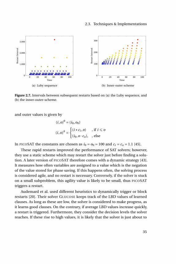
2.3. Techniques & Implementations
0 20 40 60 80 1000
1,000
2,000
3,000
Time
Res
tart
Inte
rval
(a) Luby sequence
0 20 40 60 80 1000
100
200
300
Time
Res
tart
Inte
rval
(b) Inner-outer-scheme
Figure 2.7. Intervals between subsequent restarts based on (a) the Luby sequence, and(b) the inner-outer-scheme.
and outer values is given by
(i ,o)0 = (i0,o0)
(i ,o)k =
(i ˚ ci ,o) , if i ď o
(i0,o ¨ co), , else
In PICOSAT the constants are chosen as i0 = o0 = 100 and ci = co = 1.1 [45].
These rapid restarts improved the performance of SAT solvers; however,they use a static scheme which may restart the solver just before finding a solu-tion. A later version of PICOSAT therefore comes with a dynamic strategy [43].It measures how often variables are assigned to a value which is the negationof the value stored for phase saving. If this happens often, the solving processis considered agile, and no restart is necessary. Conversely, if the solver is stuckon a small subproblem, this agility value is likely to be small, thus PICOSATtriggers a restart.
Audemard et al. used different heuristics to dynamically trigger or blockrestarts [20]. Their solver GLUCOSE keeps track of the LBD values of learnedclauses. As long as these are low, the solver is considered to make progress, asit learns good clauses. On the contrary, if average LBD values increase quickly,a restart is triggered. Furthermore, they consider the decision levels the solverreaches. If these rise to high values, it is likely that the solver is just about to
35
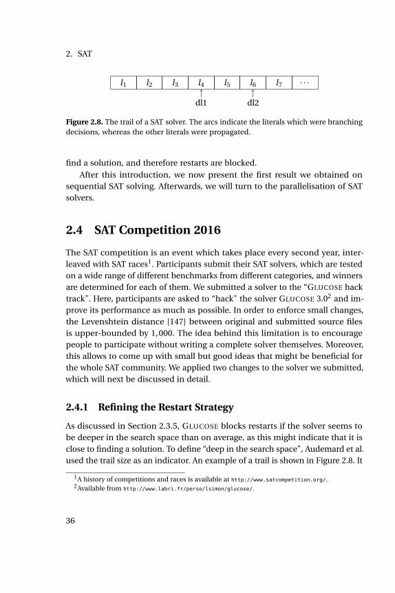
2. SAT
l1 l2 l3 l4 l5 l6 l7 ¨ ¨ ¨
dl1 dl2
Figure 2.8. The trail of a SAT solver. The arcs indicate the literals which were branchingdecisions, whereas the other literals were propagated.
find a solution, and therefore restarts are blocked.After this introduction, we now present the first result we obtained on
sequential SAT solving. Afterwards, we will turn to the parallelisation of SATsolvers.
2.4 SAT Competition 2016
The SAT competition is an event which takes place every second year, inter-leaved with SAT races1. Participants submit their SAT solvers, which are testedon a wide range of different benchmarks from different categories, and winnersare determined for each of them. We submitted a solver to the “GLUCOSE hacktrack". Here, participants are asked to “hack" the solver GLUCOSE 3.02 and im-prove its performance as much as possible. In order to enforce small changes,the Levenshtein distance [147] between original and submitted source filesis upper-bounded by 1,000. The idea behind this limitation is to encouragepeople to participate without writing a complete solver themselves. Moreover,this allows to come up with small but good ideas that might be beneficial forthe whole SAT community. We applied two changes to the solver we submitted,which will next be discussed in detail.
2.4.1 Refining the Restart Strategy
As discussed in Section 2.3.5, GLUCOSE blocks restarts if the solver seems tobe deeper in the search space than on average, as this might indicate that it isclose to finding a solution. To define “deep in the search space", Audemard et al.used the trail size as an indicator. An example of a trail is shown in Figure 2.8. It
1A history of competitions and races is available at http://www.satcompetition.org/.2Available from http://www.labri.fr/perso/lsimon/glucose/.
36
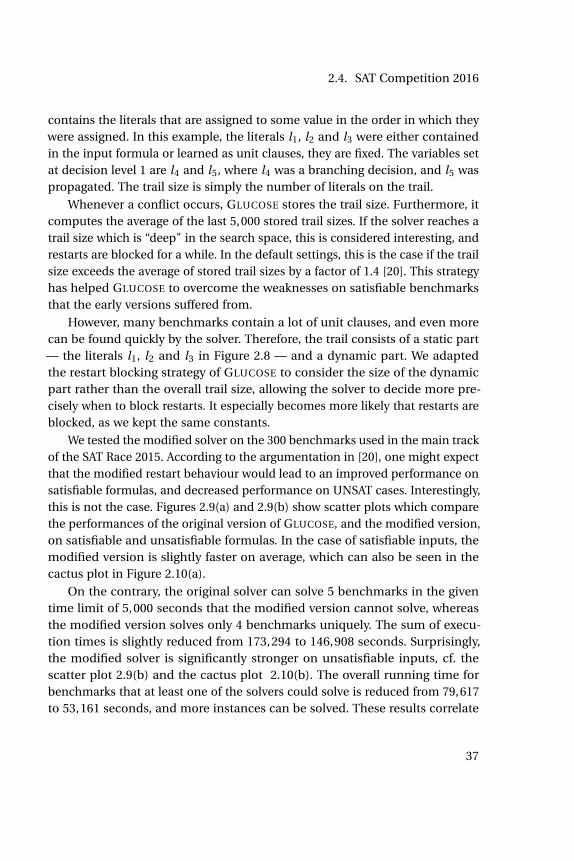
2.4. SAT Competition 2016
contains the literals that are assigned to some value in the order in which theywere assigned. In this example, the literals l1, l2 and l3 were either containedin the input formula or learned as unit clauses, they are fixed. The variables setat decision level 1 are l4 and l5, where l4 was a branching decision, and l5 waspropagated. The trail size is simply the number of literals on the trail.
Whenever a conflict occurs, GLUCOSE stores the trail size. Furthermore, itcomputes the average of the last 5,000 stored trail sizes. If the solver reaches atrail size which is “deep" in the search space, this is considered interesting, andrestarts are blocked for a while. In the default settings, this is the case if the trailsize exceeds the average of stored trail sizes by a factor of 1.4 [20]. This strategyhas helped GLUCOSE to overcome the weaknesses on satisfiable benchmarksthat the early versions suffered from.
However, many benchmarks contain a lot of unit clauses, and even morecan be found quickly by the solver. Therefore, the trail consists of a static part— the literals l1, l2 and l3 in Figure 2.8 — and a dynamic part. We adaptedthe restart blocking strategy of GLUCOSE to consider the size of the dynamicpart rather than the overall trail size, allowing the solver to decide more pre-cisely when to block restarts. It especially becomes more likely that restarts areblocked, as we kept the same constants.
We tested the modified solver on the 300 benchmarks used in the main trackof the SAT Race 2015. According to the argumentation in [20], one might expectthat the modified restart behaviour would lead to an improved performance onsatisfiable formulas, and decreased performance on UNSAT cases. Interestingly,this is not the case. Figures 2.9(a) and 2.9(b) show scatter plots which comparethe performances of the original version of GLUCOSE, and the modified version,on satisfiable and unsatisfiable formulas. In the case of satisfiable inputs, themodified version is slightly faster on average, which can also be seen in thecactus plot in Figure 2.10(a).
On the contrary, the original solver can solve 5 benchmarks in the giventime limit of 5,000 seconds that the modified version cannot solve, whereasthe modified version solves only 4 benchmarks uniquely. The sum of execu-tion times is slightly reduced from 173,294 to 146,908 seconds. Surprisingly,the modified solver is significantly stronger on unsatisfiable inputs, cf. thescatter plot 2.9(b) and the cactus plot 2.10(b). The overall running time forbenchmarks that at least one of the solvers could solve is reduced from 79,617to 53,161 seconds, and more instances can be solved. These results correlate
37

2. SAT
0 1 2 3 4 5
¨106
0
1
2
3
4
5¨106
Original solver
Solv
erw
ith
new
rest
arts
(a) SAT
0 1 2 3 4 5
¨106
0
1
2
3
4
5¨106
Original solver
Solv
erw
ith
new
rest
arts
(b) UNSAT
Figure 2.9. Pairwise comparison: Original solver vs. solver with modified restart strategy
0 20 40 60 80 100 120 1400
1
2
3
4
5
¨106
# Instances
Tim
e(m
s)
Original solverSolver with new restarts
(a) SAT
0 20 40 60 80 1000
1
2
3
4
5
¨106
# Instances
Tim
e(m
s)
Original solverSolver with new restarts
(b) UNSAT
Figure 2.10. The impact of the modified restart strategy as cactus plots.
with [43], where the author conjectures “frequent restarts may also be harmful,particularly on unsatisfiable crafted instances”.
2.4.2 Re-considering LBD
The second change we made was concerned with the management of thelearned clause database. GLUCOSE used the LBD value of learned clauses asprimary metric to decide which clauses to keep, and which to delete. We found
38
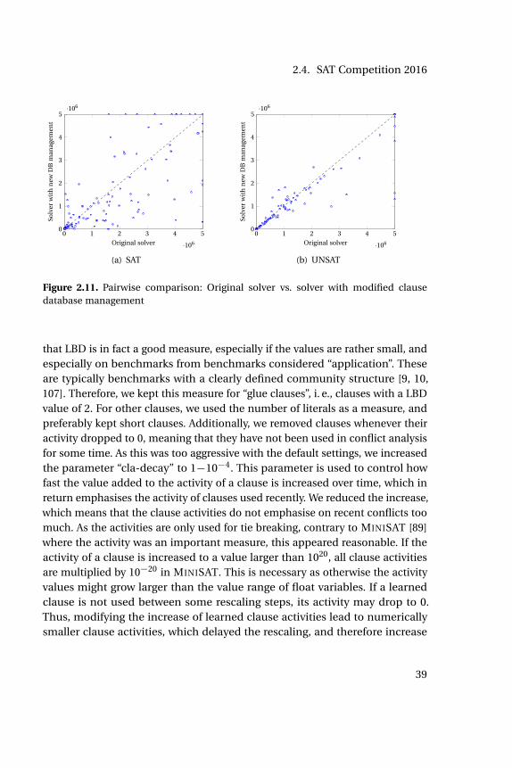
2.4. SAT Competition 2016
0 1 2 3 4 5
¨106
0
1
2
3
4
5¨106
Original solver
Solv
erw
ith
new
DB
man
agem
ent
(a) SAT
0 1 2 3 4 5
¨106
0
1
2
3
4
5¨106
Original solverSo
lver
wit
hn
ewD
Bm
anag
emen
t
(b) UNSAT
Figure 2.11. Pairwise comparison: Original solver vs. solver with modified clausedatabase management
that LBD is in fact a good measure, especially if the values are rather small, andespecially on benchmarks from benchmarks considered “application”. Theseare typically benchmarks with a clearly defined community structure [9, 10,107]. Therefore, we kept this measure for “glue clauses”, i. e., clauses with a LBDvalue of 2. For other clauses, we used the number of literals as a measure, andpreferably kept short clauses. Additionally, we removed clauses whenever theiractivity dropped to 0, meaning that they have not been used in conflict analysisfor some time. As this was too aggressive with the default settings, we increasedthe parameter “cla-decay” to 1´10´4. This parameter is used to control howfast the value added to the activity of a clause is increased over time, which inreturn emphasises the activity of clauses used recently. We reduced the increase,which means that the clause activities do not emphasise on recent conflicts toomuch. As the activities are only used for tie breaking, contrary to MINISAT [89]where the activity was an important measure, this appeared reasonable. If theactivity of a clause is increased to a value larger than 1020, all clause activitiesare multiplied by 10´20 in MINISAT. This is necessary as otherwise the activityvalues might grow larger than the value range of float variables. If a learnedclause is not used between some rescaling steps, its activity may drop to 0.Thus, modifying the increase of learned clause activities lead to numericallysmaller clause activities, which delayed the rescaling, and therefore increase
39

2. SAT
0 20 40 60 80 100 120 1400
1
2
3
4
5
¨106
# Instances
Tim
e(m
s)
Original solverNew DB management
(a) SAT
0 20 40 60 80 1000
1
2
3
4
5
¨106
# Instances
Tim
e(m
s)
Original solverNew DB management
(b) UNSAT
Figure 2.12. The impact of the modified clause database management as cactus plots.
the time until activities might eventually drop to 0.
The impact on satisfiable instances is shown in the scatter plot 2.11(a) andthe cactus plot 2.12(a). The overall running time on benchmarks solved by atleast one of the original and the modified version, decreased from 138,060to 106,201 seconds. The modified solver is especially faster on formulas ofmedium hardness, but solves 4 less benchmarks. On the contrary, the overallrunning time on unsatisfiable inputs decreases only slightly from 79,617 to74,157 seconds, but the modified solver is able to solve 5 more benchmarks.These results coincide with [12] where short clauses are found to be more usefulon satisfiable formulas, and LBD is considered more important on unsatisfiableinstances.
The performance of the submitted solver, compared with original GLU-COSE, on satisfiable and unsatisfiable formulas is shown in the scatter plots inFigs 2.13(a) and 2.13(b). Again, some diversification on satisfiable benchmarkscan be observed, and an improved average running time. In the case of unsatis-fiable benchmarks, the modified solver clearly outperforms the original version.The performance on both satisfiable and unsatisfiable instances is shown inFigure 2.14, with a clearly improved overall performance.
These performance gains could also be seen in the SAT Competition 2016 [27],where our solver won the gold medal as best GLUCOSE hack solver in the maintrack.
40

2.4. SAT Competition 2016
0 1 2 3 4 5
¨106
0
1
2
3
4
5¨106
original
mo
difi
edso
lver
(a) SAT
0 1 2 3 4 5
¨106
0
1
2
3
4
5¨106
originalm
od
ified
solv
er
(b) UNSAT
Figure 2.13. Comparison between original GLUCOSE and the hack with both optimisa-tions enabled.
0 50 100 150 200 250 3000
1
2
3
4
5
¨106
# Instances
Tim
e
standardboth optimisations
Figure 2.14. Comparison between orig-inal GLUCOSE and the hack with bothoptimisations enabled
Figure 2.15. Medal won at the SATCompetition 2016
After presenting this first result, we now turn to parallel SAT solvers. Firstly,we will give an overview over existing techniques for parallel SAT solving andactual implementations, before presenting results that were published in [97].
41

2. SAT
2.5 Parallel SAT
The success of SAT solvers has attracted interest in their parallelisation. This isnot because they naturally lend themselves to parallelisation, in contrary, thereis no obvious way to parallelise modern SAT solvers. With the improved perfor-mance of SAT solvers, they are more and more used to solve hard problems,which in return leads to an interest in even more improved performance, andmore efficient usage of modern, especially parallel, hardware.
We will start by discussing an approach which uses additional computa-tional resources to strengthen learned clauses. Next, we discuss the two mostprominent parallelisation techniques, and pose some related research ques-tions. Afterwards we discuss one result we published in [97], which tackles oneof these questions.
In sequential SAT solving, learned clauses are minimised, and then added tothe learned clause database, as discussed in Section 2.3.4. The authors of [213]suggest to use a “solver-reducer-architecture". The solver sends learned clausesto the reducer, which tries to drop some of the literals, i. e., derive a subsumingclause. If successful, this minimised clause is sent back to the solver. Thisapproach improves the performance especially on unsatisfiable formulas, butits scalability appears limited.
Another way to parallelise a SAT solver is the Shannon Expansion [195]3.Let φ denote a propositional formula, and x P vars(φ). Then,
φ” (φ^x)_ (φ^ x).
This is, if φ is satisfiable then there is at least one solution with x assigned to0, or x assigned to 1. Thus, one may split the formula into two subformulasφ1 =φ^x and φ2 =φ^ x, and solve these two formulas in parallel. Obviously,this expansion can be used recursively on the subformulas φ1 and φ2. The con-junctions that define the subformulas are often referred to as cubes [124], andthe principle of decomposing a formula with cubes is called Cube&Conquer.
Early parallel SAT solvers used this splitting approach together with loadbalancing implemented as work stealing [49, 215]. The authors report an effi-ciency of 95% on 256 CPUs. These solvers were based on the DPLL algorithm,thus, such results can be expected as there are only efficiency issues if someCPUs are idle: As depicted in Section 2.2, the DPLL algorithm does not re-use
3This expansion was mentioned already in 1848 by George Boole [51].
42
2.5. Parallel SAT
any information gained in one part of the search space in other parts. Fur-thermore, on satisfiable formulas a super-linear speed-up can be expectedfrom this approach, if the solutions are located in a small part of the searchspace [184].
By contrast, splitting the formula statically contradicts the techniques de-scribed in the previous section such as restarts and activity based search. Con-sider the formula ((a_b)^φ)^ ((a_ b)^φ) [13], where φ is unsatisfiable. ADPLL based solver will have to consider the cases b = 0 and b = 1 separately,which both simplify to φ^a, whereas a clause learning solver can solve oneof the cases, and deduce unsatisfiability of the other case from its learnedclauses easily. If b is used to split the formula, this advantage is lost unless theparallel solvers are allowed to exchange learned clauses. Furthermore, if a isused to split the formula, the subformula φ| a can be proven unsatisfiable byunit propagation. This imbalance in the hardness of the subformulas makes itnecessary to use some work balancing technique like work stealing.
In order to avoid redundant work on similar subformulas, learned clausescan be exchanged between the solver processes. Unfortunately, this approachseems to be of limited success in current solver implementations. In [145],learned clauses of size at most 2 are exchanged. This threshold on the size oflearned clauses is chosen dynamically in [153], but the performance gains arelimited.
Interestingly, for some hard combinatorial problems this approach seemsto work. The authors of [124] propose an approach where the expansion is per-formed such that the resulting subformulas become small after unit propaga-tion, and every subformula is solved by a CDCL solver. They report a speed-upfrom this approach, even if a sequential solver is used to solve one subformulaafter another. Unfortunately, it is not clear if e. g., a clause database manage-ment which is tuned to hard, combinatorial formulas might have neglectedthis effect.
Another parallel solver which splits the search space is pMiniSAT [66]. It isbased on a master-slave architecture, and the splitting is executed dynamically.If one solver is asked for a new cube, it creates one using the literal which itbranched on the lowest decision levels. Assume it was working on the cube`1^`2, and its first branching decisions were `3 and `4. Then it may extendits own cube to `1^ `2^ `3^ `4, and return the cubes `1^ `2^ `3 and`1^`2^`3^ `4. Thus the solver splits on variables that seemed interesting
43

2. SAT
to the VSIDS heuristic on the subformulas. Furthermore, the authors note thatthis approach yields many cubes which can be refuted with 1´10 conflicts.Thus, they suggest to keep a queue of cubes at the master process, which allowsfor distributing new work quickly without waiting for the reply of another slavewhere new work is stolen from.
This approach reduces the idle time of slaves, but it comes with anotherdrawback. If working on a satisfiable formula, the master may send cubes tothe slave such that every subformula which is being processed is unsatisfiable,and the cubes defining subspaces which actually contain a solution are in thework queue. Such problems are overcome in solvers like AmPharos [16], whichclearly outperforms other Cube&Conquer solvers on application benchmarks.Here, slaves work on one cube for a short time. If they neither find a solutionnor prove it unsatisfiable, they pick another cube. This comes with the advan-tage that clauses which were learned when working on one part of the searchspace, are also used for other parts. Furthermore, cubes leading to a satisfiablesubspace will eventually be considered.
These kind of problems do not arise with the other, currently more promi-nent approach in parallel SAT solving.
2.5.1 Portfolio-based Parallel SAT Solving
The portfolio approach for parallel SAT solving is based on the observation thatthe performance of sequential SAT solvers is very sensible to small changes onsome parameters, e. g., concerning the restart strategy, or the increase of VSIDSactivities.
This is exemplified by some results shown in Table 2.1 and Figure 2.16. Weran GLUCOSE on the benchmarks used in the main track of the SAT Competi-tion 2016. In the first run, we used the default random seed, and in the secondrun, we ran it 64 times with different random seeds. In both cases, a timeout of5000 seconds was used. When using a preprocessor and the default randomseed, 61 satisfiable, and 83 unsatisfiable benchmarks could be solved. Withoutpreprocessing, the results are slightly worse, with 59 and 79 solved instances.When using different random seeds and a preprocessor, 81 satisfiable bench-marks could be solved by at least one of the configurations. Without runningthe preprocessor, the number of solved satisfiable formulas increased from 59to 86. In the case of unsatisfiable benchmarks, some performance gain can
44

2.5. Parallel SAT
Table 2.1. Number of benchmarks from the SAT Competition 2016 which were solvedby GLUCOSE when running it repeatedly with different random seeds.
Configuration Presolved no PreprocessingSAT UNSAT SAT UNSAT
default 61 83 59 7964 different random seeds 81 89 86 88
0 1 2 3 4 5
¨106
0
1
2
3
4
5¨106
original
Pu
rep
ort
foli
oso
lver
Figure 2.16. Comparison of default GLUCOSE and a portfolio solver with different ran-dom seeds. The running times are given in milliseconds.
be observed, but it is not as significant. This is not too surprising as in theory,satisfiable benchmarks can be solved efficiently if the solver starts with a fittingguess on variable assignments, whereas it always has to provide a resolutionproof for unsatisfiable inputs.
The solver MANYSAT [116] won the parallel track of the SAT Race 20084,taking advantage of this instability. Here, the authors used different settings forthe restart strategy, branching, and clause learning. Furthermore, they foundthat the exchange of learned clauses significantly improves the performance.Clauses that one of the parallel solvers learns can be added to the clausedatabase of other solvers, as they are implied by the input formula. Experimen-tally, the authors found that for MANYSAT, the performance was best whenclauses with a size of at most 8 were exchanged. Later, the authors observedthat the clauses a solver learns tend to become longer over the time the solver is
4http://baldur.iti.uka.de/sat-race-2008/
45

2. SAT
running. Therefore, they suggested to adapt clause exchange dynamically [115].If only few short clauses are learned, the solvers increase the export threshold,and vice versa.
Most current portfolio-based SAT solvers also consider the LBD values fordetermining which clauses to exchange. PLINGELING shares clauses with LBDof at most 8, and size of at most 30 [44]. Furthermore, the solvers PENELOPE
and SYRUP, based on GLUCOSE, use several techniques concerned with themanagement of clause sharing. PENELOPE [12] implements freezing of clauses,as described in Section 2.3.4. Clauses which are imported from other solverscan either be set to frozen directly, or dynamically. Afterwards, freezing andreactivating are performed based on the psm measure.
SYRUP [18] performs clause exchange lazily. This is based on the observationthat many learned clauses are seen only a very few times in conflict analysis.Furthermore, on unsatisfiable formulas many learned clauses are useless inthe sense that they do not appear in the final proof of unsatisfiability [197].Thus, the authors suggest to lazily export learned clauses when they are seenin conflict analysis for the second time, and their size and LBD are belowthe respective median values of all learned clauses. They also perform lazyclause import: Imported clauses are watched only by one literal. They are onlypromoted to the two-literal-scheme when they are in conflicting state, i. e.,all of there literals are assigned to false. Thus, they are only promoted if theyprune a part of the search space that was not pruned by other clauses from thelearned clause database.
Other solvers work well, though they do not use as sophisticated techniquesfor clause exchange. In HordeSAT [29], the solvers exchange clauses once everysecond. Every solver exports clauses with a sum of sizes of at most 1,500literals, where short clauses are preferred. Furthermore, it uses hashing to filterduplicate clauses. By this, they report a super-linear speed up for up to 512processes, each of which running 4 solver threads. However, these values alsodepend on they way they are computed — with the evaluation scheme usedin [97], the speedup on 2,048 threads would have only been 4.4, and lower thanthe speed up on 1,024 threads.
There are several challenges arising in the field of parallel SAT solving.Hamadi and Wintersteiger [117] named seven challenges, including the ques-tion whether the variations of the CDCL approach are an appropriate basis forparallel solvers, or if these should be based on a totally new paradigm.
46
2.5. Parallel SAT
We will state some more challenges in the field of parallel SAT solving,mainly focussed on the portfolio approach. Afterwards, we present results forone of them, which were published in [97].
11 Challenges in Massively-Parallel Portfolio SAT Solving
1. The first questions deals with the question of how to measure the speed-upof a parallel solver. It is common to evaluate solvers on benchmarks fromSAT Competitions. These sets typically contain benchmarks that are easy,i. e., can be solved within less than a second by most sequential solvers,as well as hard benchmarks which can hardly be solved in a reasonableamount of time, even by parallel solvers. On the first kind of formulas, paral-lel solvers typically do no achieve better results than sequential ones, e. g.,because they spend some time forking MPI processes. As parallel solversare intended to solve hard problems, this is not necessarily bad, but it isimportant to be aware of this, and decide whether they should be consid-ered in an evaluation with the same weight as harder formulas. In [97], weused the some of running times on our benchmark set for the computationof speedups. This correlates to the user-experience: It compares the timerequired to solve all benchmarks with a solver on n cores with the timerequired to solve these formulas with n sequential solvers, but allowing forparallel execution of solvers on different benchmarks. Thus, this approachis somewhat realistic, but it is still pessimistic, as it does not consider thefact that a timeout has to be used especially for the sequential referencesolver. If the sequential solver cannot solve a given formula, but the parallelversion solves it, this version of computing speed-ups is biased towardsthe sequential solver. On the contrary, the authors of HordeSAT [29] com-puted speed-ups based only on benchmarks that their parallel solver couldsolve. Furthermore, they computed the overall speed-up as the arithmeticmean of the speed-ups observed on the single inputs. By this measure, theyachieved super-linear speedups on hard formulas, whereas according to ourway speed-up computation, it would have only been 4.4 on 1,024 threads.
We do not claim that our approach is the best, actually it is biased againstparallel solvers. Still, it is clear that no arithmetic means should be used, asthey emphasise good results on single tests.
Question 1. What is a fair evaluation scheme for parallel SAT solvers on a
47
2. SAT
mix of easy and very hard benchmarks?
2. It is often claimed that the scalability of portfolio solvers is limited asthe search of the single solvers synchronises over time [13]. However, itis not clear how this claimed synchronisation is defined. Considering VSIDS-activities may lead to a false-positive result: Comparing variables with highactivities between the single solvers might lead to the insight that all solversfocus on a similar subset of variables. However, this due to the nature ofVSIDS, which tends to pick central variables [134]. We conducted some testswith a student, Dennis Sen, in his Bachelor’s Thesis [194]. Here, we consid-ered the polarity vectors of the different solvers, and compared them to eachother. In these tests, we found these vectors highly volatile, and could notfind evidence of a synchronisation between solvers.
Finally, one might consider learned clauses as a criterion for the possiblesynchronisation of solvers: If clauses learned by one solver are redundant forother solvers, i. e., do not prune the search space of other solvers, this mightbe seen as a hint for synchronisation. However, checking for redundancy iscomputationally expensive, and it is not clear if this effort pays off.
In case synchronisation is detected, the first approach might be to add somerandomisation. The easiest way for this is random branching. Solvers likeGLUCOSE allow for both choosing variables randomly, and branching ona randomly chosen polarity. Using both sources of randomisation contra-dicts the idea of polarity vectors, and may, in the worst case, just result insuperfluous work.
Question 2. How can a lack of diversification in portfolio based SAT solvingbe defined and detected?
3. There is some evidence that the scalability of portfolio SAT solvers is limitedby the structure of resolution proofs [210]. The author discusses the depth ofresolution proofs in the sense that the proofs require learned clauses whichcan only be resolved from other learned clauses, which induces a sequentialstructure in the proof. This would imply a bound on the parallelisability ofportfolio solvers [133]. However, it is not clear if this is only true for someartificially created formulas, or if it also concerns so-called “real-world”problems.
48

2.5. Parallel SAT
Question 3. How deep are proofs of relevant formulas?
4. Both sequential and parallel solvers clean their databases for learned clauseregularly. In the case of sequential solvers, this process is fine-tuned towardsbenchmarks from competitions. However, parallel SAT solvers typically re-use these heuristics. Parallel portfolio solvers on hundreds of cores learn ahuge amount of clauses, and share many of them. Still, they use the sameheuristics as in the sequential case.
It is not clear how to determine a good size of the clause database of eachof the solvers. Furthermore, there is a dependancy between clause exchangeand clause management strategies. Assume a solver removes 50% of itslearned clauses whenever it cleans its clause database. Then, exchangingmore learned clauses may influence the choice of clauses kept, i. e., a higherclause exchange allows the solver to keep more clauses of medium quality.
Question 4. What is a good clause database cleaning strategy for massively-parallel portfolio solvers?
5. Which learned clauses are a good choice for exporting? This question wasalready considered in several papers [18, 115], and is one of the sevenchallenges in [117]. This question involves both the amount of clauses ex-changed, and the actual choice of a subset of learned clauses. If solvingunsatisfiable formulas, clause exchange seems to have a larger positive im-pact [29], which coincides with results from sequential SAT solving [169], andresults from our tests [97]. Most portfolio solvers export short clauses clauseswith small LBD values, i. e., based on static measures, whereas PENELOPE
export clauses lazily if they are involved in conflict analysis, and thus seeminteresting. However, these measures relate the clauses to set of learnedclauses the exporting solver is operating on; It is not clear whether this is agood measure for the usefulness for other solvers.
Question 5. What is a good clause export policy, both for satisfiable andunsatisfiable formulas?
6. Restarts are crucial for the performance of sequential CDCL solvers [20, 43,96, 112]. However, most portfolio based SAT solvers just re-use the restartpolicies of the sequential solvers they are based on.
49

2. SAT
(a) The dynamic restart policy of GLUCOSE triggers restarts if the averageLBD of learned clauses increases. More aggressive restarts might leadto more clauses with small LBD, thus turning the solvers into clauseproducers [20], which in turn create clauses that “glue” the formula. Issuch an increased amount of learned clauses helpful?
(b) Let us consider the work performed by one solver between two subse-quent restarts. The solver branches on some literals `1,`2, . . . ,`k , and isfaced with conflicts. If k1 is the lowest decision level on which a conflictoccurs, this may be seen as the refutation of the cube `1^`2^ . . .^ lk1 .In some still unpublished experiments we found that this can be usedas a hint whether portfolio solvers are better suited for some formulathan Cube&Conquer solver or vice versa: If k1 is small, this indicatesthat a Cube&Conquer solver might be a good choice, whereas largevalues for k1 indicate that the formulas is not well suited for beingsplit by short cubes. We think that this is worth a more profound re-search: does it make sense to dynamically switch between portfolioand Cube&Conquer solving?
(c) The activity values of the VSIDS heuristic are highly volatile [18]. Is thisalso a good choice for massively-parallel portfolio solvers, or does itmake sense to slightly decrease the volatility? On the one hand, forcingsolvers to remain in one part of the search space might lead to learn-ing more clauses which are relevant for this particular subspace, thusallowing them to learn stronger lemmas. On the other hand, this maylead to learning longer clauses [190] or clauses with a larger LBD value,which would reduce the amount of exported clauses.
Question 6. Are common restart-strategies well-suited for portfolio solvers?Can information about the solving progress be used to guide the parallelsolver?
7. Wieringa and Heljanko suggested a parallel solver on two cores in which onesolver is just used to strengthen the clauses learned by the other solver [213].Given one learned clause, the “reducer" branches its literals to 0, and usesBCP and the analyzeFinal-routine of MINISAT to check for a subsumingclause such that its negation unit-propagates to a conflict. This technique,which is also referred to as asymmetric branching or clause vivification [178],
50
2.5. Parallel SAT
or a similar technique might be use to minimise learned clauses beforeexporting them. However, the search for a subsuming clause somewhat con-tradicts the core idea of 1UIP learning which aims at encoding the reasonfor a conflict rather than just the decisions which, together with their im-plications, led to the conflict. Still, we consider it interesting to strengthenlearned clauses before sharing them with potentially hundreds of othersolver threads.
Question 7. Does it pay off to spend more effort in clause minimisation?
8. The notion of “clause sharing" is somewhat misleading, as portfolio solverstypically send copies of these clauses to other solver incarnations. Thus, ifseveral solvers run on the same node, clauses are stored multiply on thisnode. On the contrary, rather old solvers like MIRAXT [148] and SARTAG-NAN [140] physically share clauses between threads on a shared memorymachine. This comes with several advantages.
Ź If the solver runs on a hard formula, proofs may become large, whichmay become a problem if several solvers are executed on the same node.Therefore, a physically shared memory reduces the memory footprintsignificantly. Furthermore, the amount of memory available on hardwarelike Intel’s Xeon Phi is limited, thus this may even be mandatory whenrunning parallel SAT solvers on this kind of hardware.
Ź Communication between solver threads is easier on a shared memorymachine, which can be used to exchange information about e. g., sub-sumed clauses, as described in [140].
Ź Consider a hierarchical portfolio solver which consists of portfolio solverswhich work on a physically shared clause database on shared memorysystems, and communication between nodes is performed via MPI. Then,a learned clause could be placed in the shared clause database first, andbe sent to other nodes if it is considered relevant by other solver threads,which would result in a less local version of the lazy clause exchangepolicy described in [18].
On the other hand, using a physically shared clause database prohibits someof the techniques used to improve cache efficiency [63, 89, 156], especially
51
2. SAT
the dynamic reordering of literals in a clause. We still believe that a care-fully designed implementation can be fast enough, such that the benefitsoutweigh the decreased single thread performance.
Question 8. How can the benefits of a physically shared clause database betaken advantage of in a (hierarchical) portfolio solver?
9. How can the usefulness of a received clause be checked? In sequential SAT,a learned clause explains a conflict, and may render formerly learned clauseuseless. Even there, it’s not clear
Ź How to check if old clauses can be removed efficiently, except for sub-sumption checks.
Ź How, in the case of unsatisfiability, the finally proof is made, and whichclauses contribute to it [197].
Question 9. How can the usefulness of both a single clause and clauseexchange in general be detected during a solver run?
10. Preprocessing [88, 154, 204] and inprocessing [128, 155] are important tech-niques, especially in sequential SAT solving. Parallel bounded variable elim-ination was implemented and evaluated on a shared memory machinein [104]. However, this approach requires a synchronisation between thepreprocessing-threads which is likely to prevent this approach from scalingbeyond shared memory machines. However, bounded variable eliminationis not only useful because of the decrease in number of variables and clauses,but also as it derives subsuming clauses which improve the propagationspossible by BCP. It might be an interesting research direction to exchangeshort clauses derived in the process of variable elimination rather thanactually eliminating the variable on all nodes.
We conjecture that techniques which add clauses or variables are bettersuited for distributed parallel SAT solving.
Question 10. Which preprocessing or inprocessing techniques are helpfulin a (massively-parallel) portfolio solver?
11. Most portfolio solvers perform communication in an all-to-all manner: Aclause learned by one solver is, if so, sent to all other solvers. For a large
52
2.5. Parallel SAT
scale of parallelism this will lead to a prohibitive amount of communication.In [97], we suggested to limit the communication in terms of a communi-cation graph such that only some pairs of solvers are allowed to exchangeclauses, which will be described in the remainder of this section.
Question 11. How can the communication in a portfolio solver be con-trolled such that the solver still benefits from learned clauses, and theamount of communication does not become prohibitively large?
TOPOSAT: Communication Structures for Portfolio SAT Solvers
In this section, we present and discuss experiments which aim at answeringQuestion 11. If a portfolio solver is run on n processes, and every solving pro-cess is allowed to send some of its learned clauses to all of its neighbours, theamount of information exchanged grows by θ(n2). For large n, this becomesprohibitive both due to the amount of information transmitted through theconnecting network, and the limited ability of the single solvers to handle anarbitrary amount of clauses. This information exchange can be limited by ad-justing thresholds on when to export a clause, e. g., the maximum size or LBDvalue. Another approach is to create some locality in the parallel solver, and ex-change information locally rather than globally. This is especially advantageousif the network is heterogeneous, for example if two fast networks are connectedby a relatively slow interconnect. We therefore limited the communication byterms of a communication graph. Let p1, . . . , pn denote the processes a portfo-lio solver is made up from. For some graph G = (V ,E) with V = p1, . . . , pn, welet the solver process pi send its clauses to the processes it is connected to byan edge in G , i. e., NG (pi ), if the LBD is at most 4, a value which is quite smallcompared to the clause exchange policies e. g., used by PLINGELING [44], butseems reasonable [169]. In the case of unary and binary clauses, i. e., clausesof size at most 2, we allowed solvers to forward them if they were not knownalready, which can be checked by a simple look-up in O(1) time for unit clauses,and O(log(n)) for binary clauses. In this way, we made sure that these clauses,which we believe to significantly contribute to the solving process, eventu-ally reach all solver processes. Furthermore, we considered it unlikely that theexchange of these clauses would overload the network.
In our solver, denoted TOPOSAT after the underlying graph topology whichdetermines its communication, each solver processes runs two threads, one of
53
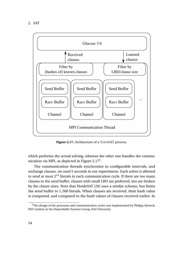
2. SAT
Figure 2.17. Architecture of a TOPOSAT process.
which performs the actual solving, whereas the other one handles the commu-nication via MPI, as depicted in Figure 2.175.
The communication threads synchronise in configurable intervals, andexchange clauses, we used 5 seconds in our experiments. Each solver is allowedto send at most 214 literals in each communication cycle. If there are too manyclauses in the send buffer, clauses with small LBD are preferred, ties are brokenby the clause sizes. Note that HordeSAT [29] uses a similar scheme, but limitsthe send buffer to 1,500 literals. When clauses are received, their hash valueis computed, and compared to the hash values of clauses received earlier. In
5The design of the processes and communication cycles was implemented by Philipp Sieweck,PhD student at the Dependable Systems Group, Kiel University.
54
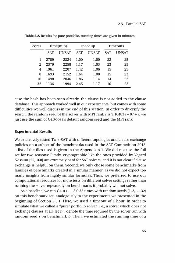
2.5. Parallel SAT
Table 2.2. Results for pure portfolio, running times are given in minutes.
cores time(min) speedup timeouts
SAT UNSAT SAT UNSAT SAT UNSAT
1 2789 2324 1.00 1.00 32 252 2379 2258 1.17 1.03 23 254 1961 2207 1.42 1.06 15 258 1693 2152 1.64 1.08 15 23
16 1498 2046 1.86 1.14 14 2232 1136 1994 2.45 1.17 10 22
case the hash has been seen already, the clause is not added to the clausedatabase. This approach worked well in our experiments, but comes with somedifficulties we well discuss in the end of this section. In order to diversify thesearch, the random seed of the solver with MPI rank i is 9.16483e +07+ i ; wejust use the sum of GLUCOSE’s default random seed and the MPI rank.
Experimental Results
We extensively tested TOPOSAT with different topologies and clause exchangepolicies on a subset of the benchmarks used in the SAT Competition 2013,a list of the files used is given in the Appendix A.1. We did not use the fullset for two reasons: Firstly, cryptographic like the ones provided by VegardNossum [25, 168] are extremely hard for SAT solvers, and it is not clear if clauseexchange is helpful on them. Second, we only chose some benchmarks fromfamilies of benchmarks created in a similar manner, as we did not expect toomany insights from highly similar formulas. Thus, we preferred to use ourcomputational resources for more tests on different solver settings rather thanrunning the solver repeatedly on benchmarks it probably will not solve.
As a baseline, we ran GLUCOSE 3.0 32 times with random seeds (1,2, . . . ,32)on this benchmark set, analogously to the experiments we presented in thebeginning of Section 2.5.1. Here, we used a timeout of 1 hour. In order tosimulate what we called a “pure” portfolio solver, i. e., a solver which does notexchange clauses at all, let ti .b denote the time required by the solver run withrandom seed i on benchmark b. Then, we estimated the running time of a
55

2. SAT
Table 2.3. TOPOSAT: Grid topology, sharing only unit clauses.
cores time(min) speedup timeouts
SAT UNSAT SAT UNSAT SAT UNSAT
1 1974 2069 1.00 1.00 19 182 1595 1688 1.23 1.22 17 184 1400 1542 1.40 1.34 12 158 1199 1438 1.64 1.44 12 14
16 917 1342 2.15 1.54 8 1332 604 1241 3.26 1.67 3 1064 547 1137 3.60 1.82 4 9
128 321 1050 6.10 1.97 1 6256 269 1003 7.33 2.06 1 6
pure portfolio solver with n processes on a benchmark b as the minimum ofthe first n random seeds,
Tn,b = min1ďiďn
ti ,b
The results are given in Table 2.2. The first column shows the number of coresused, and the next two columns show the sum of running times
∑b Tn,b both
for satisfiable and unsatisfiable formulas. The speedup, given in Columns 3 and4, is quite limited, especially in the case of unsatisfiable benchmarks. However,using 32 cores only 10 satisfiable benchmarks remain unsolved, which is a clearimprovement compared to 32 unsolved benchmarks on 1 core. As discussedin the beginning of this section, this is the expected behaviour on satisfiableformulas. In the case of unsatisfiable benchmarks, 3 more cases can be solvedwithin the given time limit when comparing the configurations on 32 and 1cores, respectively.
However, in both cases the results are rather disappointing.
We slightly increased the amount of information exchange in the nextexperiment, for which TOPOSAT was used. Here, we allowed for the exchange ofunit clauses only. The communication structure was chosen as a 2-dimensionalgrid, and solvers forwarded unit clauses. The results are given in Table 2.3.Interestingly, TOPOSAT was significantly faster than GLUCOSE 3.0 also when
56
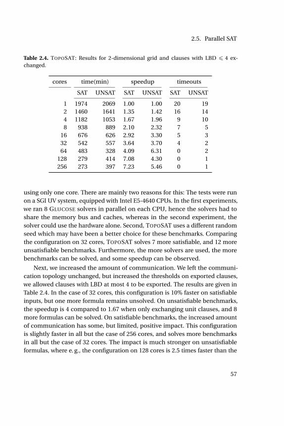
2.5. Parallel SAT
Table 2.4. TOPOSAT: Results for 2-dimensional grid and clauses with LBD ď 4 ex-changed.
cores time(min) speedup timeouts
SAT UNSAT SAT UNSAT SAT UNSAT
1 1974 2069 1.00 1.00 20 192 1460 1641 1.35 1.42 16 144 1182 1053 1.67 1.96 9 108 938 889 2.10 2.32 7 5
16 676 626 2.92 3.30 5 332 542 557 3.64 3.70 4 264 483 328 4.09 6.31 0 2
128 279 414 7.08 4.30 0 1256 273 397 7.23 5.46 0 1
using only one core. There are mainly two reasons for this: The tests were runon a SGI UV system, equipped with Intel E5-4640 CPUs. In the first experiments,we ran 8 GLUCOSE solvers in parallel on each CPU, hence the solvers had toshare the memory bus and caches, whereas in the second experiment, thesolver could use the hardware alone. Second, TOPOSAT uses a different randomseed which may have been a better choice for these benchmarks. Comparingthe configuration on 32 cores, TOPOSAT solves 7 more satisfiable, and 12 moreunsatisfiable benchmarks. Furthermore, the more solvers are used, the morebenchmarks can be solved, and some speedup can be observed.
Next, we increased the amount of communication. We left the communi-cation topology unchanged, but increased the thresholds on exported clauses,we allowed clauses with LBD at most 4 to be exported. The results are given inTable 2.4. In the case of 32 cores, this configuration is 10% faster on satisfiableinputs, but one more formula remains unsolved. On unsatisfiable benchmarks,the speedup is 4 compared to 1.67 when only exchanging unit clauses, and 8more formulas can be solved. On satisfiable benchmarks, the increased amountof communication has some, but limited, positive impact. This configurationis slightly faster in all but the case of 256 cores, and solves more benchmarksin all but the case of 32 cores. The impact is much stronger on unsatisfiableformulas, where e. g., the configuration on 128 cores is 2.5 times faster than the
57
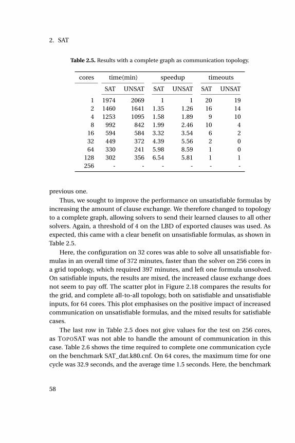
2. SAT
Table 2.5. Results with a complete graph as communication topology.
cores time(min) speedup timeouts
SAT UNSAT SAT UNSAT SAT UNSAT
1 1974 2069 1 1 20 192 1460 1641 1.35 1.26 16 144 1253 1095 1.58 1.89 9 108 992 842 1.99 2.46 10 4
16 594 584 3.32 3.54 6 232 449 372 4.39 5.56 2 064 330 241 5.98 8.59 1 0
128 302 356 6.54 5.81 1 1256 - - - - - -
previous one.
Thus, we sought to improve the performance on unsatisfiable formulas byincreasing the amount of clause exchange. We therefore changed to topologyto a complete graph, allowing solvers to send their learned clauses to all othersolvers. Again, a threshold of 4 on the LBD of exported clauses was used. Asexpected, this came with a clear benefit on unsatisfiable formulas, as shown inTable 2.5.
Here, the configuration on 32 cores was able to solve all unsatisfiable for-mulas in an overall time of 372 minutes, faster than the solver on 256 cores ina grid topology, which required 397 minutes, and left one formula unsolved.On satisfiable inputs, the results are mixed, the increased clause exchange doesnot seem to pay off. The scatter plot in Figure 2.18 compares the results forthe grid, and complete all-to-all topology, both on satisfiable and unsatisfiableinputs, for 64 cores. This plot emphasises on the positive impact of increasedcommunication on unsatisfiable formulas, and the mixed results for satisfiablecases.
The last row in Table 2.5 does not give values for the test on 256 cores,as TOPOSAT was not able to handle the amount of communication in thiscase. Table 2.6 shows the time required to complete one communication cycleon the benchmark SAT_dat.k80.cnf. On 64 cores, the maximum time for onecycle was 32.9 seconds, and the average time 1.5 seconds. Here, the benchmark
58

2.5. Parallel SAT
1 10 60
K64 time (min)
1
10
60
Gri
d 2
D,
64
core
s ti
me (
min
)
UNSAT
SAT
Figure 2.18. Scatter plot for grid and complete topology.
could be solved within 10 minutes. On a larger number of cores, the commu-nication times became prohibitive, and prevented the solver from solving thebenchmark.
So far, the results are as expected: The exchange of learned clauses is benefi-cial, especially on unsatisfiable formulas. On satisfiable benchmarks, it does notharm unless the amount of communication causes extremely large latencies.We thus sought a configuration which is still scalable, and allows for enoughclause exchange to speed up the creation of large proofs for unsatisfiable for-mulas.
First, we considered a configuration in which the degree of each node inthe communication graph depends on the total number of cores used. Everysolver was connected to O(log(n)) neighbours. For the solver with MPI rank i ,
59

2. SAT
Table 2.6. Durations of communication cycle of TOPOSAT on the formula SAT_-dat.k80.cnf
Cycle time (msec)
Procs. Kn edges max. avg. Runtime (min)
64 2016 32885 1500 10.18128 8128 400000 336630 -256 32640 - - -
we used the neighbours with MPI ranks
N (i ) = (i + j ) mod n|´nď j ď n, | j |ď log(n), j ‰ 0
Again, unit clauses were forwarded. This sparse topology was especially fastfor large numbers of solver processes, and satisfiable formulas. On 128 cores,all satisfiable formulas could be solved in 202 minutes, which is a speed-up of1.62 compared to the configuration on 64 cores, and the fastest configurationfor satisfiable benchmarks presented so far. Using 256 cores, this configurationwas slower on satisfiable formulas than when using 128 cores. As all these testswere run only once, we conjecture that this is due to the volatility of executiontimes on satisfiable benchmarks rather than a clear insight.
On unsatisfiable benchmarks, the solver using 64 cores is slower than itspendant on a complete communication graph. On the contrary, it scales whenmore cores are used, and outperforms the solver using a complete communi-cation graph even on unsatisfiable formulas on 128 and 256 cores.
Next, we slightly increased the amount of communication, and used 16and 32 neighbours for each node, if sufficiently many solver processes wereused. For small numbers of cores, this thus corresponds to a complete com-munication graph. Thus, we did not run the tests repeatedly, and the resultsequal those from Table 2.5. Furthermore, for 256 cores the configuration withmaximum node degree ∆(G) = 16 equals the above configuration with O(log(n))neighbours.
The configuration with 32 neighbours is faster in almost all cases, exceptfor the configuration on 128 cores, where it is slightly slower than the one with16 neighbours for each solver. Comparing the solver with ∆(G) = 16 to the one
60

2.5. Parallel SAT
Table 2.7. Results for a topology with ∆(G) =O(log(n)).
cores time(min) speedup timeouts
SAT UNSAT SAT UNSAT SAT UNSAT
1 1974 2069 1.00 1.00 20 192 1460 1641 1.35 1.26 16 144 1255 1179 1.57 1.75 10 98 852 900 2.31 2.30 9 4
16 712 674 2.77 3.07 7 332 517 466 3.82 4.44 3 264 327 358 6.03 5.78 1 0
128 202 272 9.77 7.60 0 0256 209 221 9.45 9.36 0 0
Table 2.8. Results for a topology with ∆(G) = 16.
cores time(min) speedup timeouts
SAT UNSAT SAT UNSAT SAT UNSAT
1 1974 2069 1.00 1.00 20 192 1460 1641 1.35 1.26 16 144 1253 1095 1.58 1.89 9 108 992 842 1.99 2.46 10 4
16 594 584 3.32 3.54 6 232 542 413 3.64 5.01 3 164 345 329 5.72 6.29 2 0
128 247 287 8.00 7.21 1 0256 167 275 11.82 7.52 0 0
with ∆(G) =O(log(n)), which uses a very similar communication graph on 128cores, and the same graph on 256 cores, shows the volatility of the runningtimes. On 256 cores, the first one is significantly faster on satisfiable, but sloweron unsatisfiable formulas.
The different topologies discussed in this section are compared in Fig-ure 2.19 for all, and in Figures 2.20 and 2.21 for satisfiable and unsatisfiable
61
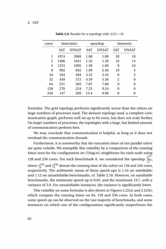
2. SAT
Table 2.9. Results for a topology with ∆(G) = 32.
cores time(min) speedup timeouts
SAT UNSAT SAT UNSAT SAT UNSAT
1 1974 2069 1.00 1.00 20 192 1460 1641 1.35 1.26 16 144 1253 1095 1.58 1.89 9 108 992 842 1.99 2.46 10 4
16 594 584 3.32 3.54 6 232 449 372 4.39 5.56 2 064 251 265 7.87 7.80 0 0
128 270 224 7.23 9.24 0 0256 147 209 13.4 9.90 0 0
formulas. The grid topology performs significantly worse than the others onlarge numbers of processes used. The densest topology used, a complete com-munication graph, performs well on up to 64 cores, but does not scale further.On larger numbers of processes, the topologies with a large, but limited amountof communication perform best.
We may conclude that communication is helpful, as long as it does notoverload the communication threads.
Furthermore, it is noteworthy that the execution times of our parallel solverare quite volatile. We exemplify this volatility by a comparison of the runningtimes seen for the configuration on O(log(n)) neighbours for each node using
128 and 256 cores. For each benchmark b, we considered the speedupt 128
b
t 256b
,
where t 128b and t 256
b denote the running time of the solver on 128 and 256 cores,respectively. The arithmetic mean of these speed-ups is 1.44 on satisfiable,and 1.12 on unsatisfiable benchmarks, cf. Table 2.10. However, on satisfiablebenchmarks, the minimum speed-up is 0.03. and the maximum 19.7, with avariance of 3.9. For unsatisfiable instances, the variance is significantly lower.
This volatility on some formulas is also shown in Figures 2.22(a) and 2.22(b),which compare the running times on 64, 128 and 256 cores. In both cases,some speed-up can be observed on the vast majority of benchmarks, and someinstances on which one of the configurations significantly outperforms the
62

2.5. Parallel SAT
4 8 16 32 64 128 256
#Cores
5
10
20
30
405060
Tota
l ru
nti
me (
h)
Suffocating on communication
Kn
Grid 2D
O(logn)
32 Neighbours
Figure 2.19. Comparison of topologies.
4 8 16 32 64 128 256
#Cores
5
10
20
30
405060
Tota
l ru
nti
me (
h)
Only SAT instances
Kn
Grid 2D
O(logn)
32 Neighbours
Figure 2.20. Comparison of topologies onsatisfiable inputs.
4 8 16 32 64 128 256
#Cores
5
10
20
30
405060
Tota
l ru
nti
me (
h)
Only UNSAT instances
Kn
Grid 2D
O(logn)
32 Neighbours
Figure 2.21. Comparison of topologies onunsatisfiable inputs.
other.
63

2. SAT
Table 2.10. Comparison of the performance on 128 and 256 cores: Speedups on SATand UNSAT instances.
cores average min max variance
SAT 1.44 0.03 19.7 3.9UNSAT 1.12 0.89 1.54 0.02ALL 1.32 0.03 19.7 2.42
0 1,000 2,000 3,000
0
1,000
2,000
3,000
64 cores
128
core
s
(a) 64 vs. 128 cores
0 1,000 2,000 3,000
0
1,000
2,000
3,000
128 cores
256
core
s
(b) 128 vs. 256 cores
Figure 2.22. TOPOSAT: Comparisons using O(log(n)) neighbours.
A Note on Clause Hashing
In the above experiments, the hash values for received clauses were computedby sorting the literals within the clauses increasingly, and applying the hashfunction of Boost6 afterwards. Although this worked well, we found later onthat there is some serious concern with this approach. We exemplify it by thefollowing experiment: Given three integers 0ď x0 < x1 < x2 < n, we computedthe hash values for all triples and different values of n. It is in the nature ofhashing the hash collisions occur in such an experiment. However, we foundthat the hash function used resulted in a huge amount of collisions. Table 2.11shows the number of triples considered, and the number of distinct hash values.It can clearly be seen that the hashing creates a huge number of collisions,which in return may result in the unintended rejection of short clauses. In
6cf. http://www.boost.org/doc/libs/1_38_0/doc/html/hash/reference.html.
64

2.5. Parallel SAT
Table 2.11. Distinct hash values
n triples hashes
100 161,700 141,588200 1,313,400 541,532300 4,455,100 948,578500 20,708,500 1,746,207
1,000 166,167,000 3,796,138
HordeSAT [29], the authors compute 4 distinct hash values for each receivedclause, and reject clauses only if each of the computed hashes has been seenbefore.
2.5.2 Subsequent Implementations
It is expected that communication will become a major concern for sufficientlylarge numbers of processes used, and on dense communication topologies in-dependent of the implementation used. However, it is noteworthy that portfoliosolvers like the prototype we submitted to the SAT competition 2016 [96] scalefurther. We conjecture that there are two problems with the approach used inTOPOSAT. Firstly, TOPOSAT imports received clauses similar to MANYSAT [116].If clauses are received between two restarts, they are imported, which involveschoosing appropriate watched literals, and backtracking in case one of theimported clauses is in conflicting state. As found in subsequent experiments, itis not necessary to import clauses as fast as possible. Therefore it appears suffi-cient to import clauses when the solver preforms a restart. This is especiallyinteresting as in the implementation of TOPOSAT, the solver thread and thecommunication thread compete for the lock protecting the receive buffer.
Second, the communication threads in TOPOSAT synchronise each timecommunication is performed. Thus, all communication is performed at thesame time, resulting in much traffic at some times, whereas the MPI network isidle at other times, which may decrease the overall throughput.
65
2. SAT
2.6 Conclusion and Open Questions
In this chapter, we gave an overview on SAT, the satisfiability problem in propo-sitional logic, and discussed proof systems. This discussion emphasised theimportance of clause learning for the performance of SAT solvers, which canbe related to the difference in strength of tree-like and unrestricted resolution.This is relevant both for the subsequent results and questions presented in thischapter, and also for the next chapter which deals with the parallelisation ofCP solvers which use a learning scheme similar to the one used in SAT solvers.Furthermore, extended resolution was discussed. It is hard to implement it inSAT solvers, therefore, we introduced predicates in hard formulas in Chapter 4before handing them to a SAT solver, which significantly reduced the size ofthe proofs created there.
Next, we discussed core techniques used in state-of-the-art SAT solvers. Wepresented the changes we made in our hack version of GLUCOSE 3, which wonthe gold medal of the GLUCOSE Hack Track of the SAT Competition 2016, anddiscussed the impact of each of the changes.
Afterwards, we turned to the parallelisation of SAT solvers, with a strongfocus on the portfolio approach. After discussing the state of the art, we posed11 questions to point at further research directions in this field. One of themwas considered in the remainder of this section, where we presented anddiscussed the impact of communication on the performance of a portfoliosolver on up to 256 cores. The results showed that the exchange of learnedclauses strictly pays off, and that a speed-up is achievable also on unsatisfiableproblems. When using more than 64 cores, communication in an all-to-allmanner resulted in an amount of traffic that TOPOSAT was not able to handle,thus, it became necessary to limit the amount of communication, which wedid by restricting clause exchange to some local neighbourhood of each solverprocess.
Future Work
Due to the versatility of SAT, problems from different domains are encoded inpropositional formulas, which makes it hard to find a configuration for a SATsolver that works well on all possible inputs. This concerns both sequentialand parallel solvers, but we conjecture that the difference is even larger in the
66
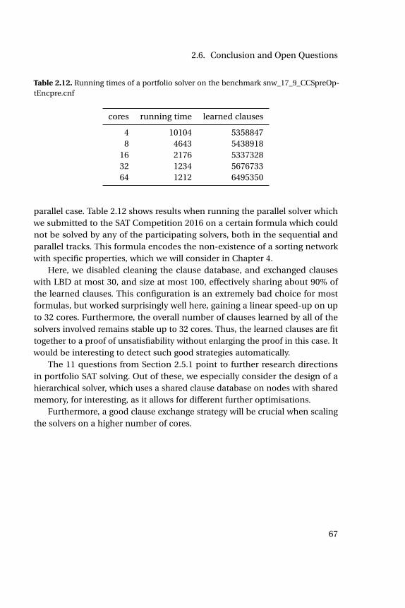
2.6. Conclusion and Open Questions
Table 2.12. Running times of a portfolio solver on the benchmark snw_17_9_CCSpreOp-tEncpre.cnf
cores running time learned clauses
4 10104 53588478 4643 5438918
16 2176 533732832 1234 567673364 1212 6495350
parallel case. Table 2.12 shows results when running the parallel solver whichwe submitted to the SAT Competition 2016 on a certain formula which couldnot be solved by any of the participating solvers, both in the sequential andparallel tracks. This formula encodes the non-existence of a sorting networkwith specific properties, which we will consider in Chapter 4.
Here, we disabled cleaning the clause database, and exchanged clauseswith LBD at most 30, and size at most 100, effectively sharing about 90% ofthe learned clauses. This configuration is an extremely bad choice for mostformulas, but worked surprisingly well here, gaining a linear speed-up on upto 32 cores. Furthermore, the overall number of clauses learned by all of thesolvers involved remains stable up to 32 cores. Thus, the learned clauses are fittogether to a proof of unsatisfiability without enlarging the proof in this case. Itwould be interesting to detect such good strategies automatically.
The 11 questions from Section 2.5.1 point to further research directionsin portfolio SAT solving. Out of these, we especially consider the design of ahierarchical solver, which uses a shared clause database on nodes with sharedmemory, for interesting, as it allows for different further optimisations.
Furthermore, a good clause exchange strategy will be crucial when scalingthe solvers on a higher number of cores.
67

Chapter 3
Parallelising ConstraintProgramming with Learning
“Those who cannot remember thepast are condemned to repeat it.”
JORGE AUGUSTÍN NICOLÁS RUIZ
DE SANTAYANA
3.1 Introduction
Constraint Programming (CP) is a declarative way to describe solutions ofproblems [188]. For example, the set of constraints
allDifferent(x1, . . . , xn)
xi ě 1 @1ď i ď n
xi < n @1ď i ď n
xi PN @1ď i ď n
describes the problem of finding a set of n natural numbers between 1 andn´1 which are pairwise non-equal. The possibility to state constraints like“allDifferent” without encoding it to e.g. SAT formulas or linear programs makesCP an easily accessible technique. Furthermore, in many cases this kind ofencoding keeps high-level structure which might be lost when translatingto SAT [203]. Thus, Constraint Programming has become an active field ofboth research and applications, e. g., in artificial intelligence, planning andoperations research.
69
3. Parallelising Constraint Programming with Learning
The above problem describes the pigeon hole problem PHP n+1n . As seen
in the previous chapter, this problem is extremely hard for SAT solvers. On thecontrary, CP solvers like GECODE [105] can solve this problem efficiently, asthey use specialised propagators — algorithms designed to handle constraintslike “allDifferent” efficiently.
In this chapter we will describe the parallelisation of the CP solver CHUFFED [62],which is a CP solver with learning, i. e., it uses clause learning techniquesas used in CDCL SAT solvers. The results from this research were publishedin [100].
We will begin with an introduction on Constraint Programming and solversfor it in Section 3.2. Next, we discuss the lazy clause generation (LCG)-approachin Section 3.3, which extends CP solvers by clause learning. Finally, we discussour work in parallelising CHUFFED.
3.2 Constraint Programming
Constraint Programming includes the description of Constraint SatisfactionProblems (CSP) as well as search strategies for finding solutions for these. Wewill firstly introduce CSPs, give some motivating examples of how they are used,and then turn to techniques for finding solutions efficiently.
3.2.1 Constraint Satisfaction Problems
We will mostly follow the notation from [188] in this section. A Constraint Satis-faction Problem (CSP) is given by a triple P= (X ,D,C ) where X = (x1, . . . , xn) isa n-tuple of variables. The domains of these variables are D = (D1, . . . ,Dn). Theset of constraints C is a t-tuple (C1, . . . ,Ct ). Each constraint Ci = (RSi ,Si ) is atuple where Si = scope(Ci ) is the set of variables appearing in Ci , and RSi is arelation on the variables in Si .
Example 3.1. Consider the CSP P= (X ,D,C ) with two variables and two con-straints.
X = (x1, x2)
D = (0, . . . ,5, 2,3)
C = (x1ě 1, x1 +x2ď 4)
70
3.2. Constraint Programming
The scope of the constraints is given by
scope(x1ě 1) = x1
scope(x1 +x2ď 4) = x1, x2.
äA solution to a CSP is a n-tuple A = (a1, . . . , an) such that
ai PDi @1ď i ď n
A |ùRSi @1ď i ď t
where the second constraint denotes that the projection of A on the variablesin Si satisfies RSi . In most cases, the constraints are given implicitly. The setof all solutions to P is denoted solns(P). In Constraint Programming, we mayconsider the decision problem solns(P)‰H, compute the set of all solutions,or search a solution which maximises some objective function σ : X ÞÑQ.
It can be seen that C SP P N P if, given a solution, every constraint canbe checked in polynomial time. Furthermore, NP-complete problems as SATcan be encoded as CSP easily, thus, solving the decision problem of a CSP isNP-hard.
3.2.2 Applications
Constraint Programming is used in a wide field of applications, among whichthere are lots of real-world problems. Nurse rostering [177] asks for shifts fornurses, and is considered in a plethora of research papers. Other problemsare vehicle routing [110] both in general of specific settings. For example, theoptimisation of routes used for snow plowing in Pittsburgh is solved usingconstraint programming [135].
Earth observation management [36] manages the pictures taken by satellitesin order to minimise overlaps. This is a computationally challenging problemwhich was solved using constraint programming.
The train lines connecting Australian coal mines with harbours were anal-ysed and optimised in [118]. More examples like network planing or schedulingcan be found in [188].
MiniZinc is language which is widely used in constraint programming [165].Listing 3.1 shows the pigeon hole problem PHP n+1
n in MiniZinc.
71
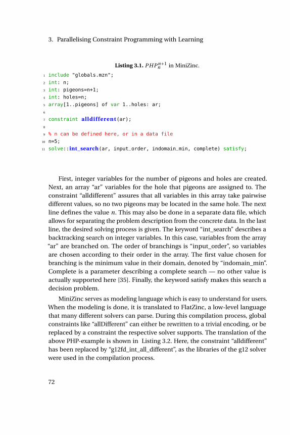
3. Parallelising Constraint Programming with Learning
Listing 3.1. PHP n+1n in MiniZinc.
1 include "globals.mzn";
2 int: n;
3 int: pigeons=n+1;
4 int: holes=n;
5 array[1..pigeons] of var 1..holes: ar;
6
7 constraint alldifferent(ar);8
9 % n can be defined here, or in a data file
10 n=5;
11 solve::int_search(ar, input_order, indomain_min, complete) satisfy;
First, integer variables for the number of pigeons and holes are created.Next, an array “ar” variables for the hole that pigeons are assigned to. Theconstraint “alldifferent” assures that all variables in this array take pairwisedifferent values, so no two pigeons may be located in the same hole. The nextline defines the value n. This may also be done in a separate data file, whichallows for separating the problem description from the concrete data. In the lastline, the desired solving process is given. The keyword “int_search” describes abacktracking search on integer variables. In this case, variables from the array“ar” are branched on. The order of branchings is “input_order”, so variablesare chosen according to their order in the array. The first value chosen forbranching is the minimum value in their domain, denoted by “indomain_min”.Complete is a parameter describing a complete search — no other value isactually supported here [35]. Finally, the keyword satisfy makes this search adecision problem.
MiniZinc serves as modeling language which is easy to understand for users.When the modeling is done, it is translated to FlatZinc, a low-level languagethat many different solvers can parse. During this compilation process, globalconstraints like “allDifferent” can either be rewritten to a trivial encoding, or bereplaced by a constraint the respective solver supports. The translation of theabove PHP-example is shown in Listing 3.2. Here, the constraint “alldifferent”has been replaced by “g12fd_int_all_different”, as the libraries of the g12 solverwere used in the compilation process.
72
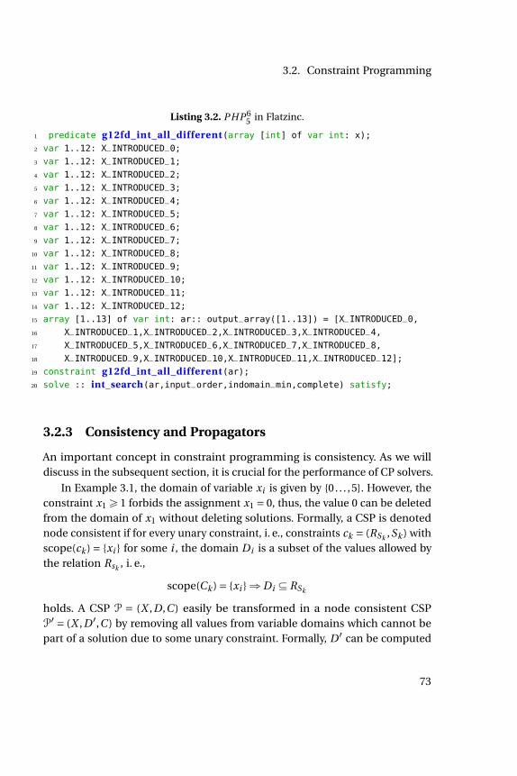
3.2. Constraint Programming
Listing 3.2. PHP 65 in Flatzinc.
1 predicate g12fd_int_all_different(array [int] of var int: x);
2 var 1..12: X_INTRODUCED_0;
3 var 1..12: X_INTRODUCED_1;
4 var 1..12: X_INTRODUCED_2;
5 var 1..12: X_INTRODUCED_3;
6 var 1..12: X_INTRODUCED_4;
7 var 1..12: X_INTRODUCED_5;
8 var 1..12: X_INTRODUCED_6;
9 var 1..12: X_INTRODUCED_7;
10 var 1..12: X_INTRODUCED_8;
11 var 1..12: X_INTRODUCED_9;
12 var 1..12: X_INTRODUCED_10;
13 var 1..12: X_INTRODUCED_11;
14 var 1..12: X_INTRODUCED_12;
15 array [1..13] of var int: ar:: output_array([1..13]) = [X_INTRODUCED_0,
16 X_INTRODUCED_1,X_INTRODUCED_2,X_INTRODUCED_3,X_INTRODUCED_4,
17 X_INTRODUCED_5,X_INTRODUCED_6,X_INTRODUCED_7,X_INTRODUCED_8,
18 X_INTRODUCED_9,X_INTRODUCED_10,X_INTRODUCED_11,X_INTRODUCED_12];
19 constraint g12fd_int_all_different(ar);20 solve :: int_search(ar,input_order,indomain_min,complete) satisfy;
3.2.3 Consistency and Propagators
An important concept in constraint programming is consistency. As we willdiscuss in the subsequent section, it is crucial for the performance of CP solvers.
In Example 3.1, the domain of variable xi is given by 0. . . ,5. However, theconstraint x1ě 1 forbids the assignment x1 = 0, thus, the value 0 can be deletedfrom the domain of x1 without deleting solutions. Formally, a CSP is denotednode consistent if for every unary constraint, i. e., constraints ck = (RSk ,Sk ) withscope(ck ) = xi for some i , the domain Di is a subset of the values allowed bythe relation Rsk , i. e.,
scope(Ck ) = xi ñDi ĎRSk
holds. A CSP P = (X ,D,C ) easily be transformed in a node consistent CSPP1 = (X ,D 1,C ) by removing all values from variable domains which cannot bepart of a solution due to some unary constraint. Formally, D 1 can be computed
73

3. Parallelising Constraint Programming with Learning
as follows.
D 1i = Di X⋂
Rk : scope(Ck ) = xi
Example 3.2. The CSP from Example 3.1 can be turned into a node consistentCSP P1 = (X ,D 1,C ) by removing the value “0” from the domain of x1.
D 11 = 0, . . . ,5X c PD1.c ě 1
= 1, . . . ,5
äA stronger form of consistency is arc consistency. In this case, binary con-
straints are considered. Let Ck be a constraint on variables xi , x j . If there existsa value in c PDi such that Ck cannot be satisfied when assigning c to xi , c canbe removed from Di without reducing the set of solutions of the respective CSP,as depicted in the following example.
Example 3.3. Consider again the CSP from Example 3.2. From the secondconstraint, we can derive
x1ď 4´x2
ď 2 because x2ě 2
and so the CSP P2 = (X , (1,2, 2,3),C ) has the same solutions as P. äThere are further, stronger forms of consistency. Obviously, the concept of
node- and arc consistency can be extended to constraints of arbitrary cardinal-ity. More forms of consistency together with a detailed analysis and algorithmscan be found in [188].
With the concept of consistencies, we may now consider propagators. Apropagator is a function f (X ,D,C ) = (X ,D 1,C ) such that the set of solutions re-mains unchanged, and the domains are not extended [170]. Thus, propagatorscreate some form of consistency.
D 1i ĎDi
solns(X ,D,C ) = solns(X ,D 1,C )
The drawback of this definition is that the identity function is also a validpropagator. Furthermore, a propagator may also be a decision procedure whichreturns empty domains for all variables if the problem is unsatisfiable. Thus,this definition includes both trivial and coNP-hard problems.
74

3.2. Constraint Programming
x1
x2
x3
1
2
Figure 3.1. Bipartite graph for an alldifferent constraint.
There exist propagators which consider more than one constraint. For exam-ple, [4] uses a preprocessing step to incorporate implications into propagatorsfor linear inequalities. In the following, we will restrict our viewpoint to localconsistencies. This is, propagators fc are connected to some constraint c, andonly check if variable domains are consistent with respect to this constraint.
For example, for the alldifferent constraint there exist propagators whichare based on graph matchings[87]. Figure 3.1 shows a bipartite graph for theconstraint alldifferent(x1, x2, x3) with x1, x2, x3 P 1,2, which is PHP 3
2 .
While it is extremely hard for SAT solvers to prove unsatisfiability of thisproblem, CP solvers can handle it efficiently. The core idea is that every feasiblesolution is a maximum matching on a this graph which covers all variablenodes. By the theorem of Hall [114], such a matching cannot exist in the abovecase as the cardinality of the left-hand side is larger than the one of the right-hand side of the graph. Some CP solvers as GECODE [105] come with very strongpropagators for this constraint, allowing them to massively prune variabledomains. In the case of pigeon hole problems PHP n+1
n , GECODE can proveunsatisfiability for n = 106 in 3 seconds on a standard computer, whereasn = 15 is intractable for SAT solvers.
Another global constraint which is frequently used is a linear inequality∑i ci xi ď k for constants ci and variables xi . The MiniZinc homepage lists
numerous global constraints [1]. Furthermore, very specialised constraintsexist. For example, [207] discusses propagators for finding Steiner trees ongraphs.
75
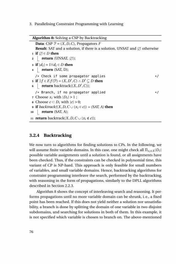
3. Parallelising Constraint Programming with Learning
Algorithm 8: Solving a CSP by Backtracking
Data: CSP P= (X ,D,C ), Propagators FResult: SAT and a solution, if there is a solution, UNSAT and H otherwise
1 if HPD then2 return (UNSAT, H);
3 if |di | = 1@di PD then4 return (SAT, D);
/* Check if some propagator applies */
5 if D f P F. f (P) = (X ,D 1,C )^D 1(D then6 return backtrack((X ,D 1,C ));
/* Branch, if no propagator applied */
7 Choose xi with |Di | > 1 ;8 Choose c ĂDi with |c| > 0;9 if backtrack((X ,D,CY xi P c) = (SAT, A) then
10 return (SAT, A);
11 return backtrack(X ,D,CY xi ∉ c);
3.2.4 Backtracking
We now turn to algorithms for finding solutions to CPs. In the following, wewill assume finite variable domains. In this case, one might check all ΠxiPX |Di |possible variable assignments until a solution is found, or all assignments havebeen checked. Thus, if the constraints can be checked in polynomial time, thisvariant of CP is NP-hard. This approach is only feasible for small numbersof variables, and small variable domains. Hence, backtracking algorithms forconstraint programming interleave the search, performed by the backtracking,with reasoning in the form of propagations, similarly to the DPLL algorithmsdescribed in Section 2.2.3.
Algorithm 8 shows the concept of interleaving search and reasoning. It per-forms propagations until no more variable domain can be shrunk, i. e., a fixedpoint has been reached. If this does not yield neither a solution nor unsatisfia-bility, a branch is done by splitting the domain of one variable in two disjointsubdomains, and searching for solutions in both of them. In this example, itis not specified which variable is chosen to branch on. The above-mentioned
76
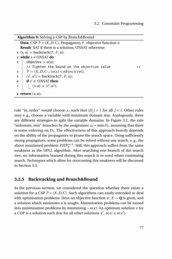
3.2. Constraint Programming
Algorithm 9: Solving a CSP by Branch&Bound
Data: CSP P= (X ,D,C ), Propagators F , objective function oResult: SAT if there is a solution, UNSAT otherwise
1 (s, a) := backtrack(P, F , o);2 while s‰UNSAT do3 objective := o(a);
/* Tighten the bound on the objective value */
4 P := (X ,D,CY o(x) < ob j ect i ve);5 (s1, a1) := backtrack(P, F , o);6 if s’ ‰ UNSAT then7 (s, a) := (s1, a1);
8 return (s, a);
rule “in_order" would choose xi such that |D j | = 1 for all j < i . Other rulesmay e. g., choose a variable with minimum domain size. Analogously, thereare different strategies to split the variable domains. In Figure 3.1, the rule“indomain_min" branches by the assignment xi = minDi , assuming that thereis some ordering on Di . The effectiveness of this approach heavily dependson the ability of the propagators to prune the search space. Using sufficientlystrong propagators, some problems can be solved without any search, e. g., theabove mentioned problem PHP n+1
n . Still, this approach suffers from the sameweakness as the DPLL algorithm. After searching one branch of the searchtree, no information learned during this search is re-used when continuingsearch. Techniques which allow for overcoming this weakness will be discussedin Section 3.3.
3.2.5 Backtracking and Branch&Bound
In the previous section, we considered the question whether there exists asolution for a CSP P= (X ,D,C ). Such algorithms can easily extended to dealwith optimisation problems. Here, an objective function o : X ÞÑQ is given, anda solution which minimises o is sought. Maximisation problems can be turnedinto minimisation problems by minimising ´o(x). An optimum solution x fora COP is a solution such that for all other solutions x1, o(x)ď o(x1).
77

3. Parallelising Constraint Programming with Learning
1 var 1..5: a;
2 solve maximize a;
1 a = 1;
2 ----------
3 a = 2;
4 ----------
5 a = 3;
6 ----------
7 a = 4;
8 ----------
9 a = 5;
10 ----------
11 ==========
Figure 3.2. Example for slow convergence of the Branch&Bound routine. The left-handside shows a tiny MiniZinc example of an optimisation problem, and the right-handside the output of the G12lazy solver when run on it.
A simple algorithm for solving constraint optimisation problems (COP) byBranch&Bound is given in Figure 9. Here, the backtrack procedure is calledrepeatedly. If it finds a solution, a tightened bound on the objective value isadded to ensure a convergence towards solution closer to the optimum. Inpractice, the tightened bound may be added to the CSP within the backtrackingalgorithm. This prevents the backtracking routine from searching parts of thesearch space repeatedly1.
However, also the convergence speed towards an optimum solution maybe quite slow, as the solver only solves decision problems repeatedly withoutconsidering the objective value. Figure 3.2 shows an artificial example for this.By default, the solver searches for solutions by branching on minimum valueswithin the variable domain. In this case, the complete domain for variable “a"is traversed, and the bound on the objective value is decreased by 1 in everyiteration.
Figure 3.3 shows data collected during a run of CHUFFED on an optimisa-tion benchmark from the MiniZinc Challenge 2013 [100]2. In both plots, thehorizontal axis represents the time, and the vertical axis shows the current
1Cf. the source code of solvers like CHUFFED (https://github.com/geoffchu/chuffed) or GECODE
http://www.gecode.org/.2see also http://www.minizinc.org/challenge.html.
78
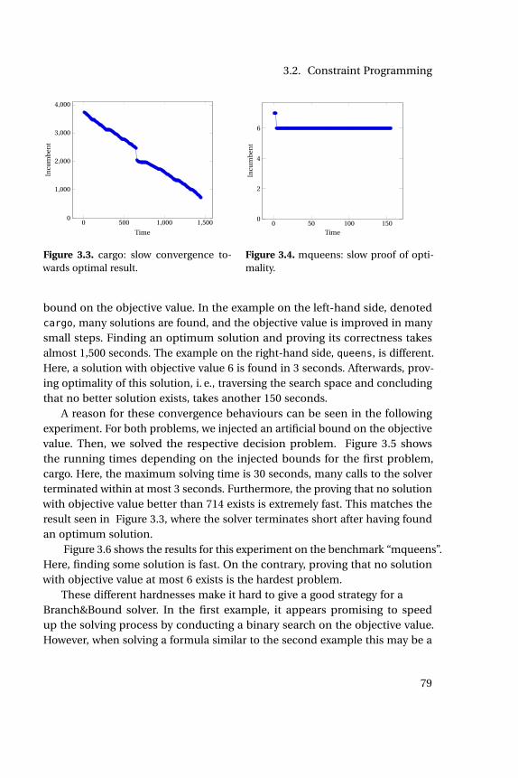
3.2. Constraint Programming
0 500 1,000 1,5000
1,000
2,000
3,000
4,000
Time
Incu
mb
ent
Figure 3.3. cargo: slow convergence to-wards optimal result.
0 50 100 1500
2
4
6
Time
Incu
mb
ent
Figure 3.4. mqueens: slow proof of opti-mality.
bound on the objective value. In the example on the left-hand side, denotedcargo, many solutions are found, and the objective value is improved in manysmall steps. Finding an optimum solution and proving its correctness takesalmost 1,500 seconds. The example on the right-hand side, queens, is different.Here, a solution with objective value 6 is found in 3 seconds. Afterwards, prov-ing optimality of this solution, i. e., traversing the search space and concludingthat no better solution exists, takes another 150 seconds.
A reason for these convergence behaviours can be seen in the followingexperiment. For both problems, we injected an artificial bound on the objectivevalue. Then, we solved the respective decision problem. Figure 3.5 showsthe running times depending on the injected bounds for the first problem,cargo. Here, the maximum solving time is 30 seconds, many calls to the solverterminated within at most 3 seconds. Furthermore, the proving that no solutionwith objective value better than 714 exists is extremely fast. This matches theresult seen in Figure 3.3, where the solver terminates short after having foundan optimum solution.
Figure 3.6 shows the results for this experiment on the benchmark “mqueens”.Here, finding some solution is fast. On the contrary, proving that no solutionwith objective value at most 6 exists is the hardest problem.
These different hardnesses make it hard to give a good strategy for aBranch&Bound solver. In the first example, it appears promising to speedup the solving process by conducting a binary search on the objective value.However, when solving a formula similar to the second example this may be a
79

3. Parallelising Constraint Programming with Learning
700 800 900 1,0000
10
20
30
Bound
Tim
e
Figure 3.5. cargo: time for decision prob-lem, depending on bound on objectivevalue.
0 10 20 300
50
100
150
Bound
Tim
e
Figure 3.6. queens: time for decision prob-lem, depending on bound on objectivevalue.
bad approach, as one might hit the hardest, and unsatisfiable case first. In theworst case, the solver might time out without finding any solution, althoughfinding suboptimal solutions is not too hard in many cases. Running timedistributions as in the second example can be found in many applications,e. g., [39, 150]. We will show solutions for this problem in Section 3.5.
3.3 Constraint Programming with Learning
Supplementing Constraint Programming with learning is a very active field ofresearch. We restrict this section to a brief overview about some techniquesand results as necessary for the subsequent sections.
The methods described so far — interleaving search with propagations —allow for an efficient traversal of the search space. Nevertheless, it suffers fromthe same weakness as the DPLL procedure for propositional logic. The solverdoes not learn from its search, and thus repeats searching similar parts of thesearch space. In Chapter 2, the CDCL technique (Conflict Driven Clause Learn-ing) was described as a way to overcome this weakness. Similar approacheswere considered in Constraint Programming more than two decades ago [86].They were used in two different ways. Firstly, new constraints were added when-ever the solver had to backtrack, trying to avoid repeated search. Second, it iscrucial to remember which parts of the search space were visited already when
80
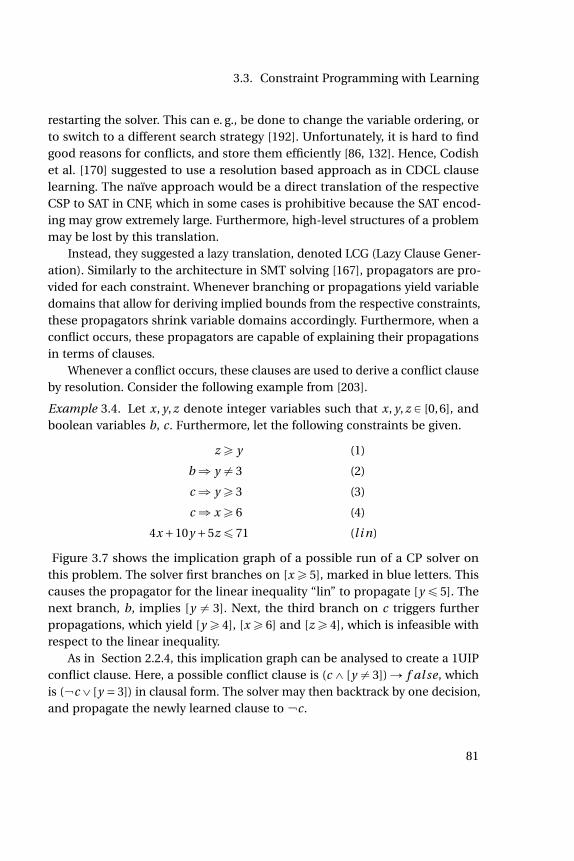
3.3. Constraint Programming with Learning
restarting the solver. This can e. g., be done to change the variable ordering, orto switch to a different search strategy [192]. Unfortunately, it is hard to findgood reasons for conflicts, and store them efficiently [86, 132]. Hence, Codishet al. [170] suggested to use a resolution based approach as in CDCL clauselearning. The naïve approach would be a direct translation of the respectiveCSP to SAT in CNF, which in some cases is prohibitive because the SAT encod-ing may grow extremely large. Furthermore, high-level structures of a problemmay be lost by this translation.
Instead, they suggested a lazy translation, denoted LCG (Lazy Clause Gener-ation). Similarly to the architecture in SMT solving [167], propagators are pro-vided for each constraint. Whenever branching or propagations yield variabledomains that allow for deriving implied bounds from the respective constraints,these propagators shrink variable domains accordingly. Furthermore, when aconflict occurs, these propagators are capable of explaining their propagationsin terms of clauses.
Whenever a conflict occurs, these clauses are used to derive a conflict clauseby resolution. Consider the following example from [203].
Example 3.4. Let x, y, z denote integer variables such that x, y, z P [0,6], andboolean variables b, c. Furthermore, let the following constraints be given.
z ě y (1)
bñ y ‰ 3 (2)
cñ y ě 3 (3)
cñ x ě 6 (4)
4x +10y +5z ď 71 (l i n)
Figure 3.7 shows the implication graph of a possible run of a CP solver onthis problem. The solver first branches on [x ě 5], marked in blue letters. Thiscauses the propagator for the linear inequality “lin” to propagate [y ď 5]. Thenext branch, b, implies [y ‰ 3]. Next, the third branch on c triggers furtherpropagations, which yield [y ě 4], [x ě 6] and [z ě 4], which is infeasible withrespect to the linear inequality.
As in Section 2.2.4, this implication graph can be analysed to create a 1UIPconflict clause. Here, a possible conflict clause is (c^ [y ‰ 3])Ñ f al se, whichis ( c_[y = 3]) in clausal form. The solver may then backtrack by one decision,and propagate the newly learned clause to c.
81
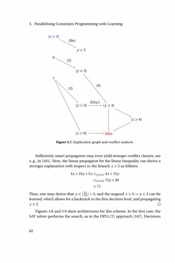
3. Parallelising Constraint Programming with Learning
[x ě 5]
b
c
y ď 5
[y ‰ 3]
[y ě 3]
[x ě 6]
[y ě 4]
[z ě 4]
false
(lin)
(2)
(3)(4)
(D(y))
Figure 3.7. Implication graph and conflict analysis.
Sufficiently smart propagators may even yield stronger conflict clauses, seee. g., in [101]. Here, the linear propagator for the linear inequality can derive astronger explanation with respect to the branch x ě 5 as follows:
4x +10y +5z ď(yďz) 4x +15y
ď(xě5) 15y +20
ď 71
Thus, one may derive that y ď b 5115 c = 3, and the nogood x ě 5ñ y ď 3 can be
learned, which allows for a backtrack to the first decision level, and propagatingy ď 3. ä
Figures 3.8 and 3.9 show architectures for this scheme. In the first case, theSAT solver performs the search, as in the DPLL(T) approach [167]. Decisions
82
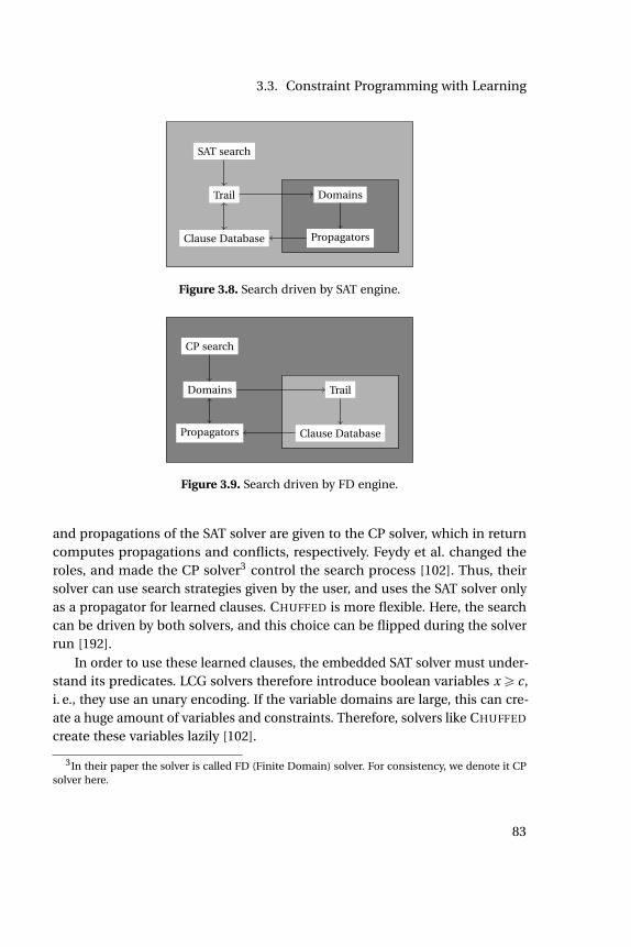
3.3. Constraint Programming with Learning
SAT search
Trail
Clause Database
Domains
Propagators
Figure 3.8. Search driven by SAT engine.
CP search
Domains
Propagators
Trail
Clause Database
Figure 3.9. Search driven by FD engine.
and propagations of the SAT solver are given to the CP solver, which in returncomputes propagations and conflicts, respectively. Feydy et al. changed theroles, and made the CP solver3 control the search process [102]. Thus, theirsolver can use search strategies given by the user, and uses the SAT solver onlyas a propagator for learned clauses. CHUFFED is more flexible. Here, the searchcan be driven by both solvers, and this choice can be flipped during the solverrun [192].
In order to use these learned clauses, the embedded SAT solver must under-stand its predicates. LCG solvers therefore introduce boolean variables x ě c,i. e., they use an unary encoding. If the variable domains are large, this can cre-ate a huge amount of variables and constraints. Therefore, solvers like CHUFFED
create these variables lazily [102].
3In their paper the solver is called FD (Finite Domain) solver. For consistency, we denote it CPsolver here.
83
3. Parallelising Constraint Programming with Learning
Among other solvers, this approach is implemented in CHUFFED [62], whichwe will use in the subsequent sections.
Despite the elegance of the lazy propagation approaches, both in SMT andLCG, it is important to note that the implementation of efficient propagators ishighly non-trivial, and in some cases, using pure propagations is even harm-ful. Propagators only explain themselves in terms of clauses. Even for simpleconstraints like XOR, a purely clause-based encoding has exponential size,cf. Section 2.1.3. Thus, the propagator may return an exponential number ofdifferent clauses as explanations for its propagations. Therefore, it is importantto choose whether to encode a constraint directly, or to propagate it [5]. Somesolvers try to automate this choice: They start with a propagation based ap-proach. If a the propagator for a constraint is used often, a direct SAT encodingfor this single constraint is added lazily [3].
3.4 Parallel Constraint Programming
There are different approaches to parallelising constraint programming solvers.We will first consider some approaches for parallel implementations of classi-cal CP solvers, i. e., solvers without learning, and then briefly repeat the coreinsights of parallel SAT solvers, as they use learning mechanisms. Afterwards,we present some results on parallel CP with learning in the next section.
A quite straightforward approach in parallelising CP solvers is the portfolioapproach: Run different solvers in parallel, and abort once the first solver hasfinished. In case there are more solvers available than computational resources,[7] discusses approaches to choose a good subset of the available solvers. In thecontext of optimisation problems, the solvers running in parallel may exchangebounds on the objective value, as it is done in [8]. Additionally, the authorsshowed that some solvers are faster than other in different phases of their run:Some are faster in finding some solutions, whereas others are faster in provingoptimality.
Another prominent approach is to split the search space, and run solverinstances in parallel on the respective subspaces. This can be done by creat-ing sets of cubes, i. e., conjunctions of predicates. For example, let x denotean integer variable with lower and upper bounds lb(x) and ub(x) such thatD(x) Ď [lb(x),ub(x)]. Then, one might split the search space by the cubes
84
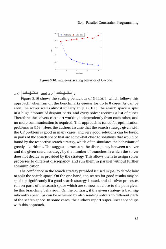
3.4. Parallel Constraint Programming
2 4 6 80
20
40
60
80
100
# threads
Tim
e
Wall time CPU time
Figure 3.10. mqueens: scaling behavior of Gecode.
x ď⌊
ub(x)+l b(x)2
⌋and x >
⌊ub(x)+lb(x)
2
⌋.
Figure 3.10 shows the scaling behaviour of GECODE, which follows thisapproach, when run on the benchmarks queens for up to 8 cores. As can beseen, the solver scales almost linearly. In [185, 186], the search space is splitin a huge amount of disjoint parts, and every solver receives a list of cubes.Therefore, the solvers can start working independently from each other, andno more communication is required. This approach is tuned for optimisationproblems in [159]. Here, the authors assume that the search strategy given withthe CP problem is good in many cases, and very good solutions can be foundin parts of the search space that are somewhat close to solutions that would befound by the respective search strategy, which often simulates the behaviour ofgreedy algorithms. The suggest to measure the discrepancy between a solverand the given search strategy by the number of branches in which the solverdoes not decide as provided by the strategy. This allows them to assign solverprocesses to different discrepancy, and run them in parallel without furthercommunication.
The confidence in the search strategy provided is used in [64] to decide howto split the search space. On the one hand, the search for good results may besped up significantly if a good search strategy is used, and all solver processesrun on parts of the search space which are somewhat close to the path givenbe this branching behaviour. On the contrary, if the given strategy is bad, sig-nificantly speedups can be achieved by also sending solvers to different partsof the search space. In some cases, the authors report super-linear speedupswith this approach.
85

3. Parallelising Constraint Programming with Learning
Besides the domain of “classical" CP, some research has been conducted inparallelising solvers in similar domains.
Wintersteiger et al. presented a parallel version of their SMT solver Z3in [214] which basically transfers the ideas of ManySAT [116]. This is, theyallow for exchanging some short clauses between the solver threads runningin parallel, and initialise variable activities randomly. The results are rathermixed, and only 4 threads are used. Furthermore, they used a set of quite easybenchmarks, which does not sufficiently show the usability of their approachon harder problems. Jordan et al. use a search space splitting approach withoutany knowledge exchange, and report significant improvements on up to 64threads [130].
In the field of quantified boolean formulas (QBF), Balyo et al. used a portfo-lio approach [28], similar to the one they used in [29] and report super-linearspeedups. Unfortunately, most of this improvement can be achieved with 2nodes, each of which uses 4 processes with 4 solver threads, which is 32 threadsaltogether. The authors do not report results for lower numbers of threads. Us-ing more cores yields a little more speedup, but the improvements are verylimited.
Altogether, splitting the search space is the predominant approach for CPsolvers, whereas some knowledge exchange is used more often in domainswhich build upon SAT solver techniques.
3.5 Parallel Constraint Programming with Learning
In [100], we built upon the parallel version of CHUFFED developed in [64] totest if, and how well, a constraint programming solver with learning can beparallelised. As CHUFFED is both kind of a SAT and CP solver, it is not clear howto parallelise it. The authors of the parallel CP solver presented in [185] write:
Our approach relies on the assumption that the resolution timeof disjoint subproblems is equivalent to the resolution time of theunion of these subproblems. If this condition is not met, thenthe parallelization of the search of a solver (not necessarily a CPSolver) based on any decomposition method, like simple staticdecomposition, work stealing or embarrassingly parallel methodsmay be unfavorably impacted.
86

3.5. Parallel Constraint Programming with Learning
100 101 102
100
101
102
port, p = 64
seq
uen
tial
Figure 3.11. suite: comparison be-tween sequential and port.
0 20 40 60 80 1000
100
200
300
# Instances
Tim
e
p = 2p = 4p = 8
p = 16p = 32p = 64
Figure 3.12. suite: scaling of port withnumber of cores.
In the case of learning solvers, this is clearly not the case, as clauses learnedfrom conflicts in one part of the search space are used to avoid redundant workin subsequent search.
On the other hand, learning constraint programming solvers typically donot create large resolution-based proofs. Here, the learned clauses are ratherused to avoid repeated search in a local part of the search space. In CHUFFED,for example, the maximum size of the learned clause database is fixed to amaximum of 100,000 clauses, contrary to SAT solvers where the maximumdatabase size is increased over the time to yield a complete solver.
In the remainder of this section, we present different approaches of par-allelising CHUFFED, and discuss results on a set of 110 benchmarks, denotedsuite. These are optimisation benchmarks taken from the MiniZinc Challenges2013 and 2014, respectively4. The benchmarks files can be found on github5.
3.5.1 Portfolio-based Parallel LCG
The first approach we present here is a portfolio as it is commonly used inSAT solving. It is based on a master-slave architecture where communication isperformed via MPI, which is used throughout this chapter. The VSIDS activitiesare initialised randomly and differently for each solver process, and someclause exchange between the solvers is allowed. Clauses learned by one solver
4http://www.minizinc.org/challenge.html5https://github.com/the-kiel/CP_benchmarks
87
3. Parallelising Constraint Programming with Learning
are sent to the master process, which dispatches them to the other solvers.Whenever a solver process finds a solution, this induces a new bound on theobjective value, which is send to the other processes as unit clause. We willdenote this configuration by port.
Figure 3.11 shows a scatter plot, which compares the running times on ourbenchmark suite between a sequential, and a portfolio solver on 64 cores, witha timeout of 300 seconds. On benchmarks with sequential running times ofat most one second, only little speedup can be observed. Here, the overheadof starting 64 MPI processes does not pay off, as the sequential solver is fastenough.
On the contrary, for harder problems, the portfolio solver clearly outper-forms the sequential version, and is able to solve 9 more problems to optimality,i. e., finding a solution and proving that no better solution exists. The scalingbehaviour is given in Figure 3.12 as a cactus plot. The more processes areused, the faster the solver gets. The drawback of this presentation is that onlysome of the benchmarks give meaningful insights: The easiest 40 benchmarkscan be solved quite fast by all solver configurations, whereas the hardest 40benchmarks time out on all configurations. We therefore discuss the resultsin this section in a two-fold manner. Firstly, we measure speedups in termsof pure running times. Secondly, we ask how fast the parallel solver is whenasked to provide a better solution than the sequential solver. We therefore con-ducted the following experiment: For every benchmark, the sequential solveris run with a timeout of 10,800 seconds. We both record the running time,and the objective value of the best solution found within this time. Next, werun the parallel solver, and abort it once a better solutions than the one fromthe sequential solver has been found. In case the sequential solver found theoptimum solutions, the parallel solver thus had to prove optimality in order toshow that no better solution exists.
Table 3.1 shows the result from this setup. The middle columns of the tableshow the geometric mean and median of the speedups on all benchmarks.On the whole benchmark set, the configuration using 64 cores achieves a sub-linear average speedup of 9.1. However, this result already indicates that it is infact possible to use CHUFFED in a portfolio configuration.
The right-hand side considers the speedups obtained on hard benchmark.Here, we considered a benchmark as hard if the sequential version of CHUFFED
could not solve it to optimality within 300 seconds. In this way, we got 51 hard
88
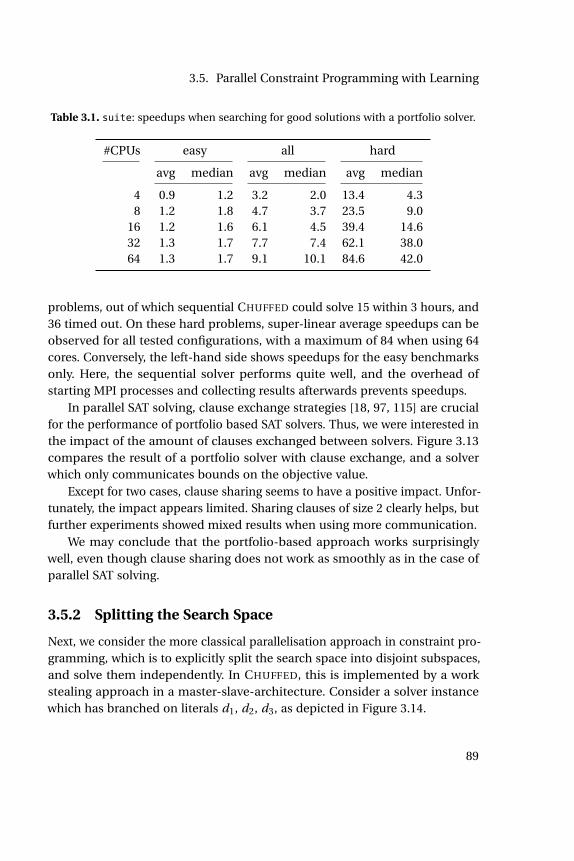
3.5. Parallel Constraint Programming with Learning
Table 3.1. suite: speedups when searching for good solutions with a portfolio solver.
#CPUs easy all hard
avg median avg median avg median
4 0.9 1.2 3.2 2.0 13.4 4.38 1.2 1.8 4.7 3.7 23.5 9.0
16 1.2 1.6 6.1 4.5 39.4 14.632 1.3 1.7 7.7 7.4 62.1 38.064 1.3 1.7 9.1 10.1 84.6 42.0
problems, out of which sequential CHUFFED could solve 15 within 3 hours, and36 timed out. On these hard problems, super-linear average speedups can beobserved for all tested configurations, with a maximum of 84 when using 64cores. Conversely, the left-hand side shows speedups for the easy benchmarksonly. Here, the sequential solver performs quite well, and the overhead ofstarting MPI processes and collecting results afterwards prevents speedups.
In parallel SAT solving, clause exchange strategies [18, 97, 115] are crucialfor the performance of portfolio based SAT solvers. Thus, we were interested inthe impact of the amount of clauses exchanged between solvers. Figure 3.13compares the result of a portfolio solver with clause exchange, and a solverwhich only communicates bounds on the objective value.
Except for two cases, clause sharing seems to have a positive impact. Unfor-tunately, the impact appears limited. Sharing clauses of size 2 clearly helps, butfurther experiments showed mixed results when using more communication.
We may conclude that the portfolio-based approach works surprisinglywell, even though clause sharing does not work as smoothly as in the case ofparallel SAT solving.
3.5.2 Splitting the Search Space
Next, we consider the more classical parallelisation approach in constraint pro-gramming, which is to explicitly split the search space into disjoint subspaces,and solve them independently. In CHUFFED, this is implemented by a workstealing approach in a master-slave-architecture. Consider a solver instancewhich has branched on literals d1, d2, d3, as depicted in Figure 3.14.
89
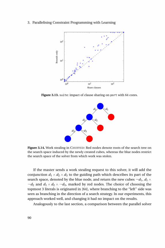
3. Parallelising Constraint Programming with Learning
100 101 102
100
101
102
Share clauses
Bo
un
ds
on
ly
Figure 3.13. suite: impact of clause sharing on port with 64 cores.
d1
d2
d3
d1
d2
d3
Figure 3.14. Work stealing in CHUFFED: Red nodes denote roots of the search tree onthe search space induced by the newly created cubes, whereas the blue nodes restrictthe search space of the solver from which work was stolen.
If the master sends a work stealing request to this solver, it will add theconjunction d1^d2^d3 to the guiding path which describes its part of thesearch space, denoted by the blue node, and return the new cubes d1, d1^
d2 and d1^ d2^ d3, marked by red nodes. The choice of choosing thetopmost 3 literals is originated in [64], where branching to the “left" side wasseen as branching in the direction of a search strategy. In our experiments, thisapproach worked well, and changing it had no impact on the results.
Analogously to the last section, a comparison between the parallel solver
90
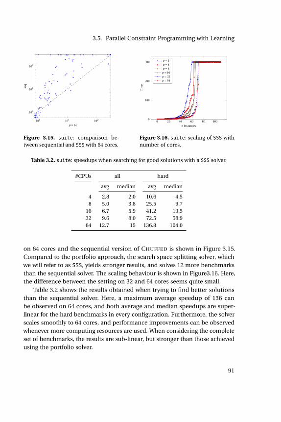
3.5. Parallel Constraint Programming with Learning
100 101 102
100
101
102
p = 64
seq
Figure 3.15. suite: comparison be-tween sequential and SSS with 64 cores.
0 20 40 60 80 1000
100
200
300
# Instances
Tim
e
p = 2p = 4p = 8
p = 16p = 32p = 64
Figure 3.16. suite: scaling of SSS withnumber of cores.
Table 3.2. suite: speedups when searching for good solutions with a SSS solver.
#CPUs all hard
avg median avg median
4 2.8 2.0 10.6 4.58 5.0 3.8 25.5 9.7
16 6.7 5.9 41.2 19.532 9.6 8.0 72.5 58.964 12.7 15 136.8 104.0
on 64 cores and the sequential version of CHUFFED is shown in Figure 3.15.Compared to the portfolio approach, the search space splitting solver, whichwe will refer to as SSS, yields stronger results, and solves 12 more benchmarksthan the sequential solver. The scaling behaviour is shown in Figure3.16. Here,the difference between the setting on 32 and 64 cores seems quite small.
Table 3.2 shows the results obtained when trying to find better solutionsthan the sequential solver. Here, a maximum average speedup of 136 canbe observed on 64 cores, and both average and median speedups are super-linear for the hard benchmarks in every configuration. Furthermore, the solverscales smoothly to 64 cores, and performance improvements can be observedwhenever more computing resources are used. When considering the completeset of benchmarks, the results are sub-linear, but stronger than those achievedusing the portfolio solver.
91

3. Parallelising Constraint Programming with Learning
100 101 102
100
101
102
Portfolio
SSS
Figure 3.17. suite: comparison of SSS and port, 64 cores.
This is also reflected in the scatter plot in Figure 3.17, where the portfolioand search space splitting solver on 64 cores are compared. The work stealingsolver performs better in average. On the other hand, the portfolio solver isfaster on some benchmarks, and can solve 2 benchmarks within the time limit.
It is noteworthy that it appears highly beneficial for the solver performanceto exchange bounds on the objective value. For experimental reasons, we ranthe SSS configuration twice. In one case, we disabled any communicationexcept for work stealing. In the other setting, we allowed the solver to commu-nicate information about the best solution found so far. In both cases, 64 coresand a timeout of 10,800 seconds was used. The results are shown in a scatterplot in Figure 3.19: The solver which shares the bound information clearlyoutperforms the configuration without communication, as all solver processescan operate on a smaller subset of the search space by pruning it with thesebounds. The geometric mean of speedups between these configurations is 2.3for all benchmarks, and rises to 14 when considering only benchmarks thatcould not be solved within 300 seconds by the non-communicating version.These results emphasise the idea of [64] where the authors argue that it isimportant for the performance of parallel solvers to find good solutions quickly,
92
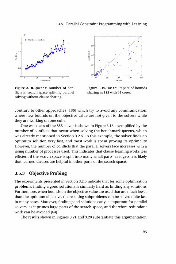
3.5. Parallel Constraint Programming with Learning
0 20 40 600
0.5
1
1.5
2
¨106
# Processes
Co
nfl
icts
Number of conflicts
Figure 3.18. queens: number of con-flicts in search space splitting parallelsolving without clause sharing.
100 101 102 103 104100
101
102
103
noShare
shar
eBo
un
ds
Figure 3.19. suite: impact of boundssharing in SSS with 64 cores.
contrary to other approaches [186] which try to avoid any communication,where new bounds on the objective value are not given to the solvers whilethey are working on one cube.
One weakness of the SSS solver is shown in Figure 3.18, exemplified by thenumber of conflicts that occur when solving the benchmark queens, whichwas already mentioned in Section 3.2.5. In this example, the solver finds anoptimum solution very fast, and most work is spent proving its optimality.However, the number of conflicts that the parallel solvers face increases with arising number of processes used. This indicates that clause learning works lessefficient if the search space is split into many small parts, as it gets less likelythat learned clauses are helpful in other parts of the search space.
3.5.3 Objective Probing
The experiments presented in Section 3.2.5 indicate that for some optimisationproblems, finding a good solutions is similarly hard as finding any solutions.Furthermore, when bounds on the objective value are used that are much lowerthan the optimum objective, the resulting subproblems can be solved quite fastin many cases. Moreover, finding good solutions early is important for parallelsolvers, as it prunes large parts of the search space, and therefore redundantwork can be avoided [64].
The results shown in Figures 3.21 and 3.20 substantiate this argumentation.
93
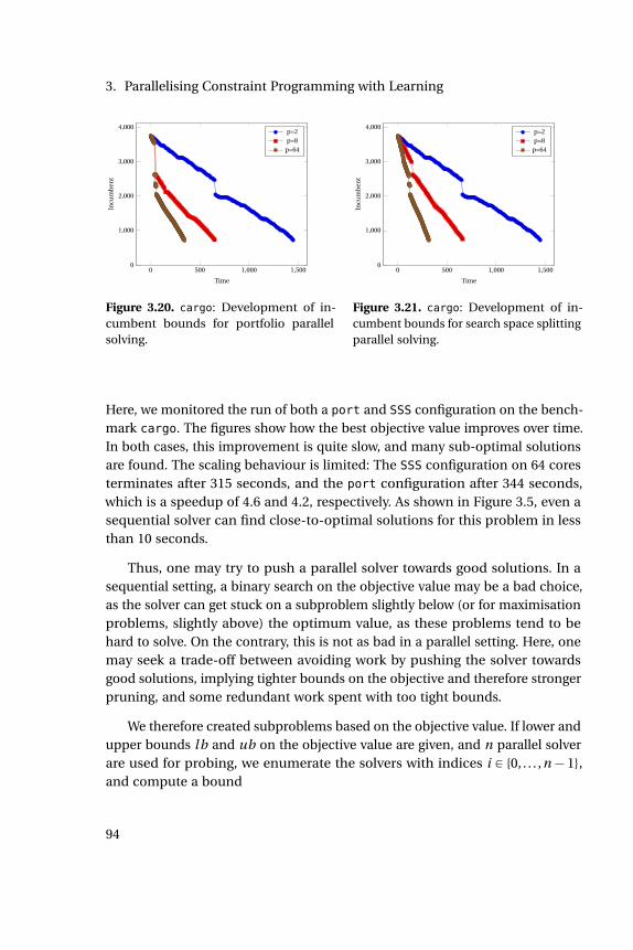
3. Parallelising Constraint Programming with Learning
0 500 1,000 1,5000
1,000
2,000
3,000
4,000
Time
Incu
mb
ent
p=2p=8
p=64
Figure 3.20. cargo: Development of in-cumbent bounds for portfolio parallelsolving.
0 500 1,000 1,5000
1,000
2,000
3,000
4,000
Time
Incu
mb
ent
p=2p=8
p=64
Figure 3.21. cargo: Development of in-cumbent bounds for search space splittingparallel solving.
Here, we monitored the run of both a port and SSS configuration on the bench-mark cargo. The figures show how the best objective value improves over time.In both cases, this improvement is quite slow, and many sub-optimal solutionsare found. The scaling behaviour is limited: The SSS configuration on 64 coresterminates after 315 seconds, and the port configuration after 344 seconds,which is a speedup of 4.6 and 4.2, respectively. As shown in Figure 3.5, even asequential solver can find close-to-optimal solutions for this problem in lessthan 10 seconds.
Thus, one may try to push a parallel solver towards good solutions. In asequential setting, a binary search on the objective value may be a bad choice,as the solver can get stuck on a subproblem slightly below (or for maximisationproblems, slightly above) the optimum value, as these problems tend to behard to solve. On the contrary, this is not as bad in a parallel setting. Here, onemay seek a trade-off between avoiding work by pushing the solver towardsgood solutions, implying tighter bounds on the objective and therefore strongerpruning, and some redundant work spent with too tight bounds.
We therefore created subproblems based on the objective value. If lower andupper bounds lb and ub on the objective value are given, and n parallel solverare used for probing, we enumerate the solvers with indices i P 0, . . . ,n´1,and compute a bound
94

3.5. Parallel Constraint Programming with Learning
bound(i ) = l b + iub´ lb
n
for solver i , which is used as upper bound on the objective value in case ofminimisation problems, and as lower bound otherwise. If one of the solversfind a solution which satisfies its bound, this is communicated to other solversas common. Conversely, if it proves that there is no solution satisfying thisbound, this implies a new lower bound on the objective value. In both cases,the solver can either compute a new bound on the objective, or continueworking without artificial bounds. In our experiments, we used half of theavailable cores for probing on the objective value, and the other half was runin portfolio or SSS configuration, respectively. The solvers running objectiveprobing guessed new bounds twice, and afterwards joined the other solverprocesses. This setting works well on a wide range of problems, however, itmight be interesting to try and choose the number of probing solvers or thenumber of re-tries automatically.
Figure 3.22 shows the impact of this approach when solving the benchmarkcargo. Here, the 64 cores were used, out of which 32 performed objectiveprobing, and the others were configured as portfolio solvers. An optimumsolution can be found in 3 seconds in this setting, which is a speedup of 114.7compared to the normal portfolio setting on 64 cores, cf. Figure 3.21, and 483compared to the sequential version of CHUFFED.
Figure 3.25 compares the plain portfolio configuration with the one us-ing probing, denoted by portP. On some benchmarks, the performance isslightly decreased, whereas significant speedups can be observed on manyothers. Similarly, we observe super-linear speedups compared to the sequentialsolver, presented in Table 3.3. On 64 cores, the speedup on hard benchmarks isincreased from 84.6 to 152, and the median from 42 to 133.6.
We implemented an analogous approach with search space splitting, calledSSSP. Here, one half of the solvers guess objective values, and the other halfruns a search space splitting approach with work stealing. Again, the probingsolvers do at most 2 guesses, and join the other solvers afterwards. A scatterplot comparing the sequential version of CHUFFED with this approach is givenin Figure 3.23, which clearly shows the positive impact of the parallelisation.The speed-ups for both all and hard benchmarks are shown in Table 3.3. Also
95
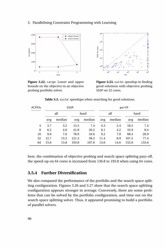
3. Parallelising Constraint Programming with Learning
1 2 30
1,000
2,000
3,000
4,000
Time
Incu
mb
ent
Upper Bound
Lower Bound
Figure 3.22. cargo: Lower and upperbounds on the objective in an objectiveprobing portfolio solver.
100 101 102 103 104
100
101
102
103
104
seq
SSSP
(32
core
s)
Figure 3.23. suite: speedup in findinggood solutions with objective probingSSSP on 32 cores.
Table 3.3. suite: speedups when searching for good solutions.
#CPUs SSSP portP
all hard all hard
avg median avg median avg median avg median
4 3.7 3.2 15.5 7.4 4.3 2.4 18.2 7.48 6.2 4.0 41.8 20.2 6.1 4.2 33.9 8.4
16 9.6 7.6 78.9 34.6 9.2 7.0 68.4 26.932 12.7 13.3 121.3 58.5 11.4 8.9 107.5 77.464 15.6 13.8 193.8 107.0 13.6 14.6 152.0 133.6
here, the combination of objective probing and search space splitting pays off,the speed-up on 64 cores is increased from 136.8 to 193.8 when using 64 cores.
3.5.4 Further Diversification
We also compared the performance of the portfolio and the search space split-ting configuration. Figures 3.26 and 3.27 show that the search space splittingconfiguration appears stronger in average. Conversely, there are some prob-lems that can be solved by the portfolio configuration, and time out on thesearch space splitting solver. Thus, it appeared promising to build a portfolioof parallel solvers.
96

3.6. Conclusion and Open Questions
100 101 102
100
101
102
SSSP
SSS
Figure 3.24. suite: comparison be-tween SSS and SSSP.
100 101 102
100
101
102
Portfolio+
Port
foli
oFigure 3.25. suite: comparison be-tween port and portP.
Table 3.4. suite: speedups for hybrid when searching good solutions.
#CPUs all hard
avg median avg median
4 4.3 3.3 18.4 6.38 6.3 4.7 38.2 19.9
16 9.6 6.4 79.9 43.032 11.7 8.8 116.0 62.464 15.7 16.0 196.0 140.0
We therefore split the solver processes in a similar way as before: One thirdof the processes ran objective probing, one third was run as portfolio solver,and one third ran search space splitting. After their second guess, the objectiveprobing solvers joined the search space splitting solvers. When considering thespeed-ups for computing good solutions, this configuration, denoted hybrid, isslightly faster than the SSSP configuration on 64 cores, as depicted in Table 3.4.
3.6 Conclusion and Open Questions
In this chapter, we gave a brief introduction to constraint programming, anddiscussed the parallelisation of the clause learning CP solver CHUFFED.
Both a portfolio approach and the typical approach in constraint program-
97

3. Parallelising Constraint Programming with Learning
100 101 102
100
101
102
port
SSS
Figure 3.26. suite: comparison be-tween SSS and port, 64 cores.
100 101 102
100
101
102
portP
SSS
Figure 3.27. suite: comparison be-tween SSS and port, 8 cores.
100 101 102
100
101
102
SSS
hybrid
solv
er
Figure 3.28. suite: comparison be-tween hybrid and SSS solver, 64 cores.
ming, the splitting of the search space into disjoint subspaces, work well. To-gether with some optimistic probing on the objective value, we achieved signif-icant speed-ups, especially in the search for good solutions. Here, all configura-tions we tried gave a super-linear speed-up.
However, there were many choices regarding that worked well in our ex-periments, but were done without a clear reason. This includes the amount ofsolvers used for objective probing, the number of re-guesses, and the splittingbetween portfolio and search space splitting solvers in the hybrid approach.It might be interesting to either find better choices here, or find a reason whythese choices worked well.
98
3.6. Conclusion and Open Questions
We do not see as impressive results when parallelising the proof of optimal-ity. Here, splitting the search space performs better than the portfolio approach,however, the speed-ups are sub-linear, even when the solver are allowed toexchange clauses. We consider this the main open problem: Parallelise learningsolvers such that they scale on unsatisfiable formulas.
This work was conducted by the author during his stay in Melbourne,Australia, with Peter J. Stuckey. Furthermore, the author would like to thankGraeme Gange for many helpful discussions.
99


Chapter 4
Sorting Networks
“alea iacta est.”
GAIUS IULIUS CAESAR
4.1 Introduction
Sorting is a fundamental and well-studied problem in Computer Science. Givena sequence a = (a1, . . . , an), one seeks to order the elements in some permuta-tion Π such that Π(a)i ďΠ(a)i+1 for 1ď i ď n´1 and some ordering ď.
There are many algorithms which solve this problem. A rather simple sort-ing algorithm is Insertion Sort [80, p. 26]. The idea of this algorithm is to insertelements into a sorted prefix of the input sequence, cf. Algorithm 10. Here, arather simple version of the algorithm is given which requires O(n2) compar-isons on every input sequence of length n, wheras smarter version require onlya linear number of comparisons when run on sorted sequences.
More sophisticated sorting algorithms are often based on the principle ofDivide&Conquer. A prominent example for this is Merge Sort [80, p. 30]. Here,the input is split in two subsequences of (almost) equal size, which are sorted.Afterwards, the results are merged to a single sorted sequence. It can easilybe seen that the merging step can be implemented using a linear numberof comparisons, and thus the overall running time is O(n log(n)). In fact, thisrunning time is optimal for sorting algorithms which operate by comparing theelements of the input sequence [80].
At a first glance, the Divide&Conquer approach of Merge Sort seems to lenditself to a trivial implementation. The recursive calls to Merge Sort can be runin parallel, and the results are merged sequentially afterwards. An analysis of
101

4. Sorting Networks
Algorithm 10: Insertion Sort
Data: Array a of length nResult: a is sorted
1 if n > 1 then/* Sort the first n´1 elements */
2 sort(a[0. . .n-2]);
/* Insert the last element at the right position */
3 for i = n´1 to 1 do4 if a[i] < a[i-1] then
/* swap */
5 swap(a, i-1, i);
Algorithm 11: Sorting algorithm for 4 elements
Data: Array a of length 4Result: a is sorted
1 compareAndSwap(a, 0, 1);2 compareAndSwap(a, 2, 3);3 compareAndSwap(a, 0, 2);4 compareAndSwap(a, 1, 3);5 compareAndSwap(a, 1, 2);
the running time reveals that the running time T can be analysed to be
T (1) = 1
T (n) = maxT(⌈n
2
⌉),T
(⌊n
2
⌋)+O(n),
which yields a linear running time. Here, the final call to Merge is the bottleneck,as it requires O(n) comparisons.
In this section we will consider one possible approach for parallel sorting al-gorithms, so-called Sorting Networks. Sorting Networks are data-oblivious sort-ing algorithms, as the sequence of comparisons they perform is independent ofthe input sequence. An example for such algorithms is given in Algorithm 11.
Here, a procedure compareAndSwap is used to compare two elements andswap them, if necessary. From this presentation it is not obvious that this
102

4.1. Introduction
i2
i1
maxi1, i2
mini1, i2
Figure 4.1. A comparator.
1
2
3
4
5
1
3
2
5
4
2
5
1
3
4
3
5
4
2
1
5
3
4
2
1
5
4
3
2
1
Figure 4.2. A sorting network on 5 channels, operating on the input (5,4,3,2,1).
algorithm actually sorts all possible inputs in increasing order. In fact, checkingthis is a co-NP complete problem [173]. As we will discuss shortly, in order toensure the correctness of a data oblivious sorting algorithm for inputs of sizen, it is sufficient to check if all 2n input vectors containing only the values 0and 1 are sorted.
It is common to present Sorting Networks as Knuth diagrams [139], asshown in Figure 4.2. Here, the input values are connected to some channels onthe left-hand side of the diagram. A vertical connection between these channelsdenotes a comparator, as depicted in Figure 4.1. Each comparator compares itsinput values, and writes them in sorted order to the channels on its right-handside.
Here, the vector (5,4,3,2,1) is given as input at the left-hand side of thenetwork. The left-most, upper-most comparator compares its inputs, 4 and5, and writes them in a sorted order on its output channels. In this way, thesequence becomes more and more sorted from the left to the right side ofthe network, and the outputs on the right-hand side of the network are sortedincreasingly, when read from top to bottom.
Figure 4.3 shows an Insertion Sort, represented as sorting network. The firstcomparator on the left-hand side creates a sorted subsequence on the first twochannels. The next two comparators insert the value from the third channelinto this sorted sequence, and this process is repeated until every element hasbeen inserted.
103
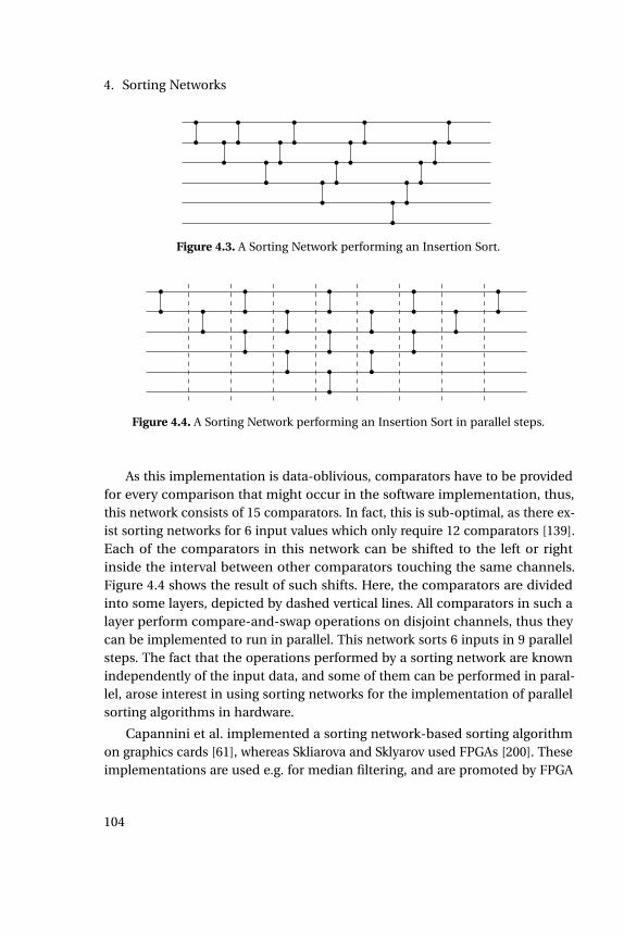
4. Sorting Networks
Figure 4.3. A Sorting Network performing an Insertion Sort.
Figure 4.4. A Sorting Network performing an Insertion Sort in parallel steps.
As this implementation is data-oblivious, comparators have to be providedfor every comparison that might occur in the software implementation, thus,this network consists of 15 comparators. In fact, this is sub-optimal, as there ex-ist sorting networks for 6 input values which only require 12 comparators [139].Each of the comparators in this network can be shifted to the left or rightinside the interval between other comparators touching the same channels.Figure 4.4 shows the result of such shifts. Here, the comparators are dividedinto some layers, depicted by dashed vertical lines. All comparators in such alayer perform compare-and-swap operations on disjoint channels, thus theycan be implemented to run in parallel. This network sorts 6 inputs in 9 parallelsteps. The fact that the operations performed by a sorting network are knownindependently of the input data, and some of them can be performed in paral-lel, arose interest in using sorting networks for the implementation of parallelsorting algorithms in hardware.
Capannini et al. implemented a sorting network-based sorting algorithmon graphics cards [61], whereas Skliarova and Sklyarov used FPGAs [200]. Theseimplementations are used e.g. for median filtering, and are promoted by FPGA
104
4.1. Introduction
manufacturers [24].
In software implementations of Merge Sort or QuickSort, it is commonto fall back to naïve algorithms like Insertion Sort on small inputs or as basecase in recursive calls. Codish et al. replaced this base case by a softwareimplementation of optimal sorting networks [72]. Here, each comparator canbe represented by conditional move (CMOV) instructions, and therefore thealgorithm can be implemented without any branch instructions.
In the application of SAT solving, Cardinality Networks, which are simplifiedversions of Sorting Networks, are used to encode cardinality constraints [11].Given a constraint
∑ni=0 li ď k for some literals li , the literals are used as inputs
of a sorting network. The network itself can be encoded using O(n log2(k))clauses and variables, which outperforms e.g. sequential counters, which re-quire O(nk) additional clauses and variables [198]. Furthermore, this encodingenforces arc consistency: If some k1 literals are set to 1, unit propagation issufficient to set the highest k1 outputs to 1 as well. If k1 > k, this leads to aconflict, and the solver can backtrack without performing further search in thispart of the search space.
The remainder of this chapter is structured as follows. First, we will discussthe construction of efficient sorting networks in Section 4.1.1. Next, we willintroduce some notation which is necessary to reason formally about sortingnetworks. Unfortunately, there is a flaw of precision in the literature on sort-ing networks, which is mostly based on different interpretations of notations.Therefore, we present correct and consistent versions of some theorems andtheir proofs in Section 4.2. Next, we turn to SAT encodings of sorting networks,which can be used both to find sorting networks of minimum depth, i. e., mini-mum number of parallel sorting steps, and prove lower bounds on the numbersof layers required to sort some n inputs. We show how the aforementionedtheorems help to remove symmetries from the search space, and decomposethe occurring problems into subproblems, which can be solved independently.We improve upon the SAT encodings used in former papers in Section 4.3,and show how a closer analysis of the symmetries on sorting networks can beused to set up an optimisation problem which effectively minimises the size ofthe SAT formulas generated to encode the existence of sorting networks withcertain properties. This leads to new upper bounds, presented in Section 4.4,and the main result, a new lower bound on the depth of sorting networks for17 elements.
105

4. Sorting Networks
Algorithm 12: Bubble Sort
Data: Array A of length nResult: A is sorted
1 for i = n-1 to 1 do2 for j = 0 to i do3 if A[ j ] > A[ j +1] then4 swap(A, j, j+1);
Figure 4.5. A Bubble Sort implemented as sorting network.
4.1.1 Construction of Sorting Networks
As seen in the introduction, the easiest way of constructing a sorting networkis to re-use data oblivious sorting algorithms like Bubble Sort as depicted inAlgorithm 12. Figure 4.5 shows the Bubble Sort for 6 elements represented assorting network. Again, we can shift the comparators to gain layers of data-independent comparators.
Interestingly, this shift yields exactly the same sorting network as the onethat was created from an Insertion Sort.
A drawback of this network is that only one layer is maximal in the sensethat no further comparator can be added. This problem is overcome in theodd-even-transposition sort, shown in Figure 4.6.
These networks consists of n layers, each of them filled with comparatorsconnecting channels (2i ,2i +1) in odd, and (2i +1,2i +2) in even layers, wherethe layers are numbered from left to right, beginning with 1. Thus, the timerequired to sort the inputs is O(n).
It is well-known that there exist sorting algorithms like Merge Sort or Heap-Sort which require O(n log(n))) comparisons. Thus, the question arose if it
106

4.1. Introduction
Figure 4.6. Odd-even-transposition sort.
is possible to construct sorting networks which use the same magnitude ofcomparators.
In 1968, Batcher presented the first algorithms to construct sorting net-works for which the number of comparators, denoted sn , is bounded by sn P
O(n log(n)2) and the number of layers, or depth, dn , is O(log(n)2) [32]. In orderto discuss these networks, the following theorem is helpful.
Theorem 4.1. (0/1-principle [139]) If a network on n input lines sorts all 2n
sequences of 0s and 1s into nondecreasing order, it will sort any sequence of nnumbers into nondecreasing order.
Thus, it is sufficient to consider only binary input vectors to reason on thecorrectness of sorting networks. Batcher gave two algorithms for constructingsorting networks, Bitonic Merge Sort and Odd-Even- Merge Sort. Here wewill present only the latter one. For simplicity, we assume that the input is asequence of length n = 2k for some k PN.
Similar to the well-known Merge Sort algorithm, it applies a merge pro-cedure on sorted sequences, gaining larger and larger sorted sequences untileventually the whole input is sorted. By the 0/1-principle, it is sufficient toconsider binary input sequences. Figure 4.7(a) shows a binary input sequencefor a merge: The upper, and lower halves are sorted. The sequence of 0s isdrawn as a white box here, whereas 1s are represented by a black box. In a firststep, Batcher’s odd-even Merge Sort sorts the subsequences consisting of allentries with even and odd indices, respectively. The core insight behind this isthat the number of ones in the odd and the even subsequences differ at mostby 2. Thus, after sorting the odd and even subsequences, the result is eithersorted already, or almost sorted, as depicted in Figure 4.7(b). In the latter case,
107
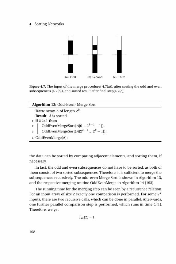
4. Sorting Networks
(a) First (b) Second (c) Third
Figure 4.7. The input of the merge procedure( 4.7(a)), after sorting the odd and evensubsequences (4.7(b)), and sorted result after final step(4.7(c))
Algorithm 13: Odd-Even- Merge Sort
Data: Array A of length 2k
Result: A is sorted1 if k ě 1 then2 OddEvenMergeSort(A[0 . . .2k´1´1]);
3 OddEvenMergeSort(A[2k´1 . . .2k´1]);
4 OddEvenMerge(A);
the data can be sorted by comparing adjacent elements, and sorting them, ifnecessary.
In fact, the odd and even subsequences do not have to be sorted, as both ofthem consist of two sorted subsequences. Therefore, it is sufficient to merge thesubsequences recursively. The odd-even Merge Sort is shown in Algorithm 13,and the respective merging routine OddEvenMerge in Algorithm 14 [193].
The running time for the merging step can be seen by a recurrence relation.For an input array of size 2 exactly one comparison is performed. For some 2k
inputs, there are two recursive calls, which can be done in parallel. Afterwards,one further parallel comparison step is performed, which runs in time O(1).Therefore, we get
Tm(2) = 1
108
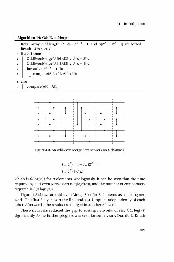
4.1. Introduction
Algorithm 14: OddEvenMerge
Data: Array A of length 2k , A[0..2k´1´1] and A[2k´1..2k´1] are sorted.Result: A is sorted
1 if k > 1 then2 OddEvenMerge(A[0]A[2] . . . A[n´2]);3 OddEvenMerge(A[1]A[3] . . . A[n´1]);
4 for i=0 to 2k´1´1 do5 compare(A[2i+1], A[2i+2]);
6 else7 compare(A[0], A[1]);
Figure 4.8. An odd-even Merge Sort network on 8 channels.
Tm(2k ) = 1+Tm(2k´1)
Tm(2k ) P θ(k)
which is θ(log(n)) for n elements. Analogously, it can be seen that the timerequired by odd-even Merge Sort is θ(log2(n)), and the number of comparatorsrequired is θ(n log2(n)).
Figure 4.8 shows an odd-even Merge Sort for 8 elements as a sorting net-work. The first 3 layers sort the first and last 4 inputs independently of eachother. Afterwards, the results are merged in another 3 layers.
These networks reduced the gap to sorting networks of size O(n log(n))significantly. As no further progress was seen for some years, Donald E. Knuth
109
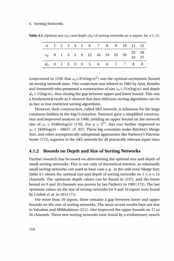
4. Sorting Networks
Table 4.1. Optimal size (sn ) and depth (dn ) of sorting networks on n inputs, for nď 12.
n 1 2 3 4 5 6 7 8 9 10 11 12
sn 0 1 3 5 9 12 16 19 25 2935 3933 37
dn 0 1 3 3 5 5 6 6 7 7 8 8
conjectured in [139] that sn P θ(n log(n)2) was the optimal asymptotic boundon sorting network sizes. This conjecture was refuted in 1983 by Ajtai, Komlósand Szemerédi who presented a construction of size sn PO(n log(n)) and depthdn PO(log(n)), thus closing the gap between upper and lower bound. This wasa fundamental result as it showed that data oblivious sorting algorithms can beas fast as less restricted sorting algorithms.
However, their construction, called AKS network, is infamous for the largeconstants hidden in the big-O notation. Paterson gave a simplified construc-tion and improved analysis in 1990, yielding an upper bound on the networksize of sn ď 6100n log(n) [176]. For n ě 227, this was further improved tosn ď 1830log(n)´58657, cf. [67]. These big constants make Batcher’s MergeSort, and other asymptotically suboptimal approaches like Parberry’s PairwiseSorter [175], superior to the AKS network for all practically relevant input sizes.
4.1.2 Bounds on Depth and Size of Sorting Networks
Further research has focussed on determining the optimal size and depth ofsmall sorting networks. This is not only of theoretical interest, as minimallysmall sorting networks can used as base case e. g., in the odd-even Merge Sort.Table 4.1 shows the optimal size and depth of sorting networks on 1ď nď 12channels. The optimum depth values can be found in [137], and the lowerbound on 9 and 10 channels was proven by Ian Parberry in 1989 [172]. The lastoptimum values on the size of sorting networks for 9 and 10 inputs were foundby Codish et al. in 2014 [71].
For more than 10 inputs, there remains a gap between lower and upperbounds on the size of sorting networks. The most recent results here are dueto Valsalam and Miikkulainen [211], who improved the upper bounds on 17 to20 channels. These new sorting networks were found by a evolutionary search
110
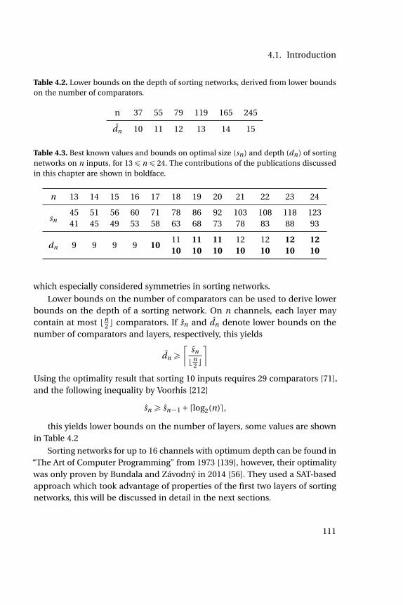
4.1. Introduction
Table 4.2. Lower bounds on the depth of sorting networks, derived from lower boundson the number of comparators.
n 37 55 79 119 165 245
dn 10 11 12 13 14 15
Table 4.3. Best known values and bounds on optimal size (sn ) and depth (dn ) of sortingnetworks on n inputs, for 13ď nď 24. The contributions of the publications discussedin this chapter are shown in boldface.
n 13 14 15 16 17 18 19 20 21 22 23 24
sn45 51 56 60 71 78 86 92 103 108 118 12341 45 49 53 58 63 68 73 78 83 88 93
dn 9 9 9 9 1011 11 11 12 12 12 1210 10 10 10 10 10 10
which especially considered symmetries in sorting networks.
Lower bounds on the number of comparators can be used to derive lowerbounds on the depth of a sorting network. On n channels, each layer maycontain at most bn
2 c comparators. If sn and dn denote lower bounds on thenumber of comparators and layers, respectively, this yields
dn ě
⌈sn
bn2 c
⌉Using the optimality result that sorting 10 inputs requires 29 comparators [71],and the following inequality by Voorhis [212]
sn ě sn´1 +dlog2(n)e,
this yields lower bounds on the number of layers, some values are shownin Table 4.2
Sorting networks for up to 16 channels with optimum depth can be found in“The Art of Computer Programming” from 1973 [139], however, their optimalitywas only proven by Bundala and Závodný in 2014 [56]. They used a SAT-basedapproach which took advantage of properties of the first two layers of sortingnetworks, this will be discussed in detail in the next sections.
111
4. Sorting Networks
An improved sorting network for 18 channels was found by Al-Haj Baddar in2009 [22]. She used a tool, SortNet, to assist her in hand-crafting this network.
Further improved sorting networks for 17, 19 and 20 channels were foundby Ehlers and Müller in 2014 [93]. The improved upper bounds on 23 and24 inputs were found by applying techniques from [71] to create a good pre-fix, and completing it to a complete sorting network using a SAT solver [90].The optimality for the case of 17 channels could be proven by a SAT-basedapproach [94].
All new bounds that this thesis is involved with are marked in bold inTable 4.3.
4.2 Properties of Sorting Networks
In this section we will discuss properties of sorting networks. These will behelpful to break symmetries in the search space in the following sections. Noneof the theorems in this section were proven by the author of this thesis, however,there is a flaw in precision in the literature. Thus, we fix some notation, andthen give consistent and correct proofs for the theorems presented here.
4.2.1 Notation and Definitions
Let us first fix some notation. Given a sequence s = (s1, . . . , sn), we will denoteits length by |s|. Its i -th element is si , for 1 ď i ď |s|. Given two indices iand j , the subsequence starting at index i and ending at index j is s[i , j ] for1ď i ď j ď |s|. A prefix of a sequence s = (s1, . . . , sn) is a sequence s[1,k] fork ď n, and a suffix is a sequence s[k,n] for k ě 1. Given two sequences a andb, their concatenation is defined as ab = (a1, . . . , a|a|,b1, . . . ,b|b|). The k-wiseconcatenation of a is denoted by ak .
We will denote permutations which swap the elements at indices i and j ,leaving all other elements at the same positions, by (i , j ).
We will denote comparators connecting channels i and j as a tuple (i , j ).This comparator will sort its smaller input value to the channel i , and thelarger value to channel j . The length of a comparator (i , j ) is |i ´ j |. In theintroduction, we considered only comparators which sort their inputs suchthat the numerically smaller input is sorted to the upper, and the larger inputis sorted to the lower output.
112
4.2. Properties of Sorting Networks
Definition 4.2 (Standard Comparator). A standard comparator is a tuple (i , j )such that i < j .
In the sorting networks presented so far, all comparators were standardcomparators.
Definition 4.3 (Standard Comparator Network). A standard comparator net-work S on n channels is a sequence of standard comparators ck = (ik , jk ) suchthat 0ď ik < jk < n for each comparator.
This definition does not actually require the network to sort its inputs -the empty sequence is also a standard comparator network. To describe that acomparator network sorts its inputs, we next consider the definition of outputsof a comparator network.
Definition 4.4 (Outputs of a Comparator Network). Let I denote the inputs ofa comparator network C on n channels. By the 0/1-principle, it is sufficient toconsider IĎ 0,1n . Let outputs denote a function which maps a comparatornetwork and a set of input vectors to the set of output vectors. This functioncan be defined inductively by computing the impact of the first comparatoron C on the inputs, and applying the suffix of C to the result. If C is the emptysequence, nothing is sorted, and therefore the outputs equal the inputs.
outputs(ε,I) = I
Otherwise, let (i , j ) denote the first comparator of C , i. e., C = (i , j )C 1. With-out loss of generality we may assume that i < j . We obtain I1 by applying thecomparator (i , j ) on all elements of I, and then apply C 1 on I1. Formally, if weapply a comparator (i , j ) on some a P 0,1n , the result is
app((i , j ), a) =
a, ai ď a j
a[0 . . . i´1]a j a[i+1. . . j´1]ai a[ j+1. . .n´1],else
With this, we may give the outputs of a comparator network as
outputs((i , j )C 1,I) = outputs(C 1, x|x = app((i , j ), x1), x1 P I)
Definition 4.5 (Standard Sorting Network). A standard sorting network is astandard comparator network which sorts all possible input sequences non-decreasingly.
113
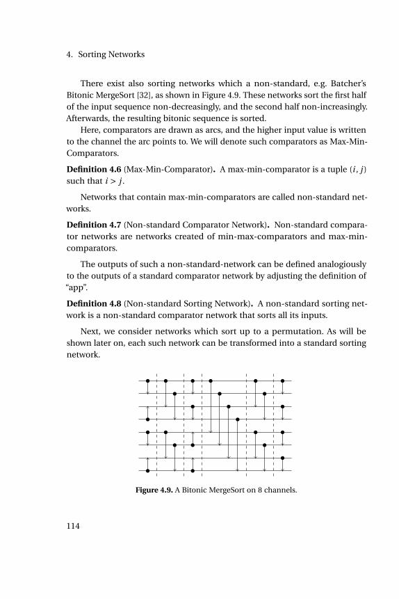
4. Sorting Networks
There exist also sorting networks which a non-standard, e.g. Batcher’sBitonic MergeSort [32], as shown in Figure 4.9. These networks sort the first halfof the input sequence non-decreasingly, and the second half non-increasingly.Afterwards, the resulting bitonic sequence is sorted.
Here, comparators are drawn as arcs, and the higher input value is writtento the channel the arc points to. We will denote such comparators as Max-Min-Comparators.
Definition 4.6 (Max-Min-Comparator). A max-min-comparator is a tuple (i , j )such that i > j .
Networks that contain max-min-comparators are called non-standard net-works.
Definition 4.7 (Non-standard Comparator Network). Non-standard compara-tor networks are networks created of min-max-comparators and max-min-comparators.
The outputs of such a non-standard-network can be defined analogiouslyto the outputs of a standard comparator network by adjusting the definition of“app”.
Definition 4.8 (Non-standard Sorting Network). A non-standard sorting net-work is a non-standard comparator network that sorts all its inputs.
Next, we consider networks which sort up to a permutation. As will beshown later on, each such network can be transformed into a standard sortingnetwork.
Figure 4.9. A Bitonic MergeSort on 8 channels.
114
4.2. Properties of Sorting Networks
4.2.2 Permutations of Sorting Networks
Definition 4.9 (Generalised Sorting Network). A non-standard comparatornetwork C is called generalised sorting network if, for some permutation Π, allits outputs are sorted after the application of Π.
Given a standard sorting network, a generalised sorting network can beobtained by permuting its channels.
Definition 4.10 (Permutations of Sorting Networks). Let C = (c1, . . . ,cs ) de-note a comparator network, and Π : 1, . . . ,n ÞÑ 1, . . . ,n denote a permuta-tion. We define the permutation of C as Π(C ) = (Π(c1), . . . ,Π(cs )), and Π(ck ) =(Π(ik ),Π( jk )).
Lemma 4.11 (Permutation of Generalised Sorting Networks). Let C denote ageneralised sorting network on n channels and d layers. Then, for any permu-tation Π : 1, . . . ,n ÞÑ 1, . . . ,n, the permuation of C under Π, Π(C ), is also ageneralised sorting network.
Proof. ([172]) As C is a generalised sorting network, there exists a permutationΠC such that the outputs of C are sorted after applying ΠC on them. Therefore,applying ΠC ˝Π
´1 on the outputs of Π(C ) yields sorted outputs.
Lemma 4.12. Every generalised sorting network which consists only of standardcomparators is a standard sorting network.
Proof. ([174]) By the definition of a generalised sorting network C , there existsa fixed permutation ΠC such that the outputs of C , permuted by ΠC , are sorted.Consider the input (1,2, . . . ,n). As C is made from standard comparators, noneof them will swap its input, thus, the output is (1,2, . . . ,n), and therefore ΠC =i d .
Knuth mentioned in [137, Exercise 5.3.4.16] that non-standard sorting net-works are no more powerful than standard sorting networks. He furthermoredescribes an algorithm, called untangle, which can turn every sorting networkinto a standard sorting network. This algorithm is shown in Algorithm 15. Inits original version, the algorithm is applied to non-standard sorting networks.Here, we consider a more general version which applies to generalised sortingnetworks.
115

4. Sorting Networks
Algorithm 15: untangle
Data: Generalised sorting network C = ((i1, j1), . . . , (in , jn)) withpermutation ΠC
Result: A standard sorting network1 Π := ΠC ;2 for k = 1 to n do3 if ik > jk then
/* Swap channels ik and jk by untangling comparators
with higher indices */
4 for l = k to n do5 if il = ik then6 il := jk ;7 else if il = jk then8 il := ik ;9 if jl = ik then
10 jl := jk ;11 else if jk = jl then12 jl :=ik ;
13 Π := (ik , jk )˝Π;
14 return C ;
(a) Bitonic Merge Sort on4 channels
(b) Untangled version
Figure 4.10. A bitonic Merge Sort and the result of untangling it.
As an example, Figure 4.10 shows a bitonic Merge Sort on 4 channels, whichis a non-standard sorting network, and a standard sorting network obtained byuntangling.
Next, we prove the correctness of the untangle-algorithm.
116

4.2. Properties of Sorting Networks
Lemma 4.13. After the k-th iteration of the outer loop, the first k comparatorsare min-max-comparators.
[174]. If ik > jk , the channels are swapped. In later iterations, this comparatoris not touched anymore, the claim follows by induction.
Lemma 4.14. After the k-th iteration of the outer loop, C is a generalised sortingnetwork, and the respective permutation is Π.
Proof. We show that if the claim holds before the k-th iteration, it also holdsafter [174]. Before the first iteration, C is a generalised sorting network withpermutation Π=ΠC . If, in iteration k, ik < jk , nothing is done; the claim holdsby induction. Otherwise, the channels ik and jk are swapped after the (k´1)-thcomparator. Thus, also the outputs on channels ik and jk are swapped. As, byinductive hypothesis, C was a generalised sorting network before this iteration,applying Π˝ (ik , jk ) on the outputs yields sorted outputs.
Lemma 4.15. The result of the untangle algorithm, denoted C , is a standardsorting network.
Proof. According to Lemma 4.13, C consists only of standard comparators, andby Lemma 4.14, it is a generalised sorting network. Thus, it is a standard sortingnetwork by Lemma 4.12.
We will use these theorems to permute the channels of sorting networks,and make the results standard sorting networks again by untangling. This isfeasible due to the next Corollary.
Corollary 4.16. Let C denote a standard sorting network. If the channels of Care permuted by some permutation Π, then untangling yields a standard sortingnetwork.
4.2.3 Prefixes of Sorting Networks
Next, we consider prefixes of sorting networks. As we will see, if the first layer ofa sorting network is not maximum, i. e., another comparator can be added to it,this yields another standard sorting network. Thus, we may break symmetriesin the search space by enforcing maximum first layers. The next lemma is basedon the observation that a comparator network which sorts some set I of inputsalso sorts all subsets of I.
117
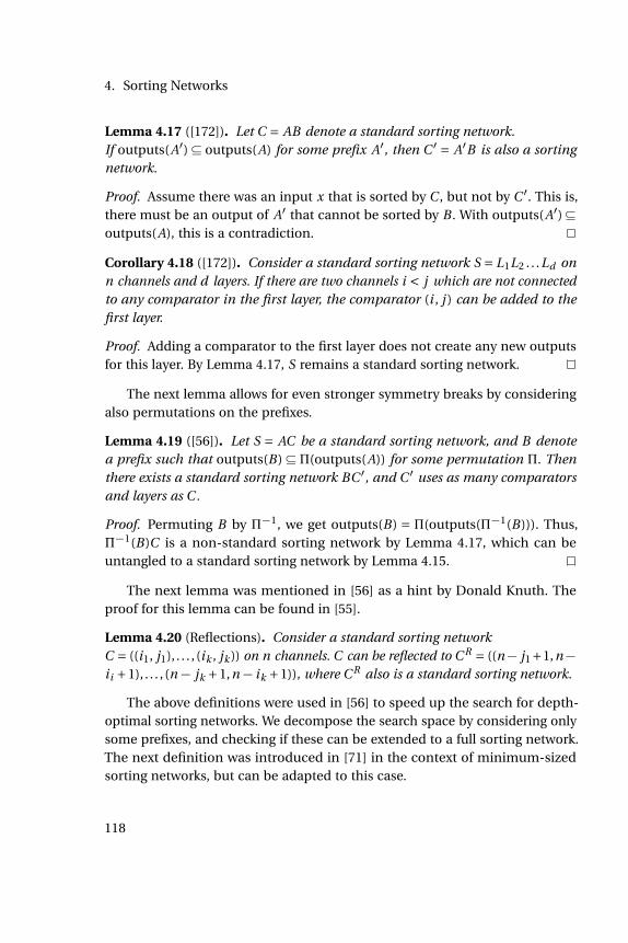
4. Sorting Networks
Lemma 4.17 ([172]). Let C = AB denote a standard sorting network.If outputs(A1)Ď outputs(A) for some prefix A1, then C 1 = A1B is also a sortingnetwork.
Proof. Assume there was an input x that is sorted by C , but not by C 1. This is,there must be an output of A1 that cannot be sorted by B . With outputs(A1)Ďoutputs(A), this is a contradiction.
Corollary 4.18 ([172]). Consider a standard sorting network S = L1L2 . . .Ld onn channels and d layers. If there are two channels i < j which are not connectedto any comparator in the first layer, the comparator (i , j ) can be added to thefirst layer.
Proof. Adding a comparator to the first layer does not create any new outputsfor this layer. By Lemma 4.17, S remains a standard sorting network.
The next lemma allows for even stronger symmetry breaks by consideringalso permutations on the prefixes.
Lemma 4.19 ([56]). Let S = AC be a standard sorting network, and B denotea prefix such that outputs(B)ĎΠ(outputs(A)) for some permutation Π. Thenthere exists a standard sorting network BC 1, and C 1 uses as many comparatorsand layers as C .
Proof. Permuting B by Π´1, we get outputs(B) = Π(outputs(Π´1(B))). Thus,Π´1(B)C is a non-standard sorting network by Lemma 4.17, which can beuntangled to a standard sorting network by Lemma 4.15.
The next lemma was mentioned in [56] as a hint by Donald Knuth. Theproof for this lemma can be found in [55].
Lemma 4.20 (Reflections). Consider a standard sorting networkC = ((i1, j1), . . . , (ik , jk )) on n channels. C can be reflected to C R = ((n´ j1+1,n´ii +1), . . . , (n´ jk +1,n´ ik +1)), where C R also is a standard sorting network.
The above definitions were used in [56] to speed up the search for depth-optimal sorting networks. We decompose the search space by considering onlysome prefixes, and checking if these can be extended to a full sorting network.The next definition was introduced in [71] in the context of minimum-sizedsorting networks, but can be adapted to this case.
118

4.2. Properties of Sorting Networks
Figure 4.11. First layer as used by Bundala&Závodný (“BZ-style”).
Definition 4.21 (Complete set of filters). Let Fk (n,d) denote a set of k-layer-prefixes of sorting networks on n channels. Fk (n,d) is a complete set of filtersif, if there exists a sorting network for n channels and d layers, there also existsone starting with a prefix from Fk (n,d).
If n and d are clear from the context, we may just write Fk . Obviously,the set of all k-layer-prefixes on n channels is a complete filter. Finding asize-minimal set of filters is as hard as determining whether a sorting networkon n channels and d layers exists: If this is not the case, the empty set is acomplete set of filters. Otherwise, the prefix of any such sorting network can bechosen as complete set of filters. Therefore, one seeks to compute small, butnot necessarily minimum sets of filters.
Corollary 4.22. For every maximal layer L, L is a complete set of filters on onelayer.
Parberry used this lemma, and considered only first layers of the formL1
P = (2i ,2i +1)[172]. This massively prunes the search space, and significantlyreduces the size of the SAT formulas we will present in the next section, as onlyoutputs of this first layer have to be considered in subsequent search.
Bundala and Závodný extended this approach to the first two layers ofsorting networks. They considered a set F2
B Z (n) where all prefixes started withthe first layer L1
B Z = ((0,n´1), (1,n´2), . . .), cf. Figure 4.11. Furthermore, theyshrank the set such that no dominated prefixes remained, and no prefixeswhich could be obtained from each other by permutations and reflections.
Formally, let F2(n) denote the set of all 2-layer prefixes on n channels. If,for two prefixes A,B P F2(n), the outputs of A are a strict subset of the (possiblypermuted) outputs of B , then B can be removed by Lemma 4.19.
119

4. Sorting Networks
outputs(A)(Π(outputs(B))ñB ∉F2B Z (n)
Furthermore, if A can be obtained from B by permuting the channels anduntangling, only one of these prefixes has to be considered, this is
outputs(A) =Π(outputs(B))ñ (A ∉F2B Z (n)_B ∉F2
B Z (n))
Lastly, reflections were removed.
A = B R ñ (A ∉F2B Z (n)_B ∉F2
B Z (n))
To generate this set, they enumerated all possible 2-layer-prefixes beginningwith a fixed, maximal first layer, and reduced this set by pairwise comparingthe outputs. This approach is computationally expensive, and was used only forgenerating prefixes on 13 channels. In [74], Codish et al. presented an efficientalgorithm to generate 2-layer-prefixes of depth-optimal sorting networks. Thisalgorithm can easily generate the set F2
B Z for 20 and more channels.
4.2.4 Suffixes of Sorting Networks
Another symmetry break was introduced by Codish et al. in [73]. The mostimportant observation here is that it is sufficient to restrict the last two layersof sorting networks to short comparators, as long comparators in these layerswould be redundant, i. e., they would never swap their inputs. Furthermore, itis sufficient to consider only few different structures here.
4.3 SAT-based Search for Improved Bounds
Although already Parberry used a SAT solver in [172], most SAT encodings cur-rently used for the modeling of sorting networks are extensions of the encodingpresented by Morgenstern and Schneider [160]. Here, we present the encodingfrom [70], which fixed some flaws in the presentation by Bundala and Závodný.Afterwards, we discuss an improved version of this encoding, which we firstlypresented in [94].
120
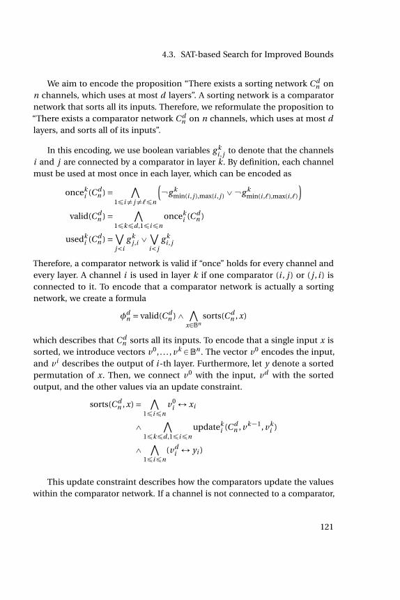
4.3. SAT-based Search for Improved Bounds
We aim to encode the proposition “There exists a sorting network C dn on
n channels, which uses at most d layers”. A sorting network is a comparatornetwork that sorts all its inputs. Therefore, we reformulate the proposition to“There exists a comparator network C d
n on n channels, which uses at most dlayers, and sorts all of its inputs”.
In this encoding, we use boolean variables g ki , j to denote that the channels
i and j are connected by a comparator in layer k. By definition, each channelmust be used at most once in each layer, which can be encoded as
onceki (C d
n ) = ∧1ďi‰ j‰`ďn
( g k
min(i , j ),max(i , j )_ g kmin(i ,`),max(i ,`)
)valid(C d
n ) = ∧1ďkďd ,1ďiďn
onceki (C d
n )
usedki (C d
n ) = ∨j<i
g kj ,i _
∨i< j
g ki , j
Therefore, a comparator network is valid if “once” holds for every channel andevery layer. A channel i is used in layer k if one comparator (i , j ) or ( j , i ) isconnected to it. To encode that a comparator network is actually a sortingnetwork, we create a formula
φdn = valid(C d
n )^∧
xPBnsorts(C d
n , x)
which describes that C dn sorts all its inputs. To encode that a single input x is
sorted, we introduce vectors v0, . . . , vk PBn . The vector v0 encodes the input,and v i describes the output of i -th layer. Furthermore, let y denote a sortedpermutation of x. Then, we connect v0 with the input, vd with the sortedoutput, and the other values via an update constraint.
sorts(C dn , x) = ∧
1ďiďnv0
i Ø xi
^∧
1ďkďd ,1ďiďnupdatek
i (C dn , vk´1, vk
i )
^∧
1ďiďn(vd
i Ø yi )
This update constraint describes how the comparators update the valueswithin the comparator network. If a channel is not connected to a comparator,
121
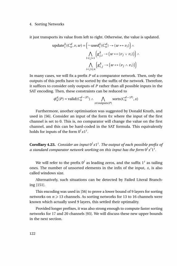
4. Sorting Networks
it just transports its value from left to right. Otherwise, the value is updated.
updateki (C d
n , v, w) =( usedk
i (C dn )Ñ (w Ø vi )
)^∧
1ď j<i
(g k
j ,i Ñ(w Ø (v j _ vi )
))^
∧i< jďn
(g k
i , j Ñ(w Ø (v j ^ vi )
))In many cases, we will fix a prefix P of a comparator network. Then, only theoutputs of this prefix have to be sorted by the suffix of the network. Therefore,it suffices to consider only outputs of P rather than all possible inputs in theSAT encoding. Then, these constraints can be reduced to
φdn (P ) = valid(C d´|P |
n )^∧
xPoutputs(P )sorts(C d´|P |
n , x)
Furthermore, another optimisation was suggested by Donald Knuth, andused in [56]. Consider an input of the form 0x where the input of the firstchannel is set to 0. This is, no comparator will change the value on the firstchannel, and this can be hard-coded in the SAT formula. This equivalentlyholds for inputs of the form 0l x1t .
Corollary 4.23. Consider an input 0l x1t . The output of each possible prefix ofa standard comparator network working on this input has the form 0l x11t .
We will refer to the prefix 0l as leading zeros, and the suffix 1t as tailingones. The number of unsorted elements in the infix of the input, x, is alsocalled windows size.
Alternatively, such situations can be detected by Failed Literal Branch-ing [151].
This encoding was used in [56] to prove a lower bound of 9 layers for sortingnetworks on ně 13 channels. As sorting networks for 13 to 16 channels wereknown which actually used 9 layers, this settled their optimality.
Provided longer prefixes, it was also strong enough to compute faster sortingnetworks for 17 and 20 channels [93]. We will discuss these new upper boundsin the next section.
122
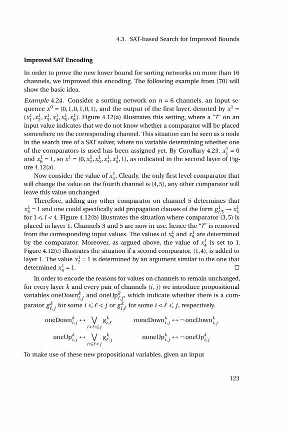
4.3. SAT-based Search for Improved Bounds
Improved SAT Encoding
In order to prove the new lower bound for sorting networks on more than 16channels, we improved this encoding. The following example from [70] willshow the basic idea.
Example 4.24. Consider a sorting network on n = 6 channels, an input se-quence x0 = (0,1,0,1,0,1), and the output of the first layer, denoted by x1 =(x1
1 , x12 , x1
3 , x14 , x1
5 , x16). Figure 4.12(a) illustrates this setting, where a “?” on an
input value indicates that we do not know whether a comparator will be placedsomewhere on the corresponding channel. This situation can be seen as a nodein the search tree of a SAT solver, where no variable determining whether oneof the comparators is used has been assigned yet. By Corollary 4.23, x1
1 = 0and x1
6 = 1, so x1 = (0, x12 , x1
3 , x14 , x1
5 ,1), as indicated in the second layer of Fig-ure 4.12(a).
Now consider the value of x14 . Clearly, the only first level comparator that
will change the value on the fourth channel is (4,5), any other comparator willleave this value unchanged.
Therefore, adding any other comparator on channel 5 determines thatx1
4 = 1 and one could specifically add propagation clauses of the form g 1i ,5Ñ x1
4for 1ď i < 4. Figure 4.12(b) illustrates the situation where comparator (3,5) isplaced in layer 1. Channels 3 and 5 are now in use, hence the “?” is removedfrom the corresponding input values. The values of x1
3 and x15 are determined
by the comparator. Moreover, as argued above, the value of x14 is set to 1.
Figure 4.12(c) illustrates the situation if a second comparator, (1,4), is added tolayer 1. The value x1
2 = 1 is determined by an argument similar to the one thatdetermined x1
4 = 1. äIn order to encode the reasons for values on channels to remain unchanged,
for every layer k and every pair of channels (i , j ) we introduce propositionalvariables oneDownk
i , j and oneUpki , j , which indicate whether there is a com-
parator g k`, j for some i ď `< j or g k
i ,` for some i < `ď j , respectively.
oneDownki , j Ø
∨i<`ď j
g ki ,` noneDownk
i , j Ø oneDownki , j
oneUpki , j Ø
∨iď`< j
g k`, j noneUpk
i , j Ø oneUpki , j
To make use of these new propositional variables, given an input
123
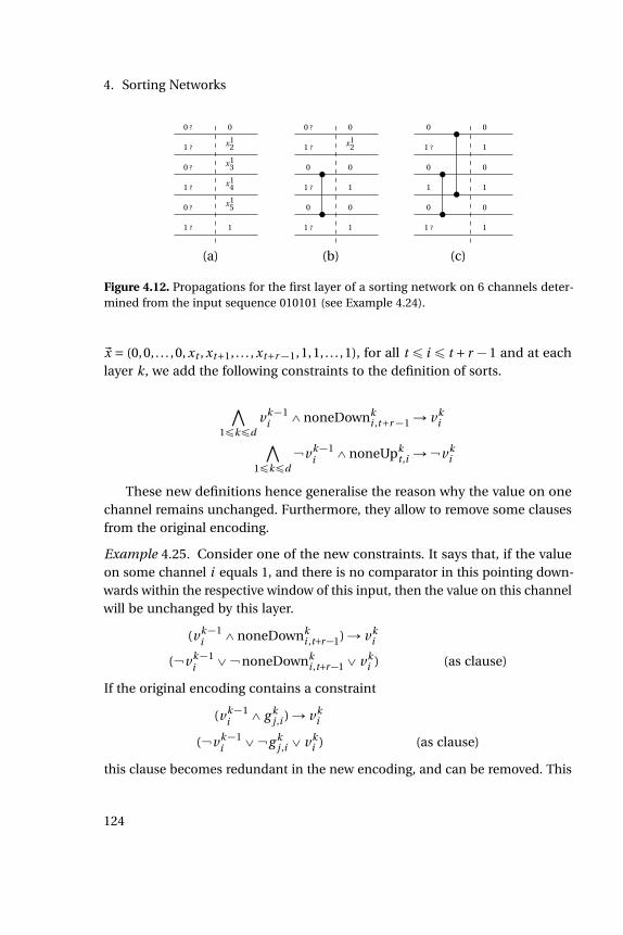
4. Sorting Networks
1 ?
0 ?
1 ?
0 ?
1 ?
0 ?
1
x15
x14
x13
x12
0
1 ?
0
1 ?
0
1 ?
0 ?
1
0
1
0
x12
0
1 ?
0
1
0
1 ?
0
1
0
1
0
1
0
(a) (b) (c)
Figure 4.12. Propagations for the first layer of a sorting network on 6 channels deter-mined from the input sequence 010101 (see Example 4.24).
~x = (0,0, . . . ,0, xt , xt+1, . . . , xt+r´1,1,1, . . . ,1), for all t ď i ď t + r ´1 and at eachlayer k, we add the following constraints to the definition of sorts.
∧1ďkďd
vk´1i ^noneDownk
i ,t+r´1Ñ vki∧
1ďkďd vk´1
i ^noneUpkt ,i Ñ vk
i
These new definitions hence generalise the reason why the value on onechannel remains unchanged. Furthermore, they allow to remove some clausesfrom the original encoding.
Example 4.25. Consider one of the new constraints. It says that, if the valueon some channel i equals 1, and there is no comparator in this pointing down-wards within the respective window of this input, then the value on this channelwill be unchanged by this layer.
(vk´1i ^noneDownk
i ,t+r 1)Ñ vki
( vk´1i _ noneDownk
i ,t+r 1_ vki ) (as clause)
If the original encoding contains a constraint
(vk´1i ^ g k
j ,i )Ñ vki
( vk´1i _ g k
j ,i _ vki ) (as clause)
this clause becomes redundant in the new encoding, and can be removed. This
124

4.3. SAT-based Search for Improved Bounds
can be seen by the following resolution steps.
( g kj ,i _ oneDownk
i ,t+r 1) (oneDownki ,t+r 1_noneDownk
i ,t+r 1)
( g kj ,i _noneDownk
i ,t+r 1)
Another resolution step yields
( vk´1i _ noneDownk
i ,t+r 1_vki ) ( g k
j ,i _noneDownki ,t+r 1)
( vk´1i _ g k
j ,i _ vki )
Thus, the clause from the original encoding became redundant, and may beremoved. This holds symmetrically for the predicates “noneUp". ä
These new predicates come with some advantages. Firstly, they allow formore propagations, as depicted in Example 4.24, which increases the consis-tency of nodes in the search tree. Secondly, the size of the number of clausesin the resulting SAT formulas can be reduced significantly, as we will detailin the next section in Table 4.6. Thirdly, these predicates generalise on thereason why the value on one channel remains unchanged. As discussed inSection 2.2.5, such generalisations allow for smaller proofs. As we will discusswhen summarising the impact of all techniques, this effect can be seen whenanalysing the statistics of solver runs on these formulas.
Next, we will consider another optimisation technique to reduce the size ofthe SAT encoding, and then discuss the impact of both techniques.
4.3.1 Prefix-Optimisation
As discussed in Section 4.2, the channels of standard sorting networks may bepermuted, and untangling the result yields another standard sorting network.In this section, we will see that different permutations of a prefix are not equallyhandy for SAT solvers, a fact that we can use to compute permutations thatyield small SAT formulas, and thus help reducing the running time of the SATsolver. Let us first consider an example.
Example 4.26. Consider the three prefixes on 6 channels and 2 layers shownin Figure 4.13. All of them are equivalent in the sense that they are untangledpermutations of each other. The leftmost prefix, P1, starts with the first layerL1
P used by Parberry. Next to it, the set of non-sorted outputs of P1 is given.
125
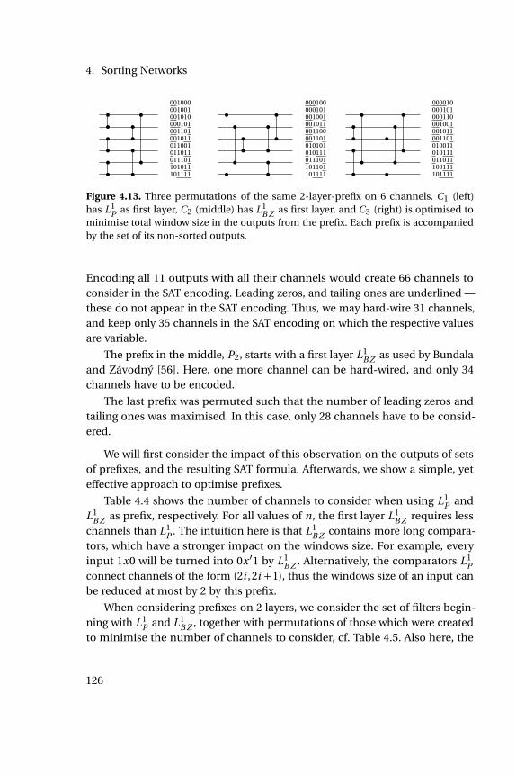
4. Sorting Networks
001000001001001010000101001101001011011001011011011101101011101111
000100000101001001001011001100001101010101010111011101101101101111
000010000101000110001001001011001101010011010111011011100111101111
Figure 4.13. Three permutations of the same 2-layer-prefix on 6 channels. C1 (left)has L1
P as first layer, C2 (middle) has L1B Z as first layer, and C3 (right) is optimised to
minimise total window size in the outputs from the prefix. Each prefix is accompaniedby the set of its non-sorted outputs.
Encoding all 11 outputs with all their channels would create 66 channels toconsider in the SAT encoding. Leading zeros, and tailing ones are underlined —these do not appear in the SAT encoding. Thus, we may hard-wire 31 channels,and keep only 35 channels in the SAT encoding on which the respective valuesare variable.
The prefix in the middle, P2, starts with a first layer L1B Z as used by Bundala
and Závodný [56]. Here, one more channel can be hard-wired, and only 34channels have to be encoded.
The last prefix was permuted such that the number of leading zeros andtailing ones was maximised. In this case, only 28 channels have to be consid-ered.
We will first consider the impact of this observation on the outputs of setsof prefixes, and the resulting SAT formula. Afterwards, we show a simple, yeteffective approach to optimise prefixes.
Table 4.4 shows the number of channels to consider when using L1P and
L1B Z as prefix, respectively. For all values of n, the first layer L1
B Z requires lesschannels than L1
P . The intuition here is that L1B Z contains more long compara-
tors, which have a stronger impact on the windows size. For example, everyinput 1x0 will be turned into 0x11 by L1
B Z . Alternatively, the comparators L1P
connect channels of the form (2i ,2i +1), thus the windows size of an input canbe reduced at most by 2 by this prefix.
When considering prefixes on 2 layers, we consider the set of filters begin-ning with L1
P and L1B Z , together with permutations of those which were created
to minimise the number of channels to consider, cf. Table 4.5. Also here, the
126
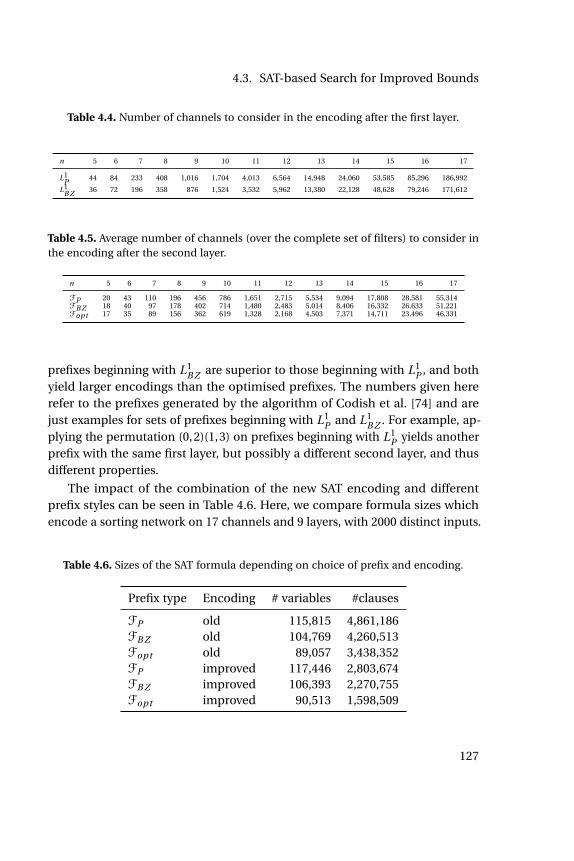
4.3. SAT-based Search for Improved Bounds
Table 4.4. Number of channels to consider in the encoding after the first layer.
n 5 6 7 8 9 10 11 12 13 14 15 16 17
L1P 44 84 233 408 1,016 1,704 4,013 6,564 14,948 24,060 53,585 85,296 186,992
L1B Z 36 72 196 358 876 1,524 3,532 5,962 13,380 22,128 48,628 79,246 171,612
Table 4.5. Average number of channels (over the complete set of filters) to consider inthe encoding after the second layer.
n 5 6 7 8 9 10 11 12 13 14 15 16 17
FP 20 43 110 196 456 786 1,651 2,715 5,534 9,094 17,808 28,581 55,314FB Z 18 40 97 178 402 714 1,480 2,483 5,014 8,406 16,332 26,633 51,221Fopt 17 35 89 156 362 619 1,328 2,168 4,503 7,371 14,711 23,496 46,331
prefixes beginning with L1B Z are superior to those beginning with L1
P , and bothyield larger encodings than the optimised prefixes. The numbers given hererefer to the prefixes generated by the algorithm of Codish et al. [74] and arejust examples for sets of prefixes beginning with L1
P and L1B Z . For example, ap-
plying the permutation (0,2)(1,3) on prefixes beginning with L1P yields another
prefix with the same first layer, but possibly a different second layer, and thusdifferent properties.
The impact of the combination of the new SAT encoding and differentprefix styles can be seen in Table 4.6. Here, we compare formula sizes whichencode a sorting network on 17 channels and 9 layers, with 2000 distinct inputs.
Table 4.6. Sizes of the SAT formula depending on choice of prefix and encoding.
Prefix type Encoding # variables #clauses
FP old 115,815 4,861,186FB Z old 104,769 4,260,513Fopt old 89,057 3,438,352FP improved 117,446 2,803,674FB Z improved 106,393 2,270,755Fopt improved 90,513 1,598,509
127

4. Sorting Networks
Choosing an optimised prefix reduces the number of both clauses and variablessignificantly. The improved encoding adds a few variables, but decreases thenumber of clauses. In the combination of new encoding and optimised prefix,the number of clauses is reduced by a factor of 3. Furthermore, the outputs ofthe permuted prefixes come with smaller window sizes. As comparators whichare longer than the maximum window size of all outputs will never swap thevalues on the channels they are connected to, they could in theory be removedfrom the encoding, yielding a equisatisfiable formula. We experimentally foundthat SAT solvers detect this fact, the VSIDS activities of variables denoting theuse of a long comparator are extremely low.
We will now turn to the techniques used to compute the improved pre-fixes. In the subsequent sections, the computation of new upper and lowerbounds will be discussed, together with the impact of these improvements inthe respective settings.
In order to compute a permutation which minimises the sum of windowssizes of the outputs of a prefix, one might try all possible permutations, andinspect the outputs of the respective permutation of the prefix. For n channels,the running time of this naïve approach is Ω(n!2n), which is intractable evenfor small values of n.
Given a prefix P on n channels and a permutation, one may evaluate thesum of window sizes of its outputs by first permuting and untangling the prefix.Then, iterate over all 2n input sequences, to compute the set of outputs of thepermuted prefix, and count the windows sizes. This approach was chosen inthe first implementation [94]. However, if several permutations of the sameprefix have to be evaluated, it is smarter to compute the set of outputs once.When untangling the prefix with respect to some permutation, the untanglealgorithm (Algorithm 15) can be used to compute the permutation which theprefix permutation induces on the set of outputs. A linear-time implementationof this algorithm is given in the Appendix A.2. As the set of outputs of a prefixis significantly smaller than the set of inputs, this improves the running time.
Let us now consider the search for a decent, i. e., not necessarily opti-mal, permutation to apply to a given prefix. In [94], we chose a simple evo-lutionary algorithm to search for good permutations. An initial populationis created by choosing some permutations uniformly randomly by a Fisher-Yates-Shuffle [103, 136]. Afterwards, in some iterations offspring are createdby randomly swapping two channels, cf. Algorithm 16. The fitness function is
128
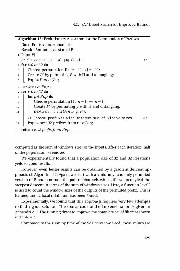
4.3. SAT-based Search for Improved Bounds
Algorithm 16: Evolutionary Algorithm for the Permutation of Prefixes
Data: Prefix P on n channels.Result: Permuted version of P
1 Pop=P ;/* Create an initial population */
2 for i=0 to 32 do3 Choose permutation Π : [n´1] ÞÑ [n´1] ;4 Create P 1 by permuting P with Π and untangling;5 Pop := PopY P 1;
6 nextGen := Pop ;7 for i=0 to 32 do8 for p P Pop do9 Choose permutation Π : [n´1] ÞÑ [n´1] ;
10 Create P 1 by permuting p with Π and untangling;11 nextGen := nextGenY p,P 1;
/* Choose prefixes with minimum sum of window sizes */
12 Pop := best 32 prefixes from nextGen;
13 return Best prefix from Pop;
computed as the sum of windows sizes of the inputs. After each iteration, halfof the population is removed.
We experimentally found that a population size of 32 and 32 iterationsyielded good results.
However, even better results can be obtained by a gradient descent ap-proach, cf. Algorithm 17. Again, we start with a uniformly randomly permutedversion of P, and compute the pair of channels which, if swapped, yield thesteepest descent in terms of the sum of windows sizes. Here, a function “eval"is used to count the window sizes of the outputs of the permuted prefix. This isiterated until a local minimum has been found.
Experimentally, we found that this approach requires very few attemptsto find a good solution. The source code of the implementation is given inAppendix A.2. The running times to improve the complete set of filters is shownin Table 4.7.
Compared to the running time of the SAT-solver we used, these values are
129

4. Sorting Networks
Algorithm 17: Gradient Descent Algorithm
Data: Prefix P on n channels.Result: Permuted version of P
1 Choose permutation Π : [n´1] ÞÑ [n´1];2 P := Π(P );3 Π := id;4 bestVal := eval(P, id);5 repeat6 Π := i d ;7 for 0ď i < j < n do8 obj := eval(P, (i, j));9 if obj < bestVal then
10 bestVal := obj;11 Π := (i , j );
12 P := Π(P );13 until Π = id;14 return P;
Table 4.7. Running times for improving the sets of prefixes.
n 7 8 9 10 11 12 13 14 15 16 17time(s) 0.01 0.02 0.07 0.12 0.68 1.45 10.7 15.8 109 166 1,066
neglectable. When proving the lower bound for n = 17 inputs, the overall CPUtime used was 27 ¨106 seconds, compared to 1,066 seconds for finding goodpermutations of the prefixes.
4.3.2 Preprocessing
There exists a plethora of preprocessing techniques for SAT solving [88, 121–123,152, 154], many of which did not prove helpful in this case. Interestingly, wefound that Failed Literal Branching [151] was helpful, as many literals “failed"and therefore could be fixed at the root of the search tree. We implementedFailed Literal Branching in our extension of MiniSAT [89]1. The specific impact
1The source code is available at https://github.com/the-kiel/JCSS.
130
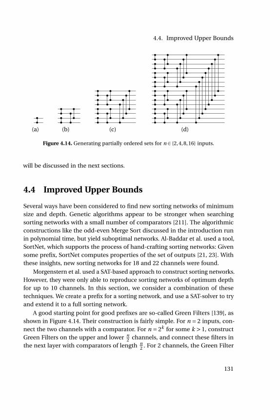
4.4. Improved Upper Bounds
(a) (b) (c) (d)
Figure 4.14. Generating partially ordered sets for n P 2,4,8,16 inputs.
will be discussed in the next sections.
4.4 Improved Upper Bounds
Several ways have been considered to find new sorting networks of minimumsize and depth. Genetic algorithms appear to be stronger when searchingsorting networks with a small number of comparators [211]. The algorithmicconstructions like the odd-even Merge Sort discussed in the introduction runin polynomial time, but yield suboptimal networks. Al-Baddar et al. used a tool,SortNet, which supports the process of hand-crafting sorting networks: Givensome prefix, SortNet computes properties of the set of outputs [21, 23]. Withthese insights, new sorting networks for 18 and 22 channels were found.
Morgenstern et al. used a SAT-based approach to construct sorting networks.However, they were only able to reproduce sorting networks of optimum depthfor up to 10 channels. In this section, we consider a combination of thesetechniques. We create a prefix for a sorting network, and use a SAT-solver to tryand extend it to a full sorting network.
A good starting point for good prefixes are so-called Green Filters [139], asshown in Figure 4.14. Their construction is fairly simple. For n = 2 inputs, con-nect the two channels with a comparator. For n = 2k for some k > 1, constructGreen Filters on the upper and lower n
2 channels, and connect these filters inthe next layer with comparators of length n
2 . For 2 channels, the Green Filter
131
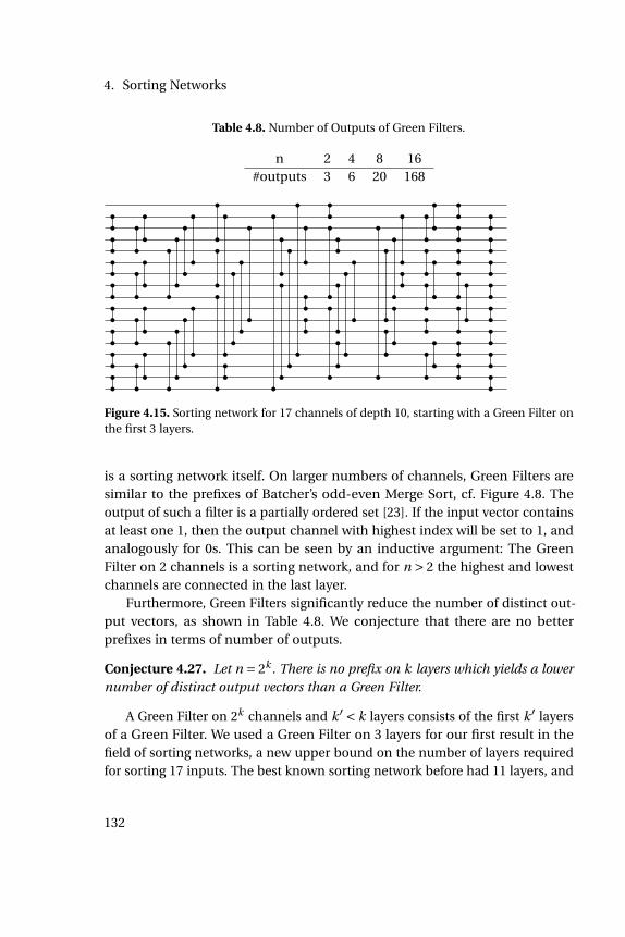
4. Sorting Networks
Table 4.8. Number of Outputs of Green Filters.
n 2 4 8 16#outputs 3 6 20 168
Figure 4.15. Sorting network for 17 channels of depth 10, starting with a Green Filter onthe first 3 layers.
is a sorting network itself. On larger numbers of channels, Green Filters aresimilar to the prefixes of Batcher’s odd-even Merge Sort, cf. Figure 4.8. Theoutput of such a filter is a partially ordered set [23]. If the input vector containsat least one 1, then the output channel with highest index will be set to 1, andanalogously for 0s. This can be seen by an inductive argument: The GreenFilter on 2 channels is a sorting network, and for n > 2 the highest and lowestchannels are connected in the last layer.
Furthermore, Green Filters significantly reduce the number of distinct out-put vectors, as shown in Table 4.8. We conjecture that there are no betterprefixes in terms of number of outputs.
Conjecture 4.27. Let n = 2k . There is no prefix on k layers which yields a lowernumber of distinct output vectors than a Green Filter.
A Green Filter on 2k channels and k1 < k layers consists of the first k1 layersof a Green Filter. We used a Green Filter on 3 layers for our first result in thefield of sorting networks, a new upper bound on the number of layers requiredfor sorting 17 inputs. The best known sorting network before had 11 layers, and
132

4.4. Improved Upper Bounds
Figure 4.16. A sorting network for 20 channels of depth 11. The first 4 layers consist ofa Green Filter on 4 layers, and a complete sorting network on the 4 innermost channels.
could be generated from the network on 18 channels and 11 layers presentedin [23] by removing one channel.
We used a Green Filter on 3 channels as prefix, leaving one channel un-touched. This prefix had 800 distinct output vectors, which is manageable forstate of the art SAT solvers [93] and the encoding described above. The resultingnetwork is shown in Figure 4.15. It was found without any of the symmetrybreaks by Codish et al., optimised prefixes or the new SAT encoding.
Similarly, a new sorting network for 20 channels was found. In this case,we used a Green Filter on 16 channels, and a complete sorting network onthe 4 remaining channels. The Green Filter has 168 distinct outputs, and the4-channel sorting network 5 outputs. Therefore, 840 distinct vectors have to besorted by the suffix of the sorting network. The result, shown in Figure 4.16, uses11 layers, thus improving the old upper bound by one layer. By monotonicity,this also gives an improved upper bound for 19 inputs.
These results gave improved bounds, however, the running times werequite high, as none of the above mentioned improvements was used. Table 4.9shows the running times when using different combinations of improved tech-niques [70]. In the general picture, all techniques improve the running times,
133

4. Sorting Networks
Table 4.9. Impact of the different optimisations in the time required to find the newsorting networks on 17 and 20 channels [70].
Symmetry Break Improved Opt. Prefix Time/s(last layers) Encoding n = 17 n = 20
yes yes yes 17 46yes yes no 78 560yes no yes 37 13,199yes no no 265 1,255no yes yes 64 97no yes no 838 412no no yes 3,723 36,159no no no 9,995 45,596
and their combination yields a speed up of 558 and 991 when computing thesorting network on 17 and 20 channels, respectively. Yet, the running timesin these cases are unstable as SAT solvers might be lucky to get the “right"random seed, and find a solution quickly even on a bad encoding. Consider forexample the second and sixth row in Table 4.9. For n = 20 channels, the SATsolver was slower when using the symmetry break on the last layers.
We submitted some SAT formulas on sorting networks to the SAT Competi-tion 2016 [95]2. In these, we encoded the search for different sorting networks,using different combinations of the optimisation described in the previous sec-tion3. Not all submitted formulas were used, however, in some cases formulaswere used which described the same setting up to one of the above techniques.This allows to see the impact on 28 different SAT solvers. A summary of allresults is given in the Appendix A.3.
Table 4.10 shows the impact of the different optimisations on satisfiableformulas which encode the existence of a sorting network on 16 channels and 9layers. Here, the first column indicates whether the symmetry break by Codish,Cruz-Filipe and Schneider-Kamp was used. The next columns indicate an
2cf. http://baldur.iti.kit.edu/sat-competition-2016/3The formulas are publicly available at https://github.com/the-kiel/SAT_benchmarks.
134

4.4. Improved Upper Bounds
Table 4.10. Results on satisfiable instances from the SAT Competition 2016. In eachformula, a sorting network on 16 channels and 9 layers was sought.
CCS prefix enc pre solved time time(all) (solved)
no no no yes 1 4971 4218no no yes yes 7 4494 2910no yes no yes 28 1051 911no yes yes yes 28 767 615yes no no yes 4 4705 2878yes yes no yes 28 458 296
optimised prefix, the improved propositional encoding, and if a preprocessorwas used on the formula beforehand, which was the case in all formulas usedin the competition. Here, the optimised prefix has the largest impact. Whenused, 28 out of 29 participating solvers were able find a sorting network inall combinations with other techniques — the 29th solver timed out on allbenchmarks. All other techniques still have some impact. Using the symmetrybreak on the suffixes increases the number of terminating solvers from 1 to 4,the improved encoding yields 7 successful runs.
However, the success in finding new sorting networks still depends on thechoice of a good prefix.
Our last result on upper bounds is a sorting network on 24 channels, and 12layers, which improves upon the best previously known sorting network by onelayer [90]. Alternatively, the number of inputs sortable by 12 layers is increasedby two. When considering only binary input sequences, this network must sortall 224 inputs. If the first layer is fixed to L1
P , which is a Green Filter on onelayer, the number of inputs to consider is reduced to 312 = 531,441, which isnot tractable for the SAT based approach. Similarly, a Green Filter on two layerswould result in 66 = 46,556 inputs, and 203 = 8,000 for three layers, cf. Table 4.8.Both is intractable for current encodings and SAT solvers.
We therefore designed a prefix on 12 channels and 5 layers which yields asmall number of distinct outputs, and created a prefix for 24 channels by usingtwo copies of the smaller prefix.
In [71], Codish et al. computed the set of all prefixes of sorting networks upto permutation, subsumption and reflections. Their algorithm can be adapted
135
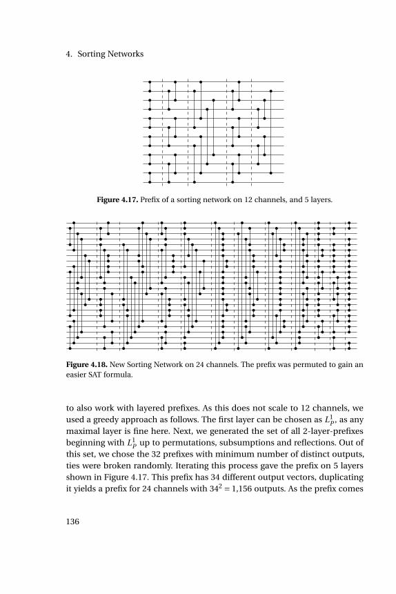
4. Sorting Networks
Figure 4.17. Prefix of a sorting network on 12 channels, and 5 layers.
Figure 4.18. New Sorting Network on 24 channels. The prefix was permuted to gain aneasier SAT formula.
to also work with layered prefixes. As this does not scale to 12 channels, weused a greedy approach as follows. The first layer can be chosen as L1
P , as anymaximal layer is fine here. Next, we generated the set of all 2-layer-prefixesbeginning with L1
P up to permutations, subsumptions and reflections. Out ofthis set, we chose the 32 prefixes with minimum number of distinct outputs,ties were broken randomly. Iterating this process gave the prefix on 5 layersshown in Figure 4.17. This prefix has 34 different output vectors, duplicatingit yields a prefix for 24 channels with 342 = 1,156 outputs. As the prefix comes
136
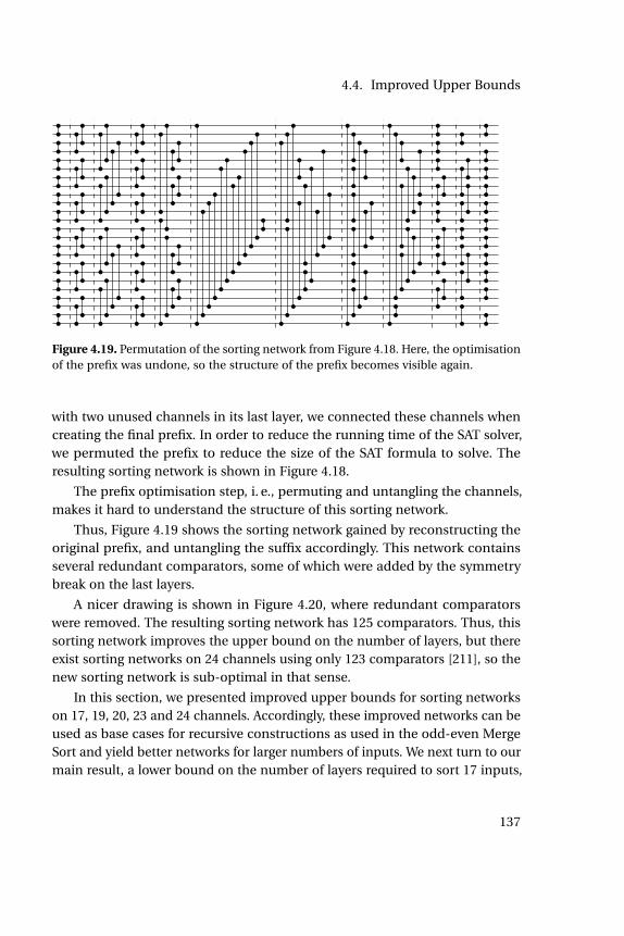
4.4. Improved Upper Bounds
Figure 4.19. Permutation of the sorting network from Figure 4.18. Here, the optimisationof the prefix was undone, so the structure of the prefix becomes visible again.
with two unused channels in its last layer, we connected these channels whencreating the final prefix. In order to reduce the running time of the SAT solver,we permuted the prefix to reduce the size of the SAT formula to solve. Theresulting sorting network is shown in Figure 4.18.
The prefix optimisation step, i. e., permuting and untangling the channels,makes it hard to understand the structure of this sorting network.
Thus, Figure 4.19 shows the sorting network gained by reconstructing theoriginal prefix, and untangling the suffix accordingly. This network containsseveral redundant comparators, some of which were added by the symmetrybreak on the last layers.
A nicer drawing is shown in Figure 4.20, where redundant comparatorswere removed. The resulting sorting network has 125 comparators. Thus, thissorting network improves the upper bound on the number of layers, but thereexist sorting networks on 24 channels using only 123 comparators [211], so thenew sorting network is sub-optimal in that sense.
In this section, we presented improved upper bounds for sorting networkson 17, 19, 20, 23 and 24 channels. Accordingly, these improved networks can beused as base cases for recursive constructions as used in the odd-even MergeSort and yield better networks for larger numbers of inputs. We next turn to ourmain result, a lower bound on the number of layers required to sort 17 inputs,
137
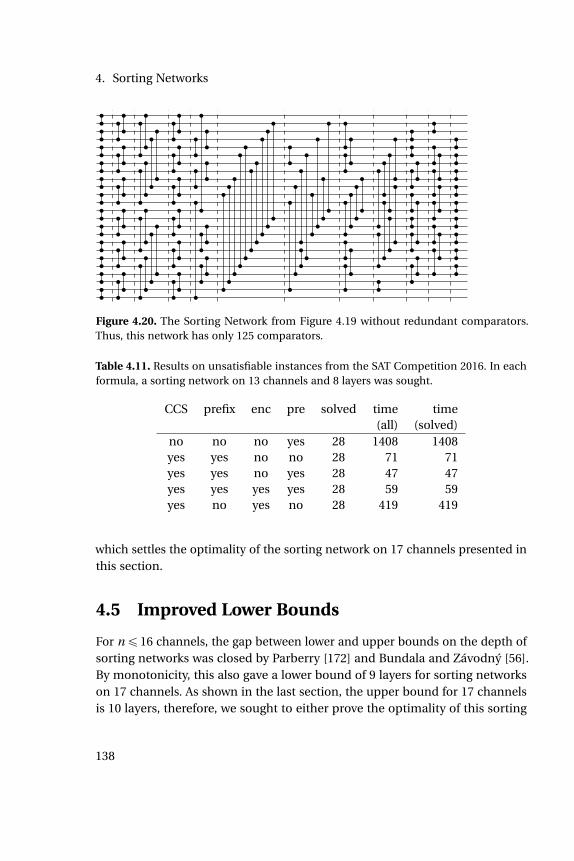
4. Sorting Networks
Figure 4.20. The Sorting Network from Figure 4.19 without redundant comparators.Thus, this network has only 125 comparators.
Table 4.11. Results on unsatisfiable instances from the SAT Competition 2016. In eachformula, a sorting network on 13 channels and 8 layers was sought.
CCS prefix enc pre solved time time(all) (solved)
no no no yes 28 1408 1408yes yes no no 28 71 71yes yes no yes 28 47 47yes yes yes yes 28 59 59yes no yes no 28 419 419
which settles the optimality of the sorting network on 17 channels presented inthis section.
4.5 Improved Lower Bounds
For nď 16 channels, the gap between lower and upper bounds on the depth ofsorting networks was closed by Parberry [172] and Bundala and Závodný [56].By monotonicity, this also gave a lower bound of 9 layers for sorting networkson 17 channels. As shown in the last section, the upper bound for 17 channelsis 10 layers, therefore, we sought to either prove the optimality of this sorting
138

4.5. Improved Lower Bounds
network, or find a better one.Parberry proved lower bounds for 9 and 10 channels by showing that L1
Pcannot be extended to a sorting network on 6 channels, therefore, the networksgiven in [139] were optimal. As discussed in Section 4.2, this is sufficient asevery sorting network for 9 channels and 6 layers could be transformed intoone having L1
P as first layer.Bundala and Závodný extended this approach to the first two layers. They
generated complete sets of filters, sets of prefixes on 2 layers such that everysorting network could be transformed into one having a prefix from this set.Thus, it was sufficient to check whether one of these prefixes could be extendedto a full sorting network.
Following this approach, we generated the complete set of filters for 17channels using the algorithm by Codish et al. [74]. In a first attempt, we usedthe encoding shown in Section 4.3 with a few optimisations. Comparators inthe last layer were restricted to length 1, and comparators in the second-to-lastlayer to length 3, referring to a preliminary version of [73]. Furthermore, weencoded inputs with only one unsorted 0 or 1 in the window of unsorted inputsas a reachability problem. This attempt was of limited success. We were able toprove that some of the prefixes could not be extended to a full sorting network,but for harder cases the SAT solver did not terminate within 50 days, so weaborted the experiment.
After developing and implementing the ideas of improving the SAT encod-ing, and permuting the prefixes, we ran the experiments again. The improve-ments clearly reduced the running times, we were able to prove that no prefixfrom F2
B Z (17) can be extended to a sorting network on 9 layers. The overallrunning time was 27.63¨106 seconds, with a maximum of 97,112 seconds. Thus,we may state the main result of this section.
Theorem 4.28. There is no sorting network on 17 channels which uses less than10 layers.
In the remainder of this section we present a more detailed analysis of theimpact of the different improvements, and a technique which helped us to gaina deeper understanding of proofs of the non-existence of sorting networks.
We implemented a refinement-based approach for generating sorting net-works, similar to techniques used in software verification [69]. The loop, drawnin Figure 4.21, starts with a SAT formula φ which encodes the existence of a
139
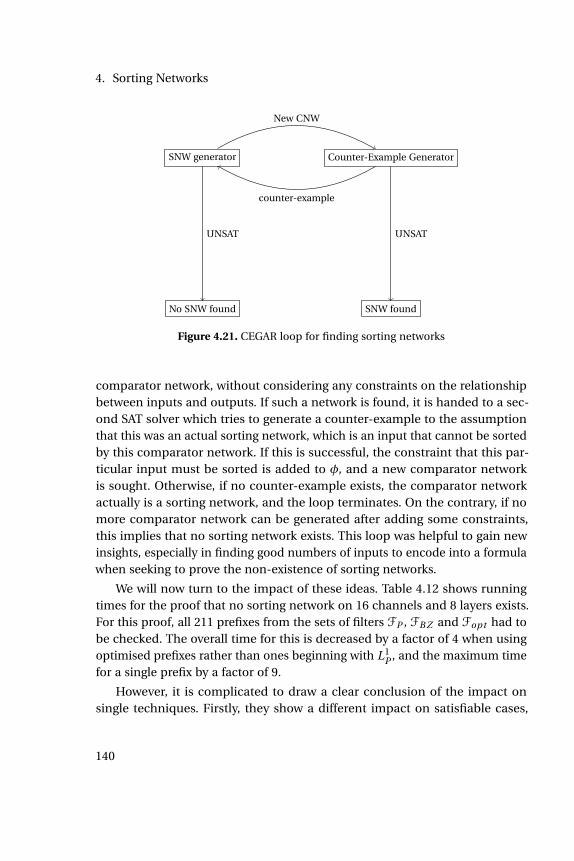
4. Sorting Networks
SNW generator Counter-Example Generator
New CNW
counter-example
No SNW found SNW found
UNSAT UNSAT
Figure 4.21. CEGAR loop for finding sorting networks
comparator network, without considering any constraints on the relationshipbetween inputs and outputs. If such a network is found, it is handed to a sec-ond SAT solver which tries to generate a counter-example to the assumptionthat this was an actual sorting network, which is an input that cannot be sortedby this comparator network. If this is successful, the constraint that this par-ticular input must be sorted is added to φ, and a new comparator networkis sought. Otherwise, if no counter-example exists, the comparator networkactually is a sorting network, and the loop terminates. On the contrary, if nomore comparator network can be generated after adding some constraints,this implies that no sorting network exists. This loop was helpful to gain newinsights, especially in finding good numbers of inputs to encode into a formulawhen seeking to prove the non-existence of sorting networks.
We will now turn to the impact of these ideas. Table 4.12 shows runningtimes for the proof that no sorting network on 16 channels and 8 layers exists.For this proof, all 211 prefixes from the sets of filters FP , FB Z and Fopt had tobe checked. The overall time for this is decreased by a factor of 4 when usingoptimised prefixes rather than ones beginning with L1
P , and the maximum timefor a single prefix by a factor of 9.
However, it is complicated to draw a clear conclusion of the impact onsingle techniques. Firstly, they show a different impact on satisfiable cases,
140
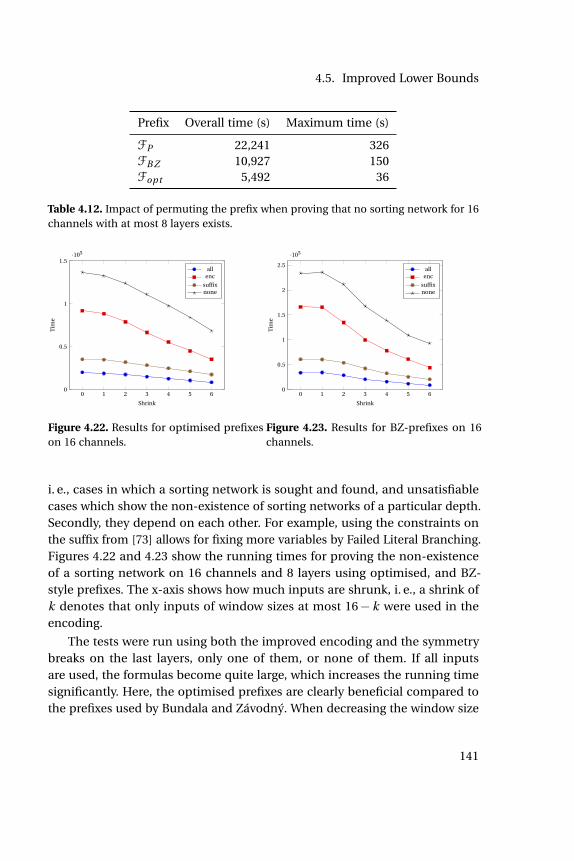
4.5. Improved Lower Bounds
Prefix Overall time (s) Maximum time (s)
FP 22,241 326FB Z 10,927 150Fopt 5,492 36
Table 4.12. Impact of permuting the prefix when proving that no sorting network for 16channels with at most 8 layers exists.
0 1 2 3 4 5 60
0.5
1
1.5¨105
Shrink
Tim
e
allenc
suffixnone
Figure 4.22. Results for optimised prefixeson 16 channels.
0 1 2 3 4 5 60
0.5
1
1.5
2
2.5
¨105
Shrink
Tim
eall
enc
suffixnone
Figure 4.23. Results for BZ-prefixes on 16channels.
i. e., cases in which a sorting network is sought and found, and unsatisfiablecases which show the non-existence of sorting networks of a particular depth.Secondly, they depend on each other. For example, using the constraints onthe suffix from [73] allows for fixing more variables by Failed Literal Branching.Figures 4.22 and 4.23 show the running times for proving the non-existenceof a sorting network on 16 channels and 8 layers using optimised, and BZ-style prefixes. The x-axis shows how much inputs are shrunk, i. e., a shrink ofk denotes that only inputs of window sizes at most 16´k were used in theencoding.
The tests were run using both the improved encoding and the symmetrybreaks on the last layers, only one of them, or none of them. If all inputsare used, the formulas become quite large, which increases the running timesignificantly. Here, the optimised prefixes are clearly beneficial compared tothe prefixes used by Bundala and Závodný. When decreasing the window size
141

4. Sorting Networks
Table 4.13. The impact of the new SAT encoding: The new variables allow for shorterproofs, as can be seen by the number of conflicts. Furthermore, the solving times arereduced significantly.
prefix encoding conflicts time
0 standard 19127761 707000 improved 9832380 24476
51 standard 29268392 11812851 improved 17811760 50699
Table 4.14. The impact of the new SAT encoding when prefixes in BZ-style are used.
prefix encoding conflicts time
0 standard 22179733 766980 improved 10686754 23818
51 standard > 60018753 > 42866651 improved > 59001902 > 428324
if the inputs used, this gap becomes significantly smaller. Furthermore, thesymmetry break on the last layers by Codish et al. has a significantly strongerimpact here than the improved encoding.
We ran similar experiments for the case of 17 channels. Table 4.13 showsthe running times and number of conflicts when proving that two prefixes fromF2
B Z (17) cannot be extended to a full sorting network on 9 layers. The prefixwith index 0 was one of the easiest in our experiments, whereas the one withindex 51 was one of the hardest cases.
Here, the optimised version of the prefixes were used. In both cases, usingthe improved encoding reduces both the number of conflicts and the runningtime. The reduced number of conflicts can be seen as a validation of the idea ofgeneralising the reasons why the value on a channel remained unchanged, theSAT solver can benefit from this. The reduced running time is both due to thereduced number of conflicts, and the smaller encoding. Next, we re-ran theseexperiments using prefixes in BZ-style, the results are given in Table 4.14. Onthe first prefix, the solver achieves similar results as when using the optimisedversion of it, the running time is less than 10% higher here when using the
142

4.6. Conclusion and Open Questions
standard encoding, and even slightly lower with the improved encoding. In thesecond case, the result is different; We aborted this experiment after severaldays. Even using the improved encoding, the solver was not able to proveunsatisfiability in this time. Thus, using the optimised version of the prefix gavea speed-up of at least 8 in this case.
4.6 Conclusion and Open Questions
In this chapter, we discussed the concept of sorting networks, and some oftheir properties. The main subject here was one property, the number of par-allel sorting steps required to sort an input. We discussed a SAT encodingwhich describes sorting networks of bounded depth, and showed how this canbe improved. Furthermore, we used the notion of symmetries of sorting net-works in a new way, such that we could use an optimisation algorithm whichcomputes permuted versions of prefixes of sorting networks which in turnsignificantly reduce the size of SAT encodings, and the running time requiredby a SAT solver on these formulas. This technique has an especially strongimpact when searching for new sorting networks rather than seeking to provetheir non-existence.
We presented new sorting networks, which improve the upper bounds onthe number of layers required to sort 17, 19, 20, 23 and 24 inputs. These net-works can be used as base case either in software implementations of sortingalgorithms, or when constructing sorting networks recursively e. g., using anodd-even Merge Sort.
Furthermore, we were able to prove the non-existence of sorting networksfor 17 inputs and 9 layers, which settles the optimality of our sorting networkfor 17 inputs, thereby answering the main open question from [73]. DonaldE. Knuth sent us an email congratulating to this result, and shows the sortingnetwork in [138].
By monotonicity, this result also increases the lower bound on the numberof layers for up to 36 inputs.
Future work
Settling the optimality of a 10-layer sorting network for 17 inputs immediatelygives rise to the question about optimal bounds for 18 inputs. We conjecture
143

4. Sorting Networks
that either finding a network on 10 channels or proving non-existence is withinreach when using some rather evolutionary than revolutionary improvements.
Ź The symmetry break on the suffix of a sorting network from [73] could beextended to the last 3 layers. This would both remove further symmetriesfrom the search space, and allow for fixing more variables in the SAT encod-ing. We furthermore conjecture that is is sufficient to consider last layerswithout “gaps”, i. e., where unconnected channels only exist at the top andbottom of the last layer.
Ź When using prefixes on two layers, some symmetry breaks could be appliedon the third layer of a sorting network. Consider the Green Filter on 12channels and 2 layers in Figure 4.24, which consists of 3 segments, each ofwhich is a Green Filter on 4 channels. Connecting the top-most channel toa channel from the second segment is symmetric to connecting it to therespective channel from the third segment, thus, one of these comparatorscould be forbidden.
Ź We only introduced predicates in the SAT encoding which describe why thevalue on a channel is not changed by a particular layer. It might be possibleto analogously generalise on the reasons why values are changed, yieldingstronger explanations, i. e., learned clauses.
Ź When trying to find improved upper bounds, a set of prefixes on three orfour layers might be generated using a limited discrepancy search (LDS) [119].Consider a greedy algorithm which, given a prefix on some layers L, gener-ates a prefix on one more layer by iteratively adding comparators (i , j ) tothe prefix such that the number of outputs |outputs(L(i , j ))| is minimised.The core idea behind LDS is that if greedy algorithms fail, they often failbecause of only a few bad decisions. Thus, considering solutions whichare similar to the one generated by the greedy algorithm might yield goodresults. This can be seen as a search limited to some local neighbourhoodof the solution given by a greedy algorithm. Before using a SAT solver totry and extend these prefixes to full sorting networks, symmetric solutionsshould be removed as presented in [71].
A drawback of the SAT encodings used so far is that they do not considersymmetries of prefixes, which we would consider a major achievement. Here,
144
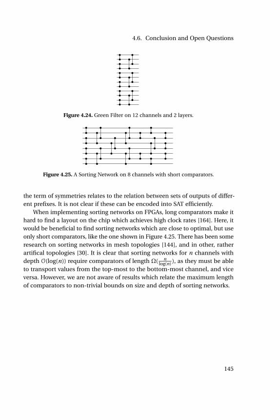
4.6. Conclusion and Open Questions
Figure 4.24. Green Filter on 12 channels and 2 layers.
Figure 4.25. A Sorting Network on 8 channels with short comparators.
the term of symmetries relates to the relation between sets of outputs of differ-ent prefixes. It is not clear if these can be encoded into SAT efficiently.
When implementing sorting networks on FPGAs, long comparators make ithard to find a layout on the chip which achieves high clock rates [164]. Here, itwould be beneficial to find sorting networks which are close to optimal, but useonly short comparators, like the one shown in Figure 4.25. There has been someresearch on sorting networks in mesh topologies [144], and in other, ratherartifical topologies [30]. It is clear that sorting networks for n channels withdepth O(log(n)) require comparators of length Ω( n
log(n) ), as they must be ableto transport values from the top-most to the bottom-most channel, and viceversa. However, we are not aware of results which relate the maximum lengthof comparators to non-trivial bounds on size and depth of sorting networks.
145

Chapter 5
Further Publications
“What else?”
GEORGE CLOONEY
Besides the research presented in this thesis, I was involved in further activities.In this chapter, I will give a brief overview on them.
Ź In the field of software verification, we sought to find data races. Theseare unsynchronised memory accesses of parallely executed threads to thesame memory location where at least one access is writing [166]. Our workfocussed on software used in embedded systems, mostly in the automotivedomain. We developed a tool, Gropius, which computed a coarse over-approximation of the set of possible data races in a program, which waspresented in [99] and [98]. Being only a prototype, it was able to analyse real-world software of about 300,000 lines of code in a few seconds, and foundbugs there. Gropius is now actively maintained and extended by PhilippSieweck.
Ź A totally different field is the design and analysis of algorithms operatingon sequences. I was involved in research regarding a version of the patternmatching problem. In k-abelian pattern matching, two words are consideredequivalent if the subsequences or factors of length k occur in both wordsin the same multiplicity. Some algorithms for this problem, together withexperimental results were presented in [91] and [92]. My contributitionhere was mostly the implementation of the developed algorithms and theexperimental section.
Ź Graph Drawing is an interesting field of research with numerous practi-cal applications. We considered CP-based and Integer Programming-based
147

5. Further Publications
approaches for computing optimal graph layouts with respect to differentcriteria. In CP-based approaches, we used the parallel version of CHUFFED
presented in Chapter 3, which showed an impressive performance. Someresults comparing a new heuristic with optimum results obtained by integerprogramming were presented in [189], an extended version was submittedto the Journal of Graph Algorithms and Applications and is currently underreview.
148

Appendix A
Appendix
A.1 List of Benchmarks Used in the Paper “Commu-nication in Massively-Parallel SAT Solving"
grieu-vmpc-31.cnf.gzpost-cbmc-zfcp-2.8-u2.cnf.gzvelev-npe-1.0-9dlx-b71.cnf.gzvelev-vliw-uns-4.0-9.cnf.gzgss-19-s100.cnf.gzgss-20-s100.cnf.gzmd5_47_4.cnf.gzmd5_48_1.cnf.gzmd5_48_3.cnf.gzdated-10-13-u.cnf.gzdated-5-13-u.cnf.gzACG-15-10p0.cnf.gzUTI-20-10p0.cnf.gzminxorminand128.cnf.gzAProVE07-27.cnf.gzzfcp-2.8-u2-nh.cnf.gzmaxor064.cnf.gzgss-18-s100.cnf.gzgus-md5-08.cnf.gzACG-20-5p0.cnf.gzslp-synthesis-aes-top27.cnf.gzaes_32_3_keyfind_2.cnf.gzblocks-blocks-36-0.130-NOTKNOWN.cnf.gzblocks-blocks-36-0.150-NOTKNOWN.cnf.gzgrid-strips-grid-y-3.045-NOTKNOWN.cnf.gzgrid-strips-grid-y-3.055-NOTKNOWN.cnf.gzgrid-strips-grid-y-3.065-SAT.cnf.gztransport-transport-city-sequential-25nodes-1000size-3degree-100mindistance-3trucks-10packages-2008seed.020-NOTKNOWN.cnf.gztransport-transport-city-sequential-25nodes-1000size-3degree-100mindistance-3trucks-10packages-2008seed.030-NOTKNOWN.cnf.gztransport-transport-city-sequential-25nodes-1000size-3degree-100mindistance-3trucks-10packages-2008seed.040-NOTKNOWN.cnf.gztransport-transport-city-sequential-25nodes-1000size-3degree-100mindistance-3trucks-10packages-2008seed.050-NOTKNOWN.cnf.gztransport-transport-city-sequential-35nodes-1000size-4degree-100mindistance-4trucks-14packages-2008seed.020-NOTKNOWN.cnf.gztransport-transport-two-cities-sequential-15nodes-1000size-3degree-100mindistance-3trucks-10packages-2008seed.020-NOTKNOWN.cnf.gztransport-transport-two-cities-sequential-15nodes-1000size-3degree-100mindistance-3trucks-10packages-2008seed.030-NOTKNOWN.cnf.gzmd5_47_1.cnf.gzmd5_47_2.cnf.gzmd5_47_3.cnf.gzmd5_48_2.cnf.gzmd5_48_4.cnf.gzmd5_48_5.cnf.gz10pipe_k.cnf.gz7pipe_k.cnf.gz8pipe_k.cnf.gz9pipe_k.cnf.gz10pipe_q0_k.cnf.gz11pipe_q0_k.cnf.gz8pipe_q0_k.cnf.gz
149

A. Appendix
partial-10-11-s.cnf.gzpartial-10-19-s.cnf.gzpartial-5-17-s.cnf.gzpartial-5-19-s.cnf.gzdated-10-11-u.cnf.gzpartial-5-13-s.cnf.gzpartial-5-15-s.cnf.gztotal-10-15-s.cnf.gzitox_vc1033.cnf.gzitox_vc1130.cnf.gzAProVE07-02.cnf.gzAProVE07-11.cnf.gzvmpc_29.cnf.gzvmpc_30.cnf.gzvmpc_33.cnf.gzvmpc_34.cnf.gz9vliw_m_9stages_iq3_C1_bug1.cnf.gz9vliw_m_9stages_iq3_C1_bug10.cnf.gz9vliw_m_9stages_iq3_C1_bug4.cnf.gz9vliw_m_9stages_iq3_C1_bug7.cnf.gz9vliw_m_9stages_iq3_C1_bug8.cnf.gz9vliw_m_9stages_iq3_C1_bug9.cnf.gz9dlx_vliw_at_b_iq4.cnf.gzAProVE09-06.cnf.gzcountbitssrl032.cnf.gzminxor128.cnf.gzminxorminand064.cnf.gzgss-17-s100.cnf.gzgss-23-s100.cnf.gzgss-24-s100.cnf.gzACG-15-10p1.cnf.gzACG-20-5p1.cnf.gzUR-15-10p0.cnf.gzUR-15-10p1.cnf.gzUR-20-5p0.cnf.gzUR-20-5p1.cnf.gzUTI-15-10p1.cnf.gzUTI-20-5p1.cnf.gzndhf_xits_21_SAT.cnf.gzrbcl_xits_14_SAT.cnf.gzvelev-pipe-sat-1.0-b7.cnf.gzvmpc_32.renamed-as.sat05-1919.cnf.gzpartial-10-17-s.cnf.gzAProVE07-03.cnf.gz9vliw_m_9stages_iq3_C1_bug6.cnf.gzq_query_3_L70_coli.sat.cnf.gzmaxor128.cnf.gzmaxxor032.cnf.gzmaxxor064.cnf.gzgss-21-s100.cnf.gzgss-22-s100.cnf.gzUCG-15-10p1.cnf.gzUTI-20-10p1.cnf.gzndhf_xits_19_UNKNOWN.cnf.gzslp-synthesis-aes-bottom13.cnf.gzslp-synthesis-aes-bottom14.cnf.gzslp-synthesis-aes-top26.cnf.gzaaai10-planning-ipc5-pathways-13-step17.cnf.gzaaai10-planning-ipc5-pathways-17-step20.cnf.gzaaai10-planning-ipc5-pathways-17-step21.cnf.gzaaai10-planning-ipc5-pipesworld-12-step15.cnf.gzaaai10-planning-ipc5-TPP-21-step11.cnf.gzaaai10-planning-ipc5-TPP-30-step11.cnf.gzhwmcc10-timeframe-expansion-k45-pdtpmsgoodbakery-tseitin.cnf.gzhwmcc10-timeframe-expansion-k45-pdtvissoap1-tseitin.cnf.gzhwmcc10-timeframe-expansion-k50-pdtpmsns2-tseitin.cnf.gzsmtlib-qfbv-aigs-ext_con_032_008_0256-tseitin.cnf.gzsmtlib-qfbv-aigs-lfsr_004_127_112-tseitin.cnf.gzsmtlib-qfbv-aigs-servers_slapd_a_vc149789-tseitin.cnf.gzaes_32_3_keyfind_1.cnf.gzE02F20.cnf.gz
150
A.2. Algorithms for the Optimisation of Prefixes
E02F22.cnf.gzE04F19.cnf.gzopenstacks-sequencedstrips-nonadl-nonnegated-os-sequencedstrips-p30_3.085-SAT.cnf.gztransport-transport-city-sequential-25nodes-1000size-3degree-100mindistance-3trucks-10packages-2008seed.060-SAT.cnf.gztransport-transport-city-sequential-35nodes-1000size-4degree-100mindistance-4trucks-14packages-2008seed.030-NOTKNOWN.cnf.gztransport-transport-city-sequential-35nodes-1000size-4degree-100mindistance-4trucks-14packages-2008seed.040-NOTKNOWN.cnf.gztransport-transport-three-cities-sequential-14nodes-1000size-4degree-100mindistance-4trucks-14packages-2008seed.030-NOTKNOWN.cnf.gztransport-transport-two-cities-sequential-15nodes-1000size-3degree-100mindistance-3trucks-10packages-2008seed.040-SAT.cnf.gzvelev-pipe-sat-1.0-b9.cnf.gzesawn_uw3.debugged.cnf.gzaes_16_10_keyfind_3.cnf.gzaes_24_4_keyfind_2.cnf.gzaes_24_4_keyfind_4.cnf.gzdated-5-19-u.cnf.gz9dlx_vliw_at_b_iq9.cnf.gzminandmaxor128.cnf.gzgss-25-s100.cnf.gzgus-md5-11.cnf.gzUR-20-10p1.cnf.gzrpoc_xits_15_SAT.cnf.gzvmpc_35.renamed-as.sat05-1921.cnf.gzvmpc_36.renamed-as.sat05-1922.cnf.gzslp-synthesis-aes-top25.cnf.gzaes_64_1_keyfind_1.cnf.gzE00N23.cnf.gztransport-transport-three-cities-sequential-14nodes-1000size-4degree-100mindistance-4trucks-14packages-2008seed.020-NOTKNOWN.cnf.gzSAT_dat.k80.cnf.gzSAT_dat.k65.cnf.gz11pipe_11_ooo.cnf.gz6s20.cnf.gz6s20.cnf.gzarcfour_initialPermutation_6_15.cnf.gzctl_4201_555_unsat.cnf.gzctl_4201_555_unsat_pre.cnf.gzctl_4291_567_1_unsat.cnf.gzk_unsat.cnf.gzp01_lb_05.cnf.gzpb_200_03_lb_01.cnf.gzpb_200_03_lb_02.cnf.gzpb_400_10_lb_00.cnf.gzbivium-39-200-0s0-0xdcfb6ab71951500b8e460045bd45afee15c87e08b0072eb174-43.cnf.gzbivium-40-200-0s0-0xd447c33176b6b675fd5f8dc3a5deda46569dc34eedf37da020-6.cnf.gzhitag2-10-60-0-0xbc15b17d0353413-10.cnf.gzhitag2-8-60-0-0xfba1a41b5dfd7f7-52.cnf.gzhitag2-7-60-0-0xe97b5f1bee04d70-47.cnf.gz
A.2 Algorithms for the Optimisation of Prefixes
Header file for different sorting network related operations
1 #include < s t r i n g . h>2 #include <iostream >3 #include <vector >4 #include <set >5 #include <map>6 #include <cstdio >7 #include <cstdl ib >8 #include <cassert >9 #include <algorithm >
151

A. Appendix
10
11 using namespace std ;12
13 /*14 * Simple structure for a comparator15 */16 s t r u c t comparator 17 i n t layer ;18 i n t from ;19 i n t to ;20 comparator ( i n t _a , i n t _b , i n t _c ) : layer ( _a ) , from ( _b ) , to ( _c ) ;21 bool operator <( const comparator & other ) 22 i f ( layer != other . layer )23 return layer < other . layer ;24 i f ( from != other . from )25 return from < other . from ;26 return to < other . to ;27 28 ;29
30 /*31 * Parse a l l l a y e r s from a given f i l e .32 */33 void parseAllLayers ( vector <vector <comparator> > & out ,34 char * fileName , i n t d i f f ) 35 FILE * fp = fopen ( fileName , " r " ) ;36 i n t BUF_SIZE = 1<<16;37 char buffer [ BUF_SIZE ] ;38 i n t rowRead = 0 ;39 while ( fp && ! f e o f ( fp ) ) 40 i n t scan = fscanf ( fp , "%s " , buffer ) ;41 i f ( scan >= 0 ) 42 char * buff = s t r t o k ( buffer , " ; " ) ;43 vector <comparator> tmp ;44 while ( buff ) 45 i n t a , b , c ;46 a = atoi ( buff ) ;47 buff = s t r t o k (NULL, " ; " ) ;48 b = atoi ( buff ) ;49 buff = s t r t o k (NULL, " ; " ) ;50 c = ato i ( buff ) ;51 buff = s t r t o k (NULL, " ; " ) ;52 tmp . push_back ( comparator ( a , b d i f f , c d i f f ) ) ;53 54 out . push_back (tmp ) ;
152
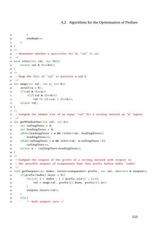
A.2. Algorithms for the Optimisation of Prefixes
55 56 rowRead++;57 58 59 /*60 * Determine whether a p a r t i c u l a r b i t in " val " i s set61 */62 bool i s S e t ( i n t val , i n t b i t ) 63 return val & (1<< b i t ) ;64 65 /*66 * Swap the b i t s of " val " at position a and b67 */68 i n t swap( i n t val , i n t a , i n t b ) 69 a s s e r t ( a < b ) ;70 i f ( val & (1<<a ) )71 i f ( ! ( val & (1<<b ) ) )72 val ^= ((1 < <a ) | (1<<b ) ) ;73 return val ;74 75 /*76 * Compute the window s i z e of an input " val " for a sort ing network on "n" inputs .77 */78 i n t getWindowSize ( i n t val , i n t n ) 79 i n t tail ingOnes = 0 ;80 i n t leadingZeros = 0 ;81 while ( leadingZeros < n && ! i s S e t ( val , leadingZeros ) )82 leadingZeros ++;83 while ( tail ingOnes < n && i s S e t ( val , n tailingOnes´1))84 tail ingOnes ++;85 return n ´ ( tail ingOnes+leadingZeros ) ;86 87 /*88 * Compute the outputs of the p r e f i x of a sort ing network with respect to89 * the possible outputs of comparators from t h i s p r e f i x before index " index "90 */91 void getOutputs ( i n t index , vector <comparator> prefix , i n t val , set <int > & outputs ) 92 i f ( p r e f i x [ index ] . layer > 0 ) 93 for ( i n t i = index ; i < p r e f i x . s i z e ( ) ; i ++)94 val = swap( val , p r e f i x [ i ] . from , p r e f i x [ i ] . to ) ;95 96 outputs . i n s e r t ( val ) ;97 98 else 99 /* both outputs zero */
153
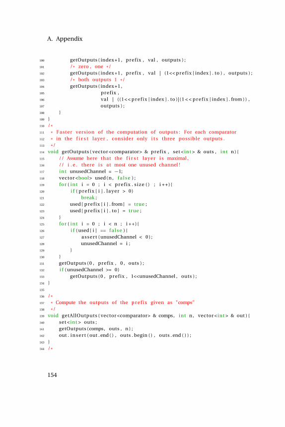
A. Appendix
100 getOutputs ( index +1 , pref ix , val , outputs ) ;101 /* zero , one */102 getOutputs ( index +1 , pref ix , val | (1<< p r e f i x [ index ] . to ) , outputs ) ;103 /* both outputs 1 */104 getOutputs ( index +1 ,105 prefix ,106 val | ((1 < < p r e f i x [ index ] . to )|(1 < < p r e f i x [ index ] . from ) ) ,107 outputs ) ;108 109 110 /*111 * Faster version of the computation of outputs : For each comparator112 * in the f i r s t layer , consider only i t s three possible outputs .113 */114 void getOutputs ( vector <comparator> & prefix , set <int > & outs , i n t n ) 115 // Assume here that the f i r s t layer i s maximal ,116 // i . e . there i s at most one unused channel !117 i n t unusedChannel = ´1;118 vector <bool> used (n , f a l s e ) ;119 for ( i n t i = 0 ; i < p r e f i x . s i z e ( ) ; i ++)120 i f ( p r e f i x [ i ] . layer > 0)121 break ;122 used [ p r e f i x [ i ] . from ] = true ;123 used [ p r e f i x [ i ] . to ] = true ;124 125 for ( i n t i = 0 ; i < n ; i ++)126 i f ( used [ i ] == f a l s e ) 127 a s s e r t ( unusedChannel < 0 ) ;128 unusedChannel = i ;129 130 131 getOutputs ( 0 , pref ix , 0 , outs ) ;132 i f ( unusedChannel >= 0)133 getOutputs ( 0 , pref ix , 1<<unusedChannel , outs ) ;134 135
136 /*137 * Compute the outputs of the p r e f i x given as "comps"138 */139 void getAllOutputs ( vector <comparator> & comps, i n t n , vector <int > & out ) 140 set <int > outs ;141 getOutputs (comps, outs , n ) ;142 out . i n s e r t ( out . end ( ) , outs . begin ( ) , outs . end ( ) ) ;143 144 /*
154
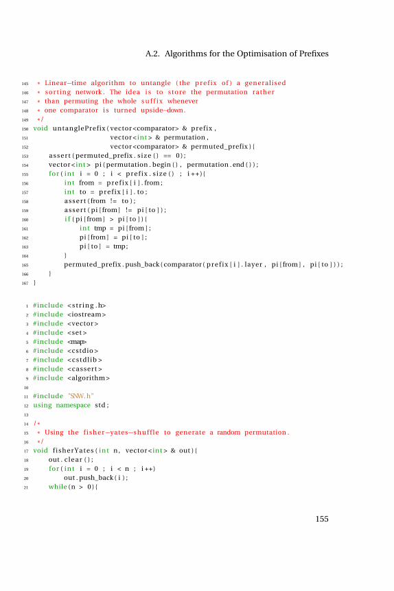
A.2. Algorithms for the Optimisation of Prefixes
145 * Linear time algorithm to untangle ( the p r e f i x of ) a generalised146 * sort ing network . The idea i s to store the permutation rather147 * than permuting the whole s u f f i x whenever148 * one comparator i s turned upside down.149 */150 void untanglePrefix ( vector <comparator> & prefix ,151 vector <int > & permutation ,152 vector <comparator> & permuted_prefix ) 153 a s s e r t ( permuted_prefix . s i z e ( ) == 0 ) ;154 vector <int > pi ( permutation . begin ( ) , permutation . end ( ) ) ;155 for ( i n t i = 0 ; i < p r e f i x . s i z e ( ) ; i ++)156 i n t from = p r e f i x [ i ] . from ;157 i n t to = p r e f i x [ i ] . to ;158 a s s e r t ( from ! = to ) ;159 a s s e r t ( pi [ from ] != pi [ to ] ) ;160 i f ( pi [ from ] > pi [ to ] ) 161 i n t tmp = pi [ from ] ;162 pi [ from ] = pi [ to ] ;163 pi [ to ] = tmp ;164 165 permuted_prefix . push_back ( comparator ( p r e f i x [ i ] . layer , pi [ from ] , pi [ to ] ) ) ;166 167
1 #include < s t r i n g . h>2 #include <iostream >3 #include <vector >4 #include <set >5 #include <map>6 #include <cstdio >7 #include <cstdl ib >8 #include <cassert >9 #include <algorithm >
10
11 #include "SNW. h"12 using namespace std ;13
14 /*15 * Using the f isher yates´s h u f f l e to generate a random permutation .16 */17 void f i sh er Y a te s ( i n t n , vector <int > & out ) 18 out . c lear ( ) ;19 for ( i n t i = 0 ; i < n ; i ++)20 out . push_back ( i ) ;21 while (n > 0 )
155
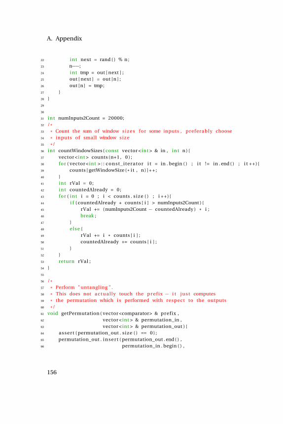
A. Appendix
22 i n t next = rand ( ) % n ;23 n ;24 i n t tmp = out [ next ] ;25 out [ next ] = out [n ] ;26 out [n] = tmp ;27 28 29
30
31 i n t numInputs2Count = 20000;32 /*33 * Count the sum of window s i z e s for some inputs , preferably choose34 * inputs of small window s i z e35 */36 i n t countWindowSizes ( const vector <int > & in , i n t n ) 37 vector <int > counts (n+1 , 0 ) ;38 for ( vector <int > : : c o ns t_ i te r a to r i t = in . begin ( ) ; i t ! = in . end ( ) ; i t ++)39 counts [ getWindowSize ( * i t , n) ] + + ;40 41 i n t rVal = 0 ;42 i n t countedAlready = 0 ;43 for ( i n t i = 0 ; i < counts . s i z e ( ) ; i ++)44 i f ( countedAlready + counts [ i ] > numInputs2Count ) 45 rVal += ( numInputs2Count ´ countedAlready ) * i ;46 break ;47 48 else 49 rVal += i * counts [ i ] ;50 countedAlready += counts [ i ] ;51 52 53 return rVal ;54 55
56 /*57 * Perform " untangling " .58 * This does not a c t u a l l y touch the p r e f i x ´ i t j u s t computes59 * the permutation which i s performed with respect to the outputs60 */61 void getPermutation ( vector <comparator> & prefix ,62 vector <int > & permutation_in ,63 vector <int > & permutation_out ) 64 a s s e r t ( permutation_out . s i z e ( ) == 0 ) ;65 permutation_out . i n s e r t ( permutation_out . end ( ) ,66 permutation_in . begin ( ) ,
156

A.2. Algorithms for the Optimisation of Prefixes
67 permutation_in . end ( ) ) ;68 for ( i n t i = 0 ; i < p r e f i x . s i z e ( ) ; i ++)69 // i s t h i s one reversed ? I f so , change permutation !70 i n t from = p r e f i x [ i ] . from ;71 i n t to = p r e f i x [ i ] . to ;72 i f ( permutation_out [ from ] > permutation_out [ to ] ) 73 i n t tmp = permutation_out [ from ] ;74 permutation_out [ from ] = permutation_out [ to ] ;75 permutation_out [ to ] = tmp ;76 77 78 79
80 /*81 Permute the output according to "permutation"82 */83 i n t permuteOutput ( i n t val , vector <int > & permutation , i n t n ) 84 i n t index = 0 ;85 i n t rVal = 0 ;86 while ( val != 0 ) 87 i f ( val & 1 ) 88 rVal | = (1 << permutation [ index ] ) ;89 90 val >>= 1 ;91 index ++;92 93 return rVal ;94 95 /*96 * Permute a l l outputs with respect the some given permutation97 */98 void getPermutedOutputs ( vector <int > & permutation ,99 vector <int > & in ,
100 vector <int > & out ,101 i n t n ) 102 for ( vector <int > : : i t e r a t o r i t = in . begin ( ) ; i t != in . end ( ) ; i t ++)103 out . push_back ( permuteOutput ( * i t , permutation , n ) ) ;104 105 106
107 i n t gradient_descent ( vector <comparator> & p ,108 i n t n ,109 vector <int > & initial_permutation ,110 i n t ( * f ) ( const vector <int >&, i n t ) ,111 bool randomised )
157

A. Appendix
112 bool local_minimum = f a l s e ;113 vector <int > current_solution ( init ial_permutation . begin ( ) ,114 init ial_permutation . end ( ) ) ;115 vector <int > outputs ;116 getAllOutputs (p , n , outputs ) ;117 vector <int > i n i t i a l Ou tpu ts ;118 getPermutedOutputs ( current_solution , outputs , init ia lOutputs , n ) ;119 i n t i n i t i a l R a t i n g = f ( init ia lOutputs , n ) ;120 i n t best_rating = i n i t i a l R a t i n g ;121 i n t pi_new_1 ;122 i n t pi_new_2 ;123 while ( ! local_minimum ) 124 local_minimum = true ;125 // Assume a l o c a l minimum has been found , unless we find a126 // better solution in t h i s i t e r a t i o n .127 // Swap 2 channels , and check i f t h i s improves " f " .128 // I f so , take the pair which y i e l d s the steepest descent129 for ( i n t i = 0 ; i < n ; i ++)130 for ( i n t j = i +1 ; j < n ; j ++)131 vector <int > new_permutation ( current_solution . begin ( ) ,132 current_solution . end ( ) ) ;133 i n t tmp = new_permutation [ i ] ;134 new_permutation [ i ] = new_permutation [ j ] ;135 new_permutation [ j ] = tmp ;136 vector <int > untangled ;137 getPermutation (p , new_permutation , untangled ) ;138 vector <int > permutedOutputs ;139 getPermutedOutputs ( new_permutation , outputs , permutedOutputs , n ) ;140 i n t new_rating = f ( permutedOutputs , n ) ;141 i f ( new_rating < best_rating ) 142 best_rating = new_rating ;143 local_minimum = f a l s e ;144 pi_new_1 = i ;145 pi_new_2 = j ;146 147 148 149 i f ( ! local_minimum ) 150 i n t tmp = current_solution [ pi_new_1 ] ;151 current_solution [ pi_new_1 ] = current_solution [ pi_new_2 ] ;152 current_solution [ pi_new_2 ] = tmp ;153 154 155 return best_rating ;156
158
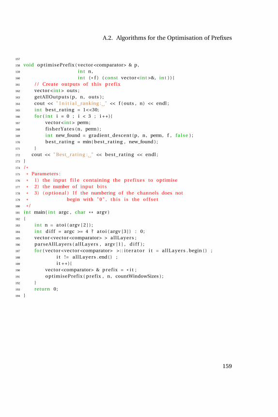
A.2. Algorithms for the Optimisation of Prefixes
157
158 void optimisePrefix ( vector <comparator> & p ,159 i n t n ,160 i n t ( * f ) ( const vector <int >&, i n t ) ) 161 // Create outputs of t h i s p r e f i x162 vector <int > outs ;163 getAllOutputs (p , n , outs ) ;164 cout << " I n i t i a l ranking : " << f ( outs , n) << endl ;165 i n t best_rating = 1<<30;166 for ( i n t i = 0 ; i < 3 ; i ++)167 vector <int > perm ;168 f i s he r Y a te s (n , perm ) ;169 i n t new_found = gradient_descent (p , n , perm, f , f a l s e ) ;170 best_rating = min( best_rating , new_found ) ;171 172 cout << " Best rat ing : " << best_rating << endl ;173 174 /*175 * Parameters :176 * 1) the input f i l e containing the p r e f i x e s to optimise177 * 2) the number of input b i t s178 * 3) ( optional ) I f the numbering of the channels does not179 * begin with "0" , t h i s i s the o f f s e t180 */181 i n t main( i n t argc , char ** argv )182 183 i n t n = atoi ( argv [ 2 ] ) ;184 i n t d i f f = argc >= 4 ? atoi ( argv [ 3 ] ) : 0 ;185 vector <vector <comparator> > a l l L a y e r s ;186 parseAllLayers ( al lLayers , argv [ 1 ] , d i f f ) ;187 for ( vector <vector <comparator> > : : i t e r a t o r i t = a l l L a y e r s . begin ( ) ;188 i t != a l l L a y e r s . end ( ) ;189 i t ++)190 vector <comparator> & p r e f i x = * i t ;191 optimisePrefix ( pref ix , n , countWindowSizes ) ;192 193 return 0 ;194
159

A. Appendix
Table A.1. Comparison of results from the SAT Competition 2016.
Channels Layers CCS prefix enc pre solved time time(all) (solved)
13 8 no no no yes 28 1532 140813 8 yes no yes no 28 576 41813 8 yes yes no no 28 240 7013 8 yes yes no yes 28 217 4713 8 yes yes yes yes 28 229 5913 9 no no no yes 28 213 4213 9 no no yes yes 28 181 913 9 no yes no yes 28 178 613 9 no yes yes yes 28 175 313 9 yes no no yes 28 200 2813 9 yes no yes yes 28 181 916 8 no no no no 16 3606 247516 8 no no no yes 27 2751 258416 8 no yes no yes 28 463 30116 9 no no no yes 1 4971 421816 9 no no yes yes 7 4494 291016 9 no yes no yes 28 1051 91116 9 no yes yes yes 28 767 61516 9 yes no no yes 4 4705 287816 9 yes yes no yes 28 458 29617 9 yes yes yes yes 0 4998 —
A.3 Comparison of Results from SAT Competition2016
This table summarises results from the SAT competition 2016. Here, CCS de-notes whether the symmetry break on suffixes by Codish, Cruz-Filipe andSchneider-Kamp was used. The use of an optimised prefix is indicated by “pre-fix", and “enc" denotes the newly introduced predicates. A preprocessor wasused if “pre" is yes.
160
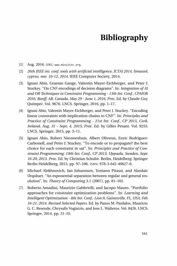
Bibliography
[1] Aug. 2016. URL: www.minizinc.org.
[2] 26th IEEE int. conf. tools with artificial intelligence, ICTAI 2014, limassol,cyprus, nov. 10-12, 2014. IEEE Computer Society, 2014.
[3] Ignasi Abío, Graeme Gange, Valentin Mayer-Eichberger, and Peter J.Stuckey. “On CNF encodings of decision diagrams”. In: Integration of AIand OR Techniques in Constraint Programming - 13th Int. Conf., CPAIOR2016, Banff, AB, Canada, May 29 - June 1, 2016, Proc. Ed. by Claude-GuyQuimper. Vol. 9676. LNCS. Springer, 2016, pp. 1–17.
[4] Ignasi Abío, Valentin Mayer-Eichberger, and Peter J. Stuckey. “Encodinglinear constraints with implication chains to CNF”. In: Principles andPractice of Constraint Programming - 21st Int. Conf., CP 2015, Cork,Ireland, Aug. 31 - Sept. 4, 2015, Proc. Ed. by Gilles Pesant. Vol. 9255.LNCS. Springer, 2015, pp. 3–11.
[5] Ignasi Abio, Robert Nieuwenhuis, Albert Oliveras, Enric Rodriguez-Carbonell, and Peter J. Stuckey. “To encode or to propagate? the bestchoice for each constraint in sat”. In: Principles and Practice of Con-straint Programming: 19th Int. Conf., CP 2013, Uppsala, Sweden, Sept.16-20, 2013. Proc. Ed. by Christian Schulte. Berlin, Heidelberg: SpringerBerlin Heidelberg, 2013, pp. 97–106. ISBN: 978-3-642-40627-0.
[6] Michael Alekhnovich, Jan Johannsen, Toniann Pitassi, and AlasdairUrquhart. “An exponential separation between regular and general res-olution”. In: Theory of Computing 3.1 (2007), pp. 81–102.
[7] Roberto Amadini, Maurizio Gabbrielli, and Jacopo Mauro. “Portfolioapproaches for constraint optimization problems”. In: Learning andIntelligent Optimization - 8th Int. Conf., Lion 8, Gainesville, FL, USA, Feb.16-21, 2014. Revised Selected Papers. Ed. by Panos M. Pardalos, MauricioG. C. Resende, Chrysafis Vogiatzis, and Jose L. Walteros. Vol. 8426. LNCS.Springer, 2014, pp. 21–35.
161

Bibliography
[8] Roberto Amadini and Peter J. Stuckey. “Sequential time splitting andbounds communication for a portfolio of optimization solvers”. In:Principles and Practice of Constraint Programming - 20th Int. Conf.,CP 2014, Lyon, France, Sept. 8-12, 2014. Proc. Ed. by Barry O’Sullivan.Vol. 8656. LNCS. Springer, 2014, pp. 108–124.
[9] Carlos Ansótegui, Jesús Giráldez-Cru, and Jordi Levy. “The communitystructure of SAT formulas”. In: Theory and Applications of SatisfiabilityTesting - SAT 2012 - 15th Int. Conf., Trento, Italy, June 17-20, 2012. Proc.Ed. by Alessandro Cimatti and Roberto Sebastiani. Vol. 7317. LNCS.Springer, 2012, pp. 410–423. ISBN: 978-3-642-31611-1.
[10] Carlos Ansótegui, Jesús Giráldez-Cru, Jordi Levy, and Laurent Simon.“Using community structure to detect relevant learnt clauses”. In: The-ory and Applications of Satisfiability Testing - SAT 2015 - 18th Int. Conf.,Austin, TX, USA, Sept. 24-27, 2015, Proc. Ed. by Marijn Heule and SeanWeaver. Vol. 9340. LNCS. Springer, 2015, pp. 238–254.
[11] Roberto Asín, Robert Nieuwenhuis, Albert Oliveras, and Enric Rodríguez-Carbonell. “Cardinality networks: a theoretical and empirical study”. In:Constraints 16.2 (2011), pp. 195–221.
[12] Gilles Audemard, Benoît Hoessen, Saïd Jabbour, Jean-Marie Lagniez,and Cédric Piette. “Revisiting clause exchange in parallel SAT solving”.In: Theory and Applications of Satisfiability Testing - SAT 2012 - 15th Int.Conf., Trento, Italy, June 17-20, 2012. Proc. Ed. by Alessandro Cimattiand Roberto Sebastiani. Vol. 7317. LNCS. Springer, 2012, pp. 200–213.ISBN: 978-3-642-31611-1.
[13] Gilles Audemard, Benoît Hoessen, Saïd Jabbour, and Cédric Piette.“Dolius: A distributed parallel SAT solving framework”. In: POS-14. 5thPragmatics of SAT workshop, workshop SAT 2014 Conf., part of FLoC2014 during the Vienna Summer of Logic, July 13, 2014, Vienna, Austria.Ed. by Daniel Le Berre. Vol. 27. EPiC Series in Computing. EasyChair,2014, pp. 1–11.
[14] Gilles Audemard, George Katsirelos, and Laurent Simon. “A restrictionof extended resolution for clause learning SAT solvers”. In: Proc. 24thAAAI Conf. on Artificial Intelligence, AAAI 2010, Atlanta, Georgia, USA,July 11-15, 2010. Ed. by Maria Fox and David Poole. AAAI Press, 2010.
162

Bibliography
[15] Gilles Audemard, Jean-Marie Lagniez, Bertrand Mazure, and LakhdarSais. “On freezing and reactivating learnt clauses”. In: Theory and Ap-plications of Satisfiability Testing - SAT 2011 - 14th Int. Conf., SAT 2011,Ann Arbor, MI, USA, June 19-22, 2011. Proc. Ed. by Karem A. Sakallahand Laurent Simon. Vol. 6695. LNCS. Springer, 2011, pp. 188–200. ISBN:978-3-642-21580-3.
[16] Gilles Audemard, Jean-Marie Lagniez, Nicolas Szczepanski, andSébastien Tabary. “An adaptive parallel SAT solver”. In: Principles andPractice of Constraint Programming - 22nd Int. Conf., CP 2016, Toulouse,France, Sept. 5-9, 2016, Proc. Ed. by Michel Rueher. Vol. 9892. LNCS.Springer, 2016, pp. 30–48. ISBN: 978-3-319-44952-4.
[17] Gilles Audemard and Laurent Simon. “Glucose: a solver that predictslearnt clauses quality”. In: SAT Competition (2009), pp. 7–8.
[18] Gilles Audemard and Laurent Simon. “Lazy clause exchange policy forparallel SAT solvers”. In: Theory and Applications of Satisfiability Testing- SAT 2014 - 17th Int. Conf., Held as Part of the Vienna Summer of Logic,VSL 2014, Vienna, Austria, July 14-17, 2014. Proc. Ed. by Carsten Sinzand Uwe Egly. Vol. 8561. LNCS. Springer, 2014, pp. 197–205.
[19] Gilles Audemard and Laurent Simon. “Predicting learnt clauses qualityin modern SAT solvers”. In: IJCAI 2009, Proc. 21st Int. Joint Conf. onArtificial Intelligence, Pasadena, California, USA, July 11-17, 2009. Ed. byCraig Boutilier. 2009, pp. 399–404.
[20] Gilles Audemard and Laurent Simon. “Refining restarts strategies forSAT and UNSAT”. In: Principles and Practice of Constraint Programming- 18th Int. Conf., CP 2012, Québec City, QC, Canada, Oct. 8-12, 2012. Proc.Ed. by Michela Milano. Vol. 7514. LNCS. Springer, 2012, pp. 118–126.
[21] Sherenaz W. Al-Haj Baddar. “Finding better sorting networks”. PhDthesis. Kent State University, 2009.
[22] Sherenaz W. Al-Haj Baddar and Kenneth E. Batcher. “An 11-step sortingnetwork for 18 elements”. In: Parallel Processing Letters 19.1 (2009),pp. 97–103.
[23] Sherenaz W. Al-Haj Baddar and Kenneth E. Batcher. Designing sortingnetworks: a new paradigm. Springer, 2011.
163
Bibliography
[24] Daniele Bagni. “Median filter and sorting network for video processingwith vivado hls”. In: Xcell Journal 86 (2014), pp. 20–28.
[25] Adrian Balint, Marijn JH Heule, Anton Belov, and Matti Järvisalo. “Theapplication and the hard combinatorial benchmarks in sat competition2013”. In: Proc. of SAT Competition (2013), p. 99.
[26] Thomas Ball, Vladimir Levin, and Sriram K. Rajamani. “A decade ofsoftware model checking with SLAM”. In: Commun. ACM 54.7 (2011),pp. 68–76.
[27] T Balyo, M J H Heule, and M J Järvisalo, eds. Proc. of sat competition2016 : solver and benchmark descriptions. Department of ComputerScience Series of Publications B , vol. B-2016-1 , University of Helsinki ,Helsinki, 2016.
[28] Tomas Balyo and Florian Lonsing. “Hordeqbf: A modular and massivelyparallel QBF solver”. In: Theory and Applications of Satisfiability Testing- SAT 2016 - 19th Int. Conf., Bordeaux, France, July 5-8, 2016, Proc. Ed. byNadia Creignou and Daniel Le Berre. Vol. 9710. LNCS. Springer, 2016,pp. 531–538.
[29] Tomas Balyo, Peter Sanders, and Carsten Sinz. “Hordesat: A massivelyparallel portfolio SAT solver”. In: Theory and Applications of Satisfiabil-ity Testing - SAT 2015 - 18th Int. Conf., Austin, TX, USA, Sept. 24-27, 2015,Proc. Ed. by Marijn Heule and Sean Weaver. Vol. 9340. LNCS. Springer,2015, pp. 156–172.
[30] Indranil Banerjee and Dana S. Richards. “Routing and sorting via match-ings on graphs”. In: CoRR abs/1604.04978 (2016).
[31] Clark Barrett, Christopher L. Conway, Morgan Deters, Liana Hadarean,Dejan Jovanovic, Tim King, Andrew Reynolds, and Cesare Tinelli.“CVC4”. In: Computer Aided Verification - 23rd Int. Int. Conf., CAV 2011,Snowbird, UT, USA, July 14-20, 2011. Proc. Ed. by Ganesh Gopalakrish-nan and Shaz Qadeer. Vol. 6806. LNCS. Springer, 2011, pp. 171–177.
[32] Kenneth E. Batcher. “Sorting networks and their applications”. In: Amer-ican Federation of Information Processing Societies: AFIPS Conf. Proc.:1968 Spring Joint Computer Conf., Atlantic City, NJ, USA, 30 Apr. - 2 May1968. Vol. 32. AFIPS Conf. Proc. Thomson Book Company, WashingtonD.C., 1968, pp. 307–314.
164

Bibliography
[33] Paul Beame, Russell Impagliazzo, Toniann Pitassi, and Nathan Segerlind.“Memoization and DPLL: formula caching proof systems”. In: 18th Annu.IEEE Conf. on Computational Complexity (Complexity 2003), 7-10 July2003, Aarhus, Denmark. IEEE Computer Society, 2003, p. 248.
[34] Paul Beame, Henry A. Kautz, and Ashish Sabharwal. “Understandingthe power of clause learning”. In: IJCAI-03, Proc. 18th Int. Joint Conf. onArtificial Intelligence, Acapulco, Mexico, Aug. 9-15, 2003. Ed. by GeorgGottlob and Toby Walsh. Morgan Kaufmann, 2003, pp. 1194–1201.
[35] Ralph Becket. Specification of flatzinc. G12. 2014.
[36] E. Bensana, Michel Lemaître, and Gérard Verfaillie. “Earth observationsatellite management”. In: Constraints 4.3 (1999), pp. 293–299.
[37] Eli Ben-Sasson, Russell Impagliazzo, and Avi Wigderson. “Near optimalseparation of tree-like and general resolution”. In: Combinatorica 24.4(2004), pp. 585–603.
[38] Eli Ben-Sasson and Avi Wigderson. “Short proofs are narrow - resolutionmade simple”. In: J. ACM 48.2 (2001), pp. 149–169.
[39] Jeremias Berg and Matti Järvisalo. “Sat-based approaches to treewidthcomputation: an evaluation”. In: 26th IEEE Int. Conf. on Tools withArtificial Intelligence, ICTAI 2014, Limassol, Cyprus, Nov. 10-12, 2014.IEEE Computer Society, 2014, pp. 328–335.
[40] Daniel Le Berre, ed. POS-14. 5th pragmatics of SAT workshop, workshopSAT 2014 conf., part of floc 2014 during the vienna summer of logic, july13, 2014, vienna, austria. Vol. 27. EPiC Series in Computing. EasyChair,2014.
[41] Christian Bessiere, ed. Principles and practice of constraint program-ming - CP 2007, 13th int. conf., CP 2007, providence, ri, usa, sept. 23-27,2007, proc. Vol. 4741. LNCS. Springer, 2007.
[42] Dirk Beyer, Thomas A. Henzinger, Ranjit Jhala, and Rupak Majumdar.“The software model checker blast”. In: STTT 9.5-6 (2007), pp. 505–525.
165

Bibliography
[43] Armin Biere. “Adaptive restart strategies for conflict driven SAT solvers”.In: Theory and Applications of Satisfiability Testing - SAT 2008, 11thInt. Conf., SAT 2008, Guangzhou, China, May 12-15, 2008. Proc. Ed. byHans Kleine Büning and Xishun Zhao. Vol. 4996. LNCS. Springer, 2008,pp. 28–33.
[44] Armin Biere. “Lingeling, plingeling and treengeling entering the satcompetition 2013”. In: Proc. of SAT Competition (2013), pp. 51–52.
[45] Armin Biere. “Picosat essentials”. In: JSAT 4.2-4 (2008), pp. 75–97.
[46] Armin Biere, Alessandro Cimatti, Edmund M. Clarke, Ofer Strichman,and Yunshan Zhu. “Bounded model checking”. In: Advances in Com-puters 58 (2003), pp. 117–148.
[47] Armin Biere, Alessandro Cimatti, Edmund M. Clarke, and Yunshan Zhu.“Symbolic model checking without bdds”. In: Tools and Algorithms forConstruction and Analysis of Systems, 5th Int. Conf., TACAS ’99, Heldas Part European Joint Conf.s on the Theory and Practice of Software,ETAPS’99, Amsterdam, The Netherlands, Mar. 22-28, 1999, Proc. Ed. byRance Cleaveland. Vol. 1579. LNCS. Springer, 1999, pp. 193–207.
[48] Miquel Bofill, Robert Nieuwenhuis, Albert Oliveras, Enric Rodríguez-Carbonell, and Albert Rubio. “The barcelogic SMT solver”. In: ComputerAided Verification, 20th Int. Int. Conf., CAV 2008, Princeton, NJ, USA,July 7-14, 2008, Proc. Ed. by Aarti Gupta and Sharad Malik. Vol. 5123.LNCS. Springer, 2008, pp. 294–298.
[49] Max Böhm and Ewald Speckenmeyer. “A fast parallel sat-solver - ef-ficient workload balancing”. In: Ann. Math. Artif. Intell. 17.3-4 (1996),pp. 381–400.
[50] Maria Luisa Bonet, Juan Luis Esteban, Nicola Galesi, and Jan Johannsen.“On the relative complexity of resolution refinements and cutting planesproof systems”. In: SIAM J. Comput. 30.5 (2000), pp. 1462–1484.
[51] George Boole. “The calculus of logic”. In: The Cambridge and DublinMathematical Journal 3 (1848). URL: http://www.maths.tcd.ie/pub/HistMath/People/Boole/CalcLogic/.
[52] George Boole. The mathematical analysis of logic. 1847.
166

Bibliography
[53] Craig Boutilier, ed. IJCAI 2009, proc. 21st int. joint conf. on artificialintelligence, pasadena, california, usa, july 11-17, 2009. 2009.
[54] Aaron R. Bradley. “Sat-based model checking without unrolling”. In: Ver-ification, Model Checking, and Abstract Interpretation - 12th Int. Conf.,VMCAI 2011, Austin, TX, USA, Jan. 23-25, 2011. Proc. Ed. by Ranjit Jhalaand David A. Schmidt. Vol. 6538. LNCS. Springer, 2011, pp. 70–87.
[55] Daniel Bundala, Michael Codish, Luís Cruz-Filipe, Peter Schneider-Kamp, and Jakub Závodný. “Optimal-depth sorting networks”. In: J.Comput. Syst. Sci. 84 (2017), pp. 185–204.
[56] Daniel Bundala and Jakub Závodný. “Optimal sorting networks”. In:Language and Automata Theory and Applications - 8th Int. Conf., LATA2014, Madrid, Spain, Mar. 10-14, 2014. Proc. Vol. 8370. LNCS. Springer,2014, pp. 236–247.
[57] Hans Kleine Büning and Xishun Zhao, eds. Theory and applications ofsatisfiability testing - SAT 2008, 11th int. conf., SAT 2008, guangzhou,china, may 12-15, 2008. proc. Vol. 4996. LNCS. Springer, 2008.
[58] Joshua Buresh-Oppenheim and Toniann Pitassi. “The complexity ofresolution refinements”. In: J. Symb. Log. 72.4 (2007), pp. 1336–1352.
[59] Samuel R Buss. Handbook of proof theory. Vol. 137. Elsevier, 1998.
[60] Cristian Cadar, Daniel Dunbar, and Dawson R. Engler. “KLEE: unas-sisted and automatic generation of high-coverage tests for complexsystems programs”. In: 8th USENIX Symp. on Operating Systems Designand Implementation, OSDI 2008, Dec. 8-10, 2008, San Diego, California,USA, Proc. Ed. by Richard Draves and Robbert van Renesse. USENIXAssociation, 2008, pp. 209–224.
[61] Gabriele Capannini, Fabrizio Silvestri, and Ranieri Baraglia. “Sorting ongpus for large scale datasets: A thorough comparison”. In: Inf. Process.Manage. 48.5 (2012), pp. 903–917.
[62] Geoffrey Chu. “Improving combinatorial optimization”. PhD thesis. Uni-versity of Melbourne, 2011.
[63] Geoffrey Chu, Aaron Harwood, and Peter J. Stuckey. “Cache consciousdata structures for boolean satisfiability solvers”. In: JSAT 6.1-3 (2009),pp. 99–120.
167
Bibliography
[64] Geoffrey Chu, Christian Schulte, and Peter J. Stuckey. “Confidence-based work stealing in parallel constraint programming”. In: Princi-ples and Practice of Constraint Programming - CP 2009, 15th Int. Conf.,CP 2009, Lisbon, Portugal, Sept. 20-24, 2009, Proc. Ed. by Ian P. Gent.Vol. 5732. LNCS. Springer, 2009, pp. 226–241.
[65] Geoffrey Chu and Peter J. Stuckey. “Structure based extended resolutionfor constraint programming”. In: CoRR abs/1306.4418 (2013). URL: http://arxiv.org/abs/1306.4418.
[66] Geoffrey Chu, Peter J Stuckey, and Aaron Harwood. “Pminisat: a paral-lelization of minisat 2.0”. In: SAT race (2008).
[67] Vasek Chvátal. Lecture notes on the new aks sorting network. LectureNotes. URL: http://users.encs.concordia.ca/~chvatal/aks.pdf.
[68] Alessandro Cimatti and Roberto Sebastiani, eds. Theory and applica-tions of satisfiability testing - SAT 2012 - 15th int. conf., trento, italy,june 17-20, 2012. proc. Vol. 7317. LNCS. Springer, 2012. ISBN: 978-3-642-31611-1.
[69] Edmund M. Clarke, Orna Grumberg, Somesh Jha, Yuan Lu, and HelmutVeith. “Counterexample-guided abstraction refinement”. In: ComputerAided Verification, 12th Int. Conf., CAV 2000, Chicago, IL, USA, July 15-19, 2000, Proc. Ed. by E. Allen Emerson and A. Prasad Sistla. Vol. 1855.LNCS. Springer, 2000, pp. 154–169. ISBN: 3-540-67770-4.
[70] Michael Codish, Luis Cruz-Filipe, Thorsten Ehlers, Mike Müller, andPeter Schneider-Kamp. “Sorting networks: to the end and back again”.In: Journal of Computer and System Sciences (2016).
[71] Michael Codish, Luís Cruz-Filipe, Michael Frank, and Peter Schneider-Kamp. “Twenty-five comparators is optimal when sorting nine inputs(and twenty-nine for ten)”. In: 26th IEEE Int. Conf. on Tools with Artifi-cial Intelligence, ICTAI 2014, Limassol, Cyprus, Nov. 10-12, 2014. IEEEComputer Society, 2014, pp. 186–193.
[72] Michael Codish, Luís Cruz-Filipe, Markus Nebel, and Peter Schneider-Kamp. “Applying sorting networks to synthesize optimized sorting li-braries”. In: Logic-Based Program Synthesis and Transformation - 25thInt. Symp., LOPSTR 2015, Siena, Italy, July 13-15, 2015. Revised Selected
168
Bibliography
Papers. Ed. by Moreno Falaschi. Vol. 9527. LNCS. Springer, 2015, pp. 127–142.
[73] Michael Codish, Luís Cruz-Filipe, and Peter Schneider-Kamp. “Sortingnetworks: the end game”. In: Language and Automata Theory and Ap-plications - 9th Int. Conf., LATA 2015, Nice, France, Mar. 2-6, 2015, Proc.Ed. by Adrian Horia Dediu, Enrico Formenti, Carlos Martín-Vide, andBianca Truthe. Vol. 8977. LNCS. Springer, 2015, pp. 664–675.
[74] Michael Codish, Luís Cruz-Filipe, and Peter Schneider-Kamp. “Thequest for optimal sorting networks: efficient generation of two-layerprefixes”. In: 16th Int. Symp. on Symbolic and Numeric Algorithms forScientific Computing, SYNASC 2014, Timisoara, Romania, Sept. 22-25,2014. Ed. by Franz Winkler, Viorel Negru, Tetsuo Ida, Tudor Jebelean,Dana Petcu, Stephen M. Watt, and Daniela Zaharie. IEEE, 2014, pp. 359–366.
[75] Michael Codish, Michael Frank, Avraham Itzhakov, and Alice Miller.“Computing the ramsey number r(4, 3, 3) using abstraction and symme-try breaking”. In: Constraints 21.3 (2016), pp. 375–393.
[76] Stephen A. Cook. “A short proof of the pigeon hole principle usingextended resolution”. In: SIGACT News 8.4 (Oct. 1976), pp. 28–32. ISSN:0163-5700.
[77] Stephen A. Cook. “The complexity of theorem-proving procedures”. In:Proc. 3rd Annu. ACM Symp. on Theory of Computing, May 3-5, 1971,Shaker Heights, Ohio, USA. Ed. by Michael A. Harrison, Ranan B. Banerji,and Jeffrey D. Ullman. ACM, 1971, pp. 151–158.
[78] Stephen A. Cook and Robert A. Reckhow. “On the lengths of proofs inthe propositional calculus (preliminary version)”. In: Proc. 6th Annu.ACM Symp. on Theory of Computing, Apr. 30 - May 2, 1974, Seattle,Washington, USA. Ed. by Robert L. Constable, Robert W. Ritchie, Jack W.Carlyle, and Michael A. Harrison. ACM, 1974, pp. 135–148.
[79] Stephen A. Cook and Robert A. Reckhow. “The relative efficiency ofpropositional proof systems”. In: J. Symb. Log. 44.1 (1979), pp. 36–50.
[80] Thomas H. Cormen, Charles E. Leiserson, Ronald L. Rivest, and CliffordStein. Introduction to algorithms, 3rd edition. 3rd. The MIT Press, 2009.
169
Bibliography
[81] Nadia Creignou and Daniel Le Berre, eds. Theory and applications ofsatisfiability testing - SAT 2016 - 19th int. conf., bordeaux, france, july5-8, 2016, proc. Vol. 9710. LNCS. Springer, 2016.
[82] Adnan Darwiche. “Decomposable negation normal form”. In: J. ACM48.4 (2001), pp. 608–647.
[83] Martin Davis, George Logemann, and Donald Loveland. “A machineprogram for theorem-proving”. In: Commun. ACM 5.7 (July 1962),pp. 394–397. ISSN: 0001-0782.
[84] Martin Davis and Hilary Putnam. “A computing procedure for quantifi-cation theory”. In: J. ACM 7.3 (July 1960), pp. 201–215. ISSN: 0004-5411.
[85] Augustus De Morgan. Formal logic, or, the calculus of inference, nec-essary and probable. London: Taylor and Walton, 1847. URL: https :
/ / archive . org / details / formallogicorthe00demouoft , %20https : / / archive .
org / details / formallogicorca00morggoog , %20https : / / archive . org / details /
formallogicorca01morggoog , %20https : / / archive . org / details / bub _ gb _
HscAAAAAMAAJ.
[86] Rina Dechter. “Enhancement schemes for constraint processing: back-jumping, learning, and cutset decomposition”. In: Artif. Intell. 41.3(1990), pp. 273–312.
[87] Nicholas Downing, Thibaut Feydy, and Peter J. Stuckey. “Explainingalldifferent”. In: 35th Australasian Computer Science Conf., ACSC 2012,Melbourne, Australia, Jan. 2012. Ed. by Mark Reynolds and Bruce H.Thomas. Vol. 122. CRPIT. Australian Computer Society, 2012, pp. 115–124.
[88] Niklas Eén and Armin Biere. “Effective preprocessing in SAT throughvariable and clause elimination”. In: Theory and Applications of Satis-fiability Testing, 8th Int. Conf., SAT 2005, St. Andrews, UK, June 19-23,2005, Proc. Ed. by Fahiem Bacchus and Toby Walsh. Vol. 3569. LNCS.Springer, 2005, pp. 61–75.
[89] Niklas Eén and Niklas Sörensson. “An extensible sat-solver”. In: Theoryand Applications of Satisfiability Testing, 6th Int. Conf., SAT 2003. SantaMargherita Ligure, Italy, May 5-8, 2003 Selected Revised Papers. Ed. byEnrico Giunchiglia and Armando Tacchella. Vol. 2919. LNCS. Springer,2003, pp. 502–518.
170
Bibliography
[90] Thorsten Ehlers. “Merging almost sorted sequences yields a 24-sorter”.In: Inf. Process. Lett. 118 (2017), pp. 17–20.
[91] Thorsten Ehlers, Florin Manea, Robert Mercas, and Dirk Nowotka. “K-abelian pattern matching”. In: Developments in Language Theory - 18thInt. Conf., DLT 2014, Ekaterinburg, Russia, Aug. 26-29, 2014. Proc. Ed. byArseny M. Shur and Mikhail V. Volkov. Vol. 8633. LNCS. Springer, 2014,pp. 178–190.
[92] Thorsten Ehlers, Florin Manea, Robert Mercas, and Dirk Nowotka. “K-abelian pattern matching”. In: J. Discrete Algorithms 34 (2015), pp. 37–48.
[93] Thorsten Ehlers and Mike Müller. “Faster sorting networks for 17, 19and 20 inputs”. In: CoRR abs/1410.2736 (2014).
[94] Thorsten Ehlers and Mike Müller. “New bounds on optimal sortingnetworks”. In: Evolving Computability - 11th Conf. on Computabilityin Europe, CiE 2015, Bucharest, Romania, June 29 - July 3, 2015. Proc.Ed. by Arnold Beckmann, Victor Mitrana, and Mariya Ivanova Soskova.Vol. 9136. LNCS. Springer, 2015, pp. 167–176.
[95] Thorsten Ehlers and Dirk Nowotka. “Sat-encodings of sorting networks”.In: SAT COMPETITION 2016 (), p. 72.
[96] Thorsten Ehlers and Dirk Nowotka. “Sequential and parallel glucosehacks”. In: SAT COMPETITION 2016 (), p. 39.
[97] Thorsten Ehlers, Dirk Nowotka, and Philipp Sieweck. “Communicationin massively-parallel SAT solving”. In: 26th IEEE Int. Conf. Tools withArtificial Intelligence, ICTAI 2014, Limassol, Cyprus, Nov. 10-12, 2014.IEEE Computer Society, 2014, pp. 709–716.
[98] Thorsten Ehlers, Dirk Nowotka, and Philipp Sieweck. “Finding raceconditions in real-time code by using formal software verification”. In:FORMS/FORMAT 2014: 10th Symp. on Formal Methods for Automa-tion and Safety in Railway and Automotive Systems. Ed. by EckehardSchnieder and Geza Tarnai. Institute for Traffic Safety and AutomationEngineering, TU Braunschweig, 2014, pp. 38–47.
171

Bibliography
[99] Thorsten Ehlers, Dirk Nowotka, Philipp Sieweck, and Johannes Traub.“Formal software verification for the migration of embedded code fromsingle- to multicore systems”. In: Software Engineering 2014, Fachta-gung des GI-Fachbereichs Softwaretechnik, 25. Februar - 28. Februar2014, Kiel, Deutschland. Ed. by Wilhelm Hasselbring and Nils ChristianEhmke. Vol. 227. LNI. GI, 2014, pp. 137–142.
[100] Thorsten Ehlers and Peter J. Stuckey. “Parallelizing constraint program-ming with learning”. In: Integration of AI and OR Techniques in Con-straint Programming - 13th Int. Conf., CPAIOR 2016, Banff, AB, Canada,May 29 - June 1, 2016, Proc. Ed. by Claude-Guy Quimper. Vol. 9676.LNCS. Springer, 2016, pp. 142–158.
[101] Thibaut Feydy, Andreas Schutt, and Peter Stuckey. “Semantic learningfor lazy clause generation”. In: 2013.
[102] Thibaut Feydy and Peter J. Stuckey. “Lazy clause generation reengi-neered”. In: Principles and Practice of Constraint Programming - CP2009, 15th Int. Conf., CP 2009, Lisbon, Portugal, Sept. 20-24, 2009, Proc.Ed. by Ian P. Gent. Vol. 5732. LNCS. Springer, 2009, pp. 352–366.
[103] R. A. Fisher and F. Yates. Statistical Tables for Biological, Agriculturaland Medical Research. 1938.
[104] Kilian Gebhardt and Norbert Manthey. “Parallel variable eliminationon CNF formulas”. In: KI 2013: Advances in Artificial Intelligence - 36thAnnu. German Conf. on AI, Koblenz, Germany, Sept. 16-20, 2013. Proc.Ed. by Ingo J. Timm and Matthias Thimm. Vol. 8077. LNCS. Springer,2013, pp. 61–73. ISBN: 978-3-642-40941-7.
[105] Gecode Team. Gecode: generic constraint development environment.Available from http://www.gecode.org. 2006.
[106] Ian P. Gent, ed. Principles and practice of constraint programming - CP2009, 15th int. conf., CP 2009, lisbon, portugal, sept. 20-24, 2009, proc.Vol. 5732. LNCS. Springer, 2009.
[107] Jesús Giráldez-Cru and Jordi Levy. “Generating SAT instances with com-munity structure”. In: Artif. Intell. 238 (2016), pp. 119–134.
[108] Andreas Goerdt. “Davis-putnam resolution versus unrestricted resolu-tion”. In: Ann. Math. Artif. Intell. 6.1-3 (1992), pp. 169–184.
172
Bibliography
[109] Andreas Goerdt. “Regular resolution versus unrestricted resolution”. In:SIAM J. Comput. 22.4 (1993), pp. 661–683.
[110] Canan Gunes, Willem Jan van Hoeve, and Sridhar R. Tayur. “Vehicle rout-ing for food rescue programs: A comparison of different approaches”.In: Integration of AI and OR Techniques in Constraint Programmingfor Combinatorial Optimization Problems, 7th Int. Conf., CPAIOR 2010,Bologna, Italy, June 14-18, 2010. Proc. Ed. by Andrea Lodi, Michela Mi-lano, and Paolo Toth. Vol. 6140. LNCS. Springer, 2010, pp. 176–180.
[111] Long Guo, Saïd Jabbour, Jerry Lonlac, and Lakhdar Sais. “Diversificationby clauses deletion strategies in portfolio parallel SAT solving”. In: 26thIEEE Int. Conf. on Tools with Artificial Intelligence, ICTAI 2014, Limassol,Cyprus, Nov. 10-12, 2014. IEEE Computer Society, 2014, pp. 701–708.
[112] Shai Haim and Marijn Heule. “Towards ultra rapid restarts”. In: CoRRabs/1402.4413 (2014).
[113] Armin Haken. “The intractability of resolution”. In: Theor. Comput. Sci.39 (1985), pp. 297–308.
[114] Philip Hall. “On representation of subsets”. In: Quart. J. Math. (Oxford)(1935), pp. 26–30.
[115] Youssef Hamadi, Saïd Jabbour, and Lakhdar Sais. “Control-based clausesharing in parallel SAT solving”. In: IJCAI 2009, Proc. 21st Int. Joint Conf.on Artificial Intelligence, Pasadena, California, USA, July 11-17, 2009.Ed. by Craig Boutilier. 2009, pp. 499–504.
[116] Youssef Hamadi, Saïd Jabbour, and Lakhdar Sais. “Manysat: a parallelSAT solver”. In: JSAT 6.4 (2009), pp. 245–262.
[117] Youssef Hamadi and Christoph M. Wintersteiger. “Seven challenges inparallel SAT solving”. In: AI Magazine 34.2 (2013), pp. 99–106.
[118] Daniel Harabor and Peter J. Stuckey. “Rail capacity modelling with con-straint programming”. In: Integration of AI and OR Techniques in Con-straint Programming - 13th Int. Conf., CPAIOR 2016, Banff, AB, Canada,May 29 - June 1, 2016, Proc. Ed. by Claude-Guy Quimper. Vol. 9676.LNCS. Springer, 2016, pp. 170–186.
173
Bibliography
[119] William D. Harvey and Matthew L. Ginsberg. “Limited discrepancysearch”. In: Proc. 14th Int. Joint Conf. on Artificial Intelligence, IJCAI95, Montréal Québec, Canada, Aug. 20-25 1995, 2 Volumes. Morgan Kauf-mann, 1995, pp. 607–615.
[120] Marijn J. H. Heule, Oliver Kullmann, and Victor W. Marek. “Solvingand verifying the boolean pythagorean triples problem via cube-and-conquer”. In: Theory and Applications of Satisfiability Testing - SAT 2016- 19th Int. Conf., Bordeaux, France, July 5-8, 2016, Proc. Ed. by NadiaCreignou and Daniel Le Berre. Vol. 9710. LNCS. Springer, 2016, pp. 228–245.
[121] Marijn Heule and Armin Biere. “Blocked clause decomposition”. In:Logic for Programming, Artificial Intelligence, and Reasoning - 19th Int.Conf., LPAR-19, Stellenbosch, South Africa, Dec. 14-19, 2013. Proc. Ed. byKenneth L. McMillan, Aart Middeldorp, and Andrei Voronkov. Vol. 8312.LNCS. Springer, 2013, pp. 423–438. ISBN: 978-3-642-45220-8.
[122] Marijn Heule, Matti Järvisalo, and Armin Biere. “Clause eliminationprocedures for CNF formulas”. In: Logic for Programming, ArtificialIntelligence, and Reasoning - 17th Int. Conf., LPAR-17, Yogyakarta, In-donesia, Oct. 10-15, 2010. Proc. Ed. by Christian G. Fermüller and AndreiVoronkov. Vol. 6397. LNCS. Springer, 2010, pp. 357–371. ISBN: 978-3-642-16241-1.
[123] Marijn Heule, Matti Järvisalo, and Armin Biere. “Efficient CNF simplifi-cation based on binary implication graphs”. In: Theory and Applicationsof Satisfiability Testing - SAT 2011 - 14th Int. Conf., SAT 2011, Ann Arbor,MI, USA, June 19-22, 2011. Proc. Ed. by Karem A. Sakallah and LaurentSimon. Vol. 6695. LNCS. Springer, 2011, pp. 201–215. ISBN: 978-3-642-21580-3.
[124] Marijn Heule, Oliver Kullmann, Siert Wieringa, and Armin Biere. “Cubeand conquer: guiding CDCL SAT solvers by lookaheads”. In: Hardwareand Software: Verification and Testing - 7th Int. Haifa Verification Conf.,HVC 2011, Haifa, Israel, Dec. 6-8, 2011, Revised Selected Papers. Ed.by Kerstin Eder, João Lourenço, and Onn Shehory. Vol. 7261. LNCS.Springer, 2011, pp. 50–65. ISBN: 978-3-642-34187-8.
174
Bibliography
[125] Marijn Heule and Sean Weaver, eds. Theory and applications of satis-fiability testing - SAT 2015 - 18th int. conf., austin, tx, usa, sept. 24-27,2015, proc. Vol. 9340. LNCS. Springer, 2015.
[126] Saïd Jabbour, Jerry Lonlac, Lakhdar Sais, and Yakoub Salhi. “Revis-iting the learned clauses database reduction strategies”. In: CoRRabs/1402.1956 (2014). URL: http://arxiv.org/abs/1402.1956.
[127] Matti Järvisalo and Allen Van Gelder, eds. Theory and applications ofsatisfiability testing - SAT 2013 - 16th int. conf., helsinki, finland, july8-12, 2013. proc. Vol. 7962. LNCS. Springer, 2013.
[128] Matti Järvisalo, Marijn Heule, and Armin Biere. “Inprocessing rules”.In: Automated Reasoning - 6th Int. Joint Conf., IJCAR 2012, Manchester,UK, June 26-29, 2012. Proc. Ed. by Bernhard Gramlich, Dale Miller, andUli Sattler. Vol. 7364. LNCS. Springer, 2012, pp. 355–370. ISBN: 978-3-642-31364-6.
[129] Robert G. Jeroslow and Jinchang Wang. “Solving propositional satisfia-bility problems”. In: Ann. Math. Artif. Intell. 1 (1990), pp. 167–187.
[130] Charles Jordan, Lukasz Kaiser, Florian Lonsing, and Martina Seidl. “Mpi-depqbf: towards parallel QBF solving without knowledge sharing”. In:Theory and Applications of Satisfiability Testing - SAT 2014 - 17th Int.Conf., Held as Part of the Vienna Summer of Logic, VSL 2014, Vienna,Austria, July 14-17, 2014. Proc. Ed. by Carsten Sinz and Uwe Egly.Vol. 8561. LNCS. Springer, 2014, pp. 430–437.
[131] Richard M. Karp. “Reducibility among combinatorial problems”. In:Proc. of a Symp. on the Complexity of Computer Computations, held Mar.20-22, 1972, at the IBM Thomas J. Watson Research Center, YorktownHeights, New York. Ed. by Raymond E. Miller and James W. Thatcher.The IBM Research Symposia Series. Plenum Press, New York, 1972,pp. 85–103.
[132] George Katsirelos and Fahiem Bacchus. “Generalized nogoods in csps”.In: Proc., The 20th Nat. Conf. on Artificial Intelligence and the 17thInnovative Applications of Artificial Intelligence Conf., July 9-13, 2005,Pittsburgh, Pennsylvania, USA. Ed. by Manuela M. Veloso and SubbaraoKambhampati. AAAI Press / The MIT Press, 2005, pp. 390–396.
175
Bibliography
[133] George Katsirelos, Ashish Sabharwal, Horst Samulowitz, and LaurentSimon. “Resolution and parallelizability: barriers to the efficient par-allelization of SAT solvers”. In: Proc. 27th AAAI Conf. on Artificial In-telligence, July 14-18, 2013, Bellevue, Washington, USA. Ed. by MariedesJardins and Michael L. Littman. AAAI Press, 2013.
[134] George Katsirelos and Laurent Simon. “Eigenvector centrality in indus-trial SAT instances”. In: Principles and Practice of Constraint Program-ming - 18th Int. Conf., CP 2012, Québec City, QC, Canada, Oct. 8-12,2012. Proc. Ed. by Michela Milano. Vol. 7514. LNCS. Springer, 2012,pp. 348–356.
[135] Joris Kinable, Willem-Jan van Hoeve, and Stephen F. Smith. “Optimiza-tion models for a real-world snow plow routing problem”. In: Integrationof AI and OR Techniques in Constraint Programming - 13th Int. Conf.,CPAIOR 2016, Banff, AB, Canada, May 29 - June 1, 2016, Proc. Ed. byClaude-Guy Quimper. Vol. 9676. LNCS. Springer, 2016, pp. 229–245.
[136] Donald E. Knuth. The art of computer programming, volume 2 (3rd ed.):seminumerical algorithms. Boston, MA, USA: Addison-Wesley LongmanPublishing Co., Inc., 1997.
[137] Donald E. Knuth. The art of computer programming, volume 3: (2nded.) sorting and searching. Redwood City, CA, USA: Addison WesleyLongman Publishing Co., Inc., 1998.
[138] Donald E. Knuth. The art of computer programming, volume 4, fascicle 6:satisfiability. 1st. Addison-Wesley Professional, 2015. ISBN: 0134397606,9780134397603.
[139] Donald E. Knuth. The art of computer programming, volume III: sortingand searching. Addison-Wesley, 1973.
[140] Stephan Kottler and Michael Kaufmann. “Sartagnan-a parallel portfoliosat solver with lockless physical clause sharing”. In: Pragmatics of SAT(2011).
[141] Daniel Kroening and Ofer Strichman. Decision procedures - an algorith-mic point of view. Texts in Theoretical Computer Science. An EATCSSeries. Springer, 2008.
[142] Oliver Kullmann. “On a generalization of extended resolution”. In: Dis-crete Applied Mathematics 96-97 (1999), pp. 149–176.
176
Bibliography
[143] Oliver Kullmann, ed. Theory and applications of satisfiability testing -SAT 2009, 12th int. conf., SAT 2009, swansea, uk, june 30 - july 3, 2009.proc. Vol. 5584. LNCS. Springer, 2009.
[144] Manfred Kunde. “Optimal sorting on multi-dimensionally mesh-connected computers”. In: STACS 87, 4th Annu. Symp. on TheoreticalAspects of Computer Science, Passau, Germany, Feb. 19-21, 1987, Proc.Ed. by Franz-Josef Brandenburg, Guy Vidal-Naquet, and Martin Wirsing.Vol. 247. LNCS. Springer, 1987, pp. 408–419. ISBN: 3-540-17219-X.
[145] Davide Lanti and Norbert Manthey. “Sharing information in parallelsearch with search space partitioning”. In: Learning and IntelligentOptimization - 7th Int. Conf., LION 7, Catania, Italy, Jan. 7-11, 2013,Revised Selected Papers. Ed. by Giuseppe Nicosia and Panos M. Pardalos.Vol. 7997. LNCS. Springer, 2013, pp. 52–58. ISBN: 978-3-642-44972-7.
[146] Daniel Larraz, Albert Oliveras, Enric Rodríguez-Carbonell, and AlbertRubio. “Proving termination of imperative programs using max-smt”.In: Formal Methods in Computer-Aided Design, FMCAD 2013, Portland,OR, USA, Oct. 20-23, 2013. IEEE, 2013, pp. 218–225.
[147] Vladimir I. Levenshtein. Binary codes capable of correcting deletions,insertions, and reversals. Tech. rep. 8. 1966, pp. 707–710.
[148] Matthew D. T. Lewis, Tobias Schubert, and Bernd Becker. “Multi-threaded SAT solving”. In: Proc. 12th Conf. on Asia South Pacific DesignAutomation, ASP-DAC 2007, Yokohama, Japan, Jan. 23-26, 2007. IEEEComputer Society, 2007, pp. 926–931. ISBN: 1-4244-0629-3.
[149] Jia Hui Liang, Vijay Ganesh, Ed Zulkoski, Atulan Zaman, and KrzysztofCzarnecki. “Understanding VSIDS branching heuristics in conflict-driven clause-learning SAT solvers”. In: Hardware and Software: Verifi-cation and Testing - 11th Int. Haifa Verification Conf., HVC 2015, Haifa,Israel, Nov. 17-19, 2015, Proc. Ed. by Nir Piterman. Vol. 9434. LNCS.Springer, 2015, pp. 225–241. ISBN: 978-3-319-26286-4.
[150] Neha Lodha, Sebastian Ordyniak, and Stefan Szeider. “A SAT approachto branchwidth”. In: Theory and Applications of Satisfiability Testing -SAT 2016 - 19th Int. Conf., Bordeaux, France, July 5-8, 2016, Proc. Ed. byNadia Creignou and Daniel Le Berre. Vol. 9710. LNCS. Springer, 2016,pp. 179–195.
177
Bibliography
[151] Inês Lynce and João P. Marques Silva. “Probing-based preprocessingtechniques for propositional satisfiability”. In: 15th IEEE Int. Conf. onTools with Artificial Intelligence (ICTAI 2003), 3-5 Nov. 2003, Sacramento,California, USA. IEEE Computer Society, 2003, p. 105.
[152] Norbert Manthey. “Coprocessor - a standalone SAT preprocessor”. In:Applications of Declarative Programming and Knowledge Management -19th Int. Conf., INAP 2011, and 25th Workshop on Logic Programming,WLP 2011, Vienna, Austria, Sept. 28-30, 2011, Revised Selected Papers.Ed. by Hans Tompits, Salvador Abreu, Johannes Oetsch, Jörg Pührer,Dietmar Seipel, Masanobu Umeda, and Armin Wolf. Vol. 7773. LNCS.Springer, 2011, pp. 297–304. ISBN: 978-3-642-41523-4.
[153] Norbert Manthey. “Towards next generation sequential and parallelSAT solvers”. PhD thesis. Dresden University of Technology, 2015. URL:http://nbn-resolving.de/urn:nbn:de:bsz:14-qucosa-158672.
[154] Norbert Manthey, Marijn Heule, and Armin Biere. “Automated reencod-ing of boolean formulas”. In: Hardware and Software: Verification andTesting - 8th Int. Haifa Verification Int. Conf., HVC 2012, Haifa, Israel,Nov. 6-8, 2012. Revised Selected Papers. Ed. by Armin Biere, Amir Nahir,and Tanja E. J. Vos. Vol. 7857. LNCS. Springer, 2012, pp. 102–117.
[155] Norbert Manthey, Tobias Philipp, and Christoph Wernhard. “Soundnessof inprocessing in clause sharing SAT solvers”. In: Theory and Appli-cations of Satisfiability Testing - SAT 2013 - 16th Int. Conf., Helsinki,Finland, July 8-12, 2013. Proc. Ed. by Matti Järvisalo and Allen VanGelder. Vol. 7962. LNCS. Springer, 2013, pp. 22–39.
[156] Norbert Manthey and Ari Saptawijaya. “Towards improving the resourceusage of SAT-solvers”. In: Pragmatics of SAT (POS). July 2010.
[157] Michela Milano, ed. Principles and practice of constraint programming- 18th int. conf., CP 2012, québec city, qc, canada, oct. 8-12, 2012. proc.Vol. 7514. LNCS. Springer, 2012.
[158] Ilya Mironov and Lintao Zhang. “Applications of SAT solvers to crypt-analysis of hash functions”. In: Theory and Applications of SatisfiabilityTesting - SAT 2006, 9th Int. Conf., Seattle, WA, USA, Aug. 12-15, 2006,Proc. Ed. by Armin Biere and Carla P. Gomes. Vol. 4121. LNCS. Springer,2006, pp. 102–115.
178

Bibliography
[159] Thierry Moisan, Claude-Guy Quimper, and Jonathan Gaudreault. “Par-allel depth-bounded discrepancy search”. In: Integration of AI and ORTechniques in Constraint Programming - 11th Int. Conf., CPAIOR 2014,Cork, Ireland, May 19-23, 2014. Proc. Ed. by Helmut Simonis. Vol. 8451.LNCS. Springer, 2014, pp. 377–393.
[160] Andreas Morgenstern and Klaus Schneider. “Synthesis of parallel sortingnetworks using SAT solvers”. In: Methoden und Beschreibungssprachenzur Modellierung und Verifikation von Schaltungen und Systemen(MBMV), Oldenburg, Germany, Feb. 21-23, 2011. Ed. by Frank Oppen-heimer. OFFIS-Institut für Informatik, 2011, pp. 71–80.
[161] Thomas Moscibroda and Roger Wattenhofer. “Coloring unstructuredradio networks”. In: Distributed Computing 21.4 (2008), pp. 271–284.
[162] Matthew W. Moskewicz, Conor F. Madigan, Ying Zhao, Lintao Zhang,and Sharad Malik. “Chaff: engineering an efficient SAT solver”. In: Proc.38th Design Automation Conf., DAC 2001, Las Vegas, NV, USA, June18-22, 2001. ACM, 2001, pp. 530–535.
[163] Leonardo Mendonça de Moura and Nikolaj Bjørner. “Z3: an efficientSMT solver”. In: Tools and Algorithms for the Construction and Analysisof Systems, 14th Int. Int. Conf., TACAS 2008, Held as Part of the JointEuropean Conferences on Theory and Practice of Software, ETAPS 2008,Budapest, Hungary, Mar. 29-Apr. 6, 2008. Proc. Ed. by C. R. Ramakrish-nan and Jakob Rehof. Vol. 4963. LNCS. Springer, 2008, pp. 337–340.
[164] René Müller, Jens Teubner, and Gustavo Alonso. “Sorting networks onfpgas”. In: VLDB J. 21.1 (2012), pp. 1–23.
[165] Nicholas Nethercote, Peter J. Stuckey, Ralph Becket, Sebastian Brand,Gregory J. Duck, and Guido Tack. “Minizinc: towards a standard CPmodelling language”. In: Principles and Practice of Constraint Program-ming - CP 2007, 13th Int. Conf., CP 2007, Providence, RI, USA, Sept.23-27, 2007, Proc. Ed. by Christian Bessiere. Vol. 4741. LNCS. Springer,2007, pp. 529–543.
[166] Robert H. B. Netzer and Barton P. Miller. “What are race conditions?some issues and formalizations”. In: LOPLAS 1.1 (1992), pp. 74–88.
179

Bibliography
[167] Robert Nieuwenhuis, Albert Oliveras, and Cesare Tinelli. “Solving SATand SAT modulo theories: from an abstract davis–putnam–logemann–loveland procedure to dpll(T)”. In: J. ACM 53.6 (2006), pp. 937–977.
[168] Vegard Nossum. “SAT-based preimage attacks on SHA-1”. MA thesis.Oslo, Norway: University of Osla, 2012.
[169] Chanseok Oh. “Between SAT and UNSAT: the fundamental differencein CDCL SAT”. In: Theory and Applications of Satisfiability Testing - SAT2015 - 18th Int. Conf., Austin, TX, USA, Sept. 24-27, 2015, Proc. Ed. byMarijn Heule and Sean Weaver. Vol. 9340. LNCS. Springer, 2015, pp. 307–323.
[170] Olga Ohrimenko, Peter J. Stuckey, and Michael Codish. “Propagation= lazy clause generation”. In: Principles and Practice of Constraint Pro-gramming - CP 2007, 13th Int. Conf., CP 2007, Providence, RI, USA, Sept.23-27, 2007, Proc. Ed. by Christian Bessiere. Vol. 4741. LNCS. Springer,2007, pp. 544–558.
[171] Barry O’Sullivan, ed. Principles and practice of constraint programming- 20th int. conf., CP 2014, lyon, france, sept. 8-12, 2014. proc. Vol. 8656.LNCS. Springer, 2014.
[172] Ian Parberry. “A computer assisted optimal depth lower bound for sort-ing networks with nine inputs”. In: Proc. 1989 ACM/IEEE Conf. on Su-percomputing. Supercomputing ’89. Reno, Nevada, USA: ACM, 1989,pp. 152–161.
[173] Ian Parberry. “On the computational complexity of optimal sorting net-work verification”. In: PARLE ’91: Parallel Architectures and LanguagesEurope, Volume I: Parallel Architectures and Algorithms, Eindhoven, TheNetherlands, June 10-13, 1991, Proc. Ed. by Emile H. L. Aarts, Jan vanLeeuwen, and Martin Rem. Vol. 505. LNCS. Springer, 1991, pp. 252–269.
[174] Ian Parberry. Parallel complexity theory. 1987.
[175] Ian Parberry. “The pairwise sorting network”. In: Parallel ProcessingLetters 2 (1992), pp. 205–211.
[176] Mike Paterson. “Improved sorting networks with o(log N) depth”. In:Algorithmica 5.1 (1990), pp. 65–92.
180
Bibliography
[177] Gilles Pesant. “Balancing nursing workload by constraint programming”.In: Integration of AI and OR Techniques in Constraint Programming -13th Int. Conf., CPAIOR 2016, Banff, AB, Canada, May 29 - June 1, 2016,Proc. Ed. by Claude-Guy Quimper. Vol. 9676. LNCS. Springer, 2016,pp. 294–302.
[178] Cédric Piette, Youssef Hamadi, and Lakhdar Sais. “Vivifying proposi-tional clausal formulae”. In: ECAI 2008 - 18th European Conf. on Arti-ficial Intelligence, Patras, Greece, July 21-25, 2008, Proc. Ed. by MalikGhallab, Constantine D. Spyropoulos, Nikos Fakotakis, and Nikolaos M.Avouris. Vol. 178. Frontiers in Artificial Intelligence and Applications.IOS Press, 2008, pp. 525–529. ISBN: 978-1-58603-891-5.
[179] Slawomir Pilarski and Gracia Hu. “Speeding up SAT for EDA”. In: 2002Design, Automation and Test in Europe Conf. and Expo. (DATE 2002),4-8 Mar. 2002, Paris, France. IEEE Computer Society, 2002, p. 1081.
[180] Knot Pipatsrisawat and Adnan Darwiche. “A lightweight componentcaching scheme for satisfiability solvers”. In: Theory and Applications ofSatisfiability Testing - SAT 2007, 10th Int. Conf., Lisbon, Portugal, May28-31, 2007, Proc. Ed. by João Marques-Silva and Karem A. Sakallah.Vol. 4501. LNCS. Springer, 2007, pp. 294–299. ISBN: 978-3-540-72787-3.
[181] Knot Pipatsrisawat and Adnan Darwiche. “On the power of clause-learning SAT solvers as resolution engines”. In: Artif. Intell. 175.2 (2011),pp. 512–525.
[182] Claude-Guy Quimper, ed. Integration of AI and OR techniques in con-straint programming - 13th int. conf., CPAIOR 2016, banff, ab, canada,may 29 - june 1, 2016, proc. Vol. 9676. LNCS. Springer, 2016.
[183] Antonio Ramos, Peter van der Tak, and Marijn Heule. “Between restartsand backjumps”. In: Theory and Applications of Satisfiability Testing- SAT 2011 - 14th Int. Conf., SAT 2011, Ann Arbor, MI, USA, June 19-22, 2011. Proc. Ed. by Karem A. Sakallah and Laurent Simon. Vol. 6695.LNCS. Springer, 2011, pp. 216–229. ISBN: 978-3-642-21580-3.
[184] V.Nageshwara Rao and Vipin Kumar. “Superlinear speedup in parallelstate-space search”. English. In: Foundations of Software Technologyand Theoretical Computer Science. Ed. by KesavV. Nori and Sanjeev
181
Bibliography
Kumar. Vol. 338. LNCS. Springer Berlin Heidelberg, 1988, pp. 161–174.ISBN: 978-3-540-50517-4.
[185] Jean-Charles Régin, Mohamed Rezgui, and Arnaud Malapert. “Embar-rassingly parallel search”. In: Principles and Practice of Constraint Pro-gramming - 19th Int. Conf., CP 2013, Uppsala, Sweden, Sept. 16-20, 2013.Proc. Ed. by Christian Schulte. Vol. 8124. LNCS. Springer, 2013, pp. 596–610.
[186] Jean-Charles Régin, Mohamed Rezgui, and Arnaud Malapert. “Improve-ment of the embarrassingly parallel search for data centers”. In: Princi-ples and Practice of Constraint Programming - 20th Int. Conf., CP 2014,Lyon, France, Sept. 8-12, 2014. Proc. Ed. by Barry O’Sullivan. Vol. 8656.LNCS. Springer, 2014, pp. 622–635.
[187] John Alan Robinson. “A machine-oriented logic based on the resolutionprinciple”. In: J. ACM 12.1 (1965), pp. 23–41.
[188] Francesca Rossi, Peter van Beek, and Toby Walsh. Handbook of con-straint programming (foundations of artificial intelligence). New York,NY, USA: Elsevier Science Inc., 2006.
[189] Ulf Rüegg, Thorsten Ehlers, Miro Spönemann, and Reinhard von Hanxle-den. “A generalization of the directed graph layering problem”. In:Graph Drawing and Network Visualization - 24th Int. Symp., GD 2016,Athens, Greece, Sept. 19-21, 2016, Revised Selected Papers. Ed. by YifanHu and Martin Nöllenburg. Vol. 9801. LNCS. Springer, 2016, pp. 196–208. ISBN: 978-3-319-50105-5.
[190] Vadim Ryvchin and Ofer Strichman. “Local restarts”. In: Theory andApplications of Satisfiability Testing - SAT 2008, 11th Int. Conf., SAT 2008,Guangzhou, China, May 12-15, 2008. Proc. Ed. by Hans Kleine Büningand Xishun Zhao. Vol. 4996. LNCS. Springer, 2008, pp. 271–276.
[191] Karem A. Sakallah and Laurent Simon, eds. Theory and applications ofsatisfiability testing - SAT 2011 - 14th int. conf., SAT 2011, ann arbor,mi, usa, june 19-22, 2011. proc. Vol. 6695. LNCS. Springer, 2011. ISBN:978-3-642-21580-3.
[192] T. Schrijvers, G. Tack, P. Wuille, H. Samulowitz, and P.J. Stuckey. “Searchcombinators”. In: Constraints 18.2 (2013), pp. 269–305.
182

Bibliography
[193] Robert Sedgewick and Michael Schidlowsky. Algorithms in java, thirdedition, parts 1-4: fundamentals, data structures, sorting, searching. 3rd.Boston, MA, USA: Addison-Wesley Longman Publishing Co., Inc., 1998.ISBN: 0201361205.
[194] Dennis Sen. “SAT-Solven auf verteilten Systemen”. MA thesis. Kiel, Ger-many: Kiel University, 2014.
[195] Claude. E. Shannon. “The synthesis of two-terminal switching circuits”.In: Bell System Technical Journal 28.1 (1949), pp. 59–98. ISSN: 1538-7305.
[196] João P. Marques Silva and Karem A. Sakallah. “GRASP: A search algo-rithm for propositional satisfiability”. In: IEEE Trans. Computers 48.5(1999), pp. 506–521.
[197] Laurent Simon. “Post mortem analysis of SAT solver proofs”. In: POS-14.5th Pragmatics of SAT workshop, workshop SAT 2014 Conf., part of FLoC2014 during the Vienna Summer of Logic, July 13, 2014, Vienna, Austria.Ed. by Daniel Le Berre. Vol. 27. EPiC Series in Computing. EasyChair,2014, pp. 26–40.
[198] Carsten Sinz. “Towards an optimal CNF encoding of boolean cardinalityconstraints”. In: Principles and Practice of Constraint Programming - CP2005, 11th Int. Conf., CP 2005, Sitges, Spain, Oct. 1-5, 2005, Proc. Ed. byPeter van Beek. Vol. 3709. LNCS. Springer, 2005, pp. 827–831.
[199] Carsten Sinz and Uwe Egly, eds. Theory and applications of satisfiabilitytesting - SAT 2014 - 17th int. conf., held as part of the vienna summer oflogic, VSL 2014, vienna, austria, july 14-17, 2014. proc. Vol. 8561. LNCS.Springer, 2014.
[200] Valery Sklyarov and Iouliia Skliarova. “High-performance implementa-tion of regular and easily scalable sorting networks on an FPGA”. In:Microprocessors and Microsystems - Embedded Hardware Design 38.5(2014), pp. 470–484.
[201] Mate Soos, Karsten Nohl, and Claude Castelluccia. “Extending SATsolvers to cryptographic problems”. In: Theory and Applications of Sat-isfiability Testing - SAT 2009, 12th Int. Conf., SAT 2009, Swansea, UK,June 30 - July 3, 2009. Proc. Ed. by Oliver Kullmann. Vol. 5584. LNCS.Springer, 2009, pp. 244–257.
183
Bibliography
[202] Niklas Sörensson and Armin Biere. “Minimizing learned clauses”. In:Theory and Applications of Satisfiability Testing - SAT 2009, 12th Int.Conf., SAT 2009, Swansea, UK, June 30 - July 3, 2009. Proc. Ed. by OliverKullmann. Vol. 5584. LNCS. Springer, 2009, pp. 237–243.
[203] Peter J. Stuckey. “There are no CNF problems”. In: Theory and Appli-cations of Satisfiability Testing - SAT 2013 - 16th Int. Conf., Helsinki,Finland, July 8-12, 2013. Proc. Ed. by Matti Järvisalo and Allen VanGelder. Vol. 7962. LNCS. Springer, 2013, pp. 19–21.
[204] Sathiamoorthy Subbarayan and Dhiraj K. Pradhan. “Niver: non increas-ing variable elimination resolution for preprocessing SAT instances”. In:SAT 2004 - The 7th Int. Int. Conf. on Theory and Applications of Satis-fiability Testing, 10-13 May 2004, Vancouver, BC, Canada, Online Proc.2004.
[205] G. S. Tseitin. “Automation of reasoning: 2: classical papers on compu-tational logic 1967–1970”. In: ed. by Jörg H. Siekmann and GrahamWrightson. Springer Berlin Heidelberg, 1983. Chap. On the Complexityof Derivation in Propositional Calculus, pp. 466–483.
[206] Olga Tveretina. “A conditional superpolynomial lower bound for ex-tended resolution”. In: Language and Automata Theory and Applications- 7th Int. Int. Conf., LATA 2013, Bilbao, Spain, Apr. 2-5, 2013. Proc. Ed. byAdrian Horia Dediu, Carlos Martín-Vide, and Bianca Truthe. Vol. 7810.LNCS. Springer, 2013, pp. 559–569.
[207] Diego de Uña, Graeme Gange, Peter Schachte, and Peter J. Stuckey.“Steiner tree problems with side constraints using constraint program-ming”. In: Proc. 30th AAAI Conf. on Artificial Intelligence, Feb. 12-17,2016, Phoenix, Arizona, USA. Ed. by Dale Schuurmans and Michael P.Wellman. AAAI Press, 2016, pp. 3383–3389.
[208] Alasdair Urquhart. “Regular and general resolution: an improved sepa-ration”. In: Theory and Applications of Satisfiability Testing - SAT 2008,11th Int. Conf., SAT 2008, Guangzhou, China, May 12-15, 2008. Proc.Ed. by Hans Kleine Büning and Xishun Zhao. Vol. 4996. LNCS. Springer,2008, pp. 277–290.
[209] Alasdair Urquhart. “The complexity of propositional proofs”. In: Bulletinof the EATCS 64 (1998).
184

Bibliography
[210] Alasdair Urquhart. “The depth of resolution proofs”. In: Studia Logica99.1-3 (2011), pp. 349–364.
[211] Vinod K. Valsalam and Risto Miikkulainen. “Using symmetry and evolu-tionary search to minimize sorting networks”. In: Journal of MachineLearning Research 14.1 (2013), pp. 303–331.
[212] D.C. van Voorhis. “Toward a lower bound for sorting networks”. In: Com-plexity of Computer Computations. Ed. by R.E. Miller and J.W. Thatcher.The IBM Research Symposia Series. Plenum Press, New York, 1972,pp. 119–129.
[213] Siert Wieringa and Keijo Heljanko. “Concurrent clause strengthening”.In: Theory and Applications of Satisfiability Testing - SAT 2013 - 16th Int.Conf., Helsinki, Finland, July 8-12, 2013. Proc. Ed. by Matti Järvisalo andAllen Van Gelder. Vol. 7962. LNCS. Springer, 2013, pp. 116–132.
[214] Christoph M. Wintersteiger, Youssef Hamadi, and Leonardo Mendonçade Moura. “A concurrent portfolio approach to SMT solving”. In: Com-puter Aided Verification, 21st Int. Conf., CAV 2009, Grenoble, France,June 26 - July 2, 2009. Proc. Ed. by Ahmed Bouajjani and Oded Maler.Vol. 5643. LNCS. Springer, 2009, pp. 715–720.
[215] Hantao Zhang, Maria Paola Bonacina, and Jieh Hsiang. “PSATO: a dis-tributed propositional prover and its application to quasigroup prob-lems”. In: J. Symb. Comput. 21.4 (1996), pp. 543–560.
[216] Lintao Zhang, Conor F. Madigan, Matthew W. Moskewicz, and SharadMalik. “Efficient conflict driven learning in boolean satisfiability solver”.In: Proc. 2001 IEEE/ACM Int. Conf. on Computer-Aided Design, ICCAD2001, San Jose, CA, USA, Nov. 4-8, 2001. Ed. by Rolf Ernst. IEEE ComputerSociety, 2001, pp. 279–285. ISBN: 0-7803-7249-2.
185