Embed Size (px)
Citation preview
Secondary Control inInverter-Based Microgrids
vorgelegt von
Ajay Krishna
an der Fakultät IV - Elektrotechnik und Informatikder Technischen Universität Berlin
zur Erlangung des Akademischen Grades
Doktor der Ingenieurwissenschaften- Dr.-Ing. -
genehmigte Dissertation
Promotionsausschuss:
Vorsitzender: Prof. Dr.-Ing. Sergio LuciaGutachter : Prof. Dr.-Ing. Jörg RaischGutachter : Prof. Dr.-Ing. Johannes SchifferGutachter : Dr. Frank Hellmann
Tag der wissenschaftlichen Aussprache: 17. Juni 2020
Berlin 2020

Abstract
The concept of microgrids is foreseen as a promising solution to tackle challenges arisingdue to the increasing integration of renewable energy sources (RESs) into electric powersystems. Due to the high share of RESs, various challenging problems arise in controllinga microgrid. In the present work, some vital control problems such as network frequencyregulation, power sharing, load voltage restoration and, voltage stability in an islandedmicrogrid are investigated. The contributions of this thesis are twofold, i.e., (a) distributedsecondary frequency control and (b) distributed voltage control.
In the former case, the main contributions are as follows: (i) Steady-state performanceof various distributed secondary frequency controllers are compared in the presenceof clock drifts, which is a non-negligible parameter uncertainty observed in microgrids.(ii) Necessary and sufficient conditions for accurate active power sharing and networkfrequency regulation are derived. (iii) A novel secondary frequency controller, termedas generalized distributed averaging integral (GDAI) control, is proposed to address theaforementioned control objectives in the presence of clock drifts. (iv) A tuning criterion isderived, which guarantees asymptotic convergence of the closed-loop system trajectorieswith the GDAI control to a desired synchronized motion.
The section on distributed voltage control considers microgrids with parallel-connectedinverters connected to a joint load at the point of common coupling (PCC). This is a com-monly encountered microgrid application. In such a network, achieving steady-stateproportional reactive power sharing and PCC/load voltage regulation are two impor-tant control objectives, especially in the case with highly inductive power lines. Thecontributions falling under this section are as follows: (i) The existence and uniquenessproperties of a positive voltage solution to the algebraic equations corresponding to theaforementioned control objectives are established. (ii) A distributed voltage control lawthat yields the desired unique voltage solution is proposed. (iii) A stability criterion whichrenders local asymptotic stability of the closed-loop equilibrium point is derived. Finally,via simulation, the performance of the control approaches presented in this thesis arevalidated for modeling errors and disturbances.
i


Zusammenfassung
Das Konzept von Microgrids könnte entscheidend zur Bewältigung von Herausforderun-gen durch die zunehmende Integration erneuerbarer Energiequellen in elektrische En-ergiesysteme beitragen. Die fluktuierende und dezentrale Einspeisung erneuerbarerEnergien führt zu vielen anspruchsvollen und neuen Aufgaben für die Regelung vonMicrogrids. In der vorliegenden Arbeit werden daher einige wichtige Regelungsproblemewie Netzfrequenzregelung, Leistungsaufteilung, Lastspannungswiederherstellung undSpannungsstabilität in einem Inselnetz untersucht. Die wissenschaftlichen Beiträgedieser Arbeit sind (a) verteilte Sekundärregelung der Frequenz und (b) verteilte Span-nungsregelung.
Im ersten Fall sind die Hauptbeiträge: (i) Die stationäre Performance verschiedenerSekundärregler wird unter Einfluss von Taktversatz (clock drifts) verglichen, welche einenicht vernachlässigbare Parameterunsicherheit in Microgrids darstellen. (ii) Es werdennotwendige und hinreichende Bedingungen für eine genaue Aufteilung der Wirkleistungund für die Netzfrequenzwiederherstellung hergeleitet. (iii) Ein neuartiger Frequen-zsekundärregler mit der Bezeichnung GDAI-Regelung (Generalized Distributed Averag-ing Integral) wird vorgeschlagen, welcher oben genannte Regelziele bei Vorhandenseinvon Taktversatz (clock drifts) einhält. (iv) Es wird ein Auslegungskriterium hergeleitet,das asymptotische Konvergenz der geschlossenen Regelkreistrajektorien mit dem GDAI-Regler zu einer gewünschten synchronisierten Bewegung garantiert.
Der Abschnitt verteilte Spannungsregelung betrachtet Microgrids mit parallel ange-schlossenen Wechselrichtern, die am Point of Common Coupling (PCC) mit einer gemein-samen Last verbunden sind. Dies stellt eine typische Microgrid-Anwendung dar. Ineinem solchen Netzwerk stellen stationäre proportionale Blindleistungsaufteilung undPCC-/Lastspannungsregulierung zwei wichtige Regelziele dar, insbesondere bei hochin-duktiven Stromleitungen. Hier sind die wissenschaftlichen Beiträge wie folgt gegliedert:(i) Es werden Existenz- und Eindeutigkeitseigenschaften einer positiven Spannungslö-sung für die algebraischen Gleichungen gemäß der oben genannten Regelziele aufgestellt.(ii) Es wird ein verteiltes Spannungsregelgesetz, das die gewünschte eindeutige Span-nungslösung erzielt, vorgeschlagen. (iii) Es wird ein Stabilitätskriterium, welches lokaleasymptotische Stabilität des Gleichgewichtspunkts im geschlossenen Regelkreis betra-chtet, hergeleitet. Schließlich wird durch Simulation die Performance der in dieser Arbeitvorgestellten Regelansätze hinsichtlich Modellierungsfehlern und Störungen validiert.
iii


Ft AÅbm·m
To my mother


Acknowledgements
First of all, I would like to express my sincere gratitude to Jörg Raisch for allowingme to pursue my Ph.D. I highly appreciate your relaxed style of offering lots offreedom to explore one’s research interests. In addition to academic matters,there are many other things I have learned from you, thanks Jörg.
Secondly, I thank you, Johannes Schiffer, for being an excellent supervisor andfriend. Starting with my master’s thesis in 2013, to this date, you were an inspi-ration to me. You know that, without your support, probably, I would not havestarted research on the topic control of microgrids. Your patience and willingnesswhile listening to my ideas–which often were quite stupid–have always amazedme. This quality is something that I will try to follow for the rest of my career.
A big thanks to Christian A. Hans, providing everything needed to start a Ph.D.at the Microgrids Group, TU Berlin. You were always there as an experiencedresearcher and as a friend who encourages early-stage researchers like me. Icherish our after-work beer sessions at Cafe-A. Almost all the pictures presentedin this thesis use your base code. Thanks a lot, Christian.
Likewise, I would like to thank all my colleagues at the Control Systems Group,TU Berlin. Especially a big thanks to my wonderful office mate, Lia Strenge. I wasalways so comfortable in our office, mainly because I never had to be consciousof anything. I was happy to keep the office as messy as I wanted to, thanks to you,Lia. Similarly, the last three years would not have been so enjoyable without you,Philipp Zitzlaff, Josep Theune, Ajay K. Sampathirao, and Steffen Hoffmann.
I am thankful to DAAD (German Academic Exchange Service) for financingmy studies at TU Berlin and many thanks to Frank Hellmann and Sergio Luciafor joining my Ph.D. committee. I want to thank my collaborators, Christian A.Hans, Nima Monshizadeh, and Thomas Kral, for their guidance, contributions,and comments at various stages of my research. Furthermore, I am very muchgrateful to the proofreaders of this thesis, Shyam K.C. Neelakandhan (Sakha),Hisham Jamal, Lia Strenge, and Ajay K. Sampathirao.
I thank my family in India, especially my mother, Usha, for supporting methroughout my life. You are the strongest woman I have ever seen, and withoutyour support, I probably wouldn’t have even made to the school, thank you Amme.A big thanks to my little family in Berlin, Aparna, Nabeel, Nilufar, and our cute
vii

little Noah. With the positive vibes you fellows create, my time at home has alwaysbeen so chilled and relaxed. Aparna, you know how our journey has been, thanksa lot for your phenomenal support. I thank all my friends for their love.
Finally, I am very much thankful to the society for providing necessary socio-economic-geographic privileges so that I got the opportunity to learn.
Contents
List of Figures xii
Abbreviations xiii
Symbols xv
1 Introduction 11.1 Motivation . . . . . . . . . . . . . . . . . . . . . . . . . . . . . . . . . 11.2 Contributions . . . . . . . . . . . . . . . . . . . . . . . . . . . . . . . 2
1.2.1 Distributed secondary frequency control . . . . . . . . . . . 31.2.2 Distributed voltage control . . . . . . . . . . . . . . . . . . . 41.2.3 Structure of the thesis . . . . . . . . . . . . . . . . . . . . . . 5
1.3 Related works . . . . . . . . . . . . . . . . . . . . . . . . . . . . . . . . 71.3.1 Introduction . . . . . . . . . . . . . . . . . . . . . . . . . . . . 71.3.2 Distributed secondary control . . . . . . . . . . . . . . . . . 8
1.3.2.1 Performance in the presence of clock drifts . . . . 91.3.3 Distributed voltage control . . . . . . . . . . . . . . . . . . . 10
1.3.3.1 Distributed voltage control in parallel microgrids 111.4 Publications . . . . . . . . . . . . . . . . . . . . . . . . . . . . . . . . 12
2 Preliminaries 132.1 Notation . . . . . . . . . . . . . . . . . . . . . . . . . . . . . . . . . . . 132.2 Control theory basics . . . . . . . . . . . . . . . . . . . . . . . . . . . 14
2.2.1 Lyapunov stability . . . . . . . . . . . . . . . . . . . . . . . . 142.3 Graph theory and consensus protocols . . . . . . . . . . . . . . . . . 15
2.3.1 Algebraic graph theory . . . . . . . . . . . . . . . . . . . . . . 152.3.2 Consensus protocols . . . . . . . . . . . . . . . . . . . . . . . 16
2.4 Power system basics . . . . . . . . . . . . . . . . . . . . . . . . . . . . 172.4.1 Network model . . . . . . . . . . . . . . . . . . . . . . . . . . 172.4.2 Power flow . . . . . . . . . . . . . . . . . . . . . . . . . . . . . 182.4.3 Kron reduction . . . . . . . . . . . . . . . . . . . . . . . . . . 18
2.5 Summary . . . . . . . . . . . . . . . . . . . . . . . . . . . . . . . . . . 19
ix
3 Problem statement 213.1 Introduction . . . . . . . . . . . . . . . . . . . . . . . . . . . . . . . . 213.2 Microgrids . . . . . . . . . . . . . . . . . . . . . . . . . . . . . . . . . 21
3.2.1 Challenges in microgrids . . . . . . . . . . . . . . . . . . . . 233.2.2 Major control tasks in microgrids . . . . . . . . . . . . . . . 243.2.3 Hierarchical control architecture . . . . . . . . . . . . . . . . 243.2.4 Class of microgrids studied in this work . . . . . . . . . . . . 253.2.5 Inverter-interfaced units in a microgrid . . . . . . . . . . . . 25
3.2.5.1 Common operating modes of an inverter . . . . . 263.3 Control objectives . . . . . . . . . . . . . . . . . . . . . . . . . . . . . 27
3.3.1 Distributed secondary frequency control . . . . . . . . . . . 283.3.1.1 The effect of clock drifts . . . . . . . . . . . . . . . 283.3.1.2 Primary control layer: decentralized proportional
control . . . . . . . . . . . . . . . . . . . . . . . . . 283.3.1.3 Secondary control layer: distributed integral con-
trol . . . . . . . . . . . . . . . . . . . . . . . . . . . 293.3.2 Distributed voltage control . . . . . . . . . . . . . . . . . . . 30
3.4 Summary . . . . . . . . . . . . . . . . . . . . . . . . . . . . . . . . . . 31
4 Microgrid model and primary control 334.1 Introduction . . . . . . . . . . . . . . . . . . . . . . . . . . . . . . . . 334.2 Network and load model: meshed microgrid . . . . . . . . . . . . . 334.3 Network and load model: parallel microgrid . . . . . . . . . . . . . 34
4.3.1 Network model . . . . . . . . . . . . . . . . . . . . . . . . . . 344.3.2 Load model . . . . . . . . . . . . . . . . . . . . . . . . . . . . 34
4.4 Inverter model . . . . . . . . . . . . . . . . . . . . . . . . . . . . . . . 364.5 Primary droop control . . . . . . . . . . . . . . . . . . . . . . . . . . 36
4.5.1 Primary droop control with inaccurate clock . . . . . . . . . 374.5.1.1 Steady-state performance . . . . . . . . . . . . . . 38
4.6 Summary . . . . . . . . . . . . . . . . . . . . . . . . . . . . . . . . . . 40
5 Distributed secondary frequency control 415.1 Introduction . . . . . . . . . . . . . . . . . . . . . . . . . . . . . . . . 415.2 Primary frequency (droop) control: Effect of clock drifts . . . . . . 425.3 Secondary frequency control: Effect of clock drifts . . . . . . . . . . 44
5.3.1 General distributed control representation . . . . . . . . . . 455.4 Problem statement . . . . . . . . . . . . . . . . . . . . . . . . . . . . 485.5 Steady-state performance . . . . . . . . . . . . . . . . . . . . . . . . 49
5.5.1 DAI and pinning control . . . . . . . . . . . . . . . . . . . . 515.6 GDAI control . . . . . . . . . . . . . . . . . . . . . . . . . . . . . . . . 515.7 Robust GDAI control design . . . . . . . . . . . . . . . . . . . . . . . 52
5.7.1 Closed-loop system . . . . . . . . . . . . . . . . . . . . . . . 535.7.1.1 Coordinate reduction and error states . . . . . . . 53
5.7.2 Stability criterion . . . . . . . . . . . . . . . . . . . . . . . . . 545.8 Summary . . . . . . . . . . . . . . . . . . . . . . . . . . . . . . . . . . 59
6 Distributed voltage control 616.1 Introduction . . . . . . . . . . . . . . . . . . . . . . . . . . . . . . . . 616.2 Model of a parallel microgrid . . . . . . . . . . . . . . . . . . . . . . 62
6.2.1 Decoupled reactive power flow . . . . . . . . . . . . . . . . 626.2.2 Inverter model for voltage control . . . . . . . . . . . . . . . 63
6.3 Problem statement . . . . . . . . . . . . . . . . . . . . . . . . . . . . 646.4 Existence of a unique stationary solution . . . . . . . . . . . . . . . 646.5 A distributed voltage control law for reactive power sharing and
PCC voltage regulation . . . . . . . . . . . . . . . . . . . . . . . . . . 666.5.1 Control law . . . . . . . . . . . . . . . . . . . . . . . . . . . . 666.5.2 Closed-loop system . . . . . . . . . . . . . . . . . . . . . . . . 676.5.3 Error states . . . . . . . . . . . . . . . . . . . . . . . . . . . . . 696.5.4 A condition for asymptotic stability . . . . . . . . . . . . . . 70
6.6 Summary . . . . . . . . . . . . . . . . . . . . . . . . . . . . . . . . . . 75
7 Case study 777.1 Introduction . . . . . . . . . . . . . . . . . . . . . . . . . . . . . . . . 777.2 Distributed secondary frequency control . . . . . . . . . . . . . . . 78
7.2.1 GDAI control . . . . . . . . . . . . . . . . . . . . . . . . . . . 807.2.2 DAI control . . . . . . . . . . . . . . . . . . . . . . . . . . . . 827.2.3 Pinning control . . . . . . . . . . . . . . . . . . . . . . . . . . 82
7.3 Distributed voltage control . . . . . . . . . . . . . . . . . . . . . . . . 837.3.1 Case 1: Load jumps . . . . . . . . . . . . . . . . . . . . . . . . 857.3.2 Case 2: Continuously fluctuating load demand . . . . . . . 86
7.4 Summary . . . . . . . . . . . . . . . . . . . . . . . . . . . . . . . . . . 89
8 Discussion and conclusion 918.1 Summary . . . . . . . . . . . . . . . . . . . . . . . . . . . . . . . . . . 918.2 Discussion . . . . . . . . . . . . . . . . . . . . . . . . . . . . . . . . . 938.3 Future research directions . . . . . . . . . . . . . . . . . . . . . . . . 94
List of Figures
2.1 A simple two bus system . . . . . . . . . . . . . . . . . . . . . . . . . . . 18
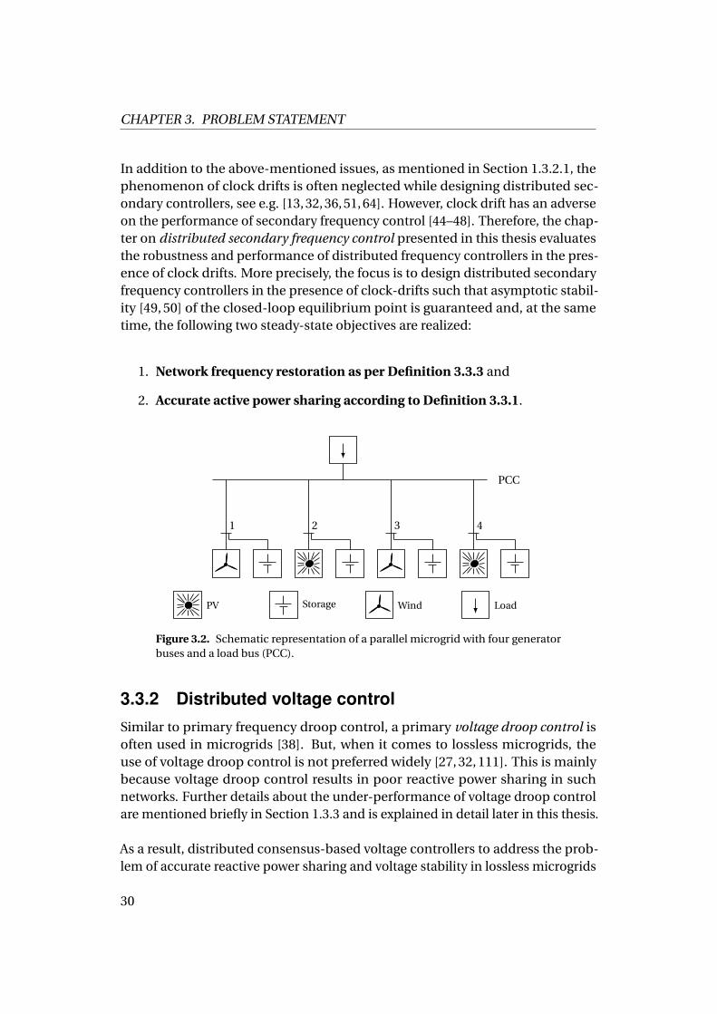
3.1 Pictorial representation of an inverter-based microgrid . . . . . . . . . 233.2 A simple picture of a parallel microgrid . . . . . . . . . . . . . . . . . . . 30
4.1 A detailed representation of a lossless parallel microgrid . . . . . . . . 35
7.1 Microgrid used to simulate distributed frequency controllers. . . . . . 797.2 Topology of the communication network used to simulate distributed
frequency controllers. . . . . . . . . . . . . . . . . . . . . . . . . . . . . . 797.3 Simulation result with the GDAI control . . . . . . . . . . . . . . . . . . 807.4 Simulation result with the DAI control . . . . . . . . . . . . . . . . . . . 817.5 Simulation result with the pinning control . . . . . . . . . . . . . . . . . 837.6 Parallel microgrid used in the simulation. . . . . . . . . . . . . . . . . . 847.7 Communication topology employed in the simulated parallel microgrid 857.8 Simulation result with the proposed distributed voltage control: load
steps . . . . . . . . . . . . . . . . . . . . . . . . . . . . . . . . . . . . . . . 877.9 Simulation result with the proposed distributed voltage control: con-
tinuosly fluctuating load demand . . . . . . . . . . . . . . . . . . . . . . 88
xii
Abbreviations
AC alternating current
DAE differential algebraic equation
DAI distributed averaging integral
DC direct current
DG distributed generator
DoS denial of service
ESS energy storage system
GDAI generalized distributed averaging integral
GFI grid-forming inverter
LHS left hand side
LMI linear matrix inequality
LV low voltage
MV medium voltage
ODE ordinary differential equation
PCC point of common coupling
xiii
PI proportional integral
PV photovoltaic
RES renewable energy source
RHS right hand side
SRF-PLL synchronous reference frame phase locked loop
UPS uninterruptible power supply
ZIP constant power/current/impedance
Symbols
R set of real numbersR≥0 set of non-negative real numbersR>0 set of positive real numbersR<0 set of negative real numbersT set of real points on the unit circle (mod 2π)∇g gradient of a function g : Rn →R
‖ ·‖2 Euclidean normA> transpose of a square matrix A|W | cardinality of a set W
N set of network nodesNi set of neighboring nodes connected to node iδi voltage phase angle at node iVi voltage amplitude at node iV d
i desired voltage amplitude at node iBi j susceptance of the power line connecting node i and jBi i shunt susceptance at node iGi i shunt conductance at node iai weighting coefficient for reactive power sharing at node iXi weighting coefficient for active power sharing at node iωi electrical frequency at node iωi internal frequency at node iωd desired nominal network frequencyµi clock drift value at inverter iPi active power injection at node iP m
i measured active power injection at node i
P di desired active power set point at node i
Qi reactive power injection at node iQm
i measured reactive power injection at node i
Qdi desired reactive power set point at node i
xv
τi time constant of the power measurement filter at node iSN
i nominal power rating of an inverter connected at node iL Laplacian matrix of a communication networkB Incidence matrix of a communication networkW Edge weight matrix of a communication network
Chapter 1
Introduction
1.1 MotivationThe electric power systems are considered as the backbone of any modern in-dustrialized society [1–3]. A power system can be broadly classified into powergenerators, transmission system, distribution system, and load centres [1, 4]. Inconventional power networks, a significant share of power generated is throughsynchronous generators, which often use fossil-fuel-based energy sources [4, 5],substantially contributing to greenhouse gas emissions. Motivated by this, toreduce greenhouse gas emissions and fossil fuel consumption in the area of powersystems, the worldwide usage of renewable energies has increased remarkably inthe recent years [6,7]. Nonetheless, the increasing integration of renewable energysources (RESs) results in various technological as well as structural changes in theexisting power grid [8–11].
In comparison to conventional generators, RESs are small-sized, i.e., the powergenerated is relatively lower. Hence, most RESs are interfaced to MV (mediumvoltage) or LV (low voltage) levels [8, 10, 11]. Also, while replacing a conventionalgenerator that typically delivers a high amount of power [12], a large number ofRESs need to be installed for balancing power demand and supply. Thus, powergeneration is moving from a relatively small number of large scale power stationsto a huge number of small-scale distributed generators (DGs). This is a majorstructural change in the existing power grid structure [6, 9].
An immediate consequence of this structural change is that power generationand consumption have become geographically closer to each other, with RESsas the primary source of power generation. Alternatively stated, such a set upcan be understood as a distribution system which–in contrast to conventional
1
CHAPTER 1. INTRODUCTION
power systems– has localized power generation and consumption involved init. Besides, the presence of a large number of DGs poses some crucial controlchallenges. For instance, in conventional power systems, the number of powergenerators is relatively small, and hence a centralized control solution wouldwork satisfactorily [1]. However, in a power grid with a large number of DGs, acentralized control solution turns out to be inefficient [13], mainly because thata central unit has to communicate to all the numerous DGs connected in thenetwork. Such a one-to-all communication system would increase the overallcommunication burden, and at the same time, would pose the risk of single-point-failures [13].
On top of the above-mentioned structural changes, a crucial technological chal-lenge is as follows. RESs connected in the grid mostly produce DC (direct current)or variable frequency AC (alternating current) power output. Hence, they are in-terfaced to the grid using power electronic inverters. The physical characteristicsof inverters largely differ from that to synchronous generators, see, e.g. [3, 14–16].As a consequence, control strategies used in conventional power systems need tobe redesigned and/or readjusted for power networks having a large number ofinverter-interfaced RESs [14, 15, 17].
One promising solution to address these issues is by using the concept of mi-crogrids [8, 10, 17–19]. A microgrid is a locally controllable electrical networkwith generators, storage units, and loads. The concept of microgrids is foreseenas a critical element in future electric power systems [10, 20]. In a general set-ting, microgrids may interact with each other [21], but - by matching generationand consumption within the microgrid as far as possible - transmitted poweris reduced, and transmission losses are decreased. Microgrids can usually beoperated in two modes, namely grid-connected mode where it is connected to theutility grid and islanded or stand-alone mode where it works as an isolated powernetwork [10, 18, 19]. In comparison to grid-connected mode, in islanded mode,control actions have to be undertaken by the units connected within the network,making it challenging [22–27]. Thus, this thesis focusses on the topic of control ofislanded microgrids.
1.2 ContributionsThe present work is dedicated to addressing the following control problems in anislanded microgrid:
1. Accurate network frequency restoration,
2
2. Active power sharing,
3. Load voltage regulation,
4. Reactive power sharing and
5. Voltage stability.
A brief overview of the relevance of the considered control objectives is given inthe sequel.
Similar to any isolated power network, maintaining a stable operating point is oftremendous importance in an islanded microgrid [22–24,28–31]. At the same time,restoring the network frequency to the nominal value and maintaining voltageamplitudes at all the buses within a specific limit is also very important [27,32,33].In some microgrid applications, like a battery energy storage system (ESS) or adistributed uninterruptible power supply (UPS) system, it is often the case thatthe DGs are connected in parallel and are feeding a common load connectedat the PCC [34, 35]. In such applications, restoring the voltage amplitude at thePCC/load bus is of great relevance [34, 35]. Finally, in any microgrid network,sharing the total system loads among the generation units in a fair manner is acrucial control objective [22, 23, 26, 27, 35].
The aforementioned contributions of this work can be divided into two mainsections. At first, the problem of distributed frequency control [13, 25, 32, 36, 37]in a microgrid with arbitrary topology (also termed as a meshed microgrid) isinvestigated. Later, voltage stability and reactive power sharing [24, 27] in amicrogrid with parallel-connected DGs connected to a common load [34, 35,38] are addressed. Unless confusion arises, such a network is called a parallelmicrogrid in the rest of this thesis.
Next, the main contributions falling under these two sections are briefly de-scribed.
1.2.1 Distributed secondary frequency controlInspired by conventional power systems, a hierarchical control architecture isadvocated for microgrids, which has primary, secondary, and tertiary controllayers [39, 40]. The chapter entitled distributed secondary frequency control inthis thesis focusses on exploring the robustness and performance of distributedsecondary frequency controllers in the presence of a non-negligible parameter
3
CHAPTER 1. INTRODUCTION
uncertainty, known as clock drifts, commonly observed in inverter-based micro-grids.
Microgrids are distributed systems where distributed computing is involved. Itis a well-known fact that distributed computing applications suffer from clockdrifts [41, 42]. In the presence of clock drifts, the steady-state performance ofprimary [16,43] and secondary frequency control [44–48] employed in a microgridare adversely affected. The contributions of this thesis regarding these issues canbe summarized as follows.
1. A general distributed integral frequency control structure is proposed tocompare the steady-state performance of various distributed secondaryfrequency controllers in the presence of clock drifts. This approach assumesthat in the primary control layer, the standard frequency droop control [38]is implemented.
2. Based on the proposed general controller structure, necessary and sufficientconditions for steady-state accurate frequency restoration and active powersharing in the presence of clock drifts are derived. Later, a novel secondaryfrequency controller, termed as generalized distributed averaging integral(GDAI) controller is presented to achieve the above-mentioned controlobjectives in the presence of clock drifts.
3. A tuning criterion in the form of a set of linear matrix inequalities (LMIs)is derived that, if feasible, guarantees asymptotic stability [49, 50] of theclosed-loop equilibrium point. The tuning criterion is derived using thestandard decoupling assumption utilized in power networks with inductivelines1, see e.g., [1, 22, 24, 27, 32].
4. The results are validated extensively, via simulation, and are comparedwith other distributed secondary frequency controllers proposed in theliterature, e.g. [13, 32, 51, 52].
1.2.2 Distributed voltage controlThis section outlines the contributions of this thesis to the topic of voltage controlin parallel microgrids. Two important control objectives in a parallel microgridwith dominantly inductive power lines are (i) reactive power sharing and (ii)load/PCC voltage restoration, see, e.g. [34, 35, 38]. In this regard, the followingresults are summarized in this thesis.
1Also referred to as lossless lines [1].
4
1. At first, the existence and uniqueness properties of a stationary solution tothe set of algebraic equations corresponding to steady-state proportionalreactive power sharing and PCC voltage restoration are established.
2. A distributed voltage controller which drives the closed-loop system trajec-tories asymptotically [49, 50] to the desired unique stationary solution isproposed.
3. Via a numerical case study, the performance of the proposed distributedvoltage controller towards further modeling errors and load disturbancesis evaluated. Operational compatibility of the proposed control approachwith the standard frequency droop control [38] is also investigated.
1.2.3 Structure of the thesisThe present thesis is arranged as six chapters with a common conclusion. Themain contents of each chapter are described concisely in the following.
Chapter 2: Preliminaries
In this chapter, some standard results from control theory, algebraic graph theory,and power systems are reviewed. After introducing the mathematical notationused in this thesis, some control theory basics, like Lyapunov stability [49, 50], arerecalled. Then, a background on algebraic graph theory [53–55] and consensusprotocols [56] are discussed. Finally, some power systems basics [1, 3, 4] requiredin the present work are presented.
Chapter 3: Problem statement
In this chapter, the microgrid concept and the formal definition of a micro-grid [8, 10, 18] are introduced. Furthermore, the main technical challenges ina microgrid are discussed. Later, the hierarchical control structure used in anislanded microgrid [39] is described. Finally, definitions regarding power shar-ing [26, 27], frequency and voltage restoration [13, 32, 36, 51, 57] are formalized.
Chapter 4: Microgrid model and primary control
The mathematical model of the microgrid studied in this thesis is introducedin this chapter. More precisely, the inverter, the load and the network modelsrequired to present the results summarized in this thesis are introduced. Fur-thermore, the standard droop control [38] used at the primary control layer isdescribed in detail. Later, the model of a droop-controlled inverter in the pres-ence of clock drifts is derived [43, 58] Finally, the steady-state performance of
5
CHAPTER 1. INTRODUCTION
frequency droop control in the presence of clock drifts and voltage droop controlin lossless microgrids are discussed in detail.
Chapter 5: Distributed secondary frequency control
This chapter focusses on the performance of secondary frequency control inmicrogrids with explicit consideration of clock drifts. More precisely, achievingcontrol objectives of steady-state
1. accurate network frequency restoration and
2. active power sharing,
with various distributed secondary frequency controllers in the presence of clockdrifts are studied.
A general distributed control representation is proposed, which can be param-eterized into the control approaches presented in [13, 32, 37, 51]. Based on thisgeneral controller representation, necessary and sufficient conditions for achiev-ing secondary frequency control objectives in the presence of clock drifts arederived. The control approaches advocated in [13, 32, 37, 51] were found to be notsatisfying the derived necessary and sufficient conditions. Yet in this section, anovel secondary frequency controller, termed as GDAI control is proposed, whichfulfils the above-mentioned control objectives in the presence of clock drifts.
In the second part of this chapter, a tuning criterion that guarantees asymptoticstability of the closed-loop (with the GDAI control) equilibrium point is presented.For deriving this result, concepts from the classical Lyapunov function-basedstability analysis employed in power networks were used, see, e.g. [25, 59].
Chapter 6: Distributed voltage control
In this chapter, the problem of voltage control in a parallel microgrid is investi-gated. More precisely, three important control objectives of
1. reactive power sharing,
2. PCC voltage restoration and
3. voltage stability,
6
in a parallel microgrid with inductive lines are addressed.
In the first part of this chapter, the existence and uniqueness properties of astationary voltage solution to the steady-state algebraic equations of reactivepower sharing and PCC voltage restoration are established. Then, inspired by [27,30], a distributed voltage controller is proposed, which at equilibrium yields thedesired stationary solution mentioned above. A stability criterion that guaranteeslocal asymptotic stability of the closed-loop equilibrium point is also derived inthis chapter.
Chapter 7: Case study
In the first section of this chapter, the performance of the GDAI controller isvalidated and is compared with other distributed control approaches [13, 32, 51]in the presence of clock drifts. To evaluate the robustness of the GDAI controltowards typical modeling uncertainties, a small line resistance is considered inthe simulated microgrid.
In the second part of this chapter, the performance of the distributed voltage con-troller designed for a parallel microgrid is validated. Furthermore, the operationalcompatibility of the same with the frequency droop control [38] is tested.
1.3 Related works
1.3.1 IntroductionIn conventional power systems, synchronous generators that operate as gridforming units are responsible for maintaining a desired stable operating point [3].However, in inverter-based microgrids, inverter-interfaced sources or, more pre-cisely, grid-forming inverters replace synchronous generators [14, 15]. A gridforming inverter is a voltage source inverter controlled using voltage and fre-quency references provided by the designer [14–16].
Motivated by the control strategies used in conventional power systems, a hier-archical control approach has been advocated for microgrids [13, 39, 60]. Onetypically distinguishes primary and secondary control layers (as in conventionalpower systems), while the top control level, which is mostly referred to as op-erational management or tertiary control, is mainly concerned with generationscheduling, see, e.g. [21, 61]. Primary control layer consists of a decentralized pro-portional control, called droop control. The decentralized aspect of droop control
7
CHAPTER 1. INTRODUCTION
facilitates that each inverter2 requires only local information for its operation,and does not need any communication with other inverters. In microgrids withinductive power lines, droop control can be divided into two, frequency droopcontrol and voltage droop control. In frequency droop control, the frequencyof an inverter depends linearly on the active power injection. Frequency droopcontrol achieves frequency stability and active power sharing [22, 62]. In the caseof voltage droop control, voltage amplitude at each inverter is in proportion to itsreactive power injection [38].
In the rest of this section, some relevant works on the topics focussed on in thisthesis are reviewed.
1.3.2 Distributed secondary controlIn islanded microgrids, frequency stability and proportional active power sharingare typically provided by the primary frequency droop control [22, 26, 38, 62, 63].Despite many advantages, a major drawback of the frequency droop control isthat the steady-state frequency usually deviates from the nominal value (50 or60 Hz). The first part of this thesis is devoted to secondary frequency control,which is responsible for correcting the steady-state frequency error caused bythe primary control layer [39]. In this regard, some related works on secondaryfrequency control are outlined in the sequel.
As most of the electrical devices are designed to operate at the nominal frequencyof 50 or 60 Hz, restoring the network frequency to the desired nominal value isvery important [1]. Conventionally, a central integral control [63] is advocated forthis task, where a central unit communicates with all the generation units. Yet,considering the complexity and the number of generation units connected ina microgrid, centralized approaches significantly increase the communicationburden and are also vulnerable to single-point-failures [13]. As a consequence,distributed secondary control architectures are being increasingly proposed forthis task [13,25,32,36,37,51,64]. Most distributed controllers only need a sparselyconnected communication network for their operation. The sparsity of the com-munication network stems from the fact that each unit in the network has tocommunicate only with its neighbors [56], thus avoiding undesired all-to-all andone-to-all communication requirements. Typically, a distributed secondary fre-quency controller is implemented by means of consensus-based algorithms, seee.g., [13, 25, 32, 36, 37, 51, 64].
2Unless confusion arises, a grid-forming inverter is denoted simply as an inverter in the restof this work.
8
There are various important aspects to be considered while designing a dis-tributed control law for a networked system like a microgrid, e.g. communicationdelay [36, 65, 66] and denial-of-service (DoS) [67, 68]. Also, finding an optimalcommunication topology for the satisfactory operation of a distributed controlleris also of great practical relevance [64–66, 69]. Irrespective of such aspects, themain advantage of using a distributed control approach in a microgrid is thatit obviates the requirement for a central communication unit, thus improvingsystem reliability and robustness towards single-point-failures [13]. Hence, sec-ondary frequency control discussed in this thesis considers distributed controlsolutions and investigates their performance towards a non-negligible parameteruncertainty usually observed in microgrids, that is explained concisely in thefollowing.
1.3.2.1 Performance in the presence of clock drifts
An inverter-based microgrid involves distributed computation, carried out at thedigital-controller of each grid-forming inverter. It is a well-known fact that theclocks used to generate time signals of these digital-controllers are not synchro-nized [41, 42]. This results in clock drifts between the inverters. In microgrids,clock drifts create frequency mismatches and disturb steady-state active powersharing [43, 58]. In the context of distributed secondary frequency control, ap-proaches presented in the literature often neglect the effect of clock drifts, see,e.g. [13, 32, 36, 51, 64]. However, recently it has been highlighted that clock driftshave an adverse effect on the performance of secondary frequency control [44–48].For example, in [70], the detrimental effect of clock drifts on distributed averagingintegral (DAI) control presented in [32, 51] has been investigated. It has beenshown that the DAI controller is unable to properly achieve usual secondaryfrequency control objectives in the presence of clock drifts. In [48], a compar-ative study comprising droop-only, droop-free and various consensus-baseddistributed control approaches in the presence of clock drifts has been presented.The authors conclude that all the approaches studied in [48] exhibit problems inachieving secondary frequency control objectives in the presence of clock drifts.
In [44], steady-state and transient performance of various decentralized sec-ondary frequency controllers in the presence of clock drifts has been compared.In a similar spirit, in [45], a decentralized secondary control approach has beenstudied and robustness of this approach towards clock drifts under high loadconditions are evaluated experimentally. Although decentralized secondary con-trollers avoid the requirement of communication, they have the disadvantagethat they exhibit inefficient allocation of generation resources and suffer frompoor robustness to measurement bias [57]. In contrast to that, a droop-free con-troller that requires neighboring node communication has been studied in [46]
9
CHAPTER 1. INTRODUCTION
considering the effect of clock drifts. However, the comparative study presentedin [48] shows that the aforementioned droop-free approach under-performs interms of active power sharing in the presence of clock drifts.
In [47], a consensus-based distributed frequency controller has been studied,where the authors confirm experimentally, that clock drifts induce power sharingerrors and frequency deviations. However, the approach investigated in [47] re-quires that each inverter has to communicate with all other inverters connected inthe microgrid. In practice, such an all-to-all communication is undesirable. In aslightly different setting, a consensus-based power control law has been designedin [71] on top of a primary angle droop3 control layer. The approach presentedin [71] is able to achieve frequency consensus and active power sharing at steady-state. Recently, a modified frequency droop control scheme to address powersharing issues in the presence of clock drifts has been presented in [73]. Nonethe-less, the approaches proposed in [71, 73] have not yet considered the mandatorysecondary frequency control objective of network frequency restoration.
A possible remedy to alleviate the impact of clock drifts is to use a global timesynchronization strategy, e.g., [63], where a central unit communicates a globaltime signal to all the generation units. Again, such a central set up increasescommunication burden and is prone to single-point-failures. Another interestingoption is to use clock synchronization protocols applied in sensor networks, seee.g. [74, 75]. Yet, when it comes to microgrids, for implementing these clocksynchronization protocols, an additional clock synchronization control has tobe designed and should–probably–be activated before primary and secondarycontrols are enabled. Adding such an additional control layer would increase theoverall complexity of the hierarchical control architecture employed in microgrids[63].
1.3.3 Distributed voltage controlIn contrast to primary frequency droop control, the use of primary voltage droopcontrol [38] is often not the most preferred solution in microgrids with inductivelines, see e.g. [24, 27, 30, 32]. This can be explained as follows.
In microgrids with inductive lines, voltage droop control [38] yields a propor-tional relation between the voltage amplitude and the reactive power flow at eachinverter. Thereby, even a small mismatch in voltage set points together with thelow resistance to inductive reactance (R/X) ratio of the power lines, resulting in
3In an angle droop controller, the voltage phase angle of a grid forming inverter is calculatedin proportion to the power injected [72].
10
undesired circulating reactive currents [24]. A detailed investigation regardingpoor reactive power sharing in lossless microgrids operated with voltage droopcontrol can be found in [32]. Thus in the sequel, some relevant works from the lit-erature to address accurate proportional reactive power sharing, and additionally,load voltage regulation in a lossless microgrid with parallel-connected invertersis reviewed.
1.3.3.1 Distributed voltage control in parallel microgrids
For improving system redundancy and reliability needed by a critical load, a com-mon practice in some microgrid applications is to connect inverter-interfacedRESs and storage units in parallel to the point of common coupling (PCC) wherethe load is connected. Such a network is commonly termed as a parallel micro-grid, see e.g. [34, 35, 38, 76, 77]. Some practical examples of parallel microgridsare battery power plants (also known as energy storage systems (ESSs)) and dis-tributed uninterruptible power supply (UPS) systems [38, 76, 77]. Similar to anislanded microgrid, the issue of power balance and network stability is of tremen-dous importance in a parallel microgrid.
As mentioned earlier, maintaining all the bus voltage amplitudes within a cer-tain limit is an important control objective in any power network. In a parallelmicrogrid, the most critical voltage amplitude is at the PCC since there is nogeneration unit present at that node. Hence, to restore the voltage at the PCC tothe nominal value, DGs connected in the microgrid should be controlled accord-ingly [34, 35, 38]. On the other hand, in a parallel microgrid with inductive powerlines, it is also of high relevance to share the reactive power demand of the loadproportionally between the DGs [34, 35, 76–81].
The problem of power sharing in parallel microgrids has been investigated in[38, 77–80, 82] using proportional droop control. In [81], a proportional-integral(PI)-based distributed controller has been proposed to address power sharing.In [34, 35], together with power sharing, the objective of PCC voltage regulationalso has been addressed using a PI controller. The aforementioned approachesassume that there exists a unique stable operating point. Stability analysis withtwo droop-controlled inverters connected in parallel has been presented in [83],where the authors linearize the power flow equations at a particular operatingpoint. In contrast to that, a decentralized quadratic voltage droop controller hasbeen proposed in [24] to ensure voltage stability in lossless microgrids. However,accurate proportional reactive power sharing cannot be guaranteed withoutrisking voltage stability [27, 30].
11
CHAPTER 1. INTRODUCTION
1.4 PublicationsA major share of this thesis is based on the following publications, to all of whichthe author of the present work has made significant contributions.
• A. Krishna, C. A. Hans, J. Schiffer, J. Raisch, and T. Kral. Steady state eval-uation of distributed secondary frequency control strategies for micro-grids in the presence of clock drifts. In Mediterranean Conference onControl and Automation (MED), pages 508-515, Valetta, Malta, 2017.
• A. Krishna, J. Schiffer and J. Raisch. A Consensus-Based Control Law forAccurate Frequency Restoration and Power Sharing in Microgrids in thePresence of Clock Drifts. In European Control Conference, pages 2575-2580,Limassol, Cyprus, 2018.
• A. Krishna, J. Schiffer and J. Raisch. Distributed Secondary FrequencyControl in Microgrids: Robustness and Steady-State Performance in thePresence of Clock Drifts. Accepted for publication at European Journal ofControl.
• A. Krishna, J. Schiffer, N. Monshizadeh, and J. Raisch A consensus-basedvoltage control for reactive power sharing and PCC voltage regulation inmicrogrids with parallel-connected inverters. In European Control Con-ference, Naples, Italy, 2019.
12
Chapter 2
Preliminaries
This chapter describes the notations and preliminaries used in this thesis. At first,the employed mathematical terminology is presented. Later, preliminaries aboutcontrol theory, algebraic graph theory, and power systems needed in this thesisare outlined.
2.1 NotationThroughout this thesis, the identity matrix of size n ×n is denoted by In , thevector of all-ones as 1n ∈Rn and the vector of all-zeros as 0n ∈Rn . The matrix ofall ones (also called the all-ones-matrix [84]) is denoted by 1n×n ∈ Rn×n unlessspecifically denoted as 1n1>
n . A matrix of all zeros is denoted by 0n×m ∈ Rn×m .An n ×n diagonal matrix with entries a j , j = 1, . . . ,n is denoted by diag(a j ). Themaximum eigenvalue of a square symmetric matrix F is denoted by λmax(F ) andthe trace of F as trace(F ). The elements below the diagonal of F are denoted by ∗.If F is positive (negative) definite, then it is denoted by F > 0 (F < 0). Similarly, ifF is positive (negative) semidefinite, F ≥ 0 (F ≤ 0). Moreover, A > B means thatA−B > 0.
Let x = col(xi ) represent a column vector with entries xi . Then, [x] denotes adiagonal matrix with diagonal entries xi . Moreover, X = blockdiag(Xi ) denotes ablock-diagonal matrix with matrix entries Xi ∈Rni×ni . For a function f (x) : Rn →R, ∇x f denotes the gradient of f (x) with respect to x ∈Rn . Finally, ‖ ·‖2 denotesthe Euclidean norm and |U | represents the cardinality of a set U .
13
CHAPTER 2. PRELIMINARIES
2.2 Control theory basicsIn this section some standard control theory concepts are surveyed. After recallingthe definition of a dynamical system, the notion of stability is introduced. Later,the classical Lyapunov stability results are recalled. These control theory basicsare based on [49, 50]. Hence, for the proofs of the theorems presented in thissection, the reader is referred to [49, 50].
The class of systems relevant in the context of this thesis are dynamical systemsin the form of an ordinary differential equation (ODE) given by [49, 50]
x = f (x(t )), (2.2.1)
where x(t) : [t0,∞) →Rn , f : Rn →Rn is a locally Lipschitz function and t0 ∈R isthe initial time.
2.2.1 Lyapunov stabilityLyapunov stability is a standard tool in control theory to study stability of the equi-librium point of systems of the form (2.2.1). This is formalized in the definitionbelow.
Definition 2.2.1. [49, Definition 3.1] Consider the system (2.2.1). Let f be a locallyLipschitz continuous function defined over the domain D ∈Rn , which contains theorigin, and f (0n) = 0n . The equilibrium point x = 0n of the system (2.2.1) is
1. stable if for each ε> 0, there is δ= δ(ε) > 0 such that
‖x(0)‖ < δ⇒‖x(t )‖ < ε,∀t ≥ 0,
2. unstable, if not stable,
3. asymptotically stable, if it is stable and δ can be chosen such that
‖x(0)‖ < δ⇒ limt→∞x(t ) = 0.
The notion of Lyapunov’s stability is formalized in the theorem below.
Theorem 2.2.2. [49, Theorem 3.3] Consider the system (2.2.1). Let f be a locallyLipschitz continuous function defined over the domain D ∈Rn , which contains the
14
origin, and f (0n) = 0n . Let V (x) be a continuously differentiable function definedover D such that
V (0n) = 0 and V (x) > 0 ∀x ∈ D \ 0n, (2.2.2)
V (x) ≤ 0 ∀x ∈ D, (2.2.3)
then x = 0n is a stable equilibrium point of the system (2.2.1). Moreover, if
V (x) < 0 ∀x ∈ D \ 0n, (2.2.4)
then x = 0n is asymptotically stable. Furthermore, if D = Rn , (2.2.2) and (2.2.4)hold for all x 6= 0n , and
‖x‖→∞⇒V (x) →∞, (2.2.5)
then x = 0n is globally asymptotically stable.
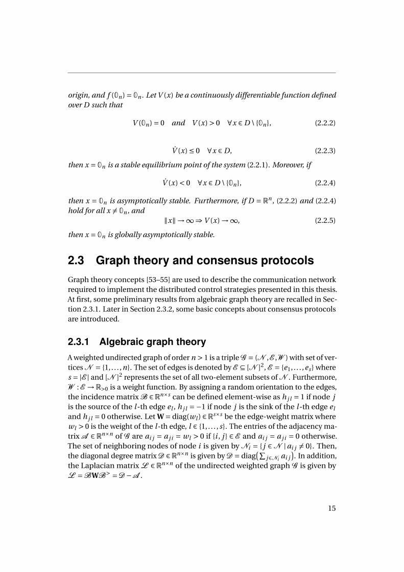
2.3 Graph theory and consensus protocolsGraph theory concepts [53–55] are used to describe the communication networkrequired to implement the distributed control strategies presented in this thesis.At first, some preliminary results from algebraic graph theory are recalled in Sec-tion 2.3.1. Later in Section 2.3.2, some basic concepts about consensus protocolsare introduced.
2.3.1 Algebraic graph theoryA weighted undirected graph of order n > 1 is a triple G = (N ,E ,W ) with set of ver-tices N = 1, . . . ,n. The set of edges is denoted by E ⊆ [N ]2, E = e1, . . . ,es wheres = |E | and [N ]2 represents the set of all two-element subsets of N . Furthermore,W : E →R>0 is a weight function. By assigning a random orientation to the edges,the incidence matrix B ∈Rn×s can be defined element-wise as h j l = 1 if node jis the source of the l-th edge el , h j l =−1 if node j is the sink of the l-th edge el
and h j l = 0 otherwise. Let W = diag(wl ) ∈Rs×s be the edge-weight matrix wherewl > 0 is the weight of the l -th edge, l ∈ 1, . . . , s. The entries of the adjacency ma-trix A ∈ Rn×n of G are ai j = a j i = wl > 0 if i , j ∈ E and ai j = a j i = 0 otherwise.The set of neighboring nodes of node i is given by Ni = j ∈N |ai j 6= 0. Then,the diagonal degree matrix D ∈Rn×n is given by D = diag
(∑j∈Ni
ai j). In addition,
the Laplacian matrix L ∈ Rn×n of the undirected weighted graph G is given byL =BWB> =D−A .
15
CHAPTER 2. PRELIMINARIES
A path is an ordered sequence of nodes such that any pair of consecutive nodesin the sequence is connected by an edge. The graph G is called connected if thereexists a path between every pair of distinct nodes. The matrix L has a simplezero eigenvalue if and only if G is connected. A corresponding right eigenvectoris 1n , i.e., L 1n = 0n , yielding L ≥ 0.
2.3.2 Consensus protocolsThe use of consensus protocols to address control objectives in multi-agent net-worked systems have become increasingly popular in the past few decades, see,e.g. [56, 85–88]. The term consensus means that a group of agents in a networkedsystem reach an agreement on a common value by negotiating with their neigh-bors [56]. The interaction rule to achieve this agreement is typically called asconsensus protocol or consensus algorithm [56]. A remarkable advantage of con-sensus protocols is that, in general, they are distributed in nature. Therefore toreach an agreement among agents, neither an all-to-all communication networknor a central communication setup are required.
Consider an undirected connected weighted graph G = (N ,E ,W ) where N ,Eand W are defined in Section 2.3.1. A simple consensus protocol which guaranteesconvergence to a common value can be represented as [56]
xi =∑
i∈Ni
ai j (x j −xi ), i ∈N , j ∈Ni , (2.3.1)
where xi is the information state of the i -th agent, ai j is the (i , j )-th entry of theadjacency matrix A of graph G and Ni is the set of neighboring nodes connectedto agent i . The consensus protocol (2.3.1) for the whole network can be writtenas
x =−L x, (2.3.2)
where x = col(xi ) ∈ Rn is the information state vector and L is the Laplacianmatrix of the graph G . The dynamics (2.3.2) at steady-state can be expressed as
0n =L xs , (2.3.3)
where the super script s denotes the steady-state value. Under the assumptionthat G is connected, 0 is a simple eigenvalue of L with a corresponding righteigenvector 1n . Therefore,
L xs = 0n ⇔ xs =α1n , α ∈R. (2.3.4)
Let x(0) ∈Rn be the initial condition of of x(t ). Then [56]
α= 1
|N |∑
i∈N
xi (0).
16
Hence, the systems of the form (2.3.2) are also known as continuous time dis-tributed averaging systems [56, 87].
2.4 Power system basicsFollowing the standard practice in AC power systems, power is typically generated,transmitted, and distributed in the form of three-phase signals [4, 12, 89]. There-fore, the present work focuses on three-phase AC power networks. It is assumedthat the three-phase signals considered in this thesis are symmetric [4, 89, 90], seealso [23, Section 2.4].
In light of these assumptions, the following sections summarize some powersystems preliminaries required throughout the present work. At first, the networkmodel is introduced, and expressions for active and reactive power flows arepresented later. Finally, a commonly used network reduction technique used inpower networks with constant impedance loads is recalled.
2.4.1 Network modelPower lines in AC networks are typically modeled as the so-called π-model [1, 4, 5,89], which consists of a series RL (resistance with inductance) element connectedin parallel with R and C (resistance and capacitance) shunt-elements. For powernetworks with short power lines, e.g. microgrids, the shunt-elements can oftenbe neglected [1, 4, 89]. Thus, a power line can be represented as a combination ofresistance and inductance connected in series.
As this thesis is devoted to addressing control issues in microgrids with domi-nantly inductive lines (i.e., lossless lines), the line resistance is neglected. LetXi j ∈ R>0 be the inductive reactance of a power line connecting two buses, sayi ∈N and j ∈N . Then,
Xi j =ωLi j ∈R>0,
where ω ∈R>0 denotes a frequency and Li j ∈R>0 is the inductance of the powerline connecting bus i and bus j . The susceptance Bi j ∈ R<0 of the power lineconnecting bus i and bus j is then given by
Bi j =−1
Xi j∈R<0. (2.4.1)
The dynamics of the power lines are assumed to be negligible [1, 3]. Thereby, itis essential to note that a power line connecting bus i and bus j is denoted by(2.4.1) in the rest of this thesis.
17
CHAPTER 2. PRELIMINARIES
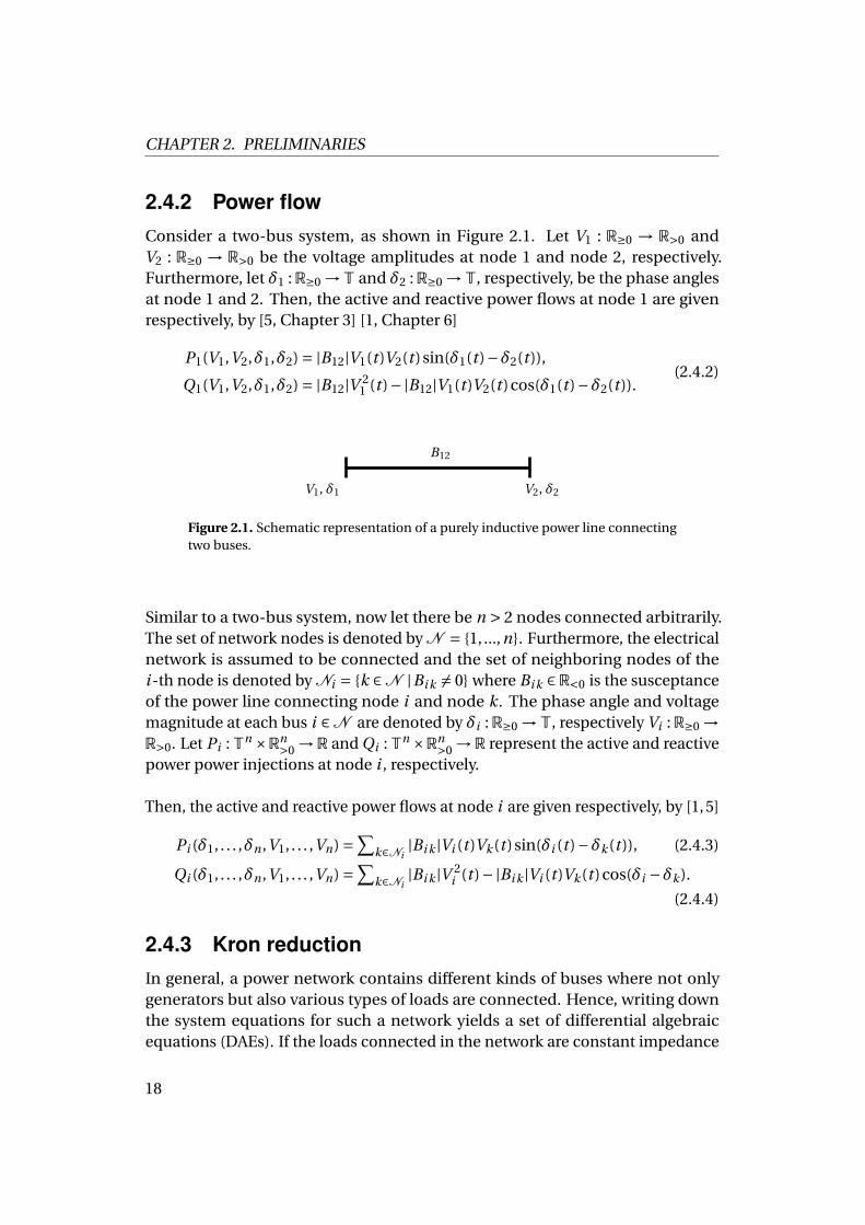
2.4.2 Power flowConsider a two-bus system, as shown in Figure 2.1. Let V1 : R≥0 → R>0 andV2 : R≥0 → R>0 be the voltage amplitudes at node 1 and node 2, respectively.Furthermore, let δ1 : R≥0 →T and δ2 : R≥0 →T, respectively, be the phase anglesat node 1 and 2. Then, the active and reactive power flows at node 1 are givenrespectively, by [5, Chapter 3] [1, Chapter 6]
P1(V1,V2,δ1,δ2) = |B12|V1(t )V2(t )sin(δ1(t )−δ2(t )),
Q1(V1,V2,δ1,δ2) = |B12|V 21 (t )−|B12|V1(t )V2(t )cos(δ1(t )−δ2(t )).
(2.4.2)
V1, δ1 V2, δ2
B12
Figure 2.1. Schematic representation of a purely inductive power line connectingtwo buses.
Similar to a two-bus system, now let there be n > 2 nodes connected arbitrarily.The set of network nodes is denoted by N = 1, ...,n. Furthermore, the electricalnetwork is assumed to be connected and the set of neighboring nodes of thei -th node is denoted by Ni = k ∈N |Bi k 6= 0 where Bi k ∈R<0 is the susceptanceof the power line connecting node i and node k. The phase angle and voltagemagnitude at each bus i ∈N are denoted by δi : R≥0 →T, respectively Vi : R≥0 →R>0. Let Pi : Tn ×Rn
>0 →R and Qi : Tn ×Rn>0 →R represent the active and reactive
power power injections at node i , respectively.
Then, the active and reactive power flows at node i are given respectively, by [1, 5]
Pi (δ1, . . . ,δn ,V1, . . . ,Vn) =∑
k∈Ni|Bi k |Vi (t )Vk (t )sin(δi (t )−δk (t )), (2.4.3)
Qi (δ1, . . . ,δn ,V1, . . . ,Vn) =∑
k∈Ni|Bi k |V 2
i (t )−|Bi k |Vi (t )Vk (t )cos(δi −δk ).
(2.4.4)
2.4.3 Kron reductionIn general, a power network contains different kinds of buses where not onlygenerators but also various types of loads are connected. Hence, writing downthe system equations for such a network yields a set of differential algebraicequations (DAEs). If the loads connected in the network are constant impedance
18
loads, then using a commonly employed network reduction technique, termedas Kron reduction, such a system of DAEs can be represented as pure ordinarydifferential equations (ODEs) [1, 91]. In a Kron-reduced network, all the buseshave a generator and a shunt admittance connected to them [1, 91].
For a Kron-reduced power network with inductive lines, active and reactive powerflows at node i are given respectively by [1]
Pi (δ1, . . . ,δn ,V1, . . . ,Vn) =Gi i V 2i (t )+
∑k∈Ni
|Bi k |Vi (t )Vk (t )sin(δi (t )−δk (t )),
Qi (δ1, . . . ,δn ,V1, . . . ,Vn) = |Bi i |V 2i (t )−
∑k∈Ni
|Bi k |Vi (t )Vk (t )cos(δi (t )−δk (t )),
(2.4.5)
where Gi i ∈ R>0 is the shunt conductance and Bi i = Bi i +∑n
k=1,k 6=i Bi k , where
Bi i ∈R<0 is the shunt susceptance. In the sequel, the dependence of voltages andphase angles on time will not be displayed unless confusion arises.
2.5 SummaryIn this chapter, the mathematical notation and preliminaries required for present-ing the results in this thesis have been outlined. At first, the notation employedthroughout this thesis has been introduced. Later some control theory basics andgraph theory results have been recalled. Finally, some important power systembasics, which are used extensively in this thesis, have been introduced.
19


Chapter 3
Problem statement
3.1 IntroductionAs discussed in Chapter 1, the increasing integration of RESs into the modernpower grid brings in various operational challenges. A possible remedy to tacklethese challenges is to consider the whole grid as a set of locally controllablesmaller networks, called microgrids [8, 17]. In this chapter, the concept of mi-crogrid is introduced, and some exciting features are highlighted. Subsequently,control challenges in operating an islanded microgrid are recalled and, the hierar-chical control architecture [63] advocated to address these challenges is discussed.Afterward, the common operating modes of inverters connected in a microgridare described. Finally, based on the discussion thus far, control problems ad-dressed in this thesis are precisely formulated.
3.2 MicrogridsTo facilitate RES-integration, the concept of microgrids has been studied withincreasing interest, both by the research community and by the industry [17–19,23, 92, 93]. The concept of a microgrid is defined as below.
Definition 3.2.1. [10, 17, 18, 23] An AC electrical network can be called an ACmicrogrid if the following conditions are satisfied.
1. It works as a connected subset of a low or medium voltage distribution systemof an AC power network.
2. It has a single point of connection to the main power grid, which is called thepoint of common coupling (PCC).
21
CHAPTER 3. PROBLEM STATEMENT
3. It is a network consisting of generation units, loads and energy storage ele-ments.
4. It can autonomously supply most of its loads using its own generation andstorage units at least for some time.
5. It can work either connected to the main grid or disconnected from it. Theformer is called grid-tied or grid-connected mode, and the latter is calledislanded or autonomous or stand-alone mode.
6. In grid-connected mode, it behaves as a single controllable generator or loadwith respect to the main grid.
7. In islanded mode, frequency, voltage, and power are actively controlledwithin the microgrid.
Another concise definition of a microgrid that incorporates the points mentionedin Definition 3.2.1 is given below.
Definition 3.2.2. [94] A microgrid is defined as a group of distributed generators,including RESs, ESSs, and loads, that operate together locally as a single control-lable entity. Microgrids exist in various sizes and configurations; they can be largeand complex networks with various generation resources and storage units servingmultiple loads, or small and simple systems supplying a single customer.
As per Definition 3.2.1 and Definition 3.2.2, the main components of a micro-grid are RESs, loads and storage units. Predominantly, photovoltaic (PV) units,wind turbines, fuel cells, and conventional synchronous generators constitutethe set of power generation units. Similar to conventional power systems, loadsconnected in a microgrid can be classified into residential, industrial, and com-mercial loads [10, 95]. Furthermore, the storage units play an important role inbalancing the intermittent nature of power demand and supply [95, 96], thusactively contributing to network control tasks. Usually, storage units are batteries,flywheels or supercapacitors. A picture of an inverter-based microgrid is given inFigure 3.1.
In essence, the concept of microgrids facilitates various advantages to modernpower systems. Some are listed below [10, 23, 38, 63].
1. The power quality can be significantly improved since the frequency andvoltage are controlled locally.
22
PCC
Main grid
1
23
4
5
6
7
8
910
11
5a
5b
9a
9c
10a
PV Storage Wind Load
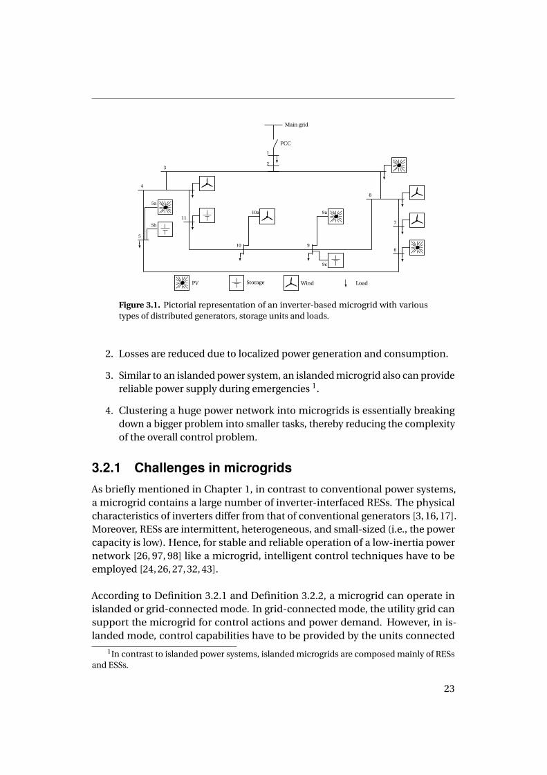
Figure 3.1. Pictorial representation of an inverter-based microgrid with varioustypes of distributed generators, storage units and loads.
2. Losses are reduced due to localized power generation and consumption.
3. Similar to an islanded power system, an islanded microgrid also can providereliable power supply during emergencies 1.
4. Clustering a huge power network into microgrids is essentially breakingdown a bigger problem into smaller tasks, thereby reducing the complexityof the overall control problem.
3.2.1 Challenges in microgridsAs briefly mentioned in Chapter 1, in contrast to conventional power systems,a microgrid contains a large number of inverter-interfaced RESs. The physicalcharacteristics of inverters differ from that of conventional generators [3, 16, 17].Moreover, RESs are intermittent, heterogeneous, and small-sized (i.e., the powercapacity is low). Hence, for stable and reliable operation of a low-inertia powernetwork [26, 97, 98] like a microgrid, intelligent control techniques have to beemployed [24, 26, 27, 32, 43].
According to Definition 3.2.1 and Definition 3.2.2, a microgrid can operate inislanded or grid-connected mode. In grid-connected mode, the utility grid cansupport the microgrid for control actions and power demand. However, in is-landed mode, control capabilities have to be provided by the units connected
1In contrast to islanded power systems, islanded microgrids are composed mainly of RESsand ESSs.
23
CHAPTER 3. PROBLEM STATEMENT
within the microgrid [23]. Another crucial challenge in islanded power networksis that the system stability is negatively affected in the presence of a noticeablechange in generation or load [99]. Therefore, this thesis focuses on control ofislanded inverter-based microgrids.
3.2.2 Major control tasks in microgridsAs outlined briefly in Chapter 1, some important control tasks in an islandedmicrogrid are listed below.
1. Frequency stability [22, 62],
2. Voltage stability [24, 27, 100],
3. Network frequency restoration [13, 32, 36, 37, 51],
4. Voltage regulation at load bus [34, 35],
5. Desired power sharing [22, 23, 27, 62],
6. Optimal dispatch of resources [26, 61].
3.2.3 Hierarchical control architectureInspired by the conventional power systems, a hierarchical control structure[39, 40, 60, 63] is advocated to tackle control problems in an islanded microgrid.This control structure has three layers, namely
1. Primary control [22, 38, 62]: A decentralized proportional (droop) control;maintain frequency stability; achieve desired power sharing at steady-state.
2. Secondary control [13, 32, 37]: Usually a distributed integral control; correctsteady-state deviations in network frequency.
3. Tertiary control or energy management [26, 61, 101]: Optimal dispatch ofgeneration, storage and loads.
24
3.2.4 Class of microgrids studied in this workMicrogrids studied in this thesis are assumed to have purely inverter-based units(both RESs and storage units) as the power sources and dominantly inductivepower lines (commonly known as lossless power lines.). Focusing on inverter-based microgrids can be justified due to the presence of a large number of dis-tributed inverter-interfaced RESs present in a microgrid [8, 10], see also [24, 27].
The assumption of lossless power lines is explained below. Power lines in micro-grids are relatively short because of closer electrical proximity between generatorsand loads. Furthermore, due to the lower power capacity of inverter-interfacedunits, they are interfaced with each other through MV or LV networks. The lineimpedances of these networks are not purely inductive but have a non-negligibleresistive part. Nevertheless, due to the presence of an output inductor and/orthe possible presence of an output transformer, inverter output impedance istypically inductive [24, 27, 76]. Thus, the inductive parts dominate the resistiveparts resulting in low resistance to inductive reactance (R/X) ratio.
In light of the above discussion, the class of microgrids considered in this thesis issolely inverter-based lossless islanded microgrids. Unless stated otherwise, suchnetworks are simply referred to as microgrids from here on.
3.2.5 Inverter-interfaced units in a microgridThe physical characteristics of inverters used in interfacing RESs to the AC gridwidely differ from that of conventional generators [3, 102]. In conventional powergrids, the task of network stabilization primarily depends on the rotational inertiaand the synchronizing dynamics of synchronous machines [3]. However, in aninverter-based microgrid, inverters connected in the network are responsible formaintaining a stable operating point [15, 17]. In the sequel, a brief introductionto inverter models and the two operating modes in which an inverter can beoperated are presented.
The output of RESs are mostly DC or variable frequency AC signals [103, 104].Hence to integrate RESs into an AC network that operates at a frequency of 50 or60 Hz, inverters are employed. The main components of an inverter are powersemiconductor devices [102, 105]. The quality of the output AC signal, e.g., interms of harmonic rejection, of an inverter-interfaced RES can be improved withthe help of an output low pass filter with RLC elements2.
2For further details about hardware design and inner control loops of an inverter, the readeris referred to [102, 105].
25
CHAPTER 3. PROBLEM STATEMENT
3.2.5.1 Common operating modes of an inverter
In general, there are two main operation modes for an inverter connected in amicrogrid [14–16, 106, 107]:
1. Grid-forming mode3: In this mode, an inverter works with pre-definedvoltage and frequency values, usually provided by the designer [15]. A grid-forming inverter can emulate a conventional generator’s behavior, thusenabling voltage and frequency control in a microgrid [38].
2. Grid-feeding mode4 : The inverter works as a power source, i.e., it suppliesa pre-specified amount of active and reactive power. A higher-level controllayer generally specifies the power injection set points of a grid-feedinginverter, see e.g. [61].
A grid-forming inverter can be represented as an ideal voltage source, and hencehas a low-output impedance [14]. Therefore, it needs an extremely precise syn-chronization mechanism to operate it in parallel with other grid-forming invert-ers [14, 108]. Later in this thesis, the problem of synchronizing grid-forminginverters in the presence of clock drifts [43, 58] is investigated in detail. In indus-trial applications, grid-forming inverters are fed by constant DC voltage sourceslike batteries or flywheels [14].
Inverters operating in grid-feeding mode are usually controllable current sourcesand thus have a high parallel output impedance. As a consequence, they aresuitable to operate in parallel with other grid-feeding inverters [14]. In practice,almost all inverter-interfaced RESs, such as PV or wind plants, are operated ingrid-feeding mode [14, 107]. However, in the absence of grid-forming inverters,grid-feeding inverters cannot operate in an islanded microgrid. This is becausegrid-forming inverters are responsible for setting voltage levels and frequency ina microgrid [14]. A thorough investigation in the direction of inverter modeling inmicrogrids can be found in [23, Section 4.2].
From the above discussion, it is clear that grid-forming inverters are essentialcomponents in islanded inverter-based microgrids. In other words, similar toa conventional power network with synchronous generators, grid-forming ca-pabilities in an inverter-based islanded microgrid are provided by grid-forminginverters [15, 19].
3Also referred as voltage source inverter (VSI) control [15].4This mode is also called as PQ control or grid-following mode [15, 19].
26
3.3 Control objectivesThis section formulates the control problems focused on in this thesis, startingwith the required definitions.
The following definitions are required throughout this thesis.
Definition 3.3.1 (Accurate proportional active power sharing [22, 26, 27]). LetXi ∈R>0 denote a constant weighting factor, P s
i the steady-state active power flow
and P di the desired active power set point at the i -th inverter, i ∈ N . Then, two
inverters, say inverter i and j , j ∈ N , j 6= i , are said to share their active powerflows accurately in proportion to Xi and X j if
Xi (P si −P d
i ) =X j (P sj −P d
j ). (3.3.1)
Definition 3.3.2 (Accurate proportional reactive power sharing [22, 26, 27]). Letai ∈R>0 denote a constant weighting factor, Q s
i the steady-state reactive power flow
and Qdi the desired reactive power set point at the i -th inverter, i ∈N . Then, two
inverters, say inverter i and j , j ∈N , j 6= i , are said to share their reactive powerflows accurately in proportion to ai and a j if
ai (Q si −Qd
i ) = a j (Q sj −Qd
j ). (3.3.2)
The parameters Xi and ai are usually specified by the designer. A commonchoice would be to select Xi = ai = 1/SN
i where SNi is the nominal power rating
(apparent power) of the i -th unit. Hence, achieving (3.3.1) and (3.3.2) ensure thatthe loads connected in the microgrid are shared among the generation units fairly,i.e., in proportion to their power ratings.
Definition 3.3.3 (Accurate network frequency restoration [13, 32, 37]). Let ω∗ ∈R>0 be the steady-state network frequency and ωd ∈ R>0 be the desired nominalfrequency in a microgrid. Then, accurate frequency restoration means that
ω∗ =ωd . (3.3.3)
Definition 3.3.4 (PCC voltage restoration [34, 35]). Let VPCC : R≥0 → R>0 be thevoltage amplitude at the PCC and V d
PCC ∈ R>0 be the desired nominal voltageamplitude required at the PCC. Then, the objective of PCC voltage restoration issatisfied if
VPCC(t ) →V dPCC as t →∞. (3.3.4)
27
CHAPTER 3. PROBLEM STATEMENT
3.3.1 Distributed secondary frequency controlThis section explains in detail the motivation to focus on the two control ob-jectives given by Definition 3.3.1 and Definition 3.3.3 in the presence of clockdrifts.
3.3.1.1 The effect of clock drifts
Clock drifts are a non-negligible parameter uncertainty observed in inverter-based microgrids [43, 58]. Apart from sensor uncertainties, the presence of clockdrifts are the main reason why grid-forming inverters fed with a fixed electricalfrequency cannot operate in parallel [14, 43, 58, 108]. In [43, Section III], this prob-lem is analytically investigated. The experimental output shown in [43, Figure4] verifies that when two grid-forming inverters operate in parallel with a fixedelectrical frequency, active power injections of the inverters diverge in the pres-ence of clock drifts. Such an undesired active power divergence can eventuallydamage the inverters. A possible solution to this issue is to provide a commonclock synchronization signal to all the grid-forming inverters [63]. Recall that amicrogrid can have a large number of grid-forming inverters connected in it. Thusproviding a clock signal to all these inverters would make the communicationsetup cumbersome.
3.3.1.2 Primary control layer: decentralized proportional control
In lossless microgrids, the standard frequency droop control yields a proportionalrelation between the active power flow and the frequency [38, Equation 13]. Ithas been shown in [43, 58] that the frequency droop control is robust towardsclock drifts. The authors of [43, 58] confirm, both analytically and experimentally,that the frequency droop control alleviates the risk of operating grid-forminginverters in parallel in the presence of clock drifts. The property of robust stabilityis mainly due to the port Hamiltonian structure [50, 109] of the dynamical systemcorresponding to a droop-controlled microgrid [22]. Due to this robustnessproperty, there is no need for providing a global clock synchronization signal toany of the inverters operating in a microgrid [43], thereby preserving one of themost important properties of frequency droop control, which is its decentralizednature. In light of the above discussion, the standard frequency droop control [38]is employed at the primary control layer throughout this thesis.
Despite the advantages mentioned above, in the presence of clock drifts, fre-quency droop control generate steady-state errors in active power injections,thereby disturbing the proportional active power sharing provided by the same[43, 58]. Furthermore, frequency droop control results in steady-state deviation in
28
the network frequency from the desired nominal value whenever there is a powerimbalance in the network [63]. Thus, the next section focuses on addressing theproblem of accurate proportional active power sharing and network frequencyrestoration in the presence of clock drifts.
3.3.1.3 Secondary control layer: distributed integral control
The proportional nature of the primary frequency droop control is the mainreason for steady-state frequency deviation [63]. This steady-state frequencyerror is corrected using a secondary controller, which typically is a simple centralintegral controller [15, 39], where a central computing unit provides a controlsignal to all the grid-forming inverters connected in the microgrid. Another ideawould be to design completely decentralized secondary frequency controllers,where at each grid-forming inverter the local frequency error5 is numericallyintegrated and is provided to all the grid-forming inverters to regulate the networkfrequency.
However, a decentralized integral secondary control usually results in poor activepower sharing and fails to achieve fast frequency regulation [26, Lemma 4.1].Like primary droop control, decentralized secondary frequency control is alsoimplemented at the grid-forming inverters connected in the network. Each grid-forming inverter corrects the local frequency error, which–due to the primarydroop control–alters the local power injection. Such a change in local powerinjection, together with the aspect of maintaining overall power balance in thenetwork, results in an enormous and unpredictable burden on the grid-forminginverters [26].
Based on the discussion thus far, distributed consensus-based integral controlapproaches are increasingly advocated to address secondary frequency controlin microgrids, see e.g. [32, 37, 40, 51]. Compared to centralized control solutions,distributed control approaches improve system reliability and reduce the com-munication effort [40]. Besides, compared to decentralized secondary control,distributed secondary controllers achieve frequency regulation and active powersharing in a collective and fair manner, i.e., without putting any generator underundesired high load stress, see e.g., [26, 51, 110]. Nevertheless, since distributedcontrol approaches require a communication network for their operation, thereare various challenging aspects to be considered while designing such controllers,e.g., communication delays [36], denial-of-service [67, 68], optimal communica-tion topology [64–66, 69].
5Local frequency error denotes the difference between the measured local frequency and thenominal desired frequency value of 50 or 60 Hz.
29
CHAPTER 3. PROBLEM STATEMENT
In addition to the above-mentioned issues, as mentioned in Section 1.3.2.1, thephenomenon of clock drifts is often neglected while designing distributed sec-ondary controllers, see e.g. [13, 32, 36, 51, 64]. However, clock drift has an adverseon the performance of secondary frequency control [44–48]. Therefore, the chap-ter on distributed secondary frequency control presented in this thesis evaluatesthe robustness and performance of distributed frequency controllers in the pres-ence of clock drifts. More precisely, the focus is to design distributed secondaryfrequency controllers in the presence of clock-drifts such that asymptotic stabil-ity [49, 50] of the closed-loop equilibrium point is guaranteed and, at the sametime, the following two steady-state objectives are realized:
1. Network frequency restoration as per Definition 3.3.3 and
2. Accurate active power sharing according to Definition 3.3.1.
PCC
4321
PV Storage Wind Load
Figure 3.2. Schematic representation of a parallel microgrid with four generatorbuses and a load bus (PCC).
3.3.2 Distributed voltage controlSimilar to primary frequency droop control, a primary voltage droop control isoften used in microgrids [38]. But, when it comes to lossless microgrids, theuse of voltage droop control is not preferred widely [27, 32, 111]. This is mainlybecause voltage droop control results in poor reactive power sharing in suchnetworks. Further details about the under-performance of voltage droop controlare mentioned briefly in Section 1.3.3 and is explained in detail later in this thesis.
As a result, distributed consensus-based voltage controllers to address the prob-lem of accurate reactive power sharing and voltage stability in lossless microgrids
30
are increasingly used [27, 30]. Inspired by the works in [27, 30], this section fo-cuses on a slightly different application of microgrids, where the generation unitsare connected in parallel [38]. With voltage stability and reactive power sharing,another important control objective in such a network is to restore the voltageamplitude at the common load bus (PCC) to the nominal value [34, 35].
As described in Section 1.3.3, a small electrical network where inverter-interfacedRESs and storage units are connected in parallel to a common load at the PCCis a typically encountered microgrid application [34, 35, 38, 77–83, 111], see Fig-ure 3.2. Recall that such networks are termed as parallel microgrids. The taskof controlling the network frequency and the voltage amplitudes in an inverter-based microgrid is the responsibility of grid-forming inverters, see Section 3.2.5.1.Hence, all the generator buses shown in Figure 3.2 are assumed to have at leastone storage unit interfaced via a grid-forming inverter connected to them.
The second part of this thesis is devoted to addressing some practically importantcontrol objectives in a parallel microgrid by actively controlling the grid-forminginverters. More precisely, the idea is to design a distributed voltage controllerfor a lossless islanded parallel microgrid, which at steady-state yields a uniquepositive voltage solution having the following desired properties:
1. PCC voltage restoration as per Definition 3.3.4,
2. Accurate reactive power sharing according to Definition 3.3.2 and
3. Asymptotic stability in accordance to Definition 2.2.1.
3.4 SummaryIn this chapter, the concept of microgrid has been introduced and the controlproblems addressed in this work have been formalized. After presenting the defi-nition of a microgrid, some interesting features of the same have been outlined.Later, some major control challenges in a microgrid and the commonly employedhierarchical control architecture have been described. The common operatingmodes of inverters connected in a microgrid have also been discussed. Finally,the control problems focused on in this thesis have been precisely formulated.
31

Chapter 4
Microgrid model and primarycontrol
4.1 IntroductionIn this chapter, the microgrid models are presented and the standard primarycontrol laws are discussed. Recall that in this thesis, the section on distributedsecondary frequency control focuses on meshed microgrids, and the section ondistributed voltage control looks into the control aspects in parallel microgrids.
Nevertheless, both cases are dedicated to microgrids with inverter-based genera-tion units, where grid-forming inverters are the main components responsiblefor controlling the network. Thus, the considered meshed and parallel microgridsdiffer only in terms of network and load models. Hence in this chapter, networkand load models corresponding to meshed and, respectively parallel microgridsare discussed. Later, the model of a grid-forming inverter is presented. Finally,the primary droop control is described.
4.2 Network and load model: meshedmicrogrid
The loads connected in the meshed microgrid model is assumed to be constantimpedance loads 1. Thus by using the Kron-reduction technique mentioned in
1 To the best of the author’s knowledge, there is no standard model to represent all types ofloads. For instance, constant power loads and dynamic loads [1, 5, 100]. Furthermore, the authorof this thesis is aware that not all kinds of loads can be represented as constant impedance loads.Hence, considering different kinds of load models while designing controllers for microgrids isleft out for future research, see e.g. [25, 110].
33
CHAPTER 4. MICROGRID MODEL AND PRIMARY CONTROL
Section 2.4.3, every bus in the network can be represented as a generator buswith a shunt admittance connected to it. Furthermore, the power lines of thenetwork are assumed to be lossless, i.e., inductive power lines. See Section 3.2.4for a discussion justifying this assumption. In the case of a lossless Kron-reducedmicrogrid, active and reactive power flows at the i -th node i ∈N , has been givenin (2.4.5).
4.3 Network and load model: parallel microgridIn this section, network and load models used to model a lossless parallel micro-grid are presented.
4.3.1 Network modelAs explained in Section 3.3.2, it is assumed that each generator bus in the consid-ered parallel microgrid has one storage unit interfaced via a grid-forming inverterconnected to it; see also Figure 3.2. Therefore, in the context of parallel microgrids,the term DG or the word inverter represents a grid-forming inverter. Thus, theconsidered parallel microgrid has n > 1 DGs, which are all connected in parallelto the PCC, see Figure 4.1. The set of DGs connected to the PCC is denoted byN = 1,2, . . . ,n. Since the parallel microgrid is also assumed to have inductivelines, a power line connecting the i -th generator bus and the load bus (PCC) isrepresented by a susceptance Bi ∈R<0.
Let δi : R≥0 → T and Vi : R≥0 → R>0 represent the phase angle and the voltagemagnitude at the i -th DGs, respectively. Furthermore, δPCC : R≥0 →T and VPCC :R≥0 →R>0, respectively, denote the phase angle and the voltage magnitude at thePCC. Then, based on (2.4.3), (2.4.4), the active and reactive power flows at thei -th DG are given respectively by
Pi (δi ,δPCC,Vi ,VPCC) = |Bi |Vi VPCC sin(δi −δPCC),
Qi (δi ,δPCC,Vi ,VPCC) = |Bi |V 2i −|Bi |Vi VPCC cos(δi −δPCC).
(4.3.1)
4.3.2 Load modelThe load connected at the PCC is assumed to be a constant current load2, repre-sented by IL ∈R<0, see Figure 4.1. This thesis follows the generator convention [89],i.e., the injected active and reactive powers are counted positively, while the ab-sorbed active and reactive powers are counted negatively. The load connected
2A study of a parallel microgrid with other types of loads, see e.g. [1, 5, 100], is planned as partof future research.
34
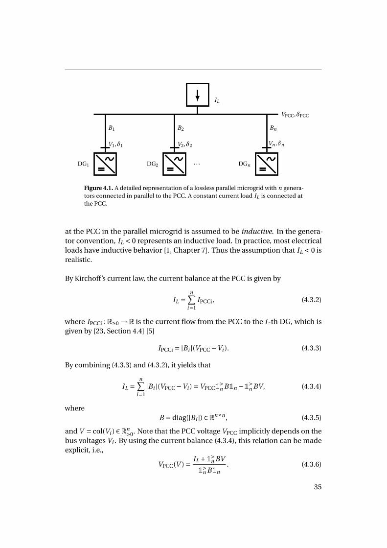
VPCC,δPCC
DGnDG2 . . .DG1
Vn ,δn
Bn
V2,δ2
B2
V1,δ1
B1
IL
Figure 4.1. A detailed representation of a lossless parallel microgrid with n genera-tors connected in parallel to the PCC. A constant current load IL is connected atthe PCC.
at the PCC in the parallel microgrid is assumed to be inductive. In the genera-tor convention, IL < 0 represents an inductive load. In practice, most electricalloads have inductive behavior [1, Chapter 7]. Thus the assumption that IL < 0 isrealistic.
By Kirchoff’s current law, the current balance at the PCC is given by
IL =n∑
i=1IPCCi, (4.3.2)
where IPCCi : R≥0 → R is the current flow from the PCC to the i -th DG, which isgiven by [23, Section 4.4] [5]
IPCCi = |Bi |(VPCC −Vi ). (4.3.3)
By combining (4.3.3) and (4.3.2), it yields that
IL =n∑
i=1|Bi |(VPCC −Vi ) =VPCC1>
n B1n −1>n BV , (4.3.4)
whereB = diag(|Bi |) ∈Rn×n , (4.3.5)
and V = col(Vi ) ∈Rn>0. Note that the PCC voltage VPCC implicitly depends on the
bus voltages Vi . By using the current balance (4.3.4), this relation can be madeexplicit, i.e.,
VPCC(V ) = IL +1>n BV
1>n B1n
. (4.3.6)
35
CHAPTER 4. MICROGRID MODEL AND PRIMARY CONTROL
4.4 Inverter modelThe standard model of a grid-forming inverter connected at the i -th node is givenby [15, 23]3
δi = uδi ,
Vi = uVi ,
(4.4.1)
where uδi : R≥0 → R and uV
i : R≥0 → R are frequency and voltage control inputsrespectively. The inverter model (4.4.1) is used throughout this thesis.
4.5 Primary droop controlIn this section, the standard practice of computing uδ
i and uVi in (4.4.1) are re-
called.
The control inputs uδi and uV
i in (4.4.1) are typically designed as the conventionalprimary droop control [38, 63], given by
uδi =ωd −kPi (P m
i −P di ), (4.5.1)
uVi =V d
i −kQi (Qmi −Qd
i ), (4.5.2)
where ωd ∈R>0 is the desired nominal frequency, V di ∈R>0 is the desired voltage
amplitude, kPi ∈R>0, respectively kQi ∈R>0 are the frequency, respectively volt-age droop coefficients and P d
i ∈ R and Qdi ∈ R are the desired power set points.
Furthermore, P mi : R≥0 →R and Qm
i : R≥0 →R are the active and reactive powersmeasured through a low pass filter with time constant τi ∈R>0. The dynamics ofthe low pass filter is given by [83, 92]
τi P mi =−P m
i +Pi ,
τi Qmi =−Qm
i +Qi ,(4.5.3)
where Pi and Qi are given by (2.4.5) for a meshed microgrid and by (4.3.1) in caseof a parallel microgrid.
Recalling (2.4.5) and (4.3.1), combining (4.4.1), (4.5.1), (4.5.2) and (4.5.3) gives theclosed-loop system corresponding to a primary droop-controlled inverter as
δi =ωd −kPi (P mi −P d
i ),
τi P mi =−P m
i +Pi ,
Vi =V di −kQi (Qm
i −Qdi ),
τi Qmi =−Qm
i +Qi .
(4.5.4)
3An underlying assumption to the model (4.4.1) is that whenever an inverter connects to aRES, it is equipped with a storage unit.
36
A tuning criterion guaranteeing asymptotic stability of the equilibrium point of(4.5.4) has been presented in [22]. However, it is important to note that in contrastto the frequency droop control (4.5.1), the voltage droop control (4.5.2) has tobe tuned in a heuristic fashion [22, 24, 27, 112]. Moreover, it has been shownin the literature, see e.g. [32], that the decentralized nature of (4.5.2) results inpoor reactive power sharing. Consequently, the rest of this thesis assume thatthe phase angles of the grid-forming inverters are controlled using the frequencydroop control (4.5.1).
For presenting the contributions coming under the section distributed secondaryfrequency control, in the sequel, the model of a primary droop-controlled inverter(4.5.4) in the presence of clock drifts is presented. In addition, the steady-stateperformance regarding
• frequency droop control (under explicit consideration of clock drifts) and
• voltage droop control
are also discussed later in this chapter.
4.5.1 Primary droop control with inaccurate clockIn practice, (4.5.4) is implemented on a digital processor employing numericalintegration. In such a setup, the phase angle δi is obtained after numericallyintegrating δi . The time signal generated by the local clock of each grid-forminginverter is used to determine the sampling interval used in the numerical integra-tion employed to calculate δi .
It is a well-known fact that the clocks used to generate these local time signals arenot synchronized [41, 42], hence resulting in clock inaccuracies or simply clockdrifts amongst the inverters. An immediate effect of clock drifts is that the sam-pling interval of the numerical integration differs between inverters. The impactof the difference in sampling intervals on the dynamics (4.5.4) is investigatednext.
In the following, an equivalent model of (4.5.4) considering clock inaccuracies ispresented. The local time signal ti ∈R of the i -th inverter expressed in terms ofthe global time signal t ∈R is given by [43, 58, 113–115]
ti =(
1
1+µi
)t +ζi , (4.5.5)
37
CHAPTER 4. MICROGRID MODEL AND PRIMARY CONTROL
where µi ∈R is the relative drift of the clock at the i -th inverter and ζi ∈R is thelocal clock offset. From (4.5.5),
d(·)d ti
= (1+µi )d(·)d t
. (4.5.6)
Suppose that the numerical integration in (4.5.4) is expressed in terms of the localtime signal ti . Inserting (4.5.6) in (4.5.4) gives
(1+µi )dδi
d t=ωd −kPi (P m
i −P di ),
(1+µi )τidP m
i
d t=−P m
i +Pi ,
Vi =V di −kQi (Qm
i −Qdi ),
(1+µi )τidQm
i
d t=−Qm
i +Qi ,
(4.5.7)
where now, the time derivatives are expressed with respect to the global timet . Without loss of generality, the offset value ζi can be included in the initialconditions of the system (4.5.7).
Following [43, 58], to investigate the effect of clock drifts, it is convenient tointroduce the internal frequency ωi : R≥0 → R of the inverter at the i -th nodewhich is related to the actual electrical frequency ωi = δi by
ωi = (1+µi )δi = (1+µi )ωi , ∀i ∈N . (4.5.8)
In the literature, the effect of clock drifts is often neglected, i.e., µi = 0 and assumethat ωi =ωi , see e.g., [13,32,36,51,64]. However, it has been shown in [43,58] thatclock drifts disturb synchronization and power sharing in microgrids, dependingupon the clock drift value µi at each inverter. This problem is explained in thesequel.
4.5.1.1 Steady-state performance
In practice, µi 6= µ j where i , j ∈N , j 6= i , i.e., the clock drifts values of differentinverters are different. Furthermore, clock drift values observed in commercialinverters can vary from 10−6 [42, 43] to 10−3 [71, Table I] depending on the qualityof the micro-controller used. Considering this fact, the system (4.5.7) at steady-state yields
(1+µi )ωsi = ωs
i =ωd −kPi (P si −P d
i ),
V si =V d
i −kQi (Q si −Qd
i ),(4.5.9)
38
where the superscript s denotes the steady-state value and ωi is given by (4.5.8).Note that
ωsi =ωs
j =ω∗,
where ωsi ∈R>0 and ωs
j ∈R>0 are the electrical frequencies at inverters i ∈N andj ∈ N at steady-state respectively and ω∗ ∈ R>0 is the synchronized electricalfrequency. Thus, the steady-state equations (4.5.9) become
ωsi = (1+µi )ωs
i = (1+µi )ω∗ =ωd −kPi (P si −P d
i ),
V si =V d
i −kQi (Q si −Qd
i ).(4.5.10)
It is a common practice to select the frequency droop gain as kPi = 1/SNi where
SNi ∈R>0 is the power rating of the i -th inverter, see [62, Theorem 7], [22, Lemma
6.2]. Hence, (4.5.10) can be expressed as
ωd − (1+µi )ω∗ =P s
i −P di
SNi
,
V si =V d
i −kQi (Q si −Qd
i ).
(4.5.11)
Recall that µi 6=µ j , j ∈N , j 6= i . Thus from (4.5.11),
P si −P d
i
SNi
6=P s
j −P dj
SNj
,
which as per Definition 3.3.1, disturbs steady-state active power sharing.
Next, looking at the steady-state equation corresponding to voltage droop controlin (4.5.11), i.e.,
V di −V s
i = kQi (Q si −Qd
i ), (4.5.12)
where it can be seen that the effect of clock drifts is negligible. Again, to under-stand the aspect of reactive power sharing, let the voltage droop gain in (4.5.12)be selected as kQi = 1/SN
i , which gives
V di −V s
i =Q s
i −Qdi
SNi
. (4.5.13)
In contrast to the concept of synchronized electrical frequency, typically thevoltage amplitudes at steady-state are different for different buses. Hence, V s
i 6=V s
j , j ∈N , j 6= i . Thus, it yields from (4.5.13) that
Q si −Qd
i
SNi
6=Q s
j −Qdj
SNj
,
which denotes poor reactive power sharing according to Definition 3.3.2, seealso [22, Remark 6.6], [32, Section III].
39
CHAPTER 4. MICROGRID MODEL AND PRIMARY CONTROL
4.6 SummaryIn this chapter, the microgrid model and the commonly used primary droopcontrol law [38] have been introduced. At first, network and load models ofmeshed and parallel microgrids considered in this thesis have been presented.Furthermore, since this thesis focuses upon inverter-based microgrids, the modelof a grid-forming inverter has been presented.
After introducing the concept of clock drifts, the model of a droop-controlledinverter in the presence of clock drifts has been derived. Additionally, the steady-state performance of frequency droop control with explicit consideration of clockdrifts has been investigated. The effect of clock drifts on voltage droop control wasfound to be negligible. Nevertheless, voltage droop control renders poor steady-state reactive power sharing. The above observation has also been explained inthis chapter.
40
Chapter 5
Distributed secondary frequencycontrol
5.1 IntroductionIn the previous chapter, the model of an inverter-based meshed microgrid hasbeen presented. Later, based on [43, 58], the model of a droop-controlled inverterunder explicit consideration of clock drifts has been derived. As shown in Chap-ter 4, clock drift disturb steady-state active power sharing provided by frequencydroop control. In this context, the contributions of this chapter can be organizedas sections:
1. Steady-state performance of distributed secondary frequency control Theidea behind this section is to compare the steady-state performance ofdistributed secondary frequency controllers, e.g. [13, 32, 36, 51, 64] in thepresence of clock drifts. The performance is compared in terms of steady-state network frequency restoration (Definition 3.3.3) and active powersharing (Definition 3.3.1). For this purpose, the model of a frequencydroop-controlled microgrid in the presence of clock drifts is recalled fromChapter 4. Then, a general distributed frequency control representation isproposed, which can be parametrized into the control approaches pre-sented in [13,32,36,51,64], and many more. Based on the proposed generaldistributed controller representation, necessary and sufficient conditionsfor accurate steady-state network frequency restoration (Definition 3.3.3)and active power sharing (Definition 3.3.1) are derived. The approachespresented in [13, 32, 36, 51, 64] were found to be not satisfying these condi-tions. Thus, a particular parameterization of the above-mentioned general
41
CHAPTER 5. DISTRIBUTED SECONDARY FREQUENCY CONTROL
distributed controller representation is proposed, which satisfies the con-ditions required for achieving the control objectives focused on in thischapter. This controller parametrization is termed as the GDAI (generalizeddistributed averaging integral) control.
2. Stability analysis and tuning criterion In this section, a tuning criterionthat guarantees local asymptotic stability of the closed-loop equilibriumpoint in the presence of uncertain clock drift values is derived. The pre-sented tuning criterion can be cast as a set of LMIs which can be easilysolved to find the stabilizing parameters of the GDAI controller.
The results presented in this chapter are based on the author’s publications[116–118].
5.2 Primary frequency (droop) control: Effectof clock drifts
As mentioned in Chapter 3, the proportional nature of primary frequency droopcontrol results in steady-state network frequency deviation from the nominalvalue. In the presence of clock drifts, proportional active power sharing providedby the frequency droop control is also disturbed, see Section 4.5.1. However, theeffect of clock drifts on voltage control is negligible. Hence, this chapter focuseson designing distributed secondary frequency controllers such that the networkfrequency is restored to a desired nominal value and active power sharing is main-tained at steady-state in the presence of clock drifts. The task of voltage controlis neglected in this chapter and is addressed in the next chapter for a differentmicrogrid application. For mathematical simplicity, the voltage amplitudes areassumed to be constant, see e.g. [36, 62]. For an analysis considering varyingvoltage amplitudes, the reader is referred to [22, 30].
Based on (4.5.7), the model of a primary-frequency droop-controlled unit in thepresence of clock drifts is given as
(1+µi )δi = ωi =ωd −kPi (P mi −P d
i ),
(1+µi )τi P mi =−P m
i +Pi ,(5.2.1)
where Pi is given by (2.4.5) which–under the standing assumption that voltageamplitudes are constant–can be expressed as
Pi (δ) =Gi i V 2i + Pi , (5.2.2)
42
where δ := col(δ1, . . . ,δn) ∈Tn and
Pi (δ) =∑
k∈Ni|Bi k |Vi Vk sin(δi −δk ). (5.2.3)
Furthermore, it is convenient to rewrite the dynamics (5.2.1) as follows. Differen-tiating the first equation in (5.2.1) with respect to time yields
(1+µi )δi = ˙ωi =−kPi P mi =−kPi
1
(1+µi )τi
(−P mi + Pi (δ)+Gi i V 2
i
), (5.2.4)
where to write the latter equality, the second equation in (5.2.1) has been used.Next, from the first equation in (5.2.1), the measured power P m
i can be expressedas
P mi = 1
kPi
(−ωi +ωd
)+P d
i . (5.2.5)
Substituting (5.2.5) in (5.2.4) and multiplying the result with 1/kPi yields
(1+µi )Mi ˙ωi =−Di (ωi −ωd )−(Pi (δ)+Gi i V 2
i −P di
), (5.2.6)
where Mi = τi /kPi ∈R>0 is the virtual inertia coefficient and Di = 1/kPi ∈R>0 isthe damping coefficient.
Combining (5.2.6) with (4.5.8) yields
(1+µi )δi = ωi ,
(1+µi )Mi ˙ωi =−Di (ωi −ωd )−(Pi (δ)+Gi i V 2
i −P di
),
(5.2.7)
which is an equivalent representation of (5.2.1). See also [119].
To derive a compact model representation of the microgrid, it is convenient tointroduce the matrices
M = diag(Mi ) ∈Rn×n , D = diag(Di ) ∈Rn×n , µ= diag(µi ) ∈Rn×n , (5.2.8)
and the vectors
ω= col(ωi ) ∈Rn , ω= col(ωi ) ∈Rn , P net = col(P di −Gi i V 2
i ) ∈Rn . (5.2.9)
Inspired by [36, 110], a potential function U : Rn →R is defined in the following:
U (δ) =−∑
i ,k∈[N ]2 |Bi k |Vi Vk cos(δi −δk ). (5.2.10)
43
CHAPTER 5. DISTRIBUTED SECONDARY FREQUENCY CONTROL
Let P (δ) = col(Pi (δ)) ∈ Rn where Pi is defined in (5.2.3). With U (δ) given by(5.2.10), note that
∇δU (δ) = P (δ).
Then, the dynamics (5.2.7) for the whole microgrid can be expressed as
(In +µ)δ= ω,
(In +µ)M ˙ω=−D(ω−1nωd )− (∇δU (δ)−P net) ,
(5.2.11)
where the matrices and the vectors used in (5.2.11) are defined in (5.2.8) and(5.2.9), respectively.
Observe that due to the skew symmetry of the power flows,
1>n P (δ) = 1>
n∇δU (δ) = 0. (5.2.12)
Next, for better clarity of the results presented in this chapter, the notion of activepower sharing given in Definition 3.3.1 is expressed for the whole network as
X(∇δU (δs)−P net)=α1n , (5.2.13)
where α ∈R, X = diag(Xi ) ∈Rn×n is a weighting matrix with Xi ∈R>0, ∇δU (δs) =∇δU (δ)|δ=δs = col(Pi (δs)) where Pi is given by (5.2.3) and P net is defined in (5.2.9).
For the purpose of attaining steady-state active power sharing using frequencydroop control, it has been shown in [62, Theorem 7], [22, Lemma 6.2] that theentries of the damping matrix D in (5.2.11) shall be chosen according to
X D = κIn , (5.2.14)
where κ ∈ R>0. Recall that D is the inverse droop coefficient matrix. Therefore,if Xi is chosen as Xi = 1/SN
i , then the condition (5.2.14) can be understood asan inversely proportional choice of droop coefficients1 in correspondence to thepower ratings2.
5.3 Secondary frequency control: Effect ofclock drifts
Like any power network, a microgrid is also designed to work very close to thenominal frequency value of 50 or 60 Hz [1, 3]. However, the proportional nature
1The condition (5.2.14) for two inverters has been briefly recalled in Section 4.5.1.2Recall that SN
i is the power rating of the i -th unit.
44
of primary droop control results in steady-state frequency deviation. Therefore,following the standard practice [26, 36, 51], a secondary control input u = col(ui ) :R≥0 →Rn is introduced to the model (5.2.11) with the aim of correcting the steady-state frequency deviation. Thus, (5.2.11) becomes
(In +µ)δ= ω,
(In +µ)M ˙ω=−D(ω−1nωd )− (∇δU (δ)−P net)+u.
(5.3.1)
Along any synchronized motion (i.e., a motion with constant electrical frequenciesωs = ω∗1n for ω∗ ∈ R>0, constant phase angle differences δs
i −δsk and constant
secondary control input us) of the system (5.3.1), it yields
1>n M(In +µ) ˙ω= 0 =−1>
n D(ωs −1nωd )
−1>n
(∇δU (δs)−P net)+1>n us .
(5.3.2)
Note that in the presence of clock drifts, internal frequencies of inverters are notuniform, i.e., from (4.5.8), ωs =ω∗1n implies that
ωs = (In +µ)ωs =ω∗(In +µ)1n . (5.3.3)
Moreover with (5.2.12) and by inserting (5.3.3) into (5.3.2), the scalar ω∗ can beobtained from (5.3.2) as
ω∗ =ωd 1>n D1n
1>n D(In +µ)1n
+ 1>n (P net +us)
1>n D(In +µ)1n
. (5.3.4)
From (5.3.4), it is obvious that ω∗ =ωd if and only if us satisfies
1>n (P net +us) =ωd1>
n Dµ1n . (5.3.5)
In the case of ideal clocks, i.e., if µ= 0n×n , from (5.3.4), it is clear that ω∗ =ωd ifand only if 1>
n (P net +us) = 0. Similar results assuming ideal inverter clocks havebeen presented in [36, 51]. However from (5.3.4), in the presence of clock drifts(i.e., µi 6= 0), satisfying 1>
n (P net +us) = 0 does not guarantee ω∗ =ωd .
5.3.1 General distributed control representationIn this section, a control law for the input is designed. The following generaldistributed control representation is proposed:
u = p,
(In +µ)p =−(B+βX DL )(ω−1nωd )−DX L X p, (5.3.6)
45
CHAPTER 5. DISTRIBUTED SECONDARY FREQUENCY CONTROL
where p : R≥0 → Rn is a new variable. Furthermore, B ∈ Rn×n and D ∈ Rn×n arediagonal controller matrices, β ∈ R is a controller parameter, L ∈ Rn×n is theLaplacian matrix of a connected and undirected graph representing the commu-nication network. Finally, X is the design parameter defined in (5.2.13). Thematrix B is commonly called the pinning gain matrix, see e.g. [13].
It is customary to use the internal frequency ω of the inverters to implement adistributed control law like (5.3.6), since it obviates the requirement for extrafrequency measurement. This is mainly because new measurement devices canpotentially increase the complexity and can bring in further measurement errorsinto the system, see e.g. [13, 32,36,51,110]. Therefore, it is essential to note that inthe control law (5.3.6), the internal frequency ω is used. However, in the worksmentioned above, the effect of clock drifts is not considered, and thus, the authorsassume that the internal frequency and the electrical frequency are the same, i.e.,ω=ω. Yet, when explicitly considering clock drifts, from (4.5.8), it is important tonote that ω= (In +µ)ω.
The control law (5.3.6) represents a generalized version of various distributedsecondary frequency controllers and can be parametrized into
1. the DAI control presented/studied in [32, 36, 51, 110] if the control parame-ters in (5.3.6) are chosen such that
B > 0,β= 0,D > 0 and (5.3.7)
2. the pinning control law proposed in [13] if the control parameters in (5.3.6)are chosen such that
B ≥ 0,B≯ 0,β= 0,D > 0. (5.3.8)
Applying the parametrization (5.3.7) in the general controller representation(5.3.6), results in the DAI controller [32, 36, 51, 110] given by
u = p,
(In +µ)p =−B(ω−1nωd )−DX L X p
B > 0.
(5.3.9)
Similarly, applying the parametrization (5.3.8) (5.3.6) gives the pinning controller[13]
u = p,
(In +µ)p =−B(ω−1nωd )−DX L X p
B ≥ 0,B≯ 0.
(5.3.10)
46
The correspondence of (5.3.10) with the control law presented in [13] is detailedin the following remark.
Remark 5.3.1. The primary frequency droop control [13, Equation 47] for thewhole microgrid expressed in the notation followed in this thesis is given by
ω=−D−1 (∇U (δ)−P net)+usec, (5.3.11)
where usec : R≥0 →Rn is the secondary control input. Note that (5.3.11) is equiva-lent to (5.3.1) if
• µ= 0n×n (yielding ω=ω, see (4.5.8)),
• τi = 0 ⇒ M = diag(τi /kPi ) = 0n×n ,
• ωd = 0 and
• usec = D−1u.
Furthermore, the secondary frequency control law proposed in [13, Equations52,53] for the whole network can be expressed as
u = p,
p =−CF
[(B+L )(ω−1nω
d )+L D−1 (∇U (δ)−P net)] ,
where CF > 0 and B ≥ 0 are diagonal controller matrices and L ∈ Rn×n is theLaplacian matrix of the communication graph. Inserting D−1
(∇U (δ)−P net)
from(5.3.11) in the above control law yields
p =−CF B(ω−1nωd )−CF L usec,
=−CF B(ω−1nωd )−CF L D−1p,
=−CF B(ω−1nωd )− 1
κCF L X p,
where usec = D−1u = D−1p and D−1 = 1κX , see (5.2.14). Considering non-zero
clock drift values as well as for CF = κDX > 0 and CF B = B ≥ 0, the control lawdescribed above is the same as (5.3.10).
In the remainder of this thesis, DAI and pinning control represent (5.3.9) and(5.3.10), respectively.
For the subsequent analysis, it is convenient to introduce the notion below.
47
CHAPTER 5. DISTRIBUTED SECONDARY FREQUENCY CONTROL
Definition 5.3.2 (Synchronized motion). The closed-loop system (5.3.1), (5.3.6)admits a synchronized motion if it has a solution for all t ≥ 0 of the form
δs(t ) = δs0 +ωs t , ωs =ω∗1n , p s ∈Rn ,
where ω∗ ∈R>0 is the synchronized electrical frequency and δs0 ∈Rn such that
|δs0,i −δs
0,k | <π
2∀i ∈N , ∀k ∈Ni .
With constant phase angle differences δsi (t)−δs
j (t) for all t ≥ 0, i , j ∈ N in thesystem (5.3.1), (5.3.6) imply that the frequencies of all the units have converged toa common value, i.e., δs
i = δsi =ω∗, ω∗ ∈R>0, thus the terminology synchronized
motion, see e.g., [110, Lemma 4.2] for further details about synchronized motionsin power system models similar to (5.3.1), (5.3.6).
Next, the standard assumption of power flow feasibility is recalled.
Assumption 5.3.3. The closed-loop system (5.3.1), (5.3.6) possesses a synchronizedmotion.
In practice, clock drift values observed in commercial inverters can vary from10−6 [42, 43] to 10−3 [71, Table I] depending on the quality of the micro-controllerused. Therefore as outlined in [43, 58], for secondary frequency control, it isreasonable to assume that the clock drifts are bounded. This is formalized in theassumption below.
Assumption 5.3.4. ‖µ‖2 ≤ ε, 0 ≤ ε< 1.
5.4 Problem statementIn light of the discussion thus far, this chapter focuses on the following problem.
Problem 5.4.1 (Secondary control objectives). Consider the closed-loop system(5.3.1), (5.3.6) with Assumption 5.3.4 and Assumption 5.3.3. Design the parametersB, β, D and the edge-weights of L in (5.3.1), (5.3.6) such that the following controlobjectives are satisfied:
1. Accurate frequency restoration as per Definition 3.3.3.
2. Accurate active power sharing according to Definition 3.3.1.
3. Asymptotic convergence of the solutions of (5.3.1), (5.3.6) to the synchronizedmotion given in Definition 5.3.2.
48
5.5 Steady-state performanceIn this section, the first two points in Problem 5.4.1 are addressed. At first, a neces-sary and sufficient condition for accomplishing the first objective in Problem 5.4.1is presented.
Lemma 5.5.1 (Accurate frequency restoration). Consider the closed-loop system(5.3.1), (5.3.6) with Assumption 5.3.3. Let D > 0. Suppose that the diagonal matrixB has at least one positive entry. Then, the synchronized electrical frequency ω∗ ofthe system (5.3.1), (5.3.6) is given by
ω∗ = 1>n D−1X −1B1n
1>n D−1X −1B(In +µ)1n
ωd . (5.5.1)
Furthermore, accurate network frequency restoration, i.e., (3.3.3), is achieved ifand only if
1>n D−1X −1Bµ1n = 0. (5.5.2)
Proof. Along any synchronized motion, the electrical frequencies at all nodes of(5.3.1), (5.3.6) have to be identical, i.e.,
δs =ωs = 1nω∗, (5.5.3)
which yields (5.3.3). Furthermore, at steady-state, p s = 0n . Hence, (5.3.6) be-comes
−(In +µ)p s = 0n = (B+βX DL )(ωs −1nωd )+DX L X p s . (5.5.4)
Multiplying (5.5.4) from the left with 1>n D−1X −1 and recalling the fact that 1>
n L =0>
n , yields0 = 1>
n D−1X −1B(ωs −1nωd ).
Using (5.3.3) in the above equation leads to
0 = 1>n D−1X −1B
((In +µ)1nω
∗−1nωd)
. (5.5.5)
Under the standing assumption that at least one entry of the diagonal matrix B ispositive, ω∗ can be solved from (5.5.5) resulting in (5.5.1).
Note that from (5.5.1), ω∗ =ωd if and only if
1>n D−1X −1B(In +µ)1n = 1>
n D−1X −1B1n ,
which is equivalent to (5.5.2), completing the proof.
49
CHAPTER 5. DISTRIBUTED SECONDARY FREQUENCY CONTROL
In the following lemma, a necessary and sufficient condition for fulfilling thesecond objective in Problem 5.4.1 is derived.
Lemma 5.5.2 (Active power sharing). Consider the closed-loop system (5.3.1),(5.3.6) with Assumption 5.3.3. Let D > 0. Suppose that the diagonal matrix B has atleast one positive entry and D is chosen as per (5.2.14). Then, active power sharingaccording to Definition 3.3.1 along the synchronized motion is achieved if and onlyif B, β, D and L are chosen such that[
D−1X −1B+ (β+κ)L]F1nω
d = 0n , (5.5.6)
where
F = 1>n D−1X −1B1n
1>n D−1X −1B(In +µ)1n
(In +µ)− In . (5.5.7)
Proof. Along a synchronized motion, the primary control dynamics (5.3.1) withus = p s (see (5.3.6)) becomes
0n =−D(ωs −1nωd )− (∇δU (δs)−P net)+p s , (5.5.8)
which can be rearranged as
p s = D(ωs −1nωd )+ (∇δU (δs)−P net) . (5.5.9)
Next, consider (5.3.6) at steady-state given by
0n = (B+βX DL )(ωs −1nωd )+DX L X p s . (5.5.10)
Inserting p s obtained from (5.5.9) in (5.5.10) results in
0n = (B+βX DL
)(ωs −1nω
d )+DX L X D(ωs −1nωd )
+DX L X(∇δU (δs)−P net) .
Under the standing assumption that (5.2.14) is satisfied, the above equationbecomes
0n = (B+βX DL +κDX L
)(ωs −1nω
d )+DX L X(∇δU (δs)−P net) ,
which, when left-multiplied with D−1X −1 > 0, yields
0n = (D−1X −1B+βL +κL
)(ωs −1nω
d )+L X(∇δU (δs)−P net) . (5.5.11)
Recall that L is the Laplacian matrix of a connected undirected graph. Hence,
L X(∇δU (δs)−P net)= 0n
50
if and only if (5.2.13) is satisfied, i.e., active power sharing. From (5.5.11),
L X(∇δU (δs)−P net)= 0n
if and only if (D−1X −1B+ (β+κ)L
)(ωs −1nω
d ) = 0n . (5.5.12)
Finally, with (5.3.3) and ω∗ given by (5.5.1), the condition (5.5.12) holds if andonly if (5.5.6) is satisfied. This completes the proof.
5.5.1 DAI and pinning controlIn this section, the steady-state behavior of the DAI control and the pinningcontrol are evaluated based on Lemma 5.5.1 and Lemma 5.5.2.
1. DAI control: Consider Lemma 5.5.1 and the DAI-parametrization (5.3.7).With (5.3.7), the condition (5.5.2) is not satisfied. Hence, the objective ofnetwork frequency restoration is not satisfied, i.e., ω∗ 6=ωd . Next, considerLemma 5.5.2. It can be directly verified that (5.3.7) does not satisfy (5.5.6)and thus steady-state active power sharing is also not achieved.
2. Pinning control: Consider Lemma 5.5.1. It can be seen that the pinning-parametrization (5.3.8) satisfies (5.5.2) if the structure of the pinning gainmatrix B ≥ 0 is chosen such that Bµ= 0n×n , resulting in ω∗ =ωd . However,(5.3.8) does not satisfy the conditions of Lemma 5.5.2. Thus in the pres-ence of clock drifts, active power sharing is not achieved using the pinningcontrol.
5.6 GDAI controlIn light of the discussion thus far, a parametrization of (5.3.6) which satisfy bothLemma 5.5.1 and Lemma 5.5.2 is yet to be presented. Since the coefficients µi
are unknown and different for different units, Lemma 5.5.2 reveals that unlikein the case of ideal clocks [13, 32, 36, 64], when taking clock drifts explicitly intoaccount, it is hard to determine B, β and D directly from the conditions presentedin Lemmata 5.5.1 and 5.5.2. Therefore, instead below, a sufficient condition forthe control parameters B, β and D satisfying Lemmata 5.5.1 and 5.5.2 is presented.
Lemma 5.6.1 (Accurate frequency restoration and active power sharing). Con-sider the closed-loop system (5.3.1), (5.3.6) with Assumption 5.3.3. Let D > 0. Sup-pose that the diagonal matrix B has at least one positive entry and D is chosen as
51
CHAPTER 5. DISTRIBUTED SECONDARY FREQUENCY CONTROL
per (5.2.14). Then, the first two objectives in Problem 5.4.1 along a synchronizedmotion are achieved if the control parameters B and β are chosen such that
Bµ= 0n×n and β=−κ. (5.6.1)
Proof. Consider Lemma 5.5.1. For Bµ = 0n×n , (5.5.2) holds. Thus, accuratenetwork frequency restoration is assured, i.e., ω∗ =ωd .
Next, consider Lemma 5.5.2. With Bµ= 0n×n , (5.5.6) becomes[(β+κ)L
]µ1nω
d = 0n ,
which holds when β=−κ. Hence, Lemma 5.5.2 is satisfied, yielding proportionalactive power sharing, completing the proof.
Applying the parameters (5.6.1) to the general distributed controller representa-tion (5.3.6) yields
u = p,
(In +µ)p = (−B+κX DL )(ω−1nωd )−DX L X p,
Bµ= 0n×n , B ≥ 0.
(5.6.2)
The condition Bµ= 0n×n can be interpreted as follows. Define the clock of one ofthe inverters in the network as master clock, say the k-th inverter, k ≥ 1. Then,µk = 0 and the drifts µi , i 6= k, of all other clocks in the microgrid are expressedwith respect to the master clock of the k-th inverter. Furthermore, the diagonalpinning gain matrix B ≥ 0 will have a non-zero positive entry only at the (k,k)-thposition, resulting in Bµ= 0n×n .
The control law (5.6.2) is termed as generalized distributed averaging integral(GDAI) control in the remainder of this thesis.
5.7 Robust GDAI control designThe GDAI controller (5.6.2) has been identified as a solution to address the firsttwo objectives mentioned in Problem 5.4.1. In this section, the third point inProblem 5.4.1 is addressed. More precisely, a sufficient tuning criterion withwhich the solutions of the system (5.3.1), (5.6.2) asymptotically converge to thesynchronized motion given in Definition 5.3.2 is presented. Here, the terminologyrobust denotes that the presented tuning criterion considers that the clock driftmatrix µ has uncertain entries.
52
5.7.1 Closed-loop systemCombining (5.3.1) and (5.6.2) yields the closed-loop system
(In +µ)δ= ω,
(In +µ)M ˙ω=−D(ω−1nωd )− (∇δU (δ)−P net)+p,
(In +µ)p = (−B+κX DL )(ω−1nωd )−DX L X p.
(5.7.1)
5.7.1.1 Coordinate reduction and error states
As the power flow ∇δU (δ) = col(Pi (δ)) only depends on angle differences (see(5.2.3)), following [22] and choosing an arbitrary node, say node n, all angles canbe expressed relative to that node, i.e.,
θ =R>δ, θ : R≥0 →Tn−1, R =[
In−1
−1>n−1
]∈Rn×(n−1).
Note that the matrix R has the property
1>n R = 0>
n−1.
With Assumption 5.3.3 for the system (5.7.1), the following error states are defined.
ω := ω− ωs = ω− (In +µ)1nωd ,
θ := θ−θs , p := p −p s , x := col(θ, ω, p
),
where θs = R>δs with δs and p s given in Definition 5.3.2. Furthermore, (5.3.3)and (3.3.3) were used to express ωs .
Thus, the resulting error dynamics of the system (5.7.1) is given by
˙θ =R>(In +µ)−1ω,
(In +µ)M ˙ω=−Dω−R[∇θU (δ(θ+θs))−∇θU (δ(θs))
]+ p,
(In +µ) ˙p = (−B+κX DL )ω−DX L X p,
(5.7.2)
where
∇θU (δ(θ+θs)) = ∂U (δ(θ+θs))
∂θ,
∇θU (δ(θs)) = ∂U (δ(θ+θs))
∂θ
∣∣θ=0n−1
.
Note that x∗ = 03n−1 is an equilibrium point of (5.7.2). Furthermore, asymptoticstability of x∗ = 03n−1 implies asymptotic convergence of the solutions of the sys-tem (5.7.1) to the synchronized motion given in Definition 5.3.2 up to a uniformshift of all angles [22].
53
CHAPTER 5. DISTRIBUTED SECONDARY FREQUENCY CONTROL
5.7.2 Stability criterionFor presenting the main result of this section, it is convenient to define the follow-ing. Since µ is a diagonal matrix, with Assumption 5.3.4,
‖µ(In +µ)−1‖2 ≤ g1(ε), g1(ε) = ε1−ε
> 0,
‖(µ2 +2µ)(In +µ)−2‖2 ≤ g2(ε), g2(ε) = ε2+2ε(1−ε)2 > 0.
(5.7.3)
Some matrices useful for presenting the stability result are defined in the following.
T :=[
T1112
(−ςIn −σD1n1>n D−1X −1 + B−κL X
)∗ T22
],
T2 :=[σM1n1>
n BX −1 σD−1X −11n1>n D
0n×n −σD−1X −11n1>n
],
Hµ :=[ςg2(ε)M 0n×n
0n×n g1(ε)D−1
],
(5.7.4)
where g1(ε) and g2(ε) are defined in (5.7.3). Furthermore, σ ∈R>0, B = D−1B ≥ 0and
T11 = ςD − σ
2
(M1n1>
n BX −1 +X −1B1n1>n M
),
T22 =X L X + σ
2
(D−1X −11n1>
n +1n1>n X −1D−1) .
The stability result is as follows.
Proposition 5.7.1. Consider the system (5.7.2) with Assumption 5.3.3. Recall g1(ε)and g2(ε) defined in (5.7.3). Suppose that there exist ς ∈R>0 and σ ∈R>0, such that
Hnom :=[ςM −σM1n1>
n D−1X −1
∗ D−1
]> Hµ, (5.7.5)
and
T >(εζ+ςg1(ε)
√λmax(D2)+1
)I2n ,
0 ≥[−ζI2n T2
∗ −ζI2n
],
(5.7.6)
where ζ ∈ R>0 and the matrices Hµ, T and T2 are defined in (5.7.4). Then, lo-cal asymptotic stability of x∗ = 03n−1 is guaranteed for all unknown clock driftssatisfying Assumption 5.3.4.
54
Proof. Consider the Lyapunov function candidate
V = ς
2ω>Mω+ςU (δ(θ+θs))−ς∇θU (δ(θs))>θ
+ 1
2p>D−1(In +µ)p
−σp>(In +µ)D−1X −11n1>n M(In +µ)ω,
(5.7.7)
where ς> 0 and σ> 0 are design parameters. The Lyapunov function V containskinetic and potential energy terms ω>Mω, respectively U (δ) [59], a quadraticterm in secondary control input p and a cross term between ω and p whichfacilitates that V is decreasing along the trajectories of (5.7.2).
First, it is shown that V is indeed positive definite under the premises of Proposi-tion 5.7.1. For this purpose, observe that ∇xV
∣∣x=x∗ = 03n−1 which confirms that
x∗ is a critical point of V . Moreover, the Hessian of V at x∗ is given by
∇2xV |x=x∗=
ς∇2θU (δ(θ+θs))|θ=0n−1
0(n−1)×n 0(n−1)×n
∗ ςM −σ(In +µ)M1n1>n D−1X −1(In +µ)
∗ ∗ D−1(In +µ)
.
(5.7.8)From [22, Lemma 5.8],
∇2θU (δ(θ+θs))|θ=0n−1
> 0.
Therefore, the Hessian ∇2xV |x=x∗ is positive definite if and only if[
ςM −σ(In +µ)M1n1>n D−1X −1(In +µ)
∗ D−1(In +µ)
]> 0. (5.7.9)
By performing a congruence transformation using the positive definite matrixS = blkdiag
((In +µ)−1, (In +µ)−1
)and by invoking Sylvester’s law of inertia [84],
it is clear that the matrix on the left hand side of (5.7.9) is positive definite if andonly if the following matrix inequality is satisfied[
ς(In +µ)−2M −σM1n1>n D−1X −1
∗ (In +µ)−1D−1
]> 0. (5.7.10)
Inequality (5.7.10) can be equivalently written as
Hnom −[ς(µ2 +2µ)(In +µ)−2M 0n×n
0n×n µ(In +µ)−1D−1
]> 0,
55
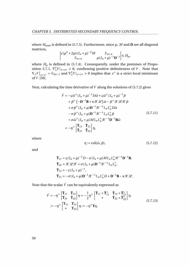
CHAPTER 5. DISTRIBUTED SECONDARY FREQUENCY CONTROL
where Hnom is defined in (5.7.5). Furthermore, since µ, M and D are all diagonalmatrices, [
ς(µ2 +2µ)(In +µ)−2M 0n×n
0n×n µ(In +µ)−1D−1
]≤ Hµ,
where Hµ is defined in (5.7.4). Consequently, under the premises of Propo-sition 5.7.1, ∇2
xV |x=x∗ > 0, confirming positive definiteness of V . Note that∇xV
∣∣x=x∗ = 03n−1 and ∇2
xV |x=x∗ > 0 implies that x∗ is a strict local minimumof V [50].
Next, calculating the time derivative of V along the solutions of (5.7.2) gives
V =−ςω>(In +µ)−1Dω+ςω>(In +µ)−1p
+ p> (−D−1B+κX L)ω− p>X L X p
+σp>(In +µ)D−1X −11n1>n Dω
−σp>(In +µ)D−1X −11n1>n p
+σω>(In +µ)M1n1>n X −1D−1Bω
=−η>[
T11 T12
T21 T22
]η,
(5.7.11)
whereη := col(ω, p), (5.7.12)
and
T11 = ς(In +µ)−1D −σ(In +µ)M1n1>n X −1D−1B,
T22 =X L X +σ(In +µ)D−1X −11n1>n ,
T12 =−ς(In +µ)−1,
T21 =−σ(In +µ)D−1X −11n1>n D +D−1B−κX L .
Note that the scalar V can be equivalently expressed as
V =−η>[
T11 T12
T21 T22
]η=−1
2η>
[T11 + T>
11 T12 + T>21
∗ T22 + T>22
]η,
:=−η>[
T11 T12
∗ T22
]η :=−η>Tη,
(5.7.13)
56
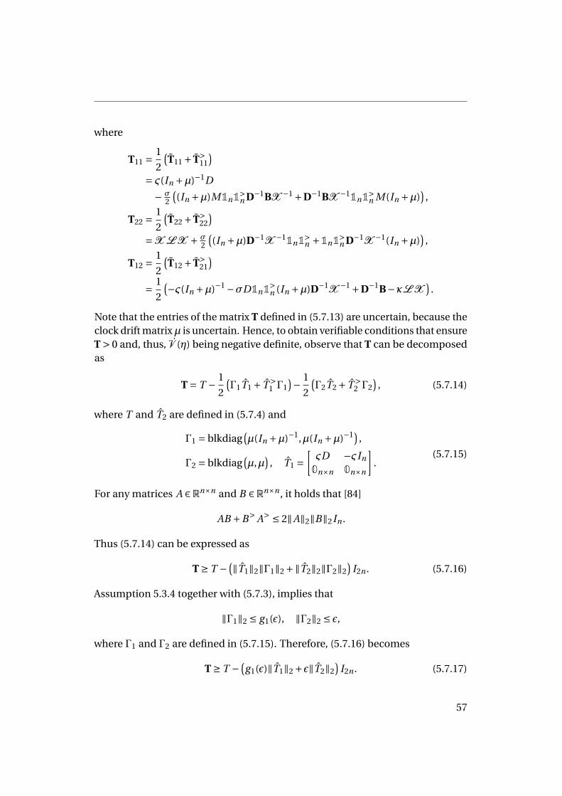
where
T11 =1
2
(T11 + T>
11
)= ς(In +µ)−1D
− σ2
((In +µ)M1n1>
n D−1BX −1 +D−1BX −11n1>n M(In +µ)
),
T22 =1
2
(T22 + T>
22
)=X L X + σ
2
((In +µ)D−1X −11n1>
n +1n1>n D−1X −1(In +µ)
),
T12 =1
2
(T12 + T>
21
)= 1
2
(−ς(In +µ)−1 −σD1n1>n (In +µ)D−1X −1 +D−1B−κL X
).
Note that the entries of the matrix T defined in (5.7.13) are uncertain, because theclock drift matrix µ is uncertain. Hence, to obtain verifiable conditions that ensureT > 0 and, thus, V (η) being negative definite, observe that T can be decomposedas
T = T − 1
2
(Γ1T1 + T >
1 Γ1)− 1
2
(Γ2T2 + T >
2 Γ2)
, (5.7.14)
where T and T2 are defined in (5.7.4) and
Γ1 = blkdiag(µ(In +µ)−1,µ(In +µ)−1) ,
Γ2 = blkdiag(µ,µ
), T1 =
[ςD −ςIn
0n×n 0n×n
].
(5.7.15)
For any matrices A ∈Rn×n and B ∈Rn×n , it holds that [84]
AB +B>A> ≤ 2‖A‖2‖B‖2In .
Thus (5.7.14) can be expressed as
T ≥ T − (‖T1‖2‖Γ1‖2 +‖T2‖2‖Γ2‖2)
I2n . (5.7.16)
Assumption 5.3.4 together with (5.7.3), implies that
‖Γ1‖2 ≤ g1(ε), ‖Γ2‖2 ≤ ε,
where Γ1 and Γ2 are defined in (5.7.15). Therefore, (5.7.16) becomes
T ≥ T − (g1(ε)‖T1‖2 +ε‖T2‖2
)I2n . (5.7.17)
57
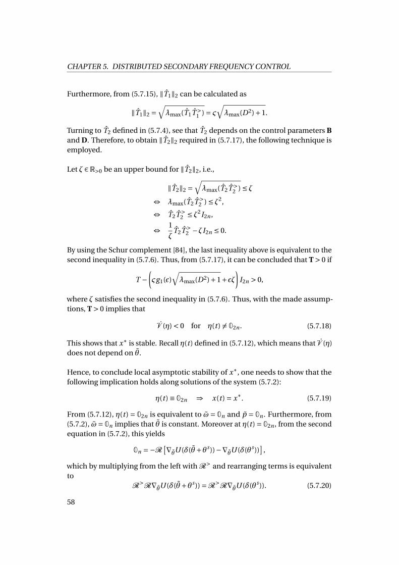
CHAPTER 5. DISTRIBUTED SECONDARY FREQUENCY CONTROL
Furthermore, from (5.7.15), ‖T1‖2 can be calculated as
‖T1‖2 =√
λmax(T1T >1 ) = ς
√λmax(D2)+1.
Turning to T2 defined in (5.7.4), see that T2 depends on the control parameters Band D. Therefore, to obtain ‖T2‖2 required in (5.7.17), the following technique isemployed.
Let ζ ∈R>0 be an upper bound for ‖T2‖2, i.e.,
‖T2‖2 =√
λmax(T2T >2 ) ≤ ζ
⇔ λmax(T2T >2 ) ≤ ζ2,
⇔ T2T >2 ≤ ζ2I2n ,
⇔ 1
ζT2T >
2 −ζI2n ≤ 0.
By using the Schur complement [84], the last inequality above is equivalent to thesecond inequality in (5.7.6). Thus, from (5.7.17), it can be concluded that T > 0 if
T −(ςg1(ε)
√λmax(D2)+1+εζ
)I2n > 0,
where ζ satisfies the second inequality in (5.7.6). Thus, with the made assump-tions, T > 0 implies that
V (η) < 0 for η(t ) 6= 02n . (5.7.18)
This shows that x∗ is stable. Recall η(t ) defined in (5.7.12), which means that V (η)does not depend on θ.
Hence, to conclude local asymptotic stability of x∗, one needs to show that thefollowing implication holds along solutions of the system (5.7.2):
η(t ) ≡ 02n ⇒ x(t ) = x∗. (5.7.19)
From (5.7.12), η(t) = 02n is equivalent to ω= 0n and p = 0n . Furthermore, from(5.7.2), ω= 0n implies that θ is constant. Moreover at η(t ) = 02n , from the secondequation in (5.7.2), this yields
0n =−R[∇θU (δ(θ+θs))−∇θU (δ(θs))
],
which by multiplying from the left with R> and rearranging terms is equivalentto
R>R∇θU (δ(θ+θs)) =R>R∇θU (δ(θs)). (5.7.20)
58
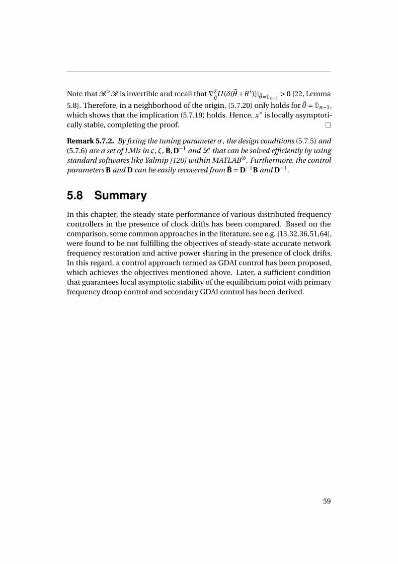
Note that R>R is invertible and recall that ∇2θU (δ(θ+θs))|θ=0n−1
> 0 [22, Lemma
5.8]. Therefore, in a neighborhood of the origin, (5.7.20) only holds for θ = 0n−1,which shows that the implication (5.7.19) holds. Hence, x∗ is locally asymptoti-cally stable, completing the proof.
Remark 5.7.2. By fixing the tuning parameter σ, the design conditions (5.7.5) and(5.7.6) are a set of LMIs in ς, ζ, B,D−1 and L that can be solved efficiently by usingstandard softwares like Yalmip [120] within MATLAB®. Furthermore, the controlparameters B and D can be easily recovered from B = D−1B and D−1.
5.8 SummaryIn this chapter, the steady-state performance of various distributed frequencycontrollers in the presence of clock drifts has been compared. Based on thecomparison, some common approaches in the literature, see e.g. [13,32,36,51,64],were found to be not fulfilling the objectives of steady-state accurate networkfrequency restoration and active power sharing in the presence of clock drifts.In this regard, a control approach termed as GDAI control has been proposed,which achieves the objectives mentioned above. Later, a sufficient conditionthat guarantees local asymptotic stability of the equilibrium point with primaryfrequency droop control and secondary GDAI control has been derived.
59

Chapter 6
Distributed voltage control
6.1 IntroductionAs described in Chapter 4, in contrast to frequency droop control, the usage ofvoltage droop control in microgrids with inductive power lines leads to poor reac-tive power sharing [32]. Moreover, achieving accurate reactive power sharing atsteady-state in the sense Definition 3.3.2 without disturbing voltage stability canalso be very challenging [25, 27]. Recently, works like [25, 27] has investigated theproblem of reactive power sharing and voltage stability in lossless AC microgrids.In a similar setting, a detailed study on addressing accurate power sharing andvoltage stability in DC microgrids has been presented in [121].
Inspired by [25, 27, 121], on top of reactive power sharing and voltage stability,regulating the voltage amplitude at a joint load is also considered in this chapter.The above-mentioned control objectives are quintessential in a microgrid withparallel-connected inverters, i.e., a parallel microgrid, where the load is connectedat the PCC [24, 34, 35].
In this regard, this chapter focuses on voltage control in lossless parallel ACmicrogrids and is organized as follows.
1. At first, the model of a lossless parallel microgrid is recalled from Chapter 4with required assumptions.
2. Then, existence and uniqueness properties of a stationary positive voltagesolution to the algebraic equations corresponding to steady-state accuratereactive power sharing and PCC voltage restoration are established.
61
CHAPTER 6. DISTRIBUTED VOLTAGE CONTROL
3. Later, a distributed voltage control law is proposed, which at equilibriumyields the desired unique voltage solution mentioned above.
4. Finally, a stability criterion is derived by using Lyapunov theory, whichguarantees asymptotic convergence of the closed-loop system trajectoriesto the desired equilibrium point. As it turned out to be the case that thestability criterion depends on the unknown voltage equilibrium, a sufficientcondition in the form of an LMI is presented. This LMI requires only theknowledge about an upper bound of the voltage equilibrium.
The results presented in this chapter is partly based on the author’s work [122].
6.2 Model of a parallel microgridIn this section, the model of a parallel microgrid described in Chapter 4 is brieflyrecalled and the assumptions required for the rest of this chapter are formalized.Starting with the decoupled reactive power flow equation, model of an inverteremployed for voltage control is described.
6.2.1 Decoupled reactive power flowConsider the power flow equations in a parallel microgrid given by (4.3.1). Thestudy presented in this chapter makes use of the standard decoupling assumption[1], which is formalized below1.
Assumption 6.2.1. |δi (t )−δPCC(t )| < ε ∀t ≥ 0, i ∈N , ε ∈R>0, ε¿ 1.
Under Assumption 6.2.1, cos(δi −δPCC) ≈ 1 and thus the reactive power flow Qi
given in (4.3.1) becomes independent of δi −δPCC, i.e.,
Qi (Vi ,VPCC) = |Bi |Vi (Vi −VPCC) . (6.2.1)
1 Recall that the considered parallel microgrid is assumed to have n > 1 inverters connected inparallel to the PCC, where a common load is present. Furthermore, the set of inverters is denotedby N = 1, . . . ,n, see Chapter 4.
62
6.2.2 Inverter model for voltage controlUnder Assumption 6.2.1, the reactive power injection depends only on the voltageamplitudes, see (6.2.1). Hence, in the rest of this chapter, angle dynamics in theinverter model (4.4.1) is neglected, yielding [27]
Vi = uVi ,
τi Qmi =−Qm
i +Qi ,(6.2.2)
where Qi is the decoupled reactive power injection given by (6.2.1) and uVi :
R≥0 →R is the voltage control input. The second equality in (6.2.2) is the powermeasurement dynamics corresponding to reactive power, obtained from (4.5.3).
Remark 6.2.2. Note that in the inverter model (6.2.2), the effect of clock drifts isneglected. This is explained below. Consider the model (6.2.2) with clock drifts, i.e.,
Vi = uVi ,
τi (1+µi )Qmi =−Qm
i +Qi .(6.2.3)
Even though the clock drift value µi has an effect on the numerical integrationof the power measurement filter in (6.2.3), the steady-state performance is notaffected. In other words, the injected reactive power and the measured reactivepower at steady-state are equal, i.e., 0 =−Qms
i +Q si .
The model (6.2.2) for the whole parallel microgrid can be expressed as
V = uV ,
τQQm =−Qm +QI ,(6.2.4)
where uV = col(uVi ) ∈ Rn , Qm = col(Qm
i ) ∈ Rn and τQ = diag(τi ) ∈ Rn×n . Further-more,
QI (V ,VPCC) = col(Qi (Vi ,VPCC)) = [V ]BV −VPCCBV , (6.2.5)
where Qi is given by (6.2.1), B > 0 is defined in (4.3.5) and [V ] = diag(Vi ) ∈Rn×n .The expression for VPCC =VPCC(V ) is given by (4.3.6). Finally, recall that the loadconnected at the PCC is represented by a constant current load IL ∈ R<0, seeSection 4.3.2.
63
CHAPTER 6. DISTRIBUTED VOLTAGE CONTROL
6.3 Problem statementRecall the definition of accurate proportional reactive power sharing, i.e., Def-inition 3.3.2. Let A = diag(ai ) and Qd
i = Qdj = 0 where i , j ∈ N . In practice, the
desired reactive power injections are provided by a higher-level control, for ex-ample, the one proposed in [123]. Thus the assumption of Qd
i =Qdj = 0 is for the
sake of simplicity and does not affect the results presented in this chapter.
The control problems investigated in this chapter are precisely described below.
Problem 6.3.1. Consider the system (6.2.4), (6.2.5), (4.3.6). Compute a control lawfor the control input uV , such that the solutions of the system (6.2.4), (6.2.5), (4.3.6)converge asymptotically to a unique stationary voltage solution V ∗ ∈Rn
>0 with thefollowing two properties:
1. Voltage regulation at the PCC, i.e.,
VPCC(V ∗) =V dPCC and (6.3.1)
2. Reactive power sharing among DGs, i.e.,
AQI (V ∗,VPCC(V ∗)) =α1n , for some α ∈R. (6.3.2)
Note that (6.3.1) is precisely (3.3.4) and (6.3.2) is (3.3.2) written for the wholenetwork.
In comparison to some related works on voltage control [27,30,32], the considera-tion of a parallel microgrid topology results in a clear voltage regulation objective,i.e., 1) in Problem 6.3.1. Besides, as shown in the sequel, this type of voltageregulation objective does not conflict with that of reactive power sharing.
6.4 Existence of a unique stationary solutionBefore proceeding to the controller design, existence and uniqueness propertiesof stationary solutions to the network equations (6.2.5), (4.3.6) under the require-ments of Problem 6.3.1 has to be investigated. More precisely, this is equivalentto investigating solutions to the set of equations (6.3.1), (6.3.2). Note that (6.3.1),(6.3.2) is a system of n +1 equations in n unknowns, i.e., V ∗ ∈ Rn
>0, hence is an
64
overdetermined system of nonlinear equations. Explicitly solving such an overde-termined system of nonlinear equations can be difficult. Yet, the following resultshows that for any A > 0 and IL < 0 there is exactly one V ∗ ∈Rn
>0, which satisfies(6.3.2) and (6.3.1) simultaneously.
Lemma 6.4.1. For any given V dPCC > 0, A > 0, and IL < 0, there exists a unique
vector V ∗ = col(V ∗i ) ∈Rn
>0 that satisfies both (6.3.1) and (6.3.2).
Proof. Consider (6.3.1) and (6.3.2). Note that any V ∗ ∈Rn>0 satisfying (6.3.1) and
(6.3.2) simultaneously has to satisfy
AQI (V ∗,V dPCC) =α1n , (6.4.1)
which by (6.2.1) can be written as
ai |Bi |(V ∗i )2 −ai |Bi |V d
PCCV ∗i −α= 0, i ∈N . (6.4.2)
Furthermore, left-multiplying (6.4.1) with 1>n A−1[V ∗]−1 yields
1>n [V ∗]−1QI (V ∗,V d
PCC) =−IL =α1>n [V ∗]−1 A−11n , (6.4.3)
where (6.2.5) and (4.3.4) were used to obtain the first equality. From (6.4.3) andthe fact that IL < 0, it is easy to see that necessarily α> 0, which means that (6.4.2)has one negative and one positive solution for V ∗
i . Denoting the latter by V +i ,
which can be calculated as
V +i =
ai |Bi |V dPCC +
√(ai |Bi |V d
PCC)2 +4ai |Bi |α2ai |Bi |
:= fi (α). (6.4.4)
Now, bearing in mind (6.4.4), it remains to show that there exists a unique α> 0that satisfies (6.4.3), which in terms of α can be written as
|IL| =α∑
i∈N
1
ai fi (α):= g (α). (6.4.5)
Note that, if such α exists and is unique, then V ∗ = col(V ∗i ) = col(V +
i ) is theunique solution to the algebraic equations (6.3.1)-(6.3.2).
From (6.4.5), it is obvious that
limα→0
g (α) = 0, limα→+∞g (α) =+∞.
65
CHAPTER 6. DISTRIBUTED VOLTAGE CONTROL
Hence, by continuity of g , there exists α> 0 that satisfies (6.4.5). To prove unique-ness, it is enough to show that g is a strictly increasing function. For this purpose,differentiating g (α) with respect to α gives
g ′(α) =∑
i∈N
1
ai fi (α)−α
∑i∈N
f ′i (α)
ai f 2i (α)
=∑
i∈N
fi (α)−α f ′i (α)
ai f 2i (α)
.
Hence, g is strictly increasing if
fi (α)−α f ′i (α) > 0, (6.4.6)
for each i ∈N . Observe that fi (α) given by (6.4.4) is concave in R≥0, thereby
fi (0) ≤ fi (α)+ f ′(α)(0−α).
Noting that fi (0) =V dPCC > 0, the latter inequality implies (6.4.6), hence confirming
the uniqueness of α > 0 which satisfies (6.4.5). Therefore, as discussed before,corresponding to this unique α> 0, there exists a unique V ∗
i = fi (α), see (6.4.4).This yields that there exists a unique voltage vector V ∗ = col(V ∗
i ) satisfying (6.3.1)-(6.3.2), completing the proof.
6.5 A distributed voltage control law forreactive power sharing and PCC voltageregulation
In this section, a distributed voltage control law to address Problem 6.3.1 isproposed.
6.5.1 Control lawConsider the parallel microgrid model (6.2.4), (6.2.5), (4.3.6). The control inputuV is computed such that
uV =V d +ν,
ν=−K L AQm −(VPCC(V )−V d
PCC
)E1n ,
(6.5.1)
where V d = col(V di ) ∈ Rn
>0 is the vector of desired voltage amplitudes at eachinverter and ν : R≥0 → Rn is a new variable. Furthermore, K = diag(ki ) ∈ Rn×n
66
where ki ∈ R>0 is a controller parameter, L ∈ Rn×n is the Laplacian matrix ofa connected undirected graph and E ∈ Rn×n is a diagonal pinning gain matrixwhich has positive entries only for the units which have access to the quantityVPCC −V d
PCC. This implies that VPCC −V dPCC is not required at all the inverters to
implement (6.5.1), hence significantly relaxing the communication requirements.Obviously, the matrix E has at least one nonzero element, i.e., E ≥ 0.
Remark 6.5.1. Similar to the inverter model (6.2.2), the effect of clock drifts onthe numerical integration performed in the controller (6.5.1) is neglected. This isbecause the steady-state performance of (6.5.1) is not disturbed in the presence ofclock drifts, which is further clarified in Lemma 6.5.3.
6.5.2 Closed-loop systemBy combining (6.2.4) and (6.5.1), the following closed-loop dynamics is obtained:
V =−K L AQm −(VPCC(V )−V d
PCC
)E1n ,
τQQm =−Qm +QI (V ,VPCC),(6.5.2)
where V (0) =V d .
Remark 6.5.2. In practice, the voltage amplitude of a grid-forming inverter isprovided by the operator. This also applies to the initial conditions of the voltagesV (0) =V d in (6.5.2). See also [14, 27].
The following vectors are essential for presenting the main results of this section.
z := col(V ,Qm) ∈R2n ,
z∗ := col(V ∗,QI (V ∗,V dPCC)) = col(V ∗,αA−11n),
α= −IL
1>n [V ∗]−1 A−11n
∈R>0,
(6.5.3)
where (6.4.1) and (6.4.3) were used to write the last two equalities. The lemmabelow presents an important property about the point z∗.
Lemma 6.5.3. The vector z∗ given by (6.5.3) is the unique equilibrium point of theclosed-loop system (6.5.2).
Proof. In the proof of Lemma 6.4.1, it has been shown that satisfying (6.3.1) and(6.3.2) yields a unique solution V ∗. In addition, since L is the Laplacian matrix of
67
CHAPTER 6. DISTRIBUTED VOLTAGE CONTROL
a connected undirected graph, recall that L 1n = 0n . As a consequence, at z = z∗,the system (6.5.2) is at equilibrium.
Next, to show that z∗ is the only equilibrium point of the system (6.5.2), theconcept of contradiction is used. Suppose that for the system (6.5.2), there existsanother equilibrium solution zs := col(V s ,Qms) ∈R2n , i.e.,
0n =−K L AQms −(VPCC(V s)−V d
PCC
)E1n ,
0n =−Qms +QI (V s ,VPCC(V s)),(6.5.4)
which readily yields
0n = K L AQI(V s ,VPCC(V s)
)+ (VPCC(V s)−V d
PCC
)E1n . (6.5.5)
Since K = diag(ki ) > 0, left-multiplying (6.5.5) with 1>n K −1 yields(
VPCC(V s)−V dPCC
)trace(K −1E) = 0. (6.5.6)
Recall that E is a diagonal positive semidefinite matrix. Hence trace(K −1E) > 0,which implies that (6.5.6) is satisfied if and only if VPCC(V s) = V d
PCC. But thisimplies that V s also has to satisfy
L AQI (V s ,VPCC(V s)) = 0n . (6.5.7)
Since L is the Laplacian matrix of an undirected connected graph, (6.5.7) isequivalent to
QI (V s ,VPCC(V s)) =βA−11n , (6.5.8)
for some β ∈R. From Lemma 6.4.1, it follows that there is only one solution, whichis V ∗, that satisfies VPCC(V s) = V d
PCC and (6.5.8) simultaneously. Consequently,V s = V ∗ and (6.5.8) becomes QI (V ∗,VPCC(V ∗)) = αA−11n where α is given by(6.5.3). From the second equation in (6.5.4), this yields Qms =αA−11n . In essence,zs := col(V s ,Qms) = col(V ∗,αA−11n) = z∗. This completes the proof.
Remark 6.5.4. The distributed voltage controller (DVC) proposed in [27] to addressthe problem of reactive power sharing in lossless meshed microgrids is given byby [27, Equation 12]
V =−K L AQm ,
τQQm =−Qm +QmeshedI (V ),
(6.5.9)
where QmeshedI (V ) = col(Qi ) ∈ Rn with Qi given by (2.4.5). Note that (6.5.2) is
similar to (6.5.9), but has a noticeable difference. More precisely, (6.5.2) is designedfor a lossless parallel microgrid where the objective of PCC voltage regulation isalso considered.
68
6.5.3 Error statesIn the sequel, the vector z = col(V ,Qm) is expressed with respect to the uniqueequilibrium point z∗ = col(V ∗,αA−11n), i.e.,
Qm :=Qm −αA−11n ,
V :=V −V ∗,
x := col(V ,Qm) ∈R2n .
(6.5.10)
Thus, the closed-loop system (6.5.2) in error states x can be expressed as
˙V =−K L AQm − (VPCC(V +V ∗)−VPCC(V ∗)
)E1n ,
τQ˙Qm =−Qm + (
QI(V +V ∗,VPCC(V +V ∗)
)−QI(V ∗,VPCC(V ∗)
)).
(6.5.11)
Note that with QI given in (6.2.5),
QI(V +V ∗,VPCC(V +V ∗)
)−QI(V ∗,VPCC(V ∗)
)= [V +V ∗]B(V +V ∗)
−VPCC(V +V ∗)B(V +V ∗)
− [V ∗]BV ∗+VPCC(V ∗)BV ∗,
= [V +2V ∗]BV −VPCC(V +V ∗)BV
− (VPCC(V +V ∗)−VPCC(V ∗)
)BV ∗,
= ([V +2V ∗]−VPCC(V +V ∗)In
)BV
− (VPCC(V +V ∗)−VPCC(V ∗)
)BV ∗.
(6.5.12)
By using (6.5.12), the closed-loop system (6.5.11) becomes
˙V =−K L AQm − (VPCC(V +V ∗)−VPCC(V ∗)
)E1n ,
τQ˙Qm =−Qm + (
[V +2V ∗]−VPCC(V +V ∗)In)
BV
− (VPCC(V +V ∗)−VPCC(V ∗)
)B [V ∗]1n ,
(6.5.13)
wherex∗ := 02n (6.5.14)
is the equilibrium point of (6.5.13). Note that x∗ is just a shift of coordinates fromthe unique equilibrium point z∗ defined in (6.5.3). Hence, asymptotic stabilityof x∗ implies that the trajectories of the closed-loop system (6.5.2) convergeasymptotically to z∗.
69
CHAPTER 6. DISTRIBUTED VOLTAGE CONTROL
6.5.4 A condition for asymptotic stabilityFor presenting the stability results, it is convenient to define the following matrix.
Φ(V ∗) :=Φ11 Φ12 Φ13
∗ Φ22 Φ23
∗ ∗ trace(BE)
∈R(2n+1)×(2n+1), (6.5.15)
where
Φ11(V ∗) =σRτ−1Q
(2[V ∗]−V d
PCCIn
)B ,
Φ12(V ∗) = 1
2
(ξMK L A−ζ
(2[V ∗]−V d
PCCIn
)B −σRτ−1
Q
),
Φ13(V ∗) = 1
2
(ξME1n −σRτ−1
Q B [V ∗]1n
),
Φ22 = ζIn − σ
2(RK L A+ AL K R) ,
Φ23(V ∗) = 1
2
(AL K B1n −σRE1n +ζB [V ∗]1n
),
where ξ ∈R>0, σ ∈R>0, ζ ∈R>0, and R ∈Rn×n , M ∈Rn×n are two positive definitediagonal matrices.
The stability result is as follows.
Proposition 6.5.5. Consider the closed-loop system (6.5.13). Suppose that thereexist ξ ∈R>0, σ ∈R>0, ζ ∈R>0 and positive definite diagonal matrices R ∈Rn×n andM ∈Rn×n . Then, x∗ is locally asymptotically stable if K , E and L are chosen suchthat [
ξM + 1trace(B) B1n1>
n B −σR
−σR ζτQ
]> 0,
Φ(V ∗) > 0,
(6.5.16)
where Φ(V ∗) is given by (6.5.15).
Proof. Consider the Lyapunov function candidate
F (x) = ξ
2V >MV + 1
2
(VPCC(V +V ∗)−VPCC(V ∗)
)2trace(B)
+ ζ
2Qm>τQQm −σQm>RV ,
(6.5.17)
where ξ ∈ R>0, ζ ∈ R>0 and σ ∈ R>0. Furthermore R ∈ Rn×n and M ∈ Rn×n arepositive definite diagonal matrices. The function (6.5.17) has three quadratic
70
terms in V , VPCC (in error states) and Qm respectively. A cross term between Vand Qm is also included in F , since it facilitates that the function F is decreasingalong the solutions of (6.5.13).
Observe that F (x∗) = 0. Moreover with VPCC given by (4.3.6), the gradient of F
with respect to x can be calculated as
∇xF =[ξMV + (
VPCC(V +V ∗)−VPCC(V ∗))
B1n −σRQm
ζτQQm −σRV
]. (6.5.18)
Evaluating the gradient at x = x∗, it can be seen that ∇xF |x∗ = 02n . Therefore, x∗
is a critical point of F [49, 50].
The Hessian of F at x = x∗ is given by
∇2xF |x∗ =
[ξM + 1
trace(B) B1n1>n B −σR
−σR ζτQ
]. (6.5.19)
Recall that M > 0, ξ> 0 and τQ > 0. Furthermore since B > 0, the matrix B1n1>n B
is positive semidefinite. Thus, both block-diagonal matrices of ∇2xF |x∗ are posi-
tive definite. Therefore, under the standing assumption that the first condition in(6.5.16) is satisfied, the LHS of (6.5.19) is positive definite, confirming that x∗ isan isolated minimum of F . Hence, F qualifies as a potential Lyapunov functionto study stability of x∗ [49, 50].
Calculating the time derivative of F along the solutions of (6.5.13) yields
F =−ξV >MK L AQm
−ξV >ME1n(VPCC(V +V ∗)−VPCC(V ∗)
)− (
VPCC(V +V ∗)−VPCC(V ∗))1>
n BK L AQm
−1>n BE1n
(VPCC(V +V ∗)−VPCC(V ∗)
)2
+σQm>RK L AQm
+σQm>RE1n(VPCC(V +V ∗)−VPCC(V ∗)
)−ζQm>Qm
+ζQm> ([V +2V ∗]−VPCC(V +V ∗)In
)BV
−ζQm>B [V ∗]1n(VPCC(V +V ∗)−VPCC(V ∗)
)+σV >Rτ−1
Q Qm
−σV >Rτ−1Q
([V +2V ∗]−VPCC(V +V ∗)In
)BV
+σV >Rτ−1Q B [V ∗]1n
(VPCC(V +V ∗)−VPCC(V ∗)
)=−η>Φ(V )η,
(6.5.20)
71
CHAPTER 6. DISTRIBUTED VOLTAGE CONTROL
where
η := V
Qm(VPCC(V +V ∗)−VPCC(V ∗)
) ∈R2n+1, (6.5.21)
and
Φ(V ) :=Φ11 Φ12 Φ13
∗ Φ22 Φ23
∗ ∗ trace(BE)
∈R(2n+1)×(2n+1), (6.5.22)
with
Φ11(V ) =σRτ−1Q
([V +2V ∗]−VPCC(V +V ∗)In
)B ,
Φ12(V ) = 1
2
(ξMK L A−σRτ−1
Q −ζB([V +2V ∗]−VPCC(V +V ∗)In
)),
Φ13(V ∗) = 1
2
(ξME1n −σRτ−1
Q B [V ∗]1n
),
Φ22 = ζIn − σ
2(RK L A+ AL K R) ,
Φ23(V ∗) = 1
2
(AL K B1n −σRE1n +ζB [V ∗]1n
).
Note thatΦ(V )|V =0n
=Φ(V ∗),
where Φ(V ∗) is defined in (6.5.15). Under the premises of Proposition 6.5.5, see(6.5.16),
Φ(V )|V =0n> 0.
Thus by continuity, there exists a (small) neighborhood around V = 0n such thatΦ(V ) > 0, and, thus, F ≤ 0. Hence, x∗ is a stable equilibrium point.
To establish asymptotic stability of x∗, the following implication has to hold alongthe solutions of the system (6.5.13):
η= 02n+1 ⇒ x(t ) = x∗ (6.5.23)
Since Φ(V ) > 0, and with η defined in (6.5.21), η= 02n+1 directly implies that V =0n and Qm = 0n . By using the definition of x and x∗ given respectively by (6.5.10)and (6.5.14), V = 0n and Qm = 0n means that x = 02n = x∗. As a consequence, theimplication (6.5.23) holds, ensuring that x∗ is locally asymptotically stable. Thiscompletes the proof.
72
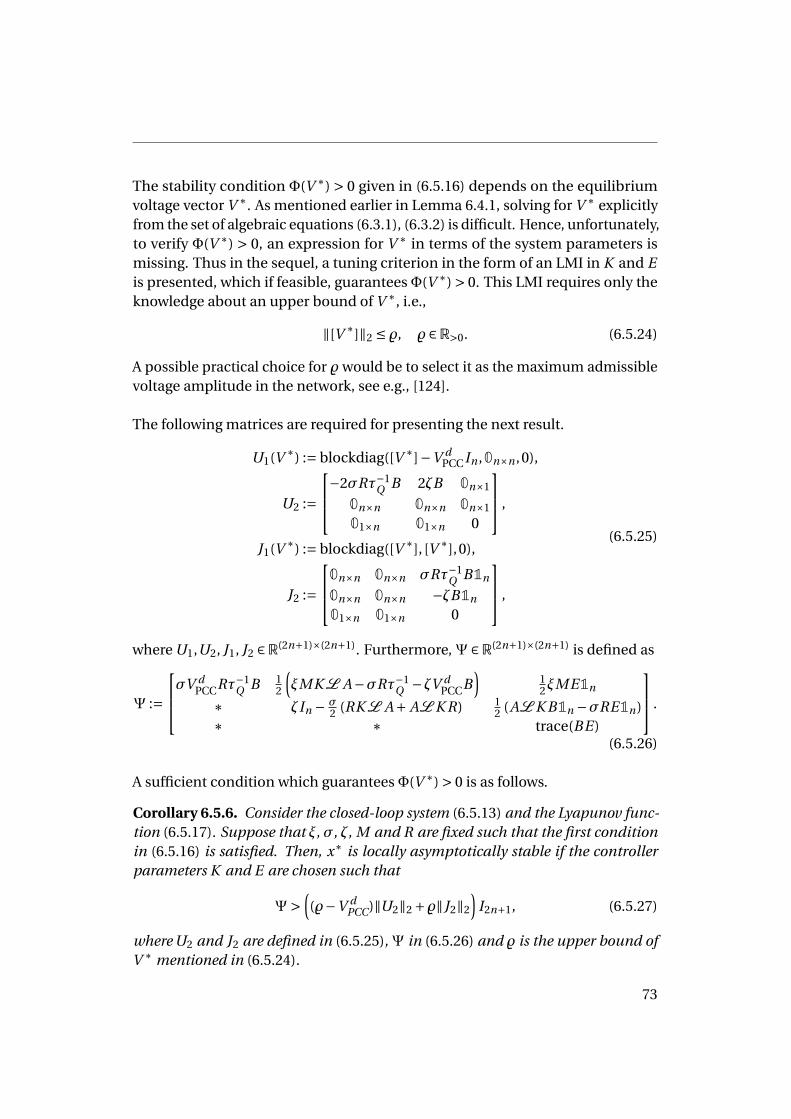
The stability condition Φ(V ∗) > 0 given in (6.5.16) depends on the equilibriumvoltage vector V ∗. As mentioned earlier in Lemma 6.4.1, solving for V ∗ explicitlyfrom the set of algebraic equations (6.3.1), (6.3.2) is difficult. Hence, unfortunately,to verify Φ(V ∗) > 0, an expression for V ∗ in terms of the system parameters ismissing. Thus in the sequel, a tuning criterion in the form of an LMI in K and Eis presented, which if feasible, guarantees Φ(V ∗) > 0. This LMI requires only theknowledge about an upper bound of V ∗, i.e.,
‖[V ∗]‖2 ≤ %, % ∈R>0. (6.5.24)
A possible practical choice for % would be to select it as the maximum admissiblevoltage amplitude in the network, see e.g., [124].
The following matrices are required for presenting the next result.
U1(V ∗) := blockdiag([V ∗]−V dPCCIn ,0n×n ,0),
U2 :=
−2σRτ−1Q B 2ζB 0n×1
0n×n 0n×n 0n×1
01×n 01×n 0
,
J1(V ∗) := blockdiag([V ∗], [V ∗],0),
J2 :=
0n×n 0n×n σRτ−1Q B1n
0n×n 0n×n −ζB1n
01×n 01×n 0
,
(6.5.25)
where U1,U2, J1, J2 ∈R(2n+1)×(2n+1). Furthermore, Ψ ∈R(2n+1)×(2n+1) is defined as
Ψ :=
σV dPCCRτ−1
Q B 12
(ξMK L A−σRτ−1
Q −ζV dPCCB
)12ξME1n
∗ ζIn − σ2 (RK L A+ AL K R) 1
2 (AL K B1n −σRE1n)∗ ∗ trace(BE)
.
(6.5.26)
A sufficient condition which guarantees Φ(V ∗) > 0 is as follows.
Corollary 6.5.6. Consider the closed-loop system (6.5.13) and the Lyapunov func-tion (6.5.17). Suppose that ξ, σ, ζ, M and R are fixed such that the first conditionin (6.5.16) is satisfied. Then, x∗ is locally asymptotically stable if the controllerparameters K and E are chosen such that
Ψ>((%−V d
PCC)‖U2‖2 +%‖J2‖2
)I2n+1, (6.5.27)
where U2 and J2 are defined in (6.5.25), Ψ in (6.5.26) and % is the upper bound ofV ∗ mentioned in (6.5.24).
73
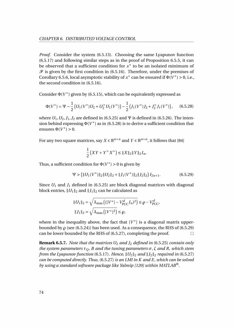
CHAPTER 6. DISTRIBUTED VOLTAGE CONTROL
Proof. Consider the system (6.5.13). Choosing the same Lyapunov function(6.5.17) and following similar steps as in the proof of Proposition 6.5.5, it canbe observed that a sufficient condition for x∗ to be an isolated minimum ofF is given by the first condition in (6.5.16). Therefore, under the premises ofCorollary 6.5.6, local asymptotic stability of x∗ can be ensured if Φ(V ∗) > 0, i.e.,the second condition in (6.5.16).
Consider Φ(V ∗) given by (6.5.15), which can be equivalently expressed as
Φ(V ∗) =Ψ− 1
2
(U1(V ∗)U2 +U>
2 U1(V ∗))− 1
2
(J1(V ∗)J2 + J>2 J1(V ∗)
), (6.5.28)
where U1,U2, J1, J2 are defined in (6.5.25) and Ψ is defined in (6.5.26). The inten-sion behind expressing Φ(V ∗) as in (6.5.28) is to derive a sufficient condition thatensures Φ(V ∗) > 0.
For any two square matrices, say X ∈Rn×n and Y ∈Rn×n , it follows that [84]
1
2
(X Y +Y >X >)≤ ‖X ‖2‖Y ‖2In .
Thus, a sufficient condition for Φ(V ∗) > 0 is given by
Ψ> (‖U1(V ∗)‖2‖U2‖2 +‖J1(V ∗)‖2‖J2‖2)
I2n+1. (6.5.29)
Since U1 and J1 defined in (6.5.25) are block diagonal matrices with diagonalblock entries, ‖U1‖2 and ‖J1‖2 can be calculated as
‖U1‖2 =√
λmax(([V ∗]−V d
PCCIn)2)≤ %−V d
PCC,
‖J1‖2 =√
λmax([V ∗]2
)≤ %,
where in the inequality above, the fact that [V ∗] is a diagonal matrix upper-bounded by % (see (6.5.24)) has been used. As a consequence, the RHS of (6.5.29)can be lower bounded by the RHS of (6.5.27), completing the proof.
Remark 6.5.7. Note that the matrices U2 and J2 defined in (6.5.25) contain onlythe system parameters τQ , B and the tuning parameters σ, ζ and R, which stemfrom the Lyapunov function (6.5.17). Hence, ‖U2‖2 and ‖J2‖2 required in (6.5.27)can be computed directly. Thus, (6.5.27) is an LMI in K and E, which can be solvedby using a standard software package like Yalmip [120] within MATLAB®.
74
6.6 SummaryThe problems of voltage stability, reactive power sharing, and PCC voltage restora-tion in a lossless parallel microgrid have been addressed in this chapter. Startingwith the proof about the existence of a unique voltage equilibrium, a distributedvoltage controller which drives the closed-loop system solutions asymptoticallyto the desired equilibrium has been presented. Alas, the derived stability criteriondepends on the voltage equilibrium. Thus, a sufficient condition that ensuresthe feasibility of the stability criterion has been derived. This sufficient conditionrequires only the knowledge about an upper bound of the voltage equilibriumand is in the form of an LMI, which can be solved numerically to obtain stabilizingcontroller parameters.
75

Chapter 7
Case study
7.1 IntroductionThis chapter is dedicated to validate, via simulation, robustness of the approachespresented in Chapter 5 and Chapter 6 towards typical modeling uncertainties andsome exogenous disturbances observed in microgrids.
At first, the performance and robustness of the GDAI controller proposed in Chap-ter 5 towards modeling uncertainties are investigated. The controller parametersare chosen based on the tuning criterion presented in Chapter 5. Furthermore,the results are compared with other distributed secondary frequency controllersin the literature; for example, the DAI control [32, 51] and the pinning control [40].
The second part of this chapter focusses on investigating whether the distributedvoltage controller proposed in Chapter 6 is robust towards load disturbances andmodeling errors like small line resistances. The operational compatibility of theproposed voltage controller with the standard frequency droop control [38] isalso examined.
Throughout this chapter, the terms weighted active power, respectively weightedreactive power represent the fraction (Pi −P d
i )/SNi , respectively Qi /SN
i where Pi ,respectively Qi are the active, respectively reactive power injections. Furthermore,SN
i ∈R>0 is the nominal power rating and P di ∈R is the desired active power set
point at the i -th inverter, i ∈N .
77
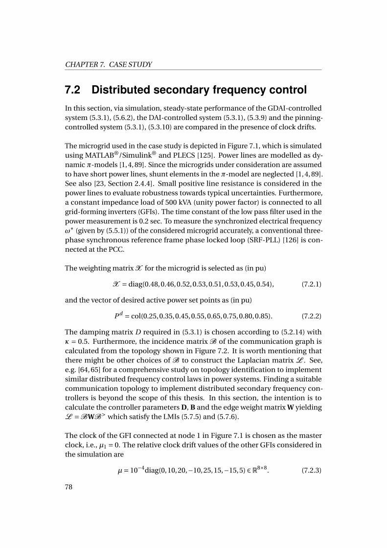
CHAPTER 7. CASE STUDY
7.2 Distributed secondary frequency controlIn this section, via simulation, steady-state performance of the GDAI-controlledsystem (5.3.1), (5.6.2), the DAI-controlled system (5.3.1), (5.3.9) and the pinning-controlled system (5.3.1), (5.3.10) are compared in the presence of clock drifts.
The microgrid used in the case study is depicted in Figure 7.1, which is simulatedusing MATLAB®/Simulink® and PLECS [125]. Power lines are modelled as dy-namic π-models [1, 4, 89]. Since the microgrids under consideration are assumedto have short power lines, shunt elements in the π-model are neglected [1, 4, 89].See also [23, Section 2.4.4]. Small positive line resistance is considered in thepower lines to evaluate robustness towards typical uncertainties. Furthermore,a constant impedance load of 500 kVA (unity power factor) is connected to allgrid-forming inverters (GFIs). The time constant of the low pass filter used in thepower measurement is 0.2 sec. To measure the synchronized electrical frequencyω∗ (given by (5.5.1)) of the considered microgrid accurately, a conventional three-phase synchronous reference frame phase locked loop (SRF-PLL) [126] is con-nected at the PCC.
The weighting matrix X for the microgrid is selected as (in pu)
X = diag(0.48,0.46,0.52,0.53,0.51,0.53,0.45,0.54), (7.2.1)
and the vector of desired active power set points as (in pu)
P d = col(0.25,0.35,0.45,0.55,0.65,0.75,0.80,0.85). (7.2.2)
The damping matrix D required in (5.3.1) is chosen according to (5.2.14) withκ = 0.5. Furthermore, the incidence matrix B of the communication graph iscalculated from the topology shown in Figure 7.2. It is worth mentioning thatthere might be other choices of B to construct the Laplacian matrix L . See,e.g. [64, 65] for a comprehensive study on topology identification to implementsimilar distributed frequency control laws in power systems. Finding a suitablecommunication topology to implement distributed secondary frequency con-trollers is beyond the scope of this thesis. In this section, the intention is tocalculate the controller parameters D, B and the edge weight matrix W yieldingL =BWB> which satisfy the LMIs (5.7.5) and (5.7.6).
The clock of the GFI connected at node 1 in Figure 7.1 is chosen as the masterclock, i.e., µ1 = 0. The relative clock drift values of the other GFIs considered inthe simulation are
µ= 10−4diag(0,10,20,−10,25,15,−15,5) ∈R8×8. (7.2.3)
78
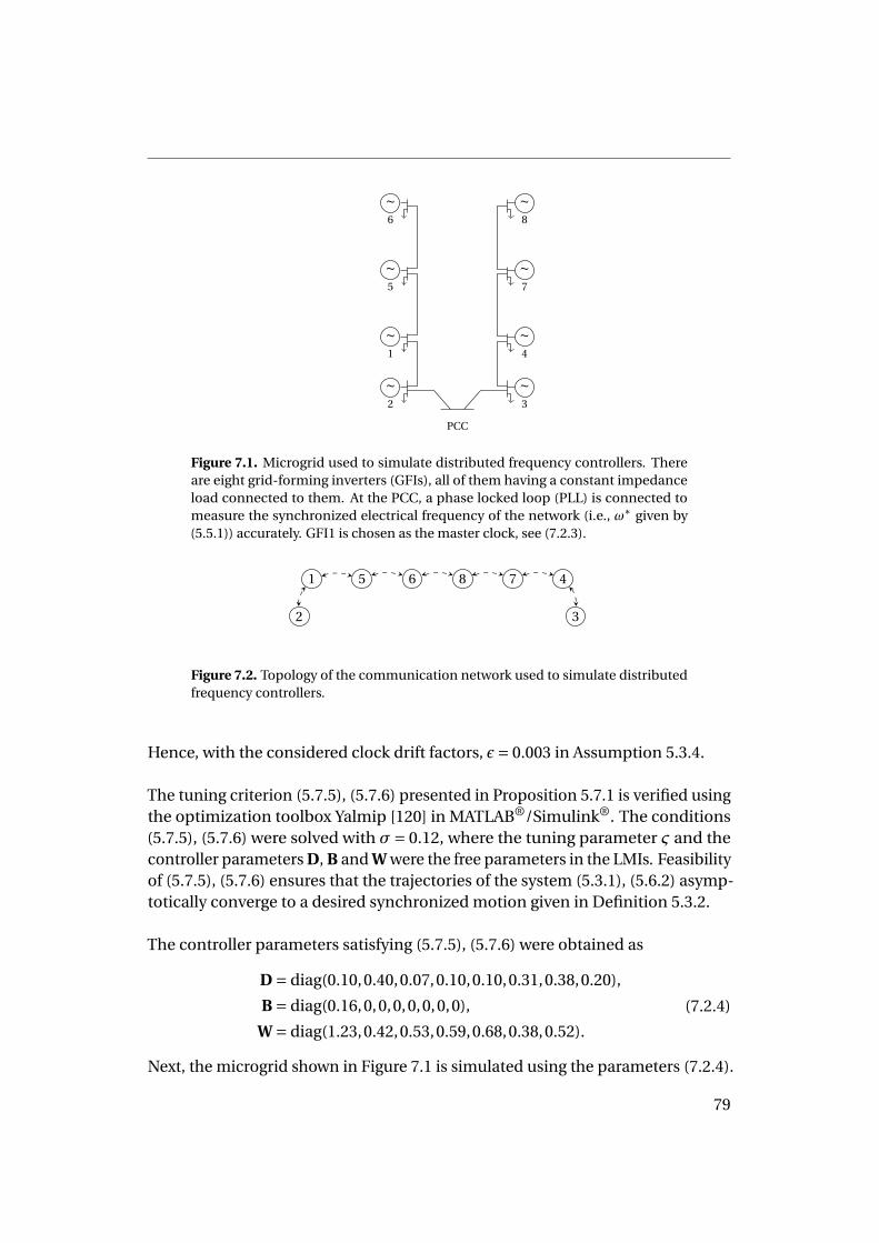
PCC
∼1
∼2
∼3
∼4
∼5
∼6
∼7
∼8
Figure 7.1. Microgrid used to simulate distributed frequency controllers. Thereare eight grid-forming inverters (GFIs), all of them having a constant impedanceload connected to them. At the PCC, a phase locked loop (PLL) is connected tomeasure the synchronized electrical frequency of the network (i.e., ω∗ given by(5.5.1)) accurately. GFI1 is chosen as the master clock, see (7.2.3).
1
2 3
45 6 78
Figure 7.2. Topology of the communication network used to simulate distributedfrequency controllers.
Hence, with the considered clock drift factors, ε= 0.003 in Assumption 5.3.4.
The tuning criterion (5.7.5), (5.7.6) presented in Proposition 5.7.1 is verified usingthe optimization toolbox Yalmip [120] in MATLAB®/Simulink®. The conditions(5.7.5), (5.7.6) were solved with σ= 0.12, where the tuning parameter ς and thecontroller parameters D, B and W were the free parameters in the LMIs. Feasibilityof (5.7.5), (5.7.6) ensures that the trajectories of the system (5.3.1), (5.6.2) asymp-totically converge to a desired synchronized motion given in Definition 5.3.2.
The controller parameters satisfying (5.7.5), (5.7.6) were obtained as
D = diag(0.10,0.40,0.07,0.10,0.10,0.31,0.38,0.20),
B = diag(0.16,0,0,0,0,0,0,0),
W = diag(1.23,0.42,0.53,0.59,0.68,0.38,0.52).
(7.2.4)
Next, the microgrid shown in Figure 7.1 is simulated using the parameters (7.2.4).
79
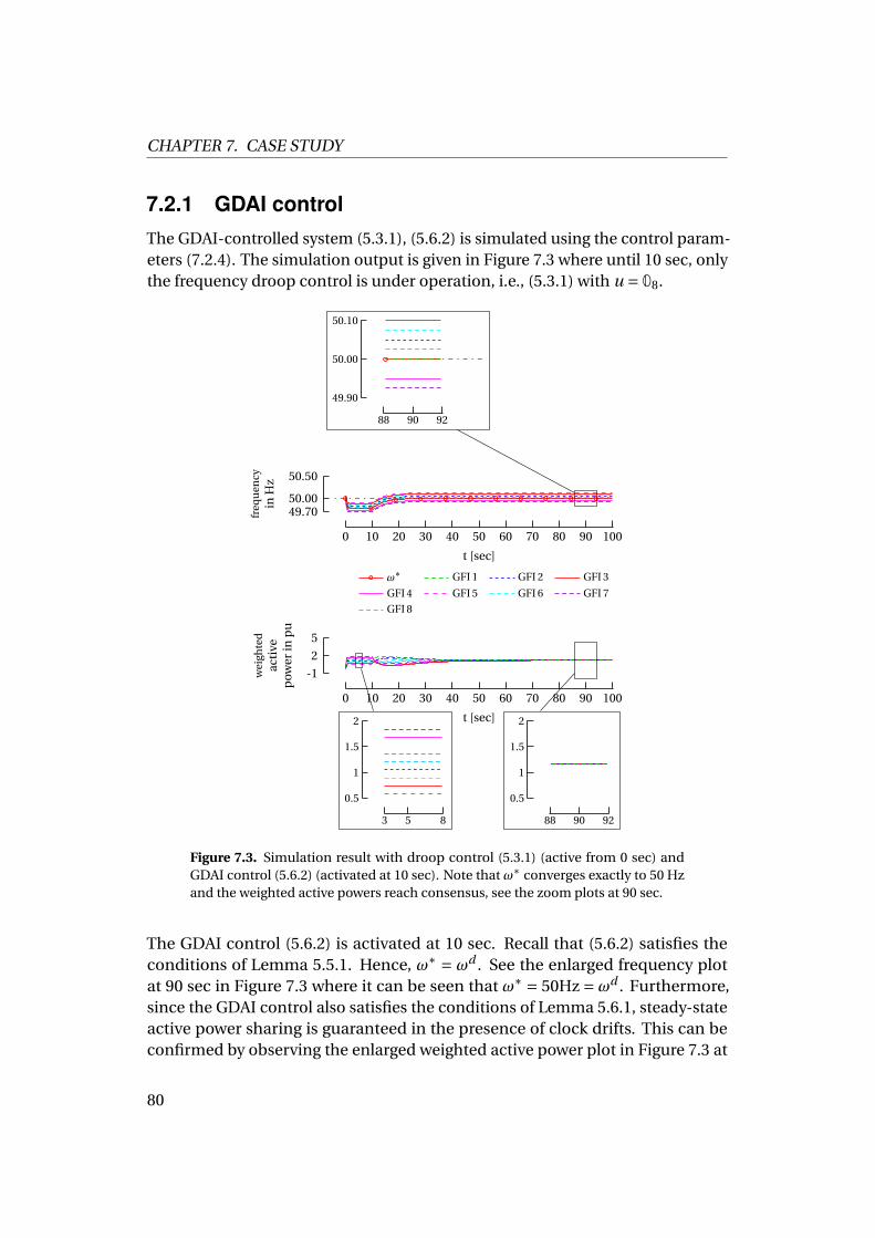
CHAPTER 7. CASE STUDY
7.2.1 GDAI controlThe GDAI-controlled system (5.3.1), (5.6.2) is simulated using the control param-eters (7.2.4). The simulation output is given in Figure 7.3 where until 10 sec, onlythe frequency droop control is under operation, i.e., (5.3.1) with u = 08.
0 10 20 30 40 50 60 70 80 90 100
49.7050.00
50.50
t [sec]
freq
uen
cyin
Hz
ω∗ GFI 1 GFI 2 GFI 3
GFI 4 GFI 5 GFI 6 GFI 7
GFI 8
0 10 20 30 40 50 60 70 80 90 100
-1
2
5
t [sec]
weigh
ted
active
pow
erin
pu
88 90 92
49.90
50.00
50.10
88 90 92
0.5
1
1.5
2
3 5 8
0.5
1
1.5
2
Figure 7.3. Simulation result with droop control (5.3.1) (active from 0 sec) andGDAI control (5.6.2) (activated at 10 sec). Note that ω∗ converges exactly to 50 Hzand the weighted active powers reach consensus, see the zoom plots at 90 sec.
The GDAI control (5.6.2) is activated at 10 sec. Recall that (5.6.2) satisfies theconditions of Lemma 5.5.1. Hence, ω∗ = ωd . See the enlarged frequency plotat 90 sec in Figure 7.3 where it can be seen that ω∗ = 50Hz =ωd . Furthermore,since the GDAI control also satisfies the conditions of Lemma 5.6.1, steady-stateactive power sharing is guaranteed in the presence of clock drifts. This can beconfirmed by observing the enlarged weighted active power plot in Figure 7.3 at
80
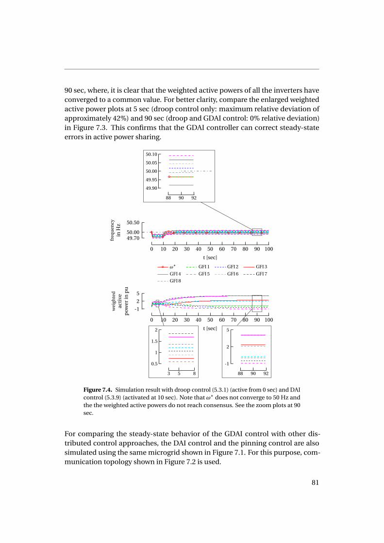
90 sec, where, it is clear that the weighted active powers of all the inverters haveconverged to a common value. For better clarity, compare the enlarged weightedactive power plots at 5 sec (droop control only: maximum relative deviation ofapproximately 42%) and 90 sec (droop and GDAI control: 0% relative deviation)in Figure 7.3. This confirms that the GDAI controller can correct steady-stateerrors in active power sharing.
0 10 20 30 40 50 60 70 80 90 100
49.7050.00
50.50
t [sec]
freq
uen
cyin
Hz
ω∗ GFI 1 GFI 2 GFI 3
GFI 4 GFI 5 GFI 6 GFI 7
GFI 8
0 10 20 30 40 50 60 70 80 90 100
-1
2
5
t [sec]
weigh
ted
active
pow
erin
pu
88 90 92
49.90
49.95
50.00
50.05
50.10
88 90 92
-1
2
5
3 5 8
0.5
1
1.5
2
Figure 7.4. Simulation result with droop control (5.3.1) (active from 0 sec) and DAIcontrol (5.3.9) (activated at 10 sec). Note that ω∗ does not converge to 50 Hz andthe the weighted active powers do not reach consensus. See the zoom plots at 90sec.
For comparing the steady-state behavior of the GDAI control with other dis-tributed control approaches, the DAI control and the pinning control are alsosimulated using the same microgrid shown in Figure 7.1. For this purpose, com-munication topology shown in Figure 7.2 is used.
81
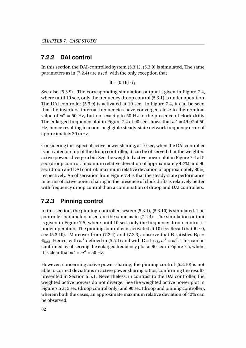
CHAPTER 7. CASE STUDY
7.2.2 DAI controlIn this section the DAI-controlled system (5.3.1), (5.3.9) is simulated. The sameparameters as in (7.2.4) are used, with the only exception that
B = (0.16) · I8.
See also (5.3.9). The corresponding simulation output is given in Figure 7.4,where until 10 sec, only the frequency droop control (5.3.1) is under operation.The DAI controller (5.3.9) is activated at 10 sec. In Figure 7.4, it can be seenthat the inverters’ internal frequencies have converged close to the nominalvalue of ωd = 50 Hz, but not exactly to 50 Hz in the presence of clock drifts.The enlarged frequency plot in Figure 7.4 at 90 sec shows that ω∗ ≈ 49.97 6= 50Hz, hence resulting in a non-negligible steady-state network frequency error ofapproximately 30 mHz.
Considering the aspect of active power sharing, at 10 sec, when the DAI controlleris activated on top of the droop controller, it can be observed that the weightedactive powers diverge a bit. See the weighted active power plot in Figure 7.4 at 5sec (droop control: maximum relative deviation of approximately 42%) and 90sec (droop and DAI control: maximum relative deviation of approximately 80%)respectively. An observation from Figure 7.4 is that the steady-state performancein terms of active power sharing in the presence of clock drifts is relatively betterwith frequency droop control than a combination of droop and DAI controllers.
7.2.3 Pinning controlIn this section, the pinning-controlled system (5.3.1), (5.3.10) is simulated. Thecontroller parameters used are the same as in (7.2.4). The simulation outputis given in Figure 7.5, where until 10 sec, only the frequency droop control isunder operation. The pinning controller is activated at 10 sec. Recall that B ≥ 0,see (5.3.10). Moreover from (7.2.4) and (7.2.3), observe that B satisfies Bµ =08×8. Hence, with ω∗ defined in (5.5.1) and with C = 08×8, ω∗ =ωd . This can beconfirmed by observing the enlarged frequency plot at 90 sec in Figure 7.5, whereit is clear that ω∗ =ωd = 50 Hz.
However, concerning active power sharing, the pinning control (5.3.10) is notable to correct deviations in active power sharing ratios, confirming the resultspresented in Section 5.5.1. Nevertheless, in contrast to the DAI controller, theweighted active powers do not diverge. See the weighted active power plot inFigure 7.5 at 5 sec (droop control only) and 90 sec (droop and pinning controller),wherein both the cases, an approximate maximum relative deviation of 42% canbe observed.
82
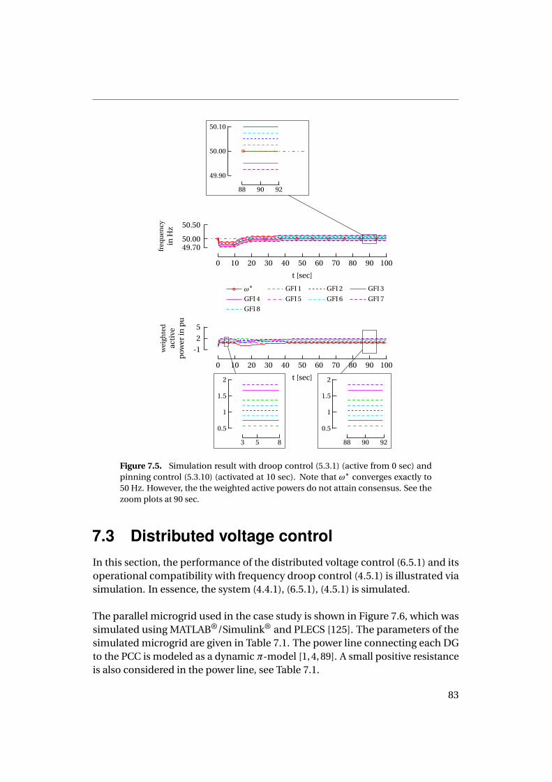
0 10 20 30 40 50 60 70 80 90 100
49.7050.00
50.50
t [sec]
freq
uen
cyin
Hz
ω∗ GFI 1 GFI 2 GFI 3
GFI 4 GFI 5 GFI 6 GFI 7
GFI 8
0 10 20 30 40 50 60 70 80 90 100
-1
2
5
t [sec]
weigh
ted
active
pow
erin
pu
88 90 92
49.90
50.00
50.10
88 90 92
0.5
1
1.5
2
3 5 8
0.5
1
1.5
2
Figure 7.5. Simulation result with droop control (5.3.1) (active from 0 sec) andpinning control (5.3.10) (activated at 10 sec). Note that ω∗ converges exactly to50 Hz. However, the the weighted active powers do not attain consensus. See thezoom plots at 90 sec.
7.3 Distributed voltage controlIn this section, the performance of the distributed voltage control (6.5.1) and itsoperational compatibility with frequency droop control (4.5.1) is illustrated viasimulation. In essence, the system (4.4.1), (6.5.1), (4.5.1) is simulated.
The parallel microgrid used in the case study is shown in Figure 7.6, which wassimulated using MATLAB®/Simulink® and PLECS [125]. The parameters of thesimulated microgrid are given in Table 7.1. The power line connecting each DGto the PCC is modeled as a dynamic π-model [1, 4, 89]. A small positive resistanceis also considered in the power line, see Table 7.1.
83
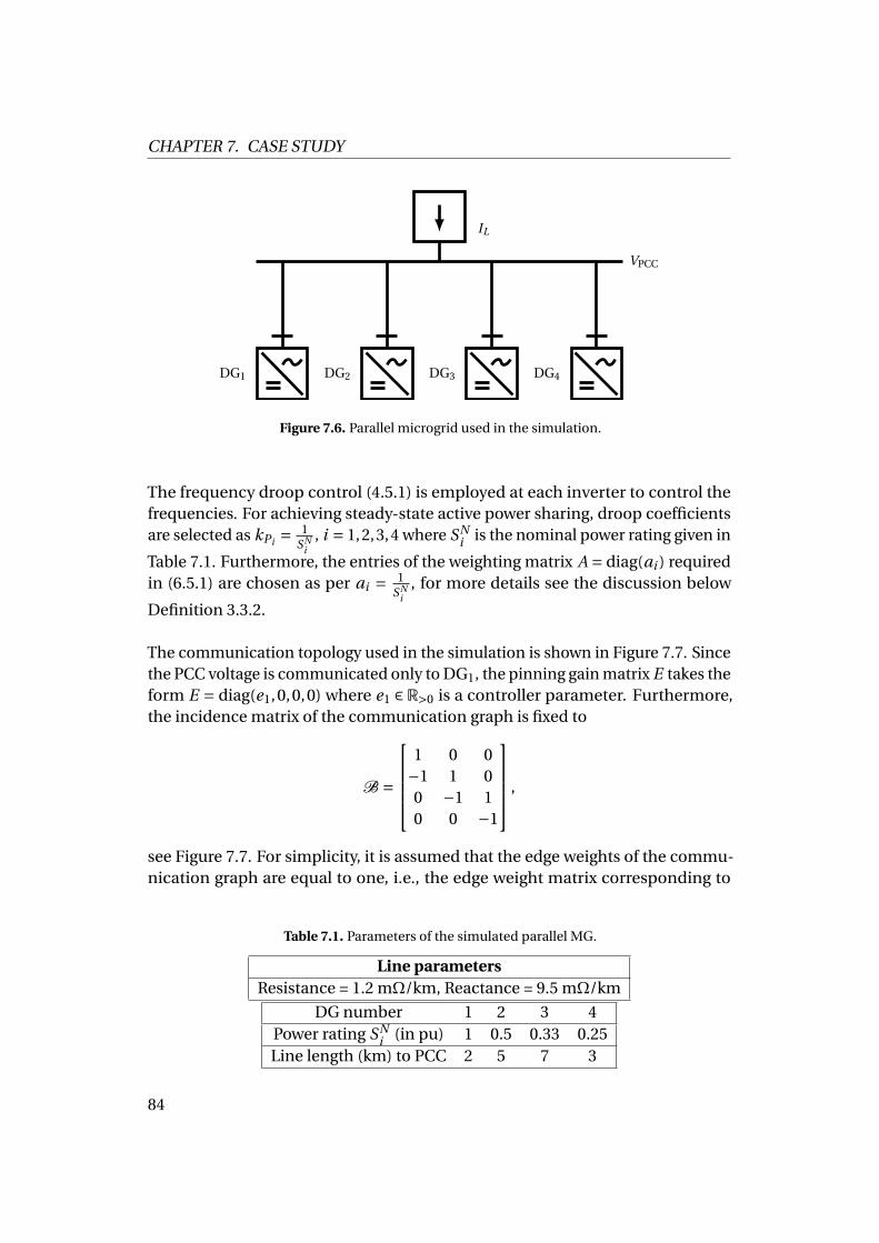
CHAPTER 7. CASE STUDY
VPCC
DG4DG3DG2DG1
IL
Figure 7.6. Parallel microgrid used in the simulation.
The frequency droop control (4.5.1) is employed at each inverter to control thefrequencies. For achieving steady-state active power sharing, droop coefficientsare selected as kPi = 1
SNi
, i = 1,2,3,4 where SNi is the nominal power rating given in
Table 7.1. Furthermore, the entries of the weighting matrix A = diag(ai ) requiredin (6.5.1) are chosen as per ai = 1
SNi
, for more details see the discussion below
Definition 3.3.2.
The communication topology used in the simulation is shown in Figure 7.7. Sincethe PCC voltage is communicated only to DG1, the pinning gain matrix E takes theform E = diag(e1,0,0,0) where e1 ∈ R>0 is a controller parameter. Furthermore,the incidence matrix of the communication graph is fixed to
B =
1 0 0−1 1 00 −1 10 0 −1
,
see Figure 7.7. For simplicity, it is assumed that the edge weights of the commu-nication graph are equal to one, i.e., the edge weight matrix corresponding to
Table 7.1. Parameters of the simulated parallel MG.
Line parametersResistance = 1.2 mΩ/km, Reactance = 9.5 mΩ/km
DG number 1 2 3 4Power rating SN
i (in pu) 1 0.5 0.33 0.25Line length (km) to PCC 2 5 7 3
84
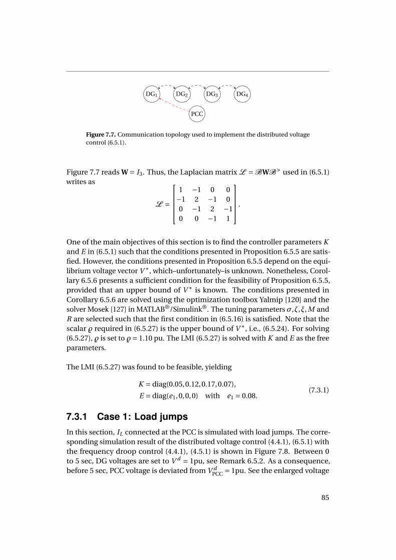
DG1 DG2 DG3 DG4
PCC
Figure 7.7. Communication topology used to implement the distributed voltagecontrol (6.5.1).
Figure 7.7 reads W = I3. Thus, the Laplacian matrix L =BWB> used in (6.5.1)writes as
L =
1 −1 0 0−1 2 −1 00 −1 2 −10 0 −1 1
.
One of the main objectives of this section is to find the controller parameters Kand E in (6.5.1) such that the conditions presented in Proposition 6.5.5 are satis-fied. However, the conditions presented in Proposition 6.5.5 depend on the equi-librium voltage vector V ∗, which–unfortunately–is unknown. Nonetheless, Corol-lary 6.5.6 presents a sufficient condition for the feasibility of Proposition 6.5.5,provided that an upper bound of V ∗ is known. The conditions presented inCorollary 6.5.6 are solved using the optimization toolbox Yalmip [120] and thesolver Mosek [127] in MATLAB®/Simulink®. The tuning parameters σ,ζ,ξ, M andR are selected such that the first condition in (6.5.16) is satisfied. Note that thescalar % required in (6.5.27) is the upper bound of V ∗, i.e., (6.5.24). For solving(6.5.27), % is set to %= 1.10 pu. The LMI (6.5.27) is solved with K and E as the freeparameters.
The LMI (6.5.27) was found to be feasible, yielding
K = diag(0.05,0.12,0.17,0.07),
E = diag(e1,0,0,0) with e1 = 0.08.(7.3.1)
7.3.1 Case 1: Load jumpsIn this section, IL connected at the PCC is simulated with load jumps. The corre-sponding simulation result of the distributed voltage control (4.4.1), (6.5.1) withthe frequency droop control (4.4.1), (4.5.1) is shown in Figure 7.8. Between 0to 5 sec, DG voltages are set to V d = 1pu, see Remark 6.5.2. As a consequence,before 5 sec, PCC voltage is deviated from V d
PCC = 1pu. See the enlarged voltage
85
CHAPTER 7. CASE STUDY
plot in Figure 7.8 before 5 sec. Furthermore, before 5 sec, it can be seen from theweighted reactive power plot in Figure 7.8 that reactive power sharing is poor.
The distributed voltage controller (6.5.1) is activated at 5 sec. After this, the PCCvoltage converges quickly to 1pu, see the enlarged plot in Figure 7.8 at 15 sec.Hence, (6.3.1), i.e., PCC voltage restoration. Furthermore, the weighted reactivepowers reach consensus, thereby confirming that the inverters share the load IL
in a proportional fashion, i.e., (6.3.2). Observe that the load jump starts at around45 sec. After the load jump, PCC voltage regulation (see the enlarged plot at 70sec) and reactive power sharing are re-established.
Furthermore, achieving PCC voltage regulation and reactive power sharing using(6.5.2) does not disturb the active power sharing provided by the frequency droopcontrol (4.5.1), see the weighted active power plot in Figure 7.8, thus confirmingthe operational compatibility of the distributed voltage controller with frequencydroop control.
7.3.2 Case 2: Continuously fluctuating load demandIn this section, a more realistic load profile provided by an industrial partner isused to simulate variations in IL . The simulation output is given in Figure 7.9.
Similar to the previous case, frequency droop control (4.5.1) is active from 0sec and the distributed voltage controller (6.5.1) is activated at 5 sec. From theenlarged voltage plots (at 15 sec and 70 sec) in Figure 7.9, it can be seen that thePCC voltage has converged to V d
PCC = 1pu. Furthermore, the weighted reactivepowers reach a consensus soon after 5 sec and are undisturbed throughout thesimulation time of 100 sec. Similar to the case of load jumps, the distributedvoltage controller does not affect active power sharing provided by frequencydroop control. See the weighted active power plot in Figure 7.9.
86
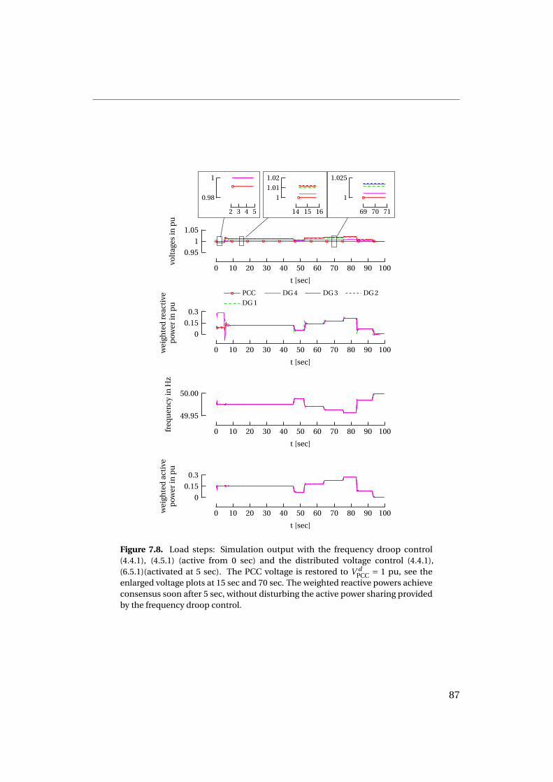
0 10 20 30 40 50 60 70 80 90 100
0.95
1
1.05
t [sec]
voltag
esin
pu
PCC DG4 DG3 DG2
DG1
0 10 20 30 40 50 60 70 80 90 100
0
0.15
0.3
t [sec]
weigh
tedreac
tive
pow
erin
pu
0 10 20 30 40 50 60 70 80 90 100
0
0.15
0.3
t [sec]
weigh
tedac
tive
pow
erin
pu
0 10 20 30 40 50 60 70 80 90 100
49.95
50.00
t [sec]
freq
uen
cyin
Hz
2 3 4 5
0.98
1
14 15 16
1
1.01
1.02
69 70 71
1
1.025
Figure 7.8. Load steps: Simulation output with the frequency droop control(4.4.1), (4.5.1) (active from 0 sec) and the distributed voltage control (4.4.1),(6.5.1)(activated at 5 sec). The PCC voltage is restored to V d
PCC = 1 pu, see theenlarged voltage plots at 15 sec and 70 sec. The weighted reactive powers achieveconsensus soon after 5 sec, without disturbing the active power sharing providedby the frequency droop control.
87
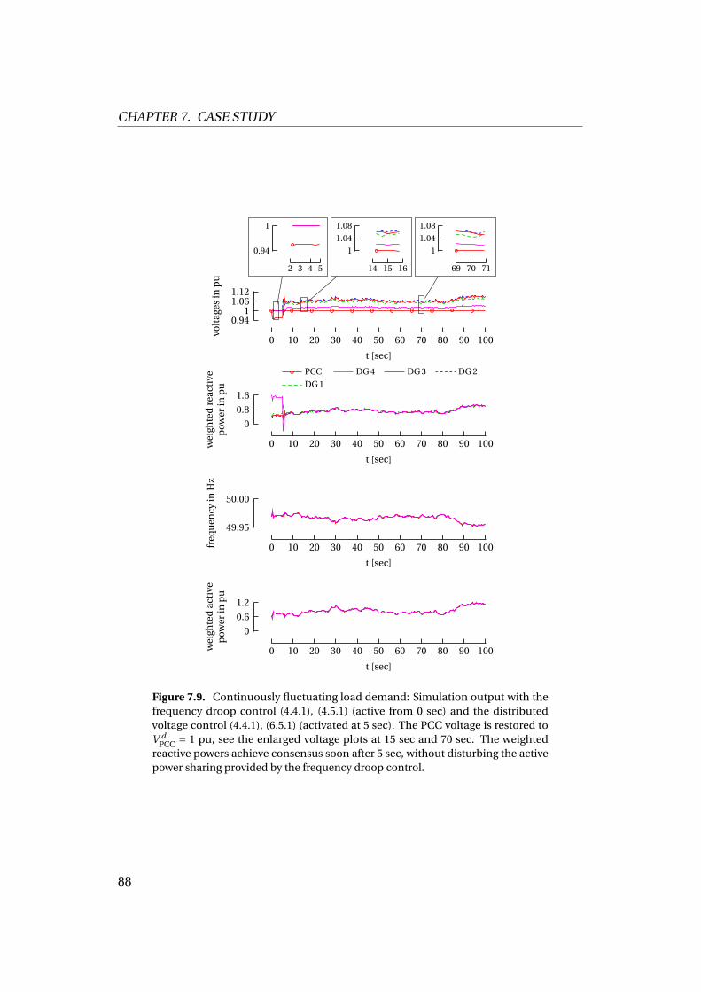
CHAPTER 7. CASE STUDY
0 10 20 30 40 50 60 70 80 90 100
0.941
1.061.12
t [sec]
voltag
esin
pu
PCC DG4 DG3 DG2
DG1
0 10 20 30 40 50 60 70 80 90 100
0
0.8
1.6
t [sec]
weigh
tedreac
tive
pow
erin
pu
0 10 20 30 40 50 60 70 80 90 100
0
0.6
1.2
t [sec]
weigh
tedac
tive
pow
erin
pu
0 10 20 30 40 50 60 70 80 90 100
49.95
50.00
t [sec]
freq
uen
cyin
Hz
2 3 4 5
0.94
1
14 15 16
1
1.04
1.08
69 70 71
1
1.04
1.08
Figure 7.9. Continuously fluctuating load demand: Simulation output with thefrequency droop control (4.4.1), (4.5.1) (active from 0 sec) and the distributedvoltage control (4.4.1), (6.5.1) (activated at 5 sec). The PCC voltage is restored toV d
PCC = 1 pu, see the enlarged voltage plots at 15 sec and 70 sec. The weightedreactive powers achieve consensus soon after 5 sec, without disturbing the activepower sharing provided by the frequency droop control.
88
7.4 SummaryIn this chapter, via simulation, robustness and performance of the control ap-proaches presented in Chapter 5 and Chapter 6 towards modeling errors anddisturbances have been studied.
For the considered case, the tuning criterion presented in Chapter 5 was foundto be feasible, confirming asymptotic convergence of the closed-loop system’strajectories with the GDAI control to a desired synchronized motion. Furthermore,the GDAI control performance has been compared with that of the DAI and thepinning control, confirming the results from Chapter 5 regarding steady-stateperformance of distributed frequency controllers in the presence of clock drifts.
In the second part of this chapter, the distributed voltage controller proposed inChapter 6 has been simulated together with the frequency droop control. Thetuning criterion presented in Chapter 6 has been used to select the parametersof the distributed voltage controller. The proposed controller’s performance hasbeen tested in the presence of small line resistances and load disturbances. Thesimulation results were found to be satisfactory.
89

Chapter 8
Discussion and conclusion
8.1 SummaryMicrogrids represent a promising solution to integrate RESs efficiently into themodern power grid. In this thesis, the concept of a microgrid has been introducedin Chapter 3. Then some of the important challenges in controlling a microgridhave been recalled in Chapter 3. In this work, some significant control prob-lems in an inverter-based islanded microgrid have been addressed, namely: (1)accurate network frequency restoration, (2) active power sharing, (3) load/PCCvoltage regulation, (4) reactive power sharing and (5) voltage stability. Clock driftis a non-negligible parameter uncertainty observed in microgrids, which has anadverse effect on the steady-state performance of primary and secondary fre-quency control. Thus, the first two objectives mentioned above were investigatedin the presence of clock drifts. These results have been summarized in Chapter 5.The last three control problems mentioned above were studied in the case of amicrogrid with parallel-connected inverters, i.e., a parallel microgrid, which isa commonly encountered microgrid application. The observations and resultsregarding voltage control have been presented in Chapter 6.
In Chapter 4, it has been shown that the steady-state active power sharing pro-vided by the standard frequency droop control is disturbed in the presence ofclock drifts. Similarly, it has been observed that the secondary frequency controlis also negatively affected by the presence of clock drifts. Inspired by this issue,in Chapter 5, the steady-state performance of various distributed secondary fre-quency controllers has been compared based on whether they achieve accuratenetwork frequency restoration and active power sharing in the presence of clockdrifts. These secondary controllers assume that the standard frequency droopcontrol is active at the primary control layer.
91
CHAPTER 8. DISCUSSION AND CONCLUSION
For the comparative study, a general distributed secondary control representationhas been proposed. This representation can be cast into some of the typicallyused distributed secondary frequency controllers like the DAI control [32, 51],the pinning control [40], and many more. Based on the proposed general con-trol representation, necessary and sufficient conditions for accurate frequencyrestoration and active power sharing have been derived with explicit considera-tion of clock drifts. The DAI controller was found to be not satisfying any of thederived conditions. However, the pinning controller seems to achieve accuratefrequency restoration, but not active power sharing. As a consequence of theobservations thus far, a novel secondary frequency control, termed as the gen-eralized distributed averaging integral (GDAI) control, has been proposed. TheGDAI control achieves the aforementioned control objectives in the presenceof clock drifts. The second part of Chapter 5 was focused on how to choose theparameters of the GDAI control such that the closed-loop system trajectories con-verge asymptotically to a desired synchronized motion. In this regard, a tuningcriterion, in the form of a set of LMIs, has been derived, which renders robuststability in the presence of unknown-bounded clock drift values.
In Chapter 6, the problem of voltage control in parallel microgrids has been inves-tigated. More precisely, two practically important control objectives of accuratereactive power sharing and voltage restoration at a joint load (at the PCC) in caseof a lossless inverter-based parallel microgrid has been investigated in detail. Atfirst, the existence and uniqueness properties of a positive voltage solution satis-fying the non-linear algebraic equations corresponding to the above-mentionedobjectives have been established. Later, a distributed voltage controller, which atsteady-state yields this unique voltage solution, has been proposed. In the secondpart of Chapter 6, a stability criterion that guarantees asymptotic convergence ofsolutions of the proposed distributed controller to the desired unique voltage so-lution has been derived. As it was found that the stability criterion depends on thevoltage equilibrium, a numerically verifiable condition to choose the parametersof the proposed controller has also been derived.
To validate the results and to check whether the presented control approacheswork well in the presence of typical modeling uncertainties and disturbances,results from Chapter 5 and Chapter 6 have been extensively tested via simulationin Chapter 7. The tuning criteria derived in Chapter 5 and Chapter 6 were foundto be feasible. Furthermore, the GDAI control proposed in Chapter 5 and thedistributed voltage control presented in Chapter 6 were found to be workingsatisfactorily in the presence of (small) line resistances and load variations.
92
8.2 DiscussionGenerally, distributed secondary frequency controllers achieve network frequencyrestoration in a fair manner [26]. Steady-state active power sharing is a niceproperty of such controllers [51, 110]. However, in the presence of clock drifts, thecommonly employed distributed frequency controllers fail to achieve accuratenetwork frequency restoration and active power sharing. Thus, a novel controlapproach termed as the generalized distributed averaging integral (GDAI) controlhas been proposed to address these issues in the presence of clock drifts. TheGDAI control is similar to the pinning control [13, Equation 47] (see also (5.3.10))and the DAI control [32, Equation 6] (see also (5.3.9)) with the difference thattogether with the mandatory secondary control input, internal frequency of aninverter should also be communicated with its neighbors, see (5.6.2). In practice,communicating such an extra signal is not an issue, since the topology used inthe GDAI control to communicate internal frequencies is the same as that usedfor communicating secondary control inputs. More precisely, the two Laplacianmatrices used in (5.6.2) are the same. Furthermore, the GDAI control only requiresthat a few grid-forming inverters (at least one) need an accurate clock, see (5.6.2).This avoids the requirement of a central unit communicating the global/accuratetime signal to all the grid-forming inverters connected in the network.
The distributed voltage control presented in Chapter 6 also requires a–sparsely–connected communication network for its operation. Furthermore, in a parallelmicrogrid setting, it is often the case that grid-forming inverters require PCCvoltage information for regulating the PCC voltage amplitude to the nominalvalue. In this regard, the proposed distributed voltage control (6.5.1) does notrequire that the PCC voltage be communicated to all the grid-forming invertersconnected in the parallel microgrid, hence avoiding an undesired one-to-allcommunication setup. This is a direct implication of the assumption that thecontroller parameter E used in (6.5.1) is a sparse diagonal positive semi-definitematrix.
In summary, various frequency and voltage control objectives in islanded mi-crogrids have been investigated in this thesis. The proposed frequency controlsolution accomplishes two important control objectives in an inverter-based mi-crogrid in the presence of clock drifts. The voltage control solution presented inthis thesis addresses three crucial control challenges in a microgrid with parallel-connected inverters.
93
CHAPTER 8. DISCUSSION AND CONCLUSION
8.3 Future research directionsIn this section, some possible extensions to this work are outlined.
Similar to any distributed control approach, the GDAI control proposed in Chap-ter 5 also requires a–sparse–communication network for its operation. As aconsequence, it is also prone to issues like communication delay and denial ofservice (DoS). Robustness of the DAI controller towards the above issues hasbeen recently investigated in [36, 65, 67]. Thus, inspired by [36, 65, 67], a possibleextension would be to explore the same with GDAI control. Another exciting ex-tension to the results presented in Chapter 5 is to quantify the robustness of GDAIcontrol towards exogenous disturbances, e.g., by calculating the L2 gain [50]. Thisproblem has been explored in the case of the DAI control in [65]. In practice, suchundesired external disturbances are widespread, and hence, the aforementionedstudy is very relevant. Furthermore, extending the stability analysis presentedin Chapter 5 to variable voltage amplitudes [30] is interesting. Another intrigu-ing idea is to design the GDAI control for microgrids with constant power loads,yielding a differential algebraic system. See, e.g. [25, 110], where the case of theDAI control with constant power loads has been explored.
Regarding Chapter 6, an immediate extension would be investigate existenceand uniqueness properties of voltage solution satisfying reactive power sharingand PCC voltage regulation with respect to a constant power load, or even aZIP1 load model. The next interesting step would be to design a distributedvoltage controller which drives the system equations to the unique solutionasymptotically.
Another idea would be to consider more than one parallel microgrid. Such asetting is especially relevant when it comes to a big battery power plant, wheremany inverter-interfaced batteries are present. More precisely, let there be m > 1parallel microgrids and each parallel microgrid has n > 1 inverters connected inparallel to a load bus. The load bus of a parallel microgrid is connected to theload bus of another parallel microgrid through a power line. In such a setting,designing voltage controllers such that voltage amplitudes at m number of loadbuses are regulated, and at the same time, the reactive power demand of thesystem loads is shared fairly between n ×m number of inverters is a vital controlobjective.
In a similar spirit to that of a bunch of parallel microgrids, consider an inverter-based microgrid with arbitrary topology. In such a meshed microgrid, often the
1ZIP stands for constant impedance/current/power, see [5, Chapter 3], [100, Chapter 3].
94
load buses and the inverter buses are different, see for example the benchmarkgrid presented in [128]. Furthermore, apart from normal loads, it is often thecase that there are critical (high-priority) loads also connected in a microgrid.Recall that grid-forming inverters are responsible for controlling such a networkto maintain a stable voltage equilibrium, achieve reactive power sharing, andrestore voltage amplitudes at the critical loads to the desired nominal value. Thelatter objective is fundamental because the loads are designed to work near theirnominal voltage value, and it is mostly the case that the loads are not controllable,e.g. ZIP loads. Therefore, designing a distributed voltage controller at each grid-forming inverter such that reactive power sharing, critical load voltage regulation,and voltage stability are ensured is interesting–albeit challenging–problem.
It is worthwhile to note that the system equations coupling reactive power andvoltage amplitudes in the case of a lossless meshed AC microgrid2 (see e.g., [24])is exactly the same as that of a meshed DC microgrid (see e.g., [121]) by replacingreactive power with active power (or simply power) and line susceptances withline conductances. Hence, the idea mentioned above for AC microgrids canbe extended to DC microgrids as well. Another interesting, but challenging,extension would be to combine the results in Chapter 5 and Chapter 6, i.e., acoupled distributed frequency and voltage control. Finally, exploring the resultsin Chapter 5 and Chapter 6 with consideration of power lines with mixed R/X(resistance/inductive reactance) ratio is also interesting.
In conclusion, there are many intriguing and challenging open problems re-garding the control of an islanded microgrid. The author hopes that the workpresented in this thesis helps to address at least some of these problems.
2Under the decoupling assumption, see Assumption 6.2.1.
95

Bibliography
[1] P. Kundur, Power system stability and control.McGraw-Hill, 1994.
[2] D. A. Jones, “Electrical engineering: the backbone ofsociety,” in IEE Proceedings A, Science, Measurementand Technology, vol. 138, no. 1. IET, 1991, pp. 1–10.
[3] P. Anderson and A. Fouad, Power System Control andStability. J.Wiley & Sons, 2002.
[4] J. J. Grainger and W. D. Stevenson, Power systemanalysis. McGraw-Hill New York, 1994, vol. 621.
[5] J. Machowski, J. Bialek, and J. Bumby, Power systemdynamics: stability and control. J.Wiley & Sons,2008.
[6] P. P. Varaiya, F. F. Wu, and J. W. Bialek, “Smart opera-tion of smart grid: Risk-limiting dispatch,” Proceed-ings of the IEEE, vol. 99, no. 1, pp. 40–57, 2011.
[7] K. Alanne and A. Saari, “Distributed energy genera-tion and sustainable development,” Renewable andSustainable Energy Reviews, vol. 10, no. 6, pp. 539–558, Dec. 2006.
[8] H. Farhangi, “The path of the smart grid,” IEEEPower and Energy Magazine, vol. 8, no. 1, pp. 18 –28,Jan./Feb. 2010.
[9] X. Fang, S. Misra, G. Xue, and D. Yang, “Smart grid -the new and improved power grid: a survey,” Com-munications Surveys & Tutorials, IEEE, vol. 14, no. 4,pp. 944–980, 2012.
[10] R. Lasseter, “Microgrids,” in IEEE Power EngineeringSociety Winter Meeting, 2002, vol. 1, 2002, pp. 305 –308 vol.1.
[11] T. Ackermann, G. Andersson, and L. Söder, “Dis-tributed generation: a definition,” Electric powersystems research, vol. 57, no. 3, pp. 195–204, 2001.
[12] W. D. Stevenson, Elements of power system analysis.McGraw Hill Kogakusha Limited, 1975.
[13] A. Bidram, F. Lewis, and A. Davoudi, “Distributedcontrol systems for small-scale power networks: Us-ing multiagent cooperative control theory,” IEEEControl Systems, vol. 34, no. 6, pp. 56–77, 2014.
[14] J. Rocabert, A. Luna, F. Blaabjerg, and P. Rodriguez,“Control of power converters in AC microgrids,”IEEE Transactions on Power Electronics, vol. 27,no. 11, pp. 4734–4749, Nov. 2012.
[15] J. Lopes, C. Moreira, and A. Madureira, “Defin-ing control strategies for microgrids islanded oper-ation,” IEEE Transactions on Power Systems, vol. 21,no. 2, pp. 916 – 924, May 2006.
[16] J. Schiffer, D. Zonetti, R. Ortega, A. Stankovic,J. Raisch, and T. Sezi, “Modeling of microgrids -from fundamental physics to phasors and voltagesources,” Automatica, vol. 74, no. 12, pp. 135–150,2016.
[17] T. Green and M. Prodanovic, “Control of inverter-based micro-grids,” Electric Power Systems Research,vol. Vol. 77, no. 9, pp. 1204–1213, July 2007.
[18] N. Hatziargyriou, H. Asano, R. Iravani, and C. Mar-nay, “Microgrids,” IEEE Power and Energy Magazine,vol. 5, no. 4, pp. 78–94, 2007.
[19] F. Katiraei, R. Iravani, N. Hatziargyriou, andA. Dimeas, “Microgrids management,” IEEE Powerand Energy Magazine, vol. 6, no. 3, pp. 54–65, 2008.
[20] R. Lasseter and P. Paigi, “Microgrid: a conceptual so-lution,” in Power Electronics Specialists Conference,2004. PESC 04. 2004 IEEE 35th Annual, vol. 6, June2004, pp. 4285 – 4290 Vol.6.
[21] C. A. Hans, P. Braun, J. Raisch, L. Grüne, andC. Reincke-Collon, “Hierarchical distributed modelpredictive control of interconnected microgrids,”IEEE Transactions on Sustainable Energy, vol. 10,no. 1, pp. 407–416, Jan 2019.
[22] J. Schiffer, R. Ortega, A. Astolfi, J. Raisch, andT. Sezi, “Conditions for stability of droop-controlledinverter-based microgrids,” Automatica, vol. 50,no. 10, pp. 2457–2469, 2014.
[23] J. Schiffer, “Stability and power sharing in micro-grids,” Ph.D. dissertation, Technische UniversitätBerlin, 2015.
[24] J. W. Simpson-Porco, F. Dörfler, and F. Bullo, “Volt-age stabilization in microgrids via quadratic droopcontrol,” IEEE Transactions on Automatic Control,vol. 62, no. 3, pp. 1239 – 1253, March 2017.
[25] C. D. Persis, N. Monshizadeh, J. Schiffer, andF. Dörfler, “A Lyapunov approach to control ofmicrogrids with a network-preserved differential-algebraic model,” in IEEE 55th Conference on Deci-sion and Control (CDC), 2016, pp. 2595 – 2600.
97
Bibliography
[26] F. Dörfler, J. W. Simpson-Porco, and F. Bullo, “Break-ing the hierarchy: Distributed control & economicoptimality in microgrids,” IEEE Transactions onControl of Network Systems, vol. 3, no. 3, pp. 241–253, Sept. 2016.
[27] J. Schiffer, T. Seel, J. Raisch, and T. Sezi, “Voltage sta-bility and reactive power sharing in inverter-basedmicrogrids with consensus-based distributed volt-age control,” IEEE Transactions on Control SystemsTechnology, vol. 24, no. 1, pp. 96–109, 2016.
[28] N. Bretas and L. F. C. Alberto, “Lyapunov functionfor power systems with transfer conductances: ex-tension of the invariance principle,” IEEE Transac-tions on Power Systems, vol. 18, no. 2, pp. 769–777,2003.
[29] R. Ortega, M. Galaz, A. Astolfi, Y. Sun, and T. Shen,“Transient stabilization of multimachine power sys-tems with nontrivial transfer conductances,” IEEETransactions on Automatic Control, vol. 50, no. 1, pp.60 – 75, jan. 2005.
[30] C. D. Persis and N. Monshizadeh, “Bregman storagefunctions for microgrid control,” IEEE Transactionson Automatic Control, vol. 63, no. 1, pp. 53–68, Jan.2017.
[31] F. Dörfler and F. Bullo, “Synchronization and tran-sient stability in power networks and non-uniformKuramoto oscillators,” SIAM Journal on Control andOptimization, vol. 50, no. 3, pp. 1616–1642, 2012.
[32] J. W. Simpson-Porco, Q. Shafiee, F. Dörfler, J. C.Vasquez, J. M. Guerrero, and F. Bullo, “Secondary fre-quency and voltage control of islanded microgridsvia distributed averaging,” IEEE Transactions on In-dustrial Electronics, vol. 62, pp. 7025–7038, 2015.
[33] J. W. Simpson-Porco, F. Dörfler, and F. Bullo, “Volt-age collapse in complex power grids,” Nature Com-munications, vol. 7, no. 10790, Feb. 2016.
[34] Q.-C. Zhong, “Robust droop controller for accu-rate proportional load sharing among inverters op-erated in parallel,” IEEE Transactions on IndustrialElectronics, vol. 60, no. 4, pp. 1281–1290, 2013.
[35] C. K. Sao and P. W. Lehn, “Autonomous load sharingof voltage source converters,” IEEE Transactions onPower Delivery, vol. 20, no. 2, pp. 1009–1016, 2005.
[36] J. Schiffer, F. Dörfler, and E. Fridman, “Robustnessof distributed averaging control in power systems:Time delays & dynamic communication topology,”Automatica, vol. 80, pp. 261–271, 2017.
[37] F. Guo, C. Wen, J. Mao, and Y. D. Song, “Distributedsecondary voltage and frequency restoration con-trol of droop-controlled inverter-based microgrids,”vol. 62, pp. 4355–4368, 2015.
[38] M. Chandorkar, D. Divan, and R. Adapa, “Control ofparallel connected inverters in standalone AC sup-ply systems,” IEEE Transactions on Industry Appli-cations, vol. 29, no. 1, pp. 136 –143, Jan./Feb. 1993.
[39] J. Guerrero, J. Vasquez, J. Matas, L. de Vicuna,and M. Castilla, “Hierarchical control of droop-controlled AC and DC microgrids: A general ap-proach toward standardization,” IEEE Transactionson Industrial Electronics, vol. 58, no. 1, pp. 158 –172,jan. 2011.
[40] A. Bidram and A. Davoudi, “Hierarchical structureof microgrids control system,” IEEE Transactions onSmart Grid, vol. 3, no. 4, pp. 1963–1976, 2012.
[41] H. Kopetz, Real-time systems: design principles fordistributed embedded applications. Springer, 2011.
[42] Anritsu, “Understanding frequency accuracy incrystal controlled instruments - application note,”Anritsu EMEA Ltd., Tech. Rep., 2001.
[43] J. Schiffer, C. A. Hans, T. Kral, R. Ortega, andJ. Raisch, “Modeling, analysis, and experimental val-idation of clock drift effects in low-inertia power sys-tems,” IEEE Transactions on Industrial Electronics,vol. 64, pp. 5942 – 5951, 2017.
[44] M. Castilla, A. Camacho, P. Martí, M. Velasco,and M. M. Ghahderijani, “Impact of clock driftson communication-free secondary control schemesfor inverter-based islanded microgrids,” IEEE Trans-actions on Industrial Electronics, vol. 65, no. 6, pp.4739 – 4749, June 2017.
[45] M. Castilla, A. Camacho, J. Miret, M. Velasco, andP. Marti, “Local secondary control for inverter-based islanded microgrids with accurate active-power sharing under high load conditions,” IEEETransactions on Industrial Electronics, vol. 66, no. 4,pp. 2529 – 2539, June 2018.
[46] J. T. Martínez, M. Castilla, J. Miret, M. M. Ghahder-ijani, and J. M. Rey, “Experimental study of clockdrift impact over droop-free distributed control forindustrial microgrids,” in 43rd Annual Conference ofthe IEEE Industrial Electronics Society , IECON, 2017,pp. 2479 – 2484.
[47] C. X. Rosero, P. Martí, M. Velasco, M. Castilla,J. Miret, and A. Camacho, “Consensus for activepower sharing and frequency restoration in is-landed microgrids subject to drifting clocks,” inIEEE 26th International Symposium on IndustrialElectronics (ISIE), 2017, pp. 70 – 75.
[48] P. Marti, J. Torres-Martinez, C. X. Rosero, M. Velasco,J. Miret, and M. Castilla, “Analysis of the effect ofclock drifts on frequency regulation and power shar-ing in inverter-based islanded microgrids,” IEEETransactions on Power Electronics, vol. 33, no. 12, pp.10 363 – 10 379, Dec. 2018.
98
[49] H. K. Khalil, Nonlinear systems. Prentice Hall, 2002,vol. 3.
[50] A. van der Schaft, L2-Gain and Passivity Techniquesin Nonlinear Control. Springer, 2000.
[51] C. Zhao, E. Mallada, and F. Dörfler, “Distributed fre-quency control for stability and economic dispatchin power networks,” in American Control Conference(ACC), July 2015, pp. 2359 – 2364.
[52] M. Andreasson, H. Sandberg, D. V. Dimarogonas,and K. H. Johansson, “Distributed integral action:Stability analysis and frequency control of powersystems,” in 51st Conference on Decision and Con-trol, Maui, HI, USA, 2012.
[53] C. Godsil and G. Royle, Algebraic Graph Theory.Springer, 2001.
[54] M. Mesbahi and M. Egerstedt, Graph theoretic meth-ods in multiagent networks. Princeton UniversityPress, 2010.
[55] R. Diestel, Graph Theory, 4th ed. Springer, 2010.
[56] R. Olfati-Saber, J. A. Fax, and R. M. Murray, “Con-sensus and cooperation in networked multi-agentsystems,” Proceedings of the IEEE, vol. 95, no. 1, pp.215–233, 2007.
[57] E. Weitenberg, Y. Jiang, C. Zhao, E. Mallada, C. D.Persis, and F. Dörfler, “Robust decentralized sec-ondary frequency control in power systems: Mer-its and trade-offs,” IEEE Transactions on AutomaticControl (Early Access), Dec. 2017.
[58] J. Schiffer, R. Ortega, C. Hans, and J. Raisch, “Droop-controlled inverter-based microgrids are robust toclock drifts,” American Control Conference, pp. 2341– 2346, 2015.
[59] M. A. Pai, Energy function analysis for power systemstability. Kluwer academic publishers, 1989.
[60] E. Planas, A. Gil-de Muro, J. Andreu, I. Kortabarria,and I. Martínez de Alegría, “General aspects, hierar-chical controls and droop methods in microgrids: Areview,” Renewable and Sustainable Energy Reviews,vol. 17, pp. 147–159, 2013.
[61] C. A. Hans, V. Nenchev, J. Raisch, and C. Reincke-Collon, “Minimax model predictive operation con-trol of microgrids,” 2014, 19th IFAC World Congress,Cape Town, South Africa.
[62] J. W. Simpson-Porco, F. Dörfler, and F. Bullo,“Synchronization and power sharing for droop-controlled inverters in islanded microgrids,” Auto-matica, vol. 49, no. 9, pp. 2603 – 2611, 2013.
[63] J. Guerrero, P. Loh, M. Chandorkar, and T. Lee, “Ad-vanced control architectures for intelligent micro-grids – part I: Decentralized and hierarchical con-trol,” IEEE Transactions on Industrial Electronics,vol. 60, no. 4, pp. 1254–1262, 2013.
[64] X. Fu, F. Dörfler, and M. R. Jovanovic, “Topologyidentification and design of distributed integral ac-tion in power networks,” in American Control Con-ference (ACC), 2016, pp. 5921 – 5926.
[65] S. Alghamdi, J. Schiffer, and E. Fridman, “Dis-tributed secondary frequency control design for mi-crogrids: Trading off l2-gain performance and com-munication efforts under time-varying delays,” inEuropean Control Conference, 2018.
[66] S. Alghamdi, J. Schiffer, and E. Fridman, “Synthesiz-ing sparse and delay-robust distributed secondaryfrequency controllers for microgrids,” IEEE Transac-tions on Control Systems Technology, 2019.
[67] E. Weitenberg, C. D. Persis, and N. Monshizadeh,“Exponential convergence under distributed averag-ing integral frequency control,” Automatica, vol. 98,pp. 103–113, Dec. 2018.
[68] C. D. Persis and P. Tesi, “Input-to-state stabilizingcontrol under denial-of-service,” IEEE Transactionson Automatic Control, vol. 60, no. 11, Nov. 2015.
[69] F. Dörfler, M. R. Jovanovic, M. Chertkov, and F. Bullo,“Sparsity-promoting optimal wide-area control ofpower networks,” IEEE Transactions on Power Sys-tems, vol. 29, no. 5, Sept. 2014.
[70] C. X. Rosero, H. Carrasco, M. Velasco, and P. Martí,“Impact of clock drifts on active power sharing andfrequency regulation in distributed-averaging sec-ondary control for islanded microgrids,” in Interna-tional Autumn Meeting on Power, Electronics andComputing, 2017, pp. 1 – 6.
[71] R. R. Kolluri, I. Mareels, T. Alpcan, M. Brazil,J. de Hoog, and D. A. Thomas, “Power sharing in an-gle droop controlled microgrids,” IEEE Transactionson Power Systems, vol. 32, no. 6, pp. 4743 – 4751, Nov.2017.
[72] R. Majumder, G. Ledwich, A. Ghosh, S. Chakrabarti,and F. Zare, “Droop control of converter-interfacedmicrosources in rural distributed generation,” IEEETransactions on Power Delivery, vol. 25, no. 4, pp.2768–2778, Oct. 2010.
[73] R. R. Kolluri, I. Mareels, T. Alpcan, M. Brazil,J. de Hoog, and D. A. Thomas, “Stability and activepower sharing in droop controlled inverter inter-faced microgrids: Effect of clock mismatches,” Au-tomatica, vol. 93, pp. 469–475, 2018.
[74] R. Solis, V. S. Borkar, and P. R. Kumar, “A new dis-tributed time synchronization protocol for multi-hop wireless networks,” in CDC, 2006, pp. 2734 –2739.
99
Bibliography
[75] L. Schenato and F. Fiorentin, “Average timesynch:A consensus-based protocol for clock synchro-nization in wireless sensor networks,” Automatica,vol. 47, no. 9, pp. 1878–1886, 2011.
[76] J. Guerrero, L. Garcia de Vicuna, J. Matas, M. Castilla,and J. Miret, “Output impedance design of parallel-connected UPS inverters with wireless load-sharingcontrol,” IEEE Transactions on Industrial Electron-ics, vol. 52, no. 4, pp. 1126 – 1135, aug. 2005.
[77] J. M. Guerrero, J. C. Vasquez, J. Matas, M. Castilla,and L. G. de Vicuna, “Control strategy for flexiblemicrogrid based on parallel line-interactive UPS sys-tems,” IEEE Transactions on Industrial Electronics,2009.
[78] J. Guerrero, J. Matas, L. G. de Vicuna, M. Castilla,and J. Miret, “Decentralized control for parallel op-eration of distributed generation inverters using re-sistive output impedance,” IEEE Transactions on In-dustrial Electronics, vol. 54, no. 2, pp. 994 –1004,April 2007.
[79] A. Tuladhar, H. Jin, T. Unger, and K. Mauch, “Controlof parallel inverters in distributed AC power systemswith consideration of line impedance effect,” IEEETransactions on Industry Applications, vol. 36, no. 1,pp. 131 –138, Jan./Feb. 2000.
[80] J. Guerrero, J. Matas, L. de Vicuna, M. Castilla, andJ. Miret, “Wireless-control strategy for parallel op-eration of distributed-generation inverters,” IEEETransactions on Industrial Electronics, vol. 53, no. 5,pp. 1461 –1470, oct. 2006.
[81] M. Marwali, J.-W. Jung, and A. Keyhani, “Control ofdistributed generation systems - part ii: Load shar-ing control,” IEEE Transactions on Power Electronics,vol. 19, no. 6, pp. 1551 – 1561, Nov. 2004.
[82] U. Borup, F. Blaabjerg, and P. Enjeti, “Sharing of non-linear load in parallel-connected three-phase con-verters,” IEEE Transactions on Industry Applications,vol. 37, no. 6, pp. 1817 – 1823, Nov/Dec 2001.
[83] E. Coelho, P. Cortizo, and P. Garcia, “Small-signalstability for parallel-connected inverters in stand-alone AC supply systems,” IEEE Transactions on In-dustry Applications, vol. 38, no. 2, pp. 533 –542,Mar./Apr. 2002.
[84] R. A. Horn and C. R. Johnson, Matrix analysis. Cam-bridge university press, 2012.
[85] R. Olfati-Saber and R. M. Murray, “Consensus prob-lems in networks of agents with switching topologyand time-delays,” IEEE Transactions on AutomaticControl, vol. 49, no. 9, pp. 1520–1533, Sept. 2004.
[86] A. Jadbabaie, J. Lin, and A. S. Morse, “Coordinationof groups of mobile autonomous agents using near-est neighbor rules,” IEEE Transactions on AutomaticControl, vol. 48, no. 6, pp. 988–1001, June 2003.
[87] W. Ren and R. W. Beard, “Consensus seeking inmulti-agent systems under dynamically changinginteraction topologies,” IEEE Transactions on Auto-matic Control, vol. 50, no. 5, p. 655–661, May 2005.
[88] L. Moreau, “Stability of multi-agent systems withtime-dependent communication links,” IEEE Trans-actions on Automatic Control, vol. 50, no. 2, pp. 169–182, Feb. 2005.
[89] J. D. Glover, M. S. Sarma, and T. J. Overbye, Powersystem analysis and design. Cengage Learning,2011.
[90] H. Akagi, E. H. Watanabe, and M. Aredes, Instanta-neous power theory and applications to power con-ditioning. John Wiley & Sons, 2007.
[91] F. Dörfler and F. Bullo, “Kron reduction of graphswith applications to electrical networks,” IEEETransactions on Circuits and Systems I: Regular Pa-pers, vol. 60, no. 1, pp. 150–163, Jan. 2013.
[92] N. Pogaku, M. Prodanovic, and T. Green, “Model-ing, analysis and testing of autonomous operationof an inverter-based microgrid,” IEEE Transactionson Power Electronics, vol. 22, no. 2, pp. 613 –625,March 2007.
[93] S. Chowdhury and P. Crossley, Microgrids and activedistribution networks. The Institution of Engineer-ing and Technology, 2009.
[94] IEEE PES Task Force on Microgrid Stability Analysisand Modeling, “Microgrid stability definitions, anal-ysis, and modeling,” IEEE Power and Energy Society,Tech. Rep., June 2018.
[95] N. Lidula and A. Rajapakse, “Microgrids research:A review of experimental microgrids and test sys-tems,” Renewable and Sustainable Energy Reviews,vol. 15, no. 1, pp. 186–202, 2011.
[96] O. Palizban, K. Kauhaniemi, and J. M. Guerrero,“Microgrids in active network management—Part I:hierarchical control, energy storage, virtual powerplants, and market participation,” Renewable andSustainable Energy Reviews, 2014.
[97] B. K. Poolla, S. Bolognani, and F. Dörfler, “Optimalplacement of virtual inertia in power grids,” Auto-matica, vol. 62, no. 12, pp. 6209 – 6220, Dec. 2017.
[98] B. K. Poolla, D. Gross, T. Borsche, S. Bolognani, andF. Dörfler, Virtual inertia placement in electric powergrids. Springer, 2018, vol. 162.
100
[99] P. Kundur, J. Paserba, V. Ajjarapu, G. Andersson,A. Bose, C. Canizares, N. Hatziargyriou, D. Hill,A. Stankovic, C. Taylor, T. Van Cutsem, and V. Vittal,“Definition and classification of power system sta-bility IEEE/CIGRE joint task force on stability termsand definitions,” IEEE Transactions on Power Sys-tems, vol. 19, no. 3, pp. 1387–1401, Aug. 2004.
[100] T. Van Cutsem and C. Vournas, Voltage stability ofelectric power systems. Springer, 1998, vol. 441.
[101] C. A. Hans, P. Sopasakis, A. Bemporad, J. Raisch,and C. Reincke-Collon, “Scenario-based model pre-dictive operation control of islanded microgrids,”in 54th IEEE Conference on Decision and Control(CDC), 2015, pp. 3272 – 3277.
[102] N. Mohan and T. M. Undeland, Power electronics:converters, applications, and design. John Wiley &Sons, 2007.
[103] R. Teodorescu, M. Liserre, and P. Rodriguez, Gridconverters for photovoltaic and wind power systems.John Wiley & Sons, 2011, vol. 29.
[104] Q.-C. Zhong and T. Hornik, Control of power invert-ers in renewable energy and smart grid integration.John Wiley & Sons, 2012.
[105] R. W. Erickson and D. Maksimovic, Fundamentals ofpower electronics. Springer, 2001.
[106] X. Wang, J. M. Guerrero, F. Blaabjerg, and Z. Chen, “Areview of power electronics based microgrids,” Jour-nal of Power Electronics, vol. 12, no. 1, pp. 181–192,2012.
[107] J. T. Bialasiewicz, “Renewable energy systems withphotovoltaic power generators: Operation and mod-eling,” IEEE Transactions on Industrial Electronics,vol. 55, no. 7, p. 2752–2758, Jul. 2008.
[108] A. Engler, “Applicability of droops in low voltagegrids,” International Journal of Distributed EnergyResources, vol. 1, no. 1, pp. 1–6, 2005.
[109] R. Ortega, A. van der Schaft, B. Maschke, and G. Es-cobar, “Interconnection and damping assignmentpassivity-based control of port-controlled Hamilto-nian systems,” Automatica, vol. 38, no. 4, pp. 585–596, April 2002.
[110] J. Schiffer and F. Dörfler, “On stability of adistributed averaging PI frequency and activepower controlled differential-algebraic power sys-tem model,” in European Control Conference (ECC),2016, pp. 1487 – 1492.
[111] J. Simpson-Porco, “A theory of solvability for losslesspower flow equations – part I: Fixed-point powerflow,” IEEE Transactions on Control of Network Sys-tems, vol. 5, no. 3, pp. 1361 – 1372, Sept. 2017.
[112] Y. W. Li and C.-N. Kao, “An accurate power con-trol strategy for power-electronics-interfaced dis-tributed generation units operating in a low-voltagemultibus microgrid,” IEEE Transactions on PowerElectronics, vol. 24, no. 12, pp. 2977 –2988, Dec.2009.
[113] L. Schenato and G. Gamba, “A distributed consen-sus protocol for clock synchronization in wirelesssensor network,” in 46th IEEE Conference on Deci-sion and Control. IEEE, 2007, pp. 2289–2294.
[114] Y. Kikuya, S. M. Dibaji, and H. Ishii, “Fault toler-ant clock synchronization over unreliable channelsin wireless sensor networks,” IEEE Transactions onControl of Network Systems, vol. 5, no. 4, pp. 1551 –1562, July 2017.
[115] Y. Kadowaki and H. Ishii, “Event-based distributedclock synchronization for wireless sensor networks,”IEEE Transactions on Automatic Control, vol. 60,no. 8, pp. 2266 – 2271, August 2015.
[116] A. Krishna, C. A. Hans, J. Schiffer, J. Raisch, andT. Kral, “Steady state evaluation of distributed sec-ondary frequency control strategies for microgridsin the presence of clock drifts,” in 25th Mediter-ranean Conference on Control and Automation(MED), 2017, pp. 508 – 515.
[117] A. Krishna, J. Schiffer, and J. Raisch, “A consensus-based control law for accurate frequency restora-tion and power sharing in microgrids in the pres-ence of clock drifts,” in European Control Confer-ence (ECC), 2018, pp. 2575 – 2580.
[118] A. Krishna, J. Schiffer and J. Raisch, “Distributedsecondary frequency control in microgrids: Robust-ness and steady-state performance in the presenceof clock drifts,” European Journal of Control (Inpress), 2019.
[119] J. Schiffer, D. Goldin, J. Raisch, and T. Sezi, “Syn-chronization of droop-controlled microgrids withdistributed rotational and electronic generation,” in52nd Conference on Decision and Control, Florence,Italy, 2013, pp. 2334–2339.
[120] J. Löfberg, “YALMIP : A toolbox for modeling and op-timization in MATLAB,” in IEEE International Sym-posium on Computer Aided Control Systems Design,Sept. 2004, pp. 284 –289.
[121] C. D. Persis, E. R.A.Weitenberg, and F. Dörfler, “Apower consensus algorithm for dc microgrids,” Au-tomatica, vol. 89, pp. 364–375, Mar. 2018.
[122] A. Krishna, J. Schiffer, N. Monshizadeh, andJ. Raisch, “A consensus-based voltage control forreactive power sharing and pcc voltage regulationin microgrids with parallel-connected inverters,” inEuropean Control Conference, 2019.
101
Bibliography
[123] S. Bolognani, G. Cavraro, and S. Zampieri, “A dis-tributed feedback control approach to the optimalreactive power flow problem,” in Control of Cyber-Physical Systems. Springer, 2013, pp. 259–277.
[124] “DIN EN 50160:2010 - Merkmale der Spannung inöffentlichen Elektrizitätsversorgungsnetzen, (engl:"Voltage characteristics of electricity supplied bypublic distribution networks),” february 2011.
[125] Plexim GmbH, “Plecs software, www.plexim.com,”2013.
[126] S. Golestan, M. Monfared, and F. D. Freijedo,“Design-oriented study of advanced synchronousreference frame phase-locked loops,” IEEE Transac-tions on Power Electronics, vol. 28, pp. 765–778, Feb.2012.
[127] Mosek, “The mosek optimization toolbox,www.mosek.com.”
[128] K. Rudion, A. Orths, Z. Styczynski, and K. Strunz,“Design of benchmark of medium voltage distribu-tion network for investigation of DG integration,”in IEEE Power Engineering Society General Meeting,2006.
102