Embed Size (px)
Citation preview
SHORT COURSE
Regression Models for Count Data:beyond Poisson model
Wagner Hugo BonatWalmes Marques ZevianiEduardo Elias Ribeiro Jr
Statistics and Geoinformation LaboratoryFederal University of Paranahttp://leg.ufpr.br

Regression Models for Count Data:beyond Poisson model
Wagner Hugo Bonat1 3
www.leg.ufpr.br/~wagner
Walmes Marques Zeviani1 3
www.leg.ufpr.br/~walmes
Eduardo Elias Ribeiro Jr2 3
www.leg.ufpr.br/~eduardojr
1Department of Statistics (DEST)Federal University of Paraná (UFPR)
2Department of Exact Sciences (LCE)ESALQ - University of São Paulo (ESALQ-USP)
3Statistics and Geoinformation Laboratory (LEG)http://www.leg.ufpr.br
Supplementary content: http://www.leg.ufpr.br/rmcdContact: [email protected]
XV EMR - Brazilian Regression Model SchoolGoiânia - Goiás, BrazilMarch 26 to 29, 2017

Contents
Preface 3
1 Introduction 5
2 Count distributions: properties and regression models 92.1 Poisson distribution . . . . . . . . . . . . . . . . . . . . . . . . 92.2 Gamma-Count distribution . . . . . . . . . . . . . . . . . . . 102.3 Poisson-Tweedie distribution . . . . . . . . . . . . . . . . . . 132.4 COM-Poisson distribution . . . . . . . . . . . . . . . . . . . . 162.5 Comparing count distributions . . . . . . . . . . . . . . . . . 18
3 The method of maximum likelihood 23
4 Models specified by second-moment assumptions 274.1 Extended Poisson-Tweedie model . . . . . . . . . . . . . . . 274.2 Estimation and Inference . . . . . . . . . . . . . . . . . . . . . 29
5 Applications 335.1 Cotton Bolls . . . . . . . . . . . . . . . . . . . . . . . . . . . . 335.2 Soybean pod and beans . . . . . . . . . . . . . . . . . . . . . 445.3 Number of vehicle claims . . . . . . . . . . . . . . . . . . . . . 615.4 Radiation-induced chromosome aberration counts . . . . . . 72
1

2 CONTENTS
Preface
The main goal of this material is to provide a technical support for thestudents attending the course ”Regression models for count data: beyondthe Poisson model“, given as part of the XV Brazilian School of Regressionmodels - March/2017 in Goiânia, Goiás, Brazil.
The main goal of this course is to present a wide range of statistical models todeal with count data. We focus on parametric and second-moment specifiedmodels. We shall present the model specification along with strategies formodel fitting and associated R(R Core Team, 2015) code. Furthermore, thisbook-course and supplementary materials, such as R code and data setsare available for the students on the web page http://cursos.leg.ufpr.br/rmcd.
We intend to keep the course in a level suitable for bachelor students whoalready attended a course on generalized linear models (Nelder and Wed-derburn, 1972). However, since the course also covers updated topics, it canbe of interest of postgraduate students and researches in general.
We designed the course for three hours of tuition. In the first part of thecourse, we shall present the analysis of count data based on fully parametricmodels. After a brief introduction and motivation on count data, we presentthe Poisson, Gamma-Count, Poisson-Tweedie and COM-Poisson distribu-tions. We explore their properties through a consideration of dispersion,zero-inflated and heavy tail indexes. Furthermore, the estimation and infer-ence for these models based on the likelihood paradigm is discussed alongwith the associated R code and worked examples.
In the second part of the course, we provide a brief introduction to theestimating function approach (Jørgensen and Knudsen, 2004, ; Bonat andJørgensen, 2016) and discuss models based on second-moment assumptionsin the style of Wedderburn (1974). In particular, we focus on the recentlyproposed Extended Poisson-Tweedie model (Bonat et al., 2016) and its specialcase the quasi-Poisson model. The estimating function approach adopted for
3

4 CONTENTS
estimation and inference is presented along with R code and data examples.The use of the R package mcglm (Bonat, 2016) is discussed for fitting theextended Poisson-Tweedie model.
We acknowledge our gratitude to the scientific committee of XV Brazilianregression model school for this opportunity.
Department of Statistics, Paraná Federal University, Curitiba, PR, Brazil.
March 27, 2017.
Chapter 1
Introduction
The analysis of count data has received attention from the statistical commu-nity in the last four decades. Since the seminal paper published by Nelderand Wedderburn (1972), the class of generalized linear models (GLMs) havea prominent role for regression modelling of normal and non-normal data.GLMs are fitted by a simple and efficient Newton scoring algorithm relyingonly on second-moment assumptions for estimation and inference. Fur-thermore, the theoretical background for GLMs is well established in theclass of dispersion models (Jørgensen, 1987, 1997) as a generalization of theexponential family of distributions.
In spite of the flexibility of the GLM class, the Poisson distribution is the onlychoice for the analysis of count data in this framework. Thus, in practicethere is probably an over-emphasis on the use of the Poisson distributionfor count data. A well known limitation of the Poisson distribution is itsmean and variance relationship, which implies that the variance equalsthe mean, referred to as equidispersion. In practice, however, count datacan present other features, namely underdispersion (mean > variance) andoverdispersion (mean < variance). There are many different possible causesfor departures from the equidispersion. Furthermore, in practical dataanalysis a number of these could be involved.
One possible cause of under/overdispersion is departure from the Pois-son process. It is well known that the Poisson counts can be interpretedas the number of events in a given time interval where the arrival’s timesare exponential distributed. In the cases where this assumption is violatedthe resulting counts can be under or overdispersed (Zeviani et al., 2014).Another possibility and probably more frequent cause of overdispersion isunobserved heterogeneity of experimental units. It can be due, for exam-
5
6 CHAPTER 1. INTRODUCTION
ple, to correlation between individual responses, cluster sampling, omittedcovariates and others.
In general, these departures from the Poisson distribution are manifested inthe raw data as a zero-inflated or heavy-tailed count distribution. It is im-portant to discuss the consequences of failing to take into account the underor overdispersion when analysing count data. In the case of overdispersion,the standard errors associated with the regression coefficients calculatedunder the Poisson assumption are too optimistic and associated hypothe-sis tests will tend to give false positive results by incorrectly rejecting nullhypotheses. The opposite situation will appear in case of underdisperseddata. In both cases, the Poisson model provides unreliable standard errorsfor the regression coefficients and hence potentially misleading inferences.However, the regression coefficients are still consistently estimated.
The strategies for constructing alternative count distributions are relatedwith the causes of the non-equidispersion. When departures from the Pois-son process are plausible the class of duration dependence models (Winkel-mann, 2003) can be employed. This class of models changes the distributionof the time between events from the exponential to more general distribu-tions, such as gamma and inverse Gaussian. In this course, we shall discussone example of this approach, namely, the Gamma-Count distribution (Ze-viani et al., 2014). This distribution assumes that the time between eventsis gamma distributed, thus it can deal with under, equi and overdispersedcount data.
On the other hand, if unobserved heterogeneity is present its in generalimplies extra variability and consequently overdispersed count data. In thiscase, a Poisson mixtures is commonly applied. This approach consists of in-clude random effects on the observation level, and thus take into account theunobserved heterogeneity. Probably, the most popular example of this ap-proach is the negative binomial model, that corresponds to a Poisson-gammamixtures. In this course, we shall present the Poisson-Tweedie family ofdistributions, which in turn corresponds to Poisson-Tweedie mixtures (Bonatet al., 2016; Jørgensen and Kokonendji, 2015). Finally, a third approach todeal with non-equidispersed count data consists of generalize the Poissondistribution by adding an extra parameter to model under and overdisper-sion. Such a generalization can be done using the class of weighted Poissondistributions (Del Castillo and Pérez-Casany, 1998). One popular example ofthis approach is the Conway–Maxwell–Poisson distribution (COM-Poisson)(Sellers and Shmueli, 2010). The COM-Poisson is a member of the exponen-tial family, has the Poisson and geometric distributions as special cases andthe Bernoulli distribution as a limiting case. It can deal with both underand overdispersed count data. Thus, given the nice properties of the COM-
7
Poisson distribution for handling count data, we chose to present this modelas part of this course.
In this course, we shall highlight and compare the flexibility of these dis-tributions to deal with count data through a consideration of dispersion,zero-inflated and heavy tail indexes. Furthermore, we specify regressionmodels and illustrate their application with three worked examples.
In Chapter 2 we present the properties and regression models associatedwith the Poisson, Gamma-count, Poisson-Tweedie and COM-Poisson distri-butions. Furthermore, we compare these distributions using the dispersion,zero-inflated and heavy tail indexes. Estimation and inference for these mod-els based on the likelihood paradigm are discussed in Chapter 3. In Chapter4, we extend the Poisson-Tweedie model using only second-moment assump-tions and present the fitting algorithm based on the estimating functionsapproach. Chapter 5 presents three worked examples.

8 CHAPTER 1. INTRODUCTION
Chapter 2
Count distributions:properties and regressionmodels
In this chapter, we present the probability mass function and discuss themain properties of the Poisson, Gamma-Count, Poisson-Tweedie and COM-Poisson distributions.
2.1 Poisson distribution
The Poisson distribution is a notorious discrete distribution. It has a dualinterpretation as a natural exponential family and as an exponential disper-sion model. The Poisson distribution denoted by P(µ) has probability massfunction
p(y;µ) =µy
y!exp−µ
=1y!
expφy− expφ, y ∈N0, (2.1)
where φ = logµ ∈ R. Hence the Poisson is a natural exponential familywith cumulant generator κ(φ) = expφ. We have E(Y) = κ′(φ) = expφ =
9
10 CHAPTER 2. COUNT DISTRIBUTIONS: PROPERTIES AND REGRESSION MODELS
µ and var(Y) = κ′′(φ) = expφ = µ. The probability mass function (2.1)can be evaluated in R through the dpois() function.
In order to specify a regression model based on the Poisson distribution,we consider a cross-section dataset, (yi, xi), i = 1, . . . ,n, where yi’s are iidrealizations of Yi according to a Poisson distribution. The Poisson regressionmodels is defined by
Yi ∼ P(µi), with µi = g−1(xi
>β).
In this notation, xi and β are (p× 1) vectors of known covariates and un-known regression parameters, respectively. Moreover, g is a standard linkfunction, for which we adopt the logarithm link function, but potentiallyany other suitable link function could be adopted.
2.2 Gamma-Count distribution
The Poisson distribution as presented in (2.1) follows directly from thenatural exponential family and thus fits in the generalized linear models(GLMs) framework. Alternatively, the Poisson distribution can be derived byassuming independent and exponentially distributed times between events(Zeviani et al., 2014). This derivation allows for a flexible framework tospecify more general models to deal with under and overdispersed countdata.
As point out by Winkelmann (2003) the distributions of the arrival timesdetermine the distribution of the number of events. Following Winkelmann(1995), let τk,k ∈N denote a sequence of waiting times between the (k−1)thand the kth events. Then, the arrival time of the yth event is given byνy =
∑yk=1 τk, for y = 1, 2, . . .. Furthermore, denote Y the total number
of events in the open interval between 0 and T . For fixed T , Y is a countvariable. Indeed, from the definitions of Y and νy we have that Y < y iffνy > T , which in turn implies P(Y < y) = P(νy > T) = 1 − Fy(T), whereFy(T) denotes the cumulative distribution function of νy. Furthermore,
P(Y = y) = P(Y < y+ 1) − P(Y < y)= Fy(T) − Fy+1(T). (2.2)
Equation (2.2) provides the fundamental relation between the distributionof arrival times and the distribution of counts. Moreover, this type of speci-fication allows to derive a rich class of models for count data by choosing
2.2. GAMMA-COUNT DISTRIBUTION 11
a distribution for the arrival times. In this material, we shall explore theGamma-Count distribution which is obtained by specifying the arrival timesdistribution as gamma distributed.
Let τk be identically and independently gamma distributed, with densitydistribution (dropping the index k) given by
f(τ;α,γ) =γα
Γ(α)τα−1 exp−γτ, α,γ ∈ R+. (2.3)
In this parametrization E(τ) = α/γ and var(τ) = α/γ2. Thus, by applyingthe convolution formula for gamma distributions, it is easy to show that thedistribution of νy is given by
fy(ν;α,γ) =γyα
Γ(yα)νyα−1 exp−γν. (2.4)
To derive the new count distribution, we have to evaluate the cumulativedistribution function, which after the change of variable u = γα can bewritten as
Fy(T) =1
Γ(yα)
∫γT
0unα−1 exp−udu, (2.5)
where the integral is the incomplete gamma function. We denote the rightside of (2.5) as G(αy,γT). Thus, the number of event occurrences during thetime interval (0, T) has the two-parameter distribution function
P(Y = y) = G(αy,γT) −G(α(y+ 1),γT), (2.6)
for y = 0, 1, . . ., where α,γ ∈ R+. Winkelmann (1995) showed that forinteger α the probability mass function defined in (2.6) is given by
P(Y = y) = exp−γTα−1∑
i=0
(γT)αy+i
αy+ i!. (2.7)
For α = 1, f(τ) is the exponential distribution and (2.6) clearly simplifies tothe Poisson distribution. The following R function can be used to evaluatethe probability mass function of the Gamma-Count distribution.
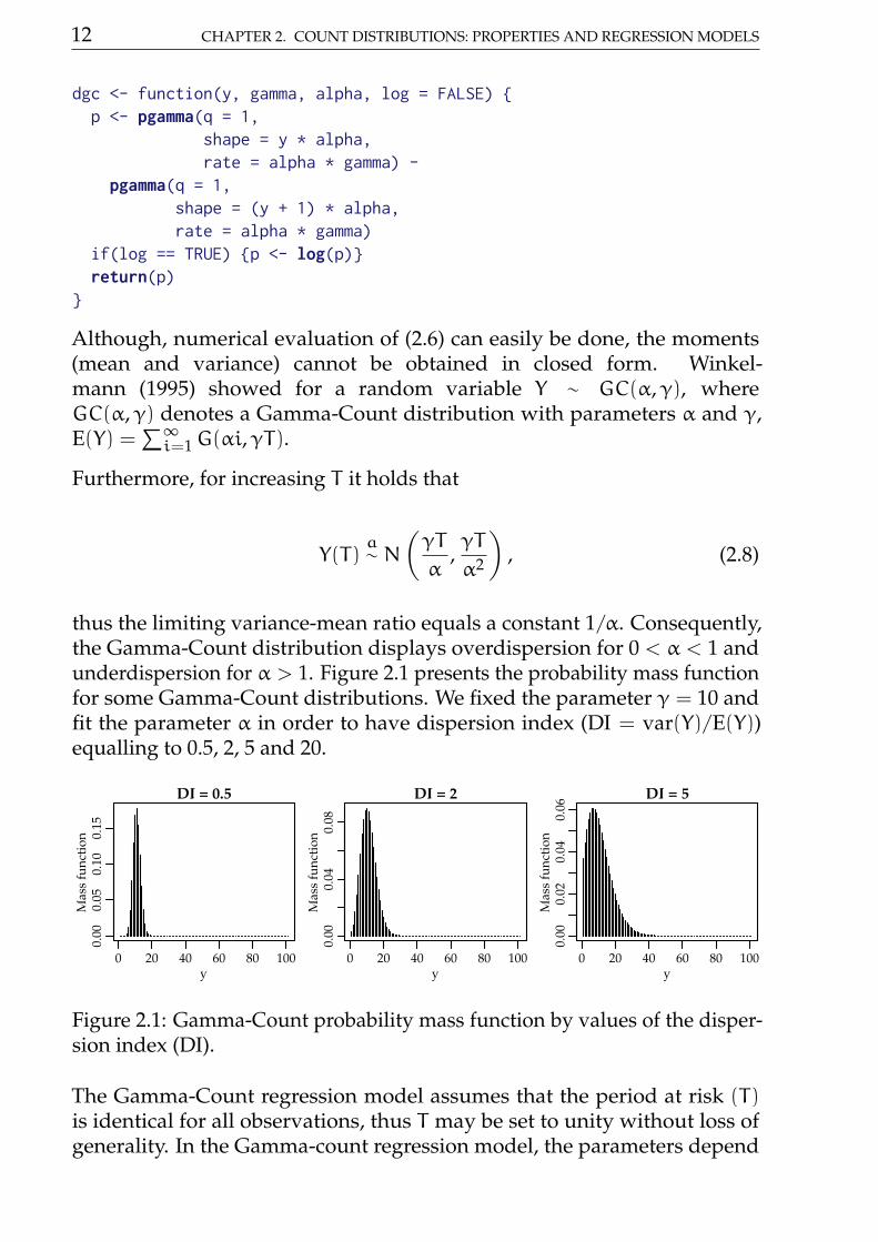
12 CHAPTER 2. COUNT DISTRIBUTIONS: PROPERTIES AND REGRESSION MODELS
dgc <- function(y, gamma, alpha, log = FALSE) p <- pgamma(q = 1,
shape = y * alpha,rate = alpha * gamma) -
pgamma(q = 1,shape = (y + 1) * alpha,rate = alpha * gamma)
if(log == TRUE) p <- log(p)return(p)
Although, numerical evaluation of (2.6) can easily be done, the moments(mean and variance) cannot be obtained in closed form. Winkel-mann (1995) showed for a random variable Y ∼ GC(α,γ), whereGC(α,γ) denotes a Gamma-Count distribution with parameters α and γ,E(Y) =
∑∞i=1G(αi,γT).
Furthermore, for increasing T it holds that
Y(T)a∼ N
(γT
α,γT
α2
), (2.8)
thus the limiting variance-mean ratio equals a constant 1/α. Consequently,the Gamma-Count distribution displays overdispersion for 0 < α < 1 andunderdispersion for α > 1. Figure 2.1 presents the probability mass functionfor some Gamma-Count distributions. We fixed the parameter γ = 10 andfit the parameter α in order to have dispersion index (DI = var(Y)/E(Y))equalling to 0.5, 2, 5 and 20.
0 20 40 60 80 100
0.00
0.05
0.10
0.15
DI = 0.5
y
Mas
s fu
nctio
n
0 20 40 60 80 100
0.00
0.04
0.08
DI = 2
y
Mas
s fu
nctio
n
0 20 40 60 80 100
0.00
0.02
0.04
0.06
DI = 5
y
Mas
s fu
nctio
n
Figure 2.1: Gamma-Count probability mass function by values of the disper-sion index (DI).
The Gamma-Count regression model assumes that the period at risk (T)is identical for all observations, thus T may be set to unity without loss ofgenerality. In the Gamma-count regression model, the parameters depend
2.3. POISSON-TWEEDIE DISTRIBUTION 13
on a vector of individual covariates xi. Thus, the Gamma-Count regressionmodel is defined by
E(τi|xi) =α
γ= g−1(−xi
>β). (2.9)
Consequently, the regression model is for the waiting times and not directlyfor the counts. Note that, E(Ni|xi) = E(τi|xi)−1 iff α = 1. Thus, β should beinterpreted accordingly. −βmeasures the percentage change in the expectedwaiting time caused by a unit increase in xi. The model parameters canbe estimated using the maximum likelihood method as we shall discuss inChapter 3.
2.3 Poisson-Tweedie distribution
The Poisson-Tweedie distribution (Bonat et al., 2016; Jørgensen and Koko-nendji, 2015; El-Shaarawi et al., 2011) consists of include Tweedie distributedrandom effects on the observation level of Poisson random variables, andthus to take into account unobserved heterogeneity. The Poisson-Tweediefamily is given by the following hierarchical specification
Y|Z ∼ Poisson(Z) (2.10)Z ∼ Twp(µ,φ),
where Twp(µ,φ) denotes a Tweedie distribution (Jørgensen, 1987, ; Jør-gensen, 1997) with probability function given by
fZ(z;µ,φ,p) = a(z,φ,p) exp(zψ− kp(ψ))/φ. (2.11)
In this notation, µ = k′p(ψ) is the expectation, φ > 0 is the dispersionparameter, ψ is the canonical parameter and kp(ψ) is the cumulant function.Furthermore, var(Z) = φV(µ) where V(µ) = k′′p(ψ) is the variance function.Tweedie densities are characterized by power variance functions of theform V(µ) = µp, where p ∈ (−∞, 0] ∪ [1,∞) is an index determining thedistribution. The support of the distribution depends on the value of thepower parameter. For p > 2, 1 < p < 2 and p = 0 the support corresponds tothe positive, non-negative and real values, respectively. In these cases µ ∈ Ω,where Ω is the convex support (i.e. the interior of the closed convex hullof the corresponding distribution support). Finally, for p < 0 the support
14 CHAPTER 2. COUNT DISTRIBUTIONS: PROPERTIES AND REGRESSION MODELS
corresponds to the real values, however the expectation µ is positive. Here,we required p > 1, to make Twp(µ,φ) non-negative.
The function a(z,φ,p) cannot be written in a closed form apart of the specialcases corresponding to the Gaussian (p = 0), Poisson (φ = 1 and p =1), non-central gamma (p = 3/2), gamma (p = 2) and inverse Gaussian(p = 3) distributions (Jørgensen, 1997). The compound Poisson distributionis obtained when 1 < p < 2. This distribution is suitable to deal withnon-negative data with probability mass at zero and highly right-skewed(Andersen and Bonat, 2016).
The Poisson-Tweedie is an overdispersed factorial dispersion model (Jør-gensen and Kokonendji, 2015) and its probability mass function for p > 1 isgiven by
f(y;µ,φ,p) =∫∞
0
zy exp−z
y!a(z,φ,p) exp(zψ− kp(ψ))/φdz. (2.12)
The integral (2.12) has no closed-form apart of the special case correspondingto the negative binomial distribution, obtained when p = 2, i.e. a Poissongamma mixture. In the case of p = 1, the integral (2.12) is replaced by asum and we have the Neyman Type A distribution. Further special casesinclude the compound Poisson (1 < p < 2), factorial discrete positive stable(p > 2) and Poisson-inverse Gaussian (p = 3) distributions (Jørgensen andKokonendji, 2015, ; Kokonendji et al., 2004).
In spite of other approaches to compute the probability mass function of thePoisson-Tweedie distribution are available in the literature (Esnaola et al.,2013, ; Barabesi et al., 2016). In this material, we opted to compute it bynumerical evaluation of the integral in (2.12) using the Monte Carlo methodas implemented by the following functions.
# Integrand Poisson X Tweedie distributionsintegrand <- function(x, y, mu, phi, power)
int = dpois(y, lambda = x)*dtweedie(x, mu = mu,phi = phi, power = power)
return(int)
# Computing the pmf using Monte Carlodptw <- function(y, mu, phi, power, control_sample)
pts <- control_sample$ptsnorma <- control_sample$normaintegral <- mean(integrand(pts, y = y, mu = mu, phi = phi,
power = power)/norma)
2.3. POISSON-TWEEDIE DISTRIBUTION 15
return(integral)dptw <- Vectorize(dptw, vectorize.args = "y")
When using the Monte Carlo method, we need to specify a proposal distribu-tion, from which samples will be taken to compute the integral as an expecta-tion. In the Poisson-Tweedie case is sensible to use the Tweedie distributionas proposal. Thus, in our function we use the argument control_sampleto provide these values. The advantage of this approach is that we needto simulate values once and we can reuse them for all evaluations of theprobability mass function, as shown in the following code.
require(tweedie)set.seed(123)pts <- rtweedie(n = 1000, mu = 10, phi = 1, power = 2)norma <- dtweedie(pts, mu = 10, phi = 1, power = 2)control_sample <- list("pts" = pts, "norma" = norma)dptw(y = c(0, 5, 10, 15), mu = 10, phi = 1, power = 2,
control_sample = control_sample)
## [1] 0.0937 0.0590 0.0354 0.0217
dnbinom(x = c(0, 5, 10, 15), mu = 10, size = 1)
## [1] 0.0909 0.0564 0.0350 0.0218
It is also possible to use the Gauss-Laguerre method to approximate theintegral in (2.12). In the supplementary material Script2.R, we provide Rfunctions using both Monte Carlo and Gauss-Laguerre methods to approxi-mate the probability mass function of Poisson-Tweedie distribution.
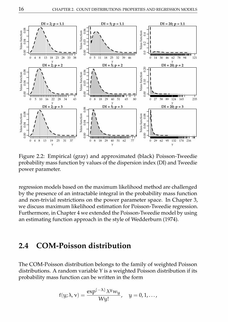
Figure 2.2 presents the empirical probability mass function of some Poisson-Tweedie distributions computed based on a sample of size 100000 (gray).Furthermore, we present an approximation (black) for the probability massfunction obtained by Monte Carlo integration. We considered differentvalues of the Tweedie power parameter p = 1.1, 2, and 3 combined withdifferent values of the dispersion index. In all scenarios the expectation µwas fixed at 10.
For all scenarios considered the Monte Carlo method provides a quite ac-curate approximation to the empirical probability mass function. For theseexamples, we used 5000 random samples from the proposal distribution.
Finally, the Poisson-Tweedie regression model is defined by
Yi ∼ PTwp(µi,φ), with µi = g−1(xi
>β),
where xi and β are (p × 1) vectors of known covariates and unknownregression parameters. The estimation and inference of Poisson-Tweedie
16 CHAPTER 2. COUNT DISTRIBUTIONS: PROPERTIES AND REGRESSION MODELS
0.00
0.04
0.08
DI = 2; p = 1.1
y
Mas
s fu
nctio
n
0 4 8 13 18 23 28 33 38
0.00
0.03
0.06
DI = 5; p = 1.1
y
Mas
s fu
nctio
n
0 5 11 18 25 32 39 46
0.0
0.2
0.4
DI = 20; p = 1.1
y
Mas
s fu
nctio
n
0 14 30 46 62 78 94 121
0.00
0.04
0.08
DI = 2; p = 2
y
Mas
s fu
nctio
n
0 5 10 16 22 28 34 43
0.00
0.03
0.06
DI = 5; p = 2
y
Mas
s fu
nctio
n
0 8 18 29 40 51 65 80
0.00
0.10
0.20
DI = 20; p = 2
y
Mas
s fu
nctio
n
0 27 58 89 124 165 235
0.00
0.04
0.08
DI = 2; p = 3
y
Mas
s fu
nctio
n
0 4 8 13 19 25 31 37
0.00
0.04
0.08
DI = 5; p = 3
y
Mas
s fu
nctio
n
0 8 18 29 40 51 62 770.
000.
040.
08
DI = 20; p = 3
yM
ass
func
tion
0 29 62 95 132 174 216
Figure 2.2: Empirical (gray) and approximated (black) Poisson-Tweedieprobability mass function by values of the dispersion index (DI) and Tweediepower parameter.
regression models based on the maximum likelihood method are challengedby the presence of an intractable integral in the probability mass functionand non-trivial restrictions on the power parameter space. In Chapter 3,we discuss maximum likelihood estimation for Poisson-Tweedie regression.Furthermore, in Chapter 4 we extended the Poisson-Tweedie model by usingan estimating function approach in the style of Wedderburn (1974).
2.4 COM-Poisson distribution
The COM-Poisson distribution belongs to the family of weighted Poissondistributions. A random variable Y is a weighted Poisson distribution if itsprobability mass function can be written in the form
f(y; λ,ν) =exp−λ λywy
Wy!, y = 0, 1, . . . ,
2.4. COM-POISSON DISTRIBUTION 17
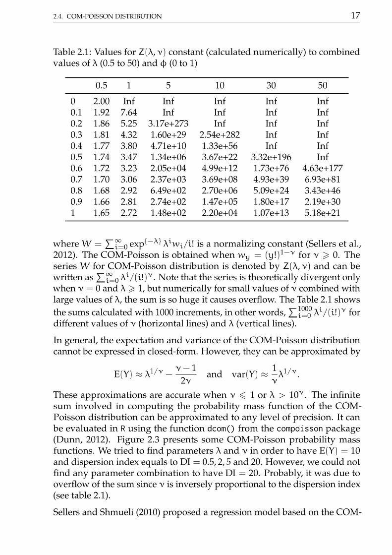
Table 2.1: Values for Z(λ,ν) constant (calculated numerically) to combinedvalues of λ (0.5 to 50) and φ (0 to 1)
0.5 1 5 10 30 50
0 2.00 Inf Inf Inf Inf Inf0.1 1.92 7.64 Inf Inf Inf Inf0.2 1.86 5.25 3.17e+273 Inf Inf Inf0.3 1.81 4.32 1.60e+29 2.54e+282 Inf Inf0.4 1.77 3.80 4.71e+10 1.33e+56 Inf Inf0.5 1.74 3.47 1.34e+06 3.67e+22 3.32e+196 Inf0.6 1.72 3.23 2.05e+04 4.99e+12 1.73e+76 4.63e+1770.7 1.70 3.06 2.37e+03 3.69e+08 4.93e+39 6.93e+810.8 1.68 2.92 6.49e+02 2.70e+06 5.09e+24 3.43e+460.9 1.66 2.81 2.74e+02 1.47e+05 1.80e+17 2.19e+301 1.65 2.72 1.48e+02 2.20e+04 1.07e+13 5.18e+21
where W =∑∞i=0 exp−λ λiwi/i! is a normalizing constant (Sellers et al.,
2012). The COM-Poisson is obtained when wy = (y!)1−ν for ν > 0. Theseries W for COM-Poisson distribution is denoted by Z(λ,ν) and can bewritten as
∑∞i=0 λ
i/(i!)ν. Note that the series is theoretically divergent onlywhen ν = 0 and λ > 1, but numerically for small values of ν combined withlarge values of λ, the sum is so huge it causes overflow. The Table 2.1 showsthe sums calculated with 1000 increments, in other words,
∑1000i=0 λ
i/(i!)ν fordifferent values of ν (horizontal lines) and λ (vertical lines).
In general, the expectation and variance of the COM-Poisson distributioncannot be expressed in closed-form. However, they can be approximated by
E(Y) ≈ λ1/ν −ν− 1
2νand var(Y) ≈ 1
νλ1/ν.
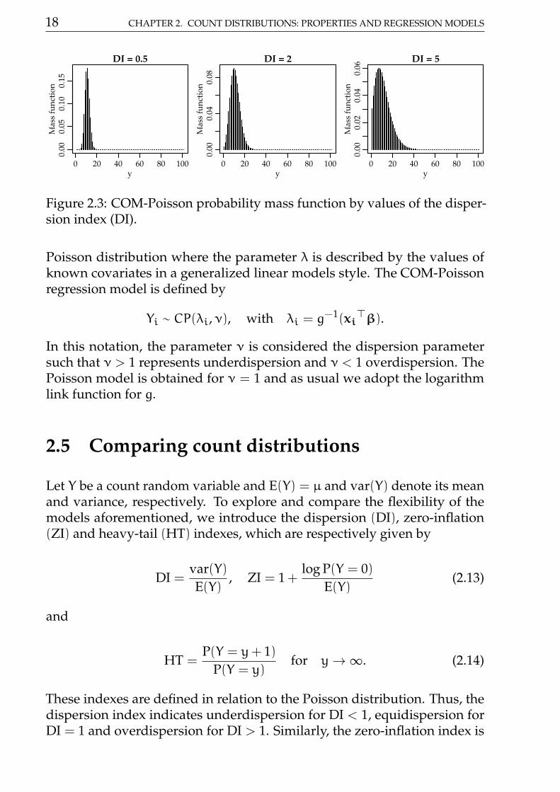
These approximations are accurate when ν 6 1 or λ > 10ν. The infinitesum involved in computing the probability mass function of the COM-Poisson distribution can be approximated to any level of precision. It canbe evaluated in R using the function dcom() from the compoisson package(Dunn, 2012). Figure 2.3 presents some COM-Poisson probability massfunctions. We tried to find parameters λ and ν in order to have E(Y) = 10and dispersion index equals to DI = 0.5, 2, 5 and 20. However, we could notfind any parameter combination to have DI = 20. Probably, it was due tooverflow of the sum since ν is inversely proportional to the dispersion index(see table 2.1).
Sellers and Shmueli (2010) proposed a regression model based on the COM-
18 CHAPTER 2. COUNT DISTRIBUTIONS: PROPERTIES AND REGRESSION MODELS
0 20 40 60 80 100
0.00
0.05
0.10
0.15
DI = 0.5
y
Mas
s fu
nctio
n
0 20 40 60 80 100
0.00
0.04
0.08
DI = 2
y
Mas
s fu
nctio
n
0 20 40 60 80 100
0.00
0.02
0.04
0.06
DI = 5
y
Mas
s fu
nctio
n
Figure 2.3: COM-Poisson probability mass function by values of the disper-sion index (DI).
Poisson distribution where the parameter λ is described by the values ofknown covariates in a generalized linear models style. The COM-Poissonregression model is defined by
Yi ∼ CP(λi,ν), with λi = g−1(xi
>β).
In this notation, the parameter ν is considered the dispersion parametersuch that ν > 1 represents underdispersion and ν < 1 overdispersion. ThePoisson model is obtained for ν = 1 and as usual we adopt the logarithmlink function for g.
2.5 Comparing count distributions
Let Y be a count random variable and E(Y) = µ and var(Y) denote its meanand variance, respectively. To explore and compare the flexibility of themodels aforementioned, we introduce the dispersion (DI), zero-inflation(ZI) and heavy-tail (HT) indexes, which are respectively given by
DI =var(Y)E(Y)
, ZI = 1 +log P(Y = 0)
E(Y)(2.13)
and
HT =P(Y = y+ 1)
P(Y = y)for y→∞. (2.14)
These indexes are defined in relation to the Poisson distribution. Thus, thedispersion index indicates underdispersion for DI < 1, equidispersion forDI = 1 and overdispersion for DI > 1. Similarly, the zero-inflation index is
2.5. COMPARING COUNT DISTRIBUTIONS 19
easily interpreted, since ZI < 0 indicates zero-deflation, ZI = 0 correspondsto no excess of zeroes and ZI > 0 indicates zero-inflation. Finally, HT→ 1when y→∞ indicates a heavy tail distribution.
For the Poisson distribution the dispersion index equals 1 ∀µ. In the Poissoncase, it is easy to show that ZI = 0 and HT → 0 when y → ∞. Thus, it isquite clear that the Poisson model can deal only with equidispersed dataand has no flexibility to deal with zero-inflation and/or heavy tail countdata. In fact, the presented indexes were proposed in relation to the Poissondistribution in order to highlight its limitations.
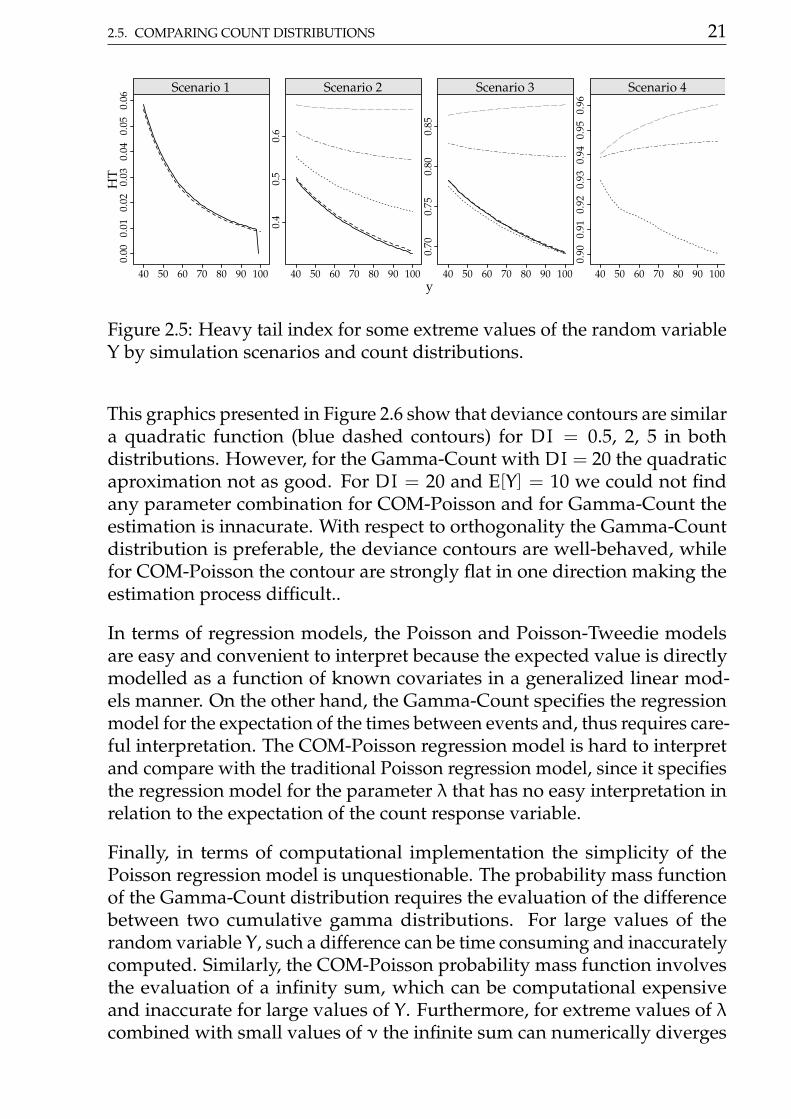
Figure 2.4 presents the relationship between mean and variance, the disper-sion and zero-inflation indexes as a function of the expected values µ fordifferent scenarios and count distributions. Scenario 1 corresponds to thecase of underdispersion. Thus, we fixed the dispersion index at DI = 0.5when the mean equalling 10. Since the Poisson-Tweedie cannot deal withunderdispersion, in this scenario we present only the Gamma-Count andCOM-Poisson distributions. Similarly, scenarios 2 − −4 are obtained byfixing the dispersion index at DI = 2, 5 and 10 when mean equalling 10.In the scenario 4 we could not find a parameter configuration in order tohave a COM-Poisson distribution with dispersion index equals 20. Conse-quently, we present results only for the Gamma-Count and Poisson-Tweediedistributions. Furthermore, Figure 2.5 presents the heavy tail index for someextreme values of the random variable Y.
The indexes presented in Figures 2.4 and 2.5 show that for all consideredscenarios the Gamma-Count and COM-Poisson distributions are quite sim-ilar. In general, for these distributions, the indexes slightly depend on theexpected values and tend to stabilize for large values of µ. Consequently, themean and variance relationship is proportional to the dispersion parametervalue. In the overdispersion case, the Gamma-Count and COM-Poissondistributions can handle with a limited amount of zero-inflation and are ingeneral light tailed distributions, i.e. HT→ 0 for y→∞.
Regarding the Poisson-Tweedie distributions the indexes show that for smallvalues of the power parameter the Poisson-Tweedie distribution is suitable todeal with zero-inflated count data. In that case, the DI and ZI are almost notdependent on the values of the mean. Furthermore, the HT decreases as themean increases. On the other hand, for large values of the power parameterthe HT increases with increasing mean, showing that the model is speciallysuitable to deal with heavy-tailed count data. In this case, the DI and ZIincrease quickly as the mean increases giving an extremely overdispersedmodel for large values of the mean. In general, the DI and ZI are larger thanone and zero, respectively, which, of course, show that the correspondingPoisson-Tweedie distributions cannot deal with underdispersed and zero-
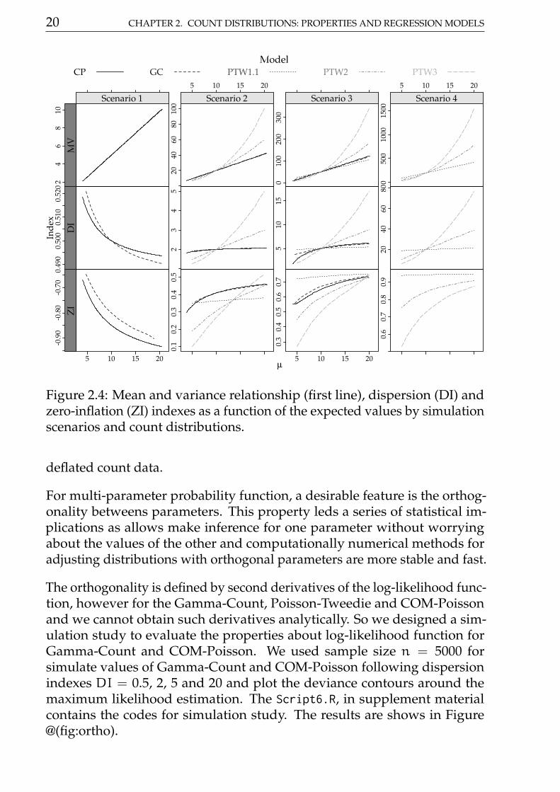
20 CHAPTER 2. COUNT DISTRIBUTIONS: PROPERTIES AND REGRESSION MODELS
µ
Inde
x-0
.90
-0.8
0-0
.70
5 10 15 20
ZI
0.1
0.2
0.3
0.4
0.5
0.3
0.4
0.5
0.6
0.7
5 10 15 20
0.6
0.7
0.8
0.9
0.49
00.
500
0.51
00.
520
DI
23
45
510
15
2040
6080
24
68
10
Scenario 1
MV
5 10 15 20
2040
6080
100
Scenario 2
010
020
030
0
Scenario 35 10 15 20
050
010
0015
00
Scenario 4
ModelCP GC PTW1.1 PTW2 PTW3
Figure 2.4: Mean and variance relationship (first line), dispersion (DI) andzero-inflation (ZI) indexes as a function of the expected values by simulationscenarios and count distributions.
deflated count data.
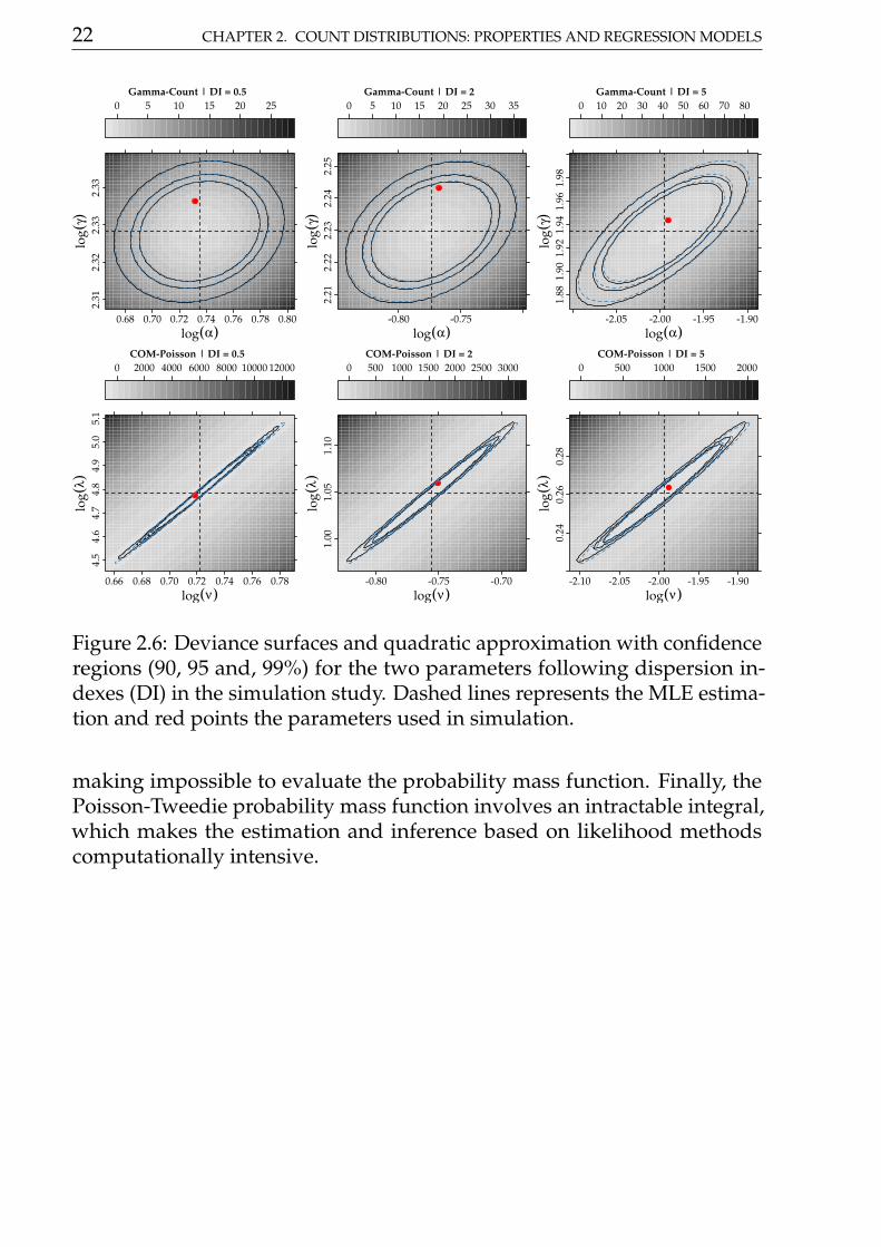
For multi-parameter probability function, a desirable feature is the orthog-onality betweens parameters. This property leds a series of statistical im-plications as allows make inference for one parameter without worryingabout the values of the other and computationally numerical methods foradjusting distributions with orthogonal parameters are more stable and fast.
The orthogonality is defined by second derivatives of the log-likelihood func-tion, however for the Gamma-Count, Poisson-Tweedie and COM-Poissonand we cannot obtain such derivatives analytically. So we designed a sim-ulation study to evaluate the properties about log-likelihood function forGamma-Count and COM-Poisson. We used sample size n = 5000 forsimulate values of Gamma-Count and COM-Poisson following dispersionindexes DI = 0.5, 2, 5 and 20 and plot the deviance contours around themaximum likelihood estimation. The Script6.R, in supplement materialcontains the codes for simulation study. The results are shows in Figure@(fig:ortho).
2.5. COMPARING COUNT DISTRIBUTIONS 21
y
HT
0.00
0.01
0.02
0.03
0.04
0.05
0.06
40 50 60 70 80 90 100
Scenario 1
0.4
0.5
0.6
40 50 60 70 80 90 100
Scenario 2
0.70
0.75
0.80
0.85
40 50 60 70 80 90 100
Scenario 3
0.90
0.91
0.92
0.93
0.94
0.95
0.96
40 50 60 70 80 90 100
Scenario 4
Figure 2.5: Heavy tail index for some extreme values of the random variableY by simulation scenarios and count distributions.
This graphics presented in Figure 2.6 show that deviance contours are similara quadratic function (blue dashed contours) for DI = 0.5, 2, 5 in bothdistributions. However, for the Gamma-Count with DI = 20 the quadraticaproximation not as good. For DI = 20 and E[Y] = 10 we could not findany parameter combination for COM-Poisson and for Gamma-Count theestimation is innacurate. With respect to orthogonality the Gamma-Countdistribution is preferable, the deviance contours are well-behaved, whilefor COM-Poisson the contour are strongly flat in one direction making theestimation process difficult..
In terms of regression models, the Poisson and Poisson-Tweedie modelsare easy and convenient to interpret because the expected value is directlymodelled as a function of known covariates in a generalized linear mod-els manner. On the other hand, the Gamma-Count specifies the regressionmodel for the expectation of the times between events and, thus requires care-ful interpretation. The COM-Poisson regression model is hard to interpretand compare with the traditional Poisson regression model, since it specifiesthe regression model for the parameter λ that has no easy interpretation inrelation to the expectation of the count response variable.
Finally, in terms of computational implementation the simplicity of thePoisson regression model is unquestionable. The probability mass functionof the Gamma-Count distribution requires the evaluation of the differencebetween two cumulative gamma distributions. For large values of therandom variable Y, such a difference can be time consuming and inaccuratelycomputed. Similarly, the COM-Poisson probability mass function involvesthe evaluation of a infinity sum, which can be computational expensiveand inaccurate for large values of Y. Furthermore, for extreme values of λcombined with small values of ν the infinite sum can numerically diverges
22 CHAPTER 2. COUNT DISTRIBUTIONS: PROPERTIES AND REGRESSION MODELS
Gamma-Count | DI = 0.5
log(α)
log(
γ )2.31
2.32
2.33
2.33
0.68 0.70 0.72 0.74 0.76 0.78 0.80
0 5 10 15 20 25Gamma-Count | DI = 2
log(α)log(
γ )2.21
2.22
2.23
2.24
2.25
-0.80 -0.75
0 5 10 15 20 25 30 35Gamma-Count | DI = 5
log(α)
log(
γ )1.88
1.90
1.92
1.94
1.96
1.98
-2.05 -2.00 -1.95 -1.90
0 10 20 30 40 50 60 70 80
COM-Poisson | DI = 0.5
log(ν)
log(
λ )4.5
4.6
4.7
4.8
4.9
5.0
5.1
0.66 0.68 0.70 0.72 0.74 0.76 0.78
0 2000 4000 6000 8000 10000 12000COM-Poisson | DI = 2
log(ν)
log(
λ )1.00
1.05
1.10
-0.80 -0.75 -0.70
0 500 1000 1500 2000 2500 3000COM-Poisson | DI = 5
log(ν)
log(
λ )0.24
0.26
0.28
-2.10 -2.05 -2.00 -1.95 -1.90
0 500 1000 1500 2000
Figure 2.6: Deviance surfaces and quadratic approximation with confidenceregions (90, 95 and, 99%) for the two parameters following dispersion in-dexes (DI) in the simulation study. Dashed lines represents the MLE estima-tion and red points the parameters used in simulation.
making impossible to evaluate the probability mass function. Finally, thePoisson-Tweedie probability mass function involves an intractable integral,which makes the estimation and inference based on likelihood methodscomputationally intensive.
Chapter 3
The method of maximumlikelihood
The estimation and inference for the models discussed in Chapter 2 can bedone by the method of maximum likelihood (Silvey, 1975). In this Chapter,we present the maximum likelihood method and its main properties alongwith some examples in R. The maximum likelihood method is applicablemainly in situations where the true distribution of the count random variableY is known apart of the values of a finite number of unknown parameters.Let f(y;θ) denote the true probability mass function of the count randomvariable Y. We assume that the family f(y;θ) is labelled by a (p× 1) pa-rameter vector θ taking values in Θ a subset of Rn. For a given observedvalue y of the a random variable Y, the likelihood function correspondingto the observation y is defined as L(θ;y) = f(y;θ). It is important to high-light that f(y;θ) is a probability mass function on the sample space. On theother hand, L(θ;y) = f(y;θ) is a function on the parameter space Θ. Thelikelihood function expresses the plausibilities of different parameters afterwe have observed y, in the absence of any other information that we mayhave about these different values. In particular, for count random variablesthe likelihood function is the probability of the point y when θ is the trueparameter.
The method of maximum likelihood has a strong intuitive appeal and ac-cording to it, we estimate the true parameter θ by any parameter whichmaximizes the likelihood function. In general, there is a unique maximizingparameter which is the most plausible and this is the maximum likelihoodestimate (Silvey, 1975). In other words, a maximum likelihood estimate θ(y)
23
24 CHAPTER 3. THE METHOD OF MAXIMUM LIKELIHOOD
is any element of Θ such that L(θ(y);y) = maxθ∈Θ
L(θ;y). At this stage, we
make the distinction between the estimate θ(y) and the estimator θ. How-ever, we are not maintain this distinction and we shall use only θ leavingthe context to make it clear whether we are thinking of θ as a function or asa particular value of a function.
Let Yi be independent and identically distributed count random variableswith probability mass function f(y;θ), whose observed values are denotedby yi for i = 1, . . . ,n. In this case, the likelihood function can be written asthe product of the individuals probability mass distributions, i.e.
L(θ;y) =n∏
i=1
L(θ;yi) =n∏
i=1
f(yi;θ). (3.1)
For convenience, in practical situations is advisable to work with the log-likelihood function obtained by taking the logarithm of Eq. (3.1). Thus, themaximum likelihood estimator (MLE) for the parameter vector θ is obtainedby maximizing the following log-likelihood function,
`(θ) =
n∑
i=1
logL(θ;yi). (3.2)
Often, it is not possible to find a relatively simple expression in closed formfor the maximum likelihood estimates. However, it is usually possible toassume that maximum likelihood estimates emerge as a solution of thelikelihood equations or also called score functions, i.e.
U(θ) =
(∂`(θ)
∂θ1
>, . . . ,
∂`(θ)
∂θp
>)>= 0. (3.3)
The system of non-linear equations in (3.3) often have to be solved numeri-cally. The entry (i, j) of the p× p Fisher information matrix Fθ for the vectorof parameter θ is given by
Fθij = −E∂2`(θ)
∂θi∂θj
. (3.4)
In order to solve the system of equations U(θ) = 0, we employ the Newtonscoring algorithm, defined by
25
θ(i+1) = θ(i) −F−1θ U(θ(i)). (3.5)
Finally, the well known distribution of the maximum likelihood estimatorθ is N(θ,F−1
θ ). Thus, the maximum likelihood estimator is asymptoticallyconsistent, unbiased and efficient.
A critical point of the approach described so far, is that we should be ableto compute the first and second derivatives of the log-likelihood function.However, for the Gamma-Count where the log-likelihood function is givenby the difference between two integrals, we cannot obtain such derivativesanalytically. Similarly, for the COM-Poisson the log-likelihood function in-volves an infinite sum and consequently such derivatives cannot be obtainedanalytically. Finally, in the Poisson-Tweedie distribution the log-likelihoodfunction is defined by an intractable integral, which implies that we cannotobtain a closed-form for the score function and Fisher information matrix.
Thus, an alternative approach is to maximize directly the log-likelihoodfunction in equation (3.2) using a derivative-free algorithm as the Nelder-Mead method (Nelder and Mead, 1965) or some other numerical methodfor maximizing the log-likelihood function, examples include the BFGS,conjugate gradient and simulated annealing. All of them are implementedin R through the optim() function. The package bbmle (?) offers a suite offunctions to work with numerical maximization of log-likelihood functionsin R. As an example, consider the Gamma-Count distribution described insubsection 2.2. The log-likelihood function for the parameters θ = (γ,α) inR is given by
ll_gc <- function(gamma, alpha, y) ll <- sum(dgc(y = y, gamma = gamma, alpha = alpha, log = TRUE))return(-ll)
Thus, for a given vector of observed count values, we can numericallymaximize the log-likelihood function above using the function mle2() fromthe bbmlepackage. It is important to highlight that by default the mle2()function requires the negative of the log-likelihood function instead of thelog-likelihood itself. Thus, our function returns the negative value of thelog-likelihood function.
require(bbmle)y <- rpois(100, lambda = 10)fit_gc <- mle2(ll_gc, start = list("gamma" = 10, "alpha" = 1),
data = list("y" = y))
26 CHAPTER 3. THE METHOD OF MAXIMUM LIKELIHOOD
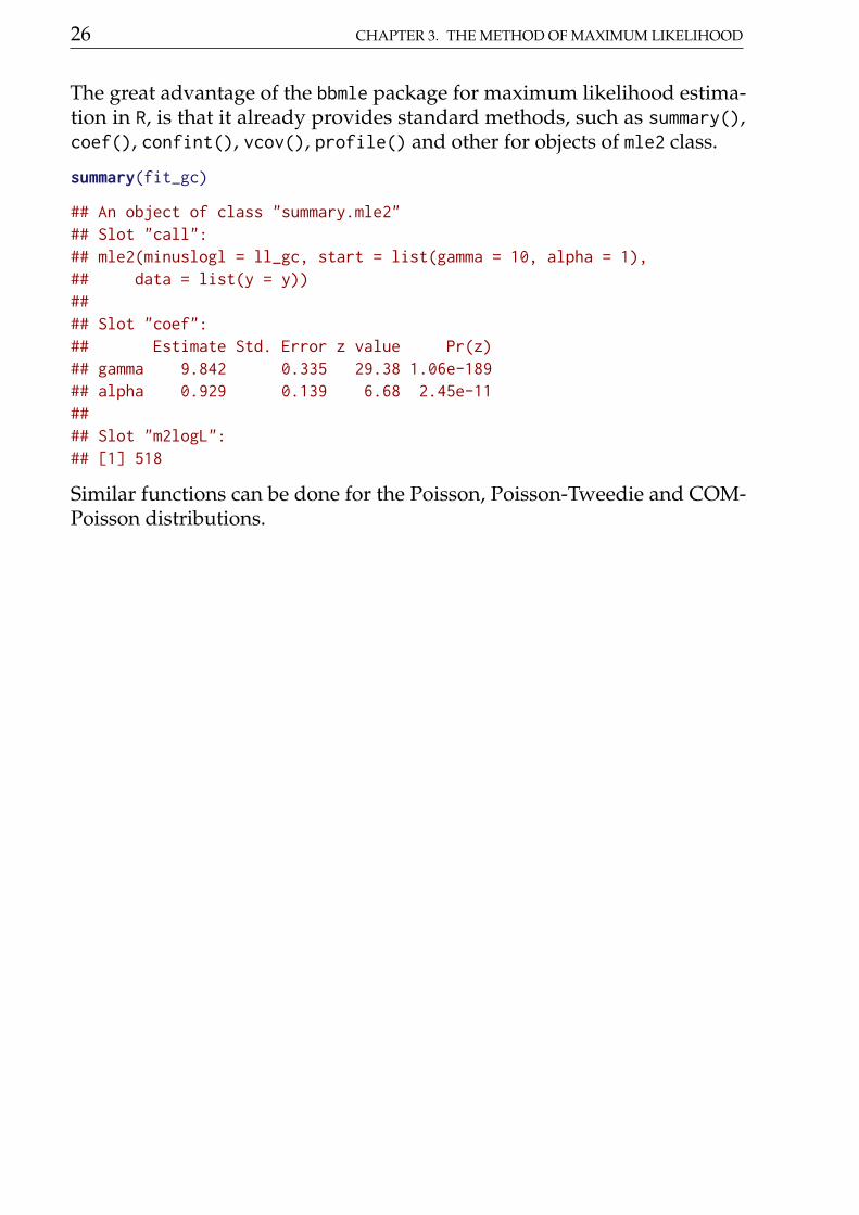
The great advantage of the bbmle package for maximum likelihood estima-tion in R, is that it already provides standard methods, such as summary(),coef(), confint(), vcov(), profile() and other for objects of mle2 class.
summary(fit_gc)
## An object of class "summary.mle2"## Slot "call":## mle2(minuslogl = ll_gc, start = list(gamma = 10, alpha = 1),## data = list(y = y))#### Slot "coef":## Estimate Std. Error z value Pr(z)## gamma 9.842 0.335 29.38 1.06e-189## alpha 0.929 0.139 6.68 2.45e-11#### Slot "m2logL":## [1] 518
Similar functions can be done for the Poisson, Poisson-Tweedie and COM-Poisson distributions.
Chapter 4
Models specified bysecond-momentassumptions
In Chapter 2, we presented four statistical models to deal with count dataand in the Chapter 3 the method of maximum likelihood was introducedto estimate the model’s parameters. As discussed in Chapter 3 the methodof maximum likelihood assumes that the true distribution of the countrandom variable Y is known apart of the values of a finite number of un-known parameters. In this Chapter, we shall present a different approach formodel specification, estimation and inference based only on second-momentassumptions.
4.1 Extended Poisson-Tweedie model
The Poisson-Tweedie distribution as presented in subsection 2.3 providesa very flexible family of count distributions, however, such a family hastwo main drawbacks: it cannot deal with underdispersed count data and itsprobability mass function is given by an intractable integral, which impliesthat estimation based on the maximum likelihood method is computationaldemanding for practical data analysis.
In spite of these issues Jørgensen and Kokonendji (2015) showed usingfactorial cumulant function that for Y ∼ PTwp(µ,φ), E(Y) = µ and var(Y) =
27
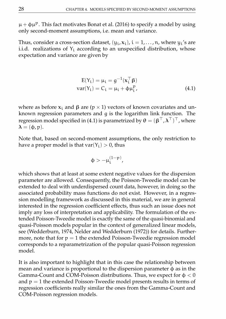
28 CHAPTER 4. MODELS SPECIFIED BY SECOND-MOMENT ASSUMPTIONS
µ+φµp. This fact motivates Bonat et al. (2016) to specify a model by usingonly second-moment assumptions, i.e. mean and variance.
Thus, consider a cross-section dataset, (yi, xi), i = 1, . . . ,n, where yi’s arei.i.d. realizations of Yi according to an unspecified distribution, whoseexpectation and variance are given by
E(Yi) = µi = g−1(x>i β)
var(Yi) = Ci = µi +φµpi , (4.1)
where as before xi and β are (p× 1) vectors of known covariates and un-known regression parameters and g is the logarithm link function. Theregression model specified in (4.1) is parametrized by θ = (β>,λ>)>, whereλ = (φ,p).
Note that, based on second-moment assumptions, the only restriction tohave a proper model is that var(Yi) > 0, thus
φ > −µ(1−p)i ,
which shows that at least at some extent negative values for the dispersionparameter are allowed. Consequently, the Poisson-Tweedie model can beextended to deal with underdispersed count data, however, in doing so theassociated probability mass functions do not exist. However, in a regres-sion modelling framework as discussed in this material, we are in generalinterested in the regression coefficient effects, thus such an issue does notimply any loss of interpretation and applicability. The formulation of the ex-tended Poisson-Tweedie model is exactly the same of the quasi-binomial andquasi-Poisson models popular in the context of generalized linear models,see (Wedderburn, 1974, Nelder and Wedderburn (1972)) for details. Further-more, note that for p = 1 the extended Poisson-Tweedie regression modelcorresponds to a reparametrization of the popular quasi-Poisson regressionmodel.
It is also important to highlight that in this case the relationship betweenmean and variance is proportional to the dispersion parameter φ as in theGamma-Count and COM-Poisson distributions. Thus, we expect for φ < 0and p = 1 the extended Poisson-Tweedie model presents results in terms ofregression coefficients really similar the ones from the Gamma-Count andCOM-Poisson regression models.
4.2. ESTIMATION AND INFERENCE 29
4.2 Estimation and Inference
Since the model presented in (4.1) is based only on second-moment assump-tions the method of maximum likelihood cannot be employed. Bonat et al.(2016) based on ideas of Jørgensen and Knudsen (2004) and Bonat and Jør-gensen (2016) proposed an estimating function approach for estimation andinference for the extended Poisson-Tweedie regression model. Bonat et al.(2016) combined the quasi-score and Pearson estimating functions for esti-mation of the regression and dispersion parameters respectively. FollowingBonat et al. (2016) the quasi-score function for β has the following form,
ψβ(β,λ) =
(n∑
i=1
∂µi∂β1
C−1i (Yi − µi), . . . ,
n∑
i=1
∂µi∂βp
C−1i (Yi − µi)
)>,
where ∂µi/∂βj = µixij for j = 1, . . . ,p. The sensitivity matrix is defined asthe expectation of the first derivative of the estimating function with respectto the model parameters. Thus, the entry (j,k) of the p× p sensitivity matrixfor ψβ is given by
Sβjk = E(∂
∂βkψβj(β,λ)
)= −
n∑
i=1
µixijC−1i xikµi. (4.2)
In a similar way, the variability matrix is defined as the variance of theestimating function. In particular, for the quasi-score function the entry (j,k)of the p× p variability matrix is given by
Vβjk = Cov(ψβj(β,λ),ψβk(β,λ)) =n∑
i=1
µixijC−1i xikµi.
The Pearson estimating function for the dispersion parameters has the fol-lowing form,
ψλ(λ,β) =
(−
n∑
i=1
∂C−1i
∂φ
[(Yi − µi)
2 −Ci
],−
n∑
i=1
∂C−1i
∂p
[(Yi − µi)
2 −Ci
])>.
Note that, the Pearson estimating functions are unbiased estimating func-tions for λ based on the squared residuals (Yi − µi)
2 with expected valueCi.
30 CHAPTER 4. MODELS SPECIFIED BY SECOND-MOMENT ASSUMPTIONS
The entry (j,k) of the 2× 2 sensitivity matrix for the dispersion parametersis given by
Sλjk = E(∂
∂λkψλj(λ,β)
)= −
n∑
i=1
∂C−1i
∂λjCi∂C−1i
∂λkCi, (4.3)
where λ1 and λ2 denote either φ or p.
Similarly, the cross entries of the sensitivity matrix are given by
Sβjλk = E(∂
∂λkψβj(β,λ)
)= 0 (4.4)
and
Sλjβk = E(∂
∂βkψλj(λ,β)
)= −
n∑
i=1
∂C−1i
∂λjCi∂C−1i
∂βkCi. (4.5)
Finally, the joint sensitivity matrix for the parameter vector θ is given by
Sθ =
(Sβ 0
Sλβ Sλ
),
whose entries are defined by equations (4.2), (4.3), (4.4) and (4.5).
We now calculate the asymptotic variance of the estimating function esti-mators denoted by θ, as obtained from the inverse Godambe informationmatrix, whose general form for a vector of parameter θ is J−1
θ = S−1θ VθS−>
θ ,where −> denotes inverse transpose. The variability matrix for θ has theform
Vθ =
(Vβ Vβλ
Vλβ Vλ
), (4.6)
where Vλβ = V>βλ and Vλ depend on the third and fourth moments of Yi,
respectively. In order to avoid this dependence on higher-order moments,we use the empirical versions of Vλ and Vλβ as given by
Vλjk =
n∑
i=1
ψλj(λ,β)iψλk(λ,β)i and Vλjβk =
n∑
i=1
ψλj(λ,β)iψβk(λ,β)i.
4.2. ESTIMATION AND INFERENCE 31
Finally, the well known asymptotic distribution of θ (Jørgensen and Knud-sen, 2004) is given by
θ ∼ N(θ, J−1θ ), where J−1
θ = S−1θ VθS−>
θ .
To solve the system of equationsψβ = 0 andψλ = 0 Jørgensen and Knudsen(2004) proposed the modified chaser algorithm, defined by
β(i+1) = β(i) − S−1β ψβ(β
(i),λ(i))
λ(i+1) = λ(i) −αS−1λ ψλ(β
(i+1),λ(i)).
The modified chaser algorithm uses the insensitivity property (4.4), whichallows us to use two separate equations to update β and λ. We introducethe tuning constant, α, to control the step-length. This algorithm is a specialcase of the flexible algorithm presented by Bonat and Jørgensen (2016) inthe context of multivariate covariance generalized linear models. Hence,estimation for the extended Poisson-Tweedie model is easily implementedin R through the mcglm (Bonat, 2016) package.

32 CHAPTER 4. MODELS SPECIFIED BY SECOND-MOMENT ASSUMPTIONS
Chapter 5
Applications
In this chapter, we will bring some applications based on real data sets toshow how use R packages to analyse count data.
5.1 Cotton Bolls
Cotton production can be drastically reduced by attack of defoliating insects.Depending on the growth stage, the plant can recover from the causeddamage and keeps production not affected or can have the productionreduced by low intensity defoliation.
A greenhouse experiment with cotton plants (Gossypium hirsutum) was doneunder a completely randomized design with five replicates to assess theeffects of five defoliation levels (0%, 25%, 50%,75% and 100%) on the ob-served number of bolls produced by plants at five growth stages: vegetative,flower-bud, blossom, fig and cotton boll. The experimental unity was a potwith two plants (Silva et al., 2012, for more). The number of cotton bolls wasrecorded at the hasvest of the experiment.
library(lattice)library(latticeExtra)library(gridExtra)library(plyr)library(car)library(corrplot)library(doBy)library(multcomp)library(mcglm)
33
34 CHAPTER 5. APPLICATIONS
library(MRDCr)ls("package:MRDCr")
## [1] "apc" "calc_mean_cmp"## [3] "calc_mean_gcnt" "calc_var_cmp"## [5] "cambras" "capdesfo"## [7] "capmosca" "cmp"## [9] "conftemp" "confterm"## [11] "convergencez" "dcmp"## [13] "dgcnt" "dpgnz"## [15] "gcnt" "led"## [17] "llcmp" "llgcnt"## [19] "llpgnz" "nematoide"## [21] "ninfas" "panel.beeswarm"## [23] "panel.cbH" "panel.groups.segplot"## [25] "peixe" "pgnz"## [27] "postura" "prepanel.cbH"## [29] "seguros" "soja"
# Documentation in Portuguese.help(capdesfo, help_type = "html")
str(capdesfo)
## 'data.frame': 125 obs. of 4 variables:## $ est : Factor w/ 5 levels "vegetativo","botão floral",..: 1 1 1 1 1 1 1 1 1 1 ...## $ des : num 0 0 0 0 0 0.25 0.25 0.25 0.25 0.25 ...## $ rept: int 1 2 3 4 5 1 2 3 4 5 ...## $ ncap: int 10 9 8 8 10 11 9 10 10 10 ...
levels(capdesfo$est) <- c("vegetative","flower-bud","blossom","fig","cotton boll")
xtabs(~est + des, data = capdesfo)
## des## est 0 0.25 0.5 0.75 1## vegetative 5 5 5 5 5## flower-bud 5 5 5 5 5## blossom 5 5 5 5 5## fig 5 5 5 5 5## cotton boll 5 5 5 5 5
Figure 5.1 (top) shows the beeswarm plot of number of cotton bolls recordedfor each combination of defoliation level and growth stage. All the points inthe sample means and variances dispersion diagram (bottom) are below theidentity line, clearly suggesting data with underdispersion.
5.1. COTTON BOLLS 35
The exploratory data analysis, although simple, was able to detect departuresfrom the Poisson equidispersion assumption. So, we have in advance fewconditions met for the use of GLM Poisson as a regression model to analysethis experiment.
Poisson, as being a process derived from the memoryless waiting timesExponential distribuition, implies that each boll is an independent event inthe artificial subjacent domain, that can be thought was the natural resourcedomain that the plant has to allocate bolls. Its is easy to assume, based onplant fisiology, that the probability of a boll decreases with the number ofprevious bolls because the plant’s resource to produce bolls is limited and itis a non memoryless process equivalent.
Based on the exploratory data analysis, a predictor with 2nd order effect ofdefoliation for each growth stage should be enough to model the numberof bolls mean in a regression model. The analysis and assessment of theeffects of the experimental factors are based on the Poisson, Gamma-countand Poisson Tweedie models.
m0 <- glm(ncap ~ est * (des + I(des^2)),data = capdesfo,family = poisson)
summary(m0)
#### Call:## glm(formula = ncap ~ est * (des + I(des^2)), family = poisson,## data = capdesfo)#### Deviance Residuals:## Min 1Q Median 3Q Max## -1.0771 -0.3098 -0.0228 0.2704 1.1665#### Coefficients:## Estimate Std. Error z value Pr(>|z|)## (Intercept) 2.2142 0.1394 15.89 <2e-16 ***## estflower-bud -0.0800 0.2007 -0.40 0.69## estblossom -0.0272 0.2001 -0.14 0.89## estfig -0.1486 0.2051 -0.72 0.47## estcotton boll 0.1129 0.1922 0.59 0.56## des 0.3486 0.6805 0.51 0.61## I(des^2) -0.7384 0.6733 -1.10 0.27## estflower-bud:des 0.1364 0.9644 0.14 0.89## estblossom:des -1.5819 1.0213 -1.55 0.12## estfig:des 0.4755 1.0194 0.47 0.64## estcotton boll:des -0.8210 0.9395 -0.87 0.38
36 CHAPTER 5. APPLICATIONS
## estflower-bud:I(des^2) 0.1044 0.9447 0.11 0.91## estblossom:I(des^2) 1.4044 1.0191 1.38 0.17## estfig:I(des^2) -0.9294 1.0323 -0.90 0.37## estcotton boll:I(des^2) 1.0757 0.9210 1.17 0.24## ---## Signif. codes: 0 '***' 0.001 '**' 0.01 '*' 0.05 '.' 0.1 ' ' 1#### (Dispersion parameter for poisson family taken to be 1)#### Null deviance: 75.514 on 124 degrees of freedom## Residual deviance: 25.331 on 110 degrees of freedom## AIC: 539.7#### Number of Fisher Scoring iterations: 4
logLik(m0)
## 'log Lik.' -255 (df=15)
We fit the GLM Poisson regression model using the stardard glm() functionin R. The fitted model summary shows the estimated parameters for thesecond order effect of defoliation crossed with growth stages levels. Theresidual deviance was 25.33 based on 110 degrees of freedoom. The ra-tio 25.33/110 = 0.23 is a strong evidence against Poisson equidispersionassumption that uses a dispersion parameter equals 1.
anova(m0, test = "Chisq")
## Analysis of Deviance Table#### Model: poisson, link: log#### Response: ncap#### Terms added sequentially (first to last)###### Df Deviance Resid. Df Resid. Dev Pr(>Chi)## NULL 124 75.5## est 4 19.96 120 55.6 0.00051 ***## des 1 15.86 119 39.7 6.8e-05 ***## I(des^2) 1 1.29 118 38.4 0.25557## est:des 4 6.71 114 31.7 0.15212## est:I(des^2) 4 6.36 110 25.3 0.17388## ---## Signif. codes: 0 '***' 0.001 '**' 0.01 '*' 0.05 '.' 0.1 ' ' 1
The analysis of deviance table did not stated effect of any interactions, neithersecond order effect of defiliation. Although, all these effects are noticeable
5.1. COTTON BOLLS 37
in Figure ??.
Figure ?? displays the four residual plots for the fitted model. Based onthese plots, there is no concern about mispecifications regarding to themodel predictor or influential observations. The only remarkable aspect isabout the range of the stardartized deviance residuals quite distant from theexpected -3 to 3 from the normal distribution. Once more, these is anothermeasure indicating a underdispersed count data.
The gcnt() is a function defined in the MRDCr package (Zeviani et al., 2016)to fit the Gamma-Count regression model. This function fits a GML-Poissonto use the estimates as initial values to optimize Gamma-Count likelihoodusing optim() through bblme package (Bolker and Team, 2016).
m1 <- gcnt(ncap ~ est * (des + I(des^2)),data = capdesfo)
summary(m1)
## An object of class "summary.mle2"## Slot "call":## bbmle::mle2(minuslogl = llgcnt, start = start, data = list(y = y,## X = X, offset = off), vecpar = TRUE)#### Slot "coef":## Estimate Std. Error z value Pr(z)## alpha 1.7110 0.1352 12.656 1.04e-36## (Intercept) 2.2580 0.0593 38.053 0.00e+00## estflower-bud -0.0765 0.0854 -0.896 3.70e-01## estblossom -0.0253 0.0851 -0.297 7.66e-01## estfig -0.1398 0.0872 -1.603 1.09e-01## estcotton boll 0.1084 0.0818 1.326 1.85e-01## des 0.3294 0.2896 1.137 2.55e-01## I(des^2) -0.6997 0.2866 -2.441 1.46e-02## estflower-bud:des 0.1337 0.4105 0.326 7.45e-01## estblossom:des -1.5020 0.4345 -3.457 5.46e-04## estfig:des 0.4218 0.4336 0.973 3.31e-01## estcotton boll:des -0.7820 0.3998 -1.956 5.05e-02## estflower-bud:I(des^2) 0.0943 0.4021 0.235 8.15e-01## estblossom:I(des^2) 1.3382 0.4335 3.087 2.02e-03## estfig:I(des^2) -0.8333 0.4390 -1.898 5.77e-02## estcotton boll:I(des^2) 1.0222 0.3920 2.608 9.11e-03#### Slot "m2logL":## [1] 408
During the optimization process for this dataset, optim() has found NaNwhen evaluating the likelihood. This occurs due little numerical precisionto calculate the difference of Gamma CDFs on tails or for extreme values,
38 CHAPTER 5. APPLICATIONS
resulting in numerical zeros and corresponding -Inf log-likelihood. This isa numerical problem that can narrow, or make things difficult, the use ofGamma-Count regression model.
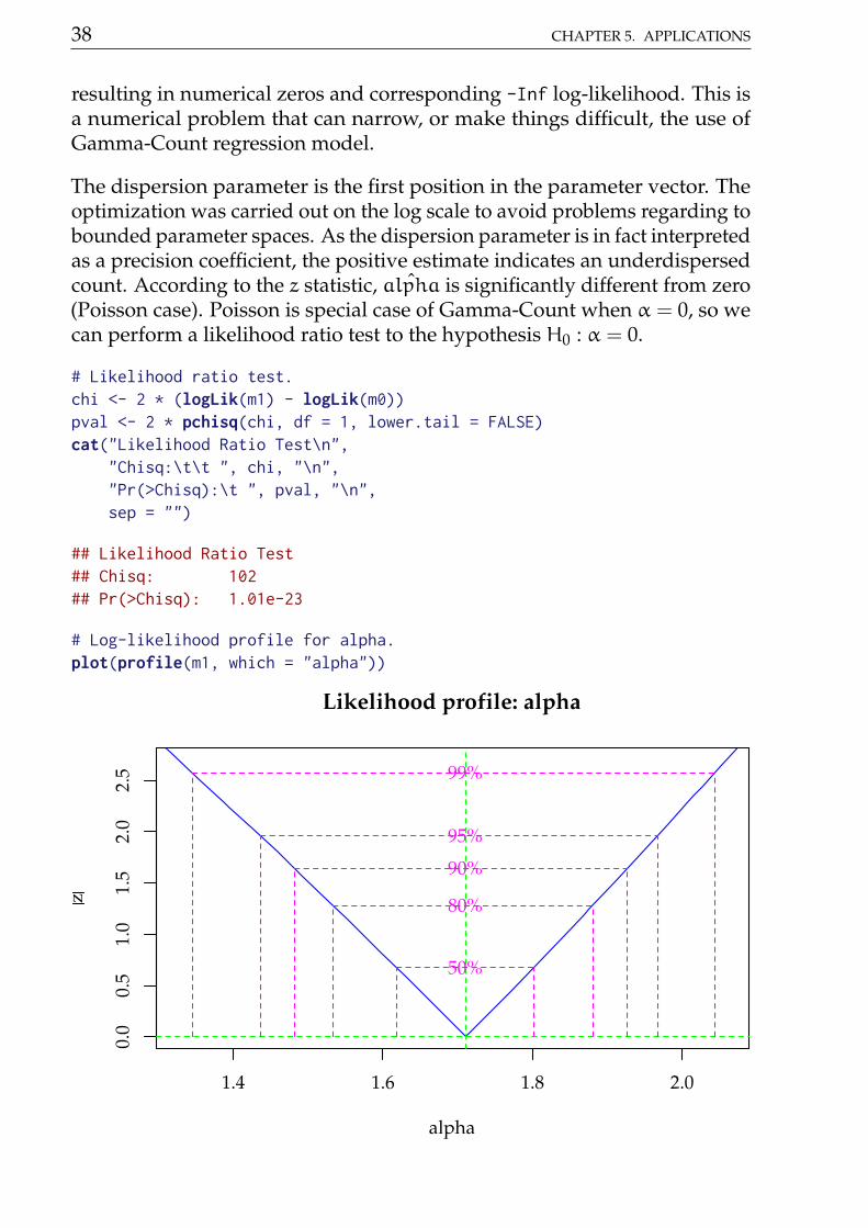
The dispersion parameter is the first position in the parameter vector. Theoptimization was carried out on the log scale to avoid problems regarding tobounded parameter spaces. As the dispersion parameter is in fact interpretedas a precision coefficient, the positive estimate indicates an underdispersedcount. According to the z statistic, ˆalpha is significantly different from zero(Poisson case). Poisson is special case of Gamma-Count when α = 0, so wecan perform a likelihood ratio test to the hypothesis H0 : α = 0.
# Likelihood ratio test.chi <- 2 * (logLik(m1) - logLik(m0))pval <- 2 * pchisq(chi, df = 1, lower.tail = FALSE)cat("Likelihood Ratio Test\n",
"Chisq:\t\t ", chi, "\n","Pr(>Chisq):\t ", pval, "\n",sep = "")
## Likelihood Ratio Test## Chisq: 102## Pr(>Chisq): 1.01e-23
# Log-likelihood profile for alpha.plot(profile(m1, which = "alpha"))
1.4 1.6 1.8 2.0
0.0
0.5
1.0
1.5
2.0
2.5
Likelihood profile: alpha
alpha
z
99%
95%
90%
80%
50%
5.1. COTTON BOLLS 39
cbind(c(0, coef(m0)), coef(m1))
## [,1] [,2]## 0.0000 1.7110## (Intercept) 2.2142 2.2580## estflower-bud -0.0800 -0.0765## estblossom -0.0272 -0.0253## estfig -0.1486 -0.1398## estcotton boll 0.1129 0.1084## des 0.3486 0.3294## I(des^2) -0.7384 -0.6997## estflower-bud:des 0.1364 0.1337## estblossom:des -1.5819 -1.5020## estfig:des 0.4755 0.4218## estcotton boll:des -0.8210 -0.7820## estflower-bud:I(des^2) 0.1044 0.0943## estblossom:I(des^2) 1.4044 1.3382## estfig:I(des^2) -0.9294 -0.8333## estcotton boll:I(des^2) 1.0757 1.0222
rstd <- summary(m1)@coef[-1, 2]/summary(m0)$coeff[, 2]plyr::each(mean, range)(rstd)
## mean range1 range2## 0.426 0.425 0.426
The estimates for the location parameters were very close. The ratio betweenGamma-Count parameters standard error and Poisson ones, on the otherhand, were 0.426 for all estimates, for 3 decimals of precision. This leads tothe conclusion that TODO relação linear no parâmetro de dispersão.
# Wald test for the interaction.a <- c(0, attr(model.matrix(m0), "assign"))ai <- a == max(a)L <- t(replicate(sum(ai), rbind(coef(m1) * 0), simplify = "matrix"))L[, ai] <- diag(sum(ai))
linearHypothesis(model = m0, # m0 is not being used here.hypothesis.matrix = L,vcov. = vcov(m1),coef. = coef(m1))
## Linear hypothesis test#### Hypothesis:## estflower - bud:I(des^2) = 0## estblossom:I(des^2) = 0## estfig:I(des^2) = 0## estcotton boll:I(des^2) = 0
40 CHAPTER 5. APPLICATIONS
#### Model 1: restricted model## Model 2: ncap ~ est * (des + I(des^2))#### Note: Coefficient covariance matrix supplied.#### Res.Df Df Chisq Pr(>Chisq)## 1 114## 2 110 4 30.5 3.8e-06 ***## ---## Signif. codes: 0 '***' 0.001 '**' 0.01 '*' 0.05 '.' 0.1 ' ' 1
# Fitting Poisson-Tweedie model.m2 <- mcglm(linear_pred = c(ncap ~ est * (des + I(des^2))),
matrix_pred = list(mc_id(data = capdesfo)),link = "log",variance = "poisson_tweedie",power_fixed = FALSE,data = capdesfo,control_algorithm = list(verbose = FALSE,
max_iter = 100,tunning = 0.5,correct = FALSE))
## Automatic initial values selected.
# Parameter estimates.summary(m2)
## Call: ncap ~ est * (des + I(des^2))#### Link function: log## Variance function: poisson_tweedie## Covariance function: identity## Regression:## Estimates Std.error Z value## (Intercept) 2.2143 0.0627 35.308## estflower-bud -0.0800 0.0904 -0.886## estblossom -0.0265 0.0900 -0.294## estfig -0.1485 0.0924 -1.607## estcotton boll 0.1128 0.0864 1.306## des 0.3486 0.3065 1.137## I(des^2) -0.7385 0.3037 -2.432## estflower-bud:des 0.1361 0.4345 0.313## estblossom:des -1.5875 0.4612 -3.442## estfig:des 0.4693 0.4602 1.020## estcotton boll:des -0.8204 0.4228 -1.940## estflower-bud:I(des^2) 0.1048 0.4259 0.246
5.1. COTTON BOLLS 41
## estblossom:I(des^2) 1.4098 0.4609 3.059## estfig:I(des^2) -0.9205 0.4671 -1.971## estcotton boll:I(des^2) 1.0752 0.4149 2.592#### Power:## Estimates Std.error Z value## 1 1.01 0.136 7.43#### Dispersion:## Estimates Std.error Z value## 1 -0.781 0.217 -3.59#### Algorithm: chaser## Correction: FALSE## Number iterations: 14
# Wald test for fixed effects.anova(m2)
## Wald test for fixed effects## Call: ncap ~ est * (des + I(des^2))#### Covariate Chi.Square Df p.value## 1 estflower-bud 9.54 4 0.0489## 2 des 1.29 1 0.2555## 3 I(des^2) 5.91 1 0.0150## 4 estflower-bud:des 25.00 4 0.0001## 5 estflower-bud:I(des^2) 30.72 4 0.0000
# New data values for prediction.pred <- with(capdesfo,
expand.grid(est = levels(est),des = seq(0, 1, length.out = 30)))
# Corresponding model matrix.X <- model.matrix(formula(m0)[-2], data = pred)pred <- list(P = pred, GC = pred, TW = pred)
# Poisson model prediction.aux <- confint(glht(m0, linfct = X),
calpha = univariate_calpha())$confintcolnames(aux)[1] <- "fit"pred$P <- cbind(pred$P, exp(aux))
# Gamma-Count model prediction.# aux <- predict(m1, newdata = X,# interval = "confidence",# type = "link")
42 CHAPTER 5. APPLICATIONS
# pred$GC <- cbind(pred$GC, exp(aux[, c(2, 1, 3)]))aux <- predict(m1, newdata = X,
interval = "confidence",type = "response")
pred$GC <- cbind(pred$GC, aux[, c(2, 1, 3)])
V <- vcov(m2)i <- grepl("^beta", rownames(V))eta <- X %*% coef(m2, type = "beta")$Estimatesstd <- sqrt(diag(as.matrix(X %*%
as.matrix(V[i, i]) %*%t(X))))
q <- qnorm(0.975) * c(lwr = -1, fit = 0, upr = 1)me <- outer(std, q, FUN = "*")aux <- sweep(me, 1, eta, FUN = "+")pred$TW <- cbind(pred$TW, exp(aux))
pred <- ldply(pred, .id = "model")pred <- arrange(pred, est, des, model)
key <- list(type = "o", divide = 1,lines = list(pch = 1:nlevels(pred$model),
lty = 1, col = 1),text = list(c("Poisson",
"Gamma-Count","Poisson-Tweedie")))
key <- list(lines = list(lty = 1),text = list(c("Poisson",
"Gamma-Count","Poisson-Tweedie")))
key$lines$col <-trellis.par.get("superpose.line")$col[1:nlevels(pred$model)]
\beginfigure[h]
5.1. COTTON BOLLS 43
Artifitial defoliation levels
Bolls
pro
duce
d
2
4
6
8
10
12
vegetative
0.0 0.2 0.4 0.6 0.8 1.0
flower-bud blossom
0.0 0.2 0.4 0.6 0.8 1.0
fig
2
4
6
8
10
12
cotton boll
PoissonGamma-CountPoisson-Tweedie
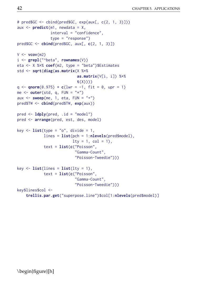
\captionFitted curves based on Poisson, Gamma-Count andPoisson-Tweedie regression models. Envelops are 95% coverage confidence
bands. \endfigure
c0 <- summary(m0)$coefficients[, 1:2]c1 <- summary(m1)@coef[, 1:2]c2 <- rbind(summary(m2)[[1]]$tau[, 1:2],
summary(m2)[[1]]$Regression[, 1:2])
# Parameter estimates according to each model.c4 <- cbind("P" = rbind(NA, c0),
"GC" = c1,"TW" = c2)
colnames(c4) <- substr(colnames(c4), 1, 6)round(c4, digits = 4)
## P.Esti P.Std. GC.Est GC.Std TW.Est TW.Std## NA NA 1.7110 0.1352 -0.7805 0.2174## (Intercept) 2.2142 0.139 2.2580 0.0593 2.2143 0.0627
44 CHAPTER 5. APPLICATIONS
## estflower-bud -0.0800 0.201 -0.0765 0.0854 -0.0800 0.0904## estblossom -0.0272 0.200 -0.0253 0.0851 -0.0265 0.0900## estfig -0.1486 0.205 -0.1398 0.0872 -0.1485 0.0924## estcotton boll 0.1129 0.192 0.1084 0.0818 0.1128 0.0864## des 0.3486 0.680 0.3294 0.2896 0.3486 0.3065## I(des^2) -0.7384 0.673 -0.6997 0.2866 -0.7385 0.3037## estflower-bud:des 0.1364 0.964 0.1337 0.4105 0.1361 0.4345## estblossom:des -1.5819 1.021 -1.5020 0.4345 -1.5875 0.4612## estfig:des 0.4755 1.019 0.4218 0.4336 0.4693 0.4602## estcotton boll:des -0.8210 0.940 -0.7820 0.3998 -0.8204 0.4228## estflower-bud:I(des^2) 0.1044 0.945 0.0943 0.4021 0.1048 0.4259## estblossom:I(des^2) 1.4044 1.019 1.3382 0.4335 1.4098 0.4609## estfig:I(des^2) -0.9294 1.032 -0.8333 0.4390 -0.9205 0.4671## estcotton boll:I(des^2) 1.0757 0.921 1.0222 0.3920 1.0752 0.4149
5.2 Soybean pod and beans
The tropical soils, usually poor in potassium (K), demand potassiumfertilization when cultivated with soybean (Glycine max L.) to obtain
satisfactory yields. Soybean production is affected by long exposition towater deficit. As postassium is a nutrient involved in the water balance inplant, by hyphotesis, a good supply of potassium avoids lose production.
The aim of this experiment was to evaluate the effects of K doses and soilhumidity levels on soybean production. The experiment was carried out in
a greenhouse, in pots with two plants, containing 5 dm3 of soil. Theexperimental design was completely randomized block with treatments in a
5 x 3 factorial arrangement. The K doses were 0, 30, 60, 120 and 180 mgdm-3 , and the soil humidity ranged from 35 to 40, 47.5 to 52.5, and 60 to
65% of the total porosity (Serafim et al., 2012, for more details).
Two count variables were recorded in this experiment: the total number ofpods per plot and the total number of grains per plot. The ratio, grains/pod,
can also be analysed, since the fisiological response can change it.
There is an outlier in the dataset at position 74 that must be removed.Potassion amount (K) will be converted to a categorical factor, despite it is a
numerical one, to prevent concerns with lack of fit, that is not the mainscope of the following analysis.
data(soja)str(soja)
## 'data.frame': 75 obs. of 5 variables:## $ K : int 0 30 60 120 180 0 30 60 120 180 ...
5.2. SOYBEAN POD AND BEANS 45
## $ umid: Factor w/ 3 levels "37,5","50","62,5": 1 1 1 1 1 2 2 2 2 2 ...## $ bloc: Factor w/ 5 levels "I","II","III",..: 1 1 1 1 1 1 1 1 1 1 ...## $ ngra: int 136 159 156 171 190 140 193 200 208 237 ...## $ nvag: int 56 62 66 68 82 63 86 94 86 97 ...
# Removing an outlier.soja <- soja[-74, ]soja <- transform(soja, K = factor(K))
5.2.1 Number of pods
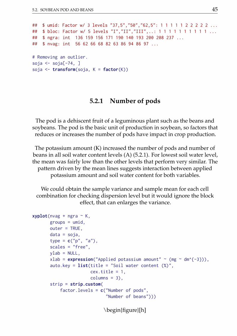
The pod is a dehiscent fruit of a leguminous plant such as the beans andsoybeans. The pod is the basic unit of production in soybean, so factors thatreduces or increases the number of pods have impact in crop production.
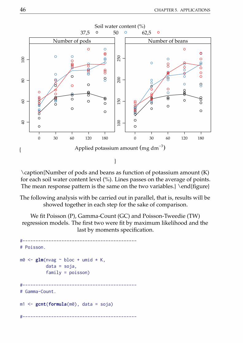
The potassium amount (K) increased the number of pods and number ofbeans in all soil water content levels (A) (5.2.1). For lowest soil water level,the mean was fairly low than the other levels that perform very similar. The
pattern driven by the mean lines suggests interaction between appliedpotassium amount and soil water content for both variables.
We could obtain the sample variance and sample mean for each cellcombination for checking dispersion level but it would ignore the block
effect, that can enlarges the variance.
xyplot(nvag + ngra ~ K,groups = umid,outer = TRUE,data = soja,type = c("p", "a"),scales = "free",ylab = NULL,xlab = expression("Applied potassium amount" ~ (mg ~ dm^-3)),auto.key = list(title = "Soil water content (%)",
cex.title = 1,columns = 3),
strip = strip.custom(factor.levels = c("Number of pods",
"Number of beans")))
\beginfigure[h]
46 CHAPTER 5. APPLICATIONS
Applied potassium amount (mg dm−3)
4060
8010
0
0 30 60 120 180
Number of pods
100
150
200
250
0 30 60 120 180
Number of beans
Soil water content (%)37,5 50 62,5
\captionNumber of pods and beans as function of potassium amount (K)for each soil water content level (%). Lines passes on the average of points.The mean response pattern is the same on the two variables. \endfigure
The following analysis with be carried out in parallel, that is, results will beshowed together in each step for the sake of comparison.
We fit Poisson (P), Gamma-Count (GC) and Poisson-Tweedie (TW)regression models. The first two were fit by maximum likelihood and the
last by moments specification.
#--------------------------------------------# Poisson.
m0 <- glm(nvag ~ bloc + umid * K,data = soja,family = poisson)
#--------------------------------------------# Gamma-Count.
m1 <- gcnt(formula(m0), data = soja)
#--------------------------------------------
5.2. SOYBEAN POD AND BEANS 47
# Tweedie.
m2 <- mcglm(linear_pred = c(nvag ~ bloc + umid * K),matrix_pred = list(mc_id(data = soja)),link = "log",variance = "poisson_tweedie",power_fixed = TRUE,data = soja,control_algorithm = list(verbose = FALSE,
max_iter = 100,tunning = 0.5,correct = FALSE))
## Automatic initial values selected.
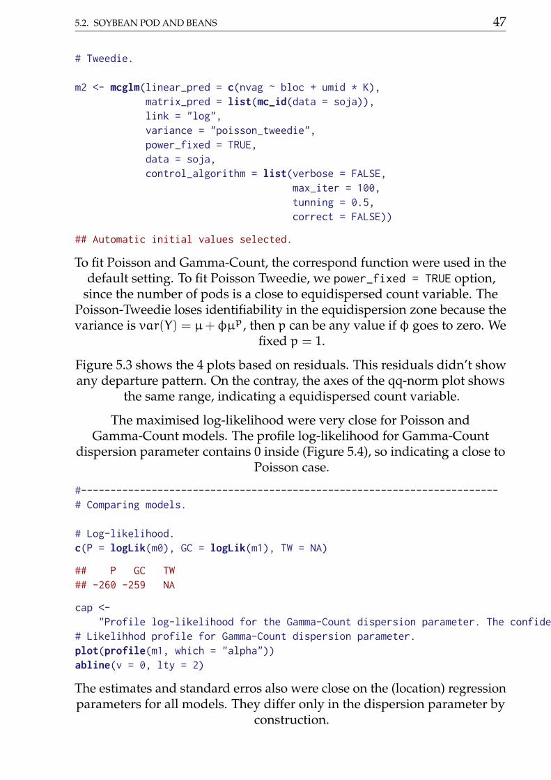
To fit Poisson and Gamma-Count, the correspond function were used in thedefault setting. To fit Poisson Tweedie, we power_fixed = TRUE option,
since the number of pods is a close to equidispersed count variable. ThePoisson-Tweedie loses identifiability in the equidispersion zone because thevariance is var(Y) = µ+φµp, then p can be any value if φ goes to zero. We
fixed p = 1.
Figure 5.3 shows the 4 plots based on residuals. This residuals didn’t showany departure pattern. On the contray, the axes of the qq-norm plot shows
the same range, indicating a equidispersed count variable.
The maximised log-likelihood were very close for Poisson andGamma-Count models. The profile log-likelihood for Gamma-Count
dispersion parameter contains 0 inside (Figure 5.4), so indicating a close toPoisson case.
#-----------------------------------------------------------------------# Comparing models.
# Log-likelihood.c(P = logLik(m0), GC = logLik(m1), TW = NA)
## P GC TW## -260 -259 NA
cap <-"Profile log-likelihood for the Gamma-Count dispersion parameter. The confidence interval based on profile likelihood contains 0 inside as indicated by the solid vertical line."
# Likelihhod profile for Gamma-Count dispersion parameter.plot(profile(m1, which = "alpha"))abline(v = 0, lty = 2)
The estimates and standard erros also were close on the (location) regressionparameters for all models. They differ only in the dispersion parameter by
construction.
48 CHAPTER 5. APPLICATIONS
c0 <- summary(m0)$coefficients[, 1:2]c1 <- summary(m1)@coef[, 1:2]c2 <- rbind(summary(m2)[[1]]$tau[, 1:2],
summary(m2)[[1]]$Regression[, 1:2])
# Parameter estimates according to each model.c4 <- cbind("P" = rbind(NA, c0),
"GC" = c1,"TW" = c2)
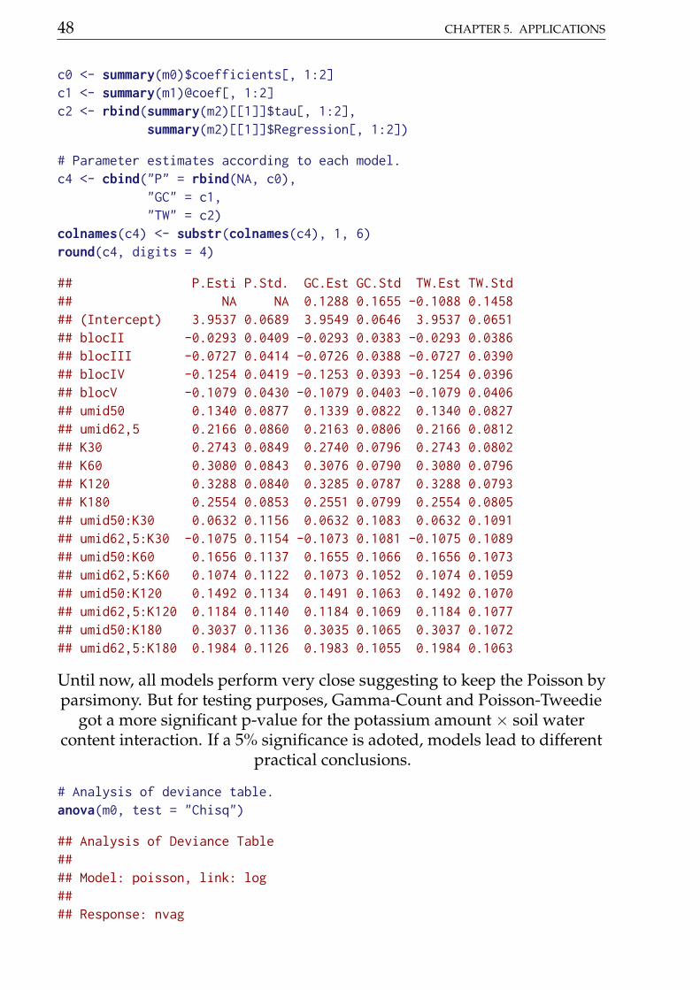
colnames(c4) <- substr(colnames(c4), 1, 6)round(c4, digits = 4)
## P.Esti P.Std. GC.Est GC.Std TW.Est TW.Std## NA NA 0.1288 0.1655 -0.1088 0.1458## (Intercept) 3.9537 0.0689 3.9549 0.0646 3.9537 0.0651## blocII -0.0293 0.0409 -0.0293 0.0383 -0.0293 0.0386## blocIII -0.0727 0.0414 -0.0726 0.0388 -0.0727 0.0390## blocIV -0.1254 0.0419 -0.1253 0.0393 -0.1254 0.0396## blocV -0.1079 0.0430 -0.1079 0.0403 -0.1079 0.0406## umid50 0.1340 0.0877 0.1339 0.0822 0.1340 0.0827## umid62,5 0.2166 0.0860 0.2163 0.0806 0.2166 0.0812## K30 0.2743 0.0849 0.2740 0.0796 0.2743 0.0802## K60 0.3080 0.0843 0.3076 0.0790 0.3080 0.0796## K120 0.3288 0.0840 0.3285 0.0787 0.3288 0.0793## K180 0.2554 0.0853 0.2551 0.0799 0.2554 0.0805## umid50:K30 0.0632 0.1156 0.0632 0.1083 0.0632 0.1091## umid62,5:K30 -0.1075 0.1154 -0.1073 0.1081 -0.1075 0.1089## umid50:K60 0.1656 0.1137 0.1655 0.1066 0.1656 0.1073## umid62,5:K60 0.1074 0.1122 0.1073 0.1052 0.1074 0.1059## umid50:K120 0.1492 0.1134 0.1491 0.1063 0.1492 0.1070## umid62,5:K120 0.1184 0.1140 0.1184 0.1069 0.1184 0.1077## umid50:K180 0.3037 0.1136 0.3035 0.1065 0.3037 0.1072## umid62,5:K180 0.1984 0.1126 0.1983 0.1055 0.1984 0.1063
Until now, all models perform very close suggesting to keep the Poisson byparsimony. But for testing purposes, Gamma-Count and Poisson-Tweedie
got a more significant p-value for the potassium amount × soil watercontent interaction. If a 5% significance is adoted, models lead to different
practical conclusions.
# Analysis of deviance table.anova(m0, test = "Chisq")
## Analysis of Deviance Table#### Model: poisson, link: log#### Response: nvag
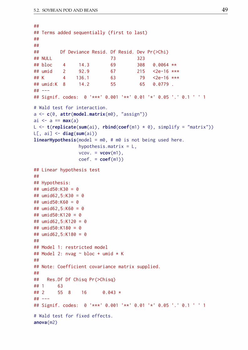
5.2. SOYBEAN POD AND BEANS 49
#### Terms added sequentially (first to last)###### Df Deviance Resid. Df Resid. Dev Pr(>Chi)## NULL 73 323## bloc 4 14.3 69 308 0.0064 **## umid 2 92.9 67 215 <2e-16 ***## K 4 136.1 63 79 <2e-16 ***## umid:K 8 14.2 55 65 0.0779 .## ---## Signif. codes: 0 '***' 0.001 '**' 0.01 '*' 0.05 '.' 0.1 ' ' 1
# Wald test for interaction.a <- c(0, attr(model.matrix(m0), "assign"))ai <- a == max(a)L <- t(replicate(sum(ai), rbind(coef(m1) * 0), simplify = "matrix"))L[, ai] <- diag(sum(ai))linearHypothesis(model = m0, # m0 is not being used here.
hypothesis.matrix = L,vcov. = vcov(m1),coef. = coef(m1))
## Linear hypothesis test#### Hypothesis:## umid50:K30 = 0## umid62,5:K30 = 0## umid50:K60 = 0## umid62,5:K60 = 0## umid50:K120 = 0## umid62,5:K120 = 0## umid50:K180 = 0## umid62,5:K180 = 0#### Model 1: restricted model## Model 2: nvag ~ bloc + umid * K#### Note: Coefficient covariance matrix supplied.#### Res.Df Df Chisq Pr(>Chisq)## 1 63## 2 55 8 16 0.043 *## ---## Signif. codes: 0 '***' 0.001 '**' 0.01 '*' 0.05 '.' 0.1 ' ' 1
# Wald test for fixed effects.anova(m2)
50 CHAPTER 5. APPLICATIONS
## Wald test for fixed effects## Call: nvag ~ bloc + umid * K#### Covariate Chi.Square Df p.value## 1 blocII 13.92 4 0.0076## 2 umid50 7.15 2 0.0280## 3 K30 20.93 4 0.0003## 4 umid50:K30 15.76 8 0.0459
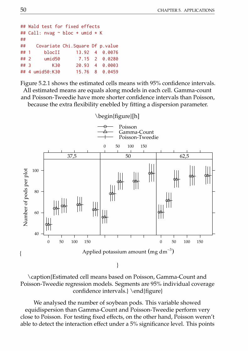
Figure 5.2.1 shows the estimated cells means with 95% confidence intervals.All estimated means are equals along models in each cell. Gamma-count
and Poisson-Tweedie have more shorter confidence intervals than Poisson,because the extra flexibility enebled by fitting a dispersion parameter.
\beginfigure[h]
Applied potassium amount (mg dm−3)
Num
ber
of p
ods
per
plot
40
60
80
100
0 50 100 150
37,5
0 50 100 150
50
0 50 100 150
62,5
PoissonGamma-CountPoisson-Tweedie
\captionEstimated cell means based on Poisson, Gamma-Count andPoisson-Tweedie regression models. Segments are 95% individual coverage
confidence intervals. \endfigure
We analysed the number of soybean pods. This variable showedequidispersion than Gamma-Count and Poisson-Tweedie perform very
close to Poisson. For testing fixed effects, on the other hand, Poisson weren’table to detect the interaction effect under a 5% significance level. This points
5.2. SOYBEAN POD AND BEANS 51
out that more flexible models are powerful in detecting effects.
5.2.2 Number of grains
For the analysis of number of beans, the same steps will be carried out, justadaptating the code when needed. The first adaptation we need make is to
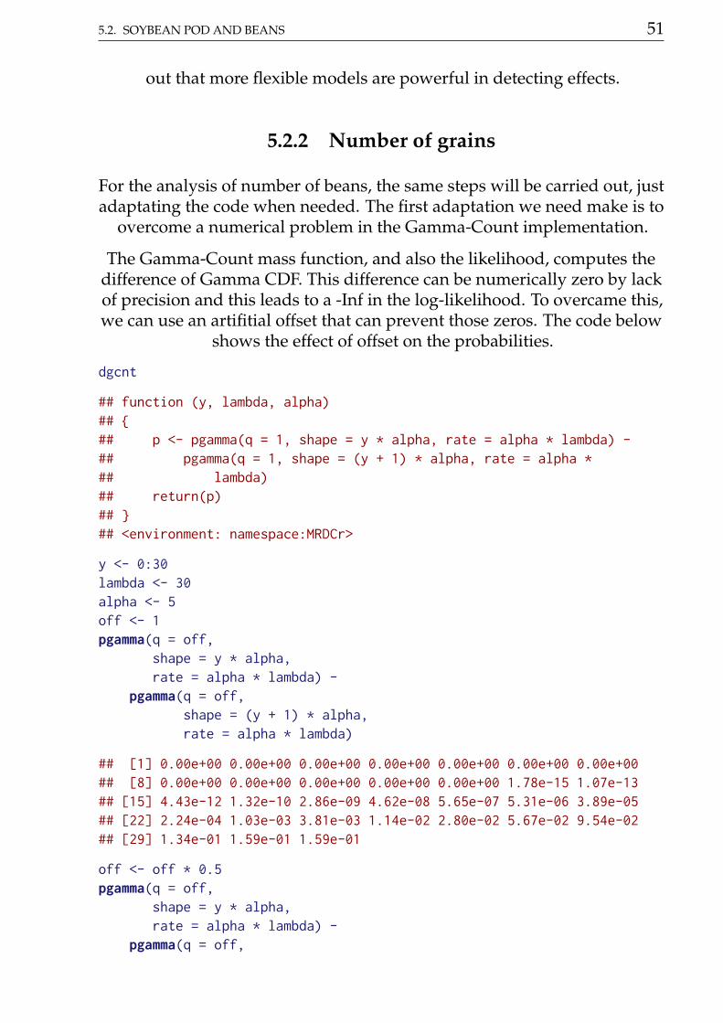
overcome a numerical problem in the Gamma-Count implementation.
The Gamma-Count mass function, and also the likelihood, computes thedifference of Gamma CDF. This difference can be numerically zero by lackof precision and this leads to a -Inf in the log-likelihood. To overcame this,we can use an artifitial offset that can prevent those zeros. The code below
shows the effect of offset on the probabilities.
dgcnt
## function (y, lambda, alpha)## ## p <- pgamma(q = 1, shape = y * alpha, rate = alpha * lambda) -## pgamma(q = 1, shape = (y + 1) * alpha, rate = alpha *## lambda)## return(p)## ## <environment: namespace:MRDCr>
y <- 0:30lambda <- 30alpha <- 5off <- 1pgamma(q = off,
shape = y * alpha,rate = alpha * lambda) -
pgamma(q = off,shape = (y + 1) * alpha,rate = alpha * lambda)
## [1] 0.00e+00 0.00e+00 0.00e+00 0.00e+00 0.00e+00 0.00e+00 0.00e+00## [8] 0.00e+00 0.00e+00 0.00e+00 0.00e+00 0.00e+00 1.78e-15 1.07e-13## [15] 4.43e-12 1.32e-10 2.86e-09 4.62e-08 5.65e-07 5.31e-06 3.89e-05## [22] 2.24e-04 1.03e-03 3.81e-03 1.14e-02 2.80e-02 5.67e-02 9.54e-02## [29] 1.34e-01 1.59e-01 1.59e-01
off <- off * 0.5pgamma(q = off,
shape = y * alpha,rate = alpha * lambda) -
pgamma(q = off,
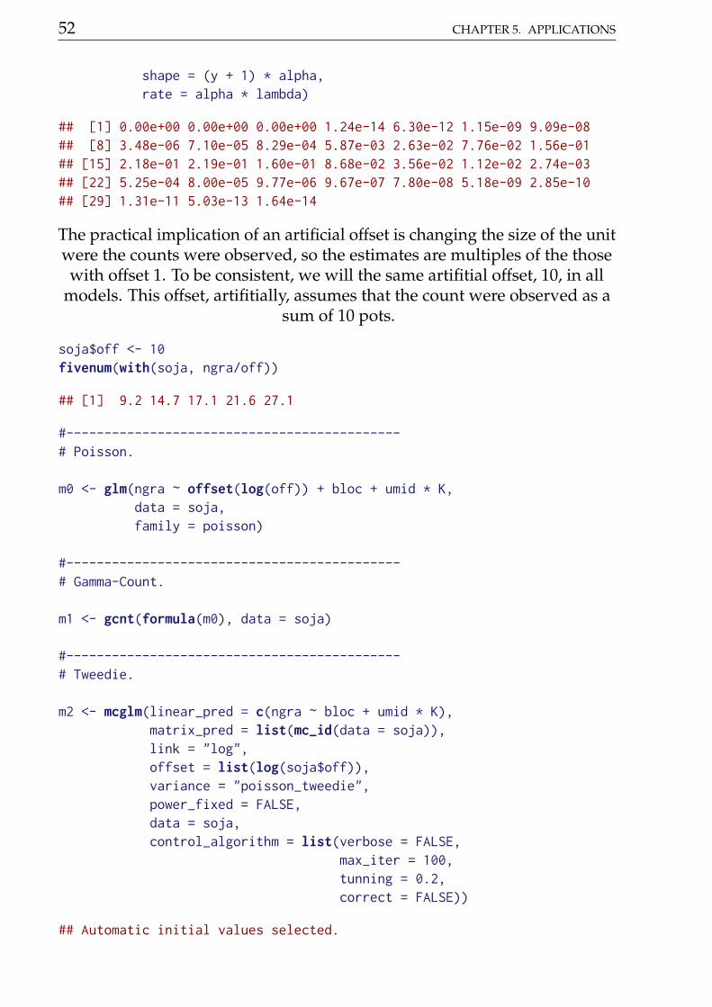
52 CHAPTER 5. APPLICATIONS
shape = (y + 1) * alpha,rate = alpha * lambda)
## [1] 0.00e+00 0.00e+00 0.00e+00 1.24e-14 6.30e-12 1.15e-09 9.09e-08## [8] 3.48e-06 7.10e-05 8.29e-04 5.87e-03 2.63e-02 7.76e-02 1.56e-01## [15] 2.18e-01 2.19e-01 1.60e-01 8.68e-02 3.56e-02 1.12e-02 2.74e-03## [22] 5.25e-04 8.00e-05 9.77e-06 9.67e-07 7.80e-08 5.18e-09 2.85e-10## [29] 1.31e-11 5.03e-13 1.64e-14
The practical implication of an artificial offset is changing the size of the unitwere the counts were observed, so the estimates are multiples of the thosewith offset 1. To be consistent, we will the same artifitial offset, 10, in all
models. This offset, artifitially, assumes that the count were observed as asum of 10 pots.
soja$off <- 10fivenum(with(soja, ngra/off))
## [1] 9.2 14.7 17.1 21.6 27.1
#--------------------------------------------# Poisson.
m0 <- glm(ngra ~ offset(log(off)) + bloc + umid * K,data = soja,family = poisson)
#--------------------------------------------# Gamma-Count.
m1 <- gcnt(formula(m0), data = soja)
#--------------------------------------------# Tweedie.
m2 <- mcglm(linear_pred = c(ngra ~ bloc + umid * K),matrix_pred = list(mc_id(data = soja)),link = "log",offset = list(log(soja$off)),variance = "poisson_tweedie",power_fixed = FALSE,data = soja,control_algorithm = list(verbose = FALSE,
max_iter = 100,tunning = 0.2,correct = FALSE))
## Automatic initial values selected.
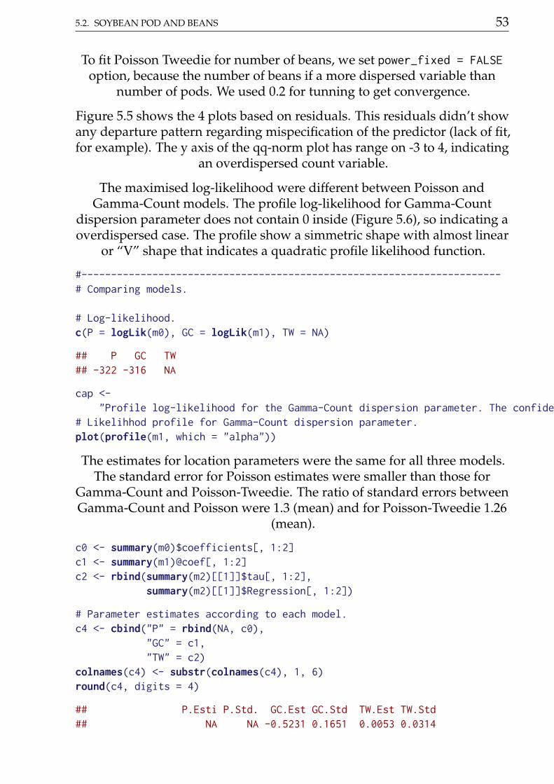
5.2. SOYBEAN POD AND BEANS 53
To fit Poisson Tweedie for number of beans, we set power_fixed = FALSEoption, because the number of beans if a more dispersed variable than
number of pods. We used 0.2 for tunning to get convergence.
Figure 5.5 shows the 4 plots based on residuals. This residuals didn’t showany departure pattern regarding mispecification of the predictor (lack of fit,for example). The y axis of the qq-norm plot has range on -3 to 4, indicating
an overdispersed count variable.
The maximised log-likelihood were different between Poisson andGamma-Count models. The profile log-likelihood for Gamma-Count
dispersion parameter does not contain 0 inside (Figure 5.6), so indicating aoverdispersed case. The profile show a simmetric shape with almost linear
or “V” shape that indicates a quadratic profile likelihood function.
#-----------------------------------------------------------------------# Comparing models.
# Log-likelihood.c(P = logLik(m0), GC = logLik(m1), TW = NA)
## P GC TW## -322 -316 NA
cap <-"Profile log-likelihood for the Gamma-Count dispersion parameter. The confidence interval based on profile likelihood contains 0 inside as indicated by the solid vertical line."
# Likelihhod profile for Gamma-Count dispersion parameter.plot(profile(m1, which = "alpha"))
The estimates for location parameters were the same for all three models.The standard error for Poisson estimates were smaller than those for
Gamma-Count and Poisson-Tweedie. The ratio of standard errors betweenGamma-Count and Poisson were 1.3 (mean) and for Poisson-Tweedie 1.26
(mean).
c0 <- summary(m0)$coefficients[, 1:2]c1 <- summary(m1)@coef[, 1:2]c2 <- rbind(summary(m2)[[1]]$tau[, 1:2],
summary(m2)[[1]]$Regression[, 1:2])
# Parameter estimates according to each model.c4 <- cbind("P" = rbind(NA, c0),
"GC" = c1,"TW" = c2)
colnames(c4) <- substr(colnames(c4), 1, 6)round(c4, digits = 4)
## P.Esti P.Std. GC.Est GC.Std TW.Est TW.Std## NA NA -0.5231 0.1651 0.0053 0.0314
54 CHAPTER 5. APPLICATIONS
## (Intercept) 2.4994 0.0448 2.4965 0.0582 2.4995 0.0549## blocII -0.0194 0.0266 -0.0194 0.0345 -0.0216 0.0352## blocIII -0.0366 0.0267 -0.0367 0.0347 -0.0376 0.0353## blocIV -0.1056 0.0272 -0.1058 0.0353 -0.1003 0.0356## blocV -0.0931 0.0279 -0.0933 0.0362 -0.0974 0.0365## umid50 0.1325 0.0569 0.1328 0.0740 0.1333 0.0696## umid62,5 0.1855 0.0562 0.1860 0.0731 0.1871 0.0690## K30 0.2980 0.0549 0.2988 0.0713 0.2992 0.0678## K60 0.3443 0.0543 0.3452 0.0706 0.3447 0.0674## K120 0.3649 0.0541 0.3659 0.0703 0.3662 0.0672## K180 0.2954 0.0549 0.2962 0.0714 0.2950 0.0679## umid50:K30 0.0434 0.0748 0.0434 0.0973 0.0401 0.0936## umid62,5:K30 -0.1367 0.0753 -0.1371 0.0979 -0.1392 0.0940## umid50:K60 0.1156 0.0736 0.1157 0.0957 0.1146 0.0926## umid62,5:K60 0.0917 0.0729 0.0917 0.0948 0.0896 0.0920## umid50:K120 0.1186 0.0733 0.1187 0.0953 0.1184 0.0923## umid62,5:K120 0.1627 0.0737 0.1628 0.0958 0.1591 0.0937## umid50:K180 0.2883 0.0733 0.2887 0.0953 0.2884 0.0923## umid62,5:K180 0.2157 0.0729 0.2159 0.0947 0.2142 0.0920
# Ratios between stardard errors.cbind(GC = summary(c4[-1, 4]/c4[-1, 2]),
TW = summary(c4[-1, 6]/c4[-1, 2]))
## GC TW## Min. 1.3 1.22## 1st Qu. 1.3 1.24## Median 1.3 1.26## Mean 1.3 1.26## 3rd Qu. 1.3 1.27## Max. 1.3 1.32
The Poisson model gave the higher statistic to the rejection of the nullhypothesis than Gamma-Count and Poisson-Tweedie because it is assuminga dispersion of 1 that is not the case. Gamma-Count and Poisson-Tweedie
perform very similar to test the interaction.
# Analysis of deviance table.anova(m0, test = "Chisq")
## Analysis of Deviance Table#### Model: poisson, link: log#### Response: ngra#### Terms added sequentially (first to last)##
5.2. SOYBEAN POD AND BEANS 55
#### Df Deviance Resid. Df Resid. Dev Pr(>Chi)## NULL 73 761## bloc 4 28 69 733 1.1e-05 ***## umid 2 185 67 548 < 2e-16 ***## K 4 380 63 168 < 2e-16 ***## umid:K 8 43 55 125 8.8e-07 ***## ---## Signif. codes: 0 '***' 0.001 '**' 0.01 '*' 0.05 '.' 0.1 ' ' 1
# Wald test for interaction.a <- c(0, attr(model.matrix(m0), "assign"))ai <- a == max(a)L <- t(replicate(sum(ai), rbind(coef(m1) * 0), simplify = "matrix"))L[, ai] <- diag(sum(ai))linearHypothesis(model = m0, # m0 is not being used here.
hypothesis.matrix = L,vcov. = vcov(m1),coef. = coef(m1))
## Linear hypothesis test#### Hypothesis:## umid50:K30 = 0## umid62,5:K30 = 0## umid50:K60 = 0## umid62,5:K60 = 0## umid50:K120 = 0## umid62,5:K120 = 0## umid50:K180 = 0## umid62,5:K180 = 0#### Model 1: restricted model## Model 2: ngra ~ offset(log(off)) + bloc + umid * K#### Note: Coefficient covariance matrix supplied.#### Res.Df Df Chisq Pr(>Chisq)## 1 63## 2 55 8 25.3 0.0014 **## ---## Signif. codes: 0 '***' 0.001 '**' 0.01 '*' 0.05 '.' 0.1 ' ' 1
# Wald test for fixed effects.anova(m2)
## Wald test for fixed effects## Call: ngra ~ bloc + umid * K
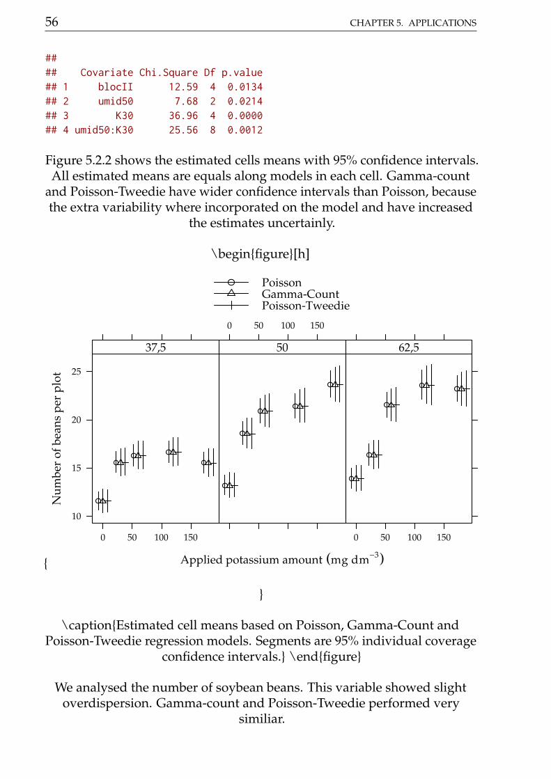
56 CHAPTER 5. APPLICATIONS
#### Covariate Chi.Square Df p.value## 1 blocII 12.59 4 0.0134## 2 umid50 7.68 2 0.0214## 3 K30 36.96 4 0.0000## 4 umid50:K30 25.56 8 0.0012
Figure 5.2.2 shows the estimated cells means with 95% confidence intervals.All estimated means are equals along models in each cell. Gamma-count
and Poisson-Tweedie have wider confidence intervals than Poisson, becausethe extra variability where incorporated on the model and have increased
the estimates uncertainly.
\beginfigure[h]
Applied potassium amount (mg dm−3)
Num
ber
of b
eans
per
plo
t
10
15
20
25
0 50 100 150
37,5
0 50 100 150
50
0 50 100 150
62,5
PoissonGamma-CountPoisson-Tweedie
\captionEstimated cell means based on Poisson, Gamma-Count andPoisson-Tweedie regression models. Segments are 95% individual coverage
confidence intervals. \endfigure
We analysed the number of soybean beans. This variable showed slightoverdispersion. Gamma-count and Poisson-Tweedie performed very
similiar.
5.2. SOYBEAN POD AND BEANS 57
5.2.3 Number of grains per pod
Analyse the number of beans per plot is better than the total number ofbeans, because the leter can be a side effect of the number of pods. We will
analyse the number of beans using the number of pods as an offset.
#--------------------------------------------# Poisson.
m0 <- glm(ngra ~ offset(log(nvag)) + bloc + umid * K,data = soja,family = poisson)
#--------------------------------------------# Gamma-Count.
m1 <- gcnt(formula(m0), data = soja)
#--------------------------------------------# Tweedie.
m2 <- mcglm(linear_pred = c(ngra ~ bloc + umid * K),matrix_pred = list(mc_id(data = soja)),link = "log",offset = list(log(soja$nvag)),variance = "poisson_tweedie",power_fixed = TRUE,data = soja,control_algorithm = list(verbose = FALSE,
max_iter = 100,tunning = 0.5,correct = FALSE))
## Automatic initial values selected.
To accomplish the fitting, we set power_fixed = TRUE otherwiseconvergence wasn’t met.
Figure 5.7 shows the 4 plots based on residuals. The y axis of the qq-normplot has range on -1.5 to 1.5, indicating an underdispersed count variable.
The maximised log-likelihood were different between Poisson andGamma-Count models. The profile log-likelihood for Gamma-Count
dispersion parameter does not contain 0 inside (Figure 5.8), so indicating anunderdispersed count. The profile likelihood is “V” shape that represents a
quadratic profile log-likelihood function.
#-----------------------------------------------------------------------
58 CHAPTER 5. APPLICATIONS
# Comparing models.
# Log-likelihood.c(P = logLik(m0), GC = logLik(m1), TW = NA)
## P GC TW## -271 -255 NA
cap <-"Profile log-likelihood for the Gamma-Count dispersion parameter. The confidence interval based on profile likelihood contains 0 inside as indicated by the solid vertical line."
# Likelihhod profile for Gamma-Count dispersion parameter.plot(profile(m1, which = "alpha"))
The point estimates for location parameters were, once more, the same forall three models. The standard error for Poisson estimates were greater than
those for Gamma-Count and Poisson-Tweedie.
c0 <- summary(m0)$coefficients[, 1:2]c1 <- summary(m1)@coef[, 1:2]c2 <- rbind(summary(m2)[[1]]$tau[, 1:2],
summary(m2)[[1]]$Regression[, 1:2])
# Parameter estimates according to each model.c4 <- cbind("P" = rbind(NA, c0),
"GC" = c1,"TW" = c2)
colnames(c4) <- substr(colnames(c4), 1, 6)round(c4, digits = 4)
## P.Esti P.Std. GC.Est GC.Std TW.Est TW.Std## NA NA 1.1225 0.1648 -0.6764 0.0446## (Intercept) 0.8482 0.0447 0.8510 0.0255 0.8482 0.0254## blocII 0.0113 0.0266 0.0114 0.0152 0.0113 0.0151## blocIII 0.0363 0.0267 0.0363 0.0152 0.0363 0.0152## blocIV 0.0194 0.0272 0.0195 0.0155 0.0194 0.0155## blocV 0.0161 0.0280 0.0163 0.0159 0.0161 0.0159## umid50 -0.0019 0.0569 -0.0023 0.0325 -0.0019 0.0324## umid62,5 -0.0312 0.0563 -0.0317 0.0321 -0.0312 0.0320## K30 0.0229 0.0549 0.0221 0.0313 0.0229 0.0312## K60 0.0345 0.0544 0.0337 0.0310 0.0345 0.0309## K120 0.0353 0.0541 0.0344 0.0309 0.0353 0.0308## K180 0.0406 0.0549 0.0399 0.0313 0.0406 0.0312## umid50:K30 -0.0187 0.0748 -0.0187 0.0427 -0.0187 0.0426## umid62,5:K30 -0.0285 0.0753 -0.0281 0.0429 -0.0285 0.0428## umid50:K60 -0.0482 0.0736 -0.0483 0.0420 -0.0482 0.0419## umid62,5:K60 -0.0140 0.0729 -0.0140 0.0416 -0.0140 0.0415## umid50:K120 -0.0304 0.0733 -0.0305 0.0418 -0.0304 0.0417## umid62,5:K120 0.0455 0.0738 0.0454 0.0421 0.0455 0.0420## umid50:K180 -0.0163 0.0733 -0.0167 0.0418 -0.0163 0.0417
5.2. SOYBEAN POD AND BEANS 59
## umid62,5:K180 0.0169 0.0729 0.0167 0.0416 0.0169 0.0415
# Ratios between stardard errors.cbind(GC = summary(c4[-1, 4]/c4[-1, 2]),
TW = summary(c4[-1, 6]/c4[-1, 2]))
## GC TW## Min. 0.57 0.569## 1st Qu. 0.57 0.569## Median 0.57 0.569## Mean 0.57 0.569## 3rd Qu. 0.57 0.569## Max. 0.57 0.569
None of the experimental factors had effect on the number of beans per pod.Althought, Gamma-Count and Poisson-Tweedie showed more favorable
statistics to the rejection of the null hypothesis than Poisson.
# Analysis of deviance table.anova(m0, test = "Chisq")
## Analysis of Deviance Table#### Model: poisson, link: log#### Response: ngra#### Terms added sequentially (first to last)###### Df Deviance Resid. Df Resid. Dev Pr(>Chi)## NULL 73 34.2## bloc 4 2.03 69 32.2 0.73## umid 2 1.75 67 30.5 0.42## K 4 3.83 63 26.6 0.43## umid:K 8 2.65 55 24.0 0.95
# Wald test for interaction.a <- c(0, attr(model.matrix(m0), "assign"))ai <- a == max(a)L <- t(replicate(sum(ai), rbind(coef(m1) * 0), simplify = "matrix"))L[, ai] <- diag(sum(ai))linearHypothesis(model = m0, # m0 is not being used here.
hypothesis.matrix = L,vcov. = vcov(m1),coef. = coef(m1))
## Linear hypothesis test##
60 CHAPTER 5. APPLICATIONS
## Hypothesis:## umid50:K30 = 0## umid62,5:K30 = 0## umid50:K60 = 0## umid62,5:K60 = 0## umid50:K120 = 0## umid62,5:K120 = 0## umid50:K180 = 0## umid62,5:K180 = 0#### Model 1: restricted model## Model 2: ngra ~ offset(log(nvag)) + bloc + umid * K#### Note: Coefficient covariance matrix supplied.#### Res.Df Df Chisq Pr(>Chisq)## 1 63## 2 55 8 8.1 0.42
# Wald test for fixed effects.anova(m2)
## Wald test for fixed effects## Call: ngra ~ bloc + umid * K#### Covariate Chi.Square Df p.value## 1 blocII 6.03 4 0.197## 2 umid50 1.26 2 0.534## 3 K30 2.09 4 0.719## 4 umid50:K30 8.20 8 0.414
Figure 5.2.3 shows the estimated cells means with 95% confidence intervals.All estimated means are equals along models in each cell. Gamma-count
and Poisson-Tweedie have more shorter confidence intervals than Poisson.
\beginfigure[h]
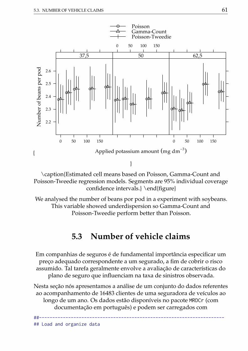
5.3. NUMBER OF VEHICLE CLAIMS 61
Applied potassium amount (mg dm−3)
Num
ber
of b
eans
per
pod
2.2
2.3
2.4
2.5
2.6
0 50 100 150
37,5
0 50 100 150
50
0 50 100 150
62,5
PoissonGamma-CountPoisson-Tweedie
\captionEstimated cell means based on Poisson, Gamma-Count andPoisson-Tweedie regression models. Segments are 95% individual coverage
confidence intervals. \endfigure
We analysed the number of beans por pod in a experiment with soybeans.This variable showed underdispersion so Gamma-Count and
Poisson-Tweedie perform better than Poisson.
5.3 Number of vehicle claims
Em companhias de seguros é de fundamental importância especificar umpreço adequado correspondente a um segurado, a fim de cobrir o risco
assumido. Tal tarefa geralmente envolve a avaliação de características doplano de seguro que influenciam na taxa de sinistros observada.
Nesta seção nós apresentamos a análise de um conjunto do dados referentesao acompanhamento de 16483 clientes de uma seguradora de veículos ao
longo de um ano. Os dados estão disponíveis no pacote MRDCr (comdocumentação em português) e podem ser carregados com
##----------------------------------------------------------------------## Load and organize data
62 CHAPTER 5. APPLICATIONS
data(package = "MRDCr")help(seguros, h = "html")
Após a tradução dos níveis das variáveis categóricas a estrutura dos dadosfica
## Translate levels of categorical variables and colnamescolnames(seguros) <- c("age", "sex", "price", "expo", "nclaims")levels(seguros$sex) <- c("Female", "Male")str(seguros)
## 'data.frame': 16483 obs. of 5 variables:## $ age : int 59 45 42 63 36 33 35 63 54 32 ...## $ sex : Factor w/ 2 levels "Female","Male": 1 2 2 1 1 2 2 2 2 2 ...## $ price : num 24.6 23.4 86.6 77.5 25.9 ...## $ expo : num 0.5 0.7 0.79 0.01 0.51 0.79 0.81 0.01 0.76 0.79 ...## $ nclaims: int 1 0 0 0 0 0 0 0 0 0 ...
In this dataset a variável age é mensurada em anos, e price em 1000 reais. Avariável expo representa o período de cobertura do cliente, durante o ano
sob análise, um valor de 0.5 significa que o cliente esteve exposto ao sinistrodurante metade do ano.
A Figura 5.9 mostra a descrição das variáveis a serem utilizadas na análise.Embora esses gráficos não considerem todas as variáveis conjuntamente, ográfico à esquerda sugere que há um excesso de contagens nulas, no geral
95.183% das contagens são 0.
Para análise desses dados consideramos efeitos quadráticos para variáveiscontínuas e intercepto variando conforme sexo do cliente. price foi tomada
como preditor pode ser escrito como
log(
µiexpoi
)=β0 +β11(sexi) +β2pricei+
+β3price2i +β4agei +β5age
2i
em R definimos o preditor conforme sintaxe para objetos da classe formula.Note que a variável expo é envolta na função offset e sendo assim é
considerado apenas como denominador das contagens.
## Define preditorform0 <- nclaims ~ offset(log(expo)) + sex +
price + I(price^2) + age + I(age^2)
Nós ajustamos os modelos de regressão Poisson e Poisson-Tweedie usandoos frameworks stats::glm e mcglm::mcglm, que se baseam em máxima
verossimilhança e especificação por momentos respectivamente.
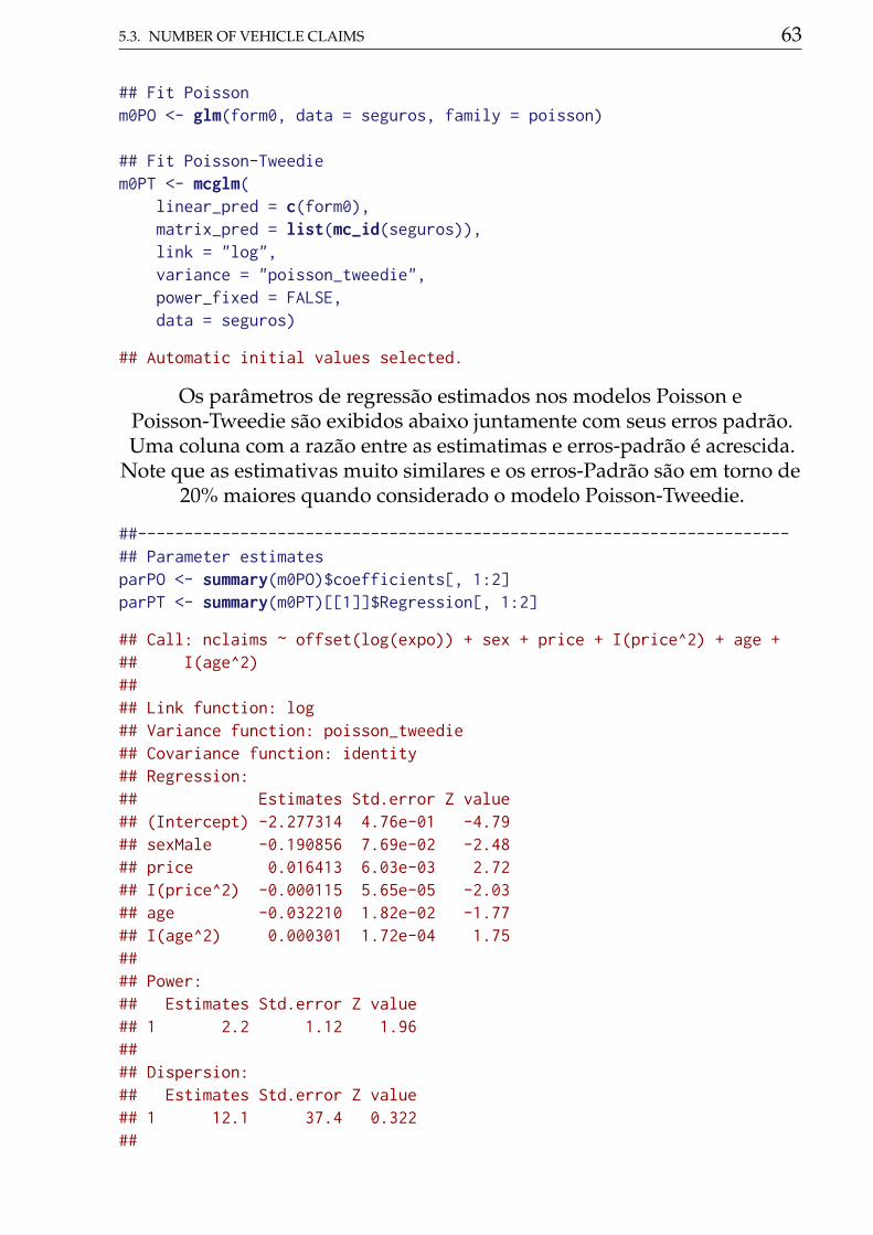
5.3. NUMBER OF VEHICLE CLAIMS 63
## Fit Poissonm0PO <- glm(form0, data = seguros, family = poisson)
## Fit Poisson-Tweediem0PT <- mcglm(
linear_pred = c(form0),matrix_pred = list(mc_id(seguros)),link = "log",variance = "poisson_tweedie",power_fixed = FALSE,data = seguros)
## Automatic initial values selected.
Os parâmetros de regressão estimados nos modelos Poisson ePoisson-Tweedie são exibidos abaixo juntamente com seus erros padrão.Uma coluna com a razão entre as estimatimas e erros-padrão é acrescida.
Note que as estimativas muito similares e os erros-Padrão são em torno de20% maiores quando considerado o modelo Poisson-Tweedie.
##----------------------------------------------------------------------## Parameter estimatesparPO <- summary(m0PO)$coefficients[, 1:2]parPT <- summary(m0PT)[[1]]$Regression[, 1:2]
## Call: nclaims ~ offset(log(expo)) + sex + price + I(price^2) + age +## I(age^2)#### Link function: log## Variance function: poisson_tweedie## Covariance function: identity## Regression:## Estimates Std.error Z value## (Intercept) -2.277314 4.76e-01 -4.79## sexMale -0.190856 7.69e-02 -2.48## price 0.016413 6.03e-03 2.72## I(price^2) -0.000115 5.65e-05 -2.03## age -0.032210 1.82e-02 -1.77## I(age^2) 0.000301 1.72e-04 1.75#### Power:## Estimates Std.error Z value## 1 2.2 1.12 1.96#### Dispersion:## Estimates Std.error Z value## 1 12.1 37.4 0.322##
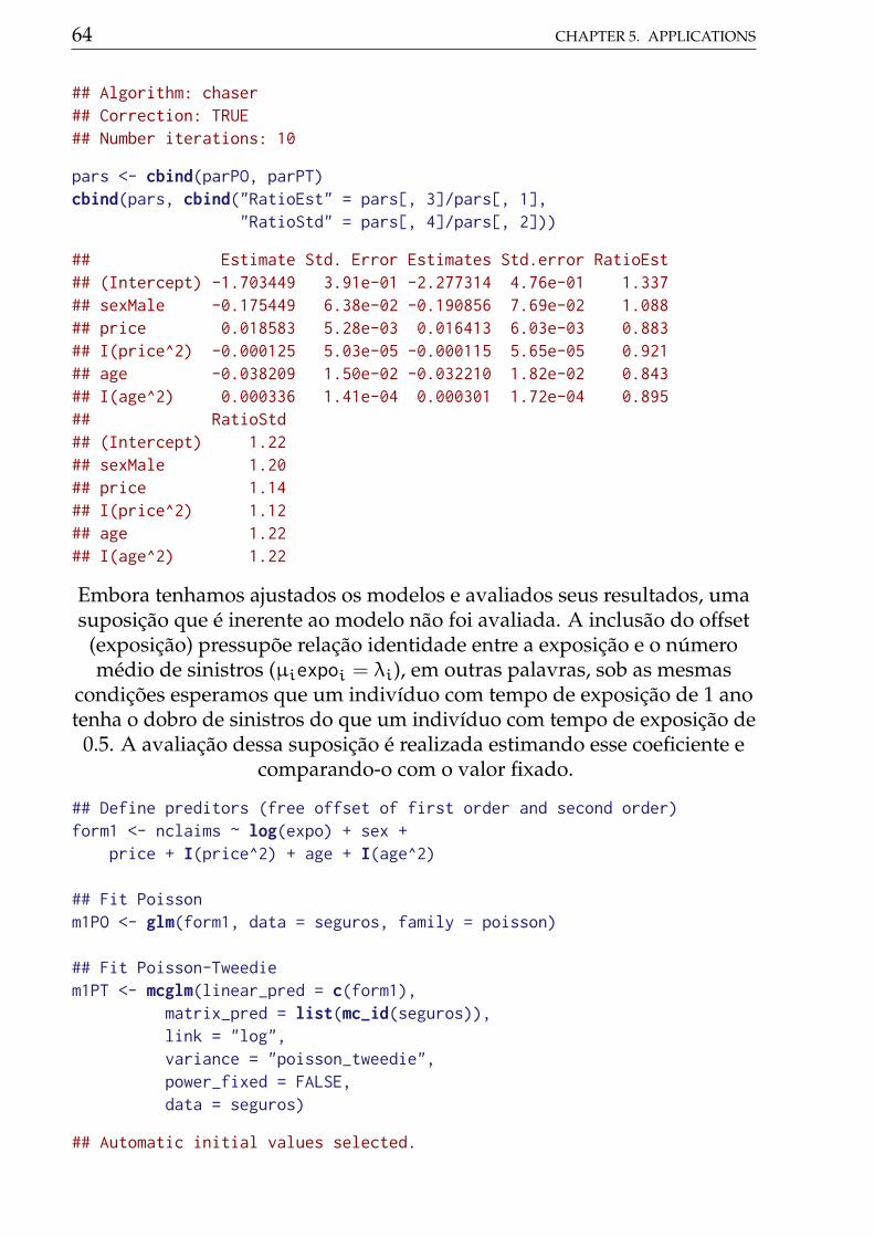
64 CHAPTER 5. APPLICATIONS
## Algorithm: chaser## Correction: TRUE## Number iterations: 10
pars <- cbind(parPO, parPT)cbind(pars, cbind("RatioEst" = pars[, 3]/pars[, 1],
"RatioStd" = pars[, 4]/pars[, 2]))
## Estimate Std. Error Estimates Std.error RatioEst## (Intercept) -1.703449 3.91e-01 -2.277314 4.76e-01 1.337## sexMale -0.175449 6.38e-02 -0.190856 7.69e-02 1.088## price 0.018583 5.28e-03 0.016413 6.03e-03 0.883## I(price^2) -0.000125 5.03e-05 -0.000115 5.65e-05 0.921## age -0.038209 1.50e-02 -0.032210 1.82e-02 0.843## I(age^2) 0.000336 1.41e-04 0.000301 1.72e-04 0.895## RatioStd## (Intercept) 1.22## sexMale 1.20## price 1.14## I(price^2) 1.12## age 1.22## I(age^2) 1.22
Embora tenhamos ajustados os modelos e avaliados seus resultados, umasuposição que é inerente ao modelo não foi avaliada. A inclusão do offset
(exposição) pressupõe relação identidade entre a exposição e o númeromédio de sinistros (µiexpoi = λi), em outras palavras, sob as mesmas
condições esperamos que um indivíduo com tempo de exposição de 1 anotenha o dobro de sinistros do que um indivíduo com tempo de exposição de
0.5. A avaliação dessa suposição é realizada estimando esse coeficiente ecomparando-o com o valor fixado.
## Define preditors (free offset of first order and second order)form1 <- nclaims ~ log(expo) + sex +
price + I(price^2) + age + I(age^2)
## Fit Poissonm1PO <- glm(form1, data = seguros, family = poisson)
## Fit Poisson-Tweediem1PT <- mcglm(linear_pred = c(form1),
matrix_pred = list(mc_id(seguros)),link = "log",variance = "poisson_tweedie",power_fixed = FALSE,data = seguros)
## Automatic initial values selected.
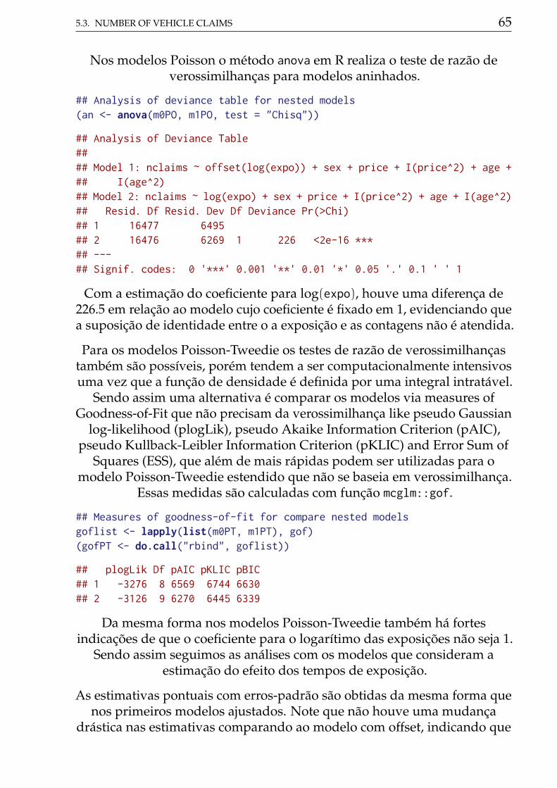
5.3. NUMBER OF VEHICLE CLAIMS 65
Nos modelos Poisson o método anova em R realiza o teste de razão deverossimilhanças para modelos aninhados.
## Analysis of deviance table for nested models(an <- anova(m0PO, m1PO, test = "Chisq"))
## Analysis of Deviance Table#### Model 1: nclaims ~ offset(log(expo)) + sex + price + I(price^2) + age +## I(age^2)## Model 2: nclaims ~ log(expo) + sex + price + I(price^2) + age + I(age^2)## Resid. Df Resid. Dev Df Deviance Pr(>Chi)## 1 16477 6495## 2 16476 6269 1 226 <2e-16 ***## ---## Signif. codes: 0 '***' 0.001 '**' 0.01 '*' 0.05 '.' 0.1 ' ' 1
Com a estimação do coeficiente para log(expo), houve uma diferença de226.5 em relação ao modelo cujo coeficiente é fixado em 1, evidenciando quea suposição de identidade entre o a exposição e as contagens não é atendida.
Para os modelos Poisson-Tweedie os testes de razão de verossimilhançastambém são possíveis, porém tendem a ser computacionalmente intensivosuma vez que a função de densidade é definida por uma integral intratável.
Sendo assim uma alternativa é comparar os modelos via measures ofGoodness-of-Fit que não precisam da verossimilhança like pseudo Gaussian
log-likelihood (plogLik), pseudo Akaike Information Criterion (pAIC),pseudo Kullback-Leibler Information Criterion (pKLIC) and Error Sum of
Squares (ESS), que além de mais rápidas podem ser utilizadas para omodelo Poisson-Tweedie estendido que não se baseia em verossimilhança.
Essas medidas são calculadas com função mcglm::gof.
## Measures of goodness-of-fit for compare nested modelsgoflist <- lapply(list(m0PT, m1PT), gof)(gofPT <- do.call("rbind", goflist))
## plogLik Df pAIC pKLIC pBIC## 1 -3276 8 6569 6744 6630## 2 -3126 9 6270 6445 6339
Da mesma forma nos modelos Poisson-Tweedie também há fortesindicações de que o coeficiente para o logarítimo das exposições não seja 1.
Sendo assim seguimos as análises com os modelos que consideram aestimação do efeito dos tempos de exposição.
As estimativas pontuais com erros-padrão são obtidas da mesma forma quenos primeiros modelos ajustados. Note que não houve uma mudança
drástica nas estimativas comparando ao modelo com offset, indicando que
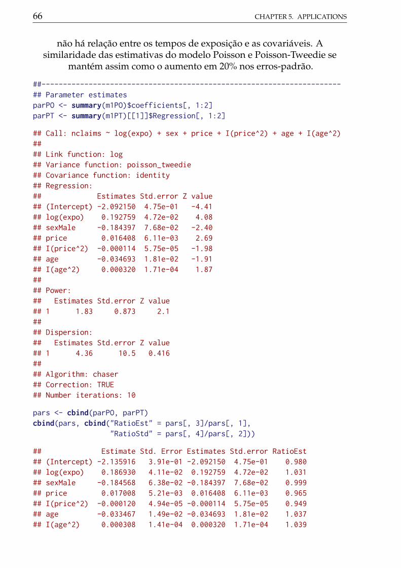
66 CHAPTER 5. APPLICATIONS
não há relação entre os tempos de exposição e as covariáveis. Asimilaridade das estimativas do modelo Poisson e Poisson-Tweedie se
mantém assim como o aumento em 20% nos erros-padrão.
##----------------------------------------------------------------------## Parameter estimatesparPO <- summary(m1PO)$coefficients[, 1:2]parPT <- summary(m1PT)[[1]]$Regression[, 1:2]
## Call: nclaims ~ log(expo) + sex + price + I(price^2) + age + I(age^2)#### Link function: log## Variance function: poisson_tweedie## Covariance function: identity## Regression:## Estimates Std.error Z value## (Intercept) -2.092150 4.75e-01 -4.41## log(expo) 0.192759 4.72e-02 4.08## sexMale -0.184397 7.68e-02 -2.40## price 0.016408 6.11e-03 2.69## I(price^2) -0.000114 5.75e-05 -1.98## age -0.034693 1.81e-02 -1.91## I(age^2) 0.000320 1.71e-04 1.87#### Power:## Estimates Std.error Z value## 1 1.83 0.873 2.1#### Dispersion:## Estimates Std.error Z value## 1 4.36 10.5 0.416#### Algorithm: chaser## Correction: TRUE## Number iterations: 10
pars <- cbind(parPO, parPT)cbind(pars, cbind("RatioEst" = pars[, 3]/pars[, 1],
"RatioStd" = pars[, 4]/pars[, 2]))
## Estimate Std. Error Estimates Std.error RatioEst## (Intercept) -2.135916 3.91e-01 -2.092150 4.75e-01 0.980## log(expo) 0.186930 4.11e-02 0.192759 4.72e-02 1.031## sexMale -0.184568 6.38e-02 -0.184397 7.68e-02 0.999## price 0.017008 5.21e-03 0.016408 6.11e-03 0.965## I(price^2) -0.000120 4.94e-05 -0.000114 5.75e-05 0.949## age -0.033467 1.49e-02 -0.034693 1.81e-02 1.037## I(age^2) 0.000308 1.41e-04 0.000320 1.71e-04 1.039
5.3. NUMBER OF VEHICLE CLAIMS 67
## RatioStd## (Intercept) 1.21## log(expo) 1.15## sexMale 1.20## price 1.17## I(price^2) 1.16## age 1.21## I(age^2) 1.21
Finalmente a Figura ??(fig:claims-pred) apresenta as curvas de prediçãoconforme cada variável, como temos mais de uma covariável numérica nomodelo, fixamos as demais variáveis seu valor mediano para construção dascurvas. O efeito quadrático das variáveis price e age é evidente. A média
de sinistros é maior para veículos entre 50 e 100 mil reais, veículos devalores baixos ou muito elevados tendem a ter um taxa de sinistros menor, oque faz sentido no mercado brasileiro onde furtos e acidentes ocorrem commaior frequência em carros populares. Para a idade temos a interpretaçãocontrária, espera-se menos sinistros para idades medianas, entre 40 e 70
anos e maiores para jovens e idosos.
Comparando os modelos temos curvas de predição e intervalos deconfiança muito similares, sendo levemente maiores quando considerado oPoisson-Tweedie. O que se destaque no gráfico é a diferença nos intervalosde confiança para o preço do veículo, nesse caso o modelo Poisson-Tweedie
é muito mais conservador onde há menos observações, no intervalo depreços mais elevados.
cap <- paste("Curves of predict values an confidence intervals (95\\%)","based on Poisson and Poisson-Tweedie regression models","for each numerical covariate setting the others in the","median.")
##-------------------------------------------## Prediction to exposureaux <- with(seguros,
expand.grid(expo = seq(min(expo), max(expo), length.out = 30),sex = unique(sex),price = median(price),age = median(age)
))
da <- data.frame(var = "Exposure", x = aux$expo, sex = aux$sex)X <- model.matrix(update(form1, NULL ~ .), data = aux)pred <- list(PO = da, PT = da)
68 CHAPTER 5. APPLICATIONS
## Poisson modelaux <- confint(glht(m1PO, linfct = X),
calpha = univariate_calpha())$confintcolnames(aux)[1] <- "fit"pred$PO <- cbind(pred$PO, exp(aux)[, c("lwr", "fit", "upr")])
## Poisson-Tweedie modelqn <- qnorm(0.975) * c(lwr = -1, fit = 0, upr = 1)V <- vcov(m1PT)i <- grepl("beta", colnames(V))eta <- X %*% coef(m1PT, type = "beta")$Estimatesstd <- sqrt(diag(as.matrix(X %*% as.matrix(V[i, i]) %*% t(X))))me <- outer(std, qn, FUN = "*")aux <- sweep(me, 1, eta, FUN = "+")pred$PT <- cbind(pred$PT, exp(aux))
## Organize predictionspredsex <- ldply(pred, .id = "model")
##-------------------------------------------## Prediction to priceaux <- with(seguros,
expand.grid(expo = median(expo),sex = unique(sex),price = seq(min(price), max(price), length.out = 30),age = median(age)
))
da <- data.frame(var = "Price", x = aux$price, sex = aux$sex)X <- model.matrix(update(form1, NULL ~ .), data = aux)pred <- list(PO = da, PT = da)
## Poisson modelaux <- confint(glht(m1PO, linfct = X),
calpha = univariate_calpha())$confintcolnames(aux)[1] <- "fit"pred$PO <- cbind(pred$PO, exp(aux)[, c("lwr", "fit", "upr")])
## Poisson-Tweedie modelqn <- qnorm(0.975) * c(lwr = -1, fit = 0, upr = 1)V <- vcov(m1PT)i <- grepl("beta", colnames(V))eta <- X %*% coef(m1PT, type = "beta")$Estimatesstd <- sqrt(diag(as.matrix(X %*% as.matrix(V[i, i]) %*% t(X))))
5.3. NUMBER OF VEHICLE CLAIMS 69
me <- outer(std, qn, FUN = "*")aux <- sweep(me, 1, eta, FUN = "+")pred$PT <- cbind(pred$PT, exp(aux))
## Organize predictionspredspr <- ldply(pred, .id = "model")
##-------------------------------------------## Prediction to ageaux <- with(seguros,
expand.grid(expo = median(expo),sex = unique(sex),price = median(price),age = seq(min(age), max(age), length.out = 30)
))
da <- data.frame(var = "Age", x = aux$age, sex = aux$sex)X <- model.matrix(update(form1, NULL ~ .), data = aux)pred <- list(PO = da, PT = da)
## Poisson modelaux <- confint(glht(m1PO, linfct = X),
calpha = univariate_calpha())$confintcolnames(aux)[1] <- "fit"pred$PO <- cbind(pred$PO, exp(aux)[, c("lwr", "fit", "upr")])
## Poisson-Tweedie modelqn <- qnorm(0.975) * c(lwr = -1, fit = 0, upr = 1)V <- vcov(m1PT)i <- grepl("beta", colnames(V))eta <- X %*% coef(m1PT, type = "beta")$Estimatesstd <- sqrt(diag(as.matrix(X %*% as.matrix(V[i, i]) %*% t(X))))me <- outer(std, qn, FUN = "*")aux <- sweep(me, 1, eta, FUN = "+")pred$PT <- cbind(pred$PT, exp(aux))
## Organize predictionspredsag <- ldply(pred, .id = "model")
##-------------------------------------------## Graphpreds <- rbind(predsex, predspr, predsag)useOuterStrips(
xyplot(fit ~ x | var + sex,data = preds,
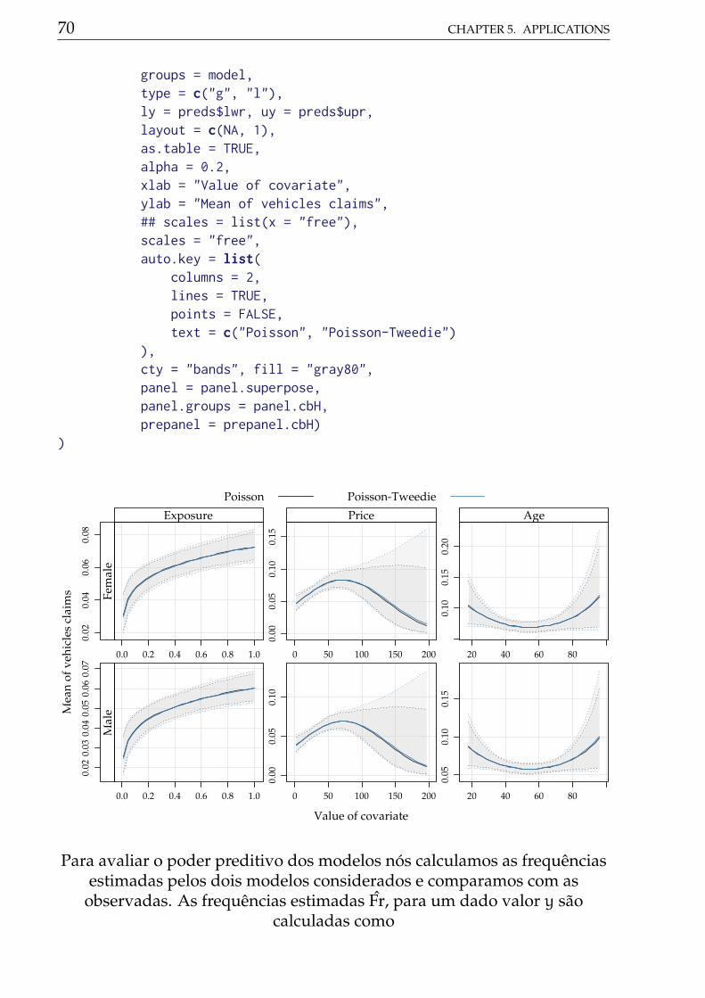
70 CHAPTER 5. APPLICATIONS
groups = model,type = c("g", "l"),ly = preds$lwr, uy = preds$upr,layout = c(NA, 1),as.table = TRUE,alpha = 0.2,xlab = "Value of covariate",ylab = "Mean of vehicles claims",## scales = list(x = "free"),scales = "free",auto.key = list(
columns = 2,lines = TRUE,points = FALSE,text = c("Poisson", "Poisson-Tweedie")
),cty = "bands", fill = "gray80",panel = panel.superpose,panel.groups = panel.cbH,prepanel = prepanel.cbH)
)
Value of covariate
Mea
n of
veh
icle
s cl
aim
s0.
020.
040.
060.
08
0.0 0.2 0.4 0.6 0.8 1.0
Exposure
Fem
ale
0.00
0.05
0.10
0.15
0 50 100 150 200
Price
0.10
0.15
0.20
20 40 60 80
Age
0.02
0.03
0.04
0.05
0.06
0.07
0.0 0.2 0.4 0.6 0.8 1.0
Mal
e
0.00
0.05
0.10
0 50 100 150 200
0.05
0.10
0.15
20 40 60 80
Poisson Poisson-Tweedie
Para avaliar o poder preditivo dos modelos nós calculamos as frequênciasestimadas pelos dois modelos considerados e comparamos com as
observadas. As frequências estimadas Fr, para um dado valor y sãocalculadas como
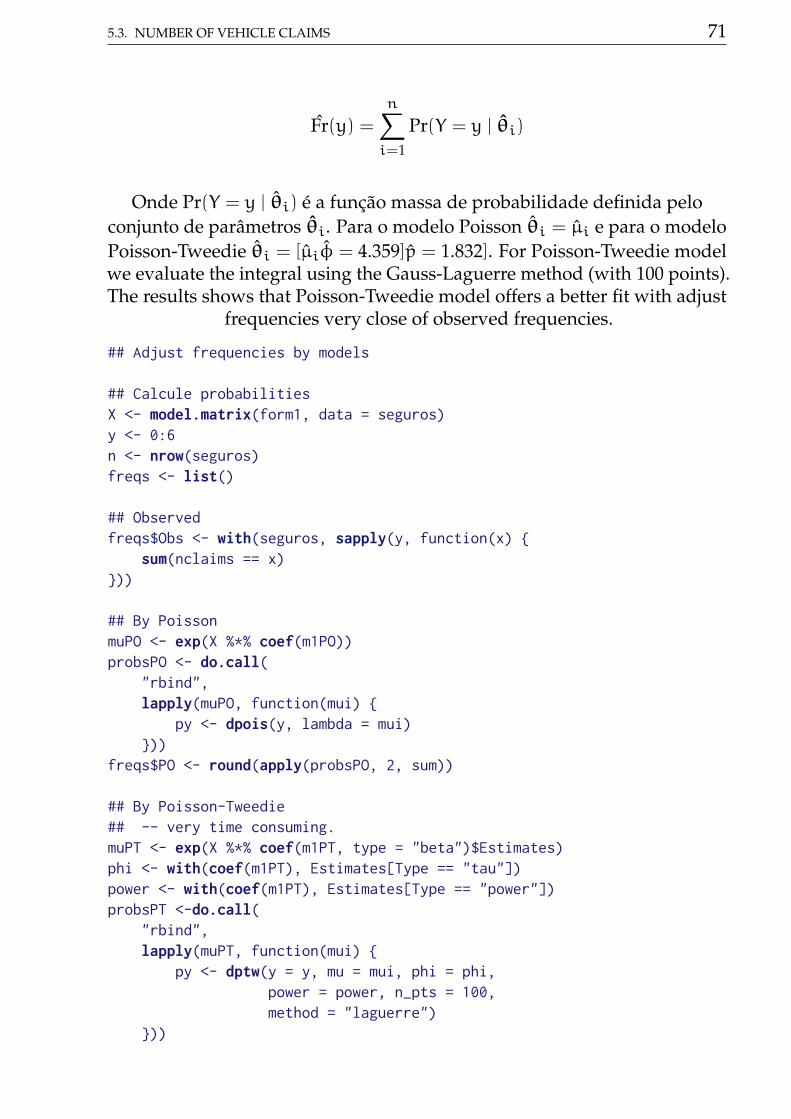
5.3. NUMBER OF VEHICLE CLAIMS 71
Fr(y) =n∑
i=1
Pr(Y = y | θi)
Onde Pr(Y = y | θi) é a função massa de probabilidade definida peloconjunto de parâmetros θi. Para o modelo Poisson θi = µi e para o modeloPoisson-Tweedie θi = [µiφ = 4.359]p = 1.832]. For Poisson-Tweedie modelwe evaluate the integral using the Gauss-Laguerre method (with 100 points).The results shows that Poisson-Tweedie model offers a better fit with adjust
frequencies very close of observed frequencies.
## Adjust frequencies by models
## Calcule probabilitiesX <- model.matrix(form1, data = seguros)y <- 0:6n <- nrow(seguros)freqs <- list()
## Observedfreqs$Obs <- with(seguros, sapply(y, function(x)
sum(nclaims == x)))
## By PoissonmuPO <- exp(X %*% coef(m1PO))probsPO <- do.call(
"rbind",lapply(muPO, function(mui)
py <- dpois(y, lambda = mui)))
freqs$PO <- round(apply(probsPO, 2, sum))
## By Poisson-Tweedie## -- very time consuming.muPT <- exp(X %*% coef(m1PT, type = "beta")$Estimates)phi <- with(coef(m1PT), Estimates[Type == "tau"])power <- with(coef(m1PT), Estimates[Type == "power"])probsPT <-do.call(
"rbind",lapply(muPT, function(mui)
py <- dptw(y = y, mu = mui, phi = phi,power = power, n_pts = 100,method = "laguerre")
))

72 CHAPTER 5. APPLICATIONS
freqs$PT <- round(apply(probsPT, 2, sum))tabf <- ldply(freqs)
colnames(tabf) <- c("", y)tabf
## 0 1 2 3 4 5 6## 1 Obs 15689 602 166 22 3 1 0## 2 PO 15498 953 31 1 0 0 0## 3 PT 15673 663 121 26 6 2 0
5.4 Radiation-induced chromosome aberrationcounts
In biological dosimetry studies essentially the response variables are datacounts. These experiments measure the number of chromosome aberrationsin human lymphocytes after to controlled exposure of ionizing radiation.
The aim of the studies are analyse the biological effects induced by ionizingradiation. The aberrations most commonly mensured are the dicentrics,
centric rings, and micronucle .
In this section the dataset considered was obtained after irradiating bloodsamples with five different doses between 0.1 and 1 Gy of 2.1 MeV neutrons.In this case, the frequencies of dicentrics and centric rings after a culture of
72 hours are analysed. The dataset was analysed by ?, as an example ofzero-inflated data and Bonat et al. (2016), using extend Poisson-Tweedie
approach.
The data are available in data/chromossome.rda file. In R it can be loadedwith
##----------------------------------------------------------------------## Loadload("./data/chromosome.rda")str(chromosome)
## 'data.frame': 5232 obs. of 2 variables:## $ ndic: num 0 0 0 0 0 0 0 0 0 0 ...## $ dose: num 0.1 0.1 0.1 0.1 0.1 0.1 0.1 0.1 0.1 0.1 ...
The Figure 5.10 shows the frequencies chromosome aberrations (left) andaverage of chromosome aberrations by radiation doses (right). Note that the
highest frequencies are observed for zero counts and the averages arebetween 0 and 1, suggesting excess zero.
5.4. RADIATION-INDUCED CHROMOSOME ABERRATION COUNTS 73
For this application we fit the Poisson, Gamma-Count, COM-Poisson andPoisson-Tweedie distributions. The linear predictor considered is a
quadratic dose model, follow Bonat et al. (2016). The codes below fit thefour models using the MRDCd and mcglm packages. Note that for MRDCr::cmpfunction we need specify sumto, the number of increments for a infinite sum,
i.e in this case Z(λi, ν) =∑50j λ
ji/(j!)
ν.
##----------------------------------------------------------------------## Modellingform <- ndic ~ dose + I(dose^2)
m0PO <- glm(form, family = poisson, data = chromosome)m0GC <- gcnt(form, data = chromosome)m0CP <- cmp(form, data = chromosome, sumto = 50)m0PT <- mcglm(
linear_pred = c(form),matrix_pred = list(mc_id(chromosome)),link = "log",variance = "poisson_tweedie",power_fixed = FALSE,data = chromosome)
## Automatic initial values selected.
No issues were reported during the estimation process. A better researchabout the algorithm covergence for Poisson-Tweedie models is
implemented by mcglm::plot(model, type = "algorithm"). This fourgraphs shows the trajectory or iterations of the fitting algorithm, we can see
that both cases the lines converged.
## Check algorithm convergenceplot(m0PT, type = "algorithm")
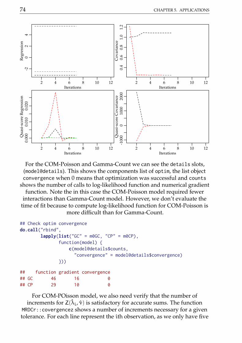
74 CHAPTER 5. APPLICATIONS
2 4 6 8 10 12
-20
24
Iterations
Reg
ress
ion
2 4 6 8 10 12
0.4
0.6
0.8
1.0
1.2
Iterations
Cov
aria
nce
2 4 6 8 10 12
0.00
00.
010
0.02
0
Iterations
Qua
si-s
core
Reg
ress
ion
2 4 6 8 10 12
-100
00
1000
2000
Iterations
Qua
si-s
core
Cov
aria
nce
For the COM-Poisson and Gamma-Count we can see the details slots,(model@details). This shows the components list of optim, the list objectconvergence when 0 means that optimization was successful and counts
shows the number of calls to log-likelihood function and numerical gradientfunction. Note the in this case the COM-Poisson model required fewer
interactions than Gamma-Count model. However, we don’t evaluate thetime of fit because to compute log-likelihood function for COM-Poisson is
more difficult than for Gamma-Count.
## Check optim convergencedo.call("rbind",
lapply(list("GC" = m0GC, "CP" = m0CP),function(model)
c(model@details$counts,"convergence" = model@details$convergence)
))
## function gradient convergence## GC 46 16 0## CP 29 10 0
For COM-POisson model, we also need verify that the number ofincrements for Z(λi, ν) is satisfactory for accurate sums. The function
MRDCr::covergencez shows a number of increments necessary for a giventolerance. For each line represent the ith observation, as we only have five
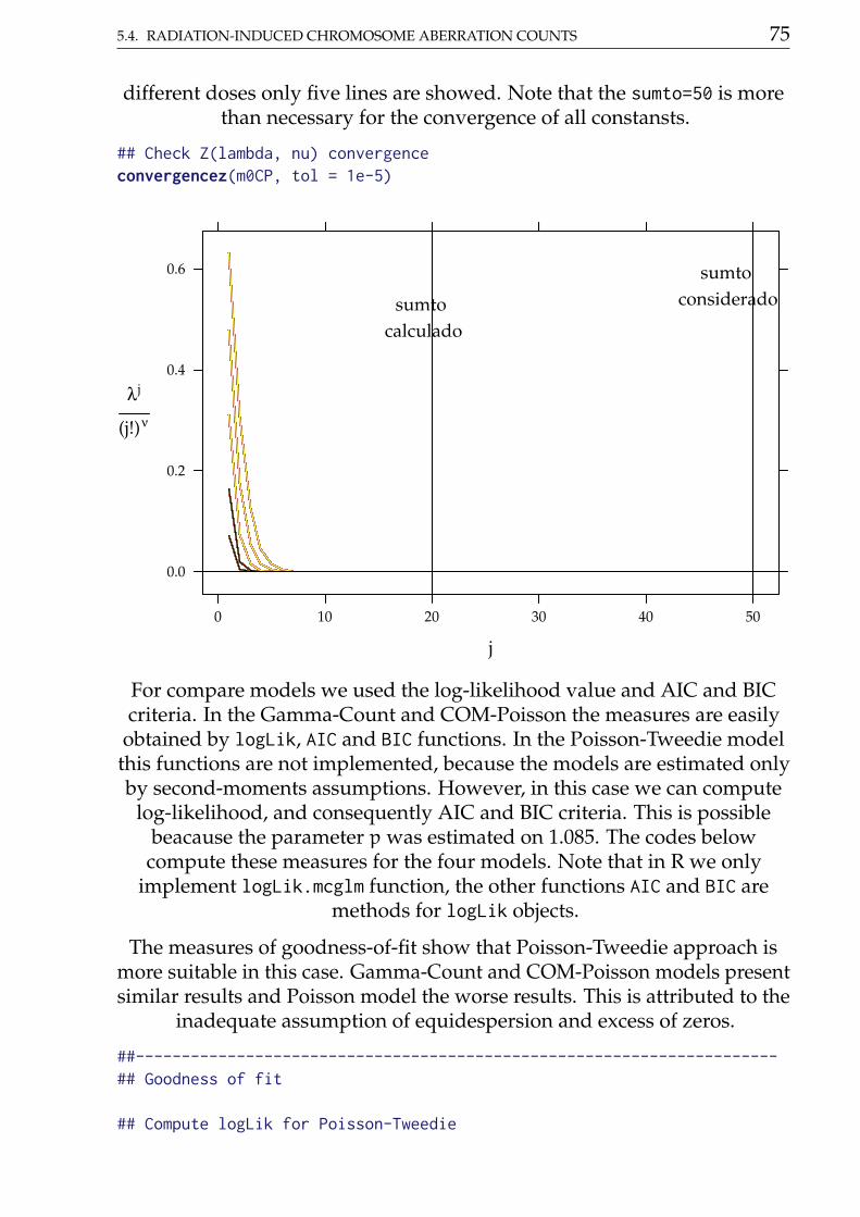
5.4. RADIATION-INDUCED CHROMOSOME ABERRATION COUNTS 75
different doses only five lines are showed. Note that the sumto=50 is morethan necessary for the convergence of all constansts.
## Check Z(lambda, nu) convergenceconvergencez(m0CP, tol = 1e-5)
j
λj
(j!)ν
0.0
0.2
0.4
0.6
0 10 20 30 40 50
sumto consideradosumto
calculado
For compare models we used the log-likelihood value and AIC and BICcriteria. In the Gamma-Count and COM-Poisson the measures are easily
obtained by logLik, AIC and BIC functions. In the Poisson-Tweedie modelthis functions are not implemented, because the models are estimated onlyby second-moments assumptions. However, in this case we can compute
log-likelihood, and consequently AIC and BIC criteria. This is possiblebeacause the parameter p was estimated on 1.085. The codes below
compute these measures for the four models. Note that in R we onlyimplement logLik.mcglm function, the other functions AIC and BIC are
methods for logLik objects.
The measures of goodness-of-fit show that Poisson-Tweedie approach ismore suitable in this case. Gamma-Count and COM-Poisson models presentsimilar results and Poisson model the worse results. This is attributed to the
inadequate assumption of equidespersion and excess of zeros.
##----------------------------------------------------------------------## Goodness of fit
## Compute logLik for Poisson-Tweedie
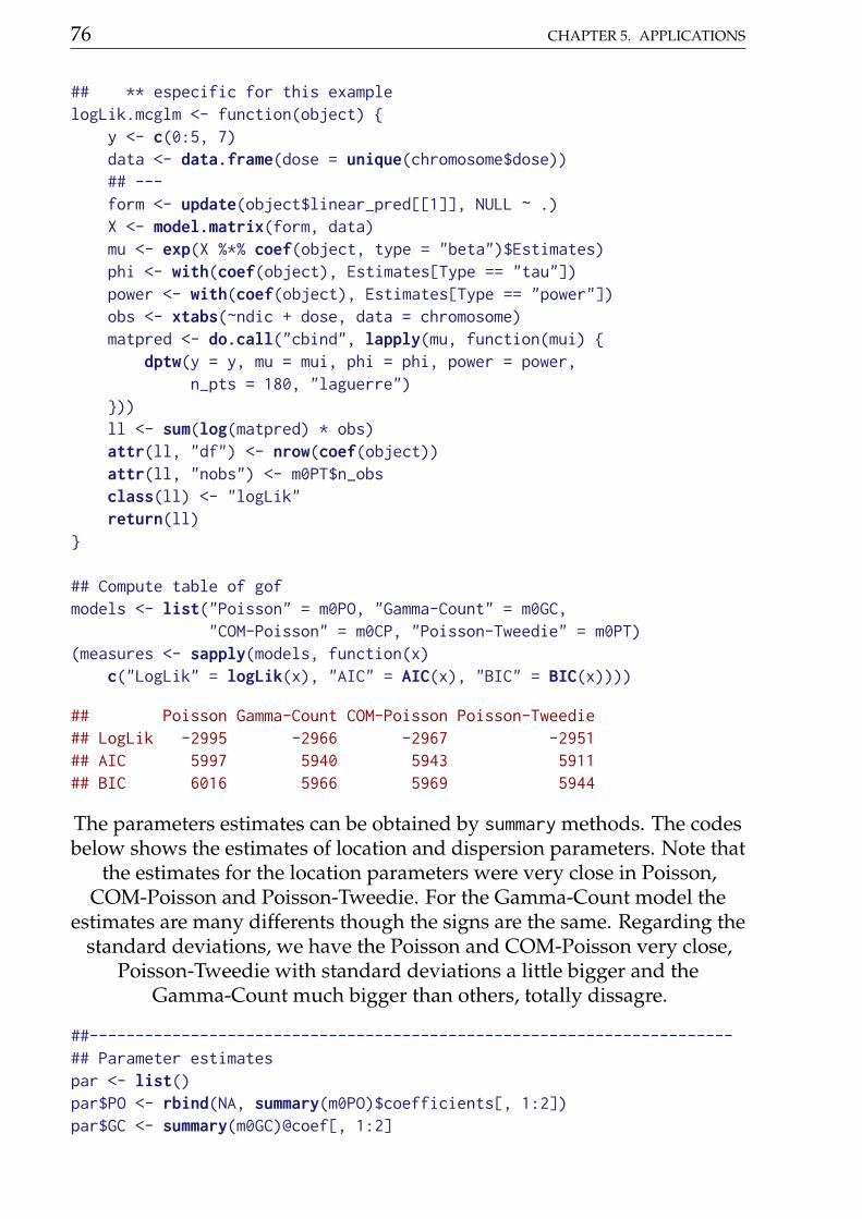
76 CHAPTER 5. APPLICATIONS
## ** especific for this examplelogLik.mcglm <- function(object)
y <- c(0:5, 7)data <- data.frame(dose = unique(chromosome$dose))## ---form <- update(object$linear_pred[[1]], NULL ~ .)X <- model.matrix(form, data)mu <- exp(X %*% coef(object, type = "beta")$Estimates)phi <- with(coef(object), Estimates[Type == "tau"])power <- with(coef(object), Estimates[Type == "power"])obs <- xtabs(~ndic + dose, data = chromosome)matpred <- do.call("cbind", lapply(mu, function(mui)
dptw(y = y, mu = mui, phi = phi, power = power,n_pts = 180, "laguerre")
))ll <- sum(log(matpred) * obs)attr(ll, "df") <- nrow(coef(object))attr(ll, "nobs") <- m0PT$n_obsclass(ll) <- "logLik"return(ll)
## Compute table of gofmodels <- list("Poisson" = m0PO, "Gamma-Count" = m0GC,
"COM-Poisson" = m0CP, "Poisson-Tweedie" = m0PT)(measures <- sapply(models, function(x)
c("LogLik" = logLik(x), "AIC" = AIC(x), "BIC" = BIC(x))))
## Poisson Gamma-Count COM-Poisson Poisson-Tweedie## LogLik -2995 -2966 -2967 -2951## AIC 5997 5940 5943 5911## BIC 6016 5966 5969 5944
The parameters estimates can be obtained by summary methods. The codesbelow shows the estimates of location and dispersion parameters. Note that
the estimates for the location parameters were very close in Poisson,COM-Poisson and Poisson-Tweedie. For the Gamma-Count model the
estimates are many differents though the signs are the same. Regarding thestandard deviations, we have the Poisson and COM-Poisson very close,
Poisson-Tweedie with standard deviations a little bigger and theGamma-Count much bigger than others, totally dissagre.
##----------------------------------------------------------------------## Parameter estimatespar <- list()par$PO <- rbind(NA, summary(m0PO)$coefficients[, 1:2])par$GC <- summary(m0GC)@coef[, 1:2]
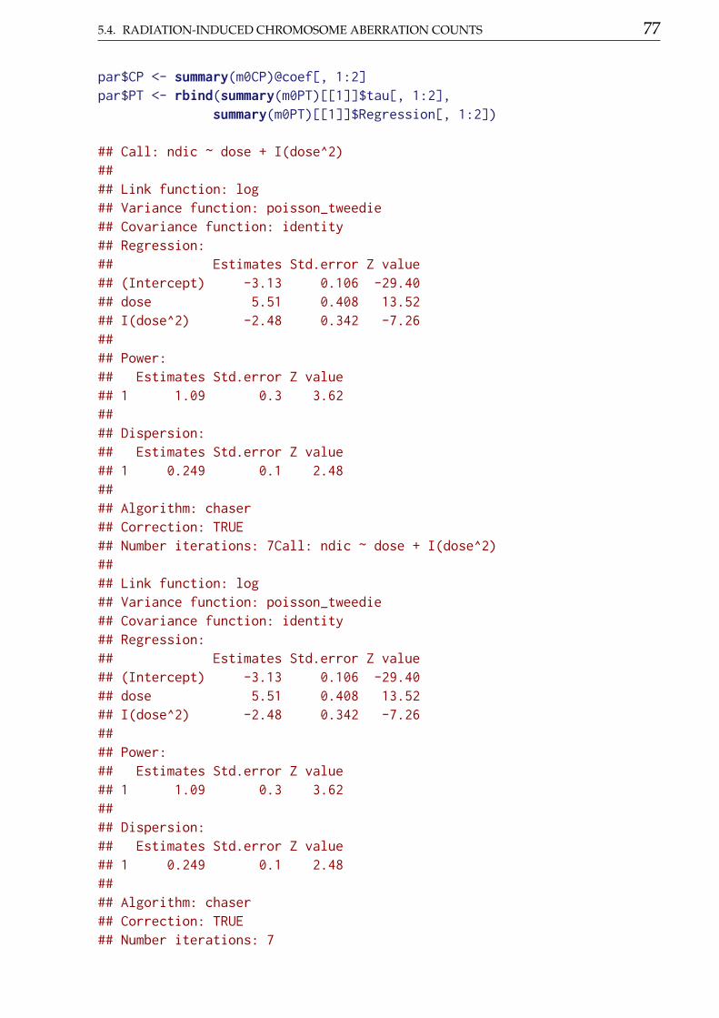
5.4. RADIATION-INDUCED CHROMOSOME ABERRATION COUNTS 77
par$CP <- summary(m0CP)@coef[, 1:2]par$PT <- rbind(summary(m0PT)[[1]]$tau[, 1:2],
summary(m0PT)[[1]]$Regression[, 1:2])
## Call: ndic ~ dose + I(dose^2)#### Link function: log## Variance function: poisson_tweedie## Covariance function: identity## Regression:## Estimates Std.error Z value## (Intercept) -3.13 0.106 -29.40## dose 5.51 0.408 13.52## I(dose^2) -2.48 0.342 -7.26#### Power:## Estimates Std.error Z value## 1 1.09 0.3 3.62#### Dispersion:## Estimates Std.error Z value## 1 0.249 0.1 2.48#### Algorithm: chaser## Correction: TRUE## Number iterations: 7Call: ndic ~ dose + I(dose^2)#### Link function: log## Variance function: poisson_tweedie## Covariance function: identity## Regression:## Estimates Std.error Z value## (Intercept) -3.13 0.106 -29.40## dose 5.51 0.408 13.52## I(dose^2) -2.48 0.342 -7.26#### Power:## Estimates Std.error Z value## 1 1.09 0.3 3.62#### Dispersion:## Estimates Std.error Z value## 1 0.249 0.1 2.48#### Algorithm: chaser## Correction: TRUE## Number iterations: 7
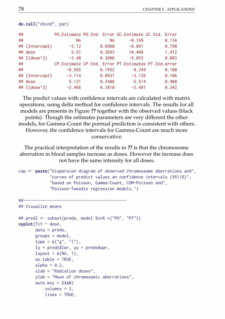
78 CHAPTER 5. APPLICATIONS
do.call("cbind", par)
## PO.Estimate PO.Std. Error GC.Estimate GC.Std. Error## NA NA -0.749 0.134## (Intercept) -3.12 0.0968 -6.091 0.798## dose 5.51 0.3693 10.468 1.472## I(dose^2) -2.48 0.3086 -5.053 0.883## CP.Estimate CP.Std. Error PT.Estimates PT.Std.error## -0.955 0.1952 0.249 0.100## (Intercept) -3.114 0.0931 -3.126 0.106## dose 5.121 0.3486 5.514 0.408## I(dose^2) -2.466 0.2818 -2.481 0.342
The predict values with confidence intervals are calculated with matrixoperations, using delta method for confidence intervals. The results for allmodels are presents in Figure ?? together with the observed values (black
points). Though the estimates parameters are very different the othermodels, for Gamma-Count the pontual prediction is consistent with others.
However, the confidence intervals for Gamma-Count are much moreconservative.
The practical interpretation of the results in ?? is that the chromosomeaberration in blood samples increase as doses. However the increase does
not have the same intensity for all doses.
cap <- paste("Dispersion diagram of observed chromossome aberrations and","curves of predict values an confidence intervals (95\\%)","based on Poisson, Gamma-Count, COM-Poisson and","Poisson-Tweedie regression models.")
##-------------------------------------------## Visualize means
## pred2 <- subset(preds, model %in% c("PO", "PT"))xyplot(fit ~ dose,
data = preds,groups = model,type = c("g", "l"),ly = preds$lwr, uy = preds$upr,layout = c(NA, 1),as.table = TRUE,alpha = 0.2,xlab = "Radiation doses",ylab = "Mean of chromosomic aberrations",auto.key = list(
columns = 2,lines = TRUE,
5.4. RADIATION-INDUCED CHROMOSOME ABERRATION COUNTS 79
points = FALSE,text = c("Poisson", "Gamma-Count",
"COM-Poisson", "Poisson-Tweedie")),cty = "bands", fill = "gray80",panel = panel.superpose,panel.groups = panel.cbH,prepanel = prepanel.cbH) +
as.layer(update(xy2, type = "p")
)
To complement the study we compute the probability distribution for thefive doses used in the experiment. This distributions are presents in Figure
5.12. Note that for 0.1Gy of 2.1MeV dose neutrons the probabilities arestrongly concentrated in 0 count, for 1Gy of 2.1MeV dose the distributions
still strongly assymmetric on the right, but the probabilities are moredispersed. It is worth mentioning that all distribuitions, thought different,
are the same average.
##-------------------------------------------## Calcule probabilitiesindex <- preds$dose %in% unique(chromosome$dose)means <- preds[index, c("model", "dose", "fit")]probs <- list()y <- 0:5
## Poisson modelindPO <- grep("PO", means$model)probs$PO <- do.call(
"rbind",lapply(indPO, function(i)
with(means, py <- dpois(y, fit[i])data.frame(dose = dose[i], y = y, prob = py)
))
)
## Gamma-Count modelindGC <- grep("GC", means$model)alpha <- exp(coef(m0GC)["alpha"])probs$GC <- do.call(
"rbind",lapply(indGC, function(i)
with(means, aux <- predict(m0GC, newdata = t(cbind(X[i, ])),
80 CHAPTER 5. APPLICATIONS
type = "link")lambda <- alpha %*% exp(aux)py <- dgcnt(y, lambda = lambda, alpha = alpha)data.frame(dose = dose[i], y = y, prob = py)
))
)
## COM-Poisson modelindCP <- grep("CP", means$model)nu <- exp(coef(m0CP)["phi"])sumto <- m0CP@data$sumtoprobs$CP <- do.call(
"rbind",lapply(indCP, function(i)
with(means, aux <- predict(m0CP, newdata = t(cbind(X[i, ])),
type = "link")lambda <- exp(aux)py <- dcmp(y, lambda = lambda, nu = nu, sumto = sumto)data.frame(dose = dose[i], y = y, prob = py)
))
)
## Poisson-Tweedie modelindPT <- grep("PT", means$model)phi <- with(coef(m0PT), Estimates[Type == "tau"])power <- with(coef(m0PT), Estimates[Type == "power"])probs$PT <- do.call(
"rbind",lapply(indPT, function(i)
with(means, py <- dptw(y = y, mu = fit[i], phi = phi,
power = power, n_pts = 180,method = "laguerre")
data.frame(dose = dose[i], y = y, prob = py))
))
## Visualize the probabilitiesdaprobs <- ldply(probs, .id = "model")
barchart(prob ~ y | factor(dose), groups = model,data = daprobs,horizontal = FALSE,
5.4. RADIATION-INDUCED CHROMOSOME ABERRATION COUNTS 81
axis = axis.grid,as.table = TRUE,origin = 0,xlab = "Number of chromosomic aberrations",ylab = "Probability",scales = list(x = list(labels = y)),auto.key = list(
columns = 2,text = c("Poisson", "Gamma-Count",
"COM-Poisson", "Poisson-Tweedie")),strip = strip.custom(
strip.name = TRUE,var.name = "dose",sep = " = "
))
str(nematoide)
## 'data.frame': 94 obs. of 5 variables:## $ cult: Factor w/ 19 levels "A","B","C","D",..: 1 1 1 1 1 2 2 2 2 2 ...## $ mfr : num 10.52 11.03 6.42 8.16 4.48 ...## $ vol : int 40 40 40 40 40 40 40 40 40 40 ...## $ nema: int 4 5 3 4 3 2 2 2 2 2 ...## $ off : num 0.263 0.276 0.161 0.204 0.112 ...
xyplot(nema/off ~ cult, data = nematoide,xlab = "Linhagens de feijão",ylab = "Número de nematoides por grama de raíz")
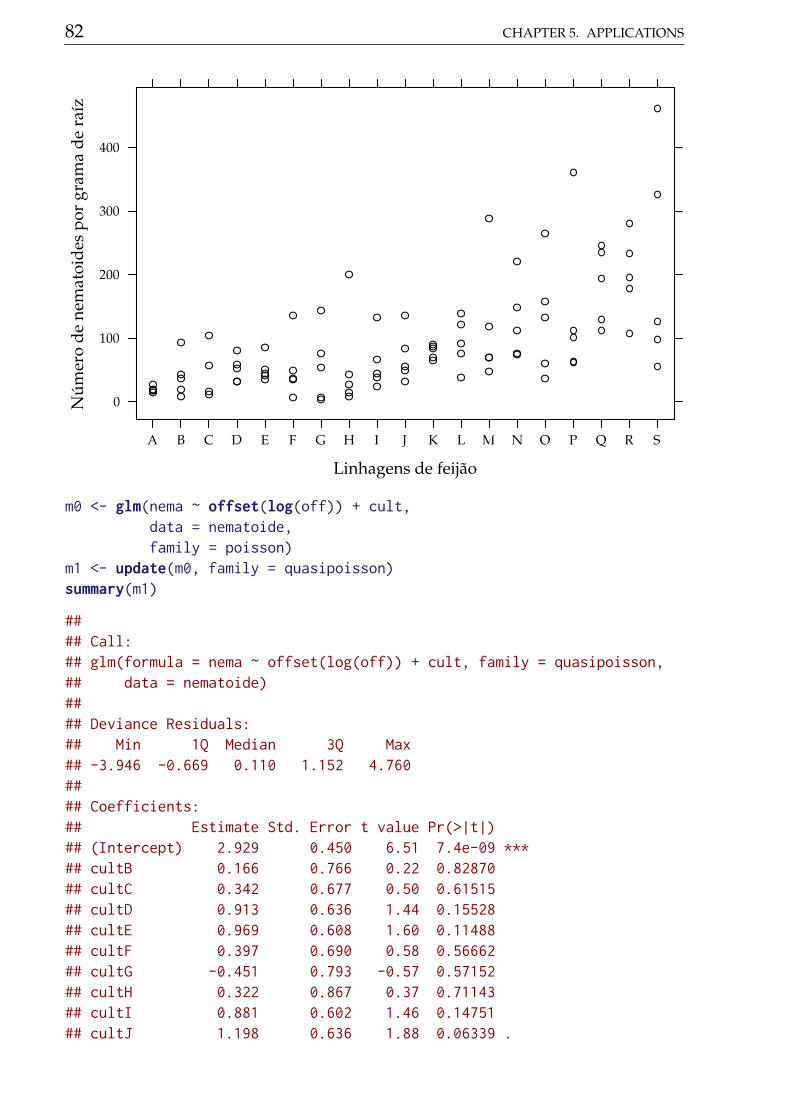
82 CHAPTER 5. APPLICATIONS
Linhagens de feijão
Núm
ero
de n
emat
oide
s po
r gr
ama
de r
aíz
0
100
200
300
400
A B C D E F G H I J K L M N O P Q R S
m0 <- glm(nema ~ offset(log(off)) + cult,data = nematoide,family = poisson)
m1 <- update(m0, family = quasipoisson)summary(m1)
#### Call:## glm(formula = nema ~ offset(log(off)) + cult, family = quasipoisson,## data = nematoide)#### Deviance Residuals:## Min 1Q Median 3Q Max## -3.946 -0.669 0.110 1.152 4.760#### Coefficients:## Estimate Std. Error t value Pr(>|t|)## (Intercept) 2.929 0.450 6.51 7.4e-09 ***## cultB 0.166 0.766 0.22 0.82870## cultC 0.342 0.677 0.50 0.61515## cultD 0.913 0.636 1.44 0.15528## cultE 0.969 0.608 1.60 0.11488## cultF 0.397 0.690 0.58 0.56662## cultG -0.451 0.793 -0.57 0.57152## cultH 0.322 0.867 0.37 0.71143## cultI 0.881 0.602 1.46 0.14751## cultJ 1.198 0.636 1.88 0.06339 .
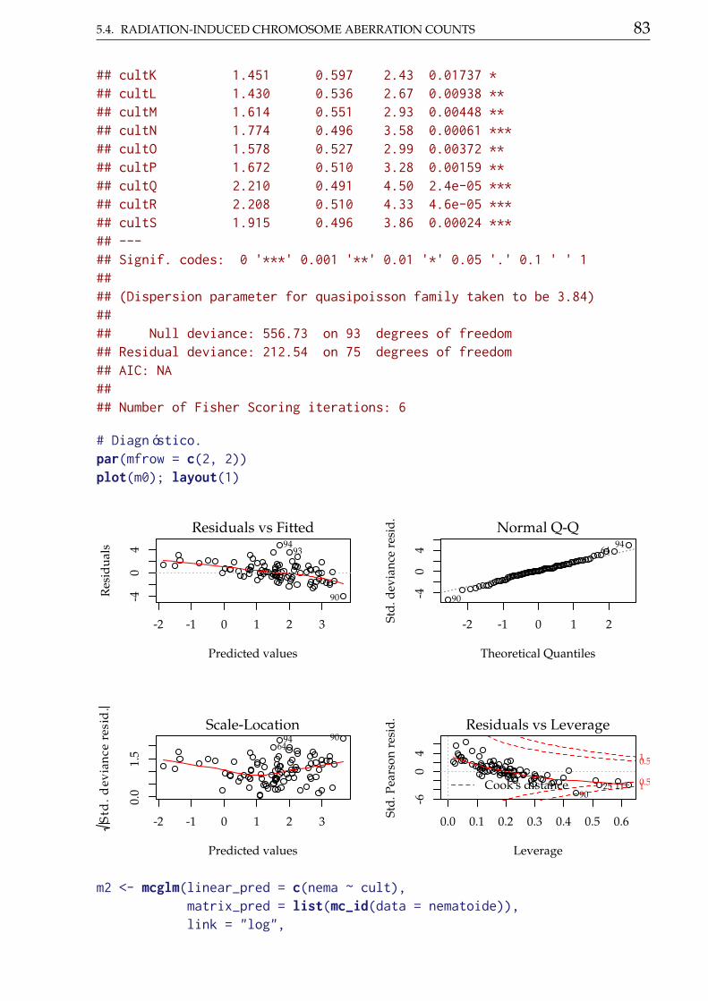
5.4. RADIATION-INDUCED CHROMOSOME ABERRATION COUNTS 83
## cultK 1.451 0.597 2.43 0.01737 *## cultL 1.430 0.536 2.67 0.00938 **## cultM 1.614 0.551 2.93 0.00448 **## cultN 1.774 0.496 3.58 0.00061 ***## cultO 1.578 0.527 2.99 0.00372 **## cultP 1.672 0.510 3.28 0.00159 **## cultQ 2.210 0.491 4.50 2.4e-05 ***## cultR 2.208 0.510 4.33 4.6e-05 ***## cultS 1.915 0.496 3.86 0.00024 ***## ---## Signif. codes: 0 '***' 0.001 '**' 0.01 '*' 0.05 '.' 0.1 ' ' 1#### (Dispersion parameter for quasipoisson family taken to be 3.84)#### Null deviance: 556.73 on 93 degrees of freedom## Residual deviance: 212.54 on 75 degrees of freedom## AIC: NA#### Number of Fisher Scoring iterations: 6
# Diagnóstico.par(mfrow = c(2, 2))plot(m0); layout(1)
-2 -1 0 1 2 3
-40
4
Predicted values
Res
idua
ls
Residuals vs Fitted94
90
93
-2 -1 0 1 2
-40
4
Theoretical Quantiles
Std.
dev
ianc
e re
sid. Normal Q-Q
90
9464
-2 -1 0 1 2 3
0.0
1.5
Predicted values
Std
.dev
ianc
ere
sid
.
Scale-Location9094
64
0.0 0.1 0.2 0.3 0.4 0.5 0.6
-60
4
Leverage
Std.
Pea
rson
res
id.
Cook's distance 10.5
0.51
Residuals vs Leverage
901125
m2 <- mcglm(linear_pred = c(nema ~ cult),matrix_pred = list(mc_id(data = nematoide)),link = "log",
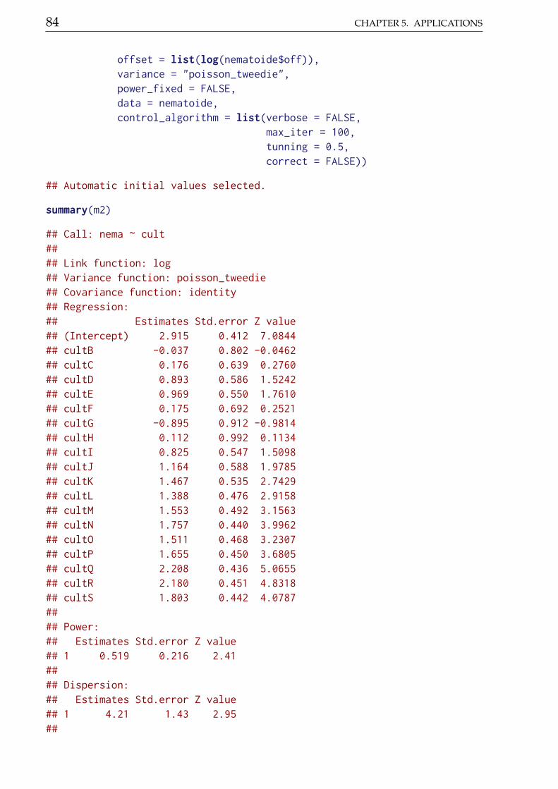
84 CHAPTER 5. APPLICATIONS
offset = list(log(nematoide$off)),variance = "poisson_tweedie",power_fixed = FALSE,data = nematoide,control_algorithm = list(verbose = FALSE,
max_iter = 100,tunning = 0.5,correct = FALSE))
## Automatic initial values selected.
summary(m2)
## Call: nema ~ cult#### Link function: log## Variance function: poisson_tweedie## Covariance function: identity## Regression:## Estimates Std.error Z value## (Intercept) 2.915 0.412 7.0844## cultB -0.037 0.802 -0.0462## cultC 0.176 0.639 0.2760## cultD 0.893 0.586 1.5242## cultE 0.969 0.550 1.7610## cultF 0.175 0.692 0.2521## cultG -0.895 0.912 -0.9814## cultH 0.112 0.992 0.1134## cultI 0.825 0.547 1.5098## cultJ 1.164 0.588 1.9785## cultK 1.467 0.535 2.7429## cultL 1.388 0.476 2.9158## cultM 1.553 0.492 3.1563## cultN 1.757 0.440 3.9962## cultO 1.511 0.468 3.2307## cultP 1.655 0.450 3.6805## cultQ 2.208 0.436 5.0655## cultR 2.180 0.451 4.8318## cultS 1.803 0.442 4.0787#### Power:## Estimates Std.error Z value## 1 0.519 0.216 2.41#### Dispersion:## Estimates Std.error Z value## 1 4.21 1.43 2.95##
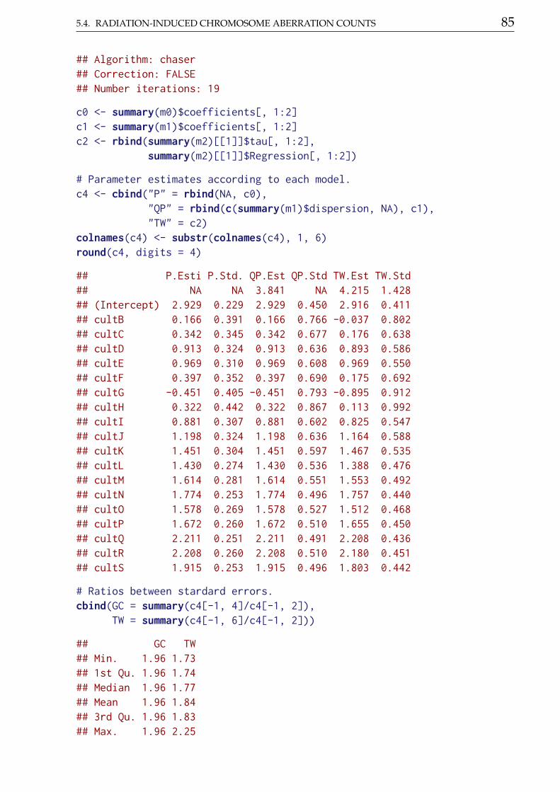
5.4. RADIATION-INDUCED CHROMOSOME ABERRATION COUNTS 85
## Algorithm: chaser## Correction: FALSE## Number iterations: 19
c0 <- summary(m0)$coefficients[, 1:2]c1 <- summary(m1)$coefficients[, 1:2]c2 <- rbind(summary(m2)[[1]]$tau[, 1:2],
summary(m2)[[1]]$Regression[, 1:2])
# Parameter estimates according to each model.c4 <- cbind("P" = rbind(NA, c0),
"QP" = rbind(c(summary(m1)$dispersion, NA), c1),"TW" = c2)
colnames(c4) <- substr(colnames(c4), 1, 6)round(c4, digits = 4)
## P.Esti P.Std. QP.Est QP.Std TW.Est TW.Std## NA NA 3.841 NA 4.215 1.428## (Intercept) 2.929 0.229 2.929 0.450 2.916 0.411## cultB 0.166 0.391 0.166 0.766 -0.037 0.802## cultC 0.342 0.345 0.342 0.677 0.176 0.638## cultD 0.913 0.324 0.913 0.636 0.893 0.586## cultE 0.969 0.310 0.969 0.608 0.969 0.550## cultF 0.397 0.352 0.397 0.690 0.175 0.692## cultG -0.451 0.405 -0.451 0.793 -0.895 0.912## cultH 0.322 0.442 0.322 0.867 0.113 0.992## cultI 0.881 0.307 0.881 0.602 0.825 0.547## cultJ 1.198 0.324 1.198 0.636 1.164 0.588## cultK 1.451 0.304 1.451 0.597 1.467 0.535## cultL 1.430 0.274 1.430 0.536 1.388 0.476## cultM 1.614 0.281 1.614 0.551 1.553 0.492## cultN 1.774 0.253 1.774 0.496 1.757 0.440## cultO 1.578 0.269 1.578 0.527 1.512 0.468## cultP 1.672 0.260 1.672 0.510 1.655 0.450## cultQ 2.211 0.251 2.211 0.491 2.208 0.436## cultR 2.208 0.260 2.208 0.510 2.180 0.451## cultS 1.915 0.253 1.915 0.496 1.803 0.442
# Ratios between stardard errors.cbind(GC = summary(c4[-1, 4]/c4[-1, 2]),
TW = summary(c4[-1, 6]/c4[-1, 2]))
## GC TW## Min. 1.96 1.73## 1st Qu. 1.96 1.74## Median 1.96 1.77## Mean 1.96 1.84## 3rd Qu. 1.96 1.83## Max. 1.96 2.25
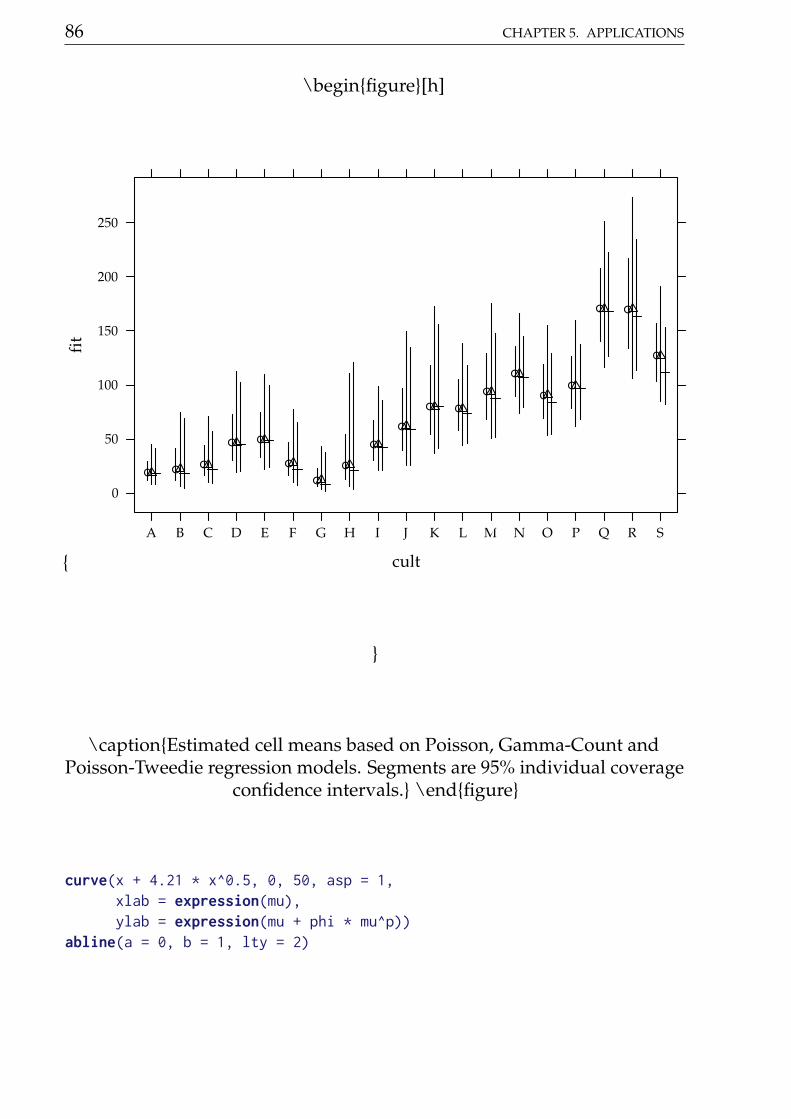
86 CHAPTER 5. APPLICATIONS
\beginfigure[h]
cult
fit
0
50
100
150
200
250
A B C D E F G H I J K L M N O P Q R S
\captionEstimated cell means based on Poisson, Gamma-Count andPoisson-Tweedie regression models. Segments are 95% individual coverage
confidence intervals. \endfigure
curve(x + 4.21 * x^0.5, 0, 50, asp = 1,xlab = expression(mu),ylab = expression(mu + phi * mu^p))
abline(a = 0, b = 1, lty = 2)
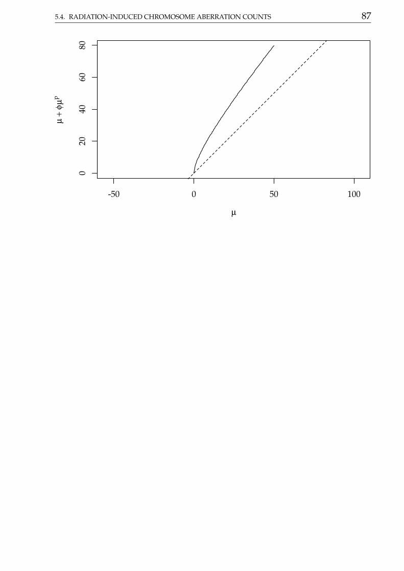
5.4. RADIATION-INDUCED CHROMOSOME ABERRATION COUNTS 87
-50 0 50 100
020
4060
80
µ
µ+
φµp
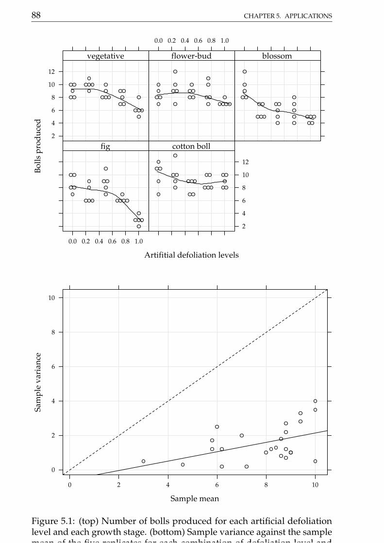
88 CHAPTER 5. APPLICATIONS
Artifitial defoliation levels
Bolls
pro
duce
d
2
4
6
8
10
12
vegetative
0.0 0.2 0.4 0.6 0.8 1.0
flower-bud blossom
0.0 0.2 0.4 0.6 0.8 1.0
fig
2
4
6
8
10
12
cotton boll
Sample mean
Sam
ple
vari
ance
0
2
4
6
8
10
0 2 4 6 8 10
Figure 5.1: (top) Number of bolls produced for each artificial defoliationlevel and each growth stage. (bottom) Sample variance against the samplemean of the five replicates for each combination of defoliation level andgrowth stage.
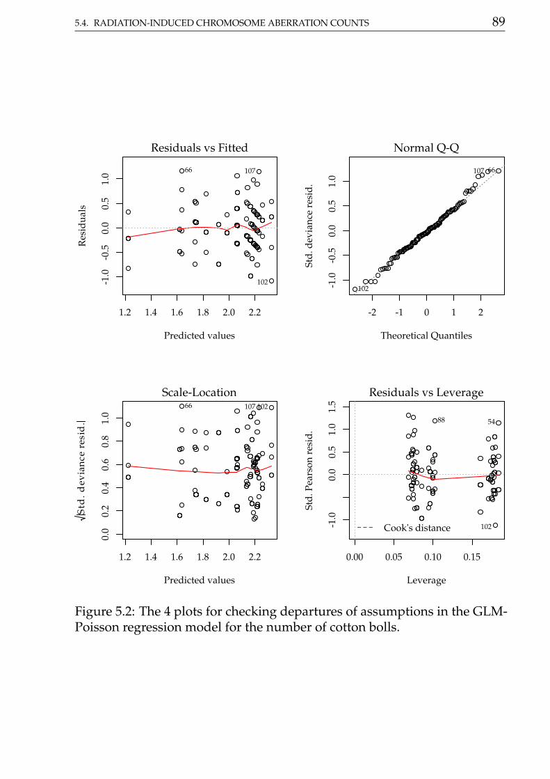
5.4. RADIATION-INDUCED CHROMOSOME ABERRATION COUNTS 89
1.2 1.4 1.6 1.8 2.0 2.2
-1.0
-0.5
0.0
0.5
1.0
Predicted values
Res
idua
ls
Residuals vs Fitted
66 107
102
-2 -1 0 1 2
-1.0
-0.5
0.0
0.5
1.0
Theoretical Quantiles
Std.
dev
ianc
e re
sid.
Normal Q-Q
66
102
107
1.2 1.4 1.6 1.8 2.0 2.2
0.0
0.2
0.4
0.6
0.8
1.0
Predicted values
Std
.dev
ianc
ere
sid
.
Scale-Location66 102107
0.00 0.05 0.10 0.15
-1.0
0.0
0.5
1.0
1.5
Leverage
Std.
Pea
rson
res
id.
Cook's distance
Residuals vs Leverage
54
102
88
Figure 5.2: The 4 plots for checking departures of assumptions in the GLM-Poisson regression model for the number of cotton bolls.
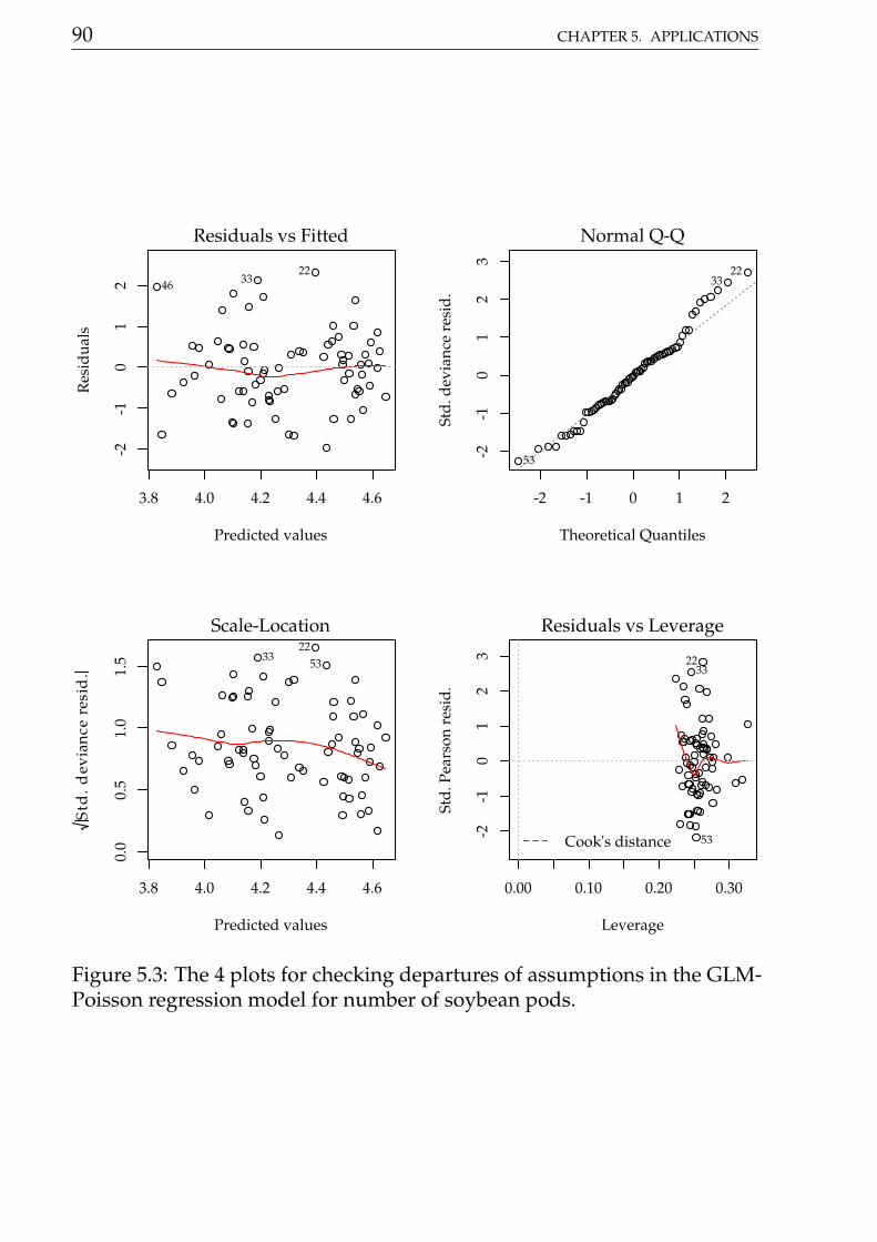
90 CHAPTER 5. APPLICATIONS
3.8 4.0 4.2 4.4 4.6
-2-1
01
2
Predicted values
Res
idua
ls
Residuals vs Fitted
223346
-2 -1 0 1 2-2
-10
12
3
Theoretical Quantiles
Std.
dev
ianc
e re
sid.
Normal Q-Q
2233
53
3.8 4.0 4.2 4.4 4.6
0.0
0.5
1.0
1.5
Predicted values
Std
.dev
ianc
ere
sid
.
Scale-Location22
33 53
0.00 0.10 0.20 0.30
-2-1
01
23
Leverage
Std.
Pea
rson
res
id.
Cook's distance
Residuals vs Leverage
2233
53
Figure 5.3: The 4 plots for checking departures of assumptions in the GLM-Poisson regression model for number of soybean pods.
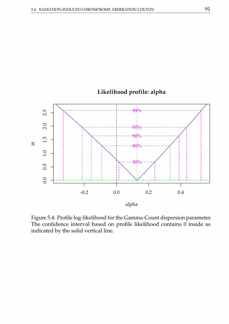
5.4. RADIATION-INDUCED CHROMOSOME ABERRATION COUNTS 91
-0.2 0.0 0.2 0.4
0.0
0.5
1.0
1.5
2.0
2.5
Likelihood profile: alpha
alpha
z
99%
95%
90%
80%
50%
Figure 5.4: Profile log-likelihood for the Gamma-Count dispersion parameter.The confidence interval based on profile likelihood contains 0 inside asindicated by the solid vertical line.
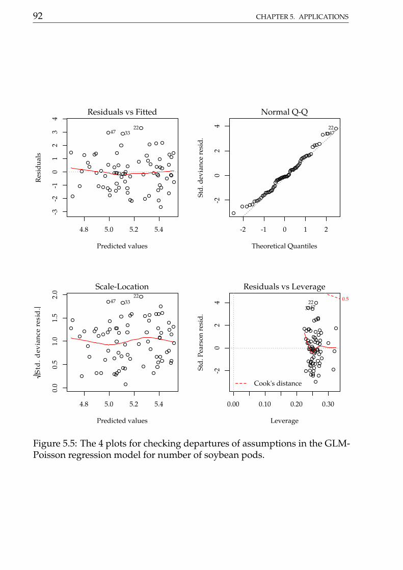
92 CHAPTER 5. APPLICATIONS
4.8 5.0 5.2 5.4
-3-2
-10
12
34
Predicted values
Res
idua
ls
Residuals vs Fitted
2247 33
-2 -1 0 1 2
-20
24
Theoretical Quantiles
Std.
dev
ianc
e re
sid.
Normal Q-Q
224733
4.8 5.0 5.2 5.4
0.0
0.5
1.0
1.5
2.0
Predicted values
Std
.dev
ianc
ere
sid
.
Scale-Location22
47 33
0.00 0.10 0.20 0.30
-20
24
Leverage
Std.
Pea
rson
res
id.
Cook's distance
0.5
Residuals vs Leverage
223347
Figure 5.5: The 4 plots for checking departures of assumptions in the GLM-Poisson regression model for number of soybean pods.

5.4. RADIATION-INDUCED CHROMOSOME ABERRATION COUNTS 93
-1.0 -0.8 -0.6 -0.4 -0.2
0.0
0.5
1.0
1.5
2.0
2.5
Likelihood profile: alpha
alpha
z
99%
95%
90%
80%
50%
Figure 5.6: Profile log-likelihood for the Gamma-Count dispersion parameter.The confidence interval based on profile likelihood contains 0 inside asindicated by the solid vertical line.
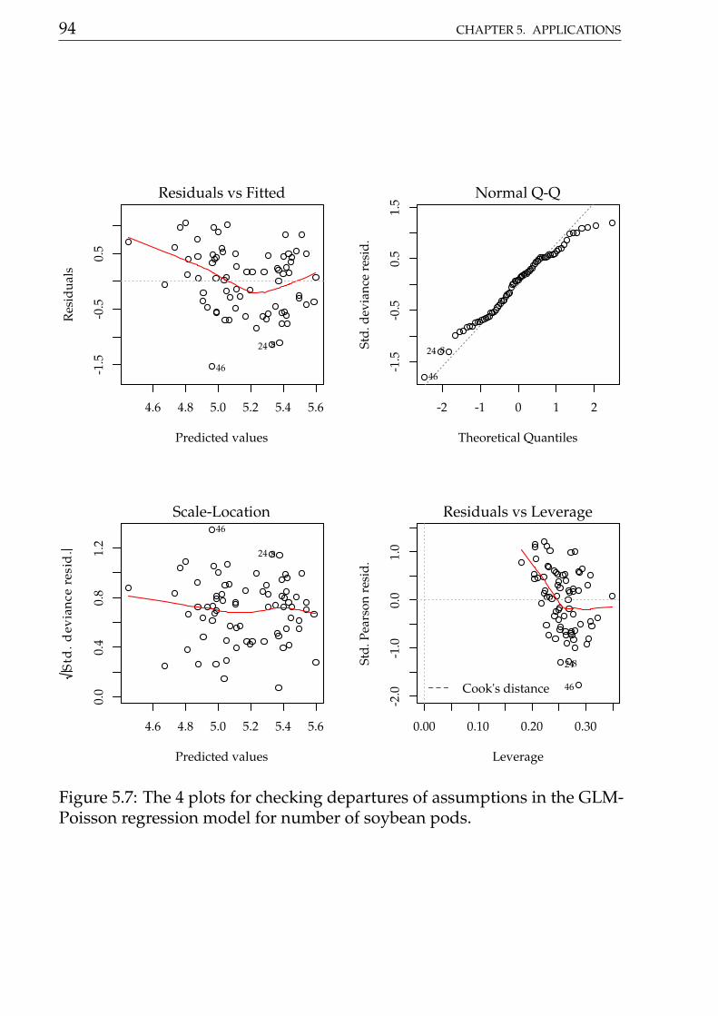
94 CHAPTER 5. APPLICATIONS
4.6 4.8 5.0 5.2 5.4 5.6
-1.5
-0.5
0.5
Predicted values
Res
idua
ls
Residuals vs Fitted
46
24 8
-2 -1 0 1 2-1
.5-0
.50.
51.
5
Theoretical Quantiles
Std.
dev
ianc
e re
sid.
Normal Q-Q
46
24 8
4.6 4.8 5.0 5.2 5.4 5.6
0.0
0.4
0.8
1.2
Predicted values
Std
.dev
ianc
ere
sid
.
Scale-Location46
24 8
0.00 0.10 0.20 0.30
-2.0
-1.0
0.0
1.0
Leverage
Std.
Pea
rson
res
id.
Cook's distance
Residuals vs Leverage
46
824
Figure 5.7: The 4 plots for checking departures of assumptions in the GLM-Poisson regression model for number of soybean pods.
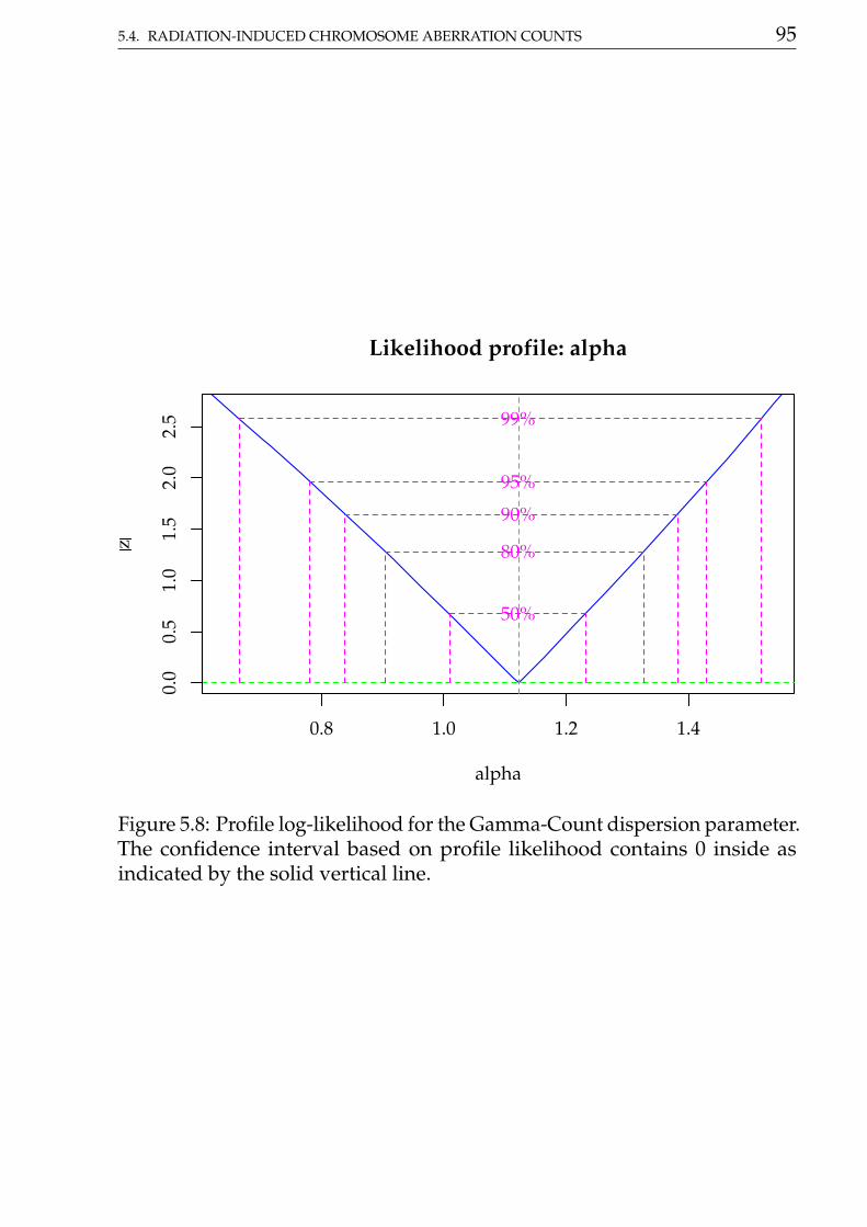
5.4. RADIATION-INDUCED CHROMOSOME ABERRATION COUNTS 95
0.8 1.0 1.2 1.4
0.0
0.5
1.0
1.5
2.0
2.5
Likelihood profile: alpha
alpha
z
99%
95%
90%
80%
50%
Figure 5.8: Profile log-likelihood for the Gamma-Count dispersion parameter.The confidence interval based on profile likelihood contains 0 inside asindicated by the solid vertical line.
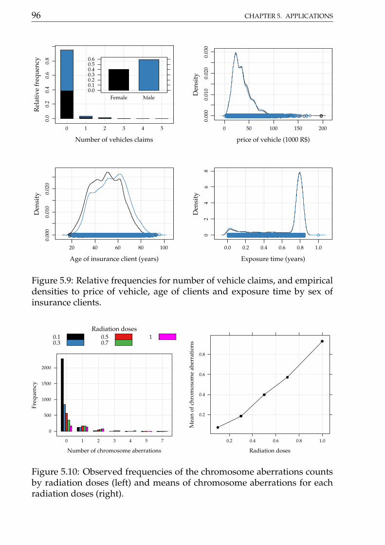
96 CHAPTER 5. APPLICATIONS
Number of vehicles claims
Rel
ativ
e fr
eque
ncy
0.0
0.2
0.4
0.6
0.8
0 1 2 3 4 5
0.00.10.20.30.40.50.6
Female Male
price of vehicle (1000 R$)
Den
sity
0.00
00.
010
0.02
00.
030
0 50 100 150 200
Age of insurance client (years)
Den
sity
0.00
00.
010
0.02
0
20 40 60 80 100
Exposure time (years)
Den
sity
02
46
8
0.0 0.2 0.4 0.6 0.8 1.0
Figure 5.9: Relative frequencies for number of vehicle claims, and empiricaldensities to price of vehicle, age of clients and exposure time by sex ofinsurance clients.
Number of chromosome aberrations
Freq
uenc
y
0
500
1000
1500
2000
0 1 2 3 4 5 7
Radiation doses0.10.3
0.50.7
1
Radiation doses
Mea
n of
chr
omos
ome
aber
ratio
ns
0.2
0.4
0.6
0.8
0.2 0.4 0.6 0.8 1.0
Figure 5.10: Observed frequencies of the chromosome aberrations countsby radiation doses (left) and means of chromosome aberrations for eachradiation doses (right).
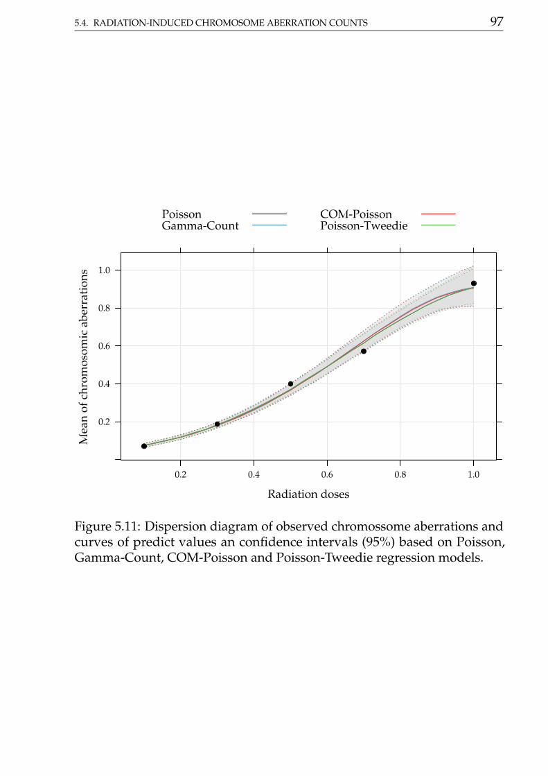
5.4. RADIATION-INDUCED CHROMOSOME ABERRATION COUNTS 97
Radiation doses
Mea
n of
chr
omos
omic
abe
rrat
ions
0.2
0.4
0.6
0.8
1.0
0.2 0.4 0.6 0.8 1.0
PoissonGamma-Count
COM-PoissonPoisson-Tweedie
Figure 5.11: Dispersion diagram of observed chromossome aberrations andcurves of predict values an confidence intervals (95%) based on Poisson,Gamma-Count, COM-Poisson and Poisson-Tweedie regression models.
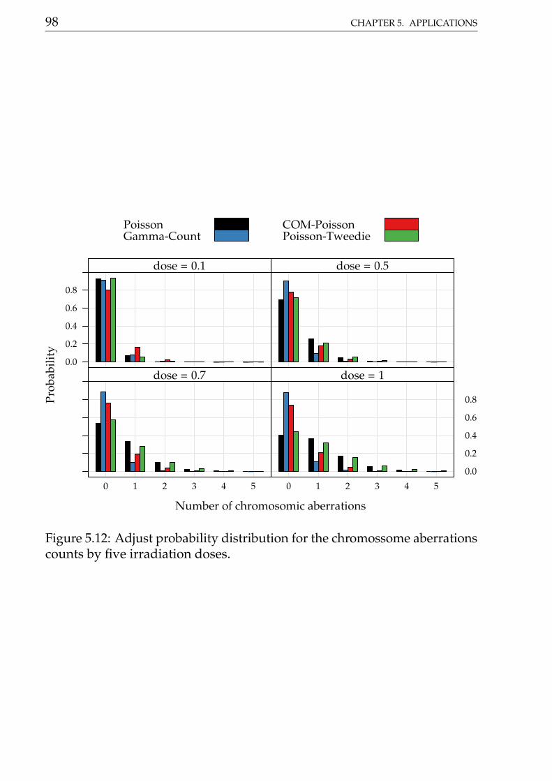
98 CHAPTER 5. APPLICATIONS
Number of chromosomic aberrations
Prob
abili
ty
0.0
0.2
0.4
0.6
0.8
= dose 0.1 = dose 0.5
0 1 2 3 4 5
= dose 0.7
0 1 2 3 4 50.0
0.2
0.4
0.6
0.8
= dose 1
PoissonGamma-Count
COM-PoissonPoisson-Tweedie
Figure 5.12: Adjust probability distribution for the chromossome aberrationscounts by five irradiation doses.
Bibliography
Andersen, D. A. and Bonat, W. H. (2016). Double generalized linear com-pound poisson models to insurance claims data. ArXiv. to appear.
Barabesi, L., Becatti, C., and Marcheselli, M. (2016). The tempered discreteLinnik distribution. ArXiv e-prints.
Bolker, B. and Team, R. D. C. (2016). bbmle: Tools for General MaximumLikelihood Estimation. R package version 1.0.18.
Bonat, W. H. (2016). mcglm: Multivariate covariance generalized linearmodels. http://git.leg.ufpr.br/wbonat/mcglm. R package version 0.3.0.
Bonat, W. H. and Jørgensen, B. (2016). Multivariate covariance generalizedlinear models. Journal of the Royal Statistical Society: Series C (AppliedStatistics), 65:649–675.
Bonat, W. H., Jørgensen, B., Kokonendji, C. C. andHinde, J., and Démetrio, C.G. B. (2016). Extended poisson-tweedie: properties and regression modelfor count data. Arxiv.
Del Castillo, J. and Pérez-Casany, M. (1998). Weighted poisson distributionsfor overdispersion and underdispersion situations. Annals of the Instituteof Statistical Mathematics, 50(3):567–585.
Dunn, J. (2012). compoisson: Conway-Maxwell-Poisson Distribution. R packageversion 0.3.
El-Shaarawi, A. H., Zhu, R., and Joe, H. (2011). Modelling species abundanceusing the Poisson-Tweedie family. Environmetrics, 22(2):152–164.
Esnaola, M., Puig, P., Gonzalez, D., Castelo, R., and Gonzalez, J. R. (2013). Aflexible count data model to fit the wide diversity of expression profilesarising from extensively replicated rna-seq experiments. BMC Bioinformat-ics, 14(1):254–276.
99
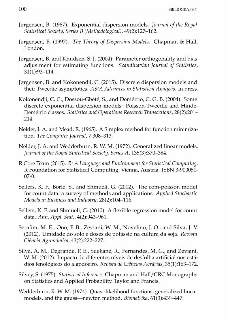
100 BIBLIOGRAPHY
Jørgensen, B. (1987). Exponential dispersion models. Journal of the RoyalStatistical Society. Series B (Methodological), 49(2):127–162.
Jørgensen, B. (1997). The Theory of Dispersion Models. Chapman & Hall,London.
Jørgensen, B. and Knudsen, S. J. (2004). Parameter orthogonality and biasadjustment for estimating functions. Scandinavian Journal of Statistics,31(1):93–114.
Jørgensen, B. and Kokonendji, C. (2015). Discrete dispersion models andtheir Tweedie asymptotics. AStA Advances in Statistical Analysis. in press.
Kokonendji, C. C., Dossou-Gbété, S., and Demétrio, C. G. B. (2004). Somediscrete exponential dispersion models: Poisson-Tweedie and Hinde-Demétrio classes. Statistics and Operations Research Transactions, 28(2):201–214.
Nelder, J. A. and Mead, R. (1965). A Simplex method for function minimiza-tion. The Computer Journal, 7:308–313.
Nelder, J. A. and Wedderburn, R. W. M. (1972). Generalized linear models.Journal of the Royal Statistical Society. Series A, 135(3):370–384.
R Core Team (2015). R: A Language and Environment for Statistical Computing.R Foundation for Statistical Computing, Vienna, Austria. ISBN 3-900051-07-0.
Sellers, K. F., Borle, S., and Shmueli, G. (2012). The com-poisson modelfor count data: a survey of methods and applications. Applied StochasticModels in Business and Industry, 28(2):104–116.
Sellers, K. F. and Shmueli, G. (2010). A flexible regression model for countdata. Ann. Appl. Stat., 4(2):943–961.
Serafim, M. E., Ono, F. B., Zeviani, W. M., Novelino, J. O., and Silva, J. V.(2012). Umidade do solo e doses de potássio na cultura da soja. RevistaCiência Agronômica, 43(2):222–227.
Silva, A. M., Degrande, P. E., Suekane, R., Fernandes, M. G., and Zeviani,W. M. (2012). Impacto de diferentes níveis de desfolha artificial nos está-dios fenológicos do algodoeiro. Revista de Ciências Agrárias, 35(1):163–172.
Silvey, S. (1975). Statistical Inference. Chapman and Hall/CRC Monographson Statistics and Applied Probability. Taylor and Francis.
Wedderburn, R. W. M. (1974). Quasi-likelihood functions, generalized linearmodels, and the gauss—newton method. Biometrika, 61(3):439–447.
BIBLIOGRAPHY 101
Winkelmann, R. (1995). Duration dependence and dispersion in count-datamodels. Journal of Business & Economic Statistics, 13(4):467–474.
Winkelmann, R. (2003). Econometric Analysis of Count Data. Springer.
Zeviani, W. M., Junior, E. E. R., and Taconeli, C. A. (2016). MRDCr: Modelosde Regressão para Dados de Contagem. R package version 0.0-2.
Zeviani, W. M., Ribeiro Jr, P. J., Bonat, W. H., Shimakura, S. E., and Muniz,J. A. (2014). The gamma-count distribution in the analysis of experimentalunderdispersed data. Journal of Applied Statistics, 41(12):2616–2626.