SkriptsprachenNumpy und Scipy

Kai Duhrkop

Lehrstuhl fuer BioinformatikFriedrich-Schiller-Universitaet Jena

kai.duehrkop@uni-jena.de

24. September 2015

24. September 2015 1 / 37

Numpy

Numpy Numerische Arrays 24. September 2015 2 / 37

numpy und scipy

import numpy as npimport s c i p y as sp

numpy

Library fur numerische Vektoren und Matrizeneffiziente Operationen auf Arraysermoglicht speichereffiziente Darstellung von numerischenArrays

scipy

Sammlung mathematischer Funktionen (numerisch, analytisch,stochastisch)arbeitet eng mit numpy zusammenhistorisch sind einige Funktionen in numpy verteilt, dieeigentlich in scipy gehoren sollten

Numpy Numerische Arrays 24. September 2015 3 / 37

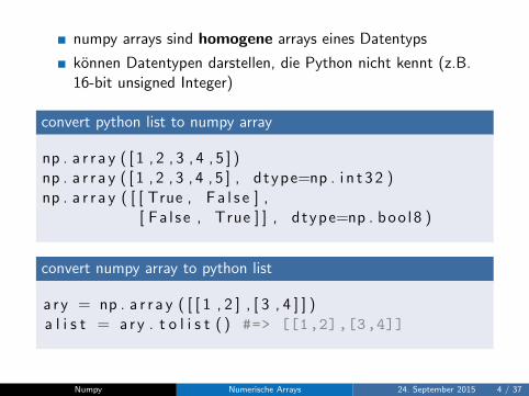
numpy arrays sind homogene arrays eines Datentyps

konnen Datentypen darstellen, die Python nicht kennt (z.B.16-bit unsigned Integer)

convert python list to numpy array

np . a r r a y ( [ 1 , 2 , 3 , 4 , 5 ] )np . a r r a y ( [ 1 , 2 , 3 , 4 , 5 ] , dtype=np . i n t 3 2 )np . a r r a y ( [ [ True , F a l s e ] ,

[ F a l s e , True ] ] , d type=np . b o o l 8 )

convert numpy array to python list

a r y = np . a r r a y ( [ [ 1 , 2 ] , [ 3 , 4 ] ] )a l i s t = a r y . t o l i s t ( ) #=> [[1,2],[3,4]]

Numpy Numerische Arrays 24. September 2015 4 / 37

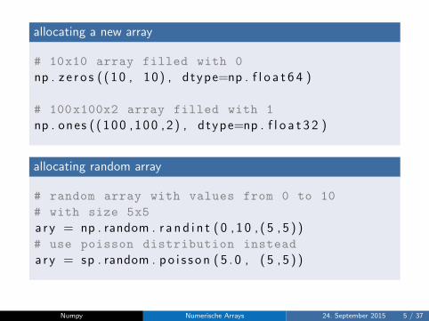
allocating a new array

# 10x10 array filled with 0

np . z e r o s ( ( 1 0 , 1 0 ) , dtype=np . f l o a t 6 4 )

# 100x100x2 array filled with 1

np . ones ( ( 1 0 0 , 1 0 0 , 2 ) , dtype=np . f l o a t 3 2 )

allocating random array

# random array with values from 0 to 10

# with size 5x5

a r y = np . random . r a n d i n t ( 0 , 1 0 , ( 5 , 5 ) )# use poisson distribution instead

a r y = sp . random . p o i s s o n ( 5 . 0 , ( 5 , 5 ) )

Numpy Numerische Arrays 24. September 2015 5 / 37

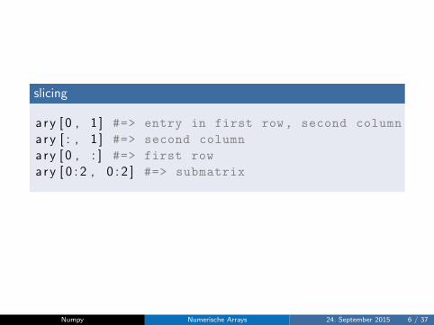
slicing

a r y [ 0 , 1 ] #=> entry in first row, second column

a r y [ : , 1 ] #=> second column

a r y [ 0 , : ] #=> first row

a r y [ 0 : 2 , 0 : 2 ] #=> submatrix

Numpy Numerische Arrays 24. September 2015 6 / 37

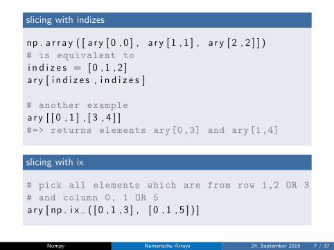
slicing with indizes

np . a r r a y ( [ a r y [ 0 , 0 ] , a r y [ 1 , 1 ] , a r y [ 2 , 2 ] ] )# is equivalent to

i n d i z e s = [ 0 , 1 , 2 ]a r y [ i n d i z e s , i n d i z e s ]

# another example

a r y [ [ 0 , 1 ] , [ 3 , 4 ] ]#=> returns elements ary[0,3] and ary[1,4]

slicing with ix

# pick all elements which are from row 1,2 OR 3

# and column 0, 1 OR 5

a r y [ np . i x ( [ 0 , 1 , 3 ] , [ 0 , 1 , 5 ] ) ]

Numpy Numerische Arrays 24. September 2015 7 / 37

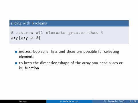
slicing with booleans

# returns all elements greater than 5

a r y [ a r y > 5 ]

indizes, booleans, lists and slices are possible for selectingelements

to keep the dimension/shape of the array you need slices orix function

Numpy Numerische Arrays 24. September 2015 8 / 37

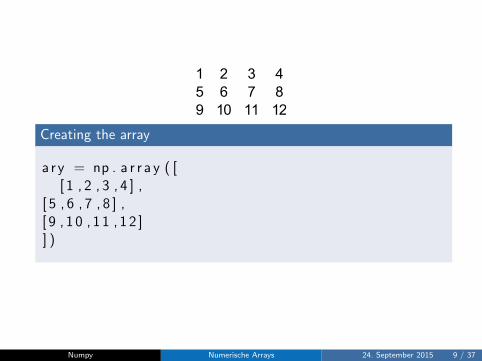
1 2 3 45 6 7 89 10 11 12

Creating the array

a r y = np . a r r a y ( [[ 1 , 2 , 3 , 4 ] ,

[ 5 , 6 , 7 , 8 ] ,[ 9 , 1 0 , 1 1 , 1 2 ]] )

Numpy Numerische Arrays 24. September 2015 9 / 37

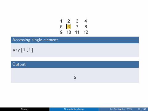
1 2 3 45 6 7 89 10 11 12

Accessing single element

a r y [ 1 , 1 ]

Output

6

Numpy Numerische Arrays 24. September 2015 10 / 37

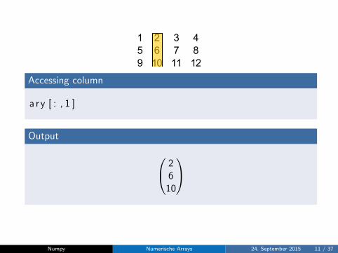
1 2 3 45 6 7 89 10 11 12

Accessing column

a r y [ : , 1 ]

Output

26

10

Numpy Numerische Arrays 24. September 2015 11 / 37

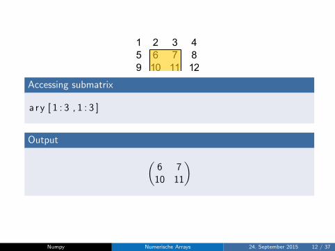
1 2 3 45 6 7 89 10 11 12

Accessing submatrix

a r y [ 1 : 3 , 1 : 3 ]

Output

(6 7

10 11

)

Numpy Numerische Arrays 24. September 2015 12 / 37

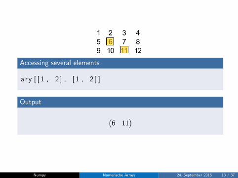
1 2 3 45 6 7 89 10 11 12

Accessing several elements

a r y [ [ 1 , 2 ] , [ 1 , 2 ] ]

Output

(6 11

)

Numpy Numerische Arrays 24. September 2015 13 / 37

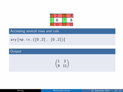
1 2 3 45 6 7 89 10 11 12

Accessing several rows and cols

a r y [ np . i x ( [ 0 , 2 ] , [ 0 , 2 ] ) ]

Output

(1 39 11

)

Numpy Numerische Arrays 24. September 2015 14 / 37

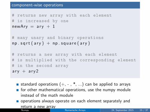
component-wise operations

# returns new array with each element

# is increased by one

newAry = a r y + 1

# many unary and binary operations

np . s q r t ( a r y ) + np . s q u a r e ( a r y )

# returns a new array with each element

# is multiplied with the corresponding element

# in the second array

a r y + a r y 2

standard operations (+, - , *, ...) can be applied to arraysfor other mathematical operations, use the numpy moduleinstead of the math moduleoperations always operate on each element separately andreturn a new arrayNumpy Numerische Arrays 24. September 2015 15 / 37

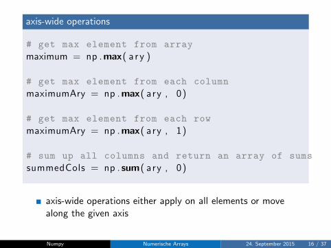
axis-wide operations

# get max element from array

maximum = np . max( a r y )

# get max element from each column

maximumAry = np . max( ary , 0)

# get max element from each row

maximumAry = np . max( ary , 1)

# sum up all columns and return an array of sums

summedCols = np . sum( ary , 0)

axis-wide operations either apply on all elements or movealong the given axis

Numpy Numerische Arrays 24. September 2015 16 / 37

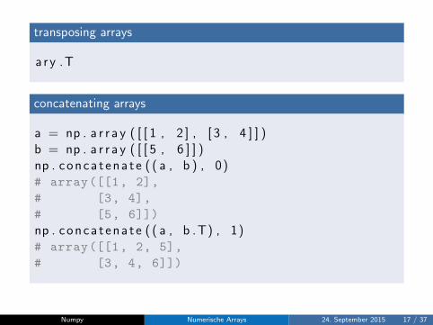
transposing arrays

a r y . T

concatenating arrays

a = np . a r r a y ( [ [ 1 , 2 ] , [ 3 , 4 ] ] )b = np . a r r a y ( [ [ 5 , 6 ] ] )np . c o n c a t e n a t e ( ( a , b ) , 0)# array([[1, 2],

# [3, 4],

# [5, 6]])

np . c o n c a t e n a t e ( ( a , b . T) , 1)# array([[1, 2, 5],

# [3, 4, 6]])

Numpy Numerische Arrays 24. September 2015 17 / 37

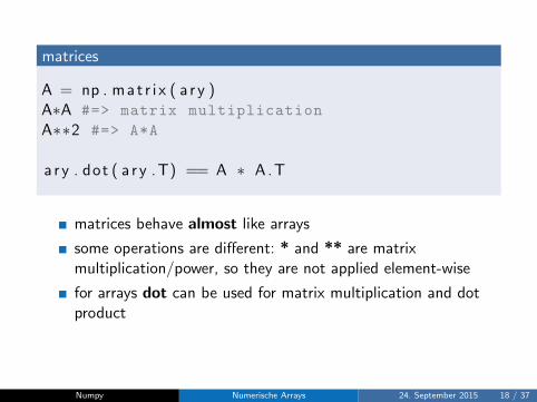
matrices

A = np . m a t r i x ( a r y )A∗A #=> matrix multiplication

A∗∗2 #=> A*A

a r y . dot ( a r y . T) == A ∗ A . T

matrices behave almost like arrays

some operations are different: * and ** are matrixmultiplication/power, so they are not applied element-wise

for arrays dot can be used for matrix multiplication and dotproduct

Numpy Numerische Arrays 24. September 2015 18 / 37

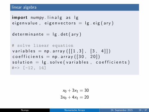
linear algebra

import numpy . l i n a l g as l ge i g e n v a l u e , e i g e n v e c t o r s = l g . e i g ( a r y )

d e t e r m i n a n t e = l g . d et ( a r y )

# solve linear equation

v a r i a b l e s = np . a r r a y ( [ [ 1 , 3 ] , [ 3 , 4 ] ] )c o e f f i c i e n t s = np . a r r a y ( [ 3 0 , 2 0 ] )s o l u t i o n = l g . s o l v e ( v a r i a b l e s , c o e f f i c i e n t s )#=> [-12, 14]

x0 + 3x1 = 30

3x0 + 4x1 = 20

Numpy Numerische Arrays 24. September 2015 19 / 37

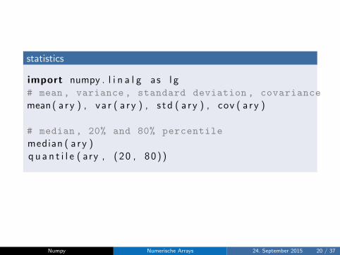
statistics

import numpy . l i n a l g as l g# mean, variance, standard deviation , covariance

mean ( a r y ) , v a r ( a r y ) , s t d ( a r y ) , cov ( a r y )

# median, 20% and 80% percentile

median ( a r y )q u a n t i l e ( ary , ( 2 0 , 8 0 ) )

Numpy Numerische Arrays 24. September 2015 20 / 37

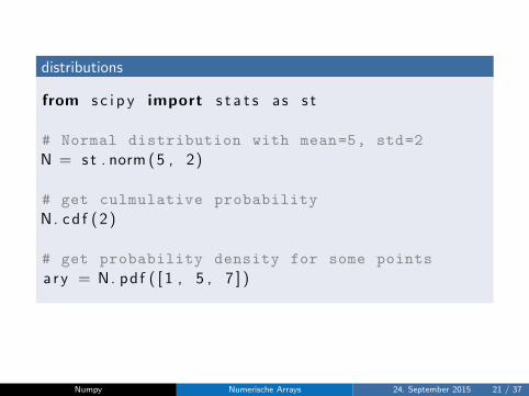
distributions

from s c i p y import s t a t s as s t

# Normal distribution with mean=5, std=2

N = s t . norm ( 5 , 2)

# get culmulative probability

N. c d f ( 2 )

# get probability density for some points

a r y = N. pdf ( [ 1 , 5 , 7 ] )

Numpy Numerische Arrays 24. September 2015 21 / 37

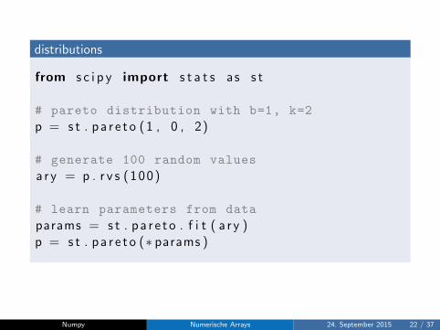
distributions

from s c i p y import s t a t s as s t

# pareto distribution with b=1, k=2

p = s t . p a r e t o ( 1 , 0 , 2)

# generate 100 random values

a r y = p . r v s ( 1 0 0 )

# learn parameters from data

params = s t . p a r e t o . f i t ( a r y )p = s t . p a r e t o (∗ params )

Numpy Numerische Arrays 24. September 2015 22 / 37

matplotlib

Matplotlib basic plotting 24. September 2015 23 / 37

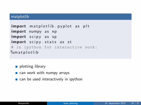
matplotlib

import m a t p l o t l i b . p y p l o t as p l timport numpy as npimport s c i p y as spimport s c i p y . s t a t s as s t# in ipython for interactive work:

%m a t p l o t l i b

plotting library

can work with numpy arrays

can be used interactively in ipython

Matplotlib basic plotting 24. September 2015 24 / 37

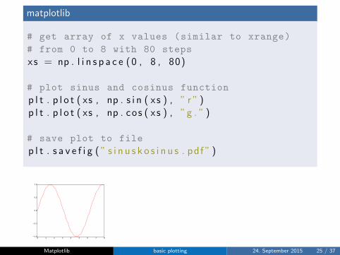
matplotlib

# get array of x values (similar to xrange)

# from 0 to 8 with 80 steps

xs = np . l i n s p a c e ( 0 , 8 , 80)

# plot sinus and cosinus function

p l t . p l o t ( xs , np . s i n ( xs ) , ” r ” )p l t . p l o t ( xs , np . cos ( xs ) , ”g . ” )

# save plot to file

p l t . s a v e f i g ( ” s i n u s k o s i n u s . pdf ” )

0 1 2 3 4 5 6 7 81.0

0.5

0.0

0.5

1.0

Matplotlib basic plotting 24. September 2015 25 / 37

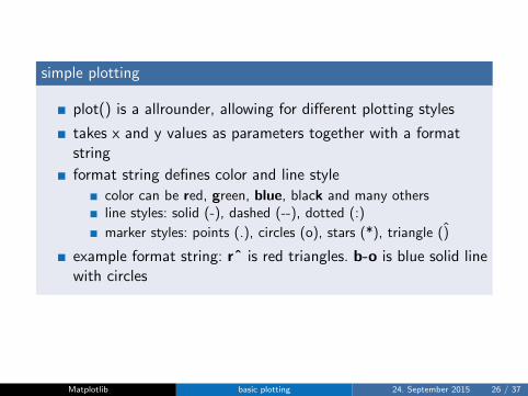
simple plotting

plot() is a allrounder, allowing for different plotting styles

takes x and y values as parameters together with a formatstring

format string defines color and line style

color can be red, green, blue, black and many othersline styles: solid (-), dashed (--), dotted (:)

marker styles: points (.), circles (o), stars (*), triangle ()

example format string: rˆ is red triangles. b-o is blue solid linewith circles

Matplotlib basic plotting 24. September 2015 26 / 37

other optional parameters

linewidth

color and marker can be used instead of format strings

markersize

label - binds a name on data (can be used later to refer tospecific datapoints)

Matplotlib basic plotting 24. September 2015 27 / 37

other plotting functions

hist for plotting histograms

lines for plotting line curves

vlines, hlines for vertical and horizontal lines

fill for filled polygons (area under the curve is filled with acolor)

pie

a lot more in http://matplotlib.org/examples/

Matplotlib basic plotting 24. September 2015 28 / 37

other plotting functions

hist for plotting histograms

lines for plotting line curves

vlines, hlines for vertical and horizontal lines

fill for filled polygons (area under the curve is filled with acolor)

pie

a lot more in http://matplotlib.org/examples/

Matplotlib basic plotting 24. September 2015 29 / 37

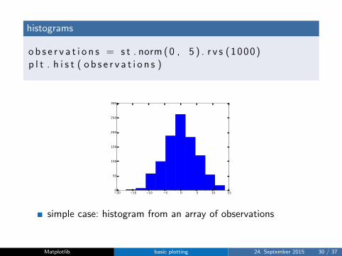
histograms

o b s e r v a t i o n s = s t . norm ( 0 , 5 ) . r v s (1000)p l t . h i s t ( o b s e r v a t i o n s )

20 15 10 5 0 5 10 150

50

100

150

200

250

300

simple case: histogram from an array of observations

Matplotlib basic plotting 24. September 2015 30 / 37

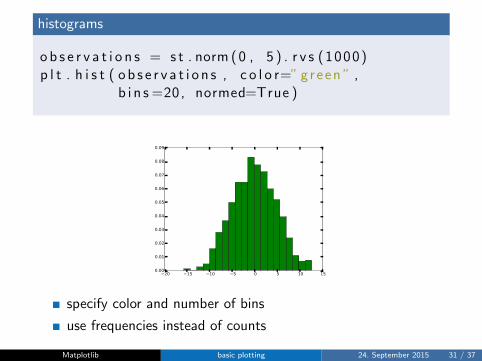
histograms

o b s e r v a t i o n s = s t . norm ( 0 , 5 ) . r v s (1000)p l t . h i s t ( o b s e r v a t i o n s , c o l o r=” g r e e n ” ,

b i n s =20, normed=True )

20 15 10 5 0 5 10 150.00

0.01

0.02

0.03

0.04

0.05

0.06

0.07

0.08

0.09

specify color and number of bins

use frequencies instead of counts

Matplotlib basic plotting 24. September 2015 31 / 37

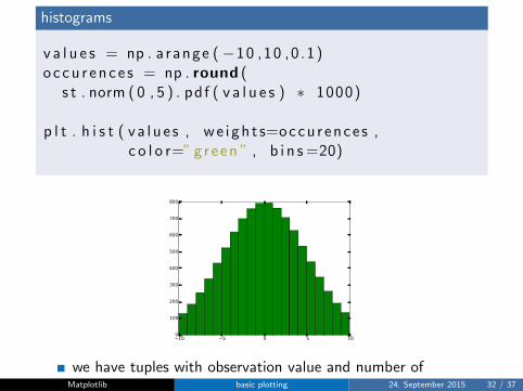
histograms

v a l u e s = np . a r an ge (−10 ,10 ,0 .1)o c c u r e n c e s = np . round (

s t . norm ( 0 , 5 ) . pdf ( v a l u e s ) ∗ 1000)

p l t . h i s t ( v a l u e s , w e i g h t s=o c c u r e n c e s ,c o l o r=” g r e e n ” , b i n s =20)

10 5 0 5 100

100

200

300

400

500

600

700

800

we have tuples with observation value and number ofobservationsuse weight vector

Matplotlib basic plotting 24. September 2015 32 / 37

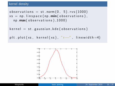
kernel density

o b s e r v a t i o n s = s t . norm ( 0 , 5 ) . r v s (1000)xs = np . l i n s p a c e ( np . min ( o b s e r v a t i o n s ) ,

np . max( o b s e r v a t i o n s ) , 1 0 0 0 )

k e r n e l = s t . g a u s s i a n k d e ( o b s e r v a t i o n s )

p l t . p l o t ( xs , k e r n e l ( xs ) , ” r−−” , l i n e w i d t h =4)

15 10 5 0 5 10 15 200.00

0.01

0.02

0.03

0.04

0.05

0.06

0.07

0.08

histograms look very different when changing the number ofbins or bin rangeskernel density is independent from any bin size or bin rangeparameterlooks like a smoothed histogramkernel density returns a function that can be applied on anarray of values (like distribution functions)

Matplotlib basic plotting 24. September 2015 33 / 37

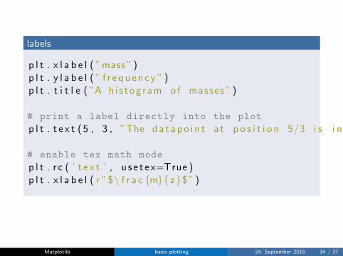
labels

p l t . x l a b e l ( ” mass ” )p l t . y l a b e l ( ” f r e q u e n c y ” )p l t . t i t l e ( ”A h i s t o g r a m o f masses ” )

# print a label directly into the plot

p l t . t e x t ( 5 , 3 , ”The d a t a p o i n t at p o s i t i o n 5/3 i s i n t e r e s t i n g ! ” )

# enable tex math mode

p l t . r c ( ’ t e x t ’ , u s e t e x=True )p l t . x l a b e l ( r ”$\ f r a c {m}{ z}$” )

Matplotlib basic plotting 24. September 2015 34 / 37

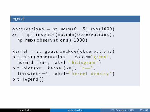
legend

o b s e r v a t i o n s = s t . norm ( 0 , 5 ) . r v s (1000)xs = np . l i n s p a c e ( np . min ( o b s e r v a t i o n s ) ,

np . max( o b s e r v a t i o n s ) , 1 0 0 0 )

k e r n e l = s t . g a u s s i a n k d e ( o b s e r v a t i o n s )p l t . h i s t ( o b s e r v a t i o n s , c o l o r=” g r e e n ” ,

normed=True , l a b e l=” h i s t o g r a m ” )p l t . p l o t ( xs , k e r n e l ( xs ) , ” r−−” ,

l i n e w i d t h =4, l a b e l=” k e r n e l d e n s i t y ” )p l t . l e g e n d ( )

Matplotlib basic plotting 24. September 2015 35 / 37

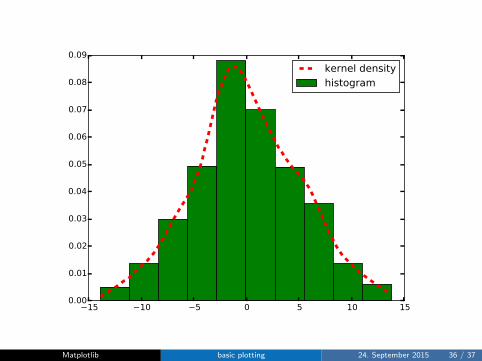
15 10 5 0 5 10 150.00

0.01

0.02

0.03

0.04

0.05

0.06

0.07

0.08

0.09kernel densityhistogram

Matplotlib basic plotting 24. September 2015 36 / 37

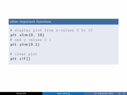
other important functions

# display plot from x-values 0 to 10

p l t . x l i m ( 0 , 10)# and y values 0 1

p l t . y l i m ( 0 , 1 )

# clear plot

p l t . c l f ( )

Matplotlib basic plotting 24. September 2015 37 / 37