econstor www.econstor.eu

Der Open-Access-Publikationsserver der ZBW – Leibniz-Informationszentrum WirtschaftThe Open Access Publication Server of the ZBW – Leibniz Information Centre for Economics

Standard-Nutzungsbedingungen:

Die Dokumente auf EconStor dürfen zu eigenen wissenschaftlichenZwecken und zum Privatgebrauch gespeichert und kopiert werden.

Sie dürfen die Dokumente nicht für öffentliche oder kommerzielleZwecke vervielfältigen, öffentlich ausstellen, öffentlich zugänglichmachen, vertreiben oder anderweitig nutzen.

Sofern die Verfasser die Dokumente unter Open-Content-Lizenzen(insbesondere CC-Lizenzen) zur Verfügung gestellt haben sollten,gelten abweichend von diesen Nutzungsbedingungen die in der dortgenannten Lizenz gewährten Nutzungsrechte.

Terms of use:

Documents in EconStor may be saved and copied for yourpersonal and scholarly purposes.

You are not to copy documents for public or commercialpurposes, to exhibit the documents publicly, to make thempublicly available on the internet, or to distribute or otherwiseuse the documents in public.

If the documents have been made available under an OpenContent Licence (especially Creative Commons Licences), youmay exercise further usage rights as specified in the indicatedlicence.

zbw Leibniz-Informationszentrum WirtschaftLeibniz Information Centre for Economics

Thöni, Christian; Gaechter, Simon

Working Paper

Peer Effects and Social Preferences in VoluntaryCooperation

CESifo Working Paper, No. 4741

Provided in Cooperation with:Ifo Institute – Leibniz Institute for Economic Research at the University ofMunich

Suggested Citation: Thöni, Christian; Gaechter, Simon (2014) : Peer Effects and SocialPreferences in Voluntary Cooperation, CESifo Working Paper, No. 4741

This Version is available at:http://hdl.handle.net/10419/96838

Peer Effects and Social Preferences in Voluntary Cooperation

Christian Thöni Simon Gächter

CESIFO WORKING PAPER NO. 4741 CATEGORY 13: BEHAVIOURAL ECONOMICS

APRIL 2014

An electronic version of the paper may be downloaded • from the SSRN website: www.SSRN.com • from the RePEc website: www.RePEc.org

• from the CESifo website: Twww.CESifo-group.org/wp T

CESifo Working Paper No. 4741

Peer Effects and Social Preferences in Voluntary Cooperation

Abstract Social preferences and social influence effects (“peer effects”) are well documented, but little is known about how peers shape social preferences. Settings where social preferences matter are often situations where peer effects are likely too. In a gift-exchange experiment with independent payoffs between two agents we find causal evidence for peer effects. Efforts are positively correlated but with a kink: agents follow a low-performing but not a high-performing peer. This contradicts major theories of social preferences which predict that efforts are unrelated, or negatively related. Some theories allow for positively-related efforts but cannot explain most observations. Conformism, norm following and social esteem are candidate explanations.

JEL-Code: C920, D030.

Keywords: social preferences, voluntary cooperation, peer effects, reflection problem, gift-exchange, conformism, social norms, social esteem, experiments.

Christian Thöni University of Lausanne Centre Walras-Pareto

UNIL-Dorigny Switzerland – 1015 Lausanne

christian.thoeni@unil.ch

Simon Gächter* University of Nottingham

School of Economics Sir Clive Granger Building

University Park United Kingdom – Nottingham, NG7 2RD

simon.gaechter@nottingham.ac.uk

*corresponding author 6 February 2014 This paper is part of a research project “Soziale Interaktionen, Unternehmenskultur and Anreizgestaltung”, financed by the Grundlagenforschungsfonds of the University of St.Gallen. We are grateful for helpful comments by Friedrich Breyer, Stefan Bühler, Rachel Croson, Tore Ellingsen, Urs Fischbacher, Yukihiko Funaki, Martin Kolmar, Tatiana Kornienko, Michael Kosfeld, Bentley MacLeod, Daniele Nosenzo, Rupert Sausgruber, Martin Sefton, Karl Schlag, Rudi Stracke, Jean-Robert Tyran, and participants at various seminars, conferences and workshops. Simon Gächter also gratefully acknowledges support under the European Research Council Advanced Investigator grant ERC-AdG 295707, and the hospitality of the Institute for Advanced Studies at Hebrew University in Jerusalem while working on this paper.

1

1. Introduction

Is pro-social voluntary cooperation subject to ‘peer effects’ that is, influenced by the behavior of comparison others? Or is pro-sociality best thought of as being a characteristic of people’s preferences that is largely immune to social influence? These questions are at the heart of this paper. Understanding how social preferences are shaped by peer effects is important because people normally do not act in a social vacuum but are constantly exposed to peers. The purpose of this paper is to clarify how social preferences and peer effects are linked both by providing novel experimental evidence and by clarifying theoretically what theories of social preferences have to say on peer effects.

Hitherto the literatures on social influence effects and social preferences are, with a few exceptions, largely unconnected. The literature on social preferences shows that many people are willing to act against their self-interest even in anonymous one-shot situations with incentives to behave selfishly and no possibilities for social influence (e.g., Fehr and Fischbacher (2002); Camerer (2003); Gintis et al. (2005)). The literatures on social influence effects show that people’s behavior in many economically important domains is often strongly shaped by what comparison others do even in the absence of material payoff spillovers.1 Similarly, social psychologists have long argued that situational cues (provided by the environment or the behavior of others) are often more important than personality traits (Asch (1952); Ross and Nisbett (1991)). Both social preferences and social influence effects are firmly established empirically, but little is known about how social preferences, which carefully control for material incentives, are influenced by, and related to, peer effects.2

It is important to be clear about our usage of the term ‘peer effects’. Sometimes this term is used as an umbrella term to describe behaviors where an agent reacts to other agents’ actions; such a behavioral reaction might be motivated by social preferences. As an example, think of voluntary contributions to a public good, where people contribute more the more other group members (‘peers’) contribute. Such ‘conditional cooperation’ can be explained by social preferences such as reciprocity or guilt aversion (Dufwenberg et al. (2011)) towards the peers whose contributions have a direct material externality on the agent by the definition of a public good. Our usage of the term peer effect is narrower. We will speak of a pure ‘peer effect’ if an agent is influenced in his or her actions by what a comparison agent does, even if there are no material spillovers between agents and hence no direct social preference links exist between peers (indirect links are possible, as our theoretical analysis will show).

Our main contribution is to demonstrate the existence of pure peer effects in a novel experimental design and to clarify the role of social preferences in explaining such pure peer effects (henceforth we will simply speak of peer effects). Specifically, our design allows us to

1 Some examples from the field comprise deviant behavior (Sampson et al. (2002)), academic success (e.g., Sacerdote (2001)), savings behavior (e.g., Duflo and Saez (2002)); conditional cooperation (Frey and Meier (2004); Chen et al. (2010)); charitable donations (Croson and Shang (2008); Shang and Croson (2009)); health-related issues like alcohol consumption (Kremer and Levy (2008)) and obesity (Christakis and Fowler (2007)) and behavior in the workplace (Ichino and Maggi (2000); Mas and Moretti (2009); Bandiera et al. (2010)). 2 There is only a small literature on peer effects in social preferences conducted in a way that carefully controls for self-regarding motives. We discuss our contribution to this literature below.

2

causally demonstrate peer effects in voluntary cooperation in an environment that tightly controls for material payoff spillovers and strategic incentives. We also analyze what all major theories of social preferences (introduced below) predict about peer effects in social preferences and we provide an experimental test of the best-reply predictions of these theories. For our analysis we are mainly interested in the well-documented social preference of reciprocity in a game of voluntary cooperation.

Understanding the link between social preferences and peer effects is important for two reasons. First, in reality social preferences are often relevant in environments that are potentially rich in possibilities for social influence effects (think of the workplace as a prime example). Second, suppose we find evidence that voluntary cooperation is subject to peer effects. What would the implication be for theories of social preferences that aim at explaining voluntary cooperation? To appreciate this question, consider that the evidence on social preferences has directed theoretical research at understanding individuals’ behavior as a feature of people’s given preferences. For example, in popular theories of inequity aversion (Bolton and Ockenfels (2000); Fehr and Schmidt (1999)) people’s social preferences are modeled as individually fixed distastes for inequitable outcomes. Evidence for peer effects would constitute a prima facie challenge to fixed preference assumptions. We deem it important to clarify whether peer effects indeed provide such a challenge.

Our tool to measure peer effects is a one-shot three-person gift-exchange game where a principal pays his or her two agents i and j a wage w (the same for both) and the agents choose efforts ei and ej. The material incentive structure gives both agents an incentive to choose minimal effort (‘to shirk’) irrespective of w and irrespective of the other agent’s effort. However, from numerous two-person gift-exchange games we expect that many agents will choose efforts that increase in the wage (see Fehr and Gächter (1998); Fehr et al. (2009); Charness and Kuhn (2011) for surveys). Since the experiment is anonymous, one-shot, and all players know this, effort choice is an expression of people’s social preference. In this situation we will speak of a ‘peer effect’ if ei = f(ej)|w, that is, holding the common wage w constant, agent i’s effort depends on agent j’s effort (f’ ≠ 0), despite the absence of any earnings interdependency between agents.

A major problem of measuring peer effects empirically is the “reflection problem” (Manski (1993), Manski (2000)) which results from the mutual social influences people might have on each other: ei = f(ej)|w and ej = f(ei)|w. If i is influenced by j and j is influenced by i it is impossible to disentangle the causal influences i and j have on each other. Here we propose a design that avoids the reflection problem. The main idea is to make the effort of the other agent exogenous. To achieve this, both agents first choose their efforts simultaneously and then, after having learned the effort decision of their co-agent, are given the opportunity to revise their effort, holding their co-agent’s effort constant. Since the design removes any material and strategic incentives to revise effort, revision decisions (compared to a control condition with no effort information) tell us about the extent to which people change their effort because of the effort chosen by the co-agent. To our knowledge, this is a novel design to measure peer effects in voluntary cooperation.

3

Effort revisions are significantly more likely and substantially bigger when agents are informed about their co-agent’s decision (in our main treatment) than when they are uniformed (control treatment). When agents learn their co-agent has provided lower effort than them they revise their efforts downwards, but they hardly increase their effort when their co-agent provided higher effort. Agents’ efforts are positively correlated but with a kink at the co-agent’s effort.

Is this peer effect evidence for the non-stability of social preferences? At first glance our results suggest this interpretation. Many agents choose non-minimal initial efforts suggesting other-regarding preferences but are then willing to revise their effort in light of effort information that is inconsequential for their own material payoff.

To understand whether peer effects in social preferences are a novel phenomenon that is incompatible with existing theories of social preferences we analyze the theoretical predictions of widely used theories of social preferences that model various distributional and/or intentional concerns. Given our research question we focus on the best-reply predictions with regard to effort changes, that is, dei/dej. To our knowledge, no such analysis has been done in the context of explaining peer effects in voluntary cooperation.

There are three main reasons for consulting theories of social preferences. First, theories of social preferences aim at explaining behavior also in novel games like ours, not just existing ones. Second, among many other games, these theories can account for non-minimal efforts in the bilateral version of the gift-exchange game. It is thus obvious to explore the explanatory power of these theories in the trilateral gift-exchange game. Third, we not only explore the implications of one particular theory but compare predictions for all major theories of social preferences with the ambition to explain behavior in many games. The reason for this comprehensive approach is to see whether these theories, which include diverse psychological motivations, come up with robust (that is, concurrent) predictions about how agent j’s effort influences agent i’s effort (that is, the sign of dei/dej). Even if these theories do not come up with concurrent predictions the question is which theories predict the peer effects we observe.

We consider (1) models of distributional preferences in the form of altruism (Cox et al. (2007), Charness and Rabin (2002)3) and inequity aversion ((Bolton and Ockenfels (2000); Fehr and Schmidt (1999)) or a combination of both (Kohler (2011)); (2) models of reciprocity (Dufwenberg and Kirchsteiger (2004); Levine (1998)); and (3) hybrid models that combine interpersonal comparisons and reciprocity (Charness and Rabin (2002); Falk and Fischbacher (2006); Cox et al. (2007)). Hence, our analysis does not favor one theory a priori.

Our analysis shows that the most robust predictions of these standard theories of social preferences are that either there are no peer effects (efforts are unrelated in models of reciprocity), or if there are peer effects, efforts are negatively related (in all other models). Three models predict that, in addition to being negatively related, efforts can also be positively related: Fehr and Schmidt (1999), Charness and Rabin (2002) and Kohler (2011). 3 We classify the basic model by Charness and Rabin (2002) as a model of altruism because – in contrast to models of inequity aversion – the derivatives of utility with respect to other player’s earnings are always non-negative (this does, however, not hold for the reciprocity extension discussed in their appendix).

4

Our experimental finding of peer effects with positively correlated efforts seems therefore inconsistent with most models. However, this evidence is not fully conclusive because the theoretical analysis makes predictions about the agents’ best-reply functions, which our simple revision decisions do not reveal.

To have a more conclusive test we therefore ran experiments where we also elicited the agents’ beliefs about the initial effort choice of their co-agent. Thus, we now observe two points on each agent’s best-response which allows us to draw conclusions about the slope of the best-reply functions. The results unambiguously reject the prediction of most theories that efforts will be negatively related. In the peer effect we observe, efforts are strategic complements, not substitutes. Also the theories that predict positively correlated efforts are only exactly consistent with a minority of choices.

While standard theories of social preferences which model distributional concerns and/or intentions, typically predict the opposite of what we observe, some recent theories of social preferences that incorporate social motives like conformism (Sliwka (2007)), norm-following (López-Pérez (2008)), or social esteem (Ellingsen and Johannesson (2008)) can explain the peer effects we observe. In our concluding section we briefly discuss these theories and provide remarks about future research.

In summary and comparison to the literature, this paper makes two main and intertwined contributions. Our first contribution is to provide novel and causal evidence for peer effects in reciprocity by using the gift-exchange game run in the direct response method and by ruling out confounding factors such as strategic incentives that might be present, for instance, in repeated interactions (as in Falk et al. (2013) who used finitely repeated simultaneous public goods games to study peer effects in voluntary cooperation). The use of the direct response method is one distinguishing feature of this paper relative to Gächter et al. (2012) and Gächter et al. (2013) who also use a three-person gift-exchange game but play it in the strategy method.4 Both studies find evidence for peer effects which take the form of positively correlated efforts, but by their strategy-method designs are unable to observe the kink in efforts we are able to observe in our design. Moreover, both papers also allow for wage inequality, which our design precludes for keeping the present research question simple. One focus of these papers is to study the role of wage inequality for peer effects, an issue which we do not consider.

Our focus on reciprocity in voluntary cooperation by using the gift-exchange game separates our study from papers that investigate and find peer effects (in the absence of any payoff spillovers like in our case) in sharing in the dictator game (Cason and Mui (1998); Bicchieri and Xiao (2009); Krupka and Weber (2009)) and in the ultimatum game (Ho and Su (2009)). Papers more closely related to the experimental part of our paper are Bardsley and Sausgruber (2005) and Mittone and Ploner (2011). Bardsley and Sausgruber provide evidence that contributions to a one-shot public good can be shaped by observing the contributions of an unrelated other group. Mittone and Ploner also study a sequential game of reciprocity, in

4 Gächter and Thöni (2010) also study a three-person gift-exchange experiment but their focus is on wage inequality; they do not study peer effects.

5

their case the trust game, and unlike us, they use the strategy method. Their central tool is an observer/observed design with the difference to our study that the relevant group of recipients is comprised of groups of four, two of which are observed and two are the observers. The results are that the observed tend to be more trustworthy than recipients in a baseline condition and the return rates ('trustworthiness') of the observed and observer recipients are positively correlated, which is evidence for peer effects in reciprocity. As will become clear below, in our design, everyone is an observer and an observed and strategic incentives to influence others is removed.

Our second contribution that separates us from all aforementioned experimental studies is to clarify the power of a range of theories of social preferences for explaining peer effects in reciprocity. We provide a formal analysis and then run further specially-designed experiments to compare the theoretical best-reply predictions (slopes) with the empirically estimated slope. To our knowledge no such analysis has yet been done in the context of peer effects. Such an analysis is important, however, to safeguard against premature declarations of peer effects as a phenomenon that requires separate explanations from those of existing theories.

Most papers which look at predictions of theories of social preferences use one model only (most typically, the Fehr and Schmidt (1999) model). As explained above, we deem it important, however, not to pre-select one particular theory but to look at a whole range of theories, which capture different psychological motivations, to understand why and when these theories can, or cannot, explain peer effects. Such an analysis can narrow the range of theories that are candidate explanations for peer effects, even if we acknowledge that one lesson of tests of theories of social preferences is that all fail in some dimensions (e.g., Charness and Rabin (2002); Engelmann and Strobel (2004); Cox et al. (2007); Falk et al. (2008); Daruvala (2010)) and maybe especially so in three-person games (e.g., Kagel and Wolfe (2001)). A comprehensive comparative analysis can provide insights about patterns of failures across classes of theories that are informative in their own right.

2. Design and procedures

2.1. The three-person gift-exchange game with a revision stage

Our three-person gift-exchange game is a simple extension of the two-player gift-exchange game (Fehr et al. (1993); Fehr et al. (1998)) – there is one principal and two identical agents. The principal first chooses the same wage { }50,100,200w∈ for both agents. After observing this wage the two agents decide simultaneously about their effort, that is, they choose { }1,2,..., 20ie ∈ . In some of the sessions we elicit the agents’ beliefs about their co-agent’s effort choice je′ (we will provide our rationale for eliciting beliefs in Section 5).

Agents then learn about the revision stage where they are informed about the ‘initial effort’ decision of their co-agent, ej.5 In light of this new information agents are told that they 5 When agents decided on their initial effort they did not yet know about the possibility to revise effort. This is necessary to avoid that the initial effort is strategically biased, which would preclude a clean measurement of peer effects. The information about the revision possibility and its description appeared on a separate screen (for the exact wordings see Appendix A). The reader may ask why this procedure rather than letting the agents

6

can, but do not have to, revise their effort. Both agents simultaneously choose a revised effort { }ˆ 1,2,..., 20ie ∈ . However, to make the revision decision incentive compatible, agents are told

that only for one randomly selected agent the revised effort will be relevant for calculating earnings, while for the other agent the initial effort will be payoff relevant. The agent whose revised effort will be payoff relevant will be decided at random. A random device generates r ∈ {0,1} with equal probability. In case r = 1 agent 1’s revised effort and agent 2’s initial effort are payoff relevant (that is, agent 2’s revised effort has no effect on any of the earnings). In case of r = 0, agent 2’s revised effort and agent 1’s initial effort are payoff relevant (and agent 1’s revised effort has no effect on any of the earnings). Thus, our design ensures that only one agent's revised effort matters, and therefore the other agent's initial effort is unaltered and remains fixed. Moreover, our procedure allows us collecting data from both agents. Subjects know this procedure (but not yet the outcome) when choosing the revised effort. The expected earnings of the principal are

[ ]1 2 1 2ˆ ˆ( ) (1 )( ) 2P rx vE r e e r e e w= + + − + − , (1)

where v > 0 is the constant marginal product of the agents’ efforts. The expected earnings of the two agents are calculated as

1 1 1 2 2 2ˆ ˆ[ ( ) (1 ) ( )] and [(1 ) ( ) ( )]r rx w E rc e r c e x w E r c e rc e= − − − = − − − , (2)

where the cost of effort is equal to c(ei) = 7(ei – 1) for both agents.6 Note that we do not allow the principal to differentiate the wages between the two agents because we want to observe the two agents in an identical situation. Allowing for different wages would have given agents motives for choosing different initial effort levels. For the same reason the two agents have an identical marginal productivity (v).

The revised effort is our main instrument to identify social interaction effects. The only change between the initial effort decision and the revision stage is the additional information about the co-agent’s effort. We will use Δei = êi – ei as a measure for the reaction to effort information, that is, as an indication for a pure peer effect.

It is important to note that we measure peer effects in a situation where the co-agent’s effort remains unchanged. This design feature avoids the reflection problem. When choosing the revised effort, agent i knows that either his decision has no effect (r = 0) or the effort of the co-agent remains unchanged (r = 1). The random selection of either the initial effort or the revised effort ensures that the co-agent’s effort is exogenous and has the added advantage that it allows us to collect revision decisions from all agents.7

choose their efforts sequentially. We could then test whether the effort decision of the second mover depends on the effort decision of the first moving agent. However, it is difficult to disentangle peer effects from the second-moving agent’s disposition to reciprocate towards the principal. The first mover might have set his or her effort strategically, to influence the second mover’s effort. Our design avoids these problems. 6 To rule out overall losses all players were endowed with 400 ECU. 7 Another possibility would have been to randomly select one agent and ask him or her whether he or she would like to revise the effort. The disadvantage of this procedure is that it would only generate data from half of the agents. Our method generates revision decisions from all agents but still preserves the feature that the other agent’s effort is exogenous if the chosen agent’s revised effort becomes relevant for calculating earnings.

7

A caveat is in order, however. We cannot rule out the possibility that subjects might want to change their effort decision in the revision stage for reasons unrelated to peer effects. For instance, one might be concerned that the mere existence of the revision stage induces an ‘experimenter demand effect’ (e.g., Orne (1962); Zizzo (2010)). If subjects are asked to decide again about their effort they might feel urged to change their decision. A second reason might be ‘virtual learning’ (Weber (2003)): the revision stage provides subjects with an additional opportunity to think through the problem. Third, effort revisions might simply occur due to change of mind or errors. Thus, in order to isolate peer effects from other sources of effort revisions we need a control treatment in addition to the ‘Effort Information treatment’ (EIT). Our control treatment, called the ‘No Information treatment’ (NIT), is identical to the game explained above except when reaching the revision stage subjects are not informed about the effort choice of the co-agent.

2.2. Further design features and procedural details

To check for the robustness of our results we change several contextual parameters across sessions. First, we vary the level of the agents’ productivity (v = 18 or v = 35 for both agents) and therefore the gains from cooperation. Second, to be able to test theoretical predictions (Section 5) we elicit beliefs about the co-agent’s initial effort choice. However, eliciting beliefs might influence effort choices (Croson (2000); Gächter and Renner (2010)). For this reason we include the belief elicitation only in some of the sessions.

Part of our participants played a one-shot, three-person gift-exchange game prior to the experiment we report in this paper. In this ‘Experiment 1’ (reported in Gächter and Thöni (2010)) agents made their effort decision in the strategy method. We will use the data from Experiment 1 to classify our subjects into selfish and non-selfish types. This provides us with a measure for other-regarding preferences that is not derived from the decisions in the experiments reported here. Subjects in Experiment 1 did not receive any information about other subjects’ decisions prior to the experiment presented in this paper.

Another group of subjects played eight rounds of a three-person gift-exchange game with random matching (in matching groups of 12 subjects). These subjects had more experience with the game prior to the start of the experiment at hand. During the eight rounds agents received information about their principal's wage offerings but agents did not receive any direct information about their co-agent's effort choices. We will label these subjects as Experienced and use this contextual variation to check whether increased experience with the game influences peer effects. See Gächter and Thöni (2010) for the results of Experiment 1 and the Experienced sessions.

We conducted the experiment at the Universities of St. Gallen and Zurich in computerized laboratories where subjects were separated by partitions and thus took their decisions in isolation and without communication. All decisions were anonymous. We used the software z-Tree (Fischbacher (2007)) to run our experiments and ORSEE (Greiner (2004)) for recruiting the subjects. Like in previous gift-exchange experiments (e.g., Fehr et al. (1997)),

8

we framed the experiment in a ‘buyer-seller’ terminology. We chose this frame because we deem it to be more neutral than a labor relations frame.8

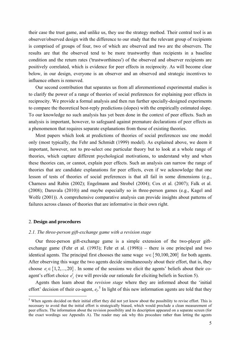
Our research question requires a one-shot experiment. We therefore took great care to ensure that subjects understand the rules, as well as the pecuniary payoff consequences of their decisions. Subjects had to answer a set of control questions on payoff consequences. To help subjects calculate earnings, the software provided a ‘What-if calculator’, where subjects could calculate the monetary payoff consequences for all players and all possible combinations of efforts and wages. The ‘What-if Calculator’ was available at all stages of the experiment. Fig. 1 illustrates an example of a decision screen subjects saw at the revision stage after having been informed about the revision stage.

Table B1 (Appendix B) provides an overview of the number of observations by treatment and contextual variation. We have observations from 18 sessions with a total of 489 participants, 326 agents and 163 principals. The majority (330) decided in the EIT. The remaining 159 subjects decided in the NIT. We imposed no time limit for decisions. The experiment lasted about 30 minutes and the average earnings were CHF 13.8 (€ 8.8).

Fig. 1. Example screen shot of the decision screen at the revision stage

in the Effort Information treatment.

3. Results I: Existence and direction of peer effects

3.1. Initial effort choices

Recall that the EIT and the NIT are identical up to the revision stage. For analyzing initial effort choices we therefore pool the data. As expected from numerous gift-exchange

8 It is of course an empirical question whether framing matters in our context. Answering this question is beyond the scope of this paper. The existing evidence from a related game (the bribery game, which contains an element of reciprocity, see Abbink and Hennig-Schmidt (2006)) suggests that framing does not matter.

9

experiments (surveyed in Fehr and Gächter (1998); Fehr et al. (2009); Charness and Kuhn (2011)), efforts increase in wages.9

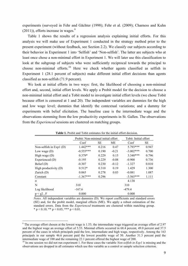
Table 1 shows the results of a regression analysis explaining initial efforts. For this analysis we will make use of Experiment 1 conducted in the strategy method prior to the present experiment (without feedback, see Section 2.2). We classify our subjects according to their behavior in Experiment 1 into ‘Selfish’ and ‘Non-selfish’. The latter are subjects who at least once chose a non-minimal effort in Experiment 1. We will later use this classification to look at the subgroup of subjects who were sufficiently reciprocal towards the principal to choose non-minimal efforts.10 Here we check whether agents classified as selfish in Experiment 1 (28.1 percent of subjects) make different initial effort decisions than agents classified as non-selfish (71.9 percent).

We look at initial efforts in two ways: first, the likelihood of choosing a non-minimal effort and, second, initial effort levels. We apply a Probit model for the decision to choose a non-minimal initial effort and a Tobit model to investigate initial effort levels (we chose Tobit because effort is censored at 1 and 20). The independent variables are dummies for the high and low wage level; dummies that identify the contextual variations; and a dummy for experiments with belief elicitation. The baseline case is the intermediate wage and the observations stemming from the low productivity experiments in St. Gallen. The observations from the Experienced sessions are clustered on matching groups.

Table 1. Probit and Tobit estimates for the initial effort decision.

Probit: Non-minimal initial effort Tobit: Initial effort Coef SE ME Coef SE Non-selfish in Exp1 (D) 1.442*** 0.216 0.47 5.793*** 0.947 Low wage (D) -0.555*** 0.190 -0.21 -3.002*** 0.700 High wage (D) 0.379* 0.229 0.15 3.340*** 0.796 Experienced (D) -0.195 0.229 -0.08 -0.900 0.736 Belief (D) -0.307 0.230 -0.12 -1.327 0.810 High productivity (D) 0.512* 0.310 0.19 1.429 1.300 Zurich (D) 0.065 0.278 0.03 -0.081 1.087 Constant -1.367*** 0.296 -3.565*** 1.111 σ 4.138 N 310 310 Log likelihood -167.6 -479.4 p < χ2 , F 0.000 0.000

Notes. All independent variables are dummies (D). We report coefficients and standard errors (SE) and, for the probit model, marginal effects (ME). We apply a robust estimation of the standard errors. Data from the Experienced treatments are clustered within matching group. * p < 0.10; ** p < 0.05; *** p < 0.01.

9 The average effort chosen at the lowest wage is 1.53; the intermediate wage triggered an average effort of 2.97 and the highest wage an average effort of 5.53. Minimal efforts occurred in 68.4 percent, 49.0 percent and 37.5 percent of the cases in which principals paid the low, intermediate and high wage, respectively. Among the 163 principals in our sample 46.6 percent paid the lowest possible wage of 50. Another 31.3 percent paid the intermediate wage of 100 and the remaining 22.1 percent offered the highest wage of 200. 10 In one session we did not run experiment 1. For these cases the variable Non-selfish in Exp1 is missing and the observations are dropped in all estimates which use this variable as a control or sample selection criterion.

10

In both models subjects classified as non-selfish in Experiment 1 are significantly more likely to choose a non-minimal initial effort; they also choose higher initial effort levels than subjects classified as selfish. Effort levels increase significantly in wages; the productivity parameter v has a marginally significant effect on the probability to choose a non-minimal effort.11 All other variables are not significant.

3.2. Existence of peer effects in voluntary cooperation

In EIT agents revise their effort in 73 out of 220 of the cases (33.2 percent). Effort revisions also occur in the NIT: 24 out of 106 agents (22.6 percent) revise their effort but are more likely in EIT than in NIT (χ2-test: p = .051).

Peer effects in our one-shot environment presumably matter most among agents who care about others’ well-being at all. Agents with no or weak other-regarding preferences might be less influenced by peer effects, compared to agents who showed a willingness to deliver non-minimal effort levels in Experiment 1. In order to investigate effort revisions of these agents, we study a reduced sample where we only look at cases in which agents chose a non-minimal effort in Experiment 1. In the EIT, 62 out of 141 (44.0 percent) of these non-selfish agents revise their effort while 21 out of 82 (25.6 percent) do so in the NIT (χ2-test: p = .006). Even more frequent are effort revisions among the subjects who chose a non-minimal initial effort. Sixty-eight percent of agents in EIT revise their effort. In NIT the corresponding number is 45 percent (χ2-test: p = .008).

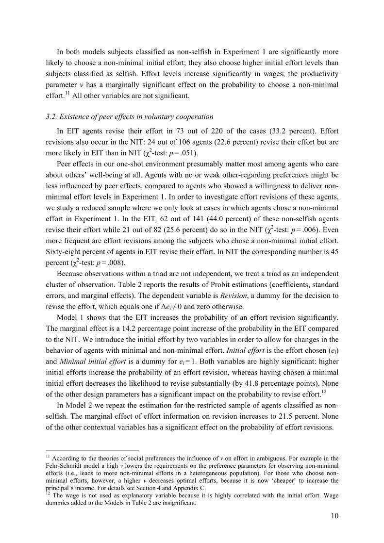
Because observations within a triad are not independent, we treat a triad as an independent cluster of observation. Table 2 reports the results of Probit estimations (coefficients, standard errors, and marginal effects). The dependent variable is Revision, a dummy for the decision to revise the effort, which equals one if Δei ≠ 0 and zero otherwise.

Model 1 shows that the EIT increases the probability of an effort revision significantly. The marginal effect is a 14.2 percentage point increase of the probability in the EIT compared to the NIT. We introduce the initial effort by two variables in order to allow for changes in the behavior of agents with minimal and non-minimal effort. Initial effort is the effort chosen (ei) and Minimal initial effort is a dummy for ei = 1. Both variables are highly significant: higher initial efforts increase the probability of an effort revision, whereas having chosen a minimal initial effort decreases the likelihood to revise substantially (by 41.8 percentage points). None of the other design parameters has a significant impact on the probability to revise effort.12

In Model 2 we repeat the estimation for the restricted sample of agents classified as non-selfish. The marginal effect of effort information on revision increases to 21.5 percent. None of the other contextual variables has a significant effect on the probability of effort revisions.

11 According to the theories of social preferences the influence of v on effort in ambiguous. For example in the Fehr-Schmidt model a high v lowers the requirements on the preference parameters for observing non-minimal efforts (i.e., leads to more non-minimal efforts in a heterogeneous population). For those who choose non-minimal efforts, however, a higher v decreases optimal efforts, because it is now ‘cheaper’ to increase the principal’s income. For details see Section 4 and Appendix C. 12 The wage is not used as explanatory variable because it is highly correlated with the initial effort. Wage dummies added to the Models in Table 2 are insignificant.

11

Table 2. Probit estimations for the decision to revise effort.

Dependent variable: Revise (dummy for êi ≠ 0) Model 1 (all agents) Model 2 (non-selfish agents only) Coef SE ME Coef SE ME EIT (D) 0.522*** 0.193 0.142 0.658*** 0.224 0.215Initial effort 0.136*** 0.039 0.040 0.133*** 0.043 0.046Minimal initial effort (D) -1.398*** 0.257 -0.418 -1.441*** 0.314 -0.446Experienced (D) -0.297 0.211 -0.082 -0.194 0.256 -0.065Belief (D) 0.242 0.216 0.071 0.080 0.257 0.028High productivity (D) 0.236 0.374 0.064 0.007 0.441 0.003Zurich (D) 0.048 0.329 0.014 0.227 0.369 0.076Constant -1.041*** 0.362 -0.957** 0.436 N 326 223 Log-likelihood -124.786 -94.851 p > χ2 0.000 0.000 Notes. The NIT is the omitted benchmark. Apart from Initial effort all independent variables are dummies (D). We report coefficients, standard errors (SE), and marginal effects (ME). Model 1 uses all agents, and Model 2 only agents classified as non-selfish according to their decision in Experiment 1. We apply a robust estimation of the SE clustered within a matching group. * p < 0.10; ** p < 0.05; *** p < 0.01.

The absolute magnitude of effort revisions is considerably larger in EIT (.97 on average) than in NIT (.37). Thus, the average absolute effort revision differs by a factor of 2.6 between treatments. This effect is not only driven by the fact that agents revise effort more frequently when information about their co-agent’s effort is provided. In the subsample of agents who actually do revise effort (Δei ≠ 0) the difference between the average absolute effort revisions increases to 1.31 effort units. If we repeat the estimates of Table 2 but apply a Tobit regression with the absolute effort revision as dependent variable we get very similar results. We summarize these findings as follows:

Result 1: We find evidence for peer effects in voluntary cooperation: Information about the other agent’s effort causes significantly more and substantially larger effort revisions compared to the No Information treatment.

3.3. Direction of peer effects

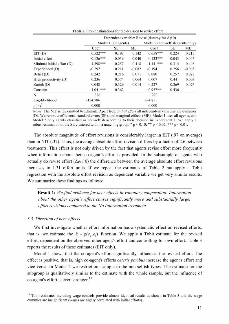
We first investigate whether effort information has a systematic effect on revised efforts, that is, we estimate the ˆ ( , )i j ie g e e= function. We apply a Tobit estimate for the revised effort, dependent on the observed other agent's effort and controlling for own effort. Table 3 reports the results of these estimates (EIT only).

Model 1 shows that the co-agent's effort significantly influences the revised effort. The effect is positive, that is, high co-agent's efforts ceteris paribus increase the agent's effort and vice versa. In Model 2 we restrict our sample to the non-selfish types. The estimate for the subgroup is qualitatively similar to the estimate with the whole sample, but the influence of co-agent's effort is even stronger.13

13 Tobit estimates including wage controls provide almost identical results as shown in Table 3 and the wage dummies are insignificant (wages are highly correlated with initial efforts).

12

The strong and positive influence of the observed co-agent’s effort on the revised effort suggests that, on average, efforts are complements. In a next step we take a closer look at how the observed difference between j’s effort and i’s effort influences i’s revision decision, that is, we look at the function ( )i j ie h e eΔ = − .

Table 3. Tobit estimations for revised effort.

Dependent variable: Revised effort (êi) Model 1 (all agents) Model 2 (non-selfish agents only) Coef SE Coef SE Co-agent's initial effort (ej) 0.292*** 0.081 0.411*** 0.115 Initial effort 0.489*** 0.092 0.373*** 0.109 Minimal initial effort (D) -4.542*** 0.737 -3.634*** 0.605 Experienced (D) 0.146 0.882 1.020 0.809 Belief (D) -0.377 0.922 -0.838 0.847 High productivity (D) -1.230 1.379 -1.707 1.134 Zurich (D) 1.323 1.149 1.065 0.930 Constant 0.236 0.909 0.923 0.848 σ 2.910 2.221 N 220 141 Log-likelihood -248.8 -180.3 p > F 0.000 0.000

Notes. Except for the Co-agent's initial effort and the Initial effort all independent variables are dummies (D). Data from EIT only. Model 1 uses all agents; Model 2 uses only agents classified as non-selfish according to their decision in Experiment 1. Robust standard errors clustered within a triad. * p < .10; ** p < .05; *** p < .01.

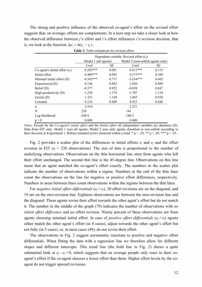
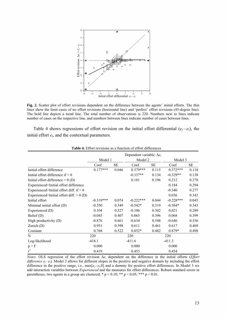
Fig. 2 provides a scatter plot of the differences in initial efforts ei and ej and the effort revision in EIT (n = 220 observations). The size of dots is proportional to the number of underlying observations. Observations on the thin horizontal line stem from agents who left their effort unchanged. The second thin line is the 45-degree line. Observations on this line mean that an agent matched the co-agent’s effort exactly. The numbers in the scatter plot indicate the number of observations within a region. Numbers at the end of the thin lines count the observations on the line for negative or positive effort differences, respectively. Numbers in areas between lines count observations within the regions between the thin lines.

For negative initial effort differentials (ej < ei), 20 effort revisions are on the diagonal, and 19 are on the zero-revision line. Eighteen observations are between the zero-revision line and the diagonal. These agents revise their effort towards the other agent’s effort but do not match it. The number in the middle of the graph (79) indicates the number of observations with no initial effort difference and no effort revision. Ninety percent of these observations are from agents choosing minimal initial effort. In case of positive effort differentials (ej > ei) agents either match the other agent’s effort (in 8 cases), adjust towards the other agent’s effort but not fully (in 5 cases), or, in most cases (49), do not revise their effort.

The observations in Fig. 2 suggest asymmetric reactions to positive and negative effort differentials. When fitting the data with a regression line we therefore allow for different slopes and different intercepts. This trend line (the bold line in Fig. 2) shows a quite substantial kink at ej – ei = 0, which suggests that on average people only react to their co-agent’s effort if the co-agent chooses a lower effort than them. Higher effort levels by the co-agent do not trigger upward revisions.

13

Fig. 2. Scatter plot of effort revisions dependent on the difference between the agents’ initial efforts. The thin lines show the limit cases of no effort revisions (horizontal line) and ‘perfect’ effort revisions (45-degree line). The bold line depicts a trend line. The total number of observations is 220. Numbers next to lines indicate number of cases on the respective line, and numbers between lines indicate number of cases between lines.

Table 4 shows regressions of effort revision on the initial effort differential (ej – ei), the initial effort ei, and the contextual parameters.

Table 4. Effort revisions as a function of effort differences

Dependent variable: Δei Model 1 Model 2 Model 3 Coef SE Coef SE Coef SE Initial effort difference 0.177*** 0.046 0.379*** 0.115 0.372*** 0.118Initial effort difference if > 0 -0.337** 0.134 -0.329** 0.138Initial effort difference > 0 (D) 0.181 0.196 0.212 0.278Experienced×Initial effort difference 0.184 0.294Experienced×Initial effort diff. if > 0 -0.340 0.277Experienced×Initial effort diff. > 0 (D) 0.036 0.342Initial effort -0.319*** 0.074 -0.222*** 0.044 -0.228*** 0.045Minimal initial effort (D) -0.550 0.349 -0.542* 0.319 -0.584* 0.343Experienced (D) 0.104 0.327 -0.106 0.302 0.021 0.289Belief (D) -0.045 0.407 0.065 0.396 0.068 0.399High productivity (D) -0.876 0.661 -0.634 0.548 -0.646 0.556Zurich (D) 0.951 0.598 0.611 0.461 0.617 0.469Constant 0.768 0.522 0.852* 0.482 0.879* 0.498N 220 220 220 Log-likelihood -418.1 -411.6 -411.3 p > F 0.000 0.000 0.000 r2 0.419 0.453 0.454

Notes. OLS regression of the effort revision Δei dependent on the difference in the initial efforts (Effort difference ej - ei). Model 2 allows for different slopes in the positive and negative domain by including the effort difference in the positive range, i.e., max[ej - ei,0] and a dummy for positive effort differences. In Model 3 we add interaction variables between Experienced and the measures for effort differences. Robust standard errors in parentheses, two agents in a group are clustered; * p < 0.10; ** p < 0.05; *** p < 0.01.

1818

20

1818181818

10

18

19

18

10

20

18

19

122020

181818

20

19

12

19

18

1220

10

20

19

1212

10

79

10

1212

8

49

12

5

49

55

49

12

8

49

12

4949

8

49

12

5

494949

-20

-15

-10

-50

510

1520

Effo

rt re

visi

on: Δ

e i =

ê i - e

i

-20 -15 -10 -5 0 5 10 15 20Initial effort differential: ej - ei

14

Model 1 disregards any kink in the revision response. The effort differential has a positive and highly significant impact on effort revisions. An increase of the effort differential by one unit induces an agent to increase his effort in the revision stage by .18 units, ceteris paribus.14

However, as Fig. 2 suggests, there are substantial differences between positive and negative effort differentials. In Model 2 we allow for different slopes by adding two additional variables for the initial effort differential. The variable Initial effort difference if > 0 is calculated as max[ej - ei, 0].

The results of Model 2 confirm the impression from Fig. 2. The coefficient of Initial effort difference is highly significant and positive. Agents who learn that their co-agent had chosen a lower effort reduce their effort on average by .38 effort units per unit of the differential. The interaction variable Initial effort difference if > 0 has a significant negative coefficient, indicating that the reaction to the effort differential is lower in the positive domain. The net effect in the domain of positive effort differentials is the sum of the first and second coefficient. The effect is still positive (.04, the sum of the first two coefficients) but not significantly different from zero (p = .436, F-test). Thus, the interaction between the two efforts is mainly driven by effort reductions of the high-effort agents. The dummy for positive effort differences is insignificant, which means that the reaction to the effort difference does not shift discontinuously at zero.

Among the remaining variables only Initial effort has a significant impact on the effort revision; the coefficient is negative. Thus, unsurprisingly, the higher the initial effort the larger is the downward revision.

Model 3 allows for the possibility that agents who are experienced with the gift-exchange game (because they played a related game prior to this one – see Section 2.2) react differently to effort information than inexperienced agents. The interaction variables are insignificant. Thus, the observed peer effects are robust to experience.

We summarize our findings in Result 2.

Result 2: Overall, effort revisions and differences in initial efforts are positively correlated. Agents who learn that their co-agent has provided less effort than them, reduce their effort significantly, whereas agents who chose a lower initial effort than their co-agent increase their effort only insignificantly.

3.4. Discussion

Results 1 and 2 establish that voluntary cooperation is subject to peer effects, and that peer effects take the form of positively correlated efforts (with a kink at the co-agents’ effort). We will address the economic significance of these findings in our concluding discussion of Section 6. From the viewpoint of the main research question of this paper these results raise the question what the implications are for standard theories of social preferences.

14 Interestingly, this result is similar to the magnitude of peer effects found in field studies. For their respective measures of peer effects Ichino and Maggi (2000) find values between 0.14 and 0.18; the Falk and Ichino (2006) estimates result in 0.14, Mas and Moretti (2009) report 0.17, and Bandiera et al. (2010) report 0.13.

15

Before we continue to investigate this question, we briefly argue why learning about the money-maximizing solution cannot account for our results. The fact that people tend to revise their efforts downwards might be seen as evidence for the relevance of learning. A closer look at our data reveals, however, that the downward revision is unlikely due to erroneously high initial efforts. First, we show in Model 3 of Table 4 that experienced subjects do not show weaker reactions to effort information (in fact, they seem to react even stronger). Second, recall that subjects had access to a ‘What-if Calculator’ when taking their decision (see Fig. 1). Our software recorded subjects’ calculations. All but 11 of our 489 subjects calculated the payoffs for the Nash equilibrium efforts and therefore should not be surprised by the fact that a co-agent with a lower effort earns a higher payoff. Thus, Results 1 and 2 are most likely not due to learning money maximization.

Are the peer effects, therefore, a new behavioral phenomenon that cannot be explained by existing theories of social preferences? At first glance, one might have this impression. Recall that our one-shot design ensures that subjects have no reason other than their social preferences when choosing their initial effort and that there are no earnings interdependencies between agents. So why would an inconsequential piece of information by another player induce a change of mind?

4. What standard models of social preferences predict about peer effects in the trilateral gift-exchange game

In this section we explore what existing theories of social preferences have to say on explaining peer effects, given that all theories we look at in this section can explain initial effort choices. We focus our analysis on the subgame starting when the two agents choose their effort. We derive agent i’s reaction function to agent j’s effort decision, that is, ei = R(ej) and focus on the derivative with respect to ej. A particular model predicts a peer effect if dei/dej ≠ 0; no peer effect is predicted if dei/dej = 0. Because (i) role allocation was random, (ii) we explained the game to the subjects as a three-player game and made them aware of the earnings consequences of each other’s choices (see instructions and Fig. 1), and (iii) subjects were not informed about any decision other three-player groups took, we assume that a group of three players forms the reference group.

In the following we derive the basic results and briefly discuss the underlying intuitions. For all details see Appendix C and for general reviews of models of social preferences see Sobel (2005) and Fehr and Schmidt (2006). Readers not interested in the details can directly refer to the summary Table 5 at the end of this section.

1. Distributional preferences. We consider models of altruism and inequity aversion.

Players have a utility function ui(xi, xj, xP) which contains as arguments the monetary earnings xi, xj and xP of the two agents i and j and the principal P, respectively. The models differ in the assumptions about the derivatives of ui with respect to other players’ earnings. Models of altruism like Charness and Rabin (2002) or Cox et al. (2008) assume that these derivatives are positive. Models of inequity aversion (Fehr and Schmidt (1999); Bolton and Ockenfels

16

(2000)) assume that these derivatives are positive as long as other players are poorer than player i but turn negative otherwise. We now discuss these models in turn.

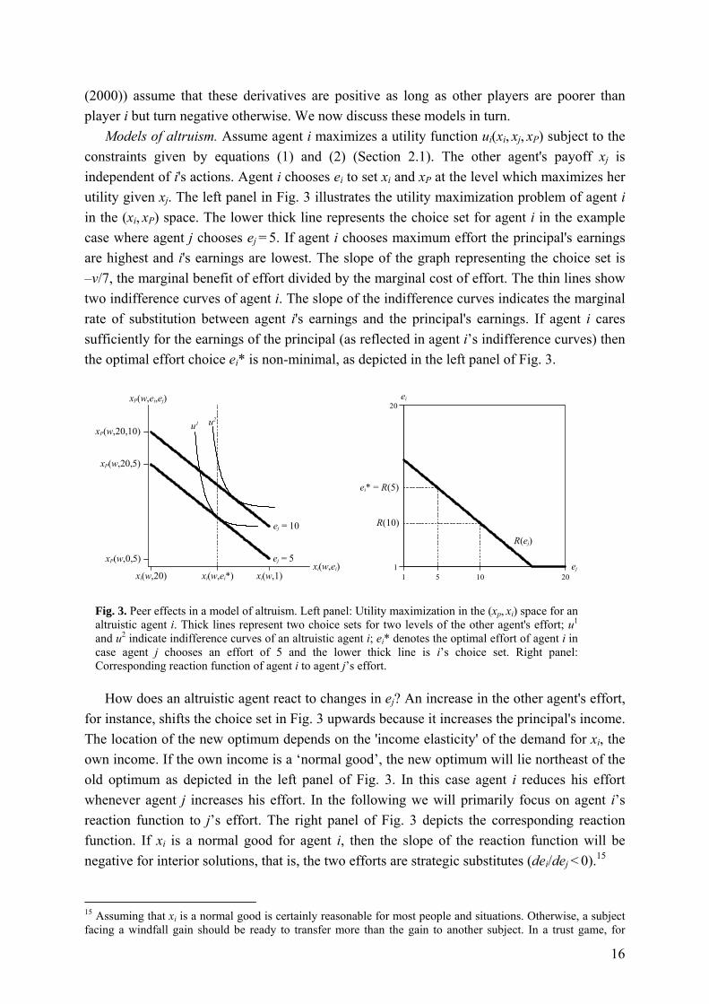
Models of altruism. Assume agent i maximizes a utility function ui(xi, xj, xP) subject to the constraints given by equations (1) and (2) (Section 2.1). The other agent's payoff xj is independent of i's actions. Agent i chooses ei to set xi and xP at the level which maximizes her utility given xj. The left panel in Fig. 3 illustrates the utility maximization problem of agent i in the (xi, xP) space. The lower thick line represents the choice set for agent i in the example case where agent j chooses ej = 5. If agent i chooses maximum effort the principal's earnings are highest and i's earnings are lowest. The slope of the graph representing the choice set is –v/7, the marginal benefit of effort divided by the marginal cost of effort. The thin lines show two indifference curves of agent i. The slope of the indifference curves indicates the marginal rate of substitution between agent i's earnings and the principal's earnings. If agent i cares sufficiently for the earnings of the principal (as reflected in agent i’s indifference curves) then the optimal effort choice ei* is non-minimal, as depicted in the left panel of Fig. 3.

Fig. 3. Peer effects in a model of altruism. Left panel: Utility maximization in the (xp, xi) space for an altruistic agent i. Thick lines represent two choice sets for two levels of the other agent's effort; u1 and u2 indicate indifference curves of an altruistic agent i; ei* denotes the optimal effort of agent i in case agent j chooses an effort of 5 and the lower thick line is i’s choice set. Right panel: Corresponding reaction function of agent i to agent j’s effort.

How does an altruistic agent react to changes in ej? An increase in the other agent's effort, for instance, shifts the choice set in Fig. 3 upwards because it increases the principal's income. The location of the new optimum depends on the 'income elasticity' of the demand for xi, the own income. If the own income is a ‘normal good’, the new optimum will lie northeast of the old optimum as depicted in the left panel of Fig. 3. In this case agent i reduces his effort whenever agent j increases his effort. In the following we will primarily focus on agent i’s reaction function to j’s effort. The right panel of Fig. 3 depicts the corresponding reaction function. If xi is a normal good for agent i, then the slope of the reaction function will be negative for interior solutions, that is, the two efforts are strategic substitutes (dei/dej < 0).15

15 Assuming that xi is a normal good is certainly reasonable for most people and situations. Otherwise, a subject facing a windfall gain should be ready to transfer more than the gain to another subject. In a trust game, for

xi(w,ei)

xP(w,ei,ej)

ej = 10

ej = 5

u1 u2

xi(w,20) xi(w,ei*) xi(w,1)

xP(w,0,5)

xP(w,20,5)

xP(w,20,10)

R(10)

ei* = R(5)

ei

ej

R(ej)

1

20

1 5 10 20

17

For expositional purposes we derive the reaction functions using a parameterized version proposed by Cox et al. (2007).16 They use a CES utility function

( )( , , ) /i j P i j j P Pu x x x x x xα α αθ θ α= + + , (3)

which allows varying the elasticity of substitution between an agent's own payoff and the other players' payoffs by ( , 0) (0,1]α ∈ −∞ ∪ ; θj and θP measure the emotional state of player i towards the other two players. Suppose for a moment that θj and θP are positive. For α = 1 the payoffs are perfect substitutes and agent i chooses either maximal effort (for θP > 7/v) or minimal effort (otherwise), irrespective of ej. In this case the slope of the reaction function is zero and there is no interior solution. Panel A of Fig. 4 shows these reaction functions as horizontal lines at the bottom and the top of i's action space. Another extreme case is when the payoffs are perfect complements and weighted equally (Leontief case α →–∞ and θP = 1). In this case agent i chooses ei to ensure xi = xP (if feasible). The reaction function can be derived by solving this equation for ei which gives us a linear function with a slope of –v/(v + 7).

Between these extremes is a continuum of negatively-sloped reaction functions. The lines in Fig. 4A show some examples. All reaction functions are linear functions that intersect at a point far to the upper left of the admissible effort space. Both the slope and the intercept of the reaction function are jointly determined by α and θP. Optimal efforts of agent i might lead to situations where the principal earns more than agent i, which is the case above the thick line in Fig. 4A. In all cases the slope lies in (–1,0) for interior solutions.

Another model of altruism is Charness and Rabin (2002) who - in the basic version - propose a utility function that captures preferences for efficiency (utilitarian) and/or care for the least fortunate (maximin). Utility is case-wise linear in all arguments:

( ) { } ( )( )( , , ) 1 min , , 1i j P i i j P i j Pu x x x x x x x x x xλ λ δ δ⎡ ⎤= − + + − + +⎣ ⎦ , (4)

with λ weighing the importance of distributional preferences ( [0,1]λ ∈ ) and δ measuring the type of distributional preferences, ranging from δ = 0 for pure efficiency concerns to δ = 1 for pure maximin concerns. Unlike the Cox et al. (2007) model, Charness and Rabin do not predict a continuum but only four distinct kinds of reaction functions: For a low enough λ an agent will always choose minimal effort. For high λ and low δ an agent seeks to maximize joint income and chooses maximum effort (thereby minimizing her own income). This reaction function is labeled as 'Utilitarian' in Fig. 4B. The most interesting cases are in between. If the maximin motive dominates (high δ), agent i increases her effort if and only if she can increase the minimal earnings in the group.

instance, a subject should return more money than received by the trustor, a behavior which is hardly ever observed. 16 The model builds on Cox and Sadiraj (2012) who introduced (in the working paper version of 2003) the CES function as shown in equation (3) and call their approach a model of egocentric other-regarding preferences, or egocentric altruism. For an application to voluntary cooperation in public goods games see also Cox and Sadiraj (2007). For a nonparametric version see Cox et al. (2008).

18

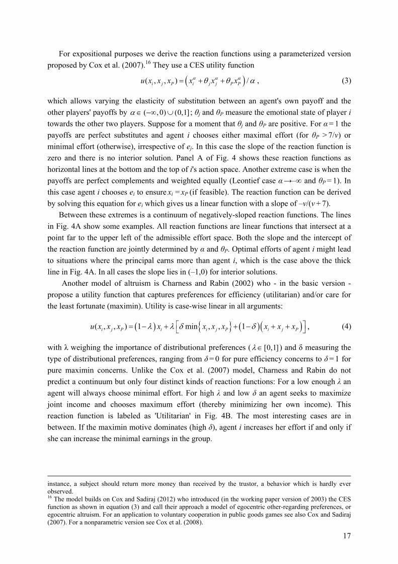
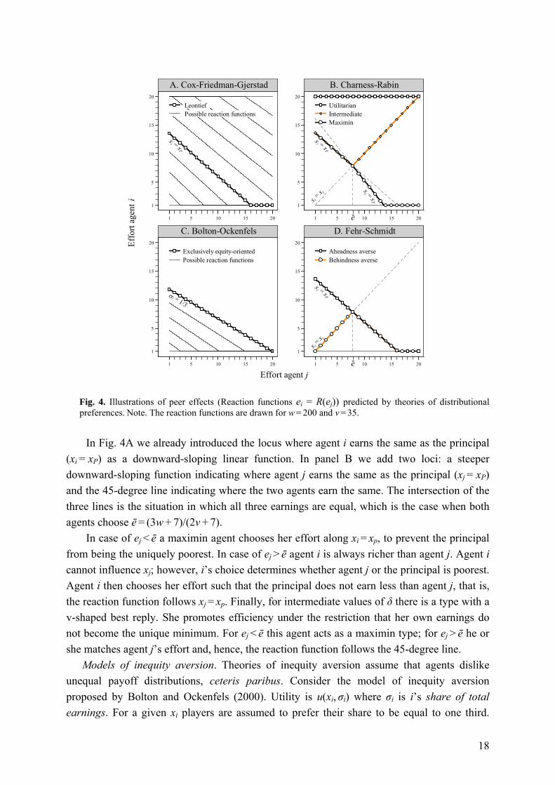
Fig. 4. Illustrations of peer effects (Reaction functions ei = R(ej)) predicted by theories of distributional preferences. Note. The reaction functions are drawn for w = 200 and v = 35. In Fig. 4A we already introduced the locus where agent i earns the same as the principal

(xi = xP) as a downward-sloping linear function. In panel B we add two loci: a steeper downward-sloping function indicating where agent j earns the same as the principal (xj = xP) and the 45-degree line indicating where the two agents earn the same. The intersection of the three lines is the situation in which all three earnings are equal, which is the case when both agents choose ē = (3w + 7)/(2v + 7).

In case of ej < ē a maximin agent chooses her effort along xi = xp, to prevent the principal from being the uniquely poorest. In case of ej > ē agent i is always richer than agent j. Agent i cannot influence xj; however, i’s choice determines whether agent j or the principal is poorest. Agent i then chooses her effort such that the principal does not earn less than agent j, that is, the reaction function follows xj = xp. Finally, for intermediate values of δ there is a type with a v-shaped best reply. She promotes efficiency under the restriction that her own earnings do not become the unique minimum. For ej < ē this agent acts as a maximin type; for ej > ē he or she matches agent j’s effort and, hence, the reaction function follows the 45-degree line.

Models of inequity aversion. Theories of inequity aversion assume that agents dislike unequal payoff distributions, ceteris paribus. Consider the model of inequity aversion proposed by Bolton and Ockenfels (2000). Utility is u(xi, σi) where σi is i’s share of total earnings. For a given xi players are assumed to prefer their share to be equal to one third.

xi = x

P

Leontief Possible reaction functions

1

5

10

15

20

1 5 10 15 20

A. Cox-Friedman-Gjerstad

xi = x

P

x i = x j x

j = xP

MaximinIntermediateUtilitarian

-e1

5

10

15

20

1 5 10 15 20

B. Charness-Rabin

σi = 1/3

Exclusively equity-orientedPossible reaction functions

1

5

10

15

20

1 5 10 15 20

C. Bolton-Ockenfels

xi = x

P

x i = x j

Aheadness averseBehindness averse

-e1

5

10

15

20

1 5 10 15 20

D. Fehr-Schmidt

Effo

rt ag

ent i

Effort agent j

19

Deviations from equality reduce utility.17 To get an intuition consider first the case of a very strongly inequity averse player, who only cares about her payoff share. In the role of agent i, this player chooses her effort such that her share of total earnings equals one third:

( , ) 1

( , ) ( , ) ( , , ) 3i i

i i j j P i j

x w ex w e x w e x w e e

=+ +

. (5)

For such a player the two efforts are strategic substitutes. To see this, consider an increase of player j’s effort. This decreases xj and increases xP. Since providing more effort is efficient the sum of xj and xP increases by v – 7 > 0 and the left-hand expression in (5) drops below 1/3. To re-establish equality agent i must decrease her effort in order to increase xi. The reaction function of such an agent is depicted in Fig. 4C, labeled as 'Exclusively equity-oriented'. Using the payoff functions (1) and (2) and solving (5) for ei one can show that the slope of the reaction function is (7 – v)/(14 + v) < 0 (note that this is not the same reaction function as the limit case in panel A where xi = xp). Players with weaker inequity aversion face a tradeoff between the benefit of their own payoff and the discomfort of earning a relative income above one third. Lower concerns for inequity aversion lead to lower efforts, ceteris paribus.

The thin lines in Fig. 4C show five examples of reaction functions. There is a lower limit of inequity aversion under which behavior is identical to money-maximization. However, it generally holds that, for interior solutions (1 < ei < 20), the slope of the reaction function is always in (–1, 0), that is, the two efforts are always strategic substitutes.

The intuition is that an inequity-averse agent providing low effort suffers from earning more than her equal share. To relieve this adverse feeling there are two possibilities: (i) she increases her own effort and thereby lowers her earnings, or (ii) the co-agent increases his effort and thereby increases the total payoff, which in turn brings the (unchanged) income of the agent at hand closer to the equal share.

The model of Fehr and Schmidt (1999) is also built on the notion of inequity aversion. However, unlike in the model by Bolton and Ockenfels (2000) players make bilateral comparisons with all group members. Players get utility from their own monetary payoff and disutility from any payoff difference with comparison partners (see also Loewenstein et al. (1989)). The utility function in the Fehr-Schmidt model is

( ) ( )( ) [ ] [ ] [ ] [ ]2 2i j i P i i j i Pu x x x x x x x x x xα β+ + + += − − + − − − + − , (6)

where [a]+ ≡ max(a,0). The disutility of earning less than another group member is linear and equal to α times the payoff difference. Earning more than another group member also leads to a disutility, weighted by β (but β < α). We illustrate the reaction functions of Fehr-Schmidt agents in Fig. 4D. Two loci are important: the negatively-sloped line where agent i earns the same as the principal and the 45-degree line where the two agents earn the same. In the intersection of the two lines all three players earn the same, which is the case at e = ē.

17 An early strand of literature incorporated envy into the utility function (Bolton (1991); Kirchsteiger (1994)). These models, however, cannot explain non-minimal efforts in our game, because players seek to maximize their absolute and relative monetary payoff.

20

The Fehr-Schmidt model predicts three types: A player with low concern for advantageous inequality (β < β' = 14/(v + 14) ≈ 0.29 for v = 35) will always choose minimal effort. For higher β there are two possibilities depending on the relative importance of α and β: If a player is relatively intolerant towards disadvantageous inequality compared to his intolerance of advantageous inequality, we call him ‘Behindness averse’ (BA; β' < β < (14 + 7α)/(v + 7)). Such a player will choose non-minimal efforts under the condition that he does not fall behind another player. For low co-agent's efforts (ej < ē) the best reply is ei = ej up to ē. For high co-agent's efforts (ej ≥ ē) he chooses the effort that equalizes his earnings to the principal's earnings. A third type called ‘Aheadness averse’ (AA; β' < β > (14 + 7α)/(v + 7)) is an agent i who (i) suffers heavily from the fact that the principal earns less than him (high β), and (ii) is relatively tolerant to the fact that he earns less than agent j (low α). Such an agent always seeks to match his payoff with the principal's payoff. The resulting reaction function is identical to the Leontief case shown in panel A of Fig. 4.

Inequity aversion and altruism. Kohler (2011) proposes a model that expands the Fehr-Schmidt utility function by adding a term γ(xj + xP), very similar to the utilitarian part of the model by Charness and Rabin (2002). Consequently, for low γ the model predicts reaction functions of the Fehr-Schmidt types; for high γ the model predicts the utilitarian and intermediate type from Charness and Rabin (2002).

2. Models of reciprocity. Theories of reciprocity model the idea that people reward kind

acts with kindness and mean acts with unkindness (Rabin (1993)). A theory of reciprocity that is adequate for our sequential gift-exchange game is the sequential reciprocity model by Dufwenberg and Kirchsteiger (2004). This theory does not predict peer effects because agent j’s effort has no influence on agent i’s earnings. Thus agent j is neither kind nor unkind to agent i. Hence, dei/dej = 0. The only reason for choosing a non-minimal effort is to reward the principal for a high wage, irrespective of the other agent’s actions.

In case of type-based reciprocity (Levine (1998)) the results are similar. In this model players gain (dis)utility from other agents’ income if they are altruistic (spiteful) types. However, since the agents cannot influence their co-agent’s income they cannot act altruistically (or spitefully) towards them and thus, do not take their actions into account. Hence, no peer effects are predicted: dei/dej = 0.

3. Hybrid models. Cox et al. (2007) and Charness and Rabin (2002) enrich their models of

altruism with reciprocity. In both cases reciprocity does, however, not change the qualitative predictions about the shape of the reaction functions discussed so far. Reciprocity means that if the agent is treated unkindly he weighs the earnings of the unkind player less or even negatively in his utility function. In both models intentions play a role only with respect to the wage offer. Low wage offers are perceived as unkind, high wages as kind. In case of Cox et al. (2007) a low wage leads to a negative θP. A player with θP < 0 chooses minimal effort irrespective of ej, thus acting like a money-maximizing agent. Also in Charness and Rabin (2002) there is a reciprocity part by which payoff-based concerns are reduced when a player is

21

treated unkindly by another player. Negative emotions towards the principal shift the reaction functions downwards but do not qualitatively change the characteristics derived above.

Finally, the model of Falk and Fischbacher (2006) combines interpersonal payoff comparisons with intentionality. Like in Dufwenberg and Kirchsteiger (2004), reciprocity does not predict a direct link between the two efforts. However, agent i wants to reciprocate to the principal and cares about earnings differences. The predictions of the Falk-Fischbacher model are very similar to the predictions of the AA-type in the Fehr-Schmidt model. For very strong reciprocal preferences the reaction function is again identical to the AA-type, weaker reciprocal preferences result in a parallel downward shift.

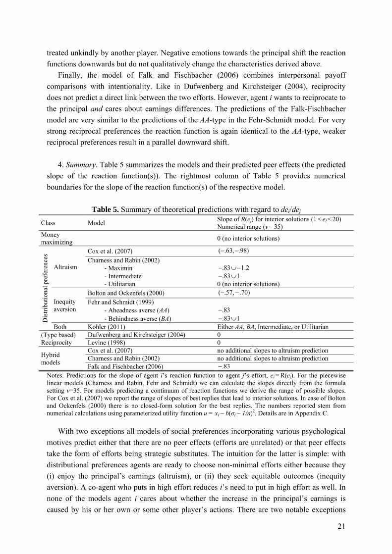
4. Summary. Table 5 summarizes the models and their predicted peer effects (the predicted

slope of the reaction function(s)). The rightmost column of Table 5 provides numerical boundaries for the slope of the reaction function(s) of the respective model.

Table 5. Summary of theoretical predictions with regard to dei/dej

Class Model Slope of R(ej) for interior solutions (1 < ei < 20) Numerical range (v = 35)

Money maximizing 0 (no interior solutions)

Dis

tribu

tiona

l pre

fere

nces

Altruism

Cox et al. (2007) ( .63, .98)− − Charness and Rabin (2002) - Maximin .83 1.2− ∪− - Intermediate .83 1− ∪ - Utilitarian 0 (no interior solutions)

Inequity aversion

Bolton and Ockenfels (2000) ( .57, .70)− − Fehr and Schmidt (1999) - Aheadness averse (AA) .83− - Behindness averse (BA) .83 1− ∪

Both Kohler (2011) Either AA, BA, Intermediate, or Utilitarian (Type based) Reciprocity

Dufwenberg and Kirchsteiger (2004) 0 Levine (1998) 0

Hybrid models

Cox et al. (2007) no additional slopes to altruism prediction Charness and Rabin (2002) no additional slopes to altruism prediction Falk and Fischbacher (2006) .83−

Notes. Predictions for the slope of agent i’s reaction function to agent j’s effort, ei = R(ej). For the piecewise linear models (Charness and Rabin, Fehr and Schmidt) we can calculate the slopes directly from the formula setting v=35. For models predicting a continuum of reaction functions we derive the range of possible slopes. For Cox et al. (2007) we report the range of slopes of best replies that lead to interior solutions. In case of Bolton and Ockenfels (2000) there is no closed-form solution for the best replies. The numbers reported stem from numerical calculations using parameterized utility function u = xi – b(σi – 1/n)2. Details are in Appendix C.

With two exceptions all models of social preferences incorporating various psychological motives predict either that there are no peer effects (efforts are unrelated) or that peer effects take the form of efforts being strategic substitutes. The intuition for the latter is simple: with distributional preferences agents are ready to choose non-minimal efforts either because they (i) enjoy the principal’s earnings (altruism), or (ii) they seek equitable outcomes (inequity aversion). A co-agent who puts in high effort reduces i’s need to put in high effort as well. In none of the models agent i cares about whether the increase in the principal’s earnings is caused by his or her own or some other player’s actions. There are two notable exceptions

22

that allow for strategic complementarity between the two efforts, the Fehr-Schmidt BA-type, and the Charness-Rabin intermediate type. Interestingly, in both cases efforts have to be one-to-one complements, that is, the two agents choose identical efforts.

Our theoretical analysis of the three-person gift-exchange game shows that the most robust (concurrent) qualitative prediction about peer effects is that the agents’ efforts are negatively related, that is, efforts are strategic substitutes (see Table 5). By contrast, Fig. 2 suggests that efforts are strategic complements. This observation of positively correlated efforts is not yet conclusive, however, because the theoretical predictions concern the slope of reaction function.18 In the following we report experiments that provide qualitative conclusions about the sign of peer effects.

5. Results II: Can standard models of social preferences explain peer effects?

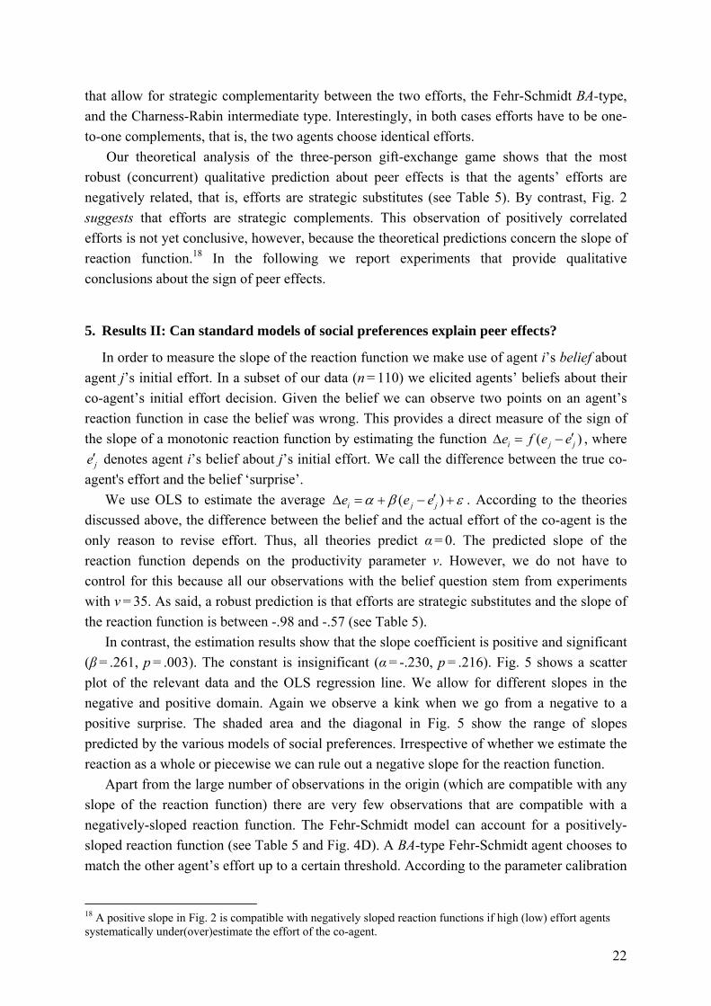
In order to measure the slope of the reaction function we make use of agent i’s belief about agent j’s initial effort. In a subset of our data (n = 110) we elicited agents’ beliefs about their co-agent’s initial effort decision. Given the belief we can observe two points on an agent’s reaction function in case the belief was wrong. This provides a direct measure of the sign of the slope of a monotonic reaction function by estimating the function ( )i j je f e e′Δ = − , where

je′ denotes agent i’s belief about j’s initial effort. We call the difference between the true co-agent's effort and the belief ‘surprise’.

We use OLS to estimate the average ( )i j je e eα β ε′Δ = + − + . According to the theories discussed above, the difference between the belief and the actual effort of the co-agent is the only reason to revise effort. Thus, all theories predict α = 0. The predicted slope of the reaction function depends on the productivity parameter v. However, we do not have to control for this because all our observations with the belief question stem from experiments with v = 35. As said, a robust prediction is that efforts are strategic substitutes and the slope of the reaction function is between -.98 and -.57 (see Table 5).

In contrast, the estimation results show that the slope coefficient is positive and significant (β = .261, p = .003). The constant is insignificant (α = -.230, p = .216). Fig. 5 shows a scatter plot of the relevant data and the OLS regression line. We allow for different slopes in the negative and positive domain. Again we observe a kink when we go from a negative to a positive surprise. The shaded area and the diagonal in Fig. 5 show the range of slopes predicted by the various models of social preferences. Irrespective of whether we estimate the reaction as a whole or piecewise we can rule out a negative slope for the reaction function.

Apart from the large number of observations in the origin (which are compatible with any slope of the reaction function) there are very few observations that are compatible with a negatively-sloped reaction function. The Fehr-Schmidt model can account for a positively-sloped reaction function (see Table 5 and Fig. 4D). A BA-type Fehr-Schmidt agent chooses to match the other agent’s effort up to a certain threshold. According to the parameter calibration

18 A positive slope in Fig. 2 is compatible with negatively sloped reaction functions if high (low) effort agents systematically under(over)estimate the effort of the co-agent.

23

suggested by Fehr and Schmidt (1999) we should observe only 10 percent BA-type agents in the experiments with the high productivity parameter; the estimates provided by Blanco et al. (2011) suggest 21 percent BA-type agents.

Could it be that the BA-type agent is much more frequent among our subjects? We check this by a case-by-case evaluation of compatibility with the BA Fehr-Schmidt prediction. An observation is called BA-compatible if (i) the initial effort is chosen according to the best-reply function given the belief about ej, and (ii) the revised effort is chosen according to the best-reply function given the observed ej.19 Of the 220 observations in the EIT, 95 (43 percent) are compatible with the BA-prediction. However, a lot of these observations are agents who choose the minimal effort and are therefore also compatible with the standard prediction. If we restrict our sample to agents with non-minimal initial efforts then only 16 out of 96 (17 percent) choose their efforts in accordance with the BA type. Another way to assess the predictive power of the BA-prediction is to look at the fraction of effort revisions (Δei ≠ 0) that are explained by the BA-type behavior. Among the 73 agents who do revise their effort only 14 agents (19 percent) do so according to the prediction.

Fig. 5. Effort revisions dependent on the difference between

the actual ej and agent i’s belief ej’. The shaded areas and the diagonal are predictions consistent with theories of social preferences.

The second theory that predicted positively-sloped reaction functions is the intermediate

type in the Charness and Rabin (2002) model. We also do a case-by-case check whether our observations are compatible with this prediction. Thirteen (6 percent) out of the 220 observations in the EIT follow this pattern. Among the 73 agents who do revise their effort six (8 percent) do so as predicted by the intermediate type. Furthermore, although the slope estimates are clearly positive, they are nowhere near unity, as the two theoretical cases would

19 Condition (i) can only be checked in the subsample where we elicited beliefs. For the remaining observations we check whether the initial effort is within the range allowed be the reaction function as shown in Fig. 4.

-10

-50

510

Effo

rt re

visi

on: ê

i - e

i

-10 -5 0 5 10Surprise: ej - e'j

24

predict. An F-test rejects the hypothesis β = 1 for both the linear and the piecewise linear estimate (p < .01).

We summarize our findings in Result 3:

Result 3: Peer effects in voluntary cooperation predominately take the form of efforts being strategic complements rather than substitutes as predicted by most theories of social preferences.

The explanations offered by standard theories of social preferences do not capture the kind of peer effects we observe. One apparent possibility to account for our empirical results is to alter the definition of the reference group. Suppose that for some reason, agents only compare among themselves, e.g., because agents feel more attached to the co-agent than to the principal. Yet, redefining the reference group to comprise the agents only does not offer a convincing explanation of our empirical findings. To see why, assume an agent with distributional preferences u(xi, xj). By design, agent i cannot influence xj. Therefore, even with altruistic preferences agent i will choose minimal effort irrespective of ej. A Fehr-Schmidt agent would as well always choose minimal effort, because adjusting to a higher co-agent's effort would require β > 1, which is ruled out by the Fehr and Schmidt (1999) model. The only model that predicts strategic complementarity in this case is Bolton and Ockenfels (2000). In the extreme case of an exclusively equity-oriented agent the reaction function is the 45-degree line, i.e., an agent would want to match the other agent’s effort. But even in this situation it is unclear why the two such agents should coordinate on a situation with non-minimal effort, because they could increase utility by choosing minimal effort.

6. Discussion: Economic significance and explanations for peer effects in voluntary cooperation

We reported results from a three-person gift-exchange experiment designed to detect peer effects in voluntary cooperation in an environment where only non-selfish social preferences can explain voluntary cooperation. In a design that avoids the reflection problem we find that voluntary cooperation is shaped by peer effects and they take the form of efforts being strategic complements, with a kink at the co-agent’s effort.

Before we focus on potential explanations of peer effects we discuss the economic significance of efforts as strategic complements. Positively correlated efforts due to peer effects allow for the possibility of multiple 'equilibria', i.e., high and low effort cultures, depending on the team composition. The ‘kinked effort function’ displayed in Fig. 2 suggests that a low effort situation is more likely to emerge because people are not willing to increase effort if others have exerted higher efforts but are ready to reduce effort if others provided less effort. However, more research is needed to understand the nature of positively correlated efforts. Our findings contrast with the field (experimental) results reported by Falk and Ichino (2006) and Mas and Moretti (2009) who find the opposite, namely that mutual observability increases the productivity of the low effort agents. We can only speculate about the reasons

25

for this result. One explanation is that our experiment is conducted in full anonymity whereas in these studies agents could observe and talk to each other, which might have exerted some social pressure on low-performing agents. An additional possible explanation is that our effort choice is an abstract decision, whereas in these studies effort is linked to a real task. The ‘social facilitation’ paradigm in social psychology (Zajonc (1965)) suggests that the mere presence of another person can improve performance (see also Falk and Ichino (2006), p. 48, for a related discussion).

We now turn to the theoretical discussion of our empirical results which are opposite to the predictions of a host of standard theories of social preferences. We showed that with a couple of exceptions efforts are predicted to be either unrelated or strategic substitutes. Negatively-related efforts arise because agents also care about the principal; the behavior of the co-agent just changes the extent to which own effort needs to be adjusted to implement the desired payoff for the principal. Perfectly matched efforts can only arise if agents are strongly ‘behindness averse’ (in the Fehr-Schmidt model) or if agents’ preferences are intermediate between utilitarian and maximin (in the Charness-Rabin model). However, even these models can only explain a minority of effort choices.20

If standard models of social preferences cannot explain the peer effects we see, the question arises whether motivations that are not captured by the standard models can explain our results. One possibility is that people are conformists - a tendency long established by social psychologists (Asch (1952)). Conformism is a psychological mechanism that “refers to the act of changing one’s behavior to match the responses of others” (Cialdini and Goldstein (2004), p. 606). Conformity is a potential channel because conformism is a very common and deeply rooted human predisposition (Henrich and Boyd (1998)) that can also explain important economic phenomena (see, e.g., Bernheim (1994); Clark and Oswald (1998)) including ones related to our research question (Sliwka (2007)).

Another possibility is that people follow a norm of reciprocity but take the behavior of others as a cue about what is an appropriate reciprocal response. Such norm-following (calibrating one’s own reciprocal response on that of others) is empirically plausible (Keizer et al. (2008); Krupka and Weber (2013)) and can explain relevant experimental data (López-Pérez (2008)).

Positively correlated efforts can also result if people are motivated by considerations of social esteem (Ellingsen and Johannesson (2008)) whereby effort choices are made to create favorable impressions in the other players. In the remainder of this paper we sketch three recent new generation models of social preferences that, respectively, incorporate conformity, norm-following, and social esteem as relevant social motivations into their frameworks. All three models predict that peer effects take the form of positively correlated efforts (for details see Appendix C).

Sliwka (2007) presents a model that allows for conformity. Selfish agents have a utility function ( )S iu x , while fair agents have distributional social preferences: ( , , )F i j Pu x x x .

20 This is in line with the results of Kagel and Wolfe (2001) who investigate three-player ultimatum games and report poor predictive success for models of inequality aversion.

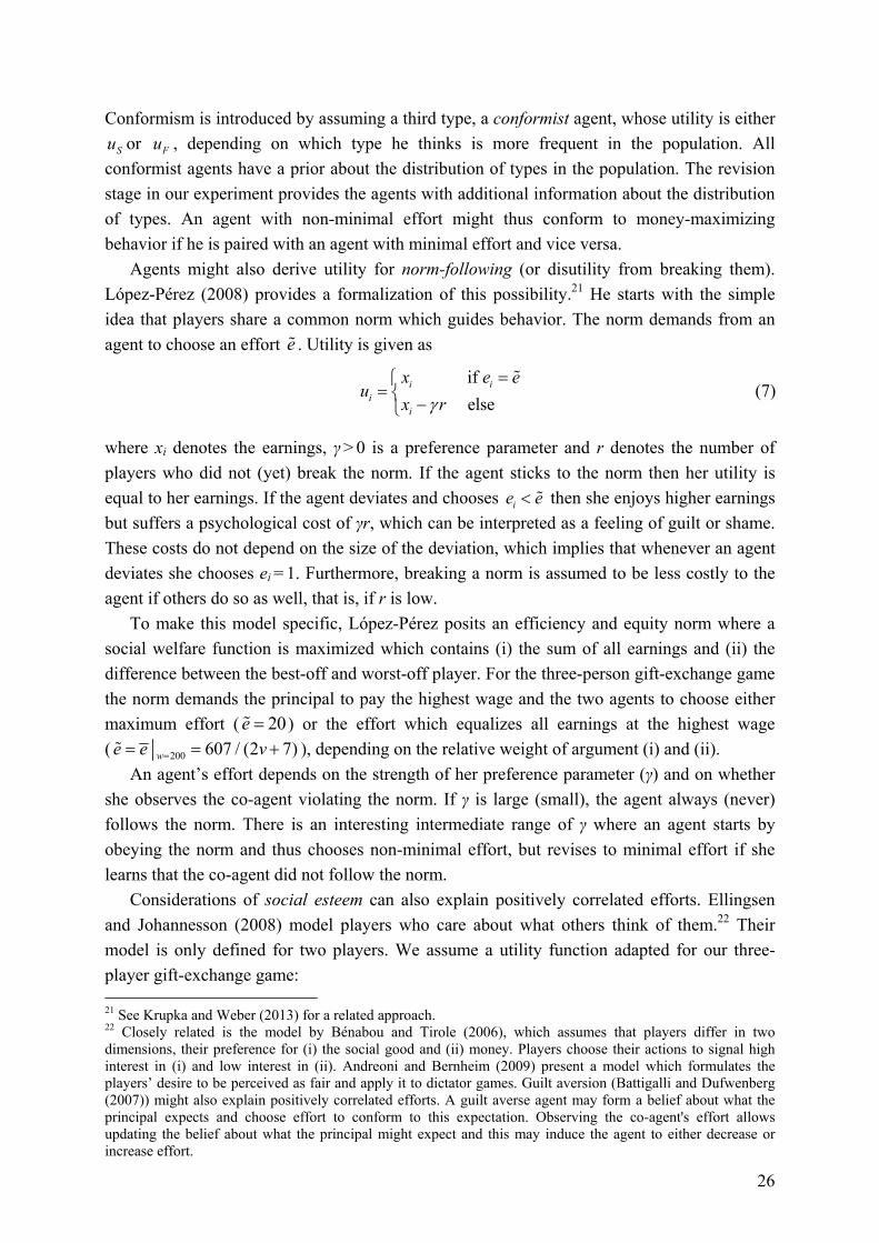
26

Conformism is introduced by assuming a third type, a conformist agent, whose utility is either

Su or Fu , depending on which type he thinks is more frequent in the population. All conformist agents have a prior about the distribution of types in the population. The revision stage in our experiment provides the agents with additional information about the distribution of types. An agent with non-minimal effort might thus conform to money-maximizing behavior if he is paired with an agent with minimal effort and vice versa.

Agents might also derive utility for norm-following (or disutility from breaking them). López-Pérez (2008) provides a formalization of this possibility.21 He starts with the simple idea that players share a common norm which guides behavior. The norm demands from an agent to choose an effort e% . Utility is given as

if else

i ii

i

x e eu

x rγ=⎧

= ⎨ −⎩

% (7)

where xi denotes the earnings, γ > 0 is a preference parameter and r denotes the number of players who did not (yet) break the norm. If the agent sticks to the norm then her utility is equal to her earnings. If the agent deviates and chooses ie e< % then she enjoys higher earnings but suffers a psychological cost of γr, which can be interpreted as a feeling of guilt or shame. These costs do not depend on the size of the deviation, which implies that whenever an agent deviates she chooses ei = 1. Furthermore, breaking a norm is assumed to be less costly to the agent if others do so as well, that is, if r is low.

To make this model specific, López-Pérez posits an efficiency and equity norm where a social welfare function is maximized which contains (i) the sum of all earnings and (ii) the difference between the best-off and worst-off player. For the three-person gift-exchange game the norm demands the principal to pay the highest wage and the two agents to choose either maximum effort ( 20e =% ) or the effort which equalizes all earnings at the highest wage ( 200 607 / (2 7)we e v== = +% ), depending on the relative weight of argument (i) and (ii).

An agent’s effort depends on the strength of her preference parameter (γ) and on whether she observes the co-agent violating the norm. If γ is large (small), the agent always (never) follows the norm. There is an interesting intermediate range of γ where an agent starts by obeying the norm and thus chooses non-minimal effort, but revises to minimal effort if she learns that the co-agent did not follow the norm.

Considerations of social esteem can also explain positively correlated efforts. Ellingsen and Johannesson (2008) model players who care about what others think of them.22 Their model is only defined for two players. We assume a utility function adapted for our three-player gift-exchange game: 21 See Krupka and Weber (2013) for a related approach. 22 Closely related is the model by Bénabou and Tirole (2006), which assumes that players differ in two dimensions, their preference for (i) the social good and (ii) money. Players choose their actions to signal high interest in (i) and low interest in (ii). Andreoni and Bernheim (2009) present a model which formulates the players’ desire to be perceived as fair and apply it to dictator games. Guilt aversion (Battigalli and Dufwenberg (2007)) might also explain positively correlated efforts. A guilt averse agent may form a belief about what the principal expects and choose effort to conform to this expectation. Observing the co-agent's effort allows updating the belief about what the principal might expect and this may induce the agent to either decrease or increase effort.

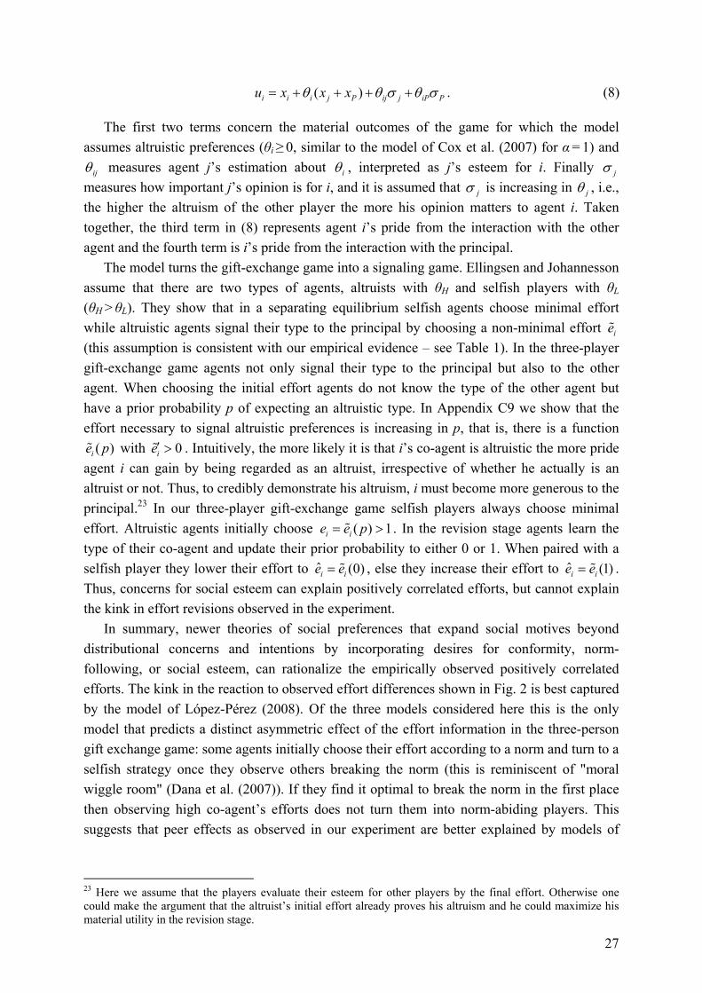
27

( )i i i j P ij j iP Pu x x xθ θ σ θ σ= + + + + . (8)

The first two terms concern the material outcomes of the game for which the model assumes altruistic preferences (θi ≥ 0, similar to the model of Cox et al. (2007) for α = 1) and

ijθ measures agent j’s estimation about iθ , interpreted as j’s esteem for i. Finally jσ measures how important j’s opinion is for i, and it is assumed that jσ is increasing in jθ , i.e., the higher the altruism of the other player the more his opinion matters to agent i. Taken together, the third term in (8) represents agent i’s pride from the interaction with the other agent and the fourth term is i’s pride from the interaction with the principal.

The model turns the gift-exchange game into a signaling game. Ellingsen and Johannesson assume that there are two types of agents, altruists with θH and selfish players with θL (θH > θL). They show that in a separating equilibrium selfish agents choose minimal effort while altruistic agents signal their type to the principal by choosing a non-minimal effort ie% (this assumption is consistent with our empirical evidence – see Table 1). In the three-player gift-exchange game agents not only signal their type to the principal but also to the other agent. When choosing the initial effort agents do not know the type of the other agent but have a prior probability p of expecting an altruistic type. In Appendix C9 we show that the effort necessary to signal altruistic preferences is increasing in p, that is, there is a function

( )ie p% with 0ie′ >% . Intuitively, the more likely it is that i’s co-agent is altruistic the more pride agent i can gain by being regarded as an altruist, irrespective of whether he actually is an altruist or not. Thus, to credibly demonstrate his altruism, i must become more generous to the principal.23 In our three-player gift-exchange game selfish players always choose minimal effort. Altruistic agents initially choose ( ) 1i ie e p= >% . In the revision stage agents learn the type of their co-agent and update their prior probability to either 0 or 1. When paired with a selfish player they lower their effort to ˆ (0)i ie e= % , else they increase their effort to ˆ (1)i ie e= % . Thus, concerns for social esteem can explain positively correlated efforts, but cannot explain the kink in effort revisions observed in the experiment.

In summary, newer theories of social preferences that expand social motives beyond distributional concerns and intentions by incorporating desires for conformity, norm-following, or social esteem, can rationalize the empirically observed positively correlated efforts. The kink in the reaction to observed effort differences shown in Fig. 2 is best captured by the model of López-Pérez (2008). Of the three models considered here this is the only model that predicts a distinct asymmetric effect of the effort information in the three-person gift exchange game: some agents initially choose their effort according to a norm and turn to a selfish strategy once they observe others breaking the norm (this is reminiscent of "moral wiggle room" (Dana et al. (2007)). If they find it optimal to break the norm in the first place then observing high co-agent’s efforts does not turn them into norm-abiding players. This suggests that peer effects as observed in our experiment are better explained by models of

23 Here we assume that the players evaluate their esteem for other players by the final effort. Otherwise one could make the argument that the altruist’s initial effort already proves his altruism and he could maximize his material utility in the revision stage.

28

conformity, norm-guided behavior or considerations of social esteem than more direct motives such as altruism or inequity aversion.

It is also possible to enrich standard theories by conformity or norm abiding motives. In models of reciprocity the necessary steps seem obvious: the parameter which governs positive or negative reciprocity towards the principal needs to depend somehow on the information about the co-agent's action. For example, in Cox et al. (2007) we could reformulate the emotional state θP as being positively related to agent i’s belief about agent j’s emotional state towards the principal, thus introducing a desire to conform into the model. In the revision stage the agent would then update his information about the emotional state of the co-agent and we could generate positively sloped reaction functions.

On the other hand one may object that these newer theories also allow for more social motives than the standard theories of social preferences, and one standard theory, the Fehr-Schmidt (1999) model (the BA-type, see Table 5), actually can, at least qualitatively, explain positively correlated efforts without resorting to additional motives. Put differently, Fehr and Schmidt (1999) might provide a parsimonious explanation of peer effects in voluntary cooperation, if we are prepared to relax the prediction that agents choose the same efforts to positively correlated efforts. Whether this is a valid argument is a task for future research and Gächter et al. (2013) provide a first step in this direction. They build on the theoretical results of this paper (that Fehr-Schmidt preferences can, at least qualitatively, explain peer effects) and also provide evidence that the measured descriptive norms are as well consistent with the peer effects we see. Interestingly, a quantitative comparison between norms and Fehr-Schmidt preferences for peer effects suggests a surprisingly strong explanatory power of Fehr-Schmidt preferences, despite unambiguous evidence that descriptive norms exhibit peer effects.

29

Appendix (For Online Publication) Christian Thöni and Simon Gächter:

Social Preferences and Peer Effects in Voluntary Cooperation

Appendix A: Experimental instructions Appendix B: Data overview Appendix C: Theoretical details

Appendix A: Instructions [In the following we will present the information subjects received during the experiment. Editorial comments like this one are added in brackets. In the majority of sessions subjects first played a three person one-shot gift-exchange game, but they did not receive any feedback about other subjects' decisions. In the sessions identified as Experienced subjects previously played a repeated three person gift-exchange game for eight periods in a stranger matching protocol. In this experiment they learned the prices paid by the principal, but not the choice of the co-agent. The game was presented in a buyer seller framing. Principals are buyers who offer a price. Sellers choose quality. The instructions and control questions to this first experiment can be found in the online supplement of Gächter and Thöni (2010). In the following we show the information subjects received at the beginning of the second experiment, which is the experiment we report in this paper.] Instructions for the Second Experiment Before we will inform you about the decisions of the other two members of your group we would like to conduct a second experiment. In this second experiment you will again receive an endowment of 400 points. Your points will again be converted at the rate of:

1 Point = 3 Rappen. The points you will earn in this experiment will be paid out to you together with your earnings from the first experiment at the end of the experiment. The Second Experiment in Detail The second experiment is very similar to the first experiment. Again one buyer and two sellers constitute a group. The assignment of the participants to the groups is done at random. Like in the first experiment the buyer has to choose the prices for his two sellers and the sellers choose their quality. Again this experiment will be conducted only once. However, there are three important differences relative to the first experiment:

• In this second experiment the buyers have to choose the same price for both buyers. • The feasible prices are now 50, 100 and 200. • The income of the buyers is calculated differently in the second experiment. Unlike in the first experiment, the sum

of the qualities in the buyers’ income is multiplied by 35 instead of 18. The income of the buyers is therefore calculated as:

Income Buyer = 35 * (Quality1 + Quality2) – Price1 – Price2 The calculation of the sellers’ incomes remains unchanged, i.e., the calculation is the same as in the first experiment:

Income Seller = Own Price1 – 7 * (Own Quality – 1) When deciding, you will again have access to the ‘What-if-calculator’ where you can check out the calculation of the incomes. Do you have any questions? [End of the printed instructions. While the buyers choose their prices the sellers see a screen containing the following information:] Unlike in the first experiment you will be informed about the price you receive from your buyer when deciding about your quality in this second experiment. You then can choose your quality as a number between 1 and 20. Since the buyer has to pay the same price to both of his sellers the other seller in your group will receive the same price as you. In this moment your buyer is choosing the price. When the price is chosen you will be informed about it and you can choose your quality. Please press “continue” when you have finished reading this information.

30

[After that, the sellers see the following decision screen. The lower part of the right panel was only included in the sessions where we elicited beliefs.]

[When all qualities are chosen, the sellers receive a second information screen. The shaded sentence only appears in the EIT. Everything else is equal.] Possible revision of your quality choice You have just chosen your quality. In the next step you can possibly revise your quality choice, if you wish to do so. You will thereby be informed about the quality that the other seller in your group has chosen. In the next screen you have to re-enter your quality choice. You have two possibilities: You can either leave your quality unchanged or you can change your quality. In any case you have to make an entry, even if you do not want to change your quality. In this case you can simply enter the same number as in the last screen. If you want to change your quality then enter your new quality. Both sellers in your group will again enter a quality. However, only one of the two sellers in your group can actually change the quality. This means that either your reentered quality or the reentered quality of the other seller will be used for the calculation of the earnings. The computer will randomly choose one of the two sellers. For the other seller the quality choice of the last screen remains unchanged. In case the computer chooses you, your income will be calculated with your reentered quality. On the other hand, if the computer chooses the other seller, then your quality choice from the last screen remains unchanged und will be used for the calculation of your income. Please contact us if something is unclear. If not, please press the “continue” button to proceed to the next screen where you can choose your quality again. [The sellers are then shown the revision screen (see Fig. 1 in the main text). In the main treatment (with wage transparency) this screen contains information about the other worker’s effort decision. Note that this is the first time the subjects learn something about the other worker’s decision. When all subjects have re-entered their quality a screen with the results of the game appears. The subjects learn the definitive qualities of the other seller and themselves and their resulting income. After that, we provide the payoff information of the first experiment.]

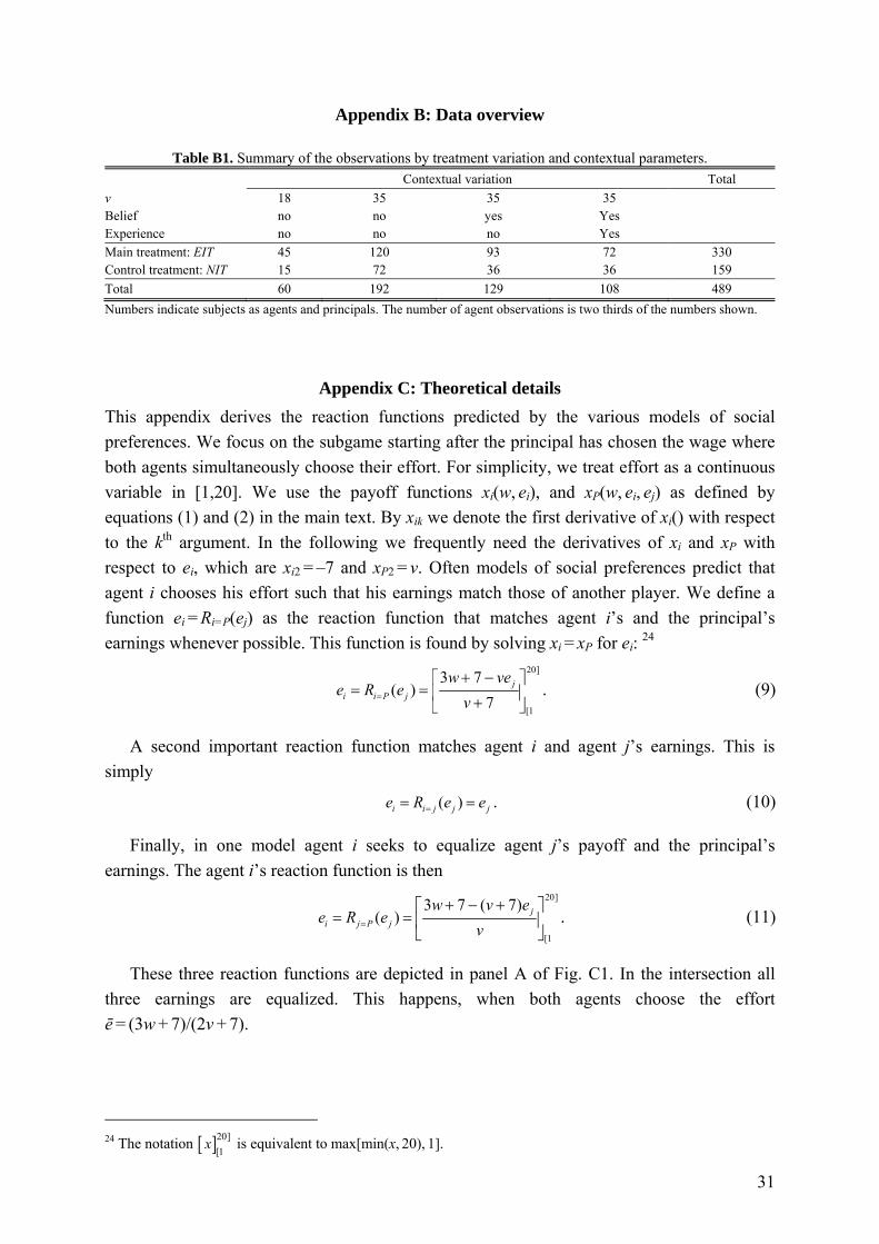
31

Appendix B: Data overview

Table B1. Summary of the observations by treatment variation and contextual parameters. Contextual variation Total v 18 35 35 35 Belief no no yes Yes Experience no no no Yes Main treatment: EIT 45 120 93 72 330 Control treatment: NIT 15 72 36 36 159 Total 60 192 129 108 489 Numbers indicate subjects as agents and principals. The number of agent observations is two thirds of the numbers shown.

Appendix C: Theoretical details This appendix derives the reaction functions predicted by the various models of social preferences. We focus on the subgame starting after the principal has chosen the wage where both agents simultaneously choose their effort. For simplicity, we treat effort as a continuous variable in [1,20]. We use the payoff functions xi(w, ei), and xP(w, ei, ej) as defined by equations (1) and (2) in the main text. By xik we denote the first derivative of xi() with respect to the kth argument. In the following we frequently need the derivatives of xi and xP with respect to ei, which are xi2 = –7 and xP2 = v. Often models of social preferences predict that agent i chooses his effort such that his earnings match those of another player. We define a function ei = Ri=P(ej) as the reaction function that matches agent i’s and the principal’s earnings whenever possible. This function is found by solving xi = xP for ei: 24

20]

[1

3 7( )

7j

i i P j

w vee R e

v=

+ −⎡ ⎤= = ⎢ ⎥+⎣ ⎦

. (9)

A second important reaction function matches agent i and agent j’s earnings. This is simply

( )i i j j je R e e== = . (10)

Finally, in one model agent i seeks to equalize agent j’s payoff and the principal’s earnings. The agent i’s reaction function is then

20]

[1

3 7 ( 7)( ) j

i j P j

w v ee R e

v=

+ − +⎡ ⎤= = ⎢ ⎥

⎣ ⎦. (11)

These three reaction functions are depicted in panel A of Fig. C1. In the intersection all three earnings are equalized. This happens, when both agents choose the effort ē = (3w + 7)/(2v + 7).

24 The notation [ ]20]

[1x is equivalent to max[min(x, 20), 1].

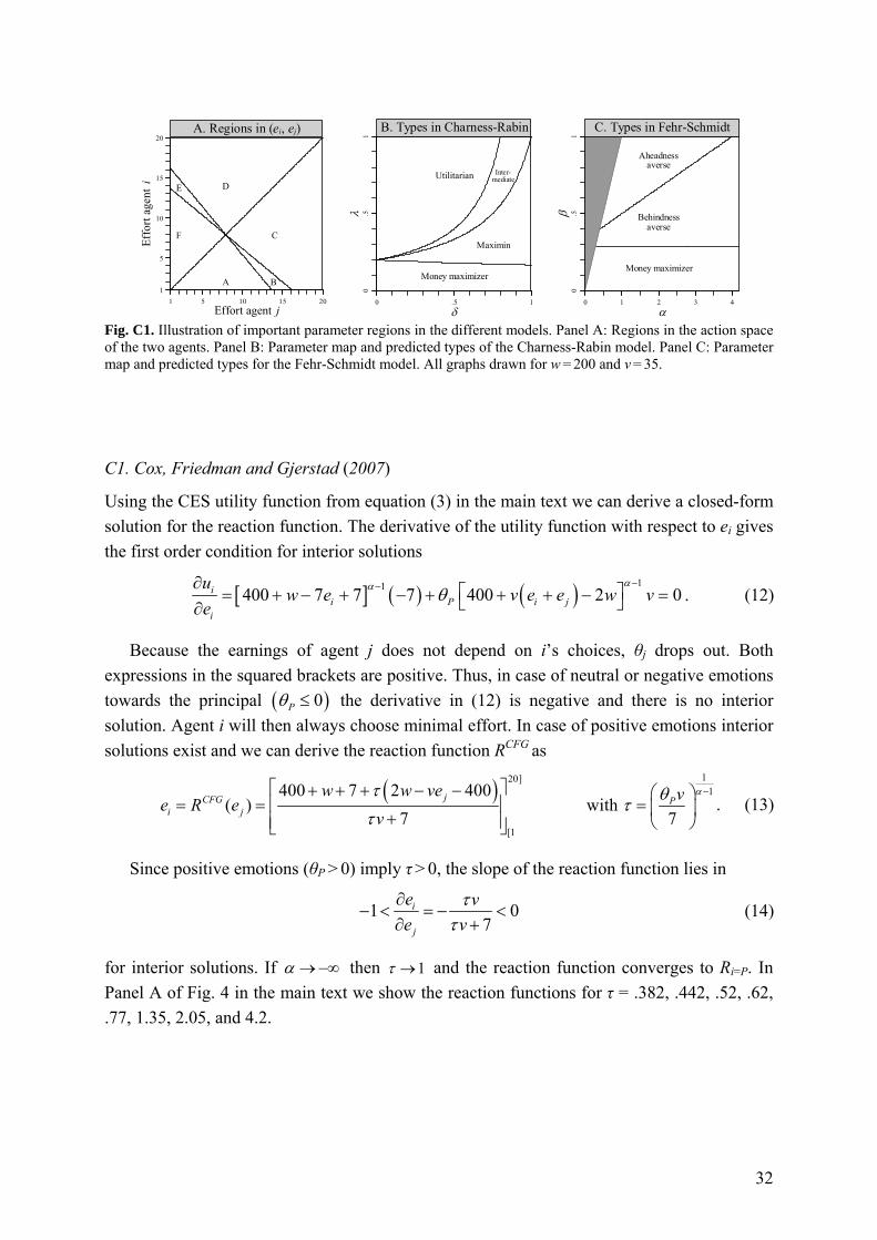
32

Fig. C1. Illustration of important parameter regions in the different models. Panel A: Regions in the action space of the two agents. Panel B: Parameter map and predicted types of the Charness-Rabin model. Panel C: Parameter map and predicted types for the Fehr-Schmidt model. All graphs drawn for w = 200 and v = 35.

C1. Cox, Friedman and Gjerstad (2007)

Using the CES utility function from equation (3) in the main text we can derive a closed-form solution for the reaction function. The derivative of the utility function with respect to ei gives the first order condition for interior solutions

[ ] ( ) ( ) 11400 7 7 7 400 2 0ii P i j

i

uw e v e e w v

eαα θ−−∂ ⎡ ⎤= + − + − + + + − =⎣ ⎦∂

. (12)

Because the earnings of agent j does not depend on i’s choices, θj drops out. Both expressions in the squared brackets are positive. Thus, in case of neutral or negative emotions towards the principal ( )0Pθ ≤ the derivative in (12) is negative and there is no interior solution. Agent i will then always choose minimal effort. In case of positive emotions interior solutions exist and we can derive the reaction function RCFG as

( )

120]1

[1

400 7 2 400( ) with

7 7jCFG P

i j

w w ve ve R ev

ατ θττ

−⎡ ⎤+ + + − − ⎛ ⎞= = =⎢ ⎥ ⎜ ⎟+⎢ ⎥ ⎝ ⎠⎣ ⎦

. (13)

Since positive emotions (θP > 0) imply τ > 0, the slope of the reaction function lies in

1 07

i

j

e ve v

ττ

∂− < = − <

∂ + (14)

for interior solutions. If α →−∞ then 1τ → and the reaction function converges to Ri=P. In Panel A of Fig. 4 in the main text we show the reaction functions for τ = .382, .442, .52, .62, .77, 1.35, 2.05, and 4.2.

A B

C

DE

F

1

5

10

15

20Ef

fort

agen

t i

1 5 10 15 20Effort agent j

A. Regions in (ei, ej)

Utilitarian Inter-mediate

Maximin

Money maximizer

0.5

1λ

0 .5 1δ

B. Types in Charness-Rabin

Aheadnessaverse

Behindnessaverse

Money maximizer

0.5

1β

0 1 2 3 4α

C. Types in Fehr-Schmidt

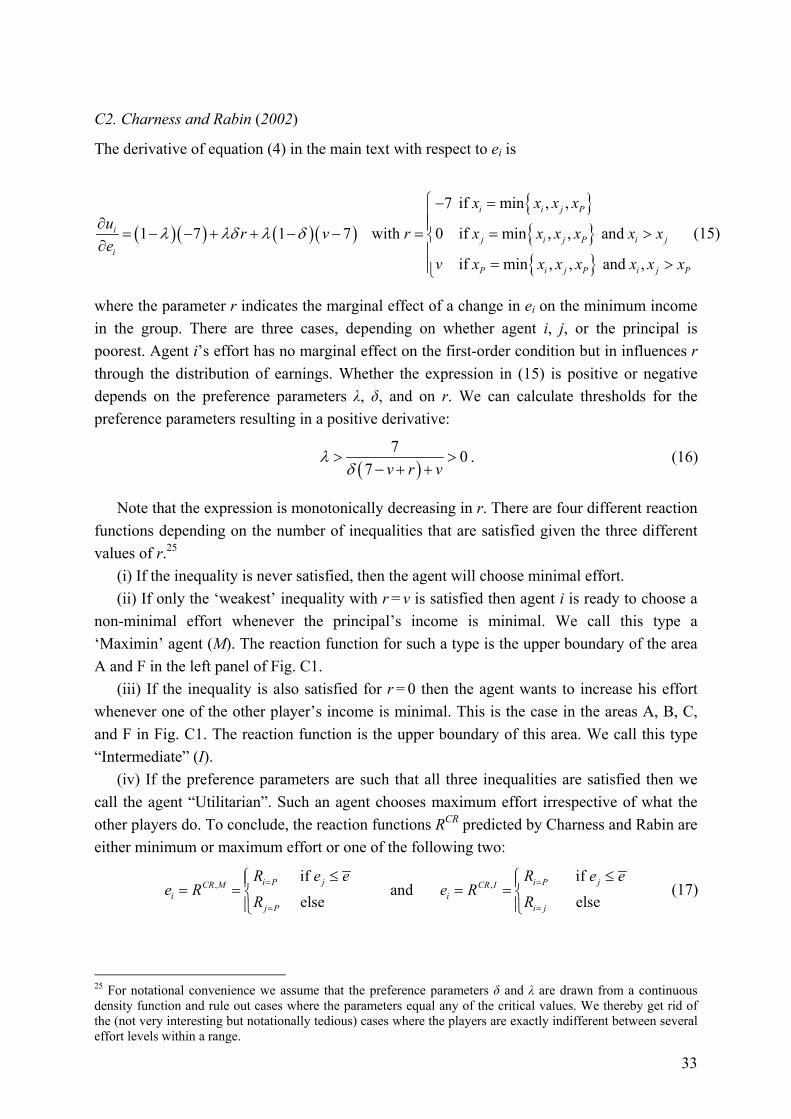
33

C2. Charness and Rabin (2002)

The derivative of equation (4) in the main text with respect to ei is

( )( ) ( )( ){ }{ }{ }

7 if min , ,

1 7 1 7 with 0 if min , , and

if min , , and ,

i i j P

ij i j P i j

i

P i j P i j P

x x x xu r v r x x x x x xe

v x x x x x x x

λ λδ λ δ

⎧− =⎪∂ ⎪= − − + + − − = = >⎨

∂ ⎪= >⎪⎩

(15)

where the parameter r indicates the marginal effect of a change in ei on the minimum income in the group. There are three cases, depending on whether agent i, j, or the principal is poorest. Agent i’s effort has no marginal effect on the first-order condition but in influences r through the distribution of earnings. Whether the expression in (15) is positive or negative depends on the preference parameters λ, δ, and on r. We can calculate thresholds for the preference parameters resulting in a positive derivative:

( )

7 07 v r v

λδ

> >− + +

. (16)

Note that the expression is monotonically decreasing in r. There are four different reaction functions depending on the number of inequalities that are satisfied given the three different values of r.25

(i) If the inequality is never satisfied, then the agent will choose minimal effort. (ii) If only the ‘weakest’ inequality with r = v is satisfied then agent i is ready to choose a

non-minimal effort whenever the principal’s income is minimal. We call this type a ‘Maximin’ agent (M). The reaction function for such a type is the upper boundary of the area A and F in the left panel of Fig. C1.

(iii) If the inequality is also satisfied for r = 0 then the agent wants to increase his effort whenever one of the other player’s income is minimal. This is the case in the areas A, B, C, and F in Fig. C1. The reaction function is the upper boundary of this area. We call this type “Intermediate” (I).

(iv) If the preference parameters are such that all three inequalities are satisfied then we call the agent “Utilitarian”. Such an agent chooses maximum effort irrespective of what the other players do. To conclude, the reaction functions RCR predicted by Charness and Rabin are either minimum or maximum effort or one of the following two:

, , if if

andelse else

i P j i P jCR M CR Ii i

j P i j

R e e R e ee R e R

R R= =

= =

≤ ≤⎧ ⎧⎪ ⎪= = = =⎨ ⎨⎪ ⎪⎩ ⎩

(17)

25 For notational convenience we assume that the preference parameters δ and λ are drawn from a continuous density function and rule out cases where the parameters equal any of the critical values. We thereby get rid of the (not very interesting but notationally tedious) cases where the players are exactly indifferent between several effort levels within a range.

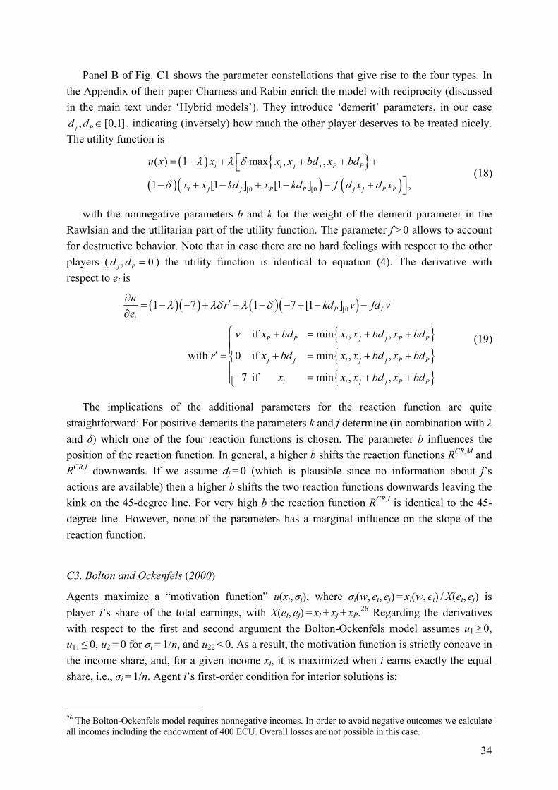
34

Panel B of Fig. C1 shows the parameter constellations that give rise to the four types. In the Appendix of their paper Charness and Rabin enrich the model with reciprocity (discussed in the main text under ‘Hybrid models’). They introduce ‘demerit’ parameters, in our case

, [0,1]j Pd d ∈ , indicating (inversely) how much the other player deserves to be treated nicely. The utility function is

( ) { }

( )( ) ( )[0 [0

( ) 1 max , ,

1 [1 ] [1 ] ,

i i j j P P

i j j P P j j P P

u x x x x bd x bd

x x kd x kd f d x d x

λ λ δ

δ

⎡= − + + + +⎣⎤− + − + − − + ⎦

(18)

with the nonnegative parameters b and k for the weight of the demerit parameter in the Rawlsian and the utilitarian part of the utility function. The parameter f > 0 allows to account for destructive behavior. Note that in case there are no hard feelings with respect to the other players ( , 0j Pd d = ) the utility function is identical to equation (4). The derivative with respect to ei is

( )( ) ( )( )

{ }{ }{ }

[01 7 1 7 [1 ]

if min , ,

with 0 if min , ,

7 if min , ,

P Pi

P P i j j P P

j j i j j P P

i i j j P P

u r kd v fd ve

v x bd x x bd x bd

r x bd x x bd x bd

x x x bd x bd

λ λδ λ δ∂ ′= − − + + − − + − −∂

⎧ + = + +⎪⎪′ = + = + +⎨⎪− = + +⎪⎩

(19)

The implications of the additional parameters for the reaction function are quite straightforward: For positive demerits the parameters k and f determine (in combination with λ and δ) which one of the four reaction functions is chosen. The parameter b influences the position of the reaction function. In general, a higher b shifts the reaction functions RCR,M and RCR,I downwards. If we assume dj = 0 (which is plausible since no information about j’s actions are available) then a higher b shifts the two reaction functions downwards leaving the kink on the 45-degree line. For very high b the reaction function RCR,I is identical to the 45-degree line. However, none of the parameters has a marginal influence on the slope of the reaction function.

C3. Bolton and Ockenfels (2000)

Agents maximize a “motivation function” u(xi, σi), where σi(w, ei, ej) = xi(w, ei) / X(ei, ej) is player i’s share of the total earnings, with X(ei, ej) = xi + xj + xP.26 Regarding the derivatives with respect to the first and second argument the Bolton-Ockenfels model assumes u1 ≥ 0, u11 ≤ 0, u2 = 0 for σi = 1/n, and u22 < 0. As a result, the motivation function is strictly concave in the income share, and, for a given income xi, it is maximized when i earns exactly the equal share, i.e., σi = 1/n. Agent i’s first-order condition for interior solutions is:

26 The Bolton-Ockenfels model requires nonnegative incomes. In order to avoid negative outcomes we calculate all incomes including the endowment of 400 ECU. Overall losses are not possible in this case.

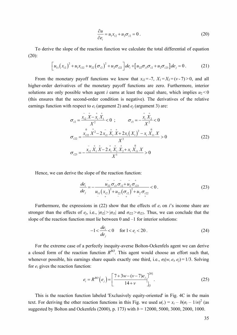
35

1 2 2 2 0i ii

u u x ue

σ∂= + =

∂. (20)

To derive the slope of the reaction function we calculate the total differential of equation (20):

( ) ( ) [ ]2 211 2 1 22 22 2 2 22 22 3 2 2 23 0σ σ σ σ σ⎡ ⎤+ + + + + =⎣ ⎦i i i i i i i i ju x u x u u de u u de . (21)

From the monetary payoff functions we know that xi2 = -7, X1 = X2 = (v - 7) > 0, and all higher-order derivatives of the monetary payoff functions are zero. Furthermore, interior solutions are only possible when agent i earns at least the equal share, which implies u2 < 0 (this ensures that the second-order condition is negative). The derivatives of the relative earnings function with respect to ei (argument 2) and ej (argument 3) are:

( )

2 1 22 32 2

0 02222 2 1 1 11

22 3

0

2 1 1 2 1123 3

0 ; 0

2 20

2 0

i i ii i

i i i ii

i i ii

x X x X x XX X

x X x X X x X x X XX

x X X x X X x X XX

σ σ

σ

σ

− + + + + +

+ − + +

− + + + + +

−= < = − <

− + −= >

− += − >

(22)

Hence, we can derive the slope of the reaction function:

( ) ( )

22 3 2 2 232 2

11 2 22 2 2 22

0i i i i

j i i i

de u ude u x u u

σ σ σσ σ

− − − − +

− − − ++ +

+= − <

+ +. (23)

Furthermore, the expressions in (22) show that the effects of ei on i’s income share are stronger than the effects of ej, i.e., |σi2| > |σi3| and σi22 > σi23. Thus, we can conclude that the slope of the reaction function must lie between 0 and –1 for interior solutions:

1 0 for 1 20ii

j

de ede

− < < < < . (24)

For the extreme case of a perfectly inequity-averse Bolton-Ockenfels agent we can derive a closed form of the reaction function RBO. This agent would choose an effort such that, whenever possible, his earnings share equals exactly one third, i.e., σi(w, ei, ej) = 1/3. Solving for ei gives the reaction function:

( )20]

[1

7 3 ( 7)14

jBOi j

w v ee R e

v+ − −⎡ ⎤

= = ⎢ ⎥+⎣ ⎦. (25)

This is the reaction function labeled 'Exclusively equity-oriented' in Fig. 4C in the main text. For deriving the other reaction functions in this Fig. we used u(.) = xi – b(σi – 1/n)2 (as suggested by Bolton and Ockenfels (2000), p. 173) with b = 12000, 5000, 3000, 2000, 1000.

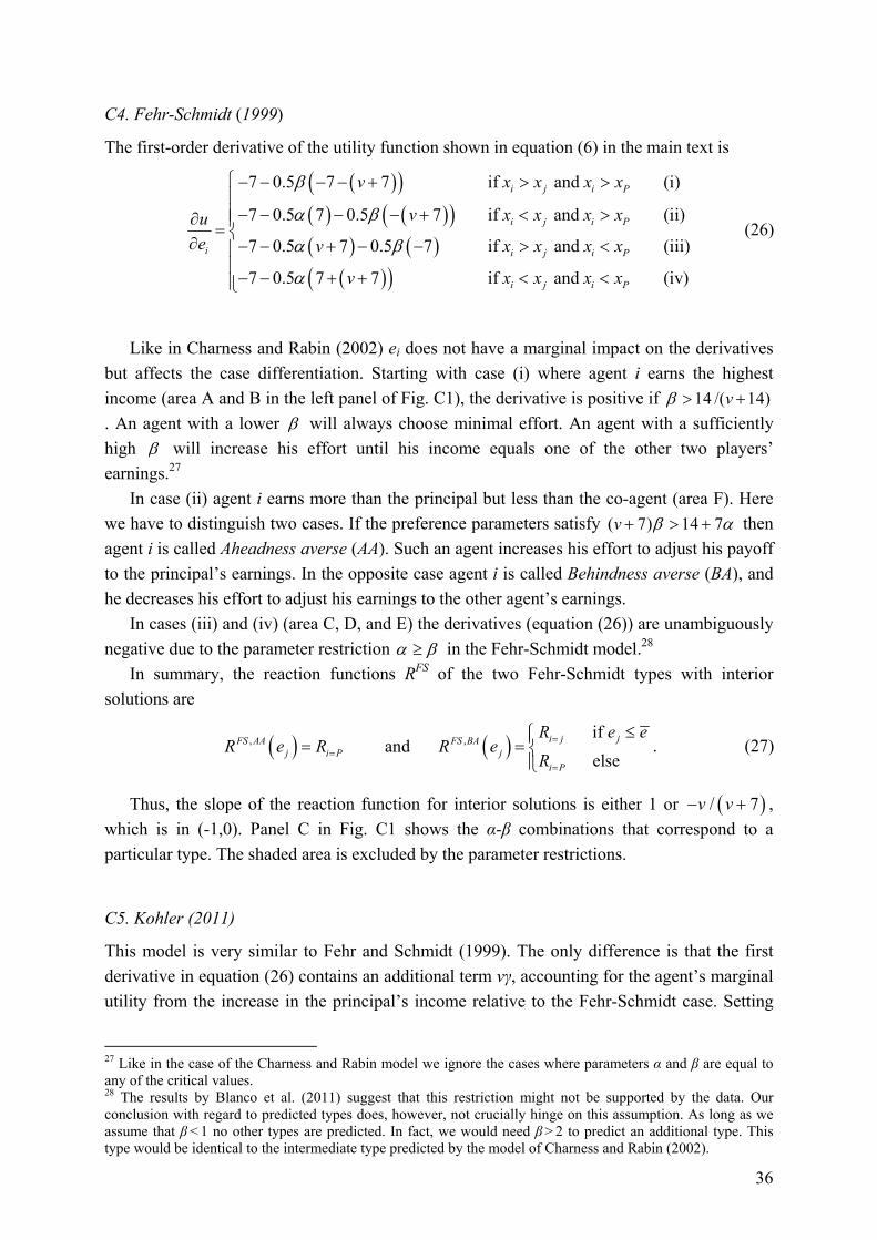
36

C4. Fehr-Schmidt (1999)

The first-order derivative of the utility function shown in equation (6) in the main text is

( )( )( ) ( )( )( ) ( )

( )( )

7 0.5 7 7 if and (i)

7 0.5 7 0.5 7 if and (ii)

7 0.5 7 0.5 7 if and (iii)

7 0.5 7 7 if and (iv)

i j i P

i j i P

i i j i P

i j i P

v x x x x

v x x x xue v x x x x

v x x x x

β

α β

α β

α

⎧− − − − + > >⎪⎪− − − − + < >∂ ⎪= ⎨

∂ − − + − − > <⎪⎪− − + + < <⎪⎩

(26)

Like in Charness and Rabin (2002) ei does not have a marginal impact on the derivatives

but affects the case differentiation. Starting with case (i) where agent i earns the highest income (area A and B in the left panel of Fig. C1), the derivative is positive if 14 /( 14)β > +v. An agent with a lower β will always choose minimal effort. An agent with a sufficiently high β will increase his effort until his income equals one of the other two players’ earnings.27

In case (ii) agent i earns more than the principal but less than the co-agent (area F). Here we have to distinguish two cases. If the preference parameters satisfy ( 7) 14 7β α+ > +v then agent i is called Aheadness averse (AA). Such an agent increases his effort to adjust his payoff to the principal’s earnings. In the opposite case agent i is called Behindness averse (BA), and he decreases his effort to adjust his earnings to the other agent’s earnings.

In cases (iii) and (iv) (area C, D, and E) the derivatives (equation (26)) are unambiguously negative due to the parameter restriction α β≥ in the Fehr-Schmidt model.28

In summary, the reaction functions RFS of the two Fehr-Schmidt types with interior solutions are

( ) ( ), , if and

elsei j jFS AA FS BA

j i P ji P

R e eR e R R e

R=

==

≤⎧⎪= = ⎨⎪⎩

. (27)

Thus, the slope of the reaction function for interior solutions is either 1 or ( )/ 7v v− + , which is in (-1,0). Panel C in Fig. C1 shows the α-β combinations that correspond to a particular type. The shaded area is excluded by the parameter restrictions.

C5. Kohler (2011)

This model is very similar to Fehr and Schmidt (1999). The only difference is that the first derivative in equation (26) contains an additional term vγ, accounting for the agent’s marginal utility from the increase in the principal’s income relative to the Fehr-Schmidt case. Setting

27 Like in the case of the Charness and Rabin model we ignore the cases where parameters α and β are equal to any of the critical values. 28 The results by Blanco et al. (2011) suggest that this restriction might not be supported by the data. Our conclusion with regard to predicted types does, however, not crucially hinge on this assumption. As long as we assume that β < 1 no other types are predicted. In fact, we would need β > 2 to predict an additional type. This type would be identical to the intermediate type predicted by the model of Charness and Rabin (2002).

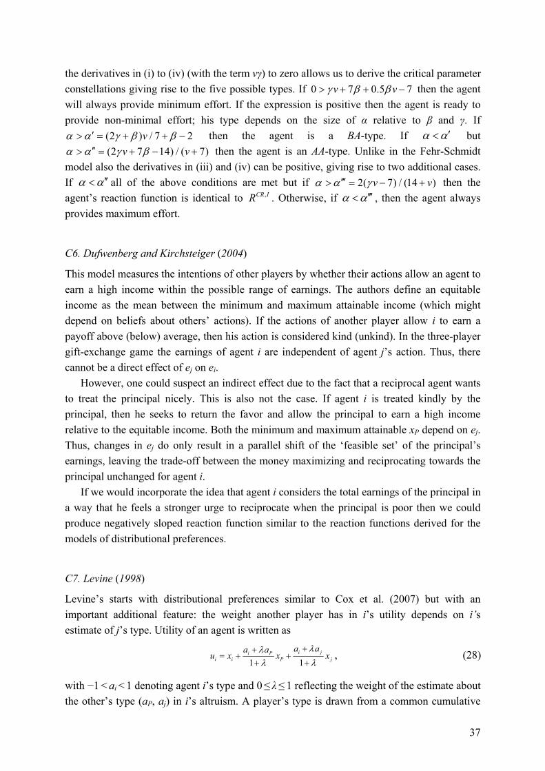
37

the derivatives in (i) to (iv) (with the term vγ) to zero allows us to derive the critical parameter constellations giving rise to the five possible types. If 0 7 0.5 7v vγ β β> + + − then the agent will always provide minimum effort. If the expression is positive then the agent is ready to provide non-minimal effort; his type depends on the size of α relative to β and γ. If

(2 ) / 7 2vα α γ β β′> = + + − then the agent is a BA-type. If α α′< but (2 7 14) / ( 7)v vα α γ β′′> = + − + then the agent is an AA-type. Unlike in the Fehr-Schmidt

model also the derivatives in (iii) and (iv) can be positive, giving rise to two additional cases. If α α′′< all of the above conditions are met but if 2( 7) / (14 )v vα α γ′′′> = − + then the agent’s reaction function is identical to ,CR IR . Otherwise, if α α′′′< , then the agent always provides maximum effort.

C6. Dufwenberg and Kirchsteiger (2004)

This model measures the intentions of other players by whether their actions allow an agent to earn a high income within the possible range of earnings. The authors define an equitable income as the mean between the minimum and maximum attainable income (which might depend on beliefs about others’ actions). If the actions of another player allow i to earn a payoff above (below) average, then his action is considered kind (unkind). In the three-player gift-exchange game the earnings of agent i are independent of agent j’s action. Thus, there cannot be a direct effect of ej on ei.

However, one could suspect an indirect effect due to the fact that a reciprocal agent wants to treat the principal nicely. This is also not the case. If agent i is treated kindly by the principal, then he seeks to return the favor and allow the principal to earn a high income relative to the equitable income. Both the minimum and maximum attainable xP depend on ej. Thus, changes in ej do only result in a parallel shift of the ‘feasible set’ of the principal’s earnings, leaving the trade-off between the money maximizing and reciprocating towards the principal unchanged for agent i.

If we would incorporate the idea that agent i considers the total earnings of the principal in a way that he feels a stronger urge to reciprocate when the principal is poor then we could produce negatively sloped reaction function similar to the reaction functions derived for the models of distributional preferences.

C7. Levine (1998)

Levine’s starts with distributional preferences similar to Cox et al. (2007) but with an important additional feature: the weight another player has in i’s utility depends on i’s estimate of j’s type. Utility of an agent is written as

1 1

i ji Pi i P j

a aa au x x x

λλλ λ

++= + +

+ +, (28)

with −1 < ai < 1 denoting agent i’s type and 0 ≤ λ ≤ 1 reflecting the weight of the estimate about the other’s type (aP, aj) in i’s altruism. A player’s type is drawn from a common cumulative

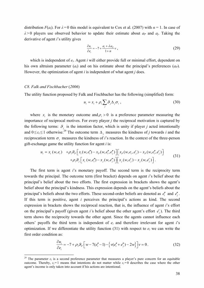
38

distribution F(ai). For λ = 0 this model is equivalent to Cox et al. (2007) with α = 1. In case of λ > 0 players use observed behavior to update their estimate about aP and aj. Taking the derivative of agent i’s utility gives

71

i i P

i

u a av

e nλ∂ +

= − +∂ +

, (29)

which is independent of ei. Agent i will either provide full or minimal effort, dependent on his own altruism parameter (ai) and on his estimate about the principal’s preferences (aP). However, the optimization of agent i is independent of what agent j does.

C8. Falk and Fischbacher (2006)

The utility function proposed by Falk and Fischbacher has the following (simplified) form:

i i i j j ij

u x ρ ϑ σ= + Δ∑ , (30)

where ix is the monetary outcome and 0iρ > is a preference parameter measuring the importance of reciprocal motives. For every player j the reciprocal motivation is captured by the following terms: jϑ is the intention factor, which is unity if player j acted intentionally and 0 ≤ εi ≤ 1 otherwise.29 The outcome term jΔ measures the kindness of j towards i and the reciprocation term iσ measures the kindness of i’s reaction. In the context of the three-person gift-exchange game the utility function for agent i is:

( , ) ( , ) ( , , ) ( , , ) ( , , )

( , ) ( , ) ( , ) ( , ) .

i i i i P i i P i j P i j P i j

i j i i j j j j j j

u x w e x w e x w e e x w e e x w e e

x w e x w e x w e x w e

ρ ϑ

ρ ϑ

′′ ′′ ′′ ′ ′′ ′⎡ ⎤ ⎡ ⎤= + − −⎣ ⎦ ⎣ ⎦′′ ′′ ′ ′⎡ ⎤ ⎡ ⎤+ − −⎣ ⎦ ⎣ ⎦

(31)

The first term is agent i’s monetary payoff. The second term is the reciprocity term towards the principal. The outcome term (first bracket) depends on agent i’s belief about the principal’s belief about the two efforts. The first expression in brackets shows the agent’s belief about the principal’s kindness. This expression depends on the agent’s beliefs about the principal’s beliefs about the two efforts. These second-order beliefs are denoted as ie′′ and je′′ . If this term is positive, agent i perceives the principal’s actions as kind. The second expression in brackets shows the reciprocal reaction, that is, the influence of agent i’s effort on the principal’s payoff (given agent i’s belief about the other agent’s effort je′ ). The third term shows the reciprocity towards the other agent. Since the agents cannot influence each others’ payoffs the third term is independent of ei and therefore irrelevant for agent i’s optimization. If we differentiate the utility function (31) with respect to ei we can write the first order condition as:

{ }7 7( 1) ( ) 2 0ii P i i j

i

uw e v e e w v

eρ ϑ

∂ ⎡ ⎤′′ ′′ ′′= − + − − − + − =⎣ ⎦∂. (32)

29 The parameter εi is a second preference parameter that measures a player’s pure concern for an equitable outcome. Thereby, εi = 1 means that intentions do not matter while εi = 0 describes the case where the other agent’s income is only taken into account if his actions are intentional.

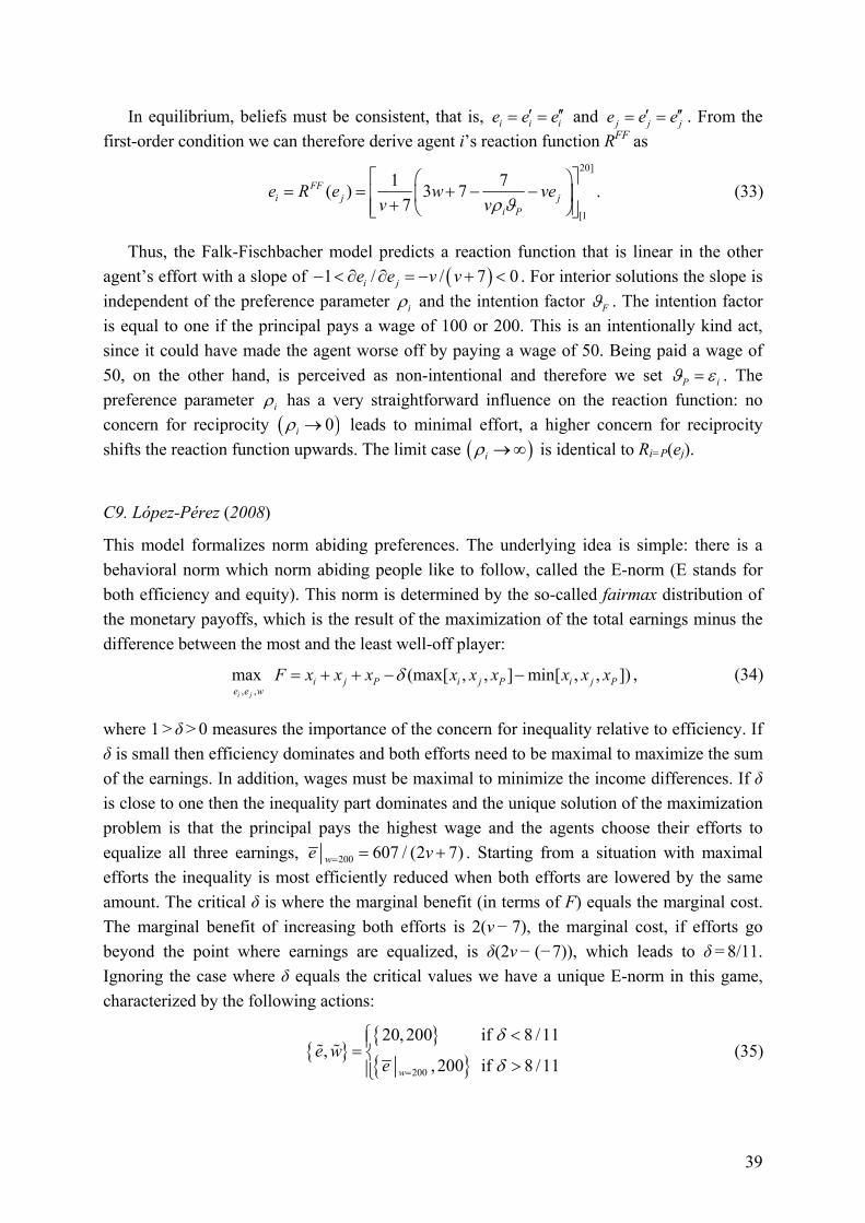
39

In equilibrium, beliefs must be consistent, that is, i i ie e e′ ′′= = and j j je e e′ ′′= = . From the first-order condition we can therefore derive agent i’s reaction function RFF as

20]

[1

1 7( ) 3 77

FFi j j

i P

e R e w vev vρϑ⎡ ⎤⎛ ⎞

= = + − −⎢ ⎥⎜ ⎟+⎢ ⎥⎝ ⎠⎣ ⎦. (33)

Thus, the Falk-Fischbacher model predicts a reaction function that is linear in the other agent’s effort with a slope of ( )1 / / 7 0i je e v v− < ∂ ∂ = − + < . For interior solutions the slope is independent of the preference parameter iρ and the intention factor Fϑ . The intention factor is equal to one if the principal pays a wage of 100 or 200. This is an intentionally kind act, since it could have made the agent worse off by paying a wage of 50. Being paid a wage of 50, on the other hand, is perceived as non-intentional and therefore we set P iϑ ε= . The preference parameter iρ has a very straightforward influence on the reaction function: no concern for reciprocity ( )0iρ → leads to minimal effort, a higher concern for reciprocity shifts the reaction function upwards. The limit case ( )iρ →∞ is identical to Ri=P(ej).

C9. López-Pérez (2008)

This model formalizes norm abiding preferences. The underlying idea is simple: there is a behavioral norm which norm abiding people like to follow, called the E-norm (E stands for both efficiency and equity). This norm is determined by the so-called fairmax distribution of the monetary payoffs, which is the result of the maximization of the total earnings minus the difference between the most and the least well-off player:

, ,

max (max[ , , ] min[ , , ])i j

i j P i j P i j Pe e w

F x x x x x x x x xδ= + + − − , (34)

where 1 > δ > 0 measures the importance of the concern for inequality relative to efficiency. If δ is small then efficiency dominates and both efforts need to be maximal to maximize the sum of the earnings. In addition, wages must be maximal to minimize the income differences. If δ is close to one then the inequality part dominates and the unique solution of the maximization problem is that the principal pays the highest wage and the agents choose their efforts to equalize all three earnings, 200 607 / (2 7)we v= = + . Starting from a situation with maximal efforts the inequality is most efficiently reduced when both efforts are lowered by the same amount. The critical δ is where the marginal benefit (in terms of F) equals the marginal cost. The marginal benefit of increasing both efforts is 2(v − 7), the marginal cost, if efforts go beyond the point where earnings are equalized, is δ(2v − (−7)), which leads to δ = 8/11. Ignoring the case where δ equals the critical values we have a unique E-norm in this game, characterized by the following actions:

{ }{ }{ }200

20,200 if 8 /11,

, 200 if 8 /11w

e we

δ

δ=

<⎧⎪= ⎨>⎪⎩

% % (35)

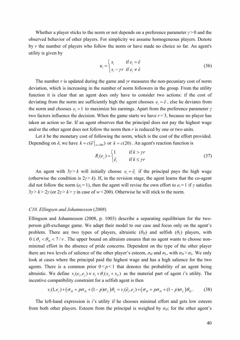
40

Whether a player sticks to the norm or not depends on a preference parameter γ > 0 and the observed behavior of other players. For simplicity we assume homogeneous players. Denote by r the number of players who follow the norm or have made no choice so far. An agent's utility is given by

if if

i ii

i i

x e eu

x r e eγ=⎧

= ⎨ − ≠⎩

%

% (36)

The number r is updated during the game and γr measures the non-pecuniary cost of norm deviation, which is increasing in the number of norm followers in the group. From the utility function it is clear that an agent does only have to consider two actions: if the cost of deviating from the norm are sufficiently high the agent chooses ie e= % , else he deviates from the norm and chooses 1ie = to maximize his earnings. Apart from the preference parameter γ two factors influence the decision. When the game starts we have r = 3, because no player has taken an action so far. If an agent observes that the principal does not pay the highest wage and/or the other agent does not follow the norm then r is reduced by one or two units.

Let k be the monetary cost of following the norm, which is the cost of the effort provided. Depending on δ, we have 200( )wk c e == or (20)k c= . An agent's reaction function is

1 if

( )if i j

i

k rR e

e k rγγ

>⎧= ⎨ ≤⎩ %

(37)

An agent with 3γ > k will initially choose i ie e= % if the principal pays the high wage (otherwise the condition is 2γ > k). If, in the revision stage, the agent learns that the co-agent did not follow the norm (ej = 1), then the agent will revise the own effort to ei = 1 if γ satisfies 3γ > k > 2γ (or 2γ > k > γ in case of w < 200). Otherwise he will stick to the norm.

C10. Ellingsen and Johannesson (2008)

Ellingson and Johannesson (2008, p. 1003) describe a separating equilibrium for the two-person gift-exchange game. We adapt their model to our case and focus only on the agent’s problem. There are two types of players, altruistic (θH) and selfish (θL) players, with 0 7 /L H vθ θ≤ < < . The upper bound on altruism ensures that no agent wants to choose non-minimal effort in the absence of pride concerns. Dependent on the type of the other player there are two levels of salience of the other player’s esteem, σH und σL, with σH > σL. We only look at cases where the principal paid the highest wage and has a high salience for the two agents. There is a common prior 0 < p < 1 that denotes the probability of an agent being altruistic. We define ( , ) ( )i i j i i j Pv e e x x xθ≡ + + as the material part of agent i’s utility. The incentive compatibility constraint for a selfish agent is then

( ) ( )(1, ) (1 ) ( , ) (1 )i j H H L L i i j H H L Hv e p p v e e p pσ σ σ θ σ σ σ θ+ + + − = + + + −% . (38)

The left-hand expression is i’s utility if he chooses minimal effort and gets low esteem from both other players. Esteem from the principal is weighed by σH; for the other agent’s

41

type is not known it is the expected weight. The right-hand side is i’s utility of choosing a non-minimal effort ie% , assuming this leads to high esteem. This effort is:

( )( )(1 )( ) 1

7H H L H L

iL

p pe p

vσ σ σ θ θ

θ+ + − −

= +−

% (39)

In a separating equilibrium the altruistic agent chooses a non-minimal effort of i ie e= % to credibly signal his altruism to the other two players; the selfish agent chooses 1ie = . What changes in the revision stage when the agents choose the revised effort ie ? When the co-agent’s effort is disclosed the agent knows whether the co-agent is altruistic or selfish. This changes the effort which credibly signals altruism. We can calculate the effort by setting either p = 0 or p = 1. Because the expression in (39) is increasing in p we have

(1) ( ) (0)i i ie e p e> >% % % . Thus, a selfish agent will always choose minimal effort. An altruistic agent will initially choose ( )i ie e p= % and revise upwards to ˆ (1)i ie e= % if the co-agent chose

( )j ie e p= % and downwards to ˆ (0)i ie e= % if the co-agent chose a minimal effort.

42

References Abbink, K., Hennig-Schmidt, H., 2006. Neutral versus loaded instructions in a bribery

experiment. Experimental Economics 9 (2), 103-121. Andreoni, J., Bernheim, D. B., 2009. Social image and the 50-50 norm: A theoretical and

experimental analysis of audience effects. Econometrica 77 (5), 1607-1636. Asch, S. E., 1952. Social psychology. Prentice Hall, Englewood Cliffs. Bandiera, O., Barankay, I., Rasul, I., 2010. Social incentives in the workplace. Review of

Economic Studies 77 (2), 417-458. Bardsley, N., Sausgruber, R., 2005. Conformity and reciprocity in public good provision.

Journal of Economic Psychology 26 (5), 664-681. Battigalli, P., Dufwenberg, M., 2007. Guilt in games. The American Economic Review 97

(2), 170-176. Bénabou, R., Tirole, J., 2006. Incentives and prosocial behavior. American Economic Review

96 (5), 1652-1678. Bernheim, B. D., 1994. A theory of conformity. Journal of Political Economy 102 (5), 841-

877. Bicchieri, C., Xiao, E., 2009. Do the right thing: But only if others do so. Journal of

Behavioral Decision Making 22 (2), 191-208. Blanco, M., Engelmann, D., Normann, H. T., 2011. A within-subject analysis of other-

regarding preferences. Games and Economic Behavior 72 (2), 321-338. Bolton, G. E., 1991. A comparative model of bargaining - theory and evidence. American

Economic Review 81 (5), 1096-1136. Bolton, G. E., Ockenfels, A., 2000. Erc: A theory of equity, reciprocity, and competition.

American Economic Review 90 (1), 166-193. Camerer, C. F., 2003. Behavioral game theory: Experiments in strategic interaction. Princeton

University Press, Princeton. Cason, T., Mui, V.-L., 1998. Social influence in the sequential dictator game. Journal of

Mathematical Psychology 42 (2-3), 248-265. Charness, G., Kuhn, P., 2011. Lab labor: What can labor economists learn from the lab? In

Ashenfelter, O., Card, D., (Eds.), Handbook of labor economics. Elsevier, Amsterdam, pp. 229-330.

Charness, G., Rabin, M., 2002. Understanding social preferences with simple tests. Quarterly Journal of Economics 117 (3), 817-869.

Chen, Y., Harper, F. M., Konstan, J., Li, S. X., 2010. Social comparisons and contributions to online communities: A field experiment on movielens. American Economic Review 100 (4), 1358-1398.

Christakis, N. A., Fowler, J. H., 2007. The spread of obesity in a large social network over 32 years. New England Journal of Medicine 357 (4), 370-379.

Cialdini, R. B., Goldstein, N. J., 2004. Social influence: Compliance and conformity. Annual Review of Psychology 55 (1), 591-621.

Clark, A. E., Oswald, A. J., 1998. Comparison-concave utility and following behaviour in social and economic settings. Journal of Public Economics 70 (1), 133-155.

Cox, J. C., Friedman, D., Gjerstad, S., 2007. A tractable model of reciprocity and fairness. Games and Economic Behavior 59 (1), 17-45.

Cox, J. C., Friedman, D., Sadiraj, V., 2008. Revealed altruism. Econometrica 76 (1), 31-69. Cox, J. C., Sadiraj, V., 2007. On modeling voluntary contributions to public goods. Public

Finance Review 35 (2), 311-332. Cox, J. C., Sadiraj, V., 2012. Direct tests of individual preferences for equity and efficiency.

Economic Inquiry 50 (4), 920-931. Croson, R., 2000. Thinking like a game theorist: Factors affecting the frequency of

equilibrium play. Journal of Economic Behavior & Organization 41 (3), 299-314. Croson, R., Shang, J., 2008. The impact of downward social information on contribution

decisions. Experimental Economics 11 (3), 221-233. Dana, J., Weber, R., Kuang, J., 2007. Exploiting moral wiggle room: Experiments

demonstrating an illusory preference for fairness. Economic Theory 33 (1), 67–80. Daruvala, D., 2010. Would the right social preference model please stand up! Journal of

Economic Behavior & Organization 73 (2), 199-208.

43

Duflo, E., Saez, E., 2002. Participation and investment decisions in a retirement plan: The influence of colleagues’ choices. Journal of Public Economics 85 (1), 121-148.

Dufwenberg, M., Gächter, S., Hennig-Schmidt, H., 2011. The framing of games and the psychology of play. Games and Economic Behavior 73 (2), 459-478.

Dufwenberg, M., Kirchsteiger, G., 2004. A theory of sequential reciprocity. Games and Economic Behavior 47 (2), 268-298.

Ellingsen, T., Johannesson, M., 2008. Pride and prejudice: The human side of incentive theory. American Economic Review 98 (3), 990-1008.

Engelmann, D., Strobel, M., 2004. Inequality aversion, efficiency, and maximin preferences in simple distribution experiments. American Economic Review 94 (4), 857-869.

Falk, A., Fehr, E., Fischbacher, U., 2008. Testing theories of fairness--intentions matter. Games and Economic Behavior 62 (1), 287-303.

Falk, A., Fischbacher, U., 2006. A theory of reciprocity. Games and Economic Behavior 54 (2), 293-315.

Falk, A., Fischbacher, U., Gächter, S., 2013. Living in two neighborhoods - social interaction effects in the laboratory. Economic Inquiry 51 (1), 563-578.

Falk, A., Ichino, A., 2006. Clean evidence on peer effects. Journal of Labor Economics 24 (1), 38-57.

Fehr, E., Fischbacher, U., 2002. Why social preferences matter - the impact of non-selfish motives on competition, cooperation and incentives. Economic Journal 112 (478), C1-C33.

Fehr, E., Gächter, S., 1998. Reciprocity and economics: The economic implications of homo reciprocans. European Economic Review 42 (3-5), 845-859.

Fehr, E., Gächter, S., Kirchsteiger, G., 1997. Reciprocity as a contract enforcement device: Experimental evidence. Econometrica 65 (4), 833-860.

Fehr, E., Goette, L., Zehnder, C., 2009. A behavioral account of the labor market: The role of fairness concerns. Annual Review of Economics 1 (1), 355-384.

Fehr, E., Kirchsteiger, G., Riedl, A., 1993. Does fairness prevent market clearing? An experimental investigation. Quarterly Journal of Economics 108 (2), 437-459.

Fehr, E., Kirchsteiger, G., Riedl, A., 1998. Gift exchange and reciprocity in competitive experimental markets. European Economic Review 42 (1), 1-34.

Fehr, E., Schmidt, K. M., 1999. A theory of fairness, competition, and cooperation. Quarterly Journal of Economics 114 (3), 817-868.

Fehr, E., Schmidt, K. M., 2006. The economics of fairness, reciprocity and altruism - experimental evidence and new theories. In Kolm, S.-C., Ythier, J. M., (Eds.), Handbook of the economics of giving, altruism and reciprocity. Elsevier B.V., Amsterdam, pp. 615-691.

Fischbacher, U., 2007. Z-tree: Zurich toolbox for readymade economic experiments. Experimental Economics 10 (2), 171-178.

Frey, B. S., Meier, S., 2004. Social comparisons and pro-social behavior. Testing 'conditional cooperation' in a field experiment. American Economic Review 94 (5), 1717-1722.

Gächter, S., Nosenzo, D., Sefton, M., 2012. The impact of social comparisons on reciprocity. The Scandinavian Journal of Economics 114 (4), 1346-1367.

Gächter, S., Nosenzo, D., Sefton, M., 2013. Peer effects in pro-social behavior: Social norms or social preferences? Journal of the European Economic Association 11 (3), 548-573.

Gächter, S., Renner, E., 2010. The effects of (incentivized) belief elicitation in public goods experiments. Experimental Economics 13 (3), 364-377.

Gächter, S., Thöni, C., 2010. Social comparison and performance: Experimental evidence on the fair wage-effort hypothesis. Journal of Economic Behavior & Organization 76 (3), 531-543.

Gintis, H., Bowles, S., Boyd, R., Fehr, E. (ed), 2005. Moral sentiments and material interests. The foundations of cooperation in economic life. MIT Press, Cambridge.

Greiner, B., 2004. An online recruitment system for economic experiments. In Kremer, K., Macho, V., (Eds.), Forschung und wissenschaftliches rechnen gwdg bericht 63. Gesellschaft für Wissenschaftliche Datenverarbeitung, Göttingen, pp. 79-93.

Henrich, J., Boyd, R., 1998. The evolution of conformist transmission and the emergence of between-group differences. Evolution and Human Behavior 19 (4), 215-241.

Ho, T. H., Su, X. M., 2009. Peer-induced fairness in games. American Economic Review 99 (5), 2022-2049.

44

Ichino, A., Maggi, G., 2000. Work environment and individual background: Explaining regional shirking differentials in a large italian firm. Quarterly Journal of Economics 115 (3), 1057-1090.

Kagel, J. H., Wolfe, K. W., 2001. Tests of fairness models based on equity considerations in a three-person ultimatum game. Experimental Economics 4 (3), 203-219.

Keizer, K., Lindenberg, S., Steg, L., 2008. The spreading of disorder. Science 322 (5908), 1681-1685.

Kirchsteiger, G., 1994. The role of envy in ultimatum games. Journal of Economic Behavior and Organization 25 (3), 373-389.

Kohler, S., 2011. Altruism and fairness in experimental decisions. Journal of Economic Behavior and Organization 80 (1), 101-109.

Kremer, M., Levy, D., 2008. Peer effects and alcohol use among college students. Journal of Economic Perspectives 22 (3), 189-206.

Krupka, E., Weber, R. A., 2009. The focusing and informational effects of norms on pro-social behavior. Journal of Economic Psychology 30 (3), 307-320.

Krupka, E. L., Weber, R. A., 2013. Identifying social norms using coordination games: Why does dictator game sharing vary? Journal of the European Economic Association 11 (3), 495-524.

Levine, D. K., 1998. Modeling altruism and spitefulness in experiments. Review of Economic Dynamics 1 (3), 593-622.

Loewenstein, G., Thompson, L., Bazerman, M., 1989. Social utility and decision making in interpersonal contexts. Journal of Personality and Social Psychology 57 (3), 426-441.

López-Pérez, R., 2008. Aversion to norm-breaking: A model. Games and Economic Behavior 64 (1), 237-267.

Manski, C. F., 1993. Identification of endogenous social effects: The reflection problem. Review of Economic Studies 116 (2), 607-654.

Manski, C. F., 2000. Economic analysis of social interactions. Journal of Economic Perspectives 13 (3), 115-136.

Mas, A., Moretti, E., 2009. Peers at work. American Economic Review 99 (1), 112-145. Mittone, L., Ploner, M., 2011. Peer pressure, social spillovers, and reciprocity: An

experimental analysis. Experimental Economics 14 (2), 203-222. Orne, M. T., 1962. On the social psychology of the psychological experiment: With particular

reference to demand characteristics and their implications. American Psychologist 17 (11), 776-783.

Rabin, M., 1993. Incorporating fairness into game-theory and economics. American Economic Review 83 (5), 1281-1302.

Ross, L., Nisbett, R. E., 1991. The person and the situation. Perspectives of social psychology. McGraw Hill Inc., New York.

Sacerdote, B., 2001. Peer effects with random assignment: Results for dartmouth roommates. Quarterly Journal of Economics 116 (2), 681-704.

Sampson, R. J., Morenoff, J. D., Gannon-Rowley, T., 2002. Assessing "neighborhood effects": Social processes and new directions in research. Annual Review of Sociology 28 (1), 443-478.

Shang, J., Croson, R., 2009. A field experiment in charitable contribution: The impact of social information on the voluntary provision of public goods. Economic Journal 119 (540), 1422-1439.

Sliwka, D., 2007. Trust as a signal of a social norm and the hidden costs of incentive schemes. The American Economic Review 97 (3), 999-1012.

Sobel, J., 2005. Interdependent preferences and reciprocity. Journal of Economic Literature 43 (2), 392-436.

Weber, R. A., 2003. 'Learning’ with no feedback in a competitive guessing game. Games and Economic Behavior 44 (1), 134-144.

Zajonc, R. B., 1965. Social facilitation. Science 149 (3681), 269-274. Zizzo, D. J., 2010. Experimenter demand effects in economic experiments. Experimental

Economics 13 (1), 75-98.