Soil erosion assessment on hillslope of GCE using RUSLE model

J. Earth Syst. Sci. (2018) 127:50 c© Indian Academy of Scienceshttps://doi.org/10.1007/s12040-018-0951-2

Soil erosion assessment on hillslope of GCEusing RUSLE model

Md. Rabiul Islam1, Wan Zurina Wan Jaafar1,*, Lai Sai Hin1, Normaniza Osman2,Moktar Aziz Mohd Din1, Fathiah Mohamed Zuki3, Prashant Srivastava4,Tanvir Islam5 and Md. Ibrahim Adham1

1Department of Civil Engineering, University of Malaya, Kuala Lumpur, Malaysia.2Institute of Biological Sciences, University of Malaya, Kuala Lumpur, Malaysia.3Department of Chemical Engineering, University of Malaya, Kuala Lumpur, Malaysia.4Institute of Environment and Sustainable Development, Banaras Hindu University, Varanasi, India.5Jet Propulsion Laboratory, California Institute of Technology, Pasadena, CA, USA.*Corresponding author. e-mail: [email protected]

MS received 7 February 2017; revised 30 August 2017; accepted 3 October 2017; published online 22 May 2018

A new method for obtaining the C factor (i.e., vegetation cover and management factor) of the RUSLEmodel is proposed. The method focuses on the derivation of the C factor based on the vegetation densityto obtain a more reliable erosion prediction. Soil erosion that occurs on the hillslope along the highway isone of the major problems in Malaysia, which is exposed to a relatively high amount of annual rainfall dueto the two different monsoon seasons. As vegetation cover is one of the important factors in the RUSLEmodel, a new method that accounts for a vegetation density is proposed in this study. A hillslope near theGuthrie Corridor Expressway (GCE), Malaysia, is chosen as an experimental site whereby eight squareplots with the size of 8×8 and 5×5 m are set up. A vegetation density available on these plots is measuredby analyzing the taken image followed by linking the C factor with the measured vegetation density usingseveral established formulas. Finally, erosion prediction is computed based on the RUSLE model in theGeographical Information System (GIS) platform. The C factor obtained by the proposed method iscompared with that of the soil erosion guideline Malaysia, thereby predicted erosion is determined byboth the C values. Result shows that the C value from the proposed method varies from 0.0162 to 0.125,which is lower compared to the C value from the soil erosion guideline, i.e., 0.8. Meanwhile predictederosion computed from the proposed C value is between 0.410 and 3.925 t ha−1 yr−1 compared to 9.367to 34.496 t ha−1 yr−1 range based on the C value of 0.8. It can be concluded that the proposed method ofobtaining a reasonable C value is acceptable as the computed predicted erosion is found to be classifiedas a very low zone, i.e. less than 10 t ha−1 yr−1 whereas the predicted erosion based on the guideline hasclassified the study area as a low zone of erosion, i.e., between 10 and 50 t ha−1 yr−1.

Keywords. Soil erosion; RUSLE; vegetation cover factor; GIS; hillslope.

1. Introduction

Soil erosion has become a global concern forsustainable livelihood and recognized as a serious

problem throughout the world. The erosion processis accelerated rapidly due to direct and indirectparticipation of human activities. This process

1

0123456789().,--: vol V

http://crossmark.crossref.org/dialog/?doi=10.1007/s12040-018-0951-2&domain=pdf

50 Page 2 of 16 J. Earth Syst. Sci. (2018) 127:50

for highland soils seriously reduces soil fertility,aggregate stability, mean weight diameter and thehydraulic conductivity (Celik 2005; Chen et al.2011; Demirci and Karaburun 2012; Paudel et al.2014). The complex and dynamic process of soilerosion happens in two stages; the first stageinvolves the detachment of soil particles and thelast stage transports the detached particles awayeither naturally or by the anthropogenic factors(Morgan 2005). Generally, cultivated area exhibitshigher erosion (Brown 1984). The erosion processcan also be triggered by natural agents such as cli-mate change, tectonic activities or human activitiesor a combination of activities (Bocco 1991; Cantonet al. 2011).

Geographical Information System (GIS) is beingused as an indispensable tool in various environ-mental problems of which the prediction of soilerosion is foremost. In fact, several soil erosionmodels can be embedded in the GIS platform. GISis known as a powerful tool for collection, stor-age, management and retrieval of a multitude ofspatial and non-spatial data in order to derive use-ful outputs (Srivastava et al. 2012, 2013; Lilhareet al. 2015). Over the years, there are a number ofsoil erosion models that have been developed withsuccessful applications such as Universal Soil LossEquation (USLE) (Wischmeier and Smith 1978),Water Erosion Prediction Project (WEPP) (Flana-gan and Nearing 1995), Soil and Water AssessmentTool (SWAT) (Arnold et al. 1998) and EuropeanSoil Erosion Model (EUROSEM) (Morgan et al.1998). From the catalogue of models, the empiricalmodel like USLE (Wischmeier and Smith 1978) isone of the most applicable and more practicableto identify yearly soil loss in large scale as well asto view the management practices applied to con-trol soil erosion. On the other hand, the processbased model is only be able to calculate soil losswith rigorous data and calculation necessities (Limet al. 2005). The contribution of vegetation coverto mitigate the soil erosion is considerably higherthan the other factors available in the field. Ingeneral, soil loss has established a negative relation-ship with vegetation canopy (Elwell and Stocking1976; Gonzalez-Botello and Bullock 2012). Vegeta-tion covers can actually absorb the kinetic energyof raindrops so as to reduce, to some extent, thesoil erosion. As vegetation keeps the soil surfaceporous, it eventually increases infiltration capacityand thereby reducing surface runoff (Baver 1956).

The effect of vegetation cover and managementfactor (C) on soil loss particularly for a large study

area is difficult to quantify accurately. Generally,the C factor estimation is carried out using litera-ture and field data by simply assigning specific Cvalue for a specific vegetation type (cover classifica-tion method) (Jurgens and Fander 1993; Folly et al.1996). However, this technique gives the value of Cfactor that is identical for large area and unableto represent the distinguished features in vegeta-tion in regional scale (Wang et al. 2002). The jointsequential co-simulation method is used to gener-ate the C factor map based on point value withLandsat TM images (Gertner et al. 2002). How-ever, fixing the appropriate points which can beused in interpolation for sampling is quite diffi-cult and costly. Normalized difference vegetationindex (NDVI) is another method to generate Cfactor map through the regression analysis. Thecorrelation between NDVI and C factor was notsatisfactory enough due to response of vegetationin vitality (De Jong 1994; Tweddale et al. 2000). Inspite of these issues, the NDVI technique is still wellrecognized throughout the world (De Jong et al.1999; Van der Knijff 1999; Hazarika and Honda2001; Melesse et al. 2001; Lu et al. 2003; Najmod-dini 2003; Cartagena 2004; Symeonakis and Drake2004; Lin et al. 2006). Another technique knownas Spectral Mixture Analysis (SMA) of satelliteimagery Landsat ETM is used as a substituteoption for estimating the C factor (De Asis andOmasa 2007). In SMA, the fraction of ground coveras well as bare land is counted which implies a rel-atively better estimation of soil erosion.

Based on the aforementioned issues, there aretwo objectives of this study; (1) to derive a vege-tation cover and management factor (C) based onthe eight experimental plots on the hillslope nearthe Guthrie Corridor Expressway (GCE) and (2)to estimate an average annual soil loss.

2. Materials and methods

2.1 Study area

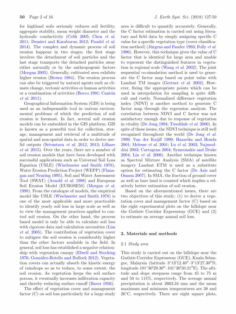
This study is carried out on the hillslope near theGuthrie Corridor Expressway (GCE), Kuala Selan-gor, Malaysia (latitude 3◦13′12.40′′–3◦13′27.30′′N;longitude 101◦30′29.30′′–101◦30′50.21′′E). The alti-tude and slope steepness range from 45 to 75 mand 50 to 115%, respectively. The average annualprecipitation is about 2663.34 mm and the meanmaximum and minimum temperatures are 38 and26◦C, respectively. There are eight square plots,

J. Earth Syst. Sci. (2018) 127:50 Page 3 of 16 50

Figure 1. Location of the study area.

64 (8 × 8 m) and 25 (5 × 5 m), situated at twodifferent locations as shown in figure 1. Each plotnamed as follows: Natural Bare Microbes (NBM),Natural Bare Non Microbes (NBNM), Planted LessDense Microbes (PLDM), Planted Less Dense NonMicrobes (PLDNM), Natural Dense Non Microbes(NDNM) and Natural Less Dense Non Microbes(NLDNM), are situated at the location 1 and Natu-ral Dense Microbes (NDM) and Natural Less DenseMicrobes (NLDM) are situated at the location 2.Table 1 presents detailed information about those

plots. The name given for each plot is based on thetwo criteria, i.e., level of vegetation cover densityand either the plot is microbes-treated or not. Alarge variety of plant species, viz., weeds, grasses,ferns and brushes height ranging from 0.5 to 2.0m are available as vegetation canopy in the plots.The infiltration capacity is ranging from 3.18 to7.62 mm h−1 implies that all plots are categorizedunder Group B till A+ based on the hydrologic soilgroup (HSG), which means infiltration varies frommoderately-well to well-draining soils. In terms of


Table

1.Hyd

rologicalandphysicalpropertiesofsoilsofthestudyarea.

Plo

ts

NB

NM

PLD

NM

NB

MP

LD

MN

LD

NM

ND

NM

NLD

MN

DM

Des

crip

tion

Natu

ralbare

nonm

icro

bes

Pla

nte

dle

ssden

se

nonm

icro

bes

Natu

ralbare

mic

robes

Pla

nte

dle

ss

den

sem

icro

bes

Natu

ralle

ssden

se

nonm

icro

bes

Natu

ralden

se

nonm

icro

bes

Natu

ralle

ss

den

sem

icro

bes

Natu

ralden

se

mic

robes

Plo

tsi

ze(m

×m

)8

×8

8×

88

×8

8×

85

×5

5×

58

×8

8×

8

HSG

AA

BB

BB

A+

A+

Avg.el

evati

on

(m)

69.5

870.8

874.3

974.3

973.5

673.5

646.3

444.9

6

Slo

pe

(%)

80.0

657.7

357.7

357.7

380.0

680.0

6113.3

880.0

6

Per

mea

bility

code

22

22

22

11

Soil

pro

per

ties

Sand

(%)

58.1

458.1

468.0

968.0

960.9

260.9

285.4

485.4

4

Silt

(%)

40.4

440.4

429.6

429.6

435.0

535.0

514.0

314.0

3

Cla

y(%

)1.4

01.4

02.2

52.2

53.1

33.1

30.3

90.3

9

Org

anic

matt

er(%

)0.3

00.3

00.2

30.2

30.7

30.7

30.2

30.2

3

Soil

textu

re2

(fine

gra

nula

r)and

3(m

ediu

mor

coars

egra

nula

r)

Note

:H

SG

:H

ydro

logic

soil

gro

up,A

+,A

,and

Bst

and

for

ver

ylo

w,lo

w,and

moder

ate

lylo

wru

noff

pote

nti

al,

resp

ecti

vel

y.

soil texture, the experimental plots are classifiedunder Group 2 and 3 whose soil texture varies fromfine to coarse granular.

2.2 Methods

The RUSLE model developed by Kanungo andSharma (2014) is employed to assess soil erosionscenario in this study. The RUSLE equation isexpressed as:

A = R×K × LS × C × P (1)

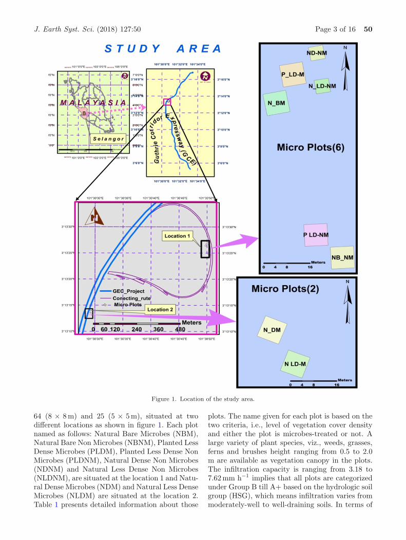
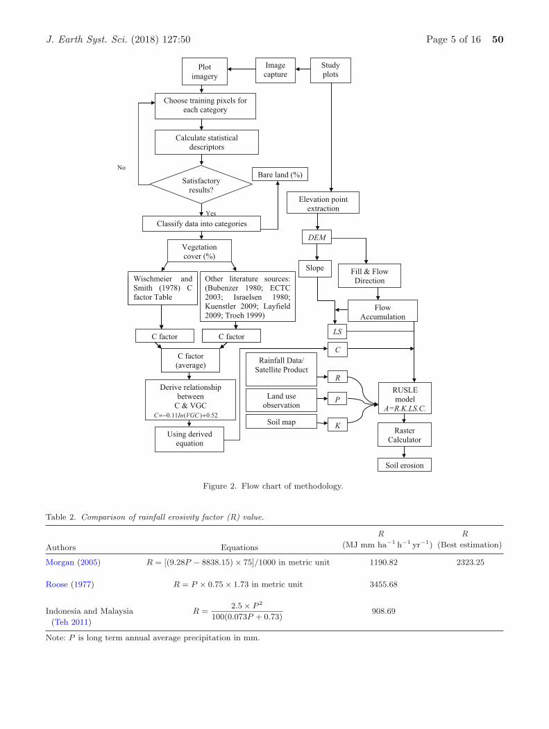
where A is the soil loss (t ha−1 yr−1); R is therainfall erosivity factor (MJ mm ha−1 h−1 yr−1);K is the soil erodibility factor (t h MJ−1 mm−1);LS is the slope length and steepness factor(dimensionless); C is the vegetation cover andmanagement factor (dimensionless), and P is thesupport practice factor (dimensionless). The over-all methodology of this study is presented schemat-ically in figure 2 and the subsequent paragraphsdescribe in detail about the preparation of RUSLEparameters.

2.2.1 Rainfall erosivity factor (R)

The potential erosion of a given rainstorm fora specific geographic location is represented bythe rainfall erosivity factor (R) (Kinnell 2014).The R is the product of event kinetic energy (E)and the maximum 30 min rainfall intensity (I30)(Wischmeier and Smith 1978). As the temporalresolution of the precipitation is not suitable tocalculate the EI30 for the study area, thereby,R is calculated based on the mean annual pre-cipitation (P). To calculate the R factor, severalformulas have been developed based on the meanannual rainfall throughout the world. This studyuses three different empirical equations developedby Roose (1977), Morgan (2005) and Teh (2011)to determine the R factor. The annual precipita-tion of the study area for the year of 2000 until2013 varies from 2237 (minimum rainfall recordedin 2002) to 3048 mm (maximum rainfall recordedin 2008). Based on the average annual precipi-tation, the R factor is calculated by employingthree different equations as shown (table 2). Thebest estimation should be the average of two Rvalues calculated by Morgan and Rose equations(Mir et al. 2010) that gives the average value of2323.25 MJ mm ha−1h−1 yr−1. This final value isused as R factor in this study.


No

Yes

Soil erosion

RUSLE model

A=R.K.LS.C.

DEM

Fill & Flow Direction

Slope

Flow Accumulation

LS

C

Elevation pointextraction

Plotimagery

Choose training pixels for each category

Soil map

Land use observation

Rainfall Data/Satellite Product

K

R

P

Studyplots

Imagecapture

WISCHMEIER AND SMITH’S C FACTOR

TABLE

C factor

OTHER LITERATURE SOURCES: (BUBENZER, 1980; ECTC, 2003;

ISRAELSEN C.E., 1980; KUENSTLER W, 2009; LAYFIELD,

2009; TROEH F.R., 1999)

C FACTOR

C FACTOR (AVERAGE)

Calculate statistical descriptors

Classify data into categories

Bare land (%)Satisfactory

results?

RasterCalculator

Using derived equation

Derive relationship between

C & VGC52.0)(11.0 +−= VGCInC

Vegetation cover (%)

Wischmeier andSmith (1978) C factor Table

Other literature sources: (Bubenzer 1980; ECTC2003; Israelsen 1980; Kuenstler 2009; Layfield2009; Troeh 1999)

C factor

C factor (average)

Figure 2. Flow chart of methodology.

Table 2. Comparison of rainfall erosivity factor (R) value.

Authors Equations

R

(MJ mm ha−1 h−1 yr−1)

R

(Best estimation)

Morgan (2005) R = [(9.28P − 8838.15) × 75]/1000 in metric unit 1190.82 2323.25

Roose (1977) R = P × 0.75 × 1.73 in metric unit 3455.68

Indonesia and Malaysia

(Teh 2011)

R =2.5 × P 2

100(0.073P + 0.73)908.69

Note: P is long term annual average precipitation in mm.


2.2.2 Soil erodibility factor (K)

The soil erodibility factor (K) is about the inherenterodibility of soil. It is a measure of susceptibilityof soil to be detached and transported by precipita-tion and surface runoff. K factor can be determinedexperimentally by integrating several soil charac-teristics such as texture, structure, organic mattercontent and permeability. The nomograph can alsobe used for calculating the K value; however,the K factor shows significantly overestimated forMalaysia soil series. Conversely, the K factor forthe study area is determined based on the obser-vation data and the analytical relationship. Theanalytical relationship developed for Malaysia soilseries is as follows:

K = [1.0 × (10−4

)M1.14 (12 −OM)

+4.5 (s− 3) + 8.0 (p− 2)]/100 (2)

where K is the soil erodibility (t h MJ−1mm−1),OM is the percentage of organic matters, s isthe soil structure code and p stands for the per-meability class and M is particle size parametercalculated as follows:

M = (%silt + %very fine sand)

×(100 − %clay). (3)

2.2.3 Slope length and steepness factor (LS)

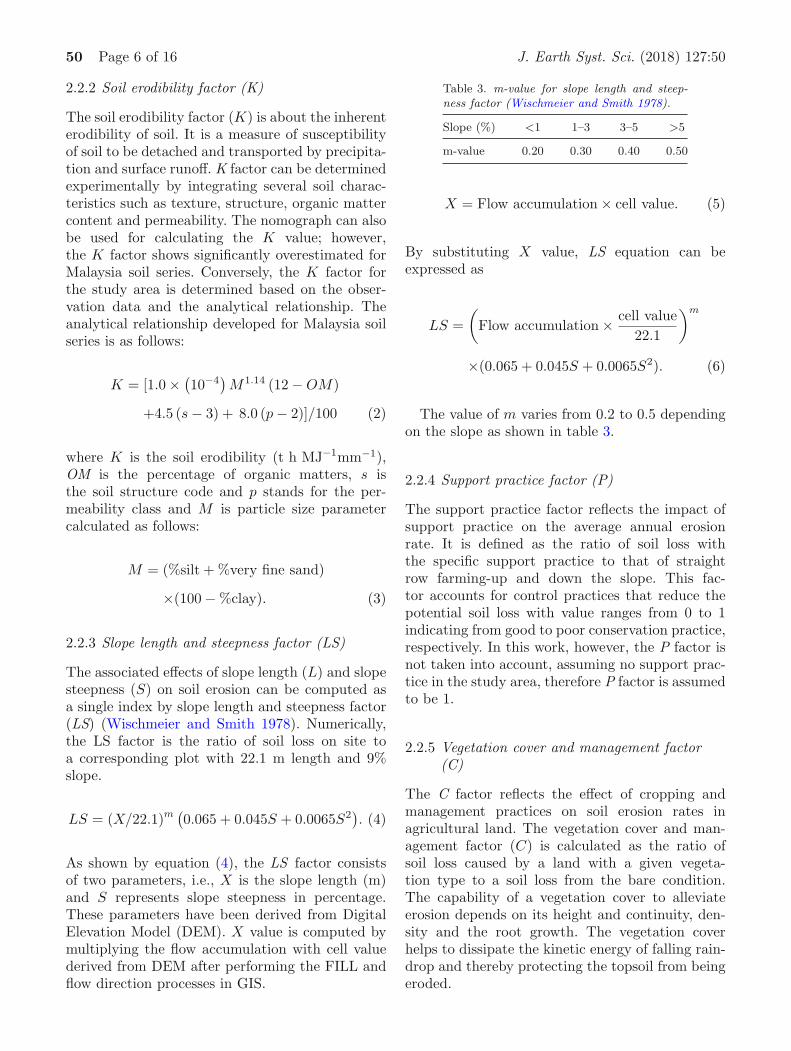
The associated effects of slope length (L) and slopesteepness (S) on soil erosion can be computed asa single index by slope length and steepness factor(LS) (Wischmeier and Smith 1978). Numerically,the LS factor is the ratio of soil loss on site toa corresponding plot with 22.1 m length and 9%slope.

LS = (X/22.1)m(0.065 + 0.045S + 0.0065S2

). (4)

As shown by equation (4), the LS factor consistsof two parameters, i.e., X is the slope length (m)and S represents slope steepness in percentage.These parameters have been derived from DigitalElevation Model (DEM). X value is computed bymultiplying the flow accumulation with cell valuederived from DEM after performing the FILL andflow direction processes in GIS.

Table 3. m-value for slope length and steep-ness factor (Wischmeier and Smith 1978).

Slope (%) <1 1–3 3–5 >5

m-value 0.20 0.30 0.40 0.50

X = Flow accumulation × cell value. (5)

By substituting X value, LS equation can beexpressed as

LS =(

Flow accumulation × cell value22.1

)m

×(0.065 + 0.045S + 0.0065S2). (6)

The value of m varies from 0.2 to 0.5 dependingon the slope as shown in table 3.

2.2.4 Support practice factor (P)

The support practice factor reflects the impact ofsupport practice on the average annual erosionrate. It is defined as the ratio of soil loss withthe specific support practice to that of straightrow farming-up and down the slope. This fac-tor accounts for control practices that reduce thepotential soil loss with value ranges from 0 to 1indicating from good to poor conservation practice,respectively. In this work, however, the P factor isnot taken into account, assuming no support prac-tice in the study area, therefore P factor is assumedto be 1.

2.2.5 Vegetation cover and management factor(C)

The C factor reflects the effect of cropping andmanagement practices on soil erosion rates inagricultural land. The vegetation cover and man-agement factor (C) is calculated as the ratio ofsoil loss caused by a land with a given vegeta-tion type to a soil loss from the bare condition.The capability of a vegetation cover to alleviateerosion depends on its height and continuity, den-sity and the root growth. The vegetation coverhelps to dissipate the kinetic energy of falling rain-drop and thereby protecting the topsoil from beingeroded.


3. Results and discussions

3.1 Vegetation cover and management factorderivation (C)

As the derivation of C factor is the main focus ofthis study, a detailed procedure is presented here.The images of vegetation cover for all plots aretaken by using a ground-digital camera and thoseimages are processed using an image classificationtool in the ArcGIS10.1. Methods used for process-ing and classifying the images are supervised clas-sification and maximum likelihood algorithm. Themaximum likelihood algorithm has been exten-sively used throughout the world for classifyingsatellite images (Vorovencii 2005). According tothis method, pixels with the similar spectral valuecan be categorized under specific classes and thesesimilarities or likelihoods are identical for all classesand that the input bands are uniformly distributed.This method, however, is a time consuming methodand provides output based on normal distributionof data in each band (Vorovencii and Muntean2012). The coverage of vegetation ground coveris determined through the ratio of pixels con-tained by vegetation ground cover and plot areaindividually.

In Malaysia, the C factor retrieval was doneby considering three land use types, i.e., repli-cated forest and undisturbed land, agricultural and

urbanized area and best management practices(BMPs) at construction sites (Department of Irri-gation and Drainage, Malaysia 2008). All plots areconsidered under the third category. As the guide-line for retrieving the C factor for the studied plotsis unclear, alternative method is suggested wherebythe calculation of C is based on the similar landuse type used by previous researchers. As a result,this study has utilized several established formu-las for the C value computation. First, Wischmeierand Smith (1978) model that requires only a per-centage of vegetation ground cover and types ofvegetation as input parameters. Those vegetationtypes are: (a) grasses or weeds with no appreciablecanopy; (b) tall weeds or short brush of 0.5 m fallheight with surface cover of decayed litter at least50 mm deep or surface cover of undecayed residue;(c) appreciable brush of 2 m height with surfacecover of decayed litter at least 50 mm deep or sur-face cover of undecayed residue, and (d) tree but noappreciable brush of 4 m height with surface coverof decayed litter at least 50 mm deep or surfacecover of undecayed residue. Second, the C fac-tor determined by several other models proposedby researchers (Bubenzer and Ka 1980; Israelsenet al. 1980; Troeh and Donahue 1999; ECTC 2003;Kuenstler 2009; Layfield 2009). In these methods,the corresponding C factor is assigned for a cer-tain type of vegetation with a specific vegetationdensity. All the C values obtained by the first and

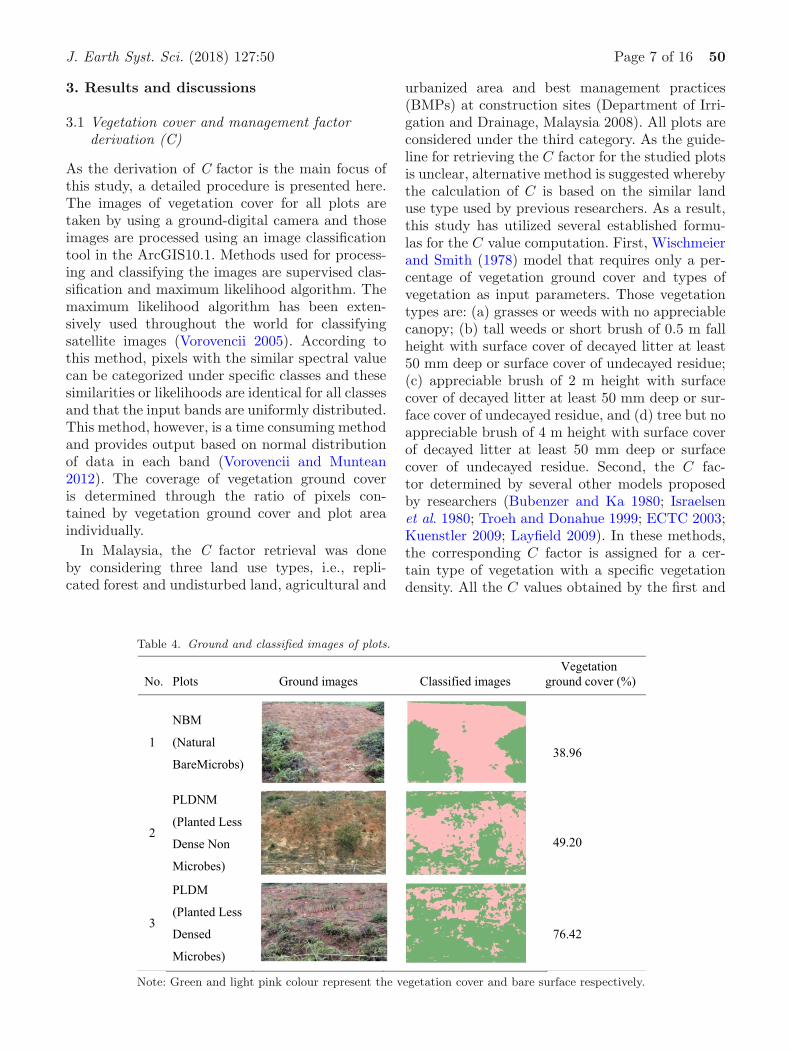
Table 4. Ground and classified images of plots.

No. Plots Ground images Classified imagesVegetation

ground cover (%)

1

NBM

(Natural

BareMicrobs)38.96

2

PLDNM

(Planted Less

Dense Non

Microbes)

49.20

3

PLDM

(Planted Less

Densed

Microbes)

76.42

Note: Green and light pink colour represent the vegetation cover and bare surface respectively.


second methods are then linking to the vegetationground cover.

Now, all plots have a set of two C values,whereby a final value is calculated by averagingthose two values. Finally, the relationship betweenvegetation ground cover (VGC) and the averageC factor is determined. After the preparation ofRUSLE parameters such as R, K, LS, P, and C asraster layers, the average annual erosion is finallyobtained by integrating the RUSLE model in aGIS platform. Using the raster calculator in spa-tial analyst tool, the soil erosion risk map is thengenerated.

3.2 Result of the C factor

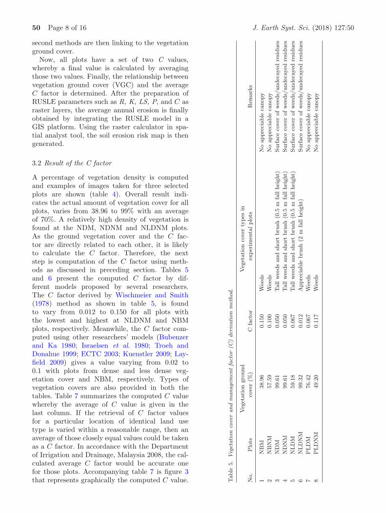
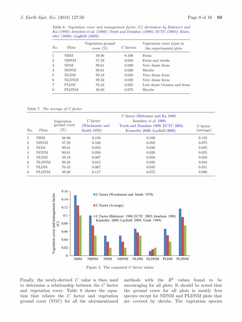
A percentage of vegetation density is computedand examples of images taken for three selectedplots are shown (table 4). Overall result indi-cates the actual amount of vegetation cover for allplots, varies from 38.96 to 99% with an averageof 70%. A relatively high density of vegetation isfound at the NDM, NDNM and NLDNM plots.As the ground vegetation cover and the C fac-tor are directly related to each other, it is likelyto calculate the C factor. Therefore, the nextstep is computation of the C factor using meth-ods as discussed in preceding section. Tables 5and 6 present the computed C factor by dif-ferent models proposed by several researchers.The C factor derived by Wischmeier and Smith(1978) method as shown in table 5, is foundto vary from 0.012 to 0.150 for all plots withthe lowest and highest at NLDNM and NBMplots, respectively. Meanwhile, the C factor com-puted using other researchers’ models (Bubenzerand Ka 1980; Israelsen et al. 1980; Troeh andDonahue 1999; ECTC 2003; Kuenstler 2009; Lay-field 2009) gives a value varying from 0.02 to0.1 with plots from dense and less dense veg-etation cover and NBM, respectively. Types ofvegetation covers are also provided in both thetables. Table 7 summarizes the computed C valuewhereby the average of C value is given in thelast column. If the retrieval of C factor valuesfor a particular location of identical land usetype is varied within a reasonable range, then anaverage of those closely equal values could be takenas a C factor. In accordance with the Departmentof Irrigation and Drainage, Malaysia 2008, the cal-culated average C factor would be accurate onefor those plots. Accompanying table 7 is figure 3that represents graphically the computed C value. Table

5.Vegetationcoverandmanagemen

tfactor(C

)derivationmethod.

No.

Plo

ts

Veg

etati

on

gro

und

cover

(%)

Cfa

ctor

Veg

etati

on

cover

types

in

exper

imen

talplo

tsR

emark

s

1N

BM

38.9

60.1

50

Wee

ds

No

appre

ciable

canopy

2N

BN

M57.5

90.1

00

Wee

ds

No

appre

ciable

canopy

3N

DM

99.6

10.0

50

Tall

wee

ds

and

short

bru

sh(0

.5m

fall

hei

ght)

Surf

ace

cover

ofw

eeds/

undec

ayed

resi

dues

4N

DN

M99.6

10.0

50

Tall

wee

ds

and

short

bru

sh(0

.5m

fall

hei

ght)

Surf

ace

cover

ofw

eeds/

undec

ayed

resi

dues

5N

LD

M59.1

80.0

67

Tall

wee

ds

and

short

bru

sh(0

.5m

fall

hei

ght)

Surf

ace

cover

ofw

eeds/

undec

ayed

resi

dues

6N

LD

NM

99.3

20.0

12

Appre

ciable

bru

sh(2

mfa

llhei

ght)

Surf

ace

cover

ofw

eeds/

undec

ayed

resi

dues

7P

LD

M76.4

20.0

67

Wee

ds

No

appre

ciable

canopy

8P

LD

NM

49.2

00.1

17

Wee

ds

No

appre

ciable

canopy


Table 6. Vegetation cover and management factor (C) derivation by Bubenzer andKa (1980); Israelsen et al. (1980); Troeh and Donahue (1999); ECTC (2003); Kuen-stler (2009); Layfield (2009).

No. PlotsVegetation ground

cover (%) C factorsVegetation cover types in

the experimental plots

1 NBM 38.96 0.100 Ferns

2 NBNM 57.59 0.050 Ferns and weeds

3 NDM 99.61 0.020 Very dense ferns

4 NDNM 99.61 0.020 Shrubs

5 NLDM 59.18 0.050 Very dense ferns

6 NLDNM 99.32 0.020 Very dense ferns

7 PLDM 76.42 0.035 Less dense Grasses and ferns

8 PLDNM 49.20 0.075 Shrubs

Table 7. The average of C factor.

No. Plots

Vegetationground cover

(%)

C factor

(Wischmeier and

Smith 1978)

C factor (Bubenzer and Ka 1980;

Israelsen et al. 1980;

Troeh and Donahue 1999; ECTC 2003;

Kuenstler 2009; Layfield 2009)C factor(average)

1 NBM 38.96 0.150 0.100 0.125

2 NBNM 57.59 0.100 0.050 0.075

3 NDM 99.61 0.050 0.020 0.035

4 NDNM 99.61 0.050 0.020 0.035

5 NLDM 59.18 0.067 0.050 0.058

6 NLDNM 99.32 0.012 0.020 0.016

7 PLDM 76.42 0.067 0.035 0.051

8 PLDNM 49.20 0.117 0.075 0.096

0

0.02

0.04

0.06

0.08

0.1

0.12

0.14

0.16

NBM NBNM NDM NDNM NLDM NLDNM PLDM PLDNM

Veg

etat

ion

cove

r and

man

agem

ent f

acto

r (C

)

C Factor (Wischmeier and Smith 1978)

C Factor (Average)

C Factor (Bubenzer 1980; ECTC 2003; Israelsen 1980;Kuenstler 2009; Layfield 2009; Troeh 1999)

Figure 3. The computed C factor values.

Finally, the newly-derived C value is then usedto determine a relationship between the C factorand vegetation cover. Table 8 shows the equa-tion that relates the C factor and vegetationground cover (VGC) for all the aforementioned

methods with the R2 values found to beencouraging for all plots. It should be noted thatthe ground cover for all plots is mostly fernspecies except for NDNM and PLDNM plots thatare covered by shrubs. The vegetation species


Table 8. Relationship between VGC and C factor.

No. Relationships R2 Methods followed

1 C = −0.13 ln(V GC) + 0.62 0.92 Graphs related to ground vegetation cover and C

factors (Wischmeier and Smith 1978)

2 C = −0.083 ln(V GC) + 0.41 0.94 Literature review (Bubenzer and Ka 1980;

Israelsen et al. 1980; Troeh and Donahue

1999; ECTC 2003; Kuenstler 2009;

Layfield 2009)

3 C = −0.11 ln(V GC) + 0.52 0.95 Averaging rational value of the vegetation

cover and management factors (C )

Figure 4. (a, b and c) Soil loss per year and RUSLE parameters for different plots.


Figure 4. (Continued).

mentioned here serves as a reference only; the roleof vegetation species in calculating the C factor,however, is not considered.

3.3 Soil erosion

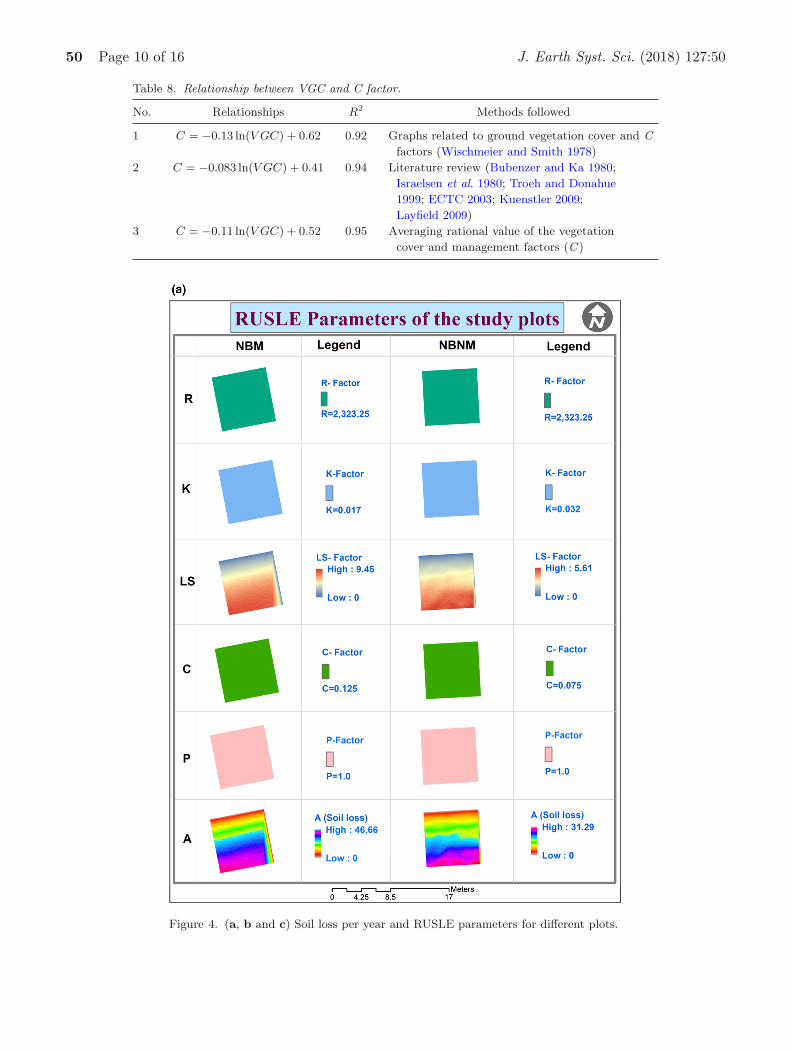
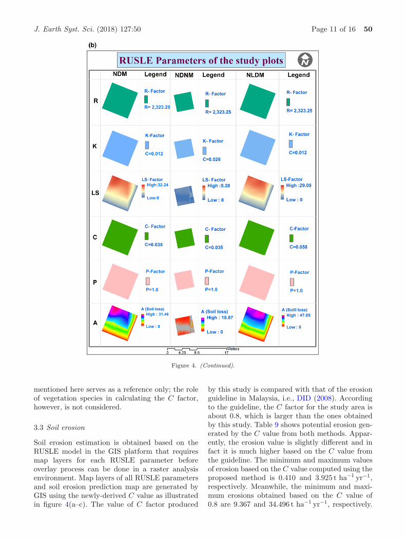
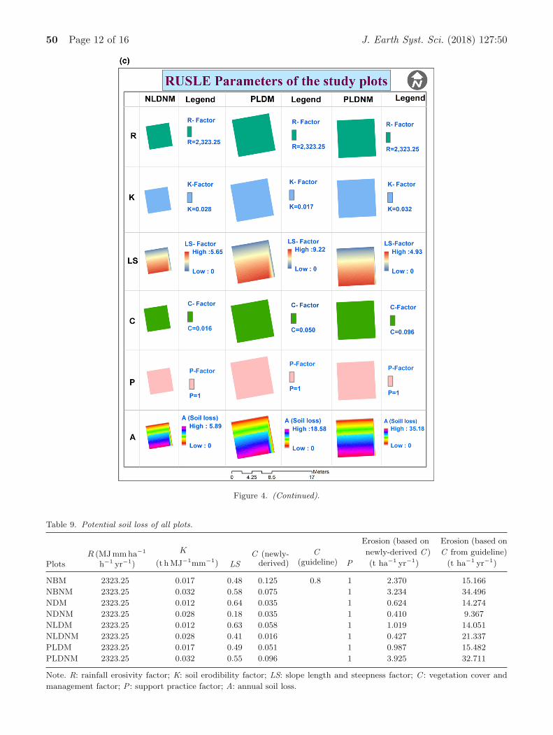
Soil erosion estimation is obtained based on theRUSLE model in the GIS platform that requiresmap layers for each RUSLE parameter beforeoverlay process can be done in a raster analysisenvironment. Map layers of all RUSLE parametersand soil erosion prediction map are generated byGIS using the newly-derived C value as illustratedin figure 4(a–c). The value of C factor produced

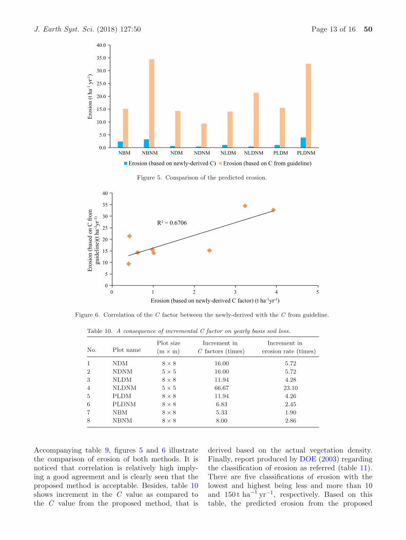
by this study is compared with that of the erosionguideline in Malaysia, i.e., DID (2008). Accordingto the guideline, the C factor for the study area isabout 0.8, which is larger than the ones obtainedby this study. Table 9 shows potential erosion gen-erated by the C value from both methods. Appar-ently, the erosion value is slightly different and infact it is much higher based on the C value fromthe guideline. The minimum and maximum valuesof erosion based on the C value computed using theproposed method is 0.410 and 3.925 t ha−1 yr−1,respectively. Meanwhile, the minimum and maxi-mum erosions obtained based on the C value of0.8 are 9.367 and 34.496 t ha−1 yr−1, respectively.


Figure 4. (Continued).

Table 9. Potential soil loss of all plots.

PlotsR (MJ mm ha−1

h−1 yr−1)

K

(t h MJ−1mm−1) LSC (newly-

derived)

C(guideline) P

Erosion (based on

newly-derived C )

(t ha−1 yr−1)

Erosion (based on

C from guideline)

(t ha−1 yr−1)

NBM 2323.25 0.017 0.48 0.125 0.8 1 2.370 15.166

NBNM 2323.25 0.032 0.58 0.075 1 3.234 34.496

NDM 2323.25 0.012 0.64 0.035 1 0.624 14.274

NDNM 2323.25 0.028 0.18 0.035 1 0.410 9.367

NLDM 2323.25 0.012 0.63 0.058 1 1.019 14.051

NLDNM 2323.25 0.028 0.41 0.016 1 0.427 21.337

PLDM 2323.25 0.017 0.49 0.051 1 0.987 15.482

PLDNM 2323.25 0.032 0.55 0.096 1 3.925 32.711

Note. R: rainfall erosivity factor; K: soil erodibility factor; LS: slope length and steepness factor; C : vegetation cover and

management factor; P : support practice factor; A: annual soil loss.


0.0

5.0

10.0

15.0

20.0

25.0

30.0

35.0

40.0

NBM NBNM NDM NDNM NLDM NLDNM PLDM PLDNM

Eros

ion

(t ha

-1yr

-1)

Erosion (based on newly-derived C) Erosion (based on C from guideline)

Figure 5. Comparison of the predicted erosion.

R² = 0.6706

0

5

10

15

20

25

30

35

40

0 1 2 3 4 5

Eros

ion

(bas

ed o

n C

from

gu

idel

ine)

(t ha

-1yr

- 1)

Erosion (based on newly-derived C factor) (t ha-1yr-1)

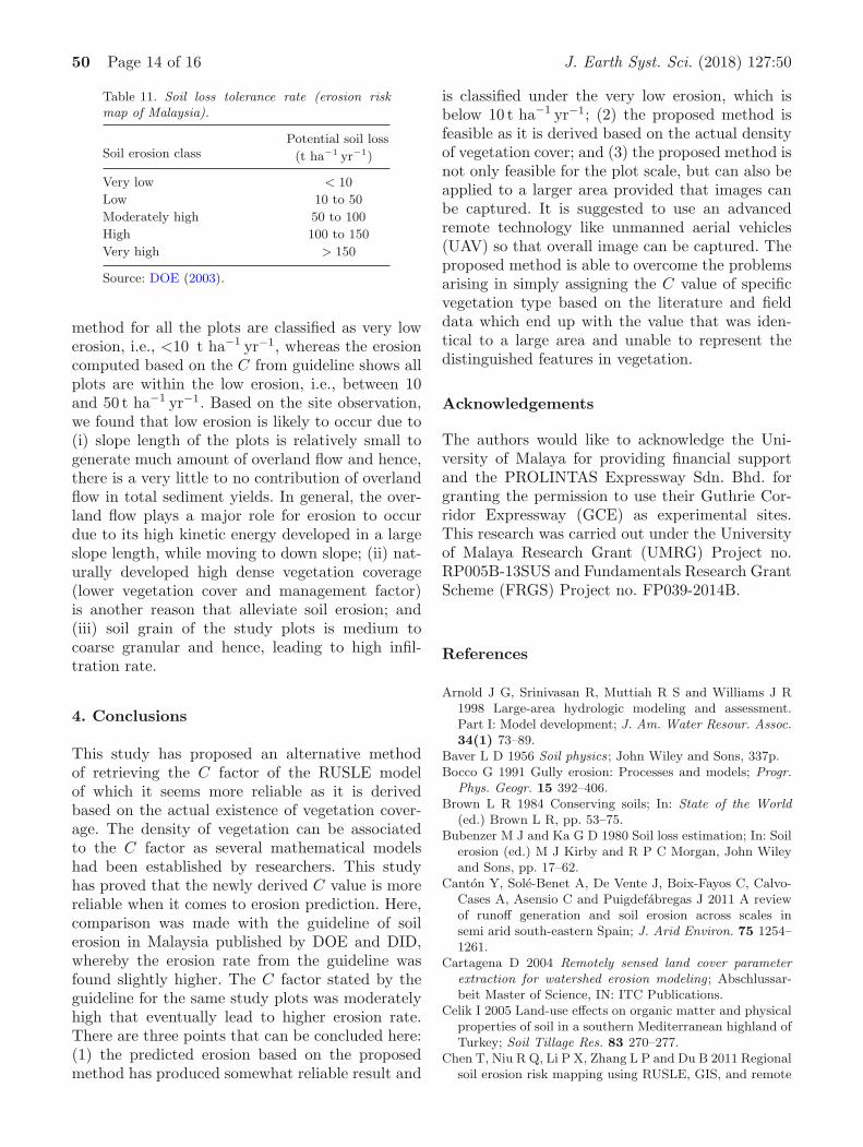
Figure 6. Correlation of the C factor between the newly-derived with the C from guideline.

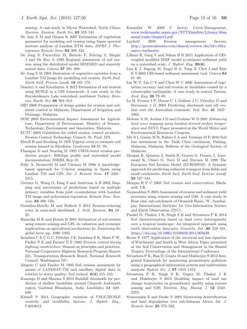
Table 10. A consequence of incremental C factor on yearly basis soil loss.

No. Plot namePlot size

(m × m)

Increment in

C factors (times)

Increment in

erosion rate (times)

1 NDM 8 × 8 16.00 5.72

2 NDNM 5 × 5 16.00 5.72

3 NLDM 8 × 8 11.94 4.28

4 NLDNM 5 × 5 66.67 23.10

5 PLDM 8 × 8 11.94 4.26

6 PLDNM 8 × 8 6.83 2.45

7 NBM 8 × 8 5.33 1.90

8 NBNM 8 × 8 8.00 2.86

Accompanying table 9, figures 5 and 6 illustratethe comparison of erosion of both methods. It isnoticed that correlation is relatively high imply-ing a good agreement and is clearly seen that theproposed method is acceptable. Besides, table 10shows increment in the C value as compared tothe C value from the proposed method, that is

derived based on the actual vegetation density.Finally, report produced by DOE (2003) regardingthe classification of erosion as referred (table 11).There are five classifications of erosion with thelowest and highest being less and more than 10and 150 t ha−1 yr−1, respectively. Based on thistable, the predicted erosion from the proposed


Table 11. Soil loss tolerance rate (erosion riskmap of Malaysia).

Soil erosion classPotential soil loss

(t ha−1 yr−1)

Very low < 10

Low 10 to 50

Moderately high 50 to 100

High 100 to 150

Very high > 150

Source: DOE (2003).

method for all the plots are classified as very lowerosion, i.e., <10 t ha−1 yr−1, whereas the erosioncomputed based on the C from guideline shows allplots are within the low erosion, i.e., between 10and 50 t ha−1 yr−1. Based on the site observation,we found that low erosion is likely to occur due to(i) slope length of the plots is relatively small togenerate much amount of overland flow and hence,there is a very little to no contribution of overlandflow in total sediment yields. In general, the over-land flow plays a major role for erosion to occurdue to its high kinetic energy developed in a largeslope length, while moving to down slope; (ii) nat-urally developed high dense vegetation coverage(lower vegetation cover and management factor)is another reason that alleviate soil erosion; and(iii) soil grain of the study plots is medium tocoarse granular and hence, leading to high infil-tration rate.

4. Conclusions

This study has proposed an alternative methodof retrieving the C factor of the RUSLE modelof which it seems more reliable as it is derivedbased on the actual existence of vegetation cover-age. The density of vegetation can be associatedto the C factor as several mathematical modelshad been established by researchers. This studyhas proved that the newly derived C value is morereliable when it comes to erosion prediction. Here,comparison was made with the guideline of soilerosion in Malaysia published by DOE and DID,whereby the erosion rate from the guideline wasfound slightly higher. The C factor stated by theguideline for the same study plots was moderatelyhigh that eventually lead to higher erosion rate.There are three points that can be concluded here:(1) the predicted erosion based on the proposedmethod has produced somewhat reliable result and

is classified under the very low erosion, which isbelow 10 t ha−1 yr−1; (2) the proposed method isfeasible as it is derived based on the actual densityof vegetation cover; and (3) the proposed method isnot only feasible for the plot scale, but can also beapplied to a larger area provided that images canbe captured. It is suggested to use an advancedremote technology like unmanned aerial vehicles(UAV) so that overall image can be captured. Theproposed method is able to overcome the problemsarising in simply assigning the C value of specificvegetation type based on the literature and fielddata which end up with the value that was iden-tical to a large area and unable to represent thedistinguished features in vegetation.

Acknowledgements

The authors would like to acknowledge the Uni-versity of Malaya for providing financial supportand the PROLINTAS Expressway Sdn. Bhd. forgranting the permission to use their Guthrie Cor-ridor Expressway (GCE) as experimental sites.This research was carried out under the Universityof Malaya Research Grant (UMRG) Project no.RP005B-13SUS and Fundamentals Research GrantScheme (FRGS) Project no. FP039-2014B.

References

Arnold J G, Srinivasan R, Muttiah R S and Williams J R1998 Large-area hydrologic modeling and assessment.Part I: Model development; J. Am. Water Resour. Assoc.34(1) 73–89.

Baver L D 1956 Soil physics; John Wiley and Sons, 337p.Bocco G 1991 Gully erosion: Processes and models; Progr.

Phys. Geogr. 15 392–406.Brown L R 1984 Conserving soils; In: State of the World

(ed.) Brown L R, pp. 53–75.Bubenzer M J and Ka G D 1980 Soil loss estimation; In: Soil

erosion (ed.) M J Kirby and R P C Morgan, John Wileyand Sons, pp. 17–62.

Canton Y, Sole-Benet A, De Vente J, Boix-Fayos C, Calvo-Cases A, Asensio C and Puigdefabregas J 2011 A reviewof runoff generation and soil erosion across scales insemi arid south-eastern Spain; J. Arid Environ. 75 1254–1261.

Cartagena D 2004 Remotely sensed land cover parameterextraction for watershed erosion modeling ; Abschlussar-beit Master of Science, IN: ITC Publications.

Celik I 2005 Land-use effects on organic matter and physicalproperties of soil in a southern Mediterranean highland ofTurkey; Soil Tillage Res. 83 270–277.

Chen T, Niu R Q, Li P X, Zhang L P and Du B 2011 Regionalsoil erosion risk mapping using RUSLE, GIS, and remote


sensing: A case study in Miyun Watershed, North China;Environ. Environ. Earth Sci. 63 533–541.

De Asis A M and Omasa K 2007 Estimation of vegetationparameter for modeling soil erosion using linear spectralmixture analysis of Landsat ETM data; ISPRS J. Pho-togramm Remote Sens. 62 309–324.

De Jong S, Paracchini M, Bertolo F, Folving S, MegierJ and De Roo A 1999 Regional assessment of soil ero-sion using the distributed model SEMMED and remotelysensed data; Catena 37 291–308.

De Jong S M 1994 Derivation of vegetative variables from aLandsat TM image for modelling soil erosion; Earth Surf.Earth Surf. Process Landf. 19 165–178.

Demirci A and Karaburun A 2012 Estimation of soil erosionusing RUSLE in a GIS framework: A case study in theBuyukcekmece Lake watershed, northwest Turkey; Envi-ron. Earth. Sci. 66 903–913.

DID 2008 Preparation of design guides for erosion and sed-iment control in Malaysia: Department of Irrigation andDrainage, Malaysia.

DOE 2003 Environmental Impact Assessment for Agricul-ture; Department of Environment, Ministry of Science,Technology, Environment and Innovation, Malaysia.

ECTC 2003 Guidelines for rolled erosion control products;Erosion Control Technology Council, St. Paul, MN.

Elwell H and Stocking M 1976 Vegetal cover to estimate soilerosion hazard in Rhodesia; Geoderma 15 61–70.

Flanagan D and Nearing M 1995 USDA-water erosion pre-diction project: Hillslope profile and watershed modeldocumentation; NSERL Rep 10.

Folly A, Bronsveld M and Clavaux M 1996 A knowledge-based approach for C-factor mapping in Spain usingLandsat TM and GIS; Int. J. Remote Sens. 17 2401–2415.

Gertner G, Wang G, Fang S and Anderson A B 2002 Map-ping and uncertainty of predictions based on multipleprimary variables from joint co-simulation with LandsatTM image and polynomial regression; Remote Sens. Env-iron. 83 498–510.

Gonzalez-Botello M and Bullock S 2012 Erosion-reducingcover in semi-arid shrubland; J. Arid. Environ. 84 19–25.

Hazarika M K and Honda K 2001 Estimation of soil erosionusing remote sensing and GIS, its valuation and economicimplications on agricultural production; In: Sustaining theglobal farm, pp. 1090–1093.

Israelsen C E C G C, Fletcher J E, Israelsen E K, Haws F W,Packer P E and Farmer E E 1980 Erosion control duringhighway construction; Manual on principles and practices,National Cooperative Highway Research Program Report221, Transportation Research Board, National ResearchCouncil, Washington DC.

Jurgens C and Fander M 1993 Soil erosion assessment bymeans of LANDSAT-TM and ancillary digital data inrelation to water quality; Soil technol. 6(3) 215–223.

Kanungo D and Sharma S 2014 Rainfall thresholds for pre-diction of shallow landslides around Chamoli–Joshimathregion, Garhwal Himalayas, India Landslides 11 629–638.

Kinnell P 2014 Geographic variation of USLE/RUSLEerosivity and erodibility factors; J. Hydrol. Eng.,C4014012.

Kuenstler W 2009 C factor: Cover-Management,www.techtransfer.osmre.gov/NTTMainSite/Library/hbmanual/rusle/chapter5.pdf.

Layfield 2009 Erosion management factors;http://geomembranes.com/shared/resview.cfm?id=18&source=technotes.

Lilhare R, Garg V and Nikam B R 2015 Application of GIS-coupled modified MMF model to estimate sediment yieldon a watershed scale; J. Hydrol. Eng. 20(6)

Lim K J, Sagong M, Engel B A, Tang Z, Choi J and KimK S 2005 GIS-based sediment assessment tool; Catena 6461–80.

Lin W-T, Lin C-Y and Chou W C 2006 Assessment of vege-tation recovery and soil erosion at landslides caused by acatastrophic earthquake: A case study in central Taiwan;Ecol. Eng. 28 79–89.

Lu H, Prosser I P, Moran C J, Gallant J C, Priestley G andStevenson J G 2003 Predicting sheetwash and rill ero-sion over the Australian continent; Soil. Res. 41 1037–1062.

Melesse A M, Jordan J D and Graham W D 2001 Enhancingland cover mapping using Landsat derived surface temper-ature and NDVI ; Paper presented at the World Water andEnvironmental Resources Congress.

Mir S I, Gasim M B, Rahim S A and Toriman M E 2010 Soilloss assessment in the Tasik Chini catchment, Pahang,Malaysia, Malaysia; Bulletin of the Geological Society ofMalaysia.

Morgan R, Quinton J, Smith R, Govers G, Poesen J, Auer-swald K, Chisci G, Torri D and Styczen M 1998 TheEuropean Soil Erosion Model (EUROSEM): A dynamicapproach for predicting sediment transport from fields andsmall catchments; Earth Surf. Earth Surf. Process. Landf.23 527–544.

Morgan R P C 2005 Soil erosion and conservation; Black-well, UK.

Najmoddini N 2003 Assessment of erosion and sediment yieldprocesses using remote sensing and GIS: A case study inRose chai sub-catchment of Orumieh Basin, W. Azarbai-jan; International Institute for Geo-Information Scienceand Earth Observation (ITC).

Paudel D, Thakur J K, Singh S K and Srivastava P K 2014Soil characterization based on land cover heterogeneityover a tropical landscape: An integrated approach usingearth observation data-sets; Geocarto. Int. 30 218–241,https://doi.org/10.1080/10106049.2014.905639.

Roose E 1977 Application of the universal soil loss equationof Wischmeier and Smith in West Africa; Paper presentedat the Soil Conservation and Management in the HumidTropics; Proceedings of the International Conference.

Srivastava P K, Han D, Gupta M and Mukherjee S 2012 Inte-grated framework for monitoring groundwater pollutionusing a geographical information system and multivariateanalysis; Hydrol. Sci. J. 57 1453–1472.

Srivastava P K, Singh S K, Gupta M, Thakur J Kand Mukherjee S 2013 Modeling impact of land usechange trajectories on groundwater quality using remotesensing and GIS; Environ. Eng. Manag. J. 12 2343–2355.

Symeonakis E and Drake N 2004 Monitoring desertificationand land degradation over sub-Saharan Africa; Int. J.Remote Sens. 25 573–592.

www.techtransfer.osmre.gov/NTTMainSite/Library/hbmanual/rusle/chapter5.pdf

www.techtransfer.osmre.gov/NTTMainSite/Library/hbmanual/rusle/chapter5.pdf

http://geomembranes.com/shared/resview.cfm?id=18&source=technotes

http://geomembranes.com/shared/resview.cfm?id=18&source=technotes

https://doi.org/10.1080/10106049.2014.905639.


Teh S H 2011 Soil erosion modeling using RUSLE and GISon Cameron highlands, Malaysia for hydropower develop-ment.

Troeh F R and Donahue R L 1999 Soil and water conserva-tion: Productivity and environment protection; Prentice-Hall, New Jersey.

Tweddale S A, Echlschlaeger C R and Seybold W F 2000An improved method for spatial extrapolation of veg-etative cover estimates (USLE/RUSLE C factor) usingLCTA and remotely sensed imagery. US Army Corps ofEngineers, Engineer Research and Development Center,Construction Engineering Research Laboratory, ERDCTechnical Report.

Van der Knijff J, Jones R and Montanarella L 1999 Soilerosion risk assessment in Italy ; European Soil Burea.

Vorovencii I 2005 Researches concerning the possibilitiesof using satellite images in forest planning works. Doc-tor’s degree paper.“Transilvania” University of Brasov,294p.

Vorovencii I and Muntean D 2012 Evaluation of super-vised classification algorithms for Landsat 5 TM images.RevCAD; J. Geod. Cadas. 11 229–238.

Wang G, Wente S, Gertner G and Anderson A 2002 Improve-ment in mapping vegetation cover factor for the universalsoil loss equation by geostatistical methods with LandsatThematic Mapper images; Int. J. Remote Sens. 23 3649–3667.

Wischmeier W and Smith D 1978 Predicting rainfall erosionlosses; USDA Agricultural Research Services Handbook537, USDA, Washington DC.

Corresponding editor: Navin Juyal

Documents

Soil erosion assessment on hillslope of GCE using RUSLE model