Embed Size (px)
Citation preview
Technische Universität München
Lehrstuhl für Angewandte Mechanik
Spatial Dynamics of Pushbelt CVTs
Dipl.-Tech. Math. Univ. Thorsten Schindler
Vollständiger Abdruck der von der Fakultät für Maschinenwesen der
Technischen Universität München zur Erlangung des akademischen Grades eines
Doktor-Ingenieurs
genehmigten Dissertation.
Vorsitzender:
Univ.-Prof. Dr.-Ing. Bernd-Robert Höhn
Prüfer der Dissertation:
1. Univ.-Prof. Dr.-Ing. habil. Heinz Ulbrich
2. Univ.-Prof. Dr. rer. nat. habil. Martin Arnold, Martin-Luther-Universität Halle-Wittenberg
Die Dissertation wurde am 01.07.2010 bei der Technischen Universität München
eingereicht und durch die Fakultät für Maschinenwesen am 05.10.2010 angenommen.


III
Acknowledgment
This work summarises my results as scientific research assistant at the Institute ofApplied Mechanics of the Technische Universität München. It was initiated andfunded by Bosch Transmission Technology B.V.
The research project would not have been possible without the support of manypeople. I would like to express my gratitude to my supervisor Prof. Dr. HeinzUlbrich who took a great interest in the topic. He offered an invaluable assistanceand guidance but also the freedom to find one’s feet and to assume responsibility forthe different tasks at his institute. Especially the last articles are the reason thatthe time was such diversified, challenging and instructive in a convenient sense.
Deepest gratitude is also due to Prof. Dr. Martin Arnold for continuous and fruitfuldiscussions about numerical mathematics and multibody formulations at differentconferences; gratitude also for his support and for him being a member of the su-pervisory committee.
I would like to thank Prof. Dr. Friedrich Pfeiffer for his commitment and mentoring.The conversations about nonsmooth mechanics always stimulated the progress ofthe thesis and my understanding for this sophisticated research field.
The cooperation with Arie van der Velde, Han Pijpers and Arjen Brandsma of BoschTransmission Technology B.V. was always like with a good colleague. I will treasurethe visits for project meetings in Tilburg.
A main contribution of the excellent working atmosphere can be traced back to thecooperativeness of all colleagues at the institute. Special thanks to Markus Friedrichand Roland Zander, as well as the whole MBSim development crew for always beingavailable to approach the solution of tricky and difficult modelling and programmingquestions. Markus Friedrich and Jan Clauberg have provided a perfect computerpool for extensive simulations for instance during the validation process. Thanks toSebastian Lohmeier for making available his LATEXclasses and to Thomas Cebullafor his notably efficient project assumption. Proofreading of the manuscript surelywas not a nice job but the feedback of Markus Friedrich, Thomas Cebulla, Arie vander Velde and Claudia Kirmeyer was detailed and constructive.
Thanks to all my friends for giving the possibility to balance in my free time andfor providing lots of ideas apart from the day-to-day work.
I wish to express my gratitude to my family for their understanding and supportthrough the duration of my studies and doing a Doctor of Philosophy.
Garching, October 2010 Thorsten Schindler
IV
Unsere Zeit steckt, wie kaum eine andere zuvor,voller Möglichkeiten – zum Guten und Bösen.
Nichts kommt von selbst.Darum – besinnt Euch auf Eure Kraft und darauf,
dass jede Zeit eigene Antworten will und man auf ihrer Höhe zu sein hat,wenn Gutes bewirkt werden soll.
Willy Brandt
18.12.1913 – 08.10.1992
4th German Chancellor
22.10.1969 – 16.05.1974
Nobel Peace Prize Laureate
10.12.1971
read by Hans-Jochen Vogel on the occasion of the socialist
international congress in Berlin on 15.09.1992
Willy Brandt was already seriously ill at this time
V
Contents
1 Point of Departure 1
1.1 Pushbelt CVTs . . . . . . . . . . . . . . . . . . . . . . . . . . . . . . . . . . 1
1.1.1 Set Up and Functionality . . . . . . . . . . . . . . . . . . . . . . . . 2
1.1.2 Important Phenomena . . . . . . . . . . . . . . . . . . . . . . . . . . 3
1.1.3 Simulation Models . . . . . . . . . . . . . . . . . . . . . . . . . . . . 51.2 Nonsmooth Multibody Systems . . . . . . . . . . . . . . . . . . . . . . . . . 5
1.2.1 Measure Differential Equation . . . . . . . . . . . . . . . . . . . . . . 6
1.2.2 Contact Laws . . . . . . . . . . . . . . . . . . . . . . . . . . . . . . . 71.2.3 Contour Description . . . . . . . . . . . . . . . . . . . . . . . . . . . 8
1.3 Integration Schemes . . . . . . . . . . . . . . . . . . . . . . . . . . . . . . . 9
1.3.1 Event-Driven Integration Schemes . . . . . . . . . . . . . . . . . . . 9
1.3.2 Time-Stepping Integration Schemes . . . . . . . . . . . . . . . . . . 101.4 MBSim . . . . . . . . . . . . . . . . . . . . . . . . . . . . . . . . . . . . . . 11
2 Model of the Pushbelt CVT 13
2.1 Bodies . . . . . . . . . . . . . . . . . . . . . . . . . . . . . . . . . . . . . . . 13
2.1.1 Elements . . . . . . . . . . . . . . . . . . . . . . . . . . . . . . . . . 142.1.2 Ring Packages . . . . . . . . . . . . . . . . . . . . . . . . . . . . . . 19
2.1.3 Pulleys . . . . . . . . . . . . . . . . . . . . . . . . . . . . . . . . . . 27
2.2 Interactions . . . . . . . . . . . . . . . . . . . . . . . . . . . . . . . . . . . . 332.2.1 Pulley – Environment Interaction . . . . . . . . . . . . . . . . . . . . 33
2.2.2 Sheave – Sheave Joint . . . . . . . . . . . . . . . . . . . . . . . . . . 34
2.2.3 Element – Pulley Contacts . . . . . . . . . . . . . . . . . . . . . . . 34
2.2.4 Element – Ring Package Contacts . . . . . . . . . . . . . . . . . . . 432.2.5 Element – Element Contacts . . . . . . . . . . . . . . . . . . . . . . 45
2.3 Assembling and Initialisation . . . . . . . . . . . . . . . . . . . . . . . . . . 47
2.3.1 Kinematics . . . . . . . . . . . . . . . . . . . . . . . . . . . . . . . . 472.3.2 Kinetics . . . . . . . . . . . . . . . . . . . . . . . . . . . . . . . . . . 48
2.3.3 Pulleys . . . . . . . . . . . . . . . . . . . . . . . . . . . . . . . . . . 55
2.3.4 Ring Packages . . . . . . . . . . . . . . . . . . . . . . . . . . . . . . 57
2.3.5 Elements . . . . . . . . . . . . . . . . . . . . . . . . . . . . . . . . . 602.4 Summary . . . . . . . . . . . . . . . . . . . . . . . . . . . . . . . . . . . . . 62
2.5 CPU Time Reduction . . . . . . . . . . . . . . . . . . . . . . . . . . . . . . 62
2.5.1 Stabilisation of the Ring Package . . . . . . . . . . . . . . . . . . . . 632.5.2 Parallel Computing Architectures . . . . . . . . . . . . . . . . . . . . 65
2.5.3 Practical Evaluations and Experiences . . . . . . . . . . . . . . . . . 67
3 Results and Validation 72
3.1 Planar Validation with Local Data . . . . . . . . . . . . . . . . . . . . . . . 723.1.1 Element – Pulley Contacts . . . . . . . . . . . . . . . . . . . . . . . 73
3.1.2 Element – Ring Package Contacts . . . . . . . . . . . . . . . . . . . 75

VI Contents
3.1.3 Element – Element Contacts . . . . . . . . . . . . . . . . . . . . . . 773.2 Spatial Validation with Global Data . . . . . . . . . . . . . . . . . . . . . . 78
3.2.1 Thrust Ratio . . . . . . . . . . . . . . . . . . . . . . . . . . . . . . . 783.2.2 Spiral Running . . . . . . . . . . . . . . . . . . . . . . . . . . . . . . 783.2.3 Alignment Setting . . . . . . . . . . . . . . . . . . . . . . . . . . . . 80
4 Conclusion 83
Bibliography 85
VII
Abstract
With a pushbelt continuously variable transmission (CVT), the whole drivetrainincluding the engine of a passenger car can operate in an optimal state at any time.For further improvements with respect to fuel consumption, dynamic simulationsof the system have been investigated by Bosch Transmission Technology B.V. andthe Institute of Applied Mechanics of the Technische Universität München in recentyears.
The underlying mathematical models are characterised by numerous contacts and alarge degree of freedom. In order to avoid high numerical stiffnesses due to springsand to encourage an efficient as well as a stable and robust numerical treatment, anonsmooth contact description is chosen. Timestepping schemes are used to inte-grate the resulting measure differential inclusions.
This work deals with a spatial transient mathematical model of pushbelt continu-ously variable transmissions to consider also out-of-plane effects, for instance push-belt misalignment. The equations of motion result from using methods of multibodytheory and nonlinear mechanics. The bodies themselves are described using rigidand large deflection elastic mechanical models. In-between the bodies, all possibleflexible or rigid contact descriptions namely frictionless unilateral contacts, bilat-eral contacts with planar friction and even unilateral contacts with spatial frictionoccur.
In comparison with the planar case, the calculation time increases significantlymainly because of the large degree of freedom and the number of contact possi-bilities. Stationary initial value problems are solved and parallelisation techniquesare tested to reduce the computational effort.
The validation with measurements of global values like thrust ratio, spiral running ofthe pushbelt in the pulleys and alignment as well as of local internal contact forcescorrelates very well. This completely proves the applicability of the simulationmodel.
Altogether, a new level of detail in CVT modelling has been achieved giving thepossibility to further analyse this complex physical system.

1
1 Point of Departure
The PhD thesis [27] marks the point of departure for the scientific discussion aboutthe current pushbelt continuously variable transmission (CVT) research project ofthe Institute of Applied Mechanics at the Technische Universität München1 withBosch Transmission Technology B.V.2 This chapter is devoted to outline the state-of-the-art concepts concerning CVTs based on the pushbelt principle, nonsmoothflexible multibody dynamics and generalised time integration schemes for measuredifferential inclusions. These topics have been the background both in [27] to achievea detailed planar dynamical model of the pushbelt CVT and in the following to derivea spatial extension. References to the respective literature and a summary of theobjectives close this introduction.
1.1 Pushbelt CVTs
The reduction of greenhouse gas emissions has become a more and more importantfactor in daily politics; for example, the United Nations climate meeting lately col-lected all top-ranking politicians within the scope of the United Nations FrameworkConvention on Climate Change in Copenhagen in December 2009. In the resultingKyoto II protocol and as a consequence of it, emission regulations will be decidedfor a responsibility phase beginning in 2013. This is similar to the constitutions inKyoto 1997 for the responsibility phase of the Kyoto I protocol and its cross-nationalrealisations from 2008 until 2012. What is the outcome of possible limitations forthe transportation sector? First off, it is important to state that urbanisation willrather support than reduce the increase of transportation activity and that the useof alternative energy is still very challenging. Therefore, it is necessary for theautomotive industry to refine the current engine and transmission technologies formeeting the early wave of emission regulations [72].
The CVT is an alternative transmission system for passenger cars with high expecta-tion values. Especially the automatically optimal operation of the whole drive trainincluding the engine explains its increasing production volume. Though there aremany kinds of CVTs [72], chain and pushbelt types are most commonly used. AtBosch Transmission Technology B.V. pushbelt mass production began in 1985. Bythe end of 2008, 13 million vehicles were equipped with this transmission type inmany markets such as Japan, Korea, China, North America and Europe [39]. Aboutthree million pushbelts are installed in over 70 different vehicle models per year.
1 http://www.amm.mw.tum.de/
2 http://www.cvt.bosch.com/
2 1 Point of Departure
1.1.1 Set Up and Functionality
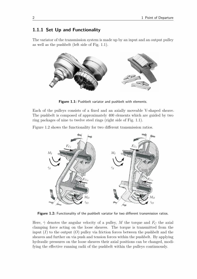
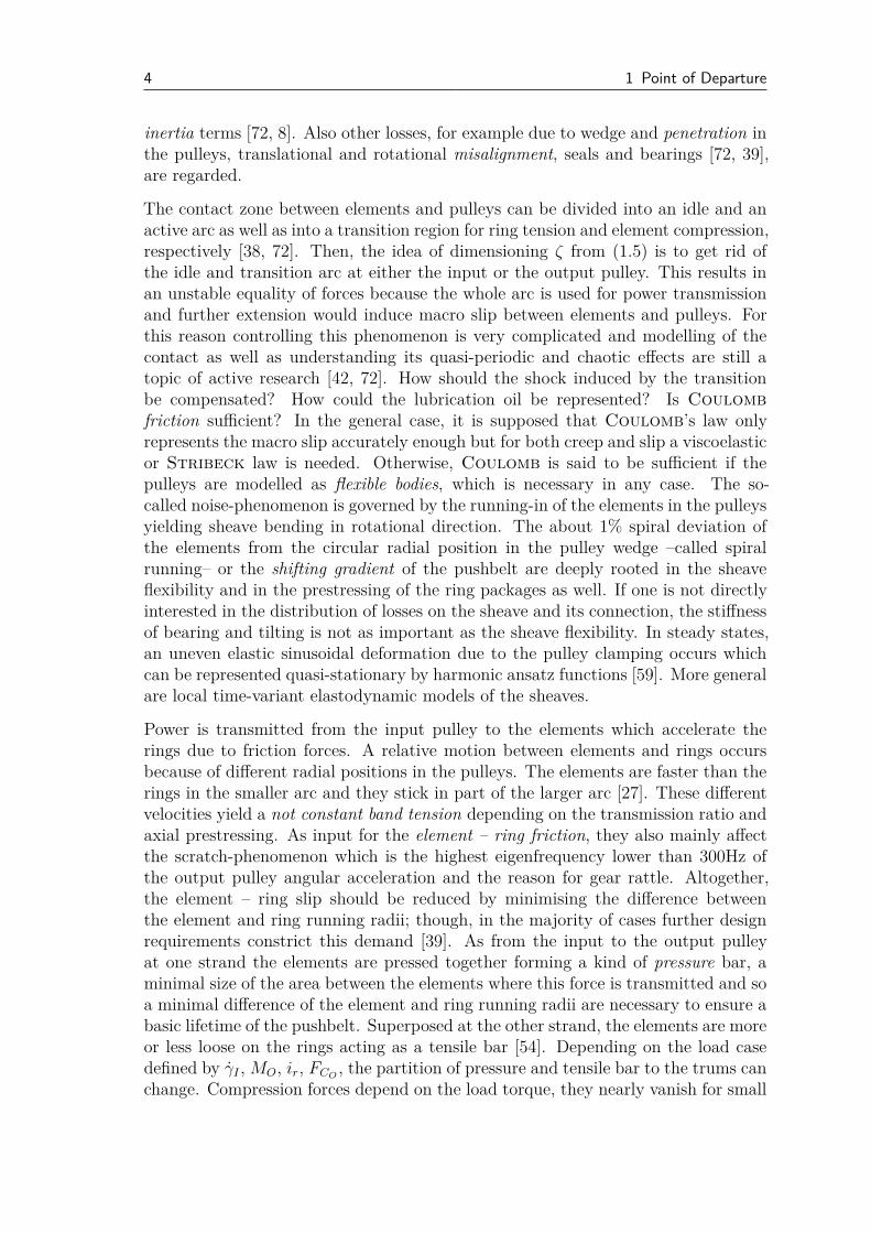
The variator of the transmission system is made up by an input and an output pulleyas well as the pushbelt (left side of Fig. 1.1).
Figure 1.1: Pushbelt variator and pushbelt with elements.
Each of the pulleys consists of a fixed and an axially moveable V-shaped sheave.The pushbelt is composed of approximately 400 elements which are guided by tworing packages of nine to twelve steel rings (right side of Fig. 1.1).
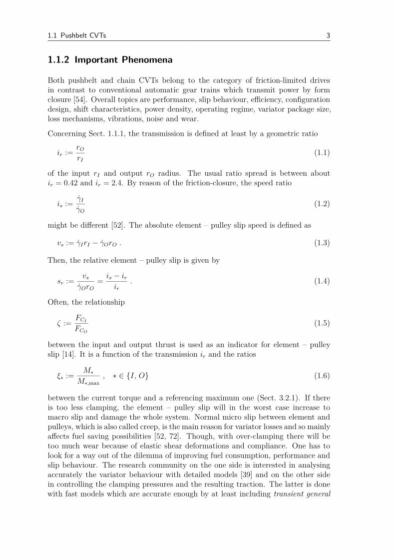
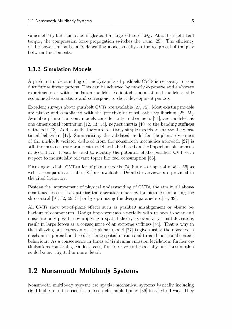
Figure 1.2 shows the functionality for two different transmission ratios.
FCIFCI
MIMI
γIγI
FCOFCO
MO MO
γO γO
Figure 1.2: Functionality of the pushbelt variator for two different transmission ratios.
Here, γ denotes the angular velocity of a pulley, M the torque and FC the axialclamping force acting on the loose sheaves. The torque is transmitted from theinput (I) to the output (O) pulley via friction forces between the pushbelt and thesheaves and further on via push and tension forces within the pushbelt. By applyinghydraulic pressures on the loose sheaves their axial positions can be changed, modi-fying the effective running radii of the pushbelt within the pulleys continuously.
1.1 Pushbelt CVTs 3
1.1.2 Important Phenomena
Both pushbelt and chain CVTs belong to the category of friction-limited drivesin contrast to conventional automatic gear trains which transmit power by formclosure [54]. Overall topics are performance, slip behaviour, efficiency, configurationdesign, shift characteristics, power density, operating regime, variator package size,loss mechanisms, vibrations, noise and wear.
Concerning Sect. 1.1.1, the transmission is defined at least by a geometric ratio
ir :=rO
rI
(1.1)
of the input rI and output rO radius. The usual ratio spread is between aboutir = 0.42 and ir = 2.4. By reason of the friction-closure, the speed ratio
is :=γI
γO
(1.2)
might be different [52]. The absolute element – pulley slip speed is defined as
vs := γIrI − γOrO . (1.3)
Then, the relative element – pulley slip is given by
sr :=vs
γOrO
=is − irir
. (1.4)
Often, the relationship
ζ :=FCI
FCO
(1.5)
between the input and output thrust is used as an indicator for element – pulleyslip [14]. It is a function of the transmission ir and the ratios
ξ∗ :=M∗
M∗,max
, ∗ ∈ {I, O} (1.6)
between the current torque and a referencing maximum one (Sect. 3.2.1). If thereis too less clamping, the element – pulley slip will in the worst case increase tomacro slip and damage the whole system. Normal micro slip between element andpulleys, which is also called creep, is the main reason for variator losses and so mainlyaffects fuel saving possibilities [52, 72]. Though, with over-clamping there will betoo much wear because of elastic shear deformations and compliance. One has tolook for a way out of the dilemma of improving fuel consumption, performance andslip behaviour. The research community on the one side is interested in analysingaccurately the variator behaviour with detailed models [39] and on the other sidein controlling the clamping pressures and the resulting traction. The latter is donewith fast models which are accurate enough by at least including transient general
4 1 Point of Departure
inertia terms [72, 8]. Also other losses, for example due to wedge and penetration inthe pulleys, translational and rotational misalignment, seals and bearings [72, 39],are regarded.
The contact zone between elements and pulleys can be divided into an idle and anactive arc as well as into a transition region for ring tension and element compression,respectively [38, 72]. Then, the idea of dimensioning ζ from (1.5) is to get rid ofthe idle and transition arc at either the input or the output pulley. This results inan unstable equality of forces because the whole arc is used for power transmissionand further extension would induce macro slip between elements and pulleys. Forthis reason controlling this phenomenon is very complicated and modelling of thecontact as well as understanding its quasi-periodic and chaotic effects are still atopic of active research [42, 72]. How should the shock induced by the transitionbe compensated? How could the lubrication oil be represented? Is Coulomb
friction sufficient? In the general case, it is supposed that Coulomb’s law onlyrepresents the macro slip accurately enough but for both creep and slip a viscoelasticor Stribeck law is needed. Otherwise, Coulomb is said to be sufficient if thepulleys are modelled as flexible bodies, which is necessary in any case. The so-called noise-phenomenon is governed by the running-in of the elements in the pulleysyielding sheave bending in rotational direction. The about 1% spiral deviation ofthe elements from the circular radial position in the pulley wedge –called spiralrunning– or the shifting gradient of the pushbelt are deeply rooted in the sheaveflexibility and in the prestressing of the ring packages as well. If one is not directlyinterested in the distribution of losses on the sheave and its connection, the stiffnessof bearing and tilting is not as important as the sheave flexibility. In steady states,an uneven elastic sinusoidal deformation due to the pulley clamping occurs whichcan be represented quasi-stationary by harmonic ansatz functions [59]. More generalare local time-variant elastodynamic models of the sheaves.
Power is transmitted from the input pulley to the elements which accelerate therings due to friction forces. A relative motion between elements and rings occursbecause of different radial positions in the pulleys. The elements are faster than therings in the smaller arc and they stick in part of the larger arc [27]. These differentvelocities yield a not constant band tension depending on the transmission ratio andaxial prestressing. As input for the element – ring friction, they also mainly affectthe scratch-phenomenon which is the highest eigenfrequency lower than 300Hz ofthe output pulley angular acceleration and the reason for gear rattle. Altogether,the element – ring slip should be reduced by minimising the difference betweenthe element and ring running radii; though, in the majority of cases further designrequirements constrict this demand [39]. As from the input to the output pulleyat one strand the elements are pressed together forming a kind of pressure bar, aminimal size of the area between the elements where this force is transmitted and soa minimal difference of the element and ring running radii are necessary to ensure abasic lifetime of the pushbelt. Superposed at the other strand, the elements are moreor less loose on the rings acting as a tensile bar [54]. Depending on the load casedefined by γI , MO, ir, FCO
, the partition of pressure and tensile bar to the trums canchange. Compression forces depend on the load torque, they nearly vanish for small
1.2 Nonsmooth Multibody Systems 5
values of MO but cannot be neglected for large values of MO. At a threshold loadtorque, the compression force propagation switches the trum [28]. The efficiencyof the power transmission is depending monotonically on the reciprocal of the playbetween the elements.
1.1.3 Simulation Models
A profound understanding of the dynamics of pushbelt CVTs is necessary to con-duct future investigations. This can be achieved by mostly expensive and elaborateexperiments or with simulation models. Validated computational models enableeconomical examinations and correspond to short development periods.
Excellent surveys about pushbelt CVTs are available [27, 72]. Most existing modelsare planar and established with the principle of quasi-static equilibrium [28, 59].Available planar transient models consider only rubber belts [71], are modeled asone dimensional continuum [12, 13, 14], neglect inertia [40] or the bending stiffnessof the belt [73]. Additionally, there are relatively simple models to analyse the vibra-tional behaviour [42]. Summarising, the validated model for the planar dynamicsof the pushbelt variator deduced from the nonsmooth mechanics approach [27] isstill the most accurate transient model available based on the important phenomenain Sect. 1.1.2. It can be used to identify the potential of the pushbelt CVT withrespect to industrially relevant topics like fuel consumption [63].
Focusing on chain CVTs a lot of planar models [74] but also a spatial model [65] aswell as comparative studies [81] are available. Detailed overviews are provided inthe cited literature.
Besides the improvement of physical understanding of CVTs, the aim in all above-mentioned cases is to optimise the operation mode by for instance enhancing theslip control [70, 52, 69, 58] or by optimising the design parameters [51, 39].
All CVTs show out-of-plane effects such as pushbelt misalignment or elastic be-haviour of components. Design improvements especially with respect to wear andnoise are only possible by applying a spatial theory as even very small deviationsresult in large forces as a consequence of an extreme stiffness [54]. That is why inthe following, an extension of the planar model [27] is given using the nonsmoothmechanics approach and so describing spatial motion and three-dimensional contactbehaviour. As a consequence in times of tightening emission legislation, further op-timisations concerning comfort, cost, fun to drive and especially fuel consumptioncould be investigated in more detail.
1.2 Nonsmooth Multibody Systems
Nonsmooth multibody systems are special mechanical systems basically includingrigid bodies and in space discretised deformable bodies [89] in a hybrid way. They
6 1 Point of Departure
are additionally characterised by rigid unilateral and bilateral contacts as well asimpacts which lead to discrete jumps within the system’s velocities. Thus, the degreeof freedom is not a constant function but changes during the simulation processand determines a time-variant topology. A unitary mathematical and numericalformulation [90] based on measure differential equations (MDE) with constraintshas been processed in the last decades at different research institutes [10, 56, 83, 77,11, 44, 45, 1, 20, 46]. It allows the efficient integration even of industrial systems withlarge numbers of transitions [54, 85, 82] and avoids both high artificial stiffnessesand additional modelling errors due to regularised interactions.
1.2.1 Measure Differential Equation
A measure differential equation [48]
Mµu = µG +∑
k
µHk (1.7)
involves measures µ representing the velocity by superscript u, integrable forces bysuperscript G and impacts at countable points in time tk, k ∈ IN, by superscriptfor Heaviside functions Hk. The symmetric and positive definite mass matrix M
depends on the position q of the system.
Equivalent to the MDE (1.7) it is also possible to distinguish between smooth (non-impulsive) dynamics
Mu = h + W λ , (1.8)
and impact (impulsive) dynamics
M k
(
u+k − u−
k
)
= W kΛk ∀k ∈ IN (1.9)
using u for denoting the weak time derivative of u and u+k as well as u−
k for describingthe velocity after and before an impact time tk. The generalised velocities u dependon the positions q via the linear equation
q = Y u with Y = Y (q) (1.10)
and the vector h contains all smooth external, internal and gyroscopic forces. Theseforces are functions of q, u and explicitly of the time t and also hold reactions ofsingle-valued contacts for example flexible ones. The directions of set-valued contactreactions are summarised in the wrench matrix
W = W (q) (1.11)
as well as λ and Λk refer to smooth and nonsmooth contact reaction values due topersisting contacts and respectively due to discrete impulses.
1.2 Nonsmooth Multibody Systems 7
1.2.2 Contact Laws
The computation of the accelerations u in (1.8) and the post-impact velocities u+k in
(1.9) requires the knowledge of the unknown contact reactions λ and Λk governedby set-valued contact laws (q, u, λ, Λk, t) ∈ N . These contact laws are describedin the following.
First of all, only smooth motion is considered which means that no impacts occur.Then, closed contact implies a bilateral constraint
gB = 0, λB ⋚ 0 , (1.12)
where gB denotes the normal distance of the interacting bodies in the contact point.The second type of contact also allows for detachment. The associated unilateralconstraint is given by the Signorini-Fichera-condition
gU ≥ 0, λU ≥ 0, gUλU = 0 (1.13)
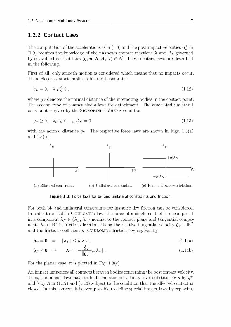
with the normal distance gU . The respective force laws are shown in Figs. 1.3(a)and 1.3(b).
λB
gB
(a) Bilateral constraint.
λU
gU
(b) Unilateral constraint.
λT
gT
+µ|λN |
−µ|λN |
(c) Planar Coulomb friction.
Figure 1.3: Force laws for bi- and unilateral constraints and friction.
For both bi- and unilateral constraints for instance dry friction can be considered.In order to establish Coulomb’s law, the force of a single contact is decomposedin a component λN ∈ {λB, λU} normal to the contact plane and tangential compo-nents λT ∈ IR2 in friction direction. Using the relative tangential velocity gT ∈ IR2
and the friction coefficient µ, Coulomb’s friction law is given by
gT = 0 ⇒ ‖λT ‖ ≤ µ|λN | , (1.14a)
gT 6= 0 ⇒ λT = −gT
‖gT ‖µ|λN | . (1.14b)
For the planar case, it is plotted in Fig. 1.3(c).
An impact influences all contacts between bodies concerning the post impact velocity.Thus, the impact laws have to be formulated on velocity level substituting g by g+
and λ by Λ in (1.12) and (1.13) subject to the condition that the affected contact isclosed. In this context, it is even possible to define special impact laws by replacing
8 1 Point of Departure
g+ with adequate physical approximations to regard for example elastic impactbehaviour [48].
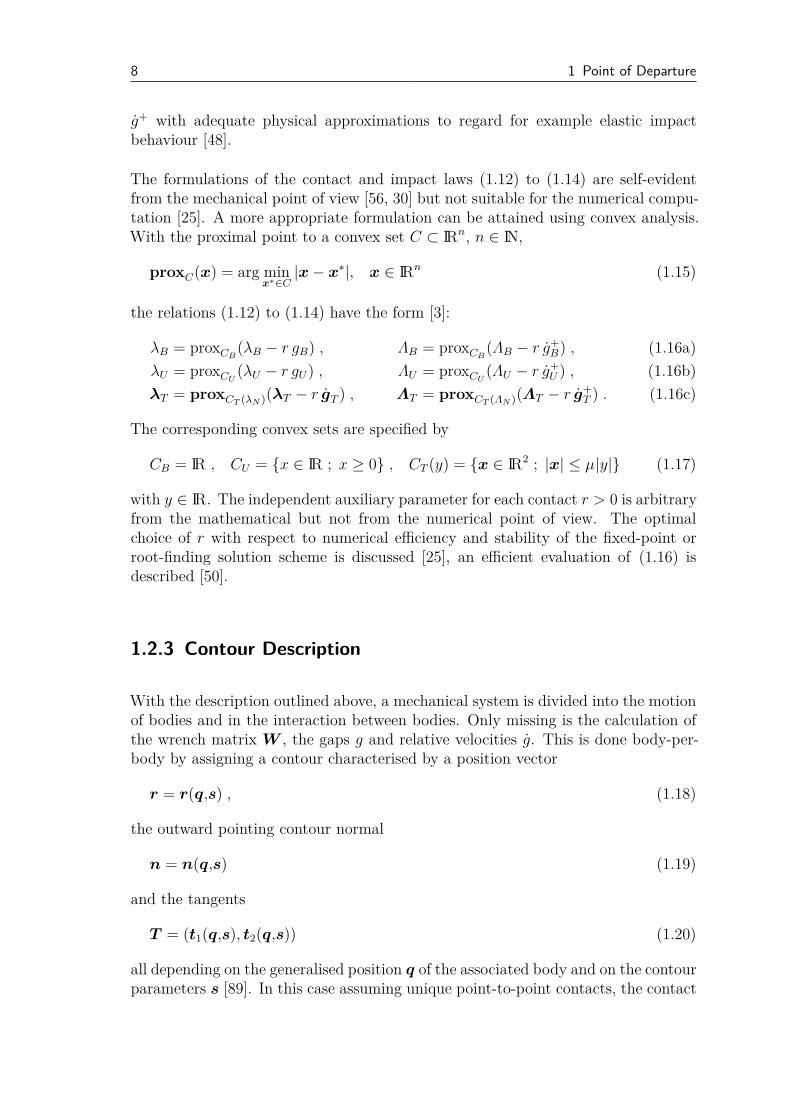
The formulations of the contact and impact laws (1.12) to (1.14) are self-evidentfrom the mechanical point of view [56, 30] but not suitable for the numerical compu-tation [25]. A more appropriate formulation can be attained using convex analysis.With the proximal point to a convex set C ⊂ IRn, n ∈ IN,
proxC(x) = arg minx∗∈C
|x − x∗|, x ∈ IRn (1.15)
the relations (1.12) to (1.14) have the form [3]:
λB = proxCB(λB − r gB) , ΛB = proxCB
(ΛB − r g+B) , (1.16a)
λU = proxCU(λU − r gU) , ΛU = proxCU
(ΛU − r g+U ) , (1.16b)
λT = proxCT (λN )(λT − r gT ) , ΛT = proxCT (ΛN )(ΛT − r g+T ) . (1.16c)
The corresponding convex sets are specified by
CB = IR , CU = {x ∈ IR ; x ≥ 0} , CT (y) = {x ∈ IR2 ; |x| ≤ µ|y|} (1.17)
with y ∈ IR. The independent auxiliary parameter for each contact r > 0 is arbitraryfrom the mathematical but not from the numerical point of view. The optimalchoice of r with respect to numerical efficiency and stability of the fixed-point orroot-finding solution scheme is discussed [25], an efficient evaluation of (1.16) isdescribed [50].
1.2.3 Contour Description
With the description outlined above, a mechanical system is divided into the motionof bodies and in the interaction between bodies. Only missing is the calculation ofthe wrench matrix W , the gaps g and relative velocities g. This is done body-per-body by assigning a contour characterised by a position vector
r = r(q,s) , (1.18)
the outward pointing contour normal
n = n(q,s) (1.19)
and the tangents
T = (t1(q,s), t2(q,s)) (1.20)
all depending on the generalised position q of the associated body and on the contourparameters s [89]. In this case assuming unique point-to-point contacts, the contact
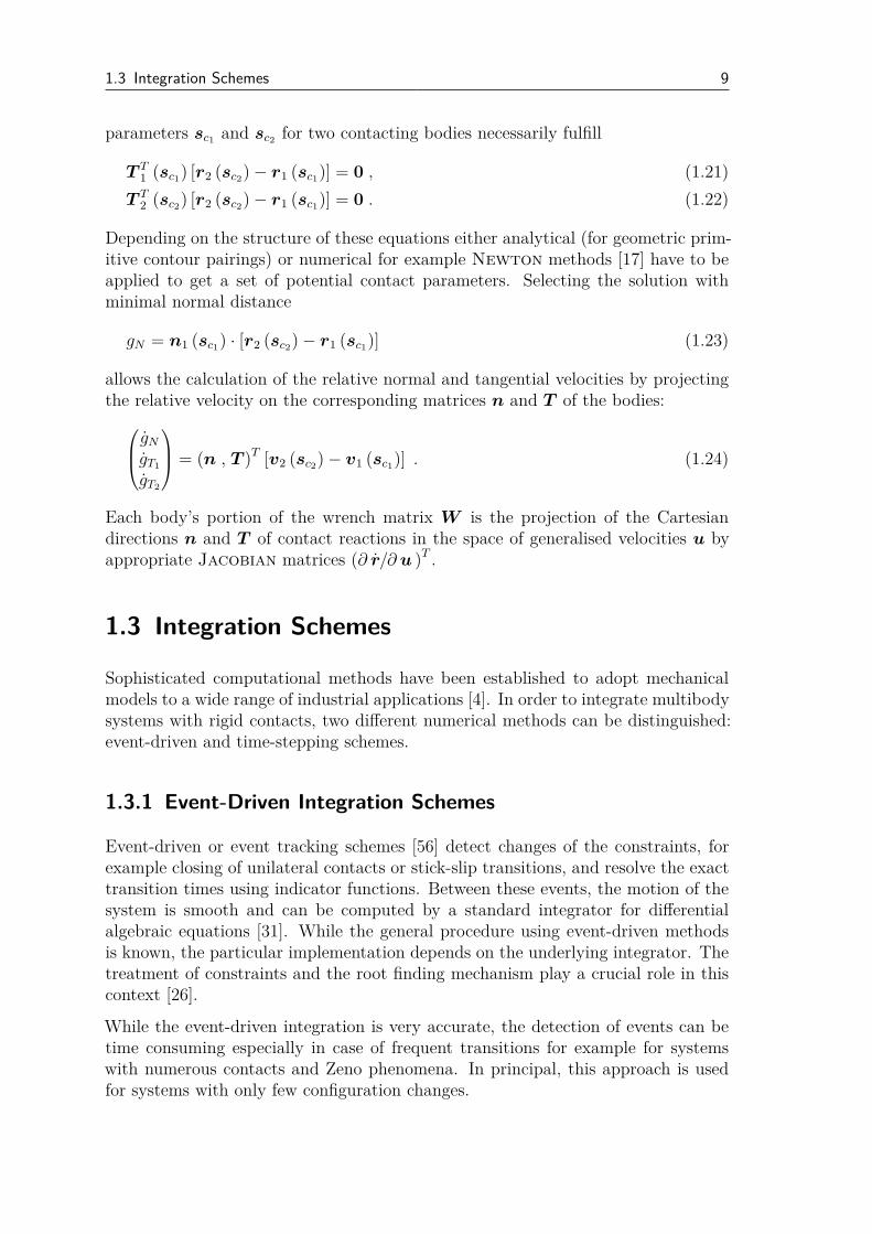
1.3 Integration Schemes 9
parameters sc1and sc2
for two contacting bodies necessarily fulfill
T T1 (sc1
) [r2 (sc2) − r1 (sc1
)] = 0 , (1.21)
T T2 (sc2
) [r2 (sc2) − r1 (sc1
)] = 0 . (1.22)
Depending on the structure of these equations either analytical (for geometric prim-itive contour pairings) or numerical for example Newton methods [17] have to beapplied to get a set of potential contact parameters. Selecting the solution withminimal normal distance
gN = n1 (sc1) · [r2 (sc2
) − r1 (sc1)] (1.23)
allows the calculation of the relative normal and tangential velocities by projectingthe relative velocity on the corresponding matrices n and T of the bodies:
gN
gT1
gT2
= (n , T )T [v2 (sc2
) − v1 (sc1)] . (1.24)
Each body’s portion of the wrench matrix W is the projection of the Cartesiandirections n and T of contact reactions in the space of generalised velocities u byappropriate Jacobian matrices (∂ r/∂ u )T .
1.3 Integration Schemes
Sophisticated computational methods have been established to adopt mechanicalmodels to a wide range of industrial applications [4]. In order to integrate multibodysystems with rigid contacts, two different numerical methods can be distinguished:event-driven and time-stepping schemes.
1.3.1 Event-Driven Integration Schemes
Event-driven or event tracking schemes [56] detect changes of the constraints, forexample closing of unilateral contacts or stick-slip transitions, and resolve the exacttransition times using indicator functions. Between these events, the motion of thesystem is smooth and can be computed by a standard integrator for differentialalgebraic equations [31]. While the general procedure using event-driven methodsis known, the particular implementation depends on the underlying integrator. Thetreatment of constraints and the root finding mechanism play a crucial role in thiscontext [26].
While the event-driven integration is very accurate, the detection of events can betime consuming especially in case of frequent transitions for example for systemswith numerous contacts and Zeno phenomena. In principal, this approach is usedfor systems with only few configuration changes.
10 1 Point of Departure
1.3.2 Time-Stepping Integration Schemes
In contrast to event-driven schemes, so-called time-stepping schemes belong to eventcapturing methods. They are based on the discretisation of the equations of motionincluding the constraints not adapting the globally fixed time step size ∆t dueto closing contacts. Hence, time-stepping schemes allow to focus on the globalaveraged physical behaviour of the simulated models. This reduces the number ofcombinatorial problems and avoids event detections. Therefore, a large number ofcontact transitions can be handled with increased computational efficiency if singleevents are not as important. On the other hand, common time-discretisations areof order one and the integrator is very sensitive with respect to the time step sizeinfluencing numerical stability and accuracy [34, 78, 24, 43, 25, 79].
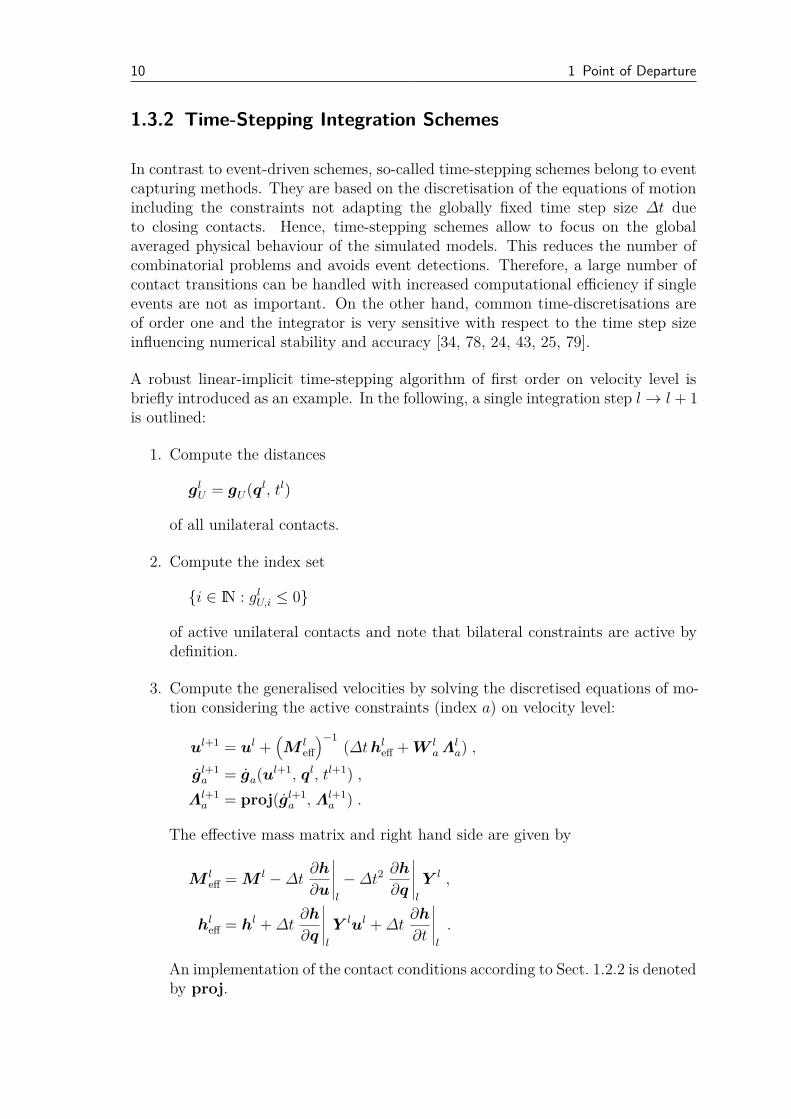
A robust linear-implicit time-stepping algorithm of first order on velocity level isbriefly introduced as an example. In the following, a single integration step l → l + 1is outlined:
1. Compute the distances
glU = gU(ql, tl)
of all unilateral contacts.
2. Compute the index set
{i ∈ IN : glU,i ≤ 0}
of active unilateral contacts and note that bilateral constraints are active bydefinition.
3. Compute the generalised velocities by solving the discretised equations of mo-tion considering the active constraints (index a) on velocity level:
ul+1 = ul +(
M leff
)−1(∆thl
eff + W la Λl
a) ,
gl+1a = ga(ul+1, ql, tl+1) ,
Λl+1a = proj(gl+1
a , Λl+1a ) .
The effective mass matrix and right hand side are given by
M leff = M l −∆t
∂h
∂u
∣∣∣∣∣l
−∆t2∂h
∂q
∣∣∣∣∣l
Y l ,
hleff = hl +∆t
∂h
∂q
∣∣∣∣∣l
Y lul +∆t∂h
∂t
∣∣∣∣∣l
.
An implementation of the contact conditions according to Sect. 1.2.2 is denotedby proj.
1.4 MBSim 11
4. Compute the new generalised positions
ql+1 = ql +∆tY l ul+1 .
5. Correct numerical drifts.
1.4 MBSim
The software for modelling and simulation of nonsmooth dynamical systems at theInstitute of Applied Mechanics of the Technische Universität München is calledMBSim [47]. Mathematically, it is based on the ideas outlined in Sects. 1.2 and1.3.
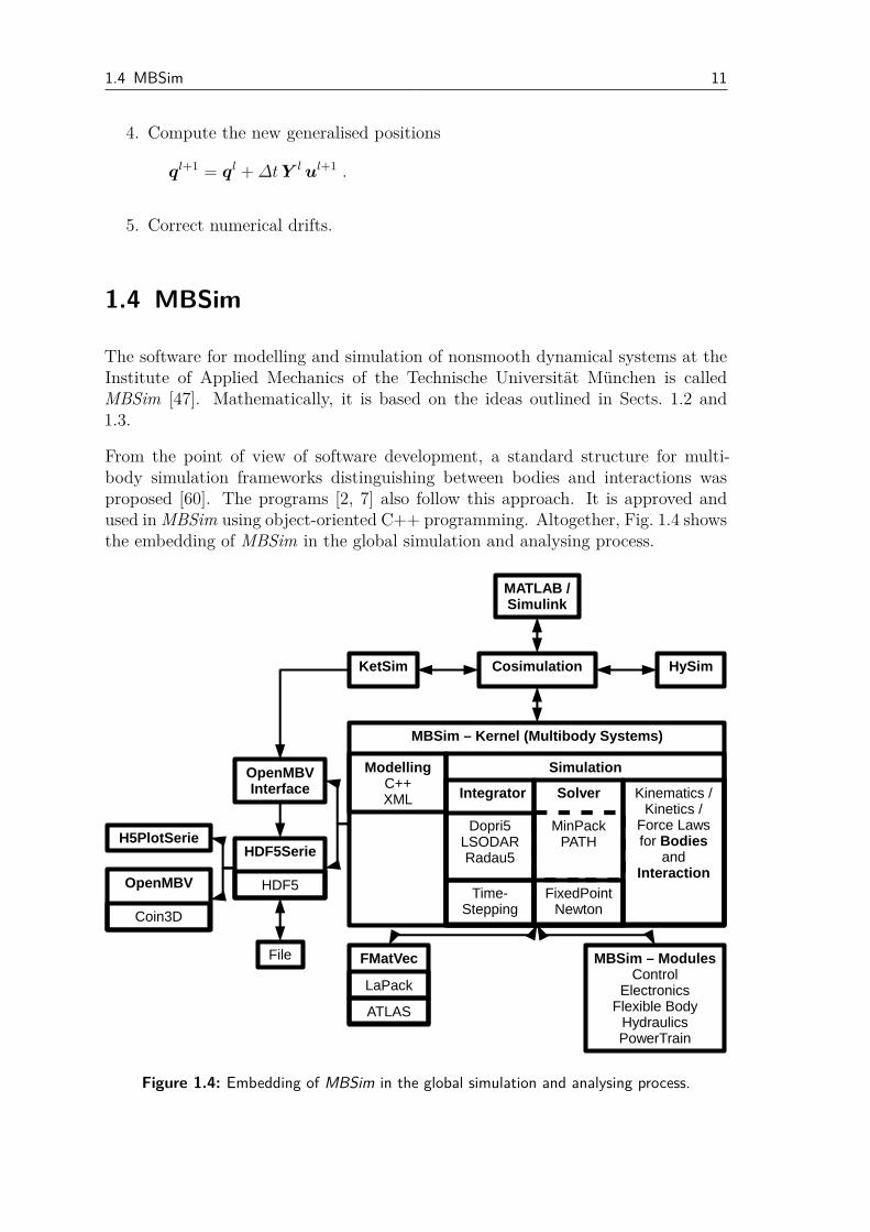
From the point of view of software development, a standard structure for multi-body simulation frameworks distinguishing between bodies and interactions wasproposed [60]. The programs [2, 7] also follow this approach. It is approved andused in MBSim using object-oriented C++ programming. Altogether, Fig. 1.4 showsthe embedding of MBSim in the global simulation and analysing process.
Figure 1.4: Embedding of MBSim in the global simulation and analysing process.
12 1 Point of Departure
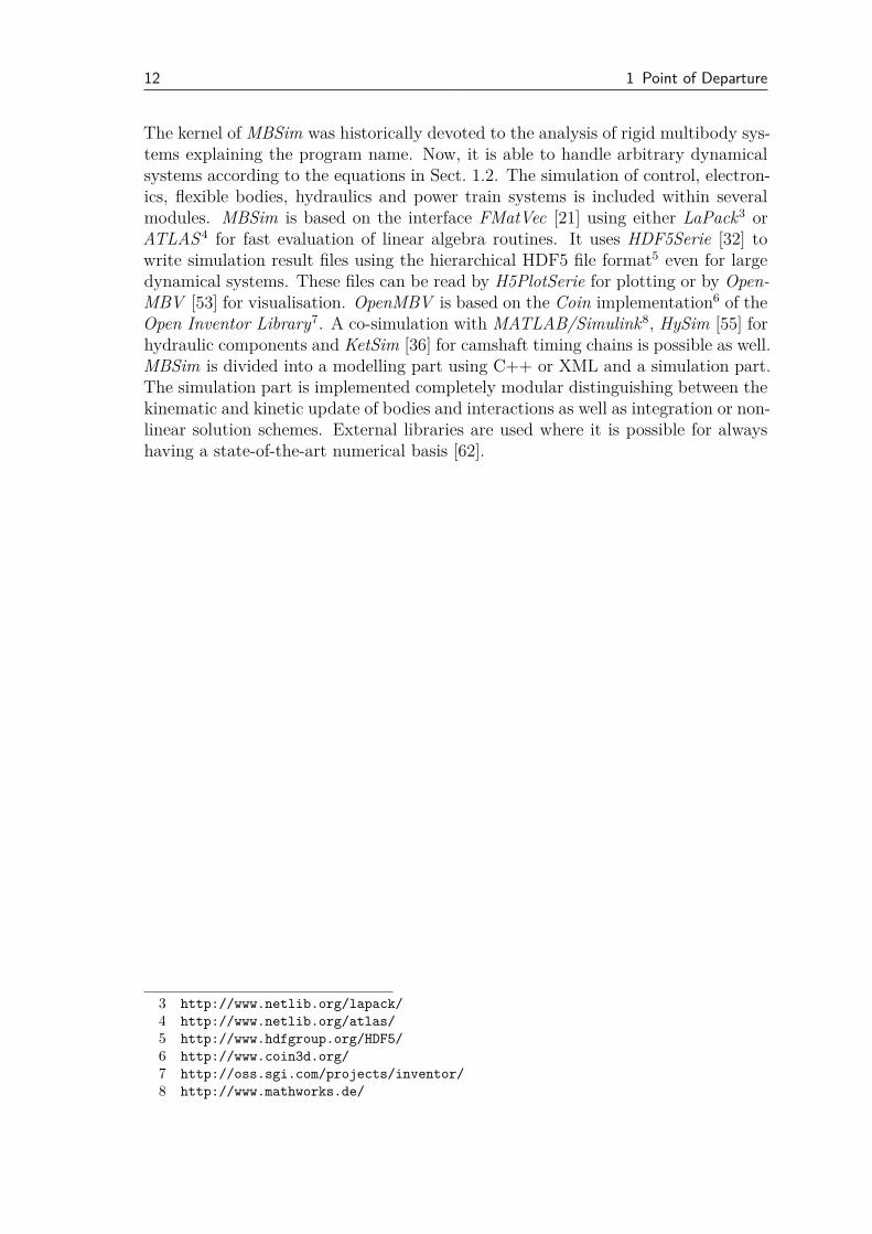
The kernel of MBSim was historically devoted to the analysis of rigid multibody sys-tems explaining the program name. Now, it is able to handle arbitrary dynamicalsystems according to the equations in Sect. 1.2. The simulation of control, electron-ics, flexible bodies, hydraulics and power train systems is included within severalmodules. MBSim is based on the interface FMatVec [21] using either LaPack3 orATLAS4 for fast evaluation of linear algebra routines. It uses HDF5Serie [32] towrite simulation result files using the hierarchical HDF5 file format5 even for largedynamical systems. These files can be read by H5PlotSerie for plotting or by Open-MBV [53] for visualisation. OpenMBV is based on the Coin implementation6 of theOpen Inventor Library7. A co-simulation with MATLAB/Simulink8, HySim [55] forhydraulic components and KetSim [36] for camshaft timing chains is possible as well.MBSim is divided into a modelling part using C++ or XML and a simulation part.The simulation part is implemented completely modular distinguishing between thekinematic and kinetic update of bodies and interactions as well as integration or non-linear solution schemes. External libraries are used where it is possible for alwayshaving a state-of-the-art numerical basis [62].
3 http://www.netlib.org/lapack/
4 http://www.netlib.org/atlas/
5 http://www.hdfgroup.org/HDF5/
6 http://www.coin3d.org/
7 http://oss.sgi.com/projects/inventor/
8 http://www.mathworks.de/
13
2 Model of the Pushbelt CVT
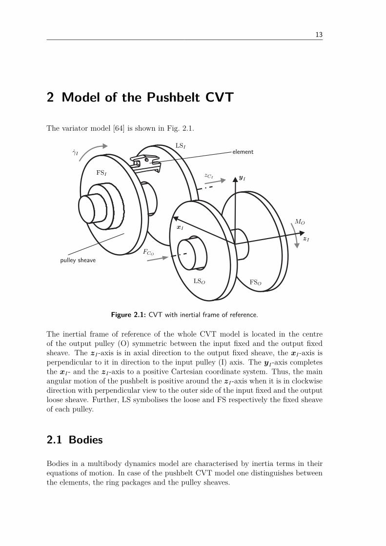
The variator model [64] is shown in Fig. 2.1.
xI
yI
zI
element
pulley sheave
γI
FSI
LSI
zCI
FSOLSO
MO
FCO
Figure 2.1: CVT with inertial frame of reference.
The inertial frame of reference of the whole CVT model is located in the centreof the output pulley (O) symmetric between the input fixed and the output fixedsheave. The zI-axis is in axial direction to the output fixed sheave, the xI-axis isperpendicular to it in direction to the input pulley (I) axis. The yI-axis completesthe xI- and the zI-axis to a positive Cartesian coordinate system. Thus, the mainangular motion of the pushbelt is positive around the zI-axis when it is in clockwisedirection with perpendicular view to the outer side of the input fixed and the outputloose sheave. Further, LS symbolises the loose and FS respectively the fixed sheaveof each pulley.
2.1 Bodies
Bodies in a multibody dynamics model are characterised by inertia terms in theirequations of motion. In case of the pushbelt CVT model one distinguishes betweenthe elements, the ring packages and the pulley sheaves.
14 2 Model of the Pushbelt CVT
2.1.1 Elements
Altogether, NE rigid elements with degree of freedom (dof) equal to six for transla-tion and Cardan rotation are used for the simulation of the CVT dynamics, whereasthe number of elements in reality is given by NE0
. Elasticity of the elements isnot regarded in the body equations of motion. Instead, it is considered within theinteraction (Sect. 2.2) quasistatically because deformations only happen in case ofcontact and affect in a much smaller scale than global motion [63].
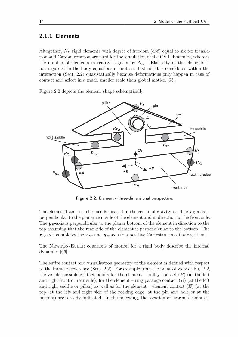
Figure 2.2 depicts the element shape schematically.
xExE
yEyE
zEzE
CC
ETET
EBEB
EPEP
EHEH
ELEL
ERER
RPRRPR
RSLRSL
RSRRSR
PFLPFL
PFRPFR
PRR
left saddle
right saddle
pillar
ear
rocking edge
pin
front side
Figure 2.2: Element - three-dimensional perspective.
The element frame of reference is located in the centre of gravity C. The xE-axis isperpendicular to the planar rear side of the element and in direction to the front side.The yE-axis is perpendicular to the planar bottom of the element in direction to thetop assuming that the rear side of the element is perpendicular to the bottom. ThezE-axis completes the xE- and yE-axis to a positive Cartesian coordinate system.
The Newton-Euler equations of motion for a rigid body describe the internaldynamics [66].
The entire contact and visualisation geometry of the element is defined with respectto the frame of reference (Sect. 2.2). For example from the point of view of Fig. 2.2,the visible possible contact points for the element – pulley contact (P ) (at the leftand right front or rear side), for the element – ring package contact (R) (at the leftand right saddle or pillar) as well as for the element – element contact (E) (at thetop, at the left and right side of the rocking edge, at the pin and hole or at thebottom) are already indicated. In the following, the location of extremal points is

2.1 Bodies 15
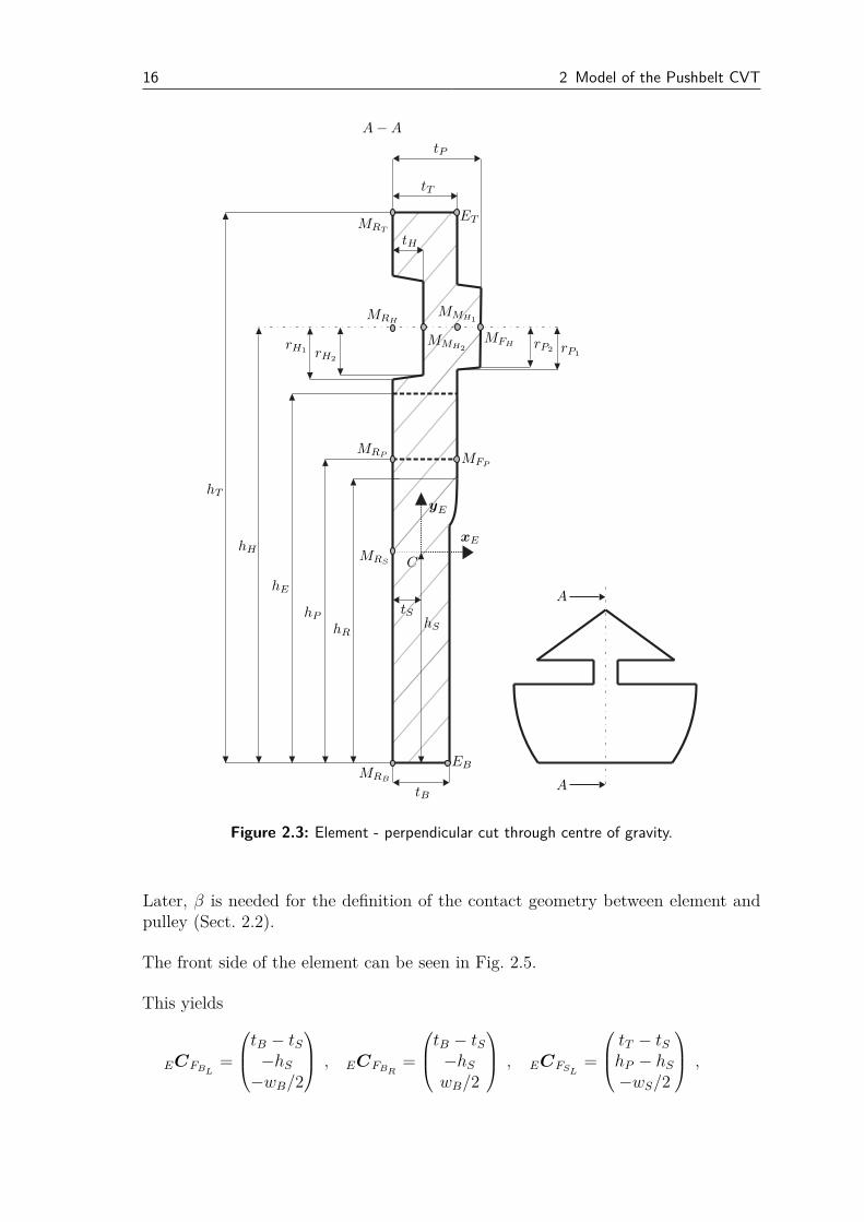
prepared. With Fig. 2.3, it holds
EMRP=
−tShP − hS
0
, EMFP
=
tT − tShP − hS
0
, EMRH
=
−tShH − hS
0
,
EMFH=
tP − tShH − hS
0
, EMMH1
=
tT − tShH − hS
0
, EMMH2
=
tH − tShH − hS
0
,
EMRS=
−tS00
, EMRB
=
−tS−hS
0
, EMRT
=
−tShT − hS
0
,
EEB =
tB − tS−hS
0
, EET =
tT − tShT − hS
0
with the indices characterising the rough position of the points.
It is assumed that the top edge, the ear plane and the saddle plane are parallel tothe bottom and that the front is piecewise parallel to the rear side. The radii of thefrustums are used in Sect. 2.2 for the explicit definition of the contact geometry.
Figure 2.4 shows the rear side of an element assuming a symmetric shape.
Then, it is
ECRBL=
−tS−hS
−wB/2
, ECRBR
=
−tS−hS
wB/2
, ECRSL
=
−tShP − hS
−wS/2
,
ECRSR=
−tShP − hS
wS/2
, EC1
RPL=
−tShP − hS
−wP/2
, EC1
RPR=
−tShP − hS
wP/2
,
EC2RPL
=
−tShE − hS
−wP/2
, EC2
RPR=
−tShE − hS
wP/2
, ECREL
=
−tShE − hS
−wE/2
,
ECRER=
−tShE − hS
wE/2
.
With α = arctan(
wS−wB
2hP
)
∈[
0,π2
)
and dP =√
r2P − h2
P/4 − (wS/4 − wB/4)2
EMRCPL=
−tS−hS + hP/2 + dP sinα
−wB/4 − wS/4 + dP cosα
,
EMRCPR=
−tS−hS + hP/2 + dP sinαwB/4 + wS/4 − dP cosα
.
16 2 Model of the Pushbelt CVT
A − A
A
A
xE
yE
C
EBMRB
MRS
MRP MFP
MRH
MFH
MMH1
MMH2
ET
tB
tS
tH
tP
tT
hS
hP
hE
hH
hT
hR
rP1
rP2rH1 rH2
MRT
Figure 2.3: Element - perpendicular cut through centre of gravity.
Later, β is needed for the definition of the contact geometry between element andpulley (Sect. 2.2).
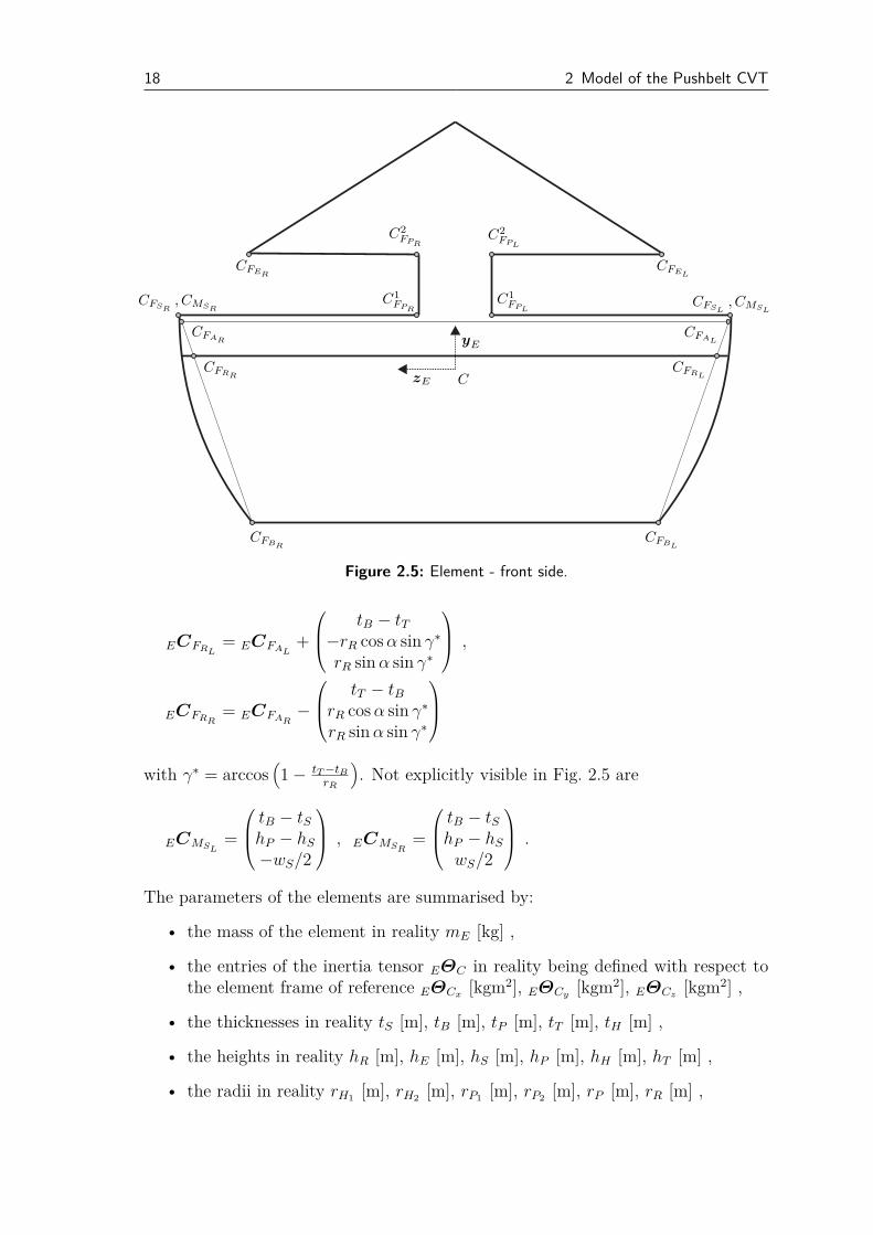
The front side of the element can be seen in Fig. 2.5.
This yields
ECFBL=
tB − tS−hS
−wB/2
, ECFBR
=
tB − tS−hS
wB/2
, ECFSL
=
tT − tShP − hS
−wS/2
,
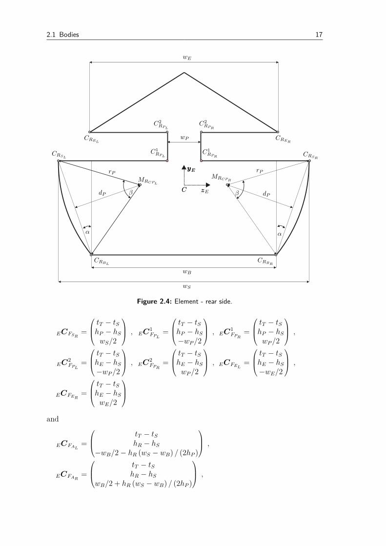
2.1 Bodies 17
yEyE
zECC
CRBRCRBL
CRSR
CRSL
C1
RPR
C1
RPL
C2
RPR
C2
RPL
CRELCRER
wB
wS
wE
wP
MRCPRMRCPL
αα
β β dPdP
rPrP
Figure 2.4: Element - rear side.
ECFSR=
tT − tShP − hS
wS/2
, EC1
FPL=
tT − tShP − hS
−wP/2
, EC1
FPR=
tT − tShP − hS
wP/2
,
EC2FPL
=
tT − tShE − hS
−wP/2
, EC2
FPR=
tT − tShE − hS
wP/2
, ECFEL
=
tT − tShE − hS
−wE/2
,
ECFER=
tT − tShE − hS
wE/2
and
ECFAL=
tT − tShR − hS
−wB/2 − hR (wS − wB) / (2hP )
,
ECFAR=
tT − tShR − hS
wB/2 + hR (wS − wB) / (2hP )
,
18 2 Model of the Pushbelt CVT
yE
zE C
CFBRCFBL
CFSR, CMSR
CFSL, CMSL
C1
FPR
C1
FPL
C2
FPR
C2
FPL
CFELCFER
CFARCFAL
CFRRCFRL
Figure 2.5: Element - front side.
ECFRL= ECFAL
+
tB − tT−rR cosα sin γ∗
rR sinα sin γ∗
,
ECFRR= ECFAR
−
tT − tBrR cosα sin γ∗
rR sinα sin γ∗
with γ∗ = arccos(
1 − tT −tB
rR
)
. Not explicitly visible in Fig. 2.5 are
ECMSL=
tB − tShP − hS
−wS/2
, ECMSR
=
tB − tShP − hS
wS/2
.
The parameters of the elements are summarised by:
• the mass of the element in reality mE [kg] ,
• the entries of the inertia tensor EΘC in reality being defined with respect tothe element frame of reference EΘCx
[kgm2], EΘCy[kgm2], EΘCz
[kgm2] ,
• the thicknesses in reality tS [m], tB [m], tP [m], tT [m], tH [m] ,
• the heights in reality hR [m], hE [m], hS [m], hP [m], hH [m], hT [m] ,
• the radii in reality rH1[m], rH2
[m], rP1[m], rP2
[m], rP [m], rR [m] ,
2.1 Bodies 19
• the widths in reality wB [m], wS [m], wP [m], wE [m] .
The effect of the change of the number of elements NE on the above mentionedparameters has to be discussed. Main criterion is the conservation with respect tothe values in reality. Defining the ratio ι = NE0
/NE yields a scaling in xE-directionand the changed "∼"-parameters
t∗ := ι t∗ , (2.1)
mE := ιmE , (2.2)
EΘCx:= ι EΘCx
, (2.3)
EΘCy:= 0.5
[
ι3(
EΘCy+ EΘCz
− EΘCx
)
+ ι(
EΘCx+ EΘCy
− EΘCz
)]
, (2.4)
EΘCz:= 0.5
[
ι3(
EΘCy+ EΘCz
− EΘCx
)
+ ι(
EΘCx+ EΘCz
− EΘCy
)]
(2.5)
used in the simulation by evaluating the change of the element thicknesses. Then,the inertia tensor does not represent the conservation of global parameters as itdepends on ι to the power of three. Thus, an additional parameter τ ∈ [0,1] isintroduced to finally declare the convex combinations
EΘCx:= EΘCx
, (2.6)
EΘCy:= τ EΘCy
+ (1 − τ) ι EΘCy, (2.7)
EΘCz:= τ EΘCz
+ (1 − τ) ι EΘCz. (2.8)
A mixture of cubic and linear dependence on ι can be defined based on the userschoice.
2.1.2 Ring Packages
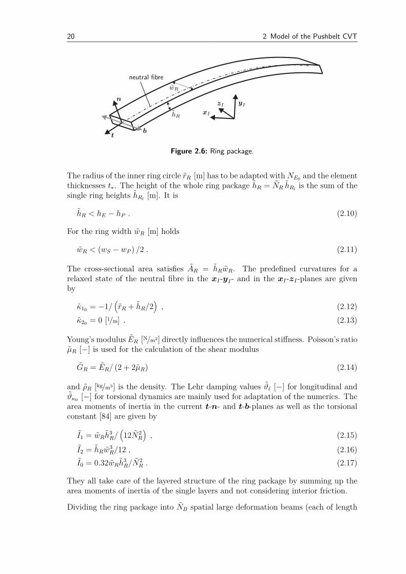
As the entire model of the variator allows transient states, no reference path of thepushbelt and thus of the ring packages can be given. Therefore, the model of thering packages has to cope with free spatial motions including geometrically nonlinearlarge translations and deflections but linear material laws. It has to be modelleddynamically because oscillations cannot be neglected [27]. As on the other hand therelative motion of the rings within the ring packages is not regarded, Fig. 2.6 showspart of a ring package homogenising NR rings with rectangular shaped cross-sectionto a one-dimensional continuum. Its motion can be described by the motion of theneutral fibre which is parametrised by the Lagrangian coordinate x ∈
[
0, lR]
. Thenormal n is pointing outwards and the tangent t is pointing along the ring circlenegatively around the zI-axis. The direction of the binormal b depends on thedefinition of the trihedral. In this section it is assumed that the vectors are orderedas t − n − b. The total length of the ring packages satisfies
lR = 2π(
rR + hR/2)
. (2.9)
20 2 Model of the Pushbelt CVT
xI
yIzI
t
n
b
wR
hR
neutral fibre
Figure 2.6: Ring package.
The radius of the inner ring circle rR [m] has to be adapted with NE0and the element
thicknesses t∗. The height of the whole ring package hR = NR hRlis the sum of the
single ring heights hRl[m]. It is
hR < hE − hP . (2.10)
For the ring width wR [m] holds
wR < (wS − wP ) /2 . (2.11)
The cross-sectional area satisfies AR = hRwR. The predefined curvatures for arelaxed state of the neutral fibre in the xI-yI- and in the xI-zI-planes are givenby
κ10= −1/
(
rR + hR/2)
, (2.12)
κ20= 0 [1/m] . (2.13)
Young’s modulus ER [N/m2] directly influences the numerical stiffness. Poisson’s ratioµR [−] is used for the calculation of the shear modulus
GR = ER/ (2 + 2µR) (2.14)
and ρR [kg/m3] is the density. The Lehr damping values ϑǫ [−] for longitudinal andϑκ0
[−] for torsional dynamics are mainly used for adaptation of the numerics. Thearea moments of inertia in the current t-n- and t-b-planes as well as the torsionalconstant [84] are given by
I1 = wRh3R/(
12N2R
)
, (2.15)
I2 = hRw3R/12 , (2.16)
I0 = 0.32wRh3R/N
2R . (2.17)
They all take care of the layered structure of the ring package by summing up thearea moments of inertia of the single layers and not considering interior friction.
Dividing the ring package into NB spatial large deformation beams (each of length
2.1 Bodies 21
l0 = lR/NB) provides a lot of modelling possibilities [87]. The model in [89] relieson the co-rotational approach [6, 16] and shows an efficient behaviour in the planarcase compared to absolute nodal coordinate formulations [18, 29, 67]. Here, it isextended to a three-dimensional description using inertial approaches [5, 68] wherethe physically interpretable Euler-Bernoulli beam formulation is used. Themathematical derivation is based on the ideas of finite element theory for assemblingand multibody formulations for the evaluation of the equations of motion for eachfinite element [61].
Coordinate settings
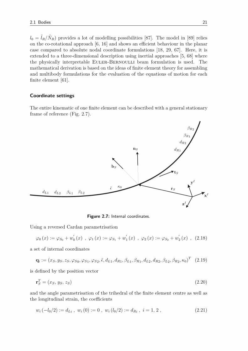
The entire kinematic of one finite element can be described with a general stationaryframe of reference (Fig. 2.7).
rS
xI
yI
zI
tS
nS
bS
ǫ κ0
dL1 dL2
dR1
dR2
βR1
βR2
βL1βL2
Figure 2.7: Internal coordinates.
Using a reversed Cardan parametrisation
ϕ0 (x) := ϕS0+ w
′
0 (x) , ϕ1 (x) := ϕS1+ w
′
1 (x) , ϕ2 (x) := ϕS2+ w
′
2 (x) , (2.18)
a set of internal coordinates
qi := (xS, yS, zS, ϕS0, ϕS1, ϕS2, ǫ, dL1, dR1, βL1, βR1, dL2, dR2, βL2, βR2, κ0)T (2.19)
is defined by the position vector
rTS = (xS, yS, zS) (2.20)
and the angle parametrisation of the trihedral of the finite element centre as well asthe longitudinal strain, the coefficients
wi (−l0/2) := dLi , wi (0) := 0 , wi (l0/2) := dRi , i = 1, 2 , (2.21)
22 2 Model of the Pushbelt CVT
w′
i (−l0/2) := βLi , w′
i (0) := 0 , w′
i (l0/2) := βRi , i = 1, 2 (2.22)
of the ansatz functions with the torsion
κ0 := Ib · In′ = w′′
0 − sin (ϕS1)w
′′
2 . (2.23)
A prime denotes the derivative with respect to the Lagrangian coordinate x. Thedegree of the real polynomials
wi := awix5 + bwi
x4 + cwix3 + dwi
x2 , i = 0, 1, 2 (2.24)
is a compromise between too much stiffening for lower orders and too much supportfor higher orders with the coefficients of w0 being constrained by the constant torsioncharacteristics of (2.23). In combination, rigid and elastic body motion are decou-pled and a compact form of the equations of motion with appropriate approximationnot depending on the boundary conditions is available for evaluation.
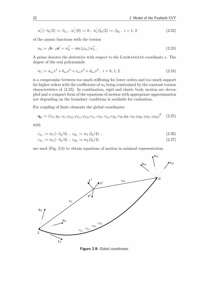
For coupling of finite elements the global coordinates
qg := (xL, yL, zL,ϕL0,ϕL1,ϕL2, cL1, cR1
, cL2, cR2
,xR, yR, zR,ϕR0,ϕR1,ϕR2)T (2.25)
with
cL1:= w1 (−l0/4) , cR1
:= w1 (l0/4) , (2.26)
cL2:= w2 (−l0/4) , cR2
:= w2 (l0/4) (2.27)
are used (Fig. 2.8) to obtain equations of motion in minimal representation.
xIyI
zI
rL
tL
nL
bL
rR
tR
nR
bR
cL1
cL2
cR1
cR2
L
R
Figure 2.8: Global coordinates.
2.1 Bodies 23
The information between the coordinate sets is transferred by the motion of theneutral fibre
Ir (x) = (1 + ǫ)∫
Itdx.= IrS + (1 + ǫ) x ItS + w1 (x) InS + w2 (x) IbS (2.28)
with
w1 := ξnw1 + ξbw2 , w2 := ηnw1 + ηbw2 . (2.29)
This results in a transformation F (qi,qg) = 0. One part can be solved analyticallywith respect to the internal coordinates:
IrS =IrL + IrR
2−
[ξn (dL1+ dR1
) + ξb (dL2+ dR2
)] InS
2
−[ηn (dL1
+ dR1) + ηb (dL2
+ dR2)] IbS
2(2.30)
and
ǫ =1
l0(IrR − IrL) · ItS − 1 , (2.31)
κ0 =1
l0[ϕR0
− ϕL0− sin (ϕS1
) (βR2− βL2
)] . (2.32)
A system of nonlinear equations
F1 := ϕS0−ϕL0
+ ϕR0
2+ sin (ϕS1
)βL2
+ βR2
2= 0 , (2.33)
F2 := ϕS1−ϕL1
+ ϕR1
2+βL1
+ βR1
2= 0 , (2.34)
F3 := ϕS2−ϕL2
+ ϕR2
2+βL2
+ βR2
2= 0 , (2.35)
F4 := βR1− βL1
− ϕR1+ ϕL1
= 0 , (2.36)
F5 := βR2− βL2
− ϕR2+ ϕL2
= 0 , (2.37)
F6 := ξn (dR1− dL1
) + ξb (dR2− dL2
) − (IrR − IrL) · InS = 0 , (2.38)
F7 := ηn (dR1− dL1
) + ηb (dR2− dL2
) − (IrR − IrL) · IbS = 0 , (2.39)
F8 := 2bw1l40/256 + 2dw1
l20/16 − cR1− cL1
= 0 , (2.40)
F9 := 2aw1l50/1024 + 2cw1
l30/64 − cR1+ cL1
= 0 , (2.41)
F10 := 2bw2l40/256 + 2dw2
l20/16 − cR2− cL2
= 0 , (2.42)
F11 := 2aw2l50/1024 + 2cw2
l30/64 − cR2+ cL2
= 0 (2.43)
in the unknowns xbe remains, which can be solved with Newton’s method usinganalytical Jacobian evaluations. The derivatives fulfill the relations
qi =dqi
dqg
qg =: Jigqg , (2.44)

24 2 Model of the Pushbelt CVT
qi =d
dt
(
dqi
dqg
)
qg +dqi
dqg
qg =: Jigqg + Jigqg (2.45)
with the expressions involving the internal coordinates xbe being calculated by thechain rule:
∂F
∂xbe
dxbe
dqg
= −∂F
∂qg
, (2.46)
∂F
∂xbe
d
dt
(
dxbe
dqg
)
= −d
dt
(
∂F
∂qg
)
−d
dt
(
∂F
∂xbe
)
dxbe
dqg
. (2.47)
Equations of motion
Energy expressions are the point of departure for the derivation of the equations ofmotion.
Mass conservation is a basic principle for the kinetic energy
T ≈1
2ρR
AR
l0/2∫
−l0/2
‖I r‖2 dx+ I0
l0/2∫
−l0/2
ω2t dx
. (2.48)
It is
ωt = ϕ0 − sin (ϕ1) ϕ2 (2.49)
the projection of the angular velocity on the local tangent neglecting angular bendingdependencies.
The elastic energy
Ve ≈ERAR
2ǫ2l0 +
ERI1
2
l0/2∫
−l0/2
(
w′′
1 − κ10
)2dx
+ERI2
2
l0/2∫
−l0/2
(
w′′
2 − κ20
)2dx+
GRI0
2
l0/2∫
−l0/2
κ20dx (2.50)
results from considering at most quadratic elastic deformation terms. The bendinglength
lb :=
l0/2∫
−l0/2
‖Ir′‖ dx ≈ (1 + ǫ) l0 +1
2
l0/2∫
−l0/2
w′
1w′
1dx+
l0/2∫
−l0/2
w′
2w′
2dx
(2.51)
contains second order terms concerning bending and so allows geometric nonlinear
2.1 Bodies 25
foreshortening. The corresponding strain is given by
ǫ :=lb − l0l0
≈ ǫ+1
2l0
l0/2∫
−l0/2
w′
1w′
1dx+
l0/2∫
−l0/2
w′
2w′
2dx
. (2.52)
The gravity Ig enters the gravitational energy
Vg = −ρRAR Ig ·
l0/2∫
−l0/2
Irdx
= −ρRAR Ig ·
l0IrS +
l0/2∫
−l0/2
w1dx InS +
l0/2∫
−l0/2
w2dx IbS
. (2.53)
Using the Lagrange II formalism
d
dt
(
∂T
∂qi
)T
−
(
∂T
∂qi
)T
+
(
∂ (Ve + Vg)
∂qi
)T
= 0 (2.54)
one derives the equations of motion. As a result of T = T (qi,qi) it holds
d
dt
(
∂T
∂qi
)T
=∂2T
∂q2i
qi +∂2T
∂qi∂qi
qi . (2.55)
Hence, the mass matrix and the smooth right hand side are given by
Mi :=∂2T
∂q2i
, hi :=
(
∂T
∂qi
)T
−
(
∂ (Ve + Vg)
∂qi
)T
−∂2T
∂qi∂qi
qi (2.56)
such that
Miqi − hi = 0 . (2.57)
Globally, the equations of motion satisfy
JTigMiJig︸ ︷︷ ︸
Mg
qg − JTig
(
hi − MiJigqg
)
︸ ︷︷ ︸
hg
= 0 . (2.58)
Damping
Damping terms have to be appended to the right hand side. The vector hi is replacedby hi + hiD with for instance
hiD := −ǫD˙ǫe7 − κ0D
κ0e16 (2.59)
26 2 Model of the Pushbelt CVT
and the unit vectors {ej}j=1,...,16 considering only prolongation and torsion. Thedamping terms ǫD, κ0D
can be added directly or for easier interpretation with Lehrdamping expressions ϑǫ, ϑκ0
. For prolongation or torsion only, the finite elementordinary differential equations reduce to
ρRARl3012
¨ǫ+ ǫD˙ǫ+ ERARl0ǫ = 0 , (2.60)
ρRI0l3012κ0 + κ0D
κ0 + GRI0l0κ0 = 0 . (2.61)
Then with the undamped eigenfrequencies
ωǫ =
√√√√12ER
ρRl20, ωκ0
=
√√√√12GR
ρRl20, (2.62)
it is
ǫD = ρRARl306ϑǫωǫ , κ0D
= ρRI0l306ϑκ0
ωκ0. (2.63)
Implicit integration
For the linear implicit integration one has to define an efficient mass matrix and anefficient right hand side. Then, the derivatives dhg/dqg and dhg/dqg are necessary.The appropriate numeric calculation can be done taking advantage of the finiteelement structure resulting in a block-diagonal implicit integration Jacobian.
Assembling of the beam elements
An extended vector of global coordinates describing the whole beam structure hasto be defined for coupling the finite elements:
qge:= (. . . , xj, yj, zj, ϕj,0, ϕj,1, ϕj,2, cj,L1
, cj,R1, cj,L2
, cj,R2, xj+1, . . .)
T . (2.64)
The relationship between the internal coordinates of the j-th finite element andthese extended global coordinates can be written as
qij = Q(
qge
)
. (2.65)
Then,
Jijge:=
dqij
dqge
(2.66)
is the Jacobian matrix of this transformation.
2.1 Bodies 27
For the whole structure with NB finite elements, one gets a sparse system of equa-tions which can be implemented very efficiently by index-scanning for used degreesof freedom on the global parts:
NB∑
j=1
JTijge
Mij Jijge
︸ ︷︷ ︸
Mge
qge−
NB∑
j=1
JTijge
(
hij − Mij Jijgeqge
)
︸ ︷︷ ︸
hge
= 0 . (2.67)
With (2.67), operations on zero entries can be avoided and arbitrary ring structuresare represented.
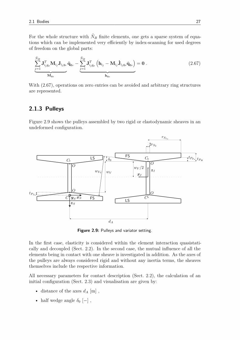
2.1.3 Pulleys
Figure 2.9 shows the pulleys assembled by two rigid or elastodynamic sheaves in anundeformed configuration.
xI
zI
yS
zS
xS
δ0
OO
OO
C C
CC
FS
FSLS
LS
wV
wV /2wVV
tPS∗
tPF∗ tPH
rS1∗
2rS2
dA
Figure 2.9: Pulleys and variator setting.
In the first case, elasticity is considered within the element interaction quasistati-cally and decoupled (Sect. 2.2). In the second case, the mutual influence of all theelements being in contact with one sheave is investigated in addition. As the axes ofthe pulleys are always considered rigid and without any inertia terms, the sheavesthemselves include the respective information.
All necessary parameters for contact description (Sect. 2.2), the calculation of aninitial configuration (Sect. 2.3) and visualisation are given by:
• distance of the axes dA [m] ,
• half wedge angle δ0 [−] ,

28 2 Model of the Pushbelt CVT
• widths of the variator wVV[m] and
wV = − (dA − 2rS2) tan (δ0) +
wVV
cos (δ0),
• radii rS1I[m] , rS1O
[m] and rS2[m] ,
• thicknesses tPH[m] ,
tPS∗=
1
2
[
tPF∗
3
rS2+ 2rS1∗
rS1∗+ rS2
+tPH
− tPF∗
2
]
,
tPF∗=(
rS1∗− rS2
)
tan (δ0) .
Assuming a symmetric shape, the moving sheave frame of reference is located inthe centre of gravity C of each sheave. The zS-axis is in axial direction normal tothe rear side, the yS-axis is initially parallel to the yI-axis of the inertial frame ofreference and the xS-axis completes a positive Cartesian coordinate system.
Rigid Sheaves
The loose sheaves (LS) have dof = 4 for axial translation, rotation and tilting aswell as the fixed sheaves (FS) have dof = 1 only for axial rotation.
With
• the sheave mass mS [kg] ,
• the inertia tensor SΘC defined with respect to the sheave frame of referencealso considering the portion of the pulley axis
the Newton-Euler equations of motion for a rigid body [66] describe the internaldynamics of each sheave.
Elastodynamic Sheaves
For elastic sheaves one has
• Young’s modulus ES [N/m2] ,
• Poisson’s ratio µS [−] ,
• density ρS [kg/m3]
and the possibility to include the axis inertia contribution.
Since contacts lead to time-variant boundary conditions, the occurring small elasticdeformations of the disk are modelled with local finite element shape functions [89].The internal sheave dynamics is described only for one single finite element using
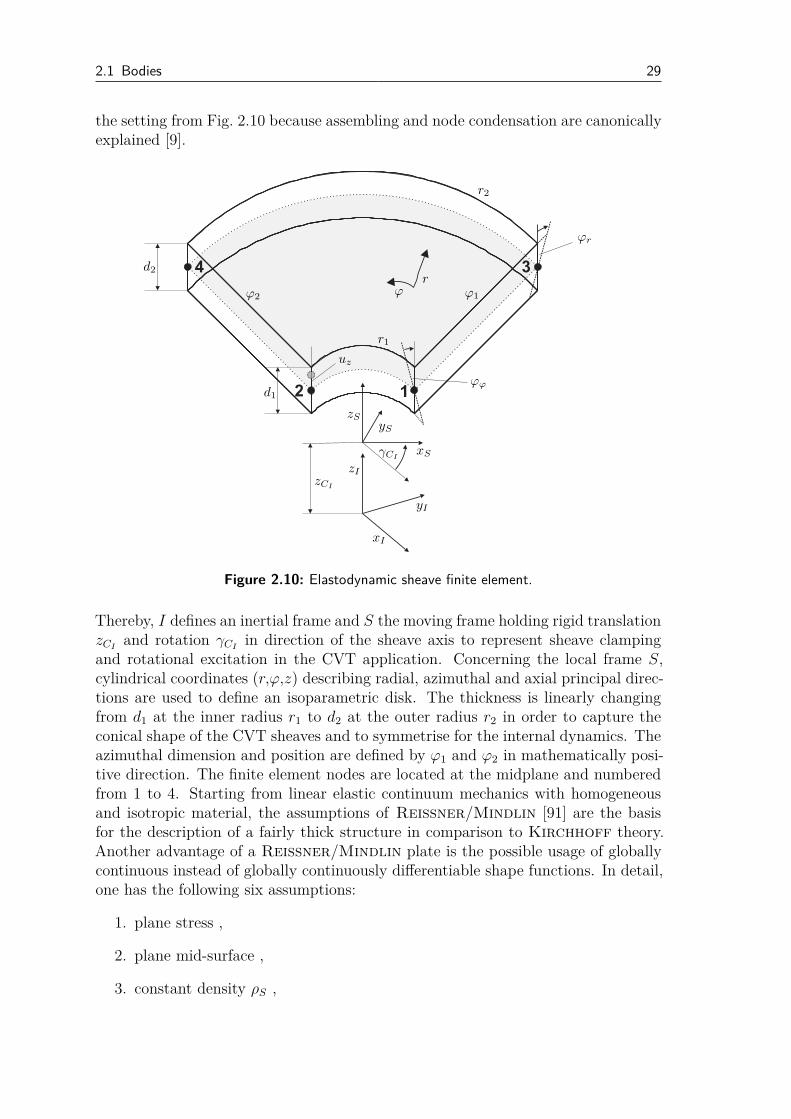
2.1 Bodies 29
the setting from Fig. 2.10 because assembling and node condensation are canonicallyexplained [9].
2 1
34
uz
r1
r2
rϕ1ϕ2
ϕr
ϕϕ
ϕ
d1
d2
xS
yS
zS
xI
yI
zIzCI
γCI
Figure 2.10: Elastodynamic sheave finite element.
Thereby, I defines an inertial frame and S the moving frame holding rigid translationzCI
and rotation γCIin direction of the sheave axis to represent sheave clamping
and rotational excitation in the CVT application. Concerning the local frame S,cylindrical coordinates (r,ϕ,z) describing radial, azimuthal and axial principal direc-tions are used to define an isoparametric disk. The thickness is linearly changingfrom d1 at the inner radius r1 to d2 at the outer radius r2 in order to capture theconical shape of the CVT sheaves and to symmetrise for the internal dynamics. Theazimuthal dimension and position are defined by ϕ1 and ϕ2 in mathematically posi-tive direction. The finite element nodes are located at the midplane and numberedfrom 1 to 4. Starting from linear elastic continuum mechanics with homogeneousand isotropic material, the assumptions of Reissner/Mindlin [91] are the basisfor the description of a fairly thick structure in comparison to Kirchhoff theory.Another advantage of a Reissner/Mindlin plate is the possible usage of globallycontinuous instead of globally continuously differentiable shape functions. In detail,one has the following six assumptions:
1. plane stress ,
2. plane mid-surface ,
3. constant density ρS ,
30 2 Model of the Pushbelt CVT
4. no dependency of the local uz displacement on z,
5. planar cross-sections remain planar ,
6. external forces only normal to mid-surface .
Then, one gets for the local displacements
ur(r,ϕ,z) = z ϕr (r,ϕ) , (2.68)
uϕ(r,ϕ,z) = −z ϕϕ (r,ϕ) , (2.69)
uz(r,ϕ,z) = uz (r,ϕ) (2.70)
with ϕr, ϕϕ and uz being unknown functions of the tilting cross-section around themidplane and of the axial translational deformation.
The co-rotational coordinate contribution
qT =(
qTr , qT
e
)
(2.71)
of each finite element to the assembled differential equations can be classified intorigid body coordinates qr being the same for all finite elements and elastic coordi-nates qe [66]. The related substructures can be seen in the derivation of the systemmatrices in the following sections.
Finite element stiffness matrix: The reduction of the stationary continuum me-chanics equations yields transverse forces and bending moments
s =
(
sr
sϕ
)
= Dsγ , (2.72)
m =
mr
mϕ
mrϕ
= Dmκ (2.73)
with shear and bending strains as well as corresponding constitutive transformationmatrices
γ =
(
γr
γϕ
)
=
(
ϕr + ∂uz
∂r
−ϕϕ + 1r
∂uz
∂ϕ
)
, (2.74)
κ =
κr
κϕ
κrϕ
=
∂ϕr
∂r1r
(
ϕr − ∂ϕϕ
∂ϕ
)
12
(
−∂ϕϕ
∂r+ 1
r
(∂ϕr
∂ϕ+ ϕϕ
))
, (2.75)
Ds = GS d σe
(
1 00 1
)
, (2.76)
Dm = KS
1 µS 0µS 1 00 0 1 − µS
(2.77)
2.1 Bodies 31
appearing at the right hand sides. Thereby,
d = d (r) =d2 − d1
r2 − r1
(r − r1) + d1 (2.78)
is the radially varying thickness of the plate, GS the shear modulus and
σe =
σ , if d/le ≥ Υ ,
σ(
dleΥ
)2, if d/le < Υ
(2.79)
an artificial finite element shear correction factor. It accounts for non-uniform distri-butions of transverse shear strains in local z-direction. The values σ = 5/6 accordingto Reissner and σ = π2/12 according to Mindlin are historically motivated. Thecorrection using the mean value of the thickness d, the element diameter le and a nu-merical parameter Υ > 0 introduces a virtual thicker plate if numerically necessary(p. 33). Further, it holds
KS =ES d
3
12 (1 − µ2S). (2.80)
According to the Lagrange II formalism (2.54), the internal right hand side of theequations of motion is given by the derivative of the potential energy with respectto the generalised coordinates. Neglecting the gravitational potential, the elasticpotential
Ve =1
2
ϕ2∫
ϕ1
r2∫
r1
γ · s rdrdϕ+
ϕ2∫
ϕ1
r2∫
r1
κ · m rdrdϕ
=1
2
ϕ2∫
ϕ1
r2∫
r1
γ · Dsγ rdrdϕ+
ϕ2∫
ϕ1
r2∫
r1
κ · Dmκ rdrdϕ
(2.81)
is a quadratic function of the strains. After discretisation
ϕhr =
∑
j
hj ϕrj , (2.82)
ϕhϕ =
∑
j
hj ϕϕj , (2.83)
uhz =
∑
j
hj uzj + hr,j ϕrj+ hϕ,j ϕϕj
(2.84)
with bilinear {hj}j as well as biquadratic {hr,j}j, {hϕ,j}j finite element shape func-
tions and nodal coordinates{
ϕrj
}
j,{
ϕϕj
}
j,{
uzj
}
j(p. 33), the energy functional
preserves its structure with a constant finite element stiffness matrix Ke:
Ve =1
2qe · Keqe . (2.85)

32 2 Model of the Pushbelt CVT
Finite element mass matrix: The kinetic energy
T =ρS
2
∫
V
(
IX + QIS (Sω ×S r))
·(
IX + QIS (Sω ×S r))
dV (2.86)
is structurally an integral of the squared plate velocity norm distribution in theinertial frame with respect to the finite element volume V . Thereby,
QIS =
cos (γCI) − sin (γCI
) 0sin (γCI
) cos (γCI) 0
0 0 1
(2.87)
is the rigid body transformation matrix between the inertial and the moving frameand
IX =
00zCI
+ QIS
r cosϕr sinϕuz
(2.88)
is the parametrised location of the midplane points resulting in
IX =
−γCIr sin (γCI
+ ϕ)γCI
r cos (γCI+ ϕ)
uz + zCI
. (2.89)
The angular velocity is given by
Sω =
00γCI
+
cosϕ − sinϕ 0sinϕ cosϕ 0
0 0 1
ϕϕ
ϕr
0
(2.90)
and the local translational parametrisation fulfills
SrT = (0, 0, z) . (2.91)
With the plate symmetry assumption, the kinetic energy can be splitted in a trans-lational and a rotational component
Ttrans =ρS
2
∫
V
IX · IX dV =ρS
2
ϕ2∫
ϕ1
r2∫
r1
(
γ2CIr2 + (uz + zCI
)2)
d r drdϕ , (2.92)
Trot =ρS
2
∫
V
(QIS (Sω ×S r)) · (QIS (Sω ×S r)) dV
=ρS
24
ϕ2∫
ϕ1
r2∫
r1
(
ω22 + ω2
1
)
d3 r drdϕ =ρS
24
ϕ2∫
ϕ1
r2∫
r1
(
ϕ2ϕ + ϕ2
r
)
d3 r drdϕ . (2.93)
2.2 Interactions 33
Discovering that there are only quadratic terms and no dependencies on the posi-tions, one obtains after discretisation
T =1
2q · Mq (2.94)
with a constant finite element mass matrix M . The only structural difference tothe finite element stiffness matrix is that the kinetic energy not only contributes tothe elastic but also to the rigid body coordinates.
Extensions for a robust integration: It is well-known that the standard Reiss-
ner/Mindlin plate model might induce shear locking effects during simulation [9].These appear both mathematically in not uniform convergence concerning a criticalparameter in the Céa lemma and mechanically in a too stiff behaviour in comparisonto an exact reference solution applying patch tests.
Mixed finite element schemes based on the Hu-Washizu functional and the inf-sup condition evaluated for example by singular value calculations are a possibilityto analyse and avoid locking of conform finite elements. These finite elements aremore complicated and it is often possible to achieve a more robust but probablynot locking-free behaviour by adaptation of the conform finite element scheme, aswell. Such an idea is followed up by extending standard bilinear ansatz functionswith biquadratic ones for a better representation of the bending modes but by alsopreserving the overall degree of freedom with additional constraints [37]. Further,the shear correction factor is adjusted to the specific finite element sizes and aselective integration is chosen. Altogether, this approach yields an admissible andeffective improvement for a lot of practical applications and can also be used in theabove situation.
2.2 Interactions
External borders, joints and contacts belong to interactions. A joint constraints twobodies bilaterally at a fixed point relative to the respective body without definingfriction. With contacts even friction can be set and moveable points of reference arepossible. For efficiency, the number of contacts should be minimised.
2.2.1 Pulley – Environment Interaction
For the output pulley, a kinetic excitation
LO =
(
FCO
MO
)
(2.95)
34 2 Model of the Pushbelt CVT
(Fig. 2.1) representing the clamping force and the load torque by linear interpolationof a time table is provided.
For the input pulley, the rotational setting is always done by the angular velocityγI . As the position is given by initialisation, the clamping velocity zCI
is defined.Again, both values are given by linear interpolation of time tables.
In the case of rigid pulleys, a linearly flexible joint is defined for the two tiltingdirections of the respective loose sheaves.
2.2.2 Sheave – Sheave Joint
The interface between a fixed and a loose sheave is defined by a translational jointensuring the same angular velocity.
2.2.3 Element – Pulley Contacts
The interaction laws and contact kinematics have to be distinguished according tothe different sheave models representing elasticity. Though, in both cases the normalcontact law is unilateral and linearly flexible representing the axial stiffness of theelements. Friction is described by a three-dimensional Stribeck-law. The frictioncoefficient is given by
µP
(
gPT
)
:= µP0+
µP1
1 + µP2‖gPT
‖kP(2.96)
with the relative tangential velocity gPTand the parameter values µP0
[−], µP1[−],
µP2
[
skP/mkP
]
as well as kP [−]. Furthermore, the element geometry remains thesame. In order to simplify contact geometries and to allow for future developments,the shape of the left and right body side of the elements are described by two circulararcs, respectively, neglecting the influence of the rocking edge (Fig. 2.2). The contourpoints of the element are given by
EP RL= EMRCPL
+ rP
0sin (β − α)
− cos (β − α)
, EP FL
= EP RL+
tB00
, (2.97)
EP RR= EMRCPR
+ rP
0− sin (α− β)cos (α− β)
, EP FR
= EP RR+
tB00
(2.98)
with
β ∈ [− arccos (dP/rP ) , arccos (dP/rP )] (2.99)
being the contour parameter. The undeformed sheaves have always frustum contours.Thus, the contact points are at least assumed to be uniquely given and to characterise
2.2 Interactions 35
three-dimensional motion of the elements even clamping between the sheaves andfriction torques.
Rigid Sheaves
For each sheave, one has to parametrise the frustum contour:
SSF (z,γ) =
rS2cos γ + z
rS1∗−rS2
tPF∗
cos γ
rS2sin γ + z
rS1∗−rS2
tPF∗
sin γ
−tPS∗+ z
(2.100)
with z ∈[
0,tPF∗
]
and γ ∈ [0,2π).
As the contact configuration between circle and frustum also occurs between adjacentelements at pin and hole, a general description follows.
First, it is roughly checked if contact is possible. A sphere is defined by the circlebeing its midplane and the frustum is estimated by a sphere from inside or fromoutside depending on the contact cases distinguished below. The distance in-betweenthese spheres is evaluated. If the distance is below a threshold, the following detailedcalculation is carried out.
A circle is given by its centre IMC , a radius rC and a binormal IbC . A frustum isdefined by the normed axis aF , the radii rF1
and rF2in direction to the axis, the
height hF , the half apex angle
ϕF := arctan(rF2
− rF1
hF
)
, (2.101)
and a starting point IP F at the centre of the bottom. The contact configurationin-between can be declared by root functions based on minimising problems or or-thogonality relations as well as conic section theory [33]. In the following, conicsection theory is discussed considering the different contact configurations.
Outer side of the circle and inner side of the frustum: First, it is checked ifthe kinematics can be simplified. One can consider a degenerated but probablyinteresting circle-to-circle contact if IaF is parallel to IbC so if ‖ IzCF ‖ = 0 with
tCF := IaF · IbC , (2.102)
IzCF := IbC − tCF IaF . (2.103)
Then with the radius
rFh= rF1
+rF2
− rF1
hF
uCF , uCF := IaF · IdCF , IdCF = IMC − IP F (2.104)
36 2 Model of the Pushbelt CVT
of the affected frustum circle, the normal distance is given by
gCF = [rFh− rC − ‖ IcCF ‖] cos (ϕF ) , IcCF := IdCF − uCF IaF . (2.105)
The last and the next calculations are only relevant if 0 ≤ uCF ≤ hF . As gCF can becomputed very early in this case, it can be used to identify open contacts gCF > 0.If ‖ IcCF ‖ = 0, there is an infinite number of possible contact points. Otherwise,the contact normal of the frustum is given by
InF = sin (ϕF ) IaF − cos (ϕF )IcCF
‖ IcCF ‖. (2.106)
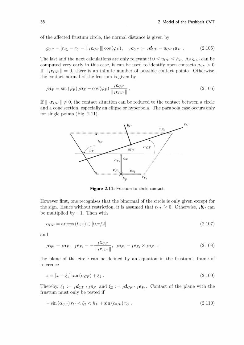
If ‖ IzCF ‖ 6= 0, the contact situation can be reduced to the contact between a circleand a cone section, especially an ellipse or hyperbola. The parabola case occurs onlyfor single points (Fig. 2.11).
hF
ϕF
aF
PF
MC
rF1
rF2
rCbC
αCF
eF1eF2
eF3
Figure 2.11: Frustum-to-circle contact.
However first, one recognises that the binormal of the circle is only given except forthe sign. Hence without restriction, it is assumed that tCF ≥ 0. Otherwise, IbC canbe multiplied by −1. Then with
αCF = arccos (tCF ) ∈ [0,π/2] (2.107)
and
IeF3= IaF , IeF1
= −IzCF
‖ IzCF ‖, IeF2
= IeF3× IeF1
, (2.108)
the plane of the circle can be defined by an equation in the frustum’s frame ofreference
z = [x− ξ1] tan (αCF ) + ξ2 . (2.109)
Thereby, ξ1 := IdCF · IeF1and ξ2 := IdCF · IeF3
. Contact of the plane with thefrustum must only be tested if
− sin (αCF ) rC < ξ2 < hF + sin (αCF ) rC . (2.110)
2.2 Interactions 37
The frustum can be parametrised by
x := rFhcos (ΨF ) , y := rFh
sin (ΨF ) , rFh:= rF1
+ tan (ϕF ) z (2.111)
with the circular ΨF ∈ [0,2π] and the axial z ∈ [0,hF ] contour parameters of thefrustum. Then, the conic section is given by
x =p cos (ΨF )
1 − cos (ΨF ) q, (2.112)
y =p sin (ΨF )
1 − cos (ΨF ) q, (2.113)
z =1
tan (ϕF )
[
p
1 − cos (ΨF ) q− rF1
]
(2.114)
with
p := rF1+ tan (ϕF ) [ξ2 − tan (αCF ) ξ1] , (2.115)
q := tan (ϕF ) tan (αCF ) . (2.116)
This conic section defines part of an ellipse for |q| < 1 and part of a hyperbola for|q| > 1. Thus by additionally excluding the cylinder (tan (ϕF ) 6= 0) and assuming afull intersection, it is possible to define the centre and the semi-major as well as thesemi-minor axis using the definition of rFh
:
IMCS := IP F +pq
1 − q2 IeF1+
1
tan (ϕF )
[
p
1 − q2− rF1
]
IeF3, (2.117)
Ic∗
CS1:=
p
1 − q2 IeF1+
1
tan (ϕF )
pq
1 − q2 IeF3, (2.118)
Ic∗
CS2:=
|p|√
|1 − q2|IeF2
. (2.119)
For a hyperbola, the transverse and imaginary axes are only defined except for thesign. The correct sign has to be chosen according to the affected cone comparingthe z-values of the hyperbola peaks. For the ellipse nothing has to be changed. Thisresults in
Ic∗
E1= Ic∗
CS1, Ic∗
E2= Ic∗
CS2, (2.120)
Ic∗
H1=
−pq
|pq|Ic∗
CS1, Ic∗
H2=
−pq
|pq|Ic∗
CS2. (2.121)
With the definitions from above, the ellipse and hyperbola are given by
IE (ρ) = IME + cos ρ Ic∗
E1+ sin ρ Ic∗
E2, (2.122)
IH (ρ) = IMH + cosh ρ Ic∗
H1+ sinh ρ Ic∗
H2(2.123)
with ρ ∈ [0,2π] for the ellipse and ρ ∈ [−σ,σ] for the hyperbola. Thereby, σ is
38 2 Model of the Pushbelt CVT
defined by the intersection of the circle plane with the larger frustum base area.The possible contact points on the circle are parametrised by
ICC (ρ) = IMC + rC InCS (ρ) (2.124)
with the normal InCS of the respective cone section. The contact points can berestricted by the necessary condition
ItCS (ρ) · [ICC (ρ) − ICS (ρ)] = 0 (2.125)
with the tangent ItCS and the parametrisations (2.122) or (2.123) of the respectivecone section. This results in the root functions
0 = 2[
− sin ρ Ic∗
E1+ cos ρ Ic∗
E2
]
· [IMC − IME]
+ sin (2ρ)[
‖ Ic∗
E1‖2 − ‖ Ic∗
E2‖2]
(ellipse) , (2.126)
0 = 2[
sinh ρ Ic∗
H1+ cosh ρ Ic∗
H2
]
· [IMC − IMH ]
− sinh (2ρ)[
‖ Ic∗
H1‖2 − ‖ Ic∗
H2‖2]
(hyperbola) (2.127)
being solved with a Newton-method using analytical Jacobians and a globalisa-tion with regula falsi. Assuming continuous contact point transition, a local searchis done after a first global contact detection. Selecting the contact parameter withthe minimum distance
gCE = ‖ IME − IMC + cos ρ Ic∗
E1+ sin ρ Ic∗
E2‖ − rC , (2.128)
gCH = ‖ IMH − IMC + cosh ρ Ic∗
H1+ sinh ρ Ic∗
H2‖ − rC (2.129)
between circle and respective cone section is sufficient if multiple contacts are ex-cluded. The resulting contact parameter ρ⋆ allows calculating the contact points onthe circle
ICC = IMC + rCICS (ρ⋆) − IMC
‖ ICS (ρ⋆) − IMC ‖. (2.130)
Then after checking if the selecting gap function (2.128) or (2.129) is negative, thecontact point on the frustum and the normals can be calculated with the ideas ofthe point-to-frustum contact from below.
Inner side of the circle and outer side of the frustum: The circle-to-circle contactonly differs in the distance and the normal
gCF = [rC − rFh− ‖ IcCF ‖] cos (ϕF ) , (2.131)
InF = − sin (ϕF ) IaF − cos (ϕF )IcCF
‖ IcCF ‖. (2.132)
The circle-to-hyperbola contact cannot appear.
2.2 Interactions 39
For the circle-to-ellipse contact only the selecting gap function
gCE = rC − ‖ IME − IMC + cos (ρ) Ic∗
E1+ sin (ρ) Ic∗
E2‖ (2.133)
is different.
Outer side of the circle and outer side of the frustum: This contact settingyields
gCF = [‖ IcCF ‖ − rC − rFh] cos (ϕF ) , (2.134)
InF = − sin (ϕF ) IaF + cos (ϕF )IcCF
‖ IcCF ‖(2.135)
for the circle-to-circle contact and the same selecting gap functions (2.128) or (2.129)as for the first contact case.
All other contact combinations are physically not possible.
Cylinder: In the case of a cylinder only the circle-to-ellipse contact occurs. Definingthe ellipse in its local coordinate system yields the parametrisation
x = rF cos (ΨF ) , y = rF sin (ΨF ) , z = [rF cos (ΨF ) − ξ1] tan (αCF ) + ξ2 (2.136)
with the radius rF of the cylinder. Transforming it into the inertial frame of referencegives the centre and the semi-major as well as the semi-minor axis
IME := IP F + [ξ2 − tan (αCF ) ξ1] IeF3, (2.137)
Ic∗
E1:=
rF
cos (αCF )[cos (αCF ) IeF1
+ sin (αCF ) IeF3] , (2.138)
Ic∗
E2:= rF IeF2
(2.139)
of the ellipse. Then with the adapted restrictions from above concerning full el-lipse and no multiple contacts, the same procedure can be used for the followingcalculations.
Point and frustum: Only the general contact between a point IQ and a frustumremains (Fig. 2.12).
Defining
Id := IQ − IP F , (2.140)
s := IaF · Id , (2.141)
Ib :=Id − s IaF
‖ Id − s IaF ‖, (2.142)
rFh:= rF1
+rF2
− rF1
hF
s (2.143)
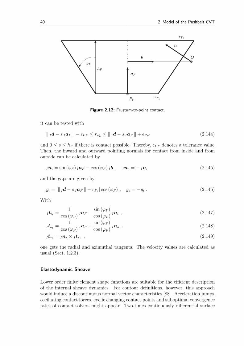
40 2 Model of the Pushbelt CVT
hF
ϕF
aF
PF
Q
rF1
rF2
n
b
Figure 2.12: Frustum-to-point contact.
it can be tested with
‖ Id − s IaF ‖ − ǫP F ≤ rFh≤ ‖ Id − s IaF ‖ + ǫP F (2.144)
and 0 ≤ s ≤ hF if there is contact possible. Thereby, ǫP F denotes a tolerance value.Then, the inward and outward pointing normals for contact from inside and fromoutside can be calculated by
Ini = sin (ϕF ) IaF − cos (ϕF ) Ib , Ino = − Ini (2.145)
and the gaps are given by
gi = [‖ Id − s IaF ‖ − rFh] cos (ϕF ) , go = −gi . (2.146)
With
Iti1=
1
cos (ϕF )IaF −
sin (ϕF )
cos (ϕF )Ini , (2.147)
Ito1=
1
cos (ϕF )IaF +
sin (ϕF )
cos (ϕF )Ino , (2.148)
It∗2= In∗ × It∗1
, (2.149)
one gets the radial and azimuthal tangents. The velocity values are calculated asusual (Sect. 1.2.3).
Elastodynamic Sheave
Lower order finite element shape functions are suitable for the efficient descriptionof the internal sheave dynamics. For contour definitions, however, this approachwould induce a discontinuous normal vector characteristics [88]. Acceleration jumps,oscillating contact forces, cyclic changing contact points and suboptimal convergencerates of contact solvers might appear. Two-times continuously differential surface
2.2 Interactions 41
parametrisations are necessary and sufficient to solve these drawbacks. Though,local shading known from computer graphics often yields sensitive solution behaviourdue to discontinuous changes of charts [88]. That is why, only global approximationsare reasonable for the underlying problem. The awarded adaptive algorithm ofCatmull-Clark would be a solution for nearly arbitrary topologies [75]. However,the discretisation reduces to a global B-spline surface for the applied regular finiteelement grid. The advantages of Catmull-Clark concerning adaptivity would nothave an effect. Finally, a global NURBS-based interpolation of finite element surfacenodes is chosen as a relatively easy but local, affine invariant, efficient, accurate andstable contour definition [76, 57].
NURBS: As surface parametrisations can be defined in a tensor product space ofcurve representations, it is sufficient to discuss one dimensional structures.
Each B-spline curve is given by n control points {IP j}j and recursively definedspline basis functions {Nj,p}j of degree p being parametrised by the real, ordered,non-periodic knot vector
S =
a, . . . , a︸ ︷︷ ︸
p+1
, sp+2, . . . , sm−p−1, b, . . . , b︸ ︷︷ ︸
p+1
(2.150)
of length m. As a reason of the global differentiability requirement, it is m = n+p+1.Then, the associated curve representation is given by
IC (s) =n∑
j=1
Nj,p (s) IP j , s ∈ [a,b] (2.151)
also allowing for smooth curve closing conditions. The dimension of the linear splinespace is given by m− p− 1. The generalisation to the projective space is called non-uniform rational B-spline (NURBS) curve
IC (s) =
∑nj=1 Nj,p (s)wj IP j∑n
k=1 Nk,p (s)wk
=n∑
j=1
Rj,p (s) IP j , s ∈ [a,b] (2.152)
because of its representation by rational basis functions {Rj,p}j, using additionalpositive weights {wj}j. As cone sections are represented exactly, the accuracy in-creases in spite of still using the efficient evaluation algorithms of the B-spline theory,for example the one of Cox-deBoor [57].
Curve fitting is of special interest in the current situation and can be done by leastsquare or interpolation algorithms. Focusing on global interpolation for exact noderepresentation, the amount per time step can be reduced to the solution of only onesparse, positive and banded linear system of equations. If
{
IQj
}
jare for instance
42 2 Model of the Pushbelt CVT
the finite element surface points to be interpolated, it is given by
N1,p (s1) · · · Nn,p (s1)...
...N1,p (sn) · · · Nn,p (sn)
IP 1...
IP n
=
IQ1...
IQn
(2.153)
with {sj}j being the evaluation points of the interpolated nodes in the parameterspace declared by an iterative chord length projection. This ansatz is based on theheuristics that also the knot vector is defined according to the chord length of theinterpolation points. The polynomial degree p is chosen to be larger than the localsmoothness demands and the weights are selected representing an initially most ac-curate approximation. A simplification is the calculation of the knot vector and thecomputation of the parameter space evaluation points once for the undeformed disk.Then, the system matrix in (2.153) has to be decomposed only in the initialisationand forward/backward substitutions suffice for the solution of (2.153) in each timestep.
Contact kinematics to a point: For the numerical calculation of contact kine-matics, the expected position, tangents, normal, velocities and Jacobians have tobe computed. Assuming a point Ip with velocity I p as contact partner, this mustonly be done concerning the sheave contour. It is satisfactory to compute the con-trol polygon concerning finite element surface node positions, translational velocitiesand Jacobians once per time step. The position of the k-th surface node is givenby (Sect. 2.1.3)
Irk =
(
cos γCI− sin γCI
sin γCIcos γCI
)(
cosϕk − sinϕk
sinϕk cosϕk
)(
rk + d2ϕrk
−d2ϕϕk
)
zCI+ uzk
+ d2
. (2.154)
The corresponding velocity fulfills
I rk =
γCI
(
− sin γCI− cos γCI
cos γCI− sin γCI
)(
cosϕk − sinϕk
sinϕk cosϕk
)(
rk + d2ϕrk
−d2ϕϕk
)
zCI+ uzk
+
(
cos γCI− sin γCI
sin γCIcos γCI
)(
cosϕk − sinϕk
sinϕk cosϕk
)(d2ϕrk
−d2ϕϕk
)
0
. (2.155)
The surface position Ir (s), translational velocity I r (s) and Jacobian J (s) distri-bution are evaluated by interpolation. They are explicitly depending on the surfaceparametrisation s ∈ IR2 and implicitly on the overall disk generalised coordinatesqg or velocities qg. Then, the tangents and the normal can be used for finding thepossible contact point sc by root functions according to Sect. 1.2.3. It would be afurther simplification to directly interpret the representation of the point Ip in the
2.2 Interactions 43
sheave cylinder coordinate system
uc :=
rc
Φc
zc
= Π (Ip) (2.156)
as a possible contact point. The measure differential equation of the disk [90] againresults with the ideas from Sect. 1.2.3.
Contact kinematics to a circle: Using the technique (2.156) for the sheave surfaceto point contact, the possible contact points only have to be examined on the circle.Let Ip (α) be the contour points on the circle and Iq (α) be the one on the sheavesurface with α ∈ [0,2π] and IzS as the axis of the sheave. Then from
minα∈[0,2π]
IzS · (Ip (α) − Iq (α)) , (2.157)
a necessary condition is given by
IzS · (Ip′ (α) − Iq′ (α)) = 0 . (2.158)
A prime denotes the derivative with respect to the circle parametrisation α and withthe radius rC and the tangent ItC (α) of the circle, it is
Ip′ (α) = rC ItC (α) . (2.159)
Further,
Iq′ (α) =(
∂Iq
∂rc
∂Iq
∂Φc0)
u′
c (α)
=(
∂Iq
∂rc
∂Iq
∂Φc0) ∂Π
∂ Ip Ip′ (α)
=(
∂Iq
∂rc
∂Iq
∂Φc0)
cosΦc sinΦc 0− sin Φc
rc
cos Φc
rc0
0 0 1
QT
IS Ip′ (α) (2.160)
results due to the chain rule, the sheave cylinder coordinate system and the trans-formation matrix QIS from the sheave moving frame to the world inertial frame ofreference.
2.2.4 Element – Ring Package Contacts
Assuming only very small clearance between the elements in longitudinal directionand the guidance of the elements by the ring packages avoiding detachment, twocontact points in the middle of the element saddles and at the element pillar define
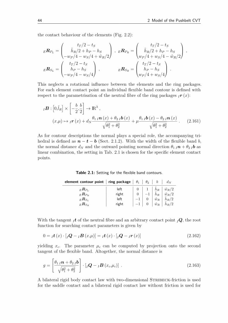
44 2 Model of the Pushbelt CVT
the contact behaviour of the elements (Fig. 2.2):
ERPL=
tT/2 − tShR/2 + hP − hS
−wP/4 − wS/4 + wR/2
, ERPR
=
tT/2 − tShR/2 + hP − hS
wP/4 + wS/4 − wR/2
,
ERSL=
tT/2 − tShP − hS
−wP/4 − wS/4
, ERSR
=
tT/2 − tShP − hS
wP/4 + wS/4
.
This neglects a rotational influence between the elements and the ring packages.For each element contact point an individual flexible band contour is defined withrespect to the parametrisation of the neutral fibre of the ring packages Ir (x):
IB :[
0,lR]
×
[
−b
2,b
2
]
→ IR3 ,
(x,µ) 7→ Ir (x) + dNθ1 In (x) + θ2 Ib (x)
√
θ21 + θ2
2
+ µθ1 Ib (x) − θ2 In (x)
√
θ21 + θ2
2
. (2.161)
As for contour descriptions the normal plays a special role, the accompanying tri-hedral is defined as n − t − b (Sect. 2.1.2). With the width of the flexible band b,the normal distance dN and the outward pointing normal direction θ1 In + θ2 Ib aslinear combination, the setting in Tab. 2.1 is chosen for the specific element contactpoints.
Table 2.1: Setting for the flexible band contours.
element contour point ring package θ1 θ2 b dN
ERPLleft 0 1 hR wR/2
ERPRright 0 −1 hR wR/2
ERSLleft −1 0 wR hR/2
ERSRright −1 0 wR hR/2
With the tangent It of the neutral fibre and an arbitrary contact point IQ, the rootfunction for searching contact parameters is given by
0 = It (x) · [IQ − IB (x,µ)] = It (x) · [IQ − Ir (x)] (2.162)
yielding xc. The parameter µc can be computed by projection onto the secondtangent of the flexible band. Altogether, the normal distance is
g =
θ1 In + θ2 Ib√
θ21 + θ2
2
· [IQ − IB (xc,µc)] . (2.163)
A bilateral rigid body contact law with two-dimensional Stribeck-friction is usedfor the saddle contact and a bilateral rigid contact law without friction is used for

2.2 Interactions 45
the pillar contact. The friction coefficient
µR
(
gRT
)
= µR0+
µR1
1 + µR2‖gRT
‖kR(2.164)
is based on the parameters µR0[−], µR1
[−], µR2
[
skR/mkR
]
and kR [−] as well as therelative velocity gRT
.
2.2.5 Element – Element Contacts
The element – element contacts can be summarised as follows.
Contour description
Between two adjacent elements the contact point EB is located at the front bottomand ET at the front head (Fig. 2.2). Additionally, there are two circular arcs withradius rR near the left and right front rocking edges
EEL =E
CFAL−
rR
00
+ rR
1 0 00 cosα sinα0 − sinα cosα
cos γsin γ
0
=E
MFAL+ rR
cos γcosα sin γ
− sinα sin γ
, (2.165)
EER =E
CFAR−
rR
00
+ rR
1 0 00 cosα − sinα0 sinα cosα
cos γsin γ
0
=E
MFAR+ rR
cos γcosα sin γsinα sin γ
(2.166)
with γ ∈ [−γ∗,0]. The binormals of the circles are given by
EbL =
0− cosα− sinα
, EbR =
0− cosαsinα
. (2.167)
A plane contour for the rear side is the counterpart for the contours described above.The pin-hole dynamics is modelled with two circle-frustum contacts (Fig. 2.13).
The curved contour of pin and hole satisfies
EEP = EMFH+
x
rP2cosψ + x
rP1−rP2
tT −tPcosψ
rP2sinψ + x
rP1−rP2
tT −tPsinψ
with x ∈ [tT − tP ,0] , (2.168)
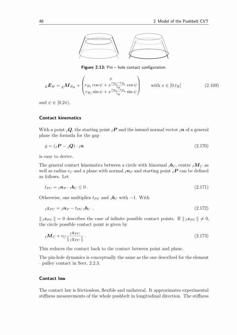
46 2 Model of the Pushbelt CVT
Figure 2.13: Pin – hole contact configuration.
EEH = EMRH+
x
rH1cosψ + x
rH2−rH1
tHcosψ
rH1sinψ + x
rH2−rH1
tHsinψ
with x ∈ [0,tH ] (2.169)
and ψ ∈ [0,2π).
Contact kinematics
With a point IQ, the starting point IP and the inward normal vector In of a generalplane the formula for the gap
g = (IP − IQ) · In (2.170)
is easy to derive.
The general contact kinematics between a circle with binormal IbC , centre IMC aswell as radius rC and a plane with normal InP and starting point IP can be definedas follows. Let
tP C = InP · IbC ≤ 0 . (2.171)
Otherwise, one multiplies tP C and IbC with −1. With
IzP C = InP − tP C IbC , (2.172)
‖ IzP C ‖ = 0 describes the case of infinite possible contact points. If ‖ IzP C ‖ 6= 0,the circle possible contact point is given by
IMC + rCIzP C
‖ IzP C ‖. (2.173)
This reduces the contact back to the contact between point and plane.
The pin-hole dynamics is conceptually the same as the one described for the element– pulley contact in Sect. 2.2.3.
Contact law
The contact law is frictionless, flexible and unilateral. It approximates experimentalstiffness measurements of the whole pushbelt in longitudinal direction. The stiffness
2.3 Assembling and Initialisation 47
at the top, at the rocking edge and at the bottom is
λEN(gEN
) =
cE1
2
(NE
lE|gEN
| − gEN0
)
for gEN≤ −gEN1
,
A
2|gEN
|kE1 for − gEN1< gEN
< 0 ,
0 for gEN≥ 0
(2.174)
using
gEN1=
kE1
kE1− 1
lENE
gEN0, (2.175)
A =cE1
kE1
(
kE1
kE1− 1
gEN0
)1−kE1(NE
lE
)kE1
(2.176)
and the global parameters gEN0[m], cE1
[N/m], kE1[−], lE [−] following the general
approach for serial spring connections. The stiffness at the pin-hole contact fulfills
λEN(gEN
) =
{
cE2|gEN
|kE2 for gEN< 0 ,
0 for gEN≥ 0
(2.177)
with cE2[N/m
kE2 ] and kE2[−].
2.3 Assembling and Initialisation
The analysis of a stationary target state is of primary interest in the majority ofindustrially relevant cases for oscillatory mechanical problems. Thus, it is preferableto calculate a suitable initial value for positions and velocities fulfilling a stationaryequality of forces and torques. This reduces at least the decay time of high-frequencyvibrations at the beginning of the time dependent simulation. The calculation ofsuch an initial value depends on the specific simulation model. One possibility is toderive a further abstraction of the dynamic model equations. Within the thematicscope, one can for instance consider the various stationary continuous belt models[65, 59] which promise to save about 0.2 s unnecessary real simulation time. Though,implications for the computing time depend on the relationship of the complexityof the dynamic and the stationary model.
2.3.1 Kinematics
With Fig. 2.14, it is
tL =√
sin2 (ϕ) d2A + d2
align (2.178)
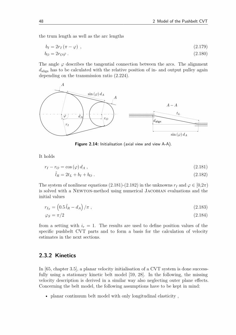
48 2 Model of the Pushbelt CVT
the trum length as well as the arc lengths
bI = 2rI (π − ϕ) , (2.179)
bO = 2rOϕ . (2.180)
The angle ϕ describes the tangential connection between the arcs. The alignmentdalign has to be calculated with the relative position of in- and output pulley againdepending on the transmission ratio (2.224).
ϕrO
rI
dA
A
A
sin (ϕ) dA
A − A
tL
dalign
sin (ϕ) dA
Figure 2.14: Initialisation (axial view and view A-A).
It holds
rI − rO = cos (ϕ) dA , (2.181)
lR = 2tL + bI + bO . (2.182)
The system of nonlinear equations (2.181)-(2.182) in the unknowns rI and ϕ ∈ [0,2π)is solved with a Newton-method using numerical Jacobian evaluations and theinitial values
rIS=(
0.5 lR − dA
)
/π , (2.183)
ϕS = π/2 (2.184)
from a setting with ir = 1. The results are used to define position values of thespecific pushbelt CVT parts and to form a basis for the calculation of velocityestimates in the next sections.
2.3.2 Kinetics
In [65, chapter 3.5], a planar velocity initialisation of a CVT system is done success-fully using a stationary kinetic belt model [59, 28]. In the following, the missingvelocity description is derived in a similar way also neglecting outer plane effects.Concerning the belt model, the following assumptions have to be kept in mind:
• planar continuum belt model with only longitudinal elasticity ,
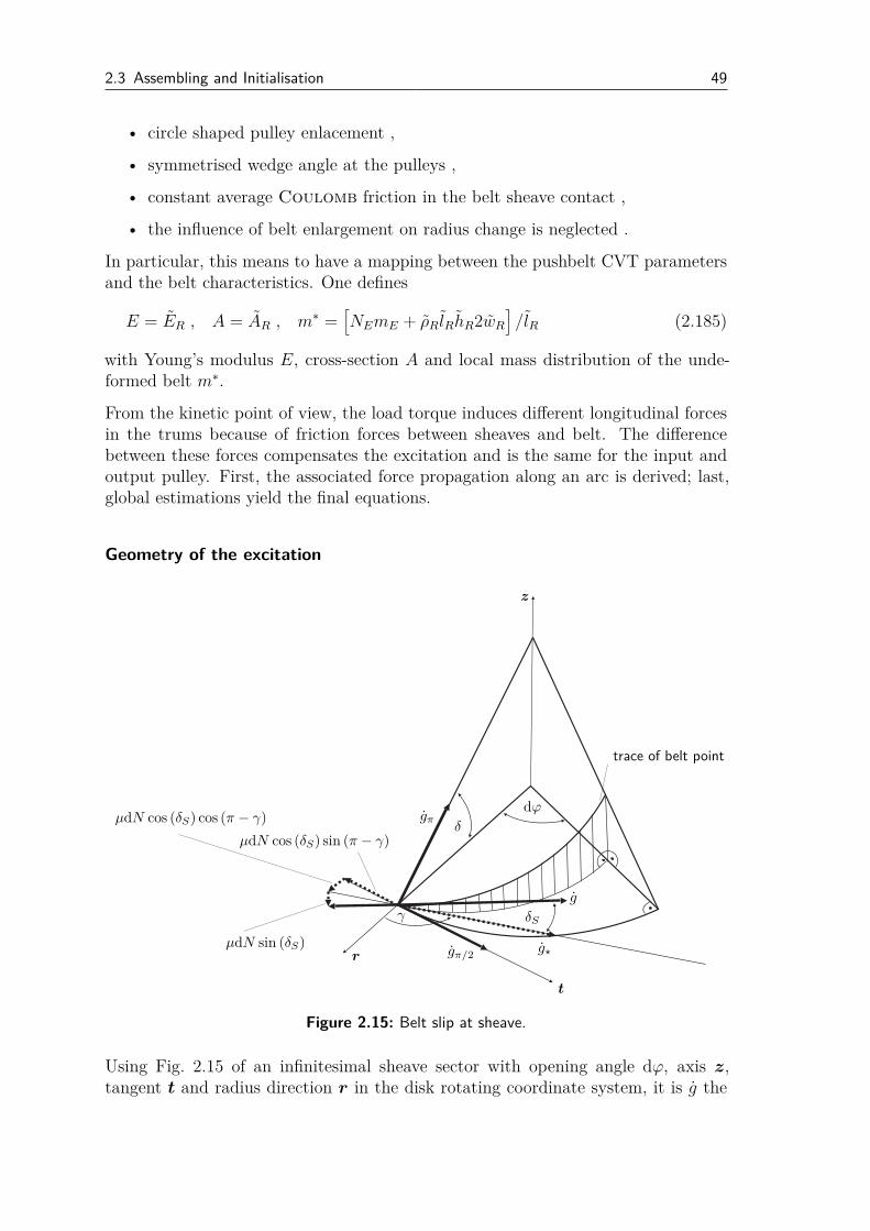
2.3 Assembling and Initialisation 49
• circle shaped pulley enlacement ,
• symmetrised wedge angle at the pulleys ,
• constant average Coulomb friction in the belt sheave contact ,
• the influence of belt enlargement on radius change is neglected .
In particular, this means to have a mapping between the pushbelt CVT parametersand the belt characteristics. One defines
E = ER , A = AR , m∗ =[
NEmE + ρR lRhR2wR
]
/lR (2.185)
with Young’s modulus E, cross-section A and local mass distribution of the unde-formed belt m∗.
From the kinetic point of view, the load torque induces different longitudinal forcesin the trums because of friction forces between sheaves and belt. The differencebetween these forces compensates the excitation and is the same for the input andoutput pulley. First, the associated force propagation along an arc is derived; last,global estimations yield the final equations.
Geometry of the excitation
trace of belt point
dϕ
δS
δ
µdN sin (δS)
µdN cos (δS) sin (π − γ)
µdN cos (δS) cos (π − γ)
γ
g⋆
gπ
gπ/2
g
z
t
r
Figure 2.15: Belt slip at sheave.
Using Fig. 2.15 of an infinitesimal sheave sector with opening angle dϕ, axis z,tangent t and radius direction r in the disk rotating coordinate system, it is g the
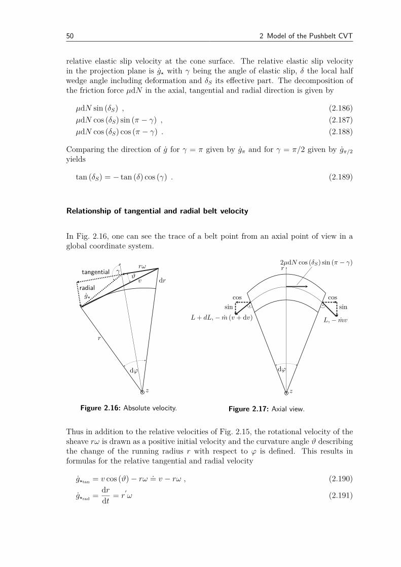
50 2 Model of the Pushbelt CVT
relative elastic slip velocity at the cone surface. The relative elastic slip velocityin the projection plane is g⋆ with γ being the angle of elastic slip, δ the local halfwedge angle including deformation and δS its effective part. The decomposition ofthe friction force µdN in the axial, tangential and radial direction is given by
µdN sin (δS) , (2.186)
µdN cos (δS) sin (π − γ) , (2.187)
µdN cos (δS) cos (π − γ) . (2.188)
Comparing the direction of g for γ = π given by gπ and for γ = π/2 given by gπ/2
yields
tan (δS) = − tan (δ) cos (γ) . (2.189)
Relationship of tangential and radial belt velocity
In Fig. 2.16, one can see the trace of a belt point from an axial point of view in aglobal coordinate system.
r
dr
g⋆
dϕ
tangential
radial
rω
z
γϑ
v
Figure 2.16: Absolute velocity.
r
L, − mv
2µdN cos (δS) sin (π − γ)
L + dL, − m (v + dv)
dϕ
z
coscos
sinsin
Figure 2.17: Axial view.
Thus in addition to the relative velocities of Fig. 2.15, the rotational velocity of thesheave rω is drawn as a positive initial velocity and the curvature angle ϑ describingthe change of the running radius r with respect to ϕ is defined. This results informulas for the relative tangential and radial velocity
g⋆tan= v cos (ϑ) − rω
.= v − rω , (2.190)
g⋆rad=
dr
dt= r
′
ω (2.191)
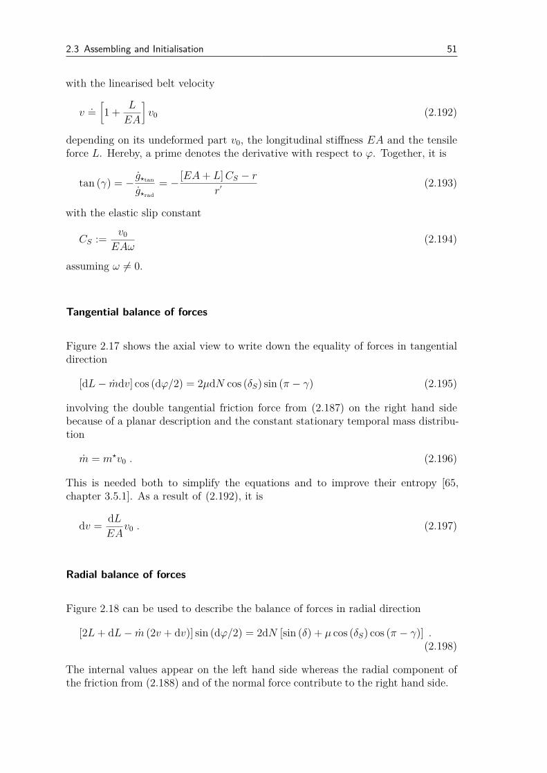
2.3 Assembling and Initialisation 51
with the linearised belt velocity
v.=[
1 +L
EA
]
v0 (2.192)
depending on its undeformed part v0, the longitudinal stiffness EA and the tensileforce L. Hereby, a prime denotes the derivative with respect to ϕ. Together, it is
tan (γ) = −g⋆tan
g⋆rad
= −[EA+ L]CS − r
r′(2.193)
with the elastic slip constant
CS :=v0
EAω(2.194)
assuming ω 6= 0.
Tangential balance of forces
Figure 2.17 shows the axial view to write down the equality of forces in tangentialdirection
[dL− mdv] cos (dϕ/2) = 2µdN cos (δS) sin (π − γ) (2.195)
involving the double tangential friction force from (2.187) on the right hand sidebecause of a planar description and the constant stationary temporal mass distribu-tion
m = m⋆v0 . (2.196)
This is needed both to simplify the equations and to improve their entropy [65,chapter 3.5.1]. As a result of (2.192), it is
dv =dL
EAv0 . (2.197)
Radial balance of forces
Figure 2.18 can be used to describe the balance of forces in radial direction
[2L+ dL− m (2v + dv)] sin (dϕ/2) = 2dN [sin (δ) + µ cos (δS) cos (π − γ)] .(2.198)
The internal values appear on the left hand side whereas the radial component ofthe friction from (2.188) and of the normal force contribute to the right hand side.
52 2 Model of the Pushbelt CVT
dS
cos −projection
sin −projection
[2L + dL] sin (dϕ/2) , − m [2v + dv] sin (dϕ/2)
µdN sin (δS)
2µdN cos (δS) cos (π − γ)
r dN
Figure 2.18: Radial view.
Axial balance of forces
The axial equilibrium of forces can be explained with Fig. 2.18 as well. With thesheave expansion force S, it is
dS = dN [cos (δ) − µ sin (δS)] . (2.199)
Change of the running radius
Equations (2.186)-(2.199) show the framework of [59, 65, 28] in its full generality.In contrast, changing of the running radius due to sheave tilting, transverse beltelasticity and axial sheave elasticity is not considered in the following because ofthe minor influence for the initialisation [65, Fig. 2.8 and 4.10]. These assumptionsinvolve
δ′ ≡ 0 , r′ ≡ 0 , γ ≡ ±π/2 , δS ≡ 0 (2.200)
and avoid numerical difficulties [65].
Summary of the stationary belt model and environment interaction
From (2.195) and (2.198), it follows by means of the linearisations
cos
(
dϕ
2
)
.= 1 , sin
(
dϕ
2
)
.=
dϕ
2, dL
dϕ
2.= 0 , (2.201)
some addition theorems and the consequences of the last paragraph
L′
=±µ [L− mv]
[1 − mωCS] sin (δ0)= ±
µ
sin (δ0)L∓
mµv0EA
[EA− mv0] sin (δ0)(2.202)
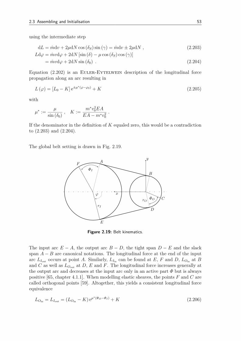
2.3 Assembling and Initialisation 53
using the intermediate step
dL = mdv + 2µdN cos (δS) sin (γ) = mdv ± 2µdN , (2.203)
Ldϕ = mvdϕ+ 2dN [sin (δ) − µ cos (δS) cos (γ)]
= mvdϕ+ 2dN sin (δ0) . (2.204)
Equation (2.202) is an Euler-Eytelwein description of the longitudinal forcepropagation along an arc resulting in
L (ϕ) = [L0 −K] e±µ∗(ϕ−ϕ0) +K (2.205)
with
µ∗ :=µ
sin (δ0), K :=
m∗v20EA
EA−m∗v20
.
If the denominator in the definition of K equaled zero, this would be a contradictionto (2.203) and (2.204).
The global belt setting is drawn in Fig. 2.19.
x
yA
B
C
D
E
F
ϕ
ΦI
ΦOrO
rI
Figure 2.19: Belt kinematics.
The input arc E − A, the output arc B − D, the tight span D − E and the slackspan A−B are canonical notations. The longitudinal force at the end of the inputarc LIout
occurs at point A. Similarly, LIincan be found at E, F and D, LOin
at Band C as well as LOout
at D, E and F . The longitudinal force increases generally atthe output arc and decreases at the input arc only in an active part Φ but is alwayspositive [65, chapter 4.1.1]. When modelling elastic sheaves, the points F and C arecalled orthogonal points [59]. Altogether, this yields a consistent longitudinal forceequivalence
LOin= LIout
= (LOin−K) eµ∗(ΦO−ΦI) +K (2.206)
54 2 Model of the Pushbelt CVT
resulting in
LOin= K ∨ ΦO = ΦI . (2.207)
Sticking implies two additional equations
rIωI = v0
(
1 +LIin
EA
)
= v0
[
1 +(LOin
−K) eµ∗ΦO +K
EA
]
(points E − F ) , (2.208)
rOωO = v0
(
1 +LOin
EA
)
(points B − C) . (2.209)
The equality of torques
MO = rO (LOout− LOin
) = rO (LOin−K)
(
eµ∗ΦO − 1)
(2.210)
with MO being the positive load torque and the axial equality of forces
FCO=∫
ϕO
S ′dϕ
=∫
ϕO
L [EA−m⋆v20] −m∗v2
0EA
2 tan (δ0)EAdϕ
=EA−m⋆v2
0
2 tan (δ0)EA
ϕ−ΦO∫
−ϕ
Ldϕ+
ϕ∫
ϕ−ΦO
Ldϕ
−
m∗v20
tan (δ0)ϕ
=EA−m⋆v2
0
2 tan (δ0)EA
[
2LOinϕ+ (LOin
−K)
(
eµ∗ΦO − 1
µ∗− ΦO
)]
−m∗v2
0ϕ
tan (δ0)(2.211)
have to be solved concerning the output pulley. Hereby, (2.204) and (2.199) yieldthe expression for S ′.
Reduction of the final equations
Goal of this paragraph is the computation of ωO, v0, ΦI , ΦO and LOinfor initialising
velocity values. Of course, it is E > 0, A > 0, δ0 > 0, ϕ > 0, m∗ > 0, rI > 0, rO > 0,ωI > 0 and thus v0 > 0 for practical settings. Then clearly,
LOin=EArOωO
v0
− EA (2.212)
according to (2.209). Concerning (2.207)-(2.211), one has to distinguish two cases:
1. For LOin= K, it follows necessarily MO = 0 and FCO
= 0. The conditionFCO
= 0 means that there is no sheave-belt contact which is practically not
2.3 Assembling and Initialisation 55
relevant. Furthermore, MO = 0 yields LOin= K or ΦO = 0 from the mathe-
matical viewpoint assuming µ > 0. From the physical viewpoint, ΦO = 0 andso also ΦI = 0 are interesting. Thus, it is
ωO =rI
rO
ωI , (2.213)
v0 =
√
(FCOtan (δ0) + EAϕ)2 + 4EAm∗r2
Iω2Iϕ
2 − EAϕ− FCOtan (δ0)
2m∗rIωIϕ.
(2.214)
2. If MO 6= 0, it is necessarily ΦI = ΦO and LOin6= K. Hence,
ΦO =1
µ∗ln
[
MO
rO (LOin−K)
+ 1
]
(2.215)
is only defined for MO > rO (K − LOin). This condition depends on the kine-
matic and kinetic setting and states the physical application in the same wayas the inequalities
ΦI < 2 (π − ϕ) , ΦO < 2ϕ (2.216)
define the active arcs. Equations (2.208) and (2.211) remain only dependingon ωO and v0. They can be solved by a generalised Newton method withnumerical Jacobian evaluation and starting values from the MO = 0 case.
Now, ωI and ωO can be used for the initialisation of the pulleys’ and ring packages’angular velocities. According to (2.192) and (2.205), the expression
v =
1 +
(
EA(
vin
v0− 1
)
−K)
eµ∗(ϕ−ϕ0) +K
EA
v0 (2.217)
explains the behaviour of the ring package belt velocity in an active arc starting fromvin at ϕ = ϕ0. Element velocities have to be inherited from the ring packages.
2.3.3 Pulleys
Of course, the centres of gravity of the fixed sheaves are always at the same positiongiven by
IrOF=
00
wV /2 + tPSO
, IrIF
=
dA
0−wV /2 − tPSI
(2.218)
but the loose sheaves depend on the transmission ratio and on the curved geometryof the elements. Figure 2.20 shows the situation neglecting the thickness of theelements.
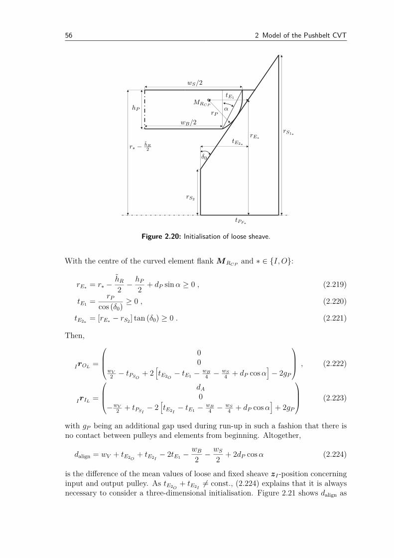
56 2 Model of the Pushbelt CVT
tE1
tE2∗
rE∗
r∗ − hR
2
hP
wS/2
wB/2
MRCP
rPα
δ0
rS1∗
rS2
tPF∗
Figure 2.20: Initialisation of loose sheave.
With the centre of the curved element flank MRCPand ∗ ∈ {I, O}:
rE∗= r∗ −
hR
2−hP
2+ dP sinα ≥ 0 , (2.219)
tE1=
rP
cos (δ0)≥ 0 , (2.220)
tE2∗= [rE∗
− rS2] tan (δ0) ≥ 0 . (2.221)
Then,
IrOL=
00
wV
2− tPSO
+ 2[
tE2O− tE1
− wB
4− wS
4+ dP cosα
]
− 2gP
, (2.222)
IrIL=
dA
0
−wV
2+ tPSI
− 2[
tE2I− tE1
− wB
4− wS
4+ dP cosα
]
+ 2gP
(2.223)
with gP being an additional gap used during run-up in such a fashion that there isno contact between pulleys and elements from beginning. Altogether,
dalign = wV + tE2O+ tE2I
− 2tE1−wB
2−wS
2+ 2dP cosα (2.224)
is the difference of the mean values of loose and fixed sheave zI-position concerninginput and output pulley. As tE2O
+ tE2I6= const., (2.224) explains that it is always
necessary to consider a three-dimensional initialisation. Figure 2.21 shows dalign as
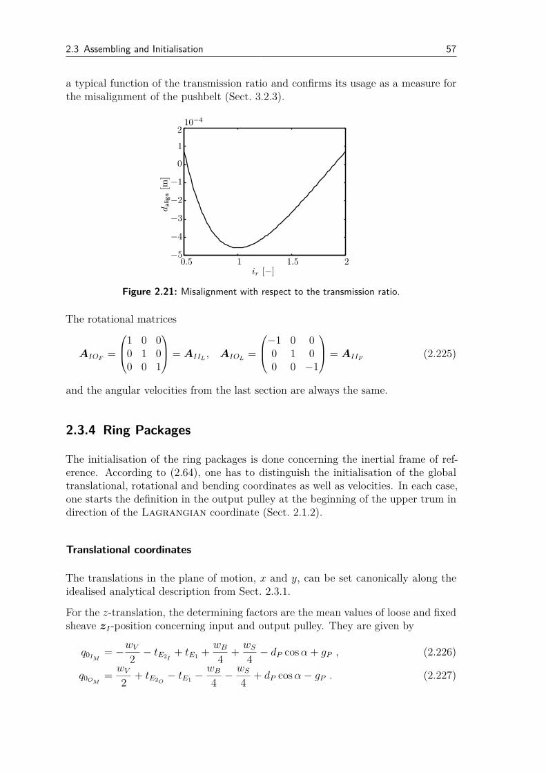
2.3 Assembling and Initialisation 57
a typical function of the transmission ratio and confirms its usage as a measure forthe misalignment of the pushbelt (Sect. 3.2.3).
ir [−]
dalign
[m]
0.5 1 1.5 2
10−4
−5
−4
−3
−2
−1
1
2
0
Figure 2.21: Misalignment with respect to the transmission ratio.
The rotational matrices
AIOF=
1 0 00 1 00 0 1
= AIIL
, AIOL=
−1 0 00 1 00 0 −1
= AIIF
(2.225)
and the angular velocities from the last section are always the same.
2.3.4 Ring Packages
The initialisation of the ring packages is done concerning the inertial frame of ref-erence. According to (2.64), one has to distinguish the initialisation of the globaltranslational, rotational and bending coordinates as well as velocities. In each case,one starts the definition in the output pulley at the beginning of the upper trum indirection of the Lagrangian coordinate (Sect. 2.1.2).
Translational coordinates
The translations in the plane of motion, x and y, can be set canonically along theidealised analytical description from Sect. 2.3.1.
For the z-translation, the determining factors are the mean values of loose and fixedsheave zI-position concerning input and output pulley. They are given by
q0IM= −
wV
2− tE2I
+ tE1+wB
4+wS
4− dP cosα+ gP , (2.226)
q0OM=wV
2+ tE2O
− tE1−wB
4−wS
4+ dP cosα− gP . (2.227)
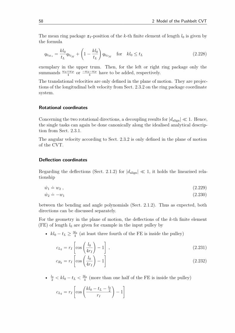
58 2 Model of the Pushbelt CVT
The mean ring package zI-position of the k-th finite element of length l0 is given bythe formula
q0M z=kl0tLq0IM
+
(
1 −kl0tL
)
q0OMfor kl0 ≤ tL (2.228)
exemplary in the upper trum. Then, for the left or right ring package only thesummands wS+wP
4or −wS−wP
4have to be added, respectively.
The translational velocities are only defined in the plane of motion. They are projec-tions of the longitudinal belt velocity from Sect. 2.3.2 on the ring package coordinatesystem.
Rotational coordinates
Concerning the two rotational directions, a decoupling results for |dalign| ≪ 1. Hence,the single tasks can again be done canonically along the idealised analytical descrip-tion from Sect. 2.3.1.
The angular velocity according to Sect. 2.3.2 is only defined in the plane of motionof the CVT.
Deflection coordinates
Regarding the deflections (Sect. 2.1.2) for |dalign| ≪ 1, it holds the linearised rela-tionship
w1.= w2 , (2.229)
w2.= −w1 (2.230)
between the bending and angle polynomials (Sect. 2.1.2). Thus as expected, bothdirections can be discussed separately.
For the geometry in the plane of motion, the deflections of the k-th finite element(FE) of length l0 are given for example in the input pulley by
• kl0 − tL ≥ 3l04
(at least three fourth of the FE is inside the pulley)
cL2= rI
[
cos
(
l04rI
)
− 1
]
, (2.231)
cR2= rI
[
cos
(
l04rI
)
− 1
]
(2.232)
• l02< kl0 − tL <
3l04
(more than one half of the FE is inside the pulley)
cL2= rI
[
cos
(
kl0 − tL − l02
rI
)
− 1
]

2.3 Assembling and Initialisation 59
−
(
3l04
− kl0 + tL
)
sin
(
kl0 − tL − l02
rI
)
, (2.233)
cR2= rI
[
cos
(
l04rI
)
− 1
]
(2.234)
• l04< kl0 − tL ≤ l0
2(more than one fourth of the FE is inside the pulley)
cL2= 0 , (2.235)
cR2= rI
[
cos
(
kl0 − tL − l04
rI
)
− 1
]
(2.236)
• kl0 − tL ≤ l04
(at most one fourth of the FE is inside the pulley)
cL2= 0 , (2.237)
cR2= 0 . (2.238)
The outer plane deflections fulfill for instance in the input pulley
• kl0 − tL ≥ 3l04
(at least three fourth of the FE is inside the pulley)
cL1= 0 , (2.239)
cR1= 0 (2.240)
• l02< kl0 − tL <
3l04
(more than one half of the FE is inside the pulley)
cL1= − sin (βalign)
[
tL − (k − 1) l0 −l04
]
, (2.241)
cR1= 0 (2.242)
• l04< kl0 − tL ≤ l0
2(more than one fourth of the FE is inside the pulley)
cL1= 0 , (2.243)
cR1= − sin (βalign)
[
(k − 1) l0 +3
4l0 − tL
]
(2.244)
• kl0 − tL ≤ l04
(at most one fourth of the FE is inside the pulley)
cL1= 0 , (2.245)
cR1= 0 (2.246)
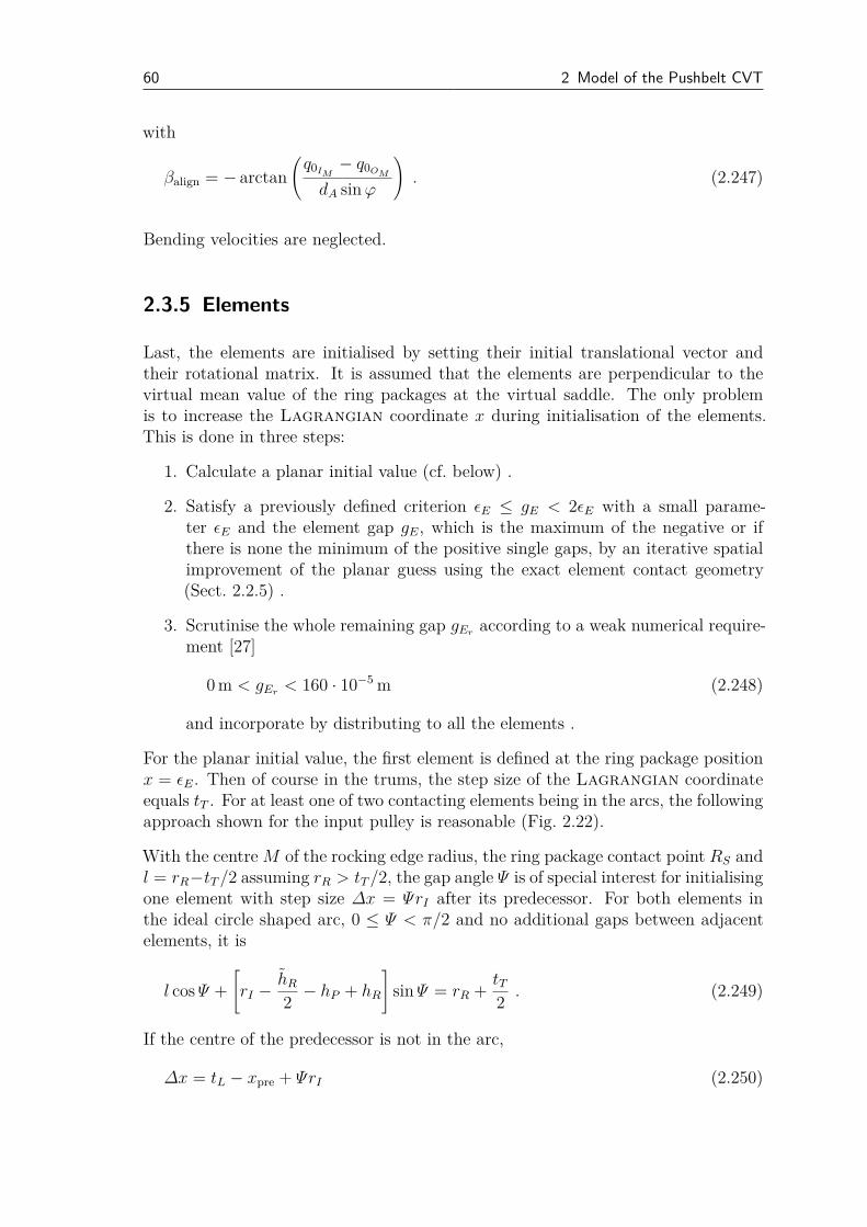
60 2 Model of the Pushbelt CVT
with
βalign = − arctan
(q0IM
− q0OM
dA sinϕ
)
. (2.247)
Bending velocities are neglected.
2.3.5 Elements
Last, the elements are initialised by setting their initial translational vector andtheir rotational matrix. It is assumed that the elements are perpendicular to thevirtual mean value of the ring packages at the virtual saddle. The only problemis to increase the Lagrangian coordinate x during initialisation of the elements.This is done in three steps:
1. Calculate a planar initial value (cf. below) .
2. Satisfy a previously defined criterion ǫE ≤ gE < 2ǫE with a small parame-ter ǫE and the element gap gE, which is the maximum of the negative or ifthere is none the minimum of the positive single gaps, by an iterative spatialimprovement of the planar guess using the exact element contact geometry(Sect. 2.2.5) .
3. Scrutinise the whole remaining gap gEraccording to a weak numerical require-
ment [27]
0 m < gEr< 160 · 10−5 m (2.248)
and incorporate by distributing to all the elements .
For the planar initial value, the first element is defined at the ring package positionx = ǫE. Then of course in the trums, the step size of the Lagrangian coordinateequals tT . For at least one of two contacting elements being in the arcs, the followingapproach shown for the input pulley is reasonable (Fig. 2.22).
With the centre M of the rocking edge radius, the ring package contact point RS andl = rR−tT/2 assuming rR > tT/2, the gap angle Ψ is of special interest for initialisingone element with step size ∆x = ΨrI after its predecessor. For both elements inthe ideal circle shaped arc, 0 ≤ Ψ < π/2 and no additional gaps between adjacentelements, it is
l cosΨ +
[
rI −hR
2− hP + hR
]
sinΨ = rR +tT2. (2.249)
If the centre of the predecessor is not in the arc,
∆x = tL − xpre + ΨrI (2.250)
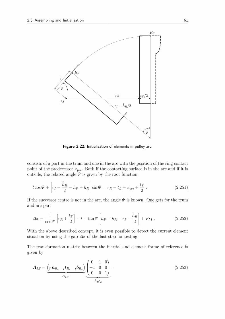
2.3 Assembling and Initialisation 61
Ψ
Ψ
rR
rI − hR/2M
l
RS
RS
tT /2
Figure 2.22: Initialisation of elements in pulley arc.
consists of a part in the trum and one in the arc with the position of the ring contactpoint of the predecessor xpre. Both if the contacting surface is in the arc and if it isoutside, the related angle Ψ is given by the root function
l cosΨ +
[
rI −hR
2− hP + hR
]
sinΨ = rR − tL + xpre +tT2. (2.251)
If the successor centre is not in the arc, the angle Ψ is known. One gets for the trumand arc part
∆x =1
cosΨ
[
rR +tT2
]
− l + tanΨ
[
hP − hR − rI +hR
2
]
+ ΨrI . (2.252)
With the above described concept, it is even possible to detect the current elementsituation by using the gap ∆x of the last step for testing.
The transformation matrix between the inertial and element frame of reference isgiven by
AIE =(
I nRv ItRv IbRv
)
︸ ︷︷ ︸
AIE
′
0 1 0−1 0 00 0 1
︸ ︷︷ ︸
AE
′E
. (2.253)
62 2 Model of the Pushbelt CVT
Further, the position of the elements can be calculated with the position IrRvof the
virtual ring package at the given value of the Lagrangian coordinate
IrE = IrRv+ AIE
tS − tT/2
−hP + hS − hR/20
. (2.254)
The velocities can also be taken from the ring package.
2.4 Summary
The overall model equations of the variator have the structure of Sect. 1.2.1 andare characterised by a large degree of freedom of about 3500 and 5500 contacts.In [27] the degree of freedom and the number of contacts of the related planarmodel based on the nonsmooth mechanics approach are summarised with 1500 and3500, respectively. Nevertheless, the modular structure of both models allows forrefinements or even substitutions of sub-models. A detailed comparison is given inTab. 2.2.
It is clear, that Young’s modulus of the ring packages influences the numericalstiffness of the whole CVT and furthermore the global time step size of explicitintegration schemes (Sect. 1.3). However, the high contact closing frequency has tobe resolved in a certain level to represent the variator dynamics. Together with thelarge degree of freedom of the system, this causes long simulation times especiallyfor the spatial model. With the techniques of Sect. 2.5 these challenges shall beeliminated and the simulation model shall be prepared for reasonable validation.
Further, the initialisation results in additional instabilities for instance because ofa jump from curvature 0 in the trum to a constant curvature 6= 0 in the arcs notbeing represented exactly by the bending polynomials. To minimise the effects onthe rest of the simulation, a special pre-integration perhaps with reduced integrationtime step size or with additional damping values in between the elements has to beperformed to get a physically valid, stationary state of the system.
2.5 CPU Time Reduction
The computational amount during the integration of a differential equation can bedivided into the amount per time step and the number of time steps as a multiplier.In the following the spatial simulation of a chain of pearls, a flexible belt with 30rigid elements that are linearly arranged, is chosen as a first benchmark problem(cp. Fig. 2.23). The elements’ kinematics is described relatively to the belt, 20 fi-nite elements have been used for its discretisation and an half-explicit timesteppingscheme [25] is applied. The main effort per time step is defined by the kinematic
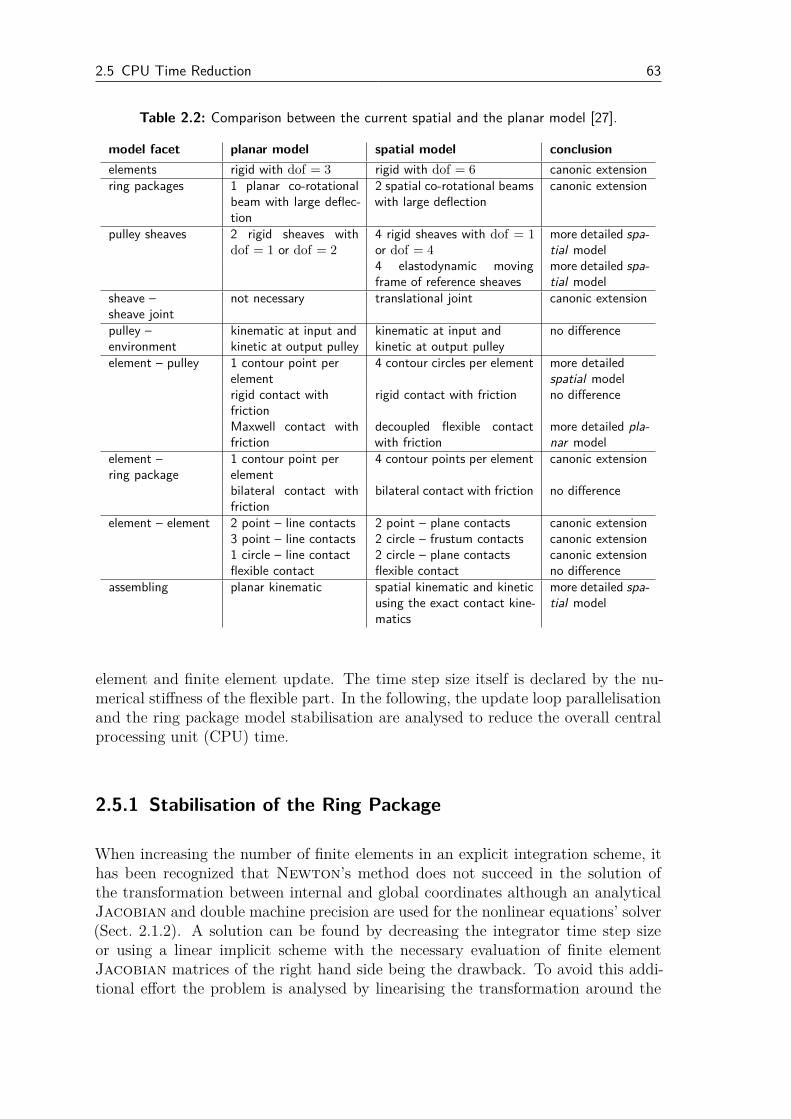
2.5 CPU Time Reduction 63
Table 2.2: Comparison between the current spatial and the planar model [27].
model facet planar model spatial model conclusion
elements rigid with dof = 3 rigid with dof = 6 canonic extensionring packages 1 planar co-rotational
beam with large deflec-tion
2 spatial co-rotational beamswith large deflection
canonic extension
pulley sheaves 2 rigid sheaves withdof = 1 or dof = 2
4 rigid sheaves with dof = 1or dof = 4
more detailed spa-
tial model4 elastodynamic movingframe of reference sheaves
more detailed spa-
tial modelsheave – not necessary translational joint canonic extensionsheave jointpulley – kinematic at input and kinematic at input and no differenceenvironment kinetic at output pulley kinetic at output pulleyelement – pulley 1 contour point per 4 contour circles per element more detailed
element spatial modelrigid contact with rigid contact with friction no differencefrictionMaxwell contact withfriction
decoupled flexible contactwith friction
more detailed pla-
nar modelelement – 1 contour point per 4 contour points per element canonic extensionring package element
bilateral contact withfriction
bilateral contact with friction no difference
element – element 2 point – line contacts 2 point – plane contacts canonic extension3 point – line contacts 2 circle – frustum contacts canonic extension1 circle – line contact 2 circle – plane contacts canonic extensionflexible contact flexible contact no difference
assembling planar kinematic spatial kinematic and kineticusing the exact contact kine-matics
more detailed spa-
tial model
element and finite element update. The time step size itself is declared by the nu-merical stiffness of the flexible part. In the following, the update loop parallelisationand the ring package model stabilisation are analysed to reduce the overall centralprocessing unit (CPU) time.
2.5.1 Stabilisation of the Ring Package
When increasing the number of finite elements in an explicit integration scheme, ithas been recognized that Newton’s method does not succeed in the solution ofthe transformation between internal and global coordinates although an analyticalJacobian and double machine precision are used for the nonlinear equations’ solver(Sect. 2.1.2). A solution can be found by decreasing the integrator time step sizeor using a linear implicit scheme with the necessary evaluation of finite elementJacobian matrices of the right hand side being the drawback. To avoid this addi-tional effort the problem is analysed by linearising the transformation around the
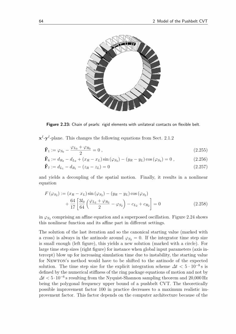
64 2 Model of the Pushbelt CVT
Figure 2.23: Chain of pearls: rigid elements with unilateral contacts on flexible belt.
xI-yI-plane. This changes the following equations from Sect. 2.1.2
F1 := ϕS0−ϕL0
+ ϕR0
2= 0 , (2.255)
F6 := dR2− dL2
+ (xR − xL) sin (ϕS2) − (yR − yL) cos (ϕS2
) = 0 , (2.256)
F7 := dL1− dR1
− (zR − zL) = 0 (2.257)
and yields a decoupling of the spatial motion. Finally, it results in a nonlinearequation
F (ϕS2) := (xR − xL) sin (ϕS2
) − (yR − yL) cos (ϕS2)
+64
17
[
3l064
(ϕL2
+ ϕR2
2− ϕS2
)
− cL2+ cR2
]
= 0 (2.258)
in ϕS2comprising an affine equation and a superposed oscillation. Figure 2.24 shows
this nonlinear function and its affine part in different settings.
The solution of the last iteration and so the canonical starting value (marked witha cross) is always in the antinode around ϕS2
= 0. If the integrator time step sizeis small enough (left figure), this yields a new solution (marked with a circle). Forlarge time step sizes (right figure) for instance when global input parameters (axis in-tercept) blow up for increasing simulation time due to instability, the starting valuefor Newton’s method would have to be shifted to the antinode of the expectedsolution. The time step size for the explicit integration scheme ∆t < 5 · 10−8 s isdefined by the numerical stiffness of the ring package equations of motion and not by∆t < 5 ·10−6 s resulting from the Nyquist-Shannon sampling theorem and 20,000 Hzbeing the polygonal frequency upper bound of a pushbelt CVT. The theoreticallypossible improvement factor 100 in practice decreases to a maximum realistic im-provement factor. This factor depends on the computer architecture because of the
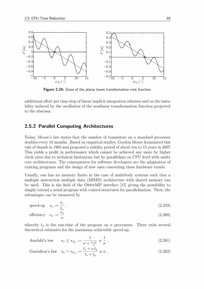
2.5 CPU Time Reduction 65
ϕS2[−]
F[m
]
−0.8
−0.6
−0.4
−0.2
0.8
0.6
0.4
0.2
0
15−10 −5 5 100−1
ϕS2[−]
F[m
]
−0.4
−0.3
−0.2
−0.1
0.5
0.4
0.3
0.2
0.1
0
15−10 −5 5 100
Figure 2.24: Zeros of the planar beam transformation root function.
additional effort per time step of linear implicit integration schemes and on the insta-bility induced by the oscillation of the nonlinear transformation function projectedto the abscissa.
2.5.2 Parallel Computing Architectures
Today, Moore’s law states that the number of transistors on a standard processordoubles every 18 months. Based on empirical studies, Gordon Moore formulated thisrule of thumb in 1965 and proposed a validity period of about ten to 15 years in 2007.This yields a profit in performance which cannot be achieved any more by higherclock rates due to technical limitations but by parallelism on CPU level with multi-core architectures. The consequences for software developers are the adaptation ofexisting programs and the design of new ones concerning these hardware trends.
Usually, one has no memory limits in the case of multibody systems such that amultiple instruction multiple data (MIMD) architecture with shared memory canbe used. This is the field of the OpenMP interface [15] giving the possibility tosimply extend a serial program with control structures for parallelisation. Then, theadvantages can be measured by
speed-up sn :=t1tn, (2.259)
efficiency en :=sn
n(2.260)
whereby tn is the run-time of the program on n processors. There exist severaltheoretical estimates for the maximum achievable speed-up,
Amdahl’s law sn ≤ sAn:=
1
σ + 1−σn
41
σ, (2.261)
Gustafson’s law sn = sGn:=
ts + n tpts + tp
4 n . (2.262)
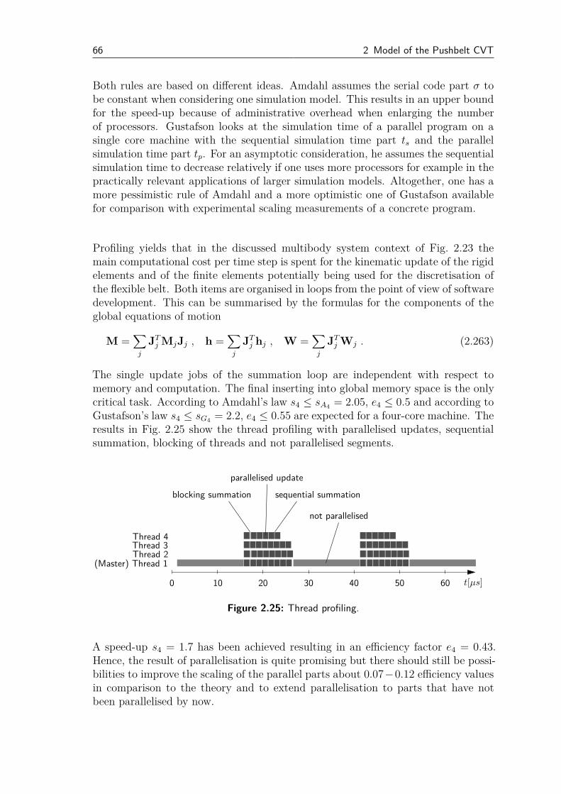
66 2 Model of the Pushbelt CVT
Both rules are based on different ideas. Amdahl assumes the serial code part σ tobe constant when considering one simulation model. This results in an upper boundfor the speed-up because of administrative overhead when enlarging the numberof processors. Gustafson looks at the simulation time of a parallel program on asingle core machine with the sequential simulation time part ts and the parallelsimulation time part tp. For an asymptotic consideration, he assumes the sequentialsimulation time to decrease relatively if one uses more processors for example in thepractically relevant applications of larger simulation models. Altogether, one has amore pessimistic rule of Amdahl and a more optimistic one of Gustafson availablefor comparison with experimental scaling measurements of a concrete program.
Profiling yields that in the discussed multibody system context of Fig. 2.23 themain computational cost per time step is spent for the kinematic update of the rigidelements and of the finite elements potentially being used for the discretisation ofthe flexible belt. Both items are organised in loops from the point of view of softwaredevelopment. This can be summarised by the formulas for the components of theglobal equations of motion
M =∑
j
JTj MjJj , h =
∑
j
JTj hj , W =
∑
j
JTj Wj . (2.263)
The single update jobs of the summation loop are independent with respect tomemory and computation. The final inserting into global memory space is the onlycritical task. According to Amdahl’s law s4 ≤ sA4
= 2.05, e4 ≤ 0.5 and according toGustafson’s law s4 ≤ sG4
= 2.2, e4 ≤ 0.55 are expected for a four-core machine. Theresults in Fig. 2.25 show the thread profiling with parallelised updates, sequentialsummation, blocking of threads and not parallelised segments.
0 10 20 30 40 50 60
(Master) Thread 1Thread 2Thread 3
t[µs]
Thread 4
blocking summation
parallelised update
sequential summation
not parallelised
Figure 2.25: Thread profiling.
A speed-up s4 = 1.7 has been achieved resulting in an efficiency factor e4 = 0.43.Hence, the result of parallelisation is quite promising but there should still be possi-bilities to improve the scaling of the parallel parts about 0.07−0.12 efficiency valuesin comparison to the theory and to extend parallelisation to parts that have notbeen parallelised by now.
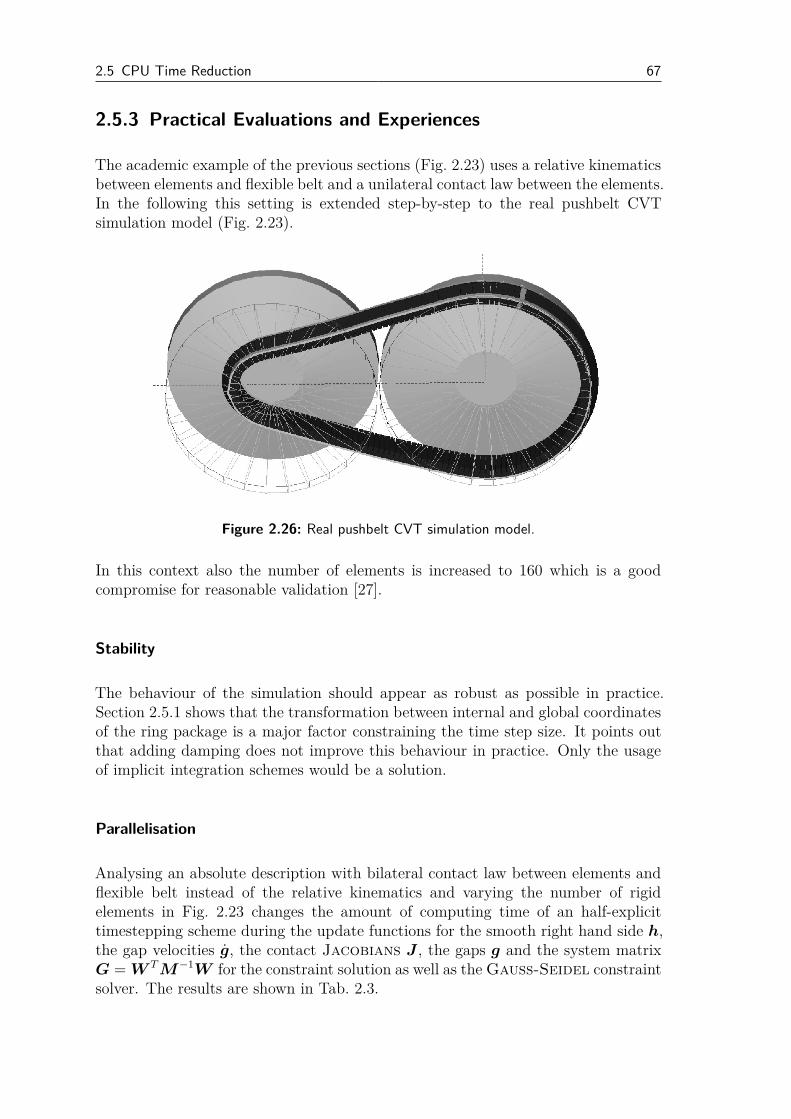
2.5 CPU Time Reduction 67
2.5.3 Practical Evaluations and Experiences
The academic example of the previous sections (Fig. 2.23) uses a relative kinematicsbetween elements and flexible belt and a unilateral contact law between the elements.In the following this setting is extended step-by-step to the real pushbelt CVTsimulation model (Fig. 2.23).
Figure 2.26: Real pushbelt CVT simulation model.
In this context also the number of elements is increased to 160 which is a goodcompromise for reasonable validation [27].
Stability
The behaviour of the simulation should appear as robust as possible in practice.Section 2.5.1 shows that the transformation between internal and global coordinatesof the ring package is a major factor constraining the time step size. It points outthat adding damping does not improve this behaviour in practice. Only the usageof implicit integration schemes would be a solution.
Parallelisation
Analysing an absolute description with bilateral contact law between elements andflexible belt instead of the relative kinematics and varying the number of rigidelements in Fig. 2.23 changes the amount of computing time of an half-explicittimestepping scheme during the update functions for the smooth right hand side h,the gap velocities g, the contact Jacobians J , the gaps g and the system matrixG = W T M−1W for the constraint solution as well as the Gauss-Seidel constraintsolver. The results are shown in Tab. 2.3.
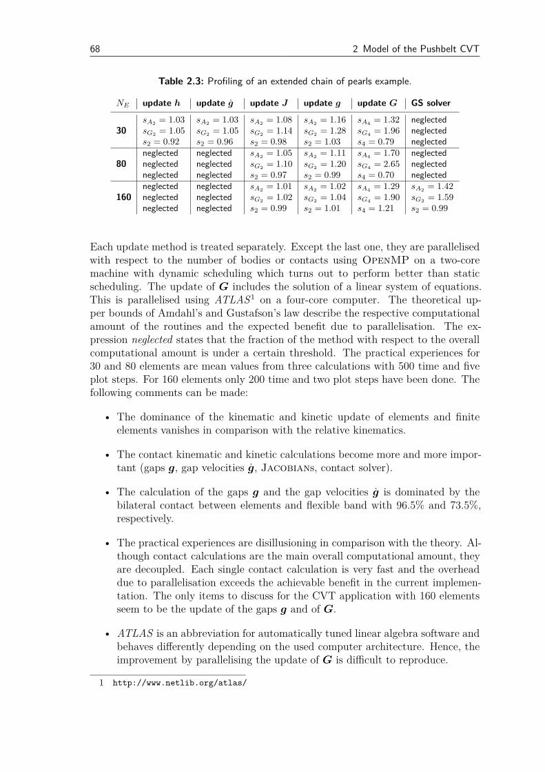
68 2 Model of the Pushbelt CVT
Table 2.3: Profiling of an extended chain of pearls example.
NE update h update g update J update g update G GS solver
30
sA2= 1.03 sA2
= 1.03 sA2= 1.08 sA2
= 1.16 sA4= 1.32 neglected
sG2= 1.05 sG2
= 1.05 sG2= 1.14 sG2
= 1.28 sG4= 1.96 neglected
s2 = 0.92 s2 = 0.96 s2 = 0.98 s2 = 1.03 s4 = 0.79 neglected
80
neglected neglected sA2= 1.05 sA2
= 1.11 sA4= 1.70 neglected
neglected neglected sG2= 1.10 sG2
= 1.20 sG4= 2.65 neglected
neglected neglected s2 = 0.97 s2 = 0.99 s4 = 0.70 neglected
160
neglected neglected sA2= 1.01 sA2
= 1.02 sA4= 1.29 sA2
= 1.42neglected neglected sG2
= 1.02 sG2= 1.04 sG4
= 1.90 sG2= 1.59
neglected neglected s2 = 0.99 s2 = 1.01 s4 = 1.21 s2 = 0.99
Each update method is treated separately. Except the last one, they are parallelisedwith respect to the number of bodies or contacts using OpenMP on a two-coremachine with dynamic scheduling which turns out to perform better than staticscheduling. The update of G includes the solution of a linear system of equations.This is parallelised using ATLAS1 on a four-core computer. The theoretical up-per bounds of Amdahl’s and Gustafson’s law describe the respective computationalamount of the routines and the expected benefit due to parallelisation. The ex-pression neglected states that the fraction of the method with respect to the overallcomputational amount is under a certain threshold. The practical experiences for30 and 80 elements are mean values from three calculations with 500 time and fiveplot steps. For 160 elements only 200 time and two plot steps have been done. Thefollowing comments can be made:
• The dominance of the kinematic and kinetic update of elements and finiteelements vanishes in comparison with the relative kinematics.
• The contact kinematic and kinetic calculations become more and more impor-tant (gaps g, gap velocities g, Jacobians, contact solver).
• The calculation of the gaps g and the gap velocities g is dominated by thebilateral contact between elements and flexible band with 96.5% and 73.5%,respectively.
• The practical experiences are disillusioning in comparison with the theory. Al-though contact calculations are the main overall computational amount, theyare decoupled. Each single contact calculation is very fast and the overheaddue to parallelisation exceeds the achievable benefit in the current implemen-tation. The only items to discuss for the CVT application with 160 elementsseem to be the update of the gaps g and of G.
• ATLAS is an abbreviation for automatically tuned linear algebra software andbehaves differently depending on the used computer architecture. Hence, theimprovement by parallelising the update of G is difficult to reproduce.
1 http://www.netlib.org/atlas/
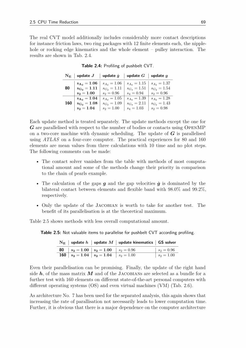
2.5 CPU Time Reduction 69
The real CVT model additionally includes considerably more contact descriptionsfor instance friction laws, two ring packages with 12 finite elements each, the nipple-hole or rocking edge kinematics and the whole element – pulley interaction. Theresults are shown in Tab. 2.4.
Table 2.4: Profiling of pushbelt CVT.
NE update J update g update G update g
80
sA2= 1.06 sA2
= 1.06 sA4= 1.15 sA2
= 1.37sG2
= 1.11 sG2= 1.11 sG4
= 1.51 sG2= 1.54
s2 = 1.00 s2 = 0.96 s4 = 0.94 s2 = 0.96
160
sA2= 1.04 sA2
= 1.05 sA4= 1.39 sA2
= 1.28sG2
= 1.08 sG2= 1.09 sG4
= 2.11 sG2= 1.43
s2 = 1.04 s2 = 1.00 s4 = 1.03 s2 = 0.98
Each update method is treated separately. The update methods except the one forG are parallelised with respect to the number of bodies or contacts using OpenMP
on a two-core machine with dynamic scheduling. The update of G is parallelisedusing ATLAS on a four-core computer. The practical experiences for 80 and 160elements are mean values from three calculations with 10 time and no plot steps.The following comments can be made:
• The contact solver vanishes from the table with methods of most computa-tional amount and some of the methods change their priority in comparisonto the chain of pearls example.
• The calculation of the gaps g and the gap velocities g is dominated by thebilateral contact between elements and flexible band with 98.0% and 99.2%,respectively.
• Only the update of the Jacobian is worth to take for another test. Thebenefit of its parallelisation is at the theoretical maximum.
Table 2.5 shows methods with less overall computational amount.
Table 2.5: Not valuable items to parallelise for pushbelt CVT according profiling.
NE update h update M update kinematics GS solver
80 s2 = 1.00 s2 = 1.00 s2 = 0.96 s2 = 0.96160 s2 = 1.04 s2 = 1.04 s2 = 1.00 s2 = 1.00
Even their parallelisation can be promising. Finally, the update of the right handside h, of the mass matrix M and of the Jacobians are selected as a bundle for afurther test with 160 elements on different state-of-the-art personal computers withdifferent operating systems (OS) and even virtual machines (VM) (Tab. 2.6).
As architecture No. 7 has been used for the separated analysis, this again shows thatincreasing the rate of parallisation not necessarily leads to lower computation time.Further, it is obvious that there is a major dependence on the computer architecture
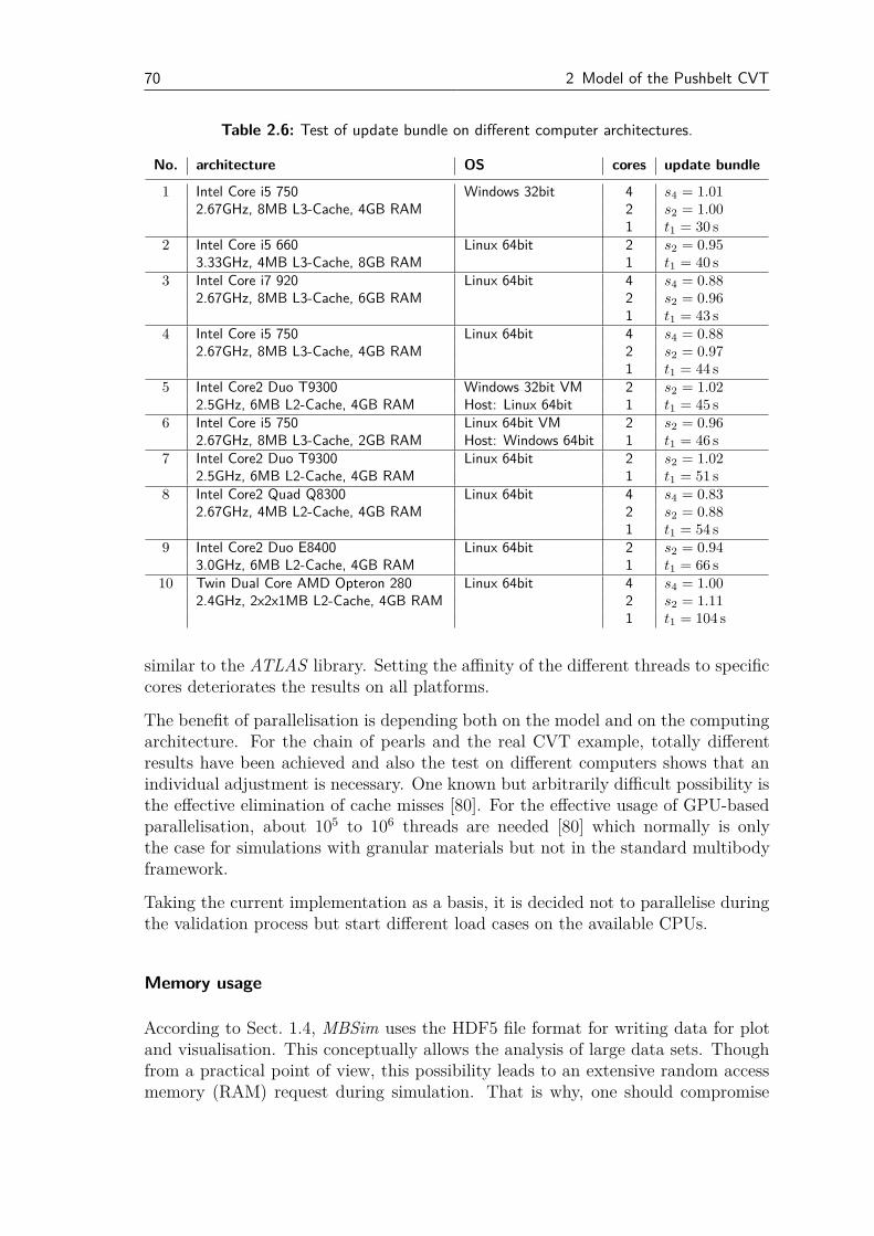
70 2 Model of the Pushbelt CVT
Table 2.6: Test of update bundle on different computer architectures.
No. architecture OS cores update bundle
1 Intel Core i5 750 Windows 32bit 4 s4 = 1.012.67GHz, 8MB L3-Cache, 4GB RAM 2 s2 = 1.00
1 t1 = 30 s2 Intel Core i5 660 Linux 64bit 2 s2 = 0.95
3.33GHz, 4MB L3-Cache, 8GB RAM 1 t1 = 40 s3 Intel Core i7 920 Linux 64bit 4 s4 = 0.88
2.67GHz, 8MB L3-Cache, 6GB RAM 2 s2 = 0.961 t1 = 43 s
4 Intel Core i5 750 Linux 64bit 4 s4 = 0.882.67GHz, 8MB L3-Cache, 4GB RAM 2 s2 = 0.97
1 t1 = 44 s5 Intel Core2 Duo T9300 Windows 32bit VM 2 s2 = 1.02
2.5GHz, 6MB L2-Cache, 4GB RAM Host: Linux 64bit 1 t1 = 45 s6 Intel Core i5 750 Linux 64bit VM 2 s2 = 0.96
2.67GHz, 8MB L3-Cache, 2GB RAM Host: Windows 64bit 1 t1 = 46 s7 Intel Core2 Duo T9300 Linux 64bit 2 s2 = 1.02
2.5GHz, 6MB L2-Cache, 4GB RAM 1 t1 = 51 s8 Intel Core2 Quad Q8300 Linux 64bit 4 s4 = 0.83
2.67GHz, 4MB L2-Cache, 4GB RAM 2 s2 = 0.881 t1 = 54 s
9 Intel Core2 Duo E8400 Linux 64bit 2 s2 = 0.943.0GHz, 6MB L2-Cache, 4GB RAM 1 t1 = 66 s
10 Twin Dual Core AMD Opteron 280 Linux 64bit 4 s4 = 1.002.4GHz, 2x2x1MB L2-Cache, 4GB RAM 2 s2 = 1.11
1 t1 = 104 s
similar to the ATLAS library. Setting the affinity of the different threads to specificcores deteriorates the results on all platforms.
The benefit of parallelisation is depending both on the model and on the computingarchitecture. For the chain of pearls and the real CVT example, totally differentresults have been achieved and also the test on different computers shows that anindividual adjustment is necessary. One known but arbitrarily difficult possibility isthe effective elimination of cache misses [80]. For the effective usage of GPU-basedparallelisation, about 105 to 106 threads are needed [80] which normally is onlythe case for simulations with granular materials but not in the standard multibodyframework.
Taking the current implementation as a basis, it is decided not to parallelise duringthe validation process but start different load cases on the available CPUs.
Memory usage
According to Sect. 1.4, MBSim uses the HDF5 file format for writing data for plotand visualisation. This conceptually allows the analysis of large data sets. Thoughfrom a practical point of view, this possibility leads to an extensive random accessmemory (RAM) request during simulation. That is why, one should compromise
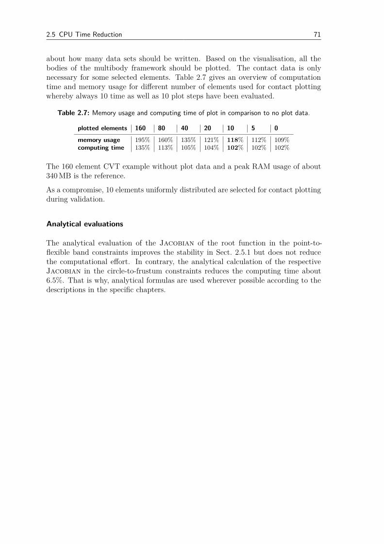
2.5 CPU Time Reduction 71
about how many data sets should be written. Based on the visualisation, all thebodies of the multibody framework should be plotted. The contact data is onlynecessary for some selected elements. Table 2.7 gives an overview of computationtime and memory usage for different number of elements used for contact plottingwhereby always 10 time as well as 10 plot steps have been evaluated.
Table 2.7: Memory usage and computing time of plot in comparison to no plot data.
plotted elements 160 80 40 20 10 5 0
memory usage 195% 160% 135% 121% 118% 112% 109%computing time 135% 113% 105% 104% 102% 102% 102%
The 160 element CVT example without plot data and a peak RAM usage of about340 MB is the reference.
As a compromise, 10 elements uniformly distributed are selected for contact plottingduring validation.
Analytical evaluations
The analytical evaluation of the Jacobian of the root function in the point-to-flexible band constraints improves the stability in Sect. 2.5.1 but does not reducethe computational effort. In contrary, the analytical calculation of the respectiveJacobian in the circle-to-frustum constraints reduces the computing time about6.5%. That is why, analytical formulas are used wherever possible according to thedescriptions in the specific chapters.
72
3 Results and Validation
A first check on the feasibility of the prescribed model can be done by verifyingglobal external signals like torques and clamping forces (thrusts). To achieve a moredeep validation on the mechanical working principles of the system, it is preferred tolook at local internal quantities for instance contact forces at the elements. Again,the review paper [72] gives a good overview about the current state of CVT mea-surements. The most interesting contributions concerning local contact forces aresummarised in [22, 23, 35, 63], [13] describes measurements at Eindhoven Universityof Technology concerning global values. Recently in [49], experiments and simu-lations concerning bearing forces have been outlined. Thereby in addition, spiralrunning, the position of loose sheaves, deformation of fixed sheaves, shaft deflec-tion, efficiency and the friction coefficients between elements and pulleys have beeninvestigated experimentally.
It is hard to analyse the mechanism of CVTs experimentally and it is not easy toadjust the input parameters for the simulation. For example, it is not exactly truethat MO = irMI because of torque loss. It could happen that one cannot reach themaximum torque in the simulation since the belt already slips. The maximum torquecan be estimated from a formula that contains for example running radius, clampingforce and friction coefficient. These quantities are always a bit uncertain such thatthe calculated maximum torque will deviate a bit from the actual maximum torque.In that case, some lower values for the final torque are tried next to some strategicpoints in between 0 and the maximum value – one can see in the following sections.
All simulations have been done after a first parameter variation. Apart from thegeometrical and material values of elements, ring package and pulleys (Sects. 2.1.1,2.1.2, 2.1.3), mainly the following parameters have been adapted: Lehr dampingvalues ϑκ0
, ϑǫ of the ring packages, tilting parameters of the loose sheaves, thefriction parameters of the interactions and lE of the element – element contact. Thesimulation has been done with 12 finite elements for 9 rings, rigid sheaves and with160 elements avoiding spurious polygonal effects. Where necessary, a dimensionlessdescription is chosen because of industrial secrecy.
3.1 Planar Validation with Local Data
A full set of local measurements has been conducted by Doshisha University in Kyotoand Honda R&D in the 1990s at low belt speeds and clamping pressures [22, 23, 35].It is important to know that obtaining these contact forces is a challenging taskrequiring complex and delicate measuring techniques [72, 27]: telemetry systems are
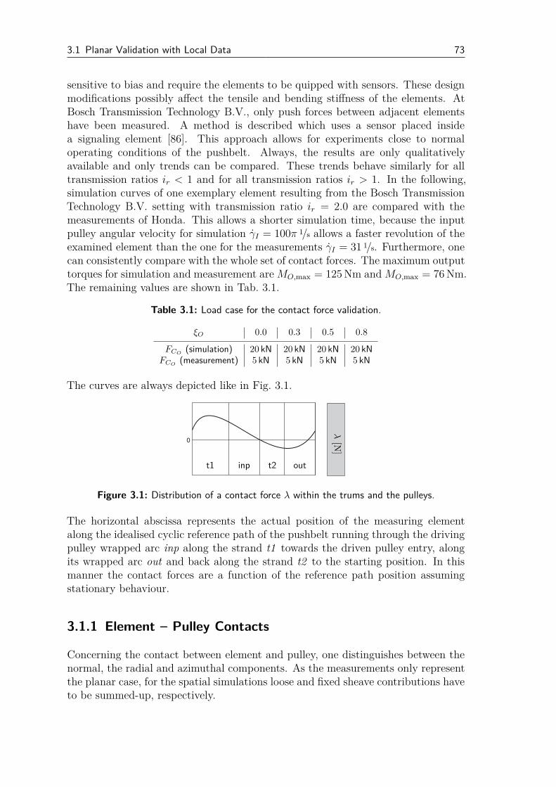
3.1 Planar Validation with Local Data 73
sensitive to bias and require the elements to be quipped with sensors. These designmodifications possibly affect the tensile and bending stiffness of the elements. AtBosch Transmission Technology B.V., only push forces between adjacent elementshave been measured. A method is described which uses a sensor placed insidea signaling element [86]. This approach allows for experiments close to normaloperating conditions of the pushbelt. Always, the results are only qualitativelyavailable and only trends can be compared. These trends behave similarly for alltransmission ratios ir < 1 and for all transmission ratios ir > 1. In the following,simulation curves of one exemplary element resulting from the Bosch TransmissionTechnology B.V. setting with transmission ratio ir = 2.0 are compared with themeasurements of Honda. This allows a shorter simulation time, because the inputpulley angular velocity for simulation γI = 100π 1/s allows a faster revolution of theexamined element than the one for the measurements γI = 31 1/s. Furthermore, onecan consistently compare with the whole set of contact forces. The maximum outputtorques for simulation and measurement are MO,max = 125 Nm and MO,max = 76 Nm.The remaining values are shown in Tab. 3.1.
Table 3.1: Load case for the contact force validation.
ξO 0.0 0.3 0.5 0.8
FCO(simulation) 20 kN 20 kN 20 kN 20 kN
FCO(measurement) 5 kN 5 kN 5 kN 5 kN
The curves are always depicted like in Fig. 3.1.
λ[N
]
t1 t2inp out
Figure 3.1: Distribution of a contact force λ within the trums and the pulleys.
The horizontal abscissa represents the actual position of the measuring elementalong the idealised cyclic reference path of the pushbelt running through the drivingpulley wrapped arc inp along the strand t1 towards the driven pulley entry, alongits wrapped arc out and back along the strand t2 to the starting position. In thismanner the contact forces are a function of the reference path position assumingstationary behaviour.
3.1.1 Element – Pulley Contacts
Concerning the contact between element and pulley, one distinguishes between thenormal, the radial and azimuthal components. As the measurements only representthe planar case, for the spatial simulations loose and fixed sheave contributions haveto be summed-up, respectively.
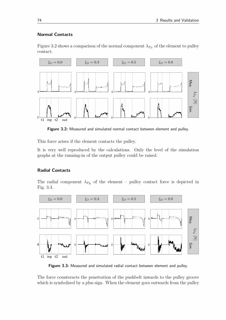
74 3 Results and Validation
Normal Contacts
Figure 3.2 shows a comparison of the normal component λPNof the element to pulley
contact.
ξO = 0.0 ξO = 0.3 ξO = 0.5 ξO = 0.8
λP
N[N
]M
ea.Sim
.
t1 t2inp out
Figure 3.2: Measured and simulated normal contact between element and pulley.
This force arises if the element contacts the pulley.
It is very well reproduced by the calculations. Only the level of the simulationgraphs at the running-in of the output pulley could be raised.
Radial Contacts
The radial component λPRof the element – pulley contact force is depicted in
Fig. 3.3.
ξO = 0.0 ξO = 0.3 ξO = 0.5 ξO = 0.8
λP
R[N
]M
ea.Sim
.
t1 t2inp out
Figure 3.3: Measured and simulated radial contact between element and pulley.
The force counteracts the penetration of the pushbelt inwards to the pulley groovewhich is symbolised by a plus sign. When the element goes outwards from the pulley
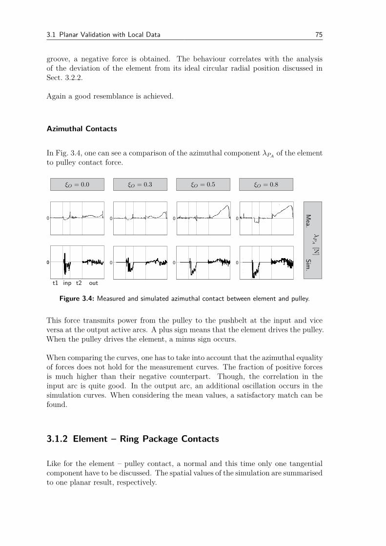
3.1 Planar Validation with Local Data 75
groove, a negative force is obtained. The behaviour correlates with the analysisof the deviation of the element from its ideal circular radial position discussed inSect. 3.2.2.
Again a good resemblance is achieved.
Azimuthal Contacts
In Fig. 3.4, one can see a comparison of the azimuthal component λPAof the element
to pulley contact force.
ξO = 0.0 ξO = 0.3 ξO = 0.5 ξO = 0.8
λP
A[N
]M
ea.Sim
.
t1 t2inp out
Figure 3.4: Measured and simulated azimuthal contact between element and pulley.
This force transmits power from the pulley to the pushbelt at the input and viceversa at the output active arcs. A plus sign means that the element drives the pulley.When the pulley drives the element, a minus sign occurs.
When comparing the curves, one has to take into account that the azimuthal equalityof forces does not hold for the measurement curves. The fraction of positive forcesis much higher than their negative counterpart. Though, the correlation in theinput arc is quite good. In the output arc, an additional oscillation occurs in thesimulation curves. When considering the mean values, a satisfactory match can befound.
3.1.2 Element – Ring Package Contacts
Like for the element – pulley contact, a normal and this time only one tangentialcomponent have to be discussed. The spatial values of the simulation are summarisedto one planar result, respectively.
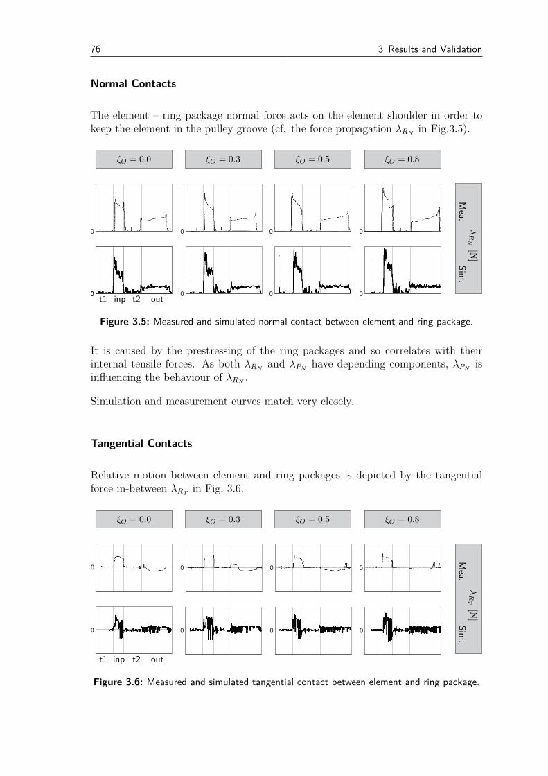
76 3 Results and Validation
Normal Contacts
The element – ring package normal force acts on the element shoulder in order tokeep the element in the pulley groove (cf. the force propagation λRN
in Fig.3.5).
ξO = 0.0 ξO = 0.3 ξO = 0.5 ξO = 0.8
λR
N[N
]M
ea.Sim
.
t1 t2inp out
Figure 3.5: Measured and simulated normal contact between element and ring package.
It is caused by the prestressing of the ring packages and so correlates with theirinternal tensile forces. As both λRN
and λPNhave depending components, λPN
isinfluencing the behaviour of λRN
.
Simulation and measurement curves match very closely.
Tangential Contacts
Relative motion between element and ring packages is depicted by the tangentialforce in-between λRT
in Fig. 3.6.
ξO = 0.0 ξO = 0.3 ξO = 0.5 ξO = 0.8
λR
T[N
]M
ea.Sim
.
t1 t2inp out
Figure 3.6: Measured and simulated tangential contact between element and ring package.
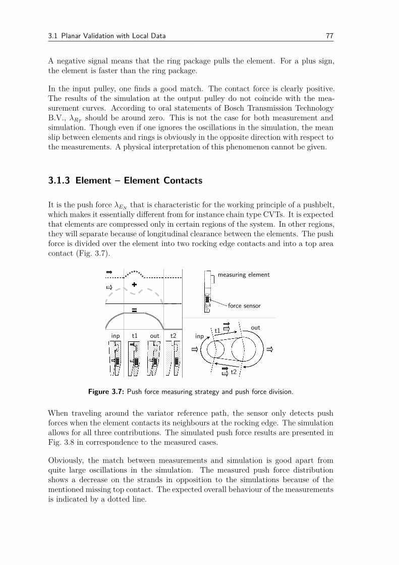
3.1 Planar Validation with Local Data 77
A negative signal means that the ring package pulls the element. For a plus sign,the element is faster than the ring package.
In the input pulley, one finds a good match. The contact force is clearly positive.The results of the simulation at the output pulley do not coincide with the mea-surement curves. According to oral statements of Bosch Transmission TechnologyB.V., λRT
should be around zero. This is not the case for both measurement andsimulation. Though even if one ignores the oscillations in the simulation, the meanslip between elements and rings is obviously in the opposite direction with respect tothe measurements. A physical interpretation of this phenomenon cannot be given.
3.1.3 Element – Element Contacts
It is the push force λENthat is characteristic for the working principle of a pushbelt,
which makes it essentially different from for instance chain type CVTs. It is expectedthat elements are compressed only in certain regions of the system. In other regions,they will separate because of longitudinal clearance between the elements. The pushforce is divided over the element into two rocking edge contacts and into a top areacontact (Fig. 3.7).
t1t1
t2
t2
inp inpoutout
measuring element
force sensor
Figure 3.7: Push force measuring strategy and push force division.
When traveling around the variator reference path, the sensor only detects pushforces when the element contacts its neighbours at the rocking edge. The simulationallows for all three contributions. The simulated push force results are presented inFig. 3.8 in correspondence to the measured cases.
Obviously, the match between measurements and simulation is good apart fromquite large oscillations in the simulation. The measured push force distributionshows a decrease on the strands in opposition to the simulations because of thementioned missing top contact. The expected overall behaviour of the measurementsis indicated by a dotted line.
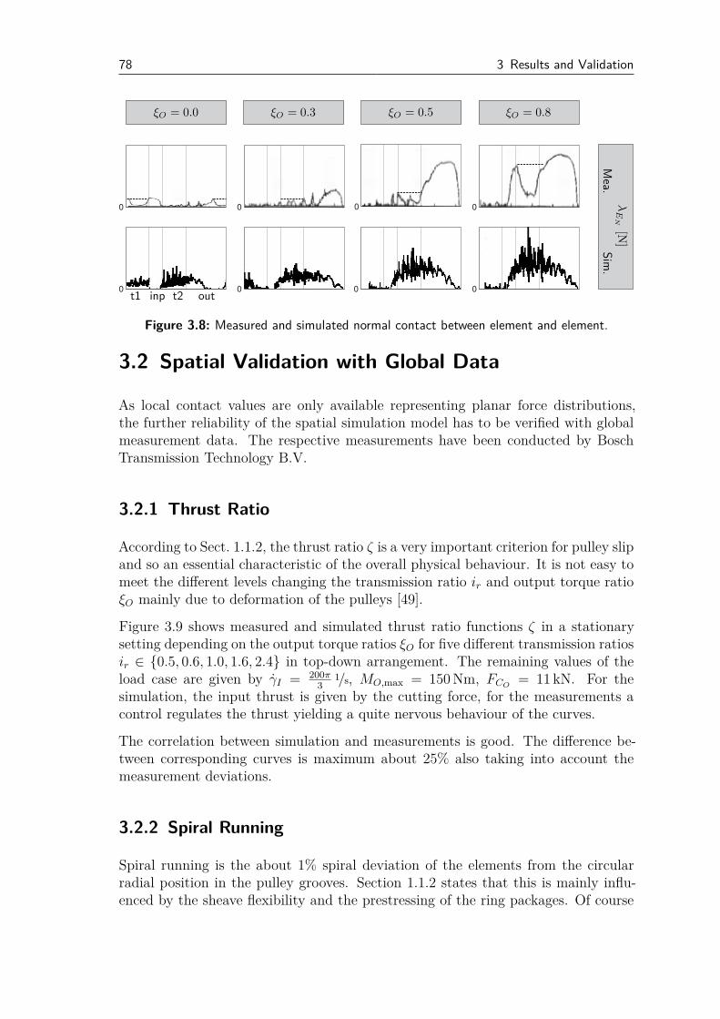
78 3 Results and Validation
ξO = 0.0 ξO = 0.3 ξO = 0.5 ξO = 0.8λ
EN
[N]
Mea.
Sim
.
t1 t2inp out
Figure 3.8: Measured and simulated normal contact between element and element.
3.2 Spatial Validation with Global Data
As local contact values are only available representing planar force distributions,the further reliability of the spatial simulation model has to be verified with globalmeasurement data. The respective measurements have been conducted by BoschTransmission Technology B.V.
3.2.1 Thrust Ratio
According to Sect. 1.1.2, the thrust ratio ζ is a very important criterion for pulley slipand so an essential characteristic of the overall physical behaviour. It is not easy tomeet the different levels changing the transmission ratio ir and output torque ratioξO mainly due to deformation of the pulleys [49].
Figure 3.9 shows measured and simulated thrust ratio functions ζ in a stationarysetting depending on the output torque ratios ξO for five different transmission ratiosir ∈ {0.5, 0.6, 1.0, 1.6, 2.4} in top-down arrangement. The remaining values of theload case are given by γI = 200π
31/s, MO,max = 150 Nm, FCO
= 11 kN. For thesimulation, the input thrust is given by the cutting force, for the measurements acontrol regulates the thrust yielding a quite nervous behaviour of the curves.
The correlation between simulation and measurements is good. The difference be-tween corresponding curves is maximum about 25% also taking into account themeasurement deviations.
3.2.2 Spiral Running
Spiral running is the about 1% spiral deviation of the elements from the circularradial position in the pulley grooves. Section 1.1.2 states that this is mainly influ-enced by the sheave flexibility and the prestressing of the ring packages. Of course
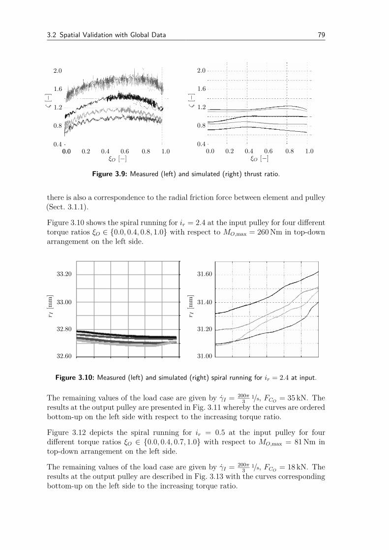
3.2 Spatial Validation with Global Data 79
ζ[−
]
ζ[−
]
ξO [−] ξO [−]
2.0 2.0
1.6 1.6
1.2 1.2
1.0 1.00.8 0.8
0.8 0.8
0.6 0.60.4 0.40.4 0.4
0.2 0.20.00.0 0.0
Figure 3.9: Measured (left) and simulated (right) thrust ratio.
there is also a correspondence to the radial friction force between element and pulley(Sect. 3.1.1).
Figure 3.10 shows the spiral running for ir = 2.4 at the input pulley for four differenttorque ratios ξO ∈ {0.0, 0.4, 0.8, 1.0} with respect to MO,max = 260 Nm in top-downarrangement on the left side.
r I[m
m]
r I[m
m]
32.60
32.80
33.00
33.20 31.60
31.40
31.20
31.00
Figure 3.10: Measured (left) and simulated (right) spiral running for ir = 2.4 at input.
The remaining values of the load case are given by γI = 200π3
1/s, FCO= 35 kN. The
results at the output pulley are presented in Fig. 3.11 whereby the curves are orderedbottom-up on the left side with respect to the increasing torque ratio.
Figure 3.12 depicts the spiral running for ir = 0.5 at the input pulley for fourdifferent torque ratios ξO ∈ {0.0, 0.4, 0.7, 1.0} with respect to MO,max = 81 Nm intop-down arrangement on the left side.
The remaining values of the load case are given by γI = 200π3
1/s, FCO= 18 kN. The
results at the output pulley are described in Fig. 3.13 with the curves correspondingbottom-up on the left side to the increasing torque ratio.
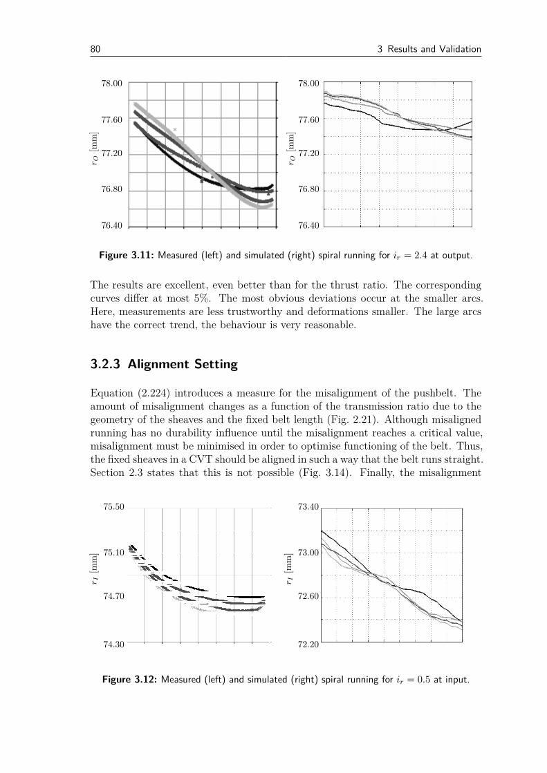
80 3 Results and Validation
r O[m
m]
r O[m
m]
78.0078.00
77.6077.60
77.2077.20
76.8076.80
76.4076.40
Figure 3.11: Measured (left) and simulated (right) spiral running for ir = 2.4 at output.
The results are excellent, even better than for the thrust ratio. The correspondingcurves differ at most 5%. The most obvious deviations occur at the smaller arcs.Here, measurements are less trustworthy and deformations smaller. The large arcshave the correct trend, the behaviour is very reasonable.
3.2.3 Alignment Setting
Equation (2.224) introduces a measure for the misalignment of the pushbelt. Theamount of misalignment changes as a function of the transmission ratio due to thegeometry of the sheaves and the fixed belt length (Fig. 2.21). Although misalignedrunning has no durability influence until the misalignment reaches a critical value,misalignment must be minimised in order to optimise functioning of the belt. Thus,the fixed sheaves in a CVT should be aligned in such a way that the belt runs straight.Section 2.3 states that this is not possible (Fig. 3.14). Finally, the misalignment
r I[m
m]
r I[m
m]
75.50
75.10
74.70
74.30
73.40
73.00
72.60
72.20
Figure 3.12: Measured (left) and simulated (right) spiral running for ir = 0.5 at input.
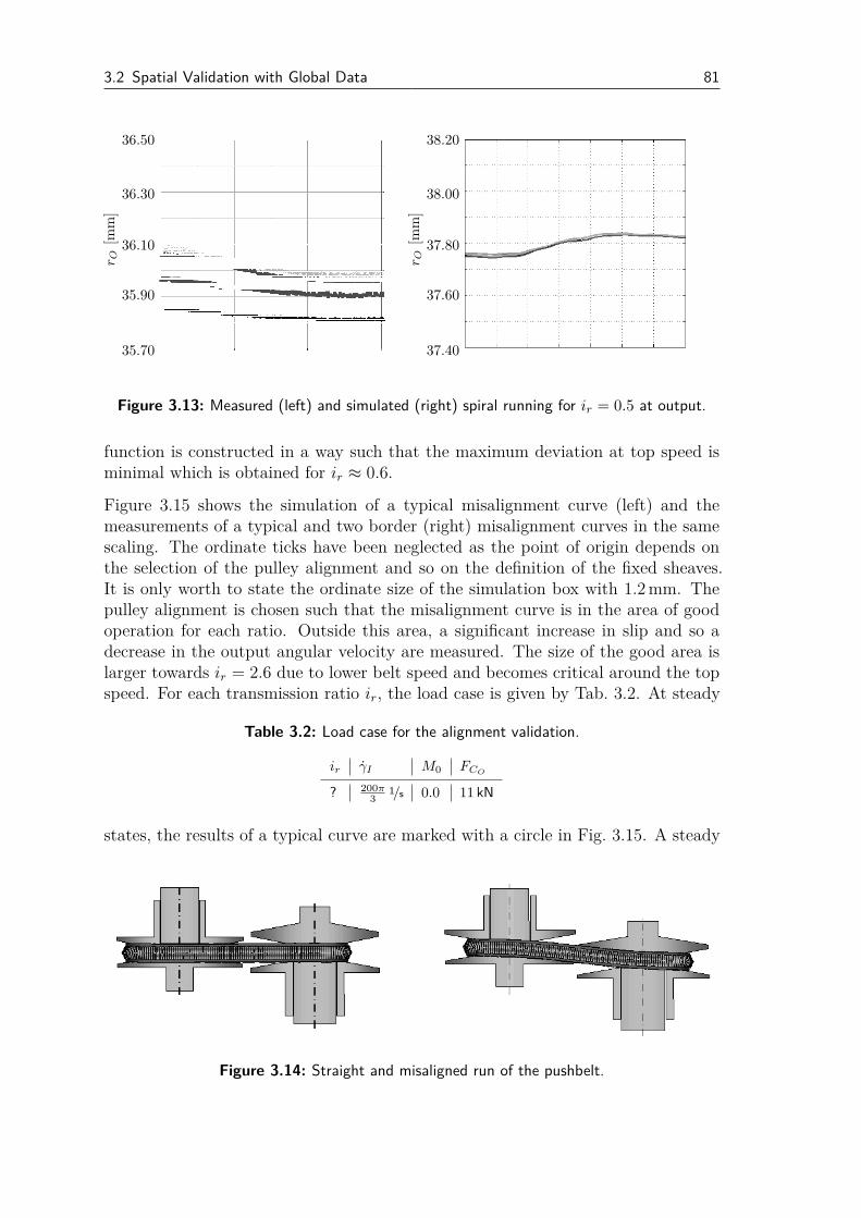
3.2 Spatial Validation with Global Data 81
r O[m
m]
r O[m
m]
38.20
38.00
37.80
37.60
37.40
36.50
36.30
36.10
35.90
35.70
Figure 3.13: Measured (left) and simulated (right) spiral running for ir = 0.5 at output.
function is constructed in a way such that the maximum deviation at top speed isminimal which is obtained for ir ≈ 0.6.
Figure 3.15 shows the simulation of a typical misalignment curve (left) and themeasurements of a typical and two border (right) misalignment curves in the samescaling. The ordinate ticks have been neglected as the point of origin depends onthe selection of the pulley alignment and so on the definition of the fixed sheaves.It is only worth to state the ordinate size of the simulation box with 1.2 mm. Thepulley alignment is chosen such that the misalignment curve is in the area of goodoperation for each ratio. Outside this area, a significant increase in slip and so adecrease in the output angular velocity are measured. The size of the good area islarger towards ir = 2.6 due to lower belt speed and becomes critical around the topspeed. For each transmission ratio ir, the load case is given by Tab. 3.2. At steady
Table 3.2: Load case for the alignment validation.
ir γI M0 FCO
? 200π3
1/s 0.0 11 kN
states, the results of a typical curve are marked with a circle in Fig. 3.15. A steady
Figure 3.14: Straight and misaligned run of the pushbelt.
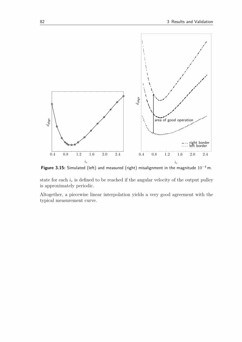
82 3 Results and Validation
ir
dalign
2.42.01.61.20.80.4
ir
dalign
area of good operation
left borderright border
2.42.01.61.20.80.4
Figure 3.15: Simulated (left) and measured (right) misalignment in the magnitude 10−4 m.
state for each ir is defined to be reached if the angular velocity of the output pulleyis approximately periodic.
Altogether, a piecewise linear interpolation yields a very good agreement with thetypical measurement curve.
83
4 Conclusion
A pushbelt CVT is an alternative transmission system with high expectation val-ues to improve fuel economy and dynamic performance of a vehicle. Though, theexpected increase has not been achieved in all cases [72]. For further analysingthe system behaviour, experimental studies can be accomplished. This is a verysophisticated and expensive task. For effectively understanding and improving thesystem, it is often better to perform computer simulations. In chapter 1, set-up andfunctionality of pushbelt CVTs are outlined and important phenomena as well asnecessary modelling prerequisites are given. A literature survey shows that there isstill no spatial model considering all relevant flexibilities and transient states causedby ratio shifting. The only validated planar model representing all these issues [27]is based on the nonsmooth mechanics approach and is the point of departure forthe present spatial extension. The basics and relevant literature citations aboutnonsmooth mechanics and its efficient discretisation with timestepping schemes aresummarised. Therefore, theoretical and numerical formalisms are introduced andthe software framework MBSim at the Institute of Applied Mechanics is described.
In chapter 2, a spatial transient model of a pushbelt variator is derived consideringthe components of the CVT and the different interactions separately. The elementsare represented by rigid bodies. For the pulley sheaves, either a rigid description ora Reissner-Mindlin finite element plate with moving frame of reference can be se-lected. The ring packages are modelled with spatial large deformation beams basedon co-rotational and inertial principles. For the interactions, it is distinguished be-tween the sheave – sheave joint ensuring the same angular velocity within a pulley,the interactions to the environment defining the load case and internal CVT contactconfigurations. For the contact between elements and pulley sheaves, the contactlaw is chosen decoupled and flexible in normal direction. For the tangential direction,a Stribeck law is chosen. In the case of rigid sheaves, the contact kinematics canbe analytically reduced and results in numerically solvable cone section problems.Otherwise, the contact kinematics has to be evaluated numerically from beginning.A NURBS-based surface description guarantees an efficient root search algorithm.For the contact between adjacent elements, only the normal direction is considered.The contact law is flexible and the respective kinematics can either be solved analyt-ically or results in the same cone section problems as in the element – pulley setting.The last contact group is the guidance of the elements by the ring packages due to abilateral normal contact law and Stribeck friction in tangential direction. In everycase, a nonlinear equation has to be solved numerically during the contact searchbecause of the numerical representation of the ring package. Initialisation and as-sembling for a stationary load case is done by using a simplified kinetic belt model.Hence, transient oscillations can be avoided. Altogether, a very detailed model has
84 4 Conclusion
been developed with a degree of freedom of about 3500 and 5500 contacts fulfillingthe necessary prerequisites from chapter 1 and extending the model [27] accordingto Tab. 2.2. Parallelisation techniques and implicit integration schemes are testedto reduce the high computation time and practical experiences are summarised.
A validation of the overall simulation model is accomplished in chapter 3. Localcontact forces between an exemplary element and the pulleys, the ring packages aswell as an adjacent element are discussed and compared. Throughout, the resultsare in good correspondence. As the available measurements only reflect the planarcase, additionally global values are examined. The thrust ratio curves differ maxi-mum about 25% and show a good correlation. The radial deviation of the elementcurve in the pulley groove from a circle is called spiral running and drifts at most 5%from the measurements. Last, the typical misalignment curve is also very well repro-duced. Overall one can conclude that the typical behaviour of the pushbelt variatorsystem at realistic operation conditions is predicted adequately by the mathematicalmodel.
The simulation model both represents the most important phenomena and showsa good correlation with experimental results. It can be applied to analyse thedynamics of the real system and to improve its performance concerning out-of-planemotion, misalignment, comfort and fuel consumption. Though to use it with controlalgorithms, as part of drivetrain models or with mathematical optimisation methods,reduced models would be more appropriate. The proposed model is an excellentorigin to develop such simplifications by model order reduction techniques [19] orby substituting some bodies for instance the ring models with the promising onein [41] or interactions for example the dynamic sheave representation with a quasi-static Maxwell law [27]. Then, these new models could be understood in detaildue to comparability and would be fast enough to derive ratio and thrust shiftingrules predicting and optimising the slip behaviour also in comparison to planardescriptions. According to the author, this will be one of the most important issuesfor the future such that it is always ensured that operating conditions automaticallymeet the load requirements [72]. Another item is the improvement of parallelisationconcepts using the OpenMP standard mainly analysing cache misses. GPU-basedparallelisation is only effective for granular materials [80].
85
Bibliography
[1] Acary, Vincent ; Brogliato, Bernard: Lecture notes in applied and compu-tational mechanics. Vol. 35: Numerical methods for nonsmooth dynamical sys-tems: applications in mechanics and electronics. 1st edition. Berlin : Springer,2008. – ISBN 3–540–75391–5
[2] Acary, Vincent ; Perignon, Franck: An introduction to Siconos / INRIA.2007. – Forschungsbericht
[3] Alart, Pierre ; Curnier, Alain: A mixed formulation for frictional contactproblems prone to Newton like solution methods. In: Comput Methods ApplMech Engrg 92 (1991), pp. 353 – 375. – ISSN 0045–7825
[4] Arnold, Martin: Numerical methods for simulation in applied dynamics. In:Arnold, Martin (Hrsg.) ; Schiehlen, Werner (Hrsg.): Simulation Techniquesfor Applied Dynamics. Wien : Springer, 2009 (CISM International Centre forMechanical Sciences 507). – ISBN 978–3–211–89548–1, pp. 191–246
[5] Bathe, Klaus-Jürgen ; Bolourchi, Said: Large displacement analysis ofthree-dimensional beam structures. In: Int J Numer Meth Eng 14 (1979), pp.961–986. – ISSN 0029–5981
[6] Belytschko, Ted ; Schwer, Leonard: Large displacement, transient analysisof space frames. In: Int J Numer Meth Eng 11 (1977), pp. 65–84. – ISSN 0029–5981
[7] Berard, Stephan ; Trinkle, Jeff ; Nguyen, Binh ; Roghani, Ben ; Fink,Jonathan ; Kumar, Vijay: daVinci Code: a multi-model simulation and anal-ysis tool for multi-body systems. In: 2007 IEEE International Conference onRobotics and Automation ; Roma, Italy, 10th-14th April 2007, IEEE, 2007. –ISBN 1–4244–0602–1, pp. 2588–2593
[8] Bhate, Rohan ; Srivastava, Nilabh: Influence of pulley actuation force onthe transient dynamics of a metal V-belt CVT. In: SAE 2009 CommercialVehicle Engineering Congress & Exhibition Technical, Rosemont, Illinois, 6thuntil 7th October 2009, 2009
[9] Braess, Dietrich: Finite elements : theory, fast solvers, and applications inelasticity theory. 3. ed. Cambridge : Cambridge University Press, 2007. – ISBN978–0–521–70518–9
86 Bibliography
[10] Brogliato, Bernard: Lecture notes in control and information sciences. Vol.220: Nonsmooth impact mechanics : models, dynamics and control. 1st edition.London : Springer, 1996. – ISBN 3–540–76079–2
[11] Brogliato, Bernard ; Dam, Tonny ten ; Paoli, Laetitia ; Genot, Frank ;Abadie, Michel: Numerical simulation of finite dimensional multibody nons-mooth mechanical systems. In: Appl Mech Rev 55 (2002), pp. 107–150. – ISSN0003–6900
[12] Bullinger, Markus ; Pfeiffer, Friedrich ; Ulbrich, Heinz: Elastic mod-elling of bodies and contacts in continuously variable transmissions. In: Multi-body System Dynamics 13 (2005), pp. 175–194. – ISSN 1573–272X
[13] Carbone, Giuseppe ; Mangialardi, Luigi ; Bonsen, Bram ; Tursi, Carlo;Veenhuizen, Bram: CVT dynamics: theory and experiments. In: Mech MachTheor 42 (2006), pp. 409–428. – ISSN 0094–114X
[14] Carbone, Guiseppe ; Novellis, Leonardo de ; Commissaris, Gijs ; Stein-
buch, Maarten: An enhanced CMM model for the accurate prediction of steadystate performance of CVT chain drives. In: J Mech Des 132 (2010), pp. 1–8. –ISSN 1050–0472
[15] Chapman, Barbara ; Gabriele ; Jost ; Pas, Ruud van d.: Using OpenMP :portable shared memory parallel programming. Cambridge, Mass. : MIT Press,2008 (Scientific and engineering computation). – ISBN 978–0–262–53302–7
[16] Crisfield, Michael A.: A consistent co-rotational formulation for non-linear,three-dimensional, beam elements. In: Comput Methods Appl Mech Engrg 81(1990), pp. 131–150. – ISSN 0045–7825
[17] Deuflhard, Peter: Springer series in computational mathematics. Vol. 35:Newton methods for nonlinear problems : affine invariance and adaptive algo-rithms. Corr. 2. print. Berlin : Springer, 2006. – ISBN 3–540–21099–7
[18] Dombrowski, Stefan von ; Schwertassek, Richard: Analysis of large flex-ible body deformation in multibody systems using absolute coordinates. In:Advances in Computational Multibody Dynamics, Lisbon, 20th-23rd September1999. Lisbon, Portugal : Instituto Superior Tecnico, 1999, pp. 359–378
[19] Fehr, Jörg ; Eberhard, Peter: Improving the simulation process in flexiblemultibody dynamics by enhanced model order reduction techniques. In: Multi-body Dynamics 2009, Eccomas Thematic Conference, Warsaw, 29th June until2nd July 2009, 2009
[20] Flores, Paulo ; Leine, Remco I. ; Glocker, Christoph: Modeling andanalysis of rigid multibody systems with translational clearance joints based onthe nonsmooth dynamics approach. In: Multibody Dynamics 2009, EccomasThematic Conference, Warsaw, 29th June until 2nd July 2009, 2009
[21] fmatvec - Fast Matrix-Vector Library. GNU Lesser General Public Licensehttp://fmatvec.berlios.de
Bibliography 87
[22] Fujii, Toru ; Kitagawa, Takashi ; Kanehara, Shigeru: A study of a metalpushing V-belt type CVT - part 2: compression force between metal blocks andring tension. In: SAE Technical Paper Series 930667 (1993), pp. 129–138. –ISSN 0148–7191
[23] Fujii, Toru ; Kurokawa, Takemasa ; Kanehara, Shigeru: A study of ametal pushing V-belt type CVT - part 1: relation between transmitted torqueand pulley thrust. In: SAE Technical Paper Series 930666 (1993), pp. 117–127.– ISSN 0148–7191
[24] Funk, Kilian ; Pfeiffer, Friedrich: A time-stepping algorithm for stiff me-chanical systems with unilateral constraints. In: International Conference onNonsmooth/Nonconvex Mechanics with Applications in Engineering , Thessa-loniki , 5th until 6th July 2002, 2002
[25] Förg, Martin: Fortschritt-Berichte VDI : Reihe 20, Rechnerunterstützte Ver-fahren. Vol. 411: Mehrkörpersysteme mit mengenwertigen Kraftgesetzen : Theo-rie und Numerik. Als Manuskript gedruckt. Düsseldorf : VDI-Verl., 2007. –ISBN 978–3–18–341120–7
[26] Förg, Martin ; Engelhard, Thomas ; Ulbrich, Heinz: Analysis of differ-ent time-integration methods applied to a nonsmooth industrial problem. In:Fifth EUROMECH Nonlinear Dynamics Conference : 7th-12th August 2005.Eindhoven : Eindhoven Univ. of Technology, August 2005
[27] Geier, Thomas: Fortschrittberichte VDI : Reihe 12, Verkehrstechnik,Fahrzeugtechnik. Vol. 654: Dynamics of push belt CVTs. Als Manuskriptgedruckt. Düsseldorf : VDI-Verl., 2007. – ISBN 978–3–18–365412–3
[28] Gerbert, Göran: Influence of band friction on metal V-belt mechanics /Division of Machine Elements, Chalmers University of Technology. Göteborg,1985 ( 1985-08-25). – Forschungsbericht
[29] Gerstmayr, Johannes: Absolute coordinate formulations for flexible multibodydynamics systems, Johannes Kepler Universität Linz, Diss., 2007
[30] Glocker, Christoph: Lecture notes in applied and computational mechanics.Vol. 1: Set-valued force laws in rigid body dynamics : dynamics of non-smoothsystems. 1st edition. Berlin : Springer Verlag, 2001. – ISBN 978–3–540–41436–0
[31] Hairer, Ernst ; Wanner, Gerhard: Springer series in computational math-ematics. Vol. 14: Solving ordinary differential equations. Corrected SecondPrinting. Berlin : Springer, 2002. – ISBN 3–540–60452–9
[32] HDF5Serie - A HDF5 Wrapper for Time Series. GNU Lesser General PublicLicensehttp://hdf5serie.berlios.de
[33] Hilbert, David ; Cohn-Vossen, Stephan: Geometry and the imagination. 2.ed., repr. Providence, RI : AMS Chelsea Publ., 1999. – ISBN 0–8218–1998–4
88 Bibliography
[34] Jean, Michel: The nonsmooth contact dynamics method. In: Comput MethodsAppl Mech Engrg 177 (1999), pp. 235–257. – ISSN 0045–7825
[35] Kanehara, Shigeru ; Fujii, Toru ; Kitagawa, Takashi: A study of a metalpushing V-belt type CVT - part 3: what forces act on metal blocks. In: SAETechnical Paper Series 940735 (1994), pp. 139–169. – ISSN 0148–7191
[36] Kell, Thomas ; Fritz, Peter ; Pfeiffer, Friedrich: Vibrations in roller chaindrives. In: 5th International Congress on Sound and Vibration, Adelaide, 15thuntil 18th December 1997, 1997
[37] Kikuchi, Fumio: An improved 4-node quadrilateral plate bending element ofthe Reissner-Mindlin type. In: Comput Mech 23 (1999), pp. 240–249. – ISSN0178–7675
[38] Klaassen, Tim ; Bonsen, Bram ; Meerakker, Koen van d. ; Vroemen,Bas ; Veenhuizen, Bram ; Veldpaus, Frans ; Steinbuch, Maarten: Theempact CVT: modelling, simulation and experiments. In: Int J Modelling,Identification and Control 3 (2008), pp. 286–296. – ISSN 1746–6172
[39] Krüssmann, Martin: A new CVT push-belt to increase driveline efficiency andpower density. In: 8th International CTI Symposium: Innovative AutomotiveTransmissions, Berlin, 30th November until 3rd December 2009, 2009
[40] Kuwabara, Shinya ; Fujii, Toru ; Kanehara, Shigeru: Power transmittingmechanisms of CVT using a metal V-belt and load distribution in the steel ring.In: SAE Technical Paper Series 980824 (1998), pp. 49–59. – ISSN 0148–7191
[41] Lang, Holger ; Linn, Joachim ; Arnold, Martin: Multibody dynamics sim-ulation of geometrically exact Cosserat rods. In: Multibody Dynamics 2009,Eccomas Thematic Conference, Warsaw, 29th June until 2nd July 2009, 2009
[42] Lebrecht, Wolfgang ; Pfeiffer, Friedrich ; Ulbrich, Heinz: Analysis of self-induced vibrations in a pushing V-belt CVT. In: International ContinuouslyVariable and Hybrid Transmission Congress, San Francisco, 23rd until 25thSeptember 2004, 2004
[43] Leine, Remco I. ; Glocker, Christoph: A set-valued force law for spatialCoulomb-Contensou friction. In: Eur J Mech 22 (2003), pp. 193–216. – ISSN0997–7546
[44] Leine, Remco I. ; Nijmeijer, Hendrik: Lecture notes in applied and computa-tional mechanics. Vol. 18: Dynamics and bifurcations of non-smooth mechanicalsystems. Corr. print. Berlin : Springer, 2006. – ISBN 3–540–21987–0
[45] Leine, Remco I. ; Wouw, Nathan van d.: Lecture notes in applied and com-putational mechanics. Vol. 36: Stability and convergence of mechanical systemswith unilateral constraints. Berlin : Springer, 2008. – ISBN 978–3–540–76975–0
[46] Luo, Albert: Discontinuous dynamical systems in time-varying domains. Bei-jing : Higher Education Press, 2009 (Nonlinear physical science). – ISBN978–3–642–00252–6
Bibliography 89
[47] MBSim - Multi-Body Simulation Software. GNU Lesser General Public Licensehttp://mbsim.berlios.de
[48] Moreau, Jean J.: Unilateral contact and dry friction in finite freedom dynam-ics. In: Nonsmooth Mechanics and Applications. Wien : Springer Verlag, 1988.– ISBN 3–211–82066–3, pp. 1–82
[49] Möller, Jens: Konstruktions- und Antriebstechnik. Vol. 3: Rechnerische undexperimentelle Bestimmung der Lagerkräfte eines stufenlosen Umschlingungs-getriebes. Tönning : Der Andere Verlag, 2010. – ISBN 978–3–89959–966–4
[50] Möller, Michael ; Leine, Remco I. ; Glocker, Christoph: An efficientapproximation of orthotropic set-valued force laws of normal cone type. In: 7thEuromech Solid Mechanics Conference, Lisbon, 7th until 11th September 2009,2009
[51] Neumann, Lutz ; Ulbrich, Heinz ; Pfeiffer, Friedrich: New model of aCVT rocker pin chain with exact joint kinematics. In: J Comput NonlinearDynam 1 (2006), pp. 143–149. – ISSN 1555–1415
[52] Noll, Erik van d. ; Sluis, Francis van d. ; Dongen, Tom van ; Velde, Arievan d.: Innovative self-optimizing clamping force strategy boosts effiency of thepushbelt CVT. In: 7th International CTI Symposium: Innovative AutomotiveTransmissions, Berlin, 1st until 4th December 2008, 2008
[53] OpenMBV - Open Multi Body Viewer. GNU General Public Licensehttp://openmbv.berlios.de
[54] Pfeiffer, Friedrich: Lecture notes in applied and computational mechanics.Vol. 40: Mechanical system dynamics. Corr. 2. print. Berlin : Springer, 2008. –ISBN 978–3–540–79435–6
[55] Pfeiffer, Friedrich ; Borchsenius, Fredrik ; Förg, Martin: New hy-draulic system modelling. In: ASME Design Engineering Technical Conference,Chicago, 2nd - 6th September 2003, 2003
[56] Pfeiffer, Friedrich ; Glocker, Christoph: Multibody dynamics with unilat-eral contacts. 1st edition. New York : John Wiley & Sons Inc., 1996 (Wileyseries in nonlinear science). – ISBN 0–471–15565–9
[57] Piegl, Les ; Tiller, Wayne: The NURBS book. 2. ed. Berlin : Springer, 1997(Monographs in visual communications). – ISBN 3–540–61545–8
[58] Rothenbühler, Yves: New slip synthesis and theoretical approach of CVTslip control, Ecole Polytechnique Federale de Lausanne, Diss., 2009
[59] Sattler, Heiko: Stationäres Betriebsverhalten stufenlos verstellbarer Metal-lumschlingungsgetriebe, Universität Hannover, Diss., 1999
[60] Schiehlen, Werner: Multibody system dynamics: roots and perspectives. In:Multibody System Dynamics 1 (1997), pp. 149–188. – ISSN 1384–5640
90 Bibliography
[61] Schindler, Thorsten ; Friedrich, Markus ; Ulbrich, Heinz: Computingtime reduction possibilities in multibody dynamics. In: Blajer, Wojciech(Hrsg.) ; Arczewski, Krzysztof (Hrsg.) ; Fraczek, Janusz (Hrsg.) ; Woj-
tyra, Marek (Hrsg.): Multibody Dynamics: Computational Methods and Ap-plications. Dordrecht : Springer, to appear 2010 (Computational Methods inApplied Sciences)
[62] Schindler, Thorsten ; Förg, Martin ; Friedrich, Markus ; Schneider,Markus ; Esefeld, Bastian ; Huber, Robert ; Zander, Roland ; Ulbrich,Heinz: Analysing dynamical phenomenons: introduction to MBSim. In: Pro-ceedings of 1st Joint International Conference on Multibody System Dynamics,Lappeenranta, 25th-27th May 2010, 2010. – ISBN 978–952–214–778–3
[63] Schindler, Thorsten ; Geier, Thomas ; Ulbrich, Heinz ; Pfeiffer,Friedrich ; Velde, Arie van d. ; Brandsma, Arjen: Dynamics of pushbeltCVTs. In: Umschlingungsgetriebe : Ketten und Riemen - Konstruktion, Sim-ulation und Anwendung von Komponenten und Systemen; Tagung Berlin, 21.und 22. Juni 2007. Düsseldorf : VDI-Verlag, 2007 (VDI-Berichte ; 1997). –ISBN 978–3–18–091997–3
[64] Schindler, Thorsten ; Ulbrich, Heinz ; Pfeiffer, Friedrich ; Velde, Arievan d. ; Brandsma, Arjen: Spatial simulation of pushbelt CVTs with timestep-ping schemes. In: Appl Numer Math (to appear 2010). – ISSN 0168–9274
[65] Sedlmayr, Martin: Fortschrittberichte VDI : Reihe 12, Verkehrstechnik,Fahrzeugtechnik. Vol. 558: Räumliche Dynamik von CVT-Keilkettengetrieben.Als Manuskript gedruckt. Düsseldorf : VDI-Verlag, 2003. – ISBN 3–18–355812–2
[66] Shabana, Ahmed: Dynamics of multibody systems. 3. ed. New York : Cam-bridge University Press, 2005. – ISBN 0–521–85011–8
[67] Shabana, Ahmed ; Bauchau, Olivier ; Hulbert, Gregory: Integrationof large deformation finite element and multibody system algorithms. In: JComput Nonlinear Dynam 2 (2007), pp. 351–359. – ISSN 1555–1415
[68] Simo, Juan C. ; Vu-Quoc, Loc: A geometrically-exact rod model incorporat-ing shear and torsion-warping deformation. In: Int J Solid Struct 27 (1991),pp. 371–393. – ISSN 0020–7683
[69] Simons, Sjoerd ; Klaassen, Tim ; Veenhuizen, Bram ; Carbone, Giuseppe:Shift dynamics modelling for optimisation of variator slip control in a pushbeltCVT. In: Int J Vehicle Design 48 (2008), pp. 45–64. – ISSN 0143–3369
[70] Sluis, Francis van d. ; Dongen, Tom van ; Spijk, Gert-Jan van ; Velde, Arievan d. ; Heeswijk, Ad van: Fuel consumption potential of the pushbelt CVT.In: FISITA 2006 : World Automotive Congress; 22 - 27 October, Yokohama,Japan. Yokohama, 2006
Bibliography 91
[71] Sorge, Francesco: Transient mechanics of V-belt variators. In: InternationalContinuously Variable and Hybrid Transmission Congress, San Francisco, 23rduntil 25th September 2004, 2004
[72] Srivastava, Nilabh ; Haque, Imtiaz: A review on belt and chain continuouslyvariable transmissions (CVT): dynamics and control. In: Mech Mach Theor 44(2008), pp. 19–41. – ISSN 0094–114X
[73] Srivastava, Nilabh ; Haque, Imtiaz: Transient dynamics of metal V-beltCVT: effect of band pack slip and friction characteristic. In: Mech Mach Theor43 (2008), pp. 459–479. – ISSN 0094–114X
[74] Srnik, Jürgen ; Pfeiffer, Friedrich: Dynamics of CVT chain drives. In: IntJ Vehicle Design 22 (1999), pp. 54–72. – ISSN 0143–3369
[75] Stadler, Michael ; Holzapfel, Gerhard: Subdivision schemes for smoothcontact surfaces of arbitrary mesh topology in 3D. In: Int J Numer Meth Eng60 (2004), pp. 1161–1195. – ISSN 0029–5981
[76] Stadler, Michael ; Holzapfel, Gerhard ; Korelc, Joze: Cn continuousmodelling of smooth contact surfaces using NURBS and application to 2Dproblems. In: Int J Numer Meth Eng 57 (2003), pp. 2177–2203. – ISSN0029–5981
[77] Stewart, David: Rigid-body dynamics with friction and impact. In: SIAMRev 42 (2000), pp. 3–39. – ISSN 1095–7200
[78] Stiegelmeyr, Andreas: A time stepping algorithm for mechanical systemswith unilateral contacts. In: ASME International Design Engineering TechnicalConference, Las Vegas, 4th until 7th September 1999, ASME, 1999
[79] Studer, Christian: Lecture notes in applied and computational mechanics.Vol. 47: Numerics of unilateral contacts and friction : modeling and numericaltime integration in non-smooth dynamics. Berlin : Springer Verlag, 2009. –ISBN 978–3–642–01099–6
[80] Tasora, Alessandro ; Negrut, Dan ; Anitescu, Mihail: GPU-based paral-lel computing for the simulation of complex multibody systems with unilateraland bilateral constraints: an overview. In: Blajer, Wojciech (Hrsg.) ; Ar-
czewski, Krzysztof (Hrsg.) ; Fraczek, Janusz (Hrsg.) ; Wojtyra, Marek(Hrsg.): Multibody Dynamics: Computational Methods and Applications. Dor-drecht : Springer, to appear 2010 (Computational Methods in Applied Sciences)
[81] Tenberge, Peter: Efficiency of chain-CVTs at constant and variable ratio:a new mathematical model for a very fast calculation of chain forces, clamp-ing forces, clamping ratio, slip, and efficiency. In: International ContinuouslyVariable and Hybrid Transmission Congress, San Francisco, 23rd until 25thSeptember 2004, 2004
92 Bibliography
[82] Thomsen, Per G. (Hrsg.): Non-smooth problems in vehicle systems dynamics :Proceedings of the Euromech 500 Colloquium. Berlin : Springer, 2010. – ISBN978–3–642–01355–3
[83] Trinkle, Jeffrey ; Pang, Jong-Shi ; Sudarsky, Sandra ; Lo, Grace: Ondynamic multi-rigid-body contact problems with Coulomb friction. In: J ApplMath Mech 4 (1997), pp. 267–279. – ISSN 0044–2267
[84] Ugural, Ansel ; Fenster, Saul: Advanced strength and applied elasticity.New York : American Elsevier, 1975. – ISBN 0–444–00160–3
[85] Ulbrich, Heinz: Some selected research activities in mechatronic applications- case studies. In: International Conference on Engineering Mechanics, Struc-tures, Engineering Geology, Rhodos, 22nd until 24th July 2009, 2009
[86] VDT. European Patent EP-0772034 Measuring system for belt forces occurringin variator systems in dynamical circumstances. 1996
[87] Wasfy, Tamer ; Noor, Ahmed: Computational strategies for flexible multi-body systems. In: Appl Mech Rev 56 (2003), pp. 553–613. – ISSN 0003–6900
[88] Wriggers, Peter: Computational contact mechanics. 1st edition. ChichesterWest Sussex : John Wiley & Sons Ltd., 2002. – ISBN 0–471–49680–4
[89] Zander, Roland: Fortschritt-Berichte VDI : Reihe 20, Rechnerunter-stützte Verfahren. Vol. 420: Flexible multi-body systems with set-valuedforce laws. Als Manuskript gedruckt. Düsseldorf : VDI-Verlag, 2009. –http://mediatum2.ub.tum.de/node?id=654788. – ISBN 978–3–18–342020–9
[90] Zander, Roland ; Schindler, Thorsten ; Friedrich, Markus ; Huber,Robert ; Förg, Martin ; Ulbrich, Heinz: Non-smooth dynamics in academiaand industry: recent work at TU München. In: Acta Mech 195 (2008), pp.167–183. – ISSN 0001–5970
[91] Zander, Roland ; Ulbrich, Heinz: Rotating elastic disks with rigid bodycontacts in MBS. In: Proceedings of the 77th Annual Meeting of the Gesellschaftfür Angewandte Mathematik und Mechanik e.V. Bremen : Universität Bremen,March 2006