Spatial Statistical Data Fusion on

Java-enabled Machines in Ubiquitous Sensor

Networks

Javier Palafox-Albarrán

Universität Bremen 2014

Spatial Statistical Data Fusion on Java-

enabled Machines in Ubiquitous

Sensor Networks

Vom Fachbereich für Physik und Elektrotechnik

der Universität Bremen

zur Erlangung des akademischen Grades eines

Doktor-Ingenieur (Dr.-Ing.)

genehmigte Dissertation

von

M.Sc. Javier Palafox-Albarrán

wohnhaft in Bremen

Referent Prof. Dr.-Ing. Walter Lang

Korreferent Prof. Dr.-Ing. Hans-Jörg Kreowski

Eingereicht am: 3.Dezember 2013

Tag des Promotionskolloquiums: 16. April 2014

It is with pleasure that I express my gratitude to all those who offered this opportunity to me:

Institute for Microsensors, -actuators and –systems (IMSAS), Institute for Production and

Logistic (BIBA) in the University of Bremen. I thank Prof. Walter Lang and Prof. Hans-Jörg

Kreowski, my thesis supervisors, for their guidance patronage. I highly appreciate the support

and guidance of Reiner Jedermann throughout the thesis. Additionally, I wish to thank Ingrid

Rügge and the graduates at the International Graduate School for Dynamics in Logistics

(IGS) for all their help and support. Also, I would like to thank Professors Bonghee Hong and

Dr Sang-Hwa Chung at Pusan National University (PNU) for their support during my

research internship in Korea.

I especially thank my family in Mexico for their support and encouragement throughout my

thesis. My loving family have also made sacrifices during my long stay in Germany, without

their unconditional care I would not made it this far.

Bremen, December. 2013

Javier Palafox

Wireless Sensor Networks (WSN) are the cornerstone of Ubiquitous Sensor Networks (USN).

They consist of small, cheap devices that have a powerful combination of sensing, computing

and communication capabilities. The first technical challenge in USN is in fact due to energy

constraints of WSN nodes. They must be able to communicate and process data efficiently

using minimum amount of energy and cover an area of interest with the minimum possible

number of sensors. The second technical challenge is to establish the communication to the

external networks such as the Internet or Cellular and to react to unexpected events; the

reaction to dynamic changes in the environment sometimes requires the deployment of new

software features into the sensor nodes.

To solve the first technical challenge, this thesis proposes the use of Information Fusion (IF)

techniques in WSN. The basic problems of data fusion are to determine the best procedure to

combine the available data and the way to describe the relationship between different sources.

It proposes the use of techniques that were designed for Geostatistics and applies them to

WSN field. Kriging and Cokriging interpolation that can be considered as Information Fusion

algorithms were tested to prove the feasibility of the methods to increase coverage with

theoretical guarantees through the use of the so called Kriging variances. To reduce energy

consumption, an innovative distributed compression method that surpasses the existing ones

was developed. The method is “a real-valued” version of Distributed Source Coding (DSC).

The modeling of correlations is based on using the so-called variogram, and uses data fusion

techniques to recover the compressed data at the sink.

The second challenge is approached through the use of existing technologies. The time

required for commercial Java-enabled sensor nodes and gateways to run IF algorithms and

selected benchmarks were tested. The Java programming language, developed by Sun

Microsystems, was selected because it was designed to offer a programming language, able to

support flexible solutions to address diverse hardware devices, and because features such as

over the air (OTA) programming in resource-constrained devices are already standardized.

The connection to the external world is demonstrated through an exemplary implementation

that can perform remote monitoring, send SMS alarms and deploy remote updates. It uses

JavaME for sensor nodes and Java/OSGi in the gateway.

Drahtlose Sensornetze (engl. Wireless Sensor Networks (WSN) ) sind der Grundstein von

allgegenwertigen Sensornetzen (engl. Ubiquitous Sensor Networks (USN)). Sie bestehen aus

kleinen, kostengünstigen Geräten, welche eine leistungsstarke Kombination aus Mess-,

Rechen- und Kommunikationsfähigkeiten besitzen. Die erste technische Herausforderung in

USN entsteht durch Energie-Einschränkungen der WSN Knoten, denn sie müssen in der Lage

sein, auf effiziente Weise Daten zu verarbeiten und zu kommunizieren, und dabei geringe

Energiemengen verbrauchen und eine möglichst große Fläche mit minimaler Anzahl an

Sensoren abdecken. Die zweite technische Herausforderung besteht darin, die

Kommunikation zu externen Netzwerken wie etwa das Internet oder mobilen Netzwerken zu

etablieren und auf unerwartete Ereignise zu reagieren: die Reaktion zu dynamischen

Veränderungen in der Umgebung braucht ein Vielfaches der Zeit, die dafür benötigt wird,

neue Software-Funktionen für die Sensorknoten bereitzustellen.

Um die erste Herausforderung zu meistern, wird in der vorliegenden Doktorarbeit die

Benutzung von Informationsfusions (IF) Techniken in WSN vorgeschlagen. Das

Hauptproblem bei Datenfusion ist die korrekte Wahl des Verfahrens, um die Daten zu

kombinieren und die Beziehung zwischen verschiedenen Quellen zu beschreiben. Die

vorgeschlagenen Techniken wurden ursprünglich für die Geostatistik entwickelt und wurden

im Rahmen dieser Arbeit im Bereich der WSN angewandt. Kriging und Cokriging

Interpolation, welche als Informationsfusion Algorithmen zählen, wurden getestet, um die

Realisierbarkeit der Methoden zur Vergrößerung der Abdeckung mit theoretischen Garantien

durch Anwendung sogennanter Kriging Varianzen zu untersuchen. Um der Energieverbrauch

zu reduzieren, wurde eine innovative Methode zur verteilten Kompression entwickelt, welche

bereits vorhandene Methoden übertrifft. Diese entwickelte Methode ist eine reellwertige

Version von Distributed Source Coding (DSC). Das Modellieren von Korrelationen basiert

auf der Benutzung eines sog. Variogramms und benutzt Datenfusions-Techniken um

komprimierte Daten zurück zu gewinnen.

Der zweiten Herausforderung wird durch die Benutzung bereits vorhandenen Technologien

begegnet. Die von kommerzielle Java Sensorknoten und Gateways benötigte Zeit um IF

Algorithmen durchzuführen und ausgewählte Benchmarken wurden getestet. Die Java

Programmiersprache, entwickelt von Sun Microsystems, wurde ausgewählt, denn es ist genau

dafür gedacht, flexible Lösungen und diverse Hardware-Geräte zu unterstützen, und weil

Funktionalitäten wie over-the-air (OTA) Programmierung in ressourcenbeschränkten Geräten

standard sind. Die Verbindung zur externen Welt wird mittels eine Beispielsimplementierung

demonstriert, welche eine Fern-Überwachung, das Senden von SMS Alarmen und das

Bereitstellen von Fern- Aktualisierungen durchführt. Diese benutzt JavaME für die

Sensorknoten und Java / OSGi beim Gateway.

1 Introduction .................................................................................................................... - 1 -

1.1 General Context ...................................................................................................... - 1 -

1.2 Cold-chain monitoring ............................................................................................ - 1 -

1.3 Outline of the thesis ................................................................................................ - 2 -

2 State of the art ................................................................................................................ - 4 -

2.1 Ubiquitous technologies ......................................................................................... - 4 -

2.2 Wireless Sensor Networks ...................................................................................... - 5 -

2.2.1 Methods to reduce energy consumption .......................................................... - 6 -

2.2.2 Methods to increase coverage ....................................................................... - 10 -

2.3 Requirements for flexibility and maintenance ...................................................... - 11 -

2.4 Sensor data fusion in WSN ................................................................................... - 11 -

2.4.1 Methods and techniques in Information Fusion ............................................ - 12 -

3 Distributed Compression at the Sensor Level .............................................................. - 16 -

3.1 Experimental Data ................................................................................................ - 16 -

3.2 Distributed Source Coding ................................................................................... - 18 -

3.2.1 DSC in wireless sensor networks .................................................................. - 21 -

3.2.2 Source space partition ................................................................................... - 21 -

3.2.3 Coset code partition ....................................................................................... - 23 -

3.2.4 Source code recovery and estimation ............................................................ - 23 -

3.3 Continuous-valued versus binary sources ............................................................ - 24 -

3.3.1 The need for signal quantization and A/D conversion .................................. - 24 -

3.4 Shifting Distributed Compression into the Continuous-Valued Domain ............. - 25 -

3.4.1 Variography ................................................................................................... - 26 -

3.5 Estimation via information fusion ........................................................................ - 30 -

3.5.1 Rate allocation ............................................................................................... - 32 -

3.6 Simulation Results ................................................................................................ - 33 -

3.6.1 Compression rates ......................................................................................... - 34 -

3.6.2 Percentage of failed estimations .................................................................... - 35 -

3.6.3 Comparison with DSC coding....................................................................... - 37 -

3.7 Summary and conclusion chapter 3 ...................................................................... - 38 -

4 Theoretical-guaranteed Increased Coverage in WSN .................................................. - 40 -

4.1 Relation between Information Fusion and Kriging Methods ............................... - 40 -

4.1.1 Conditions for Theoretical Guarantees ......................................................... - 40 -

4.1.2 Definition of Interpolation Error ................................................................... - 40 -

4.2 Ordinary Kriging vs. Deterministic Models ......................................................... - 41 -

4.2.1 Deterministic Interpolation Methods ............................................................ - 41 -

4.2.2 Kriging interpolation ..................................................................................... - 42 -

4.2.3 Variogramm fitting algorithms ...................................................................... - 43 -

4.2.4 Datasets ......................................................................................................... - 43 -

4.2.5 Resulting variogram models .......................................................................... - 44 -

4.2.6 Minimum number of required sensors .......................................................... - 48 -

4.3 Cokriging vs. Ordinary Kriging............................................................................ - 48 -

4.3.1 The linear Model of coregionalization .......................................................... - 49 -

4.3.2 Cokriging interpolation ................................................................................. - 50 -

4.3.3 Fitting the linear model of coregionalization ................................................ - 52 -

4.3.4 Resulting Coregionalisation Models ............................................................. - 53 -

4.3.5 Accuracy of the estimations .......................................................................... - 55 -

4.3.6 Accuracy of the estimation under incompleteness ........................................ - 58 -

4.3.7 Fitting the linear model of co-regionalisation under incompleteness ........... - 59 -

4.4 Summary and conclusions chapter 4 .................................................................... - 61 -

5 Feasibility of the use of Java-based deployments in Ubiquitous applications ............. - 63 -

5.1 Introduction .......................................................................................................... - 63 -

5.2 Relation with Flexibility and Maintenance .......................................................... - 63 -

5.3 Java Technologies ................................................................................................. - 64 -

5.3.1 JavaME .......................................................................................................... - 65 -

5.3.2 OSGi .............................................................................................................. - 68 -

5.4 Selected Hardware Platforms ............................................................................... - 69 -

5.4.1 Server Level .................................................................................................. - 69 -

5.4.2 Sensor Level .................................................................................................. - 70 -

5.5 Algorithms for data fusion, analysis and reduction .............................................. - 74 -

5.5.1 Standard Benchmarks .................................................................................... - 74 -

5.5.2 Cold-Chain specific algorithms ..................................................................... - 75 -

5.6 Performance Measurements Results ..................................................................... - 78 -

5.6.1 Standard benchmarks .................................................................................... - 79 -

5.6.2 Cold-chain specific algorithms ...................................................................... - 81 -

5.6.3 Statistical data fusion related algorithms ...................................................... - 82 -

5.7 Dynamic updates in OSGi-enabled devices ......................................................... - 86 -

5.8 Summary and conclusions chapter 5 .................................................................... - 87 -

6 Ubiquitous Cold-chain Monitoring Demonstrator Using Off-the-shelf devices ......... - 88 -

6.1 The Overlap of WSN with M2M and other technologies .................................... - 89 -

6.2 Concept of the demonstrator ................................................................................. - 90 -

6.3 Demonstrator Implementation .............................................................................. - 92 -

6.3.1 Sensor Level .................................................................................................. - 92 -

6.3.2 Gateway Level ............................................................................................... - 93 -

6.3.3 Client Level ................................................................................................... - 94 -

6.3.4 Software updates over multi modal networks ............................................... - 94 -

6.4 Summary and conclusions chapter 6 .................................................................... - 95 -

7 Conclusions .................................................................................................................. - 96 -

7.1.1 Summary of the results .................................................................................. - 97 -

7.2 Future Work .......................................................................................................... - 99 -

List of Symbols ................................................................................................................. - 100 -

List of Abbreviations ......................................................................................................... - 102 -

List of Figures ................................................................................................................... - 104 -

List of Tables ..................................................................................................................... - 107 -

References ......................................................................................................................... - 108 -

Appendix: List of publications .......................................................................................... - 114 -

- 1 -

1.1 General Context

In the so called cold-chain, perishable goods are transported using reefer container or trucks.

Pervasive and real time monitoring of the cargo is required, both in storage and in transit.

Management of the effect of different temperature ranges on the price depreciation due to

irreversibility of quality degradation and easy installation and operation without the necessity

of manual activities to collect temperature data are only some of the challenges [1]. Typical

industries demanding it are: pharmaceutical, fruits & vegetables, seafood, dairy products,

meet & poultry, processed food, floral, biological samples, blood units and beverages [2].

For the logistic companies, an inadequate management of the quality degradations lead to

profit reductions. According to the Food and Drug Association (FDA) 20% of all perishable

food is wasted during transportation[3].

The quality of the fresh goods is mostly determined by maintaining environmental parameters

of interest within tolerable limits. Blocked airflows or defective seals can lead to temperature

differences; such local variations are found in almost any transport and the hot spots patterns

are not repeatable from transport to transport even when the same packing and loading

schemes were used. Temperature differences up to 12 Kelvin can result in the reduction of

local quality and shelf-life [4]. Temperature is of greatest influence on the ripening state;

however, low humidity levels might lead to quality degradation by decreasing weight. The

deteriorations can lead to a decrease in the aesthetic appeal, as well as a reduction in

nutritional value.

1.2 Cold-chain monitoring

Traditionally, only temperature at the reefer unit were recorded during transportation and the

data was analyzed at the destination point. With the advancements in technology, digital,

portable data-loggers were being used to monitor the temperature inside several positions in

the cargo itself. The data was retrieved at the unloading facilities. The unpredictability of the

quality inside the cargo often led to decreased profitability for the food transport companies.

The importance of an instant identification of the quality of the assets was recognized. A new

technology was required that was able to monitor the ambient conditions, to communicate

wirelessly, be cost-efficient, small, easy to deploy, and have some smart features to detect

unwanted events such as sudden increase of temperature.

- 2 -

During the last decade a new promising technology has been emerging; it consists of small,

cheap devices that have a powerful combination of sensing, computing and communication

capabilities. In 2003, MIT’s magazine of innovation for technology review in [5] cited

Wireless Sensor Networks (WSN) as one of the top 10 emerging technologies that will have

an influence in the future.

The use of WSN in cold-chain monitoring offers additional technical challenges, such as the

restriction in mobility of the nodes once the sensors are placed into the boxes containing the

goods. Another challenge is to enable the gathered data to be transmitted using existing

internet or cellular network infrastructure [6] and to act to according to the actual quality state

of the cargo. The information about the status of the product must be available at any time and

everywhere in order to have valuable information that allows taking proper logistic actions.

This leads to further advantages such as reduction of transport volume and greenhouse gas

emissions. Actions against faulty cooling conditions can be taken as soon as a problem arises.

Goods can be sorted in the warehouse by their actual quality condition.

The deployment of WSN on refrigerated containers and trucks has, however, some

advantages that are not found on other applications: the spatial positions of the sensors can be

estimated and controlled during loading of the cargo and the environmental parameters inside

the refrigerated containers are correlated; the trucks are normally equipped with

communication gateway which have long range communication capabilities with no energy

constraints and superior computing capabilities.

1.3 Outline of the thesis

The thesis consists of two main sections: the first one focuses on exploiting the spatial

correlations between measurement points, and on the use of information fusion (IF)

techniques to improve two important figures of merit in a wireless sensor deployment: high

energy efficiency and large area coverage. The second part studies the feasibility of the

integration of existing technologies to be used in WSN. These include the execution time of

selected benchmarks on Java-enabled devices; and the efficient transmission of the gathered

information over external communication networks using off-the shelf hardware.

The first chapter introduces to the research problem and objectives. The second chapter

describes the concept of ubiquity, the technological requirements for ubiquitous computing,

and the relation with the existing technologies nowadays such as WSN, Internet and Cellular;

- 3 -

special focus is made on the existing solutions to manage coverage, energy and

maintainability in WSN. Their relationship with IF techniques is addressed and summarized.

Third chapter presents a novel method to compress data in correlated environments. The

method uses variography and IF techniques for compression, rate assignment and data

recovery. Simulation results with real world acquired datasets demonstrate their simplicity,

accuracy, and robustness. The method is suitable for data recovery at the sensor level due to

the absence of binary codes; the method can be seen as a real-valued version of Distributed

Source Coding (DSC).

Fourth chapter makes use of existing Geostatistic methods such as Kriging and Cokriging

methods and explain why these belong to the Best Linear Unbiased Estimators (BLUE)

described as an IF method. Through simulations it is shown that the methods are also suitable

to be used in WSN. They provide a measure of the accuracy of the estimates and do not

require node mobility.

Fifth chapter presents the benefits of using Java technologies in WSN. Java editions suitable

for different types of devices are described; the selected sensor nodes and gateways are

presented. Selected IF methods and performance benchmarks are tested in diverse hardware

platforms to determine their feasibility of deployment in terms of their running time.

Chapter six presents a demonstrator using only off-the shelf components. The overlap of

WSN with Machine-to-Machine (M2M) and other technologies are mentioned and the

concept is introduced. The demonstrator shows how gathered and processed data can be

visualized in a web page, how SMS alerts might be sent and remote software deployments are

possible with existing technology.

Finally, general conclusions are summarized and suggestions for future research work are

given.

- 4 -

The ubiquity or omnipresence of the information was first conceived by Mark Weiser in 1991

[7]. He termed it ubiquitous computing, where the machines fit the human environment so

that no one notice their presence. He also described the technology required to achieve it, he

wrote:

„ The technology required for ubiquitous computing comes in three parts: cheap, low-power

computers that include equally convenient displays, software for ubiquitous applications and

a network that ties them all together”

Today, Weisers’ predictions for the computer of the 21st century cannot be more accurate. The

internet is connecting everybody everywhere; mobile devices are getting smarter and cheaper

and WSN technology, despite the remaining technological challenges, is promising to get

smaller and ubiquitous. An ubiquitous application consists of three categories [8]:

Sensor Level: consists of sensor nodes that measure environmental parameters such as

humidity or temperature; convert it to a binary representation to be read by digital devices.

Each node has energy, communication and processing constraints. They are relatively cheap,

small and independently energy supplied.

Server Level: It is the intermediary sink node. Commonly named gateways they are capable

of collecting data from the sensor nodes and to communicate with external networks. They

are commonly expensive, with no severe energy or computational constraints.

Client Level: Unlike sensor and server levels which are hardware-related solutions, client

level is software-related and consists of the visualization of the data and the maintainability

and management of the network.

Sensor networks are recognized to be a key technology for building an ubiquitous system [9],

they work at the sensor level, and because they have short range communication capabilities,

WSN must rely on communication with specialized gateways, which work at the server

level, to communicate with fixed Ethernet LAN, WLAN, UMTS/GPRS, etc up to the end

user at client level.

- 5 -

2.2 Wireless Sensor Networks

The research directions in WSN can be summarized in:

Increase the area of coverage: Usually, a region of interest (ROI) is covered by the use of

several nodes. Normally some regions can be more properly monitored than others and

individual sensor nodes might have either complementary or redundant information about a

specific region. An efficient WSN deployment must be the one that -differentiate the regions

that can be properly monitored from those that cannot. It must be also be able to monitor

making use only of the necessary sensors and avoid using redundant information

Nevertheless; it has to be smart enough to make use of redundant information to make the

WSN less vulnerable to failures of a single node.

Increase energy efficiency: The most challenging issue is to improve the energy efficiency.

The energy can be consumed basically by radio communication and hardware operation.

Research work has been focused on developing energy-efficient processing techniques to

reduce radio communication and complicated computations. Distributed approaches where

the processing is made inside each node to reduce inter-node communication and avoid

central coordination are top research topics.

Improve the flexibility and maintainability: A desirable feature in a WSN is its ability to react

to environment changes and failures that were unknown at the time of their initial

deployment. Therefore, it should be able to provide dynamic features to allow complete or

partially update of the code in the sensor nodes over the air (OTA) during runtime.

An ideal WSN deployment is the one that has all desired figures of merit: broad sensing

coverage, low energy consumption, low deployment costs, and high flexibility and

maintenance. Unfortunately, several trade-offs exist between them.

The trade-offs are summarized In Table 2.1. If big batteries are used, the deployment costs are

increased but allows the use of hardware devices that are less-prone to failures and easy to

maintain. The use of powerful processors allow the programming of smarter algorithms that

might increase flexibility and maintenance but would increase costs and energy consumption.

Finally, deployment of large number of nodes increases the sensing coverage but increases

significantly the deployment costs and make them difficult to maintain.

- 6 -

Table 2.1 Trade-offs between figures of merit in WSN

Sensing Coverage Energy

consumption

Deployment costs Flexibility and

maintenance

Big batteries No trade-off “Do not worry

about it”

Powerful

Hardware

No-trade-off

Dense

Deployment

No trade-off

2.2.1 Methods to reduce energy consumption

Advancements in wireless telecommunications and electronics have been more than evident

over the last few years. Hardware devices have become smarter, smaller, multi-functional and

cheaper. These developments are in part due to Moore’s law, that states that the computing

processing is doubling approximately every 2 years, such trend has been happening for at

least three decades.

WSN however is a technology that does not benefit from this trend; the sensor nodes are

designed to be small and cheap but they have inherent memory, computing power and energy

constraints. As Schlachter mentioned in [10]:

“There is no Moore’s Law for batteries. The reason there is a Moore’s Law for computer

processors is that electrons are small and they do not take up space on a chip. Chip

performance is limited by the lithography technology used to fabricate the chips; as

lithography improves ever smaller features can be made on processors. Batteries are not like

this. Ions, which transfer charge in batteries are large, and they take up space, as do anodes,

cathodes, and electrolytes. A D-cell battery stores more energy than an AA-cell. Potentials in

a battery are dictated by the relevant chemical reactions, thus limiting eventual battery

performance. Significant improvement in battery capacity can only be made by changing to a

different chemistry”

Limitations in energy storage in WSN nodes lead to the necessity to use hardware devices

with low current-draw. Typical sensor nodes make use of energy-efficient microcontrollers

and radio transceivers. Because the radio transmission is the most expensive functionality,

short-range transmission and limited communication are basic features.

- 7 -

Anastasi [11] identified three main enabling techniques to reduce energy consumption in

wireless sensor networks: duty cycling, data-driven approaches and mobility.

As the name suggests, in duty cycling the nodes are sleeping part of their lifetime. When the

nodes are sleeping, the radio-transceiver is a low-power mode whenever communication is

not required. As soon as a new data packet arrives the radio should be switched on. A

distributed sleep/wakeup algorithm is required to decide which sensors should remain active

and which inactive.

Data-driven approaches exploit spatial and temporal correlations to avoid communication of

redundant data. Data processing and fusion techniques are applied in the context of wireless

sensor networks. This is a hot research field because algorithms in digital signal processing

and information fusion are normally energy-demanding itself to be applied in WSN.

In some cases, if the sensors are mobile, mobility can be used to reduce communication.

Nodes closer to the sink, have to relay more packets and therefore they are more prone to

suffer from premature depletion [12]. If some nodes are mobile, the traffic flow can be

altered to distribute more efficiently the relay of packets.

Heterogeneity can be also used to prolong the network lifetime in two ways. All normal nodes

can send data report to the sink via the nearest heterogeneous node, which possess high-speed

microprocessors, bigger batteries, and high-bandwidth, long-distance network

transceivers.And the nodes near the sink do not need forward vast packets from other nodes

[13]. Device heterogeneity may also be exploited by shifting resource intensive processing

tasks to other nodes within the network [14].

2.2.1.1 Data-driven approaches

According to [11], data-driven approaches can be divided into data-reduction schemes that

address the problem of sending unnecessary data and energy-efficient data acquisition that

aims to reduce the energy spent by the sensing subsystem. This thesis focus only in data-

reduction schemes; they can be divided into: in-network processing, data compression and

data prediction.

2.2.1.2 In-network processing

In-network aggregation is the global process of gathering and routing information through a

multihop network, processing data at intermediate nodes with the objective of reducing

resource consumption (in particular energy), thereby increasing network lifetime [15].

- 8 -

As the previous definition explains, in-network data aggregation involves many layers of the

protocol stack. The most important focus is on the design of an efficient routing protocol [16].

The application, routing and data aggregation layers are closely interrelated.

According to [15], we can distinguish them into two approaches:

In-network aggregation with size reduction refers combines and compress data from different

sources in order to reduce the amount of information propagating over the network. This

approach may reduce accuracy; after the information is received at the sink is usually not

possible to recover it; i.e. lossy aggregation.

In-network aggregation without size reduction merges incoming packets coming from

different sources and merges it without signal processing. This is done for example when two

attributes, for example temperature and humidity, are sent because they cannot be aggregated

together. This approach preserves the original information and can be considered lossless.

2.2.1.3 Data compression

Radio communication is the most power consuming task in wireless sensor networks.

Minimizing the data size before transmission is an effective way to reduce total power

consumption. One obstruction is that most data compression algorithms are not feasible for

WSN’s [17]. Kimura [17] mentioned two reason for that: the size of the algorithms exceeds

the memory size and the processing speed is too low in comparison to other wireless

technologies. He also mentioned the necessity to design a low-complexity and small size data

compression algorithm for sensor networks. He enlisted some of the data compression

schemes suitable for WSN, namely, coding by ordering, pipelined in-network compression,

low-complexity video compression and distributed compression.

Coding by ordering was introduced in [18], as in the case of in-network compression, is

closely related to routing protocols, in this case it is part of data funneling routing. The

algorithm combines different packets into a single one with a single header; it can be

combined with signal processing and source coding techniques. The method presents good

compressing ratio and in simple enough to be applied in WSN.

Pipelined in-network compression is present in [19]; in contrast to in-network aggregation it

is applicable to any kind of query; several queries and statistical measure cannot be supported

by aggregation. The basic idea is to collect sensor data in aggregation node’s buffers for some

time and combined the data into one single packet without redundancy.

- 9 -

Distributed Source Coding (DSC) was pioneered four decades ago by Slepian and Wolf 1973

[20]. They studied joint decoding of two the independently encoded correlated sources. Their

results became famous; surprisingly, if two random variables are correlated, they can be

compressed and decompressed lossless without necessity of communication between the

encoders. This is possible as long as the source rates satisfy conditional entropies constraints.

The correlation between the sources is known as a-priori; the sink may have to collect

information over the network, calculate the correlations between the sensors and send it

before each sensor starts compressing its reading.

DSC is protocol agnostic, it operates with any MAC protocol, network protocol and

application layer protocol [21].

2.2.1.4 Data prediction

Data prediction techniques build a model describing the sensed phenomena [11, 22]. They

can be classified into three main classes: stochastic approaches, time series forecasting and

algorithmic approaches.

Stochastic methods map data into terms of probabilities and statistics. Chu’s approach [23] is

a good example. As the authors said, the idea is to maintain dynamic probabilistic model, one

is distributed in the sensor network while the other is in the base station. The model in the

base station requires a training phase to build up a probability density function. They also

investigate how temporal and spatial correlations interact with the network topology and

evaluate the performance in real-world sensor networks.

In time series forecasting a set of historical values is used to predict future values of the same

time series. The time series is modeled for example by a Moving Average(MA), Auto-

Regressive (AR) or Auto-Regressive of a Moving Average processes. A good example is

PAQ and [24] SAF [25] that use an AR model. Their model does not include sensor readings

and is associated with an error-bound that is used to determine the validity of the model.

A method that does take into account sensor readings is the one developed by the author of

this thesis which is described in [26]. The system is based on parametric system identification

and a parameter adaptation algorithm described in [27]. It was specifically adapted for the

identification of a system which contains non-linear feedback and makes use of an

intermediary variable to transform the system into a pseudo linear one. The method is

accurate, energy-efficient and easy to implement on sensor nodes.

- 10 -

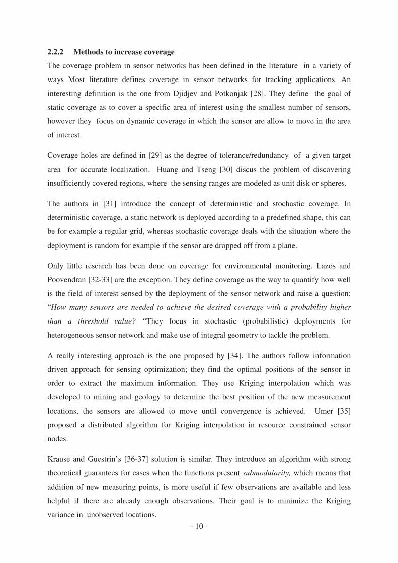
2.2.2 Methods to increase coverage

The coverage problem in sensor networks has been defined in the literature in a variety of

ways Most literature defines coverage in sensor networks for tracking applications. An

interesting definition is the one from Djidjev and Potkonjak [28]. They define the goal of

static coverage as to cover a specific area of interest using the smallest number of sensors,

however they focus on dynamic coverage in which the sensor are allow to move in the area

of interest.

Coverage holes are defined in [29] as the degree of tolerance/redundancy of a given target

area for accurate localization. Huang and Tseng [30] discus the problem of discovering

insufficiently covered regions, where the sensing ranges are modeled as unit disk or spheres.

The authors in [31] introduce the concept of deterministic and stochastic coverage. In

deterministic coverage, a static network is deployed according to a predefined shape, this can

be for example a regular grid, whereas stochastic coverage deals with the situation where the

deployment is random for example if the sensor are dropped off from a plane.

Only little research has been done on coverage for environmental monitoring. Lazos and

Poovendran [32-33] are the exception. They define coverage as the way to quantify how well

is the field of interest sensed by the deployment of the sensor network and raise a question:

“How many sensors are needed to achieve the desired coverage with a probability higher

than a threshold value? “They focus in stochastic (probabilistic) deployments for

heterogeneous sensor network and make use of integral geometry to tackle the problem.

A really interesting approach is the one proposed by [34]. The authors follow information

driven approach for sensing optimization; they find the optimal positions of the sensor in

order to extract the maximum information. They use Kriging interpolation which was

developed to mining and geology to determine the best position of the new measurement

locations, the sensors are allowed to move until convergence is achieved. Umer [35]

proposed a distributed algorithm for Kriging interpolation in resource constrained sensor

nodes.

Krause and Guestrin’s [36-37] solution is similar. They introduce an algorithm with strong

theoretical guarantees for cases when the functions present submodularity, which means that

addition of new measuring points, is more useful if few observations are available and less

helpful if there are already enough observations. Their goal is to minimize the Kriging

variance in unobserved locations.

- 11 -

Sensing optimization using Kriging can be found in geostatistics literature. For example, in

Szidarovszky [38], it is proposed a Branch-and-Bound algorithm to find the optimal sites of

drillholes; for the estimation of the minimum number of sensors, a method that takes

advantage of interesting feature of Kriging interpolation was selected. The Kriging-Variance

(KV), that measures the uncertainty of the estimation before actual measurements are

available. KV is monotonic, that means that increasing the number of measuring points will

not increase the KV. The method minimizes the number of required additional points subject

to upper bounds of the Kriging-Variance. The method, that is an unconstrained Branch-and-

Bound (BnB) algorithm, adds a measuring point if it improves the variance, or removes it, if

it does not bring any accuracy improvement. To avoid, calculation of matrix inverses each

time a point is added or removed, calculations of the inverse of a partitioned matrices are

done.

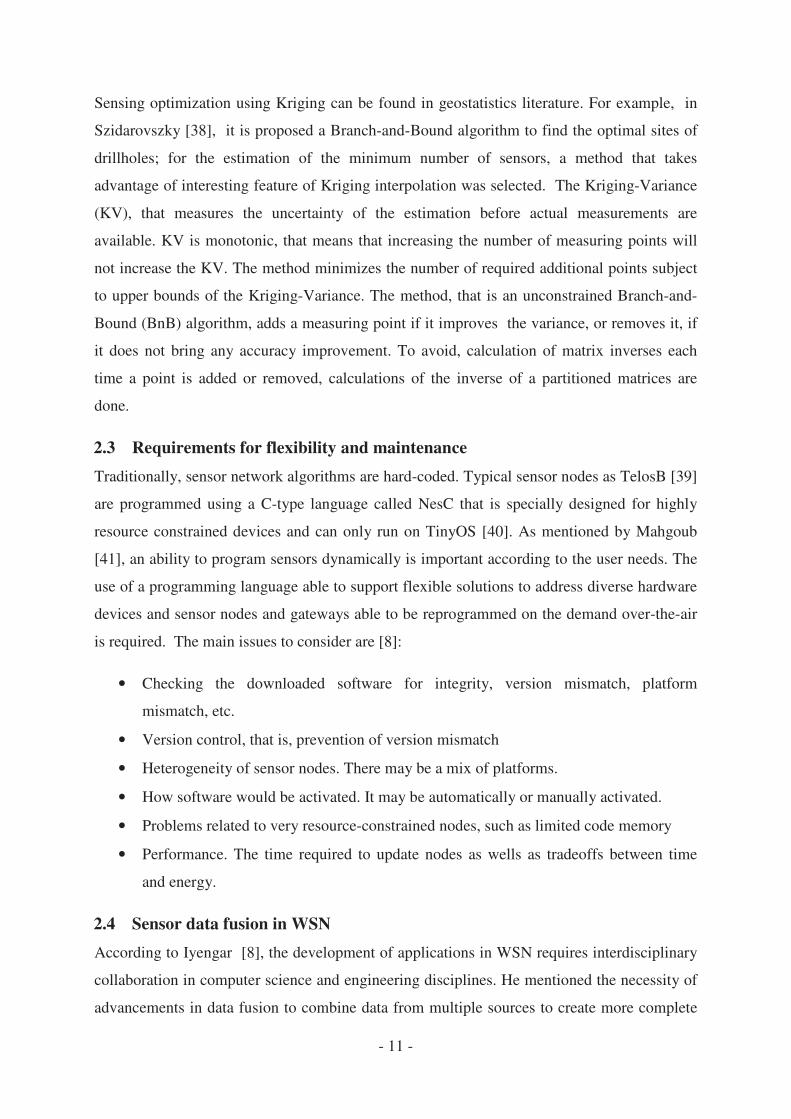
2.3 Requirements for flexibility and maintenance

Traditionally, sensor network algorithms are hard-coded. Typical sensor nodes as TelosB [39]

are programmed using a C-type language called NesC that is specially designed for highly

resource constrained devices and can only run on TinyOS [40]. As mentioned by Mahgoub

[41], an ability to program sensors dynamically is important according to the user needs. The

use of a programming language able to support flexible solutions to address diverse hardware

devices and sensor nodes and gateways able to be reprogrammed on the demand over-the-air

is required. The main issues to consider are [8]:

• Checking the downloaded software for integrity, version mismatch, platform

mismatch, etc.

• Version control, that is, prevention of version mismatch

• Heterogeneity of sensor nodes. There may be a mix of platforms.

• How software would be activated. It may be automatically or manually activated.

• Problems related to very resource-constrained nodes, such as limited code memory

• Performance. The time required to update nodes as wells as tradeoffs between time

and energy.

2.4 Sensor data fusion in WSN

According to Iyengar [8], the development of applications in WSN requires interdisciplinary

collaboration in computer science and engineering disciplines. He mentioned the necessity of

advancements in data fusion to combine data from multiple sources to create more complete

- 12 -

representation of the world. Data fusion is per se interdisciplinary; it is defined as set of

theories techniques and tools that are used to combine sensor data to improve the performance

of the system in some way. Being more specific, classified according the relation among the

sources, the ways the fusion can improve the system is in its completeness, accuracy and

certainty [42]. Incomplete information might be found, for instance, when two sources posses

information about different portions of the same environment at different positions. Inaccurate

information might be the result of environmental noise or error models, if two or more sensors

posses information about the same source, the redundant information can be used to fuse them

into a single filtered estimation that is more accurate. Certainty might be, for instance,

improved by fusing several estimations of a point of interest each one of them with high

uncertainties into a new estimation with low, acceptable variance.

The fusion type might be performed across sensors, attributes or time [43]. Fusion across

sensors is the most common one and is made through measurements of the same variable of

attribute. Fusion across attributes is made over a number of measurements that are associated

with the same situation, for example temperature and humidity in a room. Fusion across time

current measurements are fused with historical information, with this type of fusion is

possible for example predict future values with the learned information.

As mentioned before, sensor fusion is interdisciplinary; it involves disciplines like

communication engineering, geostatistics and process automation and artificial intelligence.

The methods and techniques, however can be summarized into inference, estimation,

aggregation and compression [44].

2.4.1.1

Inference is the act of deriving conclusions based on evidence. The classical inference method

is Bayesian inference used extensively in communication engineering, mathematically

speaking an uncertainty is represented in terms of conditional probabilities describing an a-

priori beliefs. The posterior probability represents the belief of hypothesis V given the

information U. The probability is calculated by:

(2.1)

Where is the belief of hypothesis V given the information U. is the prior

probability of V and is the probability of receiving U if V is true. The main design

issue is the setting of the probabilities that have to be guessed beforehand.

- 13 -

2.4.1.2

Estimation methods were developed in the control engineering field and make extensive use

of state vectors. The most common estimation methods are the Kalman Filter and Best Linear

Unbiased Estimator (BLUE)

The Kalman filter is over 50 years old but still one of the most important data fusion

algorithms [45]. The typical uses is to smooth (filter) noisy data to provide estimates of the

state vectors of the model of a dynamic system. Its mathematical derivation uses linear matrix

algebra as a minimum mean squared estimator [46]. Two pieces of information are available,

estimations and measurements, they are fused to provide the best possible estimate. The

Gaussian probability density functions of both pieces of information are multiplied together,

giving as a result another Gaussian function , that is a key point to perform the filtering in

recursive way.

Best Linear Unbiased Estimator (BLUE) has application where the Kalman Filter does not.

For example when no complete prior information is available [47], or when different

attributes must be fused, or where the dynamic model is too complex to be modeled.

A Best Linear Unbiased Estimator has the following properties:

Is Linear in data: The estimate is calculated by the sum of all the resulting multiplications of

assigned weights and available data

(2.2 )

Is unbiased : The expectation of the prediction is equal to the “real value” of the attribute.

(2.3)

Possesses theoretical Guarantees: A variance of the estimation is provided as a measure of

accuracy.

(2.4)

Where is a vector containing n weights and is the covariance Matrix.

2.4.1.3

Aggregation techniques are extensively used by database systems, developed to be used in

query languages as SQL, they summarize data. They are feasible to implement in sensor

nodes, it processess the incoming data with the local measurement by performing aggregation

operations, such as average, sum, minimum or maximum. This approach may reduce

- 14 -

accuracy; after the information is received at the sink is usually not possible to recover it. In

this thesis we are mostly interested in the average operation, that according to the law of large

numbers, the average of the results obtained from a large number of trials should be close to

the expected value.

(2.5)

2.4.1.4

Data compression is not information fusion method, however they are mentioned here

because they use Bayesian inference to decompress the received measurement. They are

based on information theory concepts. If two measurements are spatially correlated, they can

be compressed and decompressed without loss. The correlation between the sources has to be

known a-priori; the sink may have to collect information over the network, calculate the

correlations between the sensors and inform the sources how many bits are required to send in

order to be able to achieve lossless compression. The method is known as Distributed Source

Coding (DSC)

Table 2.2 summarizes some of the most important Information Fusion techniques used in

WSN

- 15 -

Table 2.2 Information Fusion in WSN

What Improves? Fusion Types Methods

In-network aggregation with

size reduction Energy consumption Across sensors Aggregation

In-network aggregation

without size reduction Energy consumption

• Across attributes

• Across sensors Aggregation

Coding by ordering Energy consumption Across sensors Compression

Pipelined in-network

compression Energy consumption Across sensors Compression

Distributed Source Coding Energy consumption

• Across sensors r

• Redundant

• Complementary

• Inference

• Compression

• Estimation

Stochastic approaches Energy consumption Across time

• Inference

• Data

prediction

Time series forecasting Energy consumption • Across time

• Across sensors

• Data

prediction

• Estimation

Kriging • Coverage

• Certainty Across sensors

• Estimation

• Inference

- 16 -

Low energy consumption is one of the most important figures of merit in sensor networks.

Exploiting the spatial correlation between the sensed points to reduce radio communication

data rates is a really good approach that can help achieve this objective. The methods used to

compress the data must be simple, accurate, and robust. Modelling the spatial correlations

using variography that is the traditional method to measure spatial correlations between

variables using two-point approaches seem to be the obvious start point.

Geostatistics is a theory of regionalized variables [48] in which variables or attributes of

interest are spatially distributed. It already has mature methods developed and tested in the

field. However their applicability to sensor networks has been limited; exceptions are for

example, [49] and [50], where kriging interpolation is performed with the aim of reducing the

number of sensors deployed.

Only a few research works have considered the links between geostatistics, data compression,

and transmission of correlated observations. Research made in [51] considered it to guide the

optimization of source-channel coding schemes, while Oldewurtel [21] applied spatial

statistics only for data modelling and simulation. DSC approach fails to make a correct link

with statistics and random fields; as a matter of fact, research work on Distributed Source

Coding (DSC) has focused mainly on finding the more robust codes and the most efficient

decoders.

In the present chapter, a method that combines geostatistical and information fusion methods

for data compression in sensor networks is presented. The reconstruction of the measurement

data can be largely simplified if the global mean of the probe points is available; the mean is

approximated by the strong law of large numbers, and by combining it with an estimation of

the variogram and with continuous-valued source space partitions, it is proved that it is

possible to perform energy-efficient, robust, and consistent data compression in sensor

networks.

The procedures were tested on two datasets recorded in a refrigerated container of dimensions

2.2 × 2.2 × 5.4 m as part of a collaborative internship with the Research Centre for Logistics

Information Technology (LIT) at the Pusan National University in Korea in 2012.

In order to increase spatial variability, the conta

temperature (15 °C) to a set point of 0 °C for 3 ho

for about 2 hours, prior to performing the actual experiment,

container to 5 °C for 80 minutes. As the most significant influenc

the loading state, two configurations were tested:

with pallets covering the floor to deflect the air flow.

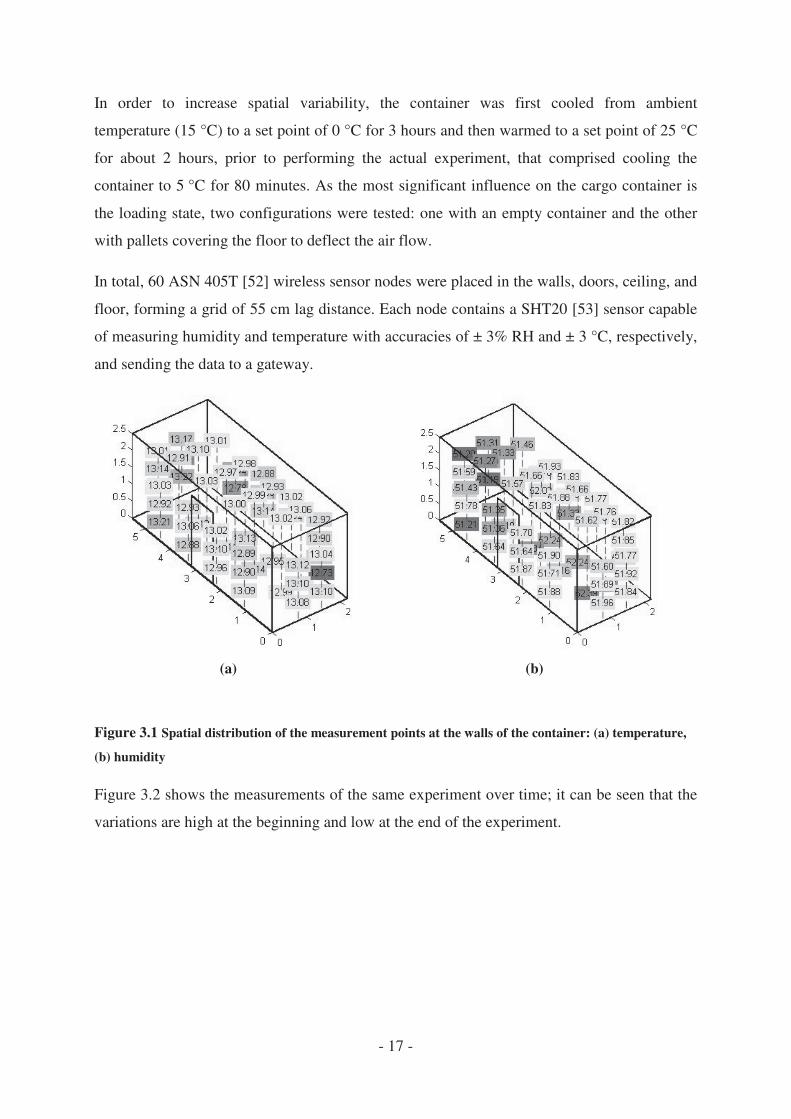
In total, 60 ASN 405T [52] wireless sensor nodes were placed in the walls, doo

floor, forming a grid of 55 cm lag distance. Each n

of measuring humidity and temperature with accuracies of ± 3% RH

and sending the data to a gateway.

(a)

Figure 3.1 Spatial distribution of the measurement points at t

(b) humidity

Figure 3.2 shows the measurements of the s

variations are high at the beginning and low at the

- 17 -

In order to increase spatial variability, the container was first cooled from ambient

temperature (15 °C) to a set point of 0 °C for 3 hours and then warmed to a set point of 25 °C

performing the actual experiment, that comprised cooling the

°C for 80 minutes. As the most significant influence on the cargo container is

the loading state, two configurations were tested: one with an empty container and the other

llets covering the floor to deflect the air flow.

wireless sensor nodes were placed in the walls, doo

floor, forming a grid of 55 cm lag distance. Each node contains a SHT20 [53]

humidity and temperature with accuracies of ± 3% RH and ± 3 °C, respectively,

and sending the data to a gateway.

(b)

Spatial distribution of the measurement points at the walls of the container: (a) temperature,

shows the measurements of the same experiment over time; it can be seen that the

variations are high at the beginning and low at the end of the experiment.

iner was first cooled from ambient

urs and then warmed to a set point of 25 °C

comprised cooling the

e on the cargo container is

one with an empty container and the other

wireless sensor nodes were placed in the walls, doors, ceiling, and

[53] sensor capable

and ± 3 °C, respectively,

he walls of the container: (a) temperature,

ame experiment over time; it can be seen that the

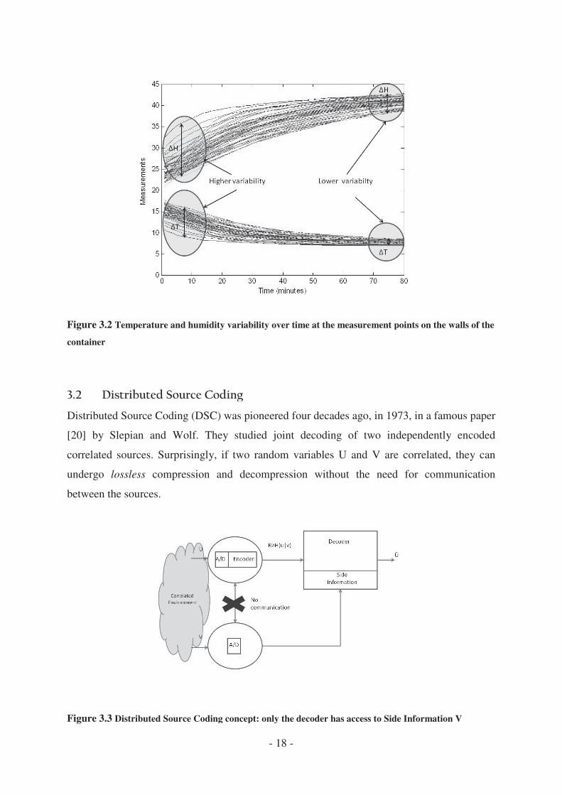
Figure 3.2 Temperature and humidity variability over time at t

container

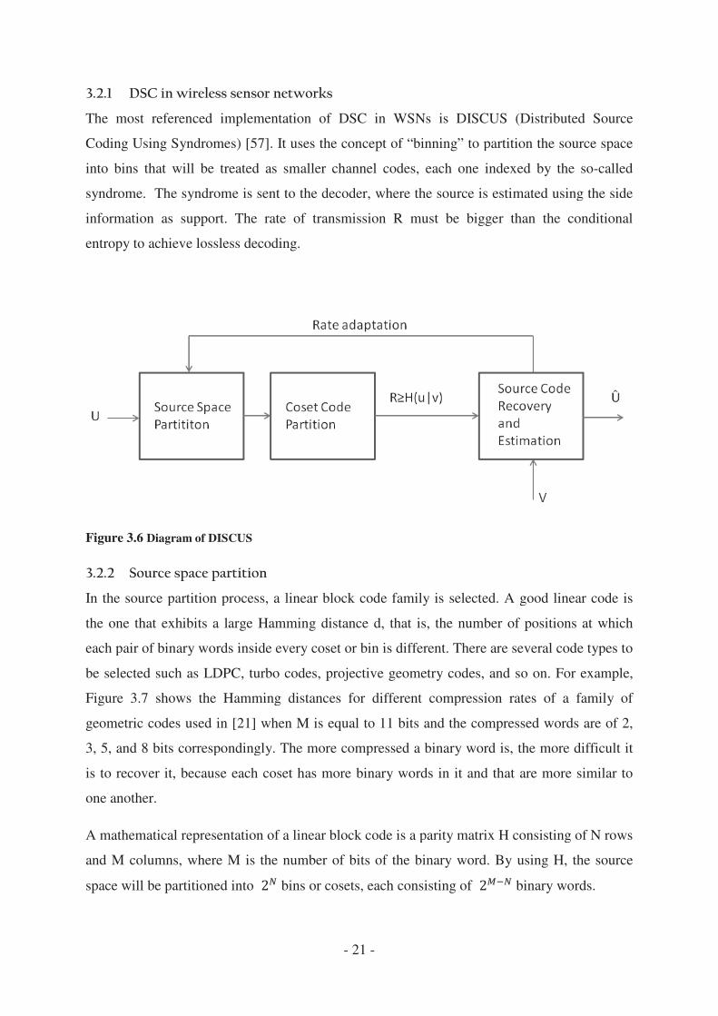
Distributed Source Coding (DSC) was pioneered four

[20] by Slepian and Wolf. They studied joint decoding of tw

correlated sources. Surprisingly, if two random variables U and V are correlated

undergo lossless compression and decompression without the need for

between the sources.

Figure 3.3 Distributed Source Coding

- 18 -

Temperature and humidity variability over time at the measurement points on the walls of the

Distributed Source Coding (DSC) was pioneered four decades ago, in 1973, in a famous paper

Slepian and Wolf. They studied joint decoding of two independently encoded

gly, if two random variables U and V are correlated

compression and decompression without the need for

Distributed Source Coding concept: only the decoder has access to Side Inform

points on the walls of the

decades ago, in 1973, in a famous paper

o independently encoded

gly, if two random variables U and V are correlated, they can

compression and decompression without the need for communication

concept: only the decoder has access to Side Information V

The correlated environment is modelled by a

binary source and V is the sink, the correlation be

with variance and mean zero.

Given a quantization step , the

of bit flipping to be less than a value p

When dealing with continuous

fact that the least significant bits will have more

significant ones, as shown in

decoding, the decoder must have been set properly w

each bit, resulting in a complex correlation model and deco

authors of [56] proposed hybrid decoding for such a purpose

Figure 3.4 Probabilities of bit-flipping of continuous

If the decoder receives incomplete but sufficient info

recovered perfectly by using the so

amount of information a random variable contains ab

source . Source coding theorems are used to determine the

transmitted in order to achieve lossless communicat

- 19 -

The correlated environment is modelled by a Binary Source Channel (BSC).

binary source and V is the sink, the correlation between them is modelled by an additive noise

and mean zero.

, the Chebyshev’s inequality can be used to bound

of bit flipping to be less than a value p if the source is compressed to n bits by

ontinuous-valued values, such a model becomes more complex du

fact that the least significant bits will have more probability of flipping than the most

significant ones, as shown in Figure 3.4. In order to increase the probability of correct

decoding, the decoder must have been set properly with different bit-flipping

, resulting in a complex correlation model and decoding methods; for example, the

proposed hybrid decoding for such a purpose

flipping of continuous-valued sources

the decoder receives incomplete but sufficient information about a source it can be

recovered perfectly by using the so-called mutual information (MI), that

amount of information a random variable contains about another variable from a

. Source coding theorems are used to determine the necessary number of bits to be

transmitted in order to achieve lossless communication.

Binary Source Channel (BSC). Usually, if U is the

tween them is modelled by an additive noise

(3.1)

bound the probability

bits by [54-55]

(3.2)

(3.3)

valued values, such a model becomes more complex due to the

probability of flipping than the most

. In order to increase the probability of correct

flipping probabilities for

ding methods; for example, the

(3.4)

rmation about a source it can be

is a measure of the

out another variable from a second

necessary number of bits to be

(3.5)

and are the so-called marginal entropies and

Mitchel [42] rewrites the last equation in a more useful represe

conditional entropy.

In bit terms, if M is the number of bits of the unc

of the compressed word, the compression rate is def

Figure 3.5 Achievable rate regions for Slepian

The theorem has applicability as a data compression

information should be transmitted only once and use

conditional entropy to recover the joint entropy. B

information theory concepts, the research focus was

- 20 -

called marginal entropies and is their joint entropy.

rewrites the last equation in a more useful representation.

In bit terms, if M is the number of bits of the uncompressed word and N is the number of bits

of the compressed word, the compression rate is defined as

Achievable rate regions for Slepian-Wolf coding of two sources

The theorem has applicability as a data compression technique in the sense that redundant

information should be transmitted only once and used in the decoder to complement the

conditional entropy to recover the joint entropy. Because it is based on binary

information theory concepts, the research focus was on channel modelling and code design.

is their joint entropy.

ntation. is the

(3.6)

(3.7)

ompressed word and N is the number of bits

(3.8)

technique in the sense that redundant

d in the decoder to complement the

ecause it is based on binary codes and

on channel modelling and code design.

The most referenced implementation of DSC in WSNs i

Coding Using Syndromes) [57]

into bins that will be treated as smaller channel c

syndrome. The syndrome is sent to the decoder, whe

information as support. The rate of tran

entropy to achieve lossless decoding.

Figure 3.6 Diagram of DISCUS

In the source partition process, a linear block cod

the one that exhibits a large Hamming distance d, t

each pair of binary words inside every coset or bin

be selected such as LDPC, turbo codes,

Figure 3.7 shows the Hamming distances for different compressi

geometric codes used in [21]

3, 5, and 8 bits correspondingly. The m

is to recover it, because each coset has more binar

one another.

A mathematical representation of a linear block code is a parity matrix

and M columns, where M is the number of bits of the

space will be partitioned into

- 21 -

The most referenced implementation of DSC in WSNs is DISCUS (Distributed Source

[57]. It uses the concept of “binning” to partition the source space

into bins that will be treated as smaller channel codes, each one indexed by the so

syndrome. The syndrome is sent to the decoder, where the source is estimated using the side

information as support. The rate of transmission R must be bigger than the conditional

entropy to achieve lossless decoding.

In the source partition process, a linear block code family is selected. A good linear code is

the one that exhibits a large Hamming distance d, that is, the number of positions at which

each pair of binary words inside every coset or bin is different. There are several code types to

be selected such as LDPC, turbo codes, projective geometry codes, and so on. For example,

shows the Hamming distances for different compression rates of a family of

when M is equal to 11 bits and the compressed words are of 2,

3, 5, and 8 bits correspondingly. The more compressed a binary word is, the more difficult

is to recover it, because each coset has more binary words in it and that are more similar to

entation of a linear block code is a parity matrix H consisting of N rows

and M columns, where M is the number of bits of the binary word. By using H, the source

space will be partitioned into bins or cosets, each consisting of binary words.

s DISCUS (Distributed Source

” to partition the source space

odes, each one indexed by the so-called

re the source is estimated using the side

smission R must be bigger than the conditional

ted. A good linear code is

hat is, the number of positions at which

is different. There are several code types to

projective geometry codes, and so on. For example,

on rates of a family of

nd the compressed words are of 2,

ore compressed a binary word is, the more difficult it

y words in it and that are more similar to

H consisting of N rows

binary word. By using H, the source

binary words.

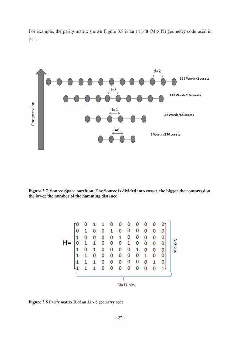
For example, the parity matrix shown

[21].

Figure 3.7 Source Space partition. the lower the number of the hamming distance

Figure 3.8 Parity matrix H of an 11 × 8 geometry code

- 22 -

the parity matrix shown Figure 3.8 is an 11 × 8 (M × N) geometry code used in

ource Space partition. The Source is divided into cosset, the bigger the cthe lower the number of the hamming distance

Parity matrix H of an 11 × 8 geometry code

is an 11 × 8 (M × N) geometry code used in

The Source is divided into cosset, the bigger the compression,

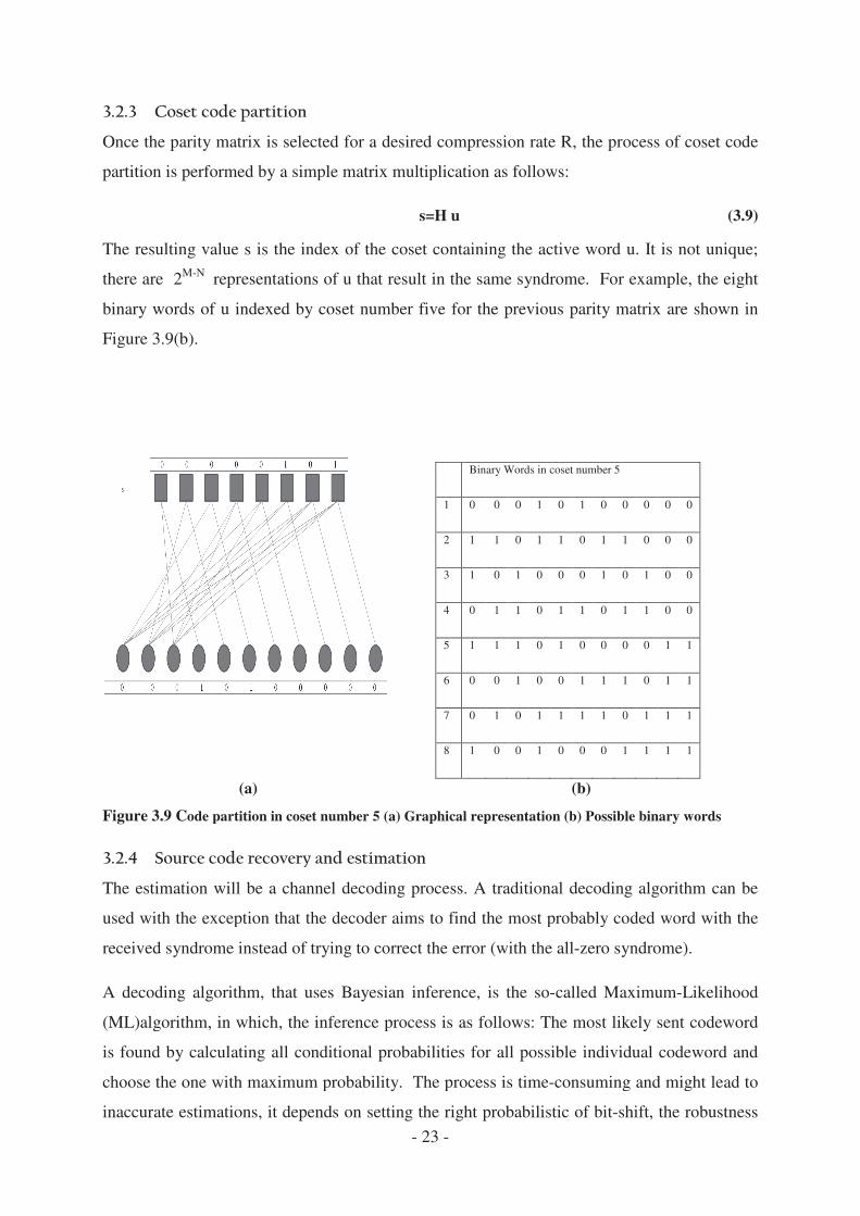
Once the parity matrix is selected for a desired co

partition is performed by a simple matrix multiplication as follows:

The resulting value s is the index of the coset con

there are 2M-N

representations of u that result in the same syndro

binary words of u indexed by coset nu

Figure 3.9(b).

(a)

Figure 3.9 Code partition in coset number 5

The estimation will be a channel decoding process. A

used with the exception that the decoder aims to fi

received syndrome instead of trying to correct the

A decoding algorithm, that uses Bayesian inference,

(ML)algorithm, in which, the inference process

is found by calculating all conditional probabiliti

choose the one with maximum probability. The proce

inaccurate estimations, it depends on setting the right probabilistic of bit

- 23 -

Once the parity matrix is selected for a desired compression rate R, the process of coset code

simple matrix multiplication as follows:

s=H u

The resulting value s is the index of the coset containing the active word u. It is not unique;

representations of u that result in the same syndrome. For example, the eight

binary words of u indexed by coset number five for the previous parity matrix are shown

Binary Words in coset number 5

1 0 0 0 1 0 1 0

2 1 1 0 1 1 0 1

3 1 0 1 0 0 0 1

4 0 1 1 0 1 1 0

5 1 1 1 0 1 0 0

6 0 0 1 0 0 1 1

7 0 1 0 1 1 1 1

8 1 0 0 1 0 0 0

(b)

coset number 5 (a) Graphical representation (b) Possible binary words

he estimation will be a channel decoding process. A traditional decoding algorithm can be

used with the exception that the decoder aims to find the most probably coded word with the

received syndrome instead of trying to correct the error (with the all-zero syndrome).

A decoding algorithm, that uses Bayesian inference, is the so-called Maximum

(ML)algorithm, in which, the inference process is as follows: The most likely sent codeword

is found by calculating all conditional probabilities for all possible individual codeword and

choose the one with maximum probability. The process is time-consuming and might lead to

t depends on setting the right probabilistic of bit-shift, the robustness

mpression rate R, the process of coset code

(3.9)

taining the active word u. It is not unique;

me. For example, the eight

mber five for the previous parity matrix are shown in

Binary Words in coset number 5

0 0 0 0

1 0 0 0

0 1 0 0

1 1 0 0

0 0 1 1

1 0 1 1

0 1 1 1

1 1 1 1

ossible binary words

traditional decoding algorithm can be

most probably coded word with the

zero syndrome).

called Maximum-Likelihood

is as follows: The most likely sent codeword

es for all possible individual codeword and

consuming and might lead to

shift, the robustness

of the used code and the number of iterations. The

Binary Symmetric Channel is NP

Another common decoding algorithm is the belief pro

message passing one. These are iterative algorithms

iteration the algorithm passes messages from messag

The messages that are passed are probabilities or

of the algorithm is its sunning time, in general, i

powerful [60].

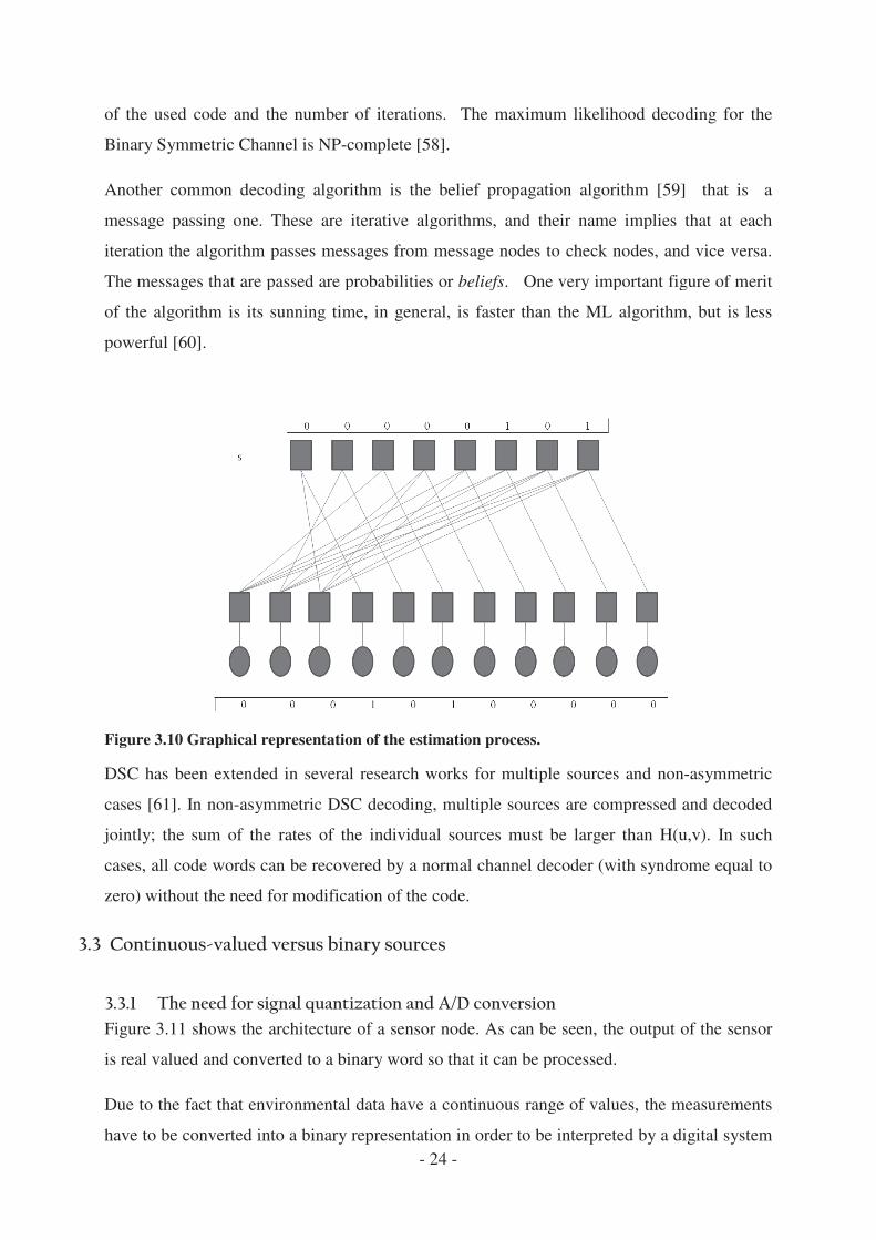
Figure 3.10 Graphical representation of the estimation process.

DSC has been extended in several research works for

cases [61]. In non-asymmetric DSC decoding, multiple sources are compr

jointly; the sum of the rates of the indiv

cases, all code words can be recovered by a normal

zero) without the need for modification of the code.

Figure 3.11 shows the architecture of a sensor node. As can be

is real valued and converted to a binary word so that it can be processed.

Due to the fact that environmental data have a cont

have to be converted into a binary representation i

- 24 -

of the used code and the number of iterations. The maximum likelihood decoding for the

Binary Symmetric Channel is NP-complete [58].

Another common decoding algorithm is the belief propagation algorithm

message passing one. These are iterative algorithms, and their name implies that

iteration the algorithm passes messages from message nodes to check nodes, and vice versa.

The messages that are passed are probabilities or beliefs. One very important figure of merit

of the algorithm is its sunning time, in general, is faster than the ML algorithm, but is less

Graphical representation of the estimation process.

DSC has been extended in several research works for multiple sources and non

asymmetric DSC decoding, multiple sources are compr

jointly; the sum of the rates of the individual sources must be larger than

cases, all code words can be recovered by a normal channel decoder (with

) without the need for modification of the code.

shows the architecture of a sensor node. As can be seen, the output of the sensor

ted to a binary word so that it can be processed.

Due to the fact that environmental data have a continuous range of values, the measurements

have to be converted into a binary representation in order to be interpreted by a digital system

maximum likelihood decoding for the

pagation algorithm [59] that is a

implies that at each

to check nodes, and vice versa.

. One very important figure of merit

s faster than the ML algorithm, but is less

multiple sources and non-asymmetric

asymmetric DSC decoding, multiple sources are compressed and decoded

idual sources must be larger than H(u,v). In such

with syndrome equal to

seen, the output of the sensor

inuous range of values, the measurements

n order to be interpreted by a digital system

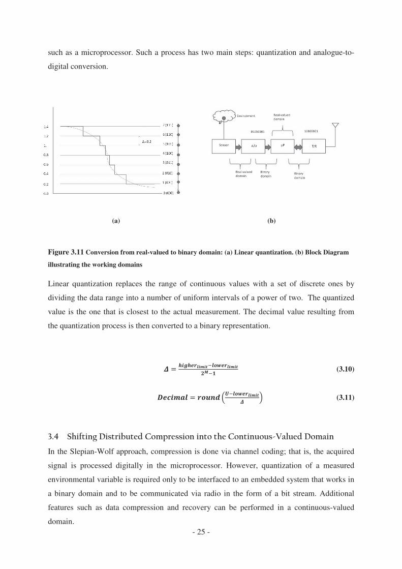
such as a microprocessor. Such a process has two main steps: quantiz

digital conversion.

(a)

Figure 3.11 Conversion from real

illustrating the working domains

Linear quantization replaces the range of continuou

dividing the data range into a number of uniform in

value is the one that is closes

the quantization process is then converted to a bin

In the Slepian-Wolf approach, compression is done via channel codi

signal is processed digitally in the microprocessor

environmental variable is required only to be inter

a binary domain and to be communicated via radio in

features such as data compression and recovery can

domain.

- 25 -

ocessor. Such a process has two main steps: quantization and analogue

(b)

Conversion from real-valued to binary domain: (a) Linear quantization. (

Linear quantization replaces the range of continuous values with a set of discrete ones by

dividing the data range into a number of uniform intervals of a power of two. The quantized

value is the one that is closest to the actual measurement. The decimal value resu

the quantization process is then converted to a binary representation.

Wolf approach, compression is done via channel coding; that is, the acquired

signal is processed digitally in the microprocessor. However, quantization of a measured

environmental variable is required only to be interfaced to an embedded system

a binary domain and to be communicated via radio in the form of a bit stream. Additional

features such as data compression and recovery can be performed in a continuous

ation and analogue-to-

valued to binary domain: (a) Linear quantization. (b) Block Diagram

s values with a set of discrete ones by

tervals of a power of two. The quantized

t to the actual measurement. The decimal value resulting from

(3.10)

(3.11)

ng; that is, the acquired

. However, quantization of a measured

faced to an embedded system that works in

the form of a bit stream. Additional

be performed in a continuous-valued

- 26 -

The approach adopted in this research work is to use a real-valued statistical domain to model

the correlation between any pair of sensing points of the environment, and geostatistical

methods are selected. The experimental variograms (EVs) from the acquired datasets need to

be calculated.

The variogram describes the statistical dependency across sensors by the expected value

E for the square of the difference in value of two points as a function of the distance h.

(3.12)

These experimental curves must be approximated by theoretical variograms conforming to the

limitations of being conditionally negative semi-definite functions. Only a limited set of

functions can be applied as theoretical variograms, for example, Gaussian, Exponential and

Spherical. They are usually described with three parameters: range, nugget and sill. The range

gives the maximum distance up to which the mutual influence of two probe points has to be

considered. Nugget and sill give the expected squared temperature deviation for very small

and very large distances.

According to Kanevski [48], Spherical, Exponential and Gaussian variogram models are the

most commonly used. The behaviour of them near the origin is of most importance in spatial

predictions: Spherical model has a linear behaviour near the origin; the Gaussian variogram

presents a very smooth behaviour at short distances, whereas an Exponential model reaches

95% of sill at the radius r. Other models include Power, Gamma, Stable and Bessel.

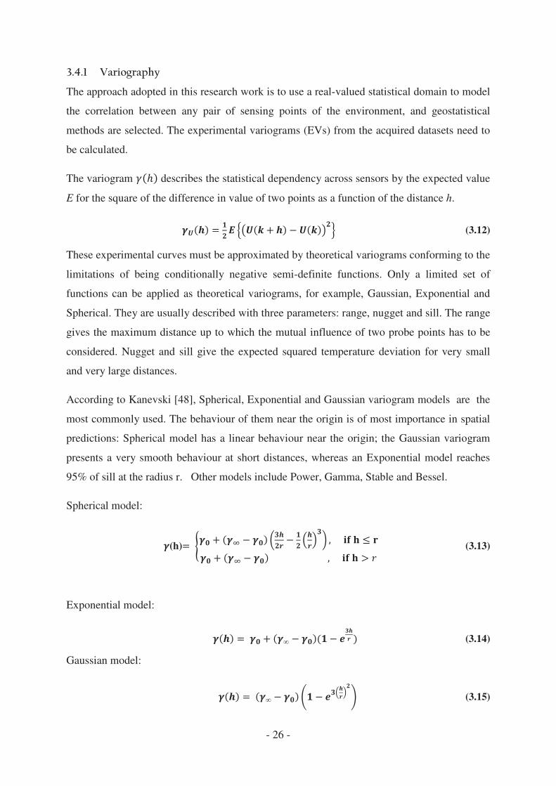
Spherical model:

(h) (3.13)

Exponential model:

(3.14)

Gaussian model:

(3.15)

3.4.1.1

An efficient variogram-fitting algorithm was found in

minimize the fitting error for an experimental, iso

using the Nelder and Mead

effective and computationally compact as it does no

Furthermore, the algorithm provides additional adva

of the function: it allows the least squares to be

experimental lag is provided. Two weighting schemes

literature. The first one is based on Cressie

lags and down-weights to the lags with a small number of observat

assigns weights based on the criterion of goodness

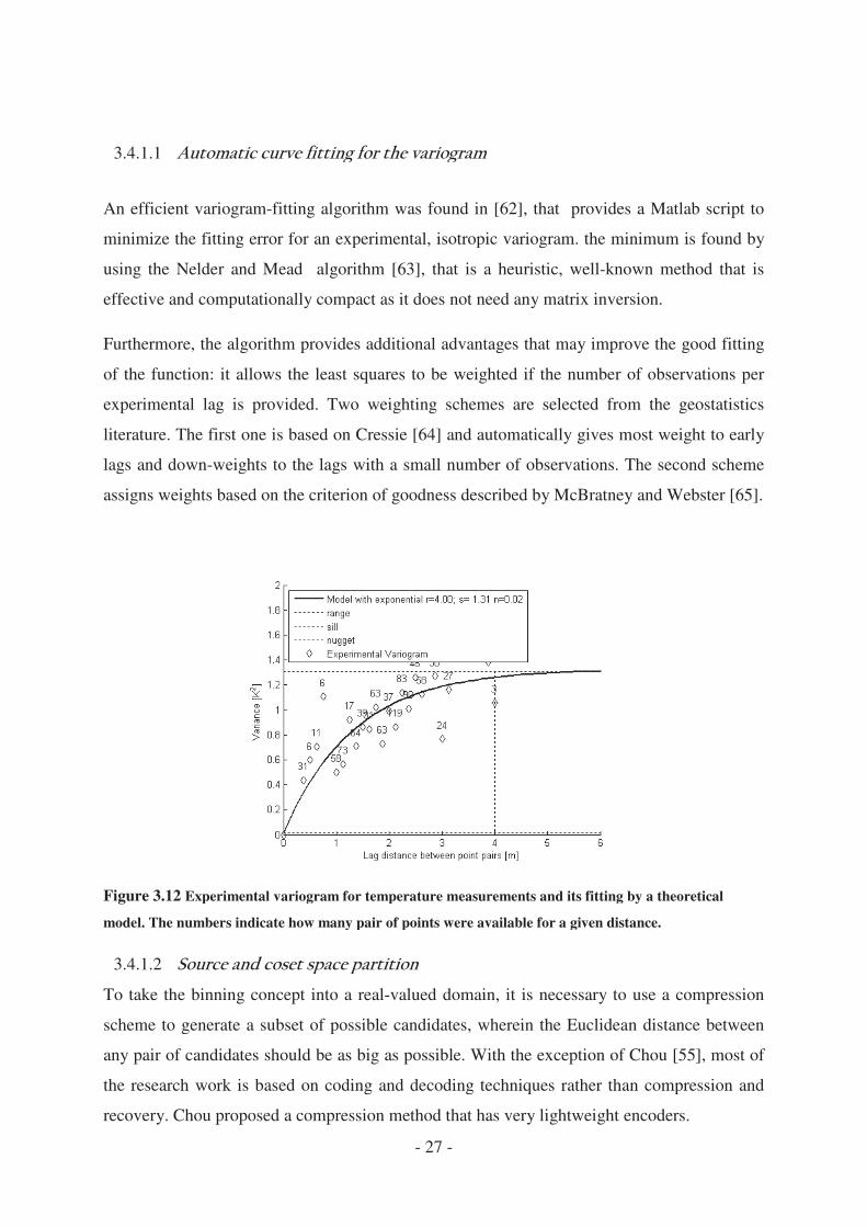
Figure 3.12 Experimental variogram for temperature measurements

model. The numbers indicate how many pair of points

3.4.1.2

To take the binning concept into a real

scheme to generate a subset of possible candidates,

any pair of candidates should be as big as possible

the research work is based on coding and decoding t

recovery. Chou proposed a compression method that h

- 27 -

fitting algorithm was found in [62], that provides a Matlab script to

minimize the fitting error for an experimental, isotropic variogram. the minimum is found by

algorithm [63], that is a heuristic, well-known method that is

effective and computationally compact as it does not need any matrix inversion.

Furthermore, the algorithm provides additional advantages that may improve the good fitting

of the function: it allows the least squares to be weighted if the number of obser

experimental lag is provided. Two weighting schemes are selected from the geostatistics

literature. The first one is based on Cressie [64] and automatically gives most weight to early

weights to the lags with a small number of observations. The second scheme

assigns weights based on the criterion of goodness described by McBratney and Webster

Experimental variogram for temperature measurements and its fitting by a theoretical

model. The numbers indicate how many pair of points were available for a given distance.

To take the binning concept into a real-valued domain, it is necessary to use a compression

scheme to generate a subset of possible candidates, wherein the Euclidean distance between

any pair of candidates should be as big as possible. With the exception of Chou

the research work is based on coding and decoding techniques rather than compression and

recovery. Chou proposed a compression method that has very lightweight encoders.

provides a Matlab script to

tropic variogram. the minimum is found by

known method that is

t need any matrix inversion.

ntages that may improve the good fitting

weighted if the number of observations per

are selected from the geostatistics

and automatically gives most weight to early

ions. The second scheme

bed by McBratney and Webster [65].

and its fitting by a theoretical

were available for a given distance.

valued domain, it is necessary to use a compression

wherein the Euclidean distance between

f Chou [55], most of

echniques rather than compression and

as very lightweight encoders.

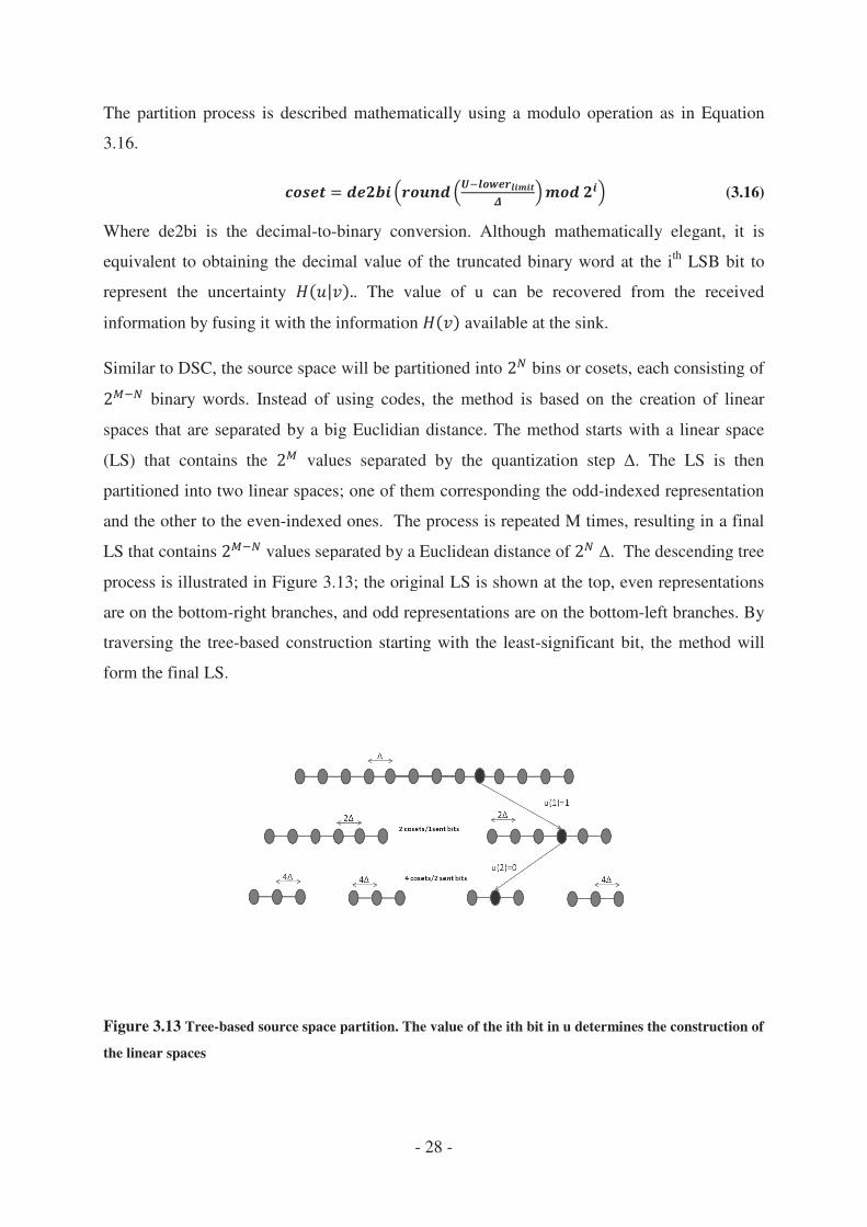
The partition process is described mathematically u

3.16.

Where de2bi is the decimal-

equivalent to obtaining the decimal value of the tr

represent the uncertainty

information by fusing it with the information

Similar to DSC, the source space will be partitione

binary words. Instead of using codes, the method is

spaces that are separated by a big Euclidian distance. The meth

(LS) that contains the values separated by the quantization step

partitioned into two linear spaces; one of them cor

and the other to the even-indexed ones. The process is repeated M times, res

LS that contains values separated by a Euclidean distance of

process is illustrated in Figure

are on the bottom-right branches, and odd representations are on the

traversing the tree-based construction starting with the least

form the final LS.

Figure 3.13 Tree-based source space partition. The value of the ith

the linear spaces

- 28 -

The partition process is described mathematically using a modulo operation

-to-binary conversion. Although mathematically elegant, it is

equivalent to obtaining the decimal value of the truncated binary word at the i

. The value of u can be recovered from the received

information by fusing it with the information available at the sink.

Similar to DSC, the source space will be partitioned into bins or cosets, each consisting of

binary words. Instead of using codes, the method is based on the creation of linear

are separated by a big Euclidian distance. The method starts with a linear space

values separated by the quantization step

partitioned into two linear spaces; one of them corresponding the odd-indexed representa

indexed ones. The process is repeated M times, res

values separated by a Euclidean distance of . The descending tree

Figure 3.13; the original LS is shown at the top, even represe

right branches, and odd representations are on the bottom

based construction starting with the least-significant bit, the method will

based source space partition. The value of the ith bit in u determines the construction of

sing a modulo operation as in Equation

(3.16)

mathematically elegant, it is

uncated binary word at the ith

LSB bit to

. The value of u can be recovered from the received

bins or cosets, each consisting of

based on the creation of linear

od starts with a linear space

values separated by the quantization step . The LS is then

indexed representation

indexed ones. The process is repeated M times, resulting in a final

. The descending tree

; the original LS is shown at the top, even representations

bottom-left branches. By

significant bit, the method will

bit in u determines the construction of

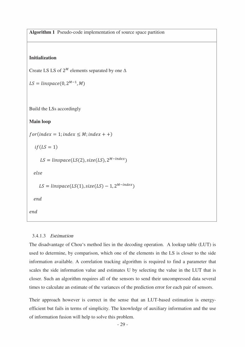
- 29 -

Algorithm 1 Pseudo-code implementation of source space partition

Initialization

Create LS LS of elements separated by one

Build the LSs accordingly

Main loop

3.4.1.3

The disadvantage of Chou‘s method lies in the decoding operation. A lookup table (LUT) is

used to determine, by comparison, which one of the elements in the LS is closer to the side

information available. A correlation tracking algorithm is required to find a parameter that

scales the side information value and estimates U by selecting the value in the LUT that is

closer. Such an algorithm requires all of the sensors to send their uncompressed data several

times to calculate an estimate of the variances of the prediction error for each pair of sensors.

Their approach however is correct in the sense that an LUT-based estimation is energy-

efficient but fails in terms of simplicity. The knowledge of auxiliary information and the use

of information fusion will help to solve this problem.

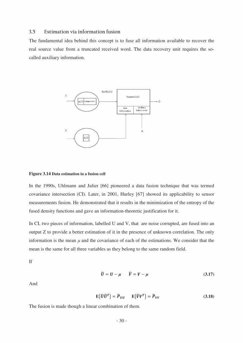
The fundamental idea behind this concept is to fuse

real source value from a truncated received word. T

called auxiliary information.

Figure 3.14 Data estimation in a fusion cell

In the 1990s, Uhlmann and Julier

covariance intersection (CI). Later, in 2001,

measurements fusion. He demonstra

fused density functions and gave an information

In CI, two pieces of information, labelled U and V,

output Z to provide a better estimation of it in the presence of

information is the mean and the covariance of each of the estimations. We c

mean is the same for all three variables as they be

If

And

The fusion is made though a linear combination of them.

- 30 -

The fundamental idea behind this concept is to fuse all information available to recover the

real source value from a truncated received word. The data recovery unit requires the so

Data estimation in a fusion cell

In the 1990s, Uhlmann and Julier [66] pioneered a data fusion technique that was termed

covariance intersection (CI). Later, in 2001, Hurley [67] showed its applicability to sensor

demonstrated that it results in the minimization of the entr

fused density functions and gave an information-theoretic justification for it.

In CI, two pieces of information, labelled U and V, that are noise corrupted, are fused into an

ovide a better estimation of it in the presence of unknown correlation. The only

and the covariance of each of the estimations. We c

mean is the same for all three variables as they belong to the same random field.

E E

fusion is made though a linear combination of them.

all information available to recover the

he data recovery unit requires the so-

pioneered a data fusion technique that was termed

showed its applicability to sensor

ted that it results in the minimization of the entropy of the

theoretic justification for it.

are noise corrupted, are fused into an

unknown correlation. The only

and the covariance of each of the estimations. We consider that the

long to the same random field.

(3.17)

(3.18)

- 31 -

Z= (3.19)

It follows that

(3.20)

The aim of the algorithm is basically to minimize the trace of by choosing the weights

and . For decompression purposes a minimization criterion has to be defined when one

of the measurements is fixed and used as side information and the correlation are known.

It is observed that Equation 3.20 can be written in terms of centred covariances

(3.21)

If the centred covariance is considered symmetric

= = (3.22)

Also, if is the side information, the expectation is constant as well

(3.23)

Traditionally, a CI iterative algorithm would have a set of measurements of both variables and

would find the matrix weights and that minimize the trace of by performing

filtering of redundant data between U and V.

Because is constant, the elements of will be weighted equally, and does not

have an effect on the minimization. The minimization depends mainly on the trace of

(3.24)

V is constant and U takes all the possible values in the coset by considering the main

diagonal of .

(3.25)

and its trace is

= (3.26)

Minimizing the trace of will lead automatically to a minimization of . If

and are the ith

elements in the main diagonal of and then

If an iterative algorithm were used to find the min

fewer proportionally big values of

it. By choosing the minimum of all of t

choose the one that contributes more to the fusion,

estimations of the source that

possibility of finding the correct source value

The value of that leads to the minimum of

And because is constant,

Equation 3.29 leads to the conclusion that the estimation in the

the mean value is the one that has a high

the conclusion that the side information plays no r

Because U and V are in fact two outcomes of the sam

variogram of the random field.

Figure 3.15 Probability density function of the random variable

partition.

- 32 -

=

If an iterative algorithm were used to find the minimum of the trace of

fewer proportionally big values of and consequently more small values of

it. By choosing the minimum of all of them, that is, the most weighted, we automatically

choose the one that contributes more to the fusion, and because all elements

that are separated by a big Euclidean distance, there is

inding the correct source value

that leads to the minimum of is:

is constant,

leads to the conclusion that the estimation in the linear space that is closer to

the mean value is the one that has a higher probability of being the correct one. It also le

the conclusion that the side information plays no role in the minimization process

Because U and V are in fact two outcomes of the same random variable,

of the random field.

Probability density function of the random variable U and its relation with the coset

(3.27)

, it would weigh

and consequently more small values of

hem, that is, the most weighted, we automatically

and because all elements of are possibly

are separated by a big Euclidean distance, there is a large

(3.28)

(3.29)

linear space that is closer to

er probability of being the correct one. It also leads to

ole in the minimization process.

is in fact the

U and its relation with the coset

- 33 -

Given the distance between two measured points and a fitted variogram model, it is possible

to have an estimate of the number of bits required to represent the source U given by the

following equations.

The expected value of is in fact the value of the fitted variogram at a distance h.

(3.30)

According to equation 3.29, the minimum value of must selected, and beacause

is the Euclidian distance between all the elements in the coset, a correct estimation is made

when

(3.31)

which leads to

(3.32)

and the assignment of rates is made by rounding the result of equation 3.32 to the next

integer and adding one to compensate for modelling inaccuracies.

(3.33)

In this section simulation results are provided. We wanted to measure compression rates due

to bit transmission and the percentage of failed estimations for different fitted variogram

models and weighting schemes. For experimental confirmation of the developed compression

method, a binary word size of 11 bits was selected. The following table shows the upper and

lower limits used for linear quantization and the corresponding quantization steps for

humidity and temperature

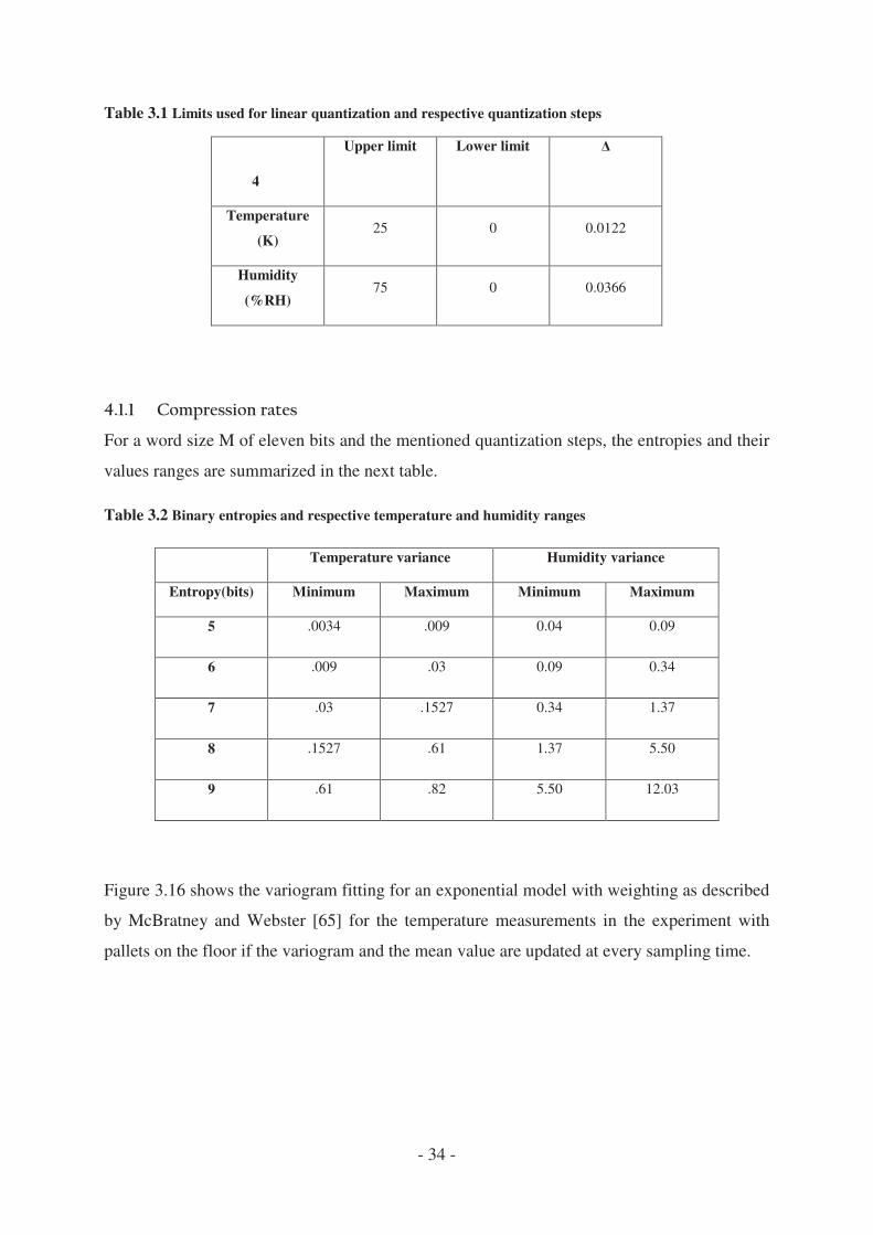
- 34 -

Table 3.1 Limits used for linear quantization and respective quantization steps

4

Upper limit Lower limit

Temperature

(K) 25 0 0.0122

Humidity

(%RH) 75 0 0.0366

For a word size M of eleven bits and the mentioned quantization steps, the entropies and their

values ranges are summarized in the next table.

Table 3.2 Binary entropies and respective temperature and humidity ranges

Temperature variance Humidity variance

Entropy(bits) Minimum Maximum Minimum Maximum

5 .0034 .009 0.04 0.09

6 .009 .03 0.09 0.34

7 .03 .1527 0.34 1.37

8 .1527 .61 1.37 5.50

9 .61 .82 5.50 12.03

Figure 3.16 shows the variogram fitting for an exponential model with weighting as described

by McBratney and Webster [65] for the temperature measurements in the experiment with

pallets on the floor if the variogram and the mean value are updated at every sampling time.

(a)

Figure 3.16 Results for temperature when the container is fille

variogram; (b) rate allocation.

The selection of the variogram model has no impact

seen in Table 3.3

Table 3.3 Average achieved compression rates for three fitted

Variogram

model

Gaussian

Spherical

Exponential

Regarding the percentage of failed estimations, the

for both experiments and for both environmental var

McBratney and Webster [65]

cases.Table 3.3 shows the results for temperature when the containe

the floor for different quantization steps.

- 35 -

(b)

Results for temperature when the container is filled with pallets: (a) spatio

The selection of the variogram model has no impact on the average compression, as can be

Average achieved compression rates for three fitted variogram models

Average compression rate ´R

Variogram

model

2 3 4

Gaussian 0.76 0.67 0.61 0.58

Spherical 0.75 0.66 0.61 0.57

Exponential 0.76 0.67 0.62 0.58

Regarding the percentage of failed estimations, the exponential model provides better results

for both experiments and for both environmental variables. The weighting scheme based on

[65] also reduces the percentage of failed estimations i

shows the results for temperature when the container is filled with pallets on

the floor for different quantization steps.

d with pallets: (a) spatio-temporal

on the average compression, as can be

exponential model provides better results

iables. The weighting scheme based on

also reduces the percentage of failed estimations in all

r is filled with pallets on

- 36 -

Table 3.4 Percentage of failed estimations for three models and two weighting schemes for temperature

measurements when the container is filled with pallets on the floor

McBratney and Webster Cressie

2 3 4 2 3 4

Gaussian 10.63 10.66 9.75 10.70 13.86 13.89 12.13 13.95

Spherical 11.44 11.47 7.50 11.53 12.55 12.58 9.44 12.67

Exponential 7.53 7.53 5.58 7.64 9.95 9.97 7.23 10.03

The next table summarizes the results for both experiments and for temperature (T) and

humidity (H) when the exponential model is fitted using the criterion of McBratney and

Webster. Every possible combination of source–sink pairs was simulated. The percentage

energy savings is calculated by averaging the N sent bits over the duration of the experiments.

It can be seen that energy savings up to 57% for temperature and up to 50% for humidity are

possible without exceeding an estimation failure rate of 10%. In the best cases it is possible to

achieve an estimation failure rate of 4% with 40% energy savings.

Table 3.5 Summary of accuracy and energy saving results for an exponential variogram model fitted

using the criterion of McBratney and Webster

Percentage of error Energy savings (%)

2 3 4 2 3 4

Container

with

pallets

T 7.53 7.53 5.58 7.64 23.82 32.79 37.95 41.77

H 6.16 6.27 7.45 6.08 26.65 35.63 41.26 44.61

Empty

container

T 7.41 7.95 9.14 7.72 39.22 48.20 53.01 57.18

H 3.91 4.06 5.42 4.42 31.96 40.93 46.61 49.91

4.1.2.1

The previous results assume that information about the mean and variogram is updated

continuously for every sample. However, because the aim is to compress data to reduce

communication, the acquisition of uncompressed data from all sensors has to be avoided as

much as possible. The datasets used in the present research work are very useful to study the

- 37 -

robustness of the method because the variances and mean of the environmental field are

changing drastically over time.

An experimental variogram data-aggregation query is far more energy-consuming than a

mean value one. However, the mean value plays a bigger role in performing a correct

estimation. It makes sense to update the mean value more often than the variogram. To test

the robustness against non-stationarity, the variogram is updated only at the times when the

sill of the fitted variogram model reaches one of the entropy transition values shown in Table

3.6. The mean is updated at regular intervals of 10 and 15 minutes.

Table 3.6 Summary of accuracy and energy savings results for an exponential variogram model fitted

using the criterion of McBratney and Webster when the mean is updated at discrete intervals

Percentage of error Energy savings (%)

Stationary-

like

10 minute

interval

15 minute

interval

Stationary-

like

10 minute

interval

15 minute

interval

Container

with

pallets

T 7.53 6.82 10.26 23.82 18.95 18.95

H 6.16 9.51 12.20 26.65 23.89 23.89

Empty

container

T 7.41 6.76 11.01 39.22 34.66 34.66

H 3.91 7.23 11.71 31.96 29.41 29.41

Table 3.6 summarizes the results when the variogram and the mean are updated at every

sampling, that can be considered a stationary-like process, and when the variogram is updated

according to the binary entropy and the mean is updated at discrete intervals. It can be seen

that, as expected, the percentage of estimation errors increases, but in the worse case it is only

12%. The energy saving decreases, but in the worse case only about 5% is not saved in

comparison with the stationary-like case,

In order to compare both approaches for distributed compression, the temperature

measurements for the container with pallets on the floor are selected. The rates are adapted

according to our method for the last sampling time. The probability of bit flip in DSC is fixed

at 0.45. An implementation of the decoder provided by [68] and geometric codes described in

[69] are used.

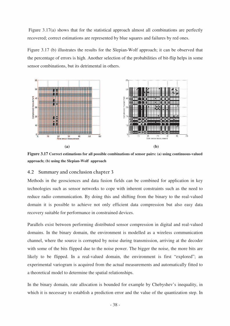
- 38 -

Figure 3.17(a) shows that for the statistical approach almost all combinations are perfectly

recovered; correct estimations are represented by blue squares and failures by red ones.

Figure 3.17 (b) illustrates the results for the Slepian-Wolf approach; it can be observed that

the percentage of errors is high. Another selection of the probabilities of bit-flip helps in some

sensor combinations, but its detrimental in others.

(a) (b)

Figure 3.17 Correct estimations for all possible combinations of sensor pairs: (a) using continuous-valued

approach; (b) using the Slepian-Wolf approach

Methods in the geosciences and data fusion fields can be combined for application in key

technologies such as sensor networks to cope with inherent constraints such as the need to

reduce radio communication. By doing this and shifting from the binary to the real-valued

domain it is possible to achieve not only efficient data compression but also easy data

recovery suitable for performance in constrained devices.

Parallels exist between performing distributed sensor compression in digital and real-valued

domains. In the binary domain, the environment is modelled as a wireless communication

channel, where the source is corrupted by noise during transmission, arriving at the decoder

with some of the bits flipped due to the noise power. The bigger the noise, the more bits are

likely to be flipped. In a real-valued domain, the environment is first “explored”; an

experimental variogram is acquired from the actual measurements and automatically fitted to

a theoretical model to determine the spatial relationships.

In the binary domain, rate allocation is bounded for example by Chebyshev’s inequality, in

which it is necessary to establish a prediction error and the value of the quantization step. In

- 39 -

the real-valued domain the fitted variogram model together with the mean value is required to

allocate ratios.

Both approaches use the concept of partitioning the source space into cosets; each element

belonging to a specific coset is “far away” from the others using a specific metric; in the

digital domain the metric used is the Hamming distance, whereas in the real-valued domain it

is a Euclidean one.

In both cases, the task of the data estimation unit is to utilize the available information

properly to select the element inside the coset that best complies with a given criterion. In the

binary domain the decoder uses complex techniques such as belief propagation to determine

which binary word is more likely to be the one sent, given the probability of bit flip during

transmission. In the real-valued domain, all elements of the coset are used together with the

auxiliary information to build a lookup table from which the minimum element is selected.

The results show that is possible to achieve perfect estimations of at least 90% of the possible

sensor combinations while reducing communication by up to 60% without needing a simple

algorithm that can be deployed in sensor nodes. It is also shown that the method is robust

against non-stationarity.

- 40 -

Information Fusion (IF) has found applicability in Geographical information systems (GIS).

In [68] several research papers regarding IF and GIS are discussed, surprisingly, Kriging

interpolation, developed for geo-statistics, is not considered. Kriging methods are IF ones,

but they have not been fully appreciated by the general fusion community. The Ordinary

Kriging method (OK) can be considered as a spatial statistical fusion method across sensors

whereas Cokriging interpolation (CK) can be considered a spatial statistical method for fusion

across attributes and sensors.

Kriging methods are based on statistical descriptions of the spatial dependencies of the

attributes, the so called variograms. They are Best Linear Unbiased Estimators (BLUE),

where “best” basically means that the estimation gives the lowest variance possible and

therefore gives strong theoretical guarantees. The condition of unbiasedness is assured by

constraining the sum of all weights of the primary attributes to be equal to one. The

minimization of the variance is then constrained to the unbiasedness condition, by using

Lagrange multipliers the problem of constrained minimization turns into a problem of

unconstrained minimization.

Kriging and cokriging errors have Gaussian distributions; it is determined by the mean µ and

the resulting Kriging variances. A correct tuning of the variogram models and parameters is a

necessary condition to the correctness of the estimation. Such correctness, can be evaluated

by cross-validating the predicted Kriging standard deviation and the actual error for each

destination point i [69]. The relation should be unitary.

(5.1)

(5.2)

The interpolation error at each point is defined as the average squared error between the

estimated value and the real value over samples.

- 41 -

(5.3)

The average prediction error over destination points was selected as a measure of the

quality of the interpolation.

(5.4)

Kriging [48, 69] performs linear interpolation to estimate the value in one destination point

by multiplying the available measurements with a set of weighting factors. Weights are

proportional to the correlation between the estimated points and the measurements; if there is

no spatial correlation all weights are equal and the estimates yield to the average value of all

measurements. In comparison with deterministic interpolation techniques such as Null-model

and Inverse Distance Weighting (IDW), provides two estimates: the values at a specific

location and the uncertainty of such estimation. The results were published in a joint paper

[70]. The contributions of the author of this thesis were on the research of the accuracy of the

Nelder-Mead method to automatically fit the variogram to the experimental data and on the

comparison with the accuracy achieved by other methods.

There are plenty of interpolation techniques, we have selected only two, IDW that takes into

account the distances between the source points and a null-model that averages all the

sources.

IDW is the most common method used to interpolate the value at an unknown location; it uses

only the geometrical distances between the source points and the destination. The

estimation at an unknown location is given by

(5.5)

And the weighting coefficients are given by:

(5.6)

It assumes that the influence of a source point on a destination point decreases with the square

of their distance.

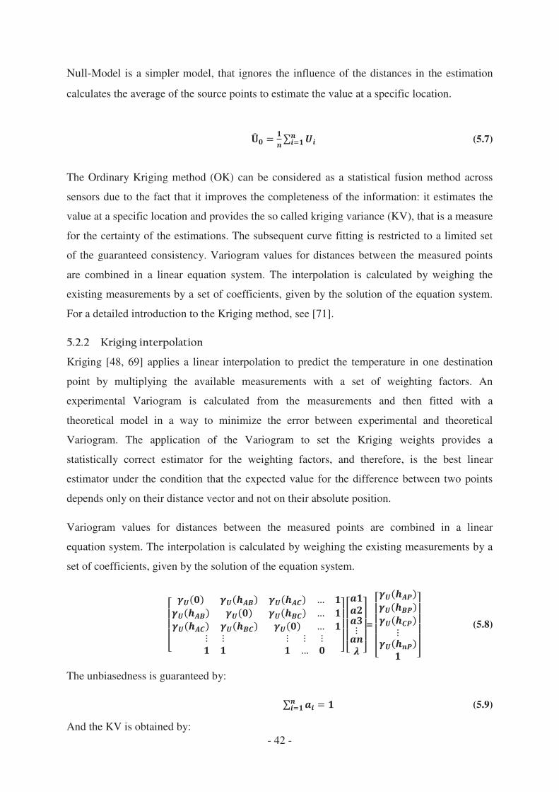
- 42 -

Null-Model is a simpler model, that ignores the influence of the distances in the estimation

calculates the average of the source points to estimate the value at a specific location.

(5.7)

The Ordinary Kriging method (OK) can be considered as a statistical fusion method across

sensors due to the fact that it improves the completeness of the information: it estimates the

value at a specific location and provides the so called kriging variance (KV), that is a measure

for the certainty of the estimations. The subsequent curve fitting is restricted to a limited set

of the guaranteed consistency. Variogram values for distances between the measured points

are combined in a linear equation system. The interpolation is calculated by weighing the

existing measurements by a set of coefficients, given by the solution of the equation system.

For a detailed introduction to the Kriging method, see [71].

Kriging [48, 69] applies a linear interpolation to predict the temperature in one destination

point by multiplying the available measurements with a set of weighting factors. An

experimental Variogram is calculated from the measurements and then fitted with a

theoretical model in a way to minimize the error between experimental and theoretical

Variogram. The application of the Variogram to set the Kriging weights provides a

statistically correct estimator for the weighting factors, and therefore, is the best linear

estimator under the condition that the expected value for the difference between two points

depends only on their distance vector and not on their absolute position.

Variogram values for distances between the measured points are combined in a linear

equation system. The interpolation is calculated by weighing the existing measurements by a

set of coefficients, given by the solution of the equation system.

= (5.8)

The unbiasedness is guaranteed by:

(5.9)

And the KV is obtained by:

- 43 -

(5.10)

Where is the lagrange multiplier

As mentioned before a correct variogram model and proper fitting of its parameter is highly

important. Besides Nelder-Mead algorithm described in [63], we selected two more methods.

5.2.3.1

A brute-force grid search was implemented. The grid search tests all combinations of range,

nugget and sill for the lowest fitting error between a given set of boundaries. For an adequate

setup of the boundaries, The algorithm searched for a sill value between 60% and 180% of the

measurement variance all measurements. The lower and upper grid boundaries for the nugget

value were set to 2% and 20% of the measurement variance, respectively; the search for the

variogram range values was performed between 1 and 10 meters.

5.2.3.2

A third method that only adapts the sill value was implemented. Based on the resulting range

of the fitting-algorithms, the fixed range was set to the average range value of the fitted

experiments. The nugget was directly set to the square of the measured sensor tolerances. The

sill was calculated to fit the average value of the theoretical model to the experimental

Variogram for large distances.

In total 14 datasets were recorded to test the Kriging procedures on different conditions: eight

in cold storage rooms and six during regular food transports.

The dimension of the cold storage rooms are of 2.6 × 2.2 × 2.3 meters. Between 54 and 68

temperature probes of PT100 type were installed at the walls. Zero and six degree Celsius

were programmed as set point temperatures, empty and loaded conditions as well as on-of an

modulated cooling modes were tested. Specific Details can be found in [72].The performance

conditions to validate the tests are the loading state (empty/full), set-points of 6 and -29 °C

The six experiments performing during food transports were acquired in collaboration with

food supplier companies and consists of two datasets recorded during terrestrial transport of

frozen-meat and four recorded during overseas transport of bananas.

- 44 -

The tests consisting of terrestrial transport of frozen meat was performed inside delivery

trucks provided by the German company Rungis Express. The trucks is separated into three

separate chambers, the experiments were performed in the deep freezer chamber with

dimensions of 2.9 × 2.5 × 2.35 meters. Forty TurboTag [73] data loggers were placed with a

set point of -29 °C.

Two of the datasets tests consisting of overseas transport of bananas were provided by

Maersk, in it forty-five sensors were placed inside the freight. The rest two datasets were

recorded within a cooperation project with Dole from Costa Rica to Antwerp. Twenty-seven

and thirty-one iButton [74] data loggers were placed in the centre of banana boxes in

experiments perform in 2010 and 2011, respectively.

The resulting variogram models and range value depend basically of the loading conditions,

dimensions of the closed, controlled environment and set point. Table 5.1 shows the average

range of the grid search Variogram models sorted by groups of experiments. It can be seen

that if the air circulates without obstacles, the temperature variations spread over a wider

range. A clear comparison is the resulting ranges of the cold storage room the average range

decreases from 4.7 to 3.4 meters in the presence of cargo. The highest range of 4.7 metre was

measured in empty cold storage rooms. Partially filled cold storage rooms and trucks showed

almost the same range of 3.25 to 4 meter. For densely packed cargo such as bananas in sea

containers the range dropped to 1.65 or 1.125 meter.

An important figure of merit is the number of neighbours that lie into the resulting variogram

range; neighbours lying above the average range have little effect on the interpolation because

their assigned weights are very low. In a worst-case scenario, if all neighbours are outside the

variogram range, all neighbours will be assigned with the same weights; the resulting

interpolation would be equal to the average of the values of the neighbours.

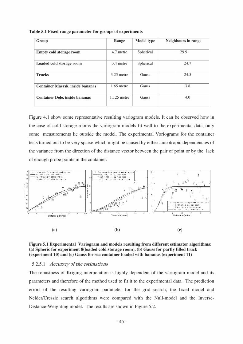
Table 5.1 Fixed range parameter for groups of experiments

Group

Empty cold storage room

Loaded cold storage room

Trucks

Container Maersk, inside bananas

Container Dole, inside bananas

Figure 4.1 show some representative resulting vario

the case of cold storage rooms the variogram models fit well to the

some measurements lie outside the model. The exper

tests turned out to be very sparse which might be c

the variance from the direction of the distance vec

of enough probe points in the container.

(a)

Figure 5.1 Experimental Variogram and models resulting from d(a) Spheric for experiment 8(loaded cold storage ro

(experiment 10) and (c) Gauss for sea container loaded with bananas (experi

5.2.5.1

The robustness of Kriging interpolation

parameters and therefore of the method used to fit

errors of the resulting variogram parame

Nelder/Cressie search algorithm

Distance-Weighting model. The results are shown in

- 45 -

Fixed range parameter for groups of experiments

Range Model type Neighbours in range

4.7 metre Spherical

3.4 metre Spherical

3.25 metre Gauss

Container Maersk, inside bananas 1.65 metre Gauss

Container Dole, inside bananas 1.125 metre Gauss

Figure 4.1 show some representative resulting variogram models. It can be observed how in

storage rooms the variogram models fit well to the experimental data, only

some measurements lie outside the model. The experimental Variograms for the container

tests turned out to be very sparse which might be caused by either anisotropic dependencies o

the variance from the direction of the distance vector between the pair of point or by the lack

of enough probe points in the container.

(b)

Experimental Variogram and models resulting from different estimator algorithms: (a) Spheric for experiment 8(loaded cold storage room), (b) Gauss for partly filled truck

Gauss for sea container loaded with bananas (experiment 11)

riging interpolation is highly dependent of the variogram model and its

parameters and therefore of the method used to fit it to the experimental data. The

ariogram parameter for the grid search, the fixed model and

Nelder/Cressie search algorithms were compared with the Null-model and the Inverse

. The results are shown in Figure 5.2.

Neighbours in range

29.9

24.7

24.5

3.8

4.0

gram models. It can be observed how in

experimental data, only

imental Variograms for the container

aused by either anisotropic dependencies of

tor between the pair of point or by the lack

(c)

ifferent estimator algorithms: partly filled truck

Gauss for sea container loaded with bananas (experiment 11)

is highly dependent of the variogram model and its

it to the experimental data. The prediction

ter for the grid search, the fixed model and

model and the Inverse-

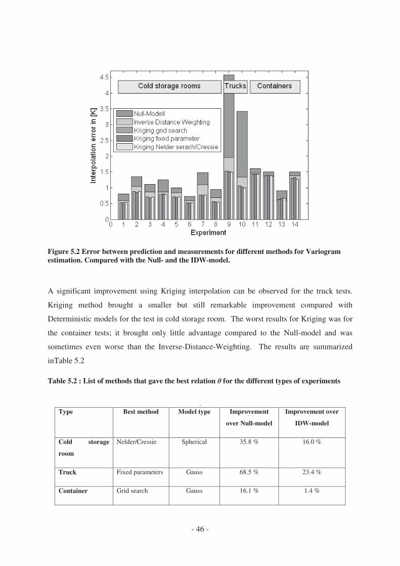
Figure 5.2 Error between prediction and measurements for diffe

estimation. Compared with the Null

A significant improvement using Kriging interpolati

Kriging method brought a

Deterministic models for the test in cold storage r

the container tests; it brought only little advanta

sometimes even worse than the Inverse

inTable 5.2

Table 5.2 : List of methods that gave the best relation

Type Best method

Cold storage

room

Nelder/Cressie

Truck Fixed parameters

Container Grid search

- 46 -

Error between prediction and measurements for different methods for Variogram

estimation. Compared with the Null- and the IDW-model.

A significant improvement using Kriging interpolation can be observed for the truck tests.

Kriging method brought a smaller but still remarkable improvement compared w

Deterministic models for the test in cold storage room. The worst results for Krigin

the container tests; it brought only little advantage compared to the Null

sometimes even worse than the Inverse-Distance-Weighting. The results are summarized

List of methods that gave the best relation for the different types of experiments

.

Best method Model type Improvement

over Null-model

Improvement over

Nelder/Cressie Spherical 35.8 %

Fixed parameters Gauss 68.5 %

Grid search Gauss 16.1 %

rent methods for Variogram

on can be observed for the truck tests.

smaller but still remarkable improvement compared with

oom. The worst results for Kriging was for

to the Null-model and was

. The results are summarized

for the different types of experiments

Improvement over

IDW-model

16.0 %

23.4 %

1.4 %

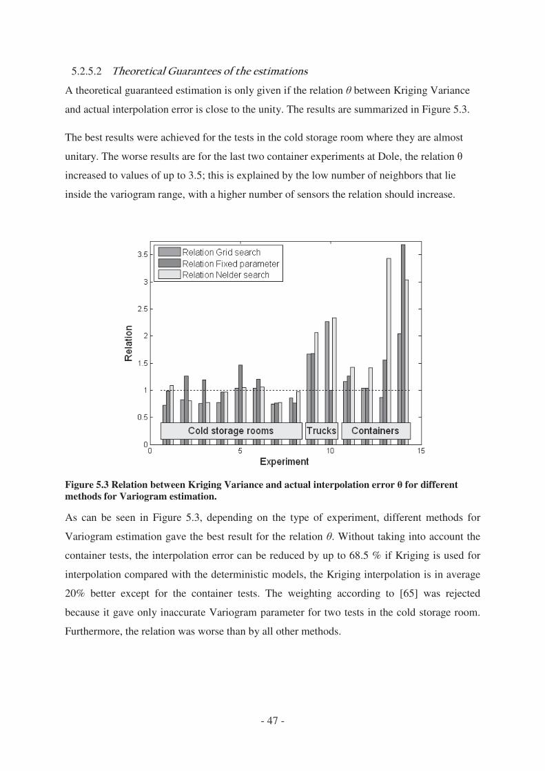
5.2.5.2

A theoretical guaranteed estimation is only given i

and actual interpolation error is close to the unity. The results are summarized i

The best results were achieved

unitary. The worse results are

increased to values of up to 3.5

inside the variogram range, with a higher number of

Figure 5.3 Relation between Kriging Variance and actual interpolation err

methods for Variogram estimation.

As can be seen in Figure 5.3

Variogram estimation gave the best result for the r

container tests, the interpolation error can be reduced by up to 68.5

interpolation compared with the d

20% better except for the container tests

because it gave only inaccurate Variogram parameter

Furthermore, the relation was worse than by all oth

- 47 -

A theoretical guaranteed estimation is only given if the relation between Kriging Variance

is close to the unity. The results are summarized i

best results were achieved for the tests in the cold storage room where they are almost

The worse results are for the last two container experiments at Dole

increased to values of up to 3.5; this is explained by the low number of neighbors

inside the variogram range, with a higher number of sensors the relation should increase.

tween Kriging Variance and actual interpolation error

methods for Variogram estimation.

3, depending on the type of experiment, different methods for

Variogram estimation gave the best result for the relation . Without taking into account the

he interpolation error can be reduced by up to 68.5 % if Kriging is used for

the deterministic models, the Kriging interpolation is in average

% better except for the container tests. The weighting according to

because it gave only inaccurate Variogram parameter for two tests in the cold storage room.

Furthermore, the relation was worse than by all other methods.

between Kriging Variance

is close to the unity. The results are summarized in Figure 5.3.

where they are almost

for the last two container experiments at Dole, the relation

; this is explained by the low number of neighbors that lie

sensors the relation should increase.

or for different

experiment, different methods for

Without taking into account the

% if Kriging is used for

, the Kriging interpolation is in average

The weighting according to [65] was rejected

for two tests in the cold storage room.

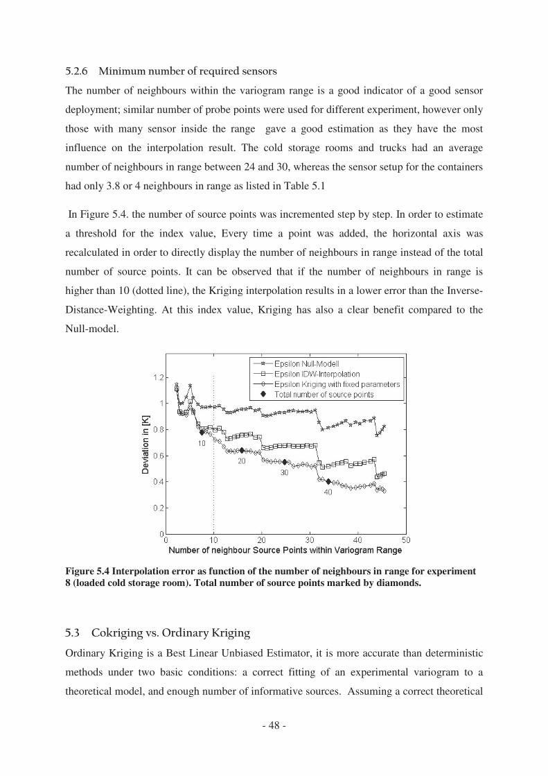
The number of neighbours within the variogram range

deployment; similar number of probe points were used for differ

those with many sensor inside the range gave a goo

influence on the interpolation result.

number of neighbours in range between 24 and 30, wh

had only 3.8 or 4 neighbours in range as listed in

In Figure 5.4. the number of source points was incremented step by

a threshold for the index value

recalculated in order to directly display the number of neighbours in range

number of source points. It can be observed that i

higher than 10 (dotted line), the Kriging interpola

Distance-Weighting. At this index value, Kriging has also a

Null-model.

Figure 5.4 Interpolation error as function of the number of ne8 (loaded cold storage room). Total number of source po

Ordinary Kriging is a Best Linear Unbiased Estimato

methods under two basic conditions: a correct fitti

theoretical model, and enough

- 48 -

The number of neighbours within the variogram range is a good indicator of a good sensor

similar number of probe points were used for different experiment, however only

those with many sensor inside the range gave a good estimation as the

influence on the interpolation result. The cold storage rooms and trucks had an average

number of neighbours in range between 24 and 30, whereas the sensor setup for the containers

had only 3.8 or 4 neighbours in range as listed in Table 5.1

the number of source points was incremented step by step. In order to estimate

a threshold for the index value, Every time a point was added, the horizontal axis was

directly display the number of neighbours in range

. It can be observed that if the number of neighbours in range is

higher than 10 (dotted line), the Kriging interpolation results in a lower error than the Inve

Weighting. At this index value, Kriging has also a clear benefit compared to the

Interpolation error as function of the number of neighbours in range for experiment oaded cold storage room). Total number of source points marked by diamonds.

Ordinary Kriging is a Best Linear Unbiased Estimator, it is more accurate than deterministic

methods under two basic conditions: a correct fitting of an experimental variogram to a

enough number of informative sources. Assuming a co

is a good indicator of a good sensor

ent experiment, however only

d estimation as they have the most

The cold storage rooms and trucks had an average

ereas the sensor setup for the containers

In order to estimate

he horizontal axis was

directly display the number of neighbours in range instead of the total

f the number of neighbours in range is

tion results in a lower error than the Inverse-

clear benefit compared to the

ighbours in range for experiment ints marked by diamonds.

r, it is more accurate than deterministic

ng of an experimental variogram to a

a correct theoretical

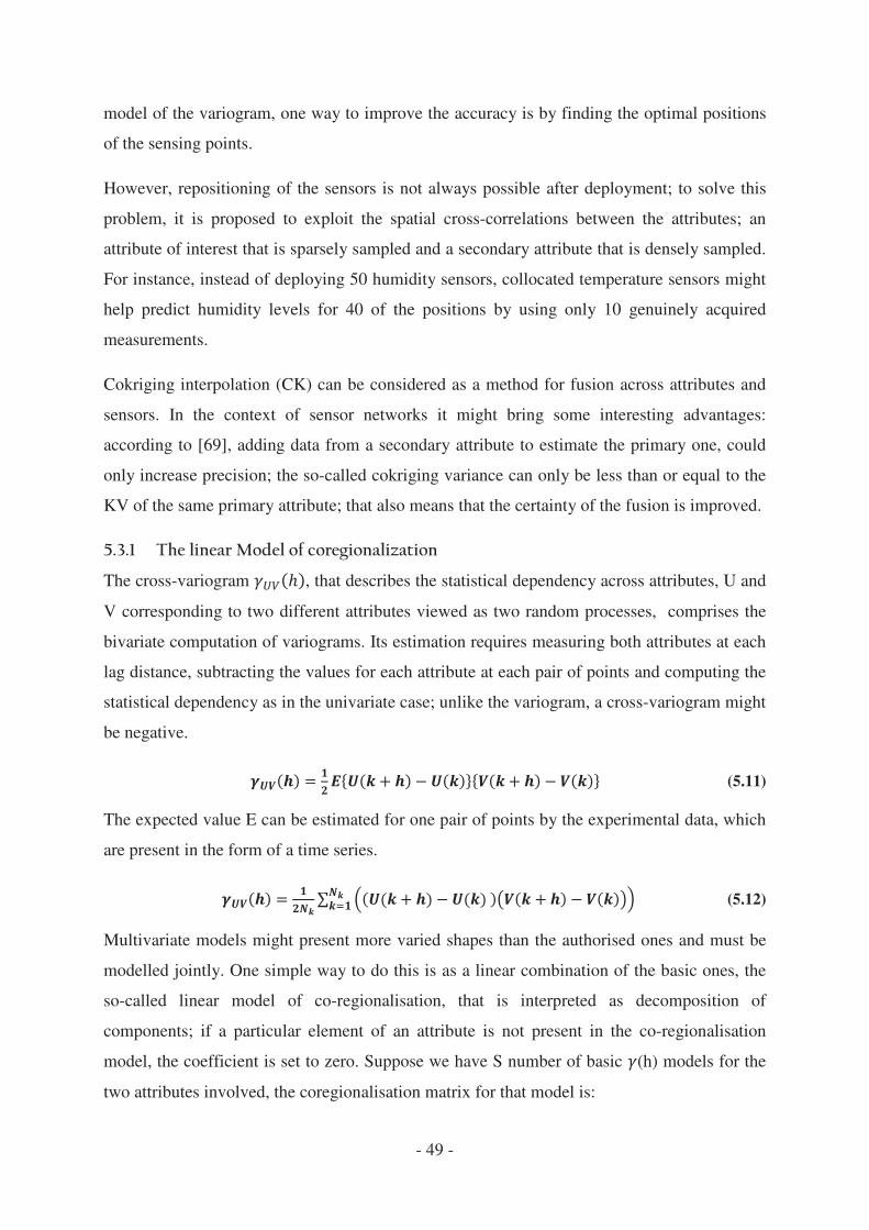
- 49 -

model of the variogram, one way to improve the accuracy is by finding the optimal positions

of the sensing points.

However, repositioning of the sensors is not always possible after deployment; to solve this

problem, it is proposed to exploit the spatial cross-correlations between the attributes; an

attribute of interest that is sparsely sampled and a secondary attribute that is densely sampled.

For instance, instead of deploying 50 humidity sensors, collocated temperature sensors might

help predict humidity levels for 40 of the positions by using only 10 genuinely acquired

measurements.

Cokriging interpolation (CK) can be considered as a method for fusion across attributes and

sensors. In the context of sensor networks it might bring some interesting advantages:

according to [69], adding data from a secondary attribute to estimate the primary one, could

only increase precision; the so-called cokriging variance can only be less than or equal to the

KV of the same primary attribute; that also means that the certainty of the fusion is improved.

The cross-variogram , that describes the statistical dependency across attributes, U and

V corresponding to two different attributes viewed as two random processes, comprises the

bivariate computation of variograms. Its estimation requires measuring both attributes at each

lag distance, subtracting the values for each attribute at each pair of points and computing the

statistical dependency as in the univariate case; unlike the variogram, a cross-variogram might

be negative.

(5.11)

The expected value E can be estimated for one pair of points by the experimental data, which

are present in the form of a time series.

(5.12)

Multivariate models might present more varied shapes than the authorised ones and must be

modelled jointly. One simple way to do this is as a linear combination of the basic ones, the

so-called linear model of co-regionalisation, that is interpreted as decomposition of

components; if a particular element of an attribute is not present in the co-regionalisation

model, the coefficient is set to zero. Suppose we have S number of basic (h) models for the

two attributes involved, the coregionalisation matrix for that model is:

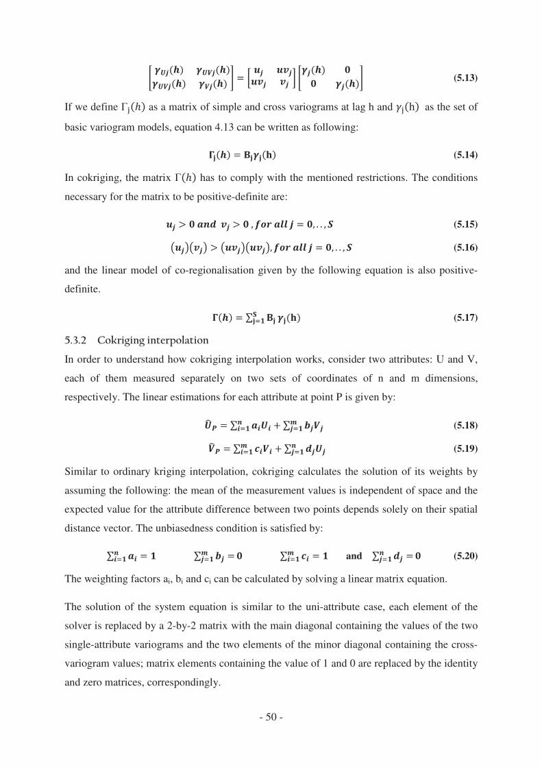
- 50 -

(5.13)

If we define as a matrix of simple and cross variograms at lag h and as the set of

basic variogram models, equation 4.13 can be written as following:

(5.14)

In cokriging, the matrix has to comply with the mentioned restrictions. The conditions

necessary for the matrix to be positive-definite are:

(5.15)

(5.16)

and the linear model of co-regionalisation given by the following equation is also positive-

definite.

(5.17)

In order to understand how cokriging interpolation works, consider two attributes: U and V,

each of them measured separately on two sets of coordinates of n and m dimensions,

respectively. The linear estimations for each attribute at point P is given by:

(5.18)

(5.19)

Similar to ordinary kriging interpolation, cokriging calculates the solution of its weights by

assuming the following: the mean of the measurement values is independent of space and the

expected value for the attribute difference between two points depends solely on their spatial

distance vector. The unbiasedness condition is satisfied by:

and (5.20)

The weighting factors ai, bi and ci can be calculated by solving a linear matrix equation.

The solution of the system equation is similar to the uni-attribute case, each element of the

solver is replaced by a 2-by-2 matrix with the main diagonal containing the values of the two

single-attribute variograms and the two elements of the minor diagonal containing the cross-

variogram values; matrix elements containing the value of 1 and 0 are replaced by the identity

and zero matrices, correspondingly.

- 51 -

(5.21)

(5.22)

The cokriging variances for the estimation of U and V at point P are giving by:

(5.23)

For attribute U at destination point P.

(5.24)

For attribute V at destination point P. Where are Lagrange multipliers

5.3.2.1

In cross-attribute fusion terminology, the completeness can be improved by bringing new

information where there is lack of it. CK is able to perform such task by supporting the

primary variable interpolation with measurements of the second one, the so called under-

sampling case. However, several factors regarding the cokriging interpolation procedure have

to be taken into account; the calculation of experimental cross-variogram pairs can only be

calculated for those measurement points where both variables are available. If, for example,

variable V is not present at the measuring point, the elements in matrix

cannot be calculated.

(5.25)

The first implication requires only the inclusion of an additional algorithm to group those

measurements points in which both measurements are available. However, the second

requires more complex modifications in the cokriging solver and the fitting algorithm.

Regarding the solver, each non-common measurement reduces the dimensions of the left

matrix by one row and column and the column dimensions of the other by one column.

Suppose that there is no measurement for variable V at point P when we have three source

points, then the solver is as follows:

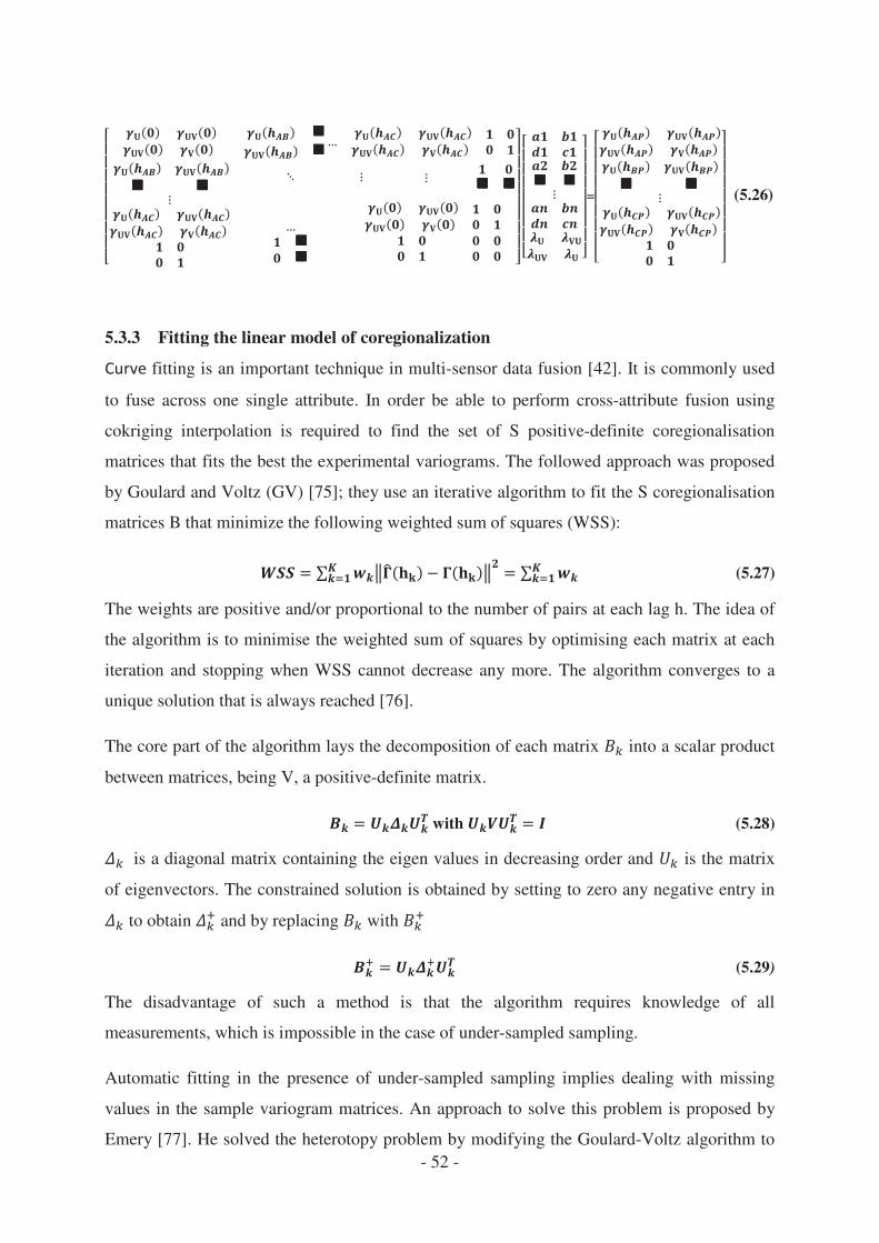
- 52 -

= (5.26)

5.3.3 Fitting the linear model of coregionalization

fitting is an important technique in multi-sensor data fusion [42]. It is commonly used

to fuse across one single attribute. In order be able to perform cross-attribute fusion using

cokriging interpolation is required to find the set of S positive-definite coregionalisation

matrices that fits the best the experimental variograms. The followed approach was proposed

by Goulard and Voltz (GV) [75]; they use an iterative algorithm to fit the S coregionalisation

matrices B that minimize the following weighted sum of squares (WSS):

(5.27)

The weights are positive and/or proportional to the number of pairs at each lag h. The idea of

the algorithm is to minimise the weighted sum of squares by optimising each matrix at each

iteration and stopping when WSS cannot decrease any more. The algorithm converges to a

unique solution that is always reached [76].

The core part of the algorithm lays the decomposition of each matrix into a scalar product

between matrices, being V, a positive-definite matrix.

with (5.28)

is a diagonal matrix containing the eigen values in decreasing order and is the matrix

of eigenvectors. The constrained solution is obtained by setting to zero any negative entry in

to obtain and by replacing with

(5.29)

The disadvantage of such a method is that the algorithm requires knowledge of all

measurements, which is impossible in the case of under-sampled sampling.

Automatic fitting in the presence of under-sampled sampling implies dealing with missing

values in the sample variogram matrices. An approach to solve this problem is proposed by

Emery [77]. He solved the heterotopy problem by modifying the Goulard-Voltz algorithm to

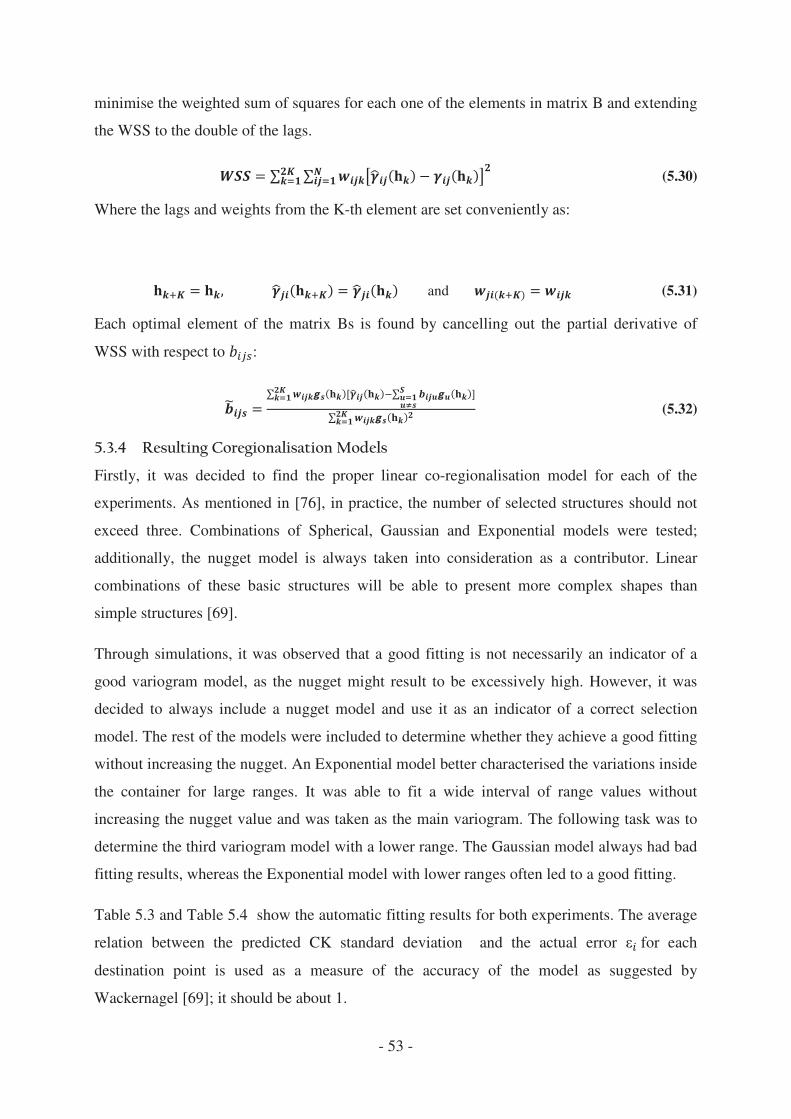
- 53 -

minimise the weighted sum of squares for each one of the elements in matrix B and extending

the WSS to the double of the lags.

(5.30)

Where the lags and weights from the K-th element are set conveniently as:

and (5.31)

Each optimal element of the matrix Bs is found by cancelling out the partial derivative of

WSS with respect to :

(5.32)

Firstly, it was decided to find the proper linear co-regionalisation model for each of the

experiments. As mentioned in [76], in practice, the number of selected structures should not

exceed three. Combinations of Spherical, Gaussian and Exponential models were tested;

additionally, the nugget model is always taken into consideration as a contributor. Linear

combinations of these basic structures will be able to present more complex shapes than

simple structures [69].

Through simulations, it was observed that a good fitting is not necessarily an indicator of a

good variogram model, as the nugget might result to be excessively high. However, it was

decided to always include a nugget model and use it as an indicator of a correct selection

model. The rest of the models were included to determine whether they achieve a good fitting

without increasing the nugget. An Exponential model better characterised the variations inside

the container for large ranges. It was able to fit a wide interval of range values without

increasing the nugget value and was taken as the main variogram. The following task was to

determine the third variogram model with a lower range. The Gaussian model always had bad

fitting results, whereas the Exponential model with lower ranges often led to a good fitting.

Table 5.3 and Table 5.4 show the automatic fitting results for both experiments. The average

relation between the predicted CK standard deviation and the actual error for each

destination point is used as a measure of the accuracy of the model as suggested by

Wackernagel [69]; it should be about 1.

- 54 -

Table 5.3 Automatic fitting results for an empty container

Ranges Predominant Model?

WSS Exponential Spherical Min Max Min Max

5.5 4.7 No .1044 1.7 2.19 1.44 2.46

5 4 Spherical .099 1.63 1.84 1.6 2.43

4 2.7 No .098 1.42 1.76 1.42 2.39

3 2 No .107 1.23 1.74 1.42 2.39

3 1.7 Exponential .108 1.21 1.77 1.44 2.39

Table 5.4Automatic fitting results for a container with pallets on the floor

Ranges WSS Exponential Spherical Min Max Min Max

5.5 4.7 Spherical .30 .34 1.06 .76 2.14

5 4 Spherical .39 .32 .98 .76 2.12

4 2.7 Exponential .57 .17 .94 .70 2.18

3 2 Exponential .71 .15 .94 .69 2.19

3 1.7 Exponential .71 .15 .94 .69 2.19

They show whether the results sills are predominantly spherical or exponential and also offer

a quick overview of the maximum and minimum relation and epsilon results after applying

cokriging interpolation.

The selected ranges are highlighted in the tables; Table 5.5 shows the numerical values of the

sills for both experiments using those ranges and Figure 5.5 shows the experimental and co-

regionalisation model for the experiments when pallets are placed on the floor.

Table 5.5 Resulting sill and range values for the best selected model

Empty Container Container with pallets

T T-H H T T-H H

Nugget 0 0 0 .01 0 0

Exponential 0.17/3 -.46/3 1.4/3 0.03/5 .016/5 0/5

Spherical 0.07/2 -.29/2 1.24/2 1.42/4 -2.86/4 5.75/4

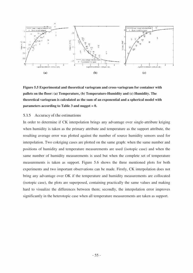
(a)

Figure 5.5 Experimental and theoretical variogram and cross

pallets on the floor: (a) Temperature, (b) Temperat

theoretical variogram is calculated as the sum of a

parameters according to Table 3 and nugget = 0.

In order to determine if CK interpolation brings an

when humidity is taken as the primary attribute and

resulting average error was plotted against the num

interpolation. Two cokriging cases are plotted on t

positions of humidity and temperature measurements

same number of humidity measurements is used but wh

measurements is taken as support.

experiments and two important observations can be m

bring any advantage over OK if the temperature and

(isotopic case), the plots are superposed, contai

hard to visualize the differences between them; sec

significantly in the heterotopic case when all temp

- 55 -

(b)

Experimental and theoretical variogram and cross-variogram for container with

pallets on the floor: (a) Temperature, (b) Temperature-Humidity and (c) Humidity. The

theoretical variogram is calculated as the sum of an exponential and a spherical model with

parameters according to Table 3 and nugget = 0.

In order to determine if CK interpolation brings any advantage over single

when humidity is taken as the primary attribute and temperature as the support attribu

resulting average error was plotted against the number of source humidity sensors used for

interpolation. Two cokriging cases are plotted on the same graph: when the same number and

positions of humidity and temperature measurements are used (isotopic case) and when the

same number of humidity measurements is used but when the complete set of temperature

measurements is taken as support. Figure 5.6 shows the three mentioned plots for both

experiments and two important observations can be made. Firstly, CK interpolation does not

bring any advantage over OK if the temperature and humidity measurements are collocated

(isotopic case), the plots are superposed, containing practically the same values and making

hard to visualize the differences between them; secondly, the interpolation error improves

significantly in the heterotopic case when all temperature measurements are taken as support.

(c)

variogram for container with

Humidity and (c) Humidity. The

n exponential and a spherical model with

y advantage over single-attribute kriging

temperature as the support attribute, the

ber of source humidity sensors used for

he same graph: when the same number and

pic case) and when the

en the complete set of temperature

ee mentioned plots for both

ade. Firstly, CK interpolation does not

humidity measurements are collocated

ning practically the same values and making

ondly, the interpolation error improves

erature measurements are taken as support.

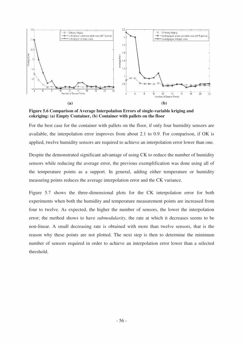
- 56 -

(a) (b)

Figure 5.6 Comparison of Average Interpolation Errors of single-variable kriging and cokriging: (a) Empty Container, (b) Container with pallets on the floor

For the best case for the container with pallets on the floor, if only four humidity sensors are

available, the interpolation error improves from about 2.1 to 0.9. For comparison, if OK is

applied, twelve humidity sensors are required to achieve an interpolation error lower than one.

Despite the demonstrated significant advantage of using CK to reduce the number of humidity

sensors while reducing the average error, the previous exemplification was done using all of

the temperature points as a support. In general, adding either temperature or humidity

measuring points reduces the average interpolation error and the CK variance.

Figure 5.7 shows the three-dimensional plots for the CK interpolation error for both

experiments when both the humidity and temperature measurement points are increased from

four to twelve. As expected, the higher the number of sensors, the lower the interpolation

error; the method shows to have submodularity, the rate at which it decreases seems to be

non-linear. A small decreasing rate is obtained with more than twelve sensors, that is the

reason why these points are not plotted. The next step is then to determine the minimum

number of sensors required in order to achieve an interpolation error lower than a selected

threshold.

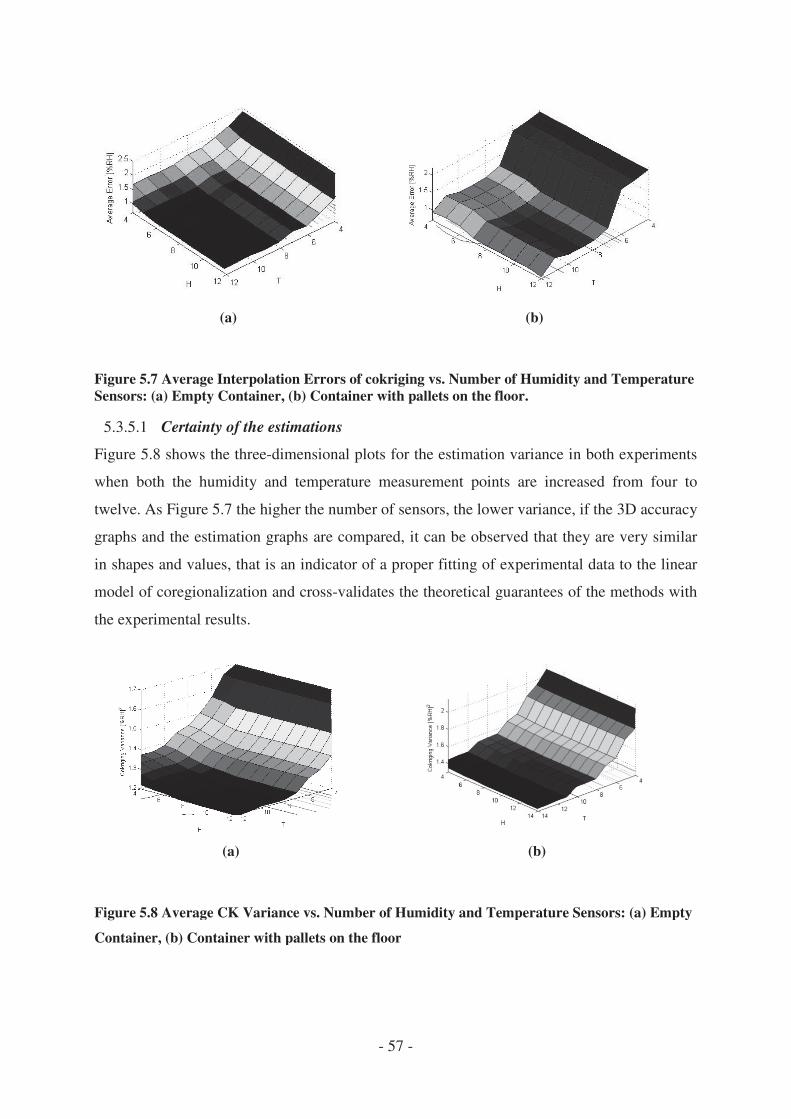
(a)

Figure 5.7 Average Interpolation Errors of cokriging vs. Numbe

Sensors: (a) Empty Container, (b) Container with pa

5.3.5.1 Certainty of the estimations

Figure 5.8 shows the three-dimensional plots for the estimation variance in bo

when both the humidity and temperature measurement

twelve. As Figure 5.7 the higher the number of sensors, the lower varianc

graphs and the estimation graphs are compared, it c

in shapes and values, that is an indicator of a proper fitting of experimental

model of coregionalization and cross

the experimental results.

(a)

Figure 5.8 Average CK Variance vs. Number of Humidity and Temp

Container, (b) Container with pallets on the floor

- 57 -

(b)

Average Interpolation Errors of cokriging vs. Number of Humidity and Temperature

Sensors: (a) Empty Container, (b) Container with pallets on the floor.

Certainty of the estimations

dimensional plots for the estimation variance in bo

when both the humidity and temperature measurement points are increased from four to

the higher the number of sensors, the lower variance, if the 3D accuracy

graphs and the estimation graphs are compared, it can be observed that they are very similar

is an indicator of a proper fitting of experimental

model of coregionalization and cross-validates the theoretical guarantees of the methods

(b)

Average CK Variance vs. Number of Humidity and Temperature Sensors: (a) Empty

Container, (b) Container with pallets on the floor

r of Humidity and Temperature

dimensional plots for the estimation variance in both experiments

points are increased from four to

the higher the number of sensors, the lower variance, if the 3D accuracy

an be observed that they are very similar

is an indicator of a proper fitting of experimental data to the linear

validates the theoretical guarantees of the methods with

erature Sensors: (a) Empty

5.3.6 Accuracy of the estimation under incompleteness

As it can be seen in Figure 5

interpolation errors over OK. It tends towards the

sensors but it does not improve in a significant wa

ordinary kriging, which is 1.42 and 0.76 for an emp

respectively. The main advantage is in reducing the

In order to illustrate the applicabili

thresholds: 1.55 and 0.85, that correspond to a 10%

obtained for both experiments, were selected. The s

in Figure 5.7 were run but in this case, with the aim of clarity,

respective threshold were set to NaN (Not

viewed from above and Figure

method to achieve good estimates with low variabili

measurements does not necessarily increase the accu

the submodularity is not achieved

the empty container and 6 of the container with pal

(a)

Figure 5.9 Average Interpolation Errors lower than the threshoContainer with pallets on the floor.

Table 5.6 shows that in the case of the empty container,

does not bring any advantage in reducing the number

achieve more accurate predictions with the same number of humidity

taking the temperature measurements as support.

- 58 -

Accuracy of the estimation under incompleteness

5.7 and Figure 5.8, CK interpolation does bring more accurate

interpolation errors over OK. It tends towards the same accuracy value with only a few

sensors but it does not improve in a significant way the lowest interpolation error achieved by

ordinary kriging, which is 1.42 and 0.76 for an empty container and a container with pallets,

respectively. The main advantage is in reducing the required number of humidity sensors.

In order to illustrate the applicability of CK in reducing the number of measuring points

thresholds: 1.55 and 0.85, that correspond to a 10% increase of the interpolation errors

obtained for both experiments, were selected. The same Matlab scripts that produced the plots

were run but in this case, with the aim of clarity, all points exceeding the

respective threshold were set to NaN (Not-a-Number). The plots then were rotated so as to be

Figure 5.9 shows that view: It can be seen that robustnees of

method to achieve good estimates with low variability, due to the submodula

measurements does not necessarily increase the accuracy of the estimation

achieved are the ones inside the red circles. Only 3 combinations for

the empty container and 6 of the container with pallets exceeded the established thresholds.

(b)

Average Interpolation Errors lower than the threshold: (a) Empty Container, (b) Container with pallets on the floor.

shows that in the case of the empty container, that has low variability, the use of CK

does not bring any advantage in reducing the number of humidity sensors; however, it can

curate predictions with the same number of humidity measurements when

taking the temperature measurements as support.

, CK interpolation does bring more accurate

same accuracy value with only a few

st interpolation error achieved by

ty container and a container with pallets,

required number of humidity sensors.

ty of CK in reducing the number of measuring points, two

increase of the interpolation errors

ame Matlab scripts that produced the plots

all points exceeding the

Number). The plots then were rotated so as to be

shows that view: It can be seen that robustnees of the CK

ty, due to the submodularity, adding more

racy of the estimation. The areas where

Only 3 combinations for

the established thresholds.

ld: (a) Empty Container, (b)

has low variability, the use of CK

of humidity sensors; however, it can

measurements when

- 59 -

Table 5.6 Number of Humidity Sensors required for OK and CK interpolations that comply

with different thresholds when the container is empty.

Threshold Number of

combinations

Combination with

minimum sensors for

humidity

Number of humidity points

required for kriging

T

1,43 66 7 9 -----

1,44 111 7 9 7

1,49 201 6 9 6

1,59 283 5 9 5

1,71 297 4 9 4

Table 5.7shows that when the variations are higher, cokriging interpolation is able to reduce

the number of humidity sensors required for OK.

Table 5.7: Number of Humidity Sensors required for Ok and CK interpolations that comply

with different thresholds when the container has pallets on the floor.

Threshold Number of

combinations

Combination with

minimum sensors for

humidity

Number of humidity points

required for kriging

H T

0,76 68 8 17 ---------

0,77 74 7 17 18

0,8 103 7 17 12

0,82 143 7 12 8

0,9 180 4 17 7

5.3.7 Fitting the linear model of co-regionalisation under incompleteness

As mentioned before, fitting the proper co-regionalisation model is the basis for CK

interpolation. The theoretical guarantees of the interpolation are void if the model is not

properly fitted. The main factor affecting this is the lack of sufficient measurements either

from the primary or secondary attribute. The method developed by Emery takes into account

the absence of such measurements but still needs to be verified as to whether the method fits

proper sills under highly heterotopic cases.

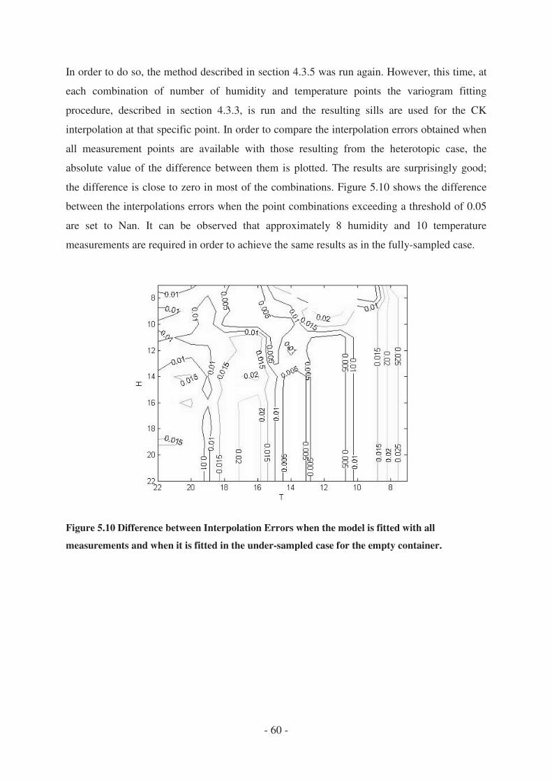
In order to do so, the method described

each combination of number of humidity and temperat

procedure, described in section

interpolation at that specific point. In order to c

all measurement points are available with those res

absolute value of the difference between them is pl

the difference is close to zero in most of the comb

between the interpolations errors when the point co

are set to Nan. It can be observed that approximate

measurements are required in order to achieve the s

Figure 5.10 Difference between Interpolation Errors when the mo

measurements and when it is fitted in the under

- 60 -

do so, the method described in section 4.3.5 was run again. However, this time, at

each combination of number of humidity and temperature points the variogram fitting

section 4.3.3, is run and the resulting sills are used for the

interpolation at that specific point. In order to compare the interpolation errors obtained when

all measurement points are available with those resulting from the heterotopic case, the

absolute value of the difference between them is plotted. The results are surprisingly good;

the difference is close to zero in most of the combinations. Figure 5.10 shows the difference

between the interpolations errors when the point combinations exceeding a threshold of 0.05

are set to Nan. It can be observed that approximately 8 humidity and 10 temperature

measurements are required in order to achieve the same results as in the fully

Difference between Interpolation Errors when the model is fitted with all

measurements and when it is fitted in the under-sampled case for the empty container.

was run again. However, this time, at

ure points the variogram fitting

, is run and the resulting sills are used for the CK

ompare the interpolation errors obtained when

ulting from the heterotopic case, the

ts are surprisingly good;

shows the difference

mbinations exceeding a threshold of 0.05

ly 8 humidity and 10 temperature

ults as in the fully-sampled case.

del is fitted with all

sampled case for the empty container.

- 61 -

One of the inherent constraints in WSN is the impossibility of deploying dense number of

sensors; to cope with it; spatial interpolation is proposed to estimate the value at the positions

that are not covered by a sensor. Deterministic methods exist but their disadvantage is the

lack of theoretical guarantees.

The Kriging method is a useful tool to interpolate a physical property for points where no

sensor is available and provides theoretical guarantees through the use of the so-called

Kriging variance. It can be used as an offline-tool to estimate to which amount the number of

sensors can be reduced for a supervision task. The theoretical guarantees are only valid if the

theoretical model is properly fitted to an experimental variogram and if sufficient number of

neighbours lie into the variogram range.

The most suitable method to verify the correctness of the variogram model is based on the

i/ k relation. The best results were achieved either by the Nelder-Mead algorithm combined

with the weighting according to Cressie or by setting the nugget by known sensor tolerances

and the range by an average value of previous experiments. If the average number of

neighboring sensors within the Variogram range is sufficient, the Kriging method provides an

interpolation, that is in average 20% more accurate than that of the inverse-distance-weighting

used as the reference method.

If the attribute of interest is not densely sampled, and only few sources are inside the

variogram range, Kriging interpolation offers few or no advantage over deterministic

methods. Fortunately, by fusing the available information with the information a secondary

correlated attribute is possible to perform accurate and theoretical guaranteed estimations

Cokriging interpolation, considered as a cross-attribute fusion technique, guarantees

theoretical performances under the assumptions that the experimental variograms are

correctly fitted to a theoretical co-regionalisation model, that has to be positive-definite. This

makes it possible to fuse different attributes to improve spatial coverage of an “expensive”

attribute with observations at a finite number of locations of a “cheap” one without the

repositioning of the sensors. It produces Best Linear Unbiased Estimation (BLUE) and

estimate corresponding variances.

The best fitting results in the fully-sampled case are obtained when the weights are set

directly proportional to the number of pairs and inversely proportional to the distance. The

Exponential model gives good fitting without increasing the nugget for several sets of ranges;

- 62 -

it is preferred if a Spherical model is added. The algorithm developed by Emery has shown to

be robust against the lack of primary and support attributes.

The cross-attribute fusion process proved to improve the completeness of the system. In the

case of under-sampled humidity points, such that all temperature points are used and only

some humidity ones, both the accuracy and variance are significantly improved, if the number

of humidity sensors is fixed, adding temperature sensors improves the accuracy. It can be

concluded that if high accuracies are required, cokriging interpolation is able to reduce the

number of humidity sensors. As an example, to achieve an accuracy of 0.76, the number of

humidity sensors can be reduced from eighteen to seven.

- 63 -

6.1 Introduction

It can be said that ubiquitous applications are inherently heterogeneous. There are three

common types of heterogeneity in wireless sensor networks: computational heterogeneity,

link heterogeneity and energy heterogeneity [78].

Energy heterogeneity: means that some nodes are battery operated and have lifetime

expectancy, while others are line powered.

Computational heterogeneity: means that some of the nodes have more computational

capabilities than others. They may have more powerful microprocessor and biggest memory

capacity.

Link heterogeneity: means that some nodes have limited communication ranges and

bandwidths.

The Java programming language was developed by Sun Microsystems and was designed to

offer a programming language, able to support flexible solutions to address diverse hardware

(heterogenous) devices. In some cases, when the algorithms are so complex to be deployed in

sensor nodes, the gateway must perform centralized processing.

On one hand, as mentioned in chapter 2, the main issues to consider for flexibility and

maintenance in WSN are [8]: Integrity checking, version control, heterogeneity management,

activation mode, and performance. On the other hand, the main characteristics of Java are

[79]: portability, robustness, security, object orientation, multithreading and synchronization.

• Version control and Integrity checking, that is, prevention of version mismatch. The

use of java-based technologies such as OSGi allows version control, high modularity,

and dynamic programming.

• Heterogeneity management of sensor nodes. The high acceptance of Java in the

programming community is mainly due to its portability. It is based on the concept of

“write once, run anywhere” (WORA). Java applications are capable of executing in

diverse hardware and operating systems.

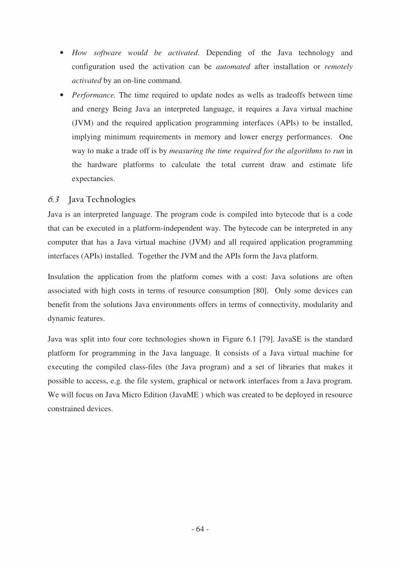
- 64 -

• How software would be activated. Depending of the Java technology and

configuration used the activation can be automated after installation or remotely

activated by an on-line command.

• Performance. The time required to update nodes as wells as tradeoffs between time

and energy Being Java an interpreted language, it requires a Java virtual machine

(JVM) and the required application programming interfaces (APIs) to be installed,

implying minimum requirements in memory and lower energy performances. One

way to make a trade off is by measuring the time required for the algorithms to run in

the hardware platforms to calculate the total current draw and estimate life

expectancies.

Java is an interpreted language. The program code is compiled into bytecode that is a code

that can be executed in a platform-independent way. The bytecode can be interpreted in any

computer that has a Java virtual machine (JVM) and all required application programming

interfaces (APIs) installed. Together the JVM and the APIs form the Java platform.

Insulation the application from the platform comes with a cost: Java solutions are often

associated with high costs in terms of resource consumption [80]. Only some devices can

benefit from the solutions Java environments offers in terms of connectivity, modularity and

dynamic features.

Java was split into four core technologies shown in Figure 6.1 [79]. JavaSE is the standard

platform for programming in the Java language. It consists of a Java virtual machine for

executing the compiled class-files (the Java program) and a set of libraries that makes it

possible to access, e.g. the file system, graphical or network interfaces from a Java program.

We will focus on Java Micro Edition (JavaME ) which was created to be deployed in resource

constrained devices.

Figure 6.1 Java technologies [79]

6.3.1 JavaME

The Java Micro Edition (JavaME) is aimed at embedde

limited resources. Sun released a cut

the resources required for Java SE.

allowing dynamic software updates such as

defined class loaders; memory management such as

from and to a native application t

opted for creating a pluggable architecture to make

Configurations: The Connected Device Configuration (CDC) includes a

of JavaSE except for GUI-related libraries. The Connected Limited Device Con

(CLDC) only contains the minimum amount of classes

JVM.

Profiles: Adds a certain set of API, and optional packages fo

regards to the profile scope. A

For example, the Mobile Information Device Profile

mobile phones, or the Personal Profile for consumer

on the former profile are called MIDlets.

Optional packages: These APIs provide general

functionalities

- 65 -

[79]

The Java Micro Edition (JavaME) is aimed at embedded systems, e.g. mobile phones with

limited resources. Sun released a cut-down version of the JVM that required less than 10%

the resources required for Java SE. The removed functionalities from JavaSE include

allowing dynamic software updates such as reflection, advanced thread control

defined class loaders; memory management such as automatic object finalization

from and to a native application through the use of the Java Native Interface (JNI).

opted for creating a pluggable architecture to make it more flexible. Java ME consists of:

The Connected Device Configuration (CDC) includes almost the entire scope

related libraries. The Connected Limited Device Con

(CLDC) only contains the minimum amount of classes necessary to enable the operation of a

Adds a certain set of API, and optional packages for additional functionality

A profile can be chosen that fits the desired target application.

For example, the Mobile Information Device Profile (MIDP) for mobile devices such as

mobile phones, or the Personal Profile for consumer electronics. Applica

on the former profile are called MIDlets.

These APIs provide general-purpose functionalities and add extra

d systems, e.g. mobile phones with

down version of the JVM that required less than 10% of

ved functionalities from JavaSE include those

reflection, advanced thread control and user-

utomatic object finalization and calls

hrough the use of the Java Native Interface (JNI).They also

it more flexible. Java ME consists of:

lmost the entire scope

related libraries. The Connected Limited Device Configuration

necessary to enable the operation of a

r additional functionality in

fits the desired target application.

(MIDP) for mobile devices such as

electronics. Applications written based

purpose functionalities and add extra

- 66 -

Figure 6.2 Architecture for CLDC and MIDP [79]

6.3.1.1

In JavaME, the activation and deactivation of the programs is done by commands. A device

running a Mobile Information Device Application (MIDlet) has an environment that enables

the user to choose MIDlets for installing, starting and removing. This so called Application

Management Software (AMS) to control the life-cycle is responsible for the interaction with

the user as well as for error handling. MIDlets have three possible states paused, active and

destroyed.

In paused state, the application is non-active; this state is entered in one of three ways: after

the MIDlet has been instantiated, if the AMS calls pauseApp() method, if an exception has

been thrown. The active state is entered once the AMS invokes the startApp() method. When

a MIDlet is in paused mode, it can be turned active by calling the startApp() method. The

destroyed state can only be entered once and is done when the AMS invokes the destroyApp()

method, all resources used by the MIDlet are released.

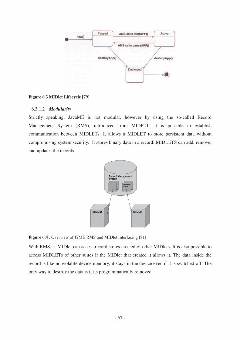
Figure 6.3 MIDlet Lifecycle [79]

6.3.1.2 Modularity

Strictly speaking, JavaME is not modular, however b

Management System (RMS)

communication between MIDLETs.

compromising system security. It stores binary data in a

and updates the records.

Figure 6.4 . Overview of J2ME RMS and MIDlet interfacing

With RMS, a MIDlet can access record stores created of other MI

access MIDLETs of other suites if the MIDlet that c

record is like nonvolatile device memory, it stays

only way to destroy the data is if its progr

- 67 -

[79]

Strictly speaking, JavaME is not modular, however by using the so

Management System (RMS), introduced from MIDP2.0, it is possible to

communication between MIDLETs. It allows a MIDLET to store persistent data without

ising system security. It stores binary data in a record: MIDLETS can add, remove,

. Overview of J2ME RMS and MIDlet interfacing [81]

MIDlet can access record stores created of other MIDlets. It is also possible to

access MIDLETs of other suites if the MIDlet that created it allows it. The data inside the

record is like nonvolatile device memory, it stays in the device even if it is switched

only way to destroy the data is if its programmatically removed.

y using the so-called Record

is possible to establish

It allows a MIDLET to store persistent data without

record: MIDLETS can add, remove,

It is also possible to

reated it allows it. The data inside the

in the device even if it is switched-off. The

- 68 -

6.3.2 OSGi

“Java runs everywhere” is not completely true. Java technologies has been divided into Java

EE, SE and ME to cope with computational heterogeneity. Ubiquitous applications must be

modular, version-controlled and dynamic. To add such functionalities, the Open Services

Gateway initiative framework (OSGi) can be used. OSGi enables the update, addition or

replacement of Java-based applications during runtime, for example over an internet

connection without being on site and without requiring restarting the devices.

The OSGi specifications are produced by the OSGi Alliance [82]. There are open source

frameworks available for the current specification “OSGi Service Platform Release 4“ (R4),

namely Apache Felix, Eclipse Equinox and Makewave Knoplerfish and commercial OSGi

frameworks such as ProSyst Software mBedded Server and Makewave Knopflerfish Pro to

name two of them.

6.3.2.1 OSGi concept of modularity

To achieve modularity, the OSGi framework utilizes a so-called Service Registry and the

concepts of bundles and services. Bundles executing within OSGi are independent of each

other, yet they communicate. They are basically Java JAR files equipped with a manifest that

describes their identity, version and dependencies form and to other bundles. Import packages

states that the bundle depends on the specified bundles, exporting states that bundles are

required by other bundles. Versions and version ranges can be specified for each package.

Bundles can be installed started, updated and uninstalled dynamically. Once a bundle is

successfully installed, it becomes resolved if all dependencies are met. Once resolved, it can

be automatically or manually started. At any point the bundles can be stopped, restarted or

uninstalled.

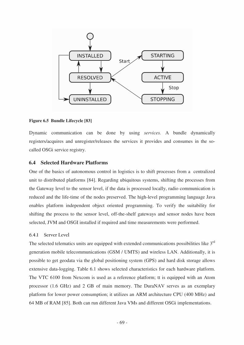
Figure 6.5 Bundle Lifecycle [83]

Dynamic communication can be done by using

registers/acquires and unregister/releases the serv

called OSGi service registry.

6.4 Selected Hardware Platforms

One of the basics of autonomous control in logistics

unit to distributed platforms [84]

the Gateway level to the sensor level, if the data is processed

reduced and the life-time of the nodes preserved.

enables platform independent object oriented progra

shifting the process to the sensor level, o

selected, JVM and OSGI installed if require

The selected telematics units are equipped with extended com

generation mobile telecommunications (GSM / UMTS) a

possible to get geodata via the global positioning

extensive data-logging. Table

The VTC 6100 from Nexcom is used as a reference pla

processor (1.6 GHz) and 2 GB of main memory.

platform for lower power consumption

64 MB of RAM [85]. Both can run different Java VMs and different OSG

- 69 -

[83]

Dynamic communication can be done by using services. A bundle dynamically

registers/acquires and unregister/releases the services it provides and consumes in the so

Platforms

e of the basics of autonomous control in logistics is to shift processes from a centralized

[84]. Regarding ubiquitous systems, shifting the proces

level to the sensor level, if the data is processed locally, radio communication is

time of the nodes preserved. The high-level programming language Java

enables platform independent object oriented programming. To verify the

shifting the process to the sensor level, off-the-shelf gateways and sensor nodes have been

selected, JVM and OSGI installed if required and time measurements were performed.

elematics units are equipped with extended communications possibilities like 3

generation mobile telecommunications (GSM / UMTS) and wireless LAN. Additionally, it is

possible to get geodata via the global positioning system (GPS) and hard disk storage allows

Table 6.1 shows selected characteristics for each hardware pl

The VTC 6100 from Nexcom is used as a reference platform; tt is equipped with an

processor (1.6 GHz) and 2 GB of main memory. The DuraNAV serves as an exemplary

platform for lower power consumption; it utilizes an ARM architecture CPU (400 MHz) and

. Both can run different Java VMs and different OSGi implementations

A bundle dynamically

ices it provides and consumes in the so-

is to shift processes from a centralized

. Regarding ubiquitous systems, shifting the processes from

locally, radio communication is

level programming language Java

. To verify the suitability for

shelf gateways and sensor nodes have been

d and time measurements were performed.

munications possibilities like 3rd

nd wireless LAN. Additionally, it is

system (GPS) and hard disk storage allows

shows selected characteristics for each hardware platform.

t is equipped with an Atom

The DuraNAV serves as an exemplary

t utilizes an ARM architecture CPU (400 MHz) and

i implementations.

Figure 6.6 VTC 6100 Plattform

6.4.2 Sensor Level

The selection of the sensor nodes

of the required algorithms in terms of

nodes, the installed Java virtual machine (JVM)

interfaces (APIs) play also a role regarding the memory and CPU requi

affecting the performance metrics can be

• Hardware configuration in terms of processor mod

• The operating systems environm

• The algorithm being tested

• The Java Virtual Machine being used

• The Java libraries being used (if any)

- 70 -

Table 6.1 Telematic platforms

DuraNAV VTC6100

CPU

(MHz)

PXA255

(400)

N270

(1600)

RAM 64 MB 1 GB

OS Linux Linux

Java

Edition

SE SE

VTC 6100 Plattform [86]

sensor nodes is of crucial importance for the analysis of the pe

of the required algorithms in terms of energy consumption. Regarding java

virtual machine (JVM) and the required applic

play also a role regarding the memory and CPU requi

the performance metrics can be:

Hardware configuration in terms of processor model, clock speed and memory size

The operating systems environment

algorithm being tested

The Java Virtual Machine being used

The Java libraries being used (if any)

is of crucial importance for the analysis of the performance

energy consumption. Regarding java-enabled sensor

application programming

play also a role regarding the memory and CPU requirements. Factors

el, clock speed and memory size

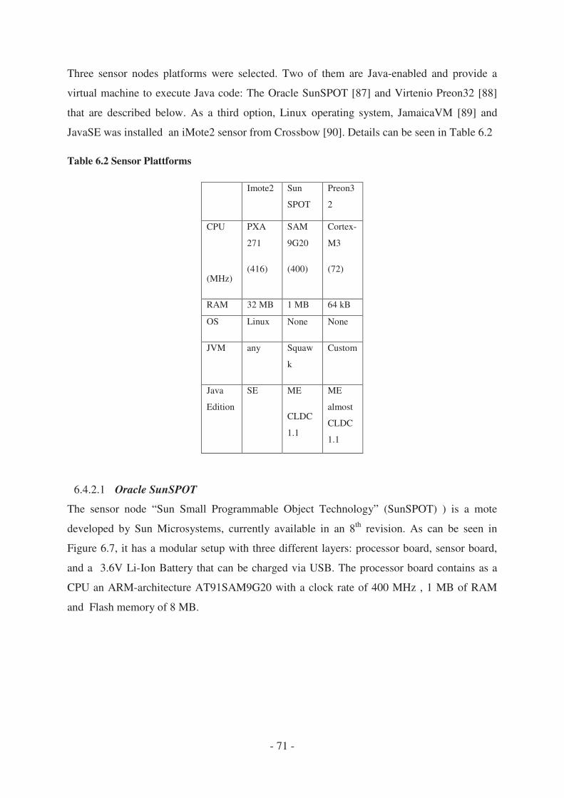
- 71 -

Three sensor nodes platforms were selected. Two of them are Java-enabled and provide a

virtual machine to execute Java code: The Oracle SunSPOT [87] and Virtenio Preon32 [88]

that are described below. As a third option, Linux operating system, JamaicaVM [89] and

JavaSE was installed an iMote2 sensor from Crossbow [90]. Details can be seen in Table 6.2

Table 6.2 Sensor Plattforms

Imote2 Sun

SPOT

Preon3

2

CPU

(MHz)

PXA

271

(416)

SAM

9G20

(400)

Cortex-

M3

(72)

RAM 32 MB 1 MB 64 kB

OS Linux None None

JVM any Squaw

k

Custom

Java

Edition

SE ME

CLDC

1.1

ME

almost

CLDC

1.1

6.4.2.1 Oracle SunSPOT

The sensor node “Sun Small Programmable Object Technology” (SunSPOT) ) is a mote

developed by Sun Microsystems, currently available in an 8th

revision. As can be seen in

Figure 6.7, it has a modular setup with three different layers: processor board, sensor board,

and a 3.6V Li-Ion Battery that can be charged via USB. The processor board contains as a

CPU an ARM-architecture AT91SAM9G20 with a clock rate of 400 MHz , 1 MB of RAM

and Flash memory of 8 MB.

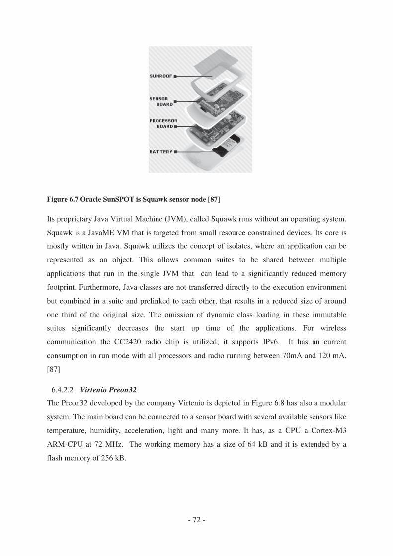
Figure 6.7 Oracle SunSPOT is Squawk

Its proprietary Java Virtual Machine (JVM)

Squawk is a JavaME VM that

mostly written in Java. Squawk utiliz

represented as an object. This allows common suites

applications that run in the single JVM

footprint. Furthermore, Java c

but combined in a suite and prelinked to each other

one third of the original size. The omission of dyn

suites significantly decreases the start up time of the ap

communication the CC2420

consumption in run mode with all processors and radio running betw

[87]

6.4.2.2 Virtenio Preon32

The Preon32 developed by the company

system. The main board can be connected to a sensor board with several ava

temperature, humidity, acceleration, light and many

ARM-CPU at 72 MHz. The working memory has a size of 64 kB

flash memory of 256 kB.

- 72 -

is Squawk sensor node [87]

Java Virtual Machine (JVM), called Squawk runs without an operating system.

that is targeted from small resource constrained devices. Its core is

Squawk utilizes the concept of isolates, where an application ca

represented as an object. This allows common suites to be shared between multiple

applications that run in the single JVM that can lead to a significantly reduced memory

classes are not transferred directly to the executio

but combined in a suite and prelinked to each other, that results in a reduced size of around

one third of the original size. The omission of dynamic class loading in these immutable

significantly decreases the start up time of the applications.

radio chip is utilized; it supports IPv6.

run mode with all processors and radio running between 70mA and 120 mA.

developed by the company Virtenio is depicted in Figure 6.8

can be connected to a sensor board with several ava

temperature, humidity, acceleration, light and many more. It has, as a CPU a C

The working memory has a size of 64 kB and i

runs without an operating system.

small resource constrained devices. Its core is

es the concept of isolates, where an application can be

to be shared between multiple

can lead to a significantly reduced memory

lasses are not transferred directly to the execution environment

results in a reduced size of around

amic class loading in these immutable

plications. For wireless

It has an current

een 70mA and 120 mA.

8 has also a modular

can be connected to a sensor board with several available sensors like

s a CPU a Cortex-M3

and it is extended by a

Figure 6.8 Virtenio Preon32 Sensor Node

Virtenio developed for it a proprietary

JavaME based and access to native applications is n

allows access to hardware components like the radio

Java Native Interface (JNI). For wireless communica

Support for IPv6 is currently under development.

model of 28,3mA(at 72 MHz)

6.4.2.3 iMote

iMote2 sensor node from Crossbow

XScale processor that can run at a clock speed of up to 416 MHz

and non-volatile memory, a power management IC

and an antenna. Furthermore, it allows stack

additional devices, such as, temperatures

The devices were enabled with JamaicaVM, running ov

of it, OSGi framework was installed

Linux operating system for the iMote2 does not supp

ARM processor. For the evaluation of power consumption of the iMot

was measured over a 1 Ohm resistor in series with the p

connected in parallel to it. The CPU of the iMote2 consumes 50 mA r

speed.

- 73 -

Virtenio Preon32 Sensor Node [88]

developed for it a proprietary Java virtual machine. Unlike,

JavaME based and access to native applications is not possible, Virtenio

ccess to hardware components like the radio that are written in C and

Java Native Interface (JNI). For wireless communication the ATRF231 radio chip is utilized.

Support for IPv6 is currently under development. It has an current consumption in

model of 28,3mA(at 72 MHz).

iMote2 sensor node from Crossbow [90] is a sensor platform with a powerful

can run at a clock speed of up to 416 MHz , it is integrated with vo

volatile memory, a power management IC to go to deep-sleep mode, a transceiver,

and an antenna. Furthermore, it allows stack ability of additional modules to interconnect

additional devices, such as, temperatures sensor cards.

The devices were enabled with JamaicaVM, running over a Linux operating system

was installed to enable features such as dynamic software

Linux operating system for the iMote2 does not support low-power deep sleep mode

For the evaluation of power consumption of the iMote2 the supply current

measured over a 1 Ohm resistor in series with the power supply wire, with a test

The CPU of the iMote2 consumes 50 mA running on full clock

Unlike, SunSPOT, that is

ot possible, Virtenio’s implementation

written in C and through the

tion the ATRF231 radio chip is utilized.

It has an current consumption in active

powerful ARM PXA271

integrated with volatile

sleep mode, a transceiver,

ability of additional modules to interconnect

Linux operating system. On top

to enable features such as dynamic software updates.

power deep sleep modes of the

e2 the supply current

ower supply wire, with a test probe

unning on full clock

Figure 6.9 Crossbow iMote2 sensor node

6.5 Algorithms for data fusion

Several algorithms have been selected to

data fusion related algorithms described from chapt

benchmarks such as Dhrystone and Linpack, and cold

calculation of shelf life as function of temperature deviation

temperature profiles.

6.5.1 Standard Benchmarks

In times when personal computers appeared and these

with today’s ones, “standard” benchmarks were desig

1. Benchmarks specially designed to test performance i

string processing, for example word processors.

2. Benchmarks specially designed to test the speed of

performance was measured in Mflops (millions of point instruction per

We have selected one benchmark from each category to test the platfo

numeric applications and Linpack

6.5.1.1 Dhrystone

The main characteristics of Dhryston

• It contains no floating point operations

• A considerable percentage of time is spent in string

• It contains hardly any tight loops so in the case of

instruction accesses will be misse

• Only a small amount of global data is manipulated

- 74 -

Crossbow iMote2 sensor node [90]

fusion, analysis and reduction

algorithms have been selected to be tested in the platforms. These include not only

data fusion related algorithms described from chapters three and four, but also “standard”

benchmarks such as Dhrystone and Linpack, and cold-chain specific algorithms such as

as function of temperature deviation, and prediction of future

Standard Benchmarks

In times when personal computers appeared and these were resource constrained compared

with today’s ones, “standard” benchmarks were designed; they fall into two categories:

Benchmarks specially designed to test performance in non numeric applications and

string processing, for example word processors.

Benchmarks specially designed to test the speed of floating point operations. The

sured in Mflops (millions of point instruction per

one benchmark from each category to test the platforms:

Linpack for numeric applications.

of Dhrystone benchmark are [91]:

t contains no floating point operations

considerable percentage of time is spent in string operations

t contains hardly any tight loops so in the case of very small caches the

instruction accesses will be missed

nly a small amount of global data is manipulated

be tested in the platforms. These include not only the

ers three and four, but also “standard”

chain specific algorithms such as

and prediction of future

were resource constrained compared

ll into two categories:

n non numeric applications and

floating point operations. The

sured in Mflops (millions of point instruction per second)

rms: Dhrystone for non-

very small caches the majority of

- 75 -

• There are two versions of the Dhrystone benchmark. We selected version 2.1 that is

the latest one.

6.5.1.2 Linpack

The main characteristics of the Linpack benchmark are [91]:

• It has a large percentage of floating point operations (division is not used);

• It uses no mathematical functions

• There are no global variables; operations being carried out on local variables results

are for single or double precision operations

• The benchmark relies heavily on the libraries being used

6.5.2 Cold-Chain specific algorithms

Through this section, it will be demonstrated that if the sensor data is processed locally, the

radio communication between hop nodes can be drastically reduced, the costs related to

satellite communication avoided and eventual quality losses due to air flow obstacles

detected. But what is the relation between the environmental parameter surrounding the

refrigerated perishable goods and the quality losses? We have to take into account that

perishable goods, are subject to metabolic processes For example, bananas are “breathing”:

they ingest oxygen and exhale CO2 and the plant hormone ethylene (C2H4) that generates

additional heat, furthermore, the final quality of the product depends directly on the severity

of the temperature deviations during transportation. Two cold-chain specific benchmarks

were selected. The aim of their inclusion is to verify if it is possible to shift the decision

making to the sensor node layer: temperature prediction and the estimation of bacterial

growth as effect of the temperature.

6.5.2.1

The future temperature values inside a refrigerated container during transportation can be

made through system identification techniques, that estimate the parameters of a modeled

system. Specially fitted to resource constrained devices are the recursive representations of

such algorithms due to their low memory and CPU requirements when compared with the

offline counterparts.

In order to model the effect of the thermal energy generated by the ripening of bananas, the

so-called Feedback-Hammerstein model [26] is used. As can be seen in

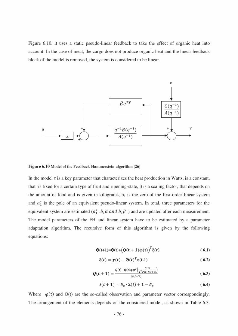
- 76 -

Figure 6.10, it uses a static pseudo-linear feedback to take the effect of organic heat into

account. In the case of meat, the cargo does not produce organic heat and the linear feedback

block of the model is removed, the system is considered to be linear.

Figure 6.10 Model of the Feedback-Hammerstein-algorithm [26]

In the model is a key parameter that characterizes the heat production in Watts, is a constant,

that is fixed for a certain type of fruit and ripening-state, is a scaling factor, that depends on

the amount of food and is given in kilograms, b1 is the zero of the first-order linear system

and is the pole of an equivalent pseudo-linear system. In total, three parameters for the

equivalent system are estimated ( ) and are updated after each measurement.

The model parameters of the FH and linear system have to be estimated by a parameter

adaptation algorithm. The recursive form of this algorithm is given by the following

equations:

ΘΘΘΘ(t+1)=ΘΘΘΘ(t)+ ( 6.1)

(t-1) ( 6.2)

( 6.3)

( 6.4)

Where and Θ(t) are the so-called observation and parameter vector correspondingly.

The arrangement of the elements depends on the considered model, as shown in Table 6.3.

+

+ +

+

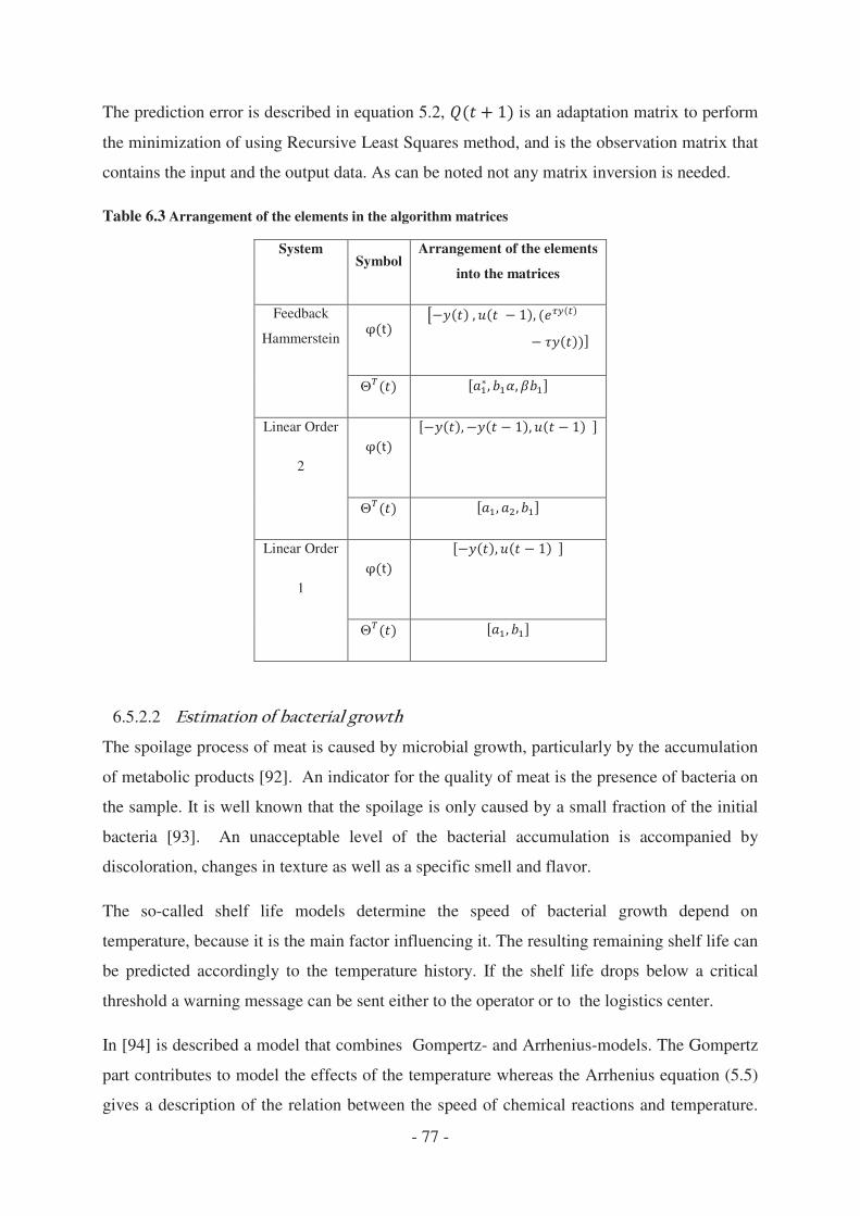
- 77 -

The prediction error is described in equation 5.2, is an adaptation matrix to perform

the minimization of using Recursive Least Squares method, and is the observation matrix that

contains the input and the output data. As can be noted not any matrix inversion is needed.

Table 6.3 Arrangement of the elements in the algorithm matrices

System Symbol

Arrangement of the elements

into the matrices

Feedback

Hammerstein

Linear Order

2

Linear Order

1

6.5.2.2

The spoilage process of meat is caused by microbial growth, particularly by the accumulation

of metabolic products [92]. An indicator for the quality of meat is the presence of bacteria on

the sample. It is well known that the spoilage is only caused by a small fraction of the initial

bacteria [93]. An unacceptable level of the bacterial accumulation is accompanied by

discoloration, changes in texture as well as a specific smell and flavor.

The so-called shelf life models determine the speed of bacterial growth depend on

temperature, because it is the main factor influencing it. The resulting remaining shelf life can

be predicted accordingly to the temperature history. If the shelf life drops below a critical

threshold a warning message can be sent either to the operator or to the logistics center.

In [94] is described a model that combines Gompertz- and Arrhenius-models. The Gompertz

part contributes to model the effects of the temperature whereas the Arrhenius equation (5.5)

gives a description of the relation between the speed of chemical reactions and temperature.

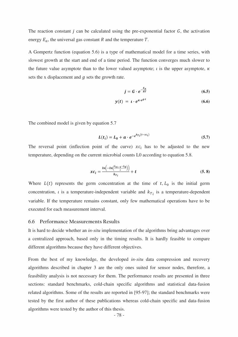
- 78 -

The reaction constant can be calculated using the pre-exponential factor , the activation

energy , the universal gas constant and the temperature .

A Gompertz function (equation 5.6) is a type of mathematical model for a time series, with

slowest growth at the start and end of a time period. The function converges much slower to

the future value asymptote than to the lower valued asymptote; is the upper asymptote,

sets the x displacement and sets the growth rate.

(6.5)

(6.6)

The combined model is given by equation 5.7

(5.7)

The reversal point (inflection point of the curve) has to be adjusted to the new

temperature, depending on the current microbial counts L0 according to equation 5.8.

(5. 8)

Where represents the germ concentration at the time of , is the initial germ

concentration, is a temperature-independent variable and is a temperature-dependent

variable. If the temperature remains constant, only few mathematical operations have to be

executed for each measurement interval.

It is hard to decide whether an in-situ implementation of the algorithms bring advantages over

a centralized approach, based only in the timing results. It is hardly feasible to compare

different algorithms because they have different objectives.

From the best of my knowledge, the developed in-situ data compression and recovery

algorithms described in chapter 3 are the only ones suited for sensor nodes, therefore, a

feasibility analysis is not necessary for them. The performance results are presented in three

sections: standard benchmarks, cold-chain specific algorithms and statistical data-fusion

related algorithms. Some of the results are reported in [95-97]; the standard benchmarks were

tested by the first author of these publications whereas cold-chain specific and data-fusion

algorithms were tested by the author of this thesis.

- 79 -

The standard benchmarks are tested for every mentioned hardware platform. The cold-chain

specific algorithms were tested for every sensor node and for the VTC gateway. The data-

fusion related algorithms were the most difficult to compare; matrix-inversion, that is

required for OK and CK interpolation was tested for every platform except from DuraNav,

cokriging interpolation and Goulard-Voltz fitting was only tested on VTC6100 because they

are high resource and energy demanding and their implementation was only feasible to

perform centralized. SunSPOT can perform floating point operations very fast and can

perform CK interpolation, however it was not tested because its performance is already

compared with the Matrix inversion.

Table 6.4 Algorithms tested for every hardware platform. The Goulard-Voltz algorithm[75] and CK interpolation required for fitting the linear model of coregionalization and perform cross-attribute fusion are only tested on the Gateway level.

The VTC 6100 unit is the only hardware platform able to run each selected algorithm and is

taken as reference point for the performance of the different platforms. Figure 6.11(a) shows

the time required to run the Dhrystone algorithm, the VTC require only 523 ms. Figure

6.11(b) shows the performane in % to the refeence

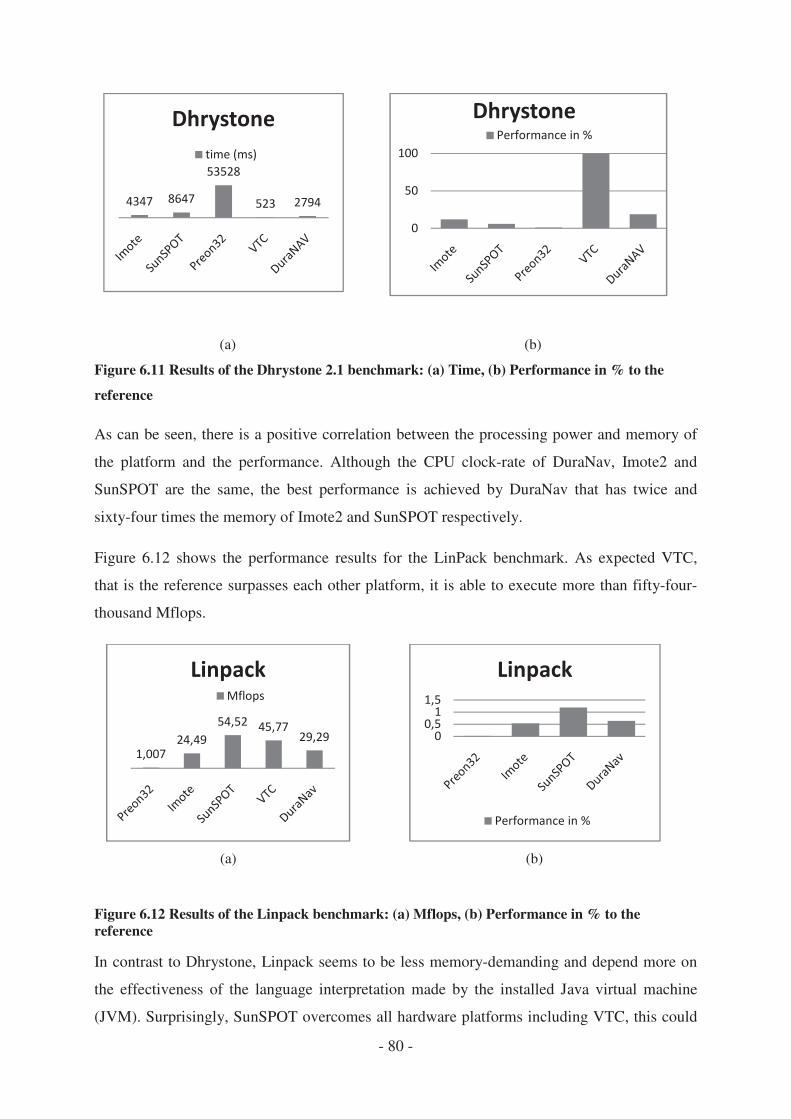
- 80 -

(a) (b)

Figure 6.11 Results of the Dhrystone 2.1 benchmark: (a) Time, (b) Performance in % to the

reference

As can be seen, there is a positive correlation between the processing power and memory of

the platform and the performance. Although the CPU clock-rate of DuraNav, Imote2 and

SunSPOT are the same, the best performance is achieved by DuraNav that has twice and

sixty-four times the memory of Imote2 and SunSPOT respectively.

Figure 6.12 shows the performance results for the LinPack benchmark. As expected VTC,

that is the reference surpasses each other platform, it is able to execute more than fifty-four-

thousand Mflops.

(a) (b)

Figure 6.12 Results of the Linpack benchmark: (a) Mflops, (b) Performance in % to the

reference

In contrast to Dhrystone, Linpack seems to be less memory-demanding and depend more on

the effectiveness of the language interpretation made by the installed Java virtual machine

(JVM). Surprisingly, SunSPOT overcomes all hardware platforms including VTC, this could

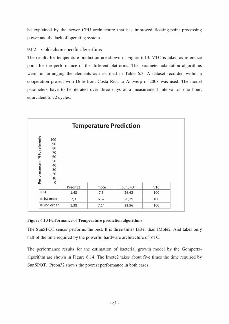
be explained by the newer CPU

power and the lack of operating system.

The results for temperature prediction are shown in

point for the performance of the different platform

were run arranging the elements as described in

cooperation project with Dole from Costa Rica to An

parameters have to be iterated over three days at a

equivalent to 72 cycles.

Figure 6.13 Performance of Temperature prediction algorithms

The SunSPOT sensor performs the best

half of the time required by the powerful hardware

The performance results for the estimation of bacte

algorithm are shown in Figure

SunSPOT. Preon32 shows the poorest performance in both cases

- 81 -

be explained by the newer CPU architecture that has improved floating

power and the lack of operating system.

The results for temperature prediction are shown in Figure 6.13. VTC is

point for the performance of the different platforms. The parameter adaptation algorithms

were run arranging the elements as described in Table 6.3. A dataset recorded within a

cooperation project with Dole from Costa Rica to Antwerp in 2008 was used.

parameters have to be iterated over three days at a measurement interval of one hour,

Performance of Temperature prediction algorithms

The SunSPOT sensor performs the best. It is three times faster than IMote2. And takes

half of the time required by the powerful hardware architecture of VTC.

The performance results for the estimation of bacterial growth model by the Gompertz

Figure 6.14. The Imote2 takes about five times the time requir

Preon32 shows the poorest performance in both cases.

has improved floating-point processing

. VTC is taken as reference

The parameter adaptation algorithms

. A dataset recorded within a

twerp in 2008 was used. The model

rement interval of one hour,

than IMote2. And takes only

rial growth model by the Gompertz-

. The Imote2 takes about five times the time required by

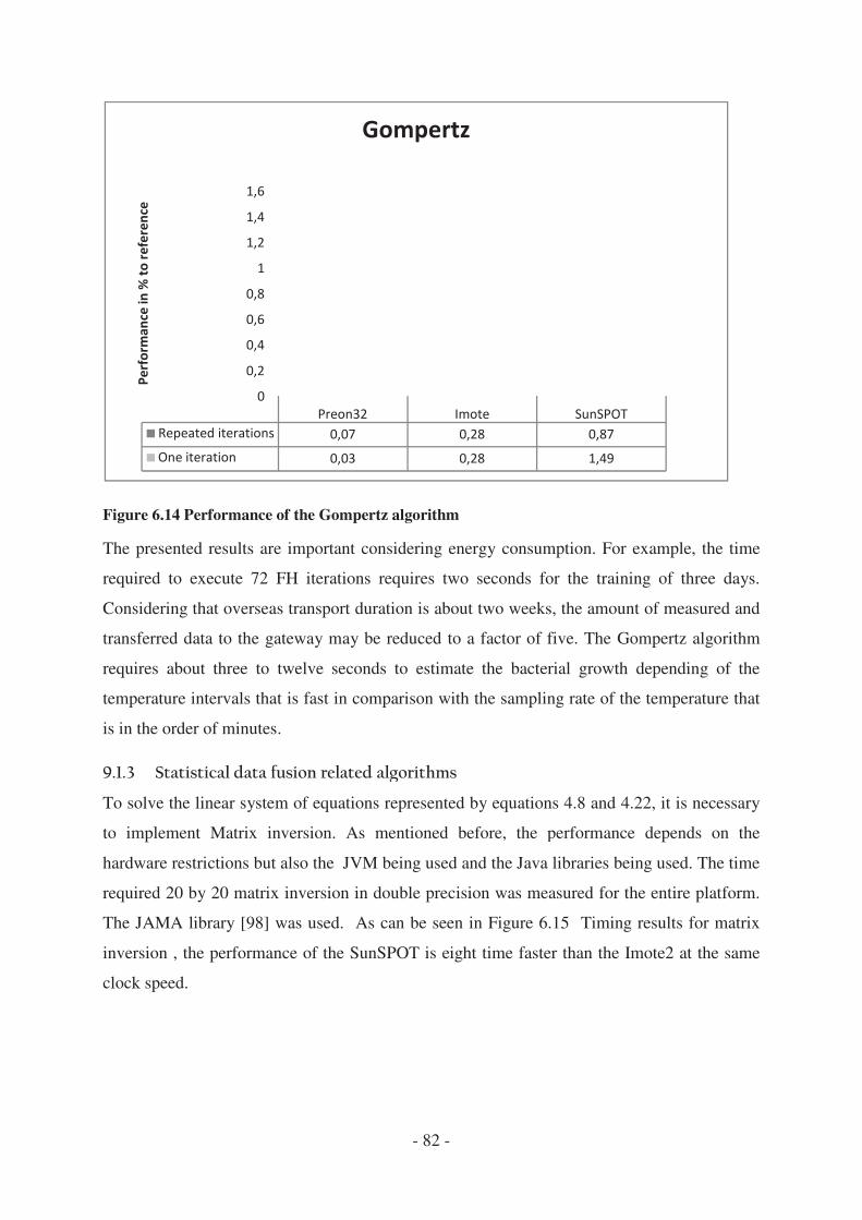
Figure 6.14 Performance of the Gompertz algorithm

The presented results are important considering ene

required to execute 72 FH iterations requires two s

Considering that overseas transport duration i

transferred data to the gateway may be reduced to a

requires about three to twelve seconds to estimate the bacteria

temperature intervals that is fast in comparison with the sampling rate of the

is in the order of minutes.

To solve the linear system of equations represented

to implement Matrix inversion.

hardware restrictions but also the JVM being used

required 20 by 20 matrix inversion in double precis

The JAMA library [98] was used.

inversion , the performance of the SunSPOT i

clock speed.

- 82 -

nce of the Gompertz algorithm

The presented results are important considering energy consumption. For example, the time

required to execute 72 FH iterations requires two seconds for the training of three days.

transport duration is about two weeks, the amount of measured and

transferred data to the gateway may be reduced to a factor of five. The Gompertz algorithm

ut three to twelve seconds to estimate the bacterial growth depending of the

is fast in comparison with the sampling rate of the

To solve the linear system of equations represented by equations 4.8 and 4.22, it is necessary

inversion. As mentioned before, the performance

hardware restrictions but also the JVM being used and the Java libraries being used.

required 20 by 20 matrix inversion in double precision was measured for

was used. As can be seen in Figure 6.15 Timing results for

, the performance of the SunSPOT is eight time faster than the Imote2 at the same

rgy consumption. For example, the time

econds for the training of three days.

the amount of measured and

factor of five. The Gompertz algorithm

l growth depending of the

is fast in comparison with the sampling rate of the temperature that

by equations 4.8 and 4.22, it is necessary

As mentioned before, the performance depends on the

being used. The time

ion was measured for the entire platform.

Timing results for matrix

s eight time faster than the Imote2 at the same

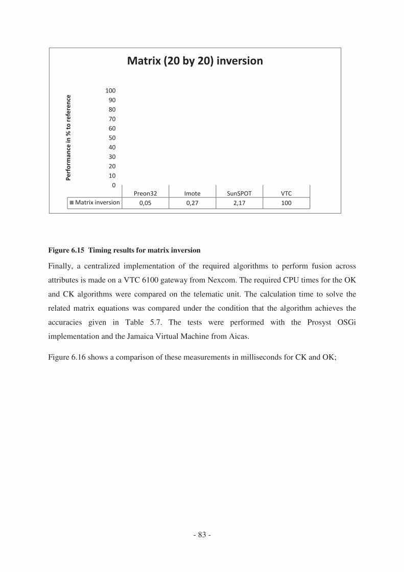
Figure 6.15 Timing results for

Finally, a centralized implementation of the

attributes is made on a VTC 6100

and CK algorithms were compared on the telematic unit. The calculatio

related matrix equations was comp

accuracies given in Table

implementation and the Jamaica Virtual Machine from

Figure 6.16 shows a comparison

- 83 -

Timing results for matrix inversion

centralized implementation of the required algorithms to perform fusion across

VTC 6100 gateway from Nexcom. The required CPU times for the OK

were compared on the telematic unit. The calculation time to solve the

related matrix equations was compared under the condition that the algorithm achieve

Table 5.7. The tests were performed with the Prosyst OSGi

implementation and the Jamaica Virtual Machine from Aicas.

shows a comparison of these measurements in milliseconds for CK and OK;

required algorithms to perform fusion across

The required CPU times for the OK

were compared on the telematic unit. The calculation time to solve the

ared under the condition that the algorithm achieves the

tests were performed with the Prosyst OSGi

these measurements in milliseconds for CK and OK;

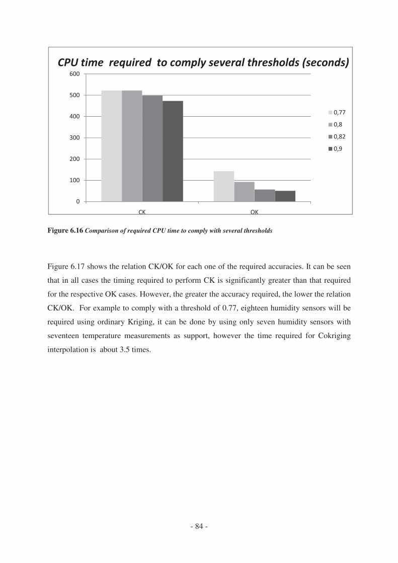
- 84 -

Figure 6.16 Comparison of required CPU time to comply with several thresholds

Figure 6.17 shows the relation CK/OK for each one of the required accuracies. It can be seen

that in all cases the timing required to perform CK is significantly greater than that required

for the respective OK cases. However, the greater the accuracy required, the lower the relation

CK/OK. For example to comply with a threshold of 0.77, eighteen humidity sensors will be

required using ordinary Kriging, it can be done by using only seven humidity sensors with

seventeen temperature measurements as support, however the time required for Cokriging

interpolation is about 3.5 times.

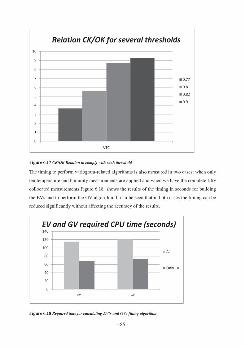
- 85 -

Figure 6.17 CK/OK Relation to comply with each threshold

The timing to perform variogram-related algorithms is also measured in two cases: when only

ten temperature and humidity measurements are applied and when we have the complete fifty

collocated measurements.Figure 6.18 shows the results of the timing in seconds for building

the EVs and to perform the GV algorithm. It can be seen that in both cases the timing can be

reduced significantly without affecting the accuracy of the results.

Figure 6.18 Required time for calculating EV’s and GVz fitting algorithm

One of the most important figures of merit of OSGi

to allow software updates or installation of new bu

restart the system. Of special importance is how mu

framework to manage softwar

bundles of different algorithm was tested.

Hammerstein algorithms were tested on the gateway

framework .

Figure 6.19 shows the results on the iMote2 and DuraNAV. The ex

standard benchmarks is in the order of eight percen

instead of class file. The Feedback

faster than the corresponding Java class.

Figure 6.19 Diffrence in execution time in % between OSGi and c

The use of OSGi framework for

resources is possible with an increased execution s

implementations.

- 86 -

One of the most important figures of merit of OSGi is its ability to provide dynamic features

to allow software updates or installation of new bundles during runtime without requiring

restart the system. Of special importance is how much overhead is created by using the OSGi

framework to manage software updates. Direct execution times of Java class files and

of different algorithm was tested. Both standard benchmarks and the Feedback

Hammerstein algorithms were tested on the gateway devices and iMote2 for

shows the results on the iMote2 and DuraNAV. The execution time

standard benchmarks is in the order of eight percent slower when an OSGi bundle is

instead of class file. The Feedback-Hammerstein OSGi bundle, however,

faster than the corresponding Java class.

Diffrence in execution time in % between OSGi and class

The use of OSGi framework for the dynamic software updates of algorithms requiring few

resources is possible with an increased execution speed when compared to Java class

is its ability to provide dynamic features

ndles during runtime without requiring to

is created by using the OSGi

. Direct execution times of Java class files and OSGi

Both standard benchmarks and the Feedback-

devices and iMote2 for Equinox OSGi

ecution time of both

t slower when an OSGi bundle is executed

, however, was up to ten %

algorithms requiring few

peed when compared to Java class

- 87 -

This chapter has shown that Java is useful to manage hardware heterogeneity. Due to its high

acceptance and maturity, portability of the code is possible. Sensor nodes that are the pillars

of ubiquitous applications are their Achilles’ heel as well. If the time required to interpret the

instructions is too big, or if the memory required for the libraries is high, their implementation

at the sensor level is unfeasible.

It was decided to test data fusion, standard benchmarks and cold-chain specific algorithms in

selected Java-enabled sensor nodes and gateways. The best performance for algorithm

requiring floating point operations are obtained with SunSPOT that uses JavaME,

unfortunately, by using it modularity is limited to the use of Record Management System

(RMS); furthermore neither, versioning nor dynamic programming is possible.

Versioning, dynamic programming and modularity in sensor nodes is possible even in sensor

nodes by the installation of Java-based technologies such as OSGi. OSGi was installed on

Imote2 sensor nodes, and DuraNAV and VTC telematic units. The time required to install

OSGi bundles was measured. Only Imote2 has enough resources for making an OSGi-

framework available on a sensor-platform. JavaME implementation of OSGi sounds

promising, but it is not yet available.

In this chapter it is also demonstrated that data reduction techniques, that are a good approach

to reduce energy consumption in the sensor nodes are energy-efficient and easy to implement

on Java-enabled sensor nodes and therefore the transmission of high volumes of sensor data to

the gateway is unnecessary.

The supervision of environmental parameters and quality state are also taken into

consideration. The combined Gompertz model that calculates the bacterial growth in meat and

the Feedback-Hammerstein that estimates the parameters of a non-linear model in fruit

transport were selected, implemented and tested.

Statistical data fusion algorithms that are good approach to avoid dense deployment of

sensors and to reduce communication if the measured data of many sensors is replaced by

their estimations are only feasible to implement at the gateway level. The time required to

achieve the same accuracy for OK by the use of CK interpolation is energy demanding,

however, it is not important because it is performed in the gateway where there are no energy

constraints.

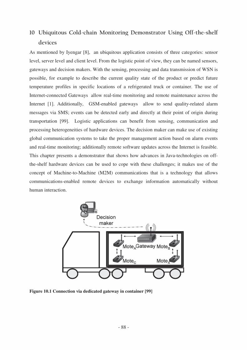
As mentioned by Iyengar [8], an ub

level, server level and client level. From the logi

gateways and decision makers.

possible, for example to describe the current quali

temperature profiles in specific locations of a ref

Internet-connected Gateways

Internet [1]. Additionally, GSM

messages via SMS; events can be detected early and directly at thei

transportation [99]. Logistic applications can benefit from

processing heterogeneities of hardware devices. The

global communication systems to take the proper management action bas

and real-time monitoring; additionally remote software updat

This chapter presents a demonstrator that shows how

the-shelf hardware devices can be used

concept of Machine-to-Machine (M2M) communications that is a technology

communications-enabled remote devices to exchange information auto

human interaction.

Figure 10.1 Connection via dedicated gateway in container

- 88 -

, an ubiquitous application consists of three categories:

level, server level and client level. From the logistic point of view, they can be named sensors,

gateways and decision makers. With the sensing, processing and data transmission

possible, for example to describe the current quality state of the product or predict future

temperature profiles in specific locations of a refrigerated truck or container.

allow real-time monitoring and remote maintenance

GSM-enabled gateways allow to send qu

; events can be detected early and directly at their point of origin during

. Logistic applications can benefit from sensing, communication and

processing heterogeneities of hardware devices. The decision maker can make use of existing

on systems to take the proper management action based on alarm events

time monitoring; additionally remote software updates across the Internet is feasible.

presents a demonstrator that shows how advances in Java-technologies

shelf hardware devices can be used to cope with these challenges; it makes use of the

Machine (M2M) communications that is a technology

enabled remote devices to exchange information auto

Connection via dedicated gateway in container [99]

iquitous application consists of three categories: sensor

they can be named sensors,

With the sensing, processing and data transmission of WSN is

he product or predict future

rigerated truck or container. The use of

and remote maintenance across the

allow to send quality-related alarm

r point of origin during

sensing, communication and

can make use of existing

on systems to take the proper management action based on alarm events

across the Internet is feasible.

technologies on off-

it makes use of the

Machine (M2M) communications that is a technology that allows

enabled remote devices to exchange information automatically without

- 89 -

A differentiation between wireless M2M and WSN is not exact. According to Webb [100],

the key requirements for M2M communications are:

• Support a large number of terminals

• Long battery life

• Mobility

• Low cost equipment

• Low cost service

• Global availability

• Ubiquity

The critical requirements for the design of M2M area networks are [101]:

• Low CPU processing power

• Limited memory

• Low data rate

• Battery operated

• Low cost

• Small size

Based on the previous descriptions, it can be said that both technologies can utilize sensors to

perform remote monitoring and communicate with each other through wireless

communication. Knowing the subtle differences will help to understand the implications of

their combined use in logistics.

M2M are deployed when power consumption is not critical, the size/weight of the devices is

not an important factor and a range of kilometres is required. Additional features may include

for example bidirectional communication. Wireless M2M covers applications involving

longer range and the node will typically be powered from the machine itself.

Wireless Sensor Networks (WSN) on the other hand is an emerging technology to monitor

ambient conditions. They are commonly considered to be stand-alone; the sensor nodes

communicate with other sensors and the gateway, but are in principle unable to communicate

with the outside world; they have only short/medium range communication.

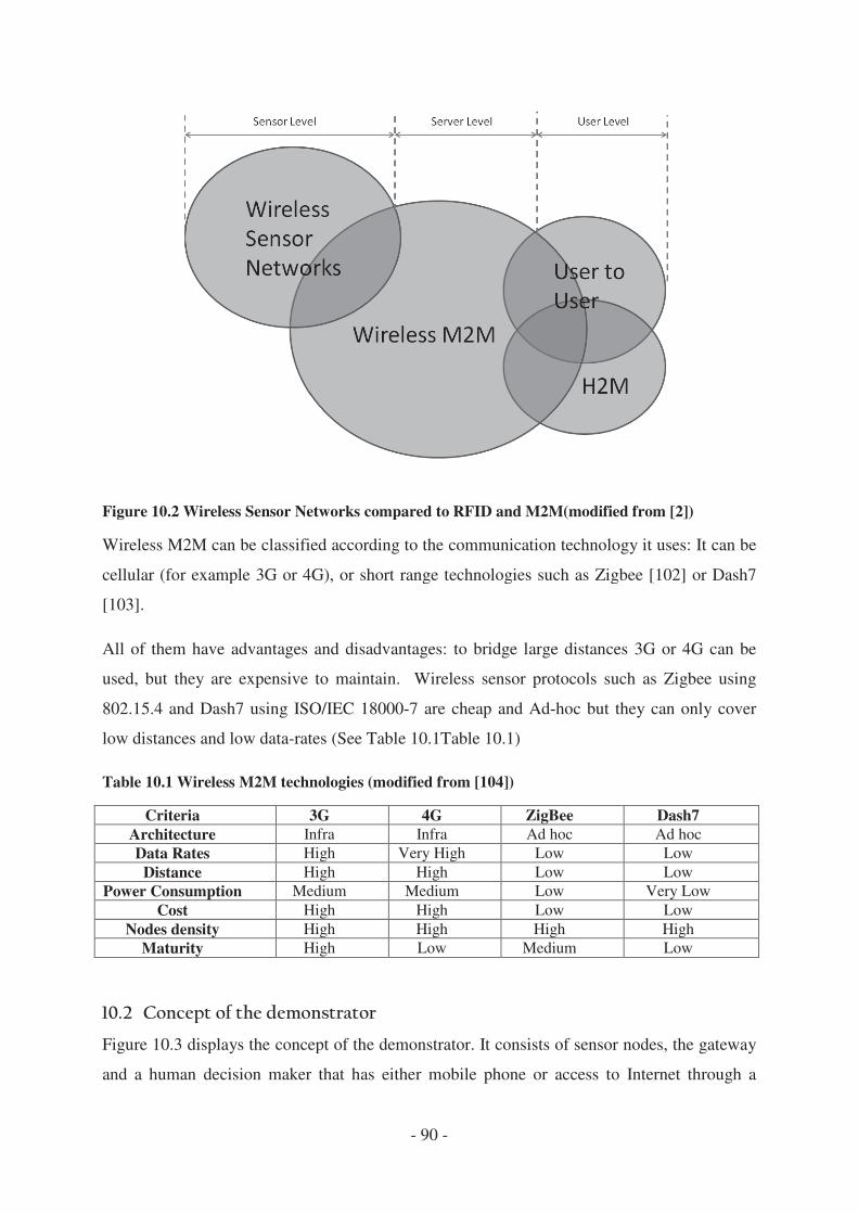
Figure 10.2 Wireless Sensor Networks compared to RFID and M2M

Wireless M2M can be classified according to the com

cellular (for example 3G or 4G), or short range technologies s

[103].

All of them have advantages and disadvantages

used, but they are expensive

802.15.4 and Dash7 using ISO/IEC 18000

low distances and low data-rates

Table 10.1 Wireless M2M techno

Criteria 3G

Architecture Infra

Data Rates High

Distance High

Power Consumption Medium

Cost High

Nodes density High

Maturity High

Figure 10.3 displays the concept of the demonstrator. It consis

and a human decision maker

- 90 -

Wireless Sensor Networks compared to RFID and M2M(modified from

Wireless M2M can be classified according to the communication technology it uses: It can be

or example 3G or 4G), or short range technologies such as Zigbee

All of them have advantages and disadvantages: to bridge large distances 3G or 4G can be

to maintain. Wireless sensor protocols such as Zigbee using

802.15.4 and Dash7 using ISO/IEC 18000-7 are cheap and Ad-hoc but they can only cover

rates (See Table 10.1Table 10.1)

technologies (modified from [104])

3G 4G ZigBee

Infra Infra Ad hoc

High Very High Low

High High Low

Medium Medium Low

High High Low

High High High

High Low Medium

displays the concept of the demonstrator. It consists of sensor

decision maker that has either mobile phone or access to Internet throu

(modified from [2])

munication technology it uses: It can be

uch as Zigbee [102] or Dash7

nces 3G or 4G can be

. Wireless sensor protocols such as Zigbee using

hoc but they can only cover

Dash7

Ad hoc

Low

Low

Very Low

Low

High

Low

nodes, the gateway

has either mobile phone or access to Internet through a

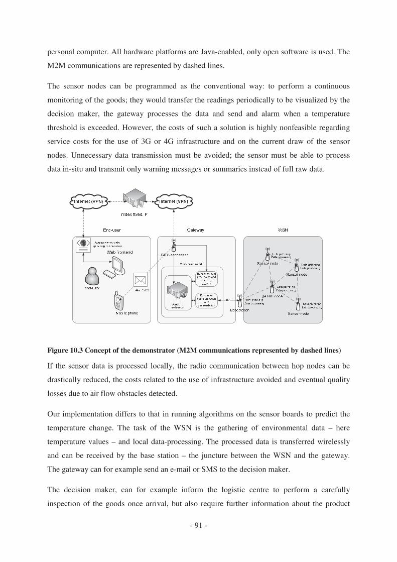
- 91 -

personal computer. All hardware platforms are Java-enabled, only open software is used. The

M2M communications are represented by dashed lines.

The sensor nodes can be programmed as the conventional way: to perform a continuous

monitoring of the goods; they would transfer the readings periodically to be visualized by the

decision maker, the gateway processes the data and send and alarm when a temperature

threshold is exceeded. However, the costs of such a solution is highly nonfeasible regarding

service costs for the use of 3G or 4G infrastructure and on the current draw of the sensor

nodes. Unnecessary data transmission must be avoided; the sensor must be able to process

data in-situ and transmit only warning messages or summaries instead of full raw data.

Figure 10.3 Concept of the demonstrator (M2M communications represented by dashed lines)

If the sensor data is processed locally, the radio communication between hop nodes can be

drastically reduced, the costs related to the use of infrastructure avoided and eventual quality

losses due to air flow obstacles detected.

Our implementation differs to that in running algorithms on the sensor boards to predict the

temperature change. The task of the WSN is the gathering of environmental data – here

temperature values – and local data-processing. The processed data is transferred wirelessly

and can be received by the base station – the juncture between the WSN and the gateway.

The gateway can for example send an e-mail or SMS to the decision maker.

The decision maker, can for example inform the logistic centre to perform a carefully

inspection of the goods once arrival, but also require further information about the product

- 92 -

quality; the system must have the ability to deploy new software such as the Gompertz model

to a chosen sensor node.

The Feedback-Hammerstein algorithm for temperature prediction was selected to demonstrate

the concept of the use of local processing of data to support decision making at affordable

costs. Regarding hardware devices, VTC6100 and SunSPOTs are selected.

For the Gateway, the Equinox OSGi-framework is installed on top of the Linux OS, that

enables a high degree of dynamics by allowing the installing or updating of software modules

remotely during runtime.

The demonstrator integrates existing M2M and WSN with Information and communication

technologies (ICT) for a logistic application, the goal is to demonstrate the use common

infrastructure for multiple application domains using heterogeneous devices [105]. The

concept was published in [106], the contribution of the author of this thesis is on the program

of the sensor node, the communication of the resulting system parameters to the gateway and

the prediction of temperature at the gateway level.

As can be seen in Figure 10.3Figure 10.4, a SunSPOT sensor node is located near the cold-

air-supply samples the local temperature periodically and broadcasts it to the rest of the

sensors located inside the boxes. These sample the local temperature in the boxes every time a

measurement from the air-supply sensor arrives. For demonstration purposes, the reading

from the sensors is replaced by reading an array of floating values containing the resulting

datasets from an experiment during a shipment of bananas from Costa Rica to Antwerp in

May 2008

Figure 10.4 Implementation of the platforms in a refrigerated c

The parameters of the Feedback

using system identification techniques.

involved in the physical system including the effec

and vegetables. An online recursive method was chosen, as it require

in terms of memory and CPU power than offline co

prediction, the model parameters have to be iterate

of one hour, equivalent to 72 cycles.

the three resulting model parameters and the last supply and output parameter

to the base station that is connected to the

The gateway is OSGi-enabled.

the form of bundles. All OSGi programms were implemented by the second autho

• One bundle receives data from the base

that is able to calculate each point of the output tempe

transport duration – typically two weeks. Base

with a defined threshold value, an event can be tri

• Other software bundle is

mail when receiving an event. For sending these no

service provider is necessary.

• Another bundle contains an application,

web-interface for displaying data in form of a table or

- 93 -

Implementation of the platforms in a refrigerated container

The parameters of the Feedback-Hammerstein model shown in Figure 5.10

using system identification techniques. It provides a meaningful descrip

involved in the physical system including the effect of transporting living goods such as fruits

n online recursive method was chosen, as it requires much lower resources

in terms of memory and CPU power than offline counterparts. In order to give an accurate

prediction, the model parameters have to be iterated over three days at a measurement interval

of one hour, equivalent to 72 cycles. After the data processing in each SunSPOT is perfor

parameters and the last supply and output parameter

station that is connected to the gateway.

enabled. Different software modules are installed in this en

OSGi programms were implemented by the second autho

One bundle receives data from the base station and also runs a prediction algorithm,

is able to calculate each point of the output temperature profile for the remaining

typically two weeks. Based on the calculations in correspondence

with a defined threshold value, an event can be triggered in the OSGi

software bundle is added to the environment, it send notifications via SMS or e

mail when receiving an event. For sending these notifications, an uplink to a mobile

service provider is necessary.

Another bundle contains an application, that can be connected to the environment, is a

interface for displaying data in form of a table or graph. It can also be used for

Figure 5.10 are calculated by

It provides a meaningful description of the factors

t of transporting living goods such as fruits

s much lower resources

unterparts. In order to give an accurate

d over three days at a measurement interval

After the data processing in each SunSPOT is performed,

parameters and the last supply and output parameters are forwarded

Different software modules are installed in this environment in

OSGi programms were implemented by the second author in [106].

station and also runs a prediction algorithm,

rature profile for the remaining

d on the calculations in correspondence

ggered in the OSGi-context.

send notifications via SMS or e-

tifications, an uplink to a mobile

can be connected to the environment, is a

graph. It can also be used for

- 94 -

remote configuration, e.g. to change the threshold value for notifications. It contains a

web-server and servlets for generating dynamic web-pages – this is for displaying data

and altering of software on the sensors.

Ubiquitous access to the container measurements is provided by existent infrastructure via a

web-interface, to allow remote software updates, bidirectional communication needs to be

established. Due to the fact that mobile service providers only assign IPs in the private

network address range like 10.x.x.x, a connection to the gateway device can’t be established.

An extra service is needed to allow that. Here, we choose the gateway provider mdex, that

represents the juncture between the two ends: Gateway and decision-maker. Both ends join a

virtual private network at the service and are so able to communicate with each other.

To provide software updates from the decision-maker to the sensor nodes, a mechanism for

the deployment is necessary. With the implementation of such mechanism, the WSN will be

able to react to environment changes and failures that were unknown at the time of their initial

deployment. Our solution consists of four steps.

1. Firstly, the new Java code has to be compiled and linked that results in a jar-archive,

which is then used to create a MIDlet suite.

2. The MIDlet suite is transferred to the OSGi-enabled gateway device, which is

connected to the base station. This can be done via an upload dialogue provided by the

web-interface.

3. A deployment script which is accessible via the web-frontend has to be executed. The

script contains information about an application descriptor and a provisioning server.

4. The SunSPOT sensor, which is a JavaME enabled device, can automatically download

the application from the specified provisioning server. Since MIDP2, the Application

Management Software (AMS) is also responsible for the downloading of applications;

it is possible to perform over-the-air (OTA) provisioning. The term describes the

ability to download and install content over a wireless network [107]. The OTA

specification defines the expected device functionality, the OTA provisioning life-

cycles, the installation process and the interactions between the AMS and the

provisioning server.

- 95 -

This chapter has presented the use of off-the-shelf hardware devices and CIT technologies to

enable ubiquitous monitoring of perishable goods. The approach is simple and affordable. It

was implemented using only free software. Linux and the OSGi-framework Equinox, with the

additional bundles needed in this context, were installed on the Gateway, and Java ME used

for the SunSPOTs.

Ubiquitousness is achieved by exploiting the long range communication capabilities of the

gateway which is the connection point to the outer world, M2M, WSN and communications

and existing infrastructure.

Furthermore, a more intelligent cargo is possible. Environmental parameters are sensed,

intelligent algorithms run on the sensor node using this acquired data and the result is

transmitted wirelessly to a gateway. This leads to the ability to create autonomous decision

making or supporting functionality or inform a (human) decision maker who can then deliver

the products by the quality state or inform the logistic center for detailed inspections. The

software needed to handle the dynamics of the application can be remotely installed or

updated.

The dynamic updates are supported by JavaME on sensor nodes and OSGi in the gateway.

JavaME on the sensor nodes is useful, because the communication volume for updating

software bundles is lower than in the case of monolithic software. However, JavaME running

on sensor nodes does not yet allow the communication between MIDlets therefore the

modularity is limited due to missing communication between different modules. Furthermore,

dynamic updating is not possible, old-versioned MIDlets must be first uninstalled. The first

OSGi ME might be soon on the market, it would be interesting to see if it will keep core

features of the OSGi technology and the Java ME CLDC compliances.

- 96 -

Wireless sensor networks are a technology that will have an impact in the future due to their

broad range of applications. It is a technology that has not been benefited from Moore’s Law;

the processors have become more powerful, faster and smaller, but due to the fact that sensor

nodes are operated by batteries, the hardware is designed to consume the less energy as

possible. The challenges in hardware design are numerous, and they include low-power

communication and low-power microcontrollers. MEMS-based sensors and actuators and

energy-scavenging [108]. As Feherenbacher [109] mentioned :

“Yes, batteries will come down in price and become smaller, but at nowhere near the same

speed — and with a lot less progress — as to be able to be compared to Moore’s Law”

Regarding information technology, solutions designed for devices with no energy-constraints

are not suitable for sensor nodes. For example, TinyOS [110] is a component-based operating

system and platform designed specifically for wireless sensor networks and 6LoWPAN [111]

is an Internet Protocol aimed to be applied to low-power devices with limited processing

capabilities such as sensor nodes.

This thesis describes the research of various interdisciplinary methods to cope with the main

technical, logistical and economical issues of applying WSN to ubiquitously monitor

perishable goods during transportation, namely low-energy consumption, large area of

coverage and flexibility. Throughout this thesis novel approaches to cope with these have

been developed and tested.

To increase the life expectancy of the WSN, it was selected to compress data by reducing the

data rates at the sensor level. Traditional information theory techniques have failed to the

computational resources required to compress and uncompress the data. The information

theories such as Slepian-Wolf [20] were developed in the seventies when every algorithm was

a computational burden and their real-world implementation of them was not under research.

With the increasing power of computers, it seems that every algorithm is feasible to be

implemented; unfortunately WSN did not profit from this trend.

In chapter 3, it was demonstrated the drawbacks of DSC. The main problem lies in the model

itself; the environment is modeled as a noisy channel when in reality it is a stochastic process.

A novel method for distributed data compression was developed. It exploits the concepts of

semivariance and pair correlation that belong to the field of spatial statistics. In situ

compression and recovery are possible but requires knowledge of the mean value. We

- 97 -

believe that this approach constitutes a fundamentally different way of compressing correlated

data that can have an enormous impact in environmental sensor networks and other related

research fields.

A novel solution to increase coverage in environmental WSN by using single and cross-

attribute information fusion is explained in chapter four. It surpasses existing techniques in

the sense that it does not require mobility of the nodes and provides a measure of the

uncertainty. It is a powerful and mature information fusion method that has been applied in

geostatistics but not on WSN. The so-called Kriging and Co-kriging interpolation methods are

Best Linear Unbiased Estimations (BLUE). The single attribute fusion brings advantages

when it is compared with deterministic models; cross-attribute fusion reduces the number of

sensors drastically in an accurate and robust way. The tested statistical fusion methods are

not limited to the scenarios of refrigerated containers considered in this work, but they are

applicable to other case scenarios.

Through feasibility tests and a demonstrator it is proposed the combination of features of

diverse existing technologies that include M2M, WSN and UMTS to cope with the

requirements of ubiquitous applications. The use of heterogeneous hardware platforms,

comprising of devices with different computational capabilities can be managed by the use of

Java technologies. The tests performed in this thesis show that today’s Java solutions can

scale to a wide range of devices. Software updates are possible thanks of the maturity of

standardized Java and OSGi technologies; as an example, SunSPOT [87] sensor nodes

already support Over-the-Air provisioning and IPv6 connections.

Table 7.1 and figure 7.1 summarize the results. The desired figures of merit can be improved

by shifting between different levels of the ubiquitous application. The energy consumption

due to radio communication can now be reduced by compressing and decompressing the data

at the sensor node; previously only the gateway had the computational capabilities to decode

(decompress) the data.

The area of coverage can be increased by performing Kriging and Co-kriging interpolation at

the gateway level. Previously, it was only possible by deploying additional nodes or by

repositioning the existing ones. The profitability of the application can be increased if in-situ

data processing is performed and only some model parameters are transmitted to the decision

maker instead of the complete raw data. Finally, flexibility and maintenance is increased if the

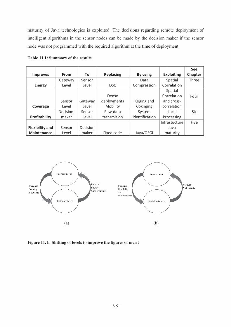
maturity of Java technologies is exploited

intelligent algorithms in the sensor nodes can be m

node was not programmed with the required algorithm

Table 11.1: Summary of the results

(a)

Figure 11.1: Shifting of levels to improve the figures of merit

- 98 -

a technologies is exploited. The decisions regarding remote deployment of

intelligent algorithms in the sensor nodes can be made by the decision maker if the sensor

node was not programmed with the required algorithm at the time of deployment.

Summary of the results

(b)

to improve the figures of merit

he decisions regarding remote deployment of

ade by the decision maker if the sensor

at the time of deployment.

- 99 -

There are many opportunities for future research, especially in the presented statistical data

fusion methods. It is desirable to calculate the experimental variogram (EV) in a distributed

and energy efficient way. Previous research work has been made to calculate the EV based on

aggregation trees that recursively partitions the space into quadrants; the problem with this

approach is that it requires broadcasting to create the trees that are complicated to implement

and energy consuming, and the variogram is only calculated for one fixed distance.

It is also necessary for the development and implementation of a distributed method for the

detection of statistical outliers. It can for example, to compare the amount of sent bits by the

source node with the difference between the mean value and the side information at the

sinking node. The robustness of the approach against dynamic changes in the environment is

also required; the variances and the mean value might change in time. Therefore, the sensor

network must be able to detect if the correlation model is valid at all times.

The presented compression methods must be compared with the existing approaches. The

effect of the network size on its lifetime must also be estimated.

Regarding Java technologies, further research on the nodes energy consumption is required. It

will be interesting to measure the energy and computational performance of the upcoming

OSGi-ME implementations and to test the dynamic updates at the sensor level. Dedicated

Java Virtual Machines and OSGi implementations will be required for more automated and

efficient dynamic updates at the three levels of the ubiquitous applications.

- 100 -

a,c

b,d

C(h)

g

E

G

h

H

H(u,v)

H(u)

i

j

k

K

L

M

n

N

Nk

p

Q(t)

r

R

s

Cokriging weights for the primary variables

Cokriging weights for the secondary variable

Polynomial containing zeros of a linear system

ij-th element of matrix

Set of 2x2 real-valued coregionalization matrices

Polynomial containing poles of linear system

Centred covariance

Polynomial describing a Moving Average process

Bacterial growth rate

Expectation

Relation between prediction error and standard deviation

Exponential factor in Gompertz Model

Lag separation vector

Parity matrix

Mutual information

Marginal entropy

Uncertainty

i-th variogram model

reaction constant in Gompertz Model

Total number of lags

temperature-dependent variable.

Total number of source points for secondary variable

Germ concentration

Binary word size

Total number of source points for primary variable

Number of bits of compressed binary word

Number of samples

Number of destination points

Probability of bit flip

Adaptation gain at time t

Variogram range

Compression rate

Syndrome

- 101 -

S

U

W

y

µ

Θ

Number of basic variogram models

Source information in real-valued domain

Estimated primary variable at point 0

Measured primary variable at point i

Estimated secondary variable at point 0

Measured secondary variable at point i

Weight at lag k

Weight Matrix

Predicted value of Feedback Hammerstein

Measured value for destination point i

Predicted value for destination point i

Isolation loses in a container

Scaling factor that depends of the amount of food

Variogram

Variogram nugget

Variogram sill

ij-th element of matrix

ij-th element of matrix

2x2 matrix of simple and theoretical cross variograms

2x2 matrix of simple and experimental cross variograms

Main value

Quantization step

Interpolation error for destination point i

Average prediction error for all destination points

Prediction Error in Feedback Hammerstein

Variance of variable i

Noise variance of the noise in a binary channel

Additive noise in a binary channel

Lagrange multiplier

Parameter vector

Observation Vector

Forgetting factor

Constant that is fixed for a certain type of fruit

Upper asymptote in Gompertz Model

Displacement in Gompertz Model

- 102 -

A/D

BSC

CI

CK

DISCUS

DSC

EV

GPRS

GV

IDW

IF

KV

LAN

LDPC

LS

MI

M2M

NaN

OK

OSGi

OTA

RH

ROI

Analogue to Digital

Binary Source Channel

Covariance Intersection

Cokriging

Distributed Source Coding Using Syndromes

Distributed Source Coding

Experimental Variogram

General Packet radio Service

Goulard-Voltz

Inverse Distance Weighing

Information Fusion

Kriging Variance

Local Area Network

Low Density Parity Check Codes

Linear Space

Mutual Information

Machine to Machine

Not a Number

Ordinary Kriging

Open Services Gateway initiative

Over the Air

Relative Humidity

Region of Interest

- 103 -

UMTS

WSN

WSS

Universal Mobile Telecommunication System

Wireless Sensor Network

Weighted Sum of Squares

- 104 -

Figure 3.1 Spatial distribution of the measurement points at the walls of the container: (a)

temperature, (b) humidity .................................................................................................... - 17 -

Figure 3.2 Temperature and humidity variability over time at the measurement points on the

walls of the container .......................................................................................................... - 18 -

Figure 3.3 Distributed Source Coding concept: only the decoder has access to Side

Information V ...................................................................................................................... - 18 -

Figure 3.4 Probabilities of bit-flipping of continuous-valued sources ................................ - 19 -

Figure 3.5 Achievable rate regions for Slepian-Wolf coding of two sources ..................... - 20 -

Figure 3.6 Diagram of DISCUS .......................................................................................... - 21 -

Figure 3.7 Source Space partition. The Source is divided into cosset, the bigger the

compression, the lower the number of the hamming distance ............................................ - 22 -

Figure 3.8 Parity matrix H of an 11 × 8 geometry code...................................................... - 22 -

Figure 3.9 Code partition in coset number 5 (a) Graphical representation (b) Possible binary

words ................................................................................................................................... - 23 -

Figure 3.10 Graphical representation of the estimation process. ........................................ - 24 -

Figure 3.11 Conversion from real-valued to binary domain: (a) Linear quantization. (b) Block

Diagram illustrating the working domains .......................................................................... - 25 -

Figure 3.12 Experimental variogram for temperature measurements and its fitting by a

theoretical model. The numbers indicate how many pair of points were available for a given

distance. ............................................................................................................................... - 27 -

Figure 3.13 Tree-based source space partition. The value of the ith bit in u determines the

construction of the linear spaces ......................................................................................... - 28 -

Figure 3.14 Data estimation in a fusion cell........................................................................ - 30 -

Figure 3.15 Probability density function of the random variable U and its relation with the

coset partition. ..................................................................................................................... - 32 -

Figure 3.16 Results for temperature when the container is filled with pallets: (a) spatio-

temporal variogram; (b) rate allocation. .............................................................................. - 35 -

Figure 3.17 Correct estimations for all possible combinations of sensor pairs: (a) using

continuous-valued approach; (b) using the Slepian-Wolf approach .................................. - 38 -

Figure 4.1 Experimental Variogram and models resulting from different estimator

algorithms: (a) Spheric for experiment 8(loaded cold storage room), (b) Gauss for partly filled

- 105 -

truck (experiment 10) and (c) Gauss for sea container loaded with bananas (experiment 11) ... -

45 -

Figure 4.2 Error between prediction and measurements for different methods for Variogram

estimation. Compared with the Null- and the IDW-model. ................................................ - 46 -

Figure 4.3 Relation between Kriging Variance and actual interpolation error for different

methods for Variogram estimation. ..................................................................................... - 47 -

Figure 4.4 Interpolation error as function of the number of neighbours in range for experiment

8 (loaded cold storage room). Total number of source points marked by diamonds. ......... - 48 -

Figure 4.5 Experimental and theoretical variogram and cross-variogram for container with

pallets on the floor: (a) Temperature, (b) Temperature-Humidity and (c) Humidity. The

theoretical variogram is calculated as the sum of an exponential and a spherical model with

parameters according to Table 3 and nugget = 0. ............................................................... - 55 -

Figure 4.6 Comparison of Average Interpolation Errors of single-variable kriging and

cokriging: (a) Empty Container, (b) Container with pallets on the floor ............................ - 56 -

Figure 4.7 Average Interpolation Errors of cokriging vs. Number of Humidity and

Temperature Sensors: (a) Empty Container, (b) Container with pallets on the floor. ........ - 57 -

Figure 4.8 Average CK Variance vs. Number of Humidity and Temperature Sensors: (a)

Empty Container, (b) Container with pallets on the floor ................................................... - 57 -

Figure 4.9 Average Interpolation Errors lower than the threshold: (a) Empty Container, (b)

Container with pallets on the floor. ..................................................................................... - 58 -

Figure 4.10 Difference between Interpolation Errors when the model is fitted with all

measurements and when it is fitted in the under-sampled case for the empty container. ... - 60 -

Figure 5.1 Java technologies [79] ....................................................................................... - 65 -

Figure 5.2 Architecture for CLDC and MIDP [79] ............................................................. - 66 -

Figure 5.3 MIDlet Lifecycle [79] ........................................................................................ - 67 -

Figure 5.4 . Overview of J2ME RMS and MIDlet interfacing [81] .................................... - 67 -

Figure 5.5 Bundle Lifecycle [83] ....................................................................................... - 69 -

Figure 5.6 VTC 6100 Plattform [86] ................................................................................... - 70 -

Figure 5.7 Oracle SunSPOT is Squawk sensor node [87] ................................................... - 72 -

Figure 5.8 Virtenio Preon32 Sensor Node [88] ................................................................... - 73 -

Figure 5.9 Crossbow iMote2 sensor node [90] ................................................................... - 74 -

Figure 5.10 Model of the Feedback-Hammerstein-algorithm [26] ..................................... - 75 -

Figure 5.11 Results of the Dhrystone 2.1 benchmark: (a) Time, (b) Performance in % to the

reference .............................................................................................................................. - 80 -

- 106 -

Figure 5.12 Results of the Linpack benchmark: (a) Mflops, (b) Performance in % to the

reference .............................................................................................................................. - 80 -

Figure 5.13 Performance of Temperature prediction algorithms ........................................ - 81 -

Figure 5.14 Performance of the Gompertz algorithm ......................................................... - 82 -

Figure 5.15 Timing results for matrix inversion ................................................................ - 83 -

Figure 5.16 Comparison of required CPU time to comply with several thresholds ........... - 84 -

Figure 5.17 CK/OK Relation to comply with each threshold .............................................. - 85 -

Figure 5.18 Required time for calculating EV’s and GVz fitting algorithm ....................... - 85 -

Figure 5.19 Diffrence in execution time in % between OSGi and class ............................. - 86 -

Figure 6.1 Connection via dedicated gateway in container [99] ......................................... - 88 -

Figure 6.2 Wireless Sensor Networks compared to RFID and M2M(modified from [2]) .. - 90 -

Figure 6.3 Concept of the demonstrator (M2M communications represented by dashed lines) -

91 -

Figure 6.4 Implementation of the platforms in a refrigerated container ............................. - 93 -

Figure 7.1: Shifting of levels to improve the figures of merit............................................ - 98 -

- 107 -

Table 2.1 Trade-offs between figures of merit in WSN ........................................................ - 6 -

Table 2.2 Information Fusion in WSN ................................................................................ - 15 -

Table 3.1 Limits used for linear quantization and respective quantization steps ................ - 34 -

Table 3.2 Binary entropies and respective temperature and humidity ranges .................... - 34 -

Table 3.3 Average achieved compression rates for three fitted variogram models ........... - 35 -

Table 3.4 Percentage of failed estimations for three models and two weighting schemes for

temperature measurements when the container is filled with pallets on the floor .............. - 36 -

Table 3.5 Summary of accuracy and energy saving results for an exponential variogram

model fitted using the criterion of McBratney and Webster ............................................... - 36 -

Table 3.6 Summary of accuracy and energy savings results for an exponential variogram

model fitted using the criterion of McBratney and Webster when the mean is updated at

discrete intervals .................................................................................................................. - 37 -

Table 4.1 Fixed range parameter for groups of experiments .............................................. - 45 -

Table 4.2 : List of methods that gave the best relation for the different types of experiments -

46 -

Table 4.3 Automatic fitting results for an empty container ................................................ - 54 -

Table 4.4Automatic fitting results for a container with pallets on the floor ....................... - 54 -

Table 4.5 Resulting sill and range values for the best selected model ................................ - 54 -

Table 4.6 Number of Humidity Sensors required for OK and CK interpolations that comply

with different thresholds when the container is empty. ...................................................... - 59 -

Table 4.7: Number of Humidity Sensors required for Ok and CK interpolations that comply

with different thresholds when the container has pallets on the floor. ................................ - 59 -

Table 5.1 Telematic platforms ............................................................................................ - 70 -

Table 5.2 Sensor Plattforms ................................................................................................ - 71 -

Table 5.3 Arrangement of the elements in the algorithm matrices ..................................... - 77 -

Table 5.4 Algorithms tested for every hardware platform. The Goulard-Voltz algorithm[75]

and CK interpolation required for fitting the linear model of coregionalization and perform

cross-attribute fusion are only tested on the Gateway level. ............................................... - 79 -

Table 6.1 Wireless M2M technologies (modified from [104]) ........................................... - 90 -

Table 7.1: Summary of the results ..................................................................................... - 98 -

- 108 -

[1] D. J. A. Bijwaard, et al., "Industry: using dynamic WSNs in smart logistics for fruits

and pharmacy," presented at the Proceedings of the 9th ACM Conference on

Embedded Networked Sensor Systems, Seattle, Washington, 2011.

[2] C. Rhee, et al., "USN applied to Smart Cold Chain based on the mesh wireless sensor

network," presented at the CartaSense, 2011.

[3] AmbientSystems. (2008, February 14). Ambient Systems’ intelligent RFID reduces

fruit and vegetables spoilage. Available:

http://coolchain.org/Websites/cca/Blog/1730299/PR%20-%20Ambient%20RFID.pdf

[4] R. Jedermann, et al., "Demo Abstract: Wireless quality monitoring in the food chain,"

presented at the 6th European Conference on Wireless Sensor Networks, Cork,

Ireland, 2009.

[5] D. Culler. (2003, February 12). 10 Emerging Technologies That Will Change the

World. Available: http://www2.technologyreview.com/featured-story/401775/10-

emerging-technologies-that-will-change-the/2/

[6] M. Becker, et al., "Challenges of Applying Wireless Sensor Networks in Logistics,"

presented at the CEWIT 2009. Wireless and IT driving Healthcare, Energy and

Infrastructure Transformation, 2009.

[7] M. Weiser, "The computer for the 21st century," SIGMOBILE Mob. Comput.

Commun. Rev., vol. 3, pp. 3-11, 1999.

[8] S. S. Iyengar, Fundamentals of sensor network programming: applications and

technology. Hoboken, NJ: Wiley 2011.

[9] Z. Tafa, "Ubiquitous Sensor Networks," in Application and Multidisciplinary Aspects

of Wireless Sensor Networks, L. Gavrilovska, et al., Eds., ed: Springer London, 2011,

pp. 267-268.

[10] F. Schlachter, "No Moore’s Law for batteries," Proceedings of the National Academy

of Sciences, vol. 110, p. 5273, April 2, 2013 2013.

[11] G. Anastasi, et al., "Energy conservation in wireless sensor networks: A survey," Ad

Hoc Netw., vol. 7, pp. 537-568, 2009.

[12] J. Li and P. Mohapatra, "Analytical modeling and mitigation techniques for the energy

hole problem in sensor networks," Pervasive Mob. Comput., vol. 3, pp. 233-254, 2007.

[13] Y. Liyang, et al., "Deploying a Heterogeneous Wireless Sensor Network," in Wireless

Communications, Networking and Mobile Computing, 2007. WiCom 2007.

International Conference on, 2007, pp. 2588-2591.

[14] A. Reinhardt and D. Burgstahler, "Exploiting Platform Heterogeneity in Wireless

Sensor Networks by Shifting Resource-Intensive Tasks to Dedicated Processing

Nodes," in Proceedings of the 14th International Symposium on a World of Wireless,

Mobile and Multimedia Networks (WoWMoM), 2013.

[15] E. Fasolo, et al., "In-network aggregation techniques for wireless sensor networks: a

survey," Wireless Communications, IEEE, vol. 14, pp. 70-87, 2007.

[16] C. Intanagonwiwat, et al., "Directed diffusion for wireless sensor networking,"

IEEE/ACM Trans. Netw., vol. 11, pp. 2-16, 2003.

[17] N. Kimura and S. Latifi, "A survey on data compression in wireless sensor networks,"

in Information Technology: Coding and Computing, 2005. ITCC 2005. International

Conference on, 2005, pp. 8-13 Vol. 2.

[18] D. Petrovic, et al., "Data funneling: routing with aggregation and compression for

wireless sensor networks," in Sensor Network Protocols and Applications, 2003.

- 109 -

Proceedings of the First IEEE. 2003 IEEE International Workshop on, 2003, pp. 156-

162.

[19] T. Arici, et al., "PINCO: a pipelined in-network compression scheme for data

collection in wireless sensor networks," in Computer Communications and Networks,

2003. ICCCN 2003. Proceedings. The 12th International Conference on, 2003, pp.

539-544.

[20] D. Slepian and J. K. Wolf, "Noiseless coding of correlated information sources,"

Information Theory, IEEE Transactions on, vol. 19, pp. 471-480, 1973.

[21] F. Oldewurtel, "Exploiting spatial correlations for efficient communication and

deployment optimisation in wireless sensor networks," PhD Thesis, RWTH, Achen,

2011.

[22] Z. Rezaei and S. Mobininejad, "Energy Saving in Wireless Sensor Networks,"

International Journal of Computer Science & Engineering Survey (IJCSES) vol. 3, p.

14, 2012.

[23] D. Chu, et al., "Approximate Data Collection in Sensor Networks using Probabilistic

Models," in Data Engineering, 2006. ICDE '06. Proceedings of the 22nd International

Conference on, 2006, pp. 48-48.

[24] D. Tulone and S. Madden, "PAQ: Time Series Forecasting for Approximate Query

Answering in Sensor Networks," in Wireless Sensor Networks. vol. 3868, K. Römer,

et al., Eds., ed: Springer Berlin Heidelberg, 2006, pp. 21-37.

[25] D. Tulone and S. Madden, "An energy-efficient querying framework in sensor

networks for detecting node similarities," presented at the Proceedings of the 9th

ACM international symposium on Modeling analysis and simulation of wireless and

mobile systems, Terromolinos, Spain, 2006.

[26] J. Palafox-Albarrán, et al., "Energy-Efficient Parameter Adaptation and Prediction

Algorithms for the Estimation of Temperature Development Inside a Food Container,"

in Lecture Notes in Electrical Engineering - Informatics in Control, Automation and

Robotics, A. J. Cetto, et al., Eds., ed Berlin: Springer, 2011, pp. 77-90.

[27] G. Zito and I. D. Landau, Digital control systems: design, identification and

implementation. London: Springer, 2006.

[28] F. Hu and Q. Hao, Intelligent sensor networks: the integration of sensor networks,

signal processing and machine learning. Boca Raton, Fla.: CRC Press, 2013.

[29] N. Ahmed, et al., "The holes problem in wireless sensor networks: a survey,"

SIGMOBILE Mob. Comput. Commun. Rev., vol. 9, pp. 4-18, 2005.

[30] C.-F. Huang and Y.-C. Tseng, "The coverage problem in a wireless sensor network,"

presented at the Proceedings of the 2nd ACM international conference on Wireless

sensor networks and applications, San Diego, CA, USA, 2003.

[31] S. Meguerdichian, et al., "Coverage problems in wireless ad-hoc sensor networks," in

INFOCOM 2001. Twentieth Annual Joint Conference of the IEEE Computer and

Communications Societies. Proceedings. IEEE, 2001, pp. 1380-1387 vol.3.

[32] L. Lazos and R. Poovendran, "Stochastic coverage in heterogeneous sensor networks,"

ACM Trans. Sen. Netw., vol. 2, pp. 325-358, 2006.

[33] L. Lazos and R. Poovendran, "Coverage In Heterogeneous Sensor Networks," in

Modeling and Optimization in Mobile, Ad Hoc and Wireless Networks, 2006 4th

International Symposium on, 2006, pp. 1-10.

[34] A. Ali, et al., "Information Driven Approach for Sensor Positioning in Wireless

Sensor Networks," presented at the INFORMATIK 2011 Informatik schafft

Communities 4.–7. , Berlin, 2011.

[35] M. Umer, et al., "Kriging for Localized Spatial Interpolation in Sensor Networks,"

presented at the Proceedings of the 20th international conference on Scientific and

Statistical Database Management, Hong Kong, China, 2008.

- 110 -

[36] A. Krause and C. Guestrin, "Optimizing Sensing: From Water to the Web," Computer,

vol. 42, pp. 38-45, 2009.

[37] A. Krause, et al., "Robust submodular observation selection," Journal of Machine

Learning Research, vol. 9, pp. 008) 2761-, 2008.

[38] F. Szidarovszky, "Multiobjective observation network design for regionalized

variables," International Journal of Mining Engineering, vol. 1, pp. 331-342,

1983/12/01 1983.

[39] CrossBow. (2013, September 5 2013). TelosB Datasheet. Available:

http://www.willow.co.uk/TelosB_Datasheet.pdf

[40] (TinyOS, September 5 2013). TinyOS Web page. Available: http://www.tinyos.net/

[41] I. Mahgoub and M. Ilyas, Smart dust: sensor network applications, architecture, and

design. Boca Raton, Fla.: CRC, Taylor & Francis, 2006.

[42] H. B. Mitchell, Data fusion: concepts and ideas. Berlin Springer, 2012.

[43] R. Boudjemaa and A. B. Forbes, Parameter Estimation Methods for Data Fusion:

National Physical Laboratory.Great Britain, Centre for Mathematics and Scientific

Computing, 2004.

[44] E. F. Nakamura, et al., "Information fusion for wireless sensor networks: Methods,

models, and classifications," ACM Comput. Surv., vol. 39, p. 9, 2007.

[45] R. Faragher, "Understanding the Basis of the Kalman Filter Via a Simple and Intuitive

Derivation [Lecture Notes]," Signal Processing Magazine, IEEE, vol. 29, pp. 128-132,

2012.

[46] J. Bibby and H. Toutenburg, Prediction and improved estimation in linear models.

Chichester Wiley, 1977.

[47] X. R. Li, et al., "Optimal linear estimation fusion .I. Unified fusion rules," Information

Theory, IEEE Transactions on, vol. 49, pp. 2192-2208, 2003.

[48] M. Kanevski and M. Maignan, Analysis and modelling of spatial environmental data

Lausanne: EPFL Press, 2004.

[49] R. Jedermann and W. Lang, "The Minimum Number of Sensors --- Interpolation of

Spatial Temperature Profiles in Chilled Transports," presented at the Proceedings of

the 6th European Conference on Wireless Sensor Networks, Cork, Ireland, 2009.

[50] R. Jedermann, et al., "Interpolation of spatial temperature profiles by sensor

networks," in Sensors, 2011 IEEE, 2011, pp. 778-781.

[51] A. R. Murugan, et al., "Correlated sources over wireless channels: cooperative source-

channel coding," Selected Areas in Communications, IEEE Journal on, vol. 22, pp.

988-998, 2004.

[52] (2012, February 12). ASN Inc. Available: http://www.asn-inc.co.kr/

[53] (2012, February 12). Datasheet SHT20. Available:

http://www.sensirion.com/fileadmin/user_upload/customers/sensirion/Dokumente/Hu

midity/Sensirion_Humidity_SHT20_Datasheet.pdf

[54] J. Chou, et al., "A distributed and adaptive signal processing approach to reducing

energy consumption in sensor networks," in INFOCOM 2003. Twenty-Second Annual

Joint Conference of the IEEE Computer and Communications. IEEE Societies, 2003,

pp. 1054-1062 vol.2.

[55] J. Chou, et al., "Tracking and exploiting correlations in dense sensor networks," in

Signals, Systems and Computers, 2002. Conference Record of the Thirty-Sixth

Asilomar Conference on, 2002, pp. 39-43 vol.1.

[56] M. Vaezi and F. Labeau, "Improved modeling of the correlation between continuous-

valued sources in LDPC-based DSC," in Signals, Systems and Computers

(ASILOMAR), 2012 Conference Record of the Forty Sixth Asilomar Conference on,

2012, pp. 1659-1663.

- 111 -

[57] S. S. Pradhan and K. Ramchandran, "Distributed source coding using syndromes

(DISCUS): design and construction," in Data Compression Conference, 1999.

Proceedings. DCC '99, 1999, pp. 158-167.

[58] E. Berlekamp, et al., "On the inherent intractability of certain coding problems

(Corresp.)," Information Theory, IEEE Transactions on, vol. 24, pp. 384-386, 1978.

[59] J. G. Proakis and M. Salehi, Digital communications, 5. ed., internat. ed. ed. Boston

2008: McGraw-Hill.

[60] J. M. Walsh and P. A. Regalia, "On the Relationship Between Belief Propagation

Decoding and Joint Maximum Likelihood Detection," Communications, IEEE

Transactions on, vol. 58, pp. 2753-2758, 2010.

[61] V. Stankovic, et al., "On code design for the Slepian-Wolf problem and lossless

multiterminal networks," Information Theory, IEEE Transactions on, vol. 52, pp.

1495-1507, 2006.

[62] W. Schwanghart. (2009, Description of the 'variogramfit' function. Available:

http://www.mathworks.com/matlabcentral/fileexchange/25948-variogramfit

[63] J. A. Nelder and R. Mead, A simplex method for function minimization, 1964.

[64] N. Cressie, "Fitting variogram models by weighted least squares," Journal of the

International Association for Mathematical Geology, vol. 17, pp. 563-586, 1985/07/01

1985.

[65] A. B. McBratney and R. Webster, "Choosing functions for semi-variograms of soil

properties and fitting them to sampling estimates," Journal of Soil Science, vol. 37, pp.

617-639, 1986.

[66] S. J. Julier and J. K. Uhlmann, "A non-divergent estimation algorithm in the presence

of unknown correlations," in American Control Conference, 1997. Proceedings of the

1997, 1997, pp. 2369-2373 vol.4.

[67] M. B. Hurley, "An information theoretic justification for covariance intersection and

its generalization," in Information Fusion, 2002. Proceedings of the Fifth

International Conference on, 2002, pp. 505-511 vol.1.

[68] V. Popovich, Information fusion and geographic information systems: towards the

digital ocean. Berlin Springer, 2011.

[69] H. Wackernagel, Multivariate geostatistics: an introduction with applications 3ed.

Berlin Springer, 2003.

[70] R. Jedermann, et al., "Modelling and interpolation of spatial temperature during food

transportation and storage by the Variogram," in The 10th International Conference

on Modeling and Applied Simulation (MAS 2011), Rome, Italy, 2011, pp. 195-201.

[71] J. Chiles and P. Delfiner, Geostatistics: Modeling Spatial Uncertainty, second ed.

New Jersey: Wiley, 2012.

[72] J. Rodríguez-Bermejo, et al., "Thermal study of a transport container," Journal of

Food Engineering, vol. 80, pp. 517-527, 2007.

[73] SealedAir. (2013, September 30). TurboTag® System. Available:

http://www.sealedairspecialtymaterials.com/eu/de/products/turbotag.aspx

[74] Maxim. (2013, September 30). Button Devices. Available:

http://www.maximintegrated.com/products/ibutton/

[75] M. Goulard and M. Voltz, "Linear coregionalization model: Tools for estimation and

choice of cross-variogram matrix," Mathematical Geology, vol. 24, pp. 269-286,

1992/04/01 1992.

[76] J. Chiles and P. Delfiner, Geostatistics: Modeling Spatial Uncertainty, first ed. New

Jersey: Wiley, 1999.

[77] X. Emery, "Iterative algorithms for fitting a linear model of coregionalization,"

Computers & Geosciences, vol. 36, pp. 1150-1160, 2010.

- 112 -

[78] M. Yarvis, et al., "Exploiting heterogeneity in sensor networks," in INFOCOM 2005.

24th Annual Joint Conference of the IEEE Computer and Communications Societies.

Proceedings IEEE, 2005, pp. 878-890 vol. 2.

[79] R. B. Hayun and S. Mason, Java ME on Symbian OS: [inside the Smartphone model].

Chichester: Wiley, 2009.

[80] R. Teodorescu and R. Pandey, "Using JIT Compilation and Configurable Runtime

Systems for Efficient Deployment of Java Programs on Ubiquitous Devices," in

Ubicomp 2001: Ubiquitous Computing. vol. 2201, G. Abowd, et al., Eds., ed: Springer

Berlin Heidelberg, 2001, pp. 76-95.

[81] IBM. (2013, Oktober 7). J2ME record management store. Available:

http://www.ibm.com/developerworks/library/wi-rms/

[82] O. Alliance. (2013, September 5 2013). OSGi Alliance. Available:

http://www.osgi.org/Main/HomePage

[83] G. Wutherich, et al., Die OSGi-Service-Platform: eine Einfuhrung mit Eclipse

Equinox, 1 ed. Heidelberg: dpunkt.verl., 2008.

[84] F. Böse and K. Windt, "Catalogue of Criteria for Autonomous Control in Logistics,"

in Understanding Autonomous Cooperation and Control in Logistics, M. Hülsmann

and K. Windt, Eds., ed: Springer Berlin Heidelberg, 2007, pp. 57-72.

[85] Eurotech. (2013, February 12). Duranav 1000. Available:

http://www.eurotech.com/en/products/DuraNAV

[86] Nexcom. (2013, February 12). VTC 6100. Available:

http://www.nexcom.com/Products/mobile-computing-solutions/in-vehicle-pc/in-

vehicle-pc/car-pc-vtc-6100

[87] Oracle. (2013, SunSPOT. Available: http://www.sunspotworld.com/

[88] Virtenio. (2013, July 2013). Preon32. Available:

http://www.virtenio.com/en/products/radio-module.html

[89] Aicas. (2013, November 14). JamaicaVM. Available:

https://www.aicas.com/cms/en/JamaicaVM

[90] CrossBow. (2013, Imote2. Available: http://www.xbow.jp/Imote2.Builder_kit.pdf

[91] R. P. Weicker, "An overview of common benchmarks," Computer, vol. 23, pp. 65-75,

1990.

[92] G. J. E. Nychas, et al., "Meat, poultry and seafood," ed Washington: ASM Press,

2007, pp. 105-140.

[93] E. Borch, et al., "Bacterial spoilage of meat and cured meat products," International

Journal of Food Microbiology, vol. 33, pp. 103-120, 1996.

[94] J. Kreyenschmidt, et al., "Determination of the shelf life of sliced cooked ham based

on the growth of lactic acid bacteria in different steps of the chain," Journal of applied

microbiology, vol. 108, pp. 510-520, 2010.

[95] A. Dannies, et al., "Feasibility of shifting decision support tools for quality estimation

in food logistics to the sensor node level," presented at the 6th International

Conference on Software Knowledge Information Management and Applications

(SKIMA), Chengdu University, 2012.

[96] A. Dannies, et al., "Dynamic Java Components in Pervasive Systems - A Review of

the Feasibility of Dynamic Data Processing on Wireless Platforms," in PECCS 2012 -

International Conference on Pervasive and Embedded Computing and

Communication Systems, Rome, Italy, 2012, pp. 58-66.

[97] A. Dannies, et al., "Smart dynamic software components enabling decision support in

Machine-to-machine networks," JCSI International Journal of Computer Science

Issues, Vol. 10, Issue 1, No 3, www.IJCSI.org, vol. 10, pp. 540-550, January 2013

2013.

- 113 -

[98] NIST. September 2013). JAMA: A Java Matrix Package. Available:

math.nist.gov/javanumerics/jama

[99] S. Zöller, et al. (2010, Deployment oft Wireless Sensor Networks in Logistics-

Potential, Requirements and a Testbed.

[100] W. Webb, Understanding Weightless: [technology, equipment, and network

deployment for M2M communications in white space]. Cambridge Cambridge Univ.

Press, 2012.

[101] D. Boswarthick, et al., M2M communications: a systems approach. Chichester: Wiley,

2012.

[102] Zigbee. (2013, October 16). Zigbee Alliance. Available: http://www.zigbee.org/

[103] Dash7. (2013, October 16). Dash7 Alliance. Available: http://www.dash7.org/

[104] P. Antonio, et al., "Architecture and Methods for Innovative Heterogeneous Wireless

Sensor Network Applications," Remote Sensing, vol. 4, pp. 1146-1161, 2012.

[105] H. Stütgen. The M2M Cloud Evolution. Available:

http://www.nec.com/en/event/mwc/pdf/18.pdf

[106] J. Palafox-Albarrán, et al., "Combining Machine-to-Machine Communications with

Intelligent Objects in Logistics," in ImViReLL'12 The Impact of Virtual, Remote and

Real Logistics Labs, Bremen, Germany, 2012, pp. 102-112.

[107] E. Ortiz. (2002, September 5 2013). Introduction to OTA Application Provisioning.

Available: http://www.oracle.com/technetwork/systems/ota-156595.html

[108] D. Puccinelli and M. Haenggi, "Wireless sensor networks: applications and challenges

of ubiquitous sensing," Circuits and Systems Magazine, IEEE, vol. 5, pp. 19-31, 2005.

[109] K. Fehrenbacher. (2010, November 18th). Dear Friedman: There Is No Moore’s Law

for Batteries. Available: http://gigaom.com/2010/09/27/dear-friedman-there-is-no-

moores-law-for-batteries/

[110] TinyOS. (2013, September 5 2013). TinyOS Web page. Available:

http://www.tinyos.net/

[111] Z. Shelby and C. Bormann, 6LoWPAN: the wireless embedded internet. Chichester:

Wiley, 2009.

- 114 -

Book Chapters

J. Palafox-Albarrán, R. Jedermann, W. Lang, Energy-Efficient Parameter

Adaptation and Prediction Algorithms for the Estimation of Temperature

Development Inside a Food Container, in: A.J. Cetto, J.-L. Ferrier, J.

Filipe (Eds.) Lecture Notes in Electrical Engineering - Informatics in

Control, Automation and Robotics, Springer, Berlin, 2011, pp. 77-90.

R. Jedermann, J. Palafox-Albarrán, A. Jabbari, W. Lang, Embedded

intelligent objects in food logistics - Technical limits of local decision

making, in: M. Hülsmann, B. Scholz-Reiter, K. Windt (Eds.)

Autonomous Cooperation and Control in Logistics, Springer, Berlin,

2011, pp. 207-228.

Journals (accepted)

A. Dannies, J. Palafox-Albarrán, W. Lang, R. Jedermann, Smart

dynamic software components enabling decision support in Machine-to-

machine networks, JCSI International Journal of Computer Science

Issues, Vol. 10, Issue 1, No 3, www.IJCSI.org, 10 (2013) 540-550.

Journals (under review)

J. Palafox-Albarran, R. Jedermann,B. Hong, W. Lang, Cokriging for

cross-attribute fusion in sensor networks. Under second review.

Submitted to Elsevier’s Information Fusion Journal Impact Factor:

2.262. 5-Year Impact Factor:2.838

J. Palafox-Albarran, B. Hong, W. Lang, R. Jedermann, A statistical

method for Data Compression and Recovery Between Continuous-

Valued Sources in WSN. Being Submitted to International Journal of

Sensor Networks (IJSNet) Impact Factor: 1.386

- 115 -

Conferences

J. Palafox-Albarrán, R. Jedermann, W. Lang, Prediction of temperature

inside a refrigerated container in the presence of perishable goods, in:

7th International Conference on Informatics in Control, Automation and

Robotics (ICINCO), Funchal, Portugal, 2010.

R. Jedermann, J. Palafox-Albarrán, J. Barreiro, L. Ruiz-Garcia, J.I.

Robla, P.D.-I.W. Lang, Modelling and interpolation of spatial

temperature during food transportation and storage by the Variogram, in:

The 10th International Conference on Modeling and Applied Simulation

(MAS 2011), Bruzzone, A.; et. al.,(eds.), Rome, Italy, 2011, pp. 195-

201.

R. Jedermann, J. Palafox-Albarrán, J.I. Robla, J. Barreiro, L. Ruiz-

Garcia, P.D.-I.W. Lang, Interpolation of Spatial Temperature Profiles by

Sensor Networks, in: 2011 IEEE SENSORS Proceedings, IEEE,

Limerick, Ireland, 2011, pp. 778-781.

J. Palafox-Albarrán, A. Dannies, B.K. Sanjeeva, W. Lang, R. Jedermann,

Combining Machine-to-Machine Communications with Intelligent

Objects in Logistics, in: D. Uckelmann, B. Scholz-Reiter, I. Rügge, B.

Hong, A. Rizzi (Eds.) ImViReLL'12 The Impact of Virtual, Remote and

Real Logistics Labs, Springer, Bremen, Germany, 2012, pp. 102-112

A. Dannies, J. Palafox-Albarrán, R. Jedermann, W. Lang, Feasibility of

shifting decision support tools for quality estimation in food logistics to

the sensor node level, in: 6th International Conference on Software

Knowledge Information Management and Applications (SKIMA),

Chengdu University, 2012, pp. 5.

Dannies, J. Palafox-Albarrán, W. Lang, R. Jedermann, Dynamic Java

Components in Pervasive Systems - A Review of the Feasibility of

Dynamic Data Processing on Wireless Platforms, in: C. Benavente-

Peces, F. Ali, J. Filipe (Eds.) PECCS 2012 - International Conference on

- 116 -

Pervasive and Embedded Computing and Communication Systems, 2012

SciTePress – Science and Technology Publications, Rome, Italy, 2012,

pp. 58-66.

H. Zhang, N. El-Berishy, D. Zastrau, S.N.K. Marwat, Y. Tan, J. Palafox-

Albarrán, I. Rügge, Interdisciplinary perspective on knowledge

management in logistics, in: LogistikManagement 2013, Bremen,

Germany, 2013.

Magazines/Research Reports

J. Palafox-Albarran, DASH7 applications, First issue of the Dash7

University Working Group (UWG)Magazine., (2012) 20-23.

J. Palafox-Albarran, A. Dannies, B.K. Sanjeeva, W. Lang, R. Jedermann,

Machine-to-Machine Communications and Intelligent Objects in

refrigerated containers Research Report 2012/13 International Graduate

School for Dynamics in Logistics, (2013).

J. Palafox-Albarran, R. Jedermann, W. Lang, Temperature Prediction

Inside a Refrigerated Food Container, Research Report 2010/11

International Graduate School for Dynamics in Logistics, (2011) 41-50.