Embed Size (px)
Citation preview
8/10/2019 speziale 1990
http://slidepdf.com/reader/full/speziale-1990 1/60
DTIC
ILE
COPY
00
NASA
Contractor Report
182017
00
ICASE Report
No.
90-26
O
ICASE
ANALYTICAL METHODS
FOR THE
DEVELOPMENT
OF
REYNOLDS
STRESS
CLOSURES
IN TURBULENCE
Charles G.
Speziale
Contract
No.
NAS1-18605
March 1990
Institute
for Computer
Applications
in Science
and
Engineering
NASA
Langley
Research
Center
Hampton, Virginia
23665-5225
Operated
by the Universities
Space
Research
Association
DTIC
S
ELECTE
OCT04
1990
D
J/SA
and
DIS
T
R
HBUTION
STATEMk.NL
A
National
Aeronautics
and
Approved
for p.u41c 00ase;
Space
Administration
Distnbutfion.U irnlt"
Langley
Research
Center
Hampton,
Virginia
23665-5225
9
904~4
8/10/2019 speziale 1990
http://slidepdf.com/reader/full/speziale-1990 2/60
ANALYTICAL
METHODS
FOR
THE DEVELOPMENT
OF REYNOLDS
STRESS
CLOSURES
IN
TURBULENCE
Charles G.
Speziale*
Institute
for Computer
Applications
in Science
and Engineering
NASA
Langley
Research Center
Hampton, VA 23665
ABSTRACT
Analytical
methods
for the
development of
Reynolds
stress
models
in
turbulence
are
reviewed in detail.
Zero,
one and two
equation models are
discussed along
with
second-order
closures.
A strong case
is made
for the superior predictive
capabilities
of
second-order closure
models
in comparison
to
the simpler models.
The central
points of
the
paper
are illustrated
by examples from
both homogeneous
and
inhomogeneous turbulence.
A discussion of the
author's views
concerning
the
progress
made
in
Reynolds
stress
modeling is
also
provided
along with a brief history
of the subject.
3n
'or
S ::ccd 5]
,
:-
jcatlon
ca
_
t
i
on
-
Availability
Codes
Avail
and/or
ist
Special
'This
research
was
supported
by
the
National Aeronautics
and Space Administration
under
NASA Con-
tract No.
NAS1-18605
while the author was
in residence
at
the
Institute for Computer
Applications
in
Science and Engineering
(ICASE),
NASA Langley Research
Center,
Hampton,
VA 23665.
i
8/10/2019 speziale 1990
http://slidepdf.com/reader/full/speziale-1990 3/60
INTRODUCTION
Despite
over a century of research,
turbulence
remains
the
major
unsolved
problem
of
classical physics.
While most researchers agree that the essential physics
of turbulent
flows
can be described
by the
Navier-Stokes
equations, limitations
in computer capacity
make
it
impossible
-
for
now and the foreseeable
future
-
to
directly
solve
these equations in
the complex
turbulent
flows of
technological interest. Hence, virtually all scientific
and
engineering calculations of non-trivial turbulent flows,
at high Reynolds numbers, are based
on some type of modeling.
This modeling can
take
a variety of forms:
(a)
Reynolds
stress
models
which allow
for the calculation of one-point first
and second
moments
such as
the mean
velocity,
mean pressure
and
turbulent kinetic
energy.
(b) Subgrid-scale models for
large-eddy simulations wherein the large,
energy containing
eddies
are
computed
directly
and
the effect of
the
small
scales
-
which
are more
universal
in
character
- are modeled.
(c) Two-point
closures or
spectral
models which provide
more
detailed
information about
the
turbulence
structure
since
they are based on the
two-point velocity correlation
tensor
(d) Pdf
models based on the joint probability density function.
Large-eddy simulations
(LES)
have
found
a
variety
of
important
geophysical
applications
where they have been used in weather forecasting as well
as in other atmospheric studies
(cf.
Deardorff 1973, Clark and
Farley
1984, and Smolarkiewicz
and Clark
1985). Likewise,
LES
has shed new
light on the
physics of
certain basic turbulent flows - which include homoge-
neous
shear
flow and channel
flow
-
at
higher
Reynolds
numbers that
are
not accessible
to di-
rect simulations (cf.
Moin and Kim 1982,
Bardina,
Ferziger and Reynolds
1983, Rogallo
and
Moin 1984, and
Piomelli,
Ferziger and Moin 1987).
Two-point closures such as
the EDQNM
model of Orszag
(1970)
have been quite
useful in the analysis of homogeneous
turbulent
flows where
they have provided
new
information
on the structure of
isotropic turbulence (cf.
Lesieur
1987)
and
on
the
effect
of
shear
and
rotation
(cf.
Bertoglio
1982).
However,
there
are a variety of
theoretical
and operational
problems with two-point closures and
large-eddy
simulations that
make
their application to strongly
inhomogeneous turbulent flows difficult,
if not impossible
- especially in irregular geometries with
solid
boundaries. There have been
no applications of
two-point closures to wall-bounded turbulent flows and virtually all
such
applications of LES have been
in
simple
geometries where Van Driest damping could
be
used
1
8/10/2019 speziale 1990
http://slidepdf.com/reader/full/speziale-1990 4/60
-
an
empirical
approach
that generally
does not work
well when
there is flow
separation.
Comparable
problems
in dealing with wall-bounded
flows
have, for the
most part, limited
methods to
free
turbulent
flows where
they have
been quite useful in the
description
of
chemically
reacting turbulence
(see
Pope
1985).
Since most
practical
engineering flows
involve complex
geometries
with
solid
boundaries
-
at
Reynolds numbers
that
are
far
higher
than those
that are accessible
to
direct
simulations
-
the preferred
approach
has
been
to
base
such
calculations
on
Reynolds stress modeling.t
This forms the
motivation for
the
present
review paper whose
purpose
is to put
into perspective some of
the more
recent theoretical
developments
in Reynolds
stress
modeling.
The concept of
Reynolds averaging
was
introduced by Sir Osborne
Reynolds
in
his
land-
mark turbulence
research of the latter
part of
the nineteenth
century (see
Reynolds 1895).
During a
comparable time frame,
Boussinesq (1877)
introduced the
concept of the
turbulent
or eddy
viscosity as the
basis
for
a
simple time-averaged
turbulence
closure. However,
it
was
not
until
after 1920
that the first successful
calculation
of a practical turbulent
flow was
achieved
based on the
Reynolds averaged
Navier-Stokes
equations with an eddy
viscosity
model.
This was
largely due to the
pioneering
work
of
Prandtl (1925)
who
introduced
the
concept of
the mixing
length
as
a
basis
for the
determination of
the
eddy viscosity. This
mix-
ing
length model
led
to closed
form solutions
for turbulent
pipe and
channel
flows
that were
remarkably successful
in
collapsing
the
existing
experimental
data. A
variety of turbulence
researchers
- most
notably
including
Von Karmadn
(1930,
1948) - made further
contributions
to
the
mixing
length approach which continued
to be a
highly active
area of research
until
the
post
World War II
period.
By
this time it
was
clear
that
the
basic
assumptions
behind
the
mixing
length approach
-
which
makes a direct
analogy between turbulent transport
processes
and
molecular transport
processes
-
were
unrealistic; turbulent
flows
do not have
a
clear
cut separation
of
scales.
With
the
desire
to
develop
more general
models, Prandtl
and
Wieghardt
(1945)
tied
the
eddy
viscosity
to
the
turbulent
kinetic
energy which was
obtained
from
a
separate modeled
transport
equation. This was a
precursor
to the one
equa-
tion
models
of
turbulence
-
or
so
called
K -
I
models
- wherein the
turbulent
length
scale
i
is specified empirically
and
the turbulent
kinetic energy
K
is
obtained
from a modeled
transport
equation. However,
these models
still
suffered
from
the deficiencies
intrinsic
to all
eddy viscosity
models:
the inability to properly
account
for
streamline curvature
and
history
effects on
the
individual Reynolds
stress components.
In a
landmark
paper by Rotta
(1951), the
foundation
was
laid for
a full
Reynolds stress
turbulence
closure which was
to
ultimately
change
the course
of Reynolds stress
modeling.
tIn
fact,
the only a tcrnative
of
comparable
simplicity
is
the
vorticity transport
theory
of Taylor (1915);
a
three-dimensional
vorticity covariance
closure along these
lines
has been
recently
pursued by Bernard and
co-workers (cf.
Bernard and Berger
1982).
2
8/10/2019 speziale 1990
http://slidepdf.com/reader/full/speziale-1990 5/60
This new approach of Rotta - which
is now
referred to as
second order
or
second moment
closure - was based on
the
Reynolds stress
transport equation. By making use of some of the
statistical ideas of Kolmogorov from the 1940's
-
and
by
introducing some entirely
new
ideas
- Rotta
succeeded
in
closing
the Reynolds stress
transport
equation.
This
new
Reynolds
stress
closure,
unlike eddy viscosity
models, accounted for both history and
nonlocal effects
on the evolution of the Reynolds stress tensor - features whose
importance
had
long
been
known. However,
since
this approach required the solution of an additional
six
transport
equations for
the
individual components of
the Reynolds
stress tensor,
it was
not
to
be
computationally
feasible
for the next few decades to
solve complex
engineering
flows
based
on a
full
second-order closure.
By
the 1970's,
with
the
wide availability of high speed
computers, a
new
thrust in
the
development
and implementation of sec',ad-order closure
models began with the
work
of Daly and Harlow (1970) and Donaldson
(1972).
In an
important
paper, Launder,
Reece
and Rodi (1975) developed a
new
second-order
closure
model
that
improved significantly on the earlier
work of
Rotta (1951).
This paper developed
more systematic
models
for the pressure-strain correlation and turbulent transport terms; a
modeled
transport
equation for the turbulent dissipation
rate was
solved
in conjunction with
this Reynolds stress closure.
However, more
importantly,
Launder,
Reece
and
Rodi
(1975)
showed
how
second-order closure
models
could
be
calibrated and applied
to
the solution of
practical engineering
flows. When the Launder,
Reece
and Rodi (1975) model is
contracted
and supplemented with an eddy viscosity representation
for the
Reynolds
stress, a two-
equation model
(referred to as the K - c model) is obtained which is identical to that
derived by Hanjalic and Launder
(1972)
a few years earlier. Because of
the
substantially
lower
computational
effort
required,
the
K
-
e
model
is
still
one
of
the
most
commonly
used
turbulence models for
the
solution of practical
engineering
problems.
Subsequent to the publication of the paper by Launder,
Reece and Rodi
(1975),
a variety
of turbulence modelers
have continued research
on
second-order closures.
Lumley
(1978)
in-
troduced the
important
constraint
of realizability and made
significant
contributions to
the
modeling
of
the
pressure-strain correlation. Launder and co-workers continued to expand
on the refinement
and application of second-order closure
models
to problems of significant
engineering interest (see Launder 1989). Speziale (1985, 1987a) exploited invariance argu-
ments - along with consistency conditions for solutions
of the
Navier-Stokes equations in
a
rapidly rotating
frame
-
to
develop
new
models
for
the rapid pressure-strain
correlation.
Haworth and Pope
(1986) developed a second-order closure
model
starting from the pdf
based
Langevin
equation.
Reynolds (1988)
has
attempted
to develop models
for the rapid
pressure-strain
correlation by using Rapid
Distortion
Theory.
In this paper, analytical methods
for
the derivation of Reynolds
stress models will be
3
8/10/2019 speziale 1990
http://slidepdf.com/reader/full/speziale-1990 6/60
reviewed. Zero,
one
and
two-equation models
will be considered
along with
second-order
closures.
Two approaches to
the
development of models will
be discussed:
(1) The continuum
mechanics
approachwhich
is typically based
on a Taylor expansion.
Invariance
constraints
-
as
well
other
consistency conditions
such
as
Rapid Distortion
Theory
(RDT)
and realizability
- are
then
used to simplify
the
model.
The remaining
constants
are evaluated by reference
to benchmark
physical
experiments.
(2)
The
statistical
mechanics
approach
which
is
based on
the construction
of an asymp-
totic
expansion. Unlike in the
continuum
mechanics approach,
here the
constants
of
the
model
are calculated
explicitly. The two
primary
examples
of
this approach
are the two-scale
DIA models
of Yoshizawa
(1984)
and
the
Renormalization Group
(RNG)
models
of Yakhot and Orszag (1986).
The
basic
methodology
of these
two techniques will
be
examined,
however,
more emphasis
will
be placed
on the continuum mechanics
approach since there
is a larger
body of literature
on this
method
and since
it has been
the author's
preferred approach. The
strengths an d
weaknesses of
a variety of
Reynolds
stress
models will
be discussed in
detail and illustrated
by examples. A
strong
case will
be
made
for
the
superior
predictive capabilities of
second-
order closures
in comparison to the older zero,
one
and two-equation models.
However,
some significant deficiencies
in the
structure of
second-order
closures that
still remain will be
pointed
out.
These
issues, as well as
the author's
views concerning
possible future directions
of
research,
will
be discussed in
the
sections
to
follow.
BASIC
EQUATIONS
OF REYNOLDS STRESS
MODELING
We
will consider the turbulent
flow
of
a
viscous,
incompressible
fluid
with
constant
prop-
erties
(limitations of
space will not allow
us to discuss
compressible
turbulence modeling
in
any
detail). The governing field
equations
are
the Navier-Stokes
and continuity
equations
which are
given by
a -X
+vV ui
(1)
aui
,axi 0 (2)
where ui
is the
velocity
vector,
p
is the modified
pressure (which can
include a
gravitational
potential),
and
v is the kinematic
viscosity of
the fluid. In (1) - (2),
the Einstein summation
convention
applies
to repeated indices.
4
8/10/2019 speziale 1990
http://slidepdf.com/reader/full/speziale-1990 7/60
The
velocity
and
pressure are
decomposed
into
mean and
fluctuating
parts as follows:
Ui=Ui Ui,
p=P P
(3)
It is assumed
that any flow
variables
4 and 4p
obey the
Reynolds averaging
rules
(cf.
Tennekes
and
Lumley
1972):
= =0(4)
€- ; + €
(5)
;
07
(6)
In a statistically
steady
turbulence,
the
mean of a
flow variable
4
can be
taken
to
be
the
simple
time
average
h)_
1
O(x, t)dt,
(7)
whereas for
a
spatially
homogeneous
flow,
a
volume average can
be
used
0
=
v_-lim
-
O
q(x
)da
(X.
For
more
general
turbulent
flows
that
are
neither statistically
steady nor
homogeneous, the
mean
of
any flow
variable
0
is taken to be the
ensemble mean
lm
1: OM
)x t)
(9)
where
an
average is taken over
N
repeated
experiments. The
ergodic hypothesis
is
assumed
to
apply
-
namely,
in a statistically
steady turbulent
flow
it
is
assumed
that
4)
=
4) (10)
and in a
homogeneous turbulent
flow
it is assumed
that
4v =4).
(11)
The
Reynolds equation
- which physically
corresponds
to a
balance of mean
linear
mo-
mentum
-
takes
the
form
a- Uj
-
= _
,
+
V2U -i
(12)
where
-
u .(13)
5
8/10/2019 speziale 1990
http://slidepdf.com/reader/full/speziale-1990 8/60
is
the
Reynolds stress tensor.
Equation
(12)
is
obtained by substituting
the
decompositions
(3)
i-to
the
Navier-Stokes equation
(1) and then
taking an
ensemble
mean. The
mean
continuity equation is
given
by
_o
(14)
axi
and
is obtained by simply taking
the
ensemble
mean of (2). Equations
(12) - (14)
do
not
represent a
closed system for the determination of
the mean velocity Ui and
mean pressure
p
due to the additional six
unknowns contained
within the Reynolds stress tensor. The
problem of Reynolds stress closure
is to tie the Reynolds
stress tensor to
the
mean velocity
field in
some
physically
consistent fashion.
In order
to
gain greater insight
into the problem of Reynolds
stress closure, we
will
now
consider
the
governing
field equations for
the fluctuation dynamics. The
fluctuating
momentum
equation -
from
which u is
determined - takes
the
form
u
+
=U
(15)
and is obtained by
subtracting (12) from
(1) after the decompositions
(3) are introduced.
The fluctuating continuity
equation, which is obtained
by subtracting (14) from (2),
is given
by
0. (16)
Equations (15)
- (16)
have solutions for the fluctuating
velocity
u
that
are
of the
general
mathematical form
u x, t) = [U
(y,
s), u'(y, 0), u'(y,
s)jav; x, t] y
E
V,
s
E
(-oo,
t)
(17)
where
Fj[
• ]
denotes a functional,
V
is
the volume
of
the fluid,
and OV is its bounding
surface. In alternative terms,
the
fluctuating velocity
is
a
functional of
the global history
of the mean
velocity field with an implicit
dependence on
its
own
initial
and
boundary
conditions.
Here
we
use the term
functional in its broadest
mathematical
sense,
namely, any
quantity determined
by a function. From
(17), we can explicitly
calculate the
Reynolds
stress
tensor
'ri
=
uu which will
also be a functional
of the global history
of the mean velocity.
However,
there
is
a serious
problem
in
regard
to
the
dependence
of
rij
on
the
initial
and
boundary conditions for
the
fluctuating
velocity as
discussed by Lumley (1970).
There is no
hope for a
workable
Reynolds stress closure
if there is a detailed dependence
on
such
initial
and boundary
conditions. For turbulent
flows that are sufficiently far from solid
boundaries
-
and sufficiently
far evolved in
time
past their initiation
- it is not unreasonable
to assume
that
the initial
and boundary
conditions
on
the
fluctuating velocity
(beyond those
for
rj)
6
8/10/2019 speziale 1990
http://slidepdf.com/reader/full/speziale-1990 9/60
merely set the
length
and time scales
of
the turbulence.
Hence,
with this
crucial
assumption,
we
obtain
the
expression
'rij(x,t)
=
Ij[U(y,
S), o(y, S),
-ro(y,
S); x,
t]
y
e
V, S E (-o,
t)
(18)
where
to is
the turbulent
length
scale,
T0
is
the
turbulent
time
scale,
and
the
functional
.Fil
depends
implicitly
on the initial
and
boundary
conditions
for r7j (see
Lumley
1970 for
a
more detailed
discussion
of these
points). Equation
(18) serves
as the
cornerstone
of
Reynolds
stress
modeling. Eddy
viscosity
models, which
are of
the form
Tij
=VT
\
+±
j/
(19)
(where
the turbulent
or
eddy viscosity
VT oc 6/7-o)
represent
one
of
the simplest
examples
of
(18).
Since
we will
be
discussing
second-order
closure models
later,
it
would
be
useful
at
this
point to
introduce
the
Reynolds
stress transport
equation
as well
as
the turbulent
dissipation
rate
transport
equation.
The latter
equation
plays an
important
role
in many commonly
used
Reynolds
stress models
where
the turbulent
dissipation
rate
is used
to build
up the
turbulent
length
and time scales.
If
we denote
the
fluctuating
momentum
equation
(15)
in operator
form
as
ICul
= 0,
(20)
then
the Reynolds
stress
transport
equation
is
obtained
from
the second
moment
u
'Cu'u
ULu
=0
(21)
whereas the
turbulent dissipation
rate
is
obtained
from
the moment
2v - (
(LU) =
0.
22 )
ax
3
ax,
More
explicitly,
the
Reynolds stress
transport
equation
(21)
is given
by (cf.
Hinze
1975)
Uk
- =
-ik
a
jk
(23)
at
-x,.
-
x,.
-
xk
- a ,
r vh,
(23)
where
-
, +au;
(24)
~~ax
ax,)(4
au
au'(25)
i
= 2v.cx '7
(25
ax-ax,.
C,,.~~t
+l
(26)
7
8/10/2019 speziale 1990
http://slidepdf.com/reader/full/speziale-1990 10/60
are the pressure-strain
correlation, dissipation
rate correlation
and
third-order
diffusion
cor-
relation,
respectively.
On
the other
hand, the
turbulent
dissipation rate transport
equation
(22) is
given by
-t
+
UiI
-
IIV
e
-
2
at
9X,
aXjaXk
acu.
au'
8u
au'
a
2
U-
-2= -
2vu'
ax axk
aXk a
r
XkaX
3
(27)
k-V
auk
aXk axm axm
aXk
ax axm~
a aDp,7u'
lu2v alzs
2vv
~
4
1
8
ax
aTxmx,
axkaxm,
axkaxm,
where
c e ii
is
the
scalar
dissipation rate.
The
seven
higher-order correlations
on
the
right-hand-side of
(27) correspond to three
physical
effects:
the first four terms give
rise
to the
production of
dissipation,
the next
two
terms
represent
the
turbulent
diffusion
of
dissipation,
and
the
last
term
represents the
turbulent dissipation
of dissipation.
Finally,
before
closing this section,
it would be useful
to briefly discuss two constraints
that have
played a
central
role
in
the formulation of
modern
Reynolds
stress
models: real-
izability and
frame invariance. The
constraint
of
realizability was rigorously
introduced by
Lurnley
(see Lumley
1978, 1983 for
a
more
detailed
discussion).
It requires that
a Reynolds
stress model yield
positive component energies, i.e.,
that
,r.. O
, L= 1,
2, 3
(28)
for
any given
turbulent
flow.
The inequality
(28) (where
Greek
indices are
used
to
indicate
that there is no
summation)
is
a direct
consequence
of
the definition
of
the Reynolds
stress
tensor given by
(13).
It
was first shown
by Lumley
that realizability could
be satisfied
identically in homogeneous
turbulent flows by Reynolds stress
transport models; this
is
accomplished by
requiring that whenever
a component energy
r~vanishes, its
time rate
also vanishes.
Donaldson
(1968) wab
probably the first
to advocate the unequivocal
use of coordinate
invariance
in
turbulence
modeling. This approach, which
Donaldson
termed
"invariant mod-
eling," was
based
on
the Reynolds
stress
transport
equation
and required that
all
modeled
terms be
cast in tensor form. Prior
to the
1970's
it was
not uncommon for
turbulence models
to be
proposed that were
incapable of
being uniquely
put
in
tensor form (hence, these older
models could
not be
properly extended
to
more complex
flows,
particularly
to
ones
involv-
ing curvilinear
coordinates).
The more
complicated
question of
frame
invariance
-
where
8
8/10/2019 speziale 1990
http://slidepdf.com/reader/full/speziale-1990 11/60
time-dependent rotations
and translations of the reference
frame
are
accounted
for
-
was
first considered
by Lumley (1970)
in
an
interesting paper.
A
more
comprehensive
analysis
of the
effect of a change of reference
frame was conducted
by the author in
a
series of
papers
published during the 1980's
(see Speziale 1989a for
a detailed review of
these results).
In an
arbitrary
non-inertial reference frame,
which can undergo
arbitrary ime-dependent rotations
and translations
relative to
an inertial
framing, the
fluctuating momentum
equation takes
the form
+
, aU2,O
+
Vr
+ - 2eij2~Ul
(29)
W xj --'
3
3
0x
Ox
u
Ox 2eijk
where
ei
3
k
is the
permutation
tensor
and
fj is the rotation
rate
of
the reference
frame relative
to
an inertial framing
(see Speziale 1989a).
From (29), it is
clear that the evolution of
the
fluctuating
velocity only depends
directly
on
the motion
of
the reference
frame
through
the
Coriolis acceleration; translational
accelerations
-
as well
as
centrifugal
and
angular
accelerations
-
only have
an indirect
effect
through the
changes
that
they
induce
in
the
mean velocity field.
Consequently,
closure
models for
the Reynolds stress tensor
must
be
form
invariant under the extended
Galilean group
of
transformations
x*
= x + c(t)
(30)
which
allows for
an
arbitrary
translational
acceleration
C of the
reference frame
relative to
an inertial framing
x.
In the
limit
of
two-dimensional turbulence
(or a turbulence
where the ratio
of the
fluc-
tuating
to
mean
time
scales
ro/To
< 1), the Coriolis
acceleration is
derivable from a scalar
potential that
can be absorbed into
the
fluctuating
pressure
(or neglected) yielding
complete
frame-indifference
(see Speziale 1981, 1983).
This invariance
under arbitrary time-dependent
rotations
and
translations
of
the reference frame specified
by
x
=
Q(t)x + c(t)
(31)
(where
Q(t)
is any time-dependent
proper-orthogonal rotation
tensor)
is
referred to
as Mate-
rial
Frame Indifference
(MFI)
-
the
term that has been traditionally
used
for
the analogous
manifest
invariance of
constituvive equations in continuum
mechanics. For
general three-
dimensional
turbulent
flow,
where
r0/T
=
0(1),
MFI
does
not
apply
as
first
pointed out
by
Lumley (1970).
However,
the Coriolis acceleration in (29)
can be combined
with the
mean
velocity
in such a way that frame-dependence
enters
exclusively
through
the appearance
of
the intrinsic
or absolute
mean vorticity defined by (see
Speziale
1989a)
Wij=
(
+ emjim
.
(32)
9
8/10/2019 speziale 1990
http://slidepdf.com/reader/full/speziale-1990 12/60
This result,
along
with the constraint
of MFI
in the two-dimensional
limit, restricts the
allowable
form of models
considerably.
ZERO-EQUATION
AND ONE-EQUATION
MODELS
BASED ON AN EDDY
VISCOSITY
In the simplest
continuum
mechanics approach
-
whose
earliest
formulations
have often
been referred to as
phenomenological
models
- the
starting point is equation
(18).
Invariance
under
the extended
Galilean group of transformations
(30) - which
any physically sound
Reynolds
stress model
must obey
- can be satisfied
identically
by
models
of
the form
ij (Xt)=
Yj[1(y,s)-11(x,s),eo(y,s),ro(y,s);x,t]
yE
V, s
E (-oo,t).
(33)
The
variables T(y, s)
- U(x, s), eo(y,
s) and
ro(y, s) can
be expanded in
a
Taylor
series
as
follows:
1(y,S)-
1(x,3) = (+- )au
+
2
oXo)
+
ai2
axiaxi
(s- t)(y-
) -i
+"
(34)
t)a
0
(s-
)
2
0
o
o(y,3)
=o
+
(Yi
-
i)Lo-
+
(s -
t)--
+
2o
++
(3)
ax t2
ax8xx
2,_
m
aij
+
(S
-
t)(y
-
Xi)
2
-to
""
(35)
.0o aro (s t)
l
2
o
'ro(Y,s)
= +(Y'-x')
x
i + ( s - t )
F
+
2 t
2
+
(y, -
X
1
)(yj
- X,)
92o
,+s0t)(y.
)Xi)
+..()
2
aOxxj
+
ta
,+
(36)
where
terms up to
the
second
order are
shown and it
is
understood
that
U, to and
7
0
on
the
r.h.s.
of
(34) - (36) are
evaluated at x and t.
After splitting
'j into isotropic
and deviatoric
parts - and applying
elementary
dimensional
analysis -
the following
expression
is
obtained:
,g6.j
- L-°JSij[V(ya) - v(x,
s); x, t]
y
E
V,
s
E (-oo, t)
(37)
where
r
0
o1 1
V=-)
K=-Ti,,
(38)
to 2
10
_ _
_ _
_ _ _ _
_ _
_
_
8/10/2019 speziale 1990
http://slidepdf.com/reader/full/speziale-1990 13/60
are,
respectively,
the
dimensionless
mean
velocity
and the turbulent
kinetic energy.
-TFj
is
a traceless
and
dimensionless
functional
of
its arguments.
By making
use of the
Taylor
expansions
(34)
-
(36), it
is a
simple matter
to
show
that
-To
);
-
a;
(
+(.9T)
(39)
where
y-
Yi
-
19x *
=
(40)
3'kzS
=
3o-
are
dimensionless
variables
of order one given
that
To is
the time
scale of the mean
flow. If ,
analogous
to the
molecular
fluctuations of
most
continuum flows,
we
assume
that there is
a
complete
separation
of scales
such
that
o <o
< 1 )
(41)
equation
(37)
can
then
be
localized in space
and
time. Of
course,
it
is
well-known
that this
constitutes
an over-simplification;
the molecular
fluctuations
of
most
continuum
flows
are
such
that
To/To < 10
-
whereas
with
turbulent
fluctuations,
ro/To
can be
of 0(1).
By making
use
of (39)
- (41),
equation
(37) can be localized
to
the
approximate
form
= 22K6jj - 2Gi(Uk ,
)
(42)
3r0
where
_Loll
(43)
is the
dimensionless
mean velocity
gradient. Since
the tensor
function
Gij is
symmetric
and
traceless
(and since
Uj is traceless) it
follows
that
- to
the
first
order
in To/To
-
form
invariance
under a
change of
coordinates
simplifies
(42) to (cf.
Smith
1971):
3
(x
Oj
I
3
=--KSij -LT \Oj+ I
(44
where
VT
/-0/
(45)
is
the
eddy
viscosity.
While
the
standard
eddy viscosity model
(44)
comes
out
of
this
derivation when
only
first order
terms in To/To
are
maintained,
anisotropic
eddy
viscosity
(or
viscoelastic)
models are obtained
when
second-order
terms are
maintained. These
more
complicated
models will be
discussed
in
the
next
section.
Eddy
viscos,.y
models are
not
closed
until
prescriptions
are made for
the turbulent
length
and time scales
in (45).
In zero
equation
models, both
£o and
r
0
are prescribed
algebraically.
11
8/10/2019 speziale 1990
http://slidepdf.com/reader/full/speziale-1990 14/60
The earliest example of a
successful
zero-equation
model
is Prandtl's
mixing length theory
(see Prandtl 1925).
By
making analogies
between the
turbulent
length
scale
and the mean
free path in the kinetic theory of gases, Prandtl argued
that VT should be of the form
1
2
, Idu
(46)
m
dy
for
a
plane shear
flow where the mean
velocity
is of
the
form
U
i(y)i.
In (46), t,, is
the
"mixing
length"
which represents
the
distance traversed by a small lump
of
fluid before
losing
its momentum. Near a
plane
solid boundary, it
was furthermore assumed that
m= Ky
(47)
where ,. is
the
Von Karma.n constant
(this result can be obtained
from
a
first-order Taylor
series
expansion
since
m must vanish at a wall).
When (46) - (47) are used
in
conjunction
with the added assumption
that
the
shear stress
is
approximately constant
in
the near
wall
region, the
celebrated
"law
of the
wall"
is obtained:
U+
In
y' + C
(48)
where y+
is measured
normal
from
the wall
and
u _ -,± = Y (49)
U,.
V
given that u, is the
friction velocity
and
C
is a
dimensionless constant. Equation
(48)
(with
K
*
0.4
and
C
-
4.9)
was
remarkably
successful in
collapsing
the experimental
data
for
turbulent
pipe and
channel flows
for
a significant range of
y+ varying
from
30 to 1,000 (see
Schlichting
1968 for an interesting review of these resultb). The law of the wall is still
heavily
used
to this day as a boundary condition
in the more sophisticated turbulence models for
which
it is either
difficult or too expensive to integrate directly
to a
solid
boundary.
During the 1960's
and
19
10's, with
the
dramatic
emergence
of computational
fluid dy-
namics, some efforts were made
to generalize mixing length models to three-dimensional
tur-
bulent flows. With
such
models,
Reynolds
averaged
computations could be
conducted with
any
existing Navier-Stokes computer code that allowed
for
a variable viscosity.
Prandtl's
mixing length
theory
(46) has two
o.raightforward
extensions to
three dimensional flows:
the strain rate
form
VT
23j,) (50)
where 3,y = 1 tii/9 . +
-j
x)
is the mean rate
of strain
tensor, or
the vorticity
form
VT=
2
(51
12
8/10/2019 speziale 1990
http://slidepdf.com/reader/full/speziale-1990 15/60
where U, =
e~jkji-k/Oxj is
the
mean vorticity
vector. The former model
(50)
is
due
to
Smagorinsky (1963)
and has
been primarily used as
a subgrid
scale
model for
large-eddy
simulations;
the latter
model (51) is due to
Baldwin and Lomax
(1978) and has been widely
used
for
Reynolds averaged aerodynamic
computations.
Both
models
- which collapse
to
Prandtl's
mixing
length theory
(46)
in
a
plane shear
flow
-
have
the
primary advantage
of
their computational
ease of application.
They suffer from
the disadvantage
of the
need
for
an
ad hoc
prescription
of the
turbulent length scale
in
each
problem solved
as well as from
the
complete neglect of history
effccts.
Furthermore, they
do
not
provide for
the
computation
of
the
turbulent
kinetic energy
which is a crucial measure
of
the intensity
of the turbulence
(such
zero-equation
models only allow
for
the calculation
of
the
mean velocity and
mean
pressure).
One-equation models
were developed
in order
to eliminate some of
the
deficiencies
cited
above, namely,
to
provide
for
the
computation of
the turbulent kinetic
energy and
to account
for some
limited
nonlocal
and history
effects in
the
determination
of
the
eddy
viscosity.
In
these
one-equation
models
of
turbulence,
the eddy viscosity
is assumed
to be of
the
form
(see Kolmogorov
1942
and
Prandtl and Wieghardt 1945)
VT
=
K21
(52)
where the turbulent
kinetic
energy
K
is
obtained
from
a
modeled
version
of its exact trans-
port
equation
aK
+ K = "q, -
u'-upu
p'u.)
+ vV
2
K.
(53)
at
ax
axi
ax
+
Equation
(53),
which
is obtained
by a simple
contraction of
(23),
can
be closed once
models
for the
turbulent transport and
dissipation
terms
(i.e.,
the
second
and third terms
on the r.h.s.
of (53)) are
provided. Consistent
with
the
assumption that
there is a clear-cut separation
of
scales
(i.e.,
that
the
turbulent
transport
processes
parallel the
molecular
ones),
the
turbulent
transport term is modeled by
a
gradient
transport
hypothesis,
i.e.,
1
-VTaK (4
u/ u/u
+ p u_1-
(54)
2 k
OKax/
where
aUK
is
a
dimensionless
constant.
By
simple scaling
arguments
-
analogous
to
those
made by
Kolmogorov
(1942)
- the turbulent
dissipation rate e is
usually
modeled
as
follows
=
K
(55)
e
where
C* is a dimensionless constant.
A closed
system
of
equations
for the
determination
of
ui,p and
K is obtained once
the turbulent length scale
I is
specified
empirically.
It
should
13
8/10/2019 speziale 1990
http://slidepdf.com/reader/full/speziale-1990 16/60
be mentioned
that
the
modeled
transport
equation
for the turbulent
kinetic energy specified
by
equations (53)
-
(55)
cannot
be
integrated to
a
solid boundary.
Either wall functions
must be
used or low-Reynolds-number versions
of
(53)
- (55) must be substituted
(cf. Norris
and
Reynolds 1975
and Reynolds
1976).
It is interesting
to note that
Bradshaw, Ferriss and
Atwell (1967)
considered an alternative one-equation
model,
based
on
a
modeled
transport
equation for the
Reynolds shear
stress uV, which
seemed to
be
better suited for turbulent
boundary
layers.
Since zero
and
one equation models
have
not
been in
the
forefront
of
turbulence
modeling
research for
the past twenty
years, we will
not
present
the
results
of
any illustrative
calcu-
lations (the reader
is
referred
to
Cebeci and Smith
1974 and Rodi 1980 for some interesting
examples).
The
primary deficiencies
of these models
are twofold:
(a)
the
use of an eddy
viscosity, and (b) the need
to provide
an
ad hoc specification
of
the
turbulence
length scale.
This
latter
deficiency
in
regard to
the
length
scale makes
zero
and
one
equation models
incomplete; the two-equation
models
that
will
be discussed in
the
next
section were the first
complete turbulence
models (i.e., models
that only
require
the
specification
of initial and
boundary
conditions for
the solution of problems).
Nonetheless, despite these
deficiencies,
zero and
one equation models
have made some important contributions
to the computation
of practical engineering
flows. Their
simplicity
of
structure - and reduced computing
times
-
continue
to make them the
most
commonly
adopted
models for complex
aerodynamic
calcu-
lations (see
Cebeci and Smith
1968 and
Johnson
and King 1984
for two of the
most
popular
such models).
TWO-EQUATION
MODELS
A variety
of two-equation models -
which
are among
the
most
popular
Reynolds
stress
models
for scientific and
engineering
calculations
-
will
be
discussed
in this
section. Models
of
the
K-c, K-i
and
K-w type will
be
considered based
on
an isotropic
and
anisotropic
eddy
viscosity. Both the continuum
mechanics and statistical mechanics approach
for deriving
such
two-equation
models
will be discussed.
The feature
that distinguishes two-equation
models
from zero- or
one-equation models
is
that
two
separate modeled
transport
equations are solved for the turbulent
length and
time
scales
(or for any two
linearly
independent
combinations
thereof). In the standard
K - C
model
-
which is
probably
the
most
popular
such model - the
length and time
scales are
built up from the turbulent
kinetic energy
and
dissipation
rate as
follows (see Hanjalic
and
Launder 1972
and Launder
and Spalding 1974):
K
K
t
0
ocK,
70
oc
K
14
8/10/2019 speziale 1990
http://slidepdf.com/reader/full/speziale-1990 17/60
Separate
modeled transport
equations are
solved
for
the
turbulent
kinetic
energy
K and
turbulent
dissipation
rate e.
In order to
close
the
exact
transport
equation
for K,
only a
model for the turbulent
transport term
on
the
r.h.s.
of (53)
is needed; consistent
with the
overriding assumption that
there
is
a
clear-cut separation
of scales,
the
gradient transport
model
(54)
is
used.
The exact
transport
equation
for
e,
given
by
(27),
can
be
rewritten
in
the form
t+
Vi/
V
+
P,
+
D,
-
5)
at
ax,(56)
where
P,
represents the
production
of dissipation
(given
by the
first
four correlations
on the
r.h.s. of
(27)),
D,
represents
the turbulent
diffusion of
dissipation
(given by the next
tw o
correlations
on
the r.h.s. of
(27)), and 4,
represents
the
turbulent
dissipation of
dissipa-
tion
(given
by the
last
term
on the r.h.s.
of
(27)).
Again,
consistent with
the underlying
assumption (41),
a
gradient
transport
hypothesis
is
used
to
model D,:
a.
VT ac)
(57)
L -Oi 0
9,
where
a, is a dimensionless
constant.
The production
of
dissipation and dissipation
of
dissipation
are modeled as
follows:
6aii
P. = P, (bei,
xj, K,e)
(58)
,
=
cI(K,c).
(59)
Eqs. (58)
- (59) are based on
the physical
reasoning that
the production
of dissipation
is
governed
by
the
level
of
anisotropy
bij
=
(-r
-
2
K8
1
)/2K
in
the
Reynolds
stress
tensor
and
the
mean
velocity gradients
(scaled
by
K and
e which determine
the
length and time scales)
whereas
the
dissipation
of dissipation
is determined
by the
length
and
time scales alone
(an
assumption motivated
by
isotropic
turbulence).
By
a
simple
dimensional
analysis it follows
that
C1).
C.
(60)
where
C,
2
is a dimensionless
constant.
Coordinate
invariance coupled
with a simple
dimen-
sional analysis yields
P.
=
-
2
C.lebiai
(61)
C
_u-
C- K i Ox
3
as
the
leading term in a
Taylor expansion of
(58) assuming
that Ijbjl
and ro/To are small
(C.
1
is a
dimensionless constant). Equation
(61) was originally
postulated based on the
15
8/10/2019 speziale 1990
http://slidepdf.com/reader/full/speziale-1990 18/60
simple physical
reasoning that the production
of dissipation
should
be
proportional
to
the
production of turbulent kinetic
energy
(cf. Hanjalic
and
Launder
1972).
A
composition
of
these various
modeled terms
yields the standard
K - e model
(cf.
Launder
and Spalding
1974):
r
O
=
2 K6
-
VT
aui
+
L,]
(62a)
VT = CK,-l
(62b)
M + -M -i
+- a
- +v
V
2
K
(62c)
t_
xi
axi
x-
(aK
axi/
i9e
ac
C
0-
C2+a
V
+
V2.(62d)
Tt+
, jxI-r i 7
C2- Ox
- VC
K
K
+
0
Oxi
Here, the
constants
assume
the approximate
values
of C. =
0.
0 9
, aK = 1.0, a 1.3,
C,1
1.44
and C.
2
=
1.92 which
are
obtained,
for the
most
part,
by comparisons
of the
model
predictions
with the results of
physical experiments
on
equilibrium
turbulent boundary
layers
and the decay
of
isotropic
turbulence.
It
should
be
noted
that the standard
K - C model
(62) cannot
be integrated to
a solid
boundary;
either
wall
functions
or some form
of damping
must be implemented
(see Patel,
Rodi
and
Scheuerer 1985
for
an extensive
review of these
methods).
At this point,
it would
be useful
to
provide
some
examples
of the
performance of
the
K
-
c model in some benchmark,
homogeneous
turbulent flows as
well as in
a non-trivial,
inhomogeneous
turbulent
flow.
It
is
a simple
matter
to
show
that
in
isotropic turbulence
where
2
2
ri
=
2K t)S
3
,
ci,
=
2
the
K
-
c model predicts the
following rate of decay
of the turbulent
kinetic energy (cf.
Reynolds 1987):
K(t) =
Ko[1
+
(C,
2
-
1)Cot/Ko]
-
1/(C
'
21)
(63)
Equation
(63)
indicates
a power law decay where
K -, t - a result
that is
not
far removed
from
what
is
observed
in physical experiments (cf.
Comte-Bellot
and
Corrsin 1971).
Homogeneous
shear
flow
constitutes another
classical
turbulent
flow
that
has been
widely
used to evaluate
models.
In this flow,
an initially
isotropic turbulence
is subjected
to a
constant
shear rate
S with
mean
velocity
gradients
(00
-
0 0 0 .
(64)
Ozj
0 0
0
16
8/10/2019 speziale 1990
http://slidepdf.com/reader/full/speziale-1990 19/60
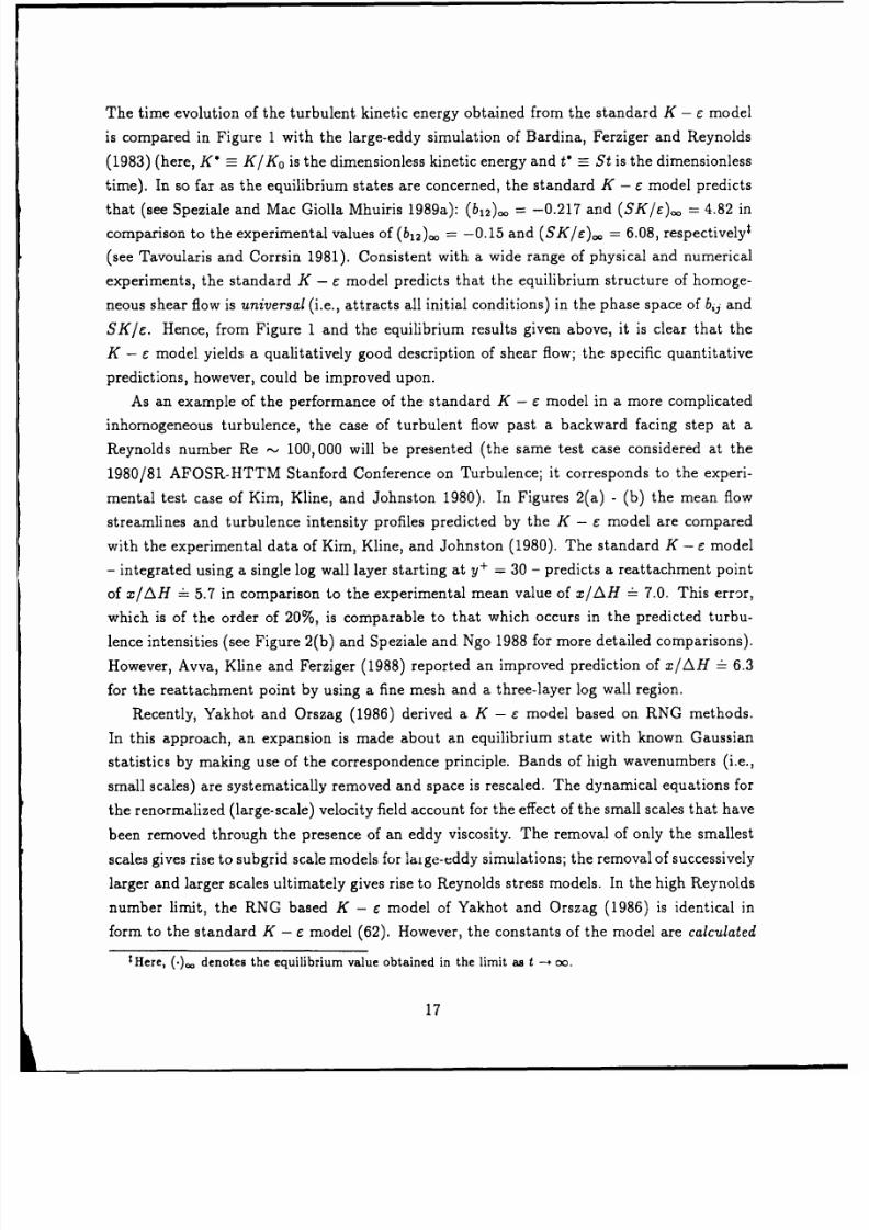
The
time
evolution
of
the turbulent kinetic
energy
obtained
from the
standard K - Cmodel
is compared in Figure 1 with
the
large-eddy simulation of Bardina, Ferziger and
Reynolds
(1983) (here, K =
K/Ko
is the
dimensionless
kinetic energy
and
t' =_
St
is the
dimensionless
time). In
so far as the equilibrium
states are concerned,
the standard K -
Cmodel
predicts
that
(see
Speziale
and
Mac Giolla
Mhuiris
19
8
9a):
(b1
2
)o,
=
-0.217
and
(SK/e)o.
=
4.82 in
comparison
to
the
experimental
values
of
(b
1
2
).. = -0.15
and
(SK/c),o
= 6.08,
respectivelyt
(see Tavoularis and Corrsin 1981). Consistent with a wide range
of
physical and numerical
experiments,
the standard K - c model predicts that the equilibrium structure of homoge-
neous shear flow is universal
(i.e.,
attracts all initial conditions) in the
phase
space of bij and
SKI. Hence,
from Figure
1 and
the equilibrium
results given above, it is
clear that the
K - c model yields
a
qualitatively good description
of
shear
flow;
the specific quantitative
predictions,
however, could be
improved
upon.
As an example of the performance of the standard K - c model in a more complicated
inhomogeneous
turbulence,
the
case of
turbulent
flow
past
a
backward
facing
step
at a
Reynolds
number Re -
100,
000 will be presented (the same test
case
considered
at
the
1980/81 AFOSR-HTTM Stanford Conference
on
Turbulence; it corresponds to the
experi-
mental test case of Kim, Kline, and
Johnston
1980). In Figures 2(a) - (b) the
mean
flow
streamlines and turbulence intensity
profiles
predicted by the K - E model are compared
with
the experimental
data
of Kim, Kline, and
Johnston (1980). The standard K - c
model
- integrated
using a single
log wall layer starting
at y+
= 30 - predicts
a
reattachment
point
of x/AH
-
5.7
in comparison to the experimental mean
value of x/AH
- 7.0.
This error,
which is of the
order of 20%,
is
comparable to
that which occurs
in the predicted turbu-
lence intensities
(see
Figure
2(b)
and Speziale
and
Ngo
1988
for
more
detailed comparisons).
However,
Avva, Kline and Ferziger
(1988) reported
an improved prediction of x/AH - 6.3
for the reattachment point by using a fine mesh and a three-layer log wall region.
Recently, Yakhot and
Orszag (1986) derived a
K -
E
model based on RNG
methods.
In
this approach, an
expansion is made
about an equilibrium state with
known
Gaussian
statistics by making
use of
the correspondence principle. Bands of high wavenumbers (i.e.,
small scales) are systematically removed and space is rescaled. The dynamical
equations
for
the
renormalized
(large-scale)
velocity field account for
the effect of the small
scales
that
have
been removed
through
the
presence
of
an
eddy
viscosity.
The
removal
of
only
the
smallest
scales gives rise
to subgrid
scale models
for
laige-eddy
simulations;
the
removal
of successively
larger and larger
scales
ultimately gives rise to Reynolds stress models. In
the
high Reynolds
number limit,
the
RNG
based
K -
c model of Yakhot
and Orszag
(1986)
is identical in
form to the standard
K - c model (62).
However, the constants of the
model
are
calculated
Here, ( )o denotes the equilibrium value obtained
in
the
limit
as t - oo.
17
8/10/2019 speziale 1990
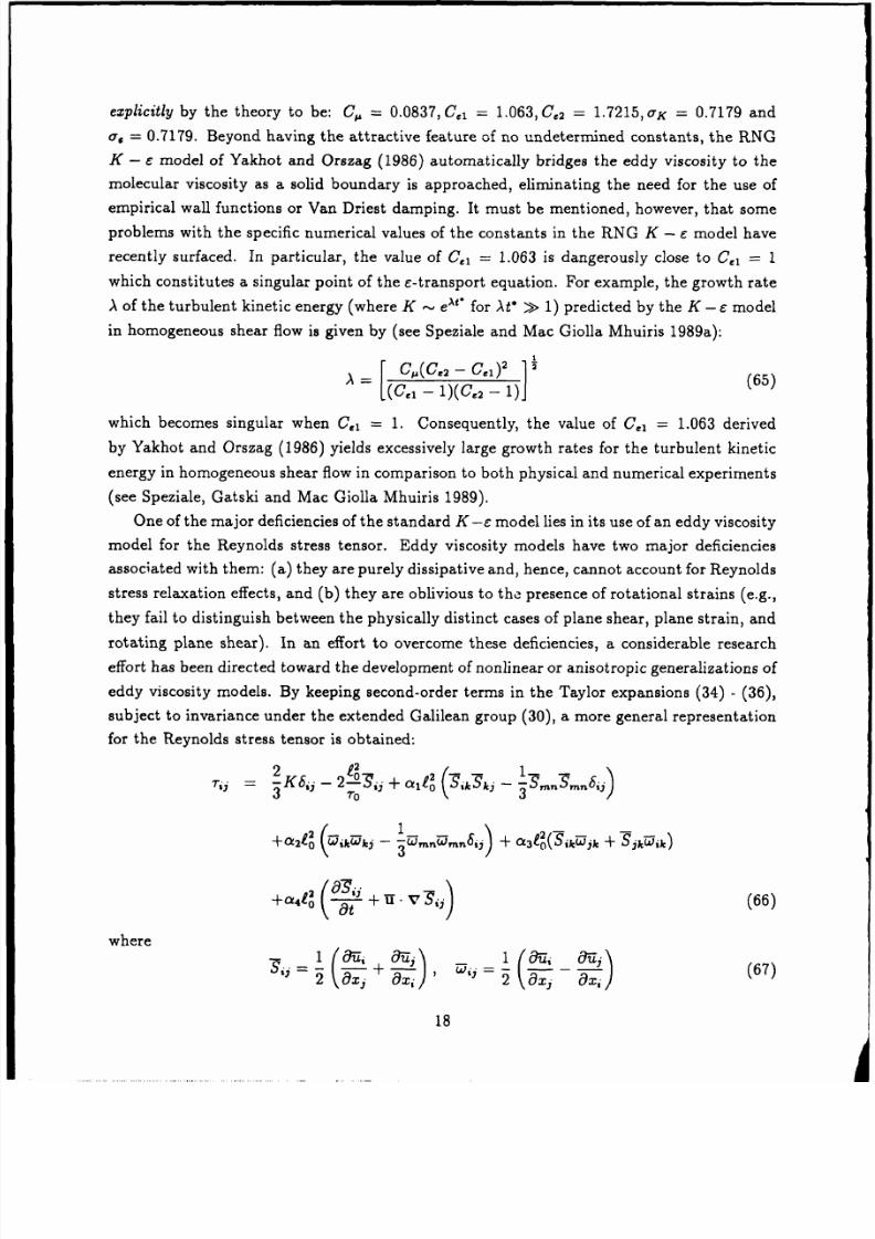
http://slidepdf.com/reader/full/speziale-1990 20/60
explicitly by
the theory
to
be:
C. = 0.0837, C,
1
= 1.063,
C,
2
=
1.
7
2
1
5
,aK
= 0.7179
and
o, =
0.7179.
Beyond
having the
attractive
feature
of
no
undetermined
constants,
the RNG
K
- c
model
of Yakhot and
Orszag
(1986) automatically
bridges
the
eddy viscosity
to the
molecular
viscosity
as a solid boundary
is
approached,
eliminating
the
need for
the
use
of
empirical
wall
functions
or
Van
Driest damping. It must
be
mentioned,
however,
that
some
problems
with
the specific numerical
values
of
the constants
in the RNG
K - e
model have
recently
surfaced.
In particular,
the value
of C.
1
=
1.063
is dangerously
close
to
C,
1
=
1
which constitutes
a singular point
of the
e-transport equation.
For example, the
growth
rate
A
of
the
turbulent
kinetic
energy (where
K e
for
At* >
1) predicted
by the
K
-
e
model
in homogeneous
shear flow
is
given by (see
Speziale and
Mac Giolla
Mhuiris
1989a):
A
=[CM.(Cc
2
-
1e)
(65)
C.1- 1)(C.2 - 1)]
which
becomes
singular when
C,
1
=
1. Consequently,
the value of
C,1
=
1.063 derived
by
Yakhot and Orszag
(1986)
yields
excessively
large
growth rates for
the
turbulent
kinetic
energy in
homogeneous
shear flow
in comparison
to both
physical and
numerical experiments
(see
Speziale,
Gatski
and Mac
Giolla Mhuiris 1989).
One
of
the
major
deficiencies
of
the standard
K-c model
lies in its
use of
an eddy viscosity
model for
the Reynolds
stress tensor.
Eddy
viscosity
models have
two
major
deficiencies
associated
with them:
(a) they
are
purely dissipative
and,
hence, cannot
account
for
Reynolds
stress relaxation
effects, and
(b) they
are
oblivious
to
the
presence of rotational
strains
(e.g.,
they
fail
to distinguish between
the
physically distinct
cases
of
plane shear, plane
strain,
and
rotating
plane shear).
In an effort to
overcome
these deficiencies,
a
considerable
research
effort
has been directed
toward the
development of
nonlinear
or
anisotropic
generalizations
of
eddy viscosity models.
By
keeping
second-order
terms
in the Taylor
expansions
(34) - (36),
subject
to
invariance under
the extended
Galilean
group (30),
a more
general
representation
for the
Reynolds
stress
tensor
is
obtained:
2
K6,,
-
2-317,,
+
alt
1e
9n_9n
i
O00Si-k
3/
+a
2
1
0
(a
-
3
mnwmn
+
C
+ g
12f\
+
U
.
(66)
where
i
x)(67)
18
8/10/2019 speziale 1990
http://slidepdf.com/reader/full/speziale-1990 21/60
are
the mean rate of
strain and
mean vorticity tensors
(a,
...
a
4
are
dimensionless
constants;
in
the
linear
limit
as
a
-- 0, the eddy viscosity
model (44)
is recovered).
When a
4
= 0,
the
deviatoric part
of
(66)
is
of
the
general form DTij
=
AiklaO-k/axt
(where
Aijke
depends
al-
gebraically on
the
mean velocity gradients)
and, hence,
the term
"anisotropic
eddy
viscosity
model"
has
been used
in
the literature.
These
models
are
probably
more
accurately
char-
acterized as
"nonlinear" or
"viscoelastic"
corrections
to the eddy viscosity
models.
Lumley
(1970)
was
probably
the first to systematically
develop such models
(with
a
4
=
0)
wherein he
built up the
length and
time
scales
from
the
turbulent
kinetic
energy, turbulent
dissipation
rate, and
the invariants of
3,i and
Oij.
Saffman
(1977) proposed
similar
anisotropic
models
which
were
solved in conjunction
with
modeled
transport
equations for K
and 2 (where
w
=_
e/K).
Pope (1975)
and Rodi
(1976)
developed
alternative
anisotropic
eddy viscosity
models
from the
Reynolds
stress transport
equation
by making an
equilibrium hypothesis.
Yoshizawa
(1984, 1987)
derived a more complete
two-equation
model
- with a nonlinear
correction
to
the
eddy
viscosity of
the
full
form
of
(66)
-
by
means
of a two-scale
Direct
In-
teraction
Approximation (DIA)
method. In
this approach, Kraichnan's
DIA formalism
(cf.
Kraichnan
1964)
is
combined
with a
scale
expansion
technique
where
the
slow
variations
of
the
mean fields are
distinguished from
the fast variations
of the fluctuating fields
by means
of a scale
parameter.
The length and time
scales of
the turbulence
are
built
up
from
the
turbulent
kinetic
energy and
dissipation
rate
for
which
modeled transport
equations are
de-
rived.
These
modeled
transport
equations
are
identical in form
to (62c) and (62d)
except for
the addition of
higher-order
cross diffusion
terms. The
numerical
values
of
the constants
are
derived
directly from the
theory (as
with the RNG
K - e model). However,
in applications
it has
been found that
these values
need to be adjusted
(see
Nisizima
and
Yoshizawa
1987).
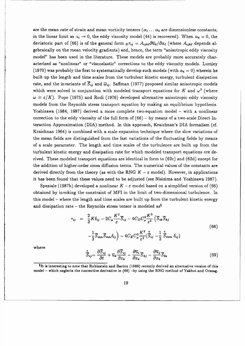
Speziale
(1987b) developed
a
nonlinear
K
-
-
model based
on
a
simplified
version
of (66)
obtained
by
invoking
the constraint
of
MFI in the
limit
of
two-dimensional
turbulence. In
this
model
-
where the
length and
time
scales
are built
up from the
turbulent
kinetic
energy
and dissipation
rate
- the
Reynolds
stress tensor
is
modeled asl
2 K 2
TO,. =
-3
K6,j
-
2C---3.
- 4C(3k kJ
(68)
1
CC
2
Kl.
I
-j)
C
sC
2
(9i
-
3
m..
where
0
S
Ui-
U
j
+
U:
3
3
(69)
at
1Ox;
axk
aX k
%It
s
interesting to note that
Rubinstein and
Barton (1989) recently derived
an alternative
version
of this
model - which neglects
the convective
derivative
in (69) -by using
the
RNG
method
of Yakhot
and Orszag.
19
8/10/2019 speziale 1990
http://slidepdf.com/reader/full/speziale-1990 22/60
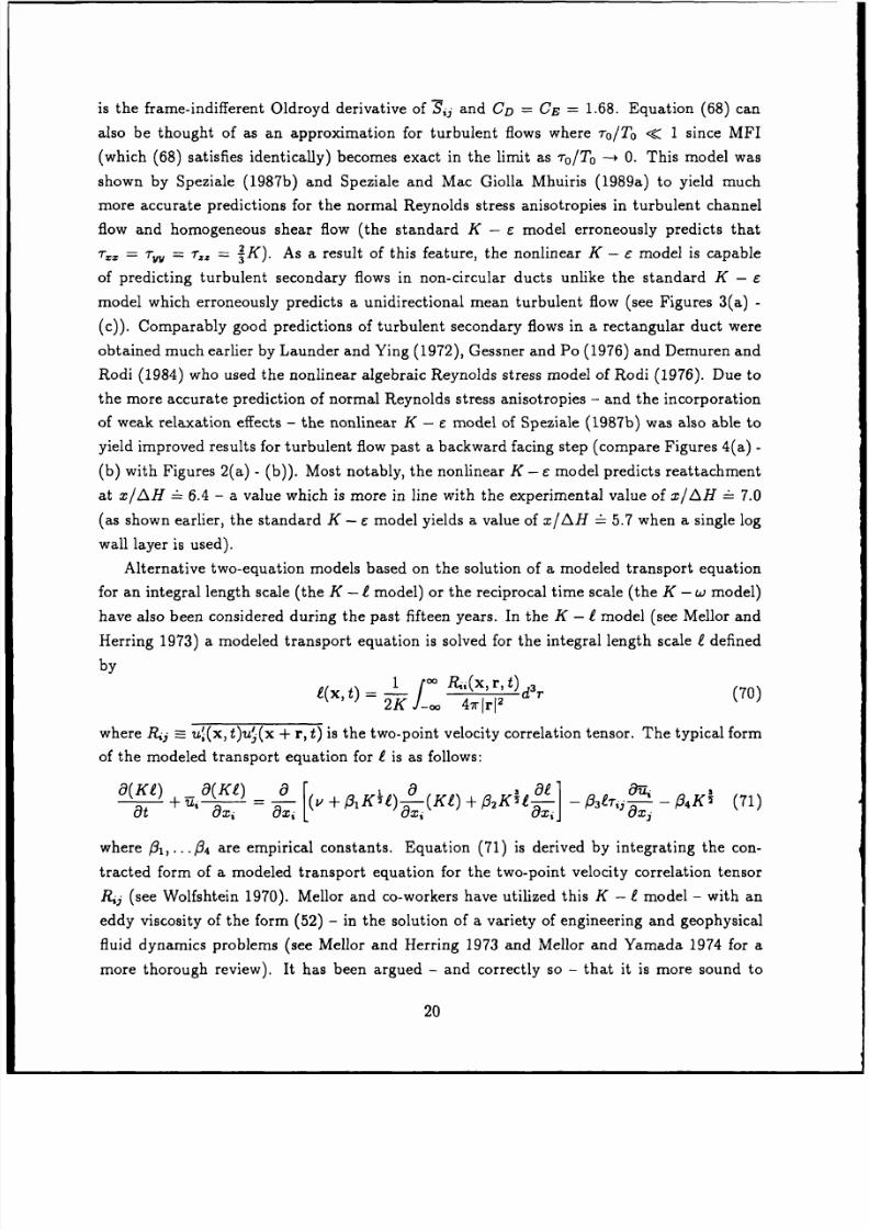
is the frame-indifferent
Oldroyd derivative
of Sij
and CD C,
=
1.68. Equation
(68) can
also be thought of
as an
approximation
for
turbulent
flows
where ro/To
< 1 since MFI
(which (68)
satisfies identically) becomes
exact
in
the limit as
ro/To --*
0. This
model was
shown
by Speziale
(1987b)
and
Speziale and
Mac Giolla
Mhuiris (1989a) to
yield much
more accurate predictions
for
the
normal
Reynolds
stress anisotropies
in
turbulent
channel
flow
and homogeneous
shear
flow
(the
standard
K
-
e model erroneously predicts
that
'r.. =
r y
=
.
K).
As a result
of this feature, the nonlinear
K
-
e
model is
capable
of
predicting
turbulent
secondary
flows in non-circular ducts
unlike
the
standard K
- C
model which
erroneously predicts a unidirectional
mean turbulent flow
(see Figures 3(a) -
(c)).
Comparably
good
predictions
of turbulent
secondary flows
in a rectangular duct
were
obtained
much
earlier by Launder and
Ying (1972), Gessner
and Po (1976) and
Demuren
and
Rodi
(1984)
who
used
the
nonlinear
algebraic Reynolds
stress model of Rodi
(1976). Due to
the more accurate prediction
of normal
Reynolds stress
anisotropies -
and
the incorporation
of
weak
relaxation
effects -
the
nonlinear
K
-
e model
of Speziale
(1987b)
was also able
to
yield
improved results for turbulent flow past
a backward
facing step (compare
Figures 4(a) -
(b) with
Figures 2(a) - (b)). Most notably, the
nonlinear
K -
e model
predicts
reattachment
at
x/AH - 6.4 -
a value which is more in
line with the experimental value
of
x/AH -
7.0
(as shown earlier, the standard
K
-
e model yields a value of x/AH
-
5.7
when
a single
log
wall layer is used).
Alternative
two-equation
models based on the
solution of
a modeled
transport equation
for
an integral length
scale (the
K
- e
model)
or
the reciprocal time
scale
(the K
-
w model)
have
also
been considered during
the
past
fifteen
years.
In
the
K
-
£
model
(see
Mellor and
Herring
1973)
a
modeled
transport
equation
is solved
for
the integral length
scale
e defined
by
1
,~x
r,
0t)
r(0
e(xt) =2--K
__
47r2
d
r
(70)
where Rj
= u(x, t)u(x
+ r, t) is the two-point velocity
correlation
tensor. The typical form
of the modeled
transport
equation
for f is
as follows:
o~lo__
~ io,- ar.O1K
l] -ir f
j
O9(KI)
a(Ki)
L9
a
a2
u
3K~ 1
a
+
+
-
)KK
71
at
axi.I1x ax ] ax
1
where 31,...f14
are empirical constants. Equation (71)
is derived by
integrating
the con-
tracted
form
of
a modeled transport equation
for the two-point
velocity correlation
tensor
Rj (see Wolfshtein
1970).
Mellor and co-workers have
utilized this
K - t model - with
an
eddy
viscosity
of
the
form (52) - in
the solution of
a variety of
engineering and
geophysical
fluid
dynamics problems
(see Mellor and
Herring
1973
and
Mellor
and
Yamada 1974 for
a
more thorough
review). It has
been argued - and
correctly so - that
it is more
sound to
20
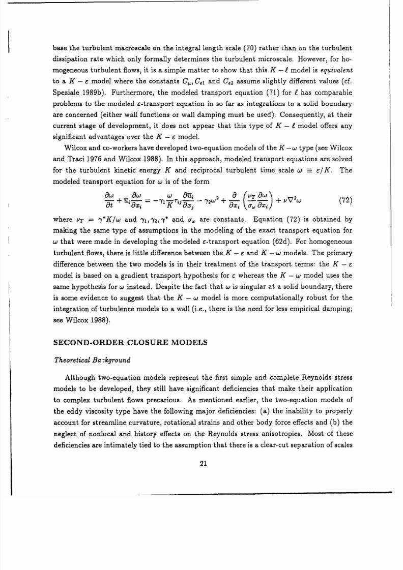
8/10/2019 speziale 1990
http://slidepdf.com/reader/full/speziale-1990 23/60
base the
turbulent macroscale
on the integral length scale (70)
rather than on the turbulent
dissipation
rate
which only
formally determines the turbulent
microscale. However,
for
ho-
mogeneous
turbulent
flows, it
is a simple
matter
to
show that this K -
e
model is equivalent
to
a K - c model
where
the constants C,, C
1
and C,
2
assume slightly
different values (cf.
Speziale 1989b).
Furthermore, the modeled
transport equation
(71)
for £ has
comparable
problems
to the modeled
c-transport
equation
in
so
far
as
integrations
to a solid boundary
are
concerned (either
wall
functions or
wall damping must be used).
Consequently, at
their
current stage of
development,
it does
not appear that this type of K - e model
offers any
significant advantages over
the K - e model.
Wilcox
and
co-workers
have developed
two-equation models
of
the
K -w type (see Wilcox
and
Traci 1976 and Wilcox 1988).
In
this
approach,
modeled transport equations are solved
for
the
turbulent
kinetic energy K and reciprocal
turbulent time
scale
w c K. The
modeled
transport equation for w
is
of
the form
aw
_w
w
0 , 2
a(
u
+w
+ Y1Ts
-Ywa
+Vw
(72)
at a+,
7
10
a
where
vT
= 7*K/w
and y1,2,qy*
and
a,, are
constants. Equation (72) is
obtained by
making the same
type of assumptions
in the modeling
of
the exact
transport equation
for
w that
were made in developing
the modeled c-transport
equation
(62d).
For homogeneous
turbulent flows,
there is little difference between
the
K -
e and K - w models. The
primary
difference
between the two models is in their
treatment of the
transport terms: the
K - 6
model is based on a gradient
transport hypothesis for c whereas
the K -
w model
uses
the
same
hypothesis
for w instead.
Despite the
fact
that w
is singular at a
solid
boundary, there
is some
evidence
to suggest that the
K -
w
model is more computationally
robust for the
integration of turbulence models
to
a wall
(i.e.,
there is
the
need
for less empirical damping;
see
Wilcox
1988).
SECOND-ORDER
CLOSURE MODELS
TheoreticalBa
:kground
Although two-equation models
represent the first simple and compleLe Reynolds
stress
models
to
be developed,
they
still
have
significant
deficiencies
that
make
their
application
to
complex
turbulent
flows precarious. As mentioned
earlier, the two-equation models
of
the
eddy viscosity type have the following major
deficiencies: (a) the
inability to properly
account
for streamline curvature,
rotational strains
and other body force effects
and
(b)
the
neglect of nonlocal
and history effects on the Reynolds
stress anisotropies. Most of
these
deficiencies are
intimately tied to the assumption
that there is a
clear-cut
separation
of scales
21
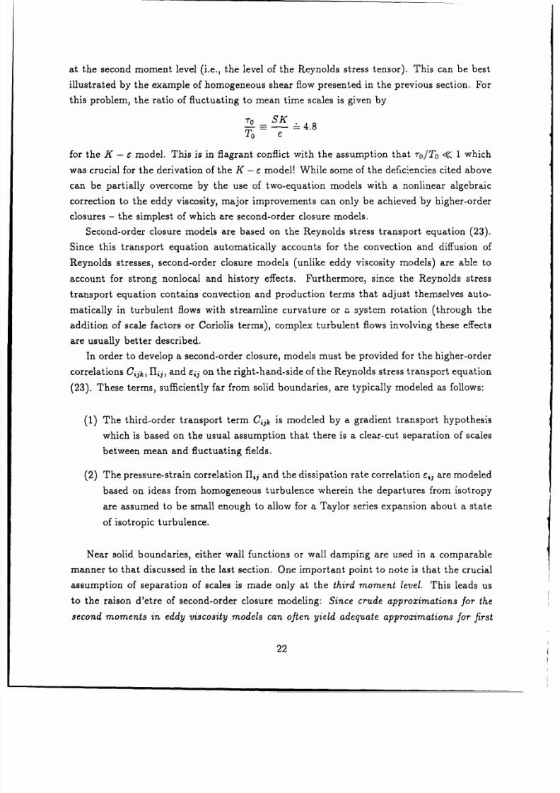
8/10/2019 speziale 1990
http://slidepdf.com/reader/full/speziale-1990 24/60
at the second
moment
level
(i.e., the
level
of the Reynolds stress tensor). This
can be
best
illustrated by the example of homogeneous
shear flow presented in the previous section. For
this
problem, the
ratio of fluctuating
to mean time scales is
given
by
7
0
SK
-
-4.8
To
e
for the K
-
e
model. This is in flagrant
conflict
with the
assumption
that
To/To
< 1 which
was crucial for the
derivation of the K - e model While
some of
the deficiencies
cited
above
can be partially
overcome by the use
of
two-equation models
with a nonlinear algebraic
correction
to the eddy viscosity,
major
improvements can only be achieved by higher-order
closures -
the
simplest of which
are second-order closure models.
Second-order
closure models are
based
on
the Reynolds stress transport equation (23).
Since
this transport equation automatically accounts
for
the convection and
diffusion of
Reynolds stresses, second-order closure models
(unlike eddy viscosity models) are
able to
account for strong nonlocal and history
effects.
Furthermore, since the Reynolds stress
transport equation contains convection and production
terms
that
adjust themselves
auto-
matically in turbulent flows with streamline curvature or
a system rotation (through the
addition of scale factors or Coriolis terms), complex
turbulent flows
involving
these
effects
are usually better described.
In order to develop a second-order closure,
models
must be
provided for the
higher-order
correlations Cijk, Hi, and eij on the
right-hand-side
of
the
Reynolds stress transport
equation
(23).
These terms,
sufficiently
far from solid boundaries, are typically
modeled
as follows:
(1)
The
third-order transport term Cijk
is
modeled
by a
gradient
transport
hypothesis
which
is based
on
the usual
assumption
that there
is
a
clear-cut separation of scales
between
mean and fluctuating
fields.
(2) The pressure-strain
correlation HI
i
and the dissipation rate correlation
eii are
modeled
based
on
ideas from homogeneous
turbulence
wherein
the
departures from
isotropy
are assumed
to be
small
enough to
allow for
a
Taylor
series expansion about a state
of
isotropic turbulence.
Near
solid
boundaries, either
wall
functions or wall
damping
are
used in a comparable
manner
to
that discussed
in the last section. One important point
to
note is
that the crucial
assumption of separation of scales
is made only
at
the third
moment
level. This leads
us
to
the raison d'etre of
second-order closure
modeling:
Since
crude
approximationsfor
the
second
moments
in
eddy
viscosity models can often
yield
adequate approximationsfor first
22
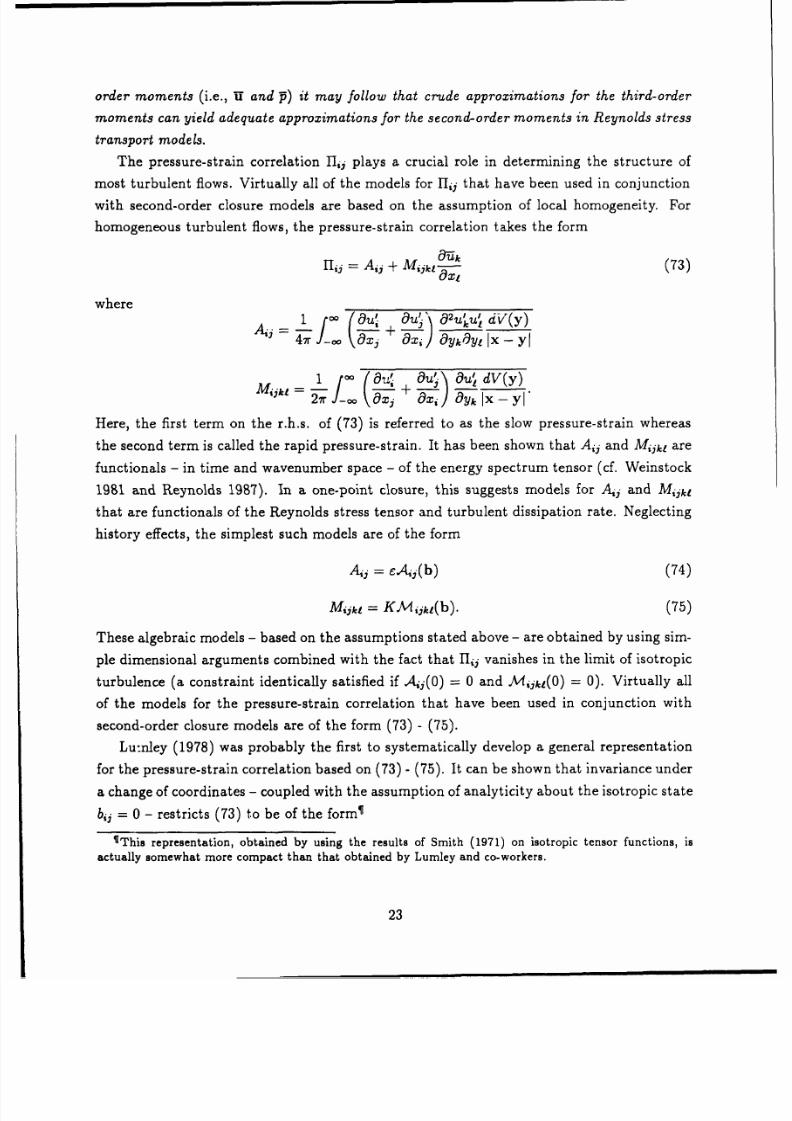
8/10/2019 speziale 1990
http://slidepdf.com/reader/full/speziale-1990 25/60
order moments (i.e.,
U
and 1)
it
may
follow that crude
approximations
for
the
third-order
moments can
yield adequate
approximations or the second-order moments in Reynolds stress
transport
models.
The pressure-strain correlation IIj plays a crucial
role in
determining the structure of
most
turbulent
flows.
Virtually
all of
the
models
for
Ij
that
have been used
in
conjunction
with second-order
closure
models are based
on
the assumption
of local
homogeneity. For
homogeneous
turbulent flows, the pressure-strain
correlation takes the
form
H1ij = A + Mijkt'auk
(73)
where
i (au' auo2u'~u'
d-v(y)
r J-o
8x
3
Ox,]
aykA~y Ix - y
Mf
(u
+
u
O
u'
dV(y)
27r + )
k Ix- YI
Here,
the
first
term on the r.h.s.
of (73)
is
referred to
as the
slow pressure-strain
whereas
the
second
term
is called the rapid pressure-strain. It has been shown that Aij and Mike are
functionals - in time
and
wavenumber
space
-
of the
energy spectrum tensor (cf.
Weinstock
1981 and Reynolds 1987). In a one-point closure, this suggests models for
Ai
3
and Mijk,
that
are functionals
of the
Reynolds stress tensor
and turbulent
dissipation
rate.
Neglecting
history
effects, the simplest
such
models are
of
the form
Aj
=
eAj(b)
(74)
Mijkl
=
KM
ike(b).
(75)
These algebraic models
-
based on the assumptions stated
above -
are obtained by
using
sim-
ple dimensional
arguments combined with
the
fact
that lli
vanishes in
the
limit
of
isotropic
turbulence
(a constraint
identically
satisfied if
Aj(O) =
0 and Mjkl(O)
=
0). Virtually all
of the
models
for the
pressure-strain correlation that have been
used
in
conjunction
with
second-order closure models are of the form (73)
-
(75).
Lu:nley
(1978) was
probably
the
first to systematically develop a general representation
for
the
pressure-strain correlation based
on (73)
-
(75).
It
can be
shown
that
invariance under
a change
of
coordinates - coupled with
the assumption of analyticity about the isotropic state
bij = 0 - restricts (73) to
be of the forml
IThis
representation, obtained
by using
the
results
of
Smith
(1971)
on
isotropic
tensor functions, is
actually
somewhat more compact than that
obtained by
Lumley and co-workers.
23
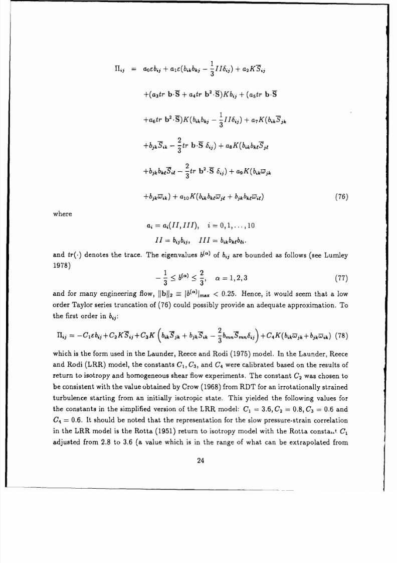
8/10/2019 speziale 1990
http://slidepdf.com/reader/full/speziale-1990 26/60
1Ij =
aoEb
ij
+
ale(bikbki
- -118i3) +
a
2
KSi
3
+(a
3
tr
b.S
+
a
4
tr
b
2
.
)Kbi,
+
(astr
b.9
2
1
+a
6
tr b
.S)K(bkbkj
-
-II63)
+
a7K(bjkS
3
k
3
+bjkSk
- 2 tr b.-9
&,j)
+ a
8
K(bikbk1S
3
j
3
+bjkbkeal
- 2tr
b
2
.S
6j) +
agK(bikUjk
3
+bj kk)
+ aloK(bkbk1Ou,
+
bjkbk
i
1
)
(76)
where
ai=a, II, II), i=0,1,...,10
II
=
bjbij,
III= bikbklbli.
and tr(.)
denotes
the trace.
The
eigenvalues
b
(
@)
of bij are bounded
as
follows
(see Lumley
1978)
=
1,2,3
(77)
3-
-3'
and for many
engineering
flow,
jjb
12
=
b(a)
,,
<
0.25.
Hence,
it would
seem that a
low
order Taylor series
truncation
of
(76) could
possibly provide an adequate
approximation.
To
the
first
order
in
b
13
:
/ 2
\
Hi
3
=
C cbti +C2 K i + C
3
K (b
i
k-jk
+ bi -3,k 3
bmn,n8ij) +C4K(bikjk+bkabik')
(78)
which is
the form used
in the Launder, Reece
and Rodi
(1975)
model. In the
Launder, Reece
and
Rodi
(LRR) model,
the
constants C1, C3,
and C4 were
calibrated based
on the
results of
return
to isotropy and homogeneous
shear flow
experiments. The
constant C2 was
chosen to
be
consistent
with
the
value
obtained
by
Crow
(1968)
from
RDT
for an
irrotationally
strained
turbulence
starting
from
an initially
isotropic state. This
yielded the following
values
for
the
constants
in the
simplified
version
of
the
LRR
model: C
,
=
3.6,
C2 =
0.8,
C3
= 0.6 and
C4 =
0.6.
It
should be noted that
the representation
for the
slow
pressure-strain
correlation
in the
LRR model
is the
Rotta
(1951)
return
to isotropy model
with the Rotta constaJ
C,
adjusted
from 2.8
to 3.6 (a value which
is
in
the
range
of
what can be extrapolated from
24
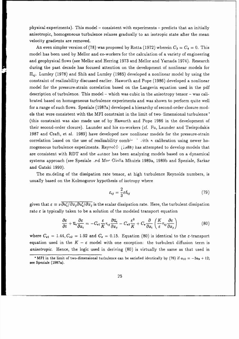
8/10/2019 speziale 1990
http://slidepdf.com/reader/full/speziale-1990 27/60
physical
experiments).
This
model
- consistent with
experiments -
predicts
that an initially
anisotropic,
homogeneous turbulence relaxes
gradually to
an
isotropic state
after the
mean
velocity gradients are
removed.
An even simpler
version of (78)
was
proposed by
Rotta (1972)
wherein
C
3
= C4 =
0.
This
model
has
been
used
by Mellor
and co-workers for
the calculation of a variety
of engineering
and
geophysical flows (see Mellor
and Herring 1973 and Mellor
and Yamada
1974).
Research
during
the
past decade
has
focused
attention on the development
of nonlinear models
for
f1ij.
Lumley (1978)
and
Shih and
Lumley (1985) developed
a nonlinear model
by using
the
constraint of
realizability
discussed earlier. Haworth
and Pope (1986) developed a nonlinear
model
for
the
pressure-strain correlation
based on the
Langevin
equation
used in
the
description
of
turbulence. This
model - which
was
cubic
in the
anisotropy
tensor -
was
cali-
brated
based
on
homogeneous
turbulence
experiments
and was shown
to perform
quite
well
for a range of
such flows. Speziale (1987a)
developed a hierarchy of
second-order closure
mod-
els
that
were
consistent with the
MFI
constraint
in
the
limit
of
two-
dimensional
turbulence*
(this
constraint was
also made use of by
Haworth
and
Pope 1986 in the
development of
their
second-order
closure).
Launder and his co-workers (cf.
Fu, Launder and Tselepidakis
1987 and
Craft, et al.
1989) have developed
new nonlinear models for
the pressure-strain
correlation based on
the use
of
realizability comb;- .ith
a calibration using newer
ho-
mogeneous turbulence
experiments.
ReynoH,
(i 88) has attempted
to develop
models that
are
consistent with RDT and the author
has been analyzing
models based
on
a
dynamical
systems approach (see Speziale .nd
Ma-
Giolla Mhuiris 1989a,
1989b
and
Speziale, Sarkar
and Gatski 1990).
The mcdeling
of
the
dissipation rate tensor,
at high turbulence
Reynolds
numbers,
is
usually
based
on the
Kolmogorov hypothesis of
isotropy where
2 =sj
(79)
3 3
given
that e
vau
/xj9u:/gxj is the
scalar
dissipation
rate.
Here, the
turbulent
dissipation
rate - is
typically
taken to be a solution of the modeled
transport
equation
ce
a
6e
-
2
a
(K
Qe
rt
Cc,--
c 2
+
c
)
(80)
at 'xi
£K
ilxp Kc2xj
Ee7 (79xj
where
C, =
1.44,
C,2
= 1.92 and
C, =
0.15.
Equation
(80)
is
identical
to the
E-transport
equation
used
in the K
-
c
model with one
exception: the
turbulent
diffusion
term
is
anisotropic. Hence,
the logic
used
in
deriving
(80)
is
virtually the same as that
used in
*MFI
in
the
limit of
two-dimensional
turbulence can
be
satisfied identically by (76)
if
alo =
-3a
9
+ 12;
see
Speziale (1987a).
25
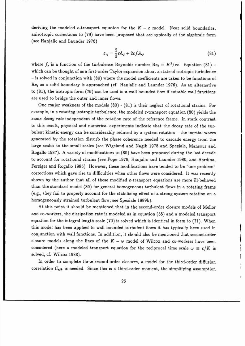
8/10/2019 speziale 1990
http://slidepdf.com/reader/full/speziale-1990 28/60
deriving
the modeled
e-transport
equation
for
the
K - e
model.
Near
solid
boundaries,
anisotropic
corrections
to
(79)
have
been
droposed
that
are
typically
of
the
algebraic
form
(see
Hanjalic
and
Launder
1976)
Eii=
2 ii
+ 2efobj
(81)
where
f, is
a
function
of
the turbulence
Reynolds
number
Ret
- K
2
/ve.
Equation
(81)
-
which
can
be
thought
of as
a first-order
Taylor
expansion
about a
state
of isotropic
turbulence
- is
solved
in conjunction
with
(80) where
the
model
coefficients
are taken
to be functions
of
Ret
as a
soli,d boundary
is
approached
(cf.
Hanjalic
and
Launder
1976).
As
an alternative
to
(81),
the isotropic
form
(79)
can be used
in a
wall
bounded
flow if
suitable
wall
functions
are used
to bridge
the
outer
and
inner flows.
One major
weakness
of
the models (80)
- (81)
is
their neglect
of
rotational
strains.
For
example,
in
a
rotating
isotropic
turbulence,
the
modeled
c-transport
equation
(80)
yields
the
same
decay
rate
independent
of
the rotation rate
of
the
reference
frame.
In stark
contrast
to this
result, physical
and numerical
experiments
indicate
that
the
decay
rate
of
the
tur-
bulent
kinetic
energy can
be
considerably
reduced
by a
system
rotation
- the inertial
waves
generated
by the
rotation
disturb
the
phase
coherence
needed
to
cascade
energy
from
the
large
scales
to
the
small
scales
(see
Wigeland
and
Nagib
1978
and
Speziale,
Mansour
and
Rogallo
1987).
A
variety
of
modifications
to (80)
have
been proposed
during
the
last
decade
to account
for
rotational
strains
(see
Pope
1978, Hanjalic
and
Launder
1980, and
Bardina,
Ferziger
and Rogallo
1985).
However,
these
modifications
have tended
to be
"one
problem"
corrections
which gave
rise
to difficulties
when other
flows were
considered.
It was
recently
shown
by
the
author
that
all of
these
modified
c-transport
equations
are more
ill-behaved
than
the
standard
model
(80) for
general homogeneous
turbulent
flows
in
a rotating
frame
(e.g.,
t ly
fail
to properly
account
for the
stabilizing
effect
of a strong
system
rotation
on
a
homogeneously
strained
turbulent
flow;
see Speziale
1989b).
At
this point
it
should
be
mentioned
that
in the
second-order
closure
models of Mellor
and co-workers,
the
dissipation
rate
is modeled
as
in equation
(55)
and a
modeled
transport
equation
for
the integral
length scale
(70)
is solved
which
is identical
in
form
to (71).
When
this
model
has been
applied
to
wall
bounded
turbulent
flows
it has
typically
been used in
conjunction with
wall
functions.
In
addition,
it should
also
be
mentioned
that
second-order
closure
models
along
the
lines
of the
K
- w model
of Wilcox
and co-workers
have
been
considered
(here a
modeled
transport
equation
for
the
reciprocal
time scale w
-
C/K is
solved;
cf.
Wilcox
1988).
In
order
to complete
thc;e
second-order
closures,
a
model
for
the third-order
diffusion
correlation
Cijk is needed.
Since
this
is a third-order
monient,
the simplifying
assumption
26
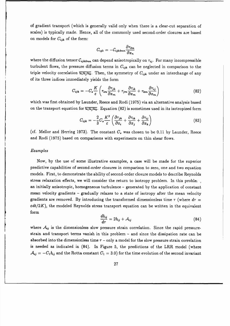
8/10/2019 speziale 1990
http://slidepdf.com/reader/full/speziale-1990 29/60
of
gradient
transport
(which
is generally
valid
only
when
there is a
clear-cut
separation
of
scales)
is
typically
made. Hence,
all
of the
commonly
used
second-order
closures
are based
on models
for
Cijk of the
form:
Ck=
-Cijoemn
O9rm
aX?,
where
the diffusion
tensor
Ciklmn
can
depend
anisotropically
on
-ri. For
many
incompressible
turbulent
flows,
the
pressure
diffusion
terms
in
C~ik can
be
neglected
in
comparison
to the
triple
velocity
correlation
UIujuk.
Then,
the
symmetry
of
Cik under
an
interchange
of an y
of
its
three indices
immediately
yields
the
form
t
9
Tk
9
Tk
OrNj
Co -c 'K
2
+T jm
+Tkm
(82)
C
~ aXmn
4
9
Xm
8
9Xm
which
was
first obtained
by Launder,
Reece
and
Rodi
(1975) via
an alternative
analysis based
on
the
transport equation
for
uiuju.
Equation
(82)
is
sometimes
used
in its
isotropized
form
2 K.
+ s
(83)
3
E
ax
axj
axj
(cf.
Mellor
and
Herring
1973). The
constant
C, was
chosen
to
be 0.11 by
Launder,
Reece
and
Rodi (1975)
based
on comparisons
with
experiments
on
thin
shear flows.
Examples
Now,
by the
use
of some
illustrative examples,
a
case
will be
made for
the superior
predictive
capabilities
of
second-order
closures in
comparison
to
zero,
one
and
two
equation
models.
First,
to
demonstrate
the
ability
of
second-order
closure
models
to describe
Reynolds
stress
relaxation
effects,
we
will
consider the
return
to isotropy problem.
In
this problel,
an
initially
anisotropic,
homogeneous
turbulence
- generated
by
the application
of
constant
mean velocity
gradients
- gradually
relaxes
to
a state
of
isotropy
after the
mean velocity
gradients
are removed.
By
introducing
the
transformed
dimensionless
time
- (where
d'r =
edt/2K),
the
modeled
Reynolds
stress
transport
equation
can be
written
in the
equivalent
form
dr=
2b
1
i
+ A j
(84)
d-
where
Aj
is the
dimensionless
slow pressure
strain correlation.
Since
the
rapid
pressure-
strain
and
transport
terms
vanish in
this
problem -
and since
the
dissipation
rate
can be
absorbed
into
the dimensionless
time
- - only
a model for
the
slow pressure
strain
correlation
is needed
as indicated
in
(84). In Figure
5,
the
predictions
of
the
LRR
model
(where
Aj
= -Clbij
and the
Rotta
constant
C
1
=
3.0) for
the time
evolution
of
the second
invariant
27
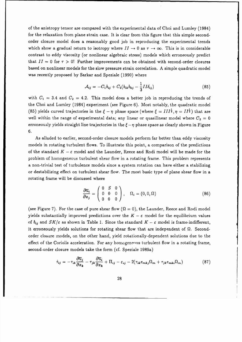
8/10/2019 speziale 1990
http://slidepdf.com/reader/full/speziale-1990 30/60
of the anistropy
tensor
are compared with the
experimental
data of Choi
and
Lumley
(1984)
for
the
relaxation from
plane
strain
case.
It is
clear
from
this
figure that
this simple second-
order closure
model
does a reasonably
good job in
reproducing the experimental trends
which
show
a gradual
return
to isotropy
where II -+ 0
as
r
- oo. This is in
considerable
contrast
to eddy
viscosity
(or
nonlinear algebraic
stress) models which
erroneously
predict
that
II = 0
for
r
>
0 Further
improvements can
be obtained
with
second-order
closures
based on nonlinear
models
for
the
slow pressure strain
correlation.
A
simple quadratic
model
was
recently proposed
by
Sarkar and Speziale (1990) where
A=
-C
1
b
i
+ C
2
(b
kbk
3
-
1116,j
(85)
3
'
with C
1
= 3.4
and C
2
=
4.2.
This model does
a better job in
reproducing
the trends
of
the Choi and
Lumley (1984)
experiment
(see
Figure
6).
Most notably, the
quadratic model
(85) yields
curved trajectories
in the
6
- 7
phase space
(where = 1111, 77
II) that
are
well within the range
of experimental
data;
any linear or quasilinear
model
where C
2
= 0
erroneously
yields straight
line
trajectories in the -q
tphase
space
as
clearly shown in
Figure
6.
As
alluded
to earlier, second-order
closure models
perform far better
than
eddy viscosity
models in rotating turbulent
flows. To
illustrate
this
point, a comparison of the
predictions
of the
standard
K - e model
and
the
Launder,
Reece
and Rodi
model will be
made for the
problem
of
homogeneous turbulent
shear flow in
a
rotating
frame. This problem represents
a non-trivial test
of turbulence models
since a
system rotation can have
either
a
stabilizing
or
destabilizing effect on turbulent
shear
flow.
The
most
basic
type
of
plane
shear
flow
in
a
rotating
frame will be
discussed where
_ _
0
0 o
,
= (0,0,Q)
(86)
(see Figure
7).
For
the
case
of
pure shear flow Q
= 0), the
Launder,
Reece
and Rodi
model
yields
substantially
improved
predictions over
the K - e
model for the
equilibrium values
of bi and
SK/e as
shown
in
Table 1.
Since
the
standard
K -
c model is
frame-indifferent,
it erroneously yields
solutions for rotating
shear
flow that are
independent of
Q. Second-
order closure
models,
on the other
hand, yield rotationally-dependent
solutions
due to the
effect
of the
Coriolis acceleration.
For
any homogeneous turbulent
flow
in a rotating
frame,
second-order
closure
models
take the
form
(cf. Speziale
1989a)
S ,:
- 7k
+
Ij -c
- (7ikemklm +
7ikemiQm)
(87)
28
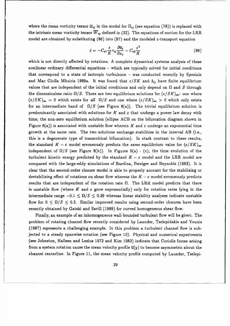
8/10/2019 speziale 1990
http://slidepdf.com/reader/full/speziale-1990 31/60
where the mean vorticity
tensor Oij in
the model
for
[Iij (see equation
(78)) is replaced
with
the
intrinsic
mean vorticity
tensor Wil defined in (32).
The equations
of motion for
the
LR R
model
are
obtained
by
substituting
(86) into (87)
and the modeled
C-transport
equation
i= -C. - c.2
-
(88)
which
is
not
directly
affected
by
rotations. A complete dynamical
systems
analysis
of
these
nonlinear ordinary
differential equations
- which are
typically solved for initial
conditions
that
correspond to
a state of isotropic
turbulence
-
was
conducted recently
by Speziale
and
Mac
Giolla
Mhuiris
1989a. It was
found that e/SK and
bij have finite
equilibrium
values
that
are
independent
of the
initial conditions and only
depend
on
£2 and
S through
the
dimensionless ratio £/S. There
are two equilibrium
solutions for (c/SK)..: one
where
(c/SK)= = 0
which exists for
all £/S and one where (e/SK)oo
> 0 which only exists
for
an intermediate
band
of
£/S
(see
Figure
8(a)). The trivial
equilibrium
solution is
predominantly
associated
with
solutions for
K and
e
that undergo
a power law decay with
time;
the
non-zero
equilibrium
solution
(ellipse
ACB on the bifurcation
diagram shown in
Figure
8(a)) is associated
with unstable flow wherein
K and
e
undergo an exponential time
growth
at
the
same
rate.
The two solutions
exchange stabilities
in the interval
AB
(i.e.,
this
is a degenerate
type of
transcritical bifurcation). In
stark contrast
to these results,
the
standard
K
- e model erroneously
predicts
the
same
equilibrium value
for (C/SK)
independent of
P/S (see Figure 8(b)).
In Figures 9(a)
-
(c),
the time evolution of the
turbulent
kinetic
energy
predicted
by the standard K
- c model and
the LRR model are
compared
with
the
large-eddy
simulations
of
Bardina,
Ferziger
and
Reynolds
(1983).
It
is
clear that the
second-order closure model
is able to properly
account for
the stabilizing or
destabilizing effect
of rotations
on shear
flow
whereas
the K - e model
erroneously predicts
results that
are independent of the
rotation rate £2. The
LRR model
predicts
that
there
is
unstable
flow
(where K
and
c
grow
exponentially) only
for rotation rates lying
in the
intermediate
range
-0.1
<
£2/S
< 0.39 whereas
linear
stability analyses
indicate unstable
flow for
0 <
£/S
< 0.5.
Similar improved
results
using
second-order closures
have
been
recently
obtained
by Gatski
and
Savill
(1989) for
curved
homogeneous shear flow.
Finally,.
an example of an
inhomogeneous wall-bounded
turbulent flow
will
be given.
The
problem
of
rotating
channel
flow
recently considered
by
Launder,
Tselepidakis and
Younis
(1987)
represents
a challenging example. In this
problem a turbulent
channel
flow is
sub-
jected
to a steady spanwise
rotation (see
Figure
10).
Physical and
numerical experiments
(see
Johnston, Halleen
and Lezius 1972
and Kim 1983) indicate that
Coriolis forces
arising
from a system rotation cause
the mean
velocity profile
U(y) to
become
asymmetric about
the
channel
centerline.
In Figure 11, the
mean
velocity
profile computed
by Launder, Tselepi-
29
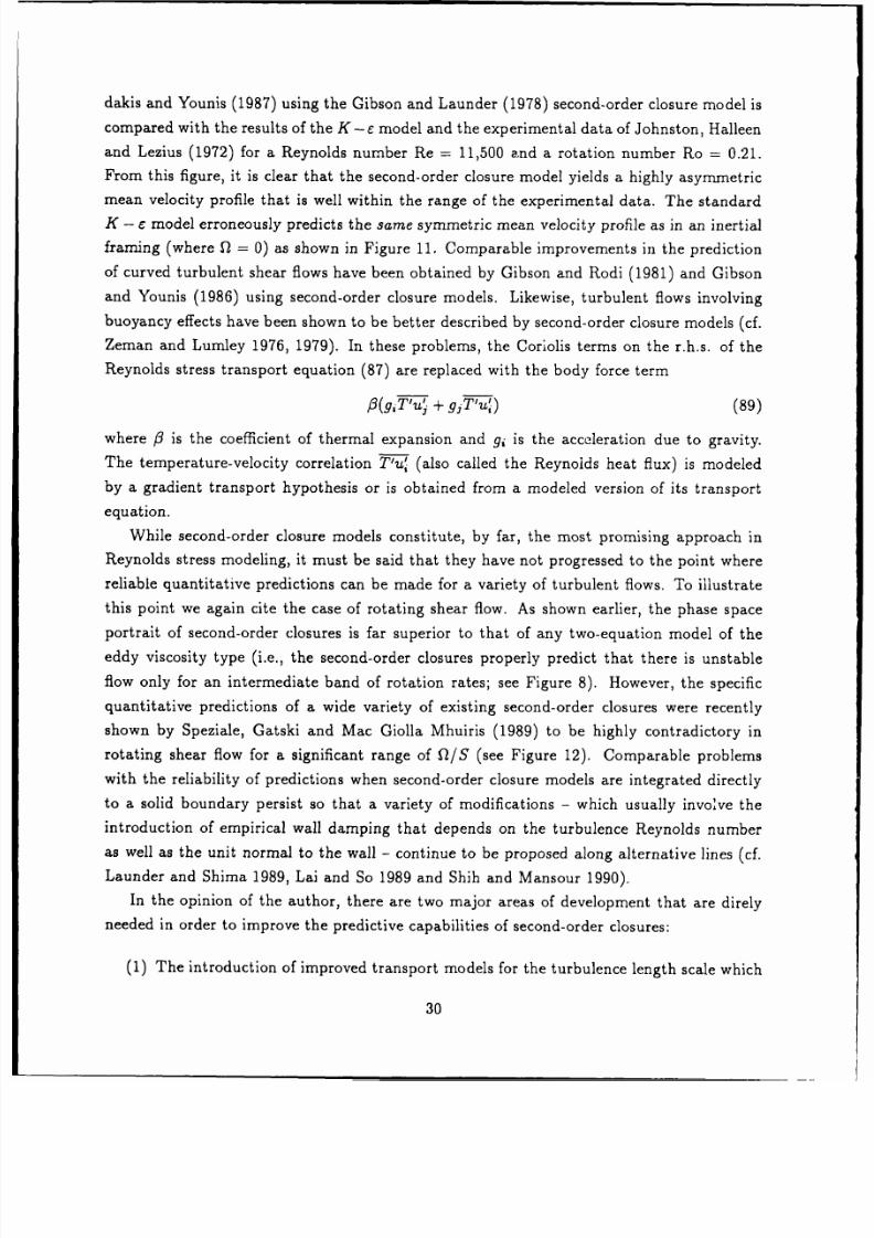
8/10/2019 speziale 1990
http://slidepdf.com/reader/full/speziale-1990 32/60
dakis and
Younis
(1987)
using the
Gibson
and
Launder
(1978)
second-order
closure
model
is
compared
with the results
of the
K - e
model and
the
experimental
data
of Johnston,
Halleen
and Lezius
(1972)
for
a
Reynolds
number
Re = 11,500
and
a
rotation
number
Ro = 0.21.
From
this
figure,
it is
clear
that the
second-order
closure
model
yields
a
highly
asymmetric
mean
velocity
profile
that is
well
within
the range of
the
experimental
data.
The
standard
K
- c
model erroneously
predicts
the
same
symmetric
mean
velocity profile
as in
an
inertial
framing
(where
l
=
0)
as
shown in
Figure 11.
Comparable
improvements
in the
prediction
of
curved turbulent
shear
flows
have
been
obtained by
Gibson
and Rodi
(1981)
and
Gibson
and
Younis
(1986)
using
second-order
closure
models.
Likewise,
turbulent
flows
involving
buoyancy
effects
have
been shown
to be better
described
by second-order
closure
models
(cf.
Zeman
and
Lumley
1976,
1979). In
these
problems,
the
Coriolis
terms on
the r.h.s. of
the
Reynolds
stress
transport
equation
(87) are
replaced
with
the
body force
term
3(g,9T'-u +
gjT'u) (89)
where
j3
is
the
coefficient
of thermal
expansion
and
g, is
the acceleration
due
to gravity.
The
temperature-velocity
correlation
Tlu
(also
called
the
Reynolds
heat flux)
is modeled
by a
gradient
transport
hypothesis
or
is
obtained
from
a
modeled version
of
its
transport
equation.
While second-order
closure
models constitute,
by far, the
most
promising
approach
in
Reynolds
stress
modeling,
it must be
said
that
they
have not
progressed
to the
point where
reliable quantitative
predictions
can be made
for a variety
of
turbulent
flows.
To
illustrate
this
point
we
again
cite
the
case of rotating
shear
flow.
As
shown earlier,
the
phase space
portrait
of
second-order
closures
is
far
superior
to
that
of
any
two-equation
model
of
the
eddy
viscosity
type (i.e.,
the
second-order
closures
properly
predict
that
there
is
unstable
flow
only for an
intermediate
band of rotation
rates;
see
Figure 8).
However,
the specific
quantitative
predictions
of
a wide
variety
of
existing
second-order
closures
were
recently
shown by
Speziale,
Gatski
and Mac
Giolla
Mhuiris
(1989)
to be
highly
contradictory
in
rotating
shear flow
for a
significant
range of
P/S
(see
Figure
12).
Comparable
problems
with the
reliability
of
predictions when
second-order
closure
models
are integrated
directly
to a solid
boundary
persist
so that a
variety of
modifications
-
which
usually
involve
the
introduction
of
empirical
wall
damping
that
depends
on
the
turbulence
Reynolds
number
as well
as the
unit normal
to the wall
-
continue
to be
proposed
along alternative
lines
(cf.
Launder
and Shima
1989,
Lai and So
1989
and
Shih
and Mansour
1990).
In
the opinion
of
the author,
there
are two
major
areas
of development
that
are
direly
needed
in order
to improve
the
predictive
capabilities
of
second-order
closures:
(1)
The
introduction
of
improved
transport
models
for the
turbulence
length
scale which
30
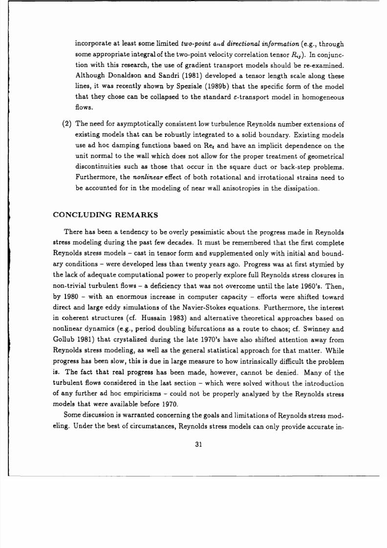
8/10/2019 speziale 1990
http://slidepdf.com/reader/full/speziale-1990 33/60
incorporate
at least
some limited
two-point a,,d directional
nformation
(e.g., through
some
appropriate
integral
of
the
two-point
velocity correlation
tensor RPj).
In
conjunc-
tion
with
this
research,
the use of
gradient
transport
models
should
be re-examined.
Although Donaldson
and
Sandri
(1981)
developed
a tensor
length
scale along
these
lines,
it was
recently
shown
by Speziale
(1989b)
that
the specific
form of the
model
that
they chose
can be collapsed
to the standard
c-transport
model
in homogeneous
flows.
(2)
The
need
for
asymptotically
consistent low
turbulence
Reynolds
number extensions
of
existing
models
that
can
be robustly
integrated
to a solid
boundary.
Existing
models
use ad
hoc
damping
functions based
on
Ret and have
an implicit
dependence
on the
unit
normal to
the
wall
which does
not allow
for
the
proper treatment
of geometrical
discontinuities
such as those
that occur
in the
square duct
or
back-step
problems.
Furthermore,
the
nonlinear
effect of
both rotational
and irrotational
strains
need to
be
accounted
for
in
the modeling
of
near
wall
anisotropies
in
the
dissipation.
CONCLUDING
REMARKS
There has
been a
tendency
to be overly
pessimistic
about the
progress made
in
Reynolds
stress
modeling
during the
past few
decades.
It must
be
remembered
that the
first
complete
Reynolds stress
models
- cast in
tensor
form and
supplemented
only
with initial and
bound-
ary conditions
-
were
developed
less than
twenty
years ago. Progress
was at
first
stymied
by
the lack
of
adequate
computational
power
to
properly
explore full
Reynolds
stress
closures
in
non-trivial turbulent
flows
- a deficiency
that was
not overcome until
the
late
1960's.
Then,
by
1980
- with an enormous
increase in
computer
capacity
- efforts were
shifted
toward
direct
and
large
eddy simulations of
the Navier-Stokes
equations. Furthermore,
the interest
in coherent
structures (cf.
Hussain
1983) and alternative
theoretical
approaches
based
on
nonlinear
dynamics
(e.g.,
period doubling
bifurcations
as a route
to chaos;
cf. Swinney
and
Gollub
1981)
that crystalized
during
the late 1970's
have also
shifted
attention
away
from
Reynolds
stress
modeling,
as
well
as the
general statistical
approach for
that matter.
While
progress
has been
slow,
this is
due in large
measure
to how
intrinsically
difficult
the problem
is.
The
fact
that
real progress has been made,
however,
cannot
be
denied. Many
of
the
turbulent
flows
considered in
the
last section
- which were
solved
without
the introduction
of
any further
ad
hoc
empiricisms
- could
not be
properly
analyzed
by the
Reynolds
stress
models
that
were
available
before
1970.
Some
discussion
is warranted
concerning the
goals
and
limitations
of
Reynolds
stress mod-
eling.
Under the
best of circumstances,
Reynolds stress
models
can only
provide
accurate
in -
31
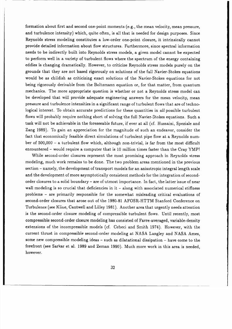
8/10/2019 speziale 1990
http://slidepdf.com/reader/full/speziale-1990 34/60
formation
about first and
second
one-point
moments
(e.g., the
mean velocity,
mean pressure,
and turbulence
intensity) which,
quite often,
is all
that is
needed for
design purposes.
Since
Reynolds
stress
modeling
constitutes
a low-order
one-point
closure,
it intrinsically
cannot
provide
detailed
information about
flow
structures. Furthermore,
since
spectral information
needs
to be
indirectly
built into
Reynolds
stress models,
a
given model
cannot be
expected
to perform well
in a
variety of turbulent
flows
where the
spectrum of
the
energy containing
eddies
is
changing dramatically.
However,
to
criticize
Reynolds stress
models
purely
on the
grounds
that
they are not
based rigorously
on solutions of
the full
Navier-Stokes
equations
would
be
as
childish
as
criticizing
exact
solutions of
the Navier-Stokes
equations
for not
being
rigorously
derivable from
the Boltzmann
equation or, for
that matter,
from
quantum
mechanics.
The
more
appropriate
question
is whether or
not
a
Reynolds
stress
model can
be developed
that will
provide
adequate engineering
answers for the
mean velocity,
mean
pressure
and turbulence
intensities
in
a
significant
range of turbulent
flows
that
are of techno-
logical
interest.
To
obtain accurate
predictions
for
these
quantities
in
all
possible
turbulent
flows will
probably
require nothing
short
of solving
the full
Navier-Stokes
equations. Such
a
task will not
be
achievable
in the foreseeable
future,
if
ever
at
all (cf.
Hussaini,
Speziale and
Zang 1989).
To
gain an
appreciation for
the magnitude
of
such an endeavor,
consider
the
fact
that
economically
feasible
direct simulations
of
turbulent
pipe
flow at a Reynolds
num-
ber
of 500,000
- a
turbulent flow
which,
although
non-trivial,
is far from
the
most difficult
encountered
- would
require a
computer that
is
10
million
times
faster
than
the
Cray YMP
While
second-order
closures
represent
the
most
promising
approach in Reynolds
stress
modeling,
much
work
remains to be
done.
The two
problem areas
mentioned
in the
previous
section
-
namely,
the
development
of
transport
models
for
an
anisotropic
integral
length
scale
and the
development of
more
asymptotically
consistent
methods for
the integration
of second-
order
closures
to a solid boundary
- are of
utmost importance.
In fact,
the
latter
issue
of near
wall modeling
is so crucial that
deficiencies
in it -
along with
associated
numerical stiffness
problems -
are primarily
responsible
for
the somewhat
misleading
critical
evaluations
of
second-order
closures that
arose out of
the
1980-81 AFOSR-HTTM
Stanford
Conference on
Turbulence
(see
Kline,
Cantwell
and
Lilley
1981).
Another area that
urgently
needs attention
is the
second-order
closure
modeling of
comprcssible turbulent
flows.
Until recently,
most
compressible
second-order
closure
modeling
has consisted
of
Favre-averaged,
variable- density
extensions of
the incompressible
models (cf.
Cebeci
and Smith
1974).
However,
with the
current thrust
in
compressible
second-order
modeling
at
NASA
Langley
and NASA Ames,
some
new
compressible
modeling ideas
- such
as dilatational
dissipation -
have
come
to the
forefront
(see
Sarkar et al.
1989 and
Zeman 1990).
Much
more work in
this
area
is needed,
however.
32
8/10/2019 speziale 1990
http://slidepdf.com/reader/full/speziale-1990 35/60
Reynolds
stress modeling
should continue to
steadily progress -
complementing
numerical
simulations of
the Navier-Stokes equations
and alternative theoretical
approaches. In fact,
with
anticipated improvements
in computer capacity,
direct numerical
simulations should
begin to play
a
pivotal
role in
the
screening and calibration
of turbulence models.
Further-
more, from
the theoretical side,
statistical
mechanics
approaches such as
RNG could be of
considerable
future use in
the
formulation
of new models
(unfortunately, at their current
stage
of development,
it does
not
appear
that
they
can reliably calibrate
turbulence
models
for use in complex
flows). Although Reynolds
stress models
provide
information
only about
a
limited
facet
of
turbulence,
this
information
can have
such important
scientific
and
engi-
neering applications
that
they are
likely
to
remain a part
of turbulence research
for
many
years
to
come.
ACKNOWLEDGEMENTS
The
author
would like to thank Drs. T.
B. Gatski,
N.
Mac
Giolla
Mhuiris
and
S. Sarkar
for
their
assistance with
some
of
the
computations
presented
in
this paper.
Helpful comments
by Dr.
M. Y. Hussaini
are
also gratefully
acknowledged. This
research
was
supported
under
NASA Contract
NAS1-18605
while
the author
was in
residence
at ICASE,
NASA
Langley
Research Center, Hampton, VA
23665.
33
8/10/2019 speziale 1990
http://slidepdf.com/reader/full/speziale-1990 36/60
References
Avva,
R. K., Kline, S. J., and
Ferziger, J.
H. 1988.
Computation of the
turbulent
flow over
a
backward-facing step
using the
zonal
modeling
approach. Stanford
University Technical
Report TF-33.
Baldwin,
B. S. and
Lomax,
H. 1978.
Thin layer
approximation
and
algebraic
model
for
separated
turbulent
flows. AIAA
Paper 78-257.
Bardina, J., Ferziger,
J. H., and
Reynolds, W.
C. 1983. Improved
turbulence
models based
on large-eddy
simulation of
homogeneous, incompressible
turbulent flows.
Stanford Uni-
versity Technical
Report TF-19.
Bardina, J.,
Ferziger, J.
H.,
and Rogallo,
R.
S.
1985. Effect of rotation
on
isotropic
turbu-
lence:
Computation
and modeling. J.
Fluid
Mech.
154:321-336.
Bernard, P. S. and
Berger, B. S. 1982.
A method
for computing
three-dimensional
turbulent
flows. SIAM
J. Appl.
Math. 42:453-470.
Bertoglio,
J.
P. 1982.
Homogeneous turbulent
field within
a
rotating
frame.
AIAA
J.
20:1175-1181.
Boussinesq,
J. 1877. Th6orie
de
l'6coulement
tourbillant. Mim Pres.
Acad.
Sci., Paris
23:46.
Bradshaw,
P., Ferriss,
D.
H., and
Atwell,
M.
P.
1967.
Calculation
of
boundary layer devel-
opment using the
turbulent
energy equation. J.
Fluid
Mech.
28:593-616.
Cebeci, T.
and Smith, A. M.
0. 1968.
Computation of
turbulent
boundary
layers. 1968
AFOSR-IFP
Stanford Conference
on Turbulence,
eds. S.
J. Kline, M. V.
Morkovin,
G.
Sovran,
and D.
S.
Cockrell, Vol. 1,
p.
346. Stanford:
Stanford
University
Press.
Cebeci, T.
and
Smith, A. M.
0.
1974.
Analysis
of Turbulent Boundary
Layers.
New
York:
Academic Press.
Choi,
K.
S. and
Lumley, J.
L.
1984.
Return
to isotropy
of homogeneous
turbulence
revisited.
Turbulence
and
Chaotic
Phenomena
in
Fluids,
ed. T.
Tatsumi, p. 267, New
York: North
Holland
Press.
Clark,
T. L.
and
Farley,
R. D.
1984.
Severe
downslope
windstorm calculations
in
two and
three
spatial dimensions using
anelastic interactive
grid
nesting:
A possible mechanism
for
gustiness. J.
Atmos. Sci.
41:329-350.
34
8/10/2019 speziale 1990
http://slidepdf.com/reader/full/speziale-1990 37/60
Comte-Bellot,
G. and
Corrsin, S.
1971. Simple
Eulerian time
correlation of full
and narrow-
band velocity
signals
in grid-generated,
isotropic turbulence.
J.
Fluid
Mech.
48:273-337.
Craft,
T.,
Fu,
S., Launder,
B. E., and
Tselepidakis,
D.
P. 1989.
Developments in
modeling
the
turbulent second-moment
pressure correlations.
UMIST
Mechanical
Engineering
Department
Report
No.
TFD/89/1.
Crow, S.
C. 1968.
Viscoelastic
properties of fine-grained
incompressible turbulence.
J.
Fluid
Mech. 33:1-20.
Daly,
B. J.
and Harlow,
F. H.
1970.
Transport
equations
in turbulence.
Phys.
Fluids
13:2634-2649.
Deardorff,
J. W.
1973. The
use
of
subgrid transport
equations
in
a three-dimensional
model
of
atmospheric
turbulence.
ASME J. Fluids
Eng. 95:429-438.
Demuren, A.
and
Rodi, W. 1984.
Calculation
of turbulence-driven
secoidary
motion in
non-circular
ducts. J.
FT.Id
Mech.
140:189-222.
Donaldson, C.
duP
':
,.
Calculation
of turbulent
shear flows for
atmospheric and
vortex
motions.
AIAA
J.
10:4-12.
Donaldson.
C. duP.
and Rosenbaum,
H.
1968. Calculation
of the
turbulent
shear
flows
thr.ugh
closure
of the Reynolds
equations
by invariant
modeling. ARAP
Report
No.
127,
Aeronautical
Research
Associates of
Princeton.
Donaldson,
C. duP.
and Sandri,
G. 1981.
On
the
inclusion of
information
on
eddy structure
in second-order
closure
model of
turbulent
flow. AGARD
Report No.
CP-308.
Fu, S., Launder,
B. E.,
and Tselepidakis,
D.
P.
1987. Accommodating
the
effects
of
high
strain rates
in
modelling
the
pressure-strain
correlation.
UMIST Mechanical
Engineering
Department
Report
TFD/87/5.
Gatski,
T.
B.
and
Savill, A.
M. 1989. An
analysis of
curvature
effects
for
the
control of
wall-bounded
shear flows.
AIAA Paper
89-1014.
Gessner,
F. B.
and
Po,
J. K. 1.976.
A Reynolds
stress model for
turbulent
corner
flow
- Part
II:
Comparisons
between theory
and
experiment. ASME J.
Fluids
Eng.
98:269-277.
Gibson, M. M.
and Launder,
B. E.
1978.
Ground effects on
pressure fluctuations
in the
atmospheric
boundary
layer.
J.
Fluid
Mech.
86:491-511.
35
8/10/2019 speziale 1990
http://slidepdf.com/reader/full/speziale-1990 38/60
Gibson,
M. M.
and Rodi,
W.
1981. A Reynolds
stress
closure
model
for turbulence
applied
to
the calculation of
a highly
curved
mixing layer. J.
Fluid Mech. 103:161-182.
Gibson, M.
M.
and
Younis, B. A. 1986. Calculation of swirling jets with a
Reynolds stress
closure.
Phys. Fluids
29:38-48.
Hanjalic, K. and Launder, B.
E. 1972. A Reynolds
stress model of turbulence
and its
application
to thin shear flows. J.
Fluid Mech. 52:609-638.
Hanjalic, K. and
Launder, B. E.
1976.
Contribution
towards a Reynolds
stress
closure for
low
Reynolds number
turbulence.
J.
Fluid
Mech. 74:593-610.
Hanjalic,
K.
and Launder,
B. E.
1980. Sensitizing the
dissipation equation
to
irrotational
strains.
ASME
J. Fluids
Eng. 102:34-40.
Haworth,
D.
C.
and Pope,
S.
B.
1986.
A
generalized
Langevin model
for
turbulent
flows.
Phys.
Fluids 29:387-405.
Hinze, J.
0. 1975.
Turbulence.
New
York: McGraw-Hill.
Hussain,
A. K.
M.
F.
1983. Coherent structures:
Reality and myth. Phys. Fluids 26:2816-
2850.
Hussaini,
M.
Y., Speziale,
C.
G.,
and Zang, T. A.
1989.
Discussion
of
the potential
an d
limitations of
direct
and large-eddy simulations.
Proceedingsof the Whither
Turbulence
Workshop, Cornell University.
To
appear
in
Lecture Notes
in
Physics,
Springer-Verlag.
Johnson,
D.
A.
and King, L.
S. 1984.
A
new turbulence closure
model for boundary
layer
flows
with
strong adverse pressure
gradients and
separation. AIAA Paper
84-0175.
Johnston,
J.
P., Halleen,
R. M., and Lezius,
D. K. 1972. Effects
of
a
spanwise
rotation
on
the structure of
two-dimensional fully-developed
turbulent channel
flow.
J.
Fluid
Mech.
56:533-557.
Kim,
J. 1983.
The effect
of rotation
on turbulence
structure.
NASA TM-84379.
Kim, J., Kline, S. J., and Johnston,
J.
P.
1980. Investigation of
a reattaching turbulent shear
layer:
Flow
over a backward-facing
step.
ASME J.
Fluids Eng.
102:302-308.
Kline, S. J., Cantwell, B.
J.,
and
Lilley, G.
M. eds.
1981.
Proceedings
of
the
1980-81
AFOSR-HTTM
Stanford
Conference
on Complex Turbulent
Flows. Stanford, CA:
Stan-
ford University
Press.
36
8/10/2019 speziale 1990
http://slidepdf.com/reader/full/speziale-1990 39/60
Kolmogorov,
A. N.
1942. The
equations of
turbulent
motion
in
an incompressible
fluid.
Izvestiya
Acad. Sci.
USSR:
Physics
6:56-58.
Kraichnan,
R.
H. 1964.
Direct
interaction
approximation
for shear
and
thermally
driven
turbulence.
Phys.
Fluids
7:1048-1062.
Lai,
Y.
G. and
So, R. M.
C. 1989. On
near
wall turbulent
flow modeling.
J.
Fluid
Mech.,
submitted for
publication.
Launder,
B.
E. 1989.
Phenomenological
modeling:
Present
and future.
Proceedings
of
the Whither
Turbulence Workshop,
Cornell
University.
To appear
in
Lecture Notes in
Physics,
Springer-Verlag.
Launder,
B. E. and
Ying, W. M.
1972.
Secondary flows
in
ducts
of
square cross-section.
J.
Fluid
Mech. 54:289-295.
Launder,
B. E. and
Spalding,
D.
B.
1974.
The
numerical computation
of
turbulent
flows.
Computer
Methods in
Applied Mechanics
and
Engineering
3:269-289.
Launder,
B.
E., Reece,
G.,
and
Rodi, W.
1975. Progress
in
the development
of a
Reynolds
stress turbulence
closure. J.
Fluid
Mech. 68:537-566.
Launder,
B.
E.,
Tselepidakis,
D.
P.,
and
Younis, B. A.
1987. A
second-moment
closure
study
of rotating
channel flow. J.
Fluid
Mech. 183:63-75.
Launder,
B.
E.
and
Shima,
N. 1989.
Second-moment
closure
for
the
near-wall sublayer:
Development
and
application.
AIAA
J.
27:1319-1323.
Lesieur,
M.
1987. Turbulence
in Fluids.
Boston:
Martinus Nijhoff.
Lumley, J.
L.
1970.
Toward a turbulent
constitutive equation.
J.
Fluid
Mech. 41:413-434.
Lumley,
J. L.
1978.
Computational
modeling of
turbulent
flows. Adv.
Appl. Mech. 18:123-
176.
Lumley,
J.
L. 1983.
Turbulence
modeling.
ASME
J.
Appl. Mech. 50:1097-1103.
Mellor,
G.
L. and
Herring, H.
J. 1973. A
survey of
mean turbulent
field closure
models.
AIAA
J.
11:590-599.
Mellor,
G. L. and
Yamada,
T.
1974. A hierarchy
of
turbulence
closure models for
planetary
boundary
layers.
J.
Atmos.
Sci. 31:1791-1806.
37

8/10/2019 speziale 1990
http://slidepdf.com/reader/full/speziale-1990 40/60
Moin,
P. and Kim,
J.
1982.
Numerical
investigation
of
turbulent
channel
flow.
J.
Fluid
Mech. 118:341-377.
Nisizima, S.
and
Yoshizawa, A. 1987.
Turbulent
channel and
Couette
flows using an anisotropic
K
- c
model. AIAA J. 25:414-420.
Norris, L. H. and Reynolds, W. C.
1975.
Turbulent channel flow with a moving wavy
boundary.
Stanford University
Technical
Report
FM-IO.
Orszag, S. A.
1970.
Analytical theories of
turbulence.
J. Fluid Mech. 41:363-386.
Patel, V. C., Rodi, W., and
Scheuerer,
G.
1985.
Turbulence models for near-wall and low
Reynolds number flows: A
review. AIAA J.
23:1308-1319.
Piomelli,
U.,
Ferziger, J.
H.,
and Moin, P. 1987. Models for large eddy simulations of
turbulent
channel
flows including transpiration.
Stanford University Technical Report
TF-32.
Pope, S. B.
1975.
A more
general
effective viscosity
hypothesis. J.
Fluid
Mech. 72:331-340.
Pope,
S.
B. 1978. An explanation of the turbulent round
jet/plane
jet
anomaly.
AIAA
J.
16:279-281.
Pope, S. B.
1985.
methods for turbulent
reactive flows. Prog. Energy
Combust.
Sci.
11:119-192.
Prandtl, L.
1925.
Uber
die ausgebildete turbulenz. ZAMM5:136-139.
Prandtl, L. and
Wieghardt,
K.
1945. Ueber
ein neues formelsystem filr die ausgebildete
turbulence.
Nachrichten der Akademie der Wissenschaften Gottingen:
Mathematisch
-
Physikalische
Klasse, pp.
6-19.
Reynolds, 0. 1895.
On
the
dynamical
theory
of incompressible viscous fluids and the
deter-
mination
of the criterion.
Phil.
Trans.
Roy.
Soc. London A186:123-164.
Reynolds, W.
C.
1976.
Computation
of
turbulent
flows.
Ann.
Rev.
Fluid
Mech.
8:183-208.
Reynolds, W. C.
1987. Fundamentals of turbulence
for turbulence modeling
and
simulation.
Lecture Notes
for Von
Karman Institute,
A GARD
Lecture Series No. 86, North Atlantic
Treaty
Organization.
Reynolds,
W.
C.
1988.
Private Communication.
38
8/10/2019 speziale 1990
http://slidepdf.com/reader/full/speziale-1990 41/60
Rodi,
W. 1976.
A new
algebraic relation
for
calculating the Reynolds
stresses. ZAMM
56:T219-221.
Rodi,
W.
1980.
Turbulence
Models
and Their
Application in Hydraulics,
Book
P,=blication
of the
International
Association
for
Hydraulics Research, Delft,
the Netherlands.
Rogallo,
R. S. and Moin,
P. 1984. Numerical
Simulation of Turbulent Flows. Ann. Rev.
Fluid
Mech.
16:99-137.
Rotta,
J.
C. 1951. Statistische Theorie
Nichthomogener
Turbulenz. Z. Phys.
129:547-572.
Rotta, J.
C. 19t2. Recent attempts
to develop a
generally
applicable calculation
method
for
turbulent
shear
flow
layers.
AGARD-CP-93, North Atlantic
Treaty Organization.
Rubinotein,
R. and Barton, J. M.
1989. Nonlinear
Reynolds
stress
models and
the
Renor-
malization
group.
Phys. Fluids
A.,
submitted
for
publication.
Saffmai.,
P. G.
1977. Results of a two-equation
model
for
turbulent flows
and development
of
a relaxation stress model for
application to straining
ard rotating flows. Project
SQUID
Workshop
on
Turbulence
in
Internal
Flows,
ed.
S. Murthy,
pp. 191-231, Hemisphere
Publishers.
Sarkar,
S., Erlebacher, G.,
Hussaini, M. Y., and Kreiss, H.
0. 1989. The analysis
and
modeling of
dilatational
terms in
compressible turbulence.
ICASE
Report
No. 89-79,
NASA Langley
Research Center.
Sarkar, S. and Speziale, C. G.
1990.
A
simple nonlinear model for
the return to isotropy
in
turbulence.
Phys.
Fluids A 2:84-93.
Schlichting,
H. 1968.
Boundary Layer
Theory.
New York: McGraw-Hill.
Shih,
T.-H. and Lumley, J. L. 1985.
Modeling
of
pressure
correlation terms in
Reynolds
stress
and scalar flux equations.
Technical
Report
No. FDA-85-3,
Cornell University.
Shih,
T.-H. and Mansour, N.
N. 1990. Second-order
modeling
of
low Reynolds number
turbulence
near
walls.
Phys. Fluids
A,
submitted
for
publication.
Smagorinsky, J. 1963. General
circulation experiments
with
the primitiv
equations. Monthly
Weather Rev. 91:99-165.
Smith, G.
F. 1971. On
isotropic functions of
symmetric tensors,
skew-symmetric tensors
and
vectors.
Int.
J.
Engng.
Sci.
9:899-916.
39
8/10/2019 speziale 1990
http://slidepdf.com/reader/full/speziale-1990 42/60
Smolarkiewicz, P.
K. and Clark, T.
L.
1985.
Numerical
simulation
of a
three-dimensional
field
of
cumulus
clouds. Part I.
Model
description, comparison
with observations
and
sensitivity
studies.
J. Atmos. Sci.
42:502-522.
Speziale,
C. G. 1981.
Some
interesting properties of
two-dimensional turbulence.
Phys.
Fluids24:1425-1427.
Speziale,
C. G.
1983.
Closure
models for
rotating two-dimensional turbulence.
Geophys.
Astrophys.
Fluid
Dynamics 23:69-84.
Speziale,
C. G. 1985. Modeling
the
pressure
gradient-velocity correlation
of turbulence.
Phys.
Fluids 28:69-71.
Speziale,
C.
G. 1987a.
Second-order closure
models for rotating
turbulent flows. Quart.
Appl.
Math.
45:721-733.
Speziale, C. G. 1987b. On
nonlinear
K
- i
and K -
e
models of turbulence. J.
Fluid
Mech.
178:459-475.
Speziale,
C.
G. 1989a.
Turbulence
modeling in non-inertial frames of
reference. Theoret.
Comput.
Fluid Dynamics 1:3-19.
Speziale, C. G. 1989b.
Discussion of
turbulence modeling:
Past and
future.
Proceedings of
the
Whither
Turbulence
Workshop,
Cornell University. To appear
in
Lecture
Notes in
Physics,
Springer-Verlag.
Speziale,
C.
G.,
Mansour, N.
N., and Rogallo,
R. S. 1987.
The
decay of isotropic
turbulence
in a rapidly rotating
frame. Proceedings of
the 1987
Summer
Program of
the Center or
Turbulence Research, eds.
P. Moin, W. C. Reynolds,
and
J.
Kim, pp.
205-211. Stanford
University
Press.
Speziale,
C. G. and
Ngo,
T. 1988. Numerical
solution
of
turbulent
flow
past a
backward
facing step using
a nonlinear
K -
e
model. Int.
J.
Eng. Sci.
26:1099-1112.
Speziale,
C.
G.
and
Mac
Giolla Mhuiris,
N.
1989a.
On
the prediction
of
equilibrium
states
in homogeneous turbulence. J.
Fluid
Mech.
209:591-615.
Speziale, C.
G. and Mac Giolla
Mhuiris, N.
1989b.
Scaling laws
for homogeneous
turbulent
shear
flows in a rotating
frame.
Phys. Fluids
A 1:294-301.
Speziale,
C. G., Gatski, T.
B.,
and Mac
Giolla
Mhuriris, N. 1989. A critical
comparison of
turbulence
models for homogeneous
shear flows in a
rotating frame.
Proceedi,.,s
of the
40
8/10/2019 speziale 1990
http://slidepdf.com/reader/full/speziale-1990 43/60
Seventh
Symposium
on
Turbulent Shear
Flows, Vol.
2,
pp. 27.3.1
-
27.3.6.
Stanford
University Press.
Speziale,
C. G.,
Sarkar,
S.,
and Gatski,
T.
B.
1990.
Modeling
the
pressure-strain
correlation
of
turbulence
-
an
invariant
dynamical systems
approach.
ICASE
Report
No. 90-5,
NASA
Langley
Research
Center.
Swinney,
H. L.
and Gollub,
J.
P. eds.
1981.
Hydrodynamic Instabilitiesand
the
Transition
to
Turbulence.
New
York: Springer-Verlag.
Tavoularis,
S. and Corrsin, S.
1981. Experiments
in
nearly
homogeneous turbulent shear
flows
with
a
uniform mean temperature gradient.
Part I. J. Fluid
Mech. 104:311-347.
Taylor,
G.
I. 1915.
Eddy motion in
the atmosphere. Phil. Trans.
Royal Soc.
London
A
215:1-26.
Tennekes,
H. and Lumley,
J.
L.
1972. A First Course in
Turbulence. Cambridge, MA:
MIT
Press.
Von K
rman, T.
1930.
Mechanische Thnlichkeit
und turbulenz. Proceedings Third
Int.
Congress Appl. Mech.,
Part
I, p. 85,
Stockholm.
Von Karm~n, T. 1948. Progress
in the statistical theory of turbulence.
Proc. Nat.
Acad.
Sci.,
Washington
34:530-539.
Weinstock,
J.
1981.
Theory
of
the
pressure-strain
rate
correlation
for
Reynolds stress
tur-
bulence closures. Part
1. J.
Fluid Mech. 105:369-396.
Wigeland,
R.
A. and Nagib,
H. M. 1978.
Grid-generated
turbulence
with and without
rotation about
the
streamwise
direction. lIT Fluids
and
Heat
Transfer
Report
R78-1,
Illinois
Institute
of Technology.
Wilcox, D. C.
1988. Reassessment of
the
scale-determining
equation
for advanced
turbulence
models.
AIAA J. 26:1299-1310.
Wilcox,
D. C.
and
Traci,
R.
M.
1976.
A
complete model
of
turbulence.
AIAA
Paper
76-351.
Wolfshtein,
M. 1970. On the length scale
of turbulence equation. IsraelJournal
of
Technology
8:87-99.
Yakhot,
V.
and Orszag,
S. A. 1986. Renormalization
group analysis of turbulence.
I. Basic
theory.
J. Sci.
Comp.
1:3-51.
41
8/10/2019 speziale 1990
http://slidepdf.com/reader/full/speziale-1990 44/60
Yoshizawa,
A. 1984. Statistical
analysis of
the deviation
of
the Reynolds stress
from its
eddy
viscosity representation. Phys.
Fluids27:1377-1387.
Yoshizawa,
A.
1987. Statistical modeling of a
transport
equation
for
the kinetic energy
dissipation
rate.
Phys. Fluids
30:628-631.
Zeman, 0.
1990. Dilatation
dissipation:
The concept and
application in modeling
compress-
ible
mixing
layers. Phys. Fluids A 2:178-188.
Zeman, 0.
and
Lunley,
J. L. 1976.
Modeling buoyancy-driven
mixed layers.
J.
Atmos. Sci.
33:1974-1988.
Zeman,
0.
and
Lumley,
J. L.
1979. Buoyancy effects in
entraining turbulent
boundary
layers:
A
second-order closure study. Turbulent
Shear Flows I, eds.
F. Durst, B. E.
Launder,
F.
W.
Schmidt, and
J.
H.
Whitelaw,
pp.
295-302,
Berlin: Springer-Verlag.
42
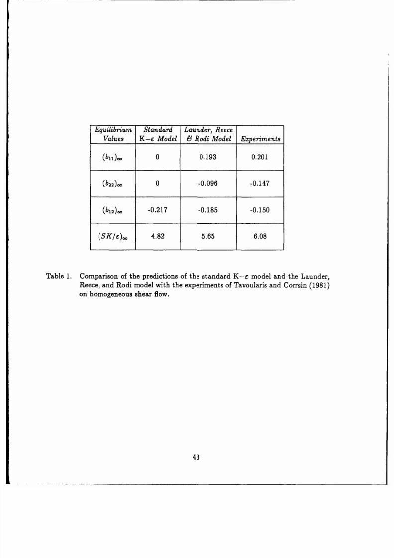
8/10/2019 speziale 1990
http://slidepdf.com/reader/full/speziale-1990 45/60
Equilibrium
Standard
Launder,
Reece
Values K-e
Model
d
Rodi
Model Experiments
0
0.193 0.201
(b
2
2
).
0
-0.096
-0.147
012).
-0.217
-0.185
-0.150
(Sg/c),o
4.82 5.65
6.08
Table 1. Comparison
of the
predictions of
the standard K-e
model
and the Launder,
Reece,
and
Rodi model
with
the
experiments
of
Tavoularis
and
Corrsin
(1981)
on homogeneous
shear
flow.
43
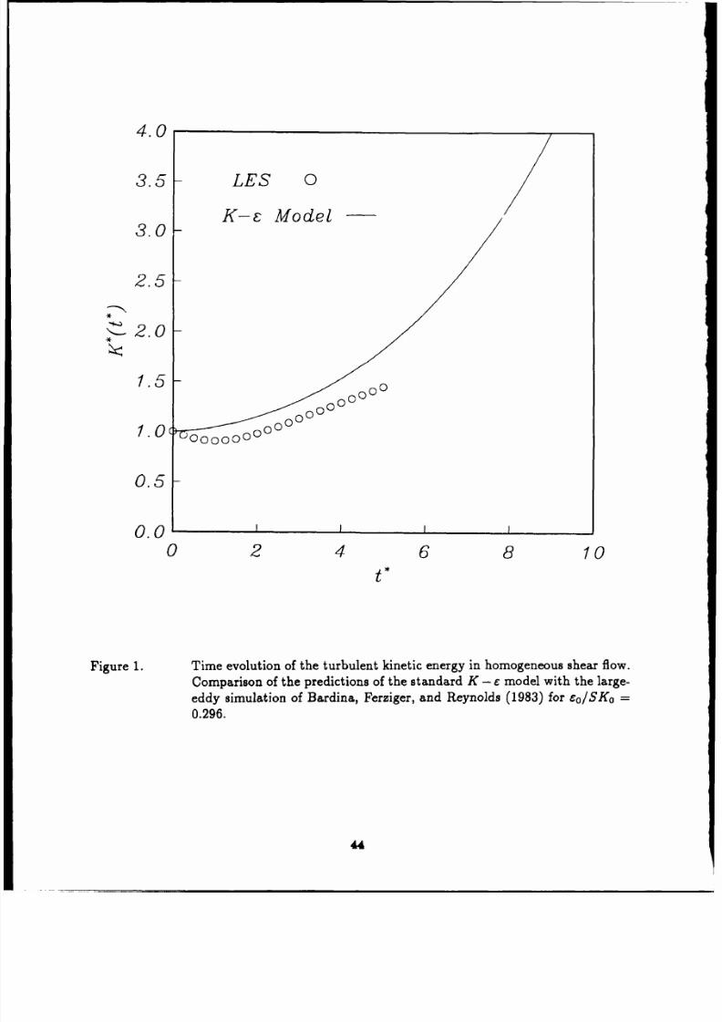
8/10/2019 speziale 1990
http://slidepdf.com/reader/full/speziale-1990 46/60
4.0
3.5- LES
0
K-E Model
3.0-
2.5
.- 2.0
1.5-
00000
1.0
000000000
0.5
0.0
1
0 2 4
6
8
10
t*
Figure 1.
Time evolution
of the turbulent
kinetic
energy
in homogeneous
shear flow.
Comparison
of
the predictions
of
the
standard K
- c model with
the large-
eddy simulation
of
Bardina,
Ferziger,
and
Reynolds
(1983) for
cO/SKo =
0.296.
44
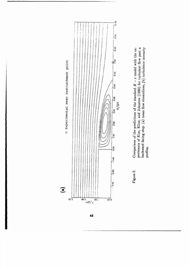
8/10/2019 speziale 1990
http://slidepdf.com/reader/full/speziale-1990 47/60
I
-P
C:C
4-)
040
4-)
I
0d0
4~ 0
4~
r.-. C
Cd
c
a
0d
.
u 0
H
N7
CC
I. Ll I
HV/
045
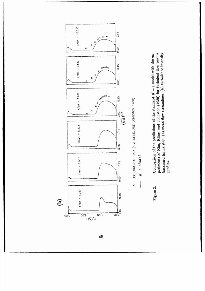
8/10/2019 speziale 1990
http://slidepdf.com/reader/full/speziale-1990 48/60
00
C0
0
0.0
00
0
o
cd
z
4)
0
0
0L
0
U20 m
II
0
0
4
Ob
44
C
0
466
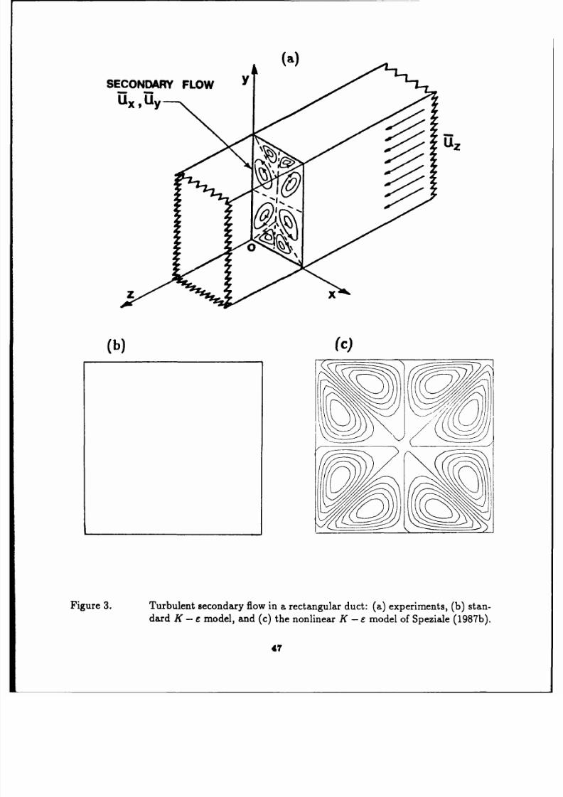
8/10/2019 speziale 1990
http://slidepdf.com/reader/full/speziale-1990 49/60
(a)
SECONDARY
FLOW
Y
Z
U
(b)
(c)
Figure
3.
Turbulent
secondary
flow
in
a
rectangular
duct:
(a)
experiments,
(b)
stan-
dard K
- c model,
and
(c) the
nonlinear
K
-
c
model
of Speziale
(1987b).
47
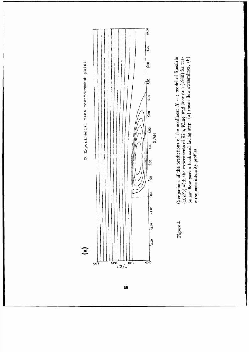
8/10/2019 speziale 1990
http://slidepdf.com/reader/full/speziale-1990 50/60
00
040
90
C2)
0J
rn
00
M
4
00
4-)
0)
u
H
o
04
r0
0)0
0)
00
u4
-0
Ed..-
cd-
4 +
o
0
m
-T.-
o
~
o
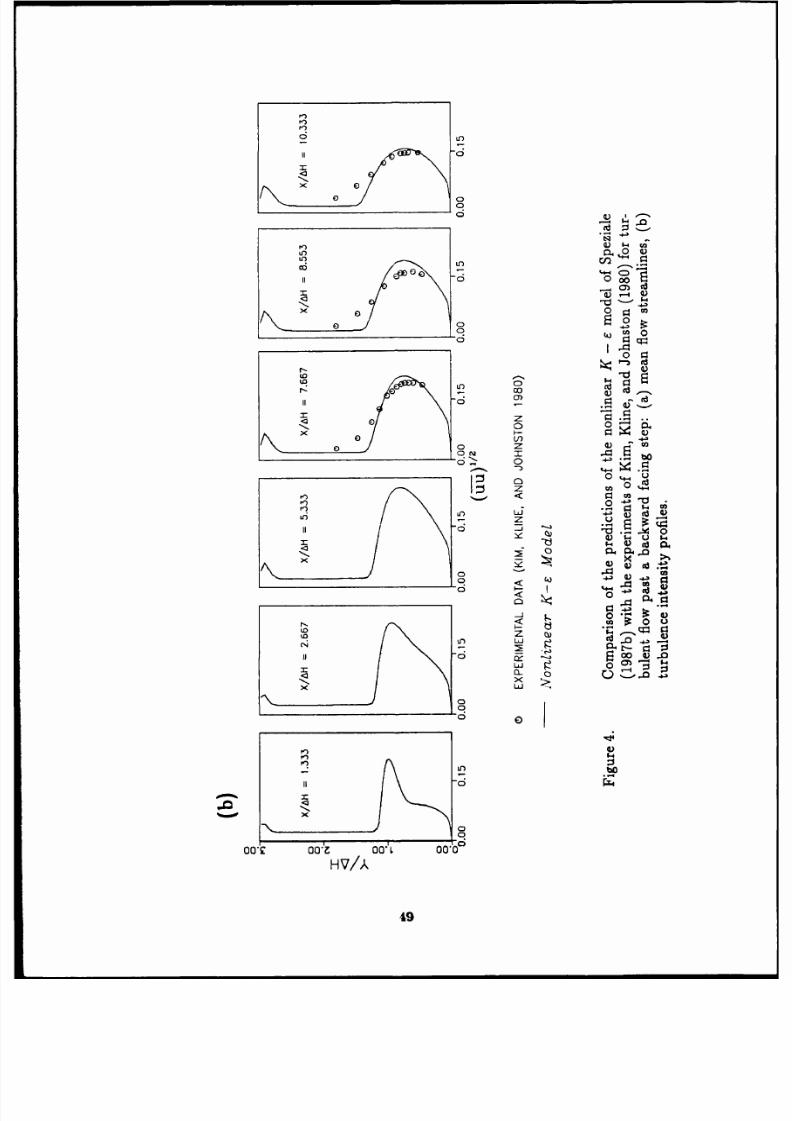
8/10/2019 speziale 1990
http://slidepdf.com/reader/full/speziale-1990 51/60
00
0n
0O 0
U*
V)-
0
O0 z
o
o
0
%4n
o
e
0
0
Of
S-
0
poo
0
.
N
0
oo
.6
-
LU
LOUb
0
I
I
HV/)V
49-
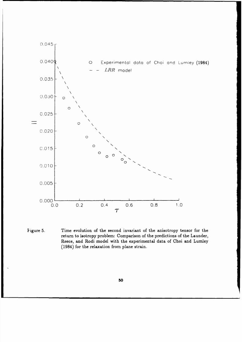
8/10/2019 speziale 1990
http://slidepdf.com/reader/full/speziale-1990 52/60
C)045
0.040( 0 Experimental data
of Choi
and Lumley (1984)
- LRR
model
0.035
0.0,_0 a
\
o \
0.025
\
0
0.020 \
0
0
00N
0.00
0.000
0.0 0.2 0.4
0.6
0.8 1.0
T
Figure
5.
Time evolution
of
the
second
invariant
of
the
anisotropy tensor
for
the
return to isotropy problem: Comparison of the predictions of the
Launder,
Reece, and Rodi
model
with
the
experimental data of Choi and Lumley
(1984) for the relaxation from plane strain.
50
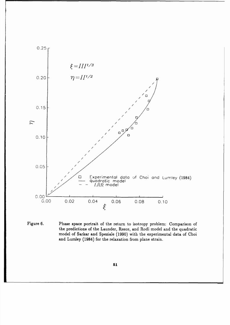
8/10/2019 speziale 1990
http://slidepdf.com/reader/full/speziale-1990 53/60
0.25
=1~f11/3
0.20
-
1
/
//
/
/
0.15
/0
/
/
/
]0
/0
0
0.10
/
0.05,
/
/
[] Experimental
data
of Choi
and
Lumley
(1984)
/
J
quadratic
model
~LRR
model
0.00
,
0.00
0.02
0.04
0.06
0.08
0.10
Figure
6.
Phase
space
portrait
of
the return
to
isotropy
problem:
Comparison
of
the
predictions
of
the
Launder,
Reece,
and Rodi
model
and the
quadratic
model
of Sarkar
and
Speziale
(1990)
with
the
experimental
data of
Choi
and
Lumley
(1984)
for
the relaxation
from
plane
strain.
/1
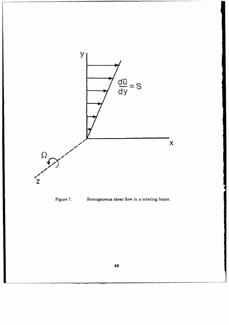
8/10/2019 speziale 1990
http://slidepdf.com/reader/full/speziale-1990 54/60
y
diJ
dy
,
x
f2
f
4,
z
Figure 7. Homogeneous
shear
flow in a rotating
frame.
52
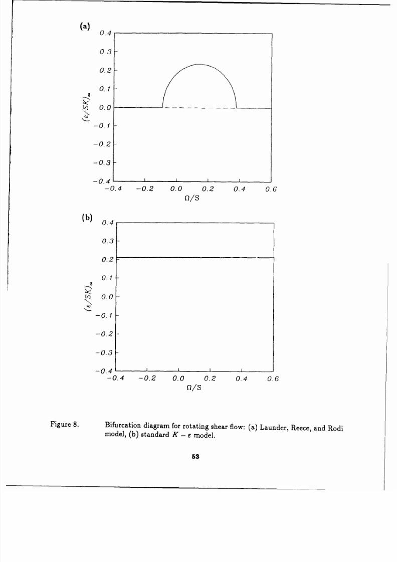
8/10/2019 speziale 1990
http://slidepdf.com/reader/full/speziale-1990 55/60
0.4
0.3
0.2
0.1
-0.
-0.2
-0.3
-0.4 -0.2 0.0 0.2
0.4
0.6
(b)
0.4
0.3
-
0.2
0.1-
0.0-
-0.1
-0.2
-
-0.3
-0.4
I
-0.4
-0.2
0.0
0.2
0.4
0.6
O/S
Figure
8.
Bifurcation
diagram
for
rotating
shear
flow:
(a)
Launder,
Reece,
and
Rodi
model,
(b) standard
K
-
e
model.
53
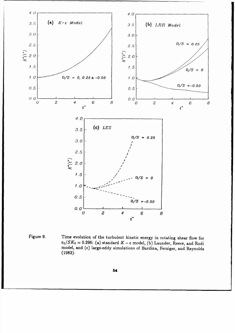
8/10/2019 speziale 1990
http://slidepdf.com/reader/full/speziale-1990 56/60
4.0
4.0
3.5
(a)
K-,
Model
3.5
b)
LRR
Model
3.0
3.0
2.5
2.5
/S
0.25
-20 2.0
1.5
1.5
Vs
= 0
1.0
/S
=
0, 0.25
-0.50
1.0
0.5
-
0.5-
n/V
0.50
00
0.01
0
2
4
6
8
0
2
46
8
t
t
4.0
35-
(c)
LE S
f/S = 0.25
3.0 -
I
I
2.5
-
I
2.05-/
II
/
1.5-
/
t - rl/s =0
1.0
--
0.5 -
fl/S =-o.5o
0.0
f
0
2
4
6
8
t*
Figure
9.
Time
evolution
of
the
turbulent
kinetic
energy
in
rotating
shear
flow
for
eo/SKo
=
0.296:
(a)
standard
K
- c
model,
(b)
Launder,
Reece,
and
Rodi
model,
and
(c)
large-eddy
simulations
of
Bardina,
Ferziger,
and
Reynolds
(1983).
54
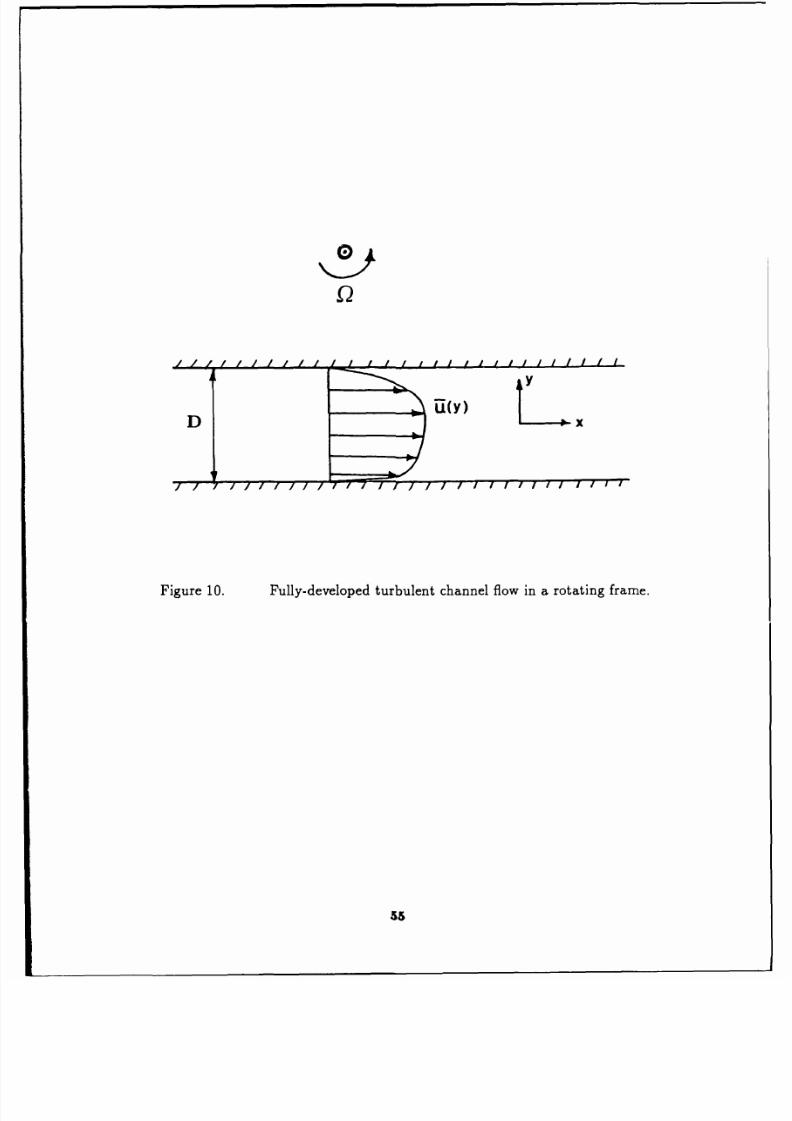
8/10/2019 speziale 1990
http://slidepdf.com/reader/full/speziale-1990 57/60
ky
MY)
D0 x
Figure 10.
Fully-developed turbulent channel
flow
in a rotating frame.
55
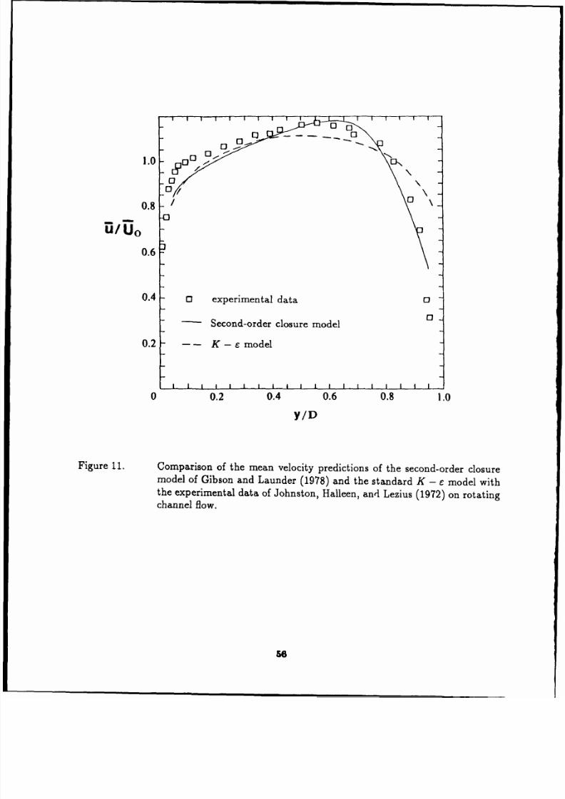
8/10/2019 speziale 1990
http://slidepdf.com/reader/full/speziale-1990 58/60
EJ
0
1.0
0s-
NE,,
-
0.8-/
U/u
0
0.6
0.4
0
experimental
data
0
-
Second-order
closure
model
0
0.2
-
K
-
e
model
I
I
I I
I
I
I I I
I 1
I I
I
I I
I
I I ,
0
0.2
0.4 0.6
0.8
1.0
Y/D
Figure
11.
Comparison
of the
mean
velocity
predictions
of the
second-order
closure
model
of
Gibson
and
Launder
(1978)
and the
standard
K - e
model
with
the
experimental
data
of
Johnston,
Halleen,
and
Lezius
(1972)
on
rotating
channel
flow.
56
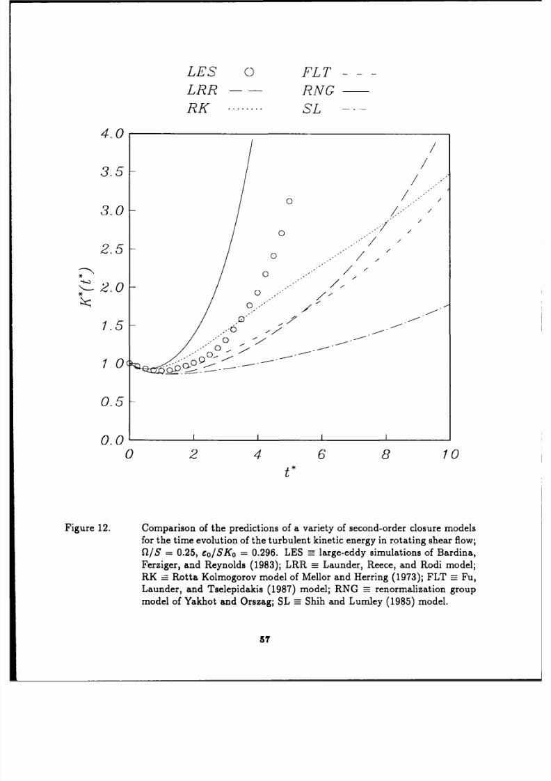
8/10/2019 speziale 1990
http://slidepdf.com/reader/full/speziale-1990 59/60
LES
0
FLT
LRR
-- RNG
RK
SL
4.0
//
3.5
/
0
7/
/
'°
.0-..
2.5-
0
0
1.5-
S0
.----
0.5
0.0 i
i
i
0 2
4
6 8
10
t
Figure
12.
Comparison
of
the
predictions
of
a variety
of
second-order
closure
models
for
the time evolution
of the turbulent
kinetic energy in rotating
shear
flow;
flIs =
0.25, eo/SKo
= 0.296.
LES large-eddy
simulations of Bardina,
Ferziger,
and Reynolds (1983);
LRR =
Launder, Reece,
and Rodi model;
RK
R=
ta Kolmogorov
model
of
Mellor and Herring (1973);
FLT
=
Fu,
Launder,
and Tselepidakis
(1987) model;
RNG = renormalization
group
model
of Yakhot
and Orszag; SL
=
Shih and
Lumley (1985)
model.
57
8/10/2019 speziale 1990
http://slidepdf.com/reader/full/speziale-1990 60/60
I14 0A
Report
Documentation
Page
1. Report
No.
2. Government
Accession No.
3.
Recipient s Catalog No.
NASA
CR-182017
ICASE
Report
No. 90-26
4. Title
and Subtitle
5.
Report
Date
ANALYTICAL
METHODS
FOR
THE
DEVELOPMENT
OF
REYNOLDS
March
1990
STRESS
CLOSURES
IN
TURBULENCE
6. Performing
Organization
Code
7.
Author(s)
8. Performing
Organization Report
No.
Charles
G.
Speziale
90-26
10. Work
Unit No.
505-90-21-01
9.
Performing
Organization
Name and Address
Institute
for Computer
Applications
in
Science
11. Contract
or Grant
No .
and
Engineering
NAS1-18605
Mail Stop
132C,
NASA Langley
Research
Center
Hampton.
VA
23665-5225
13. Type of Report
and Period
Covered
12.
Sponsoring
Agency Name
and
Address
Contractor
Report
National
Aeronautics
and
Space Administration
Langley
Research Center
14. Sponsoring
Agency Code
Hampton,
VA 23665-5225
15.
Supplementary
Notes
Langley Technical
Monitor:
To appear
in the
Annual
Review
Richard
W. Barnwell
of
Fluid
Mechanics
Final
Report
16.
Abstract
Analytical
methods
for
the
development
of
Reynolds
stress models
in
turbu-
lence are
reviewed in
detail. Zero,
one and
two equation models
are
discussed
along with
second-order
closures.
A strong
case is made
for
the
superior
pre-
dictive
capabilities
of
second-order
closure
models
in
comparison
to
the simpler
models.
The central
points of the
paper are
illustrated
by
examples from
both
homogeneous
and
inhomogeneous
turbulence.
A discussion
of
the
author s
views
concerning
the progress
made
in Reynolds
stress modeling
is also
provided
along
with
a
brief
history
of
the
subject.
17.
Key
Words
Suggested by Authorls)) ... 18. Distribution
Statement

![[Leclercq 1990] Leclercq, Robert: `Eénmansneerlandistiek ...neon.niederlandistik.fu-berlin.de/.../Duits/Leclercq_1990.pdf · [Leclercq 1990] Leclercq, Robert: `Eénmansneerlandistiek](https://img.pdfslide.org/doc/110x75/6060d53065cba57f97686fb5/leclercq-1990-leclercq-robert-enmansneerlandistiek-neon-leclercq-1990.jpg)