Embed Size (px)
Citation preview
Stability, observer design and control of networks
using Lyapunov methods
von Lars Naujok
Dissertation zur Erlangung des Grades eines Doktors der Naturwissenschaften- Dr. rer. nat. -
Vorgelegt im Fachbereich 3 (Mathematik & Informatik)der Universität Bremen
im März 2012
Tag der Einreichung: 01.03.2012
1. Gutachter: Prof. Dr. Sergey Dashkovskiy, Universität Bremen2. Gutachter: Prof. Dr. Lars Grüne, Universität Bayreuth
Acknowledgement
First of all I am deeply grateful to my advisor Sergey Dashkovskiy, who supported me withinthe three years working on this thesis by many discussions, new research ideas and takingtime for the continuous improvement of the quality of my work.I like to thank all the members of the workgroup “Mathematical Modeling of Complex
Systems”, which is a research group associated to the Center for Industrial Mathematics(ZeTeM) at the University of Bremen, for the useful discussions and seminars. Especially,I appreciate the cooperation with my colleague Michael Kosmykov, who read parts of mythesis and I enjoyed the nice atmosphere sharing an office with him. Also, I like to thankmy colleague Andrii Mironchenko for the useful discussions and the cooperation in the paperabout impulsive systems.There were helpful remarks and discussions with Lars Grüne, Hamid Reza Karimi, Daniel
Liberzon, Andy Teel and Fabian Wirth, which inspired me for parts of this thesis.The results presented in this thesis, were developed during my work as a research assis-
tant at the University of Bremen within the framework of the Collaborative Research Center(CRC) 637 “Autonomous Cooperating Logistic Processes”, subproject A5 “Dynamics of Au-tonomous Systems”, supported by the German Research Foundation (DFG). Especially, I liketo thank Michael Görges and Thomas Jagalski for the cooperation within the subproject A5.Last but not least, I will not forget the patience and support, which I got from my family,
especially from my parents, Anke und Peter, and my girlfriend Yvonne.Thank you very much.
Bremen and Hamburg, March the 1st, 2012
Lars Naujok
Abstract
We investigate different aspects of the analysis and control of interconnected systems. Dif-ferent tools, based on Lyapunov methods, are provided to analyze such systems in view ofstability, to design observers and to control systems subject to stabilization. All the differ-ent tools presented in this work can be used for many applications and extend the analysistoolbox of networks.Considering systems with inputs, the stability property input-to-state dynamical stability
(ISDS) has some advantages over input-to-state stability (ISS). We introduce the ISDS prop-erty for interconnected systems and provide an ISDS small-gain theorem with a constructionof an ISDS-Lyapunov function and the rate and the gains of the ISDS estimation for thewhole system.This result is applied to observer design for single and interconnected systems. Observers
are used in many applications where the measurement of the state is not possible or disturbeddue to physical reasons or the measurement is uneconomical. By the help of error Lyapunovfunctions we design observers, which have a so-called quasi ISS or quasi-ISDS property toguarantee that the dynamics of the estimation error of the systems state has the ISS or ISDSproperty, respectively. This is applied to quantized feedback stabilization.In many applications, there occur time-delays and/or instantaneous “jumps” of the systems
state. At first, we provide tools to check whether a network of time-delay systems hasthe ISS property using ISS-Lyapunov-Razumikhin functions and ISS-Lyapunov-Krasovskiifunctionals. Then, these approaches are also used for interconnected impulsive systems withtime-delays using exponential Lyapunov-Razumikhin functions and exponential Lyapunov-Krasovskii functionals. We derive conditions to assure ISS of an impulsive network withtime-delays.Controlling a system in a desired and optimal way under given constraints is a challenging
task. One approach to handle such problems is model predictive control (MPC). In this thesis,we introduce the ISDS property for MPC of single and interconnected systems. We provideconditions to assure the ISDS property of systems using MPC, where the previous result ofthis thesis, the ISDS small-gain theorem, is applied. Furthermore, we investigate the ISSproperty for MPC of time-delay systems using the Lyapunov-Krasovskii approach. We provetheorems, which guarantee ISS for single and interconnected systems using MPC.
Contents
Introduction 7
1 Preliminaries 15
1.1 Input-to-state stability . . . . . . . . . . . . . . . . . . . . . . . . . . . . . . . 17
1.2 Interconnected systems . . . . . . . . . . . . . . . . . . . . . . . . . . . . . . . 19
2 Input-to-state dynamical stability (ISDS) 23
2.1 ISDS for single systems . . . . . . . . . . . . . . . . . . . . . . . . . . . . . . 24
2.2 ISDS for interconnected systems . . . . . . . . . . . . . . . . . . . . . . . . . 27
2.3 Examples . . . . . . . . . . . . . . . . . . . . . . . . . . . . . . . . . . . . . . 31
3 Observer and quantized output feedback stabilization 35
3.1 Quasi-ISDS observer for single systems . . . . . . . . . . . . . . . . . . . . . . 37
3.2 Quasi-ISS and quasi-ISDS observer for interconnected systems . . . . . . . . . 42
3.3 Applications . . . . . . . . . . . . . . . . . . . . . . . . . . . . . . . . . . . . . 48
3.3.1 Dynamic quantizers . . . . . . . . . . . . . . . . . . . . . . . . . . . . 52
4 ISS for time-delay systems 55
4.1 ISS for single time-delay systems . . . . . . . . . . . . . . . . . . . . . . . . . 57
4.2 ISS for interconnected time-delay systems . . . . . . . . . . . . . . . . . . . . 61
4.2.1 Lyapunov-Razumikhin approach . . . . . . . . . . . . . . . . . . . . . 62
4.2.2 Lyapunov-Krasovskii approach . . . . . . . . . . . . . . . . . . . . . . 64
4.3 Applications in logistics . . . . . . . . . . . . . . . . . . . . . . . . . . . . . . 66
4.3.1 A certain scenario . . . . . . . . . . . . . . . . . . . . . . . . . . . . . 67
5 ISS for impulsive systems with time-delays 71
5.1 Single impulsive systems with time-delays . . . . . . . . . . . . . . . . . . . . 73
5.1.1 The Lyapunov-Razumikhin methodology . . . . . . . . . . . . . . . . . 74
5.1.2 The Lyapunov-Krasovskii methodology . . . . . . . . . . . . . . . . . . 79
5.2 Networks of impulsive systems with time-delays . . . . . . . . . . . . . . . . . 81
5.2.1 The Lyapunov-Razumikhin approach . . . . . . . . . . . . . . . . . . . 81
5.2.2 The Lyapunov-Krasovskii approach . . . . . . . . . . . . . . . . . . . . 83
5.3 Example . . . . . . . . . . . . . . . . . . . . . . . . . . . . . . . . . . . . . . . 85
5
6
6 Model predictive control 896.1 ISDS and MPC . . . . . . . . . . . . . . . . . . . . . . . . . . . . . . . . . . . 92
6.1.1 Single systems . . . . . . . . . . . . . . . . . . . . . . . . . . . . . . . 926.1.2 Interconnected systems . . . . . . . . . . . . . . . . . . . . . . . . . . . 96
6.2 ISS and MPC of time-delay systems . . . . . . . . . . . . . . . . . . . . . . . 1006.2.1 Single systems . . . . . . . . . . . . . . . . . . . . . . . . . . . . . . . 1006.2.2 Interconnected systems . . . . . . . . . . . . . . . . . . . . . . . . . . . 104
7 Summary and Outlook 1097.1 ISDS . . . . . . . . . . . . . . . . . . . . . . . . . . . . . . . . . . . . . . . . . 1097.2 Observer and quantized output feedback stabilization . . . . . . . . . . . . . . 1107.3 ISS for TDS . . . . . . . . . . . . . . . . . . . . . . . . . . . . . . . . . . . . . 1117.4 ISS for impulsive systems with time-delays . . . . . . . . . . . . . . . . . . . . 1127.5 MPC . . . . . . . . . . . . . . . . . . . . . . . . . . . . . . . . . . . . . . . . . 112
Bibliography 115
Introduction
In this thesis, we provide tools to analyze, to observe and to control networks with regard tostability based on Lyapunov methods.A network consists of an arbitrary number of interconnected subsystems. We consider
such networks, which can be modeled using ordinary differential equations of the form
xi(t) = fi(x1(t), . . . , xn(t), u(t)), i = 1, . . . , n, (1)
which can be seen as one single system of the form
x(t) = f(x(t), u(t)), (2)
where the time t is continuous, x(t) = (x1(t), . . . , xn(t))T ∈ RN , with xi(t) ∈ R
Ni , N =∑Ni,
denotes the state of the system and u ∈ Rm is a measurable and essentially bounded input
function of the system. For example, the dynamics of a logistic network, such as a productionnetwork, can be described by a system of the form (1) [48, 15, 12, 13, 103].In this work, we investigate interconnected systems in view of stability. We consider
the notion of input-to-state stability (ISS), introduced in 1989 by Sontag, [114]. ISS means,roughly speaking, that the norm of the solution of a system is bounded for all times by
|x(t;x0, u)| ≤ max {β(|x0| , t), γISS(‖u‖)} , (3)
where x(t;x0, u) denotes the solution of a system with initial value x0, where | · | denotes theEuclidean norm and ‖·‖ is the essential supremum norm. The function β : R+ × R+ → R+
increases in the first argument and tends to zero, if the second argument tends to infinity.The function γISS : R+ → R+ is strictly increasing with γISS(0) = 0, called a K∞-function.In contrast, instability of a system can lead to infinite states. For example, in case of
a logistic system the state can be the work in progress or the number of unsatisfied orders.Instability, by means of an unbounded growth of a state, for example, may cause high inven-tory costs or loss of customers, if orders will not be satisfied. Hence, for many applications itis necessary to analyze networks in view of stability and to provide tools to check whether asystem is stable to avoid such negative outcomes described above.During the last decades, several stability concepts, such as exponential stability, asymp-
totic stability, global stability and ISS were established, see [115, 64, 120], for example. Basedon ISS, several related stability properties were investigated: input-to-output stability (IOS)[56], integral ISS (iISS) [116] and input-to-state dynamical stability (ISDS) [35]. The ISS
7
8
property and its variants became important during the recent years for the stability analysisof dynamical systems with disturbances and they were applied in network control, engineer-ing, biological or economical systems, for example. Survey papers about ISS and relatedstability properties can be found in [118, 11].Furthermore, the stability analysis of single systems can be performed in different frame-
works such as passivity, dissipativity [108], and its variations [1, 36, 98, 57].It can be a challenging task to check the stability of a given system or to design a stable
system. Lyapunov functions are a helpful tool to investigate the stability of a system, sincethe existence of a Lyapunov function is sufficient for stability, see [115, 64], for example.Moreover, the necessity of the existence of a Lyapunov function for stability for some stabilityproperties was proved [115, 64]. In [119, 74], it was shown that the ISS property for a systemof the form (2) is equivalent to the existence of an ISS-Lyapunov function, which is a locallyLipschitz continuous function V : R
N → R+ that has the properties
ψ1 (|x|) ≤ V (x) ≤ ψ2 (|x|) , ∀x ∈ RN ,
V (x) ≥χ (|u|)⇒ ∇V (x) · f(x, u) ≤ −α (V (x))
for almost all x and all u, where ψ1, ψ2, χ ∈ K∞, α is a positive definite function and ∇denotes the gradient of V .Based on a Lyapunov function, we provide tools to check stability, to design observers
and to control networks. To this end, we consider interconnected systems of the form (1).The notion of ISS is a useful property for the investigation of interconnected systems in viewof stability, because it can handle internal and external inputs of a subsystem. The ISSestimation of a subsystem is the following:
∣∣xi(t;x0i , u)
∣∣ ≤ max{βi
(∣∣x0i
∣∣ , t) ,maxj �=i
γISSij
(‖xj‖[0,t]
), γISS
i (‖u‖)}, (4)
where ‖·‖[0,t] denotes the supremum norm over the interval [0, t], γISSij , γ
ISSi : R+ → R+ are
K∞-functions and are called (nonlinear) gains.Investigating a whole system in view of stability, it turns out that a network must not
possess the ISS property even if all subsystems are ISS. A method to check the stabilityproperties of networks is the so-called small-gain condition. It is based on the gains and theinterconnection structure of the system.For n = 2 coupled systems an ISS small-gain theorem was proved in [56] and its Lyapunov
version in [55], where an explicit construction of the ISS-Lyapunov function for the wholesystem was shown. For an arbitrary number of interconnected systems, an ISS small-gaintheorem was proved in [25, 98] and its Lyapunov version in [28]. For a local variant ofISS, namely LISS, a Lyapunov formulation of the small-gain theorem can be found in [27].Considering iISS, a small-gain theorem can be found in [49] for two coupled systems and in[50] for n coupled systems. Another approach, using the cycle small-gain condition, whichis equivalent to the maximum formulation of the small-gain condition in matrix form, wasused in [57, 77] to establish ISS of interconnections. A small-gain theorem considering a
9
mixed formulation of ISS subsystems in summation and maximum formulation was provedin [19, 66]. General nonlinear systems were considered in [58] and [59], where small-gaintheorems were proved, using vector Lyapunov functions.Applying the mentioned tools to check whether a system has the ISS property one can
derive the estimation (3) or (4) of the norm of the solution of a system. A stability propertyequivalent to ISS, which has some advantages over ISS, is the following:
Input-to-state dynamical stability
The definition of ISDS is motivated by the observation that the ISS estimation takes thesupremum norm of the input function u into account, despite this the input can change andespecially can tend to zero. The ISDS estimation takes essentially only the recent values ofthe input u into account and past values will be “forgotten” by time. This is known as theso-called “memory fading effect”. The ISDS estimation is of the form
|x(t;x0, u)| ≤ max{μ(η(|x0|), t), ess supτ∈[0,t]
μ(γISDS(|u(τ)|), t− τ)},
where the function μ : R+ × R+ → R+ increases in the first argument, tends to zero, if thesecond argument tends to infinity and has the property μ(r, t+ s) = μ(μ(r, t), s),∀r, t, s ≥ 0.The benefit for logistic systems, for example production networks, is the following: con-
sider the number of unprocessed parts within the system as the state, which have to be storedin a warehouse. By the ISS estimation, which gives an upper bound for the trajectory of thestate of the system, we can calculate the size or the capacity of the warehouse to guaranteestability. The costs for warehouses increase by increasing the size or dimension of the ware-house. Consider the case that the influx of parts into the system is large at the beginningof the process, i.e., the number of unprocessed parts in a system is relatively large, and theinflux tends to zero or close to zero by time. If the system has the ISS property, the number ofunprocessed parts tends also to zero or close to zero by time, which means that the warehousebecomes almost empty by time. Therefore, it is not necessary to provide a huge warehouseto satisfy the upper bound of parts calculated by the ISS estimation. Taking recent valuesof the input into account by the ISDS estimation, we can calculate tighter estimations incontrast to ISS. The size of the warehouse can be smaller, which avoids high costs caused bythe over-dimensioned warehouse.Another advantage over ISS is that the ISDS property is equivalent to the existence of an
ISDS-Lyapunov function, where μ, η and γISDS can be directly taken from the definition ofan ISDS-Lyapunov function. Considering ISS-Lyapunov functions and the ISS property, thefunctions of the according definitions are different, in general.There exist no results for the application of ISDS and its Lyapunov function characteri-
zation to networks. This work fills this gap and an ISDS small-gain theorem is proved, whichassures that a network consisting of ISDS subsystems is again ISDS under a small-gain con-dition. An explicit construction of the Lyapunov function and the corresponding gains of thewhole system is given. This result was published in [20] and presented at the CDC 2009, [26].
10
The advantages of the ISDS property will be transfered to observer design:
Observer and quantized output feedback stabilization
In many applications, measurements are used to get knowledge about the systems state. Toanalyze such systems, we consider systems with an output of the form
x = f(x, u),
y = h(x),(5)
where y ∈ RP is the output.
In view of production networks, it can happen that the measurement of the state of asystem is uneconomic or impossible due to physical circumstances or disturbed by perturba-tions, for example. For these cases, observers are used to estimate the state. An observer forthe state of the system (5) is of the form
˙ξ = F (y, ξ, u),
x = H(y, ξ, u),(6)
where ξ ∈ RL is the observer state, x ∈ R
N is the estimate of the system state x and y ∈ RP
is the measurement of y that may be disturbed by d: y = y + d. The state estimation erroris given by x = x− x.Here, we transfer the idea of ISDS to the design of an observer: the challenge is that the
observer of a general system or network should be designed in such a way that the norm of thetrajectory of the state estimation error has the ISS property or ISDS property, respectively.First approaches in the observer design using the (quasi-)ISS property with respect to the
state estimation error were performed in [110]. Motivated by the advantages of ISDS overISS, we introduce the notion of quasi-ISDS observers with respect to the state estimationerror of a system. We show that a quasi-ISDS observer can be designed, provided that thereexists an error Lyapunov function (see [88, 60]). The design of the observer is the same asfor quasi-ISS observers, based on the works [112, 60, 72, 61, 110], for example, but it hasthe advantage that the estimation of the error dynamics takes only recent disturbances intoaccount (see above for the ISDS property). Namely, if the perturbation of the measurementtends to zero, then the estimation of the norm of the error dynamics tends to zero, which isnot the case using the quasi-ISS property.The approach of the quasi-ISS/ISDS observer design is used here for interconnected sys-
tems. We design quasi-ISS/ISDS observers for each subsystem and for the whole system,provided that error Lyapunov functions of the subsystems exist and a small-gain condition issatisfied.We apply the presented approach to stabilization of single and interconnected systems
based on quantized output feedback. The problem of output feedback stabilization wasinvestigated in [62, 63, 60, 71, 72, 110], for example. The question, how to stabilize a system,
11
plays an important role in the analysis of control systems. In this work, we use quantizedoutput feedback stabilization according to the results in [7, 70, 72, 110]. A quantizer is adevice, which converts a real-valued signal into a piecewise constant signal, i.e., it maps R
P
into a finite and discrete subset of RP . It may affect the process output or may also affect
the control input.
We show that under sufficient conditions a quantized output feedback law can be designedusing quasi-ISS/ISDS observer, which guarantee that a single system, subsystems of a networkor the whole system are stable, i.e., the norm of the trajectories of the systems are bounded.Furthermore, we investigate dynamic quantizers, where the quantizers can be adapted bya so-called “zooming” variable. This leads to a feedback law, which provides asymptoticstability of a single system, subsystems of a network or the whole system. The results werepartially presented at the CDC 2010, [22].
Another type of systems is the following:
Time-delay systems
In many applications from areas such as biology, economics, mechanics, physics, social sci-ences and logistics [5, 65], there occur time-delays. For example, delays appear by consideringtransportation of material, communication and computational delays in control loops, pop-ulation dynamics and price fluctuations [94]. A time-delay systems (TDS) is given in theform
x(t) = f(xt, u(t)),
x0(τ) = ξ(τ), τ ∈ [−θ, 0] ,
and it is also called a retarded functional differential equation. θ is the maximum involveddelay and the function xt ∈ C (
[−θ, 0] ;RN)is given by xt(τ) := x(t+ τ), τ ∈ [−θ, 0], where
C([t1, t2] ;RN
)denotes the Banach space of continuous functions defined on [t1, t2] equipped
with the supremum norm. ξ ∈ C ([−θ, 0] ;RN
)is the initial function of the system.
The tool of a Lyapunov function for the stability analysis of systems without time-delayscan not be directly applied to TDS. Considering single TDS, a natural generalization of aLyapunov function is a Lyapunov-Krasovskii functional [44]. It was shown in [87] that theexistence of an ISS-Lyapunov-Krasovskii functional is sufficient for the ISS property of aTDS. In contrast to functionals, the usage of a function is more simpler for an analysis. Thismotivates the introduction of the Lyapunov-Razumikhin methodology for TDS. In [121], thesufficiency of the existence of an ISS-Lyapunov-Razumikhin function for the ISS property ofa single TDS was shown. In both methodologies, the necessity is not proved yet.
The ISS property for interconnected systems of TDS has not been investigated so far.In Chapter 4, we provide tools to analyze networks in view of ISS and LISS, based on theLyapunov-Razumikhin and Lyapunov-Krasovskii approaches, which were presented at theMTNS 2010, [21]. The results are applied to a scenario of a logistic network to demonstrate
12
the relevance of the stability analysis in applications. Further applications of the ISS propertyfor logistic networks can be found in [15, 16, 103, 12, 13], for example.The Lyapunov-Razumikhin and Lyapunov-Krasovskii approaches will be used for impul-
sive systems with time-delays:
Impulsive systems
Besides time-delays, also sudden changes or “jumps”, called impulses of the state of a systemoccur in applications, such as loading processes of vehicles in logistic networks, for example.Such systems are called impulsive systems and they are closely related to hybrid systems, see[43, 100, 34, 66], for example. They combine continuous and discontinuous behaviors of asystem:
x(t) = f(x(t), u(t)), t = tk, k ∈ N,
x(t) = g(x−(t), u−(t)), t = tk, k ∈ N,
where t ∈ R+ and tk are the impulse times.The ISS property for hybrid systems was investigated in [8] and for interconnections of
hybrid subsystems in [66].The ISS and iISS properties for impulsive systems were studied in [45] for the delay-
free case and in [10] for non-autonomous time-delay systems. Sufficient conditions, whichassure ISS and iISS of an impulsive system, were derived using exponential ISS-Lyapunov(-Razumikhin) functions and a so-called “dwell-time condition”. In [45], the average dwell-timecondition, introduced in [46] for switched systems, was used, whereas in [10] a fixed dwell-time condition was utilized. The average dwell-time condition takes the average of impulsesover an interval into account, whereas the fixed dwell-time condition considers the (minimalor maximal) interval between two impulses.In impulsive systems, also time-delays can occur. For the stability analysis for such
kinds of a system, we provide a Lyapunov-Krasovskii type and a Lyapunov-Razumikhin typeISS theorem for single impulsive time-delay systems using the average dwell-time condition.In contrast to the Razumikhin-type theorem from [10], we consider autonomous time-delaysystems and the average dwell-time condition. Our theorem allows to verify the ISS propertyfor larger classes of impulse time sequences, however, we have used an additional technicalcondition on the Lyapunov gain in our proofs.Networks of impulsive systems without time-delays and the ISS property were investigated
in [66], where a small-gain theorem was proved under the average dwell-time condition fornetworks. However, time-delays were not considered in the mentioned work.Considering networks of impulsive systems with time-delays, we prove that under a small-
gain condition with linear gains and the dwell-time condition according to [45, 66] the wholesystem has the ISS property. We use exponential Lyapunov-Razumikhin and exponentialLyapunov-Krasovskii function(al)s. The results regarding impulsive systems with time-delayswere partially presented at the NOLCOS 2010, [18], and published in [17].

13
The analysis of networks with time-delays in view of ISS motivates the investigation ofISS for model predictive control (MPC) of time-delay networks. Furthermore, the advantagesof the ISDS property over ISS will be used for MPC of networks:
Model predictive control
Model predictive control (MPC), also known as receding horizon control, is an approach foran optimal control of systems under constraints. For example, MPC can be used to control asystem in a optimal way (optimal according to small effort to achieve the goal, for example)such that the solution of the system follows a certain trajectory or that the solution is steeredto an equilibrium point, where certain constraints have to be fulfilled.By the increasing application of automation processes in industry, MPC became more
and more popular during the last decades. It has many applications in the chemical, oil orautomotive and aerospace industry, for example, see the survey papers [89, 90].MPC transforms the control problem into an optimization problem: at sampling times
t = kΔ, k ∈ N, Δ > 0, the trajectory of a system will be predicted until a predictionhorizon. A cost function J will be minimized with respect to a control u and the solutionof this optimization problem will be implemented until the next sampling time. Then, theprediction horizon is moved and the procedure starts again.By the choice of the cost function one has many degrees of freedom for the definition and
the achievement of the goals. The MPC procedure results in an optimal control to reach thegoals and to satisfy possible constraints. There could be constraints to the state space, thecontrol space or the terminal region of the state of the system. More details about MPC canbe found in [78, 9, 38], for example.However, the stability of MPC is not guaranteed in general, see [91], for example. There-
fore, it is desired to derive conditions to assure stability. An overview of existing resultsregarding (asymptotic) stability and optimality of MPC can be found in [81] and recent re-sults regarding (asymptotic) stability, optimality and algorithms of MPC can be found in[92, 84, 68, 38], for example.The ISS property for MPC was investigated in [80, 79, 73, 69] for single nonlinear discrete-
time systems with disturbances. There, sufficient conditions to guarantee ISS for MPC wereestablished. Interconnections and the ISS property for MPC were analyzed in [93]. Theapproach in these papers is that the cost function is a Lyapunov function, which implies ISS.In this thesis, we want to combine the ISDS property and MPC, which is not done yet.
Considering single nonlinear continuous-time systems, we show that the cost function ofthe used MPC scheme is an ISDS-Lyapunov function, which implies ISDS of the system. Forinterconnections, we apply the ISDS small-gain theorem, which is a result of this thesis, show-ing that the cost function of the ith subsystem of the interconnection is an ISDS-Lyapunovfunction for the ith subsystem. We establish the ISDS property for MPC of single andinterconnected nonlinear systems.Considering time-delay systems, the asymptotic stability for MPC was investigated for
14
single nonlinear continuous-time TDS in [29, 96, 95]. Besides asymptotic stability, the de-termination of the terminal cost, the terminal region and the computation of locally stabiliz-ing controller were performed in these papers, using Lyapunov-Razumikhin and Lyapunov-Krasovskii arguments.The ISS property for MPC of TDS has not been investigated so far. Here, we want
to introduce the ISS property for MPC of nonlinear single and interconnected TDS. Weshow that the cost function for a single system is an ISS-Lyapunov-Krasovskii functional andapply the ISS-Lyapunov-Krasovskii approach of the chapter regarding TDS. Using the ISSLyapunov-Krasovskii small-gain theorem for interconnections, which is a result of this thesis,we derive conditions to assure ISS for MPC of networks with TDS.The tools presented in this work enrich the toolbox for the analysis and control of in-
terconnected systems. They can be used in many applications from different areas, such aslogistics and economics, biology, mechanics and physics, or social sciences, for example.
Organization of the thesis
Chapter 1 contains all necessary notions for the analysis and for the main results of thiswork. The ISDS property is investigated in Chapter 2, where we prove an ISDS small-gaintheorem. Chapter 3 is devoted to the quasi-ISS/ISDS observer design for single systems andnetworks and the application to quantized output feedback stabilization. Time-delay systemsare considered in Chapter 4, where ISS small-gain theorems using the Lyapunov-Razumikhinand Lyapunov-Krasovskii approach are proved. They are applied to a scenario of a logisticnetwork in Section 4.3. Proceeding with impulsive systems with time-delays, ISS theoremsare given in Chapter 5. The tools within the framework of ISS/ISDS for model predictivecontrol can be found in Chapter 6. Finally, Chapter 7 summarizes the work with an overviewof all results combined with open questions and outlooks of possible future research activities.
Chapter 1
Preliminaries
In this chapter, all notations and definitions are given, which are necessary for the followingchapters. More precisely, the definition of ISS and its Lyapunov function characterization forsingle systems are included. Considering interconnected systems, we recall the main theoremsregarding ISS of networks.
By xT we denote the transposition of a vector x ∈ Rn, n ∈ N, furthermore R+ := [0,∞)
and Rn+ denotes the positive orthant {x ∈ R
n : x ≥ 0}, where we use the standard partialorder for x, y ∈ R
n given by
x ≥ y ⇔ xi ≥ yi, i = 1, . . . , n,
x ≥ y ⇔ ∃i : xi < yi and
x > y ⇔ xi > yi, i = 1, . . . , n.
For a nonempty index set I ⊂ {1, . . . , n} , n ∈ N, we denote by #I the number of elementsof I and yI := (yi)i∈I for y ∈ R
n+. A projection PI from R
n+ into R
#I+ maps y to yI . By
B(x, r) we denote the open ball with respect to the Euclidean norm around x of radius r.
|·| denotes the Euclidean norm in Rn. The essential supremum norm of a (Lebesgue-)
measurable function f : R → Rn is the smallest number K such that the set {x : f(x) > K}
has (Lebesgue-) measure zero and it is denoted by ‖f‖.|x|∞ denotes the maximum norm of x ∈ R
n and ∇V is the gradient of a function V :
Rn → R+. We denote the set of essentially bounded (Lebesgue-) measurable functions u from
R to Rm by
L∞(R,Rm) := {u : R → Rm measurable | ∃ K > 0 : |u(t)| ≤ K, for almost all (f.a.a.) t} ,
where f.a.a. means for all t except the set {t : |u(t)| > K}, which has measure zero.For t1, t2 ∈ R, t1 < t2, let C
([t1, t2] ;RN
)denote the Banach space of continuous functions
defined on [t1, t2] with values in RN and equipped with the norm ‖φ‖[t1,t2] := supt1≤s≤t2 |φ(s)|
and takes values in RN . Let θ ∈ R+. The function xt ∈ C (
[−θ, 0] ;RN)is given by xt(τ) :=
x(t+τ), τ ∈ [−θ, 0]. PC ([t1, t2] ;RN
)denotes the Banach space of piecewise right-continuous
functions defined on [t1, t2] equipped with the norm ‖·‖[t1,t2] and takes values in RN .
15
16
For a function v : R+ → Rm we define its restriction to the interval [s1, s2] by
v[s1,s2](t) :=
{v(t) if t ∈ [s1, s2],0 otherwise,
t, s1, s2 ∈ R+.
We define the following classes of functions:
Definition 1.0.1.
P := {f : Rn → R+ | f(0) = 0, f(x) > 0, x = 0} ,
K := {γ : R+ → R+ | γ is continuous, γ(0) = 0 and strictly increasing} ,K∞ := {γ ∈ K | γ is unbounded} ,L :=
{γ : R+ → R+
∣∣∣ γ is continuous and decreasing with limt→∞ γ(t) = 0
},
KL := {β : R+ × R+ → R+ | β is continuous, β(·, t) ∈ K, β(r, ·) ∈ L, ∀t, r ≥ 0} .
We will call functions of class P positive definite.
Note that, if γ ∈ K∞, then there exists the inverse function γ−1 : R+ → R+ withγ−1 ∈ K∞, see [98], Lemma 1.1.1.To introduce interconnected systems, we consider nonlinear systems described by ordinary
differential equations of the form
x(t) = f(x(t), u(t)), (1.1)
where t ∈ R+ is the (continuous) time, x denotes the derivative of x ∈ RN , the input
u ∈ L∞(R+,Rm) and f : R
N+m → RN , N,m ∈ N. We assume that the initial value
x(t0) = x0 is given and without loss of generality we consider t0 = 0. Systems of the form(1.1) are examples of dynamical systems according to [115, 64, 48].For the existence and uniqueness of a solution of a system of the form (1.1), we need the
notion of a locally Lipschitz continuous function.
Definition 1.0.2. Let f : D ⊂ RN → R
N be a function.
(i) f satisfies a Lipschitz condition in D, if there exists a L ≥ 0 such that it holds
∀ x1, x2 ∈ D : |f(x1)− f(x2)| ≤ L|x1 − x2|.
L is called Lipschitz constant and f is called Lipschitz continuous.
(ii) f is called locally Lipschitz continuous in D, if for each x ∈ D there exists a neighbor-hood U(x) such that the restriction f |D∩U satisfies a Lipschitz condition in D ∩ U .
Since we are dealing with locally Lipschitz continuous functions, we recall the followingtheorem.
Theorem 1.0.3 (Theorem of Rademacher). Let f : RN → R
N be a function, which satisfiesa Lipschitz condition in R
N . Then, f is differentiable in RN almost everywhere (a.e.) (which
means everywhere except for the set with (Lebesgue-)measure zero).
Chapter 1. Preliminaries 17
A proof can be found in [30], page 216, for example.To have existence and uniqueness of a solution of (1.1) we use the following theorem:
Theorem 1.0.4 (Carathéodory conditions). Consider a system of the form (1.1). Let thefunction f be continuous and for each R > 0 there exists a constant LR > 0 such that it holds
|f (x1, u)− f (x2, u) | ≤ LR|x1 − x2|
for all x1, x2 ∈ RN and u ∈ L∞ (R,Rm) with |x1|, |x2|, |u| ≤ R. Then, for each x0 ∈ R
N andu ∈ L∞ (R,Rm) there exists a maximal (open) interval I with 0 ∈ I and a unique absolutecontinuous function ξ(t), which satisfies
ξ(t) = x0 +∫ t
0f (x(τ), u(τ)) dτ, ∀t ∈ I.
The proof can be found in [117], Appendix C.We denote the unique function ξ from Theorem 1.0.4 by x(t;x0, u) or x(t) in short and
call it solution of the system (1.1) with initial value x0 ∈ RN and u ∈ L∞ (R+,R
m). For theexistence and uniqueness of solutions of systems of the form (1.1), we assume in the rest ofthe thesis that the function f : R
N × Rm → R
N satisfies the conditions in Theorem 1.0.4,i.e., f is continuous and locally Lipschitz in x uniformly in u.
1.1 Input-to-state stability
It is desirable to have knowledge about the systems behavior. For example, in applications itis needed to know that the trajectory of a system with bounded external input remains in aball around the origin for all times whatever the input is. This leads to the notion of (L)ISS,introduced by Sontag [114]:
Definition 1.1.1 (Input-to-state stability). The System (1.1) is called locally input-to-statestable (LISS), if there exist ρ > 0, ρu > 0, β ∈ KL and γISS ∈ K∞ such that for all |x0| ≤ ρ,‖u‖ ≤ ρu and all t ∈ R+ it holds
|x(t;x0, u)| ≤ max {β(|x0| , t), γISS(‖u‖)} . (1.2)
γISS is called gain. If ρ = ρu =∞, then system (1.1) is called input-to-state stable (ISS).
(L)ISS establishes an estimation of the norm of the trajectory of a system. On the onehand, this estimation takes the initial value into account by the term β(|x0| , t), which tendsto zero if t tends to infinity. On the other hand, it takes the supremum norm of the inputinto account by the term γISS(‖u‖).Note that we get an equivalent definition of LISS or ISS, respectively, if we replace (1.2)
by
|x(t;x0, u)| ≤ β(|x0| , t) + γISS(‖u‖), (1.3)
18 1.1. Input-to-state stability
where β and γISS in (1.2) and (1.3) are different in general. It is known for ISS systems that iflim supt→∞ u(t) = 0 then also limt→∞ x(t) = 0 holds, see [114, 118], for example. However,with t→∞, (1.2) provides only a constant positive bound for u ≡ 0.The relationship between ISS and other stability concepts was shown in [120]. One of
these concepts is the 0-global asymptotic stability (0-GAS) property, which we use in thefollowing chapters and is defined as follows (see [120]):
Definition 1.1.2. The system (1.1) with u ≡ 0 is called 0-global asymptotically stable (0-GAS), if there exists β ∈ KL such that for all x0 and for all t ∈ R+ it holds
|x(t;x0, 0)| ≤ β(|x0| , t),
where 0 denotes the input function identically equal to zero on R+.
It is not always an easy task to find the functions β and γISS to verify the ISS propertyof a system. As for systems without inputs, Lyapunov functions are a helpful tool to checkwhether a system of the form (1.1) possesses the ISS property.
Definition 1.1.3. A locally Lipschitz continuous function V : D → R+, with D ⊂ RN open,
is called a local ISS-Lyapunov function of the system (1.1), if there exist ρ > 0, ρu > 0,ψ1, ψ2 ∈ K∞, γISS ∈ K and α ∈ P such that B(0, ρ) ⊂ D and
ψ1 (|x|) ≤ V (x) ≤ ψ2 (|x|) , ∀x ∈ D, (1.4)
V (x) ≥γISS (|u|)⇒ ∇V (x) · f(x, u) ≤ −α (V (x)) (1.5)
for almost all x ∈ B(0, ρ)\ {0} and all |u| ≤ ρu. If ρ = ρu =∞, then the function V is calledan ISS-Lyapunov function of the system (1.1). γISS is called (L)ISS-Lyapunov gain.
The function V can be interpreted as the “energy” of the system. The condition (1.4)states that V is positive definite and radially bounded by two K∞-functions. The meaningof the condition (1.5) is that outside of the region {x : V (x) < γISS (|u|)} the “energy” ofthe system is decreasing. In particular, for every given external input with finite norm, theenergy of the system is bounded, which implies, by (1.4) that the trajectory of system alsoremains bounded for all times t > 0. However, there is no general method to find a Lyapunovfunction for arbitrary nonlinear systems.The equivalence of ISS and the existence of an ISS-Lyapunov function was shown in
[119, 74]:
Theorem 1.1.4. The system (1.1) possesses the ISS property if and only if there exists anISS-Lyapunov function for the system (1.1).
With the help of this theorem one can check, whether a system has the ISS property: theexistence of an ISS-Lyapunov function for the system is sufficient and necessary for ISS.Note that the ISS-Lyapunov gain γISS and the gain γISS in the definition of ISS are different
in general. An equivalent definition of an ISS-Lyapunov function can be obtained, replacing
Chapter 1. Preliminaries 19
(1.5) by
∇V (x) · f(x, u) ≤ γISS(|u|)− α(V (x)),
where γISS ∈ K, α ∈ P, which is called the dissipative Lyapunov form, see [119], for example.
1.2 Interconnected systems
Many systems in applications are networks of subsystems, which are interconnected. Thismeans that the evolution of a subsystem could depend on the states of other subsystems andexternal inputs. Analyzing such a network in view of stability the notion of ISS is useful,because it takes (internal and external) inputs of a system into account. The question is,under which condition the network possesses the ISS property and how it can be checked?For the purpose of this work, we consider n ≥ 2 interconnected subsystems of the form
xi(t) = fi(x1(t), . . . , xn(t), u(t)), i = 1, . . . , n, (1.6)
where n ∈ N, xi ∈ RNi , Ni ∈ N, u ∈ L∞ (R+,R
m), fi : R
∑nj=1 Nj+m → R
Ni . We assumethat the function fi satisfies the conditions in Theorem 1.0.4 to have existence and uniquenessof a solution of a subsystem for all i = 1, . . . , n.Without loss of generality we consider the same input function u for all subsystems in
(1.6). One can use a projection Pi such that ui is the input of the ith subsystem andfi(. . . , u) = fi(. . . , Pi(u)) = fi(. . . , ui) with u = (u1, . . . , un)T , see also [25].The ISS property for subsystems is the following: The i-th subsystem of (1.6) is called
LISS, if there exist constants ρi, ρij , ρu > 0 and functions γISS
ij , γISSi ∈ K∞ and βi ∈ KL such
that for all initial values∣∣x0
i
∣∣ ≤ ρi, all inputs ‖xj‖[0,∞) ≤ ρij , ‖u‖ ≤ ρu and all t ∈ R+ itholds
|xi(t)| ≤ max{βi
(∣∣x0i
∣∣ , t) ,maxj �=i
γISSij
(‖xj‖[0,t]
), γISS
i (‖u‖)}. (1.7)
γISSij are called gains. If ρi = ρij = ρu =∞, then the i-th subsystem of (1.6) is called ISS. Byreplacing (1.7) by
|xi(t)| ≤ βi
(∣∣x0i
∣∣ , t)+∑j �=i
γISSij
(‖xj‖[0,t]
)+ γISS
i (‖u‖) (1.8)
we get an equivalent formulation of ISS for subsystems. We refer to this as the summationformulation and (1.7) as the maximum formulation of ISS. Note that βi and the gains in (1.7)and (1.8) are different in general, but we use the same notation for simplicity.Note that in the ISS estimation (1.7) or (1.8) the internal and external inputs of a subsys-
tem are taken into account. In contrast to the ISS estimation (1.2) or (1.3) for a single system,this results in adding the gains γISS
ij
(‖xj‖[0,t]
)to the ISS estimation of the ith subsystem,
where the index j denotes the jth subsystem that is connected to the ith subsystem.Also, an ISS-Lyapunov function for the ith subsystem can be given, where the subsystems
have to be taken into account, which are connected to the ith subsystem. It reads as follows:
20 1.2. Interconnected systems
We assume that for each subsystem of the interconnected system (1.6) there exists a functionVi : Di → R+ with Di ⊂ R
Ni open, which is locally Lipschitz continuous and positive definite.Then, the function Vi is called a LISS-Lyapunov function of the i-th subsystem of (1.6), ifVi satisfies the following two conditions:There exist functions ψ1i, ψ2i ∈ K∞ such that
ψ1i (|xi|) ≤ Vi(xi) ≤ ψ2i (|xi|) , ∀ xi ∈ Di (1.9)
and there exist γISSij , γ
ISSi ∈ K, αi ∈ P and constants ρi, ρij , ρ
u > 0 such that B(0, ρi) ⊂ Di
and with x = (xT1 , . . . , x
Tn )
T it holds
Vi(xi) ≥ max{maxj �=i
γISSij (Vj(xj)) , γISS
i (|u|)}⇒ ∇Vi(xi) · fi(x, u) ≤ −αi (Vi(xi)) (1.10)
for almost all xi ∈ B(0, ρi), |xj | ≤ ρij , |u| ≤ ρu. If ρi = ρij = ρu = ∞, then Vi is calledan ISS-Lyapunov function of the i-th subsystem of (1.6). Functions γISS
ij are called (L)ISS-Lyapunov gains.Note that an equivalent formulation of an ISS-Lyapunov function can be obtained, if we
replace (1.10) by
Vi(xi) ≥∑j �=i
γISSij (Vj(xj)) + γISS
i (|u|)⇒ ∇Vi(xi) · fi(x, u) ≤ −αi (Vi(xi)) , (1.11)
where γISSij , γ
ISSi ∈ K and αi ∈ P.
We consider an interconnected system of the form (1.6) as one single system (1.1) withx =
(xT
1 , . . . , xTn
)T, f(x, u) =
(f1(x, u)T , . . . , fn(x, u)T
)T and call it overall or whole system.It is not guaranteed that the overall system possesses the ISS property even if all subsystemsare ISS. A well-developed condition to verify ISS and to construct a Lyapunov function for thewhole system is a small-gain condition, see [25, 98, 28], for example. To this end, we collectall the gains γISS
ij in a matrix, called gain-matrix Γ := (γISSij )n×n, i, j = 1, . . . , n, γISS
ii ≡ 0,which defines a map Γ : R
n+ → R
n+ by
Γ (s) :=(max
jγISS
1j (sj), . . . ,maxjγISS
nj (sj))T
, s ∈ Rn+. (1.12)
Note that the matrix Γ describes in particular the interconnection structure of the network.Moreover, it contains information about the mutual influence between the subsystems, whichcan be used to verify the (L)ISS property of networks.If we use (1.11) instead of (1.10), we collect the gains in the matrix Γ := (γISS
ij )n×n, i, j =
1, . . . , n, γISSii ≡ 0, which defines a map Γ : R
n+ → R
n+ by
Γ (s) :=
⎛⎝∑j
γISS1j (sj), . . . ,
∑j
γISSnj (sj)
⎞⎠T
, s ∈ Rn+. (1.13)
For the stability analysis of the whole system in view of LISS, we will use the followingcondition (see [27]): we say that a gain-matrix Γ satisfies the local small-gain condition(LSGC) on [0, w∗], w∗ ∈ R
n+, w
∗ > 0, provided that
Γ(w∗) < w∗ and Γ(s) ≥ s, ∀s ∈ [0, w∗] , s = 0. (1.14)
Chapter 1. Preliminaries 21
Notation ≥ denotes that there is at least one component i ∈ {1, . . . , n} such that Γ(s)i < si.In view of ISS, we say that Γ satisfies the small-gain condition (SGC) (see [98]) if
Γ(s) ≥ s, ∀ s ∈ Rn+\ {0} . (1.15)
If we consider the summation formulation of ISS or ISS-Lyapunov functions, respectively, theSGC is of the form (see also [25])(
Γ ◦D) (s) ≥ s, ∀ s ∈ Rn+\ {0} , (1.16)
where D : Rn+ → R
n+ is a diagonal operator defined by
D (s) :=
⎛⎜⎜⎝(Id+ )(s1)
...(Id+ )(sn)
⎞⎟⎟⎠ , s ∈ Rn+, ∈ K∞.
For simplicity, we will use Γ for a matrix defined by (1.12), using the maximum formulationor defined by (1.13), using the summation formulation. Note that by γISS
ij ∈ K∞ ∪ {0} andfor v, w ∈ R
n+ we get
v ≥ w ⇒ Γ(v) ≥ Γ(w).
Remark 1.2.1. The SGC (1.15) is equivalent to the cycle condition (see [98], Lemma2.3.14 for details). A k-cycle in a matrix Γ = (γij)n×n is a sequence of K∞ functions(γi0i1 , γi1i2 , . . . , γik−1ik) of length k with i0 = ik. The cycle condition for a matrix Γ is thatall k-cycles of Γ are contractions, i.e.,
γi0i1 ◦ γi1,i2 ◦ . . . ◦ γik−1,ik < Id,
for all i0, . . . , ik ∈ {1, . . . , n} with i0 = ik and k ≤ n. See [98] and [57] for further details.
To recall the Lyapunov versions of the small-gain theorem for the LISS and ISS propertyfrom [28] and [27], we need the following:
Definition 1.2.2. A continuous path σ ∈ Kn∞ is called an Ω-path with respect to Γ, if
(i) for each i, the function σ−1i is locally Lipschitz continuous on (0,∞);
(ii) for every compact set P ⊂ (0,∞) there are constants 0 < K1 < K2 such that for allpoints of differentiability of σ−1
i and i = 1, . . . , n we have
0 < K1 ≤ (σ−1i )′(r) ≤ K2, ∀r ∈ P ; (1.17)
(iii) it holds
Γ(σ(r)) < σ(r), ∀r > 0. (1.18)
22 1.2. Interconnected systems
More details about an Ω-path can be found in [98, 99, 28].The following proposition is useful for the construction of an ISS-Lyapunov function for
the whole system.
Proposition 1.2.3. Let Γ ∈ (K∞ ∪ {0})n×n be a gain-matrix. If Γ satisfies the small-gain condition (1.15), then there exists an Ω-path σ with respect to Γ. If Γ satisfies theSGC in the form (1.16), then there exists an Ω-path σ, where Γ(σ(r)) < σ(r) is replaced by(Γ ◦D) (σ(r)) < σ(r), ∀r > 0.
The proof can be found in [28], Theorem 5.2, see also [98, 99], however only the existenceis proved in these works. In [20], Proposition 3.4., it was shown how to construct a finite butarbitrary “long” path.For the case that Γ satisfies the LSGC (1.14) a strictly increasing path σ : [0, 1]→ [0, w∗]
exists, which satisfies Γ(σ(r)) < σ(r), ∀r ∈ (0, 1]. σ is piecewise linear and satisfies σ(0) =0, σ(1) = w∗, see Proposition 4.3 in [28], Proposition 5.2 in [99].Now, we recall the main results of [27] and [28]. They show under which conditions
the overall system possesses the (L)ISS property. Moreover, an explicit construction of the(L)ISS-Lyapunov function for the whole system is given.
Theorem 1.2.4. Let Vi be an ISS-Lyapunov function for the i-th subsystem in (1.6), for alli = 1, . . . , n. Let Γ be a gain-matrix and satisfies the SGC (1.15). Then, the whole systemof the form (1.1) is ISS and the ISS-Lyapunov function of the overall system is given byV (x) = maxi σ
−1i (Vi(xi)).
The proof can be found in [23], Theorem 6 or in a generalized form in [28], Corollary 5.5.A version using LISS is given by the following:
Theorem 1.2.5. Assume that each subsystem of (1.6) admits an LISS-Lyapunov functionand that the corresponding gain-matrix Γ satisfies the LSGC (1.14). Then, the whole systemof the form (1.1) is LISS and the LISS-Lyapunov function of the overall system is given byV (x) = maxi σ
−1i (Vi(xi)).
The proof can be found in [27], Theorem 5.5.An approach for a numerical construction of LISS-Lyapunov functions can be found in
[33].The mentioned theorems provide tools how to check, if a network possesses the ISS prop-
erty: we have to find ISS-Lyapunov functions and the corresponding gains for the subsystems.If the gains satisfy the small-gain condition, then the whole system is ISS.In the following chapters, we use the mentioned tools for the stability analysis, observer
design and control of interconnected systems. Moreover, tools for the stability analysis ofnetworks of time-delay systems and of networks of impulsive systems with time-delays arederived. With all these notations and considerations of this chapter, we are able to formulateand prove the main results of this work in the next chapters.
Chapter 2
Input-to-state dynamical stability(ISDS)
In this chapter, the notion of input-to-state dynamical stability (ISDS) is described and asthe main result of this chapter, we prove an ISDS-Lyapunov small-gain theorem.
The stability notion ISDS was introduced in [35], further investigated in [36] and somelocal properties studied in [40]. ISDS is equivalent to ISS, however, one advantage of ISDSover ISS is that the bound for the trajectories takes essentially only the recent values of theinput u into account and in many cases it gives a better bound for trajectories due to thememory fading effect of the input u.
Similar to ISS systems, the ISDS property of system (1.1) is equivalent to the existenceof an ISDS-Lyapunov function for system (1.1), see [36]. Also a 0-GAS small-gain theoremfor two interconnected systems with the input u = 0 can be found in [36].
Another advantage of ISDS over ISS is that the gains in the trajectory based definitionof ISDS are the same as in the definition of the ISDS-Lyapunov function, which is in generalnot true for ISS systems.
In this chapter, we extend the result for interconnected ISS systems to the case of ISDSsystems. In particular, we provide a tool for the stability analysis of networks in view ofISDS. This is a small-gain theorem for n ∈ N interconnected ISDS systems of the form (1.6)with a construction of an ISDS-Lyapunov function as well as the rates and gains of the ISDSestimation for the entire system. Moreover, we derive decay rates of the trajectories of n ∈ N
interconnected ISDS systems and the trajectory of the entire system with the external inputu = 0. These results are compared to an example in [36] for n = 2 interconnected systemswith u = 0.
The next section introduces the notion of ISDS for single systems of the form (1.1).Section 2.2 contains the main result of this chapter. Examples are given in Section 2.3.
23
24 2.1. ISDS for single systems
2.1 ISDS for single systems
We consider systems of the form (1.1). For the ISDS property we define the class of functionsKLD by
KLD := {μ ∈ KL | μ(r, t+ s) = μ(μ(r, t), s),∀r, t, s ≥ 0} .
Remark 2.1.1. The condition μ(r, t+s) = μ(μ(r, t), s) implies μ(r, 0) = r,∀ r ≥ 0. To showthis, suppose that there exists r ≥ 0 such that μ(r, 0) = r. Then
μ(r, 0) = μ(r, 0 + 0) = μ(μ(r, 0), 0) = μ(r, 0),
which is a contradiction. The last inequality follows from the strict monotonicity of μ withrespect to the first argument. This shows the assertion.
The notion of ISDS was introduced in [35] and it is as follows:
Definition 2.1.2 (Input-to-state dynamical stability (ISDS)). The system (1.1) is calledinput-to-state dynamically stable (ISDS), if there exist μ ∈ KLD, η, γISDS ∈ K∞ such thatfor all initial values x0 and all inputs u it holds
|x(t;x0, u)| ≤ max{μ(η(|x0|), t), ess supτ∈[0,t]
μ(γISDS(|u(τ)|), t− τ)} (2.1)
for all t ∈ R+. μ is called decay rate, η is called overshoot gain and γISDS is called robustnessgain.
Remark 2.1.3. One obtains an equivalent definition of ISDS if one replaces the Euclideannorm in (2.1) by any other norm. Moreover, it can be checked that all results in [36] and [35]hold true, if one uses a different norm instead of the Euclidean one.
It was shown in [35], Proposition 3.4.4 (ii) that ISDS is equivalent to ISS in the maximumformulation (1.2). Note that in contrast to ISS, the ISDS property takes essentially only therecent values of the input u into account and past values of the input will be “forgotten” bytime, which is also known as the memory fading effect. In particular, it follows immediatelyfrom (2.1):
Lemma 2.1.4. If the system (1.1) is ISDS and lim supt→∞
|u(t)| = 0, then it holds
limt→∞ |x(t;x0, u)| = 0.
Proof. Since (1.1) is ISDS we have
|x(t;x0, u)| ≤ max{μ(η(|x0|), t), ess supτ∈[0,t]
μ(γISDS(|u(τ)|), t− τ)}
= max{μ(η(|x0|), t), ess supτ∈[0, t
2 ]μ(γISDS(|u(τ)|), t− τ), ess sup
τ∈[ t2,t]
μ(γISDS(|u(τ)|), t− τ)}
≤ max{μ(η(|x0|), t), μ(γISDS(‖u‖[0, t2 ]),t
2), ess sup
τ∈[ t2,t]
μ(γISDS(|u(τ)|), 0)}.
Chapter 2. Input-to-state dynamical stability (ISDS) 25
It holds lim supt→∞
|u(t)| = 0 and u is essentially bounded, i.e., there exists a K ∈ R+ such
that ‖u‖[0,t] ≤ K, for all t > 0. Furthermore, for all ε > 0 there exists a T > 0 such thatfor all τ ∈ [
T2 , T
]it holds ess supτ∈[T
2,T ] γ
ISDS(|u(τ)|) < ε. With these considerations, theKLD-property of μ and Remark 2.1.1 we get
limt→∞ |x(t;x0, u)| ≤ lim
t→∞max{μ(η(|x0|), t), μ(γISDS(‖u‖[0, t2 ]),t
2), ess sup
τ∈[ t2,t]
γISDS(|u(τ)|)}
≤ max{ limt→∞μ(γ
ISDS(K),t
2), lim
t→∞ ess supτ∈[ t
2,t]
γISDS(|u(τ)|)} = 0.
In the rest of the thesis, we assume the functions μ, η and γISDS to be C∞ in R+ × R
or R+, respectively. This regularity assumption is not restrictive, because for non-smoothrates and gains one can find smooth functions arbitrarily close to the original ones, whichwas shown in [35], Appendix B.As we know that Lyapunov functions are an important to tool to verify the ISS property
of systems of the form (1.1), this is also the case for the ISDS property.
Definition 2.1.5 (ISDS-Lyapunov function). Given ε > 0, a function V : RN → R+, which
is locally Lipschitz continuous on RN\ {0}, is called an ISDS-Lyapunov function of the system
(1.1), if there exist η, γISDS ∈ K∞, μ ∈ KLD such that it holds
|x|1 + ε
≤ V (x) ≤ η (|x|) , ∀x ∈ RN , (2.2)
V (x) >γISDS (|u|)⇒ ∇V (x) · f(x, u) ≤ − (1− ε) g (V (x)) (2.3)
for almost all x ∈ RN\ {0} and all u, where μ solves the equation
ddtμ(r, t) = −g (μ (r, t)) , r, t > 0 (2.4)
for a locally Lipschitz continuous function g : R+ → R+.
The equivalence of ISDS and the existence of a smooth ISDS-Lyapunov function wasproved in [36]. Here, we use locally Lipschitz continuous Lyapunov functions, which aredifferentiable almost everywhere by Theorem of Rademacher (Theorem 1.0.3).
Theorem 2.1.6. The system (1.1) is ISDS with μ ∈ KLD and η, γISDS ∈ K∞, if and onlyif for each ε > 0 there exists an ISDS-Lyapunov function V .
Proof. This follows by Theorem 4, Lemma 16 in [36] and Proposition 3.5.6 in [35].
Remark 2.1.7. Note that for a system, which possesses the ISDS property, it holds that thedecay rate μ and gains η, γISDS in Definition 2.1.2 are exactly the same as in Definition 2.1.5.Recall that the gains of the definition of ISS (Definition 1.1.1) are different in general fromthe ISS-Lyapunov gains in Definition 1.1.3.
26 2.1. ISDS for single systems
In order to have ISDS-Lyapunov functions with more regularity, one can use Lemma 17in [36], which shows that for a locally Lipschitz function V there exists a smooth functionV arbitrary close to V . To demonstrate the advantages of ISDS over ISS, we consider thefollowing example:
Example 2.1.8. Consider the system
x(t) = −x(t) + u(t), (2.5)
x ∈ R, t ∈ R+ with a given initial value x0. The input is chosen as
u(t) =
{4, 0 ≤ t ≤ 10,
0, otherwise.
From the general equation for the solution of linear systems, namely x(t;x0, u) = eA(t−t0)x0+∫ tt0eA(t−s)Bu(s)ds, we get with t0 = 0
|x(t;x0, u)| ≤ |x0| e−t + ‖u‖∞ ,
which implies that the system (2.5) has the ISS property with β(|x0| , t) = |x0| e−t andγISS(‖u‖∞) = ‖u‖∞. The estimation is displayed in the Figure 2.1 with x0 = 0.1.
To verify the ISDS property, we use ISDS-Lyapunov functions. We choose V (x) = |x| asa candidate for the ISDS-Lyapunov function. For any ε > 0 and by the choice γISDS (|u|) :=1δ |u|, with given 0 < δ < 1 we obtain
(1 + ε)γISDS (|u|) ≤ V (x) ⇒ ∇V (x) · f(x, u) ≤ −1+ε2+δ−δε1−ε2 |x| ≤ −(1− ε)(1− δ) |x| .
By g (r) := (1− δ) r we get μ(r, t) = e−(1−δ)tr (as solution of μ = −g(μ)) and hence, thesystem (2.5) has the ISDS property.
Note that the choice δ close to 1 results in a sharp gain γISDS but slow decay rate μ
(Figure 2.2 with δ = 99100 and x0 = 0.1). In contrast, by a smaller choice δ this results in
more conservative gain γISDS but faster decay rate μ (Figure 2.3 with δ = 34 and x0 = 0.1).
Figure 2.1: ISS estimation with x0 = 0.1.
Chapter 2. Input-to-state dynamical stability (ISDS) 27
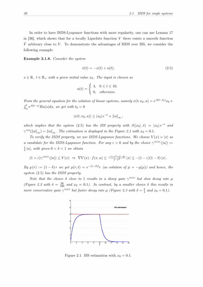
Figure 2.2: ISDS estimation with δ = 99100 ,
x0 = 0.1.Figure 2.3: ISDS estimation with δ = 3
4 ,x0 = 0.1.
From Figures 2.1-2.3, we perceive that the ISDS estimation tends to zero, if the input tendsto zero in contrast to the ISS estimation. This property of the ISDS estimation is known asthe memory fading effect.
In the next section, we provide an ISDS small-gain theorem for interconnected systemswith a construction of an ISDS-Lyapunov function for the whole system.
2.2 ISDS for interconnected systems
We consider interconnected systems of the form (1.6). The ISDS property for subsystemsreads as follows:The i-th subsystem of (1.6) is called ISDS, if there exists a KLD-function μi and functions
ηi, γISDSi and γISDS
ij ∈ K∞ ∪ {0} , i, j = 1, . . . , n with γISDSii = 0 such that the solution
xi(t;x0i , u) = xi(t) for all initial values x0
i and all inputs xj , j = i, u satisfies
|xi(t)| ≤ max{μi(ηi(|x0
i |), t),maxj �=i
νij(xj , t), νi(u, t)}
(2.6)
for all t ∈ R+, where
νi(u, t) := ess supτ∈[0,t]
μi(γISDSi (|u(τ)|), t− τ),
νij(xj , t) := supτ∈[0,t]
μi(γISDSij (|xj(τ)|), t− τ)
i, j = 1, . . . , n. γISDSij , γISDS
i are called (nonlinear) robustness gains.To show the ISDS property for networks, we need the gain-matrix ΓISDS, which is defined
by ΓISDS :=(γISDS
ij
)n×n
with γISDSii ≡ 0, i, j = 1, . . . , n and defined by (1.12).
Definition 2.2.1. For vector valued functions x = (xT1 , . . . , x
Tn )
T : R+ → R
∑ni=1 Ni with
xi : R+ → RNi and times 0 ≤ t1 ≤ t2, t ∈ R+ we define
x(t) := (|x1(t)| , . . . , |xn(t)|)T ∈ Rn+ and x [0,t] accordingly.
28 2.2. ISDS for interconnected systems
For u ∈ Rm, t ∈ R+ and s ∈ R
n+ we define
γISDS(|u(t)|) := (γISDS1 (|u(t)|), . . . , γISDS
n (|u(t)|))T ∈ Rn+,
μ(s, t) := (μ1(s1, t), . . . , μn(sn, t))T ∈ R
n+,
η(s) := (η1(s1), . . . , ηn(sn))T ∈ R
n+.
Now, we can rewrite condition (2.6) for all subsystems in a compact form
x(t) ≤ max
{μ(η(x0
), t), supτ∈[0,t]
μ (ΓISDS ( x(τ) ) , t− τ) , ess supτ∈[0,t]
μ(γISDS(|u(τ)|), t− τ)}
(2.7)
for all t ∈ R+. Note that the maximum, the supremum and the essential supremum usedin (2.7) for vectors are taken component-by-component. For the ISDS property, from (2.7),using the KLD-property of μ and with ΓISS := ΓISDS, γISS := γISDS, β(r, t) := μ(η(r), t) weget
x(t) ≤ max{β(x0 , t
),ΓISS
(x [0,t]
), γISS(‖u‖)} .
This implies that each subsystem of (1.6) is ISS and provided that ΓISDS satisfies the SGC(1.15), also ΓISS satisfies the SGC (1.15), i.e., the interconnection is ISS and hence ISDS. How-ever, we loose the quantitative information about the rate and gains of the ISDS estimationfor the whole system in such a way.In order to conserve the quantitative information of the ISDS rate and gains of the overall
system, we utilize ISDS-Lyapunov functions. For subsystems of the form (1.6) they read asfollows:We assume that for each subsystem of (1.6) there exists a function Vi : R
Ni → R+, whichis locally Lipschitz continuous and positive definite. Given εi > 0, a function Vi : R
Ni → R+,which is locally Lipschitz continuous on R
Ni\ {0} is an ISDS-Lyapunov function of the i-thsubsystem in (1.6), if it satisfies:(i) there exists a function ηi ∈ K∞ such that for all xi ∈ R
Ni it holds
|xi|1 + εi
≤ Vi(xi) ≤ ηi (|xi|) ; (2.8)
(ii) there exist functions μi ∈ KLD, γISDSi ∈ K∞∪{0}, γISDS
ij ∈ K∞∪{0} , j = 1, . . . , n, i =j such that for almost all xi ∈ R
Ni\ {0}, all inputs xj , j = i and u it holds
Vi(xi) > max{γISDSi (|u|) ,max
j �=iγISDS
ij (Vj(xj))} ⇒ ∇Vi(xi)fi(x, u) ≤ − (1− εi) gi(Vi(xi)),
(2.9)
where μi ∈ KLD solves the equation ddtμi(r, t) = −gi (μi (r, t)) , r, t > 0 for some locally
Lipschitz continuous function gi : R+ → R+.Now, we state the main result of this chapter, which provides a tool to check whether a
network possesses the ISDS property. Moreover, the decay rate and the gains of the ISDSestimation for the network can be constructed explicitly.
Chapter 2. Input-to-state dynamical stability (ISDS) 29
Theorem 2.2.2. Assume that each subsystem of (1.6) has the ISDS property. This meansthat for each subsystem and for each εi > 0 there exists an ISDS-Lyapunov function Vi, whichsatisfies (2.8) and (2.9). Let ΓISDS be given by (1.12), satisfying the small-gain condition(1.15) and let σ ∈ Kn∞ be an Ω-path from Proposition 1.2.3 with Γ = ΓISDS. Then, the wholesystem (1.1) has the ISDS property and its ISDS-Lyapunov function is given by
V (x) = ψ−1
(max
i
{σ−1
i (Vi(xi))})
(2.10)
with rates and gains
g(r) = (ψ−1)′ (ψ(r))mini
{(σ−1
i )′(σi(ψ(r)))gi(σi(ψ(r)))},
η(r) = ψ−1(maxi
{σ−1
i (ηi(r))}),
γISDS(r) = ψ−1(maxi
{σ−1
i (γISDSi (r))
}),
(2.11)
where r > 0 and ψ (|x|) = mini σ−1i
( |x|√n
).
The proof of Theorem 2.2.2 follows the idea of the proof of Theorem 5.3 in [28] andcorresponding results in [24] with changes due to the construction of the gains and of the rateof the whole system.
Proof. Let 0 = x =(xT
1 , . . . , xTn
)T . We define
V (x) := maxi
{σ−1
i (Vi(xi))}, η(|x|) := max
i
{σ−1
i (ηi(|x|))}, ψ (|x|) := min
iσ−1
i
( |x|√n
),
where Vi satisfies (2.8) for i = 1, . . . , n. Note that σ−1i ∈ K∞. Let j be such that |x|∞ = |xj |∞
for some j ∈ {1, . . . , n}, then it holds
maxiσ−1
i
( |xi|1+εi
)≥ max
iσ−1
i
( |xi|∞1+ε
)≥ σ−1
j
( |xj |∞1+ε
)≥ min
iσ−1
i
( |x|√n(1+ε)
)(2.12)
where ε := maxi εi and we have
ψ
( |x|1 + ε
)≤ V (x) ≤ η(|x|). (2.13)
Note that V is locally Lipschitz continuous and hence it is differentiable almost everywhere.We define I := {i ∈ {1, . . . , n}| V (x) = {
σ−1i (Vi(xi))
} ≥ maxj,j �=i{σ−1j (Vj(xj))}}. Fix an
i ∈ I. Let γISDS(|u|) := maxj
{σ−1
j (γISDSj (|u|))
}, j = 1, . . . , n. Assume V (x) > γISDS(|u|).
Then,
Vi(xi) = σi(V (x)) > σi(σ−1i (γISDS
i (|u|))) = γISDSi (|u|).
From (iii) in Definition 1.2.2 we have
Vi(xi) = σi(V (x)) > maxj �=i
γISDSij (σj(V (x))) ≥ max
j �=iγISDS
ij (Vj(xj)).
Thus, for almost all x ∈ RN (2.9) implies
∇V (x)f(x, u) ≤ −(1− εi)(σ−1
i
)′ (Vi(xi))gi(Vi(xi)) = −(1− εi)gi(V (x)),
30 2.2. ISDS for interconnected systems
where gi(r) :=(σ−1
i
)′ (σi(r))gi(σi(r)) is positive definite and locally Lipschitz. As index iwas arbitrary in these considerations, with γISDS(|u|) = maxj
{σ−1
j (γISDSj (|u|))
}and g(r) :=
mini gi(r), ε = maxi εi the condition (2.3) for the function V is satisfied. From (2.13) we get
|x|1 + ε
≤ ψ−1(V (x)
) ≤ ψ−1 (η (|x|))
and we define V (x) := ψ−1(V (x)
)as the ISDS-Lyapunov function candidate of the whole
system with η (|x|) := ψ−1 (η (|x|)). Note that ψ−1 ∈ K∞ and V (x) is locally Lipschitzcontinuous. By the previous calculations for V (x) it holds
V (x) > ψ−1 (γISDS (|u|)) =: γISDS (|u|) ⇒ V (x) ≤ −(1− ε)g (V (x)) , a.e.,
where g(r) := (ψ−1)′ (ψ(r)) g (ψ(r)) is locally Lipschitz continuous. Altogether, V (x) satisfies(2.2) and (2.3). Hence, V (x) is the ISDS-Lyapunov function of the whole system and byapplication of Proposition 2.1.6 the whole system has the ISDS property.
This theorem provides a tool how to check, whether a network possesses the ISDS prop-erty: one has to find the ISDS-Lyapunov functions and gains of the subsystems and hasto check, if the small-gain condition is satisfied. Moreover, the theorem gives an explicitconstruction of the ISDS-Lyapunov function and the corresponding rate and gains.In the following, we present a corollary, which is similar to Theorem 10 in [36] for two
coupled systems and covers n ∈ N coupled systems, where the rates and gains defined inTheorem 2.2.2 are used. Here, we get decay rates for the norm of the solution of the wholesystem and for each subsystem of n coupled systems with external input u = 0.
Corollary 2.2.3. Consider the system (1.6) and assume that all subsystems have the ISDSproperty with decay rates μi and gains ηi, γ
ISDSi and γISDS
ij , i, j = 1, . . . , n, i = j. If thesmall-gain condition (1.15) is satisfied, then the coupled system
x =
⎛⎜⎜⎝x1
...xn
⎞⎟⎟⎠ =
⎛⎜⎜⎝f1(x1, . . . , xn)
...fn(x1, . . . , xn)
⎞⎟⎟⎠ = f(x) (2.14)
is 0-GAS with
|xj(t)| ≤ |x(t)| ≤ μ
(ψ−1
(max
i
{σ−1
i
(ηi
(∣∣x0∣∣))}) , t) (2.15)
for i, j = 1, . . . , n, all t ∈ R+, with functions μ, σ, ψ and ηi from Theorem 2.2.2.
Remark 2.2.4. Note that for large n function ψ in (2.11) becomes “small” and hence therates and gains defined by ψ−1 become “large” which is not desired in applications. To avoidthis kind of conservativeness one can use the maximum norm |x|∞ for the states in the abovedefinitions and in Theorem 2.2.2 and Corollary 2.2.3. This is possible as we have noted inRemark 2.1.3. In this case, the division by
√n in (2.12) can be avoided and we get (2.11)
with ψ (|x|∞) = mini σ−1i (|x|∞). This is used in our examples below.
Chapter 2. Input-to-state dynamical stability (ISDS) 31
Unfortunately, we cannot compare directly the estimation of Theorem 10 in [36] with ourestimation (2.15), since another approach for estimations of the trajectories for two coupledsystems was used in [36]. The extension of this approach to n > 2 seems to be hardly possible.Our approach allows to consider n interconnected systems. In the first example of the nextsection, we compare our result for two coupled systems to the result in [36].
2.3 Examples
To compare Theorem 10 in [36] with Corollary 2.2.3 for the case of two subsystems, weconsider Example 12 given in [36].
Example 2.3.1. Consider two interconnected systems
x1(t) = −x1(t) +x32(t)2 ,
x2(t) = −x32(t) + x1(t).
As in [36] we choose Vi = |xi| and γ1(r) = 23r
3, γ2(r) = 3
√43r, η1, η2 = Id, g1(r) =
14r, g2(r) =
14r
3. It is easy to check that the small-gain condition is satisfied and an Ω-path
can be chosen by σ1(r) = Id, σ2(r) = 3
√4.493 r. For x0
1 = x02 = 2 the solution x was calculated
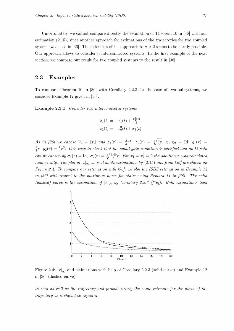
numerically. The plot of |x|∞ as well as its estimations by (2.15) and from [36] are shown onFigure 2.4. To compare our estimation with [36], we plot the ISDS estimation in Example 12in [36] with respect to the maximum norm for states using Remark 11 in [36]. The solid(dashed) curve is the estimation of |x|∞ by Corollary 2.2.3 ([36]). Both estimations tend
Figure 2.4: |x|∞ and estimations with help of Corollary 2.2.3 (solid curve) and Example 12in [36] (dashed curve)
to zero as well as the trajectory and provide nearly the same estimate for the norm of thetrajectory as it should be expected.
32 2.3. Examples
The advantage of our approach is that it can be applied for larger interconnections. Thefollowing example illustrates the application of Theorem 2.2.2 for a construction of an ISDS-Lyapunov function for the case n ≥ 2.
Example 2.3.2. Consider n ∈ N interconnected systems of the form
x1(t) = −a1x1(t) +n∑
j>1
1nb1jx
2j (t) +
1nu(t),
xi(t) = −aixi(t) + 1nbi1
√x1(t) +
n∑j>1,j �=i
1nbijxj(t) + 1
nu(t), i = 2, . . . , n,
(2.16)
for bij ∈ [0, 1) , ai = (1 + εi), εi ∈ (1,∞) and any input u ∈ Rm. We choose Vi(xi) = |xi|∞
as an ISDS-Lyapunov function candidate for the i-th subsystem, i = 1, . . . , n and define
γISDS1j (r) := b1jr
2, j = 2, . . . , n,
γISDSj1 (r) := bj1
√r, j = 2, . . . , n,
γISDSij (r) := bijr, i, j = 2, . . . , n, i = j,
γISDSi (r) := r, i = 1, . . . , n,
ΓISDS :=(γISDS
ij
)n×n
, i, j = 1, . . . , n, γISDSii ≡ 0, ηi(r) := r and μi(r, t) = e−εit r as solution
of ddtμi(r, t) = −gi(μi(r, t)) with gi(r) := εir. We obtain that Vi is an ISDS-Lyapunov function
of the i-th subsystem. To check whether the small-gain condition is satisfied, we use the cyclecondition, which is satisfied (this can be easily verified).
We choose σ(s) = (σ1(s), . . . , σn(s))T with σ1(s) := s2 and σj(s) := s, j = 2, . . . , n for
s ∈ R+, which is one of the possibilities of choosing σ. Then, σ is an Ω-path, which can beeasily checked. In particular, σ satisfies ΓISDS (σ(s)) < σ(s), ∀s > 0. Now, by application ofTheorem 2.2.2 the whole system is ISDS and the ISDS-Lyapunov function is given by
V (x) = ψ−1
(max
iσ−1
i (|xi|∞))
with ψ(r) = mini σ−1i (r) =
{ √r, r ≥ 1,
r, r < 1. The gains and rates of the ISDS estimation and
ISDS-Lyapunov function, respectively, are given by (2.11). Furthermore, if u(t) ≡ 0 then byCorollary 2.2.3 the whole system is 0-GAS and the decay rate is given by (2.15).
In the following, we illustrate the trajectory and the ISDS estimation for a system consist-ing of subsystems of the form (2.16) for n = 3. We choose ai = 11
10 , bij =12 , i, j = 1, 2, 3, i =
j, u(t) = e−t as the input and the initial values x01 = 0.5, x0
2 = 0.8 and x03 = 1.2. Then, we
calculate the ISDS estimation of the whole system as described above and get
|x(t)|∞ ≤ max{μ((x03)
2, t), ess supτ∈[0,t]
μ(√u(τ), t− τ)}.
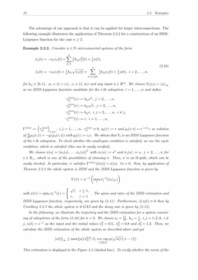
This estimation is displayed in the Figure 2.5 (dashed line). To verify whether the norm of the
Chapter 2. Input-to-state dynamical stability (ISDS) 33
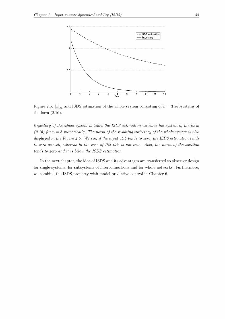
Figure 2.5: |x|∞ and ISDS estimation of the whole system consisting of n = 3 subsystems ofthe form (2.16).
trajectory of the whole system is below the ISDS estimation we solve the system of the form(2.16) for n = 3 numerically. The norm of the resulting trajectory of the whole system is alsodisplayed in the Figure 2.5. We see, if the input u(t) tends to zero, the ISDS estimation tendsto zero as well, whereas in the case of ISS this is not true. Also, the norm of the solutiontends to zero and it is below the ISDS estimation.
In the next chapter, the idea of ISDS and its advantages are transferred to observer designfor single systems, for subsystems of interconnections and for whole networks. Furthermore,we combine the ISDS property with model predictive control in Chapter 6.

34 2.3. Examples
Chapter 3
Observer and quantized outputfeedback stabilization
In this chapter, we introduce the notion of quasi-ISDS reduced-order observers and use errorLyapunov functions to design such observers for single systems. Considering interconnectedsystems we design quasi-ISS/ISDS observers for each subsystem and the whole system undera small-gain condition. This is applied to stabilization of systems subject to quantization.
We consider systems of the form (1.1) with outputs
x = f(x, u),
y = h(x),(3.1)
where y ∈ RP is the output and function h : R
N → RP is continuously differentiable with
locally Lipschitz derivative (called a C1L function). In addition, it is assumed that h(0) = 0
holds.
In practice, observers are used for systems, where the state or parts of the state cannot be measured due to uneconomic measurement costs or physical circumstances like hightemperatures, where no measurement equipment is available, for example. They are alsoused in cases, where the output of a system is disturbed and for stabilization of a system, forexample. There, a control law subject to stabilize a system is designed using the estimatedstate of the system generated by the observer based on the disturbed output. This can leadto an unbounded growth of the state estimation error and therefore to a design of a controllaw, which does not stabilizes the system.
A state observer for the system (3.1) is of the form
˙ξ = F (y, ξ, u),
x = H(y, ξ, u),(3.2)
where ξ ∈ RL is the observer state, x ∈ R
N is the estimate of the system state x and y ∈ RP
is the measurement of y that may be disturbed by d: y = y+d, where d ∈ L∞(R+,RP ). The
function F : RP ×R
L×Rm → R
L is locally Lipschitz in y and ξ uniformly in u and function
35
36
H : RP ×R
L×Rm → R
N is a C1L function. In addition, it is assumed that F (0, 0, 0) = 0 and
H(0, 0, 0) = 0 holds.
We denote the state estimation error by
x = x− x.
We are interested under which conditions the designed observer guarantees that the stateestimation error is ISS or ISDS. The used stability properties for observers are based on ISSand ISDS, and are called quasi-ISS and quasi-ISDS, respectively.
Inspired by the work [110], where the notion of quasi-ISS reduced-order observers wasintroduced and the advantages of ISDS over ISS, investigated in Chapter 2, this motivatesthe introduction of the quasi-ISDS property for observers, where the approaches of reduced-order observers and the ISDS property are combined. The property has the advantage thatthe recent disturbance of the output of the system is taken into account. We investigate underwhich conditions a quasi-ISDS reduced-order observer can be designed for single nonlinearsystems, where error Lyapunov functions (see [88, 60]) are used. The design of observers inthe context of this thesis was investigated in [112, 60, 72, 61, 110], for example, and remarkson the equivalence of full order and reduced-order observers can be found in [111].
Considering interconnected systems it is desirable to have observers for each of the sub-systems and the whole network. Here, we design quasi-ISS/ISDS reduced-order observers foreach subsystem of an interconnected system, from which an observer for the whole systemcan be designed under a small-gain condition.
Furthermore, the problem of stabilization of systems is investigated and we apply thepresented approach to quantized output feedback stabilization for single and interconnectedsystems. The goal of stabilizing a system is an important problem in applications. Manyapproaches were performed during the last years and the design of stabilizing feedback lawsis a popular research area, which is linked up with many applications. The stabilization usingoutput feedback quantization was investigated in [7, 70, 62, 63, 60, 71, 72, 110], for example.A quantizer is a device, which converts a real-valued signal into a piecewise constant signal,i.e., it maps R
P into a finite and discrete subset of RP . It may affect the process output or
may also affect the control input.
Adapting the quantizer with a so-called zoom variable this leads to dynamic quantizers,which have the advantage that asymptotic stability for single and interconnected systems canbe achieved under certain conditions.
This chapter is organized as follows: The notion of quasi-ISDS observers is introduced inSection 3.1, where the design of such an observer for single systems under the existence ofan error ISDS-Lyapunov function is performed. Section 3.2 contains all the results for thequasi-ISS/ISDS observer design according to interconnected systems. The application of theresults to quantized output feedback stabilization for single and interconnected systems canbe found in Section 3.3.
Chapter 3. Observer and quantized output feedback stabilization 37
3.1 Quasi-ISDS observer for single systems
In this section, we introduce quasi-ISDS observers and give a motivating example for theintroduction. Then, we show that the reduced-order observer designed in [110], Theorem 1,is a quasi-ISDS observer provided that an error ISDS-Lyapunov function exists.We recall the definition of quasi-ISS observers from [110], which guarantee that the norm
of the state estimation error is bounded for all times.
Definition 3.1.1 (Quasi-ISS observer). The system (3.2) is called a quasi-ISS observer forthe system (3.1), if there exists a function β ∈ KL and for each K > 0, there exists a functionγISS
K ∈ K∞ such that
|x(t)| ≤ max{β(|x0|, t), γISSK (
∥∥d[0,t]
∥∥)}, ∀t ∈ R+
whenever ||u[0,t]|| ≤ K and ||x||[0,t] ≤ K.
Modifying this definition by using the idea of the ISDS property to transfer the advantagesof ISDS over ISS to observers we define quasi-ISDS observers:
Definition 3.1.2 (Quasi-ISDS observers). The system (3.2) is called a quasi-ISDS observerfor the system (3.1), if there exist functions μ ∈ KLD, η ∈ K∞ and for each K > 0 a functionγISDS
K ∈ K∞ such that
|x(t)| ≤ max{μ(η(|x0|), t), ess supτ∈[0,t]
μ(γISDSK (|d(τ)|), t− τ)}, ∀t ∈ R+
whenever ||u[0,t]|| ≤ K and ||x||[0,t] ≤ K.
Recalling that ISDS possesses the memory fading effect, the motivation for the introduc-tion of quasi-ISDS observers is the following: quasi-ISDS observers take the recent disturbanceof the measurement into account, whereas a quasi-ISS observer takes into account the supre-mum norm of the disturbance. The advantage will be illustrated by the following example.
Example 3.1.3. Consider the system as in Example 1 in [110]
x = −x+ x2u,
y = x,(3.3)
where ˙x = −x+ y2u is an observer. We consider the perturbed measurement y = y + d, withd = e−t 1
10 . Then, the error dynamics becomes
˙x = −x+ 2xud+ ud2.
This system is ISS and ISDS from d to x when u and x are bounded. Let u ≡ 1 be constant,then the estimations of the error dynamics are displayed in the Figure 3.1 for x0 = x0 = 0.3.The ISS estimate is chosen equal to 1, since β(|x0|, t) ≤ γISS
K (∥∥d[0,t]
∥∥) for a sufficient functionβ, ‖d‖ = 1, x0 small enough and with γISS
K = Id. The ISDS estimation follows by choosing
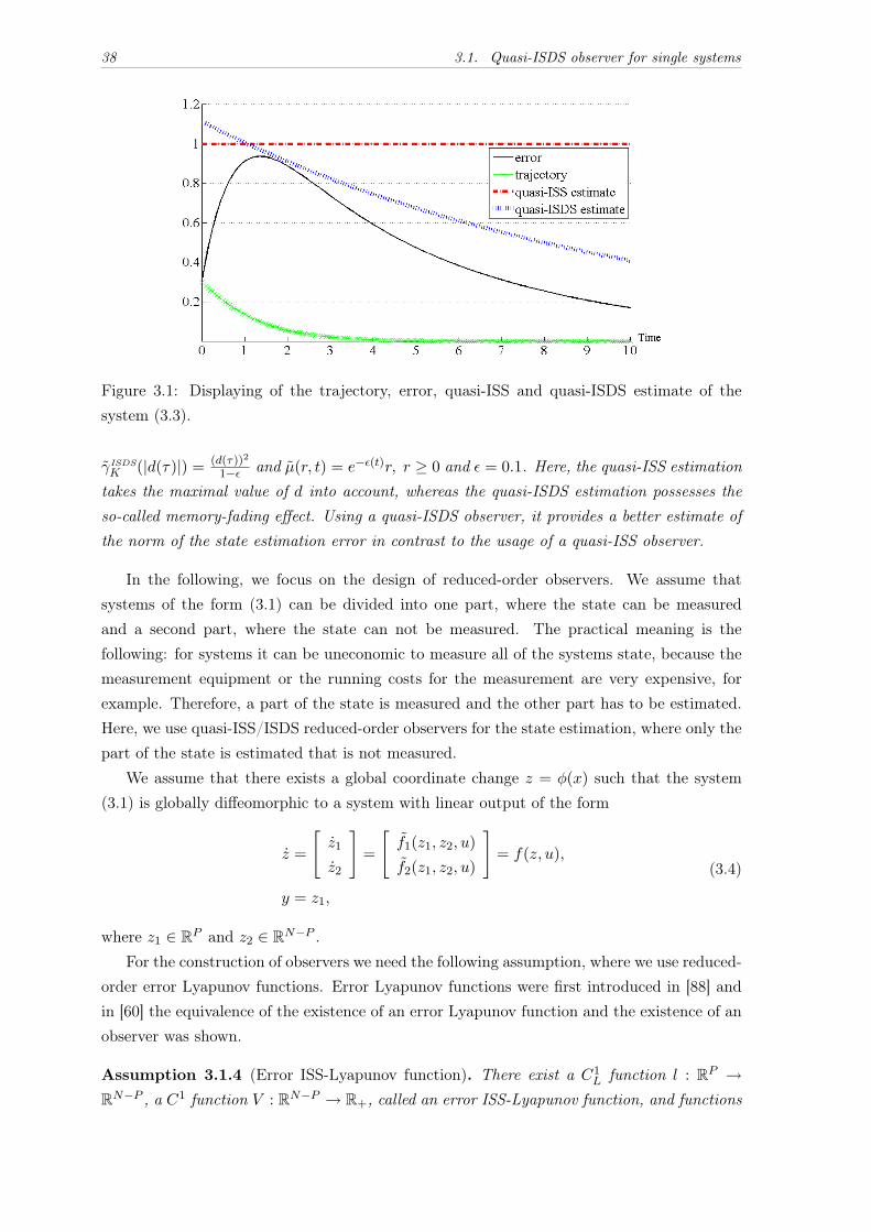
38 3.1. Quasi-ISDS observer for single systems
Figure 3.1: Displaying of the trajectory, error, quasi-ISS and quasi-ISDS estimate of thesystem (3.3).
γISDSK (|d(τ)|) = (d(τ))2
1−ε and μ(r, t) = e−ε(t)r, r ≥ 0 and ε = 0.1. Here, the quasi-ISS estimationtakes the maximal value of d into account, whereas the quasi-ISDS estimation possesses theso-called memory-fading effect. Using a quasi-ISDS observer, it provides a better estimate ofthe norm of the state estimation error in contrast to the usage of a quasi-ISS observer.
In the following, we focus on the design of reduced-order observers. We assume thatsystems of the form (3.1) can be divided into one part, where the state can be measuredand a second part, where the state can not be measured. The practical meaning is thefollowing: for systems it can be uneconomic to measure all of the systems state, because themeasurement equipment or the running costs for the measurement are very expensive, forexample. Therefore, a part of the state is measured and the other part has to be estimated.Here, we use quasi-ISS/ISDS reduced-order observers for the state estimation, where only thepart of the state is estimated that is not measured.We assume that there exists a global coordinate change z = φ(x) such that the system
(3.1) is globally diffeomorphic to a system with linear output of the form
z =
[z1
z2
]=
[f1(z1, z2, u)
f2(z1, z2, u)
]= f(z, u),
y = z1,
(3.4)
where z1 ∈ RP and z2 ∈ R
N−P .For the construction of observers we need the following assumption, where we use reduced-
order error Lyapunov functions. Error Lyapunov functions were first introduced in [88] andin [60] the equivalence of the existence of an error Lyapunov function and the existence of anobserver was shown.
Assumption 3.1.4 (Error ISS-Lyapunov function). There exist a C1L function l : R
P →R
N−P , a C1 function V : RN−P → R+, called an error ISS-Lyapunov function, and functions
Chapter 3. Observer and quantized output feedback stabilization 39
αi ∈ K∞, i = 1, . . . , 4 such that for all e ∈ RN−P , z ∈ R
N and u ∈ Rm
α1(|e|) ≤ V (e) ≤ α2(|e|), (3.5)∣∣∣∂V (e)∂e
∣∣∣ ≤ α4(V (e)), (3.6)
∂V (e)∂e
([f2(z1, e, u) +
∂l(z1)∂z1
f1(z1, e, u)]− [f2(z1, z2, u) +∂l(z1)∂z1
f1(z1, z2, u)])
≤ − α3(V (e)),(3.7)
e := e+ z2 and there exists a function α ∈ K∞ such that
α(s)α4(s) ≤ α3(s), s ∈ R+.
Remark 3.1.5. Note that in [110] the properties of an error Lyapunov function are slightlydifferent, namely for α3, α4 ∈ K∞
α1(|e|) ≤ V (e) ≤ α2(|e|),∣∣∣∂V (e)∂e
∣∣∣ ≤ α4(|e|),∂V (e)
∂e
([f2(z1, e, u) +
∂l(z1)∂z1
f1(z1, e, u)]− [f2(z1, z2, u) +∂l(z1)∂z1
f1(z1, z2, u)])
≤− α3(|e|),which are equivalent to (3.5), (3.6) and (3.7).
Now, the following lemma can be stated, which was proved in [110]. It shows, how aquasi-ISS observer for the system (3.4) can be designed, provided that an error ISS-Lyapunovfunction exists.
Lemma 3.1.6. Under Assumption 3.1.4, the system
˙ξ = f2(y, ξ − l(y), u) + ∂l(y)
∂z1f1(y, ξ − l(y), u),
z1 = y,
z2 = ξ − l(y)
(3.8)
becomes a quasi-ISS reduced-order observer for the system (3.4), where ξ ∈ RN−P is the
observer state and z1, z2 are the estimates of z1 and z2, respectively, and y = y+ d = z1 + d,which is the measurement of z1 disturbed by d.
In order to use quasi-ISDS observers we adapt Assumption 3.1.4 according to the ISDSproperty:
Assumption 3.1.7 (Error ISDS-Lyapunov function). Let ε > 0 be given. There exist a C1L
function l : RP → R
N−P , a C1 function V : RN−P → R+, called an error ISDS-Lyapunov
function, functions α, η ∈ K∞ and μ ∈ KLD such that for all e ∈ RN−P , z ∈ R
N and u ∈ Rm
|e|1+ε ≤ V (e) ≤ η(|e|), (3.9)∣∣∣∂V (e)
∂e
∣∣∣ ≤ α(V (e)), (3.10)
∂V
∂e(e)
([f2(z1, e, u) +
∂l(z1)∂z1
f1(z1, e, u)]− [f2(z1, z2, u) +∂l(z1)∂z1
f1(z1, z2, u)])
≤ − (1− ε) g(V (e)),(3.11)
40 3.1. Quasi-ISDS observer for single systems
e := e + z2, where μ solves the equation ddt μ(r, t) = −g (μ (r, t)) , r, t ≥ 0 for a locally
Lipschitz continuous function g : R+ → R+ and there exists a function α ∈ K∞ such that
α(s)α(s) ≤ (1− ε)g(s), s ∈ R+. (3.12)
The next theorem is a counterpart of Lemma 3.1.6. It provides a design of a quasi-ISDSreduced-order observer for the system (3.4) provided that an error ISDS-Lyapunov functionexists.
Theorem 3.1.8. Under Assumption 3.1.7 the system (3.8) becomes a quasi-ISDS reduced-order observer for the system (3.4).
The proof goes along the lines of the proof of Lemma 3.1.6 in [110] with correspondingchanges according to Definition 3.1.2 and Assumption 3.1.7:
Proof. We define ξ := z2 + l(z1) and convert the system (3.4) into
z1 = f1(z1, ξ − l(z1), u),y = z1,
ξ = f2(z1, ξ − l(z1), u) + ∂l(z1)∂z1
f1(z1, ξ − l(z1), u) =: F (z1, ξ, u).
With this F , the dynamic of the observer state in (3.8) can be written as ˙ξ = F (y, ξ, u), wherey = y + d and d is the measurement disturbance. Let e := ξ − ξ and from Assumption 3.1.7we obtain
V (e) =∂V (e)∂e
(f2(z1 + d, ξ − l(z1 + d), u)− f2(z1, ξ − l(z1), u)
+∂l(z1+d)∂z1
f1(z1 + d, ξ − l(z1 + d), u)− ∂l(z1)∂z1
f1(z1, ξ − l(z1), u))
=∂V (e)∂e
(f2(z1 + d, ξ − l(z1 + d), u)− f2(z1 + d, ξ − l(z1 + d), u)
+∂l(z1+d)∂z1
f1(z1 + d, ξ − l(z1 + d), u)− ∂l(z1+d)∂z1
f1(z1 + d, ξ − l(z1 + d), u))
+∂V (e)∂e
(F (y, ξ, u)− F (y, ξ, u))≤ − (1− ε) g(|e|) + α(|e|) (F (y, ξ, u)− F (y, ξ, u)) .
In [32], Lemma A.14, it was shown that there exist a continuous positive function ρ and γ ∈ Ksuch that
|F (y, ξ, u)− F (y, ξ, u)| ≤ ρ(y, ξ, u)γ(|d|)
and it follows for an arbitrary δ ∈ (0, 1) with (3.12)
V (e) ≥ α−1
(ρ(y, ξ, u)γ(|d|)
1− δ)⇒ V (e) ≤ −(1− ε)g(V (e)),
Chapter 3. Observer and quantized output feedback stabilization 41
where g(r) := δg(r), ∀r > 0. By Theorem 3.5.8 in [35] and its proof this is equivalent to
|e(t)| ≤ max
{μ(η(|e(0)|), t), ess sup
τ∈[0,t]μ(γISDS
K (|d(τ)|), t− τ)}
(3.13)
under ||z||[0,t] ≤ K, ||u[0,t]|| ≤ K, where γISDSK ∈ K∞ is parametrized by K. Now, we have
z =
(z1
z2
):=
(z1 − z1z2 − z2
)=
(d
e− (l(y)− l(z1))
).
By θK ∈ K, parametrized by K such that |l(z1 + d)− l(z1)| ≤ θK(|d|), |z1| ≤ K it follows
|z| ≤ |e|+ |d|+ θK(|d|) and |e| ≤ |z2|+ θK(|d|). (3.14)
Overall, combining (3.13) and (3.14) we have
|z| ≤ max
{μ(η(|e(0)|), t), ess sup
τ∈[0,t]μ(γISDS
K (|d(τ)|), t− τ)}+ |d(t)|+ θK(|d(t)|)
≤ max
{μ(η(|e(0)|), t), ess sup
τ∈[0,t]μ(γISDS
K (|d(τ)|), t− τ)}+ χK(|d(t)|)
where χK(s) := s+ θK(s), s ≥ 0. Since μ is a KLD-function it follows
|z| ≤ max
{2μ(η(|e(0)|), t), ess sup
τ∈[0,t]2μ(γISDS
K (|d(τ)|), t− τ), ess supτ∈[0,t]
2μ(χK(|d(τ)|), t− τ)}
≤ max
{2μ(η(|z2(0)|+ θK(|d(0)|)), t), ess sup
τ∈[0,t]2μ(γISDS
K (|d(τ)|), t− τ)},
where γISDSK (s) := max{γISDS
K (s), χK(s)}, and we used (3.14) and the inequality α(a + b) ≤max{α(2a), α(2b)} for α ∈ K, a, b ≥ 0. Furthermore, we have
|z| ≤ max
{2μ(η(2 |z2(0)|), t), 2μ(η(2θK(|d(0)|)), t), ess sup
τ∈[0,t]2μ(γISDS
K (|d(τ)|), t− τ)}
≤ max
{2μ(η(2 |z2(0)|), t), ess sup
τ∈[0,t]2μ(η(2θK(|d(τ)|)), t− τ),
ess supτ∈[0,t]
2μ(γISDSK (|d(τ)|), t− τ)
}
≤ max
{2μ(η(2 |z2(0)|), t), ess sup
τ∈[0,t]2μ(γISDS
K (|d(τ)|), t− τ)},
where γISDSK (s) := max{η(2θK(s)), γISDS
K (s)}. Finally, by definition of μ(r, t) := 2μ(r, t) andη(s) := η(2s) it follows
|z| ≤ max
{μ(η(|z(0)|), t), ess sup
τ∈[0,t]μ(γISDS
K (|d(τ)|), t− τ)},
for ||z||[0,t] ≤ K, ||u[0,t]|| ≤ K, which proves the assertion.
42 3.2. Quasi-ISS and quasi-ISDS observer for interconnected systems
Remark 3.1.9. From Chapter 2 the decay rate and the gain of the definition of ISDS arethe same as the ones using ISDS-Lyapunov functions. Note that this is not the case for thedefinition of a quasi-ISDS observer and using error ISDS-Lyapunov functions. It remains asan open topic to investigate if it is possible to use a different error ISDS-Lyapunov function,from which the information about the decay rate and the gains of the error ISDS-Lyapunovfunction can be preserved for the quasi-ISDS estimation.
In the next section, we are going to extend the notion of quasi-ISS/ISDS observers forinterconnected systems and provide tools to design such kind of observers.
3.2 Quasi-ISS and quasi-ISDS observer for interconnected sys-
tems
We consider n ∈ N interconnected systems of the form (1.6) with outputs
xi = fi(x1, . . . , xn, ui),
yi = hi(xi),(3.15)
i = 1, . . . , n, where ui ∈ RMi are control inputs, yi ∈ R
Pi are the outputs and functionshi : R
Ni → RPi are C1
L functions. In addition, it is assumed that hi(0) = 0.The state observer of the ith subsystem is of the form
˙ξi = Fi(y1, . . . , yn, ξ1, . . . , ξn, ui),
xi = Hi(y1, . . . , yn, ξ1, . . . , ξn, ui),(3.16)
i = 1, . . . , n, where ξi ∈ RLi is the observer state of the ith subsystem, xi ∈ R
Ni is theestimate of the system state xi and yi ∈ R
Pi is the measurement of yi that may be disturbedby di: yi = yi + di, di ∈ L∞(R+,R
Pi). The function Fi : RP × R
L × RMi → R
Li , P =∑i Pi, L =
∑i Li is locally Lipschitz in y = (y1, . . . , yn)T and ξ = (ξ1, . . . , ξn)T uniformly in
ui and function Hi : RP ×R
L×RMi → R
Ni is a C1L function. In addition, it is assumed that
Fi(0, 0, 0) = 0 and Hi(0, 0, 0) = 0 holds.We denote the state estimation error of the ith subsystem by xi := xi−xi. It is influenced
by the state estimation error as well as by the measurement error of the jth subsystemwhich is connected to the ith subsystem. Therefore, they have to be taken into account forthe estimation of the norm of the state estimation error of the ith subsystem. The quasi-ISS/ISDS property for interconnected systems reads as follows:
1. The ith subsystem of (3.16) is a quasi-ISS observer for the ith subsystem of (3.15),if there exists a function βi ∈ KL and for each Ki > 0 there exist functions (γKi
i )ISS,(γKi
ij )ISS ∈ K∞, j = 1, . . . , n, j = i such that
|xi(t)|
≤ max{βi(|x0
i |), t),maxj �=i
(γKiij )
ISS(||xj ||[0,t]),maxj �=i
(γKiij )
ISS(||(dj)[0,t]||), (γKii )ISS(||(di)[0,t]||)
},
whenever ||(ui)[0,t]|| ≤ Ki and ||xj ||[0,t] ≤ Ki, j = 1, . . . , n.
Chapter 3. Observer and quantized output feedback stabilization 43
2. The ith subsystem of (3.16) is a quasi-ISDS observer for the ith subsystem of (3.15),if there exist functions μi ∈ KLD, ηi ∈ K∞ and for each Ki > 0 there exist functions(γKi
i )ISDS, (γKiij )
ISDS ∈ K∞, j = 1, . . . , n, j = i such that
|xi(t)| ≤ max{μi(ηi(|x0
i |), t),maxj �=i
νij(xj , t),maxj �=i
νij(dj , t), νi(di, t)}
whenever ||(ui)[0,t]|| ≤ Ki and ||xj ||[0,t] ≤ Ki, j = 1, . . . , n, where
νij(xj , t) := supτ∈[0,t]
μi((γKiij )
ISDS(|xj(τ)|), t− τ),
νij(dj , t) := ess supτ∈[0,t]
μi((γKiij )
ISDS(|dj(τ)|), t− τ),
νi(di, t) :=ess supτ∈[0,t]
μi((γKii )ISDS(|di(τ)|), t− τ).
We assume that there exists a global coordinate change zi = φi(xi) with x = (xT1 , . . . , x
Tn )
T
such that the ith subsystem of (3.15) is globally diffeomorphic to a system with linear outputof the form
zi =
[z1i
z2i
]=
[f1i(z11, . . . , z1n, z21, . . . , z2n, ui)
f2i(z11, . . . , z1n, z21, . . . , z2n, ui)
]= fi(z1, . . . , zn, ui),
yi = z1i
(3.17)
for i = 1, . . . , n, where z1i ∈ RPi and z2i ∈ R
Ni−Pi .For the design of a quasi-ISS/ISDS observer for each subsystem of (3.15) we assume the
following:
Assumption 3.2.1. 1. For each i = 1, . . . , n there exist a C1L function li : R
Pi → RNi−Pi,
a C1 function Vi : RNi−Pi → R+, functions α1i, α2i, α3i, α4i, γij ∈ K∞, j = 1, . . . , n, j =
i such that for all ei ∈ RNi−Pi , z1i ∈ R
Pi , z2i ∈ RNi−Pi and ui ∈ R
Mi it holds
α1i(|ei|) ≤ Vi(ei) ≤ α2i(|ei|),∣∣∣∂Vi∂ei
(ei)∣∣∣ ≤ α4i(Vi(ei)),
and whenever Vi(ei) ≥ maxj �=i γij(Vj(ej)) holds, it follows
∂Vi
∂ei(ei)
([f2i(z1, e+ z2, ui) +
∂li∂z1i
(z1i)f1i(z1, e+ z2, ui)]
−[f2i(z1, z2, ui) +
∂li∂z1i
(z1i)f1i(z1, z2, ui)])
≤ − α3i(Vi(ei))
z1 = (zT11, . . . , z
T1n)
T , z2 = (zT21, . . . , z
T2n)
T , e + z2 = (e1 + z21, . . . , en + z2n)T and thereexists αi ∈ K∞ such that
αi(s)α4i(s) ≤ α3i(s), s ∈ R+.

44 3.2. Quasi-ISS and quasi-ISDS observer for interconnected systems
2. Let εi be given. For each i = 1, . . . , n there exist a C1L function li : R
Pi → RNi−Pi, a
C1 function Vi : RNi−Pi → R+, functions αi, ηi, γij ∈ K∞, j = 1, . . . , n, j = i and
μi ∈ KLD such that for all ei ∈ RNi−Pi , z1i ∈ R
Pi , z2i ∈ RNi−Pi and ui ∈ R
Mi it holds
|ei|1+εi
≤ Vi(ei) ≤ ηi(|ei|),∣∣∣∂Vi∂ei
(ei)∣∣∣ ≤ αi(Vi(ei)),
and whenever Vi(ei) > maxj �=i γij(Vj(ej)) holds, it follows
∂Vi
∂ei(ei)
([f2i(z1, e+ z2, ui) +
∂li∂z1i
(z1i)f1i(z1, e+ z2, ui)]
−[f2i(z1, z2, ui) +
∂li∂z1i
(z1, z2, ui)])
≤ − (1− εi)gi(V (ei)),
where μi solves the equation ddt μi(r, t) = −gi(μi(r, t)), r, t > 0 for a locally Lipschitz
continuous function gi : R+ → R+ and there exists αi ∈ K∞ such that
αi(s)αi(s) ≤ (1− εi)gi(s), s ∈ R+.
The next theorem is a counterpart of Lemma 3.1.6 and Theorem 3.1.8 for the design of aquasi-ISS/ISDS reduced-order observer for a subsystem of an interconnected system.
Theorem 3.2.2. 1. Under Assumption 3.2.1, point 1., the system
˙ξi = f2i(y1, . . . , yn, ξ1 − l1(y1), . . . , ξn − ln(yn), ui)
+∂li∂z1i
(yi)f1i(y1, . . . , yn, ξ1 − l1(y1), . . . , ξn − ln(yn), ui)
z1i = yi,
z2i = ξi − li(yi)
(3.18)
becomes a quasi-ISS reduced-order observer for the ith subsystem of (3.17).
2. Under Assumption 3.2.1, point 2., the system (3.18) becomes a quasi-ISDS reduced-orderobserver for the ith subsystem of (3.17).
Proof. The proof goes along the proof of Theorem 3.1.8 with changes according to the quasi-ISS/ISDS property for interconnected systems and Assumption 3.2.1.We define ξi := z2i + li(z1i). Then,
z1i = f1i(z11, . . . , z1n, ξ1 − l1(z11), . . . , ξn − ln(z1n), ui),
yi = z1i
ξi = f2i(z11, . . . , z1n, ξ1 − l1(z11), . . . , ξn − ln(z1n), ui)
+∂li∂z1i
(z1i)f1i(z1i, . . . , z1n, ξ1 − l1(z11), . . . , ξn − ln(z1n), ui)
=: Fi(z11, . . . , z1n, ξ1, . . . , ξn, ui).
Chapter 3. Observer and quantized output feedback stabilization 45
The reduced-order observer (3.18) is written as ˙ξi = Fi(y1, . . . , yn, ξ1, . . . , ξn, ui). Let ei :=
ξi − ξi. We use the shorthand for j = 1, 2
fdji = fji(y1 + d1, . . . , yn + dn, ξ1 − l1(y1 + d1), . . . , ξn − ln(yn + dn), ui),
fji = fji(y1, . . . , yn, ξ1 − l1(y1), . . . , ξn − ln(yn), ui),
then we have whenever Vi(ei) ≥ maxj �=i γij(Vj(ej)) holds, it follows
Vi(ei) =∂Vi
∂ei(ei)
([fd2i +
∂li∂z1i
(z1i + di)fd1i
]−[f2i +
∂li∂z1i
(z1i)f1i
])≤ − α3i(Vi(ei)) +
∂Vi
∂ei(ei) (Fi(y1, . . . , yn, ξ1, . . . , ξn, ui)− Fi(y1, . . . , yn, ξ1, . . . , ξn, ui))
≤ − α3i(Vi(ei)) + α4i(Vi(ei))ρi(y1, . . . , yn, ξ1, . . . , ξn, ui)maxjγi(|dj |),
where γi ∈ K and ρi is a continuous positive function such that
|Fi(y1, . . . , yn, ξ1, . . . , ξn, ui)− Fi(y1, . . . , yn, ξ1, . . . , ξn, ui)|≤ ρi(y1, . . . , yn, ξ1, . . . , ξn, ui)max
jγi(|dj |)
holds, whose existence can be shown using the results in the appendix in [32]:
|Fi(y1, . . . , yn, ξ1, . . . , ξn, ui)− Fi(y1, . . . , yn, ξ1, . . . , ξn, ui)|≤ ρi(y1, . . . , yn, ξ1, . . . , ξn, ui)γi(|(d1, . . . , dn)T |)≤ ρi(y1, . . . , yn, ξ1, . . . , ξn, ui)γi(max
j
√n|dj |)
=: ρi(y1, . . . , yn, ξ1, . . . , ξn, ui)γi(maxj|dj |).
It follows that for an arbitrary δi ∈ (0, 1), we have
Vi(ei) ≥ α−1i
((1− δi)−1ρi(y1, . . . , yn, ξ1, . . . , ξn, ui)max
jγi(|dj |)
)⇒Vi ≤ −δiα3i(Vi(ei)).
Under the conditions that ||zj ||[0,t] ≤ Ki and ||(ui)[0,t]|| ≤ Ki, j = 1, . . . , n it can be shownby standard arguments that there exist a function βi ∈ KL, functions γKi
i , γKiij ∈ K∞, j =
1, . . . , n, j = i such that
|ei(t)| ≤ max{βi(|e0i |), t),max
j �=iγKi
ij (||(ej)[0,t]||),maxjγKi
i (||(dj)[0,t]||)}, ∀t ∈ R+. (3.19)
Recalling (3.18), we have that |zi| ≤ |di| + |ei| + θKi(|di|) and |ei| ≤ |z2i| + θKi(|di|), whereθKi(|di|) is a class-K function, parametrized by Ki such that |l(z1i + di)− l(z1i)| ≤ θKi(|di|)when |z1i| ≤ Ki. Together with (3.19) we obtain
|zi(t)| ≤ max{βi(|e0i |), t),max
j �=iγKi
ij (||(ej)[0,t]||),maxjγKi
i (||(dj)[0,t]||)}+ θKi(|di(t)|) + |di(t)|
≤ max{3βi((|z0
2i|+ θKi(|d0i |)), t), 3max
j �=iγKi
ij (||z2j ||[0,t] + θKj (||(dj)[0,t]||)),
3maxj �=i
γKii (||(dj)[0,t]||), 3χKi
i (||(di)[0,t]||)},
46 3.2. Quasi-ISS and quasi-ISDS observer for interconnected systems
where χKii (r) := max{γKi
i (r), θKi(r), r}. By α(a+b) ≤ max{α(2a), α(2b)} for α ∈ K we havethat
|zi(t)|
≤ max{3βi(2|z0
2i|), t), 3βi(2θKi(|d0i |)), t), 3max
j �=iγKi
ij (2||z2j ||[0,t]),
3maxj �=i
γKiij (2θKj (||(dj)[0,t]||)), 3max
j �=iγKi
i (||(dj)[0,t]||), 3χKii (||(di)[0,t]||)
}≤ max
{βi(|z0
i |), t),maxj �=i
(γKiij )
ISS(||zj ||[0,t]),maxj �=i
(γKiij )
ISS(||(dj)[0,t]||), (γKii )ISS(||(di)[0,t]||)
},
||zj ||[0,t] ≤ Ki and ||(ui)[0,t]|| ≤ Ki, j = 1, . . . , n, where
βi(r, t) := 3βi(2r, t),
(γKiij )
ISS(r) := max{3γKi
ij (2r), 3γKiij (2θKj (r), 3γ
Kii (r)
},
(γKii )ISS(r) := max
{3βi(2θKi(r)), 0), 3χ
Kii (r)
}.
This proves that the system (3.18) is a quasi-ISS reduced-order observer for the ith subsystem.The proof for the quasi-ISDS reduced-order observer for the ith subsystem follows the
same steps as for a quasi-ISS reduced-order observer.
Now, if we define P :=∑Pi, N :=
∑Ni, m :=
∑Mi, z := (zT
1 , . . . , zTn )
T ∈ RN ,
z1 := (zT11, . . . , z
T1n)
T ∈ RP , z2 := (zT
21, . . . , zT2n)
T ∈ RP−N , u := (uT
1 , . . . , uTn )
T ∈ Rm, d =
(dT1 , . . . , d
Tn )
T and f := (fT1 , . . . , f
Tn )
T , f1 := (fT11, . . . , f
T1n)
T , f2 := (fT21, . . . , f
T2n)
T , then thesystem (3.17) can be written as a system of the form (3.4).Now, we investigate under which conditions a quasi-ISS/ISDS observer for the whole
system can be designed.We collect all gains (γKi
ij )ISS in a gain-matrix ΓISS, which defines a map as in (1.12).We
define ΓISDS accordingly. With these considerations a quasi-ISS/ISDS reduced-order observerfor the overall system can be designed.
Theorem 3.2.3. Consider a system of the form (3.17).
1. Assume that Assumption 3.2.1, point 1. and Theorem 3.2.2, point 1. hold true foreach i = 1, . . . , n. If ΓISS satisfies the SGC (1.15), then the reduced-order error Lya-punov function V as in Assumption 3.1.4 is given by V = maxi{σ−1
i (Vi)}, whereσ = (σ1, . . . , σn)T is an Ω-path from Proposition 1.2.3 and the quasi-ISS reduced-orderobserver for the overall system is given by
ξ = (ξT1 , . . . , ξ
Tn )
T , (3.20)
and
ˆξ = f2(y, ξ − l(y), u) + ∂l
∂z1(y)f1(y, ξ, u),
z1 = y,
z2 = ξ − l(y).
(3.21)
Chapter 3. Observer and quantized output feedback stabilization 47
2. Assume that Assumption 3.2.1, point 2. and Theorem 3.2.2, point 2. hold true foreach i = 1, . . . , n. If ΓISDS satisfies the SGC (1.15), then the reduced-order errorLyapunov function V as in Assumption 3.1.7 is given by V = maxi{σ−1
i (Vi)}, whereσ = (σ1, . . . , σn)T is an Ω-path from Proposition 1.2.3 and the quasi-ISDS reduced-orderobserver for the overall system is given by (3.20) and (3.21).
Proof. Ad point 1.: We define the error Lyapunov function candidate of the whole systemby V (e) = maxi{σ−1
i (Vi(ei))}, e = (e1, . . . , en)T . We have to verify the conditions fromAssumption 3.1.4, from which with the help of Lemma 3.1.6 the observer defined by (3.20)becomes a quasi-ISS reduced-order observer for the whole system of the form (3.4).Let I := {i ∈ {1, . . . , n}|V (e) = 1
siVi(ei) ≥ maxj,j �=i{ 1
sj(Vj(ej))}}. Fix an i ∈ I. Let
ei := ξi − ξi. From (1.18) it follows
Vi(ei) = σi(V (e)) > maxj �=i
(γKiij )
ISS(σi(V (e))) = maxj �=i
(γKiij )
ISS(Vi(ei))
We observe that there exist c1 > 0, c2 > 0 such that
V (e) ≥ miniσ−1
i (α1i(c1|e|)) =: α1(|e|) and V (e) ≤ maxiσ−1
i (α2i(c2|e|)) =: α2(|e|).
Now, with (1.17) it holds for each i∣∣∣∣∂V (e)∂e
∣∣∣∣ = ∣∣∣∣∂σ−1i (Vi(ei))∂ei
∣∣∣∣ = ∣∣∣∣(σ−1i )′(Vi(ei))
∂Vi(ei)∂ei
∣∣∣∣ ≤ K2α4i(Vi(ei)) ≤ α4(V (e)),
where α4(r) := maxiK2α4i(σi(r)), K2 is from (1.17) and (3.6) is satisfied.Furthermore, we have for each i that it holds
V (e) = (σ−1i )′(Vi(ei))
∂Vi(ei)∂ei
ei
= (σ−1i )′(Vi(ei))
∂Vi(ei)∂ei
([f2i(z1, e1 + z21, . . . , en + z2n, ui)
+∂li∂z1i
(z1i)f1i(z1, e1 + z21, . . . , en + z2n, ui)]
−[f2i(z1, z2, ui) +
∂li∂z1i
(z1i)f1i(z1, z2, ui)])
≤ −K1α31(Vi(ei)) ≤ −α3(V (e)),
where α3(r) := miniK1α3i(σi(r)), K1 is from (1.17) and (3.7) is satisfied. Finally, we choose afunction α ∈ K∞ such that α(s)α4(s) ≤ α3(s) and all the conditions from Assumption 3.1.4are satisfied and by application of Lemma 3.1.6 a quasi-ISS reduced-order observer of thewhole system can be designed.Ad point 2.: We define
V (e) := maxi
{σ−1
i (Vi(ei))},
η(|e|) := maxi
{σ−1
i (ηi(|e|))},
ψ (|e|) := miniσ−1
i
( |e|√n
),
(3.22)
48 3.3. Applications
where Vi satisfies the conditions in Assumption 3.2.1, point 2. for i = 1, . . . , n. Let j be suchthat |e|∞ = |ej |∞ for some j ∈ {1, . . . , n}, then we have
maxiσ−1
i
( |ei|1 + εi
)≥ max
iσ−1
i
( |ei|∞1 + ε
)≥ σ−1
j
( |ej |∞1 + ε
)≥ min
iσ−1
i
( |e|√n(1 + ε)
)(3.23)
where ε := maxi εi and we obtain
ψ
( |e|1 + ε
)≤ V (e) ≤ η(|e|). (3.24)
Then,∣∣∣∂V (e)
∂e
∣∣∣ ≤ α(V (e)) holds with α(r) := maxiK2αi(σir), r ≥ 0, where K2 is from(1.17). Furthermore, we have
V (e) ≤ −(1− ε)g(V (e))
with ε = maxi εi and g(r) := miniK1gi(σir), r ≥ 0 is positive definite and locally Lipschitz,where K1 is from (1.17). From (3.24) we get
|e|1 + ε
≤ ψ−1(V (e)
) ≤ ψ−1 (η (|e|))
and we define V (e) := ψ−1(V (e)
)as the reduced-order error Lyapunov function candidate
with η (|e|) := ψ−1 (η (|e|)). By the previous calculations for V (e) it holds
V (e) ≤ −(1− ε)g (V (e)) ,
where g(r) := (ψ−1)′ (ψ(r)) g (ψ(r)) is locally Lipschitz continuous. Altogether, V (e) satisfiesall conditions in Assumption 3.1.7. Hence, V (e) is the reduced-order error Lyapunov functionof the whole system and by application of Theorem 3.1.8 a quasi-ISDS reduced-order observerof the whole system can be designed.
Remark 3.2.4. Note that for large n the function ψ in (3.22) becomes “small” and hence therates and gains of the quasi-ISDS property defined by ψ−1 become “large”, which is not desiredin applications. To avoid this kind of conservativeness one can use the maximum norm | · |∞instead of the Euclidean one in the definitions above and in Theorem 3.2.3. In this case, thedivision by
√n in (3.23) can be avoided and we get (3.22) with ψ (|e|∞) = mini σ
−1i (|e|∞).
3.3 Applications
In this section, we investigate the stabilization of single and interconnected systems subject toquantization. At first, we consider single systems and combine the quantized output feedbackstabilization with the ISDS property as in Chapter V in [110] for the ISS property. Then,we consider interconnected systems and give a counterpart to Proposition 1 in [110] for suchkind of systems. Furthermore, we investigate dynamic quantizers, where the quantizers canbe adapted by a zooming variable. This leads to asymptotic stability of the overall closed-loopsystem.
Chapter 3. Observer and quantized output feedback stabilization 49
We consider a single system of the form (3.4). By an output quantizer we mean a piecewiseconstant function q : R
P → Q, whereQ is a finite and discrete subset of RP . The quantizationerror is denoted by
d := q(y)− y. (3.25)
We assume that there exists M > 0, the quantizer’s range, and Δ > 0, the error bound, suchthat |y| ≤ M implies |d| ≤ Δ. This property is referred to saturation in the literature, see[71], for example.Now, suppose that Assumption 3.1.7 holds and a quasi-ISDS observer has been designed as
in Lemma 3.1.8. With d as in (3.25) the observer acts on the quantized output measurementsy = q(y). Furthermore, suppose that a controller is given in the form u = k(z). We can nowdefine a quantized output feedback law by
u = k(z) = k(z + z),
where z is the state estimate generated by the observer and z = z− z is the state estimationerror. We impose on the feedback law:
Assumption 3.3.1. The system z = f(z, k(z)) = f(z, k(z + z)) is ISDS , i.e.,
|z(t)| ≤ max
{μ(η(|z0|), t), ess sup
τ∈[0,t]μ(γISDS(|z(τ)|), t− τ)
}(3.26)
for some μ ∈ KLD, η and γISDS ∈ K∞.
For a detailed discussion for the case of an ISS controller we refer to [72]. The overallclosed-loop system obtained by combining the plant, represented in the form (3.4) after asuitable coordinate change, the observer and the control law can be written as
z =
[z1
z2
]=
[f1(z1, z2, k(z))
f2(z1, z2, k(z))
],
z =
[z1
z2
]=
[q(z1)
ξ − l(q(z1))
],
˙ξ = f2(q(z1), ξ − l(q(z1)), k(z)) + ∂l
∂z1(q(z1))f1(q(z1), ξ − l(q(z1)), k(z)).
We know from the equation (3.13) in the proof of Theorem 3.1.8 that for e = ξ − ξ, whereξ = z2 + l(z1), the bound
|e(t)| ≤ max
{μ(η(|e0|), t), ess sup
τ∈[0,t]μ(γISDS(|d(τ)|), t− τ)
}
holds. Combining this with (3.26) and |z| ≤ |d| + |e| + θK(|d|), θK ∈ K, we obtain theestimation ∣∣∣∣∣
(z(t)
ξ(t)
)∣∣∣∣∣ ≤ max
{μ
(η
(∣∣∣∣∣(z0
ξ0
)∣∣∣∣∣), t
), ν(d, t)
}
50 3.3. Applications
for ‖z‖[0,t] ≤ K,∥∥u[0,t]
∥∥ = ∥∥k(z)[0,t]
∥∥ ≤ K and μ ∈ KLD, η ∈ K∞, where ν(d, t) :=ess supτ∈[0,t]
μ(γISDS(|d(τ)|), t− τ), γISDS ∈ K∞. This follows according to the lines in the proof of Theo-rem 3.1.8.
Now, we consider an interconnected system of the form (3.15) or (3.17), respectively. Theoutput quantizer of the ith subsystem is given by qi : R
Pi → Qi, where Qi is a finite subsetof R
Pi , the quantization error by di := qi(yi)− yi, the quantizer’s range Mi > 0 by |yi| ≤ Mi,which implies |di| ≤ Δi, where Δi > 0 is the error bound. We suppose that Assumption 3.2.1holds and an observer for the ith subsystem has been designed by Theorem 3.2.2, which actson the quantized output measurements yi = qi(yi).
Suppose that a controller of the ith subsystem is given by ui = ki(zi) and the quantizedoutput feedback law is defined by
ui := ki(zi) = ki(zi + zi),
where zi is the state estimate generated by the observer and zi = zi−zi is the state estimationerror. In the rest of the section we suppose the following:
Assumption 3.3.2. 1. The ith subsystem zi = fi(y1, . . . , zi, . . . , yn, ki(zi)) is ISS, i.e.,
|zi(t)| ≤ max{βi(|z0
i |, t),maxj �=i
(γij)ISS(||(zj)[0,t]||), (γi)ISS(||(zi)[0,t]||)}
for some βi ∈ KL and (γij)ISS, (γi)ISS ∈ K∞.
2. The ith subsystem zi = fi(y1, . . . , zi, . . . , yn, ki(zi)) is ISDS, i.e.,
|zi(t)| ≤ max{μi(ηi(|z0
i |), t),maxj �=i
νij(zj , t), νi(zi, t)}
for some μi ∈ KLD, η ∈ K∞ and
νij(zj , t) :=ess supτ∈[0,t]
μi((γij)ISDS(|zj(τ)|), t− τ),
νi(zi, t) :=ess supτ∈[0,t]
μi((γi)ISDS(|zi(τ)|), t− τ),
where (γij)ISDS, (γi)ISDS ∈ K∞.
It can be verified, if Assumption 3.3.2, point 1. holds for the ith subsystem of the overallclosed-loop system obtained by combining the plant, the observer and the control law that itholds∣∣∣∣∣(zi(t)
ξi(t)
)∣∣∣∣∣ ≤ max
{βi
(∣∣∣∣∣ z0i
ξ0i
∣∣∣∣∣ , t),max
j �=i(γKi
ij )ISS(||(dj)[0,t]||), (γKi
i )ISS(||(di)[0,t]||)}, (3.27)
for βi ∈ KL, (γKiij )
ISS and (γKii )ISS ∈ K∞, ||zj ||[0,t] ≤ Ki for j = 1, . . . , n, and ||(ui)[0,t]|| =
||(ki(zi))[0,t]|| ≤ Ki.
Chapter 3. Observer and quantized output feedback stabilization 51
If Assumption 3.3.2, point 2. holds for the ith subsystem of the overall closed-loop systemobtained by combining the plant, the observer and the control law, then it holds∣∣∣∣∣
(zi(t)
ξi(t)
)∣∣∣∣∣ ≤ max
{μi
(ηi
(∣∣∣∣∣ z0i
ξ0i
∣∣∣∣∣), t
),max
j �=iνij(dj , t), νi(di, t)
}(3.28)
for μi ∈ KLD, ηi, (γKiij )
ISDS, (γKii )ISDS ∈ K∞, ||zj ||[0,t] ≤ Ki, j = 1, . . . , n and ||(ui)[0,t]|| =
||(ki(zi))[0,t]|| ≤ Ki, where
νij(dj , t) :=ess supτ∈[0,t]
μi((γKiij )
ISDS(|dj(τ)|), t− τ),
νi(di, t) :=ess supτ∈[0,t]
μi((γKii )ISDS(|di(τ)|), t− τ).
Furthermore, we can show that if the small-gain condition (1.15) is satisfied for ΓISS =
((γKiij )
ISS)n×n or ΓISDS = ((γKiij )
ISDS)n×n, respectively, which defines a map as in (1.12), thenfor the overall system it holds
1. ∣∣∣∣∣(z(t)
ξ(t)
)∣∣∣∣∣ ≤ max
{β
(∣∣∣∣∣ z0
ξ0
∣∣∣∣∣ , t), (γK)ISS(||d[0,t]||)
}, (3.29)
2. ∣∣∣∣∣(z(t)
ξ(t)
)∣∣∣∣∣ ≤ max
{μ
(η
(∣∣∣∣∣ z0
ξ0
∣∣∣∣∣), t
), ess sup
τ∈[0,t]μi((γK)ISDS(|d(τ)|), t− τ)
}. (3.30)
Let κli ∈ K∞ with the property |li(z1i)| ≤ κl
i(|z1i|), ∀z1i, κui ∈ K∞ such that |ki(zi)| ≤
κui (|zi|), ∀zi and define Ki := max
{Mi, κ
ui (2Mi +Δi + κl
i(Mi +Δi))}.
With z1 = (zT11, . . . , z
T1n)
Twe give a counterpart of Proposition 1 in [110] for interconnectedsystems, which provides estimations of the norm of the systems state and the observer stateusing quantized output feedbacks.
Proposition 3.3.3. Let γKiij ≡ (γKi
ij )ISDS ≡ (γKi
ij )ISS and γKi
i ≡ (γKii )ISDS ≡ (γKi
i )ISDS.
1. Assume, max{maxj �=i γKiij (Δj), γKi
i (Δi)} ≤ Mi and∣∣∣∣∣(z0i
ξ0i
)∣∣∣∣∣ < E0i (3.31)
where E0i > 0 is such that βi(E0
i , 0) = μi(Mi, 0) = Mi. Then, the corresponding solutionof the ith subsystem of the overall closed-loop system satisfies
lim supt→∞
∣∣∣∣∣(zi(t)
ξi(t)
)∣∣∣∣∣ ≤ max{maxj �=i
γKiij (Δj), γKi
i (Δi)}. (3.32)
52 3.3. Applications
2. Assume that 1. holds for all i = 1, . . . , n. Define M := max Mi, Δ := maxΔi, K :=
maxKi and suppose that Γ = (γKiij )n×n satisfies the small-gain condition (1.15). Then,
the corresponding solution of the overall closed-loop system satisfies
lim supt→∞
∣∣∣∣∣(z(t)
ξ(t)
)∣∣∣∣∣ ≤ γK(Δ). (3.33)
Proof. Ad point 1.: Note that it holds |yi(t)| = |z1i(t)| ≤ Mi, |qi(z1i(t)) − z1i(t)| = |di(t)| ≤Δi. As long as it holds
∣∣∣∣∣(zi(t)
ξi(t)
)∣∣∣∣∣ ≤ Mi, we have |zi(t)| ≤ Mi ≤ Ki and
|ui(t)| = |ki(zi(t))| ≤ κui (|zi(t)|) ≤ κu
i (|qi(z1i(t))|+ |ξi(t)|+ |li(qi(z1i(t)))|)≤ κu
i (Mi +Δi + Mi + κli(Mi +Δi)) ≤ K.
Define T := sup
{t ≥ 0 :
∣∣∣∣∣(zi(t)
ξi(t)
)∣∣∣∣∣ < Mi
}≤ ∞. This is well-defined, since (3.31) and
βi(E0i , 0) ≥ E0
i = μi(E0i , 0) holds. It follows that (3.27) or (3.28), respectively, is true for
t ∈ [0, T ] and we obtain ∣∣∣∣∣(zi(t)
ξi(t)
)∣∣∣∣∣ < Mi, ∀t ∈ [0, T ] (3.34)
using the requirements of this proposition. Now, assume that T is finite. Therefore, there
must exists a T ∗ such that
∣∣∣∣∣(zi(T ∗)ξi(T ∗)
)∣∣∣∣∣ = Mi. But from (3.27) or (3.28), respectively, and
from the above calculations it holds
∣∣∣∣∣(zi(T ∗)ξi(T ∗)
)∣∣∣∣∣ < Mi, which contradicts the assumption
that T is finite. It follows that T is infinite and from the fact that zi and ξi are continuousthe estimation (3.34) holds for all t ≥ 0.Now, since βi ∈ KL for every ε > 0 there exists T (ε) such that
βi
(∣∣∣∣∣(z0i
ξ0i
)∣∣∣∣∣ , t)≤ ε, ∀t ≥ T (ε)
and therefore ∣∣∣∣∣(zi(t)
ξi(t)
)∣∣∣∣∣ ≤ max{maxj �=i
γKiij (Δj), γKi
i (Δi)}, ∀t ≥ T (ε),
which proves point 1.Ad point 2.: This follows by the same steps as for the proof of point 1. using (3.29) or
(3.30), respectively, under the small-gain condition.
3.3.1 Dynamic quantizers
Now, we are going to improve the mentioned results in order to get smaller bounds (3.32)and (3.33) using a dynamic quantizer, see [70, 72]. Here, we obtain asymptotic convergence
Chapter 3. Observer and quantized output feedback stabilization 53
in (3.32) and (3.33) and we use the zooming-in strategy. We consider single systems of theform (3.4) and the dynamic quantizer
qλ(y) := λq( yλ),
where λ > 0 is the zoom variable. The range of this quantizer is Mλ and Δλ is the quan-tization error. If we increase λ this is referred to the zooming-out strategy and correspondsto a larger range and quantization error and by a decreasing λ we obtain a smaller rangeand smaller quantization error, referred to the zooming-in strategy. The parameter λ can beupdated continuously, but the update of λ for discrete instants of time has some advantages,see [70]. Using a discrete time the dynamics of the system change suddenly and is referredto hybrid feedback stabilization, which was investigated in [70].Considering interconnected systems of the form (3.15) or (3.17), respectively, the dynamic
quantizer of the ith subsystem is defined by qλii (yi) := λiqi( yi
λi), λi > 0 with range Miλi and
quantization error Δiλi. Note that to get contraction of the bound (3.32) it must hold that
max{maxj �=i γKiij (Δj), γKi
i (Δi)} ≤ E0i and
βi(max{maxj �=i γKiij (Δj), γKi
i (Δi)}, 0) = μi(max{maxj �=i γKiij (Δj), γKi
i (Δi)}, 0) < Mi.
Using this, we can find a λi < 1 such that
βi(max{maxj �=i
γKiij (Δj), γKi
i (Δi)}, 0) = μi(max{maxj �=i
γKiij (Δj), γKi
i (Δi)}, 0) < Miλi.
Now, for Eλii > 0 such that βi(Eλi
i , 0) = μi(Miλi, 0) = Miλi there is a time t for which∣∣∣∣∣(zi(t)
ξi(t)
)∣∣∣∣∣ < Eλii . Define K
λii := max
{Miλi, κ
ui (2Miλi +Δiλi + κl
i(Miλi +Δiλi))}and
applying the same analysis as in Proposition 3.3.3, we obtain a smaller bound in (3.32):
lim supt→∞
∣∣∣∣∣(zi(t)
ξi(t)
)∣∣∣∣∣ ≤ max{maxj �=i
γK
λii
ij (Δjλi), γK
λii
i (Δiλi)}. (3.35)
Then, we can choose a smaller value of λi and repeat the procedure. Theoretically, wecan decrease λi to 0 and we obtain asymptotic convergence of the ith subsystem. Practically,the choice of the size of λi depends on limitations, which determines the size of the bound(3.35), see [72]. The described procedure can be applied to the overall closed-loop system and
we also obtain a smaller bound in (3.33) provided that Γ = (γKλii
ij )n×n satisfies the small-gaincondition. If we can decrease λi to 0, for all i = 1, . . . , n, we obtain asymptotic convergenceof the overall closed-loop system. We summarize the observations in the following corollary:
Corollary 3.3.4. 1. Under a dynamic quantizer of the form qλii (yi) := λiqi( yi
λi), λi > 0,
it holds for the corresponding solution of the ith subsystem of the overall closed-loopsystem:
λi → 0, ⇒ lim supt→∞
∣∣∣∣∣(zi(t)
ξi(t)
)∣∣∣∣∣ → 0.
54 3.3. Applications
2. Assume that 1. holds for all i = 1, . . . , n. Define λ := maxλi. If Γ = (γKλii
ij )n×n satisfiesthe small-gain condition, then for the corresponding solution of the overall closed-loopsystem it holds:
λ → 0, ⇒ lim supt→∞
∣∣∣∣∣(z(t)
ξ(t)
)∣∣∣∣∣ → 0.
Proof. Ad point 1.: Applying Proposition 3.3.3, point 1. by using the dynamic quantizerqλii (yi) = λiqi( yi
λi), λi > 0, we obtain (3.35). If λi → 0, the assertion follows.
Ad point 2.: This follows, using Proposition 3.3.3, point 2.
Considering another type of systems, namely systems with time-delays, we provide toolsto analyze such interconnections in view of ISS in the next chapter.
Chapter 4
ISS for time-delay systems
In this chapter, we state two main results, an ISS-Lyapunov-Razumikhin and an ISS-Lyapu-nov-Krasovskii small-gain theorem for general networks with time-delays. They provide toolshow to check, whether a network possesses the ISS property. As an application, a scenario ofa production network with transportations is analyzed in view of ISS.
Considering systems of the form (1.1) described by ODEs, the future state of the systemis independent of the past states. However, in applications the future state of a systemcan depend on past values of the state, see [44]. The systems that include such kind ofdelays are called time-delay systems (TDS) and they have applications in many areas such asbiology, economics, mechanics, physics and social sciences [5, 65], for example. In productionnetworks, the time needed for transportation of parts from one location to another can beconsidered as time-delay, for example. According to [44, 48], the dynamics of TDS can bemodeled using retarded functionals differential equations of the form
x(t) = f(xt, u(t)), t ∈ R+,
x0(τ) = ξ(τ), τ ∈ [−θ, 0] ,(4.1)
where x ∈ RN , u ∈ L∞(R+,R
m) and “·” represents the right-hand side derivative. θ is themaximum involved delay and f : C
([−θ, 0] ;RN
)×Rm → R
N is locally Lipschitz continuouson any bounded set. This guarantees that the system (4.1) admits a unique solution ona maximal interval [−θ, b), 0 < b ≤ +∞, which is locally absolutely continuous, see [44],Section 2.6. We denote the solution by x(t; ξ, u) or x(t) for short, satisfying the initialcondition x0 ≡ ξ for any ξ ∈ C([−θ, 0],RN ).
During the last fifty years, many interesting mathematical problems according to TDSwere investigated and in particular a lot of results according to stability of TDS were obtained,see for example [44, 65, 42, 82]. A common tool for the stability analysis of TDS are Lyapunovfunctionals, introduced by Krasovskii in [67], which are a natural generalization of a Lyapunovfunction for systems without time-delays. The construction of such a functional is morechallenging in contrast to the usage of a Lyapunov function. Therefore, another approach toinvestigate TDS in view of stability is a Lyapunov-Razumikhin function, see [44], Chapter5.4.
55
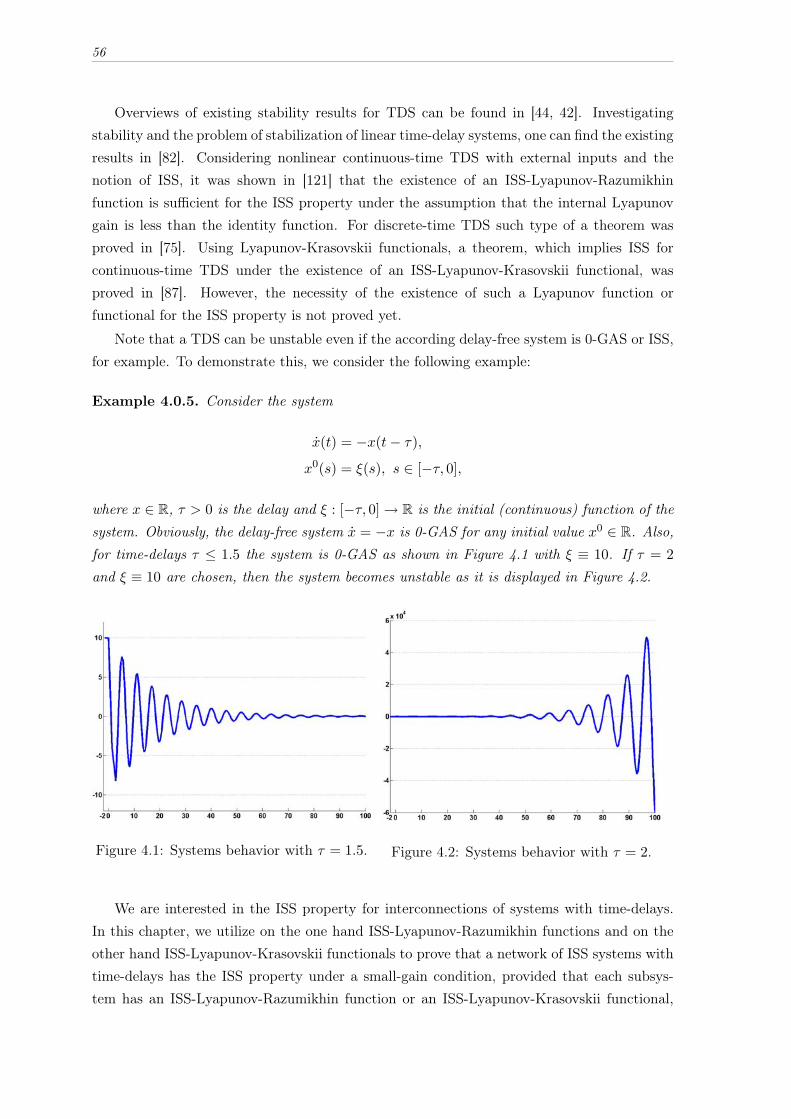
56
Overviews of existing stability results for TDS can be found in [44, 42]. Investigatingstability and the problem of stabilization of linear time-delay systems, one can find the existingresults in [82]. Considering nonlinear continuous-time TDS with external inputs and thenotion of ISS, it was shown in [121] that the existence of an ISS-Lyapunov-Razumikhinfunction is sufficient for the ISS property under the assumption that the internal Lyapunovgain is less than the identity function. For discrete-time TDS such type of a theorem wasproved in [75]. Using Lyapunov-Krasovskii functionals, a theorem, which implies ISS forcontinuous-time TDS under the existence of an ISS-Lyapunov-Krasovskii functional, wasproved in [87]. However, the necessity of the existence of such a Lyapunov function orfunctional for the ISS property is not proved yet.
Note that a TDS can be unstable even if the according delay-free system is 0-GAS or ISS,for example. To demonstrate this, we consider the following example:
Example 4.0.5. Consider the system
x(t) = −x(t− τ),x0(s) = ξ(s), s ∈ [−τ, 0],
where x ∈ R, τ > 0 is the delay and ξ : [−τ, 0]→ R is the initial (continuous) function of thesystem. Obviously, the delay-free system x = −x is 0-GAS for any initial value x0 ∈ R. Also,for time-delays τ ≤ 1.5 the system is 0-GAS as shown in Figure 4.1 with ξ ≡ 10. If τ = 2
and ξ ≡ 10 are chosen, then the system becomes unstable as it is displayed in Figure 4.2.
Figure 4.1: Systems behavior with τ = 1.5. Figure 4.2: Systems behavior with τ = 2.
We are interested in the ISS property for interconnections of systems with time-delays.In this chapter, we utilize on the one hand ISS-Lyapunov-Razumikhin functions and on theother hand ISS-Lyapunov-Krasovskii functionals to prove that a network of ISS systems withtime-delays has the ISS property under a small-gain condition, provided that each subsys-tem has an ISS-Lyapunov-Razumikhin function or an ISS-Lyapunov-Krasovskii functional,
Chapter 4. ISS for time-delay systems 57
respectively. To prove this, we construct the ISS-Lyapunov-Razumikhin function and ISS-Lyapunov-Razumikhin functional, respectively, and the corresponding gains of the wholesystem.This chapter is organized as follows: In Section 4.1, we investigate the (L)ISS property
of TDS and prove an ISS-Lyapunov-Razumikhin theorem. The ISS small-gain theoremsfor interconnected time-delay systems can be found in Section 4.2, where Subsection 4.2.1contains the ISS-Lyapunov-Razumikhin type theorem and Subsection 4.2.2 the ISS-Lyapunov-Krasovskii type theorem. In Section 4.3, we apply the mentioned results to logistic systems,namely production networks. Finally, Section 7.3 concludes the chapter with a summary andan outlook.
4.1 ISS for single time-delay systems
The notion of ISS for TDS reads as follows:
Definition 4.1.1 ((L)ISS for TDS). The system (4.1) is called LISS in maximum formula-tion, if there exist ρ > 0, ρu > 0, β ∈ KL and γ ∈ K such that for all initial functions ξsatisfying ‖ξ‖[−θ,0] ≤ ρ and all inputs u satisfying ‖u‖ ≤ ρu it holds
|x(t)| ≤ max{β(‖ξ‖[−θ,0] , t), γ(‖u‖)
}(4.2)
for all t ∈ R+. If we replace (4.2) by
|x(t)| ≤ β(‖ξ‖[−θ,0] , t) + γ(‖u‖),
then the system (4.1) is called ISS in summation formulation. If ρ = ρu =∞, then the system(4.1) is called ISS (in maximum or summation formulation).
To check, whether a TDS possesses the ISS property, we define (L)ISS-Lyapunov-Razu-mikhin functions, introduced in [121].
Definition 4.1.2 ((L)ISS-Lyapunov-Razumikhin function). A locally Lipschitz continuousfunction V : D → R+, with D ⊂ R
N open, is called a LISS-Lyapunov-Razumikhin functionof the system (4.1), if there exist ρ > 0, ρu > 0, ψ1, ψ2 ∈ K∞, χd, χu, α ∈ K such thatB(0, ρ) ⊂ D and the following conditions hold:
ψ1(|φ(0)|) ≤ V (φ(0)) ≤ ψ2(|φ(0)|), ∀φ(0) ∈ D, (4.3)
V (φ(0)) ≥ χd(∥∥V d(φ)
∥∥[−θ,0]
)+ χu(|u|) ⇒ D+V (φ(0)) ≤ −α(V (φ(0))) (4.4)
for all ‖φ‖[−θ,0] ≤ ρ, φ ∈ C([−θ, 0] ;RN
)and all |u| ≤ ρu, where V d : C
([−θ, 0] ;RN
) →C ([−θ, 0] ;R+) with V d(xt)(τ) := V (x(t + τ)), τ ∈ [−θ, 0]. D+V (x(t)) denotes the upperright-hand side derivative of V along the solution x(t), which is defined as
D+V (x(t)) := lim suph→0+
V (x(t+h))−V (x(t))h .
If ρ = ρu =∞, then the function V is called an ISS-Lyapunov-Razumikhin function.
58 4.1. ISS for single time-delay systems
Note that we get an equivalent definition of a (L)ISS-Lyapunov-Razumikhin function, ifwe replace (4.4) by
V (φ(0)) ≥ max{χd
(∥∥∥V d(φ)∥∥∥
[−θ,0]
), χu(|u|)
}⇒ D+V (φ(0)) ≤ −α(V (φ(0))), (4.5)
where χd, χu, α ∈ K and χd, χu, α are different, in general. With this definition we state thatthe existence of a LISS-Lyapunov-Razumikhin function implies LISS:
Theorem 4.1.3. If there exists a LISS-Lyapunov-Razumikhin function V for system (4.1)and χd(s) < s, s ∈ R+, s > 0, then the system (4.1) is LISS in summation formulation. Ifan LISS-Lyapunov-Razumikhin function with (4.5) and χd(s) < s, s ∈ R+, s > 0 is used,then the system (4.1) is LISS in maximum formulation.
Proof. We use (4.5) and prove the LISS property in maximum formulation. The proof usingthe summation formulation follows similarly. We use the idea of the proof of Theorem 1 in[121] with according changes to the LISS property.
Using a standard comparison principle (see [74], Lemma 4.4 or [121], Lemma 1), weobtain from (4.5) that it holds
V (x(t)) ≤ max{β(V (x0), t), χd
(sups≤t
∥∥∥V d(xs)∥∥∥
[−θ,0]
), χu(‖u‖)
}, (4.6)
β ∈ KL. It holds
sups≤t
∥∥∥V d(xs)∥∥∥
[−θ,0]≤ max
{β
(∥∥∥V d(x0)∥∥∥
[−θ,0], 0), sup
s≤tV (x(s))
}, (4.7)
taking the supremum over [0, t] in (4.6) and inserting it into (4.7), we obtain, using χd(s) <
s, s ∈ R+ and the fact that for all b1, b2 > 0 from b1 ≤ max{b2, χd(b1)} it follows b1 ≤ b2:
sups≤t
∥∥∥V d(xs)∥∥∥
[−θ,0]≤ max
{β
(∥∥∥V d(x0)∥∥∥
[−θ,0], 0), χd
(sups≤t
∥∥∥V d(xs)∥∥∥
[−θ,0]
), χu(‖u‖)
}and therefore
|x(t)| ≤ max{ψ−1
1 (β(ψ2(‖ξ‖[−θ,0]), 0)), ψ−11 (χu(‖u‖))
}, ∀t ≥ 0,
for all ‖ξ‖[−θ,0] ≤ ρ, ξ ∈ C([−θ, 0] ;RN
)and all ‖u‖ ≤ ρu. Given ε > 0 and define
κ := max{β(ψ2(ρ), 0), χu(ρu)}. Note that it holds supt≥s
∥∥V d(xs)∥∥
[−θ,0]≤ κ, which im-
plies ‖V d(x0)‖[−θ,0] ≤ κ. Let δ2 > 0 be such that β(κ, δ2) ≤ ψ1(ε) and let δ1 > θ. Then, bythe estimate (4.6) we have
supt≥s≥δ1+δ2
∥∥∥V d(xs)∥∥∥
[−θ,0]≤ sup
t≥s+δ2
V (x(s))
≤ max
{ψ1(ε), χd
(sup
s∈[0,t]
∥∥∥V d(xs)∥∥∥
[−θ,0]
), χu(‖u‖)
}.
Chapter 4. ISS for time-delay systems 59
It follows
supt≥s≥2(δ1+δ2)
∥∥∥V d(xs)∥∥∥
[−θ,0]≤ max
{ψ1(ε), χd
(sup
s∈[δ1+δ2,t]
∥∥∥V d(xs)∥∥∥
[−θ,0]
), χu(‖u‖)
}
≤ max
{ψ1(ε), (χd)2
(sup
s∈[0,t]
∥∥∥V d(xs)∥∥∥
[−θ,0]
), χu(‖u‖)
}.
Since χd < id, there exists a number n ∈ N, which depends on κ and ε such that
(χd)n(κ) ≤ max {ψ1(ε), χu(‖u‖)} .
By induction we conclude that
supt≥s≥n(δ1+δ2)
∥∥∥V d(xs)∥∥∥
[−θ,0]≤ max {ψ1(ε), χuγu(‖u‖)}
and finally we obtain
|x(t)| ≤ max{ε, ψ−1
1 (χu(‖u‖))} , ∀t ≥ n(δ1 + δ2) (4.8)
for all ‖ξ‖[−θ,0] ≤ ρ, ξ ∈ C ([−θ, 0] ;RN
)and all ‖u‖ ≤ ρu.
Using the same technique for the construction of β as in the proof of Lemma 3.10 in [17],we obtain
|x(t)| ≤ max{β(‖ξ‖[−θ,0], t), γ(‖u‖)
},
for all ‖ξ‖[−θ,0] ≤ ρ, and all ‖u‖ ≤ ρu, where γ(r) := ψ−11 (χu(r)), r ≥ 0.
Note that in [121] a similar theorem as Theorem 4.1.3 for the ISS property was proved, butthe ISS property defined in [121] differs from that in Definition 4.1.1. For systems withouttime-delays these definitions are equivalent, see [120]. Until now, it is an open problemwhether these definitions are equivalent for time-delay systems. A crucial step needed forthe proof is that the combination of global stability and the asymptotic gain property isequivalent to ISS, which is not proved yet, see [123, 122]. Nevertheless, the mentioned resultin [121] is also valid using the ISS property in Definition 4.1.1.
Theorem 4.1.4. If there exists an ISS-Lyapunov-Razumikhin function V for system (4.1)and χd(s) < s, s ∈ R+, s > 0, then the system (4.1) is ISS in summation formulation.If an ISS-Lyapunov-Razumikhin function with (4.5) is used, then the system (4.1) is ISS inmaximum formulation, if χd(s) < s, s ∈ R+, s > 0.
The proof can be found in [121] with changes according to the construction of the KL-function β as in the proof of Theorem 4.1.3 and the proof of Lemma 3.10 in [17].
Another approach to check, whether a system of the form (4.1) has the ISS property wasintroduced in [87]. There, ISS-Lyapunov-Krasovskii functionals are used. Given a locally Lip-schitz continuous functional V : C
([−θ, 0] ;RN
)→ R+, the upper right-hand side derivative
60 4.1. ISS for single time-delay systems
D+V of the functional V along the solution x(t; ξ, u) is defined according to [44], Chapter5.2:
D+V (φ, u) := lim suph→0+
1h
(V(xt+h
)− V (φ)
), (4.9)
where xt+h ∈ C ([−θ, 0] ;RN
)is generated by the solution x(t;φ, u) of x(t) = f(xt, u(t)), t ∈
(t0, t0 + h) with xt0 := φ ∈ C ([−θ, 0] ;RN
).
Remark 4.1.5. Note that in contrast to (4.9), the definition of D+V in [87] is slightlydifferent, since the functional is assumed to be only continuous and in this case, D+V cantake infinite values. Nevertheless, the results in [87] also hold true, if the functional is chosento be locally Lipschitz continuous, according to the results in [85], [86] and using (4.9).
By ‖·‖a, we indicate any norm in C([−θ, 0] ;RN
)such that for some positive reals c1, c2
the following inequalities hold
c1 |φ(0)| ≤ ‖φ‖a ≤ c2 ‖φ‖[−θ,0] , ∀φ ∈ C([−θ, 0] ;RN
).
Definition 4.1.6 (ISS-Lyapunov-Krasovskii functional). A locally Lipschitz continuous func-tional V : C
([−θ, 0] ;RN
) → R+ is called an ISS-Lyapunov-Krasovskii functional for thesystem (4.1), if there exist functions ψ1, ψ2 ∈ K∞ and functions χ, α ∈ K such that
ψ1 (|φ(0)|) ≤ V (φ) ≤ ψ2 (‖φ‖a) , (4.10)
V (φ) ≥ χ (|u|) ⇒ D+V (φ, u) ≤ −α (V (φ)) , (4.11)
for all φ ∈ C ([−θ, 0] ;RN
), u ∈ L∞(R+,R
m).
The next theorem is a counterpart to Theorem 4.1.4 with according changes to Lyapunov-Krasovskii functionals.
Theorem 4.1.7. If there exists an ISS-Lyapunov-Krasovskii functional V for the system(4.1), then the system (4.1) has the ISS property.
Proof. This follows by Theorem 3.1 in [87] with functions ρ and α3 used there definingρ := ψ−1
2 ◦ χ and
D+V (φ, u) ≤ −α3(||φ||a) ≤ −α(V (φ)),
where α := α3 ◦ ψ−12 and the functional is chosen locally Lipschitz continuous according to
the results in [85], [86].
Remark 4.1.8. We conjecture that an LISS version of Theorem 4.1.7 can be stated. Theproof will follow the lines of the one of Theorem 3.1 in [87] with according changes to theLISS property. We skip the formulation of the theorem and its proof.
Chapter 4. ISS for time-delay systems 61
Remark 4.1.9. By an ISS-Lyapunov-Razumikhin function and an ISS Lyapunov-Krasovskiifunctional, there exists two tools to check, whether a TDS has the ISS property. For somesystems, the usage of a Lyapunov-Krasovskii functional is more challenging in contrast to theusage of a Lyapunov-Razumikhin function, because the construction of such a functional isnot always an easy task. An approach to construct Lyapunov-Krasovskii functionals based ondecomposition of a TDS can be found in [51]. More examples can be found in [87, 44].
In the next section, we consider interconnected TDS and develop tools to check, whethera network of TDS has the ISS property.
4.2 ISS for interconnected time-delay systems
In this section, we provide ISS small-gain theorems for interconnected TDS using ISS-Lyapunov-Razumikhin functions and ISS-Lyapunov-Krasovskii functionals.
We consider n ∈ N interconnected TDS of the form
xi(t) = fi
(xt
1, . . . , xtn, u(t)
), i = 1, . . . , n, (4.12)
where xti ∈ C
([−θ, 0] ;RNi
), xt
i(τ) := xi(t+ τ), τ ∈ [−θ, 0] , xi ∈ RNi and u ∈ L∞(R+,R
m).θ denotes the maximal involved delay and xt
j , j = i can be interpreted as internal inputs of theith subsystem. The functionals fi : C
([−θ, 0] ;RN1
)× . . .×C ([−θ, 0] ;RNn
)×Rm → R
Ni arelocally Lipschitz continuous on any bounded set. We denote the solution of a subsystem byxi(t; ξi, u) or xi(t) for short, satisfying the initial condition x0
i ≡ ξi for any ξi ∈ C([−θ, 0],RNi).
The (L)ISS property for a subsystem of (4.12) reads as follows: The i-th subsystemof (4.12) is LISS, if there exist βi ∈ KL, γd
ij , γui ∈ K∞ ∪ {0} , j = 1, . . . , n, j = i and
ρji > 0, ρu
i > 0, j = 1, . . . , n such that for all ‖ξi‖[−θ,0] ≤ ρii, ‖xj‖[−θ,∞) ≤ ρj
i , j = i, ‖u‖ ≤ ρui
and for all t ∈ R+ it holds
|xi(t)| ≤ max{βi(‖ξi‖[−θ,0] , t),max
j,j �=iγd
ij(‖xj‖[−θ,t]), γui (‖u‖)
}. (4.13)
If ρji = ρu
i =∞, then the i-th subsystem of (4.12) is called ISS. This is referred to (L)ISS inmaximum formulation. We get an equivalent formulation, if we replace (4.13) by
|xi(t)| ≤ βi(‖ξi‖[−θ,0] , t) +∑j,j �=i
γdij(‖xj‖[−θ,t]) + γu
i (‖u‖),
where we use the same function βi and same gains for simplicity.
If we define N :=∑Ni, x := (xT
1 , . . . , xTn )
T and f := (fT1 , . . . , f
Tn )
T , then (4.12) can bewritten as a system of the form (4.1), which we call the whole system. We investigate underwhich conditions the whole system has the ISS property and utilize Lyapunov-Razumikhinfunctions as well as Lyapunov-Krasovskii functionals.
62 4.2. ISS for interconnected time-delay systems
4.2.1 Lyapunov-Razumikhin approach
A locally Lipschitz continuous function Vi : Di → R+, with Di ⊂ RNi open, is an LISS-
Lyapunov-Razumikhin function for the i-th subsystem of (4.12), if there exist functionsVj , j = 1, . . . , n, which are continuous, positive definite and locally Lipschitz continuous onR
Nj ⊃ Dj\{0}, ρji > 0, ρu
i > 0, functions ψ1i, ψ2i ∈ K∞, χui ∈ K ∪ {0}, χd
ij ∈ K∞ ∪ {0},αi ∈ K, j = 1, . . . , n, such that B(0, ρi
i) ⊂ Di and the following conditions hold:
ψ1i(|φi(0)|) ≤ Vi(φi(0)) ≤ ψ2i(|φi(0)|), ∀φi(0) ∈ Di, (4.14)
Vi(φi(0)) ≥ max{max
jχd
ij
(∥∥∥V dj (φj)
∥∥∥[−θ,0]
), χu
i (|u|)}
⇒ D+Vi(φi(0)) ≤ −αi(Vi(φi(0))),(4.15)
for all ‖φj‖[−θ,0] ≤ ρji , φj ∈ C
([−θ, 0] ;RNj
), j = 1, . . . , n and all |u| ≤ ρu
i . (4.15) can bereplaced by
Vi(φi(0)) ≥∑
j
χdij
(∥∥∥V dj (φj)
∥∥∥[−θ,0]
)+ χu
i (|u|) ⇒ D+Vi(φi(0)) ≤ −αi(Vi(φi(0))), (4.16)
where χdij , χ
ui , αi ∈ K and χd
ij , χui , αi are different, in general. Without loss of generality, we
use χdij and χ
ui for the summation and maximum formulation. If ρ
ji = ρu
i = ∞, then Vi iscalled an ISS-Lyapunov-Razumikhin function for the i-th subsystem of (4.12). We collect allthe gains in a gain-matrix Γ := (χd
ij)n×n, i, j = 1, . . . , n, which defines a map Γ : Rn+ → R
n+
by
Γ(s) =(max
jχd
1j(sj), . . . ,maxjχd
nj(sj))T
, s ∈ Rn+
using (4.15) and considering (4.16) by
Γ(s) =
⎛⎝∑j
χd1j(sj), . . . ,
∑j
χdnj(sj)
⎞⎠T
, s ∈ Rn+. (4.17)
Recall that we get for v, w ∈ Rn+: v ≥ w ⇒ Γ(v) ≥ Γ(w). In contrast to interconnected
delay-free systems the gain-matrix Γ using the Razumikhin approach has not necessarily zeroentries on the main diagonal.To check, whether a network of TDS possesses the ISS property, we state the following
theorem. It provides a tool utilizing ISS-Lyapunov-Razumikhin functions to verify ISS of anetwork under a small-gain condition.
Theorem 4.2.1. (ISS-Lyapunov-Razumikhin theorem for general networks with time-delays)Consider the interconnected system (4.12). Each subsystem has an ISS-Lyapunov-Razumikhinfunction Vi with summation formulation (4.16). If the corresponding gain-matrix Γ, given by(4.17), satisfies the small-gain condition (1.16), then the function
V (x) = maxi{σ−1
i (Vi(xi))}
Chapter 4. ISS for time-delay systems 63
is the ISS-Lyapunov-Razumikhin function for the whole system of the form (4.1), which isISS in summation formulation, where σ = (σ1, . . . , σn)T is an Ω-path as in Definition 1.2.2.The gains are given by
χd(r) := maxij
σ−1j ((χd
ij)−1((Id+
2 )−1)(χd
ij(σj(r)))),
χu(r) := maxiλ−1(χu
i (r))
for r ≥ 0, where λ(r) := mink λk(r), λk(r) := 2 (∑χd
kj(σk(r))).
Remark 4.2.2. If we consider in Theorem 4.2.1 ISS-Lyapunov-Razumikhin functions Vi withmaximum formulation (4.15) and Γ satisfies the SGC (1.15), then the whole system is ISS inmaximum formulation and the Lyapunov gains are given by
χd(r) := maxi,j
σ−1i (χd
ij(σj(r))),
χu(r) := maxiσ−1
i (χui (r)).
Proof. All subsystems of (4.12) have an ISS-Lyapunov-Razumikhin function Vi, i = 1, . . . , n,i.e., Vi satisfies (4.14) and (4.16). From the small-gain condition (1.16) for Γ, given by(4.17), it follows that there exists an Ω-path σ = (σ1, . . . , σn)T as in Definition 1.2.2 andProposition 1.2.3. Note that σ−1
i ∈ K∞, i = 1, . . . , n. Let 0 = x = (xT1 , . . . , x
Tn )
T . We define
V (x) := maxi{σ−1
i (Vi(xi))}
as the ISS-Lyapunov-Razumikhin function candidate for the overall system. Note that V islocally Lipschitz continuous. V satisfies (4.3), which can be easily checked defining ψ1(r) :=
mini σ−1i (ψ1i( r√
n)), ψ2(r) := maxi σ
−1i (ψ2i(r)), r > 0 and using the condition (4.14).
Let I := {i ∈ {1, . . . , n}| V (x) = σ−1i (Vi(xi)) ≥ maxj,j �=i{σ−1
j (Vj(xj))}}. Fix an i ∈ I.We define χd(r) := maxij σ
−1j ((χd
ij)−1((Id+
2 )−1)(χd
ij(σj(r)))), χu(r) := maxi λ−1(χu
i (r)),r > 0, where λ(r) := mink λk(r), λk(r) :=
2 (∑χd
kj(σk(r))) and assume
V (x(t)) ≥ χd
(∥∥∥V d(xt)∥∥∥
[−θ,0]
)+ χu(|u(t)|).
Note that χd(r) < r. It follows from(Γ ◦D) (σ(r)) < σ(r), ∀r > 0 that it holds
Vi(xi(t)) = σi(V (x(t))) > (Id+ )n∑
j=1
χdij(σj(V (x(t))))
≥n∑
j=1
χdij
(∥∥∥V dj (x
tj)∥∥∥
[−θ,0]
)+ χu
i (|u(t)|).
From (4.16) we obtain
D+V (x(t)) = D+σ−1i (Vi(xi(t))) = (σ−1
i )′(Vi(xi(t)))D+Vi(xi(t))
≤ −(σ−1i )′(Vi(xi(t)))αi(Vi(xi(t))) = −αi(V (x(t))),
64 4.2. ISS for interconnected time-delay systems
where αi(r) := (σ−1i )′(σi(r))αi(σi(r)), r > 0. By definition of α := mini αi, the function
V satisfies (4.4). All conditions of Definition 4.1.2 are satisfied and V is the ISS-Lyapunov-Razumikhin function of the whole system of the form (4.1). By Theorem 4.1.4, the wholesystem is ISS in summation formulation. Using the maximum formulation in (4.15), (4.5) andof the ISS property, the proof follows the same steps as for the summation formulation.
For many applications, an LISS small-gain theorem for TDS using Lyapunov-Razumikhinfunctions will be beneficial due to restrictions on the initial value or the input function inpractice. This is provided in the next corollary.
Corollary 4.2.3. Consider the interconnected system (4.12) and assume that each subsystemhas a LISS-Lyapunov-Razumikhin function Vi(xi) in summation or maximum formulation, forall ‖φj‖[−θ,0] ≤ ρj
i , φj ∈ C([−θ, 0] ;RNj
)with φj(0) = xj, j = 1, . . . , n and all |u| ≤ ρu
i . Ifthe corresponding gain-matrix Γ satisfies the LSGC (1.14), then the function V as definedin Theorem 4.2.1 is the LISS-Lyapunov-Razumikhin function for the whole system with φ =(φ1, . . . , φn)T , ‖φi‖[−θ,0] ≤ ρi, φi ∈ C
([−θ, 0] ;RNi
), where ρi := min{w∗i , ψ−1
i2 (w∗i ),minj ρ
ji}
such that ρ := min ρi and ρu := min ρui . Furthermore, the whole system is LISS in summation
or maximum formulation, respectively.
Proof. Since Γ satisfies the LSGC (1.14), we know that there exists a strictly increasing pathσ : [0, 1]→ [0, w∗], which satisfies Γ(σ(r)) < σ(r), ∀r ∈ (0, 1] and σ(0) = 0, σ(1) = w∗. TheLISS-Lyapunov-Razumikhin function candidate V (x) := maxi{σ−1
i (Vi(xi))} is well defined,because ‖φi‖[−θ,0] ≤ ψ−1
i2 (w∗i ), φi ∈ C
([−θ, 0] ;RNi
)with φi(0) = xi implies Vi(xi) ≤ w∗i .
Following the same steps as in the proof of Theorem 4.2.1, we conclude that V (x) is theLISS-Lyapunov-Razumikhin function for the whole system.
In the next subsection, we prove a small-gain theorem using Lyapunov-Krasovskii func-tionals for subsystems to check, whether a network of TDS possesses the ISS property.
4.2.2 Lyapunov-Krasovskii approach
The Krasovskii functionals for subsystems are as follows:A locally Lipschitz continuous functional Vi : C([−θ, 0];RNi) → R+ is an ISS-Lyapunov-
Krasovskii functional of the i-th subsystem of (4.12), if there exist functionals Vj , j = 1, . . . , n,which are positive definite and locally Lipschitz continuous on C([−θ, 0];RNj ), functionsψ1i, ψ2i ∈ K∞, χij , χi ∈ K ∪ {0}, αi ∈ K, j = 1, . . . , n, i = j such that
ψ1i (|φi(0)|) ≤ Vi(φi) ≤ ψ2i (‖φi‖a) , ∀φi ∈ C([−θ, 0] ,RNi
)(4.18)
Vi (φi) ≥ max {maxj,j �=i χij(Vj(φj)), χi (|u|)} ⇒ D+Vi (φi, u) ≤ −αi (Vi (φi)) , (4.19)
for all φi ∈ C([−θ, 0] ,RNi
), u ∈ L∞(R+,R
m), i = 1, . . . , n. We get an equivalent formulation,if we replace (4.19) by
Vi (φi) ≥∑j,j �=i
χij(Vj(φj)) + χi (|u|) ⇒ D+Vi (φi, u) ≤ −αi (Vi (φi)) , (4.20)
Chapter 4. ISS for time-delay systems 65
where the gains are different in general. Without loss of generality, we use χij and χi forthe summation and maximum formulation. The gain-matrix is defined by Γ := (χij)n×n,χii ≡ 0, i = 1, . . . , n and the map Γ : R
n+ → R
n+ is defined by (1.12) using (4.19) and
considering (4.20) it is defined by (1.13).The next theorem is the second main result of this chapter. It is a counterpart of The-
orem 4.2.1 and it provides a tool how to verify the ISS property for networks of TDS usingISS-Lyapunov-Krasovskii functionals.
Theorem 4.2.4. (ISS-Lyapunov-Krasovskii theorem for general networks with time-delays)Consider an interconnected system of the form (4.12). Assume that each subsystem hasan ISS-Lyapunov-Krasovskii functional Vi, which satisfies the conditions (4.18) and (4.20),i = 1, . . . , n. If the corresponding gain-matrix Γ satisfies the small-gain condition (1.16), then
V (φ) := maxi{σ−1
i (Vi(φi))}
is the ISS-Lyapunov-Krasovskii functional for the whole system of the form (4.1), which is ISSin summation formulation, where σ = (σ1, . . . , σn)T is an Ω-path as in Definition 1.2.2 andφ = (φi, . . . , φn)T ∈ C([−θ, 0];RN ). The Lyapunov gain is given by χ(r) := maxi λ
−1(χi(r))
with λ := mink=1,...,n λk, λk(r) := (∑n
j=1,k �=j χkj(σj(r))).
Remark 4.2.5. If we consider in Theorem 4.2.4 ISS-Lyapunov-Krasovskii functionals Vi
with maximum formulation (4.19) and Γ satisfies the SGC (1.15), then the whole system isISS in maximum formulation and the Lyapunov gain is given by χ(r) := maxi σ
−1i (χi(r)).
Proof. All subsystems of (4.12) have an ISS-Lyapunov-Krasovskii functional Vi, i = 1, . . . , n,i.e., Vi satisfies (4.18) and (4.20). From the small-gain condition (1.16) for Γ, there exists anΩ-path σ = (σ1, . . . , σn)T . Let 0 = xt = ((xt
1)T , . . . , (xt
n)T )T ∈ C([−θ, 0];RN ). We define
V (xt) := maxi{σ−1
i (Vi(xti))}
as the ISS-Lyapunov-Krasovskii functional candidate of the whole system. Note that V islocally Lipschitz. V satisfies (4.10), by definition of ψ1(r) := mini σ
−1i (ψ1i( r√
n)), ψ2(r) :=
maxi σ−1i (ψ2i(r)), r > 0 and using (4.18).
Let I := {i ∈ {1, . . . , n}| V (xt) ={σ−1
i
(Vi(xt
i))} ≥ maxj,j �=i{σ−1
j (Vj(xtj))}}. Fix an
i ∈ I. From (Γ ◦D) (σ(r)) < σ(r), for all r > 0 we get
σi(r) > (Id+ )
⎛⎝∑j,j �=i
χij(σj(r))
⎞⎠⇔ σi(r)−
∑j,j �=i
χij(σj(r)) >
⎛⎝ n∑j=1,i�=j
χij(σj(r))
⎞⎠ =: λi(r).
Define λ := mini λi and assume V (xt) ≥ λ−1(χi(|u|)). Then, it follows
λ(V (xt)) ≥ χi(|u|) ⇒ σi(V (xt))−∑j,j �=i
χij(σj(V (xt))) > χi(|u|)
66 4.3. Applications in logistics
and we get
Vi(xti) = σi(V (xt)) > χi(|u|) +
∑j,j �=i
χij(σj(V (xt))) = χi(|u|) +∑j,j �=i
χij(Vj(xtj)).
From (4.20) we obtain
D+V (xt, u) = (σ−1i )′(Vi(xt
i))D+Vi(xt
i, u) ≤ −(σ−1i )′(Vi(xt
i))αi(Vi(xti)) = −αi(V (xt)),
where αi(r) := (σ−1i )′(σi(r))αi(σi(r)), r ≥ 0. By definition of χ := maxi λ
−1χi and α :=
mini αi, the function V satisfies (4.11). All conditions of Definition 4.1.6 are satisfied andV is the ISS-Lyapunov-Krasovskii functional of the whole system of the form (4.1). ByTheorem 4.1.7 the whole system is ISS in summation formulation. The case in the maximumformulations follows the same steps as for the summation formulation.
4.3 Applications in logistics
In this section, we present an application of the Lyapunov-Razumikhin approach, namely theapplication of Theorem 4.2.1, for the investigation of LISS of logistics networks.A typical example of a logistic network is a production network. Such an interconnected
system describes a company or cross-company owned network with geographically dispersedplants [126], which are connected by transport routes. By an increasing number of plants andlogistic objects, a central control of the network becomes challenging. Autonomous controlcan help to handle such complex networks, see [104, 107, 106, 105], for example. Autonomouscontrol policies allow objects of a network, such as vehicles, containers or machines, forexample, to decide and to execute their own decisions based on some given rules and availablelocal information to route themselves through a network. It can be seen as a paradigm shiftfrom centralized to decentralized control in logistics.Due to economic circumstances, such as high inventory costs, for example, an unbounded
growth of the number of logistic objects such as parts or orders, is undesired in logisticnetworks. The stability analysis of logistic networks allows to get knowledge of the dynamicalproperties of a network and to design stable networks to avoid negative economic outcomes.For production networks without taking transportations into account, there exist modeling
approaches and the corresponding stability analysis for certain scenarios, see [15, 103, 12, 13],for example. In [103], a dual approach for the identification of stability regions of productionnetworks was presented: based on the mathematical stability analysis, the identified stabilityregions were refined by an engineering simulation approach. The benefit of the dual approachis that it saves much time in contrast to a pure simulation approach.Considering production networks with transportations, the modeling was performed in
[16, 12, 102, 14], for example, which we use in the next subsection. Transportations can bemodeled using TDS. In the next subsection, we provide a modeling approach to describe acertain scenario of a production network. We show, how a stability analysis can be performedusing Theorem 4.2.1. The autonomous control method, which we use in the next subsection,
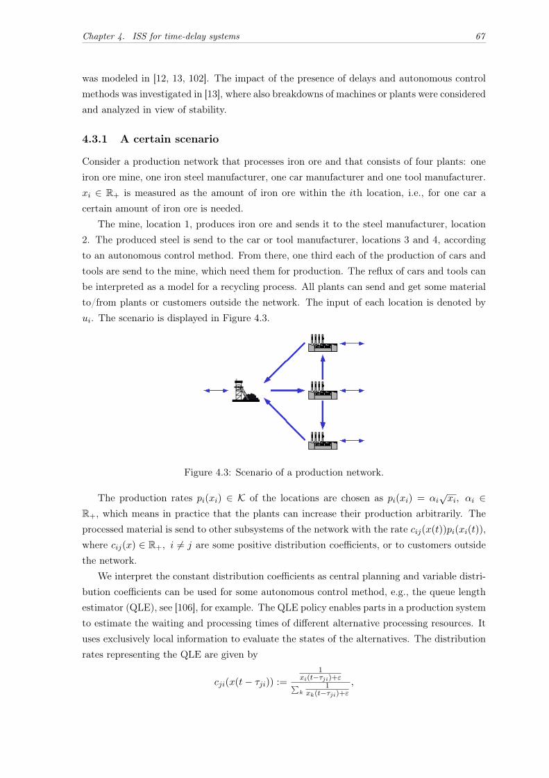
Chapter 4. ISS for time-delay systems 67
was modeled in [12, 13, 102]. The impact of the presence of delays and autonomous controlmethods was investigated in [13], where also breakdowns of machines or plants were consideredand analyzed in view of stability.
4.3.1 A certain scenario
Consider a production network that processes iron ore and that consists of four plants: oneiron ore mine, one iron steel manufacturer, one car manufacturer and one tool manufacturer.xi ∈ R+ is measured as the amount of iron ore within the ith location, i.e., for one car acertain amount of iron ore is needed.The mine, location 1, produces iron ore and sends it to the steel manufacturer, location
2. The produced steel is send to the car or tool manufacturer, locations 3 and 4, accordingto an autonomous control method. From there, one third each of the production of cars andtools are send to the mine, which need them for production. The reflux of cars and tools canbe interpreted as a model for a recycling process. All plants can send and get some materialto/from plants or customers outside the network. The input of each location is denoted byui. The scenario is displayed in Figure 4.3.
Figure 4.3: Scenario of a production network.
The production rates pi(xi) ∈ K of the locations are chosen as pi(xi) = αi√xi, αi ∈
R+, which means in practice that the plants can increase their production arbitrarily. Theprocessed material is send to other subsystems of the network with the rate cij(x(t))pi(xi(t)),where cij(x) ∈ R+, i = j are some positive distribution coefficients, or to customers outsidethe network.We interpret the constant distribution coefficients as central planning and variable distri-
bution coefficients can be used for some autonomous control method, e.g., the queue lengthestimator (QLE), see [106], for example. The QLE policy enables parts in a production systemto estimate the waiting and processing times of different alternative processing resources. Ituses exclusively local information to evaluate the states of the alternatives. The distributionrates representing the QLE are given by
cji(x(t− τji)) :=1
xi(t−τji)+ε∑k
1xk(t−τji)+ε
,
68 4.3. Applications in logistics
where k is the index of the subsystems which get material from subsystem j. It holds 0 ≤cji ≤ 1. ε > 0 is inserted to let the fractions be well-defined. The interpretation of cji is thefollowing: if the queue length of the ith subsystem is small, then more material will be sendto subsystem i in contrast to the case where xi is large and cji is small.The time needed for the transportation of material from the jth to the ith location is
denoted by τji ∈ R+. Then, the dynamics of the ith subsystem can be described by retardeddifferential equations (4.12) as
x1(t) = 13α3
√x3(t− τ31) + 1
3α4
√x4(t− τ41) + u1(t)− α1
√x1(t),
x2(t) = 610α1
√x1(t− τ12) + u2(t)− α2
√x2(t),
x3(t) =1
x3(t−τ23)+ε1
x3(t−τ23)+x4(t−τ23)+ε
610α2
√x2(t− τ23) + u3(t)− α3
√x3(t),
x4(t) =1
x4(t−τ24)+ε1
x3(t−τ24)+x4(t−τ24)+ε
610α2
√x2(t− τ24) + u4(t)− α4
√x4(t),
where xi(τ) ∈ R+, τ ∈ [−θ, 0], θ := max{τ31, τ12, τ23, τ24} are given.To apply Theorem 4.2.1, we have to find LISS-Lyapunov-Razumikhin functions and to
check, whether the small-gain condition is satisfied.We choose Vi(xi) = |xi| = xi as a LISS-Lyapunov-Razumikhin function candidate for the
ith subsystem. Obviously, Vi(xi) satisfies the condition (4.14). To prove that the condition(4.15) holds, we choose the functions χd
ij and χui as
χd1j(s) :=
(αj
α1(1−ε1)
)2s, j = 3, 4,
χdkl(s) :=
(9αl
10αk(1−εk)
)2s, kl ∈ {21, 32, 42},
χui (s) :=
(13
αi(1−εi)
s
)2
, i = 1, 2, 3, 4,
with 0 < εi < 1. We investigate the first subsystem and it holds
x1 ≥ χd1j
(||V d
j (xtj)||[−θ,0]
)⇒ 1
3αj
√||V d
j (xtj)||[−θ,0] ≤ 1
3α1(1− ε1)√x1,
x1 ≥ χu1 (|u1|) ⇒ |u1| ≤ 1
3α1(1− ε1)√x1.
Using 0 ≤ cji ≤ 1 it follows
V1(x1(t)) ≥ max{maxj χd1j(||V d
j (xtj)||[−θ,0]), χu
1(|u1(t)|)} ⇒D+V1(x1(t)) = 1
3α3
√x3(t− τ31) + 1
3α4
√x4(t− τ41) + u1(t)− α1
√x1(t)
≤ − ε1α1
√x1(t) =: −α1(V1(x1(t))).
We conclude that V1 is the LISS-Lyapunov-Razumikhin function for the first subsystem. Bysimilar calculations, we conclude that Vi are the LISS-Lyapunov-Razumikhin functions forthe subsystems. To verify whether the small-gain condition is satisfied, we use the cyclecondition (see Remark 1.2.1) and it holds with the choice εi = 1
100
χd21(χ
d32(χ
d13(s))) = ( 9α1
10α2(1−ε2))2( 9α2
10α3(1−ε3))2( α3
α1(1−ε1))2s < s,
Chapter 4. ISS for time-delay systems 69
and χd21(χ
d42(χ
d14(s))) < s by similar calculations. Thus, the cycle condition is satisfied and
the small gain condition also. By Theorem 4.2.1, the whole network is LISS for all xi(τ) ∈R+, τ ∈ [−θ, 0] and all inputs ui ∈ R+.In the next chapter, we transfer the tools of this chapter to impulsive systems with time-
delays and their interconnection.
70 4.3. Applications in logistics
Chapter 5
ISS for impulsive systems withtime-delays
Another type of systems are impulsive systems. They combine continuous and discontinuousdynamics in one system, see [3, 43], for example. The continuous dynamics is typicallydescribed by differential equations and the discontinuous behavior consists of instantaneousstate jumps that occur at given time instants, also referred to as impulses. Impulsive systemsare closely related to hybrid systems [43] and switched systems [113] and have a wide rangeof applications in network control, engineering, biological or economical systems, see [3, 124,43, 113], for example.An impulsive system is of the form
x(t) = f(x(t), u(t)), t = tk, k ∈ N,
x(t) = g(x−(t), u−(t)), t = tk, k ∈ N,(5.1)
where t0 ≤ t ∈ R+, x ∈ RN , u ∈ L∞(R+,R
m) and {t1, t2, t3, . . .} is a strictly increasingsequence of impulse times in (t0,∞) for some initial time t0 < t1. The impulse times areindependent from the state of the system. The generalization that includes state-dependentresetting of the systems state is known as hybrid systems, see for example [43, 100, 34, 66].Impulsive systems can be viewed as a subclass of hybrid systems as proposed in [100].The set of impulse times is assumed to be either finite or infinite and unbounded, and
impulse times tk have no finite accumulation point. Given a sequence {tk} and a pair of timess, t satisfying t0 ≤ s < t, N(t, s) denotes the number of impulse times tk in the semi-openinterval (s, t].Furthermore, f : R
N ×Rm → R
N , g : RN ×R
m → RN , where we assume that f is locally
Lipschitz. All signals (x and inputs u) are assumed to be right-continuous and to have leftlimits at all times and we denote x− := lims↗t x(s).These requirements assure that a unique solution of the impulsive system (5.1) exists,
which is absolutely continuous between impulses, see [43], Chapter 2.2. We denote the solutionby x(t;x0, u) or x(t) for short for any initial value x(t0) = x0.Investigating the stability of impulsive systems, it turns out that a condition on the
71
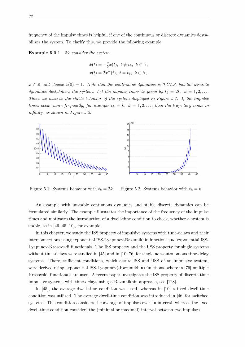
72
frequency of the impulse times is helpful, if one of the continuous or discrete dynamics desta-bilizes the system. To clarify this, we provide the following example.
Example 5.0.1. We consider the system
x(t) = −25x(t), t = tk, k ∈ N,
x(t) = 2x−(t), t = tk, k ∈ N,
x ∈ R and choose x(0) = 1. Note that the continuous dynamics is 0-GAS, but the discretedynamics destabilizes the system. Let the impulse times be given by tk = 2k, k = 1, 2, . . ..Then, we observe the stable behavior of the system displayed in Figure 5.1. If the impulsetimes occur more frequently, for example tk = k, k = 1, 2, . . ., then the trajectory tends toinfinity, as shown in Figure 5.2.
Figure 5.1: Systems behavior with tk = 2k. Figure 5.2: Systems behavior with tk = k.
An example with unstable continuous dynamics and stable discrete dynamics can beformulated similarly. The example illustrates the importance of the frequency of the impulsetimes and motivates the introduction of a dwell-time condition to check, whether a system isstable, as in [46, 45, 10], for example.In this chapter, we study the ISS property of impulsive systems with time-delays and their
interconnections using exponential ISS-Lyapunov-Razumikhin functions and exponential ISS-Lyapunov-Krasovskii functionals. The ISS property and the iISS property for single systemswithout time-delays were studied in [45] and in [10, 76] for single non-autonomous time-delaysystems. There, sufficient conditions, which assure ISS and iISS of an impulsive system,were derived using exponential ISS-Lyapunov(-Razumikhin) functions, where in [76] multipleKrasovskii functionals are used. A recent paper investigates the ISS property of discrete-timeimpulsive systems with time-delays using a Razumikhin approach, see [128].In [45], the average dwell-time condition was used, whereas in [10] a fixed dwell-time
condition was utilized. The average dwell-time condition was introduced in [46] for switchedsystems. This condition considers the average of impulses over an interval, whereas the fixeddwell-time condition considers the (minimal or maximal) interval between two impulses.
Chapter 5. ISS for impulsive systems with time-delays 73
We provide a Lyapunov-Krasovskii type theorem and a Lyapunov-Razumikhin type ISStheorem using the average dwell-time condition for single impulsive systems with time-delays.The proofs use the idea of the proof of [45], [121] and [120]. For the Razumikhin type ISStheorem we require as an additional condition that the Lyapunov gain fulfills a small-gaincondition. In contrast to the Razumikhin type theorem from [10], we consider autonomoustime-delay systems and the average dwell-time condition. Our theorem allows to verify theISS property for larger classes of impulse time sequences, however, we have used an additionaltechnical condition on the Lyapunov gain in our proofs.Considering interconnected impulsive systems, our main goal is to find sufficient conditions
which assure ISS of such interconnections without time-delays. To this end, we use theapproach used for continuous networks. We prove that under a small-gain condition withlinear gains and a dwell-time condition a network of impulsive subsystems possesses theISS property. We construct the exponential ISS-Lyapunov-Razumikhin and ISS-Lyapunov-Krasovskii function(al)s and the corresponding gains of the whole system.In Section 5.1, single impulsive systems with time-delays are considered. Subsection 5.1.2
presents the Lyapunov-Krasovskii approach and Subsection 5.1.1 presents the Lyapunov-Razumikhin approach. The ISS property for interconnections of impulsive systems withtime-delays is investigated in Section 5.2. The tools to check whether a network possesses theISS property can be found in Subsection 5.2.1 for the Lyapunov-Razumikhin approach and inSubsection 5.2.2 for the Lyapunov-Krasovskii approach. An example is given in Section 5.3.
5.1 Single impulsive systems with time-delays
We consider single impulsive system with time-delays of the form
x(t) = f(xt, u(t)), t = tk, k ∈ N,
x(t) = g((xt)−, u−(t)), t = tk, k ∈ N,(5.2)
where we make the same assumptions as in the delay-free case, where f : PC([−θ, 0] ;RN
)×R
m → RN is locally Lipschitz, g : PC
([−θ, 0] ;RN
) × Rm → R
N and we denote (xt)− :=
lims↗t xs.
We assume that the regularity conditions (see e.g., [4]) for the existence and uniqueness ofa solution of system (5.2) are satisfied. We denote the solution by x(t; ξ, u) or x(t) for shortfor any ξ ∈ PC([−θ, 0],RN ) that exists in a maximal interval [−θ, b), 0 < b ≤ +∞, satisfyingthe initial condition xt0 = ξ. The solution is piecewise right-continuous for all t ≥ t0 and itis continuous at each t = tk, t ≥ t0.The ISS property is redefined with respect to impulsive systems with time-delays, see [10]:
Definition 5.1.1 (ISS for impulsive systems with time-delays). Suppose that a sequence {tk}is given. We call the system (5.2) or (5.19) ISS, if there exist functions β ∈ KL, γu ∈ K∞,such that for every initial condition ξ ∈ PC([−θ, 0],RN ) and every input u it holds
|x(t)| ≤ max{β(‖ξ‖[−θ,0], t− t0), γu(‖u‖[t0,t])}, ∀t ≥ t0. (5.3)
74 5.1. Single impulsive systems with time-delays
The impulsive system (5.2) or (5.19) is uniformly ISS over a given class S of admissiblesequences of impulse times, if (5.3) holds for every sequence in S, with functions β and γu,which are independent on the choice of the sequence.
Remark 5.1.2. Note that we get an equivalent definition of ISS, if we use the summationformulation instead of the maximum formulation in Definition 5.1.1. In the following, weonly use the maximum formulation. The results using the summation formulation followequivalently.
We use the tools, introduced in Chapter 4, namely Lyapunov-Krasovskii functionals andLyapunov-Razumikhin functions, to check whether an impulsive time-delay system has theISS property.
5.1.1 The Lyapunov-Razumikhin methodology
At first, we give the definition of an exponential ISS-Lyapunov-Razumikhin function:
Definition 5.1.3 (Exponential ISS-Lyapunov-Razumikhin functions). A function V : RN →
R+ is called an exponential ISS-Lyapunov-Razumikhin function for the system (5.2) withrate coefficients c, d ∈ R, if V is locally Lipschitz continuous and there exist functions ψ1, ψ2,γd, γu ∈ K∞ such that
ψ1(|φ(0)|) ≤ V (φ(0)) ≤ ψ2(|φ(0)|), ∀φ(0) ∈ RN
and whenever V (φ(0)) ≥ max{γd(‖V d(φ)‖[−θ,0]), γu(|u|)} holds, it follows
D+V (φ(0)) ≤ −cV (φ(0)) and (5.4)
V (g(φ, u)) ≤ e−dV (φ(0)), (5.5)
for all φ ∈ PC ([−θ, 0] ;RN
)and u ∈ R
m, where V d : PC([−θ, 0] ;RN
) → PC ([−θ, 0] ;R+)
is defined by V d(xt)(τ) := V (x(t+ τ)), τ ∈ [−θ, 0].Roughly speaking, the condition (5.4) states that if c is positive, then the function V
decreases along the solution x(t) at t. On the other hand, if c < 0 then the function V canincrease along the solution x(t) at t. Condition (5.5) states that if d is positive, then thejump (impulse) decreases the magnitude of V . On the other hand, if d < 0 then the jump(impulse) increase the magnitude of V .
Remark 5.1.4. Note that in [10] the conditions (5.4) and (5.5) are in the dissipative form.By Proposition 2.6 in [8], the conditions in dissipative form are equivalent to the conditions inimplication form, used in Definition 5.1.3, where the coefficients c, d are different in general.
For the main result of this subsection, we need the following:
Definition 5.1.5. Assume that a sequence {tk} is given. We call the system (5.2) or (5.19)globally stable (GS), if there exist functions ϕ, γ ∈ K∞ such that for all ξ ∈ PC([−θ, 0],RN )
and all u it holds
|x(t)| ≤ max{ϕ(‖ξ‖[−θ,0]), γ(‖u‖[t0,t])}, ∀t ≥ t0. (5.6)
Chapter 5. ISS for impulsive systems with time-delays 75
The impulsive system (5.2) or (5.19) is uniformly GS over a given class S of admissiblesequences of impulse times, if (5.6) holds for every sequence in S, with functions ϕ and γu,which are independent on the choice of the sequence.
To prove a Razumikhin type theorem for the verification of ISS for impulsive time-delaysystems, we need the following characterization of the uniform ISS property:
Lemma 5.1.6. The system (5.2) or (5.19) is uniformly ISS over S, if and only if it is
• uniformly GS over S and
• there exists γ ∈ K such that for each ε > 0, ηx ∈ R+, ηu ∈ R+ there exists T ≥ 0
(which does not depend on the choice of the impulse time sequence from S) such that‖ξ‖[−θ,0] ≤ ηx and ‖u‖[t0,∞) ≤ ηu imply |x(t)| ≤ max{ε, γ(‖u‖[t0,t])}, for all t ≥ T + t0.
The proof can be found in [17]. Now, we prove as a main result of this section thefollowing theorem. It provides a tool to check whether a single impulsive system with time-delays possesses the ISS property using exponential Lyapunov-Razumikhin functions.
Theorem 5.1.7 (Lyapunov-Razumikhin type theorem). Let V be an exponential ISS-Lyapunov-Razumikhin function for the system (5.2) with c, d ∈ R, d = 0. For arbitraryconstants μ, λ > 0, let S[μ, λ] denote the class of impulse time sequences {tk} satisfying theaverage dwell-time condition
−dN(t, s)− (c− λ)(t− s) ≤ μ, ∀t ≥ s ≥ t0. (5.7)
If γd satisfies γd(r) < e−μ−|d|r, r > 0, then the system (5.2) is uniformly ISS over S[μ, λ].
For d = 0 the jumps do not influence the stability of the system and the system will be ISS,if the corresponding continuous dynamics has the ISS property. This case was investigatedmore detailed in [45], Section 6.Note that the condition (5.7) guarantees stability of an impulsive system even if the
continuous or discontinuous behavior is unstable. For example, if the continuous behavior isunstable, which means c < 0, then this condition assumes that the discontinuous behaviorhas to stabilize the system (d > 0) and the jumps have to occur often enough. Conversely, ifthe discontinuous behavior is unstable (d < 0) and the continuous behavior is stable (c > 0)
then the jumps have to occur rarely, which stabilizes the system.
Proof. From (5.4) we have for any two consecutive impulses tk−1, tk, for all t ∈ (tk−1, tk)
V (x(t)) ≥ max{γd(‖V d(xt)‖[−θ,0]), γu(|u(t)|)} ⇒ D+V (x(t)) ≤ −cV (x(t)) (5.8)
and similarly with (5.5) for every impulse time tk
V (x(tk)) ≥ max{γd(‖V d((xtk)−)‖[−θ,0]), γu(|u−(tk)|)}⇒ V (g((xtk)−, u−(tk))) ≤ e−dV (x(tk)).
(5.9)
76 5.1. Single impulsive systems with time-delays
Because of the right-continuity of x and u, there exists a sequence of times t0 := t0 < t1 <
t1 < t2 < t2 < . . . such that for i = 0, 1, . . . we have
V (x(t)) ≥ max
{γd
(sup
r∈[t0,t]
∥∥∥V d(xr)∥∥∥
[−θ,0]
), γu(‖u‖[t0,t])
}, ∀t ∈ [ti, ti+1) (5.10)
and for all i = 1, 2, . . . it holds
V (x(t)) ≤ max
{γd
(sup
r∈[t0,t]
∥∥∥V d(xr)∥∥∥
[−θ,0]
), γu(‖u‖[t0,t])
}, ∀t ∈ [ti, ti), (5.11)
where this sequence breaks the interval [t0,∞) into a disjoint union of subintervals. Supposet0 < t1, so that [t0, t1) is nonempty. Otherwise we can continue the proof in the line below(5.13). Between any two consecutive impulses tk−1, tk ∈ [t0, t1] from (5.10) and (5.8) we haveD+V (x(t))) ≤ −cV (x(t)), for all t ∈ (tk−1, tk) and therefore
V (x−(tk)) ≤ e−c(tk−tk−1)V (x(tk−1)).
From (5.9) and (5.10), we have V (x(tk)) ≤ e−dV (x−(tk)). Combining this, it follows
V (x(tk)) ≤ e−d−c(tk−tk−1)V (x(tk−1))
and by the iteration over the N(t, t0) impulses on [t0, t], we obtain the bound
V (x(t)) ≤ e−dN(t,t0)−c(t−t0)V (x(t0)), ∀t ∈ [t0, t1]. (5.12)
Using the dwell-time condition (5.7), we get
V (x(t)) ≤ eμ−λ(t−t0)V (x(t0)), ∀t ∈ [t0, t1]. (5.13)
For any subinterval of the form [ti, ti), i = 1, 2, . . ., we have (5.11) as a bound for V (x(t)).Now, consider two cases.Let ti be not an impulse time, then (5.11) is a bound for t = ti. Consider the subinterval
[ti, ti+1). Repeating the argument used to establish (5.13), with ti in place of t0 and using(5.11) with t = ti we get for all t ∈ (ti, ti+1]
V (x(t)) ≤ eμ−λ(t−ti)V (x(ti)) ≤ eμmax
⎧⎨⎩γd
⎛⎝ supr∈[t0,ti]
∥∥∥V d(xr)∥∥∥
[−θ,0]
⎞⎠ , γu(‖u‖[t0,ti])
⎫⎬⎭ .
Now, let ti be an impulse time. Then, we have
V (x(ti)) ≤ e−dmax
⎧⎨⎩γd
⎛⎝ supr∈[t0,ti]
∥∥∥V d(xr)∥∥∥
[−θ,0]
⎞⎠ , γu(‖u‖[t0,ti])
⎫⎬⎭ (5.14)
and in either case
V (x(t)) ≤ e|d|max
{γd
(sup
r∈[t0,t]
∥∥∥V d(xr)∥∥∥
[−θ,0]
), γu(‖u‖[t0,t])
}, ∀t ∈ [ti, ti]. (5.15)
Chapter 5. ISS for impulsive systems with time-delays 77
Repeating the argument used to establish (5.13), with ti in place of t0 and using (5.15)with t = ti we get
V (x(t)) ≤ eμ−λ(t−ti)V (x(ti)) ≤ eμ+|d|max
⎧⎨⎩γd
⎛⎝ supr∈[t0,ti]
∥∥∥V d(xr)∥∥∥
[−θ,0]
⎞⎠ , γu(‖u‖[t0,ti])
⎫⎬⎭ ,
for all t ∈ (ti, ti+1], i ≥ 1. Overall, we obtain for all t ≥ t0
V (x(t)) ≤ max
{eμ−λ(t−t0)V (x(t0)), eμ+|d|γd
(sup
r∈[t0,t]
∥∥∥V d(xr)∥∥∥
[−θ,0]
), eμ+|d|γu(‖u‖[t0,t])
}.
(5.16)
Now, it holds
supt≥s≥t0
∥∥∥V d(xs)∥∥∥
[−θ,0]≤ max
{∥∥∥V d(xt0)∥∥∥
[−θ,0], supt≥s≥t0
V (x(s))}. (5.17)
We take the supremum over [t0, t] in (5.16) and insert it into (5.17). Then, using γd(r) <
e−μ−|d|r and the fact that for all b1, b2 > 0 from b1 ≤ max{b2, eμ+|d|γd(b1)} it follows b1 ≤ b2,we obtain
supt≥s≥t0
‖V d(xs)‖[−θ,0] ≤ max{eμ+|d|ψ2(‖ξ‖[−θ,0]), e
μ+|d|γu(‖u‖[t0,t])}
and therefore
|x(t)| ≤ max{ψ−1
1 (eμ+|d|ψ2(‖ξ‖[−θ,0])), ψ−11 (eμ+|d|γu(‖u‖[t0,t]))
}, ∀t ≥ t0,
which means that the system (5.2) is uniformly GS over S[μ, λ].Note that ϕ(·) := ψ−1
1 (eμ+|d|ψ2(·)) is a K∞-function. Now, for given ε, ηx, ηu > 0 suchthat ‖ξ‖[−θ,0] ≤ ηx, ‖u‖[t0,∞) ≤ ηu let κ := max
{eμ+|d|ψ2(ηx), eμ+|d|γu(ηu)
}. It holds
supt≥s≥t0 ‖V d(xs)‖[−θ,0] ≤ κ. Let ρ2 > 0 be such that e−λρ2κ ≤ ψ1(ε) and let ρ1 > θ.Then, by the estimate (5.16) we have
supt≥s≥t0+ρ1+ρ2
‖V d(xs)‖[−θ,0] ≤ supt≥s≥t0+ρ2
V (x(s))
≤ max
{ψ1(ε), eμ+|d|γd
(sup
r∈[t0,t]
∥∥∥V d(xr)∥∥∥
[−θ,0]
), eμ+|d|γu(‖u‖[t0,t])
}.
Replacing t0 by t0 + ρ1 + ρ2 in the previous inequality we obtain
supt≥s≥t0+2(ρ1+ρ2)
‖V d(xs)‖[−θ,0]
≤ max
{ψ1(ε), eμ+|d|γd
(sup
r∈[t0+ρ1+ρ2,t]
∥∥∥V d(xr)∥∥∥
[−θ,0]
), eμ+|d|γu(‖u‖[t0+ρ1+ρ2,t])
}
≤ max
{ψ1(ε), (eμ+|d|γd)2
(sup
r∈[t0,t]
∥∥∥V d(xr)∥∥∥
[−θ,0]
), eμ+|d|γu(‖u‖[t0,t])
}.
78 5.1. Single impulsive systems with time-delays
Since eμ+|d|γd < Id, there exists a number n ∈ N, which depends on κ and ε such that
(eμ+|d|γd)n(κ) := (eμ+|d|γd) ◦ . . . ◦ (eμ+|d|γd)︸ ︷︷ ︸n times
(κ) ≤ max{ψ1(ε), eμ+|d|γu(‖u‖[t0,t])
}.
By induction, we conclude that
supt≥s≥t0+n(ρ1+ρ2)
‖V d(xs)‖[−θ,0] ≤ max{ψ1(ε), eμ+|d|γu(‖u‖[t0,t])
},
and finally, we obtain
|x(t)| ≤ max{ε, ψ−1
1 (eμ+|d|γu(‖u‖[t0,t]))}, ∀t ≥ t0 + n(ρ1 + ρ2). (5.18)
Thus, the system (5.2) satisfies the second property from Lemma 5.1.6, which implies that asystem of the form (5.2) is uniformly ISS over S[μ, λ].
Note that the condition γd(r) < e−μ−|d|r, r > 0 means that the gain is connected withthe average dwell-time condition (5.7). As we will see, this is also the case for interconnectedimpulsive time-delay systems. Also note that the condition γd(r) < e−μ−|d|r, r > 0 leads tosome kind of conservativeness in contrast to the condition γd(r) < r, r > 0 for time-delaysystems without impulses. To relax this condition, one can get rid of the term e−|d| in theprevious condition, which we quote in the following theorem.
Theorem 5.1.8. Consider all assumptions from Theorem 5.1.7, with γd satisfying γd(r) <
e−μr, r > 0. Then, the system (5.2) is uniformly ISS over S[μ, λ].
The proof with the technique to get rid of the term e−|d| can be found in [17]. The ideais that in the proof of Theorem 5.1.7, namely in equation (5.14), the set of time sequencesS∗[μ, λ] is considered for which the average dwell-time condition holds with the number ofjumps in the compact interval [s, t], defined by N∗(t, s), instead of the number of jumpsN(t, s) in the interval (s,t]. It can be shown that S∗[μ, λ] = S[μ, λ] and that the estimationsaround (5.14) hold true with an additional multiplier ed in (5.14), such that ede−d = 1 andthe term e−|d| is not necessary in the estimations of the proof of Theorem 5.1.7.
Remark 5.1.9. Another Razumikhin type theorem (for non-autonomous systems) has beenproposed in [10]. There, a so-called fixed dwell-time condition was used to characterize theclass of impulse time sequences, over which the system is uniformly ISS. In contrast to The-orems 1 and 2 from [10], we prove the Razumikhin type theorem (Theorem 5.1.7) over theclass of sequences, which satisfy the average dwell-time condition. This class is larger thanthe class of sequences, which satisfy the fixed dwell-time condition. However, the small-gaincondition, that we have used in this thesis, γd(r) < e−μr, r > 0 or γd(r) < e−μ−|d|r, r > 0,respectively, is stronger than that from [10].
In the next subsection, we give a counterpart to Theorem 5.1.7 or Theorem 5.1.8, respec-tively, using exponential Lyapunov-Krasovskii functionals.
Chapter 5. ISS for impulsive systems with time-delays 79
5.1.2 The Lyapunov-Krasovskii methodology
We consider another type of impulsive systems with time-delays of the form
x(t) = f(xt, u(t)), t = tk, k ∈ N,
xt = g((xt)−, u(t)), t = tk, k ∈ N,(5.19)
where we make the same assumptions as before and the functional g is now a map fromPC
([−θ, 0] ;RN
)× Rm into PC
([−θ, 0] ;RN
).
According to [48], Section 2, the initial state and the input together determine the evolu-tion of a system according to the right-hand side of the differential equation. Therefore, fortime-delay systems, we denote the state by the function xt ∈ PC([−θ, 0],RN ) and we changethe discontinuous behavior in (5.19): in contrast to the system (5.2), at an impulse time tknot only the point x(tk) “jumps”, but all the states xt in the interval (tk − θ, tk]. Due to thischange, the Lyapunov-Razumikhin approach cannot be applied. In this case, we propose touse Lyapunov-Krasovskii functionals for the stability analysis of systems of the form (5.19).Another approach using Lyapunov functionals can be found in [109]. There, Lyapunov
functionals for systems of the form (5.2) with zero input are used for stabilization resultsof impulsive systems, where the definition of such a functional is different to the approachpresented here according to impulse times.
Definition 5.1.10 (Exponential ISS-Lyapunov-Krasovskii functionals). A functional V :
PC([−θ, 0] ;RN
) → R+ is called an exponential ISS-Lyapunov-Krasovskii functional withrate coefficients c, d ∈ R for the system (5.19), if V is locally Lipschitz continuous, there existψ1, ψ2 ∈ K∞ such that
ψ1(|φ(0)|) ≤ V (φ) ≤ ψ2(|φ|a), ∀φ ∈ PC([−θ, 0] ;RN
)(5.20)
and there exists a function γ ∈ K such that whenever V (φ) ≥ γ(|u|) holds, it follows
D+V (φ, u) ≤ −cV (φ) and (5.21)
V (g(φ, u)) ≤ e−dV (φ), (5.22)
for all φ ∈ PC ([−θ, 0] ;RN
)and u ∈ R
m.
Note that the rate coefficients c, d are not required to be non-negative. The followingresult is a counterpart of Theorem 1 in [45] and Theorems 1 and 2 in [10] for impulsivesystems with time-delays using the Lyapunov-Krasovskii approach.
Theorem 5.1.11 (Lyapunov-Krasovskii type theorem). Let V be an exponential ISS-Lyapunov-Krasovskii functional for the system (5.19) with c, d ∈ R, d = 0. For arbitraryconstants μ, λ ∈ R+, let S[μ, λ] denote the class of impulse time sequences {tk} satisfyingthe dwell-time condition (5.7). Then, the system (5.19) is uniformly ISS over S[μ, λ].
Proof. From (5.21) we have for any two consecutive impulses tk−1, tk, for all t ∈ (tk−1, tk)
V (xt) ≥ γ(|u(t)|)⇒ D+V (xt, u(t)) ≤ −cV (xt) (5.23)
80 5.1. Single impulsive systems with time-delays
and similarly with (5.22) for every impulse time tk
V (xtk) ≥ γ(|u−(tk)|)⇒ V (g((xtk)−, u−(tk))) ≤ e−dV (xtk). (5.24)
Because of the right-continuity of x and u there exists a sequence of times t0 := t0 < t1 <
t1 < t2 < t2 < . . . such that we have
V (xt) ≥ γ(‖u‖[t0,t]), ∀t ∈ [ti, ti+1), i = 0, 1, . . . , (5.25)
V (xt) ≤ γ(‖u‖[t0,t]), ∀t ∈ [ti, ti), i = 1, 2, . . . , (5.26)
where this sequence breaks the interval [t0,∞) into a disjoint union of subintervals. Supposet0 < t1, so that [t0, t1) is nonempty. Otherwise we can continue the proof in the line below(5.27). Between any two consecutive impulses tk−1, tk ∈ (t0, t1] with (5.25) and (5.23) wehave D+V (xt, u(t)) ≤ −cV (xt), for all t ∈ (tk−1, tk) and therefore
V ((xtk)−) ≤ e−c(tk−tk−1)V (xtk−1).
From (5.24) and (5.25) we have V (xtk) ≤ e−dV ((xtk)−). Combining this, it follows
V (xtk) ≤ e−de−c(tk−tk−1)V (xtk−1)
and by iteration over the N(t, t0) impulses on (t0, t] we obtain the bound
V (xt) ≤ e−dN(t,t0)−c(t−t0)V (ξ), ∀t ∈ (t0, t1].Using the dwell-time condition (5.7), we get
V (xt) ≤ eμ−λ(t−t0)V (ξ), ∀t ∈ (t0, t1]. (5.27)
Now, on any subinterval of the form [ti, ti), we already have (5.26) as a bound. If ti is not animpulse time, then (5.26) is a bound for t = ti. If ti is an impulse time, then we have
V (xti) ≤ e−dγ(‖u‖[t0,ti])
and in either case
V (xt) ≤ e|d|γ(‖u‖[t0,t]), ∀t ∈ [ti, ti], i ≥ 1, (5.28)
where this bound holds for all t ≥ ti, if ti = ∞. Now, consider any subinterval of the form[ti, ti+1), i ≥ 1. Repeating the argument used to establish (5.27) with ti in place of t0 andusing (5.28) with t = ti, we get
V (xt) ≤ eμ−λ(t−ti)V (xti) ≤ eμ+|d|γ(‖u‖[t0,ti])
for all t ∈ (ti, ti+1], i ≥ 1. Combining this with (5.27) and (5.28), we obtain
V (xt) ≤ max{eμ−λ(t−t0)V (ξ), eμ+|d|γ(‖u‖[t0,t])}, ∀t ≥ t0.
By definition of β(r, t−t0) := ψ−11 (eμ−λ(t−t0)ψ2(cr)) and γu(r) := ψ−1
1 (eμ+|d|γ(r)) the uniformISS property follows from (5.20). Note that β and γu do not depend on the particular choiceof the time sequence and therefore uniformity is clear.
In the next section, we investigate interconnected impulsive time-delay systems in viewof stability.
Chapter 5. ISS for impulsive systems with time-delays 81
5.2 Networks of impulsive systems with time-delays
We consider n interconnected impulsive systems with time-delays of the form
xi(t) = fi(xt1, . . . , x
tn, ui(t)), t = tk,
xi(t) = gi((xt1)−, . . . , (xt
n)−, u−i (t)), t = tk,
(5.29)
where the same assumptions on the system as in the delay-free case are considered with thefollowing differences: We denote xt
i(τ) := xi(t+ τ), τ ∈ [−θ, 0] and (xti)−(τ) := x−i (t+ τ) :=
lims↗t xi(s + τ), τ ∈ [−θ, 0]. Furthermore, fi : PC([−θ, 0],RN1) × . . . × PC([−θ, 0],RNn) ×R
Mi → RNi , and gi : PC([−θ, 0],RN1) × . . . × PC([−θ, 0],RNn) × R
Mi → RNi , where we
assume that fi, i = 1, . . . , n are locally Lipschitz.If we define N :=
∑iNi, m :=
∑iMi, x = (xT
1 , . . . , xTn )
T , u = (uT1 , . . . , u
Tn )
T , f =
(fT1 , . . . , f
Tn )
T and g = (gT1 , . . . , g
Tn )
T , then (5.29) becomes a system of the form (5.2). TheISS property for systems with several inputs and time-delays is as follows:Suppose that a sequence {tk} is given. The ith subsystem of (5.29) is ISS, if there exist
βi ∈ KL, γij , γui ∈ K∞ ∪ {0} such that for every initial condition ξi and every input ui it
holds
|xi(t)| ≤ max{βi(‖ξi‖[−θ,0], t− t0),maxj,j �=i
γij(‖xj‖[t0−θ,t]), γui (‖ui‖[t0,t])} (5.30)
for all t ≥ t0. The ith subsystem of (5.29) is uniformly ISS over a given class S of admissiblesequences of impulse times, if (5.30) holds for every sequence in S, with functions βi, γij andγu
i that are independent of the choice of the sequence.In the following, we present tools to analyze systems of the form (5.29) in view of ISS:
exponential ISS-Lyapunov-Razumikhin functions and exponential ISS-Lyapunov-Krasovskiifunctionals for the subsystems.
5.2.1 The Lyapunov-Razumikhin approach
Assume that for each subsystem of the interconnected system (5.29) there is a given func-tion Vi : R
Ni → R+, which is continuous, positive definite and locally Lipschitz continuouson R
Ni\{0}. For i = 1, . . . , n the function Vi is an exponential ISS-Lyapunov-Razumikhinfunction of the ith subsystem of (5.29), if there exist ψ1i, ψ2i ∈ K∞, γu
i ∈ K ∪ {0}, γij ∈K∞ ∪ {0}, j = 1, . . . , n and scalars ci, di ∈ R, such that
ψ1i(|φi(0)|) ≤ Vi(φi(0)) ≤ ψ2i(|φi(0)|), ∀φi(0) ∈ RNi (5.31)
and whenever Vi(φi(0)) ≥ max{maxj γij(‖V dj (φj)‖[−θ,0]), γu
i (|ui|)} holds, it follows
D+Vi(φi(0)) ≤ −ciVi(φi(0)) (5.32)
for all φ = (φT1 , . . . , φ
Tn )
T ∈ PC([−θ, 0],RN ) and ui ∈ RMi , where V d
j : PC([−θ, 0] ;RNj
)→PC ([−θ, 0] ;R+) with V d
j (xtj)(τ) := Vj(xj(t+ τ)), τ ∈ [−θ, 0] and it holds
Vi(gi(φ1, . . . , φn, ui)) ≤ max{e−diVi(φi(0)),maxjγij(‖V d
j (φj)‖[−θ,0]), γui (|ui|)}, (5.33)
82 5.2. Networks of impulsive systems with time-delays
for all φ ∈ PC([−θ, 0],RN ) and ui ∈ RMi . Another formulation can be obtained by replacing
(5.33) by
Vi(φi(0)) ≥ max{maxjγij(‖V d
j (φj)‖[−θ,0]), γui (|ui|)} ⇒ Vi(gi(φ, ui)) ≤ e−diVi(φi(0)),
where γij , γui ∈ K∞.
In the following, we assume that the gains γij are linear and we denote throughout thechapter γij(r) = γijr, γij , r ≥ 0. All the gains are collected in a matrix Γ := (γij)n×n,i, j = 1, . . . , n, which defines a map as in (1.12).Since the gains are linear, the small-gain condition (1.15) is equivalent to
Δ(Γ) < 1, (5.34)
where Δ is the spectral radius of Γ, see [24, 98]. Note that Δ(Γ) < 1 implies that there existsa vector s ∈ R
n, s > 0 such that
Γ(s) < s. (5.35)
Now, we state one of the main results: the ISS small-gain theorem for interconnectedimpulsive systems with time-delays and linear gains. We construct the Lyapunov-Razumikhinfunction and the gain of the overall system under a small-gain condition, which is here of theform
Γ(s) ≥ min{e−μ, e−d−μ}s,∀s ∈ Rn+\ {0} ⇔ ∃s ∈ R
n+\ {0} : Γ(s) < min{e−μ, e−d−μ}s,
(5.36)
where μ is from the dwell-time condition (5.7) and d := mini di.
Theorem 5.2.1. Assume that each subsystem of (5.29) has an exponential ISS-Lyapunov-Razumikhin function with ci, di ∈ R, di = 0 and gains γu
i , γij, where γij are linear. Definec := mini ci and d := mini di. If for some μ > 0 the operator Γ satisfies the small-gaincondition (5.36), then for all λ > 0 the whole system (5.2) is uniformly ISS over S[μ, λ] andthe exponential ISS-Lyapunov-Razumikhin function is given by
V (x) := maxi{ 1
siVi(xi)}, (5.37)
where s = (s1, . . . , sn)T is from (5.36). The gains are given by
γd(r) := max{ed, 1}maxk,j
1skγkjsjr,
γu(r) := max{ed, 1}maxi
1siγu
i (r).
Proof. Let 0 = x = (xT1 , . . . , x
Tn )
T . We define V (x) as in (5.37) and show that V is theexponential ISS-Lyapunov-Razumikhin function for the overall system. Note that V is lo-cally Lipschitz continuous and satisfies (5.31), which can be easily checked. Let I := {i ∈{1, . . . , n}| V (x) = 1
siVi(xi) ≥ maxj,j �=i{ 1
sj(Vj(xj))}}. Fix an i ∈ I.
Chapter 5. ISS for impulsive systems with time-delays 83
We define the gains γd(r) := maxk,j1skγkjsjr, γu(r) := maxi
1siγu
i (r), r > 0 and assumeV (x(t)) ≥ max{γd(‖V d(xt)‖[−θ,0]), γu(|u(t)|)}. It follows
Vi(xi(t)) ≥ simax{maxk,j
1skγkjsj‖V d(xt)‖[−θ,0],max
i
1siγu
i (|u(t)|)}
≥ max{maxjγij‖V d
j (xtj)‖[−θ,0], γ
ui (|ui(t)|)}.
Then, from (5.32) we obtain
D+V (x(t)) = D+ 1siVi(xi(t)) ≤ − 1
siciVi(xi(t)) = −ciV (x(t)).
We have shown that for c = mini ci the function V satisfies (4.5) with γd, γu.Defining d := mini di and using (5.33) it holds
V (g(xt, u(t))) =maxi{ 1
siVi(gi(xt
1, . . . , xtn, ui(t)))}
≤maxi{ 1
simax{e−diVi(xi(t)),max
jγij‖V d
j (xtj)‖[−θ,0], γ
ui (|ui(t)|)}}
≤ maxi,j j �=i
{ 1sie−disiV (x(t)), 1
siγijsj‖V d(xt)‖[−θ,0],
1siγu
i (|ui(t)|)}
≤max{e−dV (x(t)), γd(‖V d(xt)‖[−θ,0]), γu(|u(t)|)}.
Defining γd(r) := edγd(r), γu(r) := edγu(r) and assuming that it holds V (x(t)) ≥max{γd(‖V d(xt)‖[−θ,0]), γu(|u(t)|)}, it follows
V (g(xt, u(t))) ≤ max{e−dV (x(t)), γd(‖V d(xt)‖[−θ,0]), γu(|u(t)|)}= max{e−dV (x(t)), e−dγd(‖V d(xt)‖[−θ,0]), e
−dγu(|u(t)|)}≤ e−dV (x(t)),
i.e., V satisfies the condition (5.5) with γd, γu. Now, define γd(r) := max{γd(r), γd(r)} andγu(r) := max{γu(r), γu(r)}. Then, V satisfies (4.5) and (5.5) with γd, γu.By (5.36) it holds
γd(r) = max{γd(r), edγd(r)} < max{min{e−μ, e−d−μ},min{ed−μ, e−μ}}r = e−μr.
All conditions of Definition 5.1.3 are satisfied and V is the exponential ISS-Lyapunov-Razumikhin function of the whole system of the form (5.2). We can apply Theorem 5.1.8 andthe whole system is uniformly ISS over S[μ, λ].
5.2.2 The Lyapunov-Krasovskii approach
Let us consider n interconnected impulsive subsystems of the form
xi(t) = fi(xt1, . . . , x
tn, ui(t)), t = tk,
xti = gi((xt
1)−, . . . , (xt
n)−, u−i (t)), t = tk,
(5.38)
k ∈ N, i = 1, . . . , n, where we make the same assumptions as in the previous subsections andthe functionals gi are now maps from PC
([−θ, 0] ;RN1
)× . . .×PC ([−θ, 0] ;RNn
)×RMi into
PC([−θ, 0] ;RNi
).
84 5.2. Networks of impulsive systems with time-delays
Note that the ISS property for systems of the form (5.38) is the same as in (5.30). If wedefine N, m, x, u, f and g as before, then (5.38) becomes a system of the form (5.19). Ex-ponential ISS-Lyapunov-Krasovskii functionals of systems with several inputs are as follows:Assume that for each subsystem of the interconnected system (5.38) there is a given
functional Vi : PC([−θ, 0] ;RNi
) → R+, which is locally Lipschitz continuous and positivedefinite. For i = 1, . . . , n the functional Vi is an exponential ISS-Lyapunov-Krasovskii func-tional of the ith subsystem of (5.38), if there exist ψ1i, ψ2i ∈ K∞, γi ∈ K ∪ {0}, γij ∈K∞ ∪ {0}, γii ≡ 0, i, j = 1, . . . , n and scalars ci, di ∈ R such that
ψ1i(|φi(0)|) ≤ Vi(φi) ≤ ψ2i(|φi|a), ∀φi ∈ PC([−θ, 0] ;RNi
)and whenever Vi(φi) ≥ max{maxj,j �=i γij(Vj(φj)), γi(|ui|)} holds, it follows
D+Vi(φi, ui) ≤ −ciVi(φi) (5.39)
and
Vi(gi(φ, ui)) ≤ max{e−diVi(φi),maxj,j �=i
γij(Vj(φj)), γi(|ui|)}, (5.40)
for all φi ∈ PC([−θ, 0] ;RNi
), φ = (φT
1 , . . . , φTn )
T and ui ∈ RMi . A different formulation can
be obtained by replacing (5.40) by
Vi(φi) ≥ max{maxj,j �=i
γij(Vj(φj)), γi(|ui|)} ⇒ Vi(gi(φ, ui)) ≤ e−diVi(φi),
where γij , γi ∈ K∞.Furthermore, we define the gain-matrix Γ = (γij)n×n with γii ≡ 0.The next result is an ISS small-gain theorem for impulsive systems with time-delays using
the Lyapunov-Krasovskii methodology. This theorem allows to construct an exponential ISS-Lyapunov-Krasovskii functional and the corresponding gain for the whole interconnectionunder a dwell-time and a small-gain condition.
Theorem 5.2.2. Assume that each subsystem of (5.38) has an exponential ISS-Lyapunov-Krasovskii functional Vi with corresponding gains γi, γij, where γij are linear, and rate coef-ficients ci, di, di = 0. Define c := min
ici and d := min
i,j, j �=i{di,− ln( sj
siγij)}. If Γ satisfies the
small-gain condition (1.15), then the impulsive system (5.19) is uniformly ISS over S[μ, λ],μ, λ > 0 and the exponential ISS-Lyapunov-Krasovskii functional is given by
V (φ) := maxi{ 1
siVi(φi)}, (5.41)
where s = (s1, . . . , sn)T is from (5.35), φ ∈ PC ([−θ, 0] ;RN
). The gain is given by γ(r) :=
max{ed, 1}maxi1siγi(r).
Proof. Let 0 = xt = ((xt1)
T , . . . , (xtn)
T )T and let V be defined by V (xt) := maxi{ 1si(Vi(xt
i))}.Define the index set I := {i ∈ {1, . . . , n}| 1
siVi(φi) ≥ maxj,j �=i{ 1
sj(Vj(φj))}}, where φi ∈
PC([−θ, 0] ;RNi
), φ = (φT
1 , . . . , φTn )
T . Fix an i ∈ I.
Chapter 5. ISS for impulsive systems with time-delays 85
It can be easily checked that the condition (5.20) is satisfied.We define γ(r) := maxi
1siγi(r), r > 0 and assume V (xt) ≥ γ(|u(t)|). It follows from
(5.35) that it holds
Vi(xti) = siV (xt) ≥ max{max
jγijsjV (xt), siγ(|u(t)|)}
≥ max{maxjγijVj(xt
j), γi(|ui(t)|)}.
Then, from (5.39) we obtain
D+V (xt, u(t)) = 1siD+Vi(xt
i, ui(t)) ≤ − 1siciVi(xt
i) = −ciV (xt).
By definition of c = mini ci, the function V satisfies (5.21) with γ.With d := mini,j, j �=i{di,− ln( sj
siγij)} and using (5.40) it holds
V (g(xt, u(t))) =maxi{ 1
siVi(gi(xt
1, . . . , xtn, ui(t)))}
≤maxi{ 1
simax{e−diVi(xt
i),maxj,j �=i
γijVj(xtj), γi(|ui(t)|)}}
≤ maxi,j j �=i
{ 1sie−disiV (xt), 1
siγijsjV (xt), 1
siγi(|ui(t)|)}
≤max{e−dV (xt), γ(|u(t)|)}.
Define γ(r) := edγ(r). If it holds V (xt) ≥ γ(|u(t)|), it follows
V (g(xt, u(t))) ≤ max{e−dV (xt), γ(|u(t)|)} = max{e−dV (xt), e−dγ(|u(t)|)} ≤ e−dV (xt)
for all xt and u and V satisfies (5.22) with γ. Define γ(r) := max{ed, 1}maxi1siγi(r), then we
conclude that V is an exponential ISS-Lyapunov-Krasovskii functional for the overall systemof the form (5.19) with rate coefficients c, d and gain γ. We can apply Theorem 5.1.11 andthe overall system is uniformly ISS over S[μ, λ], μ, λ > 0.
In the next section, we give an example of a networked control system and we applyTheorem 5.2.1 to check whether the system has the ISS property.
5.3 Example
Networked control systems (NCS) are spatially distributed systems, where sensors, actuatorsand controllers communicate through a shared band-limited digital communication network.They are applied in mobile sensor networks, remote surgery, haptics collaboration over theInternet or automated highway systems and unmanned vehicles, see [47] and the referencestherein.Stability analysis for such kinds of networks were performed in [125], [83] and [45], for
example. Here, we consider a class of NCS given by an interconnection of linear systems withtime-delays. The ith subsystem is described as follows:
xi(t) = −aixi(t) +∑
j,j �=i
aijxj(t− τij) + biνi(t),
yi(t) = xi(t) + μi(t),(5.42)
86 5.3. Example
where xi ∈ R, i = 1, . . . , n, τij ∈ [0, θ] is a time-delay of the input from the other subsystemswith maximum involved delay θ > 0 and νi ∈ L∞(R+,R) is an input disturbance. yi ∈ R is themeasurement of the system, disturbed by μi and aij , ai, bi > 0 are some parameters to describethe interconnection. {t1, t2, . . .} is a sequence of time instances at which measurements of xi
are sent. It is allowed to send only one measurement per each time instant. Between thesending of new measurements the estimate xi of xi is given by
˙xi(t) = −aixi(t) +∑
j,j �=i
aij xj(t− τij), t ∈ {t1, t2, . . .}. (5.43)
At time tk the node ik gets access to the measurement yik of xik and all other nodes stayunchanged:
xi(tk) =
{y−ik(tk), i = ik,
x−i (tk), i = ik.
The estimation error of the ith subsystem is defined as in Section 3.2 by ei := xi − xi. Thedynamics of ei can be then given by the following impulsive system:
ei(t) = −aiei(t) +∑
j,j �=i
aijej(t− τij)− biνi(t), t = tk, k ∈ N, (5.44)
ei(tk) =
{μ−ik(tk), i = ik,
e−i (tk), i = ik.(5.45)
The decision which measurement of a subsystem will be sent, is performed using some pro-tocol, see [83], for example.To verify that the error dynamics of the whole interconnected system (5.44), (5.45) has the
uniformly ISS property, we show that there exists an exponential ISS-Lyapunov-Razumikhinfunction for each subsystem and that the small-gain condition (5.36) and the dwell-timecondition (5.7) are satisfied.At first, we will define an ISS-Lyapunov-Razumikhin function candidate for each sub-
system. Consider the function Vi(ei) := |ei|. If t = tk, then Vi(gi(ei)) ≤ max{|ei|, |μi|} =max{e−diVi(ei), |μi|} with di = 0. Consider now the case t = tk. If
|ei| ≥ max{maxj,j �=i
naij
ai − εi maxt−θ≤s≤t
Vj(ej(s)), nbi|νi|ai − εi
}, εi ∈ [0, ai),
then we have
D+Vi(ei) =(−aiei +∑j,j �=i
aijej(t− τij)− biνi) · sign ei
≤− ai|ei|+∑j,j �=i
aij |ej(t− τij)|+ bi|νi| ≤ −ai|ei|+ (ai − εi)|ei|
=− εi|ei| = −εiVi(ei) =: −ciVi(ei)
Thus, the function Vi(ei) = |ei| is an exponential ISS-Lyapunov-Razumikhin function for theith subsystem with ci = εi, di = 0, γij(r) = n
|aij |ai−εi
r and γi(r) = max{1, n |bi|ai−εi
}r.
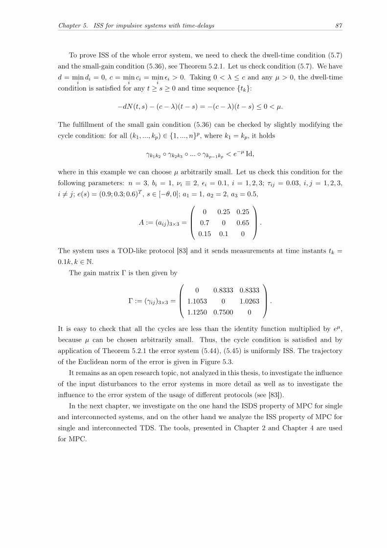
Chapter 5. ISS for impulsive systems with time-delays 87
To prove ISS of the whole error system, we need to check the dwell-time condition (5.7)and the small-gain condition (5.36), see Theorem 5.2.1. Let us check condition (5.7). We haved = min
idi = 0, c = min
ici = min
iεi > 0. Taking 0 < λ ≤ c and any μ > 0, the dwell-time
condition is satisfied for any t ≥ s ≥ 0 and time sequence {tk}:
−dN(t, s)− (c− λ)(t− s) = −(c− λ)(t− s) ≤ 0 < μ.
The fulfillment of the small gain condition (5.36) can be checked by slightly modifying thecycle condition: for all (k1, ..., kp) ∈ {1, ..., n}p, where k1 = kp, it holds
γk1k2 ◦ γk2k3 ◦ ... ◦ γkp−1kp < e−μ Id,
where in this example we can choose μ arbitrarily small. Let us check this condition for thefollowing parameters: n = 3, bi = 1, νi ≡ 2, εi = 0.1, i = 1, 2, 3; τij = 0.03, i, j = 1, 2, 3,i = j; e(s) = (0.9; 0.3; 0.6)T , s ∈ [−θ, 0]; a1 = 1, a2 = 2, a3 = 0.5,
A := (aij)3×3 =
⎛⎜⎜⎝0 0.25 0.25
0.7 0 0.65
0.15 0.1 0
⎞⎟⎟⎠ .
The system uses a TOD-like protocol [83] and it sends measurements at time instants tk =0.1k, k ∈ N.The gain matrix Γ is then given by
Γ := (γij)3×3 =
⎛⎜⎜⎝0 0.8333 0.8333
1.1053 0 1.0263
1.1250 0.7500 0
⎞⎟⎟⎠ .
It is easy to check that all the cycles are less than the identity function multiplied by eμ,because μ can be chosen arbitrarily small. Thus, the cycle condition is satisfied and byapplication of Theorem 5.2.1 the error system (5.44), (5.45) is uniformly ISS. The trajectoryof the Euclidean norm of the error is given in Figure 5.3.It remains as an open research topic, not analyzed in this thesis, to investigate the influence
of the input disturbances to the error systems in more detail as well as to investigate theinfluence to the error system of the usage of different protocols (see [83]).In the next chapter, we investigate on the one hand the ISDS property of MPC for single
and interconnected systems, and on the other hand we analyze the ISS property of MPC forsingle and interconnected TDS. The tools, presented in Chapter 2 and Chapter 4 are usedfor MPC.
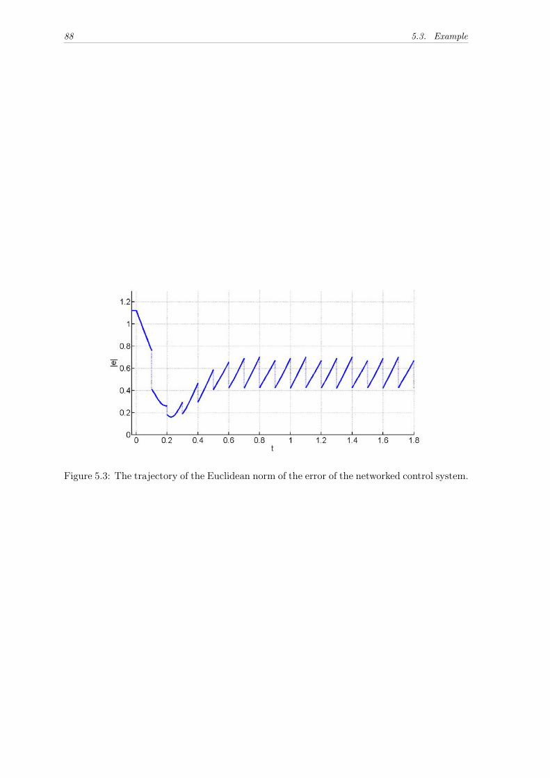
88 5.3. Example
Figure 5.3: The trajectory of the Euclidean norm of the error of the networked control system.
Chapter 6
Model predictive control
In this chapter, we introduce the ISDS property for MPC of single and interconnected systemsand we introduce the ISS property for MPC of single and interconnected TDS. We deriveconditions which assure ISDS and ISS, respectively, for such systems using an MPC schemeand using the results of Chapter 2 and Chapter 4, respectively.
The approach of MPC started in the late 1970s and spread out in the 1990s by an in-creasing usage of automation processes in the industry. It has a wide range of applications,see the survey papers [89, 90].
The aim of MPC is to control a system to follow a certain trajectory or to steer thesolution of a system into an equilibrium point under constraints and unknown disturbances.Additionally, the control should be optimal in view of defined goals, e.g., optimal regardingtime or effort. We consider systems of the form (1.1) with disturbances,
x(t) = f(x(t), w(t), u(t)), (6.1)
where w ∈ W ⊆ L∞(R+,RP ) is the unknown disturbance andW is a compact and convex set
containing the origin. The input u is a measurable and essentially bounded control subjectto input constraints u ∈ U , where U ⊆ R
m is a compact and convex set containing the originin its interior. The function f has to satisfy the same conditions as in Chapter 1 to assurethat a unique solution exists, which is denoted by x(t;x0, w, u) or x(t) in short.
Note that the majority of the works regarding MPC consider discrete-time systems. Onecan derive a discrete-time system from a continuous-time system using sampled-data systems,see [84], for example.
The principle of MPC is the following: at sampling time t = kΔ, k ∈ N, Δ > 0, thecurrent state of a system of the form (6.1) is measured, which is x(t). This is used as aninitial value to predict the trajectory of the system until the time t+ T , where T > 0 is thefinite prediction horizon, with an arbitrary control u. Let us first assume w ≡ 0. Then, thecost function defined by
J(x(t), u; t, T ) :=∫ t+T
tl(x(t′), u(t′))dt′ (6.2)
89
90
will be minimized with respect to the control u subject to constraints x ∈ X , u ∈ U , whereX ⊆ R
N is a compact and convex set containing the origin in its interior. The functionl : R
N × Rm → R+ is the stage cost and it is a penalty of the distance of the state from the
equilibrium point f(0, 0, 0) = 0 and a penalty of the control effort. A popular choice of thestage cost is l(x, u) = |x|2 + cq|u|2, for example, where cq > 0 is a weighting coefficient of thecontrol. This control strategy is referred to as open-loop MPC [79, 92, 84].A suitable approach to stabilize a system with implemented control obtained by an MPC
scheme is that the terminal predicted state of the system should satisfy a terminal constraint,namely x(t + T ) ∈ Ω, where Ω ∈ R
N is the terminal region. Then, we add the additionalterm Vf (x(t+ T )) to the cost function of the MPC scheme, where Vf : Ω→ R+.The solution of this optimization problem is a control in feedback form u∗(t) := π(t, x(t))
and u∗(t′), t′ ∈ [t, t + Δ] is applied to the system. We assume that the feedback π ∈ Π isessentially bounded, locally Lipschitz in x and measurable in t. The set Π ⊆ R
m is assumedto be compact and convex containing the origin in its interior. At the sampling time t+Δ,the state of the system will be measured and the procedure starts again moving the predictionhorizon T . Overall, an optimal control u∗(t) for t ∈ R
+ is obtained.A control law in feedback form or closed-loop control is a function π : R+×R
N → Π andit is applied to the system by u(·) = π(·, x(·)).Illustrations and more details of this procedure as well as an overview about MPC can be
found in the books [78, 9, 38] and the PhD theses [92, 84, 68], for example.We are interested in stability of MPC. It was shown in [91] that the application of the
control obtained by an MPC scheme to a system does not guarantee that a system withoutdisturbances is asymptotically stable. For stability of a system in applications it is desiredto analyze under which conditions stability of a system can be achieved using an MPCscheme. An overview about existing results regarding stability and MPC for systems withoutdisturbances can be found in [81] and recent results are included in [92, 84, 68, 38]. To designstabilizing MPC controllers for nonlinear systems, a general framework can be found in [31].On the one hand, to assure stability, there exist MPC schemes with stabilizing constraints,
see [78, 31, 9, 92, 68], for example. On the other hand conditions were derived in [37, 39, 41]to assure asymptotic stability of unconstrained nonlinear MPC schemes.Taking the unknown disturbance w ∈ W into account, MPC schemes which guarantee
ISS were developed. First results can be found in [80] regarding ISS for MPC of nonlineardiscrete-time systems. Furthermore, results using the ISS property with initial states froma compact set, namely regional-ISS, are given in [79, 92]. In [73, 69], an MPC schemewhich guarantees ISS using the so-called min-max approach was given. The approach uses aclosed-loop formulation of the optimization problem to compensate the effect of the unknowndisturbance. It takes the worst case into account, i.e., it minimizes the cost function withrespect to the control law π and maximizes the cost function with respect to the disturbancew:
minπmax
wJ(x(t), π, w; t, T ) := min
πmax
w
∫ t+T
t(l(x(t′), π(t′, x(t′)), w(t′)))dt′.
Chapter 6. Model predictive control 91
The usage of this approach is motivated by the circumstance that the solution of the open-loop MPC strategy can be extremely conservative and it can provide a small robust outputadmissible set (see [93], Definition 11, for example).Stable MPC schemes for interconnected systems were investigated in [93, 92, 41], where in
[93, 92] conditions to assure ISS of the whole system were derived and in [41] asymptoticallystable MPC schemes without terminal constraints were provided. Note that in [41], thesubsystems are not directly connected, but they exchange information over the network tocontrol themselves according to state constraints.However, for networks there exist several approaches for MPC schemes due to the in-
terconnected structure of the system. This means that large-scale systems can be difficultto control with a centralized control structure, due to computational complexity or due tocommunication bandwidth limitations, for example, see [101]. A review of architectures fordistributed and hierarchical MPC can be found in [101].Considering TDS and MPC, recent results for asymptotically stable MPC schemes of
single systems can be found in [29, 96, 95]. In these works, continuous-time TDS wereinvestigated and conditions were derived, which guarantee asymptotic stability of a TDSusing a Lyapunov-Krasovskii approach. Moreover, with the help of Lyapunov-Razumikhinarguments it was shown, how to determine the terminal cost and terminal region, and tocompute a locally stabilizing controller.For the implementation of MPC schemes in applications, numerical algorithms were de-
veloped, see [84, 68, 38] for example.This chapter provides two new directions in MPC: at first, we combine the ISDS property
with MPC for single and interconnected systems. Then, ISS of MPC for TDS is investigated.Conditions are derived such that single systems and whole networks with an optimal controlobtained by an MPC scheme have the ISDS or ISS property, respectively. The result ofChapter 2, the ISDS small-gain theorem for networks, Theorem 2.2.2, is applied as well asthe result of Chapter 4, namely Theorem 4.2.4.The ISS property for MPC schemes of TDS has not been investigated so far as well as
MPC for interconnected TDS. The approach of ISS for TDS provides the calculation of anoptimal control for TDS with unknown disturbances, which was not done before. We use themin-max closed-loop MPC strategy and Lyapunov-Krasovskii arguments.The advantage of the usage of ISDS over ISS for MPC is that the ISDS estimation takes
only recent values of the disturbance into account due to the memory fading effect, seeChapter 2. In particular, if the disturbance tends to zero, then the ISDS estimation tends tozero. Moreover, the decay rate can be derived using ISDS-Lyapunov functions.This information can be useful for applications of MPC. For example, consider two air-
planes which are flying to each other. To avoid a collision at a certain time T we use MPC tocalculate optimal controls for both planes under constraints and unknown disturbances. Thedisturbances are turbulences caused by winds, which influence the altitude of both planes.The constraint is that the altitude of the planes at time T are not equal taking the dis-turbances into account. Therefore, the ISDS or ISS estimation are used for checking the
92 6.1. ISDS and MPC
constraint. Assume that at the time t, where t is a time before the time T , the disturbances,i.e., the winds, are large. Closer to T we assume that the disturbances tend to zero. Inpractice, the information about this circumstance can be obtained from the weather forecast.Then, the following observations can be made:
The ISS estimation takes the supremum of the disturbances into account and for largedisturbances the estimation is also large. Hence, the control taking into account the collisionconstraint using the ISS estimation, is conservative and more effort for the control is usedthan it is needed. In contrast to this, the control calculated by an MPC scheme under thecollision constraint using the ISDS estimation does not need so much effort as the controlusing the ISS estimation, because we assume that the disturbances tend to zero. By thecontrol with less effort, jet fuel could be saved, for example.
This chapter is organized as follows: Section 6.1 introduces the ISDS property for MPCof nonlinear systems. A result with respect to ISDS for MPC of single systems is providedin Subsection 6.1.1 and a result for interconnected systems is included in Subsection 6.1.2.In Section 6.2, time-delay systems and ISS for MPC are considered, where Subsection 6.2.1investigates the ISS property for MPC of single systems and Subsection 6.2.2 analyzes ISSfor MPC of networks.
6.1 ISDS and MPC
In this section, we combine ISDS and MPC for nonlinear single and interconnected systems.Conditions are derived, which assure ISDS of a system obtained by application of the controlto the system (6.1), calculated by an MPC scheme.
6.1.1 Single systems
We consider systems of the form (6.1) and we use the min-max approach to calculate anoptimal control: to compensate the effect of the disturbance w, we apply a feedback controllaw π(t, x(t)) to the system. An optimal control law is obtained by solving the finite horizonoptimal control problem (FHOCP), which consists of minimization of the cost function J withrespect to π(t, x(t)) and maximization of the cost function J with respect to the disturbancew:
Definition 6.1.1 (Finite horizon optimal control problem (FHOCP)). Let 1 > ε > 0 begiven. Let T > 0 be the prediction horizon and u(t) = π(t, x(t)) be a feedback control law.The finite horizon optimal control problem for a system of the form (6.1) is formulated as
minπmax
wJ(x0, π, w; t, T )
:= minπmax
w(1− ε)
∫ t+T
t(l(x(t′), π(t′, x(t′)))− lw(w(t′)))dt′ + Vf (x(t+ T ))
Chapter 6. Model predictive control 93
subject to
x(t′) = f(x(t′), w(t′), u(t′)), x(t) = x0, t′ ∈ [t, t+ T ],
x ∈ X ,w ∈ W,
π ∈ Π,x(t+ T ) ∈ Ω ⊆ R
N ,
where x0 ∈ RN is the initial value of the system at time t, the terminal region Ω is a compact
and convex set with the origin in its interior and π(t, x(t)) is essentially bounded, locallyLipschitz in x and measurable in t. l− lw is the stage cost, where l : R
N ×Rm → R+ penalizes
the distance of the state from the equilibrium point 0 of the system and it penalizes the controleffort. lw : R
P → R+ penalizes the disturbance, which influences the systems behavior. l
and lw are locally Lipschitz continuous with l(0, 0) = 0, lw(0) = 0, and Vf : Ω → R+ is theterminal penalty.
The FHOCP will be solved at the sampling instants t = kΔ, k ∈ N, Δ ∈ R+. Theoptimal solution is denoted by π∗(t′, x(t′); t, T ) and w∗(t′), t′ ∈ [t, t + T ]. The optimal costfunction is denoted by J∗(x0, π
∗, w∗; t, T ). The control input to the system (6.1) is definedin the usual receding horizon fashion as
u(t′) = π∗(t′, x(t′); t, T ), t′ ∈ [t, t+Δ].
In the following, we need some definitions:
Definition 6.1.2. • A feedback control π is called a feasible solution of the FHOCP attime t, if for a given initial value x0 at time t the feedback π(t′, x(t′)), t′ ∈ [t, t + T ]
controls the state of the system (6.1) into Ω at time t + T , i.e., x(t + T ) ∈ Ω, for allw ∈ W.
• A set Ω ⊆ RN is called positively invariant, if for all x0 ∈ Ω a feedback control π keeps
the trajectory of the system (6.1) in Ω, i.e.,
x(t;x0, w, π) ∈ Ω, ∀t ∈ (0,∞),
for all w ∈ W.
To prove that the system (6.1) with the control obtained by solving the FHOCP has theISDS property, we need the following:
Assumption 6.1.3. 1. There exist functions αl, αw ∈ K∞, where αl is locally Lipschitzcontinuous such that
l(x, π) ≥ αl(|x|), x ∈ X , π ∈ Π,lw(w) ≤ αw(|w|), w ∈ W.
94 6.1. ISDS and MPC
2. The FHOCP in Definition 6.1.1 admits a feasible solution at the initial time t = 0.
3. There exists a controller u(t) = π(t, x(t)) such that the system (6.1) has the ISDSproperty.
4. For each 1 > ε > 0 there exists a locally Lipschitz continuous function Vf (x) such thatthe terminal region Ω is a positively invariant set and we have
Vf (x) ≤ η(|x|), ∀x ∈ Ω, (6.3)
Vf (x) ≤ −(1− ε)l(x, π) + (1− ε)lw(w), f.a.a. x ∈ Ω, (6.4)
where η ∈ K∞, w ∈ W and Vf denotes the derivative of Vf along the solution of system(6.1) with the control u ≡ π from point 3. of this assumption.
5. For each sufficiently small ε > 0 it holds
(1− ε)∫ t+T
tl(x(t′), π(t′, x(t′)))dt′ ≥ |x(t)|
1+ε . (6.5)
6. The optimal cost function J∗(x0, π∗, w∗; t, T ) is locally Lipschitz continuous.
Remark 6.1.4. In [92], it is discussed that a different stage cost, for example by the definitionof ls := l− lw, can be used for the FHOCP. In view of stability, the stage cost ls has to fulfillsome additional assumptions, see [92], Chapter 3.4.
Remark 6.1.5. The assumption (6.5) is needed to assure that the cost function satisfies thelower estimation in (2.2). However, we did not investigated whether this condition is restric-tive or not. In case of discrete-time systems and the according cost function, the assumption(6.5) is not necessary, see the proofs in [80, 79, 92, 73, 69].
The following theorem establishes ISDS of the system (6.1), using the optimal controlinput u ≡ π∗ obtained from solving the FHOCP.
Theorem 6.1.6. Consider a system of the form (6.1). Under Assumption 6.1.3, the systemresulting from the application of the predictive control strategy to the system, namely x(t) =f(x(t), w(t), π∗(t, x(t))), t ∈ R+, x(0) = x0, possesses the ISDS property.
Remark 6.1.7. Note that the gains and the decay rate of the definition of the ISDS property,Definition 2.1.2, can be calculated using Assumption 6.1.3, as it is partially displayed in thefollowing proof.
Proof. We show that the optimal cost function J∗(x0, π∗, w∗; t, T ) =: V (x0) is an ISDS-
Lyapunov function, following the steps:
• the control problem admits a feasible solution π for all times t > 0,
• J∗(x0, π∗, w∗; t, T ) satisfies the conditions (2.2) and (2.3).
Chapter 6. Model predictive control 95
Then, by application of Theorem 2.1.6, the ISDS property follows.Let us proof feasibility: we suppose that a feasible solution π(t′, x(t′)), t′ ∈ [t, t + T ] at
time t exists. For Δ > 0, we construct a control by
π(t′, x(t′)) =
{π(t′, x(t′)), t′ ∈ [t+Δ, t+ T ],
π(t′, x(t′)), t′ ∈ (t+ T, t+ T +Δ],(6.6)
where π is the controller from Assumption 6.1.3, point 3. Since π controls x(t + Δ) intox(t + T ) ∈ Ω and Ω is a positively invariant set, π(t′, x(t′)) keeps the systems trajectory inΩ for t + T < t′ ≤ t + T + Δ under the constraints of the FHOCP. This means that fromthe existence of a feasible solution for the time t, we have a feasible solution for the timet + Δ. Since, we assume that a feasible solution for the FHOCP at the time t = 0 exists(Assumption 6.1.3, point 2.), it follows that a feasible solution exists for every t > 0.We replace π in (6.6) by π∗. Then, it follows from (6.4) that it holds
J∗(x0, π∗, w∗; t, T +Δ)
≤ J(x0, π, w∗; t, T +Δ)
= (1− ε)∫ t+T
t(l(x(t′), π∗(t′, x(t′); t, T ))− lw(w∗(t′)))dt′
+ (1− ε)∫ t+T+Δ
t+T(l(x(t′), π(t′, x(t′)))− lw(w∗(t′)))dt′
+ Vf (x(t+ T +Δ))
= J∗(x0, π∗, w∗; t, T )− Vf (x(t+ T )) + Vf (x(t+ T +Δ))
+ (1− ε)∫ t+T+Δ
t+T(l(x(t′), π(t′, x(t′)))− lw(w∗(t′)))dt′
≤ J∗(x0, π∗, w∗; t, T ).
From this and with (6.3) it holds
J∗(x0, π∗, w∗; t, T ) ≤ J∗(x0, π
∗, w∗; t, 0) = Vf (x0) ≤ η(|x0|).
Now, with Assumption 6.1.3, point 5., we have
V (x0) ≥ J(x0, π∗, 0; t, T ) ≥ (1− ε)
∫ t+T
tl(x(t′), π∗(t′, x(t′)))dt′ ≥ |x0|
1+ε .
This shows that J∗ satisfies (2.2). Now, denote x0 := x(t+ h). From J∗(x0, π∗, w∗; t, T +
Δ) ≤ J∗(x0, π∗, w∗; t, T ) we get
(1− ε)∫ t+h
t(l(x(t′), π∗(t′, x(t′); t, T ))− lw(w∗(t′)))dt′ + J∗(x0, π
∗, w∗; t+ h, T +Δ− h)
≤ (1− ε)∫ t+h
t(l(x(t′), π∗(t′, x(t′); t, T ))− lw(w∗(t′)))dt′ + J∗(x0, π
∗, w∗; t+ h, T − h),
and therefore
J∗(x0, π∗, w∗; t+ h, T +Δ− h) ≤ J∗(x0, π
∗, w∗; t+ h, T − h). (6.7)
96 6.1. ISDS and MPC
Now, we show that J∗ satisfies the condition (2.3). Note that by Assumption 6.1.3, point6., J∗ is locally Lipschitz continuous. With (6.7) it holds
J∗(x0, π∗, w∗; t, T )
= (1− ε)∫ t+h
t(l(x(t′), π∗(t′, x(t′); t, T ))− lw(w∗(t′)))dt′ + J∗(x0, π
∗, w∗; t+ h, T − h)
≥ (1− ε)∫ t+h
t(l(x(t′), π∗(t′, x(t′); t, T ))− lw(w∗(t′)))dt′ + J∗(x0, π
∗, w∗; t+ h, T ).
This leads to
J∗(x0, π∗, w∗; t+ h, T )− J∗(x0, π
∗, w∗; t, T )h
≤ − 1h(1− ε)
∫ t+h
t(l(x(t′), π∗(t′, x(t′); t, T ))− lw(w∗(t′)))dt′.
For h→ 0 and using the first point of Assumption 6.1.3 we obtain
V (x0) ≤ −(1− ε)αl(|x0|) + (1− ε)αw(|w∗|), f.a.a. x0 ∈ X , ∀w ∈ W.
By definition of γ(r) := η(α−1l (2αw(r))) and g(r) := 1
2αl(η−1(r)), r ≥ 0 this implies
V (x0) > γ(|w∗|) ⇒ V (x0) ≤ −(1− ε)g(V (x0)),
where the function g is locally Lipschitz continuous. We conclude that J∗ is an ISDS-Lyapunov function for the system
x(t) = f(x(t), w(t), π∗(t, x(t)))
and by application of Theorem 2.1.6 the system has the ISDS property.
In the next subsection, we transform the analysis of ISDS for MPC of single systems tointerconnected systems.
6.1.2 Interconnected systems
We consider interconnected systems with disturbances of the form
xi(t) = fi(x1(t), . . . , xn(t), wi(t), ui(t)), i = 1, . . . , n, (6.8)
where ui ∈ RMi , measurable and essentially bounded, are the control inputs and wi ∈ R
Pi
are the unknown disturbances. We assume that the states, disturbances and inputs fulfill theconstraints
xi ∈ Xi, wi ∈ Wi, ui ∈ Ui, i = 1, . . . , n,
where Xi ⊆ RNi , Wi ⊆ L∞(R+,R
Pi) and Ui ⊆ RMi are compact and convex sets containing
the origin in their interior.Now, we are going to determine an MPC scheme for interconnected systems. An overview
of existing distributed and hierarchical MPC schemes can be found in [101]. The used scheme
Chapter 6. Model predictive control 97
in this thesis is inspired by the min-max approach for single systems as in Definition 6.1.1,see [73, 69].At first, we determine the cost function of the ith subsystem by
Ji(x0i , (xj)j �=i, πi, wi; t, T )
:= (1− εi)∫ t+T
t(li(xi(t′), πi(t′, x(t′)))− (lw)i(wi(t′))−
∑j �=i
lij(xj(t′)))dt′ + (Vf )i(xi(t+ T )),
where 1 > εi > 0, x0i ∈ Xi is the initial value of the ith subsystem at time t and πi ∈ Πi is a
feedback, essentially bounded, locally Lipschitz in x and measurable in t, where Πi ⊆ RMi is a
compact and convex set containing the origin in its interior. li−(lw)i−∑lij is the stage cost,
where li : RNi × R
Mi → R+. (lw)i : RPi → R+ penalizes the disturbance and lij : R
Nj → R+
penalizes the internal input for all j = 1, . . . , n, j = i. li, (lw)i and lij are locally Lipschitzcontinuous functions with li(0, 0) = 0, (lw)i(0) = 0, lij(0) = 0, and (Vf )i : Ωi → R+ is theterminal penalty of the ith subsystem, Ωi ⊆ R
Ni .In contrast to single systems we add the terms lij(xj), j = i to the cost function due to
the interconnected structure of the subsystems. Here, two problems arise: the formulationof an optimal control problem for each subsystem and the calculation/determination of theinternal inputs xj , j = i.We conserve the minimization of Ji with respect to πi and the maximization of Ji with
respect to wi as in Definition 6.1.1 for single systems. In the spirit of ISS/ISDS, whichtreat the internal inputs as “disturbances”, we maximize the cost function with respect toxj , j = i (worst-case approach). Since we assume that xj ∈ Xj , we get an optimal solutionπ∗i , w
∗i , x
∗j , j = i of the control problem.
The drawbacks of this approach are that, on the one hand, we do not use the systemsequations (6.8) to predict xj , j = i and, on the other hand, the computation of the optimalsolution could be numerically inefficient, especially if the number of subsystems n is “huge”or/and the sets Xi are “large”. Moreover, taking into account the worst-case approach, themaximization over xj , the obtained optimal control π∗i for each subsystem could be extremelyconservative, which leads to extremely conservative ISS or ISDS estimations.To avoid these drawbacks of the maximization of Ji with respect to xj , j = i, one could
use the systems equations (6.8) to predict xj , j = i instead.A numerically efficient way to calculate the optimal solutions π∗i , w
∗i of the subsystems is
a parallel calculation. Due to interconnected structure of the system the information aboutsystems states of the subsystems should be exchanged. But this exchange of informationcauses that an optimal solution π∗i , w
∗i could not be calculated. To the best of our knowledge,
no theorem is proved that provides the existence of an optimal solution of the optimal controlproblem using such a parallel strategy. We conclude that a parallel calculation can not helpin our case.Another approach of an MPC scheme for networks is inspired by the hierarchical MPC
scheme in [97]. One could use the predictions of the internal inputs xj , j = i as follows: atsampling time t = kΔ, k ∈ N, Δ > 0 all subsystems calculate the optimal solution iteratively.
98 6.1. ISDS and MPC
This means that for the calculation the optimal solution for the ith subsystem, the currently“optimized” trajectories of the subsystems 1, . . . , i− 1 will be used, denoted by xopt,kΔ
p , p =
1, . . . , i− 1, and the “optimal” trajectories of the subsystems i+ 1, . . . , n of the optimizationat sampling time t = (k − 1)Δ will be used, denoted by xopt,(k−1)Δ
p , p = i+ 1, . . . , n.The advantage of this approach would be that the optimal solution is not that much
conservative as the min-max approach and the calculation of the optimal solution could beperformed in a numerically efficient way, due to the usage of the model to predict the “optimal”trajectories and that the maximization over xj , j = i will be avoided. The drawback is thatthe optimal cost function of each subsystem depends on the trajectories xopt,·
j , j = i usingthis hierarchical approach. Then, to the best of our knowledge, it is not possible to show thatthe optimal cost functions are ISDS-Lyapunov functions of the subsystems, which is a crucialstep for proving ISDS of a subsystem or the whole network, because no helpful estimationsfor the Lyapunov function properties can be performed due to the dependence of the optimalcost functions of the trajectories xopt,·
j , j = i.The FHOCP for the ith subsystem reads as follows:
minπi
maxwi
max(xj)j �=i
Ji(x0i , (xj)j �=i, πi, wi; t, T )
subject to
xi(t′) = fi(x1(t′), . . . , xn(t′), wi(t′), ui(t′)), t′ ∈ [t, t+ T ],
xi(t) = x0i ,
xj ∈ Xj , j = 1, . . . , n,
wi ∈ Wi,
πi ∈ Πi,
xi(t+ T ) ∈ Ωi ⊆ RNi ,
where the terminal region Ωi is a compact and convex set with the origin in its interior.The resulting optimal control of each subsystem is a feedback control law, i.e., u∗i (t) =
π∗i (t, x(t)), where x = (xT1 , . . . , x
Tn )
T ∈ RN , N =
∑iNi and π∗i (t, x
∗i(t)) is essentiallybounded, locally Lipschitz in x and measurable in t, for all i = 1, . . . , n.To show that each subsystem and the whole system have the ISDS property using the
mentioned distributed MPC scheme, we suppose for the ith subsystem of (6.8):
Assumption 6.1.8. 1. There exist functions αli, α
wi , αij ∈ K∞, j = 1, . . . , n, j = i such
that
li(xi, πi) ≥ αli(|xi|), xi ∈ Xi, πi ∈ Πi,
(lw)i(wi) ≤ αwi (|wi|), wi ∈ Wi,
lij(xj) ≤ αij(Vj(xj)), xj ∈ Xj , j = 1, . . . , n, j = i.
2. The FHOCP admits a feasible solution at the initial time t = 0.
Chapter 6. Model predictive control 99
3. There exists a controller ui(t) = πi(t, x(t)) such that the ith subsystem of (6.8) has theISDS property.
4. For each 1 > εi > 0 there exists a locally Lipschitz continuous function (Vf )i(xi) suchthat the terminal region Ωi is a positively invariant set and we have
(Vf )i(xi) ≤ ηi(|xi|), ∀xi ∈ Ωi,
(Vf )i(xi) ≤ −(1− εi)li(xi, πi) + (1− εi)(lw)i(wi) + (1− εi)∑
j �=i lij(xj),
for almost all xi ∈ Ωi, where ηi ∈ K∞, wi ∈ Wi and (Vf )i denotes the derivative of(Vf )i along the solution of the ith subsystem of (6.8) with the control ui ≡ πi from point3. of this assumption.
5. For each sufficiently small εi > 0 it holds
(1− εi)∫ t+T
tli(xi(t′), π∗i (t
′, x(t′)))−∑j �=i
lij(xj(t′))dt′ ≥ |x(t)|1+εi
(6.9)
6. The optimal cost function J∗i (x0i , (xj)∗j �=i, π
∗i , w
∗i ; t, T ) is locally Lipschitz continuous.
Now, we can state that each subsystem possesses the ISDS property using the mentionedMPC scheme.
Theorem 6.1.9. Consider an interconnected system of the form (6.8). Let Assumption 6.1.8be satisfied for each subsystem. Then, each subsystem resulting from the application of thecontrol obtained by the FHOCP for each subsystem to the system, namely
xi(t) = fi(x1(t), . . . , xn(t), wi(t), π∗i (t, x(t))), t ∈ R+, x0i = xi(0),
possesses the ISDS property.
Proof. Consider the ith subsystem. We show that the optimal cost function Vi(x0i ) :=
J∗i (x0i , (xj)∗j �=i, π
∗i , w
∗i ; t, T ) is an ISDS-Lyapunov function for the ith subsystem. We ab-
breviate xj = (xj)∗j �=i.By following the steps of the proof of Theorem 6.1.6, we conclude that there exists a
feasible solution for all times t > 0 and that by (6.9) the functional Vi(x0i ) satisfies the
condition
|x0i |
(1+εi)≤ Vi(x0
i ) ≤ ηi(|x0i |),
using |x0| ≥ |x0i |. Note that by Assumption 6.1.8, point 6., J∗i is locally Lipschitz continuous.
We have that it holds
Vi(x0i ) ≤ −(1− εi)αl
i(η−1i (Vi(x0
i ))) + (1− εi)αwi (|w∗i |) + (1− εi)
∑j �=i
αij(Vj((x0j )))
and equivalently
Vi(x0i ) ≤ −(1− εi)αl
i(η−1i (Vi(x0
i ))) + (1− εi)max{nαwi (|w∗i |),max
j �=inαij(Vj((x0
j )))},
100 6.2. ISS and MPC of time-delay systems
which implies
Vi(x0i ) > max{γi(|w∗i |),max
j �=iγij(Vj((x0
i )))} ⇒ Vi(x0i ) ≤ −(1− εi)gi(Vi(x0
i )),
for almost all x0i ∈ Xi and all w∗i ∈ Wi, where γi(r) := ηi((αl
i)−1(2nαw
i (r))), γij(r) :=
ηi((αli)−1(2nαij(r))) and gi(r) := 1
2αli(η
−1i (r)), where gi is locally Lipschitz continuous.
Since, i can be chosen arbitrarily, we conclude that each subsystem has an ISDS-Lyapunovfunction. It follows that each subsystem has the ISDS property.
To investigate whether the whole system has the ISDS property, we collect all functionsγij in a matrix Γ := (γij)n×n, γii ≡ 0, which defines a map as in (1.12).Using the small-gain condition for Γ, the ISDS property for the whole system can be
guaranteed:
Corollary 6.1.10. Consider an interconnected system of the form (6.8). Let Assump-tion 6.1.8 be satisfied for each subsystem. If Γ satisfies the small-gain condition (1.15), thenthe whole system possesses the ISDS property.
Proof. Each subsystem has an ISDS-Lyapunov function with gains γij . This follows fromTheorem 6.1.9. The matrix Γ satisfies the SGC and all assumptions of Theorem 2.2.2 aresatisfied. It follows that with x = (xT
1 , . . . , xTn )
T , w = (wT1 , . . . , w
Tn )
T and π∗(·, x(·)) =((π∗1(·, x(·)))T , . . . , (π∗n(·, x(·)))T )T , the whole system of the form
x(t) = f(x(t), w(t), π∗(t, x(t)))
has the ISDS property.
In the next section, we investigate the ISS property for MPC of TDS.
6.2 ISS and MPC of time-delay systems
Now, we introduce the ISS property for MPC of TDS. We derive conditions to assure thata single system, a subsystem of a network and the whole system possess the ISS propertyapplying the control obtained by an MPC scheme for TDS.
6.2.1 Single systems
We consider systems of the form (4.1) with disturbances,
x(t) = f(xt, w(t), u(t)), t ∈ R+,
x0(τ) = ξ(τ), τ ∈ [−θ, 0] ,(6.10)
where w ∈ W ⊆ L∞(R+,RP ) is the unknown disturbance andW is a compact and convex set
containing the origin. The input u is an essentially bounded and measurable control subjectto input constraints u ∈ U , where U ⊆ R
is a compact and convex set containing the origin
Chapter 6. Model predictive control 101
in its interior. The function f has to satisfy the same conditions as in Chapter 4 to assurethat a unique solution exists, which is denoted by x(t; ξ, w, u) or x(t) in short.
The aim is to find an (optimal) control u such that the system (6.10) has the ISS property.
Due to the presence of disturbances, we apply a feedback control structure, which com-pensates the effect of the disturbance. This means that we apply a feedback control lawπ(t, xt) to the system. In the rest of this section, we assume that π(t, xt) ∈ Π is essentiallybounded, locally Lipschitz in xt and measurable in t. The set Π ⊆ R
m is assumed to becompact and convex containing the origin in its interior. We obtain an MPC control law bysolving the control problem:
Definition 6.2.1 (Finite horizon optimal control problem with time-delays (FHOCPTD)).Let T be the prediction horizon and π(t, xt) be a feedback control law. The finite horizonoptimal control problem with time-delays for a system of the form (6.10) is formulated as
minπmax
wJ(ξ, π, w; t, T ) := min
πmax
w
∫ t+T
t(l(x(t′), π(t′, xt′))− lw(w(t′)))dt′ + Vf (xt+T )
subject to
x(t′) = f(xt′ , w(t′), u(t′)), t′ ∈ [t, t+ T ],
x(t+ τ) = ξ(τ), τ ∈ [−θ, 0],xt′ ∈ X ,w ∈ W,
π ∈ Π,xt+T ∈ Ω ⊆ C([−θ, 0],RN ),
where ξ ∈ C([−θ, 0],RN ) is the initial function of the system at time t, the terminal region Ω
and the state constraint set X ⊆ C([−θ, 0],RN ) are compact and convex sets with the originin their interior. l − lw is the stage cost, where l : R
N × Rm → R+ and lw : R
P → R+ arelocally Lipschitz continuous with l(0, 0) = 0, lw(0) = 0, and Vf : Ω → R+ is the terminalpenalty.
The control problem will be solved at the sampling instants t = kΔ, k ∈ N, Δ ∈ R+.The optimal solution is denoted by π∗(t′, xt′ ; t, T ) and w∗(t′), t′ ∈ [t, t+ T ] and the optimalcost functional is denoted by J∗(ξ, π∗, w∗; t, T ). The control input to the system (6.10) isdefined in the usual receding horizon fashion as
u(t′) = π∗(t′, xt′ ; t, T ), t′ ∈ [t, t+Δ].
Definition 6.2.2. • A feedback control π is called a feasible solution of the FHOCPTDat time t, if for a given initial function ξ at time t the feedback π(t′, xt′), t′ ∈ [t, t+ T ]
controls the state of the system (6.10) into Ω at time t + T , i.e., xt+T ∈ Ω, for allw ∈ W.
102 6.2. ISS and MPC of time-delay systems
• A set Ω ⊆ C([−θ, 0],RN ) is called positively invariant, if for all initial functions ξ ∈ Ωa feedback control π keeps the trajectory of the system (6.10) in Ω, i.e.,
xt ∈ Ω, ∀t ∈ (0,∞),
for all w ∈ W.
For the goal of this section, establishing ISS of TDS with the help of MPC, we need thefollowing:
Assumption 6.2.3. 1. There exist functions αl, αw ∈ K∞ such that
l(φ(0), π) ≥ αl(|φ|a), φ ∈ X , π ∈ Π,lw(w) ≤ αw(|w|), w ∈ W.
2. The FHOCPTD in Definition 6.2.1 admits a feasible solution at the initial time t = 0.
3. There exists a controller u(t) = π(t, xt) such that the system (6.10) has the ISS property.
4. There exists a locally Lipschitz continuous functional Vf (φ) such that the terminal regionΩ is a positively invariant set and for all φ ∈ Ω we have
Vf (φ) ≤ ψ2(|φ|a), (6.11)
D+Vf (φ,w) ≤ −l(φ(0), π) + lw(w), (6.12)
where ψ2 ∈ K∞, w ∈ W and D+Vf denotes the upper right-hand side derivate of thefunctional V along the solution of (6.10) with the control u ≡ π from point 3. of thisassumption.
5. There exists a K∞ function ψ1 such that for all t > 0 it holds∫ t+T
tl(x(t′), π(t′, xt′))dt′ ≥ ψ1(|ξ(0)|), ξ(0) = x(t). (6.13)
6. The optimal cost functional J∗(ξ, π∗, w∗; t, T ) is locally Lipschitz continuous.
Now, we can state a theorem that assures ISS of MPC for a single time-delay system withdisturbances.
Theorem 6.2.4. Let Assumption 6.2.3 be satisfied. Then, the system resulting from theapplication of the predictive control strategy to the system, namely x(t) = f(xt, w(t), π∗(t, xt)),t ∈ R+, x0(τ) = ξ(τ), τ ∈ [−θ, 0] , possesses the ISS property.
Proof. The proof goes along the lines of the proof of Theorem 6.1.6 with according changesto time-delays and functionals, i.e., we show that the optimal cost functional V (ξ) :=
J∗(ξ, π∗, w∗; t, T ) is an ISS-Lyapunov-Krasovskii functional.
Chapter 6. Model predictive control 103
For a feasible solution for all times t > 0, we suppose that a feasible solution π(t′, xt′), t′ ∈[t, t+ T ] at time t exists. We construct a control by
π(t′, xt′) =
{π(t′, xt′), t′ ∈ [t+Δ, t+ T ],
π(t′, xt′), t′ ∈ (t+ T, t+ T +Δ],(6.14)
where π is the controller from Assumption 6.2.3, point 3, and Δ > 0. π steers xt+Δ intoxt+T ∈ Ω and Ω is a positively invariant set. This means that π(t′, xt′) keeps the systemtrajectory in Ω for t + T < t′ ≤ t + T + Δ under the constraints of the FHOCPTD. Thisimplies that from the existence of a feasible solution for the time t, we have a feasible solutionfor the time t +Δ. From Assumption 6.2.3, point 2., there exists a feasible solution for theFHOCPTD at the time t = 0 and it follows that a feasible solution exists for every t > 0.
Replacing π in (6.14) by π∗, it follows from (6.12) that it holds
J∗(ξ, π∗, w∗; t, T +Δ)
≤ J(ξ, π, w∗; t, T +Δ)
=∫ t+T
t(l(x(t′), π∗(t′, xt′ ; t, T ))− lw(w∗(t′)))dt′ +
∫ t+T+Δ
t+T(l(x(t′), π(t′, xt′))− lw(w∗(t′)))dt′
+ Vf (xt+T+Δ)
= J∗(ξ, π∗, w∗; t, T )− Vf (xt+T ) + Vf (xt+T+Δ) +∫ t+T+Δ
t+T(l(x(t′), π(t′, xt′))− lw(w∗(t′)))dt′
≤ J∗(ξ, π∗, w∗; t, T )
and with (6.11) this implies
J∗(ξ, π∗, w∗; t, T ) ≤ J∗(ξ, π∗, w∗; t, 0) = Vf (ξ) ≤ ψ2(|ξ|a).
For the lower bound, it holds
V (ξ) ≥ J(ξ, π∗, 0; t, T ) ≥∫ t+T
tl(x(t′), π∗(t′, xt′))dt′
and by (6.13) we have V (ξ) ≥ ψ1(|ξ(0)|). This shows that J∗ satisfies (4.10).Now, we use the notation xt(τ) := ξ(τ), τ ∈ [−θ + t, t]. With J∗(xt, π∗, w∗; t, T +Δ) ≤
J∗(xt, π∗, w∗; t, T ) we have∫ t+h
t(l(x(t′), π∗(t′, xt′ ; t, T ))− lw(w∗(t′)))dt′ + J∗(xt+h, π∗, w∗; t+ h, T +Δ− h)
≤∫ t+h
t(l(x(t′), π∗(t′, xt′ ; t, T ))− lw(w∗(t′)))dt′ + J∗(xt+h, π∗, w∗; t+ h, T − h).
This implies
J∗(xt+h, π∗, w∗; t+ h, T +Δ− h) ≤ J∗(xt+h, π∗, w∗; t+ h, T − h). (6.15)
104 6.2. ISS and MPC of time-delay systems
Note that by Assumption 6.2.3, point 6., J∗ is locally Lipschitz continuous. With (6.15)it holds
J∗(xt, π∗, w∗; t, T )
=∫ t+h
t(l(x(t′), π∗(t′, xt′ ; t, T ))− lw(w∗(t′)))dt′ + J∗(xt+h, π∗, w∗; t+ h, T − h)
≥∫ t+h
t(l(x(t′), π∗(t′, xt′ ; t, T ))− lw(w∗(t′)))dt′ + J∗(xt+h, π∗, w∗; t+ h, T ),
which leads to
J∗(xt+h, π∗, w∗; t+ h, T )− J∗(xt, π∗, w∗; t, T )h
≤ − 1h
∫ t+h
t(l(x(t′), π∗(t′, xt′ ; t, T ))− lw(w∗(t′)))dt′.
Let h→ 0+ and using the first point of Assumption 6.2.3 we get
D+V (xt, w∗) ≤ −αl(|xt|a) + αw(|w∗|).
By definition of χ(r) := ψ2(α−1l (2αw(r))) and α(r) := 1
2αl(ψ−12 (r)), r ≥ 0 this implies
V (xt) ≥ χ(|w∗|) ⇒ D+V (xt, w∗) ≤ −α(V (xt)),
i.e., J∗ satisfies the condition (4.11).We conclude that J∗ is an ISS-Lyapunov-Krasovskii functional for the system
x(t) = f(xt, w(t), π∗(t, xt))
and by application of Theorem 4.1.7 the system has the ISS property.
Now, we consider interconnections of TDS and provide conditions such that the wholenetwork with an optimal control obtained from an MPC scheme has the ISS property.
6.2.2 Interconnected systems
We consider interconnected systems with time-delays and disturbances of the form
xi(t) = fi
(xt
1, . . . , xtn, wi(t), ui(t)
), i = 1, . . . , n, (6.16)
where ui ∈ RMi are the essentially bounded and measurable control inputs and wi ∈ R
Pi arethe unknown disturbances. We assume that the states, disturbances and inputs fulfill theconstraints
xi ∈ Xi, wi ∈ Wi, ui ∈ Ui, i = 1, . . . , n,
where Xi ⊆ C([−θ, 0],RNi), Wi ⊆ L∞(R+,RPi) and Ui ⊆ R
Mi are compact and convex setscontaining the origin in their interior.
Chapter 6. Model predictive control 105
We assume the same MPC strategy for interconnected TDS as in Subsection 6.1.2. TheFHOCPTD for the ith subsystem of (6.16) reads as
minπi
maxwi
max(xj)j �=i
Ji(ξi, (xj)j �=i, πi, wi; t, T )
:= minπi
maxwi
max(xj)j �=i
∫ t+T
t(li(xi(t′), πi(t′, xt′
i ))− (lw)i(wi(t′))−∑j �=i
lij(xj(t′)))dt′ + (Vf )i(xt+Ti )
subject to
xi(t′) = fi(xt′1 , . . . , x
t′n , wi(t′), ui(t′)), t′ ∈ [t, t+ T ],
xi(t+ τ) = ξi(τ), τ ∈ [−θ, 0],xj ∈ Xj , j = 1, . . . , n,
wi ∈ Wi,
πi ∈ Πi,
xt+Ti ∈ Ωi ⊆ C([−θ, 0],RNi),
where ξi ∈ Xi is the initial function of the ith subsystem at time t, the terminal region Ω is acompact and convex set with the origin in its interior. πi(t, xt) is essentially bounded, locallyLipschitz in x and measurable in t and Πi ⊆ R
Mi is a compact and convex sets containingthe origin in its interior. li − (lw)i −
∑lij is the stage cost, where li : R
Ni × RMi → R+.
(lw)i : RPi → R+ penalizes the disturbance and lij : R
Nj → R+ penalizes the internal inputfor all j = 1, . . . , n, j = i. li, (lw)i and lij are locally Lipschitz continuous functions withli(0, 0) = 0, (lw)i(0) = 0, lij(0) = 0, and (Vf )i : Ωi → R+ is the terminal penalty of the ithsubsystem.
We obtain an optimal solution π∗i , (xj)∗j �=i, w∗i , where the control of each subsystem
is a feedback control law, which depends on the current states of the whole system, i.e.,ui(t) = π∗i (t, x
t), where xt = ((xt1)
T , . . . , (xtn)
T )T ∈ C([−θ, 0],RN ), N =∑
iNi.
For the ith subsystem of (6.16) we suppose:
Assumption 6.2.5. 1. There exist functions αli, α
wi , αij ∈ K∞, j = 1, . . . , n, j = i such
that
li(φi(0), πi) ≥ αli(|φi|a), φi ∈ C([−θ, 0],RNi), πi ∈ Πi,
(lw)i(wi) ≤ αwi (|wi|), wi ∈ Wi,
lij(φj(0)) ≤ αij(Vj(φj)), φj ∈ C([−θ, 0],RNj ), j = 1, . . . , n, j = i.
2. The FHOCPTD admits a feasible solution at the initial time t = 0.
3. There exists a controller ui(t) = πi(t, xt) such that the ith subsystem of (6.16) has theISS property.
106 6.2. ISS and MPC of time-delay systems
4. There exists a locally Lipschitz continuous functional (Vf )i(φi) such that the terminalregion Ωi is a positively invariant set and for all φi ∈ Ωi we have
(Vf )i(φi) ≤ ψ2i(|φi|a),D+(Vf )i(φi, wi) ≤ −li(φi(0), πi) + (lw)i(wi) +
∑j �=i lij(φj(0)),
where ψ2i ∈ K∞, φj ∈ C([−θ, 0],RNj ), j = 1, . . . , n and wi ∈ Wi. D+(Vf )i denotesthe upper right-hand side derivate of the functional (Vf )i along the solution of the ithsubsystem of (6.16) with the control ui ≡ πi from point 3. of this assumption.
5. For each i, there exists a K∞ function ψ1i such that for all t > 0 it holds∫ t+T
tli(xi(t′), πi(t′, xt′))dt′ ≥ ψ1i(|ξ(0)|), ξ(0) = x(t). (6.17)
6. The optimal cost functional J∗i (ξi, (xj)∗j �=i, π∗i , w
∗i ; t, T ) is locally Lipschitz continuous.
Now, we state that each subsystem of (6.16) has the ISS property by application of theoptimal control obtained by the FHOCPTD.
Theorem 6.2.6. Consider an interconnected system of the form (6.16). Let Assumption 6.2.5be satisfied for each subsystem. Then, each subsystem resulting from the application of thepredictive control strategy to the system, namely xi(t) = fi(xt
1, . . . , xtn, wi(t), π∗i (t, x
t)), t ∈R+, x
0i (τ) = ξi(τ), τ ∈ [−θ, 0] , possesses the ISS property.
Proof. Consider the ith subsystem. We show, that the optimal cost functional Vi(ξi) :=
J∗i (ξi, (xj)∗j �=i, π∗i , w
∗i ; t, T ) is an ISS-Lyapunov-Krasovskii functional for the ith subsystem.
We abbreviate xtj = ((xj)tj �=i)
∗.Following the lines of the proof of Theorem 6.2.4, we have that there exists a feasible
solution of the ith subsystem for all times t > 0 and that the functional Vi(ξi) satisfies thecondition
ψ1i(|ξi(0)|) ≤ Vi(ξi) ≤ ψ2i(|ξi|a),
using (6.17) and |ξ(0)| ≥ |ξi(0)|. Note that by Assumption 6.2.5, point 6., J∗i is locallyLipschitz continuous. We arrive that it holds
D+Vi(xti, w
∗i ) ≤ −αl
i(ψ−12i (Vi(xt
i))) + αwi (|w∗i |) +
∑j �=i
αij(Vj(xtj)).
This is equivalent to
D+Vi(xti, w
∗i ) ≤ −αl
i(ψ−12i (Vi(xt
i))) + max{nαwi (|w∗i |),max
j �=inαij(Vj(xt
j))},
which implies
Vi(xti) ≥ max{χi(|w∗i |),max
j �=iχij(Vj(xt
j))} ⇒ D+Vi(xti, w
∗i ) ≤ −αl
i(Vi(xti)),
Chapter 6. Model predictive control 107
where
χi(r) := ψ2i((αli)−1(2nαw
i (r))),
χij(r) := ψ2i((αli)−1(2nαij(r))),
αli(r) :=
12α
li(ψ
−12i (r)).
This can be shown for each subsystem and we conclude that each subsystem has anISS-Lyapunov-Krasovskii functional. It follows that the ith subsystem is ISS in maximumformulation.
We collect all functions χij in a matrix Γ := (χij)n×n, χii ≡ 0, which defines a map as in(1.12).Using the small-gain condition for Γ, it follows from Theorem 6.2.6:
Corollary 6.2.7. Consider an interconnected system of the form (6.16). Let Assump-tion 6.2.5 be satisfied for each subsystem. If Γ satisfies the small-gain condition (1.15), thenthe whole system possesses the ISS property.
Proof. We know from Theorem 6.2.6 that each subsystem of (6.16) has an ISS-Lyapunov-Krasovskii functional with gains χij . Since, the matrix Γ satisfies the SGC, all assumptionsof Theorem 4.2.4 are satisfied and by Remark 4.2.5 the whole system of the form
x(t) = f(xt, w(t), π∗(t, xt))
is ISS in maximum formulation, where xt = ((xt1)
T , . . . , (xtn)
T )T , w = (wT1 , . . . , w
Tn )
T andπ∗(t, xt) = ((π∗1(t, xt))T , . . . , (π∗n(t, xt))T )T .
The next chapter summarizes the thesis and open questions for future research activitiesare listed.
108 6.2. ISS and MPC of time-delay systems
Chapter 7
Summary and Outlook
We have provided several tools for different kinds of systems to analyze them in view ofstability, to design observers and to control them. This thesis has extended the analysistoolbox of nonlinear single and interconnected systems using Lyapunov methods.
The results can be used for a wide range of applications from different areas. Moreover,the theory presented here can be seen as a starting point for further investigations.
In this chapter, we summarize all main results of this thesis and propose several topicsfor future research activities as well as open questions.
7.1 ISDS
Considering networks of interconnected ISDS subsystems, we have shown that they possessthe ISDS property, if the small-gain condition (1.15) is satisfied. In this case, we have providedexplicit expressions for an ISDS-Lyapunov function and the corresponding rates and gainsof the entire interconnection, which is Theorem 2.2.2. As an application of this result, wehave investigated a system of interconnections with zero external input and we have deriveddecay rates of the subsystems and the entire system, see Corollary 2.2.3. An example withtwo systems taken from [36] compares the resulting estimates of the norm of a trajectoryobtained by [36] and by (2.15), see Example 2.3.1. Another example (Example 2.3.2) with ninterconnected ISDS systems has illustrated the application of our main result.
The ISDS property with its advantages over ISS is not deeply investigated and used inapplications and only few works exist in the research literature according to this topic untilnow. The advantages of ISDS could be used in practice for a wide range of applications toobtain (economic) benefits by the analysis of dynamical systems. For example, in productionnetworks, ISDS can help to design systems avoiding overdimensioned production lines orwarehouses.
Possible research activities regarding ISDS can be, for example: the investigation of alocal variant of ISDS (see [40]) for networks and applications to production networks, forexample. A small-gain theorem using LISDS-Lyapunov functions of the subsystems similarto Theorem 2.1.6 can be proved and the question arises, if ρ, ρu in the definition of local ISDS
109
110 7.2. Observer and quantized output feedback stabilization
(LISDS) according to LISS are equal to ρ, ρu using LISDS-Lyapunov functions.Similar to iISS (see [116, 1]), an integral variant of ISDS, namely iISDS, could be investi-
gated. Since, the set of iISS systems is larger than the set of ISS systems, this is also expectedfor iISDS systems in comparison to ISDS systems. The benefits of iISDS over ISDS or ISS forapplications and the characterization of iISDS by Lyapunov functions should be analyzed.As ISS was investigated for networks of discrete-time systems in [53, 54], this could also
be done for the ISDS property and similar theorems presented here, can be adapted for suchclass of systems. This can be used for MPC, for example. Furthermore, the ISDS propertycan be defined for time-delay systems and the influence of the presence of delays to the decayrate could be analyzed. Also, all the theory according to ISDS could be developed for TDS.This would increase the range of possible applications of ISDS.We have transfered one of the advantage of ISDS over ISS, namely the memory fading
effect, to observer design:
7.2 Observer and quantized output feedback stabilization
We have introduced the quasi-ISDS property for observers (Definition 3.1.2), which mainadvantage over the quasi-ISS property is the memory fading effect due to measurement dis-turbances. This was demonstrated in Example 3.1.3. A quasi-ISDS observer was designed(Theorem 3.1.8) using error ISDS-Lyapunov functions. Considering networks, we have shownhow to design quasi-ISS/ISDS reduced-order observers for subsystems of interconnected sys-tems in Theorem 3.2.2. They were used to design a quasi-ISS/ISDS reduced-order observerfor the overall system under a small-gain condition (Theorem 3.2.3).As an application, we have shown that quantized output feedback stabilization for a sub-
system is achievable, under the assumptions that the subsystem possesses a quasi-ISS/ISDSreduced-order observer and a state feedback controller providing ISS/ISDS with respect tomeasurement errors (Proposition 3.3.3, point 1.). If this holds for all subsystems of thelarge-scale system and the small-gain condition is satisfied, then quantized output feedbackstabilization is also achievable for the overall system (Proposition 3.3.3, point 2.). The ob-tained bounds can be improved by using dynamic quantizers. We have shown that asymptoticconvergence can be achieved for each subsystem and for the overall system provided that asmall-gain condition is satisfied.In future, it would be interesting to study the design of nonlinear output feedback control
or nonlinear observers to satisfy the small-gain condition. The application of the resultsin this thesis to the design of dynamic quantized interconnected control systems could beinvestigated. Also, the design of the observers introduced in this thesis for systems withtime-delays is of interest for future research activities as far as time-delays occur in manyreal-world applications.Moreover, it could be investigated, if the decay rate and the gains of the quasi-ISDS
property can be directly obtained by the usage of a different error ISDS-Lyapunov func-tion in opposite to the one used in Assumption 3.1.4 and adapting/improving the proof of
Chapter 7. Summary and Outlook 111
Theorem 3.1.8.
We have investigated another type of systems:
7.3 ISS for TDS
For networks of time-delay systems, we have proved two theorems: an (L)ISS-Lyapunov-Razumikhin and an ISS-Lyapunov-Krasovskii small-gain theorem. They provide a tool howto check whether a network of TDS has the (L)ISS property, using a small-gain conditionand (L)ISS-Lyapunov-Razumikhin functions or ISS-Lyapunov-Krasovskii functionals, respec-tively. Furthermore, we have shown how to construct the (L)ISS-Lyapunov-Razumikhin func-tion, the ISS-Lyapunov-Krasovskii functional and the corresponding gains of the whole sys-tem, see Theorem 4.2.1 and Theorem 4.2.4.
As an application of the results, we have considered a detailed scenario of a productionnetwork and we have analyzed it, using the presented tools in this chapter, see Section 4.3.
Further research activities could be the definition of ISDS for TDS and the investigation ofits characterization by ISDS-Lyapunov-Razumikhin functions and ISDS-Lyapunov-Krasovskiifunctionals. The influence of the decay rate of the ISDS estimation by time-delays could beanalyzed. The presented results of this work can be further extended and an ISDS small-gaintheorem for networks of TDS could be proved.
For systems without time-delays, a converse ISS-Lyapunov theorem was proved in [119,74]. This is not done yet for TDS using ISS-Lyapunov-Razumikhin functions or ISS-Lyapunov-Krasovskii functionals, respectively, and remains as an open question. Anothertopic to be analyzed is the equivalence of ISS and 0-GAS+GS, see [120] for systems withouttime-delays. Considering time-delays, this is not proved yet and new techniques should bedeveloped for the proof. For further details, see [123, 122], for example.
In practice, considering production networks it can happen that machines within a plantwill break down, for example. Using autonomous control methods, the network is stabledespite the breakdowns. Due to the idea of autonomous control, it is not necessary to mon-itor the production process such that breakdowns will not discovered or not discovered veryfast. By an increasing number of breakdowns, the performance of the network will decrease,which causes economic drawbacks. To overcome these negative outcomes, one can use a faultdetection approach (see [129, 52, 2, 6], for example) to detect breakdowns in a network usingautonomous control methods. An observer-based approach for the fault detection can be used(see [130], for example) as well as autonomous control methods. Once a fault in the networkis observed/detected, a message to the mechanics of the plant will be sent immediately suchthat the breakdown could be repaired. In practice, this would help to treat autonomouslycontrolled networks with time-delays and breakdowns or other disturbances and would helpto avoid negative economic effects.
We have used the presented tools in this chapter for the stability analysis of impulsivesystems with time-delays:
112 7.4. ISS for impulsive systems with time-delays
7.4 ISS for impulsive systems with time-delays
Considering impulsive systems with time-delays, we have introduced the Lyapunov-Krasovskiiand the Lyapunov-Razumikhin methodology for establishing ISS of single impulsive systems,see Theorem 5.1.7 and Theorem 5.1.11. Then, we have investigated networks of impulsivesubsystems with time-delays. We have proved ISS small-gain theorems, which guaranteesthat the whole network has the ISS property under a small-gain condition with linear gainsand a dwell-time condition using the Lyapunov-Razumikhin (Theorem 5.2.1) and Lyapunov-Krasovskii (Theorem 5.2.2) approach. To prove this, we have constructed the Lyapunovfunction(al)s and the corresponding gains of the whole system. These theorems provide toolsto check, whether a network of impulsive time-delay systems possesses the ISS property.
It seems that the usage of general Lyapunov functions instead of exponential Lyapunovfunctions for single systems could be possible, if the dwell-time condition is formulated in adifferent way. Then, for an interconnection one can also use general Lyapunov functions andgeneral gains instead of only linear gains. This should be investigated more detailed.
Considering interconnected impulsive systems, there is a relationship between the choiceof the gains satisfying the small-gain condition and the dwell-time condition. This is aninteresting topic for a more detailed investigation.
It could be investigated, how to develop tools for the stability analysis of interconnections,if the impulse sequences of subsystems are different. Also, a proof with nonlinear gains insteadof linear ones could be performed.
Impulsive systems using a dynamical dwell-time condition, presented in [127] for switchedsystems, could be investigated. There, the dwell-time condition is formulated using Lyapunovfunctions proving asymptotic stability. This approach can be adapted to impulsive systemsand the ISS property, where the benefits of that approach could be investigated.
Since impulsive systems are closely connected to hybrid systems, time-delays could be in-troduced to hybrid systems and such interconnections. Also, the ISDS property for impulsivesystems could be investigated. According to [45, 10], one can analyze the iISS property forinterconnected impulsive systems with and without time-delays.
The analysis of the ISDS property have motivated the investigation of ISDS for MPC ofsingle systems and networks. Moreover, the tool of a Lyapunov-Krasovskii functional havebeen used for the analysis of ISS for MPC of single systems and networks with time-delays:
7.5 MPC
We have combined the ISDS property with MPC for nonlinear continuous-time systems withdisturbances. For single systems, we have derived conditions such that by application ofthe control obtained by an MPC scheme to the system, it has the ISDS property, see Theo-rem 6.1.6. Considering interconnected systems, we have proved that each subsystem possessesthe ISDS property using the control of the proposed MPC scheme, which is Theorem 6.1.9.Using a small-gain condition, we have shown in Corollary 6.1.10 that the whole network has
Chapter 7. Summary and Outlook 113
the ISDS property. For the proof, we have used one of the results of this thesis, namelyTheorem 2.2.2.Considering single systems with time-delays, we have proved in Theorem 6.2.4 that a
TDS has the ISS property using the control obtained by an MPC scheme, where we haveused ISS-Lyapunov-Krasovskii functionals. For interconnected TDS, we have established atheorem, which guarantees that each closed subsystem obtained by application of the controlobtained by a min-max MPC scheme has the ISS property, see Theorem 6.2.6. From thisresult and using Theorem 4.2.4, we have shown that the whole network with time-delays hasthe ISS property under a small-gain condition, see Corollary 6.2.7.Note that the results presented here are first steps of the approaches of ISDS for MPC
and ISS for MPC of TDS. More detailed studies should be done in these directions, especiallyin applications of these approaches.An interesting topic for investigations is the usage of an MPC scheme for interconnected
systems, see the discussion in Subsection 6.1.2. It should be investigated if and how a differentMPC scheme which guarantees ISS or ISDS, respectively, can be formulated such that thedrawbacks of the proposed min-max approach will be eliminated.Besides the proposed closed-loop MPC scheme, conditions for open-loop MPC schemes to
ISDS or ISS of TDS, respectively, could be derived. The differences of both schemes shouldbe analyzed and applied in practice.Since we have focused on theoretical results regarding MPC, it remains to develop numer-
ical algorithms for the implementation of the proposed schemes, as in [84, 38], for example.It could be analyzed, if and how other existing algorithms could be used or how they shouldbe adapted for implementation for the results presented in this thesis.Finally, one can investigate networks, where the subsystems are not directly intercon-
nected but they are able to exchange information to control themselves in dependence of theother subsystems to fulfill possible constraints. For this case, a distributed MPC scheme asin [97, 41] should be used to calculate an optimal control for the subsystems.

114 7.5. MPC
Bibliography
[1] D. Angeli, E. D. Sontag, and Y. Wang. A characterization of integral input-to-statestability. IEEE Trans. Automat. Control, 45(6):1082–1097, 2000.
[2] L. Bai, Z. Tian, and S. Shi. Robust fault detection for a class of nonlinear time-delaysystems. J. Franklin Inst., 344(6):873–888, 2007.
[3] D. D. Bainov and P. S. Simeonov. Systems with Impulse Effect: Stability, Theory andApplications. Ellis Horwood Limited, 1989.
[4] G. Ballinger and X. Liu. Existence and uniqueness results for impulsive delay differentialequations. Dynam. Contin. Discrete Impuls. Systems, 5(1-4):579–591, 1999. Differentialequations and dynamical systems (Waterloo, ON, 1997).
[5] R. Bellman and J. M. Danskin. A survey of the mathematical theory of time lag,retarded control, and hereditary processes. R-256. The Rand Corporation, 1954.
[6] J. Bokor and Z. Szabo. Fault detection and isolation in nonlinear systems. AnnualReviews in Control, 33(2):113–123, 2009.
[7] R. W. Brockett and D. Liberzon. Quantized feedback stabilization of linear systems.IEEE Trans. Automat. Control, 45(7):1279–1289, 2000.
[8] C. Cai and A. R. Teel. Characterizations of input-to-state stability for hybrid systems.Systems & Control Letters, 58(1):47–53, 2009.
[9] E. F. Camacho and C. Bordons Alba. Model Predictive Control. Springer-Verlag, 2004.
[10] W.-H. Chen and W. X. Zheng. Input-to-state stability and integral input-to-statestability of nonlinear impulsive systems with delays. Automatica J. IFAC, 45(6):1481–1488, 2009.
[11] S. Dashkovskiy, D. Efimov, and E. D. Sontag. Input to state stability and allied systemproperties. Automation and Remote Control, 72(8):1579–1614, 2011.
[12] S. Dashkovskiy, M. Görges, M. Kosmykov, A. Mironchenko, and L. Naujok. Model-ing and stability analysis of autonomously controlled production networks. LogisticsResearch, 3(2):145–157, 2011.
[13] S. Dashkovskiy, M. Görges, and L. Naujok. Autonomous control methods in logistics -a mathematical perspective. Applied Mathematical Modelling, 36(7):2947–2960, 2012.
[14] S. Dashkovskiy, M. Görges, and L. Naujok. Stability analysis scheme for autonomouslycontrolled production networks with transportations. In Proc. of the 3rd InternationalConference on Dynamics in Logistics, LDIC 2012, Bremen, Germany, 2012. To appear.
115
116 Bibliography
[15] S. Dashkovskiy, M. Görges, and L. Naujok. Local input-to-state stability of productionnetworks. In H.-J. Kreowski, B. Scholz-Reiter, and K.-D. Thoben, editors, Dynamicsin Logistics, pages 79–89. Springer Berlin Heidelberg, 2011.
[16] S. Dashkovskiy, H. R. Karimi, M. Kosmykov, A. Mironchenko, and L. Naujok. Applica-tion of the LISS Lyapunov-Krasovskii small-gain theorem to autonomously controlledproduction networks with time-delays. In Proceedings of SysTol, Nice, France, Oct. 6-8,pages 765–770, 2010.
[17] S. Dashkovskiy, M. Kosmykov, A. Mironchenko, and L. Naujok. Stability of inter-connected impulsive systems with and without time-delays using Lyapunov methods.Nonlinear Analysis: Hybrid Systems, 6(3):899–915, 2012.
[18] S. Dashkovskiy, M. Kosmykov, and L. Naujok. ISS of interconnected impulsive systemswith and without time-delays. In Proceedings of the 8th IFAC NOLCOS, Bologna, Italy,Sep. 01-03, 2010, pages 831–836, 2010.
[19] S. Dashkovskiy, M. Kosmykov, and F. Wirth. A small gain condition for interconnec-tions of ISS systems with mixed ISS characterizations. IEEE Transactions on AutomaticControl, 55(6):1247–1258, 2011.
[20] S. Dashkovskiy and L. Naujok. ISDS small-gain theorem and construction of ISDSLyapunov functions for interconnected systems. Systems & Control Letters, 59(5):299–304, 2010.
[21] S. Dashkovskiy and L. Naujok. Lyapunov-Razumikhin and Lyapunov-Krasovskii the-orems for interconnected ISS time-delay systems. In Proceedings of the 19th MTNS2010, Budapest, Hungary, July 5-9, pages 1179–1184, 2010.
[22] S. Dashkovskiy and L. Naujok. Quasi-ISS and Quasi-ISDS Reduced-Order Observersfor interconnected Systems. In Proceedings of the 49th IEEE Conference on Decisionand Control, Dec. 15.-17., Atlanta, USA, pages 5732–5737, 2010.
[23] S. Dashkovskiy, B. S. Rüffer, and F. R. Wirth. Construction of ISS Lyapunov functionsfor networks. Technical Report 06-06, Zentrum für Technomathematik, University ofBremen, Juli 2006.
[24] S. Dashkovskiy, B. S. Rüffer, and F. R. Wirth. An ISS Lyapunov function for networksof ISS systems. In Proceedings of the 17th International Symposium on MathematicalTheory of Networks and Systems (MTNS), Kyoto, Japan, July 24-28, pages 77–82,2006.
[25] S. Dashkovskiy, B. S. Rüffer, and F. R. Wirth. An ISS small gain theorem for generalnetworks. Math. Control Signals Systems, 19(2):93–122, 2007.
[26] S. N. Dashkovskiy and L. Naujok. Input-to-state dynamical stability of interconnectedsystems. In Proceedings of the 48th IEEE Conference on Decision and Control, Shang-hai, China, Dec. 16-18, pages 1411–1416, 2009.
[27] S. N. Dashkovskiy and B. S. Rüffer. Local ISS of large-scale interconnections andestimates for stability regions. Systems & Control Letters, 59(3-4):241–247, 2010.
[28] S. N. Dashkovskiy, B. S. Rüffer, and F. R. Wirth. Small Gain Theorems for Large ScaleSystems and Construction of ISS Lyapunov Functions. SIAM Journal on Control andOptimization, 48(6):4089–4118, 2010.
Bibliography 117
[29] R. M. Esfanjani, M. Reble, U. Münz, S. K. Y. Nikravesh, and F. Allgöwer. Modelpredictive control of constrained nonlinear time-delay systems. In Proceedings of the48th IEEE Conference on Decision and Control, pages 1324–1329, 2009.
[30] H. Federer. Geometric measure theory. Die Grundlehren der mathematischen Wis-senschaften, Band 153. Springer-Verlag, 1969.
[31] F. A. C. C. Fontes. A general framework to design stabilizing nonlinear model predictivecontrollers. Systems & Control Letters, 42(2):127–143, 2001.
[32] R. A. Freeman and P. V. Kokotović. Robust nonlinear control design. Systems & Con-trol: Foundations & Applications. Birkhäuser Boston Inc., Boston, MA, 1996. State-space and Lyapunov techniques.
[33] R. Geiselhart and F. Wirth. Numerical Construction of LISS Lyapunov Functionsunder a Small Gain Condition. Mathematics of Control, Signals, and Systems (MCSS),24(1):3–32, 2012.
[34] R. Goebel, R. Sanfelice, and A. Teel. Hybrid dynamical systems. IEEE Control SystemsMagazine, pages 28–93, 2009.
[35] L. Grüne. Asymptotic behavior of dynamical and control systems under perturbation anddiscretization, volume 1783 of Lecture Notes in Mathematics. Springer-Verlag, Berlin,2002.
[36] L. Grüne. Input-to-state dynamical stability and its Lyapunov function characteriza-tion. IEEE Trans. Automat. Control, 47(9):1499–1504, 2002.
[37] L. Grüne. Analysis and design of unconstrained nonlinear MPC schemes for finite andinfinite dimensional systems. SIAM J. Control Optim., 48(2):1206–1228, 2009.
[38] L. Grüne and J. Pannek. Nonlinear Model Predictive Control. Springer-Verlag, London,2011.
[39] L. Grüne, J. Pannek, M. Seehafer, and K. Worthmann. Analysis of UnconstrainedNonlinear MPC Schemes with Time Varying Control Horizon. SIAM J. Control Optim.,48(8):4938–4962, 2010.
[40] L. Grüne and P. Saint-Pierre. An invariance kernel representation of ISDS Lyapunovfunctions. Systems & Control Letters, 55(9):736–745, 2006.
[41] L. Grüne and K. Worthmann. A distributed NMPC scheme without stabilizing terminalconstraints. In R. Johansson and A. Rantzer, editors, Distributed Decision Making andControl, pages 259–285. Springer Verlag, 2010.
[42] K. Gu, V. L. Kharitonov, and J. Chen. Stability of Time-Delay Systems. Birkhäuser,2003.
[43] W. M. Haddad, V. S. Chellaboina, and S. G. Nersesov. Impulsive and hybrid dynam-ical systems. Princeton Series in Applied Mathematics. Princeton University Press,Princeton, NJ, 2006.
[44] J. K. Hale and S. M. Verduyn Lunel. Introduction to functional-differential equations,volume 99 of Applied Mathematical Sciences. Springer-Verlag, New York, 1993.
[45] J. P. Hespanha, D. Liberzon, and A. R. Teel. Lyapunov conditions for input-to-statestability of impulsive systems. Automatica, 44(11):2735–2744, 2008.
118 Bibliography
[46] J. P. Hespanha and A. S. Morse. Stabilization of nonholonomic integrators via logic-based switching. Automatica J. IFAC, 35(3):385–393, 1999.
[47] J.P. Hespanha, P. Naghshtabrizi, and Yonggang Xu. A survey of recent results innetworked control systems. Proceedings of the IEEE, 95(1):138–162, 2007.
[48] D. Hinrichsen and A. J. Pritchard. Mathematical systems theory I, volume 48 of Textsin Applied Mathematics. Springer-Verlag, Berlin, 2005. Modelling, state space analysis,stability and robustness.
[49] H. Ito. State-dependent scaling problems and stability of interconnected iISS and ISSsystems. IEEE Trans. Automat. Control, 51(10):1626–1643, 2006.
[50] H. Ito, S. Dashkovskiy, and F. Wirth. On a small gain theorem for networks of iISS sys-tems. In Proceedings of the 48th IEEE Conference on Decision and Control, Shanghai,China, Dec. 16-18, pages 4210–4215, 2009.
[51] H. Ito, P. Pepe, and Z.-P. Jiang. Construction of Lyapunov-Krasovskii functionals forinterconnection of retarded dynamic and static systems via a small-gain condition. InProc. of CDC/CCC 2009, The Joint 48th IEEE Conference on Decision and Controland 28th Chinese Control Conference, pages 1310–1316, Shanghai, P.R. China, 2009.
[52] C. Jiang and D. H. Zhou. Fault detection and identification for uncertain linear time-delay systems. Computers & Chemical Engineering, 30(2):228–242, 2005.
[53] Z.-P. Jiang, Y. Lin, and Y. Wang. Nonlinear small-gain theorems for discrete-timefeedback systems and applications. Automatica J. IFAC, 40(12):2129–2136, 2005.
[54] Z.-P. Jiang, Y. Lin, and Y. Wang. Nonlinear Small-Gain Theorems for Discrete-TimeLarge-Scale Systems. In Proceedings of the 27th Chinese Control Conference, Kunming,Yunnan, China, July 16-18, 2008, pages 704–708, 2008.
[55] Z.-P. Jiang, I. M. Y. Mareels, and Y. Wang. A Lyapunov formulation of the nonlinearsmall-gain theorem for interconnected ISS systems. Automatica J. IFAC, 32(8):1211–1215, 1996.
[56] Z.-P. Jiang, A. R. Teel, and L. Praly. Small-gain theorem for ISS systems and applica-tions. Math. Control Signals Systems, 7(2):95–120, 1994.
[57] Z.-P. Jiang and Y. Wang. A generalization of the nonlinear small-gain theorem forlarge-scale complex systems. In Proceedings of the 7th World Congress on IntelligentControl and Automation (WCICA), pages 1188–1193, June 2008.
[58] I. Karafyllis and Z.-P. Jiang. A small-gain theorem for a wide class of feedback systemswith control applications. SIAM J. Control Optim., 46(4):1483–1517 (electronic), 2007.
[59] I. Karafyllis and Z.-P. Jiang. A vector small-gain theorem for general non-linear controlsystems. IMA Journal of Mathematical Control and Information, 28(3):309–344, 2011.
[60] I. Karafyllis and C. Kravaris. Robust output feedback stabilization and nonlinear ob-server design. Systems & Control Letters, 54(10):925–938, 2005.
[61] I. Karafyllis and C. Kravaris. From continuous-time design to sampled-data design ofobservers. IEEE Trans. Automat. Control, 54(9):2169–2174, 2009.
[62] D. Karagiannis, A. Astolfi, and R. Ortega. Two results for adaptive output feedbackstabilization of nonlinear systems. Automatica J. IFAC, 39(5):857–866, 2003.
Bibliography 119
[63] D. Karagiannis, Z. P. Jiang, R. Ortega, and A. Astolfi. Output-feedback stabilizationof a class of uncertain non-minimum-phase nonlinear systems. Automatica J. IFAC,41(9):1609–1615, 2005.
[64] H. K. Khalil. Nonlinear systems. Prentice Hall, New York, 2002.
[65] V. Kolmanovskii and A. Myshkis. Introduction to the theory and applications offunctional-differential equations, volume 463 of Mathematics and its Applications.Kluwer Academic Publishers, Dordrecht, 1999.
[66] M. Kosmykov. Hybrid dynamics in large-scale logistics networks. PhD thesis, Universityof Bremen, Germany, 2011.
[67] N. Krasovskii. Stability in Motion. Moscow, 1959. Translation, Stanford UniversityPress, 1963.
[68] M. Lazar. Predictive Control Algorithms for Nonlinear Systems. PhD thesis, TechnicalUniversity of Iasi, Romania, 2009.
[69] M. Lazar, D. M. de la Pena, W. P. M. H. Heemels, and T. Alamo. On input-to-statestability of min-max nonlinear model predictive control. Systems & Control Letters,57(1):39–48, 2008.
[70] D. Liberzon. Switching in Systems and Control. Birkhäuser, Boston, 2003.
[71] D. Liberzon. Quantization, Time Delays, and Nonlinear Stabilization. IEEE Transac-tions on Automatic Control, 51(7):1190–1195, 2006.
[72] D. Liberzon. Observer-based quantized output feedback control of nonlinear systems.In Proceedings of the 17th IFAC World Congress, Seoul, Korea, July 6-11, pages 8039–8043, 2008.
[73] D. Limon, T. Alamo, F. Salas, and E. F. Camacho. Input-to-state stability of min-max MPC controllers for nonlinear systems with bounded uncertainties. Automatica,42:797–803, 2006.
[74] Y. Lin, E. D. Sontag, and Y. Wang. A smooth converse Lyapunov theorem for robuststability. SIAM J. Control Optim., 34(1):124–160, 1996.
[75] B. Liu and D. J. Hill. Input-to-state stability for discrete time-delay systems via theRazumikhin technique. Systems & Control Letters, 58(8):567–575, 2009.
[76] J. Liu, X. Liu, and W.-C. Xie. Input-to-state stability of impulsive and switching hybridsystems with time-delay. Automatica J. IFAC, 47:899–908, 2011.
[77] T. Liu, D. J. Hill, and Z.-P. Jiang. Lyapunov formulation of ISS cyclic-small-gain incontinuous-time dynamical networks. Automatica J. IFAC, 47(9):2088–2093, 2011.
[78] J. Maciejowski. Predictive Control with Constraints. Prentice-Hall, 2001.
[79] L. Magni, D. M. Raimondo, and R. Scattolini. Regional Input-to-State Stability forNonlinear Model Predicitve Control. IEEE Trans. Automat. Control, 51(9):1548–1553,2006.
[80] D. L. Marruedo, T. Alamo, and E. F. Camacho. Input-to-state stable MPC for con-strained discrete-time nonlinear systems with bounded additive uncertainties. In Pro-ceedings of the 41st IEEE Conference on Decision and Control, Las Vegas, Nevada,USA, December, pages 4619–4624, 2002.
120 Bibliography
[81] D. Q. Mayne, J. B. Rawlings, C. V. Rao, and P. O. M. Scokaert. Constrained modelpredictive control: Stability and optimality. Automatica, 36(6):789–814, 2000.
[82] W. Michiels and S.-I. Niculescu. Stability and Stabilization of Time-Delay Systems.SIAM, 2007.
[83] D. Nesic and A.R. Teel. Input-to-state stability of networked control systems. Auto-matica, 40(12):2121–2128, 2004.
[84] J. Pannek. Receding Horizon Control: A Suboptimality-based Approach. PhD thesis,University of Bayreuth, Germany, 2009.
[85] P. Pepe. On Liapunov-Krasovskii functionals under Carathéodory conditions. Auto-matica J. IFAC, 43(4):701–706, 2007.
[86] P. Pepe. The problem of the absolute continuity for Lyapunov-Krasovskii functionals.IEEE Trans. Automat. Control, 52(5):953–957, 2007.
[87] P. Pepe and Z.-P. Jiang. A Lyapunov-Krasovskii methodology for ISS and iISS oftime-delay systems. Systems & Control Letters, 55(12):1006–1014, 2006.
[88] L. Praly. On Observers with State Independent Error Lyapunov Function. In Proceed-ings of the 5th IFAC Symposium NOLCOS’01, pages 1425–1430, July 2001.
[89] S. J. Qin and T. A. Badgwell. An Overview of Nonlinear Model Predictive ControlApplications. In F. Allgöwer and A. Zheng, editors, Nonlinear Predictive Control,pages 369–392. Birkhäuser, Berlin, 2000.
[90] S. J. Qin and T. A. Badgwell. A survey of industrial model predictive control technology.Control Engineering Practice 11, pages 733–764, 2003.
[91] T. Raff, S. Huber, Z. K. Nagy, and F. Allgöwer. Nonlinear model predicitve control of afour tank system: An experimental stability study. In Proceedings of IEEE Conferenceon Control in Applications, pages 237–242, 2006.
[92] D. M. Raimondo. Nonlinear Model Predictive Control. PhD thesis, University of Pavia,Italy, 2008.
[93] D. M. Raimondo, L. Magni, and R. Scattolini. Decentralized MPC of nonlinear sys-tems: an input-to-state stability approach. Internat. J. Robust Nonlinear Control,17(17):1651–1667, 2007.
[94] M. Reble and F. Allgöwer. General Design Parameters of Model Predictive Controlfor Nonlinear Time-Delay Systems. In Proceedings of the 49th IEEE Conference onDecision and Control, Atlanta, Georgia, USA, Dec. 15-17, pages 176–181, 2010.
[95] M. Reble, F. D. Brunner, and F. Allgöwer. Model Predictive Control for NonlinearTime-Delay Systems without Terminal Constraint. In Proceedings of the 18th IFACWorld Congress, Milano, Italy, Aug. 28 - Sep. 02, pages 9254–9259, 2011.
[96] M. Reble, R. M. Esfanjani, S. K. Y. Nikravesh, and F. Allgöwer. Model predictivecontrol of constrained non-linear time-delay systems. IMA Journal of MathematicalControl and Information, 2010.
[97] A. Richards and J. P. How. Robust distributed model predictive control. InternationalJournal of Control, 80(9):1517–1531, 2007.
Bibliography 121
[98] B. Rüffer. Monotone dynamical systems, graphs, and stability of large-scale intercon-nected systems. PhD thesis, University of Bremen, Germany, 2007.
[99] B. S. Rüffer. Monotone inequalities, dynamical systems, and paths in the positiveorthant of Euclidean n-space. Positivity, 14(2):257–283, 2010.
[100] R. G. Sanfelice. Robust Hybrid Control Systems. PhD thesis, University of California,Santa Barbara, 2007.
[101] R. Scattolini. Architectures for distributed and hierarchical Model Predictive Control- A review. Journal of Process Control, 19:723–731, 2009.
[102] B. Scholz-Reiter, S. Dashkovskiy, M. Görges, T. Jagalski, and L. Naujok. AutonomousDecision Policies for Networks of Production Systems. In D. Armbruster and K. G.Kempf, editors, Decision Policies for Production Networks, pages 79–89. Springer Ver-lag, 2012.
[103] B. Scholz-Reiter, S. Dashkovskiy, M. Görges, and L. Naujok. Stability analysis ofautonomously controlled production networks. International Journal of ProductionResearch, 49(16):4857–4877, 2011.
[104] B. Scholz-Reiter, Ch. de Beer, M. Freitag, and T. Jagalski. Bio-inspired and pheromone-based shop-floor control. International Journal of Computer Integrated Manufacturing,21(2):201–205, 2008.
[105] B. Scholz-Reiter, M. Görges, T. Jagalski, and L. Naujok. Modelling and analysis ofan autonomous control method based on bacterial chemotaxis. In Proceedings of the43rd CIRP International Conference on Manufacturing Systems (ICMS 2010), pages699–706, Neuer Wissenschaftlicher Verlag, Wien, 2010.
[106] B. Scholz-Reiter, M. Görges, and T. Philipp. Autonomously controlled productionsystems - Influence of autonomous control level on logistic performance. CIRP Annals- Manufacturing Technology, 58(1):395–398, 2009.
[107] B. Scholz-Reiter, T. Jagalski, and J. Bendul. Autonomous control of a shop floor basedon bee’s foraging behaviour. In Proceedings of the 1st International Conference onDynamics in logistics, LDIC 2007, pages 415–423. Haasis, H.-D. and Kreowski, H.-J.and Scholz-Reiter, B. (eds.), Springer, Berlin, Heidelberg, 2008.
[108] R. Sepulchre, M. Janković, and P. V. Kokotović. Constructive nonlinear control. Com-munications and Control Engineering Series. Springer-Verlag, Berlin, 1997.
[109] J. Shen, Z. Luo, and X. Liu. Impulsive Stabilization of Functional Differential Equationsvia Liapunov Functionals. Journal of Mathematical Analysis and Applications, 240(1-5):1–15, 1999.
[110] H. Shim, D. Liberzon, and J.-S. Kim. Quasi-ISS Reduced-Order Observers and Quan-tized Output Feedback. In Proceedings of the 48th IEEE Conference on Decision andControl, Shanghai, China, Dec. 16-18, pages 6680–6685, 2009.
[111] H. Shim and L. Praly. Remarks on Equivalence between Full Order and ReducedOrder Nonlinear Observers. In Proceedings of the 42nd IEEE CDC, Maui, Hawaii,USA, December, pages 5837–5840, 2003.
[112] H. Shim, J. H. Seo, and A. R. Teel. Nonlinear observer design via passivation of errordynamics. Automatica J. IFAC, 39:885–892, 2003.
122 Bibliography
[113] R. Shorten, F. Wirth, O. Mason, K. Wulff, and C. King. Stability criteria for switchedand hybrid systems. SIAM Rev., 49(4):545–592, 2007.
[114] E. D. Sontag. Smooth stabilization implies coprime factorization. IEEE Trans. Au-tomat. Control, 34(4):435–443, 1989.
[115] E. D. Sontag. Further facts about input to state stabilization. IEEE Trans. Automat.Control, 35(4):473–476, 1990.
[116] E. D. Sontag. Comments on integral variants of ISS. Systems & Control Letters, 34(1-2):93–100, 1998.
[117] E. D. Sontag. Mathematical control theory, volume 6 of Texts in Applied Mathemat-ics. Springer-Verlag, New York, second edition, 1998. Deterministic finite-dimensionalsystems.
[118] E. D. Sontag. Input to state stability: Basic concepts and results. In Nonlinear andOptimal Control Theory, pages 163–220. Springer, 2006.
[119] E. D. Sontag and Y. Wang. On characterizations of the input-to-state stability property.Systems & Control Letters, 24(5):351–359, 1995.
[120] E. D. Sontag and Y. Wang. New characterizations of input-to-state stability. IEEETrans. Automat. Control, 41(9):1283–1294, 1996.
[121] A. R. Teel. Connections between Razumikhin-type theorems and the ISS nonlinearsmall gain theorem. IEEE Trans. Automat. Control, 43(7):960–964, 1998.
[122] S. Tiwari and Y. Wang. Razumikhin-type Small-Gain Theorems for Large-Scale Sys-tems with Delay. In Proceedings of the 49th IEEE CDC, Atlanta, GA, USA, Dec. 15-17,pages 7407–7412, 2010.
[123] S. Tiwari, Y. Wang, and Z.-P. Jiang. A Nonlinear Small-Gain Theorem for Large-ScaleTime Delay Systems. In Proceedings of the 48th IEEE CDC, Shanghai, China, Dec.16-18, pages 7204–7209, 2009.
[124] A. van der Schaft and H. Schumacher. An introduction to hybrid dynamical systems,volume 251 of Lecture Notes in Control and Information Sciences. Springer-VerlagLondon Ltd., London, 2000.
[125] G. C. Walsh, H. Ye, L. G. Bushnell, J. Nilsson, and B. Bernhardsson. Stability analysisof networked control systems. Automatica, 34:57–64, 1999.
[126] H.-P. Wiendahl and S. Lutz. Production in Networks. Annals of the CIRP- Manufac-turing Technology, 51(2):1–14, 2002.
[127] Z. R. Xiang and W. M. Xiang. Stability analysis of switched systems under dynamicaldwell time control approach. Internat. J. Systems Sci., 40(4):347–355, 2009.
[128] S. Yang, B. Shi, and S. Hao. Input-to-state stability for discrete-time nonlinear impul-sive systems with delays. International Journal of Robust and Nonlinear Control, 2012.To appear.
[129] M. Zhong, S. X. Ding, J. Lam, and H. Wang. An LMI approach to design robust faultdetection filter for uncertain LTI systems. Automatica J. IFAC, 39(3):543–550, 2003.
Bibliography 123
[130] F. Zhu and F. Cen. Full-order observer-based actuator fault detection and reduced-order observer-based fault reconstruction for a class of uncertain nonlinear systems.Journal of Process Control, 20(10):1141–1149, 2010.

124 Bibliography
Index
B(x, r), 15C([t1, t2] ;RN
), 15
PC([t1, t2] ;RN
), 15
Ω-path, 21R
n+, 15
R+, 15K, 16KL, 16L, 16P, 16σ, 21xt, 15K∞, 16#I, 15
Banach space, 15
Carathéodory conditions, 17cost function, 92cycle condition, 21
dissipative Lyapunov form, 19dynamic quantizer, 52
essential supremum norm, 15Euclidean norm, 15
feasible solution, 93, 101feedback control law, 92, 101FHOCP, 92FHOCPTD, 101
Gain-matrix, 20gradient, 15
Impulsive systems, 71Impulsive systems with time-delays, 73, 79
initial value, 16input, 16interconnected system, 19ISDS small-gain theorem, 29ISS-Lyapunov-Krasovskii small-gain theorem,
65ISS-Lyapunov-Razumikhin small-gain theorem,
62
local small-gain condition, 20Locally Lipschitz continuous, 16locally Lipschitz continuous, 16Lyapunov tools
error ISDS-Lyapunov function, 39error ISS-Lyapunov function, 38exponential ISS-Lyapunov-Krasovskii func-
tional, 79exponential ISS-Lyapunov-Razumikhin func-
tion, 74ISDS-Lyapunov function, 25ISS-Lyapunov function, 18ISS-Lyapunov-Krasovskii functional, 60LISS-Lyapunov-Razumikhin function, 57
networked control systems, 85Networks of impulsive systems with time-delays,
81, 83Networks of time-delay systems, 61
optimal cost function, 93optimal cost functional, 101Ordinary differential equations, 16
partial order, 15positive definite, 16positively invariant, 93, 102
125
126 Index
prediction horizon, 92, 101Production network, 66Production network scenario, 67projection, 15
QLE, 67quantizer, 49quasi-ISDS observer, 37quasi-ISS observer, 37
small-gain condition, 21solution of a system, 17Stability
0-GAS, 18ISDS, 24ISS, 17LISS, 17
stage cost, 93, 101state of a system, 16
TDS, 55terminal penalty, 93, 101Theorem of Rademacher, 16Time-delay systems, 55
upper right-hand side derivative, 57, 59