Embed Size (px)
Citation preview
7/25/2019 StataIV Baum
http://slidepdf.com/reader/full/stataiv-baum 1/59
Instrumental Variables Estimation in Stata
Christopher F Baum1
Faculty Micro Resource CenterBoston College
March 2007
1Thanks to Austin Nichols for the use of his material on weak instruments and Mark Schaffer for helpful comments.
The standard disclaimer applies.
Christopher F Baum (Boston College) Instrumental Variables Estimation in Stata March 2007 1 / 31

7/25/2019 StataIV Baum
http://slidepdf.com/reader/full/stataiv-baum 2/59
Instrumental Variables Estimation in Stata Introduction
Instrumental variables methods are widely used in economics and
finance to deal with problems of endogeneity and measurement error.
We discuss the ivreg2 suite of programs extending official Stata’s
capabilities authored by Baum, Schaffer and Stillman. Further details
are available in Baum, An Introduction to Modern Econometrics Using
Stata (Stata Press, 2006) and Baum et al. (Stata Journal, 2007).
Instrumental variables methods can provide a workable solution to
many problems in economic research, but also bring additional
challenges of bias and precision. We consider how Generalized
Method of Moments (GMM) estimators can improve upon the
traditional two-stage least squares approach, and how the reliability ofIV methods can be assessed, particularly in the potential presence of
weak instruments .
Christopher F Baum (Boston College) Instrumental Variables Estimation in Stata March 2007 2 / 31
7/25/2019 StataIV Baum
http://slidepdf.com/reader/full/stataiv-baum 3/59
Instrumental Variables Estimation in Stata Introduction
Instrumental variables methods are widely used in economics and
finance to deal with problems of endogeneity and measurement error.
We discuss the ivreg2 suite of programs extending official Stata’s
capabilities authored by Baum, Schaffer and Stillman. Further details
are available in Baum, An Introduction to Modern Econometrics Using
Stata (Stata Press, 2006) and Baum et al. (Stata Journal, 2007).
Instrumental variables methods can provide a workable solution to
many problems in economic research, but also bring additional
challenges of bias and precision. We consider how Generalized
Method of Moments (GMM) estimators can improve upon the
traditional two-stage least squares approach, and how the reliability ofIV methods can be assessed, particularly in the potential presence of
weak instruments .
Christopher F Baum (Boston College) Instrumental Variables Estimation in Stata March 2007 2 / 31
7/25/2019 StataIV Baum
http://slidepdf.com/reader/full/stataiv-baum 4/59
Instrumental Variables Estimation in Stata Introduction
Why not always use IV?
It may be difficult to find variables that can serve as valid instruments.Most variables that have an effect on included endogenous variables
also have a direct effect on the dependent variable.
The precision of IV estimates is likely to be lower than that of OLS
estimates. In the presence of weak instruments (excluded instrumentsonly weakly correlated with included endogenous regressors) the loss
of precision will be severe. This suggests we need a method to
determine whether a particular regressor must be treated as
endogenous.
IV estimators are biased, and their finite-sample properties are often
problematic. Thus, most of the justification for the use of IV is
asymptotic. Performance in small samples may be poor.
Christopher F Baum (Boston College) Instrumental Variables Estimation in Stata March 2007 3 / 31

7/25/2019 StataIV Baum
http://slidepdf.com/reader/full/stataiv-baum 5/59
Instrumental Variables Estimation in Stata Introduction
Why not always use IV?
It may be difficult to find variables that can serve as valid instruments.Most variables that have an effect on included endogenous variables
also have a direct effect on the dependent variable.
The precision of IV estimates is likely to be lower than that of OLS
estimates. In the presence of weak instruments (excluded instrumentsonly weakly correlated with included endogenous regressors) the loss
of precision will be severe. This suggests we need a method to
determine whether a particular regressor must be treated as
endogenous.
IV estimators are biased, and their finite-sample properties are often
problematic. Thus, most of the justification for the use of IV is
asymptotic. Performance in small samples may be poor.
Christopher F Baum (Boston College) Instrumental Variables Estimation in Stata March 2007 3 / 31
I l V i bl E i i i S I d i

7/25/2019 StataIV Baum
http://slidepdf.com/reader/full/stataiv-baum 6/59
Instrumental Variables Estimation in Stata Introduction
Why not always use IV?
It may be difficult to find variables that can serve as valid instruments.Most variables that have an effect on included endogenous variables
also have a direct effect on the dependent variable.
The precision of IV estimates is likely to be lower than that of OLS
estimates. In the presence of weak instruments (excluded instrumentsonly weakly correlated with included endogenous regressors) the loss
of precision will be severe. This suggests we need a method to
determine whether a particular regressor must be treated as
endogenous.
IV estimators are biased, and their finite-sample properties are often
problematic. Thus, most of the justification for the use of IV is
asymptotic. Performance in small samples may be poor.
Christopher F Baum (Boston College) Instrumental Variables Estimation in Stata March 2007 3 / 31
I t t l V i bl E ti ti i St t I t d ti

7/25/2019 StataIV Baum
http://slidepdf.com/reader/full/stataiv-baum 7/59
Instrumental Variables Estimation in Stata Introduction
Why not always use IV?
Instruments may be weak : satisfactorily exogenous, but only weaklycorrelated with the endogenous regressors. As Bound, Jaeger, Baker
(NBER TWP 1993, JASA 1995) argue “the cure can be worse than the
disease.”
Staiger and Stock (Econometrica, 1997) formalized the definition ofweak instruments. Unfortunately many researchers conclude from
their work that if the first-stage F statistic exceeds 10, their instruments
are sufficiently strong.
Stock and Yogo (Camb.U.Press festschrift, 2005) further explore the
issue and provide useful rules of thumb for evaluating the weakness of
instruments. ivreg2 now contains Stock–Yogo tabulations based on
the Cragg–Donald statistic.
Christopher F Baum (Boston College) Instrumental Variables Estimation in Stata March 2007 4 / 31
Instrumental Variables Estimation in Stata Introduction
7/25/2019 StataIV Baum
http://slidepdf.com/reader/full/stataiv-baum 8/59
Instrumental Variables Estimation in Stata Introduction
Why not always use IV?
Instruments may be weak : satisfactorily exogenous, but only weaklycorrelated with the endogenous regressors. As Bound, Jaeger, Baker
(NBER TWP 1993, JASA 1995) argue “the cure can be worse than the
disease.”
Staiger and Stock (Econometrica, 1997) formalized the definition ofweak instruments. Unfortunately many researchers conclude from
their work that if the first-stage F statistic exceeds 10, their instruments
are sufficiently strong.
Stock and Yogo (Camb.U.Press festschrift, 2005) further explore the
issue and provide useful rules of thumb for evaluating the weakness of
instruments. ivreg2 now contains Stock–Yogo tabulations based on
the Cragg–Donald statistic.
Christopher F Baum (Boston College) Instrumental Variables Estimation in Stata March 2007 4 / 31
Instrumental Variables Estimation in Stata Introduction

7/25/2019 StataIV Baum
http://slidepdf.com/reader/full/stataiv-baum 9/59
Instrumental Variables Estimation in Stata Introduction
Why not always use IV?
Instruments may be weak : satisfactorily exogenous, but only weaklycorrelated with the endogenous regressors. As Bound, Jaeger, Baker
(NBER TWP 1993, JASA 1995) argue “the cure can be worse than the
disease.”
Staiger and Stock (Econometrica, 1997) formalized the definition ofweak instruments. Unfortunately many researchers conclude from
their work that if the first-stage F statistic exceeds 10, their instruments
are sufficiently strong.
Stock and Yogo (Camb.U.Press festschrift, 2005) further explore the
issue and provide useful rules of thumb for evaluating the weakness of
instruments. ivreg2 now contains Stock–Yogo tabulations based on
the Cragg–Donald statistic.
Christopher F Baum (Boston College) Instrumental Variables Estimation in Stata March 2007 4 / 31
Instrumental Variables Estimation in Stata Introduction
7/25/2019 StataIV Baum
http://slidepdf.com/reader/full/stataiv-baum 10/59
Instrumental Variables Estimation in Stata Introduction
IV estimation as a GMM problem
Before discussing further the motivation for various weak instrument
diagnostics, we define the setting for IV estimation as a GeneralizedMethod of Moments (GMM) optimization problem.
Christopher F Baum (Boston College) Instrumental Variables Estimation in Stata March 2007 5 / 31
Instrumental Variables Estimation in Stata The IV-GMM estimator
7/25/2019 StataIV Baum
http://slidepdf.com/reader/full/stataiv-baum 11/59
Instrumental Variables Estimation in Stata The IV GMM estimator
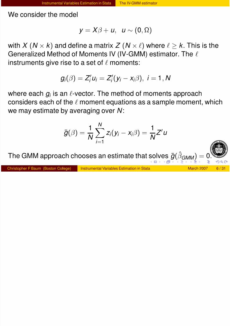
We consider the model
y = X β + u , u ∼ (0, Ω)
with X (N × k ) and define a matrix Z (N × ) where ≥ k . This is the
Generalized Method of Moments IV (IV-GMM) estimator. The
instruments give rise to a set of moments:
g i (β ) = Z
i u i = Z
i (y i − x i β ), i = 1, N
where each g i is an -vector. The method of moments approach
considers each of the moment equations as a sample moment, which
we may estimate by averaging over N :
g (β ) = 1
N
N
i =1
z i (y i − x i β ) = 1
N Z u
The GMM approach chooses an estimate that solves g (β G M M ) = 0.
Christopher F Baum (Boston College) Instrumental Variables Estimation in Stata March 2007 6 / 31
Instrumental Variables Estimation in Stata Exact identification and 2SLS

7/25/2019 StataIV Baum
http://slidepdf.com/reader/full/stataiv-baum 12/59
Instrumental Variables Estimation in Stata Exact identification and 2SLS
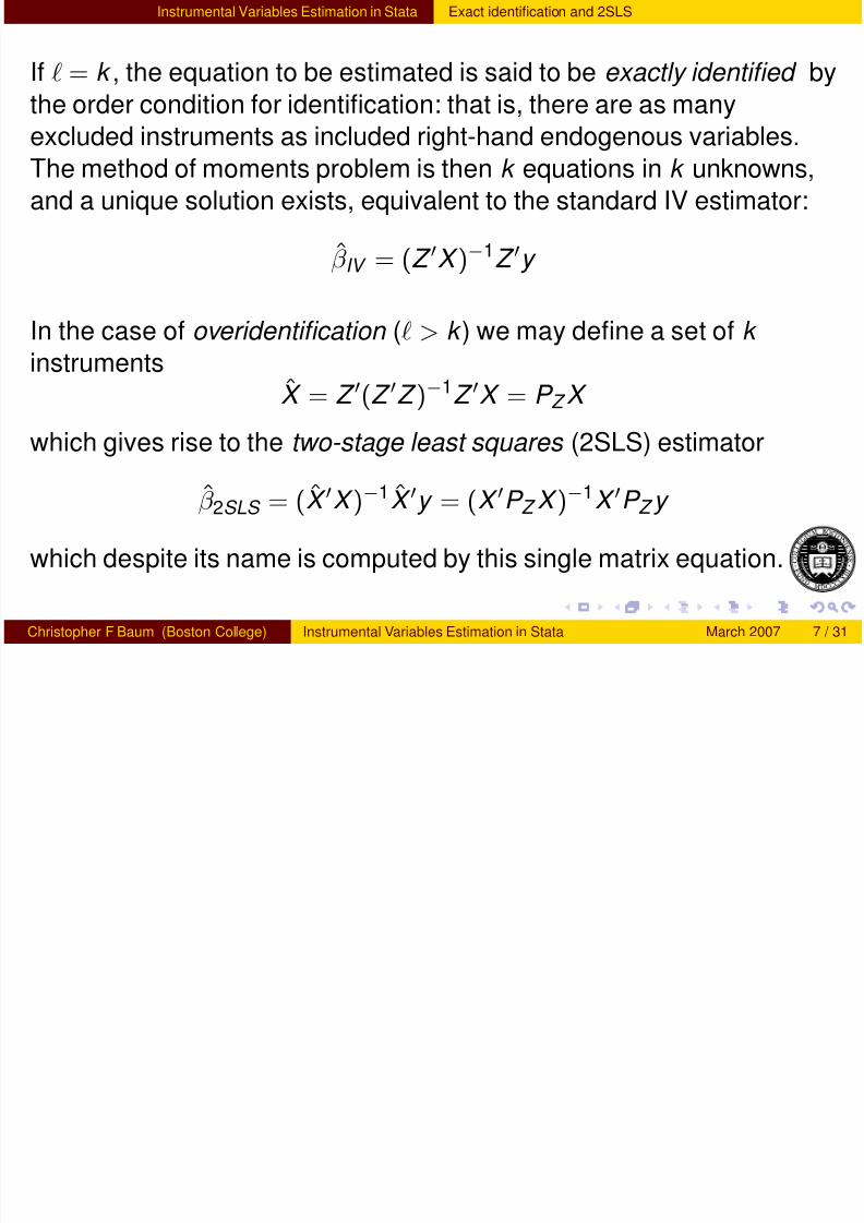
If = k , the equation to be estimated is said to be exactly identified by
the order condition for identification: that is, there are as many
excluded instruments as included right-hand endogenous variables.
The method of moments problem is then k equations in k unknowns,
and a unique solution exists, equivalent to the standard IV estimator:
β IV = (Z X )−1Z y
In the case of overidentification ( > k ) we may define a set of k
instruments
X = Z (Z Z )−1Z X = P Z X
which gives rise to the two-stage least squares (2SLS) estimator
β 2SLS = (X X )−1X y = (X P Z X )−1X P Z y
which despite its name is computed by this single matrix equation.
Christopher F Baum (Boston College) Instrumental Variables Estimation in Stata March 2007 7 / 31
Instrumental Variables Estimation in Stata Exact identification and 2SLS
7/25/2019 StataIV Baum
http://slidepdf.com/reader/full/stataiv-baum 13/59
If = k , the equation to be estimated is said to be exactly identified by
the order condition for identification: that is, there are as many
excluded instruments as included right-hand endogenous variables.
The method of moments problem is then k equations in k unknowns,
and a unique solution exists, equivalent to the standard IV estimator:
β IV = (Z X )−1Z y
In the case of overidentification ( > k ) we may define a set of k
instruments
X = Z (Z Z )−1Z X = P Z X
which gives rise to the two-stage least squares (2SLS) estimator
β 2SLS = (X X )−1X y = (X P Z X )−1X P Z y
which despite its name is computed by this single matrix equation.
Christopher F Baum (Boston College) Instrumental Variables Estimation in Stata March 2007 7 / 31
Instrumental Variables Estimation in Stata The IV-GMM approach
7/25/2019 StataIV Baum
http://slidepdf.com/reader/full/stataiv-baum 14/59
pp
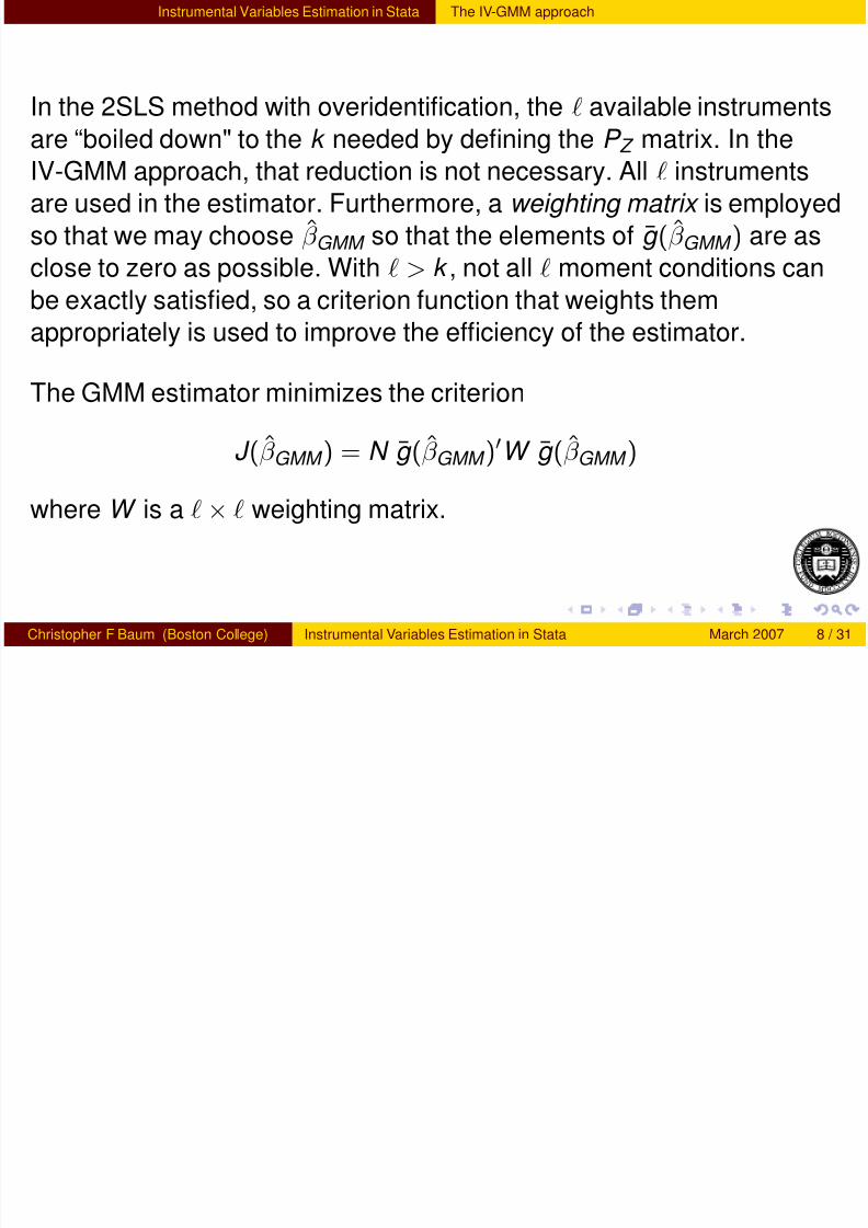
In the 2SLS method with overidentification, the available instruments
are “boiled down" to the k needed by defining the P Z
matrix. In the
IV-GMM approach, that reduction is not necessary. All instruments
are used in the estimator. Furthermore, a weighting matrix is employed
so that we may choose β GMM so that the elements of g (β GMM ) are as
close to zero as possible. With > k , not all moment conditions can
be exactly satisfied, so a criterion function that weights themappropriately is used to improve the efficiency of the estimator.
The GMM estimator minimizes the criterion
J (β GMM ) = N g (β GMM )
W g (β GMM )
where W is a × weighting matrix.
Christopher F Baum (Boston College) Instrumental Variables Estimation in Stata March 2007 8 / 31
Instrumental Variables Estimation in Stata The IV-GMM approach

7/25/2019 StataIV Baum
http://slidepdf.com/reader/full/stataiv-baum 15/59
In the 2SLS method with overidentification, the available instruments
are “boiled down" to the k needed by defining the P Z
matrix. In the
IV-GMM approach, that reduction is not necessary. All instruments
are used in the estimator. Furthermore, a weighting matrix is employed
so that we may choose β GMM so that the elements of g (β GMM ) are as
close to zero as possible. With > k , not all moment conditions can
be exactly satisfied, so a criterion function that weights themappropriately is used to improve the efficiency of the estimator.
The GMM estimator minimizes the criterion
J (β GMM ) = N g (β GMM )
W g (β GMM )
where W is a × weighting matrix.
Christopher F Baum (Boston College) Instrumental Variables Estimation in Stata March 2007 8 / 31
Instrumental Variables Estimation in Stata The GMM weighting matrix

7/25/2019 StataIV Baum
http://slidepdf.com/reader/full/stataiv-baum 16/59
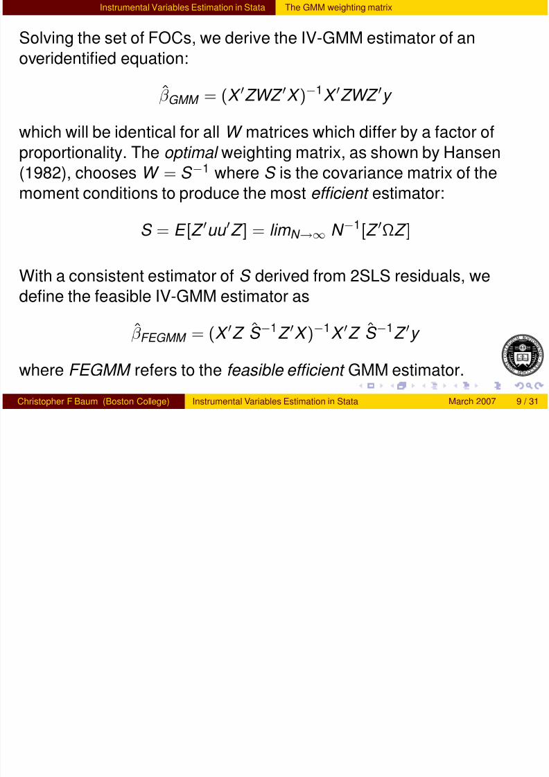
Solving the set of FOCs, we derive the IV-GMM estimator of an
overidentified equation:
β GMM = (X
ZWZ
X )−1
X
ZWZ
y
which will be identical for all W matrices which differ by a factor of
proportionality. The optimal weighting matrix, as shown by Hansen
(1982), chooses W = S −1 where S is the covariance matrix of the
moment conditions to produce the most efficient estimator:
S = E [Z uu Z ] = lim N →∞ N −1[Z ΩZ ]
With a consistent estimator of S derived from 2SLS residuals, we
define the feasible IV-GMM estimator as
β FEGMM = (X Z S −1Z X )−1X Z S −1Z y
where FEGMM refers to the feasible efficient GMM estimator.
Christopher F Baum (Boston College) Instrumental Variables Estimation in Stata March 2007 9 / 31
Instrumental Variables Estimation in Stata The GMM weighting matrix
7/25/2019 StataIV Baum
http://slidepdf.com/reader/full/stataiv-baum 17/59
Solving the set of FOCs, we derive the IV-GMM estimator of an
overidentified equation:
β GMM = (X
ZWZ
X )−1
X
ZWZ
y
which will be identical for all W matrices which differ by a factor of
proportionality. The optimal weighting matrix, as shown by Hansen
(1982), chooses W = S −1 where S is the covariance matrix of the
moment conditions to produce the most efficient estimator:
S = E [Z uu Z ] = lim N →∞ N −1[Z ΩZ ]
With a consistent estimator of S derived from 2SLS residuals, we
define the feasible IV-GMM estimator as
β FEGMM = (X Z S −1Z X )−1X Z S −1Z y
where FEGMM refers to the feasible efficient GMM estimator.
Christopher F Baum (Boston College) Instrumental Variables Estimation in Stata March 2007 9 / 31
Instrumental Variables Estimation in Stata IV-GMM and the distribution of u
7/25/2019 StataIV Baum
http://slidepdf.com/reader/full/stataiv-baum 18/59
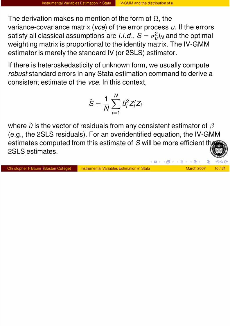
The derivation makes no mention of the form of Ω, the
variance-covariance matrix (vce ) of the error process u . If the errors
satisfy all classical assumptions are i .i .d ., S = σ2u I N and the optimal
weighting matrix is proportional to the identity matrix. The IV-GMMestimator is merely the standard IV (or 2SLS) estimator.
If there is heteroskedasticity of unknown form, we usually compute
robust standard errors in any Stata estimation command to derive a
consistent estimate of the vce . In this context,
S = 1
N
N
i =1
u 2i Z i Z i
where u is the vector of residuals from any consistent estimator of β
(e.g., the 2SLS residuals). For an overidentified equation, the IV-GMM
estimates computed from this estimate of S will be more efficient than
2SLS estimates.
Christopher F Baum (Boston College) Instrumental Variables Estimation in Stata March 2007 10 / 31
Instrumental Variables Estimation in Stata IV-GMM and the distribution of u

7/25/2019 StataIV Baum
http://slidepdf.com/reader/full/stataiv-baum 19/59
The derivation makes no mention of the form of Ω, the
variance-covariance matrix (vce ) of the error process u . If the errors
satisfy all classical assumptions are i .i .d ., S = σ2u I N and the optimal
weighting matrix is proportional to the identity matrix. The IV-GMMestimator is merely the standard IV (or 2SLS) estimator.
If there is heteroskedasticity of unknown form, we usually compute
robust standard errors in any Stata estimation command to derive a
consistent estimate of the vce . In this context,
S = 1
N
N
i =1
u 2i Z i Z i
where u is the vector of residuals from any consistent estimator of β
(e.g., the 2SLS residuals). For an overidentified equation, the IV-GMM
estimates computed from this estimate of S will be more efficient than
2SLS estimates.
Christopher F Baum (Boston College) Instrumental Variables Estimation in Stata March 2007 10 / 31
Instrumental Variables Estimation in Stata IV-GMM cluster-robust estimates
7/25/2019 StataIV Baum
http://slidepdf.com/reader/full/stataiv-baum 20/59
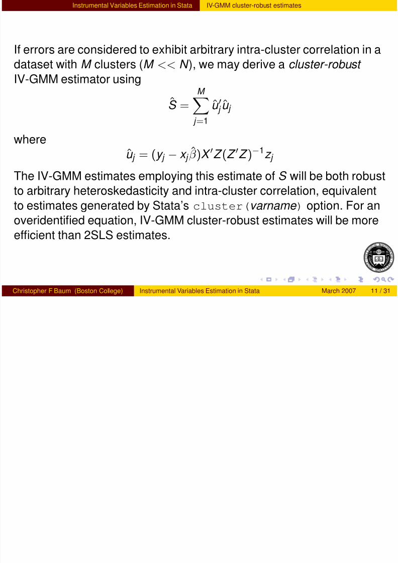
If errors are considered to exhibit arbitrary intra-cluster correlation in a
dataset with M clusters (M << N ), we may derive a cluster-robust
IV-GMM estimator using
S =M
j =1
u j u j
whereu j = (y j − x j β )X Z (Z Z )−1z j
The IV-GMM estimates employing this estimate of S will be both robust
to arbitrary heteroskedasticity and intra-cluster correlation, equivalent
to estimates generated by Stata’s cluster(varname ) option. For anoveridentified equation, IV-GMM cluster-robust estimates will be more
efficient than 2SLS estimates.
Christopher F Baum (Boston College) Instrumental Variables Estimation in Stata March 2007 11 / 31
Instrumental Variables Estimation in Stata IV-GMM HAC estimates
7/25/2019 StataIV Baum
http://slidepdf.com/reader/full/stataiv-baum 21/59
The IV-GMM approach may also be used to generate HAC standard
errors : those robust to arbitrary heteroskedasticity and autocorrelation.
Although the best-known HAC approach is that of Newey and West
(per Stata’s newey), that is only one choice of a HAC estimator that
may be applied to an IV-GMM problem.
You can also specify a vce that is robust to autocorrelation while
maintaining the assumption of conditional homoskedasticity: that is,
AC without the H .
Christopher F Baum (Boston College) Instrumental Variables Estimation in Stata March 2007 12 / 31
Instrumental Variables Estimation in Stata Implementation in Stata
7/25/2019 StataIV Baum
http://slidepdf.com/reader/full/stataiv-baum 22/59
The estimators we have discussed are available from Baum, Schaffer
and Stillman’s ivreg2 package (ssc describe ivreg2). The
ivreg2 command has the same basic syntax as Stata’s standard
ivreg:
ivreg2 depvar [varlist1] (varlist2=instlist) ///[if] [in] [, options]
The variables in varlist1 and instlist comprise Z , the matrix of
instruments. The k variables in varlist1 and varlist2 comprise
X . Both matrices by default include a units vector.
Christopher F Baum (Boston College) Instrumental Variables Estimation in Stata March 2007 13 / 31
Instrumental Variables Estimation in Stata Implementation in Stata

7/25/2019 StataIV Baum
http://slidepdf.com/reader/full/stataiv-baum 23/59
The estimators we have discussed are available from Baum, Schaffer
and Stillman’s ivreg2 package (ssc describe ivreg2). Theivreg2 command has the same basic syntax as Stata’s standard
ivreg:
ivreg2 depvar [varlist1] (varlist2=instlist) ///[if] [in] [, options]
The variables in varlist1 and instlist comprise Z , the matrix of
instruments. The k variables in varlist1 and varlist2 comprise
X . Both matrices by default include a units vector.
Christopher F Baum (Boston College) Instrumental Variables Estimation in Stata March 2007 13 / 31
Instrumental Variables Estimation in Stata ivreg2 options
7/25/2019 StataIV Baum
http://slidepdf.com/reader/full/stataiv-baum 24/59
By default ivreg2 estimates the IV estimator, or 2SLS estimator if
> k . If the gmm option is specified, it estimates the IV-GMM estimator.
With the robust option, the vce is heteroskedasticity-robust.
With the cluster(varname ) option, the vce is cluster-robust.
With the robust and bw( ) options, the vce is HAC with the default
Bartlett kernel, or “Newey–West”. Other kernel( ) choices lead to
alternative HAC estimators. Both robust and bw( ) must be
specified for HAC; estimates produced with bw( ) alone are robust to
arbitrary autocorrelation but assume homoskedasticity. NB: this willchange in the next version of ivreg2.
Christopher F Baum (Boston College) Instrumental Variables Estimation in Stata March 2007 14 / 31
Instrumental Variables Estimation in Stata Tests of overidentifying restrictions
7/25/2019 StataIV Baum
http://slidepdf.com/reader/full/stataiv-baum 25/59
If and only if an equation is overidentified , we may test whether the
excluded instruments are appropriately independent of the error
process. That test should always be performed when it is possible todo so, as it allows us to evaluate the validity of the instruments.
A test of overidentifying restrictions regresses the residuals from an IV
or 2SLS regression on all instruments in Z . Under the null hypothesis
that all instruments are uncorrelated with u , the test has alarge-sample χ2(r ) distribution where r is the number of overidentifying
restrictions.
Under the assumption of i .i .d . errors, this is known as a Sargan test ,
and is routinely produced by ivreg2 for IV and 2SLS estimates. It canalso be calculated after ivreg estimation with the overid command,
which is part of the ivreg2 suite.
Christopher F Baum (Boston College) Instrumental Variables Estimation in Stata March 2007 15 / 31
Instrumental Variables Estimation in Stata Tests of overidentifying restrictions

7/25/2019 StataIV Baum
http://slidepdf.com/reader/full/stataiv-baum 26/59
If and only if an equation is overidentified , we may test whether the
excluded instruments are appropriately independent of the error
process. That test should always be performed when it is possible todo so, as it allows us to evaluate the validity of the instruments.
A test of overidentifying restrictions regresses the residuals from an IV
or 2SLS regression on all instruments in Z . Under the null hypothesis
that all instruments are uncorrelated with u , the test has alarge-sample χ2(r ) distribution where r is the number of overidentifying
restrictions.
Under the assumption of i .i .d . errors, this is known as a Sargan test ,
and is routinely produced by ivreg2 for IV and 2SLS estimates. It canalso be calculated after ivreg estimation with the overid command,
which is part of the ivreg2 suite.
Christopher F Baum (Boston College) Instrumental Variables Estimation in Stata March 2007 15 / 31
Instrumental Variables Estimation in Stata Tests of overidentifying restrictions

7/25/2019 StataIV Baum
http://slidepdf.com/reader/full/stataiv-baum 27/59
If and only if an equation is overidentified , we may test whether the
excluded instruments are appropriately independent of the error
process. That test should always be performed when it is possible todo so, as it allows us to evaluate the validity of the instruments.
A test of overidentifying restrictions regresses the residuals from an IV
or 2SLS regression on all instruments in Z . Under the null hypothesis
that all instruments are uncorrelated with u , the test has alarge-sample χ2(r ) distribution where r is the number of overidentifying
restrictions.
Under the assumption of i .i .d . errors, this is known as a Sargan test ,
and is routinely produced by ivreg2 for IV and 2SLS estimates. It canalso be calculated after ivreg estimation with the overid command,
which is part of the ivreg2 suite.
Christopher F Baum (Boston College) Instrumental Variables Estimation in Stata March 2007 15 / 31
Instrumental Variables Estimation in Stata Tests of overidentifying restrictions

7/25/2019 StataIV Baum
http://slidepdf.com/reader/full/stataiv-baum 28/59
If we have used IV-GMM estimation in ivreg2, the test of
overidentifying restrictions becomes J : the GMM criterion function.
Although J will be identically zero for any exactly-identified equation, itwill be positive for an overidentified equation. If it is “too large”, doubt is
cast on the satisfaction of the moment conditions underlying GMM.
The test in this context is known as the Hansen test or J test , and is
routinely calculated by ivreg2 when the gmm option is employed.
The Sargan–Hansen test of overidentifying restrictions should be
performed routinely in any overidentified model estimated with
instrumental variables techniques. Instrumental variables techniques
are powerful, but if a strong rejection of the null hypothesis of theSargan–Hansen test is encountered, you should strongly doubt the
validity of the estimates.
Christopher F Baum (Boston College) Instrumental Variables Estimation in Stata March 2007 16 / 31
Instrumental Variables Estimation in Stata Tests of overidentifying restrictions
7/25/2019 StataIV Baum
http://slidepdf.com/reader/full/stataiv-baum 29/59
If we have used IV-GMM estimation in ivreg2, the test of
overidentifying restrictions becomes J : the GMM criterion function.
Although J will be identically zero for any exactly-identified equation, itwill be positive for an overidentified equation. If it is “too large”, doubt is
cast on the satisfaction of the moment conditions underlying GMM.
The test in this context is known as the Hansen test or J test , and is
routinely calculated by ivreg2 when the gmm option is employed.
The Sargan–Hansen test of overidentifying restrictions should be
performed routinely in any overidentified model estimated with
instrumental variables techniques. Instrumental variables techniques
are powerful, but if a strong rejection of the null hypothesis of theSargan–Hansen test is encountered, you should strongly doubt the
validity of the estimates.
Christopher F Baum (Boston College) Instrumental Variables Estimation in Stata March 2007 16 / 31
Instrumental Variables Estimation in Stata Testing a subset of overidentifying restrictions
7/25/2019 StataIV Baum
http://slidepdf.com/reader/full/stataiv-baum 30/59
We may be quite confident of some instruments’ independence from u
but concerned about others. In that case a GMM distance or C test
may be used. The orthog( ) option of ivreg2 will test whether asubset of the model’s overidentifying restrictions appear to be satisfied.
This is carried out by calculating two Sargan–Hansen statistics: one for
the full model and a second for the model in which the listed variables
are (a) considered endogenous, if included regressors, or (b) dropped,
if excluded regressors. In case (a), the model must still satisfy the
order condition for identification. The difference of the two
Sargan–Hansen statistics, often termed the GMM distance or C
statistic , will be distributed χ2
under the null hypothesis that thespecified orthogonality conditions are satisfied, with d.f. equal to the
number of those conditions.
Christopher F Baum (Boston College) Instrumental Variables Estimation in Stata March 2007 17 / 31
Instrumental Variables Estimation in Stata Testing a subset of overidentifying restrictions

7/25/2019 StataIV Baum
http://slidepdf.com/reader/full/stataiv-baum 31/59
We may be quite confident of some instruments’ independence from u
but concerned about others. In that case a GMM distance or C test
may be used. The orthog( ) option of ivreg2 will test whether asubset of the model’s overidentifying restrictions appear to be satisfied.
This is carried out by calculating two Sargan–Hansen statistics: one for
the full model and a second for the model in which the listed variables
are (a) considered endogenous, if included regressors, or (b) dropped,
if excluded regressors. In case (a), the model must still satisfy the
order condition for identification. The difference of the two
Sargan–Hansen statistics, often termed the GMM distance or C
statistic , will be distributed χ
2
under the null hypothesis that thespecified orthogonality conditions are satisfied, with d.f. equal to the
number of those conditions.
Christopher F Baum (Boston College) Instrumental Variables Estimation in Stata March 2007 17 / 31
Instrumental Variables Estimation in Stata Testing a subset of overidentifying restrictions
7/25/2019 StataIV Baum
http://slidepdf.com/reader/full/stataiv-baum 32/59
A variant on this strategy is implemented by the endog( ) option of
ivreg2, in which one or more variables considered endogenous canbe tested for exogeneity. The C test in this case will consider whether
the null hypothesis of their exogeneity is supported by the data.
If all endogenous regressors are included in the endog( ) option, the
test is essentially a test of whether IV methods are required toestimate the equation. If OLS estimates of the equation are consistent,
they should be preferred. In this context, the test is equivalent to a
Hausman test comparing IV and OLS estimates, as implemented by
Stata’s hausman command with the sigmaless option. Using
ivreg2, you need not estimate and store both models to generate thetest’s verdict.
Christopher F Baum (Boston College) Instrumental Variables Estimation in Stata March 2007 18 / 31
Instrumental Variables Estimation in Stata Testing a subset of overidentifying restrictions

7/25/2019 StataIV Baum
http://slidepdf.com/reader/full/stataiv-baum 33/59
A variant on this strategy is implemented by the endog( ) option of
ivreg2, in which one or more variables considered endogenous canbe tested for exogeneity. The C test in this case will consider whether
the null hypothesis of their exogeneity is supported by the data.
If all endogenous regressors are included in the endog( ) option, the
test is essentially a test of whether IV methods are required toestimate the equation. If OLS estimates of the equation are consistent,
they should be preferred. In this context, the test is equivalent to a
Hausman test comparing IV and OLS estimates, as implemented by
Stata’s hausman command with the sigmaless option. Using
ivreg2, you need not estimate and store both models to generate thetest’s verdict.
Christopher F Baum (Boston College) Instrumental Variables Estimation in Stata March 2007 18 / 31
Instrumental Variables Estimation in Stata Testing for weak instruments
7/25/2019 StataIV Baum
http://slidepdf.com/reader/full/stataiv-baum 34/59
Instrumental variables methods rely on two assumptions: the excluded
instruments are distributed independently of the error process, and
they are sufficiently correlated with the included endogenousregressors. Tests of overidentifying restrictions address the first
assumption, although we should note that a rejection of their null may
be indicative that the exclusion restrictions for these instruments may
be inappropriate. That is, some of the instruments have been
improperly excluded from the regression model’s specification.
The specification of an instrumental variables model asserts that the
excluded instruments affect the dependent variable only indirectly ,
through their correlations with the included endogenous variables. If
an excluded instrument exerts both direct and indirect influences onthe dependent variable, the exclusion restriction should be rejected.
This can be readily tested by including the variable as a regressor.
Christopher F Baum (Boston College) Instrumental Variables Estimation in Stata March 2007 19 / 31
Instrumental Variables Estimation in Stata Testing for weak instruments

7/25/2019 StataIV Baum
http://slidepdf.com/reader/full/stataiv-baum 35/59
Instrumental variables methods rely on two assumptions: the excluded
instruments are distributed independently of the error process, and
they are sufficiently correlated with the included endogenousregressors. Tests of overidentifying restrictions address the first
assumption, although we should note that a rejection of their null may
be indicative that the exclusion restrictions for these instruments may
be inappropriate. That is, some of the instruments have been
improperly excluded from the regression model’s specification.
The specification of an instrumental variables model asserts that the
excluded instruments affect the dependent variable only indirectly ,
through their correlations with the included endogenous variables. If
an excluded instrument exerts both direct and indirect influences onthe dependent variable, the exclusion restriction should be rejected.
This can be readily tested by including the variable as a regressor.
Christopher F Baum (Boston College) Instrumental Variables Estimation in Stata March 2007 19 / 31
Instrumental Variables Estimation in Stata Testing for weak instruments
7/25/2019 StataIV Baum
http://slidepdf.com/reader/full/stataiv-baum 36/59
To test the second assumption—that the excluded instruments are
sufficiently correlated with the included endogenous regressors—we
should consider the goodness-of-fit of the “first stage” regressions
relating each endogenous regressor to the entire set of instruments.
It is important to understand that the theory of single-equation (“limited
information”) IV estimation requires that all columns of X areconceptually regressed on all columns of Z in the calculation of the
estimates. We cannot meaningfully speak of “this variable is an
instrument for that regressor” or somehow restrict which instruments
enter which first-stage regressions. Stata’s ivreg or ivreg2 will not
let you do that because there is no analytical validity in such acomputation.
Christopher F Baum (Boston College) Instrumental Variables Estimation in Stata March 2007 20 / 31
Instrumental Variables Estimation in Stata Testing for weak instruments

7/25/2019 StataIV Baum
http://slidepdf.com/reader/full/stataiv-baum 37/59
To test the second assumption—that the excluded instruments are
sufficiently correlated with the included endogenous regressors—we
should consider the goodness-of-fit of the “first stage” regressions
relating each endogenous regressor to the entire set of instruments.
It is important to understand that the theory of single-equation (“limited
information”) IV estimation requires that all columns of X areconceptually regressed on all columns of Z in the calculation of the
estimates. We cannot meaningfully speak of “this variable is an
instrument for that regressor” or somehow restrict which instruments
enter which first-stage regressions. Stata’s ivreg or ivreg2 will not
let you do that because there is no analytical validity in such acomputation.
Christopher F Baum (Boston College) Instrumental Variables Estimation in Stata March 2007 20 / 31
Instrumental Variables Estimation in Stata Testing for weak instruments
7/25/2019 StataIV Baum
http://slidepdf.com/reader/full/stataiv-baum 38/59
The first and ffirst options of ivreg2 present several useful
diagnostics that assess the first-stage regressions. If there is a single
endogenous regressor, these issues are simplified, as the instruments
either explain a reasonable fraction of that regressor’s variability or not.
With multiple endogenous regressors, diagnostics are more
complicated, as each instrument is being called upon to play a role in
each first-stage regression. With sufficiently weak instruments, the
asymptotic identification status of the equation is called into question.An equation identified by the order and rank conditions in a finite
sample may still be effectively unidentified .
As Staiger and Stock (Econometrica, 1997) show, the weak
instruments problem can arise even when the first-stage t - and F -tests
are significant at conventional levels in a large sample. In the worst
case, the bias of the IV estimator is the same as that of OLS, IV
becomes inconsistent, and nothing is gained by instrumenting.
Christopher F Baum (Boston College) Instrumental Variables Estimation in Stata March 2007 21 / 31
Instrumental Variables Estimation in Stata Testing for weak instruments

7/25/2019 StataIV Baum
http://slidepdf.com/reader/full/stataiv-baum 39/59
The first and ffirst options of ivreg2 present several useful
diagnostics that assess the first-stage regressions. If there is a single
endogenous regressor, these issues are simplified, as the instruments
either explain a reasonable fraction of that regressor’s variability or not.
With multiple endogenous regressors, diagnostics are more
complicated, as each instrument is being called upon to play a role in
each first-stage regression. With sufficiently weak instruments, the
asymptotic identification status of the equation is called into question.An equation identified by the order and rank conditions in a finite
sample may still be effectively unidentified .
As Staiger and Stock (Econometrica, 1997) show, the weak
instruments problem can arise even when the first-stage t - and F -tests
are significant at conventional levels in a large sample. In the worst
case, the bias of the IV estimator is the same as that of OLS, IV
becomes inconsistent, and nothing is gained by instrumenting.
Christopher F Baum (Boston College) Instrumental Variables Estimation in Stata March 2007 21 / 31
Instrumental Variables Estimation in Stata Testing for weak instruments
7/25/2019 StataIV Baum
http://slidepdf.com/reader/full/stataiv-baum 40/59
Beyond the informal “rule-of-thumb” diagnostics such as F > 10,
ivreg2 computes several statistics that can be used to criticallyevaluate the strength of instruments. We can write the first-stage
regressions as
X = Z Π + v
With X 1 as the endogenous regressors, Z 1 the excluded instrumentsand Z 2 as the included instruments, this can be partitioned as
X 1 = [Z 1Z 2] [Π11Π12] + v 1
The rank condition for identification states that the L × K 1
matrix Π11must be of full column rank.
Christopher F Baum (Boston College) Instrumental Variables Estimation in Stata March 2007 22 / 31
Instrumental Variables Estimation in Stata The Anderson canonical correlation statistic
7/25/2019 StataIV Baum
http://slidepdf.com/reader/full/stataiv-baum 41/59
We do not observe the true Π11, so we must replace it with an
estimate. Anderson’s (John Wiley, 1984) approach to testing the rankof this matrix (or that of the full Pi matrix) considers the canonical
correlations of the X and Z matrices. If the equation is to be identified,
all K of the canonical correlations will be significantly different from
zero.
The squared canonical correlations can be expressed as eigenvalues
of a matrix. Anderson’s CC test considers the null hypothesis that the
minimum canonical correlation is zero. Under the null, the test statistic
is distributed χ2 with (L − K + 1) d.f., so it may be calculated even for
an exactly-identified equation. Failure to reject the null suggests theequation is unidentified. ivreg2 routinely reports this LR statistic.
Christopher F Baum (Boston College) Instrumental Variables Estimation in Stata March 2007 23 / 31
Instrumental Variables Estimation in Stata The Anderson canonical correlation statistic

7/25/2019 StataIV Baum
http://slidepdf.com/reader/full/stataiv-baum 42/59
We do not observe the true Π11, so we must replace it with an
estimate. Anderson’s (John Wiley, 1984) approach to testing the rankof this matrix (or that of the full Pi matrix) considers the canonical
correlations of the X and Z matrices. If the equation is to be identified,
all K of the canonical correlations will be significantly different from
zero.
The squared canonical correlations can be expressed as eigenvalues
of a matrix. Anderson’s CC test considers the null hypothesis that the
minimum canonical correlation is zero. Under the null, the test statistic
is distributed χ2 with (L − K + 1) d.f., so it may be calculated even for
an exactly-identified equation. Failure to reject the null suggests theequation is unidentified. ivreg2 routinely reports this LR statistic.
Christopher F Baum (Boston College) Instrumental Variables Estimation in Stata March 2007 23 / 31
Instrumental Variables Estimation in Stata The Cragg–Donald statistic
7/25/2019 StataIV Baum
http://slidepdf.com/reader/full/stataiv-baum 43/59
The C–D statistic is a closely related test of the rank of a matrix. While
the Anderson CC test is a LR test, the C–D test is a Wald statistic, with
the same asymptotic distribution. The C–D statistic plays an importantrole in Stock and Yogo’s work (see below). Both the Anderson and
C–D tests are reported by ivreg2 with the first option.
The canonical correlations may also be used to test a set of
instruments for redundancy (Hall and Peixe, ES WC 2000). Theredundant( ) option of ivreg2 allows a set of excluded
instruments to be tested for relevance, with the null hypothesis that
they do not contribute to the asymptotic efficiency of the equation.
All of these tests assume i .i .d . errors. In the presence of non-i .i .d .errors, they will be biased upwards, making identification appear more
likely than it really is.
Christopher F Baum (Boston College) Instrumental Variables Estimation in Stata March 2007 24 / 31
Instrumental Variables Estimation in Stata The Cragg–Donald statistic

7/25/2019 StataIV Baum
http://slidepdf.com/reader/full/stataiv-baum 44/59
The C–D statistic is a closely related test of the rank of a matrix. While
the Anderson CC test is a LR test, the C–D test is a Wald statistic, with
the same asymptotic distribution. The C–D statistic plays an importantrole in Stock and Yogo’s work (see below). Both the Anderson and
C–D tests are reported by ivreg2 with the first option.
The canonical correlations may also be used to test a set of
instruments for redundancy (Hall and Peixe, ES WC 2000). Theredundant( ) option of ivreg2 allows a set of excluded
instruments to be tested for relevance, with the null hypothesis that
they do not contribute to the asymptotic efficiency of the equation.
All of these tests assume i .i .d . errors. In the presence of non-i .i .d .errors, they will be biased upwards, making identification appear more
likely than it really is.
Christopher F Baum (Boston College) Instrumental Variables Estimation in Stata March 2007 24 / 31
Instrumental Variables Estimation in Stata The Cragg–Donald statistic

7/25/2019 StataIV Baum
http://slidepdf.com/reader/full/stataiv-baum 45/59
The C–D statistic is a closely related test of the rank of a matrix. While
the Anderson CC test is a LR test, the C–D test is a Wald statistic, with
the same asymptotic distribution. The C–D statistic plays an importantrole in Stock and Yogo’s work (see below). Both the Anderson and
C–D tests are reported by ivreg2 with the first option.
The canonical correlations may also be used to test a set of
instruments for redundancy (Hall and Peixe, ES WC 2000). Theredundant( ) option of ivreg2 allows a set of excluded
instruments to be tested for relevance, with the null hypothesis that
they do not contribute to the asymptotic efficiency of the equation.
All of these tests assume i .i .d . errors. In the presence of non-i .i .d .errors, they will be biased upwards, making identification appear more
likely than it really is.
Christopher F Baum (Boston College) Instrumental Variables Estimation in Stata March 2007 24 / 31
Instrumental Variables Estimation in Stata The Stock and Yogo approach
7/25/2019 StataIV Baum
http://slidepdf.com/reader/full/stataiv-baum 46/59
Stock and Yogo (Camb.U.Press festschrift, 2005) propose testing for
weak instruments by using the F -statistic form of the C–D statistic.
Their null hypothesis is that the estimator is weakly identified in thesense that it is subject to bias that the investigator finds unacceptably
large.
Their test comes in two flavors: maximal relative bias (relative to the
bias of OLS) and maximal size. The former test has the null that
instruments are weak, where weak instruments are those that can lead
to an asymptotic relative bias greater than some level b . This test uses
the finite sample distribution of the IV estimator, and can only be
calculated where the appropriate moments exist. The m th moment
exists iff m < (L − K + 1). The test is routinely reported in ivreg2output when it can be calculated, with the relevant critical values
calculated by Stock and Yogo.
Christopher F Baum (Boston College) Instrumental Variables Estimation in Stata March 2007 25 / 31
Instrumental Variables Estimation in Stata The Stock and Yogo approach

7/25/2019 StataIV Baum
http://slidepdf.com/reader/full/stataiv-baum 47/59
Stock and Yogo (Camb.U.Press festschrift, 2005) propose testing for
weak instruments by using the F -statistic form of the C–D statistic.
Their null hypothesis is that the estimator is weakly identified in thesense that it is subject to bias that the investigator finds unacceptably
large.
Their test comes in two flavors: maximal relative bias (relative to the
bias of OLS) and maximal size. The former test has the null that
instruments are weak, where weak instruments are those that can lead
to an asymptotic relative bias greater than some level b . This test uses
the finite sample distribution of the IV estimator, and can only be
calculated where the appropriate moments exist. The m th moment
exists iff m < (L − K + 1). The test is routinely reported in ivreg2output when it can be calculated, with the relevant critical values
calculated by Stock and Yogo.
Christopher F Baum (Boston College) Instrumental Variables Estimation in Stata March 2007 25 / 31
Instrumental Variables Estimation in Stata The Stock and Yogo approach

7/25/2019 StataIV Baum
http://slidepdf.com/reader/full/stataiv-baum 48/59
The second test proposed by Stock and Yogo is based on the
performance of the Wald test statistic for the endogenous regressors.Under weak identification, the test rejects too often. The test statistic is
based on the rejection rate r tolerable to the researcher if the true
rejection rate is 5%. Their tabulated values consider various values for
r . To be able to reject the null that the size of the test is unacceptably
large (versus 5%), the Cragg–Donald F statistic must exceed the
tabulated critical value.
The Stock–Yogo test statistics, like others discussed above, assume
i .i .d . errors.
Christopher F Baum (Boston College) Instrumental Variables Estimation in Stata March 2007 26 / 31
Instrumental Variables Estimation in Stata The Stock and Yogo approach
7/25/2019 StataIV Baum
http://slidepdf.com/reader/full/stataiv-baum 49/59
The second test proposed by Stock and Yogo is based on the
performance of the Wald test statistic for the endogenous regressors.Under weak identification, the test rejects too often. The test statistic is
based on the rejection rate r tolerable to the researcher if the true
rejection rate is 5%. Their tabulated values consider various values for
r . To be able to reject the null that the size of the test is unacceptably
large (versus 5%), the Cragg–Donald F statistic must exceed the
tabulated critical value.
The Stock–Yogo test statistics, like others discussed above, assume
i .i .d . errors.
Christopher F Baum (Boston College) Instrumental Variables Estimation in Stata March 2007 26 / 31
Instrumental Variables Estimation in Stata The Anderson–Rubin test for endogenous regressors

7/25/2019 StataIV Baum
http://slidepdf.com/reader/full/stataiv-baum 50/59
The Anderson–Rubin (Ann.Math.Stat., 1949) test for the significance
of endogenous regressors in the structural equation is robust to thepresence of weak instruments, and may be “robustified” for non-i .i .d .
errors if an alternative VCE is estimated. The test essentially
substitutes the reduced-form equations into the structural equation and
tests for the joint significance of the excluded instruments in Z 1.
If a single endogenous regressor appears in the equation, alternative
test statistics robust to weak instruments are provided by Moreira and
Poi (Stata J., 2003) and Mikusheva and Poi (Stata J., 2006) as the
condivreg and condtest commands.
Christopher F Baum (Boston College) Instrumental Variables Estimation in Stata March 2007 27 / 31
Instrumental Variables Estimation in Stata The Anderson–Rubin test for endogenous regressors
7/25/2019 StataIV Baum
http://slidepdf.com/reader/full/stataiv-baum 51/59
The Anderson–Rubin (Ann.Math.Stat., 1949) test for the significance
of endogenous regressors in the structural equation is robust to thepresence of weak instruments, and may be “robustified” for non-i .i .d .
errors if an alternative VCE is estimated. The test essentially
substitutes the reduced-form equations into the structural equation and
tests for the joint significance of the excluded instruments in Z 1.
If a single endogenous regressor appears in the equation, alternative
test statistics robust to weak instruments are provided by Moreira and
Poi (Stata J., 2003) and Mikusheva and Poi (Stata J., 2006) as the
condivreg and condtest commands.
Christopher F Baum (Boston College) Instrumental Variables Estimation in Stata March 2007 27 / 31
Instrumental Variables Estimation in Stata LIML and GMM-CUE estimation

7/25/2019 StataIV Baum
http://slidepdf.com/reader/full/stataiv-baum 52/59
OLS and IV estimators are special cases of k-class estimators : OLS
with k = 0 and IV with k = 1. Limited-information maximum likelihood
(LIML) is another member of this class, with k chosen optimally in the
estimation process. Like any ML estimator, LIML is invariant to
normalization. In an equation with two endogenous variables, it does
not matter whether you specify y 1 or y 2 as the left-hand variable.
The latest version of ivreg2 produces LIML estimates with the liml
option for equations with i .i .d . errors. If that assumption is not
reasonable, you may use the GMM equivalent: the continuously
updated GMM estimator, or CUE estimator. In ivreg2, the cue option
combined with robust, cluster and/or bw( ) options specifies thatnon-i .i .d . errors are to be modeled.
Christopher F Baum (Boston College) Instrumental Variables Estimation in Stata March 2007 28 / 31
Instrumental Variables Estimation in Stata LIML and GMM-CUE estimation
7/25/2019 StataIV Baum
http://slidepdf.com/reader/full/stataiv-baum 53/59
OLS and IV estimators are special cases of k-class estimators : OLS
with k = 0 and IV with k = 1. Limited-information maximum likelihood
(LIML) is another member of this class, with k chosen optimally in the
estimation process. Like any ML estimator, LIML is invariant to
normalization. In an equation with two endogenous variables, it does
not matter whether you specify y 1 or y 2 as the left-hand variable.
The latest version of ivreg2 produces LIML estimates with the liml
option for equations with i .i .d . errors. If that assumption is not
reasonable, you may use the GMM equivalent: the continuously
updated GMM estimator, or CUE estimator. In ivreg2, the cue option
combined with robust, cluster and/or bw( ) options specifies thatnon-i .i .d . errors are to be modeled.
Christopher F Baum (Boston College) Instrumental Variables Estimation in Stata March 2007 28 / 31
Instrumental Variables Estimation in Stata Testing for i.i.d. errors in an IV context

7/25/2019 StataIV Baum
http://slidepdf.com/reader/full/stataiv-baum 54/59
In the context of an equation estimated with instrumental variables, the
standard diagnostic tests for heteroskedasticity and autocorrelation are
generally not valid.
In the case of heteroskedasticity, Pagan and Hall (Econometric
Reviews, 1983) showed that the Breusch–Pagan or Cook–Weisberg
tests (estat hettest) are generally not usable in an IV setting.
They propose a test that will be appropriate in IV estimation where
heteroskedasticity may be present in more than one structural
equation. Mark Schaffer’s ivhettest, part of the ivreg2 suite,
performs the Pagan–Hall test under a variety of assumptions on the
indicator variables. It will also reproduce the Breusch–Pagan test ifapplied in an OLS context.
Christopher F Baum (Boston College) Instrumental Variables Estimation in Stata March 2007 29 / 31
Instrumental Variables Estimation in Stata Testing for i.i.d. errors in an IV context

7/25/2019 StataIV Baum
http://slidepdf.com/reader/full/stataiv-baum 55/59
In the context of an equation estimated with instrumental variables, the
standard diagnostic tests for heteroskedasticity and autocorrelation are
generally not valid.
In the case of heteroskedasticity, Pagan and Hall (Econometric
Reviews, 1983) showed that the Breusch–Pagan or Cook–Weisberg
tests (estat hettest) are generally not usable in an IV setting.
They propose a test that will be appropriate in IV estimation where
heteroskedasticity may be present in more than one structural
equation. Mark Schaffer’s ivhettest, part of the ivreg2 suite,
performs the Pagan–Hall test under a variety of assumptions on the
indicator variables. It will also reproduce the Breusch–Pagan test ifapplied in an OLS context.
Christopher F Baum (Boston College) Instrumental Variables Estimation in Stata March 2007 29 / 31
Instrumental Variables Estimation in Stata Testing for i.i.d. errors in an IV context
7/25/2019 StataIV Baum
http://slidepdf.com/reader/full/stataiv-baum 56/59
In the same token, the Breusch–Godfrey statistic used in the OLS
context (estat bgodfrey) will generally not be appropriate in the
presence of endogenous regressors, overlapping data or conditionalheteroskedasticity of the error process. Cumby and Huizinga
(Econometrica, 1992) proposed a generalization of the BG statistic
which handles each of these cases.
Their test is actually more general in another way. Its null hypothesis ofthe test is that the regression error is a moving average of known order
q ≥ 0 against the general alternative that autocorrelations of the
regression error are nonzero at lags greater than q. In that context, it
can be used to test that autocorrelations beyond any q are zero. Like
the BG test, it can test multiple lag orders. The CH test is available asBaum and Schaffer’s ivactest routine, part of the ivreg2 suite.
Christopher F Baum (Boston College) Instrumental Variables Estimation in Stata March 2007 30 / 31
Instrumental Variables Estimation in Stata Testing for i.i.d. errors in an IV context

7/25/2019 StataIV Baum
http://slidepdf.com/reader/full/stataiv-baum 57/59
In the same token, the Breusch–Godfrey statistic used in the OLS
context (estat bgodfrey) will generally not be appropriate in the
presence of endogenous regressors, overlapping data or conditionalheteroskedasticity of the error process. Cumby and Huizinga
(Econometrica, 1992) proposed a generalization of the BG statistic
which handles each of these cases.
Their test is actually more general in another way. Its null hypothesis ofthe test is that the regression error is a moving average of known order
q ≥ 0 against the general alternative that autocorrelations of the
regression error are nonzero at lags greater than q. In that context, it
can be used to test that autocorrelations beyond any q are zero. Like
the BG test, it can test multiple lag orders. The CH test is available asBaum and Schaffer’s ivactest routine, part of the ivreg2 suite.
Christopher F Baum (Boston College) Instrumental Variables Estimation in Stata March 2007 30 / 31
Instrumental Variables Estimation in Stata Panel data IV estimation
Panel data IV estimation

7/25/2019 StataIV Baum
http://slidepdf.com/reader/full/stataiv-baum 58/59
The features of ivreg2 are also available in the routine xtivreg2,which is a “wrapper” for ivreg2. This routine of Mark Schaffer’s
extends Stata’s xtivreg’s support for the fixed effect (fe) and first
difference (fd) estimators. The xtivreg2 routine is available from
ssc.
Just as ivreg2 may be used to conduct a Hausman test of IV vs.
OLS, Schaffer and Stillman’s xtoverid routine may be used to
conduct a Hausman test of random effects vs. fixed effects after
xtreg, re and xtivreg, re. This routine can also calculate tests
of overidentifying restrictions after those two commands as well as
xthtaylor. The xtoverid routine is also available from ssc.
Christopher F Baum (Boston College) Instrumental Variables Estimation in Stata March 2007 31 / 31
Instrumental Variables Estimation in Stata Panel data IV estimation
Panel data IV estimation
7/25/2019 StataIV Baum
http://slidepdf.com/reader/full/stataiv-baum 59/59
The features of ivreg2 are also available in the routine xtivreg2,which is a “wrapper” for ivreg2. This routine of Mark Schaffer’s
extends Stata’s xtivreg’s support for the fixed effect (fe) and first
difference (fd) estimators. The xtivreg2 routine is available from
ssc.
Just as ivreg2 may be used to conduct a Hausman test of IV vs.
OLS, Schaffer and Stillman’s xtoverid routine may be used to
conduct a Hausman test of random effects vs. fixed effects after
xtreg, re and xtivreg, re. This routine can also calculate tests
of overidentifying restrictions after those two commands as well as
xthtaylor. The xtoverid routine is also available from ssc.
Christopher F Baum (Boston College) Instrumental Variables Estimation in Stata March 2007 31 / 31