Embed Size (px)
Citation preview
Fakultät II � Informatik, Wirtschafts- und Rechtswissenschaften
Department für Informatik
State-based Timing Analysis forDistributed Systems
Von der Fakultät für Informatik, Wirtschafts- und Rechtswissenschaften der Carl vonOssietzky Universität Oldenburg zur Erlangung des Grades und Titels eines
Doktors der Ingenieurwissenschaften (Dr. Ing.)
angenommene Dissertation von
Dipl.-Inform. Tayfun Gezgin
geboren am 12.02.1984 in Bremen
Gutachter:Prof. Dr. Achim Rettberg
Prof. Dr. Bernhard JoskoProf. Dr. Marco Wehrmeister
Tag der Disputation: 02.10.2017
2
Abstract
Functionalities of systems in safety-critical domains like the automotive are typically dis-tributed over several computation units. Such systems have to work exactly as speci�edas a violation of a requirement could result in critical situations and in loss of humanlife. Error corrections after the start of production of a system could also lead to veryhigh costs. A major aspect of correctness in safety-critical systems is the timeliness ofcomputations. Systems have to �nish certain critical computations in a timely manner inorder to be safe and reliable. Thus, it is important to have rigorous analysis techniquessuch as formal veri�cation. Unfortunately, interdependencies among functions and inter-ferences on shared resources complicate the veri�cation of such hard real-time properties.Moreover, changes a�ecting the speci�cation and the implementation of a system mightoccur during the design process, which further complicate the veri�cation process, asalready performed analyses have to be repeated.This thesis addresses these problems. A state-based approach for the analysis of timing
constraints combining analytic and model checking methods is introduced. In analogyto model checking methods, the full state space for the analysis is taken into account. Inclassical scheduling analyses only the critical instance of a system is considered, whichtypically leads to highly pessimistic results. This could lead to expensive systems, as morecomputation units would be required to satisfy the timing requirements than actuallyneeded. With the approach presented in this thesis exact response times are computed.This results in a reduced demand of computation resources, while guaranteeing that alltiming constraints are still ful�lled. In order to alleviate the problem of state spaceexplosion due to state unfolding performed by the presented approach, the state spaceof an architecture is constructed in an iterative manner. Minimization operations areapplied on the interfaces between resources to keep the resulting state spaces as small aspossible. To further boost the scalability, abstraction techniques on interfaces betweendependent resources are worked out. The e�ects of the speci�c abstractions are evaluatedwith respect to the advantages for scalability and the adequacy of the results.On top of this timing analysis an impact analysis approach is introduced in this thesis
to minimize re-veri�cation e�orts of timing properties needed when the considered systemis modi�ed. Adaptations of the architecture of an already existing and analyzed systemcould be for instance the addition of new functionalities. Resulting tasks of these newfunctions could be allocated to existing resources of the system. As veri�cation tasksare typically time consuming it is desirable to minimize the e�ort of a re-veri�cationand to reuse previous results of analyses which have not been a�ected by architectural
3
changes. Two abstraction levels are de�ned which are a�ected through changes, i.e. thespeci�cation level and the implementation level.On the speci�cation level contracts are applied and a virtual integration checking tech-
nique is introduced. Contracts enable the designer to distinguish between assumed be-havior, which must be o�ered by the environment of the system, and guaranteed behavior,for which the system itself is responsible. Certain characteristics of contracts are used inthis thesis to enable a timed automaton-based veri�cation approach. Contracts are spec-i�ed by using a pattern-based language. An approach is introduced which transforms thelanguage fragments automatically to timed automata. Besides automatically verifyingthe correct compositions and re�nements of parts of a system based on the correspondingcontracts, this technique allows to determine the impact of changes on previous analysisresults on the speci�cation level. If a contract is changed in such a manner that it re�nesthe previous one, only the internals of the corresponding system have to be re-veri�ed.On the implementation level a re�nement relation between state transition systems of
interfaces of components is de�ned. If a change occurs on a resource the approach is ableto determine whether the interfaces to dependent resources are a�ected. If the interfacesdid change in a �good manner� the veri�cation of dependent resources can be omitted,thus saving unnecessary veri�cation times.In a typical system design process, all introduced concepts are exploited in combi-
nation. Therefore, an overall methodology is presented which integrates all introducedveri�cation techniques. Changing a part of a system encapsulating some functionali-ties implicates the integration of this part into its context, and the re-veri�cation of itsadapted implementation against the local speci�cation.Besides dedicated smaller examples and benchmark systems from related papers, the
presented approach is evaluated by the application of an industrial driver assistancesystem case study.
4
Zusammenfassung
Funktionalitäten von Systemen in sicherheitskritischen Domänen wie dem Automobilsek-tor sind üblicherweise über viele Berechnungseinheiten verteilt. Solche Systeme müssenexakt nach deren Spezi�kation arbeiten, da eine Verletzung einer Systemanforderungzu einer kritischen Situation führen und Menschenleben gefährden könnte. Auÿerdemführen Fehlerkorrekturen nach Produktionsstart zu hohen Kosten. Ein wesentlicher As-pekt von sicherheitskritischen Systemen ist, dass die Berechnungen rechtzeitig erfolgenmüssen. Damit solche Systeme sicher und zuverlässig arbeiten, müssen deren Berech-nungen rechtzeitig abgeschlossen werden. Deswegen ist es wichtig, dass diese Systemedurch beispielsweise der Anwendung von formaler Veri�kation gründlich analysiert wer-den. Allerdings erschweren gegenseitige Abhängigkeiten zwischen Funktionen des Sys-tems und Interferenzen zwischen verschiedenen Funktionen, die durch den Zugri� aufgemeinsam genutzten Ressourcen entstehen können, die Analysen harter Realzeiteigen-schaften. Erschwerend kommt hinzu, dass es während der Systementwicklungsphase zuÄnderungen an der Spezi�kation und der Implementierung des Systems kommen kann.Bereits durchgeführte Analysen müssen dann wiederholt werden.Im Rahmen dieser Dissertation werden solche Probleme in der Designphase von Syste-
men adressiert. In dieser Arbeit wird ein zustandsbasiertes Verfahren zum Analysierendes korrekten Schedulings vorgestellt, das analytische und Model Checking Verfahrenkombiniert. Für die Analyse wird analog zu den Model Checking Verfahren der gesamteZustandsraum berechnet. In klassischen Analysen wird ausschlieÿlich die kritische In-stanz eines Systems betrachtet. Dies führt zu pessimistischen Antwortzeiten, was wieder-rum zu teureren Systemen führen kann, da mehr Berechnungseinheiten eingeplant werdenmüssen, um den zu hoch eingeschätzten zeitlichen Anforderungen gerecht zu werden. Mitdem in dieser Arbeit vorgestellten Verfahren können solche Kosten eingespart werden,da exakte Antwortzeiten der Tasks berechnet werden. Model Checking Ansätze habentypischerweise Probleme mit der Skalierbarkeit. Die Zustandsräume werden bereits fürkleine Systeme sehr groÿ. Um dieses Problem zu verringern, wird der Zustandsraumder kompletten Architektur in dem hier vorgestellten Ansatz iterativ berechnet. DieZustandsräume an den Schnittstellen von abhängigen Ressourcen werden dabei durchspezielle Methoden minimiert. Um die Skalierbarkeit weiter zu erhöhen, werden für solcheZustandsräume weitere Abstraktionstechniken vorgestellt. Die E�ekte der einzelnen Ab-straktionstechniken werden bezüglich der Zustandseinsparung und der Genauigkeit dererzielten Ergebnisse evaluiert.Die Timing Analyse wird auÿerdem mit einer Impact Analyse erweitert, mit der
5
Re-Veri�kationen von zeitlichen Eigenschaften verringert werden sollen. Solche Re-Veri�kationen sind durch Änderungen im System erforderlich, die während der En-twurfsphase vorgenommen werden. Beispielsweise werden weitere bisher nicht einge-plante Funktionalitäten hinzugefügt, sodass weitere Tasks auf bereits existierende undanalysierte Ressourcen allokiert werden. Da Veri�kationsaufgaben typischerweise sehrzeitaufwendig sind, gibt es ein groÿes Potential Entwicklungszeiten durch das Wiederver-wenden von vorherigen Analyseergebnissen, die durch Änderungen nicht beein�usst wor-den sind, einzusparen.Durch Änderungen werden im Wesentlichen die zwei Abstraktionsebenen Spezi�kation
und Implementierung beein�usst. Auf der Spezi�kationsebene wird eine Technik zurvirtuellen Integrationsprüfung auf Basis von Contracts vorgestellt. Contracts ermöglichenes dem Entwickler, zwischen Verhalten, das durch den Kontext geliefert werden muss,und dem, das durch das System garantiert werden muss, zu unterscheiden. Einige charak-teristische Eigenschaften der Contracts werden in dieser Ausarbeitung genutzt, um eineauf Timed Automaten basierende Veri�kationstechnik zu ermöglichen. Dabei werdenContracts durch eine Pattern-basierte Sprache erfasst. Die einzelnen Pattern werdendann durch das Verfahren automatisch zu solchen Automaten transformiert. Zusätzlichzur Veri�kation der korrekten Kompositions- und Verfeinerungsbeziehungen von Teilendes Systems ermöglicht diese Technik Auswirkungen von Spezi�kationsänderungen aufbisherige Analyseergebnisse zu ermitteln.Auf der Implementierungsebene wird eine Verfeinerungsbeziehung zwischen den Zu-
standsräumen voneinander abhängiger Komponenten vorgestellt. Wenn eine Änderungan einer Ressource durchgeführt wird, ist der vorgestellte Ansatz in der Lage zu entschei-den, ob Schnittstellen zu abhängigen Ressourcen betro�en sind und damit diese neuanalysiert werden müssen oder ob unnötige Veri�kationszeit eingespart werden kann.Alle vorgestellten Konzepte �nden typischerweise im Entwurfsprozess eine kombinierteAnwendung. Deswegen wird in dieser Dissertation eine Methodik ausgearbeitet, die allevorgestellten Veri�kationstechniken integriert. Das Ändern eines Teilsystems führt zueiner Integrationsprüfung zum Restsystem und der Re-Veri�kation der internen Struk-tur oder der geänderten Implementierung. Neben dedizierten, kleineren Beispielen undBenchmark-Systemen aus verwandten Verö�entlichungen wird das hier vorgestellte Ver-fahren an einer Fallstudie zu einem Fahrerassistenzsystem evaluiert.
Contents
1. Introduction 11
1.1. Motivation . . . . . . . . . . . . . . . . . . . . . . . . . . . . . . . . . . . . 111.2. Objective of this Thesis . . . . . . . . . . . . . . . . . . . . . . . . . . . . 131.3. Context of this Thesis . . . . . . . . . . . . . . . . . . . . . . . . . . . . . 171.4. Outline . . . . . . . . . . . . . . . . . . . . . . . . . . . . . . . . . . . . . 18
2. Foundations 21
2.1. Scheduling of Real-Time Tasks . . . . . . . . . . . . . . . . . . . . . . . . 232.1.1. Tasks and Task Dependency Graphs . . . . . . . . . . . . . . . . . 242.1.2. Event Models . . . . . . . . . . . . . . . . . . . . . . . . . . . . . . 25
2.2. Timed Languages and Timed Automata . . . . . . . . . . . . . . . . . . . 272.3. Modeling of System Architectures . . . . . . . . . . . . . . . . . . . . . . . 33
2.3.1. Components and Resources . . . . . . . . . . . . . . . . . . . . . . 332.3.2. Modeling in MARTE . . . . . . . . . . . . . . . . . . . . . . . . . . 36
2.4. Speci�cation of Requirements . . . . . . . . . . . . . . . . . . . . . . . . . 382.4.1. Contract-based Design . . . . . . . . . . . . . . . . . . . . . . . . . 392.4.2. Requirement Speci�cation Language . . . . . . . . . . . . . . . . . 44
2.5. Summary . . . . . . . . . . . . . . . . . . . . . . . . . . . . . . . . . . . . 49
3. State-based Timing Analysis 51
3.1. Motivation . . . . . . . . . . . . . . . . . . . . . . . . . . . . . . . . . . . . 513.2. Related Work . . . . . . . . . . . . . . . . . . . . . . . . . . . . . . . . . . 53
3.2.1. Classical Analytical Approaches . . . . . . . . . . . . . . . . . . . . 533.2.2. Model Checking Approaches . . . . . . . . . . . . . . . . . . . . . . 563.2.3. Combination of Analytical and State-based Approaches . . . . . . 593.2.4. Contribution of this Chapter . . . . . . . . . . . . . . . . . . . . . 60
3.3. General Approach . . . . . . . . . . . . . . . . . . . . . . . . . . . . . . . 603.3.1. Iterative Analysis Approach . . . . . . . . . . . . . . . . . . . . . . 613.3.2. Symbolic Transition Systems of Resources . . . . . . . . . . . . . . 633.3.3. Simpli�cation of Symbolic Transition Systems . . . . . . . . . . . . 67
3.4. Operations on Symbolic Transition Systems . . . . . . . . . . . . . . . . . 703.4.1. Interface Computation . . . . . . . . . . . . . . . . . . . . . . . . . 703.4.2. Composition Function . . . . . . . . . . . . . . . . . . . . . . . . . 75
7
Contents
3.5. Analysis Algorithm . . . . . . . . . . . . . . . . . . . . . . . . . . . . . . . 793.5.1. Main Analysis Algorithm . . . . . . . . . . . . . . . . . . . . . . . 823.5.2. Successor Computation . . . . . . . . . . . . . . . . . . . . . . . . 833.5.3. Completeness and Soundness of Algorithm . . . . . . . . . . . . . . 913.5.4. Termination of Algorithm . . . . . . . . . . . . . . . . . . . . . . . 943.5.5. Minimization through Untimed Bisimulation, Timed Simulation
Relation . . . . . . . . . . . . . . . . . . . . . . . . . . . . . . . . . 953.6. Abstraction Techniques . . . . . . . . . . . . . . . . . . . . . . . . . . . . 97
3.6.1. Clock Resets and Duration Clocks . . . . . . . . . . . . . . . . . . 983.6.2. Clocks of Interface STSs . . . . . . . . . . . . . . . . . . . . . . . . 993.6.3. Abstraction through Simulation Relation . . . . . . . . . . . . . . . 1023.6.4. E�ects of Over-Approximations for Iterative Analysis Approach . . 1053.6.5. Testing: Abstraction through Under-Approximation . . . . . . . . 1053.6.6. Abstraction for Event Bursts . . . . . . . . . . . . . . . . . . . . . 107
3.7. Case Study: Driver Assistance System . . . . . . . . . . . . . . . . . . . . 1093.7.1. Overview . . . . . . . . . . . . . . . . . . . . . . . . . . . . . . . . 1093.7.2. Lane-Keeping-Support System . . . . . . . . . . . . . . . . . . . . 1123.7.3. Evaluation Results . . . . . . . . . . . . . . . . . . . . . . . . . . . 1143.7.4. Observation on Scalability . . . . . . . . . . . . . . . . . . . . . . . 115
3.8. Summary . . . . . . . . . . . . . . . . . . . . . . . . . . . . . . . . . . . . 115
4. Contract-based Impact Analysis 117
4.1. Motivation . . . . . . . . . . . . . . . . . . . . . . . . . . . . . . . . . . . . 1174.2. Related Work . . . . . . . . . . . . . . . . . . . . . . . . . . . . . . . . . . 118
4.2.1. Tool Support for Veri�cation of Contract Speci�cations . . . . . . 1184.2.2. Impact Analysis . . . . . . . . . . . . . . . . . . . . . . . . . . . . 1214.2.3. Contribution of this Chapter . . . . . . . . . . . . . . . . . . . . . 123
4.3. Impact Analysis Methodology . . . . . . . . . . . . . . . . . . . . . . . . . 1244.4. Impact Analysis on Speci�cation Level . . . . . . . . . . . . . . . . . . . . 129
4.4.1. Simplifying the Virtual Integration Condition . . . . . . . . . . . . 1304.4.2. Timed Automaton-based Analysis Approach . . . . . . . . . . . . . 134
4.5. Impact Analysis on Implementation Level . . . . . . . . . . . . . . . . . . 1424.5.1. Combining State-based Analysis with a Re�nement Checking Tech-
nique . . . . . . . . . . . . . . . . . . . . . . . . . . . . . . . . . . . 1434.5.2. Re�nement through Simulation Relation . . . . . . . . . . . . . . . 1454.5.3. Combining Impact Analysis with Abstractions . . . . . . . . . . . 146
4.6. Evaluation and Case Studies . . . . . . . . . . . . . . . . . . . . . . . . . . 1474.6.1. Contract-Level of the Driver Assistance System . . . . . . . . . . . 1474.6.2. Impact Analysis on the Driver Assistance System . . . . . . . . . . 1504.6.3. Evaluation of Re�nement on Implementation-Level . . . . . . . . . 151
4.7. Summary . . . . . . . . . . . . . . . . . . . . . . . . . . . . . . . . . . . . 155
8
Contents
5. Summary and Outlook 157
A. Tool Support 161
B. Handling Architectures including Restricted Loop Structures 165
C. Generated Timed Automata 169
List of Figures 173
List of Tables 177
Index 179
Nomenclature 181
Bibliography 185
9

1. Introduction
Over the last few years, the amount of functionality of systems in the hard real-time andsafety-critical domains such as the avionics or the automotive which is realized by softwareheavily increased. The usage of more and more software intensive systems targets theincrease of safety of vehicles and planes, and also targets the quality of traveling comfortand energy e�ciency. The premise to increase the safety of vehicles is to guaranteecorrect system functionality. This is achieved by testing the system intensively or byperforming exhaustive veri�cations.A major aspect of correctness is the timeliness of computations. Systems have to
�nish certain critical computations in a timely manner in order to be safe and reliable.This thesis targets the e�cient and systematic veri�cation of such timing properties ofsafety-critical systems.
1.1. Motivation
Today up to 90 percent of all innovations, i.e. new and improved functionalities, arerealized by the usage of electronic and software 1. This trend will continue in future, asX-by-Wire systems and the increased interconnection of vehicles to their environmentsleading to cooperating tra�c systems are already becoming commonplace in the market.An example in the avionics domain for this is the dynamic partitioning of the airspacewith respect to time, which was investigated in the SESAR (Single European Sky ATMResearch) program. The recent partitioning of the airspace is performed in a staticmanner, i.e. the trajectories of planes are not changed during landing approaches andtakeo�s. The shift to a dynamic partitioning, which are called 4D-trajectories, involvesan increased software-supported cooperation between the tower and the airplanes.For safety-critical systems it is crucial that these adhere to their speci�cations as a
violation of a requirement could result in critical situations leading to very high costsor even threats to human life. The veri�cation of requirements in early design steps isa critical issue as the later an error is detected in a system the higher are the costs toperform corrections.Recently, Nissan for example o�ers a car in the premium segment �tted with a steer-
by-wire system, in which the steering commands are transmitted electrically to a controlunit and then to an actuator which actually performs the steering movement. After the
1http://www.presseportal.de/pm/67565/2723743 [Jan. 18, 2016]
11
1. Introduction
...
...
Abstracted Architec.for Analysis
t1
tn
ECU
CANt1 tm
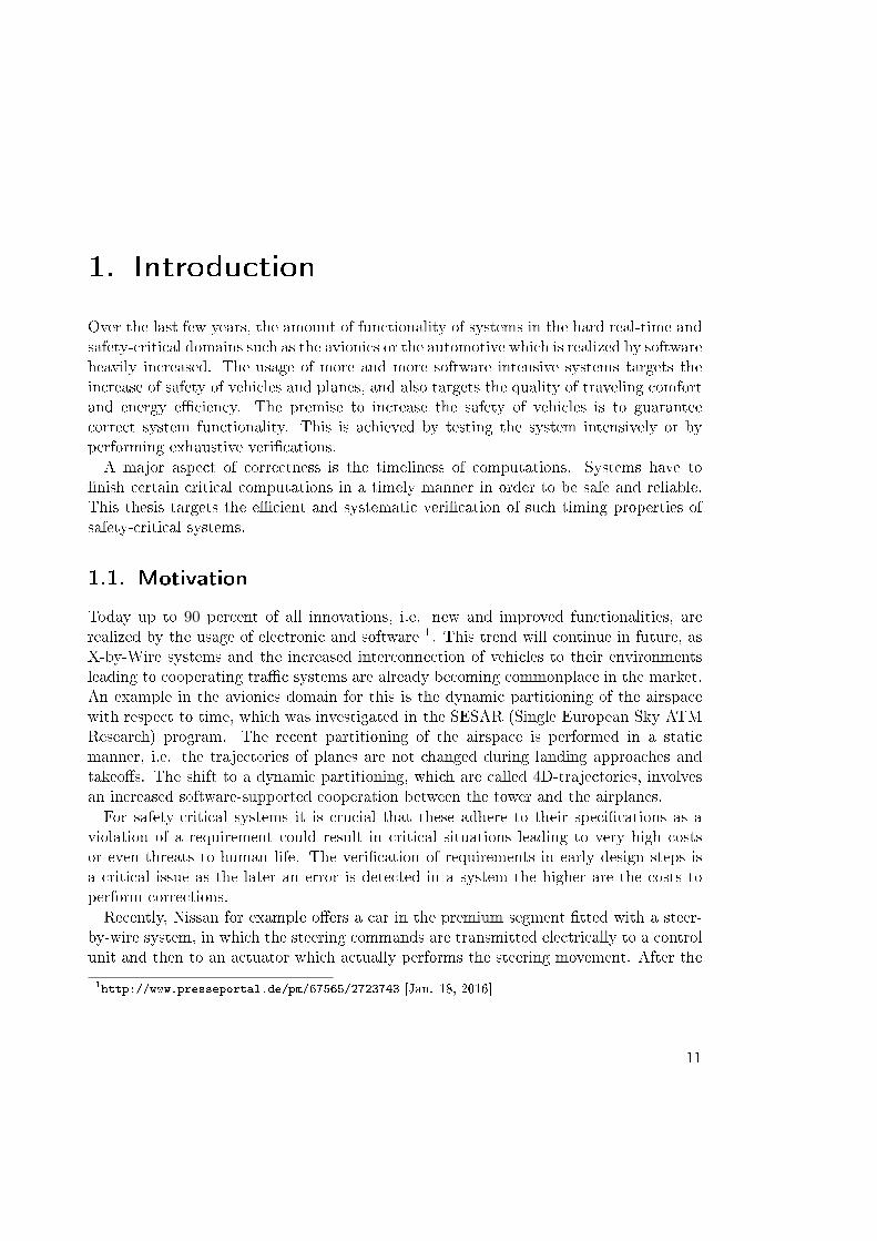
Figure 1.1.: General concept of the model-based design approach.
start of production in the year 2014 Nissan had to recall the vehicles due to some delaysin the emergency program. As recalls are quite expensive, it is desirable to performanalyses at early design steps.In order to cope with the complexity of adequately developing safety-critical systems,
the model-based design paradigm was introduced and is widely used in development pro-cesses. Systems can be build up intuitively in a bottom-up or top-down fashion by theusage of so-called components as illustrated in Figure 1.1. A component is self-containedand provides a fraction of the functionalities of a system. It has a well de�ned inter-face and may contain a set of parts or subcomponents. To specify models in a reusableand interchangeable manner it is desirable to use domain speci�c modeling standards.Typically, the design of the overall system is performed by the original equipment man-ufacturer (OEM). In a �rst step the OEM designs the software components in form oflogical architectures. The components and parts of this system are then realized andimplemented by either the OEM itself or by various suppliers. In order to get adequaterealizations from each supplier, the OEM has to specify the extra-functional propertiesand interfaces unambiguously. To capture the speci�cation of a component many speci-�cation formalisms were introduced as for instance the language of Live Sequence Charts(LSC) [DH01] or the contracts-based speci�cations [Mey92]. Such formal languages o�era rigorous semantics enabling automatic veri�cation.When all suppliers deliver the implementations of the software components (SWCs),
the OEM has to verify whether all SWCs �t together, i.e. he has to perform a consistencycheck in a black-box manner, and whether all higher level requirements which range overseveral SWCs are realized by the decomposition structure. After the implementation of allSWCs the logical architecture has to be allocated to a hardware architecture, on which thefunctionality shall be executed. The hardware architecture consists of electronic controlunits (ECUs) which are interconnected by bus systems. At this design stage technicaldetails such as resource consumptions and timing latencies have to be veri�ed. To performsuch analyses, typically the architecture is abstracted in an appropriate manner. Thekind of abstractions considered in this thesis is illustrated in the right part of Figure 1.1:ECUs and bus systems are treated logically equivalent in the sense that both represent
12

1.2. Objective of this Thesis
o1
CA
N B
us
i1
ECU 2i2
o2
i3
i4
Subsystem 1
ECU 1
ECU 3
Sub-system 1
C
Sub-system 2
...
...
...
...
C 1 C 2C 11
System 1
τ21 τ22ECU 2
τ22
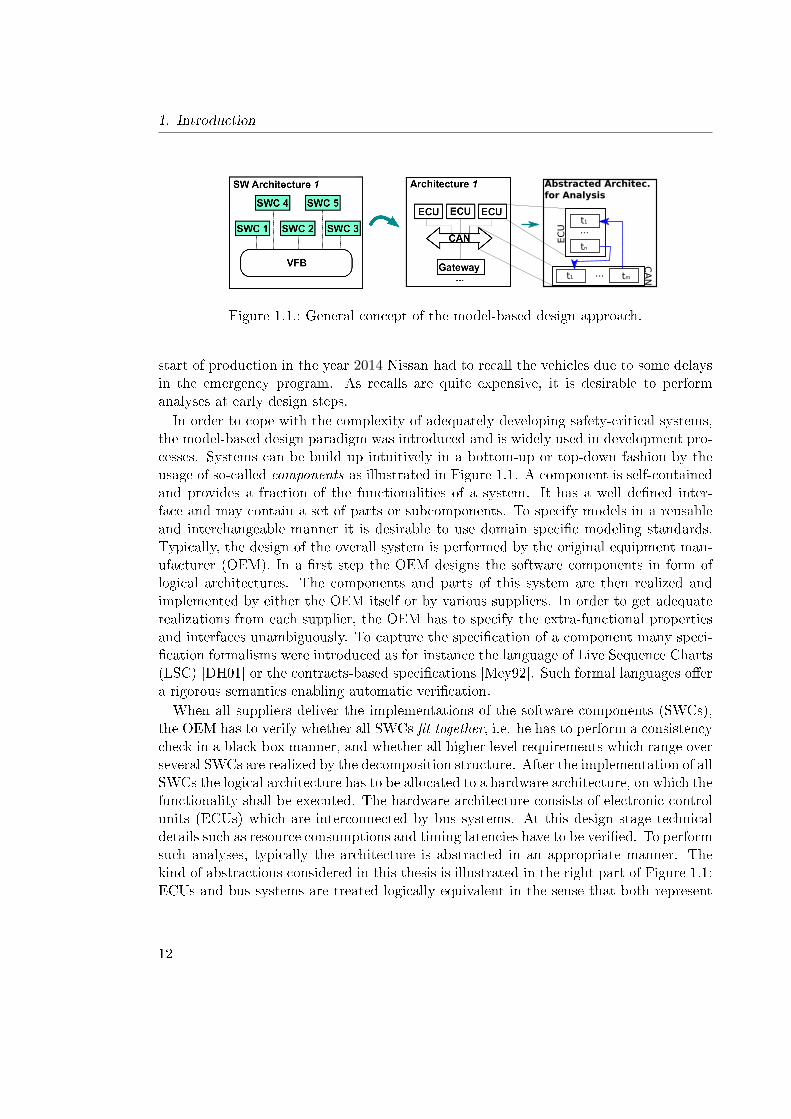
Figure 1.2.: Considered system architectures with assume/guarantee style contracts.
computation units on which a set of tasks are allocated. This is a valid approach, as abus also needs some processing time to deliver a message to the correct recipient(s). Theorder of executions of the tasks is determined by the corresponding scheduling policy.Speci�cations made during the development process of a system or a software compo-
nent are typically subject of changes. New requirements from the OEM could be statedwhich were forgotten previously, existing requirements may get re�ned or corrected, orfurther functionalities have to be included into the system. Such changes on the systemarchitecture, the parts of the implementations, or the speci�cations typically require thatalready performed analyses have to be repeated. As such tasks are time consuming it isdesirable to minimize the e�ort of a re-veri�cation.This thesis targets the analyses tasks mentioned above. Modeling languages will not be
detailed in this thesis as the scope is not the modeling but the analysis of hard real-timesystems. The contributions of this thesis and the worked out analyses tasks are detailedin the following section.
1.2. Objective of this Thesis
The objective of this thesis is the analysis and veri�cation of hard real-time systems.The focus is on the veri�cation of timing requirements in early design steps, which is acritical issue, as late changes, which have to be performed due to design errors, typicallylead to high costs.System architectures consisting of sets of processing units (ECU) and bus systems
are considered, on which a set of executable tasks is allocated as illustrated in Figure1.2. These systems can be a part of a larger context such as Subsystem 1 in the �gure.Independent tasks are triggered by events of a corresponding event stream (ES). Eventstreams are characterized by a period and a jitter. Aperiodic event streams are not con-sidered in this thesis. Event streams can be characterized by upper and lower occurrence
13
1. Introduction
curves as introduced in the real-time calculus [TCN00]. The timing speci�cations of thesystems are given in terms of assume/guarantee style contracts (abbreviated with C, Ciin Figure 1.2).Regarding the semantics of models of the considered timed systems, discrete and con-
tinuous time domains can be applied. The discrete domain is closer to �nal imple-mentations, while in the dense time semantics technical details like sampling times areabstracted. This is an advantage in early design steps, as the designer can keep thefocus on the correct functionality and the overall timings. In this thesis the dense timesemantics is considered.The approach for scheduling analysis worked out in this thesis combines both analytical
methods and model checking methods, where violations of timing constraints are decidedthrough the concept of the reachability of bad states. The scheduling analysis is based ona model checking approach covering all reachable states of the system thus determiningexact response times of the allocated tasks and end-to-end latencies of task chains.More speci�cally, the goal is to determine response times for each task and whether
some timing constraints of tasks (i.e. deadlines) and end-to-end latency constraints areviolated. For this, the entire state space of a given system architecture, which includes alltask interleavings and dependencies, is constructed in an iterative manner. The timinganalysis thereby proceeds as follows: To build the state space of a resource, its inputbehavior has to be determined, which de�nes the activation times of all allocated tasks.State spaces are represented by symbolic transition systems (STS): The states determinea range of valuations of clock variables. Also, states include the information which taskis currently running, is interrupted, or in the ready queue. A resource can have multiplesources for its inputs. To determine a single input state space for each resource, all theseinputs have to be combined by an appropriately de�ned composition operation. Thecomputed state space of a resource is then used as an input for dependent resources, i. e.for resources on which dependent tasks are allocated. To keep the interface between theresources as small as possible, parts of the state space that are not relevant for the inputbehavior of the dependent resources are abstracted.Besides the timing analysis, an impact analysis approach is worked out, which is ap-
plied if changes in the already analyzed system architecture appear. Such changes arenot unusual in a typical development process of software intensive systems. Sources ofchanges are for example the integration of new features to previously implemented soft-ware components, the update of implementations, or the change of requirements. Inthis thesis an impact analysis approach is introduced to reduce re-veri�cation aspects fortiming properties when such changes occur. The approach is able to handle changes onboth the speci�cation level and the implementation level.Suppose that the speci�cation of a system component shall be replaced. If the new
contract of the adapted speci�cation re�nes the previous contract, there is only a needto check the internals of the new component itself: If the considered component is de-composed in further subcomponents with local contracts, it has to be checked whether
14
1.2. Objective of this Thesis
State-based Timing Analysis
Impact Analysis
Determine Resource InputDetermine Resource State-
Space
Specification Level Implementation Level
Overall Methodology
Overall Control
Composition
Interface Minimization
State Abstraction
State-Space Computation
Deadline Validations
Select Resource to be analyzed
Decide Termination
Contract Level Refinement Check
Check Virtual Integration Condition
State-based Refinement Check
State-based Timing Analysis for specific Resource
Figure 1.3.: Contributions of this thesis.
the new component contract is still ful�lled by the contracts of all subcomponents. Forsuch scenarios a timed automaton-based virtual integration checking technique is intro-duced. Otherwise, if the new contract is not a re�nement of the old one, an additionalconsistency check with all dependent parts of the system has to be performed, i.e. anadditional virtual integration check has to be performed.The presented approach on the implementation level is relevant for cases where certain
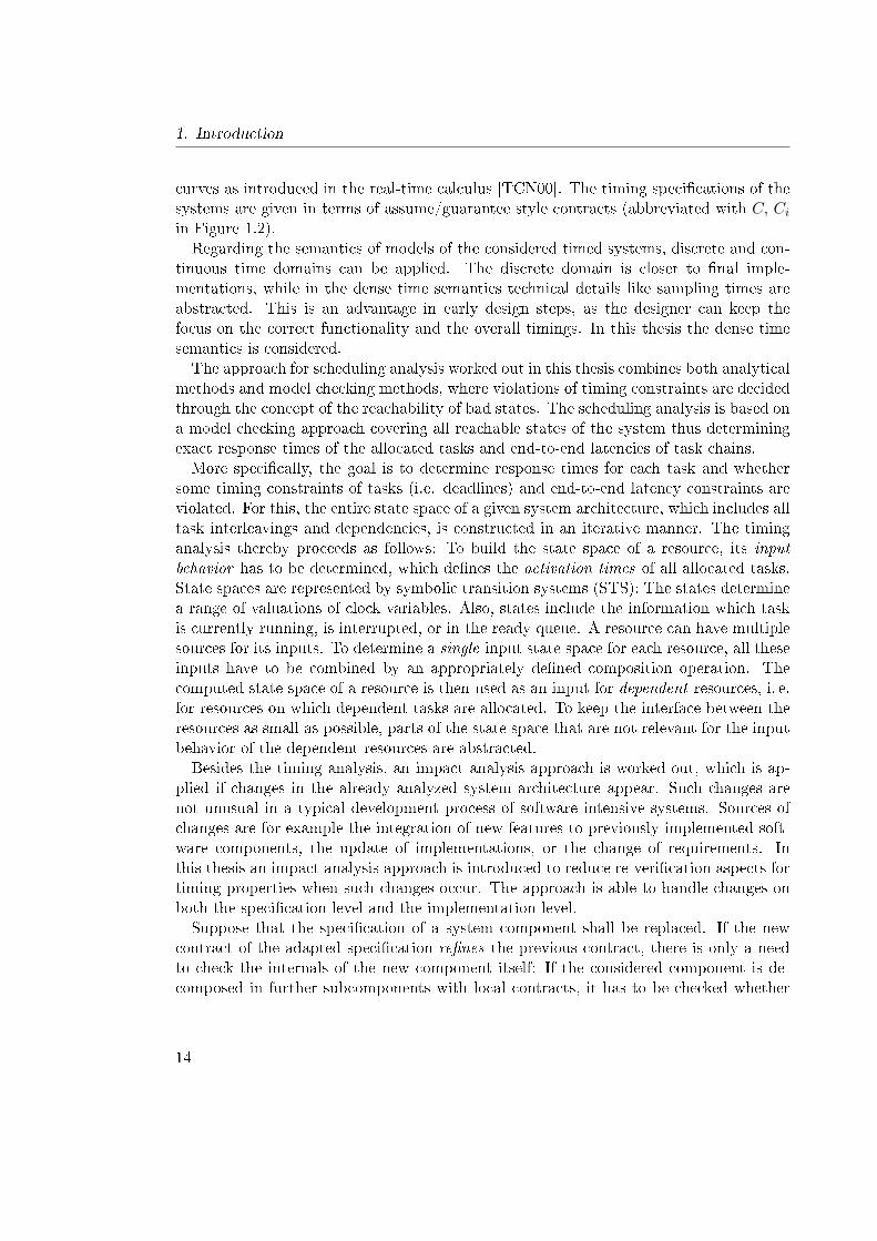
aspects of the realization of a component are changed such as adding a new task onan existing resource, the merge of two tasks in a single one, or even the change ofthe complete implementation. When such a change occurs, the approach is able todetermine whether the interfaces of dependent resources are a�ected through the conceptof a re�nement analysis: It is checked if the new interface between dependent resourcesre�nes the old interface. In such a case a re-veri�cation of dependent resources is omitted.The complete approach and the contributions are illustrated in Figure 1.3:
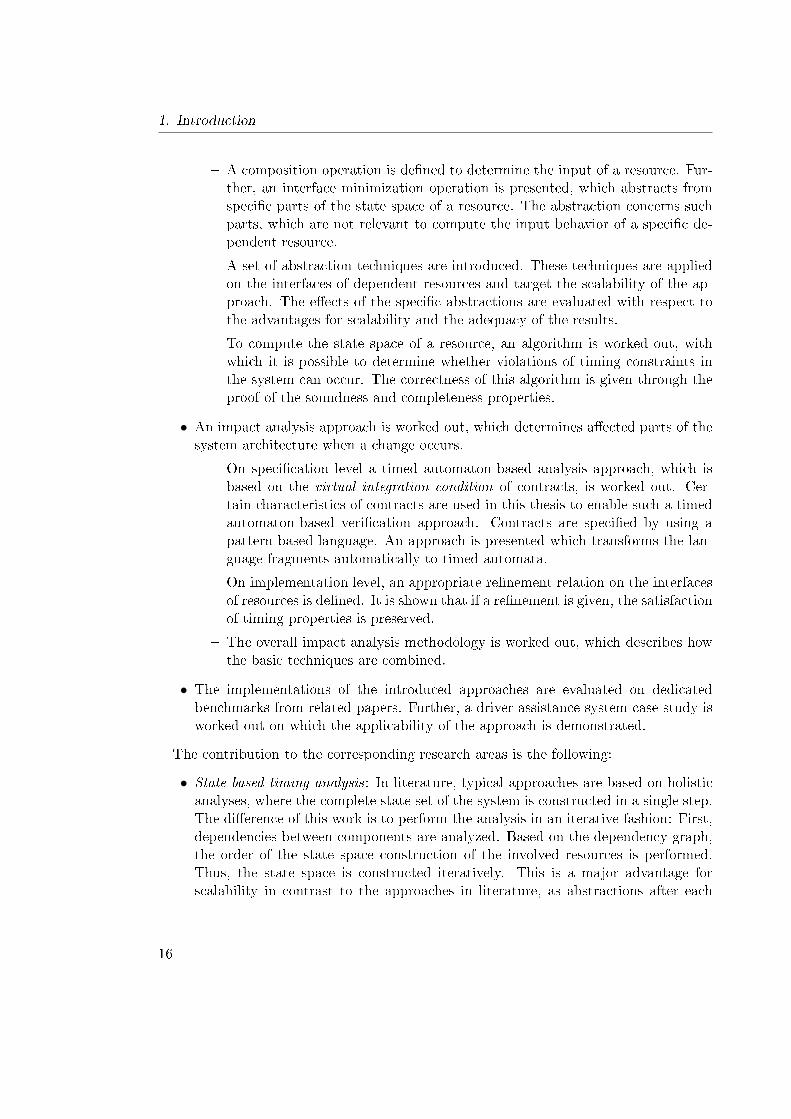
• A state-based analysis approach for timing analysis is worked out, which consists ofthe computation of the input of resources and the computation of the state spacesof resources itself. Thereby, a main control mechanism determines the order of theresources to be analyzed and decides when the termination condition is reached.To realize the state-based analysis, some operations are de�ned:
15
1. Introduction
� A composition operation is de�ned to determine the input of a resource. Fur-ther, an interface minimization operation is presented, which abstracts fromspeci�c parts of the state space of a resource. The abstraction concerns suchparts, which are not relevant to compute the input behavior of a speci�c de-pendent resource.
� A set of abstraction techniques are introduced. These techniques are appliedon the interfaces of dependent resources and target the scalability of the ap-proach. The e�ects of the speci�c abstractions are evaluated with respect tothe advantages for scalability and the adequacy of the results.
� To compute the state space of a resource, an algorithm is worked out, withwhich it is possible to determine whether violations of timing constraints inthe system can occur. The correctness of this algorithm is given through theproof of the soundness and completeness properties.
• An impact analysis approach is worked out, which determines a�ected parts of thesystem architecture when a change occurs.
� On speci�cation level a timed automaton-based analysis approach, which isbased on the virtual integration condition of contracts, is worked out. Cer-tain characteristics of contracts are used in this thesis to enable such a timedautomaton-based veri�cation approach. Contracts are speci�ed by using apattern-based language. An approach is presented which transforms the lan-guage fragments automatically to timed automata.
� On implementation level, an appropriate re�nement relation on the interfacesof resources is de�ned. It is shown that if a re�nement is given, the satisfactionof timing properties is preserved.
� The overall impact analysis methodology is worked out, which describes howthe basic techniques are combined.
• The implementations of the introduced approaches are evaluated on dedicatedbenchmarks from related papers. Further, a driver assistance system case study isworked out on which the applicability of the approach is demonstrated.
The contribution to the corresponding research areas is the following:
• State-based timing analysis: In literature, typical approaches are based on holisticanalyses, where the complete state set of the system is constructed in a single step.The di�erence of this work is to perform the analysis in an iterative fashion: First,dependencies between components are analyzed. Based on the dependency graph,the order of the state space construction of the involved resources is performed.Thus, the state space is constructed iteratively. This is a major advantage forscalability in contrast to the approaches in literature, as abstractions after each
16
1.3. Context of this Thesis
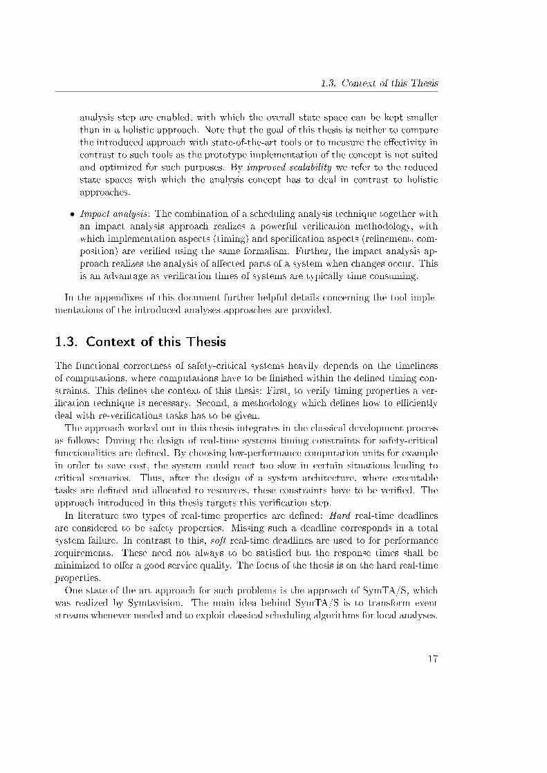
analysis step are enabled, with which the overall state space can be kept smallerthan in a holistic approach. Note that the goal of this thesis is neither to comparethe introduced approach with state-of-the-art tools or to measure the e�ectivity incontrast to such tools as the prototype implementation of the concept is not suitedand optimized for such purposes. By improved scalability we refer to the reducedstate spaces with which the analysis concept has to deal in contrast to holisticapproaches.
• Impact analysis: The combination of a scheduling analysis technique together withan impact analysis approach realizes a powerful veri�cation methodology, withwhich implementation aspects (timing) and speci�cation aspects (re�nement, com-position) are veri�ed using the same formalism. Further, the impact analysis ap-proach realizes the analysis of a�ected parts of a system when changes occur. Thisis an advantage as veri�cation times of systems are typically time consuming.
In the appendixes of this document further helpful details concerning the tool imple-mentations of the introduced analyses approaches are provided.
1.3. Context of this Thesis
The functional correctness of safety-critical systems heavily depends on the timelinessof computations, where computations have to be �nished within the de�ned timing con-straints. This de�nes the context of this thesis: First, to verify timing properties a ver-i�cation technique is necessary. Second, a methodology which de�nes how to e�cientlydeal with re-veri�cations tasks has to be given.The approach worked out in this thesis integrates in the classical development process
as follows: During the design of real-time systems timing constraints for safety-criticalfunctionalities are de�ned. By choosing low-performance computation units for examplein order to save cost, the system could react too slow in certain situations leading tocritical scenarios. Thus, after the design of a system architecture, where executabletasks are de�ned and allocated to resources, these constraints have to be veri�ed. Theapproach introduced in this thesis targets this veri�cation step.In literature two types of real-time properties are de�ned: Hard real-time deadlines
are considered to be safety properties. Missing such a deadline corresponds in a totalsystem failure. In contrast to this, soft real-time deadlines are used to for performancerequirements. These need not always to be satis�ed but the response times shall beminimized to o�er a good service quality. The focus of the thesis is on the hard real-timeproperties.One state-of-the-art approach for such problems is the approach of SymTA/S, which
was realized by Symtavision. The main idea behind SymTA/S is to transform eventstreams whenever needed and to exploit classical scheduling algorithms for local analyses.
17
1. Introduction
Event streams describe the activation patterns for tasks by upper and lower occurrencecurves, realizing a compositional analysis method. Unfortunately, this concept deliverspessimistic results when inter-ECU task dependencies exist, as the analysis abstractscompletely from concrete state-based interdependencies. The main approach of this thesispicks up on the compositional concept of SymTA/S by realizing an iterative analysis.An alternative approach is based on model checking, and has been illustrated for
example in [FPY02, DILS09]. Here, all entities like tasks, processors, and schedulers aremodeled in terms of timed automata. The most famous tool used for this approach isUppaal. Analogous to [FPY02] the full state space for the timing analysis is consideredin this thesis, where all interleavings and task dependencies are preserved. In contrast tothese works, the approach presented here constructs the state space of the architecturein an iterative manner. With this iterative approach new minimization operations onthe interfaces of dependent resources are enabled, such that a more scalable analysistechnique is realized.Technically speaking, the Uppaal DBM library 2 is used as the basis of the approach
presented in this thesis. This library includes a clock zone implementation with allnecessary basic operations such as zone intersection or reset of dedicated clocks. On topof these basic operations higher level functions to realize the computation of the statespaces of computation resources in an iterative manner are de�ned and implemented inthis thesis.Another aspect of this work is the re-veri�cation of parts of the system architecture.
During the design stage of such systems changes such as new or adapted requirementsor new features which have to be o�ered occur. Thus, besides the timing analysis,veri�cation tasks have also to deal with such changes. With this, there is a need fora methodology, which de�nes how to e�ciently deal with such re-veri�cations tasks.Ideally, this methodology is based on the de�ned veri�cation technique and extends itseamlessly by re-veri�cation abilities.
1.4. Outline
Chapter 2: Foundations In Section 2.1 the basic aspects of the scheduling of real-timetasks are introduced. An overview of scheduling policies is given. Task characteristicsare de�ned together with activation patterns, which trigger tasks at certain points intime. In Section 2.2 the formalism of timed automata and the semantics of networks oftimed automata are introduced. Section 2.3 addresses the modeling of real-time systems.The concept of components and resources are illustrated in a formal way. As designerof systems do not use these formal constructs to design system architectures, the usageof a higher level modeling pro�le called Marte is illustrated. Section 2.4 deals withthe speci�cation of requirements in a pattern-based manner and introduces the contract-
2http://people.cs.aau.dk/~adavid/UDBM/
18
1.4. Outline
based design approach. The last section summarizes all concepts introduced in thischapter.
Chapter 3: State-based Timing Analysis This chapter starts with the review of re-lated works which address the analysis of hard real-time systems. In Section 3.3 theidea of the general analysis approach is sketched, and the state space of a resource isde�ned. A simpli�ed version of the symbolic transition systems (STS) introduced in thefoundations chapter is presented. Operations on the symbolic transition systems neededto realize the analysis approach are introduced in Section 3.4, which are the abstractionand composition operations for STSs. Section 3.5 details the computation of the STS ofa resource. In Section 3.6 abstraction techniques are introduced, which lead to more pes-simistic response times but generally increase the scalability of the approach. In Section3.7 the analysis technique is applied to a lane-keeping-support system (LKS) case study.Finally, a summary of this chapter is given.
Chapter 4: Contract-based Impact Analysis First, related works on veri�cation toolsfor contract speci�cations, and on approaches reducing the e�ort of performing re-veri�cations are given. In Section 4.3 the overall methodology of the impact analysisapproach consisting of two basic veri�cation techniques on the speci�cation and the im-plementation level is presented. Both levels are detailed in the subsequent Sections 4.4and 4.5. The approach is evaluated in Section 4.6 on a driver assistance system use-case, which extends the previously introduced LKS. Finally, all results of this chapterare summarized in Section 4.7.
Chapter 5: Summary and Outlook This chapter summarizes the main results andcontributions of this work, and gives future research directions.
19

2. Foundations
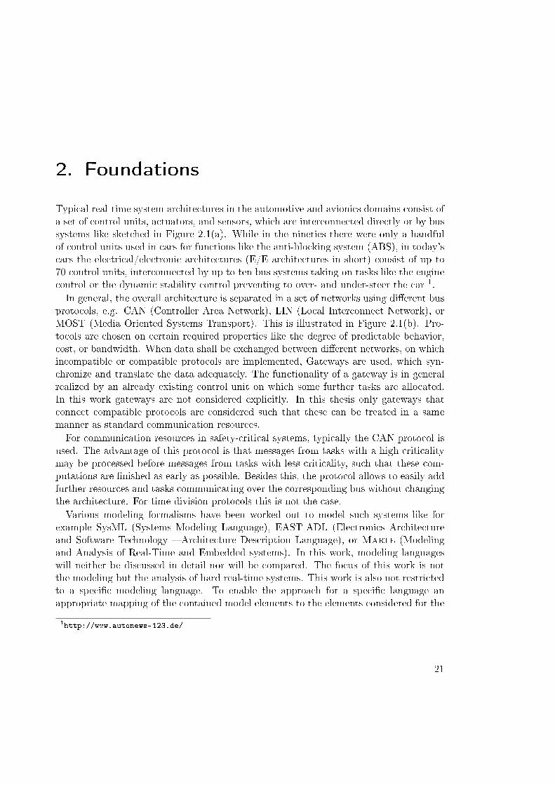
Typical real-time system architectures in the automotive and avionics domains consist ofa set of control units, actuators, and sensors, which are interconnected directly or by bussystems like sketched in Figure 2.1(a). While in the nineties there were only a handfulof control units used in cars for functions like the anti-blocking system (ABS), in today'scars the electrical/electronic architectures (E/E architectures in short) consist of up to70 control units, interconnected by up to ten bus systems taking on tasks like the enginecontrol or the dynamic stability control preventing to over- and under-steer the car 1.In general, the overall architecture is separated in a set of networks using di�erent bus
protocols, e.g. CAN (Controller Area Network), LIN (Local Interconnect Network), orMOST (Media Oriented Systems Transport). This is illustrated in Figure 2.1(b). Pro-tocols are chosen on certain required properties like the degree of predictable behavior,cost, or bandwidth. When data shall be exchanged between di�erent networks, on whichincompatible or compatible protocols are implemented, Gateways are used, which syn-chronize and translate the data adequately. The functionality of a gateway is in generalrealized by an already existing control unit on which some further tasks are allocated.In this work gateways are not considered explicitly. In this thesis only gateways thatconnect compatible protocols are considered such that these can be treated in a samemanner as standard communication resources.For communication resources in safety-critical systems, typically the CAN protocol is
used. The advantage of this protocol is that messages from tasks with a high criticalitymay be processed before messages from tasks with less criticality, such that these com-putations are �nished as early as possible. Besides this, the protocol allows to easily addfurther resources and tasks communicating over the corresponding bus without changingthe architecture. For time division protocols this is not the case.Various modeling formalisms have been worked out to model such systems like for
example SysML (Systems Modeling Language), EAST-ADL (Electronics Architectureand Software Technology � Architecture Description Language), or Marte (Modelingand Analysis of Real-Time and Embedded systems). In this work, modeling languageswill neither be discussed in detail nor will be compared. The focus of this work is notthe modeling but the analysis of hard real-time systems. This work is also not restrictedto a speci�c modeling language. To enable the approach for a speci�c language anappropriate mapping of the contained model elements to the elements considered for the
1http://www.autonews-123.de/
21
2. Foundations
(a) Structure of overall E/E-Architecture.
ABS
EngineCtrl. Unit
GearCtrl. Unit
ESP
CAN
DiagnosisInterface
Speedometer
Gateway
DistanceCtrl. Unit
Lane KeepingSupport System
CANCAN
DisplayUnit
MOST
Telematics
Amplifier
GPSA/C
DisplayUnit
Fan Ctrl. Heater
LIN
(b) Subset of di�erent subsystems interconnectedthrough various bus systems.
Figure 2.1.: E/E-Architecture of typical medium-sized cars.
analysis must be de�ned. The single restriction here might be that not the complete setof elements might be supported by the analysis approach.
Regarding the semantics of models of timed systems, discrete and continuous timedomains can be considered. The discrete domain is closer to the �nal implementation ofthe system, where problems like the sampling time have to be considered. Anyway, inearly design steps like the modeling phase the designer should not care about samplingtimes and the adequate choice of granularity. Thus, the dense time semantics has theadvantage that the designer can focus on the correct functionality and the overall timing,and abstract from such implementation details. In this thesis the dense time semanticsis considered.
For hard real-time systems it is crucial to specify requirements such as maximum end-to-end latencies in a formal manner to enable automatic analyses. In literature manymethods and techniques have been worked out for this, as for instance temporal logicswhich are based on propositional logics, pattern-based languages, or sequence diagram-based visual formalisms. On top of these formalisms the contract-based design approachwas introduced allowing to distinguish between assumed context behavior and guaranteedbehavior of the system. Such unambiguous speci�cation formalisms are especially crucialfor larger systems, where several departments of a company and various suppliers ondi�erent design levels work in parallel, and all artifacts have to be integrated in laterdesign steps. If interfaces are not speci�ed appropriately, such integration approachescould fail and lead to expensive re-designs.
In this chapter, �rst the main aspects of real-time systems such as scheduling policies,task characteristics, and activation patterns are introduced, which trigger tasks at certainpoints in time. All basic terms used in this thesis will be de�ned and outlined and thus
22
2.1. Scheduling of Real-Time Tasks
Real-Time Scheduling
Hard Deadlines Soft Deadlines
Periodic Aperiodic
Preemptive Non-Preemptive
Static Dynamic
Preemptive Non-Preemptive
Static Dynamic Static Dynamic Static Dynamic
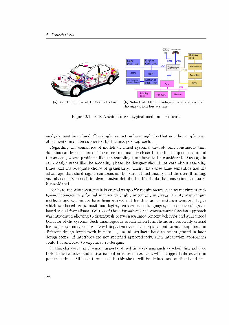
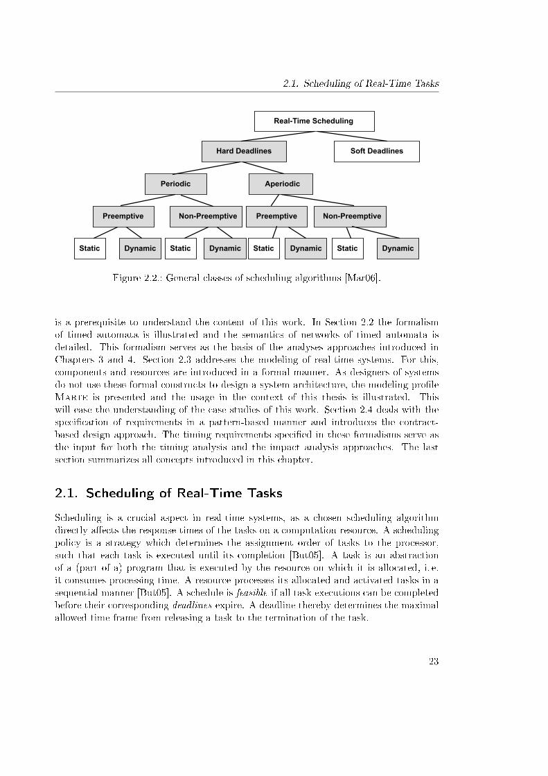
Figure 2.2.: General classes of scheduling algorithms [Mar06].
is a prerequisite to understand the content of this work. In Section 2.2 the formalismof timed automata is illustrated and the semantics of networks of timed automata isdetailed. This formalism serves as the basis of the analyses approaches introduced inChapters 3 and 4. Section 2.3 addresses the modeling of real-time systems. For this,components and resources are introduced in a formal manner. As designers of systemsdo not use these formal constructs to design a system architecture, the modeling pro�leMarte is presented and the usage in the context of this thesis is illustrated. Thiswill ease the understanding of the case studies of this work. Section 2.4 deals with thespeci�cation of requirements in a pattern-based manner and introduces the contract-based design approach. The timing requirements speci�ed in these formalisms serve asthe input for both the timing analysis and the impact analysis approaches. The lastsection summarizes all concepts introduced in this chapter.
2.1. Scheduling of Real-Time Tasks
Scheduling is a crucial aspect in real-time systems, as a chosen scheduling algorithmdirectly a�ects the response times of the tasks on a computation resource. A schedulingpolicy is a strategy which determines the assignment order of tasks to the processor,such that each task is executed until its completion [But05]. A task is an abstractionof a (part of a) program that is executed by the resource on which it is allocated, i. e.it consumes processing time. A resource processes its allocated and activated tasks in asequential manner [But05]. A schedule is feasible if all task executions can be completedbefore their corresponding deadlines expire. A deadline thereby determines the maximalallowed time frame from releasing a task to the termination of the task.
23
2. Foundations
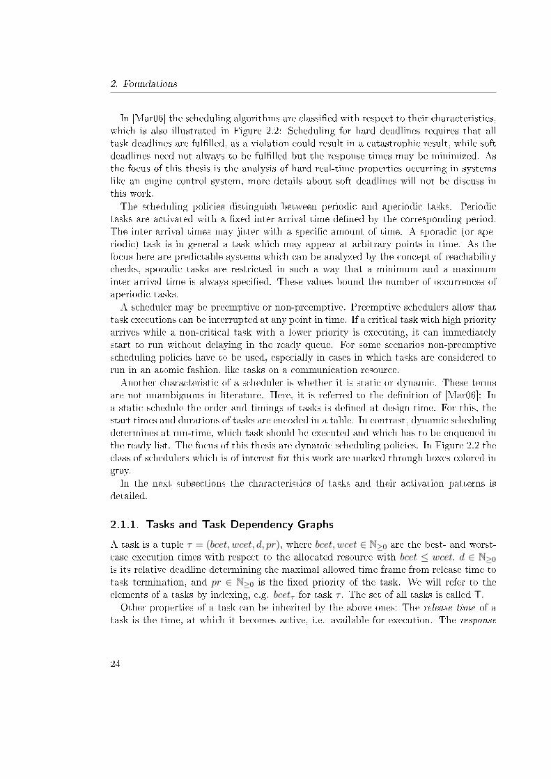
In [Mar06] the scheduling algorithms are classi�ed with respect to their characteristics,which is also illustrated in Figure 2.2: Scheduling for hard deadlines requires that alltask deadlines are ful�lled, as a violation could result in a catastrophic result, while softdeadlines need not always to be ful�lled but the response times may be minimized. Asthe focus of this thesis is the analysis of hard real-time properties occurring in systemslike an engine control system, more details about soft deadlines will not be discuss inthis work.The scheduling policies distinguish between periodic and aperiodic tasks. Periodic
tasks are activated with a �xed inter-arrival time de�ned by the corresponding period.The inter-arrival times may jitter with a speci�c amount of time. A sporadic (or ape-riodic) task is in general a task which may appear at arbitrary points in time. As thefocus here are predictable systems which can be analyzed by the concept of reachabilitychecks, sporadic tasks are restricted in such a way that a minimum and a maximuminter-arrival time is always speci�ed. These values bound the number of occurrences ofaperiodic tasks.A scheduler may be preemptive or non-preemptive. Preemptive schedulers allow that
task executions can be interrupted at any point in time. If a critical task with high priorityarrives while a non-critical task with a lower priority is executing, it can immediatelystart to run without delaying in the ready queue. For some scenarios non-preemptivescheduling policies have to be used, especially in cases in which tasks are considered torun in an atomic fashion, like tasks on a communication resource.Another characteristic of a scheduler is whether it is static or dynamic. These terms
are not unambiguous in literature. Here, it is referred to the de�nition of [Mar06]: Ina static schedule the order and timings of tasks is de�ned at design time. For this, thestart times and durations of tasks are encoded in a table. In contrast, dynamic schedulingdetermines at run-time, which task should be executed and which has to be enqueued inthe ready list. The focus of this thesis are dynamic scheduling policies. In Figure 2.2 theclass of schedulers which is of interest for this work are marked through boxes colored ingray.In the next subsections the characteristics of tasks and their activation patterns is
detailed.
2.1.1. Tasks and Task Dependency Graphs
A task is a tuple τ = (bcet, wcet, d, pr), where bcet, wcet ∈ N≥0 are the best- and worst-case execution times with respect to the allocated resource with bcet ≤ wcet, d ∈ N≥0
is its relative deadline determining the maximal allowed time frame from release time totask termination, and pr ∈ N≥0 is the �xed priority of the task. We will refer to theelements of a tasks by indexing, e.g. bcetτ for task τ . The set of all tasks is called T.
Other properties of a task can be inherited by the above ones: The release time of atask is the time, at which it becomes active, i.e. available for execution. The response
24
2.1. Scheduling of Real-Time Tasks
n
1p-j
p+j
p
p
𝜂+ 𝜂-
2j
Δt
(a) Occurrence curves.
wait
c_p <= p
releasing
c_p <= j
init
c_p <= p
c_p >= pc_p = 0
e!
c_p=0
(b) Event model automaton.
Figure 2.3.: Periodical activation of independent tasks.
time is the minimal and maximal time frame between the task release and its completion.The lateness is the di�erence between the response time and the corresponding relativedeadline.Precedence constraints between tasks are modeled by task dependency graphs as de-
�ned in the following.
De�nition 1 (Task Dependency Graph). Let T be a set of (distinct) tasks. A taskdependency graph (TDG) is a directed acyclic graph G = (T, E), where T represent thevertices of the graph and E ⊆ T × T is the set of edges representing task dependencies.Further let E∗ be the transitive closure of E. A task t1 is called an immediate predecessorof t2 if (t1, t2) ∈ E, and a predecessor if (t1, t2) ∈ E∗.
A chain of task dependencies is a path in the corresponding TDG. In literature, suchchains of tasks are also called pipelines [SSL+14]. If for a task τ there exists no taskτ ′ such that (τ ′, τ) ∈ E holds, then τ is called independent . Independent tasks aretriggered via event streams, which is the topic of the next section.
2.1.2. Event Models
Event models are models used to specify the allowed timings of events, which activatecorresponding tasks. An (in�nitely) long sequence of events is called event stream. Thus,event streams are more speci�c in the sense that event models de�ne a (possibly in�nite)set of event streams. There are several types of event models, like strictly periodic,periodic with jitter, or sporadic.In this work, the periodic with jitter model is of interest, which is characterized by
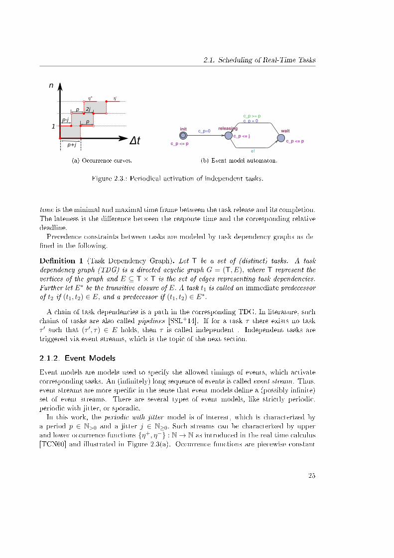
a period p ∈ N>0 and a jitter j ∈ N≥0. Such streams can be characterized by upperand lower occurrence functions {η+, η−} : N→ N as introduced in the real-time calculus[TCN00] and illustrated in Figure 2.3(a). Occurrence functions are piecewise constant
25
2. Foundations
step functions. They have unit-height steps of size one which corresponds to the occur-rence of one event characterizing the activation of a corresponding task. For any lengthof a time interval ∆t ∈ N the upper function η+(∆t) determines the maximum numberof events that can occur within a time frame of such a length, while the lower functionη−(∆t) determines the minimum number of events.The periodic with jitter event model is speci�ed through the following upper and lower
occurrence functions [RRE03]:
η+(∆t) =
⌈∆t+ j
p
⌉, (2.1)
η−(∆t) = max(0,
⌊∆t− jp
⌋). (2.2)
With this model also streams with jitter larger than the period can be captured. If thejitter is larger than the period, the initial step size of the upper function would be largerthan one, which describes that more than one event is considered to occur simultaneously.This is a pessimistic approach, as in practical cases there is always a minimal distancebetween event arrivals. Jitter typically occur when a task is triggered from another taskwith a varying response time. Such a response time is always greater than zero, as a taskwill never �nish its execution instantaneously.Non-simultaneous arrivals of events were the topic of [Ric04]: In their work the authors
introducedminimum inter-arrival times to the periodic model with jitter to support jitterlarger than the period. The model is characterized by the parameters period p, jitter jand a minimum event distance d. The minimum event distance could be for example thebest-case response time of a task, from which the considered one depends on. The modelis de�ned as follows:
η+(∆t) = min(
⌈∆t
d
⌉,
⌈∆t+ j
p
⌉). (2.3)
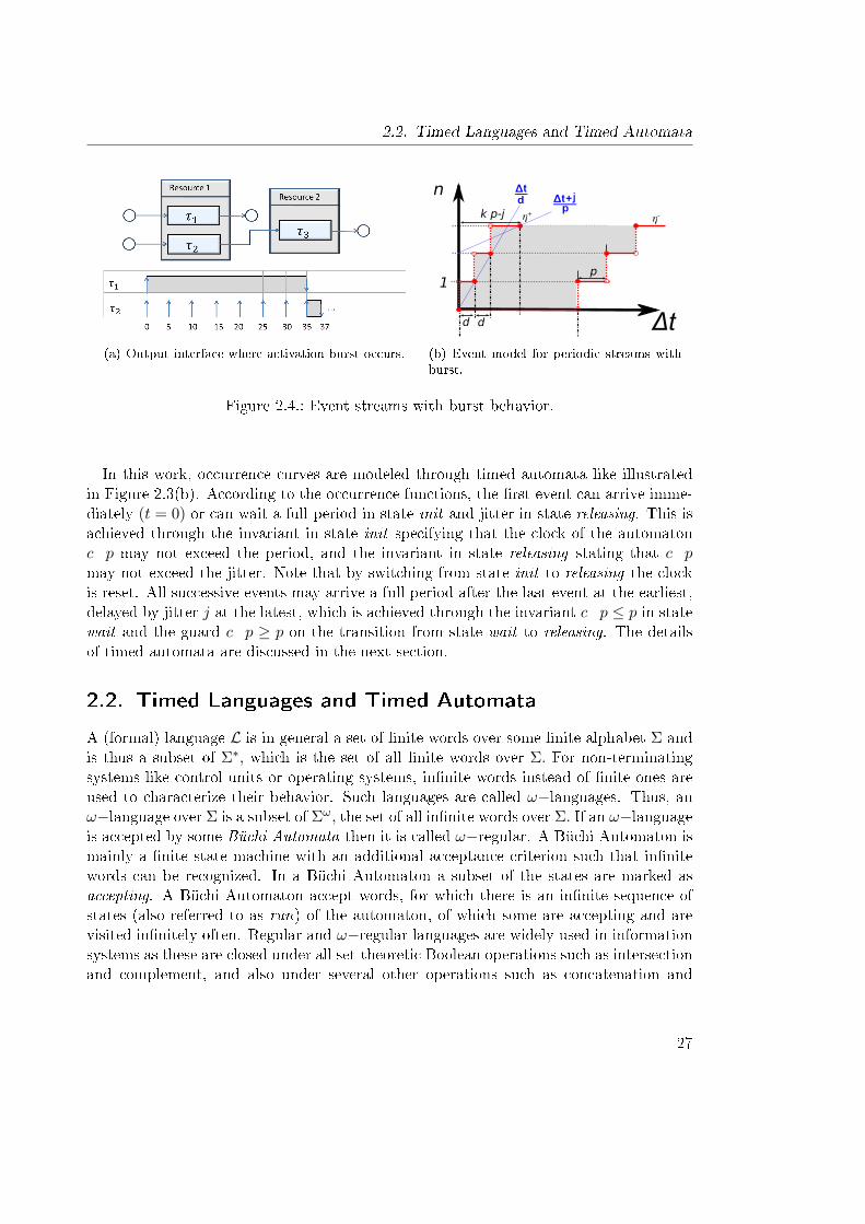
The �rst part of the function captures the burst behavior for small ∆t, the second partcaptures the long term behavior of the stream which corresponds to the standard eventmodel periodic with jitter of Formula 2.1. The lower function is the same as the standardevent model for periodic with jitter of Formula 2.2.This event model is relevant for event burst scenarios. Consider for example the
scenario of Figure 2.4(a): On Resource 1 two independent tasks τ1, τ2 are allocated, withperiods pτ1 = 50 time units and pτ2 = 5 time units, and execution times bcetτ1 = wcetτ1 =35 time units and bcetτ2 = wcetτ2 = 2 time units. As the priority of τ1 is higher than thepriority of τ2 a large response jitter from activation of the task until completion is adheredat the output of the resource. On Resource 2 the task τ3 is allocated which depends onthe output of τ2, where the event model characterized above is used to describe the eventburst activation behavior.
26
2.2. Timed Languages and Timed Automata
(a) Output interface where activation burst occurs.
n
1
d
p
𝜂+ 𝜂-
Δtd
k p-j
(b) Event model for periodic streams withburst.
Figure 2.4.: Event streams with burst behavior.
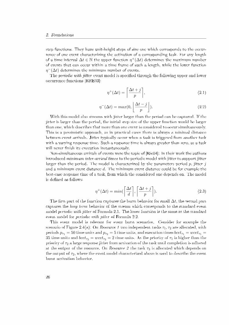
In this work, occurrence curves are modeled through timed automata like illustratedin Figure 2.3(b). According to the occurrence functions, the �rst event can arrive imme-diately (t = 0) or can wait a full period in state init and jitter in state releasing. This isachieved through the invariant in state init specifying that the clock of the automatonc_p may not exceed the period, and the invariant in state releasing stating that c_pmay not exceed the jitter. Note that by switching from state init to releasing the clockis reset. All successive events may arrive a full period after the last event at the earliest,delayed by jitter j at the latest, which is achieved through the invariant c_p ≤ p in statewait and the guard c_p ≥ p on the transition from state wait to releasing. The detailsof timed automata are discussed in the next section.
2.2. Timed Languages and Timed Automata
A (formal) language L is in general a set of �nite words over some �nite alphabet Σ andis thus a subset of Σ∗, which is the set of all �nite words over Σ. For non-terminatingsystems like control units or operating systems, in�nite words instead of �nite ones areused to characterize their behavior. Such languages are called ω−languages. Thus, anω−language over Σ is a subset of Σω, the set of all in�nite words over Σ. If an ω−languageis accepted by some Büchi Automata then it is called ω−regular. A Büchi Automaton ismainly a �nite state machine with an additional acceptance criterion such that in�nitewords can be recognized. In a Büchi Automaton a subset of the states are marked asaccepting. A Büchi Automaton accept words, for which there is an in�nite sequence ofstates (also referred to as run) of the automaton, of which some are accepting and arevisited in�nitely often. Regular and ω−regular languages are widely used in informationsystems as these are closed under all set-theoretic Boolean operations such as intersectionand complement, and also under several other operations such as concatenation and
27
2. Foundations
Kleene star.To specify the behavior of timed systems, Büchi Automata were extended by real-
valued variables called clocks in [AD94]. These automata accept timed ω−regular lan-guages over a given alphabet and an in�nite time sequence.
Timed Languages
Timed words are in�nite sequences of symbols of some �nite alphabet, enriched by amonotonically increasing in�nite time sequence. The time values determine the occur-rence times of the corresponding symbols.
De�nition 2 (Timed Word and Language). A timed word (or trace) over a non-empty�nite alphabet Σ is a pair σ = (ρ, τ) of an in�nite sequence ρ = ρ0, ρ1, · · · of symbols fromΣ, and an in�nite sequence τ = τ0, τ1, · · · of non-negative real values from R+, such that1. ∀i ∈ N : τi ≤ τi+1, (Monotonicity)2. ∀t ∈ R+ ∃i ∈ N : τi > t. (Progress)
The set of all timed words over Σ and a time sequence τ is denoted by (Σ, τ)ω.
As we will only use timed words in the following, we will abbreviate the set of all timedwords with Σω. A timed language L over Σ is a set of timed words with L ⊆ Σω. Inmany cases it is important to only consider �nite pre�xes of (in�nite) timed words. Thisis de�ned in a recursive fashion.
De�nition 3 (Trace Pre�x). Let σ = (ρ0, τ0)(ρ1, τ1) · · · be a timed trace over Σ. The�nite pre�x of σ of length n+ 1 with n ∈ N>0 is recursively de�ned as follows.
pre(σ, 0) = (ρ0, τ0),pre(σ, n) = pre(σ, n− 1)(ρn, τn).
Further for i ≥ 0 let σi := (ρi, τi) determine the ith element of a trace σ.
Timed Automata
In this work, the formalism of timed automata are used for several purposes: First, eventstreams de�ning the activation behavior of independent tasks are characterized in termsof timed automata as described in the previous subsection. Second, the worked out timinganalysis approach which is the topic of Chapter 3 is based on the symbolic representationof the induced state spaces of timed automata. Third, the virtual integration checkintroduced in Chapter 4 will also be based on this formalism.Timed automata are �nite automata extended by a �nite set of real-valued variables
called clocks. The formalism of timed automata was introduced by Alur and Dill in[AD94] in order to de�ne a modeling concept for real-time systems. Here, the syntax
28
2.2. Timed Languages and Timed Automata
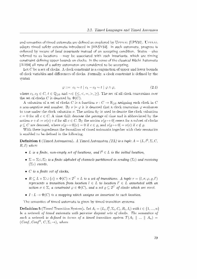
and semantics of timed automata are de�ned as employed by Uppaal [LPY97]. Uppaaladapts timed safety automata introduced in [HNSY92]. In such automata, progress isenforced by means of local invariants instead of an accepting condition. States � alsoreferred to as locations � may be associated with such invariants, which are timingconstraint de�ning upper bounds on clocks. In the sense of the classical Büchi Automata[AD94] all runs of a safety automaton are considered to be accepting.Let C be a set of clocks. A clock constraint is a conjunction of upper and lower bounds
of clock variables and di�erences of clocks. Formally, a clock constraint is de�ned by thesyntax
ϕ ::= c1 ∼ t | c1 − c2 ∼ t | ϕ ∧ ϕ, (2.4)
where c1, c2 ∈ C, t ∈ Q≥0 and ∼∈ {≤, <,=, >,≥}. The set of all clock constraints overthe set of clocks C is denoted by Φ(C).A valuation of a set of clocks C is a function ν : C → R≥0 assigning each clock in C
a non-negative real number. By ν |= ϕ it is denoted that a clock constraint ϕ evaluatesto true under the clock valuation ν. The notion 0C is used to denote the clock valuationc = 0 for all c ∈ C. A time shift denotes the passage of time and is abbreviated by thenotion ν+d := ν(c) +d for all c ∈ C. By the notion ν[% 7→ 0] resets for a subset of clocks% ⊆ C are denoted, where ν[% 7→ 0](c) = 0 if c ∈ %, and ν[% 7→ 0] = ν(c) if c /∈ %.With these ingredients the formalism of timed automata together with their semantics
is enabled to be de�ned in the following.
De�nition 4 (Timed Automaton). A Timed Automaton (TA) is a tuple A = (L, l0,Σ, C,R, I) where
• L is a �nite, non-empty set of locations, and l0 ∈ L is the initial location,
• Σ = Σ!∪Σ? is a �nite alphabet of channels partitioned in sending (Σ!) and receiving(Σ?) events,
• C is a �nite set of clocks,
• R ⊆ L×Σ ∪ {ε} ×Φ(C)× 2C × L is a set of transitions. A tuple r = (l, σ, ϕ, %, l′)represents a transition from location l ∈ L to location l′ ∈ L annotated with anaction σ ∈ Σ, a constraint ϕ ∈ Φ(C), and a set % ⊆ 2C of clocks which are reset.
• I : L→ Φ(C) is a mapping which assigns an invariant to each location.
The semantics of timed automata is given by timed transition systems.
De�nition 5 (Timed Transition System). Let Ai = (Li, l0i ,Σi, Ci, Ri, Ii) with i ∈ {1, ..., n}
be a network of timed automata with pairwise disjoint sets of clocks. The semantics ofsuch a network is de�ned in terms of a timed transition system T (A1 ‖ ... ‖ An) =(Conf ,Conf 0, C,Σ,→), where
29
2. Foundations
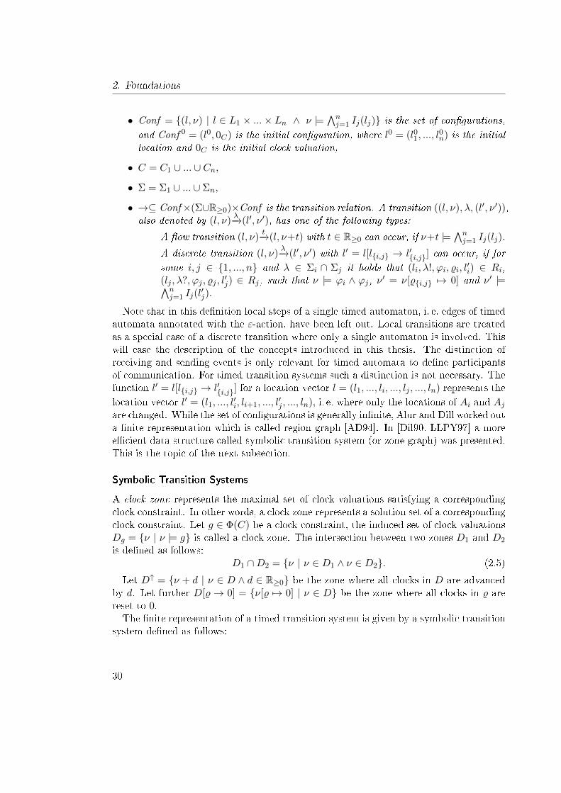
• Conf = {(l, ν) | l ∈ L1 × ...× Ln ∧ ν |=∧nj=1 Ij(lj)} is the set of con�gurations,
and Conf 0 = (l0, 0C) is the initial con�guration, where l0 = (l01, ..., l0n) is the initial
location and 0C is the initial clock valuation,
• C = C1 ∪ ... ∪ Cn,
• Σ = Σ1 ∪ ... ∪ Σn,
• →⊆ Conf×(Σ∪R≥0)×Conf is the transition relation. A transition ((l, ν), λ, (l′, ν ′)),also denoted by (l, ν)
λ−→(l′, ν ′), has one of the following types:
� A �ow transition (l, ν)t−→(l, ν+t) with t ∈ R≥0 can occur, if ν+t |=
∧nj=1 Ij(lj).
� A discrete transition (l, ν)λ−→(l′, ν ′) with l′ = l[l{i,j} → l′{i,j}] can occur, if for
some i, j ∈ {1, ..., n} and λ ∈ Σi ∩ Σj it holds that (li, λ!, ϕi, %i, l′i) ∈ Ri,
(lj , λ?, ϕj , %j , l′j) ∈ Rj, such that ν |= ϕi ∧ ϕj, ν ′ = ν[%{i,j} 7→ 0] and ν ′ |=∧n
j=1 Ij(l′j).
Note that in this de�nition local steps of a single timed automaton, i. e. edges of timedautomata annotated with the ε-action, have been left out. Local transitions are treatedas a special case of a discrete transition where only a single automaton is involved. Thiswill ease the description of the concepts introduced in this thesis. The distinction ofreceiving and sending events is only relevant for timed automata to de�ne participantsof communication. For timed transition systems such a distinction is not necessary. Thefunction l′ = l[l{i,j} → l′{i,j}] for a location vector l = (l1, ..., li, ..., lj , ..., ln) represents thelocation vector l′ = (l1, ..., l
′i, li+1, ..., l
′j , ..., ln), i. e. where only the locations of Ai and Aj
are changed. While the set of con�gurations is generally in�nite, Alur and Dill worked outa �nite representation which is called region graph [AD94]. In [Dil90, LLPY97] a moree�cient data structure called symbolic transition system (or zone graph) was presented.This is the topic of the next subsection.
Symbolic Transition Systems
A clock zone represents the maximal set of clock valuations satisfying a correspondingclock constraint. In other words, a clock zone represents a solution set of a correspondingclock constraint. Let g ∈ Φ(C) be a clock constraint, the induced set of clock valuationsDg = {ν | ν |= g} is called a clock zone. The intersection between two zones D1 and D2
is de�ned as follows:D1 ∩D2 = {ν | ν ∈ D1 ∧ ν ∈ D2}. (2.5)
Let D↑ = {ν + d | ν ∈ D ∧ d ∈ R≥0} be the zone where all clocks in D are advancedby d. Let further D[% → 0] = {ν[% 7→ 0] | ν ∈ D} be the zone where all clocks in % arereset to 0.The �nite representation of a timed transition system is given by a symbolic transition
system de�ned as follows:
30
2.2. Timed Languages and Timed Automata
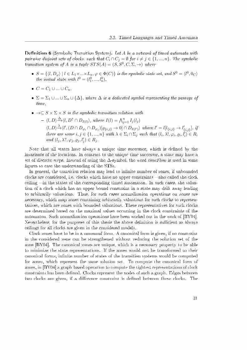
De�nition 6 (Symbolic Transition System). Let A be a network of timed automata withpairwise disjoint sets of clocks, such that Ci ∩Cj = ∅ for i 6= j ∈ {1, ..., n}. The symbolictransition system of A is a tuple STS(A) = (S, S0, C,Σ,→) where
• S = {〈l,Dϕ〉 | l ∈ L1×...×Ln, ϕ ∈ Φ(C)} is the symbolic state set, and S0 = 〈l0, 0C〉the initial state with l0 = (l01, ..., l
0n),
• C = C1 ∪ ... ∪ Cn,
• Σ = Σ1 ∪ ...∪Σn ∪ {∆}, where ∆ is a dedicated symbol representing the passage oftime,
• →⊆ S × Σ× S is the symbolic transition relation with
� 〈l,D〉 ∆−→〈l,D↑ ∩DI(l)〉, where I(l) =∧nj=1 Ij(lj)
� 〈l,D〉 λ−→〈l′, (D ∩Dϕi ∩Dϕj )[%{i,j} → 0] ∩DI(l′)〉 where l′ = l[l{i,j} → l′{i,j}], if
there are some i, j ∈ {1, ..., n} with λ ∈ Σi∩Σj such that (li, λ!, ϕi, %i, l′i) ∈ Ri
and (lj , λ?, ϕj , %j , l′j) ∈ Rj.
Note that all states have always a unique time successor, which is de�ned by theinvariants of the locations. In contrast to the unique time successor, a state may have aset of discrete steps. Instead of using the ∆-symbol, the word timeFlow is used in some�gures to ease the understanding of the STSs.In general, the transition relation may lead to in�nite number of zones, if unbounded
clocks are considered, i.e. clocks which have no upper constraints � also called the clockceiling � in the states of the corresponding timed automaton. In such cases, the valua-tion of a clock which has no upper bound constraint in a state may drift away leadingto arbitrarily valuations. Thus, for such cases normalization operations on zones arenecessary, which map zones containing arbitrarily valuations for such clocks to represen-tatives, which are zones with bounded valuations. These representatives for such clocksare determined based on the maximal values occurring in the clock constraints of theautomaton. Such normalization operations have been worked out in the work of [BY04].Nevertheless, for the purposes of this thesis the above de�nition is su�cient as alwaysceilings for all clocks are given in the considered models.Clock zones have to be in a canonical form. A canonical form is given, if no constraint
in the considered zone can be strengthened without reducing the solution set of thezone [BY04]. The canonical zones are unique, which is a necessary property to be ableto minimize the state representations. If the zones would not be transformed to theircanonical forms, in�nite number of states of the transition systems would be computedfor zones, which represent the same solution set. To compute the canonical form ofzones, in [BY04] a graph-based operation to compute the tightest representations of clockconstraints has been de�ned. Clocks represent the nodes of such a graph. Edges betweentwo clocks are given, if a di�erence constraint is de�ned between these clocks. The
31
2. Foundations
wait
c_p <= 20
releasing
c_p <= 1
init
c_p <= 20
c_p >= 20c_p = 0
e!
c_p=0l
l l
0
12
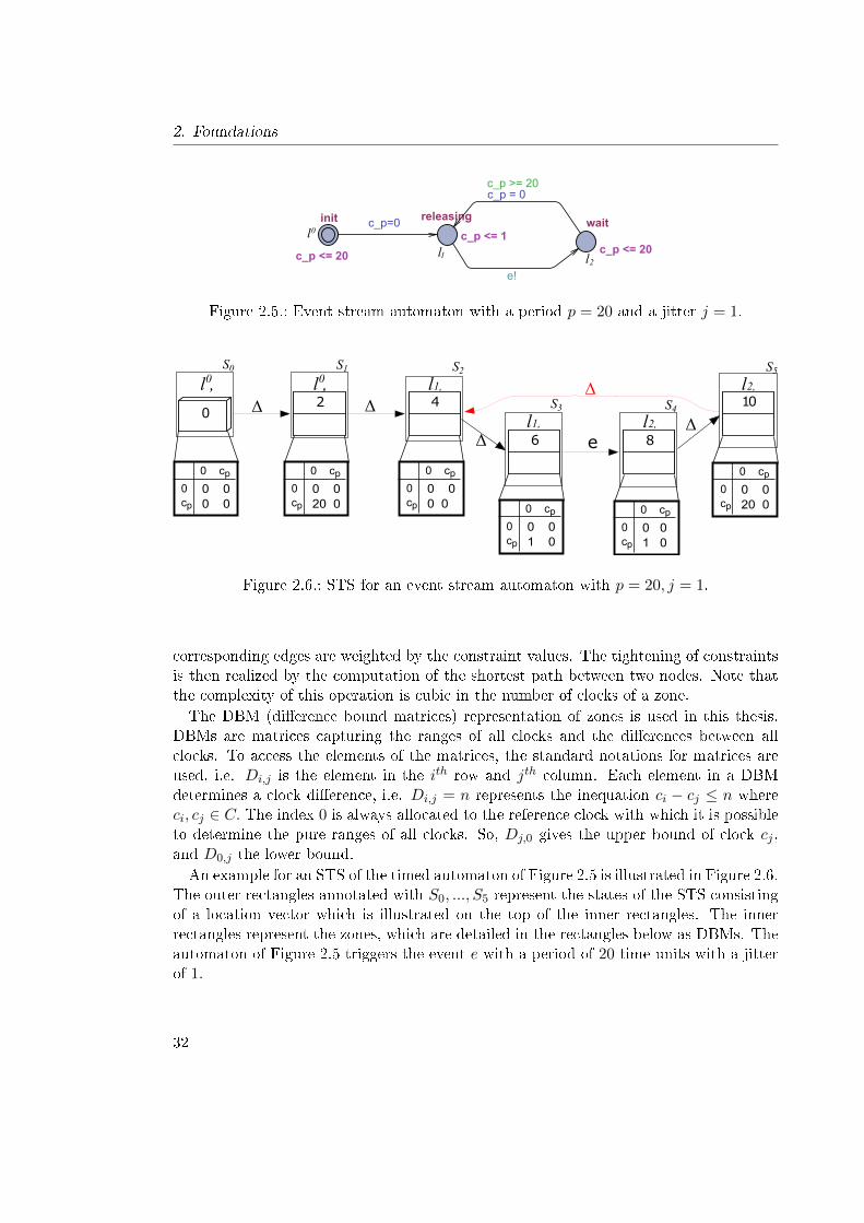
Figure 2.5.: Event stream automaton with a period p = 20 and a jitter j = 1.
02
6 8e
0 00 0
0 cp
0cp
0 0 20 0
0 cp
0cp
0 0 1 0
0 cp
0cp
0 0 1 0
0 cp
0cp
l , 0 l , 0
4
0 0 0 0
0 cp
0cp
l 1,
l2,l 1,
10l2,
0 0 20 0
0 cp
0cp
Δ
Δ
ΔΔΔ
S0 S1 S2
S3 S4
S5
Figure 2.6.: STS for an event stream automaton with p = 20, j = 1.
corresponding edges are weighted by the constraint values. The tightening of constraintsis then realized by the computation of the shortest path between two nodes. Note thatthe complexity of this operation is cubic in the number of clocks of a zone.The DBM (di�erence bound matrices) representation of zones is used in this thesis.
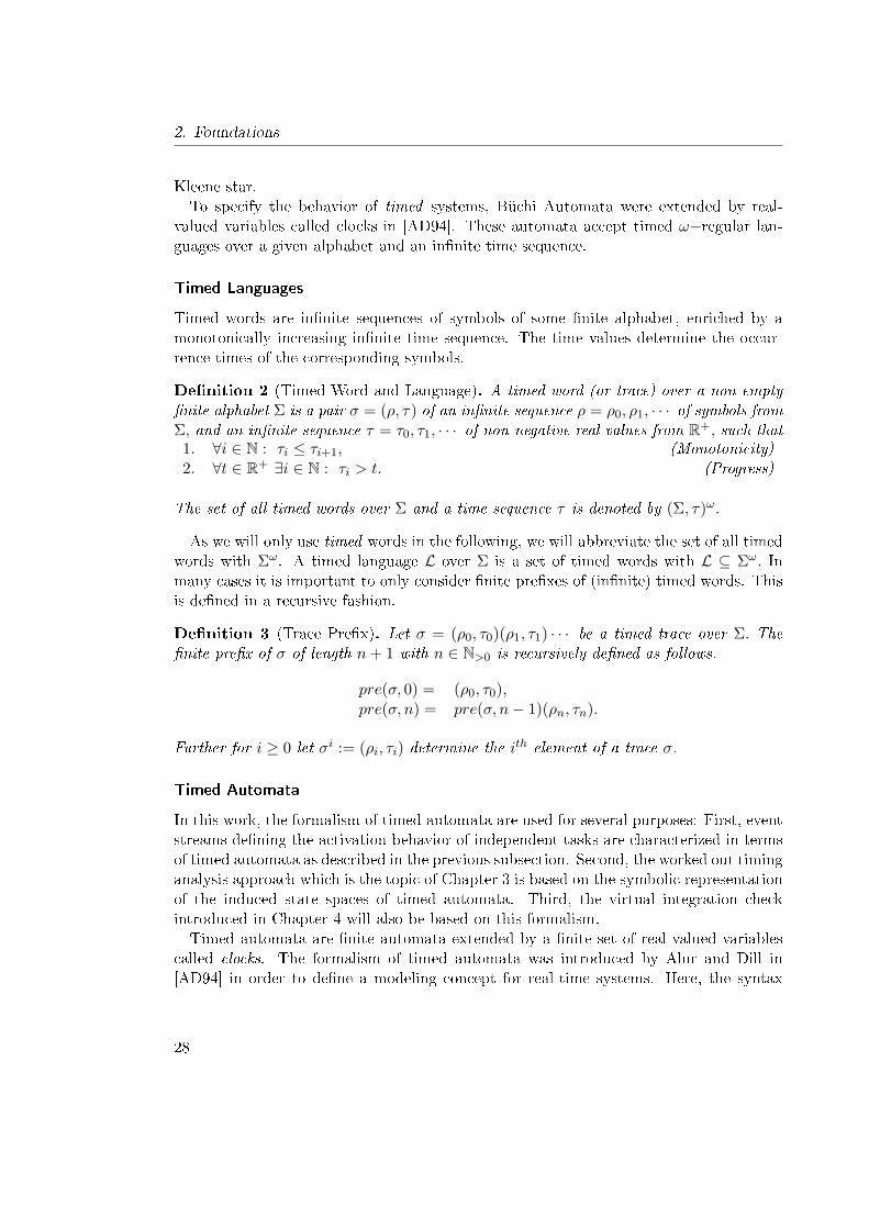
DBMs are matrices capturing the ranges of all clocks and the di�erences between allclocks. To access the elements of the matrices, the standard notations for matrices areused, i.e. Di,j is the element in the ith row and jth column. Each element in a DBMdetermines a clock di�erence, i.e. Di,j = n represents the inequation ci − cj ≤ n whereci, cj ∈ C. The index 0 is always allocated to the reference clock with which it is possibleto determine the pure ranges of all clocks. So, Dj,0 gives the upper bound of clock cj ,and D0,j the lower bound.An example for an STS of the timed automaton of Figure 2.5 is illustrated in Figure 2.6.
The outer rectangles annotated with S0, ..., S5 represent the states of the STS consistingof a location vector which is illustrated on the top of the inner rectangles. The innerrectangles represent the zones, which are detailed in the rectangles below as DBMs. Theautomaton of Figure 2.5 triggers the event e with a period of 20 time units with a jitterof 1.
32
2.3. Modeling of System Architectures
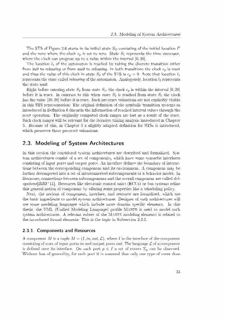
The STS of Figure 2.6 starts in its initial state SO consisting of the initial location l0
and the zone where the clock cp is set to zero. State S1 represents the time successor,where the clock can progress up to a value within the interval [0, 20].The location l1 of the automaton is reached by taking the discrete transition either
from init to releasing or from wait to releasing. In both transitions the clock cp is resetand thus the value of this clock in state S2 of the STS is cp = 0. Note that location l1represents the state called releasing of the automaton. Analogously, location l2 representsthe state wait.Right before entering state S2 from state S1, the clock cp is within the interval [0, 20]
before it is reset. In contrast to this when state S2 is reached from state S5 the clockhas the value [20, 20] before it is reset. Such pre-reset valuations are not explicitly visiblein this STS representation: The original de�nition of the symbolic transition systems asintroduced in De�nition 6 discards the information of reached interval values through thereset operation. The originally computed clock ranges are lost as a result of the reset.Such clock ranges will be relevant for the iterative timing analysis introduced in Chapter3. Because of this, in Chapter 3 a slightly adapted de�nition for STSs is introduced,which preserves these pre-reset valuations.
2.3. Modeling of System Architectures
In this section the considered system architectures are described and formalized. Sys-tem architectures consist of a set of components, which have some syntactic interfacesconsisting of input ports and output ports. An interface de�nes the boundary of interac-tions between the corresponding component and its environment. A component may befurther decomposed into a set of interconnected subcomponents or a behavior model. Inliterature, connections between subcomponents and the overall component are called del-egations[BBB+11]. Resources like electronic control units (ECUs) or bus systems re�nethis general notion of component by o�ering some properties like a scheduling policy.Next, the notions of component, interface, and resource are formalized, which are
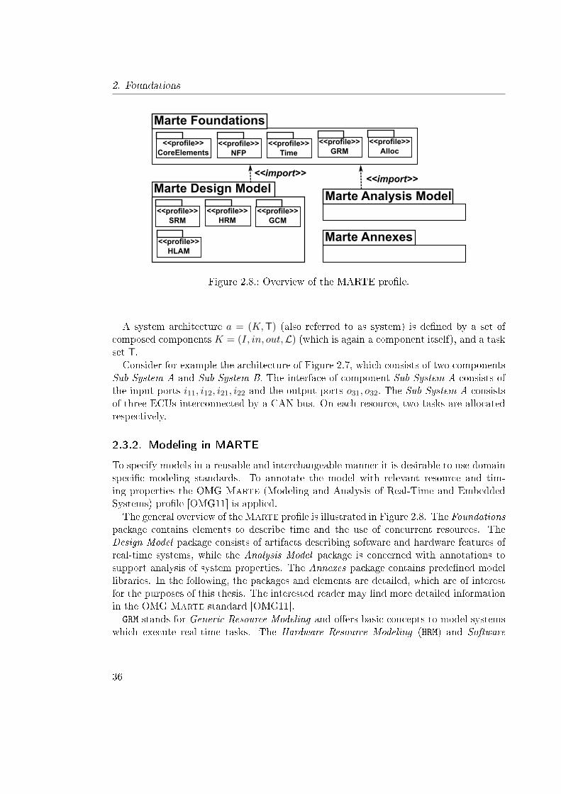
the basic ingredients to model system architectures. Designer of such architectures willuse some modeling languages which include more domain speci�c elements. In thisthesis, the UML (Uni�ed Modeling Language) pro�le Marte is used to model suchsystem architectures. A relevant subset of the Marte modeling elements is related tothe introduced formal elements. This is the topic in Subsection 2.3.2.
2.3.1. Components and Resources
A component M is a tuple M = (I, in, out,L), where I is the interface of the componentconsisting of a set of input ports in and output-ports out. The language L of a componentis de�ned over its interface. On each port p ∈ I a set of events Σp can be observed.Without loss of generality, for each port it is assumed that only one type of event does
33
2. Foundations
occur such that the alphabet of a component is directly de�ned through its port set I.This is no restriction, as a port with multiple events can be modeled also by creating oneseparate port for all events. The input and output port sets can also be determined viatwo functions de�ned as follows.
De�nition 7 (Directed Interface). An interface I consists of a set of ports. A directedinterface partitions I to input ports and output ports. For this, let {in, out} : I → I betwo disjoint functions, such that in(I) ∩ out(I) = ∅ and I = in(I) ∪ out(I), where in(I)de�nes the set of input ports and out(I) the set of output ports.
As introduced in Section 2.2 the language L of components are sets of timed wordsover its interface I. The set of all possible timed words over an interface I is given by Iω.When a set of components is considered, projection operations of the corresponding
languages are necessary to correctly de�ne the composition operations of these compo-nents.
De�nition 8 (Restriction of Words). Let σ = (ρ, τ) be a timed trace over the interfaceI and let I ′ ⊆ I. The restriction of σ to I ′, in short σ↓I′ = (ρ, τ)↓I′ , is the trace σ inwhich tuples containing events from the set I\I ′ are left out.
The restriction of a timed language is then de�ned in a straightforward manner.
De�nition 9 (Restriction of Languages). Let L be a language over the interface I andlet I ′ ⊆ I. The restriction of L to I ′ is de�ned as follows:
L↓I′ := {σ′ | ∃σ ∈ L. σ↓I′ = σ′}.
De�nition 10 (Extension of Languages). Let L be a language over the interface I ′ andlet I ′ ⊆ I. The extension of L to I is de�ned as follows:
L↑I := {σ | σ ∈ Iω. σ↓I′ ∈ L}.
Note that for each possible time sequence a word is given in Iω. Consider two disjointalphabets and a timed language which is de�ned on one of these alphabets. The extensionoperation is de�ned in such a way that all possible timed words over the second alphabetare added to the language. The following lemma formalizes this property.
Lemma 1. Let I1, I2 be two port sets with I1 ∩ I2 = ∅, and L be a non-empty languageover I1. Then (L↑I2 )↓I2 = Iω2 , i. e. the set of all words over I2.
The proof of this lemma is straightforward by applying the extension and restrictionoperations successively.A resource inherits the characteristics of a component and adds further properties. A
resource r is modeled by the tuple r = (M, T , Sch,R,A), where M is a component as
34
2.3. Modeling of System Architectures
o31
τ11
τ12 τC1
τC2
ECU 1
CAN Busi11
τ21
τ22
ECU 2
τ31
τ32
ECU 3
i12
i21
i22
o32
A: i12 occurs each 100ms
G: Whenever i12 occurs o31 occurs within [60,80]ms
iC1
iC21
G: Whenever iC1 occurs i31 occurs within 10ms
i31
i32
A: i12 occurs each 100ms with jitter 2ms
G: Whenever i12 occurs iC1 occurs within 20ms
G: Whenever i31 occurs o31 occurs within 10ms
Sub-System A
A: i21 occurs each 100ms
G: Whenever i21 occurs o32 occurs within [50,60]ms
CAN Bus
τC3
...
...
...
iC22
...
Sub-System B
A: i31 occurs each 100ms with jitter 50ms
A: iC1 occurs each 100ms with jitter 30ms
C1 C2
C3
C5
C4
Figure 2.7.: System architectures of interest.
de�ned above. A mapping T : T → B determines the set of tasks that is allocated to aresource. For each resource, a scheduling policy Sch is given such as First Come FirstServed (FIFO), Fixed Priority Scheduling (FPS) with and without preemption, or TimeDivision Multiple Access (TDMA).Two additional functions provide dynamic book keeping needed to perform scheduling
analysis. These functions depend on the state of the resource and contain the followinginformation:
• A ready list R determining tasks that are released but to which no computationtime has been allocated up to now.
• An active task map A : T → [t1, t2] with t1, t2 ∈ N≥0, which determines theinterruption times of tasks. This map is ordered and the �rst element determinesthe current running task.
Composing two components results again in a component. This is de�ned in thefollowing.
De�nition 11 (Composition of Components). Let M1,M2 be two components. Thenthe composition of both is again a component M = (I, in, out,L) with I = I1 ∪ I2, out =out1 ∪ out2, in = I\out, and L = L1
↑I ∩ L2↑I .
35
2. Foundations
Marte Foundations
<<profile>>CoreElements
<<profile>>NFP
<<profile>>Time
<<profile>>GRM
<<profile>>Alloc
Marte Design Model
<<profile>>SRM
<<profile>>HRM
<<profile>>GCM
<<profile>>HLAM
<<import>>
Marte Analysis Model
<<import>>
Marte Annexes
Figure 2.8.: Overview of the MARTE pro�le.
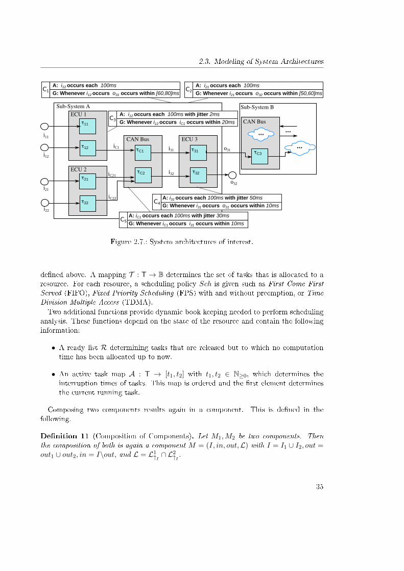
A system architecture a = (K,T) (also referred to as system) is de�ned by a set ofcomposed components K = (I, in, out,L) (which is again a component itself), and a taskset T.Consider for example the architecture of Figure 2.7, which consists of two components
Sub-System A and Sub-System B. The interface of component Sub-System A consists ofthe input ports i11, i12, i21, i22 and the output ports o31, o32. The Sub-System A consistsof three ECUs interconnected by a CAN bus. On each resource, two tasks are allocatedrespectively.
2.3.2. Modeling in MARTE
To specify models in a reusable and interchangeable manner it is desirable to use domainspeci�c modeling standards. To annotate the model with relevant resource and tim-ing properties the OMG Marte (Modeling and Analysis of Real-Time and EmbeddedSystems) pro�le [OMG11] is applied.The general overview of theMarte pro�le is illustrated in Figure 2.8. The Foundations
package contains elements to describe time and the use of concurrent resources. TheDesign Model package consists of artifacts describing software and hardware features ofreal-time systems, while the Analysis Model package is concerned with annotations tosupport analysis of system properties. The Annexes package contains prede�ned modellibraries. In the following, the packages and elements are detailed, which are of interestfor the purposes of this thesis. The interested reader may �nd more detailed informationin the OMG Marte standard [OMG11].GRM stands for Generic Resource Modeling and o�ers basic concepts to model systems
which execute real-time tasks. The Hardware Resource Modeling (HRM) and Software
36
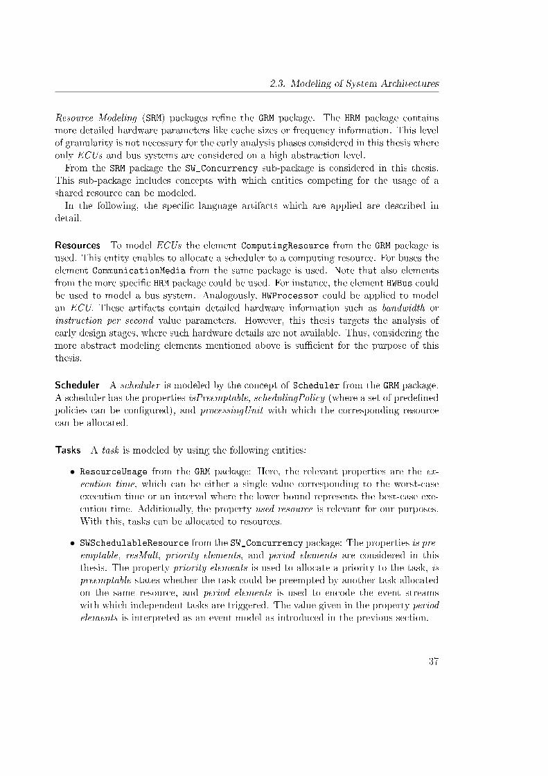
2.3. Modeling of System Architectures
Resource Modeling (SRM) packages re�ne the GRM package. The HRM package containsmore detailed hardware parameters like cache sizes or frequency information. This levelof granularity is not necessary for the early analysis phases considered in this thesis whereonly ECUs and bus systems are considered on a high abstraction level.From the SRM package the SW_Concurrency sub-package is considered in this thesis.
This sub-package includes concepts with which entities competing for the usage of ashared resource can be modeled.In the following, the speci�c language artifacts which are applied are described in
detail.
Resources To model ECUs the element ComputingResource from the GRM package isused. This entity enables to allocate a scheduler to a computing resource. For buses theelement CommunicationMedia from the same package is used. Note that also elementsfrom the more speci�c HRM package could be used. For instance, the element HWBus couldbe used to model a bus system. Analogously, HWProcessor could be applied to modelan ECU. These artifacts contain detailed hardware information such as bandwidth orinstruction per second value parameters. However, this thesis targets the analysis ofearly design stages, where such hardware details are not available. Thus, considering themore abstract modeling elements mentioned above is su�cient for the purpose of thisthesis.
Scheduler A scheduler is modeled by the concept of Scheduler from the GRM package.A scheduler has the properties isPreemptable, schedulingPolicy (where a set of prede�nedpolicies can be con�gured), and processingUnit with which the corresponding resourcecan be allocated.
Tasks A task is modeled by using the following entities:
• ResourceUsage from the GRM package: Here, the relevant properties are the ex-ecution time, which can be either a single value corresponding to the worst-caseexecution time or an interval where the lower bound represents the best-case exe-cution time. Additionally, the property used resource is relevant for our purposes.With this, tasks can be allocated to resources.
• SWSchedulableResource from the SW_Concurrency package: The properties is pre-emptable, resMult, priority elements, and period elements are considered in thisthesis. The property priority elements is used to allocate a priority to the task, ispreemptable states whether the task could be preempted by another task allocatedon the same resource, and period elements is used to encode the event streamswith which independent tasks are triggered. The value given in the property periodelements is interpreted as an event model as introduced in the previous section.
37
2. Foundations
When analyzing the dynamic behavior of the modeled resources, the maximumnumber of possible parallel activations of each task is relevant. This information isentered in the property resMult.
• Dependencies of tasks are speci�ed through the usage of the UML dependencyrelations.
End-to-end latency constraints between a set of tasks and timing constraints of singletasks are speci�ed utilizing the RSL-language, which are detailed in the next section.
2.4. Speci�cation of Requirements
Speci�cations of requirements can be performed in various manner. Early requirementsare typically captured in natural language. Unfortunately, natural language tends tobe ambiguous which could lead to misunderstandings between the OEM, suppliers, orspecial departments within a company, and to problems in the integration stage of systemparts. For example, interfaces do not �t together as di�erent value types or rangeswere expected, or an implementation does not deliver the results which were originallyexpected.Thus, a formalization of these early requirements is necessary to omit such problems.
For this, many approaches can be found in literature as for example the Linear Tem-poral Logic (LTL) [Pnu77], which extends the propositional logic by a set of temporalmodal operators. As these formalisms are quite hard to understand and to use cor-rectly in context, more intuitive graphical formalisms were de�ned like the Live SequenceCharts (LSCs) where the interaction between system components can be speci�ed inan unambiguous way [DH01]. Text-pattern-based formalisms were worked out like theRequirement Speci�cation Language (RSL) which will be the topic of Subsection 2.4.2.Besides the formalization of requirements, it is advisable to distinguish between as-
sumed and guaranteed behavior. To require for example that a component port is trig-gered periodically does not lie in the responsibility of the component itself but in theresponsibility of its context. Such a distinction eases the integration phase of com-ponents, as an automatic veri�cation of consistency of ports can be performed. Forthis purpose the contract-based design paradigm inspired by Bertrand Meyer's program-ming language Ei�el [Mey92] was worked out. The work of Bertrand Meyer enrichedobject oriented programming by using pre- and post-conditions. Later works such as[BCF+08, BDH+12, BCN+11] generalized the contract theory and made it applicablefor model-based design. In [BCN+11] a meta-theory of contracts is developed and dif-ferent concrete contract theories are cast into this framework like the one of [BCF+08],bene�ting from properties that are already established on the level of the meta-theory.Also in today's programing languages contracts are used. For example a contract def-inition is included in the Bean Validation speci�cation of the Java Enterprise Edition.
38
2.4. Speci�cation of Requirements
Methods of classes are annotated with constraints over the input parameters and returnvalues. Also a restricted form of re�nement is applied: Inheriting classes have to re�nethe annotated contracts of the corresponding root class. For this, the constraints overthe return values of the included methods are allowed to be added and be stricter, whileconstraints on the method parameters are only allowed to be de�ned on the root classlevel. As detailed later, this is consistent with the general contract re�nement de�nition.Contracts and all necessary operations on contracts are the topic of the next subsection.
2.4.1. Contract-based Design
The idea of contracts was originally inspired by Bertrand Meyer's programming languageEi�el and its design by contract paradigm [Mey92]. Requirements of systems are typicallyspeci�ed as assertions, which are basically properties that may or may not be satis�edby some behavior [BCF+08]. Formally speaking, an assertion de�nes a set of tracesover a set of variables (or ports), i. e. an assertion is a (timed) language. Let M be animplementation of a component, which again de�nes a set of traces, E a correspondingassertion, and let M and E be de�ned over the same set of ports. Then M satis�es E ifM ⊆ E.Contracts de�ne properties of component behaviors and their environments, thus are
assertions for component interfaces. Contracts follow the principle of separation of con-cerns. More speci�cally, contracts are pairs consisting of an assumption (A) and a guar-antee (G). The assumption speci�es how the context of the component, i. e. the environ-ment from the point of view of the component, should behave. Only if the assumptionholds, then the component will behave as guaranteed. This kind of speci�cation allowsto replace components by more detailed ones, if they allow a more abstract environment,without re-validating the whole system. Thus, the system decomposition can be veri�edwith respect to contracts without the knowledge of the concrete implementation.Contracts help to explicitly specify assertions about the necessary context of com-
ponents, such that implicitly assumed behavior leading to integration errors betweendi�erent development teams can be avoided. Each development team has only to relyon the speci�cation of components of other teams, i. e. these can be treated in a black-box manner, as the internal behavior is not of interest. Especially for OEM-supplierrelations this has a great bene�t, as the OEM typically does not know details aboutimplementations of components from the suppliers.Moreover, the usage of contracts can help to decrease the complexity of verifying the
implementation against its speci�cation. Such a distinction of assumed and guaranteedbehavior helps to perform more compositional analyses rather than holistic analyses.Internal implementation details of other components, on which the component underveri�cation relies to, need not to be considered. For example, consider the system inFigure 2.9, to which a contract is assigned. The system contract states that the inputport 'a' is triggered each 50ms, and when it is triggered, the system has to respond by
39
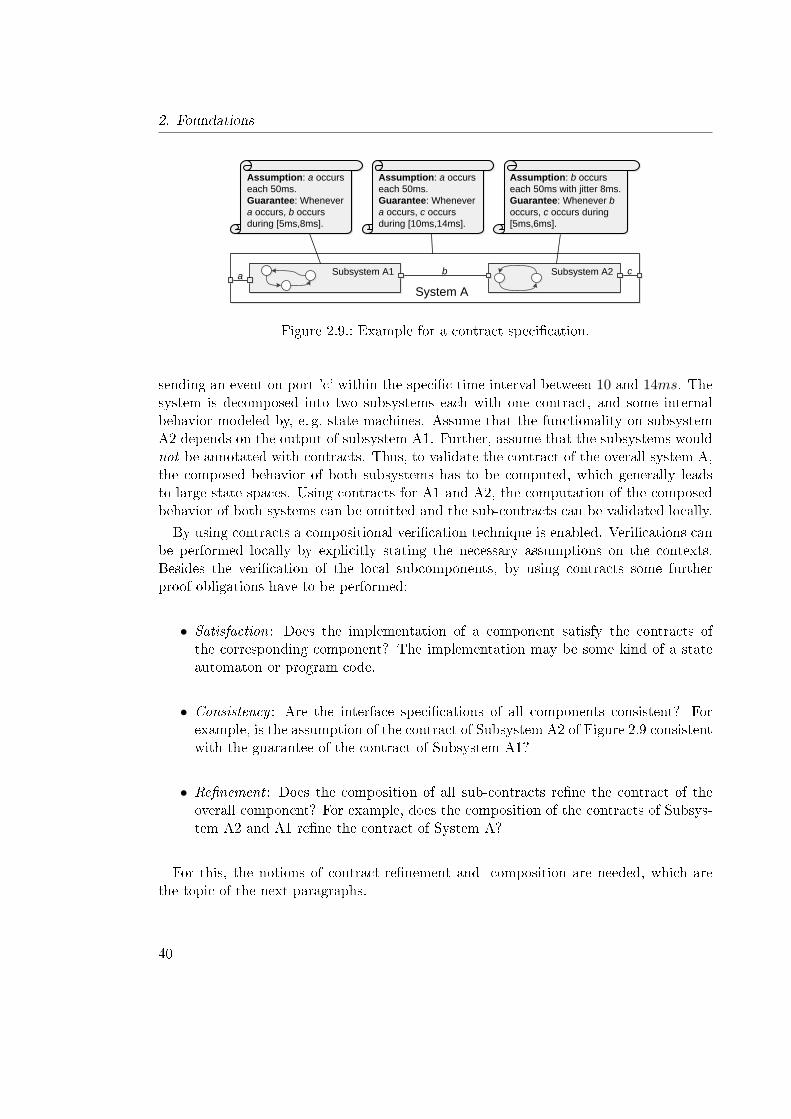
2. Foundations
System A
ca
b
Assumption: a occurs
each 50ms.
Guarantee: Whenever
a occurs, c occurs
during [10ms,14ms].
Subsystem A1 Subsystem A2
Assumption: a occurs
each 50ms.
Guarantee: Whenever
a occurs, b occurs
during [5ms,8ms].
Assumption: b occurs
each 50ms with jitter 8ms.
Guarantee: Whenever b
occurs, c occurs during
[5ms,6ms].
Figure 2.9.: Example for a contract speci�cation.
sending an event on port 'c' within the speci�c time interval between 10 and 14ms. Thesystem is decomposed into two subsystems each with one contract, and some internalbehavior modeled by, e. g. state machines. Assume that the functionality on subsystemA2 depends on the output of subsystem A1. Further, assume that the subsystems wouldnot be annotated with contracts. Thus, to validate the contract of the overall system A,the composed behavior of both subsystems has to be computed, which generally leadsto large state spaces. Using contracts for A1 and A2, the computation of the composedbehavior of both systems can be omitted and the sub-contracts can be validated locally.
By using contracts a compositional veri�cation technique is enabled. Veri�cations canbe performed locally by explicitly stating the necessary assumptions on the contexts.Besides the veri�cation of the local subcomponents, by using contracts some furtherproof obligations have to be performed:
• Satisfaction: Does the implementation of a component satisfy the contracts ofthe corresponding component? The implementation may be some kind of a stateautomaton or program code.
• Consistency : Are the interface speci�cations of all components consistent? Forexample, is the assumption of the contract of Subsystem A2 of Figure 2.9 consistentwith the guarantee of the contract of Subsystem A1?
• Re�nement : Does the composition of all sub-contracts re�ne the contract of theoverall component? For example, does the composition of the contracts of Subsys-tem A2 and A1 re�ne the contract of System A?
For this, the notions of contract-re�nement and -composition are needed, which arethe topic of the next paragraphs.
40
2.4. Speci�cation of Requirements
Semantics of Contracts
A contract C is a pair (A,G), where A, G are assertions over an alphabet Σ. Formally,the semantics of a contract is de�ned as
[[C]] := [[A]]Cmpl ∪ [[G]], (2.6)
where (X)Cmpl de�nes the complement of a set X in some universe U , and [[X]] is de-�ned as the semantic interpretation of X. In our case, [[X]] is given in terms of setsof timed words over some alphabet. The alphabet is given through the interface of thecorresponding component.For the sake of readability, the semantic braces are omitted in the following. These set
theoretic notation can also be formulated as logical Boolean formulas in an equivalentmanner. Concerning the semantics of contracts the logical notation is in the form ofC = ¬A ∨ G. Whenever needed, either the set theoretic or the logical formula notationis used.An implementation of a component satis�es its contract, if its behavior is a subset of
the behavior de�ned by the contract.
De�nition 12. Let C = (A,G) be a contract de�ned over a component interface I andM be an implementation de�ned over the same interface. The implementation satis�esthe contract, in short M |= C, if [[M ]] ⊆ [[C]].
The set relation of this de�nition between implementation and contract can also bere-formulated to M ∩A ⊆ G. Thus, if there is some behavior of the implementation andallowed or not constrained by the assumption, it should also be part of the guarantee.If not, the implementation would violate the guaranteed behavior of the correspondingcomponent.A contract (A,G) is consistent if it is implementable, i.e. it guarantees some behavior,
in short G 6= ∅. Each contract has a unique maximum implementation in the sense oflanguage inclusion, which is Mmax := ¬A ∨ G. Every possible implementation whichsatis�es its contract is thus a subset of Mmax.
Contract Composition
The composition operation on contracts is a necessary operator for component-baseddesigns, as a set of components are connected to build up more complex components.Thereby, connected components interact via their ports.To correctly create such composition structures, certain composition criteria have to be
ful�lled. These composition criteria concern syntactical aspects such as types of valueson ports which have to match, or the direction of ports, i.e. output ports have to beconnected to input ports, and components must not share output ports. Note thatvalue types on ports are not of interest in this thesis. More abstract event triggers are
41
2. Foundations
considered, as the focus here are not functional analyses, but the analysis of timing ofevent occurrences. Such structural composability aspects are not the focus of this workand will be not detailed in the following. The focus will be rather on composition criteriaconcerning the semantical aspects of components given by their speci�cations. Moredetails for composition criteria can also be found in [BCN+11].The structural composition was already been given in De�nition 11. The composition
of the interface speci�cations has to be de�ned in the following, i. e. the composition onthe speci�cation level. In [BCN+11] the criteria for a correct composition were stated. Acontract composition operation must be therefore associative, i. e. for contracts C1, C2, C3
it must hold that (C1 ⊗ C2) ⊗ C3 = C1 ⊗ (C2 ⊗ C3), and commutative, i. e. C1 ⊗ C2 =C2 ⊗ C1. These criteria have to be ful�lled as composing components in di�erent ordershall lead to the same result.The de�nition of contract composition of [Hun11] is applied in this thesis.
De�nition 13 (Composition of Contracts). Let Ci = (Ai, Gi) for i = 1, · · · , n be a setof contracts over the interfaces Ii. The composition C = (A⊗, G⊗) = C1 ⊗ · · · ⊗Cn overthe interface I =
⋃i Ii is de�ned as follows:
A⊗ =⋂iA
i↑I ∪
⋃i(A
i ∩ ¬Gi)↑I ,G⊗ =
⋂iG
i↑I .
This de�nition is obtained from the conjunction of the corresponding contracts. Thisis shown for two contracts in the following.
C1 ∧ C2 = (¬A1 ∨G1) ∧ (¬A2 ∨G2)= ¬(A1 ∨A2) ∨ (¬A1 ∧G2) ∨ (¬A2 ∧G1) ∨ (G1 ∧G2)= (A1 ∨A2) ∧ (A1 ∨ ¬G2) ∧ (A2 ∨ ¬G1)⇒ G1 ∧G2
= (A1 ∧A2) ∨ (A1 ∧ ¬G1) ∨ (A2 ∧ ¬G2)⇒ G1 ∧G2
The above composition de�nition corresponds also to the de�nitions of [BCF+08,BFM+08, QGP10] but di�ers from the formulas in [BCN+11], since it does not relyon contract saturation. That is, for a contract C, it is not required that G = ¬A ∪ Gdoes hold. Contract saturation is detailed in Section 4.4.
Contract Re�nement
An important property of contract-based design is re�nement . The intention of re�ninga property is that previously speci�ed behavior gets more concrete. As an example, theorder of a set of events on the output of a component is not known in an early stage of adesign, as the scheduler is not de�ned so far. So, all possible orderings are considered. Ina later design step, when a �xed schedule has been de�ned, the output can be re�ned to aspeci�c order of events. Another example is the allocation of a task to a resource. If thisallocation is not determined in an early design phase, a coarse interval for its executiontime has to be assumed to keep the �exibility to allocate this task to di�erent resources.The time the allocation is determined, this coarse interval is re�ned in the sense that it
42
2.4. Speci�cation of Requirements
gets tighter. The re�ned components have to respect the requirements speci�ed for theirabstract counterparts.A contract C ′ re�nes another contract C, if the assumption of C ′ is less restrictive
than the one of C, and the overall speci�ed behavior of C ′ is more restrictive than thebehavior permitted by C. In the following, the re�nement relation with respect to setsof traces is formalized.
De�nition 14 (Re�nement). Let C = (A,G), C ′ = (A′, G′) be contracts over the sameset of ports I. C ′ re�nes C, in short C ′ � C or C ′ ⇒ C as logical formula, if and only if
[[A′]] ⊇ [[A]] and [[C ′]] ⊆ [[C]].
The second condition can be simpli�ed as follows.
Lemma 2. Let C = (A,G), C ′ = (A′, G′) be contracts over the same set of ports I. Thesecond condition of the re�nement condition of De�nition 14 [[C ′]] ⊆ [[C]] can be simpli�edto [[A]] ∩ [[G′]] ⊆ [[G]], if the �rst condition [[A′]] ⊇ [[A]] holds.
Proof. ¬A′ ∨G′ ⇒ ¬A ∨G ⇔ (¬A′ ∨G′) ∧A⇒ G(A⇒A′)⇒ A ∧G′ ⇒ G
The last step follows, as ¬A′∧A = false, if A⇒ A′. From this de�nition of re�nementit can be directly followed that if an implementationM satis�es its contract C and C � C ′then M also satis�es C ′.
Virtual Integration Condition and Check
When components are decomposed to a set of interconnected subcomponents, it has tobe checked whether the contracts of all sub-contracts ��t together�, i.e. are composablewith respect to De�nition 13, and the composition of these sub-contracts re�nes thecontract of the overall component. Both proof obligations are summarized in a singlecondition called the virtual integration which was originally introduced in [DHJ+11].
Lemma 3 (Virtual Integration Condition). Let C,C1, ..., Cn with C = (A,G) and Ci =(Ai, Gi) for i = {1, · · · , n} and n ∈ N>0 be contracts. The contracts C1, ..., Cn can bevirtually integrated in the context of C if the following holds:
i) A ∧ C1 ∧ ... ∧ Cn ⇒ A1 ∧ · · · ∧An,ii) A ∧G1 ∧ ... ∧Gn ⇒ G.
The �rst condition states that the assumptions of the ith subcomponent must followfrom the contracts of the other subcomponents and the overall assumption. The secondcondition states that the contract of the overall component must follow from the sub-contracts of the composition structure. This condition is derived from the compositionoperation and re�nement relation introduced in Subsection 2.4.1. This is proved in thefollowing.
43
2. Foundations
Proof. Let C = (A,G) be a contract of a component, which is decomposed into a set ofcomponents, to which sub-contracts are allocated. Let C ′ = (A′, G′) be the contractresulting by the composition of this set of sub-contracts according to De�nition 13.According to the re�nement relation of De�nition 14 both a) A ⊆ A′, and b) A∧G′ ⊆ Gmust hold. The derivation of i) is mainly to substitute A′ =
⋂iA
i↑I ∪
⋃i(A
i ∩ ¬Gi)↑I ,and reformulate the expression to A∩
⋂i(¬Ai ∪Gi)↑I ⊆
⋂iA
i↑I . The second condition is
derived by substituting G′ accordingly.
Observe that the sub-condition i) includes negations, which complicate the applicationof veri�cations. This is especially a problem for speci�cation formalisms which are notclosed under the complementation operation such as timed automata, which shall beapplied in this thesis. In Chapter 4 (or more precisely in Section 4.4), this issue will betargeted by inspecting some characteristics of contracts.
2.4.2. Requirement Speci�cation Language
To specify the assumption and guarantee part of contracts natural language could beused, but this has disadvantages: Natural language is ambiguous and inconsistent re-quirements could be speci�ed. Moreover, an automatic analysis would not be applicable.If simulations or analyses cannot be performed, failures in the system and inconsisten-cies of its speci�cation may not be detected until late phases of the development process.These failures may lead to delays in the development process and high production costs.Formal languages could solve these problems, but in general are hard to understand andtherefore di�cult to use.To cope with the unintuitive speci�cation form of formal languages, pattern-based lan-
guages can be used: Here, a set of standard text patterns, which consist of static textelements with �xed semantic interpretations are speci�ed. With such a kind of speci�ca-tion an intuitive usage is given while the usage of automated validations and veri�cationsis still possible. In this work, a speci�c pattern-language called Requirement Speci�cationLanguage (RSL) [RSRH11, Pro07] is used. The RSL consists of text-pattern for di�erentaspects of a system design like safety, functionality, or real-time. In particular, the focusof this thesis is on the real-time pattern speci�ed in this language.The basic elements occurring in the text patterns are events, sets of events, and time
intervals. Events are signals that occur at a de�ned single point in time and have noduration, e.g. periodically sent values from sensors or messages sent over a bus system.All names of events in a set of text-pattern have to be used consistently, i. e. same eventsmust have the same identi�ers.A time interval is de�ned through two points in time. These points in time refer to
either timed values or observable events. Using timed values, the end-points of an intervalmay be inclusive or exclusive. An inclusive end-point of an interval speci�es that this
44
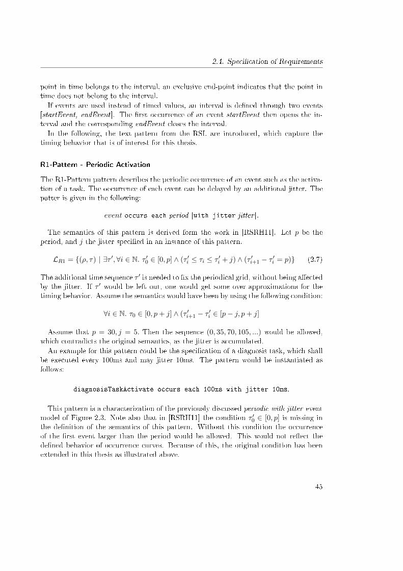
2.4. Speci�cation of Requirements
point in time belongs to the interval, an exclusive end-point indicates that the point intime does not belong to the interval.If events are used instead of timed values, an interval is de�ned through two events
[startEvent, endEvent ]. The �rst occurrence of an event startEvent then opens the in-terval and the corresponding endEvent closes the interval.In the following, the text-pattern from the RSL are introduced, which capture the
timing behavior that is of interest for this thesis.
R1-Pattern - Periodic Activation
The R1-Pattern pattern describes the periodic occurrence of an event such as the activa-tion of a task. The occurrence of each event can be delayed by an additional jitter. Thepatter is given in the following:
event occurs each period [with jitter jitter ].
The semantics of this pattern is derived form the work in [RSRH11]. Let p be theperiod, and j the jitter speci�ed in an instance of this pattern.
LR1 = {(ρ, τ) | ∃τ ′, ∀i ∈ N. τ ′0 ∈ [0, p] ∧ (τ ′i ≤ τi ≤ τ ′i + j) ∧ (τ ′i+1 − τ ′i = p)} (2.7)
The additional time sequence τ ′ is needed to �x the periodical grid, without being a�ectedby the jitter. If τ ′ would be left out, one would get some over-approximations for thetiming behavior. Assume the semantics would have been by using the following condition:
∀i ∈ N. τ0 ∈ [0, p+ j] ∧ (τ ′i+1 − τ ′i ∈ [p− j, p+ j]
Assume that p = 30, j = 5. Then the sequence (0, 35, 70, 105, ...) would be allowed,which contradicts the original semantics, as the jitter is accumulated.An example for this pattern could be the speci�cation of a diagnosis task, which shall
be executed every 100ms and may jitter 10ms. The pattern would be instantiated asfollows:
diagnosisTaskActivate occurs each 100ms with jitter 10ms.
This pattern is a characterization of the previously discussed periodic with jitter eventmodel of Figure 2.3. Note also that in [RSRH11] the condition τ ′0 ∈ [0, p] is missing inthe de�nition of the semantics of this pattern. Without this condition the occurrenceof the �rst event larger than the period would be allowed. This would not re�ect thede�ned behavior of occurrence curves. Because of this, the original condition has beenextended in this thesis as illustrated above.
45
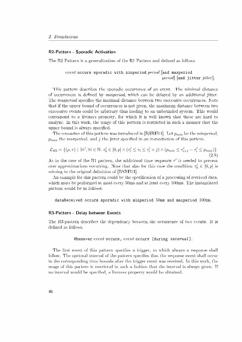
2. Foundations
R2-Pattern - Sporadic Activation
The R2-Pattern is a generalization of the R1-Pattern and de�ned as follows.
event occurs sporadic with minperiod period [and maxperiod
period ] [and jitter jitter ].
This pattern describes the sporadic occurrence of an event. The minimal distanceof occurrences is de�ned by minperiod, which can be delayed by an additional jitter.The maxperiod speci�es the maximal distance between two successive occurrences. Notethat if the upper bound of occurrences is not given, the maximum distance between twosuccessive events could be arbitrary thus leading to an unbounded system. This wouldcorrespond to a liveness property, for which it is well known that these are hard toanalyze. In this work, the usage of this pattern is restricted in such a manner that theupper bound is always speci�ed.The semantics of this pattern was introduced in [RSRH11]. Let pmin be the minperiod,
pmax the maxperiod, and j the jitter speci�ed in an instantiation of this pattern.
LR2 = {(ρ, τ) | ∃τ ′, ∀i ∈ N. τ ′0 ∈ [0, p] ∧ (τ ′i ≤ τi ≤ τ ′i + j) ∧ (pmin ≤ τ ′i+1 − τ ′i ≤ pmax)}(2.8)
As in the case of the R1-pattern, the additional time sequence τ ′ is needed to preventover-approximations occurring. Note that also for this case the condition τ ′0 ∈ [0, p] ismissing in the original de�nition of [RSRH11].An example for this pattern could be the speci�cation of a processing of received data,
which must be performed at most every 50ms and at least every 100ms. The instantiatedpattern would be as follows:
dataReceived occurs sporadic with minperiod 50ms and maxperiod 100ms.
R3-Pattern - Delay between Events
The R3-pattern describes the dependency between the occurrence of two events. It isde�ned as follows.
Whenever event occurs, event occurs [during interval ].
The �rst event of this pattern speci�es a trigger, to which always a response shallfollow. The optional interval of the pattern speci�es that the response event shall occurin the corresponding time bounds after the trigger event was received. In this work, theusage of this pattern is restricted in such a fashion that the interval is always given. Ifno interval would be speci�ed, a liveness property would be obtained.
46
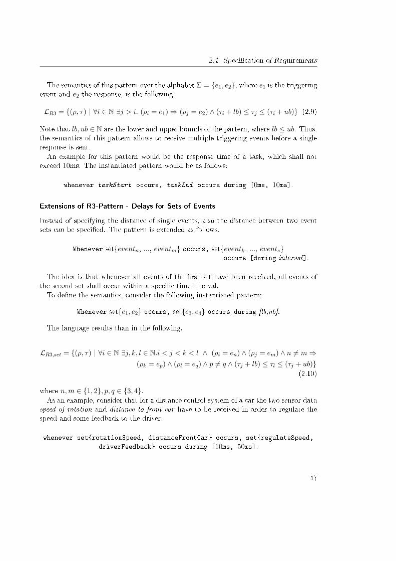
2.4. Speci�cation of Requirements
The semantics of this pattern over the alphabet Σ = {e1, e2}, where e1 is the triggeringevent and e2 the response, is the following.
LR3 = {(ρ, τ) | ∀i ∈ N ∃j > i. (ρi = e1)⇒ (ρj = e2) ∧ (τi + lb) ≤ τj ≤ (τi + ub)} (2.9)
Note that lb, ub ∈ N are the lower and upper bounds of the pattern, where lb ≤ ub. Thus,the semantics of this pattern allows to receive multiple triggering events before a singleresponse is sent.An example for this pattern would be the response time of a task, which shall not
exceed 10ms. The instantiated pattern would be as follows:
whenever taskStart occurs, taskEnd occurs during [0ms, 10ms].
Extensions of R3-Pattern - Delays for Sets of Events
Instead of specifying the distance of single events, also the distance between two eventsets can be speci�ed. The pattern is extended as follows.
Whenever set{eventn, ..., eventm} occurs, set{eventk, ..., events}occurs [during interval].
The idea is that whenever all events of the �rst set have been received, all events ofthe second set shall occur within a speci�c time interval.To de�ne the semantics, consider the following instantiated pattern:
Whenever set{e1, e2} occurs, set{e3, e4} occurs during [lb,ub].
The language results than in the following.
LR3,set = {(ρ, τ) | ∀i ∈ N ∃j, k, l ∈ N.i < j < k < l ∧ (ρi = en) ∧ (ρj = em) ∧ n 6= m⇒(ρk = ep) ∧ (ρl = eq) ∧ p 6= q ∧ (τj + lb) ≤ τl ≤ (τj + ub)}
(2.10)
where n,m ∈ {1, 2}, p, q ∈ {3, 4}.As an example, consider that for a distance control system of a car the two sensor data
speed of rotation and distance to front car have to be received in order to regulate thespeed and some feedback to the driver:
whenever set{rotationSpeed, distanceFrontCar} occurs, set{regulateSpeed,
driverFeedback} occurs during [10ms, 50ms].
47
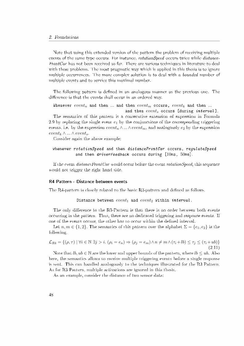
2. Foundations
Note that using this extended version of the pattern the problem of receiving multipleevents of the same type occurs. For instance, rotationSpeed occurs twice while distance-FrontCar has not been received so far. There are various techniques in literature to dealwith these problems. The most pragmatic way which is applied in this thesis is to ignoremultiple occurrences. The more complex solution is to deal with a bounded number ofmultiple events and to service this maximal number.
The following pattern is de�ned in an analogous manner as the previous one. Thedi�erence is that the events shall occur in an ordered way.
Whenever eventn and then ... and then eventm occurs, eventk and then ...and then events occurs [during interval ].
The semantics of this pattern is a consecutive extension of expression in Formula2.9 by replacing the single event e1 by the conjunctions of the corresponding triggeringevents, i.e. by the expression eventn ∧ ...∧ eventm, and analogously e2 by the expressioneventk ∧ ... ∧ events.Consider again the above example:
whenever rotationSpeed and then distanceFrontCar occurs, regulateSpeed
and then driverFeedback occurs during [10ms, 50ms].
If the event distanceFrontCar would occur before the event rotationSpeed, this sequencewould not trigger the right hand side.
R4 Pattern - Distance between events
The R4-pattern is closely related to the basic R3-pattern and de�ned as follows.
Distance between event1 and event2 within interval .
The only di�erence to the R3-Pattern is that there is no order between both eventsoccurring in the pattern. Thus, there are no dedicated triggering and response events. Ifone of the events occurs, the other has to occur within the de�ned interval.Let n,m ∈ {1, 2}. The semantics of this pattern over the alphabet Σ = {e1, e2} is the
following.
LR4 = {(ρ, τ) | ∀i ∈ N ∃j > i. (ρi = en)⇒ (ρj = em)∧n 6= m∧ (τi+ lb) ≤ τj ≤ (τi+ub)}(2.11)
Note that lb, ub ∈ N are the lower and upper bounds of the pattern, where lb ≤ ub. Alsohere, the semantics allows to receive multiple triggering events before a single responseis sent. This can handled analogously to the techniques illustrated for the R3-Pattern.As for R3-Pattern, multiple activations are ignored in this thesis.As an example, consider the distance of two sensor data:
48
2.5. Summary
Distance between rotationSpeed and distanceFrontCar within [5, 10]ms.
Whenever one of the two events rotationSpeed or distanceFrontCar occurs, the otherevent has to occur within the de�ned time interval.
2.5. Summary
In this chapter, all necessary ingredients for a model-based design of real-time systemshave been introduced and the underlying semantics were discussed. The speci�cationof tasks and the underlying architecture consisting of inter-related components and re-sources was formalized and the modeling by using Marte was discussed. Requirementsof architectures and their decomposition structures are speci�ed using the pattern-basedlanguage called Requirement Speci�cation Language (RSL). The distinction of assumedand guaranteed behaviors was discussed by using the notion of contracts. By using con-tracts proof obligations arise, including the correctness check of decomposition structures,i. e. the check whether the contract of an overall component follows from the contractsof its parts, and whether all contracts ��t together�. Further, the satisfaction of theimplementation of a component or resource has to be checked, i. e. it has to be veri�edwhether the implementation in terms of some automata structure or program code ful�llsthe corresponding contracts.
49

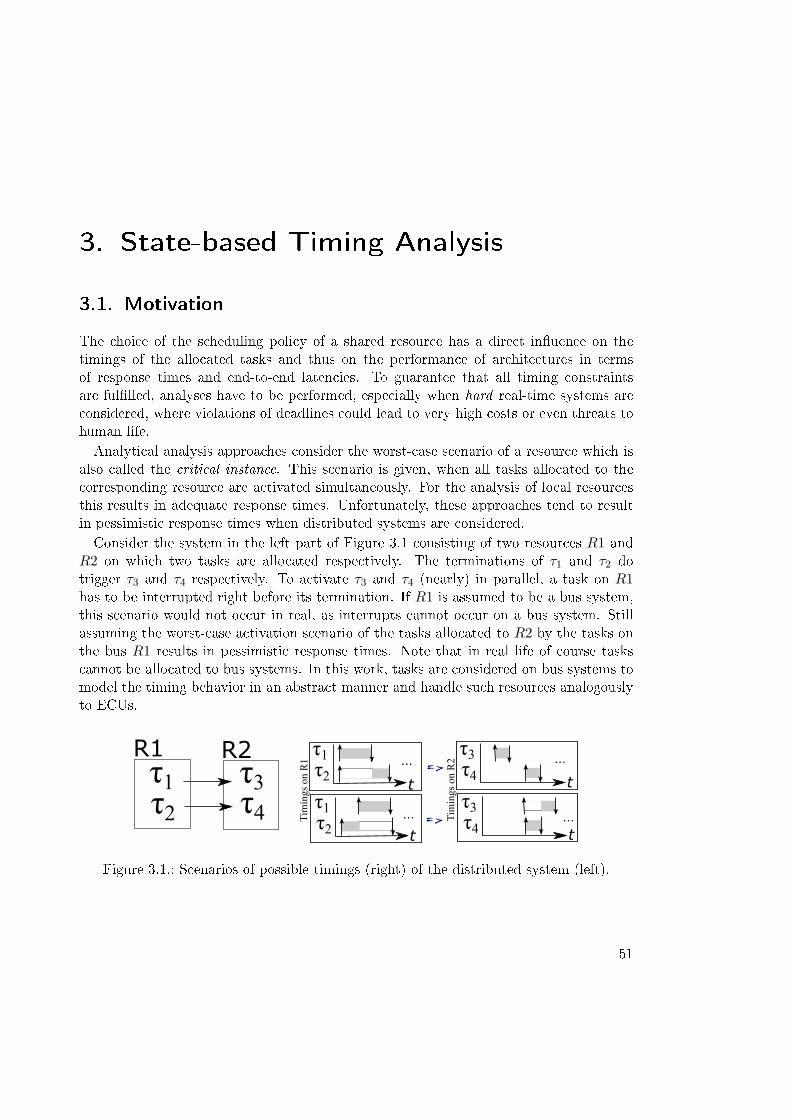
3. State-based Timing Analysis
3.1. Motivation
The choice of the scheduling policy of a shared resource has a direct in�uence on thetimings of the allocated tasks and thus on the performance of architectures in termsof response times and end-to-end latencies. To guarantee that all timing constraintsare ful�lled, analyses have to be performed, especially when hard real-time systems areconsidered, where violations of deadlines could lead to very high costs or even threats tohuman life.Analytical analysis approaches consider the worst-case scenario of a resource which is
also called the critical instance. This scenario is given, when all tasks allocated to thecorresponding resource are activated simultaneously. For the analysis of local resourcesthis results in adequate response times. Unfortunately, these approaches tend to resultin pessimistic response times when distributed systems are considered.Consider the system in the left part of Figure 3.1 consisting of two resources R1 and
R2 on which two tasks are allocated respectively. The terminations of τ1 and τ2 dotrigger τ3 and τ4 respectively. To activate τ3 and τ4 (nearly) in parallel, a task on R1has to be interrupted right before its termination. If R1 is assumed to be a bus system,this scenario would not occur in real, as interrupts cannot occur on a bus system. Stillassuming the worst-case activation scenario of the tasks allocated to R2 by the tasks onthe bus R1 results in pessimistic response times. Note that in real life of course taskscannot be allocated to bus systems. In this work, tasks are considered on bus systems tomodel the timing behavior in an abstract manner and handle such resources analogouslyto ECUs.
τ1τ2
τ3τ4
R1 R2 τ1τ2
tτ1τ2 t
=>
=>TimingsonR1
τ3τ4 tτ3τ4 t
TimingsonR2...
...
...
...
Figure 3.1.: Scenarios of possible timings (right) of the distributed system (left).
51
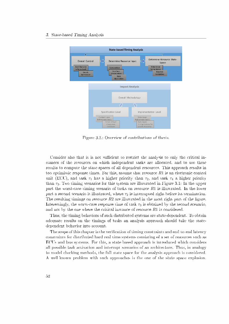
3. State-based Timing Analysis
Figure 3.2.: Overview of contributions of thesis.
Consider also that it is not su�cient to restrict the analysis to only the critical in-stances of the resources on which independent tasks are allocated, and to use theseresults to compute the state spaces of all dependent resources. This approach results intoo optimistic response times. For this, assume that resource R1 is an electronic controlunit (ECU), and task τ1 has a higher priority than τ2, and task τ4 a higher prioritythan τ3. Two timing scenarios for this system are illustrated in Figure 3.1: In the upperpart the worst-case timing scenario of tasks on resource R1 is illustrated. In the lowerpart a second scenario is illustrated, where τ2 is interrupted right before its termination.The resulting timings on resource R2 are illustrated in the most right part of the �gure.Interestingly, the worst-case response time of task τ3 is obtained by the second scenario,and not by the one where the critical instance of resource R1 is considered.
Thus, the timing behaviors of such distributed systems are state-dependent. To obtainadequate results on the timings of tasks an analysis approach should take the state-dependent behavior into account.
The scope of this chapter is the veri�cation of timing constraints and end-to-end latencyconstraints for distributed hard real-time systems consisting of a set of resources such asECUs and bus systems. For this, a state-based approach is introduced which considersall possible task activation and interrupt scenarios of an architecture. Thus, in analogyto model checking methods, the full state space for the analysis approach is considered.A well-known problem with such approaches is the one of the state space explosion.
52
3.2. Related Work
To handle this problem the state space of an architecture is constructed in an iterativemanner. On the interfaces of dependent resources minimization and abstraction methodsare applied to keep the resulting state spaces as small as possible. The worked outapproach was presented the �rst time in [GHRS12], and was later re�ned and extendedin subsequent publications [GSHR13a, GSHR13b].Referring to the overall content of this thesis, which is illustrated in Figure 3.2, this
chapter deals with the state-based timing analysis part illustrated in the upper part ofthe �gure. This analysis approach will serve as the foundation of the impact analysisapproach introduced in Chapter 4 as illustrated in the lower part of Figure 3.2, i.e. theimpact analysis will use the state-based timing analysis whenever necessary.This chapter is organized as follows. First, relevant related works are detailed which
address the analysis of hard real-time systems. In Section 3.3 the general analysis ap-proach worked out in this thesis is sketched. The state space of a resource is concretizedand a simpli�ed version of the symbolic transition systems is introduced. To realize aniterative analysis, in Section 3.4 the abstraction and composition operations for STSsare presented. Section 3.5 details the computation of a resource STS. In Section 3.6further abstraction techniques leading to more pessimistic response times while boostingthe scalability of the approach are introduced. In Section 3.7 the analysis approach isapplied to a driver assistance system case study. Finally, a summary of this chapter isgiven.
3.2. Related Work
There are two relevant research topics for this thesis, i.e. the analytical and the modelchecking-based analysis approaches for timing properties. First, the analytical � whichare also referred to as classical � approaches are detailed. Then, the model checkingapproaches are considered. The last category of related works which is considered hereis a combination of both the classical and model checking approaches.
3.2.1. Classical Analytical Approaches
In general, analytical methods are stateless methods, which solve closed form expressions.Thus, such analyses are fast and scale good with the size of the system. Unfortunately, fordistributed systems with task dependencies these approaches tend to result in pessimisticresponse times as illustrated in the introduction of this chapter. These approaches arealso not good in analyzing other relevant system properties like event ordering or safetyproperties, as for this a representation of the concrete system state is necessary.There are many works addressing the classical scheduling analyses which makes it im-
possible to give a complete list of all works. The focus here is on the most relevant worksfor the Fixed Priority Scheduling (FPS) approach, which is in the scope of this thesis.The most common holistic and compositional approaches in literature are presented here.
53
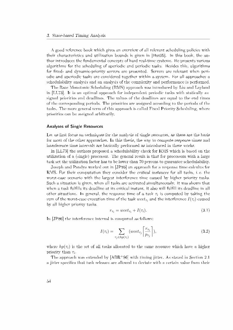
3. State-based Timing Analysis
A good reference book which gives an overview of all relevant scheduling policies withtheir characteristics and utilization bounds is given in [But05]. In this book, the au-thor introduces the fundamental concepts of hard real-time systems. He presents variousalgorithms for the scheduling of aperiodic and periodic tasks. Besides this, algorithmsfor �xed- and dynamic-priority servers are presented. Servers are relevant when peri-odic and aperiodic tasks are considered together within a system. For all approaches aschedulability analysis and an analysis of the complexity and performance is performed.The Rate-Monotonic Scheduling (RMS) approach was introduced by Liu and Layland
in [LL73]. It is an optimal approach for independent periodic tasks with statically as-signed priorities and deadlines. The values of the deadlines are equal to the end timesof the corresponding periods. The priorities are assigned according to the periods of thetasks. The more general term of this approach is called Fixed Priority Scheduling, wherepriorities can be assigned arbitrarily.
Analyses of Single Resources
Let us �rst focus on techniques for the analysis of single resources, as these are the basisfor most of the other approaches. In this thesis, the way to compute response times andinterference time intervals are basically performed as introduced in these works.In [LL73] the authors proposed a schedulability check for RMS which is based on the
utilization of a (single) processor. The general result is that for processors with a largetask set the utilization factor has to be lower than 70 percent to guarantee schedulability.Joseph and Pandya worked out in [JP86] an approach for a response time calculus for
RMS. For their computation they consider the critical instances for all tasks, i. e. theworst-case scenario with the largest interference time caused by higher priority tasks.Such a situation is given, when all tasks are activated simultaneously. It was shown thatwhen a task ful�lls its deadline at its critical instant, it also will ful�ll its deadline in allother situations. In general, the response time of a task τi is computed by taking thesum of the worst-case execution time of the task wcetτi and the interference I(τi) causedby all higher priority tasks.
rτi = wcetτi + I(τi). (3.1)
In [JP86] the interference interval is computed as follows:
I(τi) =∑
τj∈hp(τi)
(wcetτj
⌈rτipτj
⌉), (3.2)
where hp(τi) is the set of all tasks allocated to the same resource which have a higherpriority than τi.The approach was extended by [ABR+86] with timing jitter. As stated in Section 2.1
a jitter speci�es that task releases are allowed to deviate with a certain value from their
54
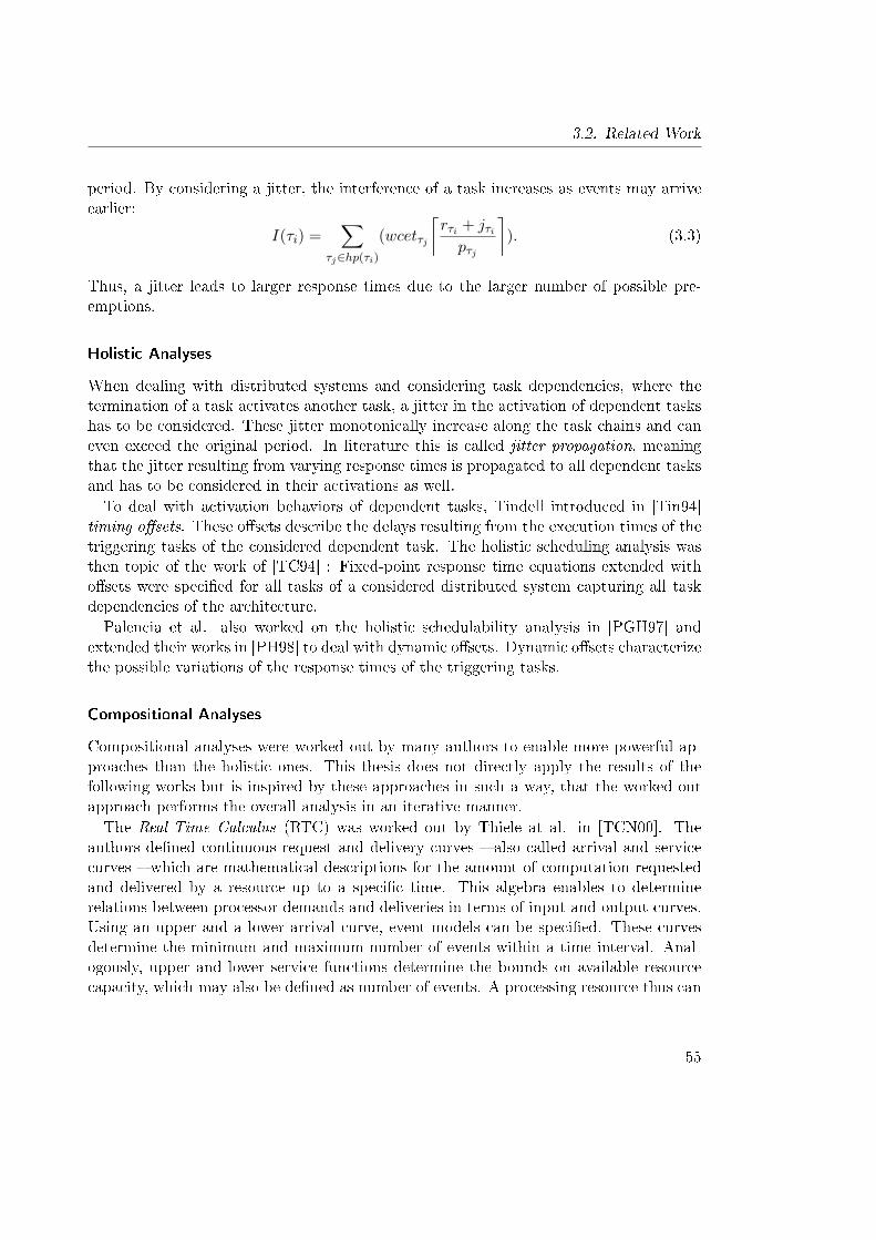
3.2. Related Work
period. By considering a jitter, the interference of a task increases as events may arriveearlier:
I(τi) =∑
τj∈hp(τi)
(wcetτj
⌈rτi + jτipτj
⌉). (3.3)
Thus, a jitter leads to larger response times due to the larger number of possible pre-emptions.
Holistic Analyses
When dealing with distributed systems and considering task dependencies, where thetermination of a task activates another task, a jitter in the activation of dependent taskshas to be considered. These jitter monotonically increase along the task chains and caneven exceed the original period. In literature this is called jitter propagation, meaningthat the jitter resulting from varying response times is propagated to all dependent tasksand has to be considered in their activations as well.To deal with activation behaviors of dependent tasks, Tindell introduced in [Tin94]
timing o�sets. These o�sets describe the delays resulting from the execution times of thetriggering tasks of the considered dependent task. The holistic scheduling analysis wasthen topic of the work of [TC94] : Fixed-point response time equations extended witho�sets were speci�ed for all tasks of a considered distributed system capturing all taskdependencies of the architecture.Palencia et al. also worked on the holistic schedulability analysis in [PGH97] and
extended their works in [PH98] to deal with dynamic o�sets. Dynamic o�sets characterizethe possible variations of the response times of the triggering tasks.
Compositional Analyses
Compositional analyses were worked out by many authors to enable more powerful ap-proaches than the holistic ones. This thesis does not directly apply the results of thefollowing works but is inspired by these approaches in such a way, that the worked outapproach performs the overall analysis in an iterative manner.The Real-Time Calculus (RTC) was worked out by Thiele at al. in [TCN00]. The
authors de�ned continuous request and delivery curves � also called arrival and servicecurves � which are mathematical descriptions for the amount of computation requestedand delivered by a resource up to a speci�c time. This algebra enables to determinerelations between processor demands and deliveries in terms of input and output curves.Using an upper and a lower arrival curve, event models can be speci�ed. These curvesdetermine the minimum and maximum number of events within a time interval. Anal-ogously, upper and lower service functions determine the bounds on available resourcecapacity, which may also be de�ned as number of events. A processing resource thus can
55
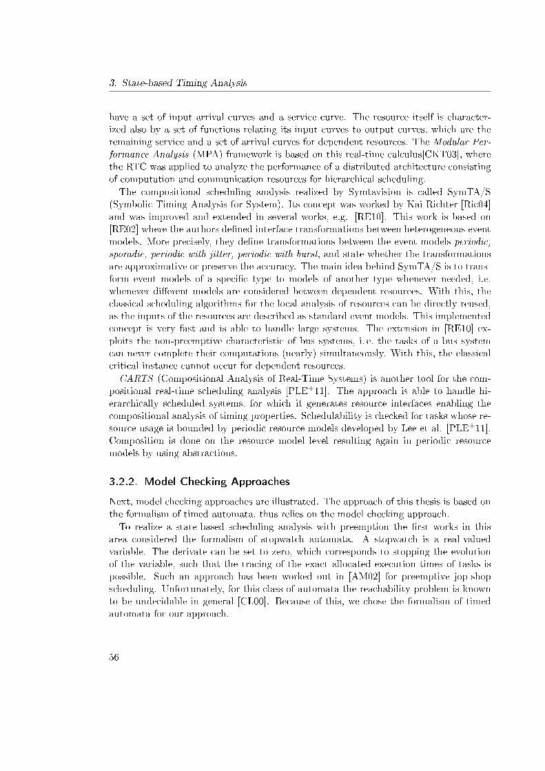
3. State-based Timing Analysis
have a set of input arrival curves and a service curve. The resource itself is character-ized also by a set of functions relating its input curves to output curves, which are theremaining service and a set of arrival curves for dependent resources. The Modular Per-formance Analysis (MPA) framework is based on this real-time calculus[CKT03], wherethe RTC was applied to analyze the performance of a distributed architecture consistingof computation and communication resources for hierarchical scheduling.The compositional scheduling analysis realized by Symtavision is called SymTA/S
(Symbolic Timing Analysis for System). Its concept was worked by Kai Richter [Ric04]and was improved and extended in several works, e.g. [RE10]. This work is based on[RE02] where the authors de�ned interface transformations between heterogeneous eventmodels. More precisely, they de�ne transformations between the event models periodic,sporadic, periodic with jitter, periodic with burst, and state whether the transformationsare approximative or preserve the accuracy. The main idea behind SymTA/S is to trans-form event models of a speci�c type to models of another type whenever needed, i.e.whenever di�erent models are considered between dependent resources. With this, theclassical scheduling algorithms for the local analysis of resources can be directly reused,as the inputs of the resources are described as standard event models. This implementedconcept is very fast and is able to handle large systems. The extension in [RE10] ex-ploits the non-preemptive characteristic of bus systems, i. e. the tasks of a bus systemcan never complete their computations (nearly) simultaneously. With this, the classicalcritical instance cannot occur for dependent resources.CARTS (Compositional Analysis of Real-Time Systems) is another tool for the com-
positional real-time scheduling analysis [PLE+11]. The approach is able to handle hi-erarchically scheduled systems, for which it generates resource interfaces enabling thecompositional analysis of timing properties. Schedulability is checked for tasks whose re-source usage is bounded by periodic resource models developed by Lee et al. [PLE+11].Composition is done on the resource model level resulting again in periodic resourcemodels by using abstractions.
3.2.2. Model Checking Approaches
Next, model checking approaches are illustrated. The approach of this thesis is based onthe formalism of timed automata, thus relies on the model checking approach.To realize a state-based scheduling analysis with preemption the �rst works in this
area considered the formalism of stopwatch automata. A stopwatch is a real-valuedvariable. The derivate can be set to zero, which corresponds to stopping the evolutionof the variable, such that the tracing of the exact allocated execution times of tasks ispossible. Such an approach has been worked out in [AM02] for preemptive jop-shopscheduling. Unfortunately, for this class of automata the reachability problem is knownto be undecidable in general [CL00]. Because of this, we chose the formalism of timedautomata for our approach.
56
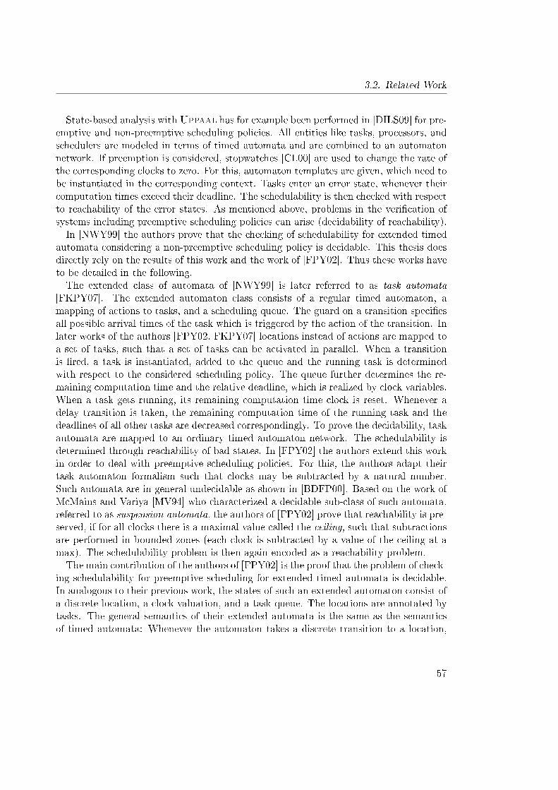
3.2. Related Work
State-based analysis with Uppaal has for example been performed in [DILS09] for pre-emptive and non-preemptive scheduling policies. All entities like tasks, processors, andschedulers are modeled in terms of timed automata and are combined to an automatonnetwork. If preemption is considered, stopwatches [CL00] are used to change the rate ofthe corresponding clocks to zero. For this, automaton templates are given, which need tobe instantiated in the corresponding context. Tasks enter an error state, whenever theircomputation times exceed their deadline. The schedulability is then checked with respectto reachability of the error states. As mentioned above, problems in the veri�cation ofsystems including preemptive scheduling policies can arise (decidability of reachability).In [NWY99] the authors prove that the checking of schedulability for extended timed
automata considering a non-preemptive scheduling policy is decidable. This thesis doesdirectly rely on the results of this work and the work of [FPY02]. Thus these works haveto be detailed in the following.The extended class of automata of [NWY99] is later referred to as task automata
[FKPY07]. The extended automaton class consists of a regular timed automaton, amapping of actions to tasks, and a scheduling queue. The guard on a transition speci�esall possible arrival times of the task which is triggered by the action of the transition. Inlater works of the authors [FPY02, FKPY07] locations instead of actions are mapped toa set of tasks, such that a set of tasks can be activated in parallel. When a transitionis �red, a task is instantiated, added to the queue and the running task is determinedwith respect to the considered scheduling policy. The queue further determines the re-maining computation time and the relative deadline, which is realized by clock variables.When a task gets running, its remaining computation time clock is reset. Whenever adelay transition is taken, the remaining computation time of the running task and thedeadlines of all other tasks are decreased correspondingly. To prove the decidability, taskautomata are mapped to an ordinary timed automaton network. The schedulability isdetermined through reachability of bad states. In [FPY02] the authors extend this workin order to deal with preemptive scheduling policies. For this, the authors adapt theirtask automaton formalism such that clocks may be subtracted by a natural number.Such automata are in general undecidable as shown in [BDFP00]. Based on the work ofMcMains and Variya [MV94] who characterized a decidable sub-class of such automata,referred to as suspension automata, the authors of [FPY02] prove that reachability is pre-served, if for all clocks there is a maximal value called the ceiling, such that subtractionsare performed in bounded zones (each clock is subtracted by a value of the ceiling at amax). The schedulability problem is then again encoded as a reachability problem.The main contribution of the authors of [FPY02] is the proof that the problem of check-
ing schedulability for preemptive scheduling for extended timed automata is decidable.In analogous to their previous work, the states of such an extended automaton consist ofa discrete location, a clock valuation, and a task queue. The locations are annotated bytasks. The general semantics of their extended automata is the same as the semanticsof timed automata: Whenever the automaton takes a discrete transition to a location,
57
3. State-based Timing Analysis
an instance of each task with which the location is annotated, is created and added tothe task queue. The task queue is a sorted list consisting of instances of tasks togetherwith their remaining computation times and deadlines, which are real valued variables.Delay transitions correspond to either resource idle times when no task is active, or theexecution of running tasks. If the automaton takes a delay transition, the remainingcomputation time of the running task and all deadlines of the other tasks are decreasedby the corresponding delay value. The schedulability is encoded as the reachability ofbad states: If there exists a state containing a task which violates its deadline but whichstill has a remaining computation time, the bad state is entered. Results of this workwere also implemented in the Times tool [AFM+04]. It is based on the Uppaal DBMlibrary, which was extended with subtraction operations on DBMs. In contrast to ourapproach, the Times tool performs analysis tasks in a holistic manner.In [KY04, FKPY07] the authors extend their work of [FPY02] and determined the
decidability and undecidability class of task automata. Their main result is that wheninterval computation times of tasks (which is the distinction between best- and worst-caseexecution times), �nishing times of tasks release new task instances, data dependencies,and preemption is considered, the problem for this class of automata is undecidable.Fortunately, the above mentioned subtraction operation is not needed to deal with
preemptive scheduling policies, as it was also demonstrated in [HV06]. The authors ofthis work use the original timed automaton formalism to model this problem and verifytiming properties by using Uppaal. As a front-end they use sequence diagrams, fromwhich timed automata are derived. The approach is applied on an in-car radio navigationsystem case study, where end-to-end latency deadlines to change the volume of the radioand the reception of tra�c message channel (TMC) signals from a radio station arespeci�ed. In [PWT+07] these automaton models were reused to apply the approach ona set of benchmark systems and to compare the analysis results to other techniques suchas MPA or SymTA/S. Unfortunately, the work of [HV06] illustrates only an instantiationof timed automata for a couple of example architectures to perform the analysis. It doesnot illustrate a general concept to automatically build the automaton network of a givensystem architecture and perform the analysis.The work presented in [BH09] deals with an extension of timed automata. The pre-
sented model is called Interrupt Timed Automata (ITA) as they de�ne interrupt levels asa control structure. On each level exactly one clock is active, where clocks from higherlevel suspend clocks on all lower levels. Guards on transitions are linear expressionsover clocks from the current level and all levels below. Updates are linear expressionsonly over clocks at levels below. This restricted model of stopwatch-automata has thecharacteristic that the reachability problem remains decidable. The model is not moreexpressive than the approaches illustrated above. In contrast to this work, the approachworks in a holistic manner. Also, the introduced formalism seems not to be as intuitiveas the formalism of timed automata.In [MC09] a compositional, timed automaton-based analysis technique for preemptive,
58
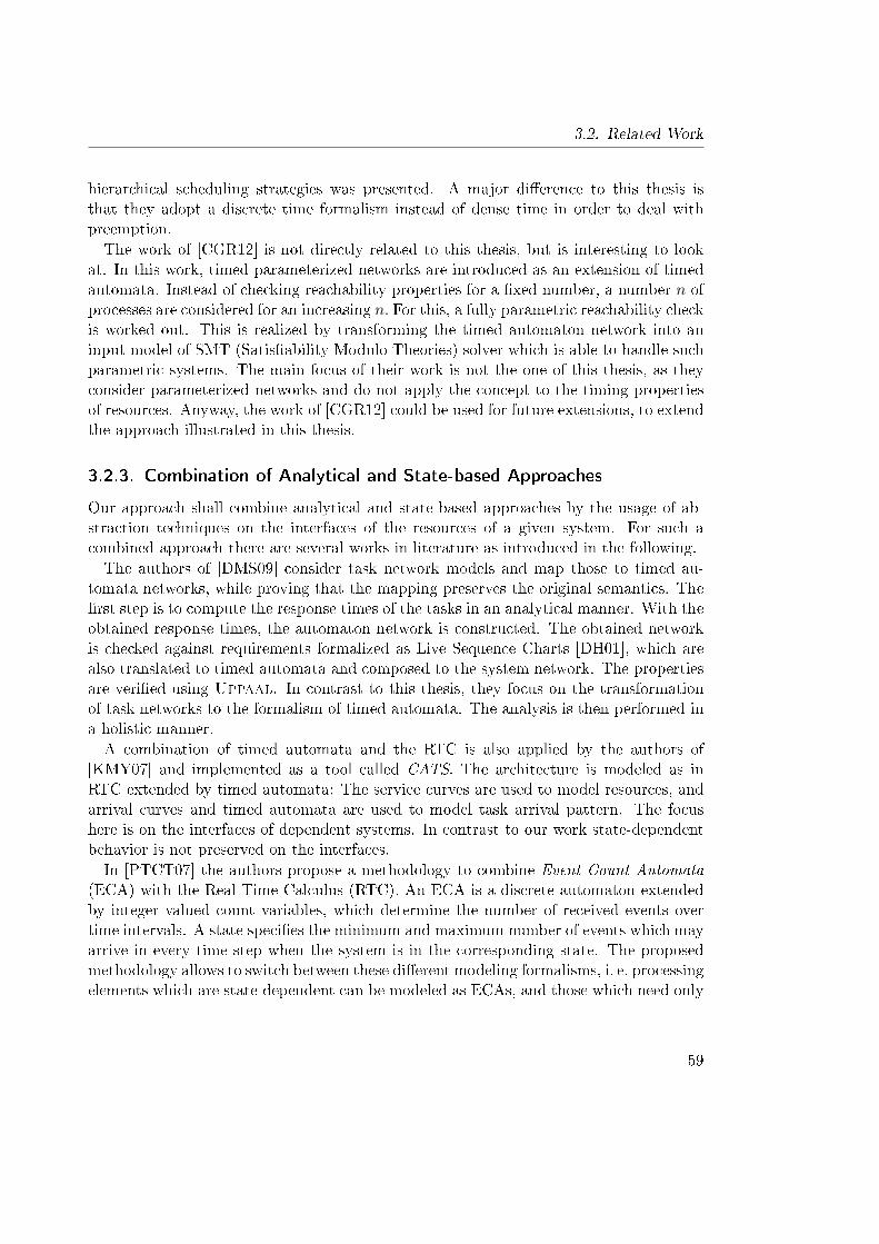
3.2. Related Work
hierarchical scheduling strategies was presented. A major di�erence to this thesis isthat they adopt a discrete time formalism instead of dense time in order to deal withpreemption.The work of [CGR12] is not directly related to this thesis, but is interesting to look
at. In this work, timed parameterized networks are introduced as an extension of timedautomata. Instead of checking reachability properties for a �xed number, a number n ofprocesses are considered for an increasing n. For this, a fully parametric reachability checkis worked out. This is realized by transforming the timed automaton network into aninput model of SMT (Satis�ability Modulo Theories) solver which is able to handle suchparametric systems. The main focus of their work is not the one of this thesis, as theyconsider parameterized networks and do not apply the concept to the timing propertiesof resources. Anyway, the work of [CGR12] could be used for future extensions, to extendthe approach illustrated in this thesis.
3.2.3. Combination of Analytical and State-based Approaches
Our approach shall combine analytical and state-based approaches by the usage of ab-straction techniques on the interfaces of the resources of a given system. For such acombined approach there are several works in literature as introduced in the following.The authors of [DMS09] consider task network models and map those to timed au-
tomata networks, while proving that the mapping preserves the original semantics. The�rst step is to compute the response times of the tasks in an analytical manner. With theobtained response times, the automaton network is constructed. The obtained networkis checked against requirements formalized as Live Sequence Charts [DH01], which arealso translated to timed automata and composed to the system network. The propertiesare veri�ed using Uppaal. In contrast to this thesis, they focus on the transformationof task networks to the formalism of timed automata. The analysis is then performed ina holistic manner.A combination of timed automata and the RTC is also applied by the authors of
[KMY07] and implemented as a tool called CATS. The architecture is modeled as inRTC extended by timed automata: The service curves are used to model resources, andarrival curves and timed automata are used to model task arrival pattern. The focushere is on the interfaces of dependent systems. In contrast to our work state-dependentbehavior is not preserved on the interfaces.In [PTCT07] the authors propose a methodology to combine Event Count Automata
(ECA) with the Real-Time Calculus (RTC). An ECA is a discrete automaton extendedby integer valued count variables, which determine the number of received events overtime intervals. A state speci�es the minimum and maximum number of events which mayarrive in every time step when the system is in the corresponding state. The proposedmethodology allows to switch between these di�erent modeling formalisms, i. e. processingelements which are state-dependent can be modeled as ECAs, and those which need only
59
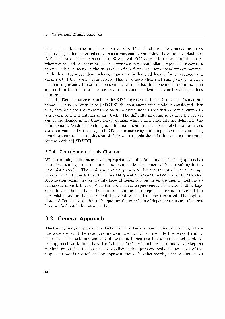
3. State-based Timing Analysis
information about the input event streams by RTC functions. To connect resourcesmodeled by di�erent formalisms, transformations between these have been worked out.Arrival curves can be translated to ECAs, and ECAs are able to be translated backwhenever needed. As our approach, this work realizes a non-holistic approach. In contrastto our work they focus on the translation of the formalisms for dependent components.With this, state-dependent behavior can only be handled locally for a resource or asmall part of the overall architecture. This is because when performing the translationby counting events, the state-dependent behavior is lost for dependent resources. Theapproach in this thesis tries to preserve the state-dependent behavior for all dependentresources.In [LPT09] the authors combine the RTC approach with the formalism of timed au-
tomata. Thus, in contrast to [PTCT07] the continuous time model is considered. Forthis, they describe the transformation from event models speci�ed as arrival curves toa network of timed automata, and back. The di�culty in doing so is that the arrivalcurves are de�ned in the time interval domain while timed automata are de�ned in thetime domain. With this technique, individual resources may be modeled in an abstractstateless manner by the usage of RTC, or considering state-dependent behavior usingtimed automata. The distinction of their work to this thesis is the same as illustratedfor the work of [PTCT07].
3.2.4. Contribution of this Chapter
What is missing in literature is an appropriate combination of model checking approachesto analyze timing properties in a more compositional manner, without resulting in toopessimistic results. The timing analysis approach of this chapter introduces a new ap-proach, which is interface driven: The state spaces of resources are computed successively.Abstraction techniques on the interfaces of dependent resources are then worked out toreduce the input behavior. With this reduced state space enough behavior shall be keptsuch that on the one hand the timings of the tasks on dependent resources are not toopessimistic, and on the other hand the overall veri�cation time is reduced. The applica-tion of di�erent abstraction techniques on the interfaces of dependent resources has notbeen worked out in literature so far.
3.3. General Approach
The timing analysis approach worked out in this thesis is based on model checking, wherethe state spaces of the resources are computed, which encapsulate the relevant timinginformation for tasks and end-to-end latencies. In contrast to standard model checking,this approach works in an iterative fashion. The interfaces between resources are kept asminimal as possible to boost the scalability of the approach, while the accuracy of theresponse times is not a�ected by approximations. In other words, whenever interfaces
60
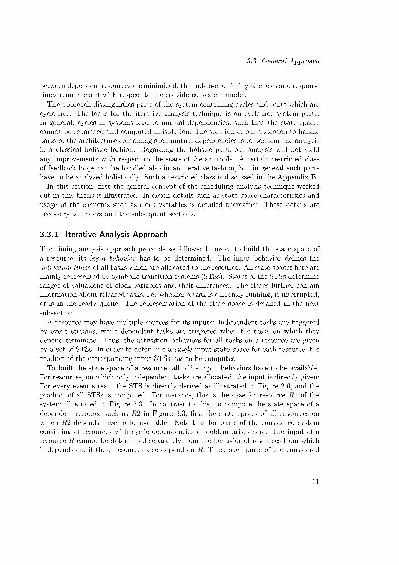
3.3. General Approach
between dependent resources are minimized, the end-to-end timing latencies and responsetimes remain exact with respect to the considered system model.The approach distinguishes parts of the system containing cycles and parts which are
cycle-free. The focus for the iterative analysis technique is on cycle-free system parts.In general, cycles in systems lead to mutual dependencies, such that the state spacescannot be separated and computed in isolation. The solution of our approach to handleparts of the architecture containing such mutual dependencies is to perform the analysisin a classical holistic fashion. Regarding the holistic part, our analysis will not yieldany improvements with respect to the state-of-the-art tools. A certain restricted classof feedback loops can be handled also in an iterative fashion, but in general such partshave to be analyzed holistically. Such a restricted class is discussed in the Appendix B.In this section, �rst the general concept of the scheduling analysis technique worked
out in this thesis is illustrated. In-depth details such as state space characteristics andusage of the elements such as clock variables is detailed thereafter. These details arenecessary to understand the subsequent sections.
3.3.1. Iterative Analysis Approach
The timing analysis approach proceeds as follows: In order to build the state space ofa resource, its input behavior has to be determined. The input behavior de�nes theactivation times of all tasks which are allocated to the resource. All state spaces here aremainly represented by symbolic transition systems (STSs). States of the STSs determineranges of valuations of clock variables and their di�erences. The states further containinformation about released tasks, i.e. whether a task is currently running, is interrupted,or is in the ready queue. The representation of the state space is detailed in the nextsubsection.A resource may have multiple sources for its inputs: Independent tasks are triggered
by event streams, while dependent tasks are triggered when the tasks on which theydepend terminate. Thus, the activation behaviors for all tasks on a resource are givenby a set of STSs. In order to determine a single input state space for each resource, theproduct of the corresponding input STSs has to be computed.To built the state space of a resource, all of its input behaviors have to be available.
For resources, on which only independent tasks are allocated, the input is directly given:For every event stream the STS is directly derived as illustrated in Figure 2.6, and theproduct of all STSs is computed. For instance, this is the case for resource R1 of thesystem illustrated in Figure 3.3. In contrast to this, to compute the state space of adependent resource such as R2 in Figure 3.3, �rst the state spaces of all resources onwhich R2 depends have to be available. Note that for parts of the considered systemconsisting of resources with cyclic dependencies a problem arises here: The input of aresource R cannot be determined separately from the behavior of resources from whichit depends on, if these resources also depend on R. Thus, such parts of the considered
61
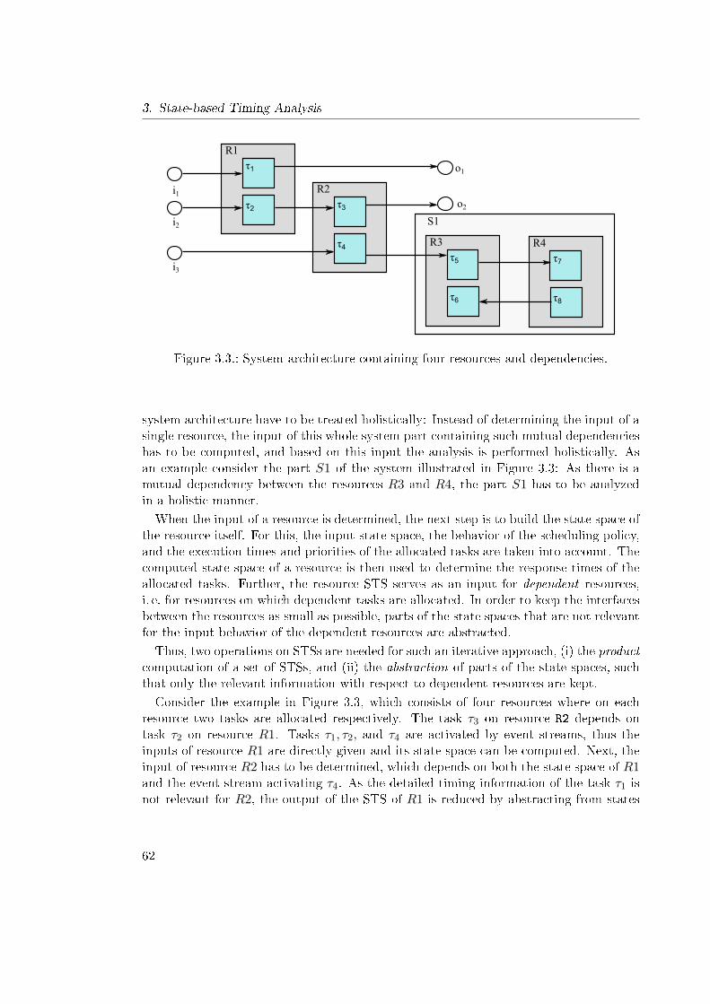
3. State-based Timing Analysis
τ1
τ2
R1
i1
i2
τ3
τ4
R2
i3
o1
o2
τ5
τ6
R3
τ7
τ8
R4
S1
Figure 3.3.: System architecture containing four resources and dependencies.
system architecture have to be treated holistically: Instead of determining the input of asingle resource, the input of this whole system part containing such mutual dependencieshas to be computed, and based on this input the analysis is performed holistically. Asan example consider the part S1 of the system illustrated in Figure 3.3: As there is amutual dependency between the resources R3 and R4, the part S1 has to be analyzedin a holistic manner.
When the input of a resource is determined, the next step is to build the state space ofthe resource itself. For this, the input state space, the behavior of the scheduling policy,and the execution times and priorities of the allocated tasks are taken into account. Thecomputed state space of a resource is then used to determine the response times of theallocated tasks. Further, the resource STS serves as an input for dependent resources,i. e. for resources on which dependent tasks are allocated. In order to keep the interfacesbetween the resources as small as possible, parts of the state spaces that are not relevantfor the input behavior of the dependent resources are abstracted.
Thus, two operations on STSs are needed for such an iterative approach, (i) the productcomputation of a set of STSs, and (ii) the abstraction of parts of the state spaces, suchthat only the relevant information with respect to dependent resources are kept.
Consider the example in Figure 3.3, which consists of four resources where on eachresource two tasks are allocated respectively. The task τ3 on resource R2 depends ontask τ2 on resource R1. Tasks τ1, τ2, and τ4 are activated by event streams, thus theinputs of resource R1 are directly given and its state space can be computed. Next, theinput of resource R2 has to be determined, which depends on both the state space of R1and the event stream activating τ4. As the detailed timing information of the task τ1 isnot relevant for R2, the output of the STS of R1 is reduced by abstracting from states
62
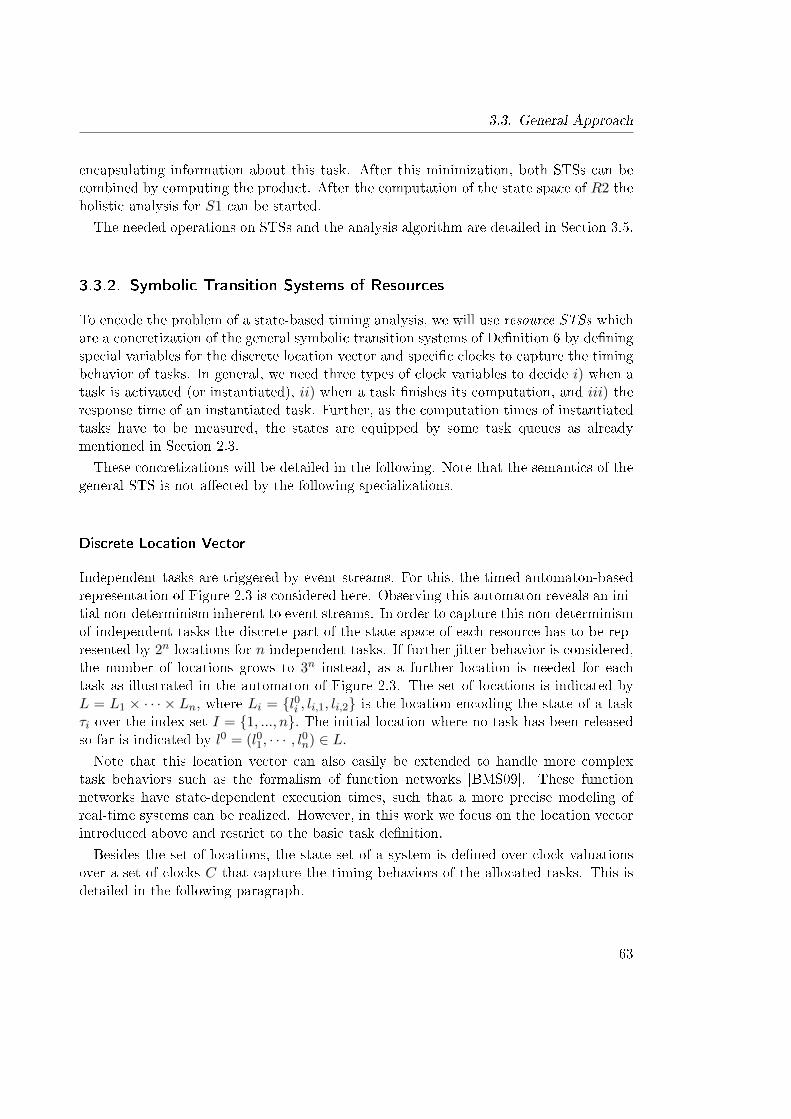
3.3. General Approach
encapsulating information about this task. After this minimization, both STSs can becombined by computing the product. After the computation of the state space of R2 theholistic analysis for S1 can be started.
The needed operations on STSs and the analysis algorithm are detailed in Section 3.5.
3.3.2. Symbolic Transition Systems of Resources
To encode the problem of a state-based timing analysis, we will use resource STSs whichare a concretization of the general symbolic transition systems of De�nition 6 by de�ningspecial variables for the discrete location vector and speci�c clocks to capture the timingbehavior of tasks. In general, we need three types of clock variables to decide i) when atask is activated (or instantiated), ii) when a task �nishes its computation, and iii) theresponse time of an instantiated task. Further, as the computation times of instantiatedtasks have to be measured, the states are equipped by some task queues as alreadymentioned in Section 2.3.
These concretizations will be detailed in the following. Note that the semantics of thegeneral STS is not a�ected by the following specializations.
Discrete Location Vector
Independent tasks are triggered by event streams. For this, the timed automaton-basedrepresentation of Figure 2.3 is considered here. Observing this automaton reveals an ini-tial non-determinism inherent to event streams. In order to capture this non-determinismof independent tasks the discrete part of the state space of each resource has to be rep-resented by 2n locations for n independent tasks. If further jitter behavior is considered,the number of locations grows to 3n instead, as a further location is needed for eachtask as illustrated in the automaton of Figure 2.3. The set of locations is indicated byL = L1 × · · · × Ln, where Li = {l0i , li,1, li,2} is the location encoding the state of a taskτi over the index set I = {1, ..., n}. The initial location where no task has been releasedso far is indicated by l0 = (l01, · · · , l0n) ∈ L.Note that this location vector can also easily be extended to handle more complex
task behaviors such as the formalism of function networks [BMS09]. These functionnetworks have state-dependent execution times, such that a more precise modeling ofreal-time systems can be realized. However, in this work we focus on the location vectorintroduced above and restrict to the basic task de�nition.
Besides the set of locations, the state set of a system is de�ned over clock valuationsover a set of clocks C that capture the timing behaviors of the allocated tasks. This isdetailed in the following paragraph.
63
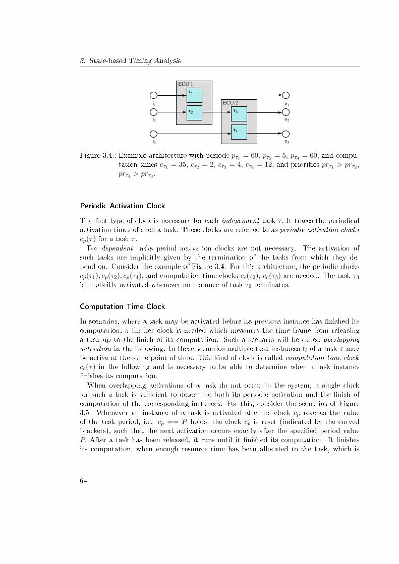
3. State-based Timing Analysis
τ1
τ2
ECU 1
i1
i2
τ3
τ4
ECU 2
i3
o1
o2
o3
Figure 3.4.: Example architecture with periods pτ1 = 60, pτ2 = 5, pτ4 = 60, and compu-tation times cτ1 = 35, cτ2 = 2, cτ3 = 4, cτ4 = 12, and priorities prτ1 > prτ2 ,prτ4 > prτ3 .
Periodic Activation Clock
The �rst type of clock is necessary for each independent task τ. It traces the periodicalactivation times of such a task. These clocks are referred to as periodic activation clockscp(τ) for a task τ .For dependent tasks period activation clocks are not necessary. The activation of
such tasks are implicitly given by the termination of the tasks from which they de-pend on. Consider the example of Figure 3.4: For this architecture, the periodic clockscp(τ1), cp(τ2), cp(τ4), and computation time clocks cc(τ2), cc(τ3) are needed. The task τ3
is implicitly activated whenever an instance of task τ2 terminates.
Computation Time Clock
In scenarios, where a task may be activated before its previous instance has �nished itscomputation, a further clock is needed which measures the time frame from releasinga task up to the �nish of its computation. Such a scenario will be called overlappingactivation in the following. In these scenarios multiple task instances ti of a task τ maybe active at the same point of time. This kind of clock is called computation time clockcc(τ) in the following and is necessary to be able to determine when a task instance�nishes its computation.When overlapping activations of a task do not occur in the system, a single clock
for such a task is su�cient to determine both its periodic activation and the �nish ofcomputation of the corresponding instances. For this, consider the scenarios of Figure3.5: Whenever an instance of a task is activated after its clock cp reaches the valueof the task period, i.e. cp == P holds, the clock cp is reset (indicated by the curvedbrackets), such that the next activation occurs exactly after the speci�ed period valueP. After a task has been released, it runs until it �nished its computation. It �nishesits computation, when enough resource time has been allocated to the task, which is
64
3.3. General Approach
τa t [ P == cp ]
cp∊[bcet, wcet]+i
...
τbt
...
cc∊[bcet, wcet]+i
[ P == cp ]
{cp} {cp} {cp}
{cp} {cp} [ P == cp ]
Figure 3.5.: Scenarios with a non-overlapping activation of task τa (left) and an overlap-ping activation of τb (right).
determined by the sum of its execution time [bcet, wcet] and a delay interval i caused byinterrupts form higher priority tasks. When there is no overlapping activation like in theleft scenario of Figure 3.5, the period clock can be used to measure this time frame, asthe clock is never reset before an instance terminates. It is assumed that the informationabout the existence and number of maximal possible overlapping activations is given apriori and not determined by the analysis approach automatically.If multiple instances can be released as illustrated in the right scenario of Figure 3.5,
this situation changes: The clock cp cannot be used to determine the above mentioned�nishing time, as cp is reset each time an instance is released. Thus, a further clock cc isneeded to trace the computation time of an active instance.
Response Time Clock
Computation time clocks are needed to determine, whether a task instance may �nish itscomputation. If the exact response times of each task instance are of interest, we needa further type of clock, which is referred to as response time clocks. Computation timeclocks are not able to measure the exact response times, as there are scenarios, wherethese have to be reset while a task instance is activated and in the ready task set.Multiple response time clocks are needed, one for each task instance ti, as the approach
relies on using simple clocks to realize the timing analysis with preemption. The reasonfor this is that neither the derivative of a clock can be changed (e.g. to stop a clock fromprogressing), nor subtraction operations can be performed as e.g. done in the work ofKr£ál and Yi [KY04].As one separate clock per task instance has to be used, the maximal number of possible
parallel activations of one task needs to be known This maximal number is called taskinstance bound and can always be derived a priori: Considering �xed priority schedulingpolicies, for an independent task the number is bounded by the maximum interrupt timefrom all higher priority tasks, and the period value of the task. For instance, considerthe task τ2 in Figure 3.4. The bound results in the following value: n = d cτ1pτ2
e + 1 = 8.
Thus, within a computation time of 35 time units of an instance of τ1, at most eightinstances of τ2 may be activated (each 5 time units).
65
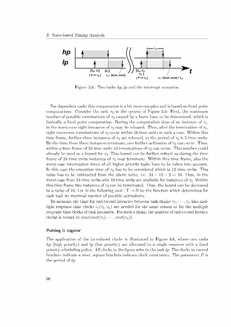
3. State-based Timing Analysis
hp
lpt{cp, cr} {cc}
cc 2 [bcet, wcet][ P == cp ]
{cp, cr, cc }[ P == cp ]
ihp
cc 2 [bcet, wcet] + ihp
Figure 3.6.: Two tasks hp, lp and the interrupt scenarios.
For dependent tasks this computation is a bit more complex and is based on �xed-pointcomputations. Consider the task τ3 in the system of Figure 3.4: First, the maximumnumber of possible terminations of τ2 caused by a burst have to be determined, which isbasically a �xed-point computation. During the computation time of an instance of τ1,in the worst-case eight instances of τ2 may be released. Thus, after the termination of τ1,eight successive terminations of τ2 occur within 16 time units in such a case. Within thistime frame, further three instances of τ2 are released, as the period of τ2 is 5 time units.By the time these three instances terminate, one further activation of τ2 can occur. Thus,within a time frame of 24 time units 12 terminations of τ2 can occur. This number couldalready be used as a bound for τ3. This bound can be further re�ned as during the timeframe of 24 time units instances of τ3 may terminate. Within this time frame, also theworst-case interruption times of all higher priority tasks have to be taken into account.In this case the execution time of τ4 has to be considered which is 12 time units. Thisvalue has to be subtracted from the above value, i.e. 24 − 12 − 2 = 10. Thus, in theworst-case from 24 time units only 10 time units are available for instances of τ3.Withinthis time frame two instances of τ3 can be terminated. Thus, the bound can be decreasedto a value of 10. Let in the following inst : T→ N be the function which determines foreach task its maximal number of possible activations.To measure the time for end-to-end latencies between task chains τ1, · · · , τn also mul-
tiple response time clocks cr(τ1, τn) are needed for the same reason as for the multipleresponse time clocks of task instances. For such a chain, the number of end-to-end latencyclocks is bound to max(inst(τ1), · · · , inst(τn)).
Putting it togeter
The application of the introduced clocks is illustrated in Figure 3.6, where two taskshp (high priority) and lp (low priority) are allocated to a single resource with a �xedpriority scheduling policy. All clocks in the �gure refer to the task lp. The clocks in curvedbrackets indicate a reset, square brackets indicate clock constraints. The parameter P isthe period of lp.
66
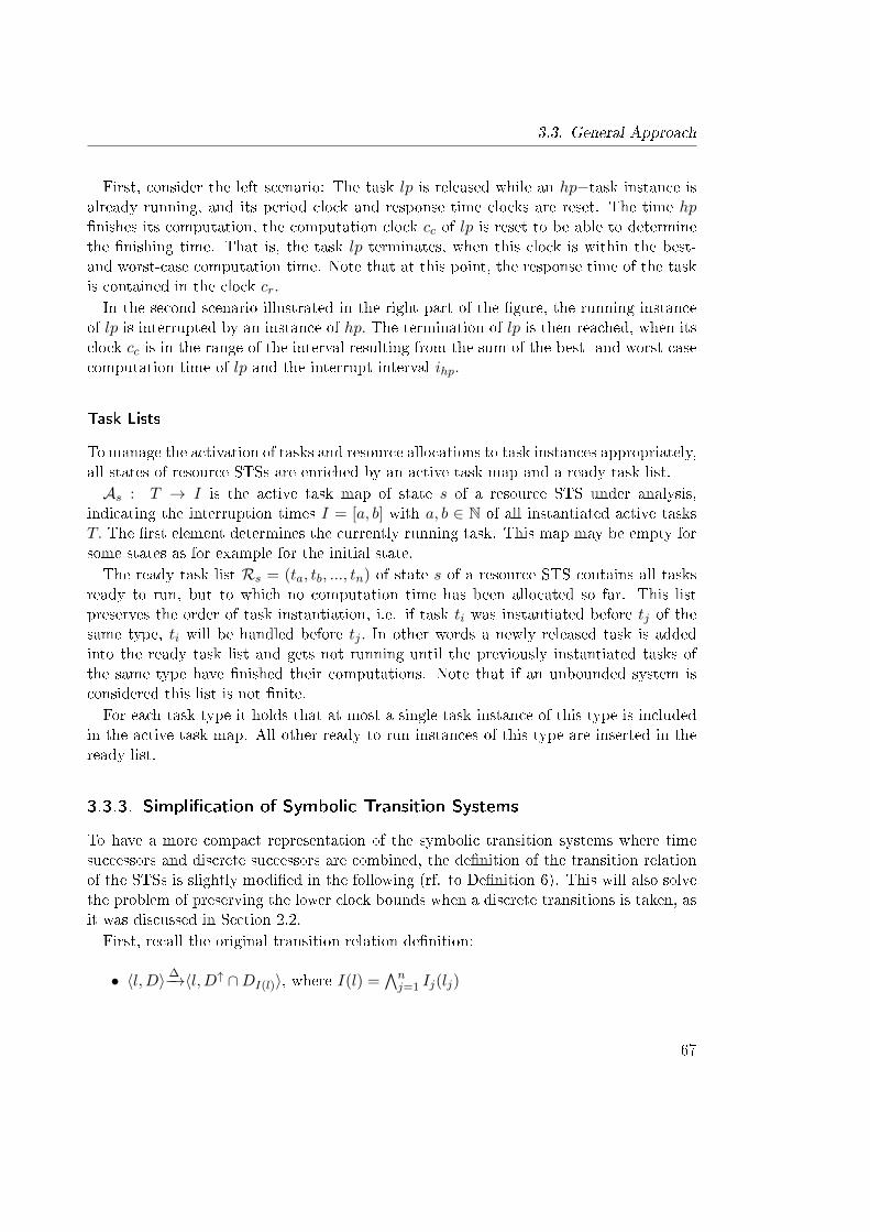
3.3. General Approach
First, consider the left scenario: The task lp is released while an hp−task instance isalready running, and its period clock and response time clocks are reset. The time hp�nishes its computation, the computation clock cc of lp is reset to be able to determinethe �nishing time. That is, the task lp terminates, when this clock is within the best-and worst-case computation time. Note that at this point, the response time of the taskis contained in the clock cr.In the second scenario illustrated in the right part of the �gure, the running instance
of lp is interrupted by an instance of hp. The termination of lp is then reached, when itsclock cc is in the range of the interval resulting from the sum of the best- and worst-casecomputation time of lp and the interrupt interval ihp.
Task Lists
To manage the activation of tasks and resource allocations to task instances appropriately,all states of resource STSs are enriched by an active task map and a ready task list.As : T → I is the active task map of state s of a resource STS under analysis,
indicating the interruption times I = [a, b] with a, b ∈ N of all instantiated active tasksT. The �rst element determines the currently running task. This map may be empty forsome states as for example for the initial state.The ready task list Rs = (ta, tb, ..., tn) of state s of a resource STS contains all tasks
ready to run, but to which no computation time has been allocated so far. This listpreserves the order of task instantiation, i.e. if task ti was instantiated before tj of thesame type, ti will be handled before tj . In other words a newly released task is addedinto the ready task list and gets not running until the previously instantiated tasks ofthe same type have �nished their computations. Note that if an unbounded system isconsidered this list is not �nite.For each task type it holds that at most a single task instance of this type is included
in the active task map. All other ready to run instances of this type are inserted in theready list.
3.3.3. Simpli�cation of Symbolic Transition Systems
To have a more compact representation of the symbolic transition systems where timesuccessors and discrete successors are combined, the de�nition of the transition relationof the STSs is slightly modi�ed in the following (rf. to De�nition 6). This will also solvethe problem of preserving the lower clock bounds when a discrete transitions is taken, asit was discussed in Section 2.2.First, recall the original transition relation de�nition:
• 〈l,D〉 ∆−→〈l,D↑ ∩DI(l)〉, where I(l) =∧nj=1 Ij(lj)
67
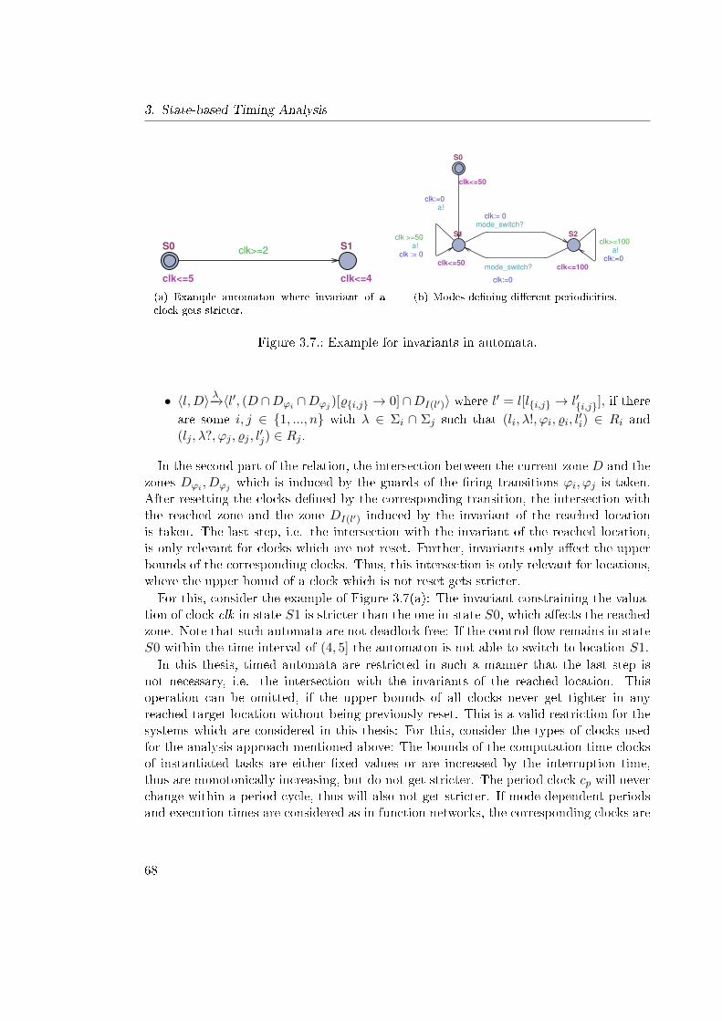
3. State-based Timing Analysis
S1
clk<=4
S0
clk<=5
clk>=2
(a) Example automaton where invariant of aclock gets stricter.
S2
clk<=100
S1
clk<=50
S0
clk<=50
clk>=100a!
clk:=0mode_switch?
clk:=0
mode_switch?clk:= 0
a!clk:=0
clk >=50a!
clk := 0
(b) Modes de�ning di�erent periodicities.
Figure 3.7.: Example for invariants in automata.
• 〈l,D〉 λ−→〈l′, (D ∩Dϕi ∩Dϕj )[%{i,j} → 0]∩DI(l′)〉 where l′ = l[l{i,j} → l′{i,j}], if thereare some i, j ∈ {1, ..., n} with λ ∈ Σi ∩ Σj such that (li, λ!, ϕi, %i, l
′i) ∈ Ri and
(lj , λ?, ϕj , %j , l′j) ∈ Rj .
In the second part of the relation, the intersection between the current zone D and thezones Dϕi , Dϕj which is induced by the guards of the �ring transitions ϕi, ϕj is taken.After resetting the clocks de�ned by the corresponding transition, the intersection withthe reached zone and the zone DI(l′) induced by the invariant of the reached locationis taken. The last step, i.e. the intersection with the invariant of the reached location,is only relevant for clocks which are not reset. Further, invariants only a�ect the upperbounds of the corresponding clocks. Thus, this intersection is only relevant for locations,where the upper bound of a clock which is not reset gets stricter.For this, consider the example of Figure 3.7(a): The invariant constraining the valua-
tion of clock clk in state S1 is stricter than the one in state S0, which a�ects the reachedzone. Note that such automata are not deadlock free: If the control �ow remains in stateS0 within the time interval of (4, 5] the automaton is not able to switch to location S1.
In this thesis, timed automata are restricted in such a manner that the last step isnot necessary, i.e. the intersection with the invariants of the reached location. Thisoperation can be omitted, if the upper bounds of all clocks never get tighter in anyreached target location without being previously reset. This is a valid restriction for thesystems which are considered in this thesis: For this, consider the types of clocks usedfor the analysis approach mentioned above: The bounds of the computation time clocksof instantiated tasks are either �xed values or are increased by the interruption time,thus are monotonically increasing, but do not get stricter. The period clock cp will neverchange within a period cycle, thus will also not get stricter. If mode-dependent periodsand execution times are considered as in function networks, the corresponding clocks are
68
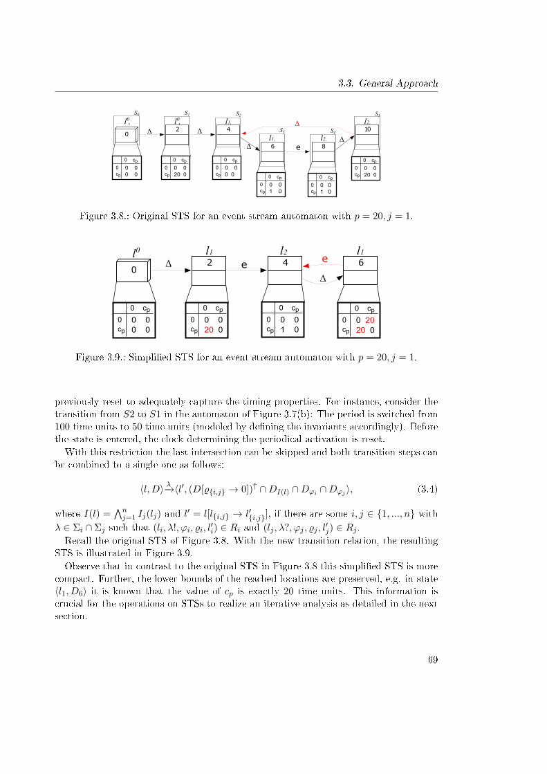
3.3. General Approach
02
6 8e
0 00 0
0 cp
0cp
0 0 20 0
0 cp
0cp
0 0 1 0
0 cp
0cp
0 0 1 0
0 cp
0cp
l , 0 l , 0
4
0 0 0 0
0 cp
0cp
l 1,
l2,l 1,
10l2,
0 0 20 0
0 cp
0cp
Δ
Δ
ΔΔΔ
S0 S1 S2
S3 S4
S5
Figure 3.8.: Original STS for an event stream automaton with p = 20, j = 1.
02 4 6e
0 0 0 0
0 cp
0cp
0 0 20 0
0 cp
0cp
0 0 1 0
0 cp
0cp
0 20 20 0
0 cp
0cp
l 0 l 1 l2 l 1Δ
Δe
Figure 3.9.: Simpli�ed STS for an event stream automaton with p = 20, j = 1.
previously reset to adequately capture the timing properties. For instance, consider thetransition from S2 to S1 in the automaton of Figure 3.7(b): The period is switched from100 time units to 50 time units (modeled by de�ning the invariants accordingly). Beforethe state is entered, the clock determining the periodical activation is reset.With this restriction the last intersection can be skipped and both transition steps can
be combined to a single one as follows:
〈l,D〉 λ−→〈l′, (D[%{i,j} → 0])↑ ∩DI(l) ∩Dϕi ∩Dϕj 〉, (3.4)
where I(l) =∧nj=1 Ij(lj) and l
′ = l[l{i,j} → l′{i,j}], if there are some i, j ∈ {1, ..., n} withλ ∈ Σi ∩ Σj such that (li, λ!, ϕi, %i, l
′i) ∈ Ri and (lj , λ?, ϕj , %j , l
′j) ∈ Rj .
Recall the original STS of Figure 3.8. With the new transition relation, the resultingSTS is illustrated in Figure 3.9.Observe that in contrast to the original STS in Figure 3.8 this simpli�ed STS is more
compact. Further, the lower bounds of the reached locations are preserved, e.g. in state〈l1, D6〉 it is known that the value of cp is exactly 20 time units. This information iscrucial for the operations on STSs to realize an iterative analysis as detailed in the nextsection.
69
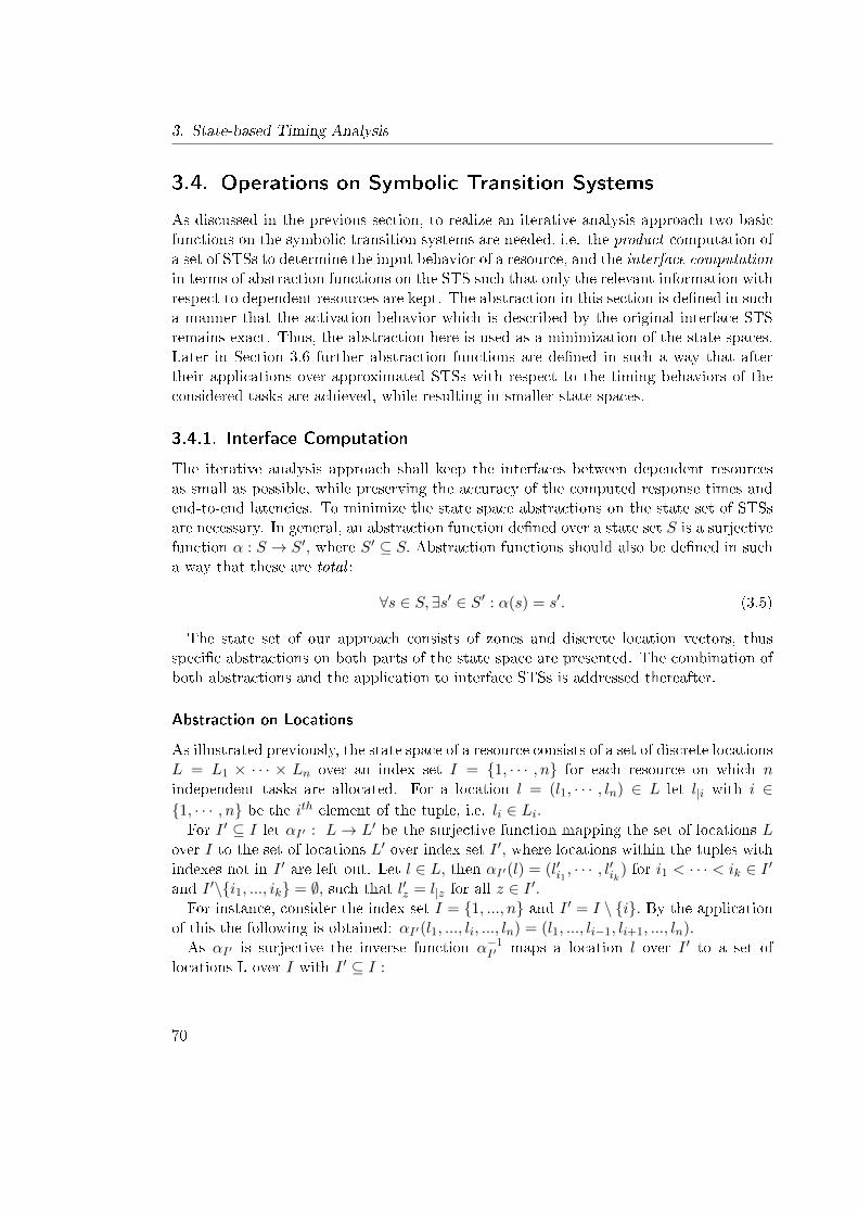
3. State-based Timing Analysis
3.4. Operations on Symbolic Transition Systems
As discussed in the previous section, to realize an iterative analysis approach two basicfunctions on the symbolic transition systems are needed, i.e. the product computation ofa set of STSs to determine the input behavior of a resource, and the interface computationin terms of abstraction functions on the STS such that only the relevant information withrespect to dependent resources are kept. The abstraction in this section is de�ned in sucha manner that the activation behavior which is described by the original interface STSremains exact. Thus, the abstraction here is used as a minimization of the state spaces.Later in Section 3.6 further abstraction functions are de�ned in such a way that aftertheir applications over-approximated STSs with respect to the timing behaviors of theconsidered tasks are achieved, while resulting in smaller state spaces.
3.4.1. Interface Computation
The iterative analysis approach shall keep the interfaces between dependent resourcesas small as possible, while preserving the accuracy of the computed response times andend-to-end latencies. To minimize the state space abstractions on the state set of STSsare necessary. In general, an abstraction function de�ned over a state set S is a surjectivefunction α : S → S′, where S′ ⊆ S. Abstraction functions should also be de�ned in sucha way that these are total :
∀s ∈ S,∃s′ ∈ S′ : α(s) = s′. (3.5)
The state set of our approach consists of zones and discrete location vectors, thusspeci�c abstractions on both parts of the state space are presented. The combination ofboth abstractions and the application to interface STSs is addressed thereafter.
Abstraction on Locations
As illustrated previously, the state space of a resource consists of a set of discrete locationsL = L1 × · · · × Ln over an index set I = {1, · · · , n} for each resource on which nindependent tasks are allocated. For a location l = (l1, · · · , ln) ∈ L let l|i with i ∈{1, · · · , n} be the ith element of the tuple, i.e. li ∈ Li.For I ′ ⊆ I let αI′ : L→ L′ be the surjective function mapping the set of locations L
over I to the set of locations L′ over index set I ′, where locations within the tuples withindexes not in I ′ are left out. Let l ∈ L, then αI′(l) = (l′i1 , · · · , l
′ik
) for i1 < · · · < ik ∈ I ′and I ′\{i1, ..., ik} = ∅, such that l′z = l|z for all z ∈ I ′.For instance, consider the index set I = {1, ..., n} and I ′ = I \ {i}. By the application
of this the following is obtained: αI′(l1, ..., li, ..., ln) = (l1, ..., li−1, li+1, ..., ln).
As αI′ is surjective the inverse function α−1I′ maps a location l over I ′ to a set of
locations L over I with I ′ ⊆ I :
70
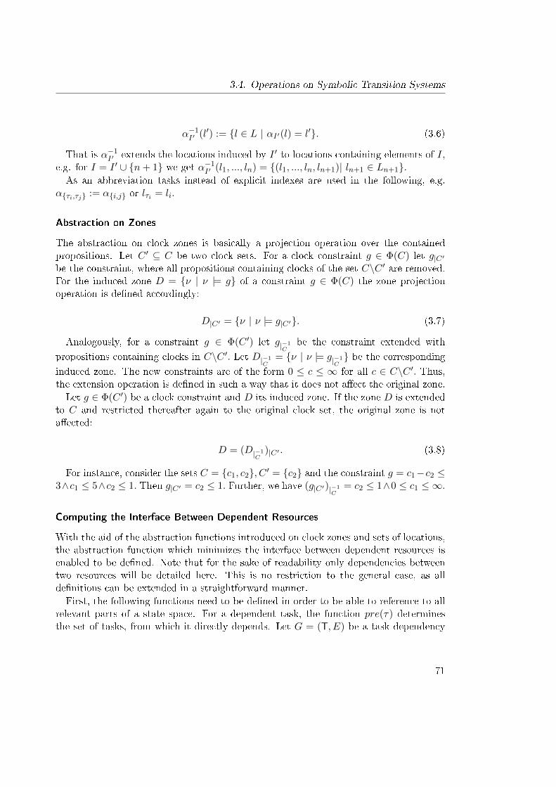
3.4. Operations on Symbolic Transition Systems
α−1I′ (l′) := {l ∈ L | αI′(l) = l′}. (3.6)
That is α−1I′ extends the locations induced by I ′ to locations containing elements of I,
e.g. for I = I ′ ∪ {n+ 1} we get α−1I′ (l1, ..., ln) = {(l1, ..., ln, ln+1)| ln+1 ∈ Ln+1}.
As an abbreviation tasks instead of explicit indexes are used in the following, e.g.α{τi,τj} := α{i,j} or lτi = li.
Abstraction on Zones
The abstraction on clock zones is basically a projection operation over the containedpropositions. Let C ′ ⊆ C be two clock sets. For a clock constraint g ∈ Φ(C) let g|C′be the constraint, where all propositions containing clocks of the set C\C ′ are removed.For the induced zone D = {ν | ν |= g} of a constraint g ∈ Φ(C) the zone projectionoperation is de�ned accordingly:
D|C′ = {ν | ν |= g|C′}. (3.7)
Analogously, for a constraint g ∈ Φ(C ′) let g|−1C
be the constraint extended with
propositions containing clocks in C\C ′. Let D|−1C
= {ν | ν |= g|−1C} be the corresponding
induced zone. The new constraints are of the form 0 ≤ c ≤ ∞ for all c ∈ C\C ′. Thus,the extension operation is de�ned in such a way that it does not a�ect the original zone.Let g ∈ Φ(C ′) be a clock constraint and D its induced zone. If the zone D is extended
to C and restricted thereafter again to the original clock set, the original zone is nota�ected:
D = (D|−1C
)|C′ . (3.8)
For instance, consider the sets C = {c1, c2}, C ′ = {c2} and the constraint g = c1−c2 ≤3∧c1 ≤ 5∧c2 ≤ 1. Then g|C′ = c2 ≤ 1. Further, we have (g|C′)|−1
C= c2 ≤ 1∧0 ≤ c1 ≤ ∞.
Computing the Interface Between Dependent Resources
With the aid of the abstraction functions introduced on clock zones and sets of locations,the abstraction function which minimizes the interface between dependent resources isenabled to be de�ned. Note that for the sake of readability only dependencies betweentwo resources will be detailed here. This is no restriction to the general case, as allde�nitions can be extended in a straightforward manner.First, the following functions need to be de�ned in order to be able to reference to all
relevant parts of a state space. For a dependent task, the function pre(τ) determinesthe set of tasks, from which it directly depends. Let G = (T, E) be a task dependency
71
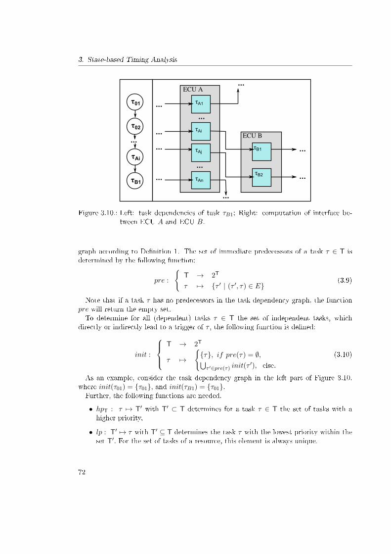
3. State-based Timing Analysis
τA1
τAi
τB1
τB2
ECU A
ECU B
...
τAj
...
τAn
...
...
...
...
...
...
...
...
τ01
τ02
τAi
τB1
...
Figure 3.10.: Left: task dependencies of task τB1; Right: computation of interface be-tween ECU A and ECU B.
graph according to De�nition 1. The set of immediate predecessors of a task τ ∈ T isdetermined by the following function:
pre :
{T → 2T
τ 7→ {τ ′ | (τ ′, τ) ∈ E}(3.9)
Note that if a task τ has no predecessors in the task dependency graph, the functionpre will return the empty set.To determine for all (dependent) tasks τ ∈ T the set of independent tasks, which
directly or indirectly lead to a trigger of τ , the following function is de�ned:
init :
T → 2T
τ 7→
{{τ}, if pre(τ) = ∅,⋃τ ′∈pre(τ) init(τ
′), else.
(3.10)
As an example, consider the task dependency graph in the left part of Figure 3.10,where init(τ01) = {τ01}, and init(τB1) = {τ01}.Further, the following functions are needed.
• hpT : τ 7→ T′ with T′ ⊂ T determines for a task τ ∈ T the set of tasks with ahigher priority,
• lp : T′ 7→ τ with T′ ⊆ T determines the task τ with the lowest priority within theset T′. For the set of tasks of a resource, this element is always unique.
72
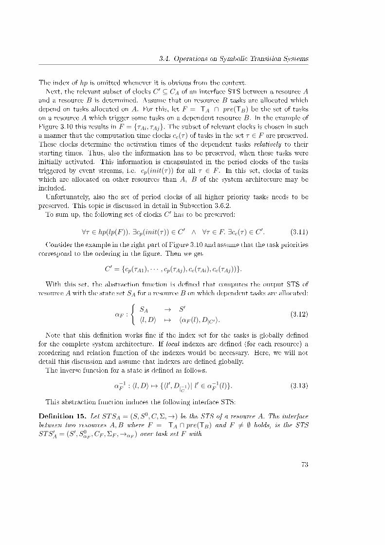
3.4. Operations on Symbolic Transition Systems
The index of hp is omitted whenever it is obvious from the context.Next, the relevant subset of clocks C ′ ⊆ CA of an interface STS between a resource A
and a resource B is determined. Assume that on resource B tasks are allocated whichdepend on tasks allocated on A. For this, let F = TA ∩ pre(TB) be the set of taskson a resource A which trigger some tasks on a dependent resource B. In the example ofFigure 3.10 this results in F = {τAi, τAj}. The subset of relevant clocks is chosen in sucha manner that the computation time clocks cc(τ) of tasks in the set τ ∈ F are preserved.These clocks determine the activation times of the dependent tasks relatively to theirstarting times. Thus, also the information has to be preserved, when these tasks wereinitially activated. This information is encapsulated in the period clocks of the taskstriggered by event streams, i.e. cp(init(τ)) for all τ ∈ F . In this set, clocks of taskswhich are allocated on other resources than A, B of the system architecture may beincluded.Unfortunately, also the set of period clocks of all higher priority tasks needs to be
preserved. This topic is discussed in detail in Subsection 3.6.2.To sum up, the following set of clocks C ′ has to be preserved:
∀τ ∈ hp(lp(F )). ∃cp(init(τ)) ∈ C ′ ∧ ∀τ ∈ F. ∃cc(τ) ∈ C ′. (3.11)
Consider the example in the right part of Figure 3.10 and assume that the task prioritiescorrespond to the ordering in the �gure. Then we get
C ′ = {cp(τA1), · · · , cp(τAj), cc(τAi), cc(τAj))}.
With this set, the abstraction function is de�ned that computes the output STS ofresource A with the state set SA for a resource B on which dependent tasks are allocated:
αF :
{SA → S′
〈l,D〉 7→ 〈αF (l), D|C′〉.(3.12)
Note that this de�nition works �ne if the index set for the tasks is globally de�nedfor the complete system architecture. If local indexes are de�ned (for each resource) areordering and relation function of the indexes would be necessary. Here, we will notdetail this discussion and assume that indexes are de�ned globally.The inverse function for a state is de�ned as follows.
α−1F : 〈l,D〉 7→ {〈l′, D|−1
C〉| l′ ∈ α−1
F (l)}. (3.13)
This abstraction function induces the following interface STS:
De�nition 15. Let STSA = (S, S0, C,Σ,→) be the STS of a resource A. The interfacebetween two resources A,B where F = TA ∩ pre(TB) and F 6= ∅ holds, is the STSSTS′A = (S′, S0
αF, CF ,ΣF ,→αF ) over task set F with
73
3. State-based Timing Analysis
• S′ = αF (S) the induced set of abstract states,
• S0αF
= αF (S0) the initial abstract state,
• CF ⊆ C the clock set as de�ned in Formula 3.11,
• ΣF ⊆ Σ the alphabet depending on the task subset F,
• →αF⊆ S′ × ΣF × S′ the abstract transition relation, where ax−→αF b i� there exists
a s1 ∈ α−1F (a) and s2 ∈ α−1
F (b) such that s1y−→s2, where x = y = λ if λ ∈ ΣF , else
x = ∆.
Each symbol in Σ represents the start or termination of a speci�c task. In the set ΣF
only those elements of Σ are preserved which represent tasks included in the set F.The transition relation of a resource STS R = (S, S0, C,Σ,→) is always left-total, that
is for every state s ∈ S there exists a successor t ∈ S such that sλ−→t for some λ ∈ Σ. Thus
all words of a resource STS are in�nite and there is no deadlock state. The abstractionfunction preserves this property.
Lemma 4 (Deadlock Free). Let STS = (S, S0, C,Σ,→) be an STS with a left-totaltransition relation. Then it holds that the transition relation of its abstraction STS′A =(S′, S0
αF, CF ,ΣF ,→αF ) according to De�nition 15 is also left-total.
Proof. Let R = (S, S0, C,Σ,→) be an STS with a left-total transition relation and R′ =(S′, S0
α, CF ,ΣF ,→α) be the abstracted STS with task set F according to De�nition 15.For s′ ∈ S′ there exists a s ∈ S such that αF (s) = s′ (Formula 3.12). As the transitionrelation of R is total, there is a t ∈ S such that s
λ−→t for some λ ∈ Σ. As αF is surjective,there is a t′ ∈ S′ with α(t) = t′. According to the transition relation of De�nition 15 itholds that s′
x−→αt′ with x ∈ ΣF .
Thus the abstract transition relation is de�ned in such a way that if there exists astate in the original STS, which has an outgoing transition to another state, there alsoexists a transition between the abstract representations of both states. With this theabstraction yields an over-approximation of the original STS, while preserving the exacttimings for the dependent tasks.
Lemma 5 (Over-Approximation). Let STSA = (S, S0, C,Σ,→) be an STS with a left-total transition relation. Then it holds that the transition relation of its abstractionSTS′A = (S′, S0
αF, CF ,ΣF ,→αF ) according to De�nition 15 is an over-approximation of
STSA.
To proof that the abstraction leads to an over-approximation, �rst a simulation relationbetween STSs has to be de�ned to be able to determine when an STS has more behaviorthan another STS.
74
3.4. Operations on Symbolic Transition Systems
De�nition 16 (Simulation relation). Given two symbolic transition systems STS1 =(S1, S
01 , C1,Σ1,→1) and STS2 = (S2, S
02 , C2,Σ2,→2) with C1 ⊆ C2 and Σ1 ⊆ Σ2. A
relation sim ⊆ S2 × S1 is a simulation relation between STS1 and STS2, if for all(〈l2, D2〉, 〈l1, D1〉) ∈ sim the following holds:
1. D1 = D2|C1.
2. For all t ∈ S2 with 〈l2, D2〉λ−→2 t there exists a s ∈ S1 such that 〈l1, D1〉
λ′−→1s and(t, s) ∈ sim, and λ = λ′ if λ ∈ Σ1, else λ
′ = ∆.
Two symbolic transition systems STS1 and STS2 are simulation equivalent, in shortSTS2 � STS1, if there exists a simulation relation sim ⊆ S2 × S1 such that (〈l02, 0C2〉,〈l01, 0C1〉) ∈ sim.
It is said that the concrete STS is simulated by the abstract STS. The proof of theover-approximation property is closely related to the proof of the left-total property:
Proof. (Lemma 5) Let R = (S, S0, C,Σ,→) be an STS with a total transition relationand R′ = (S′, S0
α, CF ,ΣF ,→α) be the abstracted STS with task set F according toDe�nition 15. The simulation relation of the states is given by sim = {(s, s′) |s ∈ S, s′ ∈S′, α(s) = s′}. Consider an element (s, s′) ∈ sim, for which holds that α(s) = s′. As Ris total, there is a transition s
λ−→t. Then, two properties hold:
• The abstraction function is surjective, such that there is a t′ ∈ S′ with α(t) = t′.
• According to the transition relation of De�nition 15 it holds that s′λ′−→αt
′ withλ = λ′ if λ ∈ ΣF , else λ′ = ∆.
With this we can conclude that (t, t′) ∈ sim. Note that this also holds for the initialstates of both STSs.
3.4.2. Composition Function
Let Ai = (Si, S0i , Ci,Σi,→i) for i = {1, ..., n} with n > 1 be a set of STSs over pairwise
disjoint clock sets Ci. In the following, the product construction A = A1 × ... × An isde�ned, which is itself an STS over the clock set C = C1∪ ...∪Cn. For each created stateof the product STS it is stored from which input states, i.e. states of the input STSsA1, ..., An, it resulted. To this end for each Ai the function ξi is introduced that mapseach product STS state to a state of Ai.The initial state of the product is given by
〈l0, 0C〉 := 〈(l01, ..., l0n), 0C1 ∪ ... ∪ 0Cn〉, (3.14)
where 〈l0i , 0Ci〉 is the initial state of Ai. Note that ξi(〈l0, 0C〉) = 〈l0i , 0Ci〉 for i ∈ {1, ..., n}.
75
3. State-based Timing Analysis
According to De�nition 6 the time successor 〈l,D′〉 of state 〈l,D〉 is then determinedby
〈l,D′〉 := 〈l,D↑ ∩D′1|−1C∩ ... ∩D′
n|−1C〉 (3.15)
where ξi(〈l,D′〉) = 〈li, D′i〉 for i ∈ {1, ..., n} are the time successors of the input states〈li, Di〉. Note that the zones from all STSs are extended to the global clock set C. Notealso that always there is a unique time successor because all input states have a uniquetime successor as illustrated in Section 2.2.Starting from the computed time successor to compute all possible discrete steps in the
product transition system, each outgoing transition (with respect to the current locationof the corresponding STS) from each STS is tried to be �red. In fact, this is also donein De�nition 6: Whenever the guards of a transition are ful�lled, a discrete transition isenabled and can be �red. This is the case, when the intersection of the zone induced bythe guard and the current zone is not empty. The maximal number of discrete successortransitions of a product automaton state is then the sum of the number of discretesuccessor transitions of each corresponding input state. The discrete successors of astate 〈l,D〉 of the product STS are given by the following set. The following de�nition isgiven for the composition of two components to keep the following discussions and proofsreadable. Note that this is no restriction to the general case as it can be easily extendedto n−components by adapting the constraint in the set de�nition.
dSucc(〈l,D〉) := { 〈l[l{i,j} → l′{i,j}], D′〉
| ∃i, j ∈ {1, ..., n}, i 6= j.〈l{i,j}, D{i,j}〉λ−→〈l′{i,j}, D
′{i,j}〉
∧ λ ∈ Σi ∩ Σj ∧ D′ 6= ∅}(3.16)
where D′ = (D∩ρ−1(D′i∩D′j)|−1C
)[ρ(D′{i,j})→ 0]∩D′i|−1C
∩D′j|−1C
, and 〈li, Di〉 = ξi(〈l,D〉)and 〈lj , Dj〉 = ξj(〈l,D〉) for all i, j ∈ {1, ..., n}. The discrete step is possible, if theresulting zone is not empty. The function ρ(D{i,...,k}) represents the set of clocks thatare reset in the corresponding zones Di, ..., Dk, and ρ−1(D{i,...,k}) represents the symbolicstates before the reset operation of the corresponding transitions have been performed.Note that the set of clocks to be reset are originally de�ned on the input transitions, butthis set can also be derived on the target zones.To proof the correctness of the product construction, the notion of equivalence has �rst
to be de�ned. The equivalence of several STSs is determined through the bisimulationrelation de�ned as follows.
De�nition 17 (Bisimulation relation). Given two symbolic transition systems STS1 =(S1, S
01 , C,Σ,→1) and STS2 = (S2, S
02 , C,Σ,→2) over the same clock set C and alphabet
Σ. A relation r ⊆ S1 × S2 is a bisimulation relation between STS1 and STS2, if for all(〈l1, D1〉, 〈l2, D2〉) ∈ r the following holds:
1. D1 = D2.
76
3.4. Operations on Symbolic Transition Systems
2. For all s ∈ S1 with 〈l1, D1〉λ−→1s there exists a t ∈ S2 such that 〈l2, D2〉
λ−→2t and(s, t) ∈ r.
3. For all t ∈ S2 with 〈l2, D2〉λ−→2t there exists a s ∈ S1 such that 〈l1, D1〉
λ−→1s and(s, t) ∈ r.
Two symbolic transition systems STS1 and STS2 are bisimulation equivalent, in shortSTS1 ≈ STS2, if there exists a bisimulation relation r ⊆ S1 × S2 such that(〈l01, 0C〉, 〈l02, 0C〉) ∈ r.
The bisimulation relation de�nes an equivalence relation between symbolic transitionsystems. Thus, if two STSs are in a bisimulation relation, they satisfy the same proper-ties. The focus of this thesis are properties concerning upper bounds of clocks like taskdeadlines and end-to-end latency constraints.
Lemma 6 (Satisfaction of Properties). A transition system STS over a clock set Cful�lls a deadline formula ϕ ∈ Φ(C), in short STS |= ϕ, i� for all reachable states 〈l,D〉of STS it holds that D ⊆ Dϕ.
The proof of this lemma is trivial: If no clock valuation exceeds the allowed boundsde�ned by the condition, the condition is ful�lled. The bisimulation relation preservesthese properties.
Theorem 1. Let STS1 ≈ STS2 be two bisimulation equivalent transition systems andlet ϕ ∈ Φ(C). It holds that STS1 |= ϕ i� STS2 |= ϕ.
Proof. (⇒) Only one direction of the theorem is shown, as the other direction is per-formed in an analogous way. Let STS1 ≈ STS2 and a formula ϕ ∈ Φ(C) be given. Let(s0, ..., sn) be a path of STS1 with s0 = 〈l01, 0C〉, si
λi−→1si+1 for all i ∈ {0, ..., n− 1}, andsn = 〈l1,n, D1,n〉 where D1,n * Dϕ. Then according to De�nition 17 (Items 2. and 3.)there is a path (t0, ..., tn) in STS2 with t0 = 〈l02, 0C〉 and ti
λi−→2ti+1 for all i ∈ {0, ..., n−1},where (si, ti) ∈ r for all i ∈ {0, ..., n} and tn = 〈l2,n, D2,n〉. As (sn, tn) ∈ r it holds thatD2,n * Dϕ (Item 3. of De�nition 17).
Theorem 2. Let A1, ..., An be a set of timed automata. Let further A = STS(A1 ×... × An) be a symbolic transition system from De�nition 6 and B = STS(A1) × ... ×STS(An) be the symbolic transition system as de�ned in this section. Then there existsa bisimulation relation such that A ≈ B.
Proof. Let A = (S, S0, C,Σ,→A) be an STS build in terms of the parallel compositionDe�nition 6 of n timed automata and let B = (X,X0, C,Σ,→B) an STS build withrespect to the product construction de�ned above. The bisimulation relation between Aand B is inductively de�ned as follows:
• (S0, X0) ∈ r with DS0 = DX0 (base case),
77
3. State-based Timing Analysis
• If (s, x) ∈ r with s ∈ S, x ∈ X and s = 〈lA, DA〉, x = 〈lB, DB〉 then DA = DB
(induction hypothesis). Two cases for the transition relation can occur:
� s has a time successor de�ned as s′ = 〈lA, D↑A ∩D′〉 with D′ = DI(l1)∧...∧I(ln),i� (according to the product de�nition) x has a time successor de�ned asx′ = 〈lB, D′′〉 with D′′ = D↑B ∩D′1|−1
C
∩ ... ∩D′1|−1C
. With D′j = D↑j ∩DI(lj) for
j ∈ {1, ..., n} we directly get D′ = D′′ and set (s′, x′) ∈ r (inductive step).
� For the discrete successors both directions need to be treated explicitly
1. s has a discrete successor de�ned as s′ = 〈l′A, D′A〉 with D′A = (DA ∩Dϕj )[ρj → 0]∩DI(l′A) and l
′A = lA[lj → l′j ], i� for a j ∈ {1, ..., n} the timed
automaton Aj has a transition (lj , λj , ϕj , ρj , l′j) ∈ Rj . Then, the STS of Aj
has a discrete successor 〈lj , Dj〉λj−→〈l′j , D′j〉 withD′j = (Dj∩Dϕj )[ρj → 0]∩
DI(l′j). Per de�nition it holds DA|Cj = Dj .With the product de�nition on
STSs, the state x has also a discrete successor 〈lB[lj → l′j ], D′B〉 withD′B =
(DB ∩ ρ−1(D′j)|−1C
)[ρ(D′j) → 0] ∩D′j|−1C
. With DA = DB and ρ−1(D′j) =
Dj ∩Dϕj we get D′A = D′B.
2. x has a discrete successor de�ned as 〈lB[lj → l′j ], D′B〉 with
D′B = (DB ∩ ρ−1(D′j)|−1C
)[ρ(D′j) → 0] ∩ D′j|−1C
i� there is an STS(Aj)
with j ∈ {1, ..., n}, which has a discrete successor 〈lj , Dj〉λ−→〈l′j , D′j〉 with
D′j = (Dj ∩Dϕj )[ρj → 0]∩DI(l′j). Per de�nition it holds that DB|Cj = Dj
and ρ−1(D′j) = Dj ∩Dϕj . Then, the corresponding timed automaton Ajhas a transition (lj , λj , ϕj , ρj , l
′j) ∈ Rj . If Aj has such a discrete transition,
then s has a discrete successor de�ned as s′ = 〈l′A, D′A〉 with D′A = (DA∩Dϕj )[ρj → 0] ∩ DI(l′A) and l′A = lA[lj → l′j ]. As DA = DB holds perassumption, we directly get D′A = D′B.
� When both 1. and 2. do hold, we set (s′, x′) ∈ r (inductive step).
The function ρ−1(D) represents the symbolic state before the reset operation of thecorresponding transition has been performed. Thus, in order to apply the product con-struction there is a need to store both the pre-reset state and the post-reset state ofdiscrete successors. By using the simpli�ed transition relation of Equation 3.4 this prob-lem is avoided, as always the pre-reset state is stored and the post-reset state is computedwhen the successor is computed.
78
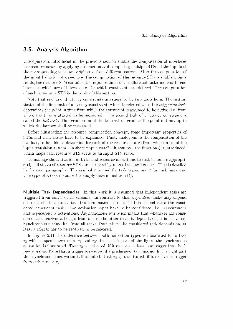
3.5. Analysis Algorithm
3.5. Analysis Algorithm
The operators introduced in the previous section enable the computation of interfacesbetween resources by applying abstraction and composing multiple STSs, if the inputs ofthe corresponding tasks are originated from di�erent sources. After the computation ofthe input behavior of a resource, the computation of the resource STS is enabled. As aresult, the resource STS contains the response times of the allocated tasks and end-to-endlatencies, which are of interest, i.e. for which constraints are de�ned. The computationof such a resource STS is the topic of this section.
Note that end-to-end latency constraints are speci�ed by two tasks here. The instan-tiation of the �rst task of a latency constraint, which is referred to as the triggering task,determines the point in time from which the constraint is assumed to be active, i.e. fromwhere the time is started to be measured. The second task of a latency constraint iscalled the tail task . The termination of the tail task determines the point in time, up towhich the latency shall be measured.
Before illustrating the resource computation concept, some important properties ofSTSs and their states have to be explained. First, analogous to the computation of theproduct, to be able to determine for each of the resource states from which state of theinput transition system � in short �input state� � it resulted, the function ξ is introduced,which maps each resource STS state to an input STS state.
To manage the activation of tasks and resource allocations to task instances appropri-ately, all states of resource STSs are enriched by maps, lists, and queues. This is detailedin the next paragraphs. The symbol τ is used for task types, and t for task instances.The type of a task instance t is simply determined by τ(t).
Multiple Task Dependencies In this work it is assumed that independent tasks aretriggered from single event streams. In contrast to this, dependent tasks may dependon a set of other tasks, i.e. the termination of tasks in this set activates the consi-dered dependent task. Two activation types have to be considered, i.e. synchronousand asynchronous activations. Asynchronous activation means that whenever the consi-dered task receives a trigger from one of the other tasks it depends on, it is activated.Synchronous means that from all tasks, from which the considered task depends on, atleast a trigger has to be received to be released.
In Figure 3.11 the di�erence between both activation types is illustrated for a taskτ3 which depends two tasks τ1 and τ2: In the left part of the �gure the synchronousactivation is illustrated. Task τ3 is activated, if it receives at least one trigger from bothpredecessors. Note that a trigger is received if a predecessor terminates. In the right partthe asynchronous activation is illustrated. Task τ3 gets activated, if it receives a triggerfrom either τ1 or τ2.
79
3. State-based Timing Analysis
τ1
τ2τ3
v
τ3
τ1τ2
τ1
τ2τ3v
τ3
τ1τ2
... ... ...
Figure 3.11.: Left: TDG with synchronous activation with resulting activation behav-ior; Right: TDG with asynchronous activation with resulting activationbehavior.
The following discrete function will determine the activation type of a task.
act : T→ {sync, async} (3.17)
For independent tasks τ we de�ne act(τ) := async.For tasks with synchronous activations all states s of a resource have a corresponding
map Ms,sync. In such a map all occurred triggers which are relevant for correspondingdependent tasks are added, i.e. Ms,sync : T → T × ... × T for all τ ∈ T ⊆ T withact(τ) = sync. If at least a trigger event from each task type on which the correspondingtasks depend on is received, an instance of the corresponding task is activated. Byactivating such a task, the map is updated appropriately, i.e. an entry from each task,on which the dependent one expects a trigger, is removed from the map. As an exampleconsider that a task τn synchronously depends on two tasks τ1, τ2. In state sm threetrigger of τ1 occurred (by terminations of corresponding instances), but no trigger ofτ2 occurred so far. Thus, we have Msm,sync(τn) = (τ1, τ1, τ1). By entering state sm+1
an instance of τ2 terminates, and thus generates a trigger for τn. An instance of τn isgenerated and the map is updated toMsm+1,sync(τn) = (τ1, τ1).For asynchronous activation patterns dependent tasks are triggered by the termination
of each task they depend on. Thus, in contrast to the synchronous case, for asynchronousactivations a map is not needed. Nevertheless, there is a need to be able to determine thetask type from which a dependent instance was activated in order to correctly computeend-to-end timing latencies. As an example consider again the task τn which dependson τ1 and τ2. An end-to-end latency is de�ned between the start of τ1 and the end ofτn. To be able to determine from which task type an instance was activated in a state s,the functionMs,async : T̄ → 2T is de�ned, where t ∈ T̄ ⊆ T with act(t) = async. Notethat the set T̄ is a set of task instances. The function is de�ned recursively: If a task tntriggers tn+1 thenMs,async(tn+1) :=Ms,async(tn) ∪ {τ(tn)}.Consider again the example above: If Msm,async(tn) = {t2} and tn triggers tn+1 by
entering state sm+1 thenMsm+1,async(tn+1) = {t2, tn}. If there is an end-to-end latencyconstraint between t1 and tn+1, it is possible to determine that the instance tn+1 was notstarted by an instance of t1.
80
3.5. Analysis Algorithm
Note that for the descriptions of the analysis algorithms the dot-notation for bothfunctions s.Masync :=Ms,async and s.Msync :=Ms,sync is used.
Controlling Boundedness If the attributes of a task are chosen inappropriately by thesystem designer, new instances of tasks may be released permanently before previouslyactivated instances �nish their computations. The simplest example for this occurs whenthe period is smaller than the execution time of the task. With such a system con�gu-ration the timing analysis approach of this thesis would not terminate and not deliverthe requested response times. Thus, there is a need of a mechanism to determine suchcon�gurations. As detailed in Subsection 3.3.2 the maximal number of possible paral-lel activations of all tasks needs to be known a priori. These numbers are relevant todetermine the needed number of response time clocks cr, as one per instance is necessary.The allocation of indexes to task instances is realized by a ring-bu�er. Whenever a new
instance of a corresponding task shall be released, an index is requested before. Thus, ifno free index is available, the approach is able to determine that the system is unboundedunder the assumption that the bound is computed according to Subsection 3.3.2.For tasks, for which the response time is not relevant, the response time clocks are
omitted to keep the state space as small as possible. Note that the engineer speci�eswhich response times are of interest and which are not. To be able to determine theboundedness for instances of such tasks, each state s counts the number of active instancesin a corresponding function, i.e. Bs : T→ N. If the number exceeds the speci�ed bound,the violation of the boundedness can be determined.
Relating Matrix Indexes As mentioned before, the valuations of all clocks are repre-sented by matrices. Each clock is referenced by a corresponding index. Clocks may beshared between a set of STSs. For example, consider a resource STS: The valuations ofsome of its clocks are directly determined by the clock valuations of the input states,as for example the clocks with which the periodic activation of independent tasks is de-termined. As an iterative analysis approach is applied, the indexes of shared clocks inthe matrices of di�erent STSs may change. Thus, there is a need to relate the indexesof shared clocks of di�erent STSs. Let C be the set of all clocks of the considered sys-tem architecture. It is assumed that C is totally ordered, i.e. the set is antisymmetric,transitive, and total. Let D be the set of all zones over all subsets of C . The clocksin the matrix representation of a zone D ∈ D may be arbitrarily ordered. To obtaina matrix which adheres to the order relation of C , the function ζ : D → D is de�nedreordering a zone D according to the total order relation. To simplify the readability,further D̃ := ζ(D) is de�ned as the short notation.An example is given in Figure 3.12 for a resource on which two independent tasks are
allocated. The matrices of the input STS of the resource consist of the period clocks ofthe tasks, as illustrated in the left-most matrix in the �gure. The period clock of τ1 has
81
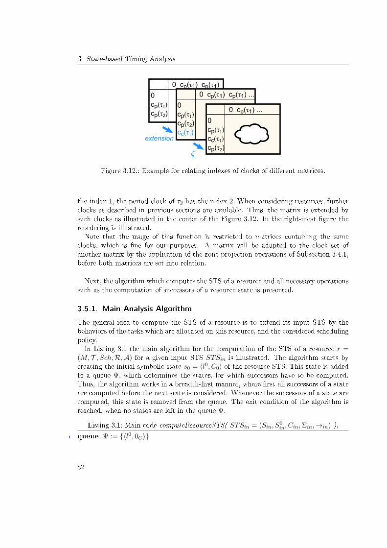
3. State-based Timing Analysis
0 cp(τ1) cp(τ1)
0cp(τ1)cp(τ2)
0 cp(τ1) cp(τ1) ...
0cp(τ1)cp(τ2)cc(τ1)
ζ
extension
0 cp(τ1) ...
0cp(τ1)cc(τ1)cp(τ2)
Figure 3.12.: Example for relating indexes of clocks of di�erent matrices.
the index 1, the period clock of τ2 has the index 2. When considering resources, furtherclocks as described in previous sections are available. Thus, the matrix is extended bysuch clocks as illustrated in the center of the Figure 3.12. In the right-most �gure thereordering is illustrated.Note that the usage of this function is restricted to matrices containing the same
clocks, which is �ne for our purposes. A matrix will be adapted to the clock set ofanother matrix by the application of the zone projection operations of Subsection 3.4.1,before both matrices are set into relation.
Next, the algorithm which computes the STS of a resource and all necessary operationssuch as the computation of successors of a resource state is presented.
3.5.1. Main Analysis Algorithm
The general idea to compute the STS of a resource is to extend its input STS by thebehaviors of the tasks which are allocated on this resource, and the considered schedulingpolicy.In Listing 3.1 the main algorithm for the computation of the STS of a resource r =
(M, T , Sch,R,A) for a given input STS STSin is illustrated. The algorithm starts bycreating the initial symbolic state s0 = 〈l0, C0〉 of the resource STS. This state is addedto a queue Ψ, which determines the states, for which successors have to be computed.Thus, the algorithm works in a breadth-�rst manner, where �rst all successors of a stateare computed before the next state is considered. Whenever the successors of a state arecomputed, this state is removed from the queue. The exit condition of the algorithm isreached, when no states are left in the queue Ψ.
Listing 3.1: Main code computeResourceSTS( STSin = (Sin, S0in, Cin,Σin,→in) ).
1 queue Ψ := {〈l0, 0C〉}
82
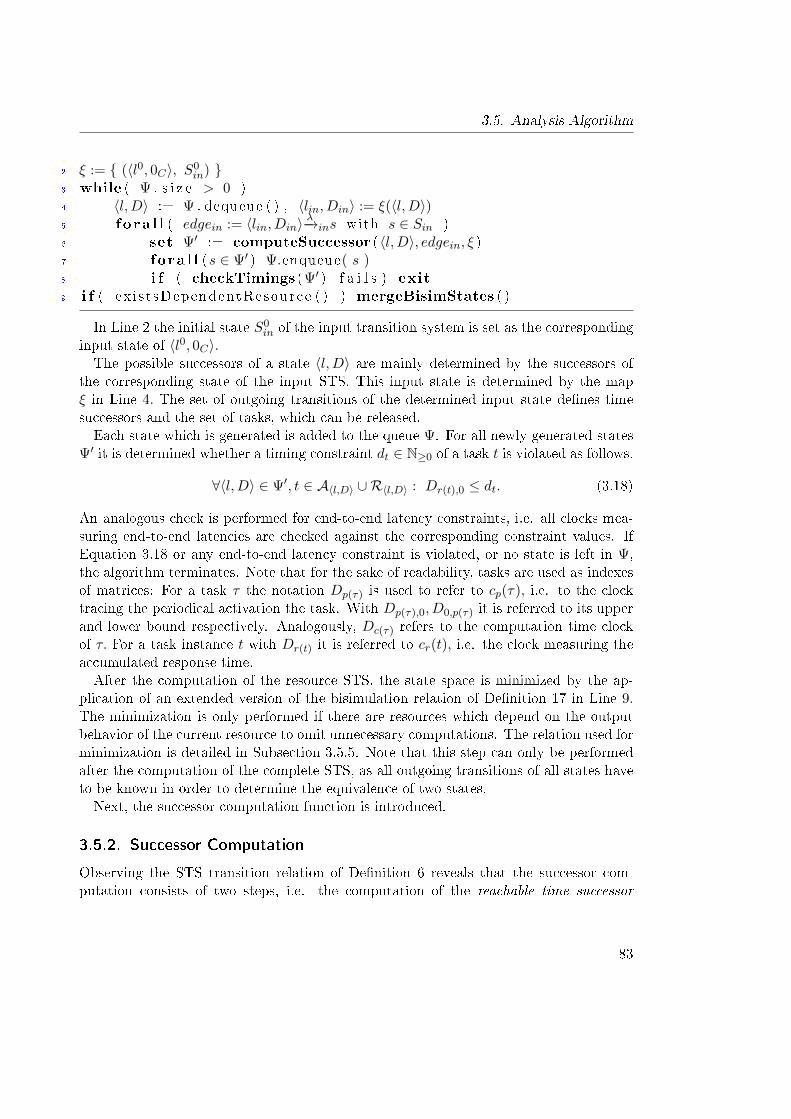
3.5. Analysis Algorithm
2 ξ := { (〈l0, 0C〉, S0in) }
3 while ( Ψ . s i z e > 0 )4 〈l,D〉 := Ψ . dequeue ( ) , 〈lin, Din〉 := ξ(〈l,D〉)5 f o ra l l ( edgein := 〈lin, Din〉
λ−→ins with s ∈ Sin )6 set Ψ′ := computeSuccessor (〈l,D〉, edgein, ξ )7 f o ra l l (s ∈ Ψ′ ) Ψ.enqueue( s )8 i f ( checkTimings (Ψ′ ) f a i l s ) exit
9 i f ( ex istsDependentResource ( ) ) mergeBisimStates ( )
In Line 2 the initial state S0in of the input transition system is set as the corresponding
input state of 〈l0, 0C〉.The possible successors of a state 〈l,D〉 are mainly determined by the successors of
the corresponding state of the input STS. This input state is determined by the mapξ in Line 4. The set of outgoing transitions of the determined input state de�nes timesuccessors and the set of tasks, which can be released.Each state which is generated is added to the queue Ψ. For all newly generated states
Ψ′ it is determined whether a timing constraint dt ∈ N≥0 of a task t is violated as follows.
∀〈l,D〉 ∈ Ψ′, t ∈ A〈l,D〉 ∪R〈l,D〉 : Dr(t),0 ≤ dt. (3.18)
An analogous check is performed for end-to-end latency constraints, i.e. all clocks mea-suring end-to-end latencies are checked against the corresponding constraint values. IfEquation 3.18 or any end-to-end latency constraint is violated, or no state is left in Ψ,the algorithm terminates. Note that for the sake of readability, tasks are used as indexesof matrices: For a task τ the notation Dp(τ) is used to refer to cp(τ), i.e. to the clocktracing the periodical activation the task. With Dp(τ),0, D0,p(τ) it is referred to its upperand lower bound respectively. Analogously, Dc(τ) refers to the computation time clockof τ. For a task instance t with Dr(t) it is referred to cr(t), i.e. the clock measuring theaccumulated response time.After the computation of the resource STS, the state space is minimized by the ap-
plication of an extended version of the bisimulation relation of De�nition 17 in Line 9.The minimization is only performed if there are resources which depend on the outputbehavior of the current resource to omit unnecessary computations. The relation used forminimization is detailed in Subsection 3.5.5. Note that this step can only be performedafter the computation of the complete STS, as all outgoing transitions of all states haveto be known in order to determine the equivalence of two states.Next, the successor computation function is introduced.
3.5.2. Successor Computation
Observing the STS transition relation of De�nition 6 reveals that the successor com-putation consists of two steps, i.e. the computation of the reachable time successor
83
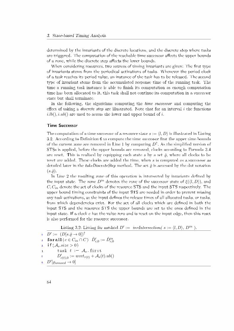
3. State-based Timing Analysis
determined by the invariants of the discrete locations, and the discrete step where tasksare triggered. The computation of the reachable time successor a�ects the upper boundsof a zone, while the discrete step a�ects the lower bounds.When considering resources, two sources of timing invariants are given: The �rst type
of invariants stems from the periodical activations of tasks. Whenever the period clockof a task reaches its period value, an instance of the task has to be released. The secondtype of invariant stems from the accumulated response time of the running task. Thetime a running task instance is able to �nish its computation as enough computationtime has been allocated to it, this task shall not continue its computation in a successorstate but shall terminate.In the following, the algorithms computing the time successor and computing the
e�ect of taking a discrete step are illustrated. Note that for an interval i the functionsi.lb(), i.ub() are used to access the lower and upper bound of i.
Time Successor
The computation of a time successor of a resource state s := 〈l,D〉 is illustrated in Listing3.2. According to De�nition 6 to compute the time successor �rst the upper time boundsof the current zone are removed in Line 1 by computing D↑. As the simpli�ed version ofSTSs is applied, before the upper bounds are removed, clocks according to Formula 3.4are reset. This is realized by equipping each state s by a set %̌, where all clocks to bereset are added. These clocks are added the time, when s is computed as a successor asdetailed later in the takeDiscreteStep method. The set %̌ is accessed by the dot notation(s.%̌).In Line 2 the resulting zone of this operation is intersected by invariants de�ned by
the input state. The zone Din denotes the zone of the successor state of ξ(〈l,D〉), andC,Cin denote the set of clocks of the resource STS and the input STS respectively. Theupper bound timing constraints of the input STS are needed in order to prevent missingany task activations, as the input de�nes the release times of all allocated tasks, or tasks,from which dependencies exist. For the set of all clocks which are de�ned in both theinput STS and the resource STS the upper bounds are set to the ones de�ned in theinput state. If a clock c has the value zero and is reset on the input edge, then this resetis also performed for the resource successor.
Listing 3.2: Listing for method D′ := invIntersection( s := 〈l,D〉, Din ).
1 D′ := (D[s.%̌→ 0])↑
2 f o ra l l (c ∈ Cin ∩ C ) D̃′c,0 := D̃inc,0
3 i f (As.size > 0)4 task t := As . f i r s t5 D′c(t),0 := wcetτ(t) +As(t).ub()6 D′[%unused → 0]
84
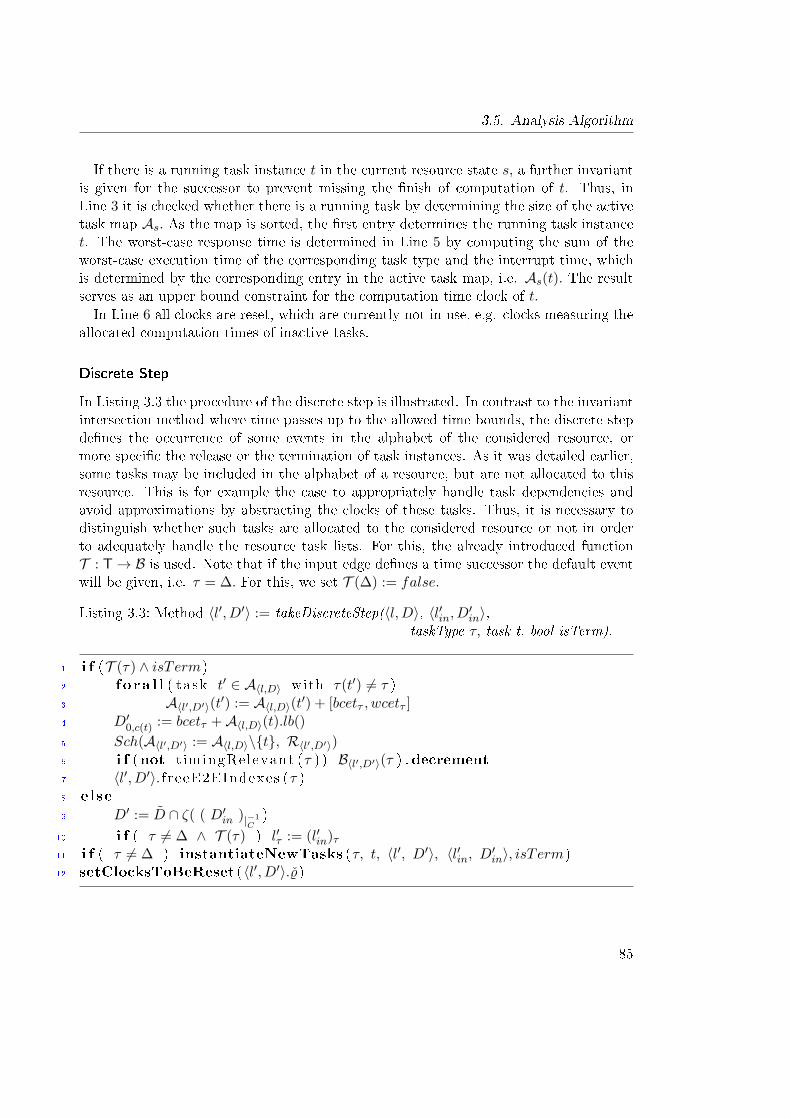
3.5. Analysis Algorithm
If there is a running task instance t in the current resource state s, a further invariantis given for the successor to prevent missing the �nish of computation of t. Thus, inLine 3 it is checked whether there is a running task by determining the size of the activetask map As. As the map is sorted, the �rst entry determines the running task instancet. The worst-case response time is determined in Line 5 by computing the sum of theworst-case execution time of the corresponding task type and the interrupt time, whichis determined by the corresponding entry in the active task map, i.e. As(t). The resultserves as an upper bound constraint for the computation time clock of t.In Line 6 all clocks are reset, which are currently not in use, e.g. clocks measuring the
allocated computation times of inactive tasks.
Discrete Step
In Listing 3.3 the procedure of the discrete step is illustrated. In contrast to the invariantintersection method where time passes up to the allowed time bounds, the discrete stepde�nes the occurrence of some events in the alphabet of the considered resource, ormore speci�c the release or the termination of task instances. As it was detailed earlier,some tasks may be included in the alphabet of a resource, but are not allocated to thisresource. This is for example the case to appropriately handle task dependencies andavoid approximations by abstracting the clocks of these tasks. Thus, it is necessary todistinguish whether such tasks are allocated to the considered resource or not in orderto adequately handle the resource task lists. For this, the already introduced functionT : T→ B is used. Note that if the input edge de�nes a time successor the default eventwill be given, i.e. τ = ∆. For this, we set T (∆) := false.
Listing 3.3: Method 〈l′, D′〉 := takeDiscreteStep(〈l,D〉, 〈l′in, D′in〉,taskType τ, task t, bool isTerm).
1 i f (T (τ) ∧ isTerm)2 f o ra l l ( task t′ ∈ A〈l,D〉 with τ(t′) 6= τ )3 A〈l′,D′〉(t′) := A〈l,D〉(t′) + [bcetτ , wcetτ ]
4 D′0,c(t) := bcetτ +A〈l,D〉(t).lb()5 Sch(A〈l′,D′〉 := A〈l,D〉\{t}, R〈l′,D′〉)6 i f (not t imingRelevant (τ ) ) B〈l′,D′〉(τ ) . decrement
7 〈l′, D′〉. f reeE2EIndexes (τ )8 else
9 D′ := D̃ ∩ ζ( ( D′in )|−1C)
10 i f ( τ 6= ∆ ∧ T (τ) ) l′τ := (l′in)τ11 i f ( τ 6= ∆ ) instantiateNewTasks (τ, t, 〈l′, D′〉, 〈l′in, D′in〉, isTerm)12 setClocksToBeReset (〈l′, D′〉.%̌)
85
3. State-based Timing Analysis
If the statement in Line 1 evaluates to true, i.e. the task t is allocated to the resourceand shall terminate its execution in the successor state, the following is performed: First,the execution time of t is accumulated to all interrupted tasks by incrementing their in-terrupt times in the active task map A〈l,D〉 (Line 2 − 3). This is analogous to classicalscheduling analysis methods, where response times are computed by a �xed point equa-tion propagating the interruptions of a task. Note that the interrupt times of only thosetasks are incremented, which have been fully interrupted by t. All tasks, which were in-stantiated after the start of t are kept in the ready task list R〈l,D〉. For instance, considerthe following scenario in the system of Figure 3.4: Let t13 be the running task instance in astate si, which gets interrupted in the successor state si+1 by a new instance t4. Then, byentering the next successor si+2 a further task instance t23 gets instantiated. The activetask map Asi+2 thus includes both tasks A = {t4 7→ [0, 0], t13 7→ [0, 0]}, while the readytask list has a single entry, i.e. Rss+2 = {t23}. In state si+3 task t4 terminates and theresulting interrupt time for task t13 is put in the active task map: Asi+3 = {t13 7→ [12, 12]}.As t shall �nish its computation, the zone of the successor gets the new constraint
c(t) ≥ bcetτ + A〈l,D〉(t).lb() on Line 4, which corresponds to the minimal amount ofcomputation time needed to terminate the task. This minimal time is the sum of thebest-case execution time and the minimal interrupt times in the current state. Note thathere only the lower bounds of the clocks have to be handled, as the upper bounds arealready handled by the invariant intersection operation.In Line 5 the task t is removed from the active task map, and the next running task
is determined by the usage of the scheduling policy. When performing A〈l,D〉\{t} alsothe index of the task is released, if a response time clock was used for t. If not, thecorresponding variable value in Line 6 is decremented. In Line 7 the indexes for the end-to-end latency clocks are handled, i.e., if t is the tail task of the latency constraint (theend point where the end-to-end latency is measured) the corresponding index is freed.If the statement in Line 1 evaluates to false, the successor of the corresponding input
state de�nes either a start of a task or the termination of a task not allocated to thecurrent resource. If the task on the current edge of the input STS is not relevant for theresource, also input edges with the ∆-event are needed to be handled by the algorithm.This event occurs, when previous abstractions of the input STS were performed. Suchedges do not instantiate tasks but de�ne timing constraints on the successors of thecurrent state. In all cases, the input successor de�nes constraints for clocks Cin ∩ Cwhich have also to be taken into account for the resource successor, as it is performedin Line 9 by taking the intersection of D and D′in. If further the input de�nes the startof a task allocated to the resource, the position of the corresponding location vector isswitched in Line 10.By starting or terminating tasks, these have also to be instantiated and the resource
task lists have to be managed. This is realized by the method instantiateNewTasks, whichis illustrated in the next paragraph.In Line 12 all clocks which need to be reset in the successor state 〈l′, D′〉 are collected
86
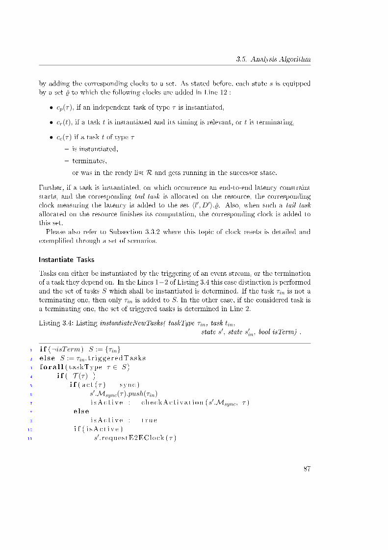
3.5. Analysis Algorithm
by adding the corresponding clocks to a set. As stated before, each state s is equippedby a set %̌ to which the following clocks are added in Line 12 :
• cp(τ), if an independent task of type τ is instantiated,
• cr(t), if a task t is instantiated and its timing is relevant, or t is terminating,
• cc(τ) if a task t of type τ
� is instantiated,
� terminates,
� or was in the ready list R and gets running in the successor state.
Further, if a task is instantiated, on which occurrence an end-to-end latency constraintstarts, and the corresponding tail task is allocated on the resource, the correspondingclock measuring the latency is added to the set 〈l′, D′〉.%̌. Also, when such a tail taskallocated on the resource �nishes its computation, the corresponding clock is added tothis set.Please also refer to Subsection 3.3.2 where this topic of clock resets is detailed and
exempli�ed through a set of scenarios.
Instantiate Tasks
Tasks can either be instantiated by the triggering of an event stream, or the terminationof a task they depend on. In the Lines 1−2 of Listing 3.4 this case distinction is performedand the set of tasks S which shall be instantiated is determined. If the task τin is not aterminating one, then only τin is added to S. In the other case, if the considered task isa terminating one, the set of triggered tasks is determined in Line 2.
Listing 3.4: Listing instantiateNewTasks( taskType τin, task tin,state s′, state s′in, bool isTerm) .
1 i f (¬isTerm) S := {τin}2 else S := τin. t r i gge r edTasks3 f o ra l l ( taskType τ ∈ S )4 i f ( T (τ) )5 i f ( act (τ ) = sync )6 s′.Msync(τ).push(τin)7 i sAc t i v e := checkAct ivat ion (s′.Msync, τ )8 else
9 i sAc t i v e := true10 i f ( i sAc t i v e )11 s′.requestE2EClock (τ )
87
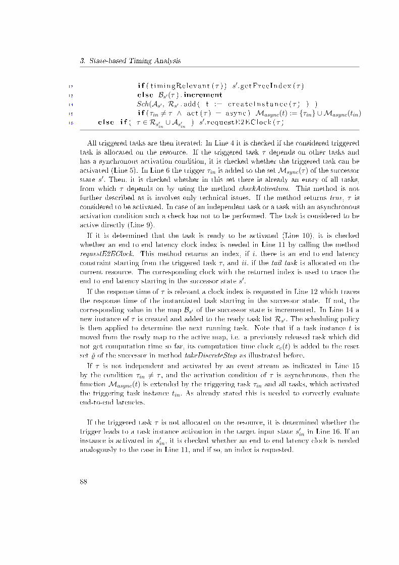
3. State-based Timing Analysis
12 i f ( t imingRelevant (τ ) ) s′.getFreeIndex (τ )13 else Bs′(τ ) . increment
14 Sch(As′ , Rs′ . add ( t := c r e a t e In s t an c e (τ ) ) )15 i f (τin 6= τ ∧ act (τ ) = async ) Masync(t) := {τin} ∪Masync(tin)16 else i f ( τ ∈ Rs′in ∪ As′in ) s′.requestE2EClock (τ )
All triggered tasks are then iterated: In Line 4 it is checked if the considered triggeredtask is allocated on the resource. If the triggered task τ depends on other tasks andhas a synchronous activation condition, it is checked whether the triggered task can beactivated (Line 5). In Line 6 the trigger τin is added to the setMsync(τ) of the successorstate s′. Then, it is checked whether in this set there is already an entry of all tasks,from which τ depends on by using the method checkActivation. This method is notfurther described as it involves only technical issues. If the method returns true, τ isconsidered to be activated. In case of an independent task or a task with an asynchronousactivation condition such a check has not to be performed. The task is considered to beactive directly (Line 9).
If it is determined that the task is ready to be activated (Line 10), it is checkedwhether an end-to-end latency clock index is needed in Line 11 by calling the methodrequestE2EClock. This method returns an index, if i. there is an end-to-end latencyconstraint starting from the triggered task τ, and ii. if the tail task is allocated on thecurrent resource. The corresponding clock with the returned index is used to trace theend-to-end latency starting in the successor state s′.
If the response time of τ is relevant a clock index is requested in Line 12 which tracesthe response time of the instantiated task starting in the successor state. If not, thecorresponding value in the map Bs′ of the successor state is incremented. In Line 14 anew instance of τ is created and added to the ready task list Rs′ . The scheduling policyis then applied to determine the next running task. Note that if a task instance t ismoved from the ready map to the active map, i.e. a previously released task which didnot get computation time so far, its computation time clock cc(t) is added to the resetset %̌ of the successor in method takeDiscreteStep as illustrated before.
If τ is not independent and activated by an event stream as indicated in Line 15by the condition τin 6= τ , and the activation condition of τ is asynchronous, then thefunctionMasync(t) is extended by the triggering task τin and all tasks, which activatedthe triggering task instance tin. As already stated this is needed to correctly evaluateend-to-end latencies.
If the triggered task τ is not allocated on the resource, it is determined whether thetrigger leads to a task instance activation in the target input state s′in in Line 16. If aninstance is activated in s′in, it is checked whether an end-to-end latency clock is neededanalogously to the case in Line 11, and if so, an index is requested.
88
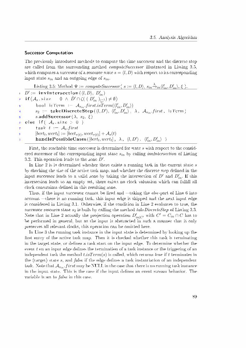
3.5. Analysis Algorithm
Successor Computation
The previously introduced methods to compute the time successor and the discrete stepare called from the surrounding method computeSuccessor illustrated in Listing 3.5,which computes a successor of a resource state s = 〈l,D〉 with respect to its correspondinginput state sin and an outgoing edge of sin.
Listing 3.5: Method Ψ := computeSuccessor( s := 〈l,D〉, sinλ−→in〈l′in, D′in〉, ξ ).
1 D′ := invIntersection (〈l,D〉, D′in )2 i f (As . s i z e = 0 ∧ D̃′ ∩ ζ( ( D′in )|−1
C) 6= ∅)
3 bool isTerm := Asin .first.isTerm(〈l′in, D′in〉)4 s2 := takeDiscreteStep (〈l,D′〉, 〈l′in, D′in〉 , λ , Asin .first , isTerm )5 s.addSuccessor (λ, s2, ξ )6 else i f ( As . s i z e > 0 )7 task t := As.first8 [bcrtt, wcrtt] := [bcetτ(t), wcetτ(t)] +As(t)9 handlePossibleCases ( [bcrtt, wcrtt] , λ , 〈l,D′〉 , 〈l′in, D′in〉 )
First, the reachable time successor is determined for state s with respect to the consid-ered successor of the corresponding input state sin by calling invIntersection of Listing3.2. This operation leads to the zone D′.In Line 2 it is determined whether there exists a running task in the current state s
by checking the size of the active task map, and whether the discrete step de�ned in theinput successor leads to a valid zone by taking the intersection of D′ and D′in. If thisintersection leads to an empty set, there exists no clock valuation which can ful�ll allclock constraints de�ned in this resulting zone.Thus, if the input successor cannot be �red and � taking the else-part of Line 6 into
account � there is no running task, this input edge is skipped and the next input edgeis considered in Listing 3.1. Otherwise, if the condition in Line 2 evaluates to true, thesuccessor resource state s2 is built by calling the method takeDiscreteStep of Listing 3.3.Note that in Line 2 actually the projection operation D′in|C′ with C
′ = Cin ∩ C has tobe performed in general, but as the input is abstracted in such a manner that it onlypreserves all relevant clocks, this operation can be omitted here.In Line 3 the running task instance in the input state is determined by looking up the
�rst entry of the active task map. Then it is checked whether this task is terminatingin the target state, or de�nes a task start on the input edge. To determine whether theevent t on an input edge de�nes the termination of a task instance or the triggering of anindependent task the method t.isTerm(s) is called, which returns true if t terminates inthe (target) state s, and false if the edge de�nes a task instantiation of an independenttask. Note thatAsin .firstmay be NULL in the case that there is no running task instancein the input state. This is the case if the input de�nes an event stream behavior. Thevariable is set to false in this case.
89
3. State-based Timing Analysis
If the computed successor does not exist yet, it is added to the graph by buildingan edge from the current state to the computed successor, and ξ(〈l′, D′〉) = 〈l′i, D′i〉 isset. Further, the created successor is added to the state set Ψ′ (not shown in the code),indicating that the successors of this state have to be computed.If the condition in Line 2 evaluates to false, but there is a running task (Line 6) in the
current resource state, it has to be determined whether this task can terminate beforethe discrete step from the input graph is taken. For this, �rst the response time inLine 8 is computed by taking the sum of its execution time and its interrupt time. ThehandlePossibleCases method then determines the possible successors.
Handle Possible Cases
The termination of a running task is determined in the code fragment of Listing 3.5 bycalling the handlePossibleCases method, which operates as follows:
1. If the running task t of type τ cannot terminate, i.e. D′c(τ),0 < bcrtτ , the intersectionbetween the zone of the state s := 〈l,D′〉 and the zone of the input state 〈l′in, D′in〉is computed, and a new task instance is released, if the input edge de�nes a taskstart. For this, s2 := takeDiscreteStep(〈l,D′〉, 〈l′in, D′in〉, λ,Asin .first, isTerm) iscalled, where isTerm := Asin .first.isTerm(〈l′in, D′in〉). Two cases can occur here:
a) If this intersection is equal to the empty set, then the discrete step cannot betaken. The intersection would result in an invalid zone, where there exists noclock valuations which ful�ll all clock constraints.
Thus, the considered input edge cannot be �red in the current resource stateand is skipped. This means that the running task has �rst to �nish its com-putation before the input edge can be taken. The program �ow is returned tothe main algorithm then, where the next input edge is considered.
b) Otherwise, if the intersection is not empty, a new instance is released if the in-put edge de�nes a task start in the current resource, i.e. if λ 6= ∆ and λ triggersan independent task allocated to the resource, or the input edge de�nes a ter-minating task triggering another task allocated to the resource. To release newtasks, the method instantiateNewTasks(λ,Asin .first, 〈l,D′〉, s′in, isTerm) iscalled. At least the new edge is added by calling s.addSuccessor(λ, s2, ξ ),where ξ is extended by ξ ∪ {(s2, 〈l′in, D′in〉)}.
2. If a running task instance t has to terminate as D0,c(t) = wcrtt holds, thens2 :=takeDiscreteStep(〈l,D′〉,−, τ(t), t, true) is called. Note that the target in-put state is not relevant in this case, as the input successor will de�ne the potentialsuccessors of s2. Again, the new edge is added by calling s.addSuccessor(τ(t), s2,ξ ), where ξ is extended by ξ ∪ {(s2, sin)}. At least, the recursion computeSucces-
90
3.5. Analysis Algorithm
sor(s2, sinλ−→in〈l′in, D′in〉, ξ) is performed. Thus, the successor of the input is tried
to be �red at the computed successor s2.
If D′c(τ),0 ≥ bcrtτ ∧D′0,c(τ) ≤ wcrtτ holds then both orderings are possible, i.e. the taskinstance may terminate before the input is �red, or vice versa �rst the input is consideredand the task instance terminates in the next successor. To realize this, both 1. and 2.are executed in this order.
3.5.3. Completeness and Soundness of Algorithm
In this section it is shown that the scheduling analysis algorithm introduced in the pre-vious subsections is correct with respect to determined timing violations. Correctnessrefers to the general terms of algorithmic correctness, i.e. that the algorithm is soundand complete.
Theorem 3. The timing analysis algorithm is sound and complete. If a timing violationis determined, it is a valid one (soundness), and if there exists a timing violation, thealgorithm will �nd a path to a state where timing requirements are violated (completeness).
The input of a resource on which only independent tasks are allocated is correct by theTheorem 2. The activations of these are represented by timed automata, which result innon-complex STSs as illustrated in Figure 3.9. As the single STSs are trivially correct,only the product of these has to be computed. So, the more general case where resourcescontain dependent tasks is considered in the following proof.
Proof. (Soundness) Assume that the algorithm terminates and returns a wrong answer,i.e. it determines that a task t violates its timing constraint d, but in real it does not.Thus, the algorithm has found a trace pre�x σ = σ1, ..., σn (n > 1) with a correspondingstate sequence s = s0, ..., sn leading to a state sn = 〈l,D〉, where it holds thatDr(t),0 > dt,(compare Equation 3.18).Assume that t is a task getting instantiated in state si, i ∈ [1, ..., n− 2]. The theorem
is proofed by performing the following case distinction on the status of the instantiatedtask.Case 1 : Consider �rst the case that task t does not get interrupted by any task after
instantiation in state si. When the task is instantiated, both clocks cc(t), cr(t) are reset,and not reset in the successors up to state sn. As all clocks progress with the same rate,both clocks have always the same valuation in all successor states of si.When computingthe zones of all states si, ..., sn, always the intersection with the upper bound constraintwcetr(t) +Asj .ub where i ≤ j ≤ n is performed in method invIntersection (Line 5). As tis never interrupted, Asj .ub equals always to zero. Thus, if Dr(t),0 > dt holds in state snit must also hold that wcetr(t) > dt, thus the counter example is valid.Case 2 : Assume again that the task t gets the status of running after instantiation.
As in the �rst case both clocks cc(t), cr(t) are reset, and not reset in the successors up to
91
3. State-based Timing Analysis
state sn. Further, assume that in the following transitions a set of higher priority taskshp(t)1, ..., hp(t)m with m ≥ 1 are instantiated, thus interrupting the execution of t. Letthe priorities of the hp−tasks be determined by their index. Let sj with j > i be the�rst successor where t is interrupted by hp(t)m.Assume that there is a sequence of hp-task activations with increasing priority, i.e.
sihp(t)m−−−−→si+1
hp(t)m−1−−−−−−→ . . .hp(t)1−−−−→si+m, in such a way that no task terminates before the
next one is activated. This is the case if the activation time is less than the bcet ofthe current running task. Thus, when computing the successor of state sk with k ∈[i + 1, ..., i + m − 1] �rst the reachable time successor in invIntersection is determined.Then in method handlePossibleCases it must hold that cc(hp(t)j) < bcrtτ(hp(t)j) for1 ≤ j ≤ m to create the above state sequence. Note that bcrt corresponds to thebcet here, as the hp-tasks were not preempted before the next higher priority task isinstantiated. From state si+1 up to state si+m at most ts = Σm
j=1 bcetτ(hp(t)j) − ε, ε→ 0time units pass.Case 2a: As each clock is incremented with the same rate, cr(t) is also incremented
with exactly this amount of time (ts). Thus, if the timing constraint violation occurs instate si+m, it must be correct.Case 2b: Assume the timing constraint violation does not occur after the activation
of hp(t)1. Then, each time an hp-task hp(t)j terminates in state s, in Line 3 of methodtakeDiscreteStep the interrupt time of each interrupted task in the As is incremented bythe execution time of the terminating task hp(t)j . Thus, when all hp-tasks terminate,and the timing constraint of t is not violated so far, t gets running again in the reachedstate sx with i+m < x < n. When the successor of sx is computed the upper bound ofthe computation time clock of t is determined in invIntersection (Line 5) by the sum ofthe wcet of the task and the upper bound of the accumulated response times determinedin Asx . If the upper bound clock valuation violates the timing constraint, it is a validviolation as all interrupts were accumulated appropriately.Case 3 : Assume there are already higher priority tasks hp(t)1, ..., hp(t)m in the active
task map Asi when t is instantiated. Further, assume that the running task has alreadyrun [lb1, ub1] time units. First, the task t is added to the ready list Rsi+1 . Both clockscc(t), cr(t) are reset, but in contrast to the previous cases only cr(t) is not reset in thesuccessors up to state sn. The computation time clock cc(t) is reset up to the state,where t gets the status running. Thus, whenever a successor is computed, (among otherclocks) the clock cr(t) keeps progressing and tracing the time since t was instantiated.As already illustrated above, this progress takes place in the invIntersection method atLine 2 and 5, and in method takeDiscreteStep in Line 4 if an hp-task is terminating,or in Line 9 if a time successor is taken or a new task is released. The time, t getsrunning, it is determined by the clock cc(t) whether its computation can be �nishedor not. The clock cr(t) traces the time since task instantiation, i.e. has progressed asfollows: cr(t) := Σm
j=2([bcetτ(hp(t)j), wcetτ(hp(t)j)]) +[bcetτ(hp(t)1), wcetτ(hp(t)1)]−[lb1, ub1].Thus, again if the timing constraint is violated, this violation is valid.
92
3.5. Analysis Algorithm
Proof. (Completeness) Assume that there exists a state of the system under analysis, forwhich the timing requirements of a task t is violated, but not found by the algorithm.Let ϕ0, · · ·ϕn be a task activation sequence leading to a schedule where an activatedtask instance t misses its timing constraint. It has to be shown that no matter whatthis activation sequence concretely looks like, the algorithm detects a timing constraintviolation caused by such a trace.A similar case distinction as above is performed.Case 1 : Assume that t is activated, set to running and not interrupted in the subse-
quent schedule. In such a case a timing constraint violation can only occur if wcetτ(t) >dt. As long as t does not �nish its computation it must hold that cc(t) < wcetτ(t)
as constrained in the handlePossibleCases method. By determining the reached timesuccessor for each state where t is running, the constraint cc(t) ≤ wcrtτ(t) is added inLine 5 of method invIntersection. As t is never interrupted in this case, it holds thatwcrtτ(t) = wcetτ(t). Thus, wcet of t is never exceeded but is reached when t �nishes itscomputation. Therefore, if wcetτ(t) > dt holds, it will be �nally determined by the mainalgorithm.Case 2 : The second cause of a timing constraint may be that t is interrupted before it
terminates. Let t get the status running after its instantiation. The time t is instantiated,its clocks cr(t) and cc(t) are reset and not reset again until t �nishes its computation.An input of a higher priority task may interrupt t in a successor state, if t has not�nished its computation up to this point, i.e. if cc(t) < wcetτ(t) holds (cf. methodhandlePossibleCases). Both clocks of the task cr(t) and cc(t) continue to progress, evenif t is interrupted. Whenever a higher priority task terminates in a state sx, its interrupttime for t is traced in the active task map Asx . With this, the clock cc(t) has to progressto the value of the sum of its worst-case execution time and the sum of the interrupttimes to be able to �nish its computations (cf. handlePossibleCases method). As theclock cr(t) progresses equally with cc(t), timing constraint violations caused by interruptswill be determined by the algorithm in the main method.Case 3 : The third case of a timing constraint violation of a task may occur when the
task t is inserted to the ready list. The only major di�erence to the second case is thatthe clock cc(t) is reset when the task gets running, while cr(t) starts to progress the timeas soon as the task is instantiated. Thus, the task t �nishes its computation, wheneverthe valuation for cc(t) is within the interval [bcet, wcet] (if it is not interrupted after itgets the status running). As cr(t) traces the time from instantiation of t, all interrupttimes are included in the valuation of this clock. Similar to the proof of the soundness,cr(t) valuates to the following: cr(t) := Σm
j=1([bcetτ(hp(t)j), wcetτ(hp(t)j)]) − [lb1, ub1],where hp(t)2, ..., hp(t)m do fully interrupt t, and t is instantiated during the execution ofhp(t)1. Again, possible timing constraint violations are detected by the main algorithm.
93
3. State-based Timing Analysis
3.5.4. Termination of Algorithm
Next, it is shown that if the algorithm computing a resource STS always terminates if itis called for �nite input STSs. For this, it is shown that only a �nite number of statesare generated, and that the recursion handlePossibleCases is called �nitely.
Proof. The recursion is entered, when a task t0 �nishes its computation. Hereby, atransition s
end(t0)−−−−→ s′ is created. If As′ .size = 0, the if part of Listing 3.5 is entered, thesuccessor according to the input state is computed, and the algorithm terminates afterinstantiating such tasks, which are triggered and for which the activation condition ismet according to the algorithm in Listing 3.4.Else, there exists at least one task t ∈ As′ , which could also terminate its computation
and trigger another task allocated to the resource. If the execution time of a task wouldbe equal to zero, the algorithm would in�nitely continue to terminate and start newtask instances through the de�ned recursion. Thus, it has to be shown that time alwaysincreases when terminating tasks, as �nally the discrete step de�ned by the edge of theinput state has to be taken before the running task can terminate. This is directly givenunder the assumption that the execution times of tasks are always greater than zero.The response times of preempted tasks are always increased when the running task t0terminates: ∀t ∈ As, τ(t) 6= τ(t0) : As′(t) = As(t) + [bcetτ(t0), wcetτ(t0)] (see Line 3 inListing 3.3). When such a preempted task gets active in the next recursion steps, thisincreased response time is used to compute the next discrete successor. With this theproof can be concluded: ∀t ∈ As ∩ As′ , τ(t) 6= τ(t0) : As(t) < As′(t).
Next, it is proofed that the algorithm computes only a �nite set of symbolic states, i.e.always terminates.
Proof. As there are only a �nite set of discrete locations, the single possible source ofin�niteness are the clock valuations. An in�nite symbolic state set would be given, ifclocks without a ceiling would be considered. Thus, we have to show that all clocksare bounded. When computing the time successor, always the invariant intersectionfunction is called: Under the assumption that all clocks of the input STS have a ceiling,it holds that there is always a ceiling for all clocks tracing the periodical activation, i.e.cp(τ) ≤ pτ . Also the clock cc(t) for the running task instance t is constrained in Line 5of Listing 3.2 by the sum of the worst-case computation time and the upper bound ofthe corresponding interrupt time. For all other tasks t in the active task map and theready list the corresponding clocks cc(t) are not constrained. Nevertheless, whenever thealgorithm of Listing 3.5 is �nished, the corresponding response time clocks are checkedagainst the deadlines, i.e. whether cr(t) ≤ dt, thus are also always bounded. If for atask t there is no response time clock, there is an instance counter variable B(t). If thiscounter exceeds the speci�ed value, an instantiated task will not be able to �nish its
94
3.5. Analysis Algorithm
computation in the allowed time frame. Note that this holds under the assumption, thatthe value for B(t) is chosen appropriately and not too restrictive.
3.5.5. Minimization through Untimed Bisimulation, Timed SimulationRelation
To minimize computed STSs a new relation is introduced in this subsection, which is acombination of a bisimulation and a simulation relation. With this relation the numberof states of a computed resource STS can be reduced without loosing any accuracy withrespect to the timing behaviors of the tasks.The idea is to merge paths which have on the one hand equivalent discrete behaviors,
i.e. paths on which the same sequences of events are produced. In the context of schedul-ing this corresponds to merging of paths which have the same ordering of task activationsand terminations. On the other hand paths which shall be merged must have a relatedtiming behavior: If all clock zones of a path p1 are a subset or equal to the clock zonesof a path p2, and p2 has an equivalent discrete behavior as p1, then p1 is obsolete. Allpossible timing behaviors of p1 are already covered by p2. Thus, the behavior representedby path p1 is a subset of the one of p2. Note that this relation is de�ned in such a man-ner that paths with equivalent timings are also merged. This relation is called untimedbisimulation, timed simulation (UBTS) and is de�ned as follows.
De�nition 18 (UBTS relation). Let two symbolic transition systems STS1 = (S1, S01 ,
C,Σ,→1) and STS2 = (S2, S02 , C,Σ,→2) over the same clock set C and alphabet Σ be
given. A relation rubts ⊆ S1 × S2 is an untimed bisimulation, timed simulation relationbetween STS1 and STS2, if for all (〈l2, D2〉, 〈l1, D1〉) ∈ rubts the following holds:
1. D2 ⊆ D1.
2. 〈l1, D1〉 is visited in�nitely if and only if 〈l2, D2〉 is visited in�nitely.
3. For all s ∈ S1 with 〈l1, D1〉λ−→1s there exists a t ∈ S2 such that 〈l2, D2〉
λ−→2t and(s, t) ∈ rubts.
4. For all t ∈ S2 with 〈l2, D2〉λ−→2t there exists a s ∈ S1 such that 〈l1, D1〉
λ−→1s and(s, t) ∈ rubts.
For (s2, s1) ∈ rubts we also write s2 2 s1.
Let rubts ⊆ S × S be an untimed bisimulation, timed simulation relation between thestate set of a single transition system STS. This relation is a preorder (re�exive andtransitive), i.e. if (s1, s2), (s2, s3) ∈ rubts then (s1, s3) ∈ rubts, but not symmetric becauseof the �rst condition of De�nition 18. When successive states are in such a relation (i.e.di�erent paths of an STS) these can be merged. The reduced STS satis�es the sametiming constraints as the original one. Unnecessary computations of redundant states
95
3. State-based Timing Analysis
e.g. when computing the state spaces of dependent resources can be omitted. Thisreduces the overall analysis time. To prove this, we need �rst to de�ne the term maximalelement as follows.
De�nition 19 (Maximal Element). Let rubts ⊆ S×S be an untimed bisimulation, timedsimulation relation between the state set of a transition system STS = (S, S0, C,Σ,→).An element s ∈ S is called maximal, if there is no s′ ∈ S with s′ 6= s such that s 2 s′.
The relation may further induce equivalence classes of states de�ned as follows.
De�nition 20 (Equivalence Class). Let rubts ⊆ S×S be an untimed bisimulation, timedsimulation relation between the state set of a transition system STS = (S, S0, C,Σ,→).Two states s, s′ ∈ S with s 6= s′ are equivalent, if s 2 s′ and s′ 2 s. The set ofall equivalence classes induced by rubts is denoted by χubts. A representative of a classc ∈ χubts is given by [c].
Lemma 7. Let S be the state set of an STS = (S, S0, C,Σ,→), rubts ⊆ S × S be anuntimed bisimulation, timed simulation relation, and ϕ a timing constraint. If s ∈ S ismaximal with respect to rubts, and s |= ϕ, then for all s′ ∈ S with s′ 2 s it holds s′ |= ϕ.
Lemma 8. Let S be the state set of an STS = (S, S0, C,Σ,→), rubts ⊆ S × S bean untimed bisimulation, timed simulation relation, and ϕ a timing constraint. For allc ∈ χubts it holds that if [c] |= ϕ then for all s ∈ c it holds that s |= ϕ.
Both lemmas do hold, as the relation is transitive. With both lemmas it is allowed tocorrectly reduce the state space of the original STS, where only the maximal states andthe representatives of every equivalence class are left. The complexity of determining thesimulation equivalent states is n(n − 1), where n is the number of states, as each statehas to be compared with all other states to determine the related states.Note that this minimization does not necessarily lead to smaller state spaces of depen-
dent resources, as no information is abstracted. Nevertheless, the computation time ofthe STSs of dependent resources is reduced, as less input states have to be considered,for which resource states have to be computed. Thus, with this technique the multiplecomputations of the same resource states can be omitted.The e�ect of this minimization technique is illustrated by applying it to the architecture
which is illustrated in Figure 3.4. The minimization is applied to the input STS ofECU2. Multiple scenarios are considered by varying the period pτ4 of task τ4. The resultis illustrated in the left part of Figure 3.13. For instance, in the scenario where theperiod of τ4 is 85 time units, the size is reduced from 10982 to 5991 states, which is asigni�cant saving. The resulting overall computation times for each scenario is illustratedin the right part of the �gure. The overall analysis time is positively a�ected, as lessinput states have to be considered for the dependent resource: While approximately 41seconds were needed in the original case to analyze the architecture with pτ4 = 85, thistime could be decreased to approximately 34 seconds.
96
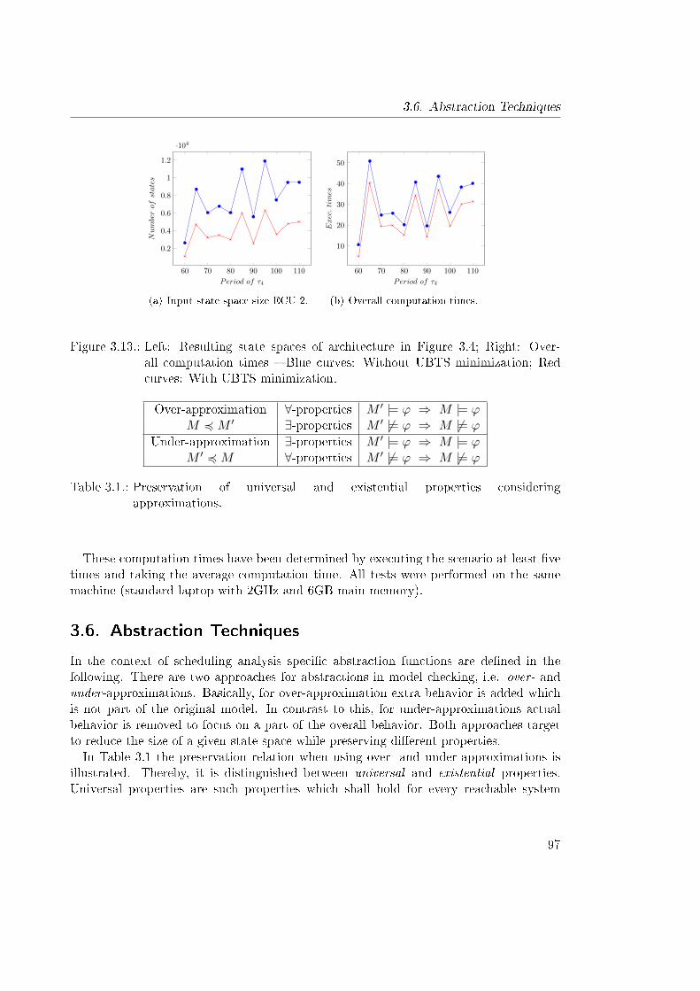
3.6. Abstraction Techniques
60 70 80 90 100 110
0.2
0.4
0.6
0.8
1
1.2
·104
Period of τ4
Numberof
states
(a) Input state space size ECU 2.
60 70 80 90 100 110
10
20
30
40
50
Period of τ4
Exec.times
(b) Overall computation times.
Figure 3.13.: Left: Resulting state spaces of architecture in Figure 3.4; Right: Over-all computation times � Blue curves: Without UBTS minimization; Redcurves: With UBTS minimization.
Over-approximation ∀-properties M ′ |= ϕ ⇒ M |= ϕM 4M ′ ∃-properties M ′ 6|= ϕ ⇒ M 6|= ϕ
Under-approximation ∃-properties M ′ |= ϕ ⇒ M |= ϕM ′ 4M ∀-properties M ′ 6|= ϕ ⇒ M 6|= ϕ
Table 3.1.: Preservation of universal and existential properties consideringapproximations.
These computation times have been determined by executing the scenario at least �vetimes and taking the average computation time. All tests were performed on the samemachine (standard laptop with 2GHz and 6GB main memory).
3.6. Abstraction Techniques
In the context of scheduling analysis speci�c abstraction functions are de�ned in thefollowing. There are two approaches for abstractions in model checking, i.e. over- andunder-approximations. Basically, for over-approximation extra behavior is added whichis not part of the original model. In contrast to this, for under-approximations actualbehavior is removed to focus on a part of the overall behavior. Both approaches targetto reduce the size of a given state space while preserving di�erent properties.In Table 3.1 the preservation relation when using over- and under-approximations is
illustrated. Thereby, it is distinguished between universal and existential properties.Universal properties are such properties which shall hold for every reachable system
97
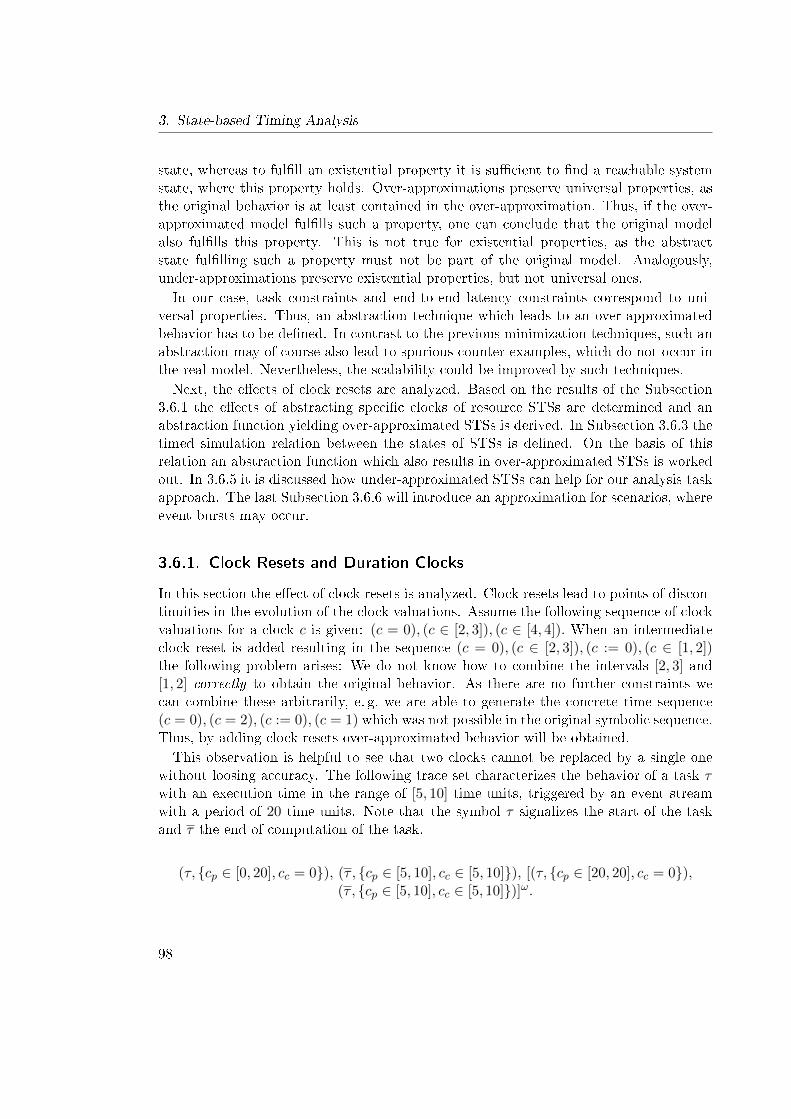
3. State-based Timing Analysis
state, whereas to ful�ll an existential property it is su�cient to �nd a reachable systemstate, where this property holds. Over-approximations preserve universal properties, asthe original behavior is at least contained in the over-approximation. Thus, if the over-approximated model ful�lls such a property, one can conclude that the original modelalso ful�lls this property. This is not true for existential properties, as the abstractstate ful�lling such a property must not be part of the original model. Analogously,under-approximations preserve existential properties, but not universal ones.In our case, task constraints and end-to-end latency constraints correspond to uni-
versal properties. Thus, an abstraction technique which leads to an over-approximatedbehavior has to be de�ned. In contrast to the previous minimization techniques, such anabstraction may of course also lead to spurious counter-examples, which do not occur inthe real model. Nevertheless, the scalability could be improved by such techniques.Next, the e�ects of clock resets are analyzed. Based on the results of the Subsection
3.6.1 the e�ects of abstracting speci�c clocks of resource STSs are determined and anabstraction function yielding over-approximated STSs is derived. In Subsection 3.6.3 thetimed simulation relation between the states of STSs is de�ned. On the basis of thisrelation an abstraction function which also results in over-approximated STSs is workedout. In 3.6.5 it is discussed how under-approximated STSs can help for our analysis taskapproach. The last Subsection 3.6.6 will introduce an approximation for scenarios, whereevent bursts may occur.
3.6.1. Clock Resets and Duration Clocks
In this section the e�ect of clock resets is analyzed. Clock resets lead to points of discon-tinuities in the evolution of the clock valuations. Assume the following sequence of clockvaluations for a clock c is given: (c = 0), (c ∈ [2, 3]), (c ∈ [4, 4]). When an intermediateclock reset is added resulting in the sequence (c = 0), (c ∈ [2, 3]), (c := 0), (c ∈ [1, 2])the following problem arises: We do not know how to combine the intervals [2, 3] and[1, 2] correctly to obtain the original behavior. As there are no further constraints wecan combine these arbitrarily, e. g. we are able to generate the concrete time sequence(c = 0), (c = 2), (c := 0), (c = 1) which was not possible in the original symbolic sequence.Thus, by adding clock resets over-approximated behavior will be obtained.This observation is helpful to see that two clocks cannot be replaced by a single one
without loosing accuracy. The following trace set characterizes the behavior of a task τwith an execution time in the range of [5, 10] time units, triggered by an event streamwith a period of 20 time units. Note that the symbol τ signalizes the start of the taskand τ the end of computation of the task.
(τ, {cp ∈ [0, 20], cc = 0}), (τ , {cp ∈ [5, 10], cc ∈ [5, 10]}), [(τ, {cp ∈ [20, 20], cc = 0}),(τ , {cp ∈ [5, 10], cc ∈ [5, 10]})]ω.
98
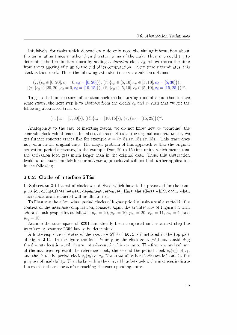
3.6. Abstraction Techniques
Intuitively, for tasks which depend on τ do only need the timing information aboutthe termination times τ rather than the start times of the task. Thus, one could try todetermine the termination times by adding a duration clock cd, which traces the timefrom the triggering of τ up to the end of its computation. Every time τ terminates, thisclock is then reset. Thus, the following extended trace set would be obtained:
(τ, {cp ∈ [0, 20], cc = 0, cd = [0, 20]}), (τ , {cp ∈ [5, 10], cc ∈ [5, 10], cd = [5, 30]}),[(τ, {cp ∈ [20, 20], cc = 0, cd = [10, 15]}), (τ , {cp ∈ [5, 10], cc ∈ [5, 10], cd = [15, 25]})]ω.
To get rid of unnecessary information such as the starting time of τ and thus to savesome states, the next step is to abstract from the clocks cp and cc such that we get thefollowing abstracted trace set:
(τ , {cd = [5, 30]}), [(δ, {cd = [10, 15]}), (τ , {cd = [15, 25]})]ω.
Analogously to the case of inserting resets, we do not know how to �combine� theconcrete clock valuations of this abstract trace. Besides the original concrete traces, weget further concrete traces like for example σ = (τ , 5), (τ , 15), (τ , 15)... This trace doesnot occur in the original case. The major problem of this approach is that the originalactivation period decreases, in the example from 20 to 15 time units, which means thatthe activation load gets much larger than in the original case. Thus, this abstractionleads to too coarse models for our analysis approach and will not �nd further applicationin the following.
3.6.2. Clocks of Interface STSs
In Subsection 3.4.1 a set of clocks was derived which have to be preserved for the com-putation of interfaces between dependent resources. Here, the e�ects which occur whensuch clocks are abstracted will be illustrated.To illustrate the e�ect when period clocks of higher priority tasks are abstracted in the
context of the interface computation, consider again the architecture of Figure 3.4 withadapted task properties as follows: pτ1 = 20, pτ2 = 10, pτ4 = 20, cτ1 = 11, cτ2 = 1, andpτ4 = 15.Assume the state space of ECU1 has already been computed and as a next step the
interface to resource ECU2 has to be determined.A �nite sequence of states of the resource STS of ECU1 is illustrated in the top part
of Figure 3.14. In the �gure the focus is only on the clock zones without consideringthe discrete locations, which are not relevant for this scenario. The �rst row and columnof the matrices represent the reference clock, the second the period clock cp(τ1) of τ1,and the third the period clock cp(τ2) of τ2. Note that all other clocks are left out for thepurpose of readability. The clocks within the curved brackets below the matrices indicatethe reset of these clocks after reaching the corresponding state.
99
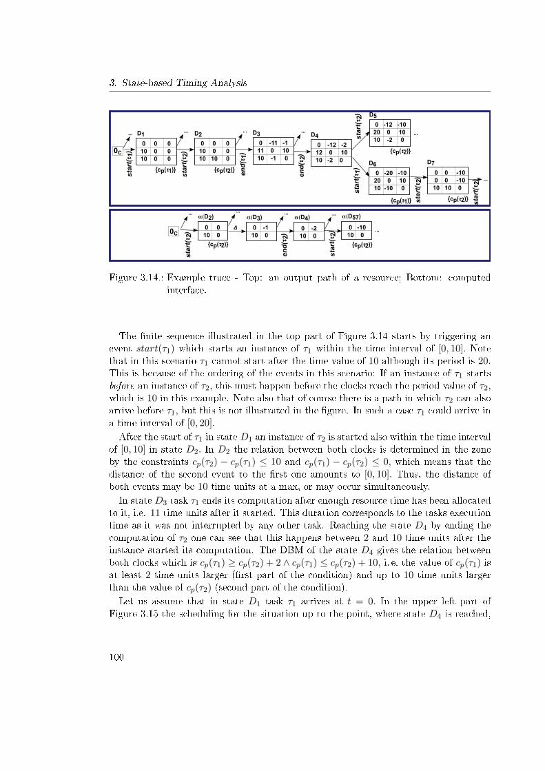
3. State-based Timing Analysis
D2
{cp(τ1)} 0 -20 -10 20 0 10 10 -10 0
0 0 10 0
α(D2)
Δ 0 -2 10 0
...
0 0 0 10 0 0 10 0 0
start(
τ 1)0C
0 0 0 10 0 0 10 10 0
D1
start(
τ 2)
end(τ 1)
D3
0 -11 -1 11 0 10 10 -1 0
{cp(τ2)}
end(τ 2)
D4
0 -12 -2 12 0 10 10 -2 0 D6
0 -12 -10 20 0 10 10 -2 0
D5
{cp(τ2)}
{cp(τ1)}
start(
τ 1)
start(
τ 2)
...
0C
start(
τ 2)
{cp(τ2)}
0 -1 10 0
α(D3)
end(τ 2)
α(D4)
start(
τ 2)
0 0 -10 0 0 -10 10 10 0
D7
start(
τ 2) 0 -10
10 0
α(D57)
...
{cp(τ2)}
{cp(τ2)}
start(
τ 2)
... ... ......
... ... ... ...
Figure 3.14.: Example trace - Top: an output path of a resource; Bottom: computedinterface.
The �nite sequence illustrated in the top part of Figure 3.14 starts by triggering anevent start(τ1) which starts an instance of τ1 within the time interval of [0, 10]. Notethat in this scenario τ1 cannot start after the time value of 10 although its period is 20.This is because of the ordering of the events in this scenario: If an instance of τ1 startsbefore an instance of τ2, this must happen before the clocks reach the period value of τ2,which is 10 in this example. Note also that of course there is a path in which τ2 can alsoarrive before τ1, but this is not illustrated in the �gure. In such a case τ1 could arrive ina time interval of [0, 20].
After the start of τ1 in state D1 an instance of τ2 is started also within the time intervalof [0, 10] in state D2. In D2 the relation between both clocks is determined in the zoneby the constraints cp(τ2) − cp(τ1) ≤ 10 and cp(τ1) − cp(τ2) ≤ 0, which means that thedistance of the second event to the �rst one amounts to [0, 10]. Thus, the distance ofboth events may be 10 time units at a max, or may occur simultaneously.
In state D3 task τ1 ends its computation after enough resource time has been allocatedto it, i.e. 11 time units after it started. This duration corresponds to the tasks executiontime as it was not interrupted by any other task. Reaching the state D4 by ending thecomputation of τ2 one can see that this happens between 2 and 10 time units after theinstance started its computation. The DBM of the state D4 gives the relation betweenboth clocks which is cp(τ1) ≥ cp(τ2) + 2 ∧ cp(τ1) ≤ cp(τ2) + 10, i. e. the value of cp(τ1) isat least 2 time units larger (�rst part of the condition) and up to 10 time units largerthan the value of cp(τ2) (second part of the condition).
Let us assume that in state D1 task τ1 arrives at t = 0. In the upper left part ofFigure 3.15 the scheduling for the situation up to the point, where state D4 is reached,
100
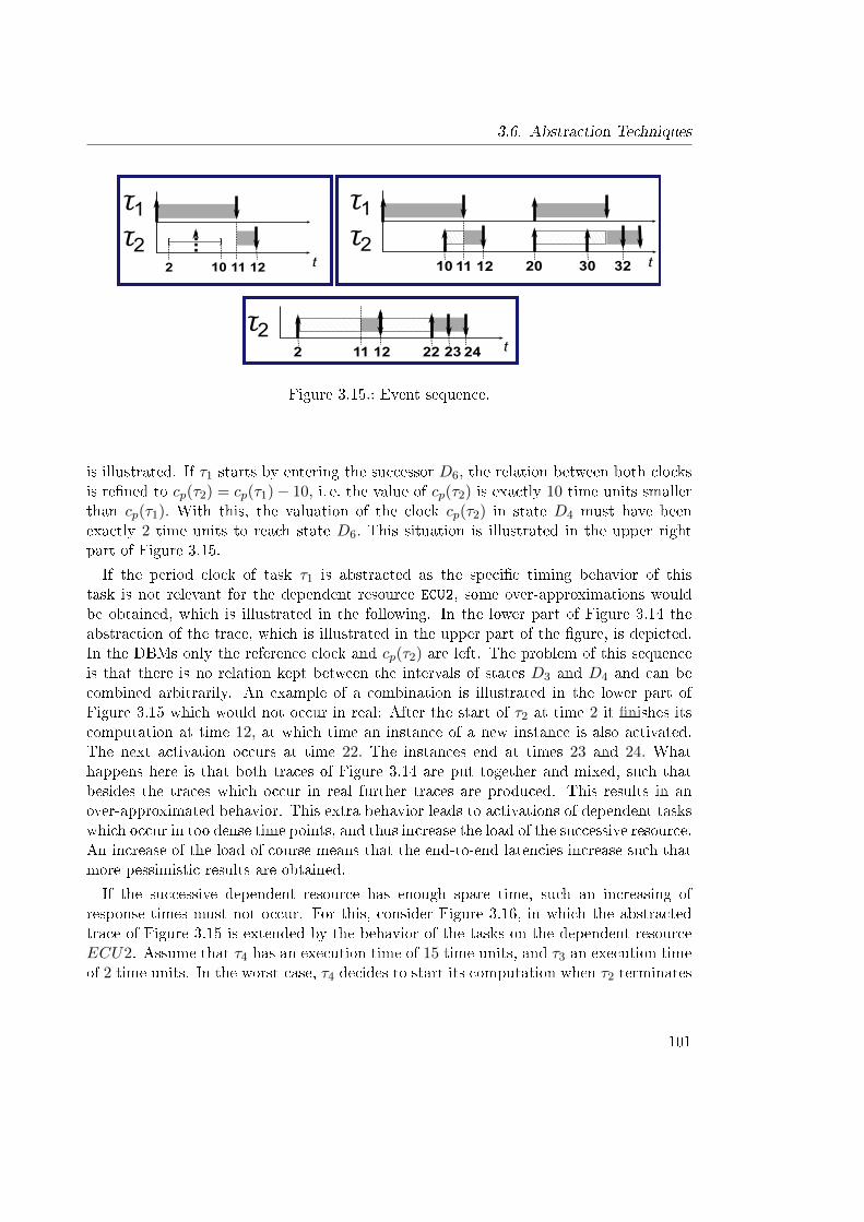
3.6. Abstraction Techniques
τ2τ1
11 10 12 30 20 t 32
τ2τ1
11 2 12 t
[ ]
10
τ211 2 12 22 t 23 24
Figure 3.15.: Event sequence.
is illustrated. If τ1 starts by entering the successor D6, the relation between both clocksis re�ned to cp(τ2) = cp(τ1)− 10, i. e. the value of cp(τ2) is exactly 10 time units smallerthan cp(τ1). With this, the valuation of the clock cp(τ2) in state D4 must have beenexactly 2 time units to reach state D6. This situation is illustrated in the upper rightpart of Figure 3.15.
If the period clock of task τ1 is abstracted as the speci�c timing behavior of thistask is not relevant for the dependent resource ECU2, some over-approximations wouldbe obtained, which is illustrated in the following. In the lower part of Figure 3.14 theabstraction of the trace, which is illustrated in the upper part of the �gure, is depicted.In the DBMs only the reference clock and cp(τ2) are left. The problem of this sequenceis that there is no relation kept between the intervals of states D3 and D4 and can becombined arbitrarily. An example of a combination is illustrated in the lower part ofFigure 3.15 which would not occur in real: After the start of τ2 at time 2 it �nishes itscomputation at time 12, at which time an instance of a new instance is also activated.The next activation occurs at time 22. The instances end at times 23 and 24. Whathappens here is that both traces of Figure 3.14 are put together and mixed, such thatbesides the traces which occur in real further traces are produced. This results in anover-approximated behavior. This extra behavior leads to activations of dependent taskswhich occur in too dense time points, and thus increase the load of the successive resource.An increase of the load of course means that the end-to-end latencies increase such thatmore pessimistic results are obtained.
If the successive dependent resource has enough spare time, such an increasing ofresponse times must not occur. For this, consider Figure 3.16, in which the abstractedtrace of Figure 3.15 is extended by the behavior of the tasks on the dependent resourceECU2. Assume that τ4 has an execution time of 15 time units, and τ3 an execution timeof 2 time units. In the worst-case, τ4 decides to start its computation when τ2 terminates
101
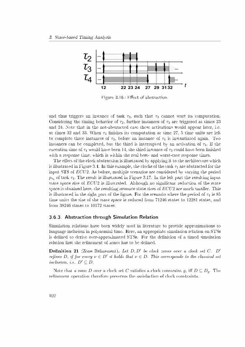
3. State-based Timing Analysis
τ2
12 22 t 23 24
τ3...
...
...
27 32
...
29 31
...
τ4Figure 3.16.: E�ect of abstraction.
and thus triggers an instance of task τ3, such that τ3 cannot start its computation.Considering the timing behavior of τ2, further instances of τ3 are triggered at times 23and 24. Note that in the not-abstracted case these activations would appear later, i.e.at times 32 and 33. When τ4 �nishes its computation at time 27, 5 time units are leftto complete three instances of τ3, before an instance of τ4 is instantiated again. Twoinstances can be completed, but the third is interrupted by an activation of τ4. If theexecution time of τ4 would have been 14, the third instance of τ3 could have been �nishedwith a response time, which is within the real best- and worst-case response times.The e�ect of the clock abstraction is illustrated by applying it to the architecture which
is illustrated in Figure 3.4. In this example, the clocks of the task τ1 are abstracted for theinput STS of ECU2. As before, multiple scenarios are considered by varying the periodpτ4 of task τ4. The result is illustrated in Figure 3.17. In the left part the resulting inputstate space size of ECU2 is illustrated. Although no signi�cant reduction of the statespace is obtained here, the resulting resource state sizes of ECU2 are much smaller. Thisis illustrated in the right part of the �gure. For the scenario where the period of τ4 is 85time units the size of the state space is reduced from 71246 states to 12281 states, andfrom 38246 states to 10172 states.
3.6.3. Abstraction through Simulation Relation
Simulation relations have been widely used in literature to provide approximations tolanguage inclusion in polynomial time. Here, an appropriate simulation relation on STSsis de�ned to derive over-approximated STSs. For the de�nition of a timed simulationrelation �rst the re�nement of zones has to be de�ned.
De�nition 21 (Zone Re�nement). Let D,D′ be clock zones over a clock set C. D′
re�nes D, if for every ν ∈ D′ it holds that ν ∈ D. This corresponds to the classical setinclusion, i.e. D′ ⊆ D.
Note that a zone D over a clock set C satis�es a clock constraint g, i� D ⊆ Dg. There�nement operation therefore preserves the satisfaction of clock constraints.
102
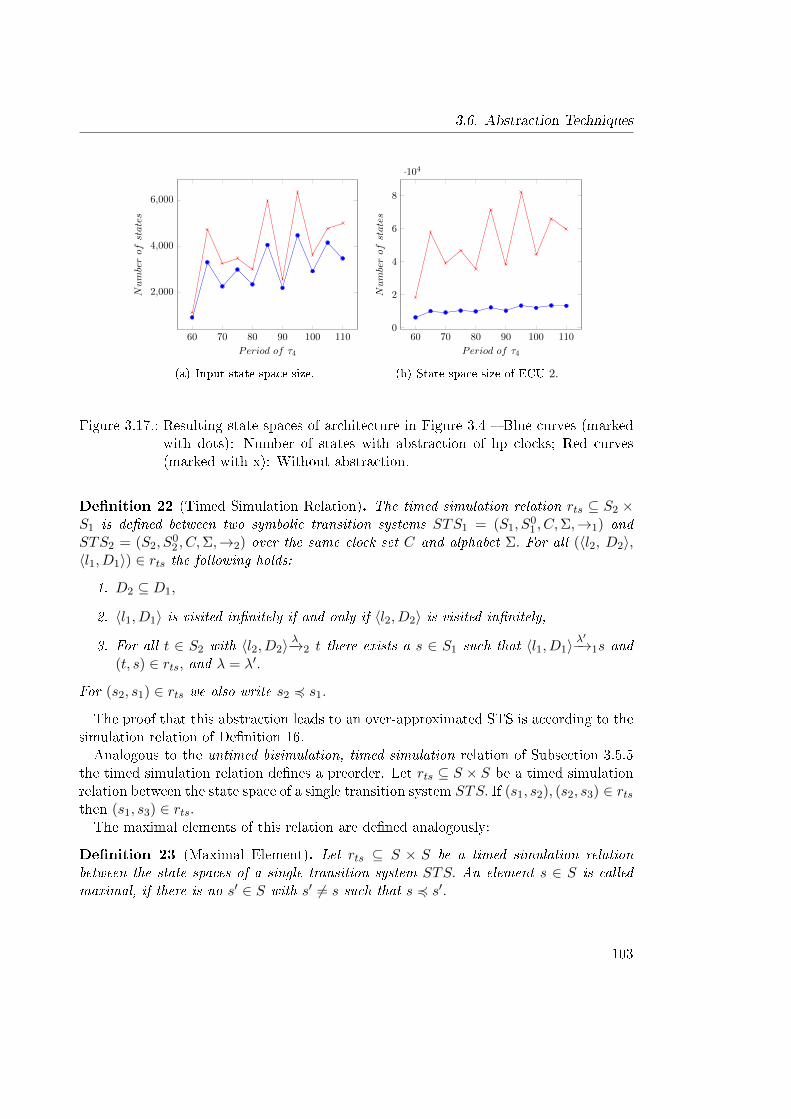
3.6. Abstraction Techniques
60 70 80 90 100 110
2,000
4,000
6,000
Period of τ4
Numberof
states
(a) Input state space size.
60 70 80 90 100 1100
2
4
6
8
·104
Period of τ4
Numberof
states
(b) State space size of ECU 2.
Figure 3.17.: Resulting state spaces of architecture in Figure 3.4 � Blue curves (markedwith dots): Number of states with abstraction of hp clocks; Red curves(marked with x): Without abstraction.
De�nition 22 (Timed Simulation Relation). The timed simulation relation rts ⊆ S2 ×S1 is de�ned between two symbolic transition systems STS1 = (S1, S
01 , C,Σ,→1) and
STS2 = (S2, S02 , C,Σ,→2) over the same clock set C and alphabet Σ. For all (〈l2, D2〉,
〈l1, D1〉) ∈ rts the following holds:
1. D2 ⊆ D1,
2. 〈l1, D1〉 is visited in�nitely if and only if 〈l2, D2〉 is visited in�nitely,
3. For all t ∈ S2 with 〈l2, D2〉λ−→2 t there exists a s ∈ S1 such that 〈l1, D1〉
λ′−→1s and(t, s) ∈ rts, and λ = λ′.
For (s2, s1) ∈ rts we also write s2 4 s1.
The proof that this abstraction leads to an over-approximated STS is according to thesimulation relation of De�nition 16.Analogous to the untimed bisimulation, timed simulation relation of Subsection 3.5.5
the timed simulation relation de�nes a preorder. Let rts ⊆ S × S be a timed simulationrelation between the state space of a single transition system STS. If (s1, s2), (s2, s3) ∈ rtsthen (s1, s3) ∈ rts.The maximal elements of this relation are de�ned analogously:
De�nition 23 (Maximal Element). Let rts ⊆ S × S be a timed simulation relationbetween the state spaces of a single transition system STS. An element s ∈ S is calledmaximal, if there is no s′ ∈ S with s′ 6= s such that s 4 s′.
103
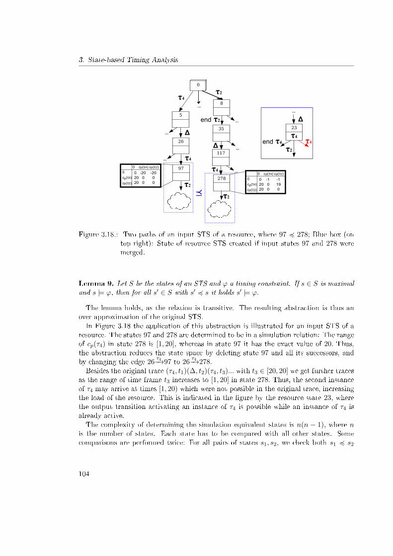
3. State-based Timing Analysis
0
5
117... 0 -20 -20 20 0 0 20 0 0
0 cp(τ4) cp(τ2)
0
cp(τ4)
cp(τ2)
8
26
35 23
278
...
...
...
...
...
...
97
...
Δ
... 0 -1 -1 20 0 19 20 0 0
0 cp(τ4) cp(τ2)
0
cp(τ4)
cp(τ2)
Δ
τ2
end τ2
Δ
τ4
end τ4
τ4
τ2
τ2
τ4
τ2
τ4τ4
Figure 3.18.: Two paths of an input STS of a resource, where 97 4 278; Blue box (ontop right): State of resource STS created if input states 97 and 278 weremerged.
Lemma 9. Let S be the states of an STS and ϕ a timing constraint. If s ∈ S is maximaland s |= ϕ, then for all s′ ∈ S with s′ 4 s it holds s′ |= ϕ.
The lemma holds, as the relation is transitive. The resulting abstraction is thus anover-approximation of the original STS.In Figure 3.18 the application of this abstraction is illustrated for an input STS of a
resource. The states 97 and 278 are determined to be in a simulation relation: The rangeof cp(τ4) in state 278 is [1, 20], whereas in state 97 it has the exact value of 20. Thus,the abstraction reduces the state space by deleting state 97 and all its successors, andby changing the edge 26
τ4−→97 to 26τ4−→278.
Besides the original trace (τ4, t1)(∆, t2)(τ4, t3)... with t3 ∈ [20, 20] we get further tracesas the range of time frame t3 increases to [1, 20] in state 278. Thus, the second instanceof τ4 may arrive at times [1, 20) which were not possible in the original trace, increasingthe load of the resource. This is indicated in the �gure by the resource state 23, wherethe output transition activating an instance of τ4 is possible while an instance of τ4 isalready active.The complexity of determining the simulation equivalent states is n(n − 1), where n
is the number of states. Each state has to be compared with all other states. Somecomparisons are performed twice: For all pairs of states s1, s2, we check both s1 4 s2
104
3.6. Abstraction Techniques
and s2 4 s1. For many cases, the complexity is reduced to n(n − 1)/2 in the best-case.For this, the already analyzed pairs are added to a hash table. Corresponding state pairsare added to this table, if the check was already successful for the �rst comparison, orif the zones are completely disjoint or not in a subset relation, such that comparing theother direction would not make any sense.
3.6.4. E�ects of Over-Approximations for Iterative Analysis Approach
So far, techniques to generate over-approximations of the original state spaces were pre-sented. Generally, over-approximations are an e�ective approach to minimize a givenstate space, such that the complexity to traverse through this state space and performsome analysis to evaluate given properties � i.e. timing deadlines in our case � on thereached states is minimized. Thereby, the over-approximation is necessary to give saferesults.The abstraction techniques illustrated in the previous subsections were implemented
and applied to our iterative analysis approach: For each computed interface STS anover-approximation is computed, which then is used as an input for dependent resources.Interestingly, this approach leads to larger state spaces for dependent resources. Thereason for this is that when performing over-approximations, more behavior is allowedto occur which also increases the load of the resources as illustrated before. As morebehavior is allowed in the input STS, more activation situations have to be handledwithin the dependent resource state spaces, leading to increased state spaces and alsolonger analyses times.The e�ect of the timed simulation relation abstraction is illustrated by applying it
to the architecture which is illustrated in Figure 3.4. In speci�c, the timed simulationrelation is applied to the input state space of ECU2. The result is illustrated in Figure3.19. Although the input state spaces for every scenario are reduced as illustrated in theleft part of the �gure, the resulting numbers of the states of the resource STSs are alwaysabove the ones without applying the abstraction on the input STSs. For instance, in thescenario where the period of τ4 is 85 time units, the state space increases from 71246states to 93869 states.To result in smaller state spaces for dependent resources, under-approximation tech-
niques would be more suitable. Unfortunately, such techniques lead to too optimisticand unsafe veri�cation results. In the next subsection, the bene�ts of such approachesin our context is discussed.
3.6.5. Testing: Abstraction through Under-Approximation
Using the concept of depth-�rst search through the state space of a resource a path whichproduces a schedule with events at �xed time intervals which repeat in�nitively often inthe same order can be determined. By reducing the state space of the resource to only
105
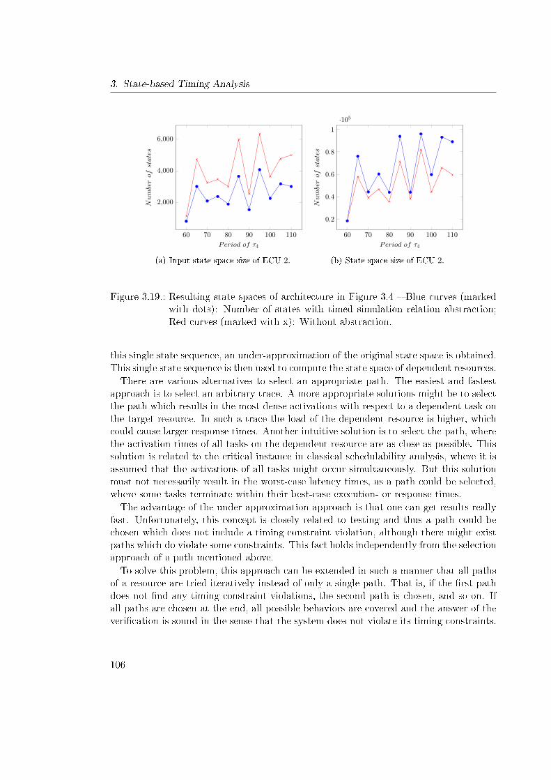
3. State-based Timing Analysis
60 70 80 90 100 110
2,000
4,000
6,000
Period of τ4
Numberof
states
(a) Input state space size of ECU 2.
60 70 80 90 100 110
0.2
0.4
0.6
0.8
1
·105
Period of τ4
Numberof
states
(b) State space size of ECU 2.
Figure 3.19.: Resulting state spaces of architecture in Figure 3.4 � Blue curves (markedwith dots): Number of states with timed simulation relation abstraction;Red curves (marked with x): Without abstraction.
this single state sequence, an under-approximation of the original state space is obtained.This single state sequence is then used to compute the state space of dependent resources.There are various alternatives to select an appropriate path. The easiest and fastest
approach is to select an arbitrary trace. A more appropriate solutions might be to selectthe path which results in the most dense activations with respect to a dependent task onthe target resource. In such a trace the load of the dependent resource is higher, whichcould cause larger response times. Another intuitive solution is to select the path, wherethe activation times of all tasks on the dependent resource are as close as possible. Thissolution is related to the critical instance in classical schedulability analysis, where it isassumed that the activations of all tasks might occur simultaneously. But this solutionmust not necessarily result in the worst-case latency times, as a path could be selected,where some tasks terminate within their best-case execution- or response times.The advantage of the under-approximation approach is that one can get results really
fast. Unfortunately, this concept is closely related to testing and thus a path could bechosen which does not include a timing constraint violation, although there might existpaths which do violate some constraints. This fact holds independently from the selectionapproach of a path mentioned above.To solve this problem, this approach can be extended in such a manner that all paths
of a resource are tried iteratively instead of only a single path. That is, if the �rst pathdoes not �nd any timing constraint violations, the second path is chosen, and so on. Ifall paths are chosen at the end, all possible behaviors are covered and the answer of theveri�cation is sound in the sense that the system does not violate its timing constraints.
106
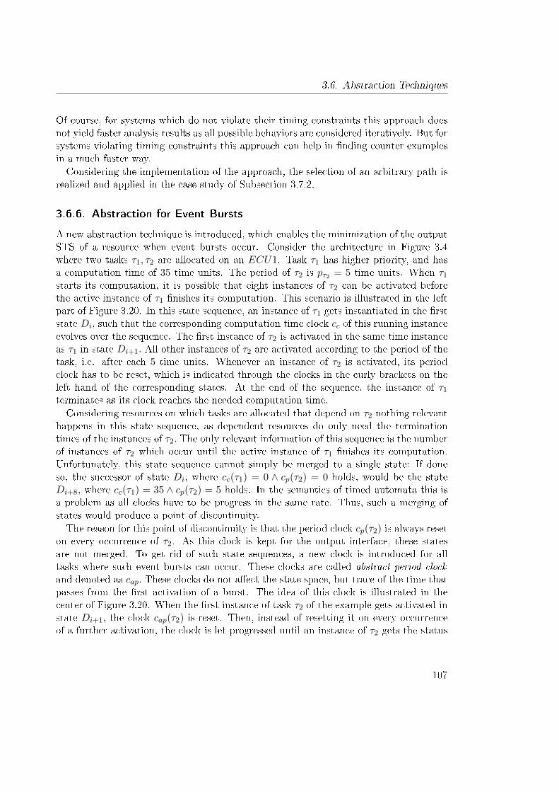
3.6. Abstraction Techniques
Of course, for systems which do not violate their timing constraints this approach doesnot yield faster analysis results as all possible behaviors are considered iteratively. But forsystems violating timing constraints this approach can help in �nding counter examplesin a much faster way.Considering the implementation of the approach, the selection of an arbitrary path is
realized and applied in the case study of Subsection 3.7.2.
3.6.6. Abstraction for Event Bursts
A new abstraction technique is introduced, which enables the minimization of the outputSTS of a resource when event bursts occur. Consider the architecture in Figure 3.4where two tasks τ1, τ2 are allocated on an ECU1. Task τ1 has higher priority, and hasa computation time of 35 time units. The period of τ2 is pτ2 = 5 time units. When τ1
starts its computation, it is possible that eight instances of τ2 can be activated beforethe active instance of τ1 �nishes its computation. This scenario is illustrated in the leftpart of Figure 3.20. In this state sequence, an instance of τ1 gets instantiated in the �rststate Di, such that the corresponding computation time clock cc of this running instanceevolves over the sequence. The �rst instance of τ2 is activated in the same time instanceas τ1 in state Di+1. All other instances of τ2 are activated according to the period of thetask, i.e. after each 5 time units. Whenever an instance of τ2 is activated, its periodclock has to be reset, which is indicated through the clocks in the curly brackets on theleft hand of the corresponding states. At the end of the sequence, the instance of τ1
terminates as its clock reaches the needed computation time.Considering resources on which tasks are allocated that depend on τ2 nothing relevant
happens in this state sequence, as dependent resources do only need the terminationtimes of the instances of τ2. The only relevant information of this sequence is the numberof instances of τ2 which occur until the active instance of τ1 �nishes its computation.Unfortunately, this state sequence cannot simply be merged to a single state: If doneso, the successor of state Di, where cc(τ1) = 0 ∧ cp(τ2) = 0 holds, would be the stateDi+8, where cc(τ1) = 35 ∧ cp(τ2) = 5 holds. In the semantics of timed automata this isa problem as all clocks have to be progress in the same rate. Thus, such a merging ofstates would produce a point of discontinuity.The reason for this point of discontinuity is that the period clock cp(τ2) is always reset
on every occurrence of τ2. As this clock is kept for the output interface, these statesare not merged. To get rid of such state sequences, a new clock is introduced for alltasks where such event bursts can occur. These clocks are called abstract period clockand denoted as cap. These clocks do not a�ect the state space, but trace of the time thatpasses from the �rst activation of a burst. The idea of this clock is illustrated in thecenter of Figure 3.20. When the �rst instance of task τ2 of the example gets activated instate Di+1, the clock cap(τ2) is reset. Then, instead of resetting it on every occurrenceof a further activation, the clock is let progressed until an instance of τ2 gets the status
107
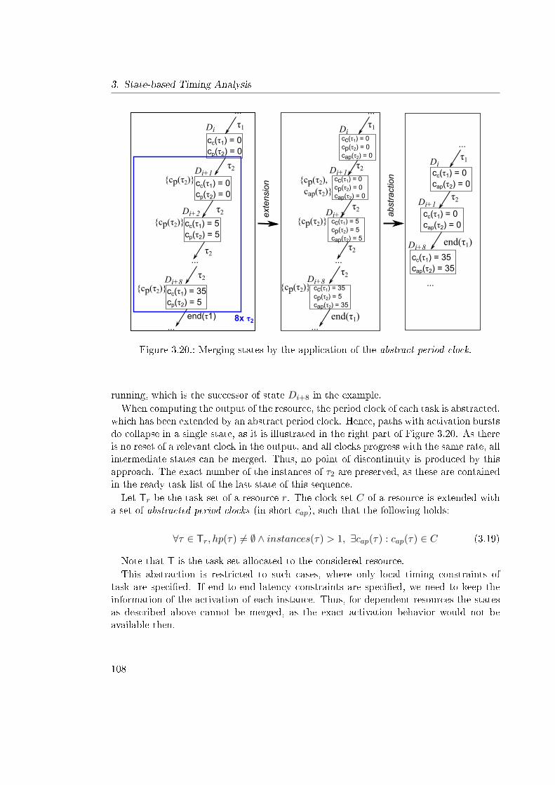
3. State-based Timing Analysis
cc(τ1) = 0cp(τ2) = 0
τ1
...
...
end(τ1)...
8x τ2
...
...
...
...
...
extension
abstraction
τ2
τ2
τ2
{cp(τ2)}
{cp(τ2)}
τ1
τ1
end(τ1)
end(τ1)
τ2
τ2
τ2
τ2
{cp(τ2)}
τ2 τ2
cc(τ1) = 0cp(τ2) = 0
cc(τ1) = 5cp(τ2) = 5
cc(τ1) = 35cp(τ2) = 5
cc(τ1) = 0cap(τ2) = 0
cc(τ1) = 0cap(τ2) = 0
cc(τ1) = 35cap(τ2) = 35
cc(τ1) = 0cp(τ2) = 0cap(τ2) = 0
cc(τ1) = 0cp(τ2) = 0cap(τ2) = 0
cc(τ1) = 5cp(τ2) = 5cap(τ2) = 5
cc(τ1) = 35cp(τ2) = 5cap(τ2) = 35
{cp(τ2),cap(τ2)}
{cp(τ2)}
{cp(τ2)}
Di+1
Di
Di+2
Di+8
Di
DiDi+1
Di+1Di+2
Di+8
Di+8
Figure 3.20.: Merging states by the application of the abstract period clock.
running, which is the successor of state Di+8 in the example.When computing the output of the resource, the period clock of each task is abstracted,
which has been extended by an abstract period clock. Hence, paths with activation burstsdo collapse in a single state, as it is illustrated in the right part of Figure 3.20. As thereis no reset of a relevant clock in the output, and all clocks progress with the same rate, allintermediate states can be merged. Thus, no point of discontinuity is produced by thisapproach. The exact number of the instances of τ2 are preserved, as these are containedin the ready task list of the last state of this sequence.Let Tr be the task set of a resource r. The clock set C of a resource is extended with
a set of abstracted period clocks (in short cap), such that the following holds:
∀τ ∈ Tr, hp(τ) 6= ∅ ∧ instances(τ) > 1, ∃cap(τ) : cap(τ) ∈ C (3.19)
Note that T is the task set allocated to the considered resource.This abstraction is restricted to such cases, where only local timing constraints of
task are speci�ed. If end-to-end latency constraints are speci�ed, we need to keep theinformation of the activation of each instance. Thus, for dependent resources the statesas described above cannot be merged, as the exact activation behavior would not beavailable then.
108
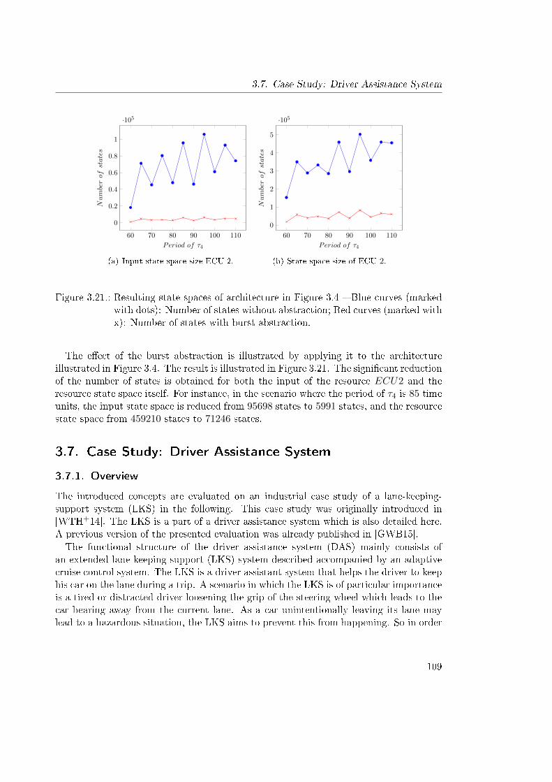
3.7. Case Study: Driver Assistance System
60 70 80 90 100 110
0
0.2
0.4
0.6
0.8
1
·105
Period of τ4
Numberof
states
(a) Input state space size ECU 2.
60 70 80 90 100 110
0
1
2
3
4
5
·105
Period of τ4
Numberof
states
(b) State space size of ECU 2.
Figure 3.21.: Resulting state spaces of architecture in Figure 3.4 � Blue curves (markedwith dots): Number of states without abstraction; Red curves (marked withx): Number of states with burst abstraction.
The e�ect of the burst abstraction is illustrated by applying it to the architectureillustrated in Figure 3.4. The result is illustrated in Figure 3.21. The signi�cant reductionof the number of states is obtained for both the input of the resource ECU2 and theresource state space itself. For instance, in the scenario where the period of τ4 is 85 timeunits, the input state space is reduced from 95698 states to 5991 states, and the resourcestate space from 459210 states to 71246 states.
3.7. Case Study: Driver Assistance System
3.7.1. Overview
The introduced concepts are evaluated on an industrial case study of a lane-keeping-support system (LKS) in the following. This case study was originally introduced in[WTH+14]. The LKS is a part of a driver assistance system which is also detailed here.A previous version of the presented evaluation was already published in [GWB15].The functional structure of the driver assistance system (DAS) mainly consists of
an extended lane-keeping-support (LKS) system described accompanied by an adaptivecruise control system. The LKS is a driver assistant system that helps the driver to keephis car on the lane during a trip. A scenario in which the LKS is of particular importanceis a tired or distracted driver loosening the grip of the steering wheel which leads to thecar bearing away from the current lane. As a car unintentionally leaving its lane maylead to a hazardous situation, the LKS aims to prevent this from happening. So in order
109
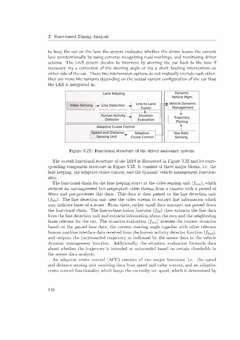
3. State-based Timing Analysis
to keep the car on the lane the system evaluates whether the driver leaves the currentlane unintentionally by using cameras recognizing road markings, and monitoring driveractions. The LKS system decides to intervene by steering the car back to the lane ifnecessary via a correction of the steering angle or via a short braking intervention oneither side of the car. These two intervention options do not mutually exclude each other,they are more like variants depending on the actual variant con�guration of the car thatthe LKS is integrated in.
Video Sensing Line Detection
Human Activity Detector
Line-to-Lane Fusion
Situation Evaluation
Speed and Distance Sensing Unit
Adaptive Cruise Control
Vehicle Dynamic Management
Trajectory Planing
Yaw Rate Sensing
Lane Keeping
Adaptive Cruise Control
Dynamic Vehicle Mgm.
Figure 3.22.: Functional structure of the driver assistance system.
The overall functional structure of the DAS is illustrated in Figure 3.22 and its corre-sponding component structure in Figure 3.23. It consists of three major blocks, i.e. thelane keeping, the adaptive cruise control, and the dynamic vehicle management function-ality.The functional chain for the lane keeping starts at the video sensing unit (fvsu), which
receives an uncompressed two mega-pixel video stream from a camera with a period of80ms and pre-processes this data. This data is then passed to the line detection unit(fldu). The line detection unit uses the video stream to extract line information whichmay indicate lanes of a street. From there, rather small data amounts are passed downthe functional chain. The line-to-lane-fusion function (fl2l) then extracts the line datafrom the line detection unit and extracts information about the own and the neighboringlanes relevant for the car. The situation evaluation (fseu) assesses the current situationbased on the passed lane data, the current steering angle together with other relevanthuman machine interface data received from the human activity detector function (fhad),and outputs the (un)intended trajectory as indicated by the sensor data to the vehicledynamic management function. Additionally, the situation evaluation forwards dataabout whether the trajectory is intended or unintended based on certain thresholds inthe sensor data analysis.An adaptive cruise control (ACC) consists of two major functions, i.e. the speed
and distance sensing unit receiving data from speed and radar sensors, and an adaptivecruise control functionality which keeps the currently set speed, which is determined by
110
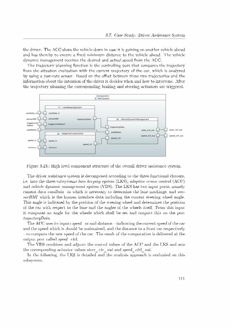
3.7. Case Study: Driver Assistance System
the driver. The ACC slows the vehicle down in case it is gaining on another vehicle aheadand has thereby to ensure a �xed minimum distance to the vehicle ahead. The vehicledynamic management receives the desired and actual speed from the ACC.The trajectory planning function is the controlling part that compares the trajectory
from the situation evaluation with the current trajectory of the car, which is analyzedby using a yaw-rate sensor. Based on the o�set between these two trajectories and theinformation about the intention of the driver it decides when and how to intervene. Afterthe trajectory planning the corresponding braking and steering actuators are triggered.
«Component»DAS-System
: LaneKeepingSystem
trajectoryData
camData_in
sensorHMI : VehicleDynamicManagement
trajectoryData
yawRateIn steer_ctrl_out
speed_ctrl speed_ctrl_out
: AdaptiveCruiseControl
speed_in
distance
speed_ctrl
camData_in
sensorHMI
yawRateIn
speed_in
distance
steer_ctrl_out
speed_ctrl_out
triggerLineDetect
triggerLineDetect
Figure 3.23.: High level component structure of the overall driver assistance system.
The driver assistance system is decomposed according to the three functional clusters,i.e. into the three subsystems lane keeping system (LKS), adaptive cruise control (ACC)and vehicle dynamic management system (VDS). The LKS has two input ports, namelycamera data camData_in which is necessary to determine the lane markings, and sen-sorHMI which is the human interface data including the current steering wheel angle.This angle is indicated by the position of the steering wheel and determines the positionof the car with respect to the lane and the angles of the wheels itself. From this inputit computes an angle for the wheels which shall be set and outputs this on the porttrajectoryData.The ACC uses its inputs speed_in and distance � indicating the current speed of the car
and the speed which is should be maintained, and the distance to a front car respectively� to compute the new speed of the car. The result of the computation is delivered at theoutput port called speed_ctrl.The VDS combines and adjusts the control values of the ACC and the LKS and sets
the corresponding actuator values steer_ctr_out and speed_ctrl_out.In the following, the LKS is detailed and the analysis approach is evaluated on this
subsystem.
111
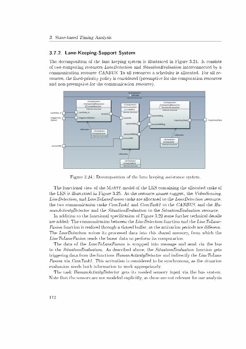
3. State-based Timing Analysis
3.7.2. Lane-Keeping-Support System
The decomposition of the lane keeping system is illustrated in Figure 3.24. It consistsof two computing resources LaneDetection and SituationEvaluation interconnected by acommunication resource CANBUS. To all resources a scheduler is allocated. For all re-sources, the �xed-priority policy is considered (preemptive for the computation resourcesand non-preemptive for the communication resource).
«Component»LKS-HW
internal structure
«Component»«ComputingResource»
LaneDetection internal structure
camData_in laneInfo
«Component»«Communication...
CANBUS internal structure
laneInfo
sensorHMI
laneInfoMsg
sensorHMIMsg
«Component»«ComputingResource»
SituationEvaluation internal structure
trajectoryData
laneInfoMsg
sensorHMIMsg
«Scheduler»ScheduleLane internal structure
«Scheduler»ScheduleBUS internal structure
«Scheduler»ScheduleSit
internal structure
camData_in
sensorHMI
trajectoryData
«Allocate»
«Allocate»
«Allocate»
triggerLineDetect
triggerLineDetect
Figure 3.24.: Decomposition of the lane keeping assistance system.
The functional view of the Marte model of the LKS containing the allocated tasks ofthe LKS is illustrated in Figure 3.25. As the resource names suggest, the VideoSensing,LineDetection, and LineToLaneFusion tasks are allocated to the LaneDetection resource,the two communication tasks ComTask1 and ComTask2 to the CANBUS, and the Hu-manActivityDetector and the SituationEvaluation to the SituationEvaluation resource.In addition to the functional speci�cation of Figure 3.22 some further technical details
are added: The communication between the LineDetection function and the LineToLane-Fusion function is realized through a shared bu�er, as the activation periods are di�erent.The LineDetection writes its processed data into this shared memory, from which theLineToLaneFusion reads the latest data to perform its computation.The data of the LineToLaneFusion is wrapped into message and send via the bus
to the SituationEvaluation. As described above, the SituationEvaluation function getstriggering data from the functions HumanActivityDetector and indirectly the LineToLaneFusion via ComTask1. This activation is considered to be synchronous, as the situationevaluation needs both information to work appropriately.The task HumanActivityDetector gets its needed sensory input via the bus system.
Note that the sensors are not modeled explicitly, as these are not relevant for our analysis
112
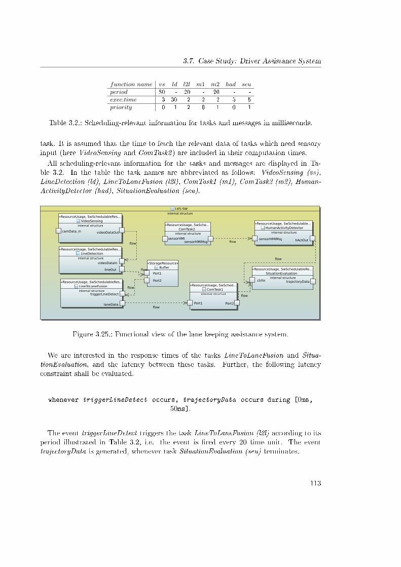
3.7. Case Study: Driver Assistance System
function name vs ld l2l m1 m2 had seu
period 80 - 20 - 20 - -
exec.time 3 30 2 2 2 5 5
priority 0 1 2 0 1 0 1
Table 3.2.: Scheduling-relevant information for tasks and messages in milliseconds.
task. It is assumed that the time to fetch the relevant data of tasks which need sensoryinput (here VideoSensing and ComTask2 ) are included in their computation times.
All scheduling-relevant information for the tasks and messages are displayed in Ta-ble 3.2. In the table the task names are abbreviated as follows: VideoSensing (vs),LineDetection (ld), LineToLaneFusion (l2l), ComTask1 (m1), ComTask2 (m2), Human-ActivityDetector (had), SituationEvaluation (seu).
LKS-SW internal structure
«ResourceUsage, SwSchedulableRes...LineToLaneFusion internal structure
laneData
«ResourceUsage, SwSched...ComTask1
internal structure
Port2 Port1
«ResourceUsage, SwSchedulable...HumanActivityDetector
internal structure
hActOut
«ResourceUsage, SwSchedulableRes...LineDetection
internal structure
videoDataIn
lineOut
«ResourceUsage, SwSche...ComTask2
internal structure
«ResourceUsage, SwSchedulableRe...SituationEvaluation
internal structure ctrlIn
«StorageResource»Buffer
Port1
Port2
«ResourceUsage, SwSchedulableRes...VideoSensing
internal structure
videoDataOut
trajectoryData
flow
flow
flow
flow
flow
flowflow
camData_in
sensorHMIsensorHMIMsg
sensorHMIMsg
triggerLineDetect
Figure 3.25.: Functional view of the lane keeping assistance system.
We are interested in the response times of the tasks LineToLaneFusion and Situa-tionEvaluation, and the latency between these tasks. Further, the following latencyconstraint shall be evaluated.
whenever triggerLineDetect occurs, trajectoryData occurs during [0ms,50ms].
The event triggerLineDetect triggers the task LineToLaneFusion (l2l) according to itsperiod illustrated in Table 3.2, i.e. the event is �red every 20 time unit. The eventtrajectoryData is generated, whenever task SituationEvaluation (seu) terminates.
113
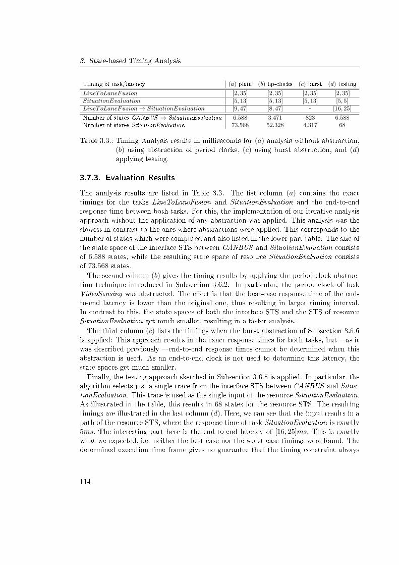
3. State-based Timing Analysis
Timing of task/latency (a) plain (b) hp-clocks (c) burst (d) testing
LineToLaneFusion [2, 35] [2, 35] [2, 35] [2, 35]
SituationEvaluation [5, 13] [5, 13] [5, 13] [5, 5]
LineToLaneFusion → SituationEvaluation [9, 47] [8, 47] - [16, 25]
Number of states CANBUS → SituationEvaluation 6.588 3.471 823 6.588Number of states SituationEvaluation 73.568 52.328 4.317 68
Table 3.3.: Timing Analysis results in milliseconds for (a) analysis without abstraction,(b) using abstraction of period clocks, (c) using burst abstraction, and (d)applying testing.
3.7.3. Evaluation Results
The analysis results are listed in Table 3.3. The �st column (a) contains the exacttimings for the tasks LineToLaneFusion and SituationEvaluation and the end-to-endresponse time between both tasks. For this, the implementation of our iterative analysisapproach without the application of any abstraction was applied. This analysis was theslowest in contrast to the ones where abstractions were applied. This corresponds to thenumber of states which were computed and also listed in the lower part table: The size ofthe state space of the interface STS between CANBUS and SituationEvaluation consistsof 6.588 states, while the resulting state space of resource SituationEvaluation consistsof 73.568 states.The second column (b) gives the timing results by applying the period clock abstrac-
tion technique introduced in Subsection 3.6.2. In particular, the period clock of taskVideoSensing was abstracted. The e�ect is that the best-case response time of the end-to-end latency is lower than the original one, thus resulting in larger timing interval.In contrast to this, the state spaces of both the interface STS and the STS of resourceSituationEvaluation get much smaller, resulting in a faster analysis.The third column (c) lists the timings when the burst abstraction of Subsection 3.6.6
is applied: This approach results in the exact response times for both tasks, but � as itwas described previously � end-to-end response times cannot be determined when thisabstraction is used. As an end-to-end clock is not used to determine this latency, thestate spaces get much smaller.Finally, the testing approach sketched in Subsection 3.6.5 is applied. In particular, the
algorithm selects just a single trace from the interface STS between CANBUS and Situa-tionEvaluation. This trace is used as the single input of the resource SituationEvaluation.As illustrated in the table, this results in 68 states for the resource STS. The resultingtimings are illustrated in the last column (d). Here, we can see that the input results in apath of the resource STS, where the response time of task SituationEvaluation is exactly5ms. The interesting part here is the end-to-end latency of [16, 25]ms. This is exactlywhat we expected, i.e. neither the best-case nor the worst-case timings were found. Thedetermined execution time frame gives no guarantee that the timing constraint always
114
3.8. Summary
holds but represents possible behavior. This result can only give a hint to what laten-cies can be expected. Still, it is a usable approach if e.g. the original analysis does notterminate because of a too large state space. The testing approach then can be used toiteratively validate such an end-to-end latency.
3.7.4. Observation on Scalability
When performing the veri�cations on the introduced case study by using our prototypeimplementation, we determined some characteristics which in�uence the run times of theveri�cation.First, the scalability of the approach heavily depends on the applied abstractions. If
a detailed veri�cation is performed where no abstractions are applied, the veri�cation isable to handle only small systems like the holistic model-checking approaches in the liter-ature. Second, major aspects of the systems under analysis which negatively in�uencedthe scalability of the approach were the following:
• Increasing number of independent tasks: The more independent tasks were de-�ned, the larger the state spaces got. The reason for this e�ect is the initial non-determinism of the initial triggering of tasks, which is de�ned by a time interval.With this, the product construction leads to large state spaces, as all possible acti-vation scenarios are constructed. When the initial non-determinism is deactivated,the resulting state spaces were much smaller. As an example, for two tasks onlytwo possible activation scenarios could occur after deactivation.
• The di�erence between the characteristics of tasks: If the periods and the executiontimes of two (or more) tasks are similar, the resulting state spaces are much smallerthan in scenarios, where these characteristics are diverging. The reason for this isthat in more heterogeneous scenarios more states are necessary to keep track of theindividual states of the tasks.
• The length of task chains: As more clocks are involved in such scenarios, whichleads to an increasing state space.
The challenge here is to �nd the appropriate abstraction level for the veri�cation task,such that on the one hand the result is usable (i.e. not too pessimistic) and on the otherhand delivers results in an acceptable amount of time.
3.8. Summary
In this chapter our state-based scheduling analysis technique for distributed real-timesystems was presented. The state space of the entire system architecture is de�ned bysymbolic transitions systems (STS) and is constructed in an iterative manner. For this,
115
3. State-based Timing Analysis
two main operations on STSs were introduced, namely the product construction and theabstraction of clocks and locations of an STS of interface STSs. It was shown that theproduct construction preserves timing properties and thus can be adequately used tosuccessively build the sate space of the whole system architecture. Based on an inputSTS of a resource describing the activation times of the allocated tasks, an algorithmwhich builds the STS of this resource was described. Based on the state space of aresource, response times are determined. This iterative analysis enables checking end-to-end constraints in a more e�cient manner than a holistic analysis as only the relevantparts of the state space are kept, while preserving all interleavings and task dependencies.Note that by enabling analysis in a more e�cient manner we refer to the reduced statespaces with which the analysis concept has to deal in contrast to holistic approaches.We did not compare the introduced approach with state-of-the-art tools as the prototypeimplementation of the concept is not suited and optimized for such purposes.Thereafter, abstraction techniques in the context of the presented iterative analy-
sis were introduced. First, the e�ect of replacing two clocks by a single one was dis-cussed. The abstraction of clocks of interface STS was illustrated and the resultingover-approximated STS was explained. The timed simulation relation was then intro-duced to apply an approximation technique, which tends to yield smaller state spacesfor holistic analysis approaches or local state spaces, but a�ects in larger state spacesfor dependent resources especially for iterative analysis approaches such as ours. As alast technique the abstraction for burst-scenarios was introduced. For all abstractiontechniques appropriate examples were studied and their e�ects have been demonstrated.Last, the applicability of the approach on a driver assistance system case study was
demonstrated. For this, the lane-keeping-support subsystem part was detailed. In par-ticular, the hardware and task architecture in terms of a Marte model was introduced,and the timing analysis was performed on this model. We compared the response timesand state spaces of our basic approach and the results of the applications of the abstrac-tion techniques. The positive e�ects on the sizes of the number of states could beendemonstrated, which boosts the scalability of state-based analysis approaches.
116
4. Contract-based Impact Analysis
4.1. Motivation
The design of a system typically consists of several speci�cation, implementation, andanalysis steps. Within these steps the speci�cation, the architectural realization, andimplementations are created to ful�ll and realize the corresponding requirements. Dur-ing the development process of such a system, business needs could change, or initiallyassumed aspects or goals could get re�ned, a�ecting the requirements of the system un-der design. Thus, the derived speci�cation and the designed architecture typically aresubject of changes. To give only some examples: Adaptations of the architecture of analready existing and analyzed system could be the removal of some resources due to costsavings, such that the tasks on this resource have to be re-allocated to the remaining re-sources. Another source of changes are incremental development cycles, where a previousversion of a system is reused to include new features. Also technical issues could causechanges: If during the integration phase errors occur as interfaces do not �t together,the speci�cations of individual components must be modi�ed, which also could a�ect thecorresponding implementations.As stated before, there are several proof obligations in safety-critical systems to assure
the correct service and to prevent failures which could lead to critical situations. Whenchanges occur, all veri�cation steps must be repeated to guarantee that the changes do notviolate any requirement. The impact analysis introduced in this chapter targets such re-veri�cations by determining the a�ected parts of the system by a change, thus preventingto perform all veri�cation steps from scratch. With this technique it is possible to keep re-veri�cations local in certain cases. Suppose that the speci�cation of a system componentshall be replaced. If the newly adapted speci�cation re�nes the previous speci�cation,only the internals of the new component itself have to be re-veri�ed without the need ofa repetition of a complete integration check of this component with its context.Refer again to the overall content of this thesis illustrated in Figure 4.1: The con-
tent of this chapter introduces the impact analysis methodology together with its basictechniques. If some parts of the architecture need to be re-veri�ed on implementationlevel, the impact analysis will use the state-based timing analysis approach introducedin Chapter 3.This chapter is organized as follows. At �rst, related works on veri�cation tools for con-
tract speci�cations and on approaches reducing the e�ort of performing re-veri�cationsare presented. In Section 4.3 the overall concept of the impact analysis approach is intro-
117
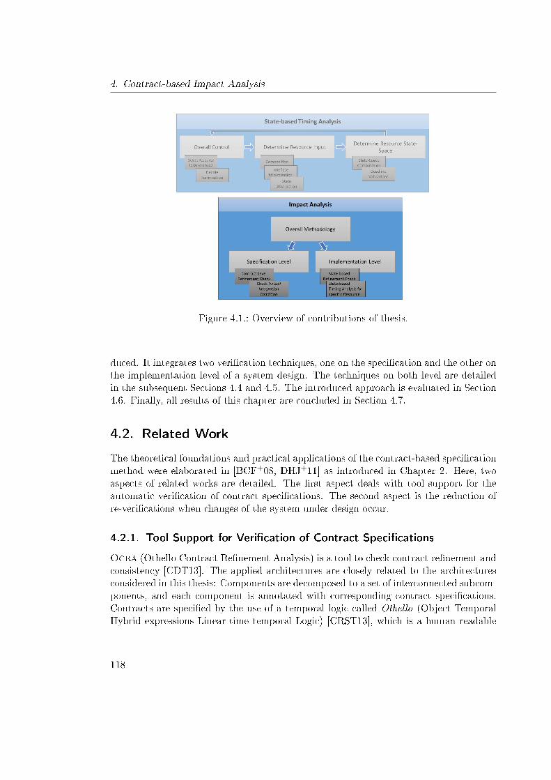
4. Contract-based Impact Analysis
Figure 4.1.: Overview of contributions of thesis.
duced. It integrates two veri�cation techniques, one on the speci�cation and the other onthe implementation level of a system design. The techniques on both level are detailedin the subsequent Sections 4.4 and 4.5. The introduced approach is evaluated in Section4.6. Finally, all results of this chapter are concluded in Section 4.7.
4.2. Related Work
The theoretical foundations and practical applications of the contract-based speci�cationmethod were elaborated in [BCF+08, DHJ+11] as introduced in Chapter 2. Here, twoaspects of related works are detailed. The �rst aspect deals with tool support for theautomatic veri�cation of contract speci�cations. The second aspect is the reduction ofre-veri�cations when changes of the system under design occur.
4.2.1. Tool Support for Veri�cation of Contract Speci�cations
Ocra (Othello Contract Re�nement Analysis) is a tool to check contract re�nement andconsistency [CDT13]. The applied architectures are closely related to the architecturesconsidered in this thesis: Components are decomposed to a set of interconnected subcom-ponents, and each component is annotated with corresponding contract speci�cations.Contracts are speci�ed by the use of a temporal logic called Othello (Object TemporalHybrid expressions Linear-time temporal Logic) [CRST13], which is a human readable
118
4.2. Related Work
language. The semantics of this language is given in terms of an extended version oflinear time temporal logic (LTL) called HRELTL (Hybrid Linear Temporal Logic withRegular Expressions). In contrast to this thesis, they use an SMT solver to check such re-lations. The backend engine of Ocra is NuSMV3 which itself is based on the SAT solverMathSAT. MathSAT only considers quanti�er free formulas, while NuSMV3 extends thisto the logic of LTL. The tool is also able to verify implementations against contracts.In contrast to this thesis the approach is restricted to discrete-time LTL contracts and�nite state machines. The main result of the authors concerning the applicability of theirapproach is that their tool scales well with the number of decomposition structures. Thereason for this lies in the nature of contracts, as the veri�cation steps are performedlocally within structures.The focus of the authors of [BMSH10] are modal input/output automata (MIO). With
this model, two types of behaviors can be described, i.e. allowed and required behaviors,modeled as may and must transitions respectively. Further, as in timed automata, input,output, and internal actions are distinguished. In their work, modalities are applied tore�nement and compatibility, as detailed in the following.A MIO A1 strongly modally re�nes another MIO A2 which is de�ned over the same
signature, if there is a strong modal re�nement relation between A1 and A2, where A1
can simulate all must transitions of A2 immediately, and whenever A1 can perform amay transition, A2 can simulate this with a corresponding may transition. Strong modalcompatibility between two MIOs A1, A2 requires that if A1 can send an output action �either by a may or a must transition � which is in the input alphabet of A2, then A2
must immediately be able to receive the message and is not allowed e.g. to take internaltransitions before.Weak modal re�nement does allow internal actions before must transitions are �red,
i.e. if the more abstract MIO is able to �re a must transition with an output action, there�ning MIO is allowed to �re a �nite set of internal must transitions, but has �nally tosimulate the must transition of the abstract MIO. With this notion of re�nement, more�exibility is allowed by e.g. the modeling of internal computations during the re�nementprocess. The weak modal compatibility is de�ned accordingly, i.e. where internal must-transitions are allowed before the synchronization has to be performed. The weak modalcompatibility allows a more loosely coupling of interfaces.This approach has also been implemented in the MIO Workbench [BML11], which
is an Eclipse-based editor for modal I/O automata equipped with a veri�cation back-end. The veri�cation back-end is able to check strong and weak modal compatibilityand re�nement. This work is related to this thesis, as it also deals with automata-basedveri�cation of properties like composition and re�nement. In contrast to this thesis, theauthors considered only untimed systems and did not consider contracts explicitly.In [AdADS+06] a tool called Ticc (Tool for Interface Compatibility and Composition)
was introduced. It checks the compatibility of component interfaces, where untimedtransition systems with input and output actions and discrete variables encoding the
119
4. Contract-based Impact Analysis
states are considered. Components are modeled based on game theory, where componentsare represented by automata with input and/or output actions on transitions. Thesemantics of such automata is given by the well-known two-player games, where the inputplayer represents the environment, and the output player represents the component itself.The authors later extended this work in [DLL+10b] for dense time systems by intro-
ducing the timed input/output automata (TIOA), which are based on a timed version ofthe game semantics, and provided also a tool called ECDAR (Environment for Compo-sitional Design and Analysis of Real-Time Systems) [DLL+10a]. In contrast to standardtimed automata, the transitions are di�erentiated between input and output transitions.Edges controlled by the environment are annotated by receiving events, while edges con-trolled by the automaton itself are annotated by sending events.The designer can create automata for both the implementation and speci�cation of a
system. After the creation, re�nement and consistency checks between all automata canbe performed through the integrated game engine, which is based on Uppaal-Tiga. Forthis, appropriate queries are de�ned to enable the veri�cation engine. The consistencycheck veri�es whether there exists an implementation which ful�lls its correspondingspeci�cation. Thus, a strategy for the output player is searched, which prevents thespeci�cation to reach a bad state. An example to verify the re�nement: Let the imple-mentations in terms of TIOA N1, ..., N3, and an overall system speci�cation automatonS be given. To check the re�nement, the query re�nement : (N1 || N2 || N3) ≤ S iscreated. In the sense of compositional design, all implementations could also get sub-speci�cations, which are again TIOA. Then, the re�nement for each implementationagainst its speci�cation would be checked, and at least the correct composition of allsub-speci�cations with the overall speci�cation would be veri�ed. The approach is a bitunintuitive, as both the speci�cation and implementation have to be created in terms ofTIOA. Further, the authors did not detail the scalability of their approach. They onlygive a hint that the scalability gets better, if sub-speci�cations are created, instead ofperforming a holistic analysis against the overall speci�cation [DLL+10a].In [CGP03] the authors state that the de�nition of appropriate assumptions for compo-
nent contracts is a complex task, and thus they claim that this task has to be automated.For this, they present an algorithm called L∗ which iteratively learns assumptions of com-ponents and their behavior. This learning is based on re�nement. They consider �nitediscrete traces produced by labeled state transition systems. The paper is restricted tocases where the system is composed of two componentsM1,M2. The goal is to decomposethe system property C = (true,G) to sub-contracts C1 = (true,A) and C2 = (A,G),i.e. to �nd an appropriate assumption A which is guaranteed from component M1 (andthus contract C1). The algorithm iteratively computes an intermediate assumption Aiconsisting of a set of �nite words. This Ai is then used as the context for M2, and itis checked whether M2 is able to ful�ll the property G. If not, the assumption is tooweak such that further behavior has to be removed. To do so, the counter-example tracereturned from the used model checker is applied. If otherwise the found assumption Aj
120
4.2. Related Work
is strong enough for M2 to guarantee G, is checked in a second step whether Aj is nottoo strong for the behavior of the predecessor component M1. As in the �rst step, if Ajis too strong, then Aj needs to be weaken by adding further behavior via the usage ofthe returned counterexample. In the other case, it holds that the property G holds forM1||M2. The authors extend the learning algorithm (among other things) to a chain ofcomponents in [PGB+08]. The basic techniques to check re�nements of contracts arealso applied in this thesis. In contrast to this thesis, the authors focus on the automaticderivation of appropriate component assumptions, while in this work the focus is on theapplication of the virtual integration of components into their context.
4.2.2. Impact Analysis
In the work of [KHM+96] the system behavior is given as a set of functions, which maydepend on each other. The work is based on regression testing, where a set of tests arede�ned for each function. If a test fails, the error is corrected and all tests are re-run. Alsopreviously successfully tested functions are re-tested to ensure, whether the changes didnot a�ect these functions. The authors applied this idea to formal veri�cation and calledthe approach regression veri�cation. The �rst part of the work is to apply an algorithmcalled localization reduction which abstracts a model P relative to a given property ϕ.That is, the algorithm determines the part of P which is relevant for the correspondingproperty ϕ, and from this it builds a reduced model P ′, which is smaller than P andthus computationally simpler. The basic idea of this reduction is the application ofthe language inclusion of automata theory, where an automaton P ′ is a reduction ofP , if L(P ) ⊆ L(P ′). Further, P ′ is obtained from ϕ and P, such that it is correct byconstruction, i.e. L(P ′) ⊆ ϕ holds. The second part targets the problem of storing themodels: The reduced models are saved by the use of hash functions. With these functionsonly the hash value of the reduced models are stored. If changes occur, the corresponding(new and old) hash values are compared to determine whether the veri�cation result isa�ected.The result of their work is that the computations of reduced models together with the
computations and the checks of the hash values is less complex than the original checksdetermining whether a system satis�es a given property. Moreover, the storage of modelsis omitted, as only the corresponding hash values are stored. The approach has beenimplemented in a veri�cation engine called COSPAN. The idea of the work of [KHM+96]is closely related to this thesis. The authors do only check a part of a given model. Incontrast to this thesis, this is realized by building a new abstract model which is su�cientto re-check a given property. Our approach does not need to calculate an abstract modelas it is able to determine indirectly a�ected parts of the given architecture, which then arere-checked. Further, the authors realize a holistic analysis, whereas the impact analysison the speci�cation level of this thesis operates in a compositional manner.The approach of [BLN+13] targets the CEGAR-based (Counterexample-Guided Ab-
121
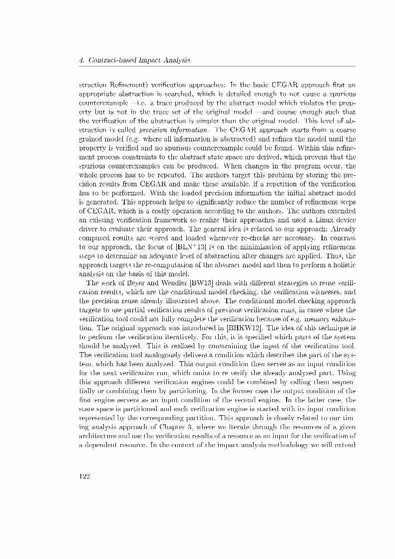
4. Contract-based Impact Analysis
straction Re�nement) veri�cation approaches: In the basic CEGAR approach �rst anappropriate abstraction is searched, which is detailed enough to not cause a spuriouscounterexample � i.e. a trace produced by the abstract model which violates the prop-erty but is not in the trace set of the original model � and coarse enough such thatthe veri�cation of the abstraction is simpler than the original model. This level of ab-straction is called precision information. The CEGAR approach starts from a coarsegrained model (e.g. where all information is abstracted) and re�nes the model until theproperty is veri�ed and no spurious counterexample could be found. Within this re�ne-ment process constraints to the abstract state space are derived, which prevent that thespurious counterexamples can be produced. When changes in the program occur, thewhole process has to be repeated. The authors target this problem by storing the pre-cision results from CEGAR and make these available, if a repetition of the veri�cationhas to be performed. With the loaded precision information the initial abstract modelis generated. This approach helps to signi�cantly reduce the number of re�nement stepsof CEGAR, which is a costly operation according to the authors. The authors extendedan existing veri�cation framework to realize their approaches and used a Linux devicedriver to evaluate their approach. The general idea is related to our approach: Alreadycomputed results are stored and loaded whenever re-checks are necessary. In contrastto our approach, the focus of [BLN+13] is on the minimization of applying re�nementsteps to determine an adequate level of abstraction after changes are applied. Thus, theapproach targets the re-computation of the abstract model and then to perform a holisticanalysis on the basis of this model.The work of Beyer and Wendler [BW13] deals with di�erent strategies to reuse veri�-
cation results, which are the conditional model checking, the veri�cation witnesses, andthe precision reuse already illustrated above. The conditional model checking approachtargets to use partial veri�cation results of previous veri�cation runs, in cases where theveri�cation tool could not fully complete the veri�cation because of e.g. memory exhaus-tion. The original approach was introduced in [BHKW12]. The idea of this technique isto perform the veri�cation iteratively. For this, it is speci�ed which parts of the systemshould be analyzed. This is realized by constraining the input of the veri�cation tool.The veri�cation tool analogously delivers a condition which describes the part of the sys-tem, which has been analyzed. This output condition then serves as an input conditionfor the next veri�cation run, which omits to re-verify the already analyzed part. Usingthis approach di�erent veri�cation engines could be combined by calling them sequen-tially or combining them by partitioning. In the former case the output condition of the�rst engine servers as an input condition of the second engine. In the latter case, thestate space is partitioned and each veri�cation engine is started with its input conditionrepresented by the corresponding partition. This approach is closely related to our tim-ing analysis approach of Chapter 3, where we iterate through the resources of a givenarchitecture and use the veri�cation results of a resource as an input for the veri�cation ofa dependent resource. In the context of the impact analysis methodology we will extend
122
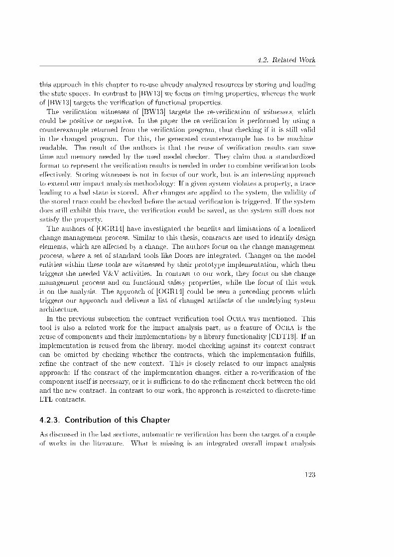
4.2. Related Work
this approach in this chapter to re-use already analyzed resources by storing and loadingthe state spaces. In contrast to [BW13] we focus on timing properties, whereas the workof [BW13] targets the veri�cation of functional properties.The veri�cation witnesses of [BW13] targets the re-veri�cation of witnesses, which
could be positive or negative. In the paper the re-veri�cation is performed by using acounterexample returned from the veri�cation program, thus checking if it is still validin the changed program. For this, the generated counterexample has to be machine-readable. The result of the authors is that the reuse of veri�cation results can savetime and memory needed by the used model checker. They claim that a standardizedformat to represent the veri�cation results is needed in order to combine veri�cation toolse�ectively. Storing witnesses is not in focus of our work, but is an interesting approachto extend our impact analysis methodology: If a given system violates a property, a traceleading to a bad state is stored. After changes are applied to the system, the validity ofthe stored trace could be checked before the actual veri�cation is triggered. If the systemdoes still exhibit this trace, the veri�cation could be saved, as the system still does notsatisfy the property.The authors of [OGR14] have investigated the bene�ts and limitations of a localized
change management process. Similar to this thesis, contracts are used to identify designelements, which are a�ected by a change. The authors focus on the change managementprocess, where a set of standard tools like Doors are integrated. Changes on the modelentities within these tools are witnessed by their prototype implementation, which thentriggers the needed V&V activities. In contrast to our work, they focus on the changemanagement process and on functional safety properties, while the focus of this workis on the analysis. The approach of [OGR14] could be seen a preceding process whichtriggers our approach and delivers a list of changed artifacts of the underlying systemarchitecture.In the previous subsection the contract veri�cation tool Ocra was mentioned. This
tool is also a related work for the impact analysis part, as a feature of Ocra is thereuse of components and their implementations by a library functionality [CDT13]. If animplementation is reused from the library, model checking against its context contractcan be omitted by checking whether the contracts, which the implementation ful�lls,re�ne the contract of the new context. This is closely related to our impact analysisapproach: If the contract of the implementation changes, either a re-veri�cation of thecomponent itself is necessary, or it is su�cient to do the re�nement check between the oldand the new contract. In contrast to our work, the approach is restricted to discrete-timeLTL contracts.
4.2.3. Contribution of this Chapter
As discussed in the last sections, automatic re-veri�cation has been the target of a coupleof works in the literature. What is missing is an integrated overall impact analysis
123
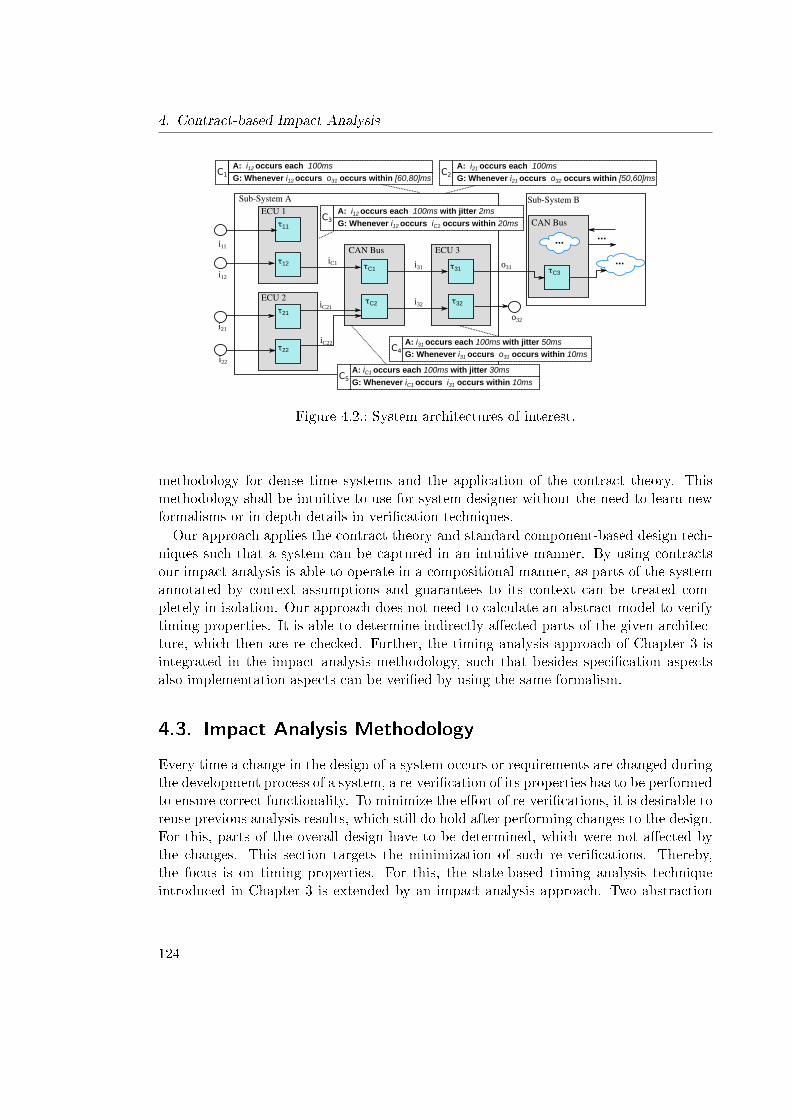
4. Contract-based Impact Analysis
o31
τ11
τ12 τC1
τC2
ECU 1
CAN Busi11
τ21
τ22
ECU 2
τ31
τ32
ECU 3
i12
i21
i22
o32
A: i12 occurs each 100ms
G: Whenever i12 occurs o31 occurs within [60,80]ms
iC1
iC21
G: Whenever iC1 occurs i31 occurs within 10ms
i31
i32
A: i12 occurs each 100ms with jitter 2ms
G: Whenever i12 occurs iC1 occurs within 20ms
G: Whenever i31 occurs o31 occurs within 10ms
Sub-System A
A: i21 occurs each 100ms
G: Whenever i21 occurs o32 occurs within [50,60]ms
CAN Bus
τC3
...
...
...
iC22
...
Sub-System B
A: i31 occurs each 100ms with jitter 50ms
A: iC1 occurs each 100ms with jitter 30ms
C1 C2
C3
C5
C4
Figure 4.2.: System architectures of interest.
methodology for dense time systems and the application of the contract theory. Thismethodology shall be intuitive to use for system designer without the need to learn newformalisms or in-depth details in veri�cation techniques.Our approach applies the contract theory and standard component-based design tech-
niques such that a system can be captured in an intuitive manner. By using contractsour impact analysis is able to operate in a compositional manner, as parts of the systemannotated by context assumptions and guarantees to its context can be treated com-pletely in isolation. Our approach does not need to calculate an abstract model to verifytiming properties. It is able to determine indirectly a�ected parts of the given architec-ture, which then are re-checked. Further, the timing analysis approach of Chapter 3 isintegrated in the impact analysis methodology, such that besides speci�cation aspectsalso implementation aspects can be veri�ed by using the same formalism.
4.3. Impact Analysis Methodology
Every time a change in the design of a system occurs or requirements are changed duringthe development process of a system, a re-veri�cation of its properties has to be performedto ensure correct functionality. To minimize the e�ort of re-veri�cations, it is desirable toreuse previous analysis results, which still do hold after performing changes to the design.For this, parts of the overall design have to be determined, which were not a�ected bythe changes. This section targets the minimization of such re-veri�cations. Thereby,the focus is on timing properties. For this, the state-based timing analysis techniqueintroduced in Chapter 3 is extended by an impact analysis approach. Two abstraction
124
4.3. Impact Analysis Methodology
levels are de�ned, which could be a�ected by changes, which are the speci�cation levelon the one hand, and the implementation level on the other hand.On the speci�cation level a virtual integration checking technique is introduced through
the concept of reachability analysis of timed automata. Suppose that the speci�cation ofa system component in terms of assume/guarantee style contracts shall be replaced. Ifthe new contract of the adapted speci�cation re�nes the previous contract, the internalsof the new component itself need to be checked. Thus, the e�ects of such changes arekept local, and only a part of the overall architecture has to be re-veri�ed. Of course, ifthe contract of a component is completely replaced, it has also be checked whether thenew speci�cation is consistent with its context.If resources are not annotated by contracts, on the implementation level state transi-
tion systems describe the behavioral interfaces between dependent resources. For suchcases, an appropriate re�nement relation between these state transition systems on theinterfaces of resources is de�ned. With this notion of re�nement, re-veri�cations of partsof the system on implementation level can be avoided.Both complete speci�cations, which fully describe the interfaces between all compo-
nents, and incomplete speci�cations, where the interface descriptions of only a subset ofcomponents is given, are considered in this thesis. In a design process incomplete speci�-cations are quite typical as some properties of parts of a system may be obtained in laterdesign steps. A complete interface speci�cation is given for e.g. the task chain τ12, τC1, τ31
in the architecture of Figure 4.2: The assumptions of the contracts of ECU1, CAN Bus,and ECU3 describe the activation behaviors of the corresponding tasks τ12, τC1, and τ31.That is, the local contracts C3, C4 and C5 can be veri�ed locally without consideringany behavior of the systems from their contexts. If the system speci�cation is completethe virtual integration checking technique allows us to determine the impact of changeswhich may occur during the development process of a system without the considerationof any implementation detail.For incomplete speci�cations a re�nement check of the behavioral interfaces of the
resources, which are determined by the iterative timing analysis technique illustrated inChapter 3, is performed. An example of an incomplete speci�cation is the task chainτ21, τC2, τ32 in the same architecture of Figure 4.2. For this task chain only an end-to-end latency constraint is speci�ed. To analyze the end-to-end latency constraint forsuch cases, the state-based analysis approach of Chapter 3 is applied. If changes in thearchitectures occur, the approach is able to handle these appropriately. For this, duringthe iterative analysis the veri�cation results are stored and can be reused in later designsteps.Generally, in a design process both approaches are exploited in combination: When a
component is replaced, the new component has to be integrated in the existing context,i.e. the impact on the speci�cation level has to be determined. In a second step, theimpact on the implementation level as described above has to be checked and the neces-sary re-veri�cations have to be performed. By applying the introduced impact analysis
125
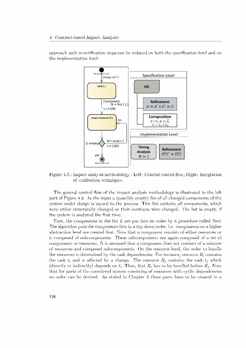
4. Contract-based Impact Analysis
approach such re-veri�cation steps can be reduced on both the speci�cation level and onthe implementation level.
Figure 4.3.: Impact analysis methodology - Left: General control �ow; Right: Integrationof veri�cation techniques.
The general control �ow of the impact analysis methodology is illustrated in the leftpart of Figure 4.3. As the input a (possibly empty) list of all changed components of thesystem under design is passed to the process. This list contains all components, whichwere either structurally changed or their contracts were changed. The list is empty, ifthe system is analyzed the �rst time.First, the components in the list L are put into an order by a procedure called Sort.
The algorithm puts the components �rst in a top-down order, i.e. components on a higherabstraction level are treated �rst. Note that a component consists of either resources oris composed of subcomponents. These subcomponents are again composed of a set ofcomponents or resources. It is assumed that a component does not consists of a mixtureof resources and composed subcomponents. On the resource level, the order to handlethe resources is determined by the task dependencies. For instance, resource Ri containsthe task ti and is a�ected by a change. The resource Rj contains the task tj which(directly or indirectly) depends on ti. Then, �rst Ri has to be handled before Rj . Notethat for parts of the considered system consisting of resources with cyclic dependenciesno order can be derived. As stated in Chapter 3 these parts have to be treated in a
126
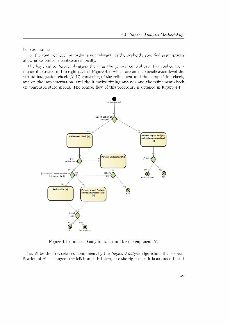
4.3. Impact Analysis Methodology
holistic manner.For the contract level, an order is not relevant, as the explicitly speci�ed assumptions
allow us to perform veri�cations locally.The logic called Impact Analysis then has the general control over the applied tech-
niques illustrated in the right part of Figure 4.3, which are on the speci�cation level thevirtual integration check (VIC) consisting of the re�nement and the composition check,and on the implementation level the iterative timing analysis and the re�nement checkon computed state spaces. The control �ow of this procedure is detailed in Figure 4.4.
Figure 4.4.: Impact Analysis procedure for a component N .
Let N be the �rst selected component by the Impact Analysis algorithm. If the speci-�cation of N is changed, the left branch is taken, else the right one. It is assumed that if
127
4. Contract-based Impact Analysis
the speci�cation is not changed, the component N is either a resource or a composition ofresources. In such a case the changes on N concern the implementation aspects, and theprocedure Perform Impact Analysis on Implementation Level is called, which consists ofthe timing analysis and the re�nement check on state transition systems as describedabove. Within this procedure, the timing analysis is performed for the directly a�ectedcomponents. Thereafter, it is checked whether the new computed state spaces of thea�ected resources re�ne the previous state spaces (computed before the correspondingchange occurred). If the new state spaces do re�ne the previous ones, then the depen-dent resources do not need to be veri�ed. The techniques on this level are detailed andaddressed in Section 4.5.
If a change concerns the speci�cation then the left branch is taken, where it is �rstchecked, whether the new contract of N re�nes its old contract. If the re�nement holds(and thus the guard Is re�nement in the �gure evaluates to true), the context of N isnot a�ected, and only the internals of this component have to be veri�ed. If thereby thedecomposition structure of N is completely speci�ed by contracts, the virtual integrationcheck of N and its decomposition structure has to be veri�ed. That is, it is checked,whether the contracts of the decomposition structure do �t to the new overall contractof N. Otherwise, if the decomposition structure has not a complete speci�cation, theimpact analysis on the implementation level is triggered, which was already describedabove. Note that if the decomposition structure is not complete, it is assumed that thisstructure corresponds to a set of resources. This is no restriction to the general case, butfacilitates the description of the approach. Note that if only the guaranteed end-to-endlatency of N is changed, only a look-up in the state spaces of the last resources has tobe performed to verify whether the new latency guarantees are still ful�lled. Otherwise,if the assumptions like task activation times are changed, the timing analysis has to berepeated for a�ected resources.
Otherwise, if the change of N is not a re�nement, the composition to its dependentresources could be a�ected such that the virtual condition check has to be performed forits context, which is obtained by the method context(N) in the �gure. Note that if forthe component no context is de�ned, the method context(N) returns nil and the VIC isskipped. If this check does not fail, further the internals of the component need to bechecked as already described.
For the overall component of N (obtained by the method N ′ :=context(N)) the VIChas only to be performed once. If there are several subcomponents of N ′ with changedcontracts in a non-re�nement manner, the logic would call the same VIC several times,which is not necessary. To prevent this repetition of the VIC, a �ag is set for a componentN ′, when the VIC for N ′ is called the �rst time.
The applied analysis techniques of this branch are detailed in the next section.
128
4.4. Impact Analysis on Speci�cation Level
As illustrated in the left part of Figure 4.3 the Impact Analysis procedure operatesuntil all components in the change list are handled.Note that if an analysis like the VIC determines that a property is not ful�lled, the
process terminates in a fail state, which indicates that the process is terminated (with anappropriate error message). In this case, the changes violate some integration aspects orthe implementation is not able to ful�ll the new guarantees under the new assumptions.In the next sections, all referred techniques will be illustrated. Note that the introduced
impact analysis approach was previously worked out and published in [GHSR14].
4.4. Impact Analysis on Speci�cation Level
As previously stated, the speci�cation of a system is subject to change. At early stages ofthe design process details are not known such as the complete scope of the functionality orarchitectural decisions which may a�ect certain performance aspects. Some requirementsmay arise during the development process which were not considered at �rst. During thedesign process such details get more and more concrete, which typically lead to changesand re�nements of existing requirements.In this thesis requirements are speci�ed by the usage of assume/guarantee style con-
tracts. If the contract of a component N is changed and the new contract re�nes theprevious one, only the internals of N need to be re-veri�ed as its context is only a�ectedin a positive manner, which means that all properties still do hold. If N is decomposedin subcomponents with local contracts, it has to be checked whether the new componentcontract is still ful�lled by the composition of the contracts of all subcomponents. As anexample, consider the following contract (AK , GK) of a component K:
(AK) sensorin occurs each 10ms
(GK) Whenever sensorin occurs, actuatorout occurs during [0, 50]ms
Suppose the guarantee is changed as follows:(G′K) Whenever sensorin occurs, actuatorout occurs during [0, 30]ms
The component K with its new contract (AK , G′K) will deliver its output signal to its
dependent components not later than 30ms anymore after activation. As the dependentresources are already able to handle the time interval [0, 50], they are also able to handlethe new interval. Thus, there is no need to analyze this property. On the other hand,the internal implementation of K has now to realize this stricter timing latency. It hasto be checked, whether there exist scenarios, in which the timing latency of 30ms cannotbe met.Otherwise, if the new contract is not a re�nement of the old one, an additional consis-
tency check with all dependent parts of the system has to be performed. Thus, it has tobe re-veri�ed whether the component can be virtually integrated to its intended context.
129
4. Contract-based Impact Analysis
Such a virtual integration check operates on the speci�cation level of a system withoutthe need to consider all implementation details at once.In the case where a part of the system is changed, and the system is fully speci�ed,
the introduced approach is able to keep the e�ects of changes local such that only a partof the whole architecture has to be re-veri�ed.For such scenarios a timed automaton-based approach is introduced in this section,
with which it is possible to automatically validate virtual integration aspects. This inte-gration encapsulates the correct composition of components with respect to their contractspeci�cations, and the correct re�nement of a higher level contract. The correspondingcondition for this was introduced in Subsection 2.4.1. Next, relevant properties of con-tracts will be inspected, which are directedness and saturation. From these properties thesimpli�cation of the original virtual integration condition will be derived, which enablesthe usage of timed automata to realize an appropriate veri�cation approach.
4.4.1. Simplifying the Virtual Integration Condition
In Subsection 2.4.1 the virtual integration condition was introduced. This condition sum-marizes the composition and re�nement checks of components, which have to be appliedwhen components are decomposed to a set of interconnected subcomponents to guaranteecorrect interaction and the consistency of the system speci�cation. Unfortunately, thiscondition includes negations. As a timed automaton approach shall be applied in this the-sis to verify this condition, and timed automata are not closed under complementation,this section deals with the simpli�cation of this property by using some characteristicsof contracts.
Saturated Contracts
In De�nition 12 it was already stated that the implementationM of a component satis�esa contract C = (A,G) of that component, if [[M ]] ⊆ [[¬A]]∪ [[G]]. From this, the maximalpossible allowed behavior of a component can be directly derived, which corresponds tothe following:
[[Mmax]] = [[¬A]] ∪ [[G]]. (4.1)
This was the topic of [BCN+11] where the term saturated was de�ned for contracts.
De�nition 24 (Saturated Contracts). Let C = (A,G) be a contract, where A, G areassertions over the interface I with I(A) ⊆ I(G). C is saturated, if [[G]] ⊇ [[¬A]].
Note that for an assertion E the function I(E) determines the set of ports, over whichit is de�ned. A contract is saturated, if the behavior which is not captured by theenvironment assumption is included in the guarantee of the component. In [BCF+08]this property is called canonical , as the maximal allowed behaviorMmax is unique. Each
130
4.4. Impact Analysis on Speci�cation Level
contract can be transformed to a saturated one (canonical form) by adding all traces of[[¬A]] to the guarantee.For instance, consider a component with an input port in and an output port out.
Let the component compute the square root of the values received on the input port,i.e. out =
√in. The component is further annotated by a contract, where its assumption
states that the values on the input port shall be greater than or equal to zero. Thecontract is saturated, if (besides the allowed input values) the guarantee de�nes also a(default) behavior for negative input values, e.g. out = NaN if in < 0.This property of contracts simpli�es the virtual integration condition. If all sub-
contracts Ci of a composite are saturated, the �rst condition of the virtual integrationcondition (cf. Lemma 3) simpli�es to
A ∧G1 ∧ · · · ∧Gn ⇒ A1 · · ·An.
This is exactly what we want to achieve, i.e. to get rid of the negation part of thisconstraint. Unfortunately, if the sub-contracts are not in saturated form, we have �rst totransform the guarantees, i.e. we have to extend the guarantee parts with the negatedform of the corresponding assumptions. E�ectively, we did not achieve anything, as thenegation part has still to be taken into account when performing veri�cations. We onlyshifted the terms including negations into the guarantee part.
Receptiveness and Directed Contracts
Contracts are typically a black-box speci�cation formalism and restrict the observablebehavior of components. Speci�cations restrict the port valuations of components with-out distinguishing between input and output ports of the corresponding component.Thereby, input ports should be controlled by the environment while the valuations of theoutput ports should depend on the behavior of the component itself. During the designstage problems could arise if this distinction is not performed in a consistent fashion,such that a guarantee is speci�ed, which restricts possible behavior of the input ports,or analogously the assumptions restrict the components output ports. Such contractsde�ne faulty speci�cations, as the component is not responsible for the input behavior,and the environment is not responsible for the component behavior.As an example let requestData be an output port and dataIn be an input port of
a component. Consider the following two assumptions captured by an R3 pattern (cf.Subsection 2.4.2):
• A1 : Whenever requestData occurs, dataIn occurs during [5,10]
• A2 : Whenever dataIn occurs, requestData occurs during [5,10]
A1 is receptive on the output port requestData as it allows occurrences of events on thatport on arbitrary points in time. In contrast to this, A2 is not receptive as it would makerestrictions to the component behavior.
131
4. Contract-based Impact Analysis
To distinguish the responsibilities of the assumptions and guarantees, in [BCF+08,BBB+11] the de�nition of receptiveness was introduced, which is illustrated in the fol-lowing.
De�nition 25 (Receptiveness). Let I be a directed interface, Φ ⊆ L(I) = (Iω × T ) aset of traces over I, and I ′ ⊆ I. Φ is called receptive on I ′, if it is non-empty and for alltraces σ ∈ Φ and for all n ∈ N the following holds:
∀ρ ∈ L(I). pre(ρ, n) = pre(σ, n) ⇒ ∃σ′ ∈ Φ. pre(σ′, n) = pre(ρ, n) ∧ σ′↓I′ = ρ↓I′ .
This condition states that if an arbitrary trace ρ in the (complete) trace set L(I) isconsidered, any trace σ in Φ with an identical pre�x can be arbitrarily extended withrespect to the ports of I ′. Thus, the trace set states no restrictions to the ports of I ′.In the following, an example for a non-receptive contract will be given to ease the
understanding of this property. Consider a component with two input ports i1, i2 and anoutput port o. The guarantee of the component restricts input ports in such a way thatalways i1 should occur before an occurrence of i2. Let σ ∈ L(G) with pre(σ, 1) = o andlet σ′ ∈ L(I) with pre(σ′, 2) = o · i2. There exists a pre�x (n = 1) such that the left partof the implication of De�nition 25 is true, but the right can never be true as there is notrace in L(G) which can be extended in a way like σ′.By applying the receptiveness property to the assumption and guarantee parts of
contracts, one can adequately distinguish the responsibilities of the input and outputbehaviors of a component. Such contracts are called directed .
De�nition 26 (Directed Contract). A contract C = (A,G) over an interface I is di-rected, if A is receptive on out(I) and G is receptive on in(I).
Note that in the following the notions in(I) and out(I) will be abbreviated to in andout respectively, if the port set I is clear from the context.For directed contracts the following corollary is derived:
Corollary 1. Let C = (A,G) be a directed contract over an interface I = in ∪ out. Ifin ⊆ I(A) then L(in) = [[A↓in ]] ∪ [[¬A↓in ]] (and analogously for the guarantee part).
If an assumption restricts all input ports of a corresponding component, all possiblewords over the input ports is obtained by taking the union of the set of traces describedby the assumption and its negation.For a directed contract C it holds that the guarantee does not restrict the language
given by the assumption, and vice versa the assumption does not restrict the set of wordsde�ned by the guarantee. Thus, the following properties are obtained:
A↓in ∩G↓in = A↓in and A↓out ∩G↓out = G↓out . (4.2)
132
4.4. Impact Analysis on Speci�cation Level
To simplify the virtual integration condition, assume that only such architectures areconsidered, where the guarantees are pairwise receptive on each other, i.e. no guaranteerestricts the language of the other guarantees.Further, the following corollary is needed.
Corollary 2. Let A,B be assertions over the interfaces ΣA,ΣB respectively. Then likein propositional logic the following holds regardless of the cut set between ΣA and ΣB :
A↑ΣB ∪ (A↑ΣB ∩B↑ΣA )⇔ A↑ΣB .
Proof. The trivial case for this is given, when both interfaces are equal, i.e. ΣA = ΣB.Let X = ΣB\ΣA and Y = ΣA\ΣB non-empty port-sets. Then according to Lemma1 (A↑X )↓X ⊇ B↓X holds. Analogously, we get (B↑Y )↓Y ⊇ A↓Y , but (B↑Y )↓Y ∩ A↓Y =A↓Y .
With these ingredients, the following theorem is derived.
Theorem 4. Let C = (A,G) be a directed contract over an interface I, and Ci = (Ai, Gi)with i ∈ {1, ..., n} a set of directed sub-contracts over the interfaces Ii with pairwisereceptive guarantees. Then the �rst condition of the VIC of Lemma 3 can be simpli�edas follows.
A ∧G1 ∧ ... ∧Gn ⇒ A1 ∧ · · · ∧An.
The proof is performed for n = 2 which is no restriction to the general case but iseasier to handle.
Proof. Let C = (A,G) be a directed contract over I, C1 = (A1, G1), C2 = (A2, G2)directed sub-contracts with pairwise receptive guarantees over I1 and I2 respectively.According to Lemma 3 the following proof obligation is obtained:
(A ∧ ¬A1 ∧ ¬A2) ∨ (A ∧ ¬A1 ∧G2) ∨ (A ∧ ¬A2 ∧G1) ∨ (A ∧G1 ∧G2)⇒ A1 ∧A2.
In order to reduce the left part to only the expression (A ∧ G1 ∧ G2), it has to beshown that all the other sub-expressions are subsets of this expression. Let Iasmp =I(A) ∪ I(A1) ∪ I(A2), Igrnt = I(G1) ∪ I(G2), and Icmpl = Iasmp ∪ Igrnt.Let us �rst focus on the �rst sub-expression (A∧¬A1∧¬A2). The subset relation does
only hold for the interface Iasmp, and not for Icmpl, i.e. (A↑Iasmp ∩¬A1↑Iasmp¬A2↑Iasmp ) ⊆A↑Iasmp ∩G1↑Iasmp ∩G2↑Iasmp : Because of the receptivity property it holds that A↑Iasmp =A↑Iasmp∩G1↑Iasmp∩G2↑Iasmp . According Corollary 2 it also holds that A↑Iasmp ⊇ A↑Iasmp∩¬A1↑Iasmp ∩¬A2↑Iasmp . From this, it can be followed that the above expression does holdfor Iasmp. To conclude the proof for this expression, we have further to inspect the wordson Igrnt: As A is receptive on Igrnt it holds that A↑Igrnt = L(Igrnt). But this also holds forthe RHS of the veri�cation condition, i.e. A1↑Igrnt = A2↑Igrnt = L(Igrnt). Because of this,it is valid to simplify the veri�cation condition by leaving out the term A ∧ ¬A1 ∧ ¬A2.
133
4. Contract-based Impact Analysis
Secondly, consider (A∧¬Ai∧Gj) for i, j ∈ {1, 2}, i 6= j. As the guarantees are pairwisedisjoint, and ¬Ai ∧ Gj ⊆ Gj holds, we can directly derive that (A ∧ ¬Ai ∧ Gj) ⊆(A ∧G1 ∧G2) holds. This concludes the proof.
Next, the relation between directed and saturated contracts are inspected.
Relation between Saturated and Directed Contracts
Originally, the goal was to show that directed contracts are also saturated, which wouldhave allowed to apply all formulas that are valid for saturated contracts also for directedcontracts without any further architectural assumptions mentioned in the previous sec-tion. Unfortunately, it turned out that none of the properties implies the other.For this, let us consider a directed contract C = (A,G) over the interface I. If C is
also saturated, its guarantee would include the negated assumption, i.e. G = ¬A↑out(I) ∪G′↑in(I)
, where G′ is the part of the guarantee without the assumption part. Indeed,the part A↑out(I) does not restrict the output ports, but possibly could add non-allowedbehavior � with respect to the guarantee � to these ports. Note that this non-allowedbehavior is consistent with the semantics of the contracts, as (false ⇒ false) is true.To illustrate the above reasoning, counter examples for both implications are given.
Note that the following assertions are speci�ed by LTL expressions. Let I = {i, o} be aninterface, where i is an input port, and o is an output port.Consider the assumption A : �(o = 2) and the guarantee G : �(o = 2 ⇒ i = 0).
Clearly, since ¬A ⊆ G holds, the contract is saturated. However, it is easy to see thatneither A is receptive on the output port, nor G is receptive on the input port.For the second implication, consider the assumption A : �(i = 0) and the guarantee
G : �(o = 2). A is receptive on the output port and G is receptive on the input port.Consider a trace satisfying the condition i = 1 ∧ o = 3. The trace is contained in thelanguage ¬A but not in G. Thus, the contract is not saturated.
4.4.2. Timed Automaton-based Analysis Approach
In this section a technique to check the re�nement and virtual integration condition ofcontracts as introduced in Subsection 2.4.1 is presented. For this, all contracts of thecorresponding system under analysis are translated to Uppaal timed automata [LPY97],and a reachability check of states violating any properties [ABL98] is performed. Thistechnique is inspired by so called observer-based analyses in literature: Properties areexpressed by employing the same formalism as the system. The system is then extendedby the resulting component. This new component is also called observer or monitor inliterature. Such a component passively observes the relevant behavior of the system anddetects faulty behavior with respect to the speci�ed property.
134
4.4. Impact Analysis on Speci�cation Level
The introduced checking technique was initially introduced in [GWG11] and [GWO14].For the analysis approach, it is assumed that the speci�cation of a system or a componentconsists of either a single contract or a set of directed contracts.
From Contracts to Timed Automata Networks
To validate the condition of Theorem 4 trigger and observer automata are derived fromthe corresponding parts of the contracts of the overall component and all of its subcom-ponents. For all parts of the contracts appearing in the left part of the implication ofthe formula of Theorem 4 trigger automata are derived, which produce the behavior asspeci�ed in their assertions. All assertions of the right part of the formula serve as passiveobserver automata, which react to the trigger automata.Let C = (A,G) be a contract of an overall component and let Ci = (Ai, Gi) for
i ∈ {1, ..., n} with n ∈ N>0 be a set of contracts of the subcomponents. C will bereferred to as global contract, and the Ci to as local contracts in the following. Tocheck the condition of Theorem 4, a timed automaton OAi is derived out of each localassumption Ai for i ∈ {1, ..., n} serving as passive observer. Further, a timed automatonOG is derived out of the global guarantee G. The transitions of each OAi for i ∈ {1, ..., n}and OG are annotated with receiving events and clock constraints in such a way that theobservers accept the set of timed traces which are element of [[Ai]] and [[G]]. For all traceswhich are not element of [[Ai]] (or [[G]]) the corresponding observer enters a bad state.Further, an automaton TA for the global assumption A and an automaton Ti with
i ∈ {1, ..., n} for each local guarantee is derived. These automata serve as trigger for theobserver automata. The transitions of TA are annotated with sending events and timingconstraints, such that TA produces all traces that are element of [[A]]. The automata forthe local guarantees consist of both receiving and sending events (see next section fordetails and examples) and are called transceiver automata in the following.From all automata the automaton network
S = TA ‖ T1 ‖ . . . ‖ Tn ‖ OA1 ‖ . . . ‖ OAn ‖ OG
is built.If one of the trigger automata produces a sequence which is not an element of [[A1 ∧
...∧An]] � and therefore the subset inclusion property of the local assumptions is violated� or not an element of [[G]] � where the subset property of the global guarantee is violated� a corresponding observer will enter a bad state. Then, S has to be checked against thefollowing Uppaal query, which is a timed computation tree logic (TCTL) formula:
R1 = A�(¬ OA1 .bad ∧ ... ∧ ¬OAn .bad ∧ ¬OG.bad) (4.3)
This formula states that a bad state of any of the observer is never reached.
135
4. Contract-based Impact Analysis
To save some states the bad states and all the transitions to the bad states of theobserver automata can also be omitted. Then, instead of checking the reachability of abad state, it is checked whether the automaton network S is deadlock free:
R2 = A�(¬ deadlock). (4.4)
Further, it has to be veri�ed, whether the transceiver automata are ever triggered, i.e.�nally leave their initial states. So, if T is a transceiver automaton and s0 is its initialstate, the following property is checked:
R2 = A♦(¬ T.s0). (4.5)
This property states that the automaton T has �nally reach some states, which aredi�erent from its initial state.If the automaton network satis�es Formula 4.3, i. e. when S |= R, it has been shown
that the system architecture annotated with the local contracts can be virtually inte-grated in the context of the system with the global contract. In other words, the set oflocal contracts re�nes the global contract.
From RSL to Timed Automata
To enable an automatic virtual integration check for contracts, where the assumptionsand guarantees are speci�ed by the usage of RSL patterns as introduced in Subsec-tion 2.4.2, these pattern have to be transformed to a formal model. In this work, thesepatterns are transformed to timed automata. The resulting automaton network is thenchecked against the properties speci�ed in the previous subsection.The R1 -pattern specifying the periodic occurrence (with some jitter) of an event is
typically used as a trigger to the rest of the system. For example, event streams de�ningthe activation of independent tasks can be speci�ed with the aid of this pattern.Considering a jitter less than or equal to the period timed automata are derived which
are illustrated in Figure 4.5: The left automaton speci�es the trigger, the center theobserver, and the right the observer automaton pattern containing an explicit bad state.According to standard event streams as introduced in the real-time calculus [TCN00] theinitial event is �red within the interval [0, period], and each successive event is �red everyperiod time unit.Note that there is an event called on which is �red from the trigger automaton and
consumed by the observer. This event is necessary to synchronize both automata suchthat the duration in states with respect to the period and the jitter can be distinguished.By �ring the event on the trigger indicates that it is ready to generate the �rst eventof the represented event stream (after possibly a delay of jitter time units). If theseautomata would be left asynchronous, the observer would not know when the triggerswitches to the state releasing. After the trigger has switched to its releasing state, it
136
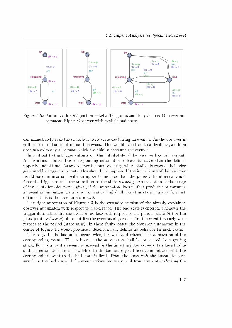
4.4. Impact Analysis on Speci�cation Level
waitclk <= p
releasing
clk <= j
S0
clk <= p
clk >= p
clk := 0 e!
on!
clk := 0
waitclk <= p
releasing
S0
clk >= p
clk := 0clk <= je?
clk <= p
on?
clk := 0
bad
waitclk <= p
releasing
S0
clk < pe?clk := 0
clk > pclk := 0
clk > pon?clk := 0
clk > je?clk := 0
clk > jclk := 0clk >= p
clk := 0clk <= je?
clk <= p
on?clk := 0
Figure 4.5.: Automata for R1 -pattern � Left: Trigger automaton; Center: Observer au-tomaton; Right: Observer with explicit bad state.
can immediately take the transition to its state wait �ring an event e. As the observer isstill in its initial state, it misses this event. This would even lead to a deadlock, as theredoes not exist any automata which are able to consume the event e.In contrast to the trigger automaton, the initial state of the observer has no invariant.
An invariant enforces the corresponding automaton to leave its state after the de�nedupper bound of time. As an observer is a passive entity, which shall only react on behaviorgenerated by trigger automata, this should not happen. If the initial state of the observerwould have an invariant with an upper bound less than the period, the observer couldforce the trigger to take the transition to the state releasing. An exception of the usageof invariants for observer is given, if the automaton does neither produce nor consumean event on an outgoing transition of a state and shall leave this state in a speci�c pointof time. This is the case for state wait.The right automaton of Figure 4.5 is the extended version of the already explained
observer automaton with respect to a bad state. The bad state is entered, whenever thetrigger does either �re the event e too late with respect to the period (state S0 ) or thejitter (state releasing), does not �re the event at all, or does �re the event too early withrespect to the period (state wait). In those faulty cases, the observer automaton in thecenter of Figure 4.5 would produce a deadlock as it de�nes no behavior for such cases.The edges to the bad state occur twice, i. e. with and without the annotation of the
corresponding event. This is because the automaton shall be prevented from gettingstuck. For instance if an event is received by the time the jitter exceeds its allowed valueand the automaton has not switched to the bad state yet, the edge annotated with thecorresponding event to the bad state is �red. From the state wait the automaton canswitch to the bad state, if the event arrives too early, and from the state releasing the
137
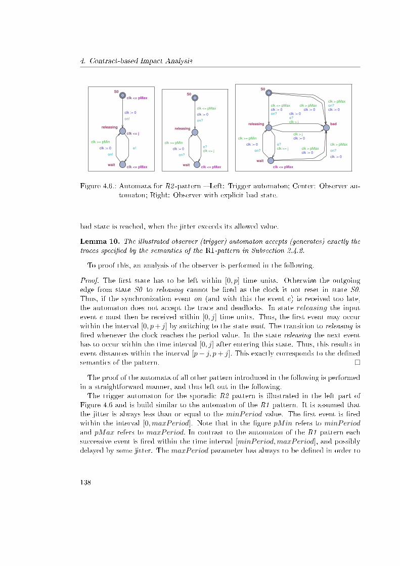
4. Contract-based Impact Analysis
waitclk <= pMax
releasing
clk <= j
S0
clk <= pMax
clk >= pMin
on!
clk := 0 e!
on!
clk := 0
waitclk <= pMax
releasing
S0
clk >= pMin
on?
clk := 0clk <= je?
clk <= pMax
on?
clk := 0
bad
wait
clk <= pMax
releasing
S0
clk > pMaxclk := 0
clk > pMax
on?
clk := 0
clk > pMaxclk := 0
clk > pMaxon?clk := 0
clk > je?clk := 0
clk > jclk := 0clk >= pMin
on?
clk := 0clk <= je?
clk <= pMax
on?clk := 0
Figure 4.6.: Automata for R2 -pattern � Left: Trigger automaton; Center: Observer au-tomaton; Right: Observer with explicit bad state.
bad state is reached, when the jitter exceeds its allowed value.
Lemma 10. The illustrated observer (trigger) automaton accepts (generates) exactly thetraces speci�ed by the semantics of the R1-pattern in Subsection 2.4.2.
To proof this, an analysis of the observer is performed in the following.
Proof. The �rst state has to be left within [0, p] time units. Otherwise the outgoingedge from state S0 to releasing cannot be �red as the clock is not reset in state S0.Thus, if the synchronization event on (and with this the event e) is received too late,the automaton does not accept the trace and deadlocks. In state releasing the inputevent e must then be received within [0, j] time units. Thus, the �rst event may occurwithin the interval [0, p+ j] by switching to the state wait. The transition to releasing is�red whenever the clock reaches the period value. In the state releasing the next eventhas to occur within the time interval [0, j] after entering this state. Thus, this results inevent distances within the interval [p− j, p+ j]. This exactly corresponds to the de�nedsemantics of the pattern.
The proof of the automata of all other pattern introduced in the following is performedin a straightforward manner, and thus left out in the following.The trigger automaton for the sporadic R2 -pattern is illustrated in the left part of
Figure 4.6 and is build similar to the automaton of the R1 -pattern. It is assumed thatthe jitter is always less than or equal to the minPeriod value. The �rst event is �redwithin the interval [0,maxPeriod]. Note that in the �gure pMin refers to minPeriodand pMax refers to maxPeriod. In contrast to the automaton of the R1 -pattern eachsuccessive event is �red within the time interval [minPeriod,maxPeriod], and possiblydelayed by some jitter. The maxPeriod parameter has always to be de�ned in order to
138
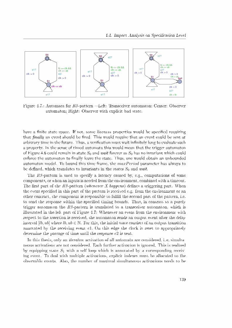
4.4. Impact Analysis on Speci�cation Level
S1
clk <= ub
S0
e1?
lb <= clk && clk <= ub
e2!
clk := 0
e1?
clk := 0
S1
S0 e2?
e1?
lb <= clk &&clk <= ub
e2?clk := 0
e1?
clk := 0bad
S1
S0
clk > ubclk := 0
clk < lb
e2?
clk := 0
e2?
e1?
lb <= clk &&clk <= ub
e2?clk := 0
e1?
clk := 0
Figure 4.7.: Automata for R3 -pattern � Left: Transceiver automaton; Center: Observerautomaton; Right: Observer with explicit bad state.
have a �nite state space. If not, some liveness properties would be speci�ed requiringthat �nally an event should be �red. This would require that an event could be sent atarbitrary time in the future. Thus, a veri�cation must wait in�nitely long to evaluate sucha property. In the sense of timed automata this would mean that the trigger automatonof Figure 4.6 could remain in state S0 and wait forever as S0 has no invariant which couldenforce the automaton to �nally leave the state. Thus, one would obtain an unboundedautomaton model. To bound this time frame, the maxPeriod parameter has always tobe de�ned, which translates to invariants in the states S0 and wait.
The R3 -pattern is used to specify a latency caused by, e.g., computations of somecomponents, or when an inputs is needed from the environment, combined with a timeout.The �rst part of the R3 -pattern (whenever X happens) de�nes a triggering part. Whenthe event speci�ed in this part of the pattern is received e.g. from the environment or another contract, the component is responsible to ful�ll the second part of the pattern, i.e.to send the response within the speci�ed timing bounds. Thus, in contrast to a purelytrigger automaton the R3 -pattern is translated to a transceiver automaton, which isillustrated in the left part of Figure 4.7: Whenever an event from the environment withrespect to the assertion is received, the automaton sends an output event after the delayinterval [lb, ub] where lb, ub ∈ N. For this, the initial state consists of an output transitionannotated by the receiving event e1. On this edge the clock is reset to appropriatelydetermine the passage of time until the response e2 is sent.
In this thesis, only an iterative activation of all automata are considered, i. e. simulta-neous activations are not considered. Each further activation is ignored. This is realizedby equipping state S1 with a self loop which is annotated by a corresponding receiv-ing event. To deal with multiple activations, explicit indexes must be allocated to theobservable events. Also, the number of maximal simultaneous activations needs to be
139
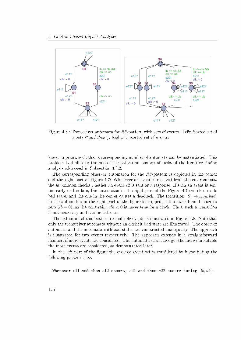
4. Contract-based Impact Analysis
S3
S1
S2
S0
e12?
e11?
e12?
clk <= ub
e21!
e12?clk := 0
e11?
lb <= clk &&clk <= ube22!clk := 0
e11?
clk := 0S5S1 S4S2
S3
S0
e12?
e11?
lb <= clk &&clk <= ube21!clk := 0
clk <= ube22!
e11?
e12? e12?e11?
e11?
clk := 0
e12?
e12?
clk <= ube21!
e12?clk := 0
e11?
lb <= clk &&clk <= ube22!clk := 0
e11?
Figure 4.8.: Transceiver automata for R3 -pattern with sets of events� Left: Sorted set ofevents (�and then�); Right: Unsorted set of events.
known a priori, such that a corresponding number of automata can be instantiated. Thisproblem is similar to the one of the activation bounds of tasks of the iterative timinganalysis addressed in Subsection 3.3.2.The corresponding observer automaton for the R3 -pattern is depicted in the center
and the right part of Figure 4.7: Whenever an event is received from the environment,the automaton checks whether an event e2 is sent as a response. If such an event is senttoo early or too late, the automaton in the right part of the Figure 4.7 switches to itsbad state, and the one in the center causes a deadlock. The transition S1 →clk<lb badin the automaton in the right part of the �gure is skipped, if the lower bound is set tozero (lb = 0), as the constraint clk < 0 is never true for a clock. Thus, such a transitionis not necessary and can be left out.The extension of this pattern to multiple events is illustrated in Figure 4.8. Note that
only the transceiver automata without an explicit bad state are illustrated. The observerautomata and the automata with bad states are constructed analogously. The approachis illustrated for two events respectively. The approach extends in a straightforwardmanner, if more events are considered. The automata structures get the more unreadablethe more events are considered, as demonstrated later.In the left part of the �gure the ordered event set is considered by instantiating the
following pattern type:
Whenever e11 and then e12 occurs, e21 and then e22 occurs during [lb, ub].
140
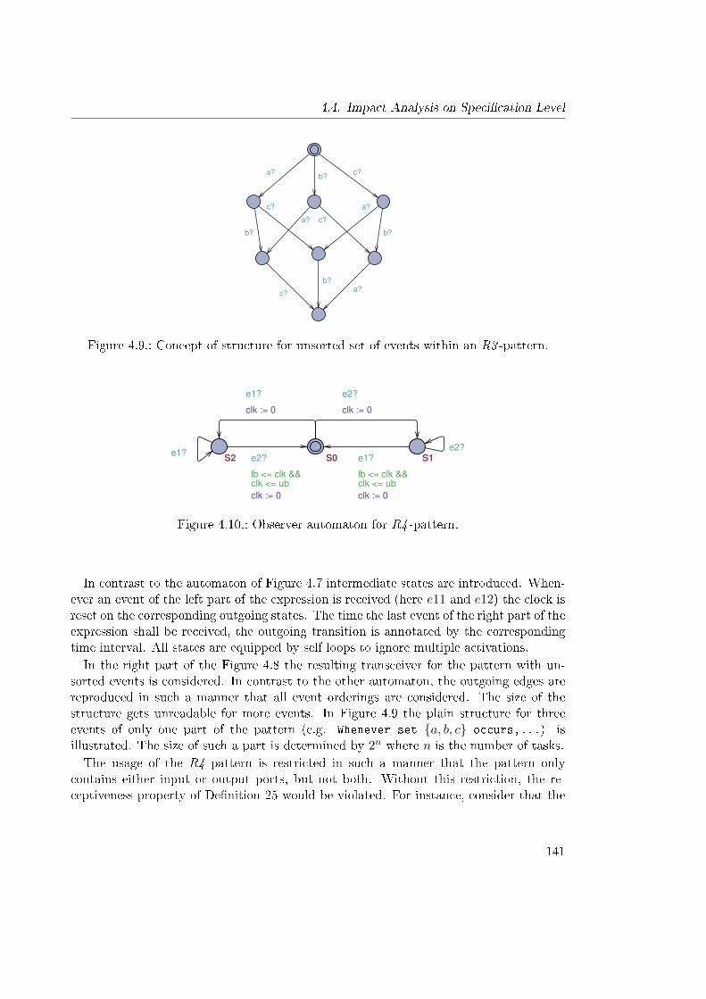
4.4. Impact Analysis on Speci�cation Level
b?
a?c?
c?
a?
b?
c?
a?
b?
c?
b?
a?
Figure 4.9.: Concept of structure for unsorted set of events within an R3 -pattern.
S1S2 S0
e2?
clk := 0
e2?e1?
lb <= clk &&clk <= ub
e2?
clk := 0
lb <= clk &&clk <= ub
e1?
clk := 0
e1?
clk := 0
Figure 4.10.: Observer automaton for R4 -pattern.
In contrast to the automaton of Figure 4.7 intermediate states are introduced. When-ever an event of the left part of the expression is received (here e11 and e12) the clock isreset on the corresponding outgoing states. The time the last event of the right part of theexpression shall be received, the outgoing transition is annotated by the correspondingtime interval. All states are equipped by self loops to ignore multiple activations.In the right part of the Figure 4.8 the resulting transceiver for the pattern with un-
sorted events is considered. In contrast to the other automaton, the outgoing edges arereproduced in such a manner that all event orderings are considered. The size of thestructure gets unreadable for more events. In Figure 4.9 the plain structure for threeevents of only one part of the pattern (e.g. Whenever set {a, b, c} occurs,...) isillustrated. The size of such a part is determined by 2n where n is the number of tasks.The usage of the R4 -pattern is restricted in such a manner that the pattern only
contains either input or output ports, but not both. Without this restriction, the re-ceptiveness property of De�nition 25 would be violated. For instance, consider that the
141
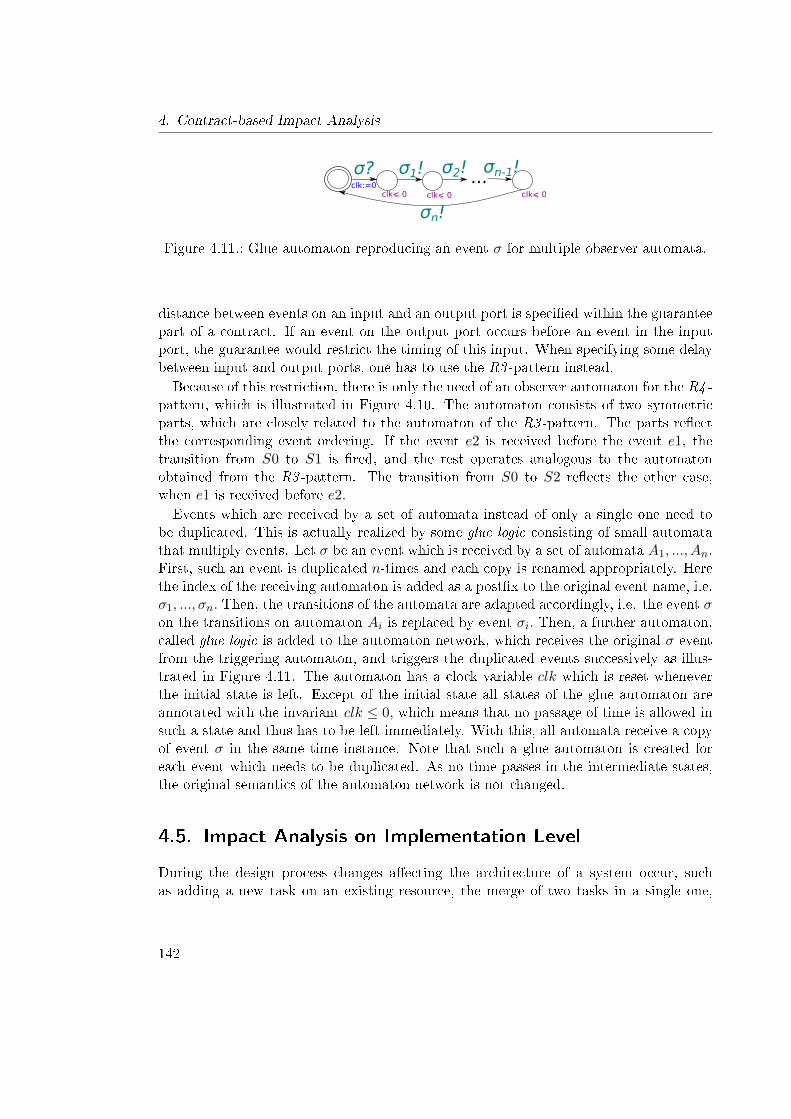
4. Contract-based Impact Analysis
σ? σ1! σ2! ...σn-1!
σn!clk< 0
clk:=0clk< 0 clk< 0
Figure 4.11.: Glue automaton reproducing an event σ for multiple observer automata.
distance between events on an input and an output port is speci�ed within the guaranteepart of a contract. If an event on the output port occurs before an event in the inputport, the guarantee would restrict the timing of this input. When specifying some delaybetween input and output ports, one has to use the R3 -pattern instead.Because of this restriction, there is only the need of an observer automaton for the R4 -
pattern, which is illustrated in Figure 4.10. The automaton consists of two symmetricparts, which are closely related to the automaton of the R3 -pattern. The parts re�ectthe corresponding event ordering. If the event e2 is received before the event e1, thetransition from S0 to S1 is �red, and the rest operates analogous to the automatonobtained from the R3 -pattern. The transition from S0 to S2 re�ects the other case,when e1 is received before e2.Events which are received by a set of automata instead of only a single one need to
be duplicated. This is actually realized by some glue logic consisting of small automatathat multiply events. Let σ be an event which is received by a set of automata A1, ..., An.First, such an event is duplicated n-times and each copy is renamed appropriately. Herethe index of the receiving automaton is added as a post�x to the original event name, i.e.σ1, ..., σn. Then, the transitions of the automata are adapted accordingly, i.e. the event σon the transitions on automaton Ai is replaced by event σi. Then, a further automaton,called glue logic is added to the automaton network, which receives the original σ eventfrom the triggering automaton, and triggers the duplicated events successively as illus-trated in Figure 4.11. The automaton has a clock variable clk which is reset wheneverthe initial state is left. Except of the initial state all states of the glue automaton areannotated with the invariant clk ≤ 0, which means that no passage of time is allowed insuch a state and thus has to be left immediately. With this, all automata receive a copyof event σ in the same time instance. Note that such a glue automaton is created foreach event which needs to be duplicated. As no time passes in the intermediate states,the original semantics of the automaton network is not changed.
4.5. Impact Analysis on Implementation Level
During the design process changes a�ecting the architecture of a system occur, suchas adding a new task on an existing resource, the merge of two tasks in a single one,
142
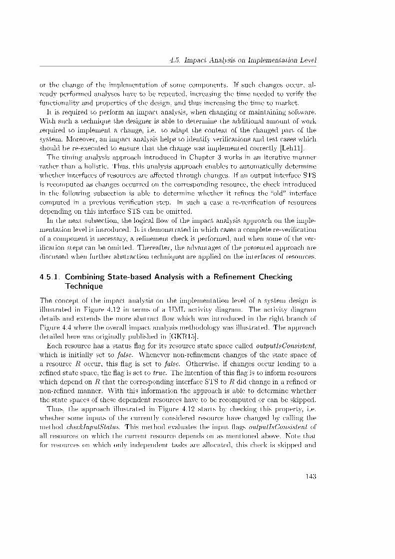
4.5. Impact Analysis on Implementation Level
or the change of the implementation of some components. If such changes occur, al-ready performed analyses have to be repeated, increasing the time needed to verify thefunctionality and properties of the design, and thus increasing the time to market.It is required to perform an impact analysis, when changing or maintaining software.
With such a technique the designer is able to determine the additional amount of workrequired to implement a change, i.e. to adapt the context of the changed part of thesystem. Moreover, an impact analysis helps to identify veri�cations and test cases whichshould be re-executed to ensure that the change was implemented correctly [Leh11].The timing analysis approach introduced in Chapter 3 works in an iterative manner
rather than a holistic. Thus, this analysis approach enables to automatically determinewhether interfaces of resources are a�ected through changes. If an output interface STSis recomputed as changes occurred on the corresponding resource, the check introducedin the following subsection is able to determine whether it re�nes the �old� interfacecomputed in a previous veri�cation step. In such a case a re-veri�cation of resourcesdepending on this interface STS can be omitted.In the next subsection, the logical �ow of the impact analysis approach on the imple-
mentation level is introduced. It is demonstrated in which cases a complete re-veri�cationof a component is necessary, a re�nement check is performed, and when some of the ver-i�cation steps can be omitted. Thereafter, the advantages of the presented approach arediscussed when further abstraction techniques are applied on the interfaces of resources.
4.5.1. Combining State-based Analysis with a Re�nement CheckingTechnique
The concept of the impact analysis on the implementation level of a system design isillustrated in Figure 4.12 in terms of a UML activity diagram. The activity diagramdetails and extends the more abstract �ow which was introduced in the right branch ofFigure 4.4 where the overall impact analysis methodology was illustrated. The approachdetailed here was originally published in [GKR15].Each resource has a status �ag for its resource state space called outputIsConsistent,
which is initially set to false. Whenever non-re�nement changes of the state space ofa resource R occur, this �ag is set to false. Otherwise, if changes occur leading to are�ned state space, the �ag is set to true. The intention of this �ag is to inform resourceswhich depend on R that the corresponding interface STS to R did change in a re�ned ornon-re�ned manner. With this information the approach is able to determine whetherthe state spaces of these dependent resources have to be recomputed or can be skipped.Thus, the approach illustrated in Figure 4.12 starts by checking this property, i.e.
whether some inputs of the currently considered resource have changed by calling themethod checkInputStatus. This method evaluates the input �ags outputIsConsistent ofall resources on which the current resource depends on as mentioned above. Note thatfor resources on which only independent tasks are allocated, this check is skipped and
143
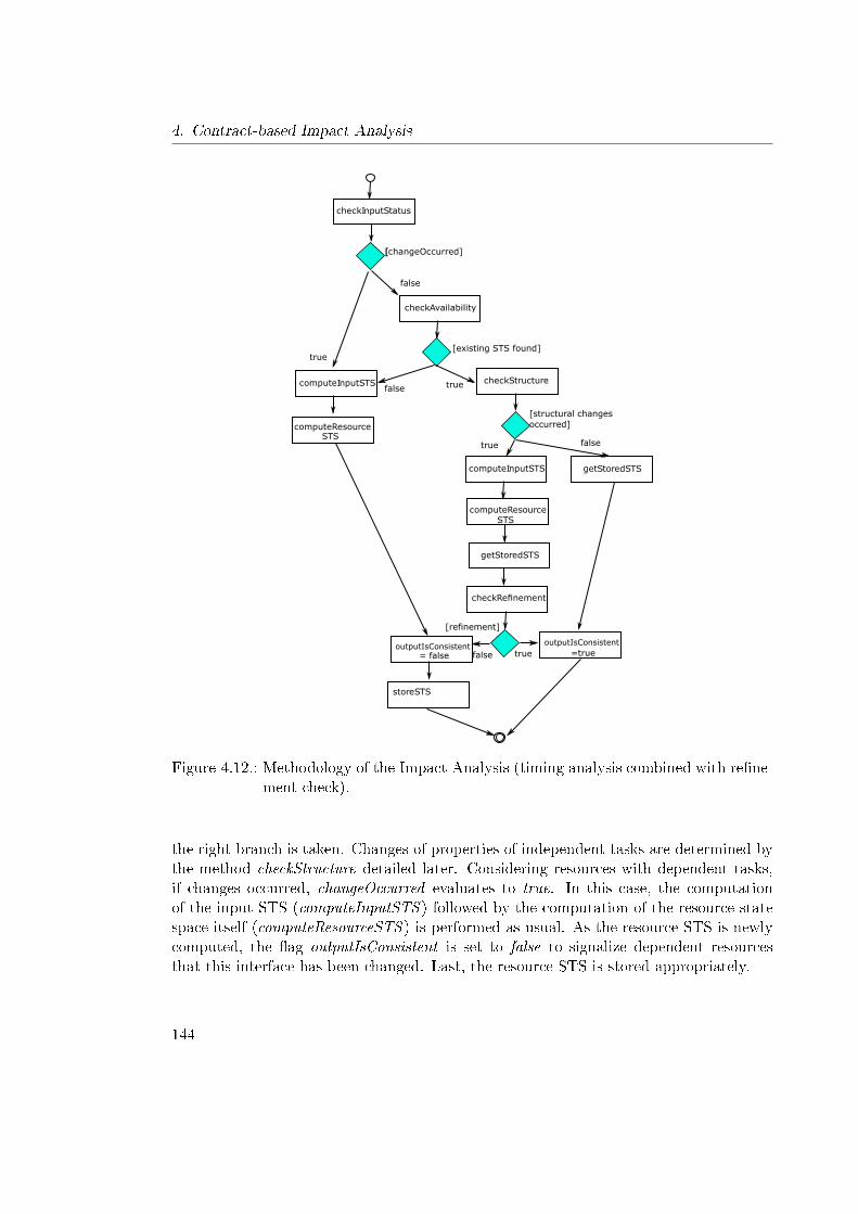
4. Contract-based Impact Analysis
checkInputStatus
checkAvailability
checkStructure
getStoredSTScomputeInputSTS
computeResource
getStoredSTS
checkRefinement
outputIsConsistentoutputIsConsistent
storeSTS
true
computeInputSTS
[[changeOccurred]
computeResource
[existing STS found]
[structural changesoccurred]
true
false true
STS
= false =true
STS
false
false true
false
[refinement]
Figure 4.12.: Methodology of the Impact Analysis (timing analysis combined with re�ne-ment check).
the right branch is taken. Changes of properties of independent tasks are determined bythe method checkStructure detailed later. Considering resources with dependent tasks,if changes occurred, changeOccurred evaluates to true. In this case, the computationof the input STS (computeInputSTS ) followed by the computation of the resource statespace itself (computeResourceSTS ) is performed as usual. As the resource STS is newlycomputed, the �ag outputIsConsistent is set to false to signalize dependent resourcesthat this interface has been changed. Last, the resource STS is stored appropriately.
144
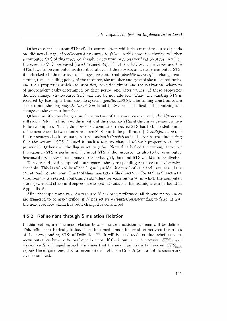
4.5. Impact Analysis on Implementation Level
Otherwise, if the output STSs of all resources, from which the current resource dependson, did not change, checkOccurred evaluates to false. In this case it is checked whethera computed STS of this resource already exists from previous veri�cation steps, in whichthe resource STS was saved (checkAvailability). If not, the left branch is taken and theSTSs have to be computed as described above. If there exists an already computed STS,it is checked whether structural changes have occurred (checkStructure), i.e. changes con-cerning the scheduling policy of the resource, the number and type of the allocated tasks,and their properties which are priorities, execution times, and the activation behaviorsof independent tasks determined by their period and jitter values. If these propertiesdid not change, the resource STS will also be not a�ected. Thus, the existing STS isrestored by loading it from the �le system (getStoredSTS ). The timing constraints arechecked and the �ag outputIsConsistent is set to true which indicates that nothing didchange on the output interface.Otherwise, if some changes on the structure of the resource occurred, checkStructure
will return false. In this case, the input and the resource STSs of the current resource haveto be recomputed. Then, the previously computed resource STS has to be loaded, and are�nement check between both resource STSs has to be performed (checkRe�nement). Ifthe re�nement check evaluates to true, outputIsConsistent is also set to true indicatingthat the resource STS changed in such a manner that all relevant properties are stillpreserved. Otherwise, the �ag is set to false. Note that before the recomputation ofthe resource STS is performed, the input STS of the resource has also to be recomputedbecause if properties of independent tasks changed, the input STS would also be a�ected.To store and load computed state spaces, the corresponding resources must be refer-
enceable. This is realized by allocating unique identi�ers to both the architecture and thecorresponding resources. The tool then manages a �le directory: For each architecture asubdirectory is created, containing subfolders for each resource, in which the computedstate spaces and structural aspects are stored. Details for this technique can be found inAppendix A.After the impact analysis of a resource N has been performed, all dependent resources
are triggered to be also veri�ed, if N has set its outputIsConsistent �ag to false. If not,the next resource which has been changed is considered.
4.5.2. Re�nement through Simulation Relation
In this section, a re�nement relation between state transition systems will be de�ned.This re�nement basically is based on the timed simulation relation between the statesof the corresponding STSs of De�nition 22. It will be used to determine, whether somerecomputations have to be performed or not. If the input transition system STSin,R ofa resource R is changed in such a manner that the new input transition system STS′in,Rre�nes the original one, than a recomputation of the STS of R (and all of its successors)can be omitted.
145
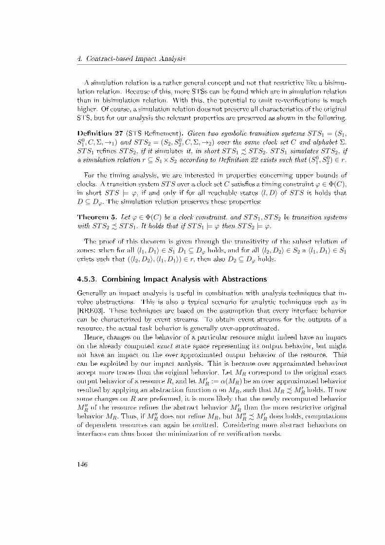
4. Contract-based Impact Analysis
A simulation relation is a rather general concept and not that restrictive like a bisimu-lation relation. Because of this, more STSs can be found which are in simulation relationthan in bisimulation relation. With this, the potential to omit re-veri�cations is muchhigher. Of course, a simulation relation does not preserve all characteristics of the originalSTS, but for our analysis the relevant properties are preserved as shown in the following.
De�nition 27 (STS Re�nement). Given two symbolic transition systems STS1 = (S1,S0
1 , C,Σ,→1) and STS2 = (S2, S02 , C,Σ,→2) over the same clock set C and alphabet Σ.
STS1 re�nes STS2, if it simulates it, in short STS1 - STS2. STS1 simulates STS2, ifa simulation relation r ⊆ S1×S2 according to De�nition 22 exists such that (S0
1 , S02) ∈ r.
For the timing analysis, we are interested in properties concerning upper bounds ofclocks. A transition system STS over a clock set C satis�es a timing constraint ϕ ∈ Φ(C),in short STS |= ϕ, if and only if for all reachable states 〈l,D〉 of STS it holds thatD ⊆ Dϕ. The simulation relation preserves these properties:
Theorem 5. Let ϕ ∈ Φ(C) be a clock constraint, and STS1, STS2 be transition systemswith STS2 - STS1. It holds that if STS1 |= ϕ then STS2 |= ϕ.
The proof of this theorem is given through the transitivity of the subset relation ofzones: when for all 〈l1, D1〉 ∈ S1 D1 ⊆ Dϕ holds, and for all 〈l2, D2〉 ∈ S2 a 〈l1, D1〉 ∈ S1
exists such that (〈l2, D2〉, 〈l1, D1〉) ∈ r, then also D2 ⊆ Dϕ holds.
4.5.3. Combining Impact Analysis with Abstractions
Generally an impact analysis is useful in combination with analysis techniques that in-volve abstractions. This is also a typical scenario for analytic techniques such as in[RRE03]. These techniques are based on the assumption that every interface behaviorcan be characterized by event streams. To obtain event streams for the outputs of aresource, the actual task behavior is generally over-approximated.Hence, changes on the behavior of a particular resource might indeed have an impact
on the already computed exact state space representing its output behavior, but mightnot have an impact on the over-approximated output behavior of the resource. Thiscan be exploited by our impact analysis. This is because over-approximated behaviorsaccept more traces than the original behavior. Let MR correspond to the original exactoutput behavior of a resource R, and letM ′R := α(MR) be an over-approximated behaviorresulted by applying an abstraction function α onMR, such thatMR -M ′R holds. If nowsome changes on R are preformed, it is more likely that the newly recomputed behaviorM ′′R of the resource re�nes the abstract behavior M ′R than the more restrictive originalbehavior MR. Thus, if M ′′R does not re�ne MR, but M ′′R -M
′R does holds, computations
of dependent resources can again be omitted. Considering more abstract behaviors oninterfaces can thus boost the minimization of re-veri�cation needs.
146
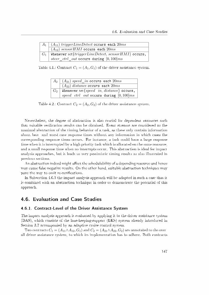
4.6. Evaluation and Case Studies
A1 (A11) triggerLineDetect occurs each 20ms(A12) sensorHMI occurs each 20ms
G1 Whenever set{triggerLineDetect, sensorHMI} occurs,
steer_ctrl_out occurs during [0, 100]ms
Table 4.1.: Contract C1 = (A1, G1) of the driver assistance system.
A2 (A21) speed_in occurs each 20ms(A22) distance occurs each 20ms
G2 Whenever set{speed_in, distance} occurs,
speed_ctrl_out occurs during [0, 100]ms
Table 4.2.: Contract C2 = (A2, G2) of the driver assistance system.
Nevertheless, the degree of abstraction is also crucial for dependent resources suchthat suitable veri�cation results can be obtained. Event streams are considered as themaximal abstraction of the timing behavior of a task, as these only contain informationabout best- and worst-case response-times without any information in which cases thecorresponding response times occurs. For instance, a task could have a large responsetime when it is interrupted by a high priority task which is allocated on the same resource,and a small response time when no interrupts occur. This abstraction is ideal for impactanalysis approaches, but it leads to very pessimistic timing results as also illustrated inprevious sections.An abstraction indeed might a�ect the schedulability of a depending resource and hence
may cause false negative results. On the other hand, suitable abstraction techniques maypave the way to omit re-veri�cations.In Subsection 4.6.3 the impact analysis approach will be adapted in such a case that it
is combined with an abstraction technique in order to demonstrate the potential of thisapproach.
4.6. Evaluation and Case Studies
4.6.1. Contract-Level of the Driver Assistance System
The impact analysis approach is evaluated by applying it to the driver assistance system(DAS), which consists of the lane-keeping-support (LKS) system already introduced inSection 3.7 accompanied by an adaptive cruise control system.Two contracts C1 = (A11∧A12, G1) and C2 = (A21∧A22, G2) are annotated to the over-
all driver assistance system, to which its implementation has to adhere. Both contracts
147
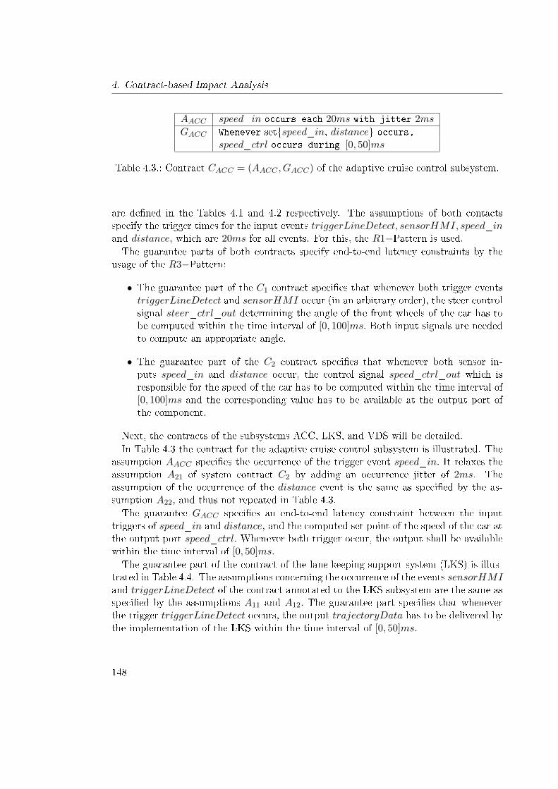
4. Contract-based Impact Analysis
AACC speed_in occurs each 20ms with jitter 2ms
GACC Whenever set{speed_in, distance} occurs,
speed_ctrl occurs during [0, 50]ms
Table 4.3.: Contract CACC = (AACC , GACC) of the adaptive cruise control subsystem.
are de�ned in the Tables 4.1 and 4.2 respectively. The assumptions of both contactsspecify the trigger times for the input events triggerLineDetect, sensorHMI, speed_inand distance, which are 20ms for all events. For this, the R1−Pattern is used.The guarantee parts of both contracts specify end-to-end latency constraints by the
usage of the R3−Pattern:
• The guarantee part of the C1 contract speci�es that whenever both trigger eventstriggerLineDetect and sensorHMI occur (in an arbitrary order), the steer controlsignal steer_ctrl_out determining the angle of the front wheels of the car has tobe computed within the time interval of [0, 100]ms. Both input signals are neededto compute an appropriate angle.
• The guarantee part of the C2 contract speci�es that whenever both sensor in-puts speed_in and distance occur, the control signal speed_ctrl_out which isresponsible for the speed of the car has to be computed within the time interval of[0, 100]ms and the corresponding value has to be available at the output port ofthe component.
Next, the contracts of the subsystems ACC, LKS, and VDS will be detailed.In Table 4.3 the contract for the adaptive cruise control subsystem is illustrated. The
assumption AACC speci�es the occurrence of the trigger event speed_in. It relaxes theassumption A21 of system contract C2 by adding an occurrence jitter of 2ms. Theassumption of the occurrence of the distance event is the same as speci�ed by the as-sumption A22, and thus not repeated in Table 4.3.The guarantee GACC speci�es an end-to-end latency constraint between the input
triggers of speed_in and distance, and the computed set point of the speed of the car atthe output port speed_ctrl. Whenever both trigger occur, the output shall be availablewithin the time interval of [0, 50]ms.
The guarantee part of the contract of the lane-keeping-support system (LKS) is illus-trated in Table 4.4. The assumptions concerning the occurrence of the events sensorHMIand triggerLineDetect of the contract annotated to the LKS subsystem are the same asspeci�ed by the assumptions A11 and A12. The guarantee part speci�es that wheneverthe trigger triggerLineDetect occurs, the output trajectoryData has to be delivered bythe implementation of the LKS within the time interval of [0, 50]ms.
148
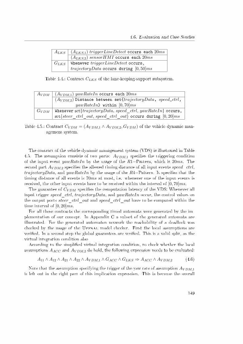
4.6. Evaluation and Case Studies
ALKS (ALKS,1) triggerLineDetect occurs each 20ms(ALKS,2) sensorHMI occurs each 20ms
GLKS Whenever triggerLineDetect occurs,trajectoryData occurs during [0, 50]ms
Table 4.4.: Contract CLKS of the lane-keeping-support subsystem.
AV DM (AV DM,1) yawRateIn occurs each 20ms(AV DM,2) Distance between set{trajectoryData, speed_ctrl,
yawRateIn} within [0, 70]ms
GV DM Whenever set{trajectoryData, speed_ctrl, yawRateIn} occurs,
set{steer_ctrl_out, speed_ctrl_out} occurs during [0, 20]ms
Table 4.5.: Contract CV DM = (AV DM,1 ∧ AV DM,2, GV DM ) of the vehicle dynamic man-agement system.
The contract of the vehicle dynamic management system (VDS) is illustrated in Table4.5. The assumption consists of two parts: AV DM,1 speci�es the triggering conditionof the input event yawRateIn by the usage of the R1−Pattern, which is 20ms. Thesecond part AV DM,2 speci�es the allowed timing distance of all input events speed_ctrl,trajectoryData, and yawRateIn by the usage of the R4−Pattern. It speci�es that thetiming distance of all events is 70ms at most, i.e. whenever one of the input events isreceived, the other input events have to be received within the interval of [0, 70]ms.The guarantee of CV DM speci�es the computation latency of the VDS: Whenever all
input trigger speed_ctrl, trajectoryData, and yawRateIn occur, the control values onthe output ports steer_ctrl_out and speed_ctrl_out have to be computed within thetime interval of [0, 20]ms.For all these contracts the corresponding timed automata were generated by the im-
plementation of our concept. In Appendix C a subset of the generated automata areillustrated. For the generated automaton network the reachability of a deadlock waschecked by the usage of the Uppaal model checker. First the local assumptions areveri�ed. In a second step the global guarantees are veri�ed. This is a valid split, as thevirtual integration condition alsoAccording to the simpli�ed virtual integration condition, to check whether the local
assumptions AACC and AV DM,2 do hold, the following expression needs to be evaluated:
A11 ∧A12 ∧A21 ∧A22 ∧AV DM,1 ∧GACC ∧GLKS ⇒ AACC ∧AV DM,2 (4.6)
Note that the assumption specifying the trigger of the yaw rate of assumption AV DM,1
is left out in the right part of this implication expression. This is because the overall
149
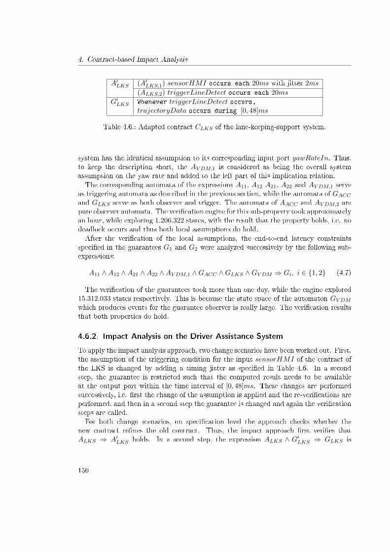
4. Contract-based Impact Analysis
A′LKS (A′LKS,1) sensorHMI occurs each 20ms with jitter 2ms
(ALKS,2) triggerLineDetect occurs each 20ms
G′LKS Whenever triggerLineDetect occurs,trajectoryData occurs during [0, 48]ms
Table 4.6.: Adapted contract CLKS of the lane-keeping-support system.
system has the identical assumption to its corresponding input port yawRateIn. Thus,to keep the description short, the AV DM,1 is considered as being the overall systemassumption on the yaw rate and added to the left part of this implication relation.The corresponding automata of the expressions A11, A12 A21, A22 and AV DM,1 serve
as triggering automata as described in the previous section, while the automata of GACCand GLKS serve as both observer and trigger. The automata of AACC and AV DM,2 arepure observer automata. The veri�cation engine for this sub-property took approximatelyan hour, while exploring 1.206.322 states, with the result that the property holds, i.e. nodeadlock occurs and thus both local assumptions do hold.After the veri�cation of the local assumptions, the end-to-end latency constraints
speci�ed in the guarantees G1 and G2 were analyzed successively by the following sub-expressions:
A11 ∧A12 ∧A21 ∧A22 ∧AV DM,1 ∧GACC ∧GLKS ∧GV DM ⇒ Gi, i ∈ {1, 2} (4.7)
The veri�cation of the guarantees took more than one day, while the engine explored15.312.033 states respectively. This is because the state space of the automaton GV DMwhich produces events for the guarantee observer is really large. The veri�cation resultsthat both properties do hold.
4.6.2. Impact Analysis on the Driver Assistance System
To apply the impact analysis approach, two change scenarios have been worked out. First,the assumption of the triggering condition for the input sensorHMI of the contract ofthe LKS is changed by adding a timing jitter as speci�ed in Table 4.6. In a secondstep, the guarantee is restricted such that the computed result needs to be availableat the output port within the time interval of [0, 48]ms. These changes are performedsuccessively, i.e. �rst the change of the assumption is applied and the re-veri�cations areperformed, and then in a second step the guarantee is changed and again the veri�cationsteps are called.For both change scenarios, on speci�cation level the approach checks whether the
new contract re�nes the old contract. Thus, the impact approach �rst veri�es thatALKS ⇒ A′LKS holds. In a second step, the expression ALKS ∧ G′LKS ⇒ GLKS is
150
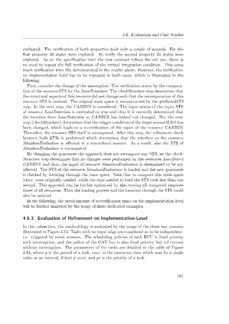
4.6. Evaluation and Case Studies
evaluated. The veri�cation of both properties took only a couple of seconds. For the�rst property 26 states were explored. To verify the second property 24 states wereexplored. As on the speci�cation level the new contract re�nes the old one, there isno need to repeat the full veri�cation of the virtual integration condition. This savesmuch veri�cation time like demonstrated in the results above. However, the veri�cationon implementation level has to be repeated in both cases, which is illustrated in thefollowing.First, consider the change of the assumption: The veri�cation starts by the computa-
tion of the resource STS for the LaneDetection. The checkStructure step determines thatthe structural aspects of this resource did not change such that the recomputation of thisresource STS is omitted. The original state space is reconstructed by the getStoredSTSstep. In the next step, the CANBUS is considered. The input status of the input STSof resource LaneDetection is evaluated to true and thus it is correctly determined thatthe interface from LaneDetection to CANBUS has indeed not changed. But the nextstep (checkStructure) determines that the trigger condition of the input sensorHMI hasbeen changed, which leads to a re-veri�cation of the input of the resource CANBUS.Thereafter, the resource STS itself is recomputed. After this step, the re�nement checkbetween both STSs is performed which determines that the interface to the resourceSituationEvaluation is a�ected in a non-re�ned manner. As a result, also the STS ofSituationEvaluation is recomputed.By changing the guarantee the approach does not recompute any STS, as the check-
Structure step determines that no changes were performed on the resources LaneDetectCANBUS and thus, the input of resource SituationEvaluation is determined to be nota�ected. The STS of the resource SituationEvaluation is loaded and the new guaranteeis checked by iterating through the state space. Note that to compute this state space14sec. were originally needed, while the time needed to load the STS took less than onesecond. This approach can be further optimized by also storing all computed responsetimes of all resources. Then the loading process and the iteration through the STS couldalso be omitted.In the following, the saved amount of re-veri�cation times on the implementation level
will be further analyzed by the usage of more dedicated examples.
4.6.3. Evaluation of Re�nement on Implementation-Level
In this subsection, the methodology is evaluated by the usage of the three test systemsillustrated in Figure 4.13. Tasks with no input edge are considered as to be independent,i.e. triggered by event streams. The scheduling policies of each ECU is �xed prioritywith interruption, and the policy of the CAN bus is also �xed priority but (of course)without interruption. The parameters of the tasks are detailed in the table of Figure4.14, where p is the period of a task, exec. is the execution time which may be a singlevalue or an interval, if bcet 6= wcet, and pr is the priority of a task.
151
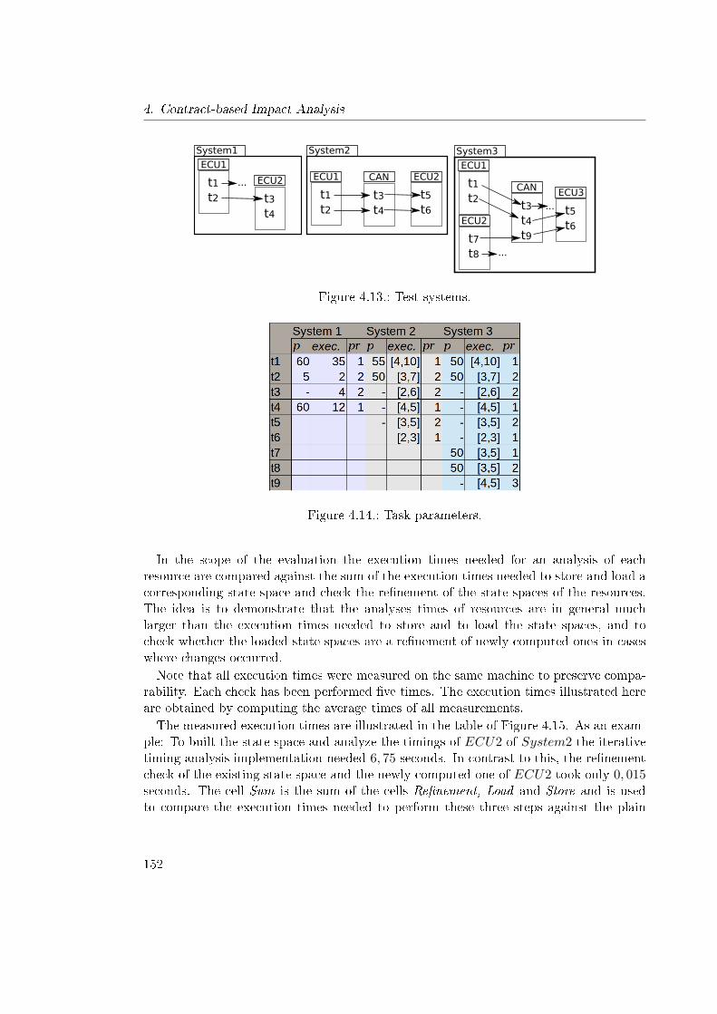
4. Contract-based Impact Analysis
t1t2
ECU1
t3t4
CAN
t5t6
ECU2
System2
t1t2
ECU1
t3t4t9
CAN
t5t6
ECU3
System3
t7t8
ECU2
...
...
t1t2
ECU1
t3t4
ECU2
System1
...
Figure 4.13.: Test systems.
Figure 4.14.: Task parameters.
In the scope of the evaluation the execution times needed for an analysis of eachresource are compared against the sum of the execution times needed to store and load acorresponding state space and check the re�nement of the state spaces of the resources.The idea is to demonstrate that the analyses times of resources are in general muchlarger than the execution times needed to store and to load the state spaces, and tocheck whether the loaded state spaces are a re�nement of newly computed ones in caseswhere changes occurred.Note that all execution times were measured on the same machine to preserve compa-
rability. Each check has been performed �ve times. The execution times illustrated hereare obtained by computing the average times of all measurements.The measured execution times are illustrated in the table of Figure 4.15. As an exam-
ple: To built the state space and analyze the timings of ECU2 of System2 the iterativetiming analysis implementation needed 6, 75 seconds. In contrast to this, the re�nementcheck of the existing state space and the newly computed one of ECU2 took only 0, 015seconds. The cell Sum is the sum of the cells Re�nement, Load and Store and is usedto compare the execution times needed to perform these three steps against the plain
152
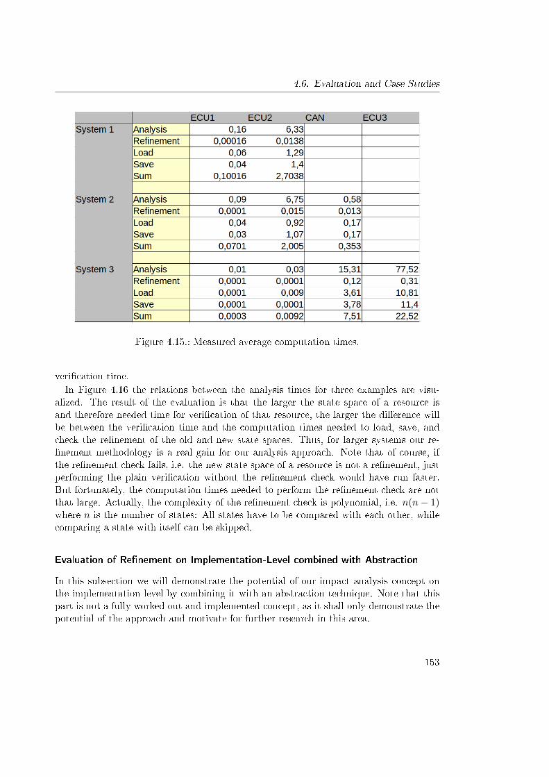
4.6. Evaluation and Case Studies
Figure 4.15.: Measured average computation times.
veri�cation time.In Figure 4.16 the relations between the analysis times for three examples are visu-
alized. The result of the evaluation is that the larger the state space of a resource isand therefore needed time for veri�cation of that resource, the larger the di�erence willbe between the veri�cation time and the computation times needed to load, save, andcheck the re�nement of the old and new state spaces. Thus, for larger systems our re-�nement methodology is a real gain for our analysis approach. Note that of course, ifthe re�nement check fails, i.e. the new state space of a resource is not a re�nement, justperforming the plain veri�cation without the re�nement check would have run faster.But fortunately, the computation times needed to perform the re�nement check are notthat large. Actually, the complexity of the re�nement check is polynomial, i.e. n(n− 1)where n is the number of states: All states have to be compared with each other, whilecomparing a state with itself can be skipped.
Evaluation of Re�nement on Implementation-Level combined with Abstraction
In this subsection we will demonstrate the potential of our impact analysis concept onthe implementation level by combining it with an abstraction technique. Note that thispart is not a fully worked out and implemented concept, as it shall only demonstrate thepotential of the approach and motivate for further research in this area.
153
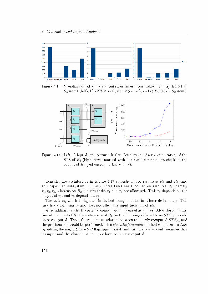
4. Contract-based Impact Analysis
Figure 4.16.: Visualization of some computation times from Table 4.15: a) ECU1 inSystem1 (left), b) ECU2 on System2 (center), and c) ECU3 on System3.
τ1
τ2
τ4
τ5
R1 R2
τ6
τ3
...
...
...
... Subsystem
...
...
STSin,R1
STSin,R2
STSout,R1
STSin,sub
10 12 14 16 18
0
200
400
600
800
1,000
Worst case execution times of τ1 and τ4
Veri�cation
timeinsec.
Figure 4.17.: Left: Adapted architecture; Right: Comparison of a re-computation of theSTS of R2 (blue curve, marked with dots) and a re�nement check on theoutput of R1 (red curve, marked with x).
Consider the architecture in Figure 4.17 consists of two resources R1 and R2, andan unspeci�ed subsystem. Initially, three tasks are allocated on resource R1, namelyτ1, τ2, τ3, whereas on R2 the two tasks τ4 and τ5 are allocated. Task τ4 depends on theoutput of τ1, and τ5 depends on τ2.
The task τ6, which is depicted in dashed lines, is added in a later design step. Thistask has a low priority and does not a�ect the input behavior of R2.
After adding τ6 to R1 the original concept would proceed as follows: After the computa-tion of the input of R1 the state space of R1 (in the following referred to as STSR1) wouldbe re-computed. Then, the re�nement relation between the newly computed STSR1 andthe previous one would be performed. This checkRefinement method would return falseby setting the outputConsistent �ag appropriately indicating all dependent resources thatits input and therefore its state space have to be re-computed.
154
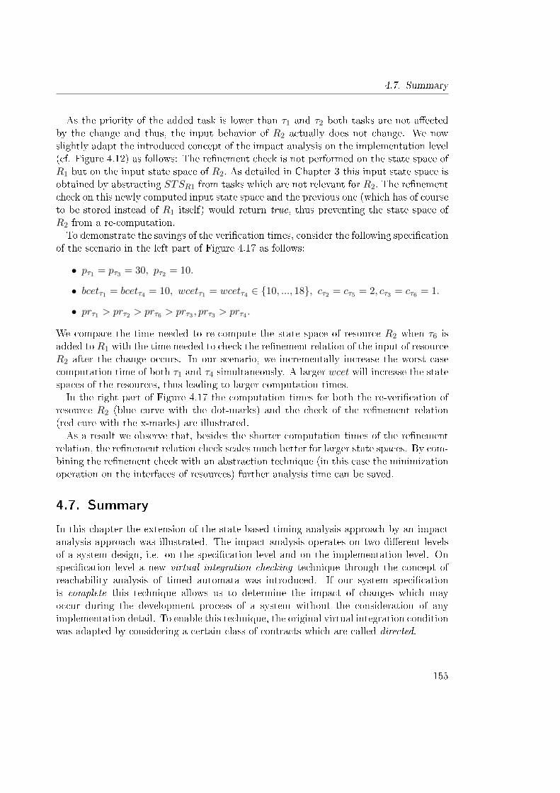
4.7. Summary
As the priority of the added task is lower than τ1 and τ2 both tasks are not a�ectedby the change and thus, the input behavior of R2 actually does not change. We nowslightly adapt the introduced concept of the impact analysis on the implementation level(cf. Figure 4.12) as follows: The re�nement check is not performed on the state space ofR1 but on the input state space of R2. As detailed in Chapter 3 this input state space isobtained by abstracting STSR1 from tasks which are not relevant for R2. The re�nementcheck on this newly computed input state space and the previous one (which has of courseto be stored instead of R1 itself) would return true, thus preventing the state space ofR2 from a re-computation.To demonstrate the savings of the veri�cation times, consider the following speci�cation
of the scenario in the left part of Figure 4.17 as follows:
• pτ1 = pτ3 = 30, pτ2 = 10.
• bcetτ1 = bcetτ4 = 10, wcetτ1 = wcetτ4 ∈ {10, ..., 18}, cτ2 = cτ5 = 2, cτ3 = cτ6 = 1.
• prτ1 > prτ2 > prτ6 > prτ3 , prτ3 > prτ4 .
We compare the time needed to re-compute the state space of resource R2 when τ6 isadded to R1 with the time needed to check the re�nement relation of the input of resourceR2 after the change occurs. In our scenario, we incrementally increase the worst casecomputation time of both τ1 and τ4 simultaneously. A larger wcet will increase the statespaces of the resources, thus leading to larger computation times.In the right part of Figure 4.17 the computation times for both the re-veri�cation of
resource R2 (blue curve with the dot-marks) and the check of the re�nement relation(red cure with the x-marks) are illustrated.As a result we observe that, besides the shorter computation times of the re�nement
relation, the re�nement relation check scales much better for larger state spaces. By com-bining the re�nement check with an abstraction technique (in this case the minimizationoperation on the interfaces of resources) further analysis time can be saved.
4.7. Summary
In this chapter the extension of the state-based timing analysis approach by an impactanalysis approach was illustrated. The impact analysis operates on two di�erent levelsof a system design, i.e. on the speci�cation level and on the implementation level. Onspeci�cation level a new virtual integration checking technique through the concept ofreachability analysis of timed automata was introduced. If our system speci�cationis complete this technique allows us to determine the impact of changes which mayoccur during the development process of a system without the consideration of anyimplementation detail. To enable this technique, the original virtual integration conditionwas adapted by considering a certain class of contracts which are called directed.
155
4. Contract-based Impact Analysis
The impact analysis approach is also de�ned on the implementation level, which isused when incomplete speci�cations are considered, or when the implementation of acomponent changes. To this end, an appropriate re�nement relation between state tran-sition systems has been de�ned. With this notion of re�nement, it is able to avoid timeconsuming re-veri�cations of parts of the system on implementation level. The imple-mentation of the impact analysis approach was illustrated. The approach was evaluatedby measuring the computation times needed to perform the full veri�cation, the storageand load of state spaces, and the computation of the re�nement check. A comparison ofthese execution times was performed. The result is that the larger a system is and theless number of components are a�ected in a non-re�nement manner, the more executiontimes can be saved needed to perform re-veri�cations.These two concepts � i.e. the impact analysis on speci�cation and implementation
level � are typically exploited in combination. Changing a component implicates theintegration of this component into its context, and the veri�cation of its implementationto the new components local speci�cation. The methodology combining all techniquesinto one single impact analysis approach was also illustrated in this chapter.
156
5. Summary and Outlook
In the �rst chapter the addressed problems in this thesis in the context of hard real-time,safety-critical systems were illustrated.
In Chapter 2 the necessary fundamentals of model-based design of real-time systemsand the underlying execution semantics were introduced. The functionality of such sys-tems is given by tasks which are characterized by best- and worst-case execution times. Ascheduler determines the order of task executions, which are activated periodically. Re-quirements of the underlying system architecture are speci�ed by the usage of contractswith which assumed and guaranteed behavior of a component can be distinguished. Theparts of the contracts are speci�ed by using the pattern-based Requirement Speci�cationLanguage. The real-time pattern of this language were described and the formal seman-tics were given. Proof obligations of correctness checks of decomposition structures wereillustrated, which include the composition and re�nement check on the level of contracts.
In Chapter 3 a new approach to analyze timing constraints of systems consisting of sev-eral computation units and bus systems was introduced. Analogously to model checking,the approach determines the reachability of states of resources, where timing constraintsof tasks or end-to-end latency constraints are violated. In contrast to such related works,the presented approach works in an iterative fashion, which enables minimization and ab-straction operations on the interfaces of dependent resources. The approach is based onthe Uppaal DBM library. This library implements the �nite clock zone representationsof valuations of real-valued variables. Using such variables, computation times of tasksare measured. On top of the basic operations of the DBM library, in Section 3.4 higherlevel functions were de�ned and implemented. In detail, in Subsection 3.4.1 abstrac-tion operations on zones and locations were de�ned to determine the minimal interfacebetween two dependent resources. It was shown that the obtained abstracted interfaceSTS is an over-approximation of the original STS and preserves deadlock-freeness. InSubsection 3.4.2 the composition of a set of STSs was presented. It was shown in The-orem 2 that the STS which is obtained by this composition operation has an equivalentbehavior to the one which is obtained by �rst composing a set of timed automata andthen building the resulting STS. The main algorithm building iteratively the state spacefor a given architecture using these operations was presented in Section 3.5.Further, abstraction techniques were introduced which allow to abstract speci�c parts
of the computed state spaces of computation resources. In detail, in Subsection 3.5.5 theuntimed bisimulation, timed simulation relation was introduced, where paths are merged
157
5. Summary and Outlook
which have on the one hand equivalent discrete behaviors and on the other hand havea related timing behavior in terms of subset relations of clock zones. The application ofthis technique did not result in much smaller state spaces of dependent resources, but didpositively a�ect the overall analysis times (cf. Figure 3.13). An abstraction techniqueusing a new timed simulation relation was introduced in Subsection 3.6.3 leading to over-approximated STSs. The e�ects of such over-approximations on the iterative analysisapproach were analyzed in Subsection 3.6.4 revealing an interesting e�ect: Although thestate spaces of the interfaces could be reduced for the applied test cases, the resultingnumbers of states of dependent resources were always above the numbers of states wherethe abstractions on the input STSs were not applied. In Subsection 3.6.6 an abstractiontechnique for interfaces where event bursts occur was presented, leading to signi�cantstate space reductions. The usage of this abstraction thereby is restricted to scenarios,where end-to-end latencies are not of interest.
The applicability of the state-based approach was studied on a driver assistance systemcase study in Section 3.7, which was modeled by the usage of the modeling frameworkMarte. The focus on the timing analysis was on the detailed subsystem which is re-sponsible for an automatic lane-keeping of a vehicle. Response times and state spaces ofthe basic approach and the results of the applications of the abstraction techniques werecompared and analyzed. The positive e�ects on the sizes of the number of states couldbeen demonstrated.
In Chapter 4 the extension of the state-based timing analysis by an impact analysiswas illustrated. The overall methodology was illustrated in Section 4.3. The impactanalysis operates on two di�erent levels of a system design, i.e. on the speci�cationlevel and on the implementation level. On speci�cation level a new virtual integrationchecking technique through the concept of reachability analysis of timed automata wasintroduced in Subsection 4.4.2 deriving timed automaton networks from sets of contractswhich are speci�ed using the Requirement Speci�cation Language (RSL). To enable such atimed automaton approach, Theorem 4 was derived. This theorem uses the directednessand receptiveness properties of contracts, resulting in a simpli�ed virtual integrationcondition, where expressions with negations do not occur.
On the implementation level an appropriate re�nement relation between state transi-tion systems was de�ned in Subsection 4.5.2. With this notion of re�nement, it is ableto avoid time consuming re-veri�cations of parts of the system on implementation level.The implementation of the impact analysis approach was illustrated. The approach wasevaluated by measuring the computation times needed to perform the full satisfactionveri�cation on the one hand, and the sum of the storage and load of state spaces and thecomputation of the re�nement check on the other hand. A comparison of these executiontimes was performed, with the result that for larger systems the re�nement methodologycan help to save much analysis times and thus to help to decrease the time to market ofa system.
158
There are many research areas for future works. This work assumes a dense timesemantics of the timing behavior of tasks. The iterative analysis approach can be com-bined by considering also the discrete semantics. Parts of an architecture, which havebeen modeled in more detail and are closer to the �nal implementation then the rest ofthe architecture may be analyzed by the usage of a discrete time back-end, while the restis analyzed by considering the dense time back-end.Future work in this area could also investigate new abstraction techniques which could
further boost the scalability of the approach. The explicit computation of the statespaces of resources in an iterative manner enables the analysis of dedicated abstractionoperations, e.g. by merging successive states or leaving out some traces. An interestingdirection is to �nd those paths of the state spaces of resources, which yield end-to-endworst-case behaviors. Analogously to classical schedulability analyses where the criticalinstance leads to worst-case timing behavior, such instance could be determined fordistributed systems.Considering the impact analysis approach, so far only the iterative activation of timed
automata was considered, i. e. simultaneous activations are not considered and ignored.To deal with multiple simultaneous activations, explicit indexes must be allocated toobservable events as illustrated in this work.In this thesis, pattern considering the real-time behavior were considered. Thus, the
approach could be extended by considering further aspects of systems like functional andsafety properties speci�ed by text pattern. This would realize a powerful multi-aspectanalysis approach.On the implementation level, alternative re�nement relation de�nitions could be in-
vestigated with which a greater set of re�ning STSs could be determined. Also, thee�ects of �rst abstracting a resource STS before performing a re�nement check - suchit was illustrated in Subsection 4.6.3 - could be analyzed, especially for new abstractiontechniques worked out in future researches.
159

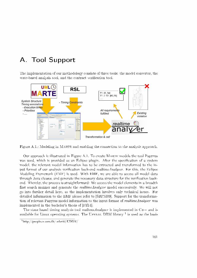
A. Tool Support
The implementation of our methodology consists of three tools: the model converter, thestate-based analysis tool, and the contract veri�cation tool.
Figure A.1.: Modeling in Marte and enabling the connection to the analysis approach.
Our approach is illustrated in Figure A.1. To create Marte models the tool Papyruswas used, which is provided as an Eclipse plugin. After the speci�cation of a systemmodel, the relevant model information has to be extracted and transformed to the in-put format of our analysis veri�cation back-end realtimeAnalyzer. For this, the EclipseModeling Framework (EMF) is used. With EMF, we are able to access all model datathrough Java classes, and generate the necessary data structure for the veri�cation back-end. Thereby, the process is straightforward: We access the model elements in a breadth�rst search manner and generate the realtimeAnalyzer model successively. We will notgo into further detail here, as the implementation involves only technical issues. Fordetailed information to the EMF please refer to [SBPM09]. Support for the transforma-tion of relevant Papyrus model information to the input format of realtimeAnalyzer wasimplemented in the bachelor's thesis of [Fif14].The state-based timing analysis tool realtimeAnalyzer is implemented in C++ and is
available for Linux operating systems. The Uppaal DBM library 1 is used as the basis
1http://people.cs.aau.dk/ adavid/UDBM/
161
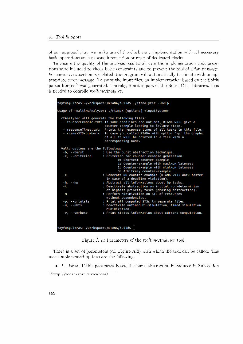
A. Tool Support
of our approach, i.e. we make use of the clock zone implementation with all necessarybasic operations such as zone intersection or reset of dedicated clocks.To ensure the quality of the analysis results, all over the implementation code asser-
tions were included to check basic constraints and to prevent the tool of a faulty usage.Whenever an assertion is violated, the program will automatically terminate with an ap-propriate error message. To parse the input �les, an implementation based on the Spiritparser library 2 was generated. Thereby, Spirit is part of the Boost-C++ libraries, thusis needed to compile realtimeAnalyzer.
Figure A.2.: Parameters of the realtimeAnalyzer tool.
There is a set of parameters (cf. Figure A.2) with which the tool can be called. Themost implemented options are the following:
• -b, �burst : If this parameter is set, the burst abstraction introduced in Subsection
2http://boost-spirit.com/home/
162
3.6.6 will be applied. If end-to-end latency constraints are de�ned in the systemwhich shall be analyzed, the program will give an error message that the abstractionis not applicable for this system.
• -c, �criterion: The user is able to determine the type of counter-example which isgenerated by the tool. The user can select between the shortest counter-example,a counter-example with maximum lateness, a counter-example with minimum late-ness, and an arbitrary counter-example. Note that the arbitrary counter-exampleis set as default. Note that this feature has been implemented in the context of thebachelor's thesis of [Koo14].
• -e: If some deadlines are violated, no counter-examples are generated if this optionis set. The tool will work a bit faster in case of a deadline violation, as no outputhas to be generated.
• -h, �hp: Abstract all information about tasks with higher priorities than relevantfor dependent resources. This technique was illustrated in Subsection 3.6.2.
• -i : With this parameter an abstraction on the initial non-determinism of the taskwith the highest priority is performed, i.e. it is assumed that the highest prioritytask is activated at time point null. This option is related to testing techniques.
• -m: In Subsection 3.5.1 it was stated that the bisimulation minimization of Sub-section 3.3.3 is only applied for resource STSs, which have dependent resources.By setting this parameter, the minimization is also performed for resource STSswhich from which no resource depends on.
• -p, �printsts: The computed state spaces of all systems will be printed into separate�les.
• -u, �ubts: Deactivate the untimed bisimulation, timed simulation minimizationpresented in Subsection 3.3.3.
• -v, �verbose: Some debug information is printed to the console. This option couldbe helpful if new features are implemented and debugging must be performed.
When the tool is called with a model, a set of �les are generated:
• counterExample.txt : If some deadlines are not met, realtimeAnalyzer will generatea counter example trace into this �le leading to failure state according to the de�nedcriterion.
• responseTimes.txt : All computed end-to-end latency times and local response timeswill be printed to this �le.
163
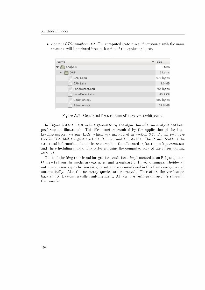
A. Tool Support
• <name>STS<number>.txt : The computed state space of a resource with the name<name> will be printed into such a �le, if the option -p is set.
Figure A.3.: Generated �le structure of a system architecture.
In Figure A.3 the �le structure generated by the algorithm after an analysis has beenperformed is illustrated. This �le structure resulted by the application of the lane-keeping-support system (LKS) which was introduced in Section 3.7. For all resourcestwo kinds of �les are generated, i.e. an .ecu and an .sts �le. The former contains thestructural information about the resource, i.e. the allocated tasks, the task parameters,and the scheduling policy. The latter contains the computed STS of the correspondingresource.The tool checking the virtual integration condition is implemented as an Eclipse plugin.
Contracts from the model are extracted and translated to timed automata. Besides allautomata, event reproduction via glue automata as mentioned in this thesis are generatedautomatically. Also the necessary queries are generated. Thereafter, the veri�cationback-end of Uppaal is called automatically. At last, the veri�cation result is shown inthe console.
164
B. Handling Architectures including
Restricted Loop Structures
So far, systems with no feedback loops were considered. If loops are contained a holisticanalysis has to be performed in general as the state spaces of the dependent resourcescannot be separated. For a restricted class of feedback-loops the iterative analysis ap-proach can still be applied. For this, assume the following scenario: Let a resource withi = n+m tasks be given. The n-highest priority tasks of a resource are either indepen-dent or depend on a set of task, where no feedback-loop is included (simple dependencychains). The m-lower priority tasks depend on tasks, which are triggered by the some ofthe n-higher priority tasks, thus leading to a feedback-loop. For loop structures of thistype the following is performed: First, the partial state space of the resource consistingof the behavior of the n-highest priority tasks is computed. This is possible and leads tocorrect timings for these tasks, as none of the m-lower priority tasks can lead to inter-ferences (cannot interrupt the other tasks). The rest of the state space of the resource iscomputed, whenever the input behavior of them-lower priority tasks has been computed.What was so far not shown is the general procedure of the realtimeAnalyzer tool.
This is illustrated in Figure B.1. As an input the parser delivers a set of resources withallocated tasks, for which the corresponding STSs have to be computed. This set isstored in a queue q. The algorithm terminates, if q is empty and thus all STSs have beencomputed, or a deadline is violated.In constraint c2 it is determined whether the input behaviors of all allocated tasks
of the currently considered resource have already been determined. If so, the input iscomputed by the application of the composition and interface computation operationsdescribed in Subsection 3.4. The resource STS is then computed and the next resource isconsidered. For now, let us skip the constraint c5 and assume that it evaluates to false.If the constraint c2 evaluates to false, it is checked in constraint c3 whether a partial
computation can be performed, i.e. the method determines the set of tasks which do notdepend on other tasks or are interrupted by such tasks as described above. With this,the above described restricted feedback-loops can be handled. If a partial computationis possible, the �ag partial is set to true and the partial state space is computed. Theconstraint c5 evaluates to true for this case and thus the resource is put again back tothe queue. The rest of the state space of this resource is then computed later, when themissing input behaviors have been determined. Thereby, the resource is also includedinto the set p which is detailed later.
165
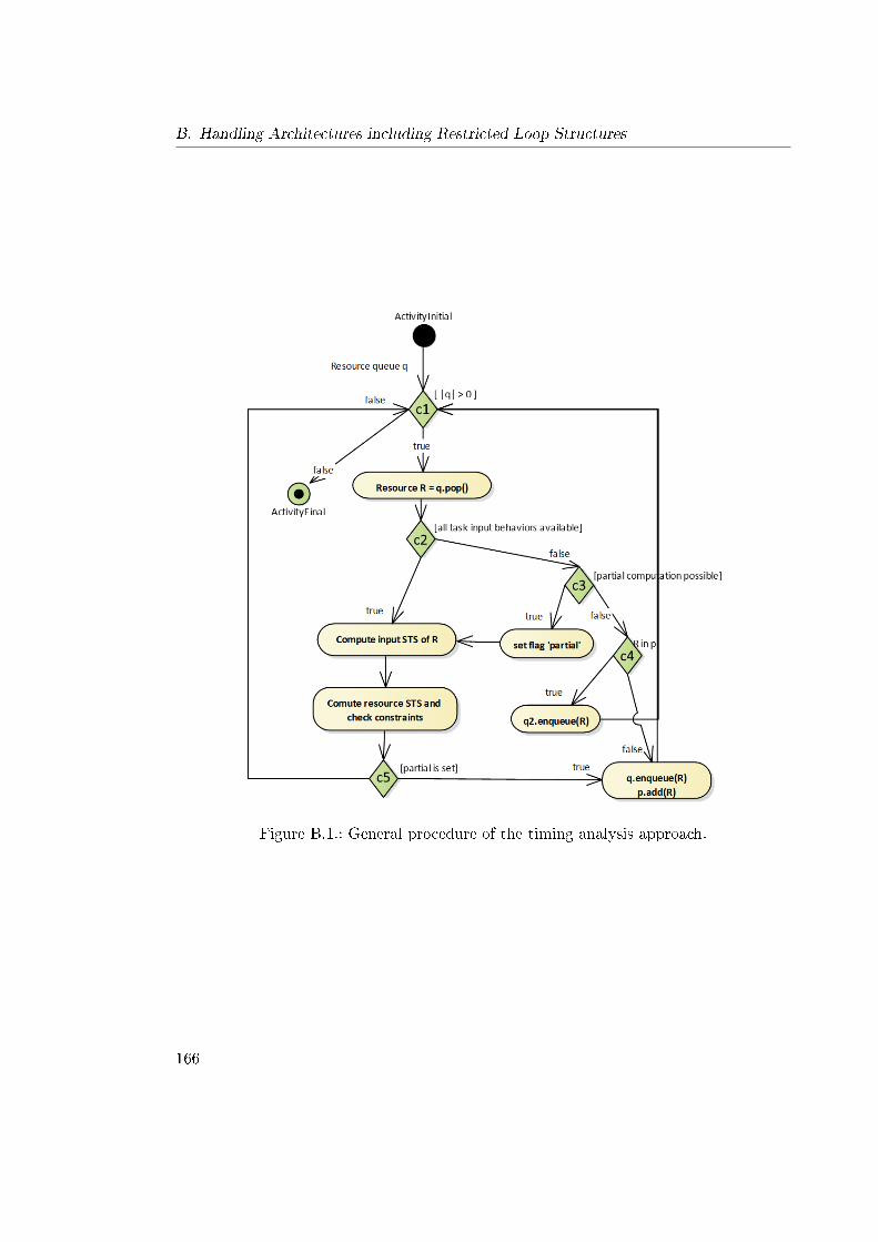
B. Handling Architectures including Restricted Loop Structures
Figure B.1.: General procedure of the timing analysis approach.
166
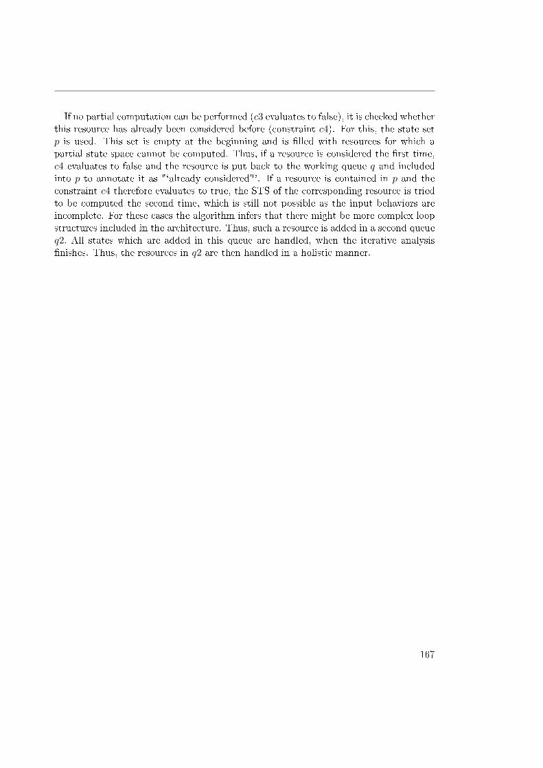
If no partial computation can be performed (c3 evaluates to false), it is checked whetherthis resource has already been considered before (constraint c4). For this, the state setp is used. This set is empty at the beginning and is �lled with resources for which apartial state space cannot be computed. Thus, if a resource is considered the �rst time,c4 evaluates to false and the resource is put back to the working queue q and includedinto p to annotate it as "`already considered"'. If a resource is contained in p and theconstraint c4 therefore evaluates to true, the STS of the corresponding resource is triedto be computed the second time, which is still not possible as the input behaviors areincomplete. For these cases the algorithm infers that there might be more complex loopstructures included in the architecture. Thus, such a resource is added in a second queueq2. All states which are added in this queue are handled, when the iterative analysis�nishes. Thus, the resources in q2 are then handled in a holistic manner.
167

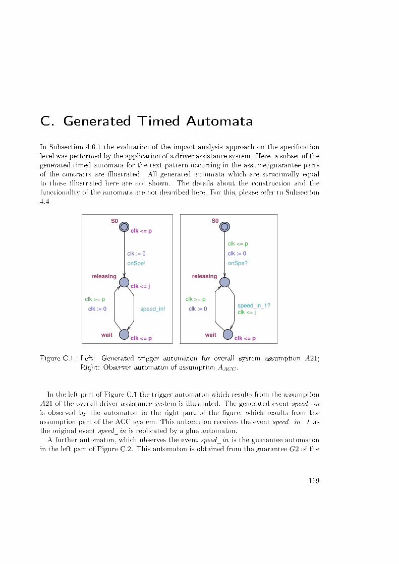
C. Generated Timed Automata
In Subsection 4.6.1 the evaluation of the impact analysis approach on the speci�cationlevel was performed by the application of a driver assistance system. Here, a subset of thegenerated timed automata for the text-pattern occurring in the assume/guarantee partsof the contracts are illustrated. All generated automata which are structurally equalto those illustrated here are not shown. The details about the construction and thefunctionality of the automata are not described here. For this, please refer to Subsection4.4
waitclk <= p
releasing
clk <= j
S0
clk <= p
clk >= p
clk := 0 speed_in!
onSpe!
clk := 0
waitclk <= p
releasing
S0
clk >= p
clk := 0clk <= jspeed_in_1?
clk <= p
onSpe?
clk := 0
Figure C.1.: Left: Generated trigger automaton for overall system assumption A21;Right: Observer automaton of assumption AACC .
In the left part of Figure C.1 the trigger automaton which results from the assumptionA21 of the overall driver assistance system is illustrated. The generated event speed_inis observed by the automaton in the right part of the �gure, which results from theassumption part of the ACC system. This automaton receives the event speed_in_1 asthe original event speed_in is replicated by a glue automaton.A further automaton, which observes the event speed_in is the guarantee automaton
in the left part of Figure C.2. This automaton is obtained from the guarantee G2 of the
169
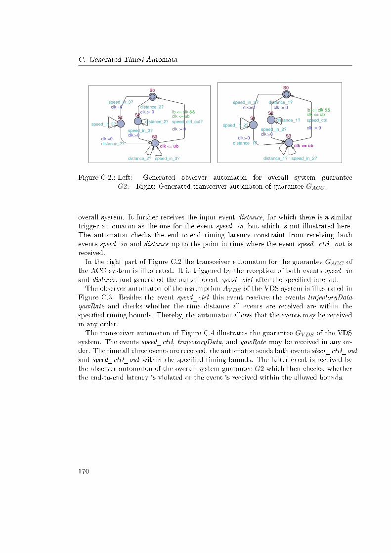
C. Generated Timed Automata
S1S2
S3
clk <= ub
S0
distance_2?speed_in_3?
distance_2?
distance_2?clk:=0
speed_in_3?clk:=0
speed_in_3?clk:=0
speed_in_3?
lb <= clk && clk <= ub
speed_ctrl_out?
clk := 0
distance_2?clk := 0
S1
S2
S3
clk <= ub
S0
distance_1?speed_in_2?
distance_1?
distance_1?clk:=0
speed_in_2?clk:=0
speed_in_2?clk:=0
speed_in_2?
lb <= clk && clk <= ub
speed_ctrl!
clk := 0
distance_1?clk := 0
Figure C.2.: Left: Generated observer automaton for overall system guaranteeG2; Right: Generated transceiver automaton of guarantee GACC .
overall system. It further receives the input event distance, for which there is a similartrigger automaton as the one for the event speed_in, but which is not illustrated here.The automaton checks the end-to-end timing latency constraint from receiving bothevents speed_in and distance up to the point in time where the event speed_ctrl_out isreceived.In the right part of Figure C.2 the transceiver automaton for the guarantee GACC of
the ACC system is illustrated. It is triggered by the reception of both events speed_inand distance and generated the output event speed_ctrl after the speci�ed interval.The observer automaton of the assumption AV DS of the VDS system is illustrated in
Figure C.3. Besides the event speed_ctrl this event receives the events trajectoryDatayawRate and checks whether the time distance all events are received are within thespeci�ed timing bounds. Thereby, the automaton allows that the events may be receivedin any order.The transceiver automaton of Figure C.4 illustrates the guarantee GV DS of the VDS
system. The events speed_ctrl, trajectoryData, and yawRate may be received in any or-der. The time all three events are received, the automaton sends both events steer_ctrl_outand speed_ctrl_out within the speci�ed timing bounds. The latter event is received bythe observer automaton of the overall system guarantee G2 which then checks, whetherthe end-to-end latency is violated or the event is received within the allowed bounds.
170
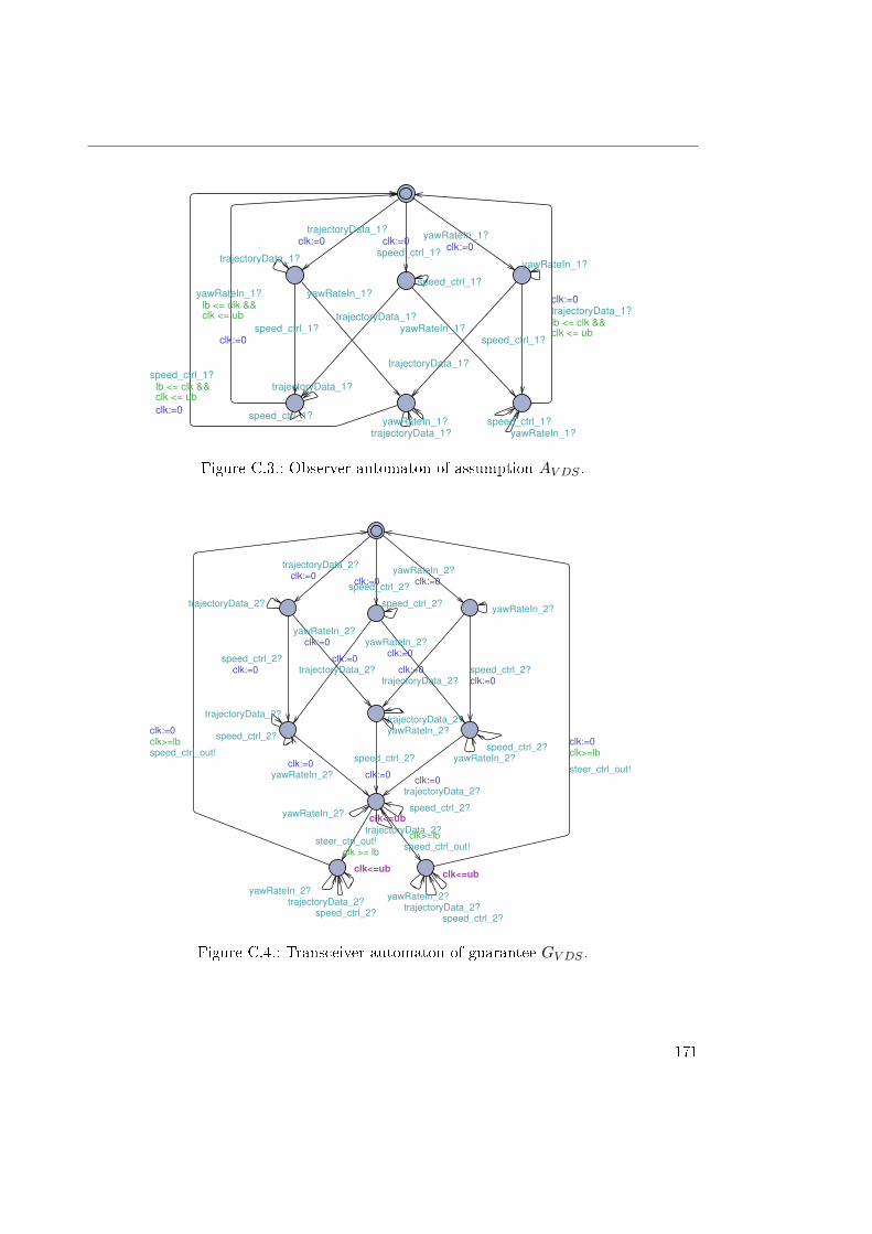
yawRateIn_1?speed_ctrl_1?
trajectoryData_1?yawRateIn_1?
trajectoryData_1?
speed_ctrl_1?
yawRateIn_1?
speed_ctrl_1?
trajectoryData_1?
lb <= clk && clk <= ub
speed_ctrl_1?
clk:=0
lb <= clk && clk <= ub
trajectoryData_1?clk:=0
lb <= clk && clk <= ub
yawRateIn_1?
clk:=0
trajectoryData_1?
yawRateIn_1?
yawRateIn_1?clk:=0
trajectoryData_1?clk:=0
speed_ctrl_1?speed_ctrl_1? yawRateIn_1?
trajectoryData_1?
speed_ctrl_1?clk:=0
Figure C.3.: Observer automaton of assumption AV DS .
clk<=ubclk<=ub
clk<=ub
trajectoryData_2?trajectoryData_2?
trajectoryData_2?
speed_ctrl_2?
yawRateIn_2?
speed_ctrl_2?
yawRateIn_2?
yawRateIn_2?speed_ctrl_2?
clk>=lb
steer_ctrl_out!
clk:=0clk>=lbspeed_ctrl_out!
clk:=0
clk>=lbspeed_ctrl_out!
clk >= lbsteer_ctrl_out!
yawRateIn_2?speed_ctrl_2?
trajectoryData_2?yawRateIn_2?
trajectoryData_2?
speed_ctrl_2?
yawRateIn_2?speed_ctrl_2?trajectoryData_2?
speed_ctrl_2?
clk:=0
trajectoryData_2?clk:=0
yawRateIn_2?clk:=0
trajectoryData_2?clk:=0
yawRateIn_2?clk:=0
yawRateIn_2?clk:=0
trajectoryData_2?clk:=0
speed_ctrl_2?clk:=0
speed_ctrl_2?clk:=0
yawRateIn_2?clk:=0
trajectoryData_2?clk:=0
speed_ctrl_2?clk:=0
Figure C.4.: Transceiver automaton of guarantee GV DS .
171

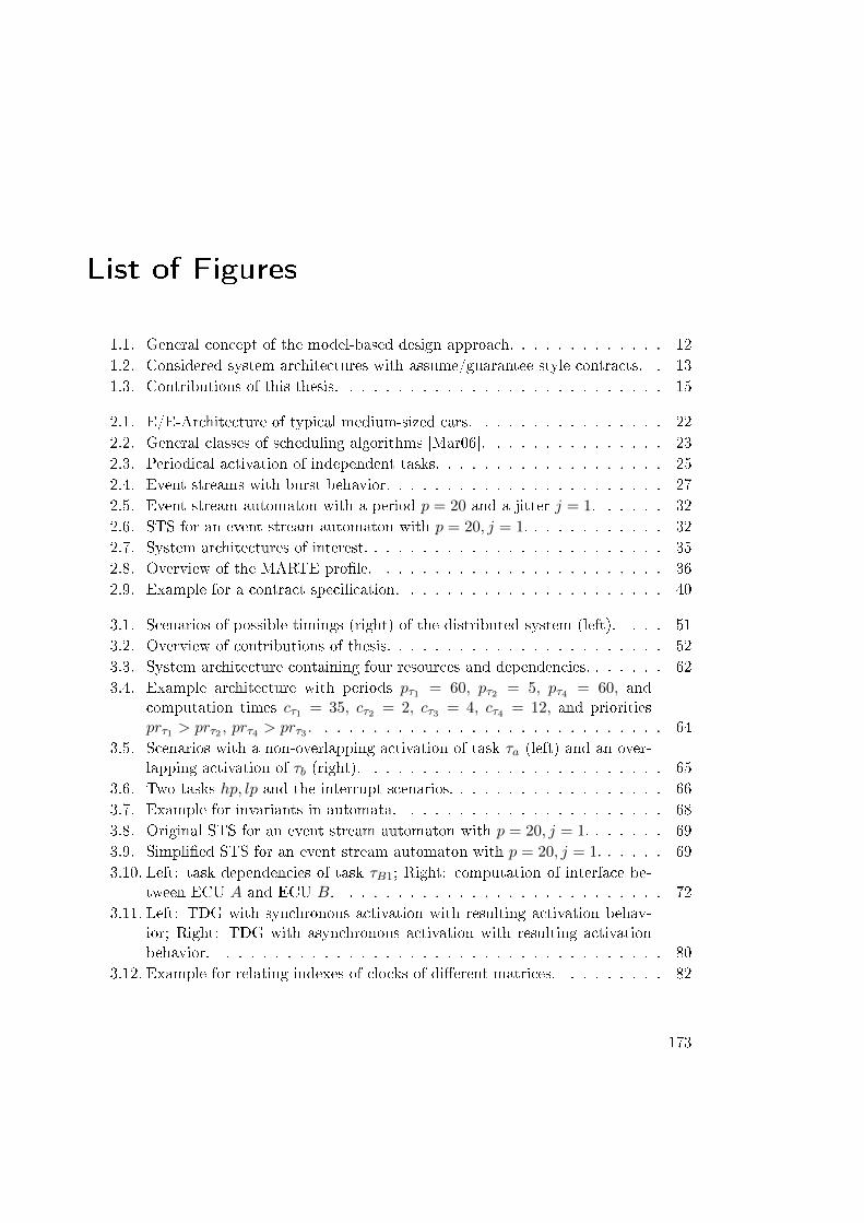
List of Figures
1.1. General concept of the model-based design approach. . . . . . . . . . . . . 121.2. Considered system architectures with assume/guarantee style contracts. . 131.3. Contributions of this thesis. . . . . . . . . . . . . . . . . . . . . . . . . . . 15
2.1. E/E-Architecture of typical medium-sized cars. . . . . . . . . . . . . . . . 222.2. General classes of scheduling algorithms [Mar06]. . . . . . . . . . . . . . . 232.3. Periodical activation of independent tasks. . . . . . . . . . . . . . . . . . . 252.4. Event streams with burst behavior. . . . . . . . . . . . . . . . . . . . . . . 272.5. Event stream automaton with a period p = 20 and a jitter j = 1. . . . . . 322.6. STS for an event stream automaton with p = 20, j = 1. . . . . . . . . . . . 322.7. System architectures of interest. . . . . . . . . . . . . . . . . . . . . . . . . 352.8. Overview of the MARTE pro�le. . . . . . . . . . . . . . . . . . . . . . . . 362.9. Example for a contract speci�cation. . . . . . . . . . . . . . . . . . . . . . 40
3.1. Scenarios of possible timings (right) of the distributed system (left). . . . 513.2. Overview of contributions of thesis. . . . . . . . . . . . . . . . . . . . . . . 523.3. System architecture containing four resources and dependencies. . . . . . . 623.4. Example architecture with periods pτ1 = 60, pτ2 = 5, pτ4 = 60, and
computation times cτ1 = 35, cτ2 = 2, cτ3 = 4, cτ4 = 12, and prioritiesprτ1 > prτ2 , prτ4 > prτ3 . . . . . . . . . . . . . . . . . . . . . . . . . . . . . 64
3.5. Scenarios with a non-overlapping activation of task τa (left) and an over-lapping activation of τb (right). . . . . . . . . . . . . . . . . . . . . . . . . 65
3.6. Two tasks hp, lp and the interrupt scenarios. . . . . . . . . . . . . . . . . . 663.7. Example for invariants in automata. . . . . . . . . . . . . . . . . . . . . . 683.8. Original STS for an event stream automaton with p = 20, j = 1. . . . . . . 693.9. Simpli�ed STS for an event stream automaton with p = 20, j = 1. . . . . . 693.10. Left: task dependencies of task τB1; Right: computation of interface be-
tween ECU A and ECU B. . . . . . . . . . . . . . . . . . . . . . . . . . . 723.11. Left: TDG with synchronous activation with resulting activation behav-
ior; Right: TDG with asynchronous activation with resulting activationbehavior. . . . . . . . . . . . . . . . . . . . . . . . . . . . . . . . . . . . . 80
3.12. Example for relating indexes of clocks of di�erent matrices. . . . . . . . . 82
173
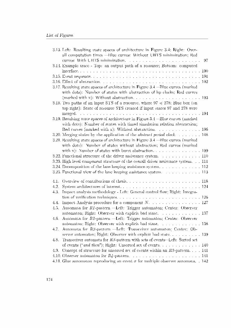
List of Figures
3.13. Left: Resulting state spaces of architecture in Figure 3.4; Right: Over-all computation times � Blue curves: Without UBTS minimization; Redcurves: With UBTS minimization. . . . . . . . . . . . . . . . . . . . . . . 97
3.14. Example trace - Top: an output path of a resource; Bottom: computedinterface. . . . . . . . . . . . . . . . . . . . . . . . . . . . . . . . . . . . . . 100
3.15. Event sequence. . . . . . . . . . . . . . . . . . . . . . . . . . . . . . . . . . 1013.16. E�ect of abstraction. . . . . . . . . . . . . . . . . . . . . . . . . . . . . . . 1023.17. Resulting state spaces of architecture in Figure 3.4 � Blue curves (marked
with dots): Number of states with abstraction of hp clocks; Red curves(marked with x): Without abstraction. . . . . . . . . . . . . . . . . . . . . 103
3.18. Two paths of an input STS of a resource, where 97 4 278; Blue box (ontop right): State of resource STS created if input states 97 and 278 weremerged. . . . . . . . . . . . . . . . . . . . . . . . . . . . . . . . . . . . . . 104
3.19. Resulting state spaces of architecture in Figure 3.4 � Blue curves (markedwith dots): Number of states with timed simulation relation abstraction;Red curves (marked with x): Without abstraction. . . . . . . . . . . . . . 106
3.20. Merging states by the application of the abstract period clock. . . . . . . . 1083.21. Resulting state spaces of architecture in Figure 3.4 � Blue curves (marked
with dots): Number of states without abstraction; Red curves (markedwith x): Number of states with burst abstraction. . . . . . . . . . . . . . . 109
3.22. Functional structure of the driver assistance system. . . . . . . . . . . . . 1103.23. High level component structure of the overall driver assistance system. . . 1113.24. Decomposition of the lane keeping assistance system. . . . . . . . . . . . . 1123.25. Functional view of the lane keeping assistance system. . . . . . . . . . . . 113
4.1. Overview of contributions of thesis. . . . . . . . . . . . . . . . . . . . . . . 1184.2. System architectures of interest. . . . . . . . . . . . . . . . . . . . . . . . . 1244.3. Impact analysis methodology - Left: General control �ow; Right: Integra-
tion of veri�cation techniques. . . . . . . . . . . . . . . . . . . . . . . . . . 1264.4. Impact Analysis procedure for a component N . . . . . . . . . . . . . . . . 1274.5. Automata for R1 -pattern � Left: Trigger automaton; Center: Observer
automaton; Right: Observer with explicit bad state. . . . . . . . . . . . . 1374.6. Automata for R2 -pattern � Left: Trigger automaton; Center: Observer
automaton; Right: Observer with explicit bad state. . . . . . . . . . . . . 1384.7. Automata for R3 -pattern � Left: Transceiver automaton; Center: Ob-
server automaton; Right: Observer with explicit bad state. . . . . . . . . . 1394.8. Transceiver automata for R3 -pattern with sets of events� Left: Sorted set
of events (�and then�); Right: Unsorted set of events. . . . . . . . . . . . . 1404.9. Concept of structure for unsorted set of events within an R3 -pattern. . . . 1414.10. Observer automaton for R4 -pattern. . . . . . . . . . . . . . . . . . . . . . 1414.11. Glue automaton reproducing an event σ for multiple observer automata. . 142
174
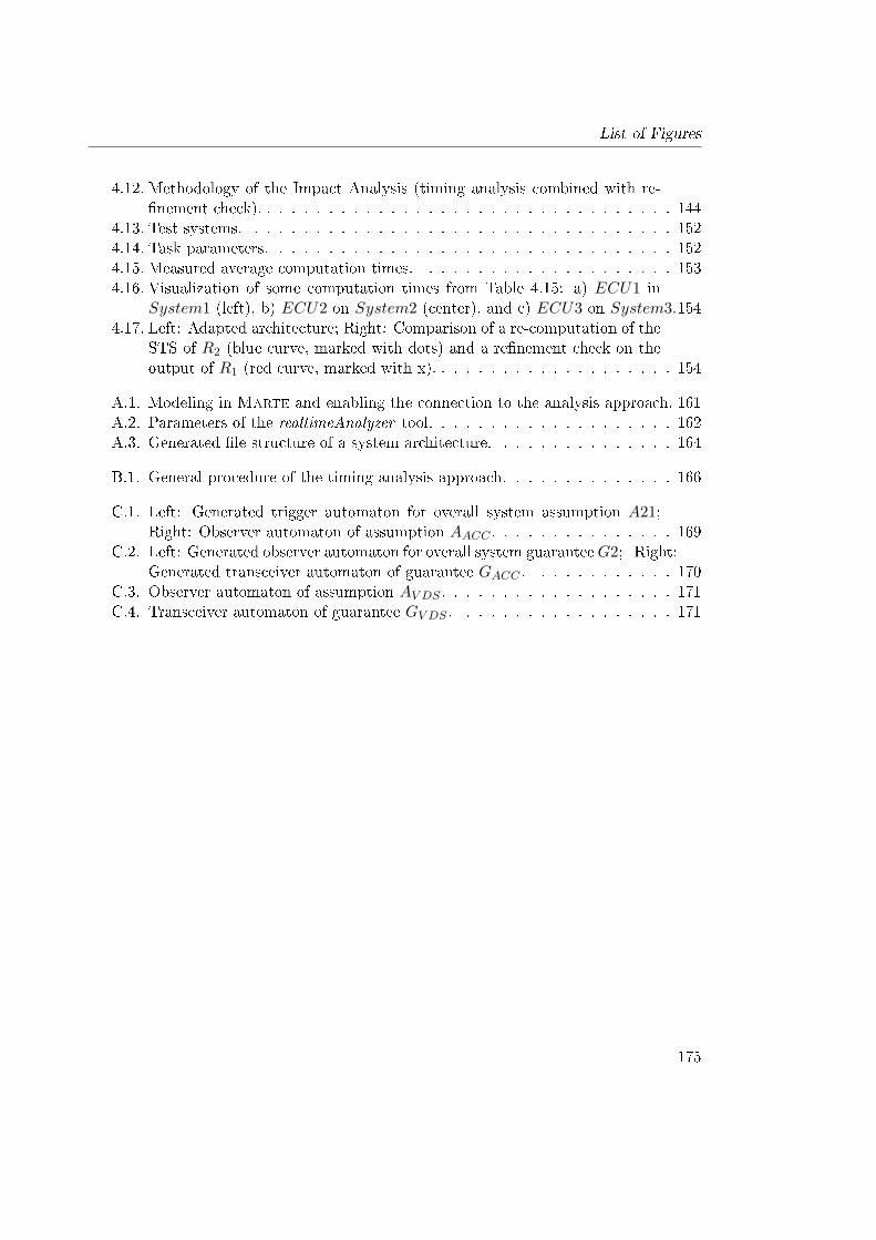
List of Figures
4.12. Methodology of the Impact Analysis (timing analysis combined with re-�nement check). . . . . . . . . . . . . . . . . . . . . . . . . . . . . . . . . . 144
4.13. Test systems. . . . . . . . . . . . . . . . . . . . . . . . . . . . . . . . . . . 1524.14. Task parameters. . . . . . . . . . . . . . . . . . . . . . . . . . . . . . . . . 1524.15. Measured average computation times. . . . . . . . . . . . . . . . . . . . . 1534.16. Visualization of some computation times from Table 4.15: a) ECU1 in
System1 (left), b) ECU2 on System2 (center), and c) ECU3 on System3.1544.17. Left: Adapted architecture; Right: Comparison of a re-computation of the
STS of R2 (blue curve, marked with dots) and a re�nement check on theoutput of R1 (red curve, marked with x). . . . . . . . . . . . . . . . . . . . 154
A.1. Modeling in Marte and enabling the connection to the analysis approach. 161A.2. Parameters of the realtimeAnalyzer tool. . . . . . . . . . . . . . . . . . . . 162A.3. Generated �le structure of a system architecture. . . . . . . . . . . . . . . 164
B.1. General procedure of the timing analysis approach. . . . . . . . . . . . . . 166
C.1. Left: Generated trigger automaton for overall system assumption A21;Right: Observer automaton of assumption AACC . . . . . . . . . . . . . . . 169
C.2. Left: Generated observer automaton for overall system guaranteeG2; Right:Generated transceiver automaton of guarantee GACC . . . . . . . . . . . . 170
C.3. Observer automaton of assumption AV DS . . . . . . . . . . . . . . . . . . . 171C.4. Transceiver automaton of guarantee GV DS . . . . . . . . . . . . . . . . . . 171
175

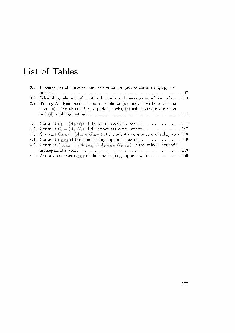
List of Tables
3.1. Preservation of universal and existential properties considering approxi-mations. . . . . . . . . . . . . . . . . . . . . . . . . . . . . . . . . . . . . . 97
3.2. Scheduling-relevant information for tasks and messages in milliseconds. . . 1133.3. Timing Analysis results in milliseconds for (a) analysis without abstrac-
tion, (b) using abstraction of period clocks, (c) using burst abstraction,and (d) applying testing. . . . . . . . . . . . . . . . . . . . . . . . . . . . . 114
4.1. Contract C1 = (A1, G1) of the driver assistance system. . . . . . . . . . . 1474.2. Contract C2 = (A2, G2) of the driver assistance system. . . . . . . . . . . 1474.3. Contract CACC = (AACC , GACC) of the adaptive cruise control subsystem. 1484.4. Contract CLKS of the lane-keeping-support subsystem. . . . . . . . . . . . 1494.5. Contract CV DM = (AV DM,1 ∧ AV DM,2, GV DM ) of the vehicle dynamic
management system. . . . . . . . . . . . . . . . . . . . . . . . . . . . . . . 1494.6. Adapted contract CLKS of the lane-keeping-support system. . . . . . . . . 150
177

Index
ω−Language, 27
Abstract Period Clock, 107Active Task Map, 35, 67Assertion, 39Asynchronous Activation, 79
Büchi Automaton, 27, 29Bisimulation Relation, 76Bus, 37
CAN, 21LIN, 21MOST, 21
Clock Constraint, 29Extension, 71Projection, 71
Clock Valuation, 29Clock Zone, 30
Boundedness, 31Canonical Form, 31Extension, 71Normalization, 31Projection, 71Zone Re�nement, 102
Complete Speci�cation, 125Completeness, 91Component, 33Computation Time Clock, 64Contract, 39, 41
Assumption, 39Canonical, 130Composition, 41
Conjunction, 42Consistency, 40Directedness, 132Guarantee, 39Maximum Implementation, 41Receptivity, 132Re�nement, 42Satisfaction, 40, 41Saturation, 130Virtual Integration Condition, 43
Correctness, 91Critical Instance, 54
Deadline, 23, 24Hard Deadline, 24Soft Deadline, 24
Deadlock Free, 74, 136Delegation, 33Di�erence Bound Matrix, 32Duration Clock, 99
Event Model, 25Event Stream, 25Jitter, 25Occurrence Function, 25Period, 25
Existential Property, 97
Fixed Priority Scheduling, 54
Incomplete Speci�cation, 125Interface, 33
Directed Interface, 34
179
Index
Port, 33Invariant, 29
Language, 27Liveness Property, 46Location Vector, 63
Observer Automaton, 134, 135
Periodic Activation Clock, 64
Ready Task List, 35, 67Reference Clock, 32Re�nement, 40Requirement, 38Resource, 33, 34, 37
Bus System, 33Electronic Control Unit, 33
Response Time Clock, 65
Satisfaction, 77Scheduling, 23
Dynamic, 24Feasibility, 23FIFO, 35FPS, 35Preemption, 24RMS, 54Scheduler, 37Scheduling Policy, 23Static, 24TDMA, 35
Simulation Relation, 74Soundness, 91Synchronous Activation, 79System Architecture, 36
Task, 23, 37Best-Case Execution Time, 24Deadline, 23, 24Hard Deadline, 24Immediate Predecessor, 25
Independent Task, 25Instance, 79Instance Bound, 65, 81Overlapping Activation, 64Predecessor, 25Priority, 24Release Time, 24Response Time, 25Soft Deadline, 24Tail Task, 79Task Dependency Graph, 25Worst-Case Execution Time, 24
TCTL, 135Timed Automaton, 28
Resource STS, 63Symbolic Transition System, 30Timed Transition System, 29
Timed Language, 28Extension, 34Restriction, 34
Timed Safety Automaton, 29Timed Simulation Relation, 103Timed Word, 28
Pre�x, 28Restriction, 34Trace, 28
Transceiver Automaton, 135Trigger Automaton, 135
UBTS Relation, 95Universal Property, 97
180

181
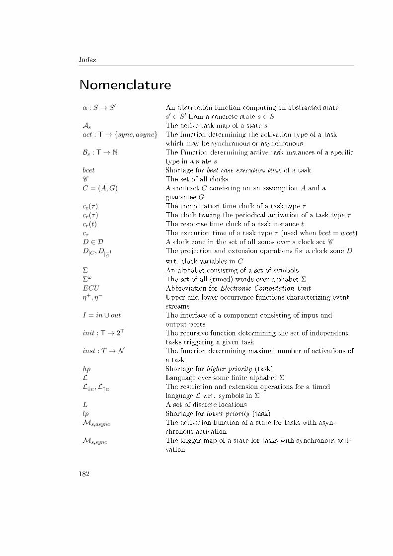
Index
Nomenclature
α : S → S′ An abstraction function computing an abstracted states′ ∈ S′ from a concrete state s ∈ S
As The active task map of a state sact : T→ {sync, async} The function determining the activation type of a task
which may be synchronous or asynchronousBs : T→ N The Function determining active task instances of a speci�c
type in a state sbcet Shortage for best-case execution time of a taskC The set of all clocksC = (A,G) A contract C consisting on an assumption A and a
guarantee Gcc(τ) The computation time clock of a task type τcr(τ) The clock tracing the periodical activation of a task type τcr(t) The response time clock of a task instance tcτ The execution time of a task type τ (used when bcet = wcet)D ∈ D A clock zone in the set of all zones over a clock set CD|C , D|−1
CThe projection and extension operations for a clock zone D
wrt. clock variables in CΣ An alphabet consisting of a set of symbolsΣω The set of all (timed) words over alphabet ΣECU Abbreviation for Electronic Computation Unitη+, η− Upper and lower occurrence functions characterizing event
streamsI = in ∪ out The interface of a component consisting of input and
output portsinit : T→ 2T The recursive function determining the set of independent
tasks triggering a given taskinst : T → N The function determining maximal number of activations of
a taskhp Shortage for higher priority (task)L Language over some �nite alphabet ΣL↓Σ ,L↑Σ The restriction and extension operations for a timed
language L wrt. symbols in ΣL A set of discrete locationslp Shortage for lower priority (task)Ms,async The activation function of a state for tasks with asyn-
chronous activationMs,sync The trigger map of a state for tasks with synchronous acti-
vation
182
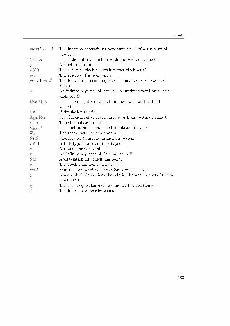
Index
max(i, · · · , j) The function determining maximum value of a given set ofnumbers
N,N>0 Set of the natural numbers with and without value 0ϕ A clock constraintΦ(C) The set of all clock constraints over clock set Cprτ The priority of a task type τpre : T→ 2T The function determining set of immediate predecessors of
a taskρ An in�nite sequence of symbols, or untimed word over some
alphabet ΣQ≥0,Q>0 Set of non-negative rational numbers with and without
value 0r,≈ Bisimulation relationR≥0,R>0 Set of non-negative real numbers with and without value 0rts,4 Timed simulation relationrubts,2 Untimed bisimulation, timed simulation relationRs The ready task list of a state sSTS Shortage for Symbolic Transition Systemτ ∈ T A task type in a set of task typesσ A timed trace or wordτ An in�nite sequence of time values in R+
Sch Abbreviation for scheduling policyν The clock valuation functionwcet Shortage for worst-case execution time of a taskξ A map which determines the relation between states of two or
more STSsχr The set of equivalence classes induced by relation rζ The function to reorder zones
183

Bibliography
[ABL98] Luca Aceto, Augusto Burgueño, and Kim Larsen. Model checking viareachability testing for timed automata. In Bernhard Ste�en, editor, Toolsand Algorithms for the Construction and Analysis of Systems, volume 1384of Lecture Notes in Computer Science (LNCS), pages 263�280. SpringerBerlin / Heidelberg, 1998. 10.1007/BFb0054177.
[ABR+86] N. C. Audsley, A. Burns, M. F. Richardson, K. Tindell, and A. J. Wellings.Applying new scheduling theory to static priority preemptive scheduling.The Computer Journal, 29 (5):390 � 395, 01/1986.
[AD94] Rajeev Alur and David L. Dill. A theory of timed automata. Theor.Comput. Sci., 126(2):183�235, April 1994.
[AdADS+06] B.Thomas Adler, Luca de Alfaro, LeandroDias Da Silva, Marco Faella, AxelLegay, Vishwanath Raman, and Pritam Roy. Ticc: A tool for interface com-patibility and composition. In Thomas Ball and RobertB. Jones, editors,Computer Aided Veri�cation, volume 4144 of Lecture Notes in ComputerScience, pages 59�62. Springer Berlin Heidelberg, 2006.
[AFM+04] Tobias Amnell, Elena Fersman, Leonid Mokrushin, Paul Pettersson, andWang Yi. Times: A tool for schedulability analysis and code generation ofreal-time systems. In Kim G. Larsen and Peter Niebert, editors, FormalModeling and Analysis of Timed Systems, volume 2791 of Lecture Notes inComputer Science, pages 60�72. Springer Berlin Heidelberg, 2004.
[AM02] Yasmina Abdeddaim and Oded Maler. Preemptive job-shop schedulingusing stopwatch automata. In in TACAS '02: Proceedings of the 8th In-ternational Conference on Tools and Algorithms for the Construction andAnalysis of Systems, pages 113�126. Springer, 2002.
[BBB+11] A. Baumgart, E. Böde, M. Büker, W. Damm, G. Ehmen, T. Gezgin,S. Henkler, H. Hungar, B. Josko, M. Oertel, T. Peikenkamp, P. Reinke-meier, I. Stierand, and R. Weber. Aritechture modeling. Technical report,OFFIS, November 2011.
185
Bibliography
[BCF+08] Albert Benveniste, Benoît Caillaud, Alberto Ferrari, Leonardo Mangeruca,Roberto Passerone, and Christos Sofronis. Multiple viewpoint contract-based speci�cation and design. In Frank S. de Boer, Marcello M. Bon-sangue, Susanne Graf, and Willem-Paul de Roever, editors, Formal Meth-ods for Components and Objects, volume 5382 of Lecture Notes in ComputerScience, pages 200�225. Springer Berlin Heidelberg, 2008.
[BCN+11] A. Benveniste, B. Caillaud, D. Nickovic, R. Passerone, J.B. Raclet,P. Reinkemeier, A. Sangiovanni-Vincentelli, W. Damm, T. Henzinger, andK. Larsen. Contracts for systems design. Inria Research Report No.8147,March 2011.
[BDFP00] Patricia Bouyer, Catherine Dufourd, Emmanuel Fleury, and Antoine Petit.Are timed automata updatable? In E. Allen Emerson and Aravinda P.Sistla, editors, Computer Aided Veri�cation, volume 1855 of Lecture Notesin Computer Science, pages 464�479. Springer Berlin Heidelberg, 2000.
[BDH+12] Sebastian Bauer, Alexandre David, Rolf Hennicker, Kim Guld-strand Larsen, Axel Legay, Ulrik Nyman, and Andrzej Wasowski. Mov-ing from speci�cations to contracts in component-based design. In Juande Lara and Andrea Zisman, editors, Fundamental Approaches to SoftwareEngineering, volume 7212 of Lecture Notes in Computer Science, pages43�58. Springer Berlin Heidelberg, 2012.
[BFM+08] Luca Benvenuti, Alberto Ferrari, Leonardo Mangeruca, Emanuele Mazzi,Roberto Passerone, and Christos Sofronis. A contract-based formalism forthe speci�cation of heterogeneous systems (invited). In FDL, pages 142�147, 2008.
[BH09] Beatrice Bérard and Serge Haddad. Interrupt Timed Automata. In Lucade Alfaro, editor, Foundations of Software Science and ComputationalStructures, volume 5504 of Lecture Notes in Computer Science, pages 197�211. Springer Berlin / Heidelberg, 2009.
[BHKW12] Dirk Beyer, Thomas A. Henzinger, M. Erkan Keremoglu, and PhilippWendler. Conditional model checking: A technique to pass informationbetween veri�ers. In Proceedings of the ACM SIGSOFT 20th InternationalSymposium on the Foundations of Software Engineering, FSE '12, pages57:1�57:11, New York, NY, USA, 2012. ACM.
[BLN+13] Dirk Beyer, Stefan Löwe, Evgeny Novikov, Andreas Stahlbauer, andPhilipp Wendler. Precision reuse for e�cient regression veri�cation. InProceedings of the 9th Joint Meeting on Foundations of Software Engineer-ing, ESEC/FSE 2013, pages 389�399, New York, NY, USA, 2013. ACM.
186
Bibliography
[BML11] SebastianS. Bauer, Philip Mayer, and Axel Legay. Mio workbench: A toolfor compositional design with modal input/output interfaces. In Tev�kBultan and Pao-Ann Hsiung, editors, Automated Technology for Veri�-cation and Analysis, volume 6996 of Lecture Notes in Computer Science,pages 418�421. Springer Berlin Heidelberg, 2011.
[BMS09] Matthias Büker, Alexander Metzner, and Ingo Stierand. Testing real-timetask networks with functional extensions using model-checking. In Proceed-ings of the 14th IEEE international conference on Emerging technologies &factory automation, ETFA'09, pages 564�573, Piscataway, NJ, USA, 2009.IEEE Press.
[BMSH10] Sebastian Bauer, Philip Mayer, Andreas Schroeder, and Rolf Hennicker.On weak modal compatibility, re�nement, and the mio workbench. InJavier Esparza and Rupak Majumdar, editors, Tools and Algorithms forthe Construction and Analysis of Systems, volume 6015 of Lecture Notesin Computer Science, pages 175�189. Springer Berlin Heidelberg, 2010.
[But05] Giorgio C. Buttazzo. Hard Real-Time Computing Systems: PredictableScheduling Algorithms and Applications. Springer Verlag, University ofPavia, Italy, 2005.
[BW13] Dirk Beyer and Philipp Wendler. Reuse of veri�cation results: Consitionalmodel checking, precision reuse, and veri�cation witnesses. In Ezio Bartocciand C.R. Ramakrishnan, editors, Model Checking Software, volume 7976 ofLecture Notes in Computer Science, pages 1�17. Springer Berlin Heidelberg,2013.
[BY04] J. Bengtsson and W. Yi. Timed automata: Semantics, algorithms andtools. In W. Reisig and G. Rozenberg, editors, Lecture Notes on Concur-rency and Petri Nets, LNCS vol. 3098. Springer�Verlag, 2004.
[CDT13] Alessandro Cimatti, Michele Dorigatti, and Stefano Tonetta. Ocra: Atool for checking the re�nement of temporal contracts. In Proceedingsof the 28th International Conference on Automation Software Engineering(ASE), pages 702�705. IEEE computer society, 2013.
[CGP03] Jamieson M. Cobleigh, Dimitra Giannakopoulou, and Corina S. P s reanu.Learning assumptions for compositional veri�cation. In Proceedings of the9th International Conference on Tools and Algorithms for the Constructionand Analysis of Systems, TACAS'03, pages 331�346, Berlin, Heidelberg,2003. Springer-Verlag.
187
Bibliography
[CGR12] Alessandro Carioni, Silvio Ghilardi, and Silvio Ranise. MCMT in the landof parametrized timed automata. In Markus Aderhold, Serge Autexier, andHeiko Mantel, editors, Proceedings of the 6th International Veri�catrionWorkshop (VERIFY), volume 3 of EPiC Series, pages 47�64, 2012.
[CKT03] S. Chakraborty, S. Künzli, and L. Thiele. A general framework for analysingsystem properties in platform-based embedded system designs. In Pro-ceedings of 6th Design, Automation and Test in Europe (DATE), pages190�195. IEEE, 2003.
[CL00] F. Cassez and K. Larsen. The impressive power of stopwatches. In Proceed-ings of the 11th International Conference on Concurrency Theory (CON-CUR), Lecture Notes in Computer Science, pages 138�152. Springer, 2000.
[CRST13] Alessandro Cimatti, Marco Roveri, Angelo Susi, and Stefano Tonetta. Val-idation of requirements for hybrid systems: A formal approach. ACMTrans. Softw. Eng. Methodol., 21(4):22:1�22:34, February 2013.
[DH01] Werner Damm and David Harel. LSCs: Breathing life into Message Se-quence Charts. Formal Methods in System Design, 19(1):45�80, July 2001.
[DHJ+11] W. Damm, H. Hungar, B. Josko, T. Peikenkamp, and I. Stierand. Usingcontract-based component speci�cations for virtual integration testing andarchitecture design. In Design, Automation Test in Europe ConferenceExhibition (DATE), 2011, pages 1�6, March 2011.
[Dil90] David Dill. Timing assumptions and veri�cation of �nite-state concurrentsystems. In Joseph Sifakis, editor, Automatic Veri�cation Methods forFinite State Systems, volume 407 of Lecture Notes in Computer Science,pages 197�212. Springer Berlin Heidelberg, 1990.
[DILS09] A. David, J. Illum, K.G. Larsen, and A. Skou. Model-based framework forschedulability analysis using uppaal 4.1. In G. Nicolescu and P.J. Moster-man, editors, Model-Based Design for Embedded Systems, 2009.
[DLL+10a] A. David, K. G. Larsen, A. Legay, U. Nyman, and A. Wasowski. ECDAR:an environment for compositional design and analysis of real time systems.In Automated Technology for Veri�cation and Analysis - 8th InternationalSymposium, ATVA 2010, Singapore, September 21-24, 2010. Proceedings,pages 365�370, 2010.
[DLL+10b] A. David, K. G. Larsen, A. Legay, U. Nyman, and A. Wasowski. TimedI/O automata: a complete speci�cation theory for real-time systems. InProceedings of the 13th ACM International Conference on Hybrid Systems:Computation and Control (HSCC), pages 91�100, 2010.
188
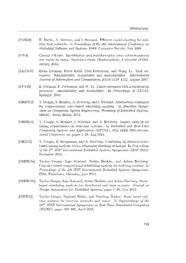
Bibliography
[DMS09] H. Dierks, A. Metzner, and I. Stierand. E�cient model-checking for real-time task networks. In Proceedings of the 6th International Conference onEmbedded Software and Systems. IEEE Computer Society, May 2009.
[Fif14] Conrad Fifelsky. Spezi�kation und transformation eines echtzeit-systemsvon marte zu rtana. Bachelor's thesis (Studienarbeit), University of Old-enburg, 2014.
[FKPY07] Elena Fersman, Pavel Kr£ál, Paul Pettersson, and Wang Yi. Task au-tomata: Schedulability, decidability and undecidability. InternationalJournal of Information and Computation, 205(8):1149�1172, August 2007.
[FPY02] E. Fersman, P. Pettersson, and W. Yi. Timed automata with asynchronousprocesses: schedulability and decidability. In Proceedings of TACAS.Springer, 2002.
[GHRS12] T. Gezgin, S. Henkler, A. Rettberg, and I. Stierand. Abstraction techniquesfor compositional state-based scheduling analysis. In Brazilian Sympo-sium on Computing System Engineering, Workshop of Embedded Systems,SBESC, Natal, Brazil, 2012.
[GHSR14] T. Gezgin, S. Henkler, I. Stierand, and A. Rettberg. Impact analysis fortiming requirements on real-time systems. In Embedded and Real-TimeComputing Systems and Applications (RTCSA), 2014 IEEE 20th Interna-tional Conference on, pages 1�10, Aug 2014.
[GKR15] T. Gezgin, B. Koopmann, and A. Rettberg. Combining an iterative state-based timing analysis with a re�nement checking technique. In Proceedingsof the 5th IFIP International Embedded Systems Symposium (IESS 2015),November 2015.
[GSHR13a] Tayfun Gezgin, Ingo Stierand, Stefan Henkler, and Achim Rettberg.Contract-based compositional scheduling analysis for evolving systems. InProceedings of the 4th IFIP International Embedded Systems Symposium,IESS, Paderborn, Germany, june 2013.
[GSHR13b] Tayfun Gezgin, Ingo Stierand, Stefan Henkler, and Achim Rettberg. State�based scheduling analysis for distributed real�time systems. Journal onDesign Automation for Embedded Systems, pages 1�18, July 2013.
[GWB15] Tayfun Gezgin, Raphael Weber, and Matthias Bueker. State-based real-time analysis for function networks and marte. In Inproceedings of the18th IEEE International Symposium on Real-Time Distributed Computing(ISORC), pages 158�165, April 2015.
189
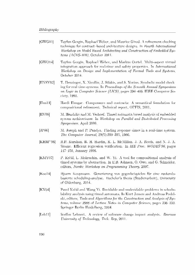
Bibliography
[GWG11] Tayfun Gezgin, Raphael Weber, and Maurice Girod. A re�nement checkingtechnique for contract�based architecture designs. In Fourth InternationalWorkshop on Model Based Architecting and Construction of Embedded Sys-tems (ACES-MB), October 2011.
[GWO14] Tayfun Gezgin, Raphael Weber, and Markus Oertel. Multi-aspect virtualintegration approach for real-time and safety properties. In InternationalWorkshop on Design and Implementation of Formal Tools and Systems,October 2014.
[HNSY92] T. Henzinger, X. Nicollin, J. Sifakis, and S. Yovine. Symbolic model check-ing for real-time systems. In Proceedings of the Seventh Annual Symposiumon Logic in Computer Science (LICS), pages 394�406. IEEE Computer So-ciety, 1992.
[Hun11] Hardi Hungar. Components and contracts: A semantical foundation forcompositional re�nement. Technical report, OFFIS, 2011.
[HV06] M. Hendriks and M. Verhoef. Timed automata based analysis of embeddedsystem architectures. In Workshop on Parallel and Distributed ProcessingSymposium, April 2006.
[JP86] M. Joseph and P. Pandya. Finding response times in a real-time system.The Computer Journal, 29(5):390�395, 1986.
[KHM+96] R.P. Kurshan, R. H. Hardin, K. L. McMillan, J. A. Reeds, and N. J. A.Sloane. E�cient regression veri�cation. In IEE Proc. WODES'96, pages147�150, January 1996.
[KMY07] P. Kr£ál, L. Mokrushin, and W. Yi. A tool for compositional analysis oftimed systems by abstraction. In E.B. Johnsen, O. Owe, and G. Schneider,editors, Nordic Workshop on Programming Theory, 2007.
[Koo14] Bjoern Koopmann. Generierung von gegenbeispielen für eine zustands-basierte scheduling-analyse. Bachelor's thesis (Studienarbeit), Universityof Oldenburg, 2014.
[KY04] Pavel Kr£ál and Wang Yi. Decidable and undecidable problems in schedu-lability analysis using timed automata. In Kurt Jensen and Andreas Podel-ski, editors, Tools and Algorithms for the Construction and Analysis of Sys-tems, volume 2988 of Lecture Notes in Computer Science, pages 236�250.Springer Berlin Heidelberg, 2004.
[Leh11] Ste�en Lehnert. A review of software change impact analysis. IlmenauUniversity of Technology, Tech. Rep, 2011.
190
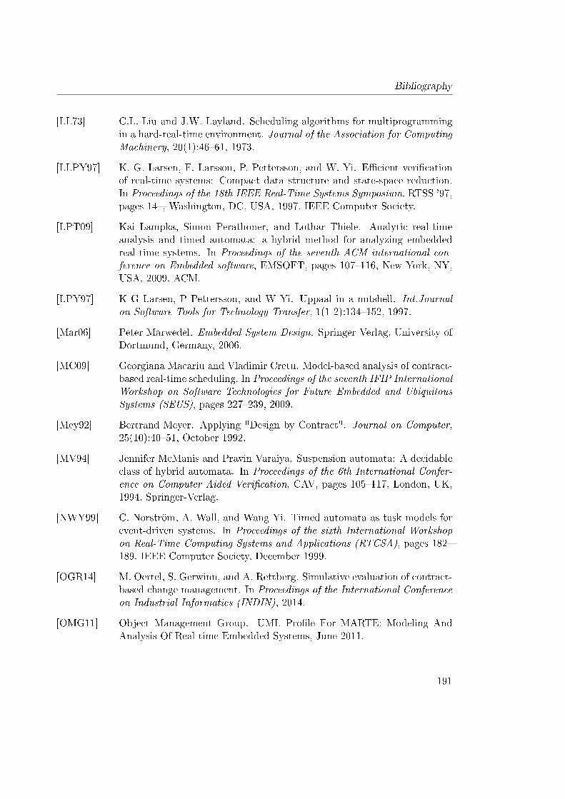
Bibliography
[LL73] C.L. Liu and J.W. Layland. Scheduling algorithms for multiprogrammingin a hard-real-time environment. Journal of the Association for ComputingMachinery, 20(1):46�61, 1973.
[LLPY97] K. G. Larsen, F. Larsson, P. Pettersson, and W. Yi. E�cient veri�cationof real-time systems: Compact data structure and state-space reduction.In Proceedings of the 18th IEEE Real-Time Systems Symposium, RTSS '97,pages 14�, Washington, DC, USA, 1997. IEEE Computer Society.
[LPT09] Kai Lampka, Simon Perathoner, and Lothar Thiele. Analytic real-timeanalysis and timed automata: a hybrid method for analyzing embeddedreal-time systems. In Proceedings of the seventh ACM international con-ference on Embedded software, EMSOFT, pages 107�116, New York, NY,USA, 2009. ACM.
[LPY97] K G Larsen, P Pettersson, and W Yi. Uppaal in a nutshell. Int.Journalon Software Tools for Technology Transfer, 1(1-2):134�152, 1997.
[Mar06] Peter Marwedel. Embedded System Design. Springer Verlag, University ofDortmund, Germany, 2006.
[MC09] Georgiana Macariu and Vladimir Cretu. Model-based analysis of contract-based real-time scheduling. In Proceedings of the seventh IFIP InternationalWorkshop on Software Technologies for Future Embedded and UbiquitousSystems (SEUS), pages 227�239, 2009.
[Mey92] Bertrand Meyer. Applying "Design by Contract". Journal on Computer,25(10):40�51, October 1992.
[MV94] Jennifer McManis and Pravin Varaiya. Suspension automata: A decidableclass of hybrid automata. In Proceedings of the 6th International Confer-ence on Computer Aided Veri�cation, CAV, pages 105�117, London, UK,1994. Springer-Verlag.
[NWY99] C. Norström, A. Wall, and Wang Yi. Timed automata as task models forevent-driven systems. In Proceedings of the sixth International Workshopon Real-Time Computing Systems and Applications (RTCSA), pages 182�189. IEEE Computer Society, December 1999.
[OGR14] M. Oertel, S. Gerwinn, and A. Rettberg. Simulative evaluation of contract-based change management. In Proceedings of the International Conferenceon Industrial Informatics (INDIN), 2014.
[OMG11] Object Management Group. UML Pro�le For MARTE: Modeling AndAnalysis Of Real-time Embedded Systems, June 2011.
191
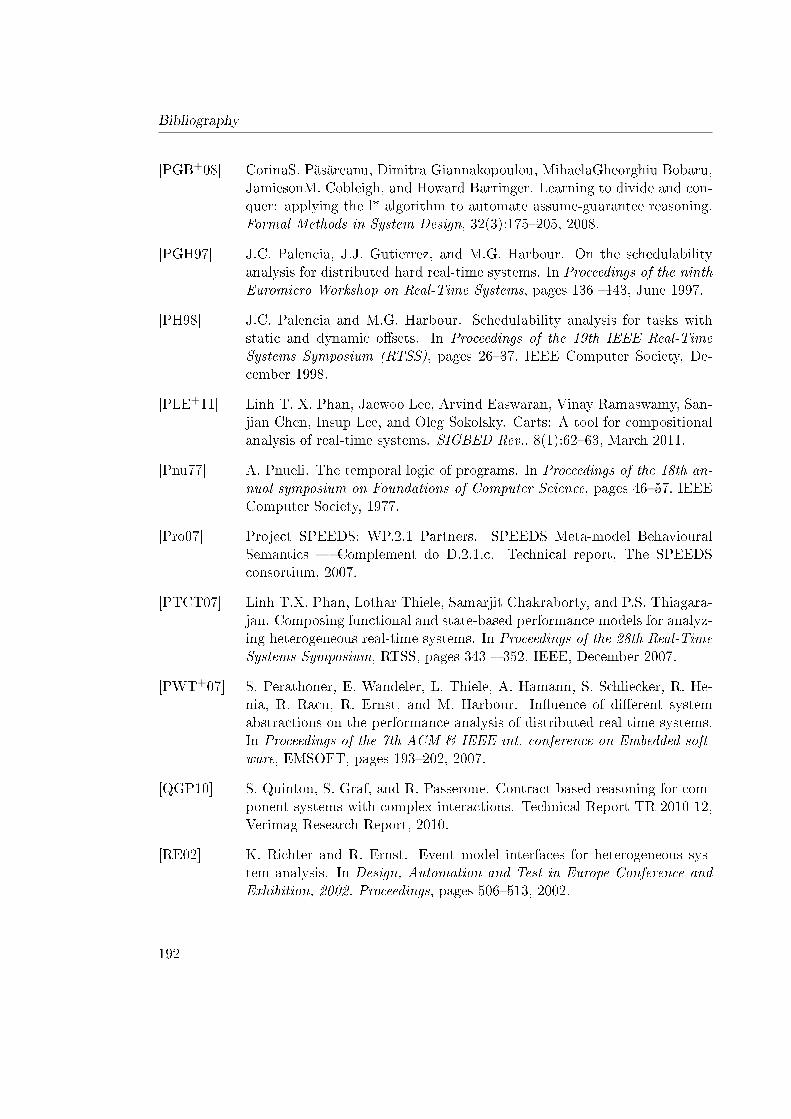
Bibliography
[PGB+08] CorinaS. P s reanu, Dimitra Giannakopoulou, MihaelaGheorghiu Bobaru,JamiesonM. Cobleigh, and Howard Barringer. Learning to divide and con-quer: applying the l* algorithm to automate assume-guarantee reasoning.Formal Methods in System Design, 32(3):175�205, 2008.
[PGH97] J.C. Palencia, J.J. Gutierrez, and M.G. Harbour. On the schedulabilityanalysis for distributed hard real-time systems. In Proceedings of the ninthEuromicro Workshop on Real-Time Systems, pages 136 �143, June 1997.
[PH98] J.C. Palencia and M.G. Harbour. Schedulability analysis for tasks withstatic and dynamic o�sets. In Proceedings of the 19th IEEE Real-TimeSystems Symposium (RTSS), pages 26�37. IEEE Computer Society, De-cember 1998.
[PLE+11] Linh T. X. Phan, Jaewoo Lee, Arvind Easwaran, Vinay Ramaswamy, San-jian Chen, Insup Lee, and Oleg Sokolsky. Carts: A tool for compositionalanalysis of real-time systems. SIGBED Rev., 8(1):62�63, March 2011.
[Pnu77] A. Pnueli. The temporal logic of programs. In Proceedings of the 18th an-nual symposium on Foundations of Computer Science, pages 46�57. IEEEComputer Society, 1977.
[Pro07] Project SPEEDS: WP.2.1 Partners. SPEEDS Meta-model BehaviouralSemantics � Complement do D.2.1.c. Technical report, The SPEEDSconsortium, 2007.
[PTCT07] Linh T.X. Phan, Lothar Thiele, Samarjit Chakraborty, and P.S. Thiagara-jan. Composing functional and state-based performance models for analyz-ing heterogeneous real-time systems. In Proceedings of the 28th Real-TimeSystems Symposium, RTSS, pages 343 � 352. IEEE, December 2007.
[PWT+07] S. Perathoner, E. Wandeler, L. Thiele, A. Hamann, S. Schliecker, R. He-nia, R. Racu, R. Ernst, and M. Harbour. In�uence of di�erent systemabstractions on the performance analysis of distributed real-time systems.In Proceedings of the 7th ACM & IEEE int. conference on Embedded soft-ware, EMSOFT, pages 193�202, 2007.
[QGP10] S. Quinton, S. Graf, and R. Passerone. Contract-based reasoning for com-ponent systems with complex interactions. Technical Report TR-2010-12,Verimag Research Report, 2010.
[RE02] K. Richter and R. Ernst. Event model interfaces for heterogeneous sys-tem analysis. In Design, Automation and Test in Europe Conference andExhibition, 2002. Proceedings, pages 506�513, 2002.
192
Bibliography
[RE10] J. Rox and R. Ernst. Exploiting inter-event stream correlations betweenoutput event streams of non-preemptively scheduled tasks. In Proceed-ings of the Conference on Design, Automation and Test in Europe, DATE,Leuven, Belgium, 2010.
[Ric04] Kai Richter. Compositional Scheduling Analysis Using Standard EventModels. PhD thesis, Technical University of Braunschweig, Braunschweig,Germany, 2004.
[RRE03] K. Richter, R. Racu, and R. Ernst. Scheduling analysis integration forheterogeneous multiprocessor SoC. In Procedings of the 24th Real-TimeSystems Symposium (RTSS), pages 236�245. IEEE Computer Society, De-cember 2003.
[RSRH11] Philipp Reinkemeier, Ingo Stierand, Philip Rehkop, and Stefan Henkler.A pattern-based requirement speci�cation language: Mapping automotivespeci�c timing requirements. In Software Engineering 2011 - Workshop-band, LNI. GI, 2011.
[SBPM09] David Steinberg, Frank Budinsky, Marcelo Paternostro, and Ed Merks.EMF: Eclipse Modeling Framework. Addison-Wesley, 2nd edition, 2009.
[SSL+14] Youcheng Sun, Romain Soulat, Giuseppe Lipari, Étienne André, and Lau-rent Fribourg. Parametric schedulability analysis of �xed priority real-timedistributed systems. In Cyrille Artho and Peter Csaba Ölveczky, editors,Formal Techniques for Safety-Critical Systems, volume 419 of Communi-cations in Computer and Information Science, pages 212�228. SpringerInternational Publishing, 2014.
[TC94] K. Tindell and J. Clark. Holistic schedulability analysis for distributedhard real-time systems. Journal of Microprocessing and Microprogramming,40:117�134, April 1994.
[TCN00] L. Thiele, S. Chakraborty, and M. Naedele. Real-time calculus for schedul-ing hard real-time systems. In Proceedings of the International Symposiumon Circuits and Systems (ISCAS), volume 4, pages 101�104. IEEE Com-puter Society, May 2000.
[Tin94] Ken Tindell. Adding Time-O�sets to Schedulability Analysis. Technicalreport, University of York, Department of Computer Science, England,1994.
[WTH+14] Raphael Weber, Eike Thaden, Stefan Henkler, Jens Hö�inger, and Ste�enProchnow. Design space exploration for an industrial lane-keeping-supportcase study. In Proceedings of DATE Conf. University Booth, 2014.
193