Eingereicht vonLukas Burgholzer

Angefertigt amInstitut für NumerischeMathematik

BetreuerDipl.-Ing. Dr. MartinNeumüller

November 2016

JOHANNES KEPLERUNIVERSITÄT LINZAltenbergerstraße 694040 Linz, Österreichwww.jku.atDVR 0093696

Structure-AcousticCoupling

Bachelorarbeitzur Erlangung des akademischen Grades

Bachelor of Science

im Bachelorstudium

Technische Mathematik

Abstract

The goal of this bachelor thesis is the coupling of the defining equations formechanics and acoustics to form a so-called structure-acoustic coupling prob-lem. In the first chapter we will therefore develop a model for the mechanicalstructure by in a first step deriving the three fundamental equations for me-chanics (the equilibrium equation, the strain-displacement-relation and theconstitutive equation). We will then combine these to arrive at the Navier-Lamé equation for isotropic, homogeneous, elastic materials. At the end ofthe first chapter we consider two special cases (the plane strain state and theplain stress state). The second chapter deals with a model for acoustics wherewe derive the corresponding fundamental equations (the continuity equation,the Euler equation and the state equation). We then consider linear versionsof these equations and combine them to form the linear acoustic wave equa-tion. Then we have a look at two special cases (plane waves and sphericalwaves) and at the end of the chapter we derive a non-linear acoustic waveequation, also called Kuznetsov equation. In the third chapter we will thenconsider the coupling of both linear models. For this we examine a solid im-mersed in an acoustic field and find coupling conditions which have to holdat the solid-fluid interface. Then we transform the Navier-Lamé equationand the linear acoustic wave equation into their weak formulation and finallycombine them to one system of coupled equations. The last chapter providessome conclusions and gives an outlook on possible further work.

i

Zusammenfassung

Das Ziel dieser Bachelorarbeit ist die Kopplung der beschreibenden Gleichun-gen der Mechanik und der Akustik, die dann ein sogennantes Fluid-StrukturKopplungsproblem bilden. Im ersten Kapitel entwickeln wir daher ein Mo-dell für die Mechanik, angefangen von der Herleitung der drei fundamenta-len Gleichungen der Mechanik (die Gleichgewichtsgleichung, die Verzerrungs-Verschiebungs-Relation und die Zustandsgleichung). Diese werden wir dannkombinieren um zur Navier-Lamé Gleichung für isotrope, homogene, ela-stische Materialen zu kommen. Am Ende des ersten Kapitels betrachten wirzwei Spezialfälle (den ebenen Verzerrungszustand und den ebenen Spannungs-zustand). Das zweite Kapitel beschäftigt sich mit einem Model für die Aku-stik, wo wir die entsprechenden beschreibenden Gleichungen herleiten (dieKontinuitätsgleichung, die Bewegungsgleichung und die Zustandsgleichungder Akustik). Wir betrachten dann lineare Versionen dieser Gleichungen undkombinieren sie zur linearen akustischen Wellengleichung. Dann folgen zweiSpezialfälle (Ebene Wellen und Kugelwellen) und am Ende des Kapitels lei-ten wir eine nichtlineare akustische Wellengleichung, auch Kuznetsov Glei-chung genannt, her. Im dritten Kapitel betrachten wir dann die Kopplungbeider linearen Modelle. Dafür analysieren wir einen von einem akustischenFeld umgebenen Festkörper und finden Kopplungsbedingungen, welche an derSchnittstelle zwischen Festkörper und Fluid gelten müssen. Dann führen wirdie Navier-Lamé Gleichung und die lineare akustische Wellengleichung inihre schwache Formulierung über und kombinieren sie zu einem einzigengekoppelten System von Gleichungen. Im letzten Kapitel finden sich einigeSchlussbemerkungen und ein Ausblick auf Möglichkeiten der Weiterarbeit.

ii

Notation

R set of real numbers

v vector

e(i) i-th Cartesian unit vector

n unit normal vector

Σ1 set of unit vectors, i.e. Σ1 := v ∈ R3 : ‖v‖ = 1

∂Ω boundary of Ω

Ω closure of Ω

div divergence

∇ gradient

curl curl

∆ Laplace operator

∂/∂x partial derivative

∂/∂n normal derivative

d/dx material/total derivative

ui,j∂ui∂xj∫

Ωdx volume integral∫

Γdsx surface integral

‖ · ‖ Euclidean norm

〈·, ·〉 Euclidean inner product

A : B∑3

i,j=1AijBij

iii

Contents

1 Derivation of a model for the mechanical structure 11.1 Stress State - Kinetic . . . . . . . . . . . . . . . . . . . . . . . 1

1.1.1 Cauchy Stress Tensor . . . . . . . . . . . . . . . . . . . 21.1.2 Equilibrium of Forces and Moments . . . . . . . . . . . 3

1.2 Strain State - Kinematic . . . . . . . . . . . . . . . . . . . . . 51.2.1 Green-St.Venant Strain Tensor . . . . . . . . . . . . . 51.2.2 Chauchy’s Strain Tensor . . . . . . . . . . . . . . . . . 6

1.3 Constitutive Equation - Hook’s Law . . . . . . . . . . . . . . . 61.4 Navier - Lamé’s Equation . . . . . . . . . . . . . . . . . . . . 7

1.4.1 Static Case . . . . . . . . . . . . . . . . . . . . . . . . 71.4.2 Dynamic Case . . . . . . . . . . . . . . . . . . . . . . . 8

1.5 Special Cases . . . . . . . . . . . . . . . . . . . . . . . . . . . 81.5.1 Plane Strain State . . . . . . . . . . . . . . . . . . . . 81.5.2 Plane Stress State . . . . . . . . . . . . . . . . . . . . . 9

2 Derivation of a model for the acoustic field 112.1 Introduction to Acoustics . . . . . . . . . . . . . . . . . . . . . 112.2 Mass Conservation - Continuity Equation . . . . . . . . . . . . 122.3 Conservation of Momentum - Euler’s Equation . . . . . . . . . 122.4 Pressure-Density-Relation - State Equation . . . . . . . . . . . 14

2.4.1 Ideal gases . . . . . . . . . . . . . . . . . . . . . . . . . 142.4.2 Liquids . . . . . . . . . . . . . . . . . . . . . . . . . . . 15

2.5 Linear Acoustic Wave Equation . . . . . . . . . . . . . . . . . 152.6 Acoustic Quantities . . . . . . . . . . . . . . . . . . . . . . . . 162.7 Special Cases . . . . . . . . . . . . . . . . . . . . . . . . . . . 17

2.7.1 Plane Waves . . . . . . . . . . . . . . . . . . . . . . . . 172.7.2 Spherical Waves . . . . . . . . . . . . . . . . . . . . . . 19

2.8 Non-linear Acoustic Wave Equation . . . . . . . . . . . . . . . 202.8.1 Non-linear Euler’s Equation . . . . . . . . . . . . . . . 202.8.2 Non-linear State Equation . . . . . . . . . . . . . . . . 212.8.3 Combination of Equations . . . . . . . . . . . . . . . . 21

3 Coupling of the two models 233.1 Solid-Fluid Interface . . . . . . . . . . . . . . . . . . . . . . . 23

iv

3.2 Coupled formulation . . . . . . . . . . . . . . . . . . . . . . . 243.2.1 Mechanical field . . . . . . . . . . . . . . . . . . . . . . 243.2.2 Acoustic field . . . . . . . . . . . . . . . . . . . . . . . 253.2.3 Coupled System . . . . . . . . . . . . . . . . . . . . . . 26

4 Conclusions 27

Bibliography 28

v

Chapter 1

Derivation of a model for themechanical structure

In this chapter we will develop a model for the mechanical field. Thereforewe will derive the three defining equations

• the equilibrium equation,

• the strain-displacement-relation,

• the constitutive equation,

and combine them to arrive at the Navier-Lamé equation. We will then havea look at two special cases, see Section 1.5.

1.1 Stress State - Kinetic

n

t(n)f

B

Ω

Γ = ∂Ω

∂B

Figure 1.1.1: Mechanical Field

Let us consider a solid body, which occupies the region Ω ⊂ R3 with suffi-ciently smooth boundary Γ = ∂Ω (see Figure 1.1.1). A bounded sub-regionof Ω with sufficiently smooth boundary is called a part. We distinguish twokinds of forces acting on Ω:

1

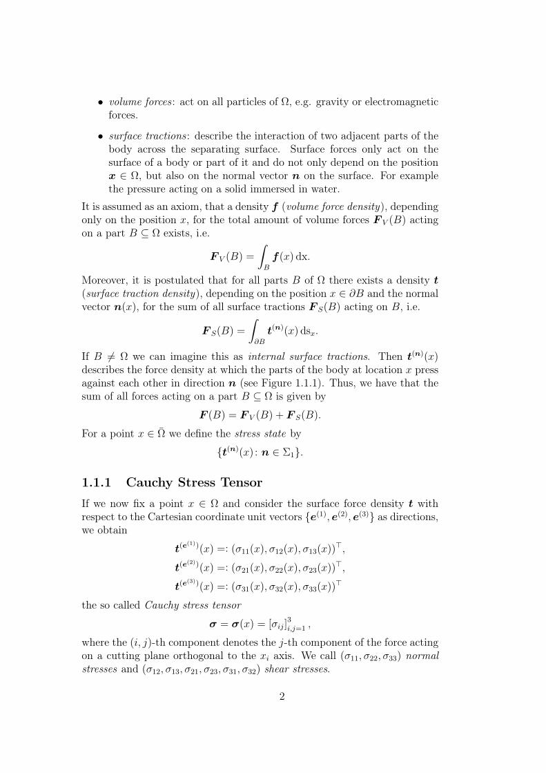
• volume forces : act on all particles of Ω, e.g. gravity or electromagneticforces.

• surface tractions : describe the interaction of two adjacent parts of thebody across the separating surface. Surface forces only act on thesurface of a body or part of it and do not only depend on the positionx ∈ Ω, but also on the normal vector n on the surface. For examplethe pressure acting on a solid immersed in water.

It is assumed as an axiom, that a density f (volume force density), dependingonly on the position x, for the total amount of volume forces F V (B) actingon a part B ⊆ Ω exists, i.e.

F V (B) =

∫B

f(x) dx.

Moreover, it is postulated that for all parts B of Ω there exists a density t(surface traction density), depending on the position x ∈ ∂B and the normalvector n(x), for the sum of all surface tractions F S(B) acting on B, i.e.

F S(B) =

∫∂B

t(n)(x) dsx.

If B 6= Ω we can imagine this as internal surface tractions. Then t(n)(x)describes the force density at which the parts of the body at location x pressagainst each other in direction n (see Figure 1.1.1). Thus, we have that thesum of all forces acting on a part B ⊆ Ω is given by

F (B) = F V (B) + F S(B).

For a point x ∈ Ω we define the stress state by

t(n)(x) : n ∈ Σ1.

1.1.1 Cauchy Stress Tensor

If we now fix a point x ∈ Ω and consider the surface force density t withrespect to the Cartesian coordinate unit vectors e(1), e(2), e(3) as directions,we obtain

t(e(1))(x) =: (σ11(x), σ12(x), σ13(x))>,

t(e(2))(x) =: (σ21(x), σ22(x), σ23(x))>,

t(e(3))(x) =: (σ31(x), σ32(x), σ33(x))>

the so called Cauchy stress tensor

σ = σ(x) = [σij]3i,j=1 ,

where the (i, j)-th component denotes the j-th component of the force actingon a cutting plane orthogonal to the xi axis. We call (σ11, σ22, σ33) normalstresses and (σ12, σ13, σ21, σ23, σ31, σ32) shear stresses.

2

Cauchy’s stress theorem

Cauchy’s stress theorem tells us that it is sufficient to know the Cauchy stresstensor to describe the whole stress state in a point x. It states

t(n)i (x) =

3∑j=1

σji(x)nj(x) = (σ>n)i for n = (n1, n2, n3)> ∈ Σ1.

The theorem can be proven by considering a body with an oblique cuttingface and investigating on the equilibrium of the forces acting on it. For adetailed proof, see [1, p. 52].

1.1.2 Equilibrium of Forces and Moments

We know from Newton’s second law of motion that the sum of all forcesacting on a body is equal to the mass of the body times its acceleration,which is called inertia. It also states that the sum of all moments is equal tothe moment of inertia.

Static Case

In the static case, i.e. a body at rest, there is no acceleration, which meansthat the sum of all forces acting on all parts of the body has to be zero. Thisis expressed as

F (Ω′) = F V (Ω′) + F S(Ω′) =

∫Ω′f(x) dx +

∫∂Ω′t(n)(x) dsx = 0

for all Ω′ ⊂ Ω with ∂Ω′ sufficiently smooth.Using Cauchy’s stress theorem and Gauß’s theorem (see [4, p. 729]) we obtain∫

Ω′[f(x) + div(σ)] dx = 0.

We now utilize the so-called Euler trick to get rid of the integral.

Theorem 1.1. (Euler trick) Let f ∈ C(Ω). If∫V

f(x) dx = 0

for arbitrary V ⊆ Ω, then

f(x) = 0 ∀x ∈ Ω.

3

Proof. Assume f(x) 6= 0 for some x ∈ Ω. Since f is continuous, it is alsonon-zero in a neighborhood Ux of x. However, choosing V = Ux yields∫

Ux

f(x) dx > 0,

which leads to a contradiction. So f(x) = 0 for all x ∈ Ω.

Since Ω′ was chosen arbitrary we may use Theorem 1.1 to drop the integraland arrive at the equilibrium equation for a body at rest

−div(σ) = f . (1.1)

Now we consider the sum of all moments, which should be zero, as for theequilibrium of forces∫

Ω′x× f(x) dx +

∫∂Ω′x× t(n)(x) dsx = 0. (1.2)

From this it follows that the stress tensor σ is symmetric.

Proof. To keep the proof short we define

σji,j :=3∑j=1

∂σji∂xj

for i = 1, 2, 3.

Then, by using partial integration, it holds that

∫Ω′x× divσ dx =

∫Ω′

x2σj3,j − x3σj2,jx3σj1,j − x1σj3,jx1σj2,j − x2σj1,j

dx

=

∫Ω′

σ23 − σ32

σ31 − σ13

σ12 − σ21

dx +

∫∂Ω′x× σ>n︸︷︷︸

=t(n)(x)

dsx.

Substituting this into the equilibrium of moments (1.2) and using (1.1) weget ∫

Ω′x× [f + divσ]︸ ︷︷ ︸

=0

−∫

Ω′

σ23 − σ32

σ31 − σ13

σ12 − σ21

dx = 0.

Since Ω′ was chosen arbitrary, there must hold σ = σ>.

If we specify a given surface traction g acting on the boundary Γ of Ω thiscorresponds to the boundary condition

t(n) = σ>n = g.

4

Dynamic Case

In the dynamic case we consider a time frame (0, T ) and a body Ω withdensity ρ(x). Let u(x, t) denote the displacement of the body and a(x, t) =∂2u∂t2

(x, t) its acceleration. Then we obtain the equation for the equilibrium offorces ∫

Ω′f(x, t) dx +

∫∂Ω′t(n)(x, t) dsx =

∫Ω′a(x, t)ρ(x) dx

for all Ω′ ⊂ Ω and all t ∈ (0, T ), which leads to the equilibrium equation fora body in motion

ρa− div(σ) = f (1.3)

by applying the same procedure as in the static case. For the equilibrium ofmoments we get∫

Ω′x× f(x, t) dx +

∫∂Ω′x× t(n)(x, t) dsx =

∫Ω′x× a(x, t)ρ(x) dx

from which it follows in a similar manner as for (1.2) that the stress tensoris symmetric.

1.2 Strain State - Kinematic

1.2.1 Green-St.Venant Strain Tensor

Under the influence of external forces a material point x of a deformablebody Ω moves in a new position x+ u(x) with the displacement vector

u(x) =

u1(x)u2(x)u3(x)

for x ∈ Ω ⊂ R3.

The distance ds between the point x and a neighboring point x+dx changesthrough deformation to ds′, i.e.

ds = ‖dx‖ and ds′ = ‖dx+ du‖

where du = u(x+ dx)− u(x). We have

(ds′)2 = 〈dx+ du,dx+ du〉 = (ds)2 + 2〈dx,du〉+ ‖du‖2.

Since we are interested in the case dx→ 0, the following relation is reason-able

du ≈ (∇u)dx.

We will now calculate the change in length (ds′)2 − (ds)2

(ds′)2 − (ds)2 = 2〈dx,du〉+ ‖du‖2 = 2〈dx, (∇u)dx〉+ 〈(∇u)dx, (∇u)dx〉= 2〈(∇u)>dx,dx〉+ 〈(∇u)>(∇u)dx,dx〉.

5

Since2〈(∇u)>dx,dx〉 = 〈(∇u)>dx,dx〉+ 〈(∇u)dx,dx〉

we arrive at

(ds′)2 − (ds)2 = 2〈12

(∇u+∇u> +∇u>∇u)dx,dx〉 = 2〈e(u)dx,dx〉

wheree = e(u) =

1

2(∇u+∇u> +∇u>∇u) (1.4)

denotes the Green-St.Venant strain tensor. The component ekk describesthe relative change in length of a line element ds parallel to the xk axis fork = 1, 2, 3. Whereas ekl for l 6= k describes the angular change between twoline elements dxk and dxl.

1.2.2 Chauchy’s Strain Tensor

If we assume that|(∇u)kl| 1 for k = 1, 2, 3,

we can neglect the quadratic terms of the Green-St.Venant strain tensor andarrive at the Cauchy strain tensor ε

e(u) ≈ ε(u) :=1

2(∇u+∇u>). (1.5)

1.3 Constitutive Equation - Hook’s LawFor linear elastic material we assume that a linear stress-strain-relation be-tween σ and ε is given by

σij =3∑

k,l=1

Dijkl εkl i, j = 1, 2, 3 (Hook’s Law)

with the elastic coefficients Dijkl for i, j, k, l = 1, 2, 3. We call the material ho-mogeneous if the elastic coefficients do not depend on x and in-homogeneousotherwise. From the symmetry of the stress and the strain tensor it followsthat the elastic coefficients fulfill

Dijkl = Dklji and Dijkl = Djikl = Djilk.

From this it follows that we can associate this fourth-order tensorD, indexedby (i, j, k, l), with a second-order tensor D, indexed by (I,K), in the following

6

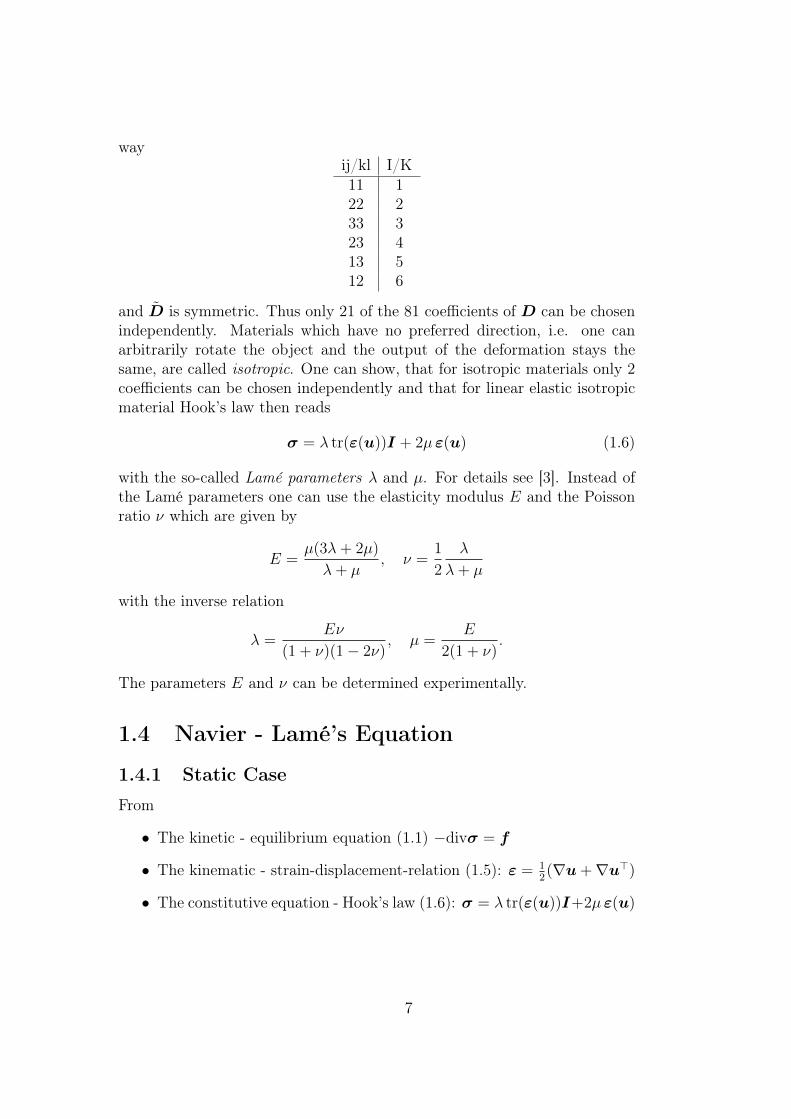
wayij/kl I/K11 122 233 323 413 512 6

and D is symmetric. Thus only 21 of the 81 coefficients of D can be chosenindependently. Materials which have no preferred direction, i.e. one canarbitrarily rotate the object and the output of the deformation stays thesame, are called isotropic. One can show, that for isotropic materials only 2coefficients can be chosen independently and that for linear elastic isotropicmaterial Hook’s law then reads

σ = λ tr(ε(u))I + 2µ ε(u) (1.6)

with the so-called Lamé parameters λ and µ. For details see [3]. Instead ofthe Lamé parameters one can use the elasticity modulus E and the Poissonratio ν which are given by

E =µ(3λ+ 2µ)

λ+ µ, ν =

1

2

λ

λ+ µ

with the inverse relation

λ =Eν

(1 + ν)(1− 2ν), µ =

E

2(1 + ν).

The parameters E and ν can be determined experimentally.

1.4 Navier - Lamé’s Equation

1.4.1 Static Case

From

• The kinetic - equilibrium equation (1.1) −divσ = f

• The kinematic - strain-displacement-relation (1.5): ε = 12(∇u+∇u>)

• The constitutive equation - Hook’s law (1.6): σ = λ tr(ε(u))I+2µ ε(u)

7

we can now derive the Lamé Equation for isotropic and homogeneous elasticmaterials in the static case:

f(1.1)= −divσ

(1.6)= −div(λtr(ε)I + 2µε)

(1.5)= −λ div(tr(∇u))I − µ div(∇u)− µ div(∇u>)

= −µ∆u− (λ+ µ)∇(divu).

So the Lamé equation now reads

−µ∆u− (λ+ µ)∇(divu) = f . (1.7)

1.4.2 Dynamic Case

For the dynamic case we derived the equilibrium equations (1.3):

ρ∂2u

∂t2− divσ = f .

Following the same procedure as above we arrive at the Navier-Lamé equationfor isotropic and homogeneous elastic materials in the dynamic case:

ρ∂2u

∂t2− µ∆u− (λ+ µ)∇(divu) = f . (1.8)

1.5 Special Cases

1.5.1 Plane Strain State

Assume a body K ⊂ R3 with constant cross-section Ω ⊂ R2, which is muchlonger in one dimension than in the other two:

K = x ∈ R3 : (x1, x2) ∈ Ω,−L < x3 < L with L diam(Ω).

The volume forces f and surface tractions t act on the plane which is or-thogonal to the x3-axis and are independent of x3, i.e.

f(x) =

f1(x1, x2)f2(x1, x2)

0

, t(x) =

t1(x1, x2)t2(x1, x2)

0

⊥ x3.

and we assumeε3i = εi3 = 0 for i = 1, 2, 3.

8

Then the displacement field u has the following form

u(x) =

u1(x1, x2)u2(x1, x2)

0

,

since0 = ε33 =

∂u3

∂x3

and 0 = − ∂ui∂x3

=∂u3

∂xifor i = 1, 2

and therefore u3 is constant. W.l.o.g. we can set this constant to 0. It followsfrom the assumptions that

σ13 = σ31 = σ23 = σ32 = 0

and that σ33 can be expressed by σ11 and σ22, because

σ33 = λ(ε11 + ε22) =λ

2(λ+ µ)(σ11 + σ22).

It can therefore be eliminated and the Lamé equation now simplifies from a3D equation to a 2D equation:

−µ∆u− (λ+ µ)∇(div u) = f with u =

(u1(x1, x2)u2(x1, x2)

), f =

(f1(x1, x2)f2(x1, x2)

).

1.5.2 Plane Stress State

Consider a deformation problem for a plate

K = x ∈ R3 : (x1, x2) ∈ Ω,−h < x3 < h with h diam(Ω).

under the influence of x3-independent volume forces and surface tractions

f(x) =

f1(x1, x2)f2(x1, x2)

0

, (x1, x2) ∈ Ω, t(x) =

t1(x1, x2)t2(x1, x2)

0

, (x1, x2) ∈ Γt

andt(x1, x2,+h) = t(x1, x2,−h) = 0, (x1, x2) ∈ Ω.

It is then assumed that

σij(x1, x2, x3) = σij(x1, x2) for i, j = 1, 2

σ3i = σi3 = 0 for i = 1, 2, 3.

From which it follows that ε33 can be expressed by ε11 and ε22 as

ε33 = −λ(ε11 + ε22)

λ+ 2µ.

9

This leads to

σ =

(σ11 σ12

σ21 σ22

)with σij =

2λµ

λ+ 2µ(ε11 + ε22)δij + 2µεij for i, j = 1, 2

and therefore, we arrive arrive at the same equations as for the plane strainstate, but with λ = 2λµ

λ+2µ.

10

Chapter 2

Derivation of a model for theacoustic field

In this chapter we will develop a model for the acoustic field. Therefore wewill derive the three defining equations

• the continuity equation,

• Euler’s equation,

• the state equation,

and combine them to arrive at the linear acoustic wave equation. We willthen consider some acoustic quantities and two special cases and end thechapter with a section on the nonlinear acoustic wave theory.

2.1 Introduction to AcousticsWe will limit ourselves to wave propagation in fluids like air and water, socalled non-viscous media. Sound (waves) can be described as small pressurefluctuations in the media. Therefore we introduce the following quantities,which one can compose into their mean part, denoted by a subscript 0, andtheir alternating part, denoted by a prime:

• the density ρ = ρ0 + ρ′,

• the pressure p = p0 + p′,

• the velocity v = v0 + v′,

where ρ′ is called acoustic density, p′ the acoustic pressure and v′ the acousticparticle velocity. In the linear theory we assume small fluctuations, i.e. thatthe alternating parts are much smaller then the mean quantities. We willnow derive the three defining equations for the acoustic field.

11

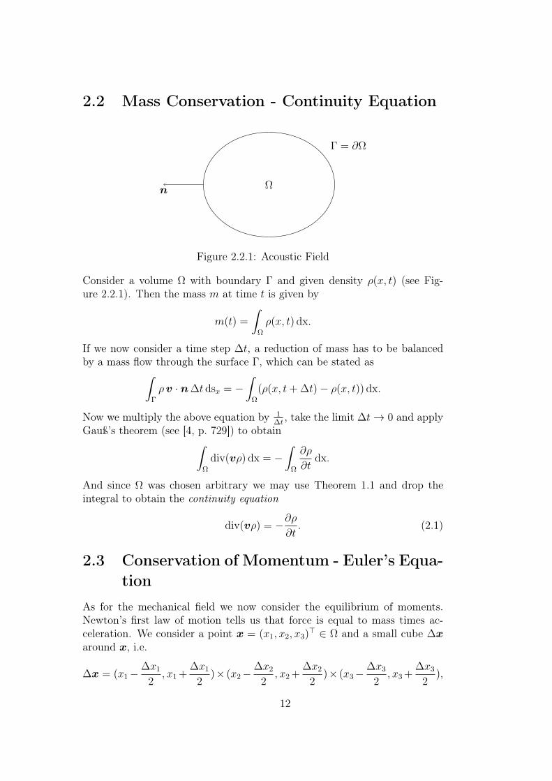
2.2 Mass Conservation - Continuity Equation

n Ω

Γ = ∂Ω

Figure 2.2.1: Acoustic Field

Consider a volume Ω with boundary Γ and given density ρ(x, t) (see Fig-ure 2.2.1). Then the mass m at time t is given by

m(t) =

∫Ω

ρ(x, t) dx.

If we now consider a time step ∆t, a reduction of mass has to be balancedby a mass flow through the surface Γ, which can be stated as∫

Γ

ρv · n∆t dsx = −∫

Ω

(ρ(x, t+ ∆t)− ρ(x, t)) dx.

Now we multiply the above equation by 1∆t, take the limit ∆t→ 0 and apply

Gauß’s theorem (see [4, p. 729]) to obtain∫Ω

div(vρ) dx = −∫

Ω

∂ρ

∂tdx.

And since Ω was chosen arbitrary we may use Theorem 1.1 and drop theintegral to obtain the continuity equation

div(vρ) = −∂ρ∂t. (2.1)

2.3 Conservation of Momentum - Euler’s Equa-tion

As for the mechanical field we now consider the equilibrium of moments.Newton’s first law of motion tells us that force is equal to mass times ac-celeration. We consider a point x = (x1, x2, x3)> ∈ Ω and a small cube ∆xaround x, i.e.

∆x = (x1−∆x1

2, x1 +

∆x1

2)× (x2−

∆x2

2, x2 +

∆x2

2)× (x3−

∆x3

2, x3 +

∆x3

2),

12

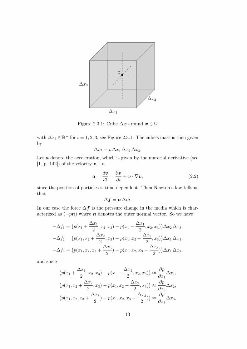
x•

∆x1

∆x2

∆x3

Figure 2.3.1: Cube ∆x around x ∈ Ω

with ∆xi ∈ R+ for i = 1, 2, 3, see Figure 2.3.1. The cube’s mass is then givenby

∆m = ρ∆x1 ∆x2 ∆x3.

Let a denote the acceleration, which is given by the material derivative (see[1, p. 142]) of the velocity v, i.e.

a =dv

dt=∂v

∂t+ v · ∇v, (2.2)

since the position of particles is time dependent. Then Newton’s law tells usthat

∆f = a∆m.

In our case the force ∆f is the pressure change in the media which is char-acterized as (−pn) where n denotes the outer normal vector. So we have

−∆f1 =(p(x1 +

∆x1

2, x2, x3)− p(x1 −

∆x1

2, x2, x3)

)∆x2 ∆x3,

−∆f2 =(p(x1, x2 +

∆x2

2, x3)− p(x1, x2 −

∆x2

2, x3)

)∆x1 ∆x3,

−∆f3 =(p(x1, x2, x3 +

∆x3

2)− p(x1, x2, x3 −

∆x3

2))∆x1 ∆x2,

and since (p(x1 +

∆x1

2, x2, x3)− p(x1 −

∆x1

2, x2, x3)

)≈ ∂p

∂x1

∆x1,(p(x1, x2 +

∆x2

2, x3)− p(x1, x2 −

∆x2

2, x3)

)≈ ∂p

∂x2

∆x2,(p(x1, x2, x3 +

∆x3

2)− p(x1, x2, x3 −

∆x3

2))≈ ∂p

∂x3

∆x3,

13

we obtain−∆f = ∇p∆x1 ∆x2 ∆x3. (2.3)

Combining (2.2) and (2.3) we now arrive at Euler’s equation

ρ

(∂v

∂t+ v · ∇v

)= −∇p. (2.4)

2.4 Pressure-Density-Relation - State EquationWe now want to derive a relation between the pressure p and the densityρ. Therefore we consider a fluid in rest, occupying the volume Ω0 withpressure p0 and density ρ0, and a fluid where an acoustic wave propagates,characterized by a volume Ω, pressure p and density ρ. If we now assume nothermal exchange between fluid particles it holds that(

Ω0

Ω

)κ=

p

p0

,

where κ denotes the so called adiabatic exponent, for details see [1, p. 143].If we further assume constant mass, i.e.

m0 = ρ0Ω0 = ρΩ,

we get that (ρ

ρ0

)κ=

p

p0

. (2.5)

We now consider two types of fluids:

2.4.1 Ideal gases

Let us consider an ideal gas, let T denote the temperature and R the specificgas constant, then we have the relation

p = ρRT

and the speed of sound c can be written as

c =√κRT ,

see [6, p. 16]. Since we consider the linear acoustic theory we may approxi-mate (

ρ

ρ0

)κ=

(ρ0 + ρ′

ρ0

)κ≈ 1 + κ

ρ′

ρ0

and arrive at the linear state equation for acoustic waves

p′

ρ′= κ

p0

ρ0

= c2. (2.6)

14

2.4.2 Liquids

For liquids we view the pressure p as a quantity depending on the density ρand the specific entropy s, which is related to heat transfer (see [1, p. 143]).The main pressure density relation is then given by

∂p(ρ, s)

∂ρ=Ks

ρ,

where Ks denotes the adiabatic bulk modulus, see [6, p. 16]. Additionallythe speed of sound c can now be expressed as

c =

√Ks

ρ,

see [6, p. 17].

2.5 Linear Acoustic Wave EquationIn this section we want to combine the three derived equations (2.1), (2.4) and(2.6) to arrive at the linear acoustic wave equation. Since we only considerlinear theory for now, we can assume that

v · ∇ρ ρ divv ≈ ρ0 divv and v · ∇v ∂v

∂t.

Therefore Euler’s equation simplifies to

∂v

∂t= − 1

ρ0

∇p (2.7)

and the continuity equation to

divv = − 1

ρ0

∂ρ

∂t. (2.8)

Now we may replace the total physical quantities (v, p, ρ) with the acousticquantities (v′, p′, ρ′), since all derivatives of the mean quantities (v0, p0, ρ0)are zero. By differentiating the linear continuity equation (2.8) with respectto t, we get

∂

∂tdivv′ = − 1

ρ0

∂2ρ′

∂t2,

and by switching the order of differentiation the equation becomes

div(∂v′

∂t) = − 1

ρ0

∂2ρ′

∂t2.

15

Using the linear Euler equation (2.7) yields

div(− 1

ρ0

∇p′) = − 1

ρ0

∂2ρ′

∂t2. (2.9)

Now we combine (2.9) with the linear state equation (2.6) ρ′ = p′/c2 to arriveat the linear acoustic wave equation for p′

∆p′ =1

c2

∂2p′

∂t2. (2.10)

One can show that for the acoustic particle velocity v′ it holds that curl(v′) =0, i.e. v′ is irrotational, see [1, p. 145], and therefore we can write v′ as thegradient of a scalar function ψ, which is then called the acoustic velocitypotential

v′ = −∇ψ. (2.11)

It follows from substituting the acoustic velocity potential into (2.7), thatthe relation between p′ and ψ is given by

p′ = ρ0∂ψ

∂t. (2.12)

Thus, we can state the wave equation for the acoustic velocity potential

∆ψ =1

c2

∂2ψ

∂t2. (2.13)

2.6 Acoustic QuantitiesIn this section we want to state some important acoustic quantities, namelythe acoustic energy density, the acoustic energy flux and acoustic impedance.Starting from the linear Euler equation (2.7), taking the dot product with v′and combining this with the linear continuity equation (2.8) and the linearstate equation (2.6) yields the following equation

∂wa∂t

+ divIa = 0 (2.14)

with the acoustic energy fluxIa = v′p′

and the total acoustic energy density

wa = wkina + wpot

a with wkina =

1

2ρ0‖v′‖2 and wpot

a =(p′)2

2ρ0c2,

16

which consists of the acoustic kinetic energy wkina and the acoustic potential

energy density wpota . Let us now consider an acoustic source with constant

angular frequency ω = 2πf . Then we can write

p′(t) = p cos(ωt) and v′(t) = v cos(ωt+ φ).

In doing so we can calculate the time averaged acoustic energy density wavaand intensity Iava (for details see [1, p. 147]) and get

wava =1

4ρ0‖v‖2 and Iava =

pv

2cosφ.

Replacing the acoustic quantities with their time averaged ones in (2.14)results in

divIava = 0

which implies ∫Ω

divIava dx =

∫Γ

Iava · n dsx = 0.

This only holds if the volume under consideration does not contain any acous-tic sources. For the case of a volume which encloses an acoustic source, theresult of the integral is the average acoustic power radiated by all enclosedsources P av

a ∫Γ

Iava · n dsx = P ava .

Another important quantity by which we characterize acoustic media (seeSection 2.7) is the acoustic impedance Za

Za =p′

‖v′‖.

2.7 Special CasesThere are two special cases we will treat in this section. First we will lookat so-called plane waves and then we will have a look at so-called sphericalwaves.

2.7.1 Plane Waves

A wave is called plane wave if it shows the same behavior in the plane or-thogonal to the direction of propagation (see Figure 2.7.1). This allows us, towrite the pressure p as a one-dimensional function in space and the velocityproportional to e(1), i.e.

p′ = p(x, t) and v′ = v′(x, t)e(1).

17

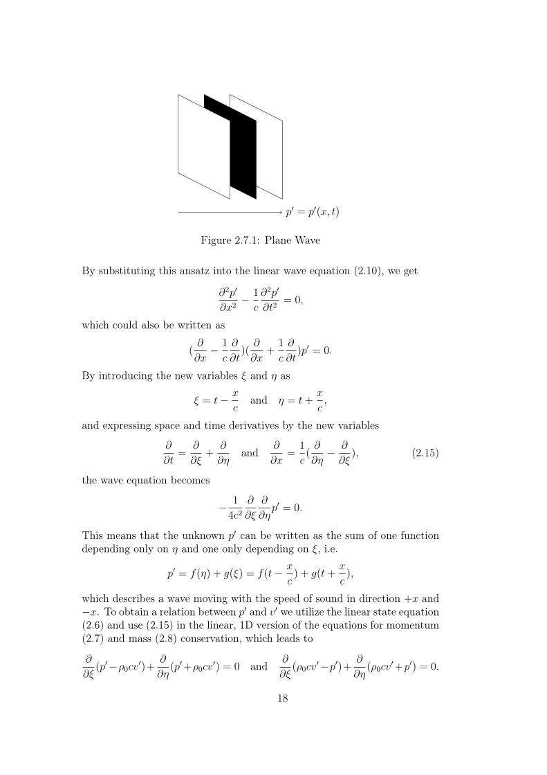
p′ = p′(x, t)

Figure 2.7.1: Plane Wave

By substituting this ansatz into the linear wave equation (2.10), we get

∂2p′

∂x2− 1

c

∂2p′

∂t2= 0,

which could also be written as

(∂

∂x− 1

c

∂

∂t)(∂

∂x+

1

c

∂

∂t)p′ = 0.

By introducing the new variables ξ and η as

ξ = t− x

cand η = t+

x

c,

and expressing space and time derivatives by the new variables

∂

∂t=

∂

∂ξ+

∂

∂ηand

∂

∂x=

1

c(∂

∂η− ∂

∂ξ), (2.15)

the wave equation becomes

− 1

4c2

∂

∂ξ

∂

∂ηp′ = 0.

This means that the unknown p′ can be written as the sum of one functiondepending only on η and one only depending on ξ, i.e.

p′ = f(η) + g(ξ) = f(t− x

c) + g(t+

x

c),

which describes a wave moving with the speed of sound in direction +x and−x. To obtain a relation between p′ and v′ we utilize the linear state equation(2.6) and use (2.15) in the linear, 1D version of the equations for momentum(2.7) and mass (2.8) conservation, which leads to

∂

∂ξ(p′−ρ0cv

′)+∂

∂η(p′+ρ0cv

′) = 0 and∂

∂ξ(ρ0cv

′−p′)+∂

∂η(ρ0cv

′+p′) = 0.

18

Adding these two equations yields

∂

∂η(p′ + ρ0cv

′) = 0

which means, that (p′ + ρ0cv′) is a function of ξ, while subtracting the two

equations tells us that∂

∂ξ(ρ0cv

′ − p′) = 0

which means that (ρ0cv′ − p′) is a function of η. Thus we have that

v′ =1

ρ0c(f(t− x

c) + g(t+

x

c)) =

p′

ρ0c.

So for plane waves we have that the ratio p′

v′is constant. This is then called

the specific acoustic impedance

Z0 =p′

v′= ρ0c.

If we further look at the acoustic energy density wa, which simplifies to

wa =ρ0(v′)2

2+

(p′)2

2ρ0c2=

(p′)2

ρ0c2,

we see that for a plane wave the acoustic kinetic energy and the acousticpotential energy are equal. Considering the acoustic energy intensity Ia weget

Ia =(p′)2

ρ0ce1 = cwae1

which can be interpreted as the acoustic energy moving with the speed ofsound.

2.7.2 Spherical Waves

For a spherical wave we assume a point source at the origin and that allquantities involved are independent of the angle φ. We now switch to spheri-cal coordinates and rewrite the linear wave equation (2.10). For this we needthe laplacian of p′ = p′(r, t), which is given by

∆p′(r, t) =∂2p′

∂r2+

2

r

∂p′

∂r=

1

r

∂2(rp′)

∂r2.

So the wave equation becomes

1

r

∂2(rp′)

∂r2− 1

c2

∂2p′

∂t2= 0. (2.16)

19

If we now express∂2p′

∂t2=

1

r

∂2(rp′)

∂t2

and multiply (2.16) with r, we arrive at the same result as for a plane wave,but with rp′ as the unknown function. From Section 2.7.1 we know that thesolution is then given by

p′(r, t) =1

r

(f(t− r

c) + g(t+

r

c)),

which implies that the pressure amplitude decreases with the distance fromthe origin. Furthermore the averaged acoustic energy intensity now onlydepends on the radius and is given by

Iavr := Iava · n =P av

4πr2.

This is also called the spherical spreading law and describes that the acousticintensity decreases with the squared distance. The last thing we want to haveis again the relation between p′ and v′ = v′(r, t)er. After some computation(see [1, p. 151]) one obtains that

limr→∞

v′(r, t) =p′

ρ0c,

so that we asymptotically have the same behavior as for plane waves.

2.8 Non-linear Acoustic Wave EquationIn this last section we want to deal with non-linear wave propagation. We willfirst find non-linear versions of the three defining equations (2.1), (2.4) and(2.6) and then proceed as before by combining these into one equation, the socalled Kuznetsov’s equation. For this we only consider lossy and compressiblefluids and further assume that v = v′. The first thing to note is, that thecontinuity equation (2.1) still holds in the non-linear case. So we just haveto replace the Euler equation (2.4) and the state equation (2.6).

2.8.1 Non-linear Euler’s Equation

In the non-linear case the equation for momentum conservation is the Navier-Stokes equation for compressible fluids (see [1, p. 156])

ρ(∂v

∂t+ (v · ∇v)) +∇p = µ∆v + (

µ

3+ ζ)∇(divv),

20

where ζ denotes the bulk viscosity and µ the shear viscosity. Using somevector identities (which assume our domain of interest to be convex) and theassumption v = v′ the equation can be rewritten as

ρ∂v′

∂t+ρ

2∇(‖v′‖2)+∇p = (

4µ

3+ζ)∆v′− (

µ

3+ζ)curl (curl(v′))+ρv′×curlv′.

We may still assume that v′ is irrotational, i.e curlv′ = 0, so the last twoterms, which are related to acoustic streaming, drop and we arrive at ournon-linear Euler equation

ρ0∂v′

∂t+ ρ′

∂v′

∂t+ρ0

2∇(‖v′‖2) +∇p′ = (

4µ

3+ ζ)∆v′. (2.17)

2.8.2 Non-linear State Equation

According to [1, p. 157] a non-linear relation between pressure and densityis given by

ρ′ =p′

c2− 1

ρ0c4

B

2A(p′)2 − κ

ρ0c4(

1

cΩ

− 1

cp)∂p′

∂t, (2.18)

where BA

is the non-linearity parameter, κ the adiabatic exponent, cΩ andcp the specific heat capacitance at constant volume respectively constantpressure.

2.8.3 Combination of Equations

To combine the equations we approximate every physical quantity in a secondorder term by it’s linear version which we obtained in the previous sections.So we will utilize

ρ′ ≈ p′

c2(2.6), ∇p′ ≈ −ρ0

∂v′

∂t(2.7) and divv′ ≈ − 1

ρ0

∂ρ′

∂t(2.8).

Starting from the continuity equation (2.1) in the form

∂ρ′

∂t+ ρ0divv′ = −ρ′divv′ − v′ · ∇ρ′

these approximations yield

∂ρ′

∂t+ ρ0divv′ =

1

2ρ0c4

∂(p′)2

∂t+

ρ0

2c2

∂‖v′‖2

∂t.

By using the non-linear state equation (2.18) this becomes

1

c2

∂p′

∂t− 1

ρ0c4

B

2A

∂(p′)2

∂t− κ

ρ0c4(

1

cΩ

− 1

cp)∂2p′

∂t2+ ρ0divv′

=1

2ρ0c4

∂(p′)2

∂t+

ρ0

2c2

∂‖v′‖2

∂t. (2.19)

21

If we now use a similar procedure for the non-linear Euler equation (see [1,p. 158]) we get

ρ0∂v′

∂t+∇p′ =

1

2ρ0c2∇(p′)2 − ρ0

2∇‖v′‖2 − 1

ρ0c2(4µ

3+ ζ)∇∂p

′

∂t. (2.20)

Just as in the linear theory (Section 2.5) we differentiate (2.19) with respect tot and apply the divergence operator to (2.20). Then we subtract the resultingequations, interchange the order of differentiation and use the linear relationsbetween space and time derivatives

∆p′ =1

c2

∂2p′

∂t2and ∆v′ =

1

c2

∂2v′

∂t2,

to finally arrive at the non-linear wave equation for p′

∆p′ − 1

c2

∂2p′

∂t2= − b

c2

∂∆p′

∂t− 1

ρ0c4

B

2A

∂2p′

∂t2− ρ0

c2

∂2‖v′‖2

∂t2,

whereb =

1

ρ0

(4µ

3+ ζ) +

κ

ρ0

(1

cΩ

− 1

cp)

denotes the diffusivity of sound. As in the linear theory, we can still expressv′ and p′ by the vector potential ψ as

v′ = −∇ψ and p′ = ρ0∂ψ

∂t.

Using this ansatz we have finally derived the so-called Kuznetsov equationfor non-linear acoustics

c2∆ψ − ∂2ψ

∂t2= − ∂

∂t

(b∆ψ +

1

c2

B

2A(∂ψ

∂t)2 + ‖∇ψ‖2

).

22

Chapter 3

Coupling of the two models

In the final chapter we consider a solid immersed in an acoustic field, e.g. aloudspeaker and the air surrounding it. Mechanical vibrations in the solidcause acoustic waves in the surrounding which act as surface tractions on thevibrating structure. We will derive the weak formulation of both PDE’s andincorporate coupling conditions. When talking about solid fluid interactionthere are two scenarios:

1. Strong coupling: Here we need to solve both equations and their cou-pling conditions simultaneously, e.g. a piezoelectric ultrasound arrayimmersed in water.

2. Weak coupling: If the pressure of the fluid on the solid can be neglected,we may compute the solutions sequentially, i.e we first calculate themechanical vibrations and then use them as input for the acoustic field.For example the acoustic noise of an electric transformer.

3.1 Solid-Fluid InterfaceTo ensure that the velocity field is continuous, we need that at the inter-face between solid and fluid the normal components of both velocity fieldscoincide. Let u be the displacement of the mechanical field and denote byv the mechanical velocity, defined as v = ∂u/∂t. Furthermore, let v′ be theacoustic particle velocity, which we expressed by the acoustic scalar potentialψ as v′ = −∇ψ, see (2.11). Then we must have that

n · (v − v′) = 0

which means thatn · ∂u

∂t= −n · ∇ψ = −∂ψ

∂n. (3.1)

23

Additionally we have to take in account that the fluid acts as a surfacetraction on the solid, which can be stated as

t(n) = −np′ =(2.12) −nρ0∂ψ

∂t, (3.2)

where p′ denotes the acoustic pressure and ρ0 the mean density of the fluid.

3.2 Coupled formulation

nΩs

Ωf

Γf

ΓInf

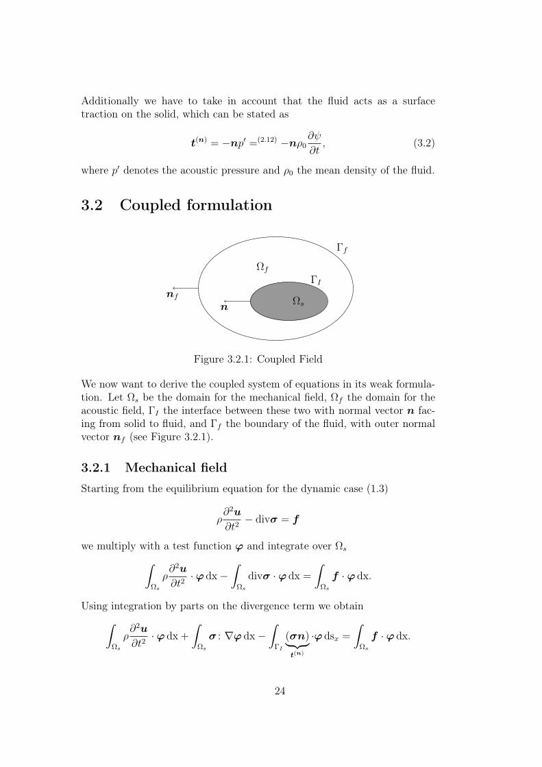
Figure 3.2.1: Coupled Field

We now want to derive the coupled system of equations in its weak formula-tion. Let Ωs be the domain for the mechanical field, Ωf the domain for theacoustic field, ΓI the interface between these two with normal vector n fac-ing from solid to fluid, and Γf the boundary of the fluid, with outer normalvector nf (see Figure 3.2.1).

3.2.1 Mechanical field

Starting from the equilibrium equation for the dynamic case (1.3)

ρ∂2u

∂t2− divσ = f

we multiply with a test function ϕ and integrate over Ωs∫Ωs

ρ∂2u

∂t2·ϕ dx−

∫Ωs

divσ ·ϕ dx =

∫Ωs

f ·ϕ dx.

Using integration by parts on the divergence term we obtain∫Ωs

ρ∂2u

∂t2·ϕ dx +

∫Ωs

σ : ∇ϕ dx−∫

ΓI

(σn)︸ ︷︷ ︸t(n)

·ϕ dsx =

∫Ωs

f ·ϕ dx.

24

Since σ = σ> we have

σ : ∇ϕ =1

2(σ : ∇ϕ) +

1

2(σ> : ∇ϕ)︸ ︷︷ ︸σ : (∇ϕ)>

= σ :1

2(∇ϕ+∇ϕ>) = σ : ε(ϕ).

From the constitutive law (1.6)

σ = λ tr(ε(u))︸ ︷︷ ︸tr(∇u)=divu

I + 2µε(u)

we get that

σ : ε(ϕ) = (2µε(u) + λ(divu)I) : ε(ϕ)

= 2µ(ε(u) : ε(ϕ)) + λ(divu) (I : ε(ϕ))︸ ︷︷ ︸tr(ε(ϕ))=divϕ

= 2µ(ε(u) : ε(ϕ)) + λ(divu)(divϕ).

So the weak formulation is given by∫Ωs

ρ∂2u

∂t2·ϕ dx +

∫Ωs

2µ(ε(u) : ε(ϕ)) + λ(divu)(divϕ) dx

−∫

ΓI

t(n) ·ϕ dsx =

∫Ωs

f ·ϕ dx. (3.3)

3.2.2 Acoustic field

For the acoustic field we start with the wave equation for the acoustic velocitypotential (2.13)

∆ψ =1

c2

∂2ψ

∂t2,

multiply it with a test function w and integrate over Ωf

−∫

Ωf

∆ψ w dx +

∫Ωf

1

c2

∂2ψ

∂t2w dx = 0.

Using partial integration on the Laplace term we obtain the weak formulationfor the acoustic field∫

Ωf

∇ψ ·∇w dx−∫

Γf

wnf ·∇ψ dsx +

∫ΓI

wn ·∇ψ dsx +

∫Ωf

1

c2

∂2ψ

∂t2w dx = 0,

(3.4)

where the plus sign in front of the interface surface integral comes from thechoice of the normal vector n.

25

3.2.3 Coupled System

Now we incorporate the coupling conditions, i.e.∫ΓI

t(n) ·ϕ dsx =(3.2) −∫

ΓI

p′n ·ϕ dsx = −∫

ΓI

ρ0∂ψ

∂tn ·ϕ dsx.

For simplicity we assume ∂ψ/∂n = 0 on Γf so we just have to deal with∫ΓI

wn · ∇ψ dsx =

∫ΓI

w∂ψ

∂ndsx =(3.1) −

∫ΓI

wn · ∂u∂t

dsx.

So the final coupled system of equations is given by∫Ωs

ρ∂2u

∂t2·ϕ dx +

∫Ωs

2µ(ε(u) : ε(ϕ)) + λ(divu)(divϕ) dx

+

∫ΓI

ρ0∂ψ

∂tn ·ϕ dsx =

∫Ωs

f ·ϕ dx∫Ωf

1

c2

∂2ψ

∂t2w dx +

∫Ωf

∇ψ · ∇w dx−∫

ΓI

wn · ∂u∂t

dsx = 0.

26

Chapter 4

Conclusions

In the course of this thesis we managed to derive all the necessary toolsto model a structure-acoustic coupling problem. For the mechanical modelwe started with the equilibrium equation (1.3), derived a linear relation be-tween the displacement and the strain in (1.5) and combined both of themwith Hook’s law for isotropic, elastic materials (1.6) to arrive at the Navier-Lamé equation (1.8). For the acoustic model we first derived the continuityequation (2.1) and the Euler equation (2.4). Additionally we used the linearstate equation (2.6) and linear versions of the Euler (2.7) and the continuityequation (2.8), to arrive at the linear acoustic wave equation (2.10). Forthe coupled system we derived coupling conditions, (3.1) and (3.2), and de-duced the weak formulations for the mechanical (3.3) and the acoustic field(3.4). By incorporating the coupling conditions we reached our final systemof coupled equations:∫

Ωs

ρ∂2u

∂t2·ϕ dx +

∫Ωs

2µ(ε(u) : ε(ϕ)) + λ(divu)(divϕ) dx

+

∫ΓI

ρ0∂ψ

∂tn ·ϕ dsx =

∫Ωs

f ·ϕ dx∫Ωf

1

c2

∂2ψ

∂t2w dx +

∫Ωf

∇ψ · ∇w dx−∫

ΓI

wn · ∂u∂t

dsx = 0.

From this one can start to think about numerical computations. One way isto apply the finite element method to the coupled system of equations, seefor example [1]. Other methods have been proposed, see for example [7] or[8]. For a further study in acoustics and structure-acoustic coupling one mayrefer to [9].

27

Bibliography

[1] M. Kaltenbacher. Numerical Simulation of Mechatronic Sensors and Ac-tuators. 2. Auflage, Springer, 2007.

[2] U. Langer. Skriptum zur Vorlesung Mathematische Modelle in der Tech-nik. Johannes Kepler Universität Linz, 2015.

[3] S. Kindermann. An introduction to mathematical methods for continuummechanics. Johannes Kepler Universität Linz, 2016.

[4] I. N. Bronstein, K. A. Semendjajew, G. Musiol, H. Mühlig. Taschenbuchder Mathematik. 7. Auflage, Harri Deutsch, 2008.

[5] M. Jung, U. Langer. Methode der finiten Elemente für Ingenieure.2. Auflage, Springer, 2013

[6] S.W. Rienstra, A. Hirschberg. An Introduction to Acoustics. EindhovenUniversity of Technology, 2016.

[7] M. Fischer, L. Gaul. Fast BEM–FEM mortar coupling for acous-tic–structure interaction. Institut A für Mechanik, Universität Stuttgart,2005.

[8] G. Hou, J. Wang and A. Layton. Numerical Methods for Fluid-StructureInteraction — A Review. Communications in Computational Physics,12(2), pp. 337–377, 2012.

[9] F. Dunn, et al. Springer Handbook of Acoustics. Springer, 2015.

28

Eidesstattliche Erklärung

Ich, Lukas Burgholzer, erkläre an Eides statt, dass ich die vorliegende Bache-lorarbeit selbständig und ohne fremde Hilfe verfasst, andere als die angegebe-nen Quellen und Hilfsmittel nicht benutzt bzw. die wörtlich oder sinngemäßentnommenen Stellen als solche kenntlich gemacht habe.

Linz, November 2016

————————————————Lukas Burgholzer

Curriculum Vitae

Name: Lukas Burgholzer

Nationality: Austria

Date of Birth: 22 January, 1994

Place of Birth: Linz, Austria

Education:2000–2004 Volksschule (elementary school)

Kremsdorf in Haid bei Ansfelden

2004–2012 Akademisches Gymnasium (secondary comprehensive school)Linz

2013–2016 Studies in Technical Mathematics,Johannes Kepler University Linz