Embed Size (px)
Citation preview
European Centre for Medium-Range Weather Forecasts
Europäisches Zentrum für mittelfristige Wettervorhersage
Centre européen pour les prévisions météorologiques à moyen terme
ESA CONTRACT REPORT
Contract Report to the European Space Agency
Tech Note - Phase II - WP1100SMOS Monitoring ReportNumber 2: Nov 2010 - Nov 2011
Joaquın Munoz Sabater,Mohamed Dahoui,Patricia de Rosnay,Lars Isaksen
ESA/ESRIN Contract4000101703/10/NL/FF/fk
Series: ECMWF ESA Project Report Series
A full list of ECMWF Publications can be found on our web site under:http://www.ecmwf.int/publications/
Contact: [email protected]
c©Copyright 2012
European Centre for Medium Range Weather ForecastsShinfield Park, Reading, RG2 9AX, England
Literary and scientific copyrights belong to ECMWF and are reserved in all countries. This publication is notto be reprinted or translated in whole or in part without the written permission of the Director-General. Appro-priate non-commercial use will normally be granted under the condition that reference is made to ECMWF.
The information within this publication is given in good faith and considered to be true, but ECMWF acceptsno liability for error, omission and for loss or damage arising from its use.
Contract Report to the European Space Agency
Tech Note - Phase II - WP1100SMOS Monitoring Report
Number 2: Nov 2010 - Nov 2011
Authors: Joaquın Munoz Sabater,Mohamed Dahoui,Patricia de Rosnay,
Lars IsaksenTechnical Note - Phase-II - WP1100
Monitoring Report Number 2: Nov 2010 - Nov 2011ESA/ESRIN Contract 4000101703/10/NL/FF/fk
European Centre for Medium-Range Weather Forecasts
Shinfield Park, Reading, Berkshire, UK
December 2011

Name Company
First version prepared by J. Munoz Sabater ECMWF(November 2011)
Quality Visa E. Kallen ECMWF
Application Authorized by ESA/ESTEC
Distribution list:ESA/ESRINLuc GovaertSusanne MecklenburgSteven DelwartESA ESRIN Documentation Desk
SERCORaffaele Crapolicchio
ESA/ESTECTania CasalMatthias DruschKlaus Scipal
ECMWFHRDivision & Section Heads
ESA monitoring report on SMOS data in the ECMWF IFS
Contents
1 Introduction 2
2 SMOS observations at ECMWF 3
3 Monitoring over land 4
3.1 Simulations of brightness temperatures. . . . . . . . . . . . . . . . . . . . . . . . . . . . . . 4
3.2 Time-averaged geographical mean fields.. . . . . . . . . . . . . . . . . . . . . . . . . . . . 5
3.3 Time series . . . . . . . . . . . . . . . . . . . . . . . . . . . . . . . . . . . . . . . . . . . . 13
3.4 Angular distribution of bias. . . . . . . . . . . . . . . . . . . . . . . . . . . . . . . . . . . . 22
3.5 Hovmoller plots. . . . . . . . . . . . . . . . . . . . . . . . . . . . . . . . . . . . . . . . . . 25
4 Monitoring over ocean 29
4.1 Simulations of brightness temperatures. . . . . . . . . . . . . . . . . . . . . . . . . . . . . . 29
4.2 Time-averaged geographical mean fields.. . . . . . . . . . . . . . . . . . . . . . . . . . . . 30
4.3 Time series . . . . . . . . . . . . . . . . . . . . . . . . . . . . . . . . . . . . . . . . . . . . 37
4.4 Hovmoller plots. . . . . . . . . . . . . . . . . . . . . . . . . . . . . . . . . . . . . . . . . . 44
5 Summary 48
6 References 49
Monitoring Report to ESA 1
ESA monitoring report on SMOS data in the ECMWF IFS
Abstract
Contracted by the European Space Agency (ESA), the EuropeanCentre for Medium-Range Weather Fore-casts (ECMWF) is involved in global monitoring and data assimilation of the Soil Moisture and OceanSalinity (SMOS) mission data. For the first time, a new innovative remote sensing technique based on ra-diometric aperture synthesis is used in SMOS to observe soilmoisture over continental surfaces and oceansalinity over oceans. Monitoring SMOS data (i.e. the comparison between the observed value and themodel equivalent of that observation) is therefore of special interest and a requirement prior to assimila-tion experiments. This report is the second Monitoring Report delivered to ESA. The objective is to reporton the monitoring activities of SMOS data over land and sea ona long term basis, investigating also themulti-angular and multi-polarised aspect of the SMOS observations. This report presents results for oneyear (November 2010- November 2011) of SMOS data monitoringin Near Real Time obtained through theSMOS monitoring suite at ECMWF.
1 Introduction
ECMWF has developed an operational chain which monitors SMOS data in Near Real Time (NRT) at globalscale, as explained in (Sabater et al. 2010). Monitoring is carried out routinely for each new type of satellitedata brought into the operational Integrated Forecasting System (IFS) at ECMWF. In Numerical Weather Pre-diction systems monitoring is mainly focused on the comparison between the observed variable and the modelequivalent simulating that observation, because this is the quantity used in the analysis.For SMOS, monitoring is produced separately for land and oceans. The reason is the strong contrast betweenthe dielectric constant of water bodies and land surfaces, which in turn produces very different emissivitiesand observed brightness temperatures at the top of the atmosphere. Thus, monitoring SMOS data separatelyover land and oceans increases the sensitivity to the statistical variables. Moreover, the multi-angular andmulti-polarised aspect of the observations is also accounted for in the monitoring chain by monitoring the dataindependently for several incidence angles of the observations and for two polarisation states at the antennareference frame.The developed framework makes it possible to obtain daily statistics of the observations, the model equivalentof the observations computed by the Community Microwave Emission Model (CMEM) [(Drusch et al. 2009;de Rosnay et al. 2009a)], and the difference between the two quantities, the so called first-guess departures.The statistics are computed over several weeks of data. Thisis a very robust way to identify systematic differ-ences between modelled values and observations. Furthermore it also set the basis to investigate and understandthe new observations before they become active in the ECMWF land assimilation scheme.
This Monitoring Report (MR2) on SMOS data is the second monitoring report delivered to ESA. In the first one[(Sabater et al. 2011b)] the monitoring website and statistical products were described. This monitoring reportshows results obtained since November 2010, the date when the monitoring suite started to produce routinelystatistics in Near Real Time (NRT) at ECMWF.
2 Monitoring Report to ESA
ESA monitoring report on SMOS data in the ECMWF IFS
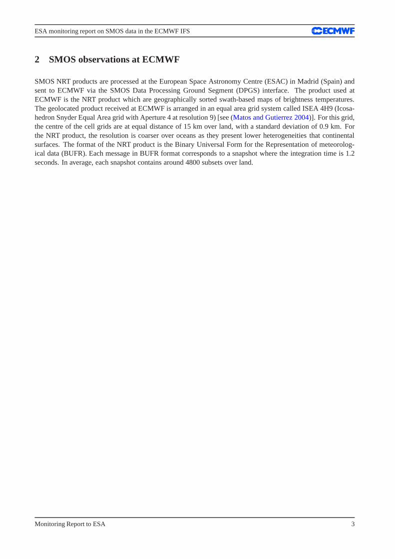
2 SMOS observations at ECMWF
SMOS NRT products are processed at the European Space Astronomy Centre (ESAC) in Madrid (Spain) andsent to ECMWF via the SMOS Data Processing Ground Segment (DPGS) interface. The product used atECMWF is the NRT product which are geographically sorted swath-based maps of brightness temperatures.The geolocated product received at ECMWF is arranged in an equal area grid system called ISEA 4H9 (Icosa-hedron Snyder Equal Area grid with Aperture 4 at resolution 9) [see (Matos and Gutierrez 2004)]. For this grid,the centre of the cell grids are at equal distance of 15 km overland, with a standard deviation of 0.9 km. Forthe NRT product, the resolution is coarser over oceans as they present lower heterogeneities that continentalsurfaces. The format of the NRT product is the Binary Universal Form for the Representation of meteorolog-ical data (BUFR). Each message in BUFR format corresponds toa snapshot where the integration time is 1.2seconds. In average, each snapshot contains around 4800 subsets over land.
Monitoring Report to ESA 3
ESA monitoring report on SMOS data in the ECMWF IFS
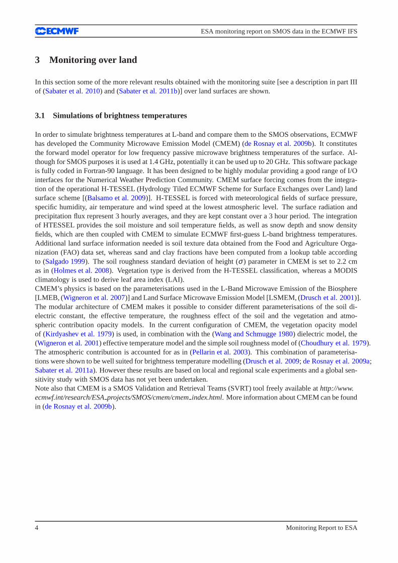
3 Monitoring over land
In this section some of the more relevant results obtained with the monitoring suite [see a description in part IIIof (Sabater et al. 2010) and (Sabater et al. 2011b)] over land surfaces are shown.
3.1 Simulations of brightness temperatures
In order to simulate brightness temperatures at L-band and compare them to the SMOS observations, ECMWFhas developed the Community Microwave Emission Model (CMEM) (de Rosnay et al. 2009b). It constitutesthe forward model operator for low frequency passive microwave brightness temperatures of the surface. Al-though for SMOS purposes it is used at 1.4 GHz, potentially itcan be used up to 20 GHz. This software packageis fully coded in Fortran-90 language. It has been designed to be highly modular providing a good range of I/Ointerfaces for the Numerical Weather Prediction Community. CMEM surface forcing comes from the integra-tion of the operational H-TESSEL (Hydrology Tiled ECMWF Scheme for Surface Exchanges over Land) landsurface scheme [(Balsamo et al. 2009)]. H-TESSEL is forced with meteorological fields of surfacepressure,specific humidity, air temperature and wind speed at the lowest atmospheric level. The surface radiation andprecipitation flux represent 3 hourly averages, and they arekept constant over a 3 hour period. The integrationof HTESSEL provides the soil moisture and soil temperature fields, as well as snow depth and snow densityfields, which are then coupled with CMEM to simulate ECMWF first-guess L-band brightness temperatures.Additional land surface information needed is soil texturedata obtained from the Food and Agriculture Orga-nization (FAO) data set, whereas sand and clay fractions have been computed from a lookup table accordingto (Salgado 1999). The soil roughness standard deviation of height (σ ) parameter in CMEM is set to 2.2 cmas in (Holmes et al. 2008). Vegetation type is derived from the H-TESSEL classification, whereas a MODISclimatology is used to derive leaf area index (LAI).CMEM’s physics is based on the parameterisations used in theL-Band Microwave Emission of the Biosphere[LMEB, (Wigneron et al. 2007)] and Land Surface Microwave Emission Model [LSMEM, (Drusch et al. 2001)].The modular architecture of CMEM makes it possible to consider different parameterisations of the soil di-electric constant, the effective temperature, the roughness effect of the soil and the vegetation and atmo-spheric contribution opacity models. In the current configuration of CMEM, the vegetation opacity modelof (Kirdyashev et al. 1979) is used, in combination with the (Wang and Schmugge 1980) dielectric model, the(Wigneron et al. 2001) effective temperature model and the simple soil roughnessmodel of (Choudhury et al. 1979).The atmospheric contribution is accounted for as in (Pellarin et al. 2003). This combination of parameterisa-tions were shown to be well suited for brightness temperature modelling (Drusch et al. 2009; de Rosnay et al. 2009a;Sabater et al. 2011a). However these results are based on local and regional scale experiments and a global sen-sitivity study with SMOS data has not yet been undertaken.Note also that CMEM is a SMOS Validation and Retrieval Teams (SVRT) tool freely available athttp://www.ecmwf.int/research/ESAprojects/SMOS/cmem/cmemindex.html. More information about CMEM can be foundin (de Rosnay et al. 2009b).
4 Monitoring Report to ESA
ESA monitoring report on SMOS data in the ECMWF IFS
3.2 Time-averaged geographical mean fields.
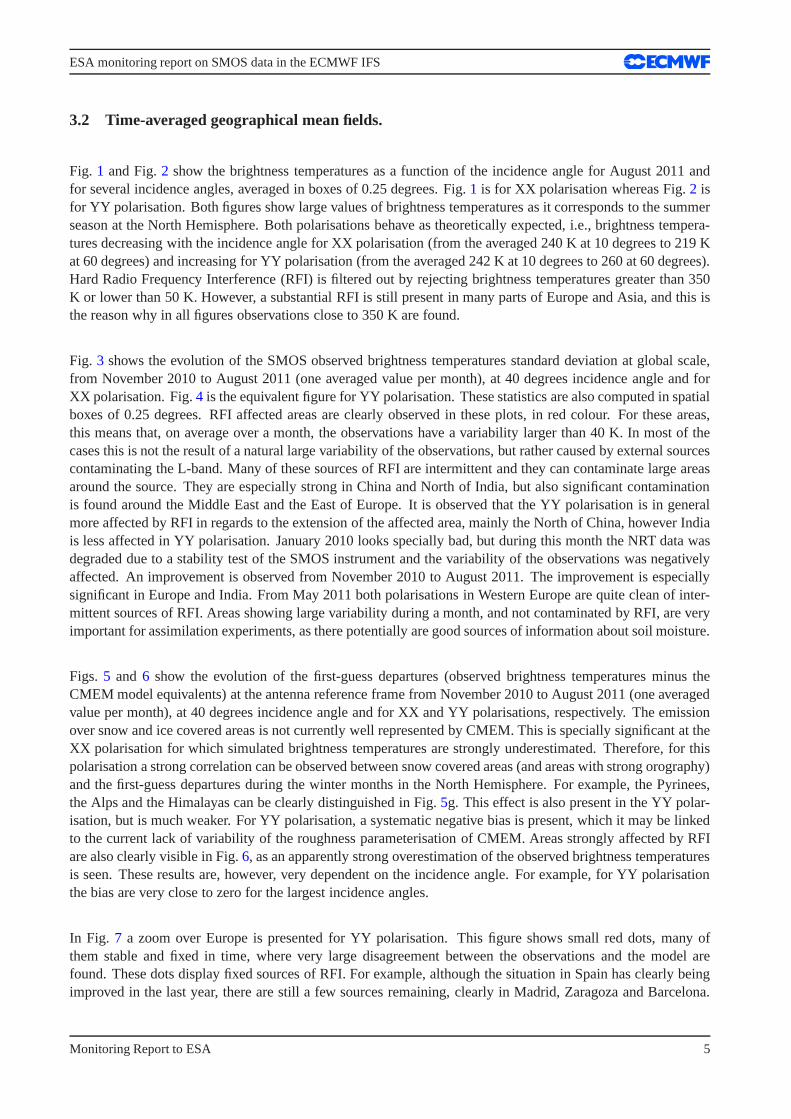
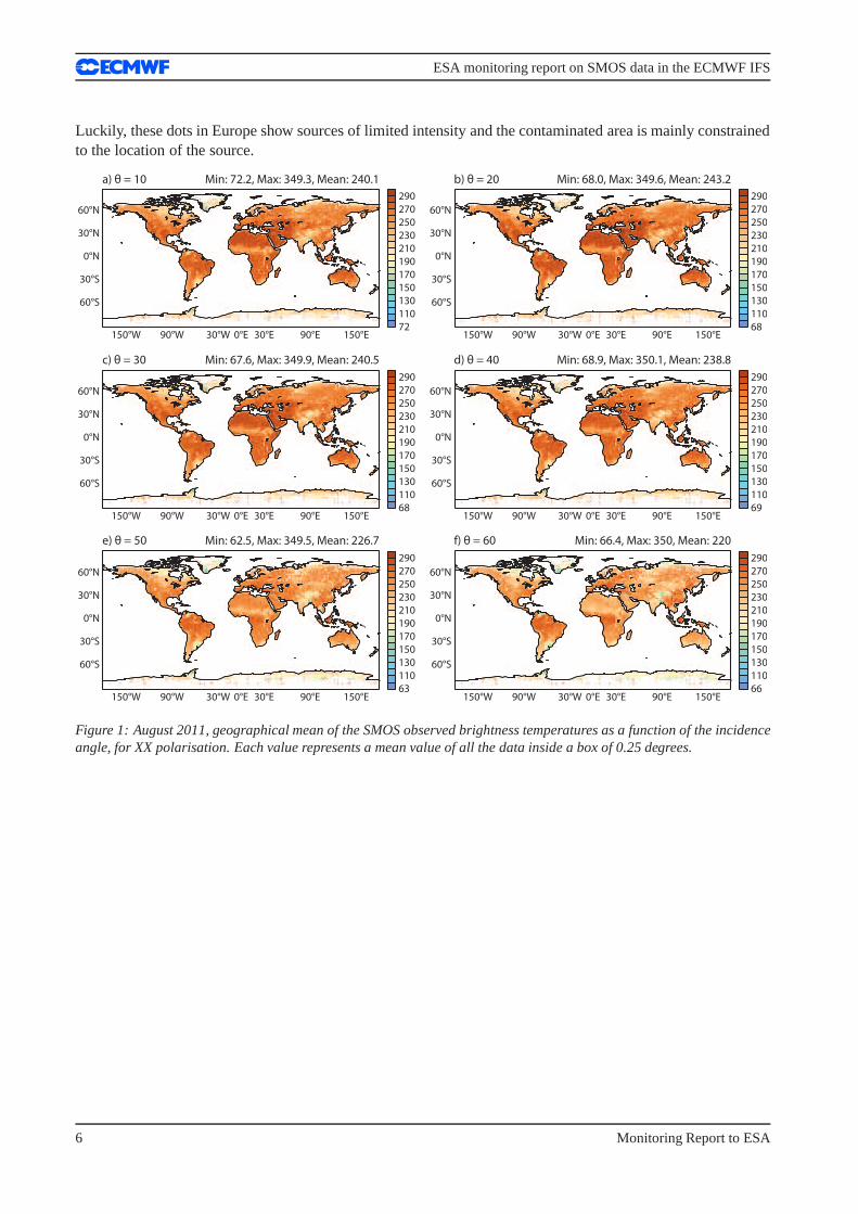
Fig. 1 and Fig.2 show the brightness temperatures as a function of the incidence angle for August 2011 andfor several incidence angles, averaged in boxes of 0.25 degrees. Fig.1 is for XX polarisation whereas Fig.2 isfor YY polarisation. Both figures show large values of brightness temperatures as it corresponds to the summerseason at the North Hemisphere. Both polarisations behave as theoretically expected, i.e., brightness tempera-tures decreasing with the incidence angle for XX polarisation (from the averaged 240 K at 10 degrees to 219 Kat 60 degrees) and increasing for YY polarisation (from the averaged 242 K at 10 degrees to 260 at 60 degrees).Hard Radio Frequency Interference (RFI) is filtered out by rejecting brightness temperatures greater than 350K or lower than 50 K. However, a substantial RFI is still present in many parts of Europe and Asia, and this isthe reason why in all figures observations close to 350 K are found.
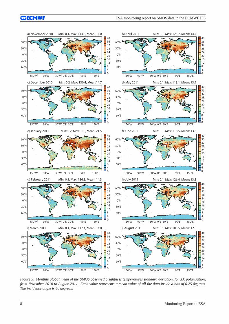
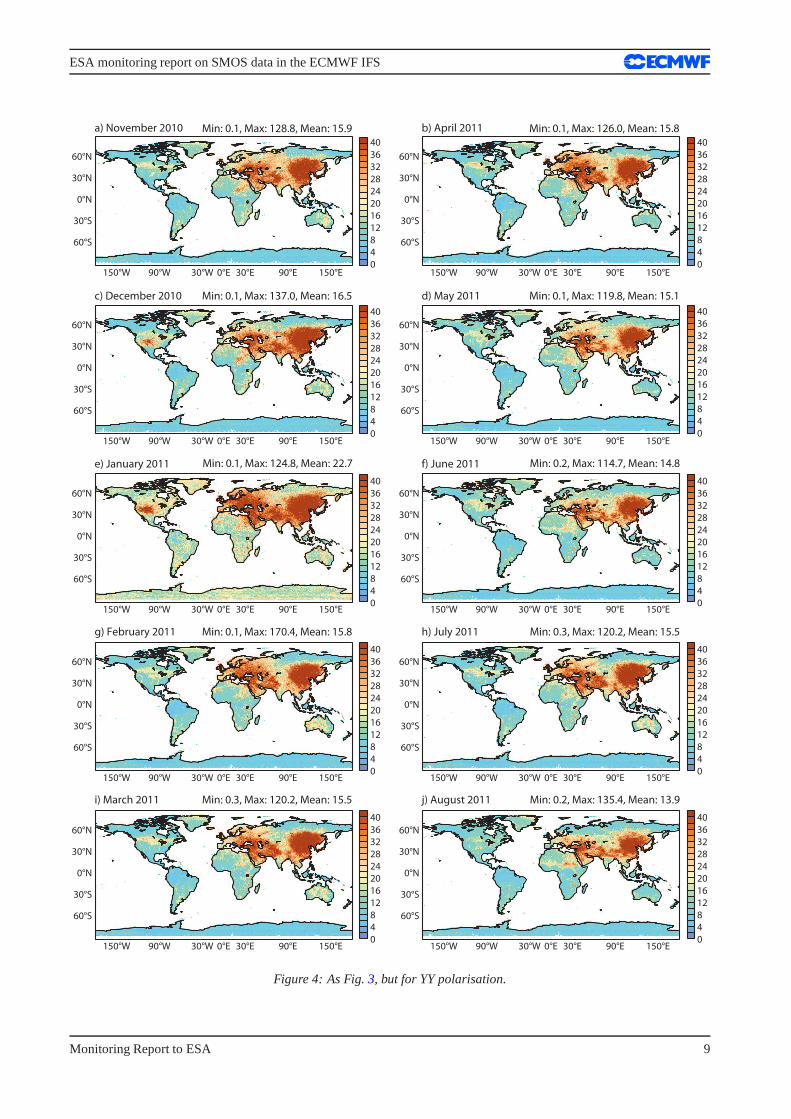
Fig. 3 shows the evolution of the SMOS observed brightness temperatures standard deviation at global scale,from November 2010 to August 2011 (one averaged value per month), at 40 degrees incidence angle and forXX polarisation. Fig.4 is the equivalent figure for YY polarisation. These statistics are also computed in spatialboxes of 0.25 degrees. RFI affected areas are clearly observed in these plots, in red colour. For these areas,this means that, on average over a month, the observations have a variability larger than 40 K. In most of thecases this is not the result of a natural large variability ofthe observations, but rather caused by external sourcescontaminating the L-band. Many of these sources of RFI are intermittent and they can contaminate large areasaround the source. They are especially strong in China and North of India, but also significant contaminationis found around the Middle East and the East of Europe. It is observed that the YY polarisation is in generalmore affected by RFI in regards to the extension of the affected area, mainly the North of China, however Indiais less affected in YY polarisation. January 2010 looks specially bad, but during this month the NRT data wasdegraded due to a stability test of the SMOS instrument and the variability of the observations was negativelyaffected. An improvement is observed from November 2010 to August 2011. The improvement is especiallysignificant in Europe and India. From May 2011 both polarisations in Western Europe are quite clean of inter-mittent sources of RFI. Areas showing large variability during a month, and not contaminated by RFI, are veryimportant for assimilation experiments, as there potentially are good sources of information about soil moisture.
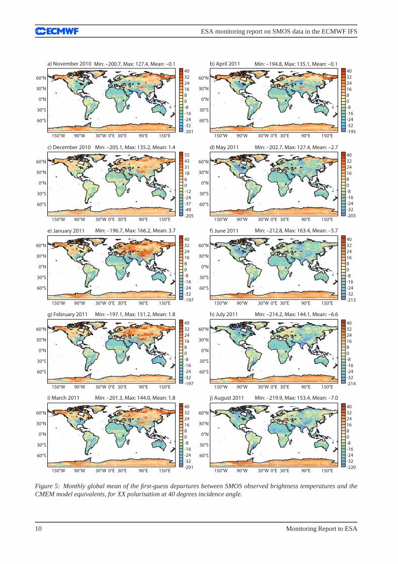
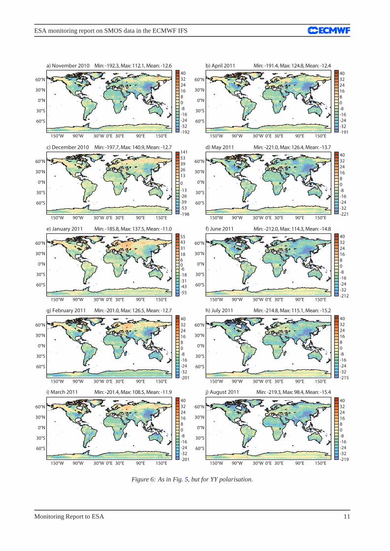
Figs. 5 and 6 show the evolution of the first-guess departures (observed brightness temperatures minus theCMEM model equivalents) at the antenna reference frame fromNovember 2010 to August 2011 (one averagedvalue per month), at 40 degrees incidence angle and for XX andYY polarisations, respectively. The emissionover snow and ice covered areas is not currently well represented by CMEM. This is specially significant at theXX polarisation for which simulated brightness temperatures are strongly underestimated. Therefore, for thispolarisation a strong correlation can be observed between snow covered areas (and areas with strong orography)and the first-guess departures during the winter months in the North Hemisphere. For example, the Pyrinees,the Alps and the Himalayas can be clearly distinguished in Fig. 5g. This effect is also present in the YY polar-isation, but is much weaker. For YY polarisation, a systematic negative bias is present, which it may be linkedto the current lack of variability of the roughness parameterisation of CMEM. Areas strongly affected by RFIare also clearly visible in Fig.6, as an apparently strong overestimation of the observed brightness temperaturesis seen. These results are, however, very dependent on the incidence angle. For example, for YY polarisationthe bias are very close to zero for the largest incidence angles.
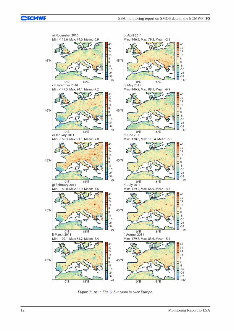
In Fig. 7 a zoom over Europe is presented for YY polarisation. This figure shows small red dots, many ofthem stable and fixed in time, where very large disagreement between the observations and the model arefound. These dots display fixed sources of RFI. For example, although the situation in Spain has clearly beingimproved in the last year, there are still a few sources remaining, clearly in Madrid, Zaragoza and Barcelona.
Monitoring Report to ESA 5
ESA monitoring report on SMOS data in the ECMWF IFS
Luckily, these dots in Europe show sources of limited intensity and the contaminated area is mainly constrainedto the location of the source.
Min: 72.2, Max: 349.3, Mean: 240.1a) θ = 10 b) θ = 20
c) θ = 30 d) θ = 40
e) θ = 50 f) θ = 60
Min: 68.0, Max: 349.6, Mean: 243.2
Min: 67.6, Max: 349.9, Mean: 240.5 Min: 68.9, Max: 350.1, Mean: 238.8
Min: 62.5, Max: 349.5, Mean: 226.7 Min: 66.4, Max: 350, Mean: 220
60°N
30°N
0°N
30°S
60°S
150°E90°E30°E0°E30°W90°W150°W
60°N
30°N
0°N
30°S
60°S
150°E90°E30°E0°E30°W90°W150°W
60°N
30°N
0°N
30°S
60°S
150°E90°E30°E0°E30°W90°W150°W
60°N
30°N
0°N
30°S
60°S
150°E90°E30°E0°E30°W90°W150°W
60°N
30°N
0°N
30°S
60°S
150°E90°E30°E0°E30°W90°W150°W
60°N
30°N
0°N
30°S
60°S
150°E90°E30°E0°E30°W90°W150°W
72
110
130
150
170
190
210
230
250
270
290
68
110
130
150
170
190
210
230
250
270
290
63
110
130
150
170
190
210
230
250
270
290
68
110
130
150
170
190
210
230
250
270
290
69
110
130
150
170
190
210
230
250
270
290
66
110
130
150
170
190
210
230
250
270
290
Figure 1: August 2011, geographical mean of the SMOS observed brightness temperatures as a function of the incidenceangle, for XX polarisation. Each value represents a mean value of all the data inside a box of 0.25 degrees.
6 Monitoring Report to ESA
ESA monitoring report on SMOS data in the ECMWF IFS
Min: 88.6, Max: 348.6, Mean: 242.1a) θ = 10 b) θ = 20
c) θ = 30 d) θ = 40
e) θ = 50 f) θ = 60
Min: 79.3, Max: 349.8, Mean: 242.5
Min: 69.3, Max: 349.1, Mean: 241.1 Min: 75.6, Max: 349.8, Mean: 246.1
Min: 54.6, Max: 350.2, Mean: 253.6 Min: 54.2, Max: 349.8, Mean: 260.4
60°N
30°N
0°N
30°S
60°S
150°E90°E30°E0°E30°W90°W150°W
60°N
30°N
0°N
30°S
60°S
150°E90°E30°E0°E30°W90°W150°W
60°N
30°N
0°N
30°S
60°S
150°E90°E30°E0°E30°W90°W150°W
60°N
30°N
0°N
30°S
60°S
150°E90°E30°E0°E30°W90°W150°W
60°N
30°N
0°N
30°S
60°S
150°E90°E30°E0°E30°W90°W150°W
60°N
30°N
0°N
30°S
60°S
150°E90°E30°E0°E30°W90°W150°W
89
110
130
150
170
190
210
230
250
270
290
69
110
130
150
170
190
210
230
250
270
290
55
110
130
150
170
190
210
230
250
270
290
79
110
130
150
170
190
210
230
250
270
290
76
110
130
150
170
190
210
230
250
270
290
110
54
130
150
170
190
210
230
250
270
290
Figure 2: As in Fig.1 but for YY polarisation.
Monitoring Report to ESA 7
ESA monitoring report on SMOS data in the ECMWF IFS
0
4
8
12
16
20
24
28
32
36
40
0
4
8
12
16
20
24
28
32
36
40
0
4
8
12
16
20
24
28
32
36
40
0
4
8
12
16
20
24
28
32
36
40
0
4
8
12
16
20
24
28
32
36
40
0
4
8
12
16
20
24
28
32
36
40
0
4
8
12
16
20
24
28
32
36
40
0
4
8
12
16
20
24
28
32
36
40
0
4
8
12
16
20
24
28
32
36
40
0
4
8
12
16
20
24
28
32
36
40
Min: 0.1, Max: 113.8, Mean: 14.0a) November 2010 b) April 2011
c) December 2010 d) May 2011
e) January 2011 f) June 2011
g) February 2011 h) July 2011
i) March 2011 j) August 2011
Min: 0.1, Max: 123.7, Mean: 14.7
Min: 0.2, Max: 130.4, Mean:14.7 Min: 0.1, Max: 113.1, Mean: 13.9
Min: 0.2, Max: 118, Mean: 21.5 Min: 0.1, Max: 118.5, Mean: 13.5
Min: 0.1, Max: 136.8, Mean: 14.3 Min: 0.1, Max: 126.4, Mean: 13.3
Min: 0.1, Max: 117.4, Mean: 14.0 Min: 0.1, Max: 103.5, Mean: 12.8
60°N
30°N
0°N
30°S
60°S
150°E90°E30°E0°E30°W90°W150°W
60°N
30°N
0°N
30°S
60°S
150°E90°E30°E0°E30°W90°W150°W
60°N
30°N
0°N
30°S
60°S
150°E90°E30°E0°E30°W90°W150°W
60°N
30°N
0°N
30°S
60°S
150°E90°E30°E0°E30°W90°W150°W
60°N
30°N
0°N
30°S
60°S
150°E90°E30°E0°E30°W90°W150°W
60°N
30°N
0°N
30°S
60°S
150°E90°E30°E0°E30°W90°W150°W
60°N
30°N
0°N
30°S
60°S
150°E90°E30°E0°E30°W90°W150°W
60°N
30°N
0°N
30°S
60°S
150°E90°E30°E0°E30°W90°W150°W
60°N
30°N
0°N
30°S
60°S
150°E90°E30°E0°E30°W90°W150°W
60°N
30°N
0°N
30°S
60°S
150°E90°E30°E0°E30°W90°W150°W
Figure 3: Monthly global mean of the SMOS observed brightness temperatures standard deviation, for XX polarisation,from November 2010 to August 2011. Each value represents a mean value of all the data inside a box of 0.25 degrees.The incidence angle is 40 degrees.
8 Monitoring Report to ESA
ESA monitoring report on SMOS data in the ECMWF IFS
0
4
8
12
16
20
24
28
32
36
40
0
4
8
12
16
20
24
28
32
36
40
0
4
8
12
16
20
24
28
32
36
40
0
4
8
12
16
20
24
28
32
36
40
0
4
8
12
16
20
24
28
32
36
40
0
4
8
12
16
20
24
28
32
36
40
0
4
8
12
16
20
24
28
32
36
40
0
4
8
12
16
20
24
28
32
36
40
0
4
8
12
16
20
24
28
32
36
40
0
4
8
12
16
20
24
28
32
36
40
a) November 2010 b) April 2011
c) December 2010 d) May 2011
e) January 2011 f) June 2011
g) February 2011 h) July 2011
i) March 2011 j) August 2011
60°N
30°N
0°N
30°S
60°S
150°E90°E30°E0°E30°W90°W150°W
60°N
30°N
0°N
30°S
60°S
150°E90°E30°E0°E30°W90°W150°W
60°N
30°N
0°N
30°S
60°S
150°E90°E30°E0°E30°W90°W150°W
60°N
30°N
0°N
30°S
60°S
150°E90°E30°E0°E30°W90°W150°W
60°N
30°N
0°N
30°S
60°S
150°E90°E30°E0°E30°W90°W150°W
60°N
30°N
0°N
30°S
60°S
150°E90°E30°E0°E30°W90°W150°W
60°N
30°N
0°N
30°S
60°S
150°E90°E30°E0°E30°W90°W150°W
60°N
30°N
0°N
30°S
60°S
150°E90°E30°E0°E30°W90°W150°W
60°N
30°N
0°N
30°S
60°S
150°E90°E30°E0°E30°W90°W150°W
60°N
30°N
0°N
30°S
60°S
150°E90°E30°E0°E30°W90°W150°W
Min: 0.1, Max: 128.8, Mean: 15.9 Min: 0.1, Max: 126.0, Mean: 15.8
Min: 0.1, Max: 137.0, Mean: 16.5 Min: 0.1, Max: 119.8, Mean: 15.1
Min: 0.1, Max: 124.8, Mean: 22.7 Min: 0.2, Max: 114.7, Mean: 14.8
Min: 0.1, Max: 170.4, Mean: 15.8 Min: 0.3, Max: 120.2, Mean: 15.5
Min: 0.3, Max: 120.2, Mean: 15.5 Min: 0.2, Max: 135.4, Mean: 13.9
Figure 4: As Fig.3, but for YY polarisation.
Monitoring Report to ESA 9
ESA monitoring report on SMOS data in the ECMWF IFS
Min: –219.9, Max: 153.4, Mean: –7.0
a) November 2010 b) April 2011
c) December 2010 d) May 2011
e) January 2011 f) June 2011
g) February 2011 h) July 2011
i) March 2011 j) August 2011
60°N
30°N
0°N
30°S
60°S
150°E90°E30°E0°E30°W90°W150°W
60°N
30°N
0°N
30°S
60°S
150°E90°E30°E0°E30°W90°W150°W
60°N
30°N
0°N
30°S
60°S
150°E90°E30°E0°E30°W90°W150°W
60°N
30°N
0°N
30°S
60°S
150°E90°E30°E0°E30°W90°W150°W
60°N
30°N
0°N
30°S
60°S
150°E90°E30°E0°E30°W90°W150°W
60°N
30°N
0°N
30°S
60°S
150°E90°E30°E0°E30°W90°W150°W
60°N
30°N
0°N
30°S
60°S
150°E90°E30°E0°E30°W90°W150°W
60°N
30°N
0°N
30°S
60°S
150°E90°E30°E0°E30°W90°W150°W
60°N
30°N
0°N
30°S
60°S
150°E90°E30°E0°E30°W90°W150°W
60°N
30°N
0°N
30°S
60°S
150°E90°E30°E0°E30°W90°W150°W
Min: –205.1, Max: 135.2, Mean: 1.4 Min: –202.7, Max: 127.4, Mean: –2.7
Min: –196.7, Max: 166.2, Mean: 3.7 Min: –212.8, Max: 163.4, Mean: –5.7
Min: –197.1, Max: 151.2, Mean: 1.8 Min: –214.2, Max: 144.1, Mean: –6.6
Min: –201.3, Max: 144.0, Mean: 1.8
Min: –200.7, Max: 127.4, Mean: –0.1
-201
-32
-24
-16
-8
0
8
16
24
32
40
-197
-32
-24
-16
-8
0
8
16
24
32
40
-197
-32
-24
-16
-8
0
8
16
24
32
40
-201
-32
-24
-16
-8
0
8
16
24
32
40
-195
-32
-24
-16
-8
0
8
16
24
32
40
-203
-32
-24
-16
-8
0
8
16
24
32
40
-213
-32
-24
-16
-8
0
8
16
24
32
40
-214
-32
-24
-16
-8
0
8
16
24
32
40
-220
-32
-24
-16
-8
0
8
16
24
32
40
Min: –194.8, Max: 135.1, Mean: –0.1
-205
-49
-37
-24
-12
0
6
18
31
43
55
Figure 5: Monthly global mean of the first-guess departures between SMOS observed brightness temperatures and theCMEM model equivalents, for XX polarisation at 40 degrees incidence angle.
10 Monitoring Report to ESA
ESA monitoring report on SMOS data in the ECMWF IFS
Min: -192.3, Max: 112.1, Mean: -12.6a) November 2010 b) April 2011
c) December 2010 d) May 2011
e) January 2011 f) June 2011
g) February 2011 h) July 2011
i) March 2011 j) August 2011
Min: -191.4, Max: 124.8, Mean: -12.4
Min: -197.7, Max: 140.9, Mean: -12.7 Min: -221.0, Max: 126.4, Mean: -13.7
Min: -185.8, Max: 137.5, Mean: -11.0 Min: -212.0, Max: 114.3, Mean: -14.8
Min: -201.0, Max: 126.5, Mean: -12.7 Min: -214.8, Max: 115.1, Mean: -15.2
Min: -201.4, Max: 108.5, Mean: -11.9 Min: -219.3, Max: 98.4, Mean: -15.4
60°N
30°N
0°N
30°S
60°S
150°E90°E30°E0°E30°W90°W150°W
60°N
30°N
0°N
30°S
60°S
150°E90°E30°E0°E30°W90°W150°W
60°N
30°N
0°N
30°S
60°S
150°E90°E30°E0°E30°W90°W150°W
60°N
30°N
0°N
30°S
60°S
150°E90°E30°E0°E30°W90°W150°W
60°N
30°N
0°N
30°S
60°S
150°E90°E30°E0°E30°W90°W150°W
60°N
30°N
0°N
30°S
60°S
150°E90°E30°E0°E30°W90°W150°W
60°N
30°N
0°N
30°S
60°S
150°E90°E30°E0°E30°W90°W150°W
60°N
30°N
0°N
30°S
60°S
150°E90°E30°E0°E30°W90°W150°W
60°N
30°N
0°N
30°S
60°S
150°E90°E30°E0°E30°W90°W150°W
60°N
30°N
0°N
30°S
60°S
150°E90°E30°E0°E30°W90°W150°W
-192
-32
-24
-16
-8
0
8
16
24
32
40
-191
-32
-24
-16
-8
0
8
16
24
32
40
-198
-53
-39
-26
-13
0
13
26
39
53
141
-221
-32
-24
-16
-8
0
8
16
24
32
40
-55
-43-31
-18
-60618
31
4355
-212
-32
-24
-16
-8
0
8
16
24
32
40
-201
-32
-24
-16
-8
0
8
16
24
32
40
-215
-32
-24
-16
-8
0
8
16
24
32
40
-201
-32
-24
-16
-8
0
8
16
24
32
40
-219
-32
-24
-16
-8
0
8
16
24
32
40
Figure 6: As in Fig.5, but for YY polarisation.
Monitoring Report to ESA 11
ESA monitoring report on SMOS data in the ECMWF IFS
a) November 2010
Min: -115.6, Max: 74.6, Mean: -6.9
b) April 2011
Min: -146.9, Max: 79.3, Mean: -2.9
c) December 2010
Min: -147.5, Max: 94.1, Mean: -7.2
d) May 2011
Min: -146.9, Max: 88.1, Mean: -6.9
e) January 2011
Min: -169.3, Max: 91.1, Mean: -2.0
f) June 2011
Min: -128.6, Max: 113.4, Mean: -6.1
g) February 2011
Min: -160.0, Max: 82.9, Mean: -4.6
h) July 2011
Min: -129.2, Max: 66.9, Mean: -4.3
i) March 2011
Min: -102.1, Max: 81.2, Mean: -6.4
j) August 2011
Min: -179.7, Max: 83.6, Mean: -5.1
45°N
15°E0°E
45°N
15°E0°E
45°N
15°E0°E
45°N
15°E0°E
45°N
15°E0°E
45°N
15°E0°E
45°N
15°E0°E
45°N
15°E0°E
45°N
15°E0°E
45°N
15°E0°E
-116
-32
-24
-16
-8
0
8
16
24
32
40
-148
-32
-24
-16
-8
0
8
16
24
32
40
-170
-32
-24
-16
-8
0
8
16
24
32
40
-160
-32
-24
-16
-8
0
8
16
24
32
40
-102
-32
-24
-16
-8
0
8
16
24
32
40
-180
-32
-24
-16
-8
0
8
16
24
32
40
-147
-32
-24
-16
-8
0
8
16
24
32
40
-147
-32
-24
-16
-8
0
8
16
24
32
40
-129
-32
-24
-16
-8
0
8
16
24
32
40
-129
-32
-24
-16
-8
0
8
16
24
32
40
Figure 7: As in Fig.6, but zoom in over Europe.
12 Monitoring Report to ESA
ESA monitoring report on SMOS data in the ECMWF IFS
3.3 Time series
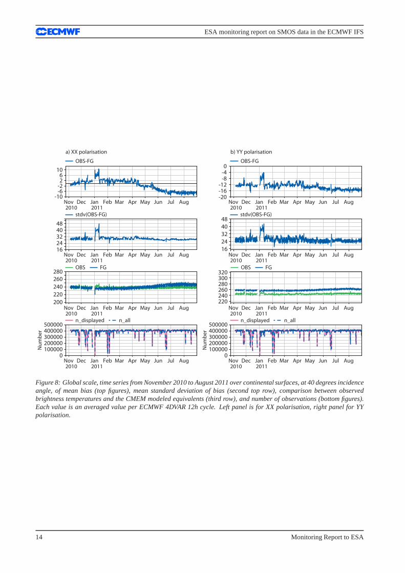
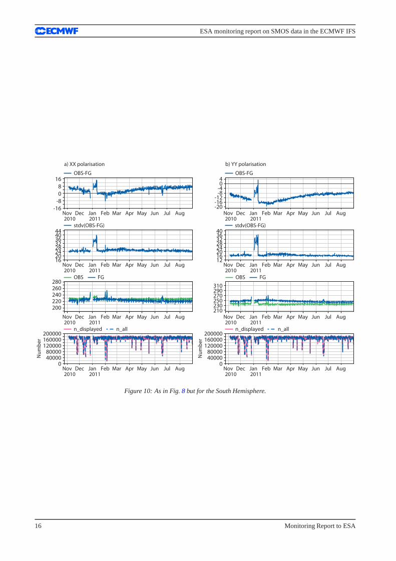
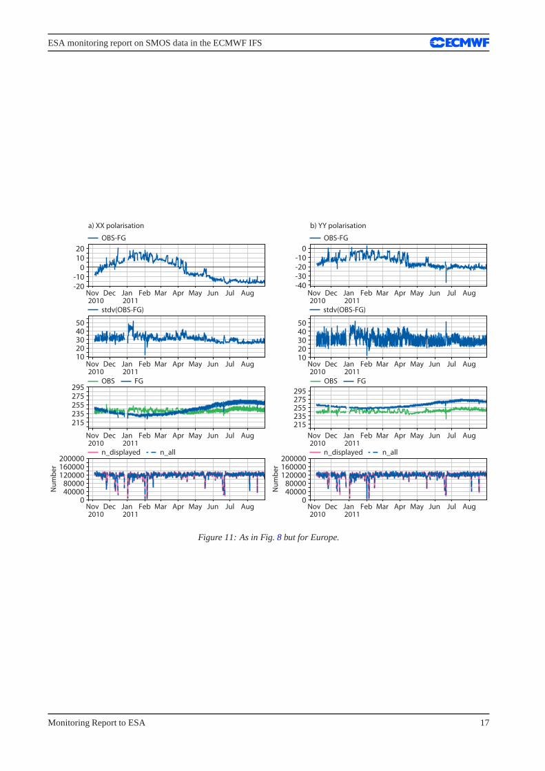
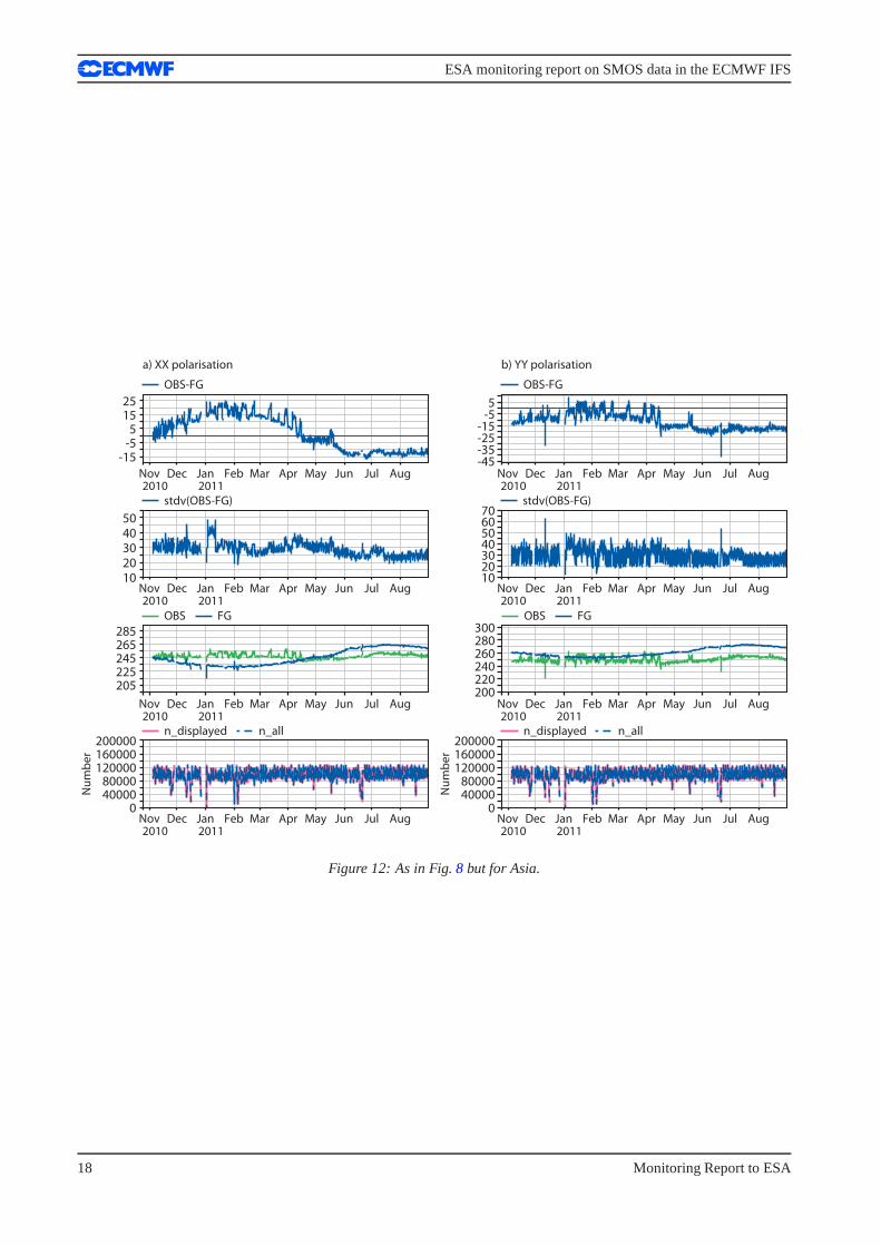
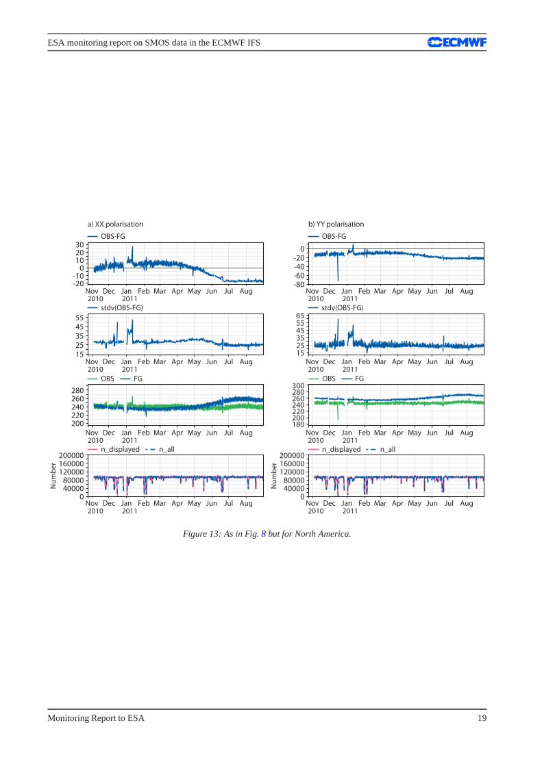
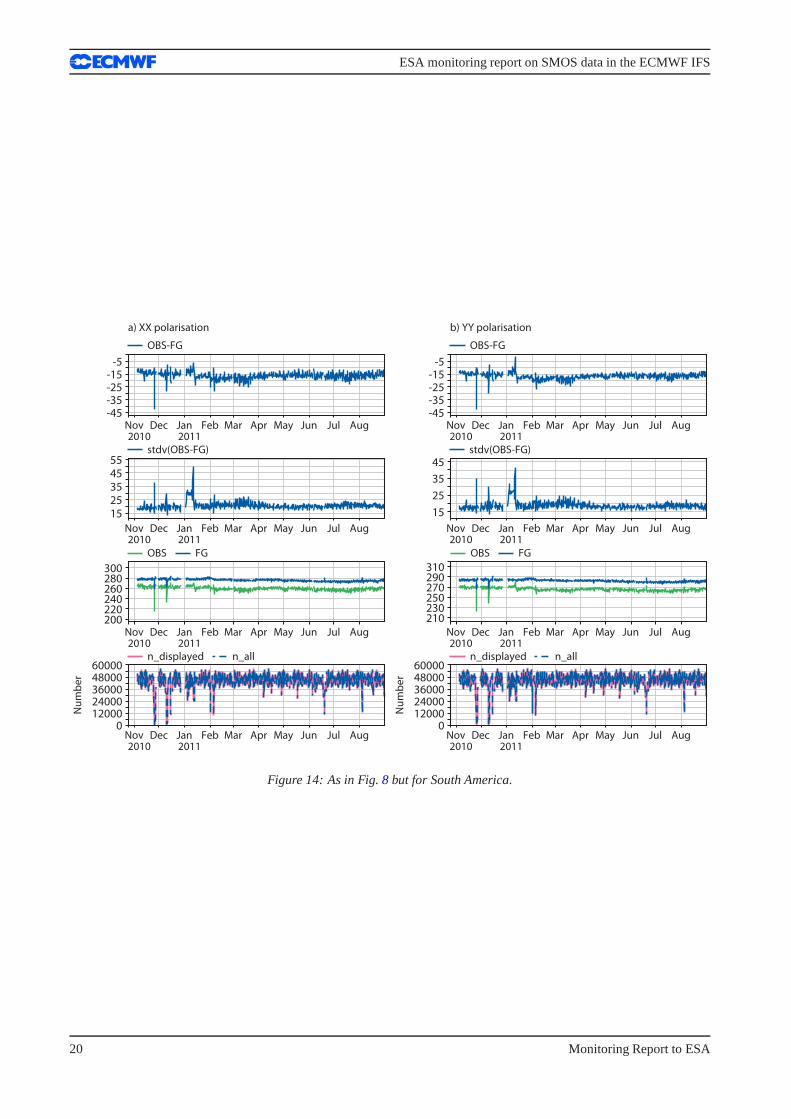
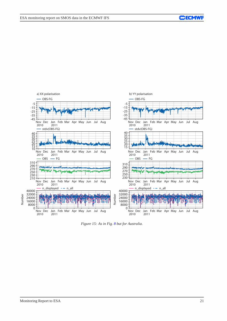
Figs.8 to 15present time series of the observed brightness temperatures, CMEM model equivalents, first guessdepartures and number of observations, from November 2010 to August 2011. Each value represents one meanvalue per ECMWF 4DVAR 12 hours assimilation cycle averaged at global scale, hemisphere or continent.
Fig. 8 presents the results obtained at global scale over land pixels. Left panel is for XX polarisation and rightpanel for YY polarisation. For YY polarisation an almost systematic negative bias is observed the whole year,increasing between April and May around 4 K in absolute value. During this period most of the melting of thesnow takes place, which explains this difference. This effect is stronger for XX polarisation because our modelis more sensitive over snow for this polarisation, as seen inFig. 5. A slightly larger variability of the bias is alsoobserved on the YY polarisation. A possible explanation is the larger influence of RFI on the YY polarisation,as seen in Fig.4, but also a larger variability is observed during the snow months at the North Hemisphere forXX polarisation.
At the end of December 2010 a stability test of the SMOS platform took place during 6 days, no data wasproduced during this period and this can clearly be seen in all the time series. During the following 2 weeks thescience data was degraded and this explains the abnormal peaks at the beginning of January 2011. In addition,the NRT processor did not work as normal until 18 February 2011 and during this period the observed bright-ness temperatures were a few degrees larger, producing larger bias, as it can be observed for January 2011 inFigs.3 and 4.
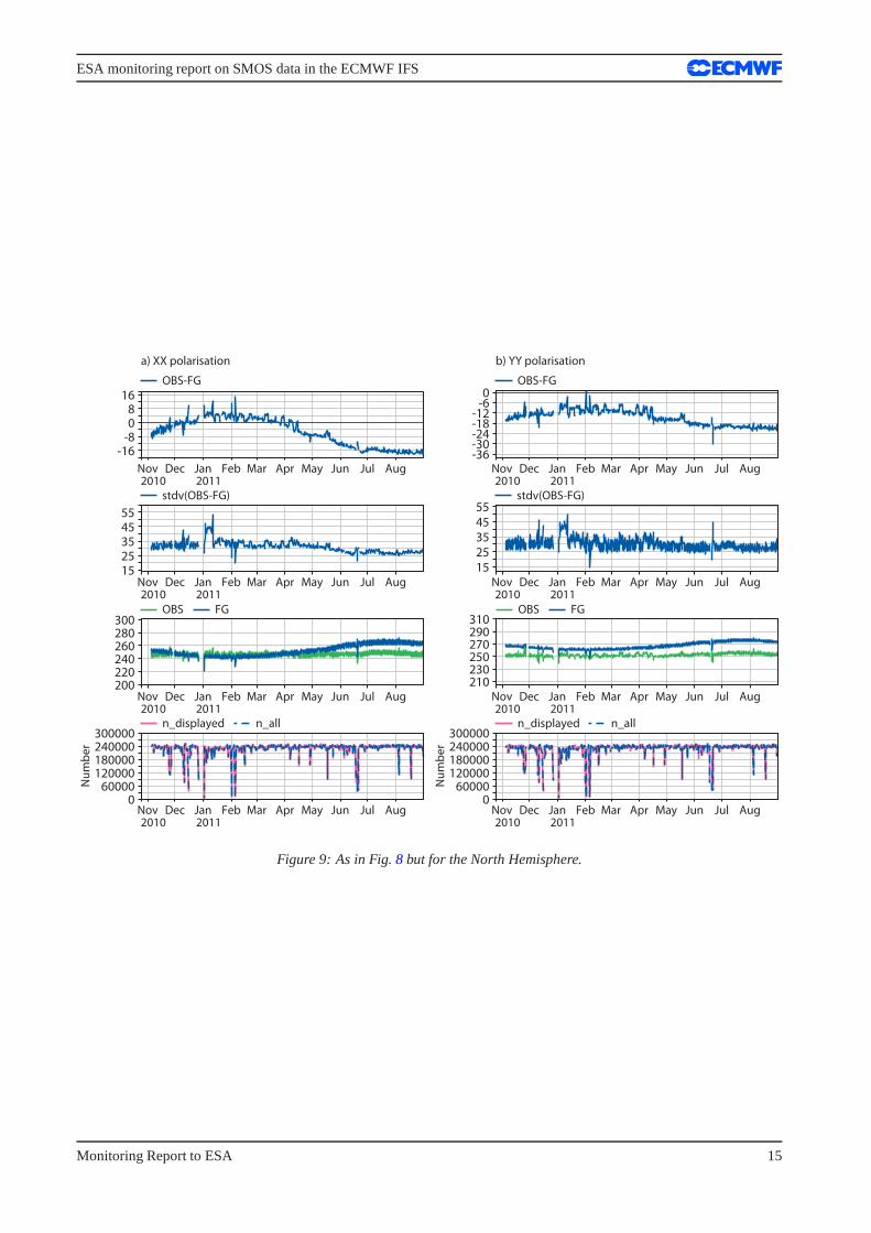
The standard deviation of the bias are smaller and more stable in the Southern Hemisphere (Fig.10) than inthe Northern Hemisphere (Fig.9) due to the stronger presence of RFI in the Northern Hemisphere, and this isespecially visible in the more affected YY polarisation. Especially strong values and variability is found in Eu-rope (Fig.11) and Asia (fig.12) where values as large as 45 K and differences of 20 K between two consecutivecycles are found. South America (Fig.14) and Australia (Fig.15) show more stable and lower values of thestandard deviation of the bias, between 18 and 20 K for South America and slightly larger for Australia. Thelarger variability on the number of observations per Australia depends logically on the position of the satelliteat the time of the acquisition.
In general, when compared to the observations the model underestimates the observed brightness temperaturesduring months with snow and overestimates them during the snow free months. Likewise, the observationsshow stronger sensibility over periods with snow than periods without snow, and the bias are more stable frommid-May onwards. The low presence of snow in the Southern Hemisphere explains why the bias are morestable throughout the whole year, although a systematic negative bias is found in South America and Australia.It is important to note that although for SMOS snow covered areas are interesting for monitoring purposes,observations over snow will not be used for assimilation experiments.
Monitoring Report to ESA 13
ESA monitoring report on SMOS data in the ECMWF IFS
-10-6-226
10
Nov Dec Jan Feb Mar Apr May Jun Jul Aug2010 2011
Nov Dec Jan Feb Mar Apr May Jun Jul Aug2010 2011
Nov Dec Jan Feb Mar Apr May Jun Jul Aug2010 2011
Nov Dec Jan Feb Mar Apr May Jun Jul Aug2010 2011
Nov Dec Jan Feb Mar Apr May Jun Jul Aug2010 2011
Nov
Nu
mb
er
Dec Jan Feb Mar Apr May Jun Jul Aug2010 2011
Nov Dec Jan Feb Mar Apr May Jun Jul Aug2010 2011
Nov Dec Jan Feb Mar Apr May Jun Jul Aug2010 2011
a) XX polarisation
OBS-FG OBS-FG
1624324048
stdv(OBS-FG)
200
220
240
260
280OBS FG OBS FG
0100000200000300000400000500000
Nu
mb
er
0100000200000300000400000500000
n_displayed n_all n_displayed n_all
-20-16-12
-8-40
b) YY polarisation
16
24
32
40
48stdv(OBS-FG)
220240260280300320
Figure 8: Global scale, time series from November 2010 to August 2011 over continental surfaces, at 40 degrees incidenceangle, of mean bias (top figures), mean standard deviation ofbias (second top row), comparison between observedbrightness temperatures and the CMEM modeled equivalents (third row), and number of observations (bottom figures).Each value is an averaged value per ECMWF 4DVAR 12h cycle. Left panel is for XX polarisation, right panel for YYpolarisation.
14 Monitoring Report to ESA
ESA monitoring report on SMOS data in the ECMWF IFS
-16-808
16
1525354555
200220240260280300
0 60000
120000180000240000300000
-36-30-24-18-12
-60
1525354555
210230250270290310
0 60000
120000180000240000300000
Nov Dec Jan Feb Mar Apr May Jun Jul Aug2010 2011
Nov Dec Jan Feb Mar Apr May Jun Jul Aug2010 2011
Nov Dec Jan Feb Mar Apr May Jun Jul Aug2010 2011
Nov Dec Jan Feb Mar Apr May Jun Jul Aug2010 2011
Nov Dec Jan Feb Mar Apr May Jun Jul Aug2010 2011
Nov Dec Jan Feb Mar Apr May Jun Jul Aug2010 2011
stdv(OBS-FG)
OBS FG OBS FG
n_displayed n_all n_displayed n_all
stdv(OBS-FG)
Nov Dec Jan Feb Mar Apr May Jun Jul Aug2010 2011
Nov Dec Jan Feb Mar Apr May Jun Jul Aug2010 2011
a) XX polarisation
OBS-FG OBS-FG
b) YY polarisation
Nu
mb
er
Nu
mb
er
Figure 9: As in Fig.8 but for the North Hemisphere.
Monitoring Report to ESA 15
ESA monitoring report on SMOS data in the ECMWF IFS
-16
-8
0
8
16
1620242832364044
200220240260280
0 40000 80000
120000160000200000
-20-16-12
-8-404
1216202428323640
210230250270290310
0 40000 80000
120000160000200000
Nov Dec Jan Feb Mar Apr May Jun Jul Aug2010 2011
Nov Dec Jan Feb Mar Apr May Jun Jul Aug2010 2011
Nov Dec Jan Feb Mar Apr May Jun Jul Aug2010 2011
Nov Dec Jan Feb Mar Apr May Jun Jul Aug2010 2011
Nov Dec Jan Feb Mar Apr May Jun Jul Aug2010 2011
Nov Dec Jan Feb Mar Apr May Jun Jul Aug2010 2011
stdv(OBS-FG)
OBS FG OBS FG
n_displayed n_all n_displayed n_all
stdv(OBS-FG)
Nov Dec Jan Feb Mar Apr May Jun Jul Aug2010 2011
Nov Dec Jan Feb Mar Apr May Jun Jul Aug2010 2011
a) XX polarisation
OBS-FG OBS-FG
b) YY polarisation
Nu
mb
er
Nu
mb
er
Figure 10: As in Fig.8 but for the South Hemisphere.
16 Monitoring Report to ESA
ESA monitoring report on SMOS data in the ECMWF IFS
-20-10
01020
1020304050
215235255275295
0 40000 80000
120000160000200000
-40-30-20-10
0
1020304050
215235255275295
0 40000 80000
120000160000200000
Nov Dec Jan Feb Mar Apr May Jun Jul Aug2010 2011
Nov Dec Jan Feb Mar Apr May Jun Jul Aug2010 2011
Nu
mb
er
Nu
mb
er
Nov Dec Jan Feb Mar Apr May Jun Jul Aug2010 2011
Nov Dec Jan Feb Mar Apr May Jun Jul Aug2010 2011
n_displayed n_all n_displayed n_all
Nov Dec Jan Feb Mar Apr May Jun Jul Aug2010 2011
Nov Dec Jan Feb Mar Apr May Jun Jul Aug2010 2011
OBS FG OBS FG
Nov Dec Jan Feb Mar Apr May Jun Jul Aug2010 2011
Nov Dec Jan Feb Mar Apr May Jun Jul Aug2010 2011
stdv(OBS-FG) stdv(OBS-FG)
a) XX polarisation
OBS-FG OBS-FG
b) YY polarisation
Figure 11: As in Fig.8 but for Europe.
Monitoring Report to ESA 17
ESA monitoring report on SMOS data in the ECMWF IFS
-15-55
1525
1020304050
205225245265285
0 40000 80000
120000160000200000
-45-35-25-15
-55
10203040506070
200220240260280300
0 40000 80000
120000160000200000
a) XX polarisation
OBS-FG OBS-FG
b) YY polarisation
Nov Dec Jan Feb Mar Apr May Jun Jul Aug2010 2011
Nov Dec Jan Feb Mar Apr May Jun Jul Aug2010 2011
Nov Dec Jan Feb Mar Apr May Jun Jul Aug2010 2011
Nov Dec Jan Feb Mar Apr May Jun Jul Aug2010 2011
stdv(OBS-FG)
OBS FG OBS FG
stdv(OBS-FG)
Nov Dec Jan Feb Mar Apr May Jun Jul Aug2010 2011
Nov Dec Jan Feb Mar Apr May Jun Jul Aug2010 2011
n_displayed n_all n_displayed n_all
Nov Dec Jan Feb Mar Apr May Jun Jul Aug2010 2011
Nov Dec Jan Feb Mar Apr May Jun Jul Aug2010 2011
Nu
mb
er
Nu
mb
er
Figure 12: As in Fig.8 but for Asia.
18 Monitoring Report to ESA
ESA monitoring report on SMOS data in the ECMWF IFS
-20-10
0102030
1525354555
200220240260280
0 40000 80000
120000160000200000
-80-60-40-20
0
152535455565
180200220240260280300
0 40000 80000
120000160000200000
a) XX polarisation
OBS-FG OBS-FG
b) YY polarisation
Nov Dec Jan Feb Mar Apr May Jun Jul Aug2010 2011
Nov Dec Jan Feb Mar Apr May Jun Jul Aug2010 2011
stdv(OBS-FG) stdv(OBS-FG)
Nov Dec Jan Feb Mar Apr May Jun Jul Aug2010 2011
Nov Dec Jan Feb Mar2010 2011
OBS FG OBS FG
Apr May Jun Jul Aug
Nov Dec Jan Feb Mar Apr May Jun Jul Aug2010 2011
Nov Dec Jan Feb Mar Apr May Jun Jul Aug2010 2011
n_displayed n_all n_displayed n_all
Nu
mb
er
Nu
mb
er
Nov Dec Jan Feb Mar Apr May Jun Jul Aug2010 2011
Nov Dec Jan Feb Mar Apr May Jun Jul Aug2010 2011
Figure 13: As in Fig.8 but for North America.
Monitoring Report to ESA 19
ESA monitoring report on SMOS data in the ECMWF IFS
-45-35-25-15
-5
1525354555
200220240260280300
0 12000 24000 36000 48000 60000
-45-35-25-15
-5
35
45
25
15
210230250270290310
0 12000 24000 36000 48000 60000
Nov Dec Jan Feb Mar Apr May Jun Jul Aug2010 2011
Nov Dec Jan Feb Mar Apr May Jun Jul Aug2010 2011
Nu
mb
er
Nu
mb
er
a) XX polarisation
OBS-FG OBS-FG
b) YY polarisation
Nov Dec Jan Feb Mar Apr May Jun Jul Aug2010 2011
Nov Dec Jan Feb Mar Apr May Jun Jul Aug2010 2011
n_displayed n_all n_displayed n_all
Nov Dec Jan Feb Mar Apr May Jun Jul Aug2010 2011
Nov Dec Jan Feb Mar Apr May Jun Jul Aug2010 2011
OBS FG OBS FG
Nov Dec Jan Feb Mar Apr May Jun Jul Aug2010 2011
Nov Dec Jan Feb Mar Apr May Jun Jul Aug2010 2011
stdv(OBS-FG) stdv(OBS-FG)
Figure 14: As in Fig.8 but for South America.
20 Monitoring Report to ESA
ESA monitoring report on SMOS data in the ECMWF IFS
-45-35-25-15
-5
10152025303540
210230250270290310
0 8000
16000 24000 32000 40000
-45-35-25-15
-5
2015
25303540
230250270290310
0 8000
16000 24000 32000 40000
Nov Dec Jan Feb Mar Apr May Jun Jul Aug2010 2011
Nov Dec Jan Feb Mar Apr May Jun Jul Aug2010 2011
Nu
mb
er
Nu
mb
er
a) XX polarisation
OBS-FG OBS-FG
b) YY polarisation
Nov Dec Jan Feb Mar Apr May Jun Jul Aug2010 2011
Nov Dec Jan Feb Mar Apr May Jun Jul Aug2010 2011
n_displayed n_all n_displayed n_all
Nov Dec Jan Feb Mar Apr May Jun Jul Aug2010 2011
Nov Dec Jan Feb Mar Apr May Jun Jul Aug2010 2011
OBS FG OBS FG
Nov Dec Jan Feb Mar Apr May Jun Jul Aug2010 2011
Nov Dec Jan Feb Mar Apr May Jun Jul Aug2010 2011
stdv(OBS-FG) stdv(OBS-FG)
Figure 15: As in Fig.8 but for Australia.
Monitoring Report to ESA 21
ESA monitoring report on SMOS data in the ECMWF IFS
3.4 Angular distribution of bias
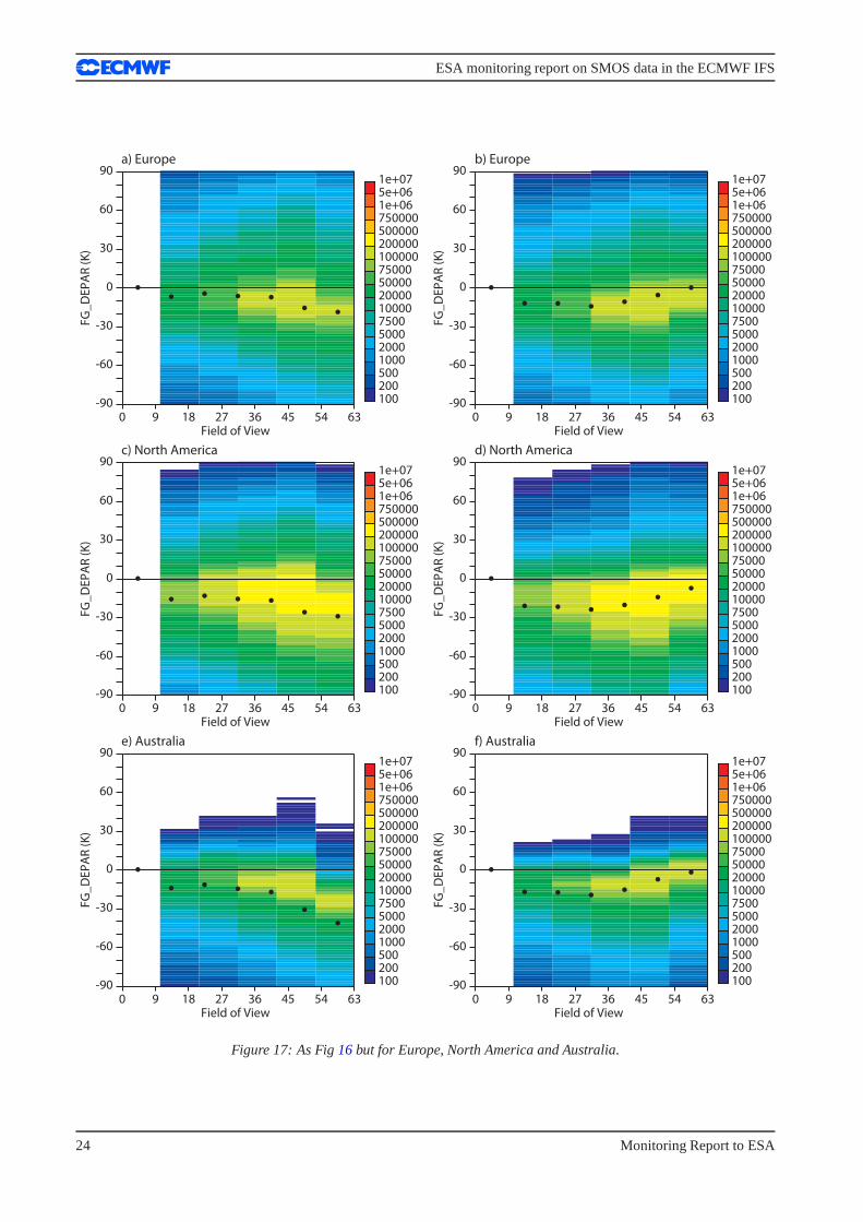
In section3.3an analysis of the bias was given at 40 degrees incidence angle. However the results presented canconsiderably change depending on the viewing angle. The most recent product incorporated in the ECMWFmonitoring suite was the angular distribution of bias (named as ’scatter plots’ in the website). In the case ofSMOS they are important, as they provide a good insight into the bias as a function of the incidence angle. Thissection summarizes the averaged results obtained for 3 months of data, from August 2011 to the end of October2011.
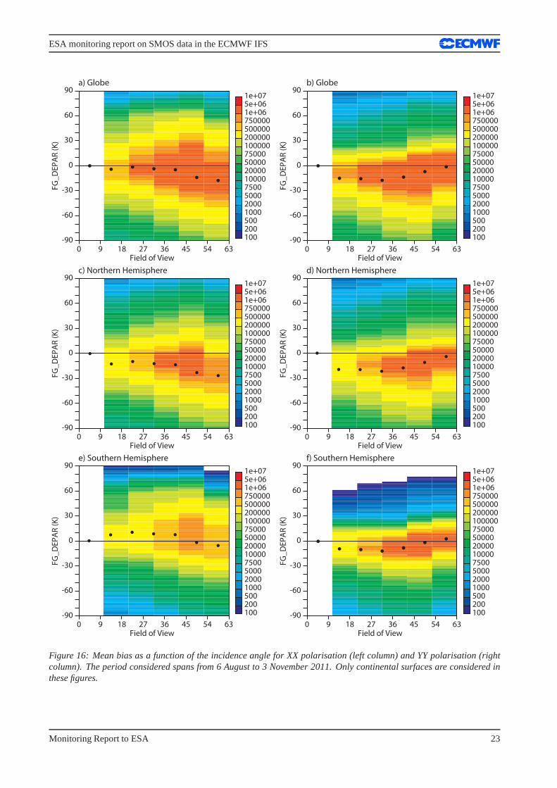
Fig. 16 presents the time and spatial averaged bias as a function of the incidence angle, at global scale for theNorthern and Southern Hemispheres, and for XX and YY polarisations. Fig.17 presents the angular distri-bution of bias for some regions: Europe, North America and Australia. The coloured scale bar refers to thenumber of observations within each level of bias. It is easily noticeable that the number of observations inFig. 16 is much larger than in Fig.17, especially near the zero bias, because the areas over whichstatistics arecomputed are much larger. At global scale the number of observations accounted for in these plots is greaterthan 254 millions, 146 millions for the Northern Hemisphereand 107 millions for the Southern Hemisphere,respectively. This gives an idea on the large number of observations obtained with SMOS, this despite that onlyobservations whose incidence angles are multiples of 10 areincluded in these plots.
It is shown that, independently of the area shown, for YY polarisation the mean bias keeps the same trend asa function of the incidence angle. In this case they are maximum at 30 degrees (around -20 K) and minimumat 60 degrees (close to zero). For XX polarisation it is more dependent on the geographical area. The reason islikely the contamination by RFI sources. For example, in Fig. 16 it is observed that the relation between meanbias and incidence angle is very different for the Northern and Southern Hemispheres at the XX polarisation.However, the trend is increasing bias (in absolute value) with increasing incidence angle, being in most of thecases maximum at 60 degrees. In the case of Australia the biasare especially significant at 60 degrees for XXpolarisation. In this case it is observed that very few departures are found greater than 20 K, whereas theycan be as negative as -90 K. A good fraction of Australia is covered by deserts and many other pixels have asignificant fraction of bare soil. The influence of the soil roughness on the simulated brightness temperaturesis especially important here, and the CMEM current parameterisation of the roughness model will be revisedaccordingly.
From these figures it is observed that for both polarisationsthere are also a significant number of observationswith large first-guess departures. These are mainly due to RFI sources, but they are not the only reason asexplained in (Sabater et al. 2011b).
22 Monitoring Report to ESA
ESA monitoring report on SMOS data in the ECMWF IFS
-90
-60
-30
0
30
60
90
FG
_D
EP
AR
(K
)
1890 27 36 45 54 63Field of View
1002005001000200050007500100002000050000750001000002000005000007500001e+065e+061e+07
a) Globe
-90
-60
-30
0
30
60
90
FG
_D
EP
AR
(K
)
1890 27 36 45 54 63Field of View
1002005001000200050007500100002000050000750001000002000005000007500001e+065e+061e+07
b) Globe
-90
-60
-30
0
30
60
90
FG
_D
EP
AR
(K
)
1890 27 36 45 54 63Field of View
1002005001000200050007500100002000050000750001000002000005000007500001e+065e+061e+07
c) Northern Hemisphere
-90
-60
-30
0
30
60
90F
G_
DE
PA
R (
K)
1890 27 36 45 54 63Field of View
1002005001000200050007500100002000050000750001000002000005000007500001e+065e+061e+07
d) Northern Hemisphere
-90
-60
-30
0
30
60
90
FG
_D
EP
AR
(K
)
1890 27 36 45 54 63Field of View
1002005001000200050007500100002000050000750001000002000005000007500001e+065e+061e+07
e) Southern Hemisphere
-90
-60
-30
0
30
60
90
FG
_D
EP
AR
(K
)
1890 27 36 45 54 63Field of View
1002005001000200050007500100002000050000750001000002000005000007500001e+065e+061e+07
f) Southern Hemisphere
Figure 16: Mean bias as a function of the incidence angle for XX polarisation (left column) and YY polarisation (rightcolumn). The period considered spans from 6 August to 3 November 2011. Only continental surfaces are considered inthese figures.
Monitoring Report to ESA 23
ESA monitoring report on SMOS data in the ECMWF IFS
-90
-60
-30
0
30
60
90
FG
_D
EP
AR
(K
)
1890 27 36 45 54 63Field of View
1002005001000200050007500100002000050000750001000002000005000007500001e+065e+061e+07
a) Europe
-90
-60
-30
0
30
60
90
FG
_D
EP
AR
(K
)
1890 27 36 45 54 63Field of View
1002005001000200050007500100002000050000750001000002000005000007500001e+065e+061e+07
b) Europe
-90
-60
-30
0
30
60
90
FG
_D
EP
AR
(K
)
1890 27 36 45 54 63Field of View
1002005001000200050007500100002000050000750001000002000005000007500001e+065e+061e+07
c) North America
-90
-60
-30
0
30
60
90
FG
_D
EP
AR
(K
)
1890 27 36 45 54 63Field of View
1002005001000200050007500100002000050000750001000002000005000007500001e+065e+061e+07
d) North America
-90
-60
-30
0
30
60
90
FG
_D
EP
AR
(K
)
1890 27 36 45 54 63Field of View
1002005001000200050007500100002000050000750001000002000005000007500001e+065e+061e+07
e) Australia
-90
-60
-30
0
30
60
90
FG
_D
EP
AR
(K
)
1890 27 36 45 54 63Field of View
1002005001000200050007500100002000050000750001000002000005000007500001e+065e+061e+07
f) Australia
Figure 17: As Fig16but for Europe, North America and Australia.
24 Monitoring Report to ESA
ESA monitoring report on SMOS data in the ECMWF IFS
3.5 Hovmoller plots
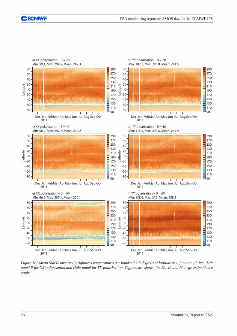
Hovmoller plots produce one mean value averaged per predefined band of latitudes as a function of time. Sothey provide a latitudinal-temporal perspective of several statistical variables and thus, they make it possible toanalyse the seasonal evolution of averaged values per latitude band. Punctual problems in the data that couldbe unnoticed in time-averaged geographical plots can be easy identified in these plots.
In Fig. 18 the evolution of the averaged brightness temperatures per band of 2.5 degrees of latitude are shownfor one year (November 2010 - November 2011). The seasonal evolution of brightness temperatures per bandof latitude is clearly shown for both polarisations, increasing towards the Northern Hemisphere from May untilAugust and increasing in the Southern Hemisphere the rest ofthe year. Maximum values are always obtainedin the tropics. A strong difference is observed in the mean brightness temperatures between 20 and 60 degreesincidence angles, with a mean difference for both polarisations of about 20 K.
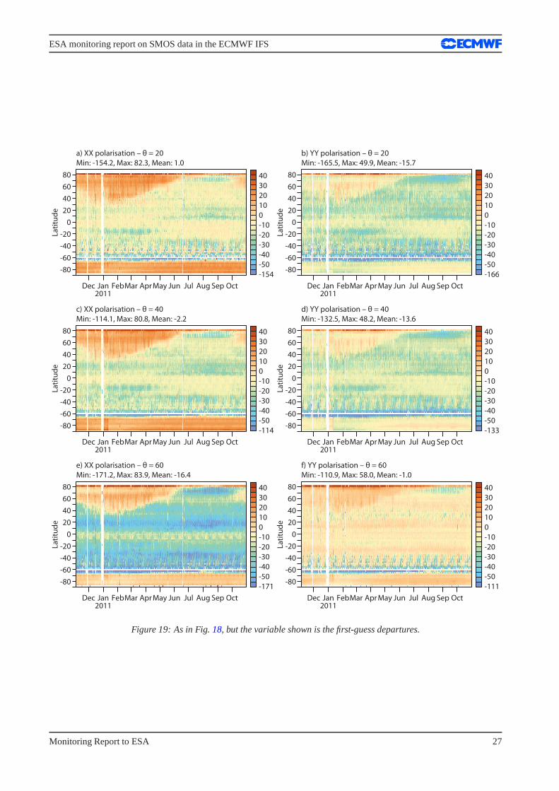
First-guess departures are presented in Fig.19. The area covered by snow is clearly seen in the XX polarisation,as the emission over snow is currently strongly underestimated, so large departures are obtained in this zone.It is observed that the maximum of snow cover is obtained between mid January and mid February, with snowdown to 30 degrees North. At 60 degrees incidence angle, the model clearly overestimates the observationsfor XX polarisation, except the areas around the Equator where the model is much closer to the observations.This is likely due to a current accurate representation of dense vegetated canopies. The white line around 60degrees South is due to the absence of land points. The emission over the poles is also underestimated for bothpolarisations and all incidence angles.
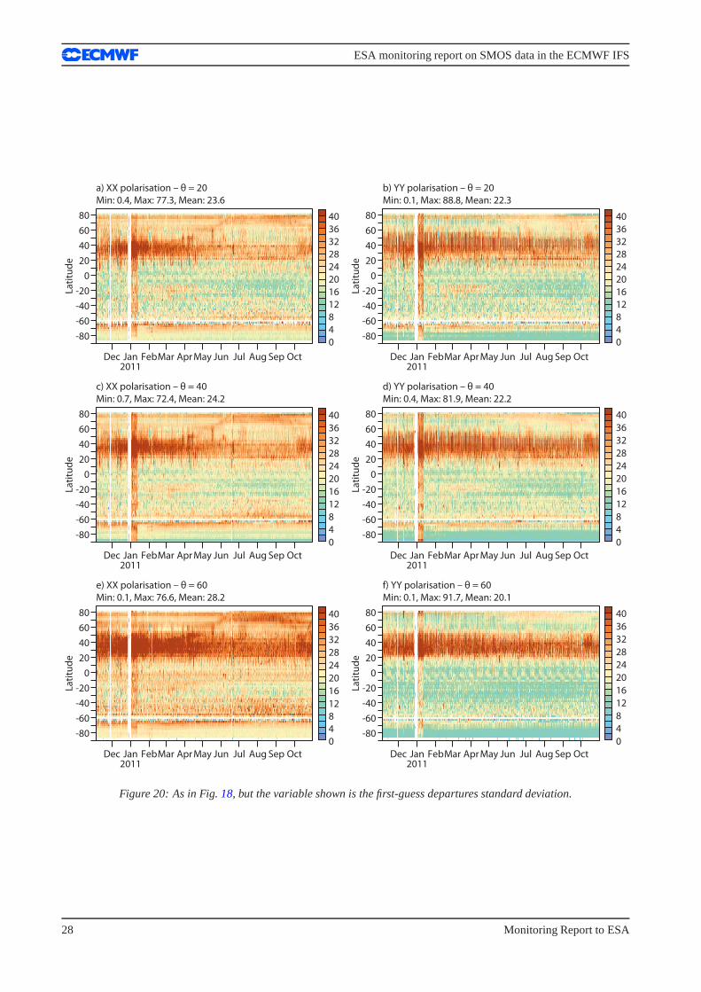
The contamination produced by intermittent sources of RFI are clearly seen in Fig.20. This figure shows thestandard deviation of the first-guess departures. A red, non-uniform strip, corresponding to large variability ofthe first-guess departures is observed between 20 and 40 degrees North. They are mainly caused by RFI. How-ever, they are not the only reason causing these large departures, also the presence of snow and ice contributes.In the time series plots (section3.3) a larger variability of the observed brightness temperatures over snow andice covered areas was observed, which increases the variability of the bias. For example, in the XX polari-sation it is clearly seen that the first-guess departures standard deviation is lower between 20 and 40 degreesNorth during the Boreal summer months. Likewise, at 60 degrees incidence angle for XX polarisation, largerdepartures between 45 and 55 degrees South are observed, very likely due to the presence of the Patagonian icesheet.
Monitoring Report to ESA 25
ESA monitoring report on SMOS data in the ECMWF IFS
-80
-60
-40
-20
0
20
40
60
80
La
titu
de
Dec Jan FebMar Apr May Jun Jul Aug Sep Oct2011
90
110
130
150
170
190
210
230
250
270
290
a) XX polarisation – θ = 20
Min: 99.4, Max: 294.5, Mean: 242.3
-80
-60
-40
-20
0
20
40
60
80
La
titu
de
Dec Jan FebMar Apr May Jun Jul Aug Sep Oct2011
90
110
130
150
170
190
210
230
250
270
290
b) YY polarisation – θ = 20
Min: 102.7, Max: 295.8, Mean: 241.5
-80
-60
-40
-20
0
20
40
60
80
La
titu
de
Dec Jan FebMar Apr May Jun Jul Aug Sep Oct2011
90
110
130
150
170
190
210
230
250
270
290
c) XX polarisation – θ = 40
Min: 96.2, Max: 292.2, Mean: 238.2
-80
-60
-40
-20
0
20
40
60
80
La
titu
de
Dec Jan FebMar Apr May Jun Jul Aug Sep Oct2011
90
110
130
150
170
190
210
230
250
270
290
d) YY polarisation – θ = 40
Min: 115.4, Max: 298.6, Mean: 244.9
-80
-60
-40
-20
0
20
40
60
80
La
titu
de
Dec Jan FebMar Apr May Jun Jul Aug Sep Oct2011
90
110
130
150
170
190
210
230
250
270
290
e) XX polarisation – θ = 60
Min: 66.9, Max: 280.1, Mean: 220.1
-80
-60
-40
-20
0
20
40
60
80
La
titu
de
Dec Jan FebMar Apr May Jun Jul Aug Sep Oct2011
90
110
130
150
170
190
210
230
250
270
290
f) YY polarisation – θ = 60
Min: 138.6, Max: 316, Mean: 258.6
Figure 18: Mean SMOS observed brightness temperatures per bands of 2.5 degrees of latitude as a function of time. Leftpanel if for XX polarisation and right panel for YY polarisation. Figures are shown for 20, 40 and 60 degrees incidenceangle.
26 Monitoring Report to ESA
ESA monitoring report on SMOS data in the ECMWF IFS
-80
-60
-40
-20
0
20
40
60
80
La
titu
de
Dec Jan FebMar Apr May Jun Jul Aug Sep Oct2011
a) XX polarisation – θ = 20
Min: -154.2, Max: 82.3, Mean: 1.0
-80
-60
-40
-20
0
20
40
60
80
La
titu
de
Dec Jan FebMar Apr May Jun Jul Aug Sep Oct2011
b) YY polarisation – θ = 20
Min: -165.5, Max: 49.9, Mean: -15.7
-80
-60
-40
-20
0
20
40
60
80
La
titu
de
Dec Jan FebMar Apr May Jun Jul Aug Sep Oct2011
c) XX polarisation – θ = 40
Min: -114.1, Max: 80.8, Mean: -2.2
-80
-60
-40
-20
0
20
40
60
80
La
titu
de
Dec Jan FebMar Apr May Jun Jul Aug Sep Oct2011
d) YY polarisation – θ = 40
Min: -132.5, Max: 48.2, Mean: -13.6
-80
-60
-40
-20
0
20
40
60
80
La
titu
de
Dec Jan FebMar Apr May Jun Jul Aug Sep Oct2011
e) XX polarisation – θ = 60
Min: -171.2, Max: 83.9, Mean: -16.4
-80
-60
-40
-20
0
20
40
60
80
La
titu
de
Dec Jan FebMar Apr May Jun Jul Aug Sep Oct2011
f) YY polarisation – θ = 60
Min: -110.9, Max: 58.0, Mean: -1.0
-154
-50
-40
-30
-20
-10
0
10
20
30
40
-114
-50
-40
-30
-20
-10
0
10
20
30
40
-171
-50
-40
-30
-20
-10
0
10
20
30
40
-166
-50
-40
-30
-20
-10
0
10
20
30
40
-133
-50
-40
-30
-20
-10
0
10
20
30
40
-111
-50
-40
-30
-20
-10
0
10
20
30
40
Figure 19: As in Fig.18, but the variable shown is the first-guess departures.
Monitoring Report to ESA 27
ESA monitoring report on SMOS data in the ECMWF IFS
-80
-60
-40
-20
0
20
40
60
80
La
titu
de
Dec Jan FebMar Apr May Jun Jul Aug Sep Oct2011
a) XX polarisation – θ = 20
Min: 0.4, Max: 77.3, Mean: 23.6
-80
-60
-40
-20
0
20
40
60
80
La
titu
de
Dec Jan FebMar Apr May Jun Jul Aug Sep Oct2011
b) YY polarisation – θ = 20
Min: 0.1, Max: 88.8, Mean: 22.3
-80
-60
-40
-20
0
20
40
60
80
La
titu
de
Dec Jan FebMar Apr May Jun Jul Aug Sep Oct2011
c) XX polarisation – θ = 40
Min: 0.7, Max: 72.4, Mean: 24.2
-80
-60
-40
-20
0
20
40
60
80
La
titu
de
Dec Jan FebMar Apr May Jun Jul Aug Sep Oct2011
d) YY polarisation – θ = 40
Min: 0.4, Max: 81.9, Mean: 22.2
-80
-60
-40
-20
0
20
40
60
80
La
titu
de
Dec Jan FebMar Apr May Jun Jul Aug Sep Oct2011
e) XX polarisation – θ = 60
Min: 0.1, Max: 76.6, Mean: 28.2
-80
-60
-40
-20
0
20
40
60
80
La
titu
de
Dec Jan FebMar Apr May Jun Jul Aug Sep Oct2011
f) YY polarisation – θ = 60
Min: 0.1, Max: 91.7, Mean: 20.1
0
4
8
12
16
20
24
28
32
36
40
0
4
8
12
16
20
24
28
32
36
40
0
4
8
12
16
20
24
28
32
36
40
0
4
8
12
16
20
24
28
32
36
40
0
4
8
12
16
20
24
28
32
36
40
0
4
8
12
16
20
24
28
32
36
40
Figure 20: As in Fig.18, but the variable shown is the first-guess departures standard deviation.
28 Monitoring Report to ESA
ESA monitoring report on SMOS data in the ECMWF IFS
4 Monitoring over ocean
In this section some of the more relevant results obtained with the monitoring suite [see a description in part IIIof (Sabater et al. 2010) and (Sabater et al. 2011b)] over oceans are presented.
4.1 Simulations of brightness temperatures
The SMOS monitoring suite developed at ECMWF (Sabater et al. 2010) produces daily statistics not only forcontinental surfaces, but also for oceans. The CMEM forwardoperator introduced in section3.1is also used tosimulate brightness temperatures over oceans surfaces. The emissivity over oceans in the L-band is currentlymodelled in CMEM in a very simple way. It considers the ocean as a smooth surface, the influence of thewind and the galactic noise are not accounted for. For the dielectric constant computation, a difference is donebetween liquid water or pure ice. As effective temperature,the sea surface temperature is used.Thus, the results presented from figures21 to 35 should be considered as preliminary. A future implemen-tation of the roughness and galactic noise contributions tothe total brightness temperatures at the top of theatmosphere will make it possible to get more robust conclusions over oceans.
Monitoring Report to ESA 29
ESA monitoring report on SMOS data in the ECMWF IFS
4.2 Time-averaged geographical mean fields.
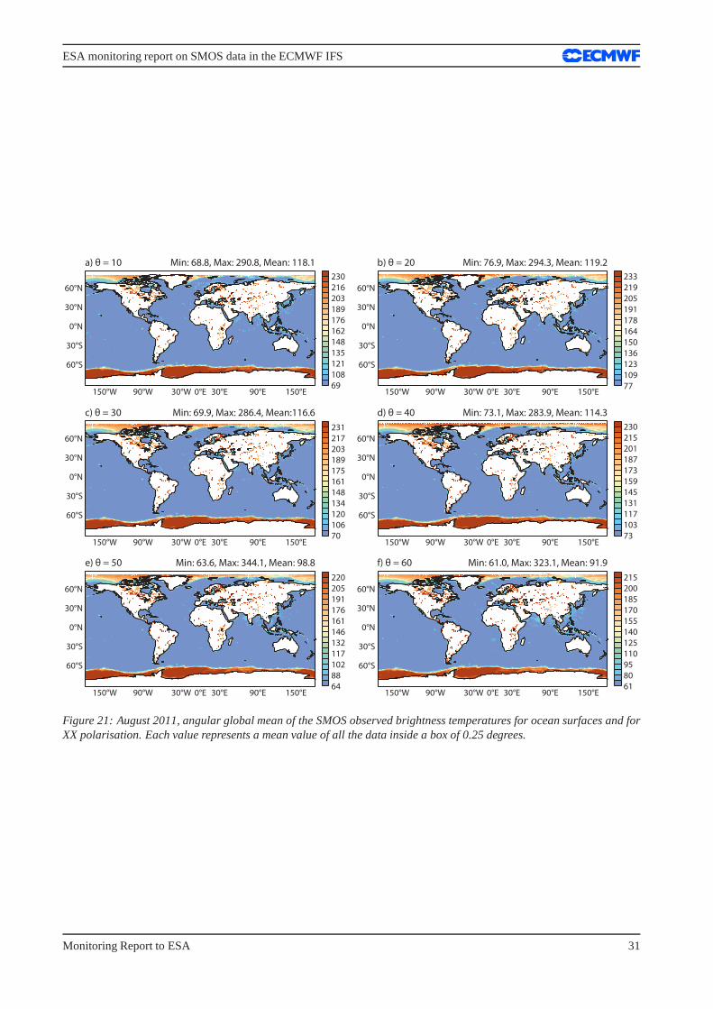
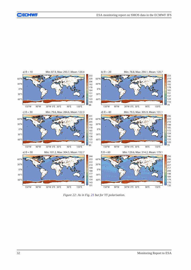
Fig. 21 and Fig.22 show the averaged brightness temperatures over ocean surfaces as a function of incidenceangle for August 2011 and for XX polarisation (Fig.21) and YY polarisation (Fig.22). Each value representsa mean value in boxes of 0.25 degrees. As it occurs over continental surfaces, brightness temperatures increasewith the incidence angle for YY polarisation and decrease for XX polarisation, with values notably lower thanover land, on average 120 K lower for August 2011. The YY polarisation has a larger angular dynamical range,of about 30 K larger in average than the XX polarisation between 20 and 60 degrees. August is a winter monthat the Southern Hemisphere and around the Antarctica the ocean is frozen. This is clearly seen in these figuresas the emissivity is much larger, and therefore the observedbrightness temperatures. Also for the North Polebrightness temperatures are significantly larger. Given that oceans are much more homogeneous than continen-tal surfaces, the map of brightness temperatures over oceans are relatively homogeneous in comparison to landsurfaces. Large inland water bodies (mainly lakes) are alsoclearly visible. For August 2011 the CMEM modellargely overestimates the brightness temperatures over lakes.
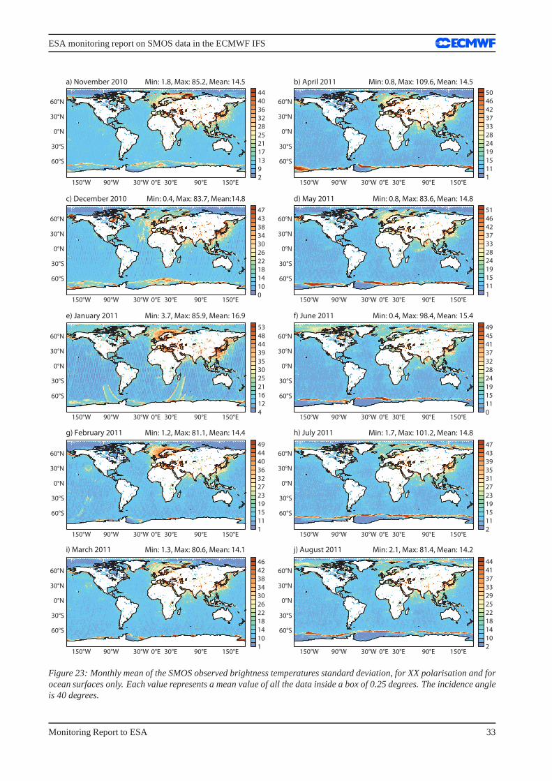
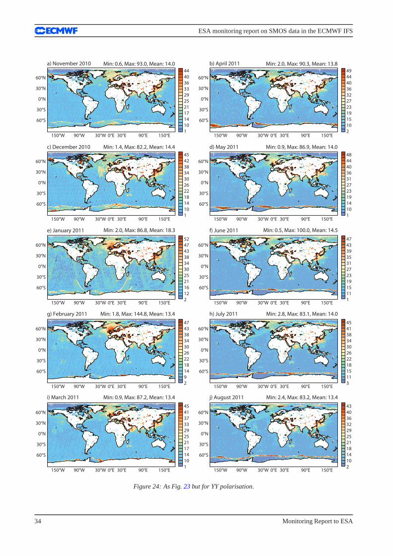
The evolution of the SMOS observed brightness temperaturesstandard deviation, from November 2010 toAugust 2011 (one averaged value per month), is shown in Fig.23. It is shown only at 40 degrees incidenceangle and for XX polarisation. Fig.24 is the equivalent figure for YY polarisation. The spatial sampling is0.25 degrees. The spatial monthly average of brightness temperatures standard deviation is more than 14 Kfor XX polarisation and slightly lower for YY polarisation.Anomalous large values are observed for January2011 which, as mentioned earlier in this report, are due to the degradation of the science data during the pe-riod following the thermal stability test of the instrumentat the end of 2010. These figures show clearly thecontamination of RFI land sources into the oceans. Near China, Middle East and Eastern European coastlinesthe standard deviation of brightness temperatures is very large, which is due to RFI. But RFI also affects areasmuch further from the coasts, although in a lesser extent. Especially interesting is the case of Europe. In bothpolarisations it can be observed that the progress made at shutting down illegal RFI sources in Europe has hada direct influence over oceans near the coasts. In the figure for August 2011 the Western European coastlineappears very clean in contrast to previous months where the RFI situation was still quite bad.The other interesting feature observed in these figures is the transition zone between frozen and liquid waterover Antarctica. Frozen and liquid water have very different dielectric properties, and therefore they presentvery different emissivities. As this is a very sensitive anddynamical zone, the variability of brightness temper-atures is very large. During the summer months at the Southern Hemisphere this transition zone can barely beobserved, or at least is very close to the Antarctica continent, whereas it moves far from the coastline duringthe winter months.
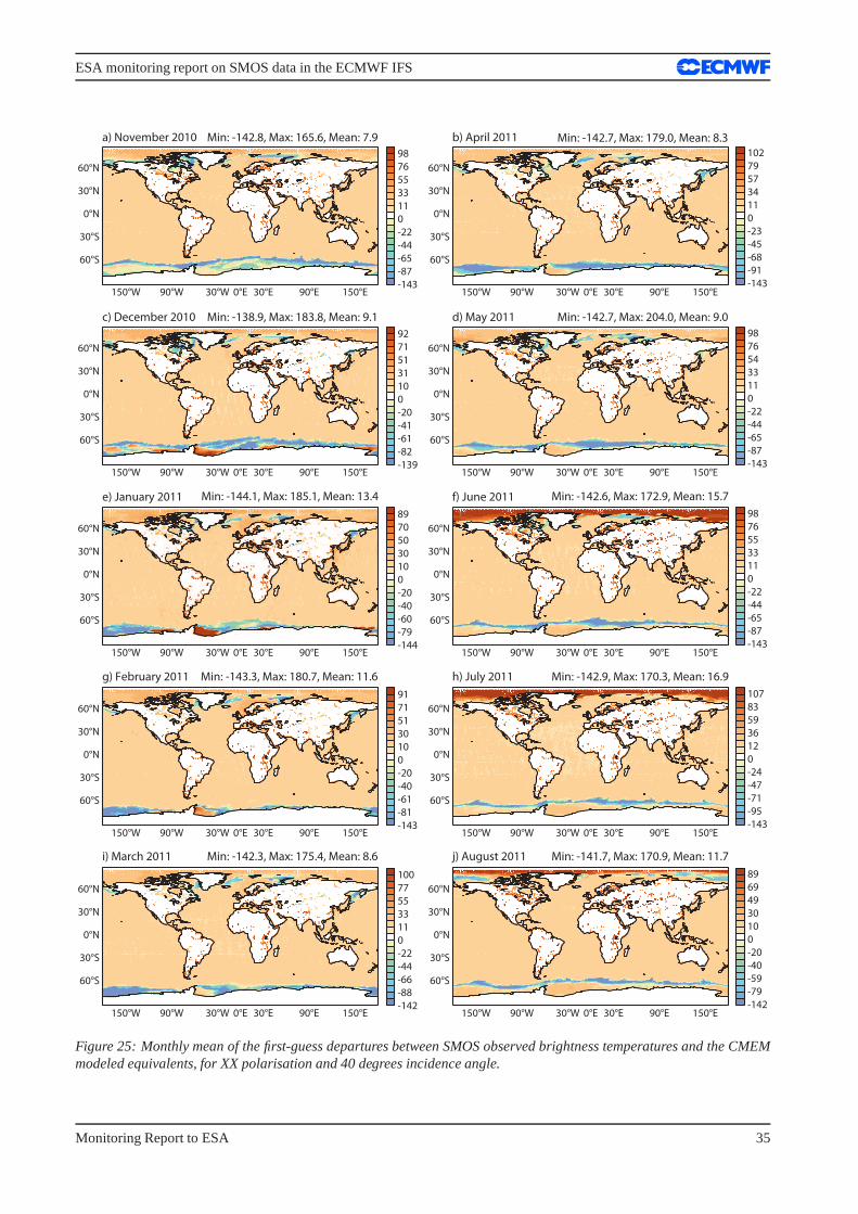
Figs.25 and26 show the evolution of the first-guess departures (observed brightness temperatures minus theCMEM model equivalents) over oceans, at the antenna reference frame from November 2010 to August 2011(one averaged value per month), at 40 degrees incidence angle, and for XX and YY polarisation, respectively.For the bulk of the oceans the first-guess departures look very systematic and they have a narrow dynamicalrange variability, lower than 10 K. They are quite constant for all months which is also partly a consequenceof the current limitations of the emission model over oceans. Simulated brightness temperatures are under-estimated for XX polarisation, slowly increasing in the North Hemisphere towards the summer months. Thesituation is just the opposite for YY polarisation, as the model systematically overestimates the observationsand the best spatial agreement is found in July 2011. Near thepoles, with frozen water and snow, the first-guessdepartures also have a very different behaviour.
30 Monitoring Report to ESA
ESA monitoring report on SMOS data in the ECMWF IFS
Min: 68.8, Max: 290.8, Mean: 118.1a) θ = 10 b) θ = 20
c) θ = 30 d) θ = 40
e) θ = 50 f) θ = 60
Min: 76.9, Max: 294.3, Mean: 119.2
Min: 69.9, Max: 286.4, Mean:116.6 Min: 73.1, Max: 283.9, Mean: 114.3
Min: 63.6, Max: 344.1, Mean: 98.8 Min: 61.0, Max: 323.1, Mean: 91.9
60°N
30°N
0°N
30°S
60°S
150°E90°E30°E0°E30°W90°W150°W
60°N
30°N
0°N
30°S
60°S
150°E90°E30°E0°E30°W90°W150°W
60°N
30°N
0°N
30°S
60°S
150°E90°E30°E0°E30°W90°W150°W
60°N
30°N
0°N
30°S
60°S
150°E90°E30°E0°E30°W90°W150°W
60°N
30°N
0°N
30°S
60°S
150°E90°E30°E0°E30°W90°W150°W
60°N
30°N
0°N
30°S
60°S
150°E90°E30°E0°E30°W90°W150°W
69
108
121
135
148
162
176
189
203
216
230
77
109
123
136
150
164
178
191
205
219
233
70
106
120
134
148
161
175
189
203
217
231
73
103
117
131
145
159
173
187
201
215
230
64
88
102
117
132
146
161
176
191
205
220
61
80
95
110
125
140
155
170
185
200
215
Figure 21: August 2011, angular global mean of the SMOS observed brightness temperatures for ocean surfaces and forXX polarisation. Each value represents a mean value of all the data inside a box of 0.25 degrees.
Monitoring Report to ESA 31
ESA monitoring report on SMOS data in the ECMWF IFS
Min: 87.9, Max: 293.7, Mean: 120.4a) θ = 10 b) θ = 20
c) θ = 30 d) θ = 40
e) θ = 50 f) θ = 60
Min: 78.8, Max: 294.1, Mean: 120.7
Min: 79.6, Max: 284.6, Mean: 122.3 Min: 79.3, Max: 305.9, Mean: 131.1
Min: 101.2, Max: 304.5, Mean: 152.7 Min: 129.6, Max: 314.2, Mean: 179.1
60°N
30°N
0°N
30°S
60°S
150°E90°E30°E0°E30°W90°W150°W
60°N
30°N
0°N
30°S
60°S
150°E90°E30°E0°E30°W90°W150°W
60°N
30°N
0°N
30°S
60°S
150°E90°E30°E0°E30°W90°W150°W
60°N
30°N
0°N
30°S
60°S
150°E90°E30°E0°E30°W90°W150°W
60°N
30°N
0°N
30°S
60°S
150°E90°E30°E0°E30°W90°W150°W
60°N
30°N
0°N
30°S
60°S
150°E90°E30°E0°E30°W90°W150°W
88
109
123
137
151
164
178
192
206
220
233
79
110
124
137
151
165
178
192
206
219
233
80
112
125
138
152
165
178
192
205
218
231
79
120
133
146
159
172
185
198
210
223
236
101
143
154
165
177
188
199
210
222
233
244
130
170
179
189
198
208
217
227
237
246
256
Figure 22: As in Fig.21but for YY polarisation.
32 Monitoring Report to ESA
ESA monitoring report on SMOS data in the ECMWF IFS
Min: 1.8, Max: 85.2, Mean: 14.5a) November 2010 b) April 2011
c) December 2010 d) May 2011
e) January 2011 f) June 2011
g) February 2011 h) July 2011
i) March 2011 j) August 2011
Min: 0.8, Max: 109.6, Mean: 14.5
Min: 0.4, Max: 83.7, Mean:14.8 Min: 0.8, Max: 83.6, Mean: 14.8
Min: 3.7, Max: 85.9, Mean: 16.9 Min: 0.4, Max: 98.4, Mean: 15.4
Min: 1.2, Max: 81.1, Mean: 14.4 Min: 1.7, Max: 101.2, Mean: 14.8
Min: 1.3, Max: 80.6, Mean: 14.1 Min: 2.1, Max: 81.4, Mean: 14.2
60°N
30°N
0°N
30°S
60°S
150°E90°E30°E0°E30°W90°W150°W
60°N
30°N
0°N
30°S
60°S
150°E90°E30°E0°E30°W90°W150°W
60°N
30°N
0°N
30°S
60°S
150°E90°E30°E0°E30°W90°W150°W
60°N
30°N
0°N
30°S
60°S
150°E90°E30°E0°E30°W90°W150°W
60°N
30°N
0°N
30°S
60°S
150°E90°E30°E0°E30°W90°W150°W
60°N
30°N
0°N
30°S
60°S
150°E90°E30°E0°E30°W90°W150°W
60°N
30°N
0°N
30°S
60°S
150°E90°E30°E0°E30°W90°W150°W
60°N
30°N
0°N
30°S
60°S
150°E90°E30°E0°E30°W90°W150°W
60°N
30°N
0°N
30°S
60°S
150°E90°E30°E0°E30°W90°W150°W
60°N
30°N
0°N
30°S
60°S
150°E90°E30°E0°E30°W90°W150°W
2
9
13
17
21
25
28
32
36
40
44
1
11
15
19
24
28
33
37
42
46
50
0
10
14
18
22
26
30
34
38
43
47
1
11
15
19
24
28
33
37
42
46
51
4
12
16
21
25
30
35
39
44
48
53
0
11
15
19
24
28
32
37
41
45
49
1
11
15
19
23
27
32
36
40
44
49
2
11
15
19
23
27
31
35
39
43
47
1
10
14
18
22
26
30
34
38
42
46
2
10
14
18
22
25
29
33
37
41
44
Figure 23: Monthly mean of the SMOS observed brightness temperatures standard deviation, for XX polarisation and forocean surfaces only. Each value represents a mean value of all the data inside a box of 0.25 degrees. The incidence angleis 40 degrees.
Monitoring Report to ESA 33
ESA monitoring report on SMOS data in the ECMWF IFS
a) November 2010 b) April 2011
c) December 2010 d) May 2011
e) January 2011 f) June 2011
g) February 2011 h) July 2011
i) March 2011 j) August 2011
60°N
30°N
0°N
30°S
60°S
150°E90°E30°E0°E30°W90°W150°W
60°N
30°N
0°N
30°S
60°S
150°E90°E30°E0°E30°W90°W150°W
60°N
30°N
0°N
30°S
60°S
150°E90°E30°E0°E30°W90°W150°W
60°N
30°N
0°N
30°S
60°S
150°E90°E30°E0°E30°W90°W150°W
60°N
30°N
0°N
30°S
60°S
150°E90°E30°E0°E30°W90°W150°W
60°N
30°N
0°N
30°S
60°S
150°E90°E30°E0°E30°W90°W150°W
60°N
30°N
0°N
30°S
60°S
150°E90°E30°E0°E30°W90°W150°W
60°N
30°N
0°N
30°S
60°S
150°E90°E30°E0°E30°W90°W150°W
60°N
30°N
0°N
30°S
60°S
150°E90°E30°E0°E30°W90°W150°W
60°N
30°N
0°N
30°S
60°S
150°E90°E30°E0°E30°W90°W150°W
Min: 0.6, Max: 93.0, Mean: 14.0 Min: 2.0, Max: 90.3, Mean: 13.8
Min: 1.4, Max: 82.2, Mean: 14.4 Min: 0.9, Max: 86.9, Mean: 14.0
Min: 2.0, Max: 86.8, Mean: 18.3 Min: 0.5, Max: 100.0, Mean: 14.5
Min: 1.8, Max: 144.8, Mean: 13.4 Min: 2.8, Max: 83.1, Mean: 14.0
Min: 0.9, Max: 87.2, Mean: 13.4 Min: 2.4, Max: 83.2, Mean: 13.4
1
10
14
17
21
25
29
33
36
40
44
2
10
15
19
23
27
32
36
40
44
49
1
10
14
18
22
26
30
34
38
42
45
1
10
14
19
23
27
31
36
40
44
48
2
12
16
21
25
30
34
38
43
47
52
1
11
15
19
23
27
31
35
39
43
47
2
9
14
18
22
26
30
34
38
43
47
3
11
15
18
22
26
30
34
38
41
45
1
10
14
17
21
25
29
33
37
41
45
2
10
14
18
21
25
29
32
36
40
43
Figure 24: As Fig.23but for YY polarisation.
34 Monitoring Report to ESA
ESA monitoring report on SMOS data in the ECMWF IFS
a) November 2010 b) April 2011
c) December 2010 d) May 2011
e) January 2011 f) June 2011
g) February 2011 h) July 2011
i) March 2011 j) August 2011
60°N
30°N
0°N
30°S
60°S
150°E90°E30°E0°E30°W90°W150°W
60°N
30°N
0°N
30°S
60°S
150°E90°E30°E0°E30°W90°W150°W
60°N
30°N
0°N
30°S
60°S
150°E90°E30°E0°E30°W90°W150°W
60°N
30°N
0°N
30°S
60°S
150°E90°E30°E0°E30°W90°W150°W
60°N
30°N
0°N
30°S
60°S
150°E90°E30°E0°E30°W90°W150°W
60°N
30°N
0°N
30°S
60°S
150°E90°E30°E0°E30°W90°W150°W
60°N
30°N
0°N
30°S
60°S
150°E90°E30°E0°E30°W90°W150°W
60°N
30°N
0°N
30°S
60°S
150°E90°E30°E0°E30°W90°W150°W
60°N
30°N
0°N
30°S
60°S
150°E90°E30°E0°E30°W90°W150°W
60°N
30°N
0°N
30°S
60°S
150°E90°E30°E0°E30°W90°W150°W
Min: -142.8, Max: 165.6, Mean: 7.9 Min: -142.7, Max: 179.0, Mean: 8.3
Min: -138.9, Max: 183.8, Mean: 9.1 Min: -142.7, Max: 204.0, Mean: 9.0
Min: -144.1, Max: 185.1, Mean: 13.4 Min: -142.6, Max: 172.9, Mean: 15.7
Min: -143.3, Max: 180.7, Mean: 11.6 Min: -142.9, Max: 170.3, Mean: 16.9
Min: -142.3, Max: 175.4, Mean: 8.6 Min: -141.7, Max: 170.9, Mean: 11.7
-143
-87
-65
-44
-22
0
11
33
55
76
98
-143
-91
-68
-45
-23
0
11
34
57
79
102
-139
-82
-61
-41
-20
0
10
31
51
71
92
-143
-87
-65
-44
-22
0
11
33
54
76
98
-144
-79
-60
-40
-20
0
10
30
50
70
89
-143
-87
-65
-44
-22
0
11
33
55
76
98
-143
-81
-61
-40
-20
0
10
30
51
71
91
-143
-95
-71
-47
-24
0
12
36
59
83
107
-142
-88
-66
-44
-22
0
11
33
55
77
100
-142
-79
-59
-40
-20
0
10
30
49
69
89
Figure 25: Monthly mean of the first-guess departures between SMOS observed brightness temperatures and the CMEMmodeled equivalents, for XX polarisation and 40 degrees incidence angle.
Monitoring Report to ESA 35
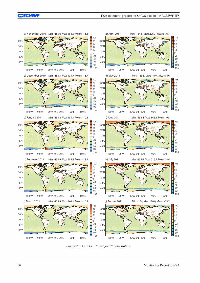
ESA monitoring report on SMOS data in the ECMWF IFS
Min: -155.6, Max: 151.5, Mean: -16.8a) November 2010 b) April 2011
c) December 2010 d) May 2011
e) January 2011 f) June 2011
g) February 2011 h) July 2011
i) March 2011 j) August 2011
Min: -154.6, Max: 206.7, Mean: -16.7
Min: -153.3, Max: 134.7, Mean: -15.7 Min: -153.8, Max: 140.4, Mean: -16
Min: -153.4, Max: 154.1, Mean: -10.3 Min: -154.4, Max: 146.3, Mean: -9.5
Min: -153.9, Max: 185.4, Mean: -13.7 Min: -153.6, Max: 216.7, Mean: -8.4
Min: -154, Max: 186.6, Mean: -13.2Min: -153.9, Max: 161.1, Mean: -16.3
60°N
30°N
0°N
30°S
60°S
150°E90°E30°E0°E30°W90°W150°W
60°N
30°N
0°N
30°S
60°S
150°E90°E30°E0°E30°W90°W150°W
60°N
30°N
0°N
30°S
60°S
150°E90°E30°E0°E30°W90°W150°W
60°N
30°N
0°N
30°S
60°S
150°E90°E30°E0°E30°W90°W150°W
60°N
30°N
0°N
30°S
60°S
150°E90°E30°E0°E30°W90°W150°W
60°N
30°N
0°N
30°S
60°S
150°E90°E30°E0°E30°W90°W150°W
60°N
30°N
0°N
30°S
60°S
150°E90°E30°E0°E30°W90°W150°W
60°N
30°N
0°N
30°S
60°S
150°E90°E30°E0°E30°W90°W150°W
60°N
30°N
0°N
30°S
60°S
150°E90°E30°E0°E30°W90°W150°W
60°N
30°N
0°N
30°S
60°S
150°E90°E30°E0°E30°W90°W150°W
-156
-96
-72
-48
-24
0
12
36
60
84
108
-155
-100
-75
-50
-25
0
12
37
62
87
112
-153
-90
-68
-45
-23
0
11
34
56
79
102
-154
-96
-72
-48
-24
0
12
36
60
84
108
-153
-89
-66
-44
-22
0
11
33
55
78
100
-154
-97
-73
-49
-24
0
12
36
61
85
109
-154
-91
-68
-45
-23
0
11
34
57
79
102
-154
-92
-69
-46
-23
0
12
35
58
81
104
-154
-97
-73
-49
-24
0
12
37
61
85
110
-154
-89
-66
-44
-22
0
11
33
55
77
100
Figure 26: As in Fig.25but for YY polarisation.
36 Monitoring Report to ESA
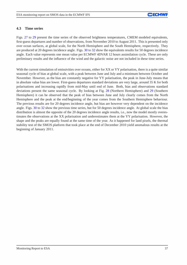
ESA monitoring report on SMOS data in the ECMWF IFS
4.3 Time series
Figs.27 to 29 present the time series of the observed brightness temperatures, CMEM modeled equivalents,first-guess departures and number of observations, from November 2010 to August 2011. This is presented onlyover ocean surfaces, at global scale, for the North Hemisphere and the South Hemisphere, respectively. Theyare produced at 20 degrees incidence angle. Figs.30to 32show the equivalents results for 50 degrees incidenceangle. Each value represents one mean value per ECMWF 4DVAR 12 hours assimilation cycle. These are onlypreliminary results and the influence of the wind and the galactic noise are not included in these time series.
With the current simulation of emissivities over oceans, either for XX or YY polarisation, there is a quite similarseasonal cycle of bias at global scale, with a peak between June and July and a minimum between October andNovember. However, as the bias are constantly negative for YY polarisation, the peak in June-July means thatin absolute value bias are lower. First-guess departures standard deviations are very large, around 35 K for bothpolarisations and increasing rapidly from mid-May until end of June. Both, bias and observations standarddeviations present the same seasonal cycle. By looking at Fig. 28 (Northern Hemisphere) and29 (SouthernHemisphere) it can be observed that the peak of bias between June and July clearly comes from the NorthHemisphere and the peak at the end/beginning of the year comes from the Southern Hemisphere behaviour.The previous results are for 20 degrees incidence angle, butbias are however very dependent on the incidenceangle. Figs.30 to 32show the previous time series, but for 50 degrees incidence angle. At global scale the biasdistribution is almost the opposite of the 20 degrees incidence angle results, i.e., now the model mostly overes-timates the observations at the XX polarisation and underestimates them at the YY polarisation. However, theshape and the peaks are equally found at the same time of the year. As it happened for land pixels, the thermalstability test of the SMOS platform that took place at the endof December 2010 yield anomalous results at thebeginning of January 2011.
Monitoring Report to ESA 37
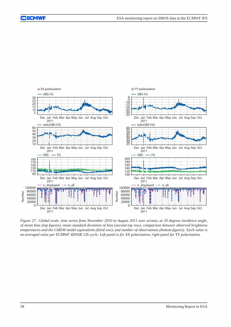
ESA monitoring report on SMOS data in the ECMWF IFS
1015
5
202530
102030405060
90110130150170190
0 20000 40000 60000 80000
100000
-30-35
-25-20-15-10
-50
404550
253035
5560
100120140160180200
0 20000 40000 60000 80000
100000
a) XX polarisation
OBS-FG OBS-FG
b) YY polarisation
n_displayed n_all n_displayed n_all
OBS FG OBS FG
stdv(OBS-FG) stdv(OBS-FG)
Nu
mb
er
Nu
mb
er
Dec Jan Feb Mar Apr May Jun Jul OctSepAug2011
Dec Jan Feb Mar Apr May Jun Jul OctSepAug2011
Dec Jan Feb Mar Apr May Jun Jul OctSepAug2011
Dec Jan Feb Mar Apr May Jun Jul OctSepAug2011
Dec Jan Feb Mar Apr May Jun Jul OctSepAug2011
Dec Jan Feb Mar Apr May Jun Jul OctSepAug2011
Dec Jan Feb Mar Apr May Jun Jul OctSepAug2011
Dec Jan Feb Mar Apr May Jun Jul OctSepAug2011
Figure 27: Global scale, time series from November 2010 to August 2011 over oceans, at 20 degrees incidence angle,of mean bias (top figures), mean standard deviation of bias (second top row), comparison between observed brightnesstemperatures and the CMEM model equivalents (third row), and number of observations (bottom figures). Each value isan averaged value per ECMWF 4DVAR 12h cycle. Left panel is forXX polarisation, right panel for YY polarisation.
38 Monitoring Report to ESA
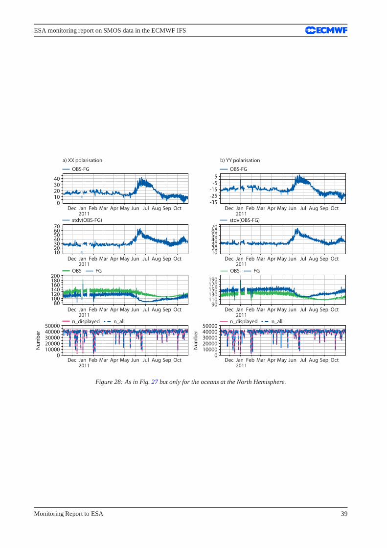
ESA monitoring report on SMOS data in the ECMWF IFS
010203040
10203040506070
80100120140160180200
0 10000 20000 30000 40000 50000
-35-25-15
-55
10203040506070
90110130150170190
0 10000 20000 30000 40000 50000
a) XX polarisation
OBS-FG OBS-FG
b) YY polarisation
n_displayed n_all n_displayed n_all
OBS FG OBS FG
Dec Jan Feb Mar Apr May Jun Jul OctSepAug2011
Dec Jan Feb Mar Apr May Jun Jul OctSepAug2011
Dec Jan Feb Mar Apr May Jun Jul OctSepAug2011
Dec Jan Feb Mar Apr May Jun Jul OctSepAug2011
Dec Jan Feb Mar Apr May Jun Jul OctSepAug2011
Dec Jan Feb Mar Apr May Jun Jul OctSepAug2011
Dec Jan Feb Mar Apr May Jun Jul OctSepAug2011
Dec Jan Feb Mar Apr May Jun Jul OctSepAug2011
stdv(OBS-FG) stdv(OBS-FG)
Nu
mb
er
Nu
mb
er
Figure 28: As in Fig.27but only for the oceans at the North Hemisphere.
Monitoring Report to ESA 39
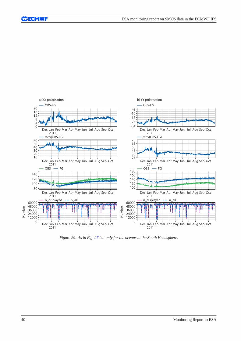
ESA monitoring report on SMOS data in the ECMWF IFS
048
121620
102030405060
80
100
120
140
0 12000 24000 36000 48000 60000
-34-26-18-10
-2
253545556575
100120140160180
0 12000 24000 36000 48000 60000
a) XX polarisation
OBS-FG OBS-FG
b) YY polarisation
n_displayed n_all n_displayed n_all
OBS FG OBS FG
Dec Jan Feb Mar Apr May Jun Jul OctSepAug2011
Dec Jan Feb Mar Apr May Jun Jul OctSepAug2011
Dec Jan Feb Mar Apr May Jun Jul OctSepAug2011
Dec Jan Feb Mar Apr May Jun Jul OctSepAug2011
Dec Jan Feb Mar Apr May Jun Jul OctSepAug2011
Dec Jan Feb Mar Apr May Jun Jul OctSepAug2011
Dec Jan Feb Mar Apr May Jun Jul OctSepAug2011
Dec Jan Feb Mar Apr May Jun Jul OctSepAug2011
stdv(OBS-FG) stdv(OBS-FG)
Nu
mb
er
Nu
mb
er
Figure 29: As in Fig.27but only for the oceans at the South Hemisphere.
40 Monitoring Report to ESA
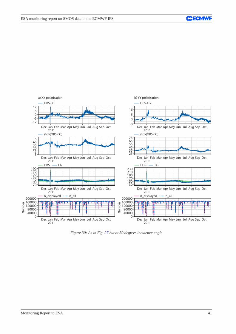
ESA monitoring report on SMOS data in the ECMWF IFS
-12-606
12
515253545
55
7090
110130150170190
0 40000 80000
120000160000200000
-8
0
8
16
253545556575
130150170190210230
0 40000 80000
120000160000200000
a) XX polarisation
OBS-FG OBS-FG
b) YY polarisation
n_displayed n_all n_displayed n_all
OBS FG OBS FG
Dec Jan Feb Mar Apr May Jun Jul OctSepAug2011
Dec Jan Feb Mar Apr May Jun Jul OctSepAug2011
Dec Jan Feb Mar Apr May Jun Jul OctSepAug2011
Dec Jan Feb Mar Apr May Jun Jul OctSepAug2011
Dec Jan Feb Mar Apr May Jun Jul OctSepAug2011
Dec Jan Feb Mar Apr May Jun Jul OctSepAug2011
Dec Jan Feb Mar Apr May Jun Jul OctSepAug2011
Dec Jan Feb Mar Apr May Jun Jul OctSepAug2011
stdv(OBS-FG) stdv(OBS-FG)
Nu
mb
er
Nu
mb
er
Figure 30: As in Fig.27but at 50 degrees incidence angle
Monitoring Report to ESA 41
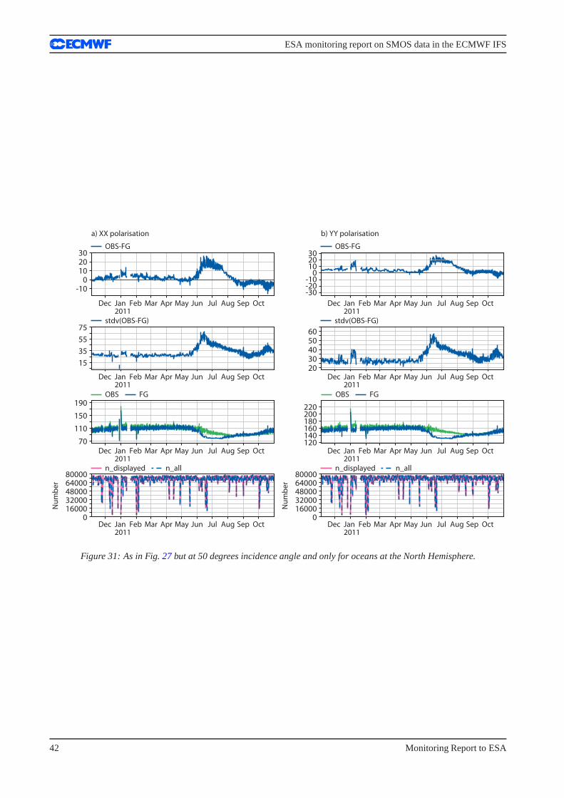
ESA monitoring report on SMOS data in the ECMWF IFS
-100
102030
15
35
55
75
70
110
150
190
0 16000 32000 48000 64000 80000
-30
-10-20
0
2010
30
2030405060
120140160180200220
0 16000 32000 48000 64000 80000
Dec Jan Feb Mar Apr May Jun Jul OctSepAug2011
Dec Jan Feb Mar Apr May Jun Jul OctSepAug2011
Nu
mb
er
Nu
mb
er
n_displayed n_all n_displayed n_all
Dec Jan Feb Mar Apr May Jun Jul OctSepAug2011
Dec Jan Feb Mar Apr May Jun Jul OctSepAug2011
OBS FG OBS FG
Dec Jan Feb Mar Apr May Jun Jul OctSepAug2011
Dec Jan Feb Mar Apr May Jun Jul OctSepAug2011
Dec Jan Feb Mar Apr May Jun Jul OctSepAug2011
Dec Jan Feb Mar Apr May Jun Jul OctSepAug2011
stdv(OBS-FG) stdv(OBS-FG)
a) XX polarisation
OBS-FG OBS-FG
b) YY polarisation
Figure 31: As in Fig.27but at 50 degrees incidence angle and only for oceans at the North Hemisphere.
42 Monitoring Report to ESA
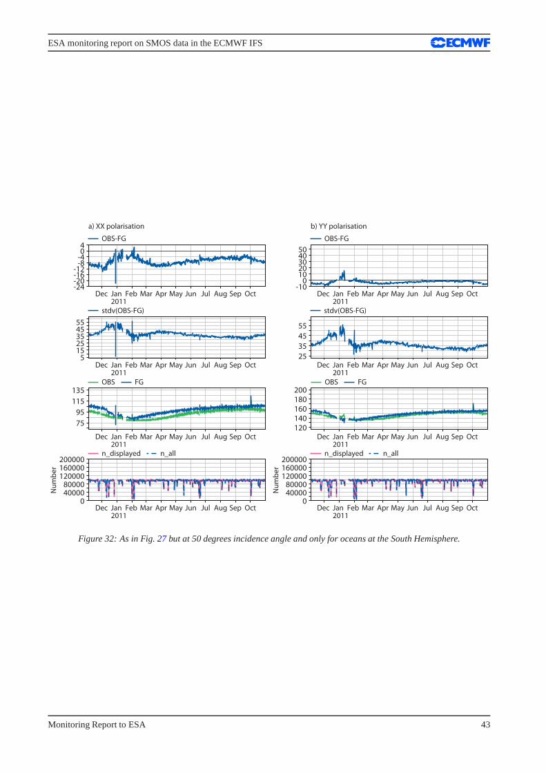
ESA monitoring report on SMOS data in the ECMWF IFS
-24-20-16-12
-8-404
51525354555
75
95
115
135
0 40000 80000
120000160000200000
-100
1020304050
25
35
45
55
120140160180200
0 40000 80000
120000160000200000
Dec Jan Feb Mar Apr May Jun Jul OctSepAug2011
Dec Jan Feb Mar Apr May Jun Jul OctSepAug2011
n_displayed n_all n_displayed n_all
Dec Jan Feb Mar Apr May Jun Jul OctSepAug2011
Dec Jan Feb Mar Apr May Jun Jul OctSepAug2011
OBS FG OBS FG
Dec Jan Feb Mar Apr May Jun Jul OctSepAug2011
Dec Jan Feb Mar Apr May Jun Jul OctSepAug2011
Dec Jan Feb Mar Apr May Jun Jul OctSepAug2011
Dec Jan Feb Mar Apr May Jun Jul OctSepAug2011
stdv(OBS-FG) stdv(OBS-FG)
a) XX polarisation
OBS-FG OBS-FG
b) YY polarisation
Nu
mb
er
Nu
mb
er
Figure 32: As in Fig.27but at 50 degrees incidence angle and only for oceans at the South Hemisphere.
Monitoring Report to ESA 43
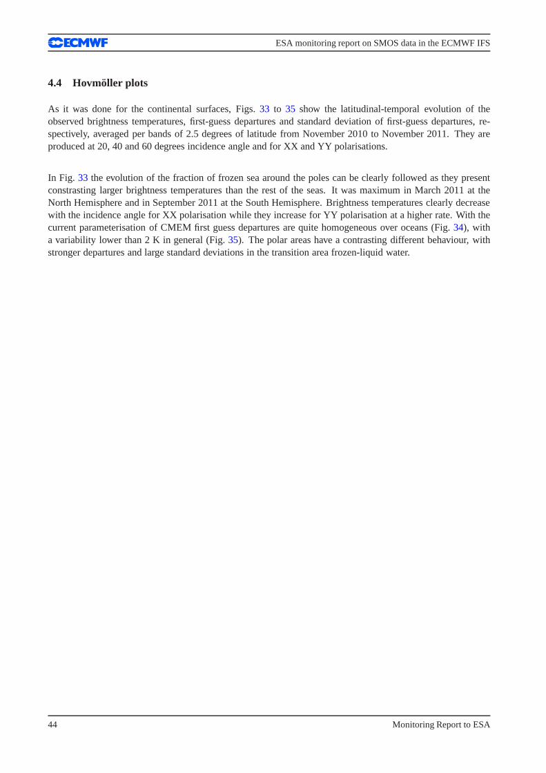
ESA monitoring report on SMOS data in the ECMWF IFS
4.4 Hovmoller plots
As it was done for the continental surfaces, Figs.33 to 35 show the latitudinal-temporal evolution of theobserved brightness temperatures, first-guess departuresand standard deviation of first-guess departures, re-spectively, averaged per bands of 2.5 degrees of latitude from November 2010 to November 2011. They areproduced at 20, 40 and 60 degrees incidence angle and for XX and YY polarisations.
In Fig. 33 the evolution of the fraction of frozen sea around the poles can be clearly followed as they presentconstrasting larger brightness temperatures than the restof the seas. It was maximum in March 2011 at theNorth Hemisphere and in September 2011 at the South Hemisphere. Brightness temperatures clearly decreasewith the incidence angle for XX polarisation while they increase for YY polarisation at a higher rate. With thecurrent parameterisation of CMEM first guess departures arequite homogeneous over oceans (Fig.34), witha variability lower than 2 K in general (Fig.35). The polar areas have a contrasting different behaviour, withstronger departures and large standard deviations in the transition area frozen-liquid water.
44 Monitoring Report to ESA
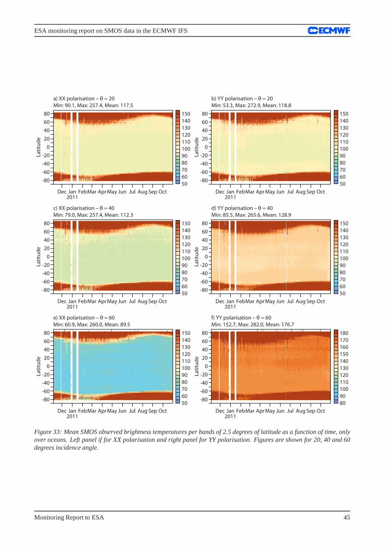
ESA monitoring report on SMOS data in the ECMWF IFS
-80
-60
-40
-20
0
20
40
60
80
La
titu
de
Dec Jan FebMar Apr May Jun Jul Aug Sep Oct2011
a) XX polarisation – θ = 20
Min: 90.1, Max: 257.4, Mean: 117.5
-80
-60
-40
-20
0
20
40
60
80
La
titu
de
Dec Jan FebMar Apr May Jun Jul Aug Sep Oct2011
b) YY polarisation – θ = 20
Min: 53.3, Max: 272.9, Mean: 118.8
-80
-60
-40
-20
0
20
40
60
80
La
titu
de
Dec Jan FebMar Apr May Jun Jul Aug Sep Oct2011
c) XX polarisation – θ = 40
Min: 79.0, Max: 257.4, Mean: 112.3
-80
-60
-40
-20
0
20
40
60
80
La
titu
de
Dec Jan FebMar Apr May Jun Jul Aug Sep Oct2011
d) YY polarisation – θ = 40
Min: 85.5, Max: 265.6, Mean: 128.9
-80
-60
-40
-20
0
20
40
60
80
La
titu
de
Dec Jan FebMar Apr May Jun Jul Aug Sep Oct2011
e) XX polarisation – θ = 60
Min: 60.9, Max: 260.0, Mean: 89.5
-80
-60
-40
-20
0
20
40
60
80
La
titu
de
Dec Jan FebMar Apr May Jun Jul Aug Sep Oct2011
f) YY polarisation – θ = 60
Min: 152.7, Max: 282.0, Mean: 176.7
50
60
70
80
90
100
110
120
130
140
150
50
60
70
80
90
100
110
120
130
140
150
50
60
70
80
90
100
110
120
130
140
150
50
60
70
80
90
100
110
120
130
140
150
50
60
70
80
90
100
110
120
130
140
150
80
90
100
110
120
130
140
150
160
170
180
Figure 33: Mean SMOS observed brightness temperatures per bands of 2.5 degrees of latitude as a function of time, onlyover oceans. Left panel if for XX polarisation and right panel for YY polarisation. Figures are shown for 20, 40 and 60degrees incidence angle.
Monitoring Report to ESA 45
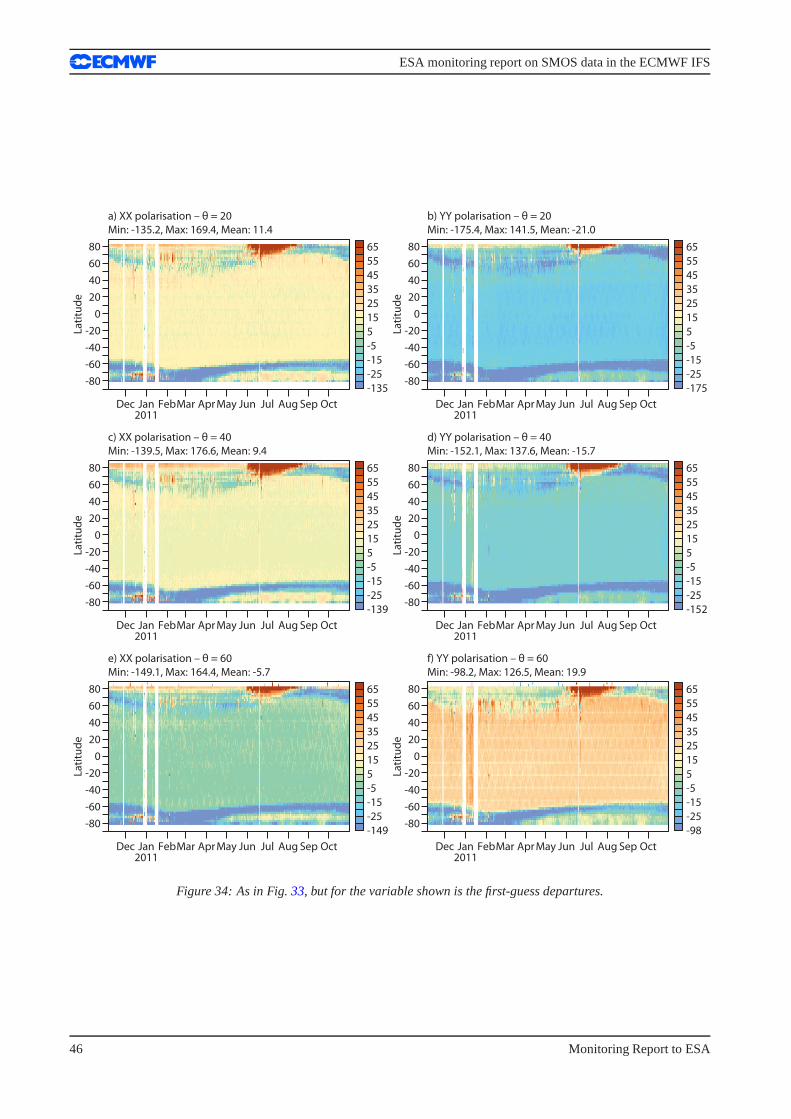
ESA monitoring report on SMOS data in the ECMWF IFS
-80
-60
-40
-20
0
20
40
60
80
La
titu
de
Dec Jan FebMar Apr May Jun Jul Aug Sep Oct2011
a) XX polarisation – θ = 20
Min: -135.2, Max: 169.4, Mean: 11.4
-80
-60
-40
-20
0
20
40
60
80
La
titu
de
Dec Jan FebMar Apr May Jun Jul Aug Sep Oct2011
b) YY polarisation – θ = 20
Min: -175.4, Max: 141.5, Mean: -21.0
-80
-60
-40
-20
0
20
40
60
80
La
titu
de
Dec Jan FebMar Apr May Jun Jul Aug Sep Oct2011
c) XX polarisation – θ = 40
Min: -139.5, Max: 176.6, Mean: 9.4
-80
-60
-40
-20
0
20
40
60
80
La
titu
de
Dec Jan FebMar Apr May Jun Jul Aug Sep Oct2011
d) YY polarisation – θ = 40
Min: -152.1, Max: 137.6, Mean: -15.7
-80
-60
-40
-20
0
20
40
60
80
La
titu
de
Dec Jan FebMar Apr May Jun Jul Aug Sep Oct2011
e) XX polarisation – θ = 60
Min: -149.1, Max: 164.4, Mean: -5.7
-80
-60
-40
-20
0
20
40
60
80
La
titu
de
Dec Jan FebMar Apr May Jun Jul Aug Sep Oct2011
f) YY polarisation – θ = 60
Min: -98.2, Max: 126.5, Mean: 19.9
-135
-25
-15
-5
5
15
25
35
45
55
65
-175
-25
-15
-5
5
15
25
35
45
55
65
-139
-25
-15
-5
5
15
25
35
45
55
65
-152
-25
-15
-5
5
5 5
15
25
35
45
55
65
-149
-25
-15
-5
15
25
35
45
55
65
-98
-25
-15
-5
15
25
35
45
55
65
Figure 34: As in Fig.33, but for the variable shown is the first-guess departures.
46 Monitoring Report to ESA
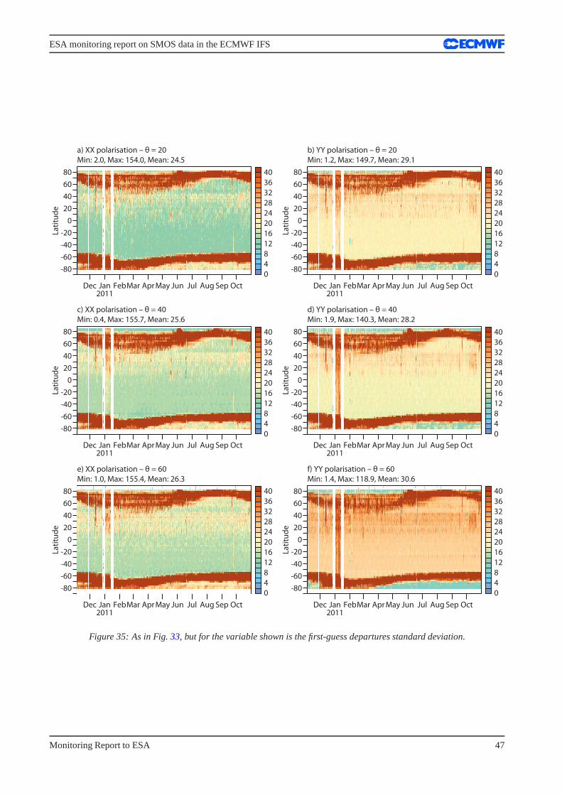
ESA monitoring report on SMOS data in the ECMWF IFS
-80
-60
-40
-20
0
20
40
60
80
La
titu
de
Dec Jan FebMar Apr May Jun Jul Aug Sep Oct2011
a) XX polarisation – θ = 20
Min: 2.0, Max: 154.0, Mean: 24.5
-80
-60
-40
-20
0
20
40
60
80
La
titu
de
Dec Jan FebMar Apr May Jun Jul Aug Sep Oct2011
b) YY polarisation – θ = 20
Min: 1.2, Max: 149.7, Mean: 29.1
-80
-60
-40
-20
0
20
40
60
80
La
titu
de
Dec Jan FebMar Apr May Jun Jul Aug Sep Oct2011
c) XX polarisation – θ = 40
Min: 0.4, Max: 155.7, Mean: 25.6
-80
-60
-40
-20
0
20
40
60
80
La
titu
de
Dec Jan FebMar Apr May Jun Jul Aug Sep Oct2011
d) YY polarisation – θ = 40
Min: 1.9, Max: 140.3, Mean: 28.2
-80
-60
-40
-20
0
20
40
60
80
La
titu
de
Dec Jan FebMar Apr May Jun Jul Aug Sep Oct2011
e) XX polarisation – θ = 60
Min: 1.0, Max: 155.4, Mean: 26.3
-80
-60
-40
-20
0
20
40
60
80
La
titu
de
Dec Jan FebMar Apr May Jun Jul Aug Sep Oct2011
f) YY polarisation – θ = 60
Min: 1.4, Max: 118.9, Mean: 30.6
0
4
8
12
16
20
24
28
32
36
40
0
4
8
12
16
20
24
28
32
36
40
0
4
8
12
16
20
24
28
32
36
40
0
4
8
12
16
20
24
28
32
36
40
0
4
8
12
16
20
24
28
32
36
40
0
4
8
12
16
20
24
28
32
36
40
Figure 35: As in Fig.33, but for the variable shown is the first-guess departures standard deviation.
Monitoring Report to ESA 47
ESA monitoring report on SMOS data in the ECMWF IFS
5 Summary
This second SMOS monitoring report presents some of the NearReal Time SMOS monitoring results obtainedfor the period November 2010- November 2011. The ECMWF passive microwaves emission model CMEM isused to simulate brightness temperatures at the top of the atmosphere. Geolocated SMOS observed brightnesstemperatures are compared to CMEM values at the satellite antenna reference frame and in NRT. A wholeannual cycle of statistical variables was computed and analysed.
Observed brightness temperatures behave as expected. Overcontinental surfaces RFI contamination is clearlyseen in most of the figures. The brightness temperatures standard deviation present large anomalous valuesmainly over China, Middle East and Eastern Europe, with the YY polarisation being more affected than the XXpolarisation. Therefore, the worst affected area by RFI is located between 20 and 40 degrees North. However,a clear improvement of the situation is observed, mainly in Western Europe where the teams fighting againstillegal sources of RFI have been most active. Static sourcesof RFI are still remaining, but they are of lessintensity. Other areas with large variability, and not affected by RFI, are very interesting from an assimilationpoint of view. Snow covered areas clearly affect first-guessdepartures at the XX polarisation, because in theseareas the CMEM modeled brightness temperatures are largelyunderestimated. A systematic negative bias isaffecting the YY polarisation.Over continental surfaces, the variability of the time series is dominated by the influence of the snow coveredareas and RFI. The Southern Hemisphere presents more stablebias throughout the year, mainly because it isless affected by RFI and has a lower annual snow coverage. Thebias are also very dependent on the incidenceangle, as shown in the plots of the angular distribution of bias. In general, they increase with the incidenceangle for XX polarisation, whereas they are maximum at 30 degrees for YY polarisation. While one of theobjectives of the monitoring is to report on all types of landcover, it should be noted that snow covered areaswill be masked in SMOS assimilation experiments, as the linkto soil moisture is lost.
The current parameterisation of the ocean emission at L-band only accounts for the emission over a smoothsurface of water. The effect of the wind and of the galactic noise is not currently accounted for. Thus, theresults presented in this report over oceans are preliminary. Observed brightness temperatures and first-guessdepartures are much more homogeneous than for land pixels, as by nature oceans present less heterogeneities.The polar regions present a clear contrast compared to the rest of the oceans, as these regions are affected bysea ice and snow cover, or a mixture of frozen and liquid water, with very different dielectric properties andbrightness temperatures.
The thermal stability test that took place in the end of December 2010 affected the NRT data until mid-February2011. The degradation of the data in this period is clearly observed in the time series, but also in the geographi-cal and Hovmoller maps. Using all these types of plots together, makes it possible to localize in time and spacepunctual problems in the data and/or the model.
Acknowledgements
This work is funded under the ESA-ESRIN contract number 4000101703/10/NL/FF/fk and is the second (MR2)of a series of Monitoring Reports to ESA. The authors would like to thank Ioannis Mallas at ECMWF, for theoperational acquisition and contribution to the processing of the data. Also many thanks to Rob Hine andAnabel Bowen, both ECMWF, for their great help with the figures shown in this report.
48 Monitoring Report to ESA
ESA monitoring report on SMOS data in the ECMWF IFS
6 References
References
[Balsamo et al. 2009] Balsamo, G., P. Viterbo, A. Beljaars, B. van den Hurk, M. Hirschi, A. Betts, and K. Sci-pal, 2009 : A revised hydrology for the ECMWF model: Verification from field site to terrestrial waterstorage and impact in the integrated forecast system.Journal of Hydrometeorology, 10,623–643. doi:10.1175/2008JHM1068.1.
[Choudhury et al. 1979] Choudhury, B. J., T. J. Schmugge, A. Chang, and R. W. Newton, 1979 : Effect ofsurface roughness on the microwave emission for soils.Journal of Geophysical Research, 84,5699–5706.
[de Rosnay et al. 2009a] de Rosnay, P., M. Drusch, A. Boone, G.Balsamo, B. Decharme, P. Harris, Y. Kerr,T. Pellarin, J. Polcher, and J.-P. Wigneron, 2009a : AMMA Land Surface Model Intercomparison Exper-iment coupled to the Community Microwave Emission Model: ALMIP-MEM. J. Geophys. Res., 114.D05108, doi:10.1029/2008JD010724.
[de Rosnay et al. 2009b] de Rosnay, P., M. Drusch, and J.M. Sabater, 2009b : Milestone 1 Technical Note PartI: SMOS global surface emission model. Technical report, European Centre for Medium-Range WeatherForecast, Reading, United Kingdom.
[Drusch et al. 2001] Drusch, M., T. Holmes, P. de Rosnay, and G. Balsamo, 2001 : Vegetative and atmosphericcorrections for the soil moisture retrieval from passive microwave remote sensing data: Results from thesouthern great plains hydrology experiment 1997.J. Hydrometeor., 2,181–192.
[Drusch et al. 2009] Drusch, M., T. Holmes, P. de Rosnay, and G. Balsamo, 2009 : Comparing ERA-40 basedL-band brightness temperatures with Skylab observations:A calibration / validation study using the Com-munity Microwave Emission Model.J. Hydrometeor., 10,213–226. doi: 10.1175/2008JHM964.1.
[Holmes et al. 2008] Holmes, T., M. Drusch, J.-P. Wigneron, and R. de Jeu, 2008 : A global simulation of mi-crowave emission: Error structures based on output from ECMWFS operational integrated forecast system.IEEE Transactions on Geoscience and Remote Sensing, 46,846 – 856.
[Kirdyashev et al. 1979] Kirdyashev, K., A. Chukhlantsev, and A. Shutko, 1979 : Microwave radiation of theearth’s surface in the presence of vegetation cover.Radiotekhnika i Elektronika, 24,256–264.
[Matos and Gutierrez 2004] Matos, P., and A. Gutierrez, 2004: SMOS L1 processor discrete global gridsdocument. Technical report, Deimos Engenharia, Lisboa, Portugal.
[Pellarin et al. 2003] Pellarin, T., J.-P. Wigneron, J.-C. Calvet, and P. Waldteufel, 2003 : Global soil moistureretrieval from a synthetic l-band brightness temperature data set.Journal of Geophysical Research, 108.
[Sabater et al. 2011a] Sabater, J.M., P. de Rosnay, and G.Balsamo, 2011a : Sensitivity of L-bandNWP forward modelling to soil roughness. Int. J. Remote Sens., pp. 1–14. iFirst 2011., doi:10.1080/01431161.2010.507260.
[Sabater et al. 2011b] Sabater, J.M., P. de Rosnay, and M. Dahoui, 2011b : SMOS Continuous MonitoringReports; Part I. Technical report, European Centre for Medium-Range Weather Forecasts, Reading, UnitedKingdom.
[Sabater et al. 2010] Sabater, J.M., P. de Rosnay, and A. Fouilloux, 2010 : Milestone 2 Technical Note, PartI:operational pre-processing chain, Part II:collocationsoftware development, Part III: Offline monitoringsuite. Technical report, European Centre for Medium-RangeWeather Forecasts, Reading, United Kingdom.
Monitoring Report to ESA 49
ESA monitoring report on SMOS data in the ECMWF IFS
[Salgado 1999] Salgado, R., 1999 : Global soil maps of sand and clay fractions and of the soil depth forMESONH simulation based on FAO/UNESCO soil maps. Technicalreport, CNRM/Meteo France. Tech.Note,59.
[Wang and Schmugge 1980] Wang, J. R., and T. Schmugge, 1980 : An empirical model for the complex di-electric permittivity of soils as a function of water content. IEEE Transactions on Geoscience and RemoteSensing, 18,288–295.
[Wigneron et al. 2007] Wigneron, J.-P., Y. Kerr, P. Waldteufel, K. Saleh, M.-J. Escorihuela, P. Richaume,P. Ferrazzoli, P. de Rosnay, R. Gurneye, J.-C. Calvet, J. Grant, M. Guglielmetti, B. Hornbuckle, C. Mt-zler, T. Pellarin, and M. Schwank, 2007 : L-band microwave emission of the biosphere (L-MEB) model:Description and calibration against experimental data sets over crop fields.Remote Sensing of Environment,107,639–655.
[Wigneron et al. 2001] Wigneron, J. P., L. Laguerre, and Y. Kerr, 2001 : A simple parameterization of theL-band microwave emission from rough agricultural soils.IEEE Transactions on Geoscience and RemoteSensing, 39,1697–1707.
50 Monitoring Report to ESA