Embed Size (px)
Citation preview
The adaptive time-dependent
density-matrix renormalization-group
method:
development and applications
Von der Fakultat fur Mathematik, Informatik und Naturwissenschaften
der Rheinisch-Westfalischen Technischen Hochschule Aachen
zur Erlangung des akademischen Grades
einer Doktorin der Naturwissenschaften genehmigte Dissertation
vorgelegt von
Diplom-PhysikerinCorinna Kollath B.Sc.
aus Stirling (Großbritannien)
Berichter: Universitatsprofessor Dr. Ulrich Schollwock
Universitatsprofessor Dr. Walter Hofstetter
Tag der mundlichen Prufung: 4. Juli 2005
Diese Dissertation ist auf den Internetseiten
der Hochschulbibliothek online verfugbar.

Contents
Zusammenfassung 7
1. Introduction 11
2. The adaptive time-dependent density-matrix renormalization-group
method 14
2.1. Can DMRG be applied to time-dependent phenomena? . . . . . 14
2.2. ‘Original’ density-matrix renormalization-group method . . . . . 16
2.2.1. Density-matrix projection . . . . . . . . . . . . . . . . . . 17
2.2.2. DMRG algorithm . . . . . . . . . . . . . . . . . . . . . . . 20
2.3. Simulation of time-dependent quantum phenomena using DMRG 23
2.4. Matrix-product states . . . . . . . . . . . . . . . . . . . . . . . . 29
2.5. TEBD simulation algorithm . . . . . . . . . . . . . . . . . . . . . 31
2.6. DMRG and matrix-product states . . . . . . . . . . . . . . . . . 36
2.7. Adaptive t-DMRG . . . . . . . . . . . . . . . . . . . . . . . . . . 39
2.8. Case study: time-dependent Bose-Hubbard model . . . . . . . . 40
2.9. Sources of error . . . . . . . . . . . . . . . . . . . . . . . . . . . . 44
2.10. Conclusion . . . . . . . . . . . . . . . . . . . . . . . . . . . . . . 45
3. Ultracold atoms in optical lattices 46
3.1. From Bose-Einstein condensation to strongly interacting Bosegases . . . . . . . . . . . . . . . . . . . . . . . . . . . . . . . . . . 46
3.2. Theoretical description: Bose-Hubbard model . . . . . . . . . . . 48
3.3. Quantum phase transition in homogeneous systems . . . . . . . . 51
3.3.1. Limit of weak interaction: superfluid phase . . . . . . . . 51
3.3.2. Limit of strong interaction: Mott-insulating phase . . . . 52
3.3.3. Quantum phase transitions . . . . . . . . . . . . . . . . . 52
3.3.4. Gutzwiller approximation . . . . . . . . . . . . . . . . . . 54
3.4. Coexistence of phases in a trapping potential . . . . . . . . . . . 56
3.5. Modifications to the finite DMRG treating confinement potentials 57
3.6. One-particle density-matrix . . . . . . . . . . . . . . . . . . . . . 58
3.6.1. Scaled one-particle density-matrix . . . . . . . . . . . . . 59
3.6.2. Comparison to the hydrodynamical approach . . . . . . . 61
3.7. Connection to experiment . . . . . . . . . . . . . . . . . . . . . . 64
3.7.1. Interference pattern . . . . . . . . . . . . . . . . . . . . . 64
3.7.2. Comparison to experiment . . . . . . . . . . . . . . . . . . 68
3.8. Conclusion . . . . . . . . . . . . . . . . . . . . . . . . . . . . . . 69
3
Contents
4. Evolution of density wave packets in ultracold bosons 71
4.1. Perturbations: experiments and theoretical descriptions . . . . . 71
4.2. Theoretical description of the density perturbation . . . . . . . . 72
4.3. Preparation of the density perturbation . . . . . . . . . . . . . . 73
4.4. Analytical approximations . . . . . . . . . . . . . . . . . . . . . . 73
4.5. Evolution of the wave packet . . . . . . . . . . . . . . . . . . . . 74
4.6. Decay of the amplitude . . . . . . . . . . . . . . . . . . . . . . . 77
4.7. Sound velocity . . . . . . . . . . . . . . . . . . . . . . . . . . . . 77
4.8. Self-steepening . . . . . . . . . . . . . . . . . . . . . . . . . . . . 82
4.9. Experimental observation . . . . . . . . . . . . . . . . . . . . . . 82
4.10. Conclusion . . . . . . . . . . . . . . . . . . . . . . . . . . . . . . 85
5. Spin-charge separation in cold Fermi gases: a real time analysis 87
5.1. Fascinating physics in one dimension . . . . . . . . . . . . . . . . 87
5.2. Hubbard model . . . . . . . . . . . . . . . . . . . . . . . . . . . . 88
5.3. Quantum phase diagram . . . . . . . . . . . . . . . . . . . . . . . 88
5.4. Spin-charge separation . . . . . . . . . . . . . . . . . . . . . . . . 89
5.5. Preparation of the perturbation . . . . . . . . . . . . . . . . . . . 90
5.6. Spin-charge separation: beyond small perturbations . . . . . . . 91
5.7. Proposed experimental realization . . . . . . . . . . . . . . . . . 95
5.8. Experimental parameters . . . . . . . . . . . . . . . . . . . . . . 97
5.9. Conclusions . . . . . . . . . . . . . . . . . . . . . . . . . . . . . . 98
6. Transport in spin-1/2 chains 99
6.1. Introduction . . . . . . . . . . . . . . . . . . . . . . . . . . . . . . 99
6.2. Model and initial state . . . . . . . . . . . . . . . . . . . . . . . . 99
6.3. Accuracy of the adaptive t-DMRG . . . . . . . . . . . . . . . . . 102
6.3.1. Error analysis for the XX-model . . . . . . . . . . . . . . 102
6.3.2. Optimal choice of DMRG parameters . . . . . . . . . . . 108
6.4. Long-time properties of the time evolution . . . . . . . . . . . . . 110
6.5. Conclusions . . . . . . . . . . . . . . . . . . . . . . . . . . . . . . 119
7. Conclusion and outlook 120
A. Higher order Suzuki-Trotter decompositions 123
B. Ultracold atoms confined in optical lattices 125
B.1. Interaction of neutral atoms with light fields . . . . . . . . . . . . 125
B.2. Optical lattices . . . . . . . . . . . . . . . . . . . . . . . . . . . . 126
B.3. Theoretical description of bosons in optical lattices . . . . . . . 128
B.3.1. Influence of periodic structures . . . . . . . . . . . . . . . 128
B.3.2. Bose-Hubbard model . . . . . . . . . . . . . . . . . . . . . 128
Bibliography 133
Acknowledgement 145
List of publications related to the thesis 147
4

Contents
Curriculum vitae 149
5

6
Zusammenfassung
Die theoretische Beschreibung zeitabhangiger Phanomene stellt nach wie voreine große Herausforderung dar, zumal in den letzten Jahren deutliche Fort-schritte bei Experimenten zur Nichtgleichgewichtsphysik erzielt wurden. In die-ser Arbeit wird die numerische Methode der adaptiven zeitabhangigen Dichte-matrix Renormalisierungsgruppe (adaptive t-DMRG) entwickelt, die uns dieMoglichkeit eroffnet, zeitabhangige Phanomene in stark korrelierten eindimen-sionalen Quantensystemen zu untersuchen. Die neue Methode ist eine Zusam-menfuhrung der Ideen des ’finite-system DMRG’ Algorithmus und des ’timeevolving block-decimation’ Algorithmus (TEBD). Sie beruht auf der Reduktiondes Hilbertraumes auf geeignet gewahlte Unterraume, die zur Beschreibung derzeitlichen Entwicklung schrittweise adaptiert werden.
Wir zeigen die Anwendbarkeit, Effizienz und Genauigkeit der adaptiven t-DMRG,indem wir die zeitliche Entwicklung drei verschiedener Systeme diskutieren: einbosonisches, ein fermionisches und ein Spin-System. Wir benutzen die Existenzeiner exakten Losung fur das XX-Modell einer Spin 1/2-Kette, um eine detail-lierte Fehleranalyse durchzufuhren. Der gesamte Fehler setzt sich aus zweiBeitragen, dem ’truncation’ Fehler und dem Suzuki-Trotter-Fehler zusammen.Die Anzahl der Zustande und die Große des Suzuki-Trotter-Zeitschritts gebeneine gute Kontrolle uber die Genauigkeit der Methode. Fur typische Wertedieser Parameter finden wir, daß der Suzuki-Trotter-Fehler bei kleinen Zeitendominiert, wohingegen fur lange Zeiten der akkumulierte ’truncation’ Fehleruberwiegt. Wir erwarten, daß dieses Verhalten sich auch auf andere Falleubertragen laßt.
Die adaptive DMRG ist somit eine gut kontrollierbare und sehr effiziente Me-thode zur Behandlung zeitabhangiger Phanomene.
Die Ergebnisse der Anwendungen konnen wie folgt zusammengefaßt werden:
Ultrakalte Bosonen Motiviert durch die großen experimentellen Fortschrit-te, die kurzlich auf dem Gebiet der ultrakalten Atome in optischen Gitternerzielt wurden, haben wir die adaptive t-DMRG auf diese Systeme angewen-det. Die Realisierung optischer Gitter eroffnet die Moglichkeit, Probleme ausder Festkorperphysik in einem System zu untersuchen, dessen Parameter bes-ser vorgegeben und zeitlich variiert werden konnen. Zunachst untersuchen wirden Einfluß des in den quantenoptischen Systemen unvermeidlichen Einschluß-potentials. In einem solchen Potential konnen gleichzeitig eine superflussigeund Mott-isolierende Phase raumlich voneinander getrennt auftreten. Wirzeigen, daß eine Charakterisierung dieser Phasen durch die zuvor skalierteEinteilchen-Dichtematrix moglich ist. Die skalierte Einteilchen-Dichtematrix
7
zeigt, wie schon die Einteilchen-Dichtematrix im homogenen System, einenalgebraischen Zerfall in der superflussigen Phase und einen exponentiellen inder Mott-isolierenden Phase. Zur experimentellen Unterscheidung der beidenPhasen ist insbesondere eine Signatur in der Halbwertsbreite der Interferenz-bilder geeignet. Diese wurde inzwischen durch Experimente bestatigt.
Als zeitabhangiges Phanomen untersuchen wir die Ausbreitung von Dichte-storungen. Insbesondere berechnen wir erstmalig die Schallgeschwindigkeit furbeliebige Wechselwirkungsstarken der Bosonen und zeigen damit die Grenzender Gultigkeitsbereiche existierender Naherungen. Aus den Rechnungen furDichtestorungen von unterschiedlicher Starke und Form konnen wir eine lineareAbhangigkeit der Geschwindigkeit von der Hohe der Storung ableiten. DieseAbhangigkeit hat Effekte wie Aufsteilung und Schockwellenformation zur Folge.Wir zeigen, daß diese Storungen schon mit den jetzigen experimentellen Mittelnmit Hilfe einer ’time-of-flight’-Messung detektiert werden konnen.
Ultrakalte Fermionen Eindimensionale Quantensysteme zeigen einige außer-gewohnliche Phanomene als Konsequenz der starken Quantenfluktuationen.Eines davon ist die Spin-Ladungstrennung. Nach der Luttinger-Flussigkeits-theorie entkoppeln Spin- und Ladungsanregungen in eindimensionalen wechsel-wirkenden Systemen bei niedrigen Energien und breiten sich mit unterschied-lichen Geschwindigkeiten aus. Wir untersuchen die Spin-Ladungstrennung an-hand des 1D Hubbard Modells erstmals mit Realzeit-Rechnungen fur Systeme,deren Großen den experimentellen entsprechen. Wir zeigen, daß die Spin-Ladungstrennung als charakteristische Eigenschaft eindimensionaler Systemeweit uber den Bereich niedriger Energien hinaus erhalten bleibt. Auf dieseErgebnisse aufbauend, schlagen wir ein Experiment vor, das es erlaubt, die Spin-Ladungstrennung in ultrakalten Fermionen zu beobachten. Unser Vorschlagbasiert auf der unterschiedlichen Ausbreitung von Spin- und Ladungsanregungenin der flussigen und Mott-isolierenden Phase. Damit werden Probleme ver-mieden, die den heutigen experimentellen Vorschlagen anhaften. Ein experi-menteller Aufbau dieser Art kann auch fur die Unterscheidung eines Mott-Isolators von einem Bandisolator verwendet werden.
Spin-1/2 Kette Der Spintransport zwischen zwei spinpolarisierten Reservoirenist eine Konfiguration von besonderem Interesse im Bereich der Spintronik.Wir modellieren dieses System durch eine Spinkette, die sich anfanglich indem Zustand
∣∣ ↑ . . . ↑↓ . . . ↓
⟩befindet. Die Kopplung beider Reservoire
ist durch die Spinwechselwirkung auf der Kette gegeben. Wir interessierenuns insbesondere dafur, wie das Langzeitverhalten des Spintransports zwischenden beiden Reservoiren von den Eigenschaften des Systems abhangt. In demBereich schwacher SzSz-Wechselwirkung ist der Transport fur lange Zeiten un-abhangig von der Dimerisierung ballistisch, wie es schon fur verschwindendeWechselwirkung und Dimerisierung bekannt war. Wir finden eine drastischeAnderung im Langzeitverhalten in der Nahe des Phasenubergangs. Hier, furstarkere Wechselwirkungen ist der Magnetisierungstransport nicht mehr bal-listisch, sondern oszilliert um einen konstanten Wert. Aus diesen Ergebnissen
8
konnen wir schließen, daß das Langzeitverhalten des Transports in diesem Sys-tem nicht alleine durch Systemeigenschaften —Integrabilitat, Kritikalitat undErhaltungsgroßen— bestimmt wird. Die abrupte Anderung des Verhaltens amPhasenubergang erklaren wir durch die Ahnlichkeit des Anfangszustandes mitdem Grundzustand in der ferromagnetischen Phase.
Die guten Ergebnisse der in dieser Arbeit dargestellten Anwendungen lassenerwarten, daß mogliche Generalisierungen der adaptiven Methode geeignet sind,zukunftig weitere interessante Fragen der Festkorperphysik und der quanten-optischen Systeme im Wechselspiel beider Gebiete zu bearbeiten.
9

10
1. Introduction
In recent years an increasing number of experimental results on time-dependentphenomena has been achieved in condensed matter and quantum optical sys-tems. In the area of condensed matter physics great experimental progress onthe study of these phenomena has been made, e.g., in nanophysics and spintron-ics. It allowed to investigate the transport behaviour through low dimensionalstructures of various geometries such as quantum dots or quantum wires andthe response of such systems to external potentials. In the area of quantumoptics one prominent example for time-dependent phenomena is the realizationof a driven quantum phase transition in ultracold bosons confined by an opti-cal lattice [1]. Time-dependent variations of the optical lattice depth allowedto drive the transition between a superfluid (metallic) and a Mott-insulatingregime.Despite the recent progress on the experimental side the theoretical descriptionof non-equilibrium phenomena is still lacking. In this work we develop a new nu-merical method, the adaptive time-dependent density-matrix renormalization-group (adaptive t-DMRG), which turns out to be very well suited to investigatetime-dependent phenomena in one-dimensional strongly correlated systems. Weshow its applicability to different physical systems: bosonic, fermionic and spinchains.
Adaptive t-DMRG As for static phenomena, the fundamental problem for thetreatment of time-dependent quantum phenomena is the large size of the Hilbertspace required. In the case of low-energy equilibrium properties the inventionof the density-matrix renormalization-group method (DMRG) brought decisiveprogress. It iteratively decimates the Hilbert space of a growing quantum sys-tem such that the state of interest, say the ground state, is approximated ina space of reduced dimension having a maximum overlap with the true state[2, 3, 4]. For time-dependent phenomena, very often a fixed reduced space ofpractical size cannot cover the whole time evolution of the system. The re-duced space has to be adapted in time to give a good description of the timeevolution of the state of interest. This was first realized in the time evolvingblock-decimation (TEBD) procedure by G. Vidal [5], an algorithm to simu-late slightly entangled quantum systems. As it is best seen in the language ofmatrix-product states, the TEBD and the DMRG are closely related. Thus, aswill be shown in chapter 2, generalizing the original DMRG can be generalizedby incorporating the idea of the TEBD algorithm. This results in a very efficientalgorithm, the adaptive t-DMRG [6, 7], which can treat time-dependent phe-nomena with remarkable success. This can be seen from the applications of theadaptive t-DMRG described in this thesis which are concerned with ultracoldbosons, fermions and spin transport in one-dimensional chains.
11
1. Introduction
Ultracold Bose gases in optical lattices The first application of the adap-tive t-DMRG presented in this work is from the area of ultracold bosons. Inrecent years the experimental progress in these systems initiated a connectionbetween quantum optics and condensed matter systems. The pioneering workwas the experimental achievement of the Bose-Einstein condensate [8, 9, 10],which opened the way to numerous exciting experiments directly probing fun-damental effects of quantum mechanics. Up until the last few years most phe-nomena experimentally exploited could be described theoretically by consid-ering the dynamics of weakly interacting Bose gases in the framework of theGross-Pitaevskii equation and the Bogoliubov theory [11, 12]. More recently anew regime, the regime of strong interaction, became experimentally accessible[13, 14, 15]. From the many-body point of view this is a more sophisticatedregime, since interaction induced many-body effects have to be taken into ac-count. The experiment which illustrated best the presence of ‘real’ many-bodyeffects was that of Greiner et al. [1] in which they managed to realize thequantum phase transition from a superfluid to a Mott-insulating phase in asystem of ultracold atoms confined to an optical lattice. This experiment hasattracted a lot of attention, since it realizes of one of the most prominent phasetransition in condensed matter systems, thereby showing the possibility to re-alize and clarify solid-state phenomena in a new context. In contrast to mostcondensed matter systems, these systems of ultracold atoms have the advan-tage that many parameters can be experimentally controlled very precisely andrapidly changed. Thereby, it opens up a whole new area of non-equilibriumphenomena, the theoretical description of which is very demanding.In this thesis we show how the new adaptive t-DMRG allows us to study some ofthese phenomena. But before this, we discuss the consequences of the presenceof an external trapping potential on the static properties of the system (chapter3). The trapping potential is one of the main differences between the quantumoptical systems and the condensed matter systems. One of the consequences isthe possibility of the spatially separated coexistence of the superfluid and theMott-insulating phases. The question arises which properties of their homo-geneous counterparts survive in these coexisting states. We show that after asimple scaling procedure the one-particle density-matrix can be used to charac-terize the state of the system just as for homogeneous systems. We confirm theapplication of the widely used hydrodynamic approach for the system with theparabolic trap in the limit of weak interactions by comparing it to the DMRGresults. Further we discuss how the different states can be distinguished ex-perimentally. Hereby we present results for the interference pattern and pointout that the experimental quantity which reveals most about the state of thesystem is the half width of the interference peak.In chapter 4 we turn to the evolution of density perturbations in a gas of ul-tracold bosons subjected to an optical lattice. We investigate the propagationof density-wave packets in a Bose-Hubbard model using the adaptive t-DMRG.Until now the propagation had only been studied for the case of very broadand weak perturbations in the presence of weak interactions. In contrast, herewe discuss the dependence of the velocity and of the decay of the amplitude ondensity, interaction strength and the extent and height of the perturbation in
12
a numerically exact way, covering a wide range of interaction and of perturba-tion strengths. By comparing our results for the sound velocity to theoreticalpredictions, we determine the limits of a Gross-Pitaevskii or Bogoliubov typedescription and the regime where repulsive one-dimensional Bose gases exhibitfermionic behaviour. In addition, we investigate the effect of self-steepening dueto the amplitude dependence of the velocity and discuss the possibilities for anexperimental detection of the moving wave packet in time-of-flight pictures.
Ultracold fermions As a second application of the adaptive t-DMRG, we in-vestigate the phenomenon of spin-charge separation and propose an experimen-tal setup for its observation in cold Fermi gases. The spin-charge separation– the complete decoupling of spin and charge excitations at low energies – isone of the key features of one-dimensional quantum physics. It is in strikingcontrast to Fermi-liquids, where elementary quasi-particles exist which carryboth charge and spin. Using the adaptive t-DMRG for the 1D Hubbard model,the splitting of local perturbations into separate wave packets carrying chargeand spin is calculated in real-time. We show the robustness of this separationbeyond the low-energy regime by studying the time evolution of density wavepackets of finite strength and at length scales down to a few lattice spacings.A striking signature of spin-charge separation is found in 1D cold Fermi gasesin a harmonic trap using the different propagation properties of the liquid andMott-insulating phases. We give quantitative estimates for an experimentalobservation of spin-charge separation in an array of atomic wires.
Spin transport The third application relates to the area of spintronics. Asimplified model for the magnetization transport between two coupled reservoirswith opposite spin polarization is studied. This is done by calculating the trans-port properties of a spin-1/2 chain which is initially in the state
∣∣ ↑ . . . ↑↓ . . . ↓
⟩,
with all spins pointing up in the left half of the system and all spins pointingdown in the right half. Thus, each half of the system corresponds to one spin-polarized reservoir. The coupling within and between the reservoirs are bothgiven by nearest-neighbour spin interactions. We focus our study on the longtime behaviour of the system. In particular, we investigate whether a sim-ple long time limit for the spin transport exists and if so, how it depends onthe properties of the system such as integrability and criticality. Time-scalesaccessible to us are of the order of 100 units of time measured in ~/J whilemaintaining insignificant error in the observables.Additionally, we perform a detailed analysis of the error made by the adaptive t-DMRG using the fact that the evolution in the XX-model is known exactly. Wefind that the error at small times is dominated by the error made by the Suzuki-Trotter decomposition whereas for longer times the DMRG truncation errorbecomes the most important, with a very sharp crossover at some “runaway”time. Overall, errors are extremely small before the “runaway” time.
13
2. The adaptive time-dependent
density-matrix
renormalization-group method
2.1. Can DMRG be applied to time-dependent
phenomena?
Over many decades the description of the physical properties of low-dimensionalstrongly correlated quantum systems has been one of the major tasks in the-oretical condensed matter physics. In most cases the problem is that due tothe large size of the Hilbert space no exact solution of the quantum systemsis possible. In low dimensional systems, in general, this task is complicatedfurther by the strong quantum fluctuations present in such systems which areusually modeled by minimal-model Hubbard or Heisenberg-style Hamiltonians.Despite the apparent simplicity of these Hamiltonians, few analytically exact so-lutions are available and most analytical approximations remain uncontrolled.Hence, numerical approaches have always been of particular interest, amongthem exact diagonalization and quantum Monte Carlo.Decisive progress in the description of the low-energy equilibrium properties ofone-dimensional strongly correlated quantum systems was achieved by the in-vention of the density-matrix renormalization-group method (DMRG) [2, 16].It is concerned with the iterative decimation of the Hilbert space of a grow-ing quantum system. The Hilbert space of this system would otherwise growexponentially, when the system is enlarged linearly. The DMRG constructs areduced space of fixed dimension and approximates the quantum state of in-terest, say the ground state, in that reduced space with a maximum of overlapwith the true state.
While the DMRG method has yielded an enormous wealth of information onthe static and dynamic equilibrium properties of one-dimensional systems [3, 4]and is one of the most powerful methods in the field, only few attempts havebeen made so far to determine the time evolution of the states of such systems,notably in a seminal paper by Cazalilla and Marston [17].In the quite different context of quantum information science G. Vidal hasrecently developed an algorithm for the simulation of slightly entangled quan-tum computations [18] that can be used to simulate time evolutions of one-dimensional systems [5]. This new algorithm, henceforth referred to as thetime-evolving block decimation (TEBD) algorithm, considers a small, dynam-ically updated subspace to efficiently represent the state of the system. It wasoriginally developed in order to show that a large amount of entanglement isnecessary to make quantum computations whereas any quantum evolution in-
14
2.1. Can DMRG be applied to time-dependent phenomena?
volving only a “sufficiently restricted” amount of entanglement can be efficientlysimulated in a classical computer using the TEBD algorithm. The above con-nection between the amount of entanglement and the complexity of simulatingquantum systems by classical computers is of obvious practical interest in con-densed matter physics. For instance, in one dimension the entanglement ofmost quantum systems happens to be “sufficiently restricted” precisely in thesense required for the TEBD algorithm to yield an efficient simulation.In this thesis the TEBD algorithm is reexpressed in a language more familiar tothe DMRG community than the one originally used in Refs. [5, 18], which madesubstantial use of the quantum information parlance. This reformulation turnsout to be a rewarding task since, as we show, the conceptual and formal simi-larities between the TEBD and DMRG are extensive. Both algorithms searchfor an approximation of the true wave function within a restricted class of wavefunctions, which can be identified as matrix-product states [19], previously alsoproposed under the name of finitely-correlated states [20]. The great advantageof the TEBD algorithm lies in its flexibility to flow in time through the sub-manifold of matrix-product states whereas the original DMRG only constructsa fixed reduced space. In this chapter we show how the two algorithms canbe integrated [6]. We will describe how the TEBD simulation algorithm canbe incorporated into preexisting, quite widely used DMRG implementations,the so-called finite-system algorithm [16] using White’s prediction algorithm[21]. The advantage of the new algorithm is that it uses well-known DMRGtechniques, such as the handling of good quantum numbers. Therefore the netresult is an extremely powerful “adaptive time-dependent DMRG” algorithm(adaptive t-DMRG).The outline of this chapter is as follows: In section 2.2 the original DMRGalgorithm is reviewed. Further details on the DMRG algorithm can be foundfor example in [3, 4, 22]. In section 2.3, the problems encountered in apply-ing DMRG to the calculation of explicitly time-dependent quantum states arediscussed. Section 2.4 reviews the language of matrix product states. Thenboth the TEBD simulation algorithm (section 2.5) and DMRG (section 2.6)are expressed in this language, revealing where both methods coincide, wherethey differ and how they can be combined. In section 2.7, the modifications tointroduce the TEBD algorithm into standard DMRG to obtain the adaptive t-DMRG are pointed out. Section 2.8 we test the new algorithm at small bosonicsystems and compare it to previous proposals. In section 2.9 the sources oferrors are identified. A detailed error analysis is performed later in the contextof spin-chains 6.3.
15
2. The adaptive time-dependent density-matrix renormalization-group method
2.2. ‘Original’ density-matrix renormalization-group
method
The density-matrix renormalization group (DMRG), which was developed byWhite in 1992 [2, 16], is one of the most precise numerical methods to studylow-dimensional strongly correlated systems. Originally, it was introduced tocompute the ground state and low-energy spectrum of a quantum system withshort-range interactions.
l
l + 1
Renormalization
l
l + 1Enlargement of Chain
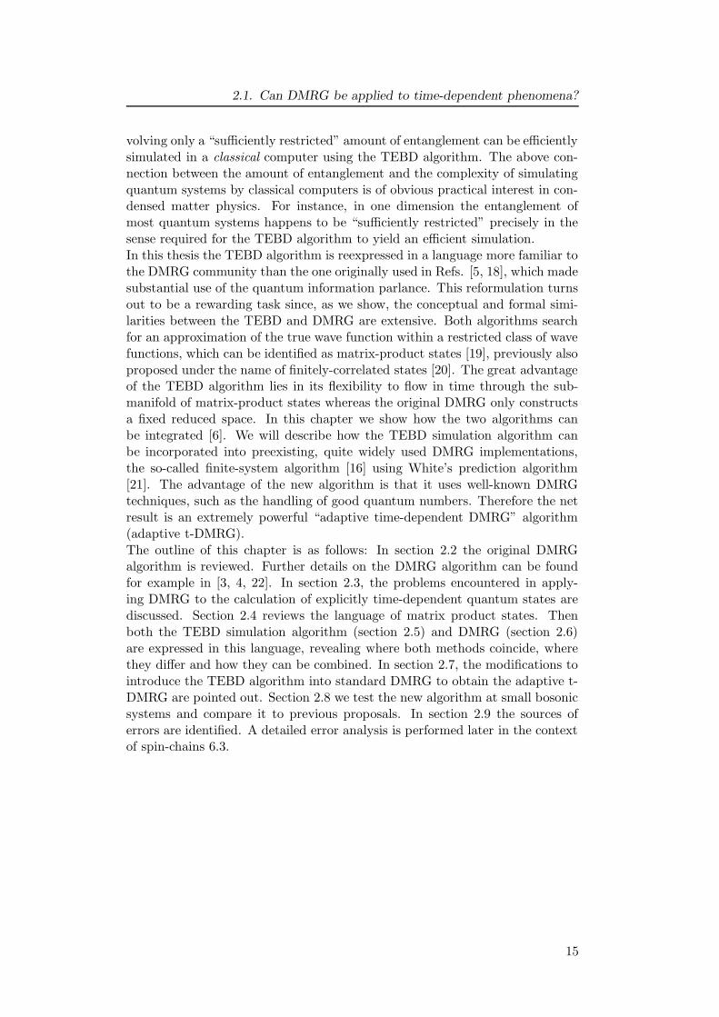
Figure 2.1.: Schematic plot of the real-space renormalization. [22]
The DMRG algorithm is based on the general concept of the ‘renormalizationmethods’. Starting from some microscopic Hamiltonian, degrees of freedom areintegrated out iteratively, such that an effective description of the system isobtained. Hereby the difficulty is to obtain an effective description which stillcovers the essential physics. The DMRG-algorithm starts with a quantum chain(also called “block”) of length l, that is sufficiently small to be represented nu-merically on a computer (Fig. 2.1). Then, the chain is enlarged sequentially byone site to increase the system size. In order to reduce the with l exponentiallygrowing dimension of the Hilbert space, after each enlargement step the systemis projected onto a fixed number m of relevant Hilbert space states sketched inFig. 2.1 by the block. All remaining states are cut off and neglected for thenext iteration step. Obviously the crucial question arises which states are inthat sense “relevant”.
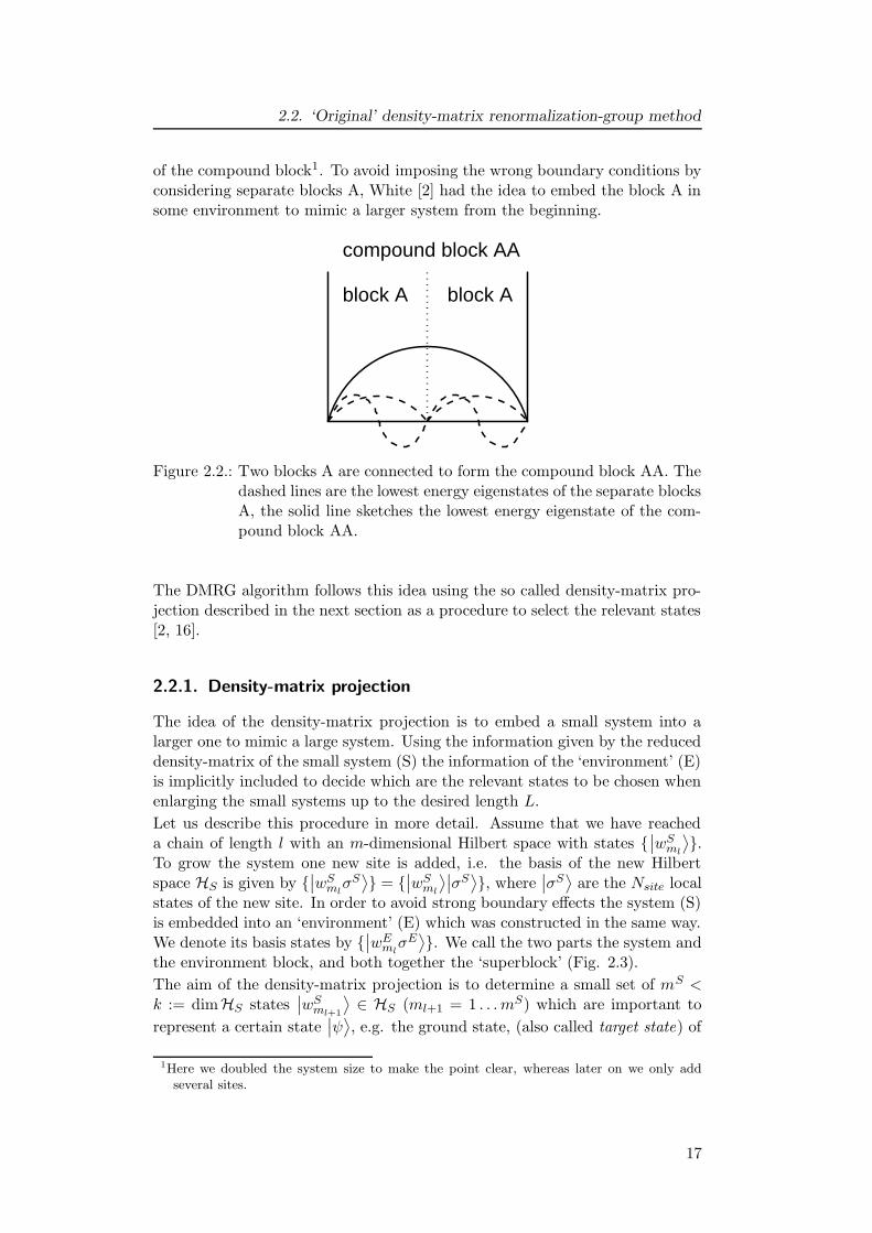
White and Noack [3] found that keeping only the lowest lying energy eigenstates,generally does not give a good decimation procedure. This can be understoodconsidering the toy model of a single non-interacting particle hopping on adiscrete one-dimensional lattice. If one starts with a small system, say blockA in Fig. 2.2, the lowest lying eigenstates (dashed curves in Fig. 2.2) for thesingle particle in the box have nodes at the lattice end of block A. If the systemis enlarged by doubling the system to obtain the compound block AA, the newlowest lying eigenstates have a maximum amplitude at the compound blockcenter. Therefore it cannot be approximated well by a restricted number ofblock states, i.e. eigenstates of the two blocks which have nodes at the center
16
2.2. ‘Original’ density-matrix renormalization-group method
of the compound block1. To avoid imposing the wrong boundary conditions byconsidering separate blocks A, White [2] had the idea to embed the block A insome environment to mimic a larger system from the beginning.
compound block AA
block A block A
Figure 2.2.: Two blocks A are connected to form the compound block AA. Thedashed lines are the lowest energy eigenstates of the separate blocksA, the solid line sketches the lowest energy eigenstate of the com-pound block AA.
The DMRG algorithm follows this idea using the so called density-matrix pro-jection described in the next section as a procedure to select the relevant states[2, 16].
2.2.1. Density-matrix projection
The idea of the density-matrix projection is to embed a small system into alarger one to mimic a large system. Using the information given by the reduceddensity-matrix of the small system (S) the information of the ‘environment’ (E)is implicitly included to decide which are the relevant states to be chosen whenenlarging the small systems up to the desired length L.
Let us describe this procedure in more detail. Assume that we have reacheda chain of length l with an m-dimensional Hilbert space with states {
∣∣wS
ml
⟩}.
To grow the system one new site is added, i.e. the basis of the new Hilbertspace HS is given by {
∣∣wS
mlσS⟩} = {
∣∣wS
ml
⟩∣∣σS⟩}, where
∣∣σS⟩
are the Nsite localstates of the new site. In order to avoid strong boundary effects the system (S)is embedded into an ‘environment’ (E) which was constructed in the same way.We denote its basis states by {
∣∣wE
mlσE⟩}. We call the two parts the system and
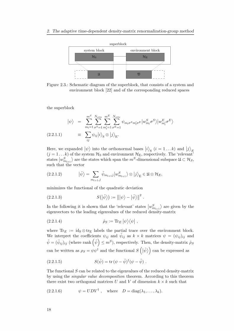
the environment block, and both together the ‘superblock’ (Fig. 2.3).
The aim of the density-matrix projection is to determine a small set of mS <k := dimHS states
∣∣wS
ml+1
⟩∈ HS (ml+1 = 1 . . . mS) which are important to
represent a certain state∣∣ψ⟩, e.g. the ground state, (also called target state) of
1Here we doubled the system size to make the point clear, whereas later on we only addseveral sites.
17
2. The adaptive time-dependent density-matrix renormalization-group method
superblock
VU
HS HE
environment blocksystem block
Figure 2.3.: Schematic diagram of the superblock, that consists of a system andenvironment block [22] and of the corresponding reduced spaces
the superblock
∣∣ψ⟩
=mS∑
ml=1
Nsite∑
σS=1
mE∑
m′l=1
Nsite∑
σE=1
ψmlσSm′lσE
∣∣wS
mlσS⟩∣∣wE
m′lσE⟩
≡∑
ij
ψij
∣∣i⟩
S⊗∣∣j⟩
E.(2.2.1.1)
Here, we expanded∣∣ψ⟩
into the orthonormal bases∣∣i⟩
S(i = 1 . . . k) and
∣∣j⟩
E(j = 1 . . . k) of the system HS and environment HE, respectively. The ‘relevant’states
∣∣wS
ml+1
⟩are the states which span the mS-dimensional subspace U ⊂ HS ,
such that the vector
(2.2.1.2)∣∣ψ⟩
=∑
ml+1,j
ψml+1j
∣∣wS
ml+1
⟩⊗∣∣j⟩
E∈ U ⊗HE,
minimizes the functional of the quadratic deviation
(2.2.1.3) S(∣∣ψ⟩)
:=∥∥∣∣ψ⟩−∣∣ψ⟩∥∥2
.
In the following it is shown that the ‘relevant’ states∣∣wS
ml+1
⟩are given by the
eigenvectors to the leading eigenvalues of the reduced density-matrix
(2.2.1.4) ρS := TrE
∣∣ψ⟩⟨ψ∣∣ ,
where TrE := idS ⊗ trE labels the partial trace over the environment block.We interpret the coefficients ψij and ψij as k × k matrices ψ = (ψij)ij and
ψ = (ψij)ij (where rank(
ψ)
≤ mS), respectively. Then, the density-matrix ρS
can be written as ρS = ψψ† and the functional S(∣∣ψ⟩)
can be expressed as
(2.2.1.5) S(ψ) = tr (ψ − ψ)†(ψ − ψ) .
The functional S can be related to the eigenvalues of the reduced density-matrixby using the singular value decomposition theorem. According to this theoremthere exist two orthogonal matrices U and V of dimension k × k such that
(2.2.1.6) ψ = UDV † , where D = diag(λ1, . . . , λk).
18
2.2. ‘Original’ density-matrix renormalization-group method
The so-called singular values λi are the square roots of the eigenvalues of ρS ,since we can write
(2.2.1.7) ρS = UDD†U † = UD2U † .
Inserting (2.2.1.6) into (2.2.1.5) and using the cyclic invariance of the trace, weobtain
(2.2.1.8) S(ψ) = tr (D − D)†(D − D) .
with D := U †ψV . In this form it can be seen that S is minimized, if D is adiagonal matrix of rank mS, whose diagonal elements are given by the leadingsingular values, i.e.
(2.2.1.9) D = diag(λ1, . . . , λmS , 0, . . . , 0) .
Without loss of generality the λi were assumed to be sorted: λ1 ≥ λ2 ≥ · · · ≥λk. We can explicitly construct
∣∣ψ⟩
which minimizes S using the eigenvectors∣∣wS
ml+1
⟩to the leading m eigenvalues of ρS :
∣∣ψ⟩
=∑
ij
(UDV †)ij∣∣i⟩
S⊗∣∣j⟩
E(2.2.1.10)
=∑
ml+1
Dml+1,ml+1
(∑
i
Uiml+1
∣∣i⟩
S
︸ ︷︷ ︸∣∣wS
ml+1
⟩
)⊗(∑
j
V ∗jml+1
∣∣j⟩
E
︸ ︷︷ ︸∣∣wE
ml+1
⟩
)
=m∑
ml+1=1
λml+1
∣∣wS
ml+1
⟩⊗∣∣wE
ml+1
⟩
Note, that the same number of states has to be kept for the system and theenvironment block, i.e. m := mS = mE. If the same projection is performedinterchanging the system and environment block, one finds that both reduceddensity-matrices have the same non-zero eigenvalues even if system and envi-ronment were different. This is also reflected in the guaranteed existence of theso-called Schmidt decomposition of the wave function [23],
(2.2.1.11)∣∣ψ⟩
=∑
α
λα
∣∣wS
α
⟩∣∣wE
α
⟩, λα ≥ 0,
which plays a key-role in the connection between the TEBD and DMRG. Thenumber of positive λα is bounded by the dimension of the smaller of the basesof system and environment.To summarize, we have proven that the relevant states of the system block torepresent the target state, e.g. the ground state, of a larger quantum chainincluding the environment are optimally given by the leading m eigenvectors ofthe reduced density-matrix ρS.The performance of the method depends critically on the decay of the eigenval-ues of the reduced density-matrix. Some insight into the quality of the trun-cation approximation made by the projection can be gained by the so-called
19
2. The adaptive time-dependent density-matrix renormalization-group method
truncated weight
(2.2.1.12) P := 1 −m∑
i=1
λ2i
which measures how much of the norm of∣∣ψ⟩
is lost. However, due to theadditional sources of ‘environmental’ errors — errors by the only approximatesimilarity of the environment block to the ‘real’ environment— the total errorin the observables calculated are often much larger than the truncated weight.A good control over the total error can in most cases be obtained by a carefulconvergence analysis in the number m of states kept.
More information about the limits of the DMRG was obtained by [24, 25, 26, 27,28, 29] by studying the ability of the DMRG decimation procedure to preservethe entanglement of
∣∣ψ⟩
between system and environment in the context ofquantum information science [23, 30]. By this a better understanding of thereasons of the breakdown of the DMRG in two-dimensional systems has beenobtained in terms of the growth of bipartite entanglement in such systems[27, 29].
More specifically, in quantum information the entanglement of∣∣ψ⟩
between sys-tem and environment is quantified by the von Neumann entropy of ρS (equiv-alently, of ρE),
(2.2.1.13) S(ρS) = −∑
λ2α log2 λ
2α,
a quantity that imposes a useful (information theoretical) bound m ≥ 2S onthe minimal number m of states to be kept during the DMRG decimationprocess if the truncated state is to be similar to
∣∣ψ⟩. Still more insight into the
power of the DMRG comes from arguments from field theory which imply that,at zero temperature, strongly correlated quantum systems are in some senseonly slightly entangled in d = 1 dimension but significantly more entangled ind > 1 dimensions: In particular, in d = 1 a block corresponding to l sites ofa gapped infinite-length chain has an entropy Sl that stays finite even in thethermodynamical limit l → ∞, while at criticality Sl only grows logarithmicallywith l. It is this saturation or, at most, moderate growth of Sl that ultimatelyaccounts for the success of DMRG in d = 1. In the general d-dimensional casethe entropy of bipartite entanglement for a block of linear dimension l scalesas Sl ∼ ld−1. Thus, in d = 2 dimensions the DMRG algorithm should keep anumberm of states that grows exponentially with l, and the simulation becomesinefficient for large l (while still feasible for small l).
2.2.2. DMRG algorithm
In this section the two DMRG algorithms, the so-called infinite-system andthe finite-system algorithm [16] are introduced. Often, a combination of bothalgorithms is applied to obtain an increased accuracy of the numerical results.
20
2.2. ‘Original’ density-matrix renormalization-group method
Infinite-system algorithm
The infinite-system algorithm is designed for computing the ground state (orlow-energy spectrum) of a quantum chain in the thermodynamic limit (L→ ∞,where L is the desired length of the system). It contains the following iterativesteps:
1. Construct a system of size l with the Hilbert space HS = {∣∣wS
ml
⟩} with
dimension mS which is small enough to be treated exactly. The operatorsused, including the Hamiltonian, are known in this basis. In the sameway construct the environment block.
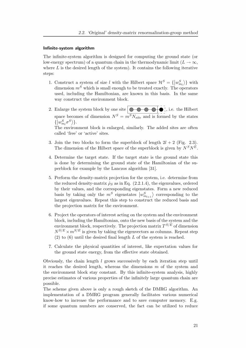
2. Enlarge the system block by one site , i.e. the Hilbert
space becomes of dimension NS = mSNsite and is formed by the states{∣∣wS
mlσS⟩}.
The environment block is enlarged, similarly. The added sites are oftencalled ‘free’ or ‘active’ sites.
3. Join the two blocks to form the superblock of length 2l + 2 (Fig. 2.3).The dimension of the Hilbert space of the superblock is given by N SNE .
4. Determine the target state. If the target state is the ground state thisis done by determining the ground state of the Hamiltonian of the su-perblock for example by the Lanczos algorithm [31].
5. Perform the density-matrix projection for the system, i.e. determine fromthe reduced density-matrix ρS as in Eq. (2.2.1.4), the eigenvalues, orderedby their values, and the corresponding eigenstates. Form a new reducedbasis by taking only the mS eigenstates
∣∣wS
ml+1
⟩corresponding to the
largest eigenvalues. Repeat this step to construct the reduced basis andthe projection matrix for the environment.
6. Project the operators of interest acting on the system and the environmentblock, including the Hamiltonian, onto the new basis of the system and theenvironment block, respectively. The projection matrix T S/E of dimensionNS/E ×mS/E is given by taking the eigenvectors as columns. Repeat step(2) to (6) until the desired final length L of the system is reached.
7. Calculate the physical quantities of interest, like expectation values forthe ground state energy, from the effective state obtained.
Obviously, the chain length l grows successively by each iteration step untilit reaches the desired length, whereas the dimensions m of the system andthe environment block stay constant. By this infinite-system analysis, highlyprecise estimates of various properties of the infinitely large quantum chain arepossible.The scheme given above is only a rough sketch of the DMRG algorithm. Animplementation of a DMRG program generally facilitates various numericalknow-how to increase the performance and to save computer memory. E.g.if some quantum numbers are conserved, the fact can be utilized to reduce
21
2. The adaptive time-dependent density-matrix renormalization-group method
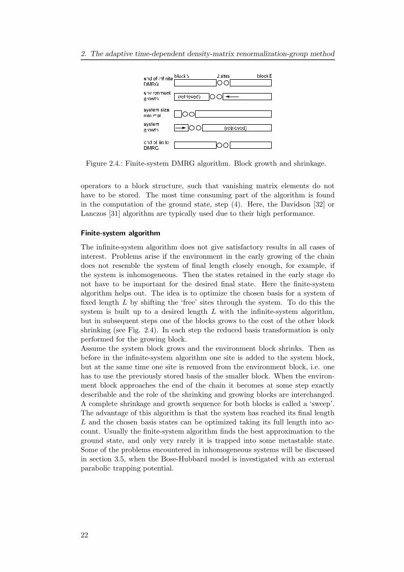
Figure 2.4.: Finite-system DMRG algorithm. Block growth and shrinkage.
operators to a block structure, such that vanishing matrix elements do nothave to be stored. The most time consuming part of the algorithm is foundin the computation of the ground state, step (4). Here, the Davidson [32] orLanczos [31] algorithm are typically used due to their high performance.
Finite-system algorithm
The infinite-system algorithm does not give satisfactory results in all cases ofinterest. Problems arise if the environment in the early growing of the chaindoes not resemble the system of final length closely enough, for example, ifthe system is inhomogeneous. Then the states retained in the early stage donot have to be important for the desired final state. Here the finite-systemalgorithm helps out. The idea is to optimize the chosen basis for a system offixed length L by shifting the ‘free’ sites through the system. To do this thesystem is built up to a desired length L with the infinite-system algorithm,but in subsequent steps one of the blocks grows to the cost of the other blockshrinking (see Fig. 2.4). In each step the reduced basis transformation is onlyperformed for the growing block.Assume the system block grows and the environment block shrinks. Then asbefore in the infinite-system algorithm one site is added to the system block,but at the same time one site is removed from the environment block, i.e. onehas to use the previously stored basis of the smaller block. When the environ-ment block approaches the end of the chain it becomes at some step exactlydescribable and the role of the shrinking and growing blocks are interchanged.A complete shrinkage and growth sequence for both blocks is called a ‘sweep’.The advantage of this algorithm is that the system has reached its final lengthL and the chosen basis states can be optimized taking its full length into ac-count. Usually the finite-system algorithm finds the best approximation to theground state, and only very rarely it is trapped into some metastable state.Some of the problems encountered in inhomogeneous systems will be discussedin section 3.5, when the Bose-Hubbard model is investigated with an externalparabolic trapping potential.
22
2.3. Simulation of time-dependent quantum phenomena using DMRG
�������������������������������������������������������������������������������������������������������������������������������������������������������������������������
�������������������������������������������������������������������������������������������������������������������������������������������������������������������������
|ψ >0
|ψ >t
(a)
reduced space
Hilbert space
����������������������������������������������������������������������������������������������������������������������������������������������������������������������������������������������������������������
��������������������������������������������������������������������������������������������������������������������������������������������������������������������������������
|ψ >0
|ψ >t
reduced spaceenlarged
Hilbert space(b)
�����������������������������������������������������������������������������������������������������������������������������������������������
�����������������������������������������������������������������������������������������������������������������������������������������������
|ψ >0
|ψ >t
����������������������������������������������������������������������������������������������������������������������������������
������������������������������������������������������������
������������������������������
������������������������������������������������������
Hilbert space
adapted
(c)
reduced spaces
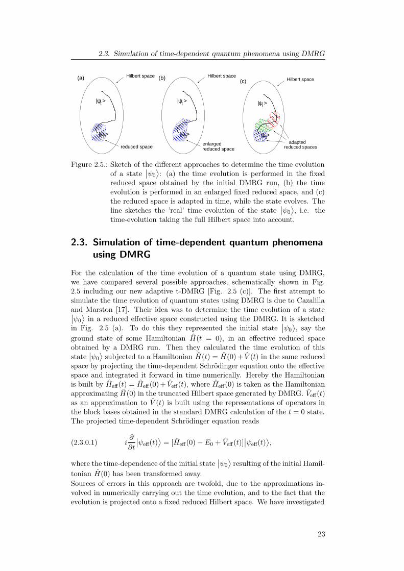
Figure 2.5.: Sketch of the different approaches to determine the time evolutionof a state
∣∣ψ0
⟩: (a) the time evolution is performed in the fixed
reduced space obtained by the initial DMRG run, (b) the timeevolution is performed in an enlarged fixed reduced space, and (c)the reduced space is adapted in time, while the state evolves. Theline sketches the ’real’ time evolution of the state
∣∣ψ0
⟩, i.e. the
time-evolution taking the full Hilbert space into account.
2.3. Simulation of time-dependent quantum phenomena
using DMRG
For the calculation of the time evolution of a quantum state using DMRG,we have compared several possible approaches, schematically shown in Fig.2.5 including our new adaptive t-DMRG [Fig. 2.5 (c)]. The first attempt tosimulate the time evolution of quantum states using DMRG is due to Cazalillaand Marston [17]. Their idea was to determine the time evolution of a state∣∣ψ0
⟩in a reduced effective space constructed using the DMRG. It is sketched
in Fig. 2.5 (a). To do this they represented the initial state∣∣ψ0
⟩, say the
ground state of some Hamiltonian H(t = 0), in an effective reduced spaceobtained by a DMRG run. Then they calculated the time evolution of thisstate
∣∣ψ0
⟩subjected to a Hamiltonian H(t) = H(0)+ V (t) in the same reduced
space by projecting the time-dependent Schrodinger equation onto the effectivespace and integrated it forward in time numerically. Hereby the Hamiltonianis built by Heff(t) = Heff(0)+ Veff (t), where Heff(0) is taken as the Hamiltonianapproximating H(0) in the truncated Hilbert space generated by DMRG. Veff(t)as an approximation to V (t) is built using the representations of operators inthe block bases obtained in the standard DMRG calculation of the t = 0 state.The projected time-dependent Schrodinger equation reads
(2.3.0.1) i∂
∂t
∣∣ψeff(t)
⟩= [Heff(0) −E0 + Veff(t)]
∣∣ψeff(t)
⟩,
where the time-dependence of the initial state∣∣ψ0
⟩resulting of the initial Hamil-
tonian H(0) has been transformed away.
Sources of errors in this approach are twofold, due to the approximations in-volved in numerically carrying out the time evolution, and to the fact that theevolution is projected onto a fixed reduced Hilbert space. We have investigated
23
2. The adaptive time-dependent density-matrix renormalization-group method
these two error sources in some detail and found that in most cases the first er-ror (i) can be well controlled whereas the error introduced by the single reducedspace (ii) causes the breakdown of the method after a relatively short time.(i) To minimize the errors induced by the forward integration in time, we com-pared two different algorithms: the adaptive Runge-Kutta and the Crank-Nicolson algorithm (see [33] and references therein).
The first order Runge-Kutta integration is based on the infinitesimal time evo-lution operator
(2.3.0.2)∣∣ψ(t+ dt)
⟩≈ (1 − iH(t)dt)
∣∣ψ(t)
⟩,
where the subscript is dropped denoting that we are dealing with effectiveHamiltonians acting on the reduced space only. As a first approach the fourth-order adaptive size Runge-Kutta algorithm [33] was applied. Hereby unphysi-cal asymmetries with respect to reflection about the center were generated in asystem with reflection symmetry. We have obtained a conceptually simple im-provement concerning the time evolution by replacing the explicitly non-unitarytime-evolution of the Runge-Kutta algorithm [see Eq. (2.3.0.2)] by the unitaryCrank-Nicolson time evolution
(2.3.0.3)∣∣ψ(t+ dt)
⟩≈ 1 − iH(t)dt/2
1 + iH(t)dt/2
∣∣ψ(t)
⟩.
To implement the Crank-Nicolson time evolution efficiently we have used a(non-Hermitian) biconjugate gradient method to calculate the denominator ofEq. (2.3.0.3). Comparing the Runge-Kutta and the Crank-Nicolson algorithm,already the first-order Crank-Nicolson (with time steps of dt = 5 × 10⁻⁵
~/J)was found to be numerically preferable over the fourth-order adaptive Runge-Kutta algorithm and well controlled by the parameter dt. In particular, theoccurrence of asymmetries with respect to reflection in the results decreased.Therefore, all static (non-adaptive) time-dependent DMRG calculations shownhere have been carried out using the Crank-Nicolson approach.(ii) However, the the error induced by the truncation leads to more severe conse-quences. The key assumption underlying the approach of Cazalilla and Marstonis that the effective fixed Hilbert space created in the preliminary DMRG runis sufficiently large that
∣∣ψ(t)
⟩can be well approximated within that Hilbert
space for all times, such that
(2.3.0.4) ε(t) = 1 − |〈ψ(t)|ψexact(t)〉|
remains small as t grows. At the momentarily available computer resourcesthis, in general, will only be true for relatively short times. A simple picture forthe breakdown is given in Fig. 2.5 (a), where the real time evolution of the stateleaves the reduced space at some time, such that it cannot be approximatedwell in the reduced space anymore.
A variety of modifications that should extend the applicability of the fixedHilbert space in time can be imagined. The underlying idea is to enlarge thereduced space ’along’ the path of the time evolution [as sketched in Fig. 2.5 (b)].
24
2.3. Simulation of time-dependent quantum phenomena using DMRG
Typically these enlargements rest on the DMRG practice of “targeting” severalstates: to construct a reduced effective space optimized to represent not onlyone but several target states. To obtain this space the reduced density-matrixis built out of a mixture of a small number of states, i.e.
(2.3.0.5) ρS = TrE
∣∣ψ⟩⟨ψ∣∣→ ρS = TrE
∑
i
αi
∣∣ψi
⟩⟨ψi
∣∣.
The reduced effective space is constructed as before by keeping only the meigenvectors with the highest weight. A simple choice uses the targeting ofHn∣∣ψ0
⟩, for n less than 10 or so, approximating the short-time evolution, which
we have found to substantially improve the quality of results for non-adiabaticswitching of Hamiltonian parameters in time: convergence in m is faster andmore consistent with the new adaptive t-DMRG method (see below).
Similarly, we have found that for adiabatic changes of Hamiltonian parametersresults improve if one targets the ground states of both the initial and finalHamiltonian.
A more elaborate, but also much more time-consuming improvement still withinthe framework of a fixed Hilbert space was proposed by Luo, Xiang and Wang[34, 35]. Additional to the ground state a finite number of quantum states atvarious discrete times should be targeted using a bootstrap procedure startingfrom the time evolution of smaller systems that are iteratively grown to thedesired final size.
To illustrate the previous approaches and to test the quality of the performanceof the different algorithms, we show results for the Bose-Hubbard Hamiltonian,
(2.3.0.6) HBH(t) = −JL−1∑
i=1
(
b†i+1bi + b†ibi+1
)
+U(t)
2
L∑
i=1
ni(ni − 1),
where the (repulsive) onsite interaction U > 0 is taken to be time-dependent.This model exhibits for commensurate filling a Kosterlitz-Thouless-like quan-tum phase transition from a superfluid phase for u < uc (with u = U/J) toa Mott-insulating phase for u > uc. For more details on the physics of theBose-Hubbard model see section 3.3. In the present section the instantaneousswitching from U1 = 2 in the superfluid phase to U2 = 40 in the Mott phaseat t = 0 in a small Bose-Hubbard system with L = 8 and open boundary con-ditions, total particle number N = 8, J = 1 were used. We compare resultsfor the nearest-neighbour correlation
⟨b†jbj+1
⟩, a robust numerical quantity, be-
tween sites 2 and 3. Up to 8 bosons per site (i.e. Nsite = 9 states per site)were allowed to avoid cut-off effects in the bosonic occupation number in allcalculations in this section. In the following all times are measured in units of~/J or 1/J , setting ~ ≡ 1.
First we compare the results for different choices of a fixed reduced space. Todo this we target (i) just the superfluid ground state
∣∣ψ0
⟩for U1 = 2 (Fig. 2.6),
(ii) in addition to (i) also the Mott-insulating ground state∣∣ψ′
0
⟩for U2 = 40 and
H(t > 0)∣∣ψ0
⟩(Fig. 2.7), (iii) in addition to (i) and (ii) also H(t > 0)2
∣∣ψ0
⟩and
H(t > 0)3∣∣ψ0
⟩(Fig. 2.8). Time evolution is calculated in the Crank-Nicolson
25
2. The adaptive time-dependent density-matrix renormalization-group method
nn−
corr
elat
ion
0
0.5
1
1.5
2
2.5
3
0 0.5 1 1.5 2 2.5 3 3.5 4
time
m=200 m=30
m=50
m=100
(i) L=8, U1=2, U2=40, J=1
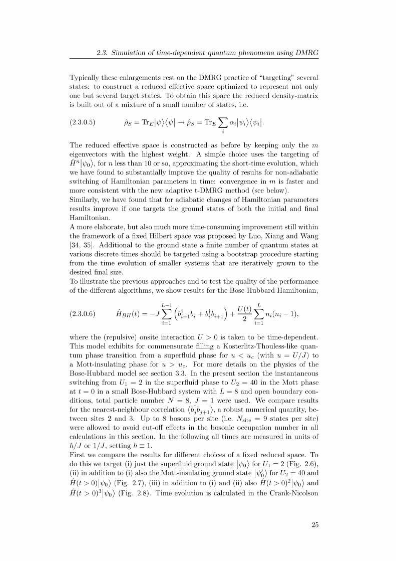
Figure 2.6.: Time evolution of the real part of the nearest-neighbour correlationsin a Bose-Hubbard model (L = 8, N = 8) with instantaneouschange of interaction strength at t = 0: superfluid state targetingonly. The different curves for different m have been shifted by one.
approach using a step width dt = 5 · 10−5. We keep up to m = 200 states toobtain converged results (meaning that we could observe no difference betweenthe results for m = 100 and m = 200) for t ≤ 4, corresponding to roughly25 oscillations. The results for the cases (ii) and (iii) are almost converged form = 50, whereas (i) shows still crude deviations.
A remarkable observation can be made if one compares the three m = 200curves (Fig. 2.9), which by standard DMRG procedure (and for lack of a bettercriterion) would be considered the final, converged outcome, both amongst eachother or to the result of the new adaptive t-DMRG algorithm which is discussedbelow: result (i) is clearly not quantitatively correct beyond very short times,whereas result (ii) agrees very well with the new algorithm, and result (iii)agrees almost (beside some small deviations at t ≈ 3) with result (ii) and thenew algorithm. Therefore we see that for case (i) the criterion of convergence inm does not give a good control to determine if the obtained results are correct.This raises as well doubts about the reliability of this criterion for cases (ii) and(iii).
The observation that even relatively robust numerical quantities such as nearest-neighbour correlations can be qualitatively and quantitatively improved by theadditional targeting of states which merely share some fundamental character-istics with the true quantum state (as we will never reach the Mott-insulatingground state) or characterize only the very short-term time evolution indicatesthat it would be highly desirable to have a modified DMRG algorithm which,for each time t, selects Hilbert spaces of dimension m such that
∣∣ψ(t)
⟩is repre-
sented optimally in the DMRG sense [compare Fig. 2.5 (c)], thus attaining at
26
2.3. Simulation of time-dependent quantum phenomena using DMRG
0
0.5
1.5
2
2.5
3
0 0.5 1 1.5 2 2.5 3 3.5 4
nn−
corr
elat
ion
time
m=200 m=30
m=50
1 m=100
(ii) L=8, U1=2, U2=40, J=1
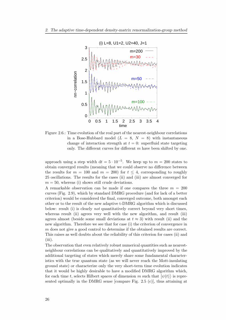
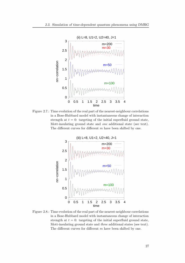
Figure 2.7.: Time evolution of the real part of the nearest-neighbour correlationsin a Bose-Hubbard model with instantaneous change of interactionstrength at t = 0: targeting of the initial superfluid ground state,Mott-insulating ground state and one additional state (see text).The different curves for different m have been shifted by one.
0
0.5
1
1.5
2
2.5
3
0 0.5 1 1.5 2 2.5 3 3.5 4
nn−
corr
elat
ion
time
m=200 m=30
m=50
m=100
(iii) L=8, U1=2, U2=40, J=1
Figure 2.8.: Time evolution of the real part of the nearest-neighbour correlationsin a Bose-Hubbard model with instantaneous change of interactionstrength at t = 0: targeting of the initial superfluid ground state,Mott-insulating ground state and three additional states (see text).The different curves for different m have been shifted by one.
27
2. The adaptive time-dependent density-matrix renormalization-group method
0
0.5
1
1.5
2
2.5
3
0 0.5 1 1.5 2 2.5 3 3.5 4
nn−
corr
elat
ion
time
(i)
(ii)
(iii)
adaptive
L=8, U1=2, U2=40, J=1
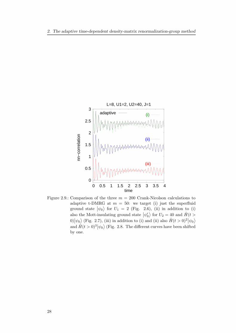
Figure 2.9.: Comparison of the three m = 200 Crank-Nicolson calculations toadaptive t-DMRG at m = 50: we target (i) just the superfluidground state
∣∣ψ0
⟩for U1 = 2 (Fig. 2.6), (ii) in addition to (i)
also the Mott-insulating ground state∣∣ψ′
0
⟩for U2 = 40 and H(t >
0)∣∣ψ0
⟩(Fig. 2.7), (iii) in addition to (i) and (ii) also H(t > 0)2
∣∣ψ0
⟩
and H(t > 0)3∣∣ψ0
⟩(Fig. 2.8. The different curves have been shifted
by one.
28
2.4. Matrix-product states
|α> |β>i i+1i−1
A [ ]i σ ioperators
auxiliary statessites
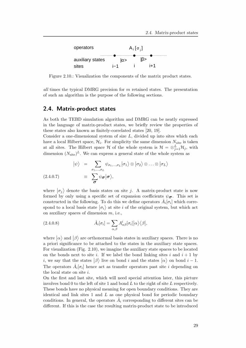
Figure 2.10.: Visualization the components of the matrix product states.
all times the typical DMRG precision for m retained states. The presentationof such an algorithm is the purpose of the following sections.
2.4. Matrix-product states
As both the TEBD simulation algorithm and DMRG can be neatly expressedin the language of matrix-product states, we briefly review the properties ofthese states also known as finitely-correlated states [20, 19].Consider a one-dimensional system of size L, divided up into sites which eachhave a local Hilbert space, Hi. For simplicity the same dimension Nsite is takenat all sites. The Hilbert space H of the whole system is H = ⊗L
j=1Hj, with
dimension (Nsite)L. We can express a general state of the whole system as
∣∣ψ⟩
=∑
σ1,...,σL
ψσ1,...,σL
∣∣σ1
⟩⊗∣∣σ2
⟩⊗ . . .⊗
∣∣σL
⟩
≡∑
σ
ψσ
∣∣σ
⟩,(2.4.0.7)
where∣∣σj
⟩denote the basis states on site j. A matrix-product state is now
formed by only using a specific set of expansion coefficients ψσ . This set isconstructed in the following. To do this we define operators Ai[σi] which corre-spond to a local basis state
∣∣σi
⟩at site i of the original system, but which act
on auxiliary spaces of dimension m, i.e.,
(2.4.0.8) Ai[σi] =∑
α,β
Aiαβ [σi]
∣∣α⟩⟨β∣∣,
where∣∣α⟩
and∣∣β⟩
are orthonormal basis states in auxiliary spaces. There is noa priori significance to be attached to the states in the auxiliary state spaces.For visualization (Fig. 2.10), we imagine the auxiliary state spaces to be locatedon the bonds next to site i. If we label the bond linking sites i and i + 1 byi, we say that the states
∣∣β⟩
live on bond i and the states∣∣α⟩
on bond i − 1.
The operators Ai[σi] hence act as transfer operators past site i depending onthe local state on site i.On the first and last site, which will need special attention later, this pictureinvolves bond 0 to the left of site 1 and bond L to the right of site L respectively.These bonds have no physical meaning for open boundary conditions. They areidentical and link sites 1 and L as one physical bond for periodic boundaryconditions. In general, the operators Ai corresponding to different sites can bedifferent. If this is the case the resulting matrix-product state to be introduced
29
2. The adaptive time-dependent density-matrix renormalization-group method
is referred to as a position-dependent matrix-product state. We also imposethe condition
(2.4.0.9)∑
σi
Ai[σi]A†i [σi] = I,
which we will see to be related to orthonormality properties of bases later.An unnormalized matrix-product state in a form that will be found useful forHamiltonians with open boundary conditions is now defined as
(2.4.0.10)∣∣ψ⟩
=∑
σ
(
⟨φL
∣∣
L∏
i=1
Ai[σi]∣∣φR
⟩
)
∣∣σ
⟩,
where∣∣φL
⟩and
∣∣φR
⟩are the left and right boundary states in the auxiliary
spaces on bonds 0 and L. They act on the product of the operators Ai toproduce scalar coefficients
(2.4.0.11) ψσ =⟨φL
∣∣
L∏
i=1
Ai[σi]∣∣φR
⟩
for the expansion of∣∣ψ⟩
(compare Eq. 2.4.0.7).Several remarks are in order. It should be emphasized that the set of statesobeying Eq. (2.4.0.10) is an submanifold of the full boundary-condition inde-pendent Hilbert space of the quantum many-body problem on L sites that ishoped to yield good approximations to the true quantum states for Hamiltoni-ans with open boundary conditions. If the dimension m of the auxiliary spacesis made sufficiently large then any general state of the system can, in principle,be represented exactly in this form (provided that
∣∣φL
⟩and
∣∣φR
⟩are chosen
appropriately), simply because the O(NsiteLm2) degrees of freedom to choose
the expansion coefficients will exceed NLsite. This is, of course, purely academic.
The practical relevance of the matrix-product states even for computationallymanageable values of m is shown by the success of DMRG, which is known[36, 37] to produce matrix-product states of auxiliary state space dimensionm, in determining energies and correlators at very high precision for moderatevalues of m. In fact, some very important quantum states in one dimension,such as the valence-bond-solid (VBS) ground state of the Affleck-Kennedy-Lieb-Tasaki (AKLT) model [38, 39, 40], can be described exactly by matrix productstates using very small m (m = 2 for the AKLT model).We now formulate a Schmidt decomposition for matrix-product states since wewill use it later on. An unnormalized state
∣∣ψ⟩
of the matrix-product form ofEq. (2.4.0.10) with auxiliary space dimension m can be written as
(2.4.0.12)∣∣ψ⟩
=m∑
α=1
∣∣wS
α
⟩∣∣wE
α
⟩,
where we have arbitrarily cut the chain into S on the left and E on the rightwith
(2.4.0.13)∣∣wS
α
⟩=∑
{σS}
[
⟨φL
∣∣∏
i∈S
Ai[σi]∣∣α⟩
]
∣∣σ
S⟩,
30
2.5. TEBD simulation algorithm
i|α >
λiα λ
i−1α
i−1|α >i
Γ [i] σ i
i+1i−1
operators
auxiliary statessites
i−1α α i
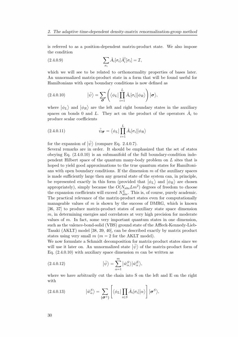
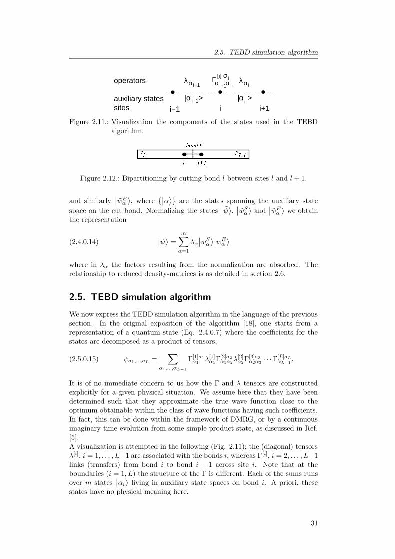
Figure 2.11.: Visualization the components of the states used in the TEBDalgorithm.
Figure 2.12.: Bipartitioning by cutting bond l between sites l and l + 1.
and similarly∣∣wE
α
⟩, where {
∣∣α⟩} are the states spanning the auxiliary state
space on the cut bond. Normalizing the states∣∣ψ⟩,∣∣wS
α
⟩and
∣∣wE
α
⟩we obtain
the representation
(2.4.0.14)∣∣ψ⟩
=
m∑
α=1
λα
∣∣wS
α
⟩∣∣wE
α
⟩
where in λα the factors resulting from the normalization are absorbed. Therelationship to reduced density-matrices is as detailed in section 2.6.
2.5. TEBD simulation algorithm
We now express the TEBD simulation algorithm in the language of the previoussection. In the original exposition of the algorithm [18], one starts from arepresentation of a quantum state (Eq. 2.4.0.7) where the coefficients for thestates are decomposed as a product of tensors,
(2.5.0.15) ψσ1,...,σL=
∑
α1,...,αL−1
Γ[1]σ1α1
λ[1]α1
Γ[2]σ2α1α2
λ[2]α2
Γ[3]σ3α2α3
· · ·Γ[L]σLαL−1
.
It is of no immediate concern to us how the Γ and λ tensors are constructedexplicitly for a given physical situation. We assume here that they have beendetermined such that they approximate the true wave function close to theoptimum obtainable within the class of wave functions having such coefficients.In fact, this can be done within the framework of DMRG, or by a continuousimaginary time evolution from some simple product state, as discussed in Ref.[5].
A visualization is attempted in the following (Fig. 2.11); the (diagonal) tensorsλ[i], i = 1, . . . , L−1 are associated with the bonds i, whereas Γ[i], i = 2, . . . , L−1links (transfers) from bond i to bond i − 1 across site i. Note that at theboundaries (i = 1, L) the structure of the Γ is different. Each of the sums runsover m states
∣∣αi
⟩living in auxiliary state spaces on bond i. A priori, these
states have no physical meaning here.
31
2. The adaptive time-dependent density-matrix renormalization-group method
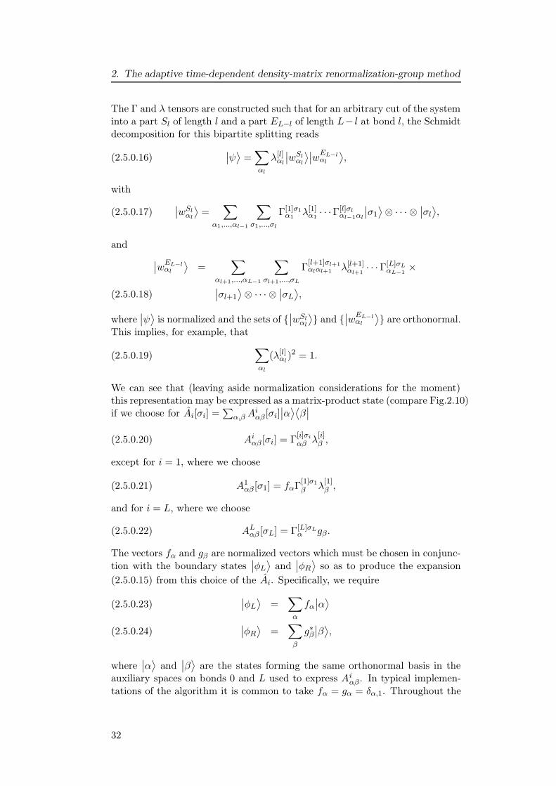
The Γ and λ tensors are constructed such that for an arbitrary cut of the systeminto a part Sl of length l and a part EL−l of length L− l at bond l, the Schmidtdecomposition for this bipartite splitting reads
(2.5.0.16)∣∣ψ⟩
=∑
αl
λ[l]αl
∣∣wSl
αl
⟩∣∣w
EL−lαl
⟩,
with
(2.5.0.17)∣∣wSl
αl
⟩=
∑
α1,...,αl−1
∑
σ1,...,σl
Γ[1]σ1α1
λ[1]α1
· · ·Γ[l]σlαl−1αl
∣∣σ1
⟩⊗ · · · ⊗
∣∣σl
⟩,
and
∣∣w
EL−lαl
⟩=
∑
αl+1,...,αL−1
∑
σl+1,...,σL
Γ[l+1]σl+1αlαl+1 λ[l+1]
αl+1· · ·Γ[L]σL
αL−1×
∣∣σl+1
⟩⊗ · · · ⊗
∣∣σL
⟩,(2.5.0.18)
where∣∣ψ⟩
is normalized and the sets of {∣∣wSl
αl
⟩} and {
∣∣w
EL−lαl
⟩} are orthonormal.
This implies, for example, that
(2.5.0.19)∑
αl
(λ[l]αl
)2 = 1.
We can see that (leaving aside normalization considerations for the moment)this representation may be expressed as a matrix-product state (compare Fig.2.10)if we choose for Ai[σi] =
∑
α,β Aiαβ [σi]
∣∣α⟩⟨β∣∣
(2.5.0.20) Aiαβ [σi] = Γ
[i]σi
αβ λ[i]β ,
except for i = 1, where we choose
(2.5.0.21) A1αβ [σ1] = fαΓ
[1]σ1
β λ[1]β ,
and for i = L, where we choose
(2.5.0.22) ALαβ [σL] = Γ[L]σL
α gβ.
The vectors fα and gβ are normalized vectors which must be chosen in conjunc-tion with the boundary states
∣∣φL
⟩and
∣∣φR
⟩so as to produce the expansion
(2.5.0.15) from this choice of the Ai. Specifically, we require
∣∣φL
⟩=
∑
α
fα
∣∣α⟩
(2.5.0.23)
∣∣φR
⟩=
∑
β
g∗β∣∣β⟩,(2.5.0.24)
where∣∣α⟩
and∣∣β⟩
are the states forming the same orthonormal basis in theauxiliary spaces on bonds 0 and L used to express Ai
αβ . In typical implemen-tations of the algorithm it is common to take fα = gα = δα,1. Throughout the
32
2.5. TEBD simulation algorithm
rest of this section we take this as the definition for gα and fα, as this allows usto treat the operators on the boundary identically to the other operators. For
the same reason we define a vector λ[0]α = δα,1.
In the above expressions (2.5.0.17-2.5.0.22) we have grouped Γ and λ such thatthe λ reside on the right of the two bonds linked by Γ. There is another validchoice for the Ai, which will produce identical states in the original system, andessentially the same procedure for the algorithm. If we set
(2.5.0.25) Aiαβ [σi] = λ[i−1]
α Γ[i]σi
αβ ,
except for i = 1, where we choose
(2.5.0.26) A1αβ [σ1] = fαΓ
[1]σ1
β ,
and for i = L, where we choose
(2.5.0.27) ALαβ [σL] = λ[L−1]
α Γ[L]σLα gβ ,
then the same choice of boundary states produces the correct coefficients. Herewe have grouped Γ and λ such that the λ reside on the left of the two bondslinked by Γ. It is also important to note that any valid choice of fα and gβ
that produces the expansion (2.5.0.15) specifically excludes the use of periodicboundary conditions. While generalizations are feasible, they will not be pur-sued here.To conclude the identification of states, we consider normalization issues. Thecondition (2.4.0.9) is indeed fulfilled for our choice of Ai[σi], because we havefrom (2.5.0.18) for a splitting at l − 1 that
∣∣w
EL−(l−1)αl−1
⟩=
∑
αlσl
Γ[l]σlαl−1αl
λ[l]αl
∣∣σl
⟩⊗∣∣w
EL−lαl
⟩
=∑
αlσl
Alαl−1αl
[σl]∣∣σl
⟩⊗∣∣w
EL−lαl
⟩,(2.5.0.28)
so that from the orthonormality of the sets of states {∣∣w
EL−(l−1)α
⟩}m
α=1, {∣∣σl
⟩}Nsite
σl=1
and {∣∣w
EL−lγ
⟩}m
γ=1,
∑
σl
Al[σl]A†l [σl] =
∑
αβγ
∑
σl
Alαγ [σl](A
lβγ [σl])
∗∣∣α⟩⟨β∣∣
=∑
αβ
⟨w
EL−(l−1)
β
∣∣w
EL−(l−1)α 〉
∣∣α⟩⟨β∣∣
=∑
αβ
dαβ
∣∣α⟩⟨β∣∣ = I.(2.5.0.29)
After introducing the notation of matrix-product states we can now consider thetime evolution for a typical (possibly time-dependent) Hamiltonian in stronglycorrelated systems that contains for simplicity only short-ranged interactions:
(2.5.0.30) H =∑
i odd
Fi,i+1 +∑
j even
Gj,j+1,
33
2. The adaptive time-dependent density-matrix renormalization-group method
Fi,i+1 and Gj,j+1 are the local Hamiltonians on the odd bonds linking i andi+1, and the even bonds linking j and j+1. While all F and G terms commuteamong each other, F and G terms do in general not commute if they share onesite. The time evolution operator for a time step dt may be approximatelyrepresented by a (first order) Suzuki-Trotter expansion as
(2.5.0.31) e−iHdt =∏
i odd
e−iFi,i+1dt∏
j even
e−iGj,j+1dt + O(dt2),
and the time evolution of the state can be computed by repeated application ofthe two-site time evolution operators exp(−iGj,j+1dt) and exp(−iFi,i+1dt). Thisis a well-known procedure in particular in Quantum Monte Carlo [41] where itserves to carry out imaginary time evolutions (checkerboard decomposition).The TEBD simulation algorithm now runs as follows [5, 18]:
1. Perform the following two steps for all even bonds (order does not matter):
(i) Apply exp(−iGl,l+1dt) to∣∣ψ(t)
⟩. For each local time update, a new
wave function is obtained. The number of degrees of freedom on the“active” bond thereby increases, as will be detailed below.
(ii) Carry out a Schmidt decomposition cutting this bond and retain asin DMRG only those m degrees of freedom with the highest weightin the decomposition.
2. Repeat this two-step procedure for all odd bonds, applying exp(−iFl,l+1dt).
3. This completes one Suzuki-Trotter time step. One may now evaluateexpectation values at selected time steps, and continue the algorithm fromstep 1.
After sketching the procedure we now consider its computational details.(i) Consider a local time evolution operator acting on bond l, i.e. sites l andl + 1, for a state
∣∣ψ⟩. The Schmidt decomposition of
∣∣ψ⟩
after partitioning bycutting bond l reads
(2.5.0.32)∣∣ψ⟩
=
m∑
αl=1
λ[l]αl
∣∣wSl
αl
⟩∣∣w
EL−lαl
⟩.
Using Eqs. (2.5.0.17), (2.5.0.18) and (2.5.0.28), we find
∣∣ψ⟩
=∑
αl−1αlαl+1
∑
σlσl+1
λ[l−1]αl−1
Alαl−1αl
[σl]Al+1αlαl+1
[σl+1] ×
∣∣w
Sl−1αl−1
⟩∣∣σl
⟩∣∣σl+1
⟩∣∣w
EL−(l+1)αl+1
⟩.(2.5.0.33)
We note, that if we identify∣∣w
Sl−1αl−1
⟩and
∣∣w
EL−(l+1)αl+1
⟩with DMRG system and
environment block states∣∣wS
ml−1
⟩and
∣∣wE
ml+1
⟩, we have a typical DMRG state
for two blocks and two sites
(2.5.0.34)∣∣ψ⟩
=∑
ml−1
∑
σl
∑
σl+1
∑
ml+1
ψml−1σlσl+1ml+1
∣∣wS
ml−1
⟩∣∣σl
⟩∣∣σl+1
⟩∣∣wE
ml+1
⟩
34
2.5. TEBD simulation algorithm
with
(2.5.0.35) ψml−1σlσl+1ml+1=∑
αl
λ[l−1]ml−1
Alml−1αl
[σl]Al+1αlml+1
[σl+1].
The local time evolution operator on site l, l + 1 can be expanded as
(2.5.0.36) Ul,l+1 =∑
σlσl+1
∑
σ′lσ′
l+1
Uσ′
lσ′
l+1σlσl+1
∣∣σ′lσ
′l+1
⟩⟨σlσl+1
∣∣
and generates∣∣ψ′⟩ = Ul,l+1
∣∣ψ⟩, where
∣∣ψ′⟩ =
∑
αl−1αlαl+1
∑
σlσl+1
∑
σ′lσ′
l+1
λ[l−1]αl−1
Alαl−1αl
[σ′l]Al+1αlαl+1
[σ′l+1]Uσlσl+1
σ′lσ′
l+1
∣∣w
Sl−1αl−1
⟩∣∣σl
⟩∣∣σl+1
⟩∣∣w
EL−(l+1)αl+1
⟩.
This can also be written as
(2.5.0.37)∣∣ψ′⟩ =
∑
αl−1αl+1
∑
σlσl+1
Θσlσl+1αl−1αl+1
∣∣w
Sl−1αl−1
⟩∣∣σl
⟩∣∣σl+1
⟩∣∣w
EL−(l+1)αl+1
⟩,
where
(2.5.0.38) Θσlσl+1αl−1αl+1 = λ[l−1]
αl−1
∑
αlσ′lσ′
l+1
Alαl−1αl
[σ′l]Al+1αlαl+1
[σ′l+1]Uσlσl+1
σ′lσ′
l+1.
(ii) Now a new Schmidt decomposition identical to that in DMRG can be carriedout for
∣∣ψ′⟩: cutting once again bond l, there are now mNsite states in each
part of the system, leading to
(2.5.0.39)∣∣ψ′⟩ =
mNsite∑
αl=1
λ[l]αl
∣∣wSl
αl
⟩∣∣w
EL−lαl
⟩.
In general the states and coefficients of the decomposition will have changedcompared to the decomposition (2.5.0.32) previous to the time evolution, whichmeans that the reduced Hilbert space has been adapted to the quantum stateat this time [compare Fig. 2.5 (c)]. We indicate this by introducing a tilde forthese states and coefficients. As in DMRG, if there are more than m non-zero
eigenvalues, we now choose the m eigenvectors corresponding to the largest λ[l]αl
to use in these expressions. The error in the final state produced as a result isproportional to the sum of the magnitudes of the discarded eigenvalues. Afternormalization, to allow for the discarded weight, the state reads
(2.5.0.40)∣∣ψ′⟩ =
m∑
αl=1
λ[l]αl
∣∣wSl
αl
⟩∣∣w
EL−lαl
⟩.
Note again that the states and coefficients in this superposition are in generaldifferent from those in Eq. (2.5.0.32); we have now dropped the tildes again, as
35
2. The adaptive time-dependent density-matrix renormalization-group method
this superposition will be the starting point for the next time evolution (stateadaption) step.
To obtain the Schmidt decomposition reduced density-matrices are formed, e.g.
ρE = TrS∣∣ψ′⟩⟨ψ′∣∣
=∑
σl+1σ′l+1αl+1α′
l+1
∣∣σl+1
⟩∣∣wαl+1
⟩⟨wα′
l+1
∣∣⟨σ′l+1
∣∣
×
∑
αl−1σl
Θσlσl+1αl−1αl+1
(
Θσlσ
′l+1
αl−1α′l+1
)∗
.(2.5.0.41)
If we now diagonalize ρE , we can read off the new values of Al+1αlαl+1
[σl+1] because
the eigenvectors∣∣w
EL−lαl
⟩obey
(2.5.0.42)∣∣w
EL−lαl
⟩=
∑
σl+1αl+1
Al+1αlαl+1
[σl+1]∣∣σl+1
⟩∣∣w
EL−(l+1)αl+1
⟩.
We also obtain the eigenvalues, (λ[l]αl
)2. Due to the asymmetric grouping of Γand λ into A discussed above, a short calculation shows that the new values forAl
αl−1αl[σl] can be read off from the slightly more complicated expression
(2.5.0.43) λ[l]αl
∣∣wSl
αl
⟩=∑
αl−1σl
λ[l−1]αl−1
Alαl−1αl
[σl]∣∣w
Sl−1αl−1
⟩∣∣σl
⟩.
The states∣∣wSl
αl
⟩are the normalized eigenvectors of ρS formed in analogy to
ρE .
The key point about the TEBD simulation algorithm is that a DMRG-styletruncation keeping the most relevant density-matrix eigenstates (or the max-imum amount of entanglement) is carried out for each local update at eachtime step. This is in contrast with time-dependent DMRG methods describedin section 2.3, where the basis states were chosen before the time evolution isperformed, and did not “adapt” to optimally represent the time-evolved state.
2.6. DMRG and matrix-product states
Typical normalized DMRG states for the combination of two blocks S and Eand two single sites (Fig. 2.13) have the form
(2.6.0.44)∣∣ψ⟩
=∑
ml−1
∑
σl
∑
σl+1
∑
ml+1
ψml−1σlσl+1ml+1
∣∣wS
ml−1
⟩∣∣σl
⟩∣∣σl+1
⟩∣∣wE
ml+1
⟩
which can be Schmidt decomposed as
(2.6.0.45)∣∣ψ⟩
=∑
ml
λ[l]ml
∣∣wS
ml
⟩∣∣wE
ml
⟩.
36
2.6. DMRG and matrix-product states
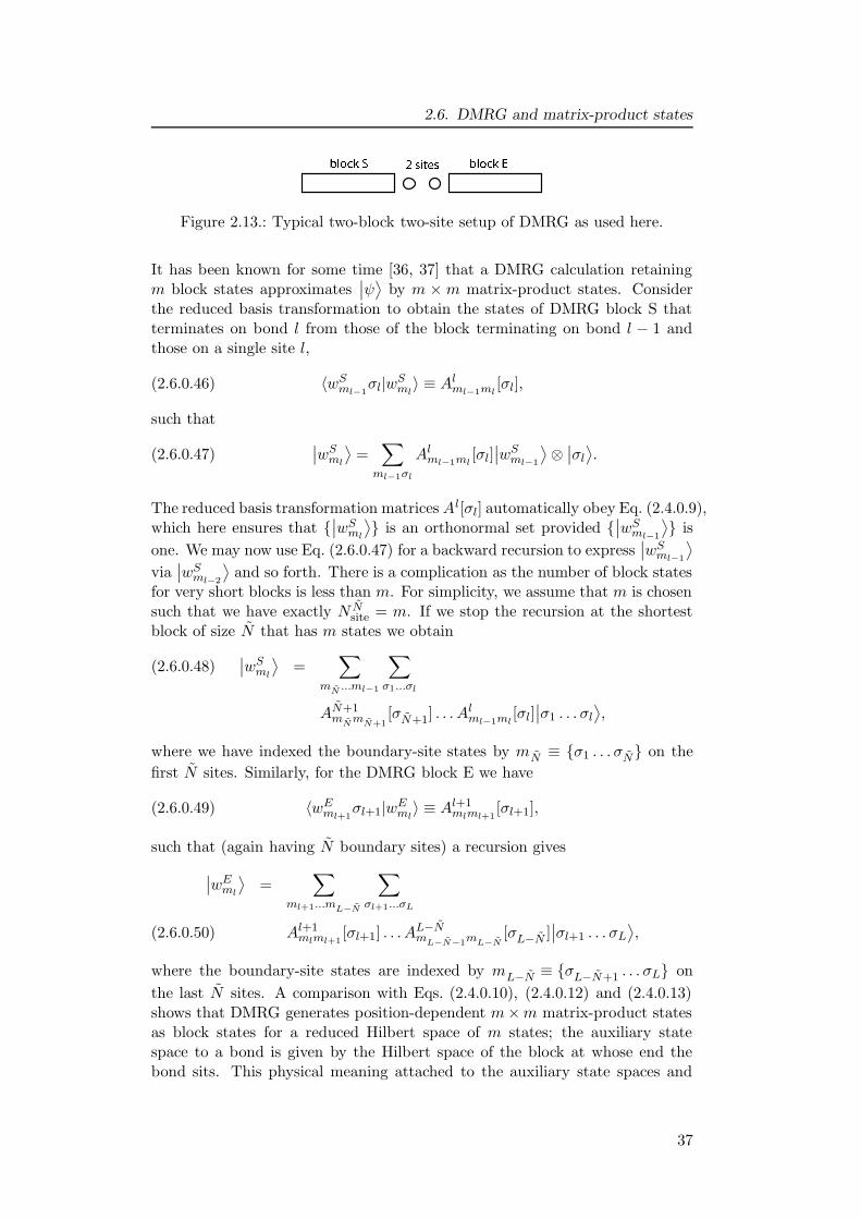
Figure 2.13.: Typical two-block two-site setup of DMRG as used here.
It has been known for some time [36, 37] that a DMRG calculation retainingm block states approximates
∣∣ψ⟩
by m × m matrix-product states. Considerthe reduced basis transformation to obtain the states of DMRG block S thatterminates on bond l from those of the block terminating on bond l − 1 andthose on a single site l,
(2.6.0.46) 〈wSml−1
σl|wSml
〉 ≡ Alml−1ml
[σl],
such that
(2.6.0.47)∣∣wS
ml
⟩=
∑
ml−1σl
Alml−1ml
[σl]∣∣wS
ml−1
⟩⊗∣∣σl
⟩.
The reduced basis transformation matrices Al[σl] automatically obey Eq. (2.4.0.9),which here ensures that {
∣∣wS
ml
⟩} is an orthonormal set provided {
∣∣wS
ml−1
⟩} is
one. We may now use Eq. (2.6.0.47) for a backward recursion to express∣∣wS
ml−1
⟩
via∣∣wS
ml−2
⟩and so forth. There is a complication as the number of block states
for very short blocks is less than m. For simplicity, we assume that m is chosensuch that we have exactly N N
site = m. If we stop the recursion at the shortestblock of size N that has m states we obtain
∣∣wS
ml
⟩=
∑
mN
...ml−1
∑
σ1...σl
(2.6.0.48)
AN+1m
Nm
N+1[σN+1] . . . A
lml−1ml
[σl]∣∣σ1 . . . σl
⟩,
where we have indexed the boundary-site states by mN ≡ {σ1 . . . σN} on the
first N sites. Similarly, for the DMRG block E we have
(2.6.0.49) 〈wEml+1
σl+1|wEml
〉 ≡ Al+1mlml+1
[σl+1],
such that (again having N boundary sites) a recursion gives
∣∣wE
ml
⟩=
∑
ml+1...mL−N
∑
σl+1...σL
Al+1mlml+1
[σl+1] . . . AL−Nm
L−N−1mL−N
[σL−N ]∣∣σl+1 . . . σL
⟩,(2.6.0.50)
where the boundary-site states are indexed by mL−N ≡ {σL−N+1 . . . σL} on
the last N sites. A comparison with Eqs. (2.4.0.10), (2.4.0.12) and (2.4.0.13)shows that DMRG generates position-dependent m×m matrix-product statesas block states for a reduced Hilbert space of m states; the auxiliary statespace to a bond is given by the Hilbert space of the block at whose end thebond sits. This physical meaning attached to the auxiliary state spaces and
37
2. The adaptive time-dependent density-matrix renormalization-group method
the fact that for the shortest block the states can be labeled by good quantumnumbers (if available) ensures through (2.6.0.46) and (2.6.0.49) that they carrygood quantum numbers for all block sizes. The big advantage is that usinggood quantum numbers allows us to exclude a large amount of wave functioncoefficients as being 0, drastically speeding up all calculations by at least one,and often two orders of magnitude.In this language the effect of the finite-system DMRG algorithm (see section2.2.2) is to shift the two free sites through the chain, growing and shrinkingthe blocks S and E as illustrated in Fig. 2.4. At each step, the ground stateis redetermined and a new Schmidt decomposition carried out in which thesystem is cut between the two free sites, leading to a new truncation and newreduced basis transformations (two matrices A adjacent to this bond). It is thusa sequence of local optimization steps of the wave function oriented towards anoptimal representation of the ground state. Typically, after some “sweeps” ofthe free sites from left to right and back, physical quantities evaluated for thisstate converge. While comparison of DMRG results to exact results shows thatone often comes extremely close to an optimal representation within the matrixstate space (which justifies the usage of the DMRG algorithm to obtain them), ithas been pointed out and numerically demonstrated [37, 42] that finite-systemDMRG results can be further improved and better matrix-product states beproduced by switching, after convergence is reached, from the S••E scheme(with two free sites) to an S•E scheme (with one free site) and to carry outsome more sweeps. This point is not pursued further here, it just serves toillustrate that finite-system DMRG for all practical purposes comes close to anoptimal matrix-product state, while not strictly reaching the optimum.We will outline the calculation for shifting the active bond by one site to theleft since it will be used in the adaptive t-DMRG.Starting from the wavefunction represented in the S••E scheme,
(2.6.0.51)∣∣ψ⟩
=∑
ml−1
∑
σl
∑
σl+1
∑
ml+1
ψml−1σlσl+1ml+1
∣∣wS
ml−1
⟩∣∣σl
⟩∣∣σl+1
⟩∣∣wE
ml+1
⟩,
one inserts the identity∑
ml
∣∣wE
ml
⟩⟨wE
ml
∣∣ to obtain
(2.6.0.52)∣∣ψ⟩
=∑
ml−1
∑
σl
∑
ml
ψml−1σlml
∣∣wS
ml−1
⟩∣∣σl
⟩∣∣wE
ml
⟩,
where
(2.6.0.53) ψml−1σlml=∑
ml+1
∑
σl+1
ψml−1σlσl+1ml+1Al+1
mlml+1[σl+1].
After inserting in a second step the identity∑
ml−2σl−1
∣∣wS
ml−2σl−1
⟩⟨wS
ml−2σl−1
∣∣,
one ends up with the wave function in the shifted bond representation:
(2.6.0.54)∣∣ψ⟩
=∑
ml−2
∑
σl−1
∑
σl
∑
ml
ψml−2σl−1σlml
∣∣wS
ml−2
⟩∣∣σl−1
⟩∣∣σl
⟩∣∣wE
ml
⟩,
where
(2.6.0.55) ψml−2σl−1σlml=∑
ml−1
ψml−1σlmlAl−1
ml−2ml−1[σl−1].
38
2.7. Adaptive t-DMRG
2.7. Adaptive t-DMRG
As the actual decomposition and truncation procedure in DMRG and the TEBDsimulation algorithm are identical, the idea of the TEBD algorithm can be car-ried over to generalize the DMRG to give a very effective method, the adaptivet-DMRG, to study time-dependent phenomena in strongly correlated quasi-onedimensional systems. In the adaptive t-DMRG the finite-system algorithm isused to carry out the sequence of local time evolutions after the initial state hasbeen determined. During each such a local time evolution the local evolutionoperator is applied to the wave function
∣∣ψ⟩
in a two-block two-site configura-tion such that the bond that is currently updated consists of the two free sites.Then new block states — best adapted to a state at any given point in thetime evolution (hence adaptive block states)— are constructed by Schmidt de-composition and truncation as in the TEBD algorithm, while maintaining thecomputational efficiency of DMRG. Then to apply the next local evolution op-erator the wave function
∣∣ψ⟩
has to be transformed between different two-blocktwo-site configurations. In finite-system DMRG such a transformation, whichwas first implemented by White [21] (“state prediction”) is routinely used topredict the outcome of large sparse matrix diagonalizations, which no longeroccur during time evolution. Here, it merely serves as a transformation to thereduced basis.The adaptive t-DMRG algorithm using the first order Suzuki-Trotter decompo-sition which incorporates the TEBD simulation algorithm in the DMRG frame-work is now set up as follows:
0. Set up a conventional finite-system DMRG algorithm with state predic-tion using the Hamiltonian at time t = 0, H(0), to determine the groundstate of some system of length L using effective block Hilbert spaces ofdimension m. At the end of this stage of the algorithm, we have for blocksof all sizes l reduced orthonormal bases spanned by states
∣∣ml
⟩, which are
characterized by good quantum numbers. Also, we have all reduced basistransformations, corresponding to the matrices A.
1. For each Suzuki-Trotter time step, use the finite-system DMRG algorithmto run one sweep with the following modifications:
i) For each even bond apply the local time evolution U at the bondformed by the free sites to
∣∣ψ⟩. This is a very fast operation com-
pared to determining the ground state, which is usually done insteadin the finite-system algorithm.
ii) As always, perform a DMRG truncation at each step of the finite-system algorithm, hence O(L) times.
(iii) Use White’s prediction method to shift the free sites by two.
2. In the reverse direction, apply step (i) to all odd bonds.
3. As in standard finite-system DMRG evaluate operators when desired atthe end of a time step. Note, that there is no need to generate theseoperators at all those time steps where no operator evaluation is desired.
39
2. The adaptive time-dependent density-matrix renormalization-group method
The calculation time of adaptive t-DMRG scales linearly in L, as opposed tothe non-adaptive time-dependent DMRG which only depends on L indirectly.The diagonalization of the density-matrices (Schmidt decomposition) scales asN3
sitem3; the preparation of the local time evolution operator as N 6
site, but thismay have to be done only rarely e.g. for discontinuous changes of interactionparameters. Carrying out the local time evolution scales as N 4
sitem2; the basis
transformation scales as N 2sitem
3. As m � Nsite typically, the algorithm isof order O(LN 3
sitem3) at each time step. In most cases a speeding up of the
algorithm can be obtained using higher order Suzuki-Trotter decompositionsgiven in appendix A. In the applications presented in this work the second-order and fourth-order Suzuki-Trotter decomposition are used.
2.8. Case study: time-dependent Bose-Hubbard model
Before we discuss the sources of error in the next section, we would like tocompare the new adaptive algorithm to the non-adaptive methods describedin section 2.3. To do this we present some results of calculations on the Bose-Hubbard Hamiltonian introduced in section 2.3 which have been carried outusing modest computational resources and an unoptimized code (this concernsin particular the operations on complex matrices and vectors). In the following,Suzuki-Trotter time steps down to dt = 5 × 10⁻⁴ in units of 1/J were chosen.Applications to systems of realistic size are shown in the following chapters.Comparing the results of the adaptive t-DMRG for the Bose-Hubbard modelwith the parameters chosen as in section 2.3 with the static time-dependentDMRG we find that the convergence in m of the adaptive algorithm is muchfaster than for the static algorithm. For the nearest neighbour correlations itsets in at about m = 40 (Fig. 2.14) for the adaptive algorithm compared tom = 100 for the static method (Fig. 2.6-2.8).
This faster convergence in m enables us to study larger systems than wouldbe accessible with non-adaptive time-dependent DMRG (Fig. 2.15). In theL = 32 system considered here, we encountered severe convergence problemsusing non-adaptive time-dependent DMRG. By contrast, in the new approachconvergence sets in for m well below 100, which is easily accessible numerically.Let us remark that the number m of states which have to be kept does certainlyvary with the exact parameters chosen, depending on whether the state can beapproximated well by matrix-product states of a low dimension. At least in thecase studied here, we found that this dependence is quite weak. We expect (alsofrom studying the time evolution of density-matrix spectra) that the systemdependence of m is roughly similar as in the static case.
Similar observations are made both for local occupancy (a simpler quantitythan nearest-neighbour correlations) and longer-ranged correlations (where weexpect less precision). Moving back to the parameter set of section 2.3, we findas expected that the result for the local occupancy (Fig. 2.16) has convergedfor the same m leading to convergence in the nearest-neighbour correlations. Incontrast, if we consider the correlation 〈b†b〉 between sites further apart fromeach other the numerical results converge more slowly under an increase of m
40
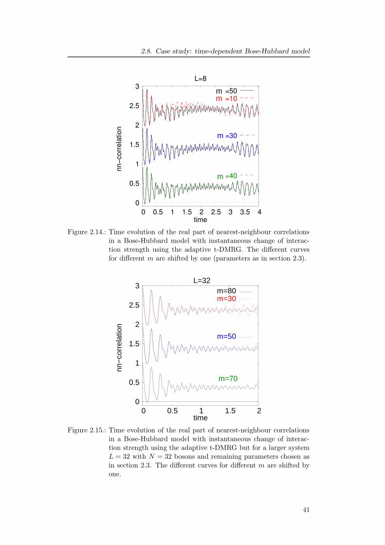
2.8. Case study: time-dependent Bose-Hubbard model
m
m
mm
Figure 2.14.: Time evolution of the real part of nearest-neighbour correlationsin a Bose-Hubbard model with instantaneous change of interac-tion strength using the adaptive t-DMRG. The different curvesfor different m are shifted by one (parameters as in section 2.3).
0
0.5
1
1.5
2
2.5
3
0 0.5 1 1.5 2
m=80 m=30
m=50
m=70
nn−
corr
elat
ion
time
L=32
Figure 2.15.: Time evolution of the real part of nearest-neighbour correlationsin a Bose-Hubbard model with instantaneous change of interac-tion strength using the adaptive t-DMRG but for a larger systemL = 32 with N = 32 bosons and remaining parameters chosen asin section 2.3. The different curves for different m are shifted byone.
41
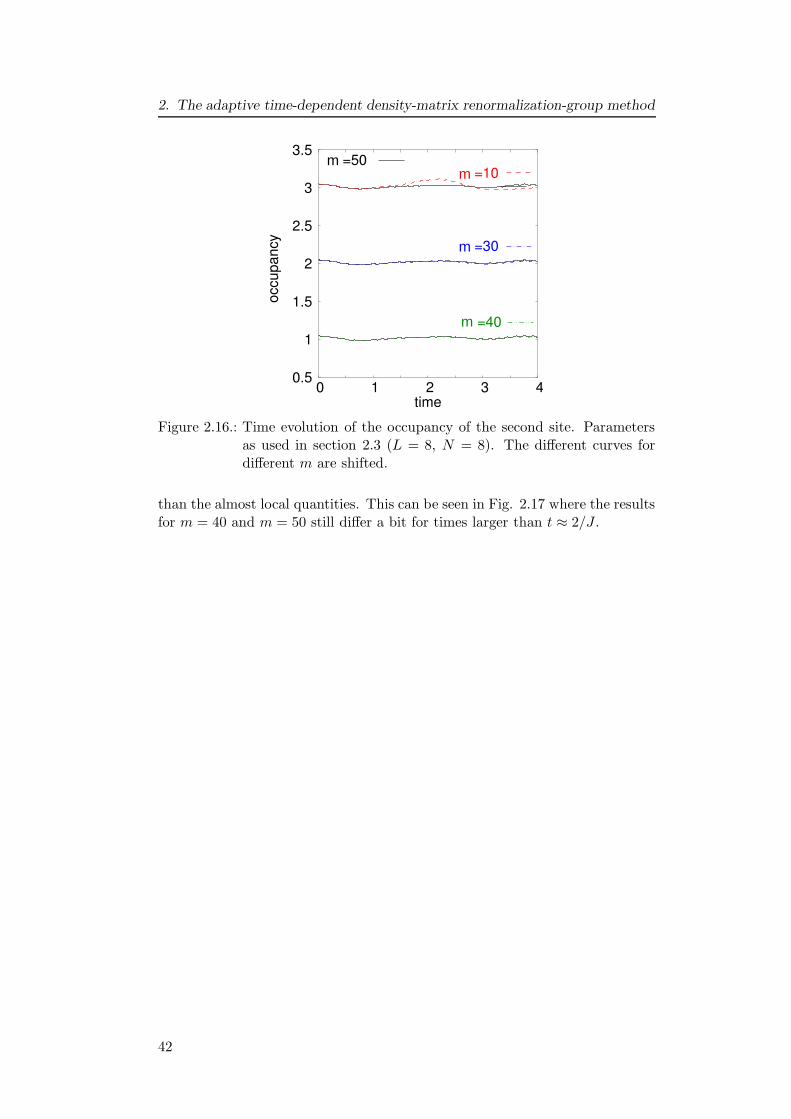
2. The adaptive time-dependent density-matrix renormalization-group method
m
m
m
m
Figure 2.16.: Time evolution of the occupancy of the second site. Parametersas used in section 2.3 (L = 8, N = 8). The different curves fordifferent m are shifted.
than the almost local quantities. This can be seen in Fig. 2.17 where the resultsfor m = 40 and m = 50 still differ a bit for times larger than t ≈ 2/J .
42
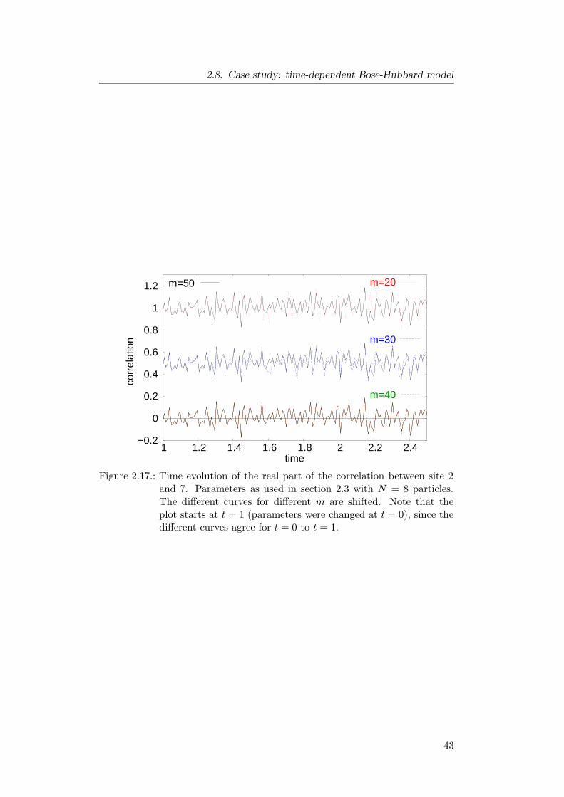
2.8. Case study: time-dependent Bose-Hubbard model
corr
elat
ion
−0.2
0
0.2
0.4
0.6
0.8
1
1.2
1 1.2 1.4 1.6 1.8 2 2.2 2.4time
m=50 m=20
m=30
m=40
Figure 2.17.: Time evolution of the real part of the correlation between site 2and 7. Parameters as used in section 2.3 with N = 8 particles.The different curves for different m are shifted. Note that theplot starts at t = 1 (parameters were changed at t = 0), since thedifferent curves agree for t = 0 to t = 1.
43
2. The adaptive time-dependent density-matrix renormalization-group method
2.9. Sources of error
After we have seen in the previous chapter that the developed algorithm per-forms very well in describing time-dependent phenomena, let us discuss herethe approximations involved. Two main sources of error occur in the adaptivet-DMRG:(i) The Suzuki-Trotter error due to the Suzuki-Trotter decomposition. For annth-order Suzuki-Trotter decomposition [41], the error made in one time stepdt is of order dtn+1. To reach a given time t one has to perform t/dt time-steps,such that in the worst case the error grows linearly in time t such that theresulting error is of order (dt)nt. In our setup of the Suzuki-Trotter decompo-sition, the error is expected to scale linearly with system size L for a genericstate, and overall it is of order (dt)nLt for the times of interest. (Eventually, theerror generally saturates at a finite value, as measured quantities are typicallybound.)(ii) The DMRG truncation error due to the representation of the time-evolvingquantum state in reduced (albeit “optimally” chosen) Hilbert spaces and dueto the repeated transformations between different truncated basis sets. Whilethe truncation error ε that sets the scale of the error of the wave function andoperators is typically very small, here it will strongly accumulate in time asO(Lt/dt) truncations are carried out up to time t. This is due to the fact thatthe truncated DMRG wave function has norm less than one and is renormalizedat each truncation by a factor of (1− ε)−1 > 1. Truncation errors should there-fore accumulate roughly exponentially with an exponent of εLt/dt, such thateventually the adaptive t-DMRG will break down at too long times. A partialcompensation of errors in observables may slow down the error growth. Theaccumulated truncation error should decrease considerably with an increasingnumber of kept DMRG states m. For a fixed time t, it should decrease asthe Suzuki-Trotter time step dt is increased, since the number of truncationsdecreases with the number of time steps t/dt.
At this point, it is worthwhile to mention that the error arising should alsobe pertinent to the very closely related time evolution algorithm introducedby Verstraete et al. [43], which differs from ours for the present purpose inone major point: In our algorithm a basis truncation is performed after eachlocal application of Ul,l+1. In their more time-consuming algorithm truncationsare performed after all local time evolutions have been carried out, i.e. aftera global time evolution using U =
∏
l Ul,l+1. In our iterative procedure, thewave function after such a full time evolution is not necessarily the globallyoptimal state representing the time-evolved state. However, for small dt thestate update via the operators Un is likely to be small. We expect the globaloptimum to be rather well approximated using the present algorithm, as seemsto be borne out by direct comparisons between both approaches. Errors shouldtherefore exhibit very similar behaviour.
A detailed error analysis of the influence of the Suzuki-Trotter error and thetruncation error on the total error can be found in section 6.3, where we compareour DMRG results for the time evolution of an initial state in a spin-1/2 XX-model to exact results.
44
2.10. Conclusion
2.10. Conclusion
While exporting ideas from one field of knowledge to another may appear as anexciting and often fruitful enterprise, differences in language and background be-tween researchers in so far separated fields can also often become a serious obsta-cle to the proper propagation and full assimilation of such ideas. In this chapterwe have translated the TEBD algorithm into the language of matrix-productstates. This language is a natural choice to express the DMRG algorithm –which, for over a decade, has dominated the simulation of one-dimensionalquantum many-body systems. The translation of the TEBD algorithm to theDMRG language has made evident that the TEBD and the DMRG algorithmshave a number of common features, a fact that was exploited in developing thenew method presented here. We have performed the corresponding modifica-tion of existing finite-system DMRG codes to incorporate the TEBD leadingto the new adaptive t-DMRG algorithm. Even without attempting to reachthe computationally most efficient incorporation of the TEBD algorithm intoDMRG implementations, the resulting code seems to perform systematicallybetter than non-adaptive time-dependent DMRG codes at very reasonable nu-merical cost. The adaptive t-DMRG converges for much smaller state spaces,as they are adapted in time to track the actual state of the evolving system.The new code by application of existing conceptual ideas, is significantly moreefficient than other existing embodiments of the TEBD, for instance thanks tothe way DMRG exploits good quantum numbers.While we have considered bosons in the example, also fermionic (see chapter5) and spin (see chapter 6) systems present no fundamental difficulties. Someinteresting topics which are best approached with the adaptive t-DMRG are pre-sented in the following chapters to show the efficiency of the developed adaptivet-DMRG. In chapter 4 the evolution of a perturbation in a bosonic system, inchapter 5 the spin-charge separation in one-dimensional fermionic systems withtwo species, and in chapter 6 a simplified model for spin transport between twospin polarized reservoirs are discussed.
45
3. Ultracold atoms in optical lattices
3.1. From Bose-Einstein condensation to strongly
interacting Bose gases
In 1995, the first experimental realizations of a Bose-Einstein condensation(BEC) were achieved in rubidium [8], sodium [9] and lithium vapors [10]. Thiswas long after the theoretical prediction of this effect by Einstein 1924, whoinvestigated the ideal Bose gas based on the statistics introduced by Bose. Themain problem in the experimental realization of Bose-Einstein condensationwas that the cloud of atoms had to be cooled to ultra low temperatures inthe nano-Kelvin regime. To reach these low temperatures became possibleonly after the development of laser and evaporative cooling techniques. In aBose-Einstein condensate a macroscopic number of bosonic atoms collectivelyoccupies the lowest energy state. Therefore, the Bose-Einstein condensatesprovide the possibility to explore quantum phenomena on a macroscopic scale.Examples are the interference between two condensates [44] or collective modes[45]. In a Bose-Einstein condensate the ratio between the interaction energybetween the atoms and their kinetic energy is usually very low, of the orderof Eint
Ekin≈ 0.02, and the theoretical description [12] of many properties is well
understood in the framework of the Gross-Pitaevskii and Bogoliubov theories.
From the viewpoint of many-particle physics the regime in which the interplaybetween the interaction and the kinetic energy becomes important is even moreinteresting than the weakly interacting regime. Fascinating many-body effectslike the quantum phase transition between a superfluid and a Mott-insultingstate occur. In this regime the Bose gas cannot be described by the Gross-Pitaevskii theory anymore, since correlations between the atoms induced bytheir interaction have to be taken into account. To reach this regime the in-teraction energy per atom has to be at least on the same order or larger thantheir kinetic energy. Experimentally this can be achieved either by increasingthe interaction energy or by further lowering the kinetic energy. Since bosonsusually interact via s-wave scattering, one way to achieve a strong couplingregime by increasing the interaction energy is to tune their s-wave scatteringlength to large values using a Feshbach resonance [11]. In 85Rb for example thescattering length has been tuned over several orders of magnitude and collapseand explosion of the condensate have been observed [13, 14]. The problem withincreasing the interaction to reach the strong coupling regime is that as theinteraction increases the three-body loss rate becomes very large and the life-time of the Bose cloud decreases drastically. The complementary approach waspursued in the experiments of Orzel et al. [15] and Greiner et al. [1]. Insteadof increasing the interaction energy the kinetic energy of the atoms is lowered
46
3.1. From Bose-Einstein condensation to strongly interacting Bose gases
to achieve a high ratio of the interaction to the kinetic energy. The quenchingof the kinetic energy is realized by loading the Bose-Einstein condensate intoan optical lattice potential. The condensate is split up into separated latticesites and the motion of the atoms is frozen except for tunneling between neigh-bouring sites. In this setup the kinetic energy of the atoms can be varied overseveral orders of magnitude by tuning the height of the optical lattice potentialand therewith changing the tunneling probability. Hence, the regime of strongcoupling is reached without the problem of destabilizing the atom cloud by in-creasing the three-body loss rate. This opens up the possibility to investigatemany problems from condensed matter physics in a new context. The advan-tage of the system of ultracold atoms in a lattice compared to condensed mattersystems is its better tunability, in particular the rapid control of parameters intime by which a whole area of new non-equilibrium phenomena can be explored.Before we discuss some of these fascinating time-dependent phenomena in chap-ter 4-5, we start here by investigating static properties of ultracold bosons inan optical lattice. In the experiment of Greiner et al. [1] the quantum phasetransition between a Mott-insulating and superfluid state was realized experi-mentally. However when analysing these experiments in contrast to condensedmatter systems the presence of a parabolic trapping potential must be takeninto account. This harmonic trapping potential causes a state in which the twophases coexist [46], though spatially separated. Due to this inhomogeneity ofthe system the usual characterization of the superfluid and the Mott-insulatingphase by the asymptotic behaviour of the one-particle density-matrix does notapply here. The following sections are devoted to analyse the observed phasetransition and in particular to establish a characteristic to distinguish the aris-ing states experimentally.We start in section 3.2 by introducing the theoretical description of the sys-tems of ultracold atoms in an optical lattice by the Bose-Hubbard model. Insection 3.3 we discuss the characteristics of the quantum phase transition ina homogeneous system. In section 3.4 coexistence between different phases inthe harmonic trapping potential is shown. The application of the finite-systemDMRG to such a system with parabolic confinement is not straightforward. Insection 3.5 we point out the problems arising and how we overcome these. Wediscuss in section 3.6 the behaviour of the one-particle density-matrix in thesystem with a parabolic confinement in order to recover a characteristic for thedifferent states and to test the results of the hydrodynamical approach. Finallyin section 3.7, we present results for the Fourier transform of the one-particledensity-matrix —the experimentally most accessible quantity— for both thesystem with and without parabolic potential and study the information it con-tains.
47
3. Ultracold atoms in optical lattices
3.2. Theoretical description: Bose-Hubbard model
Optical lattice potentials have nowadays been used in various experiments withcold atoms (see [47] and references therein). These periodic structures can beachieved using standing wave interference pattern of two counter propagatinglaser beams. The atoms in such a system can be trapped in the intensitymaxima or minima of the off-resonance light field via the optical dipole force(for details see appendix B and [48, 49] ). In the experiments [1, 50] simplecubic lattices were created by superimposing three standing waves orthogonalto each other. The laser beams used were far red detuned. Additionally tothe periodic potential, the Gaussian intensity profile of the red-detuned laserscreate a trapping potential.
Let us discuss in the following how these systems can be described theoretically.Ultracold bosons with repulsive s-wave interaction can be described by theHamiltonian
H =
∫
d3x؆(x)(p2 + Vext
)Ψ(x)(3.2.0.1)
+1
2
4πas~
M︸ ︷︷ ︸
=:g
∫
d3xΨ†(x)Ψ†(x)Ψ(x)Ψ(x).
Here Ψ(x) is the bosonic field operator for the atoms and M their mass. Thefirst term contains the kinetic energy and the contribution of external potentialsVext, like for example the lattice and trapping potentials. The second termoriginates from the interaction of the bosons with each other. In the case ofultracold bosons it is mostly well approximated by an isotropic short-rangepseudopotential and its strength is proportional to the s-wave scattering lengthas. In the dilute gases without the lattice potential the ratio of the interactionenergy and the kinetic energy is typically around γ := Eint
Ekin≈ 0.02, i.e. the Bose
gases are only weakly interacting.
The presence of a periodic potential Vlat changes the situation drastically. Thekinetic energy of the atoms is quenched, since their motion is frozen and onlytunneling between neighbouring sites is possible. The ratio between the inter-action energy and the kinetic energy increases by an immense amount whichmakes the strong coupling regime experimentally accessible (see [47, 51] andreferences therein).
In the case of a periodic potential an energy band structure emerges (appendixB.3.1) in which the gap between the lowest lying energy bands becomes largeras the lattice depth increases. At some lattice depth the energies involved in thedynamic of the system are smaller than this gap and the motion of the atomsis confined to the lowest energy band. In this regime it is favorable to work inthe basis of Wannier functions w0 of the lowest band neglecting higher bands.The Wannier functions are a set of orthonormal wave functions maximally lo-calized at the lattice sites (appendix B.3.1). The bosonic field operators can beexpanded in this basis and the continuous Hamiltonian (3.2.0.1) reduces to the
48
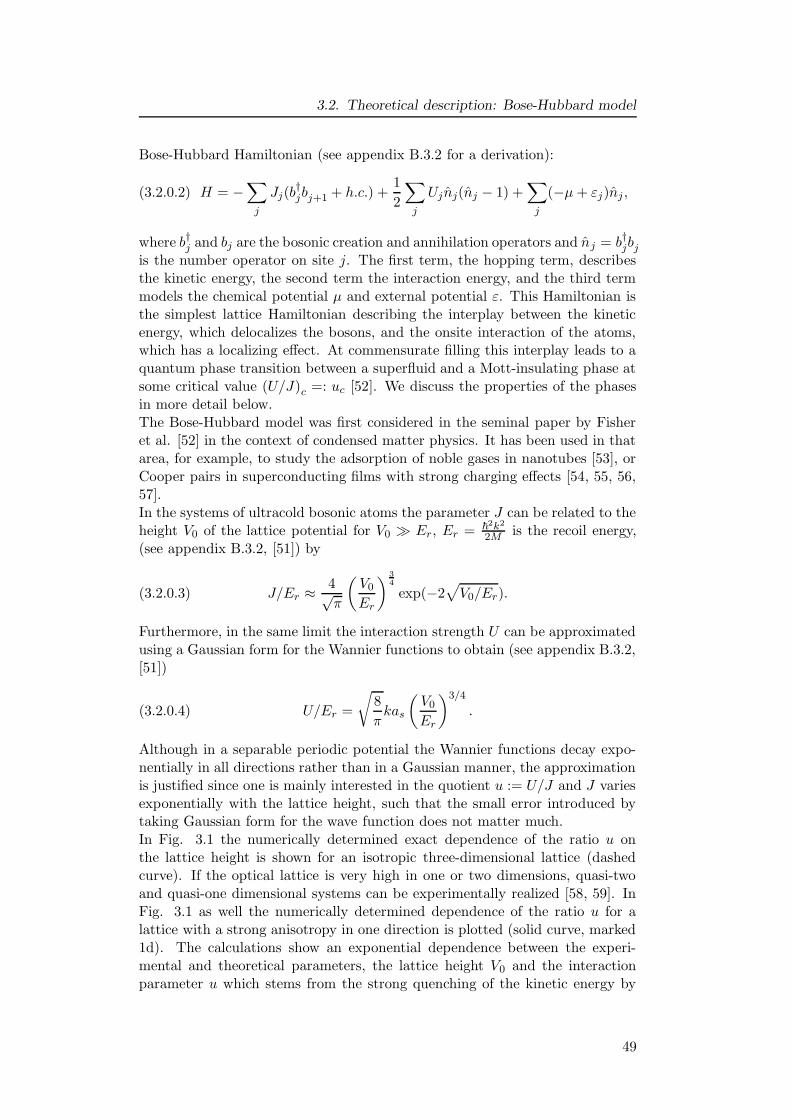
3.2. Theoretical description: Bose-Hubbard model
Bose-Hubbard Hamiltonian (see appendix B.3.2 for a derivation):
(3.2.0.2) H = −∑
j
Jj(b†jbj+1 + h.c.) +
1
2
∑
j
Ujnj(nj − 1) +∑
j
(−µ+ εj)nj ,
where b†j and bj are the bosonic creation and annihilation operators and nj = b†jbjis the number operator on site j. The first term, the hopping term, describesthe kinetic energy, the second term the interaction energy, and the third termmodels the chemical potential µ and external potential ε. This Hamiltonian isthe simplest lattice Hamiltonian describing the interplay between the kineticenergy, which delocalizes the bosons, and the onsite interaction of the atoms,which has a localizing effect. At commensurate filling this interplay leads to aquantum phase transition between a superfluid and a Mott-insulating phase atsome critical value (U/J)c =: uc [52]. We discuss the properties of the phasesin more detail below.The Bose-Hubbard model was first considered in the seminal paper by Fisheret al. [52] in the context of condensed matter physics. It has been used in thatarea, for example, to study the adsorption of noble gases in nanotubes [53], orCooper pairs in superconducting films with strong charging effects [54, 55, 56,57].In the systems of ultracold bosonic atoms the parameter J can be related to theheight V0 of the lattice potential for V0 � Er, Er = ~
2k2
2M is the recoil energy,(see appendix B.3.2, [51]) by
(3.2.0.3) J/Er ≈ 4√π
(V0
Er
) 34
exp(−2√
V0/Er).
Furthermore, in the same limit the interaction strength U can be approximatedusing a Gaussian form for the Wannier functions to obtain (see appendix B.3.2,[51])
(3.2.0.4) U/Er =
√
8
πkas
(V0
Er
)3/4
.
Although in a separable periodic potential the Wannier functions decay expo-nentially in all directions rather than in a Gaussian manner, the approximationis justified since one is mainly interested in the quotient u := U/J and J variesexponentially with the lattice height, such that the small error introduced bytaking Gaussian form for the wave function does not matter much.In Fig. 3.1 the numerically determined exact dependence of the ratio u onthe lattice height is shown for an isotropic three-dimensional lattice (dashedcurve). If the optical lattice is very high in one or two dimensions, quasi-twoand quasi-one dimensional systems can be experimentally realized [58, 59]. InFig. 3.1 as well the numerically determined dependence of the ratio u for alattice with a strong anisotropy in one direction is plotted (solid curve, marked1d). The calculations show an exponential dependence between the experi-mental and theoretical parameters, the lattice height V0 and the interactionparameter u which stems from the strong quenching of the kinetic energy by
49
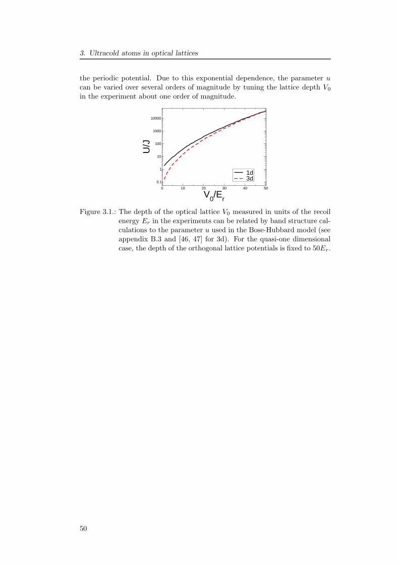
3. Ultracold atoms in optical lattices
the periodic potential. Due to this exponential dependence, the parameter ucan be varied over several orders of magnitude by tuning the lattice depth V0
in the experiment about one order of magnitude.
0 10 20 30 40 50
V0/Er
0.1
1
10
100
1000
10000
U/J
1d3d
Figure 3.1.: The depth of the optical lattice V0 measured in units of the recoilenergy Er in the experiments can be related by band structure cal-culations to the parameter u used in the Bose-Hubbard model (seeappendix B.3 and [46, 47] for 3d). For the quasi-one dimensionalcase, the depth of the orthogonal lattice potentials is fixed to 50Er.
50
3.3. Quantum phase transition in homogeneous systems
3.3. Quantum phase transition in homogeneous systems
3.3.1. Limit of weak interaction: superfluid phase
One limit which can be easily described theoretically is the limit of vanishinginteraction. For vanishing interaction U = 0 the bosons become free bosonsand the Hamiltonian (3.2.0.2) simplifies to the quadratic Hamiltonian:
Hhop = −∑
j
Jj(b†j+1bj + b†jbj+1) + (−µ+ εj)nj.
Assuming a homogeneous system, i.e. εj = 0 for all sites j, the Hamiltoniancan be diagonalized by a transformation into Fourier-space. Here we consider afixed number of particles and set µ = 0. On a finite chain of L sites the singleparticle eigenstates of the Hamiltonian are the momentum states to the energyeigenvalues Eq = −2J cos(kq). The discrete momentum kq takes the valueskq = πq
L+1 with q = −(L − 1), .., L. At temperature T = 0 the ground stateof the Hamiltonian Hhop of a system with N bosons can be constructed fromthe single particle states by occupying N -times the lowest state. Therefore, thenormalized ground state can be written as
∣∣ψ0
⟩=
1
N !(b†k1
)N∣∣0⟩
where∣∣0⟩
is the vacuum state. For an infinite system the ground state reads∣∣ψ0
⟩∝ (
∑
j bj)N∣∣0⟩. All particles are in the same delocalized single particle
state and hence the system can be described by a macroscopic wave functionwith a defined macroscopic phase, i.e. a Gross-Pitaevskii like description isrecovered.A trivial consequence is that the momentum distribution of the ground state isgiven by a high peak of weight N at the lowest possible momentum. Furtherthe delocalization of the particles shows up in strong fluctuations of the particlenumber on each site, i.e. the variance of the particle number is of the order ofthe particle number itself
⟨n2
j
⟩−⟨nj
⟩2=⟨nj
⟩+O(N
L ). In an infinite chain theexcitation spectrum is gapless.Even though interacting bosons behave often totally different from free bosons,some of the characteristics for non-interacting bosons on a lattice carry throughto weak interactions (U → 0 but U 6= 0). For example the number of atomsin the peak in the momentum distribution decreases, but stays macroscopicallyoccupied for weakly interacting bosons and the number fluctuations are still ofthe order of the occupation itself. The spectrum of weakly interacting infiniteone-dimensional Bose systems is still gapless, but the system exhibits a soundlike mode with frequency ω(k) = vsk. The dependence of the sound velocity vs
on the system parameters will be studied in chapter 4.In a one-dimensional Bose-system the superfluid phase shows several peculiar-ities due to the presence of strong quantum fluctuations in low dimensionalsystems. One example which we will meet in the following is the decay of theone-particle density-matrix
⟨b†i bi+d
⟩: in an one-dimensional system it decays
algebraically with the distance d in the superfluid phase, whereas in higher
51
3. Ultracold atoms in optical lattices
dimension true long-range order exists, i.e. the one-particle density-matrix ap-proaches a finite value for d → ∞. We will discuss the consequences of thecharacteristic structure of the one-particle density-matrix on the time-of-flightimages in chapter 3.7
3.3.2. Limit of strong interaction: Mott-insulating phase
In contrast to the delocalization in the case of weak interaction, for stronginteraction fluctuations in the particle number become energetically costly andthe atoms localize at single sites. This limit is also called the ‘atomic’ limit [52].If only the interaction is present, i.e. Hint = U
2
∑
j nj(nj − 1), the eigenstates
of the system are given by the Fock states∣∣nj
⟩. Therefore, the single particle
ground states are highly degenerate.
Assuming a system with commensurate filling, say n, the ground state factorizesinto single sites by
∣∣ψ0
⟩∝ ∏L
j=1(b†j)
n∣∣0⟩. In contrast to the superfluid limit,
here the particle number on each site is exactly determined, no macroscopicphase coherence is prevalent in the system and the momentum distribution isa constant for all momenta. The first excited state is a particle-hole excitationwith the energy E1 = U , i.e. an energy gap exists in this limit. These charac-teristics carry through to finite but small hopping coefficient J , i.e. u� 1.
For non-commensurate filling no Mott-insulating phase exists at finite hopping.To understand this consider a system with filling n = 1 in a Mott-insulatingstate and add an additional particle. The naive picture is that the additionalparticle delocalizes on top of a frozen Mott-insulating state to avoid the energyloss by interacting with a localized particle. Therefore, a fraction of the systemremains superfluid for all interaction strengths. The true many-particle statewill be more complicated than this simple picture, but will still show a remainingsuperfluid part.
3.3.3. Quantum phase transitions
If the strength of the interaction is increased one changes in the case of com-mensurate filling between two very different phases, the superfluid phase andthe Mott-insulating phase. A quantum phase transition occurs at some criti-cal value uc. The quantum phase diagram for the homogeneous Bose-Hubbardmodel was first determined by a mean-field calculation by Fisher et al. [52].Although there are considerable differences between the case of one, two, orthree dimensions induced by strong quantum fluctuations for lower dimensions,the characteristic features are similar. A sketch of the phase diagram in a one-dimensional systems calculated using DMRG [60] and Quantum Monte Carlo[61] methods is shown in Fig. 3.2.
The phase diagram shows characteristic Mott-insulating lobes at small u−1 sur-rounded by the superfluid phase. In these lobes the particle number is lockedto a certain integer value. In the superfluid phase different fillings can occur.Hence the Mott-insulating phase is incompressible, i.e. ∂n
∂µ = 0, whereas the su-perfluid phase is compressible. A signature to distinguish the phases is the de-cay of the one-particle density-matrix with the distance: in the Mott-insulating
52
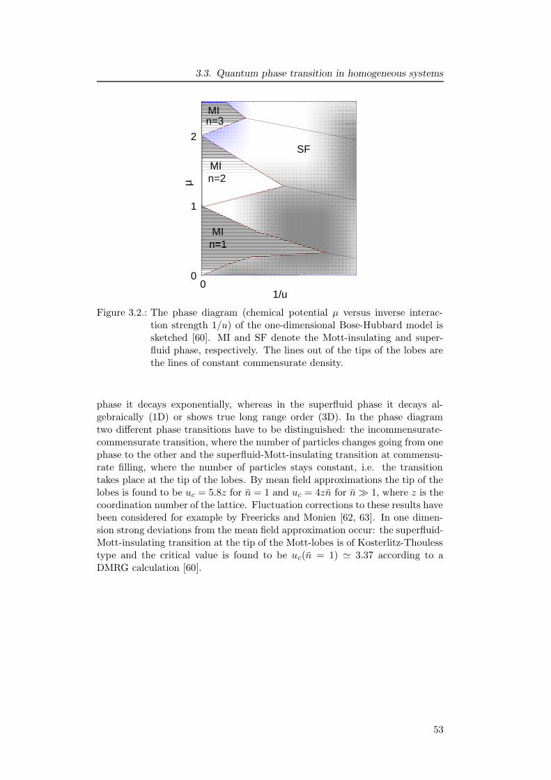
3.3. Quantum phase transition in homogeneous systems
������������������������������������������������������������������������������������������������������������������������������������������������������������������������������������������������������������������������������������������������������������������������������������������������������������������������������������������������������������������������������������������������������������������������������������������������������������������������������������������������������������������������������������������������������������������������������������������������������������������������������������������������������������������������������������������������������������������������������������������������������������������������������������������������������������������������������������������������������������������������������������������������������������������������������������������������������������������������������������������������������������������������������������������������������������������������������������������������������������������������������������������������������������������������������������������������������������������������������������������������������������������������������������������������������������������������������������������������������������������������������������������������������������������������������������������������������������������������������������������������������������������������������������������������������������������������������������������������������������������������������������������������������������������������������������������������������������������������������������������������������������������������������������������������������������������������������������������������������������������������������������������������
��������������������������������������������������������������������������������������������������������������������������������������������������������������������������������������������������������������������������������������������������������������������������������������������������������������������������������������������������������������������������������������������������������������������������������������������������������������������������������������������������������������������������������������������������������������������������������������������������������������������������������������������������������������������������������������������������������������������������������������������������������������������������������������������������������������������������������������������������������������������������������������������������������������������������������������������������������������������������������������������������������������������������������������������������������������������������������������������������������������������������������������������������������������������������������������������������������������������������������������������������������������������������������������������������������������������������������������������������������������������������������������������������������������������������������������������������������������������������������������������������������������������������������������������������������������������������������������������������������������������������������������������������������������������������������������������������������������������������������������������������������������������������������������������������������������������������������
���������������������������������������������������������������������������������������������������������������������������������������������������������������������������������������������������������������������������������������������������������������������������������������������������������������������������������������������������������������������������������������������������������������������������������������������������������������������������������������������������������������������������������������������������������������������������������������������������������������������������������������������������������������������������������������������������������������������������������������������������������������������������������������������������������������������������������������������������������������������������������������������������������������������������������������������������������������������������������������������������������������������������������������������������������������������������������������������������������������������������������������������������������������������������������������������������������������������������������������������������������������
���������������������������������������������������������������������������������������������������������������������������������������������������������������������������������������������������������������������������������������������������������������������������������������������������������������������������������������������������������������������������������������������������������������������������������������������������������������������������������������������������������������������������������������������������������������������������������������������������������������������������������������������������������������������������������������������������������������������������������������������������������������������������������������������������������������������������������������������������������������������������������������������������������������������������������������������������������������������������������������������������������������������������������������������������������������������������������������������������������������������������������������������������������������������������������������������������������������������������������������������������������������������������������������������������������������������������������������������������������������������������������������������������������������������������������������������������������������������������������������������������������������������������������������������������������������������������������������������������������������������������������������������������������������������������������������������������������������������������������������������������������������������������������������������������������������������������������������������������������������������������������������������������������������������������������������������������������������������������������������������������������������������������������������������������������������������������������������
�������������������������������������������������������������������������������������������������������������������������������������������������������������������������������������������������������������������������������������������������������������������������������������������������������������������������������������������������������������������������������������������������������������������������������������������������������������������������������������������������������������������������������������������������������������������������������������������������������������������������������������������������������������������������������������������������������������������������������������������������������������������������������������������������������������������������������������������������������������������������������������������������������������������������������������������������������������������������������������������������������������������������������������������������������������������
�����������������������������������������������������������������������������������������������������������������������������������������������������������������������������������������������������������������������������
0 0
1
2
1/u
MI
MI n=3
MI n=2
n=1
SF
µ
Figure 3.2.: The phase diagram (chemical potential µ versus inverse interac-tion strength 1/u) of the one-dimensional Bose-Hubbard model issketched [60]. MI and SF denote the Mott-insulating and super-fluid phase, respectively. The lines out of the tips of the lobes arethe lines of constant commensurate density.
phase it decays exponentially, whereas in the superfluid phase it decays al-gebraically (1D) or shows true long range order (3D). In the phase diagramtwo different phase transitions have to be distinguished: the incommensurate-commensurate transition, where the number of particles changes going from onephase to the other and the superfluid-Mott-insulating transition at commensu-rate filling, where the number of particles stays constant, i.e. the transitiontakes place at the tip of the lobes. By mean field approximations the tip of thelobes is found to be uc = 5.8z for n = 1 and uc = 4zn for n� 1, where z is thecoordination number of the lattice. Fluctuation corrections to these results havebeen considered for example by Freericks and Monien [62, 63]. In one dimen-sion strong deviations from the mean field approximation occur: the superfluid-Mott-insulating transition at the tip of the Mott-lobes is of Kosterlitz-Thoulesstype and the critical value is found to be uc(n = 1) ' 3.37 according to aDMRG calculation [60].
53
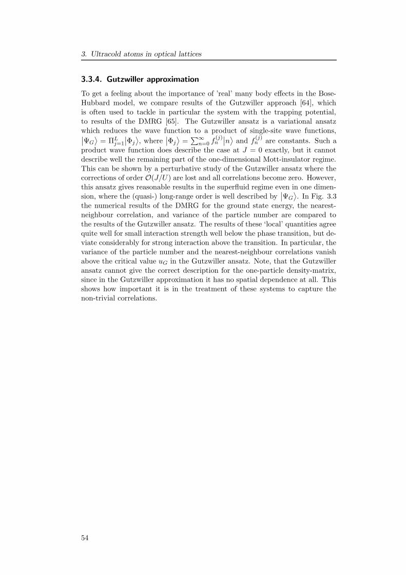
3. Ultracold atoms in optical lattices
3.3.4. Gutzwiller approximation
To get a feeling about the importance of ’real’ many body effects in the Bose-Hubbard model, we compare results of the Gutzwiller approach [64], whichis often used to tackle in particular the system with the trapping potential,to results of the DMRG [65]. The Gutzwiller ansatz is a variational ansatzwhich reduces the wave function to a product of single-site wave functions,∣∣ΨG
⟩= ΠL
j=1
∣∣Φj
⟩, where
∣∣Φj
⟩=∑∞
n=0 f(j)n
∣∣n⟩
and f(j)n are constants. Such a
product wave function does describe the case at J = 0 exactly, but it cannotdescribe well the remaining part of the one-dimensional Mott-insulator regime.This can be shown by a perturbative study of the Gutzwiller ansatz where thecorrections of order O(J/U) are lost and all correlations become zero. However,this ansatz gives reasonable results in the superfluid regime even in one dimen-sion, where the (quasi-) long-range order is well described by
∣∣ΨG
⟩. In Fig. 3.3
the numerical results of the DMRG for the ground state energy, the nearest-neighbour correlation, and variance of the particle number are compared tothe results of the Gutzwiller ansatz. The results of these ‘local’ quantities agreequite well for small interaction strength well below the phase transition, but de-viate considerably for strong interaction above the transition. In particular, thevariance of the particle number and the nearest-neighbour correlations vanishabove the critical value uG in the Gutzwiller ansatz. Note, that the Gutzwilleransatz cannot give the correct description for the one-particle density-matrix,since in the Gutzwiller approximation it has no spatial dependence at all. Thisshows how important it is in the treatment of these systems to capture thenon-trivial correlations.
54
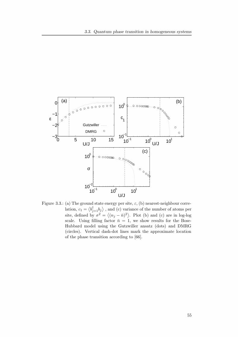
3.3. Quantum phase transition in homogeneous systems
0 5 10 15−3
−2
−1
0
U/J
ε
(a)
Gutzwiller
DMRG
10−1
100
101
10−1
100
U/J
c1
(b)
10−1
100
101
10−2
100
U/J
σ
(c)
Figure 3.3.: (a) The ground state energy per site, ε, (b) nearest-neighbour corre-
lation, c1 =⟨b†j+1bj
⟩, and (c) variance of the number of atoms per
site, defined by σ2 =⟨(nj − n)2
⟩. Plot (b) and (c) are in log-log
scale. Using filling factor n = 1, we show results for the Bose-Hubbard model using the Gutzwiller ansatz (dots) and DMRG(circles). Vertical dash-dot lines mark the approximate locationof the phase transition according to [66].
55
3. Ultracold atoms in optical lattices
3.4. Coexistence of phases in a trapping potential
In the remaining part of this chapter we present our results of DMRG calcu-lations on the quantum phase transition in the presence of a confining poten-tial [67]. The confining trap of the experiment [1] is approximately parabolic(B.2.0.4). It consists of the magnetic trap and the confining component ofthe laser which generates the optical lattice is approximately parabolic (cf.B.2.0.4). In the following the trap is modeled by setting εj = V 0
trap (aj − aj0)2
in Eq. (3.2.0.2). Here a is the lattice constant, j the lattice site, and j0 thecentral site of the lattice. We choose the strength of the trap proportional tothe onsite interaction, i.e. V 0
trap = v0U , to reproduce the experimental setup. Itguarantees that when the optical lattice depth, corresponding to the parameteru in the Bose-Hubbard model, is changed, the size of the atom cloud does notvary much for a fixed particle number as observed in the experiment.
In the presence of a parabolic trap at average filling of approximately one par-ticle per site, one can distinguish three states of the system (see [46, 68]):
(a) u < uc1: the particle distribution is incommensurate over the whole sys-tem;
(b) uc1 < u < uc2: regions with incommensurate and commensurate occu-pancy coexist; and
(c) u > uc2: the main part of the system is locked to commensurate fillingand only at the boundaries small incommensurate regions exist.
A sketch of the state diagram for v0 = 4/642 ≈ 9.8 · 10−4 is presented in Fig.3.4 (A). The insets show the characteristic shape of the particle distributionfor the three states. Note, that the critical values uc1 and uc2 depend on thefilling of the system and that for small particle numbers state (b) does not oc-cur. A simple picture of a system with a parabolic trapping potential can begained by relating it to the situation in a homogeneous system by regarding thechemical potential µ to be space-dependent. For a parabolic confining potentialthe chemical potential µ must then be inversely parabolic. The vertical linesin Fig. 3.4 (B) indicate for three different parameters u how µ would vary asthe trap is traversed from one side through the center to the other side. Thesymbols in (A) and (B) mark corresponding points. For example, moving fromone edge of the trap through the center to the other edge [going from hexagonto ellipse to hexagon in Fig. 3.4 (A) for state (b)], corresponds to increasingµ [going from hexagon to ellipse in Fig. 3.4 (B) for state (b)] and lowering µagain [going back to hexagon in Fig. 3.4 (B) for state (b)]. The regions oflocked density correspond to being in the Mott-insulating region of the phasediagram. The exact locations of the interface between the commensurate andthe incommensurate regions are difficult to determine. A good qualitative in-sight can be gained using the picture of the spatially varying chemical potentialand determining the critical chemical potential with perturbation theory for thehomogeneous system [69]. The difficulty in the exact location of the interfaces isdue to the fact that these sites correspond, using terminology appropriate for a
56
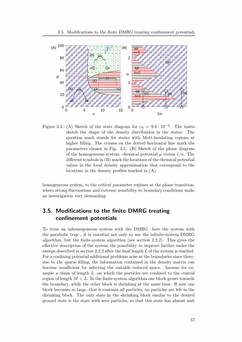
3.5. Modifications to the finite DMRG treating confinement potentials
���������������������������������������������������������������������������������������������������������������������������������������������������������������������������������������������������������������������������������������������������������������������������������������������������������������������������������������������������������������������������������������������������������������������������������������������������������������������������������������������������������������������������������������������������������������������������������������������������������������������������������������������������������������������������������������������������������������������������������������������������������������������������������������������������������������������������������������������������������������������������������������������������������������������������������������������������������������������������������������������������������������������������������������������������������������������������������������������������������������������������������������������������������������������������������������������������������������������������������������������������������������������������������������������������������������������������������������������������������������������������������������������������������������������������������������������������������������������������������������������������������������������������������������������������������������������������������������������������������������������������������������������������������������������������������������������������������������������������������������������������������������������������������������������������������������������������������������������������������������������������������������������������������������������������������������������������������
���������������������������������������������������������������������������������������������������������������������������������������������������������������������������������������������������������������������������������������������������������������������������������������������������������������������������������������������������������������������������������������������������������������������������������������������������������������������������������������������������������������������������������������������������������������������������������������������������������������������������������������������������������������������������������������������������������������������������������������������������������������������������������������������������������������������������������������������������������������������������������������������������������������������������������������������������������������������������������������������������������������������������������������������������������������������������������������������������������������������������������������������������������������������������������������������������������������������������������������������������������������������������������������������������������������������������������������������������������������������������������������������������������������������������������������������������������������������������������������������������������������������������������������������������������������������������������������������������������������������������������������������������������������������������������������������������������������������������������������������������������������������������������������������������������������������������������������������������������������������������������������������������������������������������������������������������������
�����������������������������������������������������������������������������������������������������������������������������������������������������������������������������������������������������������������������������������������������������������������������������������������������������������������������������������
�����������������������������������������������������������������������������������������������������������������������������������������������������������������������������������������������������������������������������������������������������������������������������������������������������������������������������������
����������������������������������������������������������������������������������������������������������������������������������������������������������������������������������������������������������������������������������������������������������������������������������������������������������������������������������������������������������������������������������������������������������������������������������������������������������������������������������������������������������������������������������������������������������������������������������������������������������������������������������������������������������������������������������������������������������������������������������������������������������������������������������������������������������������������������������������������������������������������������������������������������������������������������������������������
�����������������������������������������������������������������������������������������������������������������������������������������������������������������������������������������������������������������������������������������������������������������������������������������������������������������������������������������������������������������������������������������������������������������������������������������������������������������������������������������������������������������������������������������������������������������������������������������������������������������������������������������������������������������������������������������������������������������������������������������������������������������������������������������������������������������������������������������������������������������������������������������������������������
���������������������������������������������������������������������������������������������������������������������������������������������������������������������������������������������������������������������������������������������������������������������������������������������������������������������������������������������������������������������������������������������������������������������������������������������������������������������������������������������������������������������������������������������������������������������������������������������������������������������������������������������������������������������������������������������������������������������������������������������������������������������������������������������������������������������������������������������������������������������������������������������������������������������������������������������������������������������������������������������������������������������������������������������������������������������������������������������������������������������������������������������������������������������������������������������������������������������������������������������������������������������������������������������������������������������������������������������������������������������������������������������������������������������������������������������������������������������������������������������������������������������������������������������������������������������������������������������������������������������������������������������������������������������������������������������������������������������������������������������������������������������������������������������������������������������������������������������������������������������������������������������������������������������������������������������������������������������������������������������������������������������������
���������������������������������������������������������������������������������������������������������������������������������������������������������������������������������������������������������������������������������������������������������������������������������������������������������������������������������������������������������������������������������������������������������������������������������������������������������������������������������������������������������������������������������������������������������������������������������������������������������������������������������������������������������������������������������������������������������������������������������������������������������������������������������������������������������������������������������������������������������������������������������������������������������������������������������������������������������������������������������������������
��������������������������������������������������������������������������������������������������������������������������������������������������������������������������������������������������������������������������������������������������������������������������������������������������������������������������������������������������������������������������������������������������������������������������������������������������������������������������������������������������������������������������������������������������������������������������������������������
��������������������������������������������������������������������������������������������������������������������������������������������������������������������������������������������������������������������������������������������������������������������������������������������������������������������������������������������������������������������������������������������������������������������������������������������������������������������������������������������������������������������������������������������������������������������������������������������������������������������������������������������������������������������������������������������������������������������������������������������������������������������������������������������������������������������������������������������������������������������������������������������������������������������������������������������������������������������������������������������������������������������������������������������������������������������������������������������������������������������������������������������������������������������������������������������������������������������������������������������������������������������������������������������������������������������������������������������������������������������������������������������������������������������������������������������������������������������������������������������������������������������������������������������������������������������������������������������������������������������������������������������������������������������������������������������������������������������������������������������������������������������������������������������������������������������������������������������������������������������������������������������������������������������������������������������������������������������������������������������������������������������������������������������������������
� � � � � � � � � � � � � � � � � � � � � � � � � � � � � � � � � � � � � � � � � � � � � � � � � � � � � � � � � � � � � � � � � � � � � � � � � � � � � � � � � � � � � � � � � � � � � � � � � � � � � � � � � � � � � � � � � � � � � � � � � � � � � � � � � � � � � � � � � � � � � � � � � � � � � � � � � � � � � � � � � � � � � � � � � � � � � � � � � � � � � � � � � � � � � � � � � � � � � � � � � � � � � � � � � � � � � � � � � � � � � � � � � � � � � � � � � � � � � � � � � � � � � � � � � � � � � � � � � � � � � � � � � � � � � � � � � � � � � � � � � � � � � � � � � � � � � � � � � � � � � � � � � � � � � � � � � � � � � � � � � � � � � � � � � � � � � � � � � � � � � � � � � � � � � � � � � � � � � � � � � � � � � � � � � � � � � � � � � � � � � � � � � � � � � � ����������������������������������������������������������������������������������������������������������������������������������������������������������������������������������������������������������������������������������������������
�����������������������������������������������������������������������������������������������������������������������������������������������������������������������������������������������������������������������������
?
0
N
100
0 0
1
2
1/u
MI
MI n=3
MI n=2
n=1
SF
60
80
40
0 0 5 10 15
u
20
(a)
(b)
(c)
(c) (b) (a)
µ
(B) (A)
Figure 3.4.: (A) Sketch of the state diagram for v0 = 9.8 · 10−4. The insetssketch the shape of the density distribution in the states. Thequestion mark stands for states with Mott-insulating regions athigher filling. The crosses on the dotted horizontal line mark theparameters chosen in Fig. 3.5. (B) Sketch of the phase diagramof the homogeneous system: chemical potential µ versus 1/u. Thedifferent symbols in (B) mark the locations of the chemical potentialvalues in the local density approximation that correspond to thelocations in the density profiles marked in (A).
homogeneous system, to the critical parameter regimes at the phase transition,where strong fluctuations and extreme sensibility to boundary conditions makean investigation very demanding.
3.5. Modifications to the finite DMRG treating
confinement potentials
To treat an inhomogeneous system with the DMRG –here the system withthe parabolic trap–, it is essential not only to use the infinite-system DMRGalgorithm, but the finite-system algorithm (see section 2.2.2). This gives theeffective description of the system the possibility to improve further under thesweeps described in section 2.2.2 after the final length L of the system is reached.For a confining potential additional problems arise at the boundaries since there,due to the sparse filling, the information contained in the density matrix canbecome insufficient for selecting the suitable reduced space. Assume for ex-ample a chain of length L, on which the particles are confined to the centralregion of length M < L. In the finite-system algorithm one block grows towardsthe boundary, while the other block is shrinking at the same time. If now oneblock becomes so large, that it contains all particles, no particles are left in theshrinking block. The only state in the shrinking block similar to the desiredground state is the state with zero particles, so that this state has almost unit
57
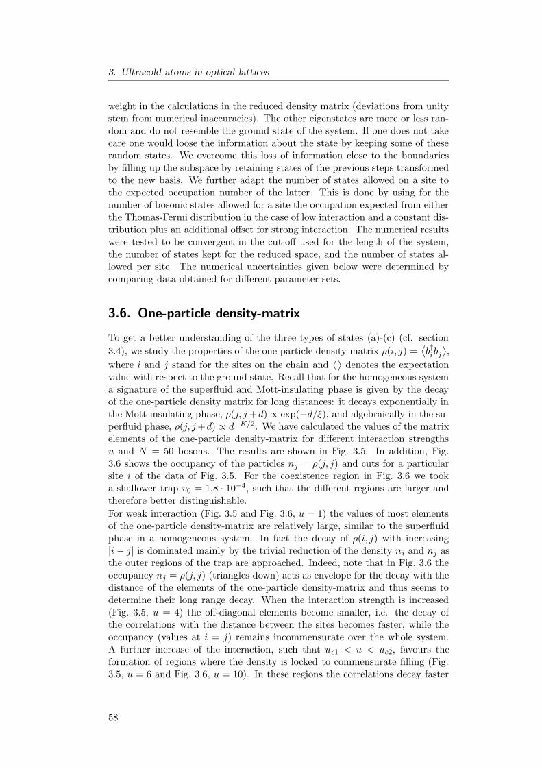
3. Ultracold atoms in optical lattices
weight in the calculations in the reduced density matrix (deviations from unitystem from numerical inaccuracies). The other eigenstates are more or less ran-dom and do not resemble the ground state of the system. If one does not takecare one would loose the information about the state by keeping some of theserandom states. We overcome this loss of information close to the boundariesby filling up the subspace by retaining states of the previous steps transformedto the new basis. We further adapt the number of states allowed on a site tothe expected occupation number of the latter. This is done by using for thenumber of bosonic states allowed for a site the occupation expected from eitherthe Thomas-Fermi distribution in the case of low interaction and a constant dis-tribution plus an additional offset for strong interaction. The numerical resultswere tested to be convergent in the cut-off used for the length of the system,the number of states kept for the reduced space, and the number of states al-lowed per site. The numerical uncertainties given below were determined bycomparing data obtained for different parameter sets.
3.6. One-particle density-matrix
To get a better understanding of the three types of states (a)-(c) (cf. section
3.4), we study the properties of the one-particle density-matrix ρ(i, j) =⟨b†ibj
⟩,
where i and j stand for the sites on the chain and⟨⟩
denotes the expectationvalue with respect to the ground state. Recall that for the homogeneous systema signature of the superfluid and Mott-insulating phase is given by the decayof the one-particle density matrix for long distances: it decays exponentially inthe Mott-insulating phase, ρ(j, j+d) ∝ exp(−d/ξ), and algebraically in the su-perfluid phase, ρ(j, j+d) ∝ d−K/2. We have calculated the values of the matrixelements of the one-particle density-matrix for different interaction strengthsu and N = 50 bosons. The results are shown in Fig. 3.5. In addition, Fig.3.6 shows the occupancy of the particles nj = ρ(j, j) and cuts for a particularsite i of the data of Fig. 3.5. For the coexistence region in Fig. 3.6 we tooka shallower trap v0 = 1.8 · 10−4, such that the different regions are larger andtherefore better distinguishable.
For weak interaction (Fig. 3.5 and Fig. 3.6, u = 1) the values of most elementsof the one-particle density-matrix are relatively large, similar to the superfluidphase in a homogeneous system. In fact the decay of ρ(i, j) with increasing|i− j| is dominated mainly by the trivial reduction of the density ni and nj asthe outer regions of the trap are approached. Indeed, note that in Fig. 3.6 theoccupancy nj = ρ(j, j) (triangles down) acts as envelope for the decay with thedistance of the elements of the one-particle density-matrix and thus seems todetermine their long range decay. When the interaction strength is increased(Fig. 3.5, u = 4) the off-diagonal elements become smaller, i.e. the decay ofthe correlations with the distance between the sites becomes faster, while theoccupancy (values at i = j) remains incommensurate over the whole system.A further increase of the interaction, such that uc1 < u < uc2, favours theformation of regions where the density is locked to commensurate filling (Fig.3.5, u = 6 and Fig. 3.6, u = 10). In these regions the correlations decay faster
58
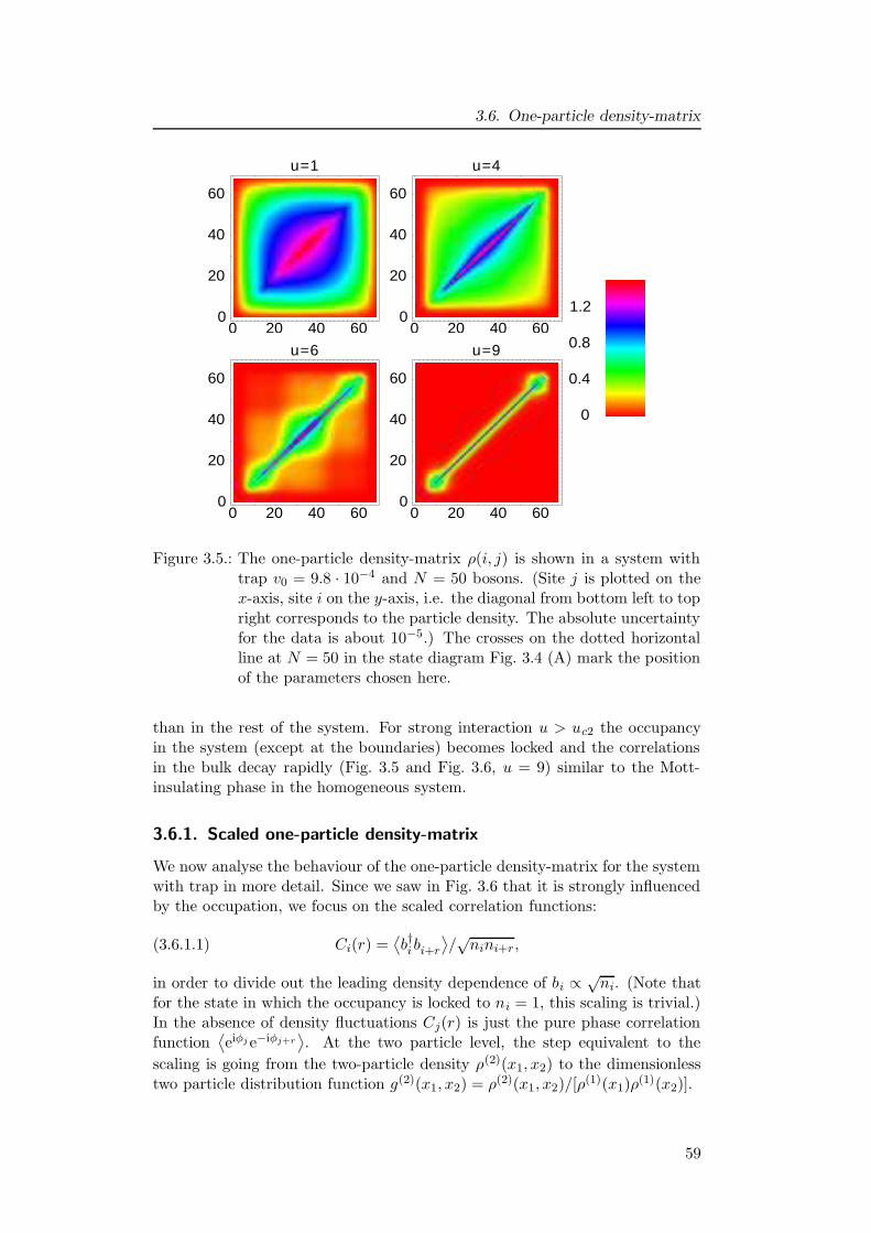
3.6. One-particle density-matrix
0 20 40 600
20
40
60
u=1
0 20 40 600
20
40
60
u=6
0 20 40 600
20
40
60
u=4
0 20 40 600
20
40
60
u=9
0
0.4
0.8
1.2
Figure 3.5.: The one-particle density-matrix ρ(i, j) is shown in a system withtrap v0 = 9.8 · 10−4 and N = 50 bosons. (Site j is plotted on thex-axis, site i on the y-axis, i.e. the diagonal from bottom left to topright corresponds to the particle density. The absolute uncertaintyfor the data is about 10−5.) The crosses on the dotted horizontalline at N = 50 in the state diagram Fig. 3.4 (A) mark the positionof the parameters chosen here.
than in the rest of the system. For strong interaction u > uc2 the occupancyin the system (except at the boundaries) becomes locked and the correlationsin the bulk decay rapidly (Fig. 3.5 and Fig. 3.6, u = 9) similar to the Mott-insulating phase in the homogeneous system.
3.6.1. Scaled one-particle density-matrix
We now analyse the behaviour of the one-particle density-matrix for the systemwith trap in more detail. Since we saw in Fig. 3.6 that it is strongly influencedby the occupation, we focus on the scaled correlation functions:
(3.6.1.1) Ci(r) =⟨b†ibi+r
⟩/√nini+r,
in order to divide out the leading density dependence of bi ∝√ni. (Note that
for the state in which the occupancy is locked to ni = 1, this scaling is trivial.)In the absence of density fluctuations Cj(r) is just the pure phase correlationfunction
⟨eiφj e−iφj+r
⟩. At the two particle level, the step equivalent to the
scaling is going from the two-particle density ρ(2)(x1, x2) to the dimensionlesstwo particle distribution function g(2)(x1, x2) = ρ(2)(x1, x2)/[ρ
(1)(x1)ρ(1)(x2)].
59
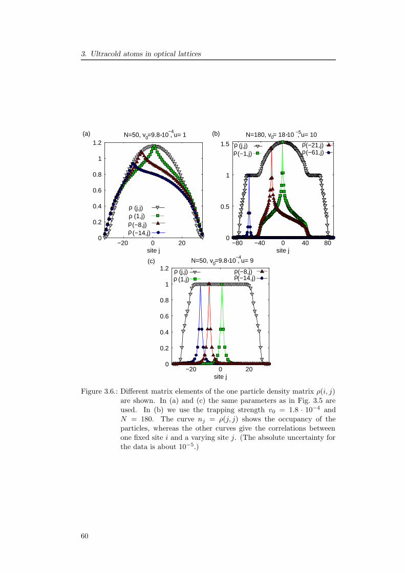
3. Ultracold atoms in optical lattices
N=50, v =9.8 10 , u= 1 −4 .
0
N=50, v =9.8 10 , u= 9 −4 .
0
0.2
0.4
0.6
0.8
1
1.2
−20 0site j
20
ρ (j,j)ρ (1,j)
ρρ
(−8,j)(−14,j)
(c)
0
0.2
0.4
0.6
0.8
1
1.2
−20 0 20site j
ρ (−14,j)
ρ (−8,j) ρ (1,j) ρ (j,j)
(a)
0
1
0.5
1.5
−40 0 40 80site j
−80
ρ ρ
ρ ρ
0 −5(b) N=180, v = 18 10 , u= 10
(−1,j) (j,j) (−21,j)
(−61,j)
.
0
Figure 3.6.: Different matrix elements of the one particle density matrix ρ(i, j)are shown. In (a) and (c) the same parameters as in Fig. 3.5 areused. In (b) we use the trapping strength v0 = 1.8 · 10−4 andN = 180. The curve nj = ρ(j, j) shows the occupancy of theparticles, whereas the other curves give the correlations betweenone fixed site i and a varying site j. (The absolute uncertainty forthe data is about 10−5.)
60
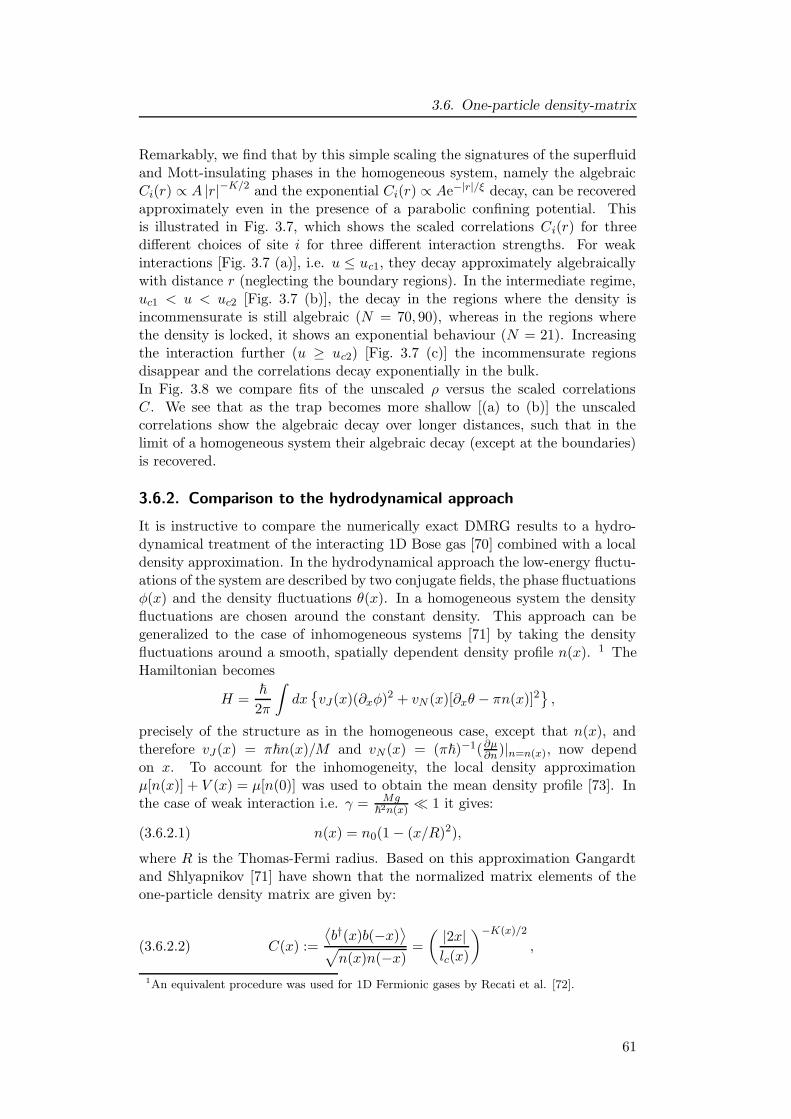
3.6. One-particle density-matrix
Remarkably, we find that by this simple scaling the signatures of the superfluidand Mott-insulating phases in the homogeneous system, namely the algebraicCi(r) ∝ A |r|−K/2 and the exponential Ci(r) ∝ Ae−|r|/ξ decay, can be recoveredapproximately even in the presence of a parabolic confining potential. Thisis illustrated in Fig. 3.7, which shows the scaled correlations Ci(r) for threedifferent choices of site i for three different interaction strengths. For weakinteractions [Fig. 3.7 (a)], i.e. u ≤ uc1, they decay approximately algebraicallywith distance r (neglecting the boundary regions). In the intermediate regime,uc1 < u < uc2 [Fig. 3.7 (b)], the decay in the regions where the density isincommensurate is still algebraic (N = 70, 90), whereas in the regions wherethe density is locked, it shows an exponential behaviour (N = 21). Increasingthe interaction further (u ≥ uc2) [Fig. 3.7 (c)] the incommensurate regionsdisappear and the correlations decay exponentially in the bulk.In Fig. 3.8 we compare fits of the unscaled ρ versus the scaled correlationsC. We see that as the trap becomes more shallow [(a) to (b)] the unscaledcorrelations show the algebraic decay over longer distances, such that in thelimit of a homogeneous system their algebraic decay (except at the boundaries)is recovered.
3.6.2. Comparison to the hydrodynamical approach
It is instructive to compare the numerically exact DMRG results to a hydro-dynamical treatment of the interacting 1D Bose gas [70] combined with a localdensity approximation. In the hydrodynamical approach the low-energy fluctu-ations of the system are described by two conjugate fields, the phase fluctuationsφ(x) and the density fluctuations θ(x). In a homogeneous system the densityfluctuations are chosen around the constant density. This approach can begeneralized to the case of inhomogeneous systems [71] by taking the densityfluctuations around a smooth, spatially dependent density profile n(x). 1 TheHamiltonian becomes
H =~
2π
∫
dx{vJ(x)(∂xφ)2 + vN (x)[∂xθ − πn(x)]2
},
precisely of the structure as in the homogeneous case, except that n(x), andtherefore vJ(x) = π~n(x)/M and vN (x) = (π~)−1(∂µ
∂n)|n=n(x), now dependon x. To account for the inhomogeneity, the local density approximationµ[n(x)] + V (x) = µ[n(0)] was used to obtain the mean density profile [73]. Inthe case of weak interaction i.e. γ = Mg
~2n(x) � 1 it gives:
(3.6.2.1) n(x) = n0(1 − (x/R)2),
where R is the Thomas-Fermi radius. Based on this approximation Gangardtand Shlyapnikov [71] have shown that the normalized matrix elements of theone-particle density matrix are given by:
C(x) :=
⟨b†(x)b(−x)
⟩
√
n(x)n(−x)=
( |2x|lc(x)
)−K(x)/2
,(3.6.2.2)
1An equivalent procedure was used for 1D Fermionic gases by Recati et al. [72].
61
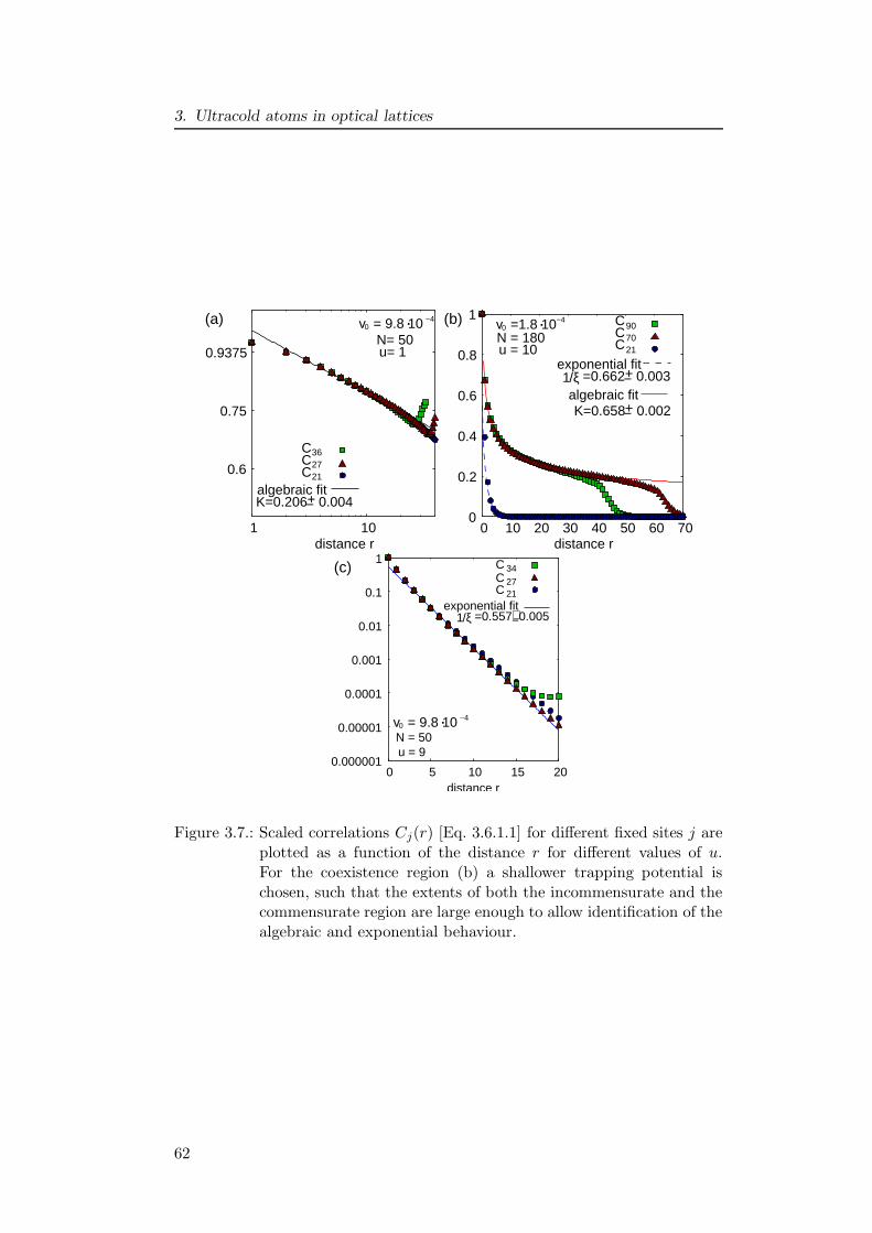
3. Ultracold atoms in optical lattices
+
34C
21C27C
20 15 10 5 0
0.0001
0.001
0.01
1
0.1
N = 50 u = 9
=0.557 0.005−exponential fit
distance r
1/ξ
0.00001
0.000001
0.6
0.75
0.9375
10 1
N= 50 u= 1
−+K=0.206 0.004algebraic fit
362721
CCC
distance r
−4 0v = 9.8 10 .
−4 0v = 9.8 10 .
exponential fit
algebraic fit−+
−+
0 10 20 30 40 50 60 70
0.2
0.4
0.6
0.8
1
0
N = 180 u = 10
K=0.658 0.002
907021
CCC
distance r
=0.662 0.0031/ξ
(a) (b)
(c)
0 .v =1.8 10 −4
Figure 3.7.: Scaled correlations Cj(r) [Eq. 3.6.1.1] for different fixed sites j areplotted as a function of the distance r for different values of u.For the coexistence region (b) a shallower trapping potential ischosen, such that the extents of both the incommensurate and thecommensurate region are large enough to allow identification of thealgebraic and exponential behaviour.
62
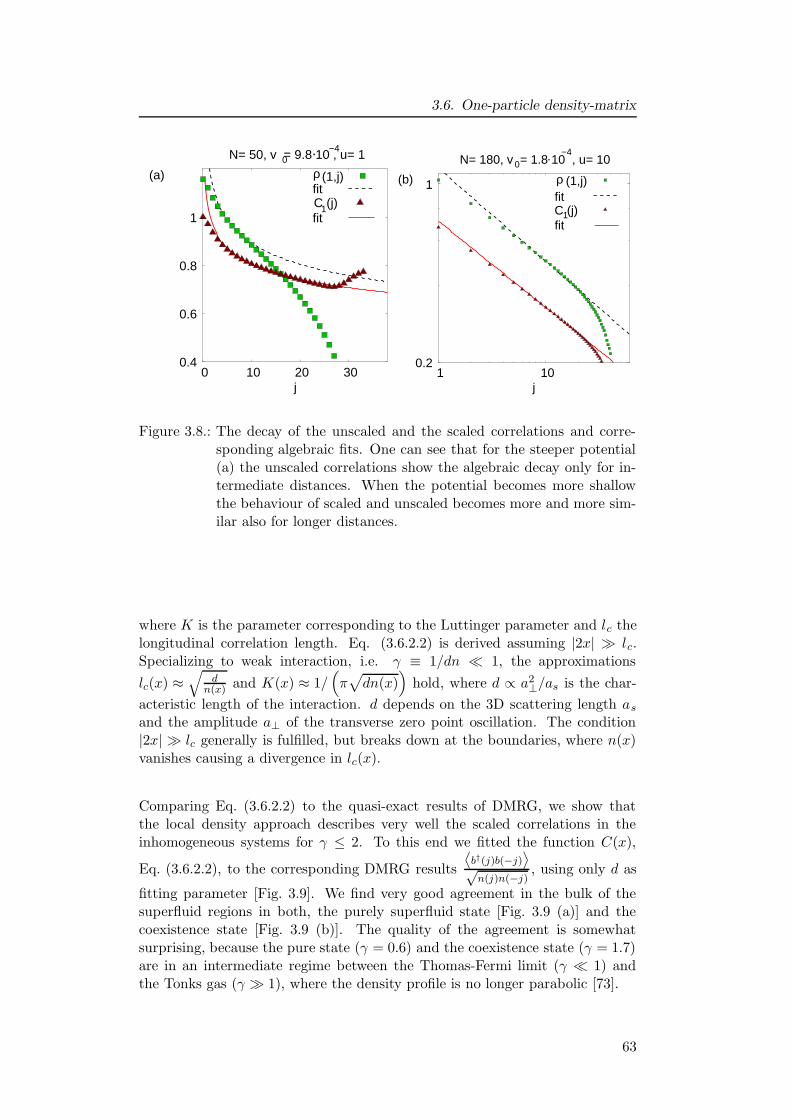
3.6. One-particle density-matrix
0.8
1
0.6
0.4 0 10 20 30
(1,j)ρ
C (j) 1
fit
fit
(a)
j
0 N= 50, v = 9.8 10 , u= 1 −4 .
0.2 1 10
1 (1,j)ρfitC (j)fit
0
(b)
1
j
. −4 N= 180, v = 1.8 10 , u= 10
Figure 3.8.: The decay of the unscaled and the scaled correlations and corre-sponding algebraic fits. One can see that for the steeper potential(a) the unscaled correlations show the algebraic decay only for in-termediate distances. When the potential becomes more shallowthe behaviour of scaled and unscaled becomes more and more sim-ilar also for longer distances.
where K is the parameter corresponding to the Luttinger parameter and lc thelongitudinal correlation length. Eq. (3.6.2.2) is derived assuming |2x| � lc.Specializing to weak interaction, i.e. γ ≡ 1/dn � 1, the approximations
lc(x) ≈√
dn(x) and K(x) ≈ 1/
(
π√
dn(x))
hold, where d ∝ a2⊥/as is the char-
acteristic length of the interaction. d depends on the 3D scattering length as
and the amplitude a⊥ of the transverse zero point oscillation. The condition|2x| � lc generally is fulfilled, but breaks down at the boundaries, where n(x)vanishes causing a divergence in lc(x).
Comparing Eq. (3.6.2.2) to the quasi-exact results of DMRG, we show thatthe local density approach describes very well the scaled correlations in theinhomogeneous systems for γ ≤ 2. To this end we fitted the function C(x),
Eq. (3.6.2.2), to the corresponding DMRG results
⟨b†(j)b(−j)
⟩
√n(j)n(−j)
, using only d as
fitting parameter [Fig. 3.9]. We find very good agreement in the bulk of thesuperfluid regions in both, the purely superfluid state [Fig. 3.9 (a)] and thecoexistence state [Fig. 3.9 (b)]. The quality of the agreement is somewhatsurprising, because the pure state (γ = 0.6) and the coexistence state (γ = 1.7)are in an intermediate regime between the Thomas-Fermi limit (γ � 1) andthe Tonks gas (γ � 1), where the density profile is no longer parabolic [73].
63
3. Ultracold atoms in optical lattices
0.7
0.8
0.9
1
0.6 0 10 20 30
1
0.5
0 −20 0 20
R=32.19+ 0.08
n =1.166+ 0.003 0 −−
DMRGfit d=1.454+ 0.004
N=50
(a)
−
x/a
x/a
C(x
/a)
n(x/
a)u=1
R=78.9+ 0.3 −
0.1
0.3
0.5
0 20 40 60 80
d=0.400+0.002
N=180
DMRG
1
1.5
0.5
0 −50 0 50
−
n =1.5307+0.0005 − 0
(b)
x/a
n(x/
a)
C(x
/a)
x/a
u=10
Figure 3.9.: Quasi-exact DMRG results for C(j) (symbols) are compared toequation (3.6.2.2) obtained by the hydrodynamical approach [71](lines). We used n(x) = n0(1 − (x/R)2), where n0 and R are de-termined by fitting to the DMRG results (see insets). The uncer-tainties are obtained by varying the fit range in the sensible regionaway from the boundaries.
3.7. Connection to experiment
3.7.1. Interference pattern
In the experiments with ultracold atoms measurements are often performed bytaking time-of-flight images. To do this the atoms are released suddenly fromall external trapping potentials and evolve freely for a certain time, the so calledtime-of-flight. After this time the column integrated density of the expandingcloud is measured by light absorption imaging. In many cases of interest theinteraction between the atoms can be neglected after switching off the externalpotentials and the density of the evolving cloud is given by [74, 75]
⟨n(r)
⟩
t=⟨φ∣∣U †
0 (t)Ψ†(r)Ψ(r)U0(t)∣∣φ⟩.
Here∣∣φ⟩
is the state of the system before it was released from the trappingpotentials and U0(t) is the free propagator. After a long time of flight the densitydistribution becomes proportional to the momentum distribution in the systembefore it was released, i.e.
⟨n(r)
⟩
t≈ (M/ht)
⟨nq(r)
⟩, where the correspondence
between the momentum in the trap and the position in the evolving cloud isgiven by q(r) = Mr/(~t). Therefore, the measured distribution can as well beexpressed in the creation and annihilation operators of the lattice model
I(k) ∝ |w(k)|2 ρ(k),
with ρ(k) =1
N
L∑
j,j′=1
ei(j−j′)ak⟨b†jbj′
⟩,(3.7.1.1)
where L is the number of sites in the chain and N the total number of parti-cles. The function w(k) is the Fourier transformation of the associated Wannier
64
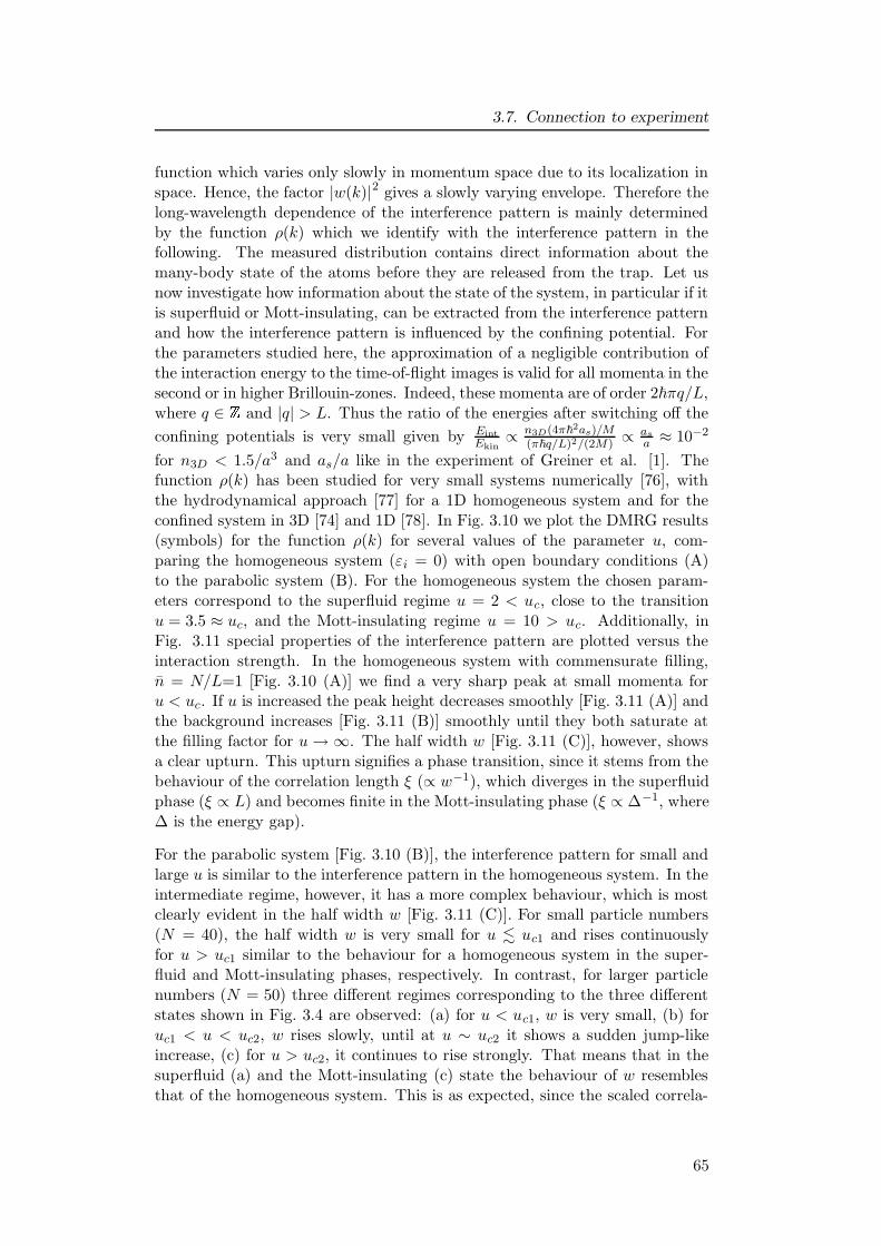
3.7. Connection to experiment
function which varies only slowly in momentum space due to its localization inspace. Hence, the factor |w(k)|2 gives a slowly varying envelope. Therefore thelong-wavelength dependence of the interference pattern is mainly determinedby the function ρ(k) which we identify with the interference pattern in thefollowing. The measured distribution contains direct information about themany-body state of the atoms before they are released from the trap. Let usnow investigate how information about the state of the system, in particular if itis superfluid or Mott-insulating, can be extracted from the interference patternand how the interference pattern is influenced by the confining potential. Forthe parameters studied here, the approximation of a negligible contribution ofthe interaction energy to the time-of-flight images is valid for all momenta in thesecond or in higher Brillouin-zones. Indeed, these momenta are of order 2~πq/L,where q ∈ �
and |q| > L. Thus the ratio of the energies after switching off the
confining potentials is very small given by EintEkin
∝ n3D(4π~2as)/M(π~q/L)2/(2M)
∝ as
a ≈ 10−2
for n3D < 1.5/a3 and as/a like in the experiment of Greiner et al. [1]. Thefunction ρ(k) has been studied for very small systems numerically [76], withthe hydrodynamical approach [77] for a 1D homogeneous system and for theconfined system in 3D [74] and 1D [78]. In Fig. 3.10 we plot the DMRG results(symbols) for the function ρ(k) for several values of the parameter u, com-paring the homogeneous system (εi = 0) with open boundary conditions (A)to the parabolic system (B). For the homogeneous system the chosen param-eters correspond to the superfluid regime u = 2 < uc, close to the transitionu = 3.5 ≈ uc, and the Mott-insulating regime u = 10 > uc. Additionally, inFig. 3.11 special properties of the interference pattern are plotted versus theinteraction strength. In the homogeneous system with commensurate filling,n = N/L=1 [Fig. 3.10 (A)] we find a very sharp peak at small momenta foru < uc. If u is increased the peak height decreases smoothly [Fig. 3.11 (A)] andthe background increases [Fig. 3.11 (B)] smoothly until they both saturate atthe filling factor for u→ ∞. The half width w [Fig. 3.11 (C)], however, showsa clear upturn. This upturn signifies a phase transition, since it stems from thebehaviour of the correlation length ξ (∝ w−1), which diverges in the superfluidphase (ξ ∝ L) and becomes finite in the Mott-insulating phase (ξ ∝ ∆−1, where∆ is the energy gap).
For the parabolic system [Fig. 3.10 (B)], the interference pattern for small andlarge u is similar to the interference pattern in the homogeneous system. In theintermediate regime, however, it has a more complex behaviour, which is mostclearly evident in the half width w [Fig. 3.11 (C)]. For small particle numbers(N = 40), the half width w is very small for u . uc1 and rises continuouslyfor u > uc1 similar to the behaviour for a homogeneous system in the super-fluid and Mott-insulating phases, respectively. In contrast, for larger particlenumbers (N = 50) three different regimes corresponding to the three differentstates shown in Fig. 3.4 are observed: (a) for u < uc1, w is very small, (b) foruc1 < u < uc2, w rises slowly, until at u ∼ uc2 it shows a sudden jump-likeincrease, (c) for u > uc2, it continues to rise strongly. That means that in thesuperfluid (a) and the Mott-insulating (c) state the behaviour of w resemblesthat of the homogeneous system. This is as expected, since the scaled correla-
65
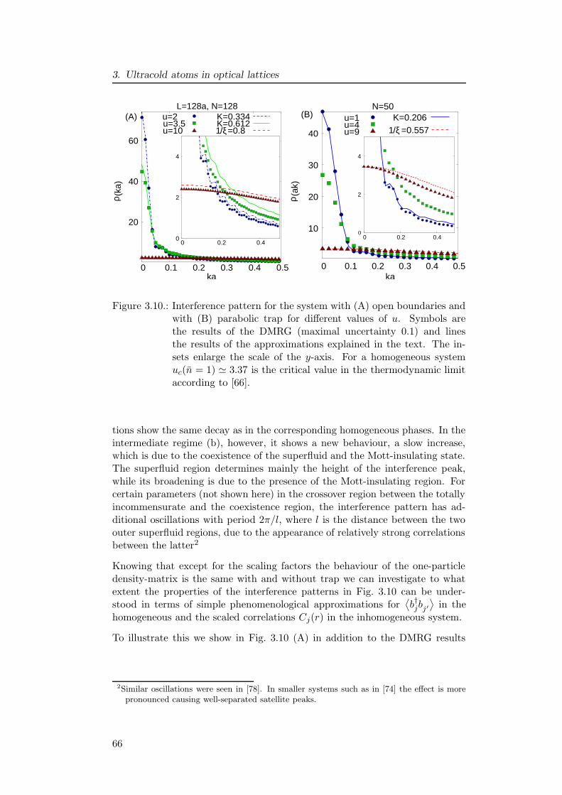
3. Ultracold atoms in optical lattices
u=4u=9
u=1
0
4
2
0.2 0.4 0
0 0.1 0.2 0.3 0.4 0.5ka
10
20
30
40
(ak)
ρ
K=0.206(B)N=50
=0.557 1/ξ(A) u=2
u=10 u=3.5
2
4
0 0 0.2 0.4
0.5
60
40
20
0 0.1 0.2 0.3 0.4ka
(ka
)ρ
K=0.334 K=0.612
=0.81/ξ
L=128a, N=128
Figure 3.10.: Interference pattern for the system with (A) open boundaries andwith (B) parabolic trap for different values of u. Symbols arethe results of the DMRG (maximal uncertainty 0.1) and linesthe results of the approximations explained in the text. The in-sets enlarge the scale of the y-axis. For a homogeneous systemuc(n = 1) ' 3.37 is the critical value in the thermodynamic limitaccording to [66].
tions show the same decay as in the corresponding homogeneous phases. In theintermediate regime (b), however, it shows a new behaviour, a slow increase,which is due to the coexistence of the superfluid and the Mott-insulating state.The superfluid region determines mainly the height of the interference peak,while its broadening is due to the presence of the Mott-insulating region. Forcertain parameters (not shown here) in the crossover region between the totallyincommensurate and the coexistence region, the interference pattern has ad-ditional oscillations with period 2π/l, where l is the distance between the twoouter superfluid regions, due to the appearance of relatively strong correlationsbetween the latter2
Knowing that except for the scaling factors the behaviour of the one-particledensity-matrix is the same with and without trap we can investigate to whatextent the properties of the interference patterns in Fig. 3.10 can be under-stood in terms of simple phenomenological approximations for
⟨b†jbj′
⟩in the
homogeneous and the scaled correlations Cj(r) in the inhomogeneous system.
To illustrate this we show in Fig. 3.10 (A) in addition to the DMRG results
2Similar oscillations were seen in [78]. In smaller systems such as in [74] the effect is morepronounced causing well-separated satellite peaks.
66
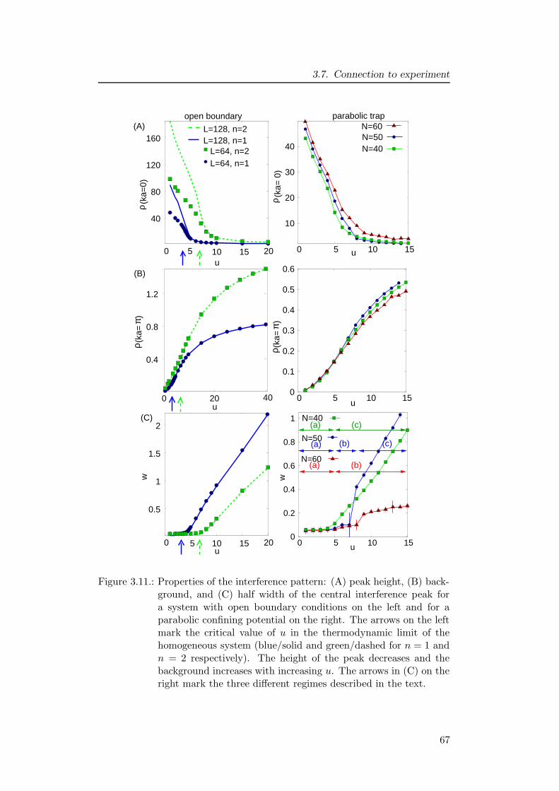
3.7. Connection to experiment
0 5 10 15
πρ (
ka=
)
πρ (
ka=
)
(a) (c)
L=128, n=2L=128, n=1
L=64, n=2L=64, n=1
30
10
0 5 10 15
N=40 N=50 N=60
40
20
u
160
120
80
40
u 0 5 10 15 20
(ka
=0)
(ka=
0)
0.4
0.8
1.2
0 20u
40
2
1.5
1
0.5
w
20u
0.6
0.5
0.4
0.3
0.2
0.1
5 0 0
10 15u
0.8
0.6
0.4
0.2
w
15
1
0 0 5 10u
(b)(a)
(a) (b) (c)N=50
N=60
N=40
open boundary parabolic trap
ρ
ρ
(A)
(B)
(C)
Figure 3.11.: Properties of the interference pattern: (A) peak height, (B) back-ground, and (C) half width of the central interference peak fora system with open boundary conditions on the left and for aparabolic confining potential on the right. The arrows on the leftmark the critical value of u in the thermodynamic limit of thehomogeneous system (blue/solid and green/dashed for n = 1 andn = 2 respectively). The height of the peak decreases and thebackground increases with increasing u. The arrows in (C) on theright mark the three different regimes described in the text.
67
3. Ultracold atoms in optical lattices
(symbols), results (lines) obtained by approximating⟨b†jbj′
⟩in Eq. (3.7.1.1) by
⟨b†jbj′
⟩=
{
A |j − j′|−K/2 for j 6= j′
nj for j = j′(3.7.1.2)
and⟨b†jbj′
⟩= Be−|j−j′|/ξ,(3.7.1.3)
for small and large u, respectively. The values of K and ξ are determined byfitting
⟨b†jbj′
⟩to DMRG results (not shown here). The constants A and B
are chosen such that the value at k = 0 agrees with the DMRG results. InFig. 3.10 (B) the approximation (lines) are obtained analogously by taking the
density scaling into account, i.e. replacing⟨b†jbj′
⟩by the algebraically and the
exponentially decaying functions times the scaling factor√njnj′
⟨b†jbj′
⟩=
{
A√njnj′ |j − j′|−K/2 for j 6= j′
nj for j = j′(3.7.1.4)
and⟨b†jbj′
⟩=
√njnj′Be−|j−j′|/ξ,
for small and large u, respectively. Hereby we use the density distributionnj = n0(1 − (j − j0)
2/R2) for u = 1, and nj = 1 for u = 9. The parametersK and ξ are determined by fitting the scaled correlation functions. Comparingthe DMRG data to the approximation we see in Fig. 3.10 that for both cases,the homogeneous system and the system with trap, this simple approximationworks very well for small values of ka; in particular, it reproduces the correctshape of the peak [even including the small non-monotonities which are due tothe finite sum in Eq. (3.7.1.1)]. Therefore, once the characteristic decay of the(scaled) one-particle density-matrix has been identified (in this case by fittingto DMRG results), our simple scaling procedure captures most of the essentialobservable physics.
3.7.2. Comparison to experiment
Clearly our calculations in one dimension cannot be compared quantitativelywith the earlier experiments in a three-dimensional lattice [1]. Recently, how-ever, an array of truly one-dimensional Bose systems has been created [59, 79].Typically, this array consists of several thousands of parallel one-dimensionalsystems, called tubes, with different fillings. The advantage of this setup com-pared to a single tube (for example realized on an atom chip) is that the signalis enhanced, but a disadvantage is that tubes with different fillings contributeto the measured signal and smear out otherwise clear structures. This canbe seen in the experimental results [79] for the half width of the interferencepattern which was measured for different lattice heights in such an array fol-lowing our predictions. In Fig. 3.12 the experimental result for the half widthis shown for one-dimensional tubes with n ≈ 1.2 (solid squares), with n ≈ 0.6(open squares) and three-dimensional system n ≈ 1 (triangles). Note, the pa-rameter J used in Fig. 3.12 is the same as the one used in this work for theone-dimensional tubes, but for the three-dimensional system the J in Fig. 3.12
68
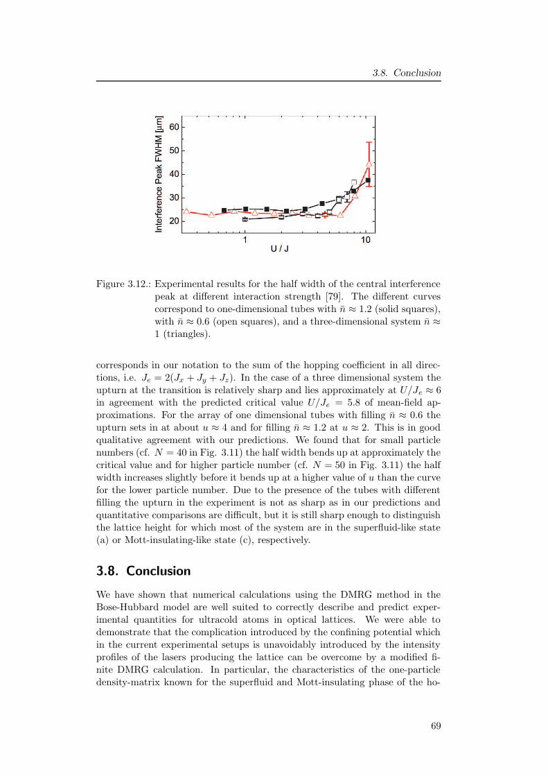
3.8. Conclusion
Figure 3.12.: Experimental results for the half width of the central interferencepeak at different interaction strength [79]. The different curvescorrespond to one-dimensional tubes with n ≈ 1.2 (solid squares),with n ≈ 0.6 (open squares), and a three-dimensional system n ≈1 (triangles).
corresponds in our notation to the sum of the hopping coefficient in all direc-tions, i.e. Je = 2(Jx + Jy + Jz). In the case of a three dimensional system theupturn at the transition is relatively sharp and lies approximately at U/Je ≈ 6in agreement with the predicted critical value U/Je = 5.8 of mean-field ap-proximations. For the array of one dimensional tubes with filling n ≈ 0.6 theupturn sets in at about u ≈ 4 and for filling n ≈ 1.2 at u ≈ 2. This is in goodqualitative agreement with our predictions. We found that for small particlenumbers (cf. N = 40 in Fig. 3.11) the half width bends up at approximately thecritical value and for higher particle number (cf. N = 50 in Fig. 3.11) the halfwidth increases slightly before it bends up at a higher value of u than the curvefor the lower particle number. Due to the presence of the tubes with differentfilling the upturn in the experiment is not as sharp as in our predictions andquantitative comparisons are difficult, but it is still sharp enough to distinguishthe lattice height for which most of the system are in the superfluid-like state(a) or Mott-insulating-like state (c), respectively.
3.8. Conclusion
We have shown that numerical calculations using the DMRG method in theBose-Hubbard model are well suited to correctly describe and predict exper-imental quantities for ultracold atoms in optical lattices. We were able todemonstrate that the complication introduced by the confining potential whichin the current experimental setups is unavoidably introduced by the intensityprofiles of the lasers producing the lattice can be overcome by a modified fi-nite DMRG calculation. In particular, the characteristics of the one-particledensity-matrix known for the superfluid and Mott-insulating phase of the ho-
69
3. Ultracold atoms in optical lattices
mogeneous system can be recovered in the confined case using a scaled one-particle density-matrix. Comparison with the local density approximation inthe weakly interacting regime showed good agreement with the DMRG calcu-lation thus providing mutual confirmation. Investigation of various quantitiesshowed that the half width of the interference peak is best suited to identifythe Mott-insulating and superfluid phases in the experiment.
70
4. Evolution of density wave packets in
ultracold bosons
4.1. Perturbations: experiments and theoretical
descriptions
In the present chapter our aim is to study the propagation of density wavepackets in a Bose-Einstein condensate confined to an optical lattice [80]. Quitegenerally, the low-lying excitations in a Bose-Einstein condensate are sound-likeand correspond to fluctuations of the condensate phase [12]. The associatedsound velocity depends on both the density in the system and the strength ofthe interaction between the atoms. Experimentally, density perturbations ina Bose-Einstein condensate have been created by applying a localized poten-tial to the Bose-Einstein condensate with a far detuned laser beam [81, 82].Alternatively, a phase imprinting method can be used, which allows to createsolitonic excitations [83, 84]. Employing these experimental techniques for thegeneration of a density perturbation in a setup of ultracold bosons in opticallattices would make the investigation of the evolution of density waves in alattice Bose gas with different interactions strengths possible.The theoretical description of these systems beyond the weak interaction limit,where a Gross-Pitaevskii or Bogoliubov description applies, is very demandingand very few results are available. In this chapter we use the adaptive t-DMRG(see section 2.7) to calculate the time evolution of the density wave packets[80]. This method allows us to find the time evolution for both weak andstrong interaction. In particular, it works best in an intermediate interactionregime, where other methods are not reliable.Most previous theoretical approaches were limited to the regime of weak inter-actions [85, 86, 87, 88], describing properly systems with many particles per site.In contrast to these, we focus here on perturbations in one-dimensional systemsat low filling, i.e. with approximately one or less than one particle per site onaverage at different interaction strengths. This regime is of particular interest,since it allows to study the behaviour of density waves near the transition froma superfluid to a Mott-insulating phase or close to the Tonks gas regime, as hasbeen realized experimentally by Stoferle et al. [89] and in references [59, 90],respectively. We focus our investigation on the sound velocity, i.e. the velocityof propagation of an infinitesimal perturbation. In particular we discuss thedependence of the sound velocity on the interaction strength and backgrounddensity. Further, we determine the velocity of propagation of a perturbationwith finite amplitude and the decay of the amplitude with time, thus analyzingnonlinear effects which are difficult to discuss analytically.To make the connection to earlier work we compare our numerical results in
71
4. Evolution of density wave packets in ultracold bosons
the limits of weak and strong interaction to different approximations: For weakinteractions a continuum description is applied, which leads to the Lieb-Linigermodel [91, 92], a system of bosons with δ-interaction. We compare the resultingsound velocity with our results and find good agreement up to intermediateinteraction strengths. A further simplification is obtained by treating the Lieb-Liniger model in a hydrodynamical approach. The sound velocity determinedby this approach is that of a Gross-Pitaevskii type description. It agrees withour result only for rather small interaction strengths. In the limit of stronginteractions and at low fillings, the Bose-Hubbard model can be mapped onto amodel of spinless fermions [93]. As expected, our numerical results for the soundvelocity in this limit smoothly approach the value predicted from this mappingto fermions [94]. Thus the adaptive t-DMRG provides a unified description forthe whole range of interaction strengths.
This chapter is organized as follows: We start by checking the applicabilityof the Bose-Hubbard model (Sec. 4.2) to describe density perturbations in asystem of ultracold bosons subjected to an optical lattice. Then we explain howa density perturbation can be created in this framework (Sec. 4.3). Before wediscuss the evolution of the perturbation in Sec. 4.5, we introduce the analyticalapproximations to which we compare our results in Sec. 4.4. In section 4.6 weanalyse the decay of the amplitude of the perturbation. Further the dependenceof the velocity, in particular the sound velocity, on system parameters like thebackground density, the interaction strength (Sec. 4.7) and the height of theperturbation (Sec. 4.8) are discussed. Finally in section 4.9, we study how thepresence of a wave packet can be detected experimentally from the interferencepattern in a time-of-flight experiment.
4.2. Theoretical description of the density perturbation
As seen in chapter 3 ultracold bosons in an optical lattice can be well describedby the Bose-Hubbard model (3.2.0.2), if the dynamics of the system is confinedto the lowest energy band induced by the lattice. Hence the additional energyby the perturbation has to be much smaller than the level spacing of the energybands induced by the optical lattice. As we will see below this gives a constrainton the strength of the density perturbation which can be described within theBose-Hubbard model. In the following we will investigate the time evolution ofdensity wave packets of approximately Gaussian form which is created at t = 0,i.e.
(4.2.0.1) ρj(t = 0) = ρ0(1 + 2ηe−j2/(2σ2)).
Here ρ0 is the background density, η the height of the perturbation, and σ itswidth. The energy change induced by such a density perturbation consists oftwo contributions: (i) the change in the interaction energy and (ii) the changein the kinetic energy.
(i) The change in the interaction energy can be estimated by taking the’mean’ interaction of the atoms in the system with the perturbation
72
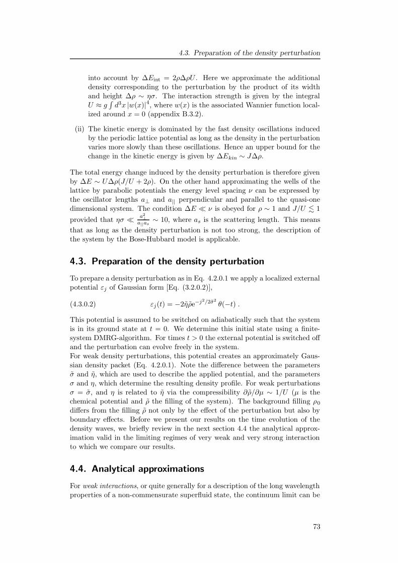
4.3. Preparation of the density perturbation
into account by ∆Eint = 2ρ∆ρU . Here we approximate the additionaldensity corresponding to the perturbation by the product of its widthand height ∆ρ ∼ ησ. The interaction strength is given by the integralU ≈ g
∫d3x |w(x)|4, where w(x) is the associated Wannier function local-
ized around x = 0 (appendix B.3.2).
(ii) The kinetic energy is dominated by the fast density oscillations inducedby the periodic lattice potential as long as the density in the perturbationvaries more slowly than these oscillations. Hence an upper bound for thechange in the kinetic energy is given by ∆Ekin ∼ J∆ρ.
The total energy change induced by the density perturbation is therefore givenby ∆E ∼ U∆ρ(J/U + 2ρ). On the other hand approximating the wells of thelattice by parabolic potentials the energy level spacing ν can be expressed bythe oscillator lengths a⊥ and a|| perpendicular and parallel to the quasi-onedimensional system. The condition ∆E � ν is obeyed for ρ ∼ 1 and J/U . 1
provided that ησ � a2⊥
a||as∼ 10, where as is the scattering length. This means
that as long as the density perturbation is not too strong, the description ofthe system by the Bose-Hubbard model is applicable.
4.3. Preparation of the density perturbation
To prepare a density perturbation as in Eq. 4.2.0.1 we apply a localized externalpotential εj of Gaussian form [Eq. (3.2.0.2)],
(4.3.0.2) εj(t) = −2ηρe−j2/2σ2θ(−t) .
This potential is assumed to be switched on adiabatically such that the systemis in its ground state at t = 0. We determine this initial state using a finite-system DMRG-algorithm. For times t > 0 the external potential is switched offand the perturbation can evolve freely in the system.For weak density perturbations, this potential creates an approximately Gaus-sian density packet (Eq. 4.2.0.1). Note the difference between the parametersσ and η, which are used to describe the applied potential, and the parametersσ and η, which determine the resulting density profile. For weak perturbationsσ = σ, and η is related to η via the compressibility ∂ρ/∂µ ∼ 1/U (µ is thechemical potential and ρ the filling of the system). The background filling ρ0
differs from the filling ρ not only by the effect of the perturbation but also byboundary effects. Before we present our results on the time evolution of thedensity waves, we briefly review in the next section 4.4 the analytical approx-imation valid in the limiting regimes of very weak and very strong interactionto which we compare our results.
4.4. Analytical approximations
For weak interactions, or quite generally for a description of the long wavelengthproperties of a non-commensurate superfluid state, the continuum limit can be
73
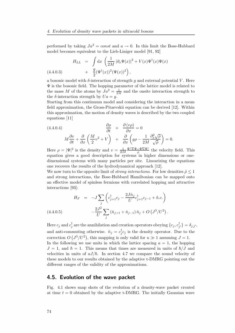
4. Evolution of density wave packets in ultracold bosons
performed by taking Ja2 = const and a → 0. In this limit the Bose-Hubbardmodel becomes equivalent to the Lieb-Liniger model [91, 92]
HLL =
∫
dx
(1
2M|∂xΨ(x)|2 + V (x)Ψ†(x)Ψ(x)
+g
2(Ψ†(x))2(Ψ(x))2
)
,(4.4.0.3)
a bosonic model with δ-interaction of strength g and external potential V . HereΨ is the bosonic field. The hopping parameter of the lattice model is related tothe mass M of the atoms by Ja2 = 1
2M and the onsite interaction strength tothe δ-interaction strength by Ua = g.Starting from this continuum model and considering the interaction in a meanfield approximation, the Gross-Pitaevskii equation can be derived [12]. Withinthis approximation, the motion of density waves is described by the two coupledequations [11]
∂ρ
∂t+
∂ (vρ)
∂x= 0(4.4.0.4)
M∂v
∂t+
∂
∂x
(M
2v2 + V
)
+∂
∂x
(
gρ− 1
2M
∂2x√ρ
√ρ
)
= 0.
Here ρ = |Ψ|2 is the density and v = 12iM
Ψ∗∇Ψ−Ψ∇Ψ∗
ρ the velocity field. Thisequation gives a good description for systems in higher dimensions or one-dimensional systems with many particles per site. Linearizing the equationsone recovers the results of the hydrodynamical approach [12].We now turn to the opposite limit of strong interactions. For low densities ρ ≤ 1and strong interactions, the Bose-Hubbard Hamiltonian can be mapped ontoan effective model of spinless fermions with correlated hopping and attractiveinteractions [93]:
HF = −J∑
j
(
c†j+1cj −2Jnj
Uc†j+1cj−1 + h.c.
)
−2J2
U
∑
j
(nj+1 + nj−1) nj +O(J3/U2
).(4.4.0.5)
Here cj and c†j are the annihilation and creation operators obeying {cj , c†j′} = δj,j′ ,
and anti-commuting otherwise. nj = c†jcj is the density operator. Due to the
correction O(J3/U2
), this mapping is only valid for u� 1 assuming J = 1.
In the following we use units in which the lattice spacing a = 1, the hoppingJ = 1, and ~ = 1. This means that times are measured in units of ~/J andvelocities in units of aJ/~. In section 4.7 we compare the sound velocity ofthese models to our results obtained by the adaptive t-DMRG pointing out thedifferent ranges of the validity of the approximations.
4.5. Evolution of the wave packet
Fig. 4.1 shows snap shots of the evolution of a density-wave packet createdat time t = 0 obtained by the adaptive t-DMRG. The initially Gaussian wave
74
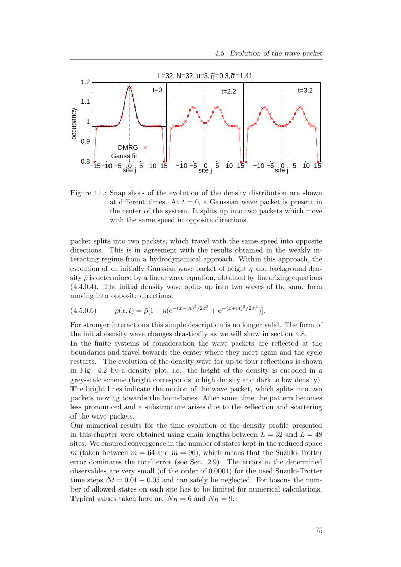
4.5. Evolution of the wave packet
−15−10 −5 0 5 10 15 −10 −5 0 5 10 15−10 −5 0 5 10 15
occu
panc
y
0.8
0.9
1
1.1
1.2
site j
Gauss fit
site j site j
L=32, N=32, u=3, =0.3, =1.41
t=2.2 t=3.2
DMRG
t=0
η~ σ~
Figure 4.1.: Snap shots of the evolution of the density distribution are shownat different times. At t = 0, a Gaussian wave packet is present inthe center of the system. It splits up into two packets which movewith the same speed in opposite directions.
packet splits into two packets, which travel with the same speed into oppositedirections. This is in agreement with the results obtained in the weakly in-teracting regime from a hydrodynamical approach. Within this approach, theevolution of an initially Gaussian wave packet of height η and background den-sity ρ is determined by a linear wave equation, obtained by linearizing equations(4.4.0.4). The initial density wave splits up into two waves of the same formmoving into opposite directions:
ρ(x, t) = ρ[1 + η(e−(x−vt)2/2σ2+ e−(x+vt)2/2σ2
)].(4.5.0.6)
For stronger interactions this simple description is no longer valid. The form ofthe initial density wave changes drastically as we will show in section 4.8.In the finite systems of consideration the wave packets are reflected at theboundaries and travel towards the center where they meet again and the cyclerestarts. The evolution of the density wave for up to four reflections is shownin Fig. 4.2 by a density plot, i.e. the height of the density is encoded in agrey-scale scheme (bright corresponds to high density and dark to low density).The bright lines indicate the motion of the wave packet, which splits into twopackets moving towards the boundaries. After some time the pattern becomesless pronounced and a substructure arises due to the reflection and scatteringof the wave packets.Our numerical results for the time evolution of the density profile presentedin this chapter were obtained using chain lengths between L = 32 and L = 48sites. We ensured convergence in the number of states kept in the reduced spacem (taken between m = 64 and m = 96), which means that the Suzuki-Trottererror dominates the total error (see Sec. 2.9). The errors in the determinedobservables are very small (of the order of 0.0001) for the used Suzuki-Trottertime steps ∆t = 0.01 − 0.05 and can safely be neglected. For bosons the num-ber of allowed states on each site has to be limited for numerical calculations.Typical values taken here are NB = 6 and NB = 9.
75
4. Evolution of density wave packets in ultracold bosons
~σ~ηL=32, u=3, N=32, =0.3, =2
5 10 15 20 25 30 0
5
10
15
20
25
30
35
40
45
50
time
0.8 0.9 1 1.1 1.2
site j
Figure 4.2.: The evolution of a density-wave packet is shown in a density plot.A linear grey scale is used, bright meaning higher densities. Thebright lines correspond to the wave packets first splitting up mov-ing towards the boundaries, being reflected by the boundaries andmeeting again in the center of the system, where the cycle startsagain.
76
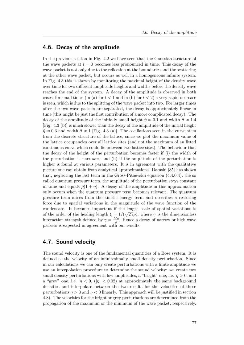
4.6. Decay of the amplitude
4.6. Decay of the amplitude
In the previous section in Fig. 4.2 we have seen that the Gaussian structure ofthe wave packets at t = 0 becomes less pronounced in time. This decay of thewave packet is not only due to the reflection at the boundaries and the scatteringat the other wave packet, but occurs as well in a homogeneous infinite system.In Fig. 4.3 this is shown by monitoring the maximal height of the density waveover time for two different amplitude heights and widths before the density wavereaches the end of the system. A decay of the amplitude is observed in bothcases; for small times (in (a) for t < 1 and in (b) for t < 2) a very rapid decreaseis seen, which is due to the splitting of the wave packet into two. For larger timesafter the two wave packets are separated, the decay is approximately linear intime (this might be just the first contribution of a more complicated decay). Thedecay of the amplitude of the initially small height η ≈ 0.1 and width σ ≈ 1.4[Fig. 4.3 (b)] is much slower than the decay of the amplitude of the initial heightη ≈ 0.3 and width σ ≈ 1 [Fig. 4.3 (a)]. The oscillations seen in the curve stemfrom the discrete structure of the lattice, since we plot the maximum value ofthe lattice occupancies over all lattice sites (and not the maximum of an fittedcontinuous curve which could lie between two lattice sites). The behaviour thatthe decay of the height of the perturbation becomes faster if (i) the width ofthe perturbation is narrower, and (ii) if the amplitude of the perturbation ishigher is found at various parameters. It is in agreement with the qualitativepicture one can obtain from analytical approximations. Damski [85] has shownthat, neglecting the last term in the Gross-Pitaevskii equation (4.4.0.4), the socalled quantum pressure term, the amplitude of the perturbation stays constantin time and equals ρ(1 + η). A decay of the amplitude in this approximationonly occurs when the quantum pressure term becomes relevant. The quantumpressure term arises from the kinetic energy term and describes a restoringforce due to spatial variations in the magnitude of the wave function of thecondensate. It becomes important if the length scale of spatial variations isof the order of the healing length ξ = 1/(
√2γρ), where γ is the dimensionless
interaction strength defined by γ = Mgρ . Hence a decay of narrow or high wave
packets is expected in agreement with our results.
4.7. Sound velocity
The sound velocity is one of the fundamental quantities of a Bose system. It isdefined as the velocity of an infinitesimally small density perturbation. Sincein our calculations we can only create perturbations with a finite amplitude weuse an interpolation procedure to determine the sound velocity: we create twosmall density perturbations with low amplitudes, a “bright” one, i.e. η > 0, anda “grey” one, i.e. η < 0, (|η| < 0.02) at approximately the same backgrounddensities and interpolate between the two results for the velocities of theseperturbations η > 0 and η < 0 linearly. This approach will be justified in section4.8). The velocities for the bright or grey perturbations are determined from thepropagation of the maximum or the minimum of the wave packet, respectively.
77
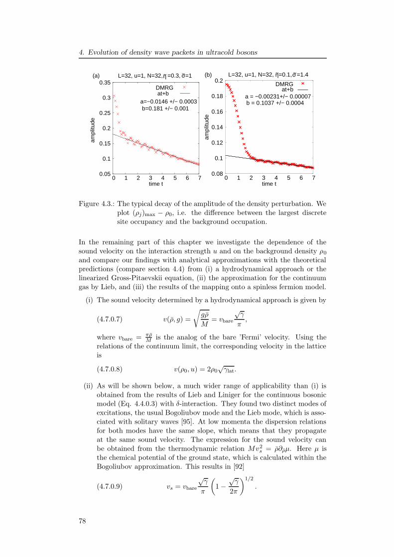
4. Evolution of density wave packets in ultracold bosons
0.05
0.1
0.15
0.2
0.25
0.3
0.35
0 1 2 3 4 5 6 7time t
a=−0.0146 +/− 0.0003b=0.181 +/− 0.001
DMRGat+b
η σ
ampl
itude
L=32, u=1, N=32, =0.3, =1 ~ ~(a)
0.08
0.1
0.12
0.14
0.16
0.18
0.2
0 1 2 3 4 5 6 7
ampl
itude
time t
L=32, u=1, N=32, =0.1, =1.4
a = −0.00231+/− 0.00007b = 0.1037 +/− 0.0004
at+bDMRG
η σ ~ ~(b)
Figure 4.3.: The typical decay of the amplitude of the density perturbation. Weplot (ρj)max − ρ0, i.e. the difference between the largest discretesite occupancy and the background occupation.
In the remaining part of this chapter we investigate the dependence of thesound velocity on the interaction strength u and on the background density ρ0
and compare our findings with analytical approximations with the theoreticalpredictions (compare section 4.4) from (i) a hydrodynamical approach or thelinearized Gross-Pitaevskii equation, (ii) the approximation for the continuumgas by Lieb, and (iii) the results of the mapping onto a spinless fermion model.
(i) The sound velocity determined by a hydrodynamical approach is given by
v(ρ, g) =
√
gρ
M= vbare
√γ
π,(4.7.0.7)
where vbare = πρM is the analog of the bare ’Fermi’ velocity. Using the
relations of the continuum limit, the corresponding velocity in the latticeis
v(ρ0, u) = 2ρ0√γlat.(4.7.0.8)
(ii) As will be shown below, a much wider range of applicability than (i) isobtained from the results of Lieb and Liniger for the continuous bosonicmodel (Eq. 4.4.0.3) with δ-interaction. They found two distinct modes ofexcitations, the usual Bogoliubov mode and the Lieb mode, which is asso-ciated with solitary waves [95]. At low momenta the dispersion relationsfor both modes have the same slope, which means that they propagateat the same sound velocity. The expression for the sound velocity canbe obtained from the thermodynamic relation Mv2
s = ρ∂ρµ. Here µ isthe chemical potential of the ground state, which is calculated within theBogoliubov approximation. This results in [92]
(4.7.0.9) vs = vbare
√γ
π
(
1 −√γ
2π
)1/2
.
78
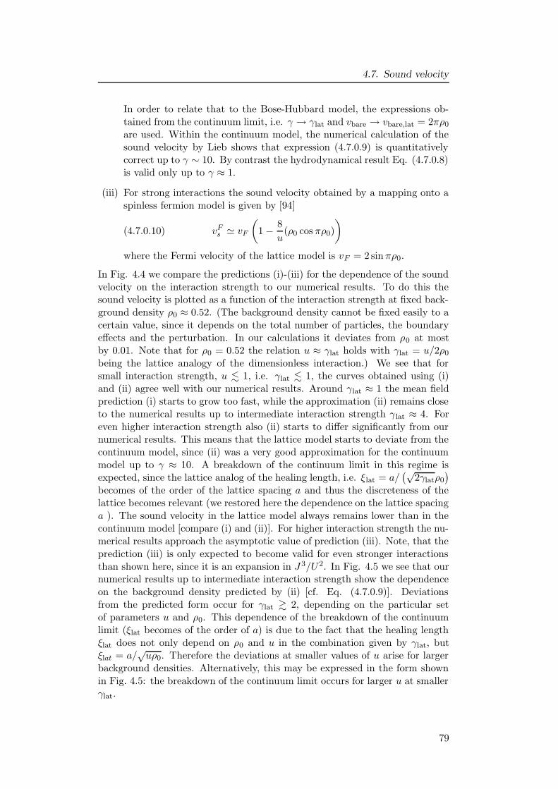
4.7. Sound velocity
In order to relate that to the Bose-Hubbard model, the expressions ob-tained from the continuum limit, i.e. γ → γlat and vbare → vbare,lat = 2πρ0
are used. Within the continuum model, the numerical calculation of thesound velocity by Lieb shows that expression (4.7.0.9) is quantitativelycorrect up to γ ∼ 10. By contrast the hydrodynamical result Eq. (4.7.0.8)is valid only up to γ ≈ 1.
(iii) For strong interactions the sound velocity obtained by a mapping onto aspinless fermion model is given by [94]
vFs ' vF
(
1 − 8
u(ρ0 cos πρ0)
)
(4.7.0.10)
where the Fermi velocity of the lattice model is vF = 2 sinπρ0.
In Fig. 4.4 we compare the predictions (i)-(iii) for the dependence of the soundvelocity on the interaction strength to our numerical results. To do this thesound velocity is plotted as a function of the interaction strength at fixed back-ground density ρ0 ≈ 0.52. (The background density cannot be fixed easily to acertain value, since it depends on the total number of particles, the boundaryeffects and the perturbation. In our calculations it deviates from ρ0 at mostby 0.01. Note that for ρ0 = 0.52 the relation u ≈ γlat holds with γlat = u/2ρ0
being the lattice analogy of the dimensionless interaction.) We see that forsmall interaction strength, u . 1, i.e. γlat . 1, the curves obtained using (i)and (ii) agree well with our numerical results. Around γlat ≈ 1 the mean fieldprediction (i) starts to grow too fast, while the approximation (ii) remains closeto the numerical results up to intermediate interaction strength γlat ≈ 4. Foreven higher interaction strength also (ii) starts to differ significantly from ournumerical results. This means that the lattice model starts to deviate from thecontinuum model, since (ii) was a very good approximation for the continuummodel up to γ ≈ 10. A breakdown of the continuum limit in this regime isexpected, since the lattice analog of the healing length, i.e. ξlat = a/
(√2γlatρ0
)
becomes of the order of the lattice spacing a and thus the discreteness of thelattice becomes relevant (we restored here the dependence on the lattice spacinga ). The sound velocity in the lattice model always remains lower than in thecontinuum model [compare (i) and (ii)]. For higher interaction strength the nu-merical results approach the asymptotic value of prediction (iii). Note, that theprediction (iii) is only expected to become valid for even stronger interactionsthan shown here, since it is an expansion in J 3/U2. In Fig. 4.5 we see that ournumerical results up to intermediate interaction strength show the dependenceon the background density predicted by (ii) [cf. Eq. (4.7.0.9)]. Deviationsfrom the predicted form occur for γlat & 2, depending on the particular setof parameters u and ρ0. This dependence of the breakdown of the continuumlimit (ξlat becomes of the order of a) is due to the fact that the healing lengthξlat does not only depend on ρ0 and u in the combination given by γlat, butξlat = a/
√uρ0. Therefore the deviations at smaller values of u arise for larger
background densities. Alternatively, this may be expressed in the form shownin Fig. 4.5: the breakdown of the continuum limit occurs for larger u at smallerγlat.
79
4. Evolution of density wave packets in ultracold bosons
0.5
1
0
1.5
2
2.5
3
0 4 8 12 16
L=32, =0.52ρ
(iii)(ii)(i)
adaptive t−DMRG
v s
u
Figure 4.4.: The dependence of the sound velocity at constant background den-sity ρ0 = 0.52 on the interaction strength is shown (note u ≈ γlat).Our numerical results (+) are compared to (i) the results Eq.(4.7.0.8) of the hydrodynamical approach, (ii) the sound velocitydetermined by Lieb Eq. (4.7.0.9), and (iii) the results Eq. (4.7.0.10)for strong interaction strength obtained by mapping onto spinlessfermions. The results of Eq. (4.7.0.10), i.e. (iii), should becomeapplicable for even stronger interactions than the ones shown here.Recall that the velocities are measured in units of aJ/~.
To summarize, we find that the sound velocity as a function of the interactionstrength shows a crossover between (ii) [cf. Eq. (4.7.0.9)], where vs/ρ0 dependsonly on the combination of ρ0 and u given by γlat, to a saturation at a valuegiven by (iii) [cf. Eq. (4.7.0.10)]. In fact, a completely analogous behaviourappears in the average kinetic energy of the particles, allowing to identify theTonks regime for quasi 1D tubes of bosons which are radially confined by a 2Doptical lattice of increasing strength [90]. The breakdown of the prediction (ii)[Eq. (4.7.0.9)] is due to the discreteness of the lattice model and takes place ifthe healing length becomes of the order of the lattice spacing.
We add some more technical remarks on the determination of the sound velocity:The uncertainties introduced in the determination of the density profiles arenegligible in comparison to the uncertainties introduced by the determinationof the sound velocity. Curve of the location of the maximum (minimum) ofthe bright (dark) wave packet versus time is fitted by a linear fit to extractthe velocity. For small interaction strength the velocity is relatively low andthe movement over a long time can be fitted such that the accuracy of theresults is of the order of ±0.01 before interpolation between η > 0 and η < 0.For higher interaction strength, the uncertainty in the results for the velocityincreases (approximately O(±0.05) for u = 6). This has two reasons: first, thevelocity increases such that the end of the chain is reached in a rather shorttime. Moreover, oscillations in the density distribution induced at the end of
80
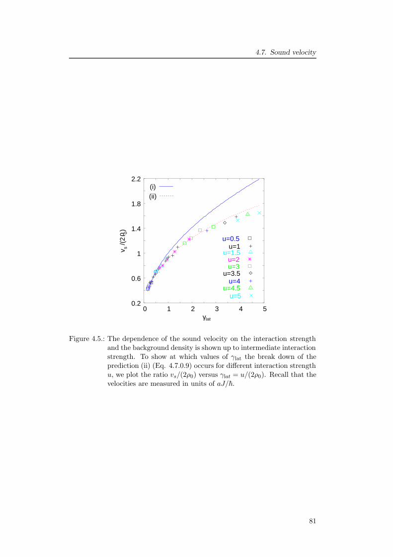
4.7. Sound velocity
(i)(ii)
0.2
0.6
1
1.4
1.8
2.2
0 1 2 3 4 5γ lat
v /(
2 )ρ 0
s
u=0.5u=1
u=1.5u=2u=3
u=3.5u=4
u=4.5u=5
Figure 4.5.: The dependence of the sound velocity on the interaction strengthand the background density is shown up to intermediate interactionstrength. To show at which values of γlat the break down of theprediction (ii) (Eq. 4.7.0.9) occurs for different interaction strengthu, we plot the ratio vs/(2ρ0) versus γlat = u/(2ρ0). Recall that thevelocities are measured in units of aJ/~.
81
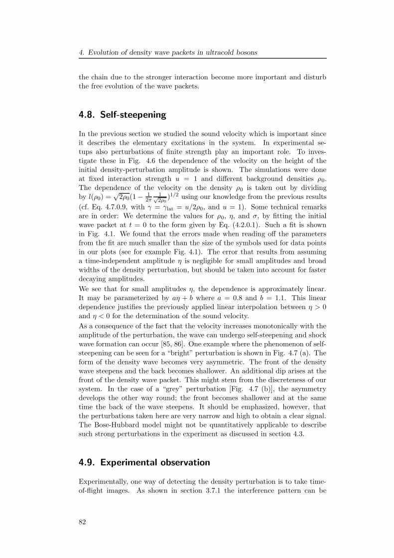
4. Evolution of density wave packets in ultracold bosons
the chain due to the stronger interaction become more important and disturbthe free evolution of the wave packets.
4.8. Self-steepening
In the previous section we studied the sound velocity which is important sinceit describes the elementary excitations in the system. In experimental se-tups also perturbations of finite strength play an important role. To inves-tigate these in Fig. 4.6 the dependence of the velocity on the height of theinitial density-perturbation amplitude is shown. The simulations were doneat fixed interaction strength u = 1 and different background densities ρ0.The dependence of the velocity on the density ρ0 is taken out by dividingby l(ρ0) =
√2ρ0(1 − 1
2π1√2ρ0
)1/2 using our knowledge from the previous results
(cf. Eq. 4.7.0.9, with γ = γlat = u/2ρ0, and u = 1). Some technical remarksare in order: We determine the values for ρ0, η, and σ, by fitting the initialwave packet at t = 0 to the form given by Eq. (4.2.0.1). Such a fit is shownin Fig. 4.1. We found that the errors made when reading off the parametersfrom the fit are much smaller than the size of the symbols used for data pointsin our plots (see for example Fig. 4.1). The error that results from assuminga time-independent amplitude η is negligible for small amplitudes and broadwidths of the density perturbation, but should be taken into account for fasterdecaying amplitudes.
We see that for small amplitudes η, the dependence is approximately linear.It may be parameterized by aη + b where a = 0.8 and b = 1.1. This lineardependence justifies the previously applied linear interpolation between η > 0and η < 0 for the determination of the sound velocity.
As a consequence of the fact that the velocity increases monotonically with theamplitude of the perturbation, the wave can undergo self-steepening and shockwave formation can occur [85, 86]. One example where the phenomenon of self-steepening can be seen for a “bright” perturbation is shown in Fig. 4.7 (a). Theform of the density wave becomes very asymmetric. The front of the densitywave steepens and the back becomes shallower. An additional dip arises at thefront of the density wave packet. This might stem from the discreteness of oursystem. In the case of a “grey” perturbation [Fig. 4.7 (b)], the asymmetrydevelops the other way round; the front becomes shallower and at the sametime the back of the wave steepens. It should be emphasized, however, thatthe perturbations taken here are very narrow and high to obtain a clear signal.The Bose-Hubbard model might not be quantitatively applicable to describesuch strong perturbations in the experiment as discussed in section 4.3.
4.9. Experimental observation
Experimentally, one way of detecting the density perturbation is to take time-of-flight images. As shown in section 3.7.1 the interference pattern can be
82
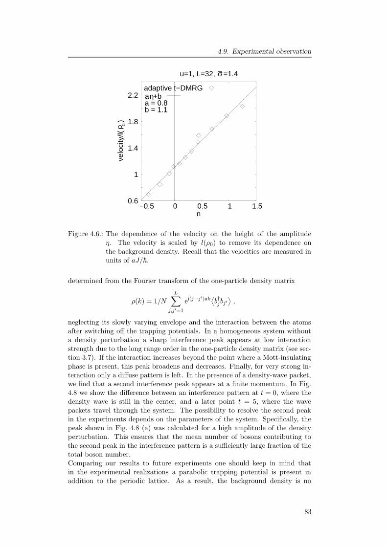
4.9. Experimental observation
0.6
1
1.4
1.8
2.2
−0.5 0 0.5 1 1.5η
velo
city
/l(
)ρ 0
adaptive t−DMRGa +bηa = 0.8b = 1.1
σu=1, L=32, =1.4 ~
Figure 4.6.: The dependence of the velocity on the height of the amplitudeη. The velocity is scaled by l(ρ0) to remove its dependence onthe background density. Recall that the velocities are measured inunits of aJ/~.
determined from the Fourier transform of the one-particle density matrix
ρ(k) = 1/N
L∑
j,j′=1
ei(j−j′)ak⟨b†jbj′
⟩,
neglecting its slowly varying envelope and the interaction between the atomsafter switching off the trapping potentials. In a homogeneous system withouta density perturbation a sharp interference peak appears at low interactionstrength due to the long range order in the one-particle density matrix (see sec-tion 3.7). If the interaction increases beyond the point where a Mott-insulatingphase is present, this peak broadens and decreases. Finally, for very strong in-teraction only a diffuse pattern is left. In the presence of a density-wave packet,we find that a second interference peak appears at a finite momentum. In Fig.4.8 we show the difference between an interference pattern at t = 0, where thedensity wave is still in the center, and a later point t = 5, where the wavepackets travel through the system. The possibility to resolve the second peakin the experiments depends on the parameters of the system. Specifically, thepeak shown in Fig. 4.8 (a) was calculated for a high amplitude of the densityperturbation. This ensures that the mean number of bosons contributing tothe second peak in the interference pattern is a sufficiently large fraction of thetotal boson number.Comparing our results to future experiments one should keep in mind thatin the experimental realizations a parabolic trapping potential is present inaddition to the periodic lattice. As a result, the background density is no
83

4. Evolution of density wave packets in ultracold bosons
−20 −10 0 10 20site j
−20 −10 0 10 20site j
−20 −10 0 10 20site j
0.8
1
1.2
1.4
occu
panc
y
L=48, N=48, u=1, =0.3, =0.5 ση~ ~
t=3.2 t=5.2t=0
(a)
−20 −10 0 10 20 −20 −10 0 10 20 −20 −10 0 10 20 0.4
0.6
0.8
1
1.2
occu
panc
y
site j site j site j
t=4.8 t=6.8 t=0
L=48, N=48, u=1, =−0.3, =1.41ση~ ~ (b)
Figure 4.7.: The evolution of a narrow density-wave packet is shown for variousfixed times. The wave packets undergo self steepening. The linesare guides to the eye.
84
4.10. Conclusion
t=0 t=5
0
5
10
15
20
25
30
0 0.2 0.4 0.6 0.8 1ka
L=32, N=32, u=1, =0.6, =1.4(k
a)ρ
η σ ~ ~
−14
−10
−6
−2
2
6
0 0.2 0.4 0.6 0.8 1
(t=
5)−
(t
=0)
ρρ
L=32, N=32, u=1, =0.6, =1.4
ka
η σ ~ ~
Figure 4.8.: On the left the interference pattern is shown for two different times.At t = 0 only one sharp interference peak at k = 0 exists. Fortimes t > 0 further peaks at finite momentum k and −k arise whichcorrespond to the moving wave packets. Here only the region k > 0is shown, exploiting a symmetry under k → −k. On the right thedifference of the interference pattern for t = 5 and t = 0 is shown.Here the errors are of the order of a few percent.
longer homogeneous (see section 3). Since the sound velocity depends on thebackground density, we expect it to vary for weak interactions according to Eq.(4.7.0.9) and for strong interactions according to Eq. (4.7.0.10). In the regionwhere the trap varies slowly enough that the background density is almostconstant, we expect the trap to have negligible effect on the motion of the wavepacket such that we can directly compare our theoretical results to experiments.
4.10. Conclusion
We have shown that the adaptive t-DMRG allows us to study the motion ofwave packets in a Bose-Hubbard model far beyond the regimes where commonlyused approximations apply. This gave us the possibility to investigate the dy-namics of density perturbations in ultracold bosons subjected to an opticallattice in many experimentally relevant situations. By comparing our resultsfor the sound velocity to the results of different approximations we determinethe regime in which they hold. The hydrodynamical approach or the linearizedGross-Pitaevskii equation agrees only well for rather weak interaction strengthsand the continuum model holds up to intermediate interaction strengths. Incontrast the fermionic model is only applicable for very strong interactions.The investigation of perturbations of experimentally realistic strength showeda decay of the amplitude and an approximately linear dependence of the veloc-ity on the height of the amplitude. This dependence gives rise to interesting
85
4. Evolution of density wave packets in ultracold bosons
effects like self steepening and shock wave formation which remain to be studiedfurther. In the experiments the density wave may be detected as an additionalpeak in the interference pattern.Let us conclude by mentioning a few open questions: In the exact solution ofthe continuum model by Lieb and Liniger there are in fact two independenttypes of excitations. One of them exhibits a generalized Bogoliubov type dis-persion, which is linear at small momenta and crosses over to a quadratic freeparticle behaviour at large momenta. The other one only exists in a finite mo-mentum range. It has been later identified as the solitary wave of the nonlinearSchrodinger equation in 1D [95, 96]. As was shown by Lieb and Liniger, thevelocity of the dark solitons for repulsive interactions is always smaller than thelinear sound velocity, coinciding with the latter only in the limit of long wavelengths. Experimentally, dark solitons have been observed in quasi 1D Bose-Einstein condensates, and have been identified by the fact that their velocitydepends on the imposed phase gradient [83, 84]. In the case of a deep latticepotential, as is studied here, solitary waves are predicted to appear in the weakcoupling regime u� 1 [97] and for sufficiently wide density perturbations whichcan be described by the 1D nonlinear Schrodinger equation. In addition, thepresence of a lattice potential implies that atoms with momenta near a recipro-cal lattice vector acquire a negative effective mass. This leads to the existenceof bright gap solitons, a subject of considerable current interest [98, 99, 75],in particular in connection with instabilities for strongly driven optical lattices[100]. In this work we focused our investigations mainly on the case of pertur-bations with small momenta, for which the two modes cannot be distinguishedby their velocity. It is an open question to which extent the density waves inour simulations, can be interpreted as solitary waves and in particular whathappens to these stable excitations in the regime of strong coupling, where thenonlinear Schrodinger equation no longer applies.
86
5. Spin-charge separation in cold Fermi
gases: a real time analysis
5.1. Fascinating physics in one dimension
In this chapter we turn to excitations in one-dimensional fermionic systems.In striking contrast to Fermi liquids, where the elementary quasiparticle exci-tations carry both charge and spin, the phenomenon of spin and charge sep-aration is predicted for one dimensional systems by the Luttinger liquid pic-ture [101, 102]. According to this picture - at low energy - the excitations ofcharge and spin completely decouple and propagate with different velocities. Incondensed matter systems, numerous experiments have looked for spin-chargeseparation e.g. in 1D metallic wires [103], in 1D organic wires [104], in carbon-nanotubes [105], and in quantum wires in semiconductors, where the differentvelocities have now clearly been observed [106]. In addition Recati et al. [72]suggested to study the phenomenon of spin-charge separation using ultracoldfermions in atomic wires. The experimental realization is now in reach by therecent creation of ultracold Fermi gases in an ’atomic quantum wire’ configu-ration. This is an array of thousands of parallel atom waveguides, which arecreated by a very strong two dimensional optical lattice [107]. The advantageof the use of systems of ultracold atoms lies in the possibility of both the tun-ing and the quantification of the interaction, allowing quantitative comparisonbetween theory and experiments. Moreover, using a very strong axial confine-ment, for atomic wires 3D effects are negligible, thus avoiding the possibility tomistake experimentally Fermi liquid collective spin and charge density modesfor the different ones in 1D. We will propose yet another experiment to ob-serve spin-charge separation effects using these very clear and tunable systemsof ultracold atoms. Our proposal does not encounter the problems which stilltrouble the approach of Recati et al. (see below).
The analysis of Recati et al. [72] is essentially based on the hydrodynamicHamiltonian of the Luttinger liquid. The inhomogeneity due to the presence ofa harmonic trap is treated within a local density approximation (see also [108]).Clearly, such an approach is only valid at low energies. It requires very weakperturbations and length scales much beyond the average interparticle spacing.In reality, with typically less than 100 atoms per atomic wire [107], strongerand more localized perturbations are required to produce observable effects. Inaddition, the effect of boundaries, where the local density approximation breaksdown, are of crucial importance. For a quantitative description of spin-chargeseparation in 1D cold Fermi gases, it is thus necessary to use a microscopicdescription like the Hubbard model and to treat properly the inhomogeneouscase with realistic system sizes. Due to the short range nature of the interac-
87
5. Spin-charge separation in cold Fermi gases: a real time analysis
tions between cold atoms, the Hubbard model is indeed a perfect descriptionof a situation, in which there is an additional optical lattice along the weaklyconfined axial direction (for bosons cf. section 3.2). Hereby the spin degreesof freedom in the Hubbard model correspond to two different hyperfine levelsin the system of ultracold fermions, and the ’charge’ density is the particledensity. Despite this we will use the terms of ‘spin’ and ‘charge’ also in thecontext of ultracold fermions. For the realistic case of low filling, the hoppingmatrix element J and the on-site Hubbard repulsion U can be straightforwardlyobtained from the known lattice parameters and the scattering length [cf. Eq.(3.2.0.3) and Eq. (3.2.0.4)]. It is the aim of the present chapter to study thephenomenon of spin-charge separation within a time-dependent calculation ofa microscopic model for parameters which would be realistic in an experimentwith cold atoms [109].
We start by introducing the one-dimensional Hubbard model (section 5.2) andits phases (section 5.3), before we introduce in section 5.4 the phenomenonof spin-charge separation. In section 5.5 we give details on the perturbationsconsidered. In section 5.6 we show our results for the real-time evolution ofspin and charge perturbations of finite strength. An experiment to observe theeffect of spin-charge separation in systems of ultracold fermions is proposed insection 5.7, before we discuss in section 5.8 the parameters which need to beachieved in such an experiment.
5.2. Hubbard model
Our starting point is the standard Hubbard model
H = −J∑
j,σ
(
c†j+1,σcj,σ + h.c.)
+ U∑
j
nj,↑nj,↓
+∑
j,σ
εj,σnj,σ(5.2.0.1)
the fermionic analog of the Bose-Hubbard model Eq. 3.2.0.2. Its parametersare the hopping matrix element J , the on-site repulsion U > 0 between fermionsof opposite spin σ =↑, ↓ at sites j = 1, . . . , L and a spin-dependent local on-siteenergy εj,σ, describing both a possible smooth harmonic confinement and time-dependent local potentials which allow to perturb the system. One introducesa ’charge’ density nc = n↑ + n↓ and a ’spin’ density ns = n↑ − n↓. Similar tobosons in an optical lattice (section 3.2), the ratio u = U/J between the on-siterepulsion U and the hopping J can easily be changed experimentally by varyingthe depth V0 of the optical lattice. We use units where both J and ~ are equalto one; thus time is measured in units of ~/J .
5.3. Quantum phase diagram
The ground state of the Hubbard model can be determined exactly by the Betheansatz [110], but due to its complicated structure the evaluation of physical
88
5.4. Spin-charge separation
quantities like correlation functions remains quite involved. As in the Bose-Hubbard model two different phases occur in the Hubbard model: a liquidphase and a Mott-insulating phase. At half filling, i.e. nc = n↑ + n↓ = 1, evenan infinitesimal small interaction U causes a Mott-insulating state, whereas atfillings different from half filling only the liquid phase occurs. Therefore only theanalogue of the commensurate-incommensurate phase transition of the bosoniccase (cf. section 3.3) exists.
The lowest excitations in the system are two collective modes, the spin andthe charge mode. In the liquid phase both of these are gapless with a linearspectrum. In contrast in the Mott-insulating phase for the charge mode a gapopens up which causes the insulating behaviour, whereas the spin mode staysgapless. In the limit of infinitely strong interaction the two modes decouple notonly for low energies and the spin part of the Hamiltonian becomes equivalentto the antiferromagnetic Heisenberg model with an exchange constant 4J 2/U .
5.4. Spin-charge separation
A simple picture for the effect of spin-charge separation can be gained consid-ering a chain at half filling with very strong interaction U between the differ-ent species. The strong interaction induces an antiferromagnetic behaviour assketched in Fig. 5.1 (a). Removing a fermion from the chain [Fig. 5.1 (b)]changes both the spin and the charge quantum number. Two excitations arecreated in this case:(i) a holon [circle in Fig. 5.1 (c)], a charge is lacking, but the spin environmentis purely antiferromagnetic and(ii) a spinon [ellipse in Fig. 5.1 (c)], two neighbouring spins are aligned, but nocharge is missing.In one dimension once created the holon and the spinon can move independentlyand freely —without any additional cost in energy— through the chain, by firstand second order hopping processes, respectively. Thus any single-particle ex-citation dissociates into these elementary excitations. In contrast if a fermionis removed from a system of higher dimension the spinon and the holon areheld together by the frustration which is created by the neighbouring chains asmarked by the box in [Fig. 5.1 (d)]. A penalty in the energy has to be paidif the spinon and holon separate. Therefore, the fermionic single-quasiparticleexcitation has a finite life time and does not split up immediately as in theone-dimensional case.
More technically this phenomenon can be described by the hydrodynamical ap-proach [70, 102], which covers the low energy properties of the one-dimensionalsystem. In this approximation the degrees of spin and charge decouple com-pletely for any strength of interaction. This becomes obvious using these degreesof freedom to express the Hamiltonian:
H = Hs +Hc with(5.4.0.2)
Hν = 1/2
∫
dx
(
uνKν∂xθ2ν +
uν
Kν(∂xφν)2
)
.(5.4.0.3)
89
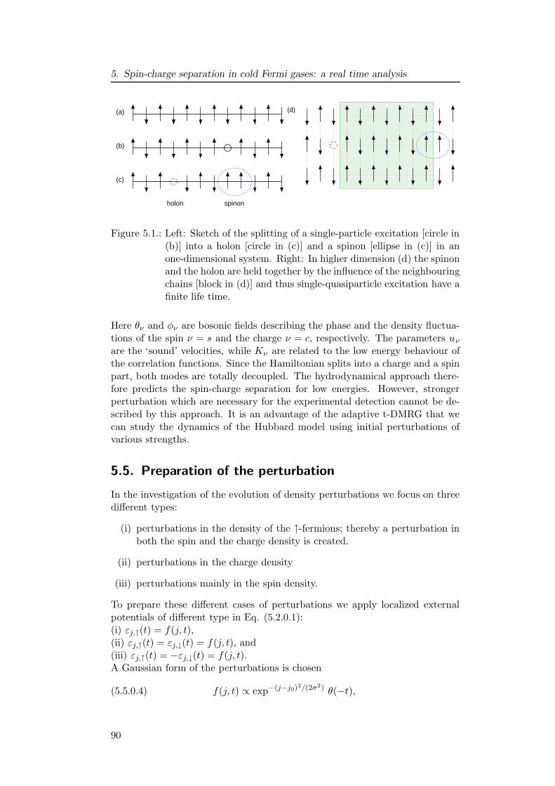
5. Spin-charge separation in cold Fermi gases: a real time analysis
(a)
(b)
(c)
holon spinon
(d)
(d)
Figure 5.1.: Left: Sketch of the splitting of a single-particle excitation [circle in(b)] into a holon [circle in (c)] and a spinon [ellipse in (c)] in anone-dimensional system. Right: In higher dimension (d) the spinonand the holon are held together by the influence of the neighbouringchains [block in (d)] and thus single-quasiparticle excitation have afinite life time.
Here θν and φν are bosonic fields describing the phase and the density fluctua-tions of the spin ν = s and the charge ν = c, respectively. The parameters uν
are the ‘sound’ velocities, while Kν are related to the low energy behaviour ofthe correlation functions. Since the Hamiltonian splits into a charge and a spinpart, both modes are totally decoupled. The hydrodynamical approach there-fore predicts the spin-charge separation for low energies. However, strongerperturbation which are necessary for the experimental detection cannot be de-scribed by this approach. It is an advantage of the adaptive t-DMRG that wecan study the dynamics of the Hubbard model using initial perturbations ofvarious strengths.
5.5. Preparation of the perturbation
In the investigation of the evolution of density perturbations we focus on threedifferent types:
(i) perturbations in the density of the ↑-fermions; thereby a perturbation inboth the spin and the charge density is created.
(ii) perturbations in the charge density
(iii) perturbations mainly in the spin density.
To prepare these different cases of perturbations we apply localized externalpotentials of different type in Eq. (5.2.0.1):(i) εj,↑(t) = f(j, t),(ii) εj,↑(t) = εj,↓(t) = f(j, t), and(iii) εj,↑(t) = −εj,↓(t) = f(j, t).A Gaussian form of the perturbations is chosen
(5.5.0.4) f(j, t) ∝ exp−(j−j0)2/(2σ2) θ(−t),
90
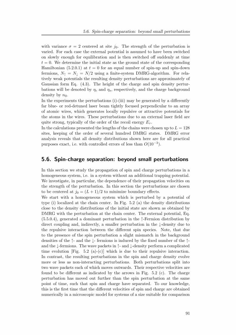
5.6. Spin-charge separation: beyond small perturbations
with variance σ = 2 centered at site j0. The strength of the perturbation isvaried. For each case the external potential is assumed to have been switchedon slowly enough for equilibration and is then switched off suddenly at timet = 0. We determine the initial state as the ground state of the correspondingHamiltonian (5.2.0.1) at t = 0 for an equal number of spin-up and spin-downfermions, N↑ = N↓ = N/2 using a finite-system DMRG-algorithm. For rela-tively weak potentials the resulting density perturbations are approximately ofGaussian form Eq. (4.3). The height of the charge and spin density pertur-bations will be denoted by ηc and ηs, respectively, and the charge backgrounddensity by n0.
In the experiments the perturbations (i)-(iii) may be generated by a differentlyfar blue- or red-detuned laser beam tightly focused perpendicular to an arrayof atomic wires, which generates locally repulsive or attractive potentials forthe atoms in the wires. These perturbations due to an external laser field arequite strong, typically of the order of the recoil energy Er.
In the calculations presented the lengths of the chains were chosen up to L = 128sites, keeping of the order of several hundred DMRG states. DMRG erroranalysis reveals that all density distributions shown here are for all practicalpurposes exact, i.e. with controlled errors of less than O(10−3).
5.6. Spin-charge separation: beyond small perturbations
In this section we study the propagation of spin and charge perturbations in ahomogeneous system, i.e. in a system without an additional trapping potential.We investigate, in particular, the dependence of their propagation velocities onthe strength of the perturbation. In this section the perturbations are chosento be centered at j0 = (L+ 1)/2 to minimize boundary effects.
We start with a homogeneous system which is perturbed by a potential oftype (i) localized at the chain center. In Fig. 5.2 (a) the density distributionsclose to the density distributions of the initial state are shown as obtained byDMRG with the perturbation at the chain center. The external potential, Eq.(5.5.0.4), generated a dominant perturbation in the ↑-Fermion distribution bydirect coupling and, indirectly, a smaller perturbation in the ↓-density due tothe repulsive interaction between the different spin species. Note, that dueto the presence of the spin perturbation a slight mismatch in the backgrounddensities of the ↑- and the ↓- fermions is induced by the fixed number of the ↑-and the ↓-fermions. The wave packets in ↑- and ↓-density perform a complicatedtime evolution [Fig. 5.2 (a)-(c)] which is due to their repulsive interaction.In contrast, the resulting perturbations in the spin and charge density evolvemore or less as non-interacting perturbations. Both perturbations split intotwo wave packets each of which moves outwards. Their respective velocities arefound to be different as indicated by the arrows in Fig. 5.2 (c). The chargeperturbation has moved out further than the spin perturbation at the samepoint of time, such that spin and charge have separated. To our knowledge,this is the first time that the different velocities of spin and charge are obtainednumerically in a microscopic model for systems of a size suitable for comparison
91
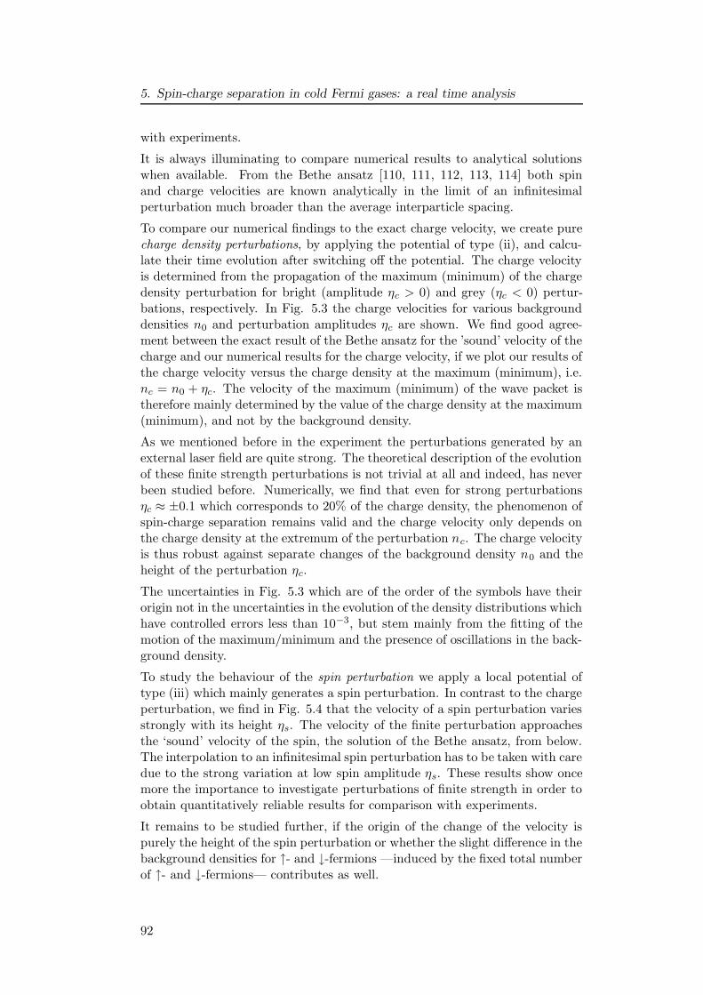
5. Spin-charge separation in cold Fermi gases: a real time analysis
with experiments.
It is always illuminating to compare numerical results to analytical solutionswhen available. From the Bethe ansatz [110, 111, 112, 113, 114] both spinand charge velocities are known analytically in the limit of an infinitesimalperturbation much broader than the average interparticle spacing.
To compare our numerical findings to the exact charge velocity, we create purecharge density perturbations, by applying the potential of type (ii), and calcu-late their time evolution after switching off the potential. The charge velocityis determined from the propagation of the maximum (minimum) of the chargedensity perturbation for bright (amplitude ηc > 0) and grey (ηc < 0) pertur-bations, respectively. In Fig. 5.3 the charge velocities for various backgrounddensities n0 and perturbation amplitudes ηc are shown. We find good agree-ment between the exact result of the Bethe ansatz for the ’sound’ velocity of thecharge and our numerical results for the charge velocity, if we plot our results ofthe charge velocity versus the charge density at the maximum (minimum), i.e.nc = n0 + ηc. The velocity of the maximum (minimum) of the wave packet istherefore mainly determined by the value of the charge density at the maximum(minimum), and not by the background density.
As we mentioned before in the experiment the perturbations generated by anexternal laser field are quite strong. The theoretical description of the evolutionof these finite strength perturbations is not trivial at all and indeed, has neverbeen studied before. Numerically, we find that even for strong perturbationsηc ≈ ±0.1 which corresponds to 20% of the charge density, the phenomenon ofspin-charge separation remains valid and the charge velocity only depends onthe charge density at the extremum of the perturbation nc. The charge velocityis thus robust against separate changes of the background density n0 and theheight of the perturbation ηc.
The uncertainties in Fig. 5.3 which are of the order of the symbols have theirorigin not in the uncertainties in the evolution of the density distributions whichhave controlled errors less than 10−3, but stem mainly from the fitting of themotion of the maximum/minimum and the presence of oscillations in the back-ground density.
To study the behaviour of the spin perturbation we apply a local potential oftype (iii) which mainly generates a spin perturbation. In contrast to the chargeperturbation, we find in Fig. 5.4 that the velocity of a spin perturbation variesstrongly with its height ηs. The velocity of the finite perturbation approachesthe ‘sound’ velocity of the spin, the solution of the Bethe ansatz, from below.The interpolation to an infinitesimal spin perturbation has to be taken with caredue to the strong variation at low spin amplitude ηs. These results show oncemore the importance to investigate perturbations of finite strength in order toobtain quantitatively reliable results for comparison with experiments.
It remains to be studied further, if the origin of the change of the velocity ispurely the height of the spin perturbation or whether the slight difference in thebackground densities for ↑- and ↓-fermions —induced by the fixed total numberof ↑- and ↓-fermions— contributes as well.
92
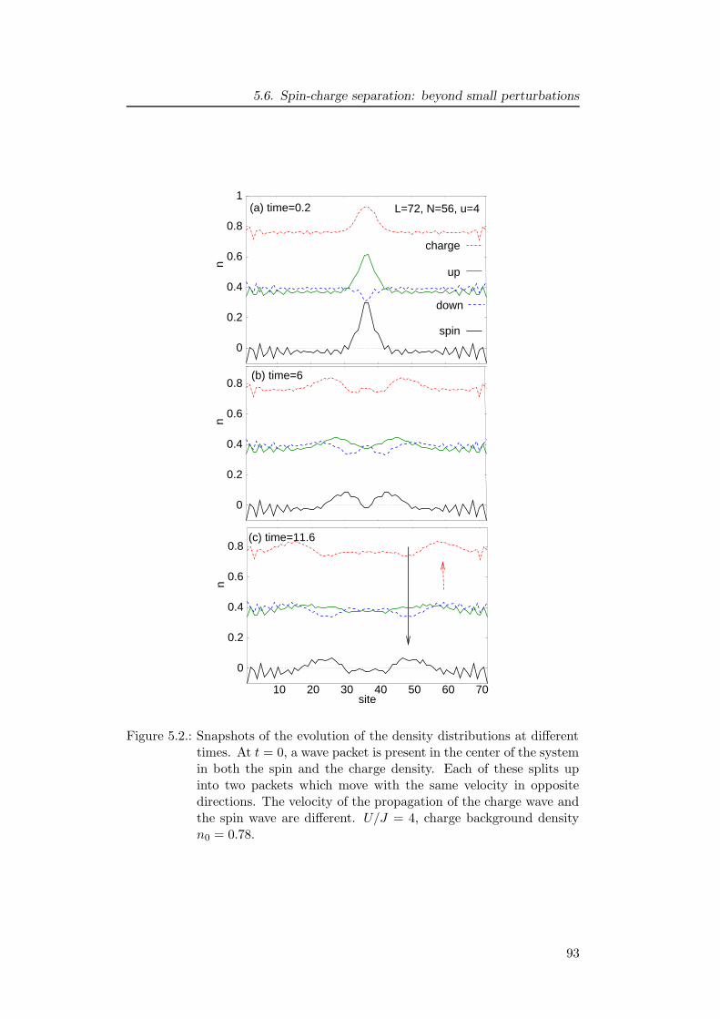
5.6. Spin-charge separation: beyond small perturbations
0
0.2
0.4
0.6
0.8
10 20 30 40 50 60 70site
n
(c) time=11.6
spin
charge
up
down
0
0.2
0.4
0.6
0.8
n
(b) time=6
0
0.2
0.4
0.6
0.8
1
n L=72, N=56, u=4 (a) time=0.2
Figure 5.2.: Snapshots of the evolution of the density distributions at differenttimes. At t = 0, a wave packet is present in the center of the systemin both the spin and the charge density. Each of these splits upinto two packets which move with the same velocity in oppositedirections. The velocity of the propagation of the charge wave andthe spin wave are different. U/J = 4, charge background densityn0 = 0.78.
93
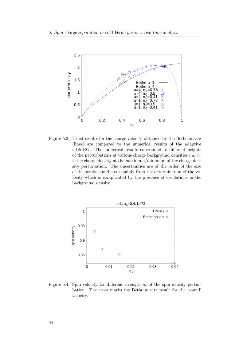
5. Spin-charge separation in cold Fermi gases: a real time analysis
u=4, n =0.5 0u=4, n =0.78 0
0
0.5
1
1.5
2
2.5
0 0.2 0.4 0.6 0.8 1
char
ge v
eloc
ity
nc
Bethe u=1Bethe u=4
u=1, n =0.41u=1, n =0.5u=1, n =0.78
0000
u=4, n =0.41
Figure 5.3.: Exact results for the charge velocity obtained by the Bethe ansatz(lines) are compared to the numerical results of the adaptivet-DMRG. The numerical results correspond to different heightsof the perturbations at various charge background densities n0. nc
is the charge density at the maximum/minimum of the charge den-sity perturbation. The uncertainties are of the order of the sizeof the symbols and stem mainly from the determination of the ve-locity which is complicated by the presence of oscillations in thebackground density.
0.85
0.9
0.95
1
0 0.01 0.02 0.03 0.04
spin
vel
ocity
u=1, n =0.4, L=72 c
DMRG
Bethe ansatz
ηs
Figure 5.4.: Spin velocity for different strength ηs of the spin density pertur-bation. The cross marks the Bethe ansatz result for the ’sound’velocity.
94

5.7. Proposed experimental realization
5.7. Proposed experimental realization
To study the separation of spin and charge experimentally in systems of ultra-cold atoms, the first idea would be to perturb the system by a localized potentialand to observe the evolution of the perturbation by measuring the densities ina certain region of the system. However, in a single one-dimensional system thesignal would be very low and in an experiment with arrays of parallel atomicwires, the different filling in individual wires would lead to a signal broadeningdue to the resulting differences in velocities. In order to avoid these problems,we suggest to look for spin-charge separation in a completely different way. Ourproposal relies on the coexistence of a Mott-insulating state and a liquid statein spatially separated regions of the system as it can be the case in the pres-ence of a parabolic trapping potential εσ,j = −Vta
2(j − L/2 + 0.5)2Er (section3.4, [115]). The idea is to use the very different behaviour of the charge andspin degrees of freedom in the Mott-insulating phase. In this phase the chargeexcitation spectrum has a gap, whereas the spin dispersion is still linear forsmall momenta, and the spin velocity is finite. By contrast, in the liquid phaseboth excitation spectra are linear for small momenta. To exploit this differ-ence in the behaviour, assume the system of one-dimensional wires confined bya trapping potential which is prepared in such a way, that a Mott-insulatingregion is present in the center of most of the wires. In these Mott-insulatingregions the charge density is locked to half-filling, nc = 1. At the boundaryof the Mott-insulating regions liquid regions exist. A localized potential whichcouples to one species [of type (i) section 5.5] in the liquid region will then cre-ate spin and charge density perturbations. While the spin density perturbationcan evolve unhindered, the charge density perturbation cannot penetrate theMott-insulating region due to its gapped spectrum. This effect can be seen fromFig. 5.5 in which calculated snapshots of the time evolution in such a situationare shown. In Fig. 5.5 (a) the perturbation, centered around site 10 is clearlyseen in the spin density and in the density of the ↑- and ↓ - fermions. In thecharge density the perturbation enlarges the region where the charge densityis locked, i.e. nc = 1. We point this out by sketching the idealized chargedensity profile without the perturbation in Fig. 5.5 (a). In Fig. 5.5 (b) and (c)the density distribution at later times are shown. Evidently, the spin densitywave propagates into the Mott-insulating region, whereas the charge densityperturbation is almost completely reflected due to the charge gap in the Mott-insulating region. The presence of spin density oscillations which are due tothe anti-ferromagnetic coupling induced by the interaction obscures the exactevolution of the spin perturbation. However by averaging over several latticesites — as it is necessary within current experimental techniques, anyway — theeffect of spin-charge separation is clearly visible. In Fig. 5.6 examples for theevolution of the sum of the charge and the spin number of particles between site25 and 35, Nc and Ns, are shown. It is clearly seen that the sum of the chargeoccupation does not change, whereas the spin occupation shows the movingwave packet. The average spin velocity can be determined from Fig. 5.6 if thedistance between the localized potential which generates the perturbation andthe center of the region over which the density is measured is known. Here, the
95
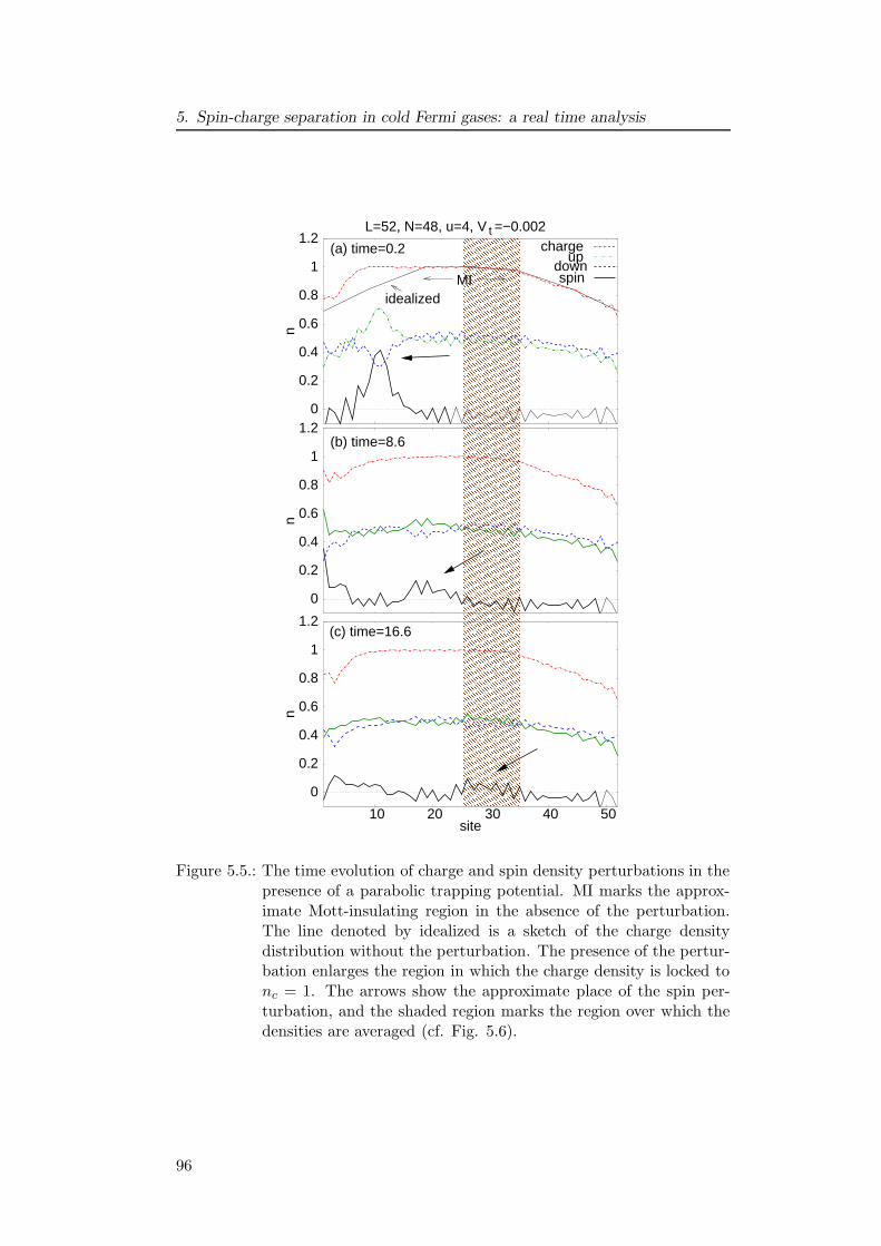
5. Spin-charge separation in cold Fermi gases: a real time analysis
����������������������������������������������������������������������������������������������������������������������������������������������������������������������������������������������������������������������������������������������������������������������������������������������������������������������������������������������������������������������������������������������������������������������������������������������������������������������������������������������������������������������������������������������������������������������������������������������������������������������������������������������������������������������������������������������������������������������������������������������������������������������������������������������������������������������������������������������������������������������������������������������������������������������������������������������������������������������������������������������������������������������������������������������������������������������������������������������������������������������������������������������������������������������������������������������������������������������������������������������������������������������������������������������������������������������������������������������������������������������������������������������������������������������������������������������������������������������������������������������������������������������������������������������������������������������������������������������������������������������������������������������������������������������������������������������������������������������������������������������������������������������������������������������������������������������������������������������������������������������������������������������������������������������������������������������������������������������������������������������������������������������������������������������������������������������������������������������������������������������������������������������������������������������������������������������������������������������������������������������������������������������������������������������������������������������������������������������������������������������������������������������������������������������������������������������������������������������������������������������������������������������������������������������������������������������������������������������������������������������������������������������������������������������������������������������������������������������������������������������������������������������������������������������������������������������������������������������������������������������������������������������������������������������������������������������������������������������������������������������������������������������������������������������������������������������������������������������������������������������������������������������������������������������������������������������������������������������������������������������������������������������������������������������������������������������������������������������������������������������������������������������������������������������������������������������������������������������������������������������������������������������������������������������������������������������������������������������������������������������������������������
����������������������������������������������������������������������������������������������������������������������������������������������������������������������������������������������������������������������������������������������������������������������������������������������������������������������������������������������������������������������������������������������������������������������������������������������������������������������������������������������������������������������������������������������������������������������������������������������������������������������������������������������������������������������������������������������������������������������������������������������������������������������������������������������������������������������������������������������������������������������������������������������������������������������������������������������������������������������������������������������������������������������������������������������������������������������������������������������������������������������������������������������������������������������������������������������������������������������������������������������������������������������������������������������������������������������������������������������������������������������������������������������������������������������������������������������������������������������������������������������������������������������������������������������������������������������������������������������������������������������������������������������������������������������������������������������������������������������������������������������������������������������������������������������������������������������������������������������������������������������������������������������������������������������������������������������������������������������������������������������������������������������������������������������������������������������������������������������������������������������������������������������������������������������������������������������������������������������������������������������������������������������������������������������������������������������������������������������������������������������������������������������������������������������������������������������������������������������������������������������������������������������������������������������������������������������������������������������������������������������������������������������������������������������������������������������������������������������������������������������������������������������������������������������������������������������������������������������������������������������������������������������������������������������������������������������������������������������������������������������������������������������������������������������������������������������������������������������������������������������������������������������������������������������������������������������������������������������������������������������������������������������������������������������������������������������������������������������������������������������������������������������������������������������������������������������������������������������������������������������������������������������������������������������������������������������������������������������������������������������������������������
L=52, N=48, u=4, V =−0.002
spin
up charge
0
0.2
0.4
0.6
0.8
1
1.2
n
t
0
0.2
0.4
0.6
0.8
1
1.2
10 20 30 40 50
n
site
0
0.2
0.4
0.6
0.8
1
1.2
n
(a) time=0.2
(c) time=16.6
(b) time=8.6
MI down
idealized
Figure 5.5.: The time evolution of charge and spin density perturbations in thepresence of a parabolic trapping potential. MI marks the approx-imate Mott-insulating region in the absence of the perturbation.The line denoted by idealized is a sketch of the charge densitydistribution without the perturbation. The presence of the pertur-bation enlarges the region in which the charge density is locked tonc = 1. The arrows show the approximate place of the spin per-turbation, and the shaded region marks the region over which thedensities are averaged (cf. Fig. 5.6).
96
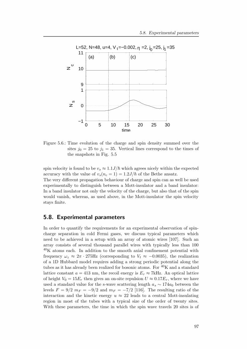
5.8. Experimental parameters
−1
0
1
0 5 10 15 20 25 30time
sc
N
9
10
11
N
L=52, N=48, u=4, V =−0.002, =2, j =25, j =35 t η
(a) (b) (c)
0 1
Figure 5.6.: Time evolution of the charge and spin density summed over thesites j0 = 25 to j1 = 35. Vertical lines correspond to the times ofthe snapshots in Fig. 5.5
spin velocity is found to be vs ≈ 1.1J/~ which agrees nicely within the expectedaccuracy with the value of vs(nc = 1) = 1.2J/~ of the Bethe ansatz.
The very different propagation behaviour of charge and spin can as well be usedexperimentally to distinguish between a Mott-insulator and a band insulator:In a band insulator not only the velocity of the charge, but also that of the spinwould vanish, whereas, as used above, in the Mott-insulator the spin velocitystays finite.
5.8. Experimental parameters
In order to quantify the requirements for an experimental observation of spin-charge separation in cold Fermi gases, we discuss typical parameters whichneed to be achieved in a setup with an array of atomic wires [107]. Such anarray consists of several thousand parallel wires with typically less than 10040K atoms each. In addition to the smooth axial confinement potential withfrequency ωz ≈ 2π · 275Hz (corresponding to Vt ≈ −0.0035), the realizationof a 1D Hubbard model requires adding a strong periodic potential along thetubes as it has already been realized for bosonic atoms. For 40K and a standardlattice constant a = 413 nm, the recoil energy is Er ≈ 7kHz. An optical latticeof height V0 = 15Er then gives an on-site repulsion U ≈ 0.17Er , where we haveused a standard value for the s-wave scattering length as ∼ 174a0 between thelevels F = 9/2 mF = −9/2 and mF = −7/2 [116]. The resulting ratio of theinteraction and the kinetic energy u ≈ 22 leads to a central Mott-insulatingregion in most of the tubes with a typical size of the order of twenty sites.With these parameters, the time in which the spin wave travels 20 sites is of
97

5. Spin-charge separation in cold Fermi gases: a real time analysis
the order of a few ms. The creation of state selective potentials for two differenthyperfine states may be done by using laser light whose frequency falls betweenthe respective transitions. This might be difficult for the F = 9/2 mF = −9/2and mF = −7/2 levels, but should be possible - for instance - using F = 9/2and F = 7/2 levels. The 1/e2-radius of the potential (Eq. 5.5.0.4) is taken tobe four lattice sites, which corresponds to a laser with an approximate 1/e2-radius of 2.1µm. Finally, to ensure that finite temperature does not destroy theMott-insulating behaviour by thermal activation, the energy scale kBT shouldbe smaller than the Mott energy gap. In recent experiments the temperaturereached was about T ∼ 0.1TF , where TF is the temperature set by the Fermienergy. Approximating the Fermi temperature by EF ∼ N/2ωz , here N is theparticle number and ωz the axial trapping frequency, the energy scale set bythe temperature is kBT ∼ 0.6Er . This is about three to four times the gap inthe Mott-insulating phase U ∼ 0.17Er for V0 = 15Er. Therefore, already thevery first experiment of 1D fermions in an optical lattice [107] is very close tomatching those conditions. Improvements can be made, e.g., by reducing theaxial confinement frequency such we expect that the necessary regime can bereached in near future.
5.9. Conclusions
We have performed the first numerical simulations of the time evolution ofcharge and spin density perturbations in real time in 1D Hubbard systemsof sizes comparable to experiments. From this it becomes evident that theseparation of spin and charge is a generic feature of 1D interacting fermions,far beyond the low-energy regime where a Luttinger liquid description applies.This opens the possibility to observe spin-charge separation experimentally insystems of ultracold atoms. We propose an experiment in which the differ-ent propagation behaviour of spin and charge perturbation in the liquid andthe Mott-insulating phases is used to observe the spin-charge separation inan array of one-dimensional systems of ultracold fermions. We expect thatthe experimental parameter regimes necessary will become accessible in nearfuture. Thus the experimental evidence for the existence of spin-charge sep-aration could be strengthened considerably relating the experimental findingsto theoretical predictions. Hereby the good control and microscopic knowl-edge about the parameters like the interaction strength make the systems ofultracold fermions advantageous. Further the same experimental setup coulddistinguish a Mott-insulator and a band insulator, one very important prooffor the importance of the interaction in these systems. Let us mention that amodification of this setup by creating an excitation with single-particle charac-ter instead of the density perturbation would allow to contrast the behaviourin one and three dimensions. Whether such a single-particle excitation can becreated and detected experimentally in these systems, remains to be shown.
98
6. Transport in spin-1/2 chains
6.1. Introduction
The transport properties of spin chains have attracted much attention recently,due to the possible applications to information storage, spintronics, and quan-tum information processing. In this chapter, we study a highly simplified pic-ture for spin transport between two coupled reservoirs of opposite spin polar-ization [117]. This is done by investigating the time evolution of an initial state∣∣ ↑ . . . ↑↓ . . . ↓
⟩, i.e. with all spins on the left half of the chain pointing up
along the z-axis modeling one of the reservoirs, and all spins on the right halfpointing down modeling the second reservoir. The spins are coupled by nearest-neighbour spin interaction (see Eq. 6.2.0.1) [117]. We are mainly interested inthe following questions: Does the state evolve into a simple long time limit? Ifso, how is this limit reached? On what properties does the long time behaviourdepend?
Analytical results for this problem are essentially restricted to the XX-chainwith and without dimerization which is amenable to an exact solution [118, 119].In Ref. [118], a scaling relation for the long-time limit was found. However,it is presently not known whether this relation is general, or whether it relieson special properties of the XX- model. If a long-time limit exists for othermodels as well, the question arises which of its characteristics are universal, andwhich depend on certain system properties. We will address these questions inthe following.
As so far no detailed error analysis of the adaptive t-DMRG has been performed,an important aspect of the present chapter is that besides their own physicalinterest, spin-1/2 chains provide an excellent benchmark for the adaptive t-DMRG, because of the nontrivial exact solution for the XX-model, againstwhich the method can be compared. This allows to analyze the accuracy ofthe adaptive t-DMRG explicitly, namely to address the questions what kindsof errors can occur in principle, which ones of these dominate in practice, andhow they can be minimized.
The outline of the chapter is as follows: In section 6.2 we introduce the modeland its characteristics. In section 6.3 a detailed error analysis is performed. Insection 6.4 we present our results for the long time limit of the time evolutionfor different interaction and dimerization strength.
6.2. Model and initial state
In this chapter we analyze the dynamics of the inhomogeneous initial state∣∣ini⟩
:=∣∣ ↑ . . . ↑↓ . . . ↓
⟩on the one-dimensional spin-1/2 chain with interactions
99

6. Transport in spin-1/2 chains
Jz1
δ
Fermion
−1
free−
FM critical
conserved current
AFM
gapped
Figure 6.1.: Quantum phase diagram of the Heisenberg model, Eq. (6.2.0.1).See [120, 121] for details.
given by the Heisenberg model
(6.2.0.1) H =∑
n
Jn(SxnS
xn+1 + Sy
nSyn+1 + JzS
znS
zn+1) ≡
∑
n
hn.
Here, ~Sn is the spin operator on site n, and Jn, Jz are interaction constants.Note, that in this chapter n denotes the site of the chain to make an easyconnection to references [117, 118]. We consider dimerized models where J z
does not depend on the site n and Jn = (1 + (−1)nδ), δ being the dimerizationcoefficient. For δ > 0, the “strong bond” with Jn = 1 + δ is chosen to be at thecenter, where the spin flip of the initial state is located.We have chosen our energy unit such that Jn = 1 for the homogeneous caseδ = 0. We also set ~ = 1, measuring time in units of ~/J . The quantum phasediagram of this model at zero temperature is well known (see [120, 121]) andsketched in Fig. 6.1. For the homogeneous case, δ = 0, the ground state hasferromagnetic / anti-ferromagnetic order with a gap in the excitation spectrumfor Jz < −1 and Jz > 1, respectively. The gap closes if |Jz | approaches 1 fromabove, and the model becomes critical for −1 < Jz < 1, i.e. gapless in thethermodynamic limit, with correlation functions showing a power-law decay.The model at the point Jz = δ = 0 is known as the XX-model. It has thespecial property that the spin-current operator J =
∑
n jn is conserved, i.e.[J,H] = 0. Here jn = JnIm (S+
n S−n+1) is the current operator on the bond
between site n and n+ 1. For finite dimerization, δ 6= 0, the spectrum is againgapped for all values of Jz.It is often useful to map the Heisenberg model onto a model of spinless fermions:
H =∑
n
Jn
[1
2(c†ncn+1 + c†n+1cn)
+Jz
(
c†ncn − 1
2
)(
c†n+1cn+1 −1
2
)]
.(6.2.0.2)
Here c†n and cn are the fermionic creation and annihilation operators. In thispicture, the first two terms describe nearest-neighbour hopping of fermions,whereas the third term (the one proportional to Jz) describes a density-densityinteraction between nearest neighbours. In particular, the case Jz = 0 describesfree fermions on a lattice, and can be solved exactly [122].
100
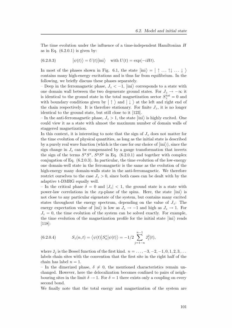
6.2. Model and initial state
The time evolution under the influence of a time-independent Hamiltonian Has in Eq. (6.2.0.1) is given by:
(6.2.0.3)∣∣ψ(t)
⟩= U(t)
∣∣ini⟩
with U(t) = exp(−iHt).
In most of the phases shown in Fig. 6.1, the state∣∣ini⟩
=∣∣ ↑ . . . ↑↓ . . . ↓
⟩
contains many high-energy excitations and is thus far from equilibrium. In thefollowing, we briefly discuss these phases separately.– Deep in the ferromagnetic phase, Jz < −1,
∣∣ini⟩
corresponds to a state withone domain wall between the two degenerate ground states. For Jz → −∞ itis identical to the ground state in the total magnetization sector S tot
z = 0 andwith boundary conditions given by
∣∣ ↑⟩
and∣∣ ↓⟩
at the left and right end ofthe chain respectively. It is therefore stationary. For finite Jz , it is no longeridentical to the ground state, but still close to it [123].– In the anti-ferromagnetic phase, Jz > 1, the state
∣∣ini⟩
is highly excited. Onecould view it as a state with almost the maximum number of domain walls ofstaggered magnetization.
In this context, it is interesting to note that the sign of Jz does not matter forthe time evolution of physical quantities, as long as the initial state is describedby a purely real wave function (which is the case for our choice of
∣∣ini⟩), since the
sign change in Jz can be compensated by a gauge transformation that invertsthe sign of the terms SxSx, SySy in Eq. (6.2.0.1) and together with complexconjugation of Eq. (6.2.0.3). In particular, the time evolution of the low-energyone domain-well state in the ferromagnetic is the same as the evolution of thehigh-energy many domain-walls state in the anti-ferromagnetic. We thereforerestrict ourselves to the case Jz > 0, since both cases can be dealt with by theadaptive t-DMRG equally well.– In the critical phase δ = 0 and |Jz | < 1, the ground state is a state withpower-law correlations in the xy-plane of the spins. Here, the state
∣∣ini⟩
isnot close to any particular eigenstate of the system, but contains many excitedstates throughout the energy spectrum, depending on the value of Jz: Theenergy expectation value of
∣∣ini⟩
is low as Jz → −1 and high as Jz → 1. ForJz = 0, the time evolution of the system can be solved exactly. For example,the time evolution of the magnetization profile for the initial state
∣∣ini⟩
reads[118]:
(6.2.0.4) Sz(n, t) =⟨ψ(t)
∣∣Sz
n
∣∣ψ(t)
⟩= −1/2
n−1∑
j=1−n
J2j(t),
where Jj is the Bessel function of the first kind. n = . . . ,−3,−2,−1, 0, 1, 2, 3, . . .labels chain sites with the convention that the first site in the right half of thechain has label n = 1.– In the dimerized phase, δ 6= 0, the mentioned characteristics remain un-changed. However, here the delocalization becomes confined to pairs of neigh-bouring sites in the limit δ → 1. For δ = 1 there exists only a coupling on everysecond bond.
We finally note that the total energy and magnetization of the system are
101
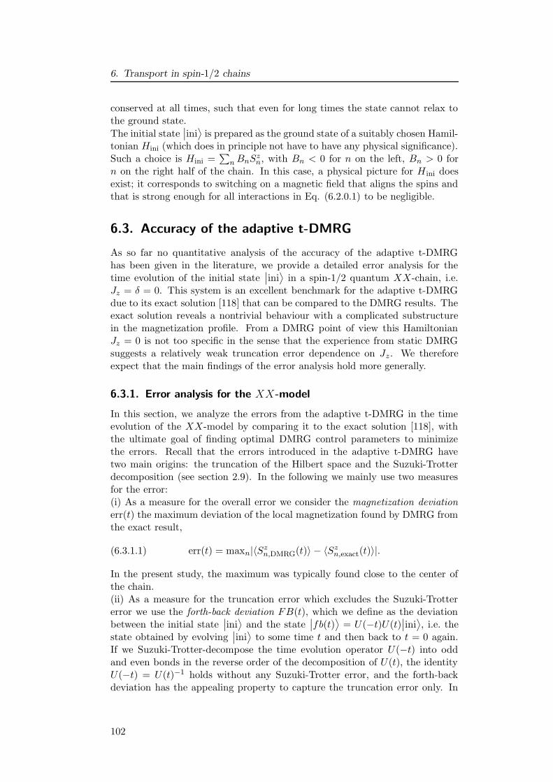
6. Transport in spin-1/2 chains
conserved at all times, such that even for long times the state cannot relax tothe ground state.
The initial state∣∣ini⟩
is prepared as the ground state of a suitably chosen Hamil-tonian Hini (which does in principle not have to have any physical significance).Such a choice is Hini =
∑
nBnSzn, with Bn < 0 for n on the left, Bn > 0 for
n on the right half of the chain. In this case, a physical picture for Hini doesexist; it corresponds to switching on a magnetic field that aligns the spins andthat is strong enough for all interactions in Eq. (6.2.0.1) to be negligible.
6.3. Accuracy of the adaptive t-DMRG
As so far no quantitative analysis of the accuracy of the adaptive t-DMRGhas been given in the literature, we provide a detailed error analysis for thetime evolution of the initial state
∣∣ini⟩
in a spin-1/2 quantum XX-chain, i.e.Jz = δ = 0. This system is an excellent benchmark for the adaptive t-DMRGdue to its exact solution [118] that can be compared to the DMRG results. Theexact solution reveals a nontrivial behaviour with a complicated substructurein the magnetization profile. From a DMRG point of view this HamiltonianJz = 0 is not too specific in the sense that the experience from static DMRGsuggests a relatively weak truncation error dependence on Jz. We thereforeexpect that the main findings of the error analysis hold more generally.
6.3.1. Error analysis for the XX-model
In this section, we analyze the errors from the adaptive t-DMRG in the timeevolution of the XX-model by comparing it to the exact solution [118], withthe ultimate goal of finding optimal DMRG control parameters to minimizethe errors. Recall that the errors introduced in the adaptive t-DMRG havetwo main origins: the truncation of the Hilbert space and the Suzuki-Trotterdecomposition (see section 2.9). In the following we mainly use two measuresfor the error:(i) As a measure for the overall error we consider the magnetization deviationerr(t) the maximum deviation of the local magnetization found by DMRG fromthe exact result,
(6.3.1.1) err(t) = maxn|〈Szn,DMRG(t)〉 − 〈Sz
n,exact(t)〉|.
In the present study, the maximum was typically found close to the center ofthe chain.(ii) As a measure for the truncation error which excludes the Suzuki-Trottererror we use the forth-back deviation FB(t), which we define as the deviationbetween the initial state
∣∣ini⟩
and the state∣∣fb(t)
⟩= U(−t)U(t)
∣∣ini⟩, i.e. the
state obtained by evolving∣∣ini⟩
to some time t and then back to t = 0 again.If we Suzuki-Trotter-decompose the time evolution operator U(−t) into oddand even bonds in the reverse order of the decomposition of U(t), the identityU(−t) = U(t)−1 holds without any Suzuki-Trotter error, and the forth-backdeviation has the appealing property to capture the truncation error only. In
102
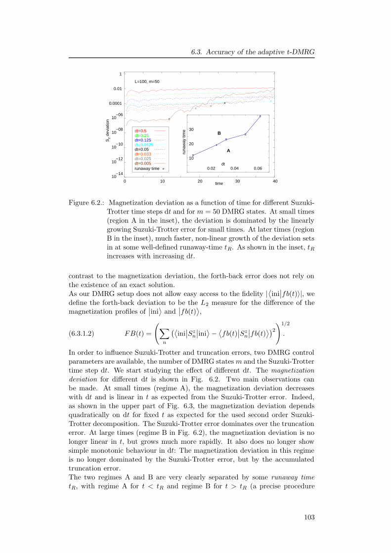
6.3. Accuracy of the adaptive t-DMRG
10−14
10−12 10
10−10 20
10−08 30
10−06
0.0001
0.01
1
0.02
0
0.04
10
0.06
20ru
naw
ay ti
me
dt
A
B
30 40
Sz
devi
atio
n
time
L=100, m=50
dt=0.5dt=0.25dt=0.125dt=0.0625dt=0.05dt=0.033dt=0.025dt=0.005runaway time
Figure 6.2.: Magnetization deviation as a function of time for different Suzuki-Trotter time steps dt and for m = 50 DMRG states. At small times(region A in the inset), the deviation is dominated by the linearlygrowing Suzuki-Trotter error for small times. At later times (regionB in the inset), much faster, non-linear growth of the deviation setsin at some well-defined runaway-time tR. As shown in the inset, tRincreases with increasing dt.
contrast to the magnetization deviation, the forth-back error does not rely onthe existence of an exact solution.As our DMRG setup does not allow easy access to the fidelity |
⟨ini∣∣fb(t)〉|, we
define the forth-back deviation to be the L2 measure for the difference of themagnetization profiles of
∣∣ini⟩
and∣∣fb(t)
⟩,
(6.3.1.2) FB(t) =
(∑
n
(⟨ini∣∣Sz
n
∣∣ini⟩−⟨fb(t)
∣∣Sz
n
∣∣fb(t)
⟩)2
)1/2
.
In order to influence Suzuki-Trotter and truncation errors, two DMRG controlparameters are available, the number of DMRG states m and the Suzuki-Trottertime step dt. We start studying the effect of different dt. The magnetizationdeviation for different dt is shown in Fig. 6.2. Two main observations canbe made. At small times (regime A), the magnetization deviation decreaseswith dt and is linear in t as expected from the Suzuki-Trotter error. Indeed,as shown in the upper part of Fig. 6.3, the magnetization deviation dependsquadratically on dt for fixed t as expected for the used second order Suzuki-Trotter decomposition. The Suzuki-Trotter error dominates over the truncationerror. At large times (regime B in Fig. 6.2), the magnetization deviation is nolonger linear in t, but grows much more rapidly. It also does no longer showsimple monotonic behaviour in dt: The magnetization deviation in this regimeis no longer dominated by the Suzuki-Trotter error, but by the accumulatedtruncation error.The two regimes A and B are very clearly separated by some runaway timetR, with regime A for t < tR and regime B for t > tR (a precise procedure
103
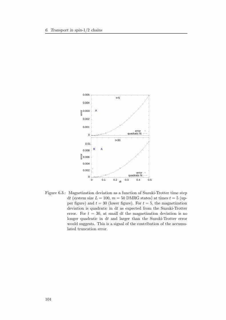
6. Transport in spin-1/2 chains
0
0
0.002
0.001
0.004
0.006
0.002
0.008
0.01
0.003
0
0.004
0.1
0.005
0.2 0.3 0.4 0.5
erro
r
dt
t=30
error
erro
r
t=5
error
quadratic fit
quadratic fit
A
B A
Figure 6.3.: Magnetization deviation as a function of Suzuki-Trotter time stepdt (system size L = 100, m = 50 DMRG states) at times t = 5 (up-per figure) and t = 30 (lower figure). For t = 5, the magnetizationdeviation is quadratic in dt as expected from the Suzuki-Trottererror. For t = 30, at small dt the magnetization deviation is nolonger quadratic in dt and larger than the Suzuki-Trotter errorwould suggests. This is a signal of the contribution of the accumu-lated truncation error.
104
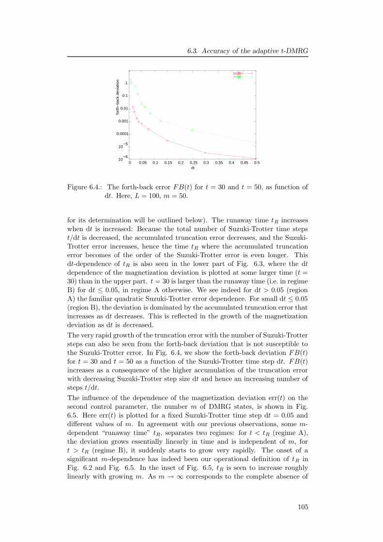
6.3. Accuracy of the adaptive t-DMRG
−610
−510
0.0001
0.001
0.01
0.1
1
0 0.05 0.1 0.15 0.2 0.25 0.3 0.35 0.4 0.45 0.5dt
t=30t=50
fort
h−ba
ck d
evia
tion
Figure 6.4.: The forth-back error FB(t) for t = 30 and t = 50, as function ofdt. Here, L = 100, m = 50.
for its determination will be outlined below). The runaway time tR increaseswhen dt is increased: Because the total number of Suzuki-Trotter time stepst/dt is decreased, the accumulated truncation error decreases, and the Suzuki-Trotter error increases, hence the time tR where the accumulated truncationerror becomes of the order of the Suzuki-Trotter error is even longer. Thisdt-dependence of tR is also seen in the lower part of Fig. 6.3, where the dtdependence of the magnetization deviation is plotted at some larger time (t =30) than in the upper part. t = 30 is larger than the runaway time (i.e. in regimeB) for dt ≤ 0.05, in regime A otherwise. We see indeed for dt > 0.05 (regionA) the familiar quadratic Suzuki-Trotter error dependence. For small dt ≤ 0.05(region B), the deviation is dominated by the accumulated truncation error thatincreases as dt decreases. This is reflected in the growth of the magnetizationdeviation as dt is decreased.
The very rapid growth of the truncation error with the number of Suzuki-Trottersteps can also be seen from the forth-back deviation that is not susceptible tothe Suzuki-Trotter error. In Fig. 6.4, we show the forth-back deviation FB(t)for t = 30 and t = 50 as a function of the Suzuki-Trotter time step dt. FB(t)increases as a consequence of the higher accumulation of the truncation errorwith decreasing Suzuki-Trotter step size dt and hence an increasing number ofsteps t/dt.
The influence of the dependence of the magnetization deviation err(t) on thesecond control parameter, the number m of DMRG states, is shown in Fig.6.5. Here err(t) is plotted for a fixed Suzuki-Trotter time step dt = 0.05 anddifferent values of m. In agreement with our previous observations, some m-dependent “runaway time” tR, separates two regimes: for t < tR (regime A),the deviation grows essentially linearly in time and is independent of m, fort > tR (regime B), it suddenly starts to grow very rapidly. The onset of asignificant m-dependence has indeed been our operational definition of tR inFig. 6.2 and Fig. 6.5. In the inset of Fig. 6.5, tR is seen to increase roughlylinearly with growing m. As m → ∞ corresponds to the complete absence of
105
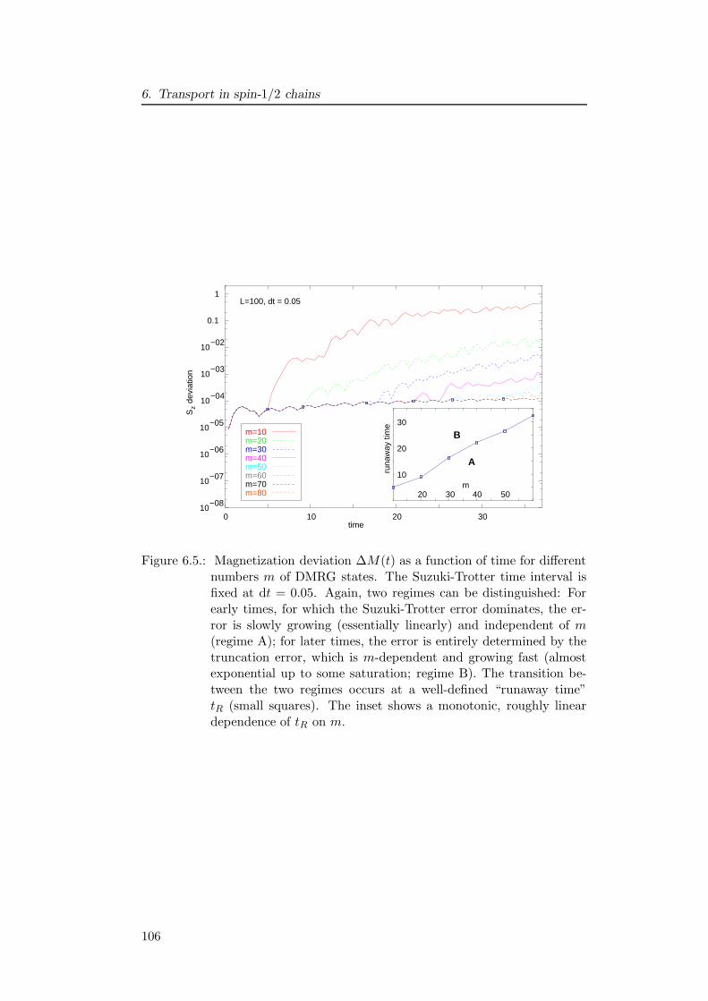
6. Transport in spin-1/2 chains
−04
−08
10
10
10
−03
−07
10
10
20
−02
−06
10
10
30−0510
0.1
20 30 40 50
runa
way
tim
e
m
A
B
1
0 10 20 30
Sz
devi
atio
n
time
L=100, dt = 0.05
m=10m=20m=30m=40m=50m=60m=70m=80
Figure 6.5.: Magnetization deviation ∆M(t) as a function of time for differentnumbers m of DMRG states. The Suzuki-Trotter time interval isfixed at dt = 0.05. Again, two regimes can be distinguished: Forearly times, for which the Suzuki-Trotter error dominates, the er-ror is slowly growing (essentially linearly) and independent of m(regime A); for later times, the error is entirely determined by thetruncation error, which is m-dependent and growing fast (almostexponential up to some saturation; regime B). The transition be-tween the two regimes occurs at a well-defined “runaway time”tR (small squares). The inset shows a monotonic, roughly lineardependence of tR on m.
106
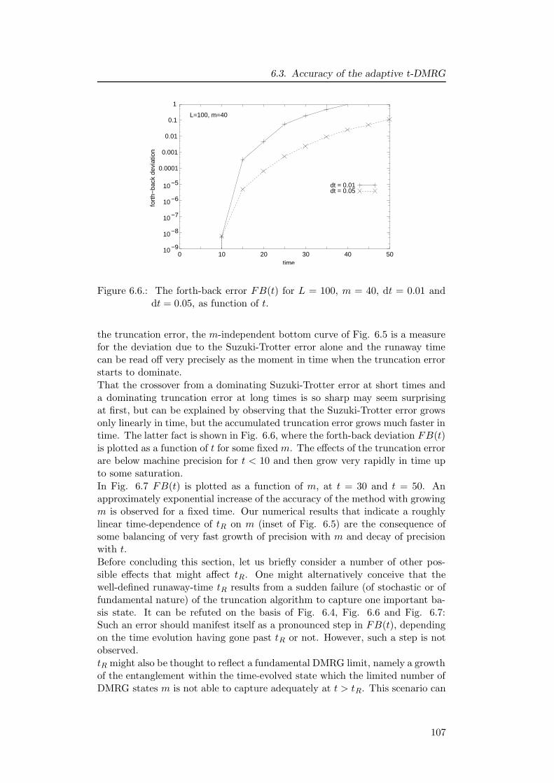
6.3. Accuracy of the adaptive t-DMRG
−910
−810
−710
−610
−510
0.0001
0.001
0.01
0.1
1
0 10 20 30 40 50
fort
h−ba
ck d
evia
tion
time
L=100, m=40
dt = 0.01dt = 0.05
Figure 6.6.: The forth-back error FB(t) for L = 100, m = 40, dt = 0.01 anddt = 0.05, as function of t.
the truncation error, the m-independent bottom curve of Fig. 6.5 is a measurefor the deviation due to the Suzuki-Trotter error alone and the runaway timecan be read off very precisely as the moment in time when the truncation errorstarts to dominate.
That the crossover from a dominating Suzuki-Trotter error at short times anda dominating truncation error at long times is so sharp may seem surprisingat first, but can be explained by observing that the Suzuki-Trotter error growsonly linearly in time, but the accumulated truncation error grows much faster intime. The latter fact is shown in Fig. 6.6, where the forth-back deviation FB(t)is plotted as a function of t for some fixed m. The effects of the truncation errorare below machine precision for t < 10 and then grow very rapidly in time upto some saturation.
In Fig. 6.7 FB(t) is plotted as a function of m, at t = 30 and t = 50. Anapproximately exponential increase of the accuracy of the method with growingm is observed for a fixed time. Our numerical results that indicate a roughlylinear time-dependence of tR on m (inset of Fig. 6.5) are the consequence ofsome balancing of very fast growth of precision with m and decay of precisionwith t.
Before concluding this section, let us briefly consider a number of other pos-sible effects that might affect tR. One might alternatively conceive that thewell-defined runaway-time tR results from a sudden failure (of stochastic or offundamental nature) of the truncation algorithm to capture one important ba-sis state. It can be refuted on the basis of Fig. 6.4, Fig. 6.6 and Fig. 6.7:Such an error should manifest itself as a pronounced step in FB(t), dependingon the time evolution having gone past tR or not. However, such a step is notobserved.
tR might also be thought to reflect a fundamental DMRG limit, namely a growthof the entanglement within the time-evolved state which the limited number ofDMRG states m is not able to capture adequately at t > tR. This scenario can
107
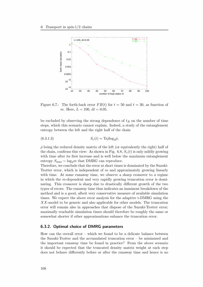
6. Transport in spin-1/2 chains
−610
−510
0.0001
0.001
0.01
0.1
1
10 20 30 40 50 60 70 80 90 100
fort
h−ba
ck d
evia
tion
number of kept states m
L=100, dt=0.05 T=30T=50
Figure 6.7.: The forth-back error FB(t) for t = 50 and t = 30, as function ofm. Here, L = 100, dt = 0.05.
be excluded by observing the strong dependence of tR on the number of timesteps, which this scenario cannot explain. Indeed, a study of the entanglemententropy between the left and the right half of the chain
(6.3.1.3) Se(t) = Trρlog2ρ,
ρ being the reduced density matrix of the left (or equivalently the right) half ofthe chain, confirms this view: As shown in Fig. 6.8, Se(t) is only mildly growingwith time after its first increase and is well below the maximum entanglemententropy Smax ∼ log2m that DMRG can reproduce.
Therefore, we conclude that the error at short times is dominated by the Suzuki-Trotter error, which is independent of m and approximately growing linearlywith time. At some runaway time, we observe a sharp crossover to a regimein which the m-dependent and very rapidly growing truncation error is domi-nating. This crossover is sharp due to drastically different growth of the twotypes of errors. The runaway time thus indicates an imminent breakdown of themethod and is a good, albeit very conservative measure of available simulationtimes. We expect the above error analysis for the adaptive t-DMRG using theXX-model to be generic and also applicable for other models. The truncationerror will remain also in approaches that dispose of the Suzuki-Trotter error;maximally reachable simulation times should therefore be roughly the same orsomewhat shorter if other approximations enhance the truncation error.
6.3.2. Optimal choice of DMRG parameters
How can the overall error – which we found to be a delicate balance betweenthe Suzuki-Trotter and the accumulated truncation error – be minimized andthe important runaway time be found in practice? From the above scenarioit should be expected that the truncated density matrix weight at each stepdoes not behave differently before or after the runaway time and hence is no
108
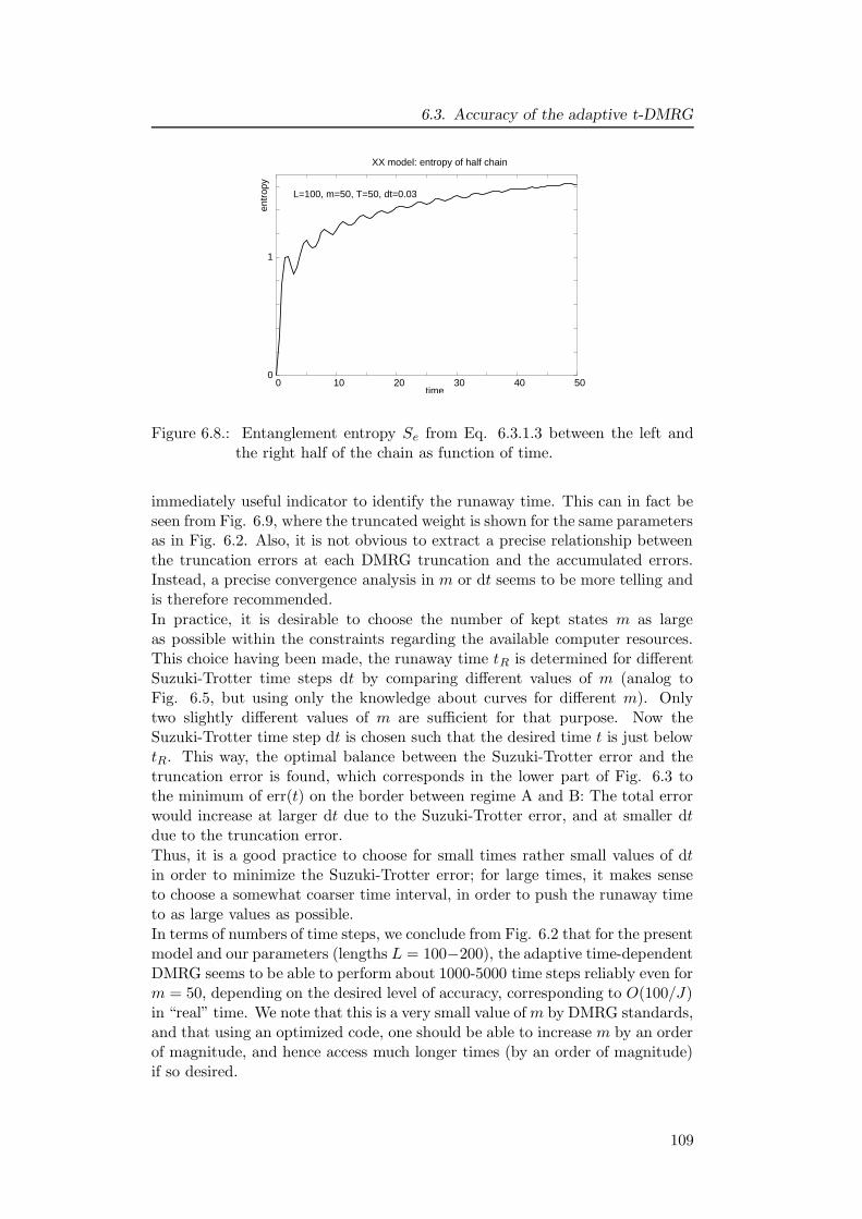
6.3. Accuracy of the adaptive t-DMRG
0
1
0 10 20 30 40 50
entr
opy
time
XX model: entropy of half chain
L=100, m=50, T=50, dt=0.03
Figure 6.8.: Entanglement entropy Se from Eq. 6.3.1.3 between the left andthe right half of the chain as function of time.
immediately useful indicator to identify the runaway time. This can in fact beseen from Fig. 6.9, where the truncated weight is shown for the same parametersas in Fig. 6.2. Also, it is not obvious to extract a precise relationship betweenthe truncation errors at each DMRG truncation and the accumulated errors.Instead, a precise convergence analysis in m or dt seems to be more telling andis therefore recommended.
In practice, it is desirable to choose the number of kept states m as largeas possible within the constraints regarding the available computer resources.This choice having been made, the runaway time tR is determined for differentSuzuki-Trotter time steps dt by comparing different values of m (analog toFig. 6.5, but using only the knowledge about curves for different m). Onlytwo slightly different values of m are sufficient for that purpose. Now theSuzuki-Trotter time step dt is chosen such that the desired time t is just belowtR. This way, the optimal balance between the Suzuki-Trotter error and thetruncation error is found, which corresponds in the lower part of Fig. 6.3 tothe minimum of err(t) on the border between regime A and B: The total errorwould increase at larger dt due to the Suzuki-Trotter error, and at smaller dtdue to the truncation error.
Thus, it is a good practice to choose for small times rather small values of dtin order to minimize the Suzuki-Trotter error; for large times, it makes senseto choose a somewhat coarser time interval, in order to push the runaway timeto as large values as possible.
In terms of numbers of time steps, we conclude from Fig. 6.2 that for the presentmodel and our parameters (lengths L = 100−200), the adaptive time-dependentDMRG seems to be able to perform about 1000-5000 time steps reliably even form = 50, depending on the desired level of accuracy, corresponding to O(100/J)in “real” time. We note that this is a very small value ofm by DMRG standards,and that using an optimized code, one should be able to increase m by an orderof magnitude, and hence access much longer times (by an order of magnitude)if so desired.
109
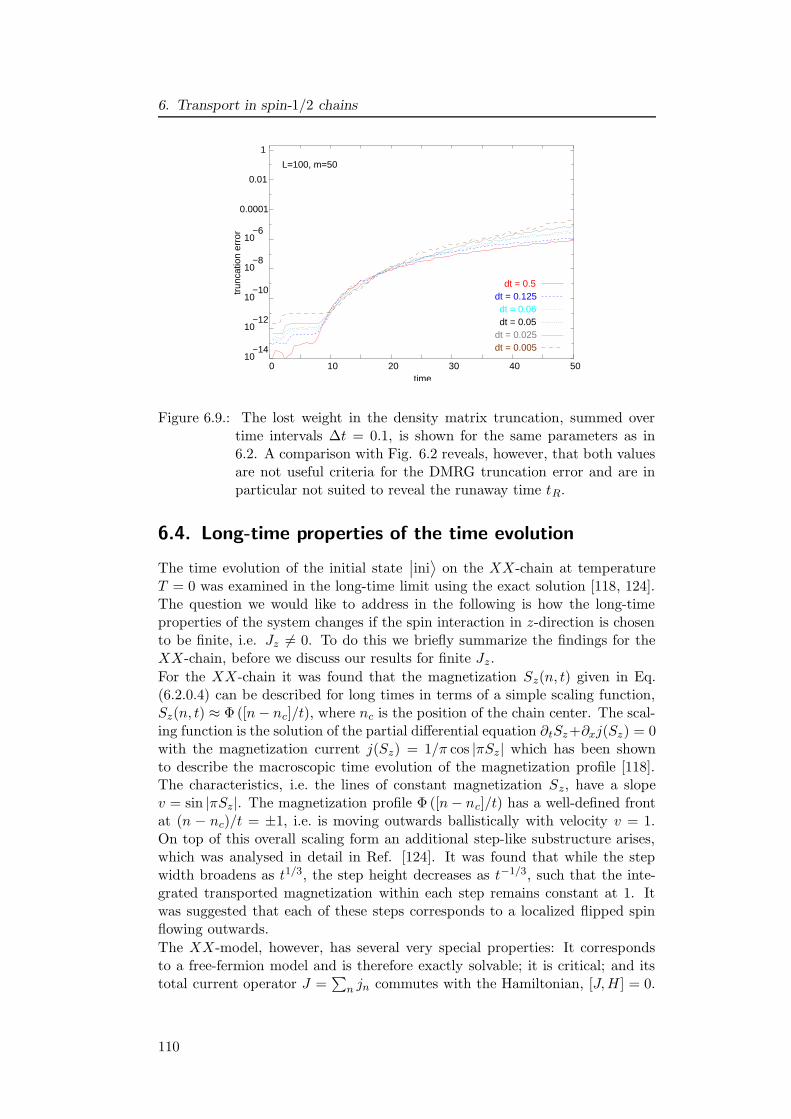
6. Transport in spin-1/2 chains
10−14
10−12
10−10
10−8
10−6
0.0001
0.01
1
0 10 20 30 40 50
trun
catio
n er
ror
time
L=100, m=50
dt = 0.5dt = 0.125dt = 0.06dt = 0.05
dt = 0.025dt = 0.005
Figure 6.9.: The lost weight in the density matrix truncation, summed overtime intervals ∆t = 0.1, is shown for the same parameters as in6.2. A comparison with Fig. 6.2 reveals, however, that both valuesare not useful criteria for the DMRG truncation error and are inparticular not suited to reveal the runaway time tR.
6.4. Long-time properties of the time evolution
The time evolution of the initial state∣∣ini⟩
on the XX-chain at temperatureT = 0 was examined in the long-time limit using the exact solution [118, 124].The question we would like to address in the following is how the long-timeproperties of the system changes if the spin interaction in z-direction is chosento be finite, i.e. Jz 6= 0. To do this we briefly summarize the findings for theXX-chain, before we discuss our results for finite Jz.
For the XX-chain it was found that the magnetization Sz(n, t) given in Eq.(6.2.0.4) can be described for long times in terms of a simple scaling function,Sz(n, t) ≈ Φ([n− nc]/t), where nc is the position of the chain center. The scal-ing function is the solution of the partial differential equation ∂tSz+∂xj(Sz) = 0with the magnetization current j(Sz) = 1/π cos |πSz| which has been shownto describe the macroscopic time evolution of the magnetization profile [118].The characteristics, i.e. the lines of constant magnetization Sz, have a slopev = sin |πSz|. The magnetization profile Φ ([n− nc]/t) has a well-defined frontat (n − nc)/t = ±1, i.e. is moving outwards ballistically with velocity v = 1.On top of this overall scaling form an additional step-like substructure arises,which was analysed in detail in Ref. [124]. It was found that while the stepwidth broadens as t1/3, the step height decreases as t−1/3, such that the inte-grated transported magnetization within each step remains constant at 1. Itwas suggested that each of these steps corresponds to a localized flipped spinflowing outwards.
The XX-model, however, has several very special properties: It correspondsto a free-fermion model and is therefore exactly solvable; it is critical; and itstotal current operator J =
∑
n jn commutes with the Hamiltonian, [J,H] = 0.
110
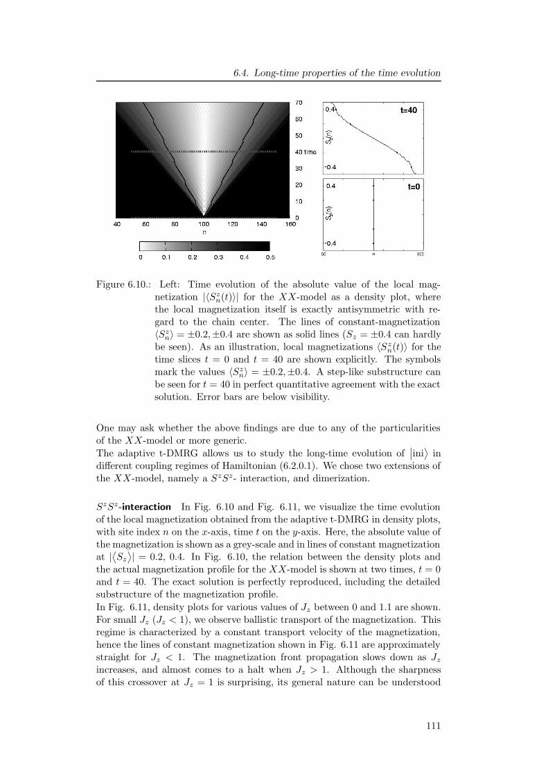
6.4. Long-time properties of the time evolution
Figure 6.10.: Left: Time evolution of the absolute value of the local mag-netization |〈Sz
n(t)〉| for the XX-model as a density plot, wherethe local magnetization itself is exactly antisymmetric with re-gard to the chain center. The lines of constant-magnetization〈Sz
n〉 = ±0.2,±0.4 are shown as solid lines (Sz = ±0.4 can hardlybe seen). As an illustration, local magnetizations 〈Sz
n(t)〉 for thetime slices t = 0 and t = 40 are shown explicitly. The symbolsmark the values 〈Sz
n〉 = ±0.2,±0.4. A step-like substructure canbe seen for t = 40 in perfect quantitative agreement with the exactsolution. Error bars are below visibility.
One may ask whether the above findings are due to any of the particularitiesof the XX-model or more generic.
The adaptive t-DMRG allows us to study the long-time evolution of∣∣ini⟩
indifferent coupling regimes of Hamiltonian (6.2.0.1). We chose two extensions ofthe XX-model, namely a SzSz- interaction, and dimerization.
SzSz-interaction In Fig. 6.10 and Fig. 6.11, we visualize the time evolutionof the local magnetization obtained from the adaptive t-DMRG in density plots,with site index n on the x-axis, time t on the y-axis. Here, the absolute value ofthe magnetization is shown as a grey-scale and in lines of constant magnetizationat |⟨Sz
⟩| = 0.2, 0.4. In Fig. 6.10, the relation between the density plots and
the actual magnetization profile for the XX-model is shown at two times, t = 0and t = 40. The exact solution is perfectly reproduced, including the detailedsubstructure of the magnetization profile.
In Fig. 6.11, density plots for various values of Jz between 0 and 1.1 are shown.For small Jz (Jz < 1), we observe ballistic transport of the magnetization. Thisregime is characterized by a constant transport velocity of the magnetization,hence the lines of constant magnetization shown in Fig. 6.11 are approximatelystraight for Jz < 1. The magnetization front propagation slows down as Jz
increases, and almost comes to a halt when Jz > 1. Although the sharpnessof this crossover at Jz = 1 is surprising, its general nature can be understood
111
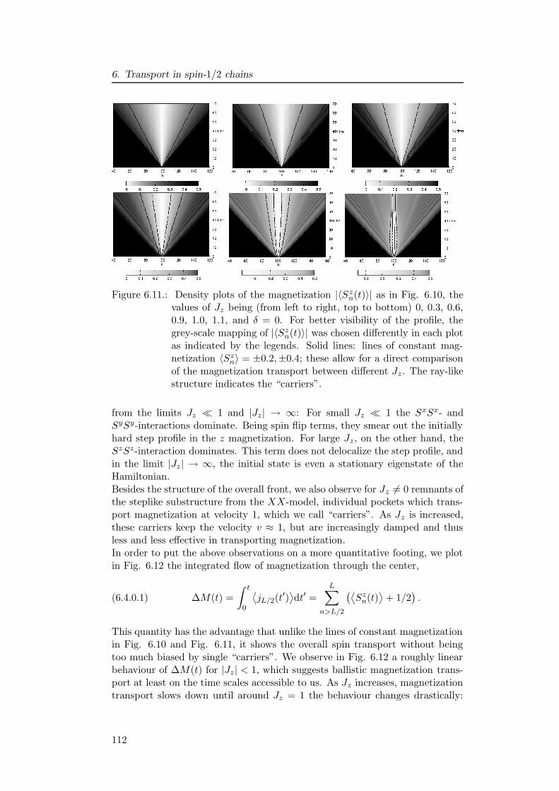
6. Transport in spin-1/2 chains
Figure 6.11.: Density plots of the magnetization |〈Szn(t)〉| as in Fig. 6.10, the
values of Jz being (from left to right, top to bottom) 0, 0.3, 0.6,0.9, 1.0, 1.1, and δ = 0. For better visibility of the profile, thegrey-scale mapping of |〈Sz
n(t)〉| was chosen differently in each plotas indicated by the legends. Solid lines: lines of constant mag-netization 〈Sz
n〉 = ±0.2,±0.4; these allow for a direct comparisonof the magnetization transport between different Jz. The ray-likestructure indicates the “carriers”.
from the limits Jz � 1 and |Jz| → ∞: For small Jz � 1 the SxSx- andSySy-interactions dominate. Being spin flip terms, they smear out the initiallyhard step profile in the z magnetization. For large Jz, on the other hand, theSzSz-interaction dominates. This term does not delocalize the step profile, andin the limit |Jz| → ∞, the initial state is even a stationary eigenstate of theHamiltonian.Besides the structure of the overall front, we also observe for Jz 6= 0 remnants ofthe steplike substructure from the XX-model, individual pockets which trans-port magnetization at velocity 1, which we call “carriers”. As Jz is increased,these carriers keep the velocity v ≈ 1, but are increasingly damped and thusless and less effective in transporting magnetization.In order to put the above observations on a more quantitative footing, we plotin Fig. 6.12 the integrated flow of magnetization through the center,
(6.4.0.1) ∆M(t) =
∫ t
0
⟨jL/2(t
′)⟩dt′ =
L∑
n>L/2
(⟨Sz
n(t)⟩
+ 1/2).
This quantity has the advantage that unlike the lines of constant magnetizationin Fig. 6.10 and Fig. 6.11, it shows the overall spin transport without beingtoo much biased by single “carriers”. We observe in Fig. 6.12 a roughly linearbehaviour of ∆M(t) for |Jz| < 1, which suggests ballistic magnetization trans-port at least on the time scales accessible to us. As Jz increases, magnetizationtransport slows down until around Jz = 1 the behaviour changes drastically:
112
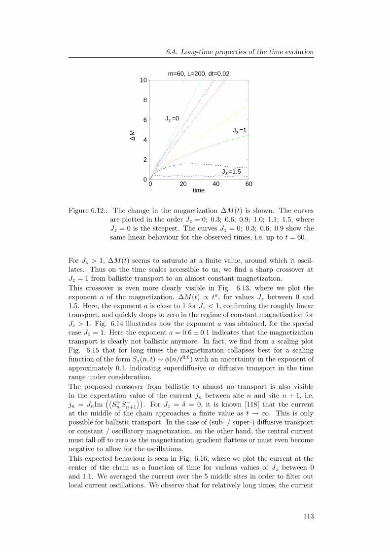
6.4. Long-time properties of the time evolution
J =0 z
J =1 z
0
2
4
6
8
10
0 20 40 60
M
time
m=60, L=200, dt=0.02
∆
J =1.5 z
Figure 6.12.: The change in the magnetization ∆M(t) is shown. The curvesare plotted in the order Jz = 0; 0.3; 0.6; 0.9; 1.0; 1.1; 1.5, whereJz = 0 is the steepest. The curves Jz = 0; 0.3; 0.6; 0.9 show thesame linear behaviour for the observed times, i.e. up to t = 60.
For Jz > 1, ∆M(t) seems to saturate at a finite value, around which it oscil-lates. Thus on the time scales accessible to us, we find a sharp crossover atJz = 1 from ballistic transport to an almost constant magnetization.
This crossover is even more clearly visible in Fig. 6.13, where we plot theexponent a of the magnetization, ∆M(t) ∝ ta, for values Jz between 0 and1.5. Here, the exponent a is close to 1 for Jz < 1, confirming the roughly lineartransport, and quickly drops to zero in the regime of constant magnetization forJz > 1. Fig. 6.14 illustrates how the exponent a was obtained, for the specialcase Jz = 1. Here the exponent a = 0.6 ± 0.1 indicates that the magnetizationtransport is clearly not ballistic anymore. In fact, we find from a scaling plotFig. 6.15 that for long times the magnetization collapses best for a scalingfunction of the form Sz(n, t) ∼ φ(n/t0.6) with an uncertainty in the exponent ofapproximately 0.1, indicating superdiffusive or diffusive transport in the timerange under consideration.
The proposed crossover from ballistic to almost no transport is also visiblein the expectation value of the current jn between site n and site n + 1, i.e.jn = JnIm
(⟨S+
n S−n+1
⟩). For Jz = δ = 0, it is known [118] that the current
at the middle of the chain approaches a finite value as t → ∞. This is onlypossible for ballistic transport. In the case of (sub- / super-) diffusive transportor constant / oscillatory magnetization, on the other hand, the central currentmust fall off to zero as the magnetization gradient flattens or must even becomenegative to allow for the oscillations.
This expected behaviour is seen in Fig. 6.16, where we plot the current at thecenter of the chain as a function of time for various values of Jz between 0and 1.1. We averaged the current over the 5 middle sites in order to filter outlocal current oscillations. We observe that for relatively long times, the current
113
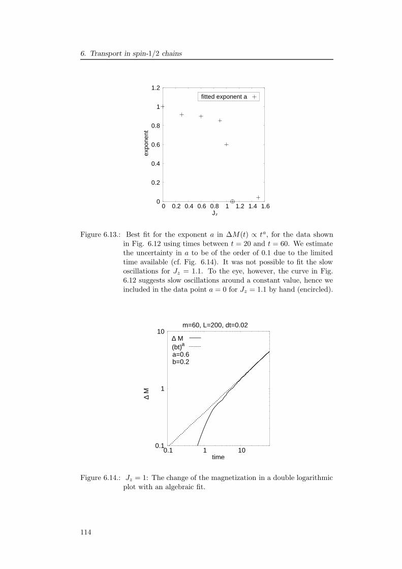
6. Transport in spin-1/2 chains
fitted exponent a
0
0.2
0.4
0.6
0.8
1
1.2
0 0.2 0.4 0.6 0.8 1 1.2 1.4 1.6Jz
expo
nent
Figure 6.13.: Best fit for the exponent a in ∆M(t) ∝ ta, for the data shownin Fig. 6.12 using times between t = 20 and t = 60. We estimatethe uncertainty in a to be of the order of 0.1 due to the limitedtime available (cf. Fig. 6.14). It was not possible to fit the slowoscillations for Jz = 1.1. To the eye, however, the curve in Fig.6.12 suggests slow oscillations around a constant value, hence weincluded in the data point a = 0 for Jz = 1.1 by hand (encircled).
0.1
1
10
0.1 1 10time
M∆
∆ M
a=0.6b=0.2
(bt)a
m=60, L=200, dt=0.02
Figure 6.14.: Jz = 1: The change of the magnetization in a double logarithmicplot with an algebraic fit.
114
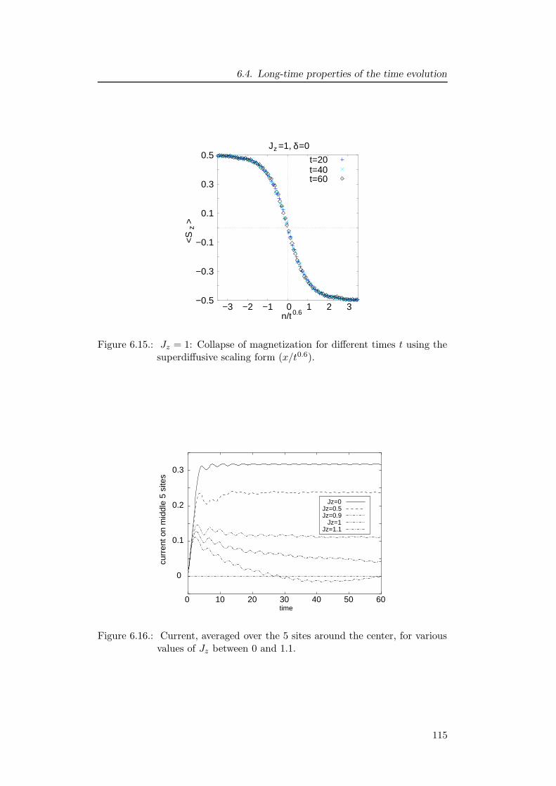
6.4. Long-time properties of the time evolution
−0.5
−0.3
−0.1
0.1
0.3
0.5
−3 −2 −1 0 1 2 3n/t
J =1, =0
0.6
z δt=20
t=60 t=40
<S
>
z
Figure 6.15.: Jz = 1: Collapse of magnetization for different times t using thesuperdiffusive scaling form (x/t0.6).
0
0.1
0.2
0.3
0 10 20 30 40 50 60
curr
ent o
n m
iddl
e 5
site
s
time
Jz=0Jz=0.5Jz=0.9
Jz=1Jz=1.1
Figure 6.16.: Current, averaged over the 5 sites around the center, for variousvalues of Jz between 0 and 1.1.
115
6. Transport in spin-1/2 chains
approaches a constant value for |Jz| < 1, whereas the current falls off rapidlyand then seems to exhibit damped oscillations around zero for |Jz| > 1. Thisstrengthens our previous conclusion of a crossover from ballistic transport to amore or less constant magnetization at |Jz | = 1.
Remarkably, this crossover for the behaviour of a high-energy quantum state∣∣ini⟩
is found at the value Jz = 1 of the quantum phase transition from thecritical phase to the Neel anti-ferromagnetic state (see Fig. 6.1), a priori a low-energy event. To understand the subtle connection between the time evolutionof∣∣ini⟩
and the phase transition, we exploit the fact that the time evolutiondoes not depend on the sign of Jz , as discussed in Sec. 6.2. Therefore thetime evolution of the high-energy state
∣∣ini⟩
for Jz > 1 is identical to thetime evolution for J ′
z = −Jz < −1, where∣∣ini⟩
is a low-energy state. At thequantum phase transition from the ferromagnetic state to the critical phase atJ ′
z = −1 the ground state, a kink state for J ′z < −1 (if we impose the boundary
condition spin up on the left boundary and spin down on the right boundary)[123], changes drastically to a state with no kink and power-law correlations forJ ′
z > −1. Therefore, our initial state is very close to an eigenstate – the groundstate – for J ′
z < −1, but not for J ′z > −1. Thus, the harsh change in the time
evolution of the high-energy state∣∣ini⟩
at Jz = 1 can be explained by the severechange in the ground state properties at J ′
z = −1, and the crossover is linkedto the quantum phase transition at the value J ′
z = −1 in the phase diagram.
Dimerization We now study the influence of a nonzero dimerization δ in theHamiltonian (6.2.0.1.) We restrict our analysis to the case Jz = 0. The dimer-ized models can still be described in terms of the free-fermion picture and areexactly solvable (for static properties see [121]). The current, however, is notconserved for nonzero dimerization and the energy spectrum has a gap. Thisexample will shed light on the question whether the long-time limit depends oncurrent conservation, on the presence of a gap, or on the free-fermion property,or another special properties of the system. As the dimerized case is also ex-actly solvable, the results could have been obtained also analytically, for exam-ple by utilizing the results for the Fourier transformation of the magnetization⟨Sz(q, t)
⟩of Ref. [119]. We expect two obvious effects of nonzero dimerization:
Firstly, the overall front velocity should slow down, because the magnetizationnow propagates faster on half of the links, but slower on the other half, the neteffect being a reduction of the total velocity. Secondly, we expect oscillationswith a period of two lattice sites. This is obvious in the limit δ → 1, where eachstrongly coupled pair of sites can be viewed as an almost isolated subsystem,in which the magnetization oscillates back and forth. We expect remnants ofthis behaviour also at dimerizations |δ| < 1. The data for the magnetizationshown in Fig. 6.17 confirms this expectation qualitatively, but does not revealany other qualitative change of the long-time limit for nonzero dimerization.For δ = 1, the system is trivially given by isolated pairs of neighbouring sites,therefore the propagation velocity drops to zero.
Fig. 6.18 and Fig. 6.19 reveal explicitly that no qualitative change occurs inthe transport behaviour as the dimerization is switched on: the change in mag-
116
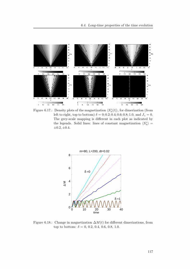
6.4. Long-time properties of the time evolution
Figure 6.17.: Density plots of the magnetization 〈Szn(t)〉, for dimerization (from
left to right, top to bottom) δ = 0; 0.2; 0.4; 0.6; 0.8; 1.0, and Jz = 0.The grey-scale mapping is different in each plot as indicated bythe legends. Solid lines: lines of constant magnetization 〈Sz
n〉 =±0.2,±0.4.
δ =1
δ =0
0
2
4
6
8
0 10 20 30 40time
M∆
m=80, L=200, dt=0.02
Figure 6.18.: Change in magnetization ∆M(t) for different dimerizations, fromtop to bottom: δ = 0, 0.2, 0.4, 0.6, 0.8, 1.0.
117
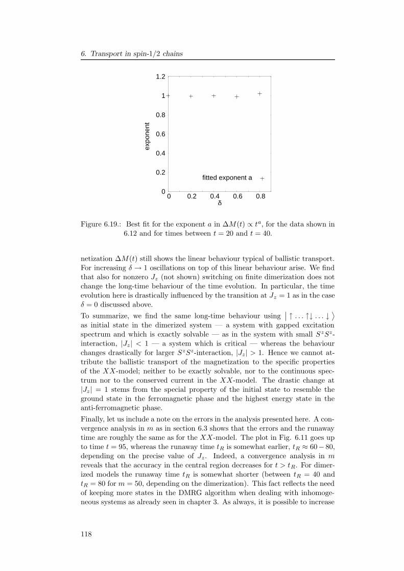
6. Transport in spin-1/2 chains
0
0.2
0.4
0.6
0.8
1
1.2
0 0.2 0.4 0.6 0.8
expo
nent
fitted exponent a
δ
Figure 6.19.: Best fit for the exponent a in ∆M(t) ∝ ta, for the data shown in6.12 and for times between t = 20 and t = 40.
netization ∆M(t) still shows the linear behaviour typical of ballistic transport.For increasing δ → 1 oscillations on top of this linear behaviour arise. We findthat also for nonzero Jz (not shown) switching on finite dimerization does notchange the long-time behaviour of the time evolution. In particular, the timeevolution here is drastically influenced by the transition at Jz = 1 as in the caseδ = 0 discussed above.
To summarize, we find the same long-time behaviour using∣∣ ↑ . . . ↑↓ . . . ↓
⟩
as initial state in the dimerized system — a system with gapped excitationspectrum and which is exactly solvable — as in the system with small S zSz-interaction, |Jz| < 1 — a system which is critical — whereas the behaviourchanges drastically for larger SzSz-interaction, |Jz | > 1. Hence we cannot at-tribute the ballistic transport of the magnetization to the specific propertiesof the XX-model; neither to be exactly solvable, nor to the continuous spec-trum nor to the conserved current in the XX-model. The drastic change at|Jz| = 1 stems from the special property of the initial state to resemble theground state in the ferromagnetic phase and the highest energy state in theanti-ferromagnetic phase.
Finally, let us include a note on the errors in the analysis presented here. A con-vergence analysis in m as in section 6.3 shows that the errors and the runawaytime are roughly the same as for the XX-model. The plot in Fig. 6.11 goes upto time t = 95, whereas the runaway time tR is somewhat earlier, tR ≈ 60− 80,depending on the precise value of Jz. Indeed, a convergence analysis in mreveals that the accuracy in the central region decreases for t > tR. For dimer-ized models the runaway time tR is somewhat shorter (between tR = 40 andtR = 80 for m = 50, depending on the dimerization). This fact reflects the needof keeping more states in the DMRG algorithm when dealing with inhomoge-neous systems as already seen in chapter 3. As always, it is possible to increase
118
6.5. Conclusions
tR by increasing m.
6.5. Conclusions
We modeled two coupled spin-polarized reservoirs by a spin-1/2 system withthe initial state
∣∣ ↑ . . . ↑↓ . . . ↓
⟩and have investigated its time evolution under
the effect of nearest-neighbour interactions with the adaptive t-DMRG.For weak SzSz-interaction, i.e. |Jz| < 1 in Eq. (6.2.0.1), and arbitrary dimeriza-tion, 0 ≤ δ < 1, we find that for long times the transport of the magnetization isballistic as it was found for the XX-model [118]. For stronger SzSz-interaction,i.e. |Jz| > 1, even in a homogeneous system without dimerization δ = 0, thelong-time evolution is completely different. The magnetization transport is nolonger ballistic, but shows oscillatory behaviour around a constant value. Henceour results suggest that the ballistic transport at long times is not an artefactof the XX-model. The drastic change or the long time behaviour at the phasetransition Jz = 1 can be attributed to the close resemblance of the initial stateto the ground state of the ferromagnetic phase (Jz < −1).Our error analysis for the adaptive t-DMRG using the exact solution of theXX-model showed that for small times the error is dominated by the Suzuki-Trottererror whereas for long times the truncation error becomes the most important.We expect this finding to be general and hold for non-exactly solvable modelsas well, and therefore it should allow to control the accuracy of the results ofadaptive t-DMRG in general models. Overall, we find this method to be veryprecise at relatively long times.
119
7. Conclusion and outlook
In this thesis we developed a powerful new computational tool, the adaptivet-DMRG. It is based on the existing finite-system DMRG, modified to incorpo-rate the TEBD algorithm. The new method is applicable to simulate the timeevolution of one-dimensional strongly correlated quantum systems. The idea ofDMRG, to construct a specially chosen reduced space of states to describe thephysics one is interested in, has been extended for time-dependent phenomena.Unlike traditional DMRG, where the reduced state space is fixed, the adaptivet-DMRG adapts the state space at each time step to cover the evolution of thesystem. Even without attempting to reach the computationally most efficientimplementation of the new algorithm, the resulting code seems to perform sys-tematically better than non-adaptive time-dependent DMRG codes, in whicha fixed reduced space is kept for all time steps. The new algorithm allows formuch smaller state spaces, because the state space changes in time and is wellchosen to track the actual state of the system at any given time. The newmethod is also significantly more efficient than other existing embodiments ofthe TEBD due to well-known DMRG techniques, for instance the way DMRGexploits good quantum numbers. Therefore, it can describe the time evolutionof one dimensional quantum systems at very reasonable numerical cost.We tested the applicability, efficiency, and accuracy of the new adaptive t-DMRGalgorithm addressing questions in different physical systems: a bosonic, a fermi-onic, and a spin system. We used the spin system to perform a detailed erroranalysis. Overall we saw that this method gives precise results for relativelylong times. The results of the applications presented in this work can be sum-marized as follows:
Ultracold bosons Motivated by recent progress in producing ultracold atomsin optical lattices, we applied the adaptive t-DMRG to analyze experimentallyrealistic situations. Ultracold bosons in optical lattices can be described bythe Bose-Hubbard model. Due to the presence of a trapping potential in theexperiments, we first had to investigate the influence of such a trapping poten-tial on the static properties of the system. In these systems a superfluid-likeand Mott-insulating-like phase can coexist. We found that in a parabolicallyconfined system the one-particle density-matrix, after a remarkably simple scal-ing, can be used to characterize the occurring phases. This scaled one-particledensity matrix shows for the superfluid-like and Mott-insulating like phasesapproximately the algebraic and exponential behaviour familiar from the one-particle density-matrix in the respective phases in the homogeneous system.We also investigated the applicability of the hydrodynamical approach to suchan inhomogeneous system and found good agreement with the DMRG resultsin the limit of weak interaction. Moreover, we saw that if the experimental
120
system consists of one-dimensional tubes with a small variance in the averagefilling, the half width of the observed interference peak can be used to distin-guish the different types of states that occur experimentally. In the meantimethe experimental results observed in [79] confirmed our theoretical predictions.
Turning to time dependent phenomena, we investigated the motion of densityperturbations, which are the lowest lying excitations of the system. By compar-ison to our numerical results, we showed that in the limit of weak interactionthe motion of relatively broad and small perturbations can be described well bythe hydrodynamical approach or the linearized Gross-Pitaevskii equation. Forintermediate interaction strength, however, the mean-field description breaksdown while the result obtained from the corresponding continuum Lieb-Linigermodel remains valid for somewhat stronger interactions. For very strong inter-actions, we found that the sound velocity is well approximated by a mappingonto a spinless fermionic model. The adaptive t-DMRG also allowed us to de-termine the sound velocity in the crossover region between these two regimes,which could not be done before. In addition, we found a linear dependence ofthe velocity on the height of the perturbation amplitude. This dependence givesrise to effects such as self steepening and shock wave formation. We have fur-ther shown that a density wave may be detected experimentally as an additionalpeak in the interference pattern.
Ultracold fermions: spin-charge separation One key feature of the physics ofone-dimensional quantum systems is the phenomenon of spin-charge separation.At low energy the excitations of charge and spin are predicted to decouple inone dimensional systems and propagate with different velocities. To study thisphenomenon we have performed numerical simulations of the time-evolutionof charge and spin density perturbations using the 1D Hubbard model. Toour knowledge these are the first real-time calculations showing spin-chargeseparation explicitly in systems of experimentally accessible sizes. We clearlyobserve the separation of spin and charge as a generic feature of 1D fermions,far beyond the low-energy regime where a Luttinger liquid description applies.Based on these results, we propose an experimental setup which should allowthe observation of this phenomenon in cold gases by exploiting the differentpropagation behaviour of spin and charge density perturbations in the liquidand Mott-insulating state. This proposal avoids the problems arising fromthe different densities in an experimental array of parallel atomic wires. Weperformed quantitative calculations of the experimental requirements whichseem to be within reach today. The different propagation behaviour can alsobe used to distinguish experimentally between a Mott- and a band insulator.
Spin-1/2 chain We have investigated a simple model for the spin transportbetween two spin polarized reservoirs a configuration of considerable interestin spintronics. To do this we have studied the evolution of the initial state∣∣ ↑ . . . ↑↓ . . . ↓
⟩under the effect of nearest-neighbour interactions using the
adaptive t-DMRG. For weak SzSz-interaction and arbitrary dimerization, wefind that for long times the transport of the magnetization is ballistic, similar
121
7. Conclusion and outlook
to the case of the XX-model (no SzSz-interaction) [118]. This finding suggeststhat the ballistic transport for long times is not an artefact of the XX-model.For stronger SzSz-interaction, even in a homogeneous system a completely dif-ferent result is obtained by the adaptive t-DMRG in the long-time evolution.The magnetization transport is no longer ballistic, but shows oscillatory be-haviour around some constant value. We found that the change in the longtime behaviour takes place abruptly at the phase transition between the (anti-)ferromagnetic phase and the critical phase. This drastic change can be at-tributed to the close resemblance of the initial state to the ground state of theferromagnetic phase.
Error analysis Using the exact solution for the XX-model we performed adetailed error analysis for the adaptive t-DMRG. We find that the error intro-duced in the adaptive t-DMRG decomposes into the Suzuki-Trotter error andthe truncation error, and can be controlled well by the size of the Suzuki-Trottertime-step and the number of states kept. Our error analysis using typical val-ues for the Suzuki-Trotter time and the number of states further shows thatfor small times the error is dominated by the Suzuki-Trotter error whereas forlong times the truncation error becomes the most important. We expect thisfinding to be general and to hold also for other models not exactly solvable.
Outlook In this thesis we showed the successful application of the adaptivet-DMRG to calculate the time-evolution of quantum states which are initiallyfar from equilibrium focusing on equal time correlation functions. The general-ization of the method to problems with explicitly time-dependent Hamiltoniansand to correlations functions at different times [7] is straightforward. Thus theadvantages of the adaptive t-DMRG can be exploited for a wide range of non-equilibrium phenomena and dynamical quantities like the dynamical structurefactor can be calculated. This might in many cases be a more efficient waythan for example using the ’dynamic DMRG’ (see reference [4] and referencestherein).So far we considered systems at zero-temperature, since in most situationsmentioned here low enough temperatures can be reached in experiments. Ageneralization to the simulation of mixed states [125, 126, 127] is possible atthe cost of introducing an auxiliary space. The method then becomes applica-ble to a large field of dissipative systems and non-dissipative systems at zeroand finite temperature. Presently very little is known about the detailed per-formance of such generalizations, but early signs look promising. As shownby the applications in this thesis the adaptive t-DMRG can address a numberof problems which could not be treated previously. We are confident that bysome generalizations the method can be taken beyond the field of applicationsstudied so far. Indeed it shows potential to address many interesting questionsand problems in the areas of condensed matter and quantum optics systems,providing for mutual benefit and cross-fertilization to both area.
122
A. Higher order Suzuki-Trotter
decompositions
To implement an nth-order Suzuki-Trotter decomposition into the adaptivet-DMRG algorithm is very easy and at hardly any algorithmic cost. A secondorder Suzuki-Trotter decomposition reads for example [41]
(A.0.0.1) e−iHdt = e−iHodddt/2e−iHevendte−iHodddt/2 +O((dt)3
),
where all local Hamiltonians on odd and even bonds have been grouped intoHodd and Heven, respectively. At first sight this seems to indicate that at eachSuzuki-Trotter time step three (instead of two) moves (“sweeps”) through thechain have to be carried out. However, in many applications at the end ofmost time steps, the Hamiltonian does not change, such that for almost all
time steps, we can contract the second e−iHodddt/2 from the previous and the
first e−iHodddt/2 from the current time step to a standard e−iHodddt time step.Hence, we incur almost no algorithmic cost. This is also standard practice inQuantum Monte Carlo [128]; following Quantum Monte Carlo, second orderSuzuki-Trotter evolution is set up as follows:
1. Start with a half-time step e−iHodddt/2.
2. Carry out successive time steps e−iHevendt and e−iHodddt.
3. At measuring times, measure expectation values before a e−iHodddt time
step, and again before a time step e−iHevendt, and form the average of thetwo values as the outcome of the measurement.
4. At times when the Hamiltonian changes, do not contract two half-timesteps into one time step.
In this way, additional algorithmic cost is only incurred at the (in many appli-cations rare) times when the Hamiltonian changes while strongly reducing theSuzuki-Trotter decomposition error.Even more precise is the fourth order Suzuki-Trotter decomposition [129, 130](we skip the third order here since this is as costly as the fourth order):
e−iHdt ≈3∏
j=1
e−iajHodddte−ibjHevendt1∏
j=3
e−iajHodddte−ibjHevendt(A.0.0.2)
with a1 = 14−√
19108 , a2 = 20−7
√19
108 , a3 = (1− 2a1 − 2a2)/2, b1 = 2/5, b2 = −1/10,and b3 = (1 − 2b1 − 2b2)/2. Therefore, eleven sweeps have to be performed
123
A. Higher order Suzuki-Trotter decompositions
per Suzuki-Trotter time step, but since accuracy grows with the fourth powerand not only quadratically as for the second order decomposition, the numberof time steps, which have to be performed to reach the demanded accuracy,decreases considerably.
124
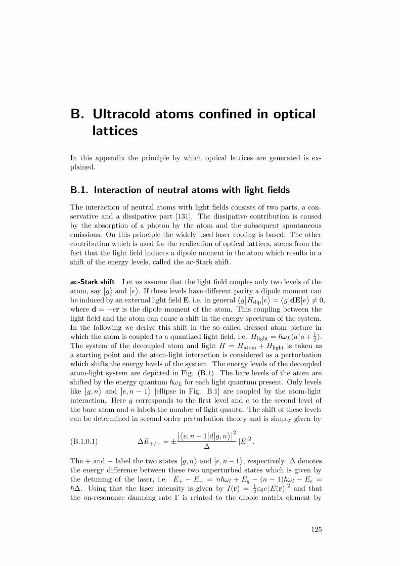
B. Ultracold atoms confined in optical
lattices
In this appendix the principle by which optical lattices are generated is ex-plained.
B.1. Interaction of neutral atoms with light fields
The interaction of neutral atoms with light fields consists of two parts, a con-servative and a dissipative part [131]. The dissipative contribution is causedby the absorption of a photon by the atom and the subsequent spontaneousemissions. On this principle the widely used laser cooling is based. The othercontribution which is used for the realization of optical lattices, stems from thefact that the light field induces a dipole moment in the atom which results in ashift of the energy levels, called the ac-Stark shift.
ac-Stark shift Let us assume that the light field couples only two levels of theatom, say
∣∣g⟩
and∣∣e⟩. If these levels have different parity a dipole moment can
be induced by an external light field E, i.e. in general⟨g∣∣Hdip
∣∣e⟩
=⟨g∣∣dE
∣∣e⟩6= 0,
where d = −er is the dipole moment of the atom. This coupling between thelight field and the atom can cause a shift in the energy spectrum of the system.In the following we derive this shift in the so called dressed atom picture inwhich the atom is coupled to a quantized light field, i.e. Hlight = ~ωL(a†a+ 1
2).The system of the decoupled atom and light H = Hatom + Hlight is taken asa starting point and the atom-light interaction is considered as a perturbationwhich shifts the energy levels of the system. The energy levels of the decoupledatom-light system are depicted in Fig. (B.1). The bare levels of the atom areshifted by the energy quantum ~ωL for each light quantum present. Only levelslike
∣∣g, n
⟩and
∣∣e, n − 1
⟩[ellipse in Fig. B.1] are coupled by the atom-light
interaction. Here g corresponds to the first level and e to the second level ofthe bare atom and n labels the number of light quanta. The shift of these levelscan be determined in second order perturbation theory and is simply given by
(B.1.0.1) ∆E+/− = ±∣∣⟨e, n− 1
∣∣d∣∣g, n
⟩∣∣2
∆|E|2 .
The + and − label the two states∣∣g, n
⟩and
∣∣e, n− 1
⟩, respectively. ∆ denotes
the energy difference between these two unperturbed states which is given bythe detuning of the laser, i.e. E+ − E− = n~ωl + Eg − (n − 1)~ωl − Ee =~∆. Using that the laser intensity is given by I(r) = 1
2ε0c |E(r)|2 and thatthe on-resonance damping rate Γ is related to the dipole matrix element by
125
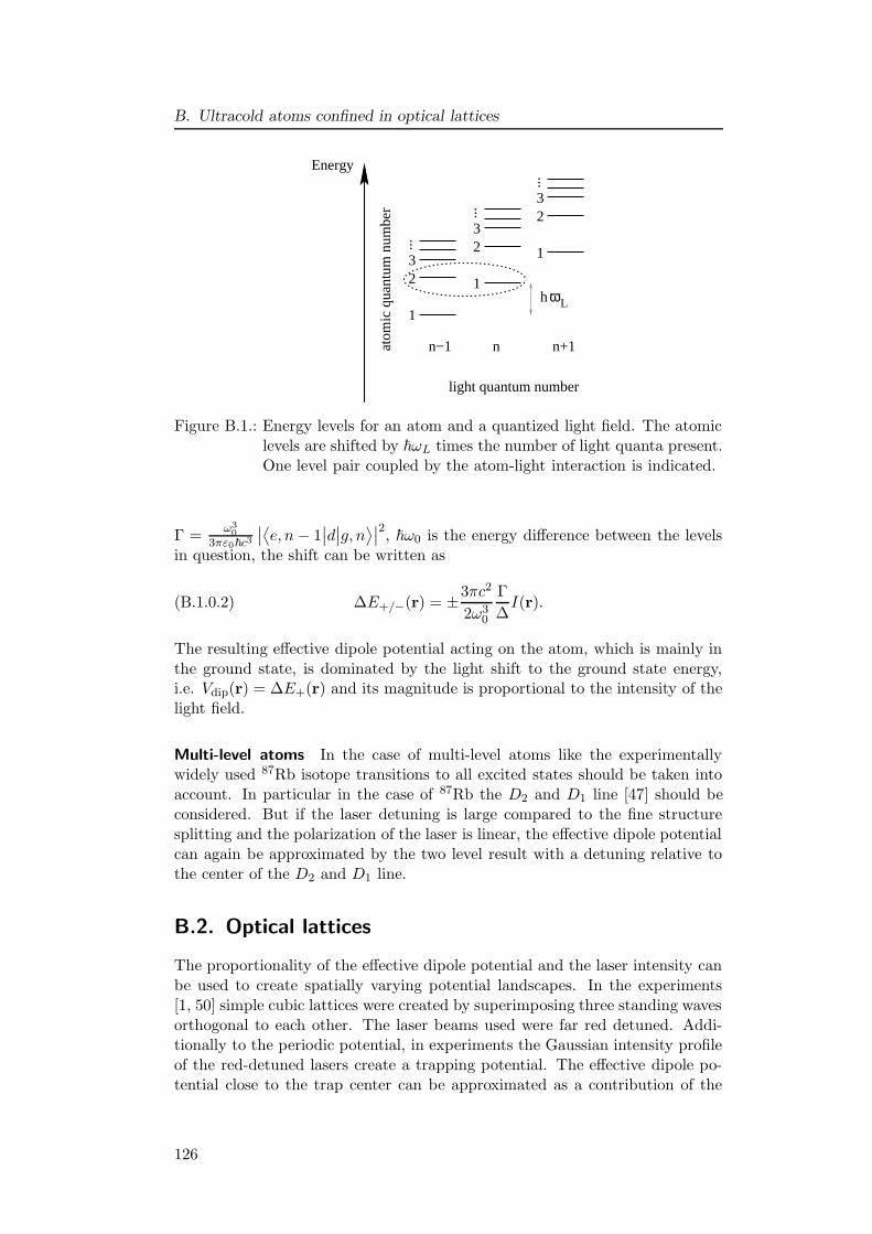
B. Ultracold atoms confined in optical lattices
2
1
3
... 2
1
3
... 2
1
3
...n−1 n
light quantum numberat
omic
qua
ntum
num
ber
n+1
h ωL
Energy
Figure B.1.: Energy levels for an atom and a quantized light field. The atomiclevels are shifted by ~ωL times the number of light quanta present.One level pair coupled by the atom-light interaction is indicated.
Γ =ω3
03πε0~c3
∣∣⟨e, n− 1
∣∣d∣∣g, n
⟩∣∣2, ~ω0 is the energy difference between the levels
in question, the shift can be written as
(B.1.0.2) ∆E+/−(r) = ±3πc2
2ω30
Γ
∆I(r).
The resulting effective dipole potential acting on the atom, which is mainly inthe ground state, is dominated by the light shift to the ground state energy,i.e. Vdip(r) = ∆E+(r) and its magnitude is proportional to the intensity of thelight field.
Multi-level atoms In the case of multi-level atoms like the experimentallywidely used 87Rb isotope transitions to all excited states should be taken intoaccount. In particular in the case of 87Rb the D2 and D1 line [47] should beconsidered. But if the laser detuning is large compared to the fine structuresplitting and the polarization of the laser is linear, the effective dipole potentialcan again be approximated by the two level result with a detuning relative tothe center of the D2 and D1 line.
B.2. Optical lattices
The proportionality of the effective dipole potential and the laser intensity canbe used to create spatially varying potential landscapes. In the experiments[1, 50] simple cubic lattices were created by superimposing three standing wavesorthogonal to each other. The laser beams used were far red detuned. Addi-tionally to the periodic potential, in experiments the Gaussian intensity profileof the red-detuned lasers create a trapping potential. The effective dipole po-tential close to the trap center can be approximated as a contribution of the
126
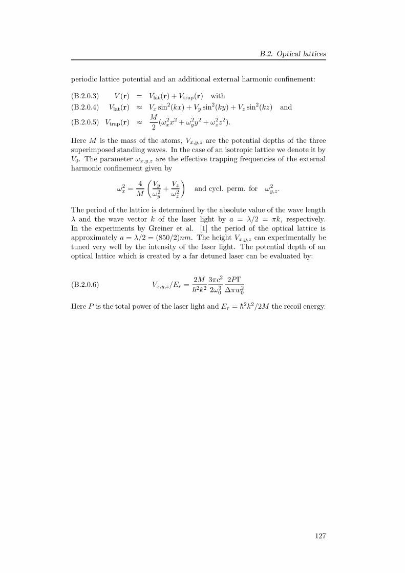
B.2. Optical lattices
periodic lattice potential and an additional external harmonic confinement:
V (r) = Vlat(r) + Vtrap(r) with(B.2.0.3)
Vlat(r) ≈ Vx sin2(kx) + Vy sin2(ky) + Vz sin2(kz) and(B.2.0.4)
Vtrap(r) ≈ M
2(ω2
xx2 + ω2
yy2 + ω2
zz2).(B.2.0.5)
Here M is the mass of the atoms, Vx,y,z are the potential depths of the threesuperimposed standing waves. In the case of an isotropic lattice we denote it byV0. The parameter ωx,y,z are the effective trapping frequencies of the externalharmonic confinement given by
ω2x =
4
M
(Vy
ω2y
+Vz
ω2z
)
and cycl. perm. for ω2y,z.
The period of the lattice is determined by the absolute value of the wave lengthλ and the wave vector k of the laser light by a = λ/2 = πk, respectively.In the experiments by Greiner et al. [1] the period of the optical lattice isapproximately a = λ/2 = (850/2)nm. The height Vx,y,z can experimentally betuned very well by the intensity of the laser light. The potential depth of anoptical lattice which is created by a far detuned laser can be evaluated by:
(B.2.0.6) Vx,y,z/Er =2M
~2k2
3πc2
2ω30
2PΓ
∆πw20
Here P is the total power of the laser light and Er = ~2k2/2M the recoil energy.
127

B. Ultracold atoms confined in optical lattices
B.3. Theoretical description of bosons in optical lattices
In this appendix the description of the ultracold bosons in an optical lattice bya lattice model, the Bose-Hubbard model is derived.
B.3.1. Influence of periodic structures
In the case of a periodic potential an energy band structure emerges. One wayto determine this energy bands is to use Bloch’s theorem which states that the
eigenstates of the Hamiltonian Hperiodic = p2
2m + Vlat(x) can be written as a
product of a plane wave and a function with the lattice periodicity, φ(n)q (x) =
eiqxu(n)q (x), where q = 2π
Laj with j = −L/2, . . . , 0, . . . , L/2 − 1 (L is the evennumber of the sites in the lattice) is called the quasi-momentum and is chosento lie in the first Brillouin zone. The quantum number n counts the energy
bands. The functions u(n)q (x) are periodic functions with lattice period a and
obey the equation
(B.3.1.1)
(1
2m(p+ ~q)2 + Vlat(x)
)
u(n)q (x) = E(n)
q u(n)q (x).
The energy bands are now obtained solving these equations in the Fourier space.Examples for different energy structures are shown in Fig. B.2 for differentheights of the lattice potential. If the lattice depth vanishes (Fig. B.2 (a)), theenergy ‘bands’ correspond to the parabolic energy of free particles, if the latticebecomes deeper (Fig. B.2 (b)) band gaps open. For deep lattices the lowestband becomes flat and the width of the first band gap corresponds to the levelspacing ~ω one would get assuming a harmonic potential V ≈ M
2 ω2(x−xj)
2 at
each lattice site. In contrast to the completely delocalized Bloch functions φ(n)q
a set of wave functions which are maximally localized at the lattice sites xj canbe defined by
(B.3.1.2) wn(x− xj) =1√Z
∑
q
eiqxjφ(n)q (x).
Here Z is the normalization. These functions are called Wannier functions.Generally, the Wannier functions show the behaviour one expects for particlesin the lattice in the sense that they become stronger localized as the latticepotential becomes deeper. Therefore, they offer an ideal tool for the discussionof phenomena in which the spatial localization in the periodic potential playsan important role.
B.3.2. Bose-Hubbard model
If the motion of the atoms is confined to the lowest energy band, it is favorableto work in the basis of Wannier functions w0 of the lowest band neglectinghigher bands. The bosonic field operators can be expanded in this basis:
(B.3.2.1) Ψ(x) =∑
j
w0(x− xj)bj ,
128
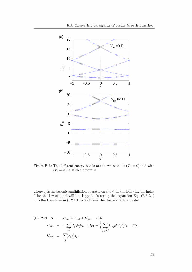
B.3. Theoretical description of bosons in optical lattices
−1 −0.5 0 0.5 1q
0
5
10
15
20
Eq
V =0 E r lat
(a)
−10
−5
0
5
10
15
20
−1 −0.5 0 0.5 1q
E
V =20 E lat r
q
(b)
Figure B.2.: The different energy bands are shown without (V0 = 0) and with(V0 = 20) a lattice potential.
where bj is the bosonic annihilation operator on site j. In the following the index0 for the lowest band will be skipped. Inserting the expansion Eq. (B.3.2.1)into the Hamiltonian (3.2.0.1) one obtains the discrete lattice model:
H = Hkin +Hint +Hpot with(B.3.2.2)
Hkin = −∑
j,j
Jj,jb†jbj , Hint =
1
2
∑
j,j,l,l
Ujjllb†jbjb
†lbl , and
Hpot =∑
j
εjb†jbj .
129
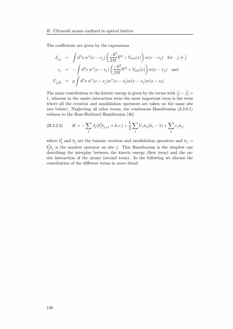
B. Ultracold atoms confined in optical lattices
The coefficients are given by the expressions
Jj,j =
∫
d3x w∗(x− xj)
(−~2
2M∇2 + Vext(x)
)
w(x− xj) for j 6= j
εj = −∫
d3x w∗(x− xj)
(−~2
2M∇2 + Vext(x)
)
w(x− xj) and
Ujjll = g
∫
d3x w∗(x− xj)w∗(x− xl)w(x − xj)w(x− xl)
The main contribution to the kinetic energy is given by the terms with∣∣j − j
∣∣ =
1, whereas in the onsite interaction term the most important term is the termwhere all the creation and annihilation operators are taken on the same site(see below). Neglecting all other terms, the continuous Hamiltonian (3.2.0.1)reduces to the Bose-Hubbard Hamiltonian [46]:
(B.3.2.3) H = −∑
j
Jj(b†jbj+1 + h.c.) +
1
2
∑
j
Ujnj(nj − 1) +∑
j
εjnj,
where b†j and bj are the bosonic creation and annihilation operators and nj =
b†jbj is the number operator on site j. This Hamiltonian is the simplest onedescribing the interplay between the kinetic energy (first term) and the on-site interaction of the atoms (second term). In the following we discuss thecontribution of the different terms in more detail.
130
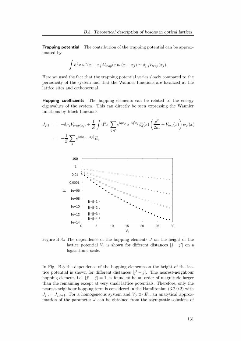
B.3. Theoretical description of bosons in optical lattices
Trapping potential The contribution of the trapping potential can be approx-imated by
∫
d3x w∗(x− xj)Vtrap(x)w(x − xj) ' δj,jVtrap(xj).
Here we used the fact that the trapping potential varies slowly compared to theperiodicity of the system and that the Wannier functions are localized at thelattice sites and orthonormal.
Hopping coefficients The hopping elements can be related to the energyeigenvalues of the system. This can directly be seen expressing the Wannierfunctions by Bloch functions
Jj′j = −δj′jVtrap(xj) +1
Z
∫
d3x∑
q,q′
eiqxj′ e−iq′xjφ∗q(x)
(p2
2m+ Vext(x)
)
φq′(x)
= − 1
Z
∑
q
eiq(xj′−xj)Eq
1e−14
1e−12
1e−10
1e−08
1e−06
0.0001
0.01
1
100
0 5 10 15 20 25 30
|J|
V0
|j’−j|=1
|j’−j|=2
|j’−j|=3
|j’−j|=4
Figure B.3.: The dependence of the hopping elements J on the height of thelattice potential V0 is shown for different distances |j − j ′| on alogarithmic scale.
In Fig. B.3 the dependence of the hopping elements on the height of the lat-tice potential is shown for different distances |j ′ − j|. The nearest-neighbourhopping element, i.e. |j ′ − j| = 1, is found to be an order of magnitude largerthan the remaining except at very small lattice potentials. Therefore, only thenearest-neighbour hopping term is considered in the Hamiltonian (3.2.0.2) withJj := Jj,j+1. For a homogeneous system and V0 � Er, an analytical approx-imation of the parameter J can be obtained from the asymptotic solutions of
131
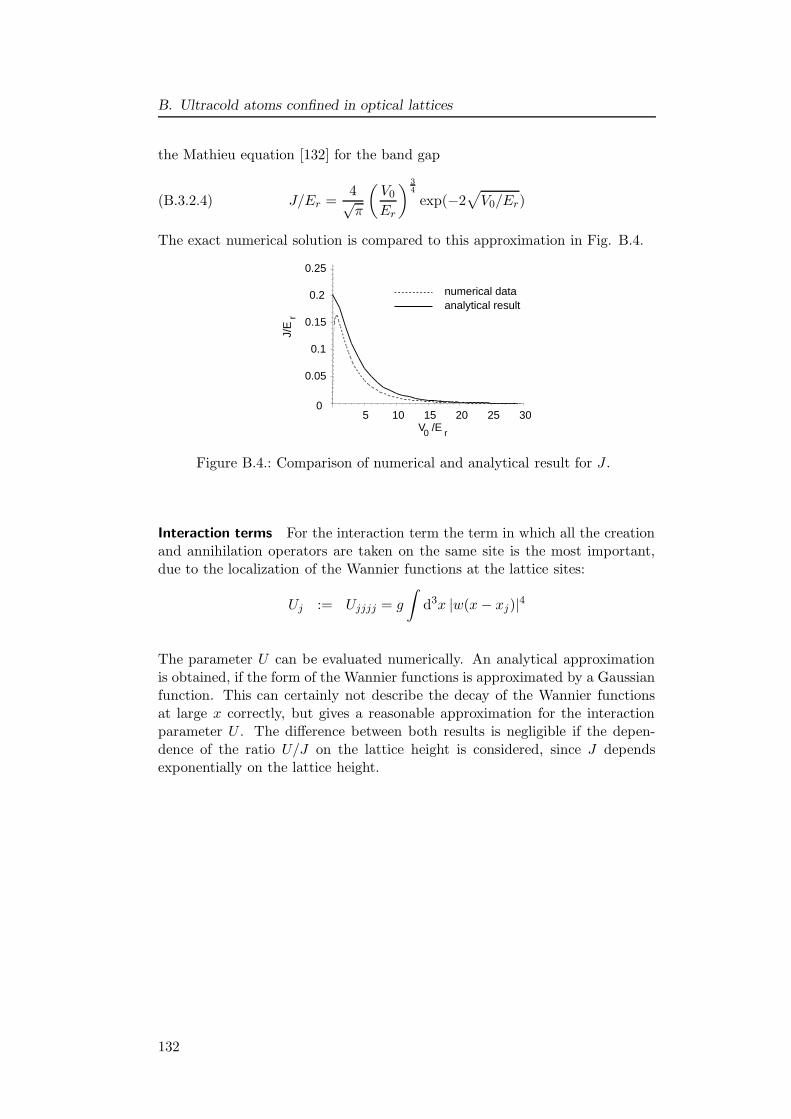
B. Ultracold atoms confined in optical lattices
the Mathieu equation [132] for the band gap
(B.3.2.4) J/Er =4√π
(V0
Er
) 34
exp(−2√
V0/Er)
The exact numerical solution is compared to this approximation in Fig. B.4.
numerical dataanalytical result
0
0.05
0.1
0.15
0.2
0.25
J/E
5
0 r
r
10 15 20 25 30V /E
Figure B.4.: Comparison of numerical and analytical result for J .
Interaction terms For the interaction term the term in which all the creationand annihilation operators are taken on the same site is the most important,due to the localization of the Wannier functions at the lattice sites:
Uj := Ujjjj = g
∫
d3x |w(x− xj)|4
The parameter U can be evaluated numerically. An analytical approximationis obtained, if the form of the Wannier functions is approximated by a Gaussianfunction. This can certainly not describe the decay of the Wannier functionsat large x correctly, but gives a reasonable approximation for the interactionparameter U . The difference between both results is negligible if the depen-dence of the ratio U/J on the lattice height is considered, since J dependsexponentially on the lattice height.
132
Bibliography
[1] M. Greiner, O. Mandel, T. Esslinger, T. Hansch, and I. Bloch. Quantumphase transition from a superfluid to a Mott insulator in a gas of ultracoldatoms. Nature, 415:39–44, 2002.
[2] S. R. White. Density matrix formulation for quantum renormalizationgroups. Phys. Rev. Lett., 69:2863, 1992.
[3] I. Peschel, X. Wang, M. Kaulke, and K. Hallberg, editors. Density-matrixRenormalization. Springer, 1998.
[4] U. Schollwock. The density-matrix renormalization-group.cond-mat/0409292, Rev. Mod. Phys. (in press), 2005.
[5] G. Vidal. Efficient simulation of one-dimensional quantum many-bodysystems. Phys. Rev. Lett., 93:040502, 2004.
[6] A. J. Daley, C. Kollath, U. Schollwock, and G. Vidal. Time-dependentdensity-matrix renormalization-group using adaptive effective Hilbertspaces. J. Stat. Mech.: Theor. Exp. , P04005, 2004.
[7] S. R. White and A. E. Feiguin. Real time evolution using the densitymatrix renormalization group. Phys. Rev. Lett., 93:076401, 2004.
[8] M. H. Anderson, J. R. Ensher, M. R. Matthews, C. E. Wieman, andE. A. Cornell. Observation of Bose-Einstein condensation in a diluteatomic vapor. Science, 269(0):198, 1995.
[9] K. B. Davis, M.-O. Mewes, M. A. Joffe, M. R. Andrews, and W. Ketterle.Evaporative cooling of sodium atoms. Phys. Rev. Lett., 74:5202, 1995.
[10] C. C. Bradley, C. A. Sackett, J. J. Tollett, and R. G. Hulet. Evidence ofBose-Einstein condensation in an atomic gas with attractive interactions.Phys. Rev. Lett., 75:1687, 1995.
[11] C. J. Pethick and H. Smith. Bose-Einstein Condensation in Dilute Gases.Cambridge University Press, 2002.
[12] L. P. Pitaevskii and S. Stringari. Bose-Einstein Condensation. OxfordUniversity Press, 2003.
[13] S. L. Cornish, N. R. Claussen, J. L. Roberts, E. A. Cornell, and C. E.Wieman. Stable 85Rb Bose-Einstein condensates with widely tunableinteractions. Phys. Rev. Lett., 85(9):1795, 2000.
133
Bibliography
[14] E. A. Donley, N. R. Claussen, S. L. Cornish, J. L. Roberts, E. A. Cornell,and C. E. Wieman. Dynamics of collapsing and expolding Bose-Einsteincondensates. Nature, 412:295, 2001.
[15] C. Orzel, A. K. Tuchman, M. L. Fenselau, M. Yasuda, and M. A. Kase-vich. Squeezed states in a Bose-Einstein condensate. Science, 291:2386,2001.
[16] S. R. White. Density-matrix algorithms for quantum renormalizationgroups. Phys. Rev. B, 48:10345, 1993.
[17] M. A. Cazalilla and J. B. Marston. Time-dependent density-matrixrenormalization-group: A systematic method for the study of quantummany-body systems out-of-equilibrium. Phys. Rev. Lett., 88:256403,2002.
[18] G. Vidal. Efficient classical simulation of slightly entangled quantumcomputations. Phys. Rev. Lett., 91:147902, 2003.
[19] A. Klumper, A. Schadschneider, and J. Zittartz. Matrix-product groundstates for one-dimensional spin-1 quantum antiferromagnets. Euro-phys. Lett., 24:293, 1993.
[20] M. Fannes, B. Nachtergaele, and R. F. Werner. Finitely correlated stateson quantum spin chains. Comm. Math. Phys., 144:3, 1992.
[21] S. R. White. Spin gaps in a frustrated Heisenberg model for CaV4O9.Phys. Rev. Lett., 77:3633, 1996.
[22] A. Kemper. Transfermatrix-DMRG for dynamics of stochastic models andthermodynamics of fermionic models. PhD thesis, Universitat zu Koln,2003.
[23] M. A. Nielsen and I. L. Chuang. Quantum computation and quantumcommunication. Cambridge University Press, 2000.
[24] T. J. Osborne and M. A. Nielsen. Entanglement, quantum phase tran-sitions, and density matrix renormalization. Quant. Inf. Proc., 1:45,2002.
[25] C. M. Dawson and M. A. Nielsen. Frustration, interaction strength andground-state entanglement in complex quantum systems. Phys. Rev. A,69:052316, 2004.
[26] H. L. Haselgrove, M. A. Nielsen, and Osborne. Entanglement, correla-tions, and the energy gap in many-body quantum systems. Phys. Rev. A,69:032303, 2004.
[27] G. Vidal, J. I. Latorre, E. Rico, and A. Kitaev. Entanglement in quantumcritical phenomena. Phys. Rev. Lett., 90:227902, 2003.
134
Bibliography
[28] J. Gaite. Entanglement entropy and the density matrix renormalizationgroup. quant-ph/0301120, 2003.
[29] J. I. Latorre, E. Rico, and G. Vidal. Ground state entanglement in quan-tum spin chains. Quant. Inf. and Comp., 4(1):048, 2003.
[30] C. H. Bennett and D. P. DiVincenzo. Quantum information and compu-tation. Nature, 404:247, 2000.
[31] C. Lanczos. An iteration method for the solution of theeigenvalue problem of linear differential and integral operators.J. Res. Natl. Bur. Stand., 45:225, 1950.
[32] E. R. Davidson. The iterative calculation of a few of the lowest eigen-values and corresponding eigenvectors of large real-symmetric matrices.J. Comput. Phys., 17:87, 1975.
[33] W. H. Press et al., editor. Numerical Recipes in C: The Art of ScientificComputing. Cambridge University Press, 1992.
[34] H. G. Luo, T. Xiang, and X. Q. Wang. Comment on ”time-dependentdensity-matrix renormalization group: A systematic method for the studyof quantum many-body out-of-equilibrium systems. Phys. Rev. Lett.,91:049701, 2003.
[35] M. A. Cazalilla and J. B. Marston. Response to ”comment on ”time-dependent density-matrix renormalization-group: A systematic methodfor the study of quantum many-body systems out-of-equilibrium””.Phys. Rev. Lett., 91:049702, 2003.
[36] S. Ostlund and S. Rommer. Thermodynamic limit of density matrixrenormalization. Phys. Rev. Lett., 75:3537, 1995.
[37] J. Dukelsky, M. A. Martin-Delgado, T. Nishino, and G. Sierra. Equiv-alence of the variational matrix product method and the density matrixrenormalization group. Europhys. Lett., 43:457, 1998.
[38] I. Affleck, T. Kennedy, E. H. Lieb, and H. Tasaki. Rigorous results onvalence-bond ground states in antiferromagnets. Phys. Rev. Lett., 59:799,1987.
[39] I. Affleck, T. Kennedy, E. H. Lieb, and H. Tasaki. Valence bond groundstates in isotropic quantum antiferromagnets. Comm. Math. Phys.,115:477, 1988.
[40] M. Fannes, B. Nachtergaele, and R. F. Werner. Exact antiferromagneticground states for quantum chains. Europhys. Lett., 10:643, 1989.
[41] M. Suzuki. Relationship between d-dimensional quantal spin systems and(d+1)-dimensional Ising systems — equivalence, critical exponents andsystematic approximants of the partition function and spin correlations—. Prog. Theor. Phys., 56:1454, 1976.
135
Bibliography
[42] H. Takasaki, T. Hikihara, and T. Nishino. Fixed point of the finite systemDMRG. J. Phys. Soc. Jpn., 68:1537, 1999.
[43] F. Verstraete, J. J. Garcia-Ripoll, and I. Cirac. Matrix product density op-erators: Simulation of finite-T and dissipative systems. Phys. Rev. Lett.,93:207204, 2004.
[44] M. R. Andrews, C. G. Townsend, H.-J. Miesner, D. S. Durfee, D. M.Kurn, and W. Ketterle. Observation of interference between two Bosecondensates. Science, 275:637, 1997.
[45] F. S. Dalfovo. Theory of Bose-Einstein condensation in trapped gases.Rev. Mod. Phys., 71:463, 1999.
[46] D. Jaksch, C. Bruder, I. Cirac, C. W. Gardiner, and P. Zoller. Coldbosonic atoms in optical lattices. Phys. Rev. Lett., 81(15):3108, 1998.
[47] M. Greiner. Ultracold quantum gases in three-dimensional optical latticepotentials. PhD thesis, Ludwig-Maximilians-Universitat Munchen, 2003.
[48] R. Grimm, M. Weidemuller, and Y. B. Ovchinnikov. Optical dipole trapsfor neutral atoms. Adv. At. Mol. Opt. Phys., 42:95, 2000.
[49] P. S. Jessen and I. H. Deutsch. Optical lattices.Adv. At. Mol. Opt. Phys., 37, 1996.
[50] M. Kohl, H. Moritz, T. Stoferle, C. Schori, and T. Esslinger. Superfluidto Mott insulator transition in one, two and three dimensions. J. of LowTemp. Phys. , 138:635, 2005.
[51] W. Zwerger. Mott-Hubbard transition of cold atoms in optical lattices.Journal of Optics B:, 5:9, 2003.
[52] M. P. A. Fisher, P. B. Weichman, G. Grinstein, and D. S. Fisher. Bo-son localization and the superfluid-insulator transition. Phys. Rev. B,40(1):546, 1989.
[53] B. Y. Chen, S. D. Mahanti, and M. Yussouff. Helium atoms in zeolitecages: Novel Mott-Hubbard and Bose-Hubbard system. Phys. Rev. Lett.,75(3):473, 1995.
[54] M.-C. Cha, M. P. A. Fisher, S. M. Girvin, M. Wallin, and A. P. Young.Universal conductivity of two-dimensional films at the superconductor-insulator transition. Phys. Rev. B, 44:6883, 1991.
[55] M. P. A. Fisher. Quantum phase transitions in disordered two-dimensionalsuperconductors. Phys. Rev. Lett., 65(7):923, 1990.
[56] M. P. A. Fisher and G. Grinstein. Quantum critical phenomena in chargedsuperconductors. Phys. Rev. Lett., 60(3):208, 1988.
136
Bibliography
[57] M. P. A. Fisher, G. Grinstein, and S. M. Girvin. Presence of quantumdiffusion in two dimensions: Universal resistance at the superconductor-insulator transition. Phys. Rev. Lett., 64(5):587, 1990.
[58] H. Moritz, T. Stoferle, M. Kohl, and T. Esslinger. Exciting collectiveoscillations in a trapped 1d gas. Phys. Rev. Lett., 91:250402, 2003.
[59] B. Paredes, A. Widera, V. Murg, O. Mandel, S. Folling, I. Cirac, G. V.Shlyapnikov, T. W. Hansch, and I. Bloch. Tonks-Girardeau gas of ultra-cold atoms in an optical lattice. Nature, 429:277, 2004.
[60] T. D. Kuhner and H. Monien. Phases of the one-dimensional Bose-Hubbard model. Phys. Rev. B, 58(22):14741, 1998.
[61] G. G. Batrouni and R. T. Scalettar. World-line quantum monte carloalgorithm for a one-dimensional Bose model. Phys. Rev. B, 46(14):9051,1992.
[62] J. K. Freericks and H. Monien. Phase diagram of the Bose-Hubbardmodel. Europhys. Lett., 26(7):551–556, 1994.
[63] J. K. Freericks and H. Monien. Strong-coupling expansions for the pureand disordered Bose-Hubbard model. Phys. Rev. B, 53(5):2691, 1996.
[64] D. S. Rokhsar and B. G. Kotliar. Gutzwiller projection for bosons.Phys. Rev. B, 44(18):10328, 1991.
[65] J. J. Garcia-Ripoll, J. I. Cirac, P. Zoller, C. Kollath, U. Schollwock, andJ. von Delft. Variational ansatz for the superfluid Mott-insulator transi-tion in optical lattices. Optics Express, 12(1):42, 2004.
[66] T. D. Kuhner, S. R. White, and H. Monien. One-dimensional Bose-Hubbard model with nearest-neighbor interaction. Phys. Rev. B,61(18):12474, 2000.
[67] C. Kollath, U. Schollwock, J. von Delft, and W. Zwerger. Spatial correla-tions of trapped 1d bosons in an optical lattice. Phys. Rev. A, 69:031601,2004.
[68] G. G. Batrouni, V. Rousseau, R. T. Scalettar, M. Rigol, A. Muramatsu,P. J. H. Denteneer, and M. Troyer. Mott domains of bosons confined onoptical lattices. Phys. Rev. Lett., 89(11):117203, 2002.
[69] N. Elstner and H. Monien. Dynamics and thermodynamics of the Bose-Hubbard model. Phys. Rev. B, 59:12184, 1999.
[70] F. D. M. Haldane. Effective harmonic-fluid approach to low-energy prop-erties of one-dimensional quantum fluids. Phys. Rev. Lett., 47:1840,1981.
[71] D. Gangardt and G. V. Shlyapnikov. Stability and phase coherence oftrapped 1d Bose gases. Phys. Rev. Lett., 90(1):010401, 2003.
137
Bibliography
[72] A. Recati, P. O. Fedichev, W. Zwerger, and P. Zoller. Spin-charge sepa-ration in ultracold quantum gases. Phys. Rev. Lett., 90:020401, 2003.
[73] V. Dunjko, V. Lorent, and M. Olshanii. Bosons in cigar-shapedtraps: Thomas-Fermi regime, Tonks-Giradeau regime, and in between.Phys. Rev. Lett., 86:5413, 2001.
[74] V. A. Kashurnikov, N. V. Prokof’ev, and B. V. Svistunov. Revealingsuperfluid-Mott-insulator transition in an optical lattice. Phys. Rev. A,66(3):031601, 2002.
[75] W. Altman, A. Polkovnikov, E. Demler, B. Halperin, and M. D. Lukin.Superfluid-insulator transition in a moving system of interacting bosons.cond-mat/0411047, 2004.
[76] R. Roth and K. Burnett. Superfluidity and interference pattern of ultra-cold bosons in optical lattices. Phys. Rev. A, 67:031602, 2002.
[77] M. A. Cazalilla. Low-energy properties of a one-dimensional system ofinteracting bosons with boundaries. Europhys. Lett., 59:793, 2002.
[78] G. Pupillo, E. Tiesinga, and C. J. Williams. Effects of inhomogeneityon the spectrum of the Mott-insulator state. Phys. Rev. A, 68:063604,2003.
[79] M. Kohl, T. Stoferle, H. Moritz, C. Schori, and T. Esslinger. 1d Bosegases in an optical lattice. Applied Physics B, 79:1009, 2004.
[80] C. Kollath, U. Schollwock, J. von Delft, and W. Zwerger. One-dimensionaldensity waves of ultracold bosons in an optical lattice. cond-mat/0411403,accepted in Phys. Rev. A, 2005.
[81] M. R. Andrews, D. M. Kurn, H. J. Miesner, D. S. Durfee, C. G. Townsend,S. Inouye, and W. Ketterle. Propagation of sound in a Bose-Einsteincondensate. Phys. Rev. Lett., 79:553, 1997.
[82] M. R. Andrews, D. M. Stamper-Kurn, H.-J. Miesner, D. S. Durfee, C. G.Townsend, S. Inouye, and W. Ketterle. Erratum: Propagation of soundin a Bose-Einstein condensate. Phys. Rev. Lett., 80:2967, 1998.
[83] S. Burger, K. Bongs, S. Dettmer, W. Ertmer, K. Sengstock, A. Sanpera,G. V. Shlyapnikov, and M. Lewenstein. Dark solitons in Bose-Einsteincondensates. Phys. Rev. Lett., 83:5198, 1999.
[84] J. Denschlag, J. E. Simsarian, D. L. Feder, C. W. Clark, L. A. Collins,J. Cubizolles, L. Deng, E. W. Hagley, K. Helmerson, W. P. Reinhardt,S. L. Rolston, B. I. Schneider, and W. D. Phillips. Generating solitons byphase engineering of a Bose-Einstein condensate. Science, 287:97, 2000.
[85] B. Damski. Formation of shock waves in a Bose-Einstein condensate.Phys. Rev. A, 69:043610, 2004.
138
Bibliography
[86] C. Menotti, M. Kramer, A. Smerzi, L. Pitaevskii, and S. Stringari. Prop-agation of sound in a Bose Einstein condensate in an optical lattice.Phys. Rev. A, 70:023609, 2004.
[87] D. Boers, C. Weiss, and M. Holthaus. Bogoliubov speed of sound for adilute Bose-Einstein condensate in a 3d optical lattice. Europhys. Lett.,67:887, 2004.
[88] A. Smerzi and A. Trombettoni. Nonlinear tight-binding approximationfor Bose-Einstein condensates in a lattice. Phys. Rev. A, 68:023613,2003.
[89] T. Stoferle, H. Moritz, C. Schori, M. Kohl, and T. Esslinger. Tran-sition from a strongly interacting 1d superfluid to a Mott insulator.Phys. Rev. Lett., 92:130403, 2004.
[90] T. Kinoshita, T. Wenger, and D. S. Weiss. Observation of a one-dimensional Tonks-Girardeau gas. Science, 305:1125, 2004.
[91] E. H. Lieb and W. Liniger. Exact analysis of an interacting Bosegas. I. the general solution and the ground state. Phys. Rev., 130:1605,1963.
[92] E. H. Lieb. Exact analysis of an interacting Bose gas. II. the excitationspectrum. Phys. Rev., 130:1616, 1963.
[93] M. A. Cazalilla. One-dimensional optical lattices and impenetrablebosons. Phys. Rev. A, 67:053606, 2003.
[94] M. A. Cazalilla. Are the Tonks regimes in the continuum and on thelattice truly equivalent? Phys. Rev. A, 70:041604(R), 2004.
[95] A. D. Jackson and G. M. Kavoulakis. Lieb mode in a quasi-one di-mensional Bose-Einstein condensate of atoms. Phys. Rev. Lett.,89(7):070403, 2002.
[96] M. Ishikawa and H. Takayama. Solitons in a one-dimensional Bose sys-tem with the repulsive delta-function interaction. J. Phys. Soc. Jap.,49:1242, 1980.
[97] N. G. Parker, N. P. Proukakis, C. F. Barenghi, and C. S. Adams. Dy-namical instability of a dark soliton in a quasi-one-dimensional Bose-Einstein condensate perturbed by an optical lattice. J. Phys. B:At. Mol. Opt. Phys., 37:S175, 2004.
[98] O. Zobay, S. Potting, P. Meystre, and E. M. Wright. Creation of gapsolitons in Bose-Einstein condensates. Phys. Rev. A, 59:643, 1999.
[99] I. Carusotto, D. Embriaco, and G. La Rocca. Nonlinear atom optics andbright-gap-soliton generation in finite optical lattices. Phys. Rev. A,65:053611, 2002.
139
Bibliography
[100] L. Fallani, L. De Sarlo, J. E. Lye, M. Modugno, R. Saers, C. Fort, andM. Inguscio. Observation of dynamical instability for a Bose-Einsteincondensate in a moving 1d optical lattice. cond-mat/0404045, 2004.
[101] J. Voit. One-dimensional Fermi liquids. Rep. Prog. Phys., 58:977, 1995.
[102] T. Giamarchi. Quantum Physics in One Dimension. Oxford UniversityPress, 2004.
[103] P. Segovia, D. Purdie, M. Hengsberger, and Y. Baer. Observation of spinand charge collective modes in one-dimensional metallic chains. Nature,402:504, 1999.
[104] T. Lorenz, M. Hofmann, M. Gruninger, A. Freimuth, G. S. Uhrig,M. Dumm, and M. Dressel. Evidence for spin-charge separation in quasi-one-dimensional organic conductors. Nature, 418:614, 2002.
[105] M. Bockrath, D. H. Cobden, J. Lu, A. G. Rinzler, R. E. Smalley, L. Ba-lents, and P. L. McEuen. Luttinger-liquid behaviour in carbon nanotubes.Nature, 397:598, 1999.
[106] O. M. Auslaender, H. Steinberg, A. Yacoby, Y. Tserkovnyak, B. I.Halperin, K. W. Baldwin, L. N. Pfeiffer, and K. W. West. Spin-chargeseparation and localization in one dimension. Science, 308:88, 2005.
[107] H. Moritz, T. Stoferle, K. Gunter, M. Kohl, and T. Esslinger. Confinementinduced molecules in a 1d Fermi gas. cond-mat/0503202, 2005.
[108] L. Kecke, H. Grabert, and W. Hausler. Charge and spin dynamics of inter-acting Fermions in a one dimensional harmonic trap. cond-mat/0411480,2004.
[109] C. Kollath, U. Schollwock, and W. Zwerger. Spin-charge separation incold Fermi gases: a real time analysis. cond-mat/0504299, submitted toPhys. Rev. Lett., 2005.
[110] E. H. Lieb and F. Y. Wu. Absence of Mott transition in an exact solutionof the short-range, one-band model in one dimension. Phys. Rev. Lett.,20(25):1445, 1968.
[111] H. Shiba. Magnetic susceptibility at zero temperature for the one-dimensional Hubbard model. Phys. Rev. B, 6(3):930, 1972.
[112] C. F. Coll. Excitation spectrum of the one-dimensional Hubbard model.Phys. Rev. B, 9(5):2150, 1974.
[113] H. J. Schulz. Correlation exponents and the metal-insulator transitionin the one-dimensional Hubbard model. Phys. Rev. Lett., 64(23):2831,1990.
[114] H. J. Schulz. Fermi liquids and non–Fermi liquids. In E. Akkermans, ed-itor, Mesoscopic Quantum Physics, volume LXI of Les Houches. Elsevier(Amsterdam), 1995.
140
Bibliography
[115] M. Rigol and A. Muramatsu. Fermionization in an expanding 1d gas ohard-core bosons. Opt. Commun. , 243:33, 2004.
[116] C. A. Regal and D. S. Jin. Measurement of positive and negatice scatter-ing lengths in a Fermi gas of atoms. Phys. Rev. Lett., 90(23):230404,2003.
[117] D. Gobert, C. Kollath, U. Schollwock, and G. Schutz. Real-time dynamicsin spin-1/2 chains with adaptive time-dependent DMRG. Phys. Rev. E,71:036102, 2005.
[118] T. Antal, Z. Racz, A. Rakos, and G. Schutz. Transport in the XXchain at zero temperature: Emergence of flat magnetization profiles.Phys. Rev. E, 59:4912, 1999.
[119] G. O. Berim, S. Berim, and G. G. Cabrera. Long-time tails and anomalousslowing down in the relaxation of spatially inhomogeneous excitations inquantum spin chains. Phys. Rev. B, 66:094401, 2001.
[120] H. J. Mikeska and A. Kolezhuk. One-dimensional magnetism. InU. Schollwock, J. Richter, D. Farnell, and R. Bishop, editors, Quantummagnetism, volume 645, page 1. Springer, Lecture notes in Physics, 2004.
[121] G. Schutz. Berry’s phase in a one-dimensional quantum many-body sys-tem. Phys. Rev. E, 49:2461, 1994.
[122] E. Lieb, T. Schultz, and D. Mattis. Antiferromagnetic chain. Ann. Phys.,16:407, 1961.
[123] H. J. Mikeska, S. Miyashita, and G. H. Ristow. s = 12 magnetic chains as
domain wall systems. J. Phys.: Condens. Matter, 3:2985, 1991.
[124] V. Hunyadi, Z. Racz, and L. Sasvari. Dynamic scaling of fronts in thequantum XX chain. Phys. Rev. E, 69:066103, 2004.
[125] U. Schollwock. Time-dependent density-matrix renormalization-groupmethods. cond-mat/0502470, 2005.
[126] F. Verstraete, M. Popp, and J. I. Cirac. Entanglement versus correlationsin spin systems. Phys. Rev. Lett., 92:027901, 2004.
[127] M. Zwolak and G. Vidal. Mixed-state dynamics in one-dimensional quan-tum lattice systems: a time-dependent superoperator renormalization al-gorithm. Phys. Rev. Lett., 93:207205, 2004.
[128] F. F. Assaad and D. Wurtz. Charge and spin structures in the one-dimensional t− j model. Phys. Rev. B, 44:2681, 1991.
[129] H. Yoshida. Construction of higher order symplectic integrators.Phys. Lett. A, 150:262, 1990.
[130] M. Krech, A. Bunker, and D. P. Landau. Fast spin dynamics algorithmsfor classical spin systems. Comp. Phys. Comm., 111:1, 1998.
141
Bibliography
[131] H. J. Metcalf and P. van der Straten. Laser Cooling and Trapping.Springer Verlag (Heidelberg), 1999.
[132] M. Abramowitz, I. A. Stegun, and F. Loesch. Handbook of mathematicalfunctions. McGraw-Hill (USA), Teubner Germany, 1960.
142
143
144
Acknowledgement
First of all I would like to thank U. Schollwock and J. von Delft for theirsupport, for the many frank and fruitful discussions, and for their helpful sug-gestions.During the past three years I have discussed on many occasions parts of thiswork. While it is practically impossible to list all persons I am grateful to, Iwould like to mention in particular:W. Zwerger for the clarifying discussions not only about quantum opticalsystems, but as well on tutorial sheets in electrodynamics and thermodynamics,W. Hofstetter for agreeing to be the co-corrector of this work and helpfuldiscussions on quantum optical systems,S. Folling, A. Widera, O. Mandel, and in particular to I. Bloch andM. Greiner for showing me the experimentalists view of the fascinating play-ground of ultracold atoms and for their optimism about the experimental real-ization of theoretical proposals,T. Esslinger, T. Stoferle, H. Moritz, M. Kohl, K. Gunther for many excitingdiscussions, their criticism and proposals for the experimental realization of thespin-charge separation in fermionic systems,D. Gobert for many fruitful discussions, the good collaboration, but in partic-ular for easing my start in Munchen, der Landeshauptstadt Bayerns,M. Cazalilla por las discusiones y por darme la posibilidad de trabajar un mesen la DIPC en San Sebastian,T. Giamarchi for his support, his helpful models and pictures, and for showingme that physics is magic,G. Schutz for many helpful discussions on the dynamics of spin systems andthe good collaboration,J.J. Garcia-Ripoll, A. J. Daley, G. Vidal, I. Cirac and P. Zoller for the goodcollaboration on the field of quantum optics and quantum information,E. Altman, E. Demler, M. Troyer, H.-J. Mikeska, A. Rakos, Z. Racz, andC. Tozzo for discussions about different parts of this thesis,my colleagues and friends in Munich and Aachen for discussions, proofread-ing, computer support, and contributing to the delightful working atmosphere:A. Friedrich, S. Kleff, T. Korb, I. McCulloch, R. Dahlke, T. Barthel,M. Chung, S. Bergvist, R. Helmes, M. Sindel, U. Hartmann, M. Storcz,L. Borda, F. Wilhelm, H. Gutmann, and the group of H. Scholler in Aachen,Studienstiftung des Deutschen Volkes and DFG grant DE 730/3-1 for financialsupport.Last but not least I would like to praise my family and my friends, in particularStephi, who diverted and supported me and who waited patiently when I was’too busy’.
145

146
List of publications related to the thesis
• Spin-charge separation in cold Fermi-gases: a real timeanalysisC. Kollath, U. Schollwock, and W. Zwergersubmitted to Phys. Rev. Lett., cond-mat/0504299
• One-dimensional density waves of ultracold bosons in anoptical latticeC. Kollath, U. Schollwock, J. von Delft, and W. Zwergeraccepted by Phys. Rev. A, cond-mat/0411403
• Real-time dynamics in spin-1/2 chains with adaptivetime-dependent DMRGD. Gobert, C. Kollath, U. Schollwock, and G. Schutz,Phys. Rev. E 71, 036102 (2005)
• Time-dependent density-matrix renormalization-groupusing adaptive effective Hilbert spacesA. J. Daley, C. Kollath, U. Schollwock and G. VidalJ. Stat. Mech.: Theor. Exp. (2004) P04005
• Spatial correlations of trapped 1d bosons in an opticallatticeC. Kollath, U. Schollwock, J. von Delft,and W. ZwergerPhys. Rev. A 69 (Rapids), 031601 (2004)cond-mat/0310388
• Variational ansatz for the superfluid Mott-insulatortransition in optical latticesJuan Jose Garcia-Ripoll, J. I. Cirac, P. Zoller,C. Kollath, U. Schollwock, and J. von DelftOptics Express, Vol. 12, No. 1 - January 12, 2004,p. 42http://www.opticsexpress.orgcond-mat/0306162
147
148
Curriculum vitae
Corinna Susan Kollath
Institute for Theoretical Physics CRWTH Aachen52056 AachenGermany
Higher Education
sinceOct. 2004
2002-2004
2001
1998-2001
1997/1998
1995-1997
July 1995
PhD student, RWTH AachenProf. U. Schollwock and Prof. J. von Delft (University ofMunich)PhD student, University of MunichProf. U. Schollwock and Prof. J. von Delftdiploma thesis ‘Quasiparticles in p-wave superconductors’in the group of Prof. M. Zirnbauer (University of Cologne)studies of physics with additional subject biologyUniversity of Colognestudies of physics and mathematicsUniversity of Glasgowstudies of physics, mathematics, and biologyUniversity of CologneAbitur, Gymnasium Erftstadt-Lechenich
University Degrees
July 2001
June 1998
Aug. 1997
Aug. 1997
diploma in physics with additional subject biologyUniversity of CologneB.Sc. Honours in Mathematics and PhysicsUniversity of Glasgow‘Vordiplom’ (intermediate degree) in physicsUniversity of Cologne‘Vordiplom’ (intermediate degree) in mathematicsUniversity of Cologne
149
Research stays
23. Feb. -6. March 2004
4. Nov. -1. Dec. 2003
University of GenevaCollaboration with Professor T. GiamarchiGeneva (Switzerland)DIPC (Donostia International Physics Center)Collaboration with PhD M. CazalillaSan Sebastian (Spain)
Scholarships
since 2002
1997/98
1997-2001
scholarship for PhD studies of the ‘Studienstiftung desdeutschen Volkes’ (German National Scholarship Foundation)scholarship of the DAAD (German Academic Exchange Ser-vice)scholarship for undergraduate studies of the ‘Studienstiftungdes deutschen Volkes’ (German National Scholarship Founda-tion)
150