THE COLLUSIVE EFFICACY OF COMPETITION CLAUSES IN …

Fakultät/ Zentrum/ Projekt XYInstitut/ Fachgebiet YZ

04-2021

wiso.uni-hohenheim.de

Institute of Economics

Hohenheim Discussion Papers in Business, Economics and Social Sciences

THE COLLUSIVE EFFICACY OF COMPETITION CLAUSES IN BERTRAND MARKETS WITH CAPACITY-CONSTRAINED RETAILERS

Michael TrostUniversity of Hohenheim

Discussion Paper 04-2021

The Collusive Efficacy of Competition Clauses

in Bertrand Markets with Capacity-Constrained Retailers

Michael Trost

Download this Discussion Paper from our homepage:

https://wiso.uni-hohenheim.de/papers

ISSN 2364-2084

Die Hohenheim Discussion Papers in Business, Economics and Social Sciences dienen der

schnellen Verbreitung von Forschungsarbeiten der Fakultät Wirtschafts- und Sozialwissenschaften. Die Beiträge liegen in alleiniger Verantwortung der Autoren und stellen nicht notwendigerweise die

Meinung der Fakultät Wirtschafts- und Sozialwissenschaften dar.

Hohenheim Discussion Papers in Business, Economics and Social Sciences are intended to make results of the Faculty of Business, Economics and Social Sciences research available to the public in

order to encourage scientific discussion and suggestions for revisions. The authors are solely responsible for the contents which do not necessarily represent the opinion of the Faculty of Business,

Economics and Social Sciences.

https://wiso.uni-hohenheim.de/papers

The Collusive Efficacy of Competition Clauses

in Bertrand Markets with Capacity-Constrained Retailers*

Michael Markus Trost�

Version: June 11, 2021

Abstract

We study the collusive efficacy of competition clauses (CC) such as the meeting competition clause

(MCC) and the beating competition clauses (BCC) in a general framework. In contrast to previous

theoretical studies, we allow for repeated interaction among the retailers and heterogeneity in their

sales capacities. Besides that, the selection of the form of the CC is endogeneized. The retailers

choose among a wide range of CC types - including the conventional ones such as the MCC and

the BCCs with lump sum refunds. Several common statements about the collusive (in)efficacy of

CCs cannot be upheld in our framework. We show that in the absence of hassle costs, MCCs might

induce collusion in homogeneous markets even if they are adopted only by few retailers. If hassle and

implementation costs are mild, collusion can be enforced by BCCs with lump sum refunds. Remark-

ably, these findings hold for any reasonable rationing rule. However, a complete specification of all

collusive CCs is in general impossible without any further reference to the underlying rationing rule.

JEL–Classifications: L11, L13, L41

Keywords: Competition clauses, price-matching guarantee, price-beating guarantee, anti-competitive

practice, capacity-constrained oligopoly

*A preliminary version of this paper was presented at the 54. (and first virtual) Hohenheimer Oberseminar (HOS 54) on

April 17, 2021. I would like to thank co-examiner Professor Oliver Budzinski for his valuable comments and suggestions.

Moreover, I am indebted to Professor Ulrich Schwalbe as well as my former colleagues Christine Eisenbraun, Jens Grub,

and Matthias Muijs for their advice and continuing encouragement.

�Institute of Economics, University of Hohenheim, [email protected].

mailto: [email protected]

1 Introduction

Low price guarantees in which the retailers promise to match or beat any lower price announced by a

competitor are widely used in retail markets. Such guarantees have been popular in various market

segments such as consumer electronics, automotive parts, DIY products, and glasses, to name only a

few. Presumably, most readers of this paper could quote a retailer offering a low price guarantee.

Competition economists have already dealt with low price guarantees since the early 80s, starting

with the seminal papers of Hay (1982) and Salop (1986). Since then, various explanations for these

marketing practices have been provided and the question of whether such practices are a matter of

competitive concern have run through many of those studies. Our paper aims to contribute to this

still ongoing debate. In doing so, we adopt the terminology often applied in research and refer to low

price guarantees as competition clauses (CC) from now on.

Most of the papers on this subject (in particular, the earlier papers like the ones of Hay, 1982, and

Salop, 1986) are very skeptical regarding CCs. Despite of their pro-competitive appeal, such clauses

are viewed as a cunning device facilitating tacit collusion. A situation in which the retailers charge

an excessively high price for the commodity might be unsustainable in competitive markets as each

retailer is tempted to slightly undercut the price in order to attract customers of its competitors.

However, this incentive can be suspended if the competitors have adopted CCs; for example in form

of price matching, also known as the meeting competition clause (MCC). A retailer could not profit

by underselling its competitors in this case as their MCCs ensure that a lower price is immediately

matched by them.

Although these arguments seem quite convincing, the claim that CCs are anti-competitive prac-

tices has come under severe attack for several reasons. One reason is that most of the studies backing

the claim, e.g., Doyle (1988), Logan and Lutter (1989) and Zhang (1995), imply that any retailer

has to adopt these clauses. This implication is however far away from the reality; usually, if CCs are

offered in some market, then only by a few retailers.

A further strong objection has been put forward by Hviid and Shaffer (1994) and Corts (1995).

They argue that even though all retailers have adopted CCs, collusion can still be levered out if one of

the retailers turns its CC into the following pledge to its customers: “Whenever my announced price

exceeds the lowest price in the market, your are entitled to buy the commodity at a price beating the

lowest price by an amount equal to a fixed proportion of the difference between my announced price

and the lowest price.”

Such beating competition clause (BCC) enables the retailer to undersell the competitors by “over-

cutting”, i.e., by announcing a price above the collusive price. Since (conventional) CCs refer to the

announced prices, the price paid at its competitors is not affected by such price announcement and,

thus, still corresponds to the collusive price. However, by exercising the BCC of the retailer, its cus-

tomers pay a lower price. In consequence, the retailer is able to undercut the collusive price without

unleashing the CCs of its competitors.

Apart from that, Hviid and Shaffer (1999) have pointed to another factor which could undermine

the collusive efficacy of CCs, the hassle costs of the customers. Such costs encompass the time and

effort a customer has to spend in order to enforce the CCs (e.g., by providing the required proofs

and by finding a qualified salesperson). The consequences of these costs are that CCs like the MCC

become a blunt instrument to deter competitors from defection. To understand this argument, let us

consider a competitor undercutting the collusive price. The retailers with MCCs immediately match

this lower price. However, the effective price (i.e., the price including the hassle) the customers of

those retailers would have to pay still exceeds the announced price of the competitor; with the final

consequence that these customers finally switch to the defecting competitor.

1


Also partly in view of these criticisms, competition economists have sought out motivations others

than tacit collusion for the use of low price guarantees. Starting with the paper of Png and Hirshleifer

(1987), some of them regard CCs as a tool to price differentiate between various groups of consumers,

e.g., between the group of uninformed loyals and well informed shoppers. Others like Moorthy and

Winter (2006) view such clauses as a device signaling low prices for the customers which are not

informed about the actual prices charged by the retailers.

None of these alternative explanations are denied in this paper. However, we question the criticism

of the claim that CCs are a device facilitating tacit collusion. Our conjecture is that the points of

criticism we invoked above are due to specific market settings assumed in the models. The primary

aim of our paper is to investigate this conjecture. In doing so, we will examine the collusive efficacy

of CCs in a market setting in several aspects more general than those used in the earlier studies.

Unlike most of those studies, we do not restrict our analysis to the duopoly case. Rather, we

consider some homogeneous oligopolistic retail market, i.e., the retailers offer the same commodity

and are not spatially differentiated. Moreover, we follow the setup of Corts (1995) and allow retailers

to choose any conceivable form of CC - including the CCs most common in real business life.

A further distinctive characteristic of our approach is that we take into account that the retailers

compete repeatedly. Since the end point of the competition might be unknown to them, the market

is modeled as an infinite multi-stage game. As far as we know, the only two other papers which study

the collusive efficacy of CCs within such game-theoretical framework are those of Liu (2013) and

Cabral et al. (2021). However, their market settings are significantly more specific than ours. Both

articles assume a duopoly and substantially restrict the CC options available for the two retailers.

Moreover, they analyze only specific spreading patterns of those CCs so that their results turn out

to be incomplete with respect to our concern.

Another peculiarity of our model is that the retailers might have different sales capacities. Most

of the previous studies on CCs have (implicitly) taken for granted that the sales capacities of the

retailers are unbounded and the demand is equally split among the retailers whenever they announce

the same price. Unlike those studies, the retailers can have different market shares in our framework

as a result of their heterogeneous sales capacities.

To the best of our knowledge, the only other paper which has so far examined the collusive efficacy

of CCs in markets with capacity-constrained retailers is the one of Tumennasan (2013). It rests on the

two-stage duopoly framework proposed by Kreps and Scheinkman (1983); the retailers choose their

sales capacities in the first stage and fix the commodity prices in the second stage. The novel feature

in the model of Tumennasan (2013) is that in the second stage, each duopolist has the additional

option to implement the MCC. The results of the paper are mixed. It turned out that the MCC

might not necessarily increase the market price in this framework. Indeed, if the capacity costs are

sufficiently large, then the MCC have either no effect or even lead to a decrease in the market price.

The approach we pursue deviates substantially from the one of Tumennasan (2013). First, the

forms of the CC rather than the sales capacities are endogeneized in our paper; the sales capacities of

the retailers are assumed to be invariable for an indefinite period of time and are taken as constant.

Besides that, most parts of our analysis do not rely on a specific rationing rule. Instead of assuming

efficient rationing as Tumennasan (2013) did, we only require that the rationing rule have some (less

contentious) properties which are satisfied by any prominent rationing rule such as the efficient or

the proportional rule.1

1In their seminal paper, Kreps and Scheinkman (1983) have demonstrated that the subgame perfect equilibrium of their

two-stage competition game induces exactly the quantities one would obtain from the standard Cournot competition game.

This result provides an instructive foundation of Cournot competition. However, as forcefully put forward by Davidson and

Deneckere (1986), it proves to be quite fragile. If a rationing rule different from efficient rationing is applied to the game,

2


This generality enables us to go beyond the fundamental question whether CCs could be used to

enforce collusion. If this fundamental claim can be affirmed, our framework allows us to examine the

spread and form of the collusive CCs. Regarding the spread, we are in particular interested in the

issue whether collusion requires that all retailers adopt CCs or whether it suffices that some of them

do it. Regarding the form, it might be interesting to know whether the MCCs induce collusion and,

if not, which other forms of CCs could do it.

To address these issues, we have organized the paper as follows. In Section 2, we present the

market model on which our analysis of competition clause policies is based. The model is an extended

capacity-constrained Bertrand competition game; before competing in prices infinitely often, the

retailers have to select a binding competition clause policy. This game is solved by the concept of

subgame perfectness in Section 3. It turns out that if the hassle and implementation costs are

sufficiently small and the retailers are neither too short-sighted nor too far-sighted, then partial

adoption of CCs suffices to induce collusion.

In Section 4, we discuss the existence, robustness, and explicit presentation of the collusive

competition clause policies. It is shown that collusion can always be reached by the retailers regardless

of which time preferences they have and which rationing rule applies to the residual market demand.

However, it is not always possible to specify all collusive competition clause policies without any

further assumptions about the underlying rationing rule. We conclude the paper in Section 5

with some remarks regarding our approach and possible future research projects. The proofs of our

theorems are relegated to the Appendix.

2 Bertrand Markets with Competition Clauses

The markets we study in this paper are oligopolistic commodity markets. Their supply side consists of

a set I := {1, . . . , n} of retailers where n ≥ 2. All retailers offer the same commodity and the provision

of the commodity generates constant and identical marginal costs c ≥ 0 for any of them. Moreover,

each retailer faces a (positive and real-valued) capacity constraint, the upper limit of the commodities

the retailer is able to supply. Without loss of generality, we assume that the retailers’ sales capacities

differ from each other so that we can arrange them in an increasing order k1 < k2 < · · · < kn.2 The

capacity of the non-empty set J ⊆ I of retailers is summarized by KJ :=∑j∈J kj . We define K∅ := 0

and denote the total (market-wide) capacity by K := KI . Retailer i’s share of the total capacity is

denoted by κi := kiK

and the coalition J ’s share of the total capacity by κJ := KJK

.

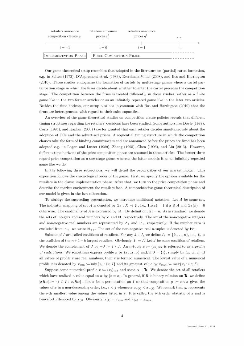
The competition between the retailers is modeled as a multi-stage game with infinite horizon. In

the first stage (period t = −1), the retailers simultaneously announce their competition clause poli-

cies. Afterwards, the retailers participate in an infinitely repeated Bertrand competition, i.e., they

simultaneously announce prices for the commodity in any of the succeeding and infinitely countable

stages (periods t = 0, 1, . . . ). We call the first stage the clause implementation phase and the suc-

ceeding stages the price competition phase. The timing of our competition game is depicted by the

below figure in which the arrow represents the time axis.

e.g., the proportional one, then it cannot any more be upheld. To avoid such fragility of our results, we have abstained

from assuming a specific rationing rule. Rather, we have striven to impose only some fundamental and less demanding

requirements on the rationing rules.

2We remark that our analysis could be extended to include cases in which retailers have identical sales capacities.

However, such generalization would expand the set of solutions without any added value. It then would hold: If outcome

o satisfies property P , then outcome o which differs from o only by permuting the retailers so that the capacities are still

ordered in a non-decreasing way would also satisfy this property. To circumvent such multiplicity, we have refrained from

such generalization.

3


t = −1

retailers announce

competition clauses g

t = 0

retailers announce

prices q0

t = 1

retailers announce

prices q1

. . .

. . .

Implementation Phase Price Competition Phase

Our game-theoretical setup resembles that adopted in the literature on (partial) cartel formation,

e.g. in Selten (1973), D’Aspremont et al. (1983), Escrihuela-Villar (2008), and Bos and Harrington

(2010). Those studies endogenize the formation of cartels by multi-stage games where a cartel par-

ticipation stage in which the firms decide about whether to enter the cartel precedes the competition

stage. The competition between the firms is treated differently in those studies; either as a finite

game like in the two former articles or as an infinitely repeated game like in the later two articles.

Besides the time horizon, our setup also has in common with Bos and Harrington (2010) that the

firms are heterogeneous with regard to their sales capacities.

An overview of the game-theoretical studies on competition clause policies reveals that different

timing structures regarding the retailers’ decisions have been studied. Some authors like Doyle (1988),

Corts (1995), and Kaplan (2000) take for granted that each retailer decides simultaneously about the

adoption of CCs and the advertised prices. A sequential timing structure in which the competition

clauses take the form of binding commitments and are announced before the prices are fixed has been

adopted e.g. in Logan and Lutter (1989), Zhang (1995), Chen (1995), and Liu (2013). However,

different time horizons of the price competition phase are assumed in these articles. The former three

regard price competition as a one-stage game, whereas the latter models it as an infinitely repeated

game like we do.

In the following three subsections, we will detail the peculiarities of our market model. This

exposition follows the chronological order of the game. First, we specify the options available for the

retailers in the clause implementation phase. After that, we turn to the price competition phase and

describe the market environment the retailers face. A comprehensive game-theoretical description of

our model is given in the last subsection.

To abridge the succeeding presentation, we introduce additional notation. Let A be some set.

The indicator mapping of set A is denoted by 1A : X → R, i.e., 1A(x) = 1 if x ∈ A and 1A(x) = 0

otherwise. The cardinality of A is expressed by |A|. By definition, |I| = n. As is standard, we denote

the sets of integers and real numbers by Z and R, respectively. The set of the non-negative integers

and non-negative real numbers are represented by Z+ and R+, respectively. If the number zero is

excluded from R+, we write R++. The set of the non-negative real n-tuples is denoted by RI+.

Subsets of I are called coalitions of retailers. For any k ∈ I, we define Ik := {k, . . . , n}, i.e., Ik is

the coalition of the n+ 1− k largest retailers. Obviously, I1 = I. Let J be some coalition of retailers.

We denote the complement of J by −J := I \ J . An n-tuple x := (xi)i∈I is referred to as a profile

of realizations. We sometimes express profile x by (xJ , x−J) and, if J = {i}, simply by (xi, x−i). If

all values of profile x are real numbers, then x is termed numerical. The lowest value of a numerical

profile x is denoted by xmin := min{xi : i ∈ I} and its greatest value by xmax := max{xi : i ∈ I}.Suppose some numerical profile x := (xi)i∈I and some α ∈ R. We denote the set of all retailers

which have realized a value equal to α by [x = α]. In general, if R is binary relation on R, we define

[xRα] := {i ∈ I : xiRα}. Let σ be a permutation on I so that composition y := x ◦ σ gives the

values of x in a non-decreasing order, i.e., i < j whenever xσ(i) < xσ(j). We remark that yi represents

the i-th smallest value among the values listed in x. It is called the i-th order statistic of x and is

henceforth denoted by x(i). Obviously, x(1) = xmin and x(n) = xmax.

4


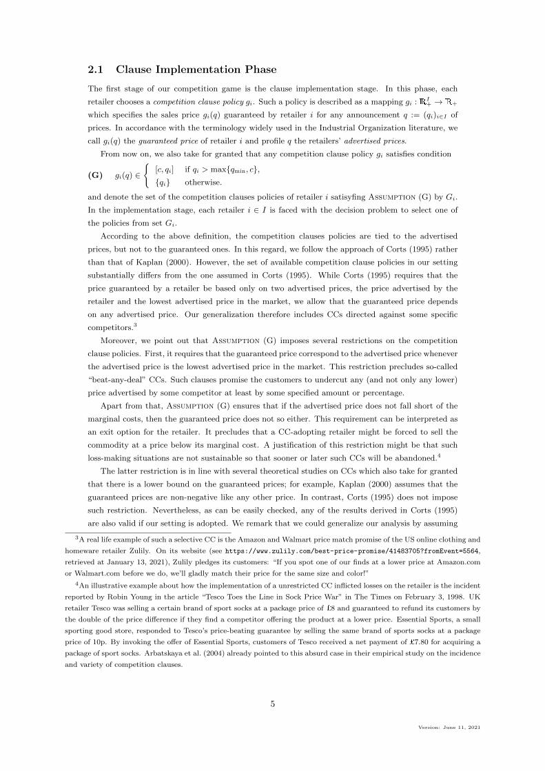
2.1 Clause Implementation Phase

The first stage of our competition game is the clause implementation stage. In this phase, each

retailer chooses a competition clause policy gi. Such a policy is described as a mapping gi : RI+ → R+

which specifies the sales price gi(q) guaranteed by retailer i for any announcement q := (qi)i∈I of

prices. In accordance with the terminology widely used in the Industrial Organization literature, we

call gi(q) the guaranteed price of retailer i and profile q the retailers’ advertised prices.

From now on, we also take for granted that any competition clause policy gi satisfies condition

(G) gi(q) ∈

{[c, qi] if qi > max{qmin, c},{qi} otherwise.

and denote the set of the competition clauses policies of retailer i satisyfing Assumption (G) by Gi.

In the implementation stage, each retailer i ∈ I is faced with the decision problem to select one of

the policies from set Gi.

According to the above definition, the competition clauses policies are tied to the advertised

prices, but not to the guaranteed ones. In this regard, we follow the approach of Corts (1995) rather

than that of Kaplan (2000). However, the set of available competition clause policies in our setting

substantially differs from the one assumed in Corts (1995). While Corts (1995) requires that the

price guaranteed by a retailer be based only on two advertised prices, the price advertised by the

retailer and the lowest advertised price in the market, we allow that the guaranteed price depends

on any advertised price. Our generalization therefore includes CCs directed against some specific

competitors.3

Moreover, we point out that Assumption (G) imposes several restrictions on the competition

clause policies. First, it requires that the guaranteed price correspond to the advertised price whenever

the advertised price is the lowest advertised price in the market. This restriction precludes so-called

“beat-any-deal” CCs. Such clauses promise the customers to undercut any (and not only any lower)

price advertised by some competitor at least by some specified amount or percentage.

Apart from that, Assumption (G) ensures that if the advertised price does not fall short of the

marginal costs, then the guaranteed price does not so either. This requirement can be interpreted as

an exit option for the retailer. It precludes that a CC-adopting retailer might be forced to sell the

commodity at a price below its marginal cost. A justification of this restriction might be that such

loss-making situations are not sustainable so that sooner or later such CCs will be abandoned.4

The latter restriction is in line with several theoretical studies on CCs which also take for granted

that there is a lower bound on the guaranteed prices; for example, Kaplan (2000) assumes that the

guaranteed prices are non-negative like any other price. In contrast, Corts (1995) does not impose

such restriction. Nevertheless, as can be easily checked, any of the results derived in Corts (1995)

are also valid if our setting is adopted. We remark that we could generalize our analysis by assuming

3A real life example of such a selective CC is the Amazon and Walmart price match promise of the US online clothing and

homeware retailer Zulily. On its website (see https://www.zulily.com/best-price-promise/41483705?fromEvent=5564,

retrieved at January 13, 2021), Zulily pledges its customers: “If you spot one of our finds at a lower price at Amazon.com

or Walmart.com before we do, we’ll gladly match their price for the same size and color!”

4An illustrative example about how the implementation of a unrestricted CC inflicted losses on the retailer is the incident

reported by Robin Young in the article “Tesco Toes the Line in Sock Price War” in The Times on February 3, 1998. UK

retailer Tesco was selling a certain brand of sport socks at a package price of £8 and guaranteed to refund its customers by

the double of the price difference if they find a competitor offering the product at a lower price. Essential Sports, a small

sporting good store, responded to Tesco’s price-beating guarantee by selling the same brand of sports socks at a package

price of 10p. By invoking the offer of Essential Sports, customers of Tesco received a net payment of £7.80 for acquiring a

package of sport socks. Arbatskaya et al. (2004) already pointed to this absurd case in their empirical study on the incidence

and variety of competition clauses.

5


https://www.zulily.com/best-price-promise/41483705?fromEvent=5564

less restrictive lower bounds on the guaranteed prices. However, we decided to refrain from such

generalizations as it would make our analysis more tedious without gaining additional insights.

The simplest competition clause policy is the one stipulating that the guaranteed price always

corresponds to the advertised price. This policy is defined by wi(q) := qi for any profile q of advertised

prices and is called the trivial competition clause policy or, simply, the no clause option. Due to

Assumption (G), any other competition clause policy gi has the property c ≤ gi(q) < qi for some

profile q of advertised prices satisfying qi > max{qmin, c}. Henceforth, we denote the set containing

all non-trivial competition clause policies (i.e., the CCs) available for retailer i by Ci.

A CC with lump sum refund entitles the customers to purchase the commodity at a price equal

to competitors’ lowest advertised price minus a specific fixed amount if the retailer fails to advertise

the lowest price in the market. In detail: Let µ ∈ R. A competition clause ge,µi of retailer i is said

to be a CC with lump sum refund µ if

ge,µi (q) := min{max{qmin − 1[q>qmin](i)µ, c}, qi}

for any profile q of advertised prices.

Obviously, the CC of the form mi := ge,0i entitles the customer to purchase the commodity at the

lowest advertised price in the market. This clause is referred to as the meeting competition clause,

also known as the price-matching guarantee. It is the most prominent type of a CC, and most of the

scientific literature on CCs focuses on this type. A CC of the form be,µi := ge,µi with µ > 0 is referred

to as a beating competition clause with a lump sum refund. It entitles the customers to purchase the

commodity at a price falling short of the lowest advertised price in the market by the amount µ if

the retailer fails to advertise the lowest price in the market.5

A clause profile g := (gi)i∈I summarizes the competition clause policies chosen in the retail market.

For example, profile w := (wi)i∈I describes the situation in which none of the retailers offers a CC

and profile m := (mi)i∈I describes the situation in which all retailers offer the MCC. The set of the

clause profiles in which the retailers’ competition clause policies satisfy Assumption (G) is denoted

by G := ×i∈IGi. Let us pick some arbitrary clause profile g ∈ G. We define C(g) := {i ∈ I : gi ∈ Ci}as the set of retailers which have adopted a CC in clause profile g. If there is a µi ∈ R for any

i ∈ C(g) so that gi = ge,µii , i.e., if each CC-adopting retailer chooses a CC with a lump sum refund,

then g is referred to as a conventional clause profile.

Our competition model adopts some of the peculiarities of the models of Chen (1995) as well as of

Hviid and Shaffer (1999). Like Chen (1995), we assume that implementing CCs causes one-off costs

for the retailers. All retailers implementing CCs incur the same fixed costs in the amount of f > 0

regardless of the chosen type of CC. The implementation costs encompass the costs of creating the

technical and personnel prerequisites for implementing a CC as well as of making the CC publicly

known. Since such expenses are largely one-off and more or less the same for any of the CC-adopting

retailers, our assumption of fixed and identical implementation costs might be reasonable. Only

retailers offering no CCs bear no fixed costs. For the sake of simplification, we take for granted that

f is discounted to period 0.

Like Hviid and Shaffer (1999), we assume that exercising CCs might be costly for the customers.

All customers making use of a CC incur the same hassle costs in the amount of z ≥ 0 per purchased

unit of the commodity regardless of at which retailer the commodity has been purchased and which

type of CC has been offered. The existence of hassle costs might be justified by the real life experience

5For example, such BCC is offered by the New Zealand tyre retailer Tony’s Tyre Service. They announce on their

website (see https://www.tonystyreservice.co.nz/tyres/price-beat-guarantee, retrieved on January 13, 2021): “We

stock leading tyre brands, at discount prices. Find a lower cash price and we guarantee to beat it by [NZ]$ 10 a tyre on a

similar quality product.”

6


https://www.tonystyreservice.co.nz/tyres/price-beat-guarantee

that exercising CCs is usually not a smooth process. In general, the burden of proof rests on the

customers. They have to spend time and effort to receive the refund guaranteed by the CC, e.g., for

providing enough and sound evidence, seeking out qualified salespersons and raising the issue with

them. If one takes for granted that each customer buys one unit of the commodity, our assumption

that the hassle costs are measured per unit of the commodity seems plausible. The assumption that

the hassle costs are identical among the customers has been made for reasons of simplification.

The effective purchase price gives the costs the customer incurs for acquiring a unit of the com-

modity. This price includes the hassle costs whenever the customer has exercised the retailer’s CC.

The effective sales price is the revenue the retailer earns per sold unit of the commodity. To provide

a formal specification of these prices, consider the situation in which retailer i has opted for the com-

petition clause policy gi and the retailers in the market advertise prices q = (qj)j∈I . The effective

purchase price of the commodity at retailer i is determined by formula

qpi := gp

i (q) := qi + 1Ci(gi) min{gi(q) + z − qi, 0}

and the effective sales price by formula

qsi := gs

i(q) := qi − 1R++(qi − gpi (q)) (qi − gi(q)).

Obviously, if gi = wi (i.e., retailer i does not adopt a CC) or gi(q) + z ≥ qi (i.e., it is not

worthwhile for the customers to make use of retailer i’s CC), then both the effective purchase and the

effective sales price at retailer i are equal to the advertised price. Otherwise, the effective sales price

corresponds to the price guaranteed by the retailers and the effective purchase price is the effective

sales price plus the hassle costs.

2.2 Price Competition Phase

Having adopted their competition clause profiles g := (gi)i∈I , the retailers take part in an infinitely

repeated Bertrand competition. At each stage t ∈ Z+ of this phase, the retailers simultaneously

advertise a price for the commodity. We denote the price advertised by retailer i at stage t by qti and

the profile listing all prices advertised at stage t by qt := (qti)i∈I . The effective sales and purchase

prices at stage t are then given by qs,t := gs(qt) and qp,t := gp(qt), respectively.

The demand side at stage t is described by market demand mapping D : R+ → R+. Its value

D(p) indicates the total quantity of the commodity demanded by the consumers if they have to pay

price p per unit of the commodity. The market demand mapping is time invariant and, therefore, not

marked with a stage index t. Moreover, we assume that

(D1) D is continuous,

(D2) there is some p > c so that D−1(0) = [p,+∞[ and D is decreasing on [0, p[.

These postulates are standard. Price p gives the highest amount the consumers are willing to pay

for the commodity and is known as the reservation price of the demand side. Due to Assumptions

(D1) and (D2), the monopolistic profit mapping π : R+ → R given by π(p) := (p−c)D(p) is continuous

and positive on open interval ]c, p[. Regarding the form of the profit mapping, it is taken for granted

that

(D3) π is strictly quasiconcave on ]c, p[.

It follows from Assumptions (D1), (D2), and (D3) that there exists a unique pm which maximizes

π. We term price pm as the collusive price and denote the monopolistic profit attained this price by

7


πm := π(pm). One can show that Assumption (D3) results if demand mapping D satisfies (D2) and

is concave on ]c, p[.6A further requirement we impose on our competition model is that

(D4) D(c) ≤ K−i for any i ∈ I.

Assumption (D4) states that the capacities of any coalition of n-1 retailers are sufficient to meet

the market demand at price equal marginal costs. If the capacity-constrained retailers were to take

part in a static Bertrand competition without CCs, then this assumption would entail that (i) the

situation in which each retailer charges a price equal to the marginal costs is a Nash equilibrium and

(ii) each retailer earns a zero profit in any Nash equilibrium.

Suppose that the consumers face purchase prices p := (pi)i∈I at stage t. Moreover, consider some

additional and hypothetical purchase price r. The residual market demand at r is defined as the

market demand at r not met by the capacities of the retailers undercutting price r. A rationing rule

would determine the exact size of residual market demand R(r|p). In the following, we present three

rationing rules, the efficient, the proportional and the perfect one. The former two have already been

extensively applied in the scientific literature.

� The efficient rationing rule Re(·|·) has been proposed by Levitan and Shubik (1972) as well as

Kreps and Scheinkman (1983). It lays down that consumers with the highest willingness to pay

are served first. In formal terms, the residual market demand resulting from efficient rationing

is given by

Re(r|p) := max{D(r)−K[p<r], 0}

for any profile p ∈ RI+ of purchase prices and any hypothetical purchase price r ∈ R+.

� The proportional rationing rule Rp(·|·) has been advocated by Beckmann (1965) as well as

Davidson and Deneckere (1986). It stipulates that each of the consumers have the same prob-

ability of being served. The residual market demand resulting from proportional rationing is

inductively specified by

Rp(r|p) :=

D(r) for any r ≤ p(1),

max

{Rp(p(i)|p)−K[p=p(i)]

D(p(i)|p), 0

}D(r) for any p(i) < r ≤ p(i+1)

where p(i) is the i-th order statistic of price profile p (i.e., the i-th smallest price in p) and

p(n+1) := +∞.

� The perfect rationing rule is the opposite extreme of the efficient rationing rule. This rule

stipulates that consumers with the lowest willingness to pay are served first. The residual

market demand resulting from perfect rationing is inductively specified by

Rl(r|p) :=

D(r) for any r ≤ p(1),

min{D(r),max{Rl(p(i)|p)−K[p=p(i)]

, 0}}

for any p(i) < r ≤ p(i+1)

where p(i) is the i-th order statistic of price profile p and p(n+1) := +∞.

6To see this, we take into account that Assumption (D2) implies (D(p)−D(p′)) (p − p′) < 0 for any different prices

p, p′ ∈]c, p[. Consider some arbitrary, but different prices p, p′ ∈]c, p[. Without any loss of generality, we can suppose that

π(p′) ≤ π(p). It holds:

π(p′) ≤ λπ(p) + (1− λ)π(p′)

=(λD(p) + (1− λ)D(p′)

) (λp+ (1− λ)p′ − c

)+ λ(1− λ)

(D(p)−D(p′)

)(p− p′)

< D(λp+ (1− λ)p′

) (λp+ (1− λ)p′ − c

)= π

(λp+ (1− λ)p′

)for any λ ∈]0, 1[.

8


In most parts of this paper, we abstain from assuming a specific rationing rule . Rather, we only

postulate that residual market demand mapping R : R+ ×RI+ → R+ satisfy the property

(R1) Re(r|p) ≤ R(r|p) ≤ Rl(r|p),

(R2) R(r|p) = R(r|p) if pi = pi for any i ∈ [p < r] and pi ≥ r for any i ∈ [p ≥ r].

Assumption (R1) requires that the lower and upper bound of the residual market demand be

the residual market demands resulting from the efficient and perfect rationing rule, respectively.

Assumption (R2) states that the residual market demand at price r is unaffected by price changes

in which the prices below r are kept constant and the other prices do not fall below r. Obviously,

both assumptions are innocuous as any reasonable rationing rule is compatible with it; for example,

the three rationing rules specified above.

The quantity of the commodity demanded by the consumers from retailer i at stage t and purchase

prices p := (pi)i∈I is derived from the residual market demand. We assume that demand mapping

Di : RI+ → R+ of retailer i is specified according to the allocation rule

(I) Di(p) :=ki

K[p=pi]

R(pi|p)

for any profile p ∈ RI+ of purchase prices.

According to this definition, the proportion of the residual market demand directed to retailer i

corresponds to i’s share of the total capacity of the retailers charging the same price as retailer i. An

argument substantiating such demand allocation is that consumers are more likely to meet retailers

with higher sales capacities than those with lower sales capacities so that they more likely to buy

the commodity from the former retailers than from the later ones. This allocation rule has already

been applied in other studies on Bertrand competition with capacity constraints; e.g., in Allen and

Hellwig (1986) as well as Osborne and Pitchik (1986).7

A retailer i is able to serve demand Di(p) as long as the demand does not exceed its capacity

constraint ki. The mapping Xi : RI+ → R+ indicating the quantity

Xi(p) := min{ki, Di(p)}

of the commodity retailer i is able to sell at profile p of purchase prices is referred to as the sales

mapping of retailer i. We conclude from Assumptions (R1) and (I) that if the purchase price of the

commodity is the same at any retailer (i.e., pi = pj for any j ∈ I), then retailer i’s share of the total

sales equals κi. For this reason, it is justified to interpret κi as retailer i’s market share at price p.

Moreover, Assumption (D4) entails that κi corresponds to the proportion of the market demand

retailer i serves if pi = pj for any j ∈ I and pi ≥ c.Let us now turn to the situation in which the retailers have implemented competition clause

policies g and advertise prices q := (qi)i∈I in period t. The profit retailer i earns in this period is

given by

πgi (q) := (qsi − c)Xi(qp).

Recall that qsi := gs

i(q) is the effective sales price charged by retailer i and qp := gp(q) summarizes

the effective purchase prices in the market. The mapping πgi : RI+ → R specifying retailer i’s period

profit πgi (q) for any profile q of advertised prices given that competition clause policies g have been

7We remark that not any theoretical analysis of markets with capacity-constrained retailers follows this allocation rule.

For example, Kreps and Scheinkman (1983) as well as Davidson and Deneckere (1986) assume that the market demand is

equally split among the duopolists whenever they set the same price and each duopolist has a capacity meeting at least

the half of the market demand. That is, both retailers have the same market share in this case regardless of their shares

of the total capacity. The same holds for the model of Tumennasan (2013), which is based on the framework of Kreps and

Scheinkman (1983).

9


implemented is referred to as retailer i’s profit mapping under clause profile g. To simplify the

notation, we write πi instead of πwi . Obviously, πi(q) = (qi − c)Xi(q) for any profile q of advertised

prices.

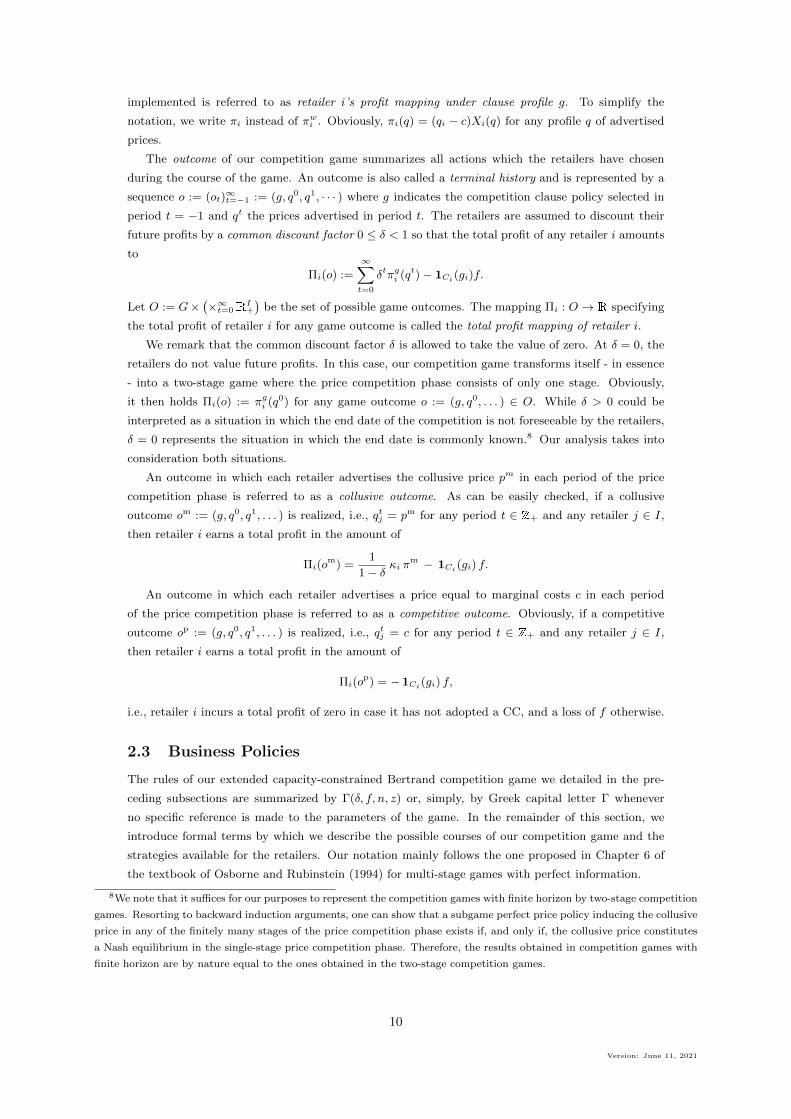
The outcome of our competition game summarizes all actions which the retailers have chosen

during the course of the game. An outcome is also called a terminal history and is represented by a

sequence o := (ot)∞t=−1 := (g, q0, q1, · · · ) where g indicates the competition clause policy selected in

period t = −1 and qt the prices advertised in period t. The retailers are assumed to discount their

future profits by a common discount factor 0 ≤ δ < 1 so that the total profit of any retailer i amounts

to

Πi(o) :=

∞∑t=0

δtπgi (qt)− 1Ci(gi)f.

Let O := G×(×∞t=0R

I+

)be the set of possible game outcomes. The mapping Πi : O → R specifying

the total profit of retailer i for any game outcome is called the total profit mapping of retailer i.

We remark that the common discount factor δ is allowed to take the value of zero. At δ = 0, the

retailers do not value future profits. In this case, our competition game transforms itself - in essence

- into a two-stage game where the price competition phase consists of only one stage. Obviously,

it then holds Πi(o) := πgi (q0) for any game outcome o := (g, q0, . . . ) ∈ O. While δ > 0 could be

interpreted as a situation in which the end date of the competition is not foreseeable by the retailers,

δ = 0 represents the situation in which the end date is commonly known.8 Our analysis takes into

consideration both situations.

An outcome in which each retailer advertises the collusive price pm in each period of the price

competition phase is referred to as a collusive outcome. As can be easily checked, if a collusive

outcome om := (g, q0, q1, . . . ) is realized, i.e., qtj = pm for any period t ∈ Z+ and any retailer j ∈ I,

then retailer i earns a total profit in the amount of

Πi(om) =

1

1− δ κi πm − 1Ci(gi) f.

An outcome in which each retailer advertises a price equal to marginal costs c in each period

of the price competition phase is referred to as a competitive outcome. Obviously, if a competitive

outcome op := (g, q0, q1, . . . ) is realized, i.e., qtj = c for any period t ∈ Z+ and any retailer j ∈ I,

then retailer i earns a total profit in the amount of

Πi(op) = −1Ci(gi) f,

i.e., retailer i incurs a total profit of zero in case it has not adopted a CC, and a loss of f otherwise.

2.3 Business Policies

The rules of our extended capacity-constrained Bertrand competition game we detailed in the pre-

ceding subsections are summarized by Γ(δ, f, n, z) or, simply, by Greek capital letter Γ whenever

no specific reference is made to the parameters of the game. In the remainder of this section, we

introduce formal terms by which we describe the possible courses of our competition game and the

strategies available for the retailers. Our notation mainly follows the one proposed in Chapter 6 of

the textbook of Osborne and Rubinstein (1994) for multi-stage games with perfect information.

8We note that it suffices for our purposes to represent the competition games with finite horizon by two-stage competition

games. Resorting to backward induction arguments, one can show that a subgame perfect price policy inducing the collusive

price in any of the finitely many stages of the price competition phase exists if, and only if, the collusive price constitutes

a Nash equilibrium in the single-stage price competition phase. Therefore, the results obtained in competition games with

finite horizon are by nature equal to the ones obtained in the two-stage competition games.

10


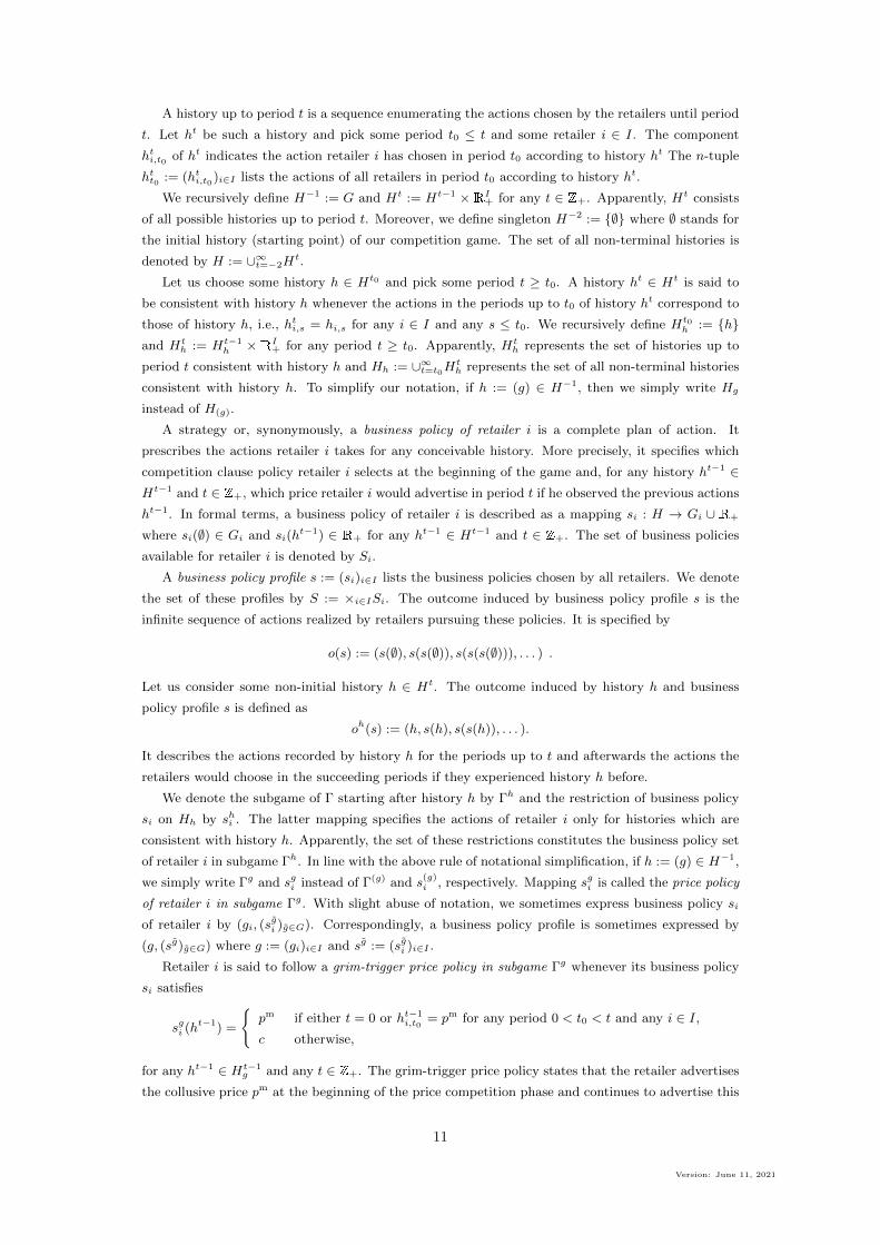
A history up to period t is a sequence enumerating the actions chosen by the retailers until period

t. Let ht be such a history and pick some period t0 ≤ t and some retailer i ∈ I. The component

hti,t0 of ht indicates the action retailer i has chosen in period t0 according to history ht The n-tuple

htt0 := (hti,t0)i∈I lists the actions of all retailers in period t0 according to history ht.

We recursively define H−1 := G and Ht := Ht−1 ×RI+ for any t ∈ Z+. Apparently, Ht consists

of all possible histories up to period t. Moreover, we define singleton H−2 := {∅} where ∅ stands for

the initial history (starting point) of our competition game. The set of all non-terminal histories is

denoted by H := ∪∞t=−2Ht.

Let us choose some history h ∈ Ht0 and pick some period t ≥ t0. A history ht ∈ Ht is said to

be consistent with history h whenever the actions in the periods up to t0 of history ht correspond to

those of history h, i.e., hti,s = hi,s for any i ∈ I and any s ≤ t0. We recursively define Ht0h := {h}

and Hth := Ht−1

h × RI+ for any period t ≥ t0. Apparently, Hth represents the set of histories up to

period t consistent with history h and Hh := ∪∞t=t0Hth represents the set of all non-terminal histories

consistent with history h. To simplify our notation, if h := (g) ∈ H−1, then we simply write Hg

instead of H(g).

A strategy or, synonymously, a business policy of retailer i is a complete plan of action. It

prescribes the actions retailer i takes for any conceivable history. More precisely, it specifies which

competition clause policy retailer i selects at the beginning of the game and, for any history ht−1 ∈Ht−1 and t ∈ Z+, which price retailer i would advertise in period t if he observed the previous actions

ht−1. In formal terms, a business policy of retailer i is described as a mapping si : H → Gi ∪ R+

where si(∅) ∈ Gi and si(ht−1) ∈ R+ for any ht−1 ∈ Ht−1 and t ∈ Z+. The set of business policies

available for retailer i is denoted by Si.

A business policy profile s := (si)i∈I lists the business policies chosen by all retailers. We denote

the set of these profiles by S := ×i∈ISi. The outcome induced by business policy profile s is the

infinite sequence of actions realized by retailers pursuing these policies. It is specified by

o(s) := (s(∅), s(s(∅)), s(s(s(∅))), . . . ) .

Let us consider some non-initial history h ∈ Ht. The outcome induced by history h and business

policy profile s is defined as

oh(s) := (h, s(h), s(s(h)), . . . ).

It describes the actions recorded by history h for the periods up to t and afterwards the actions the

retailers would choose in the succeeding periods if they experienced history h before.

We denote the subgame of Γ starting after history h by Γh and the restriction of business policy

si on Hh by shi . The latter mapping specifies the actions of retailer i only for histories which are

consistent with history h. Apparently, the set of these restrictions constitutes the business policy set

of retailer i in subgame Γh. In line with the above rule of notational simplification, if h := (g) ∈ H−1,

we simply write Γg and sgi instead of Γ(g) and s(g)i , respectively. Mapping sgi is called the price policy

of retailer i in subgame Γg. With slight abuse of notation, we sometimes express business policy si

of retailer i by (gi, (sgi )g∈G). Correspondingly, a business policy profile is sometimes expressed by

(g, (sg)g∈G) where g := (gi)i∈I and sg := (sgi )i∈I .

Retailer i is said to follow a grim-trigger price policy in subgame Γg whenever its business policy

si satisfies

sgi (ht−1) =

{pm if either t = 0 or ht−1

i,t0= pm for any period 0 < t0 < t and any i ∈ I,

c otherwise,

for any ht−1 ∈ Ht−1g and any t ∈ Z+. The grim-trigger price policy states that the retailer advertises

the collusive price pm at the beginning of the price competition phase and continues to advertise this

11


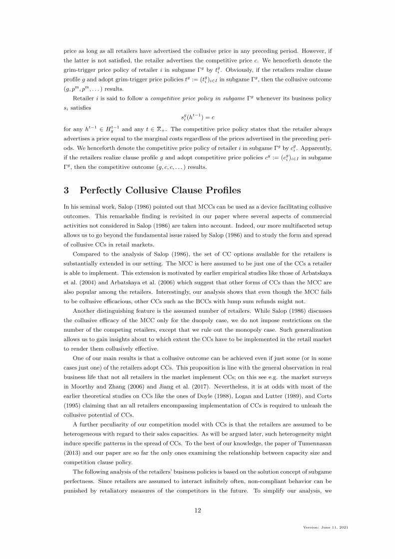
price as long as all retailers have advertised the collusive price in any preceding period. However, if

the latter is not satisfied, the retailer advertises the competitive price c. We henceforth denote the

grim-trigger price policy of retailer i in subgame Γg by tgi . Obviously, if the retailers realize clause

profile g and adopt grim-trigger price policies tg := (tgi )i∈I in subgame Γg, then the collusive outcome

(g, pm, pm, . . . ) results.

Retailer i is said to follow a competitive price policy in subgame Γg whenever its business policy

si satisfies

sgi (ht−1) = c

for any ht−1 ∈ Ht−1g and any t ∈ Z+. The competitive price policy states that the retailer always

advertises a price equal to the marginal costs regardless of the prices advertised in the preceding peri-

ods. We henceforth denote the competitive price policy of retailer i in subgame Γg by cgi . Apparently,

if the retailers realize clause profile g and adopt competitive price policies cg := (cgi )i∈I in subgame

Γg, then the competitive outcome (g, c, c, . . . ) results.

3 Perfectly Collusive Clause Profiles

In his seminal work, Salop (1986) pointed out that MCCs can be used as a device facilitating collusive

outcomes. This remarkable finding is revisited in our paper where several aspects of commercial

activities not considered in Salop (1986) are taken into account. Indeed, our more multifaceted setup

allows us to go beyond the fundamental issue raised by Salop (1986) and to study the form and spread

of collusive CCs in retail markets.

Compared to the analysis of Salop (1986), the set of CC options available for the retailers is

substantially extended in our setting. The MCC is here assumed to be just one of the CCs a retailer

is able to implement. This extension is motivated by earlier empirical studies like those of Arbatskaya

et al. (2004) and Arbatskaya et al. (2006) which suggest that other forms of CCs than the MCC are

also popular among the retailers. Interestingly, our analysis shows that even though the MCC fails

to be collusive efficacious, other CCs such as the BCCs with lump sum refunds might not.

Another distinguishing feature is the assumed number of retailers. While Salop (1986) discusses

the collusive efficacy of the MCC only for the duopoly case, we do not impose restrictions on the

number of the competing retailers, except that we rule out the monopoly case. Such generalization

allows us to gain insights about to which extent the CCs have to be implemented in the retail market

to render them collusively effective.

One of our main results is that a collusive outcome can be achieved even if just some (or in some

cases just one) of the retailers adopt CCs. This proposition is line with the general observation in real

business life that not all retailers in the market implement CCs; on this see e.g. the market surveys

in Moorthy and Zhang (2006) and Jiang et al. (2017). Nevertheless, it is at odds with most of the

earlier theoretical studies on CCs like the ones of Doyle (1988), Logan and Lutter (1989), and Corts

(1995) claiming that an all retailers encompassing implementation of CCs is required to unleash the

collusive potential of CCs.

A further peculiarity of our competition model with CCs is that the retailers are assumed to be

heterogeneous with regard to their sales capacities. As will be argued later, such heterogeneity might

induce specific patterns in the spread of CCs. To the best of our knowledge, the paper of Tumennasan

(2013) and our paper are so far the only ones examining the relationship between capacity size and

competition clause policy.

The following analysis of the retailers’ business policies is based on the solution concept of subgame

perfectness. Since retailers are assumed to interact infinitely often, non-compliant behavior can be

punished by retaliatory measures of the competitors in the future. To simplify our analysis, we

12


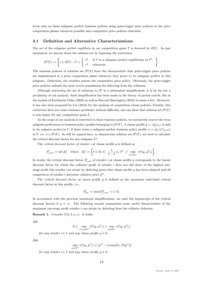
focus only on those subgame perfect business policies using grim-trigger price policies in the price

competition phases whenever possible and competitive price policies otherwise.

3.1 Definition and Alternative Characterizations

The set of the subgame perfect equilibria in our competition game Γ is denoted by S(Γ). As just

mentioned, we narrow down the solution set by imposing the restriction

Sg(Γ) :=

{s ∈ S(Γ) : sg =

{tg if tg is a subgame perfect equilibrium in Γg,

cg otherwise

}.

The business policies of solution set Sg(Γ) have the characteristic that grim-trigger price policies

are implemented in a price competition phase whenever they prove to be subgame perfect in this

subgame. Otherwise, the retailers pursue the competitive price policy. Obviously, the grim-trigger

price policies unleash the most severe punishment for defecting from the collusion.

Although restricting the set of solutions to Sg is a substantial simplification, it is by far not a

peculiarity of our analysis. Such simplification has been made in the theory of partial cartels, like in

the models of Escrihuela-Villar (2008) as well as Bos and Harrington (2010) to name a few. Moreover,

it has also been proposed by Liu (2013) for the analysis of competition clause policies. Notably, this

restriction does not cause existence problems; without difficulty, one can show that solution set Sg(Γ)

is non-empty for any competition game Γ.

As the scope of our analysis is restricted to those business policies, we exclusively reserve the term

subgame perfectness to business policy profiles belonging to Sg(Γ). A clause profile g := (gi)i∈I is said

to be subgame perfect in Γ, if there exists a subgame perfect business policy profile s := (g, (sg)g∈G)

in Γ, i.e., s ∈ Sg(Γ). As will be argued later, to characterize solution set Sg(Γ), we need to calculate

the critical discount factor for any subgame Γg.

The critical discount factor of retailer i at clause profile g is defined as

δgi,crit := inf ∆gi where ∆g

i :=

{δ ∈ [0, 1[ :

1

1− δ κi πm ≥ sup

qi 6=pmπgi (qi, p

m−i)

}.

In words, the critical discount factor δgi,crit of retailer i at clause profile g corresponds to the lowest

discount factor for which the collusive profit of retailer i does not fall short of the highest one-

stage profit this retailer can attain by defecting given that clause profile g has been adopted and all

competitors of retailer i advertise collusive price pm.

The critical discount factor at clause profile g is defined as the maximum individual critical

discount factor at this profile, i.e.,

δgcrit := max{δgi,crit : i ∈ I}.

In accordance with the previous notational simplifications, we omit the superscript of the critical

discount factors if g = w. The following remark summarizes some useful characteristics of the

maximum one-stage profit retailer i can attain by defecting from the collusive behavior.

Remark 1. Consider Γ(δ, f, n, z). It holds:

(a)

0 ≤ supc<qi 6=pm

πgi (qi, pm−i) = sup

qi 6=pmπgi (qi, p

m−i)

for any retailer i ∈ I and any clause profile g ∈ G.

(b)

supqi 6=pm

πgi (qi, pm−i) ≤ (pm − c) max{ki, D(pm)}


13


The two parts of this remark substantially simplify the calculation of the maximum one-stage

profit attainable by defection. Parts (a) and (b) provide a lower and an upper bound for this profit,

respectively. Moreover, according to part (a), it suffices for the calculation to consider only the

advertised prices above the marginal costs.

It turns out that if none of the retailers have adopted a CC (i.e., g = w) in the implementation

phase, the critical discount factor for retailer i is given as follows.

Remark 2. Consider Γ(δ, f, n, z). It holds

δi,crit = 1−max{κi,

D(pm)

K

}≥ δgi,crit


An immediate consequence of the last remark is that

δcrit = 1−max{κ1,

D(pm)K

}≥ δgcrit

for any clause profile g ∈ G. This means, the critical discount factor for clause profile w is the greatest

among the critical discount factors; or putting differently, the adoption of CCs never increases the

critical discount factor.

As can be easily checked, our competition game Γ is a multi-stage game being continuous at

infinity. We know from Theorem 3.2 in the textbook of Fudenberg and Tirole (1991) that the One-

Shot Deviation Principle holds for such games. This principle provides a simple characterization

of subgame perfect equilibria. It states that a strategy profile is subgame perfect if, and only if, there

exists no profitable one-shot deviation for each subgame and each player.9 Applying this principle to

competition game Γ, we obtain the following characterization of solution concept Sg.

Remark 3. Consider Γ(δ, f, n, z). It holds s := (g, (sg)g∈G) ∈ Sg(δ, f, n, z) if, and only if, the

properties

(T1) sgi =

{tgi if δ ≥ δgcritcgi otherwise

for any i ∈ I and g ∈ G,

(T2) Πi(o(s) ≥ Πi(o(s)) for any s := (si, s−i) ∈ S where si := (gi, (sgi )g∈G) and any i ∈ I

are satisfied.

The focus of our interest is whether solution set Sg(Γ) contains business policy profiles inducing

collusive price outcomes. We call such profiles perfectly collusive and, henceforth, denote this subset

of Sg(Γ) by

Sm(Γ) := {s ∈ Sg(Γ) : o(s) is a collusive price outcome}.

A clause profile g := (gi)i∈I is said to be perfectly collusive in Γ whenever there exists some business

policy profile s := (g, (sg)g∈G) ∈ Sm(Γ).

As will be shown next, such clause profiles can be characterized by three conditions; two refer only

to the common discount factor and the remaining one also to the implementation costs. With regard

to the latter condition, it turns out to be helpful to introduce the notion of the critical implementation

costs of clause profile g at common discount factor δ, which are defined as

fg,δcrit :=

{1

1−δκiπm if C(g) 6= ∅ where i := min C(g),

+∞ otherwise.

This value gives the collusive profit of the smallest CC-adopting retailer. Obviously, whenever the

actual implementation costs exceed fg,δcrit, then this retailer would be better off at the competitive

outcome without implementing a CC than at the collusive outcome with implementing a CC.

9For further details of this principle, we refer to the proof of Remark 3.

14


Remark 4. Consider Γ(δ, f, n, z). A clause profile g is perfectly collusive if, and only if, properties

(M1) δgcrit ≤ δ

(M2) δ < δgcrit for any g := (wi, g−i) ∈ G and any i ∈ C(g),

(M3) f ≤ f g,δcrit

are satisfied

The three properties of Remark 4 completely characterize the perfectly collusive clause profiles

and correspond to the conditions of external and internal stability in the partial cartel theory, see

D’Aspremont et al. (1983). Property (M1) covers the external stability of the collusive clause

profile: None of the non CC-adopting retailers has an incentive to adopt a CC as the collusive

outcome is already reached and, thus, the implementation of a CC would turn out to be a costly

business operation without any additional gain for them. Properties (M2) and (M3) ensure the

internal stability of the collusive clause profile: None of the CC-adopting retailers prefers repealing

the CC. Such withdrawal would induce a competitive outcome; with the consequence that none of

them would be better off.

In the remainder of this section, we discuss whether a collusive price outcome can be achieved for

any arbitrary common discount factor and, if so, which kinds of conventional clause profiles could

sustain such outcome. It turns out that the characterization of perfectly collusive clause profiles put

forward in Remark 4 becomes very useful for tackling these issues.

3.2 Collusion without Competition Clauses

This subsection provides a first insight into the incentives of the retailers to adopt CCs. As will be

demonstrated next, the adoption of CCs proves to be a sufficient, but not a necessary condition for

inducing collusion.

Proposition 5. Consider Γ(δ, f, n, z). There exists no subgame perfect business policy profile in

which a retailer adopts a CC, but which induces the competitive outcome.

According to this proposition, the only purpose of CCs in our competition model is achieving a

collusive outcome. This result relies on our implicit assumption that all consumers know all advertised

prices and competition clause policies. If this assumption is dropped, CCs could be adopted for other

reasons like signaling low prices or price differentiating between customers with low and high costs

in searching out the prices charged by other retailers.10

Jain and Srivastava (2000), Moorthy and Winter (2006), as well as Moorthy and Zhang (2006)

have strongly put forward the former purpose. Earlier studies advocating the later purpose are the

ones of Png and Hirshleifer (1987), Corts (1997), Chen et al. (2001), and Hviid and Shaffer (2012).

In these studies, some exogenously determined groups of consumers are able to take advantage of

CCs while others are not. More recent studies like the ones of Janssen and Parakhonyak (2013),

Yankelevich and Vaughan (2016), and Jiang et al. (2017) have endogenized the price search of the

consumers to motivate CCs as a device enabling price discrimination.

Interestingly, as parts of this literature suggest, if CCs are used as a signaling or price discriminat-

ing device, then CCs could have pro-competitive and welfare-enhancing effects, reducing (some of)

the effective sales prices and making better off not only the retailers but also (at least some groups

of) consumers.11 This finding however is in contrast to our Proposition 5, which rules out any other

purpose than enforcing collusion.

10Other reasons why retailers adopt CCs could be mentioned. Hviid (2010) provides a comprehensive overview of the

different motivations for CCs discussed in the scientific literature.11An opposite point of view has been taken e.g. by Budzinski and Kretschmer (2011). They claim that CCs still induce the

collusive price even though there is asymmetric information among the consumers about the price policies of the retailers.

15


Moreover, we remark that the converse of Proposition 5 does not hold. It turns out that if the

common discount factor is sufficiently large, the collusive outcome is achieved only without CCs.

Theorem 6. Consider Γ(δ, f, n, z). It holds:

(a) If clause profile w (i.e. the clause profile in which none of the retailers adopts a CC) is perfectly

collusive, then δcrit ≤ δ < 1.

(b) If δcrit ≤ δ < 1, then clause profile w is the only perfectly collusive clause profile.

The Perfect Folk Theorem put forward by Friedman (1971) states that player can reach

collusive outcomes in infinitely repeated games whenever the common discount factor is sufficiently

large. According to Theorem 6, this fundamental result remains valid even for our extended Bertrand

competition game where CCs can be adopted by the retailers at the beginning. This is due to the fact

that if the retailers value future profits sufficiently high, then the threats implicit in the grim-trigger

price policies are efficacious and deter the retailers from undercutting monopoly price pm. In this

case, adopting CCs causes only undue costs.

However, as can be easily concluded from Remarks 2 and 3, the retailers would choose the

competitive price policy in the price competition phase if the common discount factor δ were below

threshold δcrit and none of them had adopted a CC. For such discount factors, the mere grim-trigger

threats are too weak to sustain collusion. Whether collusion can then be facilitated through the

implementation of CCs, is studied in the remaining parts of this section.

3.3 Collusive Competition Clauses with Lump Sum Refunds

A strong argument against the collusive efficacy of CCs has been put forward by Hviid and Shaffer

(1994) and Corts (1995). They show that CCs are collusively ineffective if the competition between

the retailers is described as a one-stage game in which the retailers decide simultaneously about the

competition clause policies and the advertised prices.12 However, the robustness of their results might

be questionable. It turns out that their conclusion cannot easily transferred to our setting as our

modeling of the competition differs from those in two core aspects.

First, the timing of the decision-making in our framework is different. We consider competition

clause policies as binding commitments and therefore describe the competition between retailers as

a sequential-move game in which before fixing the prices, the retailers announce their competition

clause policies. That means, when the retailers advertise the prices, they have already been informed

about the competition clause policies pursued by their competitors. Second, our setting allows for a

longer time horizon. We take into account that retailers might compete with each other repeatedly

(i.e., finitely often until a unknown end point) so that non-cooperative behavior of a retailer can be

punished by non-cooperative behavior of its competitors in future periods.

As will be demonstrated below, these divergences from the settings of Hviid and Shaffer (1994) and

Corts (1995) are responsible for a different answer regarding the efficacy of CCs. More specifically, for

sufficiently small hassle and implementation costs, clause profiles in which a sufficiently large coalition

of retailers adopt CCs with well-proportionate lump sum refunds prove to be perfectly collusive in

our competition model.

12See Proposition 2 of Hviid and Shaffer (1994) and Proposition 2 of Corts (1995). It should be noted that the scope

of their results are different. Hviid and Shaffer (1994) prove the claim for any heterogeneous Bertrand duopoly in which

the MCC and the BCCs with refund factors on the price difference (“We promise that if we do not offer the lowest price

in the market, we’ll beat it by an amount equal to x % of the difference between our announced price and the lowest price

in the market.”) are the only CCs available for the retailers. Corts (1995) proves the claim for any homogeneous Bertrand

oligopoly in which the CCs can take on a wide variety of forms including the conventional ones.

16


One reason why CCs nevertheless might fail to facilitate collusion even in our setting is that the

total capacity of the CC-adopting retailers is too small in order to punish defectors. Indeed, if the

total capacity of those retailers does not meet the market demand at the monopoly price, each of

them faces the same incentive to defect from the collusion as if they had not adopted CCs. The

subsequent remark sets this point our and states that the critical discount factors of such clause

profiles correspond to the one of the trivial clause profile.

Remark 7. Consider Γ(δ, f, n, z). It holds

δgcrit = δcrit

for any clause profile g satisfying KC(g) ≤ D(pm).

An immediate consequence of this remark is that adopting a CC is pointless whenever the total

capacity of the CC-adopting retailers does not exceed the market demand at the monopoly price. We

summarize this finding in the following theorem.

Theorem 8. Consider Γ(δ, f, n, z) where δ < δcrit. Any clause profile g satisfying KC(g) ≤ D(pm) is

not perfectly collusive.

Another well-known reason why CCs become collusively ineffective are hassle costs. Such costs

drive a wedge between the effective purchase and sales prices whenever the CC is exercised. This

wedge might entail that a defecting retailer can undersell any of its competitors, including the ones

which have adopted a CC. Even if the sales prices at those competitors are below the reduced price

advertised by the defector, the purchase prices at them might exceed this advertised price due to the

hassle costs. In such a case, the CC-adopting retailers are unable to immediately penalize defections

from collusive behavior, with the consequence that the CCs become collusively ineffective.

Apart from that, even though collusive behavior can be enforced by CCs, retailers nevertheless

might abstain from offering them if their implementation is too expensive. Obviously, if the implemen-

tation costs exceed the additional profit gained by acting collusively instead of acting competitively,

then the retailer would be better off without CC.

In the following, we aim to be more specific about the consequences of the hassle and imple-

mentation costs on the collusive efficacy of CCs. In particular, we seek to provide thresholds of the

hassle and implementation costs above which collusion is not enforceable by CCs. For this purpose,

additional notation is required.

To specify the threshold for the hassle costs, we define mapping πi(·) where

πi(p) := (p− c) min{ki, D(p)}

for any p ∈ R+ and any retailer i ∈ I. Apparently, mapping πi(·) gives the profit earned by retailer

i if the customers of retailer i pay a price p and the customers of the other retailers a price above p.

Henceforth, we refer to mapping πi as the monopolistic profit mapping of retailer i. We are interested

in the price pδi for which the monopolistic profit of retailer i corresponds to the total (net) surplus

retailer i attains at the collusive outcome.

Remark 9. Consider Γ(δ, f, n, z). For any retailer i ∈ I and any common discount factor δ < δi,crit,

there is a unique pδi so that c < pδi < pm and πi(pδi ) = 1

1−δκiπm. Moreover, the conditions

(i) pβi < pδi

(ii) pδj ≤ pδi

are satisfied for any common discount factors β < δ and any retailers j ≤ i.

17


Based on price pδi , we define

µδi := pm − pδi , φδi :=pm−pδipm

, zδi := pδi − c

for any δ < δi,crit and any i ∈ I. Due to Remark 9, these values are positive. Moreover, this remark

implies that µδi and φδi is decreasing in δ and non-increasing in i, whereas zδi is increasing in δ and

non-decreasing in i.

To specify the threshold for the implementation costs, we consider the greatest number j ∈ I so

that the coalition consisting of the n+ 1− j largest retailers has a total capacity meeting the demand

at the monopoly price pm; or expressed formally, j := max{k ∈ I : KIk ≥ D(pm)}. We define

fδ := 11−δκjπ

m.

for any common discount factor δ < δcrit. Apparently, fδ is the total net surplus the retailer with

the lowest capacity in coalition Ik achieves at the collusive price outcome. We hint that Assumption

(D4) ensures fδ ≥ 11−δκ2π

m.

The following theorem provides thresholds for the hassle and implementation costs above which

CCs become an inefficacious device for collusion.

Theorem 10. Consider Γ(δ, f, n, z) where δ < δcrit. If f > fδ or z > zδ1, then there is no perfectly

collusive clause profile.

Theorems 8 and 10 point towards two technical issues preventing CCs to induce collusive behav-

ior, a too small total capacity of the CC adopting retailers and too large hassle or implementation

costs. It remains to examine the collusive efficacy of CCs in cases these technical barriers do not

prevail. We address this issue by focusing on the conventional clause profile, i.e., in which the retailers

adopt CCs with lump sum refunds.

Our first finding is that CCs with lump sum refunds less than the hassle costs are avoided by the

retailers in any circumstance. The reason for this obvious. Since such CCs do not cause a matching

or an undercutting of the defector’s price reduction, they do not remove the incentive of the retailers

to deviate from collusive behavior. Hence, such CCs prove to be ineffective in punishing defectors.

Theorem 11. Consider Γ(δ, f, n, z). There exists no perfectly collusive clause profile in which a

retailer adopts a CC with lump sum refund µ < z.

One interesting aspect of the last theorem is that it also reproduces the inefficacy result of Hviid

and Shaffer (1999) for the case of perfectly homogeneous commodities. As stated in the above

theorem, if hassle costs exists, MCCs turn out to be ineffective in facilitating collusion no matter how

small these costs are. Due to this disruptive effect, hassle costs have been referred to as the Achilles’

heel of the MCCs by Hviid and Shaffer (1999).

This pro-competitive effect of hassle costs has also been experimentally tested by Dugar and

Sorensen (2006). Their setting essentially corresponds to ours with common discount factor δ = 0.

An augmented homogeneous Bertrand trioloply is played where the three players decide in the first

stage whether they adopt the MCC and set the price of the commodity in the second stage. It is

assumed that (at least some of) the customers incur hassle costs in exercising the MCC. Dugar and

Sorensen (2006) report that if exercising the MCC is tedious for any customer, then the average

effective price is close to the one resulting from the games without the MCC option.

We remark that the ineffectiveness result of Theorem 11 hings crucially on the assumptions of

perfectly homogeneous commodity markets and simultaneous price-setting. If these assumptions are

dropped, then it might be the case that some of the CCs mentioned in the theorem become collusively

efficacious. Indeed, based on the Hotelling’s linear city model with sequential price-setting, it is shown

by Trost (2016) that MCCs prove to be collusively efficacious even if hassle costs prevail and by Pollak

18


(2017) that CCs with negative lump sum refunds (so-called CCs with markups) prove to be collusively

efficacious in the case that no hassle costs prevail.

Let us now consider clause profiles in which a sufficiently large coalition of retailers adopts CCs

with lump sum refunds in the amount of the hassle costs. Lower and upper bounds of their critical

discount factors are presented in the following remark.

Remark 12. Consider Γ(δ, f, n, z) where δ < δcrit and z ≤ zδ1. It holds:

(a) If clause profile g := (be,zJ , w−J) satisfies KJ > D(pm), then

δgcrit ≥ 1− κJ

where equality holds if z ≤ z1−κJ1 .

(b) If clause profile g := (be,zJ , w−J) satisfies κJ ≥ 1− δ, then

δgcrit ≤ δ

where equality holds if, and only if, κJ = 1− δ or z = zδ1.

Applying this remark, we conclude that such clause profiles facilitate collusion for discount values

below threshold δcrit even though (“mild”) implementation and hassle costs exist.

Theorem 13. Consider Γ(δ, f, n, z) where δ < δcrit and z ≤ zδ1. The non-trivial clause profile

g := (ge,zJ , w−J) (i.e., the clause profile in which the retailers of non-empty coalition J ⊆ I adopt

CCs with lump sum refund z while the other retailers do not adopt CCs) is perfectly collusive if and

only if the conditions

(i) 1− κJ ≤ δ,

(ii) δ < 1− κJ\{j} where j := min J ,

(iii) f ≤ f g.δcrit

are satisfied.

The conditions of this theorem are easy to interpret. Condition (i) represents the external stability

condition of the collusive clause profiles. It states that the sum of the market shares of the non CC-

adopting retailers has to be lower or equal to the common discount factor. Conditions (ii) and (iii)

represent the internal stability condition of the collusive clause profiles. The former states that the

sum of the market shares of the non CC-adopting retailers has to be large enough so that it would

exceed the common discount factor if the market share of one of CC-adopting retailers were added.

The anti-competitive prediction of Theorem 13 has already been experimentally tested by Dugar

(2007) for the specific case in which the price competition phase consists only of one stage (i.e.,

δ = 0) and no hassle costs exist (i.e., z = 0). The benchmark case of this experiment was a standard

homogeneous Bertrand triopoly game and the treatment case the two-stage game in which the three

players had the option to implement the MCC before competing in the Bertrand game. In line with

the prediction of the theorem, it was observed that all three players adopted the MCC in the majority

of the treatment cases and the average effective price in the treatment cases was significantly higher

than in the benchmark cases.

The essential point of Theorem 13 is that it challenges two fundamental claims made in several

theoretical studies on collusive CCs. First, in the case that retailers do not take into account future

profits (i.e., δ = 0), we infer from this theorem that the collusive price outcome is realized if all

retailers adopt CCs with lump sum refund z. However, this results is at odds with Proposition

2 in Corts (1995) according to which no business policy profile can substantiate supracompetitive

19


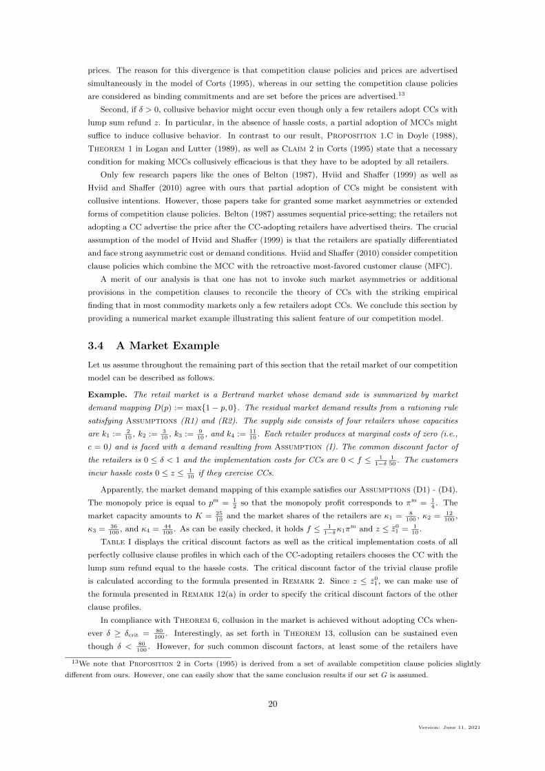
prices. The reason for this divergence is that competition clause policies and prices are advertised

simultaneously in the model of Corts (1995), whereas in our setting the competition clause policies

are considered as binding commitments and are set before the prices are advertised.13

Second, if δ > 0, collusive behavior might occur even though only a few retailers adopt CCs with

lump sum refund z. In particular, in the absence of hassle costs, a partial adoption of MCCs might

suffice to induce collusive behavior. In contrast to our result, Proposition 1.C in Doyle (1988),

Theorem 1 in Logan and Lutter (1989), as well as Claim 2 in Corts (1995) state that a necessary

condition for making MCCs collusively efficacious is that they have to be adopted by all retailers.

Only few research papers like the ones of Belton (1987), Hviid and Shaffer (1999) as well as

Hviid and Shaffer (2010) agree with ours that partial adoption of CCs might be consistent with

collusive intentions. However, those papers take for granted some market asymmetries or extended

forms of competition clause policies. Belton (1987) assumes sequential price-setting; the retailers not

adopting a CC advertise the price after the CC-adopting retailers have advertised theirs. The crucial

assumption of the model of Hviid and Shaffer (1999) is that the retailers are spatially differentiated

and face strong asymmetric cost or demand conditions. Hviid and Shaffer (2010) consider competition

clause policies which combine the MCC with the retroactive most-favored customer clause (MFC).

A merit of our analysis is that one has not to invoke such market asymmetries or additional

provisions in the competition clauses to reconcile the theory of CCs with the striking empirical

finding that in most commodity markets only a few retailers adopt CCs. We conclude this section by

providing a numerical market example illustrating this salient feature of our competition model.

3.4 A Market Example

Let us assume throughout the remaining part of this section that the retail market of our competition

model can be described as follows.

Example. The retail market is a Bertrand market whose demand side is summarized by market

demand mapping D(p) := max{1 − p, 0}. The residual market demand results from a rationing rule

satisfying Assumptions (R1) and (R2). The supply side consists of four retailers whose capacities

are k1 := 210

, k2 := 310

, k3 := 910

, and k4 := 1110

. Each retailer produces at marginal costs of zero (i.e.,

c = 0) and is faced with a demand resulting from Assumption (I). The common discount factor of

the retailers is 0 ≤ δ < 1 and the implementation costs for CCs are 0 < f ≤ 11−δ

150

. The customers

incur hassle costs 0 ≤ z ≤ 110

if they exercise CCs.

Apparently, the market demand mapping of this example satisfies our Assumptions (D1) - (D4).

The monopoly price is equal to pm = 12

so that the monopoly profit corresponds to πm = 14. The

market capacity amounts to K = 2510

and the market shares of the retailers are κ1 = 8100

, κ2 = 12100

,

κ3 = 36100

, and κ4 = 44100

. As can be easily checked, it holds f ≤ 11−δκ1π

m and z ≤ z01 = 1

10.

Table I displays the critical discount factors as well as the critical implementation costs of all

perfectly collusive clause profiles in which each of the CC-adopting retailers chooses the CC with the

lump sum refund equal to the hassle costs. The critical discount factor of the trivial clause profile

is calculated according to the formula presented in Remark 2. Since z ≤ z01 , we can make use of

the formula presented in Remark 12(a) in order to specify the critical discount factors of the other

clause profiles.

In compliance with Theorem 6, collusion in the market is achieved without adopting CCs when-

ever δ ≥ δcrit = 80100

. Interestingly, as set forth in Theorem 13, collusion can be sustained even

though δ < 80100

. However, for such common discount factors, at least some of the retailers have

13We note that Proposition 2 in Corts (1995) is derived from a set of available competition clause policies slightly

different from ours. However, one can easily show that the same conclusion results if our set G is assumed.

20


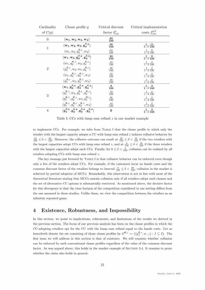
Cardinality

of C(g)

Clause profile g Critical discount

factor δgcrit

Critical implementation

costs fg,δcrit

0 (w1,w2,w3,w4) 80100

1(w1,w2,w3,g

e,z4 ) 56

1001

1−δ11100

(w1, w2, ge,z3 , w4) 64

1001

1−δ9

100

2

(w1,w2,ge,z3 ,ge,z4 ) 20

1001

1−δ9

100

(w1, ge,z2 , w3, g

e,z4 ) 44

1001

1−δ3

100

(ge,z1 , w2, w3, ge,z4 ) 48

1001

1−δ2

100

(w1, ge,z2 , ge,z3 , w4) 52

1001

1−δ3

100

(ge,z1 , w2, ge,z3 , w4) 56

1001

1−δ2

100

3

(w1,ge,z2 ,ge,z3 ,ge,z4 ) 8

1001

1−δ3

100

(ge,z1 , w2, ge,z3 , ge,z4 ) 12

1001

1−δ2

100

(ge,z1 , ge,z2 , w3, ge,z4 ) 36

1001

1−δ2

100

(ge,z1 , ge,z2 , ge,z3 , w4) 44100

11−δ

2100

4 (ge,z1 ,ge,z2 ,ge,z3 ,ge,z4 ) 0 11−δ

2100

Table I: CCs with lump sum refund z in our market example

to implement CCs. For example, we infer from Table I that the clause profile in which only the

retailer with the largest capacity adopts a CC with lump sum refund z induces collusive behavior for56100≤ δ < 80

100. Moreover, the collusive outcome can result at 20

100≤ δ < 56

100if the two retailers with

the largest capacities adopt CCs with lump sum refund z, and at 8100≤ δ < 20

100if the three retailers

with the largest capacities adopt such CCs. Finally, for 0 ≤ δ < 8100

, collusion can be realized by all

retailers adopting CCs with lump sum refund z.

The key message put forward by Table I is that collusive behavior can be enforced even though

only a few of the retailers adopt CCs. For example, if the customers incur no hassle costs and the

common discount factor of the retailers belongs to interval 8100≤ δ < 80

100, collusion in the market is

achieved by partial adoption of MCCs. Remarkably, this observation is not in line with most of the

theoretical literature stating that MCCs sustain collusion only if all retailers adopt such clauses and

the set of alternative CC options is substantially restricted. As mentioned above, the decisive factor

for this divergence is that the time horizon of the competition considered in our setting differs from

the one assumed in those studies. Unlike them, we view the competition between the retailers as an

infinitely repeated game.

4 Existence, Robustness, and Impossibility

In this section, we point to implications, refinements, and limitations of the results we derived in

the previous section. The focus of our previous analysis has been on the clause profiles in which the

CC-adopting retailers opt for the CC with the lump sum refund equal to the hassle costs. Let us

henceforth denote the set consisting of those clause profiles by Ge,z := {(ge,zJ , w−J) : J ⊆ I}. The

first issue we will address in this section is that of existence. We will examine whether collusion

can be enforced by such conventional clause profiles regardless of the value of the common discount

factor. As was argued above, this holds in the market example of Section 3.4. It remains to prove

whether the claim also holds in general.

21


It turns out that if the hassle and implementation costs are “mild”, then there exists at least one

perfectly collusive clause profile in Ge,z for any common discount factor. Usually, several of those

conventional clause profiles prove to be perfectly collusive. Since some of them seem to be more

plausible than others, we impose additional requirements on the clause profiles in order to single out

the most reasonable ones. As will be seen, these additional requirements lead to a unique solution in

Ge,z. Interestingly, this clause profile has a salient spreading pattern of the CCs.

Finally, we will take a glimpse beyond the clause profiles of Ge,z and examine the issue whether

other (conventional) clause profiles could induce collusion. By revisiting the market example of

Section 3.4, we will see that conventional clause profiles with a greater lump sum refund are also

perfectly collusive. Remarkably, some of them induce collusion in a more cost-saving way (i.e., with

a smaller number of CC-adopting retailers) than the ones of with lump sum refunds equal to the

hassle costs. We already know that the latter clause profiles are perfectly collusive regardless of the

underlying rationing rule. However, a complete explicit description of all perfectly collusive clause

profiles is in general not possible without any further reference to the underlying rationing rule.

� An Existence Result

The issue of existence is resolved by Theorems 6 and 13. These theorems ensure the non-emptiness

of solution concept Sm for sufficiently small implementation and hassle costs.

To see this result, we first note that fg,δcrit ≥1

1−δκ1πm for any clause profile g ∈ G. Moreover,

according to Remark 9, it holds zδ1 ≥ z01 for any 0 ≤ δ < δcrit. Therefore, it follows from Theorem

13 that collusion can be enforced by clause profiles of Ge,z for any common discount factor below δcrit

as long as the actual implementation and hassle costs do not exceed 11−δκ1π

m and z01 , respectively.

Apart from that, we know from Theorem 6 that collusion can result without any CCs if the common

discount factor is greater than or equal to δcrit. Putting these findings together, we obtain the

following existence result.

Corollary 14. If the implementation and hassle costs satisfy f ≤ κ1πm and z ≤ z0

1 , respectively, then

it holds for any common discount factor δ and any number of retailers n that solution set Sm(δ, f, n, z)

contains a business policy profile in which all CC-adopting retailers choose the CC with the lump sum

refund equal to hassle costs.

� A Uniqueness Result

According to the last result, if the hassle and implementation costs are sufficiently small, we find

a perfectly collusive clause profile in Ge,z for any common discount factor. However, it turns out

that Ge,z usually contains several perfectly collusive clause profile. For example, consider the market

described in Section 3.4 at common discount factor δ := 12. As can be easily inferred from Theorem

13 and Table I, collusion is reached in this situation if the coalition of the CC-adopting retailers

belongs to system J := {{3, 4}, {2, 4}, {1, 4}, {1, 2, 3}} and each of the CC-adopting retailers chooses

the CC with the lump sum refund equal to the hassle costs.

To select the most plausible ones of these solutions, we impose two additional requirements. These

requirements are based on efficiency and robustness considerations and are lexicographically ranked.

The primary requirement is cost-efficiency and refers to the total implementation costs of a clause

profile, i.e., the sum of the implementation costs of all CC-adopting retailers. A perfectly collusive

clause profile is said to be a cost-efficient in Ge,z if it there is no other perfectly collusive clause

profile in Ge,z with lower total implementation costs (or synonymously, with a smaller number of

CC-adopting retailer). This requirement can be motivated by the argument that (tacitly) concerted

competition clause policies might be easier to realize the less retailers are involved.

22


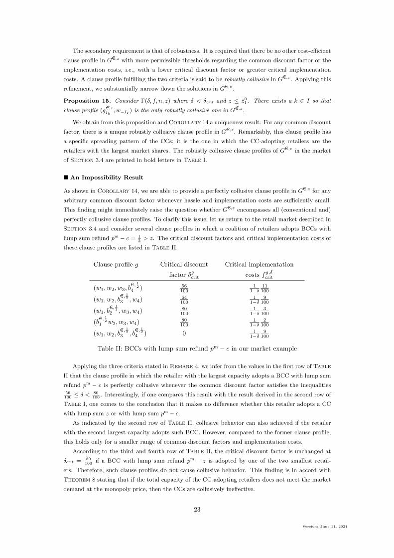
The secondary requirement is that of robustness. It is required that there be no other cost-efficient

clause profile in Ge,z with more permissible thresholds regarding the common discount factor or the

implementation costs, i.e., with a lower critical discount factor or greater critical implementation

costs. A clause profile fulfilling the two criteria is said to be robustly collusive in Ge,z. Applying this

refinement, we substantially narrow down the solutions in Ge,z.

Proposition 15. Consider Γ(δ, f, n, z) where δ < δcrit and z ≤ z01 . There exists a k ∈ I so that

clause profile (ge,zIk, w−Ik ) is the only robustly collusive one in Ge,z.

We obtain from this proposition and Corollary 14 a uniqueness result: For any common discount

factor, there is a unique robustly collusive clause profile in Ge,z. Remarkably, this clause profile has

a specific spreading pattern of the CCs; it is the one in which the CC-adopting retailers are the

retailers with the largest market shares. The robustly collusive clause profiles of Ge,z in the market

of Section 3.4 are printed in bold letters in Table I.

� An Impossibility Result

As shown in Corollary 14, we are able to provide a perfectly collusive clause profile in Ge,z for any

arbitrary common discount factor whenever hassle and implementation costs are sufficiently small.

This finding might immediately raise the question whether Ge,z encompasses all (conventional and)

perfectly collusive clause profiles. To clarify this issue, let us return to the retail market described in

Section 3.4 and consider several clause profiles in which a coalition of retailers adopts BCCs with

lump sum refund pm − c = 12> z. The critical discount factors and critical implementation costs of

these clause profiles are listed in Table II.

Clause profile g Critical discount

factor δgcrit

Critical implementation

costs fg,δcrit

(w1, w2, w3, be, 124 ) 56

1001

1−δ11100

(w1, w2, be, 123 , w4) 64

1001

1−δ9

100

(w1, be, 122 , w3, w4) 80

1001

1−δ3

100

(be, 121 w2, w3, w4) 80

1001

1−δ2

100

(w1, w2, be, 123 , b

e, 124 ) 0 1

1−δ9

100

Table II: BCCs with lump sum refund pm − c in our market example

Applying the three criteria stated in Remark 4, we infer from the values in the first row of Table

II that the clause profile in which the retailer with the largest capacity adopts a BCC with lump sum

refund pm − c is perfectly collusive whenever the common discount factor satisfies the inequalities56100≤ δ < 80

100. Interestingly, if one compares this result with the result derived in the second row of

Table I, one comes to the conclusion that it makes no difference whether this retailer adopts a CC

with lump sum z or with lump sum pm − c.As indicated by the second row of Table II, collusive behavior can also achieved if the retailer

with the second largest capacity adopts such BCC. However, compared to the former clause profile,

this holds only for a smaller range of common discount factors and implementation costs.

According to the third and fourth row of Table II, the critical discount factor is unchanged at

δcrit = 80100

if a BCC with lump sum refund pm − z is adopted by one of the two smallest retail-

ers. Therefore, such clause profiles do not cause collusive behavior. This finding is in accord with

Theorem 8 stating that if the total capacity of the CC adopting retailers does not meet the market

demand at the monopoly price, then the CCs are collusively ineffective.

23


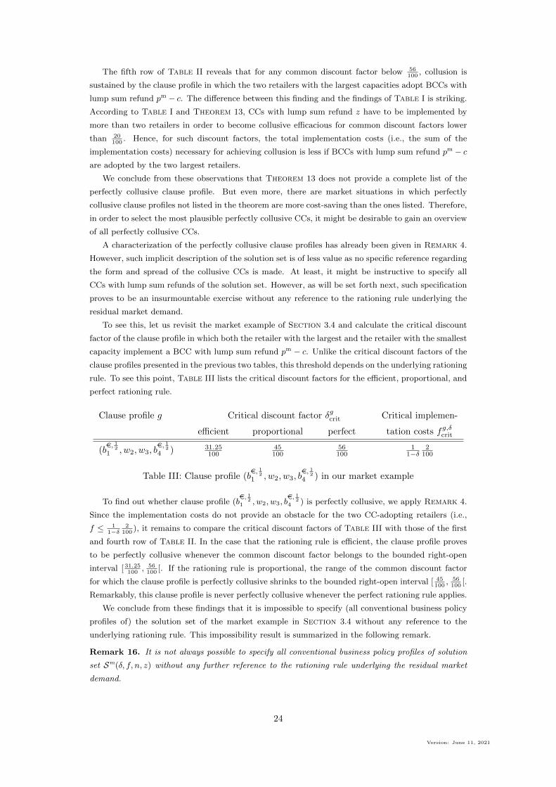
The fifth row of Table II reveals that for any common discount factor below 56100

, collusion is

sustained by the clause profile in which the two retailers with the largest capacities adopt BCCs with

lump sum refund pm − c. The difference between this finding and the findings of Table I is striking.

According to Table I and Theorem 13, CCs with lump sum refund z have to be implemented by

more than two retailers in order to become collusive efficacious for common discount factors lower

than 20100

. Hence, for such discount factors, the total implementation costs (i.e., the sum of the

implementation costs) necessary for achieving collusion is less if BCCs with lump sum refund pm − care adopted by the two largest retailers.

We conclude from these observations that Theorem 13 does not provide a complete list of the

perfectly collusive clause profile. But even more, there are market situations in which perfectly

collusive clause profiles not listed in the theorem are more cost-saving than the ones listed. Therefore,

in order to select the most plausible perfectly collusive CCs, it might be desirable to gain an overview

of all perfectly collusive CCs.

A characterization of the perfectly collusive clause profiles has already been given in Remark 4.

However, such implicit description of the solution set is of less value as no specific reference regarding

the form and spread of the collusive CCs is made. At least, it might be instructive to specify all

CCs with lump sum refunds of the solution set. However, as will be set forth next, such specification

proves to be an insurmountable exercise without any reference to the rationing rule underlying the

residual market demand.

To see this, let us revisit the market example of Section 3.4 and calculate the critical discount

factor of the clause profile in which both the retailer with the largest and the retailer with the smallest

capacity implement a BCC with lump sum refund pm − c. Unlike the critical discount factors of the

clause profiles presented in the previous two tables, this threshold depends on the underlying rationing

rule. To see this point, Table III lists the critical discount factors for the efficient, proportional, and

perfect rationing rule.

Clause profile g Critical discount factor δgcrit Critical implemen-

efficient proportional perfect tation costs fg,δcrit

(be, 121 , w2, w3, b

e, 124 ) 31.25

10045100

56100

11−δ

2100

Table III: Clause profile (be, 121 , w2, w3, b

e, 124 ) in our market example

To find out whether clause profile (be, 1

21 , w2, w3, b

e, 12

4 ) is perfectly collusive, we apply Remark 4.

Since the implementation costs do not provide an obstacle for the two CC-adopting retailers (i.e.,

f ≤ 11−δ

2100

), it remains to compare the critical discount factors of Table III with those of the first

and fourth row of Table II. In the case that the rationing rule is efficient, the clause profile proves

to be perfectly collusive whenever the common discount factor belongs to the bounded right-open

interval [ 31.25100

, 56100

[. If the rationing rule is proportional, the range of the common discount factor

for which the clause profile is perfectly collusive shrinks to the bounded right-open interval [ 45100

, 56100

[.

Remarkably, this clause profile is never perfectly collusive whenever the perfect rationing rule applies.

We conclude from these findings that it is impossible to specify (all conventional business policy

profiles of) the solution set of the market example in Section 3.4 without any reference to the

underlying rationing rule. This impossibility result is summarized in the following remark.

Remark 16. It is not always possible to specify all conventional business policy profiles of solution

set Sm(δ, f, n, z) without any further reference to the rationing rule underlying the residual market

demand.

24


5 Concluding Remarks

In their empirical study of the incidence and variety of low price guarantees, Arbatskaya et al. (2004,

p. 321) point out: “Economic theory is silent on the topic of which guarantee is best because the

literature tends to posit static models of equilibrium in which no firm is ever ‘surprised’. In this

world, both types of guarantees [MCC and BCC] are equally effective at facilitating high prices, and

there are no grounds to choose one over the other.” The aim of our paper is to remedy this obvious

shortcoming in the theoretical literature on low price guarantees. We have modeled the competition

in the retail market as an infinite multi-stage game and have examined the form and spread of low

price guarantees within this game-theoretical framework.

The starting point of our competition model is a perfectly homogeneous commodity market in

which the retailers are identical except for their sales capacities. Their competition clause policies

have been considered as binding commitments. They are implemented at the initial stage of the

competition game, the so-called clause implementation phase, and remain unchanged in the subse-

quent stages. In each of those stages, the retailers compete in the commodity market and advertise

prices for the commodity. The effective prices the retailers charge for the commodity result from

those advertised prices and the implemented competition clause policies. The stages after the clause

implementation phase constitute the so-called price competition phase.

The implementation and exertion of competition clauses (CCs) might be costly in real life. There-

fore, such costs have been taken into account in our framework. More specifically, we have assumed

that the retailers adopting CCs incur the same fixed implementation costs and the customers exercis-

ing CCs incur the same hassle costs per purchased unit of the commodity. Since a substantial part of

the theoretical literature does not consider hassle costs, we have also examined the case of no hassle

costs for the sake of comparability.

Our multi-stage competition game is one with perfect information. When the retailers decide

about the prices at some stage in the price competition phase, they know all previous choices of

their competitors. The consumers are fully informed about the advertised prices and adopted com-

petition clause policies before they go shopping. The assumption of perfect information has serious

consequences. It entails that CCs are not implemented for other reasons than facilitating collusion.

The end date of the price competition phase might, however, be unknown to the retailers. For

this reason, we have viewed the price competition between them as an infinitely repeated game.

Future profits are discounted. In order to also include the cases in which the end date of the price

competition phase is foreseeable for the retailers, we have allowed for the possibility that the common

discount factor can take the value of zero.

To make predictions of the form and spread of collusive CCs, we have applied the solution concept

of subgame perfectness. Additionally, to simplify our analysis, we have assumed that the grim-

trigger price policies are pursued by the retailers in the price competition phase whenever these

policies constitute a subgame perfect equilibrium in this subgame. Otherwise, the retailers pursue

the competitive price policies, i.e., they advertise prices equal to the marginal costs in each stage of

the price competition phase regardless of which prices have been advertised in the previous stages.

The first important result of our analysis has been that the Perfect Folk Theorem by Fried-

man (1971) can be transferred to our extended Bertrand competition game: Whenever the common

discount is sufficiently close to 1, collusive behavior of the retailers is enforceable without adopting

CCs (cf. Theorem 6). In such cases, the threats inherent in the grim-trigger price policies suffice

to induce collusion. However, those threats prove to be too weak whenever the common discount

factor is not sufficiently close to 1. One of the primary objectives of our paper is to examine whether

collusive behavior can be induced by the adoption of CCs for such common discount factors.

25


Our analysis shows that CCs can be used by the retailers as a device facilitating collusion for

any of those discount factors. However, the collusive efficacy of CCs depends on several conditions

regarding the costs, spread, and form of the CCs. Regarding the latter, we have put special emphasis

on BCCs with lump sum refunds. Such BCCs are promises of the retailers that their customers are

entitled to purchase the commodity at the lowest advertised price in the market minus a refund in

the amount of x e whenever the retailers fail to advertise the lowest price in the market.

One necessary condition for the collusive efficacy of CCs is that the implementation and hassle

costs of the CCs are sufficiently small (cf. Theorem 10). If the implementation costs exceed the

total collusive profit of the largest retailer, then it proves to be unprofitable for any retailer to adopt

CCs even though such policy would induce collusion. On the other hand, if the implementation costs

do not exceed the total collusive profit of the smallest retailer, then the implementation costs are no

longer an obstacle for using CCs as a facilitating device.

High hassle costs render any CC collusively ineffective. This follows from our requirement that

the sales price guaranteed by a CC do not fall below the marginal costs whenever the advertised price

is not below the marginal costs. This assumption has been imposed in order to avoid unsustainable

situations in which the CC-adopting retailers incur losses if their customers exercise the CCs. How-

ever, if the hassle costs are “mild” so that any worthwhile price reduction by the smallest retailer can

be immediately undercut by the BCCs of its competitors, collusion becomes enforceable.

To sum up, we agree with Hviid and Shaffer (1999) that the MCC becomes collusively ineffective

in homogeneous retail markets whenever hassle costs exit (cf. Theorem 11). Nevertheless, we cannot

confirm their claim (see Section 4.4 in Hviid and Shaffer, 1999) that other CCs are also collusively

ineffective in this case. Indeed, it has been demonstrated that the collusive outcome can be enforced

if a sufficiently large coalition of retailers offers BCCs with lump sum refunds equal to the hassle costs

(cf. Theorem 13). The reason for this divergence is due to different assumptions regarding the timing

of the competition. Unlike our setting, Hviid and Shaffer (1999) view the retail market as a one-stage

game in which the retailers choose the competition clause policies and the prices simultaneously.

A further necessary condition for the collusive efficacy of CCs is that the total capacity of the

CC-adopting retailers has to be large enough to meet the market demand at the collusive price (cf.

Theorem 8). However, it is in general not required that all retailers have to adopt CCs in order to

enforce collusion, as claimed in most of the earlier theoretical papers on the CCs like in Doyle (1988)

and Logan and Lutter (1989). Some research papers agree with ours that partial adoption of CCs is

consistent with collusive intentions. However, those papers take for granted some asymmetries in the

market such as sequential price-setting or heterogeneous cost or demand conditions. A merit of our

paper is that one has not to resort to such asymmetries to reconcile the theory of collusive CCs with

the striking empirical finding that in most commodity markets only a few retailers adopt CCs.

From the above findings, we have inferred a general collusion existence theorem. If the hassle and

implementation costs are sufficiently small, then collusion is enforceable by a coalition of retailers

adopting the BCC with the lump sum refund equal to the hassle costs. This holds regardless of the

value of the common discount factor (cf. Corollary 14). However, usually there are several of such

collusion inducing coalitions where some exhibit a higher degree of plausibility than others.

To select the most plausible ones, we have substantially refined the solution concept of subgame

perfectness. Our primary selection criterion is cost-efficiency. It requires that the collusive outcome

be induced by minimal total implementation costs. This efficiency criterion could be justified by the

argument that tacit collusion might be more easily enforced the less the number of the CC-adopting

retailers is. In the second place, we require that the coalition induce the lowest critical discount factor

and the highest critical implementation costs. That means, it has to be the most robust with respect

to decreases in the common discount factor and increases in the implementation costs.

26


Applying these refinement criteria, we have obtained a unique spreading pattern of collusively

effective CCs. It has turned out that if all CC-adopting retailers choose the BCC with the lump sum

refund equal to the hassle costs, then the most robust coalition is the one in which the retailers with

the largest market shares offer the CCs (cf. Proposition 15). Remarkably, this spreading pattern

proves to be independent of the rationing rule underlying the residual market demand.

The existence of collusive outcomes has been established by the (partial) adoption of BCCs with

lump sum refunds equal to the hassle costs. Nevertheless, it might be desirable to provide an explicit

description of all collusively effective forms of CCs. However, this task has proved to be insurmount-

able without further assumptions regarding the rationing rule (cf. Remark 16). This impossibility

result is due to the ambiguity that some forms of CCs are collusively efficacious for some rationing

rules, but not for others.

Although our theoretical analysis of the collusive efficacy of CCs is more general than most

previous ones, it has nevertheless some significant limitations which could be addressed in future

research projects. First, our analysis has been focused on the collusive efficacy of CCs with lump sum

refunds. However, as put forward by Arbatskaya et al. (2004), two other forms of CCs are also (or

even more) common in real commercial life, the CCs with a fixed refund factor on price differences

(“We promise that if we do not offer the lowest price in the market, we’ll beat it by an amount equal

to x % of the difference between our announced price and the lowest price in the market.”) and with

a refund factor on the minimum price (“We promise that if we do not offer the lowest price in the

market, we’ll beat it by x % .”). It might be interesting to know whether (the partial adoption of)

such CCs also induce collusion in our setting.

However, as we know from Remark 16, a complete description of all collusively efficacious CCs

is in general impossible without any further reference on the underlying rationing rule. A future

research project could address this problem. By tightening the solution concept and considering

specific settings of our competition model, it might be possible to explicitly specify at least all common

forms of CCs which induce collusion. For example, a promising approach might be to narrow down

the solution set to the most robust solutions; to impose additional, but reasonable requirements on

the rationing rules; and to focus on particular market structures.

Another worthwhile research issue might be to examine whether the most robust collusive solutions

have a common spreading pattern of the CCs. We already derived in Proposition 15 that if all CC-

adopting retailers choose BCCs with the lump sum refund equal to the hassle costs, the spreading

pattern of the CCs in the most robust solution is the one in which the retailers with the largest market

shares adopt the CCs. It is open question whether this salient spreading pattern of the collusive CCs

holds in general.

If this claim can be confirmed, one might have a simple demarcation criterion indicating whether

CCs are used by the retailers as a device facilitating collusion or for some other reasons. Usually,

the partial adoption of competition clauses has been interpreted as an indication that the adoption

of CCs relies on intentions others than the collusive one, e.g., to signal low price or to price differ-

entiate between uninformed loyals and well-informed shoppers; regarding this argument, see e.g. the

expositions in Section 3 in Moorthy and Winter (2006). However, as set forth in our paper, this

conclusion might not be justified in general. Rather, if the above claim holds, the market shares of the

CC-adopting retailers should be used as an indicative criterion for collusion. For example, collusive

intentions might prevail in markets where the CCs are adopted by dominant retailers. If only fringe

retailers offer CCs, the CCs might be implemented for other motives than collusion.

27


Appendix: Proofs

Proof of Remark 1.

(a) To prove this claim, we consider the situation in which clause profile g has been adopted and

retailer i advertises price qi 6= pm while its competitors advertise prices pm−i.

� Suppose qi > c. Due to Assumption (G), the effective sales price at retailer i amounts to qsi ≥ c

so that πgi (qi, pm−i) = (qs

i − c)Xi(qp) ≥ 0. We conclude from this weak inequality that

0 ≤ supc<qi 6=pm

πgi (qi, pm−i) ≤ sup

qi 6=pmπgi (qi, p

m−i).

� Suppose qi ≤ c. Due to Assumption (G), the effective sales price at retailer i is qsi = qi so that

πgi (qi, pm−i) = (qi − c)Xi(qp) ≤ 0. Note that if qi = c, we have πgi (qi, p

m−i) = (qi − c)Xi(qp) = 0.

We conclude that

supqi≤c

πgi (qi, pm−i) = 0.

By bringing the above two results together, we obtain

0 ≤ supc<qi 6=pm

πgi (qi, pm−i) = sup

qi 6=pmπgi (qi, p

m−i).

(b) To prove this claim, we consider the situation in which clause profile g has been adopted and

retailer i advertises price qi 6= pm while its competitors advertise prices pm−i.

� Suppose qi > pm. Since retailer i’s competitors are assumed to advertise collusive price pm,

Assumption (G) implies that the effective purchase price charged by them is equal to pm. The

effective purchase price at retailer i can be either above or equal to or below pm.

In the first case, Assumptions (D2), (D4), (R1), and (I) imply that the demand for the product

offered by retailer i is zero. Hence, retailer i earns a profit πgi (qi, pm−i) = 0. We conclude that

πgi (qi, pm−i) < (pm − c) min{ki, D(pm)}

if qpi > pm.

In the second case, Assumptions (R1) and (I) imply that retailer i sells quantity Xi(qp) =

κiD(pm) and, thus, earns a profit πgi (qi, pm−i) = (pm − z − c)κiD(pm). Since z ≥ 0, we have

πgi (qi, pm−i) ≤ (pm − c)κiD(pm). Moreover, Assumption (D4) entails D(pm) < K so that

(pm − c)κiD(pm) < (pm − c) max{ki, D(pm)}. We conclude that

πgi (qi, pm−i) < (pm − c) max{ki, D(pm)}

if qpi = pm.

Finally, assume the last case. Due to Assumptions (R1) and (I), retailer i sells quantity

Xi(qp) = min{ki, D(qp

i )} so that its profit amounts to πgi (qi, pm−i) = (qp

i − z− c) min{ki, D(qpi )}.

Since z ≥ 0, it holds πgi (qi, pm−i) ≤ (qp

i − c) min{ki, D(qpi )}. Moreover, qp

i < pm entails (qpi −

c) min{ki, D(qpi )} < (pm − c) min{ki, D(pm)} so that

πgi (qi, pm−i) < (pm − c) min{ki, D(pm)}.

� Suppose qi < pm. In this case, Assumption (G) implies that the effective purchase price

at retailer i corresponds to the advertised one, i.e., qpi = qi. Since retailer i’s competitors

advertise collusive price pm, it also follows from Assumption (G) that the effective purchase

prices charged by them are somewhere between c and pm. Due to Assumptions (R1) and (I),

the sales of retailer i is bounded from above by Xi(qp) ≤ min{ki, D(qi)}. Since qi < pm, we

obtain

πgi (qi, pm−i) ≤ (qi − c) min{ki, D(qi)} ≤ (pm − c) min{ki, D(pm)}.

28


Summing up the above results, we have established

supqi 6=pm

πgi (qi, pm−i) ≤ (pm − c) min{ki, D(pm)}. �

Proof of Remark 2. Let us suppose clause profile w has been implemented, i.e., none of the retailers

has adopted a CC. Moreover, consider some retailer i advertising price qi < pm. Since its competitors

are assumed to advertise collusive price pm, retailer i underbids all of them. Due to Assumptions

(R1) and (I), retailer i’s sales are then given by Xi(qi, pm−i) = min{ki, D(qi)} so that it earns a profit

πi(qi, pm−i) = (qi − c) min{ki, D(qi)}.

� Suppose ki ≤ D(pm). It follows from Assumption (D2) that πi(qi, pm−i) = (qi − c)ki. This

in turn implies supqi<pm πi(qi, pm−i) = (pm − c)ki. Applying Remark 1(b), we even obtain

supqi 6=pm πi(qi, pm−i) = (pm − c)ki. Since

1

1− δ κi π(pm) ≥ supqi 6=pm

πi(qi, pm−i) ⇐⇒ δ ≤ 1− D(pm)

K,

it holds δi,crit = min ∆i = 1− D(pm)K

.

� Suppose ki > D(pm). It follows from Assumption (D1) that there is some ε > 0 so that

ki > D(qi) for any pm − ε < qi < pm. This in turn implies Xi(qi, pm−i) = D(qi) for any

pm − ε < qi < pm. Moreover, Assumption (D1) ensures limqi↑pm Xi(qi, pm−i) = D(pm) and,

thus, limqi↑pm πi(qi, pm−i) = πm. We conclude from this result that supqi<pm πi(qi, p

m−i) = πm.

Applying Remark 1(b), we even have supqi 6=pm πi(qi, pm−i) = πm. Since

1


qi 6=pmπi(qi, p

m−i) ⇐⇒ δ ≤ 1− κi,

it holds δi,crit = min ∆i = 1− κi.

Summing up the above two cases, we have shown that supqi 6=pm πi(qi, pm−i) = (pm−c) min{ki, D(pm)}

and, thus, δi,crit = 1−max{κi, D(pm)K}.

Consider now some arbitrary clause profile g. Due to Remark 1(b) and the above result, it holds

supqi 6=pm πgi (qi, p

m−i) ≤ (pm − c) min{ki, D(pm)} = supqi 6=pm πi(qi, p

m−i). Therefore, we have

∆i :=

{δ ∈ [0, 1[:

1


πi(qi, pm−i)

}⊆

{δ ∈ [0, 1[:

1


πgi (qi, pm−i)

}=: ∆g

i .

It immediately follows from ∆i ⊆ ∆gi that δi,crit ≥ δgi,crit. �

Proof of Remark 3. To prove this remark, we resort to Theorem 3.2. of Fudenberg and Tirole

(1991). This theorem states that if a multi-stage game is continuous at infinity, then a strategy

profile is subgame perfect if, and only if, none of the players can increase its payoff in any subgame

through a one-shot deviation. This characterization of subgame perfectness is known as the One-

Shot Deviation Principle.

Our first step is to establish that this theorem is indeed applicable to our competition game.

Afterwards, the One-Shot Deviation Principle is formalized. We then apply this principle to

show that (i) the grim-trigger price policy profile tg is subgame perfect in Γg if, and only if, δ ≥ δgcrit,

and (ii) the competitive price policy profile cg is subgame perfect in subgame Γg for any δ ≥ 0. With

these results at hand, the proof of the “if”- and “only if”-part of the remark follows immediately.

29


Our competition game Γ is continuous at infinity if for any ε > 0, any retailer i ∈ I, and any

outcome o ∈ O, there exists a period t0 so that

|Πi(o)−Πi(o)| < ε

for any outcome o ∈ O satisfying ot = ot for any period t ≤ t0. To establish this property, let us

consider some ε > 0, some retailer i ∈ I, and some outcome o := (g, q0, q1, . . . ) ∈ O. We note that,

due to Assumptions (D1),(D2), (R1) and (I), the one-stage profit πi is bounded. More precisely, it

holds −cD(0) ≤ πi(q) ≤ πm for any profile q ∈ RI+ of advertised prices. Let us define η := πm+cD(0).

Obviously, it holds |πgi (q) − πgi (q)| ≤ η for any q, q ∈ RI+ and g ∈ G. Choose some sufficiently large

period t0 ≥ 0 so that δt0

1−δ η < ε. Moreover, consider some outcome o := (g, q0, q1, . . . ) ∈ O which is

consistent with outcome o up to period t0 − 1, i.e, g = g and qt = qt for any period 0 ≤ t ≤ t0 − 1.

Since

|Πi(o)−Πi(o)| =

∣∣∣∣∣∞∑t=0

δtπgi (qt)−∞∑t=0

δtπgi (qt)

∣∣∣∣∣=

∣∣∣∣∣∞∑t=t0

δt(πgi (qt)− πgi (qt)

)∣∣∣∣∣≤∞∑t=t0

δt∣∣πgi (qt)− πgi (qt)

∣∣≤ δt0

1− δ η

< ε ,

we have shown that competition game Γ satisfies continuity at infinity.

A business policy si in competition game Γ is said to be a one-shot deviation from business policy

si if si deviates from si at a single history, i.e., there is some history h so that s|H\{h} = s|H\{h} and

s(h) 6= s(h). A strategy profile s := (si)i∈I is said to satisfy the one-shot deviation property if none

of the players gains by a one-shot deviation in any subgame of Γ, or more formally, if

Πi(oh(s)) ≥ Πi(o

h(s))

for any strategy profile s := (si, s−i) ∈ S where si is a one-shot deviation from si, any player i ∈ I,

and any history h ∈ H. We remark that this property can be described in a simpler way. As can be

easily shown, it suffices to demonstrate that the above weak inequality is satisfied for any strategy

profile s := (si, s−i) ∈ S where si is a one-shot deviation from si at history h.

According to Theorem 3.2 of Fudenberg and Tirole (1991), subgame perfectness can be checked

by the one-shot deviation property. Note, since our competition game Γ is continuous at infinity, any

of its subgames is continuous at infinity, too. Therefore, it is admissible to apply the One-Stage

Deviation Principle to any subgame of Γ. In the following, we do this for the subgames Γg.

We conclude from these considerations that price policy profile sg proves to be subgame perfect

in Γg if, and only if, none of the retailers can increase its payoff by an one-shot deviation from sg in

some subgame of Γg. This in turn means that sg is subgame perfect in Γg if, and only if, it holds for

any retailer i ∈ I that Πi(oh(s)) ≥ Πi(o

h(s)) is satisfied for some business policy profile s inducing

sg in Γg and any business policy profile s := (si, s−i) which is a one-shot deviation of si at some

non-initial history h ∈ Ht0g (i.e., h is a history up to period t0 ≥ −1 according to which clause profile

g has been adopted in the implementation phase).

Let us first prove claim (i). For this purpose, we pick some clause profile g ∈ G and consider some

business policy profile s inducing the grim-trigger price policy profile tg := (tgj )j∈I in subgame Γg.

Moreover, we choose some period t0 ≥ −1 and some history h ∈ Ht0g .

30


� Suppose either t0 = −1 or ht0j,t = pm for any j ∈ I and any 0 ≤ t ≤ t0. The outcome induced by

history h and business policy profile s is oh(s) = (h, pm, pm, pm, . . . ). Pick some retailer i ∈ I and

suppose now that retailer i pursues business policy si which is one-shot deviation from business

policy si at non-initial history h ∈ Ht0g . Let sgi be the price policy in subgame Γg induced by

business policy si. Obviously, sg differs from grim-trigger price policy tgi only at history h. We

define qt0+1i := sgi (h). By construction, qt0+1

i 6= tgi (h) = pm. The outcome induced by history h

and business policy profile s := (si, s−i) is oh(s) = (h, (qt0+1i , pm

−i), c, c, . . . ).

Hence, it holds

Πi(oh(s)) ≥ Πi(o

h(s))

⇐⇒∞∑t=0

δtπgi (pm) ≥

(t0∑t=0

δtπgi (pm)

)+ δt0+1πgi (qt0+1

i , pm−i)

⇐⇒ δt0+1

1− δ πgi (pm) ≥ δt0+1πgi (qt0+1

i , pm−i)

⇐⇒ 1

1− δ κi πm ≥ πgi (qt0+1

i , pm−i).

Since qt0+1i 6= pm can be arbitrarily chosen, a one-shot deviation from the grim-trigger price

policy at history h proves to be not profitable for retailer i in subgame Γh if, and only if, the

common discount factor δ satisfies

1


qi 6=pmπgi (qi, p

m−i).

� Suppose t0 ≥ 0 and ht0j,t 6= pm for some j ∈ I and some 0 ≤ t ≤ t0. The outcome induced by

history h and business policy profile s is oh(s) := (h, c, c, c, . . . ). Pick some retailer i ∈ I and

suppose now that retailer i pursues business policy si which is one-shot deviation from business

policy si at non-initial history h ∈ Ht0g . Let sgi be the price policy in subgame Γg induced by

business policy si. Obviously, sgi differs from grim-trigger price policy tgi only at history h. As

above, we define qt0+1i := sgi (h). By construction, qt0+1

i 6= tgi (h) = c. The outcome induced by

history h and business policy profile s := (si, s−i) is oh(s) = (h, (qt0+1i , c−i), c, c, . . . ).

Note that Assumptions (D2), (D4), (R1), and (I) entail 0 ≥ πgi (qt0+1i , c−i). Therefore, we

obtain

Πi(oh(s)) − Πi(o

h(s))

=

t0∑t=0

δtπgi (ht) −

((t0∑t=0

δtπgi (ht)

)+ δt0+1πgi (qt0+1

i , c−i)

)= − δt0+1πgi (qt0+1

i , pm−i)

≥ 0.

Since qt0+1i 6= pm can be arbitrarily chosen, a one-shot deviation from the grim-trigger price

policy at history h is never profitable for retailer i in subgame Γh regardless of the common

discount factor δ ≥ 0.

Summing up the above two cases, one-shot deviations from the grim-trigger price policy are not

profitable for retailer i in any subgame of Γg if, and only if, common discount factor δ satisfies the

weak inequality1


qi 6=pmπgi (qi, p

m−i),

or equivalently, δ ≥ δgi,crit. From this weak inequality, we conclude that none of the retailers has an

incentive in some subgame of Γg to choose a one-stage deviation from the grim-trigger price policy

31


if, and only if, δ ≥ δgcrit := max{δgi,crit : i ∈ I}. Resorting to the One-Shot Deviation Principle,

we conclude that the grim-trigger price policy profile is subgame-perfect in subgame Γg as long as

δ ≥ δgcrit.

Let us now prove claim (ii). For this purpose, pick some clause profile g ∈ G and some business

policy profile s inducing the competitive price policy cg := (cgj )j∈I in subgame Γg. Moreover, choose

some period t0 ≥ −1 and some history h ∈ Ht0g . Obviously, the outcome induced by history h and

business policy profile s is oh(s) = (h, c, c, c, . . . ).

Choose some retailer i and suppose now that retailer i pursues business policy si which is one-

shot deviation from business policy si at non-initial history h ∈ Ht0g . Let sgi be the price policy in

subgame Γg induced by business policy si. Obviously, sgi differs from competitive price policy cgi only

at history h. We define qt0+1i := si(h). By construction qt0+1

i 6= cgi (h) = c. The outcome induced by

h and business policy profile s := (si, s−i) is oh(s) = (h, (qt0i , c−i), c, c, . . . ).

Due to Assumptions (D2), (D4), (R1), and (I), it holds 0 ≥ πgi (qt0+1i , c−i). Hence, we obtain

Πi(oh(s)) − Πi(o

h(s))

=

t0∑t=0

δtπgi (ht) −

((t0∑t=0

δtπgi (ht)

)+ δt0+1πgi (qt0+1

i , c−i)

)= − δt0+1πgi (qt0+1

i , pm−i)

≥ 0.

Since qt0+1i 6= pm can be arbitrarily chosen, a one-shot deviation from the competitive price policy at

history h is never profitable for retailer i in subgame Γh regardless of common discount factor δ ≥ 0.

This holds for any retailer i so that none of them has an incentive to choose a one-stage deviation

from the competitive price policy in any subgame of Γg regardless of the value of common discount

factor δ. Applying the One-Shot Deviation Principle, we conclude that the competitive price

policy is subgame-perfect in subgame Γg for any common discount factor δ ≥ 0.

Summing up, we have shown that (i) the grim-trigger price policy profile in subgame Γg is subgame

perfect if, and only if, δ ≥ δgcrit, and (ii) the competitive price policy profile in subgame Γg is subgame

perfect for any δ ≥ 0. Resorting to these results, we will prove the “if”- and “only if”-part of this

remark.

(“if ”) Let s := (si)i∈I be a strategy profile satisfying Properties (T1) and (T2). Applying our

result (i) to Property (T1), we obtain

sg =

{tg if tg is a subgame perfect equilibrium in Γg,

cg otherwise

for any clause profile g ∈ G. We also know from our result (ii) that competitive price policy profile

cg is subgame perfect in any subgame Γg. Therefore, business policy profile s induces a subgame

perfect strategy profile in any subgame Γg. This in turn implies that any one-stage deviation from

s at histories h ∈ Ht0 where t0 ≥ −1 is not profitable in subgame Γh. According to the One-Shot

Deviation Principle, in order to establish that s is subgame perfect in Γ, it remains to show that

one-stage deviations from si at initial history h := ∅ are also not profitable for any retailer i. However,

this is guaranteed by Property (T2).

(“only if ”) Let s := (si)i∈I ∈ Sg(Γ). Applying our result (i) to the construction of s, we conclude

that

sg =

{tg if tg if δ ≥ δgcrit,

cg otherwise

and, thus, Property (T1) is satisfied. Moreover, the One-Shot Deviation Principle immediately

implies Property (T2). �

32


Proof of Remark 4. (“if ”) Consider the business policy profile s := (g, (sg)g∈G) satisfying Prop-

erty (T1). By Property (M1), the grim-trigger price policies are applied by all retailers in subgame

Γg. This entails that business policy profile s induces the collusive outcome and, thus, any retailer i

earns a total profit

Πi(o(s)) =1

1− δ κi π(pm)− 1Ci(gi) f.

at this business policy profile.

Let us now consider a business policy profile s := (si, s−i)) where si := (gi, (sgi )g∈G) and gi 6= gi.

In words, the only difference between business policy profiles s and s is that retailer i pursues a

different competition clause policy. In the following, we compare the total profits retailer i earns at

those business policy profiles:

� If δ ≥ δgcrit as well as i ∈ C(g) and i ∈ C(g), then both business policy profiles induce the

collusive outcome. Since retailer i adopts a CC in both business policy profiles, we obtain

Πi(o(s)) =1

1− δ κi π(pm)− f = Πi(o(s)) .

� If δ ≥ δgcrit as well as i /∈ C(g) and i ∈ C(g), then both business policy profiles induce the

collusive outcome. Since retailer i does not adopt a CC in business policy profile s, but in

business policy profile s, we obtain

Πi(o(s)) =1

1− δ κi π(pm) >1

1− δ κi π(pm)− f = Πi(o(s)) .

� If δ < δgcrit as well as i ∈ C(g) and i ∈ C(g), then different outcomes are realized by the two

business policy profiles. While the collusive outcome is reached by business policy profile s, the

competitive outcome is reached by business policy profile s. Since retailer i adopts a CC in both

business policy profiles, we obtain

Πi(o(s)) =1

1− δ κi π(pm)− f > −f = Πi(o(s)) .

� If δ < δgcrit as well as i /∈ C(g) and i ∈ C(g), then different outcomes are realized by the two

business policy profiles. While the collusive outcome is reached by business policy profile s, the

competitive outcome is reached by business policy profile s. Since retailer i does not adopt a

CC in business policy profile s, but in business policy profile s, we obtain

Πi(o(s)) =1

1− δ κi π(pm) > −f = Πi(o(s)) .

� If i ∈ C(g) and i /∈ C(g), then g = (wi, g−i). It follows from Property (M2) that δ < δgcrit.

Hence, while business policy profile s induces the collusive outcome, business policy profile s

induces the competitive outcome. Note that retailer i adopts a CC in business policy profile s,

but does not in business policy profile s. Nevertheless, we obtain from Property (M3) that

Πi(o(s)) =1

1− δ κi π(pm)− f =1

1− δ κi π(pm)− fg,δcrit ≥ 0 = Πi(o(s)) .

Summing up, we obtain Πi(o(s)) ≥ Πi(o(s)) for any business policy profile s := (si, s−i) where

si := (gi, (sgi )g∈G). That means, Property (T2) has been established. Moreover, since business

policy profile s also satisfies Property (T1) by construction, we conclude from Remark 3 that s is

subgame perfect. As was shown above, s induces the collusive outcome. Hence, s ∈ Sm(δ, f, n, z).

(“only if ”) Suppose clause profile g is perfectly collusive. By definition, there is a business policy

profile s := (g, (sg)g∈G) ∈ Sm(δ, f, n, z). Obviously, s ∈ Sg(δ, f, n, z). We conclude from Remark

3 that s satisfies Properties (T1) and (T2). Since s induces the collusive price outcome, it holds

δ ≥ δgcrit and, hence, Property (M1) is satisfied.

33


We proceed indirectly to establish Property (M2). Let us suppose contrary to our claim that

δgcrit ≤ δ for some clause profile g := (wi, g−i) where i ∈ C(g). We define business policy profile

s := (g, (sg)g∈G). Since business policy profile sg induces the grim-trigger price policy profile in

subgame Γg, the collusive outcome is realized by s and it holds

Πi(o(s)) =1

1− δ κi π(pm) >1

1− δ κi π(pm)− f = Πi(o(s)) .

However, this result contradicts Property (T2). Hence, it holds δ < δgcrit for any g := (wi, g−i)

where i ∈ C(g). We conclude that Property (M2) is satisfied.

We also proceed indirectly to establish Property (M3). Let us suppose that Properties (M1)

and (M2) are satisfied and contrary to our claim that f > f g,δcrit. We note that the latter strict

inequality implies C(g) 6= ∅; otherwise, it would be f g,δcrit = +∞ and the strict inequality could

not be satisfied. Consider retailer i := minC(g) and business policy profile s := (si, s−i) where

si := (wi, (sgi )g∈G). Resorting to Properties (M1) and (M2), we obtain

Πi(o(s)) = 0 =1

1− δ κi π(pm)− f g,δcrit >1

1− δ κi π(pm)− f = Πi(o(s)) .

Apparently, this strict inequality violates Property (T2). Hence, it holds f ≤ f g,δcrit and, thus,

Property (M3) has been established. �

Proof of Proposition 5. We prove this claim by contradiction. Suppose s := (g, (sg)g∈G) is a

subgame perfect business policy profile (of Sg(δ, f, n, z)) in which retailer i adopts a CC, but which

induces the competitive price outcome. That means, gi 6= wi and sg = cg. Obviously, retailer i earns

a profit Πi(o(s)) = −f at this business policy profile. Consider now the business policy profile s

which corresponds to s except that instead of adopting gi retailer i abstains from offering any CC,

i.e., s := (si, s−i) where si := (wi, (sgi )g∈G). We obtain Πi(o(s)) ≥ 0 > Πi(o(s)), violating property

(T2). Remark 3 implies that s is not subgame perfect. However, this result is at odds with our

initial assumption. �

Proof of Theorem 6.

(a) We proceed indirectly. If δ < δcrit, then clause profile w (i.e., the clause profile in which none of

the retailers adopts a CC) violates Property (M1). We conclude from Remark 4 that clause profile

w is not perfectly collusive if δ < δcrit.

(b) Suppose δ ≥ δcrit. Let us first examine whether clause profile w is perfectly collusive. By

assumption, Property (M1) holds. Property (M2) is trivially satisfied because C(w) = ∅. Note

that fw,δcrit = +∞ by definition. Therefore, Property (M3) is also satisfied. We infer from Remark

4 that clause profile w is perfectly collusive.

To prove the uniqueness of the perfectly collusive clause profile, let us consider some clause profile

g 6= w. Since C(g) 6= ∅, we can pick some i ∈ C(g) and define clause profile g := (wi, g−i). Applying

Remark 2, we obtain δ ≥ δgcrit. This in turn entails that clause profile g violates Property (M1). It

follows from Remark 4 that g is not perfectly collusive. Summing up, we have shown that if δ ≥ δcrit,

then the trivial clause profile w is the unique perfectly collusive clause profile. �

Proof of Remark 7. Obviously, the claim is true for the trivial clause profile w. For this reason,

let us suppose from now on that clause profile g satisfies C(g) 6= ∅. Our assumption KC(g) ≤ D(pm)

implies k1 ≤ D(pm). Applying Remark 2, we obtain δcrit = 1− D(pm)K

.

Pick some i ∈ C(g). We examine the situation in which retailer i advertises price qi < pm while

all of its competitors advertise price pm. Since KC(g) ≤ D(pm), retailer i’s sales at the effective

34


purchase prices qp are Xi(qp) = ki by Assumptions (D2), (R1), and (I). Hence, its profit amounts

to πgi (qi, pm−i) = (qi− c)ki. Since qi < pm has been arbitrarily chosen, we have supqi<pm π

gi (qi, p

m−i) =

(pm − c)ki. It follows from Remark 1(b) that supqi 6=pm πgi (qi, p

m−i) = (pm − c)ki and, thus, δgi,crit =

1− D(pm)K

. By Remark 2, we obtain δgcrit = δcrit. �

Proof of Theorem 8. We prove this claim by contradiction. Suppose there is a perfectly collusive

clause profile g satisfying KC(g) ≤ D(pm). We already know from Remark 7 that δgcrit = δcrit. Since

δ < δgcrit is assumed, Property (M1) is violated. It follows from Remark 4 that clause profile g is

not perfectly collusive. �

Proof of Remark 9. Pick some retailer i and suppose δ < δi,crit. Due to Assumption (D2),

the monopolistic profit mapping πi(·) is continuous. Assumptions (D1) and (D3) ensure that πi(·)is increasing on [c, pm]. Moreover, it holds πi(c) = 0 and πi(p

m) = (pm − c) min{ki, D(pm)}. By

assumption and Remark 2, we have δ < 1−max{κi, D(pm)K}. Regardless of whether ki ≤ D(pm) or

ki > D(pm), we always obtain

πi(c) = 0 <1

1− δ κiπm < (pm − c) min{ki, D(pm)} = πi(p

m).

The Intermediate Value Theorem implies that there exists some pδi ∈]c, pm[ satisfying πi(pδi ) =

11−δκiπ

m. Moreover, since monopolistic profit mapping πi(·) is increasing on [c, pm], value pδi is

unique.

Consider some common discount factor β < δ. As argued above, there exists some unique pβi ∈]c, pm[ satisfying πi(p

βi ) = 1

1−βκiπm. Note that 1

1−βκiπm < 1

1−δκiπm. Since monopolistic profit

mapping πi(·) is increasing on [c, pm], we obtain pβi < pδi .

Consider some retailer j < i. As argued above, there exists some unique pδi ∈]c, pm[ so that

πi(pδi ) = 1

1−δκiπm. Since kj < ki, it holds πj(p) ≥ kj

kiπi(p) for any p ≥ c. In particular, we have

πj(pδi ) ≥

kjkiπi(p

δi ) = 1

1−δκjπm. Since monopolistic profit mapping πj(·) is increasing on [c, pm], we

conclude that pδj ≤ pδi . �

Proof of Theorem 10. We prove this claim by contradiction. Suppose that f > fδ, but g is

perfectly collusive. Since δ < δcrit, we infer from Theorem 8 that KC(g) > D(pm). Obviously,

C(g) 6= ∅ and, thus, we can define i := minC(g). By assumption, f > 11−δκiπi(p

m). However, this

strict inequality is at odds with Property (M3). It follows from Remark 4 that g is not perfectly

collusive.

From now on, we assume that f ≤ fδ, but z > zδ1 . To show that there is no perfectly collusive

collusive price even in this case, consider some arbitrary clause profile g and retailer 1. Moreover,

suppose that retailer 1 advertises some price c + zδ1 < q1 < min{c + z, pm} while its competitors

advertise price pm. Due to Assumption (G), it holds q1 < qpj for any retailer j different from 1.

Therefore, we obtain

πg1(q1, pm−1) = (q1 − c) min{k1, D(q1)} = π1(q1)

By definition, π1(c + zδ1) = 11−δκ1π

m. Since π1(·) is increasing on [c, pm], it follows πg1(q1, pm−1) >

11−δκ1π

m and, thus,

supq1 6=pm

πg1(q1, pm−1) >

1

1− δ κ1πm.

We conclude from this result that δ < δg1,crit ≤ δgcrit. However, this results violates Property (M1)

of Remark 4. Consequently, clause profile g is not perfectly collusive. �

Proof of Theorem 11. Consider a clause profile g in which retailer i offers a CC of the form ge,µi

where µ < z. Moreover, we define g := (wi, g−i), which is the clause profile corresponding to g except

from retailer i not implementing a CC. We will show δgcrit = δgcrit.

35


For this purpose, let us first consider retailer i. We suppose that this retailer advertises price

qi 6= pm while its competitors advertise price pm. In the following, we compare the profits retailer i

earns under the clause profiles g and g given such price announcements.

� Suppose qi > pm. By assumption, it holds pm − z < gsi(qi, p

m−i) ≤ gs

i(qi, pm−i) = qi. This

immediately implies gpi (qi, p

m−i) > pm and gp

i (qi, pm−i) > pm. Moreover, due to Assumption (G),

we have gpk(qi, p

m−i) = gp

k(qi, pm−i) = pm for any k 6= i. We conclude from Assumptions (D2),

(D4), (R1), and (I) that Xi(gp(qi, p

m−i)) = 0 = Xi(g

p(qi, pm−i)) and, thus, πgi (qi, p

m−i) = 0 =

πgi (qi, pm−i).

� Suppose qi < pm. By Assumption (G), we have gpi (qi, p

m−i) = gp

i (qi, pm−i) = qi. Moreover,

it holds gpk(qi, p

m−i) = gp

k(qi, pm−i) ≤ pm for any k 6= i. Since gp(qi, p

m−i) = gp(qi, p

m−i), we

obtain Xi(gp(qi, p

m−i) = Xi(g

p(qi, pm−i)). It follows from gs

i(qi, pm−i) = gs

i(qi, pm−i) = qi that

πgi (qi, pm−i) = πgi (qi, p

m−i).

Let us now consider some retailer j 6= i and suppose that this retailer advertises price qj 6= pm

while its competitors advertise price pm. In the following, we will specify the profits retailer j earns

under the clause profiles g and g given such price announcements.

� Suppose qj > pm. It holds gpj (qj , p

m−j) = gp

j (qj , pm−j) ≤ qk. Moreover, Assumption (G) implies

gpj (qj , p

m−j) = gc

j(qj , pm−j) = pm for any k 6= j. Since gp(qj , p

m−j) = gp(qj , p

m−j), we obtain

Xj(gp(qj , p

m−j) = Xk(gp(qj , p

m−j)). It follows from gs

i(qi, pm−i) = gs

j(qj , pm−j) that πgj (qj , p

m−j) =

πgj (qj , pm−j).

� Suppose qj < pm. We note that qj = gpj (qj , p

m−j) = gp

j (qj , pm−j). Moreover, it holds gp

k(qk, pm−k) =

gpk(qk, p

m−k) ≤ pm for any k 6= i, j. By assumption, we have qj−z < gs

i(qi, pm−i) ≤ gs

i(qi, pm−i) = pm.

This in turn implies qj < gpi (qi, p

m−i) ≤ gp

i (qi, pm−i) = pm. Hence, we obtain [gp(qj , p

m−j) < qj ] =

[gpj (qj , p

m−j) < qj ] and [gp(qj , p

m−j) = qj ] = [gp

j (qj , pm−j) = qj ]. We conclude from Assumptions

(R2) and (I) that Xj(gp(qj , p

m−j) = Xk(gp(qj , p

m−j)). It follows from gs

i(qi, pm−i) = gs

j(qj , pm−j)

that πgj (qj , pm−j) = πgj (qj , p

m−j).

Summing up, we have shown πgk(qk, pm−k) = πgk(qk, p

m−k) for any qk 6= pm and any k ∈ I. This

implies supqk 6=pm πgk(qk, p

m−k) = supqk 6=pm π

gk(qk, p

m−k) and, thus, δgj,crit = δgj,crit for any j ∈ I. The

latter result in turn entails δgcrit = δgcrit.

However, the equality violates Property (M2). Since according to Remark 4 this property is a

necessary condition for subgame perfect collusion, we conclude that clause profile g is not perfectly

collusive. Thereby, we have shown that none of the retailers in a perfectly collusive profile adopts a

CC with lump sum refund µ < z. �

Proof of Remark 12.

Before proving parts (a) and (b) of the claim, we derive some general statements. First, note that

if κJ ≥ 1 − δ and δ < δcrit, it follows from Remark 2 that κJ > max{κ1,

D(pm)K

}. This in turn

implies KJ > D(pm). Therefore, although not explicitly stated there, KJ > D(pm) holds even in

part (b).

Let g be a clause profile in which a coalition J ⊆ I of retailers adopt a CC with lump sum refund

z and the other retailers do not adopt a CC, i.e., g is given by g := (gJ , w−J) where gi := ge,zi for

any i ∈ J . We suppose that KJ > D(pm).

Pick some i ∈ J of the CC-adopting retailers and consider the situation in which retailer i

advertises price qi 6= pm while its competitors advertise price pm. In the following, we will provide

some upper bounds of i’s profit πgi (qi, pm−i).

36


� If qi > pm, the CC of retailer i implies qpi = pm and qs

i = pm−z. Moreover, we have qpj = qs

i = pm

for any competitor j 6= i. It follows from Assumptions (R1) and (I) that retailer i’s sales are

Xi(qp) = κiD(pm) and, thus, its profit amounts to πgi (qi, p

m−i) = (pm − z − c)κiD(pm). Since

the latter result holds for any qi > pm, we obtain

supqi>pm

πgi (qi, pm−i) = (pm − z − c)κiD(pm) .

� If c + z ≤ qi < pm, it holds qpi = qs

i = qi. Moreover, the CCs of the competitors j ∈ J \ {i}imply that qs

j = qi − z and qpj = qi for any j ∈ J \ {i}. Obviously, the competitors j ∈ I \ J

charge price qpj = qs

j = pm. It follows from Assumptions (R1) and (I) that retailer i’s sales

are Xi(qp) = min{ki, κiκJD(qi)} so that it earns a profit πgi (qi, p

m−i) = (qi − c) min{ki, κiκJD(qi)}.

Since the latter result holds for any c+ z ≤ qi < pm and KJ > D(pm) is assumed, we conclude

from Assumptions (D1), (D2), and (D3) that

supc+z≤qi<pm

πgi (qi, pm−i) = (pm − c) κi

κJD(pm) .

� If c ≤ qi < c+ z, it holds qpi = qs

i = qi. Moreover, since the CCs of the competitors j ∈ J \ {i}satisfy Assumption (G), we have qs

j = c and qpj = c + z > qi for any competitor j ∈ J \ {i}.

Obviously, the competitors j ∈ I \ J charge price qpj = qs

j = pm. It follows from Assumptions

(R1) and (I) that retailer i’s sales are Xi(qp) = min{ki, D(qi)} and, thus, its profit amounts

to πgi (qi, pm−i) = πi(qi) = (qi − c) min{ki, D(qi)}. Since the latter result holds for any c ≤

qi < c+ z and monopolistic profit mapping πi(·) is increasing on [c, pm] and continuous due to

Assumptions (D1), (D2), and (D3), we obtain

supc≤qi<c+z

πgi (qi, pm−i) = z min{ki, D(c+ z)} .

Pick now some retailer i /∈ J and suppose that it advertises price qi 6= pm while its competitors

advertise price pm. In the following, we will provide some upper bounds of i’s profit πgi (qi, pm−i).

� If qi > pm, then qpi = qs

i = qi. Moreover, we have qpj = qs

i = pm for any competitor j 6= i. It

follows from Assumptions (D4), (R1), and (I) that retailer i has no sales and, thus, its profit

is πgi (qi, pm−i) = 0. Since the latter result holds for any qi < pm, we conclude

supqi>pm

πgi (qi, pm−i) = 0.

� If c + z ≤ qi < pm, it holds qpi = qs

i = qi. Moreover, the CCs of the competitors j ∈ J imply

that qsj = qi − z and qp

j = qi for any j ∈ J . The other competitors j ∈ I \ (J ∪ {i}) charge price

qpj = qs

j = pm. It follows from Assumptions (R1) and (I) that retailer i’s sales are Xi(qp) =

min{ki, κiκJ∪{i})

D(qi)} so that it earns a profit πgi (qi, pm−i) = (qi−c) min{ki, κi

κJ∪{i}D(qi)}. Since

the latter result holds for any c+ z ≤ qi < pm and KJ > D(pm) is assumed, we conclude from

Assumptions (D1), (D2), and (D3) that

supc+z≤qi<pm

πgi (qi, pm−i) = (pm − c) κi

κJ∪{i}D(pm) .

� If c ≤ qi < c + z, it holds qpi = qs

i = qi. Since the CCs of the competitors j ∈ J satisfy

Assumption (G), we have qsj = c and qp

j = c + z > qi for any j ∈ J . The other competitors

j ∈ I \ J charge price qpj = qs

j = pm. It follows from Assumptions (R1) and (I) that retailer

i’s sales are Xi(qp) = min{ki, D(qi)} and, thus, its profit amounts to πgi (qi, p

m−i) = πi(qi) =

(qi − c) min{ki, D(qi)}. Since the latter result holds for any c ≤ qi < c + z and monopolistic

profit mapping πi(·) is increasing on [c, pm] and continuous due to Assumptions (D1), (D2),

and (D3), we obtain

supc≤qi<c+z

πgi (qi, pm−i) = z min{ki, D(c+ z)} .

37


(a) Consider some i ∈ J . We infer from our previous calculations that

supqi 6=pm

πgi (qi, pm−i) ≥

κiκJ

πm .

This in turn entails δgi,crit ≥ 1− κJ . Therefore, it holds δgcrit ≥ 1− κJ .

Consider now some arbitrary i ∈ I, but suppose z ≤ z1−κJ1 . Note that πi(p) ≤ κi

κ1π1(p) for

any p ∈ R+. Since π1(c + z1−κJ1 ) = κ1

κJπm by definition, it holds πi(c + z1−κJ

1 ) ≤ κiκJπm. Due to

Assumptions (D2) and (D3), monopolistic profit mapping π1(·) is increasing on [c, pm]. Therefore,

we obtain

supc≤qi<c+z

πgi (qi, pm−i) ≤

κiκJ

πm.

This, together with our previous calculations and Remark 1(a), entails supqi 6=pm πgi (qi, p

m−i) ≤ κi

κJπm

and, thus, δgi,crit ≤ 1−κJ for any i ∈ I. We already know that δgi,crit ≥ 1−κJ for any i ∈ J . Therefore,

δgi,crit = 1− κJ for any i ∈ J . We conclude from this result that δgcrit = 1− κJ if z ≤ z1−κJ1 .

(b) Consider some i ∈ I and suppose z ≤ zδ1 . Since κJ ≥ 1 − δ is also assumed, it follows from our

previous calculations that

supc+z≤qi<pm


κiκJπm ≤ κi

1− δ πm

where both weak inequalities turn into equalities if, and only if, κJ = 1− δ and i ∈ J .

We remark that πi(p) ≤ κiκ1π1(p) for any p ∈ R+. Since π1(c+ zδ1) = κ1

1−δπm by definition, it holds

πi(c+ zδ1) ≤ κi1−δπ

m. Since monopolistic profit mapping πi(·) is increasing on [c, pm] and continuous

due to Assumptions (D1), (D2) and (D3), it follows

supc≤qi<c+z


κi1− δ π

m

where the weak inequality becomes strict if z < zδ1 and turns into the equality if z = zδ1 and i = 1.

Summing up, the above findings and Remark 1(a) imply

supqi 6=pm


κi1− δ π

m

for any i ∈ I. This in turn entails δgi,crit ≤ δ for any i ∈ I and, thus, δgcrit ≤ δ. Moreover, we conclude

from the above findings that δgcrit = δ if, and only if, κJ = 1− δ or z = zδi . �

Proof of Theorem 13. Suppose our competition model Γ(δ, f, n, z) satisfies conditions δ < δcrit

and z ≤ zδ1 . The latter condition means that the hassle-free case z = 0 as well as the case with hassle

costs 0 < z < zδ1 are taken into account.

(“if”) Consider a non-trivial clause profile g := (ge,zJ , w−J) satisfying conditions (i) , (ii), and

(iii). We apply the characterization in Remark 4 to establish that g is perfectly collusive. Note that

condition (iii) is nothing but Property (M3). Therefore, it remains to prove Properties (M1) and

(M2).

Applying condition (i) and Remark 12(b), we obtain δgcrit ≤ δ and, thus, Property (M1). To

prove Property (M2), pick some i ∈ J and consider clause profile g := (wi, g−i). If KJ\{i} ≤ D(pm),

we resort to Remark 7 and immediately obtain δgcrit = δcrit > δ. If KJ\{i} > D(pm), we apply

Remark 12(a). This remark implies δgcrit ≥ 1−κJ\{i}. Define j := min J . Since 1−κJ\{i} ≥ 1−κJ\{j}and 1−κJ\{j} > δ due to condition (ii), we finally obtain δgcrit > δ. Summing up, we have established

Properties (M1), (M2), and (M3). Hence, g proves to be perfectly collusive.

(“only if”) Consider a non-trivial and perfectly collusive clause profile g := (ge,zJ , w−J). According

to Remark 4, clause profile g satisfies Properties (M1), (M2), and (M3). Note that the latter

property is identical to condition (iii). Therefore, it remains to prove conditions (i) and (ii).

38


Since g is perfectly collusive and δ < δcrit, Theorem 8 requires KJ > D(pm). It then follows

from Remark 12(a) that 1 − κJ ≤ δgcrit. Since δgcrit ≤ δ by Property (M1), we obtain 1 − κJ ≤ δ

and, thus, condition (i). Define j := min J and consider clause profile g := (wj , g−j). Since δgcrit > δ

by Property (M2), we deduce from Remark 12(b) that κJ\{j} < 1− δ. That means, condition (ii)

also holds. Summing up, we have shown that conditions (i), (ii), and (iii) are satisfied. �

Proof of Proposition 15. Pick some common discount factor δ ≤ δcrit and define

J :={J ⊆ I : (ge,zJ , w−J) is perfectly collusive in Γ(δ, f, n, z)

}.

Obviously, k := max{k ∈ I : 1 − κIk ≤ δ} is well-defined. We stipulate J := Ik. Since clause

profile g := (ge,zJ, w−J) satisfies the conditions (i) - (iii) of Theorem 13, it is perfectly collusive in

Γ(δ, f, n, z). Therefore, J 6= ∅. We will demonstrate that g is the only robustly collusive clause

profile in Ge,z.

Consider first some clause profile g := (ge,zJ , w−J) ∈ Ge,z where |J | < |J |. Condition (ii) of

Theorem 13 and the construction of k imply δ < 1 − κJ\{k} ≤ 1 − κJ . That means, g does not

satisfy condition (i) of Theorem 13. In consequence, g is not perfectly collusive. Since any clause

profile g := (ge,zJ , w−J) ∈ Ge,z satisfying |J | < |J | is not perfectly collusive, we have shown that g is

cost-efficient in Ge,z.

Let us now consider a clause profile g := (ge,zJ , w−J) ∈ Ge,z where J ∈ J and |J | = |J |, but

J 6= J . That is, g is a perfectly collusive clause profile of Ge,z which is different from g, but has

the same number of CC-adopting retailers. Obviously, we have 1 − κJ < 1 − κJ . It then follows

from Remark 9 that z01 < z

1−κJ

1 < z1−κJ1 . Applying Remark 12(a), we obtain δgcrit = 1 − κJ <

1 − κJ = δgcrit. Let us stipulate j := min J . By assumption, it holds j < k. This in turn implies

fδ,gcrit = 11−δκjπ

m < 11−δκkπ

m = fδ,gcrit. Summing up, we have shown that g has a lower critical discount

factor and greater critical implementation costs than g. We conclude from these results that g is the

only robustly collusive clause profile in Ge,z. �

39


References

Allen, B. and Hellwig, M. (1986). Bertrand-Edgeworth oligopoly in large markets. The Review of

Economic Studies, 53(2):175–204.

Arbatskaya, M., Hviid, M., and Shaffer, G. (2004). On the incidence and variety of low-price guar-

antees. The Journal of Law and Economics, 47(1):307–332.

Arbatskaya, M., Hviid, M., and Shaffer, G. (2006). On the use of low-price guarantees to discourage

price cutting. International Journal of Industrial Organization, 24(6):1139 – 1156.

Beckmann, M. J. (1965). Edgeworth-Bertrand duopoly revisited. In Henn, R., editor, Operations

Research Verfahren III. Meisenheim Sonderdruck, Verlag Anton Hain, 55-68.

Belton, T. M. (1987). A model of duopoly and meeting or beating competition. International Journal

of Industrial Organization, 5(4):399 – 417.

Bos, I. and Harrington, J. E. (2010). Endogenous cartel formation with heterogeneous firms. The

RAND Journal of Economics, 41(1):92–117.

Budzinski, O. and Kretschmer, J. P. (2011). Advertised meeting-the-competition clauses: Collusion

instead of price discrimination. Economics Bulletin, 31(4):3153–3157.

Cabral, L. M. B., Duerr, N., Schober, D., and Woll, O. (2021). Price matching guarantees and

collusion: Theory and evidence from germany. CEPR Discussion Paper, No. DP15823.

Chen, Y., Narasimhan, C., and Zhang, Z. J. (2001). Consumer heterogeneity and competitive price-

matching guarantees. Marketing Science, 20(3):300–314.

Chen, Z. (1995). How low is a guaranteed-lowest-price? The Canadian Journal of Economics,

28(3):683–701.

Corts, K. S. (1995). On the robustness of the argument that price-matching is anti-competitive.

Economics Letters, 47(3):417 – 421.

Corts, K. S. (1997). On the competitive effects of price-matching policies. International Journal of

Industrial Organization, 15(3):283 – 299.

D’Aspremont, C., Jacquemin, A., Gabszewicz, J. J., and Weymark, J. A. (1983). On the stability of

collusive price leadership. The Canadian Journal of Economics, 16(1):17–25.

Davidson, C. and Deneckere, R. (1986). Long-run competition in capacity, short-run competition in

price, and the Cournot model. The RAND Journal of Economics, 17(3):404–415.

Doyle, C. (1988). Different selling strategies in Bertrand oligopoly. Economics Letters, 28(4):387 –

390.

Dugar, S. (2007). Price-matching guarantees and equilibrium selection in a homogenous product

market: An experimental study. Review of Industrial Organization, 30(2):107–119.

Dugar, S. and Sorensen, T. (2006). Hassle costs, price-matching guarantees and price competition:

An experiment. Review of Industrial Organization, 28(4):359–378.

Escrihuela-Villar, M. (2008). Partial coordination and mergers among quantity-setting firms. Inter-

national Journal of Industrial Organization, 26(3):803 – 810.

40


Friedman, J. W. (1971). A non-cooperative equilibrium for supergames. The Review of Economic

Studies, 38(1):1–12.

Fudenberg, D. and Tirole, J. (1991). Game Theory. The MIT Press.

Hay, G. A. (1982). Oligopoly, shared monopoly, and antitrust law. Cornell Law Faculty Publications,

67(3).

Hviid, M. (2010). Summary of the literature on price–guarantees. Working Paper, ESRC Center of

Competition Policy and UEA Law School. http://competitionpolicy.ac.uk/documents/107435/

107582/Summary+of+LPG+literature+Final.pdf.

Hviid, M. and Shaffer, G. (1994). Do low-price guarantees facilitate collusion? Warwick Economic

Research Papers, 422.

Hviid, M. and Shaffer, G. (1999). Hassle costs: The achilles’ heel of price-matching guarantees*.

Journal of Economics & Management Strategy, 8(4):489–521.

Hviid, M. and Shaffer, G. (2010). Matching own prices, rivals’ prices or both? Journal of Industrial

Economics, 58(3):479–506.

Hviid, M. and Shaffer, G. (2012). Optimal low-price guarantees with anchoring. Quantitative Mar-

keting and Economics (QME), 10(4):393–417.

Jain, S. and Srivastava, J. (2000). An experimental and theoretical analysis of price-matching refund

policies. Journal of Marketing Research, 37(3):351–362.

Janssen, M. C. and Parakhonyak, A. (2013). Price matching guarantees and consumer search. Inter-

national Journal of Industrial Organization, 31(1):1 – 11.

Jiang, J., Kumar, N., and Ratchford, B. T. (2017). Price-matching guarantees with endogenous

consumer search. Management Science, 63(10):3489–3513.

Kaplan, T. R. (2000). Effective price-matching: a comment. International Journal of Industrial

Organization, 18(8):1291 – 1294.

Kreps, D. M. and Scheinkman, J. A. (1983). Quantity precommitment and Bertrand competition

yield cournot outcomes. The Bell Journal of Economics, 14(2):326–337.

Levitan, R. and Shubik, M. (1972). Price duopoly and capacity constraints. International Economic

Review, 13(1):111–22.

Liu, Q. (2013). Tacit collusion with low-price guarantees. The Manchester School, 81(5):828–854.

Logan, J. W. and Lutter, R. W. (1989). Guaranteed lowest prices: do they facilitate collusion?

Economics Letters, 31(2):189 – 192.

Moorthy, S. and Winter, R. A. (2006). Price-matching guarantees. The RAND Journal of Economics,

37(2):449–465.

Moorthy, S. and Zhang, X. (2006). Price matching by vertically differentiated retailers: Theory and

evidence. Journal of Marketing Research, 43(2):156–167.

Osborne, M. J. and Pitchik, C. (1986). Price competition in a capacity-constrained duopoly. Journal

of Economic Theory, 38(2):238 – 260.

41


http://competitionpolicy.ac.uk/documents/107435/107582/Summary+of+LPG+literature+Final.pdf

http://competitionpolicy.ac.uk/documents/107435/107582/Summary+of+LPG+literature+Final.pdf

Osborne, M. J. and Rubinstein, A. (1994). A Course in Game Theory. The MIT Press.

Png, I. P. L. and Hirshleifer, D. (1987). Price discrimination through offers to match price. The

Journal of Business, 60(3):365–383.

Pollak, A. (2017). Do price-matching guarantees with markups facilitate tacit collusion? theory and

experiment. Working Paper Series in Economics, 93. University of Cologne.

Salop, S. C. (1986). Practices that (credibly) facilitate oligopoly co-ordination. In Stiglitz, J. E. and

Mathewson, G. F., editors, New Developments in the Analysis of Market Structure: Proceedings of a

conference held by the International Economic Association in Ottawa, Canada. Palgrave Macmillan

UK, 265-294, London.

Selten, R. (1973). A simple model of imperfect competition, where 4 are few and 6 are many.

International Journal of Game Theory, 2(1):141–201.

Trost, M. (2016). Price-matching guarantees of price leaders. Working paper pre-

sented at the 47. Hohenheimer Oberseminar (HOS 47), Gießen, 22.10.2016. https:

//www.uni-hohenheim.de/fileadmin/einrichtungen/mikro/Paper_Lehrstuhl/Trost/Price_

Matching_Guarantees_of_Price_Leaders.pdf.

Tumennasan, N. (2013). Quantity precommitment and price-matching. Journal of Mathematical

Economics, 49(5):375–388.

Yankelevich, A. and Vaughan, B. (2016). Price-match announcements in a consumer search duopoly.

Southern Economic Journal, 82(4):1186–1211.

Zhang, Z. J. (1995). Price-matching policy and the principle of minimum differentiation. The Journal

of Industrial Economics, 43(3):287–299.

42


https://www.uni-hohenheim.de/fileadmin/einrichtungen/mikro/Paper_Lehrstuhl/Trost/Price_Matching_Guarantees_of_Price_Leaders.pdf



Hohenheim Discussion Papers in Business, Economics and Social Sciences This paper series aims to present working results of researchers of all disciplines from the Faculty of Business, Economics and Social Sciences and their cooperation partners since 2015. Institutes 510 Institute of Financial Management 520 Institute of Economics 530 Institute of Health Care & Public Management 540 Institute of Communication Science 550 Institute of Law and Legal Sciences 560 Institute of Education, Labour and Society 570 Institute of Marketing & Management 580 Institute of Interorganizational Management & Performance Research Areas INEPA “Inequality and Economic Policy Analysis” TKID “Transformation der Kommunikation – Integration und Desintegration” NegoTrans “Negotiation Research – Transformation, Technology, Media and Costs” INEF “Innovation, Entrepreneurship and Finance” WDS “Work, Digitalization and Sustainability” The following table shows recent issues of the series. A complete list of all issues and full texts are available on our homepage: https://wiso.uni-hohenheim.de/papers No. Author Title Inst 01-2018 Michael D. Howard

Johannes Kolb

FOUNDER CEOS AND NEW VENTURE MEDIA COVERAGE

INEF

02-2018 Peter Spahn UNCONVENTIONAL VIEWS ON INFLATION CONTRAOL: FORWARD GUIDANCE, THE NEO-FISHERIAN APPROACH, AND THE FISCAL THEORY OF THE PRICE LEVEL

520

03-2018 Aderonke Osikominu Gregor Pfeifer

PERCEIVED WAGES AND THE GENDER GAP IN STEM FIELDS

INEPA

04-2018 Theresa Grafeneder-Weissteiner Klaus Prettner Jens Südekum

THREE PILLARS OF URBANIZATION: MIGRATION, AGING, AND GROWTH

INEPA

05-2018 Vadim Kufenko Vincent Geloso Klaus Prettner

DOES SIZE MATTER? IMPLICATIONS OF HOUSEHOLD SIZE FOR ECONOMIC GROWTH AND CONVERGENCE

INEPA

06-2018 Michael Trost THE WHOLE IS GREATER THAN THE SUM OF ITS PARTS – PRICING PRESSURE INDICES FOR MERGERS OF VERTICALLY INTEGRATED FIRMS

520

07-2018 Karsten Schweikert TESTING FOR COINTEGRATION WITH TRESHOLD ADJUSTMENT IN THE PRESENCE OF STRUCTURAL BREAKS

520

08-2018 Evanthia Fasoula Karsten Schweikert

PRICE REGULATIONS AND PRICE ADJUSTMENT DYNAMICS: EVIDENCE FROM THE AUSTRIAN RETAIL FUEL MARKET

520

No. Author Title Inst 09-2018 Michael Ahlheim

Jan Neidhardt Ute Siepmann Xiaomin Yu

WECHAT – USING SOCIAL MEDIA FOR THE ASSESSMENT OF TOURIST PREFERENCES FOR ENVIRONMENTAL IMPROVEMENTS IN CHINA

520

10-2018 Alexander Gerybadze Simone Wiesenauer

THE INTERNATIONAL SALES ACCELERATOR: A PROJECT MANAGEMENT TOOL FOR IMPROVING SALES PERFORMANCE IN FOREIGN TARGET MARKETS

570

11-2018 Klaus Prettner Niels Geiger Johannes Schwarzer

DIE WIRTSCHAFTLICHEN FOLGEN DER AUTOMATISIERUNG

INEPA

12-2018 Martyna Marczak Thomas Beissinger

COMPETITIVENESS AT THE COUNTRY-SECTOR LEVEL: NEW MEASURES BASED ON GLOBAL VALUE CHAINS

520

13-2018 Niels Geiger Klaus Prettner Johannes Schwarzer

AUTOMATISIERUNG, WACHSTUM UND UNGLEICHHEIT

INEPA

14-2018 Klaus Prettner Sebastian Seiffert

THE SIZE OF THE MIDDLE CLASS AND EDUCATIONAL OUTCOMES: THEORY AND EVIDENCE FROM THE INDIAN SUBCONTINENT

INEPA

15-2018 Marina Töpfer THE EFFECT OF WOMEN DIRECTORS ON INNOVATION ACTIVITY AND PERFORMANCE OF CORPORATE FIRMS - EVIDENCE FROM CHINA –

INEF

16-2018 Timo Walter TRADE AND WELFARE EFFECTS OF A POTENTIAL FREE TRADE AGREEMENT BETWEEN JAPAN AND THE UNITED STATES

INEPA

17-2018 Jonas Frank THE EFFECTS OF ECONOMIC SANCTIONS ON TRADE: NEW EVIDENCE FROM A PANEL PPML GRAVITY APPROACH

INEPA

18-2018 Jonas Frank THE EFFECT OF CULTURE ON TRADE OVER TIME – NEW EVIDENCE FROM THE GLOBE DATA SET

520

19-2018 Dario Cords Klaus Prettner

TECHNOLOGICAL UNEMPLOYMENT REVISITED: AUTOMATION IN A SEARCH AND MATCHING FRAMEWORK

INEPA

20-2018 Sibylle Lehmann-Hasemeyer Andreas Neumayer

THE PERSISTENCE OF OWNERSHIP INEQUALITY – INVESTORS ON THE GERMAN STOCK EXCHANGES, 1869-1945

INEPA

21-2018 Nadja Dwenger Lukas Treber

SHAMING FOR TAX ENFORCEMENT: EVIDENCE FROM A NEW POLICY

520

22-2018 Octavio Escobar Henning Mühlen

THE ROLE OF FDI IN STRUCTURAL CHANGE: EVIDENCE FROM MEXICO

520

No. Author Title Inst 24-2018 Peng Nie

Lanlin Ding Alfonso Sousa-Poza

OBESITY INEQUALITY AND THE CHANGING SHAPE OF THE BODYWEIGHT DISTRIBUTION IN CHINA

INEPA

25-2018 Michael Ahlheim Maike Becker Yeniley Allegue Losada Heike Trastl

WASTED! RESOURCE RECOVERY AND WASTE MANAGEMENT IN CUBA

520

26-2018 Peter Spahn WAS WAR FALSCH AM MERKANTILISMUS?

520

27-2018 Sophie Therese Schneider NORTH_SOUTH TRADE AGREEMENTS AND THE QUALITY OF INSTITUTIONS: PANEL DATA EVIDENCE

INEPA

01-2019 Dominik Hartmann

Mayra Bezerra Beatrice Lodolo Flávio L. Pinheiro

INTERNATIONAL TRADE, DEVELOPMENT TRAPS, AND THE CORE-PERIPHERY STRUCTURE OF INCOME INEQUALITY

INEPA

02-2019 Sebastian Seiffert

GO EAST: ON THE IMPACT OF THE TRANSIBERIAN RAILWAY ON ECONOMIC DEVELOPMENT IN EASTERN RUSSIA

INEPA

03-2019 Kristina Bogner KNOWLEDGE NETWORKS IN THE GERMAN BIOECONOMY: NETWORK STRUCTURE OF PUBLICLY FUNDED R&D NETWORKS

520

04-2019 Dominik Hartmann Mayra Bezerra Flávio L. Pinheiro

IDENTIFYING SMART STRATEGIES FOR ECONOMIC DIVERSIFICATION AND INCLUSIVE GROWTH IN DEVELOPING ECONOMIES. THE CASE OF PARAGUAY

INEPA

05-2019 Octavio Escobar Henning Mühlen

DECOMPOSING A DECOMPOSITION: WITHIN-COUNTRY DIFFERENCES AND THE ROLE OF STRUCTURAL CHANGE IN PRODUCTIVITY GROWTH

INEPA

06-2019 Dominik Hartmann Cristian Figueroa Mary Kaltenberg Paolo Gala

MAPPING STRATIFICATION: THE INDUSTRY-OCCUPATION SPACE REVEALS THE NETWORK STRUCTURE OF INEQUALITY

INEPA

07-2019 Stephan Fichtner Herbert Meyr

BIOGAS PLANT OPTIMIZATION BY INCREASING ITS FLEXIBILITY CONSIDERING UNCERTAIN REVENUES

580

08-2019 Annika Lenz Muhammed Kaya Philipp Melzer Andreas Schmid Josepha Witt Mareike Schoop

DATA QUALITY AND INFORMATION LOSS IN STANDARDISED INTERPOLATED PATH ANALYIS – QUALITY MEASURES AND GUIDELINES

NegoTrans

09-2019 Thilo R. Huning Fabian Wahl

THE FETTERS OF INHERITANCE? EQUAL PARTITION AND REGIONAL ECONOMIC DEVELOPMENT

520

10-2019 Peter Spahn KEYNESIAN CAPITAL THEORY, DECLINING

INTEREST RATES AND PERSISTING PROFITS

520

11-2019 Thorsten Proettel INTERNATIONAL DIGITAL CURRENCIES AND THEIR IMPACT ON MONETARY POLICY – AN EXPLORATION OF IMPLICATIONS AND VULNERABILITY

520

12-2019 Franz X. Hof Klaus Prettner

RELATIVE CONSUMPTION, RELATIVE WEALTH, AND LONG-RUN GROWTH: WHEN AND WHY IS THE STANDARD ANALYSIS PRONE TO ERRONEOUS CONCLUSIONS?

INEPA

13-2019 Vadim Kufenko Vincent Geloso

WHO ARE THE CHAMPIONS? INEQUALITY, ECONOMIC FREEDOM AND THE OLYMPICS

INEPA

14-2019 Laura-Kristin Baric Niels Geiger

POLITICAL IMPLICATIONS OF ECONOMIC INEQUALITY: A LITERATURE SURVEY

INEPA

15-2019 Jens Grüb

MERGERS AND PARTIAL TACIT COLLUSION 520

01-2020 David E. Bloom

Victoria Y. Fan Vadim Kufenko Osondu Ogbuoji Klaus Prettner Gavin Yamey

GOING BEYOND GDP WITH A PARSIMONIOUS INDICATOR: INEQUALITY-ADJUSTED HEALTHY LIFETIME INCOME

INEPA

02-2020 Michael Kuhn Klaus Prettner

RISING LONGEVITY, INCREASING THE RETIREMENT AGE, AND THE CONSEQUENCES FOR KNOWLEDGE-BASED LONG-RUN GROWTH

520

03-2020 Simiao Chen Zhangfeng Jin Klaus Prettner

THE RETIREMENT MIGRATION PUZZLE IN CHINA 520

04-2020 Andreas Orland Davud Rostam-Afschar

FLEXIBLE WORK ARRANGEMENTS AND PRECAUTIONARY BEHAVIOUR: THEORY AND EXPERIMENTAL EVIDENCE

520

05-2020 Michael Fritsch Martin Obschonka Fabian Wahl Michael Wyrwich

THE DEEP IMPRINT OF ROMAN SANDALS: EVIDENCE OF LONG-LASTING EFFECTS OF ROMAN RULE ON PERSONALITY, ECONOMIC PERFORMANCE, AND WELL-BEING IN GERMANY

520

06-2020 Sibylle Lehmann-Hasemeyer Klaus Prettner Paul Tscheuschner

THE SCIENTIFIC EVOLUTION AND ITS ROLE IN THE TRANSITION TO SUSTAINED ECONOMIC GROWTH

520

07-2020 Vladan Ivanovic Vadim Kufenko

IT’S A MAN’S WORLD? THE RISE OF FEMALE ENTREPRENEURSHIP DURING PRIVATIZATION IN SERBIA

INEPA

08-2020 Stephanie Briel Aderonke Osikominu Gregor Pfeifer Mirjam Reuter Sascha Satlukal

OVERCONFIDENCE AND GENDER DIFFERENCES IN WAGE EXPECTATIONS

520

09-2020 Thomas Beissinger Joël Hellier Martyna Marczak

DIVERGENCE IN LABOUR FORCE GROWTH: SHOULD WAGES AND PRICES GROW FASTER IN GERMANY?

520

10-2020 Benjamin Jung THE HETEROGENEOUS EFFECTS OF CHINA‘S ACCESSION TO THE WORLD TRADE ORGANIZATION

INEPA

11-2020 Timo Dimitriadis Xiaochun Liu Julie Schnaitmann

ENCOMPASSING TESTS FOR VALUE AT RISK AND EXPECTED SHORTFALL MULTI-STEP FORECASTS BASED ON INFERENCE ON THE BOUNDARY

520

12-2020 Timo Dimitriadis Andrew J. Patton Patrick W. Schmidt

TESTING FORECAST RATIONALITY FOR MEASURES OF CENTRAL TENDENCY

520

13-2020 Maria Koumenta Mario Pagliero Davud Rostam-Afschar

OCCUPATIONAL LICENSING AND THE GENDER WAGE GAP

INEPA

14-2020 Franziska Brall Ramona Schmid

AUTOMATION, ROBOTS AND WAGE INEQUALITY IN GERMANY: A DECOMPOSITION ANALYSIS

INEPA

01-2021 Paul Tscheuschner ENDOGENEOUS LIFE EXPECTANCY AND R&D-

BASED ECONOMIC GROWTH

520

02-2021 Kathrin Buchali PRICE DISCRIMINATION WITH INEQUITY-AVERSE CONSUMERS: A REINFORCEMENT LEARNING APPROACH

520

03-2021 Davud Rostam-Afschar Maximiliane Unsorg

ENTRY REGULATION AND COMPETITION: EVIDENCE FROM RETAIL AND LABOR MARKETS OF PHARMACISTS

520

04-2021 Michael Trost THE COLLUSIVE EFFICACY OF COMPETITION CLAUSES IN BERTRAND MARKETS WITH CAPACITY-CONSTRAINED RETAILERS

520

IMPRINT

University of HohenheimDean’s Office of the Faculty of Business, Economics and Social Sciences Palace Hohenheim 1 B70593 Stuttgart | Germany Fon +49 (0)711 459 22488Fax +49 (0)711 459 [email protected] wiso.uni-hohenheim.de

Documents

THE COLLUSIVE EFFICACY OF COMPETITION CLAUSES IN …