The European sovereign debt crisis revived the … different adjustment strategies in the face of crisis based on inflation or deflation are embedded into different theoretical frameworks

econstor www.econstor.eu

Der Open-Access-Publikationsserver der ZBW – Leibniz-Informationszentrum WirtschaftThe Open Access Publication Server of the ZBW – Leibniz Information Centre for Economics

Standard-Nutzungsbedingungen:

Die Dokumente auf EconStor dürfen zu eigenen wissenschaftlichenZwecken und zum Privatgebrauch gespeichert und kopiert werden.

Sie dürfen die Dokumente nicht für öffentliche oder kommerzielleZwecke vervielfältigen, öffentlich ausstellen, öffentlich zugänglichmachen, vertreiben oder anderweitig nutzen.

Sofern die Verfasser die Dokumente unter Open-Content-Lizenzen(insbesondere CC-Lizenzen) zur Verfügung gestellt haben sollten,gelten abweichend von diesen Nutzungsbedingungen die in der dortgenannten Lizenz gewährten Nutzungsrechte.

Terms of use:

Documents in EconStor may be saved and copied for yourpersonal and scholarly purposes.

You are not to copy documents for public or commercialpurposes, to exhibit the documents publicly, to make thempublicly available on the internet, or to distribute or otherwiseuse the documents in public.

If the documents have been made available under an OpenContent Licence (especially Creative Commons Licences), youmay exercise further usage rights as specified in the indicatedlicence.

zbw Leibniz-Informationszentrum WirtschaftLeibniz Information Centre for Economics

Kočenda, Evzen; Maurel, Mathilde; Schnabl, Gunther

Working Paper

Short-term and long-term growth effects of exchangerate adjustment

CESifo Working Paper: Monetary Policy and International Finance, No. 4018

Provided in Cooperation with:Ifo Institute – Leibniz Institute for Economic Research at the University ofMunich

Suggested Citation: Kočenda, Evzen; Maurel, Mathilde; Schnabl, Gunther (2012) : Short-termand long-term growth effects of exchange rate adjustment, CESifo Working Paper: MonetaryPolicy and International Finance, No. 4018

This Version is available at:http://hdl.handle.net/10419/68208

Short-Term and Long-Term Growth Effects of Exchange Rate Adjustment

Evzen Kočenda Mathilde Maurel Gunther Schnabl

CESIFO WORKING PAPER NO. 4018 CATEGORY 7: MONETARY POLICY AND INTERNATIONAL FINANCE

DECEMBER 2012

An electronic version of the paper may be downloaded • from the SSRN website: www.SSRN.com • from the RePEc website: www.RePEc.org

• from the CESifo website: Twww.CESifo-group.org/wp T

http://www.ssrn.com/

http://www.repec.org/

http://www.cesifo-group.de/

CESifo Working Paper No. 4018

Short-Term and Long-Term Growth Effects of Exchange Rate Adjustment

Abstract The European sovereign debt crisis revived the discussion concerning the pros and cons of exchange rate adjustment in the face of asymmetric shocks. Exit from the euro area is to regain rapidly international competitiveness. Exchange rate stability with structural reforms could be beneficial for long-run growth. We augment the literature by analyzing short- and long-term growth effects of exchange rate flexibility in a panel-cointegration framework. Countries with a high degree of exchange rate stability exhibit lower short-term and higher long-term growth. The degree of business cycle synchronization with the anchor country matters for the impact of exchange rate flexibility on growth.

JEL-Code: C540, E320, E420, F320, F330, N200.

Keywords: exchange rate adjustment, sterilization, European sovereign debt crisis.

Evzen Kočenda Charles University and Academy of

Sciences Politických vězňů 7

Czech Republic - 11121 Prague [email protected]

Mathilde Maurel Centre d'économie de la Sorbonne Boulevard de l’Hopital 106-112

France - 75647 Paris [email protected]

Gunther Schnabl

University of Leipzig Grimmaische Straße 12

Germany - 04109 Leipzig [email protected]

Version: 22 November 2012

0

1. Introduction

The recent wave of financial, balance of payments and sovereign debt crises has revived the

discussion about the appropriate adjustment strategy in the face of asymmetric shocks. In

most crisis events such as the 1997/1998 Asian crisis, the 1998 Japanese financial crisis, the

1998 Russian flu, the 2001 collapse of the Argentine currency board and even the US

subprime market crisis, the crisis countries embarked on monetary expansion and depreciation

as crisis solution strategies. In contrast, originating in growing intra-European current account

imbalances (Arghyrou and Chortareas, 2008), during the most recent European sovereign debt

crisis a set of European crisis countries opted for staying in the Economic and Monetary

Union (EMU; the EMU crisis countries) or maintaining tight exchange rate pegs to the euro

(the Baltic countries and Bulgaria). The consequence was a strong pressure to curtail

government expenditure and to cut wages.

The different adjustment strategies in the face of crisis based on inflation or deflation are

embedded into different theoretical frameworks. Keynes (1936) and Mundell (1961) favoured

monetary expansion and depreciation to provide a quick fix for missing international

competitiveness and high unemployment. In contrast, Schumpeter (1911) and Hayek (1937)

stressed the role of wage and price cuts to boost long-term growth via an increasing marginal

efficiency of private investment. In the context of the choice of the exchange rate regime,

based on Friedman (1953), Mundell (1961) modelled the benefits of exchange rate adjustment

in the face of asymmetric shocks to stimulate (short-term) growth (Tavlas, 2009). In contrast,

McKinnon (1963) highlighted the role of fixed exchange rates for macroeconomic

stabilization and therefore as a tool for preserving the (long-term) growth performance.

Empirical studies on the impact of the exchange rate regime on growth have come to

mixed results. For instance, Levy-Yeyati and Sturzenegger (2002) who examine the impact of

the exchange rate regime on growth for a sample of 183 countries in the post-Bretton-Woods

1

era (1974-2000) based on a pooled regression framework find a negative impact of exchange

rate stability on growth for emerging market economies. In contrast, Maurel and Schnabl’s

(2012) static and dynamic panel estimations find a positive impact of exchange rate stability

on growth for a set of 60 mostly emerging market economies.

We aim to augment this literature by isolating the long-term and short-term growth effects

of exchange rate stability / flexibility based on a cointegration framework. This research

allows us to reconcile Mundell’s (1961) and McKinnon’s (1963) view on the impact of

exchange rate flexibility / stability on growth in the face of asymmetric shocks.

2. Short- and Long-Term Growth Effects of (Non-) Exchange Rate Adjustment

From 2008 to 2012 the European debt crisis revealed the different adjustment strategies to

asymmetric shocks and crisis. When many European periphery countries were hit by bursting

bubbles, the reversal of capital inflows and (near to) unsustainable debt levels, the EMU

membership barred the way towards depreciation as a quick fix for the adjustment of unit

labour costs to regain international competitiveness.

The loss of independent monetary policy and the exchange rate as adjustment tools to

asymmetric shocks made price and wage adjustments necessary, which amplified the crisis

and triggered different policy responses. Whereas Ireland (like the Baltic countries and

Bulgaria) embarked on doughty adjustment measures in the private and public sector, in

Greece political resistance retarded reforms. The delayed reforms in Greece were reflected in

substantial rescue packages and rising imbalances in the ECB’s TARGET2 mechanism,

which both provided a substitute for pre-crisis private capital inflows as financing mechanism

for persistent current account deficits.

The issue of the appropriate adjustment mechanism for unsustainable current account

deficits within the EMU is reminiscent of a discussion during world economic crisis in the

2

1930s. Whereas Keynes (1936) called for monetary expansion and depreciation to provide a

short-term growth impulse, Hayek (1937) - in the spirit of Schumpeter (1911) - stressed the

need of price and wage adjustment. The controversy between Keynes (1936) and Hayek

(1937) reflected different attitudes concerning the role of the government for macroeconomic

stabilization. Whereas Keynes (1936) stressed the need for a timely anti-cyclical public

macroeconomic impulse, Hayek (1937) believed in the self-healing forces of the market.

The real exchange rate adjustment, which is required to rebalance the current account

position of crisis countries, is framed by the theory of optimum currency areas. Building upon

Friedman’s (1953) advocacy of flexible exchange rates, Mundell (1961) assumed that

countries with a high probability of asymmetric shocks better preserve the exchange rate as an

adjustment mechanism to stabilize growth, if labour markets are rigid. This reflects the

Keynesian assumption of (short-term) price and wage rigidity and the crucial role of the

government for macroeconomic stabilization. In contrast, McKinnon (1963) argued that in

small and open economies a fixed exchange rate serves as a macroeconomic stabilizer by

absorbing nominal shocks to promote growth. To maintain a fixed exchange rate, sufficient

price and wage flexibility is necessary, which is line with Hayek’s (1937) and Schumpeter’s

(1911) notion that declining prices and wages are the prerequisite for a robust recovery after

crisis.1

1 Although the Keynesian notion of discretionary policy making is matched here with the

need for exchange rate flexibility and Hayek’s belief in price and wage adjustment as crisis

solution strategy is linked to exchange rate stability, this does not exclude that both authors

made different policy propositions concerning the choice of exchange rate regime. Keynes’

(1980) Bancor was equivalent to a fixed exchange rate regime, whereas Hayek’s (1937)

denationalization of money implies a flexible exchange rate regime. In detail Hayek (1937)

embraced fixed exchange rates for a gold standard, but not for a fiat money-based

3

The growth effects of the crisis adjustment strategies based on exchange rate or wage

adjustment have a goods market and a capital market perspective. Keynes (1936) stressed the

short-term dimension with a focus on goods markets. In his view depreciation in the case of

crisis helps to “jumpstart” the economy as real depreciation restores instantaneously the

international competiveness. Real wages decline without cumbersome wage negotiations as

inflation increases.

Hawtrey (1919), who dedicated his academic work to the deflationary consequences of the

return to the gold standard, pioneered the financial market based arguments in favour a

monetary expansion during crisis. He assumed that low-cost credit during crisis helps to

prevent a credit crunch (which is triggered by increasing risk perception in the private

banking sector) and a dismantling of investment projects. New investment is encouraged

which speeding up the recovery. As a fundamental restructuring process in the economy is

circumvented, dire wage cuts become dispensable, and this helps to maintain economic

activity via the consumption channel.

In contrast, Hayek (1937) and Schumpeter (1911) help to understand the negative long-

term growth effects of crisis therapy via monetary expansion and depreciation as restructuring

is postponed. In Schumpeter’s (1911: 350) real overinvestment theory the recession is a

process of uncertainty and disorder, which forces a reallocation of resources on the enterprise

sector (“cleansing effect”). The reallocation is a pre-requisite for long-term growth as

speculative investment is abandoned, inefficient enterprises leave the market, the efficiency of

the remaining enterprises is strengthened and new enterprises, products and production

international monetary system. As Kindleberger (1985: 1) puts it the “dichotomy is not

between any particular views of those great economists. It is rather more general, between

one school worried about inflation and deflation of prices and the quantity of money, and the

other about output and employment.

4

processes emerge. Exchange rate depreciation during crisis is an impediment to long-term

growth as the “unadapted and unlivable” persists (Schumpeter 1911: 367).2

The monetary overinvestment theory of Hayek (1937) allows approaching the long-term

growth effects of monetary expansion and depreciation from a capital market perspective.

During the upswing low interest rates set by the central bank encourage investment with

declining marginal efficiency. When rising inflation urges the central bank to lift interest rates

again, investment projects with low marginal return have to be dismantled. The resulting

cleansing effect is the prerequisite for a sustained recovery, as only dynamic investment

persists. If, however, the central bank responds to the crisis by decisive interest rate cuts,

investment projects with low marginal returns, i.e. a distorted production structure, are

conserved. A structurally declining interest rate level deprives the interest rate of its allocation

function (which separates high-return investment from low-return investment) thereby putting

a drag on long-term growth (Schnabl, 2009).

In this context the

exchange rate regime matters, as a fixed exchange rate (or membership in a monetary union)

imposes the need for structural reforms.

Furthermore, as stressed by Mundell (1961) the question of if the exchange rate regime

has a positive or negative effect on the growth performance of countries – within an

asymmetric world monetary system – hinges on the degree of business cycle synchronization

with the anchor country. Because of underdeveloped goods and capital markets small and

open economies have an inherent incentive to stabilize the exchange rate versus the currency

of a large anchor country -- usually the dollar or the euro (Calvo and Reinhart, 2002). If

business cycles are synchronized with the anchor country, the monetary policy of the anchor

2 Schumpeter’s (1911) argument, which has been designed for the private enterprise sector,

can be applied for the government sector as well. A strong recession will trigger only

structural reforms if there are restrictions on fiscal and monetary expansion in place.

5

country will be in line with the macroeconomic needs of the small open economy. If, however,

business cycles are idiosyncratic, there is a larger need to stabilize growth via exchange rate

adjustment. The recent contributions of the exchange rate regime literature in the wake of the

financial crisis are reviewed by Beckman et al., (2012).

Previous papers have tested for the overall average growth effects of exchange rate

flexibility, partially contingent on business cycle synchronization. We augment this literature

by separating between the long-term and short-term growth effects of exchange rate flexibility

based on a sample of 60 small open emerging market economies with the help of an error

correction framework.

3. Data, Flexibility Measures and Business Cycle Correlation

To trace the short-term and long-term impact of exchange rate flexibility on growth, we

choose five country groups for which the choice of the appropriate exchange rate regime has

been high on the political agenda. These country groups are the EU15, Emerging Europe, East

Asia, South America and the Commonwealth of Independent States (CIS). In the EU15 as

well as in Central, Eastern and Southeastern Europe (Emerging Europe) the discussion about

membership in the EMU and/or the optimum degree of exchange rate stability against the

euro continues to be discussed controversially.3

In East Asia and South America the optimum degree of exchange rate stability against

the dollar continues to be discussed, in particular since the Asian crisis and drastic US interest

rate cuts following the subprime crisis. Most recently, Japan, China and Brazil have been

The discussion about the pro and cons of

EMU membership was revived during the most recent crisis.

3 Kočenda and Poghosyan (2009) show that new EU members should promote nominal and

real convergence with the core EU members since both real and nominal factors impact the

variability of their exchange rate risk.

6

involved in a discussion on “currency wars” and competitive interest rate cuts. In the

Commonwealth of Independent States, Russia’s move towards a currency basket and the

depreciation of the CIS currencies during the recent crisis have revived the question about the

optimum exchange rate policy. In this context, the choice of the anchor currency and the

degree of business cycle synchronization with the anchor country play an important role.

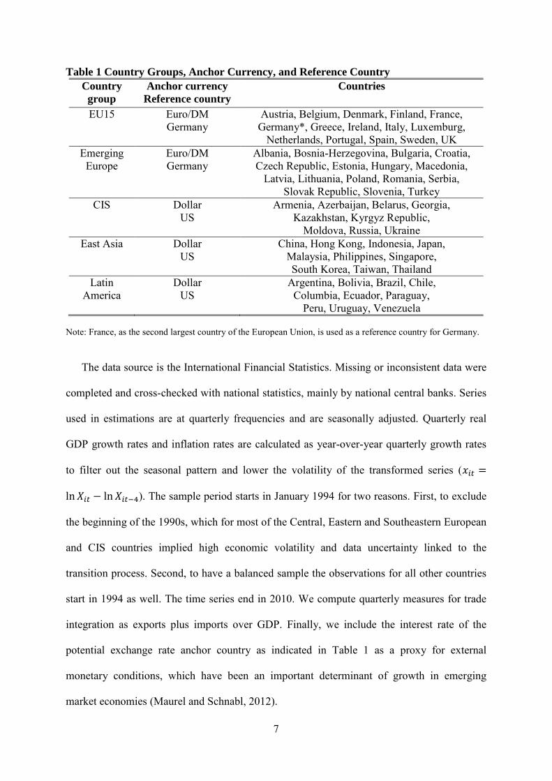
The five country groups include all countries of the respective region excluding

microstates – which may bias the sample towards a very high positive effect of exchange rate

stability on growth (Frenkel and Rose, 2002) – and excluding countries with insufficient data.

This brings us to a sample size of 60 countries. Table 1 provides an overview of all countries

under research, grouped into regions. We also list the prevalent anchor currencies and thereby

the reference countries for measuring business cycle correlation. For the countries in East

Asia, South America and the CIS the dollar has been the prevailing target of exchange rate

stabilization. Business cycle correlation is measured versus the US.

For the European countries before the introduction of the euro in 1999, the German mark

has been the dominant anchor currency (Gros and Thygesen, 1999). Since then, the euro has

become the natural anchor for the European non-EMU countries. Exchange rate flexibility is

measured in terms of exchange rate fluctuations against the German mark before 1999 and

against the euro after 1999. Once a country has entered the EMU the proxy for exchange rate

flexibility is set to zero. Business cycle correlation in Europe is measured versus Germany,

which is the largest European economy (and therefore a country with a high degree of

business cycle correlation with the euro area). For Germany, France as the second largest

European economy is used as a reference country to measure business cycle correlation.

7

Table 1 Country Groups, Anchor Currency, and Reference Country Country

group Anchor currency

Reference country Countries

EU15 Euro/DM Germany

Austria, Belgium, Denmark, Finland, France, Germany*, Greece, Ireland, Italy, Luxemburg,

Netherlands, Portugal, Spain, Sweden, UK Emerging

Europe Euro/DM Germany

Albania, Bosnia-Herzegovina, Bulgaria, Croatia, Czech Republic, Estonia, Hungary, Macedonia,

Latvia, Lithuania, Poland, Romania, Serbia, Slovak Republic, Slovenia, Turkey

CIS Dollar US

Armenia, Azerbaijan, Belarus, Georgia, Kazakhstan, Kyrgyz Republic,

Moldova, Russia, Ukraine East Asia Dollar

US China, Hong Kong, Indonesia, Japan,

Malaysia, Philippines, Singapore, South Korea, Taiwan, Thailand

Latin America

Dollar US

Argentina, Bolivia, Brazil, Chile, Columbia, Ecuador, Paraguay,

Peru, Uruguay, Venezuela Note: France, as the second largest country of the European Union, is used as a reference country for Germany.

The data source is the International Financial Statistics. Missing or inconsistent data were

completed and cross-checked with national statistics, mainly by national central banks. Series

used in estimations are at quarterly frequencies and are seasonally adjusted. Quarterly real

GDP growth rates and inflation rates are calculated as year-over-year quarterly growth rates

to filter out the seasonal pattern and lower the volatility of the transformed series (𝑥𝑖𝑡 =

ln𝑋𝑖𝑡 − ln𝑋𝑖𝑡−4). The sample period starts in January 1994 for two reasons. First, to exclude

the beginning of the 1990s, which for most of the Central, Eastern and Southeastern European

and CIS countries implied high economic volatility and data uncertainty linked to the

transition process. Second, to have a balanced sample the observations for all other countries

start in 1994 as well. The time series end in 2010. We compute quarterly measures for trade

integration as exports plus imports over GDP. Finally, we include the interest rate of the

potential exchange rate anchor country as indicated in Table 1 as a proxy for external

monetary conditions, which have been an important determinant of growth in emerging

market economies (Maurel and Schnabl, 2012).

8

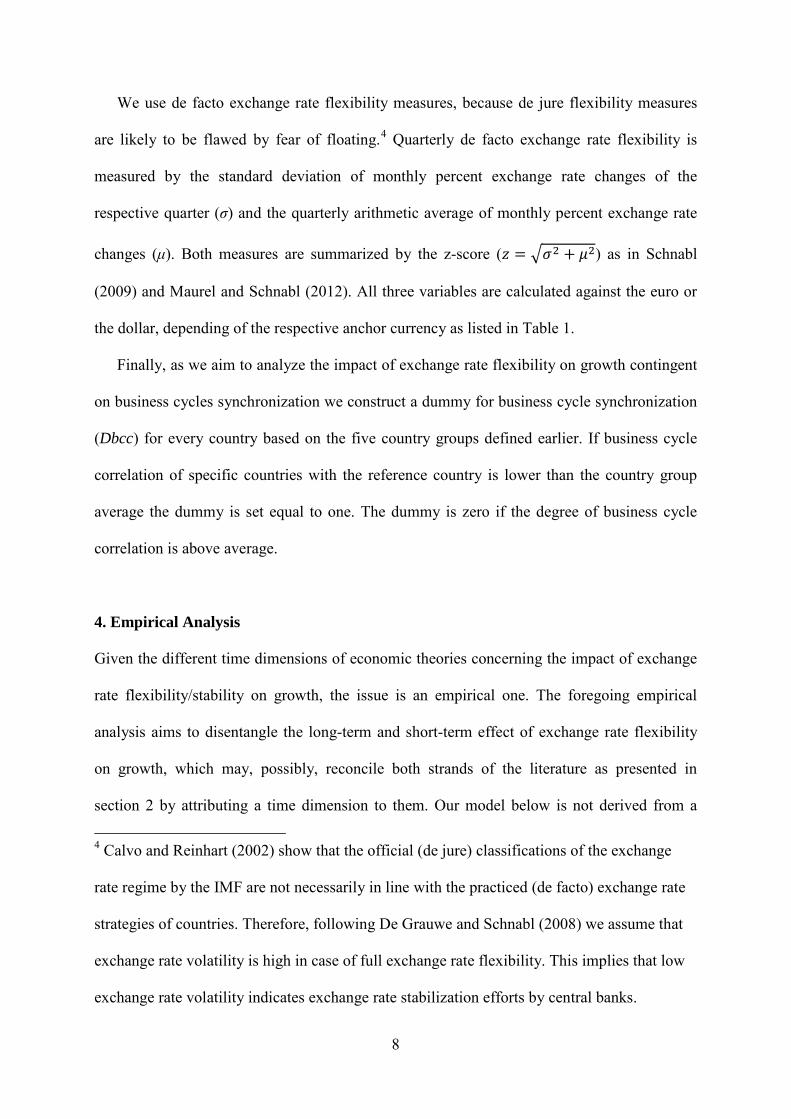
We use de facto exchange rate flexibility measures, because de jure flexibility measures

are likely to be flawed by fear of floating.4

Finally, as we aim to analyze the impact of exchange rate flexibility on growth contingent

on business cycles synchronization we construct a dummy for business cycle synchronization

(Dbcc) for every country based on the five country groups defined earlier. If business cycle

correlation of specific countries with the reference country is lower than the country group

average the dummy is set equal to one. The dummy is zero if the degree of business cycle

correlation is above average.

Quarterly de facto exchange rate flexibility is

measured by the standard deviation of monthly percent exchange rate changes of the

respective quarter (σ) and the quarterly arithmetic average of monthly percent exchange rate

changes (μ). Both measures are summarized by the z-score (𝑧 = �𝜎2 + 𝜇2) as in Schnabl

(2009) and Maurel and Schnabl (2012). All three variables are calculated against the euro or

the dollar, depending of the respective anchor currency as listed in Table 1.

4. Empirical Analysis

Given the different time dimensions of economic theories concerning the impact of exchange

rate flexibility/stability on growth, the issue is an empirical one. The foregoing empirical

analysis aims to disentangle the long-term and short-term effect of exchange rate flexibility

on growth, which may, possibly, reconcile both strands of the literature as presented in

section 2 by attributing a time dimension to them. Our model below is not derived from a

4 Calvo and Reinhart (2002) show that the official (de jure) classifications of the exchange

rate regime by the IMF are not necessarily in line with the practiced (de facto) exchange rate

strategies of countries. Therefore, following De Grauwe and Schnabl (2008) we assume that

exchange rate volatility is high in case of full exchange rate flexibility. This implies that low

exchange rate volatility indicates exchange rate stabilization efforts by central banks.

9

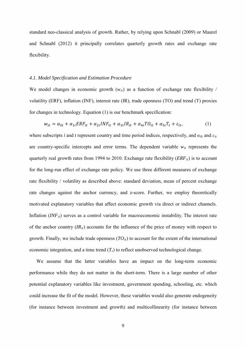
standard neo-classical analysis of growth. Rather, by relying upon Schnabl (2009) or Maurel

and Schnabl (2012) it principally correlates quarterly growth rates and exchange rate

flexibility.

4.1. Model Specification and Estimation Procedure

We model changes in economic growth (wit

𝑤𝑖𝑡 = 𝛼0𝑖 + 𝛼1𝑖𝐸𝑅𝐹𝑖𝑡 + 𝛼2𝑖𝐼𝑁𝐹𝑖𝑡 + 𝛼3𝑖𝐼𝑅𝑖𝑡 + 𝛼4𝑖𝑇𝑂𝑖𝑡 + 𝛼5𝑖𝑇𝑡 + 𝜀𝑖𝑡, (1)

) as a function of exchange rate flexibility /

volatility (ERF), inflation (INF), interest rate (IR), trade openness (TO) and trend (T) proxies

for changes in technology. Equation (1) is our benchmark specification:

where subscripts i and t represent country and time period indices, respectively, and α0i and εit

are country-specific intercepts and error terms. The dependent variable wit represents the

quarterly real growth rates from 1994 to 2010. Exchange rate flexibility (ERFit) is to account

for the long-run effect of exchange rate policy. We use three different measures of exchange

rate flexibility / volatility as described above: standard deviation, mean of percent exchange

rate changes against the anchor currency, and z-score. Further, we employ theoretically

motivated explanatory variables that affect economic growth via direct or indirect channels.

Inflation (INFit) serves as a control variable for macroeconomic instability. The interest rate

of the anchor country (IRit) accounts for the influence of the price of money with respect to

growth. Finally, we include trade openness (TOit) to account for the extent of the international

economic integration, and a time trend (Tt

We assume that the latter variables have an impact on the long-term economic

performance while they do not matter in the short-term. There is a large number of other

potential explanatory variables like investment, government spending, schooling, etc. which

could increase the fit of the model. However, these variables would also generate endogeneity

(for instance between investment and growth) and multicollinearity (for instance between

) to reflect unobserved technological change.

10

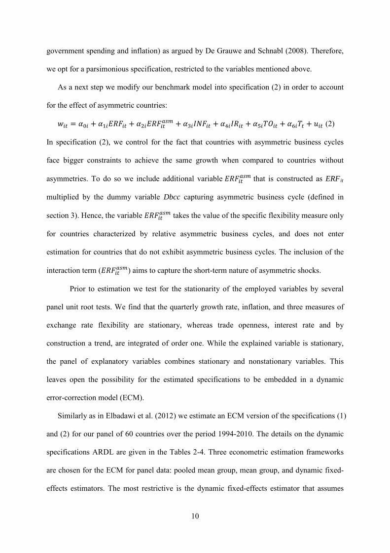
government spending and inflation) as argued by De Grauwe and Schnabl (2008). Therefore,

we opt for a parsimonious specification, restricted to the variables mentioned above.

As a next step we modify our benchmark model into specification (2) in order to account

for the effect of asymmetric countries:

𝑤𝑖𝑡 = 𝛼0𝑖 + 𝛼1𝑖𝐸𝑅𝐹𝑖𝑡 + 𝛼2𝑖𝐸𝑅𝐹𝑖𝑡𝑎𝑠𝑚 + 𝛼3𝑖𝐼𝑁𝐹𝑖𝑡 + 𝛼4𝑖𝐼𝑅𝑖𝑡 + 𝛼5𝑖𝑇𝑂𝑖𝑡 + 𝛼6𝑖𝑇𝑡 + 𝑢𝑖𝑡 (2)

In specification (2), we control for the fact that countries with asymmetric business cycles

face bigger constraints to achieve the same growth when compared to countries without

asymmetries. To do so we include additional variable 𝐸𝑅𝐹𝑖𝑡𝑎𝑠𝑚 that is constructed as ERFit

Prior to estimation we test for the stationarity of the employed variables by several

panel unit root tests. We find that the quarterly growth rate, inflation, and three measures of

exchange rate flexibility are stationary, whereas trade openness, interest rate and by

construction a trend, are integrated of order one. While the explained variable is stationary,

the panel of explanatory variables combines stationary and nonstationary variables. This

leaves open the possibility for the estimated specifications to be embedded in a dynamic

error-correction model (ECM).

multiplied by the dummy variable Dbcc capturing asymmetric business cycle (defined in

section 3). Hence, the variable 𝐸𝑅𝐹𝑖𝑡𝑎𝑠𝑚 takes the value of the specific flexibility measure only

for countries characterized by relative asymmetric business cycles, and does not enter

estimation for countries that do not exhibit asymmetric business cycles. The inclusion of the

interaction term (𝐸𝑅𝐹𝑖𝑡𝑎𝑠𝑚) aims to capture the short-term nature of asymmetric shocks.

Similarly as in Elbadawi et al. (2012) we estimate an ECM version of the specifications (1)

and (2) for our panel of 60 countries over the period 1994-2010. The details on the dynamic

specifications ARDL are given in the Tables 2-4. Three econometric estimation frameworks

are chosen for the ECM for panel data: pooled mean group, mean group, and dynamic fixed-

effects estimators. The most restrictive is the dynamic fixed-effects estimator that assumes

11

that all parameters are constant across countries, except for the intercept, which is allowed to

vary across countries. The pooled mean group estimator is more general than the dynamic

fixed-effects estimator as it imposes the restriction that all countries share the long-term

coefficients. The mean group estimator is even more general as it assumes that economies

differ in their short-term and long-term parameters.

The choice between the three estimators entails a tradeoff between consistency and

efficiency. The dynamic fixed-effects estimator dominates the other two in terms of efficiency

if the restrictions are valid. If they are not valid, the dynamic fixed effects will generate

inconsistent estimates and is dominated by the pooled mean group and mean group estimates.

The pooled mean group estimator can be assumed to offer the best compromise between

consistency and efficiency, because one would expect the long-term growth path to be driven

by a similar process across countries while the short-term dynamics around the long-term

equilibrium path differ because of idiosyncratic news and shocks to fundamentals. Following

the above arguments we perform formal Hausman tests of the implied restrictions.

By estimating both specifications (1) and (2) our objective is threefold: to highlight the

impact of exchange rate flexibility on growth, to disentangle the short-term versus long-term

effect of exchange rate flexibility on growth, and to quantify the weight of countries with

asymmetric business cycles (which we call asymmetric countries) in this impact. Our prior is

that the impact of exchange rate flexibility should be positive in the short term, especially for

asymmetric countries, but negative in the long term.

4.2. Estimation Results

The econometric estimation results are presented in Tables 2 to 4. The results are organized in

a way that columns labeled as 1 contain an overall effect via coefficients from specification

(1), while columns labeled as 2 show the effects from specification (2) where we account for

12

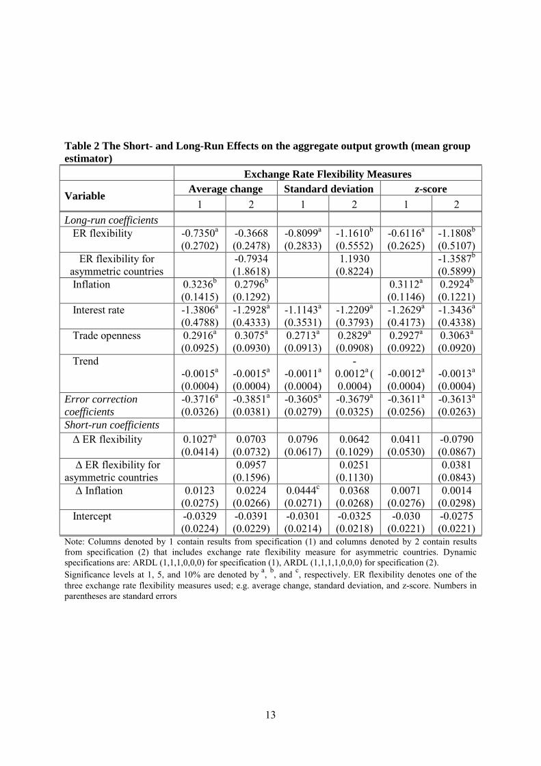
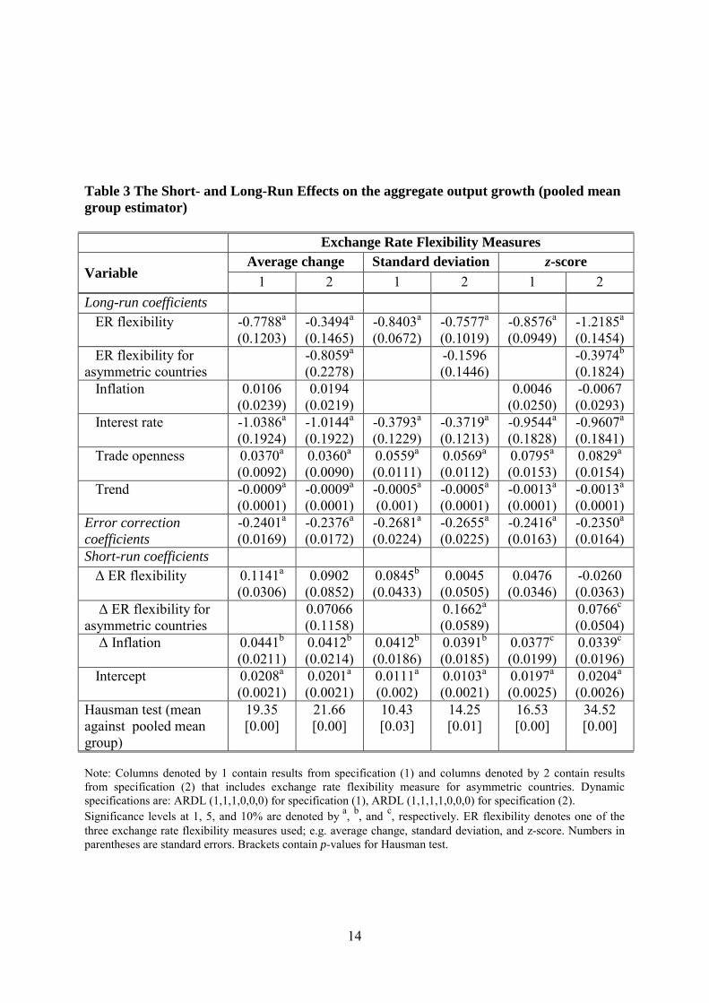
asymmetry in business cycle correlation. The null hypothesis of equality of coefficients

between pooled mean group and mean group is in most cases rejected at 1 % level. The

Hausman test favors the mean group model (Table 2) against the pooled mean group

estimator (Table 3). 5

The mean group results as presented in Table 2 suggest a negative effect of exchange rate

flexibility on growth in the long term and a positive effect of exchange rate flexibility on

growth in the short term. For all three flexibility measures (standard deviation, average yearly

change, and z-score) exchange rate flexibility has are highly significant negative effect on

growth in the long term, when controlling for interest rates in the anchor country, trade

openness, and inflation. Both trade openness and the interest rate in the large reference

country have the expected signs and are highly significant. Open economies grow faster and

the gradual decline of the interest rate level in the large anchor countries (US, euro area,

Germany) seems to have boosted growth in the emerging market economies. In the long term

higher growth levels are linked to higher inflation levels.

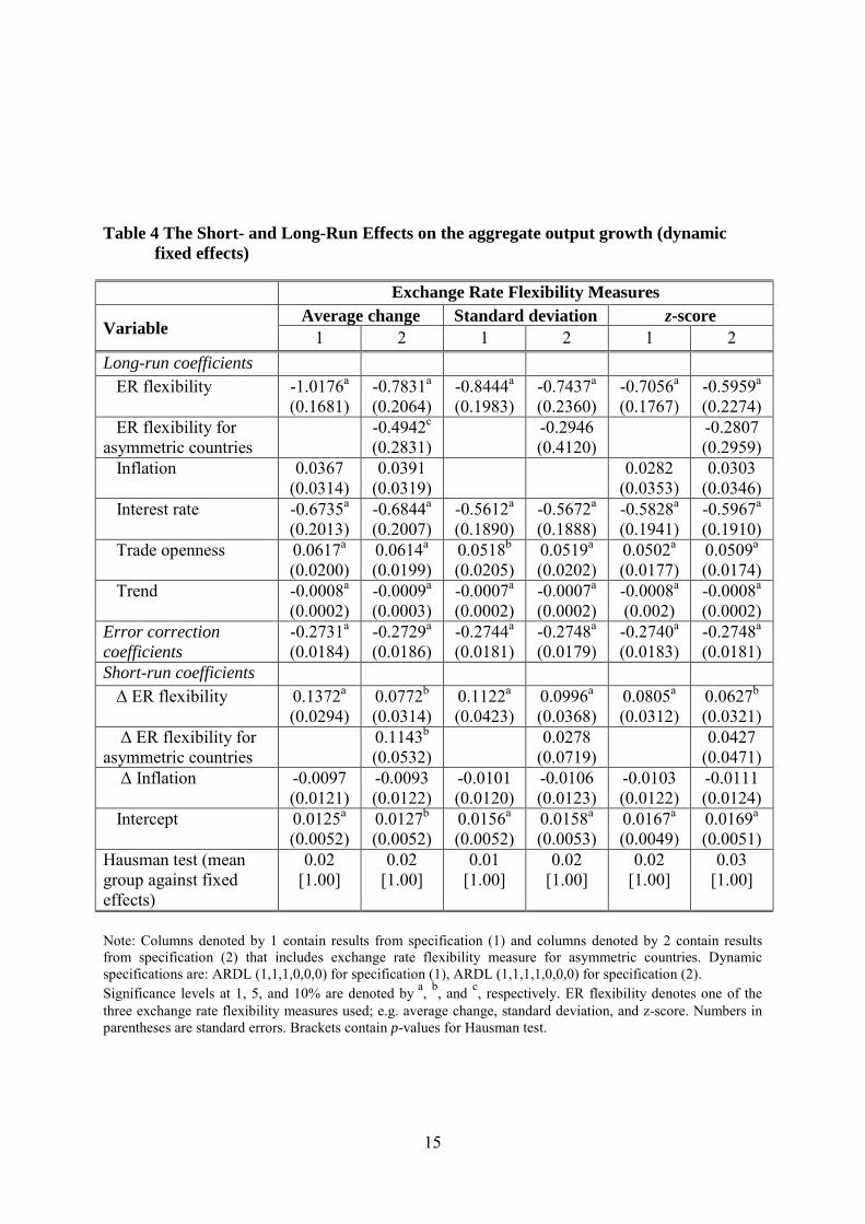
The dynamic fixed effects estimates are presented in Table 4. All

estimates support our main assumptions regarding the long- versus short-run impact of

exchange rate flexibility on growth and the more specific case of asymmetric countries.

6

The coefficient of the interaction

term is significant for the z-score measure and insignificant for the other two flexibility

measures. Negative coefficients for the interaction term indicate an additional negative effect

of exchange flexibility for asymmetric countries in the long run.

5 The mean group estimator of Pesaran and Smith (1995) is consistent but not a good

estimator when either N or T is small. Hence, we consider results of the pooled mean group

estimator on par with those of the mean group estimator.

6 Due to the lack of convergence during the estimation the inflation term is dropped from the

equation in the specification with standard deviation as a proxy for exchange rate flexibility.

13

Table 2 The Short- and Long-Run Effects on the aggregate output growth (mean group estimator)

Exchange Rate Flexibility Measures

Variable Average change Standard deviation z-score 1 2 1 2 1 2

Long-run coefficients ER flexibility -0.7350

(0.2702) a -0.3668

(0.2478) -0.8099(0.2833)

a -1.1610(0.5552)

b -0.6116(0.2625)

a -1.1808(0.5107)

b

ER flexibility for asymmetric countries

-0.7934

(1.8618) 1.1930

(0.8224) -1.3587

(0.5899) b

Inflation 0.3236(0.1415)

b 0.2796(0.1292)

b

0.3112(0.1146)

a 0.2924(0.1221)

b

Interest rate -1.3806(0.4788)

a -1.2928(0.4333)

a -1.1143(0.3531)

a -1.2209(0.3793)

a -1.2629(0.4173)

a -1.3436(0.4338)

a

Trade openness 0.2916(0.0925)

a 0.3075(0.0930)

a 0.2713(0.0913)

a 0.2829(0.0908)

a 0.2927(0.0922)

a 0.3063(0.0920)

a

Trend -0.0015(0.0004)

a -0.0015(0.0004)

a -0.0011(0.0004)

a -

0.0012a -0.0012(0.0004) (0.0004)

a -0.0013(0.0004)

a

Error correction coefficients

-0.3716(0.0326)

a -0.3851(0.0381)

a -0.3605(0.0279)

a -0.3679(0.0325)

a -0.3611(0.0256)

a -0.3613(0.0263)

a

Short-run coefficients Δ ER flexibility 0.1027

(0.0414) a 0.0703

(0.0732) 0.0796

(0.0617) 0.0642

(0.1029) 0.0411

(0.0530) -0.0790 (0.0867)

Δ ER flexibility for asymmetric countries

0.0957 (0.1596)

0.0251 (0.1130)

0.0381

(0.0843) Δ Inflation 0.0123

(0.0275) 0.0224

(0.0266) 0.0444(0.0271)

c 0.0368 (0.0268)

0.0071 (0.0276)

0.0014 (0.0298)

Intercept -0.0329 (0.0224)

-0.0391 (0.0229)

-0.0301 (0.0214)

-0.0325 (0.0218)

-0.030 (0.0221)

-0.0275 (0.0221)

Note: Columns denoted by 1 contain results from specification (1) and columns denoted by 2 contain results from specification (2) that includes exchange rate flexibility measure for asymmetric countries. Dynamic specifications are: ARDL (1,1,1,0,0,0) for specification (1), ARDL (1,1,1,1,0,0,0) for specification (2). Significance levels at 1, 5, and 10% are denoted by a, b, and c

, respectively. ER flexibility denotes one of the three exchange rate flexibility measures used; e.g. average change, standard deviation, and z-score. Numbers in parentheses are standard errors

14

Table 3 The Short- and Long-Run Effects on the aggregate output growth (pooled mean group estimator)


Variable Average change Standard deviation z-score

1 2 1 2 1 2 Long-run coefficients ER flexibility -0.7788

(0.1203) a -0.3494

(0.1465) a -0.8403

(0.0672) a -0.7577

(0.1019) a -0.8576

(0.0949) a -1.2185

(0.1454) a


-0.8059(0.2278)

a -0.1596

(0.1446) -0.3974

(0.1824) b

Inflation 0.0106 (0.0239)

0.0194 (0.0219)

0.0046 (0.0250)

-0.0067 (0.0293)

Interest rate -1.0386(0.1924)

a -1.0144(0.1922)

a -0.3793(0.1229)

a -0.3719(0.1213)

a -0.9544(0.1828)

a -0.9607(0.1841)

a


a 0.0360(0.0090)

a 0.0559(0.0111)

a 0.0569(0.0112)

a 0.0795(0.0153)

a 0.0829(0.0154)

a

Trend -0.0009(0.0001)

a -0.0009(0.0001)

a -0.0005(0.001)

a -0.0005(0.0001)

a -0.0013(0.0001)

a -0.0013(0.0001)

a


-0.2401(0.0169)

a -0.2376(0.0172)

a -0.2681(0.0224)

a -0.2655(0.0225)

a -0.2416(0.0163)

a -0.2350(0.0164)

a


(0.0306) a 0.0902

(0.0852) 0.0845(0.0433)

b 0.0045 (0.0505)

0.0476 (0.0346)

-0.0260 (0.0363)


0.07066 (0.1158)

0.1662(0.0589)

a 0.0766(0.0504)

c

Δ Inflation 0.0441(0.0211)

b 0.0412(0.0214)

b 0.0412(0.0186)

b 0.0391(0.0185)

b 0.0377(0.0199)

c 0.0339(0.0196)

c

Intercept 0.0208(0.0021)

a 0.0201(0.0021)

a 0.0111(0.002)

a 0.0103(0.0021)

a 0.0197(0.0025)

a 0.0204(0.0026)

a

Hausman test (mean against pooled mean group)

19.35 [0.00]

21.66 [0.00]

10.43 [0.03]

14.25 [0.01]

16.53 [0.00]

34.52 [0.00]


, respectively. ER flexibility denotes one of the three exchange rate flexibility measures used; e.g. average change, standard deviation, and z-score. Numbers in parentheses are standard errors. Brackets contain p-values for Hausman test.

15

Table 4 The Short- and Long-Run Effects on the aggregate output growth (dynamic

fixed effects)


Variable Average change Standard deviation z-score

1 2 1 2 1 2 Long-run coefficients ER flexibility -1.0176

(0.1681) a -0.7831

(0.2064) a -0.8444

(0.1983) a -0.7437

(0.2360) a -0.7056

(0.1767) a -0.5959

(0.2274) a


-0.4942(0.2831)

c -0.2946 (0.4120)

-0.2807

(0.2959) Inflation 0.0367

(0.0314) 0.0391

(0.0319) 0.0282

(0.0353) 0.0303

(0.0346) Interest rate -0.6735

(0.2013) a -0.6844

(0.2007) a -0.5612

(0.1890) a -0.5672

(0.1888) a -0.5828

(0.1941) a -0.5967

(0.1910) a


a 0.0614(0.0199)

a 0.0518(0.0205)

b 0.0519(0.0202)

a 0.0502(0.0177)

a 0.0509(0.0174)

a

Trend -0.0008(0.0002)

a -0.0009(0.0003)

a -0.0007(0.0002)

a -0.0007(0.0002)

a -0.0008(0.002)

a -0.0008(0.0002)

a


-0.2731(0.0184)

a -0.2729(0.0186)

a -0.2744(0.0181)

a -0.2748(0.0179)

a -0.2740(0.0183)

a -0.2748(0.0181)

a


(0.0294) a 0.0772

(0.0314) b 0.1122

(0.0423) a 0.0996

(0.0368) a 0.0805

(0.0312) a 0.0627

(0.0321) b


0.1143(0.0532)

b 0.0278 (0.0719)

0.0427 (0.0471)

Δ Inflation -0.0097 (0.0121)

-0.0093 (0.0122)

-0.0101 (0.0120)

-0.0106 (0.0123)

-0.0103 (0.0122)

-0.0111 (0.0124)

Intercept 0.0125(0.0052)

a 0.0127(0.0052)

b 0.0156(0.0052)

a 0.0158(0.0053)

a 0.0167(0.0049)

a 0.0169(0.0051)

a

Hausman test (mean group against fixed effects)

0.02 [1.00]

0.02 [1.00]

0.01 [1.00]

0.02 [1.00]

0.02 [1.00]

0.03 [1.00]


, respectively. ER flexibility denotes one of the three exchange rate flexibility measures used; e.g. average change, standard deviation, and z-score. Numbers in parentheses are standard errors. Brackets contain p-values for Hausman test.

16

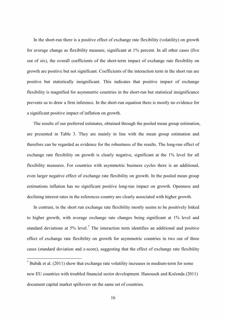
In the short-run there is a positive effect of exchange rate flexibility (volatility) on growth

for average change as flexibility measure, significant at 1% percent. In all other cases (five

out of six), the overall coefficients of the short-term impact of exchange rate flexibility on

growth are positive but not significant. Coefficients of the interaction term in the short run are

positive but statistically insignificant. This indicates that positive impact of exchange

flexibility is magnified for asymmetric countries in the short-run but statistical insignificance

prevents us to draw a firm inference. In the short-run equation there is mostly no evidence for

a significant positive impact of inflation on growth.

The results of our preferred estimates, obtained through the pooled mean group estimation,

are presented in Table 3. They are mainly in line with the mean group estimation and

therefore can be regarded as evidence for the robustness of the results. The long-run effect of

exchange rate flexibility on growth is clearly negative, significant at the 1% level for all

flexibility measures. For countries with asymmetric business cycles there is an additional,

even larger negative effect of exchange rate flexibility on growth. In the pooled mean group

estimations inflation has no significant positive long-run impact on growth. Openness and

declining interest rates in the references country are clearly associated with higher growth.

In contrast, in the short run exchange rate flexibility mostly seems to be positively linked

to higher growth, with average exchange rate changes being significant at 1% level and

standard deviations at 5% level.7

7 Bubák et al. (2011) show that exchange rate volatility increases in medium-term for some

new EU countries with troubled financial sector development. Hanousek and Kočenda (2011)

document capital market spillovers on the same set of countries.

The interaction term identifies an additional and positive

effect of exchange rate flexibility on growth for asymmetric countries in two out of three

cases (standard deviation and z-score), suggesting that the effect of exchange rate flexibility

17

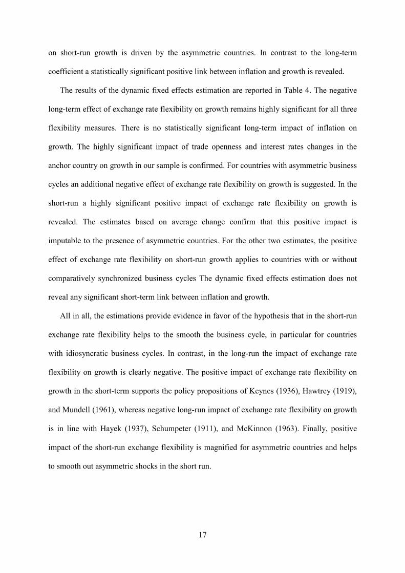
on short-run growth is driven by the asymmetric countries. In contrast to the long-term

coefficient a statistically significant positive link between inflation and growth is revealed.

The results of the dynamic fixed effects estimation are reported in Table 4. The negative

long-term effect of exchange rate flexibility on growth remains highly significant for all three

flexibility measures. There is no statistically significant long-term impact of inflation on

growth. The highly significant impact of trade openness and interest rates changes in the

anchor country on growth in our sample is confirmed. For countries with asymmetric business

cycles an additional negative effect of exchange rate flexibility on growth is suggested. In the

short-run a highly significant positive impact of exchange rate flexibility on growth is

revealed. The estimates based on average change confirm that this positive impact is

imputable to the presence of asymmetric countries. For the other two estimates, the positive

effect of exchange rate flexibility on short-run growth applies to countries with or without

comparatively synchronized business cycles The dynamic fixed effects estimation does not

reveal any significant short-term link between inflation and growth.

All in all, the estimations provide evidence in favor of the hypothesis that in the short-run

exchange rate flexibility helps to the smooth the business cycle, in particular for countries

with idiosyncratic business cycles. In contrast, in the long-run the impact of exchange rate

flexibility on growth is clearly negative. The positive impact of exchange rate flexibility on

growth in the short-term supports the policy propositions of Keynes (1936), Hawtrey (1919),

and Mundell (1961), whereas negative long-run impact of exchange rate flexibility on growth

is in line with Hayek (1937), Schumpeter (1911), and McKinnon (1963). Finally, positive

impact of the short-run exchange flexibility is magnified for asymmetric countries and helps

to smooth out asymmetric shocks in the short run.

18

Table 5: Diagnostic checking of the residuals and cointegration Flexibility measure

z-score

Model specification

1 2

Statistics Z Values

P Values

Statistics Z Values

P Values

Panel unit-root tests of the residuals

P Z L* Pm

359.2075 -9.855 -12.518 18.008

0.000 0.000 0.000 0.000

P Z L* Pm

385.5133 -10.6779 -13.5948 19.8499

0.000 0.000 0.000 0.000

Tests of cointegration

G1 G2 P1 P2

-3.828 -19.831 -24.745 -20.013

-12.192 -9.491 -10.877 -12.894

0.000 0.000 0.000 0.000

G1 G2 P1 P2

-4.088 -10.864 -22.440 -9.172

-11.048 2.434 -6.723 0.647

0.000 0.993 0.000 0.741

Flexibility measure

Standard deviation

Model specification

1 2


P Z L* Pm

367.6745 -9.7014 -12.465 18.6009

0.000 0.000 0.000 0.000

P Z L* Pm

406.1817 -10.9242 -14.1442 21.2970

0.000 0.000 0.000 0.000


G1 G2 P1 P2

-4.265 -10.361 -22.456 -8.705

-13.470 1.178 -8.163 -0.561

0.000 0.881 0.000 0.287

G1 G2 P1 P2

-4.100 -10.713 -22.010 -8.901

-10.884 2.501 -6.628 0.838

0.000 0.994 0.000 0.799

Flexibility measure

Average change

Model specification

1 2


P Z L* Pm

464.134 -12.5923 -16.7280 25.3545

0.000 0.000 0.000 0.000

P Z L* Pm

455.8971 -12.3615 -16.3874 24.7778

0.000 0.000 0.000 0.000


G1 G2 P1 P2

-3.963 -8.725 -22.069 -7.938

-11.506 2.591 -7.846 0.078

0.000 0.995 0.000 0.531

G1 G2 P1 P2

-3.905 -8.783 -20.578 -8.125

-9.617 4.036 -5.428 1.426

0.000 1.000 0.000 0.923

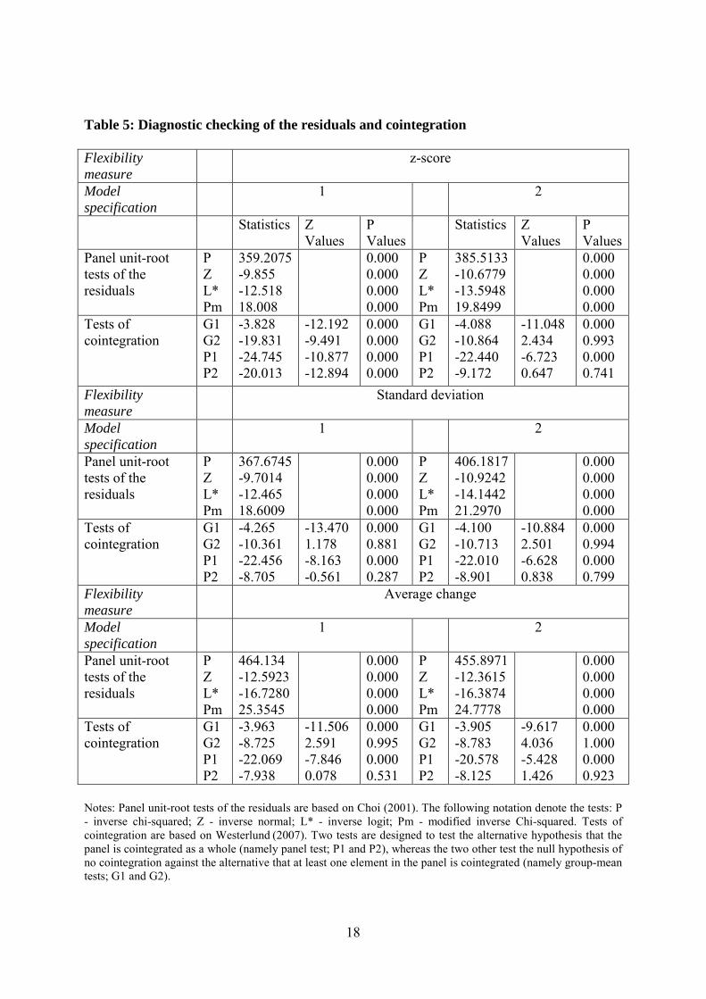
Notes: Panel unit-root tests of the residuals are based on Choi (2001). The following notation denote the tests: P - inverse chi-squared; Z - inverse normal; L* - inverse logit; Pm - modified inverse Chi-squared. Tests of cointegration are based on Westerlund

(2007). Two tests are designed to test the alternative hypothesis that the panel is cointegrated as a whole (namely panel test; P1 and P2), whereas the two other test the null hypothesis of no cointegration against the alternative that at least one element in the panel is cointegrated (namely group-mean tests; G1 and G2).

19

4.3. Diagnostic checking

We complement our analysis by diagnostic checking; results are in Table 5. We perform

panel-unit root tests designed by Choi (2001) and a battery of Westerlund (2007) tests for

cointegration. The results show that the residuals are stationary for both estimated

specifications (with or without accounting for the business cycle asymmetry). Further, no

matter what exchange rate flexibility measure is used (standard deviation, average, or z-score)

the results show that the variables are cointegrated; in all cases, two out of the four statistics

proposed by Westerlund (2007) reject the null of no cointegration. Finally, it should be noted

that Pesaran et al. (1999) show that pooled mean group estimation does not require pretesting

for unit roots and cointegration, and that pooled mean group estimation provides consistent

and efficient estimates of parameters in a long-run relationship between stationary and

integrated variables.

5. Conclusion

With the European sovereign debt crisis a controversial discussion concerning the appropriate

monetary policy and exchange rate strategy to asymmetric shocks and crisis has reemerged.

We have aimed to derive from our econometrical exercise for a panel of 60 countries a policy

recommendation for crisis countries. Our estimation results provide evidence that exchange

rate adjustment stimulates growth in the short-term, but puts a drag on the long-term growth

performance. As the overall effect is negative, the policy implication is to keep exchange rates

stable to promote long-term growth via price and wage flexibility, in the spirit of Schumpeter

(1911), Hayek (1937), and McKinnon (1963).

In line with Schnabl (2009) and based on our findings we recommend the crisis countries

to proceed with structural reforms and real wage cuts. Painful restructuring and declining

output today are likely to be rewarded with a robust economic recovery and rising income in

the future. In contrast, monetary expansion and depreciation as a crisis solution strategy can

20

be expected to provide short-term relief, but long-term pain. Mutual monetary expansion

would lead into a wave of competitive depreciations and competitive interest rate cuts, and

therefore global financial and economic instability. This would be an antidote of the

coordinated structural reforms.

References

Arghyrou, Michael G. and Georgios Chortareas, “Current Account Imbalances and Real

Exchange Rates in the Euro Area,” Review of International Economics 16 (2008):747-764.

Beckmann, Joscha, Ansgar Belke, and Frauke Dobnik, “Cross-section dependence and the

monetary exchange rate model – A panel analysis Original Research,“ The North American

Journal of Economics and Finance, 23 (2012):38-53.

Bubák, Vít, Evžen Kočenda, and Filip Žikeš, “Volatility Transmission in Emerging European

Foreign Exchange Markets,” Journal of Banking and Finance 35 (2011):2829–2841.

Calvo, Guillermo and Carmen M.

Choi, In, “Unit root tests for panel data,” Journal of International Money and Finance 20

(2001):249–272.

Reinhart, “Fear of Floating,” The Quarterly Journal of

Economics 117 (2002):379-408.

De Grauwe, Paul and Gunther Schnabl,“Exchange Rate Stability, Inflation and Growth in

(South) Eastern and Central Europe,” Review of Development Economics 12 (2008):530-

549.

Elbadawi, Ibrahim A., Linda Kaltani, and Raimundo Soto, “Aid, Real Exchange Rate

Misalignment, and Economic Growth in Sub-Saharan Africa,” World Development 40

(2012):681–700.

Frenkel, Jeffrey A. and Andrew K. Rose, “An Estimate of the Effect of Common Currencies

on Trade and Income,” Quarterly Journal of Economics 117 (2002):437-466.

21

Friedman, Milton, The Case of Flexible Exchange Rates. In: Friedman, M.: Essays is Positive

Economics, Chicago: University of Chicago Press, 1953.

Gros, Daniel and Niels Thygesen, European Monetary Integration, London: Longman Group,

1999.

Hawtrey, Ralph G., “The Gold Standard,” Economic Journal 3 (1919):428-442.

Hanousek, Jan and Evžen Kočenda, “Foreign News and Spillovers in Emerging European

Stock Markets,” Review of International Economics 19 (2011):170–188.

Hayek, Friedrich von, Monetary Nationalism and International Stability, London: Longmans

Green, 1937.

Levy-Yeyati, Eduardo and Federico Sturzenegger, “To Float or to Fix: Evidence on the

Impact of Exchange Rate Regimes on Growth,” American Economic Review 12 (2002)1-

49.

Keynes, John M., The General Theory of Employment, Interest, and Money, London:

Macmillan and Co., Ltd, 1936.

Keynes, John M., The Collected Writings, Volume 25: Activities 1940-44 - Shaping the Post-

war World: The Clearing Union, London: McMillam Press, 1980.

Kindleberger, Charles P., Keynesianism vs. Monetarism and Other Essays in Financial

History, London: Gorge Allen & Unwin, 1985.

Kočenda, Evžen and Tigran Poghosyan, “Macroeconomic Sources of Foreign Exchange Risk

in New EU Members,” Journal of Banking and Finance 33 (2009):2164-2173.

Maurel, Mathilde and Gunther Schnabl, “Keynesian and Austrian Perspectives on Crisis,

Shock Adjustment, Exchange Rate Regime and (Long-Term) Growth,” Open Economies

Review 23 (2012):847-868.

McKinnon, Ronald I., “Optimum Currency Areas,” American Economic Review 53

(1963):717-725.

22

Mundell, Robert A. “A Theory of Optimum Currency Areas,“ American Economic Review 51

(1961):657-665.

Pesaran, Hashem M., Yongcheol Shin, and Ron P. Smith, “Pooled Mean Group Estimation of

Dynamic Heterogeneous Panels,” Journal of the American Statistical Association 94

(1999):621-634.

Pesaran, Hashem M. and Ron P. Smith, “Estimating long-run relationships from dynamic

heterogeneous panels,” Journal of Econometrics 68 (1995):79–113.

Schnabl, Gunther, “Exchange Rate Volatility and Growth in Emerging Europe and East Asia,”

Open Economies Review 20 (2009):565-587.

Schumpeter, Joseph, Theorie der Wirtschaftlichen Entwicklung, Berlin, 1911.

Tavlas, George, “Optimum-Currency-Area Paradoxes,” Review of International Economics

17 (2009):536-551.

Westerlund, Joakim, “Testing for Error Correction in Panel Data,” Oxford Bulletin of

Economics and Statistics 69 (2007):709-748.