The response of the

Baltic Sea sponge Halichondria panicea

upon challenge with Vibrio bacteria

Masters Thesis

submitted by

Theresa Kuhl

September 22nd

2016 - March 27th

2017

at

FB3, Research Unit Marine Molecular Ecology

GEOMAR - Helmholtz Centre for Ocean Research Kiel

Supervisor: Dr. Lucía Pita Galán (GEOMAR)

First examiner: Prof. Dr. Herwig Stibor (LMU)

Second examiner: Prof. Dr. Ute Hentschel Humeida (GEOMAR)

2

Content

1. Zusammenfassung ................................................................................................................................... 4

2. Abstract ....................................................................................................................................................... 5

3. Introduction ............................................................................................................................................... 6

4. Material and Methods .......................................................................................................................... 11

4.1. Halichondria panicea .............................................................................................................. 11

4.2. Sponge aquaculture .................................................................................................................. 12

4.3. DNA and RNA extraction ...................................................................................................... 14

4.4. Phylogenetic analysis .............................................................................................................. 14

4.5. Experimental set-up for immune response experiment set-up .................................... 15

4.6. Antimicrobial assay (AM) ..................................................................................................... 17

4.7. Candidate genes and primer design for RT-qPCR .......................................................... 18

4.8. RT-qPCR optimization ............................................................................................................ 20

4.9. RT-qPCR experiments ............................................................................................................. 22

5. Results ..................................................................................................................................................... 23

5.1. Phylogenetic analysis .............................................................................................................. 23

5.2. Sponge aquaculture .................................................................................................................. 26

5.3. Immune response experiment ............................................................................................... 27

5.4. Antimicrobial assay ................................................................................................................. 28

5.5. RT-qPCR analysis ..................................................................................................................... 31

6. Discussion .............................................................................................................................................. 33

6.1. Phylogenetic analysis .............................................................................................................. 33

6.2. Aquaculture ................................................................................................................................ 33

6.3. Immune response experiment ............................................................................................... 34

7. References .............................................................................................................................................. 39

8. Acknowledgements ............................................................................................................................ 45

9. Appendix ................................................................................................................................................ 46

9.1. Additional samples ................................................................................................................... 46

9.1.1. Bacterioplankton samples for 16S rRNA analysis ..................................................... 46

9.1.2. Sponge material in RNAlater ............................................................................................ 46

9.2. Supplementary Material ......................................................................................................... 46

9.2.1. Fluorescein results ............................................................................................................... 46

9.2.2. Light intensity and temperature in IR2 experiment (HOBO logger) .................... 47

9.2.3. Oxygen, temperature, pH, and salinity in IR and IR2 experiment......................... 47

9.2.4. Results of antimicrobial assay within treatments ........................................................ 48

9.2.5. Genbank ID of species in phylogenetic trees (18s rRNA, ITS-2 and COI

mtDNA) ................................................................................................................................................... 49

3

9.2.6. Standard curves for primers used in RT-qPCR ............................................................ 51

9.2.6.1. Actin (reference gene) .................................................................................................... 51

9.2.6.2. Hsp70 (target gene) ......................................................................................................... 52

9.3. Procedure Protocols ................................................................................................................. 53

9.3.1. NUCLEIC ACID EXTRACTION FOR TRANSCRIPTOMICS ........................... 53

9.3.2. cDNA transcription (iScript™ Select cDNA Synthesis Kit) ................................... 58

9.3.3. FIXATION FOR FLOW CYTOMETRY OF PHYTOPLANKTON AND

BACTERIA IN SEAWATER ............................................................................................................ 59

9.3.4. ExperionTM

(ExperionTM

RNA StdSens Starter Kit) ................................................... 61

10. Declaration of authorship ............................................................................................................ 68

4

1. Zusammenfassung

Schwämme (Stamm Porifera) nehmen über ihre filtrierende Ernährungsweise ständig

Mikroorganismen auf, darunter auch potentielle Pathogene, während sie zeitgleich spezifische

mikrobielle Gemeinschaften beherbergen. Es ist noch nicht bekannt wie Schwämme die

unterschiedlichen Mikroorganismen voneinander unterscheiden (Symbionten, Nahrung,

Pathogene). Ich stellte die Hypothese auf, dass das „angeborene“ Immunsystem des

Schwamms eine Rolle spielen könnte, um eine spezifische Reaktion gegenüber den

Mikroorganismen hervorzurufen. Darüber hinaus ist die Rolle des

„angeborenen“ Immunsystems in Bezug auf das Immungedächtnis in Invertebraten aktuell

von Interesse, da es hilft, mehr über die Interaktionen von Wirt und Mikroorganismen zu

erfahren. Das Immungedächtnis in Invertebraten erfüllt eine ähnliche Funktion wie in

Vertebraten, beruht jedoch auf anderen molekularen Mechanismen.

Ich wollte die potentiellen Wege zur Erkennung von Mikroorganismen in Schwämmen

untersuchen und entwickelte dazu einen experimentellen Ansatz. Der Schwamm Halichondria

panicea konnte erfolgreich in einer Aquakultur gehalten werden. Im Experiment wurde er

einem autochthonen Vibrio Stamm aus der Ostsee und einem exogenen Vibrio Stamm aus

dem Mittelmeer ausgesetzt. Als Kontrolle diente steriles, künstliches Meerwasser. Die

Immunreaktion wurde mit einem antimikrobiellen Assay und mit differentieller

Genexpressions-Analyse (z.B., RT-qPCR des Zielgens hsp70) untersucht. Ich erwartete eine

differenzierte Immunreaktion des Schwamms gegenüber den zwei unterschiedlichen

Bakterienstämmen. Unter der Hypothese des Immungedächtnis, erwartete ich darüber hinaus

eine stärkere Immunreaktion in H. panicea gegen den exogenen Vibrio Stamm im Vergleich

zu dem autochthonen Vibrio Stamm. Die Schwämme wurden in einem Durchflusssystem mit

der Suspensions-Methode nach Barthel & Theede (1986) gehalten. Die Probenentnahme fand

nach 6h und 24h statt. Der antimikrobielle Assay zeigte die stärkste Immunreaktion nach 6

Stunden in Form eines größeren Halos. Insgesamt war die Reaktion gegenüber dem Vibrio

Stamm aus dem Mittelmeer stärker. Die real-time quantitative PCR (RT-PCR) wurde für actin

(Referenzgen) und hsp70 (Zielgen) in H. panicea optimiert. Die Expression des heat shock

protein Hsp70 war nach der Injektion mit dem Vibrio aus dem Mittelmeer erhöht. Diese

Studie stellt neue Erkenntnisse zur Immunreaktion von Schwämmen, in diesem Fall H.

panicea, gegenüber unterschiedlichen Bakterienstämmen dar und suggeriert Spezifität

gegenüber unterschiedlichen Bakterien in diesen basalen Metazoen.

5

2. Abstract

Sponges (phylum Porifera) constantly encounter microbial cells, including potential

pathogens, during their pumping activity, while harbour diverse and specific symbiotic

microbial communities. However, how sponges detect and distinguish different microbes (e.g.,

symbionts vs food bacteria vs potential pathogens) remains unknown. I hypothesized that their

innate immune system could be involved to provide specific recognition of microbes by ways

of immune memory. I aimed to investigate potential pathways of bacteria recognition in

sponges by adopting an experimental approach. First, an aquaculture flow-through system for

Baltic sponges was optimized. Then, sponges were challenged with either an autochthonous

Vibrio strain isolated from the Baltic Sea (VB) or an exogenous Vibrio strain isolated from the

Mediterranean Sea (VM). Sterile artificial seawater was used as control. The immune

response of the sponge was monitored by ways of antimicrobial assays and differential gene

expression analysis (e.g., RT-qPCR of targeted gene hsp70). I expected a differentiated

immune reaction of the sponge towards the two different bacteria strains. Moreover, under the

hypothesis of immune memory, I expected a stronger immune response in H. panicea against

the exogenous Vibrio compared to the autochthonous Vibrio. Sponges were successfully kept

in a flow-through system with a suspension method according to Barthel & Theede (1986).

Sampling occurred at two time points (6h and 24h). The antimicrobial assay showed the

strongest immune reaction after 6 hours in form of a bigger halo diameter. The overall

reaction was higher in the sponges treated with VM. The real-time quantitative PCR (RT-

qPCR) was optimized for actin (reference gene) and hsp70 (target gene) in H. panicea. The

expression level of the heat shock protein Hsp70 was increased in the VM treatment. This

study provides further insights in sponges’ immune reaction to varying bacterial strains

suggesting specificity towards different bacteria in these basal metazoans.

6

3. Introduction

Multicellular organisms arouse in a world dominated by microbes and, since then, animal

evolution has been strongly influenced by animal-microbe-interactions (Nyholm & Graf

2012). Animals and microbes not only shared the same environment, but also get involved in

stable symbiotic associations. The term “symbiosis”, defined by Anton de Bary, is used to

describe close interactions of organisms from different species, regardless of the benefits and

costs derived from the association. Some microorganisms may be harmful (pathogenic) or

beneficial (mutualistic) to the animal host, but in both cases they influence animal biology,

ecology and development (Nyholm & Graf 2012). Symbiotic relationships, such as the

Hawaiian bobtail squid Euprymna scolopes and the luminous bacterium Vibrio fischeri

(Nyholm & McFall-Ngai 2004) or the symbiosis of corals and the dinoflagellate

Symbiodinium sp. (Stat et al. 2008) are not just specialized exceptions. Every individual

animal can be considered as a community of host and microbes (the so-called holobiont) and

this new perspective has deeply impacted the understanding of the natural world (McFall-

Ngai et al. 2013).

Animals require mechanisms to control and maintain homeostasis with symbiotic

communities while preventing cheating or pathogenic infections (McFall-Ngai et al. 2013).

Animal innate immunity can mediate specific microbial recognition and animal-microbe

interactions (Nyholm & Graf 2012). Traditionally, the innate immune system has been

considered as the mechanism for anti-pathogenic defense (Owen et al. 2009; Janeway &

Medzhitov 2002). Most recently, evidence arouse that innate immunity is also involved in

maintaining the equilibrium of symbiotic host-microbe interactions (Chu & Mazmanian 2013).

The innate immune system can detect efficiently between self and non-self (Schulenburg et al.

2007) and is characterized by a quick response, within minutes to hours (Owen et al. 2009).

The innate immune response to microorganisms relies on the recognition of molecules and

molecular patterns associated with microbes. These molecular patterns were first termed

PAMPs (Pathogen associated molecular pattern) but now are often named MAMPs (Microbe

associated molecular pattern), as they are not restricted to pathogenic microorganisms.

MAMPs are conserved, repeating components on the surfaces of microbes such as

carbohydrate structures (peptidoglycan), lipopolysaccharides (LPS) or viral proteins. Pattern

recognition receptors (PRRs) of animals recognize MAMPs and activate signal cascades,

which lead to the expression of immune response proteins. The best known PRR is the Toll-

like receptor (TLR) (Lemaitre et al. 1996) with extracellular leucine-rich repeats (LRRs) for

7

binding of MAMPs. Other PRRs are NLRs (NOD-like receptors), CLRs (C-type lectin

receptors), RLRs (retinoic acid-inducible gene-I-like receptors) and SRCR (scavenger

receptor cysteine-rich) (Owen et al. 2009; Mukhopadhyay & Gordon 2004; Hanington et al.

2010). Not all metazoan organisms contain the same receptor repertoires. Their structure may

differ from the classical PRRs and functions of some receptors can also vary from the known

function in vertebrates (degenerated TLR-pathway in Cnidaria: Hemmrich et al. 2007,

Porifera: Srivastava et al. 2010; Riesgo et al. 2014; Bosch et al. 2009).

The TLR-signaling cascade seems to be highly conserved in animals and is one of the best

described innate immunity pathways. After binding of a MAMP, the TLRs dimerize and the

adaptor proteins, such as MyD88 (myeloid differentiation primary response 88 factor), attach

to the intracellular TIR domain. This activates a signal cascade which involves several signal

proteins, such as the nuclear factor kappa-light-chain-enhancer of activated B cells (NF kB),

where at the end yield changes in gene expression, such as synthesis of antimicrobial proteins.

The activated effectors differ depending on the symbiont or pathogen encounter. For example,

the pathway of antimicrobial peptides is known to build effective defensive weapons against

pathogens (Zasloff 2002), whereas the cnidarian Hydra can express species-specific

antimicrobial peptides to shape its commensal microbial community (Franzenburg et al. 2013).

The innate immunity pathways are highly conserved and of early origin (Hemmrich et al.

2007) and the gene classes developed already before porifera and eumetazoa diverged

(Larroux et al. 2006).

Invertebrate immunity can be highly specific, with different immune reaction upon different

strains (Milutinovic & Kurtz 2016; Kurtz 2004). Specificity in the immune system seems to

have primarily developed for adequate self/non-self recognition instead of pathogen defense

(Kurtz 2004; Schulenburg et al. 2007). However, specific recognition of microbes would

present evolutionary advantages not only to prevent the rejection of the symbiotic microbiota,

but also to save the energetic investment of an inflammatory response against non-pathogenic

microbes. Actually, mechanisms that combine specificity with immune memory would allow

the organism to react faster and more effective on subsequent exposure to the same microbe

by storing information about the first encounter. Immune memory was supposed to be

restricted to vertebrates, but in recent years, evidences aroused that the concept also exists in

invertebrates (ctenophores: Bolte et al. (2013); cnidarian: Brown & Rodriguez-Lanetty

(2015)). Immune memory in invertebrates might be similar in function to vertebrate adaptive

8

immunity but based on different molecular mechanisms within innate immunity (Schulenburg

2007). The presence of immune memory in basal metazoan such as Ctenophora and Cnidaria

(Bolte et al. 2013; Brown & Rodriguez-Lanetty 2015) suggests an ancient origin of this

process and opens question on whether it is also present in other early diverged phyla, such as

sponges.

Sponges (Phylum Porifera) belong to the phylogenetic oldest clades within metazoa and

developed over 600 million years ago in the precambrian era (Li et al. 1998). Therefore, they

are important for addressing evolutionary questions and identify conserved vs novel animal

traits throughout animal evolution. Additionally, sponges represent a prominent example of

complex animal-microbe interactions. When pumping water through their canal system,

sponges encounter many different kinds of microbes, including potential pathogens and food

bacteria, while harbor diverse and specific symbiotic microbial communities (Thomas et al.

2016; Taylor et al. 2007; Erwin et al. 2011; Webster & Taylor 2012). However, it is unknown

how sponges detect and distinguish different kinds of microbes (e.g., symbionts vs food

bacteria vs potential pathogens). Research on this early-diverging metazoan clade may

provide insights into conserved mechanism of animal-microbe interaction (Pita et al. 2016;

Thomas et al. 2016).

Sponges are abundant in all temperature zones including polar regions, from shallow water to

the deep sea and also in freshwater ecosystems (Taylor et al. 2007). They play a significant

role in benthic communities throughout the world. For instance, they influence nutrient cycles

and ecosystem productivity by transferring dissolved organic matter to higher trophic levels,

the so-called “sponge loop” (de Goeij et al. 2013). Additionally, they attract biotechnological

interests for new pharmaceutical compounds produced by sponge and/ or its microbes

(Mehbub et al. 2014; Indraningrat et al. 2016; Leal et al. 2012).

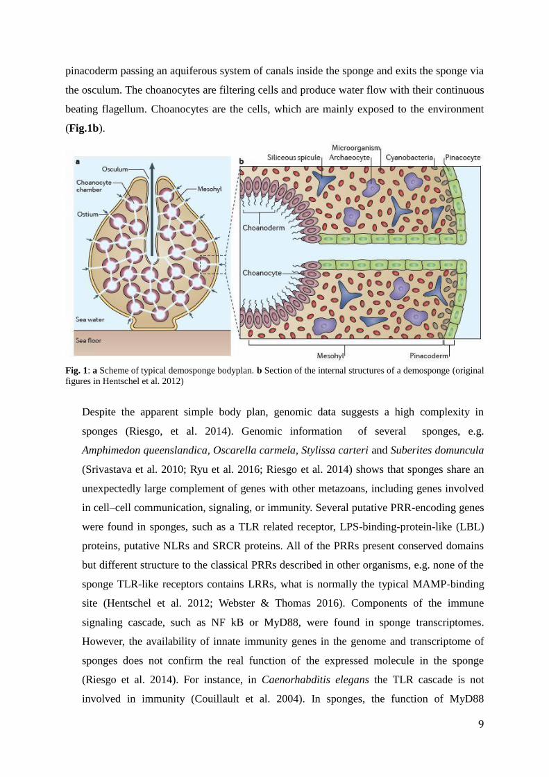
The simple poriferan body plan is unique among metazoans (Riesgo et al. 2014). Sponges do

have epithelia, but lack true tissues and organs (Dunn et al. 2015). The pinacoderm separates

the sponge from the surrounding seawater and builds the outer layer. Beneath the pinacoderm

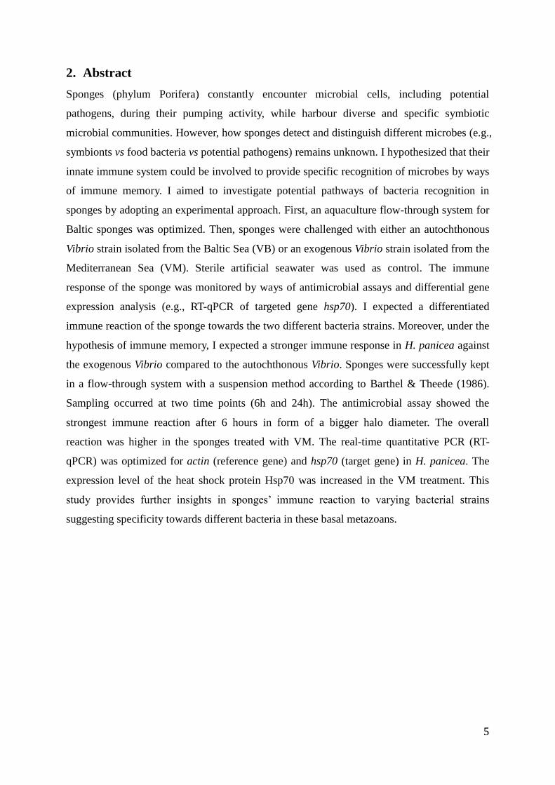
is the mesohyl, which is the functioning layer of the sponge (Fig.1a), and where metabolism,

reproduction, nutrient transfer and cell communication components are located. Inside the

mesohyl the totipotent amoeboid archeocytes and symbiotic microbes are distributed (Webster

et al. 2007). Sponges are filter feeders and water enters the body via open pores in the

9

pinacoderm passing an aquiferous system of canals inside the sponge and exits the sponge via

the osculum. The choanocytes are filtering cells and produce water flow with their continuous

beating flagellum. Choanocytes are the cells, which are mainly exposed to the environment

(Fig.1b).

Fig. 1: a Scheme of typical demosponge bodyplan. b Section of the internal structures of a demosponge (original

figures in Hentschel et al. 2012)

Despite the apparent simple body plan, genomic data suggests a high complexity in

sponges (Riesgo, et al. 2014). Genomic information of several sponges, e.g.

Amphimedon queenslandica, Oscarella carmela, Stylissa carteri and Suberites domuncula

(Srivastava et al. 2010; Ryu et al. 2016; Riesgo et al. 2014) shows that sponges share an

unexpectedly large complement of genes with other metazoans, including genes involved

in cell–cell communication, signaling, or immunity. Several putative PRR-encoding genes

were found in sponges, such as a TLR related receptor, LPS-binding-protein-like (LBL)

proteins, putative NLRs and SRCR proteins. All of the PRRs present conserved domains

but different structure to the classical PRRs described in other organisms, e.g. none of the

sponge TLR-like receptors contains LRRs, what is normally the typical MAMP-binding

site (Hentschel et al. 2012; Webster & Thomas 2016). Components of the immune

signaling cascade, such as NF kB or MyD88, were found in sponge transcriptomes.

However, the availability of innate immunity genes in the genome and transcriptome of

sponges does not confirm the real function of the expressed molecule in the sponge

(Riesgo et al. 2014). For instance, in Caenorhabditis elegans the TLR cascade is not

involved in immunity (Couillault et al. 2004). In sponges, the function of MyD88

10

involved in the recognition cascade of gram-negative bacteria has been reported (Wiens et

al. 2005), but the overall empirical evidence for gene functions in the innate immunity

pathway is still scarce.

In this Master’s thesis, I aimed to unravel the function of potential immune genes in

sponges upon encounter with different bacterial strains. The low-microbial-abundance

sponge Halichondria panicea of the Baltic Sea was exposed to heat-killed Vibrio bacteria

and the immune response of the sponge was monitored by ways of antimicrobial assays

and differential gene expression analysis (e.g., RT-qPCR of targeted genes). Heat-killed

bacteria strains were successfully used in other invertebrate studies on immune challenge

(Roth et al. 2009; Trapani et al. 2016; Zaragoza et al. 2014; Bolte et al. 2013) and Vibrio

strains in general are commonly used for immune challenge experiments in marine

invertebrates (Wright et al. 2013; Lokmer & Wegner 2015; Bolte et al. 2013). Two Vibrio

strains were applied by injection of heat-killed bacteria in the mesohyl of the sponge. The

sponge was supposed to be completely naive towards the exogenous Vibrio strain,

whereas the autochthonous Vibrio strain might have been encountered before. I expect

differential gene expression after Vibrio encounter and stronger response to the exogenous

Vibrio strain, consistent with the evolutionary concept of reducing costs and self-damage

of specific immune defense. By combining molecular analysis with an experimental

approach, this study contributes to current research priorities in sponge microbiology, such

as reveal host mechanisms involved in sponge-microbe interactions (Webster & Thomas

2016).

11

4. Material and Methods

4.1. Halichondria panicea

H. panicea (Pallas, 1766), with the common name “breadcrumb sponge” is a marine sponge

of the class Demospongiae. It belongs to the family Halichondriidae and the genus

Halichondria, with 109 accepted species and more than 200 unconfirmed species (WoRMS,

28.01.2017). H. panicea is widely distributed in the Northern Hemisphere from the Baltic and

North Sea to the North Eastern Atlantic, with sister groups in the North Pacific (Erpenbeck et

al. 2004). The main habitat is the intertidal zone, but H. panicea can also appear in the

sublittoral and down to 500 m depth. Several morphotypes are known for H. panicea:

compact, encrusting and branched forms. Also, their color varies between yellow, grey and

greenish.

The specimens investigated in this study belonged to the Baltic Sea population of H. panicea

from Kiel Bight, where this species is one of the most abundant species of sponges (Barthel

1986). They live mainly on Red algae of the phylum Phyllophora sp. or Phycodrys sp., but

also on hard substrates such as rocks. Growth, reproduction, spermatogenesis, energy budget

and biomass production were extensively investigated (Barthel & Detmer 1990; Witte et al.

1994; Barthel 1986). Their lifecycle starts in spring from a planktonic larval stage that

transform to the adult sponge after settling on either hard substrate or red algae. Over the

summer period the sponge’ body volume increases until it reaches the maximum in August.

With progressing seasons the sponge mass decreases and almost disappears in winter (Barthel,

1985; 1986; 1988). Every few weeks H. panicea sloughs off its outer tissue. The cause is

unknown, but is hypothesized that could be a mechanism to prevent sedimentary clogging of

its ostia or fouling (Barthel & Wolfrath 1989). Despite the intensive studies on physiology,

morphology and ecology, only little genetic information is available on H. panicea and its

genome is not sequenced.

Because of their high abundance H. panicea plays an important role in the habitat of the

Kieler Bay e.g. by providing nutrients to the surrounding seawater (Barthel 1988). The genus

Halichondria is also relevant for biotechnological interests for the production of antimicrobial,

antifungal or cytostatic compounds, either produced by the sponge itself or by associated

microbes (Blunt et al. 2007; Clark et al. 1992). Finally, due to its amenability to aquaculture,

it has become a potential model organism for the study of host-microbe-environment

12

interactions at Geomar (Pita et al. 2016). The morphotypes of H. panicea in this study were

yellow and red colored and of branched form.

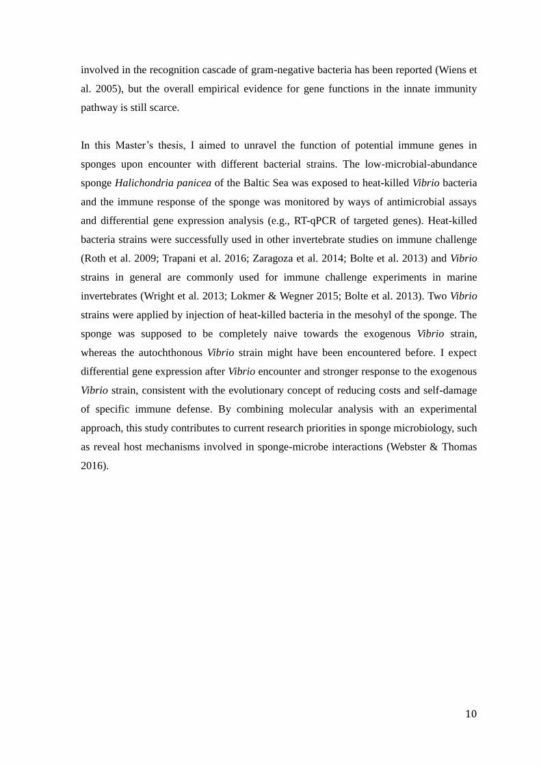
4.2. Sponge aquaculture

Sponges of the species H. panicea were provided by Claas Hiebenthal (KIMOCC, Geomar

Helmholtz Centre for Ocean Research Kiel) and sampled at Kieler Mussel farm (54°

22.558’N, 10° 9.786’E), Baltic Sea at 6 m depth. Cultivation conditions were orientated on

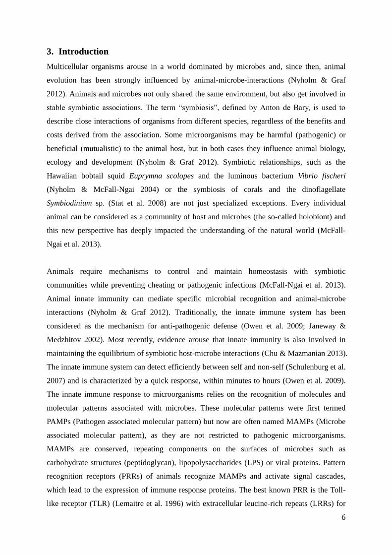
the work of Barthel & Theede (1986) and Westphal (1988). The sponges were maintained in

an open flow-through system with direct uptake of Baltic Sea water, which will keep

biological and physical parameters of the water at similar conditions (temperature; pH;

salinity) as in the field. The water is provided via a header tank to oxygenate the incoming

water to the aquaria (Fig. 2).

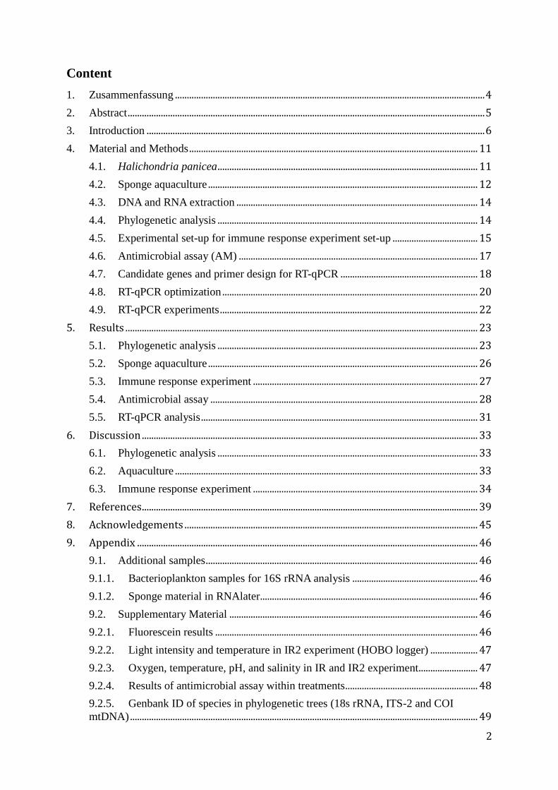
Fig.2: A, C Sponge aquaculture with a flow-through system. B sponge individuals in the tanks.

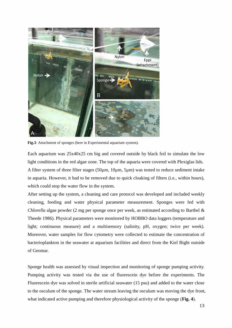
H. panicea lives regularly attached to algae and therefore a floating state enhance its

maintenance in aquaculture (Barthel & Theede 1986). Sponges were attached to nylon strings

on top of the aquarium and to a small stone on the bottom (as weight) with a 0.2 mm nylon

string (Fig. 3). PE beads were added under the sponges to prevent them from sliding down.

Handling of sponges occurred always under water to avoid air embolization.

13

Fig.3: Attachment of sponges (here in Experimental aquarium system).

Each aquarium was 25x40x25 cm big and covered outside by black foil to simulate the low

light conditions in the red algae zone. The top of the aquaria were covered with Plexiglas lids.

A filter system of three filter stages (50µm, 10µm, 5µm) was tested to reduce sediment intake

in aquaria. However, it had to be removed due to quick cloaking of filters (i.e., within hours),

which could stop the water flow in the system.

After setting up the system, a cleaning and care protocol was developed and included weekly

cleaning, feeding and water physical parameter measurement. Sponges were fed with

Chlorella algae powder (2 mg per sponge once per week, as estimated according to Barthel &

Theede 1986). Physical parameters were monitored by HOBBO data loggers (temperature and

light; continuous measure) and a multisensory (salinity, pH, oxygen; twice per week).

Moreover, water samples for flow cytometry were collected to estimate the concentration of

bacterioplankton in the seawater at aquarium facilities and direct from the Kiel Bight outside

of Geomar.

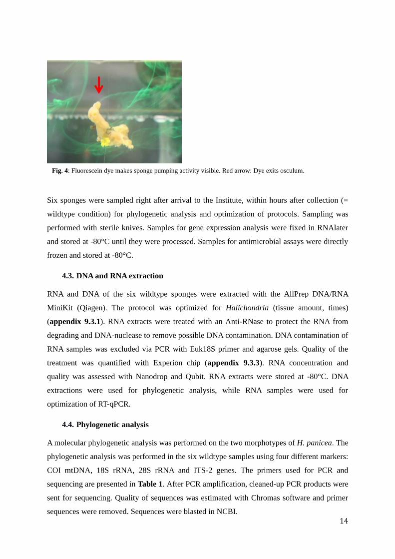
Sponge health was assessed by visual inspection and monitoring of sponge pumping activity.

Pumping activity was tested via the use of fluorescein dye before the experiments. The

Fluorescein dye was solved in sterile artificial seawater (15 psu) and added to the water close

to the osculum of the sponge. The water stream leaving the osculum was moving the dye front,

what indicated active pumping and therefore physiological activity of the sponge (Fig. 4).

14

Six sponges were sampled right after arrival to the Institute, within hours after collection (=

wildtype condition) for phylogenetic analysis and optimization of protocols. Sampling was

performed with sterile knives. Samples for gene expression analysis were fixed in RNAlater

and stored at -80°C until they were processed. Samples for antimicrobial assays were directly

frozen and stored at -80°C.

4.3. DNA and RNA extraction

RNA and DNA of the six wildtype sponges were extracted with the AllPrep DNA/RNA

MiniKit (Qiagen). The protocol was optimized for Halichondria (tissue amount, times)

(appendix 9.3.1). RNA extracts were treated with an Anti-RNase to protect the RNA from

degrading and DNA-nuclease to remove possible DNA contamination. DNA contamination of

RNA samples was excluded via PCR with Euk18S primer and agarose gels. Quality of the

treatment was quantified with Experion chip (appendix 9.3.3). RNA concentration and

quality was assessed with Nanodrop and Qubit. RNA extracts were stored at -80°C. DNA

extractions were used for phylogenetic analysis, while RNA samples were used for

optimization of RT-qPCR.

4.4. Phylogenetic analysis

A molecular phylogenetic analysis was performed on the two morphotypes of H. panicea. The

phylogenetic analysis was performed in the six wildtype samples using four different markers:

COI mtDNA, 18S rRNA, 28S rRNA and ITS-2 genes. The primers used for PCR and

sequencing are presented in Table 1. After PCR amplification, cleaned-up PCR products were

sent for sequencing. Quality of sequences was estimated with Chromas software and primer

sequences were removed. Sequences were blasted in NCBI.

Fig. 4: Fluorescein dye makes sponge pumping activity visible. Red arrow: Dye exits osculum.

15

Phylogenetic trees were designed based on COI mtDNA, 18S rRNA and ITS-2. The

phylogenetic trees included the sequences that were generated in this study, other porifera

from the NCBI database, cnidarian, ctenophores and Mus musculus, respectively Stichopus

monotuberculatus as outgroup. The sequences were aligned with MAFFT or MUSCLE and

reduced to the same length. A maximum likelihood tree was prepared in MEGA 6 with 1000

bootstrap.

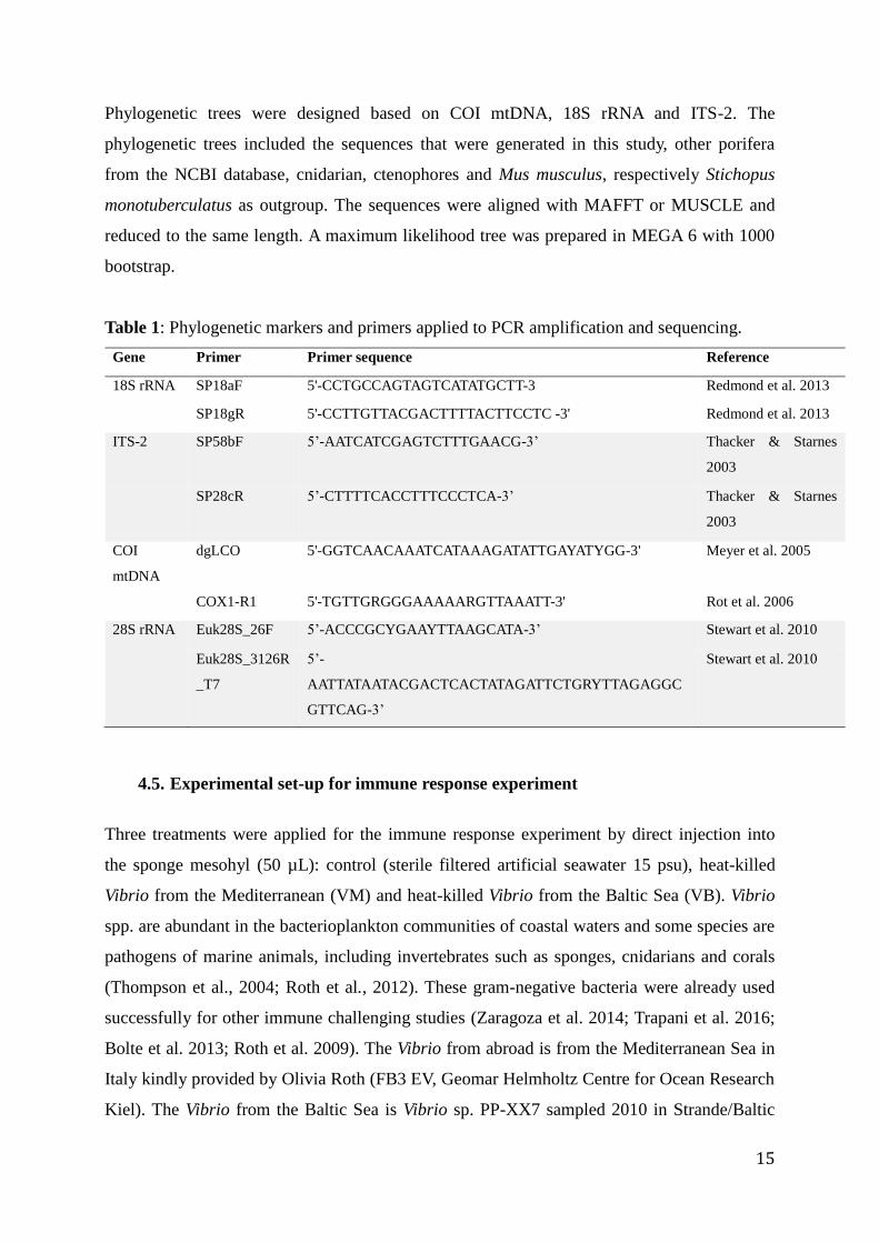
Table 1: Phylogenetic markers and primers applied to PCR amplification and sequencing.

Gene Primer Primer sequence Reference

18S rRNA SP18aF 5'-CCTGCCAGTAGTCATATGCTT-3 Redmond et al. 2013

SP18gR 5'-CCTTGTTACGACTTTTACTTCCTC -3' Redmond et al. 2013

ITS-2 SP58bF 5’-AATCATCGAGTCTTTGAACG-3’ Thacker & Starnes

2003

SP28cR 5’-CTTTTCACCTTTCCCTCA-3’ Thacker & Starnes

2003

COI

mtDNA

dgLCO 5'-GGTCAACAAATCATAAAGATATTGAYATYGG-3' Meyer et al. 2005

COX1-R1 5'-TGTTGRGGGAAAAARGTTAAATT-3' Rot et al. 2006

28S rRNA Euk28S_26F 5’-ACCCGCYGAAYTTAAGCATA-3’ Stewart et al. 2010

Euk28S_3126R

_T7

5’-

AATTATAATACGACTCACTATAGATTCTGRYTTAGAGGC

GTTCAG-3’

Stewart et al. 2010

4.5. Experimental set-up for immune response experiment

Three treatments were applied for the immune response experiment by direct injection into

the sponge mesohyl (50 µL): control (sterile filtered artificial seawater 15 psu), heat-killed

Vibrio from the Mediterranean (VM) and heat-killed Vibrio from the Baltic Sea (VB). Vibrio

spp. are abundant in the bacterioplankton communities of coastal waters and some species are

pathogens of marine animals, including invertebrates such as sponges, cnidarians and corals

(Thompson et al., 2004; Roth et al., 2012). These gram-negative bacteria were already used

successfully for other immune challenging studies (Zaragoza et al. 2014; Trapani et al. 2016;

Bolte et al. 2013; Roth et al. 2009). The Vibrio from abroad is from the Mediterranean Sea in

Italy kindly provided by Olivia Roth (FB3 EV, Geomar Helmholtz Centre for Ocean Research

Kiel). The Vibrio from the Baltic Sea is Vibrio sp. PP-XX7 sampled 2010 in Strande/Baltic

16

Sea from muddy ground in 5 m depth. It was kindly provided by Jutta Wiese and Tanja Rahn

(FB3 MI, Geomar Helmholtz Centre for Ocean Research Kiel).

Vibrio strain cultures were reactivated according to Bolte et al., 2013. Vibrio phylotypes were

taken from a frozen glycerol stock (40% glycerol) and grown in medium 101 (5 g Peptone

and 3 g meat extract per liter) adjusted for marine bacteria by addition of 1.5% NaCl and

incubated at 25°C at 180 rpm overnight. Bacteria cultures were transferred into 1.5 ml

Eppendorf tubes, heat deactivated at 65°C for 1h, centrifuged at medium speed (2000 rpm)

and then the bacterial pellet was resuspended in artificial seawater (AquaMedic, 15psu, sterile

filtered 0.22 μm).

The experiment took place in a flow-through system of 18 aquaria kindly provided by Olivia

Roth (FB3 EV, Geomar Helmholtz Centre for Ocean Research Kiel). Water samples were

taken from the aquaria before the experiments started, on both experimental days and directly

from the Kiel Bight before and after the experiments to analyze bacterioplankton

concentration in the seawater by flow cytometry. Samples were fixed with Paraformaldehyde

and Glutaraldehyde (appendix 9.3.3) to a final concentration of 1% and stored directly at

-80°C. Flow cytometry was performed at the flow cytometer FACScalibur (Becton &

Dickinson) of FB3 Research Unit “Marine Food Webs”, access kindly provided by Thomas

Hansen. Samples were diluted (1/4) with artificial seawater (16 PSU). Heterotrophic bacteria

in the water were stained with SYBRGreen solution (final concentration of 0.025%

(1:20.000)). The amount of bacteria was measured at flow rate 12 µL/min, threshold 2 min

and green fluorescence (FL1). Bacterial cells were recorded in log-scale and were identified

according to their size and fluorescence (settings: FL1 vs. SSC; FL1 threshold: 144, FSC: E02,

SSC: 460). Data analysis was performed with Microsoft® Excel and FlowingSoftware 2.5.1.

For the first immune response experiment (IR), three sponges were divided in three clones

and each clone was kept in an individual aquarium and assigned to one treatment. Thus, three

replicates per treatment. They were kept in the aquaria for 4 weeks for acclimation. The

clones of one sponge died a few days before the experiment started. Therefore, the replicates

were reduced to two per treatment. No food was provided during the experiment. In addition

the first immune response experiment (IR) was performed simultaneously in three Haliclona

sp. with the conditions described above and a second immune response experiment (IR2) was

performed with three replicates of H. panicea three months after the first experiment.

17

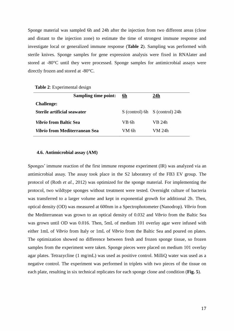
Sponge material was sampled 6h and 24h after the injection from two different areas (close

and distant to the injection zone) to estimate the time of strongest immune response and

investigate local or generalized immune response (Table 2). Sampling was performed with

sterile knives. Sponge samples for gene expression analysis were fixed in RNAlater and

stored at -80°C until they were processed. Sponge samples for antimicrobial assays were

directly frozen and stored at -80°C.

Table 2: Experimental design

Sampling time point:

Challenge:

6h 24h

Sterile artificial seawater S (control) 6h S (control) 24h

Vibrio from Baltic Sea VB 6h VB 24h

Vibrio from Mediterranean Sea VM 6h VM 24h

4.6. Antimicrobial assay (AM)

Sponges’ immune reaction of the first immune response experiment (IR) was analyzed via an

antimicrobial assay. The assay took place in the S2 laboratory of the FB3 EV group. The

protocol of (Roth et al., 2012) was optimized for the sponge material. For implementing the

protocol, two wildtype sponges without treatment were tested. Overnight culture of bacteria

was transferred to a larger volume and kept in exponential growth for additional 2h. Then,

optical density (OD) was measured at 600nm in a Spectrophotometer (Nanodrop). Vibrio from

the Mediterranean was grown to an optical density of 0.032 and Vibrio from the Baltic Sea

was grown until OD was 0.016. Then, 5mL of medium 101 overlay agar were infused with

either 1mL of Vibrio from Italy or 1mL of Vibrio from the Baltic Sea and poured on plates.

The optimization showed no difference between fresh and frozen sponge tissue, so frozen

samples from the experiment were taken. Sponge pieces were placed on medium 101 overlay

agar plates. Tetrazycline (1 mg/mL) was used as positive control. MilliQ water was used as a

negative control. The experiment was performed in triplets with two pieces of the tissue on

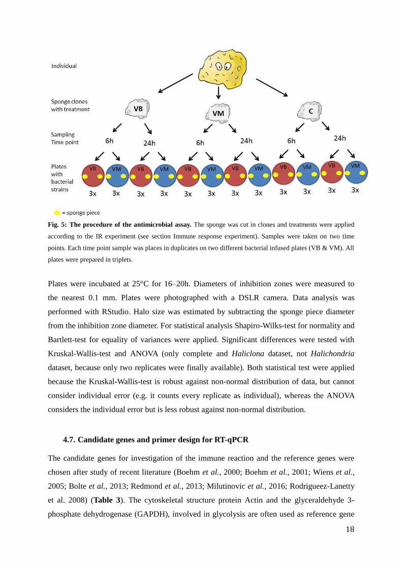
each plate, resulting in six technical replicates for each sponge clone and condition (Fig. 5).

18

Fig. 5: The procedure of the antimicrobial assay. The sponge was cut in clones and treatments were applied

according to the IR experiment (see section Immune response experiment). Samples were taken on two time

points. Each time point sample was places in duplicates on two different bacterial infused plates (VB & VM). All

plates were prepared in triplets.

Plates were incubated at 25°C for 16–20h. Diameters of inhibition zones were measured to

the nearest 0.1 mm. Plates were photographed with a DSLR camera. Data analysis was

performed with RStudio. Halo size was estimated by subtracting the sponge piece diameter

from the inhibition zone diameter. For statistical analysis Shapiro-Wilks-test for normality and

Bartlett-test for equality of variances were applied. Significant differences were tested with

Kruskal-Wallis-test and ANOVA (only complete and Haliclona dataset, not Halichondria

dataset, because only two replicates were finally available). Both statistical test were applied

because the Kruskal-Wallis-test is robust against non-normal distribution of data, but cannot

consider individual error (e.g. it counts every replicate as individual), whereas the ANOVA

considers the individual error but is less robust against non-normal distribution.

4.7. Candidate genes and primer design for RT-qPCR

The candidate genes for investigation of the immune reaction and the reference genes were

chosen after study of recent literature (Boehm et al., 2000; Boehm et al., 2001; Wiens et al.,

2005; Bolte et al., 2013; Redmond et al., 2013; Milutinovic et al., 2016; Rodrigueez-Lanetty

et al. 2008) (Table 3). The cytoskeletal structure protein Actin and the glyceraldehyde 3-

phosphate dehydrogenase (GAPDH), involved in glycolysis are often used as reference gene

19

in RT-qPCR analysis, also in studies in invertebrates (Bolte et al. 2013). Also, some authors

have used 18S rRNA gene as reference gene (Li et al. 2014) . Members of the heat shock

protein family are highly conserved and function as molecular chaperones by protecting the

organism against thermal or other stress-induced damage (Borchiellini et al. 1998). They are

also involved in intracellular protein transport and protein biogenesis (Shimpi et al. 2016) and

in immune challenge response (Brown & Rodriguez-Lanetty 2015; Brown et al. 2013).

MyD88, JNK and p38 are interesting as components of the TLR signaling pathway and

phenoloxidase and peroxiredoxin as effectors.

As no genome information is available for H. panicea, the primers were designed by using

aligned sequences of other sponge species found in NCBI and focused on the most conserved

areas. Sequences were aligned by MUSCLE in MEGA6. Degenerated primers were designed

with IDT PrimerQuestTool for primer design and evaluated with IDT OligoAnalyzerTool and

the TM calculator of Thermofisher. The designed primers were tested on cDNA of the six

wildtype samples via touch down PCR and evaluated via agarose gels. After appearance of

clear single bands, the PCR product was cleaned up with the DNA, RNA and protein

purification Kit (Macherey and Nagel) and send to sequencing. Sequences were analyzed with

Chromas for quality of sequence chromatogram and sequences were edited (e.g., removal of

primer sequence) in BioEdit v7.2.5. Sequences were blasted against the NCBI database. From

the long sequences of the investigated genes, shorter fragments (75-200bp) were designed,

which were required for qPCR analysis. Optimal annealing temperature was estimated with

gradient PCR. Fragments were sequenced again to guarantee the right target.

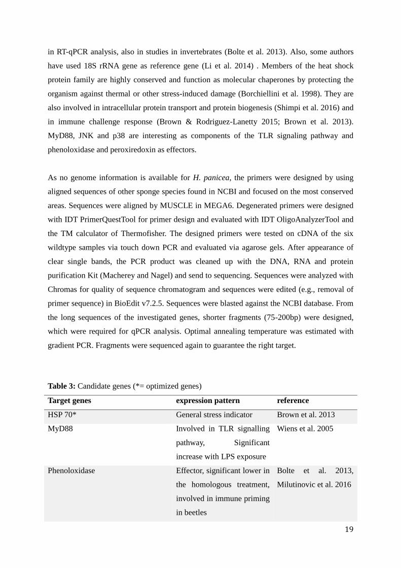
Table 3: Candidate genes (*= optimized genes)

Target genes expression pattern reference

HSP 70* General stress indicator Brown et al. 2013

MyD88 Involved in TLR signalling

pathway, Significant

increase with LPS exposure

Wiens et al. 2005

Phenoloxidase Effector, significant lower in

the homologous treatment,

involved in immune priming

in beetles

Bolte et al. 2013,

Milutinovic et al. 2016

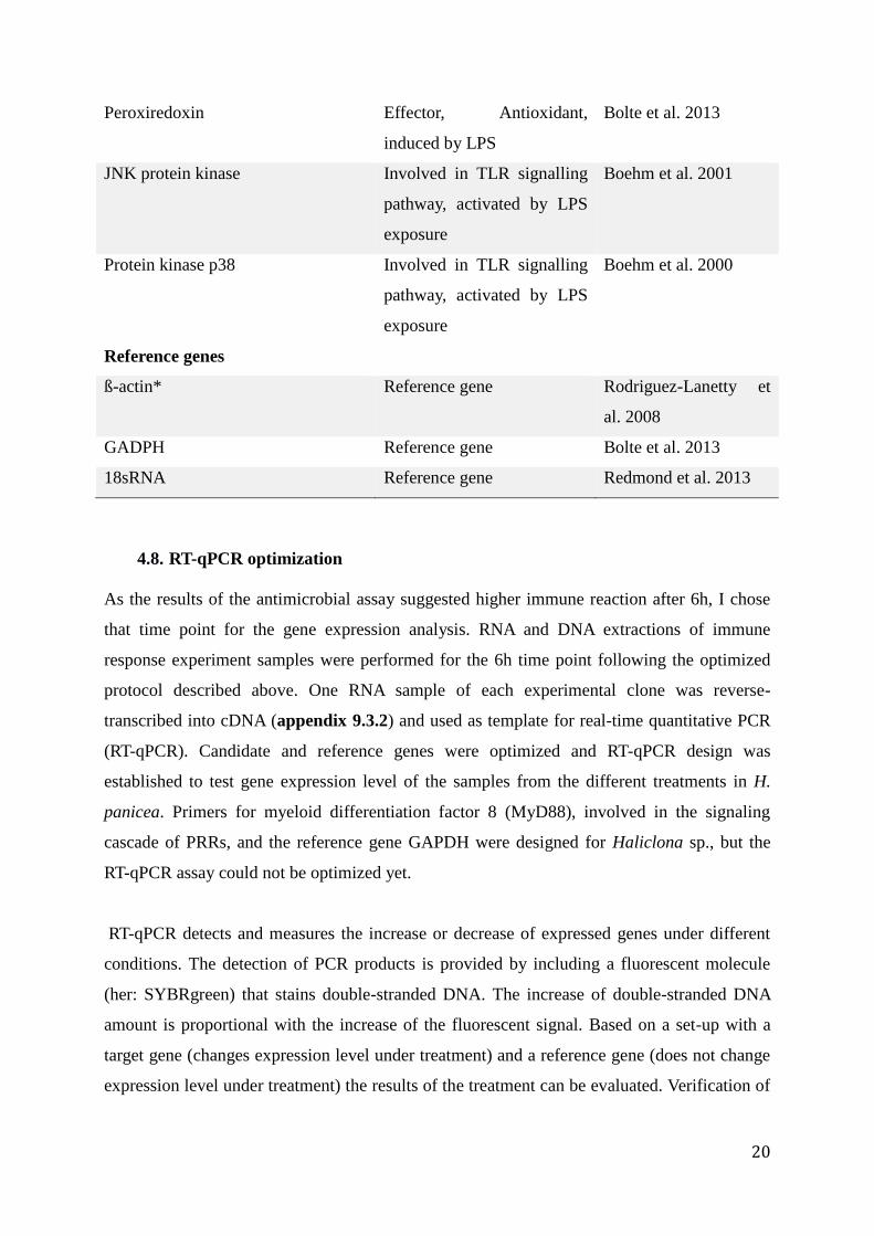
20

Peroxiredoxin Effector, Antioxidant,

induced by LPS

Bolte et al. 2013

JNK protein kinase Involved in TLR signalling

pathway, activated by LPS

exposure

Boehm et al. 2001

Protein kinase p38 Involved in TLR signalling

pathway, activated by LPS

exposure

Boehm et al. 2000

Reference genes

ß-actin* Reference gene Rodriguez-Lanetty et

al. 2008

GADPH Reference gene Bolte et al. 2013

18sRNA Reference gene Redmond et al. 2013

4.8. RT-qPCR optimization

As the results of the antimicrobial assay suggested higher immune reaction after 6h, I chose

that time point for the gene expression analysis. RNA and DNA extractions of immune

response experiment samples were performed for the 6h time point following the optimized

protocol described above. One RNA sample of each experimental clone was reverse-

transcribed into cDNA (appendix 9.3.2) and used as template for real-time quantitative PCR

(RT-qPCR). Candidate and reference genes were optimized and RT-qPCR design was

established to test gene expression level of the samples from the different treatments in H.

panicea. Primers for myeloid differentiation factor 8 (MyD88), involved in the signaling

cascade of PRRs, and the reference gene GAPDH were designed for Haliclona sp., but the

RT-qPCR assay could not be optimized yet.

RT-qPCR detects and measures the increase or decrease of expressed genes under different

conditions. The detection of PCR products is provided by including a fluorescent molecule

(her: SYBRgreen) that stains double-stranded DNA. The increase of double-stranded DNA

amount is proportional with the increase of the fluorescent signal. Based on a set-up with a

target gene (changes expression level under treatment) and a reference gene (does not change

expression level under treatment) the results of the treatment can be evaluated. Verification of

21

absolute values and relative quantification is possible. In this study relative quantification was

performed.

Important requirements for a comparable set-up are reliable reference genes and primers with

similar amplification efficiencies (to guarantee comparability between target and reference

genes). For an estimation of primer efficiency a standard curve of DNA samples of known

(for absolute quantification) or unknown (for relative quantification) concentration can be

performed. The standard curve should be performed in doubles. The replicate reactions should

be consistent and the standard curve should be as linear as possible (R²>0.98). The

amplification efficiency of the primers should be high (90–105%) and within a range of 5% to

each other to perform convenient evaluation methods such as, 2-ΔΔCt

(Livak) Method or the

ΔCt Method using a Reference Gene. In this study the primer efficiencies differed from each

other (see results). Therefore, the Pfaffl-Method was used.

Formula Pfaffl-Method

The above equation assumes that each gene (target and reference) has the same amplification

efficiency in test samples and calibrator samples, but it is not necessary that the target and

reference genes have the same amplification efficiency as each other (BIO-RAD Laboratories

2006).

The standard curve was performed from a dilution series of wildtype cDNA with 1/5 dilution.

The dilution was prepared in tRNA water (10ng/µl). tRNA is a small oligonucleotide that does

not disturb the reaction but keeps the template in solution by flattening uneven tube walls.

This improves the homogenic solution of cDNA template in the tube.

The standard curve was performed in doubles for each gene with wildtypes. Each well of the

96-well plate contained SYBR-Green qPCR buffer (1x), forward and reverse primer (300

nml), 5µl template (cDNA) and molecular H2O. Protocols for RT-qPCR conditions were

optimized for each gene. Reagents were ordered at ThermoFisher®Scientific. H2O was used

as negative control.

22

4.9. RT-qPCR experiments

Differential gene expression analysis of hsp70 and actin was performed for H. panicea.

Two qPCR experiments (= two plates) were performed with reagents described above. The

first plate contained H. panicea sponge samples from the first immune response experiment

(IR), which were two biological replicates (clones) per treatment. The second plate contained

H. panicea sponge samples from the second immune response experiment (IR2), which were

three biological replicates (no clones) per treatment. Three technical replicates per treatment

were placed on the plate. Target gene was hsp70 and reference gene was actin. Analysis of Ct

ratio was performed with RStudio and Microsoft®Excel 2010 using the Pfaffl-Method. In IR2

the ΔCt of the calibrator (=control sample) was the mean of either HSP70 controls or actin

controls to provide more homogeneity to the data, because the biological replicates were not

clones in the IR2. For statistical analysis Shapiro-Wilks-test for normality, Bartlett-test for

equality of variances and t.test (only complete and IR2 dataset, not IR dataset) were applied.

23

5. Results

5.1. Phylogenetic analysis

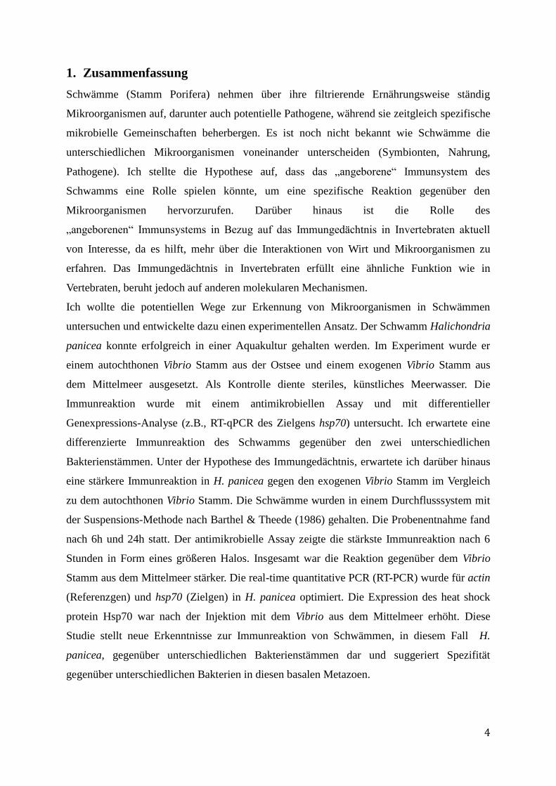
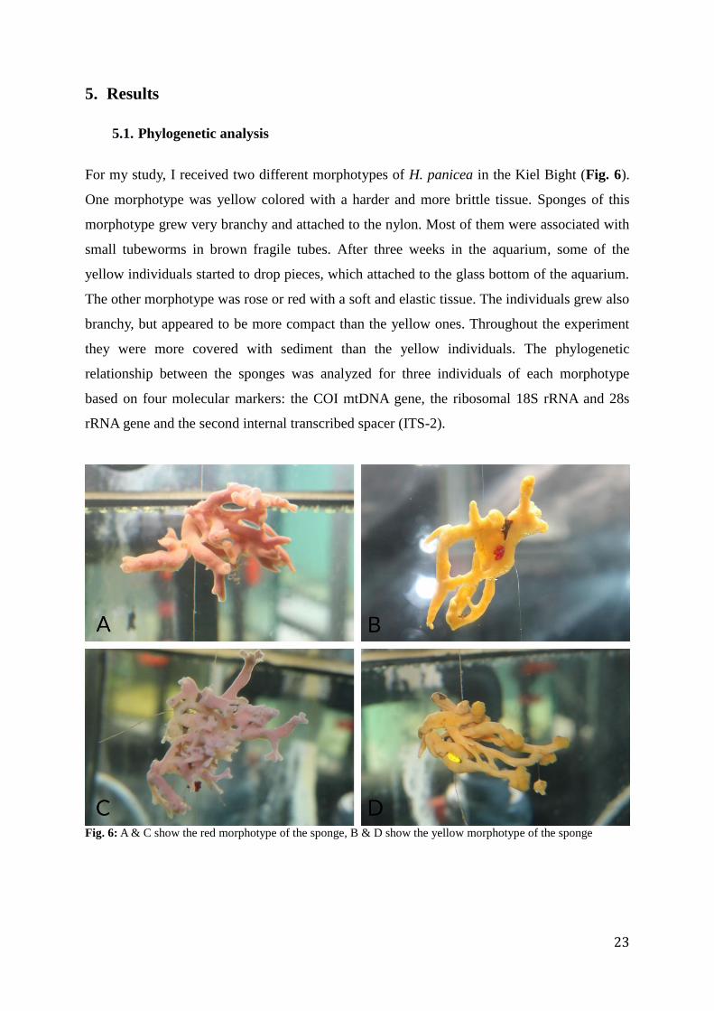
For my study, I received two different morphotypes of H. panicea in the Kiel Bight (Fig. 6).

One morphotype was yellow colored with a harder and more brittle tissue. Sponges of this

morphotype grew very branchy and attached to the nylon. Most of them were associated with

small tubeworms in brown fragile tubes. After three weeks in the aquarium, some of the

yellow individuals started to drop pieces, which attached to the glass bottom of the aquarium.

The other morphotype was rose or red with a soft and elastic tissue. The individuals grew also

branchy, but appeared to be more compact than the yellow ones. Throughout the experiment

they were more covered with sediment than the yellow individuals. The phylogenetic

relationship between the sponges was analyzed for three individuals of each morphotype

based on four molecular markers: the COI mtDNA gene, the ribosomal 18S rRNA and 28s

rRNA gene and the second internal transcribed spacer (ITS-2).

Fig. 6: A & C show the red morphotype of the sponge, B & D show the yellow morphotype of the sponge

24

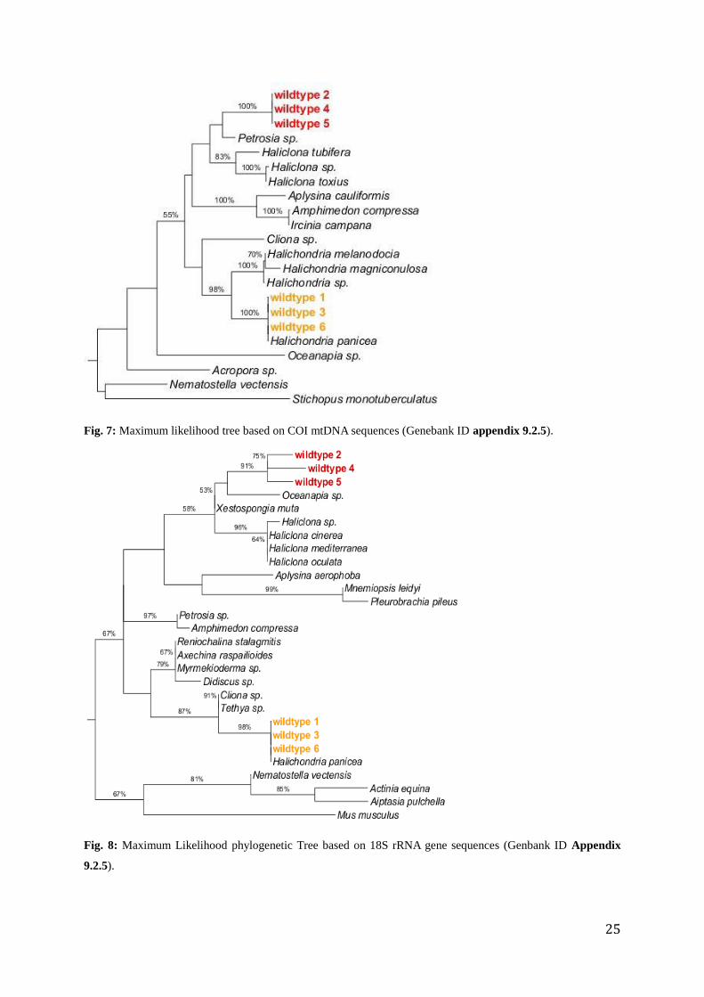
The sequences (983-1200 bp long) of the COI mtDNA primers identified the yellow

morphotype with 99% identity as Halichondria panicea (KC869423.1). The yellow

morphotypes were 99.58-99.83% identical. The red morphotype sequences were 99.15-99.66%

identical and showed 98%-99% identity with Haliclona sp. (JN242210.1). In the phylogenetic

tree based on COI mtDNA sequences the yellow morphotype clearly (bootstrap 100%)

clusters together with H. panicea (KC869423.1). The red morphotype clusters together with

Petrosia sp. (JN242220.1) (bootstrap 43%) in short distance to Haliclona sp. (LC126249.1).

The two morphotypes clearly cluster separately (Fig.7).

The sequences of 18S rRNA gene (793bp - 1169bp long) of the yellow morphotype showed

98%-99% identity with Halichondria panicea (KF699110.1). The 18s RNA gene sequences of

the red morphotype showed 87% - 95% identity with Oceanapia sp. (DQ927317.1) and 90%-

95% identity with Haliclona sp. (EU095523.1). All three yellow morphotypes are 99%

identical and red morphotype sequences were 94-98% identical. Identity between yellow

morphotypes and red morphotypes was 84-90%. The ML tree shows clearly that the two

morphotypes do not cluster together (Fig.8). The yellow morphotype clusters together with H.

panicea sequences (KF699110.1) (bootstrap 98%), whereas the red morphotype clusters

separated (bootstrap 91%) next to Oceanapia sp. (DQ927317.1), Xestospongia muta

(AY621510.1) and Haliclona sp. (AY734444.1). Ctenophore sequences cluster within the

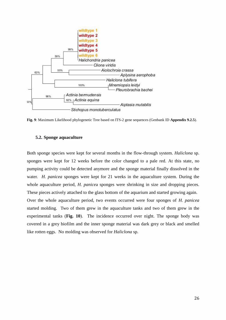
sponge sequences. In contrast, the marker ITS-2 (520bp - 580bp long) revealed that all six

wildtypes were closely-related to Halichondria sp. (AF062607.1) (99%-100% identity,

AF062607.1) and clustered together with Halichondria panicea (AF062607.1) in the ML

phylogenetic tree (Fig.9). 28S rRNA sequences (1049 - 1234 bp long) were only successfully

amplified for the yellow morphotype. The sequences showed 98-99% identity with H.

panicea (AF062607.1, HQ379242.1).

25

Fig. 7: Maximum likelihood tree based on COI mtDNA sequences (Genebank ID appendix 9.2.5).

Fig. 8: Maximum Likelihood phylogenetic Tree based on 18S rRNA gene sequences (Genbank ID Appendix

9.2.5).

26

Fig. 9: Maximum Likelihood phylogenetic Tree based on ITS-2 gene sequences (Genbank ID Appendix 9.2.5).

5.2. Sponge aquaculture

Both sponge species were kept for several months in the flow-through system. Haliclona sp.

sponges were kept for 12 weeks before the color changed to a pale red. At this state, no

pumping activity could be detected anymore and the sponge material finally dissolved in the

water. H. panicea sponges were kept for 21 weeks in the aquaculture system. During the

whole aquaculture period, H. panicea sponges were shrinking in size and dropping pieces.

These pieces actively attached to the glass bottom of the aquarium and started growing again.

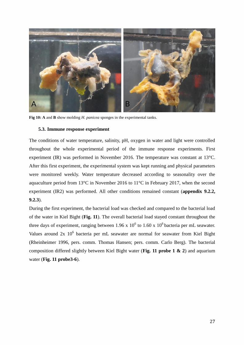
Over the whole aquaculture period, two events occurred were four sponges of H. panicea

started molding. Two of them grew in the aquaculture tanks and two of them grew in the

experimental tanks (Fig. 10). The incidence occurred over night. The sponge body was

covered in a grey biofilm and the inner sponge material was dark grey or black and smelled

like rotten eggs. No molding was observed for Haliclona sp.

27

Fig 10: A and B show molding H. panicea sponges in the experimental tanks.

5.3. Immune response experiment

The conditions of water temperature, salinity, pH, oxygen in water and light were controlled

throughout the whole experimental period of the immune response experiments. First

experiment (IR) was performed in November 2016. The temperature was constant at 13°C.

After this first experiment, the experimental system was kept running and physical parameters

were monitored weekly. Water temperature decreased according to seasonality over the

aquaculture period from 13°C in November 2016 to 11°C in February 2017, when the second

experiment (IR2) was performed. All other conditions remained constant (appendix 9.2.2,

9.2.3).

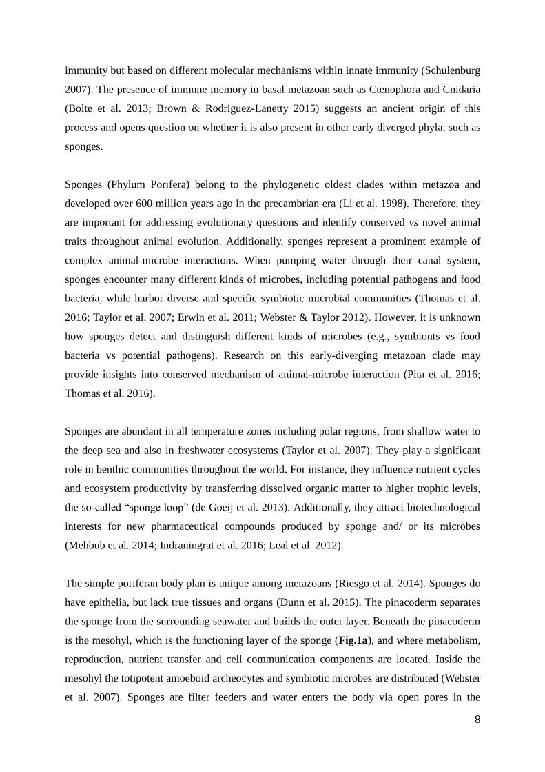
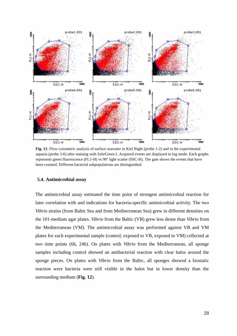
During the first experiment, the bacterial load was checked and compared to the bacterial load

of the water in Kiel Bight (Fig. 11). The overall bacterial load stayed constant throughout the

three days of experiment, ranging between 1.96 x 106 to 1.60 x 10

6 bacteria per mL seawater.

Values around 2x 106 bacteria per mL seawater are normal for seawater from Kiel Bight

(Rheinheimer 1996, pers. comm. Thomas Hansen; pers. comm. Carlo Berg). The bacterial

composition differed slightly between Kiel Bight water (Fig. 11 probe 1 & 2) and aquarium

water (Fig. 11 probe3-6).

28

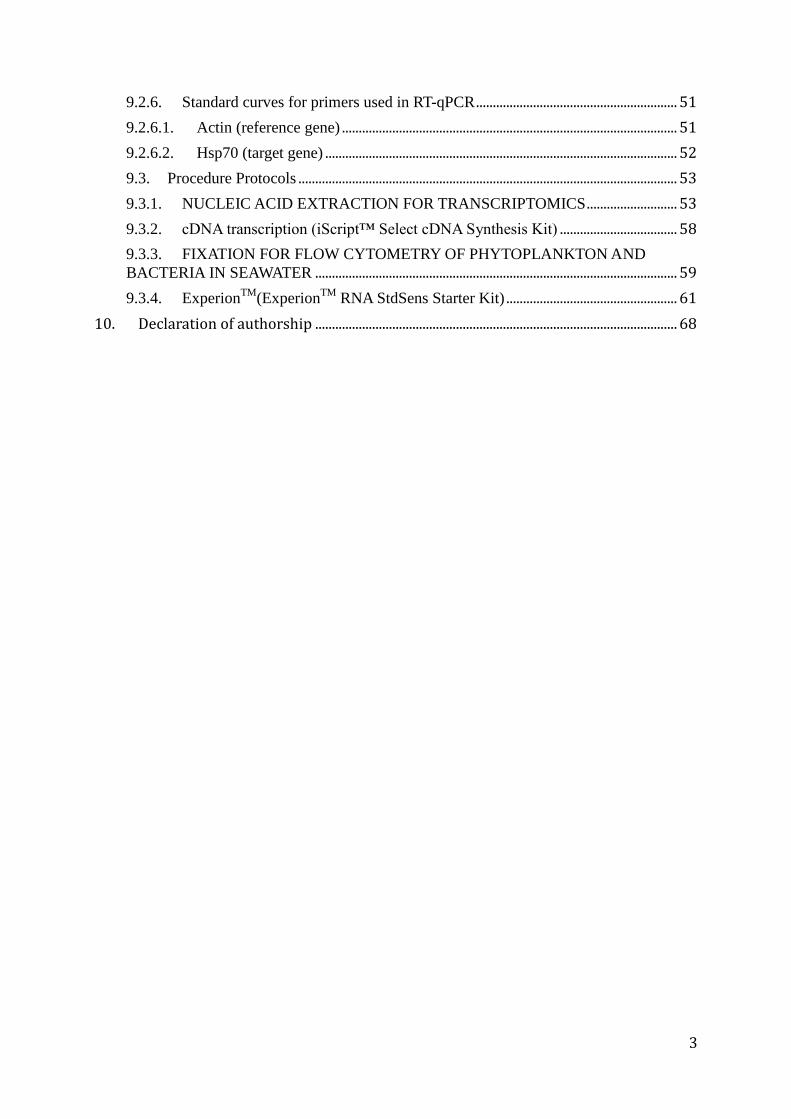
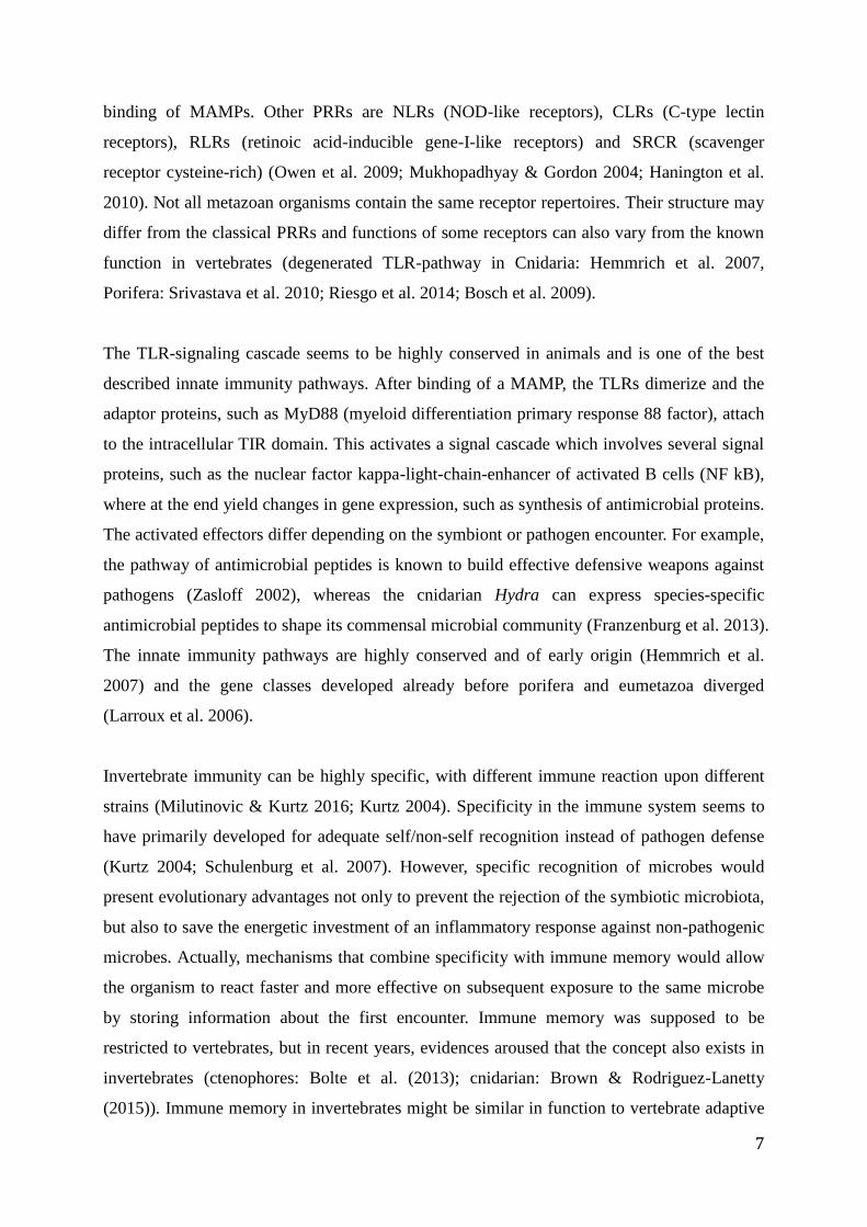
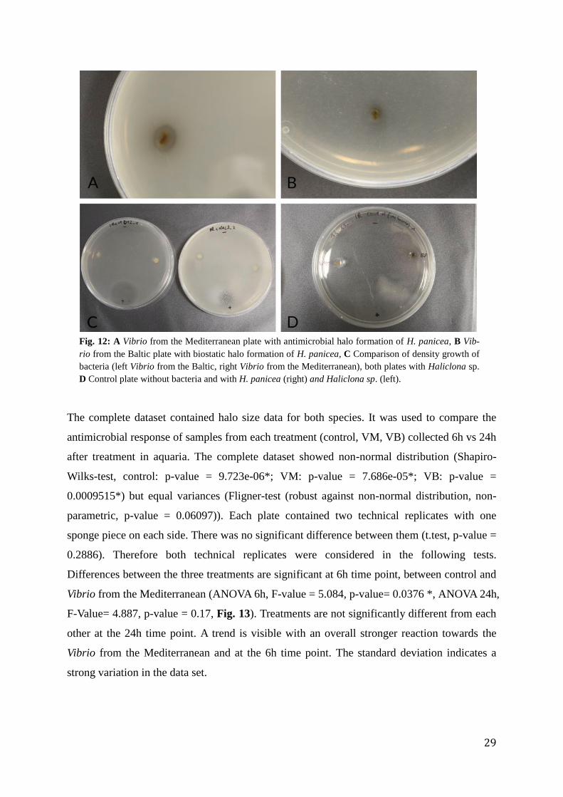
5.4. Antimicrobial assay

The antimicrobial assay estimated the time point of strongest antimicrobial reaction for

later correlation with and indications for bacteria-specific antimicrobial activity. The two

Vibrio strains (from Baltic Sea and from Mediterranean Sea) grew in different densities on

the 101-medium agar plates. Vibrio from the Baltic (VB) grew less dense than Vibrio from

the Mediterranean (VM). The antimicrobial assay was performed against VB and VM

plates for each experimental sample (control, exposed to VB, exposed to VM) collected at

two time points (6h, 24h). On plates with Vibrio from the Mediterranean, all sponge

samples including control showed an antibacterial reaction with clear halos around the

sponge pieces. On plates with Vibrio from the Baltic, all sponges showed a biostatic

reaction were bacteria were still visible in the halos but in lower density than the

surrounding medium (Fig. 12).

Fig. 11: Flow cytometric analysis of surface seawater in Kiel Bight (probe 1-2) and in the experimental

aquaria (probe 3-6) after staining with SybrGreen I. Acquired events are displayed in log mode. Each graphs

represents green fluorescence (FL1-H) vs 90º light scatter (SSC-H). The gate shows the events that have

been counted. Different bacterial subpopulations are distinguished.

29

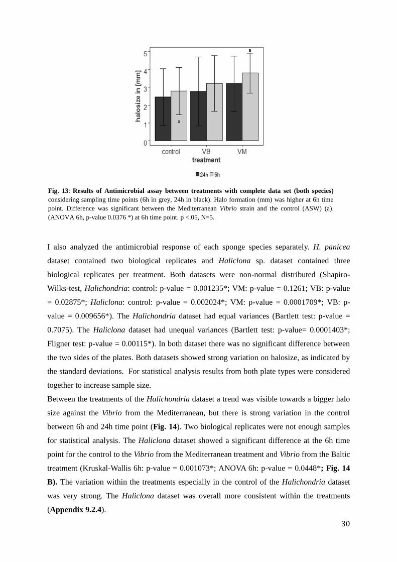
The complete dataset contained halo size data for both species. It was used to compare the

antimicrobial response of samples from each treatment (control, VM, VB) collected 6h vs 24h

after treatment in aquaria. The complete dataset showed non-normal distribution (Shapiro-

Wilks-test, control: p-value = 9.723e-06*; VM: p-value = 7.686e-05*; VB: p-value =

0.0009515*) but equal variances (Fligner-test (robust against non-normal distribution, non-

parametric, p-value = 0.06097)). Each plate contained two technical replicates with one

sponge piece on each side. There was no significant difference between them (t.test, p-value =

0.2886). Therefore both technical replicates were considered in the following tests.

Differences between the three treatments are significant at 6h time point, between control and

Vibrio from the Mediterranean (ANOVA 6h, F-value = 5.084, p-value= 0.0376 *, ANOVA 24h,

F-Value= 4.887, p-value = 0.17, Fig. 13). Treatments are not significantly different from each

other at the 24h time point. A trend is visible with an overall stronger reaction towards the

Vibrio from the Mediterranean and at the 6h time point. The standard deviation indicates a

strong variation in the data set.

Fig. 12: A Vibrio from the Mediterranean plate with antimicrobial halo formation of H. panicea, B Vib-

rio from the Baltic plate with biostatic halo formation of H. panicea, C Comparison of density growth of

bacteria (left Vibrio from the Baltic, right Vibrio from the Mediterranean), both plates with Haliclona sp.

D Control plate without bacteria and with H. panicea (right) and Haliclona sp. (left).

30

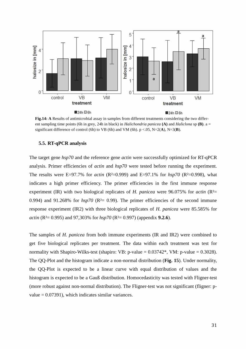
I also analyzed the antimicrobial response of each sponge species separately. H. panicea

dataset contained two biological replicates and Haliclona sp. dataset contained three

biological replicates per treatment. Both datasets were non-normal distributed (Shapiro-

Wilks-test, Halichondria: control: p-value = 0.001235*; VM: p-value = 0.1261; VB: p-value

= 0.02875*; Haliclona: control: p-value = 0.002024*; VM: p-value = 0.0001709*; VB: p-

value = 0.009656*). The Halichondria dataset had equal variances (Bartlett test: p-value =

0.7075). The Haliclona dataset had unequal variances (Bartlett test: p-value= 0.0001403*;

Fligner test: p-value = 0.00115*). In both dataset there was no significant difference between

the two sides of the plates. Both datasets showed strong variation on halosize, as indicated by

the standard deviations. For statistical analysis results from both plate types were considered

together to increase sample size.

Between the treatments of the Halichondria dataset a trend was visible towards a bigger halo

size against the Vibrio from the Mediterranean, but there is strong variation in the control

between 6h and 24h time point (Fig. 14). Two biological replicates were not enough samples

for statistical analysis. The Haliclona dataset showed a significant difference at the 6h time

point for the control to the Vibrio from the Mediterranean treatment and Vibrio from the Baltic

treatment (Kruskal-Wallis 6h: p-value = 0.001073*; ANOVA 6h: p-value = 0.0448*; Fig. 14

B). The variation within the treatments especially in the control of the Halichondria dataset

was very strong. The Haliclona dataset was overall more consistent within the treatments

(Appendix 9.2.4).

Fig. 13: Results of Antimicrobial assay between treatments with complete data set (both species)

considering sampling time points (6h in grey, 24h in black). Halo formation (mm) was higher at 6h time

point. Difference was significant between the Mediterranean Vibrio strain and the control (ASW) (a).

(ANOVA 6h, p-value 0.0376 *) at 6h time point. p <.05, N=5.

31

5.5. RT-qPCR analysis

The target gene hsp70 and the reference gene actin were successfully optimized for RT-qPCR

analysis. Primer efficiencies of actin and hsp70 were tested before running the experiment.

The results were E=97.7% for actin (R²=0.999) and E=97.1% for hsp70 (R²=0.998), what

indicates a high primer efficiency. The primer efficiencies in the first immune response

experiment (IR) with two biological replicates of H. panicea were 96.075% for actin (R²=

0.994) and 91.268% for hsp70 (R²= 0.99). The primer efficiencies of the second immune

response experiment (IR2) with three biological replicates of H. panicea were 85.585% for

actin (R²= 0.995) and 97,303% for hsp70 (R²= 0.997) (appendix 9.2.6).

The samples of H. panicea from both immune experiments (IR and IR2) were combined to

get five biological replicates per treatment. The data within each treatment was test for

normality with Shapiro-Wilks-test (shapiro: VB: p-value = 0.03742*, VM: p-value = 0.3028).

The QQ-Plot and the histogram indicate a non-normal distribution (Fig. 15). Under normality,

the QQ-Plot is expected to be a linear curve with equal distribution of values and the

histogram is expected to be a Gauß distribution. Homocedasticity was tested with Fligner-test

(more robust against non-normal distribution). The Fligner-test was not significant (fligner: p-

value = 0.07391), which indicates similar variances.

Fig.14: A Results of antimicrobial assay in samples from different treatments considering the two differ-

ent sampling time points (6h in grey, 24h in black) in Halichondria panicea (A) and Haliclona sp (B). a =

significant difference of control (6h) to VB (6h) and VM (6h). p <.05, N=2(A), N=3(B).

32

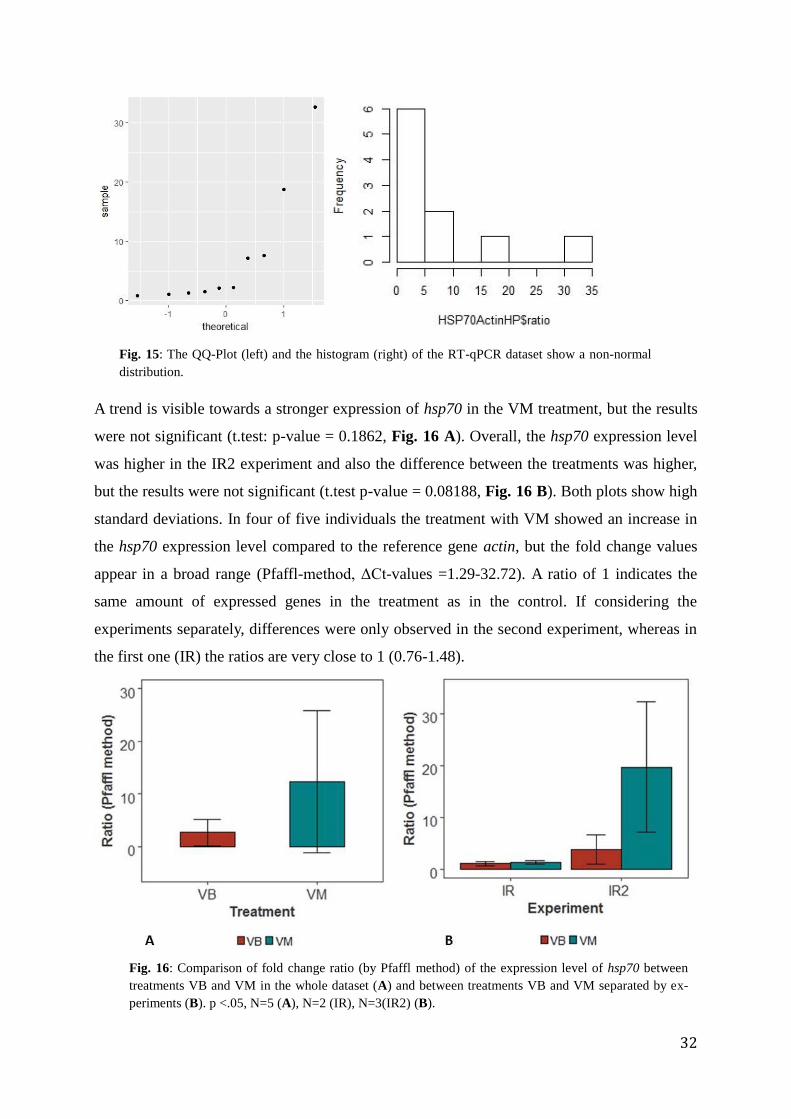
A trend is visible towards a stronger expression of hsp70 in the VM treatment, but the results

were not significant (t.test: p-value = 0.1862, Fig. 16 A). Overall, the hsp70 expression level

was higher in the IR2 experiment and also the difference between the treatments was higher,

but the results were not significant (t.test p-value = 0.08188, Fig. 16 B). Both plots show high

standard deviations. In four of five individuals the treatment with VM showed an increase in

the hsp70 expression level compared to the reference gene actin, but the fold change values

appear in a broad range (Pfaffl-method, ΔCt-values =1.29-32.72). A ratio of 1 indicates the

same amount of expressed genes in the treatment as in the control. If considering the

experiments separately, differences were only observed in the second experiment, whereas in

the first one (IR) the ratios are very close to 1 (0.76-1.48).

Fig. 15: The QQ-Plot (left) and the histogram (right) of the RT-qPCR dataset show a non-normal

distribution.

Fig. 16: Comparison of fold change ratio (by Pfaffl method) of the expression level of hsp70 between

treatments VB and VM in the whole dataset (A) and between treatments VB and VM separated by ex-

periments (B). p <.05, N=5 (A), N=2 (IR), N=3(IR2) (B).

33

6. Discussion

6.1. Phylogenetic analysis

Based on macroscopic morphological features, I characterized the sponge individuals as “yel-

low morphotype” and “red morphotype”. Phylogeny based on morphological features is often

not precise enough, as many morphological features are similar between species. Genetic

markers are a helpful tool to add to morphological classifications. However, no single ideal

marker to classify all sponges exists and even the universal barcode markers COI mtDNA,

18s rRNA, 28s rRNA or the ITS-2 region showed different resolution level depending on the

sponges investigated. For instance, 18S rRNA showed varying success for phylogenetic anal-

ysis in sponges, ranging from low phylogenetic signal (Szitenberg et al. 2013) to complete

sponge classifications in Demospongiae (Redmond et al. 2013). Therefore, the combination of

more than one molecular markers with morphological features is recommended (multilocus-

based Sponge Identification Protocol (SIP) by Yang et al. (2017); Szitenberg et al. 2013).

The most reliable markers in my study were COI mtDNA and 18S rRNA, as they amplified

sequences for both species in sufficient length and identified the two morphotypes as different

species. 28S rRNA was reported as one of the most reliable molecular markers in sponge phy-

logeny (Szitenberg et al. 2013; Yang et al. 2017), but could not be successfully amplified for

the candidate Haliclona sp. in my study. ITS-2 showed the lowest value of identification as

both morphotypes were identified as the same species H. panicea, what confirms former stud-

ies claiming ITS-2 as insufficient marker especially for Halicona sp. (Yang et al. 2017;

Redmond 2009), but contradicts reports of successful separation of sponge species based on

ITS-2 (Erwin et al. 2011). By combining different molecular markers, I was able to identify

the yellow morphotype as Halichondria panicea (18S rRNA, 28S rRNA, COI mtDNA) and

the red morphotype as Haliclona sp. (18S rRNA, COI mtDNA). A clear identification was

crucial, because the two species situation affected the experimental process and the primer

design.

6.2. Aquaculture

The aquaculture of H. panicea was successfully performed according to the suspension

method of Barthel & Theede (1986) in a flow-through system with only minor losses by

molding. Barthel & Theede (1986) also tested a second method where sponge pieces were

attached between glass slides, but the method was concluded to be less successful for survival

rate. This second method was not actively performed in this study, but broken sponge pieces

34

of H. panicea attached independently to the bottom of the aquaria and were metabolically

active. Thus, both growing conditions (suspension and attached to glass) were successful for

survival of H. panicea. The suspension method set-up used for H. panicea was also successful

for cultivating Haliclona sp. To my knowledge, this study is the first study describing a

cultivation method for Haliclona sp. in an aquarium. A cultivation method with sponge

transplants in a field aquaculture was performed with moderate success (Rosmiati et al. 2007).

H. panicea survived for 5 months in aquaculture, what is one month more than described in

Barthel & Theede (1986) as long-term survival (4 months), but shorter than reported

cultivation of H. panicea for one year (Müller 2003). The Haliclona sp. could be successfully

kept for 12 weeks. However, compared to H. panicea, the survival rate was lower and

therefore Haliclona sp. suits more to short-term maintenance. Based on the cultivation

success, H. panicea seems to be a suitable candidate for a potential model organism, as the

cultivation method is: easy to carry out and inexpensive (when flow-through system available,

e.g. at GEOMAR), provides good long-term survival and cultured individuals suit for

physiological and ecological experiments in the laboratory (Barthel & Theede 1986). The

flow-through system provides more natural conditions and is highly recommended.

Before the experiment started, two specimen of H. panicea were observed to be covered with

a grey biofilm, in its appearance similar to a fungal infection. Origins of the infection can be

multiple, such as a pathogen encounter in the aquarium, pre-infected sponge individuals from

the field or opportunistic microbes inside the sponge that turned pathogenic under aquaculture

conditions. Similar infection events of H. panicea in the field are not described in literature,

what could relate the issue to the sponge aquaculture. Infections in aquarium maintenance

were observed before for Ircinia sp. and Aplysina aerophoba (Lucía Pita Galán, pers.

comm.).The infection issue might be an interesting topic for further studies.

6.3. Immune response experiment

I hypothesized a differentiated immune reaction of the sponges towards the two different

Vibrio strains and an increased immune response to the Vibrio strain from the Mediterranean

(VM) (i.e. higher antimicrobial activity and differential gene expression), whereas the

response to the Vibrio from the Baltic Sea (VB) stays similar to that in the control. The

antimicrobial assay showed a stronger reaction to VM and a higher reaction at the 6h time

point. The expression of the heat shock protein Hsp70 was analyzed with RT-qPCR in the

35

different treatments showing an upregulation of Hsp70 in VM treatment. Both analyses, the

antimicrobial assay and the RT-qPCR, showed a differentiated reaction towards the Vibrio

strains with a higher reaction to the VM, although the reaction was not consistent in all

samples.

The antimicrobial activity of H. panicea and Haliclona sp. against both Vibrio strains

indicates that the heat-killed Vibrio strains injected were taken as microbial challenge. Results

suggested a trend towards a stronger reaction at the 6h time point in form of a wider halo

formation. The time point corresponds with the study on immune priming in Mnemiopsis

leidyi (Bolte et al. 2013). Other immunological studies in invertebrates confirm a high

immune reaction within the first 24h hours (Pham et al. 2007; Sadd & Schmid-Hempel 2006;

Zhang et al. 2011). Sampling time points can only reflect a snapshot of the physiological,

molecular and behavioral changes after microbial encounter. Therefore, they affect the results

of gene expression studies and should be carefully chosen. A stronger reaction at 6h time

point may correspond with a higher gene expression level. Therefore, the 6h time point

samples suited best for me to plan the proceedings of the experiment (RNA and DNA

extraction and qPCR optimization). However, more than one sampling time point can help to

provide a baseline for expressed genes and a time series on the reaction, e.g. monitoring of

wound healing in cnidarians (Stewart et al. 2017). Thus, samples of the 24h sampling time

point were stored for further analysis (appendix 9.1.2).

The antimicrobial assay and the RT-qPCR showed both strong variations in the dataset and

may be related to small amount of replicates (2-3 biological replicates in Halichondria

experiments, three biological replicates in Haliclona dataset). The antimicrobial activity in the

control of the Halichondria dataset was also variable and suggests a general antimicrobial

activity of the sponge by e.g. frequently expressed secondary metabolites or by compounds

released by either microbes growing on the sponge surface or sponge-associated microbes

inside the sponge (Schneemann et al. 2010; Kelman et al. 2001; Helber 2016). For future

experiments it is recommended to run the experiments with more replicates per treatment or,

if this is not possible because of logistics, analyze more samples of the same biological

replicate.

Primer design for RT-qPCR analysis in the absence of a sequenced genome turned out to be a

difficult challenge. It was not possible to optimize primers that worked for both sponge

36

species. Therefore, I focused on the sponge H. panicea, as it has been object of other studies

within the research group. For this sponge, the cytoskeletal structure protein actin was

successfully optimized as reference gene and the heat-shock protein Hsp70 gene as target.

Ideally, more than one reference gene should be included to allow the evaluation of the gene

as a reference of basal expression. In this study, the validation of actin has not been possible

yet, but actin is a commonly used reference gene, stable under abiotic and biotic stress, as

shown in other invertebrate studies (sponge: Webster et al. 2013; cnidaria: Rodriguez-Lanetty

et al. 2008; Shimpi et al. 2016). Hsp70 is not involved in the signaling cascade of the immune

reaction. However, expression changes upon microbial challenges were reported before

(Brown et al. 2013; Brown & Rodriguez-Lanetty 2015; Zhou et al. 2010). In my study the RT-

qPCR analysis, the upregulation of hsp70 gene was higher with VM treatment in the IR2

experiment. The increased hsp70 expression in VM treatment indicates a higher activity of the

immune system compared to the VB treatment. The results encourage to persist the efforts to

optimize genes involved in the immune signaling cascade.

Interestingly, the gene expression patterns (target gene expression in relation to reference) are

not consistent in both immune experiments. Both immune experiments were performed under

similar conditions. However, in the first experiment (IR) clones were used for the different

treatments, whereas in the IR2 experiment individual specimens were applied. The application

of clones in an experimental approach can be advantageous for reducing the genetic variation

and increasing homogeneity of the dataset. Clonal sponge fragments remain metabolically

active after cutting and recover quickly from wounding. However, in the case of low number

of replicates, the use of clones may cause the genetic variation of samples within replicates of

one treatment to be higher than the variation between the treatments and prevent the detection

of differential gene expression. Furthermore, sponges used in the IR2 experiment spent three

months longer in the aquaculture. Long-term aquaculture maintenance can cause changes in

the bacterial community, as was reported for H. panicea (Müller 2003). This may increase

vulnerability of sponges towards potential pathogens and therefore increase the reaction

towards the applied bacteria, what could result in the increased hsp70 expression level in the

IR2 experiment.

The sponge species investigated here showed a specific reaction upon the challenge by

different Vibrio stains. In the antimicrobial assay, both sponges showed higher intensity and

antibiotic response against the VM treatment than to VB (biostatic response). This implies a

37

specific reaction of the sponges towards the different Vibrio stains. To date, specificity on

bacterial strains was mainly reported for higher invertebrates, such as insects (Roth et al. 2009)

or crustaceans (reviewed in Schulenburg et al. 2007). However, the immune priming

experiment of Bolte et al. 2013 with Mnemiopsis leidyi suggests specificity also in basal

metazoans. The lower reaction against VB could indicate that the sponges just recognized the

strain as non-pathogenic or, considering the hypothesis of immune memory in invertebrates,

encountered this Vibrio strain before the experiment, as H. panicea was found in the same

habitat (HELCOM Red List Biotope Expert Group 2013).

Furthermore, the specificity can be designated by the Vibrio strains themselves by variable

virulence. The family of Vibrionaceae is highly diverse and members of the genus Vibrio spp.

are not necessarily pathogenic (Thompson et al. 2004). Some of them live even in symbiotic

relationships, e.g. the bioluminescent Vibrio fischeri with the Hawaiian bobtail squid

Euprymna scolopes (Nyholm & McFall-Ngai 2004). In contrast, other members are known

for their high pathogeny to, e.g. humans, such as Vibrio cholera (Thompson et al. 2004). Their

pathogenic potential is tightly coupled to environmental conditions (temperature, availability

of iron), cell density (expression of virulence genes via quorum sensing), motility and

chemotaxis (Thompson et al. 2004). Some Vibrio strains can gain or increase their pathogeny

by taking up virulent plasmids (Roux et al. 2011). The Vibrio strains used in this study were

not further classified. Therefore their virulence might vary from each other and cause different

reactions of the sponges.

To distinguish if the stronger reaction of the sponges towards the Vibrio from the

Mediterranean is caused by immune memory of the Baltic Sea sponges to VB or by the high

virulence of the VM, a similar experimental design applied to a Mediterranean sponge could

provide answers. If the reaction of the Mediterranean sponge is higher to VM than to VB, the

different immune reaction is more likely provoked by the virulence of VM. If the reaction of

the Mediterranean sponge is more intense towards the exogenous Vibrio (in their case VB)

this could indicate adaption or immune memory of the sponges. Important for the concept of

immune memory is a specific response to repeated infections compared to first encounter.

Specificity and immune memory can be further investigated by homologous vs. heterologous

treatment (Bolte et al. 2013) In this type of experiments, individuals are exposed to twice the

same Vibrio (homologous treatment) or to two different Vibrio strains (heterologous

treatment). Under the hypothesis of immune memory, I expect that the sponge will react

38

different towards the two Vibrio strains and the two treatments detectable in differentially

expressed genes. Depending on the investigated genes, I expect a downregulation consistent

with the evolutionary concept of reducing costs and self-damage of immune defense or an

upregulation of specific genes due to immune memory (quicker and more effective response

upon second injection).

The long-term cultivation in an aquaculture system was successfully established for H.

panicea, what will help to provide sponges for experiments under controlled conditions.

Furthermore, this study provides important knowledge on specificity in H. panicea towards

different Vibrio strains. Specificity in sponges unravels potential mechanisms for controlling

microbial communities in these basal metazoans and can build a baseline for more complex

processes, such as immune memory in sponges or symbiosis. The presence of specific

reactions towards bacteria in these basal metazoans suggests highly conserved pathways for

animal-microbe interactions. Further studies should focus on developing more genetic

markers involved in the host mechanism to respond to microbes.

39

7. References

Barthel, D., 1986. On the ecophysiology of the sponge Halichondria panicea in Kiel Bight. I.

Substrate specificity, growth and reproduction. Marine Ecology Progress Series, 32(2-3),

pp.291–298.

Barthel, D., 1988. On the ecophysiology of the sponge Halichondria panicea in Kiel Bight. II.

Biomass, production, energy budget and integration in environmental processes. Marine

Ecology, 43, pp.87–93.

Barthel, D. & Detmer, A., 1990. The spermatogenesis of Halichondria panicea (Porifera,

Demospongiae). Zoomorphology, 110, pp.9–15.

Barthel, D. & Theede, H., 1986. A new method for the culture of marine sponges and its

application for experimental studies. Ophelia, 25(2), pp.37–41.

Barthel, D. & Wolfrath, B., 1989. Tissue sloughing in the sponge Halichondria panicea : a

fouling organism prevents being fouled. Oecologia, 78, pp.357–360.

Blunt, J.W. et al., 2007. Marine natural products. Natural Products report, 24, pp.31–86.

Boehm, M., et al. 2000. The mitogen-activated protein kinase p38 pathway is conserved in

metazoans : Cloning and activation of p38 of the SAPK2 subfamily from the sponge

Suberites domuncula. Biology of the Cell, 92, pp. 95-104.

Boehm, M., et al., 2001. Molecular response of the sponge Suberites domuncula to bacterial

infection. Marine Biology, 139(6), pp. 1037-1045.

Bolte, S. et al., 2013. Specific immune priming in the invasive ctenophore Mnemiopsis leidyi.

Biology letters, 9(20130864), pp.1–5.

Borchiellini, C. et al., 1998. Phylogenetic analysis of the Hsp70 sequences reveals the

monophyly of Metazoa and specific phylogenetic relationships between animals and

fungi. Molecular Biology and Evolution, 15(6), pp. 647-655.

Bosch, T.C.G. et al., 2009. Uncovering the evolutionary history of innate immunity: The

simple metazoan Hydra uses epithelial cells for host defence. Developmental and

Comparative Immunology, 33(4), pp.559–569.

Brown, T., Bourne, D. & Rodriguez-lanetty, M., 2013. Transcriptional activation of c3 and

hsp70 as part of the immune response of Acropora millepora to bacterial challenges.

PLoS ONE, 8(7).

Brown, T. & Rodriguez-Lanetty, M., 2015a. Defending against pathogens - immunological

priming and its molecular basis in a sea anemone, cnidarian. Scientific reports, 5.

Chu, H. & Mazmanian, S.K., 2013. Innate immune recognition of the microbiota promotes

host-microbial symbiosis. Nature Immunology, 14(7), pp.668–675.

Clark, I. et al., 1992. Total synthesis of Halichondrin B and Norhalichondrin B. Journal of the

40

American Chemical Society, 114, pp.3162–3164.

Couillault, C. et al., 2004. TLR-independent control of innate immunity in Caenorhabditis

elegans by the TIR domain adaptor protein TIR-1 , an ortholog of human SARM. Nature

im, 5(5), pp.488–494.

Dunn, C.W., Leys, S.P. & Haddock, S.H.D., 2015. The hidden biology of sponges and

ctenophores. Trends in Ecology and Evolution, 30(5), pp.282–291.

Erpenbeck, D., Knowlton, A. & Talbot, S.L., 2004. A molecular comparison of Alaskan and

North East Atlantic Halichondria panicea ( Pallas , 1766 ) ( Porifera: Demospongiae)

Populations. Boll. Mus. Ist. Biol. Univ. Genova, 68, pp.319–325.

Erwin, P.M. et al., 2011. A specific mix of generalists: bacterial symbionts in Mediterranean

Ircinia spp. FEMS Microbiology Ecology, pp.1–19.

Franzenburg, S. et al., 2013. Distinct antimicrobial peptide expression determines host

species-specific bacterial associations. Proceedings of the National Academy of Sciences

of the United States of America, 110, pp.E3730–8.

de Goeij, J.M. et al., 2013. Surviving in a marine desert: the sponge loop retains resources

within coral reefs. Science, 342, pp.108–110.

Hanington, P.C. et al., 2010. Role for a somatically diversified lectin in resistance of an

invertebrate to parasite infection. Proceedings of the National Academy of Sciences,

107(49), pp.21087–21092.

Helber, S., 2016. Chemical ecology of Western Indian Ocean reef sponges. PhD Thesis

HELCOM Red List Biotope Expert Group, 2013. HELCOM: Biotope information sheet.

Hemmrich, G., Miller, D.J. & Bosch, T.C.G., 2007. The evolution of immunity: a low-life

perspective. Trends in Immunology, 28(10), pp.449–454.

Hentschel, U. et al., 2012. Genomic insights into the marine sponge microbiome. Nature

Reviews Microbiology, 10(9), pp.641–654.

Indraningrat, A.A.G., Smidt, H. & Sipkema, D., 2016. Bioprospecting sponge-associated

microbes for antimicrobial compounds. Marine Drugs, 14(5), pp.1–66.

Janeway, C. a & Medzhitov, R., 2002. Innate immune recognition. Annual review of

immunology, 20(2), pp.197–216.

Kelman, D. et al., 2001. Antimicrobial activity of the reef sponge Amphimedon viridis from

the Red Sea : evidence for selective toxicity. Aquatic Microbial Ecology, 24, pp.9–16.

Kurtz, J., 2004. Memory in the innate and adaptive immune systems. Microbes and Infection,

6(15), pp.1410–1417.

Larroux, C. et al., 2006. Developmental expression of transcription factor genes in a

demosponge: insights into the origin of metazoan multicellularity. Evolution and

41

Development, 8(2), pp.150–73.

Leal, M.C., Gomes, N.C.M. & Calado, R., 2012. Trends in the Discovery of New Marine

Natural Products from Invertebrates over the Last Two Decades – Where and What Are

We Bioprospecting ? PloS One, 7(1), pp.1–15.

Lemaitre, B. et al., 1996. The dorsoventral regulatory gene cassette spatzle/Toll/Cactus

controls the potent antifungal response in Drosophila adults. Cell, 86(6), pp.973–983.

Li, C., Chen, J. & Hua, T., 1998. Precambrian Sponges with Cellular Structures. Science,

279(5352), pp.879–882.

Li, Z.-Y. et al., 2014. Metabolic profiles of prokaryotic and eukaryotic communities in deep-

sea sponge Lamellomorpha sp. indicated by metagenomics. Scientific reports, 4(3895),

pp.1–11.

Lokmer, A. & Wegner, K.M., 2015. Hemolymph microbiome of Pacific oysters in response to

temperature, temperature stress and infection. The ISME journal, 9(3), pp.670–82.

McFall-Ngai, M. et al., 2013. Animals in a bacterial world, a new imperative for the life

sciences. Proceedings of the National Academy of Sciences, 110(9), pp.3229–3236.

Mehbub, M.F. et al., 2014. Marine sponge derived natural products between 2001 and 2010:

Trends and opportunities for discovery of bioactives. Marine Drugs, 12(8), pp.4539–

4577.

Meyer, C. & Eller, J., 2005. Fine scale endemism on coral reefs: Archipelagic differentiation

in turbinid gastropods. Evolution, 59(1), pp. 113-125.

Milutinovic, B. & Kurtz, J., 2016. Immune memory in invertebrates. Seminars in Immunology,

28(4), pp.328–342.

Mukhopadhyay, S. & Gordon, S., 2004. The role of scavenger receptors in pathogen

recognition and innate immunity. Immunobiology, 209, pp.39–49.

Müller, W.E.G., 2003. Sponges (Porifera). W. E. G. Müller, ed., Springer.

Nyholm, S. V & Graf, J., 2012. Knowing your friends : invertebrate bacterial symbioses.

Nature Reviews Microbiology, 10, pp.815–828.

Nyholm, S. V. & McFall-Ngai, M., 2004. The winnowing: establishing the squid–vibrio

symbiosis. Nature Reviews Microbiology, 2(8), pp.632–642.

Owen, J.A. et al., 2009. Kuby Immunology. W.H. Freeman and Company.

Pham, L. et al., 2007. A specific primed immune response in Drosophila is dependent on

phagocytes. PloS Pathogen, 3(3).

Pita, L. et al., 2016. Emerging Sponge Models of Animal-Microbe Symbioses. Frontiers in

Microbiology, 7, pp.1–8.

42

Redmond, N.E. & McCormack, G.P., 2009 Ribosomal internal transcribed spacer regions are

not suitable for intra- or inter-specific phylogeny reconstruction in haplosclerid sponges

(Porifera: Demospongiae)., Journal of the Marine Biological Association of the United

Kingdom, 89(6), pp. 1251-1256

Redmond, N.E. et al., 2013. Phylogeny and systematics of demospongiae in light of new

small-subunit ribosomal DNA (18S) sequences. Integrative and Comparative Biology,

53(3), pp.388–415.

Rheinheimer, G., 1996. Meereskunde der Ostsee. Springer

Riesgo, A. et al., 2014. The Analysis of Eight Transcriptomes from All Poriferan Classes

Reveals Surprising Genetic Complexity in Sponges. Molecular Biology and Evolution,

31(5), pp.1102–1120.

Rodriguez-Lanetty, M. et al., 2008. Analytical approach for selecting normalizing genes from

a cDNA microarray platform to be used in q-RT-PCR assays: a cnidarian case study.

Journal of biochemical and biophysical methods, 70(6), pp.985–991.

Rosmiati, Pong-masak, P.R. & Suryati, E., 2007. Sponge (Callyspongia sp., Callyspongia

basilana, and Haliclona sp.) culture with different explant sizes. Indonesian Aquaculture

Journal, 3(2), pp.125–132.

Rot, C. et al. 2006. Putative cross-kingdom horizontal gene transfer in sponge (Porifera)

mitochondria. BMC Evolutionary Biology. 6(71), pp. 1-11.

Roth, O. et al., 2012. Host are ahead in a marine host– parasite coevolutionary arms

race:innate immune system adaptationin pipefish Syngnathus typhle against Vibrio

phylotypes. Evolution, 66(8), pp.2528–2539.

Roth, O. et al., 2009. Strain-specific priming of resistance in the red flour beetle, Tribolium

castaneum. Proc Biol Sci, 276(1654), pp.145–151.

Roux, F. et al., 2011. Virulence of an emerging pathogenic lineage of Vibrio nigripulchritudo

is dependent on two plasmids. Environnmental Microbiology, 13(2), pp. 296-306

Ryu, T. et al., 2016. Hologenome analysis of two marine sponges with different microbiomes.

BMC genomics, 17(1), p.158.

Sadd, B. & Schmid-Hempel, P., 2006. Insect immunity shows Specificity in protection upon

secondary pathogen exposure. Current Biology, 16(12), pp.1206-1210

Schneemann, I. et al., 2010. Comprehensive investigation of marine actinobacteria associated

with the sponge Halichondria panicea. Applied and Environmental Microbiology, 76(11),

pp.3702–3714.

Schulenburg, H., Boehnisch, C. & Michiels, N.K., 2007. How do invertebrates generate a

highly specific innate immune response? Molecular Immunology, 44(13), pp.3338–3344.

Shimpi, G.G., Vargas, S. & Wörheide, G., 2016. Evaluation and validation of reference genes

for qPCR analysis to study climate change-induced stresses in Sinularia cf. cruciata

43

(Octocorallia: Alcyonidae). Journal of Experimental Marine Biology and Ecology, 483,

pp.42–52.

Srivastava, M. et al., 2010. The Amphimedon queenslandica genome and the evolution of

animal complexity. Nature, 466(7307), pp.720–726.

Stat, M., Morris, E. & Gates, R.D., 2008. Functional diversity in coral-dinoflagellate

symbiosis. Proceedings of the National Academy of Sciences of the United States of

America, 105(27), pp.9256–61.

Stewart, F. et al., 2010. Development and quantitative analyses of a universal rRNA-

subtraction protocol for microbial metatranscriptomics. The ISME Journal, 4(7), pp. 896-

907

Stewart, Z.K. et al., 2017. Transcriptomic investigation of wound healing and regeneration in

the cnidarian Calliactis polypus. Scientific reports, 7, pp.1–11.

Szitenberg, A. et al., 2013. Molecular phylogenetics and evolution phylogeny of Tetillidae

( Porifera , Demospongiae , Spirophorida ) based on three molecular markers. Molecular

Phylogenetics and Evolution, 67(2), pp.509–519.

Taylor, M.W. et al., 2007. Sponge-associated microorganisms: Evolution, ecology, and

biotechnological potential. Microbiology and Molecular Biology Reviews, 71(2), pp.295–

347.

Thacker, W. & Starnes, S., 2003. Host specificity of the symbiotic cyanobacterium

Oscillatoria spongeliae in marine sponges, Dysidea spp. Marine Biology, 142, pp. 643-

648.

Thomas, T. et al., 2016. Diversity, structure and convergent evolution of the global sponge

microbiome. Nature Communications, 7(May), p.11870.

Thompson, F. et al., 2004. Biodiversity of Vibrios. Microbiology and Molecular Biology

Reviews, 68(3), pp. 403-431

Trapani, M.R. et al., 2016. Specific inflammatory response of Anemonia sulcata (Cnidaria)

after bacterial injection causes tissue reaction and enzymatic activity alteration. Journal

of Invertebrate Pathology, 135, pp.15–21.

Webster, N.S., 2007. Sponge disease: A global threat? Environmental Microbiology, 9(6),

pp.1363–1375.

Webster, N. et al., 2013. A complex life cycle in a warming planet: Gene expression in

thermally stressed sponges. Molecular Ecology, 22(7), pp.1854–1868.

Webster, N.S. & Taylor, M.W., 2012. Marine sponges and their microbial symbionts: Love

and other relationships. Environmental Microbiology, 14(2), pp.335–346.

Webster, N.S. & Thomas, T., 2016. Defining the Sponge Hologenome. American Society for

Microbiology, 7(2), pp.1–14.

44

Westphal, K., 1988. Einfluss der im Schwamm Halichondria panicea vorkommenden Algen

auf Wachstum und Stoffwechsel. PhD Thesis

Wiens, M. et al., 2005. Innate immune defense of the sponge Suberites domuncula against

bacteria involves a MyD88-dependent signaling pathway: Induction of a perforin-like

molecule. Journal of Biological Chemistry, 280(30), pp.27949–27959.

Witte, U., Barthel, D. & Tendal, O., 1994. The reproductive cycle of the sponge Halichondria

panicea Pallas (1766) and its relationship to temperature and salinity. Journal of

Experimental Marine Biology and Ecology, 183, pp.41–52.

Wright, R.M. et al., 2013. Higher stress and immunity responses are associated with higher

mortality in reef-building coral exposed to a bacterial challenge. Biological Sciences,

(512), pp.60–69.

WoRMS World Register of Marine species (2016). Available at:

http://www.marinespecies.org/porifera. (Accessed: 28th Jan 2016).

Yang, Q. et al., 2017. Development of a multilocus-based approach for sponge (phylum

Porifera) identification: refinement and limitations. Scientific Reports, 7, p.41422.

Zaragoza, W.J. et al., 2014. Outcomes of Infections of Sea Anemone Aiptasia pallida with

Vibrio spp. Pathogenic to Corals. Microbial Ecology, 68(2), pp.388–396.

Zasloff, M., 2002. Antimicrobial peptides of multicellular organisms. Nature, 415, pp.389–

395

Zhang, L., et al., 2011. A Crassostrea gigas Toll-like receptor and comparative analysis of

TLR pathway in invertebrates. Fish and Shellfish Immunology, 30(2), pp. 653-660.

Zhou, J., et al. 2010. Expression of HSP60 and HSP70 in white shrimp, Litopenaeus

vannamei in response to bacterial challenge. Journal of Invertebrate Pathology, 103(3),

pp.170-178

45

8. Acknowledgements

Thank you very much

to…

…Herwig Stibor for being my first examiner and for supporting my idea to write my Masters

Thesis at Geomar in Kiel.

…Ute Hentschel Humeida for being my second examiner, giving me the opportunity to work

in her lab and for her helpful advice.

…Lucía Pita Galán for being my wonderful supervisor and for her patient explanations,

encouraging ideas and support throughout the whole thesis.

…Kristina Bayer for advice concerning the RT-qPCR.

…Olivia Roth for providing her aquarium facility for experiments and the Mediterranean

Vibrio strain.

…Jutta Wiese and Tanja Rahn, for providing the Vibrio strain from the Baltic Sea.

…Claas Hiebenthal for collecting the sponges.

…Thomas Hansen for analyzing the water samples with the FACScalibur.

…Henry Göhlich for explaining the method of antimicrobial assays.

…Sabrina Jung for advice in the lab.

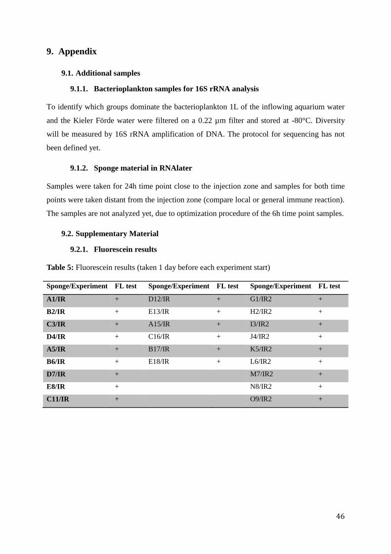
46

9. Appendix

9.1. Additional samples

9.1.1. Bacterioplankton samples for 16S rRNA analysis

To identify which groups dominate the bacterioplankton 1L of the inflowing aquarium water

and the Kieler Förde water were filtered on a 0.22 µm filter and stored at -80°C. Diversity

will be measured by 16S rRNA amplification of DNA. The protocol for sequencing has not

been defined yet.

9.1.2. Sponge material in RNAlater

Samples were taken for 24h time point close to the injection zone and samples for both time

points were taken distant from the injection zone (compare local or general immune reaction).

The samples are not analyzed yet, due to optimization procedure of the 6h time point samples.

9.2. Supplementary Material

9.2.1. Fluorescein results

Table 5: Fluorescein results (taken 1 day before each experiment start)

Sponge/Experiment FL test Sponge/Experiment FL test Sponge/Experiment FL test

A1/IR + D12/IR + G1/IR2 +

B2/IR + E13/IR + H2/IR2 +

C3/IR + A15/IR + I3/IR2 +

D4/IR + C16/IR + J4/IR2 +

A5/IR + B17/IR + K5/IR2 +

B6/IR + E18/IR + L6/IR2 +

D7/IR + M7/IR2 +

E8/IR + N8/IR2 +

C11/IR + O9/IR2 +

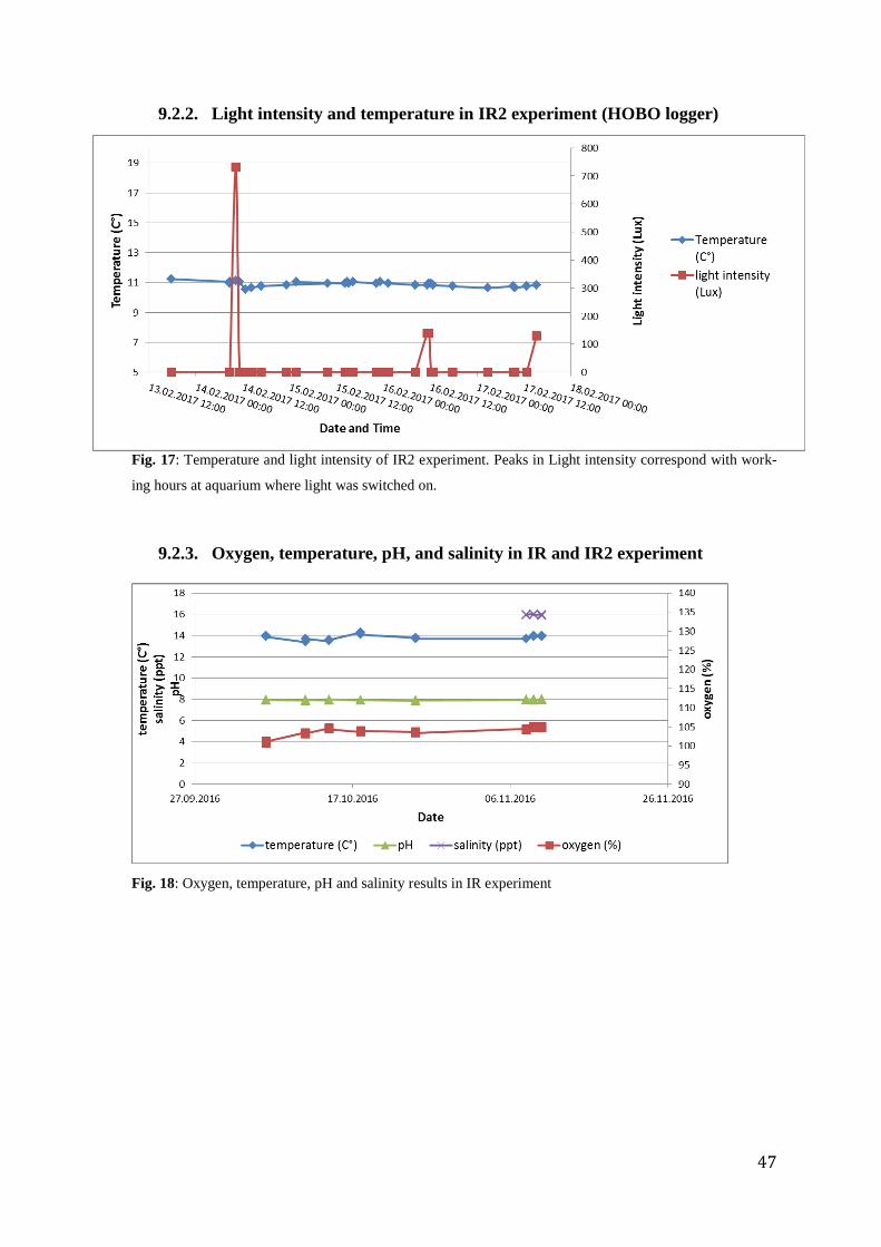
47

9.2.2. Light intensity and temperature in IR2 experiment (HOBO logger)

Fig. 17: Temperature and light intensity of IR2 experiment. Peaks in Light intensity correspond with work-

ing hours at aquarium where light was switched on.

9.2.3. Oxygen, temperature, pH, and salinity in IR and IR2 experiment

Fig. 18: Oxygen, temperature, pH and salinity results in IR experiment

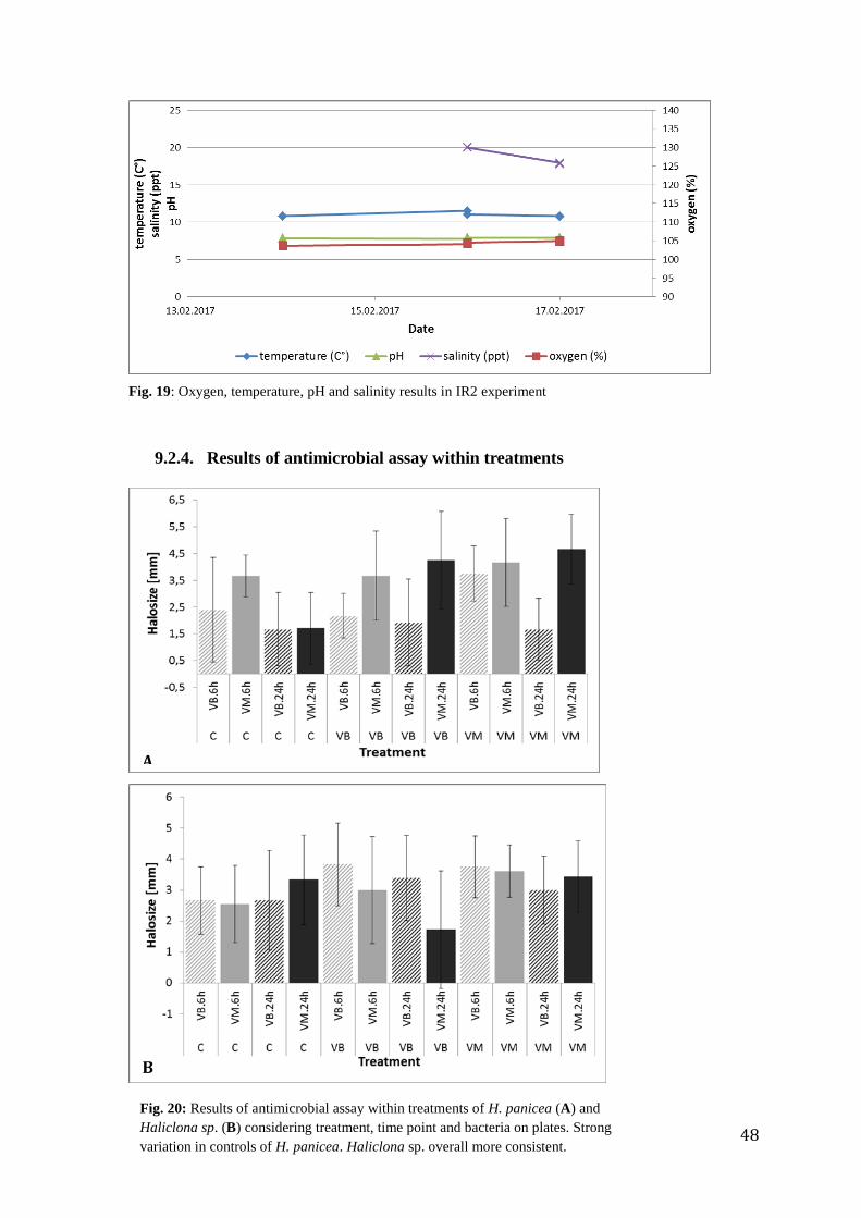
48

Fig. 19: Oxygen, temperature, pH and salinity results in IR2 experiment

9.2.4. Results of antimicrobial assay within treatments

Fig. 20: Results of antimicrobial assay within treatments of H. panicea (A) and

Haliclona sp. (B) considering treatment, time point and bacteria on plates. Strong

variation in controls of H. panicea. Haliclona sp. overall more consistent.

A

B

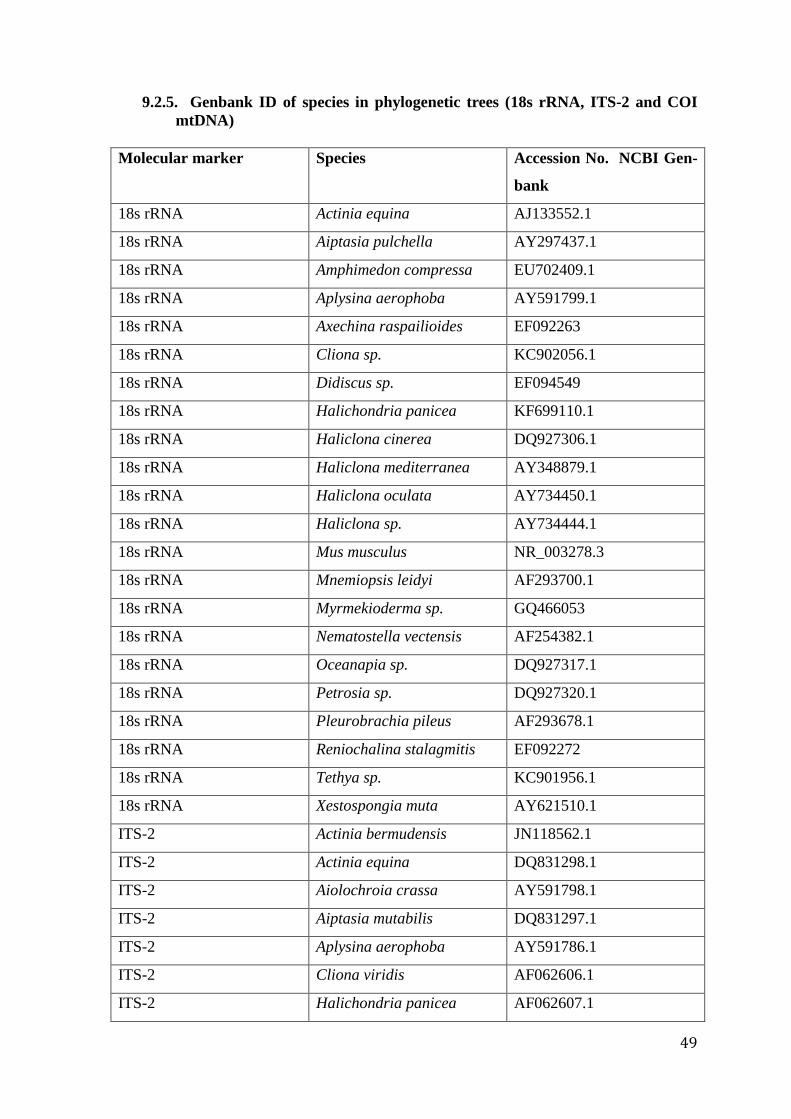
49

9.2.5. Genbank ID of species in phylogenetic trees (18s rRNA, ITS-2 and COI

mtDNA)

Molecular marker Species Accession No. NCBI Gen-

bank

18s rRNA Actinia equina AJ133552.1

18s rRNA Aiptasia pulchella AY297437.1

18s rRNA Amphimedon compressa EU702409.1

18s rRNA Aplysina aerophoba AY591799.1

18s rRNA Axechina raspailioides EF092263

18s rRNA Cliona sp. KC902056.1

18s rRNA Didiscus sp. EF094549

18s rRNA Halichondria panicea KF699110.1

18s rRNA Haliclona cinerea DQ927306.1

18s rRNA Haliclona mediterranea AY348879.1

18s rRNA Haliclona oculata AY734450.1

18s rRNA Haliclona sp. AY734444.1

18s rRNA Mus musculus NR_003278.3

18s rRNA Mnemiopsis leidyi AF293700.1

18s rRNA Myrmekioderma sp. GQ466053

18s rRNA Nematostella vectensis AF254382.1

18s rRNA Oceanapia sp. DQ927317.1

18s rRNA Petrosia sp. DQ927320.1

18s rRNA Pleurobrachia pileus AF293678.1

18s rRNA Reniochalina stalagmitis EF092272

18s rRNA Tethya sp. KC901956.1

18s rRNA Xestospongia muta AY621510.1

ITS-2 Actinia bermudensis JN118562.1

ITS-2 Actinia equina DQ831298.1

ITS-2 Aiolochroia crassa AY591798.1

ITS-2 Aiptasia mutabilis DQ831297.1

ITS-2 Aplysina aerophoba AY591786.1

ITS-2 Cliona viridis AF062606.1

ITS-2 Halichondria panicea AF062607.1

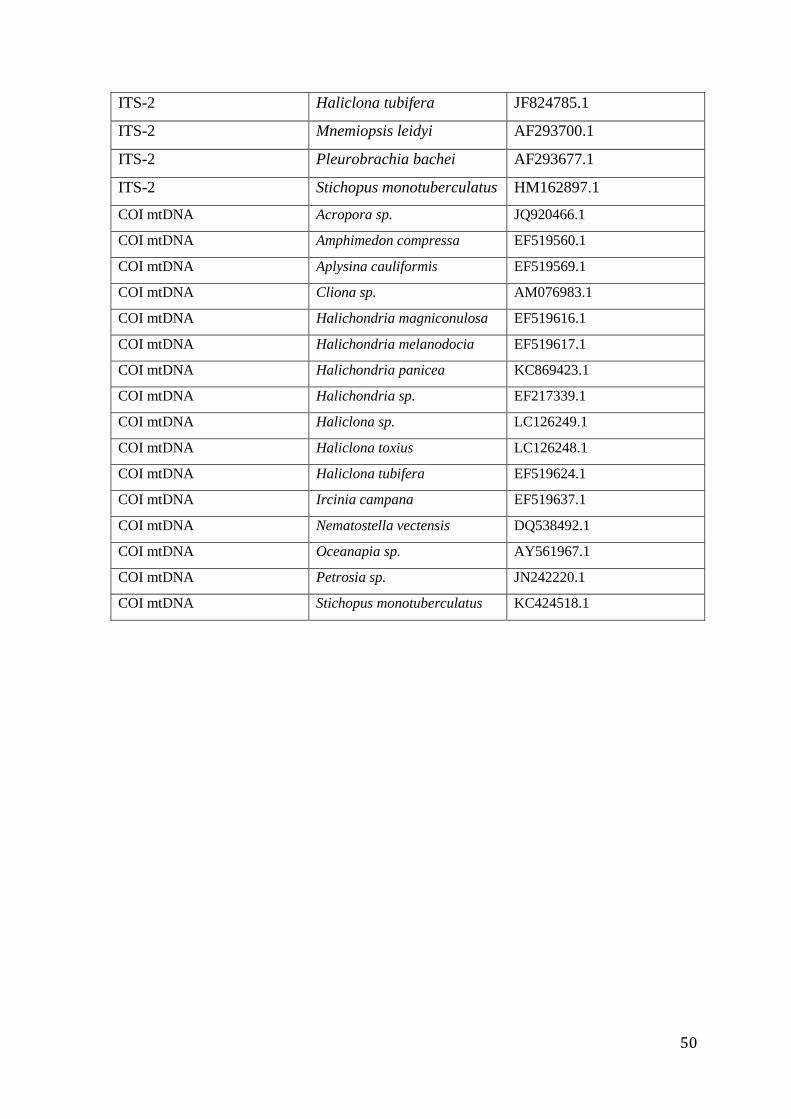
50

ITS-2 Haliclona tubifera JF824785.1

ITS-2 Mnemiopsis leidyi AF293700.1

ITS-2 Pleurobrachia bachei AF293677.1

ITS-2 Stichopus monotuberculatus HM162897.1

COI mtDNA Acropora sp. JQ920466.1

COI mtDNA Amphimedon compressa EF519560.1

COI mtDNA Aplysina cauliformis EF519569.1

COI mtDNA Cliona sp. AM076983.1

COI mtDNA Halichondria magniconulosa EF519616.1

COI mtDNA Halichondria melanodocia EF519617.1

COI mtDNA Halichondria panicea KC869423.1

COI mtDNA Halichondria sp. EF217339.1

COI mtDNA Haliclona sp. LC126249.1

COI mtDNA Haliclona toxius LC126248.1

COI mtDNA Haliclona tubifera EF519624.1

COI mtDNA Ircinia campana EF519637.1

COI mtDNA Nematostella vectensis DQ538492.1

COI mtDNA Oceanapia sp. AY561967.1

COI mtDNA Petrosia sp. JN242220.1

COI mtDNA Stichopus monotuberculatus KC424518.1

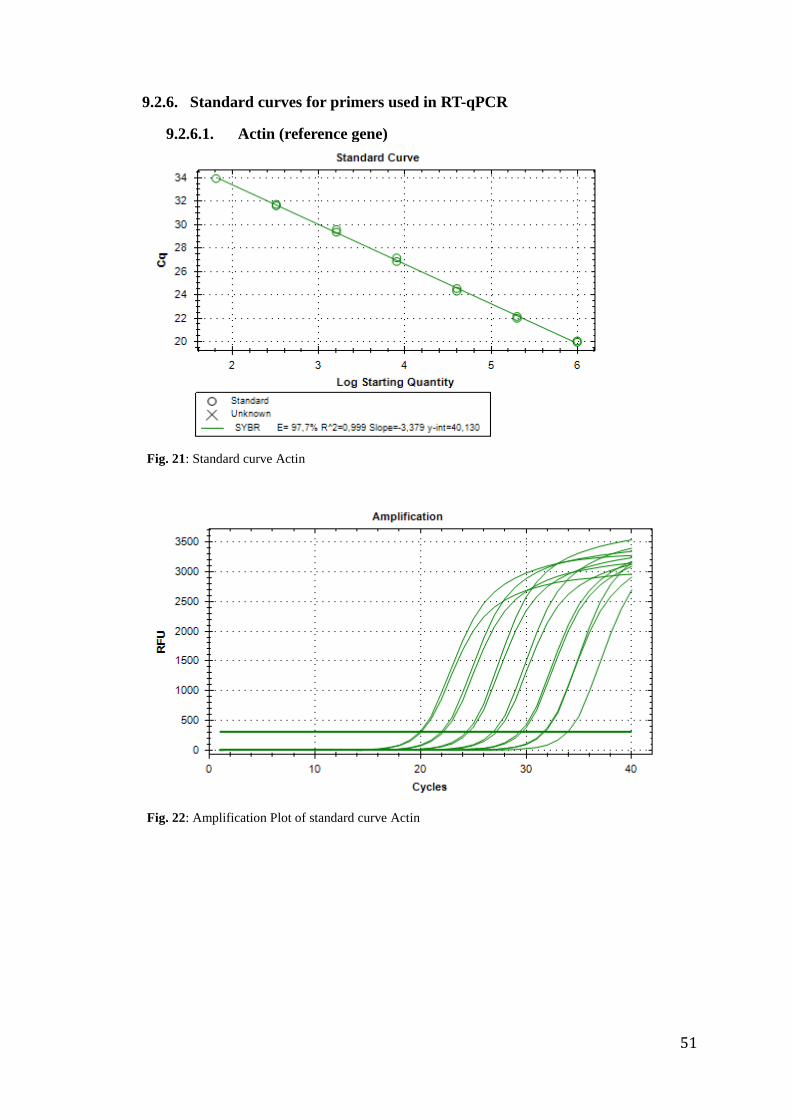
51

9.2.6. Standard curves for primers used in RT-qPCR

9.2.6.1. Actin (reference gene)

Fig. 21: Standard curve Actin

Fig. 22: Amplification Plot of standard curve Actin

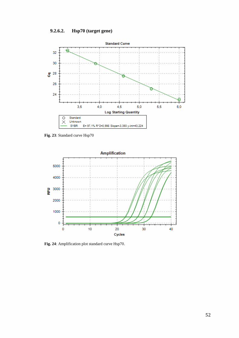
52

9.2.6.2. Hsp70 (target gene)

Fig. 23: Standard curve Hsp70

Fig. 24: Amplification plot standard curve Hsp70.

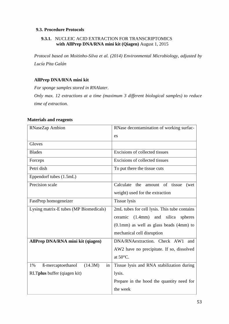
53

9.3. Procedure Protocols

9.3.1. NUCLEIC ACID EXTRACTION FOR TRANSCRIPTOMICS

with AllPrep DNA/RNA mini kit (Qiagen) August 1, 2015

Protocol based on Moitinho-Silva et al. (2014) Environmental Microbiology, adjusted by

Lucía Pita Galán

AllPrep DNA/RNA mini kit

For sponge samples stored in RNAlater.

Only max. 12 extractions at a time (maximum 3 different biological samples) to reduce

time of extraction.

Materials and reagents

RNaseZap Ambion RNase decontamination of working surfac-

es

Gloves

Blades Excisions of collected tissues

Forceps Excisions of collected tissues

Petri dish To put there the tissue cuts

Eppendorf tubes (1.5mL)

Precision scale Calculate the amount of tissue (wet

weight) used for the extraction

FastPrep homogeneizer Tissue lysis

Lysing matrix-E tubes (MP Biomedicals) 2mL tubes for cell lysis. This tube contains

ceramic (1.4mm) and silica spheres

(0.1mm) as well as glass beads (4mm) to

mechanical cell disruption

AllPrep DNA/RNA mini kit (qiagen) DNA/RNAextraction. Check AW1 and

AW2 have no precipitate. If so, dissolved

at 50°C.

1% ß-mercaptoethanol (14.3M) in

RLTplus buffer (qiagen kit)

Tissue lysis and RNA stabilization during

lysis.

Prepare in the hood the quantity need for

the week

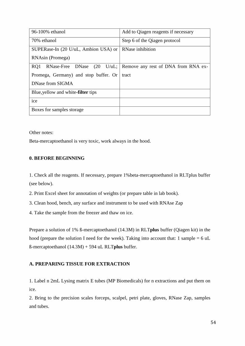
54

96-100% ethanol Add to Qiagen reagents if necessary

70% ethanol Step 6 of the Qiagen protocol

SUPERase-In (20 U/uL, Ambion USA) or

RNAsin (Promega)

RNase inhibition

RQ1 RNase-Free DNase (20 U/uL;

Promega, Germany) and stop buffer. Or

DNase from SIGMA

Remove any rest of DNA from RNA ex-

tract

Blue,yellow and white-filter tips

ice

Boxes for samples storage

Other notes:

Beta-mercaptoethanol is very toxic, work always in the hood.

0. BEFORE BEGINNING

1. Check all the reagents. If necessary, prepare 1%beta-mercaptoethanol in RLTplus buffer

(see below).

2. Print Excel sheet for annotation of weights (or prepare table in lab book).

3. Clean hood, bench, any surface and instrument to be used with RNAse Zap

4. Take the sample from the freezer and thaw on ice.

Prepare a solution of 1% ß-mercaptoethanol (14.3M) in RLTplus buffer (Qiagen kit) in the

hood (prepare the solution I need for the week). Taking into account that: 1 sample = 6 uL

ß-mercaptoethanol (14.3M) + 594 uL RLTplus buffer.

A. PREPARING TISSUE FOR EXTRACTION

1. Label n 2mL Lysing matrix E tubes (MP Biomedicals) for n extractions and put them on

ice.

2. Bring to the precision scales forceps, scalpel, petri plate, gloves, RNase Zap, samples

and tubes.

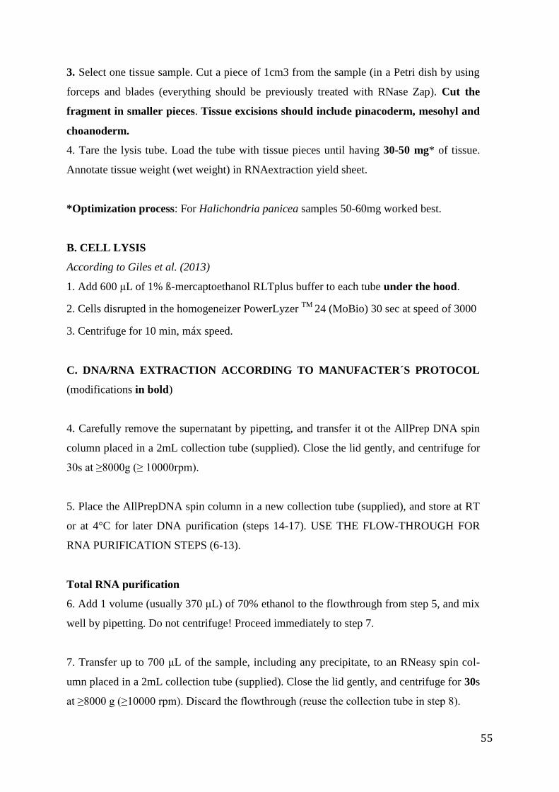
55

3. Select one tissue sample. Cut a piece of 1cm3 from the sample (in a Petri dish by using

forceps and blades (everything should be previously treated with RNase Zap). Cut the

fragment in smaller pieces. Tissue excisions should include pinacoderm, mesohyl and

choanoderm.

4. Tare the lysis tube. Load the tube with tissue pieces until having 30-50 mg* of tissue.

Annotate tissue weight (wet weight) in RNAextraction yield sheet.

*Optimization process: For Halichondria panicea samples 50-60mg worked best.

B. CELL LYSIS

According to Giles et al. (2013)

1. Add 600 μL of 1% ß-mercaptoethanol RLTplus buffer to each tube under the hood.

2. Cells disrupted in the homogeneizer PowerLyzer TM

24 (MoBio) 30 sec at speed of 3000

3. Centrifuge for 10 min, máx speed.

C. DNA/RNA EXTRACTION ACCORDING TO MANUFACTER´S PROTOCOL

(modifications in bold)

4. Carefully remove the supernatant by pipetting, and transfer it ot the AllPrep DNA spin

column placed in a 2mL collection tube (supplied). Close the lid gently, and centrifuge for

30s at ≥8000g (≥ 10000rpm).

5. Place the AllPrepDNA spin column in a new collection tube (supplied), and store at RT

or at 4°C for later DNA purification (steps 14-17). USE THE FLOW-THROUGH FOR

RNA PURIFICATION STEPS (6-13).

Total RNA purification

6. Add 1 volume (usually 370 μL) of 70% ethanol to the flowthrough from step 5, and mix

well by pipetting. Do not centrifuge! Proceed immediately to step 7.

7. Transfer up to 700 μL of the sample, including any precipitate, to an RNeasy spin col-

umn placed in a 2mL collection tube (supplied). Close the lid gently, and centrifuge for 30s

at ≥8000 g (≥10000 rpm). Discard the flowthrough (reuse the collection tube in step 8).

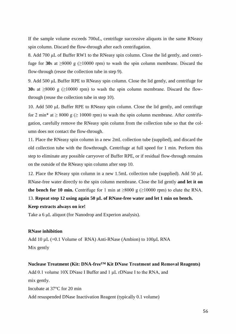
56

If the sample volume exceeds 700uL, centrifuge successive aliquots in the same RNeasy

spin column. Discard the flow-through after each centrifugation.

8. Add 700 μL of Buffer RW1 to the RNeasy spin column. Close the lid gently, and centri-

fuge for 30s at ≥8000 g (≥10000 rpm) to wash the spin column membrane. Discard the

flow-through (reuse the collection tube in step 9).

9. Add 500 μL Buffer RPE to RNeasy spin column. Close the lid gently, and centrifuge for

30s at ≥8000 g (≥10000 rpm) to wash the spin column membrane. Discard the flow-

through (reuse the collection tube in step 10).

10. Add 500 μL Buffer RPE to RNeasy spin column. Close the lid gently, and centrifuge

for 2 min* at ≥ 8000 g (≥ 10000 rpm) to wash the spin column membrane. After centrifu-

gation, carefully remove the RNeasy spin column from the collection tube so that the col-

umn does not contact the flow-through.

11. Place the RNeasy spin column in a new 2mL collection tube (supplied), and discard the

old collection tube with the flowthrough. Centrifuge at full speed for 1 min. Perform this

step to eliminate any possible carryover of Buffer RPE, or if residual flow-through remains

on the outside of the RNeasy spin column after step 10.

12. Place the RNeasy spin column in a new 1.5mL collection tube (supplied). Add 50 μL

RNase-free water directly to the spin column membrane. Close the lid gently and let it on

the bench for 10 min. Centrifuge for 1 min at ≥8000 g (≥10000 rpm) to elute the RNA.

13. Repeat step 12 using again 50 μL of RNase-free water and let 1 min on bench.

Keep extracts always on ice!

Take a 6 μL aliquot (for Nanodrop and Experion analysis).

RNase inhibition

Add 10 µL (=0.1 Volume of RNA) Anti-RNase (Ambion) to 100µL RNA

Mix gently

Nuclease Treatment (Kit: DNA-free™ Kit DNase Treatment and Removal Reagents)

Add 0.1 volume 10X DNase I Buffer and 1 μL rDNase I to the RNA, and

mix gently.

Incubate at 37°C for 20 min

Add resuspended DNase Inactivation Reagent (typically 0.1 volume)

57

and mix well.

Incubate 2min at room temperature, mixing occasionally.

Centrifuge at 10,000 × g for 1.5min and transfer the RNA to a fresh

tube.

Genomic DNA purification:

13. Add 500 uL of Buffer AW1 to the AllPrep DNA spin column from step 5. Close the lid

gently, and centrifuge for 30s at ≥8000 g (≥10000 rpm). Discard the flow-through (reuse

the spin column in step 15).

14. Add 500 uL Buffer AW2 to AllPrep DNA spin column. Close the lid gently, and cen-

trifuge for 2 min at full speed to wash the spin column membrane. After centrifugation,

carefully remove the AllPrep DNA spin column from the collection tube.

15. Repeat step 14.

16. Place the AllPrep DNA spin column in a new 1.5 mL collection tube (supplied). Add

50uL Buffer EB directly to the spin column membrane and close the lid. Incubate at room

temperature for 5 min, and then centrifuge for 1 min at ≥8000 g (≥10000 rpm) to elute the

DNA.

17. Repeat step 16. Let 1 min on bench

D. NUCLEIC ACID QUANTIFICATION

D.1. Quantification in NanoDrop:

For each extraction, annotate: concentration (ng/uL), A260, A260/280 ratio,

A260/230.

Nanodrop: Clean the sensor. Choose “Nucleic acids”. Set the type of nucleic acid (RNA or

DNA).

Use water as blank for RNA quantification. Use EB buffer as blank for DNA quan-

tification.

58

9.3.2. cDNA transcription (iScript™ Select cDNA Synthesis Kit)

1. Thaw all components except iScript reverse transcriptase. Mix thoroughly and briefly

centrifuge to collect contents to the bottom of the tube before using. Place

components on ice.

2. Add the following components to a 0.2 ml PCR tube or each well of a 96-well PCR

reaction plate on ice:

Components Volume

Nuclease-free water Variable

5x iScript select reaction mix 4 μl

Oligo(dT)20 primer or random primer 2 μl

RNA sample (1 pg to 1 μg total RNA) Variable

iScript reverse transcriptase 1 μl

Total 20 μl

Note: for multiple reactions, prepare a master mix with the above components, except

RNA, and then dispense to each reaction.

3. Mix gently and incubate as follows:

For oligo(dT)-primed cDNA reactions, incubate for 60–90 min at 42°C.

For random-primed cDNA reactions, incubate for 5 min at 25°C, then 30 min at

42°C.

4. Incubate at 85°C for 5 min to heat-inactivate the reverse transcriptase.

5. Store cDNA product at –20°C to +4°C.

6. The resulting cDNA product can be used directly for PCR amplification. Typically,

one-tenth (2 μl) of the first-strand reaction provides sufficient target for most PCR

applications. Optionally, the cDNA can be diluted in TE buffer [10 mM Tris (pH 8.0),

0.1 mM EDTA] for addition of larger volumes (5–10 μl) to PCR reactions.

59

9.3.3. FIXATION FOR FLOW CYTOMETRY OF PHYTOPLANKTON AND

BACTERIA IN SEAWATER

-Based on Pep Gasol (ICM-CSIC Barcelona, Spain) and Laura Rix (GEOMAR) protocols.

Notes:

(i) Prepare fresh and store in the fridge to use within a week (even up to several

weeks). Or prepare bigger amounts, aliquot in tubes, freeze them at -80°C and

store at -20°C (to use up to several months).

(ii) The chemical compounds used for the fixative are toxic. Work always under the

fume hood.

(iii) For heating and stirring under the hood, use one of the devices from upstairs, but

ask in advance Tanja, Ignacio and Álvaro.

Preparation of fixative-protocol for 20 mL:

1) Weight 2 g of paraformaldehyde (SIGMA P6148) under the fume hood.

2) Place in 17.6 mL of miliQ water in a beaker covered with Parafilm (to reduce water

loss through evaporation) and with a magnetic fly. Stir vigorously at 70°C for at least

2h under the fume hood, until the paraformaldehyde dissolves and saturates the water.

3) Add small amounts of 1N NaOH drop-wise until the solution becomes clear.

4) Let the solution cool to RT

5) Adjust the pH to 7.4 with 1N HCl. Add the HCl drop-wise.

6) Add 2 mL of 1 x PBS

7) Add 0.4 mL of Glutaraldehyde 25%

8) Filter through 0.2 µm polycarbonate syringe into a Falcon tube

9) Store in the fridge*

*for big amounts and long storage: Aliquot the fixative into tubes, freeze them at the -80°C

and store them at -20°C.

Sampling and sample fixation:

1) Label 15 mL sterile falcon tubes and 2 mL cryovials (final sample) in advance. Pre-

pare duplicate cryovials from each seawater sample.

2) Collect seawater sample (e.g. from bucket) or directly into the falcon tube. Rinse the

recipient three times with the water to be sampled. Then collect the water and proceed

as soon as feasible. (ideally, keep the tubes cold).

60

3) Under the hood, pipette 1.8 mL of seawater sample into 2 mL cryovials.

4) Then pipette 0.2 mL of fixative (10%) into the vial. This yields a final 1% fixative

concentration. Remember to filter before use.

5) Mix the vials and let them stand at room temperature for not least than 10 min (and

max. 30 min).

6) Quick freeze the vial in liquid nitrogen and store at -80°C. If samples are not for virus,

then tubes can be directly freeze at -80°C.

61

9.3.4. ExperionTM

(ExperionTM

RNA StdSens Starter Kit)

Protocol based on manufacture´s instruction, adapted to more straightforward procedure in

our lab.

For total RNA derived from nucleic acid extraction that showed good quality in Nanodrop.

(aliquots before RNase inhibitor and DNase treatments).

Materials and reagents

Utility

RNaseZap Ambion RNase decontamination of working surfaces

Gloves

RNase-free tubes (0.5 mL) For samples and ladder

RNA StdSens Experion kit (Bio-

Rad)

Include chips (RT, in Christina’s drawer); chemical reagents

and filter columns (in the fridge). And RNA ladder (at -80°C)

Total RNA extracts Use the aliquots!

DEPC-treated water For cleaning (take a 50 mL Falcon tube)

RNase X plus For cleaning (take a 50mL Falcon tube). Check it is transpar-

ent! Sometimes it oxidizes and looks yellow…

Thermocycler Denaturation step

Blue,yellow and white-filter tips

ice

Experion stations 3 stations: priming, vortex and electrophoresis. In Botanik I

A pen-drive To save the results

Procedure overview

1. Equilibrate reagents to room temperature for 20 min (except RNA ladder and RNA al-

iquots, that should be thaw on ice).

2. Filter gel (10 min). Add stain to filtered gel. Keep the rest of filter gel (9uL of non-

stained filter gel are needed to load G well in the chip). Filtered gel is stable for 1

month if kept protected from light at 4°C.

3. Prepare an aliquot of buffer, “B”, (15 x 5uL = 75 uL for one chip is enough).

4. Take 2µL of RNA aliquots into new 0.5 mL tubes labeled 1-12 as they are going to be

load in the chip

62

5. Heat RNA ladder and samples in thermocycler for 2 min at 70°C (heat lid ON)-

denaturation. Then keep on ice (minimum 5 min).

6. Clean electrodes before run (x 3)

7. During second cleaning, prime chip with gel-stain solution.

8. During third cleaning, load and vortex chip.

9. Run RNA StdSens analysis protocol on the Experion electrophoresis. The one for eu-

karyotic samples

10. Clean instrument electrodes.

Essential practices

Aliquot RNA ladder (2uL) in 0.5 mL RNase-free tubes and store at -80°C. Store all the other

chemical reagents of the kit at 4°C when not in use. Clean surfaces with RNaseZap. Before

using, allow kit reagents to equilibrate to room temperature with the exception of the RNA

ladder (15-20min). Vortex and briefly centrifuge all kit reagents before use. Protect RNA

stain and gel-stain solution from light.

Always heat-denature the RNA ladder and RNA samples immediately before use and keep on

ice until loading the chip.

Run the loaded chip within 5 min of loading to prevent excessive evaporation

A. EQUILIBRATING KIT REAGENTS

Filtered gel is stable for 1 month, if kept at 4°C and avoid light exposure

Remove RNA ladder and total RNA extract aliquots from -80°C and thaw on ice.

63

B. PREPARING THE GEL STAIN

C. PREPARING THE SAMPLES AND RNA LADDER

RNA ladder aliquots are ready to use: Each aliquot of RNA ladder contains already the 2uL

needed for one chip.

Prepare all samples by pipetting 3 uL sample into RNase-free 0.5 mL tube. If RNA concentra-

tion is high (>400 ng/uL) consider dilute the extract in RNase-free water. Denature the ladder

and samples for 2 minutes at 70°C in the thermocycler (big wells). Cool the denatured ladder

and samples by immediately placing the tubes on ice for 5 minutes. Spin down the ladder and

samples in a microcentrifuge for 3-5 sec.

D. CLEANING THE REAGENTS BEFORE THE RUN

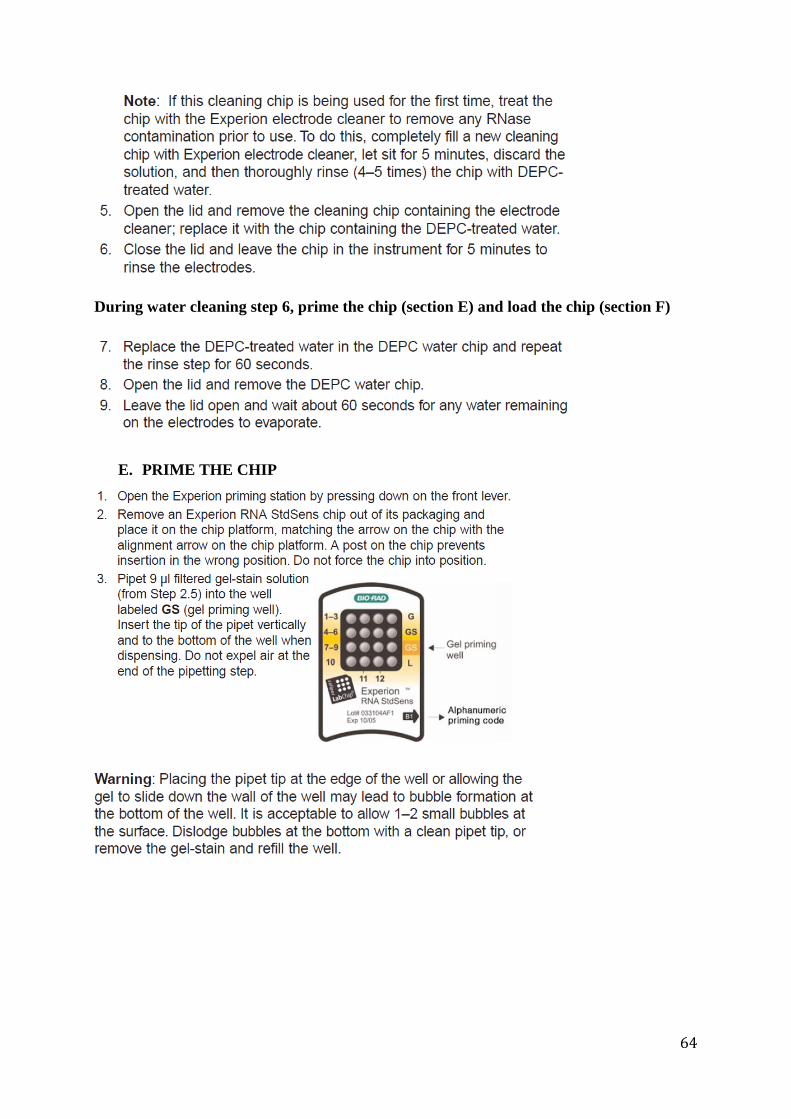
64

During water cleaning step 6, prime the chip (section E) and load the chip (section F)

E. PRIME THE CHIP

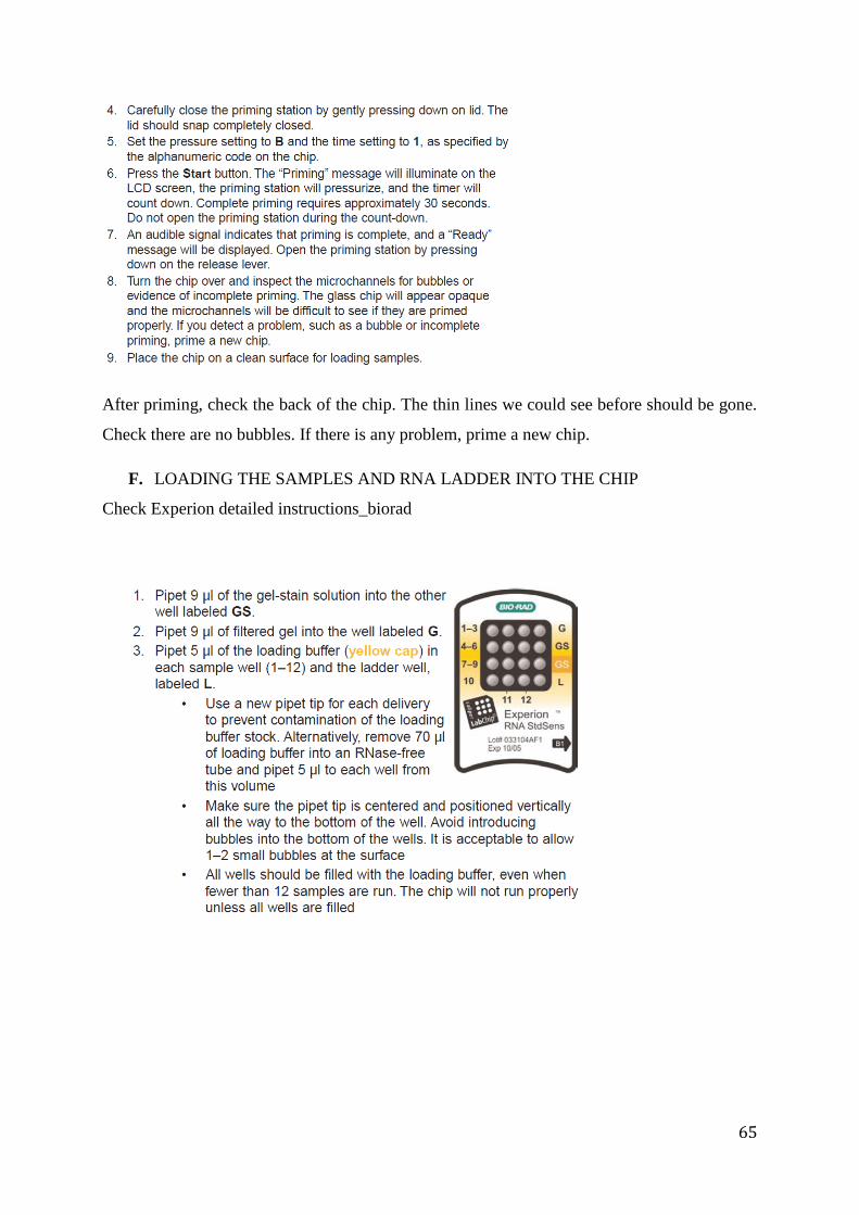
65

After priming, check the back of the chip. The thin lines we could see before should be gone.

Check there are no bubbles. If there is any problem, prime a new chip.

F. LOADING THE SAMPLES AND RNA LADDER INTO THE CHIP

Check Experion detailed instructions_biorad

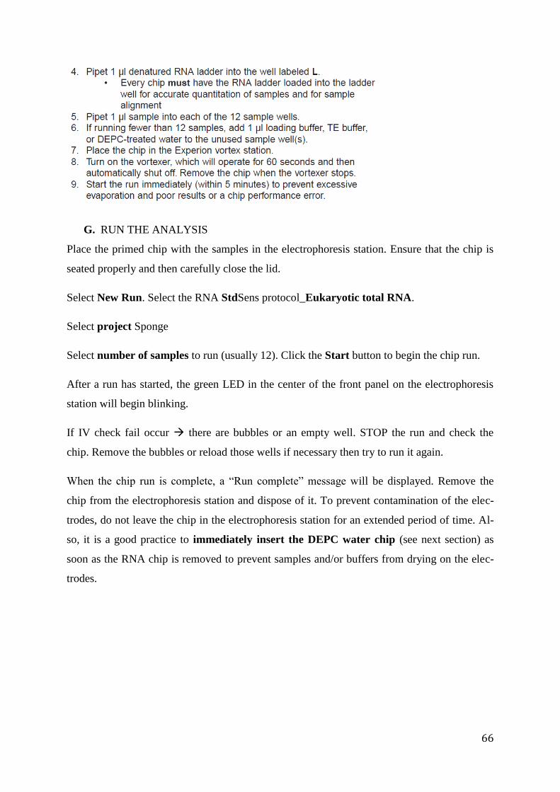
66

G. RUN THE ANALYSIS

Place the primed chip with the samples in the electrophoresis station. Ensure that the chip is

seated properly and then carefully close the lid.

Select New Run. Select the RNA StdSens protocol_Eukaryotic total RNA.

Select project Sponge

Select number of samples to run (usually 12). Click the Start button to begin the chip run.

After a run has started, the green LED in the center of the front panel on the electrophoresis

station will begin blinking.

If IV check fail occur there are bubbles or an empty well. STOP the run and check the

chip. Remove the bubbles or reload those wells if necessary then try to run it again.

When the chip run is complete, a “Run complete” message will be displayed. Remove the

chip from the electrophoresis station and dispose of it. To prevent contamination of the elec-

trodes, do not leave the chip in the electrophoresis station for an extended period of time. Al-

so, it is a good practice to immediately insert the DEPC water chip (see next section) as

soon as the RNA chip is removed to prevent samples and/or buffers from drying on the elec-

trodes.

67

H. CLEAN THE ELECTRODES AFTER A RUN

Save the results in the pen-drive.

Analysis:

Take into account that the run settings are designed for eukaryotic total RNA. However,

sponges samples (HMA) of total RNA have also important amount of prokaryotic RNA.

So,instead of the typical 2 peaks of rRNA (18S and 28S) our samples will show 4 peaks: 16S,

18S, 23S and 28S. Because of this, sometimes the software mislabel the peaks. Eukaryotic 18S

and 28SrRNA are in this case the 2nd

and the 4th

peak that appear in the graphs. If it is misla-

beled, correct them before exporting the results.

68

10. Declaration of authorship

Erklärung zur Bachelorarbeit/Masterarbeit

Hiermit versichere ich, dass die vorliegende Arbeit von mir selbstständig verfasst wurde und

dass keine anderen als die angegebenen Quellen und Hilfsmittel benutzt wurden.

Diese Erklärung erstreckt sich auch auf in der Arbeit enthaltene Graphiken,

Zeichnungen, Kartenskizzen und bildliche Darstellungen.

Bachelor's/Master’s thesis statement of originality

I hereby confirm that I have written the accompanying thesis by myself, without contributions

from any sources other than those cited in the text and acknowledgements.

This applies also to all graphics, drawings, maps and images included in the thesis.

……………………………………………… …………………………………………..

Ort und Datum Unterschrift

Place and date Signature

69

Dieses Formblatt ist ausgefüllt und vom Betreuer unterschrieben als

letzte Seite in das beim Prüfungsausschuss abzugebende Exemplar der

Masterarbeit einzubinden.

This form must be filled out and signed by your supervisor. It is to be

included in the final version of the Masters Thesis as the last page in

the copy for the Examination Board.

Name (last, first): ___________________________________________

Title of Thesis: ___________________________________________

___________________________________________

___________________________________________

Group in which the work was performed:

____________________________________________________________________________

Examiner/Supervisor: ____________________________________________

Signature (superivsor): ____________________________________________

Starting date: ____________________________________________

Submission date: ____________________________________________

______________________________________________ Signature, Chair of the Examination Board or authorized representative

In case of interruption:

This Masters Thesis was completed

from…………….. until ……………….

from …………….. until ……………….

Signature (supervisor): ______________________________________