Thema Regional Innovation Activities and Consequences

Dissertation

zur Erlangung des akademischen Grades doctor rerum politicarum

(Dr. rer. pol.)

vorgelegt dem Rat der Wirtschaftswissenschaftlichen Fakultät

der Friedrich-Schiller-Universität Jena am 31.01.2018

von: M.Sc. Moritz Zöllner

geboren am: 11. Mai 1989 in: Annweiler am Trifels

Gutachter:

1. Professor Dr. Michael Fritsch Friedrich-Schiller-Universität Jena, Lehrstuhl für Unternehmensentwicklung, Innovation und wirtschaftlichen Wandel

2. Privatdozent Dr. Holger Graf Friedrich-Schiller-Universität Jena, Lehrstuhl für Ökonomie/ Mikroökonomie

Datum der Verteidigung: 16.05.2018

I

‘Everything is a matter of degree, and there are no absolutes.’

Joel Mokyr (2005)

II

Contents List of figures ..................................................................................................... VII

List of tables ...................................................................................................... VIII

List of abbreviations and acronyms ................................................................... X

Acknowledgements ............................................................................................ XI

Co-Authorship and statement of contribution ................................................. XII

German summary .............................................................................................. XIII

Chapter 1: Innovative activities and their consequences from a regional perspective ........................................................................................ 1

1.1 Introductory remarks ......................................................................................... 1

1.2 Knowledge, networks and innovations .............................................................. 2

1.2.1 Sticky knowledge ..................................................................................... 2

1.2.2 Innovative networks ................................................................................. 3

1.2.3 Knowledge and knowledge spillovers ...................................................... 4

1.3 Innovation and its consequences ...................................................................... 7

1.3.1 Are innovations always beneficial? .......................................................... 7

1.3.2 Rising income inequality? ........................................................................ 8

1.3.3 Income inequality, triggered by innovations? ........................................... 9

1.3.4 Income inequality: a source for social-economic problems .................... 12

1.3.5 Crime and income inequality ................................................................. 14

1.4 Knowledge, networks, innovations, income inequality: Aim and scope of the

thesis .............................................................................................................. 15

1.4.1 The concept of the thesis ....................................................................... 15

1.4.2 Research gaps: Knowledge, networks and stability ............................... 16

1.4.3 Research gaps: Innovation, inequality and crime .................................. 18

III

1.5 Structure and findings of the thesis ................................................................. 21

Part I: Knowledge, innovations and networks .................................................. 25

Chapter 2: The fluidity of inventor networks .................................................... 26

2.1 Division of innovative labor, innovation networks, and regional performance . 27

2.2 The nature and the stability of cooperative Research and Development........ 29

2.3 Data and indicators......................................................................................... 31

2.3.1 Data ....................................................................................................... 31

2.3.2 Indicators ............................................................................................... 34

2.4 The development of the regional networks over time ...................................... 35

2.5 Fluidity of actors at the micro level ................................................................. 36

2.5.1 General observations ............................................................................. 36

2.5.2 What determines the reoccurrence of actors? ....................................... 40

2.6 The effect of fluidity on network structure and performance ............................ 42

2.7 Discussion: What does this mean and what do we need to know? ................ 47

2.8 Appendix ......................................................................................................... 50

Chapter 3: Actor fluidity and knowledge persistence in regional networks .. 57

3.1 Fluidity of network actors and regional knowledge .......................................... 58

3.2 Actor turnover, knowledge persistence, network characteristics, and the

performance of the regional innovation system .............................................. 59

3.3 Data and spatial framework ............................................................................. 62

3.4 Actor turnover and continuity of knowledge .................................................... 65

3.4.1 Actor turnover in inventor networks ....................................................... 65

3.4.2 Assessing the share of persistent knowledge ........................................ 67

3.5 What determines the persistence of knowledge in regional networks? ........... 69

3.6 The effect of knowledge persistence on network performance ....................... 74

3.7 Conclusion ...................................................................................................... 77

IV

3.8 Appendix ......................................................................................................... 79

Chapter 4: So what? Concluding remarks and outlook for further research ..... .......................................................................................................... 83

4.1 Summary of the empirical findings .................................................................. 83

4.2 What do we need to know? Avenues for further research ............................... 85

4.2.1 Preferential attachment: myth or fact of network formation? .................. 85

4.2.2 Falling stars: how robust are inventor networks under ‘attack’? ............ 88

4.3 General thoughts about R&D networks, innovations and potential

consequence .................................................................................................. 90

Part II: Innovations, income inequality and crime ............................................ 92

Chapter 5: Causes and consequences of income inequality – The role of innovation ........................................................................................ 93

5.1 Introduction ..................................................................................................... 94

5.2 Innovations and income inequality from a regional perspective ...................... 96

5.2.1 Innovation as a determinant of income inequality .................................. 96

5.2.2 Income inequality as a determinant of innovation .................................. 98

5.2.3 The innovation-inequality link from a regional perspective .................... 99

5.3 Data, indicators and method ......................................................................... 101

5.3.1 Data ..................................................................................................... 101

5.3.2 Indicators ............................................................................................. 102

5.3.3 Method ................................................................................................. 103

5.4 Results .......................................................................................................... 104

5.4.1 Descriptive results ............................................................................... 104

5.4.2 Regression results ............................................................................... 105

5.5 Discussion and conclusion ............................................................................ 107

5.8 Appendix ....................................................................................................... 110

V

Chapter 6: Regional income inequality and local crime rates ....................... 112

6.1 Crime and income inequality ......................................................................... 113

6.2 Income inequality and crime from a regional perspective ............................. 115

6.2.1 The relation between income inequality and crime .............................. 115

6.2.2 Previous empirical findings .................................................................. 116

6.3 Data, indicators and method ......................................................................... 118

6.3.1 Data ..................................................................................................... 118

6.3.2 Method ................................................................................................. 120

6.3.3 Indicators ............................................................................................. 120

6.4 Crime and inequality – General observations ................................................ 122

6.5 Income inequality, crime and regional differences ........................................ 125

6.5.1 Crime and income inequality ............................................................... 125

6.5.2 ‘City, country, river’, or: do regional differences matter? ...................... 126

6.5.3 Decomposing the effect of income inequality on categories of crime .. 129

6.6 Summary and discussion .............................................................................. 130

6.7 Appendix ....................................................................................................... 133

Chapter 7: So what? Concluding remarks and outlook for further research ..... ........................................................................................................ 141

7.1 A summary of the empirical findings ............................................................. 141

7.2 What do we need to know? Avenues for further research ............................. 143

7.2.1 R&D expenditures and income inequality ............................................ 143

7.2.2 Entrepreneurship and income inequality .............................................. 145

7.2.3 Inequality and crime – An instrumental variable approach .................. 147

Chapter 8: Conclusion ...................................................................................... 151

8.1 Concluding remarks of Part I: Knowledge, innovation and networks ............. 151

8.2 Concluding remarks of Part II: Innovations, income inequality, and crime .... 152

VI

8.2.1 Part IIa: Causes of income inequality .................................................. 152

8.2.2 Part IIb: Consequences of income inequality ....................................... 153

8.3 Final thoughts ................................................................................................ 154

Bibliography ...................................................................................................... 155

Statutory declaration ........................................................................................ 180

Presentations and publications ....................................................................... 181

VII

List of figures Figure 1.1: Real disposable income growth 2007 - 2014 ..................................... 8

Figure 1.2: The conceptual framework of the thesis ........................................... 15

Figure 2.1: The regional framework of the analysis ............................................ 33

Figure 2.2: Share of actors that are present in different numbers of time periods

......................................................................................................... 37

Figure 2.3: Positions of newly emerging and of discontinued actors over the

entire observation period .................................................................. 39

Figure 2.A1: Shares of actors by number of patents (all periods) ......................... 50

Figure 2.A2: Shares of actors by number of degrees (all periods)........................ 50

Figure 3.1: The regional framework of the analysis ............................................ 63

Figure 3.2: Share of actors that are present in different numbers of time periods

......................................................................................................... 65

Figure 3.3: Positions of newly emerging and of discontinued actors over the

entire observation period .................................................................. 66

Figure 4.1: Share of actors that attach to already existing actors within a network

......................................................................................................... 86

Figure 4.2: Comparing the degree distribution between attached and non-

attached actors................................................................................. 87

Figure 4.3: Development of the share of isolates, by randomly removed actors (a)

and key actors (b) ............................................................................ 89

Figure 4.4: Development of the share of the largest component, by randomly

removed actors (a) and key actors (b) ............................................. 89

Figure 6.1: Number of criminal offenses per 100,000 habitants over the

population in 2010 .......................................................................... 123

VIII

List of tables Table 2.1: Correlations between fluidity of actors and links ............................... 37

Table 2.2: Marginal effects of the binominal logistic regression models ............ 41

Table 2.3: The relationship between the shares of discontinued actors, shares of

new actors and network structure ..................................................... 43

Table 2.4: The relationship between the shares of discontinued actors, new

actors and patent productivity ........................................................... 45

Table 2.5: The relationship between the shares of ceased and new links with

patent productivity ............................................................................. 46

Table 2.A1: Descriptive statistics of variables (all regions and all periods) .......... 51

Table 2.A2: Correlations between variables ......................................................... 52

Table 2.A3: Numbers of nodes, ties, components, and total patents in different

time periods....................................................................................... 53

Table 2.A4: Several structural characteristic in different time periods .................. 53

Table 2.A5: Number of co-patents and single patents (all regions) ...................... 53

Table 2.A6: Logistic regressions .......................................................................... 54

Table 2.A7: Descriptive statistics for measures of fluidity, network structure and

network performance ........................................................................ 55

Table 2.A8: Rank correlations between measures of fluidity, network structure and

network performance ........................................................................ 56

Table 3.1: Share of knowledge of previous period that remains in the network . 69

Table 3.2a: Actor fluidity, network characteristics and the share of knowledge

transfer over time ― complete transfer of knowledge assumed........ 71

Table 3.2b: Actor fluidity, network characteristics and the share of knowledge

transfer over time ― 50% knowledge transfer assumed ................... 72

Table 3.2c: Actor fluidity, network characteristics and the share of knowledge

transfer over time ― weighted knowledge transfer assumed ............ 73

Table 3.3: The relationship between the share of persistent and new knowledge

and patent productivity ...................................................................... 75

IX

Table 3.4: The relationship of new actors attached to components and new

actors that are isolates on patent productivity ................................... 77

Table 3.A1: Numbers of nodes, ties, components, and total patents in different

time periods....................................................................................... 79

Table 3.A2: Shares of discontinued actors and new actors in the case study

regions in different time periods ........................................................ 80

Table 3.A3: Descriptive statistics .......................................................................... 80

Table 3.A4: Number of co-patents, single patents, mean degree (all regions) ..... 81

Table 3.A5: Rank correlation of variables ............................................................. 82

Table 5.1: Estimation results VAR model (including control variables) ............ 106

Table 5.A1: Description of the study variables ................................................... 110

Table 5.A2: Descriptive statistic of the study variables ....................................... 110

Table 5.A3: Spearman rank correlation .............................................................. 111

Table 5.A4: Correlation matrix ............................................................................ 111

Table 5.A5: Granger causality test ..................................................................... 111

Table 6.1: The relationship between income inequality and regional crime rates

........................................................................................................ 126

Table 6.2: Income inequality and crime rates - Comparing West and East

Germany ......................................................................................... 128

Table 6.3: Income inequality and crime rates - Comparing cities and rural areas

........................................................................................................ 128

Table 6.A1: Descriptive summary of dependent and explanatory variables ....... 133

Table 6.A2: Total number of crime offenses and shares of property and violent

crime ............................................................................................... 134

Table 6.A3: Spearman rank correlation .............................................................. 135

Table 6.A4: Decomposing crime ........................................................................ 136

Table 6.A5: Decomposing crime, comparing West and East German districts ... 137

Table 6.A6: Decomposing crime, comparing cities and rural districts ................ 138

Table 6.A7: Definition of dependent and explanatory variables .......................... 139

Table 6.A8: Different inequality measures and their significance level ............... 140

Table 7.1: Estimation results VAR model ......................................................... 144

X

List of abbreviations and acronyms EPO European Patent Office

F&E Forschung und Entwicklung

GDP Gross Domestic Product

GSOEP German Socioeconomic Panel

IAB Institute for Employment Research

ICT Information and communication technologies

IMF International Monetary Fund

IPC International Patent Classification

IPR Intellectual property rights

IV Instrumental variable

LM Lagrange multiplier

LR Likelihood ratio

OECD Organization for Economic Co-operation and Development

OLS Ordinary least squares

PCT Patent Cooperation Treaty

RIS Regional innovation system

PKS Polizeiliche Kriminalstatistik

RQ Research Question

R&D Research and Development

SBTC Skill-biased technology change

SIAB-R Sample of Integrated Labor Market Biographies Regional File

UK United Kingdom

US United States of America

VAR Vector Autoregression

ZEW Zentrum für Europäische Wirtschaftsforschung

XI

Acknowledgements First and foremost, I would like to express my deep gratitude to the principal super-

visor of my thesis, Prof. Dr. Michael Fritsch. Dr. Fritsch always shared his valuable

knowledge and experience with me, and gave me generous guidance during the

time of my research and the writing of this thesis.

Special thanks are also due to Dr. Michael Wyrwich. Without his valuable com-

ments and warm words of encouragement during my research, I never would have

completed this thesis.

I am also grateful to Dr. Holger Graf for being the second supervisor of my thesis

and my colleague Dr. Tina Haußen, who offered help and advice countless times.

I would also like to thank my sister, Laura Zöllner, and my parents, Heike und

Berthold Zöllner, for their continuous support.

Finally, I express my sincere gratitude to Nicole Köhler, for her warm words and

patience, especially during the last several months.

XII

Co-Authorship and statement of contribution Part I of the thesis which encompasses the Chapters 2, 3 and 4 is based on the

two co-authored yet unpublished papers titled (1) ‘The fluidity of inventor networks’

(Jena Economic Research Papers # 2017-009, Friedrich Schiller University Jena)

and (2) ‘Actor fluidity and knowledge persistence in regional networks’. Part II of

the thesis, comprising the Chapters 5, 6 and 7 is based on the two yet unpublished

papers titled (3) ‘Causes and consequences of income inequality: The role of inno-

vation’ and the single authored paper (4) ‘The relationship between income ine-

quality and crime across space: Evidence for German districts’.

The papers (1) and (2) are based on joint work with Michael Fritsch (Depart-

ment of Economics at the University of Jena). While my effort of preparation and

implementation of the empirical analysis was larger than that of Michael Fritsch, he

contributed more to writing Paper (1). The distribution of tasks regarding the writing

of paper (2) was about equal, whereas the programming and implementation of the

models was mainly done by me. Paper (3) was a joint project with Maximilian Gö-

thner. The implementation of the empirical methods as well as the writing of the

empirical part of the paper was mainly done by me, whereas the elaboration of the

theoretical part was mainly done by Maximilian Göthner.

XIII

German summary - Deutsche Zusammenfassung Die vorliegende Dissertationsschrift befasst sich mit innovativen Aktivitäten und

deren Wirkung im regionalen Raum. Innovationen und das damit einhergehende

neu geschaffene Wissen sind wesentliche Treiber wirtschaftlicher und gesellschaft-

licher Entwicklung. Innovationen beziehungsweise neue Technologien können zu

neuen Produkten oder Märkten führen, verbessern die Produktivität von Unter-

nehmen und beeinflussen das Wohlbefinden von Individuen. Allerdings können

auch negative Effekte von Innovationen ausgehen. So können Innovationen zu

Umweltverschmutzung führen, vorhandene Industrien und Märkte ablösen oder

durch das Ersetzen von (routinierten) Arbeitsplätzen (z.B. Fließbandarbeit) zu er-

höhter Arbeitslosigkeit und Einkommensungleichheit führen.

In diesem Kontext umfasst diese Dissertationsschrift zwei Teile. Der erste Teil

(Kapitel 2, 3 und 4) der Arbeit befasst sich mit dem Generieren von Wissen und

Innovationen in Form von Netzwerken, wobei die Stabilität solcher Netzwerkbezie-

hungen im Vordergrund steht. Der zweite Teil (Kapitel 5, 6 und 7) hingegen kon-

zentriert sich auf die durch Innovationen induzierte Einkommensungleichheit und in

einem darauf aufbauenden Schritt mit dem Zusammenhang zwischen Einkom-

mensungleichheit und dem sozioökonomischen Problem regionaler Kriminalität.

Umfangreiche empirische Befunde belegen die elementare Bedeutung von

Wissen für den innovativen Prozess und den damit verbunden wirtschaftlichen und

gesellschaftlichen Wandel. Innovativ tätig zu sein umfasst bestehendes Wissen zu

verwenden, ebenso wie die Fähigkeit, neues Wissen zu schaffen und Existieren-

des anderer Quellen zu nutzen. Der interaktive Austausch von Informationen und

Wissen zwischen verschiedenen Individuen sowie die Stabilität solcher interaktiven

Beziehungen in Form von Netzwerken steht dabei im Vordergrund. Unternehmen

beziehungsweise Individuen treten solchen Netzwerkbeziehung bei, da diese den

Innovationsprozess vereinfachen. Der Grund dafür ist, dass Netzwerke durch Ar-

beitsteilung geprägt sind, das heißt, dass die Interaktionen von den unterschiedlich

XIV

ausgeprägten Fähigkeiten und Kompetenzen profitieren. Ebenfalls profitieren Ak-

teure auch indirekt von den Aktivitäten anderer, da Netzwerke auch ein Ausgangs-

punkt von Wissensspillovern sind.

Die ökonomische Literatur ist sich einig, dass das Generieren von Innovatio-

nen innerhalb eines Netzwerkes vorwiegend von zwei Faktoren abhängig ist: von

deren Akteuren (Netzwerkkomposition) und der Struktur eines Netzwerkes. Eine

große Bandbreite von empirischen Ergebnissen zeigt, dass neben der Struktur ei-

nes Netzwerkes auch die Akteure, die sich durch unterschiedliche Fähigkeiten und

Wissen auszeichnen (Heterogenität), einen positiven Effekt auf die Produktion von

Innovation haben. Der Austausch der verschiedenen Wissensbasen sowie die

Nutzung der unterschiedlich ausgeprägten Fähigkeiten, hängen allerdings stark

von der Struktur eines Netzwerkes ab. Netzwerke mit einer dichten und lokal

geclusterten Struktur vereinfachen sowie beschleunigen den Austausch von Infor-

mationen und Wissen zwischen Akteuren, was sich ebenfalls positiv auf die Ent-

wicklung von Innovationen auswirkt. Ausgehend davon ist eine strukturelle Stabili-

tät für den kontinuierlichen Austausch von Informationen und Wissen sowie der

Produktion von Innovationen wichtig.

In der Literatur wurde bisher angenommen, dass Kooperationen in Forschung

und Entwicklung (F&E) andauern beziehungsweise über die Zeit stabil sind. Das

liegt daran, dass der Aufbau von solchen Kooperationen mit hohen Transaktions-

kosten verbunden ist. Im Falle einer Auflösung einer solchen kooperativen Verbin-

dung würden die vorherigen Investitionen zu sogenannten ‚sunk costs‘. Des Weite-

ren unterstützen die Ergebnisse von Barabási und Albert (1999, 2000) diese An-

nahme. So zeigen sie, dass Netzwerke durch persistente Akteure und deren Ko-

operationsbeziehungen charakterisiert sind. Ebenfalls zeigen Netzwerke kontinu-

ierliches Wachstum sowie die Tendenz neuer Akteure, sich mit bereits gut inte-

grierten Akteuren zu vernetzen („preferential attachment“-Annahme), auf. Daher ist

es nicht verwunderlich, dass in der gängigen Literatur von der Annahme persisten-

ter Kooperationsbeziehungen in einem Netzwerk ausgegangen wird.

XV

Kapitel 2 der vorliegenden Dissertationsschrift zeigt jedoch, dass sich F&E

Netzwerke durch eine hohe Fluidität auf der Erfinderebene auszeichnen, was wie-

derum den bisherigen Annahmen aus der Literatur widerspricht. Die geringe Per-

sistenz der Akteure führt zu einer Zunahme der isolierten Akteure, also Akteure die

keine Kooperationen pflegen, und hat gleichzeitig einer Verringerung des Anteils

der größten Netzwerkkomponente zur Folge. Beide Entwicklungen zusammen

werden als Fragmentierungsprozess verstanden, in welchem der Austausch von

Informationen und Wissen zwischen den Akteuren aufgrund der verfallenden

Netzwerkstrukturen abnimmt. Allerdings existiert auch ein signifikanter und zu-

gleich positiver Zusammenhang zwischen dem Anteil der fluiden Akteure und der

Produktivität eines Netzwerkes.1 Dieser Zusammenhang kann dadurch erklärt

werden, dass neue Akteure auch neues Wissen mit in das Netzwerk einbringen

und somit einen positiven Einfluss auf die Performance eines Netzwerkes bezie-

hungsweise auf das Regionale Innovationssystem haben.

Ausgehend von den Beobachtungen der Fluidität regionaler Erfindernetzwer-

ke ergeben sich zwei Fragen, denen sich Kapitel 3 widmet. Erstens, inwiefern be-

einflussen nicht-persistente Akteure und die Struktur eines Netzwerkes den Anteil

persistenten Wissens (Wissensstock)? Zweitens, welche Rolle spielt der Anteil

persistenten und neuen Wissens für die Effizienz eines Netzwerkes beziehungs-

weise eines Regionalen Innovationssystems (RIS)? Die empirischen Ergebnisse

aus Kapitel 3 zeigen, dass Konnektivität gemessen am Anteil der größten Netz-

werkkomponente sowie die Größe eines Netzwerkes einen signifikanten und posi-

tiven Einfluss auf den Wissensstock hat. Wie zu erwarten war, hat der Anteil nicht-

persistenter Akteure einen signifikanten und negativen Effekt auf den regionalen

Wissensstock, da (implizites) Wissen in den einzelnen Erfindern verankert ist und

beim Verlassen des Netzwerkes somit nicht mehr zur Verfügung steht. Somit stellt

sich die Frage nach der Bedeutung persistenten beziehungsweise neuen Wissens

für die Produktivität eines Netzwerkes beziehungsweise für die Effizienz eines RIS.

Wie zu erwarten ist, zeigen die empirischen Ergebnisse, vor allem für den Anteil

neuen Wissens, einen positiven Zusammenhang auf. Des Weiteren konnte gezeigt 1 Netzwerk-Produktivität wird als die Anzahl der Patente pro 1000 F&E Beschäftigter gemessen.

XVI

werden, dass die Kombination aus bestehenden und neuen Wissen für die Produk-

tivität und Effizienz eines Netzwerkes eine hohe Bedeutung hat. Auf Basis der dar-

gestellten Ergebnisse der Kapitel 2 und 3 leiten sich Forschungsfragen ab, welche

in Kapitel 4 skizziert und diskutiert werden.

Innovationen führen zu positiven Ergebnissen für eine Wirtschaft und Gesell-

schaft, allerdings gilt das nicht für alle Gesellschaftsgruppen gleichermaßen. Inno-

vationen beziehungsweise neue Technologien können neben einer erhöhten Um-

weltverschmutzung zu Arbeitslosigkeit oder zu steigender Einkommensungleich-

heit führen. Letzteres ist von besonderer Relevanz, da viele ökonomische und ge-

sellschaftliche Probleme mit (steigender) Einkommensungleichheit verbunden sind.

Dazu zählen beispielsweise gesellschaftliche Segregation, sinkende Gesundheits-

vorsorge oder eine Erhöhung der Kriminalität.

Innovationen können bestehende Arbeitsplätze ersetzen, indem Arbeitsplätze

mit routinierten Abläufen durch neue Technologien ersetzt werden. Da diese Arbei-

ten vorwiegend von geringer qualifizierten Arbeitnehmern durchgeführt werden, ist

vor allem diese Gesellschaftsgruppe von steigernder Arbeitslosigkeit betroffen.

Somit können Innovationen die Nachfrage und das damit verbundene Einkommen

Geringqualifizierter senken. Andererseits sind hochqualifizierte Arbeitskräfte erfor-

derlich, die in der Lage sind, neue Technologien zu verstehen und zu nutzen. Dies

wiederum führt dazu, dass deren Nachfrage und Einkommen steigt. Beide Entwick-

lungen zusammen genommen münden in eine Konzentration am oberen Ende der

Einkommensverteilung, wodurch die Einkommensungleichheit steigt.

In diesem Kontext widmet sich Kapitel 5 den Zusammenhang von Innovatio-

nen beziehungsweise neuen Technologien und deren Effekt auf die Einkom-

mensungleichheit in einem regionalen Kontext. Die Problematik die hierbei existiert

und im Wesentlichen in der Literatur vernachlässigt wurde, ist, dass Regionen, die

hochqualifizierte Arbeitskräfte anziehen, zu einer höheren Einkommensungleich-

heit, aber auch zu einer höheren Innovationsleistung führen können. Um diesen

möglichen Zusammenhängen Rechnung zu tragen, wurde ein Vektorautoregressi-

ves Model mit einer implementierten Differenzialgleichung erster Ordnung genutzt.

XVII

Die Ergebnisse zeigen, dass eine Granger-Kausalität existiert und demnach eine

Steigerung der Innovationsleistung zu einer Erhöhung der regionalen Einkom-

mensungleichheit führt. Ebenso zeigen die empirischen Befunde, dass steigende

Einkommensungleichheit nach kurzer Zeit einen negativen Effekt auf die Innovati-

onsleistung einer Region hat.

Kapitel 6 der Arbeit befasst sich schließlich mit dem Phänomen der Einkom-

mensungleichheit und dem daraus resultierenden sozioökonomischen Problem

regionaler Kriminalität. Eine umfangreiche Analyse über den Zusammenhang zwi-

schen Einkommensungleichheit und verschiedenen Deliktarten (vorwiegend Delik-

te mit einem monetären Motiv) sowie die Betrachtung eines ganzen Landes und

nicht nur für eine Auswahl bestimmter Regionen oder Städte sind in der Literatur

allerdings nur rar zu finden. Dies ist aber wichtig, da sowohl Einkommensungleich-

heit und Kriminalität ungleich im Raum verteilt sind und somit ein regionales Phä-

nomen darstellt. Neben der Vernachlässigung regionaler Unterschiede, wurde

ebenso in der Literatur eine scharfe Unterscheidung nach verschiedenen Deliktar-

ten nicht berücksichtigt und im Wesentlichen nach übergeordneten Deliktgruppen

(Gewalt- und Eigentumsdelikte) unterschieden, die sich allerdings in Motiv und

Ausmaß oftmals unterscheiden.

Kapitel 6 der Arbeit profitiert von einer detaillierten Kriminalitätsstatistik,

wodurch eine genaue Analyse nach verschiedenen Deliktarten möglich ist. Die

theoretische Grundlage basiert auf Gary Beckers „Economic theory of crime“

(1968) und der Erweiterung von Isaac Ehrlich (1973). Die empirischen Befunde

zeigen, dass ein signifikanter und positiver Zusammenhang zwischen regionaler

Einkommensungleichheit und lokaler Kriminalität besteht, welcher in Regionen mit

höherer Einkommensungleichheit stärker ausgeprägt ist.

Abschließend wird in Kapitel 7 die Ergebnisse der Kapitel 5 und 6 zusam-

mengefasst und auf deren Basis, weitere Forschungsfragen entwickelt. Die vorlie-

gende Dissertationsschrift endet mit einem kurzen Fazit (Kapitel 8).

1

Chapter 1

Innovative activities and their consequences from a regional perspective

1.1 Introductory remarks

Knowledge is a fundamental driver for (regional) development and, in particular,

important for the production of innovations and the provision of entrepreneurial op-

portunities (Feldman, 1999; Acs, Braunerhjelm & Audretsch, 2009; Milanovic,

2011). Innovations benefit not only the inventor, they have a positive impact on the

economy and society (Feldman, 1999; Mokyr, 2005). New products can foster

emerging markets (Ahuja, 2000), enhance the productivity of firms and organiza-

tions (Howells, 2002; Huergo & Jaumandreu, 2004), and improve the well-being of

individuals within a community (Howells, 2002).

Of course, the ‘flip side of the coin’ is that not all population segments within a

region benefit from innovations. For example, routinized jobs held by low-skilled

workers might be replaced by new technologies (Lindert & Williamson, 1983) lead-

ing to higher levels of unemployment (Acemoglu, Aghion & Violante, 2001). New

technologies also require workers with specific skills. Typically, this leads to a

higher demand and increased wages for such individuals. Both of these conse-

quences of innovation trigger income inequality (Breau, Kogler & Bolton, 2014), a

phenomenon that is connected with several socio-economic problems, such as

hostility and racism (Williams, Feaganes & Barefoot, 1995), destabilizing social

behavior (Putman, 2001) and crime (Kelly, 2000; Wu & Wu, 2012).

The production of new knowledge in the development of innovative activities

has a profound impact on the economy and society, making innovations a signifi-

cant event. This thesis is grounded in the broad topic of regional innovative activi-

ties. Part I deals with the innovation process and its favorable impact on regional

2

innovation systems, while Part II addresses the potentially adverse side effects of

innovations for certain population segments (Acemoglu, Aghion & Violante, 2001;

Lee & Rodríguez-Pose, 2013).

1.2 Knowledge, networks and innovations

1.2.1 Sticky knowledge

Knowledge is a crucial factor in creating innovations (Leonard & Sensiper, 2011).

Innovations, in turn, stimulate economic growth and development (Mokyr, 2005;

Wang & Wang, 2012). In particular, they affect the (long-term) performance of

firms, organizations and institutions, and enhance the success and well-being of

individuals and communities (Howells, 2002). The ability to innovate not only re-

quires applying existing knowledge, it involves the creation and acquisition of

knowledge; a collective phenomenon (Fleming & Koen, 2007) that has dramatically

increased during recent years (Wuchty, Jones & Uzzi, 2007; Jones, Wuchty & Uz-

zi, 2008). Based on interactions between individuals, this mutual exchange implies

that knowledge and its production is a socially constructed process (Berger &

Luckmann, 1966).

Polanyi (1966) distinguishes between two broad types of knowledge, i.e. ex-

plicit (or codified) knowledge and tacit knowledge (see, e.g. Chen & Stewart, 2010;

Wang & Wang, 2012). The distinction between these two broad types is based on

the degree of formalization that influences the ease of knowledge exchange be-

tween individuals or firms. Explicit knowledge encompasses knowledge or infor-

mation that is easily transmittable in formal or systematic languages and, therefore,

requires no direct interaction between individuals (Howell, 2002; Coakes, 2006).

Tacit knowledge, on the contrary, involves non-codifiable experiences, scientific

intuition (Ziman, 1978), or the development of certain skills (Delamont & Atkinson,

2001), such as craft skills. Tacit knowledge is ‘sticky’, meaning that it is embodied

in individuals (Lenoard & Sensiper, 2011) and hard to transfer in any formal or cod-

ified way (Szulanski, 1996; Li & Hsieh, 2009; Holste & Fields, 2010). Consequently,

direct exchanges, such as face-to-face contacts (Storper & Venables, 2004), are

3

important for transferring tacit knowledge between individuals, whereas explicit

knowledge can be transferred in any form, for instance, by publications or patents.

1.2.2 Innovative networks

Knowledge creation, or the development of an individual’s set of knowledge, is in-

fluenced by human interactions that are situated within a geographical, social, cul-

tural and economic context (Diez, 2000; Howells, 2002; Jackson, 2008). Collabora-

tions are based on the division of labor between actors, such as private firms and

public education and research institutions. Firms or individuals enter such networks

in order to facilitate the creation, acquisition and diffusion of knowledge (Feldman,

1999), and lower the costs of the diffusion of innovations (Diez, 2000). The result-

ing (social) networks then serve as channels for transferring information and

knowledge (Johansson, 1995), which, in turn, is a highly important component of

the innovation process (Bercovitz & Feldman, 2011).

The research field of networks provides a set of conceptual, methodological

and analytical approaches to explain the interaction between actors (Wasserman &

Faust, 2007; Jackson, 2008), the structure of their cooperation activities, network

performance (Phelps, 2010) and, in particular, the efficiency of a region in terms of

productivity (Davis, 1978; Ejermo & Karlsson, 2006). Network performance can be

measured by the ease of knowledge transfers between network actors (Albert,

Jeong & Barabási, 2000) or, in case of patent based inventor networks, as patent

productivity (Fritsch & Slavtchev, 2011). The latter corresponds to the number of

patents per R&D employees and is used to measure the efficiency of a regional

innovation system (RIS) (see, Fritsch, 2002; Fritsch & Slavtchev, 2011). In such

inventor networks, cooperative activities lead to new knowledge, mainly through

recombination of existing knowledge. This recombination is a key component of the

innovative process (Bercovitz & Feldman, 2011) that makes networks a source for

innovations beyond the boundaries of firms and institutions (Capaldo, 2007).

The (innovative) output and the ease to exchange knowledge and information

between actors depend on a network’s composition of actors and its structural

4

characteristics (Capaldo, 2007; Schilling & Phelps, 2007; Phelps, 2010). Networks

with heterogeneous actors benefit from a wider range of different sources of

knowledge, resources and skills that enhance the production of innovations (Powell

et al., 2005; Capaldo, 2007; Phelps, 2010). Thus, it can be assumed that network

actors are individuals with higher levels of education, since the formation of links in

R&D networks implies a process of screening and selection (Storper & Venables,

2004; Wilhelmsson, 2009). Further, due to their heterogeneity, actors differ with

regard to their number of patents or cooperation partners. The latter plays a crucial

role for the robustness of such a network. A network is described as robust if an

actor can vanish from the network without affecting the network’s performance (Al-

bert, Jeong & Barabási, 2000).

In addition to the composition of a network, scholars have shown that its

structural characteristics are especially important for a network’s efficiency and for

generating innovative outputs (Capaldo, 2007; Schilling & Phelps, 2007; Phelps,

2010). The structure of a network determines the amount and speed of knowledge

transfer through a network’s links and, therefore, significantly influences an actor’s

performance2 (Schilling & Phelps, 2007). Locally clustered networks with short av-

erage path lengths3 noticeably enhance knowledge transfers (Schilling & Phelps,

2007), and even creativity (Uzzi & Spiro, 2005) that facilitates the creation of inno-

vations (Ahuja, 2000). While innovation is strongly linked to newness and creativity

(Wang & Wang, 2012), networks are fruitful in providing breadth and manifold

sources of knowledge (sets). Thus, links that serve as a channel for knowledge

transfers make networks mechanisms of knowledge spillover (Schilling & Phelps,

2007).

1.2.3 Knowledge and knowledge spillovers

Knowledge spillover describes a process where knowledge spills over from one

individual to another individual (Howells, 2002). In the traditional economic litera-

2 Performance of a network or a single actor is the patent output, respectively patent productivity. 3 Average path lengths is defined as the average shortest path between two nodes within a network

(Wassermann & Faust, 2007).

5

ture, knowledge spillovers count as costless and frictionless processes, and has

been treated as a public good that is easily transferred between firms, institutions

and individuals (O’Mahony & Vecchi, 2009). Thus, knowledge and knowledge spill-

overs have been seen as public goods, because it was assumed that it is impossi-

ble to exclude others from benefiting from its use (Saviotti, 1998). Knowledge spill-

over becomes available through several channels, including (scientific) publica-

tions, patents or informal exchanges, such as face-to-face contact (Storper & Ve-

nables, 2004) that makes them non-excludable (Howell, 2002).

There is empirical evidence that highlights the importance of knowledge spill-

overs in the generation of innovative outputs and in enhancing the productivity

within a region.4 Knowledge spillovers often involve collaborative activities that

combine a variety of existing knowledge sets (Bercovitz & Feldman, 2011). This

combination contributes to the generation of innovations (Wang & Noe, 2010) and

is vital to the performance of a firm or individual (Wang & Wang, 2012). Existing

knowledge, especially tacit knowledge, influences the quality of innovations that

are, in turn, related to a firm’s performance (Wang & Wang, 2012). Quality is,

therefore, measured as the effect on changes in performance (Thornhill, 2006).

Knowledge spillovers are locally bounded, meaning that the benefit depends

on the spatial (Feldman, 1999) and technological (Jaffe, 1986) proximity between

the origin of knowledge and the receiver. If firms could innovate without sharing

their knowledge, they would be operating in isolation. The literature, however, re-

veals a very different scenario (Feldman, 1999). For instance, Jaffe, Trajtenberg

and Henderson (1993) detect spatially-bounded knowledge spillovers by identifying

local patterns of patent citations (also see, Jaffe, 1989). Both, Almedia and Kogut

(1997) and Jaffe and Trajtenberg (1999) analyze patent citations and confirm the

localization of knowledge flows (for a brief overview, see Audretsch & Feldman,

2004). Zucker and Darby (1996) focus on star scientists5 in the field of biotechnol-

4 For a critical review, see Breschi and Lissoni (2001) and Audretsch and Feldman (2004). 5 Star scientists are defined as highly productive individuals.

6

ogy and find that their geographical localization is strongly linked to new biotech-

nology firms or institutions.

However, the existence of knowledge spillovers does not automatically mean

that each individual is able to extract and acquire externally generated knowledge

(O’Mahony & Vecchi, 2009). Existing knowledge based on one’s own R&D activi-

ties is fundamentally important for the ability to understand and use external or new

knowledge (Cohen & Levinthal, 1990; Zahra & George, 2002). There is a rich lit-

erature linking the output of R&D activities with productivity gains. This literature

shows that innovative activities are invariably found to have significant and positive

effects (see, Greer, Harrison & Van Reenen, 2006; Thornhill, 2006; O’Mahony &

Vecchi, 2009).

The current literature also states that knowledge and localized knowledge

spillovers contribute to higher rates of innovations (Fleming & Koen, 2009), en-

hance entrepreneurial activities (Acs, Braunerhjelm & Audretsch, 2009) and in-

crease productivity (Jaffe, Trajtenberg & Henderson, 1993; Feldman, 1999) within

a geographically bounded area. This implies that knowledge and knowledge spillo-

vers are an externality and important for explaining innovations and productivity

gains, but also that the role played by innovative networks as the source of spillo-

vers is of crucial importance.

In general, what we can draw from the literature above is that knowledge and

knowledge spillovers are a fundamental driver for the production of innovations

(Feldman, 1999; Howell, 2002). In particular, innovations are the result of a mutual

exchange of information and existing sets of knowledge. However, such mutual

exchanges, in the form of innovative networks, facilitate the innovative process due

to a pronounced division of labor. In this way, networks represent not only a re-

gion’s knowledge stock, but also the source of knowledge spillovers through its

collaborative activities (Wang & Noe, 2010). Thus, networks are extremely im-

portant for the diffusion of knowledge and the generation of innovations.

7

1.3 Innovation and its consequences

1.3.1 Are innovations always beneficial?

Innovations are favorable for an economy (Feldman, 1999), leading to new prod-

ucts (Ahuja, 2000), new markets (Fritsch & Müller, 2004) or enhancing the produc-

tivity of a region (Mokyr, 2005). However, even if innovations lead to an improve-

ment in the economy, this does not mean that all population groups within a society

reap the benefits. However, innovations, specifically new technologies can also

have negative effects. They can cause pollution (e.g. in agriculture; Just, Schmitz &

Zilberman, 1979), unemployment due to the displacement of industries and/or

markets (Abernathy & Clark, 1985), or income inequality (Breau, Kogler & Bolton,

2014).

Income inequality is an interesting side effect, because it can be associated

with several economic and social problems. There are two potential links that can

explain why innovations lead to higher income inequality. First, new technologies

can lead to mechanization of routinized tasks that are largely performed by low-

skilled workers (Autor, Levy & Murnane, 2003). Such a replacement decreases the

demand for low-skilled workers and consequently increases unemployment of this

population segment. Second, innovations, or new technologies, require individuals

with certain skills and abilities. As a result, there is an increased demand for such

highly-skilled individuals and their income rises. This increase leads to a concen-

tration of incomes at the top of the income distribution (DiNardo & Pischke, 1997).

Yet, it must be mentioned that inequality is, per se, not a bad phenomenon.

Innovations produce rents from new products or processes. It is the prospect of

such rents that motivates individuals and firms to put effort into R&D. In fact, a cer-

tain amount of income inequality is necessary in order to stimulate economic

growth and progress. It is a useful tool to encourage and reward people with talent,

hard-earned skills and the intrinsic motivation to engage in innovative and entre-

preneurial activities (Milanovic, 2011). Further, while innovations increase the in-

come of their inventors (Aghion et al., 2015), it also improves the overall welfare of

8

a state, particularly if the government offers an efficient redistribution of wealth

(Spencer, Kirchhoff & White, 2008). This type of income growth is not only favora-

ble for the overall economy (Galor & Zeira, 1993), but has the potential of benefit-

ing all population segments.

1.3.2 Rising income inequality?

During the last decades, inequality in earnings sharply increased between and

within countries. The average income inequality in the member states of the Or-

ganization for Economic Co-operation and Development (OECD) currently meas-

ured is at its highest level since the mid-1980s (Cingano, 2014). A comparison of

the development of income dispersion since the crises in 2007 shows an increas-

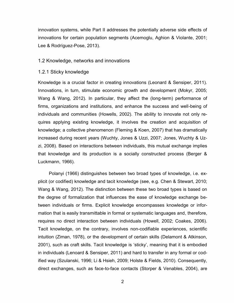
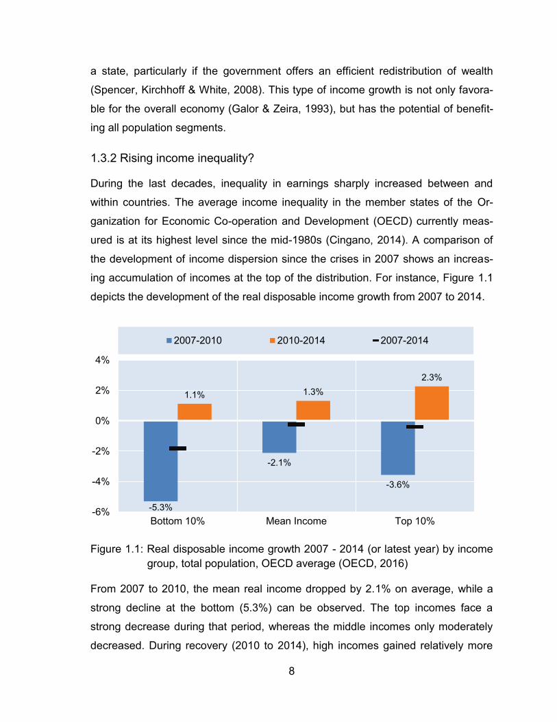
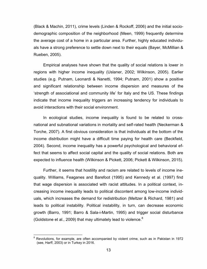
ing accumulation of incomes at the top of the distribution. For instance, Figure 1.1

depicts the development of the real disposable income growth from 2007 to 2014.

Figure 1.1: Real disposable income growth 2007 - 2014 (or latest year) by income group, total population, OECD average (OECD, 2016)

From 2007 to 2010, the mean real income dropped by 2.1% on average, while a

strong decline at the bottom (5.3%) can be observed. The top incomes face a

strong decrease during that period, whereas the middle incomes only moderately

decreased. During recovery (2010 to 2014), high incomes gained relatively more

-5.3%

-2.1%

-3.6%

1.1% 1.3% 2.3%

-6%

-4%

-2%

0%

2%

4%

Bottom 10% Mean Income Top 10%

2007-2010 2010-2014 2007-2014

9

due to unequal labor income growths (OECD, 2016), leading to increased income

inequality.

In Germany, the results regarding the development of wage dispersion varies

across income levels. An increasing level of inequality across the general popula-

tion, or at least at the top or bottom of the income distribution in the last decades is

typically detected (OECD, 2016), while top income households’ increase their dis-

posal income due to unequal labor market growth (Bach, Corneo & Steine, 2009;

Biewen & Juhasz, 2012; OECD, 2016). At the country level, income inequality de-

creased (Statistisches Bundesamt, 2017), but within Germany, the data tell a dif-

ferent story. Regions are not homogenous. It is therefore not surprising that East

and West German regions already reveal different levels (Gernandt & Pfeiffer,

2007; Biewen & Juhasz, 2012) and growth rates (Ambrosio & Frick, 2007) of in-

come inequality. Inequality in earnings rose in East and West Germany, but with a

more pronounced growth rates in East Germany, while West Germany reached

already a high level (Fuchs-Schündeln, Krueger & Sommer, 2010). This trend can

be observed especially after the reunification in 1990, and primarily in East Ger-

many (Biewen, 2000; Ambrosio & Frick, 2007), at the lower end of the distribution;

individuals had to face an increasing inequality in earnings (Fuchs-Schündeln,

Krueger & Sommer, 2010). These differences mainly arose from the economic

struggles at the East German labor markets (Fritsch et al., 2014). The development

of the East-West wage premium shows that East German income levels are grad-

ually approaching those of West Germany (Bach, Corneo & Steiner, 2009; Fuchs-

Schündeln, Krueger & Sommer, 2010), but are still lagging with regard to the aver-

age income level (Ambrosio & Frick, 2007). Traditionally, however, Germany

counts as a low-inequality country (compared with the US or Israel), but in the last

two decades exhibits an increasing level of income inequality in East and West

German regions. This trend has accelerated since 2010 (Cingano, 2014).

1.3.3 Income inequality, triggered by innovations?

Increasing income inequality is not a modern phenomenon. It has been a recurring

phenomenon over the past several centuries, and is characterized by upward and

10

downward trends. Structural change caused by the introduction of advanced tech-

nologies led to unemployment of workers with low levels of education. This is es-

pecially true in old industry sectors, and is one of the primary causes of increased

income inequality (Maddison, 2001).

For instance, during the Industrial Revolution in the 18th century in England, a

continuous and broad implementation of new technologies (innovations) led to

growth accelerations (Collins, 1969), a rise in the standard of living and to the crea-

tion of new products and markets (Mokyr, 2005). Researchers agree (Lindert &

Williamson, 1983; Maddison, 2001; Mokyr, 2005; Allen, 2009) that this rapid devel-

opment was based on the broad and comprehensive scientific knowledge stock

that was the source for new technologies (innovations) (Mokyr, 2005). This devel-

opment took place not only in England, but spread to other countries a few years

later, such as Germany or France. As these new technologies appeared, for in-

stance, mechanization of ploughing and harvesting, the demand for labor in the

agriculture sector was affected. This sector is populated by mainly low skilled

workers (Lindert & Williamson, 1983) leading to higher levels of unemployment for

this poorly educated population segment. At the same time, the demand for better

educated worker increased, because they were better able to understand and use

these new technologies (Allen, 2009). The wages of this population segment in-

creased since higher skill levels were required, and because of the innovation-

driven productivity gains that led to higher profits, especially for factory owners

(Lindert & Williamson, 1983; Maddison, 2001). The growing wage gap between

these different population segments, and the rising unemployment of ‘common’

workers, whose workplace could be easily replaced by new technologies, finally led

to a dramatically high accumulation of incomes at the top of the income distribu-

tion. The growth in income inequality and unemployment finally led to impoverish-

ment of common workers, a scenario that is known in the literature as pauperism

(Lindert & Williamson, 1983).

Pauperism, caused by the introduction of new technologies, dates back more

than 190 years. Although the pattern and origin of the current disparity between

11

rich and poor is similar (new technologies are replacing low-skilled workers and

require high-skilled individuals), the gap between the poor and the rich is no longer

as extreme as it was during the Industrial Revolution. Although income inequality

has decreased in the 20th century, wage dispersions have been on the increase

since the 1980s (Mokyr, 2005; Atkinson & Bourguignon, 2014), a reality that may

be due to the introduction of new technologies. For instance, Krueger (1993) inves-

tigates the effect of the introduction of the personal computer on wages. He ana-

lyzes a population survey of computer users and finds that employees who are

able to use a personal computer increase their wage by 10 to 15%, whereas the

income of non-users decreases (see, also DiNardo & Pischke, 1997). He argues

that new technologies increase the demand and wages for skilled workers. Simul-

taneously, demand and earnings of low-skilled workers decrease. These two paral-

lel developments lead to an increasing income inequality between high- and low-

skilled workers.

Both the introduction of new technologies during the Industrial Revolution in

Great Britain, and the widespread application of the personal computer in the tech-

nological age, are structural changes with far reaching consequences. However,

the effect of innovations on income inequality is not always clear. The current lit-

erature agrees that several channels exist through which innovations affect income

inequality. First, new technologies increase regional productivity by raising a firm’s

productivity or that of its workforce which, in turn, affects the wages of skilled work-

ers. Second, an innovation-driven productivity increases inequality between firms

and leads, again, to wage dispersion within an industry (Faggio, Salvanes & Van

Reenen, 2007). Third, regions that are already innovative are more attractive for

highly skilled and well paid workers. This attraction creates a hotbed for future in-

novative activities (Jaffe, Trajtenberg & Henderson, 1993). Finally, innovations are

clustered in space. Skill-biased technology change approach (SBTC) either com-

plements or substitutes particular jobs (Breau, 2007; Lee, 2011), and leads to an

accumulation at the top of the income distribution.

12

The SBTC approach is probably the most prominent theory linking the effect

of new technologies and increasing wage inequality (Acemoglu, Aghion & Violante,

2001; Breau, 2007; Lee, 2011; Van Reenen, 2011; Lee & Rodríguez-Pose, 2013).

The concept has its origin in the observation that returns to skills6 have experi-

enced a sharp increase over the past decades (Acemoglu & Autor, 2011). This de-

velopment is comparable with the Industrial Revolution or the introduction of the

personal computer. Studies conducted for the German labor market show a rise in

the returns to skills, also referred to as skill premium, starting in the early 1990s

(Dustmann, Ludsteck & Schönberg, 2007).

However, the wage differential between high and low skilled workers is mainly

determined by how much the supply of skilled labor increases, and by the degree

or sophistication of technological change. The latter determinant is assumed to be

skill-biased in the sense that the introduction of new technologies increases the

demand for educated workers (Acemoglu & Autor, 2011) and decreases the de-

mand for low and medium-skilled labor. Presuming that the implementation of

technological novelties requires the accumulation and processing of new infor-

mation, skill inevitably facilitates this process (Greenwood & Yorukoglu, 1997).

Besides the several channels how innovations or new technologies, can trig-

ger income inequality, the question remains why is it important to observe these

developments? One reason is that income inequality may cause several social and

economic problems (see, e.g. Wilkinson & Pickett, 2007).

1.3.4 Income inequality: a source for social-economic problems7

Rising income inequality leads to increasing economic and regional segregation.

The poor are becoming more and more segregated from the rest of the population

(Alesina, Di Tella & MacCulloch, 2004; Neckerman & Torche 2007). One possible

reason for this segregation is rising housing prices. A number of regional aspects

drive the relative costs of purchasing a home. Factors such as school quality

6 Returns to skills are typically measured as the relative wage of college graduates and high school

graduates. 7 For an extensive overview, see Neckerman and Torche (2007) or Wilkinson and Pickett (2007).

13

(Black & Machin, 2011), crime levels (Linden & Rockoff, 2006) and the initial socio-

demographic composition of the neighborhood (Meen, 1999) frequently determine

the average cost of a home in a particular area. Further, highly educated individu-

als have a strong preference to settle down next to their equals (Bayer, McMillian &

Rueben, 2005).

Empirical analyses have shown that the quality of social relations is lower in

regions with higher income inequality (Uslaner, 2002; Wilkinson, 2005). Earlier

studies (e.g. Putnam, Leonardi & Nanetti, 1994; Putnam, 2001) show a positive

and significant relationship between income dispersion and measures of the

‘strength of associational and community life’ for Italy and the US. These findings

indicate that income inequality triggers an increasing tendency for individuals to

avoid interactions with their social environment.

In ecological studies, income inequality is found to be related to cross-

national and subnational variations in mortality and self-rated health (Neckerman &

Torche, 2007). A first obvious consideration is that individuals at the bottom of the

income distribution might have a difficult time paying for health care (Beckfield,

2004). Second, income inequality has a powerful psychological and behavioral ef-

fect that seems to affect social capital and the quality of social relations. Both are

expected to influence health (Wilkinson & Pickett, 2006; Pickett & Wilkinson, 2015).

Further, it seems that hostility and racism are related to levels of income ine-

quality. Williams, Feaganes and Barefoot (1995) and Kennedy et al. (1997) find

that wage dispersion is associated with racist attitudes. In a political context, in-

creasing income inequality leads to political discontent among low-income individ-

uals, which increases the demand for redistribution (Meltzer & Richard, 1981) and

leads to political instability. Political instability, in turn, can decrease economic

growth (Barro, 1991; Barro & Sala-i-Martin, 1995) and trigger social disturbance

(Goldstone et al., 2009) that may ultimately lead to violence.8

8 Revolutions, for example, are often accompanied by violent crime, such as in Pakistan in 1972

(see, Harff, 2003) or in Turkey in 2016.

14

1.3.5 Crime and income inequality

The most prominent explanation for why economic circumstances affect criminal

behavior is described by Nobel Prize winner Gary Becker (1968). Becker treats

criminals as rational individuals that seek to maximize their own well-being, albeit

through illegal behavior. Individuals that expect lower returns from the market for

common work, compared to high-income individuals, increase the time they allo-

cate to criminal activities. This cost-benefit comparison is indeed a pure rational

consideration that mainly focuses on economic circumstances such as unemploy-

ment (Gould, Weinberg & Mustard, 2002), poverty (Pare & Felson, 2014) or in-

come inequality (Kelly, 2000), and not on social or psychological influences (Wil-

kinson, 2005; Neckerman & Torch, 2007).

The Strain theory (Merton, 1938) and the disorganization theory (Shaw &

McKay, 1942) attempt to fill this gap by linking social and psychological effects to

economic circumstances, i.e. income inequality (Kelly, 2000). In this sense, crimi-

nal behavior is not only attributed to rational behavior, but also to social and psy-

chological aspects, such as strain and frustration, resulting in an undermining of

social community behavior. Hence, if the distance in incomes of the rich and the

poor increases, the probability of unsuccessful individuals seeking compensation

by any means, including committing crime, increases (Fajnzylber, Lederman &

Loyza, 2002).

Whereas both the social and psychological based theories are able to explain

violent crimes, Becker (1968) provides a theoretical framework explaining why in-

come inequality triggers pecuniary crime.9 The current empirical literature has fre-

quently tested Becker’s theory (see, Ehrlich, 1973; Grogger, 1998; Nilsson, 2001;

Chintrakarn & Herzer, 2012). The Strain theory and disorganization theory, howev-

er, have rarely been the center of contemplation (see, Kelly, 2000; Agnew, 2001;

Neumayer, 2005; partly Wu & Wu, 2012). Most studies show that crime rates are

higher in regions with higher levels of income inequality (Fowles & Merva, 1996;

Fajnzylber, Lederman & Loyza, 2002; Soares, 2004; Chintrakarn & Herzer, 2012). 9 For a more detailed overview, regarding the theoretical framework, see Chapter 6.

15

Some studies, however, do not find evidence for the existence of such an inequali-

ty-crime link (see, Fougère, Kramarz & Pouget, 2009; Pare & Felson, 2014). Obvi-

ously, the topic is highly ambiguous with contradictory findings, and requires further

research.

1.4 Knowledge, networks, innovations, income inequality: Aim and scope of the thesis

1.4.1 The concept of the thesis

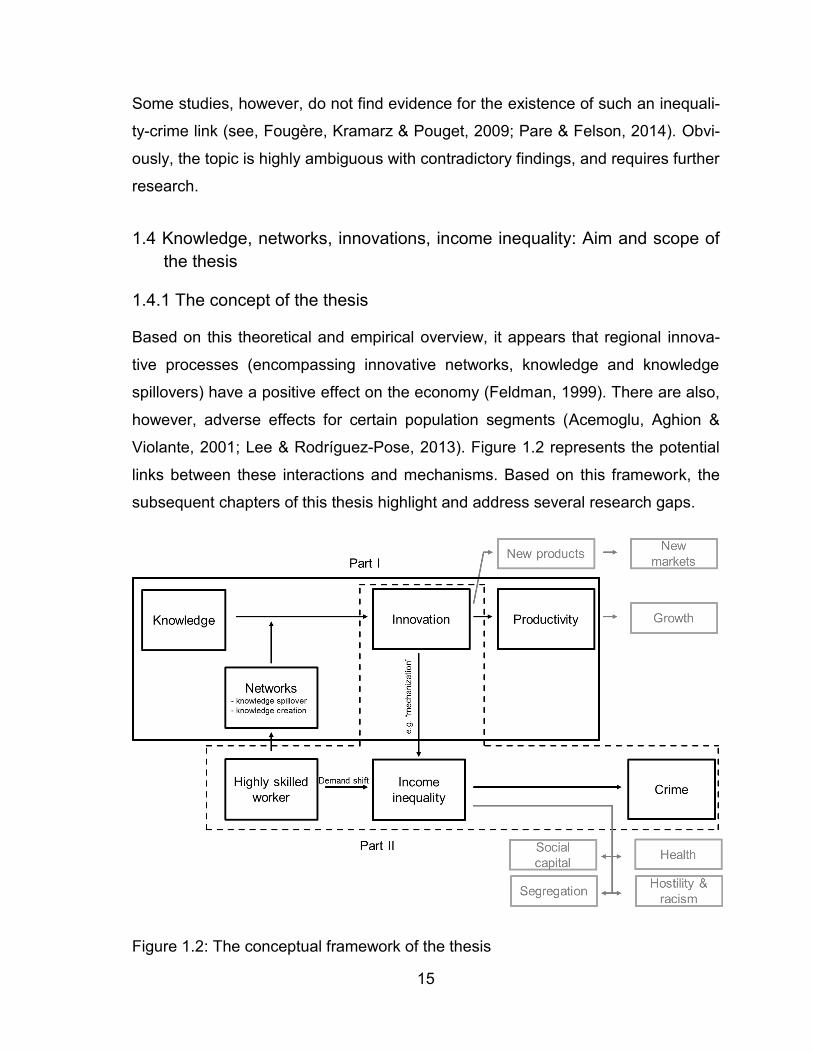
Based on this theoretical and empirical overview, it appears that regional innova-

tive processes (encompassing innovative networks, knowledge and knowledge

spillovers) have a positive effect on the economy (Feldman, 1999). There are also,

however, adverse effects for certain population segments (Acemoglu, Aghion &

Violante, 2001; Lee & Rodríguez-Pose, 2013). Figure 1.2 represents the potential

links between these interactions and mechanisms. Based on this framework, the

subsequent chapters of this thesis highlight and address several research gaps.

Figure 1.2: The conceptual framework of the thesis

16

1.4.2 Research gaps: Knowledge, networks and stability

Knowledge and its exchange is crucially important to produce innovations (Leonard

& Sensiper, 2011) that in turn affect the (long-term) performance of firms, organiza-

tions and institutions, and enhance the success and well-being of individuals and

communities (Howells, 2002). The creation of new knowledge and the production

of innovations depend highly on two components: the exchange of ideas with oth-

ers as expressed in the development of networks (Feldman, 1999; Bercovitz &

Feldman, 2011) and the specific knowledge stock of an individual (Diez, 2000;

Howell, 2002). The following two sub-chapters are situated in Part I of the above

Figure 1.2.

1.4.2.1 Dynamic networks, stable networks?

Based on the current literature (Powell et al., 2005; Jackson, 2008; Barabási,

2009), a heterogeneous composition of actors and a specific structure of a network

(favorable to knowledge spillovers) are particularly important for producing innova-

tions and for improving regional productivity (Feldman, 1999). The structural stabil-

ity of a network determines the degree to which there is a continuous flow of

knowledge transfers and spillovers. Scholars assume that cooperative activities in

R&D should be long lasting because the establishment of these relationships is

associated with high transaction costs (Ejermo & Karlsson, 2006). Since innovative

activities are characterized by high levels of risk and uncertainty, a trustful relation-

ship between network actors that requires partner-specific effort is important

(Liebeskind et al., 1995; Gilsing & Nooteboom, 2005). Further, to identify a suitable

cooperation partner and to establish a well-working interface, frequent face-to-face

contacts are required (Storper & Venables, 2004; Ejermo & Karlsson, 2006). Costs

would be sunk if the relationship is abandoned. In turn, the costs to maintain such

cooperative relationships are comparatively low as long as both actors continue to

benefit from each other (Ahuja, 2000).

Very few scholars have empirically test these assumptions. The most promi-

nent example is Barabási and Albert (1999, 2000). According to their findings, ac-

tors tend to persist in a network that shows continual growth and displays preferen-

17

tial attachment (when actors tend to collaborate with other well-embedded actors).

Networks that reveal these two generic mechanisms show properties such as

scale-free or fat-tailed degree distributions (Powell et al., 2005), and seem to be

highly robust against randomly omitted actors (Barabási & Albert, 1999, 2000).

Such a robustness or stability depends on the heterogeneity of network actors that

fit quite well with the characteristics of real world networks (Powell et al., 2005).

Consequently, scholars exclude groups of unstable observations because they

regard them to be outliers (see, e.g. Balland, De Vaan & Boschma, 2012).

Following the transaction cost theory and the results of Barabási and Albert

(1999, 2000), it is not surprising that the literature assumes permanent network

actors and stable relationships over time. This is, however, a naïve assumption,

since network actors may move between firms or regions. Further, permanent

knowledge exchanges are not fruitful, in general. Since actors become more and

more homogenous regarding their knowledge stock (Granovetter, 1973), output of

further cooperative activities can be hampered. Consequently, knowledge about

actor fluidity (entry and exit of actors) is rather scarce. Therefore, Chapter 2, em-

bedded in Part I of this thesis (see, Figure 1.2), seeks to answer the following re-

search questions (RQ):

RQ1: In case of high levels of actor-turnover, what determines the reoccur-

rence of actors in the subsequent time period?

RQ2: What are the consequences of fluidity for a network’s structural char-

acteristics and the performance (patent productivity) of the respective

RIS?

1.4.2.2 Does actor ‘fluidity’ mean knowledge ‘fluidity’?

Networks are important for the transfer of knowledge (Feldman, 1999), its produc-

tion and, in general, for productivity gains (Wiklund & Shepard, 2003). Knowledge,

especially tacit knowledge, which is sticky and hard to transfer (Szulanski, 1996; Li

& Hsieh, 2009), is crucially important for future innovations (Katila & Ahuja, 2002;

Wu & Shanley, 2009). In case of actor fluidity, the embodied knowledge of a dis-

18

continued actor would disappear and lead to a decreasing regional knowledge

stock. But, knowledge production is a collaborative activity. Therefore, knowledge

spreads between team members. With this, knowledge of those actors that disap-

pear from an inventor network may still be available because it has been passed

onto network actors who are still present.

In line with the earlier discussion about the structural composition of a net-

work (see, Capaldo, 2007; Schilling & Phelps, 2007; Phelps, 2010), it is important

to analyze how far structural network characteristics influence the persistence of

knowledge, specifically the knowledge stock, of a RIS. It could be assumed that

highly interconnected networks reveal a high share of knowledge persistence,

since an intensive exchange of knowledge among actors takes place (Howell,

2002). But, this is only the case if we can assume that knowledge is fully trans-

ferred between all team members. This is another naïve assumption, since net-

works benefit from division of labor and the different skills and knowledge of team

members (Wuchty, Jones & Uzzi, 2007). Thus, an assessment of the share of per-

sistent knowledge and its impact on the performance of a network is an important

step to understanding the dynamics behind the transfer and creation of knowledge.

Further, entries of new actors are associated with new sets of knowledge that can

influence also the performance of a respective network. Based on this argumenta-

tion, Chapter 3 (see, Figure 1.2) tries to answer the following research questions:

RQ3: Which structural characteristics of a network determine the share of

persistent knowledge?

RQ4: To what extent does persistent and new knowledge affect the perfor-

mance of a RIS?

1.4.3 Research gaps: Innovation, inequality and crime

Innovations can have advantageous effects on an economy and society (see,

Feldman, 1999; Ahuja, 2000; Fritsch & Müller, 2004; Mokyr, 2005), but they can

also have adverse effects on some population segments (see, Maddison, 2001;

Breau, Kogler & Bolton, 2014). For instance, new technologies can replace routine-

19

jobs, which may ultimately lead to an increase in income inequality (Autor, Levy &

Murnane, 2003).

Income inequality is an important topic since many studies claim a relation-

ship with social and economic problems.10 However, most of the studies that focus

on income inequality are done at the aggregated (country) level (Atkinson & Bour-

guignon, 2000, 2014; Salverda et al., 2014) and neglect, therefore, the heterogene-

ity of regions. Regions differ in terms of labor markets, housing prices, consump-

tion cost and their innovative performance.

The following two subchapters (see, Figure 1.2) focus on the effect of innova-

tions on income inequality, and the relationship between income inequality and

crime, by considering regional differences.

1.4.3.1 Regional differences in innovative activities and income inequality

Innovations tend to be clustered in space (Jaffe, Trajtenberg & Henderson, 1993)

and are not equally distributed. Also, the level of income inequality differs between

regions. Following the current literature (see, e.g. Acemoglu, Aghion & Violante,

2001; Lee, 2011; Lee & Rodríguez-Posé, 2013; Breau, Kogler & Bolton, 2014), the

effect of new technologies is most distinct in regions with high levels of innovative

activities. Thus, the gap between low-skilled and high-skilled individuals should be

larger in regions with a high level of innovative outputs compared to less innovative

regions.

Most of the current studies focus only on the largest 20 cities in a country

(see, e.g. Breau, Kogler & Bolton, 2014), or compare only countries (for an over-

view see, e.g. Piketty & Saez, 2006). Consequently, differences between regions

within a country (for instance, between rural versus urban areas) are neglected.

The literature does not only lack regional analyses, but also long-term assess-

ments. Further, there is a lack of research on the effect of long-lasting income ine-

quality on the regional level of innovative activities. Additionally, it is still an open

question whether higher income inequality and higher innovation output are caused 10 For an extended overview, see Neckerman and Torche (2007).

20

by the regional population share of highly educated individuals who enjoy higher

levels of income. Thus, Chapter 5 addresses the following research question:

RQ5: Do changes in innovative activities lead to changes in income ine-

quality at the regional level? Or do already high levels of income ine-

quality decrease (increase) innovative activities within a region?

1.4.3.2 Regional income inequality and local crime rates

A current debate in economics deals with the question of whether and how income

inequality is related to socio-economic problems such as crime (Wilkinson &

Pickett, 2007, 2009). Crime is a serious problem in many societies, not only be-

cause of its economic cost, but also because it undermines social values and leads

to a generalized fear in the population. Inequality lowers the returns from work in

the labor market for low-income individuals (Becker, 1968), increases the strain

and frustration of economically unsuccessful people (Merton, 1938), or leads to an

undermining of social values (Shaw & McKay, 1942) that finally triggers criminal

behavior (Kelly, 2000).

Most current studies on that research question focus on the US (Cohen, Fel-

son & Land, 1980; Ehrlich, 1996; Fishback, Johnson & Kantor, 2010) or on Great

Britain (Machin, Marie & Vujic, 2011), and mainly only observe large metropolitan

areas (see, e.g. Kelly, 2000). However, countries are made up of numerous re-

gions that differ in terms of their labor market, housing prices or consumption

costs. These, in turn, influence individuals’ income and well-being, but also the

probability to commit crime (Merton, 1938; Shaw & McKay, 1942; Runciman, 1966;

Becker, 1968). In addition, many studies only analyze the relationship between

income inequality and categories of crime, neglecting the different motives and

scope of various crimes. On this basis, Chapter 6 tries to answer the following fur-

ther research question:

RQ6: Does an effect between income inequality and different categories of

local crime rates exist?

21

1.5 Structure and findings of the thesis

This thesis is grounded in the broad topic of regional innovations, focusing on the

production and potential consequences of these innovations. Therefore, the thesis

is split into two parts. The Part I includes Chapters 2, 3 and 4, and deals with the

production of new knowledge and innovations within teams (networks), the stability

of such R&D cooperative relations and the persistence of knowledge within a re-

gion. After highlighting the importance of innovations for an economy, Part II

(Chapters 5, 6 and 7) highlights the potentially adverse effects of innovations.

Namely, regional income inequality caused by the introduction of new technologies

concentrating income at the top of the income distribution. Further, since income

inequality is associated with several socio-economic problems, Part II of this thesis

focuses on the relationship between regional income inequality and local crime

rates.

Chapter 2 (‘The fluidity of inventor networks’) lays the foundation for Part I of

the thesis by offering the observation that inventor networks are highly unstable at

the inventor (micro) level. This finding contradicts the assumptions of the transac-

tion cost theory (Ejermo & Karlsson, 2006), and the conclusions drawn by Barabási

and Albert (1999, 2000). As discussed in Chapter 1, Section 1.4.2, transaction cost

theory deems R&D relationships to be stable because of the costs incurred finding

and establishing cooperative relations and building trust. However, Chapter 2 will

show that most inventors are only active in one period. This low persistence of in-

ventors may lead to some fragmentation of the overall network, or affect the net-

work’s performance.11 Indeed, the overall results suggest that actor fluidity in-

creases the share of isolates and decreases the share of the largest component,

indicating the fragmentation of the network. However, the actor turn-over seems to

be positively related to the performance of a network, suggesting that replacement

of ‘old’ actors by new ones may be beneficial for the performance of the inventor

network, and for the RIS. Thus, Chapter 2 provides two contributions: First, it chal-

lenges the widespread assumption of stable network relationships; second, it 11 Network performance is measured by patent productivity, indicating the level of efficiency of a

regional innovation system

22

shows how levels of fluidity affect the productivity and efficiency of regional innova-

tive systems.

Based on the findings of Chapter 2, two questions arise. First, are persistent

relations and a network’s structure important characteristics for the maintenance of

knowledge that spreads among team members during collective R&D activities?

Second, does persistent knowledge play a crucial role for the efficiency of a re-

gional innovation system? Chapter 3 (‘Actor fluidity and knowledge persistence in

regional networks’) tries to answer these two questions. The first question is ad-

dressed by analyzing the effect of several network characteristics on the share of

persistent knowledge. For instance, the literature suggests that dense and large

networks lead to a higher distribution of knowledge among inventors (Uzzi & Spiro,

2005; Schilling & Phelps; 2007; Tang, Mu & MacLachlan, 2008). The findings pre-

sented in Chapter 3 support these assumptions. We find that density (respectively

connectivity) and size is significant and positive related to the share of persistent

knowledge. For the share of isolates we find the opposite to be true. Further, the

share of discontinued actors negatively influences the share of persistent

knowledge. This is not surprising, since (tacit) knowledge is embodied within indi-

viduals.

The second question addresses the importance of persistent knowledge for

the efficiency of a RIS. However, the results indicate that the share of persistent

knowledge, as to be expected, is positively related to the development of patent

productivity when we control for the share of new knowledge. This indicates that

both kinds of knowledge sources drive the productivity and efficiency of a network.

Thus, Chapter 3 provides new insights regarding the manifold discussion of the

importance of persistent and new knowledge by offering evidence about

knowledge sources in regional inventor networks.

Chapters 2 and 3 deal with the issue of fluidity and persistent and new

knowledge within a network. Chapter 4 briefly summarizes the main results and

provides a discussion of current limitations, followed by the development of further

research questions.

23

Chapter 5 (‘Causes and consequences of income inequality: The role of inno-

vation’) provides an analysis of the relationship between innovative activities and

income inequality at the regional level. Here, we focus on distributional effects of

innovative activities on regional wages. The analyses uses patent applications as a

proxy for the regional level of innovation activity (Smith, 2006), and basically fol-

lows the theoretical considerations of Acemoglu, Aghion and Violante (2001), as

well as those of Lee and Rodríguez-Pose (2013). Thus, higher innovative activities

lead to a higher demand for skilled workers and a declining demand for low-skilled

workers. This change in demand has a concurrent effect on their respective wages

(Breau, Kogler & Bolton, 2014). A Vector autoregression model (VAR), combined

with a first order difference equation is used to take into account the potentially re-

verse causal effects. Regions that attract high-skilled worker can lead to higher

income inequality but, likewise, to higher innovative output. Thus, income inequality

can increase the incentive to innovate. However, the opposite may also be true,

meaning that higher levels of income inequality could discourage people from en-

gaging in innovative activities (see, Weinhold & Nair-Reichert, 2009). Further, the

extended model allows us to analyze how changes in innovative activities Granger-

causes changes in income inequality. Further, changes in income inequality

Granger-causes changes in innovative activities to decrease, indicating that higher

levels of income inequality decreases the tendency to be innovative active. In this

line, Chapter 5 provides evidence for the Granger-causal relationship between in-

novative activities and income inequality, at a regional level.

To be clear, income inequality per se is not a bad phenomenon (Milanovic,

2011), since it is an expression of just rewards for efforts. However, it can also lead

to socio-economic problems, such as crime (see, Section 1.3.4). Chapter 6 (‘Re-

gional income inequality and local crime rates’) considers the relationship between

income inequality and crime for German regions. A comprehensive regional analy-

sis (as yet barely touched on in the literature) is important since income inequality

is unevenly distributed across regions. The same holds for regional crimes rates.

Further, both variables are a local but not a country-wide event (Gould, Weinberg &

Mustard, 2002). The theoretical background of this chapter is mainly based on

24

Becker’s ‘Economic theory of crime’ approach (Becker, 1968) and the extensions

by Ehrlich (1973). For the empirical analyses, a fixed effect model is used that

support a positive and significant relation between regional income inequality and

local crime rates. Further, the Spatial Autocorrelation model shows that no cross-

sectional dependency exists, indicating that the use of Panel models is sufficient. It

also supports the assumption that criminals tend to commit crimes in familiar sur-

roundings (see, Glaeser & Sacerdote, 1999). With this, Chapter 6 reveals a com-

prehensive analysis for German regions over a five-year period and provides evi-

dence for the existence of an inequality-crime link.

The findings from Chapter 5 discusses how innovation activities can negative-

ly affect regions, i.e. increasing income inequality, whereas Chapter 6 addresses,

in a much-advanced step, the relationship between income inequality and local

crime rates. After a short summary and discussion of the main results and their

limitations, an outlook for potential research questions can be found in Chapter 7.

Chapter 8 provides a final brief conclusion.

25

Part I Knowledge, innovations and networks

‘It is the long history of humankind […] those who learned to collaborate

and improvise most effectively have prevailed.’

Charls Darwin (1859)

26

Chapter 2

The fluidity of inventor networks

Abstract:12 We investigate the stability of cooperative relationships between inven-

tors and consequences for the characteristics and patent productivity of the re-

spective RIS. The empirical analysis is for nine German regions over a period of 15

years. We find a rather high level of ‘fluidity’, i.e. entry and exit of actors, as well as

instability of their relationships over time. The aggregate characteristics of the re-

gional networks are, however, quite robust even with high levels of micro-level flu-

idity. There are both significantly positive and negative relationships between mi-

cro-level fluidity and the performance of the respective RIS.

12 This chapter is joint work with Michael Fritsch. A version of this chapter was under review at the

journal Research Policy, when this PhD was submitted. We are indebted to Holger Graf and Muhamed Kudic for helpful comments on an earlier version of this paper.

27

2.1 Division of innovative labor, innovation networks, and regional performance

Innovation processes are increasingly characterized by a pronounced division of

labor among actors, such as private firms and public institutions of education and

research (Wuchty, Jones & Uzzi, 2007; Jones, Wuchty & Uzzi, 2008). This division

of innovative labor has become an important topic of innovation research. A main

focus of this research is on the networks of relationships among actors. It is a basic

conjecture of this type of research that embeddedness in networks and the struc-

ture of these networks leads to more highly effective innovation processes and

higher levels of innovation.13 The analysis of innovation networks plays a particu-

larly prominent role in attempts to explain the performance of regions (Ejermo &

Karlsson, 2006; Fleming, King & Juda, 2007).

Although research on regional networks has produced many interesting re-

sults concerning network structures and the role of certain types of actors (for an

overview, see Cantner & Graf, 2011), still little is known about the dynamic charac-

teristics and development of network structures over time. In fact, empirical studies

on the stability of network structures and of the underlying relationships hardly ex-

ist. Many scholars claim that cooperative relationships between actors should be

long lasting because the effort of establishing and maintaining a trusting relation-

ship would be sunk if the link is abandoned (Storper & Venables, 2004; Gilsing &

Nooteboom, 2005; Ejermo & Karlsson, 2006). Stability of network ties is a key as-

sumption of Barabási & Albert’s (1999, 2000) well-known model of network devel-

opment.14 Quite remarkably, some researchers even exclude unstable relation-

13 There are two main reasons why embeddedness in networks may have a positive effect on the

performance of actors. First, interaction with others may be an important channel for transferring (tacit) knowledge (Owen-Smith & Powell, 2004; Storper & Venables, 2004). Particularly, face-to-face contact promotes the development of personal trust that can be regarded as an important precondition for fruitful R&D cooperation. Second, the formation of links in R&D networks implies a process of screening and selection. Assuming that actors choose cooperation partners according to their abilities, actors included in a network have been positively evaluated. This positive selection of relatively able cooperation partners should have a positive effect on the probability of success (Granovetter, 1995; Storper & Venables, 2004; Wilhelmsson, 2009).

14 Barabási and Albert (1999) investigate two generic mechanisms for large networks: (i) networks grow over time by entry of new actors, and (ii) the new actors tend to collaborate with already well embedded actors (preferential attachment).

28

ships from their empirical analysis because they regard them as outliers (e.g. Bal-

land, De Vaan & Boschma, 2012).

This chapter seeks to shed some light on the dynamics of innovation net-

works. We describe and analyze the disappearance of actors and links, as well as

the emergence of new actors and links, and the consequences for network struc-

ture and performance. Our data is patent information on co-inventorship for nine

German regions over a time span of 15 years. The starting point of our analyses

are hypotheses about the stability of cooperative relationships in Research and

Development (R&D). Testing the assumption of stable network relationships with

these data we find a surprisingly high level of instability. Our analysis shows that

inventors that appear to be well embedded within a network in one period are un-

likely to re-occur in the following (three year) period. As a result, links between

nodes of the networks tend to be highly unstable. Hence, in contrast to a wide-

spread assumption, regional innovation networks are characterized by a rather

high level of fluidity with quickly changing relationships between actors over time.

However, we find that when we relate the measures of actor fluidity to the structure

of a network, these structures remain rather stable. There are both significantly

positive and negative relationships between the micro-level fluidity of actors and

links with the performance of the respective regional innovation system in terms of

patent productivity. Based on these results we draw conclusions for theory and for

further research.

In what follows, we first review the reasons offered for the stability of R&D

cooperation and implications for network development (Section 2.2). Section 2.3

introduces the spatial framework, data, indicators and modelling of our analysis,

followed by a brief overview on the development of networks over time (Section

2.4). We then describe the magnitude of the fluidity phenomenon and perform mi-

cro-level analyses in order to identify determinants of the reoccurrence of actors in

subsequent time periods (Section 2.5). Section 2.6 analyzes the relationship be-

tween micro-level fluidity and the macro structure, as well as the performance of

29

the specific networks we exam. Finally, we discuss the results and draw conclu-

sions for theory and further research (Section 2.7).

2.2 The nature and the stability of cooperative Research and Development

Cooperation in Research and Development is characterized by considerable levels

of uncertainty and asymmetric information. The uncertainty follows from the very

nature of R&D as a discovery procedure. Since the result of this discovery proce-

dure is unknown ex ante, it cannot be completely specified in an R&D contract,

leaving room for opportunistic behavior of cooperation partners. Asymmetric infor-

mation arises when there is incomplete knowledge about the abilities and future

behavior of a potential cooperation partner. Because R&D involves asymmetric

information and the danger of opportunistic behavior by a cooperation partner,

successful cooperation requires trust (Noteboom, 2002; Gilsing & Noteboom,

2005). Another reason why trust is a critical component of any cooperative R&D

effort is the considerable transfer of information and knowledge between partners

that may be regarded sensitive. When engaging in cooperative R&D, actors need

to trust that their partners will not use this information in an undesirable way. The

development of trust between actors is often based on past experiences of fre-

quent and intensive collaborations and an actor’s reputation (Tomkins, 2001;

Gilsing & Nooteboom, 2005).

The R&D problems of uncertainty and asymmetric information are reflected in

the transaction costs of establishing a cooperative relationship. There are costs

involved in identifying a suitable cooperation partner, in negotiating the terms of the

cooperation and in establishing a well-working and trust-based relationship that

may require frequent face-to-face contacts (Storper & Venables, 2004; Gilsing &

Nooteboom, 2005; Ejermo & Karlsson, 2006). Particularly, the generation of trust

involves a partner-specific effort that is irreversible and is sunk if a relationship is

abandoned. Sunk costs of terminating cooperative R&D relationship may also oc-

cur if the relationship requires specific skills and equipment (e.g. Powell et al.,

2005). The sunk costs of abandoning a R&D cooperation create an incentive for

30

actors to maintain the relationship over longer periods of time, unless maintaining

the relationship is more costly than establishing a new relationship with a different

actor. Based on these arguments we expect:

Hypothesis I: Cooperative relationships between actors in R&D are long-lasting. Hence, actors remain in the network for longer periods of time so that the level of ‘fluidity’ is rather low.

The model of Barabási and Albert (1999, 2000) assumes that network rela-

tionships are stable over time so that all actors that are part of a network at a cer-

tain point in time remain in the network in subsequent periods. Based on this stabil-

ity assumption, Barabási & Albert (1999, 2000) investigate a certain mode of tie

formation, ‘preferential attachment’. According to the preferential attachment mode

of tie formation, new actors are especially attracted to and try to link with already

well embedded actors. Barabási & Albert (1999, 2000) run simulations of network

dynamics based on the preferential attachment mode. The resulting networks show

properties such as a scale-free or fat-tailed degree distribution15 that fit quite well

with the characteristics of large and heterogeneous real world networks (Powell et

al., 2005). They then examine the structural robustness of the simulated networks

if network actors are randomly omitted.

Barabási and Albert (1999, 2000) use the average length of the shortest path

between any two nodes in the network as the indicator for the robustness of a net-

work. They argue that this measure can be regarded as an indicator for the ease of

transferring information and knowledge within a network. The smaller the length of

the average shortest path, the lower the frictions created when there is an ex-

change between actors, and the better the interconnectivity of a network. Based on

their simulations, Barabási and Albert (1999, 2000) conclude that the disappear-

ance of actors has a rather minor effect on average path length. Their results sug-

gest that large scale-free networks (Powell et al., 2005) are highly robust against

randomly removed nodes.

15 Scale-free networks are characterized by a highly heterogeneous degree distribution that

includes some nodes with many degrees and a long tail of nodes with very few connections.

31

The high level of macro-level stability of networks found by Barabási and Al-

bert (1999, 2000) in their simulations, despite the disruption of randomly removed

nodes, raises the question about the relationship between micro-level stability and

the robustness of a network from a macro-level perspective. Does high fluidity of

actors and links, in fact, lead to unstable network structures? To what extent does

micro-level stability, in terms of persistence of actors and links, constitute a pre-

condition for stability at the macro-level? Following Albert, Jeong and Barabási

(2000), the performance of large scale-free networks is highly stable with regard to

fluctuations of actors and links for two reasons. First, since most actors in such

type of network have only a few links (Albert, Jeong & Barabási, 2000), the proba-

bility that a randomly removed actor has a central position in the network is rather

low. Second, assuming that new actors tend to gravitate to well-embedded actors

(‘preferential attachment’) there is a high probability that these new actors are at

least as well connected in the network as the discontinued actors. Based on these

considerations we expect:

Hypothesis II: Macro-level robustness and performance of scale-free networks does not require high levels of stability of actors and their links at the micro-level.

Dynamic innovation processes require some fluidity of actors and links, yet

abandoning cooperative relationships and establishing new links may imply con-

siderable sunk costs and significant effort. It is rather unclear how the fluidity of

actors and links might impact the performance of a RIS. Due to this ambiguity, we

abstain from setting up a concrete hypothesis about the expected relationship be-

tween RIS performance and the fluidity of actors and their links.

2.3 Data and indicators

2.3.1 Data

We analyze inventor networks based on data from the DEPATISnet database

(www.depatisnet.de) maintained by the German Patent and Trademark Office

(Deutsches Patent- und Markenamt). Analysis of inventor networks is based on the

32

assumption that actors who are named as inventors on the same patent docu-

ment16 know each other and have worked together (Balconi, Breschi & Lissoni,

2004). Patents are assigned to regions based on the information about the resi-

dence of the inventor. We are well aware that patents reflect only a part of the di-

verse types of formal and informal relationships among innovating actors.17 It is,

however, plausible to assume that documented co-inventorship implies other forms

of cooperation, such as co-publications and informal knowledge exchange. A com-

prehensive data source that accounts for the variety of relationships between inno-

vating actors does not exist.

We construct the regional inventor networks in nine German planning regions

for five, three-year periods18 over a time span of 15 years (1994 to 2008). Five of

these regions are located in East Germany, the former socialist GDR, and four re-

gions are in West Germany (see, Figure 2.1). Planning regions are functional spa-

tial units that tend to be somewhat larger than labor market regions or travel-to-

work areas. They normally comprise several NUTS3-level districts, namely, a core

city and its surrounding area. While districts are administrative geographic units,

planning regions are more often used for spatial analysis and policy development,

particularly regarding public infrastructure planning. We consider planning regions

to be more suitable for an analysis of regional innovation systems for two reasons.

First, a single district, particularly a core city, is probably too small to include the

most important actors of innovation-related local interaction. The second reason is

of a methodological nature; since patents are assigned to the residence of the in-

ventor, taking simply a core city as a region would lead to an underestimation of

patenting activity since many inventors who work in cities have their private resi-

dence in surrounding districts.

16 By harmonizing the data, we corrected for misspellings and compared the obtaining individuals

regarding their first name, second name and ZIP code. If all of these three criteria were identical, we assumed that the individuals are identical.

17 A comparison of regional innovation networks constructed with different data sources (Fritsch, Titze & Piontek, 2017) finds that patent data tend to underestimate links of private sector firms, while universities and other public research institutions are well-represented in patent data.

18 These periods are 1994-96, 1997-99, 2000-02, 2003-05 and 2006-08.

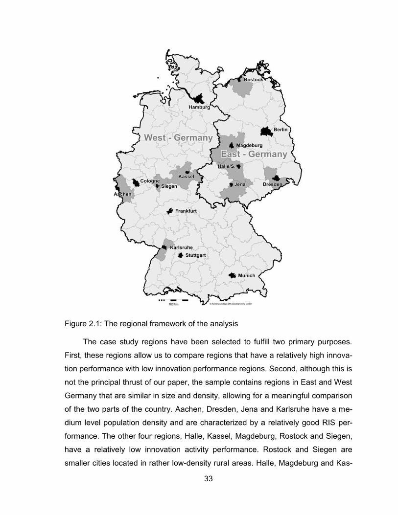
33

Figure 2.1: The regional framework of the analysis

The case study regions have been selected to fulfill two primary purposes.

First, these regions allow us to compare regions that have a relatively high innova-

tion performance with low innovation performance regions. Second, although this is

not the principal thrust of our paper, the sample contains regions in East and West

Germany that are similar in size and density, allowing for a meaningful comparison

of the two parts of the country. Aachen, Dresden, Jena and Karlsruhe have a me-

dium level population density and are characterized by a relatively good RIS per-

formance. The other four regions, Halle, Kassel, Magdeburg, Rostock and Siegen,

have a relatively low innovation activity performance. Rostock and Siegen are

smaller cities located in rather low-density rural areas. Halle, Magdeburg and Kas-

34

sel are larger urban areas, but they can hardly be considered as densely populat-

ed. Each region hosts at least one university. Data on the regional number of em-

ployees in R&D are from the Establishment History File of the Institute for Em-

ployment Research. Figure 2.1 shows the location of the nine case-study regions.

2.3.2 Indicators

The following measures are used to investigate the fluctuation of actors at the mi-

cro-level. The dependent variable is the presence of an actor in the network, i.e. if

he or she has contributed to a patent in a previous period. This variable has the

value 1 if the actor was present in any previous period and it is 0 otherwise. We

measure the amount of an actor’s innovative output by the number of patents filed

in a certain period that mention him or her as an inventor. The intensity of an ac-

tor’s involvement in a network is measured by three variables:

the number of links that an actor maintains with other actors in the network dur-

ing a certain period of time (degree);

the presence of an actor in the largest component (1 = yes; 0 = no);

being an isolate (degree = 0) with no links to other actors.

Characteristics of a network are measured by variables, such as the mean

degree, the share of the largest component, the share of isolates, the overall clus-

tering coefficient, and the patent productivity. The mean degree is the average

number of links an actor maintains, constituting a precondition of knowledge and

information transfers (Jackson, 2008). Average path length is defined as the aver-

age shortest path between two nodes within a network (Albert, Jeong & Barabási,

2000; Wassermann & Faust, 2007). Patent productivity is the number of patents

per R&D employee, and describes the performance of a network. The higher the

level of patent productivity the better the performance, in terms of generating new

ideas (Fritsch & Slavtchev, 2011). Table 2.A1 in the Appendix provides descriptive

statistics for the variables and Table 2.A2 displays the correlations between varia-

bles.

35

The distribution of the number of patents per actor is highly skewed (Figure

2.A1 in the Appendix). While over 60 percent of all actors have just one patent,

less than 20 percent have two patents, and the share of actors with larger numbers

of patents is rather small. The degree distribution of the networks (Figure 2.A2 in

the Appendix) corresponds to a scale-free distribution, i.e. there are only a few ac-

tors with relatively numerous network links, while most actors have very few or no

relationships. As mentioned in Section 2.2, this type of network should be better

able to compensate for discontinued nodes than a network where all actors have

about the same number of links (Barabási & Albert, 1999; Albert, Jeong & Bara-

bási, 2000; Jackson, 2008; Khokhlova & Kipnis, 2013).

2.4 The development of the regional networks over time

The nine regional inventor networks we exam show quite diverse characteristics

with regard to the numbers of patents, actors, ties, and components. All regions,

except Halle and Aachen, show steady growth in the numbers of actors (network

size) and ties (Table 2.A3). In all regions, the number of components increases

over the period of analysis. Except for Halle, all regions exhibit a total increase in

the mean degree, indicating increasing interconnectedness of regional actors (Ta-

ble 2.A4). The number of patents varies slightly over time but does not exhibit any

clear trend. It reaches its maximum in the 1997-99 period, followed by a decrease

in the following two period, and an increase in the final period (Table 2.A5).

The share of co-patents increases over the observation period, accounting for

about 90 percent in the final sub-period. We also find a growing number of inven-

tors per patent (Table 2.A5). These developments of the mean degree and the in-

creasing importance of R&D collaborations are in line with overall trends reported

in the literature (e.g. Wuchty, Jones & Uzzi, 2007; Jones, Wuchty & Uzzi, 2008)

and indicate an increasing importance of research collaboration. The steady

growth of nearly all networks, together with an increasing mean degree over time,

is consistent with Barabási and Albert’s (1999) preferential attachment hypothesis

36

claiming that new actors are more likely to link with relatively well-embedded ac-

tors.

Due to the increasing mean degree of the networks over time, one might also

expect a decrease of average path length. We find, however, that the average path

length increases in most of the networks (Table 2.A4). The increasing path length

can be explained by an exponential increase in the number of potential cooperation

partners created by the growing number of actors, a higher share of actors in the

largest component of a network and a larger average component size.19 An addi-

tional explanation could be that the growing number of components (Table 2.A3)

may also indicate greater variety of knowledge fields within a region. As a conse-

quence of the rather pronounced effects of changes in the number of actors on

average path length, we refrain from using average path length as an indicator for

network performance, in contrast to Albert, Jeong and Barabási (2000).

2.5 Fluidity of actors at the micro level

2.5.1 General observations

This section analyzes the fluidity of actors at the micro level over time. What de-

termines the reemergence of actors in a subsequent time period, and how do ac-

tor’s positions within a network change over time?

In contrast to the widespread assumption that actors and ties in networks are

rather persistent (Section 2.2), our data shows a rather high level of actor turnover.

We find that more than 78 percent of all actors are present only in one observation

period, 14.51 percent are active in two periods and only about 7 percent appear in

networks for more than two periods (Figure 2.2). On average, 32.34 percent of the

actors that are active in a network are carryovers from the previous period. Hence,

at least 60 percent of the inventors in a regional network appear in a sub-period for

19 Isolates are not included in the calculation of the average component size.

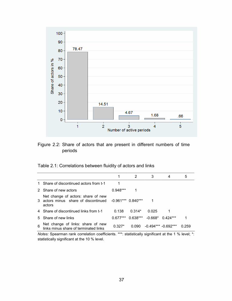
37

Figure 2.2: Share of actors that are present in different numbers of time periods

Table 2.1: Correlations between fluidity of actors and links

1 2 3 4 5

1 Share of discontinued actors from t-1 1 2 Share of new actors 0.948*** 1

3 Net change of actors: share of new actors minus share of discontinued actors

-0.961*** 0.840*** 1

4 Share of discontinued links from t-1 0.138 0.314* 0.025 1 5 Share of new links 0.677*** 0.638*** -0.668* 0.424*** 1

6 Net change of links: share of new links minus share of terminated links

0.327* 0.090 -0.494*** -0.692*** 0.259

Notes: Spearman rank correlation coefficients. ***: statistically significant at the 1 % level; *: statistically significant at the 10 % level.

38

the first time. Based on these figures, we clearly have to reject our Hypothesis I

about the persistence of actors at the micro-level.20

Table 2.1 shows rank correlations between the shares of discontinued and

newly occurring actors and links. Looking at the statistical relationships between

the different measures for the fluidity of actors we find a remarkably strong rela-

tionship between the share of discontinued actors and the share of new actors in-

dicating that the number of exits from the network is more or less completely sub-

stituted by about the same number of newcomers. As to be expected there are

considerable correlations between the fluidity of actors and of links. However, cor-

relations between the fluidity of actors and links and the measures for the different

types of link changes are considerably less pronounced than those between the

measures for the fluidity of actors. Most interestingly, the correlations between the

net change of the number of actors with the share of new links as well as with the

net change of the number of links are significantly negative. This suggests that an

increasing number of actors does not necessarily lead to a larger number of con-

nections within the regional innovation system.

There is a pronounced tendency of new actors to occur as part of a collabora-

tion. Nearly 93 percent of the new actors are part of a component (around 9 per-

cent are part of the largest component) while only 7 percent occur first as an iso-

late. These shares closely correspond to the overall shares of co-patents or iso-

lates respectively (Table 2.A5). The largest components of the networks grow over

time (see Table 2.A4) as they have a larger inflow of new actors as compared to

the loss due to discontinued actors. With regard to the isolates, we can see the

opposite development, i.e. there are more discontinued than new actors. For the

other components (excluding the largest component) the inflow of new actors and

the number of discontinued actors are of about the same magnitude (Figure 2.3).

20 Persistence of links among actors is even less pronounced. We find that 83.73 percent of the

links exist only in one period, 13.06 percent last for two periods, 2.51 percent of the links can be found in three periods, 0.52 percent in four periods and only 0.17 percent of the links last over five periods.

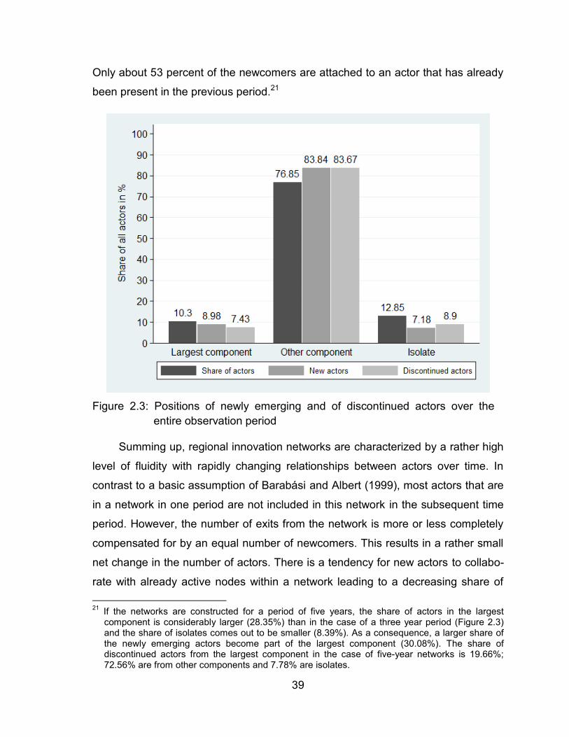
39

Only about 53 percent of the newcomers are attached to an actor that has already

been present in the previous period.21

Figure 2.3: Positions of newly emerging and of discontinued actors over the

entire observation period

Summing up, regional innovation networks are characterized by a rather high

level of fluidity with rapidly changing relationships between actors over time. In

contrast to a basic assumption of Barabási and Albert (1999), most actors that are

in a network in one period are not included in this network in the subsequent time

period. However, the number of exits from the network is more or less completely

compensated for by an equal number of newcomers. This results in a rather small

net change in the number of actors. There is a tendency for new actors to collabo-

rate with already active nodes within a network leading to a decreasing share of 21 If the networks are constructed for a period of five years, the share of actors in the largest

component is considerably larger (28.35%) than in the case of a three year period (Figure 2.3) and the share of isolates comes out to be smaller (8.39%). As a consequence, a larger share of the newly emerging actors become part of the largest component (30.08%). The share of discontinued actors from the largest component in the case of five-year networks is 19.66%; 72.56% are from other components and 7.78% are isolates.

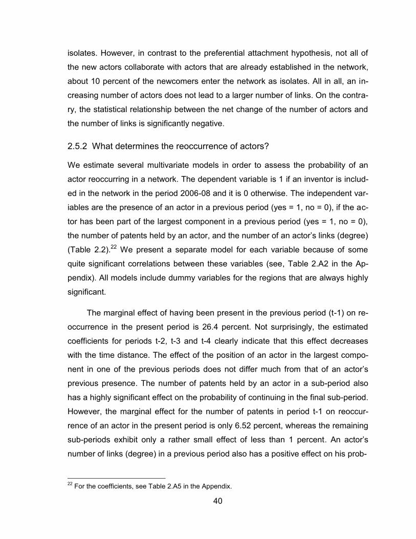
40

isolates. However, in contrast to the preferential attachment hypothesis, not all of

the new actors collaborate with actors that are already established in the network,

about 10 percent of the newcomers enter the network as isolates. All in all, an in-

creasing number of actors does not lead to a larger number of links. On the contra-

ry, the statistical relationship between the net change of the number of actors and

the number of links is significantly negative.

2.5.2 What determines the reoccurrence of actors?

We estimate several multivariate models in order to assess the probability of an

actor reoccurring in a network. The dependent variable is 1 if an inventor is includ-

ed in the network in the period 2006-08 and it is 0 otherwise. The independent var-

iables are the presence of an actor in a previous period (yes = 1, no = 0), if the ac-

tor has been part of the largest component in a previous period (yes = 1, no = 0),

the number of patents held by an actor, and the number of an actor’s links (degree)

(Table 2.2).22 We present a separate model for each variable because of some

quite significant correlations between these variables (see, Table 2.A2 in the Ap-

pendix). All models include dummy variables for the regions that are always highly

significant.

The marginal effect of having been present in the previous period (t-1) on re-

occurrence in the present period is 26.4 percent. Not surprisingly, the estimated

coefficients for periods t-2, t-3 and t-4 clearly indicate that this effect decreases

with the time distance. The effect of the position of an actor in the largest compo-

nent in one of the previous periods does not differ much from that of an actor’s

previous presence. The number of patents held by an actor in a sub-period also

has a highly significant effect on the probability of continuing in the final sub-period.

However, the marginal effect for the number of patents in period t-1 on reoccur-

rence of an actor in the present period is only 6.52 percent, whereas the remaining

sub-periods exhibit only a rather small effect of less than 1 percent. An actor’s

number of links (degree) in a previous period also has a positive effect on his prob-

22 For the coefficients, see Table 2.A5 in the Appendix.

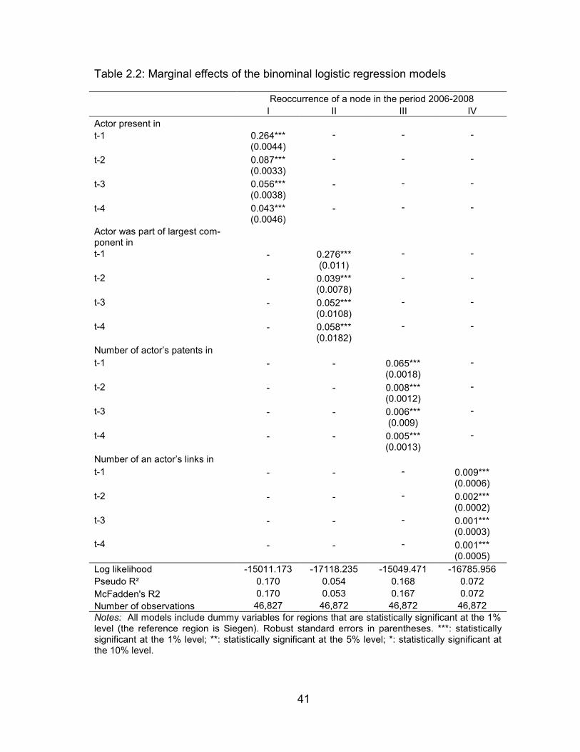
41

Table 2.2: Marginal effects of the binominal logistic regression models

Reoccurrence of a node in the period 2006-2008

I II III IV Actor present in t-1 0.264*** - - - (0.0044) t-2 0.087*** - - - (0.0033) t-3 0.056*** - - - (0.0038) t-4 0.043*** - - -

(0.0046)

Actor was part of largest com-ponent in

t-1 - 0.276*** - - (0.011) t-2 - 0.039*** - - (0.0078) t-3 - 0.052*** - - (0.0108) t-4 - 0.058*** - -

(0.0182)

Number of actor’s patents in t-1 - - 0.065*** -

(0.0018) t-2 - - 0.008*** - (0.0012) t-3 - - 0.006*** - (0.009) t-4 - - 0.005*** - (0.0013) Number of an actor’s links in t-1 - - - 0.009*** (0.0006) t-2 - - - 0.002*** (0.0002) t-3 - - - 0.001*** t-4

(0.0003) - - - 0.001***

(0.0005) Log likelihood -15011.173 -17118.235 -15049.471 -16785.956 Pseudo R² 0.170 0.054 0.168 0.072 McFadden's R2 0.170 0.053 0.167 0.072 Number of observations 46,827 46,872 46,872 46,872 Notes: All models include dummy variables for regions that are statistically significant at the 1% level (the reference region is Siegen). Robust standard errors in parentheses. ***: statistically significant at the 1% level; **: statistically significant at the 5% level; *: statistically significant at the 10% level.

42

ability of being present in a subsequent period. This result suggests that compara-

tively well connected inventors tend to be active over a longer time span and, thus,

have a higher probability of being involved in future projects. The marginal effect of

this variable for all sub-periods is, however, less than 1 percent, and decreases

with the time distance. Thus, an actor’s embeddedness must not be a major factor

in explaining his or her or reemergence in a later period. These surprising results

for an actor’s number of patents and an actor’s degree are in accordance with the

observation that slightly less that 40 percent of the inventors generate two or more

patents (see Figure 2.A1 in the Appendix), and that about half of all actors do not

have more than three links (Figure 2.A2 in the Appendix).

Putting all the results of the empirical models together, we can conclude that

the pure presence of an actor and his position in the largest component of a net-

work are more important for reoccurrence in a subsequent period than a high indi-

vidual performance as represented by the individual’s degree and the absolute

number of patents. Having been part of the largest component in t-1 has the

strongest impact on the reoccurrence of a node in the final sub-period. The number

of an actor’s patents as well as his or her number of links has only a minor impact

on subsequent network presence.

2.6 The effect of fluidity on network structure and performance

The previous section showed that networks are characterized by a high level of

actor fluidity at the micro-level. This raises the question about the relationship be-

tween micro-level fluidity of a network and its macro structure. According to our

Hypothesis II the macro structure of a network should be unaffected by the fluctua-

tion of actors. To investigate the effect of actor fluctuation on network structure we

run fixed effects regressions with three fluidity measures as independent variables:

the share of discontinued actors from period t-1, the share of new actors, and the

43

net change in the number of actors. Table 2.3 shows the results for the dependent

variables share of the largest component, share of isolates, and mean degree.23

Table 2.3: The relationship between the shares of discontinued actors, shares of new actors and network structure

Variables Share of largest component Share of isolates Mean degree Share of discontinued actors from t-1

-0.356** (0.146) - - 0.230***

(0.067) -

- -1.810 (2.558) - -

Share of new actors - -0.691***

(0.232) - - 0.118 (0.132) - - -2.226

(4.259) -

Net change number of actors - - 0.240

(0.219) - - -0.414*** (0.062) - - 3.586

(4.266)

Constant 0.339*** (0.104)

0.612*** (0.176)

0.077*** (0.024)

-0.047 (0.048)

0.025 (0.100)

0.137*** (0.007)

5.957*** (1.829) 6.373**

(3.237) 4.491*** (0.473)

Adjusted R² 0.740 0.761 0.728 0.744 0.639 0.642 0.631 0.628 0.629 Notes: Fixed effects panel regressions. Robust standard errors in parentheses. ***: statistically signifi-cant at the 1 % level; **: statistically significant at the 5 % level. The number of observations is 36 in all models (nine regions).

We find that the share of discontinued actors from the previous period is sig-

nificantly related to a smaller share of actors in the largest component and a higher

share of isolates. The mean degree seems to be, however, unaffected by the fluidi-

ty of actors. A higher share of new actors is related to a smaller share of actors in

the largest component, and a higher net change of the number of actors is related

to a lower share of isolates. The non-significance of a relationship between the

share of new actors and the share of isolates is consistent with the observation that

the vast majority of new actors does not enter as an isolate, but connect with a

component (Section 2.5.1). It is quite remarkable that the relationship between the

three fluidity indicators and the mean degree is not statistically significant. This re-

sult suggests that the number of new links created by new actors is not significantly

smaller than the number of links that are disrupted because of actors exiting the

network. This corresponds to our earlier finding that the share of actors who attach

themselves to a network component is larger among newcomers than among

those who exit (Section 2.5.1). Relationships with other measures of network struc- 23 See Tables 2.A8 and 2.A9 for descriptive statistics and correlations between the variables.

44

ture such as average component size, network centralization and overall clustering

coefficient were found to be not statistically significant.24 All in all, we can conclude

from the results of these regressions that fluidity of actors leads to some fragmen-

tation of a network, but does not affect the average number of relationships. Be-

sides these observations, network structures appear to be rather robust with re-

gards to entry and exit of actors, supporting our Hypothesis II.

For investigating the effect of fluidity of actors on the performance of the re-

spective regional innovation system we use patent productivity as the measure of

performance. Patent productivity is the number of patents filed by private sector

innovators with at least one inventor residing in the respective region per 1,000

R&D employees. While this metric reflects the level of the efficiency of a RIS

(Fritsch, 2002; Fritsch & Slavtchev, 2011), we also take the percent change of the

patent productivity to analyze the development of that level. Two control variables

are included in all models. The first of these variables is the share of service sector

employment, this accounts for the observation that the propensity of actors in this

sector to apply for a patent is comparatively low (Fritsch & Slavtchev, 2011).

Hence, we expect a negative sign for the respective coefficient because regions

with higher shares of service employment should have lower numbers of patents.

The second control variable is the share of manufacturing employees in establish-

ments with less than 50 employees. This control variable accounts for the observa-

tion that the number of patents per unit of R&D input tends to be higher in smaller

firms than in larger firms (for a theoretical explanation and discussion, see Cohen

and Klepper, 1996) so that we expect a negative sign for this variable.

In the model with the percent change of patent productivity as the dependent

variable, we also include the level of patent productivity in the base year. This vari-

able should have a negative sign for two reasons. First, regions with an already

relatively high level of patent productivity may have lower potentials for improve-

ments than regions that are characterized by a comparatively low performance.

24 The squared form of the fluidity measures is never statistically significant, indicating absence of

non-linear relationships.

45

Second, the level of patent productivity in the base year controls for a regression to

the mean effect. This denotes the phenomenon that periods of relatively large

changes into one direction may be followed by periods where the changes are rela-

tively small or even in the opposite direction.

Table 2.4: The relationship between the shares of discontinued actors, new actors and patent productivity

Generally, the relationship between the indicators for the fluidity of actors and

our measures of network performance are highly statistically significant (Table 2.4).

The significantly positive signs of the estimated coefficient for both, the share of

discontinued actors and the share of new actors, suggests that replacement of ‘old’

actors by new ones may be conducive for the performance of the respective re-

gional innovation system. We find, however, a significantly negative relationship

between patent productivity and the net change of the number of actors. This result

could be caused by the trend towards an increasing number of inventors per patent

(see Table 2.A5 in the Appendix), so that the number of inventors grows stronger

than the number of patents.

Patent productivity (ln) Change of patent productivity (%)

Share of discontinued actors from t-1

1.501*** (0.417) - - 1.387***

(0.434) -

Share of new actors in t0 - 2.647*** (0.934) - - 2.299**

(0.954)

Net change number of actors - - -2.999*** (0.726) - - -2.870***

(0.756)

Share of service employment -0.768 (1.762)

0.560 (1.787)

-1.935 (1.773)

-1.228 (1.744)

-0.192 (1.818)

-2.267 (1.717)

Employment share of manufacturing establishments < 50 employees

0.638 (0.779)

1.280 (0.791)

0.048 (0.791)

0.950 (0.766)

1.463* (0.799)

0.416 (0.761)

Patent productivity in t-1 (ln) - - - -0.911*** (0.177)

-0.848*** (0.186)

-.951*** (0.168)

Constant -0.425 (1.521)

-3.163** (1.554)

2.415 (1.777)

0.003 (1.568)

-2.199 (1.759)

2.607 (1.714)

Adjusted R² 0.636 0.663 0.737 0.497 0.535 0.677 Notes: Fixed effects panel regressions. Robust standard errors in parentheses. ***: statistically significant at the 1 % level; **: statistically significant at the 5 % level; *: statistically significant at the 10% level. The number of observations is 36 in all models (nine regions).

46

Table 2.5: The relationship between the shares of ceased and new links with patent productivity

Patent productivity (ln) Change of patent productivity (%)

Share of discontinued links from t-1

-4.810** (1.919) - - -5.117***

(1.715) - -

Share of new links - 6.135*** (2.118) - - 5.638***

(2.140) - Net change number of links - - 6.579***

(1.187) - - 6.236*** (1.069)

Share of service employment 1.088 (1.807)

1.166 (1.741)

0.256 (1.357)

-0.743 (1.750)

0.368 (1.778)

-0.756 (1.298)

Employment share of manufacturing establishments < 50 employees

0.463 (0.932)

1.203 (0.791)

-0.460 (0.708)

0.170 (0.887)

1.398* (0.785)

-0.289 (0.649)

Patent productivity in t-1 (ln) - - - -0.629*** (0.168)

-0.863*** (0.183)

-0.803*** (0.126)

Constant 2.886 (2.618)

-7.376*** (2.303)

-0.560 (1.213)

5.064** (2.523)

-6.179** (2.610)

0.409 (1.200)

Adjusted R² 0.643 0.667 0.803 0.580 0.552 0.765 Notes: Fixed effects panel regressions. Robust standard errors in parentheses. ***: statistically significant at the 1 % level; **: statistically significant at the 5 % level. The number of observations is 36 in all models (nine regions).

There are also highly significant relationships between the fluidity of links and

network performance, but the directions of the effects are quite different from the

estimations for fluidity of actors (Table 2.5). The negative effect of the share of

ceased links may indicate negative effects of dissolving R&D cooperation on the

division of innovative labor. In contrast, the pronounced positive coefficients for the

share of new links and the net change of the number of links suggest that newly

established relationships, as well as increasing numbers of relationships, are con-

ducive to the performance of RIS. These results clearly support the notion that the

connectedness of actors resulting in an intense transfer of knowledge along with

the division of innovative labor are both important determinants of the performance

of regional innovation systems (Fritsch & Slavtchev, 2011). The results for the con-

trol variables remain the same as in the analysis of the fluidity of actors (Table 2.4).

47

2.7 Discussion: What does this mean and what do we need to know?

We investigated the stability of cooperative relationships within regional inventor

networks, focusing our analysis on the effect of the fluidity of actors and their links

for the structural stability of networks and the performance of the respective re-

gional innovation system. The analysis was performed for nine German planning

regions over a period of 15 years (1994-2008). At the micro-level of individual in-

ventors, we observed rather high levels of fluctuation of actors across time periods.

This finding challenges considerations that suggest longer-term stability of R&D

cooperation because of transaction costs, as well as the assumptions of the well-

established Barabási and Albert (1999, 2000, 2002) model. We find that the pure

presence of an actor and an actor’s position in the largest component have a high-

er impact on the probability of his or her reemergence in a subsequent period than

an inventors’ performance in terms of the number of patents or links.

Our analyses show some statistically significant relationships between fluidity

at the micro-level and stability of network structure. Higher fluidity of actors leads to

more fragmentation, as indicated by a lower share of the largest component and a

higher share of isolates. However, there is no statistically significant relationship

with the mean degree and other conventional measures of network structure. This

result suggests that abandoned ties due to actors leaving the network are, more or

less, completely replaced by newly established relationships. We found pro-

nounced statistically significant relationships between the fluidity of actors and pa-

tent productivity as a measure for the performance of the respective regional inno-

vation system. This result suggests that the termination of cooperative relation-

ships due to fluidity of actors is not generally harmful for regional innovation activi-

ties. However, the net change in the number of actors is negatively related to the

performance of the respective regional innovation system. In contrast, an increase

in the number of links among actors is positively related to network performance.

This is consistent with the notion that the intensity of knowledge transfer and divi-

sion of innovative labor are important determinants of the performance of regional

innovation systems (Fritsch & Slavtchev, 2011).

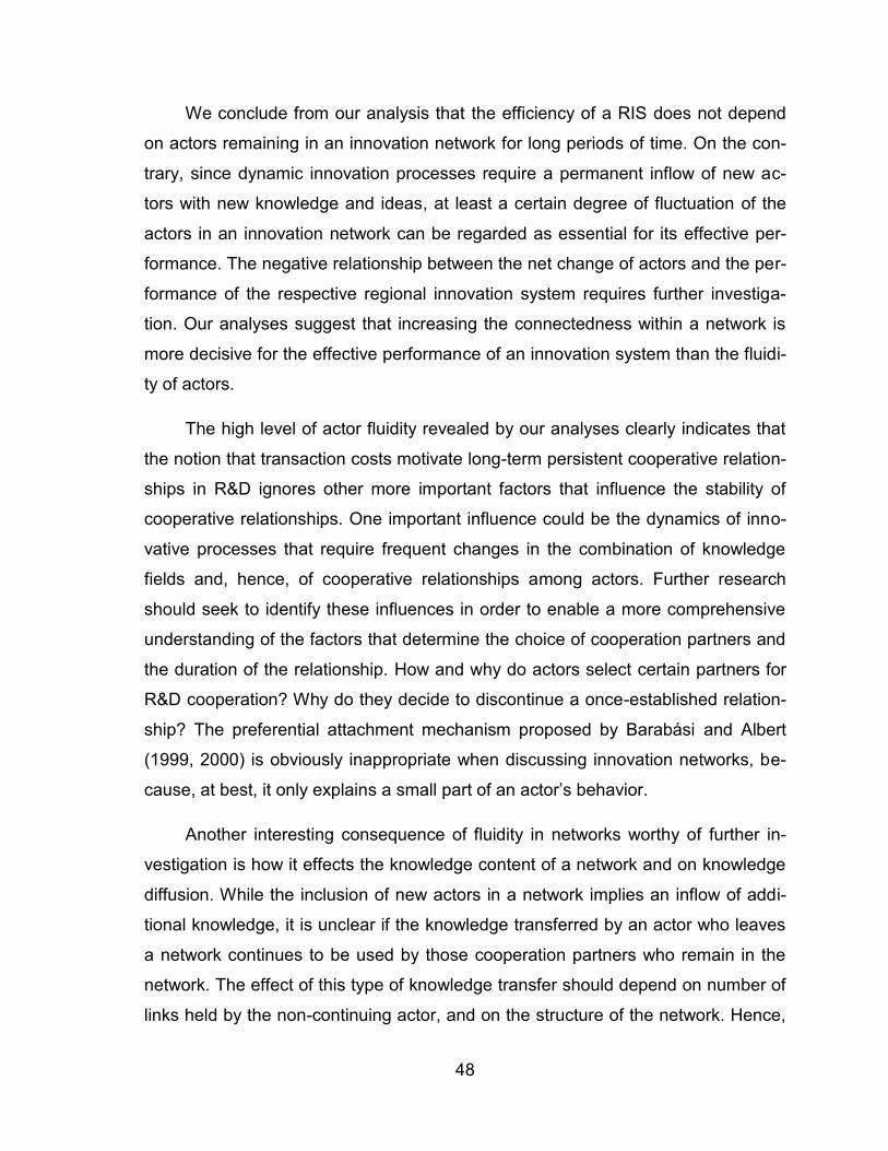
48

We conclude from our analysis that the efficiency of a RIS does not depend

on actors remaining in an innovation network for long periods of time. On the con-

trary, since dynamic innovation processes require a permanent inflow of new ac-

tors with new knowledge and ideas, at least a certain degree of fluctuation of the

actors in an innovation network can be regarded as essential for its effective per-

formance. The negative relationship between the net change of actors and the per-

formance of the respective regional innovation system requires further investiga-

tion. Our analyses suggest that increasing the connectedness within a network is

more decisive for the effective performance of an innovation system than the fluidi-

ty of actors.

The high level of actor fluidity revealed by our analyses clearly indicates that

the notion that transaction costs motivate long-term persistent cooperative relation-

ships in R&D ignores other more important factors that influence the stability of

cooperative relationships. One important influence could be the dynamics of inno-

vative processes that require frequent changes in the combination of knowledge

fields and, hence, of cooperative relationships among actors. Further research

should seek to identify these influences in order to enable a more comprehensive

understanding of the factors that determine the choice of cooperation partners and

the duration of the relationship. How and why do actors select certain partners for

R&D cooperation? Why do they decide to discontinue a once-established relation-

ship? The preferential attachment mechanism proposed by Barabási and Albert

(1999, 2000) is obviously inappropriate when discussing innovation networks, be-

cause, at best, it only explains a small part of an actor’s behavior.

Another interesting consequence of fluidity in networks worthy of further in-

vestigation is how it effects the knowledge content of a network and on knowledge

diffusion. While the inclusion of new actors in a network implies an inflow of addi-

tional knowledge, it is unclear if the knowledge transferred by an actor who leaves

a network continues to be used by those cooperation partners who remain in the

network. The effect of this type of knowledge transfer should depend on number of

links held by the non-continuing actor, and on the structure of the network. Hence,

49

the effect of a well-connected member belonging to the largest component of a

network should be much more significant than that of an isolate or of someone in a

small component. Moreover, the structure of the network should play a role here.

Does a larger and denser network lead to higher robustness against missing

nodes?

A principal shortcoming of our analysis may follow from the fact that our data,

drawn from patent statistics, covers only a certain aspect of innovation activities,

i.e. research that leads to a patent application. Actors may pursue other types of

collaborative innovation that do not lead to a patent application, e.g. basic re-

search, that are not recorded in patent data. Hence, it could well be that data

sources with a more comprehensive coverage of innovation activity would show

higher levels of long-lasting R&D cooperation.

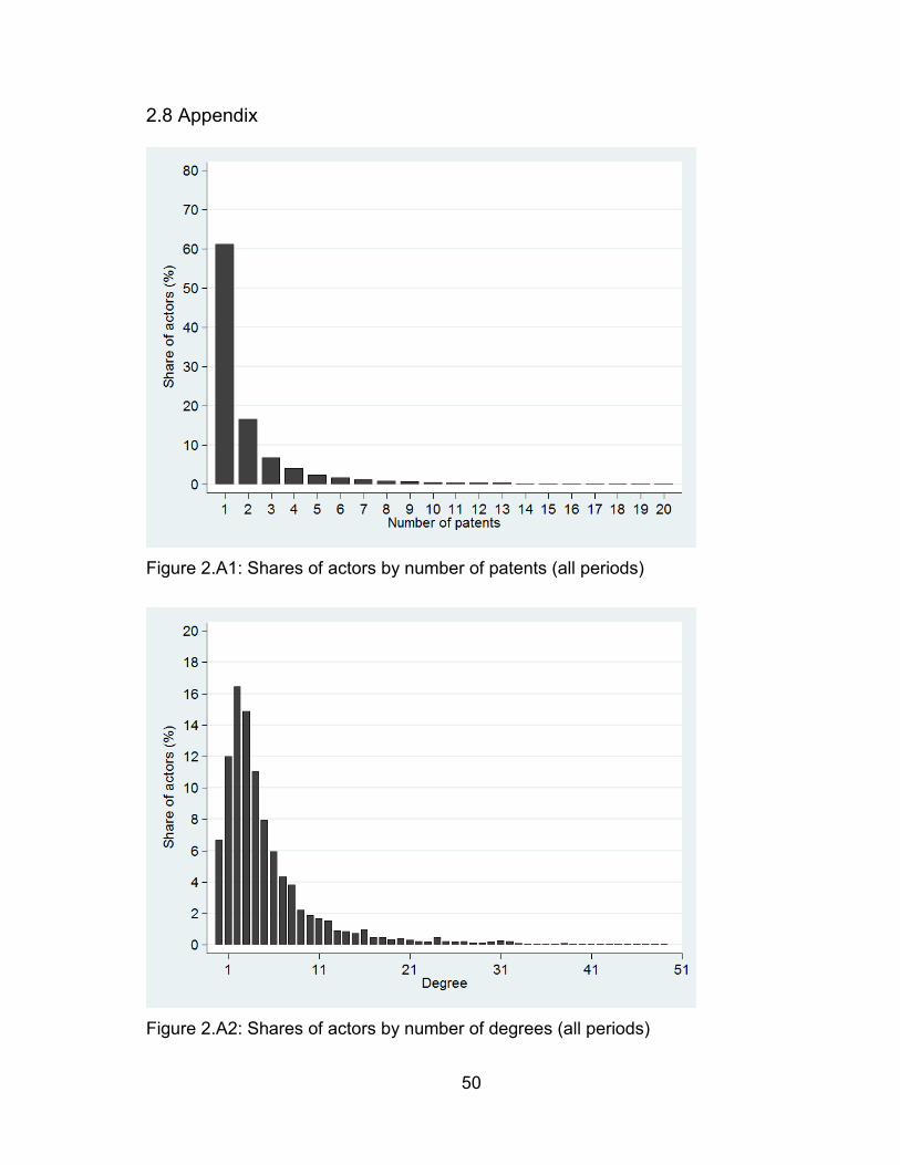
50

2.8 Appendix

Figure 2.A1: Shares of actors by number of patents (all periods)

Figure 2.A2: Shares of actors by number of degrees (all periods)

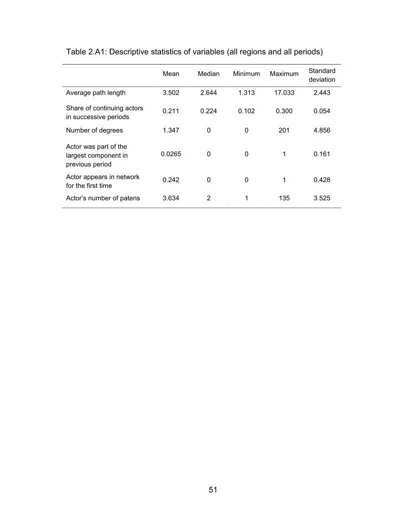
51

Table 2.A1: Descriptive statistics of variables (all regions and all periods)

Mean Median Minimum Maximum Standard deviation

Average path length 3.502 2.644 1.313 17.033 2.443

Share of continuing actors in successive periods

0.211 0.224 0.102 0.300 0.054

Number of degrees 1.347 0 0 201 4.856

Actor was part of the largest component in previous period

0.0265 0 0 1 0.161

Actor appears in network for the first time

0.242 0 0 1 0.428

Actor’s number of patens 3.634 2 1 135 3.525

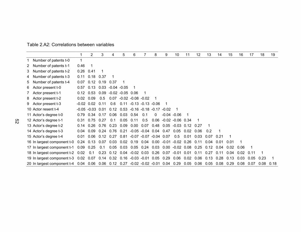
52

Table 2.A2: Correlations between variables

1 2 3 4 5 6 7 8 9 10 11 12 13 14 15 16 17 18 19 1 Number of patents t-0 1 2 Number of patents t-1 0.46 1 3 Number of patents t-2 0.26 0.41 1 4 Number of patents t-3 0.11 0.18 0.37 1 5 Number of patents t-4 0.07 0.12 0.19 0.37 1 6 Actor present t-0 0.57 0.13 0.03 -0.04 -0.05 1 7 Actor present t-1 0.12 0.53 0.09 -0.02 -0.05 0.06 1 8 Actor present t-2 0.02 0.09 0.5 0.07 -0.02 -0.08 -0.02 1 9 Actor present t-3 -0.02 0.02 0.11 0.6 0.11 -0.13 -0.13 -0.06 1 10 Actor resent t-4 -0.05 -0.03 0.01 0.12 0.53 -0.16 -0.18 -0.17 -0.02 1 11 Actor’s degree t-0 0.79 0.34 0.17 0.06 0.03 0.54 0.1 0 -0.04 -0.06 1 12 Actor’s degree t-1 0.31 0.75 0.27 0.1 0.05 0.11 0.5 0.06 -0.02 -0.06 0.34 1 13 Actor’s degree t-2 0.14 0.26 0.76 0.23 0.09 0.00 0.07 0.48 0.05 -0.03 0.12 0.27 1 14 Actor’s degree t-3 0.04 0.09 0.24 0.76 0.21 -0.05 -0.04 0.04 0.47 0.05 0.02 0.06 0.2 1 15 Actor’s degree t-4 0.01 0.06 0.12 0.27 0.81 -0.07 -0.07 -0.04 0.07 0.5 0.01 0.03 0.07 0.21 1 16 In largest component t-0 0.24 0.13 0.07 0.03 0.02 0.19 0.04 0.00 -0.01 -0.02 0.26 0.11 0.04 0.01 0.01 1 17 In largest component t-1 0.09 0.25 0.1 0.05 0.03 0.05 0.24 0.03 0.00 -0.02 0.08 0.25 0.12 0.04 0.02 0.06 1 18 In largest component t-2 0.02 0.1 0.23 0.12 0.04 -0.02 0.03 0.26 0.07 -0.01 0.01 0.11 0.27 0.11 0.04 0.02 0.11 1 19 In largest component t-3 0.02 0.07 0.14 0.32 0.16 -0.03 -0.01 0.05 0.29 0.06 0.02 0.06 0.13 0.28 0.13 0.03 0.05 0.23 1 20 In largest component t-4 0.04 0.06 0.06 0.12 0.27 -0.02 -0.02 -0.01 0.04 0.29 0.05 0.06 0.05 0.08 0.29 0.08 0.07 0.08 0.18

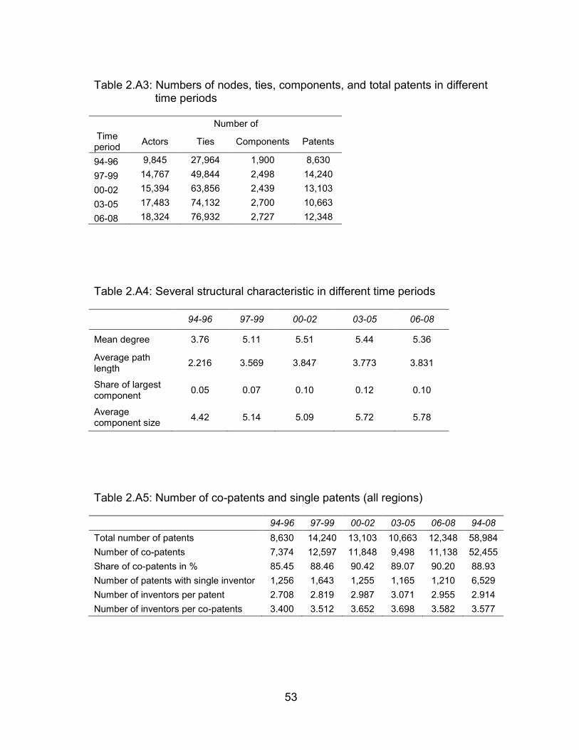
53

Table 2.A3: Numbers of nodes, ties, components, and total patents in different time periods

Number of Time period Actors Ties Components Patents

94-96 9,845 27,964 1,900 8,630 97-99 14,767 49,844 2,498 14,240 00-02 15,394 63,856 2,439 13,103 03-05 17,483 74,132 2,700 10,663 06-08 18,324 76,932 2,727 12,348

Table 2.A4: Several structural characteristic in different time periods

94-96 97-99 00-02 03-05 06-08

Mean degree 3.76 5.11 5.51 5.44 5.36

Average path length 2.216 3.569 3.847 3.773 3.831

Share of largest component 0.05 0.07 0.10 0.12 0.10

Average component size 4.42 5.14 5.09 5.72 5.78

Table 2.A5: Number of co-patents and single patents (all regions)

94-96 97-99 00-02 03-05 06-08 94-08

Total number of patents 8,630 14,240 13,103 10,663 12,348 58,984 Number of co-patents 7,374 12,597 11,848 9,498 11,138 52,455 Share of co-patents in % 85.45 88.46 90.42 89.07 90.20 88.93 Number of patents with single inventor 1,256 1,643 1,255 1,165 1,210 6,529 Number of inventors per patent 2.708 2.819 2.987 3.071 2.955 2.914 Number of inventors per co-patents 3.400 3.512 3.652 3.698 3.582 3.577

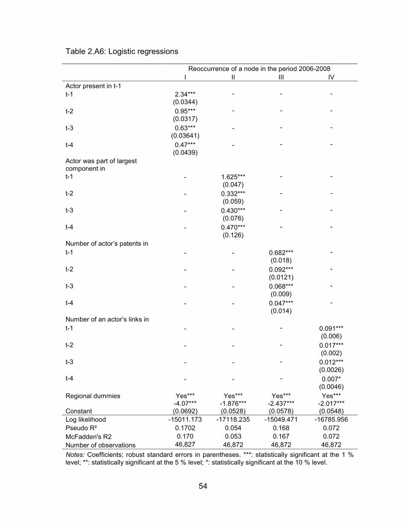
54

Table 2.A6: Logistic regressions

Reoccurrence of a node in the period 2006-2008

I II III IV Actor present in t-1 t-1 2.34*** - - - (0.0344) t-2 0.95*** - - - (0.0317) t-3 0.63*** - - - (0.03641) t-4 0.47*** - - -

(0.0439)

Actor was part of largest component in

t-1 - 1.625*** - - (0.047) t-2 - 0.332*** - - (0.059) t-3 - 0.430*** - - (0.076) t-4 - 0.470*** - -

(0.126)

Number of actor’s patents in t-1 - - 0.682*** -

(0.018) t-2 - - 0.092*** - (0.0121) t-3 - - 0.068*** - (0.009) t-4 - - 0.047*** - (0.014) Number of an actor’s links in t-1 - - - 0.091*** (0.006) t-2 - - - 0.017*** (0.002) t-3 - - - 0.012*** t-4

(0.0026) - - - 0.007*

(0.0046) Regional dummies Yes*** Yes*** Yes*** Yes***

Constant -4.07*** (0.0692)

-1.876*** (0.0528)

-2.437*** (0.0578)

-2.017*** (0.0548)

Log likelihood -15011.173 -17118.235 -15049.471 -16785.956 Pseudo R² 0.1702 0.054 0.168 0.072 McFadden's R2 0.170 0.053 0.167 0.072 Number of observations 46,827 46,872 46,872 46,872 Notes: Coefficients; robust standard errors in parentheses. ***: statistically significant at the 1 % level; **: statistically significant at the 5 % level; *: statistically significant at the 10 % level.

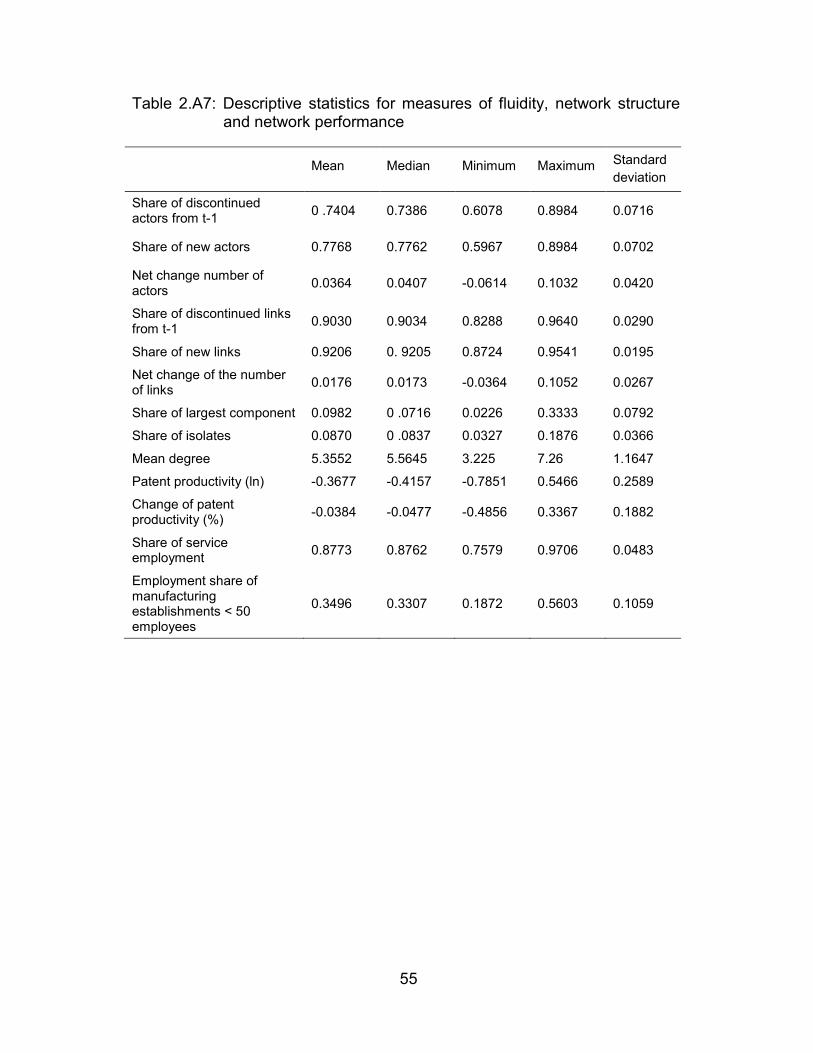
55

Table 2.A7: Descriptive statistics for measures of fluidity, network structure and network performance

Mean Median Minimum Maximum Standard deviation

Share of discontinued actors from t-1 0 .7404 0.7386 0.6078 0.8984 0.0716

Share of new actors 0.7768 0.7762 0.5967 0.8984 0.0702

Net change number of actors 0.0364 0.0407 -0.0614 0.1032 0.0420

Share of discontinued links from t-1 0.9030 0.9034 0.8288 0.9640 0.0290

Share of new links 0.9206 0. 9205 0.8724 0.9541 0.0195

Net change of the number of links 0.0176 0.0173 -0.0364 0.1052 0.0267

Share of largest component 0.0982 0 .0716 0.0226 0.3333 0.0792

Share of isolates 0.0870 0 .0837 0.0327 0.1876 0.0366

Mean degree 5.3552 5.5645 3.225 7.26 1.1647

Patent productivity (ln) -0.3677 -0.4157 -0.7851 0.5466 0.2589

Change of patent productivity (%) -0.0384 -0.0477 -0.4856 0.3367 0.1882

Share of service employment 0.8773 0.8762 0.7579 0.9706 0.0483

Employment share of manufacturing establishments < 50 employees

0.3496 0.3307 0.1872 0.5603 0.1059

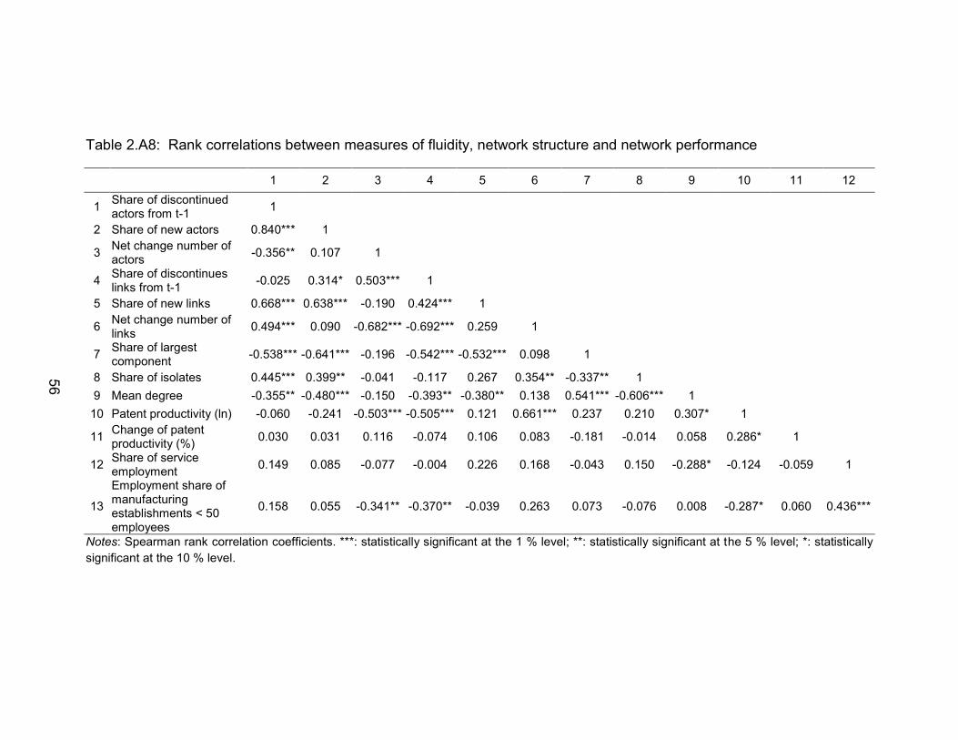
56

Table 2.A8: Rank correlations between measures of fluidity, network structure and network performance

1 2 3 4 5 6 7 8 9 10 11 12

1 Share of discontinued actors from t-1 1

2 Share of new actors 0.840*** 1

3 Net change number of actors -0.356** 0.107 1

4 Share of discontinues links from t-1 -0.025 0.314* 0.503*** 1

5 Share of new links 0.668*** 0.638*** -0.190 0.424*** 1

6 Net change number of links 0.494*** 0.090 -0.682*** -0.692*** 0.259 1

7 Share of largest component -0.538*** -0.641*** -0.196 -0.542*** -0.532*** 0.098 1

8 Share of isolates 0.445*** 0.399** -0.041 -0.117 0.267 0.354** -0.337** 1 9 Mean degree -0.355** -0.480*** -0.150 -0.393** -0.380** 0.138 0.541*** -0.606*** 1

10 Patent productivity (ln) -0.060 -0.241 -0.503*** -0.505*** 0.121 0.661*** 0.237 0.210 0.307* 1

11 Change of patent productivity (%) 0.030 0.031 0.116 -0.074 0.106 0.083 -0.181 -0.014 0.058 0.286* 1

12 Share of service employment 0.149 0.085 -0.077 -0.004 0.226 0.168 -0.043 0.150 -0.288* -0.124 -0.059 1

13

Employment share of manufacturing establishments < 50 employees

0.158 0.055 -0.341** -0.370** -0.039 0.263 0.073 -0.076 0.008 -0.287* 0.060 0.436***

Notes: Spearman rank correlation coefficients. ***: statistically significant at the 1 % level; **: statistically significant at the 5 % level; *: statistically significant at the 10 % level.

57

Chapter 3

Actor fluidity and knowledge persistence in regional

networks

Abstract:25 The development of inventor networks is characterized by high

numbers of new actors while a considerable part of incumbent actors disap-

pears. We estimate the persistence of knowledge in regional inventor networks

using alternative assumptions about knowledge transfer. Based on these esti-

mates we analyze how the size and the structure of a network may influence

knowledge persistence over time. In a final step we assess the effect of persis-

tent knowledge as well as of the knowledge of new actors on the performance

of regional innovation systems (RIS). The final section summarizes and draws

conclusions for further research.

25 This chapter was inspired by Chapter 2 and is co-authored by Michael Fritsch.

58

3.1 Fluidity of network actors and regional knowledge

Networks of inventors are often characterized by high levels of actor-turnover.

In a study of inventor networks in German regions over five three-year periods,

Fritsch and Zoellner (2017) found that the majority of actors are only active in

one period and are not contained in successive periods. On average, only about

one third (32.34%) of the actors that are present in a network in a certain period

have also been included in the previous period. Hence, a majority of about two

third of inventors in a regional network occur in a certain sub-period for the first

time. These figures clearly indicate that the majority of links among inventors

are of rather short term.

The consequences of this high level of actor-turnover or ‘fluidity’ for the

network and the functioning of the respective regional innovation system (RIS)

are largely unexplored. In general, the high levels of fluidity in inventor networks

can be regarded an indication that there are benefits of switching cooperation

partners despite considerable transaction costs. These transaction costs involve

the effort of establishing new links and sunk costs related to abandoning an es-

tablished link. The benefits may particularly consist of access to new knowledge

through newly established links.

The empirical analyses of the performance of inventor networks in Ger-

man regions by Fritsch and Zoellner (2017) show mixed results for the relation-

ship between turnover of inventors with the performance of the respective RIS

measured by the level and change of the number of patents per R&D employee

(patent productivity). While there was a significantly positive relationship of the

share of new actors with RIS performance, the relationship of patent productivi-

ty with the share of discontinued actors was also positive but it was negative for

the share of discontinued links (Fritsch & Zoellner, 2017). An explanation for the

positive relationship between RIS performance and the share of new actors is

probably the additional knowledge that the new inventors add to the system.

The reason for the non-negative relationship between the share of discontinued

actors and RIS performance may be that the knowledge of discontinuing actors

remains in their cooperation partners who continue in the network.

59

Based on the data used by Fritsch and Zoellner (2017), we investigate two

potential sources of knowledge, namely persistent knowledge and the

knowledge of actor who enter inventor networks in nine German regions. We try

to assess how much of the knowledge of those actors that disappear from an

inventor network may still be available because it has been passed on to con-

tinuing network actors during their cooperation. For this purpose we identify

those actors that have cooperated with discontinuing actors and ask, if these

co-inventors are included in the network in the subsequent period. We assume

that at least part of the knowledge of a discontinued actor is still available if co-

inventors are still contained in the network. Based on alternative assumptions

about the amount of knowledge transfer among co-inventors, we estimate the

share of knowledge that is still available in the network and analyze the role of

network characteristics for knowledge continuity. Our analyses suggest that the

level of knowledge that persists in a network is particularly higher in well-

integrated networks that have relatively high shares of actors in the largest

component, a large average component and team size, and low shares of iso-

lates. Finally, we analyze the effect of persistent knowledge as well as of the

knowledge of new actors on the performance of RIS.

In what follows, we first discuss the cost and the benefits of changing ac-

tors and relationships in innovation networks (Section 3.2). Section 3.3 intro-

duces data and indicators and in the following section we assess the effect of

actor fluidity on the continuity of knowledge in the network (Section 3.4). We

then investigate to what extent the level of knowledge continuity is related to

characteristics of the respective inventor network (Section 3.5). The effect of

knowledge persistence on the performance of RIS is investigated in Section 3.6.

The final section (Section 3.7) summarizes the results and concludes.

3.2 Actor turnover, knowledge persistence, network characteristics, and the performance of the regional innovation system

A rich literature exists that addresses the relation between a network’s structural

characteristics and knowledge creation and knowledge diffusion (see, Ahuja,

2000; Cowan & Jonard, 2004; Copaldo, 2007; Schilling & Phelps, 2007; Phelps,

2010). In particular the structure of a network determines the amount and speed

60

of knowledge diffusion (Capaldo, 2007; Schilling & Phelps, 2007; Tang, Mu &

MacLachlan, 2008) and should, therefore, have an effect on performance of the

respective innovation activity. Regardless of the fact that many scholars ana-

lyzed the influence of network structure on knowledge diffusion in different

ways, they all have one thing in common: Locally clustered networks (cohesion)

with a short average path length (range) are conducive to knowledge transfer.

Cohesion and range of networks do not only facilitate the creation of knowledge

(Ahuja, 2000; Uzzi & Spiro, 2005), they also noticeably enhance the transfer

and storage of knowledge within a network (Feldman, 1999; Schilling & Phelps,

2007). While the range of a network ensures that manifold sources of heteroge-

neous knowledge can be reached (Schilling & Phelps, 2007), cohesion facili-

tates that knowledge can rapidly spread among network actors (Burt, 2001;

Cowan & Jonard, 2004; Fritsch & Kauffeld-Monz, 2010).

Cohesion is beneficial for the transfer and storage of knowledge for two

reasons. First, and not surprisingly, a high connectedness of actors is fruitful for

the transfer of knowledge between actors (Fritsch & Kauffeld-Monz, 2010).

Thus, the easier the exchange of knowledge is, the more knowledge is spread

and stored in the network. Second, networks involve the process of monitoring

(Storper & Venables, 2004; Wilhelmsson, 2009) that may increase the ambition,

motivation and competitiveness of actors (Storper & Venables, 2004). Hence,

unproductive and unsuccessful actors or actors that avoid transferring their

knowledge (accurately) would leave a network since other inventors would not

cooperate with them (‘reputation effect’; see, Reaganz & McEvily, 2003). Fol-

lowing the literature, an optimal network structure should thus be locally clus-

tered with a short average path length (see also, Burt, 2000; Reaganz & Zuck-

ermann, 2001).

Another important characteristic of a network is its size. Network size de-

termines the knowledge that is available (see, Fronczak, Fronczak & Holyst,

2004). The larger a network, the more knowledge sources and possible cooper-

ation partners are accessible. The latter is important for the storage of

knowledge within a network, since larger networks also encompass a higher

number of suitable cooperation partners. By running several simulation models,

Tang, Mu and MacLachlan (2008) find that the share of actors that engage into

61

cooperative activities increases proportional with a network’s size. Thus, larger

networks should benefit from a higher intensity of knowledge exchanges. How-

ever, larger networks also have to deal with larger distances in terms of path

length between actors.

Knowledge, especially tacit knowledge, is fundamentally important for fu-

ture innovations but cannot be easily codified (Katila & Ahuja, 2009). Given that

networks are characterized by high levels of actor fluidity, the embodied

knowledge of a discontinued actor vanishes, which, ultimately, leads to a de-

creasing regional knowledge stock and hampers the performance of a respec-

tive RIS. However, if an actor disappears from a network, his knowledge is not

necessarily lost but may persist in the network because it has been transferred

to co-inventors (who are still part of the network) during the period of their co-

operation. Cooperative activities then not only lead to the generation of new

knowledge, but they also secure that a certain amount of knowledge persists

within a network. Hence, keeping knowledge of discontinuing actors available

may therefore be an important way how networks affect the performance of the

respective RIS. Another important source of knowledge is the entry of new ac-

tors who make their knowledge available in the network which leads to new op-

portunities for recombination (see, Bercovitz & Feldman, 2011).

Based on these considerations we test the following hypotheses:

Hypothesis I: The better the connectedness of actors in a network, the more knowledge of discontinuing actors can persist in the network and is available in later periods.

Hypothesis II: The size of a network is positive related to the transfer and storage of knowledge.

Hypothesis III: The more knowledge of discontinuing actors remains to be available in the network the better the performance of the re-spective innovation system.

Hypothesis IV: The larger the share actors who enter the network and make their knowledge available the better the performance of the re-spective innovation system.

62

3.3 Data and spatial framework

We analyze inventor networks based on patent application as documented in

the DEPATISnet database (www.depatisnet.de) maintained by the German Pa-

tent and Trademark Office (Deutsches Patent- und Markenamt). The key as-

sumption in constructing these networks is that actors who are named as inven-

tors in the same patent document know each other and have worked together in

generating the respective invention (Balconi, Breschi & Lissoni, 2004). Patents

are assigned to regions based on the information about the residence of the

inventor. If a part of the inventors of a patent have residences in different re-

gions we divide the respective patent by the number of inventors involved and

assign only that fraction to the region that corresponds to those inventors that

have their residence in the region.26

We construct the regional inventor networks in nine German planning re-

gions for five three-year periods27 over a time span of 15 years (1994 to 2008).

Five of these regions are located in East Germany, the former socialist GDR,

and four regions are in West Germany (see, Figure 3.1). Planning regions are

functional spatial units that are somewhat larger than labor market regions or

travel-to-work areas. They normally comprise several NUTS3-level districts,

namely, a core city and its surrounding area. While districts are administrative

geographic units, planning regions are more often used for spatial analysis and

policy development, particularly regarding public infrastructure planning. We

consider planning regions as more suitable than districts for an analysis of re-

gional innovation systems (RIS) for two reasons. First, a single district, particu-

larly a core city, is probably too small to include the most important actors of

innovation-related local interaction. The second reason is of a methodological

nature: since patents are assigned to the residence of the inventor, taking just a

core-city as a region would lead to an underestimation of patenting activity since

many inventors who work in cities have their private residence in surrounding

districts.

26 If a patent has three inventors and only two inventors have their residence in the region, we

assign two third of the patent to the region. Hence, the number of regional patents may not always be a whole number.

27 These periods are 1994-96, 1997-99, 2000-02, 2003-05 and 2006-08.

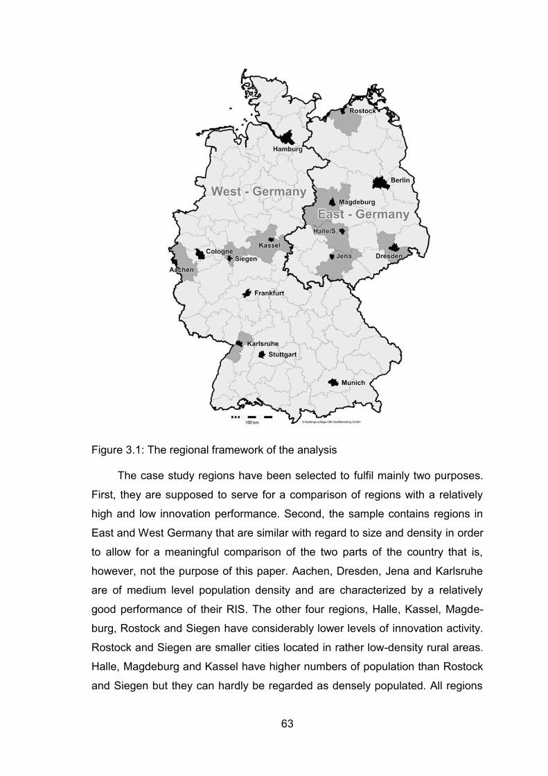
63

Figure 3.1: The regional framework of the analysis

The case study regions have been selected to fulfil mainly two purposes.

First, they are supposed to serve for a comparison of regions with a relatively

high and low innovation performance. Second, the sample contains regions in

East and West Germany that are similar with regard to size and density in order

to allow for a meaningful comparison of the two parts of the country that is,

however, not the purpose of this paper. Aachen, Dresden, Jena and Karlsruhe

are of medium level population density and are characterized by a relatively

good performance of their RIS. The other four regions, Halle, Kassel, Magde-

burg, Rostock and Siegen have considerably lower levels of innovation activity.

Rostock and Siegen are smaller cities located in rather low-density rural areas.

Halle, Magdeburg and Kassel have higher numbers of population than Rostock

and Siegen but they can hardly be regarded as densely populated. All regions

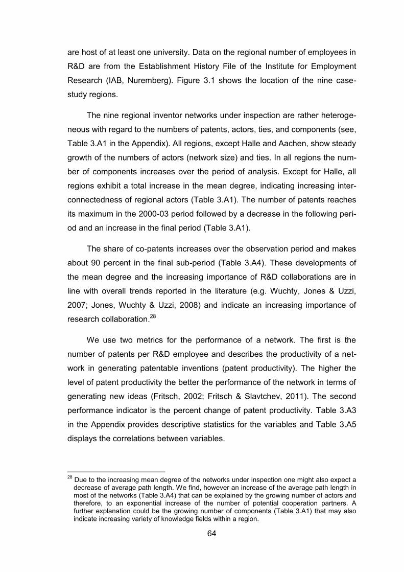
64

are host of at least one university. Data on the regional number of employees in

R&D are from the Establishment History File of the Institute for Employment

Research (IAB, Nuremberg). Figure 3.1 shows the location of the nine case-

study regions.

The nine regional inventor networks under inspection are rather heteroge-

neous with regard to the numbers of patents, actors, ties, and components (see,

Table 3.A1 in the Appendix). All regions, except Halle and Aachen, show steady

growth of the numbers of actors (network size) and ties. In all regions the num-

ber of components increases over the period of analysis. Except for Halle, all

regions exhibit a total increase in the mean degree, indicating increasing inter-

connectedness of regional actors (Table 3.A1). The number of patents reaches

its maximum in the 2000-03 period followed by a decrease in the following peri-

od and an increase in the final period (Table 3.A1).

The share of co-patents increases over the observation period and makes

about 90 percent in the final sub-period (Table 3.A4). These developments of

the mean degree and the increasing importance of R&D collaborations are in

line with overall trends reported in the literature (e.g. Wuchty, Jones & Uzzi,

2007; Jones, Wuchty & Uzzi, 2008) and indicate an increasing importance of

research collaboration.28

We use two metrics for the performance of a network. The first is the

number of patents per R&D employee and describes the productivity of a net-

work in generating patentable inventions (patent productivity). The higher the

level of patent productivity the better the performance of the network in terms of

generating new ideas (Fritsch, 2002; Fritsch & Slavtchev, 2011). The second

performance indicator is the percent change of patent productivity. Table 3.A3

in the Appendix provides descriptive statistics for the variables and Table 3.A5

displays the correlations between variables.

28 Due to the increasing mean degree of the networks under inspection one might also expect a

decrease of average path length. We find, however an increase of the average path length in most of the networks (Table 3.A4) that can be explained by the growing number of actors and therefore, to an exponential increase of the number of potential cooperation partners. A further explanation could be the growing number of components (Table 3.A1) that may also indicate increasing variety of knowledge fields within a region.

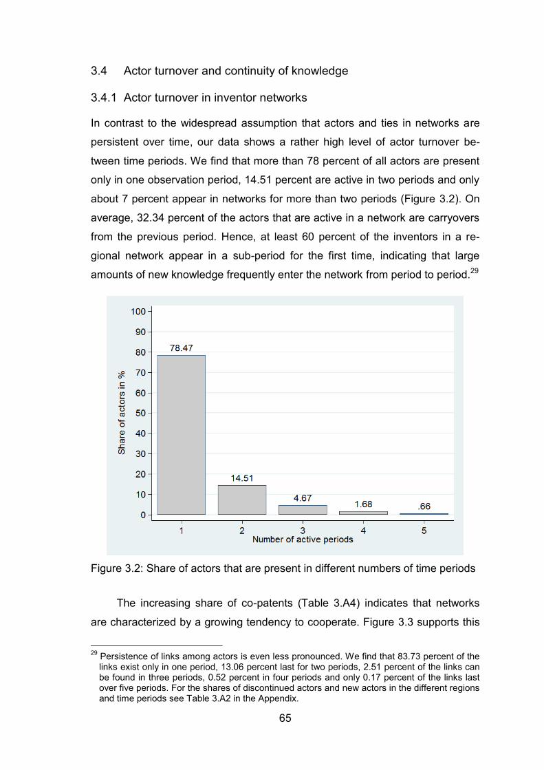
65

3.4 Actor turnover and continuity of knowledge

3.4.1 Actor turnover in inventor networks

In contrast to the widespread assumption that actors and ties in networks are

persistent over time, our data shows a rather high level of actor turnover be-

tween time periods. We find that more than 78 percent of all actors are present

only in one observation period, 14.51 percent are active in two periods and only

about 7 percent appear in networks for more than two periods (Figure 3.2). On

average, 32.34 percent of the actors that are active in a network are carryovers

from the previous period. Hence, at least 60 percent of the inventors in a re-

gional network appear in a sub-period for the first time, indicating that large

amounts of new knowledge frequently enter the network from period to period.29

Figure 3.2: Share of actors that are present in different numbers of time periods

The increasing share of co-patents (Table 3.A4) indicates that networks

are characterized by a growing tendency to cooperate. Figure 3.3 supports this

29 Persistence of links among actors is even less pronounced. We find that 83.73 percent of the

links exist only in one period, 13.06 percent last for two periods, 2.51 percent of the links can be found in three periods, 0.52 percent in four periods and only 0.17 percent of the links last over five periods. For the shares of discontinued actors and new actors in the different regions and time periods see Table 3.A2 in the Appendix.

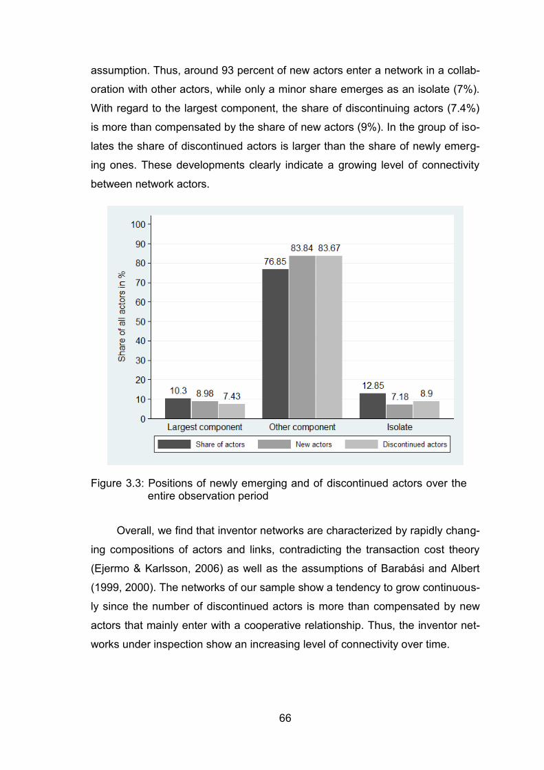
66

assumption. Thus, around 93 percent of new actors enter a network in a collab-

oration with other actors, while only a minor share emerges as an isolate (7%).

With regard to the largest component, the share of discontinuing actors (7.4%)

is more than compensated by the share of new actors (9%). In the group of iso-

lates the share of discontinued actors is larger than the share of newly emerg-

ing ones. These developments clearly indicate a growing level of connectivity

between network actors.

Figure 3.3: Positions of newly emerging and of discontinued actors over the entire observation period

Overall, we find that inventor networks are characterized by rapidly chang-

ing compositions of actors and links, contradicting the transaction cost theory

(Ejermo & Karlsson, 2006) as well as the assumptions of Barabási and Albert

(1999, 2000). The networks of our sample show a tendency to grow continuous-

ly since the number of discontinued actors is more than compensated by new

actors that mainly enter with a cooperative relationship. Thus, the inventor net-

works under inspection show an increasing level of connectivity over time.

67

3.4.2 Assessing the share of persistent knowledge

We use several indicators for assessing the amount of a discontinuing actor’s

knowledge that may be still available because it has been passed on to his co-

inventors in the previous period. For this purpose we identify those co-inventors

of a discontinued inventor that are still included in the network in the subse-

quent period. If a co-inventor of a discontinued actor remains in the network we

assume that at least parts of the patent-specific knowledge of the discontinued

actor is still available. If a discontinued actor was involved in several co-patents,

we assume that he only transfers that knowledge that is specific to the patented

invention and not the knowledge that for relevant for his other patents.

In the baseline version we assume that the patent-specific knowledge of a

discontinuing actor is entirely transferred to each co-inventor during the time of

collaboration. We then identify those inventors who remain active in the network

in the subsequent period and the knowledge that they represent. Based on this

information we finally determine the amount of continuing knowledge.

In detail we proceed as follows:

We generate a list of all patents with involvement of regional inventors that

represents the knowledge stock of period t0.

If an inventor of period t0 is still in the network in period t1 we assign his pa-

tents of period t0 to him.

The share of knowledge that is transferred between period t0 and t1 is the

number of patents in the list for period t1 over the total number of patents in

period t0.30

As robustness checks, we also calculate the share of knowledge that is

transferred across periods in two alternative ways.

The first alternative method is based on the assumption that knowledge

transfer among inventors is not complete but that inventors keep parts of

their knowledge that is completely lost when they discontinue in the network.

30 Since an inventor of period t0 may not be present in t1 but reemerge in a later period t2 or t3,

we run additional models to compare the list of patens between more distant time periods as a robustness check. However, the direction and significance of the coefficients remain the same.

68

We assume that co-inventors transfer only 50 percent of their knowledge to

each co-inventor.

In a second alternative way of calculating the transferred knowledge we as-

sume that the complete patent-specific knowledge is equally divided among

all co-inventors. Hence, if there are, say, three (five) co-inventors of a patent,

each co-inventor represents one third (one fifth) of the new knowledge that is

behind the patent. In a next step, we check which inventors remain active

within a network in the next period. If only one inventor remains active in the

following period, then one third (one fifths) of the knowledge remains availa-

ble. In case of two remaining actors, two third (two fifth) of the knowledge is

available. The rest of the procedure follows the previous model. The idea be-

hind this second alternative way of estimating the amount of knowledge

transfer is that there should be more specialization and division of labor in

larger teams so that the knowledge of an actor may not be completely trans-

ferred to all team members. Moreover, larger teams may be characterized by

a rather pronounced division of labor between specialists that are only able to

understand only parts of the knowledge.

Based on the first method of estimating the transfer of knowledge between

periods that assumes that the knowledge of an actor is completely transferred

to all his co-inventors, we find that between 30.1% and 92.7% of the knowledge

a period remains in the network in the subsequent period despite high levels of

fluidity (Table 3.1). This share does, however, vary considerably across time

periods and regions. If we assume an only 50% transfer of knowledge, the

share of remaining knowledge ranges between 10.0% and 44.2%. Under the

assumption that the share of transferred knowledge depends on the number of

co-inventors the share of transferred knowledge is between 16.2% and 30.1%.

These figures clearly suggest that the fluidity of actors leads to considerable

losses of knowledge in the respective RIS even if it is assumed that inventor’s

knowledge is completely transferred to all co-inventors during the cooperation.

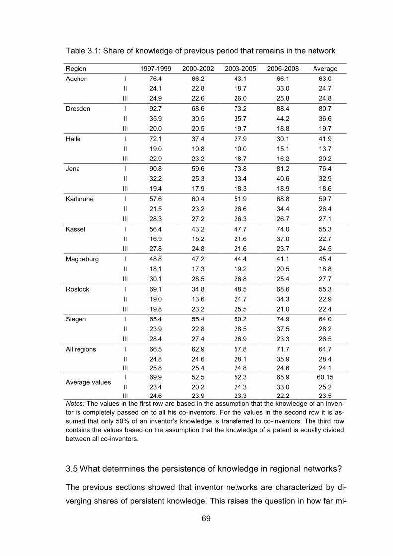
69

Table 3.1: Share of knowledge of previous period that remains in the network

Region 1997-1999 2000-2002 2003-2005 2006-2008 Average Aachen I 76.4 66.2 43.1 66.1 63.0 II 24.1 22.8 18.7 33.0 24.7 III 24.9 22.6 26.0 25.8 24.8 Dresden I 92.7 68.6 73.2 88.4 80.7 II 35.9 30.5 35.7 44.2 36.6 III 20.0 20.5 19.7 18.8 19.7 Halle I 72.1 37.4 27.9 30.1 41.9 II 19.0 10.8 10.0 15.1 13.7 III 22.9 23.2 18.7 16.2 20.2 Jena I 90.8 59.6 73.8 81.2 76.4 II 32.2 25.3 33.4 40.6 32.9 III 19.4 17.9 18.3 18.9 18.6 Karlsruhe I 57.6 60.4 51.9 68.8 59.7 II 21.5 23.2 26.6 34.4 26.4 III 28.3 27.2 26.3 26.7 27.1 Kassel I 56.4 43.2 47.7 74.0 55.3 II 16.9 15.2 21.6 37.0 22.7 III 27.8 24.8 21.6 23.7 24.5 Magdeburg I 48.8 47.2 44.4 41.1 45.4 II 18.1 17.3 19.2 20.5 18.8 III 30.1 28.5 26.8 25.4 27.7 Rostock I 69.1 34.8 48.5 68.6 55.3 II 19.0 13.6 24.7 34.3 22.9 III 19.8 23.2 25.5 21.0 22.4 Siegen I 65.4 55.4 60.2 74.9 64.0 II 23.9 22.8 28.5 37.5 28.2 III 28.4 27.4 26.9 23.3 26.5 All regions I 66.5 62.9 57.8 71.7 64.7 II 24.8 24.6 28.1 35.9 28.4

III 25.8 25.4 24.8 24.6 24.1

Average values I 69.9 52.5 52.3 65.9 60.15 II 23.4 20.2 24.3 33.0 25.2

III 24.6 23.9 23.3 22.2 23.5 Notes: The values in the first row are based in the assumption that the knowledge of an inven-tor is completely passed on to all his co-inventors. For the values in the second row it is as-sumed that only 50% of an inventor’s knowledge is transferred to co-inventors. The third row contains the values based on the assumption that the knowledge of a patent is equally divided between all co-inventors.

3.5 What determines the persistence of knowledge in regional networks?

The previous sections showed that inventor networks are characterized by di-

verging shares of persistent knowledge. This raises the question in how far mi-

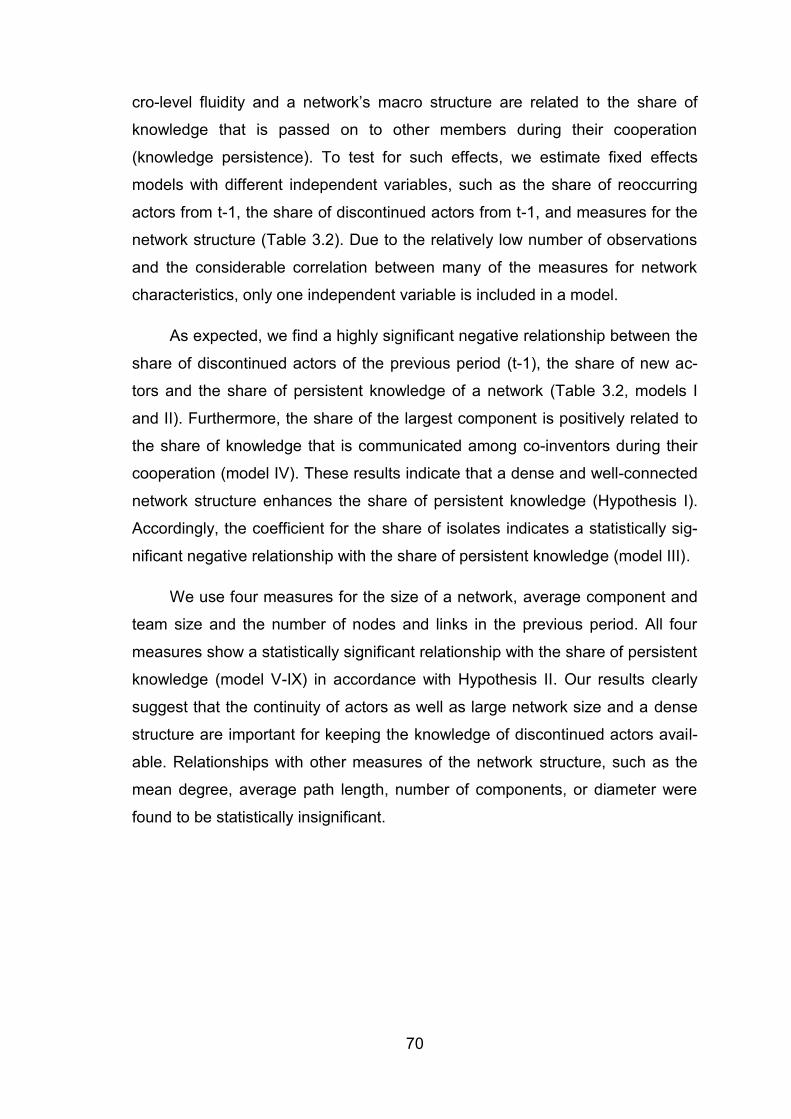
70

cro-level fluidity and a network’s macro structure are related to the share of

knowledge that is passed on to other members during their cooperation

(knowledge persistence). To test for such effects, we estimate fixed effects

models with different independent variables, such as the share of reoccurring

actors from t-1, the share of discontinued actors from t-1, and measures for the

network structure (Table 3.2). Due to the relatively low number of observations

and the considerable correlation between many of the measures for network

characteristics, only one independent variable is included in a model.

As expected, we find a highly significant negative relationship between the

share of discontinued actors of the previous period (t-1), the share of new ac-

tors and the share of persistent knowledge of a network (Table 3.2, models I

and II). Furthermore, the share of the largest component is positively related to

the share of knowledge that is communicated among co-inventors during their

cooperation (model IV). These results indicate that a dense and well-connected

network structure enhances the share of persistent knowledge (Hypothesis I).

Accordingly, the coefficient for the share of isolates indicates a statistically sig-

nificant negative relationship with the share of persistent knowledge (model III).

We use four measures for the size of a network, average component and

team size and the number of nodes and links in the previous period. All four

measures show a statistically significant relationship with the share of persistent

knowledge (model V-IX) in accordance with Hypothesis II. Our results clearly

suggest that the continuity of actors as well as large network size and a dense

structure are important for keeping the knowledge of discontinued actors avail-

able. Relationships with other measures of the network structure, such as the

mean degree, average path length, number of components, or diameter were

found to be statistically insignificant.

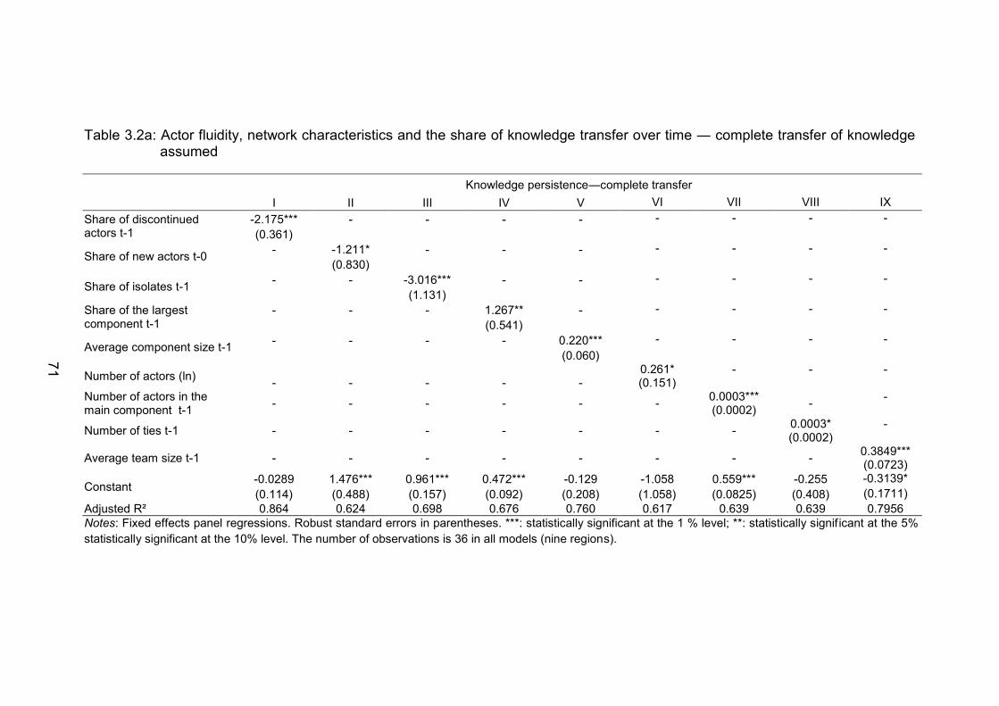
71

Table 3.2a: Actor fluidity, network characteristics and the share of knowledge transfer over time ― complete transfer of knowledge assumed

Knowledge persistence―complete transfer

I II III IV V VI VII VIII IX

Share of discontinued actors t-1

-2.175*** - - - - - - - - (0.361)

Share of new actors t-0 - -1.211* - - - - - - -

(0.830)

Share of isolates t-1 - - -3.016*** - - - - - -

(1.131)

Share of the largest component t-1

- - - 1.267** - - - - -

(0.541)

Average component size t-1 - - - - 0.220*** - - - -

(0.060)

Number of actors (ln) - - - - - 0.261* (0.151)

- - -

Number of actors in the main component t-1 - - - - - - 0.0003***

(0.0002) - -

Number of ties t-1 - - - - - - - 0.0003* (0.0002)

-

Average team size t-1 - - - - - - - - 0.3849*** (0.0723)

Constant -0.0289 1.476*** 0.961*** 0.472*** -0.129 -1.058 0.559*** -0.255 -0.3139* (0.114) (0.488) (0.157) (0.092) (0.208) (1.058) (0.0825) (0.408) (0.1711)

Adjusted R² 0.864 0.624 0.698 0.676 0.760 0.617 0.639 0.639 0.7956 Notes: Fixed effects panel regressions. Robust standard errors in parentheses. ***: statistically significant at the 1 % level; **: statistically signif icant at the 5% % level; *: statistically significant at the 10% level. The number of observations is 36 in all models (nine regions).

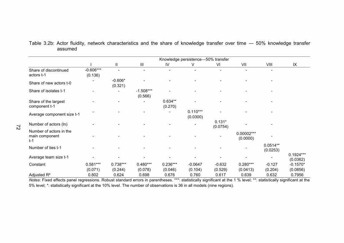
72

Table 3.2b: Actor fluidity, network characteristics and the share of knowledge transfer over time ― 50% knowledge transfer assumed

Knowledge persistence―50% transfer

I II III IV V VI VII VIII IX

Share of discontinued actors t-1

-0.606*** - - - - - - - (0.136)

Share of new actors t-0 - -0.606* - - - - - -

(0.321) Share of isolates t-1 - - -1.508*** - - - - -

(0.566) Share of the largest component t-1

- - - 0.634** - - - -

(0.270)

Average component size t-1 - - - - 0.110*** - - -

(0.0300)

Number of actors (ln) - - - - - 0.131* (0.0754) - -

Number of actors in the main component t-1

- - - - - - 0.00002*** (0.0000) -

Number of ties t-1 - - - - - - - 0.0514** (0.0253)

Average team size t-1 - - - - - - - - 0.1924*** (0.0362)

Constant 0.581*** 0.738*** 0.480*** 0.236*** -0.0647 -0.632 0.280*** -0.127 -0.1570*

(0.071) (0.244) (0.078) (0.046) (0.104) (0.529) (0.0413) (0.204) (0.0856) Adjusted R² 0.802 0.624 0.698 0.676 0.760 0.617 0.639 0.632 0.7956 Notes: Fixed effects panel regressions. Robust standard errors in parentheses. ***: statistically significant at the 1 % level; **: statistically significant at the 5% level; *: statistically significant at the 10% level. The number of observations is 36 in all models (nine regions).

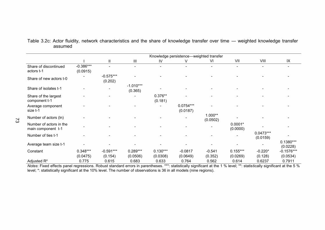
73

Table 3.2c: Actor fluidity, network characteristics and the share of knowledge transfer over time ― weighted knowledge transfer assumed

Knowledge persistence―weighted transfer

I II III IV V VI VII VIII IX

Share of discontinued actors t-1

-0.386*** - - - - - - - - (0.0915)

Share of new actors t-0 - -0.575*** - - - - - - -

(0.202)

Share of isolates t-1 - - -1.010*** (0.365)

- - - - - -

Share of the largest component t-1

- - - 0.376** - - - - -

(0.181) Average component size t-1

- - - - 0.0754*** - - - -

(0.0187)

Number of actors (ln) - - - - - 1.000** (0.0502) - - -

Number of actors in the main component t-1 - - - - - - 0.0001*

(0.0000) - -

Number of ties t-1 - - - - - - - 0.0473*** (0.0159) -

Average team size t-1 - - - - - - - - 0.1380*** (0.0228)

Constant 0.348*** -0.591*** 0.289*** 0.130*** -0.0817 -0.541 0.155*** -0.220* -0.1576***

(0.0475) (0.154) (0.0506) (0.0308) (0.0649) (0.352) (0.0269) (0.128) (0.0534) Adjusted R² 0.775 0.615 0.683 0.633 0.764 0.562 0.614 0.6237 0.7911 Notes: Fixed effects panel regressions. Robust standard errors in parentheses. ***: statistically significant at the 1 % level; **: statistically significant at the 5 % level; *: statistically significant at the 10% level. The number of observations is 36 in all models (nine regions).

74

3.6 The effect of knowledge persistence on network performance

For investigating the effect of persistent knowledge and of new knowledge on

the performance of the respective regional innovation system we use patent

productivity as a measure of performance. Patent productivity is defined as the

number of patents filed by private sector innovators with at least one inventor

residing in the respective region per 1,000 R&D employees. While this metric

reflects the level of the efficiency of a RIS (Fritsch, 2002; Fritsch & Slavtchev,

2011), we also use the percentage change of patent productivity to analyze the

development of that level.

All models include the share of manufacturing employees in establish-

ments with less than 50 employees as a control variable. This variable accounts

for the observation that the number of patents per unit of R&D input tends to be

higher in smaller firms than in larger firms (for a theoretical explanation and dis-

cussion, see Cohen and Klepper, 1996). Hence, we expect a negative sign for

the estimated coefficient of this variable. In the models for the change of patent

productivity, we also include the level of patent productivity in the previous peri-

od. The estimated coefficient of this variable should have a negative sign for

two reasons. First, regions with an already relatively high level of patent produc-

tivity may have lower potentials for improvements than regions that are charac-

terized by a comparatively low performance. Second, the level of patent produc-

tivity in the base year controls for a regression to the mean effect. This effect

denotes the phenomenon that periods with relatively large changes into one

direction may be followed by periods where the changes are relatively small or

even work in the opposite direction.

The estimation results of Table 3.3 provide empirical evidence for the posi-

tive connection between the performance of a network and the two potential

sources of knowledge, namely new and persistent knowledge. Thus, we find a

significantly positive relationship between a network’s patent productivity and

the share of new actors (model I) as well as with the share of persistent

knowledge (models III and IV). The non-significance of the share of persistent

knowledge in model II that does not contain the share of new knowledge may

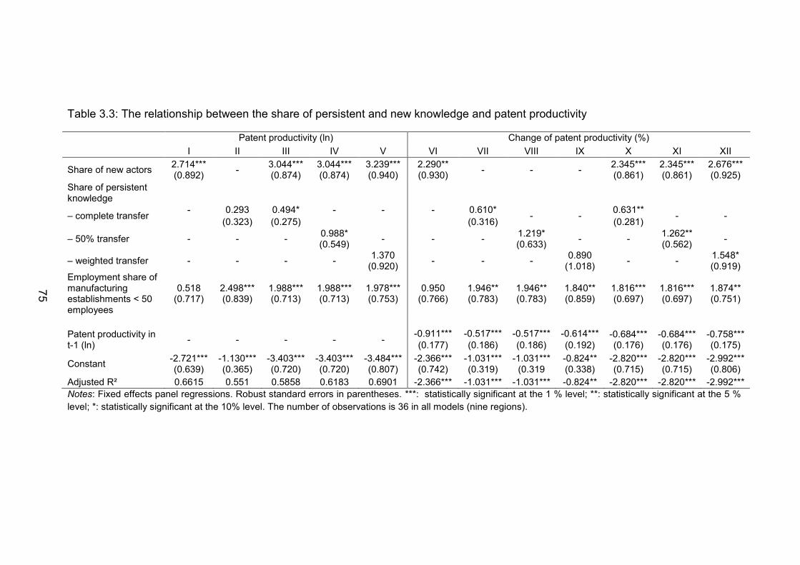
75

Table 3.3: The relationship between the share of persistent and new knowledge and patent productivity

Patent productivity (ln) Change of patent productivity (%)

I II III IV V VI VII VIII IX X XI XII

Share of new actors 2.714*** (0.892) - 3.044***

(0.874) 3.044*** (0.874)

3.239*** (0.940)

2.290** (0.930) - - - 2.345***

(0.861) 2.345*** (0.861)

2.676*** (0.925)

Share of persistent knowledge

– complete transfer - 0.293 0.494* - - - 0.610* - - 0.631** - - (0.323) (0.275) (0.316) (0.281)

– 50% transfer - - - 0.988* (0.549) - - - 1.219*

(0.633) - - 1.262** (0.562) -

– weighted transfer - - - - 1.370 (0.920) - - - 0.890

(1.018) - - 1.548* (0.919)

Employment share of manufacturing establishments < 50 employees

0.518 (0.717)

2.498*** (0.839)

1.988*** (0.713)

1.988*** (0.713)

1.978*** (0.753)

0.950 (0.766)

1.946** (0.783)

1.946** (0.783)

1.840** (0.859)

1.816*** (0.697)

1.816*** (0.697)

1.874** (0.751)

Patent productivity in t-1 (ln) - - - - - -0.911*** -0.517*** -0.517*** -0.614*** -0.684*** -0.684*** -0.758***

(0.177) (0.186) (0.186) (0.192) (0.176) (0.176) (0.175)

Constant -2.721*** -1.130*** -3.403*** -3.403*** -3.484*** -2.366*** -1.031*** -1.031*** -0.824** -2.820*** -2.820*** -2.992*** (0.639) (0.365) (0.720) (0.720) (0.807) (0.742) (0.319) (0.319 (0.338) (0.715) (0.715) (0.806)

Adjusted R² 0.6615 0.551 0.5858 0.6183 0.6901 -2.366*** -1.031*** -1.031*** -0.824** -2.820*** -2.820*** -2.992*** Notes: Fixed effects panel regressions. Robust standard errors in parentheses. ***: statistically significant at the 1 % level; **: statistically significant at the 5 % level; *: statistically significant at the 10% level. The number of observations is 36 in all models (nine regions).

76

be caused by the relatively high correlation between the measures of these two

knowledge sources. The insignificance of the coefficient of the weighted meas-

ure of knowledge transfer in models V and XI may result from the fact that ac-

cording to the construction of this measure only smaller amounts of the total

knowledge are transferred so that the share of persistent knowledge is underes-

timated.

We also find statistically positive relationships for our measure of new

knowledge in the models for the change of patent productivity (Table 3.3, mod-

els VI-XII). For two out of our three measures of knowledge persistence we also

find a statistically significant relationship with the expected positive sign (Table

3.3, models VII-IX). Again, the weighted knowledge transfer remains statistically

insignificant. When we introduce the share of new actors (models X-XII), all

three measures of knowledge persistence are statistically significant, supporting

our earlier finding that both existing and new knowledge are highly important to

enhance the efficiency of a RIS. This indicates that the generation of inventions

benefits from persistent as well as from new sources of knowledge. Since most

actors enter a network as part of a team, this result suggests that it is combina-

tions of existing and new knowledge drive the patent productivity of a network.

We test this assumption by splitting the share of new actors into those that enter

a network as part of a team and those who enter as isolates. The results of Ta-

ble 3.4 reveal that the share of actors that enter a network through cooperative

activities noticeable increase the productivity of the respective RIS while the

share of new actors who enter as isolates is insignificant. However, the former

share also contains as well actors that enter a network through new compo-

nents.

To sum up, our results indicate that the share of old knowledge that re-

mains in a regional inventor network across subsequent time periods is only

relevant for the performance of the respective RIS (measured by patent produc-

tivity) if we control for the share of new actors. Based on the results of Table

3.4, the combination of existing and new knowledge is the driver of perfor-

mance. Thus, we can partly accept Hypotheses III. We, moreover, find strong

evidence for the effect of new sets of knowledge (new actors) on the perfor-

mance of a RIS, being consistent with our Hypothesis IV.

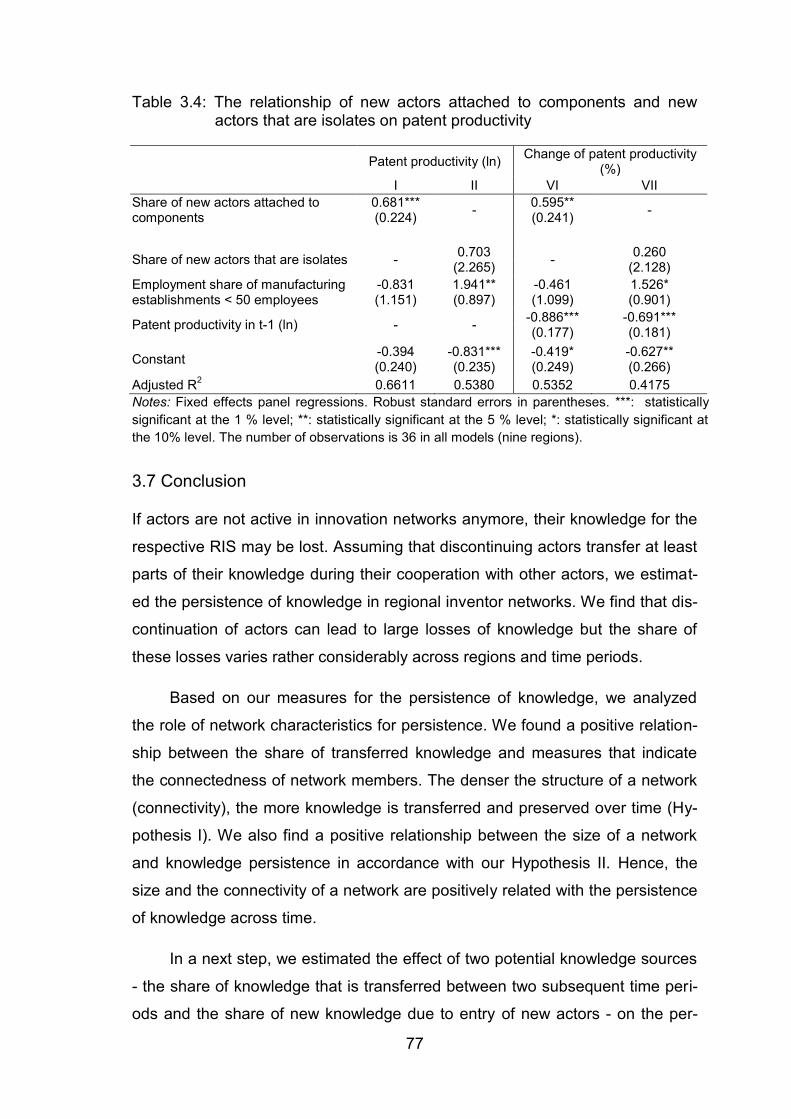
77

Table 3.4: The relationship of new actors attached to components and new actors that are isolates on patent productivity

Patent productivity (ln) Change of patent productivity (%)

I II VI VII Share of new actors attached to components

0.681*** (0.224) - 0.595**

(0.241) -

Share of new actors that are isolates - 0.703 - 0.260 (2.265) (2.128)

Employment share of manufacturing establishments < 50 employees

-0.831 (1.151)

1.941** (0.897)

-0.461 (1.099)

1.526* (0.901)

Patent productivity in t-1 (ln) - - -0.886*** -0.691*** (0.177) (0.181)

Constant -0.394 -0.831*** -0.419* -0.627** (0.240) (0.235) (0.249) (0.266)

Adjusted R2 0.6611 0.5380 0.5352 0.4175 Notes: Fixed effects panel regressions. Robust standard errors in parentheses. ***: statistically significant at the 1 % level; **: statistically significant at the 5 % level; *: statistically significant at the 10% level. The number of observations is 36 in all models (nine regions).

3.7 Conclusion

If actors are not active in innovation networks anymore, their knowledge for the

respective RIS may be lost. Assuming that discontinuing actors transfer at least

parts of their knowledge during their cooperation with other actors, we estimat-

ed the persistence of knowledge in regional inventor networks. We find that dis-

continuation of actors can lead to large losses of knowledge but the share of

these losses varies rather considerably across regions and time periods.

Based on our measures for the persistence of knowledge, we analyzed

the role of network characteristics for persistence. We found a positive relation-

ship between the share of transferred knowledge and measures that indicate

the connectedness of network members. The denser the structure of a network

(connectivity), the more knowledge is transferred and preserved over time (Hy-

pothesis I). We also find a positive relationship between the size of a network

and knowledge persistence in accordance with our Hypothesis II. Hence, the

size and the connectivity of a network are positively related with the persistence

of knowledge across time.

In a next step, we estimated the effect of two potential knowledge sources

- the share of knowledge that is transferred between two subsequent time peri-

ods and the share of new knowledge due to entry of new actors - on the per-

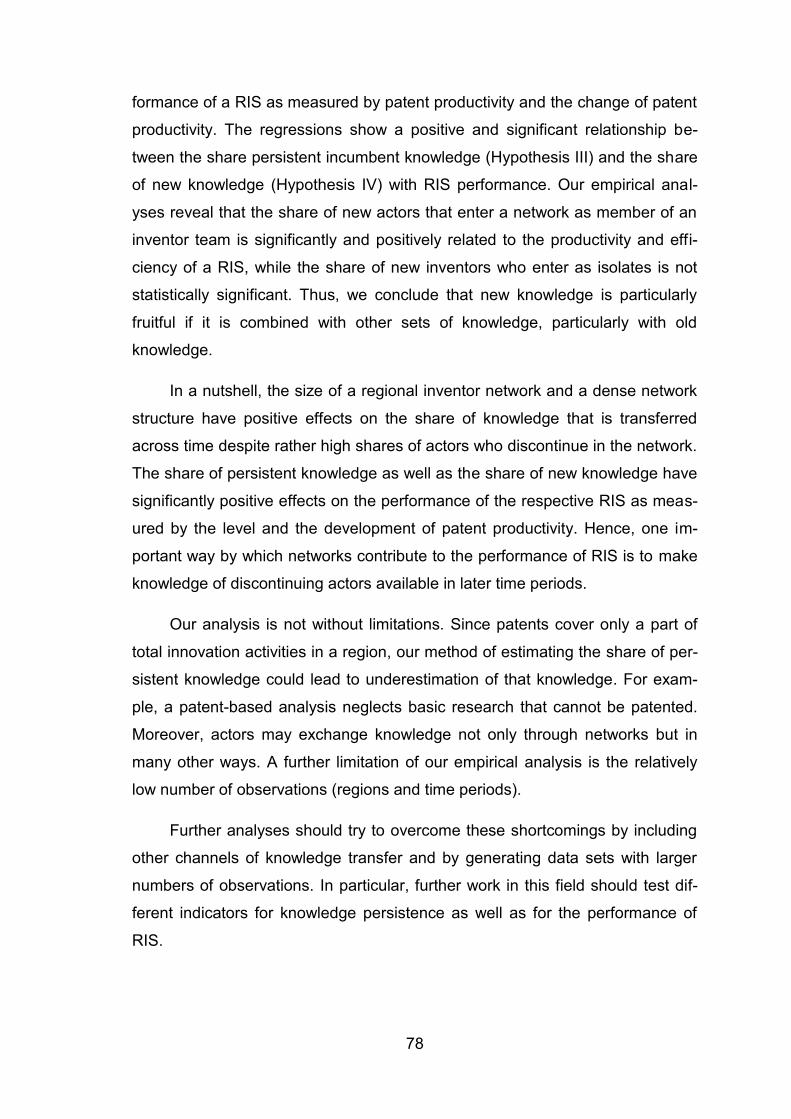
78

formance of a RIS as measured by patent productivity and the change of patent

productivity. The regressions show a positive and significant relationship be-

tween the share persistent incumbent knowledge (Hypothesis III) and the share

of new knowledge (Hypothesis IV) with RIS performance. Our empirical anal-

yses reveal that the share of new actors that enter a network as member of an

inventor team is significantly and positively related to the productivity and effi-

ciency of a RIS, while the share of new inventors who enter as isolates is not

statistically significant. Thus, we conclude that new knowledge is particularly

fruitful if it is combined with other sets of knowledge, particularly with old

knowledge.

In a nutshell, the size of a regional inventor network and a dense network

structure have positive effects on the share of knowledge that is transferred

across time despite rather high shares of actors who discontinue in the network.

The share of persistent knowledge as well as the share of new knowledge have

significantly positive effects on the performance of the respective RIS as meas-

ured by the level and the development of patent productivity. Hence, one im-

portant way by which networks contribute to the performance of RIS is to make

knowledge of discontinuing actors available in later time periods.

Our analysis is not without limitations. Since patents cover only a part of

total innovation activities in a region, our method of estimating the share of per-

sistent knowledge could lead to underestimation of that knowledge. For exam-

ple, a patent-based analysis neglects basic research that cannot be patented.

Moreover, actors may exchange knowledge not only through networks but in

many other ways. A further limitation of our empirical analysis is the relatively

low number of observations (regions and time periods).

Further analyses should try to overcome these shortcomings by including

other channels of knowledge transfer and by generating data sets with larger

numbers of observations. In particular, further work in this field should test dif-

ferent indicators for knowledge persistence as well as for the performance of

RIS.

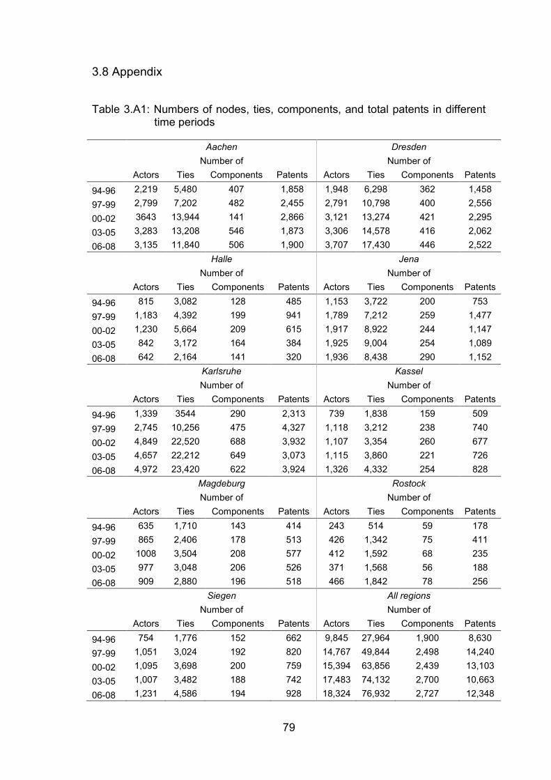
79

3.8 Appendix

Table 3.A1: Numbers of nodes, ties, components, and total patents in different time periods

Aachen Dresden

Number of Number of Actors Ties Components Patents Actors Ties Components Patents

94-96 2,219 5,480 407 1,858 1,948 6,298 362 1,458 97-99 2,799 7,202 482 2,455 2,791 10,798 400 2,556 00-02 3643 13,944 141 2,866 3,121 13,274 421 2,295 03-05 3,283 13,208 546 1,873 3,306 14,578 416 2,062 06-08 3,135 11,840 506 1,900 3,707 17,430 446 2,522

Halle Jena

Number of Number of Actors Ties Components Patents Actors Ties Components Patents

94-96 815 3,082 128 485 1,153 3,722 200 753 97-99 1,183 4,392 199 941 1,789 7,212 259 1,477 00-02 1,230 5,664 209 615 1,917 8,922 244 1,147 03-05 842 3,172 164 384 1,925 9,004 254 1,089 06-08 642 2,164 141 320 1,936 8,438 290 1,152

Karlsruhe Kassel

Number of Number of Actors Ties Components Patents Actors Ties Components Patents

94-96 1,339 3544 290 2,313 739 1,838 159 509 97-99 2,745 10,256 475 4,327 1,118 3,212 238 740 00-02 4,849 22,520 688 3,932 1,107 3,354 260 677 03-05 4,657 22,212 649 3,073 1,115 3,860 221 726 06-08 4,972 23,420 622 3,924 1,326 4,332 254 828

Magdeburg Rostock

Number of Number of Actors Ties Components Patents Actors Ties Components Patents

94-96 635 1,710 143 414 243 514 59 178 97-99 865 2,406 178 513 426 1,342 75 411 00-02 1008 3,504 208 577 412 1,592 68 235 03-05 977 3,048 206 526 371 1,568 56 188 06-08 909 2,880 196 518 466 1,842 78 256

Siegen All regions

Number of Number of Actors Ties Components Patents Actors Ties Components Patents

94-96 754 1,776 152 662 9,845 27,964 1,900 8,630 97-99 1,051 3,024 192 820 14,767 49,844 2,498 14,240 00-02 1,095 3,698 200 759 15,394 63,856 2,439 13,103 03-05 1,007 3,482 188 742 17,483 74,132 2,700 10,663 06-08 1,231 4,586 194 928 18,324 76,932 2,727 12,348

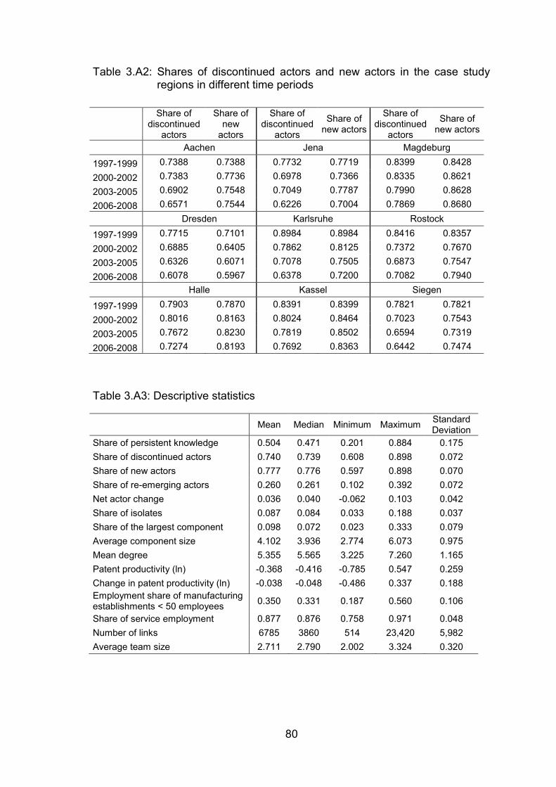
80

Table 3.A2: Shares of discontinued actors and new actors in the case study regions in different time periods

Table 3.A3: Descriptive statistics

Mean Median Minimum Maximum Standard Deviation

Share of persistent knowledge 0.504 0.471 0.201 0.884 0.175 Share of discontinued actors 0.740 0.739 0.608 0.898 0.072 Share of new actors 0.777 0.776 0.597 0.898 0.070 Share of re-emerging actors 0.260 0.261 0.102 0.392 0.072 Net actor change 0.036 0.040 -0.062 0.103 0.042 Share of isolates 0.087 0.084 0.033 0.188 0.037 Share of the largest component 0.098 0.072 0.023 0.333 0.079 Average component size 4.102 3.936 2.774 6.073 0.975 Mean degree 5.355 5.565 3.225 7.260 1.165 Patent productivity (ln) -0.368 -0.416 -0.785 0.547 0.259 Change in patent productivity (ln) -0.038 -0.048 -0.486 0.337 0.188 Employment share of manufacturing establishments < 50 employees 0.350 0.331 0.187 0.560 0.106

Share of service employment 0.877 0.876 0.758 0.971 0.048 Number of links 6785 3860 514 23,420 5,982 Average team size 2.711 2.790 2.002 3.324 0.320

Share of discontinued

actors

Share of new

actors

Share of discontinued

actors

Share of new actors

Share of discontinued

actors

Share of new actors

Aachen Jena Magdeburg

1997-1999 0.7388 0.7388 0.7732 0.7719 0.8399 0.8428 2000-2002 0.7383 0.7736 0.6978 0.7366 0.8335 0.8621 2003-2005 0.6902 0.7548 0.7049 0.7787 0.7990 0.8628 2006-2008 0.6571 0.7544 0.6226 0.7004 0.7869 0.8680

Dresden Karlsruhe Rostock

1997-1999 0.7715 0.7101 0.8984 0.8984 0.8416 0.8357 2000-2002 0.6885 0.6405 0.7862 0.8125 0.7372 0.7670 2003-2005 0.6326 0.6071 0.7078 0.7505 0.6873 0.7547 2006-2008 0.6078 0.5967 0.6378 0.7200 0.7082 0.7940

Halle Kassel Siegen

1997-1999 0.7903 0.7870 0.8391 0.8399 0.7821 0.7821 2000-2002 0.8016 0.8163 0.8024 0.8464 0.7023 0.7543 2003-2005 0.7672 0.8230 0.7819 0.8502 0.6594 0.7319 2006-2008 0.7274 0.8193 0.7692 0.8363 0.6442 0.7474

81

Table 3.A4: Number of co-patents, single patents, mean degree (all regions)

94-96 97-99 00-02 03-05 06-08 94-08

Total number of patents 8,63 14,24 13,10 10,66 12,35 58,98 Number of co-patents 7,37 12,60 11,85 9,50 11,14 52,46 Share of co-patents in % 85.45 88.46 90.42 89.07 90.20 88.93 Number of patents with single inventor 1,26 1,64 1,26 1,17 1,21 6,53 Number of inventors per patent 2.71 2.82 2.99 3.07 3.00 2.91 Number of inventors per co-patents 3.40 3.51 3.65 3.70 3.58 3.58 Mean degree 3.76 5.11 5.51 5.44 5.36 3.76 Average path lengths 2.22 3.57 3.85 3.77 3.83 3.45

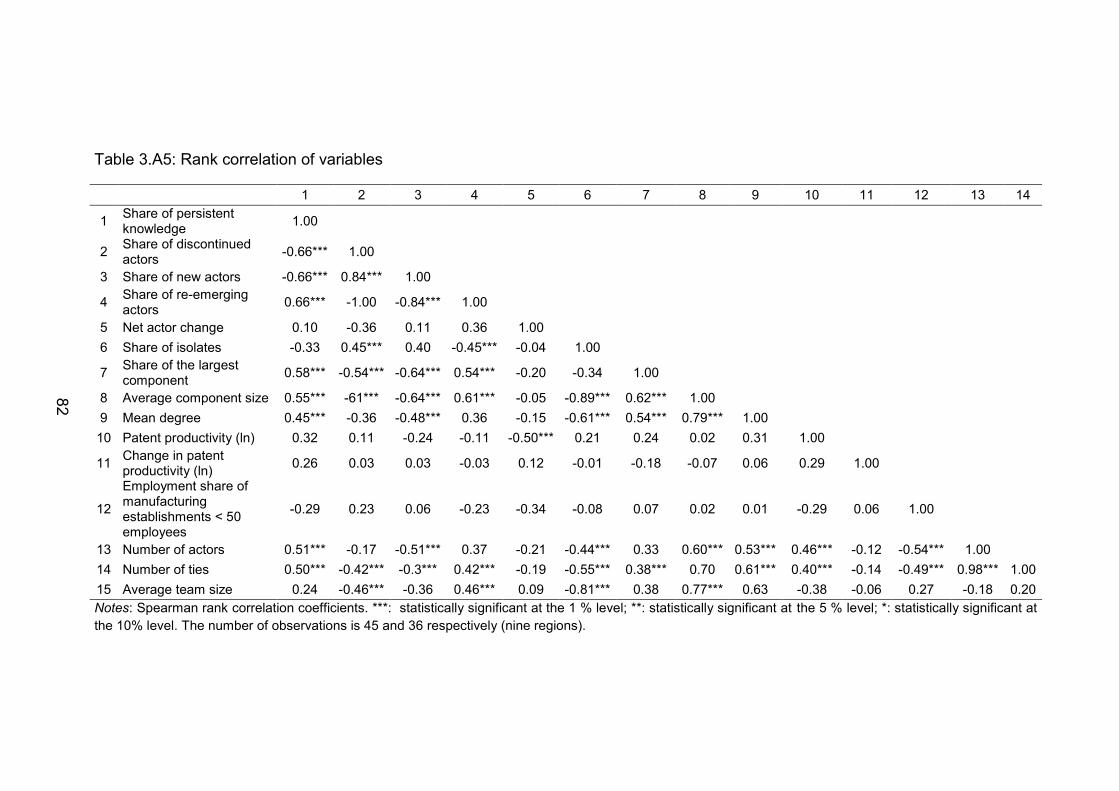
82

Table 3.A5: Rank correlation of variables

1 2 3 4 5 6 7 8 9 10 11 12 13 14

1 Share of persistent knowledge 1.00

2 Share of discontinued actors -0.66*** 1.00

3 Share of new actors -0.66*** 0.84*** 1.00

4 Share of re-emerging actors 0.66*** -1.00 -0.84*** 1.00

5 Net actor change 0.10 -0.36 0.11 0.36 1.00 6 Share of isolates -0.33 0.45*** 0.40 -0.45*** -0.04 1.00

7 Share of the largest component 0.58*** -0.54*** -0.64*** 0.54*** -0.20 -0.34 1.00

8 Average component size 0.55*** -61*** -0.64*** 0.61*** -0.05 -0.89*** 0.62*** 1.00 9 Mean degree 0.45*** -0.36 -0.48*** 0.36 -0.15 -0.61*** 0.54*** 0.79*** 1.00

10 Patent productivity (ln) 0.32 0.11 -0.24 -0.11 -0.50*** 0.21 0.24 0.02 0.31 1.00

11 Change in patent productivity (ln) 0.26 0.03 0.03 -0.03 0.12 -0.01 -0.18 -0.07 0.06 0.29 1.00

12

Employment share of manufacturing establishments < 50 employees

-0.29 0.23 0.06 -0.23 -0.34 -0.08 0.07 0.02 0.01 -0.29 0.06 1.00

13 Number of actors 0.51*** -0.17 -0.51*** 0.37 -0.21 -0.44*** 0.33 0.60*** 0.53*** 0.46*** -0.12 -0.54*** 1.00 14 Number of ties 0.50*** -0.42*** -0.3*** 0.42*** -0.19 -0.55*** 0.38*** 0.70 0.61*** 0.40*** -0.14 -0.49*** 0.98*** 1.00 15 Average team size 0.24 -0.46*** -0.36 0.46*** 0.09 -0.81*** 0.38 0.77*** 0.63 -0.38 -0.06 0.27 -0.18 0.20 Notes: Spearman rank correlation coefficients. ***: statistically significant at the 1 % level; **: statistically significant at the 5 % level; *: statistically significant at the 10% level. The number of observations is 45 and 36 respectively (nine regions).

83

Chapter 4

So what? Concluding remarks and outlook for further research

In the following, a brief summary of the two previous chapters is provided in order

to set the starting points for developing ideas for future research (see, Section 4.1).

Given that both Chapters 2 and 3 deal with stability issues regarding the efficiency

of a network and a RIS, the focus of Section 4.2 contains general remarks on the

entrance of new actors and their tendency to connect to well-embedded actors

(preferential attachment hypothesis), as well as the importance of key actors for a

network’s robustness.

4.1 Summary of the empirical findings

Chapter 2 challenged the widespread assumption, based on transaction cost theo-

ry (Ejermo & Karlsson, 2006) and the results of Barabási-Albert’s model (1999,

2000), that there are primarily long-lasting relationships among actors within re-

gional inventor networks. The findings from Chapter 2 suggest that most of the

network actors are only active once and disappear in the subsequent period. This

high level of fluidity affects not only the structure of a network, but also influences

the performance of a respective RIS.

The fluidity of actors leads to a fragmentation of networks that is measured by

the effect of the share of discontinued actors on the share of the largest compo-

nent, respectively on the share of isolates. However, besides the negative effect on

the connectivity of a network,31 the fluidity of actors does not seem to hamper the

efficiency of a RIS. This is so because patent productivity benefits from the

knowledge of new inventors that seem to replace the position of discontinued ac-

tors. Within a network, ties serve as channels for knowledge transfers and are,

31 As stated in Chapter 2, the share of discontinued actors is negatively related to the share of the

largest component and positively to the share of isolates.

84

therefore, crucial for the efficiency of a RIS (Fritsch & Slavtchev, 2011). In this way,

the results suggest that a high share of instable links hamper the efficiency of a

network’s patent productivity. Overall, the empirical results from Chapter 2 suggest

that the pronounced level of actor turn-over decreases the connectedness of a

network, but is fruitful for a RIS’s efficiency.

Chapter 3, inspired by the findings of the previous chapter, deals with ques-

tion of the relationship between fluidity and the share of persistent knowledge. A

rich and comprehensive knowledge base is the foundation of the innovative pro-

cess and a primary driver of technological change (Howell, 2000; Bercovitz &

Feldman, 2011). Given that knowledge is embedded within an inventor, how much

of it passes to other team members during cooperative activities? Scholars have

frequently shown (see, Capaldo, 2007; Schilling & Phelps, 2007; Phelps, 2010)

that the structure of a network, i.e. its connectedness, and its size (Tang, Mu &

MacLachlan, 2008) are important for generating new knowledge. The main results

of Chapter 3 are in line with these findings and extend them by showing that a net-

work’s structural characteristics even influence the degree of persistent knowledge.

Well connected networks,32 thus, positively affect the share of remaining

knowledge. This indicates that the knowledge of well-embedded inventors (e.g.

members of the largest component) is more persistent than that of inventors work-

ing in isolation. This illustrates that networks are important as a source of new

knowledge - due to the high fluidity of actors - and persistent knowledge, especially

as the knowledge stock of the corresponding RIS.

The primary shortcoming of inventor network analyses is that patents cover

only a small amount of innovation activities, respectively knowledge. Thus, R&D

activities involving basic research do not appear in such statistics. It is, therefore,

only possible to draw a snapshot of the real world relationships between innovative

actors and the general stability of network relationships. Further, patent statistics

32 We state that the share of the largest component and average component size are indicators for

the connectivity of a network, whereas the share of isolates indicates a fragmentation of a network.

85

do not contain any information about the amount of work that each inventor puts

into the development process of a patent.

4.2 What do we need to know? Avenues for further research

4.2.1 Preferential attachment: myth or fact of network formation?

For quite some time, scholars tacitly assumed that a network’s structure originates

randomly. This consideration was based on Erdös and Rényi’s (1959) work about

random networks (Watts & Strognatz, 1998; Barabási, 2009). However, Barabási

and Albert (1999) provide evidence that networks are characterized by a self-

organizational behavior that evolves independently of their origin, age, function or

scope, and leads to similar network topologies. Self-organizational behavior or

preferential attachment connotes that new nodes exhibit higher preferences to col-

laborate with well-embedded actors within a network. Therefore, the higher the

number of an actor’s links, the higher the probability to attach new links (‘rich get

richer’ effect; Amaral et al., 2000; Capocci et al. 2006; Jackson, 2008).

Analyzing a scientific collaboration network, Newman (2001) argues that the

probability of acquiring a new collaboration partner increases with the number of

past collaborations. This is in line with the assumed preferential attachment hy-

potheses, proposed by Barabási and Albert (1999, 2000). Thus, an actor’s number

of cooperation partners (degree) grows at rates that are proportional to his or her

number of already existing links (Newman, 2001; Jackson, 2008). Similarly,

Capocci et al. (2006) support Newman’s results by showing that all subsamples of

Wikipedia are characterized by permanent growth and self-organizational behavior

(preferential attachment). Leskovec, Huttenlocher and Kleinberg (2010) analyze

the creation of links between actors in different social networks. By analyzing un-

derlying mechanism of networks, they found that networks organize themselves at

a local level, an indication for preferential attachment (Newman, 2003).

Based on the analysis of nine German planning regions, Chapter 2 was able

to detect a high structural robustness of inventor networks, suggesting that new

actors take over the position of drop-outs. Thus, new actors collaborate with al-

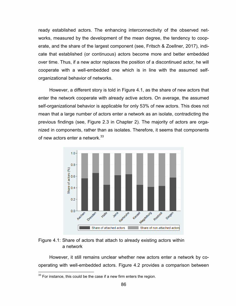
86

ready established actors. The enhancing interconnectivity of the observed net-

works, measured by the development of the mean degree, the tendency to coop-

erate, and the share of the largest component (see, Fritsch & Zoellner, 2017), indi-

cate that established (or continuous) actors become more and better embedded

over time. Thus, if a new actor replaces the position of a discontinued actor, he will

cooperate with a well-embedded one which is in line with the assumed self-

organizational behavior of networks.

However, a different story is told in Figure 4.1, as the share of new actors that

enter the network cooperate with already active actors. On average, the assumed

self-organizational behavior is applicable for only 53% of new actors. This does not

mean that a large number of actors enter a network as an isolate, contradicting the

previous findings (see, Figure 2.3 in Chapter 2). The majority of actors are orga-

nized in components, rather than as isolates. Therefore, it seems that components

of new actors enter a network.33

Figure 4.1: Share of actors that attach to already existing actors within

a network

However, it still remains unclear whether new actors enter a network by co-

operating with well-embedded actors. Figure 4.2 provides a comparison between 33 For instance, this could be the case if a new firm enters the region.

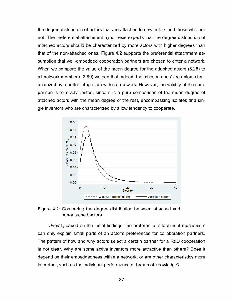
87

the degree distribution of actors that are attached to new actors and those who are

not. The preferential attachment hypothesis expects that the degree distribution of

attached actors should be characterized by more actors with higher degrees than

that of the non-attached ones. Figure 4.2 supports the preferential attachment as-

sumption that well-embedded cooperation partners are chosen to enter a network.

When we compare the value of the mean degree for the attached actors (5.28) to

all network members (3.89) we see that indeed, the ‘chosen ones’ are actors char-

acterized by a better integration within a network. However, the validity of the com-

parison is relatively limited, since it is a pure comparison of the mean degree of

attached actors with the mean degree of the rest, encompassing isolates and sin-

gle inventors who are characterized by a low tendency to cooperate.

Figure 4.2: Comparing the degree distribution between attached and

non-attached actors

Overall, based on the initial findings, the preferential attachment mechanism

can only explain small parts of an actor’s preferences for collaboration partners.

The pattern of how and why actors select a certain partner for a R&D cooperation

is not clear. Why are some active inventors more attractive than others? Does it

depend on their embeddedness within a network, or are other characteristics more

important, such as the individual performance or breath of knowledge?

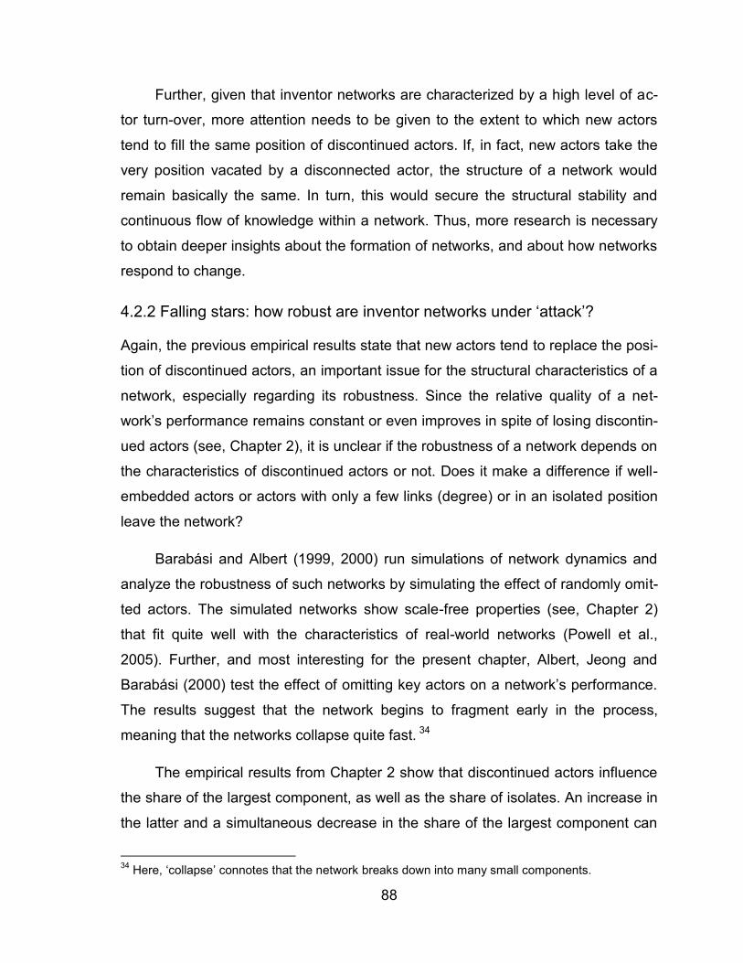
88

Further, given that inventor networks are characterized by a high level of ac-

tor turn-over, more attention needs to be given to the extent to which new actors

tend to fill the same position of discontinued actors. If, in fact, new actors take the

very position vacated by a disconnected actor, the structure of a network would

remain basically the same. In turn, this would secure the structural stability and

continuous flow of knowledge within a network. Thus, more research is necessary

to obtain deeper insights about the formation of networks, and about how networks

respond to change.

4.2.2 Falling stars: how robust are inventor networks under ‘attack’?

Again, the previous empirical results state that new actors tend to replace the posi-

tion of discontinued actors, an important issue for the structural characteristics of a

network, especially regarding its robustness. Since the relative quality of a net-

work’s performance remains constant or even improves in spite of losing discontin-

ued actors (see, Chapter 2), it is unclear if the robustness of a network depends on

the characteristics of discontinued actors or not. Does it make a difference if well-

embedded actors or actors with only a few links (degree) or in an isolated position

leave the network?

Barabási and Albert (1999, 2000) run simulations of network dynamics and

analyze the robustness of such networks by simulating the effect of randomly omit-

ted actors. The simulated networks show scale-free properties (see, Chapter 2)

that fit quite well with the characteristics of real-world networks (Powell et al.,

2005). Further, and most interesting for the present chapter, Albert, Jeong and

Barabási (2000) test the effect of omitting key actors on a network’s performance.

The results suggest that the network begins to fragment early in the process,

meaning that the networks collapse quite fast. 34

The empirical results from Chapter 2 show that discontinued actors influence

the share of the largest component, as well as the share of isolates. An increase in

the latter and a simultaneous decrease in the share of the largest component can

34 Here, ‘collapse’ connotes that the network breaks down into many small components.

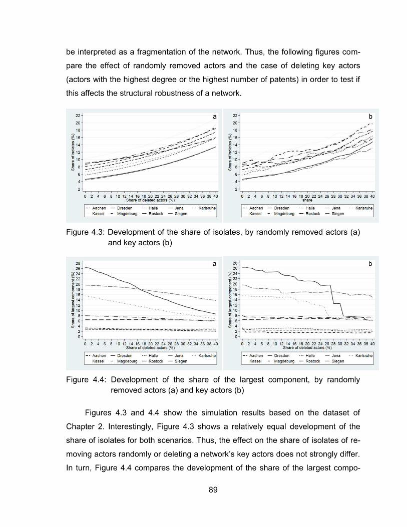
89

be interpreted as a fragmentation of the network. Thus, the following figures com-

pare the effect of randomly removed actors and the case of deleting key actors

(actors with the highest degree or the highest number of patents) in order to test if

this affects the structural robustness of a network.

Figure 4.3: Development of the share of isolates, by randomly removed actors (a)

and key actors (b)

Figure 4.4: Development of the share of the largest component, by randomly

removed actors (a) and key actors (b)

Figures 4.3 and 4.4 show the simulation results based on the dataset of

Chapter 2. Interestingly, Figure 4.3 shows a relatively equal development of the

share of isolates for both scenarios. Thus, the effect on the share of isolates of re-

moving actors randomly or deleting a network’s key actors does not strongly differ.

In turn, Figure 4.4 compares the development of the share of the largest compo-

90

nent in case of randomly omitting nodes or in case of deleting a network’s key ac-

tors. The results reveal a stronger and continuous decrease of the share of the

largest component by randomly omitted nodes and a relatively robustness, fol-

lowed by a late collapse of the network if key actors are deleted. This is surprising,

since it contradicts the findings from the literature. However, Albert, Jeong and

Barabási (2000) use average path lengths as an indicator of performance. Chapter

2 demonstrates that this measure is inappropriate for the evaluation of inventor

networks’ performance.

Since the previous chapter shows that also the assumed preferential attach-

ment mechanism applies only for a small part of an actor’s behavior, structural ro-

bustness is likely driven by other factors. For the moment, it seems that it is un-

clear whether the position an actor holds in a network, or the embeddedness of an

actor within a network is the critical factor giving the network structural robustness.

4.3 General thoughts about R&D networks, innovations and potential consequence

The creation and diffusion of knowledge often takes place within regional R&D

networks (Diez, 2000; Howells, 2002; Jackson, 2008). The collaboration in such

networks is based on the division of labor, meaning that actors with certain talents,

skills and individual knowledge stocks interact there. Even if these actors are highly

heterogeneous, they have one thing in common: they are above average educat-

ed, especially in case of R&D networks (see, Capaldo, 2007; Schilling & Phelps,

2007; Phelps, 2010). According to the current literature (see, Wuchty, Jones & Uz-

zi, 2007; Jones, Wuchty, Uzzi, 2008), collaborative activities are becoming more

and more important. Thus, it is not surprising that most R&D networks seem to

grow continuously (see, Table 2.A3; Powell et al., 2005; Wuchty, Jones & Uzzi,

2007), indicating an increasing share of network actors in a respective region. Fur-

ther, based on the concept of human capital, previous investments in education

and training increase individuals’ future financial returns (Blundell et al., 1999; Ac-

emoglu & Autor, 2011). Consequently, the share of highly educated and well-paid

individuals increases with the network size. If the share of those individuals in-

91

creases out of proportion to the share of semi- and low-skilled workers, income

inequality should increase due to a concentration at the top of the income distribu-

tion.

Networks that are an important part of the innovation process (Bercovitz &

Feldman, 2011) facilitate not only the creation and diffusion of new knowledge, but

also the production of innovations. Such regional innovative activities can lead to

new markets (Ahuja, 2000), foster a region’s productivity (Howells, 2002; Huergo &

Jaumandreu, 2004), or enhance an individual’s well-being (Howells, 2002). In spite

of these positive ramifications of innovations, they can also have negative effects

for some population segments. In light of the skill-biased technology change ap-

proach, innovations or new technologies often replace routine work that is primarily

carried out by low-skilled workers. Thus, it is technically feasible that jobs involving

routinized tasks could be replaced by the use of machines. It so happens that

mostly manual tasks, such as work on the assembly line, fall into this category as

they are characterized as repetitive. By contrast, it is rather difficult to replace

workers in ‘non-routine’ occupations, because it is almost impossible to set-up well-

defined rules according to which machines can be programmed. Moreover, new

technologies require individuals that are able to understand and use them. The

demand and wages of such skilled individuals will tend to increase, while the in-

come of low-skilled individuals will decrease. Both developments lead to an in-

creasing income inequality in the respective region.

Having discussed the positive effects of networks and innovations in Chapter

1, Part II of this thesis addresses their reverse effect for some population seg-

ments. While there may be other reverse effects, Part II focuses on the causes of

income inequality and its potential consequences. Specifically, the focuses lies on

the SBTC approach to investigate the causes of income inequality, and Becker’s

(1968) “Economic theory of crime” approach to examine the relationship between

income inequality and an increase in regional crime rates.

92

Part II Innovations, income inequality and crime

‘No society can surely be flourishing and happy, of which the far greater part of the

members are poor and miserable.’

Adam Smith (1778)

93

Chapter 5

Causes and consequences of income inequality: The role of

innovation

Abstract:35 We investigate the lead-lag relationship between innovative activities

and income inequality for 402 German districts over the period 1992-2012. The

results obtained from a Vector autoregression (VAR) model with implemented first-

order differentiation show that an increase in innovative activities is associated with

a subsequent increase in income inequality. Additionally, an increasingly asymmet-

ric wage dispersion is associated with decreasing innovation activities within a re-

gion. Based on these results we draw conclusions for policy and further research.

35 This chapter is based on the joint work with Maximilian Göthner. Both authors are indebted to

Michael Fritsch, Oliver Kirchkamp and Michael Wyrwich for helpful comments.

94

5.1 Introduction

Income inequality has increased in most OECD countries over the past two to

three decades (OECD, 2014). For instance, in the US the income share of the top

1% has soared, rising from earning on average 27 times more than the bottom 1%

in 1980s to 81 times more in 2014. The top 1% income share is now almost twice

as large as the bottom 50% share. There has been close to zero growth for the

working population in the bottom 50% of the income distribution since 1980 (Piket-

ty, Saez & Zucman, 2016). Researchers have attributed this development to a mul-

titude of factors, including trade and financial globalization (e.g. Feenstra & Han-

son, 1996), changes in labor market institutions (e.g. Wilkinson & Pickett, 2010),

educational attainment (e.g. De Gregorio & Lee, 2002), and technological change

(e.g. Acemoglu, 2002; Card & DiNardo, 2002; Jaumotte, Lall & Papageorgiou,

2013).

This study draws from the latter stream of literature and investigates the

causal link between income inequality and innovation. Innovation is a fundamental

driver of economic growth (Feldman, 1999; Mokyr, 2005), for example, by creating

new markets/products (Ahuja, 2000), improving productivity of firms (Huergo &

Jaumandreu, 2002) and even enhancing individual well-being (Howells, 2002).

However, innovations might not necessarily be beneficial for all segments of socie-

ty. New technological developments can lead to the replacement of routinized jobs

that are mostly occupied by low-skilled workers. Consequently, demand for these

workers decreases, leading to decreasing income levels. Further, benefiting from

new technological developments, particularly information and communication tech-

nologies (ICTs) requires skills and capabilities to be able to understand and use

these new technologies. The result is a skill premium provided by the labor market.

Both developments - the decreasing demand for low-skilled workers and the in-

creasing demand for high-skilled workers due to technological progress - have led

to a significant widening of the gap in wages between those at the top of the skill

distribution and those at the bottom (Autor, Katz & Kearney, 2008; Goos, Manning

& Salmons, 2009). Income inequality, in turn, is associated with a number of social

95

and economic issues (Wilkinson & Pickett, 2007), such as social segregation

(Alesion, Di Tella & MacCulloch, 2004), lower quality of social relationships (Uslan-

er, 2002), mortality (Neckerman & Torche, 2007), violence and crime (Kelly, 2007;

Goldstone et al., 2009).

However, perfect equality may not be desirable as well. Financial gain is im-

portant to spur risky entrepreneurial and innovation activity (Milanovic, 2011; Aghi-

on et al., 2015). Thus, a certain level of income inequality could be beneficial to

stimulate innovative activities. Overall, innovations can trigger income inequality

(Lee & Rodríguez-Pose, 2013) and, in turn, income inequality seems to incentivize

R&D investments (Milanovic, 2011). The former line of reasoning - income ine-

quality relates to innovation - is supported by an emerging stream of literature (see,

Acemoglu, Aghion & Violante, 2000; Breau, 2007; Lee, 2011; Van Reenen, 2011;

Lee & Rodríguez-Pose, 2013). However, the effect of income inequality on regional

innovative activities is rather neglected by previous research. Thus, important

questions remain unanswered. For example, do regions characterized by higher

levels of innovation activity also exhibit a larger dispersion of wages among the

workforce? Or does causality run in the opposite direction, i.e. does the level of

income inequality determine innovative output?

This chapter aims to shed light on these issues by exploring the co-evolution

of income inequality and innovation activity at the regional level. We use a unique

dataset, tracking 402 German districts over the period 1992-2012, to gain new in-

sights into the dynamics of the innovation-inequality link. In order to exploit our da-

taset properly, Vector autoregression (VAR) model with implemented first-order

differentiation are utilized.

Our key contribution to the literature is that, as far as we are aware, the un-

derlying paper of this chapter is the first study to present systematic data that offers

support for the interrelatedness of processes regarding the development of innova-

tion and unequal income distributions. With our regional-level analysis we further

add to existing studies that largely focus on single metropolitan areas (Breau,

Kogler & Bolton, 2014; Aghion et al., 2015) or study inequalities across countries

96

(for an overview see, e.g. Piketty & Saez, 2006), thereby neglecting important re-

gional differences, for example, regarding local labor markets, consumption costs

or housing prices. Finally, most studies use data for the US, Canada or UK

(Kopczuk & Saez, 2004; Atkinson, 2006; Breau, Kogler & Bolton, 2014), which are

countries characterized by rather high levels of income inequality. Investigating the

link between innovation and inequality in Germany thus seems particularly promis-

ing as our results could help evaluate the generalizability of previous findings to

countries with moderate levels of income inequality.

We provide evidence for the co-evolutionary dynamics underlying the devel-

opment of innovation and income inequality. In particular, we find that an increase

in patenting activity in the past is associated with an increasingly asymmetric in-

come distribution. At the same time, however, an increasing level of regional in-

come inequality seems to be followed by a decrease in innovation output. Taking

together, this study suggests that innovation can be both cause and consequence

of regional income inequality.

The rest of the paper is organized as follows. In the next section (Section

5.2), we outline the background literature on which our study is based, pointing out

possible causal connections between innovation and income inequality. Section

5.3 introduces the dataset, methodology and measurement. Section 5.4 presents

the empirical results. The paper concludes with a discussion of our results and

their implications for future research (Section 5.5).

5.2 Innovations and income inequality from a regional perspective

5.2.1 Innovation as a determinant of income inequality

The skill-biased technological change (SBTC) hypothesis is a widely invoked ap-

proach to understand the relationship between innovation and income inequality.

The general idea of SBTC is that technological change, particularly advancements

in information and communication technologies (ICTs), does not benefit all workers

equally. It is assumed that the diffusion of new ICTs in recent decades has led to

an increase in the demand for highly-skilled (i.e. college-educated) but not for low-

97

skilled (i.e. non-college educated) workers and to higher wages for highly-

educated, highly-skilled workers whose competences are complementary to com-

puter technologies (Acemoglu, 2002; Card & DiNardo, 2002; Goldin & Katz, 2009).

As a consequence, both the high-skill/low-skill employment ratio and the wage

premium associated with high skills are expected to increase, and are considered

as the main drivers of higher income inequality. Consistent with the SBTC hypoth-

esis, empirical research has repeatedly linked computerization of workplaces and

skill-based inequality. Employing U.S. microdata for the years 1984 and 1989,

Krueger (1993) showed that highly educated workers are more likely to work with

computers and that using a computer on the job raised a worker’s wage by 10 to

15 percent. Similarly, positive returns to on-the-job computer use were found for

Germany (DiNardo & Pischke, 1997) and France (Entorf, Gollcar & Kramraz,

1999). Establishment- and industry-level data further revealed an increasing share

of skilled workforce and a decreasing share of unskilled workforce overtime pre-

ceded by investments in new ICTs (e.g. Berman, Bound & Griliches, 1994; Dunne

& Schmitz, 1995).

A more recent stream of literature proposed a ‘task-based’ version of the

SBTC, emphasizing the role of the content of different job tasks (rather than the

skilled/unskilled dichotomy) in explaining inequality patterns in wages (Autor, Levy,

& Murnane, 2003; Autor, Katz, & Kearney, 2008; Acemoglu & Autor, 2011). The

task-based framework delineates two broad sets of tasks according to the extent of

their vulnerability of computerization: routine and non-routine tasks. Due to the re-

petitive and rule-based nature of routine tasks (e.g. bookkeeping, cashiering, cal-

culating), they can easily be expressed in computer code. Thus, jobs intensive in

routine tasks are highly prone to computer substitution. Non-routine tasks comprise

a wide range of abstract and manual tasks. Non-routine abstract tasks (e.g. man-

aging, advising, designing, programming) require creativity, persuasion, and prob-

lem-solving skills. Workers performing these tasks usually benefit from ICTs as

computer technology complements their high skills, hence, increasing their produc-

tivity. Non-routine manual tasks (e.g. cleaning, servicing, car driving) generally re-

quire few cognitive skills and lower levels of education, but require more flexibility

98

than computers can currently offer and thus cannot (yet) be automated. The impli-

cation of the task-based approach is that technological change contributes to in-

creasing income inequality by causing the labor market to polarize (Spitz-Oener,

2008; Autor & Dorn, 2013; Goos, Manning & Salomons, 2014). The phenomenon

of job polarization refers to the shifting of employment away from jobs in the middle

of the occupational skill distribution towards both the high- and low-skill tails of the

distribution. That is, there has been an increase in highly paid, high-skilled jobs

performing non-routine abstract tasks on the one hand, and on the other, there is a

growing share of low-pay, low-skill jobs that comprise non-routine manual tasks. By

contrast, routine jobs in the middle of the pay/skill distribution are increasingly au-

tomated away. In various industrialized economies, these changes in the composi-

tion of the workforce have led to a significant widening of the gap in wages be-

tween those at the top of the skill distribution and those at the bottom (Autor et al.,

2008; Goos et al., 2009).

5.2.2 Income inequality as a determinant of innovation

There might also be a reverse causality in the relationship between innovation and

income inequality. Accordingly, a more unequal (more equal) level of income distri-

bution can discourage (encourage) people from engaging in innovative activities,

hence, decreasing (increasing) the level of innovation (Weinhold & Nair-Reichert,

2009). The basic assumption is that the highly-skilled and highly paid workers de-

mand high-quality products whilst low-skilled workers will only be able to afford

goods of a basic quality. These singular tastes of affluent individuals could foster

research in new technological areas not only because of the consumption decision

but also due to the fact that wealthy people might as well financially support certain

research projects (Zweimüller, 2000). Assuming a rather unequal income distribu-

tion, it might also be the case that wealth is concentrated among only a few people

with an extremely homogeneous demand for goods. A situation like this will lead to

a decline in the innovation level as the economic incentive to engage in innovative

activities is simply missing. The opposite will occur if the income distribution is

more equal and individuals exhibit a diverse demand. This in turn allows firms to

99

exploit new market opportunities and stimulates their engagement in the creation of

new innovative products and services. Under special circumstances in which peo-

ple try to identify and distinguish themselves through the consumption of certain

goods, this process might even be accelerated as the demand for exclusive niche

products rises. Companies will then be challenged to serve the respective markets

by providing new and innovative products (Zweimüller, 2000; Lee & Rodríguez-

Pose, 2013).

5.2.3 The innovation-inequality link from a regional perspective

This study takes a regional perspective on the link between innovation and income

inequality. Looking at inequalities within the regions of a country is important for

several reasons. First, rather than being evenly distributed across space, innova-

tion activity tends to be clustered. Studies investigating regional patterns of patent

citations show that especially cities and regions are hotbeds for innovation (Jaffe,

Trajtenberg & Henderson, 1993). The same holds for income inequality (Ambrosio

& Frick, 2007). Thus, regions are highly heterogeneous regarding the distribution of

both variables of interest. Second, since income inequality is a relative measure,

meaning that individuals compare themselves with their social environment; re-

gional characteristics play a crucial role. Regions differ regarding the efficiency of

their labor market, consumption cost or housing prices. An analysis aggregated at

a higher geographical level neglects these regional differences. Finally, effective

regional policies to tackle income inequality need to take care of regional idiosyn-

crasies.

There is a small but growing empirical literature that examines the relation-

ship between innovation and income distribution at a regional level. One of the first

studies was carried out by Donegan and Lowe (2008) who identified determinants

of income inequality by means of a cross-sectional OLS model using data on 277

Metropolitan statistical areas in the US. In order to assess the contribution of

SBTC, the authors adopted the Milken Institute’s Tech-Pole variable (i.e. a meas-

ure of high-tech industrial output), developed by Florida (2002), and proved a sig-

100

nificant and positive correlation between innovation and the level of income ine-

quality.

Lee (2011) examined the innovation-inequality link in a panel of 90 European

regions over the period 1996-2001, using European Community Household Panel

data. Two indicators are used to assess the level of regional innovation activity, the

number of patent applications and employment in knowledge-based industries.

Fixed effects regressions reveal that higher levels of regional innovation lead to

higher levels of regional wage dispersion. This relationship is particularly strong for

the regional patent output, while there is also a positive effect for employment in

knowledge-intensive financial services. In any case, the results are very sensitive

to diverse inequality measurements.

Building on the previous study, Lee and Rodríguez-Pose (2013) used the

IPUMS Current Population Survey to add data on 70 US cities. The positive inno-

vation-inequality link could be confirmed for the European regions. For US cities it

is only patenting activity in the ICT sector that seems to impact on the level of in-

come inequality, i.e. the higher the number of ICT patents, the more asymmetric

the income distribution. Differences in the results for European Regions and US

cities are attributed to prevailing differences in the labor market regulations and

migration structures.

Breau, Kogler and Bolton (2014) investigate the empirical link between inno-

vation and income inequality across 85 metropolitan areas in Canada. Exploiting

Canadian census data and patent data provided by the US Patent Trademark Of-

fice for the years 1996-2006, they show that innovative cities exhibit a larger distri-

bution of earnings. Their findings are robust with respect to different inequality

measurements and various control variables.

101

5.3 Data, indicators and method

5.3.1 Data

In our analysis, we test the relationship between innovation activities and income

inequality across 402 German districts. All information concerning local employ-

ment and wages is obtained from the Sample of Integrated Labor Market Biog-

raphies Regional File (SIAB-R), a two percent random sample drawn from the full

population of the Integrated Employment Biographies, provided by the Institute of

Employment Research at the German Federal Employment Agency (IAB, Nurem-

berg). This highly reliable administrative dataset comprises marginal, part-time and

regular employees as well as job searchers and benefit recipients covering the

years 1975 to 2014 (for details, see vom Berge, Burghardt & Trenkle, 2013). It pro-

vides detailed information on daily wages for employees subject to social security

contributions (wages of civil servants and self-employed workers are not included),

as well as information on occupation, industry affiliation, workplace location and

demographic information on age, gender, nationality and educational attainment.

We complement the SIAB-R data with patent data obtained from the Europe-

an Patent Office (EPO) and the Patent Cooperation Treaty (PCT) to measure re-

gional innovation activities. Patents provide information about the applicant, the

inventors and the scope of knowledge (IPC classes) and are assigned to regions

based on the information about the residence of the inventor. Following Jaffe, Tra-

jtenberg and Henderson (1993), patent counts are a reliable proxy for regional lev-

els of innovation activities.

To investigate the effect of innovation on inequality across space, we inte-

grate several regional control variables to test for regional differences. These were

provided by the Federal Statistical Office and the IAB. Overall, all variables in our

dataset relate to the district-level over a time span of 21 years, covering the years

1992 to 2012.

102

5.3.2 Indicators

Income inequality

Income inequality can be separated into several different dimensions. A general

distinction can be made between functional inequality - referring to the division of

income between capital rents and labor remuneration in an economy, and personal

inequality - based on income differences across households, regardless of the na-

ture of their assets/holdings (Antonelli & Gehringer, 2017). The concept of personal

inequality can be further refined into income inequality, where income refers both

to wage income and to other income sources such as rents, and wage inequality

(for a more precise discussion of the typology see e.g. Aghion, Howitt, & Violante,

2002). This paper follows the latter conception and defines income inequality as

the variation in the distribution of wage income among the working population lo-

cated in a specific geographical area.

One of the most established measures of income inequality is the Gini coeffi-

cient (see, e.g. Lee, 2011; Lee & Rodríguez-Pose, 2013; Breau, Kogler & Bolton,

2014), in particular because of its robustness (Jenkins, 1991, 2009). Since the SI-

AB-R data is top-coded, we do not have sufficient information on the upper part of

the income distribution to use the Gini coefficient as indicator of income inequality

in our study. Instead, we compute the distance (difference) between the median

and the bottom 10% of the income distribution as our inequality measure (see, Ehr-

lich, 1973). The higher the value, the larger the difference between the median in-

come and the lowest income levels in a region, and, hence, the higher is regional

income inequality. Our inequality measure is based on periodically earnings ob-

tained by individuals during the respective year within their region of residence. To

ensure validity, the sample is restricted to people aged 16 and older.

Innovation activity

To measure innovative activities in regions, we use the number of patent applica-

tions divided by 100,000 inhabitants (Lee, 2011; Lee & Rodríguez-Pose, 2013).

Patents are a form of intellectual property rights (IPR) used to protect inventions

103

developed by firms, institutions or individuals. Against this background, they can be

interpreted as an indicator for inventive technologies with a marketable potential.

Patents provide information on the technological content and the geographical lo-

cation of the invention process which allows assessing the innovativeness of a re-

gion, the mobility of an inventor and the related diffusion of knowledge. Thus, it is a

measure of the impact of one invention on the development of another one (Smith,

2006).

Control variables

To provide valid inferences about the actual impact of innovation on inequality of

income and to control for the influence of other factors, it is necessary to set up a

multidimensional model which accounts for its multifarious nature. Therefore, we

include economic, social and spatial variables. Economic variables are important

since the economic development of a region or its level of unemployment can have

a strong impact on the dependent inequality measure (demand-side factors). So-

cial and demographic factors comprising information on the regional age structure,

education level, migration level and gender are known as supply-side factors.

5.3.3 Method

The main focus of this study is on the observation of the co-evolutionary dynamics

between innovation and income inequality. As explained above, innovative activi-

ties may increase income inequality due to a growing demand for and income of

skilled workers, whereas the demand for low-skilled workers decreases for two po-

tential reasons. First, mainly routinized jobs are performed by low-skilled workers

that can be more easily replaced by new technologies. Second, the introduction of

new technologies requires certain skills that are only insufficiently available for low-

skilled workers. Simultaneously, it could be that regions which already attracted

highly-skilled and well-paid workers show higher levels of income inequality, while

also achieving higher innovative output. In turn, higher levels of income inequality

could as well decrease the level of innovative activities.

104

In recognition of the complex and interrelated nature of the development of

patenting activity and income inequality, we employ a vector autoregression (VAR)

model with an implemented first-order differentiation (see, Thurik, Carree & Van

Stel, 2008). The VAR model consists of two regression equations with the change

in the regional patent rate (𝑃) and the change in income inequality (𝐼) as depend-

ent variables. We also include control variables and multiple time lags (see, Stock

& Watson, 2003). The model reads as follows:

𝐼𝑖𝑡 − 𝐼𝑖,𝑡−𝑇 = 𝛼 + ∑ 𝜌𝑙(𝑃𝑖,𝑡−𝑙𝑇 − 𝑃𝑖,𝑡−(𝑙+1)𝑇)𝐿𝑙=1 + ∑ 𝜇𝑙(𝐼𝑖,𝑡−𝑙𝑇 − 𝐼𝑖,𝑡−(𝑙+1)𝑇) + ∑ 𝜎(𝐶𝑖,𝑡−𝑙𝑇 −𝐿

𝑙=1𝐿𝑙=1

𝐶𝑖,𝑡−(𝑙+1)𝑇) + ∑ 𝜏𝑡𝐷𝑡 + 𝑢1𝑖𝑡𝑇𝑡=1 (1)

𝑃𝑖𝑡 − 𝑃𝑖,𝑡−𝑇 = 𝛼 + ∑ 𝛽𝑙(𝐼𝑖𝑡−𝑙𝑇 − 𝐼𝑖𝑡−(𝑙+1)𝑇)𝐿𝑙=1 + ∑ 𝛾𝑙(𝑃𝑖𝑡−𝑙𝑇 − 𝑃𝑖𝑡−(𝑙+1)𝑇) + ∑ 𝜎(𝐶𝐼𝑖,𝑡−𝑙𝑇 −𝐿

𝑙=1𝐿𝑙=1

𝐶𝑖,𝑡−(𝑙+1)𝑇) + ∑ 𝛿𝑡𝐷𝑡 + 𝑢2𝑖𝑡𝑇𝑡=1 (2)

where 𝑖 is a region index, 𝑇 is the time span in years, 𝐿 is the number of time lags

included, 𝐶 are control variables, 𝐷𝑡 are time dummies and 𝑢1𝑖𝑡 and 𝑢2𝑖𝑡 are possi-

bly correlated error terms.

Using the panel data set for 402 German regions between the years 1992 to

2012, we consider year-by-year changes for all study variables. Furthermore, we

test for the number of time lags by computing several information criteria as well as

a sequence of likelihood ratio (LR) tests (Lütkepohl, 2005). Including more lags

seems to be appropriate, since the effect of innovations does not occur immediate-

ly. Following the LR test, we include eight one-year lags.

5.4 Results

5.4.1 Descriptive results

An overview and brief description of all study variables is provided in Table 5.A1.

As can be seen in table 5.A2, income inequality in Germany has grown by 8.2%

since the early 1990s. This development is in line with studies suggesting that the

German labor market is subject to a trend of continuous wage dispersion (Ger-

nandt & Pfeiffer, 2007). In turn, regional innovation activities increased by around

105

12.1%. Table 5.A3 presents the rank correlations between income inequality, pa-

tent rate and control variables. As expected, the regional patent rate is significantly

and positively correlated with local income inequality.36

5.4.2 Regression results

Table 5.1 presents our findings on the relationship between innovation activity and

the local wage distribution. In the left column, the dependent variable is the change

in income inequality. As explanatory variables, the two VAR series for income ine-

quality and innovation (eight lags are included) and also control variables are in-

cluded. The right column shows the regression with the change in patent rate as

the dependent variable.

We find that changes in the patent rate Granger-cause changes in income in-

equality (see left column in Table 5.1). Clearly, new technological developments

require some time to be implemented and spread in the market. Interestingly, the

effect disappears after four years and appears again in the fifth lag. Further, the

coefficient is largest for the seventh lag, indicating that the effect of innovative ac-

tivities on income inequality requires some time to unfold its potential. After the ef-

fect sets in the second lag, the value of the coefficient decreases initially. This is

not surprising, as workers - even with lower skill levels - seem to learn and use

new technologies over time. For instance, after the introduction of computer tech-

nology in the 1980s (see, Krueger, 1993; DiNardo & Pischke, 1997), income of

low-skilled workers decreased because they did not benefit from computers in the

workplace to the same extent as highly skilled workers. Overall, we can accept the

hypnotized relationship that innovative activities Granger-cause income inequality

at the regional level.

36 Table 5.A4 in the Appendix provides the correlation matrix for all used variables.

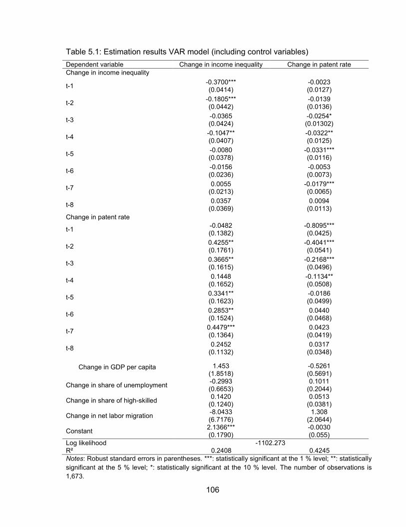
106

Table 5.1: Estimation results VAR model (including control variables) Dependent variable Change in income inequality Change in patent rate Change in income inequality t-1 -0.3700***

(0.0414) -0.0023 (0.0127)

t-2 -0.1805*** (0.0442)

-0.0139 (0.0136)

t-3 -0.0365 (0.0424)

-0.0254* (0.01302)

t-4 -0.1047** (0.0407)

-0.0322** (0.0125)

t-5 -0.0080 (0.0378)

-0.0331*** (0.0116)

t-6 -0.0156 (0.0236)

-0.0053 (0.0073)

t-7 0.0055 (0.0213)

-0.0179*** (0.0065)

t-8 0.0357 (0.0369)

0.0094 (0.0113)

Change in patent rate

t-1 -0.0482 (0.1382)

-0.8095*** (0.0425)

t-2 0.4255** (0.1761)

-0.4041*** (0.0541)

t-3 0.3665** (0.1615)

-0.2168*** (0.0496)

t-4 0.1448 (0.1652)

-0.1134** (0.0508)

t-5 0.3341** (0.1623)

-0.0186 (0.0499)

t-6 0.2853** (0.1524)

0.0440 (0.0468)

t-7 0.4479*** (0.1364)

0.0423 (0.0419)

t-8 0.2452 (0.1132)

0.0317 (0.0348)

Change in GDP per capita 1.453 (1.8518)

-0.5261 (0.5691)

Change in share of unemployment -0.2993 (0.6653)

0.1011 (0.2044)

Change in share of high-skilled 0.1420 (0.1240)

0.0513 (0.0381)

Change in net labor migration -8.0433 (6.7176)

1.308 (2.0644)

Constant 2.1366*** (0.1790)

-0.0030 (0.055)

Log likelihood -1102.273 R² 0.2408 0.4245 Notes: Robust standard errors in parentheses. ***: statistically significant at the 1 % level; **: statistically significant at the 5 % level; *: statistically significant at the 10 % level. The number of observations is 1,673.

107

Finally, we test whether regions that previously attracted highly skilled work-

ers and, thus, are characterized by higher levels of income inequality also show

higher levels of innovative output. In this sense, income inequality is a result of the

innovativeness of a region and should be related to increasing innovative activities

in the future (see also, Jaumotte, Lall & Papageorgiou, 2013). However, the empir-

ical results do not seem to support this view. We find that increasing income ine-

quality Granger-causes innovative activities to decrease (see the right column in

Table 5.1). We interpret this result in the way that persistent or long-lasting income

inequality hampers the incentive to rewards additional effort, for instance, in the

form of additional income. Thus, the initial consideration that regions that already

attracted an over proportional share of highly-skilled individuals and therefore in-

crease both innovative output and income inequality is not supported by the data.

As a robustness check, we run the Granger causality Wald test to control for

the Granger causality of each variable in the VAR individually, followed by as-

sessing the Granger causality of all variables jointly (see, Table 5.A5). For both

cases, the variables are statistical significant, indicating that innovative activities

Granger-cause income inequality and vice versa.

5.5 Discussion and conclusion

This paper aimed at investigating co-evolutionary dynamics, that is, the lead–lag

relationship between the change in the patent rate and income inequality for Ger-

man districts over a period of 21 years. Different regional characteristics were addi-

tionally controlled for. Because of the complex and endogenous nature of the re-

spective variables, VAR model with an implemented first-order differentiation were

applied. Our analysis provided deeper insights into the development of regions

over time, i.e. the interrelated processes regarding regional innovation and wage

distribution. To know about these processes is a prerequisite for designing appro-

priate regional innovation policies as well as measures to alleviate income inequali-

ty.

108

We found that changes in the regional patent rate Granger-cause income in-

equality to increase after two years. This result is in line with a number of theoreti-

cal and empirical studies that positively link innovation and earnings inequality

(see, Kuznets, 1955; Van Reenen, 1996; Acemoglu, 2002; Autor & Dorn, 2009;

Glaeser, Resseger & Tobio, 2009; Acemoglu & Autor, 2011). Further, our empiri-

cal model obtain by testing the potential reverse effect that changes in income ine-

quality Granger-cause changes in innovative activities to decrease after three

years. This finding was surprising since we expect that regions that already charac-

terized by both, higher shares of highly skilled individuals and levels of income ine-

quality, trigger innovative activities. However, the VAR model indicates that in-

creasing, respectively slightly longer lasting income inequality might have de-

creased the incentive to innovate in the long-run.

Since income inequality is associated with several (socio-) economic issues

(see, Neckerman & Torch, 2007), policy should try to reduce income inequality.

While there does not seem to be a one-size-fits-all policy approach to tackle in-

come inequality, implementing a taxation system that relieves low and middle class

incomes could be one appropriate solution to reduce disproportional disadvantages

for specific parts of society (Dabla-Norris et al., 2015). Following the IMF (2014),

fiscal policy that already plays a significance role in terms of reducing income ine-

quality should also focus on making existing redistribution more efficient. Such pol-

icies could be more strongly linked with personal wealth, emphasize larger pro-

gressive income taxation and focus on removing opportunities to evade taxes.

Given that low-skilled workers are more likely to be disadvantaged by techno-

logical change, policies to increase skill levels, such as comprehensive labor mar-

ket programs educating low-skilled worker on new technologies in their work envi-

ronment, could be another important way to tackle income inequality (Dabla-Norris

et al., 2015). From the literature on Active Labor Market Policies we learned that

self-employment is a good way to overcome labor market obstacles and to secure

the own standard of living (Caliendo et al., 2015). Thus, besides redistribution poli-

109

cies, becoming an entrepreneur could help reduce income inequality. However,

this remains to be an important topic for further research.

Finally, as with all studies, ours has several limitations. Our measure of in-

come inequality is derived from data on pre-tax earnings. Therefore, we do not

take account of the redistributive effects of tax transfer policies in Germany. More-

over, we use the regional patenting rate to measure innovation activity. This might

render some well-known limitations to our study (see, Griliches, 1994, for an ex-

tended discussion). Patent data might underestimate innovative performance as

not all patentable inventions are patented. Firms may use other strategies to ap-

propriate the benefits of their R&D efforts, such as secrecy or lead time (Arundel,

2001). Reasons for not patenting may also include the lengthy application process

relative to the duration of the innovation cycle, the perceived ease of inventing

around a patent, and patenting costs (Cohen, Nelson & Walsh, 2000). Also, only

the result of successful innovative processes can become patent. Hence, all inno-

vative processes which do not lead to a patentable result are not taken into ac-

count.

110

5.8 Appendix

Table 5.A1: Description of the study variables

Definition of variables

Income inequality Distance between median gross income and gross income of the lower 10% of the income distribution.

Patent rate Number of patent applications per in 100.000 inhabitants.

GDP Gross domestic product per capita.

Share of unemployed Share of individuals that have no job and aged above 16 years.

Share of part-time employees Share of individuals that do not work 40 hours a week.

Net labor migration Individuals that move because of their job opportunities. Notes: All variables are calculated as change variables with a one-year lag. All explanatory varia-bles are in logarithm form.

Table 5.A2: Descriptive statistic of the study variables

Variables Mean Median Minimum Maximum Standard deviation

Growth rate (%)

Income inequality 0.3715 0.4132 0.2865 0.4958 0.0389 8,24

Patent rate 0.0042 0.0015 0.0000 0.1109 0.0079 12,10

GDP 0.0469 0.0266 0.0057 1.8996 0.1025 64.17

Unemployment 0.0930 0.0770 0.0394 0.2187 0.0446 -36,22

High-skilled worker 0.1740 0.1302 0.0654 0.4900 0.3086 29.71

Net labor migration 0.0046 0.0047 -0.0134 0.0284 0.0047 10.02

111

Table 5.A3: Spearman rank correlation

1 2 3 4 5 6

1 Income inequality 1

2 Patent rate 0.123*** 1

3 GDP per capita 0.161*** 0.107** 1

4 Share of unemploy-ment -0.008 0.063 -0.116*** 1

5 Share high skilled labor 0.282*** 0.162*** 0.460*** -0.081* 1

6 Net labor migration -0.033 0.055 0.080* 0.022 -0.094* 1

Table 5.A4: Correlation matrix

1 2 3 4 5 6

1 Income inequality 1

2 Patent rate 0.0631 1

3 GDP per capita 0.1550 0.0016 1

4 Share of unemployment -0.0315 0.0353 -0.1392 1

5 Share high skilled labor 0.2807 0.0754 0.4248 -0.0865 1

6 Net labor migration -0.0531 0.0323 0.0939 0.0332 -0.0540 1

Table 5.A5: Granger causality test

Equation Excluded Chi² p-value

Income inequality Patent rate 21.735 0.005 Income inequality All 21.735 0.005

Patent rate Income inequality 24.378 0.002 Patent rate All 24.378 0.002

112

Chapter 6

Regional income inequality and local crime rates

Abstract:37 We investigate the relation between income inequality and several

categories of crime with a special focus on regional differences, such as differ-

ences between West-East and urbanization regions in Germany. The empirical

analysis is for 289 German grown districts over a period of five years. We find a

positive and significant relation between income inequalities and property, respec-

tively pecuniary crimes in different regional settings. The effect on violent crime

was always insignificant.

37 This chapter is based on a single-authored paper with the title ‘The relationship between income

inequality and crime across space: Evidence for German districts’. I am grateful to Tina Haußen, Michael Wyrwich and Robert Gold for many helpful discussions and suggestions. Further, I would also like to thank the Federal Criminal Police Office for providing the data.

113

6.1 Crime and income inequality

Crime is a serious problem in many societies; not only because of its economic

costs (see, e.g. Anderson, 1999; Cárdenas, 2002; Powell, Manish & Nair, 2010)

but also because it undermines social values and leads to fears in the population

(Norris, Koniasty & Thompson, 1997). In economics, whether or not an individual

commits crime is modeled as a cost-benefit decision (Becker, 1968; Chiu & Mad-

den, 1998; Kelly, 2000; Lochner, 2004). The benefits comprise income derived

from crime but also the satisfaction, preferences and tastes of the criminal. The

costs, on the contrary, encompass forgone labor market earnings, the criminal

could have earned if he had not committed a crime but also the probability and se-

verity of punishment and being caught (Doyle et al., 1999). In societies with a high-

ly unequal income distribution, it is more likely for the low-income earners that the

benefits of crime exceed its costs since income losses are low but possible gains

are high (Becker, 1968). That is why a current debate in economics - just like this

chapter - is concerned with the question of whether and how rising income inequal-

ity causes an increase in crime rates (Wilkinson & Pickett, 2007, 2009).

In the present chapter, we test the relationship between income inequality

and crime for 289 German regions for several reasons. First, the current literature

that deals with this topic mainly focuses on the US (Kelly, 2000; Gould, Weinberg &

Mustard, 2002; Brush, 2007) or Great Britain (Machin, Marie & Vujic, 2011; Wu &

Wu, 2012), with either country being characterized by a high level of income ine-

quality and high crime rates. In Germany, both income inequality and crime are at

a distinctly lower level than in the USA or Great Britain. Still, a regionally different

increase in income inequality and crime rates can also be observed (see, Entorf &

Spengler, 2000; Ambrosio & Frick, 2007; PKS, 2016). Our analysis thus serves as

a robustness check to test whether the inequality-crime link assumption also holds

under these conditions.

Second, most existing studies only concentrate on large metropolitan areas

(see, e.g. Kelly, 2000) or countries as a whole (Soares, 2004; Pare & Felson,

114

2014), which neglects regional differences at the labor market as well as differ-

ences in housing prices and consumption costs – all of which influence an individ-

ual’s income (Becker, 1968), well-being (Merton, 1938; Shaw & McKay, 1942;

Runciman, 1966) and the probability to commit crime. Specifically in the German

case, some policies and institutions are implemented on a regional level and, thus,

differ between federal states (‘Länder’) (e.g. labor market policies or educational

system). Further, income inequality can lead to regional segregation and suburban-

ization (Jargowsky & Park, 2009) which is why an investigation at the regional –

not national – level is particularly important and highly interesting.

Third, particularly low chances of career advancement opportunities in Ger-

many make it difficult for individuals to increase their initial income significantly and

to leave their original position in the income distribution (path dependency), com-

pared to the US (‘American dream’; see, Olsen, Kalleberg & Nesheim, 2010). That

makes Germany, once again, highly interesting as a research case.

Finally, this chapter benefits from a rich crime dataset that allows distinguish-

ing between several categories of crime, especially for pecuniary crime. Thus,

more detailed analyses between income inequality and different categories of

crimes (mostly with a monetary incentive) are possible that can ultimately lead to a

better understanding of the relation between income inequality and crime.

In what follows, we first review the theoretical relation between income ine-

quality, and criminal activities followed by a brief literature review of current empiri-

cal results (Section 6.2). Section 6.3 introduces the spatial framework, data, indica-

tors and modelling of our empirical analysis. A brief overview about the develop-

ment of inequality and crime over time is given in Section 6.4. We then empirically

test the relation between inequality and crime in a fixed effects model to control for

within effects, followed by a spatial autocorrelation model in order to test in how far

spatial patterns exist, meaning if regional level of income inequality and crime af-

fects the levels of both variables in an adjacent region and vice versa. Further, we

use several subsamples to distinguish between East and West Germany and cities

and rural areas to test in how far regional differences influence the effect of ine-

115

quality on crime (Section 6.5). Finally, we discuss the results and draw conclusions

for further research (Section 6.6).

6.2 Income inequality and crime from a regional perspective

6.2.1 The relation between income inequality and crime

Income inequality results from the fact that individuals with different effort and

(scarce) talents and skills are remunerated differently in the market (Samuelson &

Nordhaus, 2010). A certain degree of income inequality can therefore even be ad-

vantageous, as it increases incentives to work and the intrinsic motivation to en-

gage in innovative and entrepreneurial activities – which ultimately fosters econom-

ic progress and growth (Milanovic, 2011). However, the different growth of incomes

at the lower and upper end of the income distribution may also lead to higher bene-

fits of crime exceeding its costs which should more likely applies to low-income

than high-income earners. It is therefore possible that rising income inequality

causes an increase in crime rates (Becker, 1968).

However, income inequality affects the decision to predominately commit

crime (see, e.g. Kelly, 2000; Soares, 2004; Neckerman & Torche, 2007). More

specifically, individuals calculate the expected returns from committing crime and

these returns increase with rising wage dispersion (Kelly, 2000). This relation is

predicted by three different theories: the economic theory of crime (Becker, 1968),

Merton’s (1938) Strain theory, and the Shaw and McKay’s (1942) social disorgani-

zation theory.

In the economic theory of crime (Becker, 1968) it is assumed that individuals

allocate their time based on a comparison of expected returns (costs and benefits)

from labor market and criminal activities (Kelly, 2000). For criminal activities, bene-

fits comprise income derived from crime but also the satisfaction, preferences and

tastes of the criminal. The costs, on the contrary, encompass the probability and

severity of punishment and being caught but also forgone labor market earnings,

the criminal could have earned if he had not committed a crime (Doyle et al.,

1999). Individuals at the bottom of the income distribution have lower opportunity

116

costs to commit crime because of relatively lower income losses in case of pun-

ishment. Further, criminal activity against the rich is typically more worthwhile. And

if in case of increasing income inequality the rich get richer, the attractiveness for

crime against them increases (Chiu & Madden, 1998), especially for low-income

individuals. In this way, income inequality is predicted to increase crime rates, as it

is more likely for the low-income earners that the benefits of crime exceed its costs

(Becker, 1968).

In the Strain theory, it is assumed that individuals put their success in relation

to that of their environment (Merton, 1938). The larger the gap between low- and

high-income individuals, the more strained and frustrated unsuccessful individuals

become. With this, their incentives to search by all means for compensation, also

including to commit crime, increases (see also, Runciman, 1966).

Finally, in the social disorganization theory it is assumed that economic cir-

cumstances can undermine social community behavior (Shaw & McKay, 1942).

Such a circumstance could be a high level of income inequality that, on the one

hand, triggers regional poverty due to income based social segregation (Linden &

Rockoff, 2006) and on the other hand, it decreases social affiliation to the individu-

als around (Kelly, 2000; Uslaner, 2002; Wilkinson, 2005).

The three theories complement instead of substituting each other, since each

only refers to a different facet of the determinants, by which income inequality in-

fluences crime rates. Yet, all are related to individuals’ income. While Becker’s the-

ory tries to explain the impact on pecuniary crime, the Strain and disorganization

theories focus on a broader range of categories of crime (such as aggravated as-

sault).

6.2.2 Previous empirical findings

In a number of empirical studies Becker’s economic theory of crime is tested. Dur-

ing the last decades, more and more scholars have studied the relationship be-

117

tween income inequality and crime38. Yet they do so more indirectly by observing

the effect of low incomes on criminal commitment (Ehrlich, 1973). Ehrlich (1973)

uses the fraction of individuals with a monthly wage less than the median wage in a

region as a proxy for inequality and detects a significant and positive relation be-

tween income inequality and crime. Kelly (2000) finds a significant effect on violent

crime, but not on property crime for the US. Using Swedish county data, Nilsson

(2004) detects a positive relation between income inequality and overall crime as

well as for specific categories of property crime. Saridakis (2004) investigates a

positive short-term relation between income inequality and crime and no long-run

effect, whereas Chintrakarn and Herzer (2012) find a negative long-run effect. Fa-

jnzylber, Lederman and Loyza (2002) and Choe (2008) detect only a positive effect

on robbery, but not on other types of violent crime. Many, but not all studies (see,

e.g. Fougère, Kramarz & Pouget, 2009; Pare & Felson, 2014) find that crime rates

are higher in areas with high income inequality (see, e.g. Fowles & Merva, 1996;

Fajnzylber, Lederman & Loyza, 2002; Soares, 2004). In summary, the link between

income inequality and crime is rather ambiguous.

Likewise, in the sociological literature, empirical tests of the Strain and disor-

ganization theory largely yield inconsistent findings (Kelly, 2000; Agnew 2001).

Kelly (2000) states that the Strain and disorganization theory could explain the re-

lation between income dispersion and violent crime, whereas Neumayer (2005)

has a contradictory view. Fajnzylber, Lederman and Loyza (2002) in turn, support

the assumed relation that individuals, who are negatively faced by income inequali-

ty, are searching by all means for compensation including to commit outrages.

The underlying paper differs from the existing empirical literature in a number

of ways. First, to our knowledge, most empirical studies that test the impact of ine-

quality on crime have been done for the US or Great Britain. As already mentioned,

the US and Great Britain are a special case, regarding levels of inequality, crime

and the institutional settings. Testing the same link for Germany would lead to a

robustness check for previous studies. Further, the formal and informal institutional 38 See, e.g. Grogger (1998); Levitt (1996, 1997, 1998); Tauchen, Witte and Griesinger (1994);

Freeman (1994); Ehrlich (1996, 2008); Beckett and Sasson (2003); Tonry and Farrington (2005).

118

settings strongly differ already between German regions that make them heteroge-

neous and a regional analysis necessary.39 Second, most studies focus on total,

property and violent crime only and not on individual categories. In the underlying

paper, we explicitly take into account that the effect of income inequality can

strongly differ between different categories of crime. For instance, robbery counts

as violent crime since it is highly connected with violence but it is largely based on

financial incentives. Third, how the effect varies over time is still not clear. Fourth,

we use specific data at the district level to control for economic and social circum-

stances. Further, this chapter contributes to the current discussion by providing the

first empirical analysis of the aforementioned context at the district level in Germa-

ny, that is, at a more disaggregated data level.

6.3 Data, indicators and method

6.3.1 Data

In order to test the impact of income inequality on regional crime rates, we combine

several publicly available datasets to create a rich, comprehensive database.

The aggregated crime data that all Land Offices of Criminal Investigation re-

port to the Federal Criminal Police Office is obtained from the German crime statis-

tics (‘Polizeiliche Kriminalstatistik’; PKS). For each district, the PKS yields the

number of total offenses and its sub-categories. With this, it is possible to compute

rates for property and violent crime as well as several sub-categories. We count

burglary, larceny, and auto theft as property crime, whereas violent crime compris-

es murder, manslaughter, rape, robbery, and aggravated assault40.

Data on income inequality among individuals in all German regions is ob-

tained from the Sample of Integrated Labor Market Biographies Regional File (SI-

AB-R), provided by the Research Institute of the Federal Employment Agency

39 This should also be the case for comparing large metropolitan areas in the US, since the

institutional settings differ between the different states (e.g. Californian versus Texas) and was therefore neglected.

40 Therefore, we follow Gould, Weinberg and Mustard (2002) and Kelly’s (2000) definition of property and violent crime.

119

(IAB, Nuremberg). The SIAB-R is a two-percent random sample that is drawn from

the full population of the Integrated Employment Biographies that contains the re-

quired information. This highly reliable administrative dataset comprises marginal,

part-time and regular employees as well as job searchers and benefit recipients

covering the years 1975 to 2014 (for details, see vom Berge et al., 2013). It pro-

vides detailed information on daily wages for employees subject to social security

contributions (wages of civil servants and self-employed workers are not included),

as well as information on occupation, workplace location as well as demographic

information on age, gender, nationality and educational attainment.

To investigate the effect of inequality on crime across space, we integrate

several regional variables to test for regional differences, such as city dummies,

regional levels of GDP, or the average duration of unemployed individuals (see,

Greenberg, 2001). These are provided by the Federal Statistical Office. All varia-

bles in our constructed database are reported at the district-level and cover the

years between 2004 and 2016. Unfortunately, crime data at the required regional

and comprehensive division of offenses is only provided for the years 2010 to

2016, and information on income inequality is only made available until 2014. The

constructed dataset therefore comprises the years 2010 to 2015. Table 6.A1 in the

Appendix provides a descriptive overview of all explanatory variables.

We focus on the NUTS-3 district level for several reasons: First, inequality

measures depend on an individual’s environment. Small spatial units are thus re-

quired. Second, regions within a country are highly heterogeneous. They differ not

only in terms of their labor market characteristics but also in terms of consumption

costs and housing prices. However, to obtain a sufficient number of observations

for our inequality and crime rate computation, we reduce our sample by merging

districts (regional labor markets) to obtain an appropriate number of observations

per spatial unit. This was only done if the district was too small with regard to the

number of observations or adjacent to a city. Further this procedure addresses the

problem that individuals work and live in different regions. Thus, they compare their

120

income with the income of two different environments. Nevertheless, our data set

comprises a total of 289 merged regions.

6.3.2 Method

In this paper we use a data set covering information on 289 regions over several

consecutive years, i.e. from 2010 to 2015. A fixed effects model is applied in order

to exploit the panel structure of our dataset and to control for unobserved, time-

invariant explanatory factors. However, since our dataset comprises only six years,

and since the variation in the independent variables is comparatively small, by us-

ing a fixed effects model it could be that we are leaving out much of the information

in the time-invariant part (see, e.g. Audretsch, Dohse & Niebuhr, 2015). Therefore,

using a fixed effects model could lead to an underestimation of the true effect

(Hausman & Taylor, 1981). To test whether this is problematic, we estimate both

fixed and random effects models. By running the Hausman test (Hausman, 1978),

we test which of both models is the most appropriate. The Hausman test exhibits

that the results are in favor of the fixed effects model which is why we apply this

model (Wu & Wu, 2012).

Further, we test for spatial dependency to control for dynamic interactions

and to control for unobserved heterogeneity (Anselin, 1988; Florax, Folmer & Rey,

2003). We run the modified Lagrange multiplier (LM) test, discussed in Anselin et

al. (1996), to investigate the presence or absence of spatial correlations. Applying

the robust LM test reveals that we can claim that there is no spatial error and no

spatial lag (Florax, Folmer & Rey, 2003). Consequently, our fixed effect model is

not biased due to regional dependencies or dynamic interactions between regions.

6.3.3 Indicators

Dependent variable: Crime rates

The dependent variable for our panel data models is the crime rate for each of the

289 districts. Crime rates – separated by type of offense – are given as offenses

121

over the general population (Scorzafave & Soares, 2009; Chintrakarne & Herzer,

2012; Stock & Watson, 2015).

There are several reasons to question the reliability of the crime data used.

First, measurement errors may exist since not every crime is reported to the police

and this under-reporting varies between the types of crime and district of jurisdic-

tion. Moreover, the methods of collecting and reporting data vary across the Ger-

man Federal States (see, Goud, Weinberg & Mustard, 2002; Bug & Meier, 2015).

To address this cross-district variation and the reliability issues, we follow Ehrlich’s

(1996) approach. He shows that the logarithms of the reported crime rates are pro-

portional to the true crime rates, which is why ‘[it] can be thought of as proxies for

the true variables’ (Ehrlich, 1996, p. 57). The logarithm of the crime rates is thus

used in our empirical models.

Income inequality

In most of the existing studies that deal with the relation between inequality and

crime (see, e.g. Kelly, 2000; Fajnzylber, Lederman & Loyza, 2002; Nilsson, 2004)

the Gini coefficient is used as a measure of income inequality, in particular be-

cause of its robustness (Jenkins, 1991, 2009). Since the data is top-coded, infor-

mation on the income of the richest people is missing. Accordingly, the Gini coeffi-

cient is no meaningful measure in our dataset. We therefore compute the distance

(difference) between the mean income and the 10% at the bottom of the income

distribution as our inequality measure (see, Ehrlich, 1973). The higher the value,

the greater the income differences between mean incomes and incomes at the bot-

tom of the income distribution, that is, the higher is the income inequality. Our ine-

quality measure is based on periodically earnings obtained by individuals during

the respective year within their region of residence. To ensure validity, the sample

is restricted to people aged 16 and older. We perform robustness checks with other

inequality measures such as the 90/10, 75/25 income ratio and other distance

measures.

122

Control variables: Testing for regional differences

To provide valid inferences about the actual impact of inequality on crime and to

control for the influence of other factors, it is necessary to set up a multidimension-

al model which accounts for its multifarious nature. We include economic, social

and spatial variables. Economic variables are important since the regional econom-

ic development may strongly influence criminal behavior in that region (demand-

side factors) (Gould, Weinberg & Mustard, 2002). Social and demographic factors

that comprise information on the regional age structure or the education level are

known as supply-side factors. Spatial indicators such as dummies for regional in-

come levels are included as well (see, e.g. Kelly, 2000).

6.4 Crime and inequality – General observations

Before turning to the empirical analysis and its implications (see, Section 6.5), it is

useful to have a closer look at the descriptive statistics of the dependent variables,

namely property and violent crime rates and several (sub-) categories of pecuniary

crime. According to Table 6.A1, the number of all criminal offenses has grown na-

tionwide by 6.0% over the whole period of consideration (2010-2015). Table 6.A2

provides more detailed information about the development of the total number and

shares of property and violent offenses as well as the shares of several (sub-) cat-

egories of pecuniary crime over time. From 2010 to 2015, almost half of all crimes

committed were property offences (more than 45%). The evolution of the overall

crime rate over time is similar to that of property crime. In each year of the obser-

vation period, the property crime index is dominated by larceny (83.0-86.5%)

whereas 8.7-12.0% are auto theft and 4.5-5.6% are burglary. 2.9% to 3.4% of all

crimes are violent offences. They also show a declining trend between 2010 and

2015. Violent crime is predominantly aggravated assault (69.2-72.3%) and robbery

(22.2-25.5%), while rape (3.9-4.2%), murder and manslaughter (1.1-1.2%) account

for only a small percentage of all violent crimes.

During this period, not only an increase in total crime rates can be observed,

but also large differences between the German regions. Figure 6.1, for example,

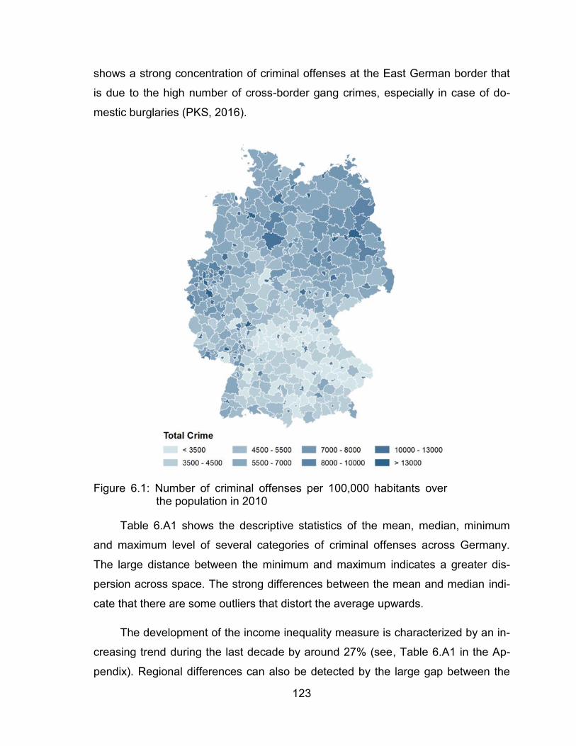
123

shows a strong concentration of criminal offenses at the East German border that

is due to the high number of cross-border gang crimes, especially in case of do-

mestic burglaries (PKS, 2016).

Figure 6.1: Number of criminal offenses per 100,000 habitants over

the population in 2010

Table 6.A1 shows the descriptive statistics of the mean, median, minimum

and maximum level of several categories of criminal offenses across Germany.

The large distance between the minimum and maximum indicates a greater dis-

persion across space. The strong differences between the mean and median indi-

cate that there are some outliers that distort the average upwards.

The development of the income inequality measure is characterized by an in-

creasing trend during the last decade by around 27% (see, Table 6.A1 in the Ap-

pendix). Regional differences can also be detected by the large gap between the

124

minimum and maximum level of income inequality, indicating regional variations

across space and time (Table 6.A1). This development is in line with studies sug-

gesting that the German labor market is subject to a trend of continuous wage dis-

persion (Gernandt & Pfeiffer, 2007).

The key question that arises is whether inequality plays a role in explaining

the rise in regional crime rates. Table 6.A3 shows rank correlations between re-

gional crime rates and the level of income inequality. We find a significant and

positive correlation between these two measures, indicating that wage dispersion

and regional crime rates may be linked. Moreover, regional crime rates are signifi-

cantly positive correlated with the average duration of unemployed individuals and

its GDP, which is in line with the results found in the related literature (see, e.g.

Freeman, 1994; Gould, Weinberg & Mustard, 2002; Andresen, 2015). The popula-

tion share of young individuals (aged between 16 and 24 years) and the share of

individuals at risk of poverty are, in turn, significantly negatively related to regional

crime rates. The negative sign is surprising, since this population segment is as-

sumed to be most responsive to commit crimes (Cohen & Land, 1987) and contra-

dicts earlier findings (Kelly, 2000). An explanation could be that many young indi-

viduals have, compared to older ones, lower incomes and therefore fewer assets.

As a consequence, regions with a high share of young aged individuals provide

lower opportunities for rewarding criminal activities. The same holds for regions

with higher shares of individuals living in poverty. The share of individuals that

graduated from college is, contradicting our expectations, statistically significantly

and positively correlated with regional crime rates. Since highly educated individu-

als are associated with higher incomes, it indicates that these regions make crime,

such as burglary, more worthwhile (Chiu & Madden, 1998). As expected, the

shares of single head households and non-qualified individuals as well show a

considerable positive and significant relation on regional crime rates. However,

rank correlations test only for pure correlations but neglect regional effects that are

particularly crucial.

125

Our first results suggest that there is a link between income inequality and

crime. However, only little is known about the strength and direction of this rela-

tionship and whether it is also present at the regional level or different regional set-

tings.

6.5 Income inequality, crime and regional differences

6.5.1 Crime and income inequality

For our empirical study, we use multivariate fixed effects models with year dum-

mies and regional income dummies to investigate the relationship between region-

al crime rates and income inequality. Regional income dummies rank regions ac-

cording to their income level, compared to the national average income. Since the

effect of income inequality on crime rates does not have to be immediate, we use a

one year lag in all models (see also, Kelly, 2000; Wu & Wu, 2012).

In all models, the logarithm form of property and violent crime rates were

used as the dependent variable (see, Ehrlich, 1973, 1996). We introduce several

control variables to check for economic and social circumstances, whereby our

main explanatory variable is income inequality. Table 6.A7 in the Appendix pro-

vides an overview on all used variables.

In Table 6.1, our results for the dependent variables property and violent

crime rates are reported. We distinguish between the two, because property crime

seems to be more driven by financial incentives (Becker, 1968), whereas violent

crime seems to be triggered by search for compensation of individuals at the bot-

tom of the income distribution by all means, including to commit outrages (Fajnzyl-

ber, Lederman & Loayza, 2002). Indeed, we find a significant and positive relation

between income inequality and regional property crime rates. That the effect al-

ready appears in the short-term can be explained in the nature of human beings to

maintain the once achieved standard of living. Therefore, relative impoverishment

can immediately lead to an increased incentive for criminal activities, with the over-

riding aim of securing (financial) living standards. However, we are not able to

identify a significant relation between income inequality and violent crime rates.

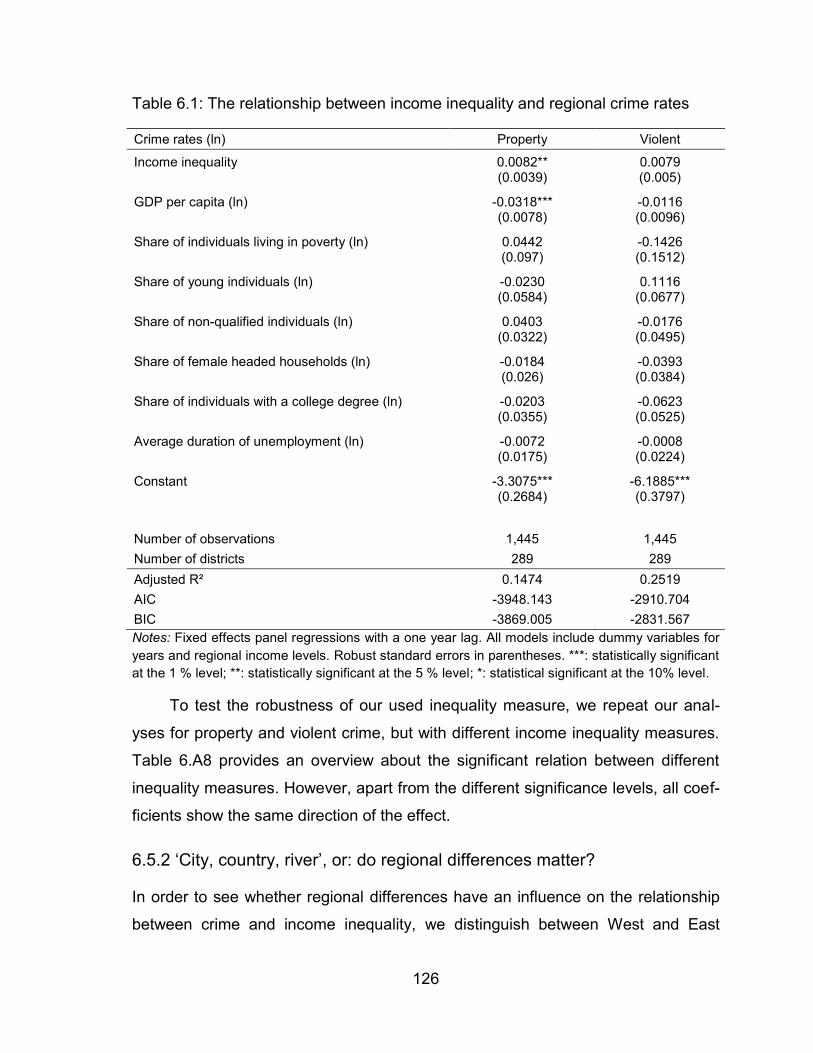
126

Table 6.1: The relationship between income inequality and regional crime rates

Crime rates (ln) Property Violent

Income inequality 0.0082** 0.0079 (0.0039) (0.005)

GDP per capita (ln) -0.0318*** -0.0116 (0.0078) (0.0096)

Share of individuals living in poverty (ln) 0.0442 -0.1426 (0.097) (0.1512)

Share of young individuals (ln) -0.0230 0.1116 (0.0584) (0.0677)

Share of non-qualified individuals (ln) 0.0403 -0.0176 (0.0322) (0.0495)

Share of female headed households (ln) -0.0184 -0.0393 (0.026) (0.0384)

Share of individuals with a college degree (ln) -0.0203 -0.0623 (0.0355) (0.0525)

Average duration of unemployment (ln) -0.0072 -0.0008 (0.0175) (0.0224)

Constant -3.3075*** -6.1885*** (0.2684) (0.3797) Number of observations 1,445 1,445 Number of districts 289 289 Adjusted R² 0.1474 0.2519 AIC -3948.143 -2910.704 BIC -3869.005 -2831.567 Notes: Fixed effects panel regressions with a one year lag. All models include dummy variables for years and regional income levels. Robust standard errors in parentheses. ***: statistically significant at the 1 % level; **: statistically significant at the 5 % level; *: statistical significant at the 10% level.

To test the robustness of our used inequality measure, we repeat our anal-

yses for property and violent crime, but with different income inequality measures.

Table 6.A8 provides an overview about the significant relation between different

inequality measures. However, apart from the different significance levels, all coef-

ficients show the same direction of the effect.

6.5.2 ‘City, country, river’, or: do regional differences matter?

In order to see whether regional differences have an influence on the relationship

between crime and income inequality, we distinguish between West and East

127

Germany, cities and rural regions. The procedure is based on the idea that the ine-

quality-crime link should be more distinct in regions with higher income inequality,

as in case of West Germany and cities.41 The comparison between West and East

Germany in Table 6.2 shows that the effect of income inequality on property crime

rates remains significant only for West Germany. For the subsample of East Ger-

many, the effect disappears completely and indicates that financial incentives to

commit crime are higher in West German regions. The literature has shown (see,

Freeman, Grogger & Sonstelie, 1996; Chiu & Madden, 1998) that the number of

financial driven crimes increases as the income distribution becomes more une-

qual. That is the case, according to our used data, since the differences between

average income and the income at the bottom of the income distribution are much

higher in West Germany. Further, the data shows that regions in West Germany

are more dense, meaning that they provide more opportunities for criminal activi-

ties (Glaeser & Sacerdote, 1999). The effect on violent crime is insignificant.

Comparing cities and rural districts is necessary, since the average of crimi-

nal offenses is 3.97 times higher in cities compared to rural areas, making them to

hotbeds for criminal activities (Bettencourt et al., 2006; PKS, 2016) for several rea-

sons. First, cities make crime more worthwhile, because of reducing transport

costs (Glaeser & Sacerdote, 1999). Transport costs are measured by the distance

a criminal has to travel to potential crime scenes, which are higher in low dense

areas. Indeed, the criminological literature suggests that criminals do not travel

long distances to commit crime (Hipp, 2007). Second, dense areas provide more

potential victims or opportunities for criminals. Third, cities lower the costs for crime

by lowering the probability of arrest and therefore the probability of punishment.

This is, while the pool of potential suspects is much larger in cities compared to

rural areas. Thus, policy can work more efficient in areas with a small population

density (Glaeser & Sacerdote, 1999).

41 Income inequality and the number of criminal offenses are higher in cities. To address a potential

city-effect, we divide the number of criminal offenses by the population of a district. With this division, we obtain local crime rates that take into account population density and therefore the possibilities of criminal activities (see, Glaeser & Sacerdote, 1999).

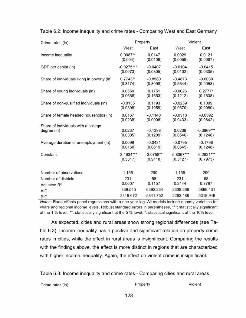
128

Table 6.2: Income inequality and crime rates - Comparing West and East Germany

Crime rates (ln) Property Violent West East West East

Income inequality 0.0087** 0.0147 0.0029 0.0121

(0.004) (0.0106) (0.0059) (0.0087)

GDP per capita (ln) -0.0275*** -0.0407 -0.0104 -0.0415

(0.0073) (0.0305) (0.0102) (0.0305)

Share of individuals living in poverty (ln) 0.7743** -0.8580 -0.4873 -0.6030

(0.3174) (0.8098) (0.5644) (0.9053)

Share of young individuals (ln) 0.0550 0.1751 -0.0026 0.2777*

(0.0668) (0.1653) (0.1212) (0.1638)

Share of non-qualified individuals (ln) -0.0135 0.1193 -0.0259 0.1009

(0.0308) (0.1059) (0.0670) (0.0980)

Share of female headed households (ln) 0.0167 -0.1148 -0.0318 -0.0592

(0.0238) (0.0908) (0.0433) (0.0842)

Share of individuals with a college degree (ln) 0.0237 -0.1398 0.0209 -0.3869***

(0.0305) (0.1209) (0.0546) (0.1248)

Average duration of unemployment (ln) 0.0099 -0.0431 -0.0795 -0.1798

(0.0160) (0.0619) (0.0645) (0.1248)

Constant -3.4634*** -3.0758** -5.8067*** -6.2621***

(0.3317) (0.9118) (0.5127) (0.7973)

Number of observations 1,155 290 1,155 290 Number of districts 231 58 231 58 Adjusted R² 0.0607 0.1157 0.2444 0.3797

AIC -339.545 -6392.234 -2338.266 -5869.431

BIC -3319.672 -5841.752 -2262.488 -5318.949 Notes: Fixed effects panel regressions with a one year lag. All models include dummy variables for years and regional income levels. Robust standard errors in parentheses. ***: statistically significant at the 1 % level; **: statistically significant at the 5 % level; *: statistical significant at the 10% level.

As expected, cities and rural areas show strong regional differences (see Ta-

ble 6.3). Income inequality has a positive and significant relation on property crime

rates in cities, while the effect in rural areas is insignificant. Comparing the results

with the findings above, the effect is more distinct in regions that are characterized

with higher income inequality. Again, the effect on violent crime is insignificant.

Table 6.3: Income inequality and crime rates - Comparing cities and rural areas

Crime rates (ln) Property Violent

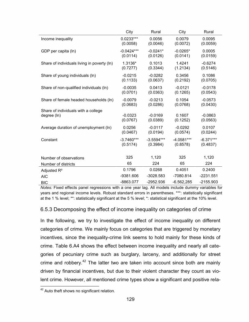
129

City Rural City Rural

Income inequality 0.0233*** 0.0056 0.0079 0.0095

(0.0058) (0.0046) (0.0072) (0.0059)

GDP per capita (ln) -0.0424*** -0.0241* -0.0265* 0.0005

(0.0114) (0.0126) (0.0141) (0.0159)

Share of individuals living in poverty (ln) 1.3136* 0.1013 1.4241 -0.6274

(0.7277) (0.3344) (1.2134) (0.5146)

Share of young individuals (ln) -0.0215 -0.0282 0.3456 0.1086

(0.1133) (0.0637) (0.2192) (0.0705)

Share of non-qualified individuals (ln) -0.0035 0.0413 -0.0121 -0.0178

(0.0701) (0.0363) (0.1265) (0.0543)

Share of female headed households (ln) -0.0079 -0.0213 0.1054 -0.0573

(0.0683) (0.0286) (0.0768) (0.0430)

Share of individuals with a college degree (ln) -0.0323 -0.0169 0.1607 -0.0863

(0.0767) (0.0389) (0.1252) (0.0563)

Average duration of unemployment (ln) 0.0256 -0.0117 -0.0292 0.0107

(0.0467) (0.0194) (0.0574) (0.0244)

Constant -3.7460*** -3.5594*** -4.0581*** -6.371***

(0.5174) (0.3984) (0.8578) (0.4837)

Number of observations 325 1,120 325 1,120 Number of districts 65 224 65 224

Adjusted R² 0.1796 0.0268 0.4051 0.2400 AIC -9381.606 -3028.583 -7080.814 -2231.551 BIC -8863.077 -2952.936 -6.562,285 -2155.903 Notes: Fixed effects panel regressions with a one year lag. All models include dummy variables for years and regional income levels. Robust standard errors in parentheses. ***: statistically significant at the 1 % level; **: statistically significant at the 5 % level; *: statistical significant at the 10% level.

6.5.3 Decomposing the effect of income inequality on categories of crime

In the following, we try to investigate the effect of income inequality on different

categories of crime. We mainly focus on categories that are triggered by monetary

incentives, since the inequality-crime link seems to hold mainly for these kinds of

crime. Table 6.A4 shows the effect between income inequality and nearly all cate-

gories of pecuniary crime such as burglary, larceny, and additionally for street

crime and robbery.42 The latter two are taken into account since both are mainly

driven by financial incentives, but due to their violent character they count as vio-

lent crime. However, all mentioned crime types show a significant and positive rela- 42 Auto theft shows no significant relation.

130

tion, supporting the assumed link between income inequality and pecuniary crimes.

To test the robustness of our used inequality measure, we further test different in-

come inequality measures. Again, all coefficients show the same direction of the

effect, but with different significance levels (see, Table 6.A8).

We run the same models again, but with a West-East distinction (see, Table

6.A5). Interestingly, the effect on robbery is insignificant for West and East Germa-

ny, whereas the effect on burglary is only significant in East and the effect on lar-

ceny only in West Germany. Further, the effect on street crime is highly significant

in West Germany. Since West Germany is faced with higher levels of income ine-

quality, the positive and significant results for West Germany are not surprising.

Remarkably, income inequality only has a significant and positive impact on burgla-

ry in East Germany. This finding contradicts the assumptions from literature that

the number of burglaries increases as the income distribution becomes more une-

qual (see, Freeman, 1996; Chiu & Madden, 1998). However, if we assume that the

detection rate can be interpreted as a measure for police efficiency (see, Wu & Wu,

2012), then the probability to get imprisoned for burglaries in East Germany is 30%

(PKS, 2016) lower than in West Germany, making such crimes in East Germany

more attractive.

Comparing cities and rural areas for different categories of crime, the results

in table 6.A6 shows that the inequality-crime link especially holds for cities, as we

can already see in Table 6.3.

6.6 Summary and discussion

We investigated the relationship between income inequality and different catego-

ries of crime at the district level, focusing on different regional aspects (Fajnzylber,

Lederman & Loayza, 2002). The analysis was performed for all 289 German dis-

tricts over a period of six years (2010-2015). Especially for categories of crime that

are triggered by monetary motives, we found strong and positive relationships that

differ strongly in terms of their magnitude between regions.

131

In case of aggregate criminal activities (property and violent crime), we sup-

port earlier findings, that the inequality-crime link is the strongest in regions with

higher levels of income inequality. Particularly, the effect is mostly pronounced in

dense areas, such as cities (see also, Glaeser & Sacerdote, 1999). Further, the

results indicate that the inequality-crime link is the strongest in areas with low

transportation costs, a low probability of punishment and high opportunities that

makes crime more beneficial.

After decomposing property and violent crime into subcategories, we also

found significant and positive results. Again, the assumed relations hold for regions

with higher levels of inequality (West Germany) and dense areas (cities). Surpris-

ingly, burglary in East Germany shows a significant relation, whereas the effect

disappears in West Germany. Due to the low R², we conclude that the relation de-

pends on the variety of different drivers of burglary and that omitted variables exist.

Still, we can conclude that German districts are highly heterogeneous with regard

to the magnitude and significance of the relationship between income inequality

and different categories of crime.

Additionally, we have to highlight that income inequality is only one of several

causes for crime, but it seems this effect is particularly affected by regional factors.

Given these results, the empirical analysis is a meaningful contribution to the newly

emerging branch of research that investigates the role of income inequality in the

context of continuously increasing categories of pecuniary crimes within regions.

Further, we can briefly draw a few directions that public policy should follow.

First, comparing the results with the findings of earlier studies for the UK and US,

we can conclude that the institutional settings in Germany that secure low income

individuals or unemployed individuals reduce the incentive to commit crime. Fur-

ther, the effort to diminish high levels of income inequality could reduce pecuniary

crimes. Nevertheless, we should not neglect other policies that could reduce crime:

better economic conditions that lower unemployment rates or poverty that, in turn,

have an additional crime reducing effect.

132

A principal shortcoming of our analysis, and simultaneously our avenue for

further research, is that our crime data covers only six years, making it impossible

to investigate long-run effects. Further, we were not able to add a victim survey

that could enrich our dataset regarding scope and validity, since no such dataset

for these years and all regions exist for Germany. Additionally, we had some ob-

stacles regarding the selection of categories of crime. For the dataset from 2010

compared with 2015, only a few categories of crime at the district level were pub-

lished by the PKS. Therefore, analyses for more categories of crime such as fraud

would enrich the current debate about the inequality-crime link.

Our analyses would also benefit from a dataset that provides information on

income which is not top-coded. Further, the share of the population with only pri-

mary education is underrepresented (compared to the OECD report 2016 for Ger-

many). This means that it is not possible to analyze the frustration of individuals at

the bottom of the income distribution due to the non-existing possibilities for career

advancement opportunities. Finally, we were not able to control for the natural rate

of crime, since we have no information about criminals and their income. Also, in-

stead of using income inequality, wealth inequality could be used, since this meas-

ure encompasses the total amount of assets of a household and its income.

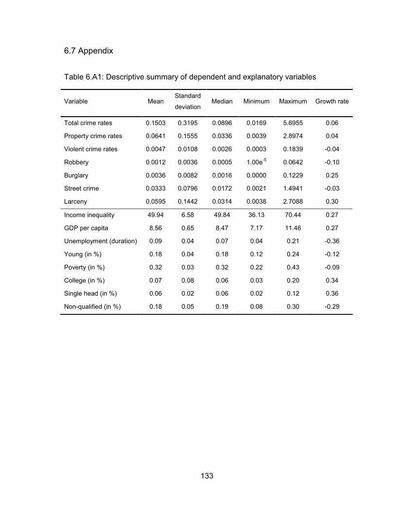
133

6.7 Appendix

Table 6.A1: Descriptive summary of dependent and explanatory variables

Variable Mean Standard

deviation Median Minimum Maximum Growth rate

Total crime rates 0.1503 0.3195 0.0896 0.0169 5.6955 0.06

Property crime rates 0.0641 0.1555 0.0336 0.0039 2.8974 0.04

Violent crime rates 0.0047 0.0108 0.0026 0.0003 0.1839 -0.04

Robbery 0.0012 0.0036 0.0005 1.00e-5 0.0642 -0.10

Burglary 0.0036 0.0082 0.0016 0.0000 0.1229 0.25

Street crime 0.0333 0.0796 0.0172 0.0021 1.4941 -0.03

Larceny 0.0595 0.1442 0.0314 0.0038 2.7088 0.30

Income inequality 49.94 6.58 49.84 36.13 70.44 0.27

GDP per capita 8.56 0.65 8.47 7.17 11.46 0.27

Unemployment (duration) 0.09 0.04 0.07 0.04 0.21 -0.36

Young (in %) 0.18 0.04 0.18 0.12 0.24 -0.12

Poverty (in %) 0.32 0.03 0.32 0.22 0.43 -0.09

College (in %) 0.07 0.08 0.06 0.03 0.20 0.34

Single head (in %) 0.06 0.02 0.06 0.02 0.12 0.36

Non-qualified (in %) 0.18 0.05 0.19 0.08 0.30 -0.29

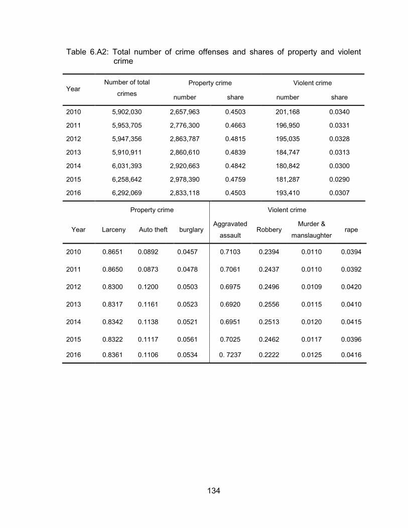
134

Table 6.A2: Total number of crime offenses and shares of property and violent crime

Year Number of total

crimes Property crime Violent crime

number share number share

2010 5,902,030 2,657,963 0.4503 201,168 0.0340

2011 5,953,705 2,776,300 0.4663 196,950 0.0331

2012 5,947,356 2,863,787 0.4815 195,035 0.0328

2013 5,910,911 2,860,610 0.4839 184,747 0.0313

2014 6,031,393 2,920,663 0.4842 180,842 0.0300

2015 6,258,642 2,978,390 0.4759 181,287 0.0290

2016 6,292,069 2,833,118 0.4503 193,410 0.0307

Property crime Violent crime

Year Larceny Auto theft burglary Aggravated

assault Robbery

Murder &

manslaughter rape

2010 0.8651 0.0892 0.0457 0.7103 0.2394 0.0110 0.0394

2011 0.8650 0.0873 0.0478 0.7061 0.2437 0.0110 0.0392

2012 0.8300 0.1200 0.0503 0.6975 0.2496 0.0109 0.0420

2013 0.8317 0.1161 0.0523 0.6920 0.2556 0.0115 0.0410

2014 0.8342 0.1138 0.0521 0.6951 0.2513 0.0120 0.0415

2015 0.8322 0.1117 0.0561 0.7025 0.2462 0.0117 0.0396

2016 0.8361 0.1106 0.0534 0. 7237 0.2222 0.0125 0.0416

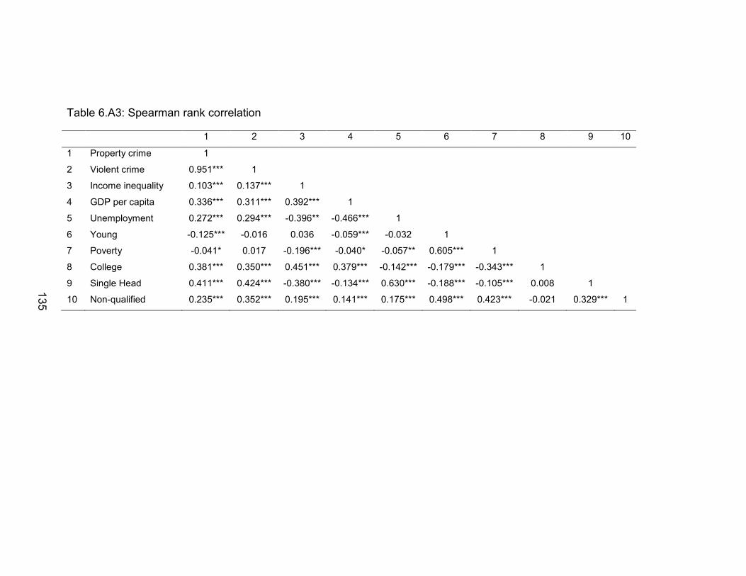
135

Table 6.A3: Spearman rank correlation

1 2 3 4 5 6 7 8 9 10

1 Property crime 1

2 Violent crime 0.951*** 1

3 Income inequality 0.103*** 0.137*** 1

4 GDP per capita 0.336*** 0.311*** 0.392*** 1

5 Unemployment 0.272*** 0.294*** -0.396** -0.466*** 1

6 Young -0.125*** -0.016 0.036 -0.059*** -0.032 1

7 Poverty -0.041* 0.017 -0.196*** -0.040* -0.057** 0.605*** 1

8 College 0.381*** 0.350*** 0.451*** 0.379*** -0.142*** -0.179*** -0.343*** 1

9 Single Head 0.411*** 0.424*** -0.380*** -0.134*** 0.630*** -0.188*** -0.105*** 0.008 1

10 Non-qualified 0.235*** 0.352*** 0.195*** 0.141*** 0.175*** 0.498*** 0.423*** -0.021 0.329*** 1

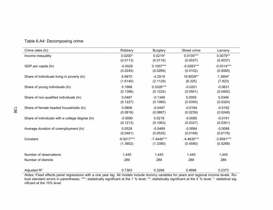
136

Table 6.A4: Decomposing crime

Crime rates (ln) Robbery Burglary Street crime Larceny Income inequality 0.0200* 0.0219* 0.0100*** 0.0079**

(0.0113) (0.0116) (0.0037) (0.0037)

GDP per capita (ln) -0.0028 0.1007*** -0.0283*** -0.0314***

(0.0245) (0.0269) (0.0102) (0.0085)

Share of individuals living in poverty (ln) 6.6870 -4.2519 19.8029** 1.3904*

(1.6140) (2.1129) (8.325) (7.823)

Share of young individuals (ln) 0.1668 0.3326*** -0.0201 -0.0631

(0.1396) (0.1224) (0.0501) (0.0492)

Share of non-qualified individuals (ln) 0.0487 -0.1349 0.0005 0.0346

(0.1227) (0.1060) (0.0350) (0.0324)

Share of female headed households (ln) 0.0806 -0.0447 -0.0184 -0.0182

(0.0818) (0.0887) (0.0239) (0.0248)

Share of individuals with a college degree (ln) -0.0090 0.0218 -0.0095 -0.0191

(0.1213) (0.1063) (0.0337) (0.0351)

Average duration of unemployment (ln) 0.0528 -0.0469 -0.0064 -0.0088

(0,0481) (0,0525) (0,0169) (0,0176)

Constant -6.9217*** -7.4446*** -4.4635*** -3.8591***

(1.3652) (1.3380) (0.4590) (0.5288)

Number of observations 1,445 1,445 1,445 1,445 Number of districts 289 289 289 289 Adjusted R² 0.7363 0.3268 0.4686 0.2373 Notes: Fixed effects panel regressions with a one year lag. All models include dummy variables for years and regional income levels. Ro-bust standard errors in parentheses. ***: statistically significant at the 1 % level; **: statistically significant at the 5 % level; *: statistical sig-nificant at the 10% level.

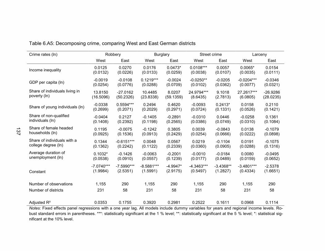
137

Table 6.A5: Decomposing crime, comparing West and East German districts

Crime rates (ln) Robbery Burglary Street crime Larceny West East West East West East West East

Income inequality 0.0125 0.0270 0.0176 0.0473* 0.0108*** 0.0057 0.0065* 0.0154 (0.0132) (0.0226) (0.0133) (0.0259) (0.0038) (0.0107) (0.0035) (0.0111)

GDP per capita (ln) -0.0019 -0.0108 0.1219*** -0.0024 -0.0250** -0.0205 -0.0204*** -0.0346 (0.0254) (0.0776) (0.0288) (0.0709) (0.0102) (0.0362) (0.0077) (0.0321)

Share of individuals living in poverty (ln)

13.8150 -27.0162 10.4485 8.0207 24.9794*** 9.1018 27.2617*** -26.9286 (16.5096) (50.2326) (23.8338) (59.1359) (8.6435) (2.7813) (6.0805) (28.0235)

Share of young individuals (ln) -0.0338 0.5594*** 0.2494 0.4620 -0.0093 0.2413* 0.0158 0.2110 (0.2699) (0.2071) (0.2029) (0.2971) (0.0724) (0.1331) (0.0526) (0.1421)

Share of non-qualified individuals (ln)

-0.0404 0.2127 -0.1405 -0.2891 -0.0310 0.0446 -0.0258 0.1361 (0.1408) (0.2392) (0.1198) (0.2565) (0.0386) (0.0749) (0.0310) (0.1084)

Share of female headed households (ln)

0.1195 -0.0075 -0.1242 0.3805 0.0039 -0.0843 0.0138 -0.1079 (0.0925) (0.1536) (0.0913) (0.2429) (0.0254) (0.0666) (0.0222) (0.0898)

Share of individuals with a college degree (ln)

0.1344 -0.6151*** 0.0048 0.0567 0.0219 -0.1104 0.0191 -0.1075 (0.1362) (0.2242) (0.1122) (0.2339) (0.0360) (0.0905) (0.0288) (0.1316)

Average duration of unemployment (ln)

0.1032* -0.1426 -0.0063 -0.2001 -0.0010 -0.0184 0.0080 -0.0495 (0.0538) (0.0910) (0.0557) (0.1239) (0.0177) (0.0489) (0.0159) (0.0652)

Constant -7.0740*** -7.5990*** -8.5881*** -4.9947* -4.3463*** -3.4368** -3.4801*** -2.5378 (1.9984) (2.5351) (1.5991) (2.9175) (0.5497) (1.2827) (0.4334) (1.6651)

Number of observations 1,155 290 1,155 290 1,155 290 1,155 290 Number of districts 231 58 231 58 231 58 231 58 Adjusted R² 0.0353 0.1755 0.3920 0.2981 0.2522 0.1611 0.0968 0.1114 Notes: Fixed effects panel regressions with a one year lag. All models include dummy variables for years and regional income levels. Ro-bust standard errors in parentheses. ***: statistically significant at the 1 % level; **: statistically significant at the 5 % level; *: statistical sig-nificant at the 10% level.

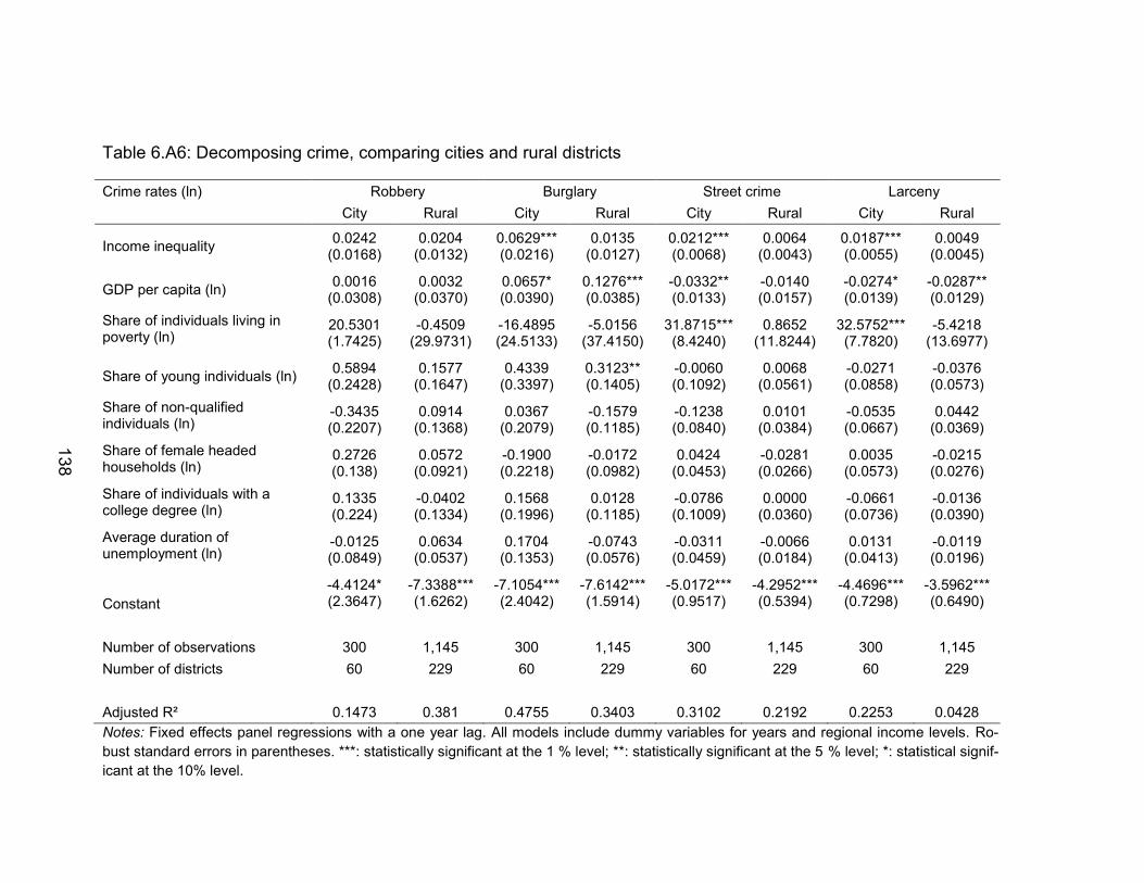
138

Table 6.A6: Decomposing crime, comparing cities and rural districts

Crime rates (ln) Robbery Burglary Street crime Larceny City Rural City Rural City Rural City Rural

Income inequality 0.0242 0.0204 0.0629*** 0.0135 0.0212*** 0.0064 0.0187*** 0.0049 (0.0168) (0.0132) (0.0216) (0.0127) (0.0068) (0.0043) (0.0055) (0.0045)

GDP per capita (ln) 0.0016 0.0032 0.0657* 0.1276*** -0.0332** -0.0140 -0.0274* -0.0287** (0.0308) (0.0370) (0.0390) (0.0385) (0.0133) (0.0157) (0.0139) (0.0129)

Share of individuals living in poverty (ln)

20.5301 -0.4509 -16.4895 -5.0156 31.8715*** 0.8652 32.5752*** -5.4218 (1.7425) (29.9731) (24.5133) (37.4150) (8.4240) (11.8244) (7.7820) (13.6977)

Share of young individuals (ln) 0.5894 0.1577 0.4339 0.3123** -0.0060 0.0068 -0.0271 -0.0376 (0.2428) (0.1647) (0.3397) (0.1405) (0.1092) (0.0561) (0.0858) (0.0573)

Share of non-qualified individuals (ln)

-0.3435 0.0914 0.0367 -0.1579 -0.1238 0.0101 -0.0535 0.0442 (0.2207) (0.1368) (0.2079) (0.1185) (0.0840) (0.0384) (0.0667) (0.0369)

Share of female headed households (ln)

0.2726 0.0572 -0.1900 -0.0172 0.0424 -0.0281 0.0035 -0.0215 (0.138) (0.0921) (0.2218) (0.0982) (0.0453) (0.0266) (0.0573) (0.0276)

Share of individuals with a college degree (ln)

0.1335 -0.0402 0.1568 0.0128 -0.0786 0.0000 -0.0661 -0.0136 (0.224) (0.1334) (0.1996) (0.1185) (0.1009) (0.0360) (0.0736) (0.0390)

Average duration of unemployment (ln)

-0.0125 0.0634 0.1704 -0.0743 -0.0311 -0.0066 0.0131 -0.0119 (0.0849) (0.0537) (0.1353) (0.0576) (0.0459) (0.0184) (0.0413) (0.0196)

Constant -4.4124* -7.3388*** -7.1054*** -7.6142*** -5.0172*** -4.2952*** -4.4696*** -3.5962*** (2.3647) (1.6262) (2.4042) (1.5914) (0.9517) (0.5394) (0.7298) (0.6490)

Number of observations 300 1,145 300 1,145 300 1,145 300 1,145 Number of districts 60 229 60 229 60 229 60 229 Adjusted R² 0.1473 0.381 0.4755 0.3403 0.3102 0.2192 0.2253 0.0428 Notes: Fixed effects panel regressions with a one year lag. All models include dummy variables for years and regional income levels. Ro-bust standard errors in parentheses. ***: statistically significant at the 1 % level; **: statistically significant at the 5 % level; *: statistical signif-icant at the 10% level.

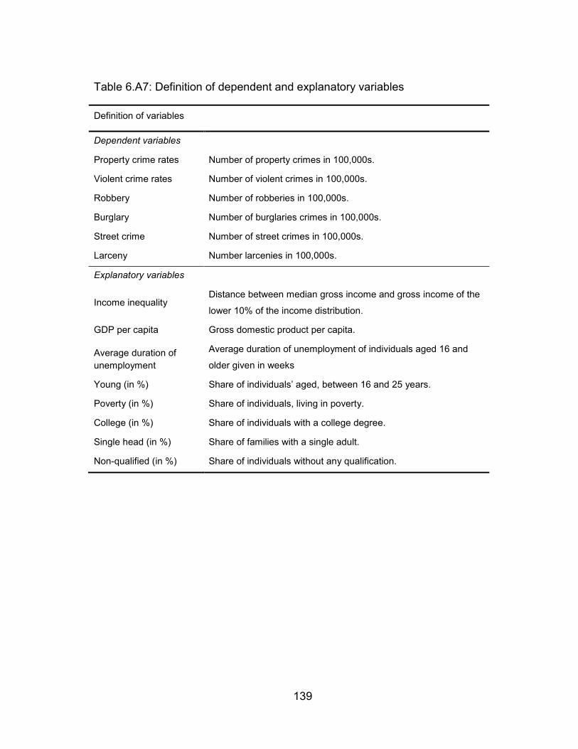
139

Table 6.A7: Definition of dependent and explanatory variables

Definition of variables

Dependent variables

Property crime rates Number of property crimes in 100,000s.

Violent crime rates Number of violent crimes in 100,000s.

Robbery Number of robberies in 100,000s.

Burglary Number of burglaries crimes in 100,000s.

Street crime Number of street crimes in 100,000s.

Larceny Number larcenies in 100,000s.

Explanatory variables

Income inequality Distance between median gross income and gross income of the

lower 10% of the income distribution.

GDP per capita Gross domestic product per capita.

Average duration of unemployment

Average duration of unemployment of individuals aged 16 and

older given in weeks

Young (in %) Share of individuals’ aged, between 16 and 25 years.

Poverty (in %) Share of individuals, living in poverty.

College (in %) Share of individuals with a college degree.

Single head (in %) Share of families with a single adult.

Non-qualified (in %) Share of individuals without any qualification.

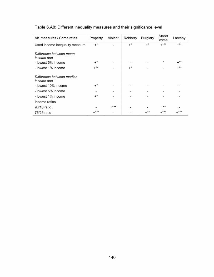
140

Table 6.A8: Different inequality measures and their significance level

Alt. measures / Crime rates Property Violent Robbery Burglary Street crime Larceny

Used income inequality measure +* - +* +* +*** +**

Difference between mean income and

- lowest 5% income +* - - - * +** - lowest 1% income +** - +* - - +**

Difference between median income and

- lowest 10% income +* - - - - - - lowest 5% income - - - - - - - lowest 1% income +* - - - - - Income ratios 90/10 ratio - +*** - - +** - 75/25 ratio +*** - - +** +*** +***

141

Chapter 7

So what? Concluding remarks and outlook for further research

Section 7.1 offers a brief summary of the main results and shortcomings of Part II

of this thesis. Whereas Chapter 5 deals with the causes of income inequality,

Chapter 6 addresses the potential consequences of unevenly distributed income,

namely, an increase in regional crime rates. Based on the initial findings and short-

comings, Section 7.2 provides general remarks regarding measuring innovative

activities and the potential effect of entrepreneurship on income inequality. Section

7.2 also provides general thoughts about a method for identifying a causal relation-

ship between income inequality and local crime rates.

7.1 A summary of the empirical findings

Chapter 5 deals with several aspects dealing with the implementation of new tech-

nologies. The emergence of new technologies is measured by the rate of patents

granted. Using this evidence, the effect of new technologies on regional income

distribution is investigated. It is evident that new technologies often replace routine

jobs that are mostly performed by low-skilled workers (Breau, Kogler & Bolton,

2014). Consequently, as industry-specific unemployment increases, the demand

for and wages of workers in the corresponding sectors will decrease. Simultane-

ously, new technologies require individuals with specific skills that enable them to

understand and use these new technologies. Thus, the demand for these workers

and their wages will increase (Acemoglu, Aghion & Violante, 2001). Both patterns

lead to a concentration of incomes at the top of the income distribution.

In the current literature (see, Lee, 2011; Lee & Rodríguez-Pose, 2013; Breau,

Kogler & Bolton, 2014), it is mainly assumed that new technologies increase in-

come inequality. There might also, however, be a reverse effect that is largely ne-

glected. Specifically, innovative regions can attract highly educated and well-paid

workers, leading to higher income inequality, while simultaneously fostering larger

142

innovative output. However, the opposite may also be true, meaning that higher

levels of income inequality could discourage people from engaging in innovative

activities (see, Weinhold & Nair-Reichert, 2009). Chapter 5 uses a VAR model with

an implemented first order difference equation to analyze the relationship between

innovations, measured by changes in regional patent rates, and changes in re-

gional income inequality. The results suggest that indeed, innovations Granger-

cause income inequality to increase. Further, changes in income inequality

Granger-cause changes in patent rates to decrease, suggesting that income ine-

quality decreases the incentive for innovative activities within a region. Thus, Chap-

ter 5 contributes to the current discussion by providing evidence for the existence

of both potential links between innovation, high-skilled individuals and income ine-

quality.

Chapter 6 deals with the relationship between regional income inequality and

crime rates.43 The empirical results suggest that indeed, income inequality is signif-

icantly and positively related to local crime rates, i.e. in case of pecuniary crime.

Comparing different regional settings, the results exhibit that the relationship be-

tween income inequality and crime rates becomes more pronounced and signifi-

cant, the larger the level of income inequality. It is worth mentioning that the ine-

quality-crime link is tested for Germany, a country that is not characterized by ex-

tremely high levels of income inequality and crime, as is the case for the US (see,

Cohen, Felson & Land, 1980; Ehrlich, 1996; Fishback, Johnson & Kantor, 2010)

and Great Britain (see, Machin, Marie & Vujic, 2011). Chapter 6 also investigates if

this relationship holds in regions with a moderate level of the two variables of inter-

est. This the first analysis conducted for an entire country at the regional level, and

not simply for a few selected regions or cities (see, Kelly, 2000; Soares, 2004; Pare

& Felson, 2014). Regional differences that influence an individual’s well-being and

probability to commit crime (Merton, 1938; Shaw & McKay, 1942; Runciman, 1966;

Becker, 1968), e.g. in labor markets, housing prices, income or consumption costs,

were thus explicitly considered.

43 For a theoretical overview, see Chapter 6, Section 6.2.1.

143

Several limitations affect the results discussed in Chapter 5. First, the compu-

tation of income inequality is based on pre-tax earnings, neglecting redistributive

effects of tax–transfer policies. Second, the measure for innovative activities, pa-

tents only covers certain aspect of new technologies and innovative activities.

Chapter 6 has several shortcomings, as well. The time period under consideration

is quite short. The inclusion of a victim surveys that would have enhanced the va-

lidity and scope of the objective and subjective awareness analyses is missing.

Further, it was not possible to control for a natural rate of crime, since no infor-

mation was available about criminals, their motives or income. The natural rate of

crime connotes that individuals have a preference to commit crime that is inde-

pendent from their income and environment, or other socio-economic factors.

7.2 What do we need to know? Avenues for further research

7.2.1 R&D expenditures and income inequality

In Chapter 5, patents were used as a proxy for the innovative activity within a re-

gion. However, the disadvantage of using patents as a proxy for innovative activi-

ties (output analysis) is that only successful R&D activities are considered. Further,

only research activities that lead to patent applications are covered, meaning that,

for example, basic research is not recorded in the data. In general, the possibilities

to protect innovations are manifold (e.g. secrecy or lead time that makes it impos-

sible for competitors to understand and use it) (see, Cohen, Nelson & Walsh,

2000). Instead of analyzing patents as the output of R&D activity, scholars could

focus on the input side by assessing the effect of regional R&D expenditures on

income inequality.

In the following Table 7.1, an additional regression analysis, based on the

Vector autoregression model from Chapter 5 (see, Table 5.1) is used as a robust-

ness check for testing the relationship between innovative activities and income

inequality. Instead of using patents (output analysis), the share of high-skilled indi-

viduals is used as a measure for (potential) R&D employees (input analysis). In-

deed, the findings in Table 7.1 indicate that changes in the share of R&D employ-

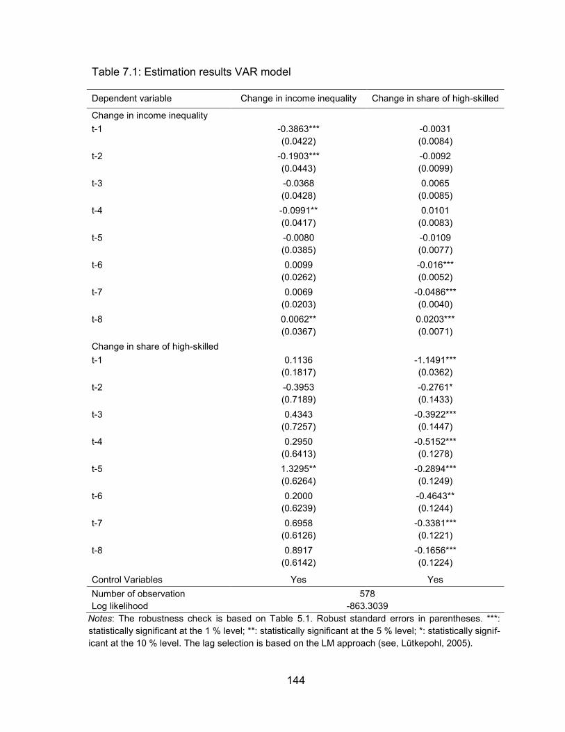
144

Table 7.1: Estimation results VAR model

Dependent variable Change in income inequality Change in share of high-skilled

Change in income inequality t-1 -0.3863*** -0.0031

(0.0422) (0.0084)

t-2 -0.1903*** -0.0092

(0.0443) (0.0099)

t-3 -0.0368 0.0065 (0.0428) (0.0085) t-4 -0.0991** 0.0101 (0.0417) (0.0083) t-5 -0.0080 -0.0109 (0.0385) (0.0077) t-6 0.0099 -0.016***

(0.0262) (0.0052)

t-7 0.0069 -0.0486*** (0.0203) (0.0040) t-8 0.0062** 0.0203*** (0.0367) (0.0071) Change in share of high-skilled t-1 0.1136 -1.1491***

(0.1817) (0.0362)

t-2 -0.3953 -0.2761*

(0.7189) (0.1433)

t-3 0.4343 -0.3922***

(0.7257) (0.1447)

t-4 0.2950 -0.5152*** (0.6413) (0.1278) t-5 1.3295** -0.2894*** (0.6264) (0.1249) t-6 0.2000 -0.4643** (0.6239) (0.1244) t-7 0.6958 -0.3381*** (0.6126) (0.1221) t-8 0.8917 -0.1656*** (0.6142) (0.1224)

Control Variables Yes Yes Number of observation 578 Log likelihood -863.3039

Notes: The robustness check is based on Table 5.1. Robust standard errors in parentheses. ***: statistically significant at the 1 % level; **: statistically significant at the 5 % level; *: statistically signif-icant at the 10 % level. The lag selection is based on the LM approach (see, Lütkepohl, 2005).

145

ees Granger-cause changes in regional income inequality to increase after five

years. However, the share of high-skilled individuals only provides a narrow insight

into the true nature and scope of innovative activities as it does not contain any

information regarding the expenditures for laboratories, employees, and input fac-

tors, such as chemicals or other material. This could lead to an underestimation of

the R&D-inequality link. Thus, regional R&D expenditures should be used as a

more appropriate measure for regional innovative activities to get a deeper insight

on how R&D input affects regional wage dispersion. The SIAB-R dataset used in

this thesis has its own limitations. Unfortunately, for the period under consideration

and the regional analysis, there is currently no suitable dataset available that con-

tains detailed information on R&D expenditure.

7.2.2 Entrepreneurship and income inequality

Based on the findings outlined in Chapter 5, innovative activities lead to a concen-

tration of incomes at the top of the income distribution. The question that arises

here is: Given that income inequality is associated with several economic and so-

cial problems (DiNardo & Pischke, 1997; Maddison, 2001; Mokyr, 2005; Breau,

Kogler & Bolton, 2014), does this mean that a society should decrease its innova-

tive activities in order to decrease income inequality? This question can simply be

answered with ‘no’, since innovations are a fundamental driver for economic

growth, well-being, and the emergence of new products and markets (Ahuja, 2000;

Howells, 2000; Fritsch & Müller, 2004).

A certain level of income inequality creates incentives for individuals to en-

gage in innovative and entrepreneurial activities (Milanovic, 2011) as talent,

(scarce) skills and intrinsic motivation are rewarded in the labor market. The moti-

vation to engage into self-employment is expected to depend on the individual’s

(socio-) economic circumstances that promote or hamper his or her decision to

become an entrepreneur or not (Xavier-Oliviera, Laplume & Pathak, 2015). Coun-

tries, and specific regions within countries, with higher levels of income inequality

usually have higher start-up rates (Lipmann et al., 2005). Income inequality can

therefore be one potential trigger of self-employment (Milanovic, 2011). However,

146

the question of reverse causality, i.e. whether and how start-ups influence income

inequality, has not yet been fully answered (see, Xavier-Oliviera, Laplume &

Pathak, 2015). Start-ups differ in terms of their founders’ motivations and aims. On

the one hand, individuals at the bottom of the income distribution, could improve

their living conditions by increasing their income through entrepreneurial activities

(necessity entrepreneurs; Burton, Ketchen & Ireland, 2013; Laplume, Pathak &

Xavier-Oliveira, 2014), which in turn could lead to decreasing income inequality.

On the other hand, income inequality could also increase, since starting a business

requires a certain educational level and the individuals who have this level of edu-

cation usually earn well (opportunity entrepreneurs; Reynolds et al., 2002). Start-

ups that result from identified opportunities could therefore accelerate the concen-

tration of wages at the top of the income distribution.

An appropriate model is necessary to test the relationship between income

inequality and regional start-ups. Income inequality can trigger start-up rates, since

entrepreneurs identify opportunities to start a firm, or because it is the only possibil-

ity to secure their standard of living. However, necessity-motivated start-ups could

decrease income inequality, whereas opportunity driven start-ups may increase

wage dispersion. Both potential links should, thus, be addressed. The modified

VAR model used in Chapter 5 is such a suitable model, since it can test if changes

in income inequality trigger changes in start-up rates and vice versa. However,

since the distinction between necessity and opportunity-driven start-ups matters, a

separate model for each is needed. Thus, it could be possible to test if income ine-

quality triggers (opportunity) necessity motivated start-ups that simultaneously (in-

crease) decrease income inequality.

An empirical analysis would require a sufficiently large data set, i.e. a suffi-

ciently large number of observations at the regional level. Furthermore, the obser-

vation period must be long enough to estimate long-term effects. Finally, an ideal

data set should also include information about the individual motives for starting a

business in order to understand how far necessity or opportunity entrepreneurs

differently affect income inequality. Besides the SIAB dataset (see, Chapter 5), the

147

Mannheim Enterprise Panel of the Centre for European Economic Research

(ZEW) provides information about the number of different kinds of start-ups, such

as high-tech, technological advanced or service oriented establishments. Unfortu-

nately, the ZEW dataset contains no information about the motives of an entrepre-

neur. The German Socio-Economic Panel Study (GSOEP) encompasses compre-

hensive information about German households, making it possible to identify en-

trepreneurs and their motivations for starting their own business (Block & Sandner,

2009). Unfortunately, the number of observations included in the GSOEP data set

is too small, making a regional examination impossible.

7.2.3 Inequality and crime – An instrumental variable approach

After focusing on the causes of income inequality, Part II of the thesis also ad-

dresses one consequence of income inequality. There is a wide range of literature

showing that income inequality is associated with several social problems, such as

social segregation, a reduction in the quality of social ties, an increase in violence

and racism, a reduction in self-reported health, and an increase in crime rates (see,

Kelly, 2000; Uslaner, 2002; Alesina, Di Tella & MacCulloch, 2004; Wilkinson, 2005;

Neckerman & Torche 2007; Wilkinson & Pickett, 2007). Crime, specifically property

crime, incurs costs (Miller, Cohen & Wiersema, 1995) for prevention and police,

incarceration, private deterrence as well as costs to the victims (Anderson, 1999).

Further, it increases uncertainty, undermines the security of property rights, causes

productivity losses and, ultimately, reduces long-run economic growth (Cardenas,

2002; Powell, Manish & Nair, 2010). Thus, it is not surprisingly that crime becomes

a topic of interest in economics.

In Chapter 6 of this thesis, it was shown that a relationship between regional

income inequality and crime rates exists. It could not be shown, however, whether

this relationship is causal. Instead of a fixed effects panel model, an instrumental

variable (IV) regression could be estimated. This is used to solve the endogeneity

problem that one or more independent variables could be correlated with the resid-

ual and thus test causality. Specifically, the endogenous explanatory variable is

replaced by an instrument that has to fulfill two properties: It must not correlate with

148

the residual (exogeneity), but it must correlate with the variable to be replaced (rel-

evance) (Stock & Watson, 2015).

The literature states that an endogeneity problem may exist due to measure-

ment errors in crime data, omitted variables (Fajnzlber, Lederman & Loayza,

2002), not measurable state-specific effects (unobserved heterogeneity) or due to

joint endogeneity between income inequality and crime (Doyl, Ahmed & Horn,

1999; Fajnzylber, Lederman & Loayza, 2002). Regarding the latter, it is assumed

that income inequality triggers crime (see, Neckerman & Torche, 2007), but crime

can also influence income inequality within a region for two reasons. First, espe-

cially individuals with high incomes have the incentive and the financial possibility

to move away from regions with high crime rates. Second, regions with high crime

rates may be discourage settlement by individuals with high incomes, and deter the

establishment of new businesses (Powell, Manish & Nair, 2010). All of these pos-

sible scenarios could change income inequality in the respective region.

The economic literature that addresses potential endogeneity problems be-

tween income inequality and other economic and social factors is scare. It is mostly

argued that there is no suitable instrument to replace income inequality (see, Dein-

inger & Squire, 1996; Ravallion, 2003), as it can work through a variety of channels

(Forbes, 2000). When scholars address this issue, they often use a lagged value

(see, e.g. Deininger & Squire, 1996; Forbes, 2000; Ravallion, 2003) or a change

value (Voitchovsky, 2005) of income inequality as an instrument. However, this is

only possible in case of weak endogeneity (Greene, 2003).

In the studies by Engerman and Sokoloff (1997, 2000), the potentially endog-

enous relationship between income inequality and economic growth in developing

countries is addressed. The endogeneity problems lie in the fact that income ine-

quality or inequality in general can be interpreted as a sign of poorly functioning

institutions and low levels of human capital that influence both, income inequality

and growth. To solve this potential dual-causality problem, they replace income

inequality by a historical and geographical instrument, that is, factor endowments in

agriculture (Easterly, 2007). Engerman and Sokoloff (1997, 2000) argue that land

149

endowments are a good predictor for income inequality since it measures the ex-

ogenous suitability of land for wheat against sugar, coffee and other staple crops.

During colonization, the New World specialized in the production of these products,

through the use of slave labor. In contrast, the cultivation of wheat was character-

ized by machinery during this era (Lindert & Williamson, 1983). Consequently, in

countries (or colonies) where slavery was practiced and provided the manpower for

agricultural development (Engerman & Sokoloff, 1997, 2000), disproportionate

shares of wealth and human capital were held by a small share of the European

elite (see, also Raghuram & Zingales, 2006; Easterly, 2007). Thus, factor endow-

ments in agriculture are used as an instrument for long-lasting income inequality

(see, Engerman & Sokoloff, 1997, 2000; Raghuram & Zingales, 2006; Easterly,

2007).

Additionally, some studies use (mature) cohort size as an instrument for in-

come inequality (‘cohort-size hypotheses’; Higgins & Williamson, 2002). For in-

stance, instead of using a lagged value of income inequality (see, Forbes, 2000),

Jong-Sung and Khagram (2005), and Leight (2006), use the ‘mature cohort size’

relative to the adult population within a country as an instrument for income ine-

quality. If large cohorts lie in the middle of the age-earning curve, when the income

is the highest, labor market glut lowers rewards and, therefore, income inequality

decreases (market saturation of labor supply). If the cohort is mainly characterized

by young or old adults, labor market glut will lower the incomes at both tails of the

age-earning curve and income inequality is augmented.

Unfortunately, literature that addresses the potential joint endogeneity prob-

lem between income inequality and crime is scarce. The problem of omitted varia-

bles or state-specific effects is often addressed (see, Holtz-Eakin, 1994; Levitt,

1998; Doyl, Ahmed & Horn, 1999; Kelly, 2000), but the issue of the potentially joint

endogeneity of income inequality is neglected (Fajnzylber, Lederman & Loayza,

2002).

However, Doyle, Ahmed and Horn (1999) show that low-skilled workers are

more likely to respond to changes in income by committing crimes. Thus, the rela-

150

tionship between income, specifically income inequality, and crime is more pro-

nounced in sectors that are dominated by low-skilled workers. The results of Chap-

ter 5 of the present thesis, and those of the current literature (see, Acemoglu, Agh-

ion & Violante, 2001; Lee, 2011; Lee & Rodríguez-Pose, 2013; Breau, Kogler &

Bolton, 2014), show that especially this group of individuals is most affected and

suffers the most from income inequality. This is because innovations, especially

new technologies, increase income inequality due to replacement of routine jobs

most frequently held by low-skilled individuals. Hence, based on the findings in

Chapter 5, it might be possible to use innovations (e.g. patents) as an instrument

for inequality. This could solve the potential joint endogeneity problem and allow us

to measure the effect of income inequality on crime, which is explained by innova-

tions.

Whether or not the exogeneity condition is met is unlikely for two reasons.

First, innovative regions are characterized by a pronounced share of highly skilled

individuals, indicating a higher average income level. Thus, in such ‘richer’ regions

the attractiveness for crime increases. Second, as mentioned earlier, areas with

high crime rates tend to deter the establishment of new business and may be unat-

tractive to individuals with high incomes. Crime might actually hamper innovative

activities in a region by driving away the very highly skilled individuals necessary

for such activities. For these reasons, the exogeneity assumption seems not to be

fulfilled.

The above explanations show the econometric problems that exist when as-

sessing the causal effect between inequality of income and crime at the regional

level. First of all, it would have to be made clearer what kind of income inequality

affects crime. On this basis, one could then search for a suitable instrument for

income inequality. Doing so was out of scope of this thesis and is, therefore, left for

future research.

151

Chapter 8

Conclusion

This thesis is grounded in the broad topic of regional innovative activities, with an

emphasis on the production and potential consequences of these activities. Part I

of this thesis focuses on the diffusion and production of knowledge and innovations

brought about by cooperative R&D relationships (networks), the stability of such

interactions and the persistence of knowledge within a region. Part II addresses the

potential reverse effects that innovations may create, specifically income inequality

within a region. The question of whether regional income inequality is, in turn, as-

sociated with socio-economic problems, such as crime, is also dealt within the

second part.

8.1 Concluding remarks of Part I: Knowledge, innovation and networks

Knowledge and its exchange are crucial factors for innovations (Leonard & Sen-

siper, 2011). Such an exchange between actors in networks is based on the divi-

sion of labor that facilitates the diffusion of information and knowledge (Johansson,

1995). This is highly important for the innovation process (Bercovitz & Feldman,

2011). The efficiency of such interactions between individuals or firms, measured

by the speed of knowledge diffusion (Albert, Jeong & Barabási, 2000) or by patent

productivity (Fritsch & Slavtchev, 2011), depends on a network’s composition of

actors and its structural characteristics (Capaldo, 2007). Especially the latter plays

a crucial role in terms of the efficiency of the network (Schilling & Phelps, 2007;

Phelps, 2010).

However, many scholars assume that, because of high transaction cost, net-

work cooperative relationships (i.e. of R&D networks) are particularly long lasting

(see, Liebeskind et al., 1995; Ejermo & Karlsson, 2006). In part, this assumption is

based on the notion that if a network relation is abandoned, the previous cost and

effort is ‘sunk’. Barabási and Albert (1999, 2000) also support the assumption of

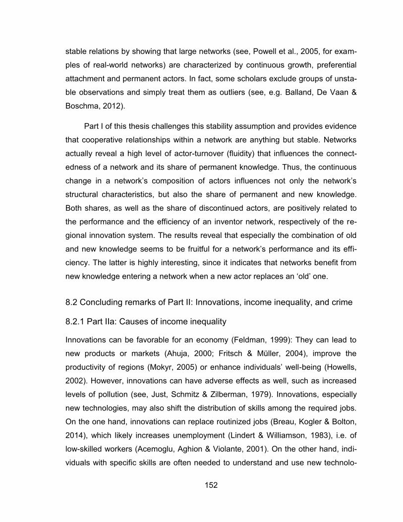
152

stable relations by showing that large networks (see, Powell et al., 2005, for exam-

ples of real-world networks) are characterized by continuous growth, preferential

attachment and permanent actors. In fact, some scholars exclude groups of unsta-

ble observations and simply treat them as outliers (see, e.g. Balland, De Vaan &

Boschma, 2012).

Part I of this thesis challenges this stability assumption and provides evidence

that cooperative relationships within a network are anything but stable. Networks

actually reveal a high level of actor-turnover (fluidity) that influences the connect-

edness of a network and its share of permanent knowledge. Thus, the continuous

change in a network’s composition of actors influences not only the network’s

structural characteristics, but also the share of permanent and new knowledge.

Both shares, as well as the share of discontinued actors, are positively related to

the performance and the efficiency of an inventor network, respectively of the re-

gional innovation system. The results reveal that especially the combination of old

and new knowledge seems to be fruitful for a network’s performance and its effi-

ciency. The latter is highly interesting, since it indicates that networks benefit from

new knowledge entering a network when a new actor replaces an ‘old’ one.

8.2 Concluding remarks of Part II: Innovations, income inequality, and crime

8.2.1 Part IIa: Causes of income inequality

Innovations can be favorable for an economy (Feldman, 1999): They can lead to

new products or markets (Ahuja, 2000; Fritsch & Müller, 2004), improve the

productivity of regions (Mokyr, 2005) or enhance individuals’ well-being (Howells,

2002). However, innovations can have adverse effects as well, such as increased

levels of pollution (see, Just, Schmitz & Zilberman, 1979). Innovations, especially

new technologies, may also shift the distribution of skills among the required jobs.

On the one hand, innovations can replace routinized jobs (Breau, Kogler & Bolton,

2014), which likely increases unemployment (Lindert & Williamson, 1983), i.e. of

low-skilled workers (Acemoglu, Aghion & Violante, 2001). On the other hand, indi-

viduals with specific skills are often needed to understand and use new technolo-

153

gies. While there is an increase in the demand and incomes for highly educated

individuals, the reverse is true for low-educated individuals. Both developments

simultaneously trigger income inequality.

Chapter 5 of this thesis addresses income inequality as one of the potentially

adverse effects of innovations. By using a modified VAR model (see, Chapter 5),

indications of a causal relationship of two potential links are obtained. On the one

hand, changes in innovative activities Granger-cause income inequality to in-

crease. On the other hand, changes in income inequality Granger-cause innovative

activities to decrease, indicating that higher levels of income inequality discourage

individuals from engaging in innovative activities within a region. Thus, Chapter 5

provides evidence for these two causal relationships within a regional context.

8.2.2 Part IIb: Consequences of income inequality

Wage dispersion is a highly interesting topic, since it is associated with several

(socio-) economic problems, such as segregation (Alesina, Di Tella & MacCulloch,

2004), hostility and racism (Williams, Feaganes & Barefoot, 1995), or crime (Kelly,

2000; Wu & Wu, 2012).44 Crime, in turn, is responsible for any number of economic

and social costs (Miller, Cohen & Wiersema, 1995). There are costs incurred for

prevention, policy and incarceration (Anderson, 1999). Crime increase a general-

ized fear in the population, and causes an uncertainty to start an own business,

with concomitant productivity losses and reduce long-run economic growth (Car-

denas, 2002; Powell, Manish & Nair, 2010). Given these circumstances, a current

debate in economics deals with the question of whether and how income inequality

is related to crime (Kelly, 2000; Neckerman & Torch, 2007; Wilkinson & Pickett,

2007, 2009)

Chapter 6 of this thesis addresses this research question, albeit at the re-

gional level. Specifically, the results reveal that a positive and significant relation-

44 For a more detailed overview of potential socio-economic problems triggered by income

inequality, see Neckerman and Torche (2007).

154

ship exists between income inequality and crime, and that this link is strongest in

regions with the highest levels of income inequality.45

8.3 Final thoughts

If, as shown in this thesis, innovations lead to supposed economic problems such

as income inequality, should an economy then cease to innovate? This question

can be answered clearly with ‘no’, for two main reasons. On the one hand, innova-

tive activities can not only increase the incomes of the founders (Aghion et al.,

2015), but also increase the welfare of the economy as the production of new

knowledge is one of the main drivers of economic growth (Ahuja, 2000) and one

source of enhancing individuals’ well-being (Howells, 2002). On the other hand, a

certain degree of income inequality can even positively affect individual productivity

by creating labor incentives, since it reflects that individuals are rewarded based on

their talents and (scare) skills (Milanovic, 2011). Nevertheless, income inequality

can also lead to social and economic problems, especially if the inequality is too

high. Therefore, policies that attempt to mitigate the problems caused by income

inequality, without overly restricting incentives to innovate, should be pursued.

45 Further, Chapter 6 provides evidence that the assumed income inequality-crime link also holds in

countries with more moderate levels of income inequality and crime.

155

Bibliography Abernathy, Wiliam J. and Kim B. Clark (1985): Innovation - Mapping the winds of

creative destruction. Research policy, 14(1), 3-22.

Acemoglu, Daron, Philippe Aghion and Giovanni L. Violante (2001): Deunioniza-tion, technical change and inequality. Carnegie-Rochester conference series on public policy, 55(1), 229-264.

Acemoglu, Daron (2002): Technical change, inequality, and the labor market. Journal of Economic Literature, 40(1), 7-72.

Acemoglu, Daron and David Autor (2011): Skills, tasks and technologies - Implica-tions for employment and earnings. In: David Card and Orley Ashenfelter (eds.), Handbook of Labor Economics, Amsterdam: Elsevier, 1043-1171.

Acs, Zoltan (2000): Regional innovation, knowledge and global change, London: Pinter.

Acs, Zoltan, Pontus Braunerhjelm, David B. Audretsch and Bo Carlsson (2009): The knowledge spillover theory of entrepreneurship. Small Business Econom-ics, 32(1), 15-30.

Aghion, Philippe, Peter Howitt and Giovanni L. Violante (2002): General purpose technology and wage inequality. Journal of Economic Growth, 7(4), 315-345.

Aghion, Philippe, Ufuk Akcigit, Antonun Bergeaud, Richard Blundell and David Hémous (2015): Innovation and top income inequality, #w21247, Cambridge: National Bureau of Economic Research.

Agnew, Robert (2001): Building on the foundation of general strain theory - Speci-fying the types of strain most likely to lead to crime and delinquency. Journal of Research in Crime and Delinquency, 38(4), 319-361.

Ahuja, Gautam (2000): Collaboration networks, structural holes, and innovation - A longitudinal study. Administrative Science Quarterly, 45(3), 425-455.

Albert, Réka, Hawoong Jeong and Albert-László Barabási (2000): Error and attack tolerance of complex networks. Nature, 406(6794), 378-382.

Albert, Réka and Albert-Lászlo Barabási (2002): Statistical mechanics of complex networks. Review of Modern Physics, 74, 47-97.

156

Alesina, Alberto, Rafael Di Tella and Robert MacCulloch (2004): Inequality and happiness - Are Europeans and Americans different? Journal of Public Eco-nomics, 88(9), 2009-2042.

Allen, Robert C. (2009): Engels’ pause - Technical change, capital accumulation, and inequality in the British Industrial Revolution. Explorations in Economic History, 46(4), 418-435.

Amaral, Luis A. N., Antonio Scala, Marc Barthelemy and Eugene Stanley (2000): Classes of small-world networks. Proceedings of the National Academy of Sciences, 97(21), 11149-11152.

Ambrosio, Conchita and Joachim Frick (2007): Income satisfaction and relative deprivation - An empirical link. Social Indicators Research, 81, 497-519.

Andersson, Åke (1985): Creativity and regional development. Papers of the Re-gional Science Association, 56(1), 5-20.

Anderson, David A. (1999): The aggregate burden of crime. The Journal of Law and Economics, 42(2), 611-642.

Andresen, Martin A. (2015): Unemployment, GDP, and crime - The importance of multiple measurements of the economy. Canadian Journal of Criminology and Criminal Justice, 57, 35-58.

Antonelli, Cristiano and Agnieszka Gehringer (2017): Technological change, rent and income inequalities - A Schumpeterian approach. Technological Forecas-ting and Social Change, 115, 85-98.

Antoni, Manfred, Andreas Ganzer and Philipp vom Berge (2016): Stichprobe der Integrierten Arbeitsmarktbiographien (SIAB) 1975 - 2014. FDZ-Datenreport, 04/2016, Nürnberg.

Anselin, Luc (1988): Spatial econometrics - Methods and models, Dorddrecht: Kluwer: Academic Publisher.

Anselin, Luc, Anil K. Bera, Raymond J. Florax and Mann J. Yoon (1996): Simple diagnostic tests for spatial dependence. Regional Science and Urban Eco-nomics, 26(1), 77-104.

Arundel, Anthony (2001): The relative effectiveness of patents and secrecy for ap-propriation. Research Policy, 30(4), 611-624.

Asheim, Bjørn, Lars Coenen and Martin Svensson-Henning (2003): Nordic SMEs and regional innovation systems. NordiskIndustrifond, 1-95.

157

Atkinson, Anthony B. and François Bourguignon (2000): Introduction - Income dis-tribution and economics. In: Anthony B. Atkinson (ed.), Handbook of income distribution, Amsterdam: Elsevier.

Atkinson, Anthony (2006): Top Incomes in the United Kingdom over the Twentieth Century. In: Anthony B. Atkinson and Thomas Piketty (eds.), Top Incomes over the Twentieth Century, Oxford: Oxford University Press, 82-140.

Atkinson, Anthony B. and François Bourguignon (2014): Introduction - Income dis-tribution and economics. In: Anthony B. Atkinson (ed.), Handbook of income distribution, Amsterdam: Elsevier.

Audretsch, David B. and Maryann P. Feldman (2004): Knowledge spillovers and the geography of innovation. Handbook of regional and urban economics, 4, 2713-2739.

Audretsch, David B., Dirk Dohse and Annekatrin Niebuhr (2015): Regional unem-ployment structure and new firm formation. Papers in Regional Sci-ence, 94(1), 115-138.

Autor, David H., Frank Levy and Richard J. Murnane (2003): The skill content of recent technological change - An empirical exploration. The Quarterly Journal of Economics, 118(4), 1279-1333.

Autor, David H., Lawrence F. Katz and Melissa S. Kearney (2008): Trends in US wage inequality - Revising the revisionists. The Review of Economics and Statistics, 90(2), 300-323.

Autor, David and David Dorn (2009): Inequality and specialization - The growth of low-skill service jobs in the United States, #15150 NBER Working Paper Se-ries, Cambridge: National Bureau of Economic Research.

Autor, David H. and David Dorn (2013): How technology wrecks the middle class. The New York Times, 24.

Bach, Stefan, Giacomo Corneo and Viktor Steiner (2009): From bottom to top - The entire income distribution in Germany, 1992–2003. Review of Income and Wealth, 55(2), 303-330.

Balconi, Margherita, Stefano Breschi and Francesco Lissoni (2004): Networks of inventors and the role of academia - An exploration of Italian patent data. Re-search Policy, 33(1), 127-145.

Balland, Pierre-Alexandre, Mathijs De Vaan and Ron Boschma (2012): The dy-namics of interfirm networks along the industry life cycle - The case of the

158

global video game industry, 1987–2007. Journal of Economic Geography, 13(5), 741-765.

Barabási, Albert-Lászlo and Réka Albert (1999): Emergence of scaling in random networks. Science, 286(5439), 509-512.

Barabási, Albert-László (2009): Scale-free networks - A decade and beyond. Sci-ence, 325(5939), 412-413.

Barro, Robert J. (1991): Economic growth in a cross section of countries. The Quarterly Journal of Economics, 106(2), 407-443.

Barro, Robert J. and Xavier Sala-i-Martin (1995): Economic growth, Cambridge, Massachusetts: MIT Press.

Baum, Christopher F. (2006): An Introduction to modern econometrics using Stata, Texas: Stata Press.

Bayer, Patrick, Robert McMillan and Kim Rueben (2005): Residential segregation in general equilibrium, # 11095, Cambridge: National Bureau of Economic Research.

Becker, Gary S. (1968): Crime and punishment - An economic approach. Journal of political economy, 76(2), 169-217.

Beckett, Katherine and Theodore Sasson (2003): The politics of injustice - Crime and punishment in America, London: Sage Publications.

Beckfield, Jason (2004): Does Income Inequality Harm Health? New Cross-National Evidence. Journal of Health and Social Behavior, 45(3), 231-248.

Berman, Eli, John Bound and Zvi Griliches (1994): Changes in the demand for skilled labor within US manufacturing - Evidence from the annual survey of manufactures. The Quarterly Journal of Economics, 109(2), 367-397

Bettencourt, Luìs A., José Lobo, Dirk Helbing, Christian Kühnert and Geoffrey B. West (2007): Growth, innovation, scaling, and the pace of life in cities. Pro-ceedings of the National Academy of Sciences, 104(17), 7301-7306.

Bercovitz, Jane and Maryann Feldman (2011): The mechanisms of collaboration in inventive teams - Composition, social networks, and geography. Research Policy, 40(1), 81-93.

Berger, Peter L. and Thomas Luckmann (1966): The social construction of reali-ty Garden City, New York: Doubleday.

159

Berry, William D, Jacqueline H. DeMeritt and Justin Esarey (2010): Testing for in-teraction in binary logit and probit models - Is a product term essential? Amer-ican Journal of Political Science, 54(1), 248-266.

Biewen, Martin (2000): Income inequality in Germany during the 1980s and 1990s. Review of Income and Wealth, 46(1), 1-19.

Biewen, Martin and Andos Juhasz (2012): Understanding rising income inequality in Germany, 1999/2000–2005/2006. Review of Income and Wealth, 58(4), 622-647.

Black, Sandra and Stephen Machin (2011): Housing valuations of school perfor-mance. In: Eric A. Hanushek, Stephen J. Machin and Ludger Woessmann (eds.), Handbook of the Economics of education, Amsterdam: Elsevier, 485-519.

Block, Jörn and Philipp Sandner (2009): Necessity and opportunity entrepreneurs and their duration in self-employment - Evidence from German micro data. Journal of Industry, Competition and Trade, 9(2), 117-137.

Blundell, Richard, Lorraine Dearden, Costas Meghir and Barbara Sianesi (1999): Human capital investment - The returns from education and training to the in-dividual, the firm and the economy. Fiscal studies, 20(1), 1-23.

Boschma, Ron A. (2005): Proximity and Innovation - A Critical Assessment. Re-gional Studies, 39(1), 61-74.

Breau, Sébastien (2007): Income inequality across Canadian provinces in an era of globalization - Explaining recent trends. The Canadian Geographer/Le Ge-ographe canadien, 51(1), 72-90.

Breau, Sébastian, Dieter F. Kogler and Kenyon C. Bolton (2014): On the relation-ship between innovation and wage inequality - New evidence from Canadian cities. Economic Geography, 90(4), 351-373.

Breschi, Stefano and Francesco Lissoni (2001): Knowledge spillovers and local innovation systems - A critical survey. Industrial and corporate change, 10(4), 975-1005.

Brush, Jesse (2007): Does income inequality lead to more crime? A comparison of cross-sectional and time-series analyses of United States counties. Econom-ics letters, 96(2), 264-268.

Bruton, Garry D., David J. Ketchen and Duane R. Ireland (2013): Entrepreneurship as a solution to poverty. Journal of Business Venturing, 28(6), 683-689.

160

Bug, Mathias and Kristina Meier (2015): Aufbereitung der Kriminalstatistik zu ei-nem aussagekräftigen Bedrohungsbild - Vorschläge der Berechnung. DIW-Wochenbericht, 82(3), 27-35.

Burt, Ronald S. (2000): The network structure of social capital. Research in Organ-izational Behavior, 22, 345-423.

Burt, Ronald S. (2001): Structural holes versus network closure as social capital. In: Nan Lin, Karen S. Cook and Ronald S. Burt (eds.), Social capital: theory and research, Berlin: De Gruyter, 31-56.

Caliendo, Marco, Jens Hogenacker, Steffen Künn and Frank Wießner (2015): Sub-sidized start-ups out of unemployment - A comparison to regular business start-ups. Small Business Economics, 45(1), 165-190.

Cantner, Uwe and Holger Graf (2006): The network of innovators in Jena - An ap-plication of social network analysis. Research Policy, 35(4), 463-480.

Cantner, Uwe and Holger Graf (2011): Innovation networks - Formation, perfor-mance and dynamics. In: Christiano Antonelli (ed.): Handbook on the Eco-nomic Complexity of Technological Change, Cheltenham: Elgar, 366-394.

Capaldo, Antonio (2007): Network structure and innovation - The leveraging of a dual network as a distinctive relational capability. Strategic Management Journal, 28(6), 585-608.

Capocci, Andrea, Vito D. P. Servedio, Francesca Colaiori, Luciana S. Buriol, Debo-ra Donato, Stefano Leonardi and Guido Caldarelli (2006): Preferential at-tachment in the growth of social networks - The internet encyclopedia Wik-ipedia. Physical review E, 74(3), 036116.

Card, David and John E. DiNardo (2002): Skill-biased technological change and rising wage inequality - Some problems and puzzles. Journal of Labor Eco-nomics, 20(4), 733-783.

Cárdenas, Mauricio (2002): Economic growth in Colombia - A reversal of fortune? Archivos de Economía, 178.

Carsrud, Alan and Malin Brännback (2011): Entrepreneurial motivations - What do we still need to know? Journal of Small Business Management, 49(1), 9-26.

Chen, Lee and Rodney A. Stewart (2010): The moderating effect of knowledge sharing on the relationship between manufacturing activities and business performance. Knowledge Management Research & Practice, 8(4), 285-306.

161

Chintrakarn, Pandej and Dierk Herzer (2012): More inequality, more crime? A pan-el cointegration analysis for the United States. Economics Letters, 116(3), 389-391.

Chiu, W. Henry and Paul Madden (1998): Burglary and income inequality. Journal of Public Economics, 69(1), 123-141.

Choe, Choe, J. (2008): Income inequality and crime in the United States. Econom-ics Letters, 101(1), 31-33.

Cingano, Federico (2014): Trends in Income Inequality and its Impact on Economic Growth. OECD Social, Employment and Migration Working Papers, #163, Paris: OECD Publishing.

Coakes, Elayne (2006): Storing and sharing knowledge - Supporting the manage-ment of knowledge made explicit in transnational organisations. The Learning Organization, 13(6), 579-593.

Collins, E. J. (1969): Harvest Technology and Labour Supply in Britain, 1790‐1870. The Economic History Review, 22(3), 453-473.

Cohen, Lawrence E., Marcus Felson and Kenneth C. Land (1980): Property crime rates in the United States - A macrodynamic analysis, 1947-1977; with ex ante forecasts for the mid-1980s. American Journal of Sociology, 86(1), 90-118.

Cohen, Lawrence E. and Kenneth C. Land (1987): Age structure and crime - Symmetry versus asymmetry and the projection of crime rates through the 1990s. American Sociological Review, 170-183.

Cohen, Wesley M. and Daniel A. Levinthal (1990): Absorptive capacity - A new perspective on learning and innovation. Administrative Science Quarterly, 35, 128-152.

Cohen, Wesley M. and Steven Klepper (1996): Firm size and the nature of innova-tion within industries - The case of process and product R&D. The review of Economics and Statistics, 232-243.

Cohen, Wesley. M., Richard R. Nelson and John P. Walsh (2000): Protecting their intellectual assets - Appropriability conditions and why US manufacturing firms patent (or not), #w7552, Cambridge: National Bureau of Economic Re-search.

162

Cooke, Philip, Stephen Roper and Peter Wylie (2003): The Golden thread of inno-vation' and northern Ireland's evolving regional innovation system. Regional Studies, 37(4), 365-379.

Cornett, Andreas P. (2009): Aims and strategies in regional innovation and growth policy - A Danish perspective. Entrepreneurship & Regional Development, 21(4), 399-420.

Cowan, Robin and Nicolas Jonard (2004): Network structure and the diffusion of knowledge. Journal of Economic Dynamics & Control, 18(8), 938-954.

Dabla-Norris, M. Era, Kalpana M. Kochhar, Nujin M. Suphaphiphat, Frantisek Ricka and Evridiki Tsounta (2015): Causes and consequences of income ine-quality - A global perspective, Washington: International Monetary Fund.

Damanpour, Fariborz (1996): Organizational Complexity and Innovation - Develop-ing and testing multiple contingency models. Management Science, 42(5), 693-716.

Darwin, Charls (1859): On the origin of species, New York.

Davis, William G. (1978): Social Networks - A Developing paradigm by Samuel Leinhardt. American Anthropologist, 80, 686-688.

Deininger, Klaus and Lyn Squire (1996): A new data set measuring income ine-quality. The World Bank Economic Review, 10(3), 565-591.

Delamont, Sara and Paul Atkinson (2001): Doctoring uncertainty - Mastering craft knowledge. Social Studies of Science, 31(1), 87-107.

Diez, Javier R. (2000): Innovative networks in manufacturing - Some empirical evi-dence from the metropolitan area of Barcelona. Technovation, 20(3), 139-150.

DiNardo, John E. and Jörn-Steffen Pischke (1997): The returns to computer use revisited - Have pencils changed the wage structure too? The Quarterly Jour-nal of Economics, 112(1), 291-303.

Doloreux, David and Saeed Parto (2005): Regional Innovation Systems - Current Discourse and Unresolved Issues. Technology in Society, 27(2), 133-153.

Donegan, Mary and Nichola Lowe (2008): Inequality in the creative city - Is there still a place for ‘old-fashioned’ institutions? Economic Development Quarterly, 22(1), 46-62.

163

Dosi, Giovanni (1988): Sources, procedures, and microeconomic effects of innova-tion. Journal of Economic Literature, 26, 1120-1171.

Doyle, Joanne M., Ehsan Ahmed and Robert N. Horn (1999): The effects of labor markets and income inequality on crime - Evidence from panel data. South-ern Economic Journal, 717-738.

Dunne, Timothy, and James A. Schmitz Jr. (1995): Wages, employment structure and employer size-wage premia - Their relationship to advanced-technology usage at US manufacturing establishments. Economica, 89-107.

Dustmann, Christian, Johannes Ludsteck and Uta Schönberg (2009): Revisiting the German wage structure. The Quarterly Journal of Economics, 124(2), 843-881.

Easterly, William (2007): Inequality does cause underdevelopment - Insights from a new instrument. Journal of Development Economics, 84(2), 755-776.

Ehrlich, Isaac (1973): Participation in illegitimate activities - A theoretical and em-pirical investigation. Journal of political Economy, 8(3), 521-565.

Ehrlich, Isaac (1996): Crime, punishment, and the market for offenses. The Journal of Economic Perspectives, 10(1), 43-67.

Ehrlich, Isaac (2008): The deterrent effect of capital punishment. In: Hugo Mialon and Paul Rubin (eds.), Economics, Law and Individual Rights, London: Routledge, 370-397.

Ejermo, Olof and Charlie Karlsson (2006): Interregional inventor networks as stud-ied by patent coinventorships. Research Policy, 35(3), 412-430.

Engerman, Stanley and Kenneth Sokoloff (1997): Factor endowments, institutions, and differential paths of growth among new world economies - A view from economic historians of the United States. In: Stephen Haber (ed.), How Latin America Fell Behind, Stanford CA: Stanford University Press, 260-304.

Entorf, Horst, Michel Gollac and Francis Kramarz (1999): New technologies, wag-es, and worker selection. Journal of Labor Economics, 17(3), 464-491

Entorf, Horst, and Hannes Spengler (2000): Socioeconomic and demographic fac-tors of crime in Germany - Evidence from panel data of the German states. International review of law and economics, 20(1), 75-106.

Erdös, Paul and Alfréd Rény (1960): On the evolution of random graphs. Academic Science, 5, 17-60.

164

Fajnzylber, Pablo, Daniel Lederman and Norman Loayza (2002): What causes vio-lent crime? European Economic Review, 46(7), 1323-57.

Federal Office for Building and Regional Planning (Bundesamt für Bauwesen und Raumordnung) (2003): Aktuelle Daten zur Entwicklung der Städte, Kreise und Gemeinden, 17, Bonn: Federal Office for Building and Regional Planning.

Feenstra, Robert C. and Gordon H. Hanson (1996): Globalization, outsourcing, and wage inequality. American Economic Review, 86(2), 240-245.

Feldman, Maryann P. (1999): The new economics of innovation, spillovers and agglomeration - A review of empirical studies. Economics of innovation and new technology, 8(1-2), 5-25

Feldman, Maryann and Dieter Kogler (2010): Stylized facts in the geography of innovation. In: Bronwyn Hall and Nathan Rosenberg (eds.), Handbook of the Economics of Innovation, 1, Oxford: Elsevier, 381-410.

Field, Andy P., Jeremy Miles and Zoe Field (2012): Discovering statistics using R, Los Angeles: Sage.

Fleming, Lee, Lyra Colfer, Alexandra Marin and Jonathan McPhie (2004): Why the valley went first - Agglomeration and emergence in regional inventor net-works. In: John F. Padgett and Walter Powell (eds.), Networks and Market Transformation, New Jersey: Princeton University Press, 520-544.

Fleming, Lee and Koen Frenken (2007): The evolution of inventor networks in the Silicon Valley and Boston Regions. Advances in Complex Systems, 10(1), 53-71.

Fleming, Lee, Charles King III and Adam I. Juda (2007): Small world and regional innovation. Organization Science, 18, 938-954.

Florax, Raymond J., Hendrik Folmer and Sergio J. Rey (2003): Specification searches in spatial econometrics - The relevance of Hendry’s methodolo-gy. Regional Science and Urban Economics, 33(5), 557-579.

Florida, Richard (2002): The rise of the creative class, and how it is transforming work, leisure, community and everyday life, New York: Basic Books.

Forbes, Kristin J. (2000): A reassessment of the relationship between Inequality and Growth. American Economic Review, 90(4), 869-887.

165

Fougère, Denis, Francis Kramarz, and Julien Pouget (2009): Youth unemployment and crime in France. Journal of the European Economic Association, 7(5), 909-938.

Fowles, Richard and Mary Merva (1996): Wage inequality and criminal activity - An extreme bounds analysis for the United States, 1975–1990. Criminology, 34(2), 163-182.

Freeman, Richard B. (1994): Crime and the labor market. In: James Q. Wilson and Joan Petersilia (eds.), Crime and public policy, San Francisco: Institute for Contemporary Studies, 89-106.

Freeman, Scott, Jeffrey Grogger and Jon Sonstelie (1996): The spatial concentra-tion of crime. Journal of Urban Economics, 40(2), 216-231.

Fritsch, Michael (2002): Measuring the quality of regional innovation systems – A knowledge production function approach. International Regional Science Re-view, 25(1), 86-101.

Fritsch, Michael and Pamela Mueller (2004): Effects of new business formation on regional development over time. Regional Studies, 38(8), 961-975.

Fritsch, Michael and Martina Kauffeld-Monz (2010): The impact of network struc-ture on knowledge transfer - An application of social network analysis in the context of regional innovation networks. The Annals of Regional Science, 44(1), 21-38.

Fritsch, Michael and Holger Graf (2011): How sub-national conditions affect re-gional innovation systems - The case of the two Germanys. Papers in Re-gional Science, 90(2), 331-354.

Fritsch, Michael and Viktor Slavtchev (2011): Determinants of the efficiency of re-gional innovation systems. Regional Studies, 45(7), 905-918.

Fritsch, Michael, Elisabeth Bublitz, Alina Sorgner and Michael Wyrwich (2014): How much of a socialist legacy? The re-emergence of entrepreneurship in the East German transformation to a market economy. Small Business Econom-ics, 43(2), 427-446.

Fritsch, Michael and Muhamed Kudic (2016): Preferential attachment and pattern formation in R&D networks - Plausible explanation or just a widespread myth? Jena Economic Research Papers # 2016-005, Friedrich Schiller Uni-versity Jena.

166

Fritsch, Michael, Mirko Titze and Matthias Piontek (2017): Knowledge interactions in regional innovation networks - Comparing data sources, Jena Economic Research Papers # 2017-0XX, Friedrich Schiller University Jena.

Fritsch, Michael and Moritz Zoellner (2017): The fluidity of inventor networks, Jena Economic Research Papers # 2017-0XX, Friedrich Schiller University Jena.

Fronczak, Agata, Piotr Fronczak and Janusz A. Hołyst (2004): Average path length in random networks. Physical Review E, 70(5), 056110.

Fuchs-Schündeln, Nicola, Dirk Krueger and Mathias Sommer (2010): Inequality trends for Germany in the last two decades - A tale of two countries. Review of Economic Dynamics, 13(1), 103-132.

Galor, Oded and Joseph Zeira (1993): Income distribution and macroeconom-ics. The Review of Economic Studies, 60(1), 35-52.

Gernandt, Johannes and Friedhelm Pfeiffer (2007): Rising wage inequality in Ger-many. Jahrbücher für Nationalökonomie und Statistik, 227(4), 358-380.

Gilsing, Victor and Bart Nooteboom (2005): Density and strength of ties in innova-tion networks - An analysis of multimedia and biotechnology. European Man-agement Review, 2(3), 179-197.

Glaeser, Edward L. and Bruce Sacerdote (1999): Why is there more crime in cit-ies? Journal of Political Economy, 107(6), 225-258.

Glaeser, Edward L., Matt Resseger and Kristina Tobio (2009): Inequality in cities. Journal of Regional Science, 49(4), 617-646.

Goldin, Claudia Dale, and Lawrence F. Katz (2008): The race between education and technology, Cambridge: Harvard University Press.

Goldstone, Jack A., Robert H. Bates, David L. Epstein, Ted R. Gurr, Michael B. Lustik, Monty G. Marshall, Jay Ulfelder and Mark Woodward (2010): A global model for forecasting political instability. American Journal of Political Sci-ence, 54(1), 190-208.

Goos, Maarten, Alan Manning and Anna Salomons (2009): Job polarization in Eu-rope. The American Economic Review, 99(2), 58-63.

Goos, Maarten, Alan Manning and Anna Salomons (2014): Explaining job polariza-tion - Routine-biased technological change and offshoring. The American Economic Review, 104(8), 2509-2526.

167

Gould, Eric D., Bruce A. Weinberg and David B. Mustard (2002): Crime rates and local labor market opportunities in the United States, 1979–1997. The Review of Economics and Statistics, 84(1), 45-61.

Granovetter, Mark S. (1973): The strength of weak ties. American Journal of Soci-ology, 78, 1360-1380.

Greenberg, David F. (2001): Time series analysis of crime rates. Journal of Quanti-tative Criminology, 17(4), 291-327.

Greenwood, Jeremy and Mehmet Yorukoglu (1997): 1974. Carnegie-Rochester Conference Series on Public Policy, 46, 49-95.

Greene, William H. (2003): Econometric analysis, 5, New Jersey: Pearson Educa-tion.

Greer, John Michael, Rupert Harrison and John Van Reenen (2006): How special is the special relationship? Using the impact of US R&D spillovers on UK firms as a test of technology sourcing. The American Economic Review, 96(5), 1859-1875.

Gregorio, Jose De and Jong-Wha Lee (2002): Education and income inequality - New evidence from cross-country data. Review of Income and Wealth, 48(3), 395-416.

Griliches, Zvi (1984): R&D and productivity growth at the firm level. In: Zvi Griliches (ed.), R&D, Patents and productivity, Chicago: University of Chicago Press, 339–374.

Griliches, Zvi (1994): Productivity, R&D, and the data constraint. The American Economic Review, 84(1), 1-23.

Grogger, Jeff (1998): Market wages and youth crime. Journal of Labor Economics, 16(4), 756-790.

Harff, Barbara (2003): No lessons learned from the Holocaust? Assessing risks of genocide and political mass murder since 1955. American Political Science Review, 97, 57–73.

Hausman Jerry A. (1978): Specification tests in econometrics. Econometrica, 46, 1251-1271.

Hausman Jerry A. and William E. Taylor (1981): Panel data and unobservable indi-vidual effects. Econometrica, 49, 1377-1398

168

Higgins, Matthew and Jeffrey G. Williamson (2002): Explaining inequality the world round - Cohort size, Kuznets curves, and openness. Journal of Southeast Asian Studies, 40(3), 268-302

Hipp, John R. (2007): Income inequality, race, and place - Does the distribution of race and class within neighborhoods affect crime rates? Criminology, 45(3), 665-697.

Howells, Jeremy R. L. (2002): Tacit knowledge, innovation and economic geogra-phy. Urban studies, 39(5-6), 871-884.

Holtz-Eakin, Douglas (1994): Public-sector capital and the productivity puzzle. Re-view of Economics and Statistics, 76, 12-21.

Holste, J. Scott and Dail Fields (2010): Trust and tacit knowledge sharing and use. Journal of Knowledge Management, 14, 128–140.

Hopfield, John (1982): Neural networks and physical systems with emergent col-lective. Proceedings of the National Academy of Science of the United States of America (PNAS), 79, 2554-2558.

Huergo, Elena and Jordi Jaumandreu (2004): Firms' age, process innovation and productivity growth. International Journal of Industrial Organization, 22(4), 541-559.

International Monetary Fund (IMF) (2014): Fiscal policy and income inequality, Washington: IMF Policy Paper.

Jackson, Matthew O. (2008): Social and economic networks, New Jersey: Prince-ton University Press.

Jaffe, Adam B. (1986): Technological opportunity and spillovers of R&D - Evidence from firms' patents, profits and market value. American Economic Review, 76, 984-999.

Jaffe, Adam B. (1989): Characterizing the ‘technological position’ of firms, with ap-plication to quantifying technological opportunity and research spillovers. Re-search Policy, 18(2), 87–97.

Jaffe, Adam B., Manuel Trajtenberg and Rebecca Henderson (1993): Geographic localization of knowledge spillovers as evidenced by patent citations. The Quarterly Journal of Economics, 108(3), 577-598.

169

Jaffe, Adam B. and Manuel Trajtenberg (1999): International knowledge flows - Evidence from patent citations. Economics of Innovation and New Technolo-gy, 8, 105–136.

Jargowsky, Paul A. and Yoonhwan Park (2009): Cause or consequence? Subur-banization and crime in US metropolitan areas. Crime and Delinquency, 55(1), 28-50.

Jenkins, Stephen (1991): The measurement of income inequality. Economic Ine-quality and Poverty, 3-31.

Jenkins, Stephen P. (2009): Distributionally-sensitive inequality indices and the GB2 income distribution. The Review of Income and Wealth, 55(2), 392-398

Jeong, Hawoong, Zoltan Néda and Albert-Lászlo Barabási (2003): Measuring pref-erential attachment in evolving networks. Europhysics Letters, 61(4), 567-572.

Johansson, Börje (1995): The dynamics of economic networks. In: David Batten, John Casti and Roland Thord (eds.), Networks in Action, Berlin: Springer, 287-308.

Jones, F. Benjamin, Stefan Wuchty and Brian Uzzi (2008): Multi-university re-search teams - Shifting impact, geography, and stratification in science. Sci-ence, 322(5905), 1259-1262.

Jong-Sung, You and Sanjeev Khagram (2005): A comparative study of inequality and corruption. American Sociological Review, 70(1), 136-157.

Just, Richard E., Andrew Schmitz and David Zilberman (1979): Technological change in agriculture. Science, 206(14), 1277-1280.

Katila Riitta A. and Gautam Ahuja (2002): Something old, something new - A longi-tudinal study of search behavior and new product introduction. Academy of Management, 45(6), 1183-1194.

Kelly, Morgan (2000): Inequality and crime. The Review of Economics and Statis-tics, 82(4), 530-539.

Kennedy, Brian P., Ichiro Kawachi, Kimberly Lochner, Camara Jones and Deborah Prothrow-Stith (1997): (Dis)respect and black mortality. Ethnicity & Dis-ease, 7(3), 207-214.

170

Khokhlova, Tatyana N. and Mikhail M. Kipnis (2013): The breaking of a delayed ring neural network contributes to stability - The rule and exceptions. Neural Networks, 48, 148-152.

Knorr-Cetina, Karin (1999): Epistemic cultures – How the sciences make knowledge, Cambridge: Harvard University Press.

Kopczuk, Wojciech and Emmanuel Saez (2004): Top wealth shares in the United States, 1916-2000 - Evidence from estate tax returns. National Tax Journal, 57(2), 445-487

Krueger, Alan B. (1993): How computers have changed the wage structure - Evi-dence from microdata, 1984–1989. The Quarterly Journal of Economics, 108(1), 33-60.

Kuznets, Simon (1955): Economic growth and income inequality. American Eco-nomic Review, 45(1), 1-28.

Laplume, André O., Saurav Pathak and Emanuel Xavier-Oliveira (2014): The poli-tics of intellectual property rights regimes - An empirical study of new tech-nology use in entrepreneurship. Technovation, 34(12), 807-816.

Lee, Neil (2011): Are innovative regions more unequal? Evidence from Europe. Environment and Planning. Government and Policy, 29(1), 2-23.

Lee, Neil and Andrés Rodríguez-Pose (2013): Innovation and spatial inequality in Europe and USA. Journal of Economic Geography, 13(1), 1-22.

Leigh, Andrew (2006): Does equality lead to fraternity? Economics letters, 93(1), 121-125.

Leonard, Dorothy and Sylvia Sensiper (2011): The role of tacit knowledge in group innovation. In: Dorothy Leonard (ed.), Managing knowledge assets, creativity and innovation, London: World Scientific Publishing Co. Pte. Ltd., 301-323.

Levitt, Steven D. (1996): The effect of prison population size on crime rates - Evi-dence from prison overcrowding litigation. The Quarterly Journal of Econom-ics, 111(2), 319-351.

Levitt, Steven D. (1997): Using electoral cycles in police hiring to estimate the ef-fect of police on crime. American Economic Review, 87(3), 270-279.

Levitt, Steven D. (1998): Why do increased arrest rates appear to reduce crime - Deterrence, incapacitation, or measurement error? Economic inquiry, 36(3), 353-372.

171

Leskovec, Jure, Daniel Huttenlocher and Jon Kleinberg (2010): Predicting positive and negative links in online social networks. In: Michael Rappa (ed.), Pro-ceedings of the 19th international conference on World wide web, New York: ACM Press, 641-650.

Li, Chia-Ying and Chang-Tseh Hsieh (2009): The impact of knowledge stickiness on knowledge transfer implementation, internalization, and satisfaction for multinational corporations. International Journal of Information Manage-ment, 29(6), 425-435.

Liebeskind, Julia P., Amalya L. Oliver, Lynne G. Zucker and Marilynn Brewer (1996): Social networks, learning and flexibility - Sourcing scientific knowledge in new biotechnology firms. Organization Science, 7(4), 428-443.

Linden, Leigh L. and Jonah E. Rockoff. (2006): There goes the neighborhood? Es-timates of the impact of crime risk on property values from Megan's Laws, #w12253, Cambridge: National Bureau of Economic Research.

Lindert, Peter H. and Jeffrey G. Williamson (1983): English workers’ living stand-ards during the industrial revolution - A new look. The Economic History Re-view, 36(1), 1-25.

Lippmann, Stephen, Amy Davis, and Howard E. Aldrich (2005): Entrepreneurship and inequality. In: Keister L. A. (ed.), Research in the sociology of work, 15, Bingley: Emerald Group Publishing Limited, 3-31.

Lochner, Lance (2004): Education, work, and crime - A human capital ap-proach. International Economic Review, 45(3), 811-843.

Lütkepohl, Helmut (2005): New introduction to multiple time series analysis, New York: Springer.

Machin, Stephen, Olivier Marie and Sunčica Vujić (2011): The crime reducing ef-fect of education. The Economic Journal, 121(552), 463-484.

Maddison, Angus (2001): Development centre studies the world economy - A mil-lennial perspective. Paris: OECD Publisher.

Malmberg, Anders and Peter Maskell (2002): The elusive concept of localization economies - Towards a knowledge-based theory of spatial clustering. Envi-ronment and Planning, 34(3), 429-449.

Meen, Geoffrey (1999): Regional house prices and the ripple effect - A new inter-pretation. Housing studies, 14(6), 733-753.

172

Meltzer, Allan H. and Scott F. Richard (1981): A rational theory of the size of gov-ernment. Journal of political Economy, 89(5), 914-927.

Merton, Robert (1938): Social Structure and Anomie. American Sociological Re-view, 3, 672-682.

Milanovic, Branko (2011): The haves and the have-Nots - A brief and idiosyncratic history of global inequality, New York: Basic Books.

Milgram, Stanley (1967): The small-world problem. Psychology Today, 1, 61-67.

Miller, Ted R., Mark A. Cohen and Brian Wiersema (1995): Crime in the United States - Victim costs and consequences. Final report to National Institute of Justice, Washington DC, USA.

Mokyr, Joel (2005): Long-term economic growth and the history of technology. In: Philippe Aghion and Steven N. Durlauf (eds.): Handbook of economic growth, 1b, Amsterdam: Elsevier, 1113-1180.

Neckerman, Kathryn M. and Florencia Torche (2007): Inequality - Causes and consequences. Annual Review of Sociology, 33, 335-357.

Neumayer, Eric (2005): Inequality and violent crime - Evidence from data on rob-bery and violent theft. Journal of Peace Research, 42(1), 101-112.

Newman, Mark E. (2001): The structure of scientific collaboration networks. Pro-ceedings of the National Academy of Science of the United States of America (PNAS), 98, 404-409.

Newman, Mark E. (2003): The structure and function of complex networks. SIAM Review, 45(2), 167-256.

Nilsson, Anna (2004): Income inequality and crime - The case of Sweden, #2004-6 Working Paper, Upsalla: IFAU-Institute for Labour Market Policy Evaluation.

Nooteboom, Bart (2002): Trust - Forms, foundations, functions, failures and fig-ures. Cheltenham: Edward Elgar.

Norris, Fran H., Krzysztof Kaniasty and Martie P. Thompson (1997): The psycho-logical consequences of crime - Findings from a longitudinal population-based study. In: Robert Carl Davis, Arthur J. Lurigio and Wesley G. Skogan (eds.), Victims of crime, Thousand Oaks: Sage Publications, 146-166.

Novak, Martin, Corina Tarnita and Edward Wilson (2010): The evolution of eusoci-ality. Nature, 466(7310), 1057-1062.

173

OECD (2014): All on board - Making inclusive growth happen, Paris: OECD Pub-lishing.

OECD (2016): Inequality update, Bielefeld: W. Bertelsmann Verlag.

Olsen, Karne M., Arne Kalleberg and Torstein Nesheim (2010): Perceived job qual-ity in the United States, Great Britain, Norway and West Germany, 1989-2005. European Journal of Industrial Relations, 16(3), 221-240.

O’Mahony, Mary and Michaela Vecchi (2009): R&D, knowledge spillovers and company productivity performance. Research Policy, 38(1), 35-44.

Owen-Smith, Jason and Walter Powell (2004): Knowledge networks as channels and conduits - The effects of spillovers in the Boston biotechnology communi-ty. Organization Science, 15(1), 5-21.

Pare, Paul-Philippe and Richard Felson (2014): Income inequality, poverty and crime across nations. The British Journal of Sociology, 65(3), 434-458.

Phelps, Corey C. (2010): A longitudinal study of the influence of alliance network structure and composition on firm exploratory innovation. Academy of Man-agement Journal, 53(4), 890-913.

Pickett, Kate E. and Richard G. Wilkinson (2015): Income inequality and health - A causal review. Social Science & Medicine, 128, 316-326.

Piketty, Thomas and Emmanuel Saez (2006): The evolution of top incomes - A historical and international perspective, #w11955, Cambridge: National Bu-reau of Economic Research.

Piketty, Thomas, Emmanuel Saez and Gabriel Zucman (2016): Distributional na-tional accounts - Methods and estimates for the United States, #w22945, Cambridge: National Bureau of Economic Research.

Polanyi, Michael (1966): The logic of tacit inference. Philosophy, 41(155), 1-18.

Polizeiliche Kriminalstatistik (PKS) (2010-2016). www.bka.de

Ponds, Roderik, Frank van Oort and Koen Frenken (2009): Innovation, spillovers and university-industry collaboration - An extended knowledge production function approach. Journal of Economic Geography, 10, 1-25.

Powell, Walter W., Douglas R. White, Kenneth W. Koput and Jason Owen-Smith (2005): Network dynamics and field evolution - The growth of interorganiza-tional collaboration in the life sciences. American Journal of Sociology, 110, 1132-1205.

174

Powell, Benjamin, G. P. Manish and Malavika Nair (2010): Corruption, crime and economic growth. In: Bruce Benson and Paul Zimmerman (eds.), Handbook on the economics of crime, Cheltenham: Edward Elgar Publishing, 328-341.

Prell, Christina (2010): Social network analysis - History, theory and methodology, Los Angeles: Sage.

Putnam, Robert D., Robert Leonardi and Raffaella Y. Nanetti (1994): Making de-mocracy work - Civic traditions in modern Italy, Princeton: Princeton Universi-ty Press.

Putnam, Robert D. (2001): Bowling alone - The collapse and revival of American community, New York: Simon and Schuster.

Raghuram, Rajan and Luigi Zingales (2006): The persistence of underdevelopment - Institutions, human capital, or constituencies? #12093, Cambridge: National Bureau of Economic Research.

Ravallion, Martin (2003): Inequality convergence. Economics Letters, 80(3), 351-356.

Reagans, Ray and Ezra W. Zuckerman (2001): Networks, diversity and perfor-mance - The social capital of R&D units. Organization Science, 12, 502-517.

Reagans, Ray and Bill McEvily (2003): Network structure and knowledge transfer - The effects of cohesion and range. Administrative Science Quarterly, 48(2), 240-267.

Reagans, Ray and Ezra Zuckerman (2012): Networks, diversity, and productivity - The social capital of corporate R&D teams. Organization Science, 14, 502-517.

Reynolds, Paul D. et al. (2002): Global entrepreneurship monitor executive report 2002 – Executive report. Kauffman Center for Entrepreneurial Leadership at the Ewing Marion Kauffman Foundation, Kansas City, MO.

Rodríguez‐Pose, Andrés and Vassilis Tselios (2009): Education and income ine-quality in the regions of the European Union. Journal of Regional Science, 49(3), 411-437.

Runciman, Walter Garrison (1966): Relative deprivation and social justice – A study of attitudes to social inequality in twentieth century England - London: Penguin Books Ltd.

175

Salverda, Wiemer, Brian Nolan, Daniele Checchi, Ive Marx, Abigail McKnight, István G. Tóth and Herman van de Werfhorst (2014): Changing inequalities in rich countries - Analytical and comparative perspectives, Oxford: Oxford Uni-versity Press.

Samuelson, Paul A. and William D. Nordhaus (2010): Economics, New York: McGraw-Hill.

Saridakis, George (2004): Violent crime in the United States of America - A time-series analysis between 1960–2000. European Journal of Law and Econom-ics, 18(2), 203-221.

Saviotti, Pier P. (1998): On the dynamics of appropriability, of tacit and of codified knowledge. Research policy, 26(7), 843-856.

Schilling, Melissa A. and Corey C. Phelps (2007): Interfirm collaboration networks - The impact of large-scale network structure on firm innovation. Management Science, 53(7), 1113-1126.

Scorzafave, Luiz Guilherme and Milena Karla Soares (2009): Income inequality and pecuniary crimes. Economics Letters, 104(1), 40-42.

Shaw, Clifford and Henry McKay (1942): Juvenile delinquency and urban areas, Chicago: University of Chicago Press.

Sleuwaegen, Leo and Priscilla Boiardi (2014): Creativity and regional innovation - Evidence from EU Regions. Research Policy, 43(9), 1508-1522.

Smith, Adam (1778): An inquiry into the nature and causes of the wealth of nations, London: C. Knight.

Smith, Keith (2006): Measuring innovation. In: Jan Fagerberg, David C. Mowery and Richard R. Nelson (eds.). The Oxford handbook of innovation, Oxford: Oxford University Press.

Soares, Rodrigo (2004): Development, crime and punishment - Accounting for the international differences in crime rates. Journal of Development Economics, 73(1), 155-184.

SOEP (2001): The German socio-economic Panel (GSOEP) after more than 15 years - Overview. Vierteljahrshefte zur Wirtschaftsforschung, 70(1), 7-14.

Sokoloff, Kenneth and Stanley Engerman (2000): Institutions, factor endowments, and paths of development in the New World. Journal of Economic Perspec-tives, 14(3), 217-232.

176

Spencer, Aron S., Bruce A. Kirchhoff and Craig White (2008): Entrepreneurship, innovation, and wealth distribution - The essence of creative destruc-tion. International Small Business Journal, 26(1), 9-26.

Spengler, Anja (2008): The establishment history panel. Schmollers Jahrbuch / Journal of Applied Social Science Studies, 128, 501–509.

Spitz-Oener, Alexandra (2008): The returns to pencil use revisited. ILR Re-view, 61(4), 502-517.

Statistisches Bundesamt (2017): Jahresgutachten - Für eine zukunftsorientierte Wirtschaftspolitik, Wiesbaden.

Stephan, Paula (1996): The economics of science. Journal of Economic Literature, 34(3), 1199-1235.

Stifterverband (2014): Forschung und Entwicklung, Zahlen und Fakten der Wis-senschaftsstatistik GmbH im Stifterverband. Essen: Stifterverband.

Stock, James and Mark Watson (2015): Introduction to econometrics, Boston: Pearson.

Stuart, Toby (2000): Interorganizational alliances and the performance of firms - A study of growth and innovation rates in a high-technology industry. Strategic Management Journal, 21, 791-811.

Szulanski, Gabriel (1996): Exploring internal stickiness - Impediments to the trans-fer of best practice within the firm. Strategic Management Journal, 17(2), 27-43.

Tang, Fangcheng, Jifeng Mu and Douglas L. MacLachlan (2008): Implication of network size and structure on organizations’ knowledge transfer. Expert Sys-tems with Applications, 34(2), 1109-1114.

Tauchen, Helen, Ann Dryden Witte and Harriet Griesinger (1994): Criminal deter-rence - Revisiting the Issue with a birth cohort. Review of Economics and Sta-tistics, 76, 399-412.

Thurik, Roy, Martin Carree, André Van Stel and David B. Audretsch (2008): Does self-employment reduce unemployment? Journal of Business Ventur-ing, 23(6), 673-686.

Thornhill, Stewart (2006): Knowledge, innovation and firm performance in high-and low-technology regimes. Journal of Business Venturing, 21(5), 687-703.

177

Tomkins, Cyril (2001): Interdependencies, trust and information in relationships, alliances and networks. Accounting, Organization and Society, 26(2), 161-191.

Tonry, Michael and David P. Farrington (2005): Punishment and crime across space and time. Crime and Justice, 33, 1-39.

Uslaner, Eric M. (2002): The moral foundations of trust, Cambridge: University Press.

Uzzi, Brian and Jarrett Spiro (2005): Collaboration and creativity - The small world problem. American Journal of Sociology, 111(2), 447-504.

Van Reenen, John (1996): The creation and capture of rents - Wages and innova-tion in a panel of U.K. companies. The Quarterly Journal of Economics, 111(1), 195-226.

Van Reenen, John (2011): Wage inequality, technology and trade - 21st century evidence. Labour Economics, 18(6), 730-741.

Voitchovsky, Sarah (2005): Does the profile of income inequality matter for eco-nomic growth? Journal of Economic Growth, 10(3), 273-296.

Vom Berge, Philipp, Anja Burghardt and Simon Trenkle (2013): Sample of inte-grated labour market biographies – Regional file 1975-2010 (SIAB-R 7510), FDZ-Datenreport, 09/2013, Nuremberg.

Wang, Sheng and Raymond A. Noe (2010): Knowledge sharing - A review and directions for future research. Human Resource Management Review, 20(2), 115-131.

Wang, Zhining and Nianxin Wang (2012): Knowledge sharing, innovation and firm performance. Expert Systems with Applications, 39(10), 8899-8908.

Wasserman, Stanley and Katherine Faust (2007): Social Network Analysis - Meth-ods and Applications, New York: Cambridge University Press.

Watts, Duncan J. and Steven H. Strogatz (1998): Collective dynamics of ‘small-world’ networks. Nature, 393(6684), 440-442.

Weinhold, Diana and Usha Nair-Reichert (2009): Innovation, inequality and intel-lectual property rights. World Development, 37(5), 889-901.

Wiklund, Johan and Dean Shepherd (2003): Knowledge-based resources, entre-preneurial orientation, and the performance of small and medium-sized busi-nesses. Strategic Management Journal, 24(13), 1307-1314.

178

Wilhelmsson, Mats (2009): The spatial distribution of inventor networks. Annals of Regional Science, 43(3), 645-668.

Wilkinson, Richard G. (2005): The impact of inequality - How to make sick societies healthier, New York: The New Press.

Wilkinson, Richard. G. and Kate E. Pickett (2006): Income inequality and popula-tion health - A review and explanation of the evidence. Social Science & Med-icine, 62(7), 1768-1784.

Wilkinson, Richard G. and Kate E. Pickett (2007): The problems of relative depriva-tion - Why some societies do better than others. Social Science & Medi-cine, 65(9), 1965-1978.

Wilkinson, Richard G. and Kate E. Pickett (2009): The spirit level - Why more equal societies almost always do better, 6, London: Allen Lane.

Wilkinson, Richard and Kate Pickett (2010): The spirit level - Why equality is better for everyone, London: Penguin.

Williams, Redford B., John R. Feaganes and John C. Barefoot (1995): Hostility and death rates in 10 US cities. Psychosomatic Medicine, 57(1), 94.

Wu, Jianfeng and Mark T. Shanley (2009): Knowledge stock, exploration, and in-novation - Research on the United States electromedical device indus-try. Journal of Business Research, 62(4), 474-483.

Wu, Dongxu and Zhongmin Wu (2012): Crime, inequality and unemployment in England and Wales. Applied Economics, 44(29), 3765-3775.

Wuchty, Stefan, Benjamin F. Jones and Brian Uzzi (2007): The increasing domi-nance of teams in production of knowledge. Science, 316(5827), 1036-1039.

Xavier-Oliveira, Emanuel, André O Laplume and Saurav Pathak (2015): What mo-tivates entrepreneurial entry under economic inequality? The role of human and financial capital. Human Relations, 68(7), 1183-1207.

Zahra, Shaker A. and Gerard George (2002): Absorptive capacity - A review, re-conceptualization, and extension. Academy of Management Review, 27(2), 185–203.

Ziman, John M. (1978): Reliable knowledge - An exploration of the grounds for be-lief in science, Cambridge: Cambridge University Press.

Zucker, Lynne G. and Michael R. Darby (1996): Star scientists and institutional transformation - Patterns of invention and innovation in the formation of the

179

biotechnology industry. Proceedings of the National Academy of Science, 93, 12709–12716.

Zweimüller, Josef (2000): Schumpeterian entrepreneurs meet Engel's law - The impact of inequality on innovation-driven growth. Journal of Economic Growth, 5(2), 185-206.

180

Statutory Declaration Erklärung nach §4 Abs. 1 S. 3 PromO: Hiermit erkläre ich,

1. dass mir die geltende Promotionsordnung bekannt ist;

2. dass ich die Dissertation selbst angefertigt, keine Textabschnitte eines Drit-ten oder eigener Prüfungsarbeiten ohne Kennzeichnung übernommen und alle von mir benutzten Hilfsmittel, persönlichen Mitteilungen und Quellen in meiner Arbeit angegeben habe;

3. dass ich bei der Auswahl und Auswertung des Materials sowie bei der Her-stellung des Manuskriptes keine unzulässige Hilfe in Anspruch genommen habe;

4. dass ich nicht die Hilfe eines Promotionsberaters in Anspruch genommen habe und dass Dritte weder unmittelbar noch mittelbar geldwerte Leistungen von mir für Arbeiten erhalten haben, die im Zusammenhang mit dem Inhalt der vorgelegten Dissertation stehen;

5. dass ich die Dissertation noch nicht als Prüfungsarbeit für eine staatliche oder andere wissenschaftliche Prüfung eingereicht habe;

6. dass ich nicht die gleiche, eine in wesentlichen Teilen ähnliche oder eine andere Abhandlung bei einer anderen Hochschule bzw. anderen Fakultät als Dissertation eingereicht habe.

Date, Signature: ___________________________________ (Moritz Zöllner)

181

Presentations and Publications

International Conference, Workshops and Sumer Schools

International Conferences

2016 3rd Geography of Innovation International Conference 2016, Tou-

louse, France.

European Regional Science Association (ERSA), Wien, Austria.

2017 European Regional Science Association (ERSA), Groningen, Neth-

erland.

FIRES Conference, Athens, Greece.

Workshops

2015 Jena Economic Research Workshop. Graduate College “Innovation

and the Dynamics of Industries”, Jena, Germany.

Jena Economic Research Workshop. Graduate College “Productivi-

ty and Efficiency Measurement”, Jena, Germany.

1st EAEPE RA[X] Networks Workshop Essen, Germany.

2016 Jena Economic Research Workshop. Graduate College “Education,

Human Capital and Innovation”, Jena, Germany.

Jena Economic Research Workshop. Graduate College “Economet-

rics of Competitive and Regulated Markets”, Jena, Germany.

Workshops (continues)

2016 Jena Lecture Series in Economic Geography (Workshop), Jena,

182

Germany.

2017 Jena Economic Research Workshop. Graduate College “Entrepre-

neurial and Innovative Systems”, Jena, Germany.

CGDE Doctoral Workshop, Jena, Germany.

CGDE Workshop “Frontiers in Econometrics”, Halle, Germany.

Summer Schools

2015 9th Summer School on Innovation and Uncertainty, Jena, Germany.

2016 10th Summer School on Innovation and Uncertainty, Jena, Germany.

List of Publications

Working Papers

An evaluation of German active labor market policies and its entre-

preneurship promotion (No. 2016-022). Jena Economic Research

Papers.

The Fluidity of inventor networks (No. 2017-009). Friedrich-Schiller-

University Jena.

Date, Signature: ___________________________________ (Moritz Zöllner)