Embed Size (px)
Citation preview
econstor www.econstor.eu
Der Open-Access-Publikationsserver der ZBW – Leibniz-Informationszentrum WirtschaftThe Open Access Publication Server of the ZBW – Leibniz Information Centre for Economics
Standard-Nutzungsbedingungen:
Die Dokumente auf EconStor dürfen zu eigenen wissenschaftlichenZwecken und zum Privatgebrauch gespeichert und kopiert werden.
Sie dürfen die Dokumente nicht für öffentliche oder kommerzielleZwecke vervielfältigen, öffentlich ausstellen, öffentlich zugänglichmachen, vertreiben oder anderweitig nutzen.
Sofern die Verfasser die Dokumente unter Open-Content-Lizenzen(insbesondere CC-Lizenzen) zur Verfügung gestellt haben sollten,gelten abweichend von diesen Nutzungsbedingungen die in der dortgenannten Lizenz gewährten Nutzungsrechte.
Terms of use:
Documents in EconStor may be saved and copied for yourpersonal and scholarly purposes.
You are not to copy documents for public or commercialpurposes, to exhibit the documents publicly, to make thempublicly available on the internet, or to distribute or otherwiseuse the documents in public.
If the documents have been made available under an OpenContent Licence (especially Creative Commons Licences), youmay exercise further usage rights as specified in the indicatedlicence.
zbw Leibniz-Informationszentrum WirtschaftLeibniz Information Centre for Economics
Ahlfeldt, Gabriel; Koutroumpis, Pantelis; Valletti, Tommaso
Working Paper
Speed 2.0 - Evaluating Access to Universal DigitalHighways
CESifo Working Paper, No. 5186
Provided in Cooperation with:Ifo Institute – Leibniz Institute for Economic Research at the University ofMunich
Suggested Citation: Ahlfeldt, Gabriel; Koutroumpis, Pantelis; Valletti, Tommaso (2015) : Speed2.0 - Evaluating Access to Universal Digital Highways, CESifo Working Paper, No. 5186
This Version is available at:http://hdl.handle.net/10419/107347
Speed 2.0 Evaluating Access to Universal Digital Highways
Gabriel Ahlfeldt Pantelis Koutroumpis
Tommaso Valletti
CESIFO WORKING PAPER NO. 5186 CATEGORY 11: INDUSTRIAL ORGANISATION
JANUARY 2015
An electronic version of the paper may be downloaded • from the SSRN website: www.SSRN.com • from the RePEc website: www.RePEc.org
• from the CESifo website: Twww.CESifo-group.org/wp T
CESifo Working Paper No. 5186
Speed 2.0 Evaluating Access to Universal Digital Highways
Abstract This paper shows that having access to a fast Internet connection is an important determinant of capitalization effects in property markets. Our empirical strategy combines a boundary discontinuity design with controls for time-invariant effects and arbitrary macro-economic shocks at a very local level to identify the causal effect of broadband speed on property prices from variation that is plausibly exogenous. Applying this strategy to a micro data set from England between 1995 and 2010 we find a significantly positive effect, but diminishing returns to speed. Our results imply that disconnecting an average property from a high-speed first-generation broadband connection (offering Internet speed up to 8 Mbit/s) would depreciate its value by 2.8%. In contrast, upgrading such a property to a faster connection (offering speeds up to 24 Mbit/s) would increase its value by no more than 1%. We decompose this effect by income and urbanization, finding considerable heterogeneity. These estimates are used to evaluate proposed plans to deliver fast broadband universally. We find that increasing speed and connecting unserved households passes a cost-benefit test in urban and some suburban areas, while the case for universal delivery in rural areas is not as strong.
JEL-Code: L100, H400, R200.
Keywords: internet, property prices, capitalization, digital speed, universal access to broadband.
Gabriel Ahlfeldt London School of Economics
United Kingdom / London [email protected]
Pantelis Koutroumpis
Imperial College London United Kingdom / London
Tommaso Valletti
Imperial College London United Kingdom / London [email protected]
January 2015 We thank Kris Behrens, Brahim Boualam, Donald Davis, Gilles Duranton, Oliver Falck, Steve Gibbons, Shane Greenstein, Stephan Heblich, Christian Hilber, Hans Koster, Marco Manacorda, Jos van Ommeren, Henry Overman, Ignacio Palacios Huerta, Olmo Silva, Daniel Sturm, Maximilian von Ehrlich, and seminar participants in Barcelona, Bilbao, Boston (NBER Summer Institute), Florence, Kiel, London (SERC and Ofcom), Paris, Rome, St. Petersburg, Torino, Washington D.C. and Weimar for very useful comments.
Ahlfeldt/ Koutroumpis /Valletti – Speed 2.0 1
1 Introduction
The importance of speed is well recognized. Higher speed brings workers and firms closer
together and increases welfare due to travel-time savings and agglomeration benefits.4
Infrastructure projects—such as new metro lines, highways, high-speed rail or airports, all of
which presumably increase speed within or between cities and regions—have long been popular
among policy makers. The economic impact of such projects is well understood, and supportive
evidence is relatively robust (see e.g. Baum-Snow, 2007; Baum-Snow and Kahn, 2000; Cohen
and Paul, 2004; Duranton et al., 2014; Duranton and Turner, 2011; Faber, 2014; Michaels, 2008).
In this paper, we deal with a different type of speed: digital speed. Does it matter how quickly
one can surf the Internet using broadband? The possibilities that come with a faster Internet are
countless: video streaming, e-commerce, or telecommuting, to name just a few. In a recent best
seller, Michael Lewis (2014) argues that superfast connections have even been used by high-
frequency traders to rig the US equity market.5 In contrast to the classic infrastructures
mentioned above, it is normally left to the market to supply Internet connections, via Internet
Service Providers such as telecom and cable providers. Policy makers have traditionally limited
their interventions to a few targeted rural areas. Perhaps as a way to escape the economic crisis,
this discreet approach has changed recently. In the US, the Federal Communications Commission
(FCC) launched the National Broadband Plan in 2010 to improve Internet access. One goal is to
provide 100 million American households with access to 100 Mbit/s connections by 2020.6 In
Europe, broadband is one of the pillars of Europe 2020, a ten-year strategy proposed by the
European Commission. Its Digital Agenda identifies targets that are as aspiring as the US’s: also
by 2020, every European citizen will need access to at least 30 Mbit/s.7
We argue that it is possible to infer the value brought by a faster Internet connection via changes
in property prices. Theoretically, it is evident that fixed broadband, by far the usual way people
connect to the fast Internet, comes bundled with a property whose price might, therefore, be
affected. Broadband availability and speed comprise just one characteristic of a property that
contributes to determining its value (along with local amenities, infrastructure, and other
neighborhood characteristics). Anecdotal evidence makes a strong case that broadband access is
4 Beginning with Marshall (1920), there is a long tradition of research into various forms of agglomeration benefits (e.g. Amiti and Cameron, 2007; Arzaghi and Henderson, 2008; Ciccone and Hall, 1996; Duranton and Puga, 2004; Fujita et al., 1999; Lucas and Rossi-Hansberg, 2002; Redding et al., 2011; Redding and Sturm, 2008; Rosenthal and Strange, 2001). 5 Using fibre-optic cables that link superfast computers to brokers, the high-frequency traders intercepted and bought the orders of some stock traders, selling the shares back to them at a higher price and pocketing the margin. The key to this scheme was an 827-mile cable running from Chicago to New Jersey that reduced the journey of data from 17 to 13 milliseconds (Lewis, 2014). 6 http://www.broadband.gov/plan/ 7 Additionally, at least 50% of European households should have Internet connections above 100 Mbit/s. http://ec.europa.eu/digital-agenda/our-goals/pillar-iv-fast-and-ultra-fast-internet-access

Ahlfeldt/ Koutroumpis /Valletti – Speed 2.0 2
an important determinant of capitalization effects in property markets. In 2012, The Daily
Telegraph, a major UK daily newspaper, reported the results of a survey among 2,000
homeowners, showing that a fast connection is one of the most important factors sought by
prospective buyers. The article states that “... a good connection speed can add 5 percent to a
property’s value.” Perhaps more tellingly, the survey says that one in ten potential buyers reject
a potential new home because of a poor connection, and that, while 54% considered broadband
speed before moving in, only 37% looked at the local crime rate.8 Rightmove, one of the main
online real estate portals in the UK, rolled out a new service in 2013 to enable house hunters to
discover the broadband speed available at any property listed on the site, along with more-
typical neighborhood information such as transport facilities or schools.9
To empirically estimate the impact of broadband speed on house prices, we have access to very
detailed and unique information about broadband development and residential properties for
the whole of England, over a rather long period (1995-2010). We find that an elasticity of
property prices with respect to speed of about 3% at the mean of the Internet speed
distribution. However we also find diminishing returns—that is, the increase in value is greater
when starting from relatively slow connections, which helps to put the empirical results in the
right perspective. The average property price increased by 2.8% when going from a slow
narrowband dial-up connection to the first generation of ADSL broadband Internet connections,
which allowed a speed of up to 8 Mbit/s. The price increased by an additional 1% when a newer
technology, ADSL2+, was rolled out to offer Internet speeds up to 24 Mbit/s. In other words,
families are willing to pay a premium of 1% of the property price when, other things equal, the
property is supplied by a fast connection compared to a normal broadband connection. This
effect corresponds to an increase in school quality by about one third of a standard deviation
(Gibbons et al., 2013) or a reduction in distance to the nearest London underground station of
about one third of a kilometer (Gibbons and Machin, 2005).
We further decompose these average results by income and degree of urbanization. It turns out
that the gains are very heterogeneous, and they are highest at the top of the distribution, among
the richest people living in the most densely populated areas, London in particular. Put
differently, these results imply that, on average, a household would be willing to spend, over and
above the subscription fee to the Internet provider, an extra £8 (≈$12) per month to get the high
speed ensured by ADSL2+ compared to an otherwise identical property that only had access to a
8http://www.telegraph.co.uk/property/propertynews/9570756/Fast-broadband-more-important-to-house-buyers-than-parking.html 9 http://www.rightmove.co.uk/broadband-speed-in-my-area.html. Prior to this service, people looked for postcode-level speed information in broadband provider websites, forum discussions, and web-based speed checkers. This type of information started to appear with the launch of the first ADSL connections in the early 2000s; see, e.g., : http://forums.digitalspy.co.uk/showthread.php?t=190825.
Ahlfeldt/ Koutroumpis /Valletti – Speed 2.0 3
more basic ADSL connection. In rich and dense places like London the surplus can be as high as
£25 (≈$37.5) per month. Endowed with these findings, we then evaluate the benefits of the EU
Digital Targets for different regions in England, which we compare with available cost estimates.
We find that increasing speed and connecting unserved households passes a cost-benefit test in
urban areas, while the case for universal delivery in rural areas is not very strong.
In order to provide reliable estimates of the impact of broadband speed on property prices, we
need to avoid the circular problem present in all spatial concentrations of economic activities.
First, we need to separate the effect of high broadband speed on property prices from other
favorable locational characteristics, such as good transport access or schools. Second, the
available speed is endogenous to factors that determine broadband demand and are likely
correlated with property prices, such as high levels of income and education levels. Thus, to
avoid spurious correlation, we have to account for macroeconomic shocks such as gentrification
(e.g. Brueckner and Rosenthal, 2009) that potentially affect speed and property prices
simultaneously.
We are able to trace the presence of broadband, and its speed, at the level of each local delivery
point, called a Local Exchange (LE) in the UK (this would be called the Central Office in the US).
Every home can be supplied by one and only one LE, which we can perfectly identify. Within a
given LE area, the distance between the user’s premises and the LE is, by far, the most important
factor affecting the performance of a given connection. In addition, LEs have been upgraded at
different points in time, with some exchanges boasting faster technologies than others. The local
distribution from legacy phone networks does not influence phone quality but does affect
broadband quality. This provides us with an ideal variation of speed over time within an
extremely small area. We are able to identify the causal effect of digital speed on property prices
from two alternative sources of variation. First, we exploit a discontinuity across LE boundaries
over time. Adjacent properties can belong to the catchment areas of different LEs and, therefore,
with different distances to the exchange and possibly also different vintages of technology.
Holding constant all shocks to a spatially narrow area along the boundary of two LEs, the
discontinuous changes in speed that arise from LE upgrades at both sides of such a boundary
provide variation that is as good as random. In other words, we compare the house prices of two
properties, located next to each other, that are observationally equivalent in terms of
characteristics but for the speed available to each one of them. Second, we use variation over
time within LEs. Because we can hold constant any macroeconomic shock that mutually
determines property prices and upgrade decisions, which are made at the LE level, the
conditional variation in speed is plausibly exogenous. Both identification strategies result in
very similar estimates.
Ahlfeldt/ Koutroumpis /Valletti – Speed 2.0 4
Our work is related to two streams in the literature. In general, our methods are common to a
large literature in urban and public economics that has explored capitalization effects of local
public goods or non-marketed externalities more generally (Ahlfeldt and Kavetsos, 2014; Chay
and Greenstone, 2005; Davis, 2004; Gibbons and Machin, 2005; Greenstone and Gallagher, 2008;
Linden and Rockoff, 2008; Oates, 1969; Rosen, 1974; Rossi-Hansberg et al., 2010). We use
similar methods and show how they also can be used in settings where, a priori, one would not
think of an externality. Here, we deal with a market that is largely competitive and privately
supplied, but there are still capitalization effects: a good part of the consumer surplus associated
with broadband consumption seems to go to the property seller as a scarcity rent, and not to the
broadband supplier.
A second stream in the literature to which we contribute is related to the evaluation of
broadband demand and of the benefits associated with Internet deployment. At a macro level,
Czernich et al. (2011), using a panel of OECD countries, estimate a positive effect that Internet
infrastructure has on economic growth. Kolko (2012) also finds a positive relationship between
broadband expansion and local growth with US data, while Forman et al. (2012) study whether
the Internet affects regional wage inequality. Greenstein and McDevitt (2011) provide
benchmark estimates of the economic value created by broadband Internet in the US. Some
studies assess the demand for residential broadband: Goolsbee and Klenow (2006) use survey
data on individuals’ earnings and time spent on the Internet, while Nevo et al. (2013) employ
high-frequency broadband usage data from one ISP.10 To our knowledge, ours is the first study
to estimate consumer surplus from Internet usage using property prices for a large economy.
The rest of the paper is organized as follows. In Section 2, we describe the development of
broadband Internet in England and discuss the theoretical linkage between broadband speed
and property prices. Section 3 presents the empirical strategy and describes the data. The main
results are shown and discussed in Section 4. Section 5 uses the empirical findings to quantify
the benefits for the EU 2020 digital targets. Finally, Section 6 concludes.
2 The broadband market
In this section, we first describe the recent development of broadband Internet in England and
then give an overview of its variation over time and space. We then provide a simple theoretical
model that links broadband availability, and its speed, to property prices.
10 See, also, Rosston et. al (2010). Other socio-economic effects of the Internet that have been empirically analyzed include voting behavior (Falck et al., 2014), school outcomes (Faber et al., 2013; Goolsbee and Guryan, 2006), sex crime (Bhuller et al., 2013), television viewing (Liebowitz and Zentner, 2010), retail (Jin and Kato, 2007), the airline industry (Ater and Orlov, 2014) and social learning (Moretti, 2011).
Ahlfeldt/ Koutroumpis /Valletti – Speed 2.0 5
2.1 The broadband market in England
The market for Internet services in England11 is characterized by the presence of a network,
originally deployed by British Telecom (BT) during the first part of the 20th century to provide
voice telephony services. BT was state-owned until its privatization in 1984. This network
consists of 3,897 Local Exchanges (LEs). Each LE is a node of BT’s local distribution network
(sometimes called the “local loop”) and is the physical building used to house internal plant and
equipment. From the LE, lines are then further distributed locally, by means of copper lines, to
each building in which customers live or work, which tend to be within two kilometers from the
LE. LEs aggregate local traffic and then connect up to the network’s higher levels (e.g., the
backbone) to ensure world-wide connectivity, typically by means of high-capacity (fiber) lines.
While the basic topology of BT’s network was decided several decades ago, technology has
proven extremely flexible. The old copper technology, until the end of the 90s, provided a speed
up to 64 Kbit/s per channel via dial-up (modem) connections. Without having to change the
cables in the local loop, it has been possible to supply high-speed Internet by installing special
equipment in the LEs. A breakthrough occurred with a family of technologies called DSL (Digital
Subscriber Line), which use a wider range of frequencies over the copper line, thus reaching
higher speeds. The first major upgrade program involved bringing the ADSL technology to each
LE. BT began the program in early 2000 and took several years to complete it. This upgrade
could initially improve Internet speed by a factor 40 compared to a standard dial-up modem
and, afterwards, allowed speeds up to 8 Mbits/s.
Along with technological progress, the regulatory framework also evolved over the same period.
Ofcom, the UK’s regulator for communications, required BT to allow potential entrants to access
its network via the so-called “local loop unbundling” (LLU). LLU is the process whereby BT
makes its local network of LEs available to other companies. Entrants are then able to place their
own equipment in the LE and to offer services directly to customers. LLU started to gain pace in
2005, and entrants have progressively targeted those LEs in more densely populated areas.12
A further major improvement occurred with ADSL2+. This upgrade, which allows for download
speeds, theoretically, up to 24 Mbit/s, started around 2007. It was first adopted by some of the
new LLU entrants, and BT followed with some lag. ADSL, LLU, and ADSL2+ are going to be major
shifters of speed in our data, as they varied substantially over time and by LE. In addition, all
11 The broadband description applies to the whole of the UK. However, since our property data cover only England, we always refer to England alone throughout the paper. 12 At the retail level, competition is intense and broadband retail prices are completely unregulated. Nardotto et al. (forthcoming) analyze the entry process in UK’s broadband, and the impact that regulation had on it. See Chen and Savage (2010) for a related analysis for the US.
Ahlfeldt/ Koutroumpis /Valletti – Speed 2.0 6
technologies based on DSL are “distance-sensitive” because their performance decreases
significantly as you get further away from the relevant LE.
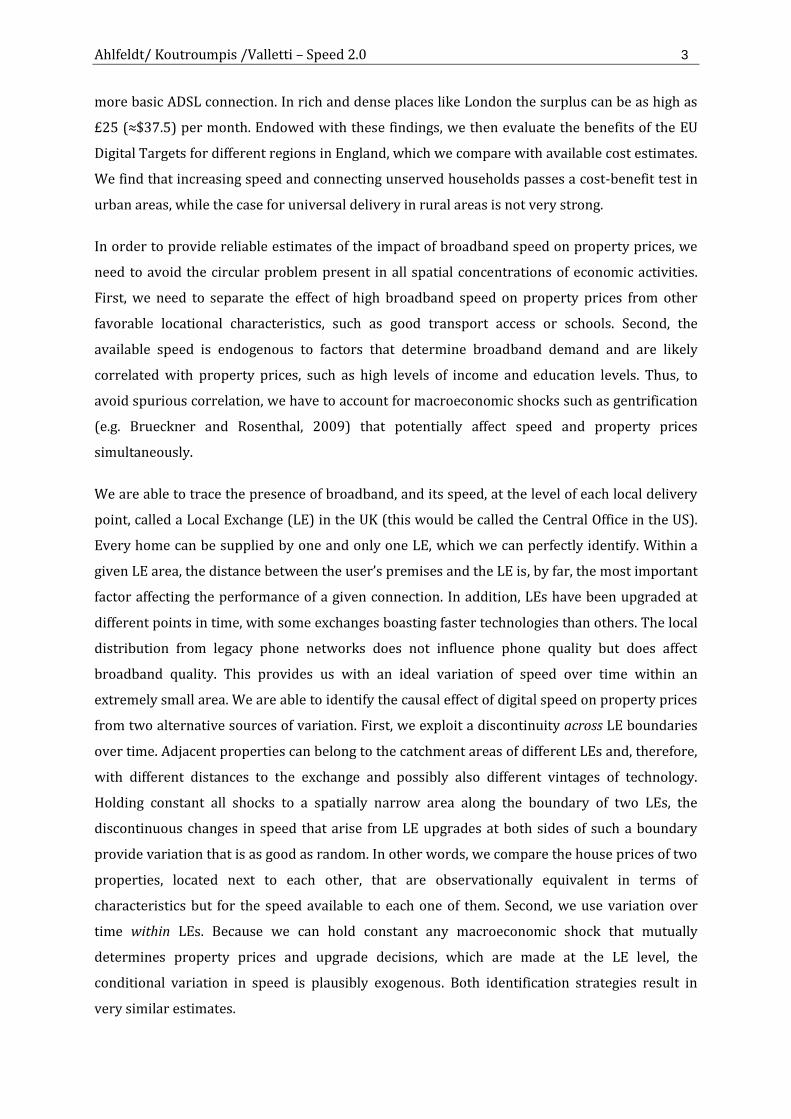
Figure 1 shows the share of English households in the catchment area of LEs enabled with ADSL
(black solid line) or with LLU entrants (grey solid line).13 We therefore cover the period that was
crucial for the development of residential Internet. The share of properties in our sample
reflects very closely the general technological pattern (dotted curves), providing reassurance on
its representativeness. In Appendix A, we provide further empirical evidence, showing maps of
how these technological changes occurred by region and over time.
Notes: Black (grey) lines refer to ADSL (LLU) activation. Solid (dashed) lines refer to all households in
England (Nationwide transactions data set)
Figure 1: Share of households with ADSL/LLU over time
Figure 2 is a static map of a few Local Exchanges located north of London. The figure reports the
location of the relevant LEs in that area (big black dots), and their catchment areas, based on the
full postcodes served (black boundaries). Each colored dot represents the location of one
transaction in the property dataset, where different colors correspond to different distances
from the exchange. Black icons denote groups of properties that have been matched to common
boundary segments. These two figures show two important things that will inform our empirical
strategy. First, there is considerable variation both in the distance between premises and the
relevant LE, and in the technology available over time at a given LE, which should have an
impact on the available speed for a specific property. We will, thus, be able to control for
13 We do not show ADSL2+ in order not to clutter the figure, but it would lie below the LLU curve.
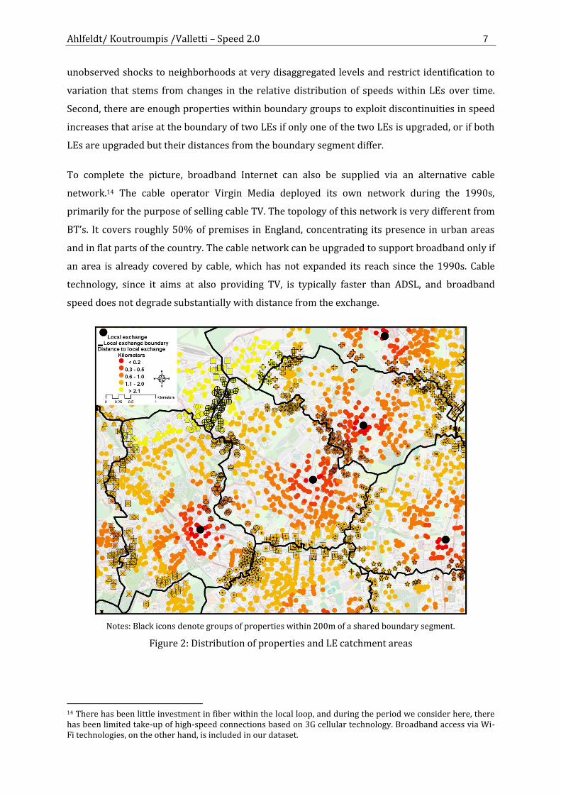
Ahlfeldt/ Koutroumpis /Valletti – Speed 2.0 7
unobserved shocks to neighborhoods at very disaggregated levels and restrict identification to
variation that stems from changes in the relative distribution of speeds within LEs over time.
Second, there are enough properties within boundary groups to exploit discontinuities in speed
increases that arise at the boundary of two LEs if only one of the two LEs is upgraded, or if both
LEs are upgraded but their distances from the boundary segment differ.
To complete the picture, broadband Internet can also be supplied via an alternative cable
network.14 The cable operator Virgin Media deployed its own network during the 1990s,
primarily for the purpose of selling cable TV. The topology of this network is very different from
BT’s. It covers roughly 50% of premises in England, concentrating its presence in urban areas
and in flat parts of the country. The cable network can be upgraded to support broadband only if
an area is already covered by cable, which has not expanded its reach since the 1990s. Cable
technology, since it aims at also providing TV, is typically faster than ADSL, and broadband
speed does not degrade substantially with distance from the exchange.
Notes: Black icons denote groups of properties within 200m of a shared boundary segment.
Figure 2: Distribution of properties and LE catchment areas
14 There has been little investment in fiber within the local loop, and during the period we consider here, there has been limited take-up of high-speed connections based on 3G cellular technology. Broadband access via Wi-Fi technologies, on the other hand, is included in our dataset.
Ahlfeldt/ Koutroumpis /Valletti – Speed 2.0 8
2.2 A simple conceptual model
Unlike for local public goods such as good (public) schools, public safety, or air quality, which are
often analysed in the house price capitalization literature, households subscribed to broadband
pay a price to their Internet provider. A capitalization effect of broadband is, therefore, not an
obvious feature of the spatial equilibrium. The purpose of this section is to introduce a simple
model that links broadband speed to property prices. Our intention is not to introduce a model
for structural estimation, but, rather, to think about this link in a simple and transparent
manner. For this purpose, imagine that there is a population of household buyers whose total
number is normalized to unity. The value of a property is denoted as V, which can be made
dependent on all its characteristics, such as number of rooms, local amenities, etc., except for
broadband availability, which is described next. The price of a property is denoted as P.
Households are heterogeneous in their value of using broadband. Value can derive from
different sources—from leisure (surfing the Internet) to being able to work from home. We are
not interested in the particular channel, but simply imagine that people are heterogeneous in the
way that they use and value the Internet. Let v∙log(q) denote the gross utility of household type v
using a broadband of quality q, where q is, for instance, the speed of the connection. This
specification reflects diminishing marginal returns to speed, as well as the fact that everybody
would enjoy faster connections, ceteris paribus, despite heterogeneity in tastes. The distribution
of household types v is assumed to be uniform between 0 and 1.15
The consumers’ choice is whether or not to purchase broadband, conditional on having bought a
property. We normalize the payoffs from not using broadband to zero. Broadband of quality q is
sold at a price p. Then, households whose value of broadband is high enough will purchase a
broadband connection. In particular, the marginal broadband household is defined by v* =
p/log(q), and all types between v* and 1 purchase broadband.
On the property supply side, we assume that homes in a given area are scarce, such that sellers
can always extract all buyers’ net surplus. Alternatively, one can also assume that sellers are able
to observe buyers’ types—during negotiations, for example—and make take-it-or-leave-it offers
leading to the same outcome. Households are assumed to be perfectly mobile, with reservation
utility U. House prices will, therefore, be
𝑃 = {𝑉 − 𝑈 for 𝑣 < 𝑣∗ (households without broadband),
𝑉 − 𝑈 + 𝑣log(𝑞) − 𝑝 for 𝑣 ≥ 𝑣∗ (households with broadband).
(1)
15 The example is generalizable to a more general distribution function F(v) that satisfies the monotone hazard rate condition. Note that costs and benefits from using broadband are expressed in present discounted values, rather than in per-period flows, to make them directly comparable with the purchase price of a property.

Ahlfeldt/ Koutroumpis /Valletti – Speed 2.0 9
To close the model and generate simple closed-form solutions, imagine that broadband is
supplied locally by n ≥ 1 identical oligopolistic providers at a cost c per unit of quality. For the
problem to make economic sense, it must be that c < log(q), as, otherwise, not even the
household with the highest willingness to pay would get a broadband subscription supplied at
cost. Suppliers are modeled à la Cournot: let xi denote the quantity supplied by firm i and
𝑋 = ∑ 𝑥𝑖𝑛𝑖=1 the aggregate supply. Since it is 1 − 𝑣∗ = ∑ 𝑥𝑖
𝑛𝑖=1 , we obtain the inverse demand
function 𝑝 = (1 − ∑ 𝑥𝑖𝑛𝑖=1 )log(q). Thus, provider i maximizes its profits (𝑝 − 𝑐)𝑥𝑖 = (1 − 𝑥𝑖 −
𝑋−𝑖) log(𝑞) 𝑥𝑖. Taking the FOC, and focusing on a symmetric equilibrium where 𝑋−𝑖 = (𝑛 − 1)𝑥𝑖,
we obtain that, at equilibrium, the broadband price is 𝑝∗ = 𝑐 +log(𝑞)−𝑐
𝑛+1.
Since the econometrician will not observe types, but just the average prices in a given area with
or without broadband subscription, we can calculate these averages from (1) as
𝑃 = (𝑉 − 𝑈)𝑣∗ + ∫ [𝑉 − 𝑈 + 𝑣log(𝑞) − 𝑝∗]d𝑣1
𝑣∗= 𝑉 − 𝑈 + (
𝑛
𝑛 + 1)
2
[log(𝑞) − 𝑐]2
log(𝑞). (2)
Eq. (2) confirms the intuition that broadband speed gets capitalized into house prices. In
particular, they increase with speed q, and at a decreasing rate if c is not too large.16
The model also has an ancillary prediction about broadband penetration in a given area. This
provides a useful check for the robustness of our main results. Penetration is given by
𝑃𝑒𝑛𝑒𝑡𝑟𝑎𝑡𝑖𝑜𝑛 = 1 − 𝑣∗ =𝑛
𝑛 + 1[1 −
𝑐
log(𝑞)], (3)
which is also increasing in speed q, and at a decreasing rate.
Note that the main prediction that property prices increase with speed is independent of the
precise market structure of the broadband market: it is stronger when n gets large, but it holds
even for a monopolist provider when n = 1. In other words, there are limits to the consumer
surplus that ISPs can appropriate when speed increases. Competition is the upper limit, in fact
broadband subscription fees cannot increase with willingness to pay for speed when
competition is intense, as they will just reflect costs. But even a monopolist would be
constrained by its inability to observe different types perfectly and would, therefore, leave some
information rent to higher types. Our approach presumes that all remaining consumer surplus
from broadband, over and above the broadband price paid to the provider, is appropriated by
the seller of the property. If this were not the case, then the impact that broadband might have
16 It is
𝜕𝑃
𝜕𝑞=
[log(𝑞)2−𝑐2]
2(𝑛+1)2log(𝑞)> 0 and
𝜕2𝑃
𝜕𝑞2 = −𝑛2[log(𝑞)3−𝑐2(2+log(𝑞))]
2(𝑛+1)2𝑞2log(𝑞)3 , which is always negative if c is small.

Ahlfeldt/ Koutroumpis /Valletti – Speed 2.0 10
on property prices would underestimate the consumer surplus from broadband use. We will
return to this point in our conclusions.
3 Empirical framework
The primary aim of our empirical strategy is to provide a causal estimate of the impact of high-
speed broadband supply on house prices. The empirical challenge in estimating this causal effect
is to separate the effect of broadband supply from unobserved and potentially correlated
determinants of house prices. In particular, we must ensure that there are no omitted variables
that simultaneously determine broadband supply and house prices. We argue that robust
identification can be achieved from discontinuous variation in speed over time and across LE
boundaries. Variation over time helps disentangle the effect of broadband supply from
unobserved (spatially) correlated location factors, such as good transport access or better
schools. By further placing properties into groups that are near to and share the same LE
boundary, it is possible to control for shocks at a very small spatial level. We argue that variation
in speed over time across an LE boundary within such a small area is plausibly exogenous and as
good as random. We also run an alternative identification which relies on the comparison of
house prices to broadband supply over time and within LE areas. Decisions that affect the
broadband supply of a property are generally taken at the level of the LE serving an area.
Conditional on shocks to a certain LE catchment area—such as a sudden increase in income or
education of the local population—within-LE variation in speed over time that results from the
distance of a property from the relevant exchange can be assumed to be exogenous.17
We follow the popular hedonic pricing method to separate various determinants of property
prices. Rosen (1974) has provided the micro-foundations for interpreting parameters estimated
in a multivariate regression of the price of the composite good housing against several internal
and locational characteristics as hedonic implicit attribute prices. Underlying the hedonic
framework is the idea that, given free mobility in spatial equilibrium, all locational
(dis)advantages must be offset by means of property price capitalization.18 There is a long
tradition in the literature—dating back at least as far as Oats (1969)—that made use of the
hedonic method to value local public goods while holding confounding factors constant. One of
the typical challenges faced by such hedonic valuation studies is the potential for bias due to
omitted variables that are correlated with a phenomenon of interest. Recent applications of the
17 Note that local exchange areas are relatively small. The median radius of a local exchange area is less than six km, as far as old voice telephony services are concerned. As for broadband, the area where it can be supplied effectively is even smaller, up to 2-3 km from the local exchange, as shown below in the results. In cities, the median radius of an LE is much smaller—e.g., less than two km in London. 18 Capitalization is a central prediction of spatial equilibrium models and has frequently been used to infer e.g. quality of life (Gabriel and Rosenthal, 2004; Shapiro, 2006).
Ahlfeldt/ Koutroumpis /Valletti – Speed 2.0 11
hedonic method have tackled this problem by making use of variation over time to identify the
effects of locational improvements from unobserved time-invariant locational factors (Ahlfeldt
and Kavetsos, 2014; Chay and Greenstone, 2005; Davis, 2004; Linden and Rockoff, 2008).
Both of the empirical specifications we employ are drawn from this line of research. We model
the (log) price of a property sold at a full postcode i at time t and served by LE j as a function of
the available broadband speed, as well as a range of internal and locational property
characteristics that are partially observed and partially unobserved. Our baseline empirical
specification is a variant of a spatial boundary discontinuity design:
log(𝑃𝑖𝑗𝑘𝑡) = ∑ 𝛼𝑚(𝑆𝑖𝑗𝑡)𝑚2
𝑚=1+ ∑ 𝜏𝑛(𝐷𝐼𝑆𝑇𝑖𝑗)
𝑛4
𝑛=1+ X𝑖
′μt + 𝜓𝑘𝑡 + 𝜑𝑗 + 𝜖𝑖𝑗𝑡 , (4)
where 𝑆𝑖𝑗𝑡 is the available broadband speed, and 𝐷𝐼𝑆𝑇𝑖𝑗 is the Euclidian distance from a
postcode i to the relevant LE j. We use a quadratic specification for broadband speed to allow the
property price to vary non-linearly with speed, as predicted by our simple model. The distance
polynomial controls for unobserved time-invariant locational characteristics that are correlated
with distance to the LE, so that the speed effect is identified from variation over time alone. As
discussed in more detail in the next section, our variable of interest 𝑆𝑖𝑗𝑡 is constructed using
fourth-order polynomials of 𝐷𝐼𝑆𝑇𝑖𝑗 following an engineering literature. The control variable
approach is therefore equivalent to postcode fixed effects in terms of its power to absorb
unobserved locational effects that are correlated with 𝑆𝑖𝑗𝑡. Compared to the alternative of using
postcode fixed effects, we prefer this control variable approach because of a relatively limited
number of repeated sales at the same postcode level.19 X𝑖′ is a vector of property and locational
characteristics discussed in the data section. This is interacted with a full set of year effects, so
that μt is a matrix of implicit prices for attribute-year combinations. 𝜑𝑗 is a dummy to control for
unobserved time-invariant LE effects. Finally, k indexes properties that lie along the same
boundary segment that separates two LE areas. We match properties in LE j to the nearest
property in LE l≠j and define a common time-varying fixed effect 𝜓𝑘𝑡 for properties in j whose
nearest neighbor is in l and vice versa. Fig. 2 illustrates the matching of properties to common
boundary FE.
This specification exploits the discontinuity at the boundaries between LEs. Overall, there are
86,569 LE boundary x year effects in our data, which denote boundary segments that are
common to the same two LEs. With this specification, we attribute differences in price changes
over time across a common boundary to the respective differences in speed changes over time.
19 Less than half (15 percent) of the full postcodes in the Nationwide data set contain two (three) or more transactions. On average, there are 2.15 transactions per full postcode over the 15-year period we cover.
Ahlfeldt/ Koutroumpis /Valletti – Speed 2.0 12
We restrict our sample to properties that are close to an LE boundary to explicitly exploit the
spatial discontinuities in speed changes that arise across an LE boundary if the broadband
infrastructure is altered. We note that a discontinuity arises not only if just one of two adjacent
LEs is upgraded, but also if both LEs are upgraded, and the distance to the respective LEs differs
significantly at both sides of the LE boundary. Because, at a local level, the allocation of a
property to either side of the same boundary is as good as random, it is unlikely that unobserved
shocks exist that impact speed and property prices on one side of the boundary but not on the
other. Such shocks are absorbed by the LE boundary x year effects.
We also estimate an alternative specification in which we replace the LE boundary x year effects
with a set of 37,804 LE x year fixed effects 𝜑𝑗𝑡 that control for all macroeconomic shocks at the
LE level:
log(𝑃𝑖𝑗𝑡) = ∑ 𝛼𝑚(𝑆𝑖𝑗𝑡)𝑚2
𝑚=1+ ∑ 𝜏𝑛(𝐷𝐼𝑆𝑇𝑖𝑗)
𝑛4
𝑛=1+ X𝑖
′μt + 𝜑𝑗𝑡 + 𝜖𝑖𝑗𝑡 , (5)
With this specification we focus on a different source of variation, compared to eq. (4). Instead of
exploiting discontinuous variation in speed over time across LE boundaries we now identify
exclusively from continuous variation in speed over time within LEs. In estimating eq. (5) we
also use the universe of transactions and variation in speed, which helps addressing the external
validity problem inherent to all boundary discontinuity designs. This specification delivers a
causal effect of broadband speed on house prices under the identifying assumption that year-
specific shocks that potentially determine broadband capacity are uncorrelated with distance to
the LE within the area that the LE serves. This is a plausible assumption for two reasons. First,
any change to the LE technology will affect the entire catchment area served by the LE, so it is
rational for broadband suppliers to base decisions on the average trend in this area. It is,
therefore, unlikely that within-LE shocks that might affect property prices—e.g., an income
increase among the population near the LE relative to other areas—would also affect the
technological upgrading decisions above and beyond their effect on the LE area average, which
is captured by 𝜑𝑗𝑡 . Second, LEs serve relatively small areas, with a layout that was defined
decades ago and boundaries that do not line up with spatial statistical units, such as census
wards. The catchment area of each LE is typically known only to providers and is not used to
create any other related boundaries. Reliable information on year-on-year changes at the sub-LE
area level is difficult to obtain, which makes it unlikely that providers would be able respond to
within LE-area shocks even if they wanted to.20 This specification is arguably more open to
20 It is telling that all the regulatory analysis done by Ofcom, which relies on information supplied by the broadband operators, is, indeed, conducted at the LE level, instead of at a more disaggregated level, such as street cabinets. This is because the regulator believes that the relevant market for business decisions is the LE, which is where most investments have to be sunk.
Ahlfeldt/ Koutroumpis /Valletti – Speed 2.0 13
criticism because there may be within-LE trends in property prices that are correlated with
distance to the LE, something that is absent with the previous specification relying on the
boundary discontinuity. It is noteworthy that the interactions of year effects and attributes X𝑖′
flexibly control for property price trends that are correlated with any of the observable
structural and locational characteristics. Conditional on these controls it is less likely that
within-LE trends, which are correlated with but not causally related to changes in speed within
LEs over time, confound the estimated broadband speed effect. Moreover, we can also use
program-evaluation techniques to reassure ourselves that, conditional on the strong controls
employed, there are no within LE trends correlated with distance to the LE that could lead to
spurious broadband supply effects.
We finally note that eq. (4) and eq. (5) are mutually complementary. Adding LE x year fixed
effects 𝜑𝑗𝑡 to eq. (4) would partially absorb the identifying discontinuous variation in speed over
time across LE boundaries. Likewise, adding LE x year boundary fixed effects 𝜓𝑘𝑡 to eq. (5)
would partially absorb the identifying continuous variation in speed over time within LEs.
Because the two equations are designed to identify the broadband capitalization effect from two
different types of variation, consistent estimates will be particularly indicative of robustness.
3.1 Raw data
Our dataset stems from several sources. The main block concerns the development of
broadband in England over the period 1995-2010. Ofcom has made available to us all the
information it collects on the broadband market for regulatory purposes. The dataset comprises
quarterly information at the level of each of the 3,897 LEs in England. For each local exchange,
we know the precise coverage of BT’s local network—that is, all the specific full postcodes
served by a certain LE—and, therefore, we know how many buildings and total lines can
eventually have broadband. We can identify when a LE was upgraded to ADSL or ADSL2+, and if
and when it attracted entrants via LLU. We also know, in the catchment area of the LE, whether
or not cable is available. Finally, we know how broadband penetration varies over time in a
given LE, as we are told the total number of subscribers (via BT, via an entrant, or via cable),
which can be compared to the total lines available locally to compute broadband penetration.
This detailed information was supplemented with information on broadband speed tests carried
out by individuals in 2009 and 2010. We obtained three million tests from a private company.21
For each individual/speed test, we observe the operator, the contract option chosen by the user,
the location (full post code), as well as when the test was carried out. Thus, we can calculate the
distance between the user’s premises (the geographic center of the six-digit postcode area
21 http://www.broadbandspeedchecker.co.uk

Ahlfeldt/ Koutroumpis /Valletti – Speed 2.0 14
where the test is run) and the exact location of the relevant LE. The dataset contemplates two
measures of performance: download speed and upload speed. We focus on the former, which is,
by far, the more important feature for residential household users.
For the analysis of the capitalization effects of broadband capacity, we use transactions data
related to mortgages granted by the Nationwide Building Society between 1995 and 2010. The
data for England comprise more than one million observations,22 and include the price paid for
individual housing units along with detailed property characteristics. These characteristics
include floor space (m²), the type of property (detached, semi-detached, flat, bungalow or
terraced), the date of construction, the number of bedrooms and bathrooms, garage or parking
facilities and the type of heating. There is also some buyer information, including the type of
mortgage (freehold or leasehold) and whether they are first-time buyers. Note that the
transaction data include the full UK postcode of the property sold, allowing it to be assigned to
grid-reference coordinates. We remark that a full postcode unit contains about 10-15
households, which are all connected to the same LE.23
With this information, it is possible within GIS to calculate distances to LEs. Furthermore, it is
possible to calculate distances and other spatial measures (e.g., densities) for the amenities and
environmental characteristics such as National Parks, as well as natural features such as lakes,
rivers and coastline. The postcode reference also allows a merger of transactions and various
household characteristics (median income and ethnic composition) from the UK census; natural
land cover and land use; and various amenities, such as access to employment opportunities,
cultural and entertainment establishments and school quality. A more-detailed description of all
the data used is in Appendix B.
3.2 The relationship among technology, distance and speed
As said above, we have very detailed information on the exact broadband capacity to deliver
achievable speeds at a specific property at a high spatial detail, but not over the entire period.
We know, however, the technology available in each LE at different points in time. We now
establish the technological relationship between effective Internet speed, the technology of a LE,
and the distance from a test location to the LE, using the comprehensive data set of Internet
speed tests in the sub-period 2009-10. Combining both ingredients, it is possible to generate the
22 This represents 10% of all mortgages issued in England over the period. 23 This dataset has also been used by Ahlfeldt et al. (2014), who test the predictions of a political economy model of conservation area designation. It is important to clarify that a full (typically, 7 digit) postcode in the UK captures a narrowly defined area. To give a sense of the detail, there are approximately 2 million postcodes in the UK. A full postcode is not an address, but still covers areas that are on average within a radius of 50m, which gets even narrower in densely populated areas (e.g., 20m in London).
Ahlfeldt/ Koutroumpis /Valletti – Speed 2.0 15
micro-level Internet speed panel variable we require for a robust identification of the causal
effect of broadband capacity on house prices.
We model broadband capacity as a function of LE characteristics and the distance to the LE, as
well as the interaction between the two. In doing so, we first need to account for a significant
proportion of speed tests that are likely constrained not only by technological limitations
(distance to the LE and LE characteristics), but also by the plans users have chosen to subscribe
to. In other words, speed can be low not because technology is limited, but because a subscriber
with small consumption choses a plan with limitations. We want to get rid of these plans so that
we can unravel the true speed that a certain technology can potentially supply. To identify the
plans that do not constrain broadband speed beyond the technological limitations of the LE, we
run the following auxiliary regression:
log(𝑆𝑖𝑗𝑡) = ∑ 𝛼𝑚
12
𝑚=2+ ∑ 𝛼ℎ
23
ℎ=1+ ∑ 𝛼𝑤
6
𝑤=1+ ∑ 𝛼𝑝
62
𝑝=1+ ∑ 𝛼𝑑
60
𝑑=2+ 𝜑𝑗𝑡 + 𝜀𝑖𝑗𝑡 , (6)
where 𝑆𝑖𝑗𝑡 is the actual broadband speed test score measured at postcode i served by local
exchange j at time t. 𝛼𝑚 are month of the year effects (baseline category is January), 𝛼ℎ are hours
of the day effects (baseline category 0h), 𝛼𝑤 are day of the week effects (baseline category
Sunday), 𝛼𝑝 are Internet plan effects (baseline category is missing information), 𝛼𝑑 are distance
to LE effects captured by 100m bins (e.g., 2 covers distances from 150 to 250m, baseline
category is 0-150m), and 𝜑𝑗𝑡 are a set of LE-year specific fixed effects that capture unobserved
LE characteristics in a given year. For the ensuing analysis, we keep observations whose 𝛼𝑝 falls
in the upper quartile, as the plans that realize the fastest actual speeds are unlikely to be
constrained by the operator.
Using this sub-sample of speed tests that should be constrained only by technology, we then
establish the technological relationship between available broadband speed 𝑆𝑖𝑗𝑡 and distance to
the relevant LE (𝐷𝐼𝑆𝑇𝑖𝑗) for each technological category 𝑄 = {ADSL, ADSL + LLU, ADSL2 +} in
separate regressions of the following type:
log(𝑆𝑖𝑗𝑡) = ∑ 𝛼𝑚𝑄
12
𝑚=2+ ∑ 𝛼ℎ𝑄
23
ℎ=1+ ∑ 𝛼𝑤𝑄
6
𝑤=1+ ∑ 𝛼𝑛𝑄(𝐷𝐼𝑆𝑇𝑖𝑗)
𝑛4
𝑛=0+ 𝜑𝑗𝑄 + 𝜔𝑡𝑄 + 𝜀𝑖𝑗𝑡𝑄 .
(7)
The fourth-order polynomial is used to capture the non-linearities reported in the technical
literature.24 Since we drop 75% of the observations compared to eq. (6) and split the remaining
24 For a list of the factors that affect local broadband speed, see, e.g., the explanation provided by BT: http://bt.custhelp.com/app/answers/detail/a_id/7573/c/. A detailed analysis of the factors that affect the performance of ADSL networks is found in Summers (1999). We note that the choice of a fourth-order polynomial for distance was dictated by its goodness of fit. There was no gain in going towards higher orders.
Ahlfeldt/ Koutroumpis /Valletti – Speed 2.0 16
sample into three categories in order to find technology-specific effects, we account for location
and year effects separately, rather than accounting for their interaction, to save degrees of
freedom in sparsely populated LEs. Based on the estimated distance decay parameters 𝛼𝑛𝑄 and
the known Q-type upgrade dates 𝑇𝑗𝑄, it is then straightforward to predict the available
broadband speed at any postcode i that is served by a LE j over the entire period:
𝑆𝑖𝑗𝑡 = {
𝐼𝑆𝐷𝑁 = 128 Kbit/ sec if 𝑡 < 𝑇𝑗𝐴𝐷𝑆𝐿,
exp [∑ 𝛼𝑛𝑄(𝐷𝐼𝑆𝑇𝑖𝑗)𝑛4
𝑛=0] if 𝑇𝑗
𝑄 ≤ 𝑡 < 𝑇𝑗𝑄′ .
(8)
This compact formulation says that, before broadband is rolled out in LE j, the line is served with
a basic ISDN technology, as a voice telephony line is in place. Then, ADSL brings its upgraded
speed at any period after 𝑇𝑗𝐴𝐷𝑆𝐿. The decay parameters may further change if the LE additionally
receives, at a certain point in time 𝑇𝑗𝑄′
, technology Q′ = {ADSL + LLU, ADSL2 +}.
We start by reporting the results on the physical relationship among speed, technological
characteristics of the LE, and distance between the premise and the LE, as described by model
(7). Our findings are shown in Table 1.25
Although, due to space limitations, we do not detail the various fixed effects in the table, they all
show a very reasonable behavior. The time of day is an important factor: the average connection
speed reaches its peak at 5 a.m., when download speed is about 12% faster than the reference
speed at midnight. It then gradually declines, with speed 3% lower at noon, 11% lower at 6 p.m.
and close to 20% lower at 8 p.m., when the worst daily speed is attained. From then on, the
average speed of a connection gradually increases until 5 a.m. The day of the week also
determines average speed: it is lowest over the weekend, when residential users tend to be at
home. These findings are due to obvious local congestion when most people are online
simultaneously. Congestion is, thus, another facet of speed that shows striking analogies in the
digital and the real worlds (see e.g. Couture et al., 2012; Duranton and Turner, 2011).
Turning to the impact of distance, which is of more direct interest for our purposes, this is
shown in columns (1), (2), and (3) of Table 1 for ADSL, LLU, and ADSL 2+, respectively. Distance
plays a statistically very significant role for all of them. Table 1, column (4) also runs a placebo
test. The cable technology, which is available only in some parts of the country, does not rely on
25 It is important to note that, throughout the whole paper, we refer to the “nominal” speed typically advertised by operators in their plans, as this is the most commonly understood measure of speed that users look for when subscribing to a plan. This is not the same as “actual” speed, which is measured in the dataset on speed tests. The discrepancy for the top unconstrained plans is actually quite large and amounts to a factor 4 (results are available on request from the authors). This factor is also in line with independent findings of Ofcom; see, e.g., http://stakeholders.ofcom.org.uk/market-data-research/other/telecoms-research/broadband-speeds/speeds-nov-dec-2010/, and Figure 1.2 in particular).
Ahlfeldt/ Koutroumpis /Valletti – Speed 2.0 17
copper wires and does not suffer from distance-decay problems. Thus, the distance of a home
from any exchange should not impact speed. Column (4) reports the results for one set of cable
contracts offered by the cable provider, and, indeed, distance has no impact on speed.
One way of showing the relevance of the results is to evaluate the fit of the polynomial
approximation. We estimate the distance relationships replacing the polynomial, as estimated in
Table 1, with a set 100m distance bin effects, as used in model (3). Results are shown in Figure 3.
Solid lines are the fourth-order polynomials (from Table 1) fitted into the raw data (not the
dots). The dots indicate the point estimates of 100m bins obtained in separate regressions for
each technology. The fit is quite striking, especially for distances up to 5 km from the LE—for
greater distances, there is also more noise because there are few observations beyond that
distance. We are, thus, confident that we can approximate the real speed sufficiently precisely so
that attenuation bias can be ignored in equations (4) and (5). We further note that we use
estimated parameters of a physical relationship that depends on distance and LE technology to
approximate our speed capacity variable. This is different from a generated regressor recovered
from an auxiliary first-stage estimation, which would require bootstrapping in the second-stage.
(1) (2) (3) (4) log of download speed (in kbit/s)
Technology Broadband ADSL
Broadband ADSL+LLU
Broadband ADSL2+
Cable
Distance from test postcode to LE in km
0.184 (0.145)
0.057 (0.121)
0.053 (0.071)
0.016 (0.032)
Distance ^2 -0.293*** (0.097)
-0.287*** (0.097)
-0.491*** (0.055)
0.016 (0.029)
Distance ^3 0.058** (0.024)
0.070** (0.028)
0.141*** (0.017)
-0.001 (0.010)
Distance ^4 -0.003* (0.002)
-0.005** (0.002)
-0.011*** (0.002)
-0.001 (0.001)
Constant 7.869*** (0.098)
8.214*** (0.065)
8.672*** (0.036)
8.334*** (0.017)
LE effects YES YES YES YES Month effects YES YES YES YES Day of the week effects YES YES YES YES Hour of the day effects YES YES YES YES Year effects YES YES YES YES r2 0.174 0.160 0.198 0.034 N 53,961 64,447 310,256 290,067 Notes: Only observations falling into the top-quartile of contracts are used in the regressions. Standard errors
in parentheses are clustered on LEs. * p<0.1, ** p<0.05, *** p<0.01
Table 1: Speed results
These results confirm the key role played by distance. First, there is strong speed decay by
distance: as a building happens to be farther away from the relevant LE, its actual speed goes
down compared to another dwelling connected to the same LE with the same technology, but
closer to the exchange. This phenomenon is particularly strong within 3 km (2 miles) around an
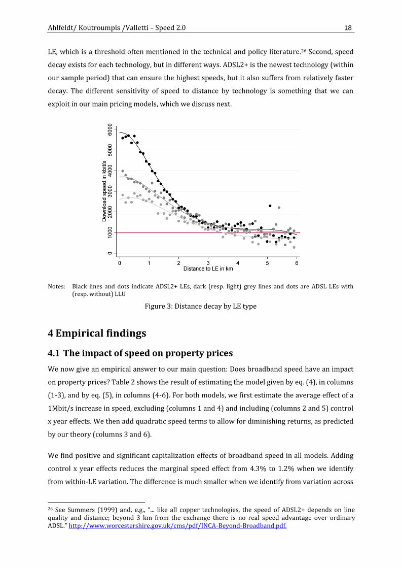
Ahlfeldt/ Koutroumpis /Valletti – Speed 2.0 18
LE, which is a threshold often mentioned in the technical and policy literature.26 Second, speed
decay exists for each technology, but in different ways. ADSL2+ is the newest technology (within
our sample period) that can ensure the highest speeds, but it also suffers from relatively faster
decay. The different sensitivity of speed to distance by technology is something that we can
exploit in our main pricing models, which we discuss next.
Notes: Black lines and dots indicate ADSL2+ LEs, dark (resp. light) grey lines and dots are ADSL LEs with (resp. without) LLU
Figure 3: Distance decay by LE type
4 Empirical findings
4.1 The impact of speed on property prices
We now give an empirical answer to our main question: Does broadband speed have an impact
on property prices? Table 2 shows the result of estimating the model given by eq. (4), in columns
(1-3), and by eq. (5), in columns (4-6). For both models, we first estimate the average effect of a
1Mbit/s increase in speed, excluding (columns 1 and 4) and including (columns 2 and 5) control
x year effects. We then add quadratic speed terms to allow for diminishing returns, as predicted
by our theory (columns 3 and 6).
We find positive and significant capitalization effects of broadband speed in all models. Adding
control x year effects reduces the marginal speed effect from 4.3% to 1.2% when we identify
from within-LE variation. The difference is much smaller when we identify from variation across
26 See Summers (1999) and, e.g., “... like all copper technologies, the speed of ADSL2+ depends on line quality and distance; beyond 3 km from the exchange there is no real speed advantage over ordinary ADSL.” http://www.worcestershire.gov.uk/cms/pdf/INCA-Beyond-Broadband.pdf.
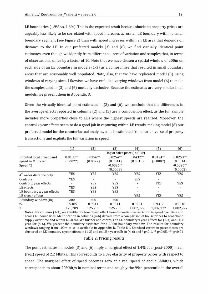
Ahlfeldt/ Koutroumpis /Valletti – Speed 2.0 19
LE boundaries (1.9% vs. 1.6%). This is the expected result because shocks to property prices are
arguably less likely to be correlated with speed increases across an LE boundary within a small
boundary segment (see Figure 2) than with speed increases within an LE area that depends on
distance to the LE. In our preferred models (3) and (6), we find virtually identical point
estimates, even though we identify from different sources of variation and samples that, in terms
of observations, differ by a factor of 10. Note that we have chosen a spatial window of 200m on
each side of an LE boundary in models (1-3) as a compromise that resulted in small boundary
areas that are reasonably well populated. Note, also, that we have replicated model (3) using
windows of varying sizes. Likewise, we have excluded varying windows from model (6) to make
the samples used in (3) and (6) mutually exclusive. Because the estimates are very similar in all
models, we present them in Appendix D.
Given the virtually identical point estimates in (3) and (6), we conclude that the differences in
the average effects reported in columns (2) and (5) are a composition effect, as the full sample
includes more properties close to LEs where the highest speeds are realized. Moreover, the
control x year effects seem to do a good job in capturing within-LE trends, making model (6) our
preferred model for the counterfactual analysis, as it is estimated from our universe of property
transactions and exploits the full variation in speed.
(1) (2) (3) (4) (5) (6) log of sales price (in GBP) Imputed local broadband speed in MBit/sec
0.0189*** (0.0022)
0.0156*** (0.0022)
0.0254*** (0.0041)
0.0432*** (0.0018)
0.0124*** (0.0007)
0.0253*** (0.0014)
Speed^2
-0.0026*** (0.0009)
-0.0026*** (0.0002)
4th
order distance poly. YES YES YES YES YES YES
Controls YES - - YES - - Control x year effects - YES YES - YES YES LE effects YES YES YES - - - LE boundary x year effects YES YES YES - - - LE x year effects - - - YES YES YES Boundary window (m) 200 200 200 - - - r2 0.9485 0.9511 0.9511 0.9224 0.9317 0.9318 N 125,209 125,209 125,209 1,082,777 1,082,777 1,082,777
Notes: For columns (1-3), we identify the broadband effect from discontinuous variation in speed over time and across LE boundaries. Identification in columns (4-6) derives from a comparison of house prices to broadband supply over time and within LE areas. We further add controls on LE boundary x year effects for (1-3) and LE x year for (4-6). We present the boundary estimates for a 200m boundary window. The results for boundary windows ranging from 100m to ∞ is available in Appendix D, Table D1. Standard errors in parentheses are clustered on LE boundary x year effects in (1-3) and on LE x year cells in (4-6) and * p<0.1, ** p<0.05, *** p<0.01
Table 2: Pricing results
The point estimates in models (3) and (6) imply a marginal effect of 1.4% at a (post-2000) mean
(real) speed of 2.2 Mbit/s. This corresponds to a 3% elasticity of property prices with respect to
speed. The marginal effect of speed becomes zero at a real speed of about 5Mbit/s, which
corresponds to about 20Mbit/s in nominal terms and roughly the 99th percentile in the overall

Ahlfeldt/ Koutroumpis /Valletti – Speed 2.0 20
speed distribution in our data. The implied effect on property prices at this point is 3.8% and,
thus, £8,360 (≈$12,540) for a property worth £220,000 (≈$330,000, the mean house price in
2005, which is the middle point of the 2000-2010 period of Internet development we cover).27 It
is interesting to see that the marginal effect (i.e., the impact of a marginal increase in speed on
net consumer surplus in our model) is about zero, close to the maximum actual speed that we
observe in the data. There would be no particular reason for suppliers to provide speed above
the maximum observed levels in our data, as no further surplus could be created.
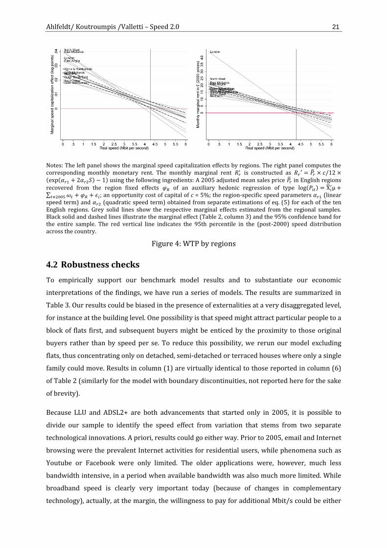
Using our preferred specification (6), we have produced results that show the capitalization
effect by region. These are summarized in Figure 4. The left panel (in logs) shows the results as
percentages, while the right panel (in levels) converts the findings in monetary rents. It is
reassuring that the marginal effects look relatively similar. It seems important to acknowledge
that prices differ substantially across English regions. Similar marginal capitalization effects
may, therefore, imply different rents. In fact, the striking, though perhaps not surprising, result is
that we get a broadband marginal monetary rent that is about twice as high in London as in any
other English region. After having estimated separate effects for each region, London shows
higher than average willingness to pay for broadband, but it is not an outlier in this distribution.
The difference in the marginal rent is, instead, attributable to the higher house-price levels in
London. Usage is probably also a lot higher in London than in the rest of the country, but
competition among broadband providers is very intense in London, so they cannot really price-
differentiate accordingly. It is sellers in London who ultimately receive a higher rent from
broadband usage.
Our results do suggest that a broadband rent exists in general. Local characteristics, however,
also seem to be important. The rent is rather low in regions with a higher share of low-income
rural areas, which is probably where access to broadband is a problem. It seems that the benefits
are relatively small where the policy maker is most likely to intervene. If the subsidies required
are sufficiently low, there may still be some rationale for interventions. What also seems to be
important is that the rent is declining in speed. For policy, this may imply that what is really
important is to make sure that everyone gets access to some decent broadband connection.
Getting access to very high speeds should, perhaps, not be the priority. This is what we analyze
in the policy section. Before doing so, however, we conduct some further checks to reassure that
broadband speed does, indeed, cause an increase in property prices.
27 This premium is comparable to, e.g., an increase in floor size of about 8 square meters, holding all other housing characteristics (e.g., the number of rooms) constant, or a reduction in distance to the nearest underground station by roughly one kilometer (Gibbons and Machin, 2005).
Ahlfeldt/ Koutroumpis /Valletti – Speed 2.0 21
Notes: The left panel shows the marginal speed capitalization effects by regions. The right panel computes the corresponding monthly monetary rent. The monthly marginal rent 𝑅𝑟
′ is constructed as 𝑅𝑟′ = �̅�𝑟 × 𝑐/12 ×(exp(𝛼𝑟1 + 2𝛼𝑟2𝑆) − 1) using the following ingredients: A 2005 adjusted mean sales price �̅�𝑟 in English regions recovered from the region fixed effects 𝜑𝑅 of an auxiliary hedonic regression of type log(𝑃𝑖𝑡) = X̃𝑖
′μ +∑ 𝜔𝑡𝑡≠2005 + 𝜑𝑅 + 𝜖𝑖; an opportunity cost of capital of c = 5%; the region-specific speed parameters 𝛼𝑟1 (linear speed term) and 𝛼𝑟2 (quadratic speed term) obtained from separate estimations of eq. (5) for each of the ten English regions. Grey solid lines show the respective marginal effects estimated from the regional samples. Black solid and dashed lines illustrate the marginal effect (Table 2, column 3) and the 95% confidence band for the entire sample. The red vertical line indicates the 95th percentile in the (post-2000) speed distribution across the country.
Figure 4: WTP by regions
4.2 Robustness checks
To empirically support our benchmark model results and to substantiate our economic
interpretations of the findings, we have run a series of models. The results are summarized in
Table 3. Our results could be biased in the presence of externalities at a very disaggregated level,
for instance at the building level. One possibility is that speed might attract particular people to a
block of flats first, and subsequent buyers might be enticed by the proximity to those original
buyers rather than by speed per se. To reduce this possibility, we rerun our model excluding
flats, thus concentrating only on detached, semi-detached or terraced houses where only a single
family could move. Results in column (1) are virtually identical to those reported in column (6)
of Table 2 (similarly for the model with boundary discontinuities, not reported here for the sake
of brevity).
Because LLU and ADSL2+ are both advancements that started only in 2005, it is possible to
divide our sample to identify the speed effect from variation that stems from two separate
technological innovations. A priori, results could go either way. Prior to 2005, email and Internet
browsing were the prevalent Internet activities for residential users, while phenomena such as
Youtube or Facebook were only limited. The older applications were, however, much less
bandwidth intensive, in a period when available bandwidth was also much more limited. While
broadband speed is clearly very important today (because of changes in complementary
technology), actually, at the margin, the willingness to pay for additional Mbit/s could be either
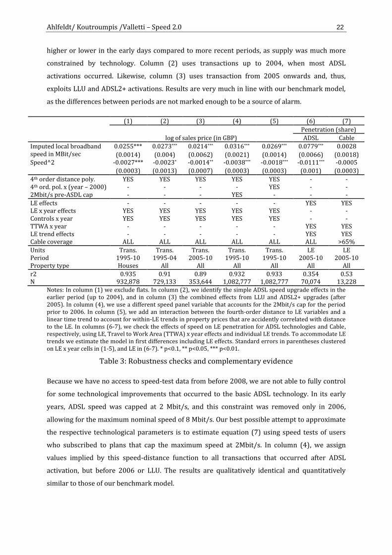
Ahlfeldt/ Koutroumpis /Valletti – Speed 2.0 22
higher or lower in the early days compared to more recent periods, as supply was much more
constrained by technology. Column (2) uses transactions up to 2004, when most ADSL
activations occurred. Likewise, column (3) uses transaction from 2005 onwards and, thus,
exploits LLU and ADSL2+ activations. Results are very much in line with our benchmark model,
as the differences between periods are not marked enough to be a source of alarm.
(1) (2) (3) (4) (5) (6) (7)
Penetration (share)
log of sales price (in GBP) ADSL Cable
Imputed local broadband speed in MBit/sec
0.0255*** 0.0273*** 0.0214*** 0.0316*** 0.0269*** 0.0779*** 0.0028
(0.0014) (0.004) (0.0062) (0.0021) (0.0014) (0.0066) (0.0018) Speed^2 -0.0027*** -0.0023* -0.0014** -0.0038*** -0.0018*** -0.0111*** -0.0005
(0.0003) (0.0013) (0.0007) (0.0003) (0.0003) (0.001) (0.0003)
4th order distance poly. YES YES YES YES YES - - 4th ord. pol. x (year – 2000) - - - - YES - - 2Mbit/s pre-ASDL cap - - - YES - - -
LE effects - - - - - YES YES LE x year effects YES YES YES YES YES - - Controls x year YES YES YES YES YES - - TTWA x year - - - - - YES YES LE trend effects - - - - - YES YES Cable coverage ALL ALL ALL ALL ALL ALL >65%
Units Trans. Trans. Trans. Trans. Trans. LE LE Period 1995-10 1995-04 2005-10 1995-10 1995-10 2005-10 2005-10 Property type Houses All All All All All All
r2 0.935 0.91 0.89 0.932 0.933 0.354 0.53 N 932,878 729,133 353,644 1,082,777 1,082,777 70,074 13,228
Notes: In column (1) we exclude flats. In column (2), we identify the simple ADSL speed upgrade effects in the earlier period (up to 2004), and in column (3) the combined effects from LLU and ADSL2+ upgrades (after 2005). In column (4), we use a different speed panel variable that accounts for the 2Mbit/s cap for the period prior to 2006. In column (5), we add an interaction between the fourth-order distance to LE variables and a linear time trend to account for within-LE trends in property prices that are accidently correlated with distance to the LE. In columns (6-7), we check the effects of speed on LE penetration for ADSL technologies and Cable, respectively, using LE, Travel to Work Area (TTWA) x year effects and individual LE trends. To accommodate LE trends we estimate the model in first differences including LE effects. Standard errors in parentheses clustered on LE x year cells in (1-5), and LE in (6-7). * p<0.1, ** p<0.05, *** p<0.01.
Table 3: Robustness checks and complementary evidence
Because we have no access to speed-test data from before 2008, we are not able to fully control
for some technological improvements that occurred to the basic ADSL technology. In its early
years, ADSL speed was capped at 2 Mbit/s, and this constraint was removed only in 2006,
allowing for the maximum nominal speed of 8 Mbit/s. Our best possible attempt to approximate
the respective technological parameters is to estimate equation (7) using speed tests of users
who subscribed to plans that cap the maximum speed at 2Mbit/s. In column (4), we assign
values implied by this speed-distance function to all transactions that occurred after ADSL
activation, but before 2006 or LLU. The results are qualitatively identical and quantitatively
similar to those of our benchmark model.
Ahlfeldt/ Koutroumpis /Valletti – Speed 2.0 23
One concern with the identification from within-LE variation (Table 2, column 6) is that there
may be within-LE trends in property prices that are accidently correlated with distance to the
LE, which could bias our speed results. To control for a long-run trend correlated with distance
to the LE and not absorbed by control x year effects, we add an interaction between the fourth-
order distance to LE variables and a linear time trend in column (5). This is a strong control as it
is likely to partially absorb the effect of speed upgrades if capitalization occurs smoothly over
time. The speed effect, however, remains remarkably close to the benchmark model, pointing to
speed capitalization effects that occur discontinuously in time. To illustrate this discontinuous
pattern in the spatiotemporal adjustment in property prices to LE upgrades in a transparent
way, we additionally employ a variant of the difference-in-differences (DD) approach. The full
methodology is explained in Appendix C, where we discuss a reduced-form DD specification,
which is expanded to account for spatial heterogeneity and for a temporal structure in the
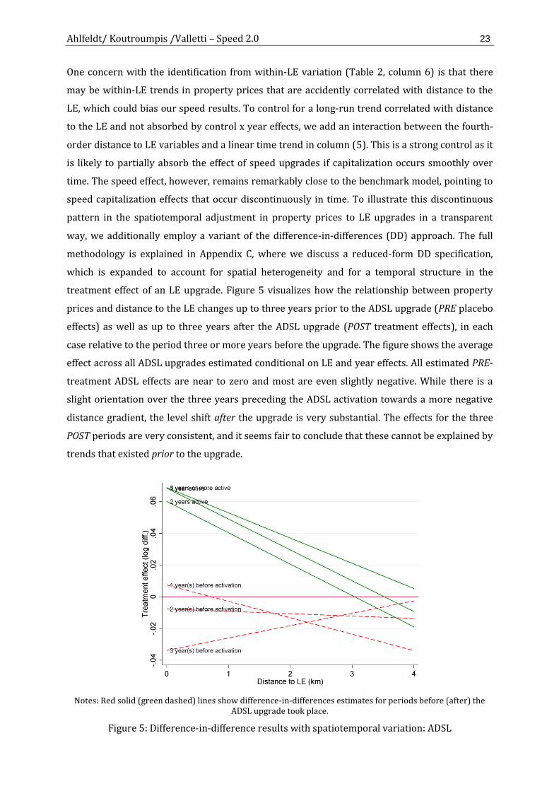
treatment effect of an LE upgrade. Figure 5 visualizes how the relationship between property
prices and distance to the LE changes up to three years prior to the ADSL upgrade (PRE placebo
effects) as well as up to three years after the ADSL upgrade (POST treatment effects), in each
case relative to the period three or more years before the upgrade. The figure shows the average
effect across all ADSL upgrades estimated conditional on LE and year effects. All estimated PRE-
treatment ADSL effects are near to zero and most are even slightly negative. While there is a
slight orientation over the three years preceding the ADSL activation towards a more negative
distance gradient, the level shift after the upgrade is very substantial. The effects for the three
POST periods are very consistent, and it seems fair to conclude that these cannot be explained by
trends that existed prior to the upgrade.
Notes: Red solid (green dashed) lines show difference-in-differences estimates for periods before (after) the
ADSL upgrade took place.
Figure 5: Difference-in-difference results with spatiotemporal variation: ADSL
Ahlfeldt/ Koutroumpis /Valletti – Speed 2.0 24
We now return to eq. (4), which exploits the spatial boundary discontinuity. A popular validation
exercise in the literature is to test for discontinuities in alternative spatial variables that
potentially determine the outcome measure but are not related to the phenomenon of interest
(e.g. Gibbons, et al., 2013). As we identify from variation that is discontinuous in space and time,
we are interested in whether other outcome variables systematically adjust where and when
speed increases due to LE upgrades. In Table D3 in Annex D we present estimates of eq. (4)
using a range of buyer or property related characteristics as dependent variables. We find no
significant effect of broadband speed on whether a buyer is a first-time buyer or signs a
leasehold contract, on the size of transacted properties, on whether these properties are new,
have central heating or are flats (instead of houses). These results are reassuring in the sense
that they make it less likely that our estimated effect of broadband speed on property prices is
driven by changes in the composition of buyers or property characteristics.
As a final check, we recall that our theoretical model makes an ancillary prediction about
broadband penetration in a given area, which we can use to lend further robustness to our
findings and to gain insights into the channels through which the broadband effect operates.
Penetration, defined as the ratio of the number of households connected to broadband over all
households in a certain area, should increase in broadband speed at a decreasing rate (see eq.
(3)). We use a strongly balanced panel of penetration rates available quarterly across LEs,
ranging from the last quarter of 2005 to the second quarter of 2010, the same period as used in
model (3). Because we cannot exploit within-LE variation, we cannot add LE x year effects to
control for unobserved macroeconomic shocks at the LE level. Still, to strengthen identification,
we allow for TTWA x year effects and individual LE trends (on top of LE effects).28 As the model
predicts, we find a positive speed effect on penetration that diminishes in speed (column 6). To
evaluate whether unobserved shocks (e.g., gentrification) that impact broadband demand
(penetration) and upgrade decisions (and, thus, speed) are driving the results, we also conduct a
falsification test using cable broadband penetration rates as the dependent variable. Cable is a
completely separate technology that should not, per se, be affected by the speed of the ADSL-
based network. As cable is available only in some parts of the country, we restrict the analysis to
those LEs with high potential cable coverage according to the Ofcom definition (more than 65%
of households in a given catchment area are “passed” by cable and, thus, have potential access to
cable). Reassuringly, we do not find a significant effect of speed in this placebo test (column 7).
Because unobserved macroeconomic shocks that are correlated with our speed measure and
increase broadband demand should also show up in higher cable penetration rates, we conclude
that the ADSL penetration effect is unlikely to be spurious. These results support our main
28 Travel to Work Areas (TTWAs) are self-contained labor market areas defined by the Office for National Statistics. At least 75% of an area's resident workforce work in the area and at least 75% of the people who work in the area also live in the area. According to the 2007 definition there are 243 TTWAs in the UK.
Ahlfeldt/ Koutroumpis /Valletti – Speed 2.0 25
finding that households value broadband. Moreover, they suggest that the benefits from
broadband are at least partially incurred through consumption of broadband at home, and not
only through the attraction of amenities such as internet cafes, or places of cultural production
and consumption that depend on a decent broadband connection to operate.
5 Evaluation of the EU Digital Agenda
In this section, we propose an evaluation of the EU Digital Agenda. As discussed in the
Introduction, by 2020, every EU household should have access to at least 30 Mbit/s. In order to
conduct the counterfactuals, we use the estimated capitalization effects from the hedonic
regressions in order to make welfare comparisons.
The conclusion about willingness to pay for broadband upgrades requires us to think carefully
about the nature of heterogeneity in broadband demand. As put by Kuminoff et al. (2013, p.
1038) it is legitimate to make welfare comparisons using results from hedonic regressions only
when the analyst can reasonably answer ‘yes’ to the following questions: “Do the data describe a
single geographic market connected by a common hedonic price function? Was the gradient of
the price function constant over the duration of the study period? Are the “treated” houses in the
sample representative of the population of interest?” As for the single geographic market, we
show below how to extend our estimates to each catchment area covered by LEs, which can be
distinguished by urbanization and by income levels. As for the time-variation of the gradient of
the price function, we did not find any particularly worrying variation at least between the sub-
periods pre- and post-2005 that we could test in Table 3. The final point is instead more
controversial and harder to tackle in a reduced-form framework like ours. For sure, the
buildings in our sample seem to be representative of the population. Figure 1 already gave some
information about this, and we run several other reassuring tests in this direction.29 From our
tests for broadband speed effects on buyer and property characteristics (see Table D3 in
Appendix D) we also know that buyers and properties before and after speed upgrades are
similar. However, people moving into properties may sort themselves according to their
preference for broadband speed and depending on whether fast internet connections are
abundant or scarce, the recovered willingness to pay by marginal buyers may under- or
overstate the average willingness to pay. The virtually immediate capitalization of increases in
broadband capacity (see Figure 5) seems to suggest that fast connections during our study
period were relatively scarce, thus, the sorting effect will likely be upward.
29 We find that our sample of property transactions closely resembles the full population of postcodes in terms of the kernel distribution of distances to the nearest LE, which is the most important determinant of speed.
Ahlfeldt/ Koutroumpis /Valletti – Speed 2.0 26
The only characteristic of buyers that we observe in our sample is whether a buyer is a first time
buyer (which is highly likely to be correlated with age). In Table D4 in Appendix D we rerun our
preferred models (column 3 and 6 in Table 2) separately for buyers who did and did not
purchase a property for the first time. We do not find any notable difference between the two
groups on the willingness to pay for speed, both in the overall sample, and at the boundaries.
While this is reassuring with respect to sorting, we are aware of the limitations of our data in
that we lack household characteristics. Keeping this limitation in mind, we now offer guidance
on how to interpret our results. In our policy experiment, we are going to increase Internet
speed available locally to some households. If a household was interested in this higher level of
speed, but could not find it as it was not available for various reasons (for instance, because it is
too costly to deploy a faster technology in that area), we can indeed use our results to estimate
the benefit to that household from a speed increase. However, if a household was not interested
in the Internet, and decided not to subscribe, it is also likely that this household will be reluctant
to subscribe also when we change the speed of the Internet. This is particularly relevant as the
EU target states that every household should have at least 30 Mbit/s, and thus broadband supply
would have to be expanded considerably. Using the results from existing subscribers to inform
the welfare attributable to these households is likely to lead to an overestimation of the true
benefits from speed. For these reasons, we propose below to distinguish between benefits from
“speed upgrades” and those from “coverage upgrades”. This distinction keeps the welfare results
separate between households with and without a broadband connection, as the former results
are probably more credible than the latter.
We now present our policy experiment. In order to provide an estimate of the costs and benefits
of the proposed targets, one would need to first establish the counterfactual—that is, what
speeds will be reached by 2020 without interventions? The targets themselves must be
interpreted, as the EU guidelines are not very clear. For instance, “having access” may simply
mean that the target speed is technologically available in a certain area or, alternatively, that
each household must effectively subscribe to that target speed.
In order to move forward, we have to make some explicit assumptions. We propose the
following methodology. First, we take advantage of a useful and timely report published in
November 2013 by the DCMS, the UK government’s department responsible for the Internet.
The report forecasts the distribution, by density decile, of the broadband speeds that will be
reached in England by 2020 in the absence of interventions. This is shown in Table 4.

Ahlfeldt/ Koutroumpis /Valletti – Speed 2.0 27
Density decile
1 2 3 4 5 6 7 8 9 10
Speed (Mbit/s)
3.88 32.23 75.84 120.06 169.18 218.40 250.41 277.96 294.88 332.77
Source: DCMS (2013)
Table 4: Predicted broadband speeds in England by 2020
We make some small adjustments to account for the fact that the DCMS refers to the sum of
upload and download speeds, while the EU Digital Agenda refers only to download speeds.30 It
turns out that, with a very good degree of approximation, the EU target implies bringing every
household to at least the average speed of the second decile of the speed distribution. We use
this information to anchor our data. Of course, the broadband market will evolve between now
and 2020. Our maintained hypothesis is, however, that the current relative distribution of
speeds is informative as to where the market will go. Someone currently in the bottom decile of
the distribution will also be at the bottom of the distribution in 2020, and so forth. Everyone will
likely move towards higher speeds, but in a proportional manner.
If one is prepared to accept our assumption, then the rest of the exercise follows quite naturally.
Since we can estimate benefits from broadband at the LE level, we take the 2010 distribution of
speeds in England at the same LE level (see Appendix E for more details). Within this
distribution, we take the average speed of the second decile, which becomes our “target-
equivalent” speed to which everybody should aspire by 2020. We thus interpret the policy “as if”
everybody should have access to at least the speed of the second decile, which we denote as
T2020.
Having identified the “target-equivalent” speed in our data, we turn to the benefits for each LE,
as this is where the targets might have an impact. To calculate LE-specific estimates of the
broadband benefits, we run an augmented version of our benchmark model allowing for
interaction among speed, income and urbanization
log(𝑃𝑖𝑗𝑡) = ∑ 𝛼𝑚(𝑆𝑖𝑗𝑡)𝑚2
𝑚=1+ 𝛽1(𝑆𝑖𝑗𝑡 × 𝐼𝑖) + 𝛽2(𝑆𝑖𝑗𝑡
2 × 𝐼𝑖) + 𝛾1(𝑆𝑖𝑗𝑡 × 𝑈𝑖)
+ 𝛾2(𝑆𝑖𝑗𝑡2 × 𝑈𝑖) + ∑ 𝜏𝑛(𝐷𝐼𝑆𝑇𝑖𝑗)
𝑛4
𝑛=1+ X𝑖
′μt + 𝜑𝑗𝑡 + 𝜖𝑖𝑗𝑡 .
(9)
This is essentially the same as eq. (5), having added the income I of an LE (calculated at the 2005
ward level) and its urbanization U (share of urbanized area within a 1km2 grid).
We can calculate LE-specific estimates of the broadband benefits as:
30 See European Parliament (2013). The upload speed is roughly 10% of the download speed.
Ahlfeldt/ Koutroumpis /Valletti – Speed 2.0 28
𝛼1𝑗 = 𝛼1 + 𝛽1𝐼𝑗 + 𝛾1𝑈𝑗 ,
𝛼2𝑗 = 𝛼2 + 𝛽2𝐼𝑗 + 𝛾2𝑈𝑗,
where Ij and Uj are the means of the properties transacted within LE j. The marginal effect is
(𝜕𝑙𝑜𝑔𝑃
𝜕𝑆)
𝑗= 𝛼1𝑗 + 2𝛼2𝑗 𝑆.
To get to the marginal rent, we require some LE-level mean prices that account for differences in
income and urbanization. One approach would be to use local means estimated in a similar way
to the regional prices used in Figure 4 (see Figure notes for details), just at a more local level
(using finer fixed effects). The other approach is to make the price income and urbanization
specific—i.e., estimate prices as function of U and I:
log(𝑃𝑖𝑡) = 𝑎𝐼𝐼𝑖 + 𝑎𝑈𝑈𝑖 + X̃𝑖′μ + ∑ 𝜔𝑡
𝑡≠2005+ 𝜖𝑖. (10)
The advantage of this approach is that it is possible to express the rent entirely as a function of S,
U, I.31
For each local exchange, we also know the average speed (T) and the proportion of households
(x) that have access to broadband. In every LE, we proceed as follows:
If T > T2020, then no speed upgrade is needed in that LE. If one interprets “access” in the
Digital Agenda as “technological availability,” then nothing should happen in that LE. If,
instead, one interprets the target more strictly—i.e., literally all households should
actually subscribe to broadband with a minimum speed—then the unconnected
households will need to be covered as long as x is less than 100% in that LE. For these
households, the benefit is calculated by giving them the target speed T1 (starting from a
basic connection, corresponding to ISDN, as they will have a telephone line): we call this
possible benefit “coverage upgrade.”
If T < T2020 in a given LE, the households with broadband will need a speed upgrade,
leading to an increase in benefits corresponding to an increase in speed from T to T2020 in
that LE: we call this benefit “speed upgrade.” As above, if the unconnected households
also must be connected, the “coverage upgrade” benefit is similarly calculated by giving
them the target speed T2020 (starting from a basic connection).
31 It is 𝑟 =
𝑐
12× exp(𝑎0 + 𝑎𝑈𝑈 + 𝑎𝐼𝐼) × (exp(𝛼1 + 2𝛼2𝑆 + 𝛽1𝐼 + 2𝛽2𝑆 × 𝐼 + 𝛾1𝑈 + 2𝛾2𝑆 × 𝑈) − 1).
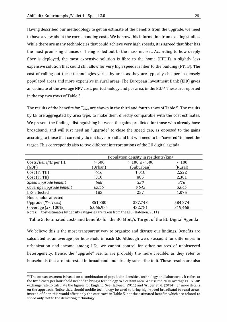
Ahlfeldt/ Koutroumpis /Valletti – Speed 2.0 29
Having described our methodology to get an estimate of the benefits from the upgrade, we need
to have a view about the corresponding costs. We borrow this information from existing studies.
While there are many technologies that could achieve very high speeds, it is agreed that fiber has
the most promising chances of being rolled out to the mass market. According to how deeply
fiber is deployed, the most expensive solution is fibre to the home (FTTH). A slightly less
expensive solution that could still allow for very high speeds is fiber to the building (FTTB). The
cost of rolling out these technologies varies by area, as they are typically cheaper in densely
populated areas and more expensive in rural areas. The European Investment Bank (EIB) gives
an estimate of the average NPV cost, per technology and per area, in the EU.32 These are reported
in the top two rows of Table 5.
The results of the benefits for T2020 are shown in the third and fourth rows of Table 5. The results
by LE are aggregated by area type, to make them directly comparable with the cost estimates.
We present the findings distinguishing between the gains predicted for those who already have
broadband, and will just need an “upgrade” to close the speed gap, as opposed to the gains
accruing to those that currently do not have broadband but will need to be “covered” to meet the
target. This corresponds also to two different interpretations of the EU digital agenda.
Population density in residents/km2 Costs/Benefits per HH (GBP)
> 500 (Urban)
> 100 & < 500 (Suburban)
< 100 (Rural)
Cost (FTTH) 416 1,018 2,522 Cost (FTTB) 310 885 2,301 Speed upgrade benefit 668 330 376 Coverage upgrade benefit 8,855 4,645 3,065 LEs affected 183 257 1,075 Households affected: Upgrade (T < T2020) 851,880 387,743 584,874 Coverage (x < 100%) 5,066,954 432,781 319,468 Notes: Cost estimates by density categories are taken from the EIB (Hätönen, 2011)
Table 5: Estimated costs and benefits for the 30 Mbit/s Target of the EU Digital Agenda
We believe this is the most transparent way to organize and discuss our findings. Benefits are
calculated as an average per household in each LE. Although we do account for differences in
urbanization and income among LEs, we cannot control for other sources of unobserved
heterogeneity. Hence, the “upgrade” results are probably the more credible, as they refer to
households that are interested in broadband and already subscribe to it. These results are also
32 The cost assessment is based on a combination of population densities, technology and labor costs. It refers to the fixed costs per household needed to bring a technology to a certain area. We use the 2010 average EUR/GBP exchange rate to calculate the figures for England. See Hätönen (2011) and Gruber et al. (2014) for more details on the approach. Notice that, should mobile technology be used to bring high-speed broadband to rural areas, instead of fiber, this would affect only the cost rows in Table 5, not the estimated benefits which are related to speed only, not to the delivering technology.
Ahlfeldt/ Koutroumpis /Valletti – Speed 2.0 30
in line with the looser interpretation of the targets, whereby technology must be available, but
subscription decisions are left to individuals.
The “coverage” results apply, instead, to households that currently do not have a basic version of
broadband, even in areas where fast broadband is available. This could be due to affordability
issues, in which case our results on coverage would stand if appropriate subsidies were also
given to those households. But one could also argue that these households are simply not
interested in broadband, and never will be, unless additional actions are also taken—e.g., to
increase their degree of digital literacy (especially for households with older people). If one
takes a stricter interpretation of the Digital Agenda, such that every household must have
broadband of a certain minimum speed, one cannot just ignore the issue. Instead of arguing one
way or another, we give each set of results separately.
Households in urban areas clearly pass the cost-benefit test. The benefits of the upgrade per
household are already sufficient to cover its cost, even with the most expensive FTTH
technology. As for suburban households, FTTB might be considered, but the benefits of the
speed upgrade alone are still less than 40% of its cost. If a small percentage of the coverage
benefits could also be realized, one could also argue for FTTB in suburban areas. Rural areas are,
instead, the most problematic: this is where costs are highest and benefits lowest. The benefits
from the speed upgrade are about 15% of the cost of bringing fast broadband. Only if one is
willing to accept that at least two thirds of the coverage benefits will also be realized, then the
case for FTTB passes a cost-benefit test under the stricter interpretation of the Digital Agenda in
rural areas.
The last rows in Table 5 give some sense of the total impact of the policy. Almost two hundred
LEs would need to be upgraded in urban areas, but they would affect large numbers of
households, as the population density is high. Overall, the speed upgrade would affect just over
1.8m households, and possibly fewer than 1.3m if rural areas were thought to fail the
cost/benefit test. Connecting the unconnected is, instead, a more ambitious goal, which puts the
number of affected households well over 5m. These large differences are due to the ambiguity in
interpreting the policy targets.
Our welfare assessment is based on the costs to supply broadband—and net household benefits
from using it—over and above the price paid to Internet Service Providers. We have been silent
so far on the actual broadband price that subscribers pay. This is not a problem if the price is
competitive, so that ISPs themselves make no extra rents. If, though, there were private rents to
ISPs, then our analysis would underestimate welfare effects since ISPs’ profits are excluded from
our analysis.
Ahlfeldt/ Koutroumpis /Valletti – Speed 2.0 31
We finish this exercise by commenting on the possible direction of bias in our results. First, our
whole approach depends on estimating broadband value from property scarcity prices. If the
property market were oversupplied instead, then we would systematically underestimate
consumer surplus from broadband consumption, as sellers would not be able to capture
broadband rents. In this respect, it is well documented that the supply of properties in England
is severely constrained by the planning system (Hilber and Vermeulen, 2014). More land is
covered by greenbelts that prevent expansion of developed areas (and in some areas even by
golf courses) than by housing. This restriction of developable land leads to the economically
paradoxical combination of skyrocketing house prices (more than tripled in England and more
than quadrupled in London over the past 15 years) and historically low construction levels
(Cheshire, 2014). Still, it is safe to say that our estimates should provide a lower bound to net
consumer surplus.
Second, and more relevant for the policy exercise, the relative scarcity of properties may be
lower in rural areas compared to urban areas. If that were the case, then the underestimation
would be more severe for the former than for the latter. While it is beyond the scope of the
current work to use a measure of the tightness of the property market, we have information
about the number of days it takes, on average, to sell a property from when it is first put on sale,
which is an indication of how many active prospective buyers there are for that property. On the
basis of this imperfect metric, there is no evidence that the supply of properties in rural areas is
considerably more elastic than in urban areas.33
Third, if buyers anticipated broadband speed increases over time, the present value of a
technological upgrade would be reduced, and we would similarly underestimate the consumer
surplus. When we run DDs for each technological upgrade (see Figure 5 and Appendix C), we
find some genuine discontinuities in property prices associated with the various generations of
broadband technologies, which reveals that the benefits of the introduction of ADSL and of its
subsequent upgrades were not fully anticipated by consumers.
Fourth, we calculate the benefits from the digital targets in a certain LE by eventually changing
only the speed in that LE, and keeping all other parameters constant. While this is not
particularly controversial for urbanization, we also keep income constant. If, say, broadband
became available in rural area A, and some rich people were induced, as a consequence, to move
to that area A from some other area B, we would have to use their income to evaluate the policy
33 For instance, in January 2007, before the financial crisis, it took, on average, 86 days to sell a property in Greater London, the most densely populated area in England, and 95 days to sell one in rural Devon. After the crisis, these went up to 178 days and 206 days, respectively, but the relative ratio did not change (see “Time on the market report for England”, http://www.home.co.uk/guides/).
Ahlfeldt/ Koutroumpis /Valletti – Speed 2.0 32
(starting with the speed level available in their original area B). Since none of this information is
available, our policy experiment is valid to the extent that there is very low mobility among LEs.
Fifth, we estimate only the private gains from residential broadband Internet. Therefore, we may
be missing various positive network externalities linked to high-speed communications.34 It is
notable, however, that urban areas already pass the cost-benefit test and rural areas fail by a
large margin. Because most economic activity concentrates in urban areas, it is unlikely that the
qualitative conclusions from our policy exercise would change if, for instance, the effects on
firms were taken into account.
Sixth, and as we acknowledged more generally at the beginning of this section, we cannot tell
what part of our property capitalization effects could be due to pure sorting. This is why we
decided to be as transparent as possible by presenting the benefit results split into two parts.
Perhaps the results are less credible at the extensive margin (bringing people to fast Internet for
the first time) than at the intensive margin (giving a faster connection to those who already use
the Internet). If this is the case, as already argued above, our most convincing estimates of
broadband benefits are those capturing the speed upgrade, while the coverage upgrade
estimates should be taken with more caution.
6 Conclusions
This paper evaluates the extent to which broadband speed is capitalized into house prices. We
estimate consumer surplus associated with broadband Internet speed by using microdata on
property prices in England between 1995 and 2010. We find a 3% elasticity of property prices
with respect to speed at the mean of the speed distribution in our data. Because of significant
diminishing returns to speed, this elasticity applies only to marginal changes and properties
with average Internet connections. Upgrading a property from a normal (8 Mbit/s) to a fast (24
Mbit/s) connection increases the value, on average, by 1%. This is still a large effect. We argue
that this is a good measure of net consumer surplus associated with broadband usage. This is
true as long as properties are scarce and sellers are, thus, able to extract buyers’ consumer
surplus, or else our results would underestimate the impact on consumer surplus. We also find
considerable heterogeneity of these benefits in each area where the Internet is locally deployed.
We then use the estimates to evaluate the benefits associated with government initiatives to
upgrade digital speed. We show that urban areas pass a cost-benefit test of current EU policy
proposals, while the case for these policy interventions is not very strong in rural areas.
34 See Rysman (2004) for an analysis of network effects on consumer surplus.
Ahlfeldt/ Koutroumpis /Valletti – Speed 2.0 33
Since it is largely urban areas that pass a cost-benefit test, the question arises: Why do ISPs
supply sub-optimal speed in those areas, where there seems to be a willingness to pay that is in
excess of costs? The reason is that the broadband rent goes to the “wrong” economic agent. The
broadband speed rent is, in fact, appropriated by the seller, not by the ISPs. The ISPs supply
broadband according to supply and demand conditions in the broadband market, which is
largely a competitive one. But these conditions do not necessarily reflect the scarcity rents that
exist in the property market. In fact, competition among ISPs is actually tougher in urban areas,
where property prices are typically higher: an ISP that tried to charge its customers more would
just lose market share.
An implication of our results is that there may be a coordination problem among sellers and
landlords in the undersupplied areas that pass the cost-benefit tests, perhaps because they are
unaware or, most likely, because of their fragmentation. While it would be collectively rational
for these sellers and landlords to get together and pay some of the ISPs’ delivery costs of
upgraded technologies—as, then, their properties would become more valuable—freeriding
problems make this scenario unlikely. As with other infrastructures, the coordination problem,
therefore, rationalizes the public delivery of broadband to undersupplied areas in combination
with levies charged to sellers and landlords to recover part of the costs. The political economy of
the housing-markets literature suggests that homeowners and landlords would support such
initiatives as long as the anticipated capitalization gain exceeds the infrastructure levy (Ahlfeldt,
et al., 2014; Dehring et al., 2008; Fischel, 2001; Oates, 1969).

Ahlfeldt/ Koutroumpis /Valletti – Speed 2.0 34
Appendices (for the referees only)
Appendix A: Evolution of broadband in England
Figure A1 below shows the evolution of the availability of ADSL (first panel), LLU (second panel
panel), and ADSL2+ (last panel) in every area of England over the study period. The red dots
show the location of all the LEs in England. The first panel shows that ADSL became ubiquitous
by the end of the period, though upgrades happened at different points in time in different areas.
The second and last panels show that LLU and ADSL2+ did not diffuse everywhere, and a
considerable part of the country (the hatched areas, which are concentrated in the rural parts of
the country) did not attract sufficient economic interest from providers to bring faster
broadband there.
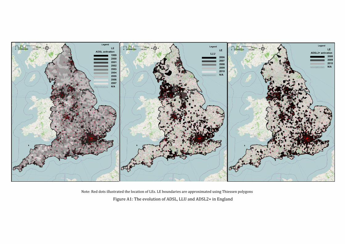
Note: Red dots illustrated the location of LEs. LE boundaries are approximated using Thiessen polygons
Figure A1: The evolution of ADSL, LLU and ADSL2+ in England

Ahlfeldt/ Koutroumpis /Valletti – Speed 2.0 36
Appendix B: Data description
In this appendix, we introduce the additional non-broadband speed-related covariates we use in
the capitalization regressions in more detail. Table B1 provides a summary. See, also, Ahlfeldt et
al. (2014).
Neighborhood characteristics
The main variables used for estimating capitalization effects of neighborhood characteristics are
median income and ethnic composition. The income data provide a model-based estimate of
median household income produced by Experian for Super Output Areas of the lower level
(LSOA). This is assigned to the transaction data based on postcode. The data on ethnicity were
made available by the 2001 UK Census at the level of Output Area (OA). Shares of each of the 16
ethnic groups and a Herfindahl index35 were computed to capture the ethnic composition of
neighborhoods.
Environmental variables
The environmental variables capture the amenity value of areas e.g. designated as natural parks,
various features of the natural environment, and different types of land cover and use.
Geographical data (in the form of ESRI shapefiles) for UK National Parks, Areas of Outstanding
Natural Beauty, and National Nature Reserves are available from Natural England. National
Parks and Areas of Outstanding Natural Beauty are protected areas of countryside designated
because of their significant landscape value. National Nature Reserves are “established to
protect sensitive features and to provide ‘outdoor laboratories’ for research.” Straight-line
distances to these designations were computed for the housing units as geographically located
by their postcodes. Furthermore, density measures that take into account both the distance to
and the size of the features were created. We apply a kernel density measure (Silverman, 1986)
with a radius of 2km, which is considered to be the maximum distance people are willing to
walk (Gibbons and Machin, 2005).
The location of lakes, rivers and coastline is available from the GB Ordinance Survey. The
distance to these features is also computed for the housing units from the transaction data. The
UK Land Cover Map produced by the Centre for Ecology and Hydrology describes land coverage
by 26 categories, as identified by satellite images. We follow Mourato et al. (2010), who
construct nine broad land cover types from the 26 categories. Shares of each of these nine
35 The Herfindahl index (𝐻𝐼) is calculated according to the following relation: 𝐻𝐼 = ∑ 𝑠𝑖
2𝑁𝑖=1 , where 𝑠𝑖 is the
share of ethnicity 𝑖 in the LSOA, and N is the total number of ethnicities.

Ahlfeldt/ Koutroumpis /Valletti – Speed 2.0 37
categories in 1km grid squares are calculated, and the housing units take on the value of the grid
square in which they reside.
The generalized Land Use Database (GLUD) available from the Department for Communities
and Local Government gives area shares of nine different types of land use within Super Output
Areas, lower level (LSOA). These nine types are domestic buildings, non-domestic buildings,
roads, paths, rail, domestic gardens, green space, water, and other land use. These shares are
assigned to the housing units based on the LSOA in which they are located.
Amenities
The locational amenities variables capture the benefits a location offers in terms of accessibility,
employment opportunities, school quality, and the proximity of cultural and entertainment
establishments.
Employment accessibility is captured both by the distance to Travel to Work Area (TTWA)
centroid and by a measure of employment potentiality. TTWAs represent employment zones,
and the distance to the center of these zones is a proxy for accessibility to employment
locations. A more complex measure of accessibility is the employment potentiality index. This is
computed at the Super Output Area, lower level (LSOA) and represents an average of
employment in neighboring LSOAs, weighted by their distance.
Key Stage 2 (ages 7–11) assessment scores are available from the Department for Education at
the Super Output Area, middle layer (MSOA). School quality is captured at the house level by
computing a distance-weighted average of the KS2 scores of nearby MSOA centroids.
Geographical data on the locations of motorways, roads, airports, rail stations and rail tracks are
available from the GB Ordinance Survey. Distances were computed from housing units to
motorways, A-roads, B-roads and rail stations to capture accessibility. Buffer zones were
created around the motorways and roads along with distance calculations to rail tracks and
airports in order to capture the unpleasant noise effects of transport infrastructure.
Further data on local amenities were taken from the Ordinance Survey (police stations, places of
worship, hospitals, leisure centers) and OpenStreetMap (cafés, restaurants/fast food outlets,
museums, nightclubs, bars/pubs, theaters/cinemas, kindergartens and monuments,
attractions). The number of listed buildings was provided by English Heritage. Kernel densities
for these amenities were computed for housing units using a kernel radius of 2km and a
quadratic kernel function (Silverman, 1986). The radius of 2km is consistent with amenities
having a significant effect on property prices only when they are within walking distance.
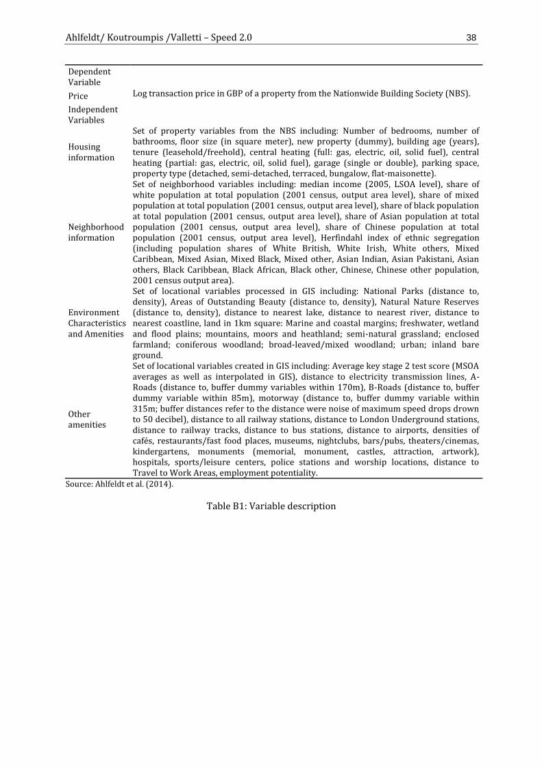
Ahlfeldt/ Koutroumpis /Valletti – Speed 2.0 38
Dependent Variable
Price Log transaction price in GBP of a property from the Nationwide Building Society (NBS).
Independent Variables
Housing information
Set of property variables from the NBS including: Number of bedrooms, number of bathrooms, floor size (in square meter), new property (dummy), building age (years), tenure (leasehold/freehold), central heating (full: gas, electric, oil, solid fuel), central heating (partial: gas, electric, oil, solid fuel), garage (single or double), parking space, property type (detached, semi-detached, terraced, bungalow, flat-maisonette).
Neighborhood information
Set of neighborhood variables including: median income (2005, LSOA level), share of white population at total population (2001 census, output area level), share of mixed population at total population (2001 census, output area level), share of black population at total population (2001 census, output area level), share of Asian population at total population (2001 census, output area level), share of Chinese population at total population (2001 census, output area level), Herfindahl index of ethnic segregation (including population shares of White British, White Irish, White others, Mixed Caribbean, Mixed Asian, Mixed Black, Mixed other, Asian Indian, Asian Pakistani, Asian others, Black Caribbean, Black African, Black other, Chinese, Chinese other population, 2001 census output area).
Environment Characteristics and Amenities
Set of locational variables processed in GIS including: National Parks (distance to, density), Areas of Outstanding Beauty (distance to, density), Natural Nature Reserves (distance to, density), distance to nearest lake, distance to nearest river, distance to nearest coastline, land in 1km square: Marine and coastal margins; freshwater, wetland and flood plains; mountains, moors and heathland; semi-natural grassland; enclosed farmland; coniferous woodland; broad-leaved/mixed woodland; urban; inland bare ground.
Other amenities
Set of locational variables created in GIS including: Average key stage 2 test score (MSOA averages as well as interpolated in GIS), distance to electricity transmission lines, A-Roads (distance to, buffer dummy variables within 170m), B-Roads (distance to, buffer dummy variable within 85m), motorway (distance to, buffer dummy variable within 315m; buffer distances refer to the distance were noise of maximum speed drops drown to 50 decibel), distance to all railway stations, distance to London Underground stations, distance to railway tracks, distance to bus stations, distance to airports, densities of cafés, restaurants/fast food places, museums, nightclubs, bars/pubs, theaters/cinemas, kindergartens, monuments (memorial, monument, castles, attraction, artwork), hospitals, sports/leisure centers, police stations and worship locations, distance to Travel to Work Areas, employment potentiality.
Source: Ahlfeldt et al. (2014).
Table B1: Variable description
Ahlfeldt/ Koutroumpis /Valletti – Speed 2.0 39
Appendix C: Program evaluation
1. Empirical framework
Given the distance decay in the effect of broadband, an upgrade of an LE can be viewed as an
event that should exert spatially variant effects on nearby property prices. The effect of the
event on property prices can, thus, be analyzed using quasi-experimental research designs that
have become popular in the program evaluation literature. In this appendix, we complement the
empirical analysis presented in the main paper using a reduced-form empirical specification
that is a mix of hedonic modeling, panel econometrics, and a DD method, which accommodates
multiple treatment dates and spatial heterogeneity in the treatment effect within an area served
by an LE.
The point of departure is the following specification:
log(𝑃𝑖𝑗𝑡) = ∑ 𝛽0𝑄(𝑃𝑂𝑆𝑇𝑗𝑡𝑄
)𝑄
+ ∑ 𝛽1𝑄(𝑃𝑂𝑆𝑇𝑗𝑡𝑄
× 𝐷𝐼𝑆𝑇𝑖𝑗)𝑄
+ 𝛽3𝐷𝐼𝑆𝑇𝑖𝑗 + X𝑖′μ + 𝜑𝑗 + 𝜔𝑡 + 𝜀𝑖𝑗𝑡
where P is the sales price of a property that sells in postcode i served by LE j in year t, X𝑖′ is a
vector of structural, location and neighborhood variables and μ is a vector of implicit hedonic
prices. 𝜑𝑗 is a fixed effect for whether a property is located within the catchment area of an LE j,
𝜔𝑡 is a year fixed effect and 𝜀𝑖𝑗𝑡 a random error term. 𝑃𝑂𝑆𝑇𝑗𝑡𝑄 are 0,1 indicator variables
indexing whether at time t, LE j had been upgraded to quality level Q = {ADSL, LLU, ADSL2 +}.
The treatment effect of a certain type of LE upgrade Q on property prices at a given distance
from an upgraded LE is given by 𝛽0𝑄 + 𝛽1𝑄𝐷𝐼𝑆𝑇𝑖𝑗 . The DD comparison relative to LEs that were
not upgraded and the period before the upgrade is, thus, made at every distance from the
upgraded LEs.
A typical concern in DD analyses are temporal trends that are correlated with but not causally
related to the treatment. Identification, in general, cannot be considered credible if changes in
property prices near to LEs following an upgrade can be explained by (relative) trends in the
neighborhoods that existed prior to the upgrade. The concern is relevant in our case because
the assignment of the LE upgrade is not technologically random. Therefore, we expand the
spatial DD model to allow for a temporal structure in the treatment effect of an LE upgrade.
In the first step, we allow for additional spatially varying DD effects for each of the three years
immediately preceding an upgrade. Because we do not expect capitalization effects in
anticipation of an upgrade, these effects can be viewed as placebo-treatment effects. We
estimate the following model:
Ahlfeldt/ Koutroumpis /Valletti – Speed 2.0 40
log(𝑃𝑖𝑗𝑡) = ∑ 𝛽0𝑄𝑃𝑂𝑆𝑇𝑗𝑡𝑄
𝑄+ ∑ 𝛽1𝑄(𝑃𝑂𝑆𝑇𝑗𝑡
𝑄× 𝐷𝐼𝑆𝑇𝑖𝑗)
𝑄+ ∑ ∑ 𝛽0𝑍𝑄(𝑃𝑅𝐸𝑍𝑗𝑡
𝑄)
𝑄𝑍
+ ∑ ∑ 𝛽1𝑍𝑄(𝑃𝑅𝐸𝑍𝑗𝑡𝑄
× 𝐷𝐼𝑆𝑇𝑖𝑗)𝑄𝑍
+ 𝛽3𝐷𝐼𝑆𝑇𝑖𝑗 + X𝑖′μ + 𝜑𝑗 + 𝜔𝑡 + 𝜀𝑖𝑗𝑡 ,
where 𝑃𝑅𝐸𝑍𝑗𝑡𝑄
indexes an LE x year cell Z years before a Q-type upgrade of LE j. Note that these
PRE effects provide a DD comparison relative to LEs that where not upgraded and the period
four or more years before an activation. In a further expansion, we replace the POST effects with
separate DD effects for each of the two first years subsequent to an upgrade and a residual
category that contains all subsequent years.
2. Empirical results
We report in Table C1 the results on spatiotemporal trends around the upgrade dates. To keep
the tabular presentation compact, we report parametric results for models in which we add the
PRE placebo DD effects, but no separate POST effects (column 2 in Table C1). In the graphical
illustration for the ADSL upgrade in Figure 5 in the main text, we also allow DD effects to vary
by years following designation. To save space, we do not show the corresponding figures for the
LLU and ADSL2+ upgrades, but we discuss the results next.
The pattern of time-varying LLU effects is as follows. All POST effects show the expected pattern
with a positive level shift that flattens out towards the fringe of the LE. The effect increases
notably from the first to the second POST period and moderately afterwards. Two of the three
PRE-effects are not in line with a successful falsification test at first glance. The effects are
positive, and one shows a notable negative slope. A closer inspection reveals, however, that the
PRE effects decline towards the activation date. Also, the negative slope tends to disappear over
time. Pre-trends, thus, are negatively correlated with the treatment and are reversed just at the
time of the upgrade, which makes a particularly strong case for impact.
The ADSL2+ effects show a similar pattern. In the model with separate PRE-effects (where the
comparison is made relative to four and more years before activation), the ADSL2+ POST effect
turns out to be negative at all distances to the LE. This is not the expected result, even though
there is negative decay, as expected. The POST effect is, however, significantly more positive
than any of the three PRE effects, in all areas that are relatively close to the LE. Moreover, the
earlier PRE effects show a positive distance trend, which is reversed only one year before the
ADSL2+ activation. As with the LLU effects, the inspection indicates that pre-trends are
negatively correlated with the treatment, which strengthens the sense of impact.
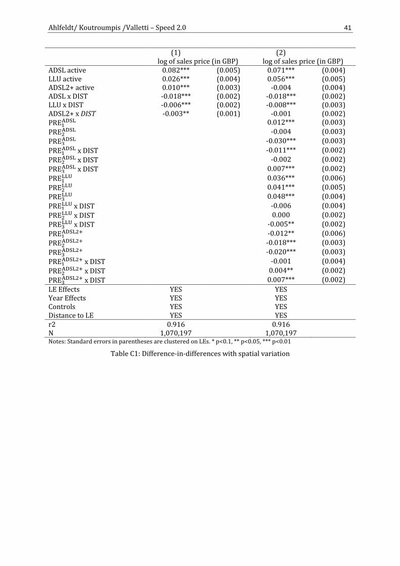
Ahlfeldt/ Koutroumpis /Valletti – Speed 2.0 41
(1) (2) log of sales price (in GBP) log of sales price (in GBP) ADSL active 0.082*** (0.005) 0.071*** (0.004) LLU active 0.026*** (0.004) 0.056*** (0.005) ADSL2+ active 0.010*** (0.003) -0.004 (0.004) ADSL x DIST -0.018*** (0.002) -0.018*** (0.002) LLU x DIST -0.006*** (0.002) -0.008*** (0.003) ADSL2+ x DIST -0.003** (0.001) -0.001 (0.002) PRE1
ADSL 0.012*** (0.003)
PRE2ADSL -0.004 (0.003)
PRE3ADSL -0.030*** (0.003)
PRE1ADSL x DIST -0.011*** (0.002)
PRE2ADSL x DIST -0.002 (0.002)
PRE3ADSL x DIST 0.007*** (0.002)
PRE1LLU 0.036*** (0.006)
PRE2LLU 0.041*** (0.005)
PRE3LLU 0.048*** (0.004)
PRE1LLU x DIST -0.006 (0.004)
PRE2LLU x DIST 0.000 (0.002)
PRE3LLU x DIST -0.005** (0.002)
PRE1ADSL2+ -0.012** (0.006)
PRE2ADSL2+ -0.018*** (0.003)
PRE3ADSL2+ -0.020*** (0.003)
PRE1ADSL2+ x DIST -0.001 (0.004)
PRE2ADSL2+ x DIST 0.004** (0.002)
PRE3ADSL2+ x DIST 0.007*** (0.002)
LE Effects YES YES Year Effects YES YES Controls YES YES Distance to LE YES YES r2 0.916 0.916 N 1,070,197 1,070,197 Notes: Standard errors in parentheses are clustered on LEs. * p<0.1, ** p<0.05, *** p<0.01
Table C1: Difference-in-differences with spatial variation
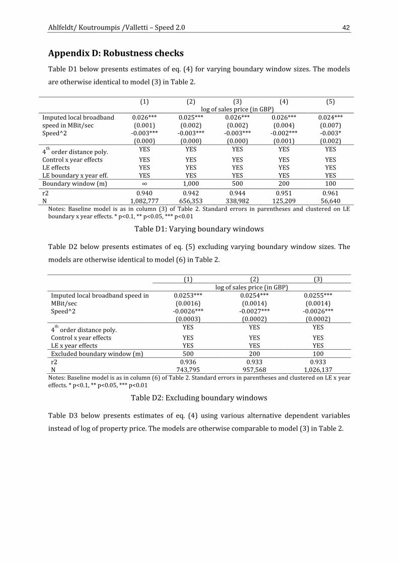
Ahlfeldt/ Koutroumpis /Valletti – Speed 2.0 42
Appendix D: Robustness checks
Table D1 below presents estimates of eq. (4) for varying boundary window sizes. The models
are otherwise identical to model (3) in Table 2.
(1) (2) (3) (4) (5) log of sales price (in GBP) Imputed local broadband speed in MBit/sec
0.026*** (0.001)
0.025*** (0.002)
0.026*** (0.002)
0.026*** (0.004)
0.024*** (0.007)
Speed^2 -0.003*** (0.000)
-0.003*** (0.000)
-0.003*** (0.000)
-0.002*** (0.001)
-0.003* (0.002)
4th
order distance poly. YES YES YES YES YES
Control x year effects YES YES YES YES YES LE effects YES YES YES YES YES LE boundary x year eff. YES YES YES YES YES Boundary window (m) ∞ 1,000 500 200 100
r2 0.940 0.942 0.944 0.951 0.961 N 1,082,777 656,353 338,982 125,209 56,640
Notes: Baseline model is as in column (3) of Table 2. Standard errors in parentheses and clustered on LE boundary x year effects. * p<0.1, ** p<0.05, *** p<0.01
Table D1: Varying boundary windows
Table D2 below presents estimates of eq. (5) excluding varying boundary window sizes. The
models are otherwise identical to model (6) in Table 2.
(1) (2) (3) log of sales price (in GBP) Imputed local broadband speed in MBit/sec
0.0253*** (0.0016)
0.0254*** (0.0014)
0.0255*** (0.0014)
Speed^2 -0.0026*** (0.0003)
-0.0027*** (0.0002)
-0.0026*** (0.0002)
4th
order distance poly. YES YES YES
Control x year effects YES YES YES LE x year effects YES YES YES Excluded boundary window (m) 500 200 100 r2 0.936 0.933 0.933 N 743,795 957,568 1,026,137
Notes: Baseline model is as in column (6) of Table 2. Standard errors in parentheses and clustered on LE x year effects. * p<0.1, ** p<0.05, *** p<0.01
Table D2: Excluding boundary windows
Table D3 below presents estimates of eq. (4) using various alternative dependent variables
instead of log of property price. The models are otherwise comparable to model (3) in Table 2.
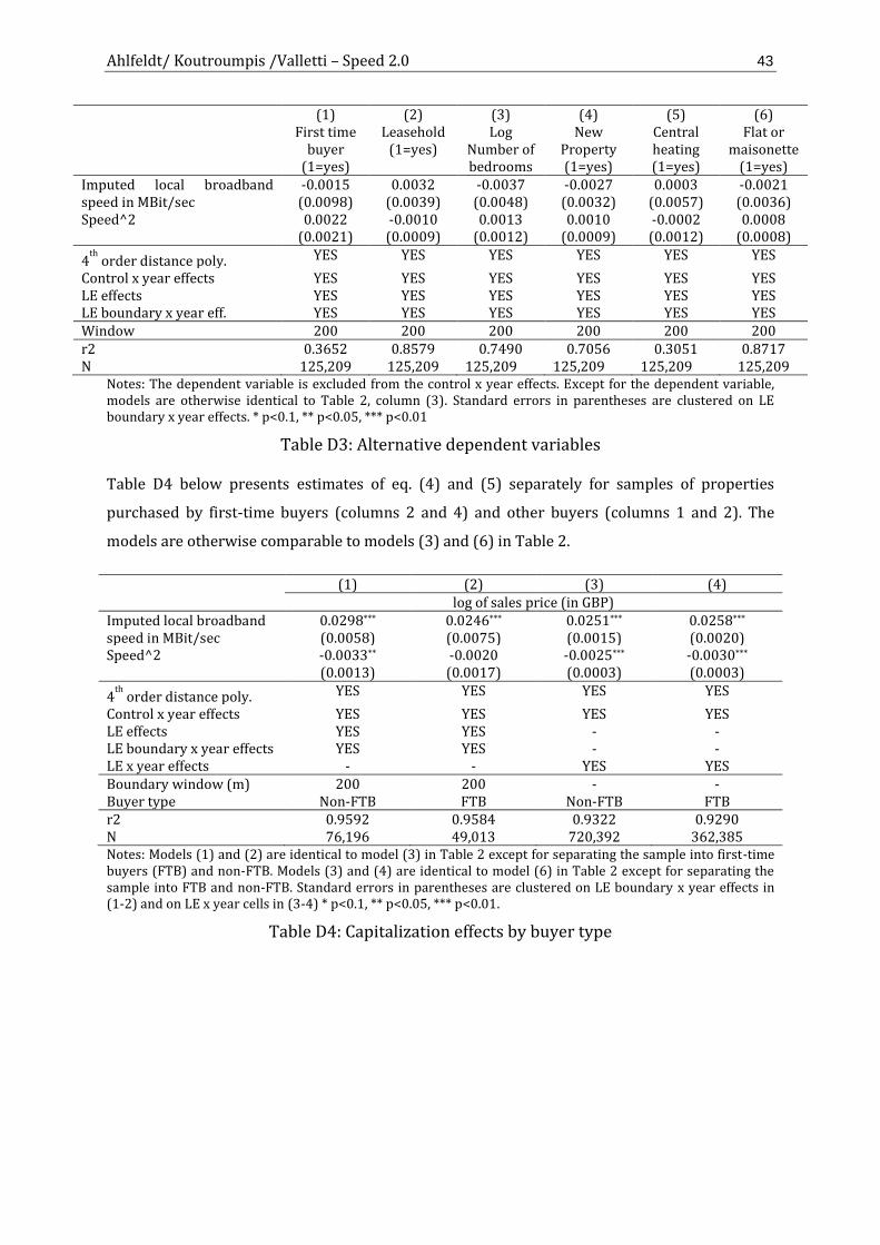
Ahlfeldt/ Koutroumpis /Valletti – Speed 2.0 43
(1) (2) (3) (4) (5) (6) First time
buyer (1=yes)
Leasehold (1=yes)
Log Number of bedrooms
New Property (1=yes)
Central heating (1=yes)
Flat or maisonette
(1=yes) Imputed local broadband speed in MBit/sec
-0.0015 (0.0098)
0.0032 (0.0039)
-0.0037 (0.0048)
-0.0027 (0.0032)
0.0003 (0.0057)
-0.0021 (0.0036)
Speed^2 0.0022 (0.0021)
-0.0010 (0.0009)
0.0013 (0.0012)
0.0010 (0.0009)
-0.0002 (0.0012)
0.0008 (0.0008)
4th
order distance poly. YES YES YES YES YES YES
Control x year effects YES YES YES YES YES YES LE effects YES YES YES YES YES YES LE boundary x year eff. YES YES YES YES YES YES Window 200 200 200 200 200 200 r2 0.3652 0.8579 0.7490 0.7056 0.3051 0.8717 N 125,209 125,209 125,209 125,209 125,209 125,209
Notes: The dependent variable is excluded from the control x year effects. Except for the dependent variable, models are otherwise identical to Table 2, column (3). Standard errors in parentheses are clustered on LE boundary x year effects. * p<0.1, ** p<0.05, *** p<0.01
Table D3: Alternative dependent variables
Table D4 below presents estimates of eq. (4) and (5) separately for samples of properties
purchased by first-time buyers (columns 2 and 4) and other buyers (columns 1 and 2). The
models are otherwise comparable to models (3) and (6) in Table 2.
(1) (2) (3) (4) log of sales price (in GBP) Imputed local broadband speed in MBit/sec
0.0298*** (0.0058)
0.0246*** (0.0075)
0.0251*** (0.0015)
0.0258*** (0.0020)
Speed^2 -0.0033** (0.0013)
-0.0020 (0.0017)
-0.0025*** (0.0003)
-0.0030*** (0.0003)
4th
order distance poly. YES YES YES YES
Control x year effects YES YES YES YES LE effects YES YES - - LE boundary x year effects YES YES - - LE x year effects - - YES YES Boundary window (m) 200 200 - - Buyer type Non-FTB FTB Non-FTB FTB r2 0.9592 0.9584 0.9322 0.9290 N 76,196 49,013 720,392 362,385 Notes: Models (1) and (2) are identical to model (3) in Table 2 except for separating the sample into first-time buyers (FTB) and non-FTB. Models (3) and (4) are identical to model (6) in Table 2 except for separating the sample into FTB and non-FTB. Standard errors in parentheses are clustered on LE boundary x year effects in (1-2) and on LE x year cells in (3-4) * p<0.1, ** p<0.05, *** p<0.01.
Table D4: Capitalization effects by buyer type
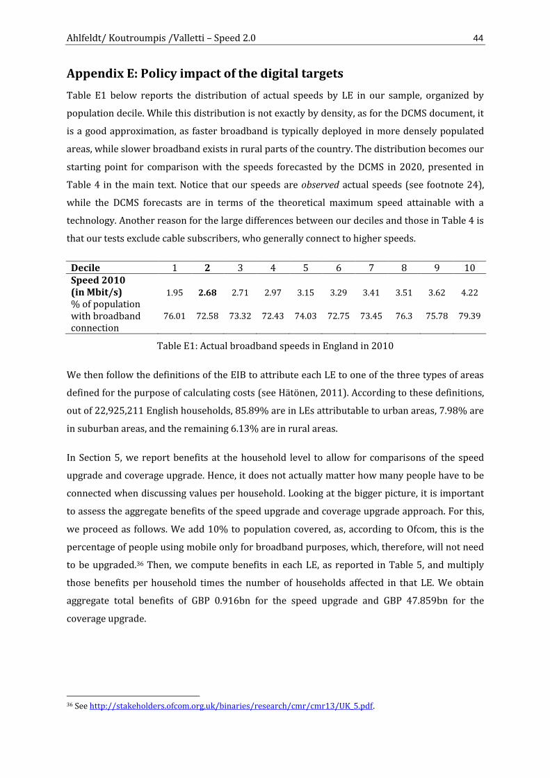
Ahlfeldt/ Koutroumpis /Valletti – Speed 2.0 44
Appendix E: Policy impact of the digital targets
Table E1 below reports the distribution of actual speeds by LE in our sample, organized by
population decile. While this distribution is not exactly by density, as for the DCMS document, it
is a good approximation, as faster broadband is typically deployed in more densely populated
areas, while slower broadband exists in rural parts of the country. The distribution becomes our
starting point for comparison with the speeds forecasted by the DCMS in 2020, presented in
Table 4 in the main text. Notice that our speeds are observed actual speeds (see footnote 24),
while the DCMS forecasts are in terms of the theoretical maximum speed attainable with a
technology. Another reason for the large differences between our deciles and those in Table 4 is
that our tests exclude cable subscribers, who generally connect to higher speeds.
Decile 1 2 3 4 5 6 7 8 9 10 Speed 2010 (in Mbit/s) 1.95 2.68 2.71 2.97 3.15 3.29 3.41 3.51 3.62 4.22
% of population with broadband connection
76.01 72.58 73.32 72.43 74.03 72.75 73.45 76.3 75.78 79.39
Table E1: Actual broadband speeds in England in 2010
We then follow the definitions of the EIB to attribute each LE to one of the three types of areas
defined for the purpose of calculating costs (see Hätönen, 2011). According to these definitions,
out of 22,925,211 English households, 85.89% are in LEs attributable to urban areas, 7.98% are
in suburban areas, and the remaining 6.13% are in rural areas.
In Section 5, we report benefits at the household level to allow for comparisons of the speed
upgrade and coverage upgrade. Hence, it does not actually matter how many people have to be
connected when discussing values per household. Looking at the bigger picture, it is important
to assess the aggregate benefits of the speed upgrade and coverage upgrade approach. For this,
we proceed as follows. We add 10% to population covered, as, according to Ofcom, this is the
percentage of people using mobile only for broadband purposes, which, therefore, will not need
to be upgraded.36 Then, we compute benefits in each LE, as reported in Table 5, and multiply
those benefits per household times the number of households affected in that LE. We obtain
aggregate total benefits of GBP 0.916bn for the speed upgrade and GBP 47.859bn for the
coverage upgrade.
36 See http://stakeholders.ofcom.org.uk/binaries/research/cmr/cmr13/UK_5.pdf.

Ahlfeldt/ Koutroumpis /Valletti – Speed 2.0 45
Bibliography
Ahlfeldt, G. M., and Kavetsos, G. (2014). Form or Function? The impact of new sports stadia on property prices in London. Journal of the Royal Statistical Society A, 177(1), 169-190.
Ahlfeldt, G. M., Moeller, K., Waights, S., and Wendland, N. (2014). Game of zones: The political economy of conservation areas. CESifo Working Paper No. 4755.
Amiti, M., and Cameron, L. (2007). Economic Geography and Wages. Review of Economics and Statistics, 89(1), 15-29.
Arzaghi, M., and Henderson, J. V. (2008). Networking off Madison Avenue. The Review of Economic Studies, 75(4), 1011-1038.
Ater, I., and Orlov, E. (2014). The Effect of the Internet on Performance and Quality: Evidence from the Airline Industry. Review of Economics and Statistics, Early Access.
Baum-Snow, N. (2007). Did Highways Cause Suburbanization? The Quarterly Journal of Economics, 122(2), 775-805.
Baum-Snow, N., and Kahn, M. E. (2000). The effects of new public projects to expand urban rail transit. Journal of Public Economics, 77(2), 241-263.
Bhuller, M., Havnes, T., Leuven, E., and Mogstad, M. (2013). Broadband Internet: An Information Superhighway to Sex Crime? The Review of Economic Studies, Online First.
Brueckner, J. K., and Rosenthal, S. S. (2009). Gentrification and Neighborhood Housing Cycles: Will America's Future Downtowns be Rich? The Review of Economics and Statistics, 91(4), 725-743.
Chay, K. Y., and Greenstone, M. (2005). Does Air Quality Matter? Evidence from the Housing Market. Journal of Political Economy, 113(2), 376-424.
Chen, Y., and Savage, S. J. (2010). The Effects of Competition on the Price for Cable Modem Internet Access. Review of Economics and Statistics, 93(1), 201-217.
Cheshire, P. C. (2014). Turning houses into gold: the failure of British planning. CentrePiece, Spring 2014, 15-18.
Ciccone, A., and Hall, R. E. (1996). Productivity and the Density of Economic Activity. American Economic Review, 86(1), 54-70.
Cohen, J. P., and Paul, C. J. M. (2004). Public Infrastructure Investment, Interstate Spatial Spillovers, and Manufacturing Costs. Review of Economics and Statistics, 86(2), 551-560.
Couture, V., Duranton, G., and Turner, M. A. (2012). Speed. Working Paper. Czernich, N., Falck, O., Kretschmer, T., and Woessmann, L. (2011). Broadband Infrastructure and
Economic Growth. Economic Journal, 121(552), 505-532. Davis, L. W. (2004). The Effect of Health Risk on Housing Values: Evidence from a Cancer
Cluster. American Economic Review, 94(5), 1693-1704. DCMS. (2013). UK Broadband Impact Study. Department for Culture, Media and Sport, November
2013. London. Dehring, C. A., Depken, C. A., and Ward, M. R. (2008). A direct test of the homevoter hypothesis.
Journal of Urban Economics, 64(1), 155-170. Duranton, G., Morrow, P. M., and Turner, M. A. (2014). Roads and Trade: Evidence from the US.
The Review of Economic Studies, 81(2), 681-727. Duranton, G., and Puga, D. (2004). Micro-foundations of urban agglomeration economies. In J. V.
Henderson and J.-F. Thisse (Eds.), Handbook of Regional and Urban Economics (Vol. 4, pp. 2063-2117): Elsevier.
Duranton, G., and Turner, M. A. (2011). The Fundamental Law of Road Congestion: Evidence from US Cities. American Economic Review, 101(6), 2616-2652.
European Parliament. (2013). Entertainment x.0 to Boost Broadband Deployment. PE 507.479, Directorate-General for Internal Policies, October 2013. Brussels.
Faber, B. (2014). Trade Integration, Market Size, and Industrialization: Evidence from China's National Trunk Highway System. The Review of Economic Studies, 81(3), 1046-1070.
Faber, B., Sanchis-Guarner, R., and Weinhardt, F. (2013). ICT and Education: Evidence from Internet Access at Pupil Home Addresses. Working Paper.

Ahlfeldt/ Koutroumpis /Valletti – Speed 2.0 46
Falck, O., Gold, R., and Heblich, S. (2014). E-Lections: Voting Behavior and the Internet. American Economic Review, 104(7), 2238-2265.
Fischel, F. A. (2001). The Homevoter Hypothesis (Vol. Cambridge, MA.): Harvard University Press. Forman, C., Goldfarb, A., and Greenstein, S. (2012). The Internet and Local Wages: A Puzzle.
American Economic Review, 102(1), 556-575. Fujita, M., Krugman, P., and Venables, A. J. (1999). The spatial economy: Cities, regions, and
international trade. Cambridge and London: MIT Press. Gabriel, S. A., and Rosenthal, S. S. (2004). Quality of the Business Environment Versus Quality of
Life: Do Firms and Households Like the Same Cities? The Review of Economics and Statistics, 86(1), 483.
Gibbons, S., and Machin, S. (2005). Valuing rail access using transport innovations. Journal of Urban Economics, 57(1), 148-169.
Gibbons, S., Machin, S., and Silva, O. (2013). Valuing school quality using boundary discontinuities. Journal of Urban Economics, 75(0), 15-28.
Goolsbee, A., and Guryan, J. (2006). The Impact of Internet Subsidies in Public Schools. Review of Economics and Statistics, 88(2), 336-347.
Goolsbee, A., and Klenow, P. J. (2006). Valuing Consumer Products by the Time Spent Using Them: An Application to the Internet. American Economic Review, 96(2), 108-113.
Greenstein, S., and McDevitt, R. C. (2011). The broadband bonus: Estimating broadband Internet's economic value. Telecommunications Policy, 35(7), 617-632.
Greenstone, M., and Gallagher, J. (2008). Does Hazardous Waste Matter? Evidence from the Housing Market and the Superfund Program. The Quarterly Journal of Economics, 123(3), 951-1003.
Gruber, H., Hätönen, J., and Koutroumpis, P. (2014). Broadband access in the EU: An assessment of future economic benefits. Telecommunications Policy, 38(11), 1046-1058.
Hätönen, J. (2011). The economic impact of fixed and mobile high-speed networks. EIB Papers, 16(2), 30-59.
Hilber, C. A. L., and Vermeulen, W. (2014). The impact of supply constraints on house prices in England. Economic Journal, forthcoming.
Jin, G. Z., and Kato, A. (2007). Dividing Online and Offline: A Case Study. The Review of Economic Studies, 74(3), 981-1004.
Kolko, J. (2012). Broadband and local growth. Journal of Urban Economics, 71(1), 100-113. Kuminoff, N. V., Smith, V. K., and Timmins, C. (2013). The New Economics of Equilibrium Sorting
and Policy Evaluation Using Housing Markets. Journal of Economic Literature, 51(4), 1007-1062.
Lewis, M. (2014). Flash Boys. New York: W.W. Norton. Liebowitz, S. J., and Zentner, A. (2010). Clash of the Titans: Does Internet use Reduce Television
Viewing? Review of Economics and Statistics, 94(1), 234-245. Linden, L., and Rockoff, J. E. (2008). Estimates of the Impact of Crime Risk on Property Values
from Megan's Laws. American Economic Review, 98(3), 1103-1127. Lucas, R. E., Jr., and Rossi-Hansberg, E. (2002). On the Internal Structure of Cities. Econometrica,
70(4), 1445-1476. Marshall, A. (1920). Principles of Economics. London: Macmillan. Michaels, G. (2008). The Effect of Trade on the Demand for Skill: Evidence from the Interstate
Highway System. Review of Economics and Statistics, 90(4), 683-701. Moretti, E. (2011). Social Learning and Peer Effects in Consumption: Evidence from Movie Sales.
The Review of Economic Studies, 78(1), 356-393. Mourato, S., Atkinson, G., Collins, M., Gibbons, S., MacKerron, G., and Resende, G. (2010).
Economic Analysis of Cultural Services. UK NEA Economic Analysis Report. Nardotto, M., Valletti, T., and Verboven, F. (forthcoming). Unbundling the Incumbent: Evidence
from UK Broadband. Journal of the European Economic Association. Nevo, A., Turner, J., and Williams, J. (2013). Usage-Based Pricing and Demand for Residential
Broadband. Working Paper.

Ahlfeldt/ Koutroumpis /Valletti – Speed 2.0 47
Oates, W. E. (1969). The Effects of Property Taxes and Local Public Spending on Property Values: An Empirical Study of Tax Capitalization and the Tiebout Hypothesis. Journal of Political Economy, 77(6), 957-971.
Redding, S. J., Sturm, D., and Wolf, N. (2011). History and Industry Location: Evidence from German Airports. Review of Economics and Statistics, 93(3), 814-831.
Redding, S. J., and Sturm, D. M. (2008). The costs of remoteness: evidence from German division and reunification. American Economic Review, 98(5), 1766-1797.
Rosen, S. (1974). Hedonic Prices and Implicit Markets: Product Differentiation in Pure Competition. Journal of Political Economy, 82(1), 34-55.
Rosenthal, S. S., and Strange, W. C. (2001). The Determinants of Agglomeration. Journal of Urban Economics, 50(2), 191-229.
Rossi-Hansberg, E., Sarte, P.-D., and Owens, R. (2010). Housing Externalities. Journal of Political Economy, 118(3), 485-535.
Rosston, G., Savage, S., and Waldman, D. (2010). Household Demand for Broadband Internet Services. B.E. Journal of Economic and Policy Analysis (Advances), 10(1).
Rysman, M. (2004). Competition Between Networks: A Study of the Market for Yellow Pages. The Review of Economic Studies, 71(2), 483-512.
Shapiro, J. M. (2006). Smart cities: quality of life, productivity, and the growth effects of human capital. The Review of Economics and Statistics, 88(2), 324-335.
Silverman, B. W. (1986). Density Estimation. London: Chapman and Hall. Summers, C. K. (1999). ADSL: standards, implementation, and architecture (Vol. 4). Boca Raton,
Florida: Crc Press.