Embed Size (px)
Citation preview
Fachbereich 4: Informatik
Volume Hatchingfor Illustrative Visualization
Diplomarbeitzur Erlangung des Grades eines Diplom-Informatikers
im Studiengang Computervisualistik
vorgelegt von
Moritz Gerl
Erstgutachter: Prof. Dr.-Ing. Stefan Muller
(Institut fur Computervisualistik, AG Computergraphik)
Zweitgutachter: Ao.Univ.Prof. Dr. Eduard Groller
Betreuender Assistent: Dipl.-Ing. Stefan Bruckner
(Technische Universitat Wien,
Institut fur Computergraphik und Algorithmen,
AG Visualisierung)
Koblenz, im November 2006
Erklarung
Ich versichere, dass ich die vorliegende Arbeit selbstandig verfasst und
keine anderen als die angegebenen Quellen und Hilfsmittel benutzt habe.
Ja Nein
Mit der Einstellung der Arbeit in die Bibliothek bin ich einverstanden. � �
Der Veroffentlichung dieser Arbeit im Internet stimme ich zu. � �
. . . . . . . . . . . . . . . . . . . . . . . . . . . . . . . . . . . . . . . . . . . . . . . . . . . . . . . . . . . . . . . . . . . . . . . . . . . . . . . . .(Ort, Datum) (Unterschrift)
Contents
1 Introduction 1
2 Related Work 4
2.1 Volume Rendering . . . . . . . . . . . . . . . . . . . . . . . . 4
2.1.1 Image-Order Volume Rendering . . . . . . . . . . . . 4
2.1.2 Object-Order Volume Rendering . . . . . . . . . . . . 5
2.1.3 Hybrid-Order Volume Rendering . . . . . . . . . . . 5
2.1.4 GPU-Based Volume Rendering . . . . . . . . . . . . . 6
2.2 Non-Photorealistic Rendering . . . . . . . . . . . . . . . . . . 6
2.2.1 Line Drawing . . . . . . . . . . . . . . . . . . . . . . . 7
2.2.2 Pen-And-Ink Rendering . . . . . . . . . . . . . . . . . 8
2.2.3 Pencil Drawing and Hatching . . . . . . . . . . . . . . 10
2.3 NPR in Volume Visualization . . . . . . . . . . . . . . . . . . 14
2.3.1 Two-Level Volume Rendering . . . . . . . . . . . . . . 14
2.3.2 Volume Rendering with a modified Optical Model . . 15
2.3.3 An Interactive System for Illustrative Visualization . 17
2.3.4 Line Drawings from Volume Data . . . . . . . . . . . 19
2.3.5 Pen-And-Ink Rendering in Volume Visualization . . 19
2.3.6 Volume Hatching . . . . . . . . . . . . . . . . . . . . . 21
2.4 Curvature Estimation in Volume Visualization . . . . . . . . 24
2.5 Evenly Spaced Streamlines . . . . . . . . . . . . . . . . . . . . 25
3 Volume Hatching 26
3.1 Contour Drawing . . . . . . . . . . . . . . . . . . . . . . . . . 29
3.1.1 Contour Extraction . . . . . . . . . . . . . . . . . . . . 30
3.1.2 Contour Filtering . . . . . . . . . . . . . . . . . . . . . 30
3.1.3 Seed Point Detection . . . . . . . . . . . . . . . . . . . 32
3.1.4 Stroke Generation . . . . . . . . . . . . . . . . . . . . 34
3.2 Stroke Rendering . . . . . . . . . . . . . . . . . . . . . . . . . 38
3.3 Curvature Estimation . . . . . . . . . . . . . . . . . . . . . . . 40
3.4 Volume Hatching Experiments . . . . . . . . . . . . . . . . . 42
3.4.1 Hatching using a Lighting Transfer Function . . . . . 42
3.4.2 Applying Tonal Art Maps to Volume Rendering . . . 43
3.4.3 Quadtree-Based Stroke Seeding . . . . . . . . . . . . . 44
i
3.5 Streamline-Based Volume Hatching . . . . . . . . . . . . . . 45
3.5.1 Creating Evenly-Spaced Streamlines . . . . . . . . . . 45
3.5.2 Stroke Generation . . . . . . . . . . . . . . . . . . . . 46
3.5.3 Stroke Rendering . . . . . . . . . . . . . . . . . . . . . 47
3.5.4 Hatching Layers . . . . . . . . . . . . . . . . . . . . . 49
3.5.5 Crosshatching . . . . . . . . . . . . . . . . . . . . . . . 51
3.6 Volumetric Hatching . . . . . . . . . . . . . . . . . . . . . . . 53
3.6.1 Segmental Raycasting . . . . . . . . . . . . . . . . . . 53
3.6.2 Relevant Iso-Surface Detection . . . . . . . . . . . . . 54
4 Implementation 57
5 Results 60
5.1 Contour Drawing . . . . . . . . . . . . . . . . . . . . . . . . . 60
5.2 Volume Hatching . . . . . . . . . . . . . . . . . . . . . . . . . 70
5.3 Benchmarks . . . . . . . . . . . . . . . . . . . . . . . . . . . . 88
6 Summary 90
6.1 Introduction . . . . . . . . . . . . . . . . . . . . . . . . . . . . 90
6.2 Contour Drawing . . . . . . . . . . . . . . . . . . . . . . . . . 90
6.3 Stroke Rendering . . . . . . . . . . . . . . . . . . . . . . . . . 91
6.4 Curvature Estimation . . . . . . . . . . . . . . . . . . . . . . . 92
6.5 Streamline-Based Volume Hatching . . . . . . . . . . . . . . 92
6.5.1 Creating Evenly-Spaced Streamlines . . . . . . . . . . 92
6.5.2 Stroke Generation . . . . . . . . . . . . . . . . . . . . 93
6.5.3 Stroke Rendering . . . . . . . . . . . . . . . . . . . . . 93
6.5.4 Hatching Layers . . . . . . . . . . . . . . . . . . . . . 94
6.5.5 Crosshatching . . . . . . . . . . . . . . . . . . . . . . . 95
6.5.6 Volumetric Hatching . . . . . . . . . . . . . . . . . . . 95
6.6 Results . . . . . . . . . . . . . . . . . . . . . . . . . . . . . . . 96
7 Conclusions and Future Work 97
ii
1 Introduction
The evolution of drawing reaches back to the origin of human cultural his-
tory. Over 20.000 years ago prehistoric men started to picture their environ-
ment in petroglyphs. From these caveman paintings to mythological de-
pictions of the ancient Egyptians, from medieval illuminated manuscripts
to Leonardo Da Vinci’s anatomical studies in the Renaissance, drawings
served the purpose of transforming information into a visually perceptible
form. Maybe it is this historical tradition that gives drawings the character
of being perceived as beautiful by a widespread public. Maybe it is the ab-
stract nature of drawings that lets them be an art form commonly chosen
for illustration. Often the first type of imagery we deal with in our lifetime
are hand-drawn images in children’s books. So we literally grow up with
drawings as a familiar medium for depiction. This could also be a cause
for the high acceptance drawings usually meet.
Drawings are commonly used in a scientific and educational context to con-
vey complex information in a comprehensible and effective manner. Illus-
tration demands abstraction for focusing attention on important features by
avoiding irrelevant detail. Abstraction is a characteristic inherent in draw-
ing, as a drawing always abstracts real world. Therefore drawings serve
the purpose of illustration very well. In addition to that, the expressiveness
and attraction of drawings bestow them the property of communicating in-
formation in a way mostly felt as enjoyable.
Specific applications of volume visualization require exactly these visual
properties. Therefore increasing effort has been spent on developing and
applying illustrative or non-photorealistic rendering methods for volume
visualization in recent years. This is the field of study this thesis is de-
voted to. The described capabilities of drawing make it the art form we
chose to mimic for the non-photorealistic volume rendering approach de-
veloped in this thesis. A common shading technique in drawings is hatch-
ing. Hatching is also standard practice in schematic hand-drawn illustra-
tions as known from textbooks. We implemented a system capable of gen-
erating hatching drawings from volume datasets. The basic idea was to
exploit illustrative and aesthetic excellence of hatching drawings for the
creation of expressive representations of volumetric data.
1
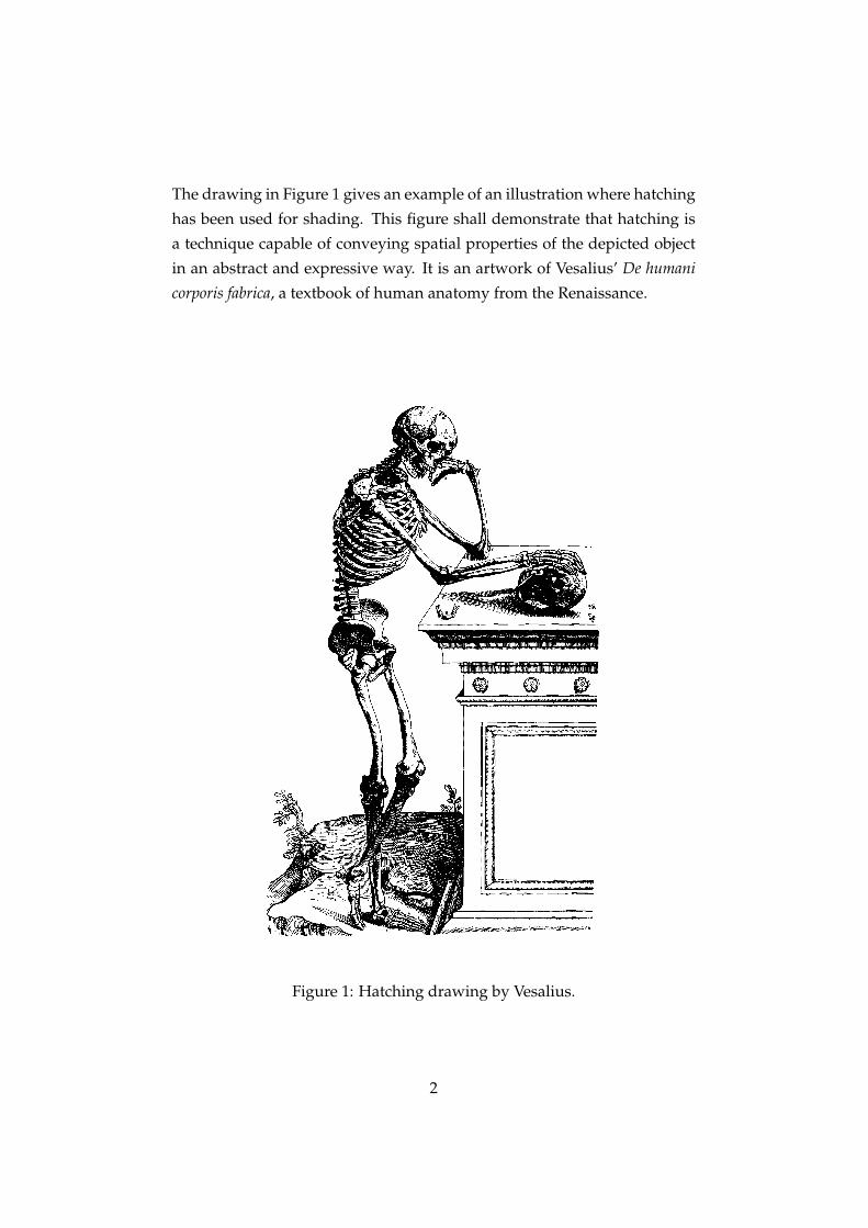
The drawing in Figure 1 gives an example of an illustration where hatching
has been used for shading. This figure shall demonstrate that hatching is
a technique capable of conveying spatial properties of the depicted object
in an abstract and expressive way. It is an artwork of Vesalius’ De humanicorporis fabrica, a textbook of human anatomy from the Renaissance.
~e
ilet
Figure 1: Hatching drawing by Vesalius.
2
We propose some possible fields of application to further explain the moti-
vation to engage in generating hatching drawings from three-dimensional
data. The majority of these data are generated in medical scanning de-
vices, and medicine offers numerous possibilities for employing volume
hatching. One possible medical application would be to illustrate upcom-
ing surgeries to patients. Explaining a surgery with the help of a volume
hatching rendering is perhaps more comprehensible for a layman than with
tomography slices. It also could be more readily accepted by patients as a
realistic rendering, due to the visually pleasing nature of hand drawings
and the distaste of some people on viewing inner body parts realistically.
Another potential field of application for volume hatching is the automated
generation of educational illustrations. Figures in scientific textbooks, for
instance in medicine or botany, which shall convey important structural
features by a schematic representation of objects, are often drawn by hand.
The preferred drawing medium here is pen-and-ink, and a reduced draw-
ing technique is used where shading is realized with a sparse and even
hatching. Volume hatching can be employed for creating images resem-
bling such illustrations from volumetric data. On the one hand, this offers
the possibility for automated generation of still images for text- or school-
books. On the other hand, interactive illustrations could be applied in
teaching, since they provide exploration and examining possibilities while
depicting the objects in a familiar illustrative style.
This thesis is organized as follows. First, we give an overview about re-
search done in fields related to this thesis in Chapter 2. In Chapter 3 we
present the algorithms we developed for rendering hatching drawings from
volume data. This includes the creation of contour drawings, curvature
estimation and generation of hatching strokes. We continue with shortly
outlining the concept of implementing these algorithms in Chapter 4. In
Chapter 5 we present and discuss result images, revealing advantages and
limitations of our approach. We summarize the content of this thesis in
Chapter 6. Finally, we draw a conclusion on the results of this thesis and
propose ideas for further enhancing our work in Chapter 7.
3
2 Related Work
This chapter will outline the current state of research in computer graphics
disciplines related to this thesis. We begin with a brief overview of existing
volume rendering approaches. Thereafter relevant features of the field of il-
lustrative or non-photorealistic rendering (NPR) will be presented. Finally,
applications of non-photorealistic rendering techniques to volume visual-
ization will be summarized.
2.1 Volume Rendering
The subject matter of volume visualization are volumetric datasets, com-
monly given as regular three-dimensional grids of sample values denoted
as voxels. The majority of volumetric datasets are produced in medical
imaging processes and therefore represent density values of organic tis-
sues. For the task of transforming these datasets into a visually perceptible
form, several approaches have been proposed.
One way of rendering a volumetric dataset is to create proxy geometry
which is pictured with traditional computer graphics methods. The other
way, which will be discussed here, is rendering the volume directly abdi-
cating the need for computing an intermediate geometric representation.
These approaches can be classified by the order the data is being processed
into image-order, object-order and hybrid-order methods. Newer tech-
niques utilize programmable graphics hardware for volume rendering. Di-
rect volume rendering concepts involve an illumination model and a so-
called transfer function, which maps scalar values of the dataset to color
and opacity values. A surface within a volume satisfying the constraint
that all voxels contain the same intensity value is denoted as iso-surface.
2.1.1 Image-Order Volume Rendering
In image-order volume rendering, the pixels on the image plane are being
traversed computing the contribution of the corresponding voxels to each
pixel. A common image-order algorithm is raycasting [28]. This algorithm
casts viewing rays into the volume, starting at image plane pixels.
In fixed intervals along the ray, the volumetric signal is reconstructed from
4
the samples and optical properties at the resample locations are determined.
The color information gained along the ray is accumulated and results in
the pixel color value.
Several publications [30, 29, 39, 24] deal with increasing the performance of
the basic raycasting algorithm. The image quality attained with raycasting
is very high, often regarded as the best among the volume rendering ap-
proaches, respectively competing with the image quality of splatting which
we will discuss next.
2.1.2 Object-Order Volume Rendering
Object-order volume rendering techniques traverse the dataset and calcu-
late each voxel’s contribution to the image. Splatting [56] is a well-known
object-order algorithm which processes the voxels, evaluates the optical
model and projects the color contributions onto the image plane.
Further research enhancing this approach aims at improving the image
quality [35] and performance [36] of splatting.
2.1.3 Hybrid-Order Volume Rendering
The shear-warp algorithm [26] was proposed intending to combine advan-
tages of image-order and object-order methods. The shear-warp algorithm
decomposes the viewing transformation into a shear and a warp transfor-
mation. Shearing the volume slices yields sampling rays parallel to the
principal viewing direction. This allows for traversing volume and image
simultaneously. An intermediate projection is calculated and subsequently
warped onto the image plane.
The shear-warp algorithm is a very efficient software volume rendering al-
gorithm, but suffers from a low image quality. This is due to the fact that
only bilinear interpolation is available during reconstruction.
Some work [48] has been done to enhance the low image quality of the
shear-warp algorithm.
5
2.1.4 GPU-Based Volume Rendering
With the increase of the computing power of graphics hardware, approaches
were developed which apply the programmability of the Graphics Process-
ing Unit (GPU) to volume visualization.
One way to use the GPU for volume rendering is exploiting 2D texture
mapping functionality [42]. A common technique stores three stacks of
2D textures, one for each major viewing axis. The stack corresponding the
most to the viewing direction is chosen and its textures are mapped on
object-aligned quads which are rendered with alpha blending.
Other methods utilize the 3D texture mapping capability of GPUs [4, 12, 55,
34]. Thereby, the whole dataset is used as a 3D texture. This volume tex-
ture is mapped onto view-aligned quads which are rendered using alpha
blending. One problem of 3D texture mapping is the limitation of available
video memory.
As the functionality of programming the GPU has expanded in the last
years, it is now possible to implement traditional volume rendering algo-
rithms such as raycasting to be performed on the GPU [46, 15].
2.2 Non-Photorealistic Rendering
In contrast to traditional computer graphics disciplines, which are con-
cerned with generating realistic images, the area of non-photorealistic ren-
dering (NPR) deals with creating imagery in artistic or expressive styles.
Research in the area of NPR has enabled mimicking a wide variety of styles
used in visual arts with computer graphics methods. Painterly rendering
for instance deals with the simulation of watercolor [6] or oil [16] paintings.
Other NPR techniques employ alternative shading models such as cartoon
and metal shading [13] to implement diverse rendering styles. We will here
focus on related work concerned with hand drawn imagery, namely line
drawing, pencil and pen-and-ink drawing. We start by examining research
on contour-depicting line drawings, then have a look at pen-and-ink ren-
dering and finally survey techniques which produce hatching and pencil
drawings from polygonal data.
6
2.2.1 Line Drawing
Line drawings are conventionally used for illustrations, and the line is a
commonly used primitive in computer graphics. Numerous researchers
have developed strategies for creating line drawings with the computer.
Interrante et al. [19] propose ridge and valley lines for rendering transpar-
ent skin surfaces. In order to enable a simultaneous display of multiple
layers of data, lines depicting important shape features are detected and
rendered appropriately to augment the spatial perception of the rendering.
The quality of line drawings has been further enhanced by methods such
as varying the line width, as proposed by Gooch et al. [14].
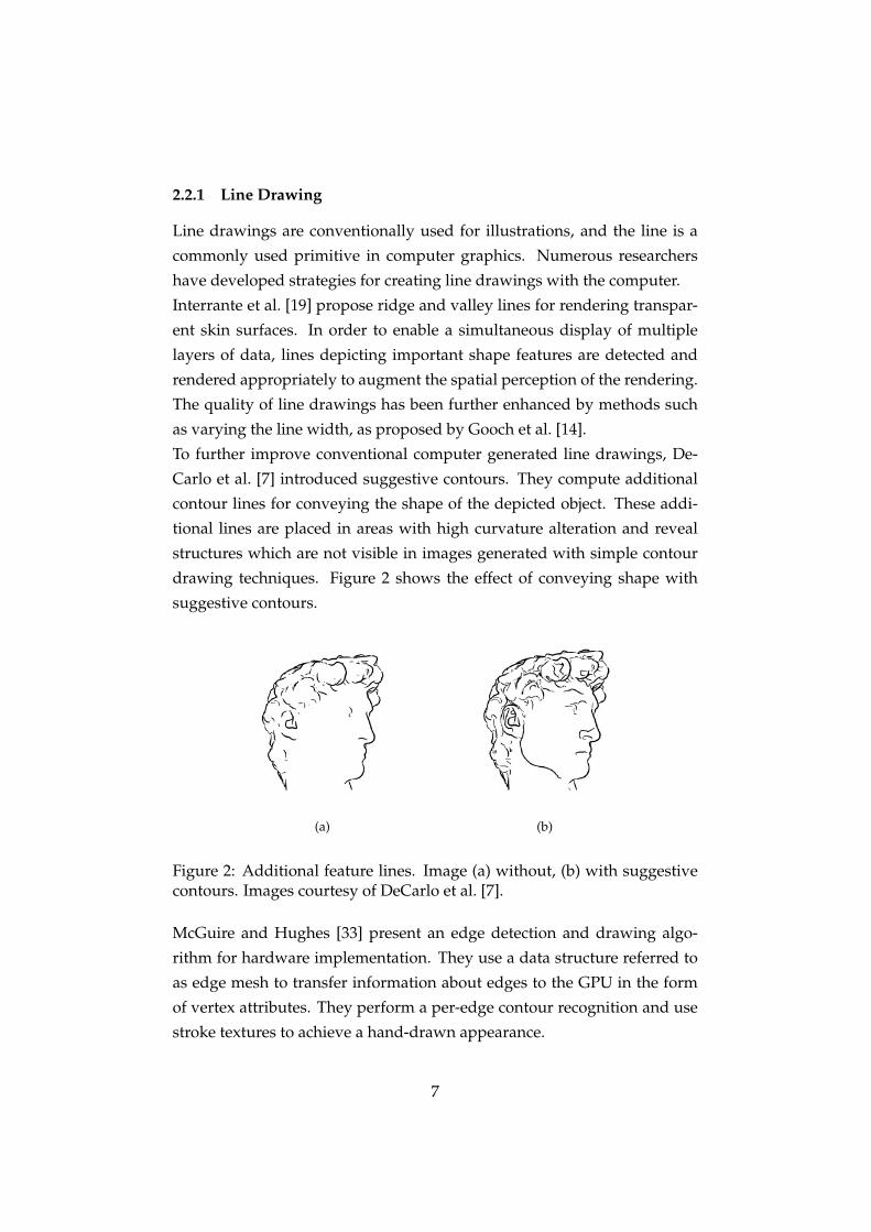
To further improve conventional computer generated line drawings, De-
Carlo et al. [7] introduced suggestive contours. They compute additional
contour lines for conveying the shape of the depicted object. These addi-
tional lines are placed in areas with high curvature alteration and reveal
structures which are not visible in images generated with simple contour
drawing techniques. Figure 2 shows the effect of conveying shape with
suggestive contours.
(a) (b)
Figure 2: Additional feature lines. Image (a) without, (b) with suggestivecontours. Images courtesy of DeCarlo et al. [7].
McGuire and Hughes [33] present an edge detection and drawing algo-
rithm for hardware implementation. They use a data structure referred to
as edge mesh to transfer information about edges to the GPU in the form
of vertex attributes. They perform a per-edge contour recognition and use
stroke textures to achieve a hand-drawn appearance.
7
Markosian et al. [32] are concerned with efficient silhouette rendering of
3D models with different drawing styles. They use a modification of a
common hidden line removal algorithm for an efficient visibility determi-
nation. They manage to identify silhouette edges and render them main-
taining inter-frame coherence at interactive rates.
2.2.2 Pen-And-Ink Rendering
Pen-and-ink drawings are an expressive medium and a favored technique
among illustrators. Its clearness and directness originate from the circum-
stance that all visual properties such as shape, shade and texture of the
object to be drawn have to be suggested just by the arrangement and size
of individual strokes. Pen-and-ink offers just one color and tone.
Winkenbach and Salesin [57] propose a method to render computer gen-
erated pen-and-ink illustrations of 3D models. They introduce the con-
cept of stroke textures for mimicking different drawing styles and mate-
rials. A stroke texture contains multiple strokes arranged in regular pat-
terns which represent various materials. It has to convey both tone and
texture, whereby a darker tone is achieved through a higher density of
strokes. They prioritize the strokes in order to render them sequentially
until the desired tone is obtained. They emphasize the need for a tight
linkage of texture and tone, which are usually separated in the rendering
pipeline, and the importance of a combination of 2D and 3D information.
Winkenbach and Salesin depict boundary outlines via drawing strokes of
a boundary edge with a dedicated texture. The interior outlines are used
for accentuating strokes or suggesting shadow directions. Outline strokes
are minimized by drawing a contour stroke only if the tones of its adjacent
faces differ sufficiently. Outline strokes are also used to assist the spatial
impression by varying the line thickness according to local illumination
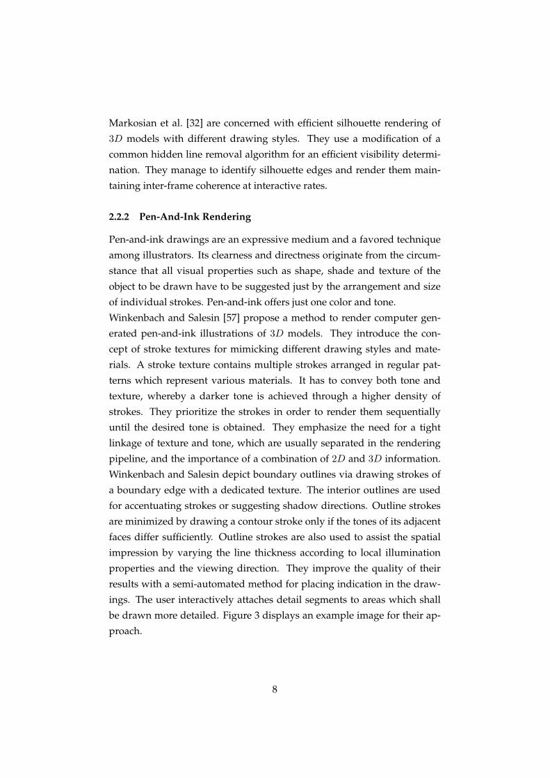
properties and the viewing direction. They improve the quality of their
results with a semi-automated method for placing indication in the draw-
ings. The user interactively attaches detail segments to areas which shall
be drawn more detailed. Figure 3 displays an example image for their ap-
proach.
8
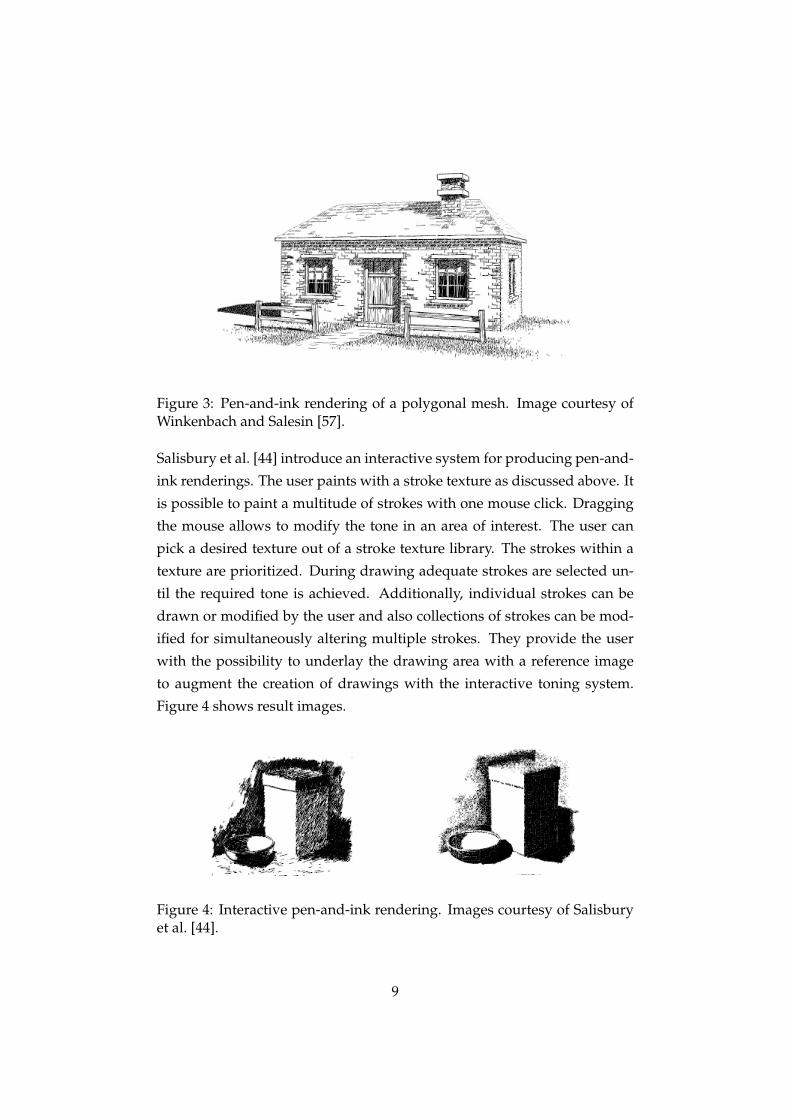
Figure 3: Pen-and-ink rendering of a polygonal mesh. Image courtesy ofWinkenbach and Salesin [57].
Salisbury et al. [44] introduce an interactive system for producing pen-and-
ink renderings. The user paints with a stroke texture as discussed above. It
is possible to paint a multitude of strokes with one mouse click. Dragging
the mouse allows to modify the tone in an area of interest. The user can
pick a desired texture out of a stroke texture library. The strokes within a
texture are prioritized. During drawing adequate strokes are selected un-
til the required tone is achieved. Additionally, individual strokes can be
drawn or modified by the user and also collections of strokes can be mod-
ified for simultaneously altering multiple strokes. They provide the user
with the possibility to underlay the drawing area with a reference image
to augment the creation of drawings with the interactive toning system.
Figure 4 shows result images.
Figure 4: Interactive pen-and-ink rendering. Images courtesy of Salisburyet al. [44].
9
2.2.3 Pencil Drawing and Hatching
Praun et al. [41] proposed an interesting approach for creating hatchings
from 3D models in real time. Hatching strokes over arbitrary surfaces are
drawn to convey material, tone and form of the model. They introduce
the concept of Tonal Art Maps, compilations of mipmapped textures corre-
sponding to various tones and resolutions. A texture of a Tonal Art Map
contains multiple strokes. The density of strokes corresponds to the tone
the texture represents. A Tonal Art Map is computed in a preprocessing
step and used for texturing a 3D model with appropriate stroke textures.
One constraint during the creation of the strokes of the Tonal Art Map tex-
tures is a nesting property. All strokes of textures with a lighter tone appear
in those of darker tones, so a tone variation can be depicted coherently and
smoothly. In order to obtain a consistent stroke size and density in all res-
olutions, the hatching strokes are scaled according to the resolution and
the mipmap levels are used for different primitive sizes. To gain an evenly
spacing of the strokes, they generate multiple random strokes and select
the stroke most suitable. During rendering, the tone of a surface is de-
termined and used to select the proper texture out of the Tonal Art Map.
Hardware multitexturing is exploited to blend together multiple hatching
stroke textures per face. A 6-way blending scheme allows for producing
smooth tone and orientation transitions and for maintaining spatial and
temporal coherence. They use a lapped texture [40] parameterization with
overlapping patches oriented to the curvature of the object. Lapped tex-
tures are a mechanism for texturing an arbitrary surface geometry with the
assistance of overlapping patches aligned to a tangential vector field.
In order to incorporate various rendering styles in the real time hatching
approach, the arrangement pattern and visual properties of the strokes can
be modified. The results achieved with this hatching technique are of high
image quality and are rendered at interactive frame rates. Figure 5 shows
an example hatching image of this technique.
10
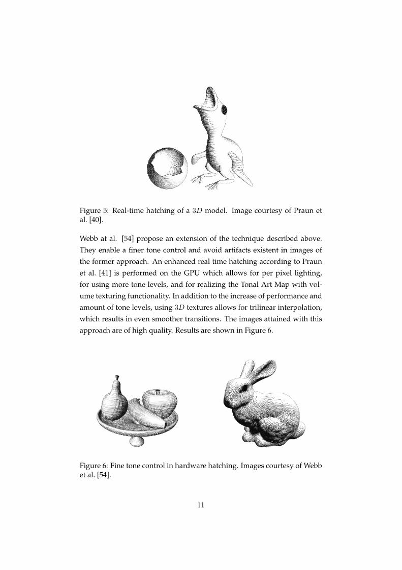
Figure 5: Real-time hatching of a 3D model. Image courtesy of Praun etal. [40].
Webb at al. [54] propose an extension of the technique described above.
They enable a finer tone control and avoid artifacts existent in images of
the former approach. An enhanced real time hatching according to Praun
et al. [41] is performed on the GPU which allows for per pixel lighting,
for using more tone levels, and for realizing the Tonal Art Map with vol-
ume texturing functionality. In addition to the increase of performance and
amount of tone levels, using 3D textures allows for trilinear interpolation,
which results in even smoother transitions. The images attained with this
approach are of high quality. Results are shown in Figure 6.
Figure 6: Fine tone control in hardware hatching. Images courtesy of Webbet al. [54].
11
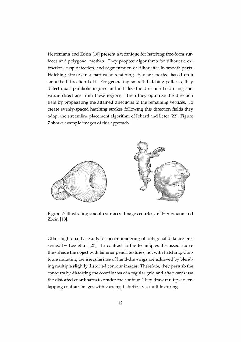
Hertzmann and Zorin [18] present a technique for hatching free-form sur-
faces and polygonal meshes. They propose algorithms for silhouette ex-
traction, cusp detection, and segmentation of silhouettes in smooth parts.
Hatching strokes in a particular rendering style are created based on a
smoothed direction field. For generating smooth hatching patterns, they
detect quasi-parabolic regions and initialize the direction field using cur-
vature directions from these regions. Then they optimize the direction
field by propagating the attained directions to the remaining vertices. To
create evenly-spaced hatching strokes following this direction fields they
adapt the streamline placement algorithm of Jobard and Lefer [22]. Figure
7 shows example images of this approach.
Figure 7: Illustrating smooth surfaces. Images courtesy of Hertzmann andZorin [18].
Other high-quality results for pencil rendering of polygonal data are pre-
sented by Lee et al. [27]. In contrast to the techniques discussed above
they shade the object with laminar pencil textures, not with hatching. Con-
tours imitating the irregularities of hand-drawings are achieved by blend-
ing multiple slightly distorted contour images. Therefore, they perturb the
contours by distorting the coordinates of a regular grid and afterwards use
the distorted coordinates to render the contour. They draw multiple over-
lapping contour images with varying distortion via multitexturing.
12
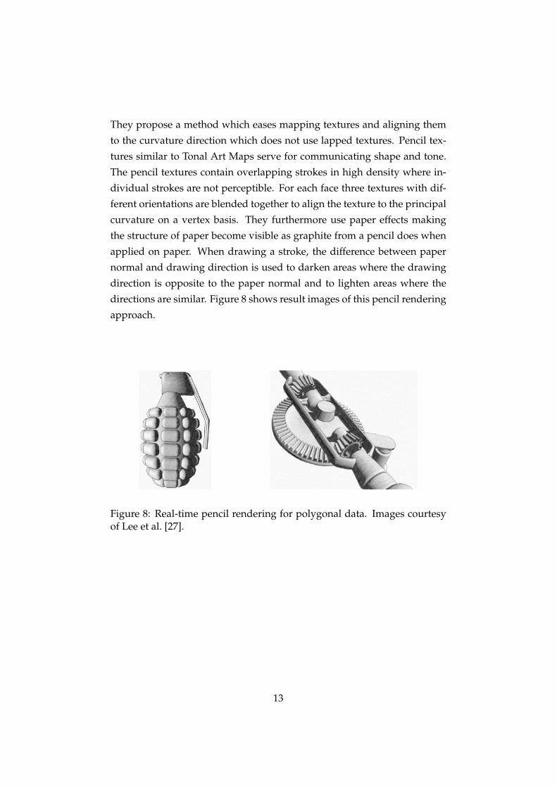
They propose a method which eases mapping textures and aligning them
to the curvature direction which does not use lapped textures. Pencil tex-
tures similar to Tonal Art Maps serve for communicating shape and tone.
The pencil textures contain overlapping strokes in high density where in-
dividual strokes are not perceptible. For each face three textures with dif-
ferent orientations are blended together to align the texture to the principal
curvature on a vertex basis. They furthermore use paper effects making
the structure of paper become visible as graphite from a pencil does when
applied on paper. When drawing a stroke, the difference between paper
normal and drawing direction is used to darken areas where the drawing
direction is opposite to the paper normal and to lighten areas where the
directions are similar. Figure 8 shows result images of this pencil rendering
approach.
Figure 8: Real-time pencil rendering for polygonal data. Images courtesyof Lee et al. [27].
13
2.3 NPR in Volume Visualization
Non-photorealistic rendering methods are used in volume visualization
due to their property of communicating visual information in a sparse, ab-
stract form omitting irrelevant details while emphasizing critical aspects.
Hand-drawn illustrations are used in many sciences for schematic repre-
sentations or easy comprehensible imagery, for instance in teaching or text-
books. With the task of realizing such traditional illustration techniques
with NPR methods, numerous approaches have emerged and will be out-
lined here. We start with discussing two-level volume rendering [17], an
important work towards NPR in volume visualization. We continue with
having a look at NPR methods involving a modified optical model to allow
for transparency or alternative shading styles. Then we survey pen-and-
ink rendering for volumes, which is a technique well suited for depicting
scientific objects. Finally we present hatching techniques for volumetric
datasets, which are the substance of this thesis.
2.3.1 Two-Level Volume Rendering
Two-level volume rendering [17] plays a crucial role in the evolution of
NPR in volume visualization. In this work, Hauser et al. propose an
approach which enables rendering subsets of a volumetric dataset in di-
verse styles. Different parts of the dataset are depicted individually with
different rendering algorithms and are composed in a final merging step.
This concept proves its strength when inner structures and semitransparent
outer regions shall be rendered simultaneously, enabling a focus+context
oriented visual representation. It also enables utilizing non-photorealistic
shading or rendering models. This can be applied for example for render-
ing outer surfaces with an NPR line drawing technique while using a direct
volume rendering algorithm for inner parts. The volume is rendered in two
levels. One is the local level, on which each object is rendered individually
and the other is a global level wherein all local levels are combined in the
final compositing operation.
Rheingans and Ebert [11] also present the idea of combining realistic and
non-photorealistic rendering techniques for volume illustration.
14
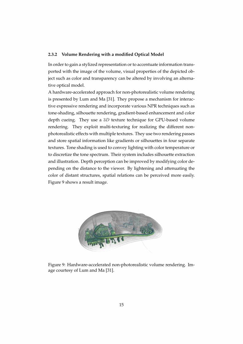
2.3.2 Volume Rendering with a modified Optical Model
In order to gain a stylized representation or to accentuate information trans-
ported with the image of the volume, visual properties of the depicted ob-
ject such as color and transparency can be altered by involving an alterna-
tive optical model.
A hardware-accelerated approach for non-photorealistic volume rendering
is presented by Lum and Ma [31]. They propose a mechanism for interac-
tive expressive rendering and incorporate various NPR techniques such as
tone-shading, silhouette rendering, gradient-based enhancement and color
depth cueing. They use a 3D texture technique for GPU-based volume
rendering. They exploit multi-texturing for realizing the different non-
photorealistic effects with multiple textures. They use two rendering passes
and store spatial information like gradients or silhouettes in four separate
textures. Tone shading is used to convey lighting with color temperature or
to discretize the tone spectrum. Their system includes silhouette extraction
and illustration. Depth perception can be improved by modifying color de-
pending on the distance to the viewer. By lightening and attenuating the
color of distant structures, spatial relations can be perceived more easily.
Figure 9 shows a result image.
Figure 9: Hardware-accelerated non-photorealistic volume rendering. Im-age courtesy of Lum and Ma [31].
15
Another method for non-photorealistic rendering of volumes is proposed
by Salah et al. [43]. They use it for illustratively rendering segmented
anatomical data. The algorithm is based on surface points which are ex-
tracted as a subset of the segmented objects in an initial step. The shading is
performed with halftoning, but the work focusses on silhouette extraction
and rendition. Silhouettes are estimated via the normals corresponding
to the surface points and the viewing position. The outlines are rendered
using disks which are oriented to the normals so that the normals are per-
pendicular to the plane defined by the disk. These oriented disks result in
ellipsoids in image space and their combination yields the impression of a
hand-drawn outline consisting of multiple overlapping strokes.
Viola and Groller [52] deal with the concept of smart visibility in visual-
ization, which extends the transparency model of Diepstraten et al. [8].
They smartly uncover areas of high importance occluded by outer regions.
One way to implement this is by reducing the opacity of objects occluding
the important parts. Another way is by deforming or translating objects.
This originates from technical illustration techniques denoted as cut-away
views, ghosted views and exploded views. These techniques manage to
emphasize and illuminate the most important information in a manner pro-
viding easy perception and visual harmony.
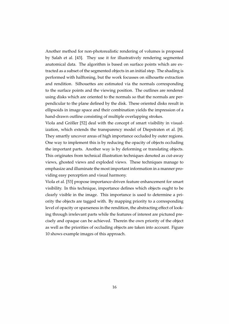
Viola et al. [53] propose importance-driven feature enhancement for smart
visibility. In this technique, importance defines which objects ought to be
clearly visible in the image. This importance is used to determine a pri-
ority the objects are tagged with. By mapping priority to a corresponding
level of opacity or sparseness in the rendition, the abstracting effect of look-
ing through irrelevant parts while the features of interest are pictured pre-
cisely and opaque can be achieved. Therein the own priority of the object
as well as the priorities of occluding objects are taken into account. Figure
10 shows example images of this approach.
16
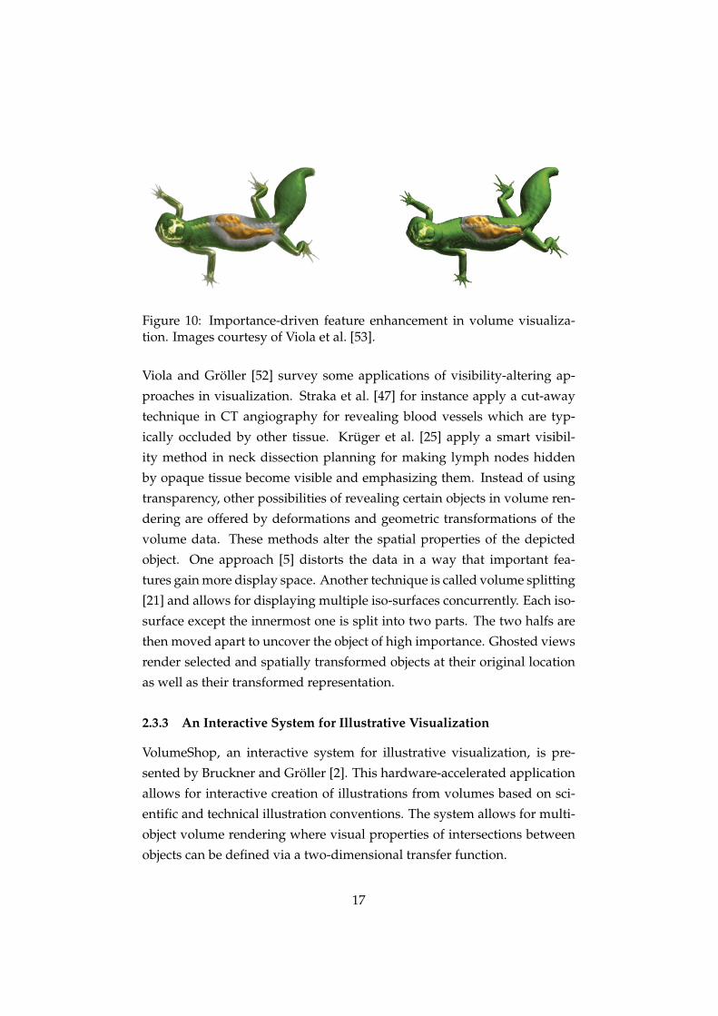
Figure 10: Importance-driven feature enhancement in volume visualiza-tion. Images courtesy of Viola et al. [53].
Viola and Groller [52] survey some applications of visibility-altering ap-
proaches in visualization. Straka et al. [47] for instance apply a cut-away
technique in CT angiography for revealing blood vessels which are typ-
ically occluded by other tissue. Kruger et al. [25] apply a smart visibil-
ity method in neck dissection planning for making lymph nodes hidden
by opaque tissue become visible and emphasizing them. Instead of using
transparency, other possibilities of revealing certain objects in volume ren-
dering are offered by deformations and geometric transformations of the
volume data. These methods alter the spatial properties of the depicted
object. One approach [5] distorts the data in a way that important fea-
tures gain more display space. Another technique is called volume splitting
[21] and allows for displaying multiple iso-surfaces concurrently. Each iso-
surface except the innermost one is split into two parts. The two halfs are
then moved apart to uncover the object of high importance. Ghosted views
render selected and spatially transformed objects at their original location
as well as their transformed representation.
2.3.3 An Interactive System for Illustrative Visualization
VolumeShop, an interactive system for illustrative visualization, is pre-
sented by Bruckner and Groller [2]. This hardware-accelerated application
allows for interactive creation of illustrations from volumes based on sci-
entific and technical illustration conventions. The system allows for multi-
object volume rendering where visual properties of intersections between
objects can be defined via a two-dimensional transfer function.
17
VolumeShop additionally offers different non-photorealistic shading mod-
els such as cartoon and metal shading. It enables interactive selection with
a three-dimensional painting method.
Bruckner and Groller use selective illustration techniques for focus+context
visualization. Cutaway views and ghosting can be achieved as well as
importance-driven volume rendering for smart visibility according to Vi-
ola et al. [52]. Illustrative context-preserving volume rendering [1] is per-
formed for simultaneous visualization of interior and exterior structures.
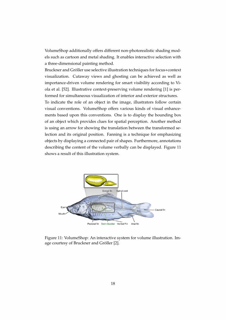
To indicate the role of an object in the image, illustrators follow certain
visual conventions. VolumeShop offers various kinds of visual enhance-
ments based upon this conventions. One is to display the bounding box
of an object which provides clues for spatial perception. Another method
is using an arrow for showing the translation between the transformed se-
lection and its original position. Fanning is a technique for emphasizing
objects by displaying a connected pair of shapes. Furthermore, annotations
describing the content of the volume verbally can be displayed. Figure 11
shows a result of this illustration system.
Figure 11: VolumeShop: An interactive system for volume illustration. Im-age courtesy of Bruckner and Groller [2].
18
2.3.4 Line Drawings from Volume Data
Burns et al. [3] develop a technique for directly extracting and rendering
silhouettes and suggestive contours [7] of volumetric data. They suggest a
seed-and-traverse algorithm for contour extraction. Initial seed points are
detected with the help of an equation for iso-surface and contour defini-
tion. Once a contour-containing surface voxel is determined based on this
equation, the contour is followed using a variant of the marching lines algo-
rithm [50]. In order to bypass the need for examining all voxels, they utilize
a seed-and-traverse algorithm denoted as walking contours. Starting with
an initial seed they perform a marching lines search along the silhouette
until returning to the initial seed. During animation, adequate seed points
from the previous frame are re-used exploiting spatio-temporal coherency
of contour lines. New seed points are found in random cells using a gradi-
ent approximation for determining if the cell contains a contour. For com-
prehensible rendering, they distinguish between different families of lines
such as silhouette lines or suggestive contours and depict them in differing
rendering styles. Line visibility is computed using raycasting.
2.3.5 Pen-And-Ink Rendering in Volume Visualization
As pointed out before, pen-and-ink drawing is a popular illustration tech-
nique due to the degree of abstraction achieved in its pictorial representa-
tions. A psychological study with architects [45] showed that pen-and-ink
imagery often is preferred to a realistic one. Therein architects were asked
to compare computer generated sketches against realistic CAD images and
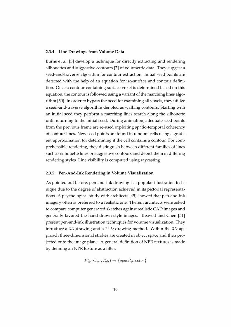
generally favored the hand-drawn style images. Treavett and Chen [51]
present pen-and-ink illustration techniques for volume visualization. They
introduce a 3D drawing and a 2+D drawing method. Within the 3D ap-
proach three-dimensional strokes are created in object space and then pro-
jected onto the image plane. A general definition of NPR textures is made
by defining an NPR texture as a filter:
F (p, Oatt, Tatt) → {opacity, color}
19
Here p is a point in texture space, Oatt are object attributes correlated with
p and Tatt is a set of texture attributes. They use 3D textures to create the
three-dimensional strokes. They suggest an approach that renders the vol-
ume in two passes. One is for lighting computation with traditional volume
rendering mechanisms. The other rendering pass serves for the creation
of the three-dimensional strokes using the intermediate volume rendering
output as input.
Treavett and Chen further suggest a 2+D approach applying two-phase
rendering. In the first phase all relevant information about the object is
gathered in object space and stored in dedicated image buffers. The second
phase is used for creating strokes in image space. The particular renditions
are then composed in an amalgamation step to produce the final image.
This is referred to as a 2+D technique because 2D image elements are cre-
ated using 3D information. The intermediate images serve to determine
visual properties of the pen-and-ink drawing. Outlines can be extracted
with the help of the distance variation between adjacent pixels or the angle
between viewing direction and gradient. The length, thickness and density
of the strokes can be controlled in dependance of the lighting. Strokes can
be oriented along the curvature of the rendered object. This 2+D concept
was adopted for the volume hatching method developed in this thesis.
Figure 12 displays example images of this approach.
Figure 12: Pen-and-ink rendering in volume visualization. Images courtesyof Treavett and Chen [51].
20
2.3.6 Volume Hatching
We now have a look at two hatching techniques for volumetric data. One
was presented by Nagy et al. [38] together with fragment shader implemen-
tations of toon shading and silhouette rendering for volumes. The hatch-
ing is created in two passes. In the first pass a hatching direction field is
set up by computing higher order differential characteristics like curvature
and storing them in a hierarchical data structure. The second pass serves
for creating three-dimensional strokes in object space coinciding with this
hatching field and rendering them as line primitives. In order to access cur-
vature data efficiently they encode it into an octree representation. For the
creation of hatching strokes seed points indicating the start position of the
strokes are distributed in the volume. Initial seed points are determined
with a data driven placement method. Therefore the octree structure is tra-
versed using scalar values and curvature information to decide whether
seed points have to be inserted in the current cell. The octree allows for
efficiently skipping empty regions, planar areas and structures specified
to be transparent. The number of seed points is chosen in dependance of
normalized gradient magnitude and mean curvature information. They
position a larger amount of seeds in areas of high curvature and place seed
points more sparsely in homogeneous areas. The seed points are initially
placed in the center of the cells and then shifted towards iso-surfaces. For
hatching the object a subset of this pre-computed seed point set is selected
during runtime and a three-dimensional stroke is created for each selected
seed point. A path following the principal curvature direction is traced
in object space. A stroke is stored as a set of points and rendered using
line primitives. The direction field is numerically integrated employing
a Runge-Kutta integration with adaptive step size. The strokes are ren-
dered as line strips enhanced by anisotropic line shading. In addition to
that Nagy et al. determine whether a part of a stroke depicts a front fac-
ing or a back facing part of the surface and use this information to color
the strokes respectively. By using different colors for front and back facing
regions they implement two-sided lighting. Furthermore cross-hatching of
dark regions is performed using the minimal curvature direction. The con-
cept of pre-computing strokes in object space and the graphics hardware
21
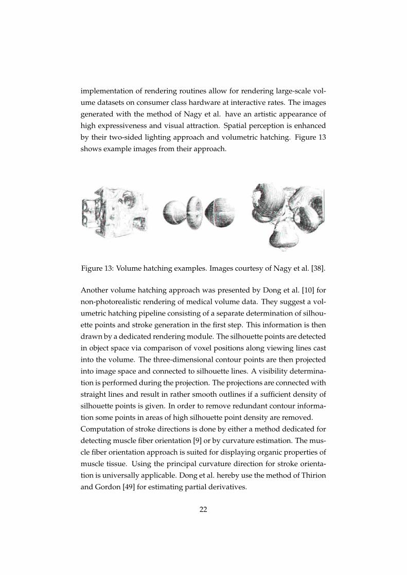
implementation of rendering routines allow for rendering large-scale vol-
ume datasets on consumer class hardware at interactive rates. The images
generated with the method of Nagy et al. have an artistic appearance of
high expressiveness and visual attraction. Spatial perception is enhanced
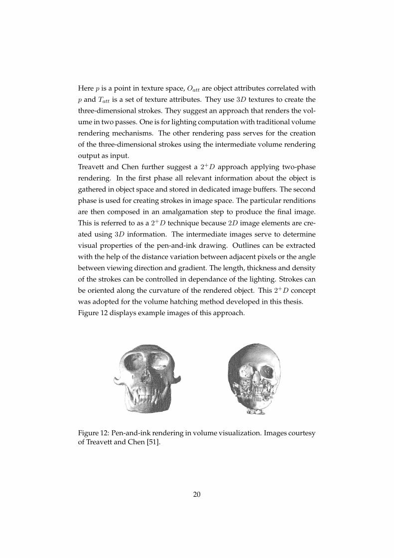
by their two-sided lighting approach and volumetric hatching. Figure 13
shows example images from their approach.
Figure 13: Volume hatching examples. Images courtesy of Nagy et al. [38].
Another volume hatching approach was presented by Dong et al. [10] for
non-photorealistic rendering of medical volume data. They suggest a vol-
umetric hatching pipeline consisting of a separate determination of silhou-
ette points and stroke generation in the first step. This information is then
drawn by a dedicated rendering module. The silhouette points are detected
in object space via comparison of voxel positions along viewing lines cast
into the volume. The three-dimensional contour points are then projected
into image space and connected to silhouette lines. A visibility determina-
tion is performed during the projection. The projections are connected with
straight lines and result in rather smooth outlines if a sufficient density of
silhouette points is given. In order to remove redundant contour informa-
tion some points in areas of high silhouette point density are removed.
Computation of stroke directions is done by either a method dedicated for
detecting muscle fiber orientation [9] or by curvature estimation. The mus-
cle fiber orientation approach is suited for displaying organic properties of
muscle tissue. Using the principal curvature direction for stroke orienta-
tion is universally applicable. Dong et al. hereby use the method of Thirion
and Gordon [49] for estimating partial derivatives.
22
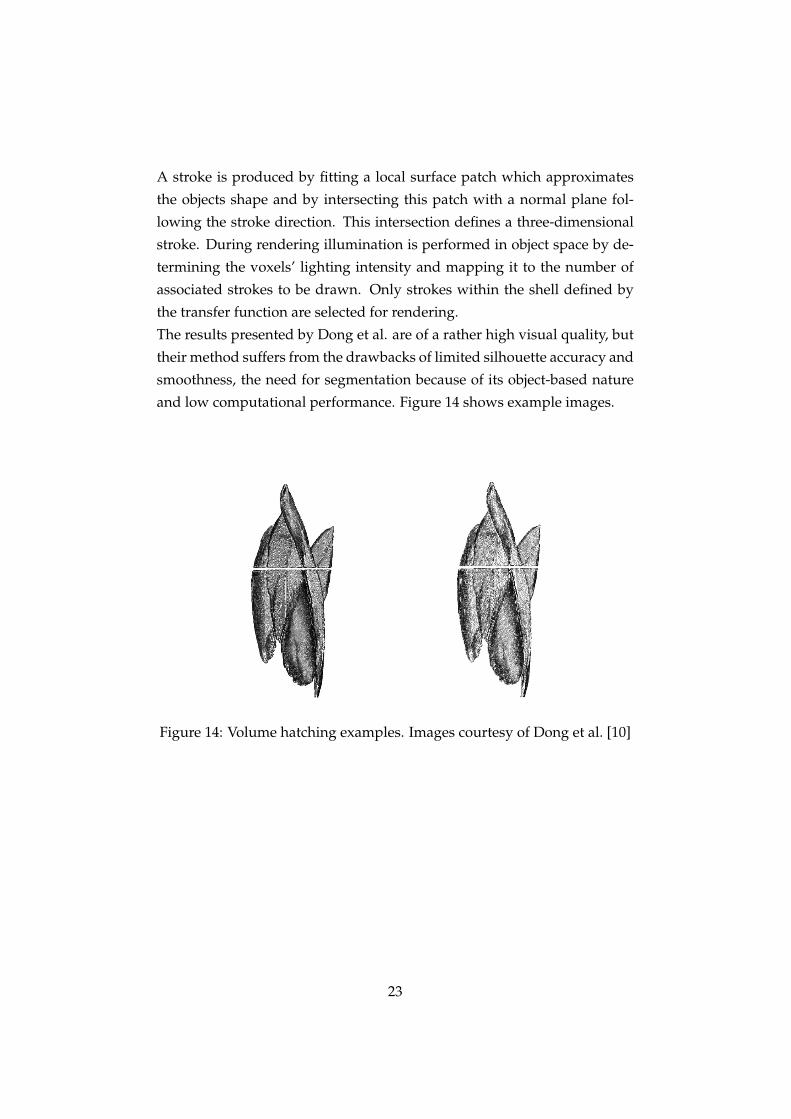
A stroke is produced by fitting a local surface patch which approximates
the objects shape and by intersecting this patch with a normal plane fol-
lowing the stroke direction. This intersection defines a three-dimensional
stroke. During rendering illumination is performed in object space by de-
termining the voxels’ lighting intensity and mapping it to the number of
associated strokes to be drawn. Only strokes within the shell defined by
the transfer function are selected for rendering.
The results presented by Dong et al. are of a rather high visual quality, but
their method suffers from the drawbacks of limited silhouette accuracy and
smoothness, the need for segmentation because of its object-based nature
and low computational performance. Figure 14 shows example images.
Figure 14: Volume hatching examples. Images courtesy of Dong et al. [10]
23
2.4 Curvature Estimation in Volume Visualization
In order to integrate higher order differentials into the transfer function,
Kindlmann et al. [23] suggest a method for direct curvature estimation.
This technique was adopted for curvature computation in the volume hatch-
ing system developed in this thesis. In volume hatching, curvature direc-
tion can be used for aligning hatching strokes to the object’s shape. The
first-order derivatives of the scalar values make up the gradient vector,
which approximates a surface normal. The gradient is used for illumina-
tion, visibility and silhouette computation in volume visualization. Cur-
vature is defined through the second-order derivatives of the volumetric
function. It represents the variation of surface normals. Kindlmann et
al. employ a convolution-based approach for measuring the curvature and
suggest three simple implementation steps for realizing it. This technique
is based on a tangent space projection of the Hessian matrix. Various filter-
ing techniques are examined for reconstruction and experiments result in
the statement that a B-spline-based convolution is well suited for curvature
estimation.
Kindlmann et al. introduce the concept of thickness-controlled contours.
Herein the normal curvature along the viewing direction is used to mod-
ulate the width of contours in the volume contour rendering. This can be
used for rendering contours of consistent and controllable width avoid-
ing that contours become thicker in low-curvature regions. Contours with
varying width appear if just the gradient and viewing direction are used
for contour computation.
24
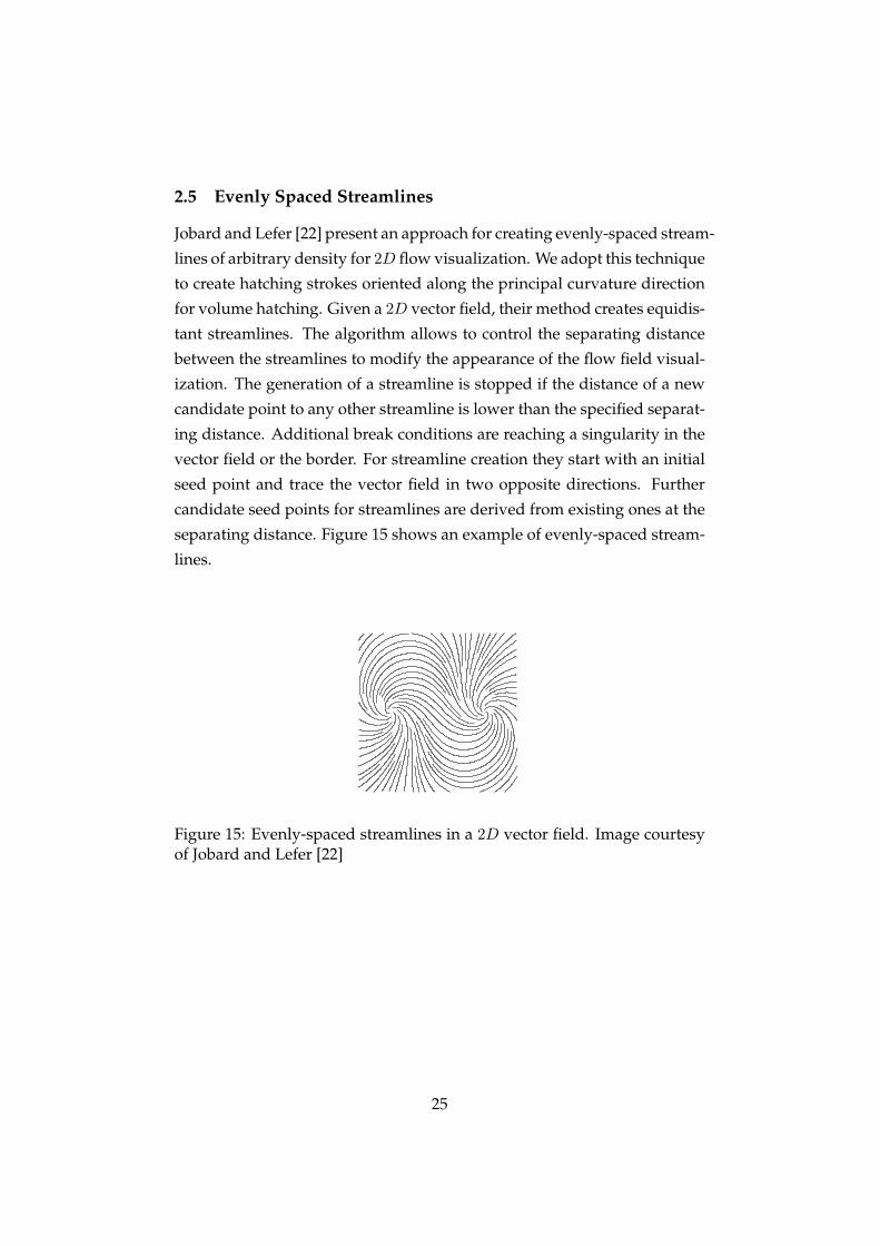
2.5 Evenly Spaced Streamlines
Jobard and Lefer [22] present an approach for creating evenly-spaced stream-
lines of arbitrary density for 2D flow visualization. We adopt this technique
to create hatching strokes oriented along the principal curvature direction
for volume hatching. Given a 2D vector field, their method creates equidis-
tant streamlines. The algorithm allows to control the separating distance
between the streamlines to modify the appearance of the flow field visual-
ization. The generation of a streamline is stopped if the distance of a new
candidate point to any other streamline is lower than the specified separat-
ing distance. Additional break conditions are reaching a singularity in the
vector field or the border. For streamline creation they start with an initial
seed point and trace the vector field in two opposite directions. Further
candidate seed points for streamlines are derived from existing ones at the
separating distance. Figure 15 shows an example of evenly-spaced stream-
lines.
Figure 15: Evenly-spaced streamlines in a 2D vector field. Image courtesyof Jobard and Lefer [22]
25
3 Volume Hatching
In this chapter we present the techniques developed for rendering images
of volume datasets which resemble hand-drawn hatchings. We start with
explaining the rendering pipeline of our volume hatching system. Then
a survey of the system which is used for depicting contours with a hand-
drawn appearance is given. We continue by explaining the method we
employ for rendering stylized strokes. Afterwards we address curvature
estimation which is used for hatching stroke orientation. Then we outline
some experimental approaches which emerged while searching for a strat-
egy for volume hatching. We proceed with discussing our final approach
to volume hatching based on streamlines. Finally we describe the way we
enable volumetric hatching.
26
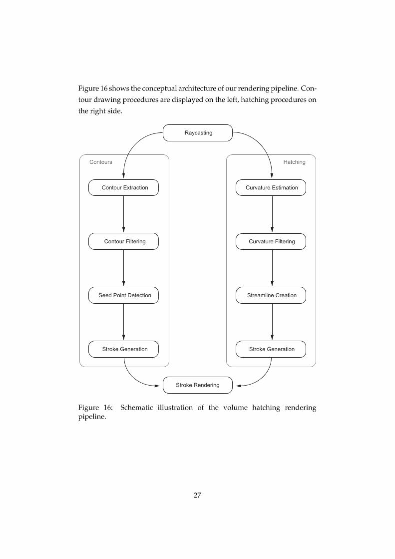
Figure 16 shows the conceptual architecture of our rendering pipeline. Con-
tour drawing procedures are displayed on the left, hatching procedures on
the right side.
Raycasting
Contour Extraction
Seed Point Detection
Stroke Generation
Contour Filtering
Stroke Rendering
Curvature Estimation
Streamline Creation
Stroke Generation
Curvature Filtering
Contours Hatching
Figure 16: Schematic illustration of the volume hatching renderingpipeline.
27
The input to the volume hatching pipeline is a volume dataset, its output is
an image consisting of contour and hatching strokes. Contours and hatch-
ing strokes are created separately and merged for the final image. The first
step in the pipeline is a raycasting procedure. For samples at the first ray-
object intersection, optical and spatial properties of the rendered object are
computed and stored in 2D textures. We subsequently use this information
to determine the adequate placement and orientation of strokes.
For contour drawing the required information to be generated during ray-
casting is information on contour locations (see Section 3.1.1). The input for
this operation is the volume dataset, the output is a 2D contour texture. In
a preprocessing step this contour information is filtered (see Section 3.1.2)
and the output is the filtered contour texture. Then seed points on the con-
tour are detected with a line-following algorithm (see Section 3.1.3). This
operation gets the filtered contour texture as input and generates an array
of contour points as output. Afterwards strokes are generated from this set
of contour points (see Section 3.1.4), yielding an array of strokes as output.
Each stroke is defined by a number of control points. Finally the contour
strokes are rendered (see Section 3.2).
For the hatching strokes the reference information to be generated during
raycasting is information on lighting intensity and curvature direction (see
Section 3.3). The output of the raycasting operation are two 2D textures
containing this information. Curvature information is smoothed in a pre-
processing operation (see Section 3.3), which outputs a filtered curvature
direction texture. Then streamlines are created using the curvature direc-
tion image as input (see Section 3.5.1). The output of this operation is a set
of curvature-aligned streamlines. Simultaneously to creating streamlines,
hatching strokes are generated by extracting them from the streamlines (see
Section 3.5.2). Output of this operation is a set of hatching strokes. Each
stroke is defined by an array of control points. Streamline generation and
stroke extraction are repeated to produce hatching (see Section 3.5.4) and
crosshatching layers (see Section 3.5.5). Subsequently hatching strokes are
rendered (see Section 3.5.3).
28
3.1 Contour Drawing
In the following we explain the algorithms we use for extracting and ren-
dering contours in a visually pleasant manner. The majority of NPR tech-
niques depict contours using simple rendering methods. Although sophis-
ticated silhouette extraction mechanisms have emerged, the rendering of
silhouettes is mostly done using line primitives or just black color for con-
tour pixels. If only contours are drawn this might not be a problem. As
soon as contours are drawn in combination with hatching using a different
rendering style it affects image quality. It conveys the impression of hatch-
ing an object with a pencil and drawing its contours with another draw-
ing medium, for instance pen-and-ink. In contrast to that, we developed
an approach for stylized contour depiction. It is based on a simulation of
the human hand-drawing process and allows for rendering both contours
and hatching with identical visual appearance. When a pencil drawer cre-
ates the outline of an object, he draws multiple overlapping strokes for
approximating the silhouette and refines it incrementally. This can result
in a sketchy visual appearance when the contours are drawn fast or in
a smooth and precise appearance where individual strokes are no longer
recognizable. As this thesis is concerned with generating imagery with a
hand-drawn appearance, we try to mimic the hand drawing process by
depicting multiple strokes following the contours. Strokes are not drawn
as line primitives. A stroke is depicted by a brush texture drawn along a
spline, which enables smooth strokes and various stylization. Our contour
drawing mechanism consists of four steps. Initially, silhouette extraction is
performed during raycasting (see Section 3.1.1). Afterwards the contours
are filtered (see Section 3.1.2). Then we use a line-following algorithm to
sequentially find points on the contour (see Section 3.1.3). Finally, subsets
of these points are selected and used as spline control points for drawing
contour strokes, as described in Section 3.1.4.
29
3.1.1 Contour Extraction
Detecting contours is performed during volume rendering. We use the an-
gle between gradient and viewing direction as a criterion for silhouette ex-
traction. It is based on the fact that contours lie in regions where a sur-
face is perpendicular to the viewing direction. These are regions where the
dot product between view vector and gradient yields a small value. We
additionally implement the concept of thickness-controlled contours sug-
gested by Kindlmann et al. [23]. Applying this method is advantageous
for our line-following algorithm. Without thickness-controlled contours,
planar areas result in thick contours. When tracing thick contours, our
line-following algorithm generates adjacent contour points in a zigzag ar-
rangement of high density, because too many adjacent contour locations
are detected.
The contour detection is done at the positions of the first ray-object intersec-
tions, which define the outer shell of the volume. We additionally compute
the image-space direction of the contour through the cross product between
viewing direction and gradient. As we use a GPU raycaster for volume ren-
dering, all these contour extraction routines can be performed efficiently in
graphics hardware. Contour information is stored in a dedicated texture
image. Figure 17(a) shows a contour image generated with the described
methods. The color coding uses green for contours in x direction, blue for
contours in y direction and alpha for the contour value.
3.1.2 Contour Filtering
To improve the results of our line-following method for finding control
points on the contour, we filter the contour image in a preprocessing step.
We employ a Gaussian convolution in order to eliminate noise and close
gaps. As contour points are detected by sequentially finding adjacent posi-
tions on the contour lines, the line-following algorithm would stop at gaps
in the contour. It stops because no new adjacent contour position can be
detected at such positions. Most of these gaps are closed by Gauss filtering
the contours, so the line-following algorithm can generate longer sequences
of contour seed points.
30
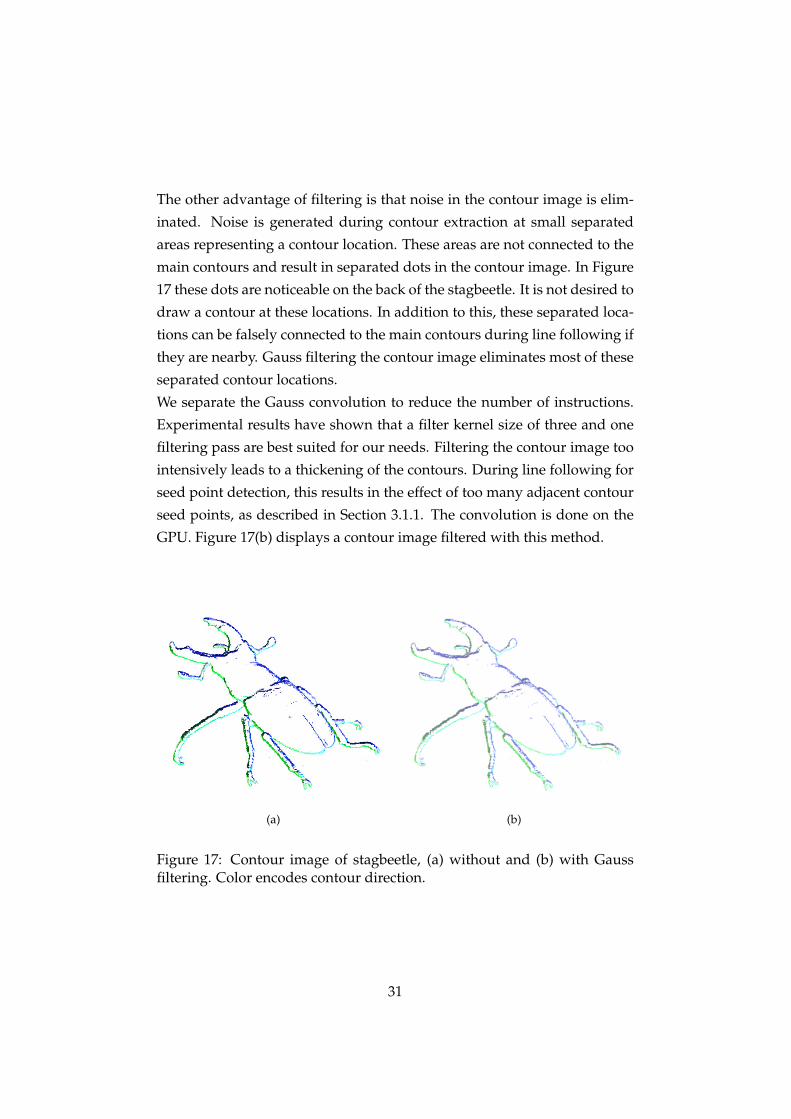
The other advantage of filtering is that noise in the contour image is elim-
inated. Noise is generated during contour extraction at small separated
areas representing a contour location. These areas are not connected to the
main contours and result in separated dots in the contour image. In Figure
17 these dots are noticeable on the back of the stagbeetle. It is not desired to
draw a contour at these locations. In addition to this, these separated loca-
tions can be falsely connected to the main contours during line following if
they are nearby. Gauss filtering the contour image eliminates most of these
separated contour locations.
We separate the Gauss convolution to reduce the number of instructions.
Experimental results have shown that a filter kernel size of three and one
filtering pass are best suited for our needs. Filtering the contour image too
intensively leads to a thickening of the contours. During line following for
seed point detection, this results in the effect of too many adjacent contour
seed points, as described in Section 3.1.1. The convolution is done on the
GPU. Figure 17(b) displays a contour image filtered with this method.
(a) (b)
Figure 17: Contour image of stagbeetle, (a) without and (b) with Gaussfiltering. Color encodes contour direction.
31
3.1.3 Seed Point Detection
In order to detect seed points on the contours in a partially sequential or-
der, we employ a recursive line-following algorithm. It starts with finding
initial points which serve as start points for following the lines. We need
multiple start locations for sampling all silhouette lines which are possibly
unconnected. The start points are detected using horizontal and vertical
equidistant scanlines. These scanlines are traversed in left-to-right respec-
tively bottom-to-top order, checking if the corresponding contour values
exceed a dedicated threshold. If a contour location is detected, a start point
is generated and a small number of successive pixels on the scanline is
skipped in order to avoid setting multiple start points at nearly the same
contour position.
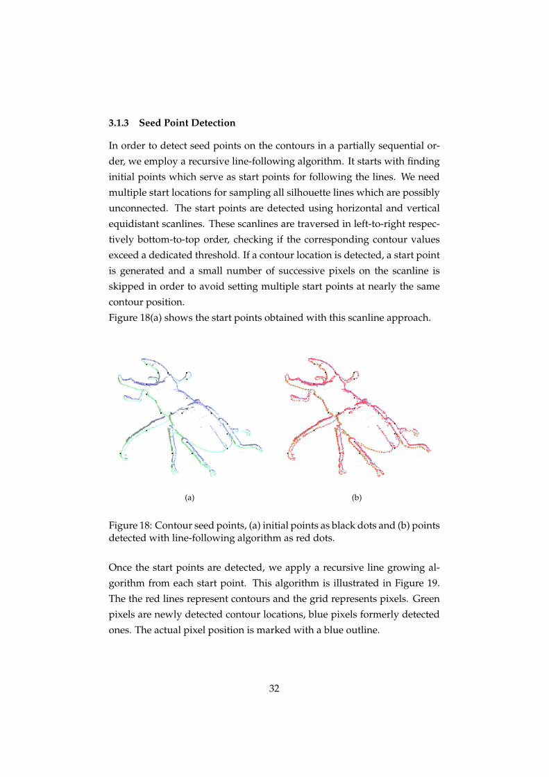
Figure 18(a) shows the start points obtained with this scanline approach.
(a) (b)
Figure 18: Contour seed points, (a) initial points as black dots and (b) pointsdetected with line-following algorithm as red dots.
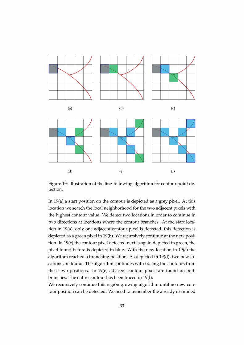
Once the start points are detected, we apply a recursive line growing al-
gorithm from each start point. This algorithm is illustrated in Figure 19.
The the red lines represent contours and the grid represents pixels. Green
pixels are newly detected contour locations, blue pixels formerly detected
ones. The actual pixel position is marked with a blue outline.
32
(a) (b) (c)
(d) (e) (f)
Figure 19: Illustration of the line-following algorithm for contour point de-tection.
In 19(a) a start position on the contour is depicted as a grey pixel. At this
location we search the local neighborhood for the two adjacent pixels with
the highest contour value. We detect two locations in order to continue in
two directions at locations where the contour branches. At the start loca-
tion in 19(a), only one adjacent contour pixel is detected, this detection is
depicted as a green pixel in 19(b). We recursively continue at the new posi-
tion. In 19(c) the contour pixel detected next is again depicted in green, the
pixel found before is depicted in blue. With the new location in 19(c) the
algorithm reached a branching position. As depicted in 19(d), two new lo-
cations are found. The algorithm continues with tracing the contours from
these two positions. In 19(e) adjacent contour pixels are found on both
branches. The entire contour has been traced in 19(f).
We recursively continue this region growing algorithm until no new con-
tour position can be detected. We need to remember the already examined
33
locations in order to proceed along the contour lines and to provide a stop-
ping condition for the recursion. The examined locations are marked with
the help of a boolean field.
When the recursion stops contour points are seeded in fixed intervals dur-
ing backtracking. This mechanism yields points on the contour in equal
distances. These contour seed points are stored in an array. In Figure 18(b)
the contour points obtained with the described algorithm are shown as red
dots. The black dots are the start points obtained with the scanline ap-
proach. Contour points traced from the same start point are gained in se-
quential order. This partially-sequential organization of points eases the
selection of control points appropriate for a spline representation.
3.1.4 Stroke Generation
We now discuss how control points for splines used for drawing silhouette
strokes are selected from the set of partially-sequential contour points. As
mentioned previously, strokes in the contour drawing should overlap. The
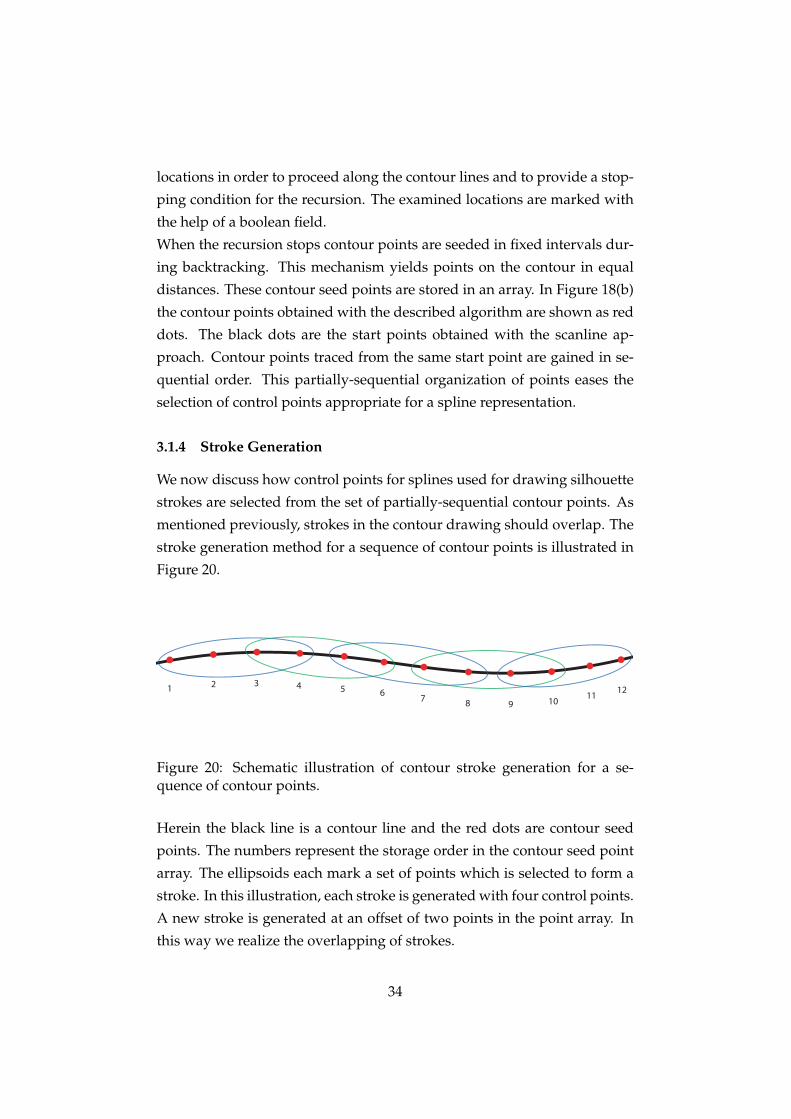
stroke generation method for a sequence of contour points is illustrated in
Figure 20.
1 2 3 4 5 67 8 9 10
1112
Figure 20: Schematic illustration of contour stroke generation for a se-quence of contour points.
Herein the black line is a contour line and the red dots are contour seed
points. The numbers represent the storage order in the contour seed point
array. The ellipsoids each mark a set of points which is selected to form a
stroke. In this illustration, each stroke is generated with four control points.
A new stroke is generated at an offset of two points in the point array. In
this way we realize the overlapping of strokes.
34
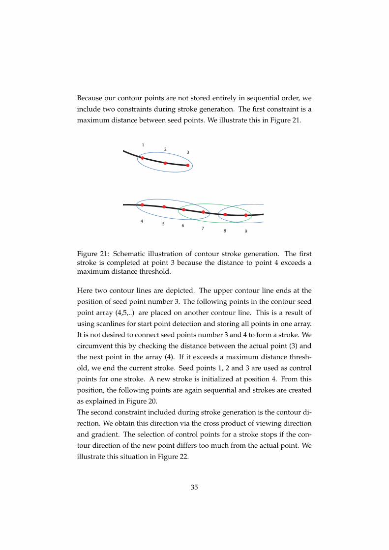
Because our contour points are not stored entirely in sequential order, we
include two constraints during stroke generation. The first constraint is a
maximum distance between seed points. We illustrate this in Figure 21.
12
3
45 6
7 8 9
Figure 21: Schematic illustration of contour stroke generation. The firststroke is completed at point 3 because the distance to point 4 exceeds amaximum distance threshold.
Here two contour lines are depicted. The upper contour line ends at the
position of seed point number 3. The following points in the contour seed
point array (4,5,..) are placed on another contour line. This is a result of
using scanlines for start point detection and storing all points in one array.
It is not desired to connect seed points number 3 and 4 to form a stroke. We
circumvent this by checking the distance between the actual point (3) and
the next point in the array (4). If it exceeds a maximum distance thresh-
old, we end the current stroke. Seed points 1, 2 and 3 are used as control
points for one stroke. A new stroke is initialized at position 4. From this
position, the following points are again sequential and strokes are created
as explained in Figure 20.
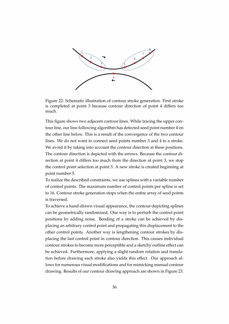
The second constraint included during stroke generation is the contour di-
rection. We obtain this direction via the cross product of viewing direction
and gradient. The selection of control points for a stroke stops if the con-
tour direction of the new point differs too much from the actual point. We
illustrate this situation in Figure 22.
35
1
2
4
5
6
7
8
3
Figure 22: Schematic illustration of contour stroke generation. First strokeis completed at point 3 because contour direction of point 4 differs toomuch.
This figure shows two adjacent contour lines. While tracing the upper con-
tour line, our line-following algorithm has detected seed point number 4 on
the other line below. This is a result of the convergence of the two contour
lines. We do not want to connect seed points number 3 and 4 to a stroke.
We avoid it by taking into account the contour direction at these positions.
The contour direction is depicted with the arrows. Because the contour di-
rection at point 4 differs too much from the direction at point 3, we stop
the control point selection at point 3. A new stroke is created beginning at
point number 5.
To realize the described constraints, we use splines with a variable number
of control points. The maximum number of control points per spline is set
to 16. Contour stroke generation stops when the entire array of seed points
is traversed.
To achieve a hand-drawn visual appearance, the contour-depicting splines
can be geometrically randomized. One way is to perturb the control point
positions by adding noise. Bending of a stroke can be achieved by dis-
placing an arbitrary control point and propagating this displacement to the
other control points. Another way is lengthening contour strokes by dis-
placing the last control point in contour direction. This causes individual
contour strokes to become more perceptible and a sketchy outline effect can
be achieved. Furthermore, applying a slight random rotation and transla-
tion before drawing each stroke also yields this effect. Our approach al-
lows for numerous visual modifications and for mimicking manual contour
drawing. Results of our contour drawing approach are shown in Figure 23.
36
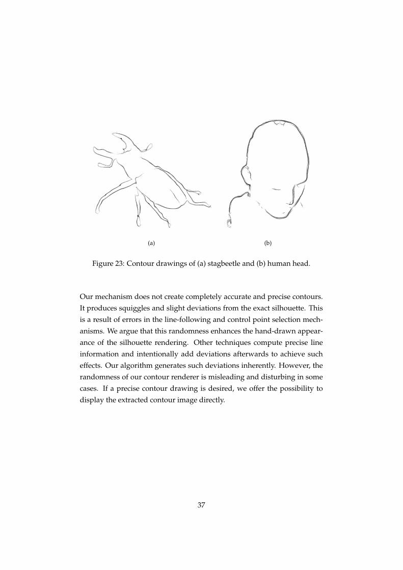
(a) (b)
Figure 23: Contour drawings of (a) stagbeetle and (b) human head.
Our mechanism does not create completely accurate and precise contours.
It produces squiggles and slight deviations from the exact silhouette. This
is a result of errors in the line-following and control point selection mech-
anisms. We argue that this randomness enhances the hand-drawn appear-
ance of the silhouette rendering. Other techniques compute precise line
information and intentionally add deviations afterwards to achieve such
effects. Our algorithm generates such deviations inherently. However, the
randomness of our contour renderer is misleading and disturbing in some
cases. If a precise contour drawing is desired, we offer the possibility to
display the extracted contour image directly.
37
3.2 Stroke Rendering
In this section we will discuss our method for drawing strokes as textured
splines. We employ this method for both contour and hatching strokes to
achieve the same visual representation for these basic image elements. In
comparison to drawing line primitives, as many stroke-based rendering ap-
proaches do, it allows for a stylized rendition of the strokes. In order to en-
able drawing smooth strokes of arbitrary shape we choose splines as a ba-
sis for our stroke rendering technique. Each stroke is drawn along a spline
defined by a number of control points. Following brush-based drawing,
which is commonly used in drawing applications, we blend multiple over-
lapping quads bearing a brush texture along a curve. Using this method we
can easily change the drawing style for simulating various artistic drawing
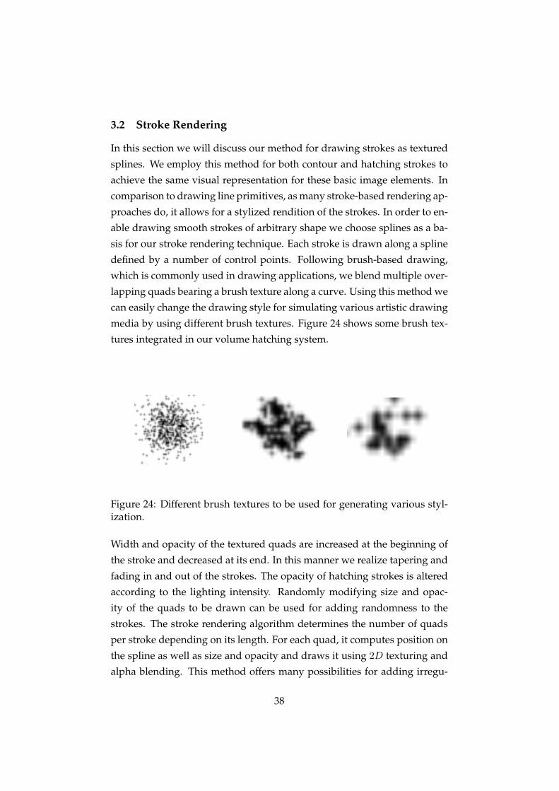
media by using different brush textures. Figure 24 shows some brush tex-
tures integrated in our volume hatching system.
Figure 24: Different brush textures to be used for generating various styl-ization.
Width and opacity of the textured quads are increased at the beginning of
the stroke and decreased at its end. In this manner we realize tapering and
fading in and out of the strokes. The opacity of hatching strokes is altered
according to the lighting intensity. Randomly modifying size and opac-
ity of the quads to be drawn can be used for adding randomness to the
strokes. The stroke rendering algorithm determines the number of quads
per stroke depending on its length. For each quad, it computes position on
the spline as well as size and opacity and draws it using 2D texturing and
alpha blending. This method offers many possibilities for adding irregu-
38
larities and for individualizing strokes. These possibilities are not given if
only one texture is used for the entire stroke. In Section 3.1.4 it is described
how strokes can be geometrically randomized. Furthermore, drawing each
stroke individually implies higher irregularities than texture-based hatch-
ing approaches. This leads to a less artificial and computer-generated vi-
sual impression.
In order to limit computational cost, we use simple Bezier splines. These
curves can easily be computed with the algorithm of De Casteljau. The
fact that Bezier curves are approximating, not interpolating splines is not
of crucial importance due to the fact that we define rather short splines
with a high number of control points. The curves are almost interpolating.
Although our approach involves drawing a high amount of geometry for
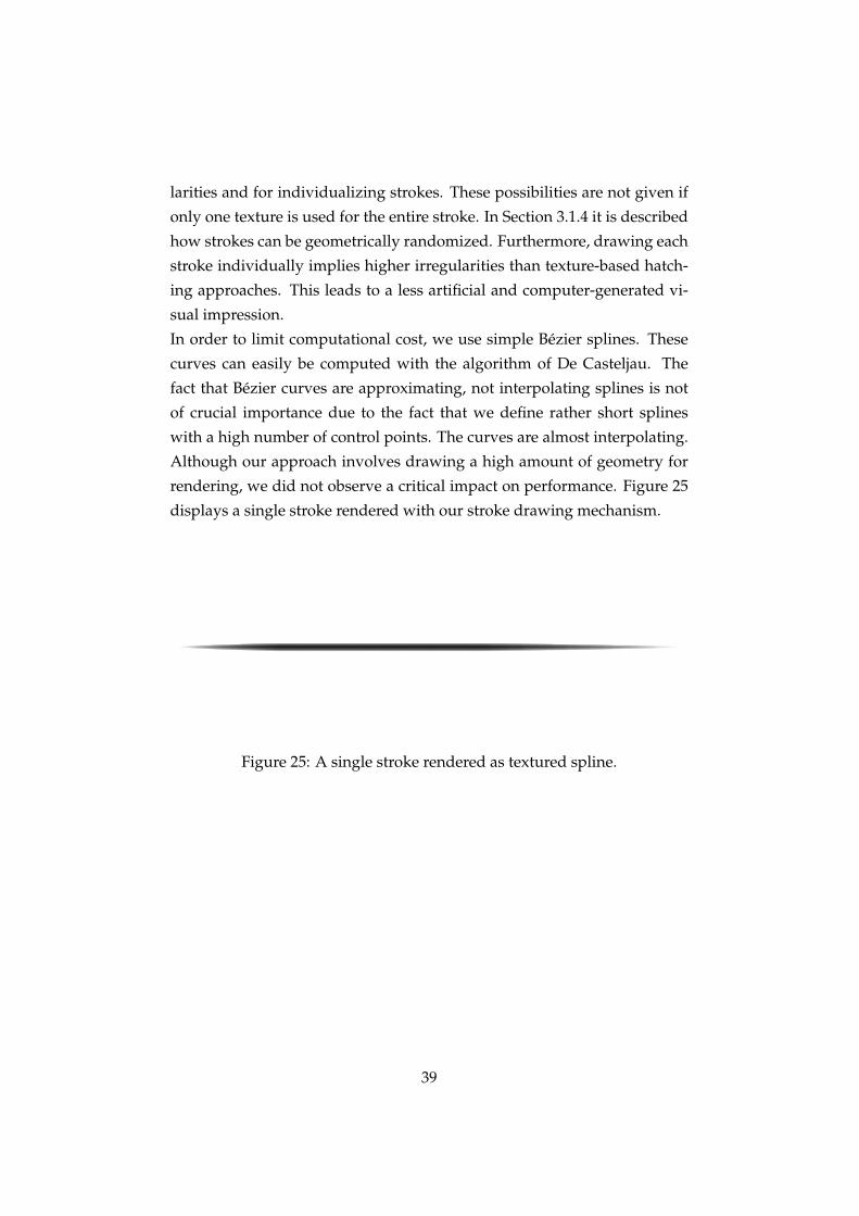
rendering, we did not observe a critical impact on performance. Figure 25
displays a single stroke rendered with our stroke drawing mechanism.
Figure 25: A single stroke rendered as textured spline.
39
3.3 Curvature Estimation
We approximate curvature information to align hatching strokes to the sur-
face of the rendered object. This is advantageous for displaying spatial
properties of the dataset. We use the method of Kindlmann et al. [23] to
estimate curvature information (see Section 2.4). We use the following ex-
pressions:
1. n = −g/|g|, where g is the gradient.
2. P = I − nnT , where I is the identity matrix.
3. G = −PHP/|g|, where H is the Hessian matrix.
4. T = trace(G), F = frobeniusnorm(G)
5. κ1 = T+√
2F 2−T 2
2 , κ2 = T−√
2F 2−T 2
2
Therein κ1 is the principal, κ2 the secondary curvature magnitude. Prin-
cipal curvature direction and magnitude of a sample on an iso-surface are
computed in the fragment shader and stored in a 2D texture. We obtain the
Hessian matrix by determining central differences of pre-computed gradi-
ent vector components. Curvature magnitude values are represented as
eigenvalues of G. Determining the curvature directions requires comput-
ing the eigenvectors corresponding to κ1 and κ2. This requires solving a
linear equation system. We employ Gauss-Seidel iteration, which is also
suitable for fragment shader implementation. We use four iterations to ap-
proximate the solution of the equation system.
After rendering curvature information to dedicated textures, we smooth
this data by performing a Gauss filtering. We use a convolution kernel
weighted with the curvature magnitude to implement a filtering sensitive
to the degree of curvature. In analogy to the filtering of contour informa-
tion (see Section 3.1.2), we use a separated filter. We apply multiple Gauss
filtering passes in order to smooth curvature directions in a way that they
are suitable for obtaining smooth hatching strokes. If the curvature direc-
40
tion is not smoothed properly, curvature irregularities result in discontin-
uous strokes and the variation between hatching stroke directions is too
large. Furthermore the filtering operation is necessary to avoid hatching
too many details of the depicted object. We observed that the computation
of the second-order derivative information does not critically decrease the
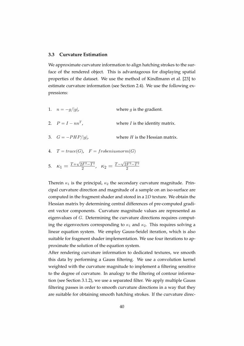
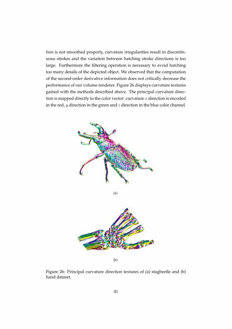
performance of our volume renderer. Figure 26 displays curvature textures
gained with the methods described above. The principal curvature direc-
tion is mapped directly to the color vector: curvature x direction is encoded
in the red, y direction in the green and z direction in the blue color channel.
(a)
(b)
Figure 26: Principal curvature direction textures of (a) stagbeetle and (b)hand dataset.
41
3.4 Volume Hatching Experiments
In the following we will outline earlier strategies we tried for generat-
ing hatching images from volumes. The first experiment used a three-
dimensional lighting transfer function to create strokes. The second ex-
perimental approach was concerned with applying a hatching technique
for polygonal data to volume rendering. Then we decided to follow a 2+D
approach based on rendering each hatching stroke individually and tested
a quadtree-based stroke placement before settling on our streamline-based
approach.
3.4.1 Hatching using a Lighting Transfer Function
Bruckner and Groller [2] use a two-dimensional lighting transfer function
in VolumeShop to realize various lighting models, silhouette enhancement
and to emphasize intersections of different objects. One experimental ap-
proach for volume hatching basically extends this two-dimensional light-
ing transfer function into the third dimension. The third dimension is ac-
cessed according to curvature magnitude. Black slices in this transfer func-
tion serve to render pixels of equal curvature magnitude in black. In this
manner we produced black curvature-aligned strokes within the volume
rendering. The problem with this approach is that it is only applicable for
synthetic datasets with very smooth surfaces. Curvature irregularities in
real-world datasets rather result in irregular sets of dots instead of strokes.
We therefore decided to try other methods for realizing volume hatching.
However, we got a stippling renderer as a byproduct of this experiment.
We generated a three-dimensional lighting transfer function which con-
tains dots instead of black slices. The density of dots was set appropriately
to cover areas of high curvature and low lighting intensity with denser stip-
ples. Figure 27 shows a result image of this method.
42
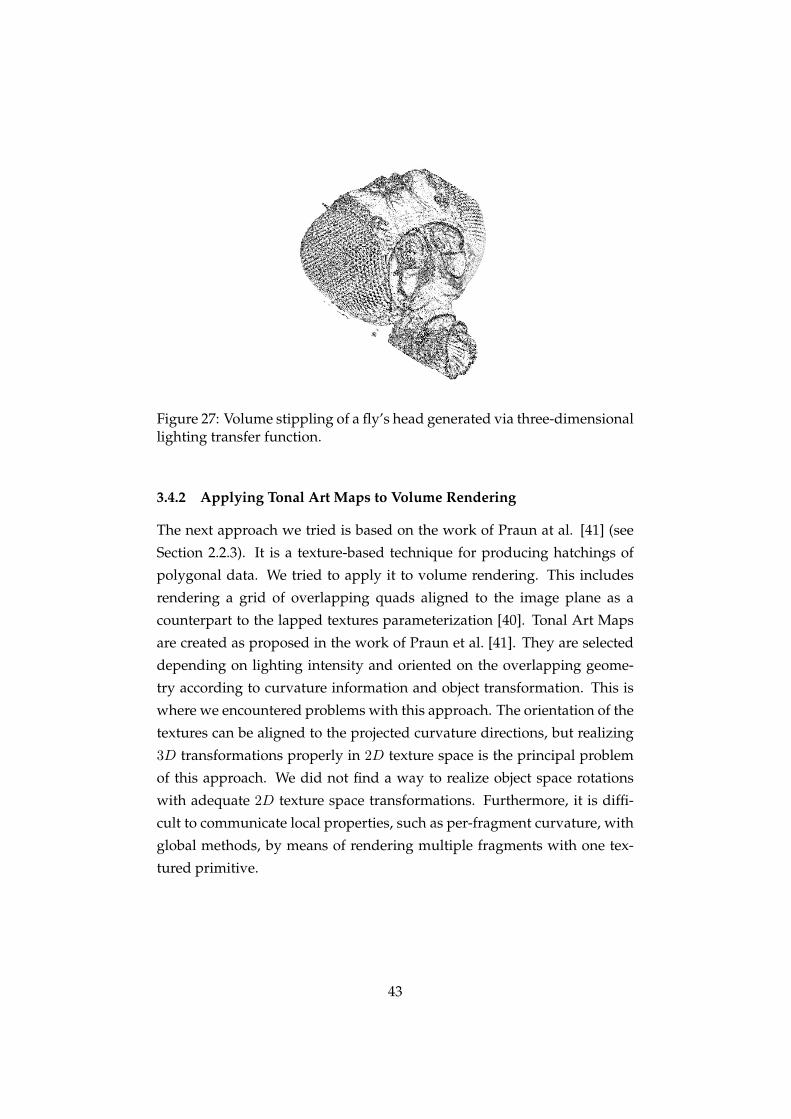
Figure 27: Volume stippling of a fly’s head generated via three-dimensionallighting transfer function.
3.4.2 Applying Tonal Art Maps to Volume Rendering
The next approach we tried is based on the work of Praun at al. [41] (see
Section 2.2.3). It is a texture-based technique for producing hatchings of
polygonal data. We tried to apply it to volume rendering. This includes
rendering a grid of overlapping quads aligned to the image plane as a
counterpart to the lapped textures parameterization [40]. Tonal Art Maps
are created as proposed in the work of Praun et al. [41]. They are selected
depending on lighting intensity and oriented on the overlapping geome-
try according to curvature information and object transformation. This is
where we encountered problems with this approach. The orientation of the
textures can be aligned to the projected curvature directions, but realizing
3D transformations properly in 2D texture space is the principal problem
of this approach. We did not find a way to realize object space rotations
with adequate 2D texture space transformations. Furthermore, it is diffi-
cult to communicate local properties, such as per-fragment curvature, with
global methods, by means of rendering multiple fragments with one tex-
tured primitive.
43
3.4.3 Quadtree-Based Stroke Seeding
Due to the problems we met with the texture-based approach mentioned
in Section 3.4.2, we tried a mechanism which allows for better taking into
account local properties. We generated each hatching stroke individually
instead of using textures containing multiple strokes. We had lighting in-
tensity and curvature direction information ready for placing and orienting
hatching strokes. The difficulty was to find an appropriate seeding strategy
for placing the strokes. They have to be somehow evenly distributed and
placed according to the brightness.
The first mechanism we explored uses a quadtree constructed dependent
on the lighting intensity. Stroke seed points are placed within the quadtree
nodes while the corresponding lighting intensity and size of the node de-
fines the amount of strokes contained. We generate stroke seeds according
to a pseudo-random distribution to achieve inter-frame coherence.
The limitation of this approach is that it is capable of generating equally
distributed stroke seed points according to the lighting intensity, but does
not ensure that the strokes are evenly spaced. As we just seed points, which
are used as stroke start positions, and not strokes themselves, this approach
does not provide strokes which are equidistant along their entire length.
44
3.5 Streamline-Based Volume Hatching
Searching for a method for placing equidistant, curvature-aligned strokes
in image space, we applied Jobard and Lefer’s technique [22] for creating
evenly-spaced streamlines. It is a 2D flow visualization method and cre-
ates equidistant lines following the directions specified by a 2D vector field
(see Section 2.5). In this section we first present how we adopt Jobard and
Lefer’s algorithm for our problem. Afterwards, we discuss a technique to
extract strokes from a set of streamlines. We draw the strokes as textured
splines. Then we explain how we use multiple streamline sets to create
hatching layers representing regions of different lighting intensities.
3.5.1 Creating Evenly-Spaced Streamlines
As noted before, we compute curvature directions in object space. In or-
der to use these direction vectors as input for the streamline generation, we
project them onto the image plane by applying the viewing transformation.
This is done each time the algorithm reads out a direction vector, because
we encountered computation errors when projecting the curvature direc-
tion in the fragment shader and storing the projected vectors in the curva-
ture texture.
In some cases and configurations, the generation of new streamlines from a
single initial one is not sufficient to fill arbitrary shapes with streamlines. It
may occur that the algorithm leaves regions uncovered when starting from
only one position, depending on the shape of the rendered object. This
originates from the fact that the method was developed for a continuous
vector field. We use multiple start candidate positions arranged in a regu-
lar grid in order to cover the whole object with streamlines.
The streamline placement algorithm of Jobard and Lefer allows to define
the distance between streamlines. With creating multiple streamline sets
of different streamline distances we obtain the basis for generating hatch-
ing layers of different densities. Figure 28 shows streamlines following the
principal curvature directions of volume datasets.
45
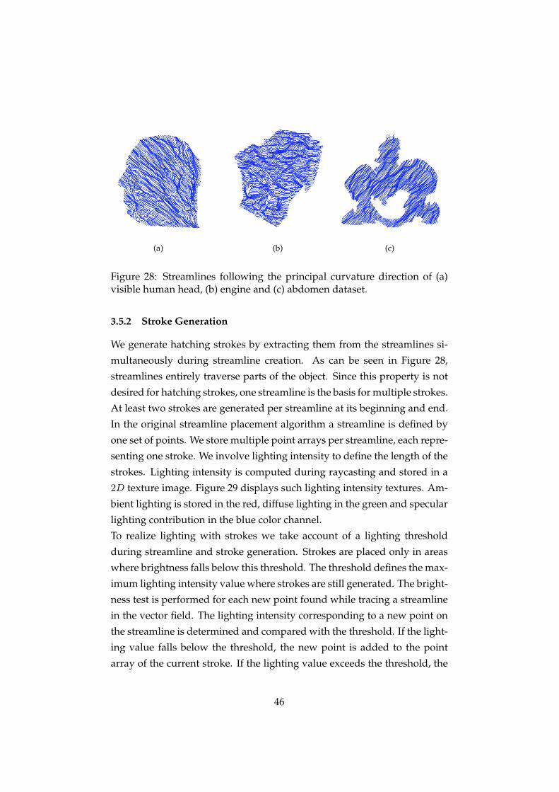
(a) (b) (c)
Figure 28: Streamlines following the principal curvature direction of (a)visible human head, (b) engine and (c) abdomen dataset.
3.5.2 Stroke Generation
We generate hatching strokes by extracting them from the streamlines si-
multaneously during streamline creation. As can be seen in Figure 28,
streamlines entirely traverse parts of the object. Since this property is not
desired for hatching strokes, one streamline is the basis for multiple strokes.
At least two strokes are generated per streamline at its beginning and end.
In the original streamline placement algorithm a streamline is defined by
one set of points. We store multiple point arrays per streamline, each repre-
senting one stroke. We involve lighting intensity to define the length of the
strokes. Lighting intensity is computed during raycasting and stored in a
2D texture image. Figure 29 displays such lighting intensity textures. Am-
bient lighting is stored in the red, diffuse lighting in the green and specular
lighting contribution in the blue color channel.
To realize lighting with strokes we take account of a lighting threshold
during streamline and stroke generation. Strokes are placed only in areas
where brightness falls below this threshold. The threshold defines the max-
imum lighting intensity value where strokes are still generated. The bright-
ness test is performed for each new point found while tracing a streamline
in the vector field. The lighting intensity corresponding to a new point on
the streamline is determined and compared with the threshold. If the light-
ing value falls below the threshold, the new point is added to the point
array of the current stroke. If the lighting value exceeds the threshold, the
46
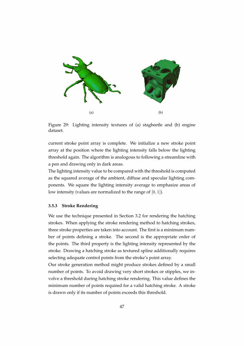
(a) (b)
Figure 29: Lighting intensity textures of (a) stagbeetle and (b) enginedataset.
current stroke point array is complete. We initialize a new stroke point
array at the position where the lighting intensity falls below the lighting
threshold again. The algorithm is analogous to following a streamline with
a pen and drawing only in dark areas.
The lighting intensity value to be compared with the threshold is computed
as the squared average of the ambient, diffuse and specular lighting com-
ponents. We square the lighting intensity average to emphasize areas of
low intensity (values are normalized to the range of [0, 1]).
3.5.3 Stroke Rendering
We use the technique presented in Section 3.2 for rendering the hatching
strokes. When applying the stroke rendering method to hatching strokes,
three stroke properties are taken into account. The first is a minimum num-
ber of points defining a stroke. The second is the appropriate order of
the points. The third property is the lighting intensity represented by the
stroke. Drawing a hatching stroke as textured spline additionally requires
selecting adequate control points from the stroke’s point array.
Our stroke generation method might produce strokes defined by a small
number of points. To avoid drawing very short strokes or stipples, we in-
volve a threshold during hatching stroke rendering. This value defines the
minimum number of points required for a valid hatching stroke. A stroke
is drawn only if its number of points exceeds this threshold.
47
As the generation of a streamline starts at an arbitrary point on the line and
integrates the vector field in two opposite directions, the order of points in
the streamline stroke’s array does not necessarily match the required stroke
drawing direction. We have to ensure that the streamline stroke points are
processed in the proper order. Therefore we include the constraint that all
hatching strokes have to be drawn from dark to bright areas. To achieve
this, we read out the lighting intensities corresponding to the first and the
last point of a stroke’s point array. If the lighting intensity at the first point
is above that of the last point, we invert the processing order of the point
array for control point extraction.
In addition to determining the length of strokes according to the tone, we
involve lighting during stroke rendering. We want to achieve the effect
of applying more color in darker areas. We therefore pass the lighting in-
tensity values at the beginning and end of a stroke to the stroke rendering
routine. We adjust the alpha values of the brush-textured quads according
to the corresponding brightness. As we draw a relatively high amount of
quads we can achieve smooth tone transitions within a stroke.
We have to make a selection of control points from the stroke’s point ar-
ray for a spline representation. This is realized by picking points as control
points in fixed intervals. The variation in the length of strokes does not
raise a problem, since our stroke rendering algorithm is capable of process-
ing splines with a different number of control points. Selecting a subset
of the streamline points as control points results in smoothing curvature
irregularities and discontinuities. This smoothing operation is advanta-
geous for producing visually pleasant strokes. We also experimented with
drawing strokes along the streamlines directly using the streamline points.
Due to curvature irregularities and discontinuities inherent in most vol-
ume datasets this yields noisy strokes. Smoothing the streamline strokes
by drawing them along Bezier curves achieves better results.
48
3.5.4 Hatching Layers
With the methods described in the previous sections we are able to render a
hatching drawing for one level of brightness. The application of a lighting
threshold during stroke generation from streamlines yields strokes in areas
with a lighting intensity below the threshold. For producing pen-and-ink
style illustrations rendering one level of tone is sufficient. Hatching strokes
in a pen-and-ink illustration usually represent just one level of brightness.
Shading with different tones and a transition between darker and brighter
regions within the shading is usually not desired. Renderings in the style
of pen-and-ink illustrations can be generated with our system using just
one hatching layer. Since we focus on mimicking pencil hatching images,
we want our volume hatching system to be capable of rendering transi-
tions between areas of different lighting intensity. In order to achieve this
we use four layers of hatching strokes. Each layer represents one level of
lighting intensity or tone. In dark areas we draw short strokes of high den-
sity, brighter areas are rendered with longer strokes of lower density. Each
hatching layer is computed in a separate rendering pass. The four layers
are overlaid to produce the final hatching image.
We control the length of the strokes for each layer using the lighting thresh-
old for stroke extraction from the streamlines. This allows for adjusting the
length of the hatching strokes to the level of tone the layer represents. We
use a low lighting threshold for the darkest level and a higher threshold
value for the brightest level. These two values are linearly interpolated
for the two levels in between. By modifying the lighting thresholds the
brightness and contrast of the hatching drawing can be controlled. The
distance between the two thresholds defines the degree of lighting varia-
tion between the four hatching layers.
To control the hatching stroke density the separating distance between the
streamlines is altered. We control the brightness of each level through
stroke density. Darker areas contain more hatching strokes than brighter
ones. Creating streamlines with a small separating distance yields strokes
of high density. The definition of a separating distance for each hatching
layer is done analogous to the definition of lighting thresholds: we define a
low value for the darkest level and a higher value for the brightest level. We
49
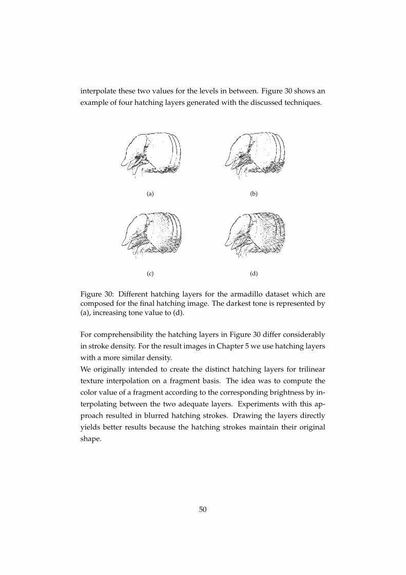
interpolate these two values for the levels in between. Figure 30 shows an
example of four hatching layers generated with the discussed techniques.
(a) (b)
(c) (d)
Figure 30: Different hatching layers for the armadillo dataset which arecomposed for the final hatching image. The darkest tone is represented by(a), increasing tone value to (d).
For comprehensibility the hatching layers in Figure 30 differ considerably
in stroke density. For the result images in Chapter 5 we use hatching layers
with a more similar density.
We originally intended to create the distinct hatching layers for trilinear
texture interpolation on a fragment basis. The idea was to compute the
color value of a fragment according to the corresponding brightness by in-
terpolating between the two adequate layers. Experiments with this ap-
proach resulted in blurred hatching strokes. Drawing the layers directly
yields better results because the hatching strokes maintain their original
shape.
50
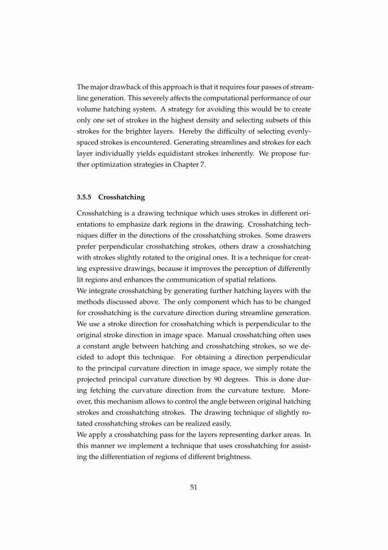
The major drawback of this approach is that it requires four passes of stream-
line generation. This severely affects the computational performance of our
volume hatching system. A strategy for avoiding this would be to create
only one set of strokes in the highest density and selecting subsets of this
strokes for the brighter layers. Hereby the difficulty of selecting evenly-
spaced strokes is encountered. Generating streamlines and strokes for each
layer individually yields equidistant strokes inherently. We propose fur-
ther optimization strategies in Chapter 7.
3.5.5 Crosshatching
Crosshatching is a drawing technique which uses strokes in different ori-
entations to emphasize dark regions in the drawing. Crosshatching tech-
niques differ in the directions of the crosshatching strokes. Some drawers
prefer perpendicular crosshatching strokes, others draw a crosshatching
with strokes slightly rotated to the original ones. It is a technique for creat-
ing expressive drawings, because it improves the perception of differently
lit regions and enhances the communication of spatial relations.
We integrate crosshatching by generating further hatching layers with the
methods discussed above. The only component which has to be changed
for crosshatching is the curvature direction during streamline generation.
We use a stroke direction for crosshatching which is perpendicular to the
original stroke direction in image space. Manual crosshatching often uses
a constant angle between hatching and crosshatching strokes, so we de-
cided to adopt this technique. For obtaining a direction perpendicular
to the principal curvature direction in image space, we simply rotate the
projected principal curvature direction by 90 degrees. This is done dur-
ing fetching the curvature direction from the curvature texture. More-
over, this mechanism allows to control the angle between original hatching
strokes and crosshatching strokes. The drawing technique of slightly ro-
tated crosshatching strokes can be realized easily.
We apply a crosshatching pass for the layers representing darker areas. In
this manner we implement a technique that uses crosshatching for assist-
ing the differentiation of regions of different brightness.
51
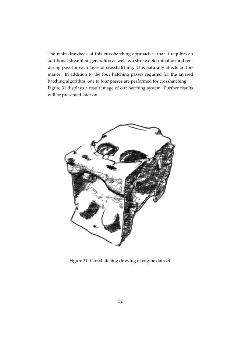
The main drawback of this crosshatching approach is that it requires an
additional streamline generation as well as a stroke determination and ren-
dering pass for each layer of crosshatching. This naturally affects perfor-
mance. In addition to the four hatching passes required for the layered
hatching algorithm, one to four passes are performed for crosshatching.
Figure 31 displays a result image of our hatching system. Further results
will be presented later on.
Figure 31: Crosshatching drawing of engine dataset.
52
3.6 Volumetric Hatching
The techniques presented in the previous sections are capable of producing
hatching drawings of iso-surfaces within volume datasets. Due to using a
raycasting system and traversing the volume just to one sample after the
first ray-object intersection, the methods described so far are related to sur-
faces. The renderings used to generate hatching strokes represent the outer
shell of the object specified by the transfer function. This thesis is con-
cerned with producing volumetric hatchings and not only hatching images
of the outer surface. Volumetric is used here to indicate a simultaneous
visual representation of overlapping or occluded structures in the volume
dataset. In this section we address the problem of volumetric hatching.
We will survey two methods which serve this purpose. First we present
an approach which is based on traversing the volume in segments. Then
we discuss a technique which involves an analysis of the transfer function
to determine relevant iso-surfaces. It generates volumetric hatchings by
blending together hatching images of these iso-surfaces.
3.6.1 Segmental Raycasting
The method we initially intended to employ for volumetric hatching tra-
verses the volume in segments. Raycasting is performed in segments or
slabs. Instead of processing all samples along a ray in one step, we involve
a fixed interval during raycasting. This interval defines the thickness of
the segments. The segmental raycasting method requires an interleaved
rendering scheme. Raycasting and hatching are performed in alternating
order for each segment. The algorithm processes n samples along the ray
and stores optical and spatial properties of the dataset computed from this
n samples in textures. Based on these textures, hatching strokes are gen-
erated representing the visible structures within the current slab. Then the
next n samples along the ray are processed and the hatching strokes for the
next slab are generated. This interleaved raycasting and stroke rendering
is continued until the entire volume is traversed.
The problem of this segmental approach is that it is not sensitive to the
spatial arrangement of objects within the dataset. It is not well suited for
displaying connected structures with hatching strokes. As the stroke gener-
53
ation is performed for each slab individually, objects are split in parts and
these parts are hatched separately. This results in visually disconnected
structures which should be drawn as a whole. Furthermore it may gen-
erate hatching strokes for unimportant parts of structures. This appears
when small parts of structures are separated in an individual slab and cov-
ered with hatching strokes. If strokes are generated for the entire surface,
this small parts of structures may not be perceivable due to the smoothing
operations applied during curvature estimation and stroke generation.
3.6.2 Relevant Iso-Surface Detection
Due to the problems of our initial approach to volumetric hatching we de-
veloped another technique to realize the simultaneous hatched display of
interior and exterior structures in volume datasets. This technique applies
our hatching methods to multiple iso-surfaces. An analysis of the transfer
function is performed to detect iso-surfaces relevant for the volumetric ren-
dering. Contour and hatching strokes are generated for each of these sur-
faces, taking into account the transparencies specified by the transfer func-
tion. The hatched surfaces are overlaid to produce the volumetric hatching
image.
The transfer function analysis is based on the fact that visible surfaces in
a volume rendering are defined by maxima of the transfer function. We
exploit this property to detect iso-surfaces which have to be rendered. The
number of maxima in the transfer function defines the number of relevant
iso-surfaces and therewith the number of hatching passes. The transfer
function is analyzed by traversing the axis which represents the scalar val-
ues and detecting the maxima and minima of the opacity values. For each
local maximum of the function we store the position of the directly pre-
ceding local minimum on the data value axis. Additionally, we store the
opacity value corresponding to the maximum. The scalar values represent-
ing the local minima in the transfer function are then used as thresholds
during raycasting. At the rendering pass of an iso-surface related to a max-
imum we take the preceding minimum as a threshold. This threshold af-
fects the transfer function readout at a resample location in the raycaster. If
the scalar value at a resample location falls below the threshold, we return
an opacity value of zero at the transfer function readout. In this way we
54
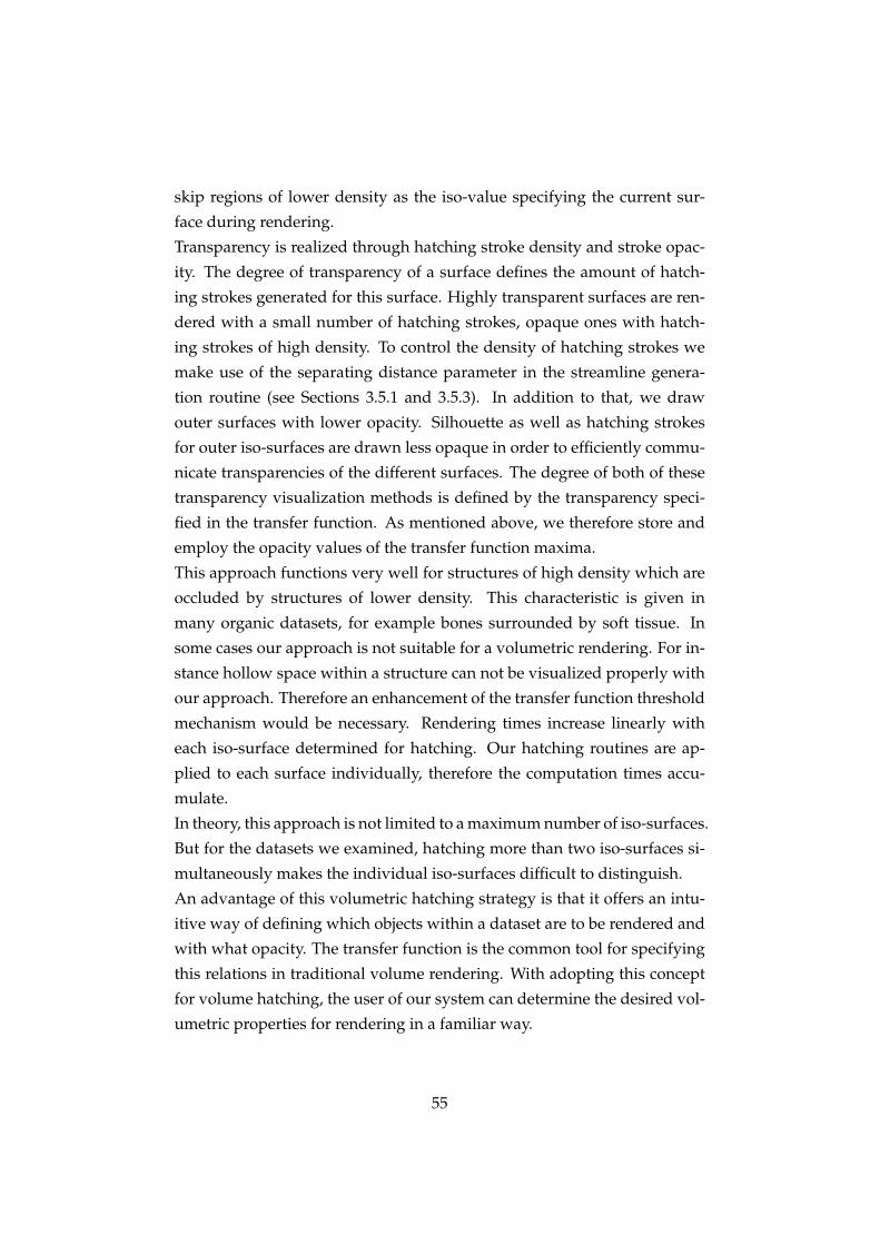
skip regions of lower density as the iso-value specifying the current sur-
face during rendering.
Transparency is realized through hatching stroke density and stroke opac-
ity. The degree of transparency of a surface defines the amount of hatch-
ing strokes generated for this surface. Highly transparent surfaces are ren-
dered with a small number of hatching strokes, opaque ones with hatch-
ing strokes of high density. To control the density of hatching strokes we
make use of the separating distance parameter in the streamline genera-
tion routine (see Sections 3.5.1 and 3.5.3). In addition to that, we draw
outer surfaces with lower opacity. Silhouette as well as hatching strokes
for outer iso-surfaces are drawn less opaque in order to efficiently commu-
nicate transparencies of the different surfaces. The degree of both of these
transparency visualization methods is defined by the transparency speci-
fied in the transfer function. As mentioned above, we therefore store and
employ the opacity values of the transfer function maxima.
This approach functions very well for structures of high density which are
occluded by structures of lower density. This characteristic is given in
many organic datasets, for example bones surrounded by soft tissue. In
some cases our approach is not suitable for a volumetric rendering. For in-
stance hollow space within a structure can not be visualized properly with
our approach. Therefore an enhancement of the transfer function threshold
mechanism would be necessary. Rendering times increase linearly with
each iso-surface determined for hatching. Our hatching routines are ap-
plied to each surface individually, therefore the computation times accu-
mulate.
In theory, this approach is not limited to a maximum number of iso-surfaces.
But for the datasets we examined, hatching more than two iso-surfaces si-
multaneously makes the individual iso-surfaces difficult to distinguish.
An advantage of this volumetric hatching strategy is that it offers an intu-
itive way of defining which objects within a dataset are to be rendered and
with what opacity. The transfer function is the common tool for specifying
this relations in traditional volume rendering. With adopting this concept
for volume hatching, the user of our system can determine the desired vol-
umetric properties for rendering in a familiar way.
55
Volumetric hatching is a technique well suited for illustration purposes
due to its abstract and sparse way of conveying spatial information within
volume datasets. Figure 32 presents a result image achieved with the de-
scribed iso-surface detection and hatching mechanism.
Figure 32: Volumetric hatching of hand dataset.
56
4 Implementation
The volume hatching system discussed in the previous chapters is imple-
mented as a plug-in to the volume illustration software VolumeShop [2]
(see Section 2.3.3). This application offers basic functionality required for
the realization of the volume hatching software. A graphical user inter-
face (GUI) as well as routines for dataset import, transfer function design
and interaction are provided by VolumeShop and can be used directly. The
software is written in C++ using OpenGL for graphics support, Qt as win-
dowing toolkit and the GL Shading Language (GLSL) as shader language.
In the following, we will outline the architecture of our volume hatching
system by describing the basic functionality of the most important classes.
RendererVolumeHatcher
The class RendererVolumeHatcher is a modification of the volume render-
ing class of VolumeShop. It holds the objects needed for contour drawing
and hatching. We will shortly present the processing order of the main
rendering loop provided by this class. First the shader programs for ray-
casting are executed and reference information on contours, lighting and
curvature are rendered to 2D textures using an OpenGL framebuffer ob-
ject. Then these textures are filtered in fragment shaders. The following
operations are executed on the CPU. We therefore copy the reference tex-
tures from graphics memory to main memory using OpenGL texture data
reading functions. Subsequently silhouette drawing and hatching are per-
formed by calling the corresponding methods of the dedicated classes.
57
ContourDrawer
The class ContourDrawer provides functionality for drawing contours with
overlapping strokes (see Section 3.1). The algorithms for contour point de-
tection (see Section 3.1.3) and contour stroke generation (see Section 3.1.4)
are implemented as described in the related sections. These routines are
not suited for parallel execution for graphics hardware exploitation and
are therefore processed on the CPU. Contour strokes are rendered using
the class Stroker.
Hatcher
The class Hatcher serves the purpose of producing hatching strokes (see
Section 3.5). It controls the layered hatching scheme (see Section 3.5.4) by
executing the corresponding methods of the class Streamlines. This involves
the generation of streamlines following the principal curvature direction
(see Section 3.5.1) and the simultaneous extraction of hatching strokes from
the streamlines (see Section 3.5.2). Hatching strokes are subsequently ren-
dered with the class Stroker calling a method which fulfills the conditions
required therein (see Section 3.5.3).
Stroker
Stroke rendering methods are encapsulated and implemented in the class
Stroker. It provides the mechanism for drawing strokes as textured splines
(see Section 3.2). Contour and hatching strokes rendering routines are sep-
arated to provide the possibility of rendering contours and hatching in dif-
ferent styles. We employ the Developers Image Library (DevIL) [58] for
importing the brush texture images. OpenGL texture mapping is utilized
for displaying the textured quads.
58
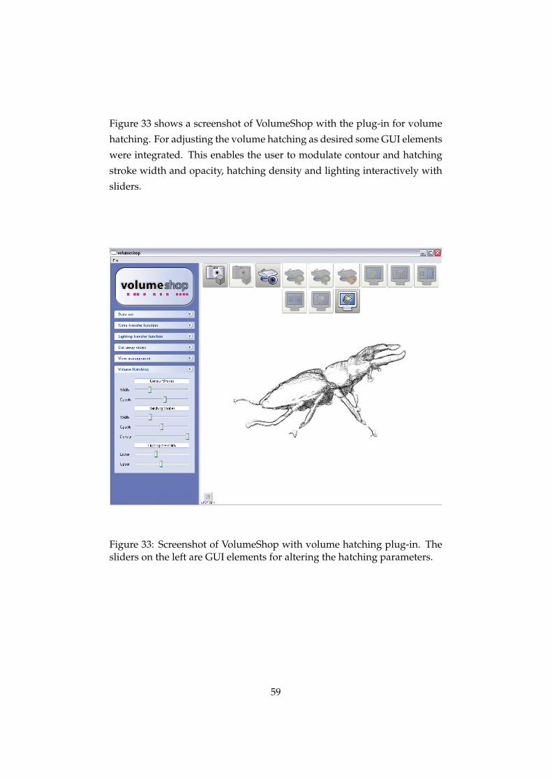
Figure 33 shows a screenshot of VolumeShop with the plug-in for volume
hatching. For adjusting the volume hatching as desired some GUI elements
were integrated. This enables the user to modulate contour and hatching
stroke width and opacity, hatching density and lighting interactively with
sliders.
Figure 33: Screenshot of VolumeShop with volume hatching plug-in. Thesliders on the left are GUI elements for altering the hatching parameters.
59
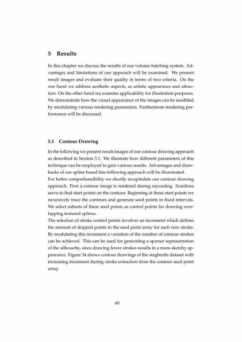
5 Results
In this chapter we discuss the results of our volume hatching system. Ad-
vantages and limitations of our approach will be examined. We present
result images and evaluate their quality in terms of two criteria. On the
one hand we address aesthetic aspects, as artistic appearance and attrac-
tion. On the other hand we examine applicability for illustration purposes.
We demonstrate how the visual appearance of the images can be modified
by modulating various rendering parameters. Furthermore rendering per-
formance will be discussed.
5.1 Contour Drawing
In the following we present result images of our contour drawing approach
as described in Section 3.1. We illustrate how different parameters of this
technique can be employed to gain various results. Advantages and draw-
backs of our spline based line-following approach will be illuminated.
For better comprehensibility we shortly recapitulate our contour drawing
approach. First a contour image is rendered during raycasting. Scanlines
serve to find start points on the contour. Beginning at these start points we
recursively trace the contours and generate seed points in fixed intervals.
We select subsets of these seed points as control points for drawing over-
lapping textured splines.
The selection of stroke control points involves an increment which defines
the amount of skipped points in the seed point array for each new stroke.
By modulating this increment a variation of the number of contour strokes
can be achieved. This can be used for generating a sparser representation
of the silhouette, since drawing fewer strokes results in a more sketchy ap-
pearance. Figure 34 shows contour drawings of the stagbeetle dataset with
increasing increment during stroke extraction from the contour seed point
array.
60
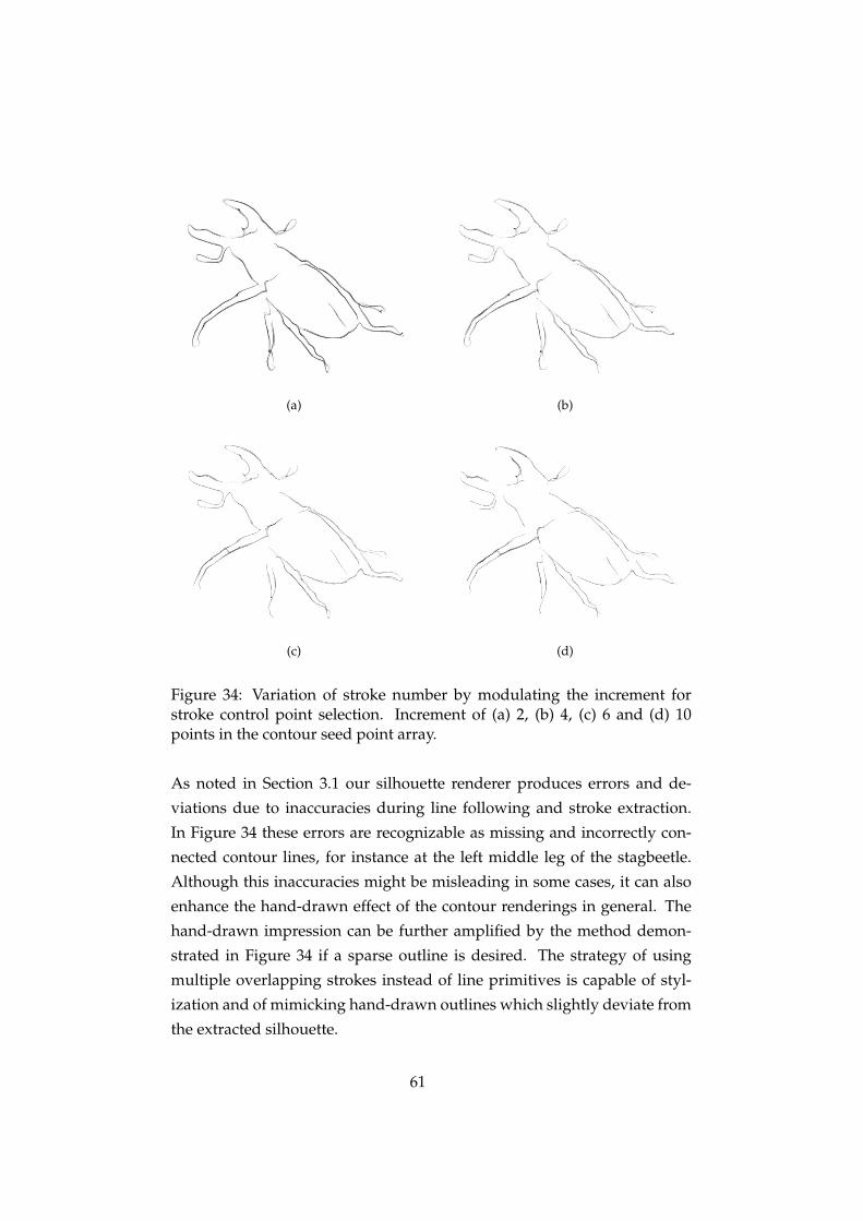
(a) (b)
(c) (d)
Figure 34: Variation of stroke number by modulating the increment forstroke control point selection. Increment of (a) 2, (b) 4, (c) 6 and (d) 10points in the contour seed point array.
As noted in Section 3.1 our silhouette renderer produces errors and de-
viations due to inaccuracies during line following and stroke extraction.
In Figure 34 these errors are recognizable as missing and incorrectly con-
nected contour lines, for instance at the left middle leg of the stagbeetle.
Although this inaccuracies might be misleading in some cases, it can also
enhance the hand-drawn effect of the contour renderings in general. The
hand-drawn impression can be further amplified by the method demon-
strated in Figure 34 if a sparse outline is desired. The strategy of using
multiple overlapping strokes instead of line primitives is capable of styl-
ization and of mimicking hand-drawn outlines which slightly deviate from
the extracted silhouette.
61
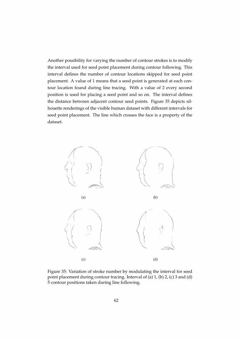
Another possibility for varying the number of contour strokes is to modify
the interval used for seed point placement during contour following. This
interval defines the number of contour locations skipped for seed point
placement. A value of 1 means that a seed point is generated at each con-
tour location found during line tracing. With a value of 2 every second
position is used for placing a seed point and so on. The interval defines
the distance between adjacent contour seed points. Figure 35 depicts sil-
houette renderings of the visible human dataset with different intervals for
seed point placement. The line which crosses the face is a property of the
dataset.
(a) (b)
(c) (d)
Figure 35: Variation of stroke number by modulating the interval for seedpoint placement during contour tracing. Interval of (a) 1, (b) 2, (c) 3 and (d)5 contour positions taken during line following.
62
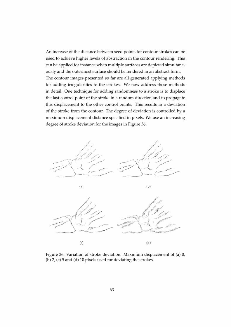
An increase of the distance between seed points for contour strokes can be
used to achieve higher levels of abstraction in the contour rendering. This
can be applied for instance when multiple surfaces are depicted simultane-
ously and the outermost surface should be rendered in an abstract form.
The contour images presented so far are all generated applying methods
for adding irregularities to the strokes. We now address these methods
in detail. One technique for adding randomness to a stroke is to displace
the last control point of the stroke in a random direction and to propagate
this displacement to the other control points. This results in a deviation
of the stroke from the contour. The degree of deviation is controlled by a
maximum displacement distance specified in pixels. We use an increasing
degree of stroke deviation for the images in Figure 36.
(a) (b)
(c) (d)
Figure 36: Variation of stroke deviation. Maximum displacement of (a) 0,(b) 2, (c) 5 and (d) 10 pixels used for deviating the strokes.
63
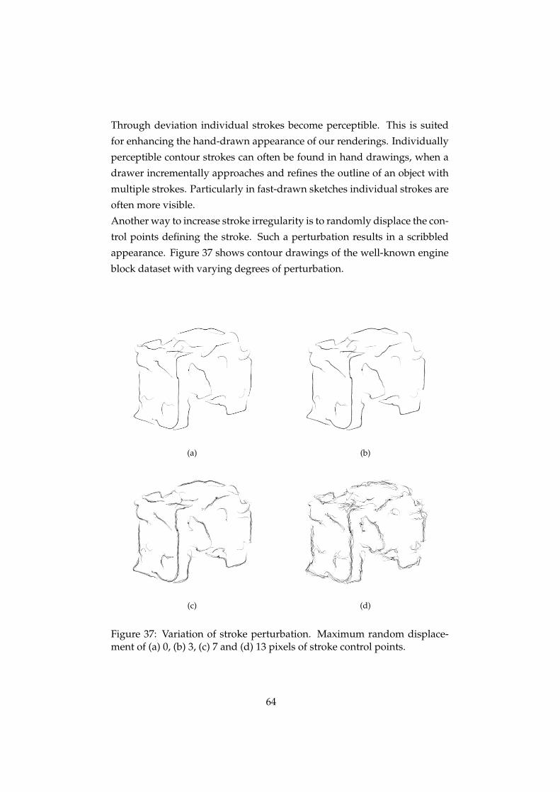
Through deviation individual strokes become perceptible. This is suited
for enhancing the hand-drawn appearance of our renderings. Individually
perceptible contour strokes can often be found in hand drawings, when a
drawer incrementally approaches and refines the outline of an object with
multiple strokes. Particularly in fast-drawn sketches individual strokes are
often more visible.
Another way to increase stroke irregularity is to randomly displace the con-
trol points defining the stroke. Such a perturbation results in a scribbled
appearance. Figure 37 shows contour drawings of the well-known engine
block dataset with varying degrees of perturbation.
(a) (b)
(c) (d)
Figure 37: Variation of stroke perturbation. Maximum random displace-ment of (a) 0, (b) 3, (c) 7 and (d) 13 pixels of stroke control points.
64
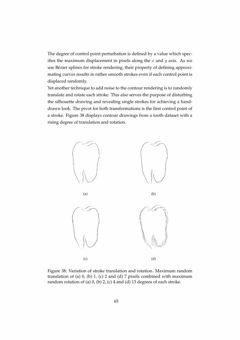
The degree of control point perturbation is defined by a value which spec-
ifies the maximum displacement in pixels along the x and y axis. As we
use Bezier splines for stroke rendering, their property of defining approxi-
mating curves results in rather smooth strokes even if each control point is
displaced randomly.
Yet another technique to add noise to the contour rendering is to randomly
translate and rotate each stroke. This also serves the purpose of disturbing
the silhouette drawing and revealing single strokes for achieving a hand-
drawn look. The pivot for both transformations is the first control point of
a stroke. Figure 38 displays contour drawings from a tooth dataset with a
rising degree of translation and rotation.
(a) (b)
(c) (d)
Figure 38: Variation of stroke translation and rotation. Maximum randomtranslation of (a) 0, (b) 1, (c) 2 and (d) 7 pixels combined with maximumrandom rotation of (a) 0, (b) 2, (c) 4 and (d) 13 degrees of each stroke.
65
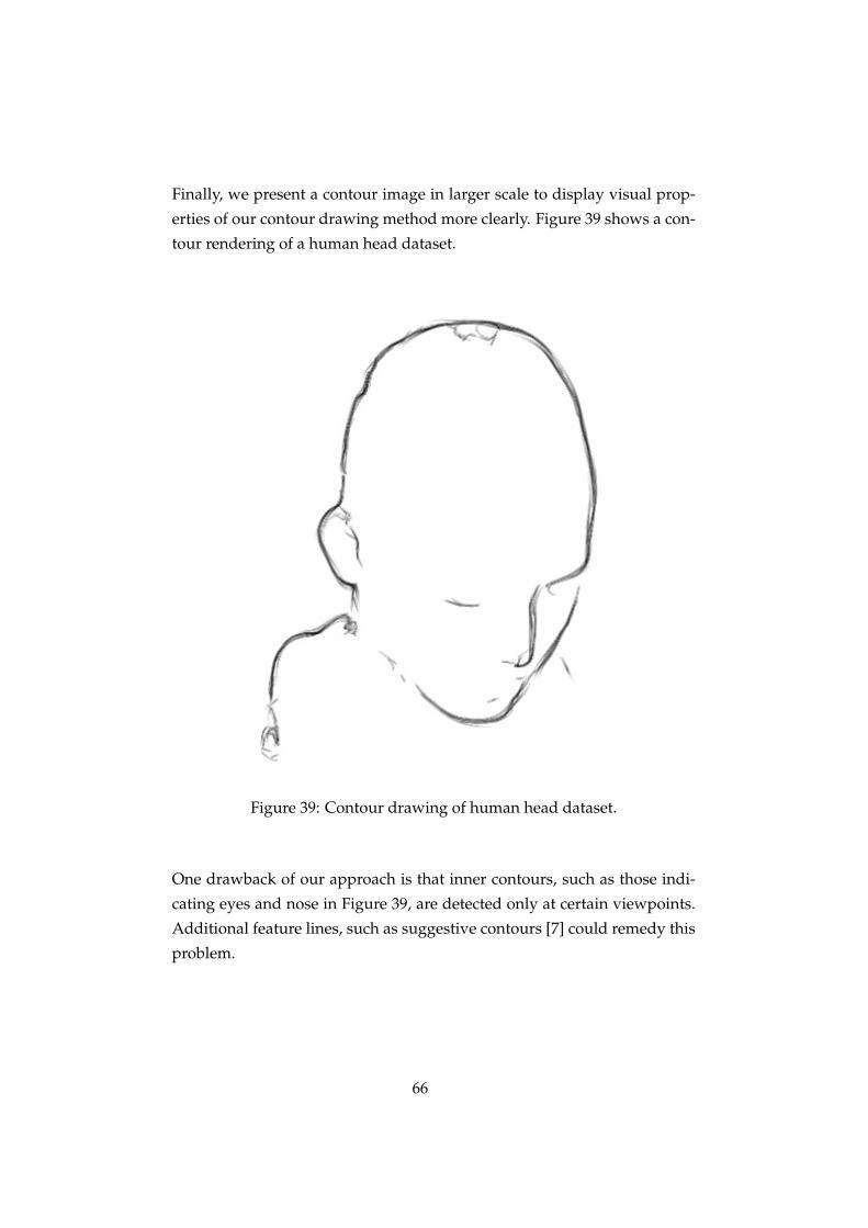
Finally, we present a contour image in larger scale to display visual prop-
erties of our contour drawing method more clearly. Figure 39 shows a con-
tour rendering of a human head dataset.
Figure 39: Contour drawing of human head dataset.
One drawback of our approach is that inner contours, such as those indi-
cating eyes and nose in Figure 39, are detected only at certain viewpoints.
Additional feature lines, such as suggestive contours [7] could remedy this
problem.
66
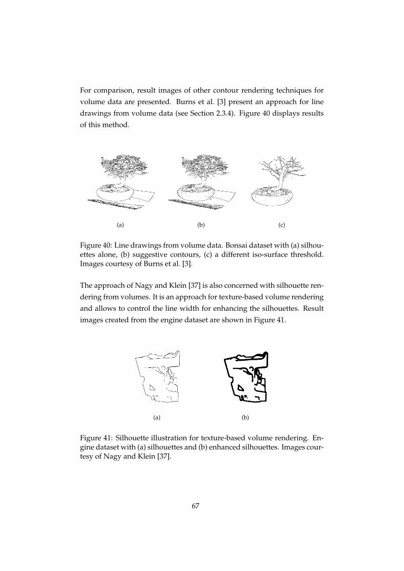
For comparison, result images of other contour rendering techniques for
volume data are presented. Burns et al. [3] present an approach for line
drawings from volume data (see Section 2.3.4). Figure 40 displays results
of this method.
(a) (b) (c)
Figure 40: Line drawings from volume data. Bonsai dataset with (a) silhou-ettes alone, (b) suggestive contours, (c) a different iso-surface threshold.Images courtesy of Burns et al. [3].
The approach of Nagy and Klein [37] is also concerned with silhouette ren-
dering from volumes. It is an approach for texture-based volume rendering
and allows to control the line width for enhancing the silhouettes. Result
images created from the engine dataset are shown in Figure 41.
(a) (b)
Figure 41: Silhouette illustration for texture-based volume rendering. En-gine dataset with (a) silhouettes and (b) enhanced silhouettes. Images cour-tesy of Nagy and Klein [37].
67
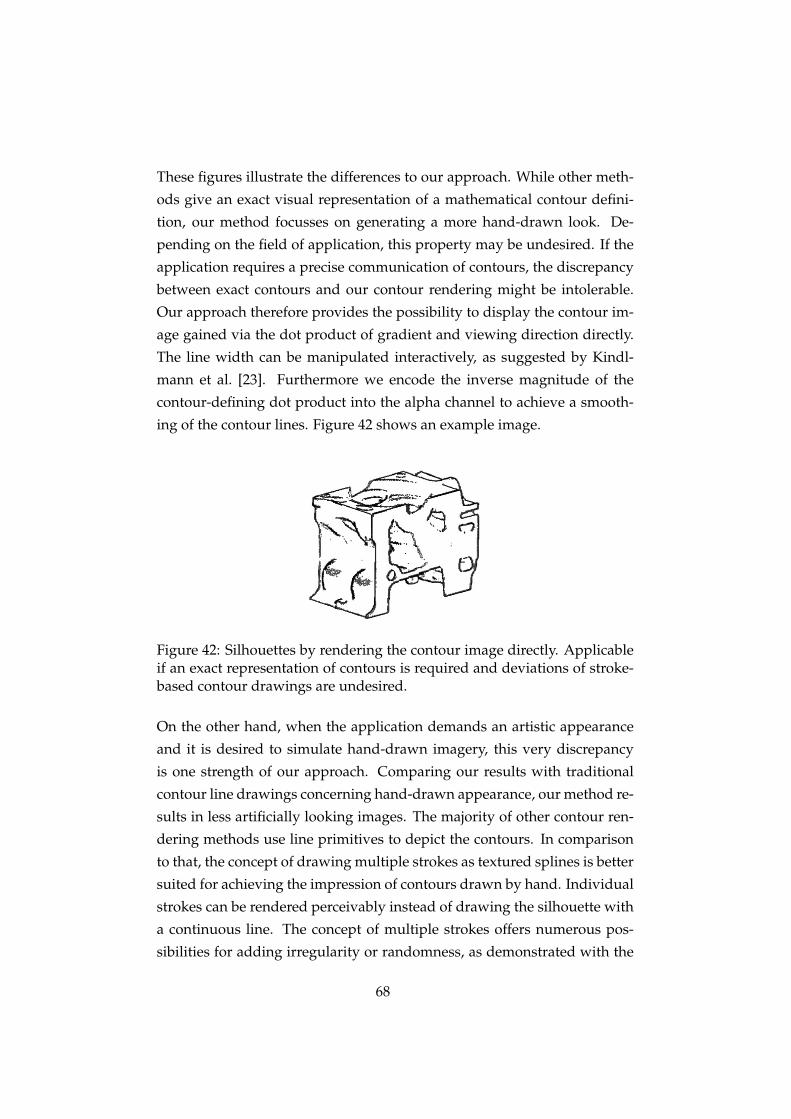
These figures illustrate the differences to our approach. While other meth-
ods give an exact visual representation of a mathematical contour defini-
tion, our method focusses on generating a more hand-drawn look. De-
pending on the field of application, this property may be undesired. If the
application requires a precise communication of contours, the discrepancy
between exact contours and our contour rendering might be intolerable.
Our approach therefore provides the possibility to display the contour im-
age gained via the dot product of gradient and viewing direction directly.
The line width can be manipulated interactively, as suggested by Kindl-
mann et al. [23]. Furthermore we encode the inverse magnitude of the
contour-defining dot product into the alpha channel to achieve a smooth-
ing of the contour lines. Figure 42 shows an example image.
Figure 42: Silhouettes by rendering the contour image directly. Applicableif an exact representation of contours is required and deviations of stroke-based contour drawings are undesired.
On the other hand, when the application demands an artistic appearance
and it is desired to simulate hand-drawn imagery, this very discrepancy
is one strength of our approach. Comparing our results with traditional
contour line drawings concerning hand-drawn appearance, our method re-
sults in less artificially looking images. The majority of other contour ren-
dering methods use line primitives to depict the contours. In comparison
to that, the concept of drawing multiple strokes as textured splines is better
suited for achieving the impression of contours drawn by hand. Individual
strokes can be rendered perceivably instead of drawing the silhouette with
a continuous line. The concept of multiple strokes offers numerous pos-
sibilities for adding irregularity or randomness, as demonstrated with the
68
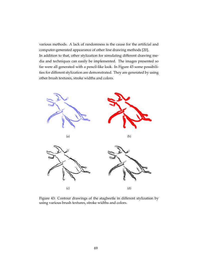
various methods. A lack of randomness is the cause for the artificial and
computer-generated appearance of other line drawing methods [20].
In addition to that, other stylization for simulating different drawing me-
dia and techniques can easily be implemented. The images presented so
far were all generated with a pencil-like look. In Figure 43 some possibili-
ties for different stylization are demonstrated. They are generated by using
other brush textures, stroke widths and colors.
(a) (b)
(c) (d)
Figure 43: Contour drawings of the stagbeetle in different stylization byusing various brush textures, stroke widths and colors.
69
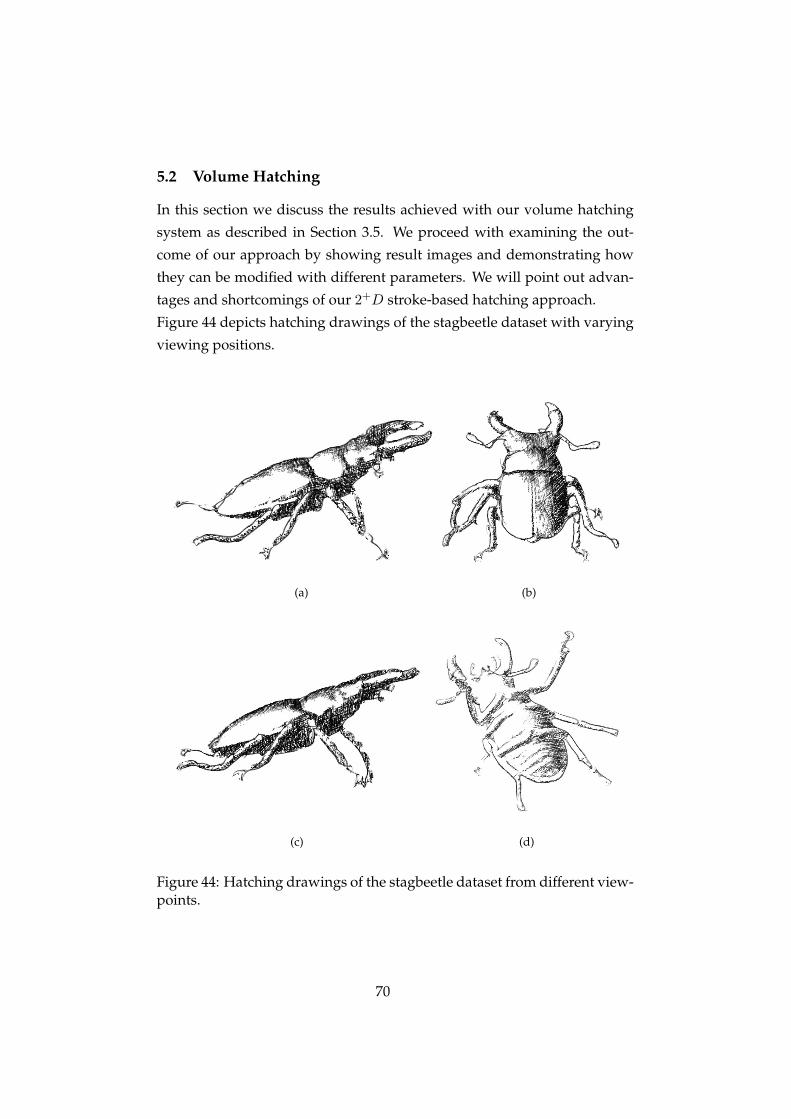
5.2 Volume Hatching
In this section we discuss the results achieved with our volume hatching
system as described in Section 3.5. We proceed with examining the out-
come of our approach by showing result images and demonstrating how
they can be modified with different parameters. We will point out advan-
tages and shortcomings of our 2+D stroke-based hatching approach.
Figure 44 depicts hatching drawings of the stagbeetle dataset with varying
viewing positions.
(a) (b)
(c) (d)
Figure 44: Hatching drawings of the stagbeetle dataset from different view-points.
70
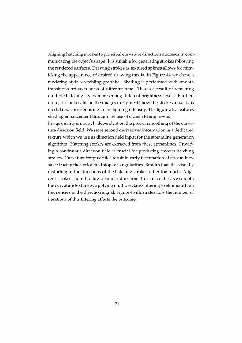
Aligning hatching strokes to principal curvature directions succeeds in com-
municating the object’s shape. It is suitable for generating strokes following
the rendered surfaces. Drawing strokes as textured splines allows for mim-
icking the appearance of desired drawing media, in Figure 44 we chose a
rendering style resembling graphite. Shading is performed with smooth
transitions between areas of different tone. This is a result of rendering
multiple hatching layers representing different brightness levels. Further-
more, it is noticeable in the images in Figure 44 how the strokes’ opacity is
modulated corresponding to the lighting intensity. The figure also features
shading enhancement through the use of crosshatching layers.
Image quality is strongly dependent on the proper smoothing of the curva-
ture direction field. We store second derivatives information in a dedicated
texture which we use as direction field input for the streamline generation
algorithm. Hatching strokes are extracted from these streamlines. Provid-
ing a continuous direction field is crucial for producing smooth hatching
strokes. Curvature irregularities result in early termination of streamlines,
since tracing the vector field stops at singularities. Besides that, it is visually
disturbing if the directions of the hatching strokes differ too much. Adja-
cent strokes should follow a similar direction. To achieve this, we smooth
the curvature texture by applying multiple Gauss filtering to eliminate high
frequencies in the direction signal. Figure 45 illustrates how the number of
iterations of this filtering affects the outcome.
71
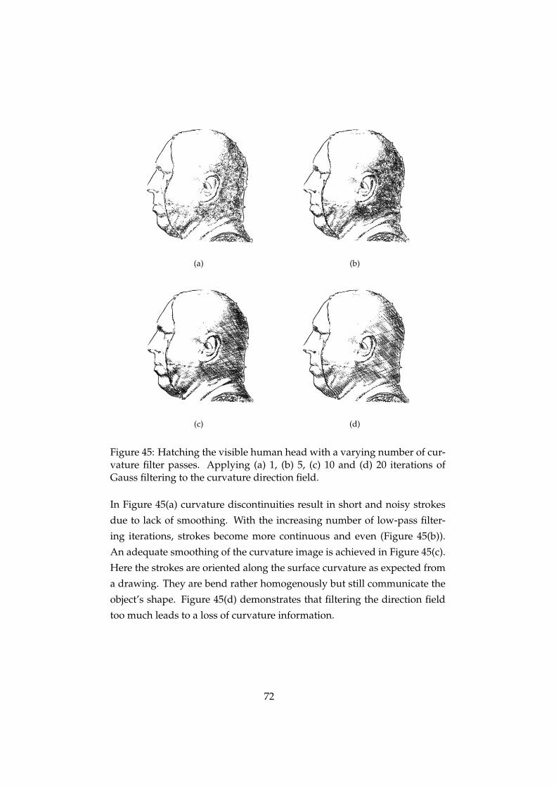
(a) (b)
(c) (d)
Figure 45: Hatching the visible human head with a varying number of cur-vature filter passes. Applying (a) 1, (b) 5, (c) 10 and (d) 20 iterations ofGauss filtering to the curvature direction field.
In Figure 45(a) curvature discontinuities result in short and noisy strokes
due to lack of smoothing. With the increasing number of low-pass filter-
ing iterations, strokes become more continuous and even (Figure 45(b)).
An adequate smoothing of the curvature image is achieved in Figure 45(c).
Here the strokes are oriented along the surface curvature as expected from
a drawing. They are bend rather homogenously but still communicate the
object’s shape. Figure 45(d) demonstrates that filtering the direction field
too much leads to a loss of curvature information.
72
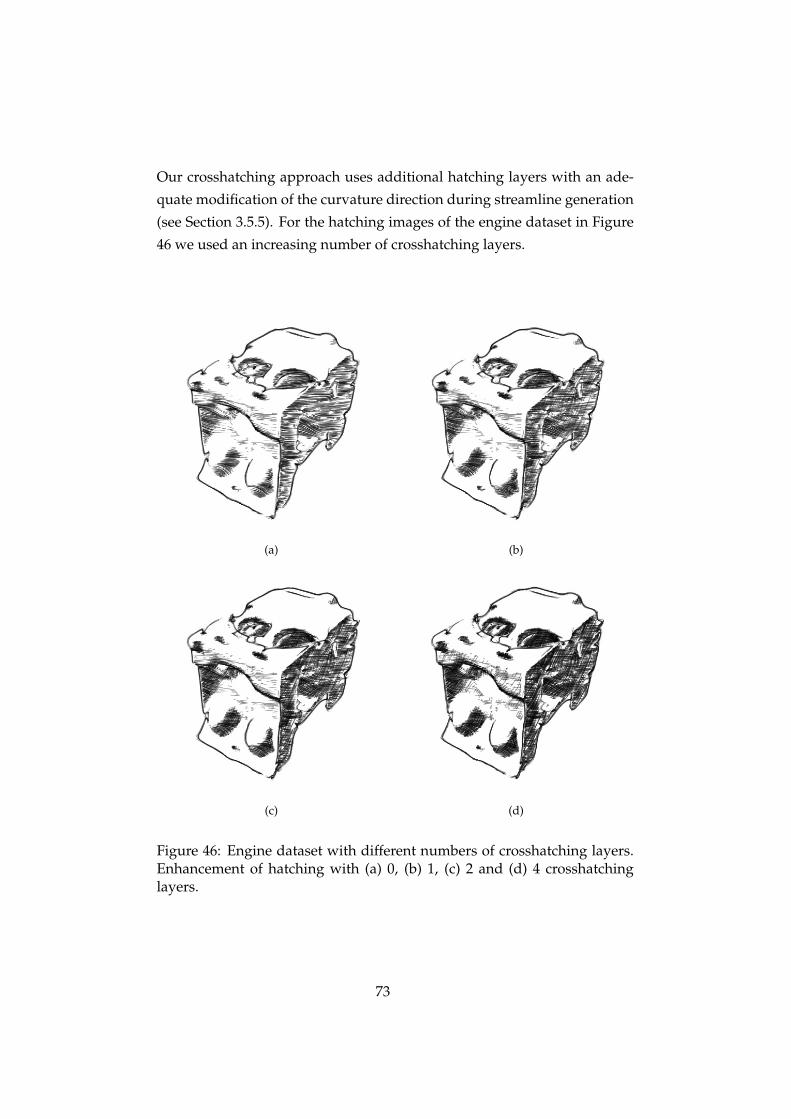
Our crosshatching approach uses additional hatching layers with an ade-
quate modification of the curvature direction during streamline generation
(see Section 3.5.5). For the hatching images of the engine dataset in Figure
46 we used an increasing number of crosshatching layers.
(a) (b)
(c) (d)
Figure 46: Engine dataset with different numbers of crosshatching layers.Enhancement of hatching with (a) 0, (b) 1, (c) 2 and (d) 4 crosshatchinglayers.
73
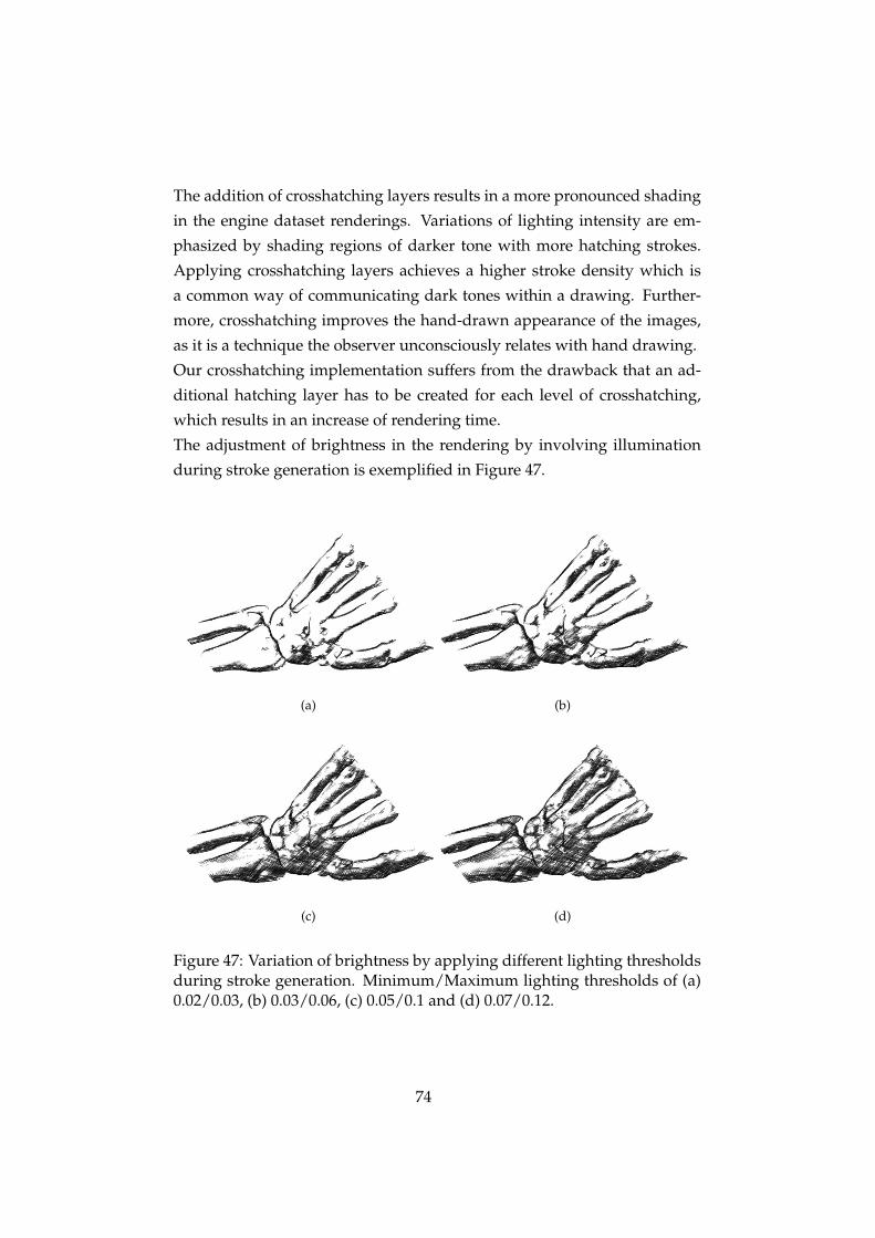
The addition of crosshatching layers results in a more pronounced shading
in the engine dataset renderings. Variations of lighting intensity are em-
phasized by shading regions of darker tone with more hatching strokes.
Applying crosshatching layers achieves a higher stroke density which is
a common way of communicating dark tones within a drawing. Further-
more, crosshatching improves the hand-drawn appearance of the images,
as it is a technique the observer unconsciously relates with hand drawing.
Our crosshatching implementation suffers from the drawback that an ad-
ditional hatching layer has to be created for each level of crosshatching,
which results in an increase of rendering time.
The adjustment of brightness in the rendering by involving illumination
during stroke generation is exemplified in Figure 47.
(a) (b)
(c) (d)
Figure 47: Variation of brightness by applying different lighting thresholdsduring stroke generation. Minimum/Maximum lighting thresholds of (a)0.02/0.03, (b) 0.03/0.06, (c) 0.05/0.1 and (d) 0.07/0.12.
74
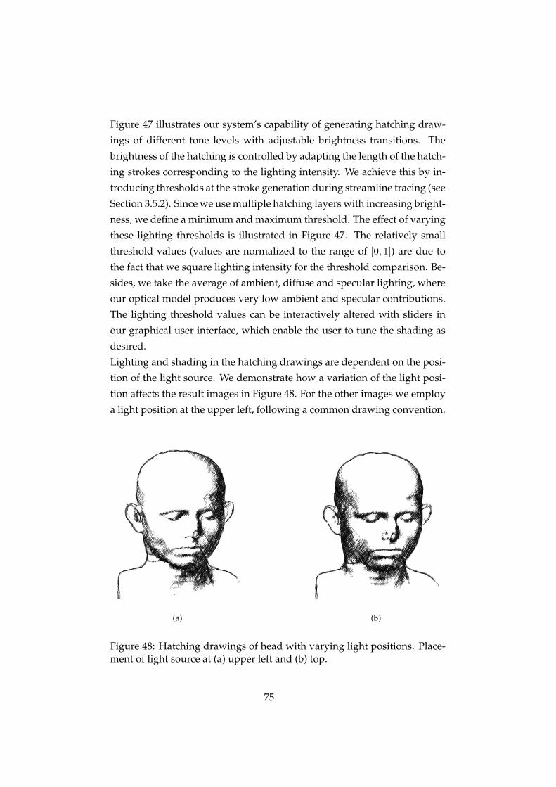
Figure 47 illustrates our system’s capability of generating hatching draw-
ings of different tone levels with adjustable brightness transitions. The
brightness of the hatching is controlled by adapting the length of the hatch-
ing strokes corresponding to the lighting intensity. We achieve this by in-
troducing thresholds at the stroke generation during streamline tracing (see
Section 3.5.2). Since we use multiple hatching layers with increasing bright-
ness, we define a minimum and maximum threshold. The effect of varying
these lighting thresholds is illustrated in Figure 47. The relatively small
threshold values (values are normalized to the range of [0, 1]) are due to
the fact that we square lighting intensity for the threshold comparison. Be-
sides, we take the average of ambient, diffuse and specular lighting, where
our optical model produces very low ambient and specular contributions.
The lighting threshold values can be interactively altered with sliders in
our graphical user interface, which enable the user to tune the shading as
desired.
Lighting and shading in the hatching drawings are dependent on the posi-
tion of the light source. We demonstrate how a variation of the light posi-
tion affects the result images in Figure 48. For the other images we employ
a light position at the upper left, following a common drawing convention.
(a) (b)
Figure 48: Hatching drawings of head with varying light positions. Place-ment of light source at (a) upper left and (b) top.
75
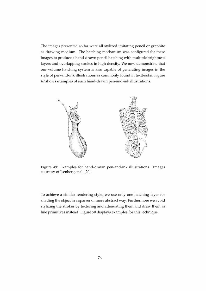
The images presented so far were all stylized imitating pencil or graphite
as drawing medium. The hatching mechanism was configured for these
images to produce a hand-drawn pencil hatching with multiple brightness
layers and overlapping strokes in high density. We now demonstrate that
our volume hatching system is also capable of generating images in the
style of pen-and-ink illustrations as commonly found in textbooks. Figure
49 shows examples of such hand-drawn pen-and-ink illustrations.
Figure 49: Examples for hand-drawn pen-and-ink illustrations. Imagescourtesy of Isenberg et al. [20].
To achieve a similar rendering style, we use only one hatching layer for
shading the object in a sparser or more abstract way. Furthermore we avoid
stylizing the strokes by texturing and attenuating them and draw them as
line primitives instead. Figure 50 displays examples for this technique.
76
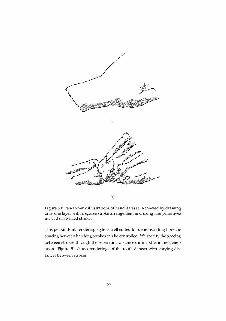
(a)
(b)
Figure 50: Pen-and-ink illustrations of hand dataset. Achieved by drawingonly one layer with a sparse stroke arrangement and using line primitivesinstead of stylized strokes.
This pen-and-ink rendering style is well suited for demonstrating how the
spacing between hatching strokes can be controlled. We specify the spacing
between strokes through the separating distance during streamline gener-
ation. Figure 51 shows renderings of the tooth dataset with varying dis-
tances between strokes.
77
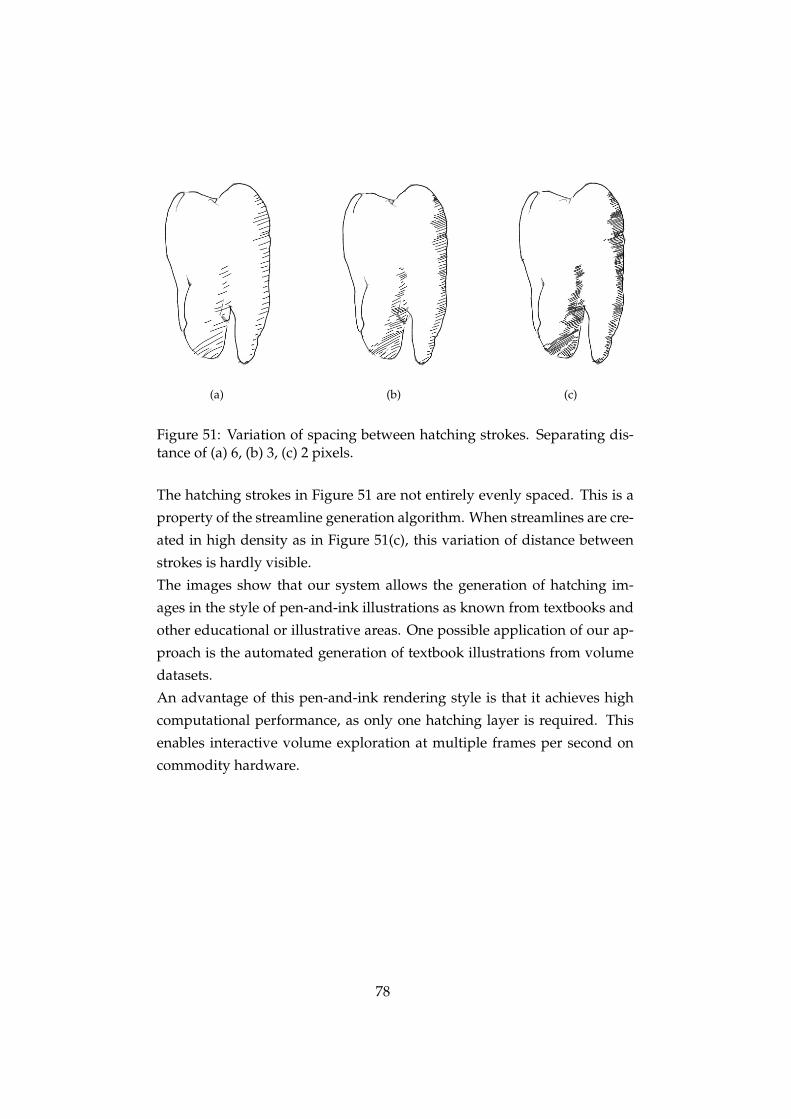
(a) (b) (c)
Figure 51: Variation of spacing between hatching strokes. Separating dis-tance of (a) 6, (b) 3, (c) 2 pixels.
The hatching strokes in Figure 51 are not entirely evenly spaced. This is a
property of the streamline generation algorithm. When streamlines are cre-
ated in high density as in Figure 51(c), this variation of distance between
strokes is hardly visible.
The images show that our system allows the generation of hatching im-
ages in the style of pen-and-ink illustrations as known from textbooks and
other educational or illustrative areas. One possible application of our ap-
proach is the automated generation of textbook illustrations from volume
datasets.
An advantage of this pen-and-ink rendering style is that it achieves high
computational performance, as only one hatching layer is required. This
enables interactive volume exploration at multiple frames per second on
commodity hardware.
78
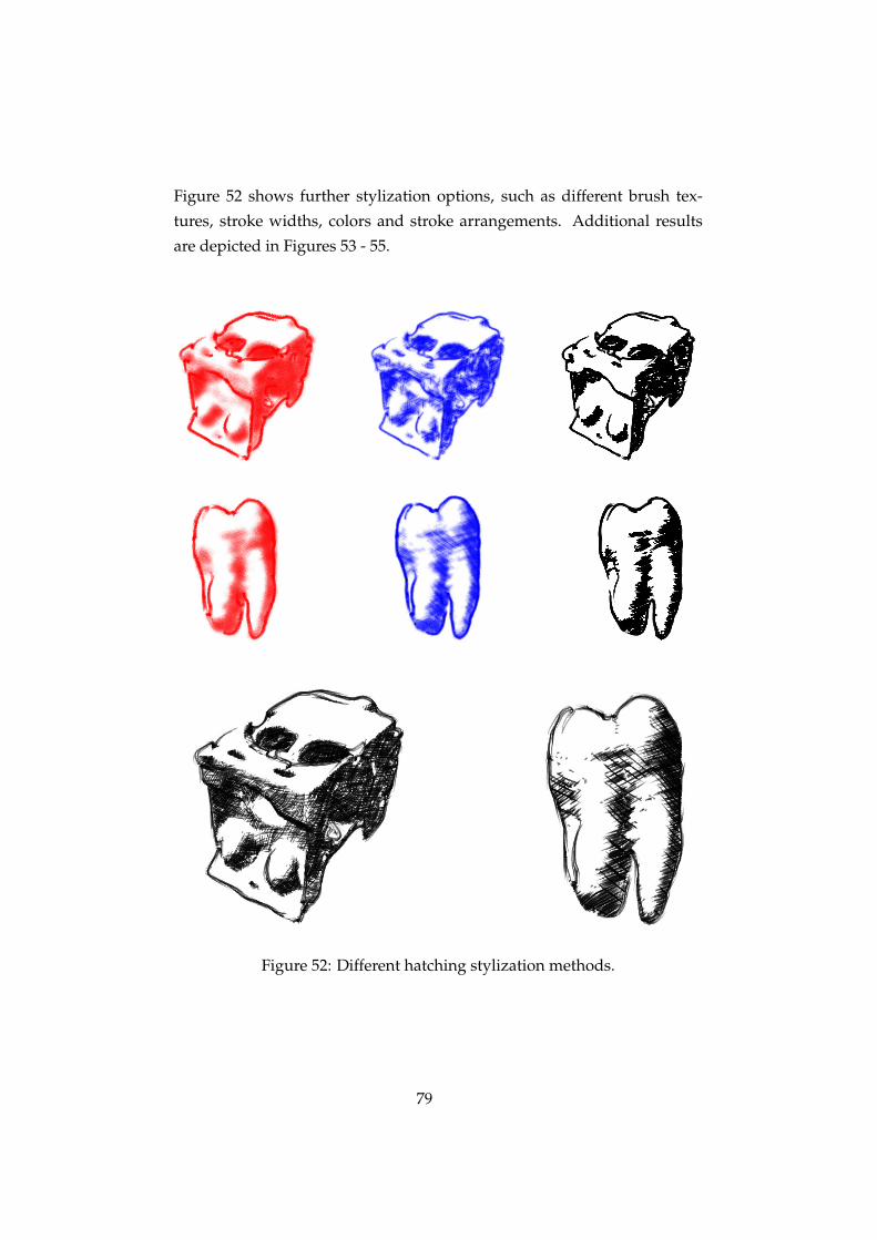
Figure 52 shows further stylization options, such as different brush tex-
tures, stroke widths, colors and stroke arrangements. Additional results
are depicted in Figures 53 - 55.
Figure 52: Different hatching stylization methods.
79
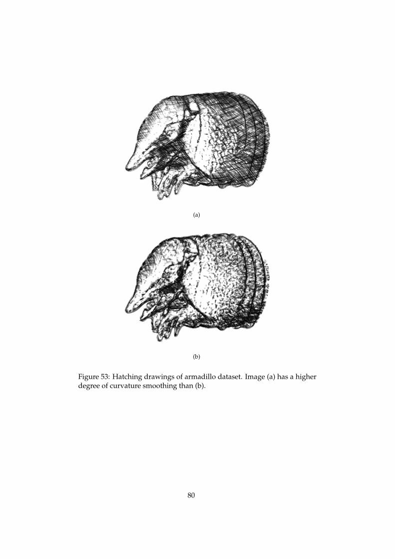
(a)
(b)
Figure 53: Hatching drawings of armadillo dataset. Image (a) has a higherdegree of curvature smoothing than (b).
80
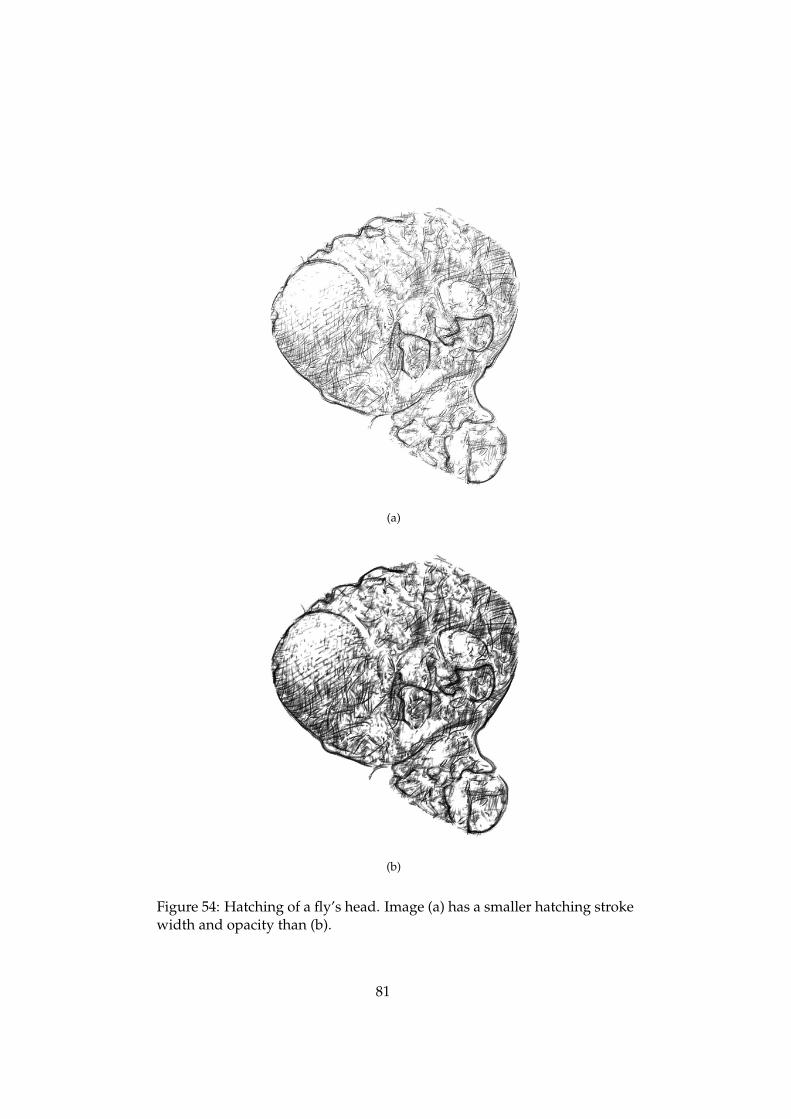
(a)
(b)
Figure 54: Hatching of a fly’s head. Image (a) has a smaller hatching strokewidth and opacity than (b).
81
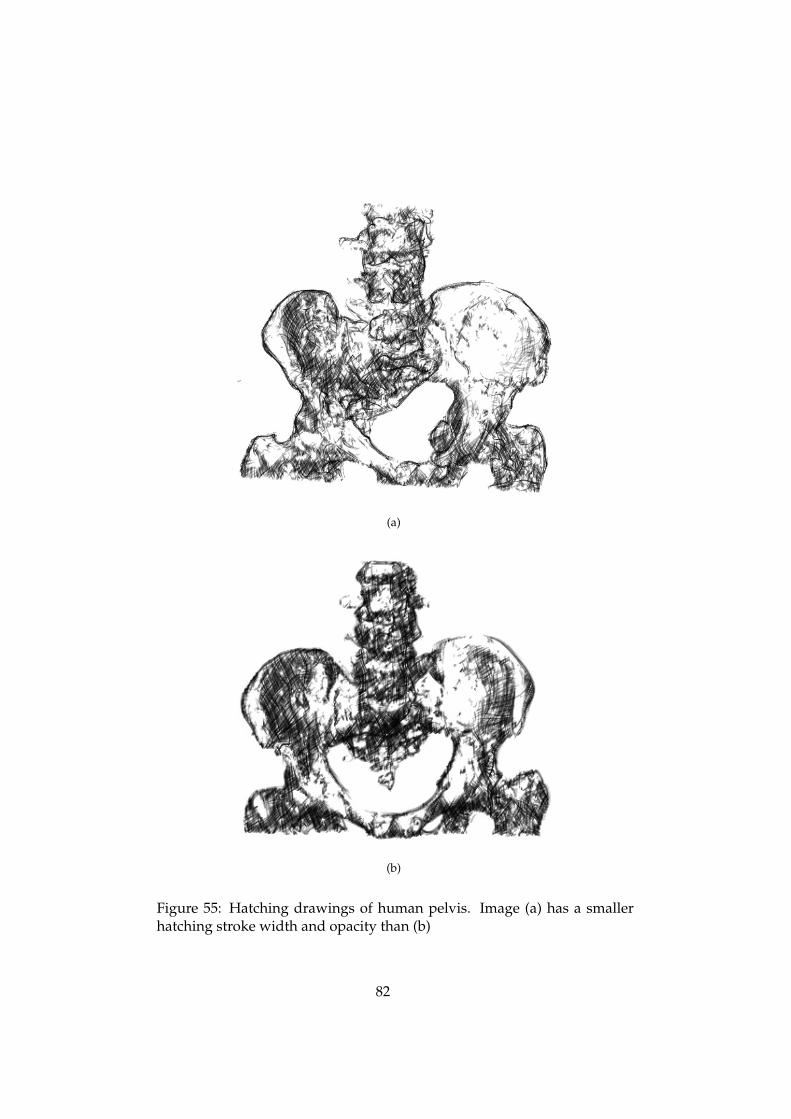
(a)
(b)
Figure 55: Hatching drawings of human pelvis. Image (a) has a smallerhatching stroke width and opacity than (b)
82
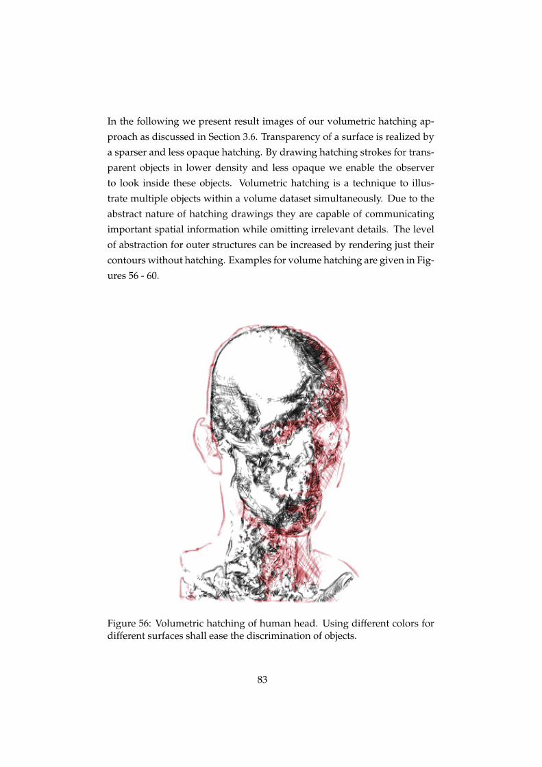
In the following we present result images of our volumetric hatching ap-
proach as discussed in Section 3.6. Transparency of a surface is realized by
a sparser and less opaque hatching. By drawing hatching strokes for trans-
parent objects in lower density and less opaque we enable the observer
to look inside these objects. Volumetric hatching is a technique to illus-
trate multiple objects within a volume dataset simultaneously. Due to the
abstract nature of hatching drawings they are capable of communicating
important spatial information while omitting irrelevant details. The level
of abstraction for outer structures can be increased by rendering just their
contours without hatching. Examples for volume hatching are given in Fig-
ures 56 - 60.
Figure 56: Volumetric hatching of human head. Using different colors fordifferent surfaces shall ease the discrimination of objects.
83
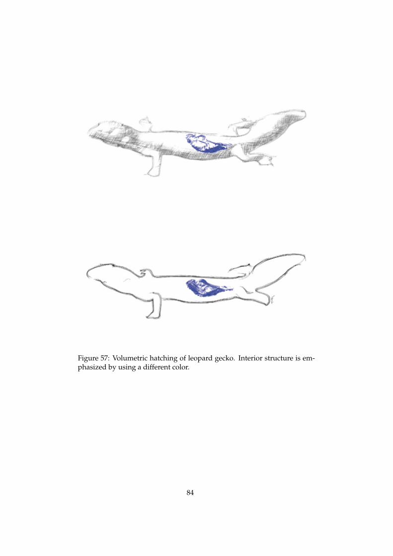
Figure 57: Volumetric hatching of leopard gecko. Interior structure is em-phasized by using a different color.
84
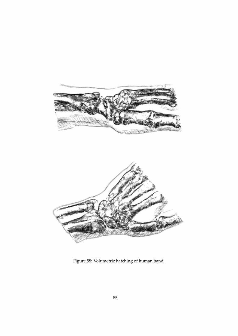
Figure 58: Volumetric hatching of human hand.
85
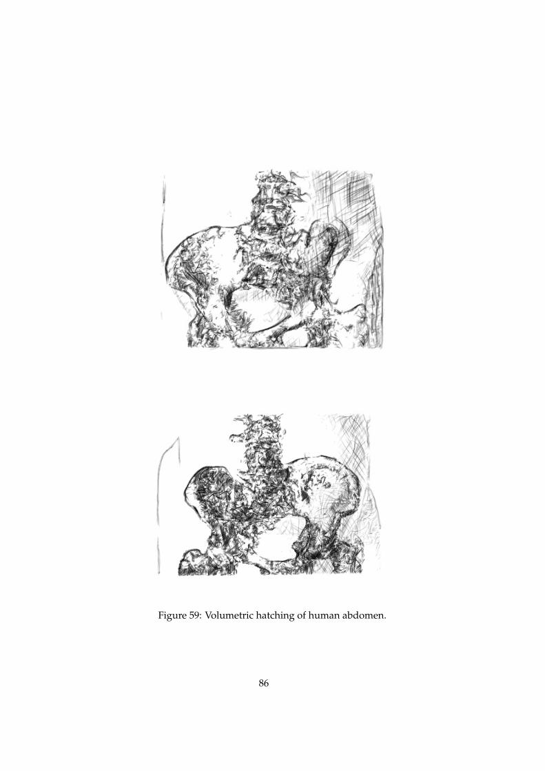
Figure 59: Volumetric hatching of human abdomen.
86
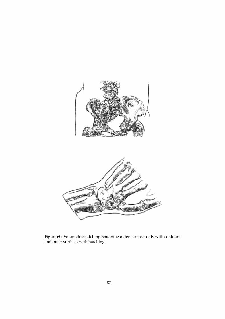
Figure 60: Volumetric hatching rendering outer surfaces only with contoursand inner surfaces with hatching.
87
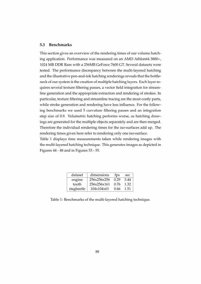
5.3 Benchmarks
This section gives an overview of the rendering times of our volume hatch-
ing application. Performance was measured on an AMD Athlon64 3800+,
1024 MB DDR Ram with a 256MB GeForce 7600 GT. Several datasets were
tested. The performance discrepancy between the multi-layered hatching
and the illustrative pen-and-ink hatching renderings reveals that the bottle-
neck of our system is the creation of multiple hatching layers. Each layer re-
quires several texture filtering passes, a vector field integration for stream-
line generation and the appropriate extraction and rendering of strokes. In
particular, texture filtering and streamline tracing are the most costly parts,
while stroke generation and rendering have less influence. For the follow-
ing benchmarks we used 5 curvature filtering passes and an integration
step size of 0.9. Volumetric hatching performs worse, as hatching draw-
ings are generated for the multiple objects separately and are then merged.
Therefore the individual rendering times for the iso-surfaces add up. The
rendering times given here refer to rendering only one iso-surface.
Table 1 displays time measurements taken while rendering images with
the multi-layered hatching technique. This generates images as depicted in
Figures 44 - 48 and in Figures 53 - 55.
dataset dimensions fps secengine 256x256x256 0.29 3.44tooth 256x256x161 0.76 1.32
stagbeetle 104x104x61 0.66 1.51
Table 1: Benchmarks of the multi-layered hatching technique.
88
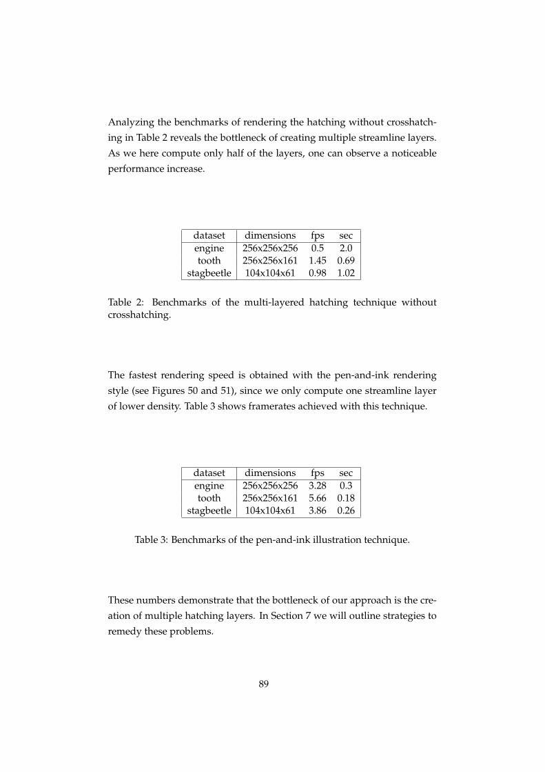
Analyzing the benchmarks of rendering the hatching without crosshatch-
ing in Table 2 reveals the bottleneck of creating multiple streamline layers.
As we here compute only half of the layers, one can observe a noticeable
performance increase.
dataset dimensions fps secengine 256x256x256 0.5 2.0tooth 256x256x161 1.45 0.69
stagbeetle 104x104x61 0.98 1.02
Table 2: Benchmarks of the multi-layered hatching technique withoutcrosshatching.
The fastest rendering speed is obtained with the pen-and-ink rendering
style (see Figures 50 and 51), since we only compute one streamline layer
of lower density. Table 3 shows framerates achieved with this technique.
dataset dimensions fps secengine 256x256x256 3.28 0.3tooth 256x256x161 5.66 0.18
stagbeetle 104x104x61 3.86 0.26
Table 3: Benchmarks of the pen-and-ink illustration technique.
These numbers demonstrate that the bottleneck of our approach is the cre-
ation of multiple hatching layers. In Section 7 we will outline strategies to
remedy these problems.
89
6 Summary
In this chapter we summarize the most important ideas presented in this
thesis.
6.1 Introduction
Non-photorealistic rendering techniques provide abstraction and styliza-
tion possibilities useful for illustrative visualization. Applying pen-and-ink
techniques such as contour drawing and hatching to volume rendering can
communicate spatial properties of volume data in a visually pleasant way.
Images, for instance, could be more readily accepted by observers which
are unfamiliar with looking inside the human body. Realistic rendering
models might be perceived with distaste in this context. Another applica-
tion possibility is given by the automated creation of textbook illustrations
from volumetric data.
6.2 Contour Drawing
We present an image space approach for stylized contour depiction. It is
based on rendering the contour with multiple overlapping strokes. Strokes
are displayed with a brush texture drawn along a spline, which enables
smooth strokes and various stylization possibilities. Our contour draw-
ing technique consists of four steps. Initially, silhouette extraction is per-
formed. Afterwards the contours are filtered. Then we use a line-following
algorithm to sequentially find points on the contour. Finally, subsets of
these points are selected and used as spline control points for drawing con-
tour strokes.
For silhouette extraction we use the angle between gradient and view-
ing direction. We realize the concept of thickness-controlled contours sug-
gested by Kindlmann et al. [23]. The contour detection is implemented for
graphics hardware execution. An output contour image is rendered to a 2D
texture. This contour texture is preprocessed with Gauss filtering in order
to improve the result of our line-following method.
In order to detect points on the contour in a partially sequential order, we
employ a recursive line-following algorithm. Initial points are detected
90
with scanlines. For each location we search the local pixel neighborhood
for the two pixels with the highest contour value. We recursively continue
at the two locations detected until no new contour position can be deter-
mined. When the recursion stops contour points are seeded in fixed inter-
vals during backtracking, yielding equidistant points on the contour.
Afterwards stroke control points are selected from this set of partially-
sequential contour points. We use splines with a variable number of con-
trol points. Starting from one point, we keep adding the successive points
to a stroke until either the distance or contour direction of the next point
differs too much from the last point. Control point selection for the next
stroke starts at a small offset in the contour point array, so the overlapping
of strokes is realized.
We use various geometrical randomization methods like stroke deviation
and perturbation to achieve a hand-drawn visual appearance. Our ap-
proach does not create completely accurate and precise contours. It pro-
duces squiggles and slight deviations from the exact silhouette. This is a re-
sult of errors in the line-following and control point selection mechanisms.
We argue that this randomness enhances the hand-drawn appearance of
the silhouette rendering. But it can also be disturbing and misleading for
some applications.
6.3 Stroke Rendering
Strokes are rendered as textured splines. We draw a stroke with multiple
overlapping quads bearing a brush texture along a Bezier curve. This al-
lows for a stylized stroke rendering capable of simulating various artistic
drawing media. Width and opacity are modulated for realizing tapering
and fading of strokes. Opacity of hatching strokes is defined according
to the lighting intensity. Various randomization techniques allows for in-
dividualizing strokes. Drawing each stroke individually produces larger
irregularities as hatching approaches which use textures containing mul-
tiple strokes. This leads to a less artificial and computer generated visual
impression.
91
6.4 Curvature Estimation
We compute curvature information to align hatching strokes to the surface
of the rendered object. We implement the algorithm proposed by Kindl-
mann et al. [23]. For solving linear equation systems to compute eigen-
vectors which represent principal curvature directions we use the Gauss-
Seidel method. We smooth the curvature data with multiple Gauss fil-
tering passes. We use a convolution kernel weighted with the curvature
magnitude to implement a curvature-sensitive filtering. Curvature direc-
tions have to be smoothed properly, in order to obtain continuous and even
hatching strokes and to avoid hatching too many details. All these curva-
ture estimation and filtering operations are performed on the GPU.
6.5 Streamline-Based Volume Hatching
For realizing volume hatching we chose a stroke-based 2+D approach. In-
termediate information representing spatial and optical properties, namely
curvature and lighting, is rendered to 2D textures. Based on this informa-
tion we place and orient hatching strokes in image space. Searching for
a method for generating equidistant, curvature-aligned strokes in image
space, we applied Jobard and Lefer’s technique [22] for creating evenly-
spaced streamlines. It is a flow visualization method and creates equidis-
tant lines following the directions specified by a 2D vector field. We adapted
Jobard and Lefer’s algorithm for our problem and generate streamlines on
a curvature direction field. We simultaneously extract strokes from these
streamlines and render them as textured splines. We use multiple stream-
line sets to create hatching layers representing regions of different lighting
intensities.
For generating volumetric representations, we apply this hatching tech-
nique to multiple iso-surfaces.
6.5.1 Creating Evenly-Spaced Streamlines
We compute curvature directions in object space and afterwards project
them onto the image plane. This direction field is taken as input for the
evenly-spaced streamline generation algorithm of Jobard and Lefer [22].
In some cases and configurations, the generation of new streamlines from
92
a single initial one is not sufficient to fill arbitrary shapes with streamlines.
Therefore we use multiple initial candidate positions arranged in a regular
grid in order to cover the whole object with streamlines.
The streamline algorithm allows to define the distance between stream-
lines. With creating multiple streamline sets with different separating dis-
tances we obtain the basis for generating hatching layers of different den-
sities.
6.5.2 Stroke Generation
We generate hatching strokes by extracting them from the streamlines si-
multaneously with streamline creation. One streamline is the basis for
multiple strokes. We involve lighting intensity to define the length of the
strokes. To realize lighting with strokes we take account of a lighting thresh-
old during streamline generation. Strokes are placed only in areas where
brightness falls below this threshold. At each new point, the correspond-
ing lighting intensity is compared with the threshold. If it falls below the
threshold, the new point is added to the current stroke. If it exceeds the
threshold, the current stroke is completed. We initialize a new stroke at
the position where the lighting intensity falls below the lighting threshold
again.
6.5.3 Stroke Rendering
When applying the textured splines stroke rendering method to hatching
strokes, three stroke properties are taken into account. The first is a min-
imum number of points defining a stroke. The second is the appropriate
order of the points. The third property is the lighting intensity. Drawing
a stroke as spline additionally requires selecting adequate control points
from the stroke’s point array.
Our stroke generation method might produce strokes represented by just a
few points. To avoid drawing very short strokes we use a threshold defin-
ing the minimum number of points.
As the generation of a streamline starts at an arbitrary point on the line and
integrates the vector field in two opposite directions, the order of points
in a stroke’s array does not necessarily match the required stroke drawing
93
direction. We have to ensure that the points are processed in the proper
order. Therefore we include the constraint that all hatching strokes have to
be drawn from dark to bright areas. To achieve this, we invert the process-
ing order of the point array for control point extraction if the first point of
a stroke corresponds to a higher lighting intensity than its last point.
In addition to determining the length of strokes according to the tone, we
involve lighting during stroke rendering. So the effect of applying more
color in darker areas is achieved. We adjust the opacity of the textured
quads to the corresponding brightness.
We have to make a selection of control points from a stroke’s point array
for a spline representation. This is realized by selecting points as control
points in fixed intervals. Selecting a subset of the streamline points as con-
trol points and drawing interpolating splines results in low-pass filtering
of curvature discontinuities and generates smooth strokes.
6.5.4 Hatching Layers
With the methods described previously we are able to render a hatching
drawing for one level of brightness. For producing pen-and-ink style illus-
trations one level of tone is sufficient, because here it is common to shade
the pictured object in an abstract manner. For mimicking pencil hatching
images, we achieve transitions between areas of different lighting intensity
by using four layers of hatching strokes. Each layer represents one level of
tone. In dark areas we draw short strokes of high density, brighter areas
are rendered with longer strokes of lower density.
We control the length of the strokes for each layer by using the lighting
threshold for stroke extraction from streamlines. This allows for adjusting
the length of the hatching strokes to the level of tone the layer represents.
We use a minimum and a maximum threshold and interpolate the values
for the layers in between. With these thresholds the brightness and contrast
of the hatching drawing can be controlled. The distance between the two
thresholds defines the degree of lighting variation between the four hatch-
ing layers.
To control the hatching stroke density the separating distance between the
streamlines is employed. Additionally to opacity modulation and stroke
length we control the brightness of each level by stroke density.
94
6.5.5 Crosshatching
We integrate crosshatching by generating further hatching layers. The only
component which has to be changed for crosshatching is the curvature di-
rection during streamline generation. For crosshatching, we use a stroke
direction which is perpendicular to the original stroke direction in image
space. Manual crosshatching often uses a constant angle between hatching
and crosshatching strokes, so we decided to adopt this technique. To ob-
tain a direction perpendicular to the principal curvature direction in image
space, we rotate the projected principal curvature direction by 90 degrees.
6.5.6 Volumetric Hatching
To realize volumetric hatching, in terms of a simultaneous hatched display
of interior and exterior structures, we apply our hatching methods to multi-
ple iso-surfaces. An analysis of the transfer function is performed to detect
iso-surfaces relevant for the volumetric rendering. Contour and hatching
strokes are generated for each of these surfaces, taking into account the
transparencies specified by the transfer function. The hatched surfaces are
overlaid to produce the volumetric hatching image.
The transfer function analysis is based on detecting relevant iso-surfaces
through local maxima and minima of the transfer function. The number of
local maxima defines the number of visible iso-surfaces and therewith the
number of hatching passes. Minima are used as thresholds affecting the
transfer function readout during raycasting. If the scalar value at a resam-
ple location falls below the threshold, a zero color contribution is assumed.
Transparency is realized by means of hatching stroke density and stroke
opacity. The degree of a surface’s transparency defines the opacity and
density of hatching strokes generated for this surface. The degree of trans-
parency modulation is specified with the transfer function.
Variations of volumetric hatching include applying different rendering styles
to the different surfaces or depicting outer surfaces with contours only and
hatching the inner structures.
95
6.6 Results
We discussed the results of the volume hatching system and described its
advantages and limitations. We presented result images and examined
their quality in terms of aesthetics and applicability to illustration pur-
poses. We demonstrated how the visual appearance of the images can
be altered by modulating various rendering parameters. Furthermore we
benchmarked rendering performance.
The majority of examples presented implement the style of hand-drawn
pencil hatchings, but we also demonstrated the capability of generating
abstract pen-and-ink illustrations as found in textbooks.
We showed that the major shortcomings of our approach are the inaccura-
cies of our contour drawing mechanism and the non-interactive framerates
of multi-layered hatching. Rendering benchmarks revealed the bottleneck
of creating multiple streamline layers and evidenced that interactivity is
achieved if only one layer is created.
96
7 Conclusions and Future Work
We presented an approach capable of visualizing volumetric data with non-
photorealistic rendering techniques mimicking hand-drawn hatching im-
agery in different artistic styles such as pencil or pen-and-ink drawing. We
use this visualization method for creating volumetric hatching drawings.
Our system allows for generating hatching images from volume data in
various rendering stylization covering a wide spectrum from artistic hand-
drawn graphite hatchings to abstract pen-and-ink illustrations as found
in textbooks. One advantage of our approach is the hand-drawn appear-
ance of our results. We try to avoid the artificial look of many computer-
generated drawings, although at the cost of accuracy. We focused on achiev-
ing such an appearance and tried to design algorithms which mimic hand
drawing processes. The techniques developed for this thesis provide the
functionality required in possible application areas such as surgery illus-
tration or automated creation of textbook illustrations. We discussed the
result images with experts from the field of drawing. This revealed sev-
eral shortcomings of our approach, but the image quality was regarded as
promising.
One limitation of our system is the lack of accuracy of our contour drawing
method. However, this randomness can also be beneficial as it creates a
hand-drawn impression. The other drawback is that we do not achieve an
interactive rendering performance. In the following, we address possibili-
ties for further enhancing and improving our mechanisms.
The randomness of our contour rendering approach originates from the
fact that our recursive line-following and stroke extraction algorithms are
suboptimal. Involving a rather large neighborhood in the line searching
results in false connections between adjacent contour lines. We need this
large neighborhood to compensate gaps in the contour image. Gauss fil-
tering the image too intensively to close all this gaps leads to a broaden-
ing of contours, which is also disadvantageous for the line-following algo-
rithm. Therefore a more sophisticated contour filtering scheme would al-
low for decreasing the search neighborhood and would avoid the problem
of falsely connected adjacent contour lines. Detecting multiple line-tracing
start points with scanlines leads to a noncontinuous sequentiality within
97
the contour point array. The tracing algorithm starts from numerous posi-
tions and stores detected points in the same array. This makes the task of
determining which contour points are selected to form strokes more diffi-
cult. One way of solving this is separately storing contour points detected
at tracing the contour from one position. This would require multiple con-
tour point arrays, one for each start point. This method would guarantee
that points are provided in sequential order. In addition to that, there could
be developed other ways of detecting appropriate start points to decrease
their number.
With these methods, it should be possible to fix the defects of our con-
tour renderer. But perhaps it would destroy the hand-drawn impression
it achieves as a result of its faultiness. Mimicking human manufacture de-
mands implicating human shortcomings.
We showed that the bottleneck of our approach is the creation of up to
eight layers of streamlines. We originally intended to use a higher varia-
tion of stroke density for the different hatching layers and therefore cre-
ated multiple streamline layers. We found out that the images look better
when all layers are created in high density. Therefore the streamline layers
are quite similar to each other. So generating only two layers of stream-
lines, one for basic hatching and one for crosshatching, could be sufficient
to create images in similar quality. The concept of multiple hatching lay-
ers representing different tone levels could still be implemented, but all
the strokes would have to be generated from these two sets of streamlines.
By rendering the hatching layers with a slight offset for displacing them
would result in a similar visual impression as creating strokes from mul-
tiple streamline layers of similar density. Rendering benchmarks given in
Section 5.3 prove that our approach achieves interactive framerates if only
one layer of streamlines is generated.
As the vector field integration is the most costly part of our application,
another acceleration strategy is to downsample the curvature field and to
trace the streamlines on a smaller image. Rendering time directly corre-
lates with the size of the curvature vector field. Even faster and having the
same effect would be to perform the volume rendering for calculating all
intermediate spatial and optical information on a smaller viewport. This
would achieve a high performance increase. Downsampling the curvature
98
field additionally implies smoothing the curvature information. Rendering
time spent on multiple filtering passes could be saved. So this approach
would efficiently accelerate the three most expensive computations of our
implementation, namely volume rendering, curvature smoothing and vec-
tor field integration, at the same time.
Another acceleration possibility will be given in the near future by geome-
try shader functionality included in Shader Model 4.0. As it will be possible
to create vertices on the GPU, the vector field integration and stroke gener-
ation could be executed in graphics hardware.
Realizing these optimization strategies would make it possible to perform
volume hatching at multiple frames per second in a quality similar to the
result images presented.
The visual similarity to artistic drawing media could be increased by apply-
ing dedicated NPR methods, for instance involving paper effects for pencil
rendering as used by Lee et al. [27] (see Section 2.2.3).
In order to further improve the image quality in aesthetic aspects it will be
necessary to perform extensive user studies. Furthermore, exchange with
experts in drawing has to be continued. Since these people professionally
deal with creating drawings, they can easily discover aesthetic shortcom-
ings in computer-generated drawings.
Further ideas include the integration of focus+context approaches such as
importance driven volume rendering in our hatching technique. These
methods for emphasizing volumetric relations combined with the abstrac-
tion and stylization capabilities of volume hatching could create powerful
ways of illustrating volumetric data.
99

Acknowledgements
First of all, I thank my supervisor Stefan Bruckner for all his support and
help. I further thank Eduard Groller and Stefan Muller for their supervi-
sion and valuable discussions. Many thanks to Otto Mittmannsgruber and
Daniel v. Chamier-Glisczinski for their advice related to drawing. Finally, I
want to express my gratitude to my parents for making this work possible.
100
References
[1] S. Bruckner, S. Grimm, A. Kanitsar, and M. E. Groller. Illustrative
context-preserving volume rendering. In Proceedings of EuroVis 2005,
pages 69–76, 2005.
[2] S. Bruckner and M. E. Groller. VolumeShop: An interactive system
for direct volume illustration. In Proceedings of IEEE Visualization 2005,
pages 671–678, 2005.
[3] M. Burns, J. Klawe, S. Rusinkiewicz, A. Finkelstein, and D. DeCarlo.
Line drawings from volume data. ACM Transactions on Graphics,
24(3):512–518, 2005.
[4] B. Cabral, N. Cam, and J. Foran. Accelerated volume rendering and
tomographic reconstruction using texture mapping hardware. In Pro-ceedings of VolVis 1994, pages 91–98, 1994.
[5] M. S. T. Carpendale, D. J. Cowperthwaite, and F. D. Fracchia. Distor-
tion viewing techniques for 3-dimensional data. In Proceedings of theIEEE InfoVis 1996, pages 46–53, 1996.
[6] C. J. Curtis, S. E. Anderson, J. E. Seims, K. W. Fleischer, and D. H.
Salesin. Computer-generated watercolor. Computer Graphics, 31(An-
nual Conference Series):421–430, 1997.
[7] D. DeCarlo, A. Finkelstein, S. Rusinkiewicz, and A. Santella. Sug-
gestive contours for conveying shape. ACM Transactions on Graphics,
22(3):848–855, 2003.
[8] J. Diepstraten, D. Weiskopf, and T. Ertl. Transparency in interactive
technical illustrations. Computer Graphics Forum, 21(3):317–325, 2002.
[9] F. Dong, G. J. Clapworthy, and M. Krokos. Volume rendering of fine
details within medical data. In Proceedings of IEEE Visualization 2001,
pages 387–394, 2001.
[10] F. Dong, G. J. Clapworthy, H. Lin, and M. Krokos. Nonphotorealistic
rendering of medical volume data. IEEE Computer Graphics and Appli-cations, 23(4):44–52, 2003.
101
[11] D. S. Ebert and P. Rheingans. Volume illustration: non-photorealistic
rendering of volume models. In Proceedings of IEEE Visualization 2000,
pages 195–202, 2000.
[12] A. Van Gelder and K. Kim. Direct volume rendering with shading via
three-dimensional textures. In Proceedings of VolVis 1996, pages 23–30,
1996.
[13] A. Gooch, B. Gooch, P. Shirley, and E. Cohen. A non-photorealistic
lighting model for automatic technical illustration. In Proceedings ofSIGGRAPH 1998, pages 447–452, 1998.
[14] B. Gooch, P.-P. J. Sloan, A. Gooch, P. Shirley, and R. F. Riesenfeld. Inter-
active technical illustration. In Symposium on Interactive 3D Graphics,
pages 31–38, 1999.
[15] M. Hadwiger, C. Sigg, H. Scharsach, K. Buhler, and M. Gross. Real-
time ray-casting and advanced shading of discrete isosurfaces. Com-puter Graphics Forum, 24(3):303–312, 2005.
[16] P. Haeberli. Paint by numbers: abstract image representations. In
Proceedings of SIGGRAPH 1990, pages 207–214, 1990.
[17] H. Hauser, L. Mroz, G.-I. Bischi, and M. E. Groller. Two-level volume
rendering - fusing MIP and DVR. In Proceedings of IEEE Visualization2000, pages 211–218, 2000.
[18] A. Hertzmann and D. Zorin. Illustrating smooth surfaces. In Proceed-ings of SIGGRAPH 2000, pages 517–526, 2000.
[19] V. Interrante, H. Fuchs, and S. M. Pizer. Enhancing transparent skin
surfaces with ridge and valley lines. In Proceedings of IEEE Visualization1995, pages 52–59, 1995.
[20] T. Isenberg, P. Neumann, S. Carpendale, M. C. Sousa, and J. A. Jorge.
Non-photorealistic rendering in context: An observational study. In
Proceedings of NPAR 2006, pages 115–126, 2006.
[21] S. Islam, S. Dipankar, D. Silver, and M. Chen. Spatial and temporal
splitting of scalar fields in volume graphics. In Proceedings of IEEEVolVis 2004, pages 87– 94, 2004.
102
[22] B. Jobard and W. Lefer. Creating evenly-spaced streamlines of arbi-
trary density. In Proceedings of Eurographics Workshop on Visualizationin Scientific Computing ’97, pages 43–56, 1997.
[23] G. Kindlmann, R. Whitaker, T. Tasdizen, and T. Moller. Curvature-
based transfer functions for direct volume rendering: Methods and
applications. In Proceedings of IEEE Visualization 2003, pages 513–520,
2003.
[24] G. Knittel. The UltraVis system. In Proceedings of VolVis 2000, pages
71–79, 2000.
[25] A. Kruger, C. Tietjen, J. Hintze, B. Preim, I. Hertel, and G. Strau. In-
teractive visualization for neck-dissection planning. In Proceedings ofEuroVis 2005, pages 295– 302, 2005.
[26] P. Lacroute and M. Levoy. Fast Volume Rendering Using a Shear-WarpFactorization of the Viewing Transformation. PhD thesis, Stanford Uni-
versity, Computer Systems Laboratory, 1995.
[27] H. Lee, S. Kwon, and S. Lee. Real-time pencil rendering. In Proceedingsof NPAR 2006, pages 37–45, 2006.
[28] M. Levoy. Display of surfaces from volume data. IEEE ComputerGraphics and Applications, 8(3):29–37, 1988.
[29] M. Levoy. Efficient ray tracing of volume data. ACM Transactions onGraphics, 9(3):245–261, 1990.
[30] M. Levoy. Volume rendering by adaptive refinement. The Visual Com-puter, 6(1):2–7, 1990.
[31] E. B. Lum and K.-L. Ma. Hardware-accelerated parallel non-
photorealistic volume rendering. In Proceedings of NPAR 2002, pages
67–74, 2002.
[32] L. Markosian, M. A. Kowalski, S. J. Trychin, L. D. Bourdev, D. Gold-
stein, and J. F. Hughes. Real-time nonphotorealistic rendering. In Pro-ceedings of SIGGRAPH 1997, pages 415–420, 1997.
103
[33] M. McGuire and J. F. Hughes. Hardware-determined feature edges. In
Proceedings of NPAR 2004, pages 35–147, 2004.
[34] M. Meißner, U. Hoffmann, and W. Straßer. Enabling classification
and shading for 3D texture mapping based volume rendering using
OpenGL and extensions. In Proceedings of IEEE Visualization 1999,
pages 207–214, 1999.
[35] K. Mueller and R. Crawfis. Eliminating popping artifacts in sheet
buffer-based splatting. In Proceedings of IEEE Visualization 1998, pages
239–246, 1998.
[36] K. Mueller, N. Shareef, J. Huang, and R. Crawfis. High-quality splat-
ting on rectilinear grids with efficient culling of occluded voxels. IEEETransactions on Visualization and Computer Graphics, 5(2):116–134, 1999.
[37] Z. Nagy and R. Klein. High-quality silhouette illustration for texture-
based volume rendering. In Proceedings of WSCG 2004, pages 301–308,
2004.
[38] Z. Nagy, J. Schneider, and R. Westermann. Interactive volume illustra-
tion. In Proceedings of VMV 2002, pages 497–504, 2002.
[39] S. Parker, M. Parker, Y. Livnat, P.-P. Sloan, C. Hansen, and P. Shirley.
Interactive ray tracing for volume visualization. IEEE Transactions onVisualization and Computer Graphics, 5(3):238–250, 1999.
[40] E. Praun, A. Finkelstein, and H. Hoppe. Lapped textures. In Proceed-ings of SIGGRAPH 2000, pages 465–470, 2000.
[41] E. Praun, H. Hoppe, M. Webb, and A. Finkelstein. Real-time hatching.
In Proceedings of SIGGRAPH 2001, pages 581–586, 2001.
[42] C. Rezk-Salama, K. Engel, M. Bauer, G. Greiner, and T. Ertl. Interac-
tive volume rendering on standard PC graphics hardware using multi-
textures and multi-stage rasterization. In Proceedings of the Workshop onGraphics Hardware 2000, pages 109–118, 2000.
[43] Z. Salah, D. Bartz, and W. Straßer. Illustrative rendering of segmented
anatomical data. In Proceedings of SimVis 2005, pages 175–184, 2005.
104
[44] M. P. Salisbury, S. E. Anderson, R. Barzel, and D. H. Salesin. Interactive
pen-and-ink illustration. In Proceedings of SIGGRAPH 1994, pages 101–
108, 1994.
[45] J. Schumann, T. Strothotte, S. Laser, and A. Raab. Assessing the ef-
fect of non-photorealistic rendered images in CAD. In Proceedings ofSIGCHI 1996, pages 35–41, 1996.
[46] S. Stegmaier, M. Strengert, T. Klein, and T. Ertl. A simple and flex-
ible volume rendering framework for graphics-hardware-based ray-
casting. In Proceedings of the International Workshop on Volume Graphics2005, pages 187–195, 2005.
[47] M. Straka, M. Cervenansky, A. La Cruz, A. Kochl, M. Sramek, M. E.
Groller, and D. Fleischmann. The VesselGlyph: Focus & context visu-
alization in CT-angiography. In Proceedings of IEEE Visualization 2004,
pages 385–392, 2004.
[48] J. Sweeney and K. Mueller. Shear-warp deluxe: the shear-warp al-
gorithm revisited. In Proceedings of the Joint EUROGRAPHICS - IEEETCVG Symposium on Visualization 2002, pages 95–104, 2002.
[49] J.-P. Thirion and A. Gourdon. Computing the differential characteris-
tics of isointensity surfaces. Computer Vision and Image Understanding,
61(2):190–202, 1995.
[50] J.-P. Thirion and A. Gourdon. The 3d marching lines algorithm. Graph-ical Models and Image Processing, 58(6):503–509, 1996.
[51] S. M. F. Treavett and M. Chen. Pen-and-ink rendering in volume vi-
sualisation. In Proceedings of IEEE Visualization 2000, pages 203–210,
2000.
[52] I. Viola and M. E. Groller. Smart visibility in visualization. In Proceed-ings of EG Workshop on Computational Aesthetics in Graphics, Visualiza-tion and Imaging, pages 209–216, 2005.
[53] I. Viola, A. Kanitsar, and M. E. Groller. Importance-driven volume
rendering. In Proceedings of IEEE Visualization 2004, pages 139–145,
2004.
105
[54] M. Webb, E. Praun, A. Finkelstein, and H. Hoppe. Fine tone control in
hardware hatching. In Proceedings of NPAR 2002, pages 53–58, 2002.
[55] R. Westermann and T. Ertl. Efficiently using graphics hardware in vol-
ume rendering applications. In Proceedings of SIGGRAPH 1998, pages
169–178, 1998.
[56] L. Westover. Footprint evaluation for volume rendering. ComputerGraphics, 24(4):367–376, 1990.
[57] G. Winkenbach and D. H. Salesin. Computer-generated pen-and-ink
illustration. Computer Graphics, 28(Annual Conference Series):91–100,
1994.
[58] D. Woods. DevIL: A full featured cross-platform image library.
http://openil.sourceforge.net/, 2006.
106
List of Figures
1 Hatching drawing by Vesalius . . . . . . . . . . . . . . . . . . 2
2 Suggestive contours [7] . . . . . . . . . . . . . . . . . . . . . . 7
3 Pen-and-ink rendering [57] . . . . . . . . . . . . . . . . . . . 9
4 Interactive pen-and-ink rendering [44] . . . . . . . . . . . . . 9
5 Real-time hatching [40] . . . . . . . . . . . . . . . . . . . . . . 11
6 Fine tone control in hardware hatching [54] . . . . . . . . . . 11
7 Illustrating smooth surfaces [18] . . . . . . . . . . . . . . . . 12
8 Real-time pencil rendering [27] . . . . . . . . . . . . . . . . . 13
9 Non-photorealistic volume rendering [31] . . . . . . . . . . . 15
10 Importance-driven feature enhancement [53] . . . . . . . . . 17
11 An interactive system for volume illustration [2] . . . . . . . 18
12 Pen-and-ink rendering in volume visualization [51] . . . . . 20
13 Volume hatching images of Nagy et al. [38] . . . . . . . . . . 22
14 Volume hatching images of Dong et al. [10] . . . . . . . . . . 23
15 Evenly-spaced streamlines [22] . . . . . . . . . . . . . . . . . 25
16 Rendering pipeline . . . . . . . . . . . . . . . . . . . . . . . . 27
17 Contour image of stagbeetle . . . . . . . . . . . . . . . . . . . 31
18 Contour seed points . . . . . . . . . . . . . . . . . . . . . . . 32
19 Illustration of line-following algorithm . . . . . . . . . . . . . 33
20 Illustration of contour stroke generation 1 . . . . . . . . . . . 34
21 Illustration of contour stroke generation 2 . . . . . . . . . . . 35
22 Illustration of contour stroke generation 3 . . . . . . . . . . . 36
23 Contour drawings . . . . . . . . . . . . . . . . . . . . . . . . . 37
24 Different brush textures . . . . . . . . . . . . . . . . . . . . . 38
25 Stroke as textured spline . . . . . . . . . . . . . . . . . . . . . 39
26 Curvature direction textures . . . . . . . . . . . . . . . . . . . 41
27 Volume stippling . . . . . . . . . . . . . . . . . . . . . . . . . 43
28 Curvature-following streamlines . . . . . . . . . . . . . . . . 46
29 Lighting intensity textures . . . . . . . . . . . . . . . . . . . . 47
30 Hatching layers . . . . . . . . . . . . . . . . . . . . . . . . . . 50
31 Crosshatching of engine dataset . . . . . . . . . . . . . . . . . 52
32 Volumetric hatching of hand dataset . . . . . . . . . . . . . . 56
33 Screenshot of VolumeShop [22] . . . . . . . . . . . . . . . . . 59
107
34 Variation of control point selection increment . . . . . . . . . 61
35 Variation of seed point placement interval . . . . . . . . . . . 62
36 Variation of stroke deviation . . . . . . . . . . . . . . . . . . . 63
37 Variation of stroke perturbation . . . . . . . . . . . . . . . . . 64
38 Variation of stroke translation and rotation . . . . . . . . . . 65
39 Contour drawing human head . . . . . . . . . . . . . . . . . 66
40 Burns: Line drawings from volume data [3] . . . . . . . . . . 67
41 Nagy: Silhouette illustration [37] . . . . . . . . . . . . . . . . 67
42 Drawing contour image directly . . . . . . . . . . . . . . . . 68
43 Contour drawings with different stylization . . . . . . . . . . 69
44 Variation of viewpoint . . . . . . . . . . . . . . . . . . . . . . 70
45 Variation of curvature filter passes . . . . . . . . . . . . . . . 72
46 Varying number of crosshatching layers . . . . . . . . . . . . 73
47 Variation of brightness . . . . . . . . . . . . . . . . . . . . . . 74
48 Variation of light position . . . . . . . . . . . . . . . . . . . . 75
49 Hand-drawn pen-and-ink illustrations. . . . . . . . . . . . . 76
50 Pen-and-ink illustration of hand . . . . . . . . . . . . . . . . 77
51 Variation of distance between strokes . . . . . . . . . . . . . 78
52 Hatching stylization . . . . . . . . . . . . . . . . . . . . . . . 79
53 Hatching of armadillo . . . . . . . . . . . . . . . . . . . . . . 80
54 Hatching of a fly’s head . . . . . . . . . . . . . . . . . . . . . 81
55 Hatching drawings of human pelvis . . . . . . . . . . . . . . 82
56 Volumetric hatching of human head . . . . . . . . . . . . . . 83
57 Volumetric hatching of gecko . . . . . . . . . . . . . . . . . . 84
58 Volumetric hatching of human hand . . . . . . . . . . . . . . 85
59 Volumetric hatching of human abdomen . . . . . . . . . . . . 86
60 Volumetric hatching with contours for outer surface . . . . . 87
108

List of Tables
1 Multi-layered hatching benchmarks . . . . . . . . . . . . . . 88
2 Multi-layered hatching benchmarks without crosshatching . 89
3 Pen-and-ink illustration benchmarks . . . . . . . . . . . . . . 89
109