Vorlesung Teil 3 Distribution Centers and Order Picking

1

Distribution Centers and Order Picking

© Institut für Fördertechnik und Logistiksysteme - Universität Karlsruhe (TH)2

IFL

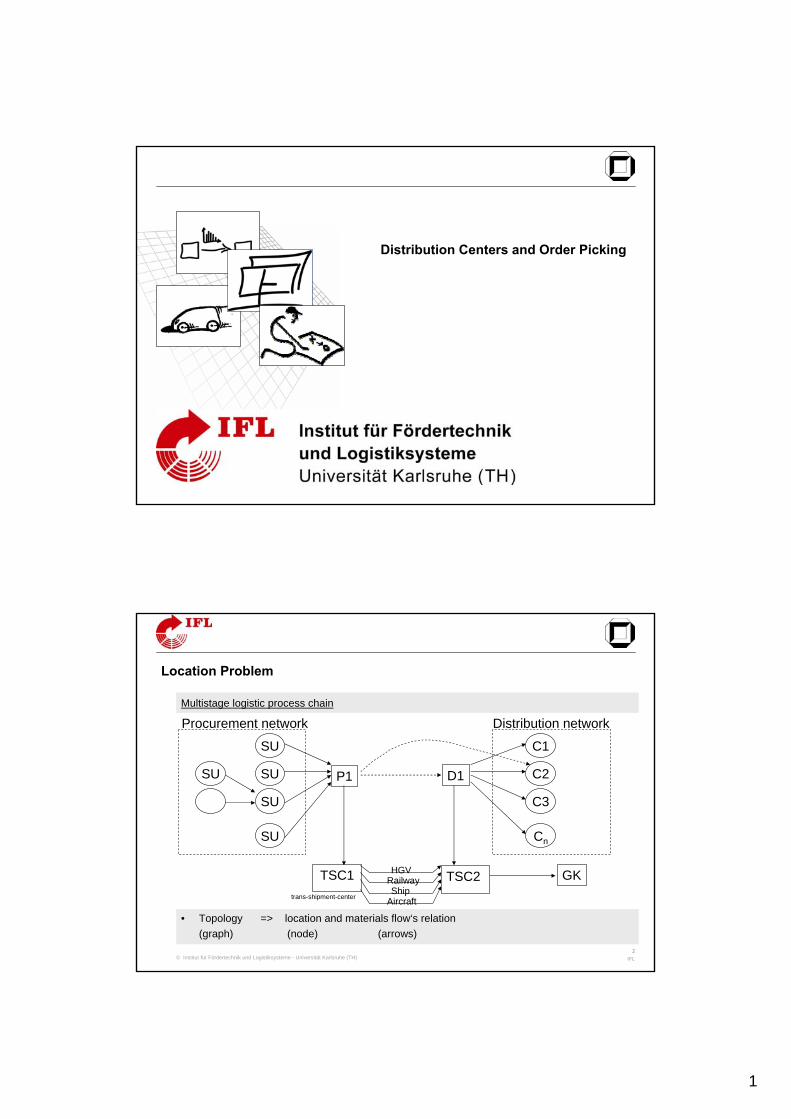
Multistage logistic process chain

• Topology => location and materials flow‘s relation(graph) (node) (arrows)

Procurement network Distribution network

SU

SU

SU

SU

SU

C1

P1 D1 C2

C3

Cn

TSC1 GKHGVRailwayShip

Aircraft

Location Problem

TSC2trans-shipment-center

2


IFL

Definition: strategic decision about the geographic place and amount of locations (for production, warehousing, distribution, etc.)

Site-related factors:

• Basement and site

• Traffic and transport

• Infrastructure

• Labor force

• Procurement

• Turnover

• Tax

• etc.

Location Problem


IFL

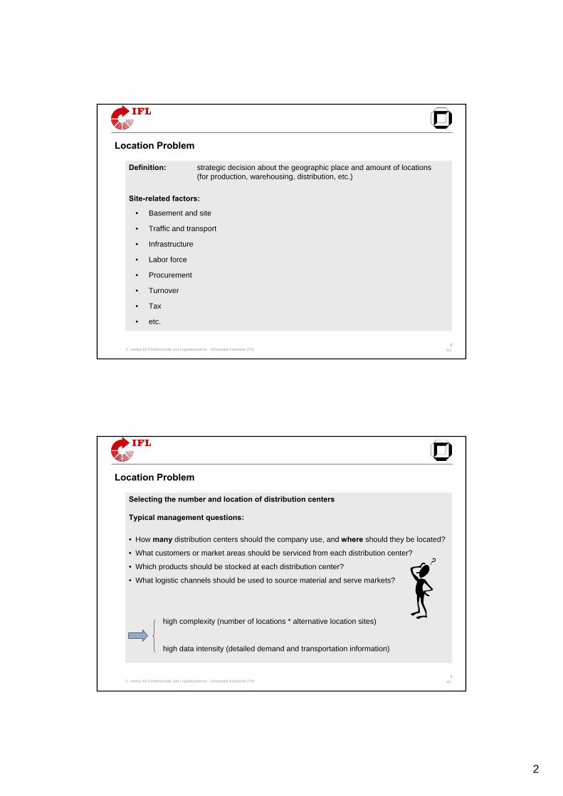
Selecting the number and location of distribution centers

Typical management questions:

• How many distribution centers should the company use, and where should they be located?

• What customers or market areas should be serviced from each distribution center?

• Which products should be stocked at each distribution center?

• What logistic channels should be used to source material and serve markets?

high complexity (number of locations * alternative location sites)

high data intensity (detailed demand and transportation information)

Location Problem

3


IFL

models and methods to solve the Warehouse Location Problem (WLP)

• analytic techniques

• linear programming techniques

• Simulation

Objective: Minimize the total costs

Examples: • continuous model (Steiner-Weber) (1)

• discrete model (2)

• Break-Even-Analysis (3)

Location Problem


IFL

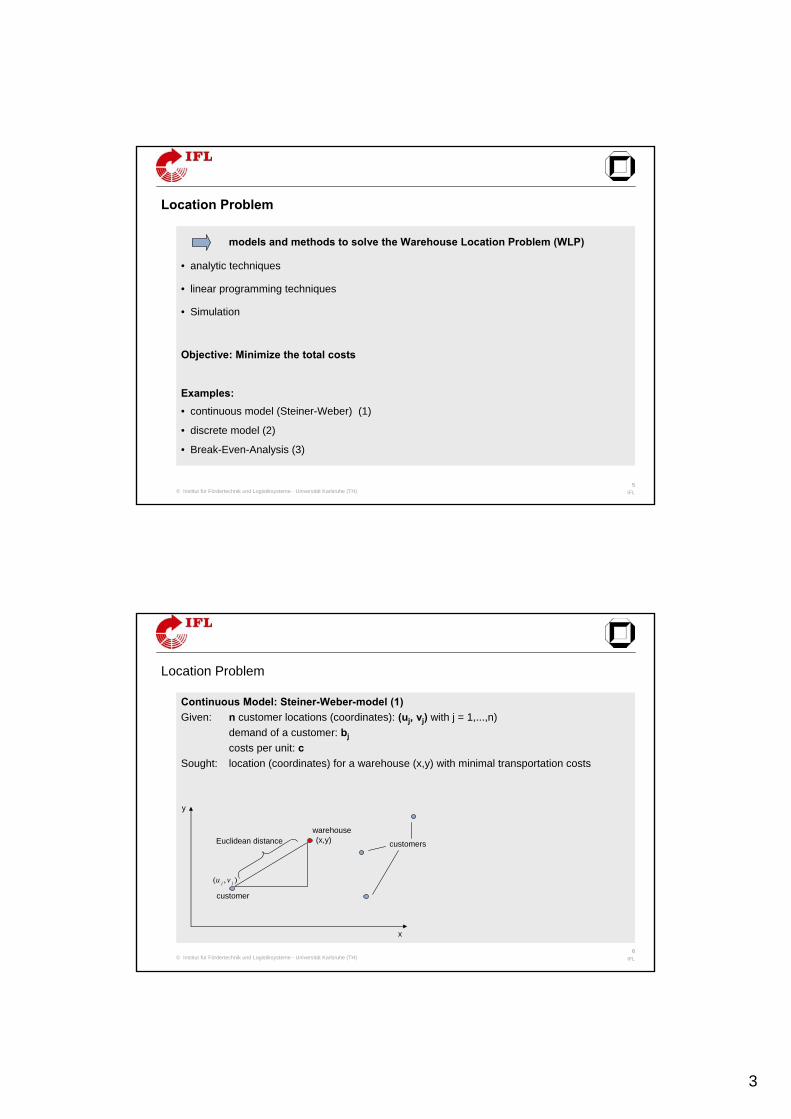
Continuous Model: Steiner-Weber-model (1)Given: n customer locations (coordinates): (uj, vj) with j = 1,...,n)

demand of a customer: bj

costs per unit: cSought: location (coordinates) for a warehouse (x,y) with minimal transportation costs

(x,y)

),( jj vu

warehouse

customer

Euclidean distance customers

x

y

Location Problem

4


IFL

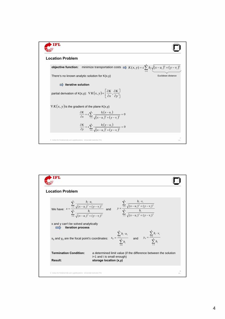
objective function: minimize transportation costs

There‘s no known analytic solution for K(x,y)

iterative solution

partial derivation of K(x,y):

is the gradient of the plane K(x,y)

( ) ( )22

1),( ii

n

ii vyuxbcyxK −+−= ∑

=

( ) ⎥⎦

⎤⎢⎣

⎡∂∂

∂∂

=∇yK

xKyxK ,,

( )yxK ,∇

( )( ) ( )

01

22=

−+−

−=

∂∂ ∑

=

n

i ii

ii

vyux

uxbcxK

( )( ) ( )

01

22=

−+−

−=

∂∂ ∑

=

n

i ii

ii

vyux

uybcyK

Location Problem

Euclidean distance


IFL

We have: and

x and y can’t be solved analyticallyiteration process

x0 and y0 are the focal point’s coordinates: and

Termination Condition: a determined limit value (if the difference between the solutioni+1 and i is small enough)

Result: storage location (x,y)

∑

∑

=

=

−+−

−+−

⋅

= n

i ii

i

n

i ii

ii

vyuxb

vyuxvb

y

122

122

)()(

)()(

∑

∑

=

=

−+−

−+−

⋅

= n

i ii

i

n

i ii

ii

vyuxb

vyuxub

x

122

122

)()(

)()(

∑

∑

=

=

⋅= n

ii

n

iii

b

ubx

1

10

∑

∑

=

=

⋅= n

ii

n

iii

b

vby

1

10

Location Problem

5


IFL

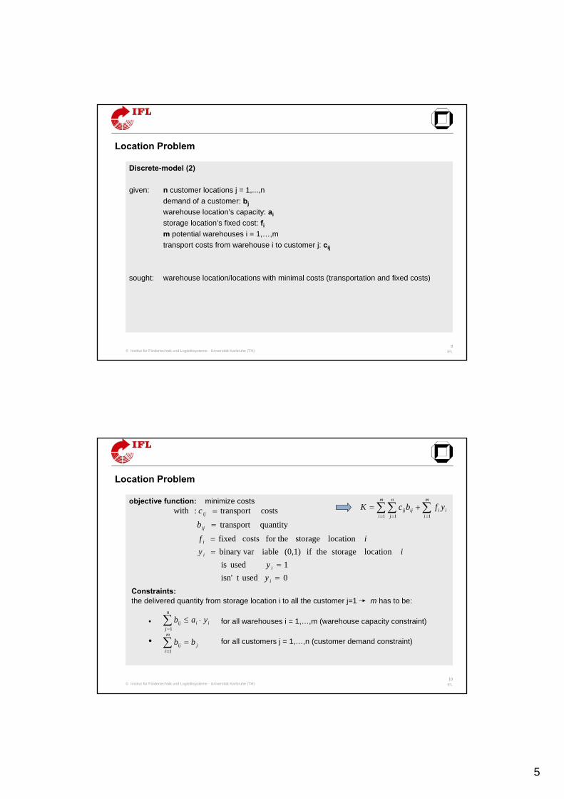
Discrete-model (2)

given: n customer locations j = 1,...,ndemand of a customer: bjwarehouse location’s capacity: ai

storage location’s fixed cost: fi

m potential warehouses i = 1,…,mtransport costs from warehouse i to customer j: cij

sought: warehouse location/locations with minimal costs (transportation and fixed costs)

Location Problem


IFL

objective function: minimize costsi

m

i

m

ii

n

jijij yfbcK ∑ ∑∑

= ==

+=1 11

0 usedt isn' 1 used is

location storage theif (0,1) iablebinary var location storage for the costs fixed

quantitytransport costs transport :with

==

==

=

=

i

i

i

i

ij

ij

yy

iyif

bc

Constraints:the delivered quantity from storage location i to all the customer j=1 m has to be:

• for all warehouses i = 1,…,m (warehouse capacity constraint)

• for all customers j = 1,…,n (customer demand constraint)

ii

n

jij yab ⋅≤∑

=1

j

m

iij bb =∑

=1

Location Problem

6


IFL

Break-Even-Analysis (3)

Basis: simplified costs’ consideration• Linear, static cost’s function• Fixed costs specific for a storage location: fi• Variable costs specific for a storage location (gradient αi)

Goods‘ quantity(production quantity)

Costs

0=f

1α

2α2f

1f

Break-Even

Outsourcing: product oriented, no fixed cost

Storage location 2

Storage location 1

So far there is no economic storage location=> outsourcing

Location Problem


IFL

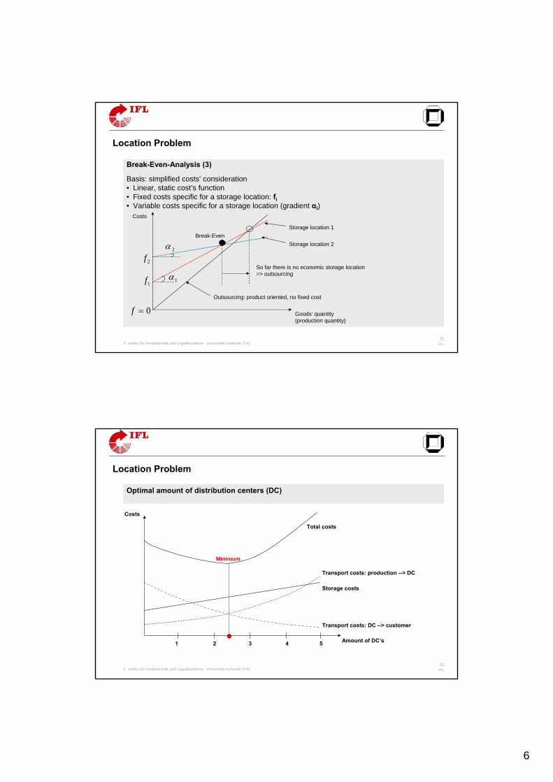
Optimal amount of distribution centers (DC)

Costs

Transport costs: DC --> customer

Transport costs: production --> DC

Storage costs

Total costs

Amount of DC‘s1 432

Minimum

Location Problem

5

7


IFL

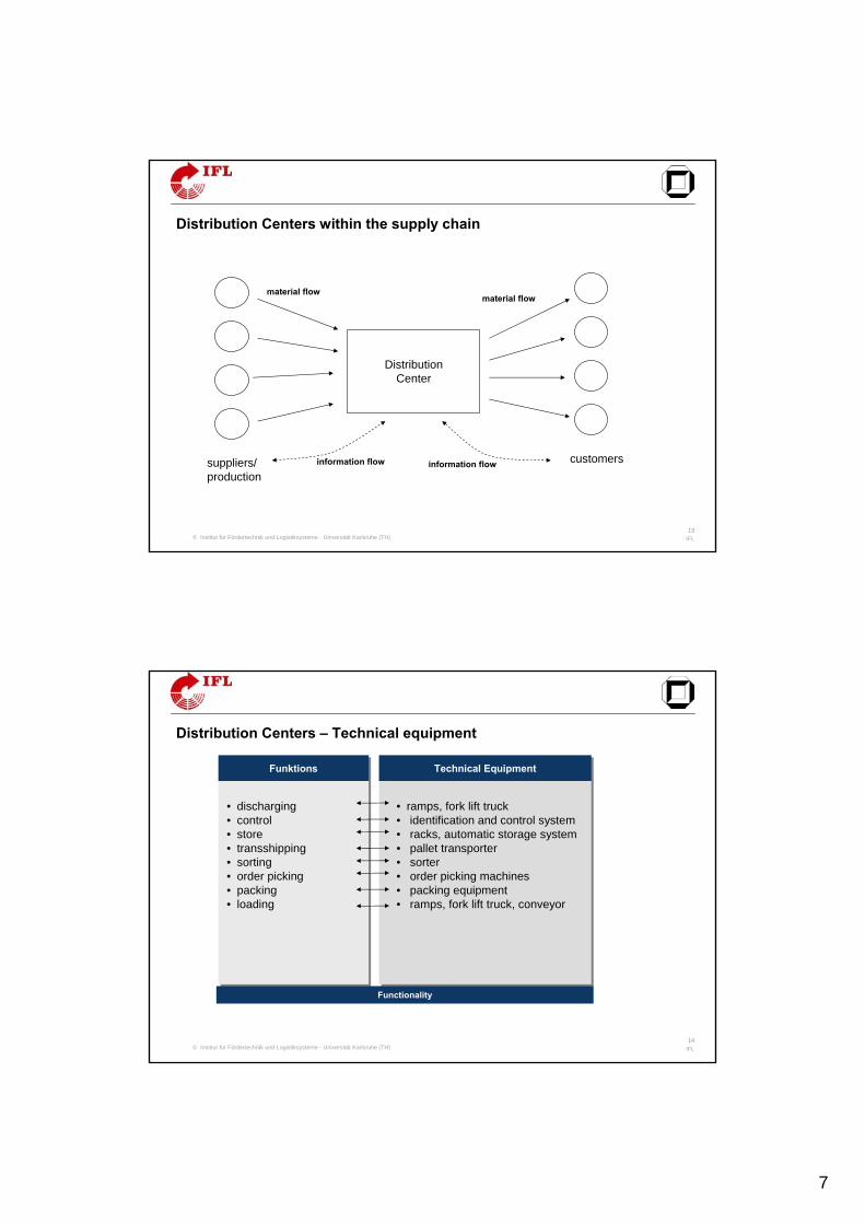
DistributionCenter

suppliers/production

customers

material flowmaterial flow

information flow information flow

Distribution Centers within the supply chain


IFL

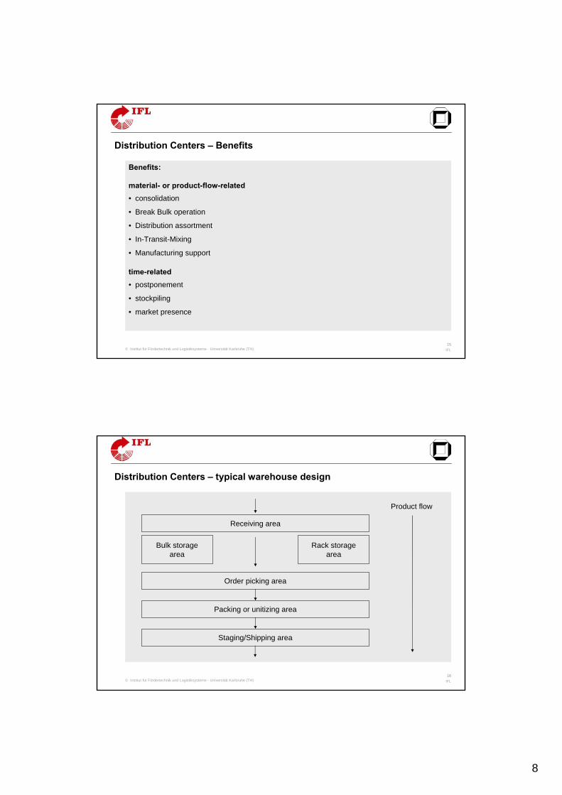
Distribution Centers – Technical equipment

Technical EquipmentTechnical EquipmentFunktions

• discharging• control• store• transshipping • sorting• order picking• packing• loading

• ramps, fork lift truck• identification and control system• racks, automatic storage system• pallet transporter• sorter• order picking machines• packing equipment• ramps, fork lift truck, conveyor

Functionality

8


IFL

Benefits:

material- or product-flow-related• consolidation

• Break Bulk operation

• Distribution assortment

• In-Transit-Mixing

• Manufacturing support

time-related• postponement

• stockpiling

• market presence

Distribution Centers – Benefits


IFL

Receiving area

Bulk storagearea

Rack storagearea

Staging/Shipping area

Packing or unitizing area

Order picking area

Product flow

Distribution Centers – typical warehouse design

9


IFL

a) b)

cost

s

timedeliveryb

K LK G

KBb

stoc

k

quantity delivered

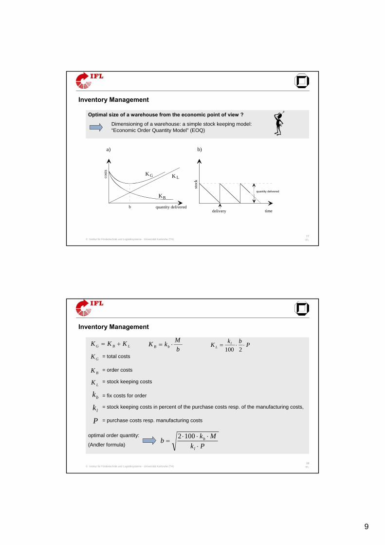
Optimal size of a warehouse from the economic point of view ?

Dimensioning of a warehouse: a simple stock keeping model:“Economic Order Quantity Model” (EOQ)

Inventory Management

quantity delivered


IFL

optimal order quantity:

(Andler formula)

LBG KKK +=bMkK bB ⋅= PbkK l

L ⋅⋅=2100

GK

bk

BK

lk

= total costs

= order costs

LK = stock keeping costs

= fix costs for order

= stock keeping costs in percent of the purchase costs resp. of the manufacturing costs,

PkMkb

l

b

⋅⋅⋅⋅

=1002


P = purchase costs resp. manufacturing costs

10


IFL

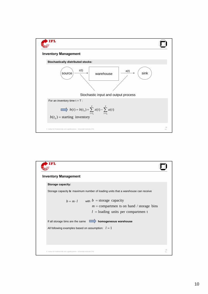
Stochastically distributed stocks:

warehousesource sinkz(t) a(t)

Stochastic input and output processFor an inventory time t = T :

∑ ∑= =

−+=T

tt

T

tt

tatztbtb0 0

)()()()( 0

inventory starting )( 0 =tb



IFL

Storage capacity:

Storage capacity b: maximum number of loading units that a warehouse can receive

with

If all storage bins are the same homogeneous warehouse

All following examples based on assumption:

tcompartmenper units loading bins storage / handon tscompartmen

capacity storage

===

lmblmb ⋅=

1=l


11


IFL

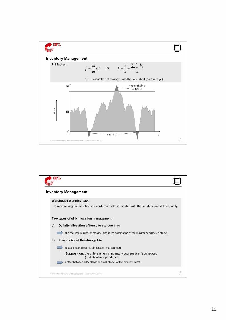
Fill factor :or

= number of storage bins that are filled (on average)

1≤=mmf

b

b

bbf

k

j j∑ === 1

m

t

m

0

not availablecapacity

shortfall

stoc

k


m


IFL

Warehouse planning task:

Dimensioning the warehouse in order to make it useable with the smallest possible capacity

Two types of of bin location management:

a) Definite allocation of items to storage bins

the required number of storage bins is the summation of the maximum expected stocks

b) Free choice of the storage bin

chaotic resp. dynamic bin location management

Supposition: the different item‘s inventory courses aren‘t correlated (statistical independence)

Offset between either large or small stocks of the different items


12


IFL

Warehouse planning task:

i. Stock analysis (observed values, forecast values)

ii. Stationary distribution of the stock referring to the items can be derived

iii. Analysis of the stock distributions for each item

- mean value, variance, variation coefficient

Planning the warehouse‘s dimension so that it is able to receive goods(with a given statistical security)

)( jbf



IFL

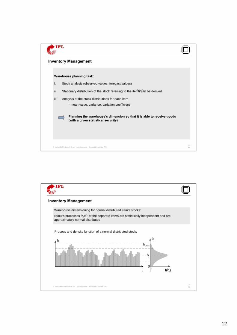
Warehouse dimensioning for normal distributed item’s stocks:

Stock’s processes of the separate items are statistically independent and are approximately normal distributed

)(tb j

bj

f(bj)t

bjbj

bj,max

bj

0

Process and density function of a normal distributed stock:


13


IFL

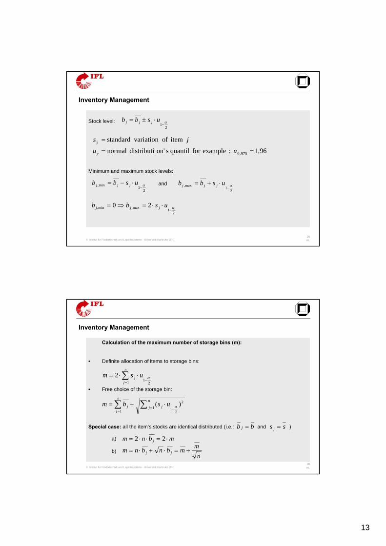
Stock level:

Minimum and maximum stock levels:

and

21 α−

⋅±= usbb jjj

96,1 :examplefor quantil son'distributi normal

item of variationstandard

975,0

j

==

=

uu

js

γ

21min, α−

⋅−= usbb jjj2

1max, α−

⋅+= usbb jjj

21max,min 20 α−

⋅⋅=⇒= usbb jjj,



IFL

Calculation of the maximum number of storage bins (m):

• Definite allocation of items to storage bins:

• Free choice of the storage bin:

Special case: all the item’s stocks are identical distributed (i.e.: and )

a)

b)

∑= −

⋅⋅=n

jj usm

1 21

2 α

∑∑ = −=

⋅+=n

j j

n

jj usbm

12

211

)( α

mbnm j ⋅=⋅⋅= 22

nmmbnbnm jj +=⋅+⋅=


bb j = ss j =

14


IFL

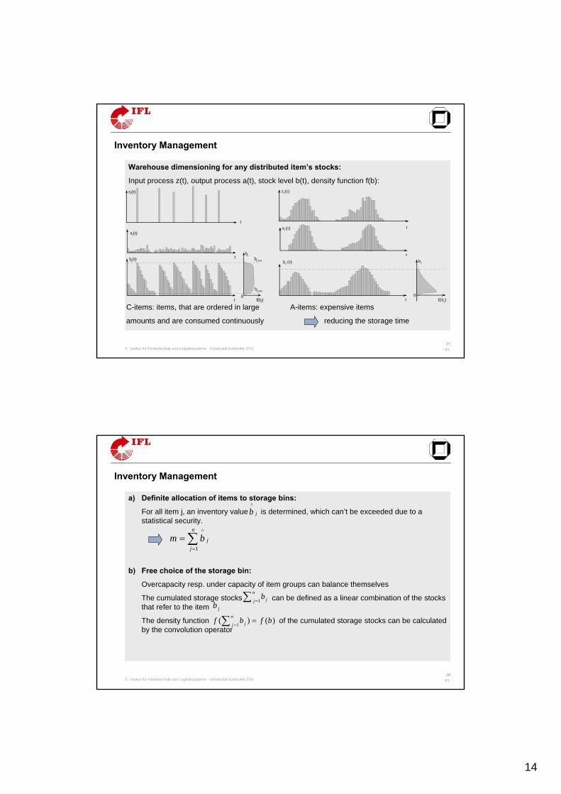
Warehouse dimensioning for any distributed item’s stocks:

Input process z(t), output process a(t), stock level b(t), density function f(b):

t

(t)

(t)

t

t

bj

bj

f(bj)

bj,max

0

aj

zj

(t)

bj,min

t

(t)

(t)

taj

zj

t

bjbj

f(bj)0

(t)

C-items: items, that are ordered in large

amounts and are consumed continuously

A-items: expensive items

reducing the storage time



IFL

a) Definite allocation of items to storage bins:

For all item j, an inventory value is determined, which can’t be exceeded due to a statistical security.

b) Free choice of the storage bin:

Overcapacity resp. under capacity of item groups can balance themselves

The cumulated storage stocks can be defined as a linear combination of the stocks that refer to the item

The density function of the cumulated storage stocks can be calculated by the convolution operator

jb^

∑=

=n

jjbm

1

^

∑ =

n

j jb1

jb

)()(1

bfbf n

j j =∑ =


15


IFL

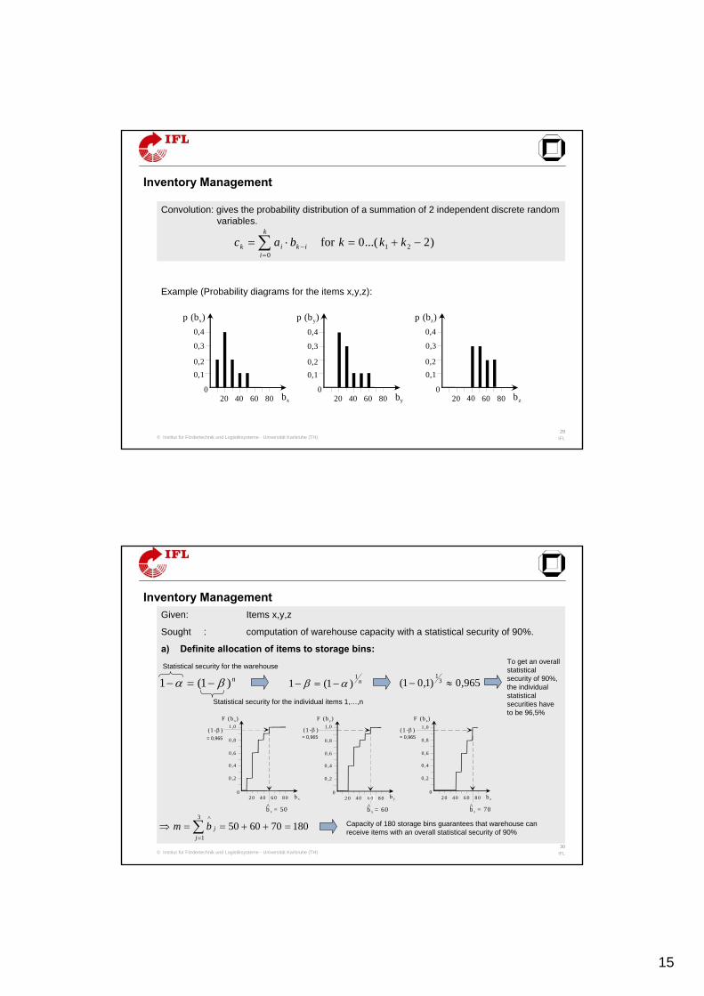
Convolution: gives the probability distribution of a summation of 2 independent discrete random variables.

)2...(0for 210

−+=⋅= −=∑ kkkbac ik

k

iik

p (bx)

20 40 60 80

0,10,2

0,3

0,4

bx

0

p (by)

20 40 60 80

0,10,2

0,3

0,4

by

0

p (bz)

20 40 60 80

0,10,2

0,3

0,4

bz

0

Example (Probability diagrams for the items x,y,z):



IFL

Given: Items x,y,z

Sought : computation of warehouse capacity with a statistical security of 90%.

a) Definite allocation of items to storage bins:

n)1(1 βα −=− n1

)1(1 αβ −=−

1807060503

1

^=++==⇒ ∑

=jjbm

6 0

F (b x)

2 0 4 0 6 0 8 0

0 ,2

0 ,4

b x

0

0 ,6

0 ,8

1 ,0F (b y)

b y2 0 4 0 8 0

0 ,2

0 ,4

0

0 ,6

0 ,8

1 ,0F (b z)

b z2 0 4 0 6 0 8 0

0 ,2

0 ,4

0

0 ,6

0 ,8

1 ,0(1 -β )

b̂ = 50x b̂ = 60y b̂ = 70z

(1 -β )(1 -β )


965,0)1,01( 31≈−

Statistical security for the warehouse

Statistical security for the individual items 1,…,n

Capacity of 180 storage bins guarantees that warehouse canreceive items with an overall statistical security of 90%

To get an overallstatisticalsecurity of 90%, the individualstatisticalsecurities haveto be 96,5%

= 0,965 = 0,965 = 0,965

16


IFL

b) Free choice of the storage bin:

)()()()( zybb

x

z

xjj bPbPbPbbP

z

xj j

∑∑∑

===

==

)()( bpbpc z =⊗

cbpbp yx =

⎟⎟⎟⎟⎟⎟⎟⎟⎟⎟⎟⎟⎟

⎠

⎞

⎜⎜⎜⎜⎜⎜⎜⎜⎜⎜⎜⎜⎜

⎝

⎛

=

⎟⎟⎟⎟⎟⎟

⎠

⎞

⎜⎜⎜⎜⎜⎜

⎝

⎛

⊗

⎟⎟⎟⎟⎟⎟

⎠

⎞

⎜⎜⎜⎜⎜⎜

⎝

⎛

=⊗

01,002,004,010,015,016,022,022,008,0

1,01,01,03,04,0

1,01,02,04,02,0

)()(



IFL

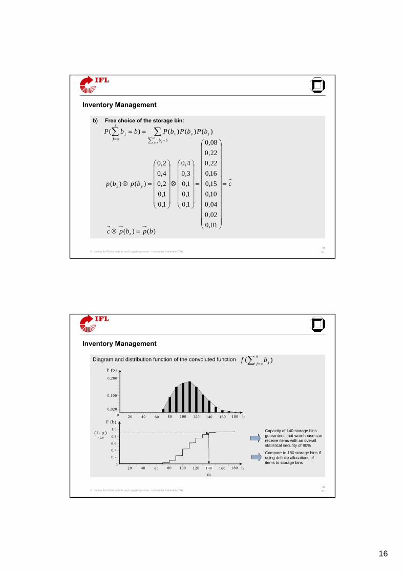
Diagram and distribution function of the convoluted function

F (b)

0,2

0,4

0

0,6

0 ,8

1 ,0

P (b)

20 40 60 80

b

bm

(1- α )

100 120 160 180

0,200

0 20 40 60 80 100 120 140 160 180

0,020

0,100

140

a)

b)

)(∑ =

n

xj jbf


= 0,9

Capacity of 140 storage binsguarantees that warehouse canreceive items with an overallstatistical security of 90%

Compare to 180 storage bins ifusing definite allocations of items to storage bins

17


IFL

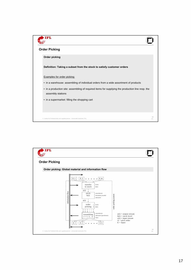
Order picking

Definition: Taking a subset from the stock to satisfy customer orders

Examples for order picking:

• in a warehouse: assembling of individual orders from a wide assortment of products

• in a production site: assembling of required items for supplying the production line resp. the

assembly stations

• in a supermarket: filling the shopping cart

Order Picking


IFL

routstim e

assortm entinventory m odelam ounts

routstim e

assortm entam ounts (positions)tim e

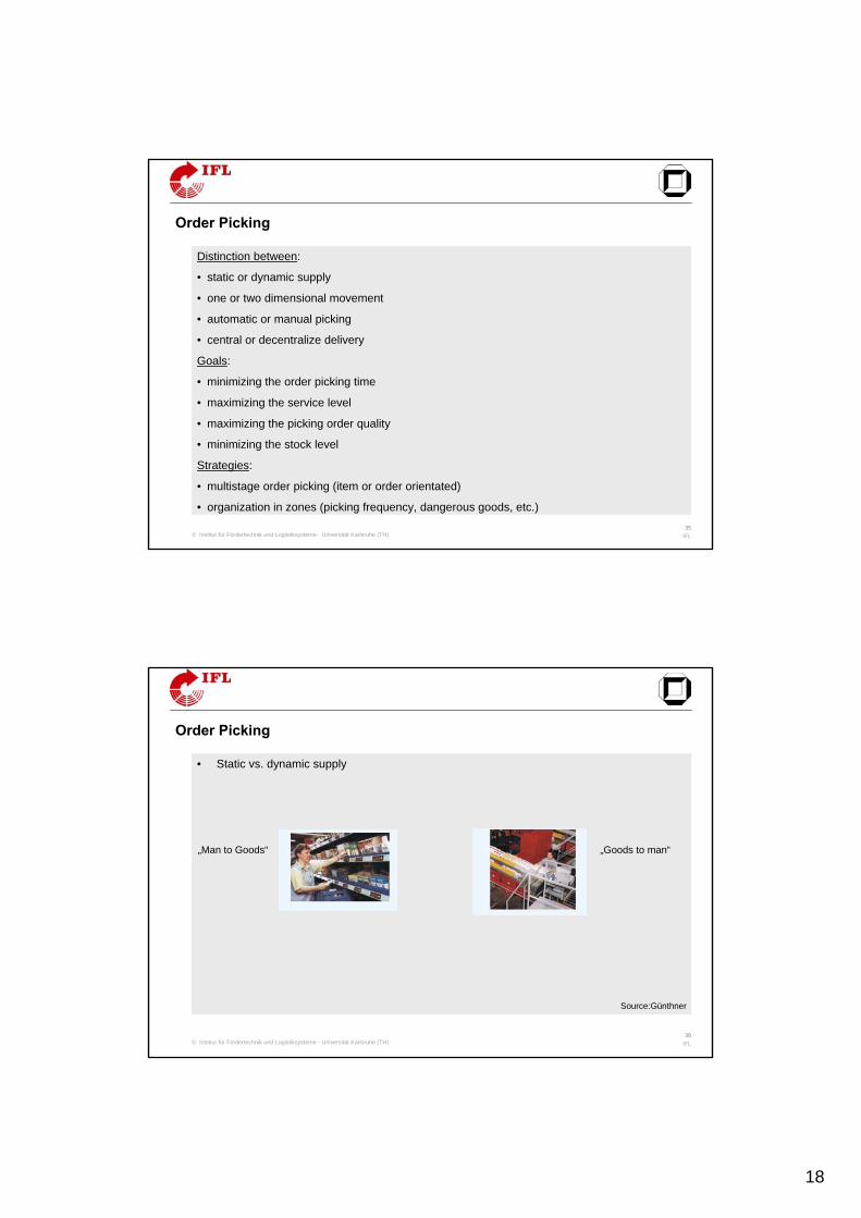
z(t)

a(t)

info

rmat

ion

flow

orde

r pic

king

syst

em

stockb(t)

orderpicking

assem blingr = 1, 2,...n

transferto stock

E mE 2E 1 . . . . .

. . . . .A 1 A 2 A k

a(t) = output streamb(t) = stock levelz(t) = input streamA = pick orderE = input

Order picking: Global material and information flow

Order Picking

18


IFL

Distinction between:

• static or dynamic supply

• one or two dimensional movement

• automatic or manual picking

• central or decentralize delivery

Goals:

• minimizing the order picking time

• maximizing the service level

• maximizing the picking order quality

• minimizing the stock level

Strategies:

• multistage order picking (item or order orientated)

• organization in zones (picking frequency, dangerous goods, etc.)

Order Picking


IFL

Order Picking

• Static vs. dynamic supply

Source:Günthner

„Man to Goods“ „Goods to man“

19


IFL

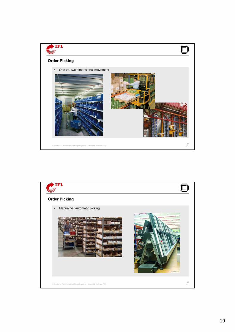
Order Picking

• One vs. two dimensional movement


IFL

Order Picking

• Manual vs. automatic picking

20


IFL

Order Picking

• central vs. decentralized delivery

Base Station


IFL

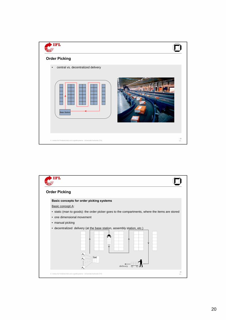
Basic concepts for order picking systems

Basic concept A:

• static (man to goods): the order picker goes to the compartments, where the items are stored

• one dimensional movement

• manual picking

• decentralized delivery (at the base station, assembly station, etc.)

delivery

Order Picking

21


IFL

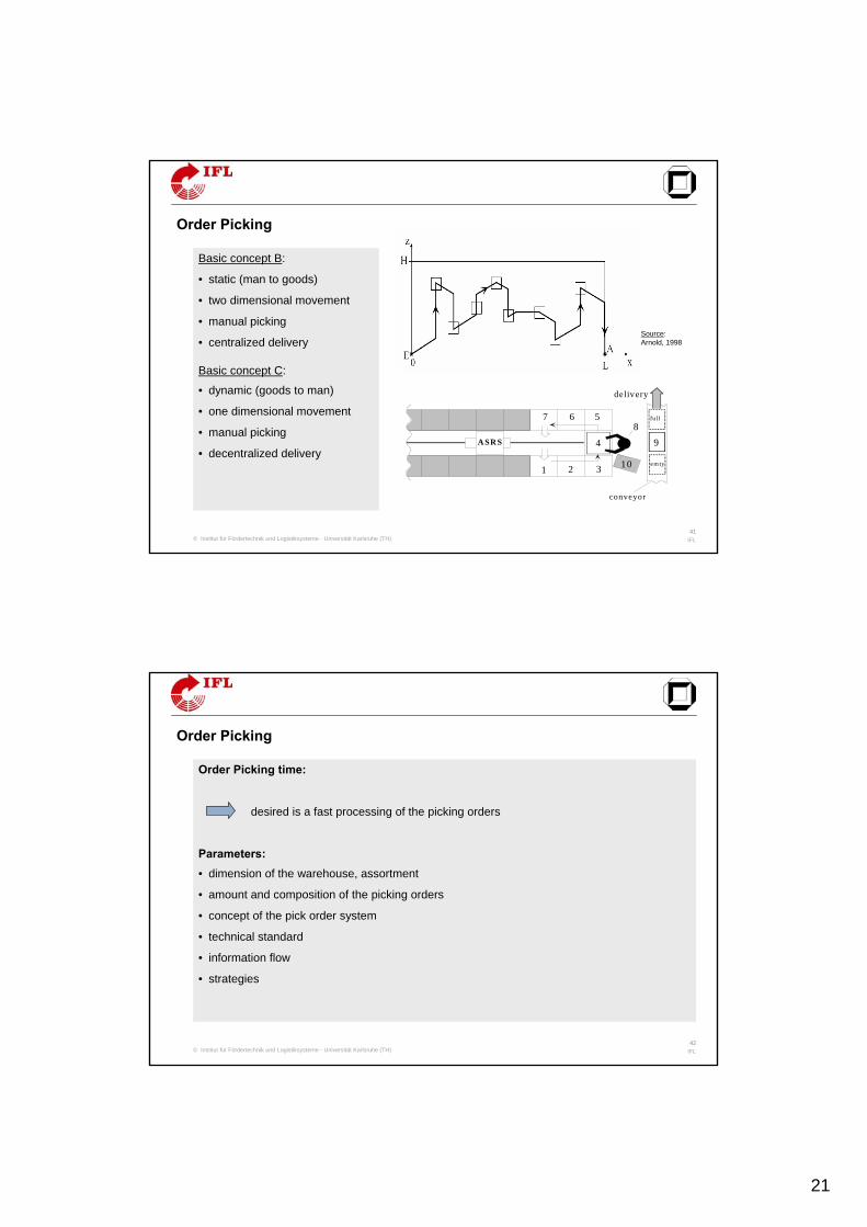
Basic concept B:

• static (man to goods)

• two dimensional movement

• manual picking

• centralized delivery

Basic concept C:

• dynamic (goods to man)

• one dimensional movement

• manual picking

• decentralized delivery1 2 3

4

5678

9A SR S

delivery

conveyor

10

full

em ty

Order Picking

Source: Arnold, 1998


IFL

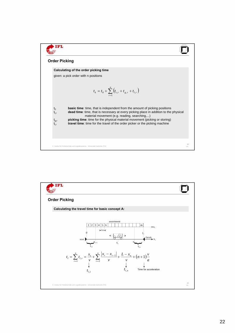
Order Picking time:

desired is a fast processing of the picking orders

Parameters:• dimension of the warehouse, assortment

• amount and composition of the picking orders

• concept of the pick order system

• technical standard

• information flow

• strategies

Order Picking

22


IFL

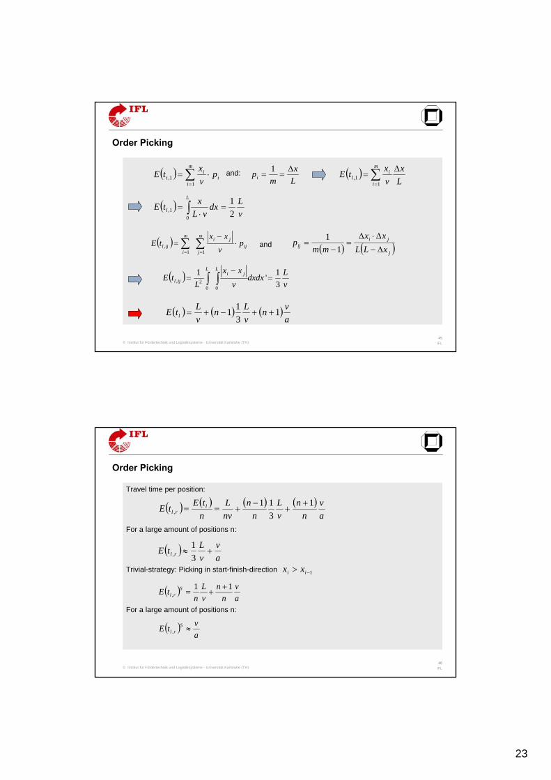
Calculating of the order picking time

given: a pick order with n positions

t0 basic time: time, that is independent from the amount of picking positionstt,r dead time: time, that is necessary at every picking place in addition to the physical

material movement (e.g. reading, searching,...)tg,r picking time: time for the physical material movement (picking or storing)tl,r travel time: time for the travel of the order picker or the picking machine

( )∑=

+++=n

rrlrgrtk ttttt

1,,,0

Order Picking


IFL

Calculating the travel time for basic concept A:

1 2 3 4 5 6 massortment

Δx

startfinish

tl,1

xr=1 xrxr=n

tl,n

xr

xi

L0

{{

( )∑ ∑= =

− ++−

+−

+==n

r

nn

r

rrrll a

vnv

xLvxx

vxtt

1 2

11, 1

1,lt nlt , Time for acceleration

Order Picking

23


IFL

and:

and

( ) i

m

i

it p

vxtE ⋅= ∑

=11, L

xm

piΔ

==1 ( )

Lx

vxtE

m

i

il

Δ= ∑

=11,

( )vLdx

vLxtE

L

l 21

01, =

⋅= ∫

( ) ij

m

j

jim

iijl p

vxx

tE ⋅−

= ∑∑== 11

, ( ) ( )j

jiij xLL

xxmm

pΔ−

Δ⋅Δ=

−=

11

( )vLdxdx

vxx

LtE

Lji

L

ijl 31'1

002, =

−= ∫∫

( ) ( ) ( )avn

vLn

vLtE l 1

311 ++−+=

Order Picking


IFL

Travel time per position:

For a large amount of positions n:

Trivial-strategy: Picking in start-finish-direction

For a large amount of positions n:

( ) ( ) ( ) ( )av

nn

vL

nn

nvL

ntEtE l

rl1

311

,+

+−

+==

( )av

vLtE rl +≈

31

,

1−> ii xx

( )av

nn

vL

ntE S

rl11

,+

+=

( )avtE S

rl ≈,

Order Picking

24


IFL

Sequence problem

given: amount of compartments

sought: sequence of compartments, so that the required travel time is minimal

Problems:

• distance measuring

• often several order pickers are in activity. This can lead to disruptions

Solution:

different Strategies (e.g. Mäander-Strategy, Largest-Gap-Strategy, diverse algorithms for routing, ...)

Order Picking


IFL

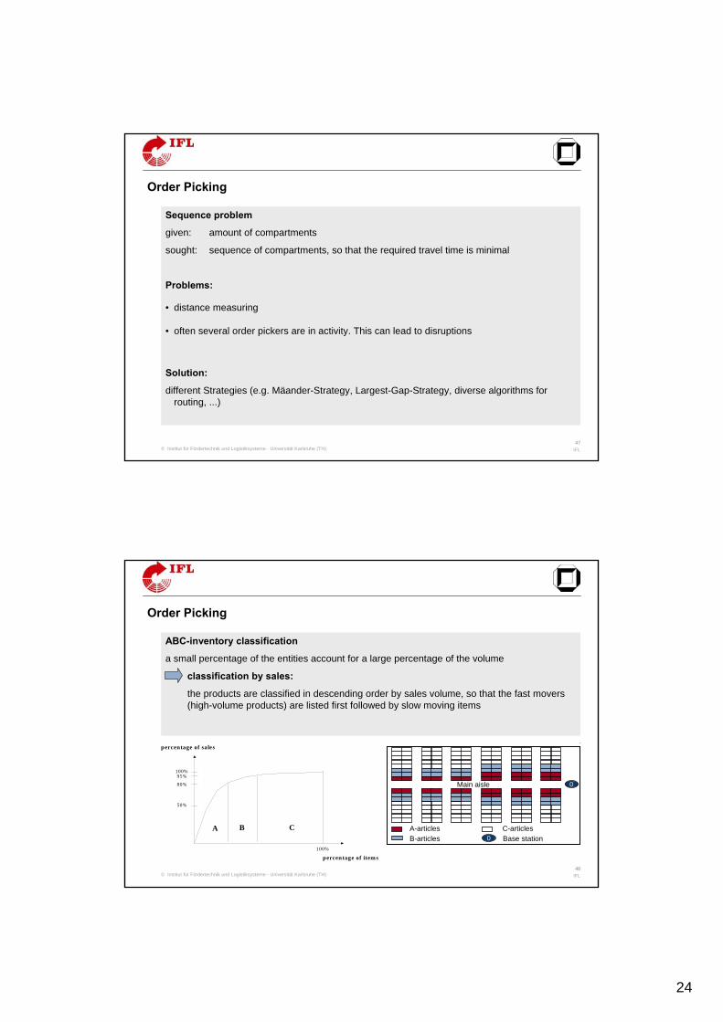
ABC-inventory classification

a small percentage of the entities account for a large percentage of the volume

classification by sales:

the products are classified in descending order by sales volume, so that the fast movers (high-volume products) are listed first followed by slow moving items

100%

50%

80%

95%

A B C

percentage of sales

percentage of items100%

Order Picking

B-articles

Main aisle

C-articlesA-articlesBase station0

0

Documents

Vorlesung Teil 3 Distribution Centers and Order Picking