Wage Drift, Immigration, and Union Behavior∗

Max Alberta and Jürgen Mecklb

[a] Department of Economics, University of Saarbrücken, PO–Box 151150,

D–66041 Saarbrücken, Germany, E-mail: max.albert@mx.uni-saarbrücken.de.

[b] Department of Economics, University of Giessen, Licher Str. 66, D–35394

Giessen, Germany, E-mail: juergen.meckl@wirtschaft.uni-giessen.de.

Preliminary Version, May 30, 2006

Abstract

We analyze the effect of immigration on employment in a model ac-counting for the wage–drift phenomenon (the positive relationship be-tween the minimum wage and the aggregate wage span) that char-acterizes the German labor market. Wage drift is explained by anemployment magnification effect resulting from structural shifts ofemployment. The presence of the magnification effect has surpris-ing implications for the impact of immigration on employment andon unions’ wage claims. For plausible parameter values, immigrationraises employment of the home labor force even if all immigrants findemployment, and immigration is not expected to act as a disciplinarydevice for unions.

Keywords: immigration, unemployment, efficiency wage, wage drift,wage span

JEL classifications: F11, F22, J31, J64

∗We are grateful to Elke Amend, Lucas Bretschger, Christian Lumpe, Stefanie Mehret,and Benjamin Weigert for useful hints and comments.

1

1 Introduction

Immigration of labor is widely considered as a threat to the labor–marketprospects of the home labor force. Native workers directly competing withimmigrants typically fear an erosion of their wage incomes or even a lossof their jobs. In labor markets where union behavior plays an importantrole in the determination of wages, the impact of immigration decisivelydepends on how unions’ wage policies react to immigration. Unions aretypically expected to be disciplined by immigration when native workers arereplaced by immigrants and thus either become unemployed (Schmidt, Stilz& Zimmermann, 1994; Bauer & Zimmermann, 1997) or are forced to applyfor low–wage jobs in a secondary labor market (Fuest & Thum, 2000, 2001).

The present paper argues that at the outset it is not clear whether immi-gration disciplines unions in such a way that they reduce their wage claimsin favor of native workers’ employment prospects.1 We work out how unions’preferences about the wage income of workers and unemployment determinethe reaction of wage claims to immigration. Taking additional stylized factsof the German labor market into account, our theoretical analysis of thelabor market effects of immigration casts doubts on the relevance of thereplacement effect of immigration. A more aggressive wage policy becomesplausible once immigration raises employment chances of native workers. Weshow that a seemingly unrelated phenomenon, wage drift, is relevant for theexistence of a replacement effect.

We analyze the effects of immigration on wages and employment in asimplified model of a small open economy. We assume that unemploymentis mainly caused by downward rigidity of wages due to minimum wages.2

1The disciplinary force of the replacement effect may be also reduced or even reversedif unions represent the interests of heterogeneous groups of labor, e.g. skilled and unskilledlabor (Schmidt et al., 1994). The present paper complements this analysis by arguingthat such an augmentation of union interests is not necessary for immigration to inducemore aggressive wage claims. Unions may react to immigration with more aggressive wageclaims even if labor is homogeneous.

2The institutional differences between minimum wages and German “Tariflöhne” are ofno importance in our context. Since we refer to data for West Germany only, we shouldproperly write West Germany rather than Germany throughout.

1

However, although there is unemployment, wages typically are higher thanthe legal minimum; (relative) wage spans (w − wmin)/wmin, with w as theactual wage and wmin as the minimum wage, are positive. As has beenrecognized by Gahlen & Ramser (1987) and Schlicht (1992), positive wagespans can be explained by assuming that the minimum wage influences thestandard of fairness in an Akerlof–Yellen efficiency–wage model (Akerlof,1982; Akerlof & Yellen, 1990).

The efficiency–wage approach of Gahlen & Ramser and Schlicht impliesthat wage spans fall if the minimum wage rises. However, as these authorshave already noted themselves, aggregate data on Germany show that the av-erage wage span increased with the minimum wage for the 1970ies and 80ies.Using slightly different data, we find qualitatively the same result (see ap-pendix): the elasticity of the average wage with respect to the minimum wageis greater than 1, which means that the average wage span (w −wmin)/wmin

rises with wmin. This phenomenon is called (positive) wage drift. In recentyears, however, wage spans seem to have fallen with the minimum wage ?implying a negative wage drift.

Schlicht (1992) attributes a positive wage drift, which is inconsistent withthe results from his one–sector model, to effects of aggregation. This is a rea-sonable explanation. It is well known that there are persistent intersectoralwage differentials. If a rise of the minimum wage shifts employment to high–wage sectors, the average wage can increase relative to the minimum wageeven if wage spans fall in every sector.

If such an explanation is correct, however, further, more surprising con-sequences will follow. Raising the minimum wage leads to an increase ofunemployment even in a one–sector model. The shift of employment fromlow–wage to high–wage sectors in a multisectoral model magnifies this ef-fect because, as Albert & Meckl (2001a,b) have shown for similar models,high–wage sectors contribute relatively more to unemployment than low–wage sectors. Immigration has the opposite effect. It would lead to moreemployment even in a one–sector model. In a multisectoral model with wagedrift, immigration shifts employment from high–wage to low–wage sectors,implying an employment magnification effect. The surprising result is that,for plausible values of the relevant parameters, the employment magnifica-

2

tion effect implies more employment for the home labor force even if allimmigrants find employment.

This is the opposite of the replacement effect. It is obvious that unionswith sufficient preferences for the income of employed workers have an in-centive to appropriate at least some of the efficiency gains of immigration byraising the minimum wage. But also in a negative wage drift regime unionsmay react with aggressive wage claims to immigration if unions put consid-erable weight on employment. This counterintuitive result follows from theproperty of the negative–wage–drift regime where a rise in minimum wagesgenerates an increase in aggregate employment by appropriate adjustment ofthe economy’s sectoral structure.

The paper proceeds as follows. Section 2 introduces the model. Section3 analyzes the effects of a change in minimum wages and of immigration.Section 4 considers union behavior in the presence of immigration. Section5 concludes. The appendix reports a regression analysis demonstrating wagedrift on the German labor market for the period from 1970 to 1995.

2 The Model

We consider an economy that can produce up to n ≥ 2 goods using laborand m = n − 1 non-labor factors of production. The labor supply L > 0 isexogenous, and the endowments vi of non-labor factors are fixed. There isfree trade in goods and perfect competition in all markets except the labormarket, where a minimum wage wmin > 0 exists. Goods prices pj are fixedon world markets. The vector of goods prices is p. The vector of non-laborendowments is v, and the vector of respective factor prices, r, is determinedon perfectly competitive national markets. Sectoral production functions fj,j = 1, . . . , n, are nondecreasing, concave, and linearly homogeneous in factorinputs.

2.1 Efficiency–Wage Setting

Each worker supplies one unit of labor. One cause of involuntary unemploy-ment is a minimum wage, which is determined by some centralized wage–

3

setting process. For the moment, we take the minimum wage as exogenouslygiven. We incorporate efficiency wages as a second cause of unemploymentin order to make the model consistent with two important stylized facts: thepersistence of intersectoral wage differentials over time, and the existence ofa positive span between minimum wages and effective wages (wage span).Our efficiency–wage approach is summarized in the following assumptions.

Assumption 1 The sectoral labor input in efficiency units is gj(wj/`)Lj,where ` is a reference wage against which workers measure the wage offer wj

of sector j’s representative firm.

Assumption 2 The function gj is strictly increasing and strictly concavewith gj(1) = 0 and limx→∞ g′j(x) = 0.

These assumptions capture the essentials of Schlicht’s (1992) modificationof the fair–wage approach of Akerlof (1982) and Akerlof & Yellen (1990).When deciding about their effort, workers respect a fairness norm. Theeffort required by this norm is assumed to depend on the employer’s wageoffer wj and a reference wage `. Effort actually supplied by a worker isthen an increasing function of the relative wage wj/`. Following a suggestionby Layard, Nickell & Jackmann (1994, 37), we assume that the relationbetween the productivity of labor and effort—just like any other productionfunction—is sector–specific.

The technical assumptions on the shape of gj are standard and give riseto proposition 1.

Proposition 1 Efficient sectoral wages are uniquely determined by a fixedand sector–specific markup qj > 0 on the reference wage: wj = (1 + qj)`.

Proof . A competitive firm facing a given minimum wage wmin and givenprices for other factors of production chooses a wage offer wj minimizing thecosts wj/gj(wj/`) of labor in efficiency units. It is necessary and sufficientfor a solution that the elasticity of the function gj is equal to 1 (Solow, 1979).In view of assumption 2, this is true at some unique value wj/` > 1. Hence,the cost–minimizing wage offer is wj = (1 + qj)` for some qj > 0.

4

On the basis of the chosen wage rate wj = (1+qj)` and corresponding pro-ductivity of labor gj

def= gj(1+qj), firms solve the standard cost–minimization

problem, treating the reference wage ` as a parameter:

bj(`, r)def= min

Lj ,vj≥0

{(1 + qj)`Lj + r.vj : fj(gjLj, v

j) ≥ 1}

(1)

This unit–cost function has all the standard properties. The envelope theo-rem implies

(a)∂bj

∂`= (1 + qj)aLj (b)

∂bj

∂rh

= ahj, h = 1, . . . ,m , (2)

where aLj is the input coefficients of labor and ahj is the input coefficient offlex–price factor h.

A major simplification in the presentation of results that are derived inthe following is achieved by a change of variables. Mainly for want of a betterword, we have opted for a name that has, at least, some mnemonic value.

Definition 1 The variable Njdef= (1 + qj)Lj is called the labor absorption of

sector j. The variable Ndef=

∑j Nj is called aggregate labor absorption.

We define production functions using the new variable:

fj(Nj, vj)

def= fj

[gjNj/(1 + qj), v

j]

(3)

This definition just hides the constants in fj and can be used to write theunit–cost function as:

bj(`, r) ≡ minNj ,vj≥0

{`Nj + r.vj : fj(Nj, v

j) ≥ 1}

(4)

Thus, the reference wage ` is the price of sectoral labor absorption, andabsorption enters the cost minimization problem in the same way as employ-ment does in the standard case. Input coefficients are given by the factor-price derivatives of bj; specifically, aNj(`, r)

def= ∂bj(`, r)/∂` is the input coeffi-

cient of labor absorption. The input coefficient of labor is aLj = aNj/(1+qj).Our specification of the reference wage is inspired by Schlicht (1992).

With

5

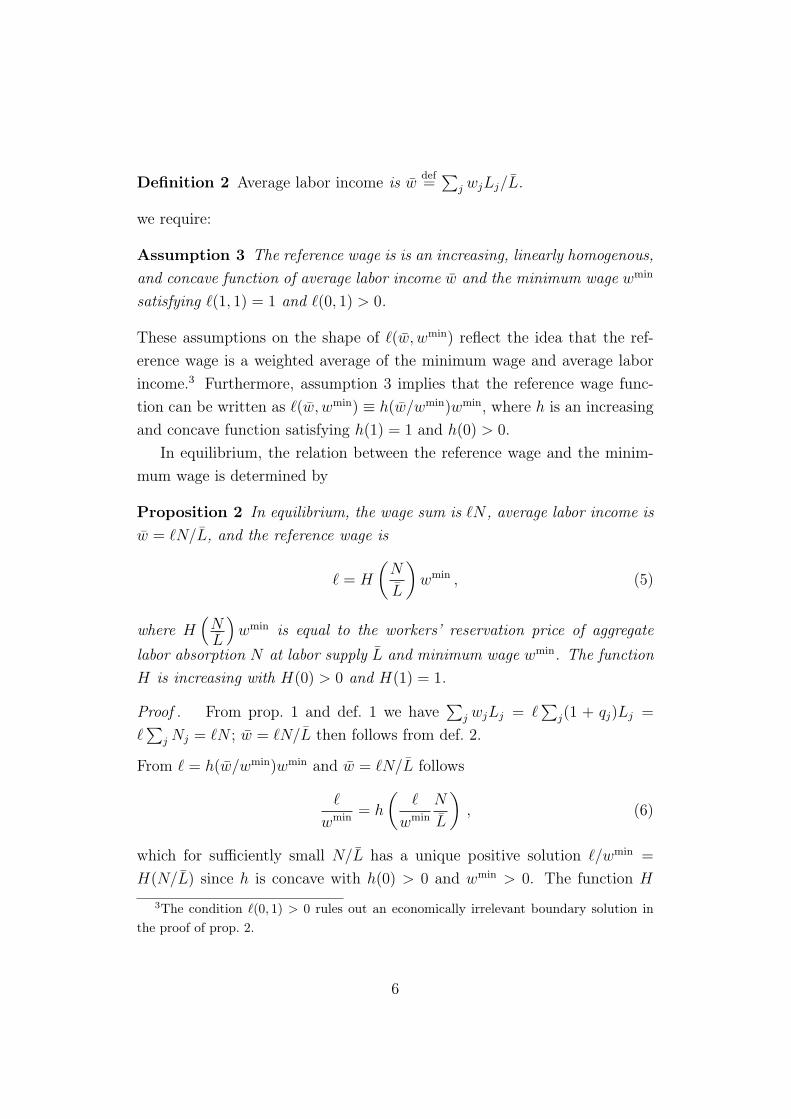
Definition 2 Average labor income is wdef=

∑j wjLj/L.

we require:

Assumption 3 The reference wage is is an increasing, linearly homogenous,and concave function of average labor income w and the minimum wage wmin

satisfying `(1, 1) = 1 and `(0, 1) > 0.

These assumptions on the shape of `(w, wmin) reflect the idea that the ref-erence wage is a weighted average of the minimum wage and average laborincome.3 Furthermore, assumption 3 implies that the reference wage func-tion can be written as `(w, wmin) ≡ h(w/wmin)wmin, where h is an increasingand concave function satisfying h(1) = 1 and h(0) > 0.

In equilibrium, the relation between the reference wage and the minim-mum wage is determined by

Proposition 2 In equilibrium, the wage sum is `N , average labor income isw = `N/L, and the reference wage is

` = H

(N

L

)wmin , (5)

where H(

NL

)wmin is equal to the workers’ reservation price of aggregate

labor absorption N at labor supply L and minimum wage wmin. The functionH is increasing with H(0) > 0 and H(1) = 1.

Proof . From prop. 1 and def. 1 we have∑

j wjLj = `∑

j(1 + qj)Lj =

`∑

j Nj = `N ; w = `N/L then follows from def. 2.

From ` = h(w/wmin)wmin and w = `N/L follows

`

wmin= h

(`

wmin

N

L

), (6)

which for sufficiently small N/L has a unique positive solution `/wmin =

H(N/L) since h is concave with h(0) > 0 and wmin > 0. The function H

3The condition `(0, 1) > 0 rules out an economically irrelevant boundary solution inthe proof of prop. 2.

6

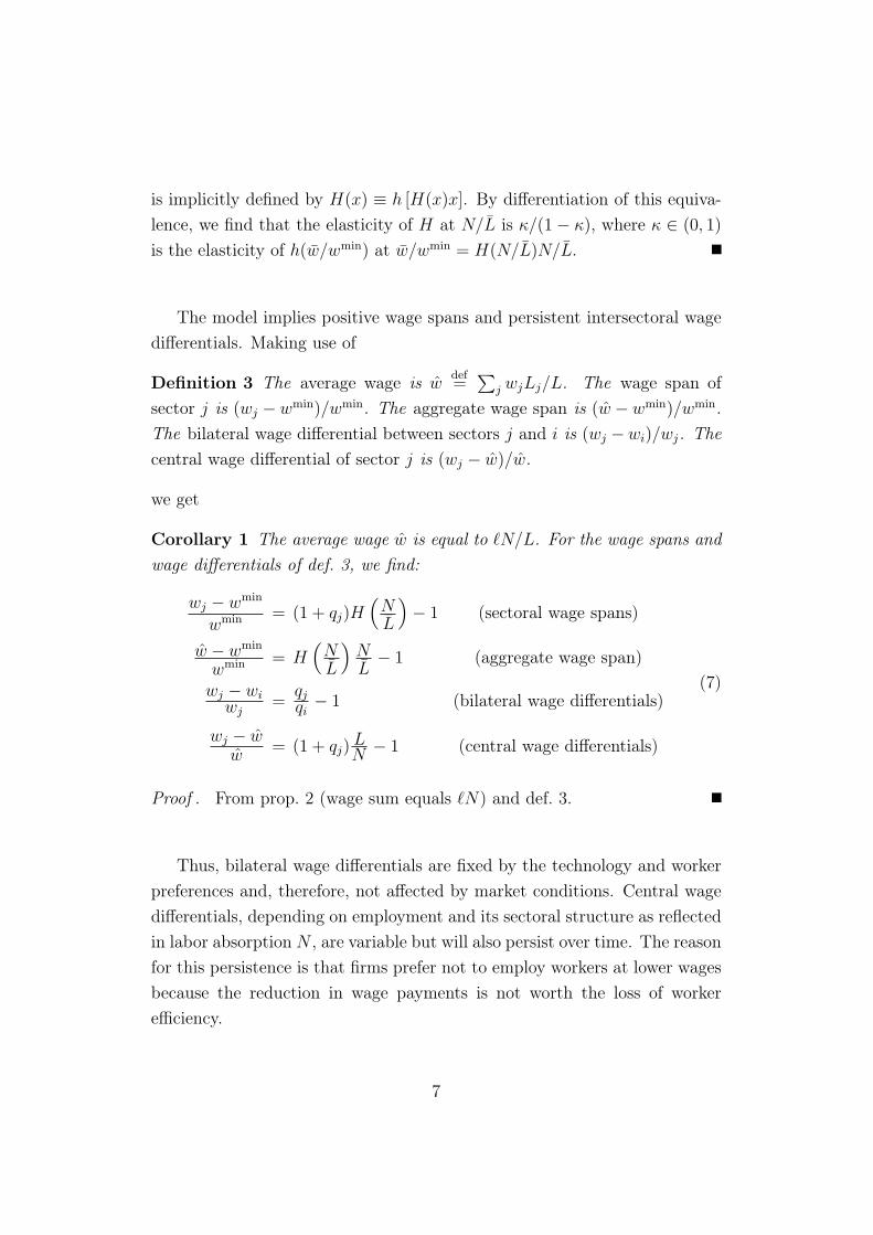
is implicitly defined by H(x) ≡ h [H(x)x]. By differentiation of this equiva-lence, we find that the elasticity of H at N/L is κ/(1− κ), where κ ∈ (0, 1)

is the elasticity of h(w/wmin) at w/wmin = H(N/L)N/L.

The model implies positive wage spans and persistent intersectoral wagedifferentials. Making use of

Definition 3 The average wage is wdef=

∑j wjLj/L. The wage span of

sector j is (wj − wmin)/wmin. The aggregate wage span is (w − wmin)/wmin.The bilateral wage differential between sectors j and i is (wj −wi)/wj. Thecentral wage differential of sector j is (wj − w)/w.

we get

Corollary 1 The average wage w is equal to `N/L. For the wage spans andwage differentials of def. 3, we find:

wj − wmin

wmin = (1 + qj)H(

NL

)− 1 (sectoral wage spans)

w − wmin

wmin = H(

NL

)NL− 1 (aggregate wage span)

wj − wiwj

=qjqi− 1 (bilateral wage differentials)

wj − ww

= (1 + qj)LN − 1 (central wage differentials)

(7)

Proof . From prop. 2 (wage sum equals `N) and def. 3.

Thus, bilateral wage differentials are fixed by the technology and workerpreferences and, therefore, not affected by market conditions. Central wagedifferentials, depending on employment and its sectoral structure as reflectedin labor absorption N , are variable but will also persist over time. The reasonfor this persistence is that firms prefer not to employ workers at lower wagesbecause the reduction in wage payments is not worth the loss of workerefficiency.

7

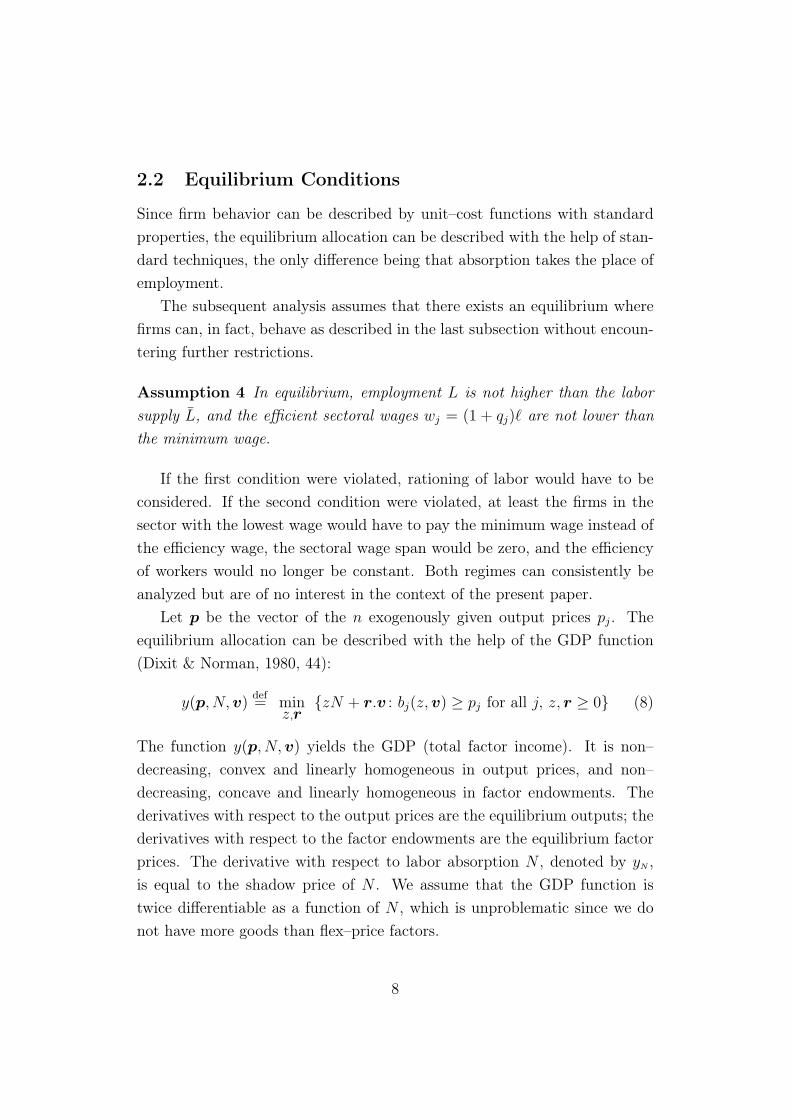
2.2 Equilibrium Conditions

Since firm behavior can be described by unit–cost functions with standardproperties, the equilibrium allocation can be described with the help of stan-dard techniques, the only difference being that absorption takes the place ofemployment.

The subsequent analysis assumes that there exists an equilibrium wherefirms can, in fact, behave as described in the last subsection without encoun-tering further restrictions.

Assumption 4 In equilibrium, employment L is not higher than the laborsupply L, and the efficient sectoral wages wj = (1 + qj)` are not lower thanthe minimum wage.

If the first condition were violated, rationing of labor would have to beconsidered. If the second condition were violated, at least the firms in thesector with the lowest wage would have to pay the minimum wage instead ofthe efficiency wage, the sectoral wage span would be zero, and the efficiencyof workers would no longer be constant. Both regimes can consistently beanalyzed but are of no interest in the context of the present paper.

Let p be the vector of the n exogenously given output prices pj. Theequilibrium allocation can be described with the help of the GDP function(Dixit & Norman, 1980, 44):

y(p, N,v)def= min

z,r{zN + r.v : bj(z, v) ≥ pj for all j, z, r ≥ 0} (8)

The function y(p, N,v) yields the GDP (total factor income). It is non–decreasing, convex and linearly homogeneous in output prices, and non–decreasing, concave and linearly homogeneous in factor endowments. Thederivatives with respect to the output prices are the equilibrium outputs; thederivatives with respect to the factor endowments are the equilibrium factorprices. The derivative with respect to labor absorption N , denoted by yN ,is equal to the shadow price of N . We assume that the GDP function istwice differentiable as a function of N , which is unproblematic since we donot have more goods than flex–price factors.

8

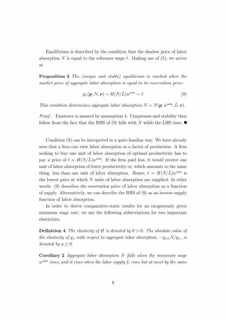
Equilibrium is described by the condition that the shadow price of laborabsorption N is equal to the reference wage `. Making use of (5), we arriveat

Proposition 3 The (unique and stable) equilibrium is reached when themarket price of aggregate labor absorption is equal to its reservation price:

yN(p, N,v) = H(N/L)wmin = ` (9)

This condition determines aggregate labor absorption N = N(p, wmin, L, v).

Proof . Existence is assured by assumption 4. Uniqueness and stability thenfollow from the fact that the RHS of (9) falls with N while the LHS rises.

Condition (9) can be interpreted in a quite familiar way. We have alreadyseen that a firm can view labor absorption as a factor of production. A firmseeking to buy one unit of labor absorption of optimal productivity has topay a price of ` = H(N/L)wmin. If the firm paid less, it would receive oneunit of labor absorption of lower productivity or, which amounts to the samething, less than one unit of labor absorption. Hence, ` = H(N/L)wmin isthe lowest price at which N units of labor absorption are supplied. In otherwords: (9) describes the reservation price of labor absorption as a functionof supply. Alternatively, we can describe the RHS of (9) as an inverse supplyfunction of labor absorption.

In order to derive comparative-static results for an exogenously givenminimum wage rate, we use the following abbreviations for two importantelasticities.

Definition 4 The elasticity of H is denoted by θ > 0. The absolute value ofthe elasticity of yN with respect to aggregate labor absorption, −yNNN/yN , isdenoted by η ≥ 0.

Corollary 2 Aggregate labor absorption N falls when the minimum wagewmin rises, and it rises when the labor supply L rises but at most by the same

9

percentage:∂N(p, wmin, L, v)

∂wminwmin

N = − 1θ + η

< 0

∂N(p, wmin, L, v)∂L

LN = θ

θ + η∈ (0, 1]

(10)

Proof . (10) is obtained from (9) by straightforeward computation.

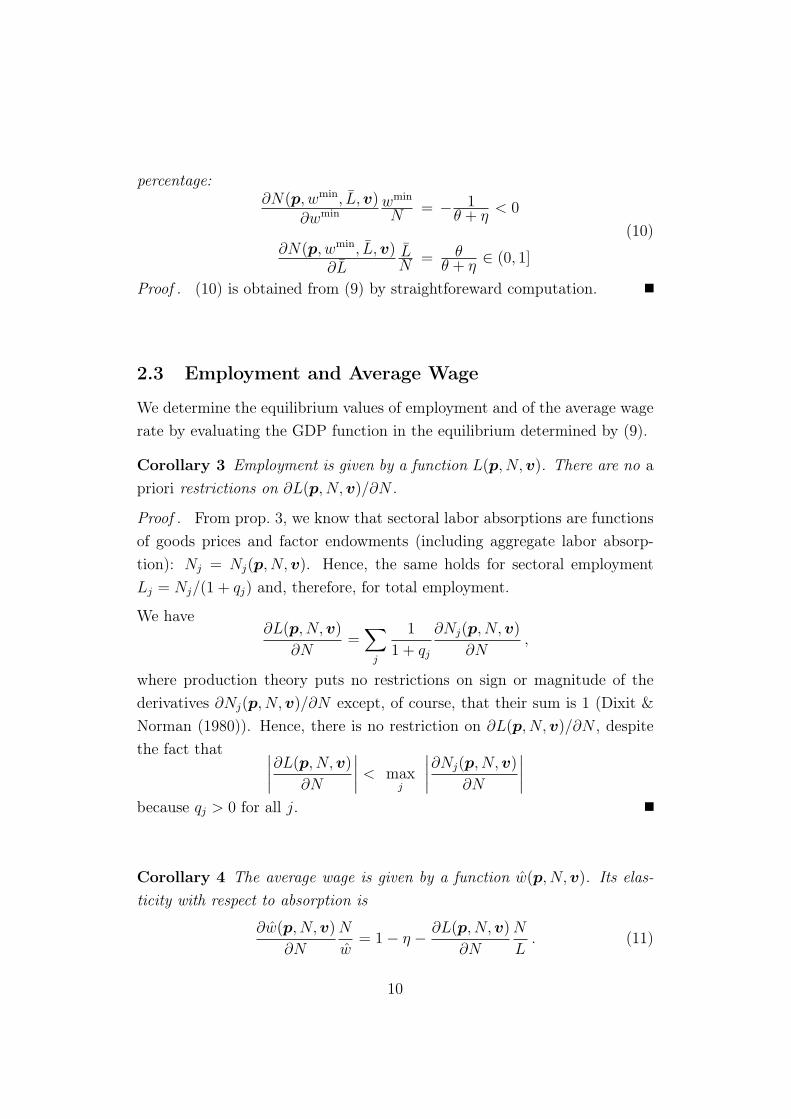
2.3 Employment and Average Wage

We determine the equilibrium values of employment and of the average wagerate by evaluating the GDP function in the equilibrium determined by (9).

Corollary 3 Employment is given by a function L(p, N,v). There are no apriori restrictions on ∂L(p, N,v)/∂N .

Proof . From prop. 3, we know that sectoral labor absorptions are functionsof goods prices and factor endowments (including aggregate labor absorp-tion): Nj = Nj(p, N,v). Hence, the same holds for sectoral employmentLj = Nj/(1 + qj) and, therefore, for total employment.

We have∂L(p, N, v)

∂N=

∑j

1

1 + qj

∂Nj(p, N,v)

∂N,

where production theory puts no restrictions on sign or magnitude of thederivatives ∂Nj(p, N,v)/∂N except, of course, that their sum is 1 (Dixit &Norman (1980)). Hence, there is no restriction on ∂L(p, N,v)/∂N , despitethe fact that ∣∣∣∣∂L(p, N, v)

∂N

∣∣∣∣ < maxj

∣∣∣∣∂Nj(p, N,v)

∂N

∣∣∣∣because qj > 0 for all j.

Corollary 4 The average wage is given by a function w(p, N,v). Its elas-ticity with respect to absorption is

∂w(p, N, v)

∂N

N

w= 1− η − ∂L(p, N,v)

∂N

N

L. (11)

10

Proof . We have w = `N/L (cor. 1) and ` = yN (prop. 3); the functionresults from substituting yN(p, N,v) and L(p, N,v) (cor. 3) in yNN/L. Theelasticity results from differentiation using prop. 3 and def. 4.

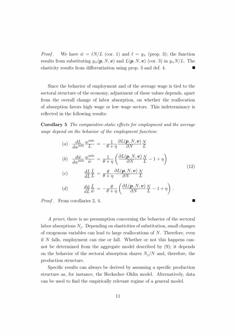
Since the behavior of employment and of the average wage is tied to thesectoral structure of the economy, adjustment of these values depends, apartfrom the overall change of labor absorption, on whether the reallocationof absorption favors high–wage or low–wage sectors. This indeterminacy isreflected in the following results:

Corollary 5 The comparative-static effects for employment and the averagewage depend on the behavior of the employment function:

(a) dLdwmin

wmin

L = − 1θ + η

∂L(p, N,v)∂N

NL

(b) dwdwmin

wmin

w= 1

θ + η

(∂L(p, N,v)

∂NNL − 1 + η

)(c) dL

dLLL = θ

θ + η∂L(p, N,v)

∂NNL

(d) dwdL

Lw

= − θθ + η

(∂L(p, N,v)

∂NNL − 1 + η

).

(12)

Proof . From corollaries 2, 4.

A priori, there is no presumption concerning the behavior of the sectorallabor absorptions Nj. Depending on elasticities of substitution, small changesof exogenous variables can lead to large reallocations of N . Therefore, evenif N falls, employment can rise or fall. Whether or not this happens can-not be determined from the aggregate model described by (9); it dependson the behavior of the sectoral absorption shares Nj/N and, therefore, theproduction structure.

Specific results can always be derived by assuming a specific productionstructure as, for instance, the Heckscher–Ohlin model. Alternatively, datacan be used to find the empirically relevant regime of a general model.

11

3 Wage Drift and Employment Effects of Im-migration

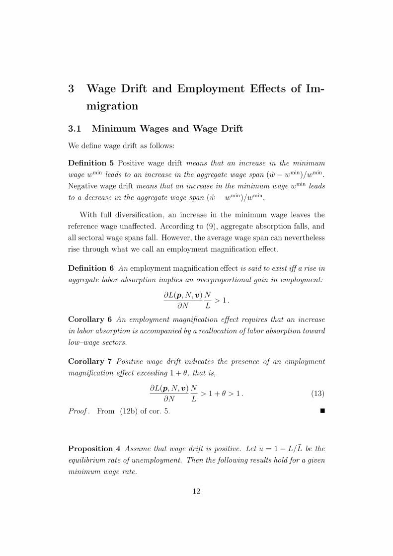
3.1 Minimum Wages and Wage Drift

We define wage drift as follows:

Definition 5 Positive wage drift means that an increase in the minimumwage wmin leads to an increase in the aggregate wage span (w − wmin)/wmin.Negative wage drift means that an increase in the minimum wage wmin leadsto a decrease in the aggregate wage span (w − wmin)/wmin.

With full diversification, an increase in the minimum wage leaves thereference wage unaffected. According to (9), aggregate absorption falls, andall sectoral wage spans fall. However, the average wage span can neverthelessrise through what we call an employment magnification effect.

Definition 6 An employment magnification effect is said to exist iff a rise inaggregate labor absorption implies an overproportional gain in employment:

∂L(p, N,v)

∂N

N

L> 1 .

Corollary 6 An employment magnification effect requires that an increasein labor absorption is accompanied by a reallocation of labor absorption towardlow–wage sectors.

Corollary 7 Positive wage drift indicates the presence of an employmentmagnification effect exceeding 1 + θ, that is,

∂L(p, N,v)

∂N

N

L> 1 + θ > 1 . (13)

Proof . From (12b) of cor. 5.

Proposition 4 Assume that wage drift is positive. Let u = 1− L/L be theequilibrium rate of unemployment. Then the following results hold for a givenminimum wage rate.

12

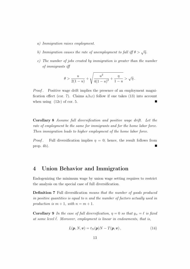
a) Immigration raises employment.

b) Immigration causes the rate of unemployment to fall iff θ >√

η.

c) The number of jobs created by immigration is greater than the numberof immigrants iff

θ >u

2(1− u)+

√u2

4(1− u)2 +η

1− u>√

η .

Proof . Positive wage drift implies the presence of an employment magni-fication effect (cor. 7). Claims a,b,c) follow if one takes (13) into accountwhen using (12c) of cor. 5.

Corollary 8 Assume full diversification and positive wage drift. Let therate of employment be the same for immigrants and for the home labor force.Then immigration leads to higher employment of the home labor force.

Proof . Full diversification implies η = 0; hence, the result follows fromprop. 4b).

4 Union Behavior and Immigration

Endogenizing the minimum wage by union wage setting requires to restrictthe analysis on the special case of full diversification.

Definition 7 Full diversification means that the number of goods producedin positive quantities is equal to n and the number of factors actually used inproduction is m + 1, with n = m + 1.

Corollary 9 In the case of full diversification, η = 0 so that yN = ` is fixedat some level ¯. Moreover, employment is linear in endowments, that is,

L(p, N,v) = tN(p)N − T (p, v) , (14)

13

where T (p, v)def= −

∑i ti(p)vi. There are no a priori restrictions on the signs

of tN , ti. The average wage is given by

w =¯

tN

(1 +

T

L

). (15)

Proof . Linearity follows from the factor market clearing conditions. Anemployment magnification effect means that the elasticity of employmentw.r.t. labor absorption is greater than 1, which is only possible if tN and T

are positive. The expression for the average wage uses w = ¯N/L (see cor.1) and (14).

4.1 Wage Setting Equilibrium

Consider a monopolistic union with utility function U(w, L/L) setting theminimum wage under conditions of full diversification. The union can movealong the constraint (15) since N must adapt to changes in the minimumwage such that yN = ¯. Full diversification means that the union mustaccept the price of labor absorption as it is determined on world markets.

Let U be increasing, concave, and linearly homogeneous. The union prob-lem is

maxw,L/L

{U(w, L/L) : w =

¯

tN

(1 +

T

L

)}. (16)

We focus on interior optima.The FOC is

V

(wL

L

)def=

∂U(w, L/L)

∂(L/L)

/∂U(w, L/L)

∂w=

¯

tN

T

L2 L , (17)

where V with V ′ > 0 is the (absolute value of the) marginal rate of substi-tution and the RHS is the absolute value of the slope of the constraint (15).Note that the FOC is only consistent with T/tN > 0; since T + L = tNN ,this implies T/(T + L) > 0.

Let σ denote the (absolute value of the) elasticity of substitution of theutility function:

σdef=

(V ′

V

wL

L

)−1

> 0 (18)

14

From (17) and (18) we get

V ′ =1

σ

T

T + L. (19)

For any given point satisfying the FOC, we can find any value for σ since σ

only measures the local curvature. Hence, as long as the SOC are satisfied,we can discuss comparative statics for different values of σ.

Differentiation of the LHS of (17) yields

V ′(

wL

L

) (dw

dL

L

L− wL

L2

)= −L

σ

2T + L

T + L

T ¯

tNL3 < 0 . (20)

Differentiation of the RHS of (17) yields

−2T ¯

tNL3 L < 0 . (21)

The SOC are fulfilled if, for higher values of L on the constraint, the indif-ference curves are flatter than the constraint, that is, if the LHS falls morein absolute terms than the RHS:

−L

σ

2T + L

T + L

T ¯

tNL3 < −2T ¯

tNL3 L . (22)

Since T/tN > 0, we can write the SOC as

σ <T + L/2

T + L< 1 . (23)

Thus, if the union’s indifference curves become too flat (i.e. if w and L/L aretoo good substitutes from the perspective of the union), a full-diversificationequilibrium with positive wage drift is not possible. Specifically, Cobb-Douglas preferences, where σ = 1, are ruled out. Note that the SOC requires(T + L/2)/(T + L) > 0.

4.2 Wage Setting and Immigration

Under full diversification, the reaction of employment to immigration if theunion does not adjust the minimum wage is given by (12c) of cor. 5, togetherwith η = 0 and L = tNN − T . This yields

dL

dL

L

L=

T + L

L. (24)

15

Note that without further restrictions the sign of this elasticity is indetermi-nate.

In general, however, the union will adjust its wage claims. We can usethe results from the union’s optimization problem in order to analysze howimmigration affects the union’s policy. From (17) we derive the comparativestatic effect on employment with respect to immigration as

dLdL

LL =

T ¯

tNL2 − V ′wL

2 T ¯

tNL2 − 1σ

2T+LT+L

T ¯

tNL2

=T ¯

tNL2 − 1σ

T ¯

tNL2

2 T ¯

tNL2 − 1σ

2T+LT+L

T ¯

tNL2

=1

2

1− σT+L/2T+L

− σ> 0 .

(25)

The SOC (cf. (23)) imply that the union always adjusts the minimum wagein such a way that immigration leads to a positive employment effect.

If (25) and (24) are equal, union preferences require no adjustment of theminimum wage at all. We find equality if

σ =T

T + L/2<

T + L/2

T + L< 1 . (26)

This condition is consistent with equilibrium. It depends on the union’spreferences whether it will pursue a policy that counteracts the employmenteffects of immigration. As a result, whether immigration disciplines a unionor not depends on union preferences. Irrespective of its specific preferences,however, the union does never adjust wages so dramatically that positiveemployment effects of immigration at a given minimum wage are reversed.

Even given union preferences, it is not clear whether the union will raiseor lower the minimum wage as a consequence of immigration. The nextsection shows there are two different regimes with different implications forunion behavior. It moreover shows that, under the assumptions made so far,the regime can be identified by observing the wage drift.

4.3 Immigration, Wage Drift and Union Behavior

We can now discuss the union’s reaction to immigration under alternativewage–drift regimes. Our main result is stated in the following proposition:

16

Proposition 5 Assume full diversification and positive wage drift. Unionsare disciplined by immigration iff w and L/L are good substitutes from theperspective of the union: σ > T/(T + L/2). On the other hand, immigrationcauses unions to raise their wage claims iff w and L/L are poor substitutesfrom the perspective of the union: σ < T/(T + L/2).Proof . Immigration in the presence of positive wage drift implies (dL/dL)

(L/L) > 1 and (dL/dwmin) (wmin/L) < 0 (see cor. 8). The result thenfollows from conditions (24) and (25).

This proposition proves our claim stated in the introduction: Unions withpreferences sufficiently biased in favor of the income of employed workers havean incentive to appropriate some of the gains from immigration by raisingthe minimum wage.

Things are a bit more complicated in the regime of negative wage drift.Negative wage drift implies

∂L

∂N

N

L< 1 + θ .

This condition is either compatible with (∂L/∂N)(N/L) < 0 (case 1), orwith 0 < (∂L/∂N)(N/L) < 1 + θ (case 2). Thus we get

Proposition 6 Assume full diversification and negative wage drift.(i) Immigration causes unions to raise their wage claims in case 1.(ii) Immigration causes unions to raise their wage claims iff w and L/L arepoor substitutes from the perspective of the union: σ < T/(T + L/2). On theother hand, unions are disciplined by immigration iff w and L/L are goodsubstitutes from the perspective of the union: σ > T/(T + L/2).Proof . Part (i) follows from cor. 8 and (25). Part (ii) follows from conditions(24) and (25)

5 Conclusion

Our analysis has shown how the reaction of unions to labor immigration isrelated to the phenomenon of wage drift determined by adjustment of an

17

economy’s sectoral structure. For given union preferences about wage in-comes of employed workers and employment rates, the immigration–inducedchange in wage policies depends on the wage–drift regime of the economy.In the case of positive wage drift and high substitutability between wage in-comes and employment, immigration does not generate a replacement effectand unions react with more aggressive wage claims. At least for german labormarkets, this case has some plausibility.

Intuitively, the mechanism driving our results about wage drift works asfollows. A rise in the minimum wage increases the reference wage, but bya smaller percentage. Sectoral wages, which are given by a constant sector–specific markup on the reference wage, rise but sectoral wage spans fall. If,nevertheless, the aggregate wage span rises (wage drift), this must be be-cause the change shifts employment to high–wage sectors. This is in linewith the usual assumption that a rise in minimum wages mainly endangerslow–wage jobs. However, high–wage sectors contribute more to unemploy-ment than low–wage sectors. Therefore, the wage–drift phenomenon indi-cates that unemployment goes up for two reasons, a macroeconomic reasonand a structural reason: labor becomes more expensive, and employmentshifts toward sectors which contribute more to unemployment. The addi-tional, structural effect is called the employment magnification effect since itimplies that changes in employment are larger in a multisectoral model withwage drift than in a one–sector model.

Immigration works in the other direction. It puts downward pressureon average labor income, which lowers the reference wage of workers. In aone–sector model, such a change would never be sufficient to create enoughjobs to employ the immigrants, not to speak of the home labor force. In amultisectoral model with wage drift, however, the employment magnificationeffect extends the range of possible results. Under quite plausible assump-tions, the employment magnification effect is strong enough to create moreemployment than necessary to employ the immigrants.

The reduction in wage spans by immigration as well as the positive effecton home employment imply that immigration does not neccessarily workas a discplining device for unions. On the contrary, immigration creates anincentive for unions to raise the minimum wage and thus to appropriate some

18

of the gains from immigration with respect to employment.

References

Akerlof, G. A. (1982), “Labor contracts as a partial gift exchange,” QuarterlyJournal of Economics, 97, 583–569.

Akerlof, G. A. & J. L. Yellen (1990), “The fair wage–effort hypothesis andunemployment,” Quarterly Journal of Economics, 105, 255–283.

Albert, M. & J. Meckl (2001a), “Efficiency–wage unemployment and intersec-toral wage differentials in a Heckscher–Ohlin model,” German EconomicReview, 2, 273–287.

— (2001b), “Green tax reform and two–component unemployment: Doubledividend or double loss?” Journal of Institutional and Theoretical Eco-nomics, 157, 265–281.

Bauer, T. & K. F. Zimmermann (1997), “Integrating the east: the labormarket effects of immigration,” in: S. W. Black (ed.), Europe’s EconomyLooks East—Implications for Germany and the European Union, pp. 269–306, Cambridge University Press, Cambridge.

Dixit, A. K. & V. K. Norman (1980), Theory of International Trade, Cam-bridge University Press, Cambridge/UK.

Fuest, C. & M. Thum (2000), “Welfare effects of immigration in a dual labormarket,” Regional Science and Urban Economics, 30, 557–563.

— (2001), “Immigration and skill formation in unionized labor markets,”European Journal of Political Economy, 17, 557–573.

Gahlen, B. & H. J. Ramser (1987), “Effizienzlohn, Lohndrift und Beschäf-tigung,” in: G. Bombach, B. Gahlen, & A. E. Ott (eds), Arbeitsmärkteund Beschäftigung. Fakten, Analysen, Perspektiven, pp. 129–160, MohrSiebeck, Tübingen.

19

Layard, R., S. Nickell, & R. Jackmann (1994), The Unemployment Crisis,Oxford University Press, Oxford.

Schlicht, E. (1992), “Wage generosity,” Journal of Institutional and Theoret-ical Economics, 148, 437–451.

Schmidt, C. M., A. Stilz, & K. F. Zimmermann (1994), “Mass migration,unions, and government intervention,” Journal of Public Economics, 55,185–201.

Solow, R. M. (1979), “Another possible source of wage stickiness,” Journalof Macroeconomics, 1, 79–82.

20