Embed Size (px)
Citation preview
Wavelet based image compression
using FPGAs
Dissertation
zur Erlangung des akademischen Grades
doctor rerum naturalium (Dr. rer. nat.)
vorgelegt der
Mathematisch-Naturwissenschaftlich-Technischen Fakultätder Martin-Luther-Universität Halle-Wittenberg
von Herrn Jörg Ritter
geb. am 12. April 1971 in Greiz
Gutachter:
1. Prof. Dr. Paul Molitor, Martin-Luther-University Halle-Wittenberg, Germany
2. Prof. Dr. Scott Hauck, University of Washington, Seattle, WA, USA
3. Prof. Dr. Thomas Rauber, University of Bayreuth, Germany
Halle (Saale), 06.12.2002
urn:nbn:de:gbv:3-000004615[http://nbn-resolving.de/urn/resolver.pl?urn=nbn%3Ade%3Agbv%3A3-000004615]
Abstract
In this work we have studied well known state of the art image compression algorithms. These codecs arebased on wavelet transforms in most cases. Their compression efficiency is widely acknowledged. Thenew upcoming JPEG2000 standard, e.g., will be based on wavelet transforms too. However, hardwareimplementations of such high performance image compressors are non trivial. In particular, the on chipmemory requirements and the data transfer volume to external memory banks are tremendous.We suggest a solution which minimizes the communication time and volume to external random accessmemory. With negligible internal memory requirements this bottleneck can be avoided using the partitionedapproach to wavelet transform images proposed in this thesis. Based on this idea we present modificationsto the well known algorithm of Said and PearlmanSet Partitioning In Hierarchical Trees SPIHTto restrictthe necessity of random access to the whole image to a small subimage only, which can be stored onchip. The compression performance in terms of visual property (measured with peak signal to noise ratio)compared to the original codec remains still the same or nearly the same. The computational power of theproposed circuits targeting to programmable hardware are promising. We have realized a prototype of thiscodec in a XC4000 Xilinx FPGA running at 40MHz which compresses images 10 times faster than a 1GHzAthlon processor. An application specific integrated circuit based on our approach should be much fasterover again.
Zusammenfassung
Im Rahmen dieser Disseration haben wir die besten, derzeit verfügbaren Bildkompressionsverfahren ana-lysiert. Die meisten dieser Algorithmen basieren auf Wavelet-Transformationen. Durch diese Technikkönnen erstaunliche Ergebnisse im Vergleich zu den bekannten, auf diskreten Kosinus-Transformationenbasierenden Verfahren erreicht werden. Unterstrichen wird diese Tatsache durch die Wahl eines wavelet-basierten Kodierers von der Joint Picture Expert Group als Basis für den neuen JPEG2000 Standard. DieEntwicklung von speziellen Hardware-Architekturen für diese Kompressionsalgorithmen ist sehr komplex,da meist viel interner Speicher benötigt wird und zusätzlich riesige Datenmengen zwischen Peripherie unddem Hardware-Baustein ausgetauscht werden müssen.Wir stellen in dieser Arbeit einen Ansatz vor, welcher ausgesprochen wenig internen Speicher erfordertund gleichzeitig das zu transportierende Datenvolumen drastisch reduziert. Aufbauend auf diesem par-titionierten Ansatz zur Wavelet-Transformation von Bildern stellen wir Modifikationen des bekanntenKompressionsverfahrens von Said und PearlmanSet Partitioning In Hierarchical Trees SPIHTvor, umdiesen effektiv in Hardware realisieren zu können. Diese Veränderungen sind notwendig, da im Origi-nal extensiv von dynamischen Datenstrukuren Gebrauch gemacht wird, welche sich nicht oder nur miterheblich Aufwand an Speicher realisieren lassen. Die visuelle Qualität im Vergleich zum Originalalgo-rithmus bleibt jedoch exakt gleich oder ist dieser sehr ähnlich. Jedoch sind die Geschwindigkeitsvorteileunserer Architektur gegenüber aktuellen Prozessoren von Arbeitsplatzrechnern sehr vielversprechend, waswir durch praktische Versuche auf einem programmierbaren Hardware-Baustein überzeugend nachweisenkonnten. Wir haben einen Prototypen auf einem Xilinx XC4000 FPGA realisiert, welcher mit 40 MHzgetaktet werden konnte. Schon dieser Prototyp des Hardware-Bildkomprimierers komprimiert Bilder 10mal schneller als ein Athlon Prozessor getaktet mit 1GHz. Ein mit ensprechender Technologie basierendauf unserem partitioniertem Ansatz produzierter anwendungsspezifischer Schaltkreis würde diese Leistungnoch bei weitem übertreffen.
Contents
1 Mathematical Background 71.1 Discrete Signal and Filters. . . . . . . . . . . . . . . . . . . . . . . . . . . . . . . . . . 7
1.1.1 z-Transform . . . . . . . . . . . . . . . . . . . . . . . . . . . . . . . . . . . . . 81.1.2 Impulse train function. . . . . . . . . . . . . . . . . . . . . . . . . . . . . . . . 8
1.2 Measure of Information. . . . . . . . . . . . . . . . . . . . . . . . . . . . . . . . . . . . 91.3 Distortion Measures. . . . . . . . . . . . . . . . . . . . . . . . . . . . . . . . . . . . . . 101.4 Downsampling, Upsampling, and Delay. . . . . . . . . . . . . . . . . . . . . . . . . . . 111.5 Wavelets. . . . . . . . . . . . . . . . . . . . . . . . . . . . . . . . . . . . . . . . . . . .131.6 Discrete Wavelet Transforms. . . . . . . . . . . . . . . . . . . . . . . . . . . . . . . . . 141.7 Cohen-Daubechies-Feauveau CDF(2,2) Wavelet. . . . . . . . . . . . . . . . . . . . . . . 171.8 Lifting Scheme . . . . . . . . . . . . . . . . . . . . . . . . . . . . . . . . . . . . . . . .20
1.8.1 Integer-to-Integer Mapping. . . . . . . . . . . . . . . . . . . . . . . . . . . . . . 221.8.2 Lifting Scheme and Modular Arithmetic. . . . . . . . . . . . . . . . . . . . . . . 22
2 Wavelet transforms on images 232.1 Reflection at Image Boundary. . . . . . . . . . . . . . . . . . . . . . . . . . . . . . . . 242.2 2D-DWT . . . . . . . . . . . . . . . . . . . . . . . . . . . . . . . . . . . . . . . . . . .262.3 Normalization Factors of the CDF(2,2) Wavelet in two Dimensions. . . . . . . . . . . . . 28
3 Range of CDF(2,2) Wavelet Coefficients 313.1 Estimation of Coefficients Range using Lifting with Rounding. . . . . . . . . . . . . . . 353.2 Range of coefficients in the two dimensional case. . . . . . . . . . . . . . . . . . . . . . 38
4 State of the art Image Compression Techniques 414.1 Embedded Zerotree Wavelet Encoding. . . . . . . . . . . . . . . . . . . . . . . . . . . . 41
4.1.1 Wavelet Transformed Images. . . . . . . . . . . . . . . . . . . . . . . . . . . . . 414.1.2 Shapiro’s Algorithm . . . . . . . . . . . . . . . . . . . . . . . . . . . . . . . . . 41
4.2 SPIHT- Set Partitioning In Hierarchical Trees. . . . . . . . . . . . . . . . . . . . . . . . 454.2.1 Notations. . . . . . . . . . . . . . . . . . . . . . . . . . . . . . . . . . . . . . .454.2.2 Significance Attribute . . . . . . . . . . . . . . . . . . . . . . . . . . . . . . . . 464.2.3 Parent-Child Relationship of the LL Subband. . . . . . . . . . . . . . . . . . . . 464.2.4 The basic Algorithm. . . . . . . . . . . . . . . . . . . . . . . . . . . . . . . . . 46
5 Partitioned Approach 495.1 Drawbacks of the Traditional 2D-DWT on Images. . . . . . . . . . . . . . . . . . . . . . 495.2 Partitioned 2D-DWT . . . . . . . . . . . . . . . . . . . . . . . . . . . . . . . . . . . . . 50
5.2.1 Lossless Image Compression. . . . . . . . . . . . . . . . . . . . . . . . . . . . . 515.2.2 Lossy Image Compression. . . . . . . . . . . . . . . . . . . . . . . . . . . . . . 525.2.3 Boundary Treatment. . . . . . . . . . . . . . . . . . . . . . . . . . . . . . . . . 535.2.4 Future Work: Taking Advantage of Subimage and QuadTree Similarities. . . . . 54
5.3 Modifications to theSPIHTCodec . . . . . . . . . . . . . . . . . . . . . . . . . . . . . . 555.3.1 Exchange of Sorting and Refinement Phase. . . . . . . . . . . . . . . . . . . . . 55
3
4 CONTENTS
5.3.2 Memory Requirements of the Ordered Lists. . . . . . . . . . . . . . . . . . . . . 555.4 Comparison between the Original and the ModifiedSPIHTAlgorithm . . . . . . . . . . . 58
6 FPGA architectures 616.1 Prototyping Environment. . . . . . . . . . . . . . . . . . . . . . . . . . . . . . . . . . . 61
6.1.1 The Xilinx XC4085 XLA device. . . . . . . . . . . . . . . . . . . . . . . . . . . 636.2 2D-DWT FPGA Architectures targeting Lossless Compression. . . . . . . . . . . . . . . 646.3 2D-DWT FPGA Architectures targeting Lossy Compression. . . . . . . . . . . . . . . . 65
6.3.1 2D-DWT FPGA Architecture based on Divide and Conquer Technique. . . . . . 656.3.2 2D-DWT FPGA Pipelined Architecture. . . . . . . . . . . . . . . . . . . . . . . 66
6.4 FPGA-Implementation of the ModifiedSPIHTEncoder. . . . . . . . . . . . . . . . . . . 706.4.1 Hardware Implementation of the Lists. . . . . . . . . . . . . . . . . . . . . . . . 726.4.2 Efficient Computation of Significances. . . . . . . . . . . . . . . . . . . . . . . 726.4.3 Optional Arithmetic Coder. . . . . . . . . . . . . . . . . . . . . . . . . . . . . . 74
7 Conclusions and Related Work 797.1 EBCOTand JPEG2000. . . . . . . . . . . . . . . . . . . . . . . . . . . . . . . . . . . . 79
7.1.1 TheEBCOTAlgorithm . . . . . . . . . . . . . . . . . . . . . . . . . . . . . . . . 807.2 Similarities and Differences of JPEG2000 and our Approach. . . . . . . . . . . . . . . . 82
A Hard/Software Interface MicroEnable 85A.1 Register/DMA on Demand Transfer, C example. . . . . . . . . . . . . . . . . . . . . . . 85A.2 Register/DMA on Demand Transfer, VHDL example. . . . . . . . . . . . . . . . . . . . 87A.3 Matlab/METAPOST-Scripts . . . . . . . . . . . . . . . . . . . . . . . . . . . . . . . . . 91
Introduction
Reading a user manual of a new mobile phone you may wonder whether it is possible to make a phonecall at all. We grant that this is overstated. But besides the central functionality of a mobile phone thereare a lot of additional features. Many of them fall into the category of multimedia applications. You canplay music, hear radio, read and write emails, and surf in the internet. However, even with new connectionstandards like GPRS, HSCD, or UMTS, which provide high speed data transfers, the bandwidth is limited.Data compression and error resilience in noisy environments like transfers to mobile phones are basicallyto provide those multimedia features. In contrast to a personal computer where you can rely on powerfulprocessors with huge main storage capabilities one has to think about low cost hardware solutions, here.This is also the case for digital cameras. The photograph expects that immediately after taking a picture hecan inspect the result. To support this behavior the picture has to be compressed, stored on a flash memorycard, decompressed, and shown at a LCD display in nearly real time. Features like high speed previews withincremental refinement have to be provided. Furthermore the digital photograph could expect, that morethan say 36 pictures can be stored on the memory stick. Therefore efficient hardware image compressionalgorithms with excellent visual properties are necessary.Even surfing the world wide web using a powerful personal computer and high speed internet access weoften have to wait until web sites are rendered. Basicly not the searched information itself determinesthe data transfer volume but the presentation of it and accessory advertising. These product presentationsheavy rely on color illustrations or animations. Thus the surfer and manufacturer are interested in efficientdata compression methods, too. The potential customer finds the information he was looking for in shortertime and the supplier saves money for server farms to provide huge bandwidth.In this work we have studied well known state of the art image compression algorithms. These codecs arebased on wavelet transformations in most cases. Their compression efficiency is widely acknowledged.The new upcoming JPEG2000 standard will be based on wavelet transformations, too. Hardware imple-mentations of such high performance image compressors are non trivial. Especially the on chip memoryrequirements and the data transfer volume to external memory banks are tremendous.We suggest a solution which minimizes the communication time and volume to external random accessmemory. With negligible internal memory requirements this bottleneck could be avoided using a parti-tioned approach to wavelet transform images. Based on this idea we propose modifications to the wellknown algorithm of Said and PearlmanSet Partitioning in Hierarchical Trees SPIHTto restrict the neces-sity of random access to the whole image to a small subimage only, which can be stored on chip. However,the compression performance in terms of visual property (measured with peak signal to noise ratio) com-pared to the original codec is still the same or nearly the same. The computational power of the proposedcircuits targeting to programmable hardware are promising. We have realized a prototype of this codec ina XC4000 Xilinx FPGA running at 40MHz which compresses images 10 times faster than a 1GHz Athlonprocessor. An application specific integrated circuit based on our approach should be much faster overagain.
This thesis is structured as follows.
Mathematical background In Chapter1we introduce necessary notations and discuss up/downsamplingand delaying of discrete signals in detail. These techniques will be very useful in Chapter3. Furthermorewe give a short overview of the coherence of wavelet transforms and filtering.
5
6 CONTENTS
Wavelet transform on images The digital representation of images and the tensor product of one di-mensional wavelet transforms applied to images are introduced in Chapter2. We also discuss the implicitstorage of the normalization factors, which are necessary to preserve the average brightness of the images.
Range of CDF(2,2) wavelet coefficients In Chapter3 the dynamic range of coefficients after a wavelettransformation had taken place is analyzed. We deduce lower and upper bounds for the endpoints of thecorresponding intervals for each scale and orientation. Theses bounds are used to reduce the memoryrequirements down to the minimum.
State of the art image compression techniquesBefore we present the central part of this thesis, wegive a survey of state of the art wavelet based image compression techniques in Chapter4. We shortlyoutline the embedded zerotree wavelet algorithm of Shapiro and discuss theSPIHT algorithm in moredetail. This codec is widely acknowledged as a reference for effective image compression methods withexcellent visual properties of the reconstructed images.
Partitioned Approach In Chapter5 we present in detail the main contribution of this thesis, the par-titioned approach to wavelet transform images. At first we motivate, why there is a need for such anapproach, if one considers implementations of image compression algorithm based on wavelet transformsin programmable hardware. Furthermore to achieve efficient circuits with respect to clock rate and datathroughput we present necessary modifications of the originalSPIHTcodec and compare them in terms ofvisual quality.
FPGA Architectures The designs are discussed in Chapter6. Here we present VHDL projects for thepartitioned approach itself and the appropriate adaptedSPIHTcodec. We discuss our prototyping environ-ment, a PCI card equipped with a Xilinx FPGA, which offers the opportunity to us to derive convincingexperimental result.
Conclusions and Related Work To conclude this thesis we summerize our obtained results in termsof theoretical aspects as well as practical experiences. Furthermore the features of the upcoming newJPEG2000 standard and the integrated compressor named EBCOT are exemplified. We balance the advan-tages and disadvantages of our approach to the proposed method in the JPEG2000 standard.
Acknowledgements I thank my advisor Prof. Dr. Paul Molitor who arouses my interest in waveletbased image compression and for all the fruitful discussions. Special thanks to Stepan Sutter, HenningThielemann, and Görschwin Fey for their corporation in the last years. Thanks to all my colleagues whosefeedback has allowed me to improve the contents of this thesis. A special acknowledgment to Sandro Wefelfor his continuing support throughout the whole process of developing and writing this thesis.
Chapter 1
Mathematical Background
Wavelet based image compression techniques are funded on several fundamental mathematical theories.The wavelet transform used to decorrelate the input signal has its theoretical roots in several traditionalsciences like Fourier analysis, signal processing, or filter theory. Here we cannot give a detailed intro-duction to all concepts. We restrict our explanations to the central notations, which are necessary for theunderstanding of this thesis.
1.1 Discrete Signal and Filters
Discrete signals and filters can be represented by vectors. In many cases we do not distinguish betweensignals of finite or infinite length. A signalx is written as
x = (. . . , x−2, x−1, x0, x1, x2, . . . ),
with coefficientsxn ∈ Z, R, or C for all n ∈ Z. Analogously, a filterf with coefficientsfm ∈ Z, R, or Cfor all m ∈ Z (often calledfilter taps) is declared by
f = (. . . , f−2, f−1, f0, f1, f2, . . . ).
Sometimes it is necessary to locate the coefficient at index zero. We then emphasize that coefficient likethis
x = (. . . , 0.25,1.25,−0.5, 0.75, . . . ).
Usually, the signal and filter coefficients are non zero at finite positions only. If so, the corresponding signaland filters have so calledfinite support. Let fa andfb be the right most and left most non zero coefficient,respectively. Thenumber of tapsor similarly thefilter lengthis then defined as
|f | = b− a+ 1.
In the filter theory one distinguishes betweenfinite impulse response (FIR)and infinite impulse response(IIR) filters. The impulse response of a filterf is the filter output if the filter input is the signalδ defined by
δn ={
1 : n = 00 : else
,
where all samples are zero except one. If the impulse response is finite, because there is no feedback in thefilter, the filter is calledFIR filter. This category of filters has some important advantages:
• simple to implement (MAC operations (multiply and accumulate)),
• desirable numeric properties (with respect to fixed and floating point arithmetic), and
• they can be designed to belinear phase. Linear phase filters do not distort the phase by introducingsome delay if (and only if) its coefficients are symmetrical around the center coefficient.
7
8 CHAPTER 1. MATHEMATICAL BACKGROUND
In this thesis we will restrict to FIR filter and we use the notionfilter as an acronym of FIR filter.
Theconvolutiony = f ∗ x of a signalx with a filterf is the signaly with
yn :=∑k∈Z
fkxn−k =∑k∈Z
fn−kxk.
1.1.1 z-Transform
In Chapter3 we will estimate greatest lower and least upper bounds for the minimal bitwidth necessaryto store coefficients as result of wavelet transform. In order to compute accurate estimations we have toanalyze filtered signals. A helpful technique will be the so calledz-transform. This is a generalization ofthe discrete time Fourier transform. It is defined for filters and signals by
F (z) =∑l∈Z
flz−l and X(z) =
∑k∈Z
xkz−k, (1.1)
respectively, wherez ∈ C, i.e., the variablez is of type complex number. Assuming that thez-transformand its inverse exist, we will denote by
f ←→ F and x←→ X
a transform pair. Note that for discrete signals with finite support theregion of convergence(ROC) is thewholez-plane, e.g., the series given in Equation (1.1) converge for allz with 0 < |z| < ∞. The relationf ←→ F is a one-to-one mapping, iff is a discrete signal or filter with finite support. For a detaileddiscussion of the properties ofz-transformswe refer to [OS89].
For a filtered signaly = f ∗ x theconvolution theorem
y = f ∗ x←→ Y = F ·X,
holds since
Y (z) =∑n∈Z
ynz−n
=∑n∈Z
(∑k∈Z
fkxn−k
)z−n
=∑k∈Z
∑n∈Z
fkxn−kz−n
=∑k∈Z
fk
∑n∈Z
xn−kz−n
=∑k∈Z
fk
∑n′∈Z
xn′z−n′−k
=∑k∈Z
fkz−k∑n∈Z
xnz−n
= F (z)X(z)
for all z ∈ C.
1.1.2 Impulse train function
Beside filtering the upsampling, downsampling, and delaying of a signal are of interest, too. Here theimpulse train functionplays an important rule. It is defined by
δ(m)n =
∑k∈Z
δn−k·m ={
1 : ∃k′ ∈ Z : n = k′ ·m0 : else,
1.2. MEASURE OF INFORMATION 9
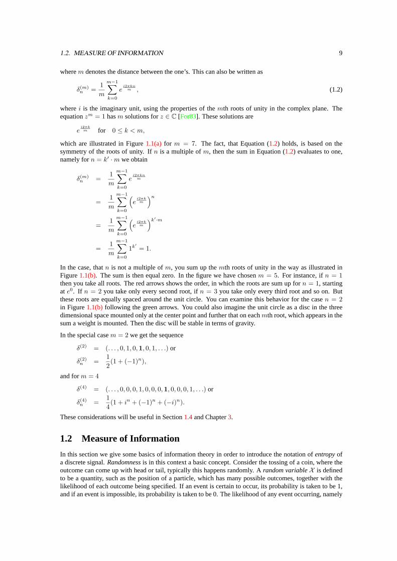
wherem denotes the distance between the one’s. This can also be written as
δ(m)n =
1m
m−1∑k=0
ei2πkn
m , (1.2)
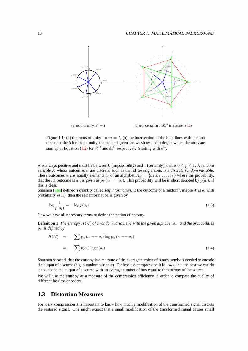
wherei is the imaginary unit, using the properties of themth roots of unity in the complex plane. Theequationzm = 1 hasm solutions forz ∈ C [For83]. These solutions are
ei2πk
m for 0 ≤ k < m,
which are illustrated in Figure1.1(a) for m = 7. The fact, that Equation (1.2) holds, is based on thesymmetry of the roots of unity. Ifn is a multiple ofm, then the sum in Equation (1.2) evaluates to one,namely forn = k′ ·m we obtain
δ(m)n =
1m
m−1∑k=0
ei2πkn
m
=1m
m−1∑k=0
(e
i2πkm
)n
=1m
m−1∑k=0
(e
i2πkm
)k′·m
=1m
m−1∑k=0
1k′ = 1.
In the case, thatn is not a multiple ofm, you sum up themth roots of unity in the way as illustrated inFigure1.1(b). The sum is then equal zero. In the figure we have chosenm = 5. For instance, ifn = 1then you take all roots. The red arrows shows the order, in which the roots are sum up forn = 1, startingat e0. If n = 2 you take only every second root, ifn = 3 you take only every third root and so on. Butthese roots are equally spaced around the unit circle. You can examine this behavior for the casen = 2in Figure1.1(b) following the green arrows. You could also imagine the unit circle as a disc in the threedimensional space mounted only at the center point and further that on eachmth root, which appears in thesum a weight is mounted. Then the disc will be stable in terms of gravity.
In the special casem = 2 we get the sequence
δ(2) = (. . . , 0, 1, 0,1, 0, 1, . . .) or
δ(2)n =12(1 + (−1)n),
and form = 4
δ(4) = (. . . , 0, 0, 0, 1, 0, 0, 0,1, 0, 0, 0, 1, . . .) or
δ(4)n =14(1 + in + (−1)n + (−i)n).
These considerations will be useful in Section1.4and Chapter3.
1.2 Measure of Information
In this section we give some basics of information theory in order to introduce the notation ofentropyofa discrete signal.Randomnessis in this context a basic concept. Consider the tossing of a coin, where theoutcome can come up with head or tail, typically this happens randomly. Arandom variableX is definedto be a quantity, such as the position of a particle, which has many possible outcomes, together with thelikelihood of each outcome being specified. If an event is certain to occur, its probability is taken to be 1,and if an event is impossible, its probability is taken to be 0. The likelihood of any event occurring, namely
10 CHAPTER 1. MATHEMATICAL BACKGROUND
1−1
1
−1
ei2π0/7
ei2π1/7
ei2π2/7
ei2π3/7
ei2π4/7
ei2π5/7
ei2π6/7
(a) roots of unity,z7 = 1
1−1
1
−1
ei2π0/5
ei2π1/5
ei2π2/5
ei2π3/5
ei2π4/5
(b) representation ofδ(5)n in Equation (1.2)
Figure 1.1: (a) the roots of unity form = 7, (b) the intersection of the blue lines with the unitcircle are the5th roots of unity, the red and green arrows shows the order, in which the roots aresum up in Equation (1.2) for δ(1)n andδ(2)n respectively (starting withe0).
p, is always positive and must lie between 0 (impossibility) and 1 (certainty), that is0 ≤ p ≤ 1. A randomvariableX whose outcomesα are discrete, such as that of tossing a coin, is adiscrete random variable.These outcomesα are usually elementsai of an alphabetAX = {a1, a2, . . . , ak} where the probability,that theith outcome isai, is given aspX (α == ai). This probability will be in short denoted byp(ai), ifthis is clear.Shannon [Sha] defined a quantity calledself information. If the outcome of a random variableX is ai withprobabilityp(ai), then the self information is given by
log1
p(ai)= − log p(ai) (1.3)
Now we have all necessary terms to define the notion ofentropy.
Definition 1 The entropyH(X ) of a random variableX with the given alphabetAX and the probabilitiespX is defined by
H(X ) = −∑
i
pX (α == ai) log pX (α == ai)
= −∑
i
p(ai) log p(ai) (1.4)
Shannon showed, that the entropy is a measure of the average number of binary symbols needed to encodethe output of a source (e.g. a random variable). For lossless compression it follows, that the best we can dois to encode the output of a source with an average number of bits equal to the entropy of the source.
We will use the entropy as a measure of the compression efficiency in order to compare the quality ofdifferent lossless encoders.
1.3 Distortion Measures
For lossy compression it is important to know how much a modification of the transformed signal distortsthe restored signal. One might expect that a small modification of the transformed signal causes small
1.4. DOWNSAMPLING, UPSAMPLING, AND DELAY 11
distortions in the restored data. But there is an uncertainty in general. Consider an input signalx (e.g., animage data) and the operationW which is performed by a complete wavelet transform (see Section1.6forexplanations). The transformed signalWx is now modified by a lossy compression.
Let us assume that the lossy compression process outputs signalα. Because every wavelet transformapplied for compression must be invertible, there exists a signaly such thatWy = α. Thus input signalyis restored by the decompression step.
We are looking for an accurate estimation of how much the original signal changes if a modification occurson the transformed signal, in other words, how much distortion is introduced in the compression process.For measuring the difference of two signals or the introduced distortion thesignal to noise ratio(SNR) andthepeak signal to noise ratio(PSNR) (see [TM02], [Say96]) are widely used. They provide a compromisebetween visual perception and easiness of computation.
Both theSNR and thePSNR are logarithmic scaled forms of the EUCLIDean metric of two vectors/signalsx andy
‖x− y‖2 =√∑
i
(xi − yi)2
where the possible value range of the sampled data and the number of samples have an influence, too.Let x, y be signals, each consisting ofn values with a possible range of[0, xmax] (e.g. [0, 255] for 8 bitimages), then
• themean squared errorMSE is defined by
MSE(x, y) :=1n
n−1∑i=0
(xi − yi)2
• thesignal to noise ratioSNR is defined by
SNR(x, y) := 10 log10
‖x‖22‖x− y‖22
dB
• thepeak signal to noise ratioPSNR is defined by
PSNR(x, y) := 20 log10
xmax ·√n
‖x− y‖2dB
= 10 log10
x2max
MSE(x, y)dB
where the units of measurement aredecibels(abbreviated todB).
1.4 Downsampling, Upsampling, and Delay
Downsampling bymd andupsampling bymu are used to express wavelet transforms in terms of filteroperations (md,mu ∈ N). That is, after filtering all samples with indices modulomd different from zeroare discarded ormu − 1 samples are inserted at every index, respectively.
Downsamplinga sequencex bymd can be expressed as
yn = xn·md
12 CHAPTER 1. MATHEMATICAL BACKGROUND
or in z-transform domain
Y (z) =1md
md−1∑k=0
X(e−i2πk
md z1
md )
with y ←→ Y andx←→ X. This can be shown using Equation (1.2)
Y (z) =∑k∈Z
xkmdz−k
=∑n∈Z
xnδ(md)n z
−nmd
=∑n∈Z
xn
(1md
md−1∑k=0
ei2πkn
md
)z−nmd
=1md
md−1∑k=0
(∑n∈Z
xnei2πkn
md z−nmd
)
=1md
md−1∑k=0
(∑n∈Z
xn
(e−i2πk
md z1
md
)−n)
=1md
md−1∑k=0
X(e−i2πk
md z1
md
).
Upsamplinga sequencex bymu can be expressed as
yn ={xn/mu
: ∃k ∈ Z : n = k ·mu
0 : else
or in z-transform domain
Y (z) =∑n∈Z
ynz−n
=∑k∈Z
xkz−(k·mu)
=∑k∈Z
xk (zmu)−k
= X(zmu)
with y ←→ Y andx←→ X.
The downsampling and upsampling operation for signalx are denoted byx ↓ md andx ↑ mu, respec-tively. In the following illustrations we will depict both operations with the symbols↓ md and ↑ mu ,respectively.
In order to discard even or odd indexed samples we also need the termdelay bymdly wheremdly ∈ Z.Consider the sequencey defined byyn = xn−mdly , that is the signalx delayed bymdly. In z-transformdomain this can be expressed as
Y (z) = z−mdlyX(z).
1.5. WAVELETS 13
This can be easily seen by pluggingxn−mdly into the definition of thez-transform, i.e.,
Y (z) =∑
n
ynz−n
=∑
n
xn−mdlyz−n
=∑n′
xn′z−n′−mdly
= z−mdly∑
n
xnz−n
= z−mdlyX(z).
1.5 Wavelets
Wavelets (little waves) are functions that are concentrated in time as well as in frequency around a certainpoint. For practical applications we choose wavelets which correspond to a so calledmultiresolution anal-ysis[Dau92] due to the reversibility and the efficient computation of the appropriate transform. Waveletsfulfil certain self similarity conditions. When talking about wavelets, we mostly mean a pair of functions:the scaling functionφ and the wavelet functionψ [Swe96], [Thi01]. Several extensions to this basic schemeexist, but for the introduction we will concentrate on this case. The self similarity (refinement condition)of the scaling functionφ is bounded to a filterh and is defined by
φ(t) =√
2∑k∈Z
hkφ(2t− k) t, hk ∈ R (1.5)
which means thatφ remains unchanged if you filter it withh, downsample it by a factor of two, andamplify the values by
√2, successively (see Figure1.2). One could also say, thatφ is the eigenfunction
with eigenvalue 1 of the linear operator that is described by the refinement. Since eigenfunctions are uniqueonly if the amplitude is given, the scaling function is additionally normalized to∑
k∈Zφ(k) =
√2
to make it unique.The wavelet functionψ is built onφ with help of a filterg (Figure1.3):
ψ(t) =√
2∑k∈Z
gkφ(2t− k) gk ∈ R. (1.6)
φ andψ are uniquely determined by the filtersh andg.Variants of these functions are defined, which are translated by an integer, compressed by a power of two,and usually amplified by a power of
√2:
ψj,l(t) = 2j/2ψ(2jt− l) (1.7)
φj,l(t) = 2j/2φ(2jt− l) (1.8)
with j, l ∈ Z, t ∈ R
• j denotes the scale – the biggerj the higher the frequency and the thinner the wavelet peak
• l denotes the translation – the biggerl the more shift to the right, and the biggerj the smaller thesteps
14 CHAPTER 1. MATHEMATICAL BACKGROUND
−1 0 1
0
1 ∑k∈Z
hkφ(2t− k)
−1 0 1
0
1φ(2t− 1)φ(2t+ 1) φ(2t)
−1 0 1
0
1φ(t)
−1 0 1
0
1h1φ(2t− 1)h−1φ(2t+ 1)
h0φ(2t)
a
c
bd
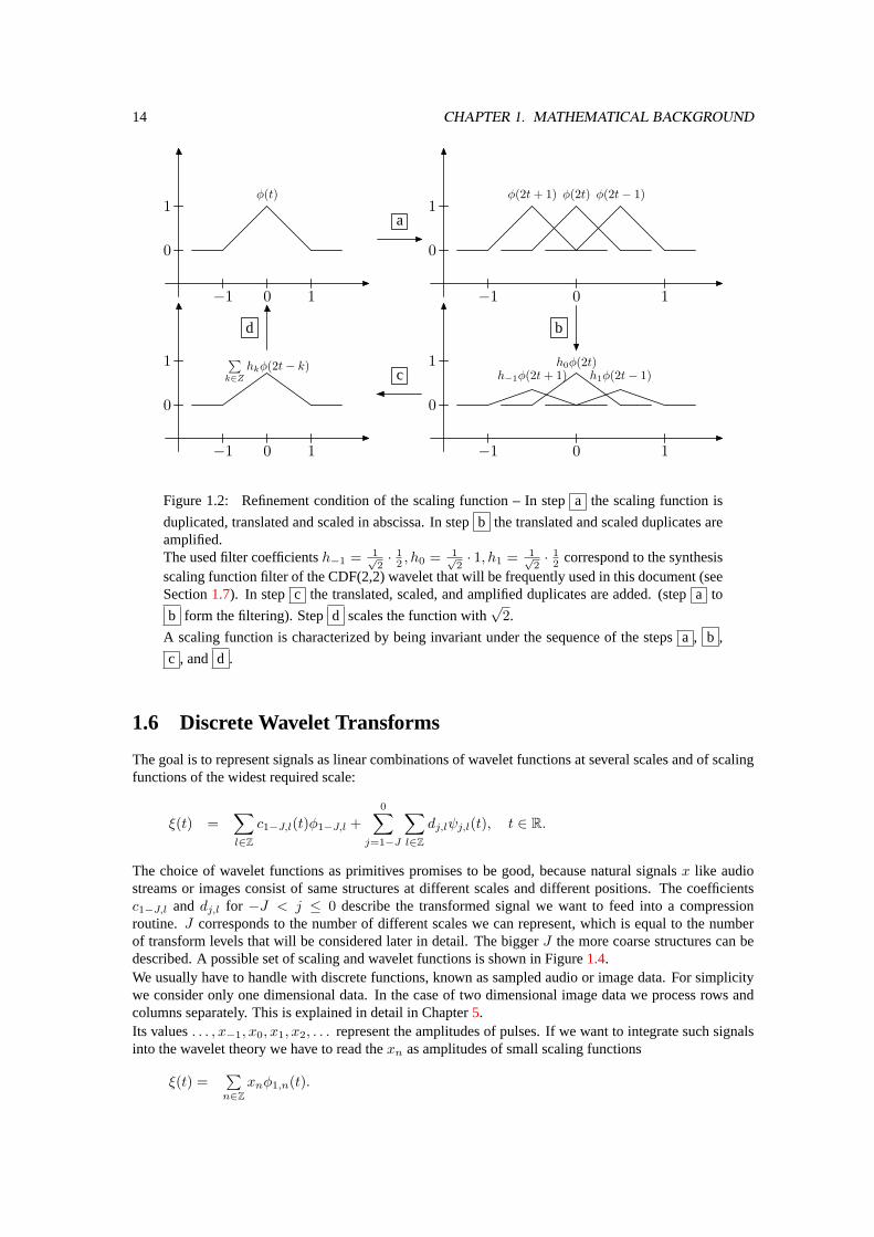
Figure 1.2: Refinement condition of the scaling function – In stepa the scaling function is
duplicated, translated and scaled in abscissa. In stepb the translated and scaled duplicates areamplified.The used filter coefficientsh−1 = 1√
2· 1
2 , h0 = 1√2· 1, h1 = 1√
2· 1
2 correspond to the synthesisscaling function filter of the CDF(2,2) wavelet that will be frequently used in this document (seeSection1.7). In step c the translated, scaled, and amplified duplicates are added. (stepa to
b form the filtering). Stepd scales the function with√
2.
A scaling function is characterized by being invariant under the sequence of the stepsa , b ,
c , and d .
1.6 Discrete Wavelet Transforms
The goal is to represent signals as linear combinations of wavelet functions at several scales and of scalingfunctions of the widest required scale:
ξ(t) =∑l∈Z
c1−J,l(t)φ1−J,l +0∑
j=1−J
∑l∈Z
dj,lψj,l(t), t ∈ R.
The choice of wavelet functions as primitives promises to be good, because natural signalsx like audiostreams or images consist of same structures at different scales and different positions. The coefficientsc1−J,l anddj,l for −J < j ≤ 0 describe the transformed signal we want to feed into a compressionroutine. J corresponds to the number of different scales we can represent, which is equal to the numberof transform levels that will be considered later in detail. The biggerJ the more coarse structures can bedescribed. A possible set of scaling and wavelet functions is shown in Figure1.4.We usually have to handle with discrete functions, known as sampled audio or image data. For simplicitywe consider only one dimensional data. In the case of two dimensional image data we process rows andcolumns separately. This is explained in detail in Chapter5.Its values. . . , x−1, x0, x1, x2, . . . represent the amplitudes of pulses. If we want to integrate such signalsinto the wavelet theory we have to read thexn as amplitudes of small scaling functions
ξ(t) =∑n∈Z
xnφ1,n(t).
1.6. DISCRETE WAVELET TRANSFORMS 15
−1 0 1 2
0
1(t)
−1 0 1 2
0
1g3φ(2t− 3)
g2φ(2t− 2)g0φ(2t)g−1φ(2t+ 1)
g1φ(2t− 1)
−1 0 1 2
0
1
φ(t)
−1 0 1 2
0
1
∑k∈Z
gkφ(2t− k)
a
b
c
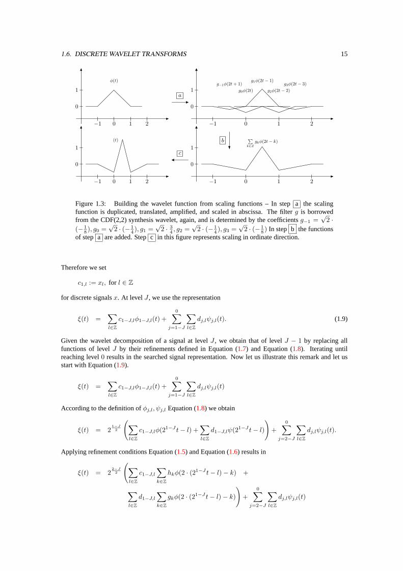
Figure 1.3: Building the wavelet function from scaling functions – In stepa the scalingfunction is duplicated, translated, amplified, and scaled in abscissa. The filterg is borrowedfrom the CDF(2,2) synthesis wavelet, again, and is determined by the coefficientsg−1 =
√2 ·
(− 18 ), g0 =
√2 · (− 1
4 ), g1 =√
2 · 34 , g2 =
√2 · (− 1
4 ), g3 =√
2 · (− 18 ) In step b the functions
of step a are added. Stepc in this figure represents scaling in ordinate direction.
Therefore we set
c1,l := xl, for l ∈ Z
for discrete signalsx. At levelJ , we use the representation
ξ(t) =∑l∈Z
c1−J,lφ1−J,l(t) +0∑
j=1−J
∑l∈Z
dj,lψj,l(t). (1.9)
Given the wavelet decomposition of a signal at levelJ , we obtain that of levelJ − 1 by replacing allfunctions of levelJ by their refinements defined in Equation (1.7) and Equation (1.8). Iterating untilreaching level0 results in the searched signal representation. Now let us illustrate this remark and let usstart with Equation (1.9).
ξ(t) =∑l∈Z
c1−J,lφ1−J,l(t) +0∑
j=1−J
∑l∈Z
dj,lψj,l(t)
According to the definition ofφj,l, ψj,l Equation (1.8) we obtain
ξ(t) = 21−J
2
(∑l∈Z
c1−J,lφ(21−J t− l) +∑l∈Z
d1−J,lψ(21−J t− l)
)+
0∑j=2−J
∑l∈Z
dj,lψj,l(t).
Applying refinement conditions Equation (1.5) and Equation (1.6) results in
ξ(t) = 22−J
2
(∑l∈Z
c1−J,l
∑k∈Z
hkφ(2 · (21−J t− l)− k) +
ξ(t) 22−J
2
(∑l∈Z
d1−J,l
∑k∈Z
gkφ(2 · (21−J t− l)− k)
)+
0∑j=2−J
∑l∈Z
dj,lψj,l(t)
16 CHAPTER 1. MATHEMATICAL BACKGROUND
−4 0 4 8
0
1
−4 0 4 8
0
1
−4 0 4 8
0
1
−4 0 4 8
0
1
−4 0 4 8
0
1
−4 0 4 8
0
1
−4 0 4 8
0
1
−4 0 4 8
0
1
−4 0 4 8
0
1
−4 0 4 8
0
1
−4 0 4 8
0
1
−4 0 4 8
0
1
−4 0 4 8
0
1
φ−2,0 φ−2,1
−2,0 −2,1
−1,0
−1,1 −1,2
0,0 0,1 0,2 0,3 0,4 0,5
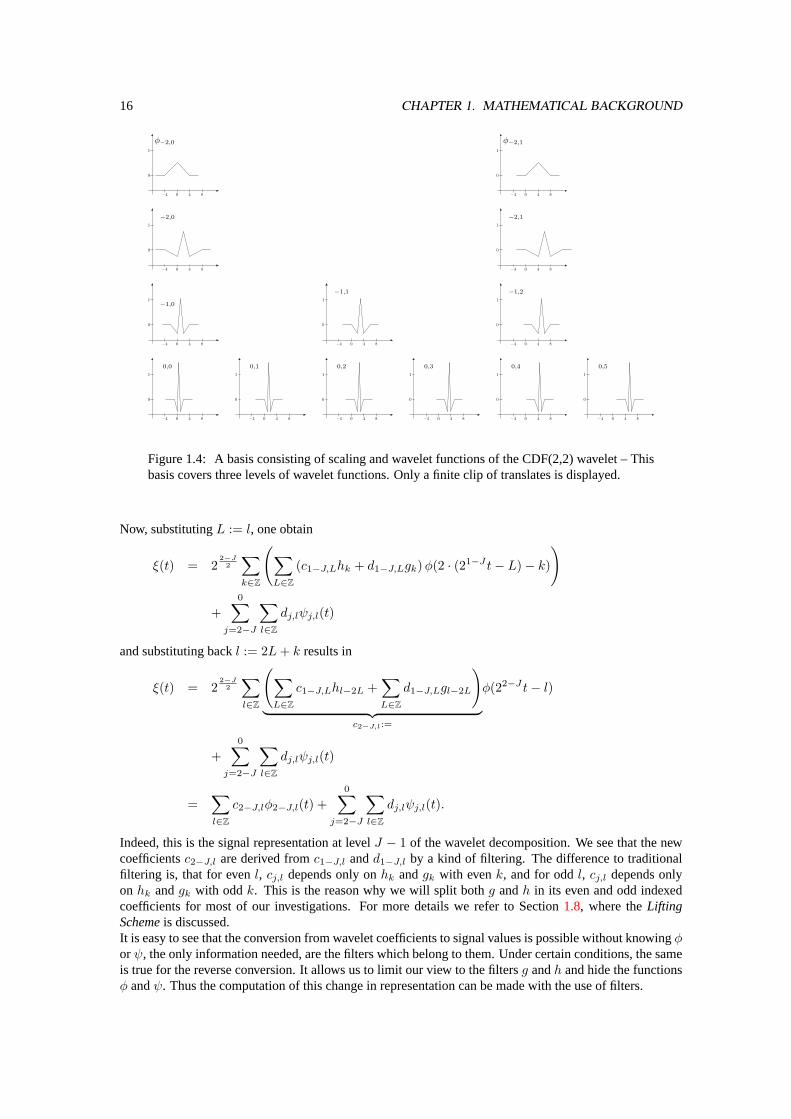
Figure 1.4: A basis consisting of scaling and wavelet functions of the CDF(2,2) wavelet – Thisbasis covers three levels of wavelet functions. Only a finite clip of translates is displayed.
Now, substitutingL := l, one obtain
ξ(t) = 22−J
2
∑k∈Z
(∑L∈Z
(c1−J,Lhk + d1−J,Lgk)φ(2 · (21−J t− L)− k)
)
+0∑
j=2−J
∑l∈Z
dj,lψj,l(t)
and substituting backl := 2L+ k results in
ξ(t) = 22−J
2
∑l∈Z
(∑L∈Z
c1−J,Lhl−2L +∑L∈Z
d1−J,Lgl−2L
)︸ ︷︷ ︸
c2−J,l:=
φ(22−J t− l)
+0∑
j=2−J
∑l∈Z
dj,lψj,l(t)
=∑l∈Z
c2−J,lφ2−J,l(t) +0∑
j=2−J
∑l∈Z
dj,lψj,l(t).
Indeed, this is the signal representation at levelJ − 1 of the wavelet decomposition. We see that the newcoefficientsc2−J,l are derived fromc1−J,l andd1−J,l by a kind of filtering. The difference to traditionalfiltering is, that for evenl, cj,l depends only onhk andgk with evenk, and for oddl, cj,l depends onlyon hk andgk with oddk. This is the reason why we will split bothg andh in its even and odd indexedcoefficients for most of our investigations. For more details we refer to Section1.8, where theLiftingSchemeis discussed.It is easy to see that the conversion from wavelet coefficients to signal values is possible without knowingφorψ, the only information needed, are the filters which belong to them. Under certain conditions, the sameis true for the reverse conversion. It allows us to limit our view to the filtersg andh and hide the functionsφ andψ. Thus the computation of this change in representation can be made with the use of filters.
1.7. COHEN-DAUBECHIES-FEAUVEAU CDF(2,2) WAVELET 17
In the following we have to distinguish between the conversion from the original signal to the waveletcoefficients and from the wavelet coefficients back to the signal or an approximated version of it. The firstconversion is usually denoted bywavelet analysisor wavelet decomposition, and the second bywaveletsynthesisor wavelet reconstruction. We will use these notions throughout the document.Since the filters and the scaling and wavelet function can differ for wavelet analysis and synthesis (forinstance in the case of biorthogonal bases) we will denote the analysis scaling and wavelet functions byφ and ψ, respectively. For the synthesis scaling and wavelet functions we use the symbolsφ andψ,respectively. The corresponding filters are denoted accordingly byg, h andg, h.
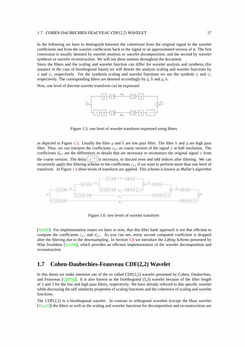
Now, one level of discrete wavelet transform can be expressed
↓ 2
↓ 2
h
gz1
↑ 2
↑ 2
h
+
g z−1
xn x′n
c0,l
d0,l
Figure 1.5: one level of wavelet transform expressed using filters
as depicted in Figure1.5. Usually the filterg and h are low pass filter. The filterh and g are high passfilter. Thus, we can interpret the coefficientsc0,l as coarse version of the signalx at half resolution. Thecoefficientsd0,l are the differences or details that are necessary to reconstruct the original signalx from
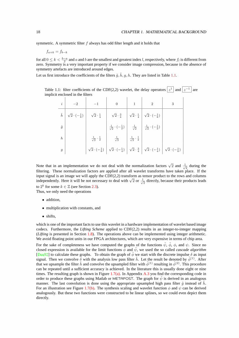
the coarse version. The delayz−1 is necessary, to discard even and odd indices after filtering. We canrecursively apply this filtering scheme to the coefficientscj,l if we want to perform more than one level oftransform. In Figure1.6three levels of transform are applied. This scheme is known asMallat’s algorithm
↓ 2
↓ 2
h
gz1
↓ 2
↓ 2
h
gz1
↓ 2
↓ 2
h
gz1
↑ 2
↑ 2
h
+
g z−1
↑ 2
↑ 2
h
+
g z−1
↑ 2
↑ 2
h
+
g z−1
xn x′n
d0,l
d−1,l
d−2,l
c0,l
c−1,l
c−2,l
c′−1,l
c′0,l
Figure 1.6: tree levels of wavelet transform
[Mal89]. For implementation issues we have to note, that this filter bank approach is not that efficient tocompute the coefficientscj,l and dj,l. As you can see, every second computed coefficient is droppedafter the filtering due to the downsampling. In Section1.8 we introduce theLifting Schemepresented byWim Sweldens [Swe96], which provides an efficient implementation of the wavelet decomposition andreconstruction.
1.7 Cohen-Daubechies-Feauveau CDF(2,2) Wavelet
In this thesis we make intensive use of the so called CDF(2,2) wavelet presented by Cohen, Daubechies,and Feauveau [CDF92]. It is also known as the biorthogonal (5,3) wavelet because of the filter lengthof 5 and3 for the low and high pass filters, respectively. We have already referred to this specific waveletwhile discussing the self similarity properties of scaling functions and the coherence of scaling and waveletfunctions.
The CDF(2,2) is a biorthogonal wavelet. In contrast to orthogonal wavelets (except the Haar wavelet[Haa10]) the filters as well as the scaling and wavelet functions for decomposition and reconstructions are
18 CHAPTER 1. MATHEMATICAL BACKGROUND
symmetric. A symmetric filterf always has odd filter length and it holds that
fa+k = fb−k
for all 0 ≤ k < b−a2 anda andb are the smallest and greatest indexl, respectively, wherefl is different from
zero. Symmetry is a very important property if we consider image compression, because in the absence ofsymmetry artefacts are introduced around edges.
Let us first introduce the coefficients of the filtersg, h, g, h. They are listed in Table1.1.
Table 1.1: filter coefficients of the CDF(2,2) wavelet, the delay operatorsz1 and z−1 areimplicit enclosed in the filters
i −2 −1 0 1 2 3
h√
2 · (− 18)
√2 · 1
4
√2 · 3
4
√2 · 1
4
√2 · (− 1
8)
g 1√2· (− 1
2) 1√
2
1√2· (− 1
2)
h 1√2· 1
21√2
1√2· 1
2
g√
2 · (− 18)
√2 · (− 1
4)
√2 · 3
4
√2 · (− 1
4)
√2 · (− 1
8)
Note that in an implementation we do not deal with the normalization factors√
2 and 1√2
during thefiltering. These normalization factors are applied after all wavelet transforms have taken place. If theinput signal is an image we will apply the CDF(2,2) transform as tensor product to the rows and columnsindependently. Here it will be not necessary to deal with
√2 or 1√
2directly, because their products leads
to 2k for somek ∈ Z (see Section2.3).Thus, we only need the operations
• addition,
• multiplication with constants, and
• shifts,
which is one of the important facts to use this wavelet in a hardware implementation of wavelet based imagecodecs. Furthermore, theLifting Schemeapplied to CDF(2,2) results in an integer-to-integer mapping(Lifting is presented in Section1.8). The operations above can be implemented using integer arithmetic.We avoid floating point units in our FPGA architectures, which are very expensive in terms of chip area.
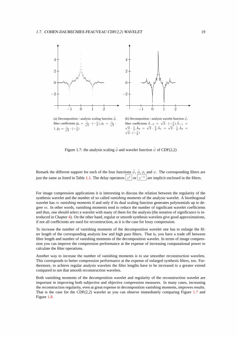
For the sake of completeness we have computed the graphs of the functionsψ, φ, φ, andψ. Since noclosed expression is available for the limit functionsφ and ψ, we used the so calledcascade algorithm[Dau92] to calculate these graphs. To obtain the graph ofφ we start with the discrete impulseδ as inputsignal. Then we convolveδ with the analysis low pass filterh. Let the result be denoted byφ(1). Afterthat we upsample the filterh and convolve the upsampled filter withφ(1) resulting inφ(2). This procedurecan be repeated until a sufficient accuracy is achieved. In the literature this is usually done eight or ninetimes. The resulting graph is shown in Figure1.7(a). In AppendixA.3 you find the corresponding code inorder to produce these graphs using Matlab orMETAPOST. The graph forψ is derived in an analogousmanner. The last convolution is done using the appropriate upsampled high pass filterg instead ofh.For an illustration see Figure1.7(b). The synthesis scaling and wavelet functionφ andψ can be derivedanalogously. But these two functions were constructed to be linear splines, so we could even depict themdirectly.
1.7. COHEN-DAUBECHIES-FEAUVEAU CDF(2,2) WAVELET 19
−1 0 1 2
−2
0
2
4
(a) Decomposition / analysis scaling functionφ,
filter coefficientsg0 = 1√2· (− 1
2), g1 = 1√
2·
1, g2 = 1√2· (− 1
2)
−1 0 1 2
−2
0
2
4
(b) Decomposition / analysis wavelet functionψ,
filter coefficientsh−2 =√
2 · (− 18), h−1 =√
2 · 14, h0 =
√2 · 3
4, h1 =
√2 · 1
4, h2 =√
2 · (− 18)
Figure 1.7: the analysis scalingφ and wavelet functionψ of CDF(2,2)
Remark the different support for each of the four functionsψ, φ, φ, andψ. The corresponding filters are
just the same as listed in Table1.1. The delay operatorsz1 or z−1 are implicit enclosed in the filters.
For image compression applications it is interesting to discuss the relation between the regularity of thesynthesis wavelet and the number of so calledvanishing momentsof the analysis wavelet. A biorthogonalwavelet hasm vanishing momentsif and only if its dual scaling function generates polynomials up to de-greem. In other words, vanishing moments tend to reduce the number of significant wavelet coefficientsand thus, one should select a wavelet with many of them for the analysis (the notation of significance is in-troduced in Chapter4). On the other hand, regular or smooth synthesis wavelets give good approximations,if not all coefficients are used for reconstruction, as it is the case for lossy compression.
To increase the number of vanishing moments of the decomposition wavelet one has to enlarge the fil-ter length of the corresponding analysis low and high pass filters. That is, you have a trade off betweenfilter length and number of vanishing moments of the decomposition wavelet. In terms of image compres-sion you can improve the compression performance at the expense of increasing computational power tocalculate the filter operations.
Another way to increase the number of vanishing moments is to use smoother reconstruction wavelets.This corresponds to better compression performance at the expense of enlarged synthesis filters, too. Fur-thermore, to achieve regular analysis wavelets the filter lengths have to be increased to a greater extendcompared to not that smooth reconstruction wavelets.
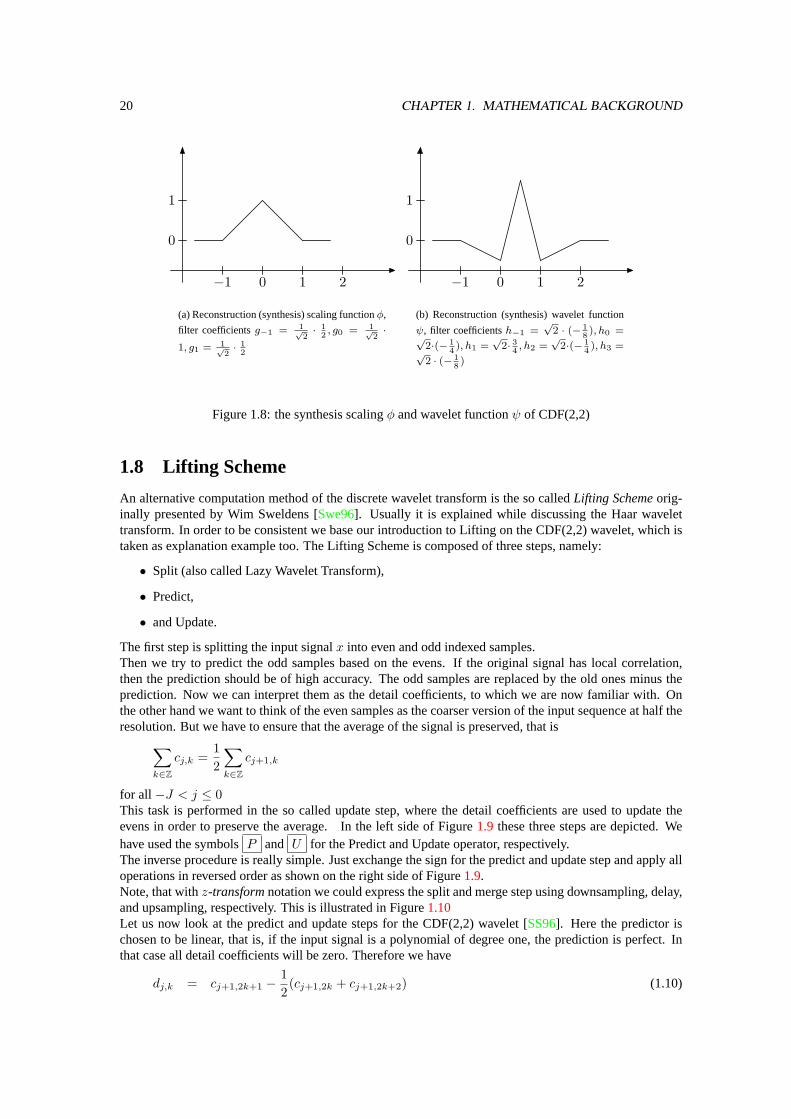
Both vanishing moments of the decomposition wavelet and regularity of the reconstruction wavelet areimportant in improving both subjective and objective compression measures. In many cases, increasingthe reconstruction regularity, even at great expense in decomposition vanishing moments, improves results.That is the case for the CDF(2,2) wavelet as you can observe immediately comparing Figure1.7 andFigure1.8.
20 CHAPTER 1. MATHEMATICAL BACKGROUND
−1 0 1 2
0
1
(a) Reconstruction (synthesis) scaling functionφ,
filter coefficientsg−1 = 1√2· 1
2, g0 = 1√
2·
1, g1 = 1√2· 1
2
−1 0 1 2
0
1
(b) Reconstruction (synthesis) wavelet function
ψ, filter coefficientsh−1 =√
2 · (− 18), h0 =√
2·(− 14), h1 =
√2· 3
4, h2 =
√2·(− 1
4), h3 =√
2 · (− 18)
Figure 1.8: the synthesis scalingφ and wavelet functionψ of CDF(2,2)
1.8 Lifting Scheme
An alternative computation method of the discrete wavelet transform is the so calledLifting Schemeorig-inally presented by Wim Sweldens [Swe96]. Usually it is explained while discussing the Haar wavelettransform. In order to be consistent we base our introduction to Lifting on the CDF(2,2) wavelet, which istaken as explanation example too. The Lifting Scheme is composed of three steps, namely:
• Split (also called Lazy Wavelet Transform),
• Predict,
• and Update.
The first step is splitting the input signalx into even and odd indexed samples.Then we try to predict the odd samples based on the evens. If the original signal has local correlation,then the prediction should be of high accuracy. The odd samples are replaced by the old ones minus theprediction. Now we can interpret them as the detail coefficients, to which we are now familiar with. Onthe other hand we want to think of the even samples as the coarser version of the input sequence at half theresolution. But we have to ensure that the average of the signal is preserved, that is∑
k∈Zcj,k =
12
∑k∈Z
cj+1,k
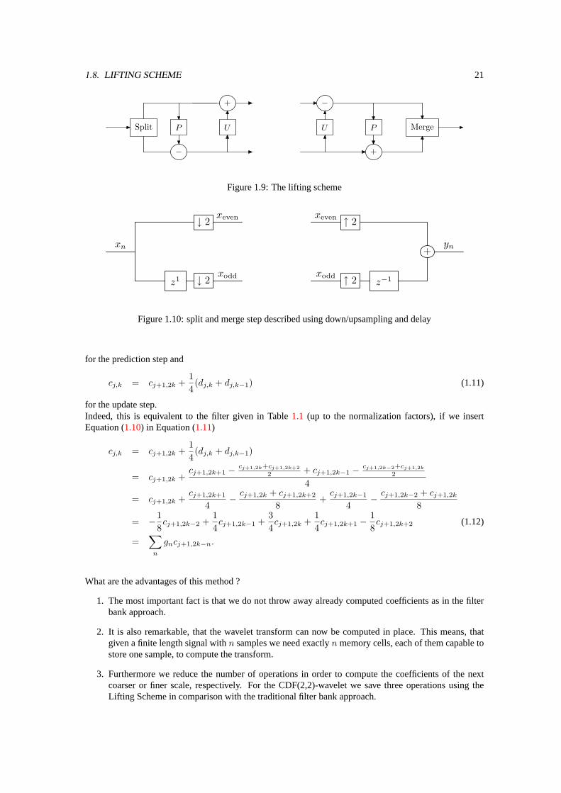
for all −J < j ≤ 0This task is performed in the so called update step, where the detail coefficients are used to update theevens in order to preserve the average. In the left side of Figure1.9 these three steps are depicted. Wehave used the symbolsP and U for the Predict and Update operator, respectively.The inverse procedure is really simple. Just exchange the sign for the predict and update step and apply alloperations in reversed order as shown on the right side of Figure1.9.Note, that withz-transformnotation we could express the split and merge step using downsampling, delay,and upsampling, respectively. This is illustrated in Figure1.10Let us now look at the predict and update steps for the CDF(2,2) wavelet [SS96]. Here the predictor ischosen to be linear, that is, if the input signal is a polynomial of degree one, the prediction is perfect. Inthat case all detail coefficients will be zero. Therefore we have
dj,k = cj+1,2k+1 −12(cj+1,2k + cj+1,2k+2) (1.10)
1.8. LIFTING SCHEME 21
Split P
−
+
U
−
U P
+
Merge
Figure 1.9: The lifting scheme
z1
↓ 2
↓ 2 z−1
↑ 2
↑ 2
+xn yn
xeven
xodd
xeven
xodd
Figure 1.10: split and merge step described using down/upsampling and delay
for the prediction step and
cj,k = cj+1,2k +14(dj,k + dj,k−1) (1.11)
for the update step.Indeed, this is equivalent to the filter given in Table1.1 (up to the normalization factors), if we insertEquation (1.10) in Equation (1.11)
cj,k = cj+1,2k +14(dj,k + dj,k−1)
= cj+1,2k +cj+1,2k+1 − cj+1,2k+cj+1,2k+2
2 + cj+1,2k−1 − cj+1,2k−2+cj+1,2k
2
4
= cj+1,2k +cj+1,2k+1
4− cj+1,2k + cj+1,2k+2
8+cj+1,2k−1
4− cj+1,2k−2 + cj+1,2k
8
= −18cj+1,2k−2 +
14cj+1,2k−1 +
34cj+1,2k +
14cj+1,2k+1 −
18cj+1,2k+2 (1.12)
=∑
n
gncj+1,2k−n.
What are the advantages of this method ?
1. The most important fact is that we do not throw away already computed coefficients as in the filterbank approach.
2. It is also remarkable, that the wavelet transform can now be computed in place. This means, thatgiven a finite length signal withn samples we need exactlyn memory cells, each of them capable tostore one sample, to compute the transform.
3. Furthermore we reduce the number of operations in order to compute the coefficients of the nextcoarser or finer scale, respectively. For the CDF(2,2)-wavelet we save three operations using theLifting Scheme in comparison with the traditional filter bank approach.
22 CHAPTER 1. MATHEMATICAL BACKGROUND
1.8.1 Integer-to-Integer Mapping
Obviously, the application of the filter bank approach or the Lifting Scheme leads to coefficients, which arenot integers in general. In the field of hardware image compression it would be convenient, that coefficientsand the pixel of the reconstructed image are integers too. Chao et.al.[CFH96] and Cohen et.al.[CDSY97]have introduced techniques for doing so. The basic idea is to modify the computation of the Predict andUpdate step in the following way
d′j,k = c′j+1,2k+1 − bP cc′j,k = c′j+1,2k + bUc ,
wherec′1,k = c1,k = xk for all k ∈ Z. Here the symbolsP andU represent any reasonable predictor orupdate operator, respectively.
Remark It is easy to verify, that perfect reconstruction in case of lossless compression is guaranteed,since that same value of the modified predictor and update operator is added and subtracted. However,since we lose the linearity of the transform due to the rounding, the influence of this modification in termsof image compression efficiency is hard to estimate. Fortunately, our practical experiences do not show anyremarkable differences between the Lifting Scheme and the modified version.
For the special case of the CDF(2,2) wavelet we therefore use the prediction and update steps as follows:
d′j,k = c′j+1,2k+1 −⌊
12(c′j+1,2k + c′j+1,2k+2)
⌋(1.13)
c′j,k = c′j+1,2k +⌊
14(d′j,k + d′j,k−1)
⌋. (1.14)
As a consequence the coefficients of all scales−J < j ≤ 0 can be stored as integers and for all operationsinteger arithmetic is sufficient. Note, that the coarser the scale the more bits are necessary to store thecorresponding coefficients. To overcome the growing bitwidth at coarser scales modular arithmetic can beused in the case of lossless compression.
1.8.2 Lifting Scheme and Modular Arithmetic
Chao et.al. suggest to use modular arithmetic in combination with the Lifting Scheme [CFH96]. We usethe symbols⊕ and for the modular addition and subtraction, which are defined as
a⊕ b := a+ b mod m and
a b := a− b mod m
for reasonablem ∈ N, respectively. Equation (1.13) and Equation (1.14) now look like
d′j,k = c′j+1,2k+1 ⌊
12(c′j+1,2k ⊕ c′j+1,2k+2)
⌋c′j,k = c′j+1,2k ⊕
⌊14(d′j,k ⊕ d′j,k−1)
⌋.
As a consequence, all coefficients at all scales as well as the reconstructed signal have the same bitwidth asthe original sequence, if we initializem = 2dpth, wheredpth is the given bitwidth of the original samples.Additionally, the computational units for addition and subtraction have to be provided form bit operandsonly. With respect to the hardware implementation we save memory resources and logic in the arithmeticlogic units.Remark, that this modification is only feasible in case of lossless compression. The approach of Chao et.al.is limited to lossless compression, since in fact transform coefficients of large magnitude become small dueto modular arithmetic. This is counterproductive for quantization purposes in wavelet based compressiontechniques, where coefficients with large magnitude are considered as important and small coefficients tendto be neglected (see Chapter4 for a detailed discussion of wavelet based image codecs).
Chapter 2
Wavelet transforms on images
Until now we have discussed one dimensional wavelet transforms. Images are obviously two dimensionaldata. To transform images we can use two dimensional wavelets or apply the one dimensional transformto the rows and columns of the image successively as separable two dimensional transform. In most ofthe applications, where wavelets are used for image processing and compression, the latter choice is taken,because of the low computational complexity of separable transforms.
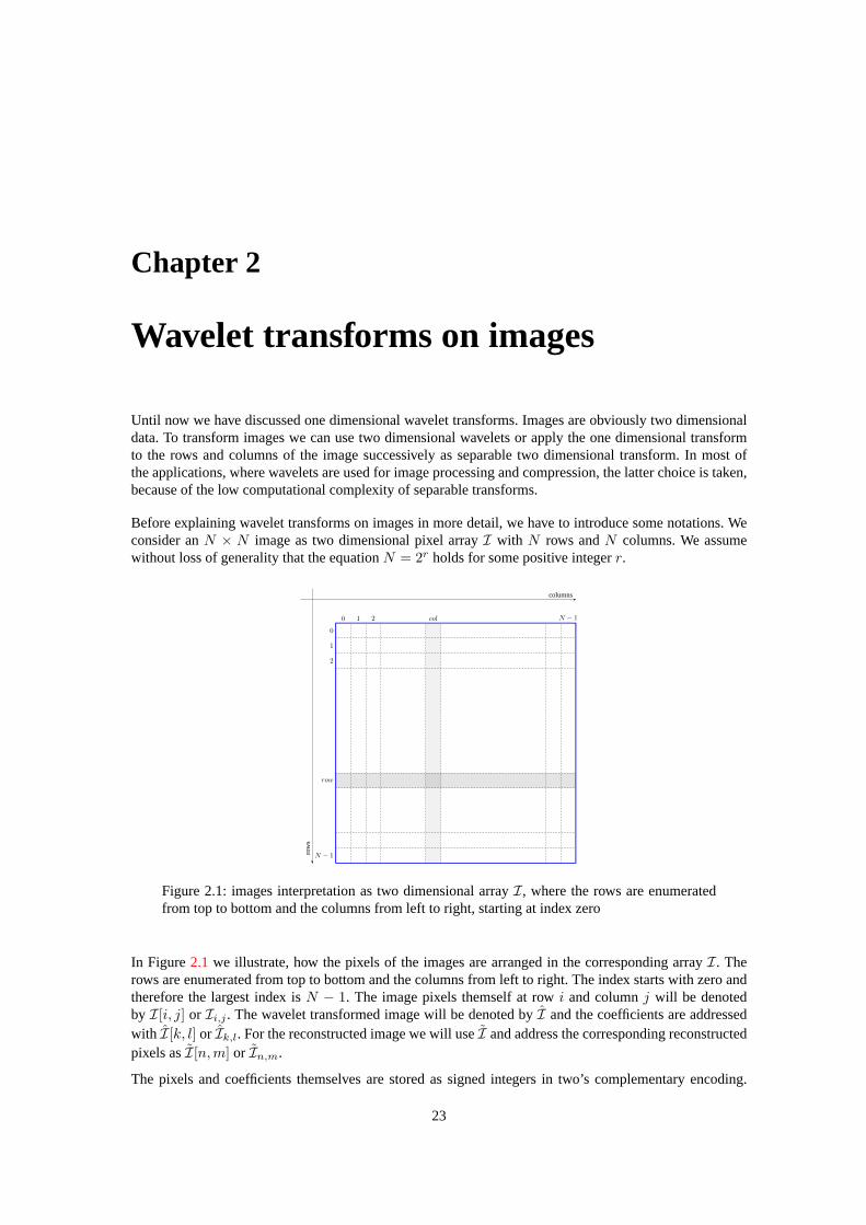
Before explaining wavelet transforms on images in more detail, we have to introduce some notations. Weconsider anN × N image as two dimensional pixel arrayI with N rows andN columns. We assumewithout loss of generality that the equationN = 2r holds for some positive integerr.
0 1 2 N − 1
0
1
2
N − 1
row
col
row
s
columns
Figure 2.1: images interpretation as two dimensional arrayI, where the rows are enumeratedfrom top to bottom and the columns from left to right, starting at index zero
In Figure2.1 we illustrate, how the pixels of the images are arranged in the corresponding arrayI. Therows are enumerated from top to bottom and the columns from left to right. The index starts with zero andtherefore the largest index isN − 1. The image pixels themself at rowi and columnj will be denotedby I[i, j] or Ii,j . The wavelet transformed image will be denoted byI and the coefficients are addressedwith I[k, l] or Ik,l. For the reconstructed image we will useI and address the corresponding reconstructedpixels asI[n,m] or In,m.
The pixels and coefficients themselves are stored as signed integers in two’s complementary encoding.
23
24 CHAPTER 2. WAVELET TRANSFORMS ON IMAGES
Therefore the range is given as
I[row, col] ∈[−2dpth−1, 2dpth−1 − 1
],
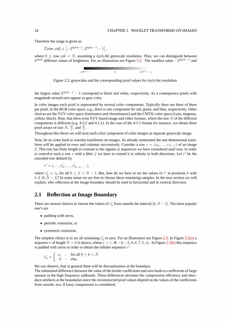
where0 ≤ row, col < N , assuming adpth-bit greyscale resolution. Thus, we can distinguish between2dpth different values of brightness. For an illustration see Figure2.2. The smallest value−2dpth−1 and
−2dpth−1 2dpth−1 − 10
Figure 2.2: greyscales and the corresponding pixel values fordpth-bit resolution
the largest value2dpth−1 − 1 correspond to black and white, respectively. As a consequence pixels withmagnitude around zero appear as grey color.
In color images each pixel is represented by several color components. Typically there are three of themper pixel. In the RGB color space, e.g., there is one component for red, green, and blue, respectively. Otherchoices are the YUV color space (luminance and chrominance) and the CMYK color space (cyan, magenta,yellow, black). Note, that there exist YUV based image and video formats, where the sizeN of the differentcomponents is different (e.g. 4:2:2 and 4:1:1). In the case of the 4:1:1 format for instance, we obtain threepixel arrays of sizeN , N
4 , andN4 .
Throughout this thesis we will treat each color component of color images as separate greyscale image.
Now, let us come back to wavelet transforms on images. As already mentioned the one dimensional trans-form will be applied to rows and columns successively. Consider a rowr = (r0, . . . , rN−1) of an imageI. This row has finite length in contrast to the signals or sequences we have considered until now. In orderto convolve such a rowr with a filter f we have to extend it to infinity in both directions. Letr′ be theextended row defined by
r′ = (. . . , r′0, . . . , r′N−1, . . .),
wherer′k = rk for all 0 ≤ k < N − 1. But, how do we have to set the values ofr′ at positionsk withk /∈ [0, N − 1]? In some sense we are free to choose these remaining samples. In the next section we willexplain, why reflection at the image boundary should be used in horizontal and in vertical direction.
2.1 Reflection at Image Boundary
There are several choices to choose the values ofr′k from outside the interval[0, N − 1]. The most popularone’s are
• padding with zeros,
• periodic extension, or
• symmetric extension.
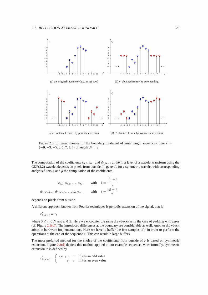
The simplest choice is to set all remainingr′k to zero. For an illustration see Figure2.3. In Figure2.3(a)asequencer of lengthN = 8 is shown, wherer = (−8,−3,−5, 0, 6, 7, 5, 4). In Figure2.3(b)this sequenceis padded with zeros in order to obtain the infinite sequencer′:
r′k ={rk : for all 0 ≤ k < N0 : else.
We can observe, that in general there will be discontinuities at the boundary.The substantial difference between the value of the border coefficients and zero leads to coefficients of largeamount in the high frequency subbands. These differences decrease the compression efficiency and intro-duce artefacts at the boundaries since the reconstructed pixel values depend on the values of the coefficientsfrom outside, too, if lossy compression is considered.
2.1. REFLECTION AT IMAGE BOUNDARY 25
−3−2−1 0 1 2 3 4 5 6 7 8 9 10 11
−8−6−4−2
0246
i
ri
(a) the original sequencer(e.g. image row)
−3−2−1 0 1 2 3 4 5 6 7 8 9 10 11
−8−6−4−2
0246
. . . . . .
j
r′j
(b) r′ obtained fromr by zero padding
−3−2−1 0 1 2 3 4 5 6 7 8 9 10 11
−8−6−4−2
0246
. . . . . .
j
r′j
(c) r′ obtained fromr by periodic extension
−3−2−1 0 1 2 3 4 5 6 7 8 9 10 11
−8−6−4−2
0246
. . . . . .
j
r′j
(d) r′ obtained fromr by symmetric extension
Figure 2.3: different choices for the boundary treatment of finite length sequences, herer =(−8,−3,−5, 0, 6, 7, 5, 4) of lengthN = 8
The computation of the coefficientsc0,0, c0,1 andd0,N−1 at the first level of a wavelet transform using theCDF(2,2) wavelet depends on pixels from outside. In general, for a symmetric wavelet with correspondinganalysis filtersh andg the computation of the coefficients
c0,0, c0,1, . . . , c0,l with l =
∣∣∣h∣∣∣+ 1
2
d0,N−1−l, d0,N−l, . . . , d0,N−1 with l =|g|+ 1
2
depends on pixels from outside.
A different approach known from Fourier techniques is periodic extension of the signal, that is
r′k·N+l = rl
where0 ≤ l < N andk ∈ Z. Here we encounter the same drawbacks as in the case of padding with zeros(cf. Figure2.3(c)). The introduced differences at the boundary are considerable as well. Another drawbackarises in hardware implementations. Here we have to buffer the first samples ofr in order to perform theoperations at the end of the sequencer. This can result in large buffers.
The most preferred method for the choice of the coefficients from outside ofr is based on symmetricextension. Figure2.3(d)depicts this method applied to our example sequence. More formally, symmetricextensionr′ is defined by
r′k·N+l ={rN−1−l : if k is an odd value
rl : if k is an even value.
26 CHAPTER 2. WAVELET TRANSFORMS ON IMAGES
where0 ≤ l < N andk ∈ Z. The already mentioned difference between coefficients at the boundary donot appear using this kind of extension. Furthermore due to the locally known coefficients no significant,additional amount of buffer memory is required.
In the following we assume, that the boundary treatment was done using symmetric extension. Thereforewe do not distinguish between finite and infinite sequence anymore.
2.2 2D-DWT
Now we are able to discuss the separable two dimensional wavelet transform in detail. Consider again a rowr of a given image of sizeN ×N . Recall from Section1.8the computation of a specific wavelet transformusing the Lifting Scheme. After one level of transform we obtainN
2 coefficientsc0,l and N2 coefficients
d0,k with 0 ≤ l, k < N2 . These are given in interleaved order, that is
(c0,0, d0,0, c0,1, d0,1, . . . , c0,N−1, d0,N−1), (2.1)
because of the split in odd and even indexed positions in the Lifting Scheme. Usually the row of (2.1) isrearranged to
r(0) = (c0,0, c0,1, . . . , c0,N−1, d0,0, d0,1, . . . , d0,N−1),
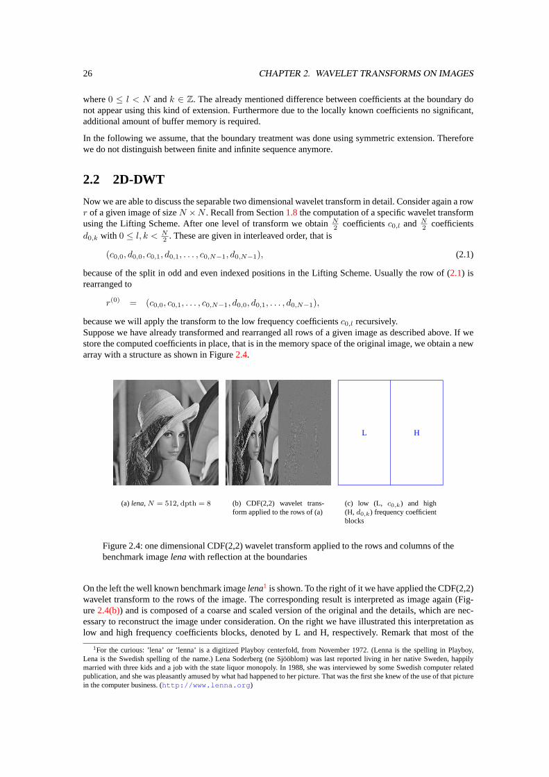
because we will apply the transform to the low frequency coefficientsc0,l recursively.Suppose we have already transformed and rearranged all rows of a given image as described above. If westore the computed coefficients in place, that is in the memory space of the original image, we obtain a newarray with a structure as shown in Figure2.4.
(a) lena,N = 512, dpth = 8 (b) CDF(2,2) wavelet trans-form applied to the rows of (a)
L H
(c) low (L, c0,k) and high(H, d0,k) frequency coefficientblocks
Figure 2.4: one dimensional CDF(2,2) wavelet transform applied to the rows and columns of thebenchmark imagelenawith reflection at the boundaries
On the left the well known benchmark imagelena1 is shown. To the right of it we have applied the CDF(2,2)wavelet transform to the rows of the image. The corresponding result is interpreted as image again (Fig-ure2.4(b)) and is composed of a coarse and scaled version of the original and the details, which are nec-essary to reconstruct the image under consideration. On the right we have illustrated this interpretation aslow and high frequency coefficients blocks, denoted by L and H, respectively. Remark that most of the
1For the curious: ’lena’ or ’lenna’ is a digitized Playboy centerfold, from November 1972. (Lenna is the spelling in Playboy,Lena is the Swedish spelling of the name.) Lena Soderberg (ne Sjööblom) was last reported living in her native Sweden, happilymarried with three kids and a job with the state liquor monopoly. In 1988, she was interviewed by some Swedish computer relatedpublication, and she was pleasantly amused by what had happened to her picture. That was the first she knew of the use of that picturein the computer business. (http://www.lenna.org )
2.2. 2D-DWT 27
high frequency coefficientsd0,k are shown in grey color, which corresponds to small values around zero(cf. Figure2.2).
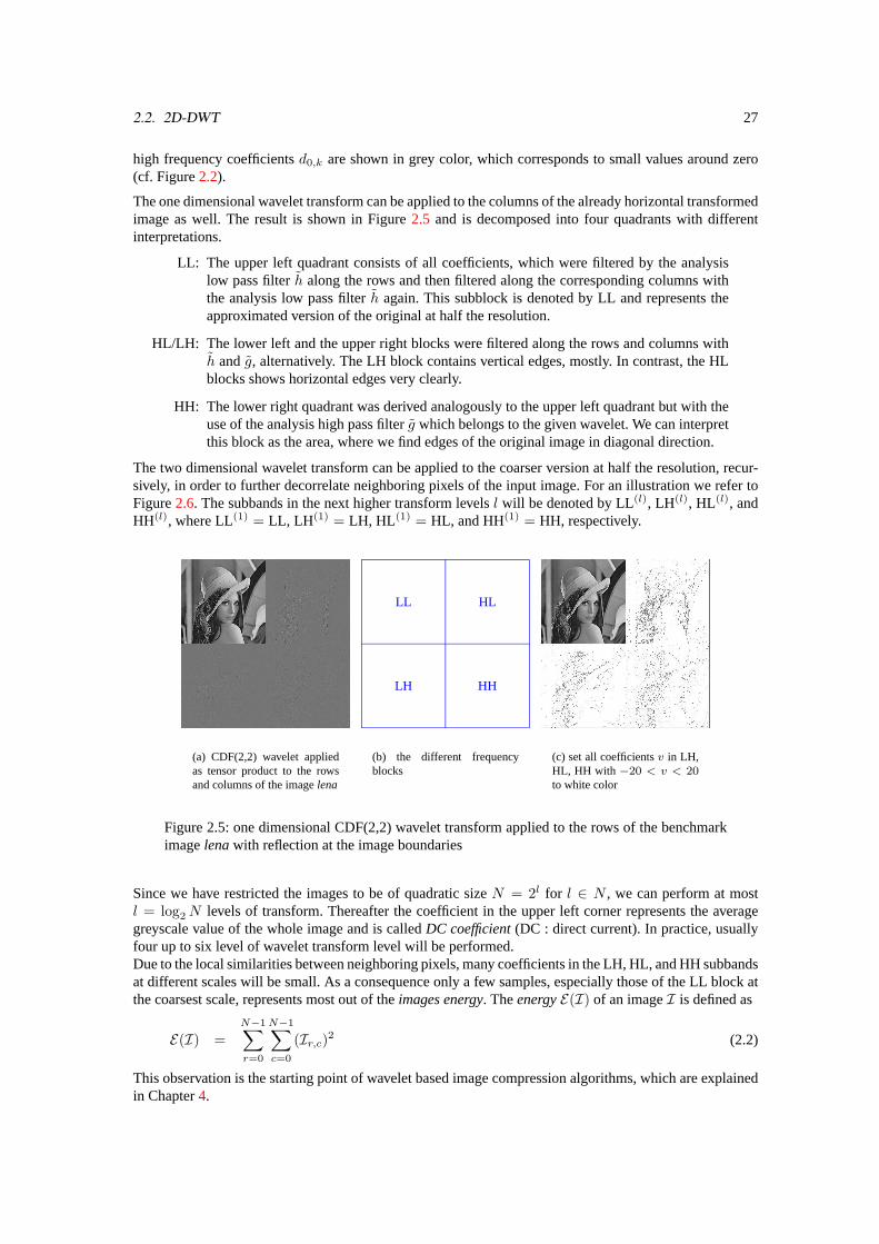
The one dimensional wavelet transform can be applied to the columns of the already horizontal transformedimage as well. The result is shown in Figure2.5 and is decomposed into four quadrants with differentinterpretations.
LL: The upper left quadrant consists of all coefficients, which were filtered by the analysislow pass filterh along the rows and then filtered along the corresponding columns withthe analysis low pass filterh again. This subblock is denoted by LL and represents theapproximated version of the original at half the resolution.
HL/LH: The lower left and the upper right blocks were filtered along the rows and columns withh andg, alternatively. The LH block contains vertical edges, mostly. In contrast, the HLblocks shows horizontal edges very clearly.
HH: The lower right quadrant was derived analogously to the upper left quadrant but with theuse of the analysis high pass filterg which belongs to the given wavelet. We can interpretthis block as the area, where we find edges of the original image in diagonal direction.
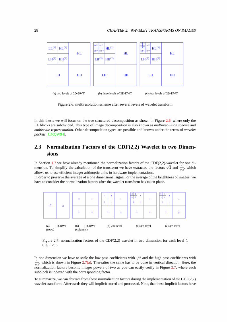
The two dimensional wavelet transform can be applied to the coarser version at half the resolution, recur-sively, in order to further decorrelate neighboring pixels of the input image. For an illustration we refer toFigure2.6. The subbands in the next higher transform levelsl will be denoted by LL(l), LH(l), HL(l), andHH(l), where LL(1) = LL, LH (1) = LH, HL(1) = HL, and HH(1) = HH, respectively.
(a) CDF(2,2) wavelet appliedas tensor product to the rowsand columns of the imagelena
LL HL
LH HH
(b) the different frequencyblocks
(c) set all coefficientsv in LH,HL, HH with −20 < v < 20to white color
Figure 2.5: one dimensional CDF(2,2) wavelet transform applied to the rows of the benchmarkimagelenawith reflection at the image boundaries
Since we have restricted the images to be of quadratic sizeN = 2l for l ∈ N , we can perform at mostl = log2N levels of transform. Thereafter the coefficient in the upper left corner represents the averagegreyscale value of the whole image and is calledDC coefficient(DC : direct current). In practice, usuallyfour up to six level of wavelet transform level will be performed.Due to the local similarities between neighboring pixels, many coefficients in the LH, HL, and HH subbandsat different scales will be small. As a consequence only a few samples, especially those of the LL block atthe coarsest scale, represents most out of theimages energy. TheenergyE(I) of an imageI is defined as
E(I) =N−1∑r=0
N−1∑c=0
(Ir,c)2 (2.2)
This observation is the starting point of wavelet based image compression algorithms, which are explainedin Chapter4.
28 CHAPTER 2. WAVELET TRANSFORMS ON IMAGES
HL
LH HH
LH(2)
LL (2)
HH(2)
HL(2)
(a) two levels of 2D-DWT
HL
LH HH
LH(2) HH(2)
HL(2)
LH(3)
LL (3)
HH(3)
HL(3)
(b) three levels of 2D-DWT
HL
LH HH
LH(2) HH(2)
HL(2)
LH(3) HH(3)
HL(3)LL (4)
LH(4) HH(4)
HL(4)
(c) four levels of 2D-DWT
Figure 2.6: multiresolution scheme after several levels of wavelet transform
In this thesis we will focus on the tree structured decomposition as shown in Figure2.6, where only theLL blocks are subdivided. This type of image decomposition is also known asmultiresolution schemeandmultiscale representation. Other decomposition types are possible and known under the terms ofwaveletpackets[CMQW94].
2.3 Normalization Factors of the CDF(2,2) Wavelet in two Dimen-sions
In Section1.7 we have already mentioned the normalization factors of the CDF(2,2)-wavelet for one di-mension. To simplify the calculation of the transform we have extracted the factors
√2 and 1√
2, which
allows us to use efficient integer arithmetic units in hardware implementations.In order to preserve the average of a one dimensional signal, or the average of the brightness of images, wehave to consider the normalization factors after the wavelet transform has taken place.
√2
1√2
(a) 1D-DWT(rows)
2
12
1
1
(b) 1D-DWT(columns)
4
2
2
1
12
1
1
(c) 2nd level
8
4
4
2
2
2
1
12
1
1
(d) 3rd level
16
8
8
4
4
4
2
2
2
1
12
1
1
(e) 4th level
Figure 2.7: normalization factors of the CDF(2,2) wavelet in two dimension for each levell,0 ≤ l < 5
In one dimension we have to scale the low pass coefficients with√
2 and the high pass coefficients with1√2, which is shown in Figure2.7(a). Thereafter the same has to be done in vertical direction. Here, the
normalization factors become integer powers of two as you can easily verify in Figure2.7, where eachsubblock is indexed with the corresponding factor.
To summarize, we can abstract from those normalization factors during the implementation of the CDF(2,2)wavelet transform. Afterwards they will implicit stored and processed. Note, that these implicit factors have

2.3. NORMALIZATION FACTORS OF THE CDF(2,2) WAVELET IN TWO DIMENSIONS 29
no influence to the growth of bitwidth, which is necessary to store the wavelet coefficients.

30 CHAPTER 2. WAVELET TRANSFORMS ON IMAGES
Chapter 3
Range of CDF(2,2) Wavelet Coefficients
As we have seen in Section1.6wavelet transforms can be expressed using filters.Recursively filtering a signal with low and high pass FIR filters generally results in growing bitwidth of thescaling and wavelet coefficients. If we focus on hardware implementation this is equivalent with growingmemory requirements to store the coefficients with additional bits. Thus we are interested in finding thesmallest bitwidth, which is necessary to store the coefficients without any loss of information.More formally, we are searching for minimal intervals[cj , cj ] and[dj , dj ] wherecj , dj , cj , dj ∈ Z, cj ≤ cj ,
anddj ≤ dj for all −J < j ≤ 0, such that
cj,l ∈ [cj , cj ] and dj,l ∈ [dj , dj ]
holds for alll ∈ Z and−J < j ≤ 0.
Assume an image with a color depth ofdpth bits using two’s complement number representation is given.Then the range of the pixel values is given as the interval of integers
[−2dpth−1, 2dpth−1 − 1].
Thus the minimum and maximum values of all coefficients ofc0,i are
c0 ≤ maxi
(h ∗ x)i = −−2dpth−1
8 + 2dpth−1−14 +
3(2dpth−1−1)4 + 2dpth−1−1
4 − −2dpth−1
8
= 322dpth−1 − 5
4
c0 ≥ mini
(h ∗ x)i = − 2dpth−1−18 + −2dpth−1
4 +3(−2dpth−1)
4 + −2dpth−1
4 − 2dpth−1−18
= − 322dpth−1 + 1
4
The same computation can be done for the coefficientsd0,j :
d0 ≤ maxj
((g ∗ x)j) = −−2dpth−1
2 + 2dpth−1 − 1 − −2dpth−1
2
= 2dpth − 1
d0 ≥ minj
((g ∗ x)j) = − 2dpth−1−12 − 2dpth−1 − 2dpth−1−1
2
= −(2dpth − 1)
Therefore the range of the coefficientsc0,i is[ ⌊−3
22dpth−1 +
14
⌋,
⌈322dpth−1 − 5
4
⌉ ],
31
32 CHAPTER 3. RANGE OF CDF(2,2) WAVELET COEFFICIENTS
and the range of the coefficientsd0,j is[−(2dpth − 1), 2dpth − 1
].
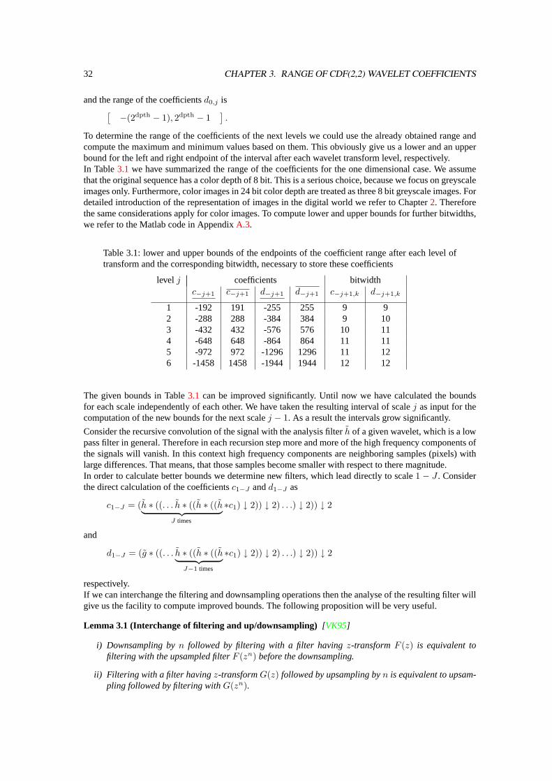
To determine the range of the coefficients of the next levels we could use the already obtained range andcompute the maximum and minimum values based on them. This obviously give us a lower and an upperbound for the left and right endpoint of the interval after each wavelet transform level, respectively.In Table3.1 we have summarized the range of the coefficients for the one dimensional case. We assumethat the original sequence has a color depth of 8 bit. This is a serious choice, because we focus on greyscaleimages only. Furthermore, color images in 24 bit color depth are treated as three 8 bit greyscale images. Fordetailed introduction of the representation of images in the digital world we refer to Chapter2. Thereforethe same considerations apply for color images. To compute lower and upper bounds for further bitwidths,we refer to the Matlab code in AppendixA.3.
Table 3.1: lower and upper bounds of the endpoints of the coefficient range after each level oftransform and the corresponding bitwidth, necessary to store these coefficients
level j coefficients bitwidthc−j+1 c−j+1 d−j+1 d−j+1 c−j+1,k d−j+1,k
1 -192 191 -255 255 9 92 -288 288 -384 384 9 103 -432 432 -576 576 10 114 -648 648 -864 864 11 115 -972 972 -1296 1296 11 126 -1458 1458 -1944 1944 12 12
The given bounds in Table3.1 can be improved significantly. Until now we have calculated the boundsfor each scale independently of each other. We have taken the resulting interval of scalej as input for thecomputation of the new bounds for the next scalej − 1. As a result the intervals grow significantly.
Consider the recursive convolution of the signal with the analysis filterh of a given wavelet, which is a lowpass filter in general. Therefore in each recursion step more and more of the high frequency components ofthe signals will vanish. In this context high frequency components are neighboring samples (pixels) withlarge differences. That means, that those samples become smaller with respect to there magnitude.In order to calculate better bounds we determine new filters, which lead directly to scale1 − J . Considerthe direct calculation of the coefficientsc1−J andd1−J as
c1−J = (h ∗ ((. . . h ∗ ((h ∗ ((h︸ ︷︷ ︸J times
∗c1) ↓ 2)) ↓ 2) . . .) ↓ 2)) ↓ 2
and
d1−J = (g ∗ ((. . . h ∗ ((h ∗ ((h︸ ︷︷ ︸J−1 times
∗c1) ↓ 2)) ↓ 2) . . .) ↓ 2)) ↓ 2
respectively.If we can interchange the filtering and downsampling operations then the analyse of the resulting filter willgive us the facility to compute improved bounds. The following proposition will be very useful.
Lemma 3.1 (Interchange of filtering and up/downsampling) [VK95]
i) Downsampling byn followed by filtering with a filter havingz-transformF (z) is equivalent tofiltering with the upsampled filterF (zn) before the downsampling.
ii) Filtering with a filter havingz-transformG(z) followed by upsampling byn is equivalent to upsam-pling followed by filtering withG(zn).
33
Proof:
We have to show that the equation
f ∗ (x ↓ n) = ((f ↑ n) ∗ x) ↓ n (3.1)
holds in order to prove part i) of Lemma3.1. In z-transform domain the left side of Equa-tion (3.1) is obviously equivalent to
F (z)1n
n−1∑k=0
X(e−i2πk
n z1n
).
On the right side of Equation (3.1) we let f ′ = (f ↑ n) ∗ x. Then we have inz-transformdomain
1n
n−1∑k=0
F ′(e−i2πk
n z1n
).
SinceF ′(z) = F (zn)X(z) we obtain
1n
n−1∑k=0
F((e−i2πk
n z1n
)n)X(e
−i2πkn z
1n ) =
1n
n−1∑k=0
F(e−i2πkz
)X(e−i2πk
n z1n
)which can be transformed into
F (z)1n
n−1∑k=0
X(e−i2πk
n z1n )
by using
ei2π = 1, e−i2πk = (ei2π)−k = 1, for k ∈ Z.
The second proposition of Lemma3.1 is trivial, since both sides of the equation
(f ∗ x) ↑ n = (f ↑ n) ∗ (x ↑ n) (3.2)
leads inz-transform domain toF (zn)X(zn).
�
With the help of the proposition of Lemma3.1 we can interchange the filtering and up/downsamplingoperations to make the computation of the bounds independent of the underlying signalx.Let s(0) be the original sequencec1 filtered with the analysis low pass filterh, that is
s(0) = h ∗ c1.
Note, that downsampling by two of this intermediate signals(0) leads toc0. We can obtains(j) as
s(j) = h ∗ (s(j+1) ↓ 2)
for all J < j < 0.
Using Equation (3.1) we can exchange the filtering and the downsampling operation as follows
s(j) = ((h ↑ 2) ∗ s(j+1)) ↓ 2.
34 CHAPTER 3. RANGE OF CDF(2,2) WAVELET COEFFICIENTS
That is, we can first compute the filterh′ = (h ↑ 2) before considering signals(j+1). Sinces(j+1) can bederived froms(j+2) in the same manner, we have
s(j) = ((h ↑ 2) ∗ s(j+1)) ↓ 2= ((h ↑ 2) ∗ (h ∗ (s(j+2) ↓ 2))) ↓ 2= ((h ↑ 2) ∗ ((h ↑ 2) ∗ s(j+2)) ↓ 2) ↓ 2= ((((h ↑ 2) ↑ 2) ∗ (h ↑ 2) ∗ s(j+2)) ↓ 2) ↓ 2.
Since the operation∗ is associative, we get
s(j) = (((h ↑ 4) ∗ (h ↑ 2)) ∗ s(j+2)) ↓ 4.
After J level we obtain
s(1−J) = (((h ↑ 2J) ∗ (h ↑ 2J−1) ∗ . . . ∗ (h ↑ 21)) ∗ s0) ↓ 2J . (3.3)
We will prove this by induction over the number of levelsJ .
Proof:
First we have to verify that the statement holds forJ = 1
s(−1) = h ∗ (s(0) ↓ 2)= ((h ↑ 2) ∗ s(0)) ↓ 2,
which was already mentioned.
Now assume, that
s(1−J) = (((h ↑ 2J) ∗ (h ↑ 2J−1) ∗ . . . ∗ (h ↑ 21)) ∗ s(0)) ↓ 2J (3.4)
holds for someJ with J > 1. We now have to show thats(−(J+1)) can be represented accord-ingly. Let
h(J) = (h ↑ 2J) ∗ (h ↑ 2J−1) ∗ . . . ∗ (h ↑ 21)
be the iterated and upsampled filter corresponding to levelJ .
Using Equation (3.4) we obtain
s(−(J+1)) = h ∗ (s(−J) ↓ 2)
= h ∗([
(h(J) ∗ s(0)) ↓ 2(J)]↓ 2)
= h ∗[(h(J) ∗ s(0)) ↓ 2(J+1)
]=
((h ↑ 2(J+1)) ∗ (h(J) ∗ s(0))
)↓ 2(J+1)
=((h ↑ 2(J+1)) ∗
[((h ↑ 2J) ∗ (h ↑ 2J−1) ∗ . . . ∗ (h ↑ 21)) ∗ s(0)
])↓ 2(J+1)
=(((h ↑ 2(J+1)) ∗ (h ↑ 2J) ∗ (h ↑ 2J−1) ∗ . . . ∗ (h ↑ 21)) ∗ s(0)
)↓ 2(J+1)
which proves the supposition. �
In an analogous manner we define the filterg(J) for the high pass filterg. In Table3.2we have summarizedthe range of the coefficients for the one dimensional case. We again assume that the original sequence hasa color depth of 8 bit.
3.1. ESTIMATION OF COEFFICIENTS RANGE USING LIFTING WITH ROUNDING 35
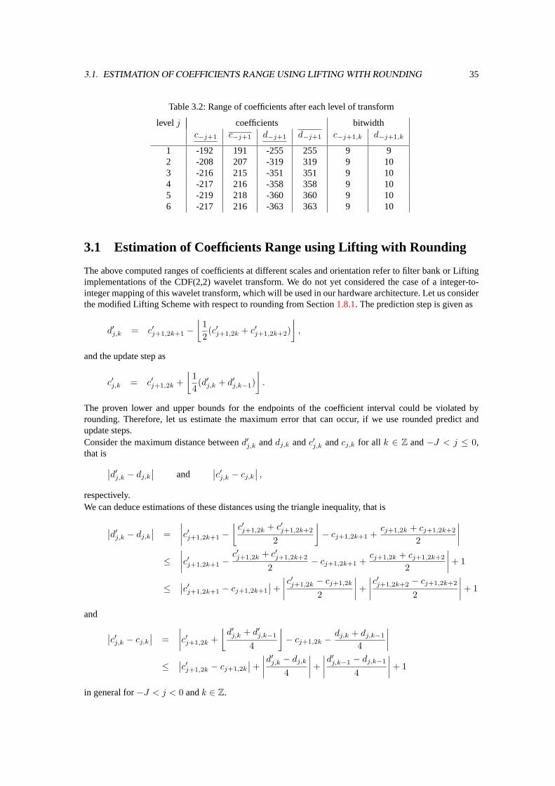
Table 3.2: Range of coefficients after each level of transform
level j coefficients bitwidthc−j+1 c−j+1 d−j+1 d−j+1 c−j+1,k d−j+1,k
1 -192 191 -255 255 9 92 -208 207 -319 319 9 103 -216 215 -351 351 9 104 -217 216 -358 358 9 105 -219 218 -360 360 9 106 -217 216 -363 363 9 10
3.1 Estimation of Coefficients Range using Lifting with Rounding
The above computed ranges of coefficients at different scales and orientation refer to filter bank or Liftingimplementations of the CDF(2,2) wavelet transform. We do not yet considered the case of a integer-to-integer mapping of this wavelet transform, which will be used in our hardware architecture. Let us considerthe modified Lifting Scheme with respect to rounding from Section1.8.1. The prediction step is given as
d′j,k = c′j+1,2k+1 −⌊
12(c′j+1,2k + c′j+1,2k+2)
⌋,
and the update step as
c′j,k = c′j+1,2k +⌊
14(d′j,k + d′j,k−1)
⌋.
The proven lower and upper bounds for the endpoints of the coefficient interval could be violated byrounding. Therefore, let us estimate the maximum error that can occur, if we use rounded predict andupdate steps.Consider the maximum distance betweend′j,k anddj,k andc′j,k andcj,k for all k ∈ Z and−J < j ≤ 0,that is∣∣d′j,k − dj,k
∣∣ and∣∣c′j,k − cj,k∣∣ ,
respectively.We can deduce estimations of these distances using the triangle inequality, that is
∣∣d′j,k − dj,k
∣∣ =∣∣∣∣c′j+1,2k+1 −
⌊c′j+1,2k + c′j+1,2k+2
2
⌋− cj+1,2k+1 +
cj+1,2k + cj+1,2k+2
2
∣∣∣∣≤
∣∣∣∣c′j+1,2k+1 −c′j+1,2k + c′j+1,2k+2
2− cj+1,2k+1 +
cj+1,2k + cj+1,2k+2
2
∣∣∣∣+ 1
≤∣∣c′j+1,2k+1 − cj+1,2k+1
∣∣+ ∣∣∣∣c′j+1,2k − cj+1,2k
2
∣∣∣∣+ ∣∣∣∣c′j+1,2k+2 − cj+1,2k+2
2
∣∣∣∣+ 1
and ∣∣c′j,k − cj,k∣∣ =∣∣∣∣c′j+1,2k +
⌊d′j,k + d′j,k−1
4
⌋− cj+1,2k −
dj,k + dj,k−1
4
∣∣∣∣≤
∣∣c′j+1,2k − cj+1,2k
∣∣+ ∣∣∣∣d′j,k − dj,k
4
∣∣∣∣+ ∣∣∣∣d′j,k−1 − dj,k−1
4
∣∣∣∣+ 1
in general for−J < j < 0 andk ∈ Z.
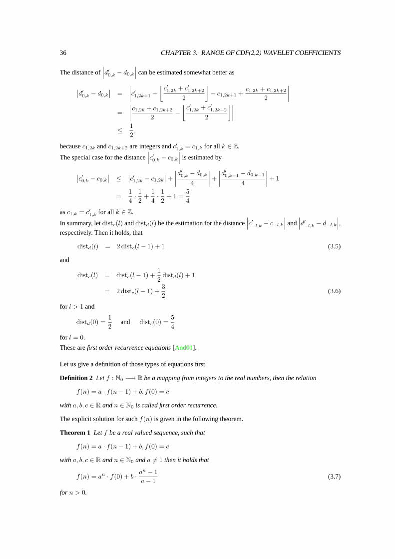
36 CHAPTER 3. RANGE OF CDF(2,2) WAVELET COEFFICIENTS
The distance of∣∣∣d′0,k − d0,k
∣∣∣ can be estimated somewhat better as
∣∣d′0,k − d0,k
∣∣ =∣∣∣∣c′1,2k+1 −
⌊c′1,2k + c′1,2k+2
2
⌋− c1,2k+1 +
c1,2k + c1,2k+2
2
∣∣∣∣=
∣∣∣∣c1,2k + c1,2k+2
2−⌊c′1,2k + c′1,2k+2
2
⌋∣∣∣∣≤ 1
2,
becausec1,2k andc1,2k+2 are integers andc′1,k = c1,k for all k ∈ Z.
The special case for the distance∣∣∣c′0,k − c0,k
∣∣∣ is estimated by
∣∣c′0,k − c0,k
∣∣ ≤ ∣∣c′1,2k − c1,2k
∣∣+ ∣∣∣∣d′0,k − d0,k
4
∣∣∣∣+ ∣∣∣∣d′0,k−1 − d0,k−1
4
∣∣∣∣+ 1
=14· 12
+14· 12
+ 1 =54
asc1,k = c′1,k for all k ∈ Z.
In summary, letdistc(l) anddistd(l) be the estimation for the distance∣∣∣c′−l,k − c−l,k
∣∣∣ and∣∣∣d′−l,k − d−l,k
∣∣∣,respectively. Then it holds, that
distd(l) = 2 distc(l − 1) + 1 (3.5)
and
distc(l) = distc(l − 1) +12
distd(l) + 1
= 2distc(l − 1) +32
(3.6)
for l > 1 and
distd(0) =12
and distc(0) =54
for l = 0.
These arefirst order recurrence equations[And01].
Let us give a definition of those types of equations first.
Definition 2 Letf : N0 −→ R be a mapping from integers to the real numbers, then the relation
f(n) = a · f(n− 1) + b, f(0) = c
with a, b, c ∈ R andn ∈ N0 is called first order recurrence.
The explicit solution for suchf(n) is given in the following theorem.
Theorem 1 Letf be a real valued sequence, such that
f(n) = a · f(n− 1) + b, f(0) = c
with a, b, c ∈ R andn ∈ N0 anda 6= 1 then it holds that
f(n) = an · f(0) + b · an − 1a− 1
(3.7)
for n > 0.
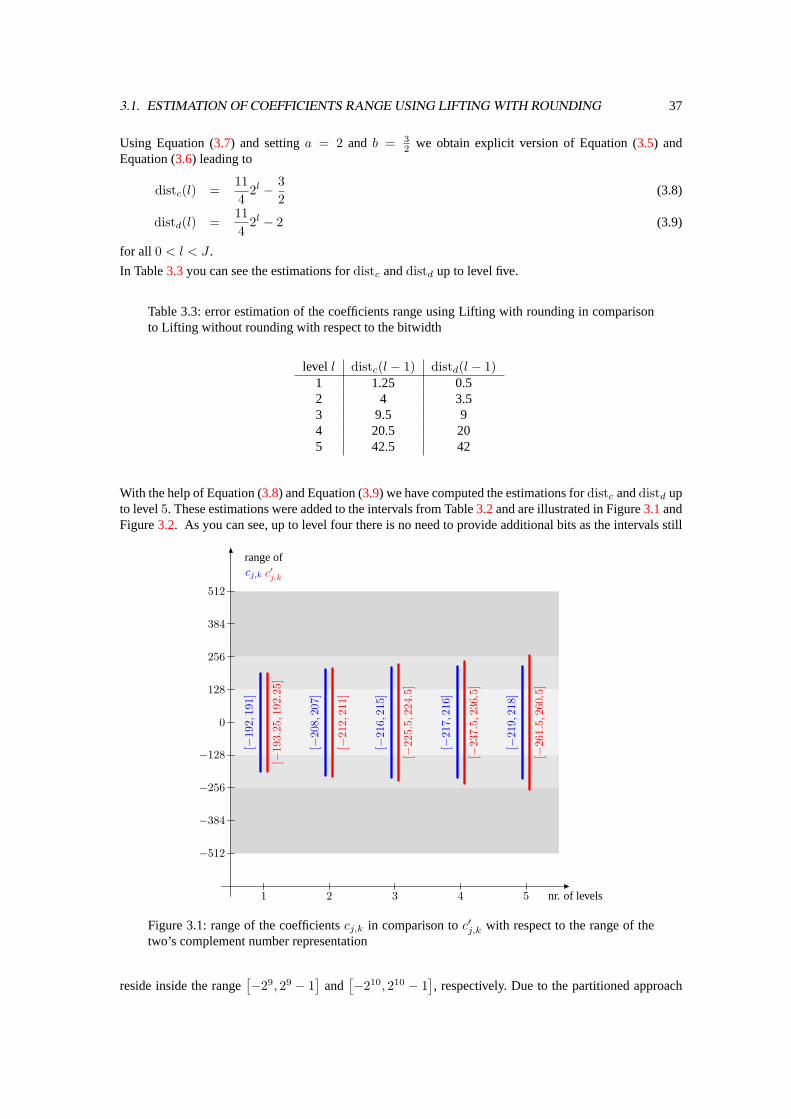
3.1. ESTIMATION OF COEFFICIENTS RANGE USING LIFTING WITH ROUNDING 37
Using Equation (3.7) and settinga = 2 and b = 32 we obtain explicit version of Equation (3.5) and
Equation (3.6) leading to
distc(l) =114
2l − 32
(3.8)
distd(l) =114
2l − 2 (3.9)
for all 0 < l < J .
In Table3.3you can see the estimations fordistc anddistd up to level five.
Table 3.3: error estimation of the coefficients range using Lifting with rounding in comparisonto Lifting without rounding with respect to the bitwidth
level l distc(l − 1) distd(l − 1)1 1.25 0.52 4 3.53 9.5 94 20.5 205 42.5 42
With the help of Equation (3.8) and Equation (3.9) we have computed the estimations fordistc anddistd upto level5. These estimations were added to the intervals from Table3.2and are illustrated in Figure3.1andFigure3.2. As you can see, up to level four there is no need to provide additional bits as the intervals still
[−19
2,19
1]
[−19
3.25,1
92.2
5]
[−20
8,20
7]
[−21
2,21
1]
[−21
6,21
5]
[−22
5.5,
224.
5]
[−21
7,21
6]
[−23
7.5,
236.
5]
[−21
9,21
8]
[−26
1.5,
260.
5]
cj,k c′j,k
nr. of levels
rangeof
1 2 3 4 5
−512
−384
−256
−128
0
128
256
384
512
Figure 3.1: range of the coefficientscj,k in comparison toc′j,k with respect to the range of thetwo’s complement number representation
reside inside the range[−29, 29 − 1
]and
[−210, 210 − 1
], respectively. Due to the partitioned approach
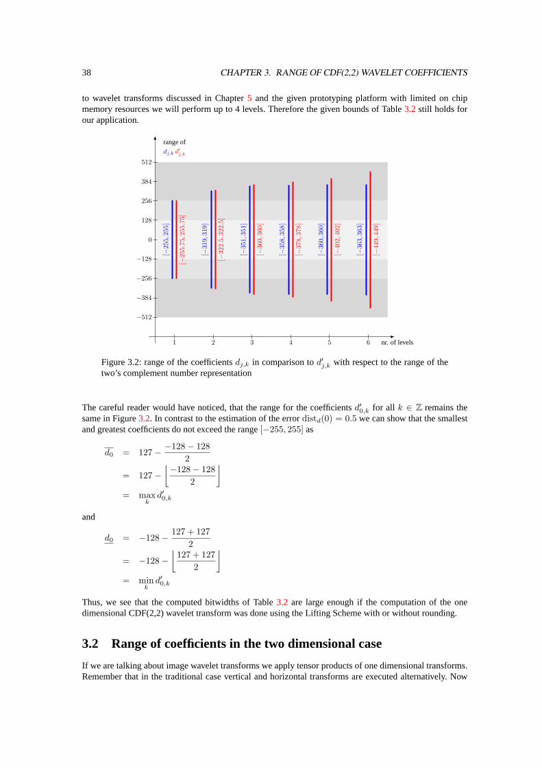
38 CHAPTER 3. RANGE OF CDF(2,2) WAVELET COEFFICIENTS
to wavelet transforms discussed in Chapter5 and the given prototyping platform with limited on chipmemory resources we will perform up to 4 levels. Therefore the given bounds of Table3.2 still holds forour application.
[−25
5,25
5]
[−25
5.75,2
55.7
5]
[−31
9,31
9]
[−32
2.5,
322.
5]
[−35
1,35
1]
[−36
0,36
0]
[−35
8,35
8]
[−37
8,37
8]
[−36
0,36
0]
[−40
2,40
2]
[−36
3,36
3]
[−44
9,44
9]
dj,k d′j,k
nr. of levels
rangeof
1 2 3 4 5 6
−512
−384
−256
−128
0
128
256
384
512
Figure 3.2: range of the coefficientsdj,k in comparison tod′j,k with respect to the range of thetwo’s complement number representation
The careful reader would have noticed, that the range for the coefficientsd′0,k for all k ∈ Z remains thesame in Figure3.2. In contrast to the estimation of the errordistd(0) = 0.5 we can show that the smallestand greatest coefficients do not exceed the range[−255, 255] as
d0 = 127− −128− 1282
= 127−⌊−128− 128
2
⌋= max
kd′0,k
and
d0 = −128− 127 + 1272
= −128−⌊
127 + 1272
⌋= min
kd′0,k
Thus, we see that the computed bitwidths of Table3.2 are large enough if the computation of the onedimensional CDF(2,2) wavelet transform was done using the Lifting Scheme with or without rounding.
3.2 Range of coefficients in the two dimensional case
If we are talking about image wavelet transforms we apply tensor products of one dimensional transforms.Remember that in the traditional case vertical and horizontal transforms are executed alternatively. Now
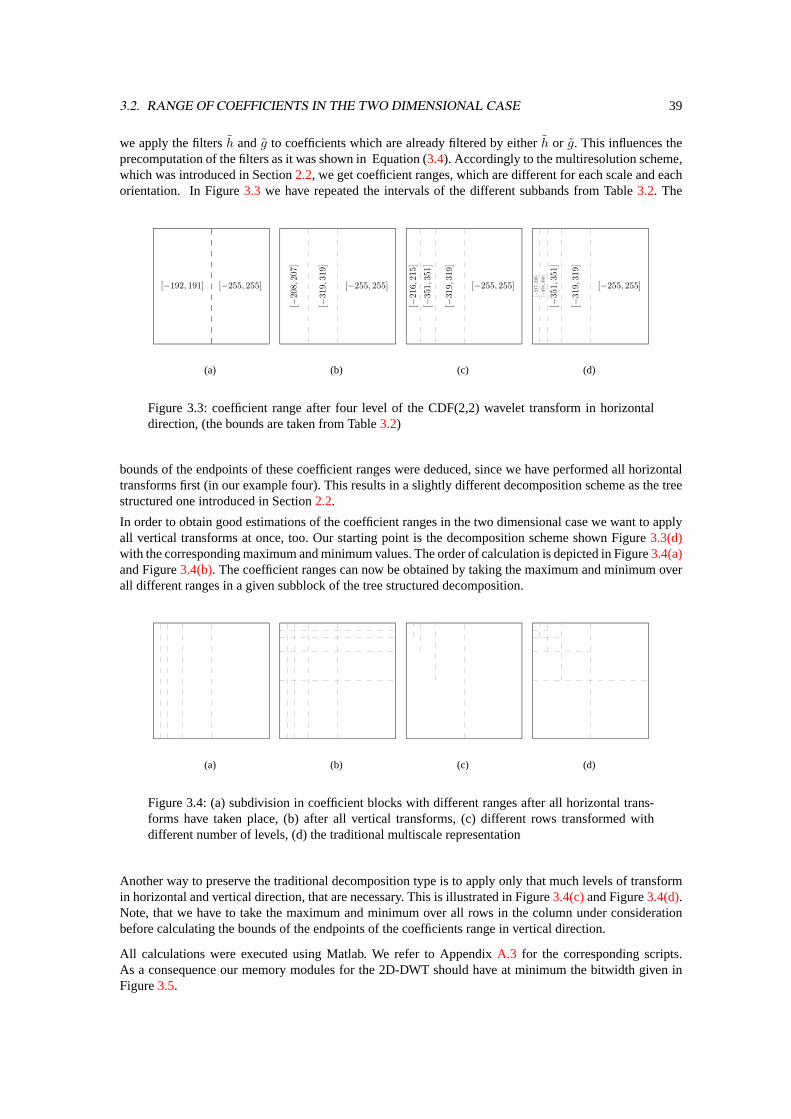
3.2. RANGE OF COEFFICIENTS IN THE TWO DIMENSIONAL CASE 39
we apply the filtersh andg to coefficients which are already filtered by eitherh or g. This influences theprecomputation of the filters as it was shown in Equation (3.4). Accordingly to the multiresolution scheme,which was introduced in Section2.2, we get coefficient ranges, which are different for each scale and eachorientation. In Figure3.3 we have repeated the intervals of the different subbands from Table3.2. The
[−192, 191] [−255, 255]
(a)
[−255, 255][−
208,
207]
[−31
9,31
9]
(b)
[−255, 255]
[−31
9,31
9]
[−21
6,21
5]
[−35
1,35
1]
(c)
[−255, 255]
[−31
9,31
9]
[−35
1,35
1]
[−21
7,21
6]
[−35
8,35
8]
(d)
Figure 3.3: coefficient range after four level of the CDF(2,2) wavelet transform in horizontaldirection, (the bounds are taken from Table3.2)
bounds of the endpoints of these coefficient ranges were deduced, since we have performed all horizontaltransforms first (in our example four). This results in a slightly different decomposition scheme as the treestructured one introduced in Section2.2.
In order to obtain good estimations of the coefficient ranges in the two dimensional case we want to applyall vertical transforms at once, too. Our starting point is the decomposition scheme shown Figure3.3(d)with the corresponding maximum and minimum values. The order of calculation is depicted in Figure3.4(a)and Figure3.4(b). The coefficient ranges can now be obtained by taking the maximum and minimum overall different ranges in a given subblock of the tree structured decomposition.
(a) (b) (c) (d)
Figure 3.4: (a) subdivision in coefficient blocks with different ranges after all horizontal trans-forms have taken place, (b) after all vertical transforms, (c) different rows transformed withdifferent number of levels, (d) the traditional multiscale representation
Another way to preserve the traditional decomposition type is to apply only that much levels of transformin horizontal and vertical direction, that are necessary. This is illustrated in Figure3.4(c)and Figure3.4(d).Note, that we have to take the maximum and minimum over all rows in the column under considerationbefore calculating the bounds of the endpoints of the coefficients range in vertical direction.
All calculations were executed using Matlab. We refer to AppendixA.3 for the corresponding scripts.As a consequence our memory modules for the 2D-DWT should have at minimum the bitwidth given inFigure3.5.

40 CHAPTER 3. RANGE OF CDF(2,2) WAVELET COEFFICIENTS
The hardware implementation of these memory modules is done using slices of different bitwidth. Theseslices are shown in Figure3.5 as dashed lines. Note, that we take the maximum bitwidth of the severalsubbands of the slice. For further details of the implementation itself see Section6.3.2.
10
11
11
10
11
11
10
11
11
10
11
11
10
10
10111111 11
Figure 3.5: minimal affordable memory bitwidth
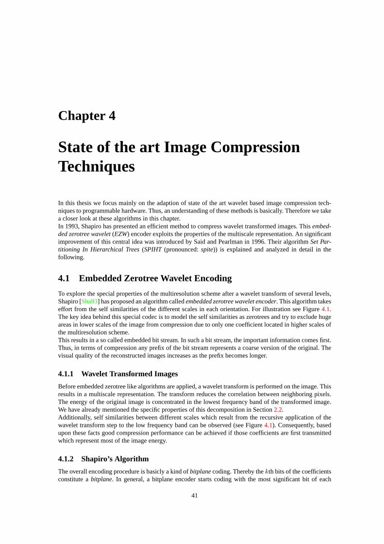
Chapter 4
State of the art Image CompressionTechniques
In this thesis we focus mainly on the adaption of state of the art wavelet based image compression tech-niques to programmable hardware. Thus, an understanding of these methods is basically. Therefore we takea closer look at these algorithms in this chapter.In 1993, Shapiro has presented an efficient method to compress wavelet transformed images. Thisembed-ded zerotree wavelet(EZW) encoder exploits the properties of the multiscale representation. An significantimprovement of this central idea was introduced by Said and Pearlman in 1996. Their algorithmSet Par-titioning In Hierarchical Trees(SPIHT (pronounced:spite)) is explained and analyzed in detail in thefollowing.
4.1 Embedded Zerotree Wavelet Encoding
To explore the special properties of the multiresolution scheme after a wavelet transform of several levels,Shapiro [Sha93] has proposed an algorithm calledembedded zerotree wavelet encoder. This algorithm takeseffort from the self similarities of the different scales in each orientation. For illustration see Figure4.1.The key idea behind this special codec is to model the self similarities as zerotrees and try to exclude hugeareas in lower scales of the image from compression due to only one coefficient located in higher scales ofthe multiresolution scheme.This results in a so called embedded bit stream. In such a bit stream, the important information comes first.Thus, in terms of compression any prefix of the bit stream represents a coarse version of the original. Thevisual quality of the reconstructed images increases as the prefix becomes longer.
4.1.1 Wavelet Transformed Images
Before embedded zerotree like algorithms are applied, a wavelet transform is performed on the image. Thisresults in a multiscale representation. The transform reduces the correlation between neighboring pixels.The energy of the original image is concentrated in the lowest frequency band of the transformed image.We have already mentioned the specific properties of this decomposition in Section2.2.Additionally, self similarities between different scales which result from the recursive application of thewavelet transform step to the low frequency band can be observed (see Figure4.1). Consequently, basedupon these facts good compression performance can be achieved if those coefficients are first transmittedwhich represent most of the image energy.
4.1.2 Shapiro’s Algorithm
The overall encoding procedure is basicly a kind ofbitplanecoding. Thereby thekth bits of the coefficientsconstitute abitplane. In general, a bitplane encoder starts coding with the most significant bit of each
41
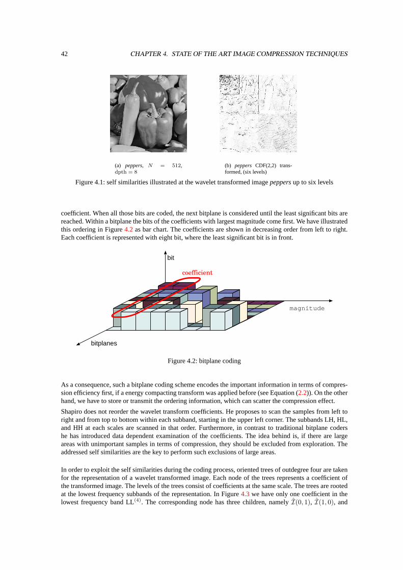
42 CHAPTER 4. STATE OF THE ART IMAGE COMPRESSION TECHNIQUES
(a) peppers, N = 512,dpth = 8
(b) peppers CDF(2,2) trans-formed, (six levels)
Figure 4.1: self similarities illustrated at the wavelet transformed imagepeppersup to six levels
coefficient. When all those bits are coded, the next bitplane is considered until the least significant bits arereached. Within a bitplane the bits of the coefficients with largest magnitude come first. We have illustratedthis ordering in Figure4.2 as bar chart. The coefficients are shown in decreasing order from left to right.Each coefficient is represented with eight bit, where the least significant bit is in front.
bitplanes
bit
coefficient
magnitude
Figure 4.2: bitplane coding
As a consequence, such a bitplane coding scheme encodes the important information in terms of compres-sion efficiency first, if a energy compacting transform was applied before (see Equation (2.2)). On the otherhand, we have to store or transmit the ordering information, which can scatter the compression effect.
Shapiro does not reorder the wavelet transform coefficients. He proposes to scan the samples from left toright and from top to bottom within each subband, starting in the upper left corner. The subbands LH, HL,and HH at each scales are scanned in that order. Furthermore, in contrast to traditional bitplane codershe has introduced data dependent examination of the coefficients. The idea behind is, if there are largeareas with unimportant samples in terms of compression, they should be excluded from exploration. Theaddressed self similarities are the key to perform such exclusions of large areas.
In order to exploit the self similarities during the coding process, oriented trees of outdegree four are takenfor the representation of a wavelet transformed image. Each node of the trees represents a coefficient ofthe transformed image. The levels of the trees consist of coefficients at the same scale. The trees are rootedat the lowest frequency subbands of the representation. In Figure4.3 we have only one coefficient in thelowest frequency band LL(4). The corresponding node has three children, namelyI(0, 1), I(1, 0), and
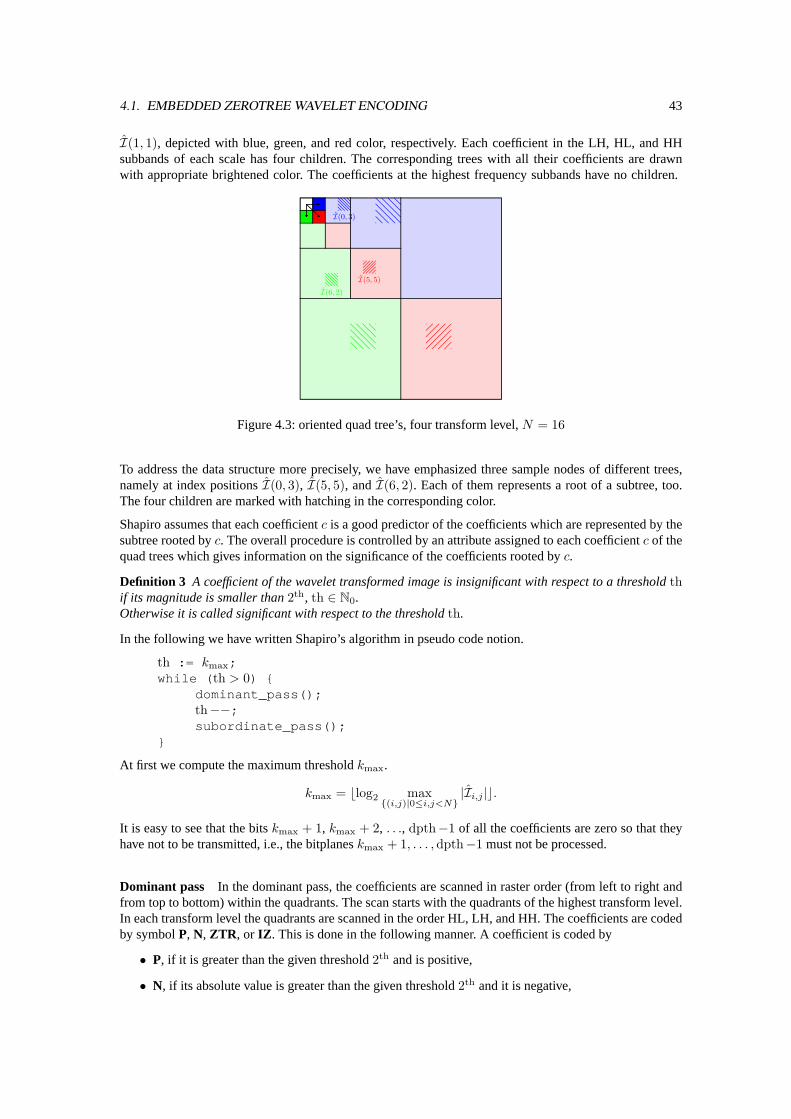
4.1. EMBEDDED ZEROTREE WAVELET ENCODING 43
I(1, 1), depicted with blue, green, and red color, respectively. Each coefficient in the LH, HL, and HHsubbands of each scale has four children. The corresponding trees with all their coefficients are drawnwith appropriate brightened color. The coefficients at the highest frequency subbands have no children.
I(6, 2)
I(5, 5)
I(0, 3)
Figure 4.3: oriented quad tree’s, four transform level,N = 16
To address the data structure more precisely, we have emphasized three sample nodes of different trees,namely at index positionsI(0, 3), I(5, 5), andI(6, 2). Each of them represents a root of a subtree, too.The four children are marked with hatching in the corresponding color.
Shapiro assumes that each coefficientc is a good predictor of the coefficients which are represented by thesubtree rooted byc. The overall procedure is controlled by an attribute assigned to each coefficientc of thequad trees which gives information on the significance of the coefficients rooted byc.
Definition 3 A coefficient of the wavelet transformed image is insignificant with respect to a thresholdthif its magnitude is smaller than2th, th ∈ N0.Otherwise it is called significant with respect to the thresholdth.
In the following we have written Shapiro’s algorithm in pseudo code notion.
th := kmax;while ( th > 0) {
dominant_pass();th−−;subordinate_pass();
}
At first we compute the maximum thresholdkmax.
kmax = blog2 max{(i,j)|0≤i,j<N}
|Ii,j |c.
It is easy to see that the bitskmax + 1, kmax + 2, . . ., dpth−1 of all the coefficients are zero so that theyhave not to be transmitted, i.e., the bitplaneskmax + 1, . . . ,dpth−1 must not be processed.
Dominant pass In the dominant pass, the coefficients are scanned in raster order (from left to right andfrom top to bottom) within the quadrants. The scan starts with the quadrants of the highest transform level.In each transform level the quadrants are scanned in the order HL, LH, and HH. The coefficients are codedby symbolP, N, ZTR , or IZ . This is done in the following manner. A coefficient is coded by
• P, if it is greater than the given threshold2th and is positive,
• N, if its absolute value is greater than the given threshold2th and it is negative,
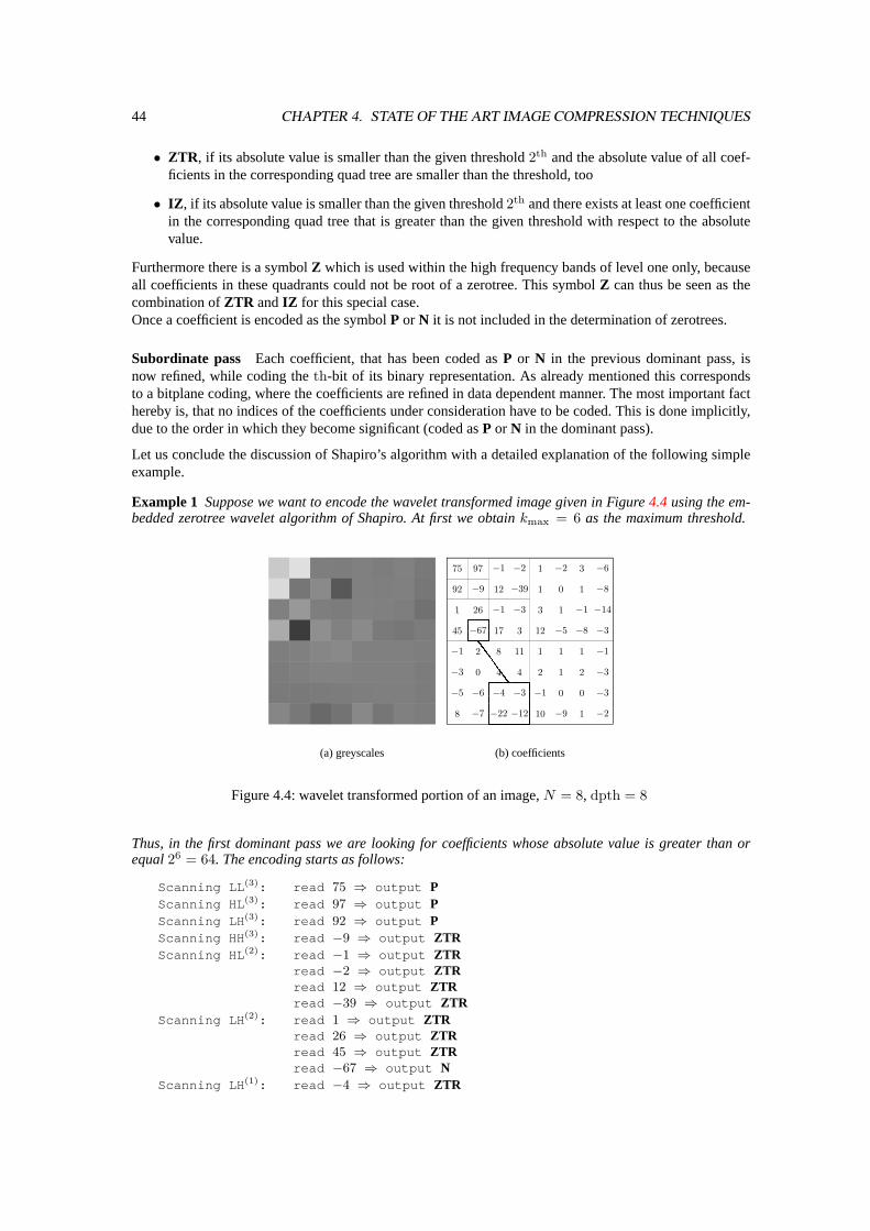
44 CHAPTER 4. STATE OF THE ART IMAGE COMPRESSION TECHNIQUES
• ZTR , if its absolute value is smaller than the given threshold2th and the absolute value of all coef-ficients in the corresponding quad tree are smaller than the threshold, too
• IZ , if its absolute value is smaller than the given threshold2th and there exists at least one coefficientin the corresponding quad tree that is greater than the given threshold with respect to the absolutevalue.
Furthermore there is a symbolZ which is used within the high frequency bands of level one only, becauseall coefficients in these quadrants could not be root of a zerotree. This symbolZ can thus be seen as thecombination ofZTR andIZ for this special case.Once a coefficient is encoded as the symbolP or N it is not included in the determination of zerotrees.
Subordinate pass Each coefficient, that has been coded asP or N in the previous dominant pass, isnow refined, while coding theth-bit of its binary representation. As already mentioned this correspondsto a bitplane coding, where the coefficients are refined in data dependent manner. The most important facthereby is, that no indices of the coefficients under consideration have to be coded. This is done implicitly,due to the order in which they become significant (coded asP or N in the dominant pass).
Let us conclude the discussion of Shapiro’s algorithm with a detailed explanation of the following simpleexample.
Example 1 Suppose we want to encode the wavelet transformed image given in Figure4.4using the em-bedded zerotree wavelet algorithm of Shapiro. At first we obtainkmax = 6 as the maximum threshold.
(a) greyscales
75 97 −1 −2 1 −2 3 −6
92 −9 12 −39 1 0 1 −8
1 26 −1 −3 3 1 −1 −14
45 −67 17 3 12 −5 −8 −3
−1 2 8 11 1 1 1 −1
−3 0 4 4 2 1 2 −3
−5 −6 −4 −3 −1 0 0 −3
8 −7 −22 −12 10 −9 1 −2
(b) coefficients
Figure 4.4: wavelet transformed portion of an image,N = 8, dpth = 8
Thus, in the first dominant pass we are looking for coefficients whose absolute value is greater than orequal26 = 64. The encoding starts as follows:
Scanning LL (3): read 75 ⇒ output PScanning HL (3): read 97 ⇒ output PScanning LH (3): read 92 ⇒ output PScanning HH (3): read −9 ⇒ output ZTRScanning HL (2): read −1 ⇒ output ZTR
read −2 ⇒ output ZTRread 12 ⇒ output ZTRread −39 ⇒ output ZTR
Scanning LH (2): read 1 ⇒ output ZTRread 26 ⇒ output ZTRread 45 ⇒ output ZTRread −67 ⇒ output N
Scanning LH (1): read −4 ⇒ output ZTR
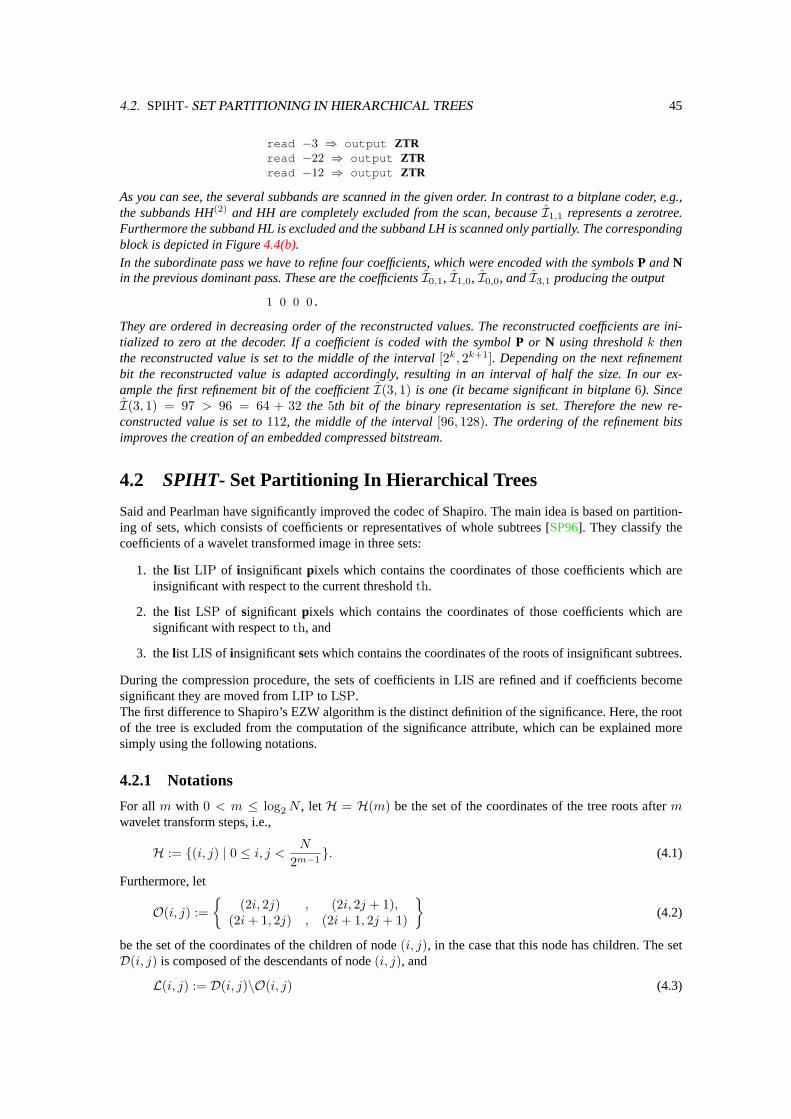
4.2. SPIHT- SET PARTITIONING IN HIERARCHICAL TREES 45
read −3 ⇒ output ZTRread −22 ⇒ output ZTRread −12 ⇒ output ZTR
As you can see, the several subbands are scanned in the given order. In contrast to a bitplane coder, e.g.,the subbands HH(2) and HH are completely excluded from the scan, becauseI1,1 represents a zerotree.Furthermore the subband HL is excluded and the subband LH is scanned only partially. The correspondingblock is depicted in Figure4.4(b).In the subordinate pass we have to refine four coefficients, which were encoded with the symbolsP andNin the previous dominant pass. These are the coefficientsI0,1, I1,0, I0,0, andI3,1 producing the output
Scanning LL (3): 1 0 0 0.
They are ordered in decreasing order of the reconstructed values. The reconstructed coefficients are ini-tialized to zero at the decoder. If a coefficient is coded with the symbolP or N using thresholdk thenthe reconstructed value is set to the middle of the interval[2k, 2k+1]. Depending on the next refinementbit the reconstructed value is adapted accordingly, resulting in an interval of half the size. In our ex-ample the first refinement bit of the coefficientI(3, 1) is one (it became significant in bitplane6). SinceI(3, 1) = 97 > 96 = 64 + 32 the 5th bit of the binary representation is set. Therefore the new re-constructed value is set to112, the middle of the interval[96, 128). The ordering of the refinement bitsimproves the creation of an embedded compressed bitstream.
4.2 SPIHT- Set Partitioning In Hierarchical Trees
Said and Pearlman have significantly improved the codec of Shapiro. The main idea is based on partition-ing of sets, which consists of coefficients or representatives of whole subtrees [SP96]. They classify thecoefficients of a wavelet transformed image in three sets:
1. the list LIP of insignificantpixels which contains the coordinates of those coefficients which areinsignificant with respect to the current thresholdth.
2. the list LSP of significant pixels which contains the coordinates of those coefficients which aresignificant with respect toth, and
3. the list LIS of insignificantsets which contains the coordinates of the roots of insignificant subtrees.
During the compression procedure, the sets of coefficients inLIS are refined and if coefficients becomesignificant they are moved fromLIP to LSP.The first difference to Shapiro’s EZW algorithm is the distinct definition of the significance. Here, the rootof the tree is excluded from the computation of the significance attribute, which can be explained moresimply using the following notations.
4.2.1 Notations
For allm with 0 < m ≤ log2N , letH = H(m) be the set of the coordinates of the tree roots aftermwavelet transform steps, i.e.,
H := {(i, j) | 0 ≤ i, j < N
2m−1}. (4.1)
Furthermore, let
O(i, j) :={
(2i, 2j) , (2i, 2j + 1),(2i+ 1, 2j) , (2i+ 1, 2j + 1)
}(4.2)
be the set of the coordinates of the children of node(i, j), in the case that this node has children. The setD(i, j) is composed of the descendants of node(i, j), and
L(i, j) := D(i, j)\O(i, j) (4.3)
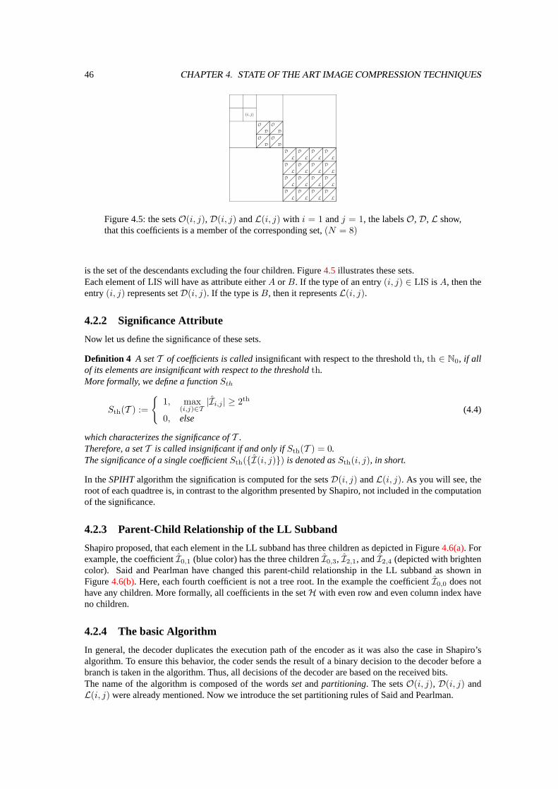
46 CHAPTER 4. STATE OF THE ART IMAGE COMPRESSION TECHNIQUES
(i, j)
OD
OD
OD
ODDL
DL
DL
DL
DL
DL
DL
DL
DL
DL
DL
DL
DL
DL
DL
DL
Figure 4.5: the setsO(i, j), D(i, j) andL(i, j) with i = 1 andj = 1, the labelsO, D, L show,that this coefficients is a member of the corresponding set,(N = 8)
is the set of the descendants excluding the four children. Figure4.5 illustrates these sets.Each element ofLIS will have as attribute eitherA orB. If the type of an entry(i, j) ∈ LIS isA, then theentry(i, j) represents setD(i, j). If the type isB, then it representsL(i, j).
4.2.2 Significance Attribute
Now let us define the significance of these sets.
Definition 4 A setT of coefficients is calledinsignificant with respect to the thresholdth, th ∈ N0, if allof its elements are insignificant with respect to the thresholdth.More formally, we define a functionSth
Sth(T ) :=
{1, max
(i,j)∈T|Ii,j | ≥ 2th
0, else(4.4)
which characterizes the significance ofT .Therefore, a setT is called insignificant if and only ifSth(T ) = 0.The significance of a single coefficientSth({I(i, j)}) is denoted asSth(i, j), in short.
In theSPIHTalgorithm the signification is computed for the setsD(i, j) andL(i, j). As you will see, theroot of each quadtree is, in contrast to the algorithm presented by Shapiro, not included in the computationof the significance.
4.2.3 Parent-Child Relationship of the LL Subband
Shapiro proposed, that each element in the LL subband has three children as depicted in Figure4.6(a). Forexample, the coefficientI0,1 (blue color) has the three childrenI0,3, I2,1, andI2,4 (depicted with brightencolor). Said and Pearlman have changed this parent-child relationship in the LL subband as shown inFigure4.6(b). Here, each fourth coefficient is not a tree root. In the example the coefficientI0,0 does nothave any children. More formally, all coefficients in the setH with even row and even column index haveno children.
4.2.4 The basic Algorithm
In general, the decoder duplicates the execution path of the encoder as it was also the case in Shapiro’salgorithm. To ensure this behavior, the coder sends the result of a binary decision to the decoder before abranch is taken in the algorithm. Thus, all decisions of the decoder are based on the received bits.The name of the algorithm is composed of the wordssetandpartitioning. The setsO(i, j), D(i, j) andL(i, j) were already mentioned. Now we introduce the set partitioning rules of Said and Pearlman.
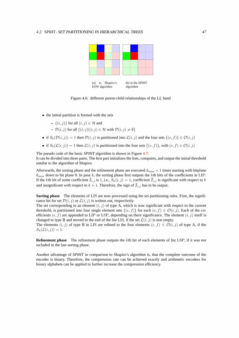
4.2. SPIHT- SET PARTITIONING IN HIERARCHICAL TREES 47
(a) in Shapiro’sEZW algorithm
(b) in theSPIHTalgorithm
Figure 4.6: different parent-child relationships of the LL band
• the initial partition is formed with the sets
– {(i, j)} for all (i, j) ∈ H and
– D(i, j) for all {(i, j)|(i, j) ∈ H with D(i, j) 6= ∅}
• if Sk(D(i, j)) = 1 thenD(i, j) is partitioned intoL(i, j) and the four sets{(e, f)} ∈ O(i, j)
• if Sk(L(i, j)) = 1 thenL(i, j) is partitioned into the four sets{(e, f)}, with (e, f) ∈ O(i, j)
The pseudo code of the basicSPIHTalgorithm is shown in Figure4.7.It can be divided into three parts. The first part initializes the lists, computes, and output the initial thresholdsimilar to the algorithm of Shapiro.
Afterwards, the sorting phase and the refinement phase are executedkmax + 1 times starting with bitplanekmax down to bit plane 0. In passk, the sorting phase first outputs thekth bits of the coefficients inLIP.If the kth bit of some coefficientIi,j is 1, i.e.,Sk(i, j) = 1, coefficientIi,j is significant with respect tokand insignificant with respect tok + 1. Therefore, the sign ofIi,j has to be output.
Sorting phase The elements ofLIS are now processed using the set partitioning rules. First, the signifi-cance bit for setD(i, j) orL(i, j) is written out, respectively.The set corresponding to an element(i, j) of type A, which is now significant with respect to the currentthreshold, is partitioned into four single element sets{(e, f)} for each(e, f) ∈ O(i, j). Each of the co-efficients(e, f) are appended toLIP or LSP, depending on there significance. The element(i, j) itself ischanged to type B and moved to the end of the listLIS, if the setL(i, j) is non empty.The elements(i, j) of type B in LIS are refined to the four elements(e, f) ∈ O(i, j) of type A, if theSk(L(i, j)) = 1.
Refinement phase The refinement phase outputs thekth bit of each elements of listLSP, if it was notincluded in the last sorting phase.
Another advantage ofSPIHT in comparison to Shapiro’s algorithm is, that the complete outcome of theencoder is binary. Therefore, the compression rate can be achieved exactly and arithmetic encoders forbinary alphabets can be applied to further increase the compression efficiency.
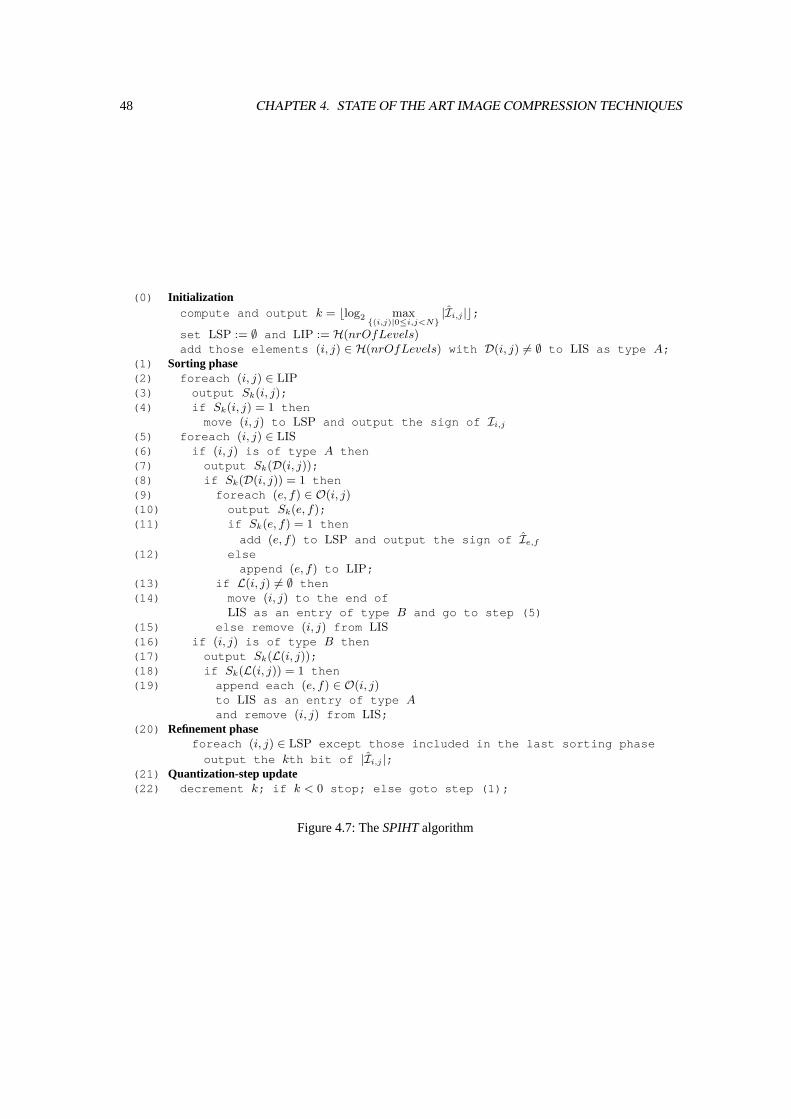
48 CHAPTER 4. STATE OF THE ART IMAGE COMPRESSION TECHNIQUES
(0) Initializationcompute and output k = blog2 max
{(i,j)|0≤i,j<N}|Ii,j |c;
set LSP := ∅ and LIP := H(nrOfLevels)add those elements (i, j) ∈ H(nrOfLevels) with D(i, j) 6= ∅ to LIS as type A;
(1) Sorting phase(2) foreach (i, j) ∈ LIP(3) output Sk(i, j);(4) if Sk(i, j) = 1 then
move (i, j) to LSP and output the sign of Ii,j
(5) foreach (i, j) ∈ LIS(6) if (i, j) is of type A then(7) output Sk(D(i, j));(8) if Sk(D(i, j)) = 1 then(9) foreach (e, f) ∈ O(i, j)(10) output Sk(e, f);(11) if Sk(e, f) = 1 then
add (e, f) to LSP and output the sign of Ie,f
(12) elseappend (e, f) to LIP;
(13) if L(i, j) 6= ∅ then(14) move (i, j) to the end of
LIS as an entry of type B and go to step (5)(15) else remove (i, j) from LIS(16) if (i, j) is of type B then(17) output Sk(L(i, j));(18) if Sk(L(i, j)) = 1 then(19) append each (e, f) ∈ O(i, j)
to LIS as an entry of type Aand remove (i, j) from LIS;
(20) Refinement phaseforeach (i, j) ∈ LSP except those included in the last sorting phase
output the kth bit of |Ii,j |;(21) Quantization-step update(22) decrement k; if k < 0 stop; else goto step (1);
Figure 4.7: TheSPIHTalgorithm
Chapter 5
Partitioned Approach
In this chapter we present the partitioned approach to wavelet transform images. This partitioned approachitself was developed in 19981.At first we motivate, why there is a need for such an approach, if one considers implementations of imagecompression algorithm based on wavelet transforms in programmable hardware. We discuss accuratelywhy these wavelet based image compression algorithms need to be adapted at all to implement them intoprogrammable hardware. Then we present the application of the partitioned approach to lossless imagecompression. The more interesting investigation is the extension to lossy image compression, where wehave to deal with boundary effects between the image partitions. Here we present different solutions inorder to avoid block artefacts known from compression methods based on discrete cosine transforms.
In Section5.3 of this chapter we present the modifications to the originalSPIHTalgorithm, which cor-respond to the accommodation to the partitioned approach and the necessities for hardware architectureswith minimal memory requirements. Then we compare the two algorithms in terms of mean squared errorin Section5.4.
5.1 Drawbacks of the Traditional 2D-DWT on Images
Let us review the traditional two dimensional discrete wavelet transform on images introduced in Chapter2.We have seen, that images are wavelet transformed using the one dimensional transform applied to rowsand columns of the image, separately. In Section1.8we have introduced the Lifting Scheme as a techniqueto compute the transform in place.In the case, that the image can be stored completely in main memory (software solution) of a PC or in onchip memory (hardware solution) the transform can easily be implemented. The only additional buffer weneed has a size comparable to the size of a row or a column, respectively, to reorder the low and high passcoefficients. To compute the 2D-DWT we have to load the image into the memory. Then we transform itusing the mentioned buffer, if enough internal memory is available. Typically, images have hundreds ofrows and columns and each pixel is represented by one up to24 bits or even more. Therefore we have todeal with data volumes of several kbytes up to a couple of megabytes. Obviously, this exceeds the memorylimits, if we consider hardware solutions. Thus, we have to limit the number of rows and columns andthe maximum bitwidth. As a consequence images of larger sizes must be split into manageable pieces.Remember from Section2.1 that we then have to deal with boundary effects even at the boundary of eachpiece of the original image, when targeting to lossy compression.
1 After making first experiences with the corresponding hardware architecture for lossless image compression on FPGAs we havepublished the basic ideas at the Custom Integrated Circuits Conference in 2000 (CICC2000) [RM00]. The extension to lossy imagecompression was presented at the ACM conference on Field Programmable Gate Arrays in 2001 (FPGA2001) [RM01]. The FPGAimplementation of a modifiedSPIHTalgorithm based on the partitioned approach was published at the ACM conference on FieldProgrammable Gate Arrays (FPGA2002) [RFM02a] and the45th Midwest Symposium on Circuit and Systems (MWSCAS2002) in2002 [RFM02b].
49
50 CHAPTER 5. PARTITIONED APPROACH
On the other hand we can store the image data externally and compute the transform row by row and col-umn by column, reducing the internal memory to the size of a row or column. In that case, the data transferfrom and to the internal memory will become the bottleneck of the implementation. Remark, that alreadytransformed coefficients have to be saved and loaded again during the next level of computation. Further-more, after the whole transform had taken place, the transformed image is stored in external memory, butan embedded zerotree wavelet coder needs random access to it.
To overcome these difficulties we will present the partitioned approach to wavelet transform images, whichis applicable to both lossless and lossy compression.
5.2 Partitioned 2D-DWT
Let us start with some notations. Remember from Chapter2 that we consider anN × N image as twodimensional pixel arrayI with N rows andN columns and assume adpth-bit greyscale resolution. Fur-thermore, we assume without loss of generality that the equationN = 2k holds for some positive integerk.Partitioning an imageI into (N
q )2 quadratic subimages
I(0,0), . . . , I( Nq −1, N
q −1)
of sizeq with q = 2r for some positive integer1 ≤ r < k results in subimages with
I(s,t)[i, j] = I[s · q + i, t · q + j]
for all 0 ≤ s, t < Nq and0 ≤ i, j < q.
Before the transform takes place, we partition the original imageI into quadratic subimagesI(s,t) asdescribed above. Then each subimage is transformed in the conventional way. We refer for an illustrationto Figure5.1. The first idea is to transform the subimages independently of the neighboring subimages.However, this approach is only applicable, if no quantization takes place, otherwise artefacts are introduced.What are the advantages and disadvantages of this partitioned approach?
+ The internal memory requirements are dramatically reduced.
+ The subimages can be transformed independently of each other.
+ The traditional 2D-DWT can be directly applied to the subimages without any modifications.
− It is not applicable for lossy compression.
For lossy compression we have to take into account the coefficients of the neighboring subimages in orderto guarantee that the partitioned approach is as efficient as the traditional one. We will denote this typeof transformation aspartitioned approach with boundary treatment. Suppose we have given a wavelettransformed imageI using the traditional approach as shown in Figure5.1(a). We have to manage that thepartitioned transformed image is a permutation of the coefficients of the traditional transformed image. Forillustration consider Figure5.2(b). Consider the LL subband on the left of Figure5.2(a), which correspondsto the approximated original at half the resolution, and the64 LL subbands of all partitions on the right.We observe, that composing all LL subbands on the right results in the LL subband on the left.
We can compute the partitioned 2D-DWT with boundary treatment even without the traditional one givenfirst. We will discuss it later in this chapter. Let us summarize first the advantages and disadvantages forthis kind of partitioned transform, too.
+ The internal memory requirements are dramatically reduced, too. In contrast to the approach withreflection at the partition boundaries we need additional memory for coefficients of neighboringsubimages or we have to deal with increased data transfer volume.
+ It is applicable for lossy compression.
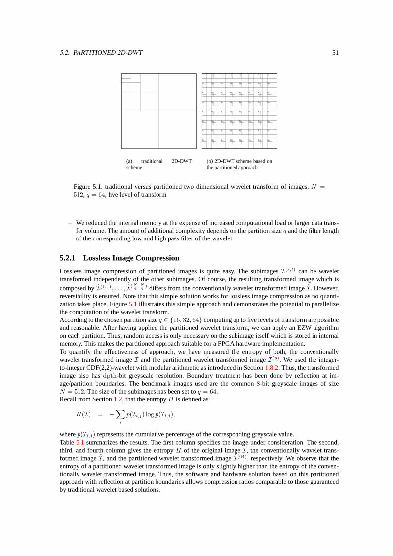
5.2. PARTITIONED 2D-DWT 51
(a) traditional 2D-DWTscheme
(b) 2D-DWT scheme based onthe partitioned approach
Figure 5.1: traditional versus partitioned two dimensional wavelet transform of images,N =512, q = 64, five level of transform
− We reduced the internal memory at the expense of increased computational load or larger data trans-fer volume. The amount of additional complexity depends on the partition sizeq and the filter lengthof the corresponding low and high pass filter of the wavelet.
5.2.1 Lossless Image Compression
Lossless image compression of partitioned images is quite easy. The subimagesI(s,t) can be wavelettransformed independently of the other subimages. Of course, the resulting transformed image which iscomposed byI(1,1), . . . , I( N
q , Nq ) differs from the conventionally wavelet transformed imageI. However,
reversibility is ensured. Note that this simple solution works for lossless image compression as no quanti-zation takes place. Figure5.1 illustrates this simple approach and demonstrates the potential to parallelizethe computation of the wavelet transform.According to the chosen partition sizeq ∈ {16, 32, 64} computing up to five levels of transform are possibleand reasonable. After having applied the partitioned wavelet transform, we can apply an EZW algorithmon each partition. Thus, random access is only necessary on the subimage itself which is stored in internalmemory. This makes the partitioned approach suitable for a FPGA hardware implementation.To quantify the effectiveness of approach, we have measured the entropy of both, the conventionallywavelet transformed imageI and the partitioned wavelet transformed imageI(p). We used the integer-to-integer CDF(2,2)-wavelet with modular arithmetic as introduced in Section1.8.2. Thus, the transformedimage also hasdpth-bit greyscale resolution. Boundary treatment has been done by reflection at im-age/partition boundaries. The benchmark images used are the common8-bit greyscale images of sizeN = 512. The size of the subimages has been set toq = 64.Recall from Section1.2, that the entropyH is defined as
H(I) = −∑
i
p(Ii,j) log p(Ii,j),
wherep(Ii,j) represents the cumulative percentage of the corresponding greyscale value.Table5.1 summarizes the results. The first column specifies the image under consideration. The second,third, and fourth column gives the entropyH of the original imageI, the conventionally wavelet trans-formed imageI, and the partitioned wavelet transformed imageI(64), respectively. We observe that theentropy of a partitioned wavelet transformed image is only slightly higher than the entropy of the conven-tionally wavelet transformed image. Thus, the software and hardware solution based on this partitionedapproach with reflection at partition boundaries allows compression ratios comparable to those guaranteedby traditional wavelet based solutions.
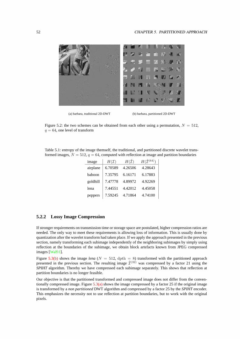
52 CHAPTER 5. PARTITIONED APPROACH
(a) barbara, traditional 2D-DWT (b) barbara, partitioned 2D-DWT
Figure 5.2: the two schemes can be obtained from each other using a permutation,N = 512,q = 64, one level of transform
Table 5.1: entropy of the image themself, the traditional, and partitioned discrete wavelet trans-formed images,N = 512, q = 64, computed with reflection at image and partition boundaries
image H(I) H(I) H(I(64))
airplane 6.70589 4.26506 4.28643
baboon 7.35795 6.16171 6.17883
goldhill 7.47778 4.89972 4.92269
lena 7.44551 4.42012 4.45058
peppers 7.59245 4.71864 4.74100
5.2.2 Lossy Image Compression
If stronger requirements on transmission time or storage space are postulated, higher compression ratios areneeded. The only way to meet these requirements is allowing loss of information. This is usually done byquantization after the wavelet transform had taken place. If we apply the approach presented in the previoussection, namely transforming each subimage independently of the neighboring subimages by simply usingreflection at the boundaries of the subimage, we obtain block artefacts known from JPEG compressedimages [Wal91].
Figure 5.3(b) shows the imagelena (N = 512, dpth = 8) transformed with the partitioned approachpresented in the previous section. The resulting imageI(32) was compressed by a factor 21 using theSPIHTalgorithm. Thereby we have compressed each subimage separately. This shows that reflection atpartition boundaries is no longer feasible.
Our objective is that the partitioned transformed and compressed image does not differ from the conven-tionally compressed image. Figure5.3(a)shows the image compressed by a factor 25 if the original imageis transformed by anon partitionedDWT algorithm and compressed by a factor 25 by theSPIHTencoder.This emphasizes the necessity not to use reflection at partition boundaries, but to work with the originalpixels.
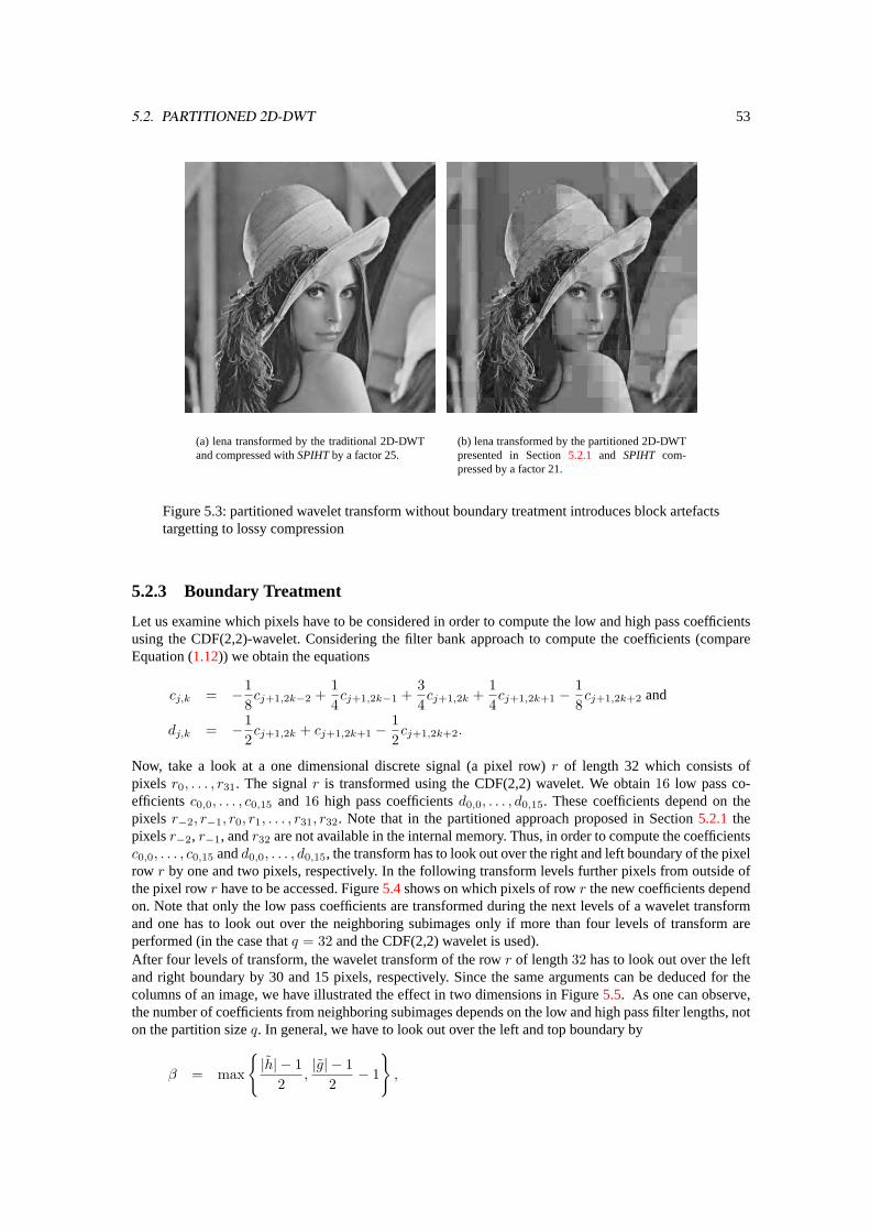
5.2. PARTITIONED 2D-DWT 53
(a) lena transformed by the traditional 2D-DWTand compressed withSPIHTby a factor 25.
(b) lena transformed by the partitioned 2D-DWTpresented in Section5.2.1 and SPIHT com-pressed by a factor 21.
Figure 5.3: partitioned wavelet transform without boundary treatment introduces block artefactstargetting to lossy compression
5.2.3 Boundary Treatment
Let us examine which pixels have to be considered in order to compute the low and high pass coefficientsusing the CDF(2,2)-wavelet. Considering the filter bank approach to compute the coefficients (compareEquation (1.12)) we obtain the equations
cj,k = −18cj+1,2k−2 +
14cj+1,2k−1 +
34cj+1,2k +
14cj+1,2k+1 −
18cj+1,2k+2 and
dj,k = −12cj+1,2k + cj+1,2k+1 −
12cj+1,2k+2.
Now, take a look at a one dimensional discrete signal (a pixel row)r of length 32 which consists ofpixels r0, . . . , r31. The signalr is transformed using the CDF(2,2) wavelet. We obtain16 low pass co-efficientsc0,0, . . . , c0,15 and16 high pass coefficientsd0,0, . . . , d0,15. These coefficients depend on thepixels r−2, r−1, r0, r1, . . . , r31, r32. Note that in the partitioned approach proposed in Section5.2.1 thepixelsr−2, r−1, andr32 are not available in the internal memory. Thus, in order to compute the coefficientsc0,0, . . . , c0,15 andd0,0, . . . , d0,15, the transform has to look out over the right and left boundary of the pixelrow r by one and two pixels, respectively. In the following transform levels further pixels from outside ofthe pixel rowr have to be accessed. Figure5.4shows on which pixels of rowr the new coefficients dependon. Note that only the low pass coefficients are transformed during the next levels of a wavelet transformand one has to look out over the neighboring subimages only if more than four levels of transform areperformed (in the case thatq = 32 and the CDF(2,2) wavelet is used).After four levels of transform, the wavelet transform of the rowr of length32 has to look out over the leftand right boundary by 30 and 15 pixels, respectively. Since the same arguments can be deduced for thecolumns of an image, we have illustrated the effect in two dimensions in Figure5.5. As one can observe,the number of coefficients from neighboring subimages depends on the low and high pass filter lengths, noton the partition sizeq. In general, we have to look out over the left and top boundary by
β = max
{|h| − 1
2,|g| − 1
2− 1
},
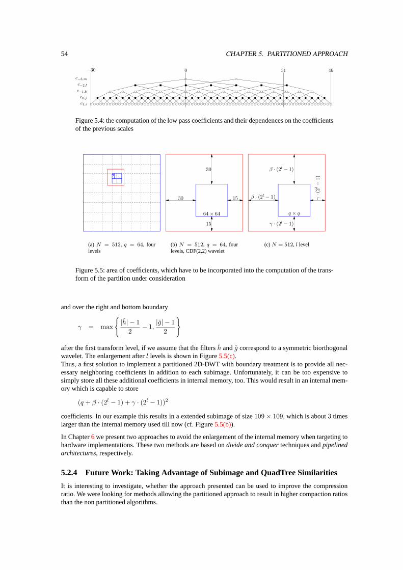
54 CHAPTER 5. PARTITIONED APPROACH
0 31−30 46
c1,i
c0,j
c−1,k
c−2,l
c−3,m
Figure 5.4: the computation of the low pass coefficients and their dependences on the coefficientsof the previous scales
(a) N = 512, q = 64, fourlevels
30 15
30
15
64× 64
(b) N = 512, q = 64, fourlevels, CDF(2,2) wavelet
β · (2l − 1) γ·(
2l−
1)
β · (2l − 1)
γ · (2l − 1)
q × q
(c)N = 512, l level
Figure 5.5: area of coefficients, which have to be incorporated into the computation of the trans-form of the partition under consideration
and over the right and bottom boundary
γ = max
{|h| − 1
2− 1,
|g| − 12
}
after the first transform level, if we assume that the filtersh andg correspond to a symmetric biorthogonalwavelet. The enlargement afterl levels is shown in Figure5.5(c).Thus, a first solution to implement a partitioned 2D-DWT with boundary treatment is to provide all nec-essary neighboring coefficients in addition to each subimage. Unfortunately, it can be too expensive tosimply store all these additional coefficients in internal memory, too. This would result in an internal mem-ory which is capable to store
(q + β · (2l − 1) + γ · (2l − 1))2
coefficients. In our example this results in a extended subimage of size109× 109, which is about3 timeslarger than the internal memory used till now (cf. Figure5.5(b)).
In Chapter6 we present two approaches to avoid the enlargement of the internal memory when targeting tohardware implementations. These two methods are based ondivide and conquertechniques andpipelinedarchitectures, respectively.
5.2.4 Future Work: Taking Advantage of Subimage and QuadTree Similarities
It is interesting to investigate, whether the approach presented can be used to improve the compressionratio. We were looking for methods allowing the partitioned approach to result in higher compaction ratiosthan the non partitioned algorithms.
5.3. MODIFICATIONS TO THE SPIHTCODEC 55
One point of departure could be to classify the subimages with respect to similarity, to compress onlyone representativeJC of each classC, and to represent the remaining subimagesI of classC by theimageI − JC which specifies the differences between subimageI and its representativeJC . Anotherpoint of departure could be to exploit similarities between the trees of the multiscale representation. Thereare similarities between the quadtrees. The difficulty is a convincing measure of similarity, which is ofadequately computational complexity. We have made some experiences with the mean squared error andthe gain of reduced output of theSPIHTalgorithm. Unfortunately, the computational overload was to largein order to obtain useful results.
5.3 Modifications to theSPIHT Codec
In this section we present the modifications necessary to obtain an efficient hardware implementation oftheSPIHTcompressor based on the partitioned approach to wavelet transform images.At first, we exchange the sorting phase with the refinement phase to save memory for status information.However, the greatest challenge is the hardware implementation of the three listsLIP, LSP, andLIS. In thefollowing we deduce estimations of the memory requirements of these lists. This section will be concludedwith the outline of the modifiedSPIHTencoder.
5.3.1 Exchange of Sorting and Refinement Phase
In the basicSPIHT algorithm status information has to be stored for the elements ofLSP specifyingwhether the corresponding coefficient has been added toLSP in the current iteration of the sorting phase(see Line 20 in Figure4.7). In the worst case all coefficients become significant in the same iteration.Consequently, we have to provide a memory capacity ofq2 bits to store this information. However, if weexchange the sorting and the refinement phase, we do not need to consider this information anymore. Thecompressed data stream is still decodable and it is not increased in size. Of course, we have to consider thatthere is a reordering of the transmitted bits during an iteration. We will take a closer look at this problemin Section5.4.
5.3.2 Memory Requirements of the Ordered Lists
To obtain an efficient realization of the listsLIP, LSP, andLIS, we first have to specify the operations thattake place on these lists and deduce worst case space requirements in a software implementation.
Estimations for LIS
We have to provide the following operations forLIS:
• initialize as empty list (Line 0),
• append an element (Line 0 and 19),
• sequentially iterate the elements (Line 5),
• delete the element under consideration (Line 15 and 19),
• move the element under consideration to the end of the list and change the type (Line 14).
Note that the initialization phase cannot be neglected because there are several partitions to compress.Dependent on the realization chosen the cost of the initialization phase can be linear in the number ofelements.The estimation of the space requirement forLIS is simplified by the fact thatLIS is an independent set,i.e., for all elementsv, w ∈ LIS it holds thatv is neither a predecessor nor a successor ofw with respectto the corresponding quad tree. This can be easily proved by complete induction [Fey01]. Note that if thelist is longest, then all its elements are of typeA. Consequently, the number of elements ofLIS is smaller
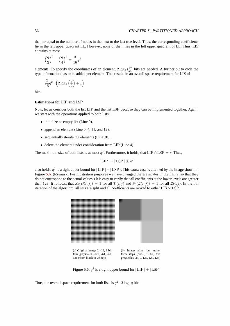
56 CHAPTER 5. PARTITIONED APPROACH
than or equal to the number of nodes in the next to the last tree level. Thus, the corresponding coefficientslie in the left upper quadrant LL. However, none of them lies in the left upper quadrant of LL. Thus,LIScontains at most(q
2
)2
−(q
4
)2
=316q2
elements. To specify the coordinates of an element,2 log2
(q2
)bits are needed. A further bit to code the
type information has to be added per element. This results in an overall space requirement forLIS of
316q2 ·
(2 log2
(q2
)+ 1)
bits.
Estimations for LIP and LSP
Now, let us consider both the listLIP and the listLSP because they can be implemented together. Again,we start with the operations applied to both lists:
• initialize as empty list (Line 0),
• append an element (Line 0, 4, 11, and 12),
• sequentially iterate the elements (Line 20),
• delete the element under consideration fromLIP (Line 4).
The maximum size of both lists is at mostq2. Furthermore, it holds, thatLIP∩LSP = ∅. Thus,
|LIP |+ |LSP | ≤ q2
also holds.q2 is a tight upper bound for|LIP |+ |LSP |. This worst case is attained by the image shown inFigure5.6. (Remark: For illustration purposes we have changed the greyscales in the figure, so that theydo not correspond to the actual values.) It is easy to verify that all coefficients at the lower levels are greaterthan 126. It follows, thatS6(D(i, j)) = 1 for all D(i, j) andS6(L(i, j)) = 1 for all L(i, j). In the6thiteration of the algorithm, all sets are split and all coefficients are moved to eitherLIS or LSP.
(a) Original image (q=16, 8 bit,four greyscales -128, -61, -60,126 (from black to white))
(b) Image after four trans-form steps (q=16, 9 bit, fivegreyscales -33, 0, 126, 127, 128)
Figure 5.6:q2 is a tight upper bound for|LIP |+ |LSP |
Thus, the overall space requirement for both lists isq2 · 2 log2 q bits.
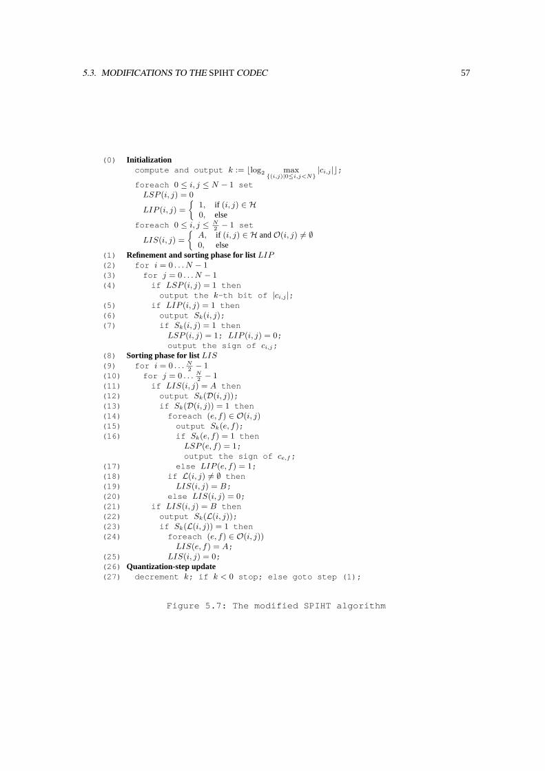
5.3. MODIFICATIONS TO THE SPIHTCODEC 57
(0) Initializationcompute and output k := blog2 max
{(i,j)|0≤i,j<N}|ci,j |c;
foreach 0 ≤ i, j ≤ N − 1 setLSP (i, j) = 0
LIP (i, j) =
{1, if (i, j) ∈ H0, else
foreach 0 ≤ i, j ≤ N2− 1 set
LIS(i, j) =
{A, if (i, j) ∈ H andO(i, j) 6= ∅0, else
(1) Refinement and sorting phase for listLIP(2) for i = 0 . . . N − 1(3) for j = 0 . . . N − 1(4) if LSP (i, j) = 1 then
output the k-th bit of |ci,j |;(5) if LIP (i, j) = 1 then(6) output Sk(i, j);(7) if Sk(i, j) = 1 then
LSP (i, j) = 1; LIP (i, j) = 0;output the sign of ci,j ;
(8) Sorting phase for listLIS(9) for i = 0 . . . N
2− 1
(10) for j = 0 . . . N2− 1
(11) if LIS(i, j) = A then(12) output Sk(D(i, j));(13) if Sk(D(i, j)) = 1 then(14) foreach (e, f) ∈ O(i, j)(15) output Sk(e, f);(16) if Sk(e, f) = 1 then
LSP (e, f) = 1;output the sign of ce,f ;
(17) else LIP (e, f) = 1;(18) if L(i, j) 6= ∅ then(19) LIS(i, j) = B;(20) else LIS(i, j) = 0;(21) if LIS(i, j) = B then(22) output Sk(L(i, j));(23) if Sk(L(i, j)) = 1 then(24) foreach (e, f) ∈ O(i, j))
LIS(e, f) = A;(25) LIS(i, j) = 0;(26) Quantization-step update(27) decrement k; if k < 0 stop; else goto step (1);
Figure 5.7: The modified SPIHT algorithm
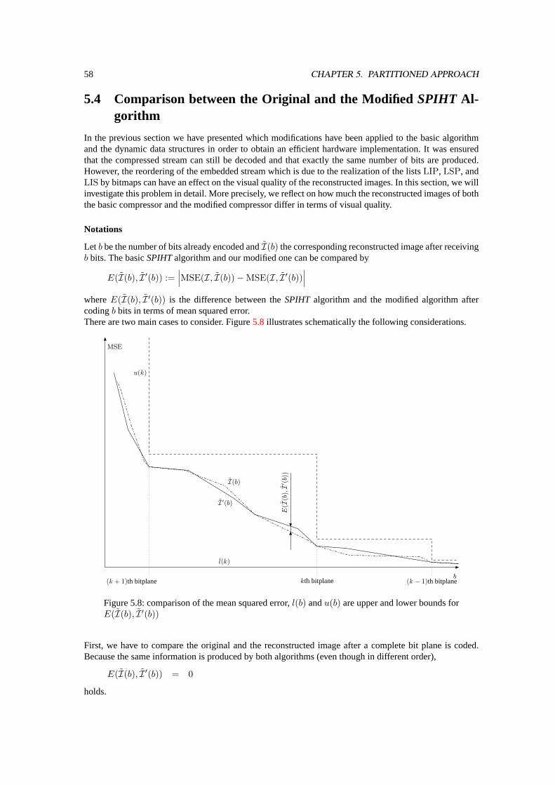
58 CHAPTER 5. PARTITIONED APPROACH
5.4 Comparison between the Original and the ModifiedSPIHT Al-gorithm
In the previous section we have presented which modifications have been applied to the basic algorithmand the dynamic data structures in order to obtain an efficient hardware implementation. It was ensuredthat the compressed stream can still be decoded and that exactly the same number of bits are produced.However, the reordering of the embedded stream which is due to the realization of the listsLIP, LSP, andLIS by bitmaps can have an effect on the visual quality of the reconstructed images. In this section, we willinvestigate this problem in detail. More precisely, we reflect on how much the reconstructed images of boththe basic compressor and the modified compressor differ in terms of visual quality.
Notations
Let b be the number of bits already encoded andI(b) the corresponding reconstructed image after receivingb bits. The basicSPIHTalgorithm and our modified one can be compared by
E(I(b), I ′(b)) :=∣∣∣MSE(I, I(b))−MSE(I, I ′(b))
∣∣∣whereE(I(b), I ′(b)) is the difference between theSPIHT algorithm and the modified algorithm aftercodingb bits in terms of mean squared error.There are two main cases to consider. Figure5.8 illustrates schematically the following considerations.
MSE
(k + 1)th bitplane kth bitplane (k − 1)th bitplaneb
E(I
(b),I′
(b))
I(b)
I ′(b)
u(k)
l(k)
Figure 5.8: comparison of the mean squared error,l(b) andu(b) are upper and lower bounds forE(I(b), I ′(b))
First, we have to compare the original and the reconstructed image after a complete bit plane is coded.Because the same information is produced by both algorithms (even though in different order),
E(I(b), I ′(b)) = 0
holds.
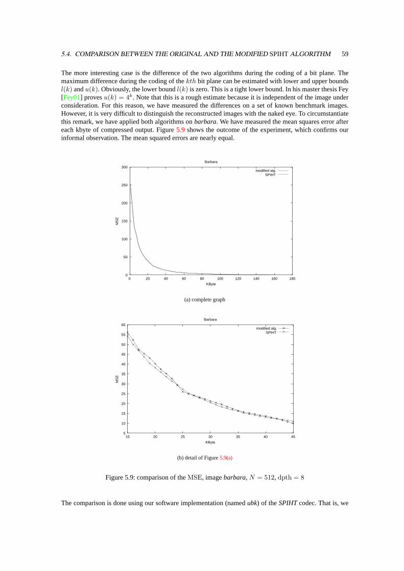
5.4. COMPARISON BETWEEN THE ORIGINAL AND THE MODIFIED SPIHTALGORITHM 59
The more interesting case is the difference of the two algorithms during the coding of a bit plane. Themaximum difference during the coding of thekth bit plane can be estimated with lower and upper boundsl(k) andu(k). Obviously, the lower boundl(k) is zero. This is a tight lower bound. In his master thesis Fey[Fey01] provesu(k) = 4k. Note that this is a rough estimate because it is independent of the image underconsideration. For this reason, we have measured the differences on a set of known benchmark images.However, it is very difficult to distinguish the reconstructed images with the naked eye. To circumstantiatethis remark, we have applied both algorithms onbarbara. We have measured the mean squares error aftereach kbyte of compressed output. Figure5.9 shows the outcome of the experiment, which confirms ourinformal observation. The mean squared errors are nearly equal.
0
50
100
150
200
250
300
0 20 40 60 80 100 120 140 160 180
MS
E
KByte
Barbara
modified alg.SPIHT
(a) complete graph
5
10
15
20
25
30
35
40
45
50
55
60
15 20 25 30 35 40 45
MS
E
KByte
Barbara
modified alg.SPIHT
(b) detail of Figure5.9(a)
Figure 5.9: comparison of theMSE, imagebarbara,N = 512, dpth = 8
The comparison is done using our software implementation (namedubk) of theSPIHTcodec. That is, we
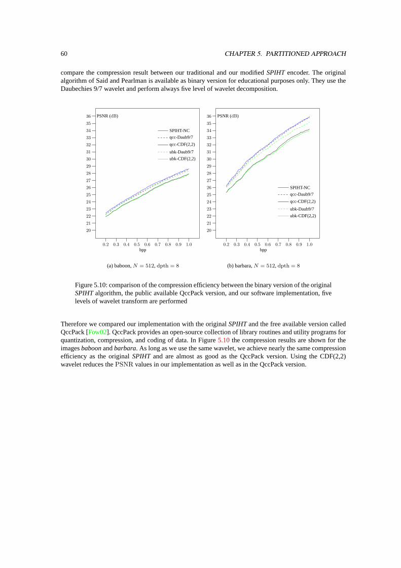
60 CHAPTER 5. PARTITIONED APPROACH
compare the compression result between our traditional and our modifiedSPIHTencoder. The originalalgorithm of Said and Pearlman is available as binary version for educational purposes only. They use theDaubechies 9/7 wavelet and perform always five level of wavelet decomposition.
PSNR(dB)
20
21
22
23
24
25
26
27
28
29
30
31
32
33
34
35
36
0.2 0.3 0.4 0.5 0.6 0.7 0.8 0.9 1.0
SPIHT-NC
qcc-Daub9/7
qcc-CDF(2,2)
ubk-Daub9/7
ubk-CDF(2,2)
bpp
(a) baboon,N = 512, dpth = 8
PSNR(dB)
20
21
22
23
24
25
26
27
28
29
30
31
32
33
34
35
36
0.2 0.3 0.4 0.5 0.6 0.7 0.8 0.9 1.0
SPIHT-NC
qcc-Daub9/7
qcc-CDF(2,2)
ubk-Daub9/7
ubk-CDF(2,2)
bpp
(b) barbara,N = 512, dpth = 8
Figure 5.10: comparison of the compression efficiency between the binary version of the originalSPIHTalgorithm, the public available QccPack version, and our software implementation, fivelevels of wavelet transform are performed
Therefore we compared our implementation with the originalSPIHTand the free available version calledQccPack [Fow02]. QccPack provides an open-source collection of library routines and utility programs forquantization, compression, and coding of data. In Figure5.10 the compression results are shown for theimagesbaboonandbarbara. As long as we use the same wavelet, we achieve nearly the same compressionefficiency as the originalSPIHT and are almost as good as the QccPack version. Using the CDF(2,2)wavelet reduces thePSNR values in our implementation as well as in the QccPack version.
Chapter 6
FPGA architectures
In this chapter we present several architectures and complete designs which are all based on the developedpartitioned approach for wavelet-based image compression for programmable hardware. All designs werespecified using the hardware description language VHDL. We turned our attention to rapid prototypingwithout heavy manual optimizations after synthesis. As a consequence the experimental results mainlyshow the mightiness of the partitioned approach1.Each design was developed to run at our prototyping environment. This environment consists of a PCequipped with a PCI card where a Xilinx XC4000XLA FPGA is mounted. The advantages and disadvan-tages of this prototyping environment are explained in Section6.1.All designs were described in VHDL language. As synthesis tool we decided to use the FPGA compilerfrom Synopsys. The resulting netlists in EDIF format are taken as input to the Xilinx implementation flow(mapping, place and route, timing analysis and bit stream generation) to generate a configuration bit stream.We dispensed with manually optimizations like floor planning. These bitstreams are further processed withan utility calledHap-Generatorfrom the vendor of the prototyping environment. The resulting files areused to configure the FPGA using the provided software interface over the PCI bus.In Section6.2we present a complete design for partitioned two dimensional discrete wavelet transform forlossless compression capable of running at 40MHz at our prototyping environment. Then we show severalarchitectures to compute a partitioned wavelet transform for lossy compression in programmable hardware.These architectures can be combined with the design for lossy compression, which is shown in detail inSection6.3. This design implements the well knownSPIHTalgorithm of Said and Pearlman adapted toour partitioned approach. Furthermore an arithmetic encoder can be included in the architecture to furtherimprove the compression rates.
6.1 Prototyping Environment
In order to obtain experimental results on real world data we have used a PC equipped with a FPGAPCI board as prototyping platform. This PC is running under WinNTR©and Linux operating system. TheFPGA prototyping board was manufactured by Silicon Software GmbH, Mannheim, Germany [Gmb99].It is equipped with a Xilinx device of the XC4000XLA series. The device has the speed index−09 and ismounted on the PCI board in a HQ240 package. The data path diagram of the board is shown in Figure6.1.Beside the Xilinx device the PCI card is equipped with 2Mbyte SRAM which is connected directly to theFPGA with 36 data lines. This memory bank can be accessed with at most 80MHz frequency. Furthermorethere is a programmable clock generator and a device to manage the communication with the PCI bus.The prototyping environment provides several mechanism to exchange data between the mounted Xilinxdevice, the local SRAM and the PC main memory. These could be categorized into
1. direct access to registers/latches (configured into the FPGA)
1Stephan Sutter and Görschwin Fey, students of mine, assist me to implement, simulate, synthesize and validate the VHDL designsin the scope of their master theses [Sut99], [Fey01].
61
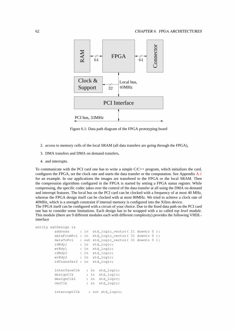
62 CHAPTER 6. FPGA ARCHITECTURES
PCI Interface
RA
M
Con
nect
or
Clock&Support
FPGA
PCI bus,33MHz
Localbus,40MHz
64 64
32
Figure 6.1: Data path diagram of the FPGA prototyping board
2. access to memory cells of the local SRAM (all data transfers are going through the FPGA),
3. DMA transfers and DMA on demand transfers,
4. and interrupts.
To communicate with the PCI card one has to write a simple C/C++ program, which initializes the card,configures the FPGA, set the clock rate and starts the data transfer or the computation. See AppendixA.1for an example. In our applications the images are transfered to the FPGA or the local SRAM. Thenthe compression algorithms configured in the FPGA is started by setting a FPGA status register. Whilecompressing, the specific codec takes over the control of the data transfer at all using the DMA on demandand interrupt features. The local bus on the PCI card can be clocked with a frequency of at most 40 MHz,whereas the FPGA design itself can be clocked with at most 80MHz. We tried to achieve a clock rate of40MHz, which is a strength constraint if internal memory is configured into the Xilinx device.The FPGA itself can be configured with a circuit of your choice. Due to the fixed data path on the PCI cardone has to consider some limitations. Each design has to be wrapped with a so calledtop level module.This module (there are 9 different modules each with different complexity) provides the following VHDL-interface
entity extDesign isaddress : in std_logic_vector( 21 downto 0 );dataFromPci : in std_logic_vector( 31 downto 0 );dataToPci : out std_logic_vector( 31 downto 0 );rdRdy1 : in std_logic;wrRdy1 : in std_logic;rdRdy2 : in std_logic;wrRdy2 : in std_logic;rdTransfer2 : in std_logic;
interfaceClk : in std_logic;designClk : in std_logic;designClk2 : in std_logic;cmcClk : in std_logic;
interruptClk : out std_logic;
6.1. PROTOTYPING ENVIRONMENT 63
interruptSignal : out std_logic;interruptStatus : in std_logic
);
end extDesign;
To communicate with both the PC main memory and the local SRAM one has to multiplex the bussesdataFromPci anddataToPci . This decreases the routability of the design in a significant manner.Another disadvantage with respect to our application are the fixed alignments of the busses to the primaryports of the device at north and south side. Since arithmetic components like adder should be alignedvertical due to the fast carry chain in XC4000 devices data ideally flows in horizontal direction. This givesa contradiction to the port alignments at the north and south side.The prototyping environment had influence to our designs, too. Using huge internal RAM modules leadsto a substantial drawback using devices without BlockRAMR©like the devices of the XC4000XLA series.The RAM has to be configured into theCLBs. EachCLB can represent a 16x1 bit or a 32x1 bit RAMblock with 4 or 5 address lines, respectively. These address lines have to be connected to eachCLB of thecorresponding RAM module. As a consequence huge fanout is introduced. This is problematical in terms ofroutability and overall performance constraints. Newer devices provide special components like RAM cellsand arithmetical units in the FPGA. Since there was no budget to buy a second prototyping environment,we can only provide experimental result based on the givenµEnable product.
6.1.1 The Xilinx XC4085 XLA device
The Xilinx XC4085 device consists of a matrix ofConfigurable Logic Blocks(CLB) with 56 rows and56columns. TheseCLBs are SRAM based and can be configured many times. After shut down the powersupply they have to be reconfigured. TheCLBs could be interconnected with horizontal and verticalsignals.Figure6.2shows the schematic of oneCLB [Xil97]. It can be configured to represent any function with 4or 5 inputs (see Figure6.2: function generatorF , G, orH). Furthermore there are mainly two flip-flops,two tristate drivers and the so calledcarry-logicavailable. The routing is done usingprogrammable switchmatrices(PSM), see Figure6.3(b). Remark that each switch corresponds to a multiplexer with a specificdelay. EachCLB can be configured to provide internal RAM. In order to do this, conceive the four inputsignals toF andG as address lines. Thus aCLB provides two 16×1 or one 32×1 random access memorymodule, respectively. At maximum we have 12kbyte RAM available. Each RAM block can be configuredwith different behavior:
• synchronous RAM: edge-triggered
• asynchronous RAM: level-sensitive
• single-port-RAM
• dual-port-RAM
The provided tristate drivers are somewhat counter productive in our specific application. In fact, they couldbe connected to horizontal (especially long) lines only. In contrast, the wide address and data busses, whereswitching between different signal source (the typical application field of tristate drivers) is necessary,have to be routed in vertical direction, due to the generated modules from the Xilinx toolsLogibloxR©orCore-generatorR©.Using multiplexer instead of tristate drivers reduces the time for place and route dramatically or makes iteven possible to place and route the design at all.Arithmetic operations are supported by the dedicatedcarry logic in the XC4000 family [New96]. EachCLB contains hard-wired carry logic to accelerate arithmetic operations. Fast adders can be constructed assimple ripple carry adders, using the special carry logic to calculate and propagate the carry between fulladders in adjacentCLBs. OneCLB is capable of realizing two full adders.
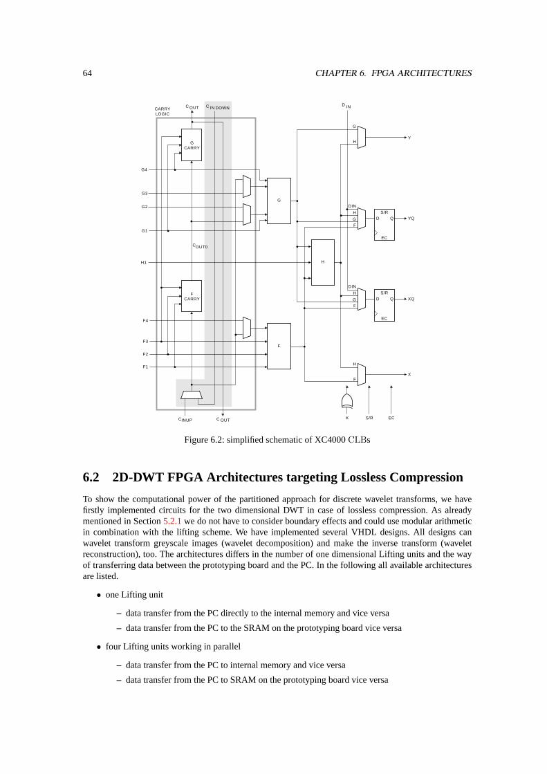
64 CHAPTER 6. FPGA ARCHITECTURES
D QS/R
EC
YQ
Y
DIN
H
GF
G
H
D QS/R
EC
XQ
DIN
H
GF
H
X
H
F
G
G4
G3
G2
G1
FF3
F2
F1
F4
FCARRY
GCARRY
C C DOWNCARRYLOGIC
D
CC UP K S/R EC
H1
OUT
INOUT IN
IN
COUT0
Figure 6.2: simplified schematic of XC4000CLBs
6.2 2D-DWT FPGA Architectures targeting Lossless Compression
To show the computational power of the partitioned approach for discrete wavelet transforms, we havefirstly implemented circuits for the two dimensional DWT in case of lossless compression. As alreadymentioned in Section5.2.1we do not have to consider boundary effects and could use modular arithmeticin combination with the lifting scheme. We have implemented several VHDL designs. All designs canwavelet transform greyscale images (wavelet decomposition) and make the inverse transform (waveletreconstruction), too. The architectures differs in the number of one dimensional Lifting units and the wayof transferring data between the prototyping board and the PC. In the following all available architecturesare listed.
• one Lifting unit
– data transfer from the PC directly to the internal memory and vice versa
– data transfer from the PC to the SRAM on the prototyping board vice versa
• four Lifting units working in parallel
– data transfer from the PC to internal memory and vice versa
– data transfer from the PC to SRAM on the prototyping board vice versa
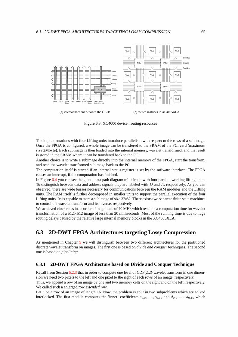
6.3. 2D-DWT FPGA ARCHITECTURES TARGETING LOSSY COMPRESSION 65
Quad
Quad
Single
Double
Long
DirectConnect
Long
CLB
Long GlobalClock
Long Double Single GlobalClock
CarryChain
DirectConnect
(a) interconnections between theCLBs
CLB
PSM PSM
PSMPSM
CLB CLB
CLB CLB CLB
CLB CLB CLB
Doubles
Singles
Doubles
X6601
(b) switch matrices in XC4085XLA
Figure 6.3: XC4000 device, routing resources
The implementations with four Lifting units introduce parallelism with respect to the rows of a subimage.Once the FPGA is configured, a whole image can be transfered to the SRAM of the PCI card (maximumsize 2Mbyte). Each subimage is then loaded into the internal memory, wavelet transformed, and the resultis stored in the SRAM where it can be transfered back to the PC.Another choice is to write a subimage directly into the internal memory of the FPGA, start the transform,and read the wavelet transformed subimage back to the PC.The computation itself is started if an internal status register is set by the software interface. The FPGAcauses an interrupt, if the computation has finished.In Figure6.4you can see the global data path diagram of a circuit with four parallel working lifting units.To distinguish between data and address signals they are labeled withD andA, respectively. As you canobserved, there are wide busses necessary for communications between the RAM modules and the Liftingunits. The RAM itself is further decomposed in smaller units to support the parallel execution of the fourLifting units. Its is capable to store a subimage of size 32×32. There exists two separate finite state machinesto control the wavelet transform and its inverse, respectively.We achieved clock rates in an order of magnitude of 40 MHz which result in a computation time for wavelettransformation of a 512×512 image of less than 20 milliseconds. Most of the running time is due to hugerouting delays caused by the relative large internal memory blocks in the XC4085XLA.
6.3 2D-DWT FPGA Architectures targeting Lossy Compression
As mentioned in Chapter5 we will distinguish between two different architectures for the partitioneddiscrete wavelet transform on images. The first one is based ondivide and conquertechniques. The secondone is based onpipelining.
6.3.1 2D-DWT FPGA Architecture based on Divide and Conquer Technique
Recall from Section5.2.3that in order to compute one level of CDF(2,2)-wavelet transform in one dimen-sion we need two pixels to the left and one pixel to the right of each rows of an image, respectively.Thus, we append a row of an image by one and two memory cells on the right and on the left, respectively.We called such a enlarged rowextended row.Let r be a row of an image of length16. Now, the problem is split in two subproblems which are solvedinterlocked. The first module computes the ’inner’ coefficientsc0,0, . . . , c0,15 andd0,0, . . . , d0,15 which
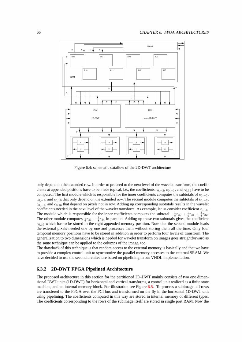
66 CHAPTER 6. FPGA ARCHITECTURES
R00 R01 R02 R03
R10
RAM
R11 R13R12
2D-DWT invers 2D-DWT
FSMFSM
I/O-unit
DAD A
D
D
A
A
D
D
P
U
P
U
P
U
P
U
Figure 6.4: schematic dataflow of the 2D-DWT architecture
only depend on the extended row. In order to proceed to the next level of the wavelet transform, the coeffi-cients at appended positions have to be made topical, i.e., the coefficientsc0,−2, c0,−1, andc0,16 have to becomputed. The first module which is responsible for the inner coefficients computes the subtotals ofc0,−2,c0,−1, andc0,16 that only depend on the extended row. The second module computes the subtotals ofc0,−2,c0,−1, andc0,16 that depend on pixels not in row. Adding up corresponding subtotals results in the waveletcoefficients needed in the next level of the wavelet transform. As example, let us consider coefficientc0,16.The module which is responsible for the inner coefficients computes the subtotal− 1
8r30 + 14r31 + 3
4r32.The other module computes14r33 −
18r34 in parallel. Adding up these two subtotals gives the coefficient
c0,16 which has to be stored in the right appended memory position. Note that the second module loadsthe external pixels needed one by one and processes them without storing them all the time. Only fourtemporal memory positions have to be stored in addition in order to perform four levels of transform. Thegeneralization to two dimensions which is needed for wavelet transform on images goes straightforward asthe same technique can be applied to the columns of the image, too.The drawback of this technique is that random access to the external memory is basically and that we haveto provide a complex control unit to synchronize the parallel memory accesses to the external SRAM. Wehave decided to use the second architecture based on pipelining in our VHDL implementation.
6.3.2 2D-DWT FPGA Pipelined Architecture
The proposed architecture in this section for the partitioned 2D-DWT mainly consists of two one dimen-sional DWT units (1D-DWT) for horizontal and vertical transforms, a control unit realized as a finite statemachine, and an internal memory block. For illustration see Figure6.5. To process a subimage, all rowsare transfered to the FPGA over the PCI bus and transformed on the fly in the horizontal 1D-DWT unitusing pipelining. The coefficients computed in this way are stored in internal memory of different types.The coefficients corresponding to the rows of the subimage itself are stored in single port RAM. Now the
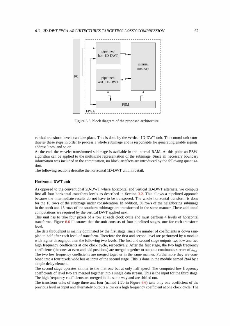
6.3. 2D-DWT FPGA ARCHITECTURES TARGETING LOSSY COMPRESSION 67
PC
FSM
pipelinedvert. 1D-DWT
pipelinedhor. 1D-DWT
internalmemory
FPGA
Figure 6.5: block diagram of the proposed architecture
vertical transform levels can take place. This is done by the vertical 1D-DWT unit. The control unit coor-dinates these steps in order to process a whole subimage and is responsible for generating enable signals,address lines, and so on.At the end, the wavelet transformed subimage is available in the internal RAM. At this point an EZW-algorithm can be applied to the multiscale representation of the subimage. Since all necessary boundaryinformation was included in the computation, no block artefacts are introduced by the following quantiza-tion.The following sections describe the horizontal 1D-DWT unit, in detail.
Horizontal DWT unit
As opposed to the conventional 2D-DWT where horizontal and vertical 1D-DWT alternate, we computefirst all four horizontal transform levels as described in Section3.2. This allows a pipelined approachbecause the intermediate results do not have to be transposed. The whole horizontal transform is donefor the 16 rows of the subimage under consideration. In addition, 30 rows of the neighboring subimagein the north and 15 rows of the southern subimage are transformed in the same manner. These additionalcomputations are required by the vertical DWT applied next.This unit has to take four pixels of a row at each clock cycle and must perform 4 levels of horizontaltransforms. Figure6.6 illustrates that the unit consists of four pipelined stages, one for each transformlevel.The data throughput is mainly dominated by the first stage, since the number of coefficients is down sam-pled to half after each level of transform. Therefore the first and second level are performed by a modulewith higher throughput than the following two levels. The first and second stage outputs two low and twohigh frequency coefficients at one clock cycle, respectively. After the first stage, the two high frequencycoefficients (the ones at even and odd positions) are merged together to output a continuous stream ofd0,j .The two low frequency coefficients are merged together in the same manner. Furthermore they are com-bined into a four pixels wide bus as input of the second stage. This is done in the module named2to4by asimple delay element.The second stage operates similar to the first one but at only half speed. The computed low frequencycoefficients of level two are merged together into a single data stream. This is the input for the third stage.The high frequency coefficients are merged in the same way and are shifted out.The transform units of stage three and four (named1i2o in Figure6.6) take only one coefficient of theprevious level as input and alternately outputs a low or a high frequency coefficient at one clock cycle. The
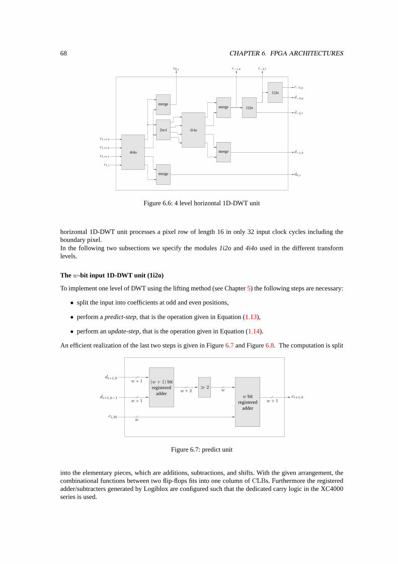
68 CHAPTER 6. FPGA ARCHITECTURES
4i4o
c1,i
c1,i+1
c1,i+2
c1,i+3
merge
2to4
merge
4i4o
merge
merge 1i2o
1i2o
d0,j
d−1,k
d−2,l
d−3,p
c−3,q
c0,j c−1,k c−2,l
Figure 6.6: 4 level horizontal 1D-DWT unit
horizontal 1D-DWT unit processes a pixel row of length 16 in only 32 input clock cycles including theboundary pixel.In the following two subsections we specify the modules1i2o and4i4o used in the different transformlevels.
Thew-bit input 1D-DWT unit (1i2o)
To implement one level of DWT using the lifting method (see Chapter5) the following steps are necessary:
• split the input into coefficients at odd and even positions,
• perform apredict-step, that is the operation given in Equation (1.13),
• perform anupdate-step, that is the operation given in Equation (1.14).
An efficient realization of the last two steps is given in Figure6.7and Figure6.8. The computation is split
w
w
w + 1w + 1
w + 1
w + 2
di+1,k
di+1,k−1
ci,2k
(w + 1) bitregistered
adderw bit
registeredadder
� 2
ci+1,k
Figure 6.7: predict unit
into the elementary pieces, which are additions, subtractions, and shifts. With the given arrangement, thecombinational functions between two flip-flops fits into one column ofCLBs. Furthermore the registeredadder/subtracters generated by Logiblox are configured such that the dedicated carry logic in the XC4000series is used.
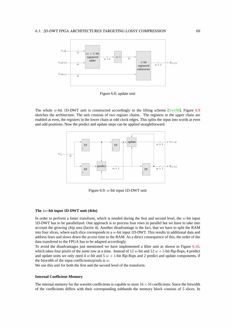
6.3. 2D-DWT FPGA ARCHITECTURES TARGETING LOSSY COMPRESSION 69
w
w
w
w
w + 1
w + 1
ci,2k
ci,2k+2
ci,2k+1
(w + 1) bitregistered
adderw bit
registeredsubstractor
� 1
di+1,k
Figure 6.8: update unit
The wholew-bit 1D-DWT unit is constructed accordingly to the lifting scheme [Swe96]. Figure 6.9sketches the architecture. The unit consists of two register chains. The registers in the upper chain areenabled at even, the registers in the lower chain at odd clock edges. This splits the input into words at evenand odd positions. Now the predict and update steps can be applied straightforward.
w
w + 1
w + 1
w + 1FF
FF FF
FFpredict
update
ci,j
di+1,k
ci+1,k
Figure 6.9:w-bit input 1D-DWT unit
The 4w-bit input 1D-DWT unit (4i4o)
In order to perform a faster transform, which is needed during the first and second level, thew-bit input1D-DWT has to be parallelized. One approach is to process four rows in parallel but we have to take intoaccount the growing chip area (factor 4). Another disadvantage is the fact, that we have to split the RAMinto four slices, where each slice corresponds to aw-bit input 1D-DWT. This results in additional data andaddress lines and slows down the access time to the RAM. As a direct consequence of this, the order of thedata transfered to the FPGA has to be adapted accordingly.To avoid the disadvantages just mentioned we have implemented a filter unit as shown in Figure6.10,which takes four pixels of thesamerow at a time. Instead of 12w-bit and 12w+1-bit flip-flops, 4 predictand update units we only need 4w-bit and 5w + 1-bit flip-flops and 2 predict and update components, ifthe bitwidth of the input coefficients/pixels isw.We use this unit for both the first and the second level of the transform.
Internal Coefficient Memory
The internal memory for the wavelet coefficients is capable to store16×16 coefficients. Since the bitwidthof the coefficients differs with their corresponding subbands the memory block consists of 5 slices. In
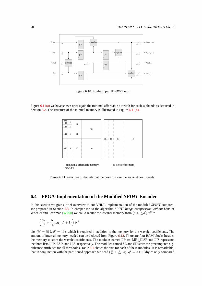
70 CHAPTER 6. FPGA ARCHITECTURES
ci,j
ci,j+1
ci,j+2
ci,j+3
di+1,l
ci+1,k
di+1,l+1
ci+1,k+1
w
w
w
w
w + 1
w + 1
w + 1
w + 1
w + 1
FF
FF
FF
FF
FFpredict
predict
update
update
Figure 6.10:4w-bit input 1D-DWT unit
Figure6.11(a)we have shown once again the minimal affordable bitwidth for each subbands as deduced inSection3.2. The structure of the internal memory is illustrated in Figure6.11(b).
10
11
11
10
11
11
10
11
11
10
11
11
10
10
10111111 11
(a) minimal affordable memorybitwidth
1111 11 11 10
(b) slices of memory
Figure 6.11: structure of the internal memory to store the wavelet coefficients
6.4 FPGA-Implementation of the ModifiedSPIHT Encoder
In this section we give a brief overview to our VHDL implementation of the modifiedSPIHTcompres-sor proposed in Section5.3. In comparison to the algorithmSPIHT Image compression without ListsofWheeler and Pearlman [WP00] we could reduce the internal memory from(4 + 5
16d′)N2 to(
3716
+516
log2(d′ + 1)
)N2
bits (N = 512, d′ = 11), which is required in addition to the memory for the wavelet coefficients. Theamount of internal memory needed can be deduced from Figure6.12. There are four RAM blocks besidesthe memory to store the wavelet coefficients. The modules namedLP := LIP
⋃LSP andLIS represents
the three listsLIP, LSP, andLIS, respectively. The modules namedSL andSD store the precomputed sig-nificance attributes for all thresholds. Table6.1shows the size for each of these modules. It is remarkable,that in conjunction with the partitioned approach we need( 37
16 + 516 · 4) · q2 = 0.111 kbytes only compared
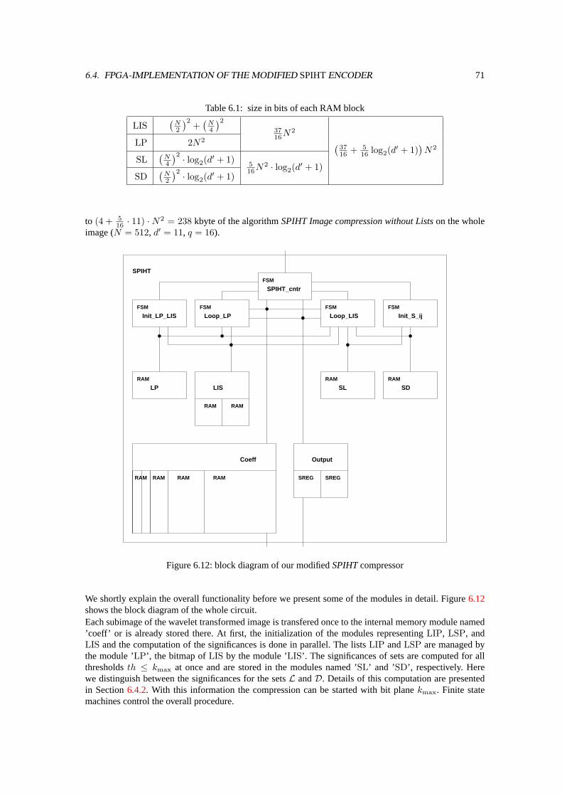
6.4. FPGA-IMPLEMENTATION OF THE MODIFIED SPIHTENCODER 71
Table 6.1: size in bits of each RAM block
LIS(
N2
)2+(
N4
)2LP 2N2
3716N
2
SL(
N4
)2 · log2(d′ + 1)
(3716 + 5
16 log2(d′ + 1))N2
SD(
N2
)2 · log2(d′ + 1)516N
2 · log2(d′ + 1)
to (4 + 516 · 11) ·N2 = 238 kbyte of the algorithmSPIHT Image compression without Listson the whole
image (N = 512, d′ = 11, q = 16).
Loop_LPFSM
Loop_LISFSM
RAM
LPRAM
SDRAM
SL
SPIHT_cntrFSM
FSM
SPIHT
LIS
RAMRAM
OutputCoeff
RAMRAMRAMRAM SREG SREG
Init_LP_LISFSM
Init_S_ij
Figure 6.12: block diagram of our modifiedSPIHTcompressor
We shortly explain the overall functionality before we present some of the modules in detail. Figure6.12shows the block diagram of the whole circuit.Each subimage of the wavelet transformed image is transfered once to the internal memory module named’coeff’ or is already stored there. At first, the initialization of the modules representingLIP, LSP, andLIS and the computation of the significances is done in parallel. The listsLIP andLSP are managed bythe module ’LP’, the bitmap ofLIS by the module ’LIS’. The significances of sets are computed for allthresholdsth ≤ kmax at once and are stored in the modules named ’SL’ and ’SD’, respectively. Herewe distinguish between the significances for the setsL andD. Details of this computation are presentedin Section6.4.2. With this information the compression can be started with bit planekmax. Finite statemachines control the overall procedure.
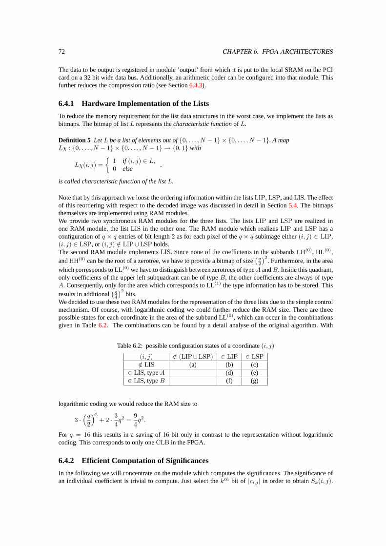
72 CHAPTER 6. FPGA ARCHITECTURES
The data to be output is registered in module ’output’ from which it is put to the local SRAM on the PCIcard on a 32 bit wide data bus. Additionally, an arithmetic coder can be configured into that module. Thisfurther reduces the compression ratio (see Section6.4.3).
6.4.1 Hardware Implementation of the Lists
To reduce the memory requirement for the list data structures in the worst case, we implement the lists asbitmaps. The bitmap of listL represents thecharacteristic functionof L.
Definition 5 LetL be a list of elements out of{0, . . . , N − 1} × {0, . . . , N − 1}. A mapLχ : {0, . . . , N − 1} × {0, . . . , N − 1} → {0, 1} with
Lχ(i, j) ={
1 if (i, j) ∈ L,0 else
.
is called characteristic function of the listL.
Note that by this approach we loose the ordering information within the listsLIP, LSP, andLIS. The effectof this reordering with respect to the decoded image was discussed in detail in Section5.4. The bitmapsthemselves are implemented using RAM modules.We provide two synchronous RAM modules for the three lists. The listsLIP andLSP are realized inone RAM module, the listLIS in the other one. The RAM module which realizesLIP andLSP has aconfiguration ofq × q entries of bit length2 as for each pixel of theq × q subimage either(i, j) ∈ LIP,(i, j) ∈ LSP, or (i, j) /∈ LIP∪LSP holds.The second RAM module implementsLIS. Since none of the coefficients in the subbands LH(0), HL(0),and HH(0) can be the root of a zerotree, we have to provide a bitmap of size
(q2
)2. Furthermore, in the area
which corresponds to LL(0) we have to distinguish between zerotrees of typeA andB. Inside this quadrant,only coefficients of the upper left subquadrant can be of typeB, the other coefficients are always of typeA. Consequently, only for the area which corresponds to LL(1) the type information has to be stored. Thisresults in additional
(q4
)2bits.
We decided to use these two RAM modules for the representation of the three lists due to the simple controlmechanism. Of course, with logarithmic coding we could further reduce the RAM size. There are threepossible states for each coordinate in the area of the subband LL(0), which can occur in the combinationsgiven in Table6.2. The combinations can be found by a detail analyse of the original algorithm. With
Table 6.2: possible configuration states of a coordinate(i, j)
(i, j) /∈ (LIP∪LSP) ∈ LIP ∈ LSP/∈ LIS (a) (b) (c)
∈ LIS, typeA (d) (e)∈ LIS, typeB (f) (g)
logarithmic coding we would reduce the RAM size to
3 ·(q
2
)2
+ 2 · 34q2 =
94q2.
For q = 16 this results in a saving of16 bit only in contrast to the representation without logarithmiccoding. This corresponds to only oneCLB in the FPGA.
6.4.2 Efficient Computation of Significances
In the following we will concentrate on the module which computes the significances. The significance ofan individual coefficient is trivial to compute. Just select thekth bit of |ci,j | in order to obtainSk(i, j).
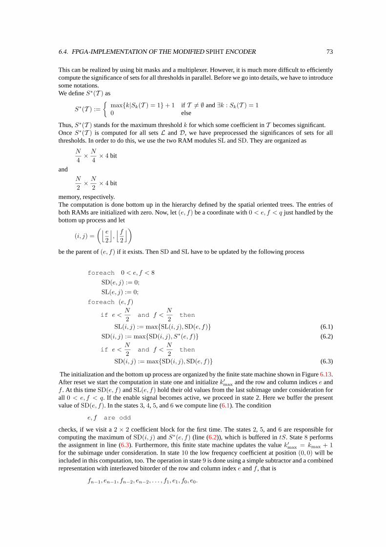
6.4. FPGA-IMPLEMENTATION OF THE MODIFIED SPIHTENCODER 73
This can be realized by using bit masks and a multiplexer. However, it is much more difficult to efficientlycompute the significance of sets for all thresholds in parallel. Before we go into details, we have to introducesome notations.We defineS∗(T ) as
S∗(T ) :={
max{k|Sk(T ) = 1}+ 1 if T 6= ∅ and∃k : Sk(T ) = 10 else
Thus,S∗(T ) stands for the maximum thresholdk for which some coefficient inT becomes significant.OnceS∗(T ) is computed for all setsL andD, we have preprocessed the significances of sets for allthresholds. In order to do this, we use the two RAM modulesSL andSD. They are organized as
N
4× N
4× 4 bit
and
N
2× N
2× 4 bit
memory, respectively.The computation is done bottom up in the hierarchy defined by the spatial oriented trees. The entries ofboth RAMs are initialized with zero. Now, let(e, f) be a coordinate with0 < e, f < q just handled by thebottom up process and let
(i, j) =(⌊e
2
⌋,⌊f
2
⌋)be the parent of(e, f) if it exists. ThenSD andSL have to be updated by the following process
foreach 0 < e, f < 8SD(e, j) := 0;SL(e, j) := 0;
foreach (e, f)
if e <N
2and f <
N
2then
SL(i, j) := max{SL(i, j),SD(e, f)} (6.1)
SD(i, j) := max{SD(i, j), S∗(e, f)} (6.2)
if e <N
2and f <
N
2then
SD(i, j) := max{SD(i, j),SD(e, f)} (6.3)
The initialization and the bottom up process are organized by the finite state machine shown in Figure6.13.After reset we start the computation in state one and initializek′max and the row and column indicese andf . At this timeSD(e, f) andSL(e, f) hold their old values from the last subimage under consideration forall 0 < e, f < q. If the enable signal becomes active, we proceed in state 2. Here we buffer the presentvalue ofSD(e, f). In the states3, 4, 5, and6 we compute line (6.1). The condition
e, f are odd
checks, if we visit a2 × 2 coefficient block for the first time. The states2, 5, and6 are responsible forcomputing the maximum ofSD(i, j) andS∗(e, f) (line (6.2)), which is buffered intS. State8 performsthe assignment in line (6.3). Furthermore, this finite state machine updates the valuek′max = kmax + 1for the subimage under consideration. In state10 the low frequency coefficient at position(0, 0) will beincluded in this computation, too. The operation in state9 is done using a simple subtractor and a combinedrepresentation with interleaved bitorder of the row and column indexe andf , that is
fn−1, en−1, fn−2, en−2, . . . , f1, e1, f0, e0.
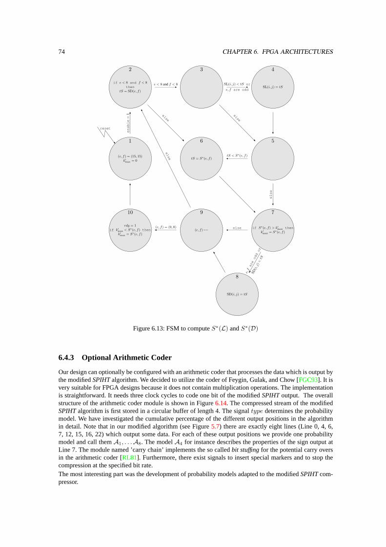
74 CHAPTER 6. FPGA ARCHITECTURES
1
(e, f) = (15, 15)k′max = 0
2
if e < 8 and f < 8then
tS = SD(e, f)
3 4
SL(i, j) = tS
56
tS = S∗(e, f)
7
if S∗(e, f) > k′max thenk′max = S∗(e, f)
8
SD(i, j) = tS
9
(e, f)−−
10
rdy = 1if k′max < S∗(e, f) then
k′max = S∗(e, f)
resete
na
ble
=1 else
tS < S∗(e, f)
else
SD(i, j
) <tS
e,f
are
odd
or
else
else(e, f) = (0, 0)
els
e
e < 8 andf < 8 SL(i, j) < tS or
e, f are odd
Figure 6.13: FSM to computeS∗(L) andS∗(D)
6.4.3 Optional Arithmetic Coder
Our design can optionally be configured with an arithmetic coder that processes the data which is output bythe modifiedSPIHTalgorithm. We decided to utilize the coder of Feygin, Gulak, and Chow [FGC93]. It isvery suitable for FPGA designs because it does not contain multiplication operations. The implementationis straightforward. It needs three clock cycles to code one bit of the modifiedSPIHToutput. The overallstructure of the arithmetic coder module is shown in Figure6.14. The compressed stream of the modifiedSPIHTalgorithm is first stored in a circular buffer of length 4. The signaltype determines the probabilitymodel. We have investigated the cumulative percentage of the different output positions in the algorithmin detail. Note that in our modified algorithm (see Figure5.7) there are exactly eight lines (Line 0, 4, 6,7, 12, 15, 16, 22) which output some data. For each of these output positions we provide one probabilitymodel and call themA1, . . .A8. The modelA4 for instance describes the properties of the sign output atLine 7. The module named ’carry chain’ implements the so calledbit stuffingfor the potential carry oversin the arithmetic coder [RL81]. Furthermore, there exist signals to insert special markers and to stop thecompression at the specified bit rate.The most interesting part was the development of probability models adapted to the modifiedSPIHTcom-pressor.
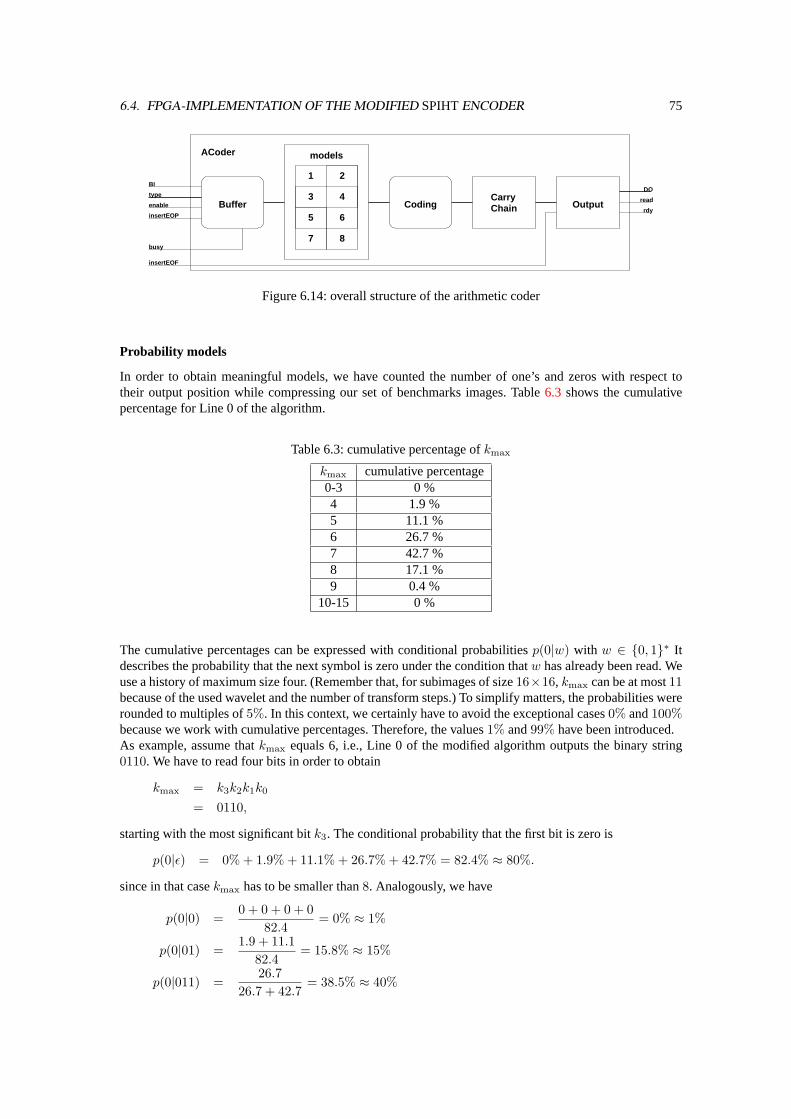
6.4. FPGA-IMPLEMENTATION OF THE MODIFIED SPIHTENCODER 75
models
1
3
5
7 8
6
4
2DO
read
rdy
BI
type
enable
insertEOP
ACoder
busy
Buffer CodingCarryChain Output
insertEOF
Figure 6.14: overall structure of the arithmetic coder
Probability models
In order to obtain meaningful models, we have counted the number of one’s and zeros with respect totheir output position while compressing our set of benchmarks images. Table6.3 shows the cumulativepercentage for Line 0 of the algorithm.
Table 6.3: cumulative percentage ofkmax
kmax cumulative percentage0-3 0 %4 1.9 %5 11.1 %6 26.7 %7 42.7 %8 17.1 %9 0.4 %
10-15 0 %
The cumulative percentages can be expressed with conditional probabilitiesp(0|w) with w ∈ {0, 1}∗ Itdescribes the probability that the next symbol is zero under the condition thatw has already been read. Weuse a history of maximum size four. (Remember that, for subimages of size16×16, kmax can be at most11because of the used wavelet and the number of transform steps.) To simplify matters, the probabilities wererounded to multiples of5%. In this context, we certainly have to avoid the exceptional cases0% and100%because we work with cumulative percentages. Therefore, the values1% and99% have been introduced.As example, assume thatkmax equals 6, i.e., Line 0 of the modified algorithm outputs the binary string0110. We have to read four bits in order to obtain
kmax = k3k2k1k0
= 0110,
starting with the most significant bitk3. The conditional probability that the first bit is zero is
p(0|ε) = 0% + 1.9% + 11.1% + 26.7% + 42.7% = 82.4% ≈ 80%.
since in that casekmax has to be smaller than8. Analogously, we have
p(0|0) =0 + 0 + 0 + 0
82.4= 0% ≈ 1%
p(0|01) =1.9 + 11.1
82.4= 15.8% ≈ 15%
p(0|011) =26.7
26.7 + 42.7= 38.5% ≈ 40%
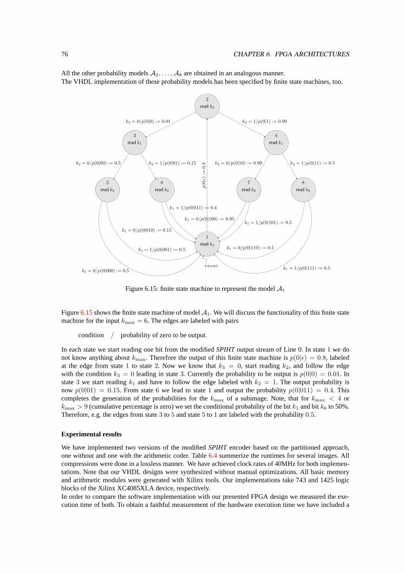
76 CHAPTER 6. FPGA ARCHITECTURES
All the other probability modelsA2, . . . ,A8 are obtained in an analogous manner.The VHDL implementation of these probability models has been specified by finite state machines, too.
readk2
readk1 readk1
readk0 readk0 readk0 readk0
readk3
2
3 4
5 6 7 8
1
k3 = 0/p(0|0) := 0.01 k3 = 1/p(0|1) := 0.99
k2 = 0/p(0|00) := 0.5 k2 = 1/p(0|01) := 0.15 k2 = 0/p(0|10) := 0.99 k2 = 1/p(0|11) := 0.5
p(0|ε
):=
0.8
k1 = 0/p(0|000) := 0.5
k1 = 1/p(0|001) := 0.5
k1 = 0/p(0|010) := 0.15
k1 = 1/p(0|011) := 0.4
k1 = 0/p(0|100) := 0.95k1 = 1/p(0|101) := 0.5
k1 = 0/p(0|110) := 0.5
k1 = 1/p(0|111) := 0.5reset
Figure 6.15: finite state machine to represent the modelA1
Figure6.15shows the finite state machine of modelA1. We will discuss the functionality of this finite statemachine for the inputkmax = 6. The edges are labeled with pairs
condition / probability of zero to be output.
In each state we start reading one bit from the modifiedSPIHToutput stream of Line 0. In state1 we donot know anything aboutkmax. Therefore the output of this finite state machine isp(0|ε) = 0.8, labeledat the edge from state1 to state2. Now we know thatk3 = 0, start readingk2, and follow the edgewith the conditionk3 = 0 leading in state3. Currently the probability to be output isp(0|0) = 0.01. Instate3 we start readingk1 and have to follow the edge labeled withk2 = 1. The output probability isnow p(0|01) = 0.15. From state6 we lead to state1 and output the probabilityp(0|011) = 0.4. Thiscompletes the generation of the probabilities for thekmax of a subimage. Note, that forkmax < 4 orkmax > 9 (cumulative percentage is zero) we set the conditional probability of the bitk1 and bitk0 to 50%.Therefore, e.g. the edges from state3 to 5 and state5 to 1 are labeled with the probability0.5.
Experimental results
We have implemented two versions of the modifiedSPIHTencoder based on the partitioned approach,one without and one with the arithmetic coder. Table6.4 summerize the runtimes for several images. Allcompressions were done in a lossless manner. We have achieved clock rates of 40MHz for both implemen-tations. Note that our VHDL designs were synthesized without manual optimizations. All basic memoryand arithmetic modules were generated with Xilinx tools. Our implementations take 743 and 1425 logicblocks of the Xilinx XC4085XLA device, respectively.In order to compare the software implementation with our presented FPGA design we measured the exe-cution time of both. To obtain a faithful measurement of the hardware execution time we have included a

6.4. FPGA-IMPLEMENTATION OF THE MODIFIED SPIHTENCODER 77
Table 6.4: execution times of hard- and software implementations in the case of lossless com-pression, 8 bit grey-scale images of sizeN = 512, partition sizeq = 16
image ubk-software FPGAarithm. coder
without withbaboon 2.3 s 204.0 ms 272.3 msbarbara 2.0 s 203.1 ms 254.0 msgoldhill 2.0 s 195.8 ms 246.9 ms
lena 1.9 s 192.5 ms 236.4 mspeppers 1.9 s 196.7 ms 245.0 ms
counter (resolution 25ns) into the design. We could improve the compression time of512 × 512 × 8 bitgreyscale images by a factor of 10 in comparison to an AMD 1GHz Athlon processor.The effect of the arithmetic coder upon the compression ratio is shown in Table6.5. The coder compressestheSPIHToutput by further 2 to 4 percent. It is remarkable, that the compression ratio is always improved,in the lossless as well as in the lossy case.
Table 6.5: influence of the arithmetic coder
image baboon barbara goldhill lena peppers0.5 bpp 95.9 98.6 97.4 97.3 95.7lossless 97.8 97.3 96.8 96.0 96.1

78 CHAPTER 6. FPGA ARCHITECTURES
Chapter 7
Conclusions and Related Work
In this thesis we have presented a partitioned approach to wavelet based image compression and its applica-tion to image encoders using programmable hardware. We have developed an efficient FPGA architectureof the state of the art image codecSPIHT, which is comparable to the original software solution in termsof visual quality. We have achieved clock rates of 40MHz for our FPGA implementations. Note that ourVHDL designs were synthesized without manual optimizations. All basic memory and arithmetic moduleswere generated with Xilinx tools. We could improve the compression time of512× 512× 8 bit greyscaleimages by a factor of 10 in comparison to an AMD 1GHz Athlon processor. The optional arithmetic codercompresses the modifiedSPIHToutput by further 2 to 4 percent. It is remarkable, that the compressionratio is always improved, in the lossless as well as in the lossy case.The main contribution is that we have proposed image encoder suitable for low cost programmable hard-ware devices with minimal internal memory requirements. This method outperform the recently publishedalgorithm of Wheeler and PearlmanSPIHT Image Compression without Lists[WP00] with respect to theaffordable memory.
In the following we will introduced the upcoming new JPEG2000 standard, which is also wavelet based,but is not premised on an embedded zerotree wavelet encoder. Afterwards, we will balance the advantagesand disadvantages of our approach to the proposed method in the JPEG2000 standard.It will become apparent, that there are some marked similarities to our partitioned approach. We emphasizethat both developments were done independently of each other. Note, that until now to our knowledgeno JPEG2000 encoder ASIC (application specific integrated circuit) is available. First intelligent propertycores for JPEG2000 codecs are offered by Amphion Semiconductor Ltd. and inSilicon Corporation in 2002[Amp02], [ inS02].
7.1 EBCOT and JPEG2000
An algorithm namedEBCOT, EmbeddedBlock Coding with Optimal Truncation presented by DavidTaubman [Tau00] was chosen as the central codec behind the new JPEG2000 Standard [TM02]. Mostly allof the desired features of the new still image compression standard are supported by theEBCOTalgorithm.The most import ones are
• excellent visual quality of the reconstructed images even at lowest bit rates
• SNR scalability
• resolution scalability
• region of interest coding
• error resilience (noisy channels).
79
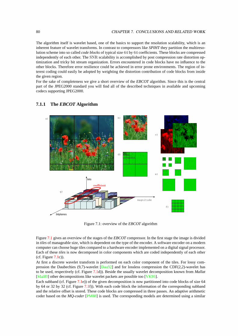
80 CHAPTER 7. CONCLUSIONS AND RELATED WORK
The algorithm itself is wavelet based, one of the basics to support the resolution scalability, which is aninherent feature of wavelet transforms. In contrast to compressors likeSPIHTthey partition the multireso-lution scheme into so calledcode blocksof typical size64 by 64 coefficients. These blocks are compressedindependently of each other. TheSNR scalability is accomplished by post compression rate distortion op-timization and tricky bit stream organization. Errors encountered in code blocks have no influence to theother blocks. Therefore error resilience could be achieved in error prone environments. The region of in-terest coding could easily be adopted by weighting the distortion contribution of code blocks from insidethe given region.For the sake of completeness we give a short overview of theEBCOTalgorithm. Since this is the centralpart of the JPEG2000 standard you will find all of the described techniques in available and upcomingcodecs supporting JPEG2000.
7.1.1 TheEBCOT Algorithm
bitplanes
bits
coefficient
a) b)
c)
d)
e)
f)
g)
magnitude
Figure 7.1: overview of theEBCOTalgorithm
Figure7.1gives an overview of the stages of theEBCOTcompressor. In the first stage the image is dividedin tilesof manageable size, which is dependent on the type of the encoder. A software encoder on a moderncomputer can choose huge tiles compared to a hardware encoder implemented on a digital signal processor.Each of thesetiles is now decomposed in color components which are coded independently of each other(cf. Figure7.1c)).At first a discrete wavelet transform is performed on each color component of the tiles. For lossy com-pression the Daubechies (9,7)-wavelet [Dau92] and for lossless compression the CDF(2,2)-wavelet hasto be used, respectively (cf. Figure7.1d)). Beside the usually wavelet decomposition known fromMallat[Mal89] other decompositions like wavelet packets are possible too [VK95].Each subband (cf. Figure7.1e)) of the given decomposition is now partitioned into code blocks of size 64by 64 or 32 by 32 (cf. Figure7.1f)). With each code block the information of the corresponding subbandand the relative offset is stored. These code blocks are compressed in three passes. An adaptive arithmeticcoder based on theMQ-coder[PM88] is used. The corresponding models are determined using a similar
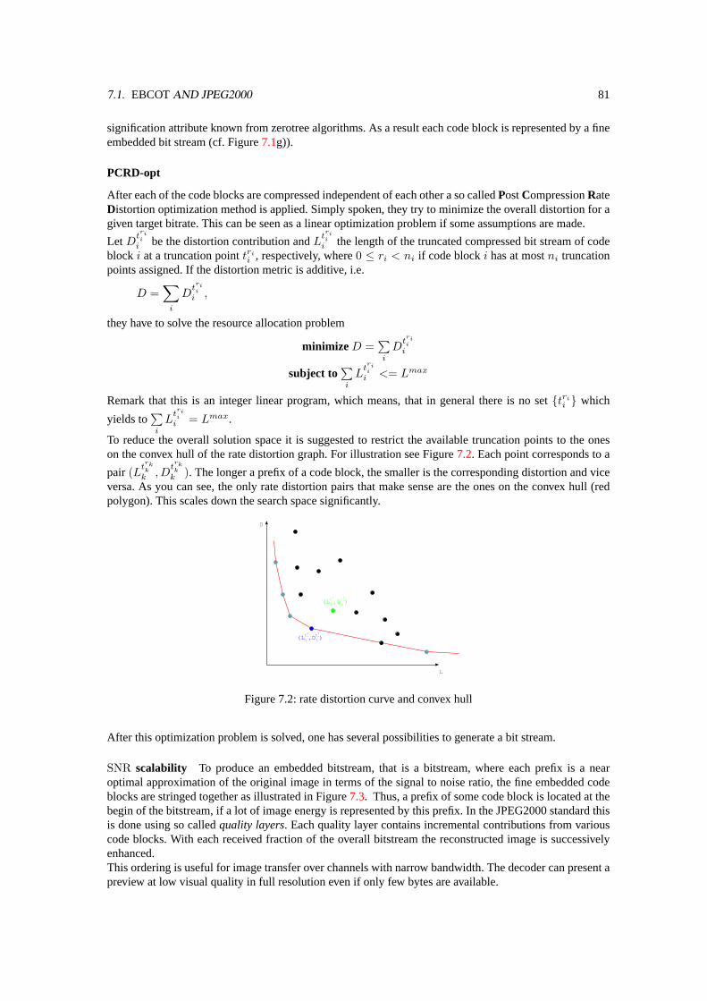
7.1. EBCOTAND JPEG2000 81
signification attribute known from zerotree algorithms. As a result each code block is represented by a fineembedded bit stream (cf. Figure7.1g)).
PCRD-opt
After each of the code blocks are compressed independent of each other a so calledPostCompressionRateDistortion optimization method is applied. Simply spoken, they try to minimize the overall distortion for agiven target bitrate. This can be seen as a linear optimization problem if some assumptions are made.
LetDtrii
i be the distortion contribution andLtrii
i the length of the truncated compressed bit stream of codeblock i at a truncation pointtri
i , respectively, where0 ≤ ri < ni if code blocki has at mostni truncationpoints assigned. If the distortion metric is additive, i.e.
D =∑
i
Dtrii
i ,
they have to solve the resource allocation problem
minimize D =∑i
Dtrii
i
subject to∑i
Ltrii
i <= Lmax
Remark that this is an integer linear program, which means, that in general there is no set{trii } which
yields to∑i
Ltrii
i = Lmax.
To reduce the overall solution space it is suggested to restrict the available truncation points to the oneson the convex hull of the rate distortion graph. For illustration see Figure7.2. Each point corresponds to a
pair (Ltrkk
k , Dtrkk
k ). The longer a prefix of a code block, the smaller is the corresponding distortion and viceversa. As you can see, the only rate distortion pairs that make sense are the ones on the convex hull (redpolygon). This scales down the search space significantly.
L
D
(Lt2i
i ,Dt2i
i )
(Lt8i
i ,Dt8i
i )
Figure 7.2: rate distortion curve and convex hull
After this optimization problem is solved, one has several possibilities to generate a bit stream.
SNR scalability To produce an embedded bitstream, that is a bitstream, where each prefix is a nearoptimal approximation of the original image in terms of the signal to noise ratio, the fine embedded codeblocks are stringed together as illustrated in Figure7.3. Thus, a prefix of some code block is located at thebegin of the bitstream, if a lot of image energy is represented by this prefix. In the JPEG2000 standard thisis done using so calledquality layers. Each quality layer contains incremental contributions from variouscode blocks. With each received fraction of the overall bitstream the reconstructed image is successivelyenhanced.This ordering is useful for image transfer over channels with narrow bandwidth. The decoder can present apreview at low visual quality in full resolution even if only few bytes are available.
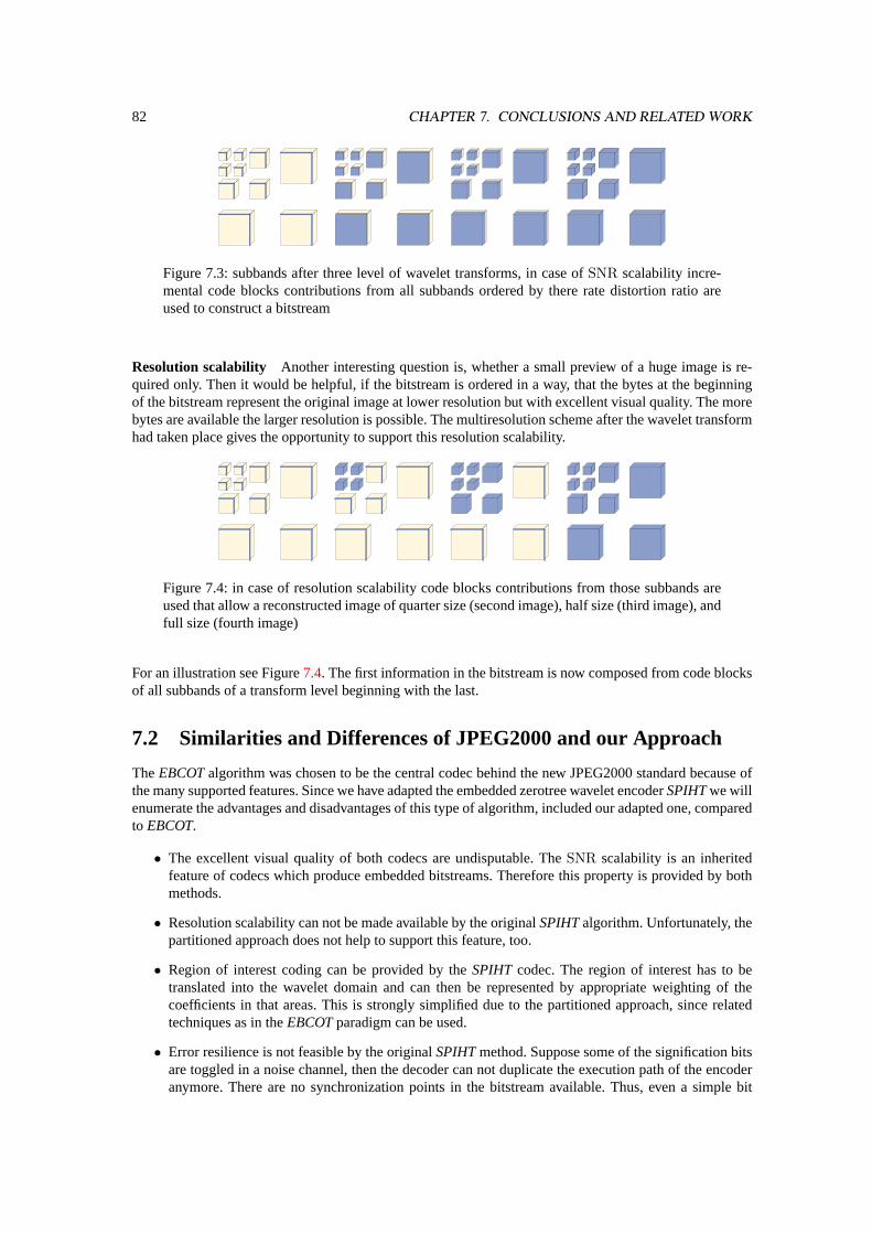
82 CHAPTER 7. CONCLUSIONS AND RELATED WORK
Figure 7.3: subbands after three level of wavelet transforms, in case ofSNR scalability incre-mental code blocks contributions from all subbands ordered by there rate distortion ratio areused to construct a bitstream
Resolution scalability Another interesting question is, whether a small preview of a huge image is re-quired only. Then it would be helpful, if the bitstream is ordered in a way, that the bytes at the beginningof the bitstream represent the original image at lower resolution but with excellent visual quality. The morebytes are available the larger resolution is possible. The multiresolution scheme after the wavelet transformhad taken place gives the opportunity to support this resolution scalability.
Figure 7.4: in case of resolution scalability code blocks contributions from those subbands areused that allow a reconstructed image of quarter size (second image), half size (third image), andfull size (fourth image)
For an illustration see Figure7.4. The first information in the bitstream is now composed from code blocksof all subbands of a transform level beginning with the last.
7.2 Similarities and Differences of JPEG2000 and our Approach
TheEBCOTalgorithm was chosen to be the central codec behind the new JPEG2000 standard because ofthe many supported features. Since we have adapted the embedded zerotree wavelet encoderSPIHTwe willenumerate the advantages and disadvantages of this type of algorithm, included our adapted one, comparedto EBCOT.
• The excellent visual quality of both codecs are undisputable. TheSNR scalability is an inheritedfeature of codecs which produce embedded bitstreams. Therefore this property is provided by bothmethods.
• Resolution scalability can not be made available by the originalSPIHTalgorithm. Unfortunately, thepartitioned approach does not help to support this feature, too.
• Region of interest coding can be provided by theSPIHT codec. The region of interest has to betranslated into the wavelet domain and can then be represented by appropriate weighting of thecoefficients in that areas. This is strongly simplified due to the partitioned approach, since relatedtechniques as in theEBCOTparadigm can be used.
• Error resilience is not feasible by the originalSPIHTmethod. Suppose some of the signification bitsare toggled in a noise channel, then the decoder can not duplicate the execution path of the encoderanymore. There are no synchronization points in the bitstream available. Thus, even a simple bit

7.2. SIMILARITIES AND DIFFERENCES OF JPEG2000 AND OUR APPROACH 83
fault can distort the whole decompression procedure. In the case, that bit faults are introduced in abitstream generated using the modifiedSPIHTencoder based on the partitioned approach, the impactof such an incident is limited to the corresponding subimage. This is similar to the error handling oftheEBCOTalgorithm.
• A feature, that is not provided by theEBCOTcompressor, is taking advantage of the self similari-ties between the different subbands in each orientation. The partitioning into code blocks offers theopportunity of parallel processing and efficient hardware architectures. Our partitioned approach iscapable to take advantage of the mentioned self similarities as well as the preferences of the localprocessing of each subimage.
• Besides the excellent techniques to compress the individual code blocks the post compression ratedistortion optimization is the key to obtain good performance. The price to pay is the computationalcomplexity in order to implement this optimization. The currently available JPEG2000 codecs suffersespecially from the tremendous computation times [Ada01], [Tau02]. However, the post compressionrate distortion optimization can be combined with the partitioned approach in order to improve thecompression efficiency.

84 CHAPTER 7. CONCLUSIONS AND RELATED WORK
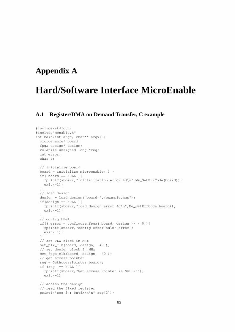
Appendix A
Hard/Software Interface MicroEnable
A.1 Register/DMA on Demand Transfer, C example
#include<stdio.h>#include"menable.h"int main(int argc, char** argv) {
microenable* board;fpga_design* design;volatile unsigned long *reg;int error;char c;
// initialize boardboard = initialize_microenable( ) ;if( board == NULL ){
fprintf(stderr,"initialization error %d\n",Me_GetErrCode(board));exit(-1);
}// load designdesign = load_design( board,"./example.hap");if(design == NULL ){
fprintf(stderr,"load design error %d\n",Me_GetErrCode(board));exit(-1);
}// config FPGAif(( error = configure_fpga( board, design )) < 0 ){
fprintf(stderr,"config error %d\n",error);exit(-1);
}// set PLX clock in MHzset_plx_clk(board, design, 40 );// set design clock in MHzset_fpga_clk(board, design, 40 );// get access pointerreg = GetAccessPointer(board);if (reg == NULL ){
fprintf(stderr,"Get access Pointer is NULL\n");exit(-1);
}// access the design// read the fixed registerprintf("Reg 3 : 0x%8X\n\n",reg[3]);
85
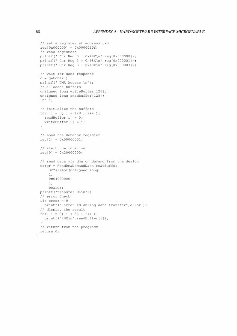
86 APPENDIX A. HARD/SOFTWARE INTERFACE MICROENABLE
// set a register at address 0x0reg[0x000000] = 0x00000f0f;// read registersprintf(" Ctr Reg 0 : 0x%8X\n",reg[0x000000]);printf(" Ctr Reg 1 : 0x%8X\n",reg[0x000001]);printf(" Ctr Reg 3 : 0x%8X\n",reg[0x000003]);
// wait for user responsec = getchar() ;printf(" DMA Access \n");// allocate buffersunsigned long writeBuffer[128];unsigned long readBuffer[128];int i;
// initialize the buffersfor( i = 0; i < 128 ; i++ ){
readBuffer[i] = 0;writeBuffer[i] = i;
}
// Load the Rotator registerreg[1] = 0x00000001;
// start the rotationreg[0] = 0x20000000;
// read data via dma on demand from the designerror = ReadDmaDemandData(readBuffer,
32*sizeof(unsigned long),1,0x04000000,1,board);
printf("transfer OK\n");// error Checkif( error < 0 )
printf(" error %d during data transfer",error );// display the resultfor( i = 0; i < 32 ; i++ ){
printf("%8X\n",readBuffer[i]);}// return from the programmreturn 0;
}
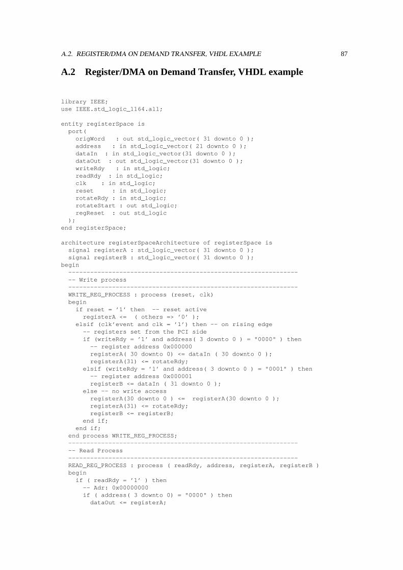
A.2. REGISTER/DMA ON DEMAND TRANSFER, VHDL EXAMPLE 87
A.2 Register/DMA on Demand Transfer, VHDL example
library IEEE;use IEEE.std_logic_1164.all;
entity registerSpace isport(
origWord : out std_logic_vector( 31 downto 0 );address : in std_logic_vector( 21 downto 0 );dataIn : in std_logic_vector(31 downto 0 );dataOut : out std_logic_vector(31 downto 0 );writeRdy : in std_logic;readRdy : in std_logic;clk : in std_logic;reset : in std_logic;rotateRdy : in std_logic;rotateStart : out std_logic;regReset : out std_logic
);end registerSpace;
architecture registerSpaceArchitecture of registerSpace issignal registerA : std_logic_vector( 31 downto 0 );signal registerB : std_logic_vector( 31 downto 0 );
begin----------------------------------------------------------------- Write process---------------------------------------------------------------WRITE_REG_PROCESS : process (reset, clk)begin
if reset = ’1’ then -- reset activeregisterA <= ( others => ’0’ );
elsif (clk’event and clk = ’1’) then -- on rising edge-- registers set from the PCI sideif (writeRdy = ’1’ and address( 3 downto 0 ) = "0000" ) then
-- register address 0x000000registerA( 30 downto 0) <= dataIn ( 30 downto 0 );registerA(31) <= rotateRdy;
elsif (writeRdy = ’1’ and address( 3 downto 0 ) = "0001" ) then-- register address 0x000001registerB <= dataIn ( 31 downto 0 );
else -- no write accessregisterA(30 downto 0 ) <= registerA(30 downto 0 );registerA(31) <= rotateRdy;registerB <= registerB;
end if;end if;
end process WRITE_REG_PROCESS;----------------------------------------------------------------- Read Process---------------------------------------------------------------READ_REG_PROCESS : process ( readRdy, address, registerA, registerB )begin
if ( readRdy = ’1’ ) then-- Adr: 0x00000000if ( address( 3 downto 0) = "0000" ) then
dataOut <= registerA;
88 APPENDIX A. HARD/SOFTWARE INTERFACE MICROENABLE
-- Adr: 0x00000001elsif ( address( 3 downto 0) = "0001" ) then
dataOut <= registerB;-- Adr: 0x00000003elsif ( address( 3 downto 0) = "0011" ) then
dataOut( 15 downto 0 ) <= "1010101000010010";dataOut( 31 downto 16 ) <= "0001001000110100";
elsedataOut <= (others=>’0’);
end if;else
dataOut <= (others=>’0’);end if;
end process READ_REG_PROCESS;
------------------------------------------------------------------ Set the registers to the output----------------------------------------------------------------regReset <= registerA(30);origWord <= registerB;rotateStart <= registerA(29);
end registerSpaceArchitecture;
A.2. REGISTER/DMA ON DEMAND TRANSFER, VHDL EXAMPLE 89
library IEEE;use IEEE.std_logic_1164.all;use IEEE.std_logic_unsigned.all;
entity rotator isport (
wordIn : in STD_LOGIC_VECTOR (31 downto 0);wordOut : out STD_LOGIC_VECTOR (31 downto 0);rotateEnable : in std_logic;rotateStart : in std_logic;rotateRdy : out std_logic;rotateAlmostRdy : out std_logic;clk : in std_logic;reset : in STD_LOGIC
);end rotator;
architecture rotatorBehave of rotator istype fsmStateType is ( idle, rotate );signal fsmState : fsmStateType;
beginFSM_PROCESS : process( clk, fsmState, rotateStart, reset, wordIn )
variable countValue : integer;variable tmpValue : std_logic_vector( 31 downto 0 );variable tmpBit : std_logic;
beginif reset = ’1’ then
countValue := 0;fsmState <= idle;wordOut <= wordIn;rotateAlmostRdy <= ’0’;
elsif clk’event and clk = ’1’ then-- default assignmentrotateAlmostRdy <= ’0’;
case fsmState iswhen idle => -- wait for the start signal
if rotateStart = ’1’ thentmpValue := wordIn;countValue := 0;fsmState <= rotate;wordOut <= tmpValue;
end if;rotateRdy <= ’0’;
when rotate => -- rotate until the 32 roundif countValue <= 30 then-- rotate another bit
if rotateEnable = ’1’ thentmpBit := tmpValue(31);tmpValue(31 downto 1) := tmpValue(30 downto 0);tmpValue(0) := tmpBit;wordOut <= tmpValue;countValue := countValue + 1;rotateRdy <= ’0’;
end if;-- generate the rotateAlmostRdy signalif( countValue = 31 ) then

90 APPENDIX A. HARD/SOFTWARE INTERFACE MICROENABLE
rotateAlmostRdy <= ’1’;end if;
else-- finish the rotationrotateRdy <= ’1’;if rotateStart = ’1’ then
fsmState <= idle;end if;
end if;end case;
end if;end process;
end rotatorBehave;
A.3. MATLAB/METAPOST-SCRIPTS 91
A.3 Matlab/METAPOST-Scripts
%% Matlab code to draw the limit functions ψ and ψ%
impulse=[1];
g0=sqrt(2)*[-1/8,1/4,3/4,1/4,-1/8];h0=1/sqrt(2)*[0,0,-1/2,1,-1/2];dwtsig=impulse;
for level=1:7dwtsig=sqrt(2)*conv(dwtsig,g0);g0=upsample(g0);h0=upsample(h0);
end
dwtsig2=sqrt(2)*conv(dwtsig,h0);dwtsig=sqrt(2)*conv(dwtsig,g0);
x=[-2:4/(length(dwtsig)-1):2];length(x)y=[-2:4/(length(dwtsig2)-1):2];length(y)plot(x,dwtsig,y,dwtsig2); grid
%% Matlab code to compute the ranges of wavelet coefficients%
l=[-1/8,1/4,3/4,1/4,-1/8];h=[-1/2,1,-1/2];
echo on;cdfRange(6,l,h,127,-128);cdfRange(1,l,h,255,-255);cdfRange(2,l,h,319,-319);cdfRange(3,l,h,351,-351);cdfRange(4,l,h,358,-358);cdfRange(4,l,h,216,-217);
92 APPENDIX A. HARD/SOFTWARE INTERFACE MICROENABLE
%% Matlab code -- utility functions%
function cdfRange(level,l,h,max,min);maxl=max;maxh=max;minl=min;minh=min;
lup=l;hup=h;
for i=1:level[maxl,minl]=maxmin(l,max,min)[maxh,minh]=maxmin(h,max,min)lup=upsample(lup);hup=upsample(hup);h=conv(l,hup);l=conv(l,lup);
end
function f = upsample(x)n=length(x);for i=1:n
f(2*i-1)=x(i);if i<n
f(2*i)=0;end
end
function [maxf,minf] = minmax(f,max,min);maxf=0;minf=0;for I = 1:length(f);
if f(I)<0maxf=maxf+min*f(I);minf=minf+max*f(I);
elsemaxf=maxf+max*f(I);minf=minf+min*f(I);
endendmaxf=ceil(maxf);minf=floor(minf);end
A.3. MATLAB/METAPOST-SCRIPTS 93
%% METAPOST code to draw the limit function φ%
input mpFunctions
beginfig(1);
e:=10mm;
drawxyaxis(1mm,0e,0e,1e,1e,-1,2,-2,4,1,1,1,2);
numeric g[],dwtsigg[];g1=sqrt(2)*(-1/8);g2=sqrt(2)*(1/4);g3=sqrt(2)*(3/4);g4=sqrt(2)*(1/4);g5=sqrt(2)*(-1/8);
dwtsigg[1]:=1;
approx:=7;i:=1;
for level=1 upto approx:conv(dwtsigg,g);i:=1;forever:
dwtsigg[i]:=sqrt(2)*dwtsigg[i];exitif unknown dwtsigg[i+1];i:=i+1;
endfor;if (level<approx):
upsample(g);fi;
endfor;
pair p[];for k=1 upto i:
p[k]:=(k*0.1e,dwtsigg[k]*0.5e);endfor;draw (
(for k=1 upto i-1: p[k] -- endfor p[i])xscaled (10/((2**approx)-1))) shifted (0,2e);
endfig;end;

94 APPENDIX A. HARD/SOFTWARE INTERFACE MICROENABLE
Bibliography
[Ada01] Michael D. Adams.The JasPer Project Home Page, 2001.http://www.ece.uvic.ca/~mdadams/jasper/ .
[Amp02] Amphion Semiconductor Ltd.JPEG2000 Core Accelerates Next-Generation Image Com-pression for Digital Cameras, 2002.http://www.amphion.com .
[And01] Peter Andree. MATH Online, September 2001.http://www.ksk.ch/mathematik/mathonline/ .
[CDF92] A. Cohen, I. Daubechies, and J.C. Feauveau. Biorthogonal bases of compactly supportedwavelets.Communications on Pure and Applied Mathematics, 45:485–560, 1992.
[CDSY97] R. Calderbank, I. Daubechies, W. Sweldens, and B.-L. Yeo. Lossless image compressionusing integer to integer wavelet transforms. InInternational Conference on Image Processing(ICIP), Vol. I, pages 596–599. IEEE Press, 1997.
[CFH96] H. Chao, P. Fisher, and Z. Hua. An approach to integer wavelet transformations for losslessimage compression.Technical Paper, University of North Texas, Denton, TX 76208, 1996.
[CMQW94] R. Coifman, Y. Meyer, St. R. Quake, and M. V. Wickerhauser. Signal processing and com-pression with wavelet packets. InWavelets and Their Applications, volume 442 ofNATO ASISeries C: Mathematical and Physical Sciences, pages 363–379. Kluwer Academic Publish-ers, Dordrecht/Boston/London, 1994.
[Dau92] I. Daubechies.Ten Lectures on Wavelets. Number 61 in CBMS/NSF Series in Applied Math.SIAM, 1992.
[Fey01] G. Fey. Set Partitioning in Hierarchical Trees: A FPGA - implementation.Master Thesis (ingerman), Martin-Luther-University Halle, Germany, 2001.
[FGC93] G. Feygins, P. G. Gulak, and P. Chow. Minimizing error and vlsi complexity in the multi-plication free approximation of arithmetic coding.IEEE Transactions on Signal Processing,1993.
[For83] O. Forster.Analysis 1,2,3. Vieweg, Braunschweig, Germany, 1983.
[Fow02] James E. Fowler.The QccPack, 2002.http://qccpack.sourceforge.net .
[Gmb99] Silicon Software GmbH. microEnable - A FPGA prototyping platform.Data sheet and Usermanual, 1999.
[Haa10] A. Haar. Zur Theorie der orthogonalen Funktionensysteme.Math. Annal., 69:331–371, 1910.
[inS02] inSilicon Corporation.JPEG2000 Encoder, 2002.http://www.inSilicon.com .
[Mal89] S. Mallat. A theory for multiresolution signal decomposition: the wavelet representation.IEEE Transactions on Pattern Recognition and Mach. Intell., 11(3):674–693, 1989.
95
96 BIBLIOGRAPHY
[New96] Bernie New. Using the Dedicated Carry Logic in XC4000E. Technical report, Xilinx Inc.,July 1996.
[OS89] A.V. Oppenheim and R.W. Shafer.Discrete-Time Signal Processing. Prentice-Hall, Engle-wood Cliffs, New Jersey 07632, 1989.
[PM88] W. Pennebaker and J. Mitchell. An overview of the basic principles of the q-coder adaptivebinary arithmetic coder. InIBM J. Res. Develop, volume 32(6), pages 717–726, 1988.
[RFM02a] J. Ritter, G. Fey, and P. Molitor. An efficient FPGA implementation of the SPIHT algorithm.In Tenth International Symposium on Field Programmable Gate Arrays, Poster session. ACM,March 2002.
[RFM02b] J. Ritter, G. Fey, and P. Molitor. SPIHT implemented in a XC4000 device. InProceedings ofthe Midwest Symposium on Circuit and Systems. IEEE, 2002.
[RL81] J. Rissanen and G. G. Langdon. Universal modeling and coding.IEEE Transactions onInformation Theory, 2:27, 1981.
[RM00] J. Ritter and P. Molitor. A partitioned wavelet-based approach for image compression usingFPGA’s. InProceedings of the 2000 Custom Integrated Circuits Conference, pages 547–550.IEEE, 2000.
[RM01] J. Ritter and P. Molitor. A pipelined architecture for partitioned DWT based lossy imagecompression using FPGAs. InNinth International Symposium on Field Programmable GateArrays. ACM, February 2001.
[Say96] K. Sayood. Introduction to Data Compression. Morgan Kaufmann Publishers, Inc., SanFrancisco, CA 94104-3205, 1996.
[Sha] C. E. Shannon. A Mathematical Theory of Communication.Bell Systems Technical Journal,27:379–423,623–656.
[Sha93] J.M. Shapiro. Embedded image coding using zerotrees of wavelet coefficients. InTransac-tions on Signal Processing, volume 11, pages 3115–3162. IEEE, 1993.
[SP96] A. Said and W. A. Pearlman. A New Fast and Efficient Image Codec Based on Set Partitioningin Hierarchical Trees.IEEE Transactions on Circuit and Systems for Video Technology, 6,1996.
[SS96] W. Sweldens and P. Schröder. Building your own wavelets at home. InWavelets in ComputerGraphics, pages 15–87. ACM SIGGRAPH Course notes, 1996.
[Sut99] St. Sutter. FPGA-architectures for partitioned wavelet transformations on images.Masterthesis (in German), Martin-Luther-University Halle-Wittenberg, D-06099 Halle, Germany,1999.
[Swe96] W. Sweldens. The lifting scheme: A custom-design construction of biorthogonal wavelets.Appl. Comput. Harmon. Anal., 3(2):186–200, 1996. http://cm.bell-labs.com/who/wim/papers/papers.html#lift2 .
[Tau00] D. Taubman. High performance scalable image compression with EBCOT. InTransactionson Image Processing, volume 9(7), pages 1158–1170. IEEE, 2000.
[Tau02] D. Taubman.Kakadu Software - A Comprehensive Framework for JPEG2000, 2002.http://www.kakadusoftware.com .
[Thi01] H. Thielemann. Adaptive construction of wavelets for image compression.Master Thesis,Martin-Luther-University Halle, Germany, 2001.

BIBLIOGRAPHY 97
[TM02] D. Taubman and M. Marcellin.JPEG 2000: Image compression fundamentals, standards andpractice. Kluwer Academic Publishers, Norwell, Massachusetts 02061, 2002.
[VK95] M. Vetterli and J. Kovacevic.Wavelets and Subband Coding. Prentice-Hall, EnglewoodCliffs, New Jersey 07632, 1995.
[Wal91] G.K. Wallace. The JPEG still picture compression standard.Comm. ACM, vol. 34, 34:30–44,1991.
[WP00] F. W. Wheeler and W. A. Pearlman. SPIHT Image Compression without Lists.IEEE Inter-national Conference on Acoustics, Speech and Signal Processing ICASSP, 2000.
[Xil97] Xilinx Inc. Xilinx XC4000E and XC4000X Series FPGA Data Sheet, November 1997.
Jörg Ritter
Persönliche Angaben
Familienstand: ledig
Staatsangehörigkeit: deutsch
Geburtstag: 12.04.1971
Geburtsort: Greiz
Ausbildung
1987 Polytechnische Oberschule Greiz-PohlitzAbschlußzeugnis (Gesamtnote: sehr gut)
1989 Erweiterte OberschuleTheodor NeubauerGreizAbitur (Gesamtnote: sehr gut)
1997 Universität des SaarlandesDiplom-Hauptprüfung für Informatiker, Nebenfach Wirtschaftswissenschaften(Gesamtnote gut)
September 2002 Martin-Luther-Universität Halle-WittenbergEinreichung der Promotionsarbeit
Wehrdienst
1989-1990 Grundwehrdienst in der Nationalen Volksarmee der ehemaligen DDR
Beruflicher Werdegang
1994-1997 Universität des Saarlandeshilfswissenschaftlicher Mitarbeiter im Sonderforschungsbereich 124VLSI Entwurfsmethoden und Parallelitätder Deutschen Forschungsgemeinschaft (DFG)
1997-1998 Universität des Saarlandeswissenschaftlicher Mitarbeiter am Lehrstuhl für Angewandte Mathematikund Theoretische Informatik (Prof. Dr. Günter Hotz)
1998-2002 Martin-Luther-Universität Halle-Wittenbergwissenschaftlicher Mitarbeiter am Lehrstuhl für Technische Informatik(Prof. Dr. Paul Molitor)

Promotionsverfahren Jörg Ritter
Eidesstattliche Erklärung
Hiermit erkläre ich an Eides Statt, daß ich diese Arbeit selbständig und ohne fremde Hilfe verfaßt, andereals die von mir angegebenen Quellen und Hilfsmittel nicht benutzt und die den benutzten Werken wörtlichoder inhaltlich entnommenen Stellen als solche kenntlich gemacht habe.
Um einen Doktorgrad habe ich mich bisher nicht beworben.
Jörg Ritter
Halle/Saale, den 06.12.2002